Oregon Watershed Assessment Manual - KrisWeb
583
Watershed Assessment Water Quality Monitoring Guide Aquatic Habitat Guide Oregon Watershed Assessment Manual Each chapter of the manual is available for download as an Adobe Acrobat file. Table of Contents 24 KB PDF ■ Introduction to Watershed Assessment 1.1 MB PDF ■ Watershed Fundamentals 3 MB PDF ■ Start-Up and Identification of Watershed Issues 1.5 MB PDF ■ Historical Conditions Assessment 173 KB PDF ■ Channel Habitat Type Classification 392 KB PDF ■ Descriptions of Channel Habitat Types 7.7 MB PDF ■ Hydrology and Water Use 1.4 MB PDF ■ Riparian/Wetlands Assessment 1.1 MB PDF ■ Sediment Sources Assessment 1.8 MB PDF ■ Channel Modification Assessment 178 KB PDF ■ Water Quality Assessment 253 KB PDF ■ Watershed Characterization of Temperature - Umpqua Basin 38 KB PDF ■ Fish and Fish Habitat Assessment 940 KB PDF ■ Watershed Condition Evaluation 420 KB PDF ■ Monitoring Plan 231 KB PDF ■ Acknowledgments 23 KB PDF ■ Acronyms Used In This Manual 24 KB PDF ■ To obtain a hard copy of the manual. Please send your request along with the $45.00 fee made out to the: “Oregon Watershed Enhancement Board” and mail to: Publication Request Oregon Watershed Enhancement Board 775 Summer Street NE, Suite 360 Salem, Oregon 97301-1290 (503) 986-0178 For more information about Adobe Acrobat file format. or to download acrobat reader, visit Adobe.com. OWEB Publications http://www.oweb.state.or.us/publications/wa_manual99.shtml (1 of 2) [11/20/2000 8:27:49 AM]
-
Upload
khangminh22 -
Category
Documents
-
view
3 -
download
0
Transcript of Oregon Watershed Assessment Manual - KrisWeb

Watershed Assessment
Water Quality MonitoringGuide
Aquatic Habitat Guide
Oregon Watershed Assessment ManualEach chapter of the manual is available for download as anAdobe Acrobat file.Table of Contents 24 KB PDF■
Introduction to Watershed Assessment 1.1 MB PDF■
Watershed Fundamentals 3 MB PDF■
Start-Up and Identification of Watershed Issues 1.5 MB PDF■
Historical Conditions Assessment 173 KB PDF■
Channel Habitat Type Classification 392 KB PDF■
Descriptions of Channel Habitat Types 7.7 MB PDF■
Hydrology and Water Use 1.4 MB PDF■
Riparian/Wetlands Assessment 1.1 MB PDF■
Sediment Sources Assessment 1.8 MB PDF■
Channel Modification Assessment 178 KB PDF■
Water Quality Assessment 253 KB PDF■
Watershed Characterization of Temperature - Umpqua Basin 38 KB PDF■
Fish and Fish Habitat Assessment 940 KB PDF■
Watershed Condition Evaluation 420 KB PDF■
Monitoring Plan 231 KB PDF■
Acknowledgments 23 KB PDF■
Acronyms Used In This Manual 24 KB PDF■
To obtain a hard copy of the manual. Please send your request along with the$45.00 fee made out to the: “Oregon Watershed Enhancement Board” andmail to:
Publication RequestOregon Watershed Enhancement Board775 Summer Street NE, Suite 360Salem, Oregon 97301-1290(503) 986-0178
For more information about Adobe Acrobat file format. or to downloadacrobat reader, visit Adobe.com.
OWEB Publications
http://www.oweb.state.or.us/publications/wa_manual99.shtml (1 of 2) [11/20/2000 8:27:49 AM]

Oregon Watershed Assessment ManualTable of Contents
ACRONYMS USED IN THIS MANUAL
INTRODUCTION TO WATERSHED ASSESSMENT
What Is “Watershed Assessment?”
Why Conduct a Watershed Assessment?
How this Assessment Works
About the Manual
Glossary
WATERSHED FUNDAMENTALS
Introduction
What is a Watershed?
Watershed Terminology
Definitions
Assessment Size
Regional Patterns in Watershed Conditions
Large-Scale Processes
Stream Network
Water Dynamics
The Hydrologic Cycle
Hydrologic Data: Collection and Use
Consumptive Uses of Water
Soil Erosion and Sediment In Streams
Raindrop Splash
Ravel
Surface Rilling
Shallow and Deep-Seated Landslides
Soil Creep and Earth Flows
Road-Related Erosion
Channel Erosion
Vegetation
Role of Upland Vegetation
Role of Riparian Vegetation
Role of Ambient Air Temperature
Summary
Wetlands
Water Quality Improvement
Flood Attenuation and Desynchronization

Oregon Watershed Assessment ManualTable of Contents (continued)
Oregon Watershed Assessment Manual Page 2 Table of Contents
Groundwater Recharge and Discharge
Fish and Wildlife Habitat
Aquatic Resources
Water Quality
Beneficial Uses of Water
Criteria and Indicators
Fisheries Resources
Potential Land Management Effects
General
Cumulative Effects
References
Glossary
COMPONENT I—START-UP AND IDENTIFICATION OFWATERSHED ISSUES
The Assessment Start-Up Process
Overview
Step 1: Identify Project Manager
Step 2: Coordinate Community Input
Step 3: Identify Assessment Team
Step 4: Compile Initial Materials
Step 5: Create the Base Map
Step 6: Refine the Land Use Map
Step 7: Acquisition and Compilation of Other Data
Identification of Watershed Issues
Critical Questions
Identify Typical Issues Associated with Land Use
References
Glossary
Appendix I-A: Background on State and Federal Regulatory Issues
Fisheries
Water Quality Laws and Programs
Appendix I: Blank Form

Oregon Watershed Assessment ManualTable of Contents (continued)
Oregon Watershed Assessment Manual Page 3 Table of Contents
COMPONENT II—HISTORICAL CONDITIONS ASSESSMENT
Introduction
Critical Questions
Assumptions
Materials Needed
Necessary Skills
Final Products of the Historic Conditions Component
Methods
Step 1: Gather Existing Information
Step 2: Complete a Descriptive Historical Narrative
Step 3: Complete Historical Conditions Time Line
Step 4: Organize Historical Information by Subwatershed
Step 5: Map Historical Channel and Riparian Modifications
Step 6: Complete Summary and Conclusions
Step 7: Document Sources of Information
Step 8: Evaluate Confidence in the Assessment
References
Appendix II-A: Outline of the Historical Conditions Report
Appendix II-B: A Historical Conditions Narrative for a Watershed
Appendix II-C: A Historical Conditions Time Line for a Watershed in Oregon
Appendix II-D: Organization of Historical Information on Watershed Resources
by Subwatershed Locations
Appendix II-E: Blank Forms

Oregon Watershed Assessment ManualTable of Contents (continued)
Oregon Watershed Assessment Manual Page 4 Table of Contents
COMPONENT III—CHANNEL HABITAT TYPE CLASSIFICATION
Introduction
Critical Questions
Assumptions
Materials Needed
Necessary Skills
Final Products of the CHT Classification Component
Methods
Overview
Step 1: Prepare Maps and Materials
Step 2: Break Out Stream Segments Based on Gradient Class
Step 3: Estimate Channel Confinement
Step 4: Assign Initial CHT Designation
Step 5: Improve the Mapping
Step 6: Determine CHT Sensitivity
Step 7: Evaluate Confidence in Mapping
Step 8: Prepare for Condition Evaluation
References
Glossary
Appendix III-A: Descriptions of Channel Habitat Types
Channel Habitat Typing Background
Small Estuarine Channel (ES)
Large Estuarine Channel (EL)
Low Gradient Large Floodplain Channel (FP1)
Low Gradient Medium Floodplain Channel (FP2)
Low Gradient Small Floodplain Channel (FP3)
Alluvial Fan Channel (AF)
Low Gradient Moderately Confined Channel (LM)
Low Gradient Confined Channel (LC)
Moderate Gradient Moderately Confined Channel (MM)
Moderate Gradient Confined Channel (MC)
Moderate Gradient Headwater Channel (MH)
Moderately Steep Narrow Valley Channel (MV)
Bedrock Canyon Channel (BC)
Steep Narrow Valley Channel (SV)
Very Steep Headwater (VH)
References
Glossary
Appendix III-B: Blank Forms

Oregon Watershed Assessment ManualTable of Contents (continued)
Oregon Watershed Assessment Manual Page 5 Table of Contents
COMPONENT IV—HYDROLOGY AND WATER USE
Introduction
Linkages To Other Components
Section I: Hydrology
Critical Questions
Assumptions
Materials Needed
Necessary Skills
Final Products of the Hydrology Section
Hydrologic Condition Characterization
Hydrologic Condition Assessment
Section II: Water Use
Critical Questions
Assumptions
Materials Needed
Final Products of the Water Use Section
Water Use Characterization
Water Use Assessment
Confidence in Assessments
Further Analyses
References
Glossary
Appendix IV-A: Forms and Worksheets
Appendix IV-C: Resources For Data Acquisition
USGS
Publications
Regional Offices of Oregon Watershed Resources Department
Appendix IV-D: Background Hydrologic Information
Land Use Impacts on Hydrology
Water Law and Water Use Background
References

Oregon Watershed Assessment ManualTable of Contents (continued)
Oregon Watershed Assessment Manual Page 6 Table of Contents
COMPONENT V—RIPARIAN/WETLANDS ASSESSMENT
Introduction
Section I: Riparian Zone Condition
Critical Questions
Assumptions
Materials Needed
Time Needed
Necessary Skills
Final Products of the Riparian Zone Condition Section
Methods
Section II: Wetland Characterization and Functional Assessment
Purpose
Critical Questions
Assumptions
Materials Needed
Necessary Skills
Final Products of the Wetland Characterization Section
Wetland Characterization Methods
References
Glossary
Appendix V-A: Blank Forms
Appendix V-B: Field Measurement of Stream Shading
COMPONENT VI—SEDIMENT SOURCES ASSESSMENT
Introduction
Critical Questions
Assumptions
Materials Needed
Necessary Skills
Final Products of the Sediment Sources Component
Methods
Step 1: Update Roads on Watershed Base Map
Step 2: Identify Potential Sediment Sources
Step 3: Evaluate Sediment Sources
Step 4: Evaluate Confidence In Assessment
References
Glossary
Appendix VI-A: Examples of Finished Sediment - Source Maps

Oregon Watershed Assessment ManualTable of Contents (continued)
Oregon Watershed Assessment Manual Page 7 Table of Contents
COMPONENT VII—CHANNEL MODIFICATION ASSESSMENT
Introduction
Critical Questions
Assumptions
Materials Needed
Necessary Skills
Final Products of the Channel Modification Assessment
Channel Modification Mapping Procedures
Step 1: Gather Available Information
Step 2: Map Channel Modifications
Step 3: Evaluate Impact of Modifications
Step 4: Identify Affected CHTs
Step 5: Evaluate Confidence in the Assessment
Glossary
Appendix VII-A: Blank Forms
COMPONENT VIII—WATER QUALITY ASSESSMENT
Introduction
Critical Questions
Assumptions
Materials Needed
Necessary Skills
Final Products of the Water Quality Assessment
Assessment Overview
Step 1: Identify Sensitive Beneficial Uses in the Watershed
Step 2: Identify Water Quality Criteria Applicable to the Sensitive Beneficial Uses
Step 3: Assemble Existing Water Quality Information
Step 4: Evaluate Water Quality Conditions Using Available Data
Step 5: Draw Inferences from the Water Quality Assessment
Additional Resources
EPA Publications
US Geological Survey
The Oregon Plan
References
Glossary
Appendix VIII-A: Watershed Characterization of Temperature—Umpqua Basin
Appendix VIII-B: Data Assessment
Appendix VIII-C: Blank Forms

Oregon Watershed Assessment ManualTable of Contents (continued)
Oregon Watershed Assessment Manual Page 8 Table of Contents
COMPONENT IX—FISH AND FISH HABITAT ASSESSMENT
Introduction
Critical Questions
Assumptions
Materials Needed
Necessary Skills
Final Products of the Fish and Fish Habitat Component
Assessment Methodology
Step 1: Identify Fish Species and Populations
Step 2: Create Fish Distribution Maps
Step 3: Complete Habitat Condition Summary
Step 4: Migration Barrier Identification
Step 5: Evaluate Confidence in the Assessment
References
Glossary
Appendix IX-A: ODFW Habitat Benchmarks
Appendix IX-B: Example Habitat Condition Summary Forms
Example Form F-2a: Pool Habitat Condition Summary Big Elk Watershed
Example Form F-2b: Riffle and Woody Debris Habitat Condition Summary
Example Form F-2c: Riparian Habitat Condition Summary
Appendix IX-C: Example Form F-3: Fish Passage Evaluation
Appendix IX-D: Blank Forms

Oregon Watershed Assessment ManualTable of Contents (continued)
Oregon Watershed Assessment Manual Page 9 Table of Contents
COMPONENT X—WATERSHED CONDITION EVALUATION
Introduction
Critical Questions
Assumptions
Materials Needed
Necessary Skills
Final Products of the Watershed Condition Evaluation
Methods
Step 1: Review Summary Data and Identify Missing Pieces
Step 2: Gather Assessment Products and Produce Channel Habitat–Fish
Use Map
Step 3: Organize Watershed Condition Evaluation Meetings
Step 4: Summarize Historical and Current Watershed Conditions
Step 5: Identify Watershed Protection and Restoration Opportunities
Step 6: List Action Issues and Map Watershed Protection and
Restoration Opportunities
References
Appendix X-A: Blank Forms
Appendix X-B: Examples of Watershed Issues and Action Opportunities
COMPONENT XI—MONITORING PLAN
Introduction
Necessary Skills
Final Products of the Monitoring Component
Filling Data Gaps
Identifying Data Gaps
Developing a Monitoring Plan
Stage 1: Objectives
Stage 2: Resources
Stage 3: Monitoring Details
Stage 4: Pilot Project
Stage 5: Review and Revise
Written Monitoring Plan
Monitoring Protocols
Additional Resources for Developing Monitoring Plans
References
Appendix XI-A: Monitoring Outline for Selected Issues

Oregon Watershed Assessment ManualTable of Contents (continued)
Oregon Watershed Assessment Manual Page 10 Table of Contents

Introduction to WatershedAssessmentTable of Contents
What is “Watershed Assessment?”................... 3
Why Conduct a Watershed Assessment?......... 3
How this Assessment Works ............................. 3
About the Manual ................................................ 4
Glossary .............................................................. 7


Oregon Watershed Assessment Manual Page 3 Introduction to Watershed Assessment
Introduction to Watershed Assessment
WHAT IS “WATERSHED ASSESSMENT?”
A watershed assessment is a process for evaluating how well a watershed is working. This processincludes steps for identifying issues, examining the history of the watershed, describing its features,and evaluating various resources within the watershed.
The assessment outlined in this manual requires a lot of interaction between people interested in thewatershed, so that means lots of meetings, right from the start. People who conduct the assessmentget to “collect data” and develop maps. Even more interesting are the field trips to the watershedthat will be required. The assessment will require help from resource specialists to plan surveys,interpret results, and analyze the information and data that has been collected. Finally, theassessment concludes with a report or record of the assessment, so the results can be put to gooduse.
WHY CONDUCT A WATERSHED ASSESSMENT?
Most readers, by the time they pick up this manual, have a pretty good idea of the reasons forconducting watershed assessments. Of the many reasons and benefits we could name, a few standout. Our overall reason is to find out where, within in a given watershed, we need to restore naturalprocesses or features related to fish habitat and water quality. Specifically, watershed assessmentshelp us accomplish the following goals:
• Identify features and processes important to fish habitat and water quality.
• Determine how natural processes are influencing those resources.
• Understand how human activities are affecting fish habitat and water quality.
• Evaluate the cumulative effects of land management practices over time.
In other words, the assessment helps us determine which features and processes in the watershedare working well and which are not. An assessment can’t give us site-specific prescriptions for fixingproblems, but it can, and should, tell us what we need to know to develop action plans andmonitoring strategies for protecting and improving fish habitat and water quality.
HOW THIS ASSESSMENT WORKS
This assessment is designed to be used by local citizen groups such as watershed councils and soiland water conservation groups, with some assistance from technical experts. It contains theinformation needed for a broad-scale screening that can be used on any landscape in Oregon, fromcoastal rain forest to Great Basin desert.
Oregon has many different kinds of landscapes, of course, each with its own characteristic geology,climate, topography, and natural disturbances (such as storms, fires, and so on). To help identify

Oregon Watershed Assessment Manual Page 4 Introduction to Watershed Assessment
these large-scale characteristics, the assessment incorporates the use of ecoregions,1 that is,landscapes that share fundamental characteristics. The use of ecoregions also helps identify andinterpret regional watershed patterns. (For more information about ecoregions, see Appendix A.)
Although the assessment begins by looking at characteristics and processes of the entire watershed,it bridges the gap to specific conditions within portions of individual streams by stratifying thestream network into Channel Habitat Types (known to fish biologists and hydrologists as“CHTs”). The CHTs are determined by the slope of the channel bottom (from shallow to steep,known as channel gradient) and the width of its valley (from wide to narrow). This helps usdetermine which portions of the stream network have high potential for fish production and whichare sensitive to disturbance. This information, along with knowledge of the areas currently used byfish, leads to identifying the following:
• Areas with the highest potential for improvement
• High-priority areas for restoration
• The types of improvement actions that will be most effective
The thinking behind the assessment is that streams and their channels are the result not only ofsurrounding landform, geology, and climate, but of all upslope and in-stream influences as well. Theassessment is directed at broad-scale patterns. It uses aspects of water quality and fish habitat asindicators of watershed health. To identify potential problems, the assessment relies on existingdata, local knowledge of land managers, and field surveys. This approach reveals which natural andhuman-altered processes are influencing a watershed’s ability to produce cold, clear water and tosupport native fish populations.
In a way, the assessment is like a screening for human health. Doctors screen our tendencies forheart disease by considering our family histories, lifestyles, and test results for cholesterol and so on.The results of the screenings don’t tell us whether or not we have heart disease, but rather help thedoctor (and us) determine if further tests are warranted. That’s what this watershed assessmentdoes: It identifies potential problems that need further investigation.
How big is a watershed? For the purposes of this assessment, we have settled on watersheds ofabout 60,000 acres. We use the watershed boundaries established by the US Geologic Survey. (Forthose who are familiar with their system of delineating and coding the basins and watersheds in theUnited States, this assessment is aimed at “5th field” watersheds, which are usually between 40,000and 120,00 acres.) The assessment procedures would not be valid for evaluating large river or oceanconditions, although it may be possible in the future to aggregate compatible data from adjacentwatersheds within an ecoregion.
ABOUT THE MANUAL
This manual is a rather thick, heavy document, because it contains so much information aboutwatersheds and their processes. But don’t be discouraged by its size. The discussions, instructions,and procedures are well within the grasp of the average citizen interested in watersheds, water, and
1 Terms found in bold italic throughout the text are defined in the Glossary at the end of this Introduction.

Oregon Watershed Assessment Manual Page 5 Introduction to Watershed Assessment
fish. In fact, the State of Oregon developed this manual specifically to help watershed councilsnavigate through an evaluation of their watersheds, especially those councils participating in theOregon Plan for Salmon and Watersheds.
In addition, the manual is a valuable tool that can be used as:
1. A textbook to learn and teach about watersheds
2. A cookbook on how to compile and evaluate information about watersheds
3. A reference of procedures for watershed assessment
The manual is organized into three main sections:
1. An overview of Watershed Fundamentals that provide a background on watershed processesand ways human actions can change those processes. (Read through this section to buildyour mental muscles for thinking and talking about watersheds. Or, skip it for now andsneak back occasionally later on to review a hot topic under discussion).
2. A “cookbook” containing specific assessment components, illustrated in Figure 1. Eachcomponent can be completed separately and then brought together in a workshop formatwith a Watershed Technical Team.
Figure 1. The Watershed Assessment Manual is divided into components so that watershedcouncils can identify and use those components that meet their needs. Different people can workon different components at the same time.

Oregon Watershed Assessment Manual Page 6 Introduction to Watershed Assessment
3. A concluding Watershed Condition Evaluation and Monitoring Plan. These components bring itall together after the other components have been completed. With this effort, you’ll makesense out of all the maps and information you’ve worked on to this point.
As mentioned above, the main body of the manual is divided into components (see Figure 1) so thatwatershed councils—and others who conduct the assessment—can plan and allocate their resourcesand time. Different people can work on different components at the same time.
1. The first component, Start-Up and Identification of Watershed Issues, sets the stage for theassessment, and helps the assessment team compile background information needed later inthe assessment.
2. The next two components, Historical Conditions and Channel Habitat Type Classification, involvedeveloping basic maps and gathering background information.
3. Then there are six procedural components for watershed characterization and assessment;these are the guts of the assessment, what makes it work.
4. Finally, the last two components, Watershed Condition Evaluation and Monitoring Plan bring it alltogether, revealing which areas need protection and which have high potential for restoringwater quality and fish habitat.
Each component begins with a set of standard topics:
1. A list of critical questions to guide the approach used in each component and let you knowwhat’s coming
2. The assumptions behind the component and its procedures to help you understand what’sgoing on
3. The skills needed to complete the component, to help you figure out who should be workingon this part, and whether or not you’ll need additional technical expertise
How many components will be needed for an assessment? The manual was developed so that watershedcouncils could identify and use those components that meet their needs. The number of components that will beused will depend on the watershed in question and on resources available to conduct the assessment.Small watersheds with a history of little human activity may require only a few components for anassessment, while larger, more complex watersheds will require more. Likewise, for watershedcouncils that are just getting started and have few resources, only a few essential components may bepossible, just enough to give them an idea of what they need to do next. Other watershed councils,those that have been in existence for some time and have more resources, may be able to complete afull complement of the components they need (although not necessarily all the components in themanual) for their assessment. Our advice: Get organized first, identify your human resources for theassessment, and get advice from resource experts before you decide how many components to usein your assessment.
Where did all the information come from to develop the manual? Many references and sources ofexpertise were used. Scientists usually include the sources of information they use within the body

Oregon Watershed Assessment Manual Page 7 Introduction to Watershed Assessment
of their texts, but to maintain readability, the references used to develop this manual are shown atthe end of each component.
Like any watershed assessment, the manual is a work in progress. We think we used the best currentinformation available, but as new information becomes available, we’ll be revising the manual. Ifyou’re using the manual to learn more about watersheds, or as a tool to teach others aboutwatersheds, we hope you find it useful. If you are a member of a watershed council—using themanual as your guide, your cookbook, and your constant reference—we hope you wear it out soon.Good luck.
GLOSSARY
channel gradient: The slope of the stream channel floor (or the water surface) with respect to thehorizontal, measured in the direction of flow.
channel confinement: Ratio of bankfull channel width to width of modern floodplain. Modernfloodplain is the flood-prone area and may correspond to the 100-year floodplain. Typically,channel confinement is a description of how much a channel can move within its valley before it isstopped by a hill slope or terrace.
Channel Habitat Types (CHT): Groups of stream channels with similar gradient, channelpattern, and confinement. Channels within a particular group are expected to respond similarly tochanges in environmental factors that influence channel conditions. In this process, CHTs are usedto organize information at a scale relevant to aquatic resources, and lead to identification ofrestoration opportunities.
channel pattern: Description of how a stream channel looks as it flows down its valley (forexample, braided channel or meandering channel).
ecoregion: Land area with fairly similar geology, flora and fauna, and landscape characteristics thatreflect a certain ecosystem type.

��������� ���� ������
Table of Contents
Introduction..........................................................3What is a Watershed?..........................................3Watershed Terminology ......................................4
Definitions ........................................................4Assessment Size .............................................4
Regional Patterns in WatershedConditions ................................................6
Large-Scale Processes ....................................6Stream Network ...............................................7
Water Dynamics.................................................10The Hydrologic Cycle .....................................10Hydrologic Data: Collection and Use..............12Consumptive Uses of Water...........................15
Soil Erosion and Sediment in Streams.............15Raindrop Splash ............................................17Ravel .............................................................17Surface Rilling................................................17Shallow and Deep-Seated Landslides............18Soil Creep and Earth Flows............................19Road-Related Erosion....................................20Channel Erosion ............................................20
Vegetation ..........................................................21Role of Upland Vegetation .............................21Role of Riparian Vegetation ...........................22Role of Ambient Air Temperature ...................24Summary .......................................................25
Wetlands.............................................................25Water Quality Improvement............................25Flood Attenuation and
Desynchronization....................................26Groundwater Recharge and Discharge ..........26Fish and Wildlife Habitat ................................26
Aquatic Resources ............................................26Water Quality......................................................26
Beneficial Uses of Water................................27Criteria and Indicators ....................................27
Fisheries Resources..........................................29

Table of Contents (continued)
Potential Land Management Effects.................37General ..........................................................37Cumulative Effects .........................................37
References .........................................................40Glossary .............................................................41

������ ������ ��������� ���� ��� � ������ ��� �����
Figure 1. Watershed is an area of land that drainsdownslope to the lowest point.
��������� ���� ������
INTRODUCTION
������ ������� � ��� � ������� �� �� ��������� ������� ������ ������� ���� ��� �� �
����� ������������ �� �� ����������� �� �� ������� ��� ��� ������� ������ ����
������� ���������� ���� ����� ������� ��� �������� ����������� �� ������� ��������
��� ������ �� ��� ���� ��������� �� �������� ������ ��� �� ������ �� �� ��������
������ ������� �������� ��� �� ���� ������� �������� ������ ��� ��������
�������� ���� ������ �� ���� � ���� �������� !�� "����� �� ����� ��� ������� �� �����
����������� ��� ���� ���� ������� ����� ������ ������ ���� ����#����� ������
������� ��� ��#����� ��� �������
WHAT IS A WATERSHED?
�� ��� ��������� ���� � �� ��� �� ���� ���� ������ �������� �� �� ����� �����
$!���� %&� �� ���� ���� � ���� �� � ������ �� ������� �������� ���� ��� ����������
�� �� �� ������ '������� ��� �������� ����� ���� � ����� ��� ���� ����� ���� ���
����������� ����� �� �� ���� ���� ���������� (����� �� ��� ���� ������� �� ����
������ �� � ����� �������� ��� �� � ��� �� ����� ���� �� �����#���� "���
�������� �� ���� �� ������ )��� ������ ��� ������ �� ���� ��� �� �������� �������� ���
����� �������� ������� ������ �� �� ����� ��������� *� �� � �������� ��� ���� ��
������ ������� �������� ����� � ������������ ��� ���� ����� ����� ������� ��
������� �������� ���� ������
�� ��+�� ����#��� ������ ��
������ ��� �� �� �� �����
��� �� ���� ����� ��� �� ��
�������� ������� ����� ��
�� �� ����� �� �� ����� ��
�����
�� ���������� �� �� �����
����� �� �� ������� ����� ���
� ���� ��������� �� ��
��� �� �� ������� ����
,��������� ���� �� �� �������
������� ��� ��� ������ ���
�� ����� ��� ����� ����
��� ����������� ��� ���
������� ��� ��� ���� ������
-��� �� ���� ����
��������� �� � �������� ���
������� ���� ����� �� ����
������� �������� �� ��� ��
� ����� ��� � ��� ������ �������� ��� ���� ��� ������ � ��� �������� �� ��� �� �� ���� ��������

������ ������ ��������� ���� ��� � ������ ��� �����
������ �� �� ������� �� ���� �� ����������� �� �� ������� �� �������� ����������
!�� ���� ������ ����� ������ �� ������� ������ � ������� ��� �� ������ �� ���� ����
������� ����������
WATERSHED TERMINOLOGY
Definitions
��������� �� ��� �� ������� ���� �� � ��� ������ �� ��.�� ��� ���� ��� ��� ��������
� ��� ���� �� ��� �������� ����� ��� �� ����� �������� ����� ��� �� # ���� �� ���� ��� ��
���� ���� ���� ����� ����� �� ��� ���� ������� ���� �� � ����� ���� ����� ��� �� ����
������� ��� ���� �� ������� � ������� �� � ������� �� �� �������� �� !���� '��� ��
������� /������� ������� ����� ����� ���� ��� �� ������� ���� $!���� 0&� *� ��������� ��
��������� ������� �� �� ������� ����� ������ ��� �� �������� ��������� �� ������������
��� ��� �� 12 '������� 2���� $12'2& ��� ������ ���� ���� ������ � ��� ���� ������� $(1,& ��� � �� �� ����� ��������� ���� ��� � �� ���� ����� �� �� �� ���������� ���� ��� ������� �� ���� ����� �� ��� �� �� ��� ���� ����� (1, 3�� � %456555%����� �� ������� ���� �� �� ����� !��� �� �� �������� 7��� ��� �� ����� �� �� � 8�� ����(1,� �� 2��� �� 9���� ��� 86 8�� ���� (1,:�� ��� 8�� ���� (1,:� �� ��� ���� ��� ��2��� �� 9���� ��� �� ������ ��� ������ ���� ;�� ���� (1,:�� ��� �� %�5<= ;�� ������������� ���� �� ����� ��. �� ;>�0%> ���� !����� �� �������� �� ����� �� ��� �������� ���� �������� ����� �������. ����������� � �� �������� �� 2��� �� 9���� �� �������������� �� ��������� <�� ���� �� �������� ��������
Assessment Size
�� �������� �� ������ �� ������ � �������� ����� ��� ����� � ������ ����� �� �����*� ���� �� �������� ��������� �� �� ������ �� ���� �� ���������� ������� ��. ������� ����� � �������� ������� �� �������� ������� ���������� ?�������� � ����#���
������ �������� �� � ��� ���� ����� �� �� �� �� �� �� -��� ��� ?���� $-��� ��� %66;& ��
�� 1��� ,���� �� )������ �������� ?��+�� ��� ��� ��� ���� ������� ���������� �� ����
��� �� ��� ���� ��� ����� ���+� ��������.����� ��� ��������� / ���������
�������� �� � ��� ���� ���� �� � �������� ����
��� �� �� �������� �� ����� ���� ������� �� ���� ���
��� ������� ��� ������� ��� �� � ��������� ���� ��
�������� ���� �� �� ��� ���� �� ����� �� �� ���
���� �� �� ����� ���� �� �� ������� � �� �������
����������� ���� ��� ��� �� ���������� 9� �� ����
����� � ��������� �������� �� � ��� ����� ���� ��� ����� ����� ���#����� �����������
�� ��� ���� �� ���"� �� ������ ���� ����������� �� ����� ����� !�� ��� ������ ����
���������� ������ ��� �������� �� ��� ����� ����������� �
���������� � �! �� "#�### ������ �� "������ %�5<= ;�� ���� �������� ����� �
�� 2��� �� 9���� ������ ��� �� �� ���� ��� ��������� �� �������� ����� �� ������ �� ����� ����� ��������� ���� ���� ����� �� ������ �� �� ��� ��� ���� �������� �������� �� � ����� ���� �� �� �����
��� ������� ��� � �� ����
�������� ��� �� ��� ���� � ���������� ���� ����������

������ ������ ��������� ���� ��� � ������ ��� �����
Figure 2. Suggested terminology for watershed descriptive terms based on USGShydrologic “fields.” These fields correspond to the following terms: river basin (3rd field),sub-basin (4th field), and watershed (5th field). In the figure, the Willamette River Basin isdivided into sub-basins including the Middle Fork Willamette, which is divided intowatersheds including the Middle Fork Willamette downstream tributaries. This watershedthen includes a subwatershed, drainage, and site, as seen in the lower right of the figure.

������ ������ ��������� ���� ��� � ������ ��� �����
REGIONAL PATTERNS IN WATERSHED CONDITIONS
Large-Scale Processes
�� ������� ������ ��� ����� ����� ����� �� �� ��� ������ �� ���� ��� �������� �� ��������� �� ������� ������ ��� �������� �� �� ��� ������� �� ��� ��� ������ ����� ������� ������ �� �������� ���� ������� �� ������ �� ������ ��� �� ������ �� ������� ���� ����� ������� /���� ������ ��������� ���� �� ������ �� ���� �� ������ �� ���� ������������� �� �� ���� �������� )���� ���� �� ��� ���� ���� �� �� ����:� ����� �������� ������ ��������� ����� �����
�� ��������� ���� ����� ��� ���� ���� ������ ������ �� ������ �� ������� ��� ������ ��� ���������� ���� ����� ���� �� �������� ���� �� ���� ������� �� �������� ��������@������� �������� ��� ���� $��������� ��������& �� ��������� ��� ��� ������ �� ��������� ������� �� �� ����� ���� ���� � ������� ����� ��� ������ �������� ������� �������� ��������
*� �������� �� �� ������ ������� ���� ���� �� �������� �������� �� �� +� �� ������������ ��� ���� �� ��� � ���������� ������ �� ����� ����� ���������� 3������������ ��� ��� ����#��� ���� ��� ����� �� ��� ���� ����� �� ���� �������� �� �� ��� �����.�� ��� �� � ���� �� ��� ���� �� ���� ���� ���� �� ����� ������ ������������ �������� ������ ����� ������ �� ���������� ����A��� "����� � ���� ����� ���������� ��� ������ ��� �������� ���������A������� � ��������� ������ �� ��������� ������ -��� ����# ��� �����#��� ������� ������ ��� �� �� ������� ���� �� �� �������:���������� ��� �� � ���� �������� ��� ������ �� ���� ������ �� ����� !�� "����� �������� ��� �� ������ ��� ��������� �� �� �� ����� ���� ��� ��� �������� ������ �� ������������ ��� �� ���� �� ��������� ��� ������� ���� �� �����
(���� �������� �� ������ �� ������� ������ �� ����� � ������� �� ������ ��� �������� ����� ������� ������� !�� "����� �� ���.����� ��� ����� ����� ���� ��� �� ����� ������� �� ������� �� ���� $!���� =&� ��� ��������� �� ����� ��� ����� ��� ���������� ��� � �� �� ���� ���� ����� "��� �� �������� ���������� ,�������� ������� ���� ���� ����������� �� ��� ����� ���� ��� �������� ������ ������� �������� ��
� ���� ����� � �������� �� ������ �� ���#������ �������� �� �������� �������
/�� �� ��� ������ ���� ������ ��� ��� �� ������������ ������� ��� �������� ���� ���� ������������������� @��� ���� �� ���� ���� ��� ������������������ �� ����� �� �� �������� �� 2��� ��9���� �� ������ ���� ������� ���� ��� � ��������������� �� �������� �� �� ������� ��� ���������� ��
����� ��� ������ ������� ���� ���� ������� �� ������ ������ ��� ��������� ���������� ����� ������ ������� ������������� ��������� ������ ���� ��� �������� ������ ���� )�� ������ ��� ���������� ������ �� ����� ���� ���� �� ���� ��� ��������� �������� �� �� ������ ���� �������� ������ ��� @�� *** ��� @�� *B ������� �� ����������. ������� ������ � ������� $!���� 8�&
��� ������� � � ��� ��������
�� ��������� ������ ��� � �
��� ������� � ��� ��
������� � ��� ������� ���� ���� ����������

������ ������ ��������� ���� ��� � ������ ��� �����
��� �� �� !������ "��
��� � � ��� � ������� �� ��� ����� � !"��
Figure 3. Human activities such as urbanization and road development can modify the routingof water. An increase in impervious surfaces causes a decrease in infiltration and an increase inrunoff.
Stream Network
�� ������ ���� ����� �� � ��������� ������� ���� �� � ��� � �� ������� ����� 9� ����� ���� �� ������ ��� ������ ��������� ���� ����� ������� ����������� ��� �� ����
��. ��� �� ��� �������� 9� � ���� ���� ��������������� ��� ������ ������ �� �� �� ������ �����.������������ ��� �� �� ��� � �� ����� �� � ����� �������� ���� ���� �� ����� ����� ������ � ��������� �� ���� ������� ������ ������� ��� ����#
����� ,����� ������� �� ��� �������� ������ ��� ������ ������ �� ������ ���� �������������� ������� ����������� $!���� ;&� ��� ����� ������ ������ � ���� �� ���� ������������� ������ �� ������ � ������� �� ������� ��� �����#���� ������������� ��� ����������� ����� ���� �� ���� ������� ������� ����� $,(��&� ���� ����� ������������� �����

������ ������ ��������� ���� ��� � ������ ��� �����
Figure 4. This assessment manual uses Level III (shown in figure) and IV ecoregions to characterize patterns withina watershed.

������ ������ ��������� ���� ��� � ������ ��� �����
��� �������� ��������� ���
������ ����������� ���������
�� ��� ����� ������ �� �������� ��������
�������� ���� ��� �� �������� ��� �������� ��� ����� ��� ����� ������ ����������� ���
��� ���������� �� ��� �������� ��������� �� �������� ����� ������� �� ��� �������� ����������
��������������
��� �������� !��������� "��������� ��������� �������� ����������# ��� �������� ��
������������ ��������� ������ �� �������# ���� �������� ������ �# ��� ��������� �� ��
�������� �� ��� ������� �# ��� ������ ���� ������
���� ���������� ��� !����� $���������� "���������
��������� �#���������# ���������� �� ��� ������� ��
��� ������� ��� ���� �������� �# ������ ���� �����
%����� �� �� ��� �� ������ ������ ��������� ���� ��������
������� ��� �� ��� �������� ��������� ����
��������� �� ������ ������� &�� ��� ������ ��� ����� �� ��� ��� �� ������� �����'� �� ������ ��������� ��� ������� ��������� �� ��������
Figure 5. Typical distribution of CHTs in a mountainous watershed.

������ ������ ��������� ���� ��� �� ������ ��� �����
Figure 6. The hydrologic cycle describes the circulation of water around the earth, from ocean toatmosphere to the earth’s surface and back to the ocean again.
WATER DYNAMICS
"�#��� �� �� �'��������� ������� �������� ��� ������� �� ���� ��� ���� ����� �# �������� ��������� ��� � ��� ��� ������������ �� �������� �� ��� �� � �� �� �� �����# �������(��� ���� �� � �� �� ������� �� ����� ��� ����� �� )����# �� ��� ��� �� ����������� ������� ������ ��� ���� �������� �� ����� �������# ��� ������������ ��� �#������# ��
������� �� �� � �� ����� ��� �������� �� ����
The Hydrologic Cycle
��� �� ������ ����� �&����� *� ��������� ��� ���������� �� ��� ����� ��� ����� ���� ���� ����������� �� ��� ����+� ������ �� ��� �� ��� ���� ���� %����� �������� ,-. �� ��� ����+�������� ��# ���� ���� �� ��� �������� �� ��� ������� ���� �#���� /��� �����# �������� ������� ��� ����� ��� ������ ��� ��� ���� ��� ��� ������� �� ��� �� ����������� �# �����#��� �� ����� 0�� �� ��� ���� ������ ���� �� ������������� ��� ��� � ���� �� � ��� ����� ������� �� �� ����� ��� ���� ��������
1����������� ��� ������ ��� ������ �� ��� ���� ����� ������� ����� ��������� ��� #�� 2�����3
�� 4� ����������� �# ��������� �� �������� �� ��������� ��� �� ��� ����������
�� $��� �� ������ �� ��� ������ �� ������� ���� �� ����� �#����� ��������# ����� ��� # ��� �� ��� �����
�� 4� ������ �� ��� ���� ������ ���� ������ �� ������ ��� ������ ������ �� �����
������ ������ ��������� ���� ��� �� ������ ��� �����
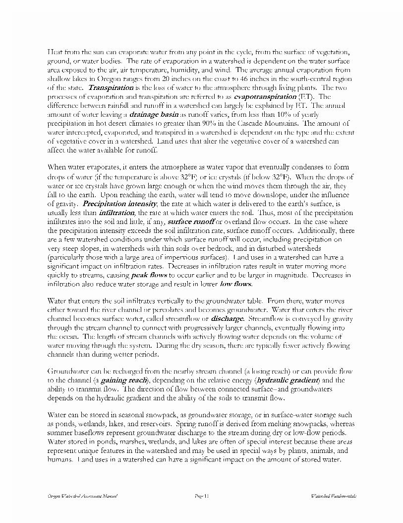
�� ���� ��� ��� �� ������� ��� ���� �# ����� �� ��� �#���� ���� ��� ������ �� ����������������� �� ��� ������� ��� ��� �� ��������� �� ������� �� ��������� �� ��� ��� �������� �'����� �� ��� ��� �� ����������� �������#� �� ���� ��� ����� ���� ��������� ��������� ���� �� %����� ����� ���� �- ������ �� ��� ���� �� 5* ������ �� ��� ������������ �������� ��� ����� ����������� �� ��� ���� �� ��� �� ��� ��������� ������� ������ ������ ��� � ���������� �� ��������� �� ����������� �� �������� �� � ��������������� �6��� ������������� ��� ��� ������ �� ������ �� ������� �� �����# �� �'������ �# 6�� ��� ��������� �� ��� ������ ������ ���� � ������ ������ ���� ���� ��� �-. �� #���#������������ �� ��� ������ ������� �� ������ ��� 7-. �� ��� !���� $�������� ��� ����� �� ��� ������������ ��������� �� ��������� �� ������� �� ��������� �� ��� �#�� �� ��� �'������ ��������� ����� �� �������� (�� ���� ��� ���� ��� ��������� ����� �� ������� ������� ��� ��� ������ ��� �������
2��� ��� ��������� �� ������ ��� ��������� � ��� ���� ��� ��������# ��������� �� ����
����� �� ��� ��� ��� ���������� �� ���� ��°&� �� ��� ��#���� ��� ���� ��°&�� 2��� ��� ����� �� ��� �� ��� ��#���� ��� ��� � ���� ������ �� ��� ��� ��� ����� ���� ������� ��� ��� ���#��� �� ��� ����� 8��� ������� ��� ����� ��� ��� ���� �� ���� �� ������� ����� ��� ����������� �����#� ���������� �������� ��� ��� � ���� ��� �� ��������� �� ��� ����+� ������� �������# ���� ��� ���������� ��� ��� � ���� ��� ������ ��� ����� ����� ���� �� ��� ���������������������� ���� ��� ���� �� ������� �� �#� ������� ������ �� ������� ��� ������� 9� ��� ��� ������� ������������ ��������# �'����� ��� ���� ����������� ���� ������ ������ ������� "���������#� ������� �� ������� ���������� ����� ���� ������ ������ ��� ������ ��������� ������������ �����# ����� ������� �� �������� ��� ���� ����� ���� �������� �� �� ��������� ������������������# ����� ��� ���� �� �� ���������� ��������� (�� ���� �� ������� �� ��� ���������� ����� �� ����������� ����� :������� �� ����������� ���� ������ �� ��� ������ ����)�����# �� ������� ������ ���� ����� �� ����� ������ �� �� �� ����� �� ��������� :������� ������������� ��� ������ ��� ������ �� ������ �� �� �� ��� ������
2��� ��� ������ ��� ���� ���������� ��������# �� ��� ������ ��� ����� &��� ������ ��� ����������� �� �� ��� ����� ������ �� ��������� �� ������� ������ ���� 2��� ��� ������ ��� ����������� ������� ������ ���� ����� �������� �� �������� /������� �� �����#�� �# �����#������� ��� ����� ������ �� ������� ��� ������������# ����� �������� ��������# ��� ��� ������� ����� ��� ������ �� ����� ������� ��� ������# ��� ��� ��� ������� �� ��� ������ �� ��� ������ ������� ��� �#����� :����� ��� ��# ������ ����� �� �#�����# �� �� ������# ��� ���������� ��� ������ ����� ��������
;����� ��� �� �� �������� ���� ��� ����# ����� ������ � ������ ����� �� �� ������� ��� �� ��� ������ � ����� ������� ��������� �� ��� ������� �����# ��� ����� ��� ���� �� ��������# �� ������� ��� � ��� ��������� �� ��� ��� ��� ��������� ������� �� ������ ����������� �� ��� �#������ ������� �� ��� �����# �� ��� ����� �� ������� ��� �
2��� �� �� ������ �� ������ ��� ���� � ������ ��� ������� �� �� ������� ��� ������ ����� ������ ������� ����� �� ����������� /����� ������ �� ������� ���� ������� ��� ����� ����������� ������ � ��������� ������ ��� �������� �� ��� ����� ������ ��# �� �� ���� ��������2��� ������ �� ������ ������� ������� �� ���� �� ����� �� ������ �������� ������ ����� ������������ ���)�� ������� �� ��� ������� �� �# �� ���� �� ������ #� �# ������ ������ �������� (�� ���� �� ������� �� ��� ���������� ����� �� ��� ����� �� ������ ����

������ ������ ��������� ���� ��� �� ������ ��� �����
!��������� ��� ������ ��� ����������� ��� �� ��� ��� �� ��������� �� ��� ����� �� ��� ����
�� ������ ��� �������
Hydrologic Data: Collection and Use
��� 8/;/ �� ���� �������# ����������� ��� ����������� ��� ��� �� �������� ����� �������
��� ������ �������� ��� ��# ������ �� ������ ���������� ��� ������#� ��� ������� ���� �����
������� �� ��������� �����# �� ����� ������� ���� ������� ��� ��� ����� ����� ������� �������
��� ��� ����� ��� ��� ���#� ������#� �� ���� ��� �< ���� ����������� ��� ��� � �������
���� ��� �< ���� ������� ��� �� ���� 8/;/ �������� �� �� ��� �� ������� �� ���
9�������� #�������� ���������� �� �� ������=�� �� �����#�� �� ��# #�� &�� �������� ���
���� �� �������� ���� ���� �� ����� �� �������� /��� �#���� ���� �#�������� ���� ����� ������# ��� ����� ���� ��������� ���������� �� ���������� �� &����� ,� ��� )�����# ��
��� ��� ��� ������� ��� ������ �� ����� �� ����� �� ��# �# ������ ������ �� ��������
���������� ��� #�� � ��� � ���� #�� �� #���
��� ���� �� ��� �#������� �������� � �������#��� ������������ �� �������� 9� ��������
���� ��� ��� � �� �������� �������# ���� ���������� ��� ���� �#������� ����� ����� ��
��� ��� ������ �� ������ ��� � ��������� ������ ��� ����� ����� ����� ����� ���> �������
/������#� �������� ���� ��� ���� �������� ��� ��� � ��� � ���� �#������� ��� ���
�������� ������ ��������� �� ��� ��� ���� ������ �"���� �� ?����� 4��� ��� �� ����� ������ ��
����� �������� ������ ������� ��� ��� � �� ��# ��������� ��� ���� �#������� ��� ����� �������� ��� ��� � � ������� �� ������ ��� � �&����� ,��
#�������� �� ��� ��������� ������� ������� ��� #��< ����� �#�������� �� �����
����������� �� ��������� ��� ������ �� ��� ���� ��� ������ �� ������ �#�����# � �� @ �#�� :�����
����� ������ ��� �� ��������� �# ��� ������� �� �� ������ �� ������ ��� ��� ����� �������
/���� �� ���� ���� ��� ��� ��� �� ���� ���� ��� ����� ��� �� ��� ������� �� ��� ��� ������
����� �� ���# �� �� ������ ��� ��� ��� ������ � ��� ���� 9� ��� ������� �� ��� ����� �� ����
�� ��� ������� �� ����� ��� �'���� ��� ��� �� ��������� �� ��� ��� ��� ��� ��������
�������� ���� "���� ��� ��� ������ ��� �������� ��� ������# �������� � ��� ������ �����
Figure 7. Typical hydrographs from different ecoregions, showing the differences betweenstorm-driven runoff (A) and spring snowmelt (B).

������ ������ ��������� ���� ��� �� ������ ��� �����
�� � ��� ������ �� ��� ������ �������� ����������#� 2�������� ��� ����� ������ ��>�� ��������� ���� �� ���� ��� ��������# )�����#� �� ����� �#�������� ��� �� ������������# ����� ��������# ������� ������ ����� /��� �������� �� ����� �������� �� � A����#�B (���� �������� �� �������� ��� ���� ����� ��� ����� ��� �� ��� �'������� ������ ��� ���� �� ��� ����������� �� ������������ �#�������� �&����� C��
2���� ������ ��� ���� ��� ��� ��� �������� �� #���� ����� ��� ��������� �������� �� ������# ���� ������� �� ����� ������� ��� ��� �� ���������� ��� ������ ��� �� �� ���� � ��������� �� ��� ��� ������� &�� �'����� ��� �� �� �� ���� �� ��������� �� ���� ��� ����� ������ �� ��� ����� #��� "���� ��� ���������# ��� � �'����� ����� ���� � ����� ��������� �# ����� �� �� ��������
9��������� �� ����� �'����� ������ �� �� ������ ��������� ������ ������ �� ����� ��� ���� ����� ����� ������ �� �� ����� ��� ���� ����� ����� �������� �� ����� ��� ��������� ���������� ��� ������ �� ������� �����# �� ��� �� ��������� ����� �� � #� ���� ��� ����
�#�� �� �'����� ����� �# ����� ����� �# ����� #��� "��#��� �� ��� �������� �������� ��������������� # �� ��������� ��� ���������# ��� � ����� �� ����� �������� ��� �� �'�������&�� �'����� �--�#�� ����� �� �. ����� �� ��������� �� �# ����� #��< �@�#�� ����� �� 5. ���������# �� ��������� �� �# ����� #��� &����� 7 ���������� ���� �'���� ����������
������� ��� �������������
Figure 8. Hydrograph patterns showing the difference between watersheds with asteeper topography, which have a rapid runoff response (top), and watersheds with flattertopography, which have a slower, more prolonged runoff response (bottom).
������ ������ ��������� ���� ��� �� ������ ��� �����
(�� ���� �� ������� �� ��� ���������� ����� �� ��� ���)����# �� ������� &�� �'�����
���������� ��� �� ��������� �� ������ ��� ���)����# �� �������� �� ������ �� ��� ������� ����� ����� ���� ��� ��< ��������� ��������� ���� �� �����# ���� ���� ������ �� �#������������������
8����������� ��������� ������ �� �������� �� �� ���� ��� ���� ����=� ��� ��������# �� ���
�������+� �������� �� ������� ����������� ��� #������# �� 2��� 8�� "��������� ����������������� ��������� �� �� �� ����� �� ��� ���� ������������������ �� #��� ��������
(�� ��� �� ��������� ����� �� ����� ��� �� ���
�������� ������ �� ��� �������� (�������� �������������� �� �������# ��������� ��� ��� ������� 0������
��������� ��� ������ ��� ����� �� ����������� ��� ���� ���� ��� �� ������ �� ��������������� ����� D�������� ������ �� ��� ������� ��� ��������� �� ������������� ��������
��� ������� �� ����� ����������� �� ����� ��� ������ �� ��� ����� ��� ������� ��������# ������������� ���� ��� #������# �� 2��� 8�� ��������� �������� � ������������������# �� ��������� ��� �'���� �� ����� ��������
��� ��������
��� ���� ��� �������� ��
��� �� ������ ������ ������������ �����
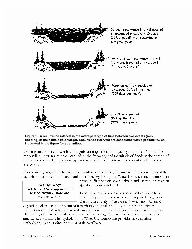
Figure 9. A recurrence interval is the average length of time between two events (rain,flooding) of the same size or larger. Recurrence intervals are associated with a probability, asillustrated in the figure for streamflow.

������ ������ ��������� ���� ��� �� ������ ��� �����
��� ��������
��� ���� ��� ��������
�� ��� �� ������ �������������� ����
8����=���� �������� ��� �� �� ���������� ������� �� ����� ��� �� ��� ���� ��� �� �� ���
������� �# ����� ���� �������� �� ������ �� �������� ��� ��� �� ���� ���� )���� ������ ��
������� ��� ������� ���� ����� �� ������� ������ �� ��� �� 8���� ���������� �� �����
��� �� ��� ����� ���� ����������# ��� �� ����� �� ���� ������ ���� ��� �������� ��������� ��
��� ���� ��� ������ ��� ������ �#���� �� �� ������ �� ������� ������ �� ��� ��
�������� �� ������� ���� ����������� ��������� ��� ������ ��� ��������� ����������� ��
��� �� ��� ��� ������ �� �������� �� �������� ������ �� ������� �������� &��� �'�������
�������� ��� ��� �� E������ �� ������ ���������� �� ������ ���� ���� 9� ��� ������ ��
�������� ������ ��� ������� ����������< ����� �������� ���� ������ E������ ���������
����������� �� ���� �� ��������� 9� ����� �� ������� ��� ���� ������������ ��������
���������� �# ���� �� ����� ���� �� ������� 9� ������� ������� ���� ��� ���� �� �����������
���� ��� ��������� �� ����� ������ ��� �� ��)����� �� ����������� ��� �������� ����>���� �����
������ ���� ��������#�
9� ��� ���� ��� ��� ������ �� ���������� ����� �� � �������� ���� �� ������� ���� ������
������ �� ����� ������ �� ������ ������ �'���� ��� ������ �� �� ����� A�� ������� �����B ���� ������� ������� ��� � �� ������� ����� ���������� �� ��� ������ ����� �� ������
���������� �� ������ �������#� ���� �� ������� �� ���� �������� ���������� ����������� �� ���
6��������� ������'��
Consumptive Uses of Water
��� ��� �� ��� �� ��� �����# �� ���# �������� �� ��� ����� �� ������ ������#� %�������#� ���
��� �� ������� �� ��� � �� ����������� ��� �������� �� ��� ������� �� �������� 2���
������ ��� �� ���� �'��������# ��� ���������� ��� ��� ��
�E���� ������ �� ����� ������ �� �� �������� ���������
�� �������� ����� ������������ ����� ���� ���������
����� �� ��� ������ ������ ��� �������� �� ���
��������� �������� ��� �� "� �������� ��� �� ���
��������� ������� �� �� �������# ��� �������� �� ������
�� ����������� ��� ����� �� ���� ����� ��� ������ �� ��� ������� �� ��� ����#����� ���
#������# �� 2��� 8�� ��������� �������� ����������# �� ��� ���� ����������
SOIL EROSION AND SEDIMENT IN STREAMS
/������� �� ������ ����� ���� ��� ������� �� ����� ���� ����� �������� �� ����� �������
������ ���� ������ �� ��������� �� ���������� ��� /������� /������ "���������
��������� ������� ������� �� ���� ��������� �� ����� ���������� &��� �������� ��������� ��
��� �������� �# ������ �� ���� ������ �� ������ ������� �� ���� ���� ��������� �� ���
������ &��� �������� �# ����� ��� �'����� ���� ������� ��������� �# )���� �������� ��������
��� ���� �����# �� ����� /�������� ��������� ���� ��������# ��������� �� ��� ����� ����
�������� ���� ���� �������� (��� �������� �� ����� ��������� �� ���� ���� ��� ������ �����#�
��������� �� ������������� ����� �� �� ���� ������� ��� �� ���� ����� �������� ����� �� ���
������� ��������� �� ��������� �������� ��
��� ������� �� ��� ������#��� ���� �� ��� ��������� � ��� ��� �� �������� ���� ���� ������� ��
���� ��������� ��� ��� �� �������� ����� ��������� ��������� ��� ��������� ��� ������ �� ������#

������ ������ ��������� ���� ��� � ������ ��� �����
�� ������ �� �������� ��� ������ �� ��� ������ !��� 0��� ����� )�����# ������ �� ��� ����
������� ���� ����� �� ���� ��������� �� ��� ��� �# ������ ���� �� ��� ����� ����� ��������� �����
����� ������ �� ���� ����� ������# �� ����� ��������� 9� �������� ������ %����� ��������
�����# ����� ���� ��� �# ��� �� �� ������� ��� ������#��� ����� �� ��������# ��� ��������� ��
��� ���� 9� ����� �������� �� ������ %������ ������ �� ������ �� ������ �� ����� ����� ���
��������
��� ��������� ����� ����� ��� ������� �� ����� ������ ��� ������� ������� �� ��������
8����������� ��� ����������� ��� ��� ����� �� ������������ ������� �� �������� ��
���������� ������� ���������� ���� 2� ��� ������ ������� ���� ����� ������� ����< �� ���� ��
���� �� ���������� �� ������� ��� ����� ������� ���� �� �������� ������ )���� ��������
��� �����# ������� �� ��� ����� ����������� 4����� � �� ��������� ���# ������������
�������� �� �� �������� �� ��������� �� ������� ��������� �� ������ �# �������� ����������
������ ��� ��������� ������� �� ���������� ������� �� ����� ����� �� ���� ����� ������ ��
��������� �� ��� ��������
��� /������� /������ "��������� ��������� ������� ������� ��� �������#��� ������ ������� ��
������� ���� ��� ����� ��� ����� �������� �������� �������3
�� 0�� ���������#�� /���� ���������# ���� ������ �� ������� 0��� ��� ������5� 8��� ������@� /����� ������� ���� ���� ���*� /����� ������� ���� ���� ���,� /����� ������� ���� ������ ���C� %���� �������� �������
9� ������� �� �������#��� �������� �������� �������� ��� �������� ��������� ����� ���������
���� �������� �� ��� ������� ��� ������ �������� ��� ��������� ������� ��� �� ����
���������� �� ��������� ���� ���� ����� ������� �� ��������
9� �� �������� �� �������=� ��� ���� ������� ���� ��� ������� �� ���� ����� ������ �� ������ ���
������ ���� �� ���� �� �� ����� ����� �� ������ �� ������ ��� �� �� ���� �� ��' ���� ��� ��
������� ������ ��� �������� ������ ��� ������� &�� �'����� ��� ������� ���� ������ ���
������ �� �� �������� ���� ���������� ����� ���� ��� �������� ��� �� �������� ���� �� ���
���� ��� �� ��� ������ ��� ������+� ������ �� ��� ������
��� ����������� ��� ��� ������� �� �������� �� ��� ����� �� ������ ������� ��� ������ ���� ��
��������� �� �� ��� ��� ������ " ���� �'���� �� ���� �� ����� ��� ���� ���� ���� ��������
��� ��� �� ��� ������ 4���� ��� �� �� �� ��������� � ������� �������� ��� ���� ������� ��
�������� ���� ����� �� �� ����������� �� ������ �� ��� ����� ��� 2���� ��� �� �����
��� ���� ���� �� �� ��� �� ��� ������ ������� ����� ������# �� �����# ���� ��� �������� ��
����# ������� 9� ���� ����� ��� ���� �� ������ �� ���� ��� ��������� �� ������� %� ������� �� ���
����� �� ������'�� �� �������# �� �� ��� ��� ������ ����� ������ ��������� �� ��������
�� �������
������ ������ ��������� ���� ��� � ������ ��� �����
"������ �������� ������������ �� ��� ������� �� ������������ �������# ����� �� ������ ������
�����)���� ������� �#�����#� � ������� ������ ����� �� ����� ��� ������ ���# ���� ����# �����
��� ������� ���� �� ������ ������ ���� ������ �� ���� �� ���� �����# �� ����� �� ����
������� "� �'���� �� ���� �� ��� &�����# �77* ����� �� ��� 2�������� 0���� ����� %��� C-. ��
��� ���� �������� ���������� ��� ��� 2�������� 0���� �������� ������ �� �#� �� &�����#
��� ��� ����� ���� ����� 9� ��� �������� ���������� �� ����� ��� �'����� ���# ������
A�����B ����������� ��� �������� #���� ���� ������# �� �����# ��������������
����� �� ������ �� ��������� ��� ���� ���� �� ����� �� ���� ����� �������� ��� ��'�
�������� ������� ����� ������� ����������
Raindrop Splash
��� ��� ������ ������ ��� ������� ���� ��� ���� ������� ������ ���� ������ �� ������������ ����� �� �� ����������� %� ������� ������� ����� ������� ���� �������� ��� �������# �� ���
�� ����� �� �� �� ����� ������� �� ����� �# ��� ��� ��� � ���� ��� ���� ������� 9���������#�
���� �������� ����� �# ��� ��������� �� ������� �� ������������� ��� ��� ���������� �# ��#
�������� �� �������� ��� ������� ������ ����������
0������ ����� �� ��� ������ �� ���� �� %����� ����� ����� ����������� D�������� ��
������ ������ � ��� ���� ������ ������ ��� �����# �� ������� �� ��� ���� ������ ������
� ����� �� �������#� ������� ��=���� �� �������������# ���� ������� ���� ���������� �������
������� ����� �� ������ 0������ ����� �� ���� ��������� ���� ��� ���� �� ��� ���# ����������� � ����� ������� ���� ������� ���� �� ������� ��� �� ����� ���� �� ��� �� �����
Ravel
/��� ����� ������ ���� �������� � ���# ��#� %� ������� ������� �����# �� �'���� ��� ������ ���
���� ��� ���� �������� �� �������� ���� �� ������ ������ �� ��������� ���� ����� ����������������# ������ �� ����� &���� ����� ����� ��� ���������� ���� �# �������� ��� ������ ���
������# ���� ��� ���� ��������� 4�� ��� ���� �� ������� ��=���� ����� �� ������ ����� ����
�������� �� ��� ��� ������ 9� ���� ���� �� ��� �������� ���� ������ ���� �� ���� �� � ��� ���
����� �� ���� ������ ������ ���# ������ �� ��� ��� ��� �� �������� 0��� �� ��� ������ ��
������ ��� ����� ����� ���� ��� ������� ���� �������� ��� ������ ��� # ���� ��� ������
Surface Rilling
2��� ��� ��� ���� ��� ������ �� ��� ���� �� ���# ��� ������ ���� �� ������� ����� ���� ������F���� ���� ������� ���� ��� ����� ���� �� %������ ��� �����# �� ��� ���� �� ����� ��� �� �����#
������ ��� ��� ������ ��������#� �� �� ��� ��� � ���� ��� ���� ������� � ����� ������ �������
���� ����� ���� ��� �����# �� ��� ���� �� ����� ��� �� ���� �������� ���� � ��� ��������
��������# ��=�� ���� ��� �� ����� ������� �� ��� �������# ������ �# ��� ������ 0����� ��������
�� ��� �������� �� ������ ������ ��� � �� ����� �� ������ ���� ���� ����� ���� ��� ���� ��
������� :���� ����� �� ������� ����� �����# �� ����� ���� D�������� ������ ����� ����� ��
���� �������� �#�����# ������� ���� ����������# ���� �����

������ ������ ��������� ���� ��� �� ������ ��� �����
Shallow and Deep-Seated Landslides
/���� ��������� �� �� ������ ������ �� ���# ����� ������� ��������# ���� �������������#������� ����� ����� ��������� �� ���� ������ �� ���� ����������� �� ��� �������� �&����� �-��;����# �������� ���� �� ����� ����������� ���� ���� �� ��� ���� ������ �� ���� ����� ����������������� ��� ������ ��� ���� ��� ���� �� ������ (��� ������ �� ��� ������ �������
���������� ���� ��� �� �� �� ���� ������ ������������# ������ �� ������ ��� ���� ������������ ���� ��� ���������� �� ������� ����� ���������� " ����� �� ����� ���� ����� �� ��������� ���� ����� �� �� �� ��������� �# ���� ��� �� ������� ������ ������������ �� ���� %��'������# ����� ������� �� �� ���� ��� � ��� ���� ��� ����� �� ����� �� ���� ��� ���� �� ����
������ �������������# ������� "���� ������ ������ �� ����� ������� �� ����� ��� ���� ���������������� ��� ����� �� ��� �������� ����� ��� ������ ��� ���� ��� �� ��� �� ���� �� ����� ������������
/���� ��������� �#�����# ������� �� ������ ����� �� ��� ����� �� ��� ������ ������ �� ������
������ ���# ��� �� �� ������� 2��� ����� ��������� ���� ���� ������ ���# �� ������� ���� �����G ���� �������� �� ���� �� � ����� ������ �&����� �-�� ��� ��� �� ������������ �� ��� �����# ��� � � �� ����� �� ������ D��������� ����� ��������� �� ���� �� ������ �� ��� ������ ��� �� ����� ������������ ��� ������ ��� ����� ���� �� ������ �� ���
������� ����� ������� ��� ������� �� ������ ��� �� �� ��������� � ��� � ���������� ����������� ����� ��� ��� �� ���� ��� ���� ����� (��� ��� �� �������� ����� �� �� ��� ����������� �� ������� ��� ����� �� ����� �� ��� �� �� ��������# ��� ��� ���� ��� ��� �������
:��������� ��������� ����� �������� ���� ����� ������������ ��� �� ��� ������� ������ ��
�� ��������� �&����� �-�� ��� ��������� ��� ���������� ���������� ��������� �� ������ �� ����������� ����� ������� ������ ���# ������ �� ������� ��� �� �������� ��������� %���� �������� ���������� ��������� ������� �������������� �� ������ ��� ��� ����� ������� �� ��� ��� �������� ������ �� ��������������� �� ���� ������� �� ��������� ��� �������� ����
���������� ����>���� ������ %����� ��� ������ ���� �� ���������� ������ �� ���� ��� ������������ �� ������ �� ��� ����� �� ����� ��������� ��� ���� �����# �� ���� ���� �� ����� �#��� ������������ ��������� ������� ������� ����� �������� �� ���� �������� 9� ���� ����� ����������
Figure 10. Deep-seated landslides often originate from shallow depressions, but canalso involve a broader area of a hillslope. When shallow landslides move into achannel they can trigger debris flows—a rapid movement of soil down a steep channel.

������ ������ ��������� ���� ��� �� ������ ��� �����
��������� �� �� �� ������ ��� �� ������� ������ �� ��� ���� ������ �� �������� ����������
Soil Creep and Earth Flows
��� ����� ������ � �����# ����� ��� ���� ����� �� ����� �� �� ������ � ���� ��� ���� ���������� /��� ����� ������ �� �� ������� ��� ��� �� ���� ��������� �� ����� ������� 6��� ��� ��� ���� ���� ����� �'���� ���# ����� � ����� ��� ���� ��� ������� ��� ���� �� ���� ������
����� �� ��� ������ �� � ���� ��� ����� ������ ������ � ��� ���� ���# �� ������ �� ������� ����� �&����� ���� !������� ���� �� ���� ��� � �� ��������# ��������� ����� �������� �������� ������ ��� ���� #� �����# ������ ���� ��� ��
/��� ����� �� ���� ��� � �� ����� ��������� ������� ���� ���� ��������� �� ��������
����� ��������� &�� �'����� ���������� ����� ��� ������� �� ������������ ����� ������ ��������������� �� ������� ���� �������� �� ���� ���� ��� �� %��� � ���� ��� ����������������� ����� �� ������ ��� �� �� ���� �� ��' ��� ��������
Figure 11. Soil creep and earth flows occur as gravity moves soil downhill toward streams.Trees on the surface of an earth flow often become tilted as the soil they are rooted in movesdownhill.

������ ������ ��������� ���� ��� �� ������ ��� �����
��� ������ ������� ���� ������������ ���������
Road-Related Erosion
��� ��� ��� ��� �� ������ ���������# ���������� ������� ������� 9��������# ����� ���� �������� ������������� ��� �� ������� 1��� ������ �� ���� �� ��� �� ����#��� �� ����������� ��� ��� ������� 9������� ��������� �� ������ ��� ������� �� ���� �������� �� ���������� ������ ������ �������
0�� ������ ��� �� ����� ��� ��� �E���� �� ��� ����� �� �������� �� ������� �� ������ ����� ���� ��� ������ �� � ����� ��������� ������ ���� ��� ���� ����� � ������ ��������=�� �� ������� ������� �� ������� 9� ������� ������� ��� ������ �� ����� ����� ��������� �� ������� ���� �� ���������� �������� "��������� ��=��� �� �������� �� ������� � ��������������� ������� ���� # ���� ������� ��������� ���� �������#� �� ��������# ��������� ������ ������ ��� ������������ �� ������� ������ �� ������� ���� ��� �������
Channel Erosion
��� ������� �� ������ �������� �������������� ��������# ���������� ���������� ���� � ��� �����#� �� ��������� ������ ��� �� ��� ������ ������� ������ �� ������# �� ������� ���������' ����������� ���� ����� ������ ������ ��� ����� ������� �� ������ �� ����# �����%�� �� ��� ���� ������� ������� �� ���� �#���� �������� �� ������ �������� 9� �� ����� ���������������� ���� ��� ����� �� �� ����� ������ ��� ��� ��������� ������� !���������� ���� �� ������ �� ����� �� ��� ���� ����� �� �������� �# ��������# ������� ��� ����������� ��� ������ �����# �� ��������� ������ ���� � �������� ��������� !����� ������� �� ��������� ��������� ����� ��������� ���� ������ �� ��� �� �� ��� �������# ��� �� ������� �� ���� ������
!����� ������� ����� ������ ��� �������� �������� �������� �� �� �� ��� � �� ����� ����'���� ����� �����# �� �������� � ��� ������ ��� �� ���� "� ���� ������� ���������� ��� ������ ��� ���� �� ���� ������ ������� :����� ������� ������� ��� ������ �� �����)���� ���������� �����# �� �������# ����� ����� �#�����# �'��������� ��� ������� �� �������� ������ ����� ��� ������� $��� �� ��� ����� �����# �� ����� �� ������ �������� �������� ����� ���������� ����� 9� ������� �� ����� �������������� ������ ����������� ��� ���� �� ������ ������� ��������� �# ��� ������ �#��� ���� �� �� ���� ������ �� ��� ������� ������ �� ������# ��������� &�� �'����� �� ���������� ������ ��� ���� ������ �������� �� ���� ����� ������������ �������� �� ����� ���)����# �� �������� �����#�
��� ����� ������ ���� �� ������������ ������� ��� ����� ��� ��� ������� ������ �� ������������������� !����� ���� ��� �������� ������ # �� ��������=� ������ �������� �� ���
�������� ��� !����� ���� �#�� !�������������������� �� ��� ���� ��������� �� �� ������# ������� ����� ������� �� ���� ��������� �� ��� ������� ����� ����� ��� ��� �������� ��� ��� ������ �������� 9��������� ������������ �� ������� ��� � ���� ������
���������� ���������� ���� �� ������� ���� �� ������ ����� ��� ��������
:�� �� ��� ������'��# �� ��� ��# ����������� ��� ��������� ������ �������� �� �� ��#��� �������� �� ���� �������� �� ������� ��������� ������������� ��� ������ �������� 9� ����� ����������� �� �������� ������� �� ���������� ��������������� �� �#��������� ������ �� ����������
������ ������ ��������� ���� ��� �� ������ ��� �����
��� ��������
��������� �������� ���
�������� ������� ��
���������� �� ��� ��������� ���� �����������
��� �������� �����
�������� �� ���������
�� ��� ������ �� ���������������� �� ���� �������
��� �������� ��� ����
��� �������� �� ���������
�� ��� ���������� ������������ ���������
VEGETATION
��� ��������� �� ���� ��� ��������� ������� �� ������� ������� ������ ������� ������
�������� ��������� ���� ������������ ����������� ��=���� �� ���������� �� ���� ���� �����
������ �� ���������# ����� ��� ������������ �������� �������# �� ������� �� ��� �����
�� ������ �� ������� �� ������ ����� �������� ������� �� �� �������� �� ��������� ���
��������� �� ��������� �� �������� �� �� �������� ��
��������� �� ��������# ��������� ���� ����� �� ���
)����#�
D�������� ������� �� ������������� ����� �������
�������# ����� ���� ����� &���� �� �����# ������� ��
��������� ���������� ��� �� ��� �������� �� ����
�������� ���� ���� �� ��� ��������� �� �� �������� ���
���)����# �� ���� ��������� ����� �������� �� � ���� �#����� ����� �� %����� ���� ��� �� ���
��� �� �������� �� ������������� �� ���� ����� �� ����� ������ �� ��������� ���������� ��
���������� �� ���������� &��� ������� �� ��� �������# ������� �# ��������#< ����� �����������
������ ���� ���� ���)�����# ��� ��� ����# ������� &���� �� �� ���������� �� ������� ���
������ ����� �� �������� ��� ���� �� �'������ ��� ���� �� ����� �� �������=��� �� ���� �� ���
��� �� ��� ������ �� ������#��� �������� ������ �������#� �#�����#� ���������� ����� ���� �
���� ������� �� ���� ��� ��� ���������� ��������� ��� �� �� �� �#��� �� �������# �������
9������ �� ������ ��� ����� ���� �#���� 2��� ��#� ��� ������ ������� ���� ����� ������ �#
������� �� ������ ���������� ��� ���� �� ���� �������� �� ��������# ���� ��� ����� ��� �#����
������# �� ����� �� ����� ������������ �� ����� ������� �� ��������� �� ��� �������� ��
��������� �� ��� 6��������� ������' �� ������� �� ���� ���� �� ��� �������� !���������
����������
Role of Upland Vegetation
D�������� ��������� �� ��� ������ �� ������ ���� ���������� ��� ��� ������ ���������� ��
������ ���� ����� �� ������ ���� ���� ������ ������ ��� ������ ��� ������ ������ �� 9�
�������� ��� �������� ��=��� �� ����������� �� ���
��������� ����� ��# ������� �������� &����#� ���������
����������� �� ������# �� ������ �� ������� ���� ��������
(���� �� ������� ��������� ��� ������ ��� �� ������ ���
������ �� ������� ������ D�������� ������ ���� ��� �����
�� ������� ������ �� � ������ ������ ��� ��������
���������� �� ��� ���� �#��� 0��� �#����� ���� �� ���� ���� ������ ���� ������ �� ������� 2���
��������� �� ����� ���# ����� ����� ���� ��� ���� ��� ������� ���� �� � �������� ���������
�� ������ ��������� �� ���� ������ ��� ������� �� ��������� ������ �� ���� ������� ��
��������� �� ��� /������� /������ ����������
9� ���� ��� �� %������ ����� �������� �# ���������
��� ����������� �� ��� ������ �� ��� ���� �� �������
9� ��� �� ��� ������ !������ ��� ���� �� ���� ���
�# �� ��������� ������ ��� ��������# �� �� ���#
����� ������ ��� ���� ���� ��� ����� ���� 9� ������
%������ ������� �� ��������� �# ����� ��� ������� ��

������ ������ ��������� ���� ��� �� ������ ��� �����
��� ���������� �� ����� ���������# ������� ��� ������ �� ����� �� ������ �� ��� ��� ������
�� ������� 0����� �� ������� ��������� �� ��� ������� ��� #���� �� �������� ������
��� ����� �� ���� ������� ������� ��� ������ �� ����������� ��� ������� �� ��������� ������ ��
��� �#������# �� ��� ������� �� ������� �� ��� #������# �� 2��� 8�� "���������
����������
Role of Riparian Vegetation
��� ����� ��� ���� ������ �� ������ �� ������ �����< ��� ������������ ���� �����������
��� ����� ����� �� �������� �� � ������ ��������� 0����� ��� �������# ��� ������ ������
�� ���� �������� ��� �E���� ����� ���� �� �����# �� ������������� " ��� �����# ��
�#��������� ����������� �� ������ ��������� ��������� ��� ������� �� ��� ������ �����
0����� ��������� ���������� ���� ����� �� ��� )����# �� ������ �� #�� 0�����
��������� �# �� � ������ �� ���� ���� ������� �������� �� ��������� ��� �� ������� ���
����� �� ������ ��������� ������=� ����� ���� �# �������� ������� �� ���������� �����
������� ���� �� ��������� /�������� ��������� �������� ����� ��� �������� ���� �� ���� ���
�� ��� ��� �� ������� ���� ������ ��� ����� 9� �������� ��������� ������ �� � �������� ������
�� ��������� �� ��� ������ :����� ���� ����� ��� �� ������ ��������� �# ��� �� �������� ���
�����# �� ����� ����� ���������� ������� �&����� ���� "������� �� �� ����� �� �������� ���������
�� ������ ���������� ���# �� ��������� �� )�����# �� �� ��#��� ��� ����� �� ���� ���������
�������� ���� ��������� ������� ���# �� ��� ��������� �� ��� ������ ��� �� ��������� ������ ��
���� ��� �� ��� ������ �� �� ��������� ���� ��� ����������H �������� 0����� ��� ��� ��
Figure 12. The riparian zone provides a number of functions, as illustrated.

������ ������ ��������� ���� ��� �� ������ ��� �����
��� �������� ������� ���
!������"�������� ��������������� ��� ��� �� #�$�
����������� �� ������� ����� � � ��# ������ ��� ��� �������# ������� ��� ����� ��������� ����������� ��������� �� ������ ����
Large Wood Recruitment
0����� ��� �� � �������� ������ �� ���� ���# ������ �(2:� ��� ������� �� �� ������� ���
��� ����� ������� (2: �������� ���� ������ ���� ��� �� ���� �������� �� �� ��������� �� ���
����� �# ��� �������� �������# ������� �� ������ �� �� ������ "� ��������� ����� ����� ����
���� ��� ������ �� ����� ��� �# ��� �� ������ ���� ��� ����� �# ��������� �&����� ����
9� ��� ����� ������� (2: ������� �� ��������� ��� � ������# ��������� ������� ���������
������ ��� ���� ��� ������ ����� �� ������� ��� ������� ��� �� ��������� �������# �� ������� ����
������'��# �������� ����� ���� ��������� ������ ������ ���� �� �������� ������ ��� ��� ����
������ ���� ����� ��� �� (2: ��� ������ ������ ����� ��� �������� �� �� ��=�� �� ������� 9�
���� ��� ��� ������� ��� �������� �������� �������� �� ������� 9� ����� �������
���������� �� �������� ������ (2: ����� �������� �� ���� ������� (2: ��#� � ��������
���� �� ����� �������� �#����� �# �������� ��� ������ �� �������� ����� ����� �����# ��������
������ ��� ����������� �# )���� ������� ��� ��������#
����� � ���� ��� �����
��� ��������� �� ������ =���� ��� ��������� (2: �����
�# ���������� ��� 6��������� ������' ��������
����������� �� �������� ������ ��������� �� ��� ���� �� (2: �� ��������� ��� �� ��� ����� ���
0�����>2������ "��������� ��������� �������� ����������# �� ����� �� ������ ���
��������� �������� ��� ������ =�����
Figure 13. Large woody debris is recruited to the stream by bank erosion, mortality (disease orfire), or wind throw.

������ ������ ��������� ���� ��� �� ������ ��� �����
Riparian Shade
"������� ����� ��������� ������� ������ ����� ������ �� ������� �� ��� ����� � ������ �������� ��� ������ �� ��� ��� ������� ����� ������ �� ���������� ��� ���� �������� ������ ������� ������ ������ ��� ������G���� �������� 0����� ���������� ������� ��� ����������� ��� ���� �������� �� ���������� �� ���������� ��������� � ��� � ������� ������
�������� �� ���� �� ������� ������
/��� �������� �# ������ ��������� ������ ����� ���������� �# �������� ��� ������ �� ����������� �� ��� ��� ������� "������� ��� ��������� ������ ��� ����� ��� �� ��� ������ ���������� �� ��� ���������� ��� �� ������� ���� ���� ������ �� ���# ���� ������� ��� ������
���� ������ ���� �������� 0������ ���� ��������� �� ��������� �� ����� ������ �� ������������������ �� ��� ����������� �� ���# ��� ������� ���� �&����� �5� �� �������� ������������� ��� ������ ��� ��� �� ������ ����� ��� ����� �� ����� �� ���� ��� ����� ���
����� �� ������� ��������� 9� ���� ��� ������ ���� ��#���� ��� ��������# �� ��� ��� ��
��� ������� ���������� �����
Role of Ambient Air Temperature
9� ���� ������ ��������� �� �������� �� �����# �������� �� ����� �������< ��� ��� �� ����
�� ���� ��� ���� ����� ��������� ������ ������ ������������ ������ ��� ������� ����� ��� ����
����� ��� ��� ������ ��� ������ ������ ����������� ��� �� ��� ������ ��������� ���� 9�����
Figure 14. Radiation from vegetation decreases fluctuation of water temperatures on a dailybasis in forested streams compared with streams that have no canopy cover. Inputs of coolgroundwater are also a significant source of stream cooling in some areas.

������ ������ ��������� ���� ��� �� ������ ��� �����
�� ���� ������ ��� �� ��� ���������� ������ �� ����� ������� �� ���� ��� �&����� �5��
(��� ���� ������ ���� ��� ������� �� ���� ����� ������������
/���� ����������� �� ������ ��� ��� ������ �� ���������� ������ �� ��� ������ ������
���� �� ��� ���� �� ��� ������� ��������� �������� ��� ��������� �� ��� ����� ��
������ ���� ��� ���# ������� �� ����� ���������� ����� ��� ���# ����� �� �� �����������
�#�����#� ��� �'���� ���# ���������� ������ �� ��� ��� �������� �� ��� ������� ������ ���
� ����� �� ���# ������� �&����� �5��
9� ��# ������ �� %������ ���������� �������� � �� �� ��� ��� ��� ��� ��� ��� �� ���
�������� ��������� �� ��� ����� ��� ����������� �� ��� #��� ���� ���������� �������� ��� ���
��� ��� �'���� ��� ���������� �� ������ �� ���� ��� ��� ��� �������� �� ��� ����� ��
��� ��� �� ������ !����)�����#� ��� �'���� ���� ����� ����������� �# �� ������ �� �� �
��� �� ������� #��� ���� ������ ��� ����� �������� ��� ��� ����� �� ������ ��� #���
Summary
"�� �� ��� ��#���� ��������� ��������� ���� ��# ���� �� ��� ���������� �� ���� � �����
��������� ������# �� ������ =���� �� �#�����# ��� ���� �������� ������� ��� �� �� ������ �#
�������� ���������� ��� 0�����>2������ "��������� ��������� �������� ����������# ��
��������� ��� ������� ��������� �� ��� ���� ���������� �� �� ������� ��� ������ �� ��������� ��
��������� ���� ������� ��� 6��������� ������' �������� ����������� �� �������� ����
�������� ��� ������ ��������� �� ��������� ��� �� ��� ����� ��� 2��� I����# "���������
��������� ���������� ���� �'������ ���� ����� ����������� ��� ���� �����������
WETLANDS
2������ �� �� ������� �� ��� ������ =���� �� ���# �� ����� �� ������� ��� ��� �� �������
������ ���������� �� ����� ������� 2������ ������� �����# �� �������� ����������
��������� ��� )����# ������������ ���� ���������� �� ���#�������=����� ������ ���
������� �� ��������� �� ���� �� ������� ������ ����� ��������� �� ��������� �� ��� ����� ���
������������
Water Quality Improvement
2������ �� �� ��� )����# ����������� �# ������� ��������� �� ���������� ��� �# ��
������ �� ��� ���������� :���� ����� ��������� ����� �� ��� ��� ��� �� �������� �� ����
���� ��� � ��������� �� ������ ���� "������� ���������� �� ��������� �� ��������� �� �� ������
���������� �'������� ������������ �# ��� ������� ������ �� ��� ����� ������� 2���
����� �� ���E����� �� ������� �������� ����������� ��� ������ �������� �� ��� ����� ���
�����< ���� ����� ���� ����� ����� ��� �� ����� �����
D�������� ����� ������ ��� �� �������� ������ ��������� �� ���� ��'���� ������# ����������
�� ������ ���������� ��� ������� ����������� �� ��# ����� ����� ����� �� � ��������
��������� �� ����� ��# ��������� �� ���������� ����� ��� �����# �� ����� �� �������
���� �������� �� �������3 "� ������ ������ ��'��� �� ����� �� �� ����� ������ �� ��� �����
��������# �� ������� ��� �����+� �����# �� �������=� ��� ��������� �������� ���� �������

������ ������ ��������� ���� ��� � ������ ��� �����
�������� 9� �������� ���� ������� �� ���# �� ��������� ��������� �� ��'��� ��� ���� ���
�#����� ������� ��# ��'��� �� �����# ��������� �� ���� ������ ����� �� ����� �� ����������
Flood Attenuation and Desynchronization
2������ �� ���� ������� �� ������ �������� �# �������� ������������� �� ���#��� ������ �������
2������ ����� ��� ��������� �� ����� �� ���� ��� ��� �� ���������� ����� �����
&���� ��� ���#�������=���� ������ ��� ������ ������ �� ��� ������� ���������# �����
���� �������� ��� ��� �� ��� ���� ��������� ������ � ��������� ���#�������=���� ��
�������# ������ �� ��� ������ ��������� �� ��� �������< ����� ����� �������� �� �� ������
# ���� ��� ��������� ��� �� ����� ���#� ��� �� �� ������ �� ��� ������� �� �������
���������� ������ �� ����
Groundwater Recharge and Discharge
2������ �� ��������# �������� ��� ������ ���� �� ���� ������ �� �������� �� �������
������#��� �������� 2������ �� ������� �� ������ ��� �������� ��� �# ���� �'����
�������� � ���� ��� ����� ������ ������� 9� ������ %������ ��������� �� ���� � �� �����
��� ���� �� �'������ ��� ������ ������� �� �������� �
Fish and Wildlife Habitat
2������ ������� ����� �� ���� ��� ��� �����# �� )���� �� ���������� ���� �� ����
�������� $�# ������� ���# �� ������ ��� �� �� ������� �� ����� ���� �#���� 9� ������� �� �������#
��������� ������ ������ �� ���������# ������� ���� ������� ���� �� ��� ���������� ���������
���������#� ��� ������� ��� )����# �� ������ �������#� ������� ������ ������� ��������
������� �� ������� ��� ��� ����������� ����� �������
AQUATIC RESOURCES
��� �������� ���� ������# �������� ��������� ��������� �������� �� �������� ��� �������
��������� ��������=�� ����� ��������� ������ ���# ��������� ��������� �� ��� )����# �� ���
������� �� ��� ��� ���� ��� ��������� �� )���� ���������� &�������� �� ��� )����# ��
�������� )���� ��������� ��� �� ������� � ��������� �'�������� �� �����# ���������
��� ����������� ��� ��� ����� ��������� �� ���� ��� ��������# ������ �� ��������� �� ���� �����
�� ��� /����8� �� 9������������ �� 2������� 9����� ��������� �����������
WATER QUALITY
" ���������� �� ��� ����� ������� ��������� �� ��� ������ �� ���� ��������� ����������
��� )����# � �������� ���� �� ����� �� ������ 2��� )����# �� ��������� �� ����� �� ���
��������� ���� �� ��� �� ��� ����� �� )����# ������ �� ������� ����� ����� $������ �� ���
)����#G��� ������� �� ���������G������� ��� ���������� ��� ��� ��� ��������� ���� �� ��� ��
��� ����� �� ���� ������� �� ������� ������� ��� ����� ��� ������� ������# ������� ���
������������ ���������� �� &����� �@�

������ ������ ��������� ���� ��� � ������ ��� �����
Beneficial Uses of Water
��� ������ �� ������ �� ��� ������� �������� �� %����� ������� ��������� ���� �� ���� ��
����� ��� ��� )����# ���������� �� �� �������# �� �������# ��� ��������� ���� �� ��� ��� ��
�������� �� ��� ������� � ��� � ����� ��� �� ����������# ���������� �� ��� %����� ���
)����# �������� 4�������� ���� ��������� ���� ��� )����# ������� ���#� &�� �'�����
��������� ��� �������� ��� �������# ������� �� ��� �������� �� �������� ��� �� ���� ������
�� �������� ��� �� ���������� �� ��������� ����� ������� ���� � ����� ����� "��������� ���
��� ��� �������� ���� ���������� ������� �� �������� �� ��� ����� �#���� ���� � �����������
��������� �'#���� ������ �� ������� �����������
Criteria and Indicators
2��� )����# ������� ������� ����� �#���� ��� ��������� �� ������� �� �������� ���������
����� 2��� )����# ������� �� ����������# ���������� �� ��� /��� 2��� I����# /������ �# �E��
����� ����� 9�������� ����� �� ����� ���� �� ��� ��#��� ��� ��� ���� ������� �� ��� ������#
�������� �������� ��� ���� �� ������� �� ��������� �� &����� �@ ���������� ��� ����������� ��� ���
��������� ���� �� ��� �� ��� �������� ������� ��� �# ���� ��� )����# �� ��� ��������� ����
2��� )����# �������� �� �� ������� ���� ������ �E�� ��������� ��� ��#���G����������
������� ����������� ��������� �'#���� �� ��'���� 2��� )����# ����� �� �� ������� ���������#
�# �'������ ��� ����� �� ��� )���� ��������# ����� )���� ������������ �� ���� �����������
Figure15. Measures of water quality—the criteria or indicators—provide the connectionbetween the beneficial uses of water and the natural and human sources of watershed inputs.These relationships provide the context for water quality and fisheries assessments.

������ ������ ��������� ���� ��� �� ������ ��� �����
Nutrients
F�������� ����� �� �������� ��� �������� ��� �� �� ��� �� )���� ����� �� ���� 9� ����
������ ������� ��� ��� ������ �� ��� ��������� �� �� ����� A������#����B "��� ��
)���� ����� �� �������# ��� �� ��� ����� ����#���� �� �� � ��� �����# ��������� ��
�����G���������� ��� ���+� �����# ���� ���� ��� �� ���� �# )���� ������� �� ����������
����� ������������ �� ���� ������� ���� ��� ����� ����� 6'���� ��� �� )���� ���� ��� ���
�� ����� ������� ������� �� ��� ������� ������ �� ������� �� �� ����� ���� ���� � �����
�� ����� ��� �'������� ��� �� �� ������ �� �� �� �� ��������� �'#��� �� ��������� ���
���������� �� ������ ��� �� ������� �������� ��� �� ��'�� �� ��������� �� ��������
1��������� �� �������� �� ��� �E�� ��� ����������� ��������� �� ���� �� �� ��������� ���
����� �� ��� )����# ���������
Bacteria
4����� �� ��� �������� ����� �� ���� � ��������� �� ���� ��� �����# )����# �� ��� ��� ���������
� ������� �� ��������� �������� 4����� �� ��� �������� ����� �� ����� �� ���� �������� ���
���������� ������ ��������� ������ �������� ������ �� ����� ����� �� �����< �����
������ �� ��������� �� ����������� �� ������ ���� �# �� ��� ��������� ��=���� �� ����
������� ��� /��� �� %����� ��������� ��� ��� �� ���������� ��� � � ���� � ��� ������� �������� ��� ��� ������ ���������� ���� � � ������� �� ���� �������� ������ � ��� �������� �� ������� �������� ���� ���� ��� ��������� ��� ���� � ��� �� ���� �������� ���� ��� �������� �������� �� ���������� ������ ��� ���� �������� ��������� ����� �������� ��� ���� ������ �������� ������# �� ��� ������������ ��� �� �������# ���� ������� � ���� ��������� �����
&��� �������� ������ ����� ������ ���� ��# ������� �������� ��� ���� �� ���� ������ ���� �� ���������� ��������� 9� ���� ����� ������� ����������� ������ �������# ���������� ���������� �� ���� ������ �� ������� ;��� ��������� ����� �� ��� ������� ��� �� ����������� ��������� ������� ���������� ������ ���� ������� ������� %��� �������� ����������� ������� ��� �E����# ������ �� ��� ������ �� �� ������ �� �������� ��������� ��� �������������� �� �� � ��������� ��� ���� �������� ������< ������ �� ����������� ��� ��������������� �� ��������� ������� �������� ���������� �� ���� ���������
Temperature and Dissolved Oxygen
!��� ����������� �� ���� ��������� �'#��� �� �������# ������� �� ������ ��� ������������� ���� �� ��� �������� )���� ��������#� /������ ���������� ����� ��� ����������� ��� �� ���� ������# ����� �� ��������G���� ��������� �� ����� ��� ���������� ����#������������� E������� ������� �� E������� ��������� ��� ��������� ������� ��� ����������������� �� ���� �� �������# �� ����� �������� (������# ������� ������ ��� ����������� ����� E������� ������� ����� ������� ������������ &���� ������� ������ ��� ������ �� ������������� �� ���� �� E������� �������� ������� �� ���� �� ���� �������� %����� ���)����# ������� �� ���������� �� ������� ���� ���������� ���� �� �������� ������� �� ����� ����� �������������# �� ������� �������# �� �� �� ������� ������� ��� �� ����� ������� ��� �� ��������� ��� �� E��������� �������� ����������� ��� ������� ����� �� ����� �� ������� �����# ��������� ��� ����� �������� " ������ �������� ������ �� *5J &�������� �,��# ������ ������� �'���� ������������ � ���������� �� %����� �� ��� ���� �� ���������� ����� ���������������� /����� ��������� �4�#� �� /�������� �77,� %����� :�������� �� 6�����������

������ ������ ��������� ���� ��� �� ������ ��� �����
I����# �77@� ��� ���� ��������� �# ���� ������� �� ���� ��������� ��� �������� ���� ��� ���
������� �� �� ������ �� ��� � ���� �� �� �� ���� ��� ������� ��� ��������� �'#����� ���� ��#��������� ��)�������� �� ����� ��� ������� !������ ��������� �'#��� ������ ��� ��������� ������ ��� ���� ������� �� �������# �� ����� �������� ��� ���# ���� ����� �� ���� �� ����# ��������� �� ��� ������� �� �'#��� ����� ��� �� � ��� ������� ����� ����� 2���
�'#��� �� ���� ��������� ������� ����#�� �� ������ ��� ���� �� ������� �� ������ ���#���� �� ��������� /������ E�������� ������� �� ��������� �'#��� ���� ��� ��������� ��� ��� ������� ���������� ���������#� �� � ������ ���������� �� �������# �������� 2��� )����# ��������� ���������� �� ������� ��� ��� ����� ����������� ���� �������� ���� ������� ����������
��������� �'#��� �� ������� )���� ����� ��� ������������ �� ��������� �'#��� �� �������� ����# ������3 ��� ����������� ������ �� ��������� ��� ����������� ��� �������#� ������������������#� �� ��� �'#��� ����� �� ������ ������� ��� ������� �� �'#��� �� ��� �� �������#������ �� ��� ���������� �� ��������� ��������� �� ���������� ���������� �� ��������
��������� ������� ��������� ���� �� ������� � ��� ��� �����
Toxic Contaminants
��'�� ���������� ����� �� �������� ���������� �# ���� ��������� ��� �# �� ����������� �������� �� )���� ��������� %����� ��������� �� ������ �������� ��� �� ���� ���
�����# �� ��������� �������� �� � ���������� �� ����������� $���� ����� ����� ������#� ��� ��� ���������� ���� ��� ����������� �� ����������� ������ ������ �� ��������� ���������� ���#�� ���� ��'�� ������ ��'����# ������ ���� �� ��������� �� )���� ��������� ���� ����� ���������� �������� 2��� )����# ������� ���� �� ����� ������� �� ���������� �# �'������ )����
�������� �� ��� ������� �� �������# �� ����������� � �� ������������ @-. �� ����������� ���� ����� ��� ������� �������� ������� ����� � ������� ������� ��� ���� �#��� �������� ��� ������� �� ��� �� �� ������������� ����� ������ ��'����# ����� �� ��� ���� ��� ����E����# �� ��� )����# ������� ����������� �# 8/ 6����������� 1��������� "����# �61"��
��� /��� �� %����� �� ������ ������� ����������� �# 61" �� ������ �� �������� ����� ���
61" A;��������B
4����� �� ��� ��� �����# �� ������ ��������� �� �� ��� ������� �� ���� ��� ������� ��� ���
������� �� ��������� ���������� 6���������� ��� A���B ����� ��� ����� �������� �� ��� ���E���
�� ���������� ����� ���� ���������� �� ����� �� ����� ������ ��������� ���������� ��� ���
��������� ���������� ��� ��������� ������ �� �� ������ ��� ������ �� ����� � ������ �������
�'����� ��� ��������� ������� 9� ������ �� ����� �'��������� �� ��������� ���� ��� )����#
��������� �� ��'��������� ������ �� ����������
$���� ������� ���� � ���� �� ������ ������ �� ������ �� �������=�� =���� ��� �# ������
����� �������� ���� � ������� =���� ������� ���� ������#� �� ������� ����� ����� �� ����
������ ��� �� ��������� ����� �� �� ������ ���� � ��������� �� ��������� ������� !������ ���
����� �� �'������� � ���� �� ������� ������ ��'����# ��� ���� ����� �� ���� �� ��� �������
�� ��� ��������� ���� �� ��������� ��� ������� �� �'������� � �������� �� ��������
FISHERIES RESOURCES
4����� ������������ �� ������� ������� ���� �� A���� �� �����B �� ��������� ��� �����
������ ��� ���� �� �� �������� �� ��������� ��� ������� �� ���� ��� �� ��� ����� ��)���������
�� ���� �� ��� �������� ��� �������� ����� � ��� ����� � ���� ���� �� ����� � ����� �� �� �77@�

������ ������ ��������� ���� ��� �� ������ ��� �����
������� ���������� �� ���� 5- ����� ���� ������� ��������� �� %������ ��� �������� �� ���
���� �������� ����� �� ���� �� ��� ���� �� ������������=�� � � �������� �� ������� ������
����� �� ���� �� ���� ��� ������� ������ ������ �� ����� ���� ��������� ������� ������� ��
�������� ������� ���������� �� ����� ����������� 9� ��� ���� ����� �� ���������
���������� ���� �������� ���� ������ �# �� ����� �� ������ ��� �������� ����� �� �����
��������
/������� ��� ��� �����# �� ���� ������# ������� �&����� �*�� ���# �# �� ��� ������G
�������� ���� ������� �� ����� ���� ������# �� ��� ���� �� ��������� �� ����� ��� ������ ��
�� �� ���# �# �� ��� ��� �� ����� ����� ������ ����� �� ��� ����� ��� ���� %� ���# �#
���� ��� ��� ���� ����� �#����� �� ���������� �� ��� ����� ��� ��� ���� ���# ��� �����
!������� ����� ��������� �� �������� ����� �� ��� ���� ������ �������� ��������
��������� �� %������ "�������� ���� ����� �� ������>�����#� ����� ��� ����� ��
%������ ��� ��� ���� ������� �������������� 0����� ������ � ����� �� �������� �������� �����
�� ��� ���� ������ �������� ��������< ���� ����� ��� ����� �� %����� ��� ��� �������
������������� ��� ���� ������# ������� �� ������������ �� ��� ����� ��� ��� �� ��� ���� ������
�������� �� ������=�� �� ���� � �� ��������� �� ��� ����� ��� ������� �&����� �,�� �����
������������ �� ������ �� �����< �� �� ��� �������� ��� ���� ������� �� ��� ���� ������# �������
����� �� ��� ������� �� ������� &�� ���� ����� ��� &��� �� &��� ���� "���������
��������� ��� ����� �� �������� ��� ��� � ���� ������# ������� �� ���� ��������� �� �����
�������� ��� �������� ����� � ��� ����� � ���� ���� �� ����� �������� ���� ����������������
���������� �� ������� ���� ������� ���������� �� ��� ���� ������# ������� �� ���������� ����
������� ��� �# ����� �� #��� ��������
Figure 16. Salmon and trout have three distinct life history patterns: (1) “anadromous,”spending some portion of their life history in the ocean and returning to freshwater streamsto spawn; (2) “resident,” spending their entire lives in the stream network; or (3) fluvial oradfluvial, moving between large river systems or reservoirs and the stream network wherethey were born.

������ ������ ��������� ���� ��� �� ������ ��� �����
Table 1. Generalized life history patterns of anadromous salmon, steelhead, and trout in the Pacific Northwest.1
SpeciesAdult
ReturnSpawningLocation
Eggs inGravel2
Young inStream
FreshwaterHabitat
Young MigrateDownstream
Time inEstuary
Time inOcean
Adult Weight(average)
COHO Oct-Jan coastal streams,shallow tributaries
Oct-May 1+yrs tributaries,main-stem,slack water
Mar-Jul (2nd yr) few days 2 yrs 5-20 lb (8)
CHUM Sept-Jan coastal rivers andstreams lowerreaches
Sep-Mar days-weeks little time infresh water
shortly after leavinggravel
4-14 days 2.5-3 yrs 8-12 lb (10)
CHINOOK main-stem largeand small rivers
main-stem-large andsmall rivers
days-months
2-5 yrs
spring Jan-Jul Jul-Jan 1+yrs Mar-Jul (2nd yr) 10-20 lb (15)summer Jun-Aug Sep-Nov 1+yrs spring (2nd yr) 10-30 lb (14)fall Aug-Mar Sep-Mar 3-7 months Apr-Jun (2nd yr) 10-40 lb
STEELHEAD3 tributaries,streams, & rivers
tributaries less than amonth
1-4 yrs
winter Nov-Jun Nov-Jun Feb-Jul 1-3 yrs Mar-Jun (2nd-5th yr) 5-28 l b(8)spring Feb-Jun Feb-Jun Dec-May 1-2 yrs spring & summer (3rd-
4th yr)5-20 lb
summer (Col. R.)
Jun-Oct Jun-Oct Feb-Jun 1-3 yrs Mar-Jun ( 3rd-5th yr) 5-30 lb (8)
summer (coastal)
Apr-Nov Apr-Nov Feb-Jul 1-2 yrs Mar-Jun (of 2nd-5th yr) 5-30 lb (8)
Inland ColumbiaSTEELHEAD/REDBAND
Jun-Oct tributaries spring 1-3 yrs orresident
1-3rd yr less than amonth
1-4 yrs
Oregon BasinREDBAND
residentspring
spring resident resident na na
Coastal-Sea RunCUTTHROAT
Jul-Dec tiny tributaries ofcoastal streams
Dec-Jul 1-3 yrs(2 avg.)
tributaries Mar-Jun (2nd-4th yr) less than amonth
0.5-1 yrs 0.5-4 lb (1)
LahontanCUTTHROAT
resident spring resident tributaries,lakes
resident na na
WestslopeCUTTHROAT
residentMar-Jul
small tributaries Apr-Aug resident tributaries resident na na
BULL TROUT Jul-Oct cold headwaters,spring-fed streams
Sep-Apr 1-3 yrs(2 avg.)
prefer water< 15oC
spring, summer, fall(1st-3rd yr)
na na 0.5-20 lb (varieswith form)
1 Life h is tory p atterns vary— fish in each w atersh ed m ay h ave u niq u e t im in g and p atterns of sp aw nin g, grow th, and m igratio n. As p art o f th e f ish assessm ent you w illupd ate th is ch art.
2 Th e eg gs of m os t salm o nids tak e 3-5 m o nths to h atch at th e preferred w ater tem p erature of 50-5 5ºF; stee lh ead eggs c an h atch in 2 m o nths.3 S teelh ead, un lik e salm o n and co astal cutthro at trout, m ay not d ie after sp aw ning. Th ey can m igrate b ack out to s ea an d return in later years to sp aw n ag ain.F rom : S tream Net W eb page (w ww .stream net.o rg) – fac t sheets

������ ������ ��������� ���� ��� �� ������ ��� �����
������� ������ ���� ������ ��� ��� �� �� ������� ��� ������ ���� �������� �� �� �� � ��� ��� � � �� � ����� �� ��� �������� � ���� �� ������� ����� � ������ �� �� � �� ��� � �������� ������� �� ��� ��� �������� � ����� � �� ������� ����� � � �� �� �� � ������ � �� � � ���� �� �� �� ��� �� ������� � ���� ���� �� �� � �� � !����� �������" � �� � �� ���� �� �� � � �� ���� �� #����� ������� � ���� ���� �� �� � �� �� �������� ���� �� �� �� ���� � �� � � ���� ���� �� � ������� � ����� ������� ���� �� � ��� ���� �� �� ��� ���� � �� ��$���� �� � �� ��� %&� �������� �� #����� ������� � ������ ���� '��� �� �� �� � ���������� ���� �� �� ��� �� ��� ���� � ������ �� ��������� ( � ��� '�� �� ������� �� ���� ������ � � �� ���� ��� �� ���� % �� ) �������� � � �� ����� � ���� * � � �� + ������� , �� ���� ������� ������ �� � �� �� �
Figure 17. Salmonid distribution in a watershed varies by species and life history stage.
������ ������ ��������� ���� ��� �� ������ ��� �����
������ �� �� ����� ���� � �� �� #�� ���� �� ������ -�� � ������ ������� �� �� �� ���� � �� �� ���� � �� �� �� �� �� ������� ���� ��� ���� . �� �� � /0 ������� ���� �� � �� ��� ������ ���� *0 �� 10 �������
���� ���� �� ���� ���� ���� ���� ,�� �� � �� ������ ���� �� � � �� ���� �� � � ����� ��$���� �� � �� ��� %&� �������� ��� ��� !���� � ���� '��� �� �� ��� � �� ������ �$���� �� � �� � �� �� �� ������� � � �� �� ��� � �������� �� �� ��� �� !��� ������ �� �� � � � � �� �� � � � ������ �� �� �� �� � � ��� �������� � � ����� �� �� ������ �� � �� �� ����� �� �� �� ������� � �� 2�� �� � ����� �� �� �� ���� � ���� ���� � �� �� �� �� �� 3� � ����� �� �� �� � �� �� ������� * � � �� � ���������� 4������� ���� � % � �� �� � � ��� ��� � � ���� � '��� �� �� ������� � �� ���� ������ � �� � *+ �������
���� ���������� ��� 5 3� ������ ����� �� �� � �������� �� ����� ����� �� � ��� � ��� � � � � ���� ��� ������ ���� � �� � �� �� ������� ��� ���� ������������� ��6�� ���� ��������� ���� ��� ����� �� � �� ������ ����� � � ������ � �� 7� ���5 �*� ������ � �6������ ������ �.� ���� ������ 8��� � ����6�� � � ������ �� �%� 7� ��� 8���� ���� ������
������ ���� � � ����� ������ ����� ��� ����� � �� �� �� ���� 4��������� �� ��� ��� �� �� �� ��$ �� ���� � � ���� �� ��� �������� ���� �� ��2�� �� �� � � �� � � * �� 1 � �� �� �� �� �� � � ��� �������� �� ���� ��#� � � �� � ��� �� ���� � * �� % � ��� !��� �� � � ��� �� � �� �� �� �� �� � 4� �� 7���� � � � � 9���� �$���: ����� 3� � ���� ��� � � � ������ ���� �� �� � ����� �� �������� !���� ��� �� � � �� � ,�� �� � �� !��� � � �9���� �$���: ����� 3� � ���� � ��� � ��� ���� �� � �� � �� ����� � �� �� � ����� �� �� �� � ��� ����� � ��� � ��� �������� #� � � � ���� �� ���� � �� ��������� - ��� �� ������ ����� � ��� �� �� �� ��� � � ����� ���������� �� �� ���� �� � -����� ����� ������ ���� �� �� ���� � �� ������� 8��� ������ ���� � � ���� ��� ��� ��� �
����� �������� ����� � ��� ����� ����� �� �� ������ 8��� �� �� �� ���� 4�������� 3��� ����� �� � ����� � �������� �� � � �� � ��� �� � ���������� ���� �� ����� �� ����� �� �� �� ��� � ���� �� 3� � � �� ���� � � ��������� ��������� �� ��� �� ��� � ��� ���� �� �� �������� ����� 2�� �� �� � �� ��� � ������� �� �� �� �� � �� ����� 4��� ���� �� � � � ���� �$��� ����� �� ���� �� �� �� � � �� � 4��� �� 7���� � �� ������ ��� � � � ������ ����� ���������� 7�� ���� ��������� �� ���� �$��� �� � � � ����� �� 7� ���� �� � ��������� ����� �� ��� ��� �� � �� �'� �� �� ���
����� ����� � ��� ��� ����� �� �� ������� �����5 ;���� #��� � <� � !� ��<� � ��� -��� = �� �������� = �� ���� <� � #�� � <� � �� 4� ���>�������� �� �� �� �� � ����� � ���� � � ���� � �� ���� � ����� � ��� �� �� �� ��� �� ;��� 8���� 3� � ����� � ��� � �� ����� �� �� ��� � ��� �� ���� �� �� �� (� � 8��� ��� �� �� � �� � ������ ?��������� �� � � ���� �������������� �� ���� � �� ������� �� ����� � �� �� � ����� � � �� � �� �������� � �� ��� �� �� � ���� � � �� � � �� ���� �� 3� ������� ���� ���� ���������

������ ������ ��������� ���� ��� �� ������ ��� �����
��� ���� � ���� ���� �
������ ��� ���� � ������ �� ��������
��� ������� �� ������� �� ������� ��� �� ������ � �� ���� � �� �� � ����� ��� ��� � �� �� ��� �� � ���� ����� �� �������� �������� ����������
������ ��� �� ��� ����� �� � ��������� �� 7� ���5 �*� ���� �������� ������ ����� ������ �� �� �� ���� 4�������� �.� <����� �������� ������ ��������� �� ����� �� �� 7� ���� ���%� � ����� �������� ������ ����� ����� �� �� 2��� "� 8����
������ ������ ��� �� ���� �� ������� ��� ���� #�� ����� �� �� �� � ��� ��� �� � ��� �� �� �� � �� ��� � �� �� �� �� �� 3� � ���� �� �� ������ �� ��� �� '�� �� � � �� �� 2�� �� 2��� �������� ����� � �� �� ���� �� � �� ���������� �� # $��� �������� ����� �� � �� � ���� �� .0 ���� � �� � ���� �� 1�������
������� ������ ��� ������ � ���� ��� �� �� �� ���� �� �������� <� <������ 3� � ���� �� ��� � �� ��� �� ���� ��� ����������� <������������� � �� �� � ��$��� � �� ������ �� ��� �� ��� ���� �� �� ��� � ������ �� � �� � ���
������ ������ ��� ��� ����� �� �� 2��� "� 8��� �� 7� ���� 3� � ��������� �� � ��� �� �� ������� �� � ��� �� �� �� ��� � ���� � �� �� ���� �� ��@ ����� �������� � �� ���� � �� � � �� ��� ��� �� ��� � ��� �� ��� �� ��� �� ��� � �������� ����� �� � ��������� �� 7� ��� �� � � �� � � �� ��� � �����
���� ��� � ��� ��� � � � � �� ������ - � ��� �� � � � �� �� ����� ��������� ��7� ��� � �� ������ � ������ �� �� ��� � ����� ����� � �� ���� ��� �� � � � ����� � �� ���� ����� � ������ � 8� ����� �� 7� ��� �� ��� �������� �� ������� ��� ���5 3� ��� � �*� ����� ���� ��� ����� � �� � � � �� � � ������ �� ���� �� ��� ��� �.� �� � �� ��� ����� �� �� ��� �� �� ���� �� �� �������� �� �� �%� � ��� �� ���� ��� � ��� �� �� �� ��� � � ����� ��� �� �� ���� �� �� 3� �������� ����� �� �� ����� ��� ��� ������ ��� � �� �� �� ������� �������� �� 3������ �� ����� ����� ���� � ����� � �� �� �� ��� ���� ��� � �������� 8� ����� ���� ����� �� ��� ���� ���� � + �� �� � �� �� �� ��� *.�� ��� � ��� 3� � ������ ���� �� �� � � �� � � �� ���� � � � �� ����� �� �� �������� �� �� � ��� � ��� 8� ����� � �� ����� �� ��� � ���� �� �� ���� �� %0 �������� � � A�� ���� �� ��� �
3� � � ��� � ��� �� ��$��� � ���� ����� ��� �� �� �� ���������� �� ������� ������ �� �� ���� � ��� � �� �� �� �� ������� � ���� *B�� >����� ����� � ��� � ����� � ��� �� �� �
� ����� ��� � ����� ����� � �� ���� ������� ��� ��������� ��� �� �� � �� ���� ��� �� 3� 7� ���" ���� �� �� ��� �� @���� �� ����� � �� ���� ������ �� ��� � ����� �� ���� �� � +�000 �� � ����� � ���� �� �� �� � � �� � � �� � �� ���������
�� � ��� � � ������ ����� ����������� 3� ��� �� ��� ?���� !�� ��� �� ������ �� �� ��� � � ������ �� � � ��������� �� ��� � �� ��� �� ���� �� ��������� �� ���� ����� ���� �� ��� ��
C� �� � � ���� �� � ���������� �� �� �� ������� � ��� �� �������� ����� �� ���� ����������� 7� ��� �� ��� �� ����� ��� ������ � ����� � �� ������� � ������ �� �� �� ��� ��

������ ������ ��������� ���� ��� �� ������ ��� �����
Figure 18. Elements of in-stream fish habitat that affectsalmonid production in fresh water include depth and watervelocity, cover, spawning gravels, and temperature ranges.
These conditions are dependent on such physicalcharacteristics as pools and side channels, substrate, andriparian vegetation.
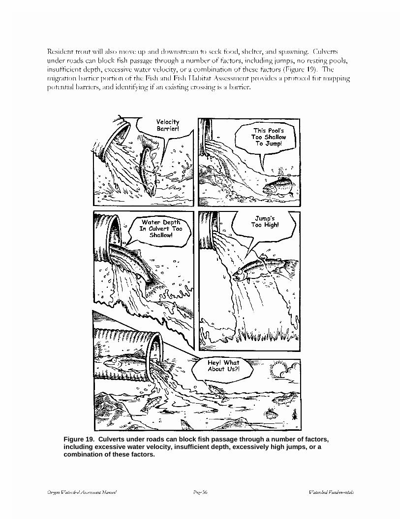
������ ������ ��������� ���� ��� �� ������ ��� �����
�������� ��� �� � � ��� �� ��� �������� � ���� ��� ��� ��� ��� ��������� �� ����
���� ��� ��� � �� ���� ������� ����� � ����� � ������ ��� ����� ������ � ������ � ��
������������ ������ ��������� ���� �� ����� � ��������� � ����� ����� ������ !"� #��
������� ���� ���� � ��� ���� ��� ���� $������ %��������� ������ � ��� � �������
������� ������ ��� ����������� �� �� �������� ������ �� � �����
Figure 19. Culverts under roads can block fish passage through a number of factors,including excessive water velocity, insufficient depth, excessively high jumps, or acombination of these factors.

������ ������ ��������� ���� ��� �� ������ ��� �����
POTENTIAL LAND MANAGEMENT EFFECTS
General
&������ ������� � ������ �� ����� ���������� �� ����� � ��� ����� � ��� ���������� ���
��� ������� � ��� �������� � ��� ����������� $���� ���������� ��� ����� ����������� ����
� �� �� �������� ������� ������� �� �������� � �������� #��� �������� ���������� �����
�����'�� ���� �� �� ��� ����� �� ����� ��� ���������� ���������� �� �������� ������� ����
��� �� ����������� ��� ����� � ��� �������� ���� � ������ � �������� ��� ���� ��� ������� �
������� �������� $���� ��� ��� ���������� ��� �� ���� � ����� � ������� �������� #�� � (
������'�� ��� ����� � ����������� ���� ��� �� ������ �� �������� ��� ��� ���������� ��� ���� ��
��� �������� ��� ����� � ����� ����������� �� ���� � ���� ������� ���� )�� ��� ���������
#�� ��������� ������ ���� � ����� � ����������� ���������� � ���� �����
Cumulative Effects
���� ����� ������� ��� �� ������� �� ��� ������� � ��� ��������� ������ �� ��� ��������� �
����� �������� ������� ���� ��� ������� � ��� ��� ��� ��� ����� ���������� ����������
����� ���� ��� �� ��� ��������� %������ � ���� ���������� ��������� ������ ���� ��
������ ��� �� � ����� � ��� ��� ������ ������ ���� ������� ���� ��� ����������� ����
���� ����� �� ��� ��������� #�� ����� ������� ������� �� ��� ����� �� � ����� �� �
������� � ��� �������� ���������� ���� ����� � ��� ��� �� ��� �������� ����� � ��� ������
� ������� ����������� � ����� �� �� � ������ ������� ����� ������� ��������� ����� ������
������� ���� ������ ������ � ��� ������� ��� ��� � ������ �� ���������� ����
���� ��� ��� �� � ����� � � *+, ��)������ ,������� �� �� ����� ��� ���� ������ ���
���� ������ �'�� ��� ������ ����� ��� ������ #���� ������� ������� ������� ����
������-��� �������� � ������� ����� � ����� �� ��� � �� � ���� ������ ��������
������� ��� ��������� ���� ����� ������� �� �������� �� ��� ���������� ����� �� ���������
��� ����������� ��� ����� � ������� ����������� �� ��������� ��� ����� ������ ��� �������
�������� ������ �� ��� ���� ��� ������ ������"� ��� �� �������� ��� ����� � ����������
������� ��� �� +������� ������� .�� ������
#�� ������ � ��� �������� �� �� ��� � ���������� ������� � ���� ��� ���� ���� ���� #���
���������� �������� ��� ����� � ������� ����� � ������� ����� ���� ���� ��� ������� �
�������� ������ $������ #����� #��� ����� � � �������� ��� ������ � �������� �����������
�� ����������� ������� ���������� ���� ��� ���� ��-��� ������ ������� ������ �� ��� ���� ���
������ �'����"� ��� ���� ����� ���� ����� ��� ����� ������� ������ ������ �� ���������
�� ������ '���"� #�� ������ $������ #��� � ����������� ������� ���������� ����� ������
���� �� ��� ��������� � � ������� ��� �� ��� ��� �������� � ����������� ����� ����� �
������� �������������� #���� ��������� ������ ��� ���� ����� � ��� ���� � � �-�� ��������
������� ������ ������� ��� ����������� ������

������ ������ ��������� ���� ��� �� ������ ��� �����
Table 2. Summary of potential stream impacts from human activities.
Human Activity Potential Disturbances Potential Habitat/Watershed Process ResponsesTimber harvest • removal of riparian zone canopy cover
• soil disturbance, increased erosion of fine sediments• alteration of total basin vegetation cover
• increased summer water temperatures• reduced woody debris recruitment potential• decrease in interstitial spaces and pools (spawning and rearing habitat)• alteration of timing and magnitude of peak flows (hydrology)• change in timing and characteristics of landslides
Transportation (roaddevelopment, rail,bridges, etc.)
• surface erosion, increased fine-sediment inputs• destabilization of upslope areas
increased coarse- and fine-sediment inputs• blockage of migratory corridors (culverts)• loss of riparian vegetation• chemical spills, toxics, nutrient runoff
• decrease in interstitial spaces and pools (spawning and rearing habitat)• major channel disruption & catastrophic loss of habitat with major
events• loss of migratory population component• increased summer water temperatures• reduced woody debris recruitment potential• chemical contamination• changes in peak flows
Agriculture/livestockgrazing
• bank damage• soil compaction• in-channel stream bed disruption• removal of bank vegetation• changes in vegetation species & distribution
• decreased bank stability & direct inputs of fine sediments• reduced water infiltration, changes in peak flows, reduced baseflows• loss or disruption of summer rearing habitat• loss of cover, increased summer water temperatures & formation of
anchor ice• increased stream nutrients
Agriculture/crops • soil compaction• surface erosion, increased fine-sediment inputs• removal of bank vegetation• chemical, nutrient runoff
• decreased bank stability & direct inputs of fine sediments• reduced water infiltration, changes in peak flows, reduced baseflows• loss of cover, increased summer water temperatures & formation of
anchor ice• increased stream nutrients, contamination
Mining • streambed disturbance• fine-sediment inputs• chemical runoff or seepage to groundwater
• loss or disruption of spawning & summer rearing habitat• creation of chemical barriers &/or direct fish mortality, groundwater
contaminationDams (hydroelectricdevelopment, watersupply, irrigationdiversions)
• blockage of migratory corridors• changes in temperature, sediment delivery, flow
regime due to dam regulation• increased temperatures, fine sediments, chemicals
and nutrients with wastewater returns• channel dewatering
• loss of migratory/anadromous population component• overall decrease in habitat condition• direct mortality loss of one or more year-classes, reduction of redds,
loss of available habitat• loss of anadromous prey base/nutrients• loss or disruption of spawning & summer rearing habitat
�
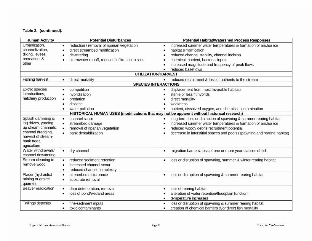
������ ������ ��������� ���� ��� �� ������ ��� �����
Table 2. (continued).
Human Activity Potential Disturbances Potential Habitat/Watershed Process ResponsesUrbanization,channelization,diking, levees,recreation, &other
• reduction / removal of riparian vegetation• direct streambed modification• dewatering• stormwater runoff, reduced infiltration to soils
• increased summer water temperatures & formation of anchor ice• habitat simplification• reduced channel stability, channel incision• chemical, nutrient, bacterial inputs• increased magnitude and frequency of peak flows• reduced baseflows
UTILIZATION/HARVESTFishing harvest • direct mortality • reduced recruitment & loss of nutrients to the stream
SPECIES INTERACTIONSExotic speciesintroductions,hatchery production
• competition• hybridization• predation• disease• water pollution
• displacement from most favorable habitats• sterile or less fit hybrids• direct mortality• weakness• nutrient, dissolved oxygen, and chemical contamination
HISTORICAL HUMAN USES (modifications that may not be apparent without historical research)Splash damming &log drives, yardingup stream channels,channel dredging,harvest of stream-bank trees,agriculture
• channel scour• streambed damage• removal of riparian vegetation• bank destabilization
• long-term loss or disruption of spawning & summer rearing habitat• increased summer water temperatures & formation of anchor ice• reduced woody debris recruitment potential• decrease in interstitial spaces and pools (spawning and rearing habitat)
Water withdrawals/channel dewatering
• dry channel • migration barriers, loss of one or more year-classes of fish
Stream cleaning toremove wood
• reduced sediment retention• increased channel scour• reduced channel complexity
• loss or disruption of spawning, summer & winter rearing habitat
Placer (hydraulic)mining or gravelquarries
• streambed disturbance• substrate removal
• loss or disruption of spawning & summer rearing habitat
Beaver eradication • dam deterioration, removal• loss of pond/wetland areas
• loss of rearing habitat• alteration of water retention/floodplain function• temperature increases
Tailings deposits • fine-sediment inputs• toxic contaminants
• loss or disruption of spawning & summer rearing habitat• creation of chemical barriers &/or direct fish mortality

������ ������ ��������� ���� ��� �� ������ ��� �����
��� ������� �� ����
��������� ����� � � ������ �
�� �� ����� � � ��� ��
� �������� ������ � ���������� � ��������
��� ��� �� ������ ��������� ����� ����� ��������� � ���� ��� ����������� ���� �� �������� ���������� � ������������ �� ���� ��������� �� �� �� ����� �� ��������� ���������� ����� ��� � ����������� �� ������ �������� ���� ���������� � ���������� �� ��� ��������������� ��� ������� ��� ����� ������� ������������ ��� ��� ���������� ������ �� ��� ��������� �� ����
������ �������� ��������!� ������ �� ������� � ������� ���� ����� � ��� �������
REFERENCES
"������ #�$�� � %��� "� �� &'('� ��� %���� � )��������� �� *����� *������ ������ ���+������ ���� %� ,����
"������ -�.� &''/� %���� ����� �� ������� %���� ������� ������� 0�������� *������+������� (� "����� � +1�
"���� +� &'2(� 0�������� #� ���� �� ���������� -����������� � "�������� �������� 3* ��������� �� ��������� ���������� 1��
"�� � +�� � 1� *��� ����� &''4� ��� *��������� "��� ��� $�����5� *���� ����������*�� � �6 ������ 7�������� � *������ ������� $����� 1�������� �� �����������7������ ���������� ����� �������� )����� � $������
"����� .�)�� � -�#� ����� &'((� 8���� ������ �� #� �������������� )������ )����� $9��� �
"������ 1�:�� +�;� #����� � -�+� #������ &''4� *���� �� $�����5� "��� ������ $�����1�������� �� 0��� � ��� ����� *���� $������
���� ����� � "� .�������� &'2<� 0��� +������� � 0��� )����6 � )������ =�� � �� *������0��� )���� )�������� 3* 0����� *������� +>4&<<>/� ���������� 1��
#������ "�� *� .����� �� �� &''?� "������ -����� �� ��� *���� �� ��� 0��� �� $������ $�����1�������� �� 0��� � ��� ����� *���� $������
.������� �� &'((� ������ *��� +�������� -������ 3��������� )����� %� "�������� %.�
;����� � ;�"� &''@� � :�� �� ��� -����� #��� 3��������� )����� ����� ��� +��
;���� - *� � -��� 0�������� &''(� 0����� �������� *��� ����� +*3 )����������� "�!����+��
;������� -�A�� +� A������ � .� )����� &'4?� #� ������ ��� ��������� +�=�>#���� %� ,����
+����� ��-� B� �C� &''&� 8��������� �� 0����� � -����� +������� �� *����� 0������ ����� #������ ������� 0�������� *������ *����� )���������� "����� � +1�
$������� .�+� � ��;� =����� &'2(� ��������� �� ��� )����� %�������� 3���� *���� ����������� )��������� ������� ��������� $-� )�D(<<DE>2(D<EE�

������ ������ ��������� ���� ��� �� ������ ��� �����
$������� .�� &''@� ���������6 ����� ������� ��� ������������ ��������� ������ ? ����*� 1��� � ��)� *����� � �� "�������� ��������� � �������6 ����� ��� ��� ��������������� � ������� ������ ;��� )���������� "�� -���� 0;�
$����� 1�������� �� ����������� 7������ &''?� &''&>&''@ ���� 7����� *�� � � -�����$����� 1�������� �� ����������� 7������ )����� � $������
$*3 1��� 1�������� &''2� ������� *��� ����6 � ;������ =�� �� $����� *��� 3�������������������
)����� "� &''/� $��� ������ �� %���� )����� *����� �� 3��������� �� ��������� )�����*������
-������ 8��������� 9������� ���������� �������� ������� � ��� ������� *���F0� ���=�� � ��� ������� �������� :������ /�/� ������ &''?�
*������� � 1�-� &'4/� ��� �� ������� +�������� .��� ����� G *���� %� ,����
�������� )��� &'24� �������� %���� ����� �� ��� ����� ����� � �������� 3��������� )�����
,���� *� &'22� � ������ � *����6 � %������� #� ����� � ���>�>*���� 0��� �����
3* =�������� *������ &'4@� +�6 #� �������� 3��� +� ��� *��� �� $������ 3* 1�������� ����� 8�������� ���������� 1��
:������ -�� =� +������� A� �������� .� *� ���� � �� �������� &'2<� ��� -���� ����������������� �� �� .����� �� 0��� ������ *������� :��� E4�
GLOSSARY
�������� *�������� ��� �� ��� ������ B��� �9����� ����C�
�������+������� ������ ������ ��� �� ������ � ������ ��� �� ���� �� �����������
� ��������� 0��� ��� ���� ���� ��� �� �� ����� ��� ��� ����� �������
������� � �� � �� ���� ��� �� ������� ����� ���� � �� ���� ��� �� ���� � �������� ������ ��� ����������
�� ������� �� ������ �����9� ��� �������� ����� ����� ������� 1����� ���� ������������ ������� ������ �� ������� ������ �� � �������� �����������
������� *�������� ��� �� ������� �� ��������� �� ������ �������
�� ��� ������ ��� ���������� ��������� ���� ����� ���
��� � ���������� � ���� ��� �� ��������� ���� ������ � ������9 ������ ������� ��9������ ����� ����� ��� ����� � ��� ��� �������� �������� � ���� ��� ��� �� �������� ���� ����
������ � ������ ������ ������� ����� ������� ��� � �� ����� ������

������ ������ ��������� ���� ��� �� ������ ��� �����
��� � �� � ��� �� -��� �� ������� ������ � �� �� � �� �� �� ��� ���� ����� +� ���
���� ���� �� ��� ���� >����� �� � �� ��������� �� ��� &<<>��� ���� ����� ��������������� ����������� �� ���������� �� �� ���� ������ �� ���� ����� ��� ����� ������ �� �������� �� ���� ����� �� �������
��� � ������� ����� ������ =����� �� ����� ������� ��� ������ �� ����� �������
������� � ������ ���� ������� ����� �������� ����� �� �9����� �� ������ �������� ��
������ �� ������������ ������ ��� ��������� ������ ��� ������� 8� ���� �������� �#�� �� ���
�� �����!� ���������� � ���� ������� �� ����� ���������� � �� �� � ����������� ��
���������� ��������������
��� � ������ � 1���������� �� �� ����� ������ ����� � �� ���� �� ��� ����� B���
�9����� ��� � ������ �� ��� ����� ������C�
����� � ����� ������� �� ������ ������ ������ � "��� ����� �� ������� �� ����
������������� ��������� ����� ��� ���� �� ���� �������� �� ����� ��������� 9����� �� ����� ���
���� �������� ����� � ����� ���� ������� ��� � ����� ���� �� �� �� �����
�� ��������� ��� ������� ���������� ������ ���������� � ��� ������ ������ ������ ��� �
����� ���� � ������ ���� � � ����� ��� ��������
������ ��� � ���� �� �� ��� � ��� �� ��9���� �� ����� ���� ����� � ���� ��� ���� ������
������� �� ����� �������
���������� $�����H ��� ��� �� ������ ���� �� �������
�������� ��� ����� ��� �� ����� ������ � �� ����� �������� ���� � ���� �� ������ ��
�� ��� ��� ���� �� ��� �� �������� ���� ����>���� �� ����������� � �� ����� ������
������ � �� ���� ���� ����
���� ��� ���� � � ��������� � �� ������� ������� �� ������ �
��� ����� ������ ����� ������ ������ ���� �����
�������� � ;� ��� ��� ����� ������ �������� ���� � ���� � �� ���� ������������� ���
������� ������ ��������� �����
������� � ��� ������� ��������� �� ���� ������� ���� ��� �� ������ ������ �� ���� �� �������
������ ��� 0�� ������ �� ��� ���� �� ��� ��� ��� ��� �� ���� ������ �� ����� ������� ���� �
����� �� ��� �� ��� ������
������� �� ��������� ��� �� ��� � �������
�������� �������� � ��� ��� ����� �� ��� ������ �� ��� ��������� ������� ����
��������� � ������������
��� �� ������ *�� ���� �����

������ ������ ��������� ���� ��� �� ������ ��� �����
��� ���� ����� � ���� ���� ������ �� ����� �� ��� ������ �� ���� ��
��� ����� ��� ������� ����� �� ��� ��� ������ ����� ����� ���� ������
������ � ��� ��� �� ������� ����� ������ ���������� �� ��� ����� �� ��� ������� �������
� �������� � ����� �� ���� ����� ����
���� ���� 0��� ��� ��� �� ����� ������ � ��� �� ������ ����� �����������
��� � � ������ -��� ���� ����� ��� �� ������ ���� ��� ����� ������ �� ������ ������
����
���� � ������ � � ������� ������� �� ����� ������ ������� ��� ���� ����� ��� �� �����
��������� ��� �������� ����� ��������
�������� ������ � ��������� ������ ���� ����� ���� ����� ����� ������� �� ����� �����
�������H �� ��� ������ �� ��� ��� ������ ���� ��������� ������ 3�� �� ������ �� ����
����� > � ������>��� ���� � �� � �9�������� �� ��� ������� ������ ������ �� �������
����������� � ���� �� ������ ���� ����� ���� �� ������� ���� ��� �������� ����� ���� �����
��������� ����� ��� ���������� �� ��� ���� ��� ����� ���� ���� �� ��������� � ��� ��
���� ����
��������� ��� ������� �� ��� ������� �� ��� ���� ��� ��������� ���� ��� �����
��������� ! �� ����� ��!���� 3* =�������� *����� ���������� ��� ��������� �� ��������
������ �� � �� �9������ �� ���������� �����
����������� ����� *���� ��� � ��� ����� ��� �� ���� � ���� ������� ��� ��� �� ������
�������
���������� ������� *����� B���� � �������C ��� ��� ��� ���� �� ������ �������� ���
����� �� ����������� �� ������������ ���� ��� ����� �
� ������� � ��� ��� �� �������� �� ��� ���� ��� ��������� ���� ��� �����
���� ����� ������ �"#$�� ;���� ������� �� ���� � �� ��� ����� ������� �� ������ �����
�������� �� ����� ����� � ����� ��� ����� � �� ��� � ���� ����� �������
����� ����������� )�� �� ��� �������� ��� ��� ���������� �� ������� ������ � �����
������ ��� �������
�� ����� ���� �� ������� � ��� �� ����5� ���� ������ ��� � ��������� ����� ������������
������� ��� ��H ��� �9����� ������ ������� ������� � �������� ����������� �� ����
�����
�� ���� ��� ������� ��� �� ��� ��� ����� ����� �� �����

������ ������ ��������� ���� ��� �� ������ ��� �����
���� ����� �� ���� ��� ���� ������ ��� 1������� �������� �� ���� � ����� �� ��
���������� �������
��� ���� �� ���� ����� ������ ����� ������� ����� ��� ������
���� ��� ��� �9���� ����������� ��� �� ��� ����� ����� �� ����� ����� �� �����
������������ � ��� ����� ��������� B������C �� ������� ���� ������ �� ��� �������� �� �����������
������������ � �� ����� ��� ��� � ���� ��� �� ������� �� ��� ����5� �������
��� ���� ������ ������ ����� ��� ��� ��� ���� ��� ���� ������� %�� ������ �� ���� ��$������
��� %� %� �� ���� ������� ������� �� ����� �� �� ����� ������ ��� ��� ������� -��>��>��� ������ ������ ����� ����� ��� �������� ��� !����
����� �� ������ ���� �� ������� ��������� ����� ���� ������ � ����� ����� �� $���� ���� ������� ������ ���� ����� ������ �� �� ��
������� �� � �������� ������ � ������� 1�������� ���� ��������� ����� �� ��� ����� �������� ���� ������ �� ������ B���� ���� ���C �� ��� ��� ��!� �� ������ -��������� �������� ��������� ��� ����������� B0�� �9����� /?>��� ���� ��� ��� @I ���������� ���������� �� �� ����� ����C
��������� ���� ����� ������� � ����������� ���� �������� ��� ����� �� ��!� �� ���� ����� �� ������ �� ��� ���� ���������� ��� �� B�������C �� ��� ����� ������� +�������� �������������� ����� � ���� �� ��� ��� ��� �� ���������� �� ���� ����� ������� �� ��� �� ����� ���� �� �� �� ������ � �������� ���� ������� �������
����� ��� ������ ����� �����
������ � ���� %���������� ���� ��� ����� �� ��� ��� ����� ������ ����� ������ ������
��� � ������� ��� ��� ������ ���� �� ��� ������� ��� �������� �� ������ �����
������� �������� ���� ��� ����� ������ � �������
������� &� ����� �� ������������� ����� ������ ���� ��� ���5� � �� ��� �� ����� ������� ���� ����������� � ���� ���� ������������ ������������� � �� ������� ��� ������ �� ���� ��������� ��������� �� ����� ��� ��������� �� ����� ����������
������� ��������� � :�������� ������ �� �� ��� ��� ���� �� ����� �� ����� �� � �� ��� ������� ��� �� �� ����� ���� ������� �� ��� ������ ������ 8���� �� ��� �� � ��� ���� ������ ������ � ����� ������� B���� +���� &''&C�
���� ��� 0��� �� ��� ����� ���������� ����� ��� ������ ������ ���� ��������� �������� � �������� =�������� ��� ���� ������ ������ �� ������ ������ � ����

������ ������ ��������� ���� ��� �� ������ ��� �����
������ ��' � � � � ������� 0������� �� ����� ����� � ������ ������ ��������� �
������� ���� ������� � �� �� � ���� �� �������
��� ������ ���� ������ ����� ��� ���� ����� ������ � ���� ��� ���� �� ��������
������� ���� �� ������� ��� ����� �� ��� ������� �� ��� &J ����� �� ��� �� ��������������
����� ����� �� #�������� ������� ���� ���� � � ����� ����� ����� �� ������ ��� � ����� ��� � � ���� ������ B������ ��� �9��������C �� ������ ��� ������ � ����� ���� ������ ����� ��������
���� � � ������ ��� ���� ��� ��� ������ ������ ����� ����
��� �%������ � ���� � ���� �� ������ ��������� � ���� ������ �� ���� �� ��� ����� ������
������ ��� � �� ��� ������ �� ���� �� �� ���� ������ ����� B����� �������� ����� ����������C ���� ����� �������� #����������� ���� ������� � ��� �� ������ ����� ��� ��� ���������� �� ����� ���� ������ �� �� ������ ���� ������ ����� ��� � ������� �� ���� ��������� �������� ���� � �� ����� ����� �9���� ������� "����� ����� ������� � ���� �� ��� ���� ������ �� �� ��������� ��� ������ ��������
������ �� ���� ����� ��� �� ������ ���� ������ �� ����� ����� ������� �� ����� ����9������ � ����� �� ����� ������ ��� ����� ���� �� ���
���������� +����� �� ������ ������ ��� ����� ��� �� �� ������
������ �� �� ���� ��� ���� ����� ��� ��� �� ��� �� ������ ����������� ��� �����
��� �������� � ;��� �� ��� �� ��� ��������� ���� ������ ������
��� � ��������� � :�������� ������ ��� ����� ������� ������ �� ���� ���� ������ ��� ������� ������� �� ��� �� ���� ������ � ���� !�����
�� � ����� ���� ������ �� ��� ��������� � ������� �� ����� �� ������ ����� �� �� �

Component IStart-Up and Identificationof Watershed Issues
Table of Contents
The Assessment Start-Up Process ................... I-3
Overview.......................................................... I-3
Step 1: Identify Project Manager..................... I-4
Step 2: Coordinate Community Input .............. I-4
Step 3: Identify Assessment Team ................. I-5
Step 4: Compile Initial Materials...................... I-5
Step 5: Create the Base Map.......................... I-8
Step 6: Refine Land Use Map....................... I-11
Step 7: Acquisition and Compilation of
Other Data ............................................... I-13
Identification of Watershed Issues.................. I-13
Critical Questions .......................................... I-14
Identify Typical Issues Associated with
Land Use ................................................. I-14
References ......................................................... I-18
Glossary ............................................................... 18
Appendix I-A: Background on State and
Federal Regulatory Issues
Fisheries
Water Quality Laws and Programs
Appendix I-B: Blank Form
Form SU-1: Issue Identification Form


Oregon Watershed Assessment Manual Page I-3 Start-Up and Issue Identification
Component IStart-Up and Identification of Watershed Issues
THE ASSESSMENT START-UP PROCESS
Overview
Watershed assessments can be used to meet a wide variety of goals. An assessment can function asa catalyst to establishing a community-based watershed group. Or it can provide an already-established group with a structured compilation of available watershed data, along with a review ofthe existing watershed conditions.
The initial step of the watershed assessment process is identifying the assessment team and gatheringbasic watershed information. These tasks are described in the steps below. After putting together ateam and gathering information, the key to a smooth and successful assessment is establishingeffective communications between the community, the assessment team, and technical supportspecialists, and ensuring that each group understands the goals of the process. The project manageror coordinator plays an important role in establishing and facilitating these communications.Important to the assessment is involvement, from the start, of property owners and otherstakeholders in the watershed. The property owners should understand the goals of the process andbe engaged in the process at the beginning. In addition, property owners often have detailed localknowledge, which can provide valuable insights to understanding watershed condition. Ultimately,stakeholders need to have ownership in the assessment process in order to develop support foridentified enhancement and protection opportunities.
Stakeholders (including property owners, local residents, agency and industry representatives) shouldunderstand that watersheds are complicated, and that they will need to invest time either completingthe assessment or reviewing and understanding the assessment findings.
The project manager leads this Start-Up and Identification of Watershed Issues component,oversees completion of each assessment component, and facilitates communications between theassessment team, the community, and local landowners. The first task of the project manager is toidentify how the assessment components will be completed. The team may consist of staff orvolunteers who have the skills and time to complete one or more assessment components. Theproject manager needs to track the progress of the watershed assessment team to ensure theassessment components are completed in a timely manner. The project manager will also beresponsible for gathering and compiling basic maps and data, which are needed throughout theentire assessment.
Informing landowners in the watershed about the proposed watershed assessment, and buildingtheir understanding and support for the process, will help ensure that the assessment findings will beutilized. The project manager needs to notify the community that the assessment is taking place andprovide opportunities for community involvement and input. Notices can be posted in prominentlocations; landowners in the watershed, as well as local agency representatives, should be mailednotices. Community meetings designed to obtain input and identify issues will engage interestedparties in the process; the information gathered can be used to help focus the assessment. During

Oregon Watershed Assessment Manual Page I-4 Start-Up and Issue Identification
the Watershed Condition Evaluation phase at the end of the assessment, the start-up issues can berevisited to determine if these issues were adequately evaluated or if new issues were identified.
Necessary Skills
The project manager should have good organizational and communication skills. Meetingfacilitation skills will help focus community meetings and build support for the assessment process.
Final Products of the Start-Up Component
The products of this component will be used in subsequent portions of the assessment. Thefollowing items need to be collected or developed:
• Base Map• Ecoregion1 locations and descriptions• Refined Land Use Map: Map showing location of key land uses in the watershed• Recent stereo aerial photographs covering the entire assessment area• Issues Identification Form (Form SU-1)
Step 1: Identify Project Manager
The project manager will be responsible for assigning tasks, contacting stakeholders, and trackingand coordinating the completion of the assessment components. The project manager may alsohelp with data acquisition and facilitate data transfer between the people working on individualcomponents.
Step 2: Coordinate Community Input
There are a number of potential methods to solicit input from the local community for the purposeof building support for the project. The following tasks are recommended, although you may find ituseful to structure them differently, depending on your knowledge of the community and yourgoals:
1. The project manager and assessment team should meet with the watershed council andtechnical advisors to review the list of potential issues. After this meeting, the watershedcouncil should identify an appropriate forum for involving local property owners, local andcommunity leaders, community action groups, and other stakeholders in the watershed inreviewing the list of issues. It is important that all parties understand that a watershedassessment cannot address all potential community concerns or issues.
2. Hold a series of informal meetings with community groups on their own ground. Forexample, presentations could be made at regularly scheduled meetings of the local Soil andWater Conservation District, small communities, industry associations, and interest groups.
Making the various entities comfortable with the process will take considerable time. A reasonableexpectation is that the initial process of identifying issues and interacting with the community will
1 Terms that appear in bold italic throughout this text are defined in a Glossary at the end of this component.

Oregon Watershed Assessment Manual Page I-5 Start-Up and Issue Identification
take several months. A number of data-gathering efforts, such as obtaining historical accounts andagency data records, can occur concurrently with the issue identification process.
Step 3: Identify Assessment Team
Completing an assessment is a big commitment in time and resources. We expect that it will takebetween 4 to 8 months to complete an assessment, depending on the watershed and thecommitment of the assessment team. It would be very difficult for a single person to compile anentire watershed assessment in a timely manner. Hence, a team of people will usually be involved incompleting the process. This watershed assessment process is designed for people who do notnecessarily have specialized technical training. Each component lists specific skills which are eitherrequired or would be helpful in completing that component. You may be able to find staff on thewatershed council, volunteers, students, consultants, or some mix of people who have the skills andcan commit the time to completing one or more assessment components. The project managerneeds to assign responsibility for specific components based on the person’s skills, interests, andavailability. Each potential team member should review the appropriate section of the manual to becertain they feel qualified to complete that portion of the assessment.
Step 4: Compile Initial Materials
Decide on Watershed
There are 1,063 5th field watersheds in the State of Oregon, with an average size of 58,218 acres. Ageographic area of approximately 50,000 to 100,000 acres is an appropriate size to complete awatershed assessment. Watersheds of this size canusually be mapped at 1:24,000 scale (1 inch equals2,000 feet) on standard plotter paper, and the scaleprovides adequate resolution for data display.
Obtain USGS Maps
A complete set of US Geological Survey (USGS) 7.5-minute topographic maps (also at 1:24,000 scale) forthe entire watershed will be useful for initialorientation in the watershed, and for completing someassessment components. (See Contact Informationsidebar for how to obtain copies of USGS and othermaps.) The USGS also publishes a key to topographicmap symbols, which will be useful for interpretingmaps in some of the components. (Also see How toInterpret a Topographic Map sidebar.) In order todecide which maps are needed, you will need to locatean index map to identify names of map sheets (quads)covering your watershed. This information is usuallyavailable where you purchase maps. In addition, othermaps used in the assessment will orient off of theUSGS quad maps, so a list of quads covering thewatershed will be useful for obtaining other background information.
CONTACT INFORMATION FORMAP ACQUISITION
Topographic maps ($4 to $5/map)
• Nature of the Northwest Store, OregonBuilding, Portland (503) 872-2750
• USGS Map Sales, Box 25286, FederalCenter Building 810, Denver, CO 80225;(800) 872-6277
• Oregon State University, Valley Libraryhttp://www.orst.edu/dept/library/
• Local outdoor stores or bookstores
ODF stream classification maps
• ODF Fish Presence Coordinator(503) 945-7483. Cost $1.50/quad sheet+ $2.35 shipping (up to 12 maps)

Oregon Watershed Assessment Manual Page I-6 Start-Up and Issue Identification
Obtain ODF Stream ClassificationMaps
These black-and-white maps produced bythe Oregon Department of Forestry (ODF)are extremely useful and are available at alower cost than USGS maps. You will needat least one complete set for the entirewatershed, although you may want to orderseveral sets. The ODF stream classificationmaps were developed from USGS quadmaps, and have an enhanced streamnetwork. The stream classification mapsalso show breaks between “large,”“medium,” and “small” streams; andupstream limit of fish use. The accuracy offish distribution and stream size informationon these maps varies across regions andwatersheds. The analyst performing theFish and Fish Habitat Assessmentcomponent will update the information onthese maps. There is a current effort todigitize these maps into GeographicInformation System (GIS) format, anddigital versions should be availablesometime in 1999.
Obtain Recent Stereo AerialPhotographs
Recent stereo aerial photographs coveringthe entire assessment area are essential forthe Riparian/Wetlands Assessmentcomponent, and are useful for completingthe Channel Habitat Type Classification andSediment Sources assessment components,as well as others. Stereo aerial photographsallow the analyst to view the area of interestthree-dimensionally. A scale of 1:12,000 ispreferable, although smaller scales maysuffice. Color or color-infraredphotographs are preferred.
If stereo aerial photographs are not availableorthophotos may be of some use.Orthophotos are aerial photos that havebeen corrected to remove displacement. Orthophotos are scale-correct but can only be viewed two-dimensionally.
HOW TO INTERPRET A TOPOGRAPHIC MAP*
Each contour line on a topographic map represents a verticaldistance above a reference point such as sea level. All pointsalong a contour line are at the same elevation. The differencebetween two adjacent contours is called the contour interval. Itrepresents the vertical distance you would need to climb ordescend from one contour elevation to the next.
The horizontal distance between contours is determined by thesteepness of the landscape. On relatively flat ground, two 20-foot contours can be far apart horizontally. On a steep cliff, two20-foot contours might be directly above and below each other.In both cases the vertical distance between contour lines is still20 feet.
Water always flows downhill perpendicularly to the contourlines. As you go upstream, successively higher and highercontour lines first parallel then cross the stream. This isbecause the floor of a river valley rises as you go upstream.Likewise, the valley slopes upward on each side of the stream.A general rule is that topographic lines always point upstream.With that in mind, it is not difficult to make out drainage patternsand the direction of flow on the landscape. In the figure, thedirection of streamflow is from Point A to Point B
* Adapted from the Oregon Freshwater AssessmentMethodology (Roth et al. 1996).

Oregon Watershed Assessment Manual Page I-7 Start-Up and Issue Identification
The owner of the aerial photos for your watershed may not wish to loan out photos; however, youmay be allowed to photocopy the set. Photocopies made using a high-quality machine(approximately $1/copy; cheaper sometimes for a large order) work well, and is a lower-costalternative than buying your own set. Several possible sources for aerial photographs are listed inthe Aerial Photos sidebar.
AERIAL PHOTOS
Training in InterpretationAerial photos are used for the Riparian/Wetlands Assessment component, and are very useful for theSediment Sources and Channel Habitat Type Classification assessment components.
Examples of information gained from aerial photos include overall land use, riparian area width andspecies composition, evidence of historic changes, assistance in determining types of stream channels,identification of sediment sources, and evaluation of road networks. For someone without training inaerial photo interpretation and in working with stereo images, making sense of a series of aerial photoscan be a daunting task. One approach is to find someone with experience reading aerial photos; perhapsan employee of a large landowner or a resource agency staff member may be able to help. That personmay be willing to perform the aerial photo tasks, or to provide orientation and coaching to the persondoing the interpretation. Consulting the Oregon State University (OSU) Extension Forester for your countymay also help identify others who could provide expertise.
If training in aerial photo interpretation is desired, resources are available. The OSU College of Forestryperiodically offers a short course on Mapping from Aerial Photographs. Contact the College of ForestryConference Assistance Office at (541) 737-2329 (www.cof.orst.edu/cof or [email protected]).
Useful textbook resources include:Paine, D.P, 1981. Aerial Photography and Image Interpretation for Resource Management. John Wileyand Sons, New York. 571 pp.
Avery, T.E. and G.L. Berlin, 1992. Fundamentals of Remote Sensing and Airphoto Interpretation, 5th
edition. Macmillan Publishing Co., New York. 472 pp.
Sources for Aerial Photos• Oregon Department of Forestry• Natural Resource Conservation Service (NRCS)• Local Soil and Water Conservation District• University of Oregon Map and Aerial Photography Library, 165 Condon Hall, Eugene, OR 97403-
1251; (541) 346-4565; http://libweb.uoregon.edu/~map/• Local US Forest Service district or Bureau of Land Management district• Oregon State University, Valley Library http://www.orst.edu/dept/library/• Other possible agencies include: US Army Corps of Engineers, USGS, Oregon Department of
Transportation, Bonneville Power Administration (if watershed located near major transmission lines),and county government
Commercial sources for photos in Oregon:• WAC Corporation, 520 Conger Street, Eugene, OR 97402-9817; (800) 845-8088• Spencer B. Gross, Inc., 13545 NW Science Park Drive, Portland, OR 97229; (503) 646-1733
Other possible sources of photos:• Large forest landowners

Oregon Watershed Assessment Manual Page I-8 Start-Up and Issue Identification
Step 5: Create the Base Map
After materials are compiled, your first big task is to create a base map for the assessment. If thewatershed council has GIS support, the State Service Center for GIS (SSCGIS) can provide basemaps of watersheds that include the stream network, watershed boundaries, subwatershedboundaries, estuary boundaries, roads, legal boundaries, and locations of major cities and towns.These maps are available to download off the SSCGIS World Wide Web site or the center can becontracted to provide initial GIS map products. (See sidebar, Some GIS Mapping Options, formore information.)
SOME GIS MAPPING OPTIONS
Free DataYou can obtain baseline information from the State Service Center for GIS (SSCGIS) Web site atwww.SSCGIS.state.or.us. This information includes major roads, waterbodies, public land survey(Township, Range and Section lines), watershed boundaries, generalized zoning, land ownership, citylimits, urban growth boundaries, and 1990 census information on population. Available data includes fishdistribution, 303(d) listed streams, and watershed council boundaries. This information is available for theentire state and can be downloaded directly from the Web site. You will need some type of GIS browser toimport and view the data, and must be able to cookie-cut the data to your watershed (data is in county orstate-wide format). Local governments often have a wealth of digital information that they are willing toshare with other groups. Contact the State of Oregon GIS Data Administrator for contacts with localgovernment GIS groups in your watershed. The local governments may have technical resources to helpyou.
Additional data may be available for the area where the assessment is taking place. Contact the State ofOregon GIS Data Administrator for more information:
(503) 373-7461 or (503) [email protected]
http://www.SSCGIS.state.or.us
Professional GIS ServicesThere are several methods of obtaining quality GIS services. Several consultants work with watershedcouncils and provide GIS support for a fee. A list of these consultants can be obtained from the Governor’sWatershed Enhancement Board (503-378-3589).
The SSCGIS has provided base information to several watershed councils at the request of the Governor’sWatershed Enhancement Board. Base maps of major roads, streams, waterbodies, ownership,generalized zoning, and the USGS quad maps of topography can be obtained for $1,500 per 5th fieldwatershed. Additional GIS services are available. Contact the SSCGIS at (503) 378-4163 for additionalinformation and price quotes.
Coordination of Digital DataThe state would like to coordinate the update of base information and the additional data collected duringthe assessment process. This digital data could then be used for regional or multiple basin assessments.Whatever the process you use to develop your base information, please contact the SSCGIS to make sureyour results are incorporated into the Oregon Digital Map Library.

Oregon Watershed Assessment Manual Page I-9 Start-Up and Issue Identification
Numerous sources of GIS data are available, and deciding what data to use can be confusing. Inaddition, the usability of the data depends on the scale at which the data was collected and compiled,and the format and presentation of the data. Sorting through maps to determine the metadata (dataabout data) used to create them can be an overwhelming task. Then it takes a solid understandingof the mapping process and professional judgement to determine if the data accurately portraysconditions. GIS support requires professional expertise, which in itself can be time-consuming andexpensive. For these reasons, this assessment process does not require GIS support to becompleted. However GIS support can expedite creation of the base map, and allows for better-quality final maps and more options for summarizing results. We have described in the followingsubsections a process for developing your own base maps without GIS support.
Choose the Best Watershed Map
The ODF stream classification maps are the most informative maps and are usually the best-suitedfor use as base maps. The initial base map is made by cutting and pasting together the paper quadmaps to produce a single map of the entire assessment area. Many photocopy shops have large-format copy machines that can reproduce several copies of this map for use in subwatersheddelineation.
Identify Subwatersheds
You will need to partition the large watersheds into subwatersheds of roughly equal size to provide aframework for organizing and summarizing the data. There is currently no standard delineation of6th field Hydrologic Unit Codes (HUCs) (subwatersheds), although in some portions of the state6th field HUCs are mapped, and these established subwatersheds may be adequate for theassessment. If 6th field watersheds have not been mapped, the project manager, in consultation withthe assessment team, will be responsible for deciding how to partition the watershed. Usuallywatersheds can be divided up into 6 to 12 subwatersheds depending on the overall geomorphologyand land use patterns.
Delineation can be based on a combination of factors, including major changes in topography, landuse, and stream size. (See Delineating Watersheds and Subwatersheds sidebar for mappinginstructions.) Where some subwatersheds are dominated by different land uses, certain individualsor groups within the councils may take responsibility for specific uses (agriculture, forestry, asuburban stream) with which they are familiar, while still working to ensure consistency of analysiswithin the watershed. It may also be possible and desirable to separate out a tributary or sub-basinthat has been highly impacted (greater than, say, 50%) by development. Subwatershed boundariescan be identified by following the major topographic features dividing drainage areas (tributaries). Itmay take several attempts to decide on an appropriate delineation for subwatershed boundaries.Subwatersheds should be named for the major tributary within the subwatershed so that referencesto the subwatersheds will be consistent through all assessment components. Once thesubwatersheds have been identified and agreed upon, they should be delineated on all of the basemaps. Because subwatersheds are so fundamental to watershed characterization and assessment, thewatershed technical team should review and approve the proposed division of subwatersheds.

Oregon Watershed Assessment Manual Page I-10 Start-Up and Issue Identification
Delineate Ecoregions
The Level III and IV ecoregions of Oregon and Washington are mapped in the Ecoregion appendixof this manual. Locate your watershed on the map and identify the ecoregion(s) that occur in yourwatershed. If more than one ecoregion occurs in your watershed, draw the divisions betweenecoregions on the map. Find the appropriate ecoregion descriptions in the Ecoregion appendix.These descriptions contain information useful for most components of the assessment. Make copiesof the pertinent description for each member of the assessment team.
Finalize Base Map
You should now have a paper map at 1:24,000 scale produced either by GIS or cutting and taping.The map should show the watershed partitioned into named subwatersheds of roughly equal size,the stream network, stream names along with watershed boundaries, estuary boundaries, sectionboundaries, present ecoregions, major roads, and the locations of cities and towns. Additional copiesof this map can now be produced (either plotted from GIS or copied on a large-format copymachine) on paper or Mylar and given to the assessment team members to start their assessments.Paper maps can be laminated so that information can be added with a fine-tipped marker and erasedif a correction is needed.

Oregon Watershed Assessment Manual Page I-11 Start-Up and Issue Identification
DELINEATING WATERSHEDS AND SUBWATERSHEDS*
The head of a watershed is the point where land slopes away into another watershed. Generally, this occurs athill tops, ridge lines, or saddles. If you were to join all of the high points around a stream, you would have thewatershed boundary. The following example shows how to locate and connect all of the high points around awatershed on a topographic map.
1. Draw a circle at the outlet or lowest point of the stream or tributary in question.
2. Put small x’s on the high points along both sides of the stream, working your way upstream.
3. Starting at the circle, draw a line connecting the x’s. This line should always cross the contours at rightangles (i.e., it should be perpendicular to each contour line it crosses).
4. Continue the line until it circles the stream watershed.
The boundary will appear as a solid line around the stream or tributary. Generally, surface-water runoff from rainfalling anywhere in this boundary flows into the subwatershed stream.
*Adapted from the Oregon Freshwater Assessment Methodology (Roth et al. 1996).

Oregon Watershed Assessment Manual Page I-12 Start-Up and Issue Identification
HOW TO MEASURE WATERSHED AREA
Grid MethodThe grid method entails constructing arectangular grid and counting squares,estimating partial squares. Usually it is easiestto trace the basin outline onto a sheet of graphpaper, and count the squares on that grid.Converting the number of squares to an areavalue depends on the scale of the map you areusing. If you are using a USGS quad map, thescale is 1 inch equals 2,000 feet or 1 squareinch equals 0.143 square miles (Dunne andLeopold 1978).
How many squares inches did you count inyour drainage basin?
Multiply this number by 0.143 and the result isthe area in square miles.
To convert to acres: 1 square mile = 640acres.
Planimeter MethodA planimeter is a small device with a hingedmechanical arm. One end of the arm is fixed toa weighted base while the other end has anattached magnifying lens with a pointer. Youtrace around the area to be measured with thepointer. The planimeter readout registers thearea being measured.
Planimeters cost between several hundred to athousand dollars depending on the degree ofsophistication. They are available fromforestry or engineering supply companies.
Step 6: Refine the Land Use Map
The Refined Land Use Map will be used inassessment components to identify the types andareas of potential land use impacts. Land usemaps are available at 1:24,000 from the SSCGIS.In addition, users should request an ownershipmap to help with validation of the land useswithin the mapped categories. The land use mapprovided by the SSCGIS is based on zoningdesignations and is produced at a larger scale thanother maps used in the assessment. This meansusers will need to make some additions to createthe Refined Land Use Map for use in theassessments.
For the assessment process the watershed landuses are placed into the four categories: (1)forestry, (2) agriculture, (3) rangeland, and (4)urban. Typically, stakeholders will have specificunderstanding of land uses in the watershed. Theactual land uses should be validated usingownership maps, local knowledge, aerial photovalidation, or field visits.
In this step, you inspect the land use mapprovided by the SSCGIS and identify the differentland uses present in your watershed and in each ofits subwatersheds. The land use map acquiredfrom the SSCGIS is based on local zoningdesignations. These designations may notaccurately represent the actual land uses in thewatershed. First you need to validate theboundaries around the mapped land uses usingaerial photographs or orthophoto quadrangle maps. Orient yourself to a landmark visible on boththe photo or map (road and streams are often good points of reference). Visually compare theboundaries of observed land uses (i.e., fields, forests) to the mapped land uses. On the land usemap, mark the corrected land use boundaries. Using this corrected, Refined Land Use Map,determine the area (acres or square miles) of forestry, agriculture, range land, and/or urban land usesin each subwatershed. The areas in each land use can either be estimated using GIS or calculatedusing either the rectangular grid method or a planimeter (see the How to Measure Watershed Areasidebar). The project manager should make an effort to ensure that the Refined Land Use Maprepresents the actual land uses as accurately as possible and make sure the stakeholders in thewatershed agree with the maps at this stage.

Oregon Watershed Assessment Manual Page I-13 Start-Up and Issue Identification
Step 7: Acquisition and Compilation of Other Data
Table 1 lists basic data needs and identifies which assessment components utilize specific dataproducts. The project manager may want to order additional data materials for other assessmentcomponents to facilitate the process. Directions for acquiring materials for a specific assessmentcomponent can be found in that component.
IDENTIFICATION OF WATERSHED ISSUES
Critical watershed issues should be identified early in the process to help focus the watershedassessment. Although all elements of the watershed characterization and assessment generally applyto a watershed, this step will help the council in understanding how the assessment products fit intocurrent state and federal regulatory direction. In addition, early identification of importantwatershed issues may help direct where time will be spent.
Table 1. List of basic background materials needed for a watershed assessment.
HistoricalConditions CHT
Hydrology& Water
UseRiparian/Wetlands
SedimentSources
ChannelModifi-cation
WaterQuality
Fish &Fish
Habitat
Watershed basemap
√ √ √ √ √ √ √ √
Land use map √ √ √
USGS topo maps √ √ √
Aerial photographs √ √ √ √ √
Orthophoto quads √ √ √
Ecoregionsummary
√ √ √
Oregon Departmentof Fish and Wildlifeand other physicalstream habitatsurveys
√ √ √*
CHT map √ √ √ √
Historic conditionsummary table
√ √
Mean annualprecipitation map
√*
NRCS county soilsurveys
√ √*
USGS stream gagedata
√*
Division of StateLands wetlandinventory maps
√*
National WetlandInventory maps
√*
* Indicates that directions for obtaining this information are included in this component.
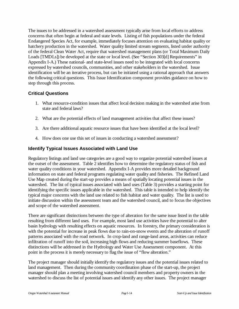
Oregon Watershed Assessment Manual Page I-14 Start-Up and Issue Identification
The issues to be addressed in a watershed assessment typically arise from local efforts to addressconcerns that often begin at federal and state levels. Listing of fish populations under the federalEndangered Species Act, for example, immediately focuses attention on evaluating habitat quality orhatchery production in the watershed. Water quality limited stream segments, listed under authorityof the federal Clean Water Act, require that watershed management plans (or Total Maximum DailyLoads [TMDLs]) be developed at the state or local level. (See “Section 303[d] Requirements” inAppendix I-A.) These national- and state-level issues need to be integrated with local concernsexpressed by watershed councils, communities, and other stakeholders in the watershed. Issueidentification will be an iterative process, but can be initiated using a rational approach that answersthe following critical questions. This Issue Identification component provides guidance on how tostep through this process.
Critical Questions
1. What resource-condition issues that affect local decision making in the watershed arise fromstate and federal laws?
2. What are the potential effects of land management activities that affect these issues?
3. Are there additional aquatic resource issues that have been identified at the local level?
4. How does one use this set of issues in conducting a watershed assessment?
Identify Typical Issues Associated with Land Use
Regulatory listings and land use categories are a good way to organize potential watershed issues atthe outset of the assessment. Table 2 identifies how to determine the regulatory status of fish andwater quality conditions in your watershed. Appendix I-A provides more detailed backgroundinformation on state and federal programs regulating water quality and fisheries. The Refined LandUse Map created during the start-up provides a means of spatially locating potential issues in thewatershed. The list of typical issues associated with land uses (Table 3) provides a starting point foridentifying the specific issues applicable in the watershed. This table is intended to help identify thetypical major concerns with the land use related to fish habitat and water quality. The list is used toinitiate discussion within the assessment team and the watershed council, and to focus the objectivesand scope of the watershed assessment.
There are significant distinctions between the type of alteration for the same issue listed in the tableresulting from different land uses. For example, most land use activities have the potential to alterbasin hydrology with resulting effects on aquatic resources. In forestry, the primary consideration iswith the potential for increase in peak flows due to rain-on-snow events and the alteration of runoffpatterns associated with the road network. In crop-land and range-land areas, activities can reduceinfiltration of runoff into the soil, increasing high flows and reducing summer baseflows. Thesedistinctions will be addressed in the Hydrology and Water Use Assessment component. At thispoint in the process it is merely necessary to flag the issue of “flow alteration.”
The project manager should initially identify the regulatory issues and the potential issues related toland management. Then during the community coordination phase of the start-up, the projectmanager should plan a meeting involving watershed council members and property owners in thewatershed to discuss the list of potential issues and identify any other issues. The project manager

Oregon Watershed Assessment Manual Page I-15 Start-Up and Issue Identification
can then complete Form SU-1: Issues Identification form. Table 4 provides an example of acompleted Issues Identification form.
The completed Issues Identification form is used to base discussions between the assessment teamand the water council regarding approaches for addressing potential issues in the watershed. Asillustrated in Table 4, conditions that warrant a regulatory status in Item 1 may conflict withlandowner perceptions or local information (i.e., temperature). The information compiled in Items1 to 3 is used for Item 4, identifying the relevance to the watershed assessment process. Forexample, a detailed temperature analysis and monitoring are recommended because there is potentialconflict over whether temperature is an issue.
Table 2. Identifying regulatory issues in your watershed.
RegulatoryProgram How to Determine Watershed Status
Federal andstateendangeredspecies
The Oregon Natural Heritage Program (ONHP) provides standard data on endangeredspecies and communities. This listing includes all species with state and/or federal listingstatus. To request data, write or fax to the address or number below, stating your dataneeds. Include the following information:
Name, address, and phone number of user or organizationType of data neededSpecific locations of data needed, if appropriateExplanation of how the information will be used
Fees are charged to cover the cost of providing data services. The minimum charge is$30. Charges are based at the rate of $50 per hour of staff time required, plus a $0.50per record printout fee, and a $20 computer access fee. A fee estimate can be givenprior to initiating a search. Send data requests to:
Oregon Natural Heritage Program821 SE 14th AvenuePortland, OR 97214-2531(503) 731-3070 ext. 335 or 338; fax (503) 230-9639
The ONHP publication Rare, Threatened and Endangered Plants and Animals of Oregon(March 1998, 92 pp.) has tables listing the status of species of concern in the state bycounties. This listing will be adequate for an initial identification of key species. Theprincipal tables from this document are available online at:
http://www.heritage.tnc.org/nhp/us/or/index.html#publications
303(d) waterquality listings
Information on beneficial uses, water quality criteria, and 303(d) listings are available onthe Oregon Department of Environmental Quality (ODEQ) Internet site or by contactingthe local office of ODEQ. The information can be obtained by following the hypertextlinks starting with the ODEQ Internet home page.
ODEQ Home page: http://www.DEQ.state.or.us
Web links: DEQ Home Page ⇒ Water Quality Program ⇒ 303(d) List
Section 303(d) List: This list shows parameters, the basis, and supporting data. Querythe list for the specific stream segments and download this information.
More 303(d) Information (optional): The 303(d) List site contains additional informationabout water quality limited streams and TMDLs, including information on listing criteria,TMDL schedules, priorities, 303(d) database, fact sheets, guidance, and examples ofTMDLs.
Phone Numbers(800) 452-4011 ODEQ Public Information(503) 229-5279 Water Quality Division

Oregon Watershed Assessment Manual Page I-16 Start-Up and Issue Identification
Table 3. Typical issues organized by major land use activity.
Land Use Category Habitat-Related Issues Water Quality Issues
Forestry Channel modificationPool quantity and qualityLarge wood abundanceShade and canopySubstrate qualityFlow alterationPassage barriers
TemperatureTurbidityFine sedimentsPesticides and herbicides
Crop-land grazing Channel modificationPool quantity and qualityLarge wood abundanceShade and canopySubstrate qualityFlow alteration
TemperatureDissolved oxygenTurbidityFine sedimentsSuspended sedimentsNutrients, bacteriaPesticides and herbicides
Feedlots and dairies Channel modification Suspended SedimentsNutrientsBacteria
Urban areas Flow alterationChannel modificationPool quantity and qualityLarge wood abundanceShade and canopySubstrate qualityPassage barriers
TemperatureDissolved oxygenTurbiditySuspended sedimentsFine sedimentsNutrientsOrganic and inorganic toxics
Mining Channel modificationPool quantity and qualitySubstrate quality
TurbiditySuspended sedimentsFine sedimentsHeavy metals
Dams and irrigation works Flow alterationChannel modificationPool quantity and qualitySubstrate qualityPassage barriers
TemperatureDissolved oxygenFine sediments
Road networks Flow alterationChannel modificationPool quantity and qualitySubstrate qualityPassage barriers
TurbiditySuspended sedimentsFine sediments

Oregon Watershed Assessment Manual Page I-17 Start-Up and Issue Identification
Table 4. Example of a completed Issues Identification Form (Form SU-1).
Location—Oregon Coast Watershed
Endangered Species Act
Coho salmon – threatened
Steelhead trout – candidate
Chum salmon – state sensitive listing
1. Identify aquatic resource issues based onstate and federal laws.
Clean Water Act – 303 (d) List
Habitat modification
Sediment
Temperature – summer
Land Use Designation
95 % – Forest lands
05 % – Mixed agriculture and rural residential
2. Identify potential issues related to landmanagement.
Potential Issues
Channel modification
Pool quantity and quality
Large wood frequency and recruitment potential
Shade and canopy
Substrate quality
Flow alteration
3. Check these potential issues with thewatershed council and local community.
Example Outcomes
• Abandoned mines in headwaters.
• Watershed assessment on federal lands indicatedtemperature violations.
• Landowners believe that temperature is not aproblem.
• Landslides have frequently closed the county roadat the bottom of the drainage.
4. Revise list of issues and identifyrelevance to watershed assessmentprocess.
Focus Issues
• Coho juveniles require habitat with deep pools andoverhead cover supplied by large woody debris(LWD).
• Investigate LWD potential and existing shade.
• Since temperature may be an issue, plan ondetailed analysis of continuous records (7-dayaverages); potential for summer monitoring.
• Look for records on heavy metals.
• Screen for forest harvest effects on peak flows.
• Investigate landslides along lower road. Recruitagency specialist or hire technical consultant.

Oregon Watershed Assessment Manual Page I-18 Start-Up and Issue Identification
REFERENCES
Dunne, T. and L.B. Leopold. 1978. Water and Environmental Planning. W.H. Freeman and Co.,New York.
Roth, E., R. Olsen, P. Snow, and R. Sumner. 1996. Oregon Freshwater Assessment Methodology.Second edition. Oregon Division of State Lands, Salem.
GLOSSARY
ecoregion: Land areas with fairly similar geology, flora and fauna, and landscape characteristics thatreflect a certain ecosystem type.
Geographic Information System (GIS): A computer system designed for storage, manipulation,and presentation of geographical information such as topography, elevation, geology, etc.
Hydrologic Unit Codes (HUCs): US Geological Survey designations that correspond to specificwatersheds, and are expressed in a hierarchical scale.
orthophoto: A combined aerial photograph and planimetric (no indications of contour) mapwithout image displacements and distortions.
planimeter: An instrument for measuring the area of a plane (2-dimensional) figure by tracing itsboundary line.
stereo aerial photo: Pairs of photos taken from the air that can be viewed through a stereoscope toreveal three-dimensional features of the landscape.


Appendix I-ABackground on State andFederal Regulatory Issues


Oregon Watershed Assessment Manual Page 1 Appendix I-A
APPENDIX I-A: BACKGROUND ON STATE AND FEDERALREGULATORY ISSUES
The Oregon watershed assessment is targeted at “aquatic resource issues.” Fish and water quality arethe primary drivers for watershed assessment and restoration in Oregon. The assessment processfocuses on evaluating watershed processes that influence the ability of the watershed to produceclean water and support fish populations. This appendix summarizes the regulatory policies thatdirect aquatic resource protection at the state and federal level. Numerous other laws regulate landmanagement activities, such as the National Environmental Policy Act or local planning and zoningregulations, which are not discussed here. These other laws will influence what restoration actionscan be taken and how they are conducted.
Fisheries
Federal Endangered Species Act
The Endangered Species Act (ESA) of 1973 provides for listing of native animal and plant species asendangered and provided means for their protection.1 The US Fish and Wildlife Service (USFWS;responsible for inland fish, wildlife, and plants) and the National Marine Fisheries Service (NMFS;responsible for marine and anadromous fish and marine mammals) are the designated federalagencies responsible for administering the law. The key components of the ESA include thefollowing:
1. Defining categories of “endangered” and “threatened,” and listing populations.
2. Requiring all federal agencies to undertake programs for the conservation of endangered andthreatened species.
3. Prohibiting these agencies from authorizing, funding, or carrying out any action that wouldjeopardize a listed species or destroy or modify its “critical habitat.”
Before proceeding on any action that may affect endangered species, federal agencies must“consult” with the NMFS or USFWS. Consultation is a formal process that evaluates the effects ofthe action and determines if the activity needs to be modified to reduce the potential effect on theorganism. In addition, the ESA applies broad “taking” prohibitions to all threatened or endangeredanimal species. In Oregon, there are 25 species of fish, 8 species of birds, 5 species of mammals,and 14 species of plants listed or proposed for listing under the ESA at the time of this writing.
Oregon State Endangered Species Programs
The Oregon Endangered Species Act of 1987 (ORS 496.172) gave the Oregon Department ofAgriculture (ODA) responsibility and jurisdiction over threatened and endangered plants. TheOregon Department of Fish and Wildlife (ODFW) has responsibility for threatened and endangeredfish and wildlife. Both of these agencies have entered into cooperative (Section 6) agreements withthe USFWS to continue research and conservation programs for animal and plant species under the 1 The ESA defines endangered as any species (except insects) “in danger of extinction throughout all or a significantportion of it range,” and as threatened any likely to become endangered “within the foreseeable future throughout all ora significant portion of its range.”

Oregon Watershed Assessment Manual Page 2 Appendix I-A
federal ESA. The Oregon Natural Heritage Program (ONHP) has a similar agreement with theUSFWS for invertebrates.
The ODFW maintains a list of threatened andendangered species; currently 35 species of fishand wildlife are on the list. The Oregon actrequires state agencies to develop programs forthe management and protection of endangeredspecies, and requires agencies to comply withguidelines adopted by the Oregon Fish andWildlife Commission for threatened species.The Oregon Fish and Wildlife Commission hasprovided criteria for listing and delisting species,and for protecting listed species.
The Oregon Fish and Wildlife Commission hasalso adopted a rule requiring the department todevelop and maintain a state list of sensitivespecies for vertebrates. Sensitive speciesconstitute naturally reproducing nativevertebrates that are likely to become threatenedor endangered throughout all or a significantportion of their range in Oregon. The sensitivespecies list, which is divided into four categories(see sidebar), is for the express purpose ofencouraging actions that will prevent furtherdecline in species’ populations and/or habitats,thus avoiding the need for listing.
Water Quality Laws and Programs
Federal Clean Water Act
The 1972 Federal Clean Water Act (CWA) as amended gives the state responsibility for setting waterquality standards and developing water quality management programs which ensure that the goals ofthe CWA are met. Recent judicial actions have focused attention on listing of impaired watersunder Section 303(d) of the CWA. States in the Pacific Northwest, including Oregon, havesignificantly increased the number of stream segments that are designated as water quality limitedunder the provisions of the act. Listing of the stream segment as water quality limited requires thestate to prepare a Total Maximum Daily Load (TMDLs) plan or a water quality management planthat will function as a TMDL plan for nonpoint sources (e.g., forestry, agriculture, grazing, anduntreated urban stormwater runoff). Information collected during a watershed assessment can beused to assist the state in evaluating the status for listing and in developing the management plansrequired under the act. In addition, Section 404 of this law regulates the discharge of fill materialinto wetlands and other “Waters of the United States.”
OREGON STATE SENSITIVESPECIES CATEGORIES
Critical (SC)—Species for which listing asthreatened or endangered is pending; or thosefor which listing as threatened or endangeredmay be appropriate if immediate conservationactions are not taken.
Vulnerable (SV)—Species for which listing asthreatened or endangered is not believed to beimminent and can be avoided through continuedor expanded use of adequate protectivemeasures and monitoring.
Peripheral or Naturally Rare (SP)—Peripheralspecies are those whose Oregon populations areon the edge of their range. Naturally rare speciesare those which had low population numbershistorically in Oregon because of naturally limitingfactors. Maintaining the status quo for thehabitats and populations of these species is aminimum requirement.
Undetermined Status (SU)—Animals in thiscategory are species for which status is unclear.They may be susceptible to population decline ofsufficient magnitude that they could qualify forendangered, threatened, critical, or vulnerablestatus, but scientific study will be required beforea judgement can be made.

Oregon Watershed Assessment Manual Page 3 Appendix I-A
Oregon Department of Environmental Quality
In Oregon, the Department of Environmental Quality (ODEQ) has the responsibility fordeveloping standards that protect beneficial uses such as drinking water, cold-water fisheries,salmonid spawning, industrial water supply, recreation, and agriculture. The state must monitorwater quality and review available data and information to determine if the standards are being met.Section 303(d) of the CWA requires the state to develop a list of waterbodies that do not meetstandards, and to submit an updated list to the US Environmental Protection Agency (EPA) every 2years. The list provides a way for Oregonians to identify problems and develop and implementwatershed recovery plans to protect beneficial uses while achieving federal and state water qualitystandards. There are 1,067 streams and rivers, 32 lakes, and 1,168 stream segments on the 1998303(d) list, which covers 13,892 miles of streams in Oregon.
The 303(d) list is a useful source for identifying water quality issues that are important in thewatershed. The list identifies the parameter, the basis for the listing, and information that supportedthe listing. The watershed assessment can be useful in part to evaluate the basis for listing, evaluatethe adequacy of supporting data, and establish a monitoring plan to fill data gaps. The programsdescribed below and in the sidebars on pages 5 and 6 have been developed to provide solutions tothese issues.
Relationship of Watershed Assessment to TMDL Requirements
Watershed assessment can be an important tool in completing the planning and assessment elementsfor TMDL plans required under the CWA. State agencies have developed watershed managementplans to respond to these requirements for nonpoint source watersheds. Several of these initiativesled to watershed planning documents which have similar names, but may differ in their content andstanding in fulfilling the requirements of the CWA. It is useful to review the intended purpose ofthese programs, then identify the potential role that watershed assessment can play in resolving theseissues.
Section 303(d) Requirements
Section 303(d) of the 1972 federal CWA requires states to develop a list of waterbodies that cannotmeet water quality standards without application of additional pollution controls. These waters arereferred to as “water quality limited” and must be periodically identified in each state. In Oregon,this responsibility rests with the ODEQ. Water quality limited waters requiring the application of aTMDL plan are identified in the 303(d) list. This list, developed by the ODEQ, is subject to publicreview and must be approved by EPA.
The 303(d) list is really a subset of the larger list of water quality limited waters. These waters aredefined not by whether they meet the standards, but by whether treatments above and beyond “bestavailable technology” and normally applied “best management practices” are required to protectbeneficial uses. In other words, a waterbody will retain its water quality limited status so long as theattainment of water quality standards requires a heightened level of treatment or watershedmanagement, even if standards are currently being met or a TMDL plan is being implemented.Those waters that (1) don’t meet standards and (2) haven’t yet received TMDL plans or equivalentsare placed on the 303(d) list. The other water quality limited waterbodies will still be identified inODEQ’s regular Water Quality Status Assessment (305[b]) report.

Oregon Watershed Assessment Manual Page 4 Appendix I-A
A full TMDL development process determines the pollutants causing water quality impairments,identifies maximum permissible loading capacities for the waterbody in question, and then, for eachrelevant pollutant, assigns load allocations to each of the different sources, point (e.g., sewagetreatment plants, industrial facilities) and nonpoint, in the watershed. Different TMDLdevelopment processes will be used in different situations depending on the types of sourcesinvolved. More complex and lengthy processes are required where the contributions of both pointsources and nonpoint sources make the situation complex. Where only nonpoint sources areinvolved, the TMDL development process will generally be less complex, although a thoroughunderstanding of the watershed and its water quality are necessary in either case.
Water Quality Management Area Plans
In 1993, the state legislature approved Senate Bill (SB) 1010, which requires the Oregon Departmentof Agriculture (ODA) to help reduce water pollution from agricultural sources and improve overallwatershed conditions in various areas throughout the state. SB 1010 directs ODA to work withfarmers and ranchers to develop overall agricultural water quality management area plans forwatersheds that are required by state or federal law to have such plans in place.
Landowners who conduct agricultural activities within areas delineated by ODA where anagricultural water quality management area plan is in place are required to perform activities inconformance with the plan. The goal of a plan is to improve the overall health of the watershed;specific practices will not be prescribed to landowners as long as the goal is being met. However,landowners contributing to water quality problems who do not take voluntary steps to addressproblems may be subject to specific compliance orders and/or enforcement action. Other regulatoryand nonregulatory programs are explained in the following sidebars.

Oregon Watershed Assessment Manual Page 5 Appendix I-A
OTHER WATER QUALITY PROGRAMS
Comprehensive Land Use Plans
These plans, required for all areas of Oregon by state law, address the protection and managementof a number of natural resource values, including water resources. Developed by cities and countiesin accordance with statewide goals and guidelines, these plans are based on detailed inventories andare implemented through enforceable local ordinances which govern the location and execution ofmany land use and land management activities. Under these plans, local governments must developstorm water treatment plans.
Oregon Forest Practices Act (FPA)
The forestry practices resulting from this program have been conditionally approved by EPA as the“best management practices” (BMPs) for water quality protection on state and private forest landswithin the boundary of the Coastal Nonpoint Source Control Program. Water quality protections infederal forest practices must meet or exceed the effectiveness of the FPA practices. The OregonDepartment of Forestry has already served as the lead agency for TMDL development on state andprivate forest lands in several basins.
Public Land Management Plans
Between them, the US Forest Service and Bureau of Land Management manage over 50% ofOregon’s land area, and federal lands in national parks, federal wildlife refuges, and militaryreservations are another 5% or 6%. These federal lands are a large majority of the area in many ruralwatersheds. Federal laws require detailed management plans for these lands, and the law alsorequires that the plans be consistent with the Clean Water Act and with state environmentalprotection programs.

Oregon Watershed Assessment Manual Page 6 Appendix I-A
NONREGULATORY STATE FISHERIES AND WATERSHED PLANS
Oregon Plan for Salmon and Watersheds (Oregon Plan)
The Oregon Plan originated in 1995 as an effort to address declining populations of coastal cohosalmon. The plan has been expanded to include nonlisted coho populations and declining steelheadpopulations. The goal of the plan is to restore fish populations to productive and sustainable levels thatwill provide environmental, cultural, and economic benefits. While the Plan focuses on the needs ofsalmon, it is designed to conserve and restore crucial elements of natural systems that support fish,wildlife, and people. The Oregon Plan relies on four fundamental approaches to accomplish the goal ofsecuring and protecting healthy fish habitat: (1) community-based action, (2) government coordination,(3) monitoring and accountability, and (4) making improvements over time. Watershed councils play akey role in developing watershed restoration plans and engaging landowners in restoration actions. Thiswatershed assessment guide is being developed as a tool to assist watershed councils in conducting theassessment as a necessary first step to implementing meaningful restoration activities. The HealthyStreams Partnership described below is a component of the Oregon Plan.
Healthy Streams Partnership
The Healthy Streams Partnership was formed in an effort to find cooperative solutions to water qualityproblems. The partnership is made up of representatives from the agricultural community, forestry,environmental groups, local government and state agencies, and the governor’s office. The partnershipuses existing regulations under the departments of Agriculture, Forestry and Environmental Quality toaddress waterbodies that currently do not meet water quality standards. The partnership providessupport to state agencies and, at the same time, ensures that landowners and other individuals will haveextensive opportunity for input into decisions. Restoring Oregon’s waters will meet the requirements ofthe federal Clean Water Act, settle lawsuits related to the act, and help ensure success of the OregonPlan for Salmon and Watersheds to restore salmon and steelhead runs.
Governor’s Watershed Enhancement Board (GWEB)
By providing grant funds, technical assistance, and information, GWEB supports the work of watershedcouncils and other parties and is the primary source of state funding for investment in a variety ofwatershed enhancement projects. GWEB is designed to work closely with the Healthy StreamsPartnership and the Oregon Plan for Salmon and Watersheds.


Appendix I-BBlank Form


Form SU-1: Issue Identification Form
Watershed Name:
Participants in Issue Identification:
Endangered Species Act1. Identify aquatic resource issues based onstate and federal laws.
Clean Water Act – 303(d) List
Land Use Designations in Watershed2. Identify potential issues related to landmanagement.
Potential Issues
3. Check these potential issues with thewatershed council and local community.
4. Revise list of issues and identifyrelevance to watershed assessmentprocess.
Focus Issues


Component IIHistorical ConditionsAssessmentTable of Contents
Introduction...................................................... II-3
Critical Questions ......................................... II-3
Assumptions................................................. II-3
Materials Needed ......................................... II-3
Necessary Skills ........................................... II-4
Final Products of the Historic Conditions
Component............................................. II-4
Methods ............................................................ II-4
Step 1: Gather Existing Information.............. II-4
Step 2: Complete a Descriptive
Historical Narrative ................................. II-5
Step 3: Complete Historical Conditions
Time Line ............................................... II-6
Step 4: Organize Historical Information
by Subwatershed.................................... II-6
Step 5: Map Historical Channel and
Riparian Modifications ............................ II-6
Step 6: Complete Summary and
Conclusions............................................ II-7
Step 7: Document Sources of
Information ............................................. II-7
Step 8: Evaluate Confidence in the
Assessment............................................ II-7
References ....................................................... II-8
Appendix II-A: Outline of the Historical
Conditions Report
Appendix II-B: A Historical Conditions
Narrative for a Watershed
Appendix II-C: A Historical Conditions
Time Line for a Watershed in
Oregon
Table of Contents (continued)
Appendix II-D: Organization of Historical
Information on Watershed
Resources by Subwatershed
Locations
Appendix II-E: Blank Forms
Form HC-1: Historical Channel and
Riparian Modification Inventory
Form HC-2: Historical Channel and
Riparian Modifications
Confidence Evaluation

Oregon Watershed Assessment Manual Page II-3 Historical Conditions Assessment
Component IIHistorical Conditions Assessment
INTRODUCTION
Historical information can provide clues to the status of the watershed around the time of Europeanexploration/settlement, and to how conditions have changed through time. A great variety andabundance of historical information exists, including museums, agency archives, literature, and oralhistories. It is important to focus the search of historical materials to emphasize issues that relate tolandscape conditions, aquatic/riparian habitat, fish populations, and water quality. Issues to beexplored through investigation of historical information include settlement patterns, direct impactsto the stream channels, riparian vegetation patterns and change, natural and human-causeddisturbance such as floods and fire, fish presence and distribution, and resource use through time.
Critical Questions
1. What were the characteristics of the watershed’s resources at the time of Europeanexploration/settlement?
2. What are the historical trends and locations of land use and other management impacts inthe watershed?
3. What are the historical accounts of fish populations and distribution?
4. Where are the locations of historic floodplain, riparian area, channel, and wetlandmodifications, and what was the type and extent of the disturbance?
Assumptions
• Historical accounts provide clues that can be used to develop an understanding of thecondition of key watershed resources before settlement.
• Some historic land use, management, and in-channel activities have changed the qualityand/or quantity of aquatic habitat resources from European settlement conditions.
Materials Needed
• 7.5-minute US Geological Survey (USGS) topographic maps of the watershed (fromStart-Up and Identification of Watershed Issues component)
• Project base map or Mylar overlay the size of the base map (from Start-Up andIdentification of Watershed Issues component)
• Sharp pencil, colored pencils, thin permanent markers (optional: colored adhesive dots)
• USGS topographic map symbols (from Start-Up and Identification of Watershed Issuescomponent)

Oregon Watershed Assessment Manual Page II-4 Historical Conditions Assessment
• Historical data and information from many sources (see Step 1: Gather ExistingInformation, below)
• A map wheel (or an engineer’s ruler with inches marked in 10ths so you can easily entermeasurements into a calculator will work if you measure carefully)
Necessary Skills
Uncovering historical accounts and documents about a watershed requires a lot of detective work.The minimum skills necessary to produce a historical condition report include: (1) the ability anddesire to search for and compile information from a variety of information sources and individuals,and (2) the ability to summarize information in a report format. The ability to use aerialphotographs will help you accomplish this task, but is not required.
Final Products of the Historic Conditions Component
The final product will be a concise report on your watershed’s historical conditions that includes thefollowing seven components:
1. A descriptive historical narrative
2. Historical conditions time line
3. Historical information referenced by stream/subwatershed location
4. Historical Channel and Riparian Modification Inventory (from Form HC-1) and Map
5. A summary of historical information and trends, and conclusions on impacts on aquatic/riparian resources
6. A comprehensive listing of the sources of information
7. Confidence Evaluation (Form HC-2)
Appendix II-A provides a suggested outline of the historical condition report. Note that theHistorical Channel and Riparian Modification Inventory will be carried over to the ChannelModification Assessment component to help produce a comprehensive picture of the channelmodifications that may be impacting aquatic resources. The current degree of impact from thehistorical channel modifications will be determined in that assessment. As a result, it is importantthat these tasks are coordinated; you are encouraged to read the Channel Modification Assessmentcomponent before beginning the investigation of historical conditions.
METHODS
Step 1: Gather Existing Information
Begin assembling and investigating historical information from a variety of sources. It is impossibleto list all of the sources of historical information for a watershed; the following information sources

Oregon Watershed Assessment Manual Page II-5 Historical Conditions Assessment
are good starting points. Places to look for such information include local historical societies; city,state, and university libraries; government agencies and their archives; and so on.
• Old maps- explorers’ sketches- old timber cruise maps
• Landscape photographs• Aerial photographs• Accounts from literature
- local and state history books- newspaper accounts- scientific journals and other studies- published oral histories
• Historical archives and museums• Oral history interviews
- long-time watershed residents- resource agency personnel
• County, state, and federal agency reports/databases- General Land Office survey records- US Army Corps of Engineers snag removal records- fish hatchery records- fish catch records- navigability reports- fish counts at dams and other passage facilities- stream habitat surveys- spawning surveys- stream channel-obstruction reports- tax records
Step 2: Complete a Descriptive Historical Narrative
This section weaves together a “story” of the watershed. The historical narrative begins bydescribing the status of your watershed’s resources from the time of the earliest recorded accounts,and traces land use changes, fish populations, and resource management of the watershed throughtime. It is important to use a variety of information sources to construct this history, includinghistorical documents and interviews with agency personnel and long-time watershed residents.Begin by reviewing written literature and agency reports on a watershed, then proceed to interviews.Reviewing the written materials first will provide a context for historical information that will helpyou frame questions for the interview process.
There is usually a wealth of historical information available for any watershed. As a result, it isimportant to focus the scope of the investigation on information that provides clues on impacts toriparian/aquatic systems, including issues that have impacted water quality, fish habitat, and changesin fish abundance.

Oregon Watershed Assessment Manual Page II-6 Historical Conditions Assessment
General information on landscape conditions at the time of exploration/settlement (for example,vegetation patterns, fire history, and wildlife sightings) provides a context, then can be used wheninterpreting land use development and management impacts through time. The description ofpresettlement conditions should emphasize vegetation patterns, Native American use, presence andabundance of fish and wildlife species, fish habitat, and natural disturbance patterns. Thedescription of historical land use patterns and trends should focus on settlement patterns andresource management through time. Appendix II-B provides an example of historical informationused to construct a narrative.
Step 3: Complete Historical Conditions Time Line
The historical conditions time line provides a chronological list of natural and human-caused eventsthat have helped shape the watershed. The historical narrative will help you determine the eventsthat should be included in the time line. Appendix II-C provides an example of a historicalconditions time line.
Step 4: Organize Historical Information by Subwatershed
Describing the specific location of historical observations provides a way to interpret the location,extent, and intensity of habitat modifications through time. Historical literature (especially agencyreports such as habitat surveys), resident interviews, and photographs can provide locations offloodplain, riparian, channel, and wetland habitats, as well as land use modifications.
Organize the relevant historical information by each subwatershed (or tributary stream) within thelarger watershed analysis area. You can produce a table that organizes observations for a specificsubwatershed within four categories: (1) vegetation/wildlife patterns, (2) patterns of settlement andagricultural practices, (3) stream channel/riparian habitat, (4) fish species and abundance, (5) waterquality information, and (6) other observations. Appendix II-D provides an example of an approachfor organizing the historical observations.
Step 5: Map Historical Channel and Riparian Modifications
The collected and summarized historical information is used to map and categorize historicalchannel and riparian vegetation modifications. The objective of the mapping is to capture historicalactivities that impacted the watershed’s habitat, especially actions that continue to influence streamchannels and riparian vegetation. Historical channel modifications include activities such aschannelization and dikes, removal of large wood, splash dams, and other activities that can impactthe quality of channel habitat. (See the Watershed Fundamentals component of this manual formore on activities that impact streams.) Historical activities that could impact riparian vegetationinclude roads and railroads along streams, agricultural practices, logging, old homesteads, andgrazing.
The following steps apply to mapping historical channel and riparian modifications.
• Use the historical assessment, especially information generated about the subwatersheds, todetermine the locations of documented channel and riparian impacts.

Oregon Watershed Assessment Manual Page II-7 Historical Conditions Assessment
• Create a map legend with symbols (or pen colors) to represent each type of impact (largewood cleaning, areas with dikes, dam sites, logging railroads, homesteads, etc.).
• Map different types of impacts using different techniques. For example, map small featuresin one location (an old dam or homestead, for example) with an X or brightly colored dot;map linear features (impacts from large wood removal or roads, for example) in or along thestream channel with a colored marking pen.
• Draw each modification site or area onto the Historical Channel and Riparian ModificationMap using the appropriate number from the Historical Channel and Riparian ModificationInventory (Form HC-1), which contains information about the activity. Where more thanone modification activity overlaps, draw both mapping symbols. Where you are unsure ofthe exact beginning or end of a feature, put a question mark at the beginning and/or end ofthe map symbol.
• Label each historical channel and riparian modification/disturbance site with a number. Fillout the first three columns on the Historical Channel and Riparian Modification Inventory(Form HC-1) for each site.
• Sign and date the map.
Step 6: Complete Summary and Conclusions
In this section you will briefly summarize the key findings, emphasizing historical conditions at thetime of exploration/settlement and change through time. The conclusions should concentrate onhistorical factors that have modified channel habitat and are limiting current watershed conditions,especially in floodplains, riparian areas, and wetlands.
Step 7: Document Sources of Information
It is important to document where you obtained your historical information, including interviews.Reference every statement you make and cite the source of the information at the end of thehistorical assessment report. Reference sources of information on channel impacts on the HistoricalChannel Modification Inventory form.
Step 8: Evaluate Confidence in the Assessment
You can evaluate the strength of your historical channel and riparian modification mapping byconsidering the resources used, whether resources reached similar conclusions, and so on. FormHC-2 provides criteria for the evaluation. If the type or quality of information used to map the fishdistributions differs significantly from area to area, fill out one form for each general area. If thetype or quality of information used to map historical channel and riparian modifications in thewatershed differs significantly from area to area, fill out a form that evaluates each general area.

Oregon Watershed Assessment Manual Page II-8 Historical Conditions Assessment
REFERENCES
Benner, P.A., and J.R. Sedell. 1997. Upper Willamette River Landscape: A Historic Perspective.Pages 23-47 in: Laenen, A. and D.A. Dunnette (eds.), River Quality: Dynamics and Restoration.Lewis Publishers, New York.
Coulton, K., P.B. Williams, and P.A. Benner. 1996. An Environmental History of the TillamookBay Estuary and Watershed. Tillamook Bay National Estuary Project Technical Report 09-96,Garibaldi, Oregon.
McIntosh, B.A., J.R. Sedell, J.E. Smith, R.C. Wissmar, S.E. Clarke, G.H. Reeves, and L.A. Brown.1993. Management History of East Side Ecosystems: Changes in Fish Habitat Over 50 Years,1935 to 1992. Pages 291-483 in: P.F. Hessburg (ed.), East Side Forest Ecosystem HealthAssessment. Volume III, Assessment. US Department of Agriculture, Forest Service,Wenatchee, Washington.
Sedell, J.R. and W.S. Duval. 1985. Water Transportation and Storage of Logs. In: W.R. Meehan(ed.). Influence of forest and rangeland management on anadromous fish habitat in westernNorth America. General Technical Report. PNW-186. US Department of Agriculture, ForestService, Pacific Northwest Research Station, Portland, Oregon.
Skovlin, J.M, J.W. Thomas. 1995. Interpreting Long-Term Trends in Blue Mountain Ecosystemsfrom Repeat Photography. General Technical Report. PNW-GTR-315. US Department ofAgriculture, Forest Service, Pacific Northwest Research Station, Portland, Oregon.
University of Oregon Map Library, http://libweb.uoregon.edu/map/ This online library has anumber of historical maps and aerial photographs, including a cartobibliography of UnitedStates Geological Survey Topographic Maps of Oregon, 1889 to the present.


Appendix II-AOutline of the HistoricalConditions Report


Oregon Watershed Assessment Manual Page 1 Appendix II-A
APPENDIX II-A: OUTLINE OF THE HISTORICAL CONDITIONS REPORT
1. Descriptive historical narrative for the watershedA. Watershed resources at the time of exploration/settlement
1. Vegetation2. Native American uses (fire, etc.)3. Presence and abundance of fish species4. Fish habitat5. Natural disturbance patterns (e.g., fire and floods)
B. Historical settlement, land use, and resource management patterns and trends1. Settlement patterns and development: rural and urban2. Roads3. Dikes4. Logging practices5. Agriculture6. Urbanization7. Grazing8. Mining9. Water use, diversions (withdrawals, dams, etc.)10. Fisheries exploitation11. Changes in disturbance patterns (e.g., fire)12. Fish hatcheries and production records
2. Historical conditions time line
3. Historical information referenced by stream/subwatershed locationA. Channel/riparian habitatB. Observations of fish species and abundanceC. Water quality informationD. Other observations
4. Map of historical channel and riparian modifications
5. Summary and conclusionsA. Summary of presettlement historical conditions and changeB. Conclusions about historical conditions that are currently impacting channels/riparian
vegetation and other watershed resources
6. Sources of information


Appendix II-BA Historical ConditionsNarrative for a Watershed


Oregon Watershed Assessment Manual Page 1 Appendix II-B
APPENDIX II-B: A HISTORICAL CONDITIONS NARRATIVE FOR AWATERSHED
Watershed Resources at the Time of Exploration/Settlement
Vegetation: One account in 1885 stated: “The amount of green timber is small…the devastatingfire of several years ago…destroyed many square miles of timber leaving a forest of deadtrees…These defunct monarchs of the forest are now rapidly decaying and disappearing, and as theygo…”
Fish Species and Abundance: Fishing records from the early 1900s suggest that the Yaquina Basincoho salmon run may have been in the 20,000–30,000 range, and the chinook salmon run was over10,000 fish (ODFW 1991).
Fish Habitat: Beavers were probably historically numerous in the tributary streams, which wouldhave created pool, backwater, and wetland habitats. Although there are no recorded accounts ofbeaver activity from the 1800s, interviews with watershed residents provide clues that beavers wereonce more abundant, especially in the lower portions of key tributaries.
Natural Disturbance Patterns: There is evidence that, historically, the Oregon Coast Rangeexperienced infrequent forest fires that covered large areas. On August 25, 1849, LieutenantTheodore Talbot reported from the central Coast Range that: “The mountains were enveloped withsuch a dense mass of smoke, occasioned by some large fires to the south of us, that we could see butlittle of the surrounding country. These fires are of frequent occurrence in the forests of Oregon,raging with violence for months, until quelled by continued rains of the winter season…” (LincolnCounty Historical Society 1980, p. 3).
Floods: There are a number of recorded accounts of flooding in the Yaquina Watershed. Majorfloods were noted in 1889-1890, 1911, 1921, 1964, and 1996.
Settlement History and Management Trends
Summary: Since the period of settlement in the 1870s, lowland forests and areas along the streamshave been cleared for homes, agriculture, and grazing.
Logging: Big Elk Creek provided a convenient method for moving logs to the mill sites: “The logswould slide down [the hill] into the river or river bottom. Sometimes they would build chutes at thebottom of the hill leading to the river, and when the logs slid to the bottom of the hill, they wouldhit the chute and slide into the river…After they got the logs in the river they would raft them downto the mill…” (Hodges 1978, p. 218).
Fishing, Hatcheries, and Fish Population Trends: Commercial fishing for coho salmon in theYaquina Basin began in the 1880s (ODFW 1991). Gillnets were the most common gear used in theriver between Elk City and the mouth. It is estimated that in 1908 nearly 26,000 coho salmon werecanned (ODFW 1991).


Appendix II-CA Historical ConditionsTime Line for aWatershed in Oregon

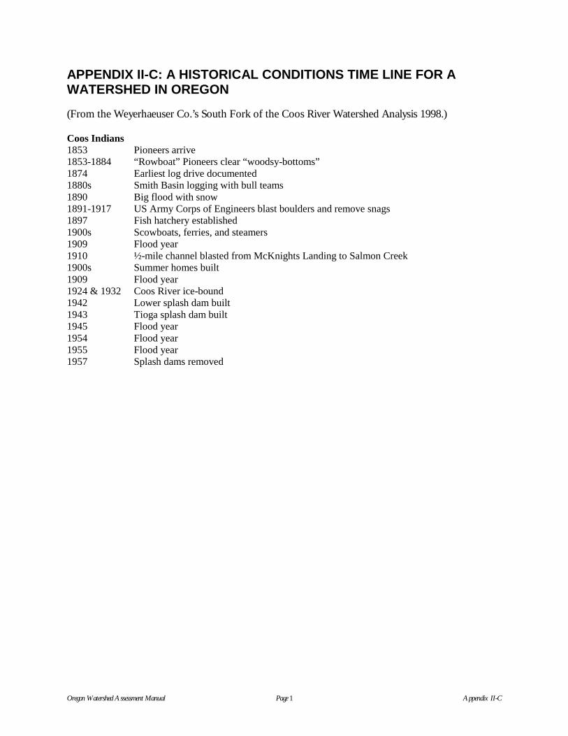
Oregon Watershed Assessment Manual Page 1 Appendix II-C
APPENDIX II-C: A HISTORICAL CONDITIONS TIME LINE FOR AWATERSHED IN OREGON
(From the Weyerhaeuser Co.’s South Fork of the Coos River Watershed Analysis 1998.)
Coos Indians1853 Pioneers arrive1853-1884 “Rowboat” Pioneers clear “woodsy-bottoms”1874 Earliest log drive documented1880s Smith Basin logging with bull teams1890 Big flood with snow1891-1917 US Army Corps of Engineers blast boulders and remove snags1897 Fish hatchery established1900s Scowboats, ferries, and steamers1909 Flood year1910 ½-mile channel blasted from McKnights Landing to Salmon Creek1900s Summer homes built1909 Flood year1924 & 1932 Coos River ice-bound1942 Lower splash dam built1943 Tioga splash dam built1945 Flood year1954 Flood year1955 Flood year1957 Splash dams removed


Appendix II-DOrganization of HistoricalInformation on WatershedResources by SubwatershedLocations
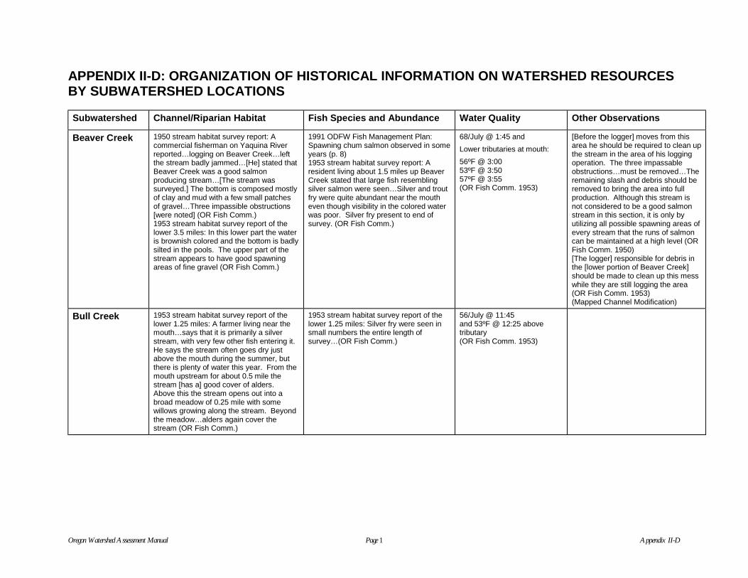
Oregon Watershed Assessment Manual Page 1 Appendix II-D
APPENDIX II-D: ORGANIZATION OF HISTORICAL INFORMATION ON WATERSHED RESOURCESBY SUBWATERSHED LOCATIONS
Subwatershed Channel/Riparian Habitat Fish Species and Abundance Water Quality Other Observations
Beaver Creek 1950 stream habitat survey report: Acommercial fisherman on Yaquina Riverreported…logging on Beaver Creek…leftthe stream badly jammed…[He] stated thatBeaver Creek was a good salmonproducing stream…[The stream wassurveyed.] The bottom is composed mostlyof clay and mud with a few small patchesof gravel…Three impassible obstructions[were noted] (OR Fish Comm.)1953 stream habitat survey report of thelower 3.5 miles: In this lower part the wateris brownish colored and the bottom is badlysilted in the pools. The upper part of thestream appears to have good spawningareas of fine gravel (OR Fish Comm.)
1991 ODFW Fish Management Plan:Spawning chum salmon observed in someyears (p. 8)1953 stream habitat survey report: Aresident living about 1.5 miles up BeaverCreek stated that large fish resemblingsilver salmon were seen…Silver and troutfry were quite abundant near the moutheven though visibility in the colored waterwas poor. Silver fry present to end ofsurvey. (OR Fish Comm.)
68/July @ 1:45 and
Lower tributaries at mouth:
56ºF @ 3:0053ºF @ 3:5057ºF @ 3:55(OR Fish Comm. 1953)
[Before the logger] moves from thisarea he should be required to clean upthe stream in the area of his loggingoperation. The three impassableobstructions…must be removed…Theremaining slash and debris should beremoved to bring the area into fullproduction. Although this stream isnot considered to be a good salmonstream in this section, it is only byutilizing all possible spawning areas ofevery stream that the runs of salmoncan be maintained at a high level (ORFish Comm. 1950)[The logger] responsible for debris inthe [lower portion of Beaver Creek]should be made to clean up this messwhile they are still logging the area(OR Fish Comm. 1953)(Mapped Channel Modification)
Bull Creek 1953 stream habitat survey report of thelower 1.25 miles: A farmer living near themouth…says that it is primarily a silverstream, with very few other fish entering it.He says the stream often goes dry justabove the mouth during the summer, butthere is plenty of water this year. From themouth upstream for about 0.5 mile thestream [has a] good cover of alders.Above this the stream opens out into abroad meadow of 0.25 mile with somewillows growing along the stream. Beyondthe meadow…alders again cover thestream (OR Fish Comm.)
1953 stream habitat survey report of thelower 1.25 miles: Silver fry were seen insmall numbers the entire length ofsurvey…(OR Fish Comm.)
56/July @ 11:45and 53ºF @ 12:25 abovetributary(OR Fish Comm. 1953)

Appendix II-EBlank Forms


Form HC-1: Historical Channel and Riparian Modification Inventory
Watershed: Page_____of_____
Name: Date:
SiteNo.
Historical Channel andRiparian ModificationActivity Description Data/Information Source
ChannelHabitat Type
ChannelLength (mi)


Form HC-2: Historical Channel and Riparian Modifications Confidence Evaluation
Watershed: Form # ____ of ______
Area, sub-basin:
Name of mapper(s):
Technical expertise or relevant experience:
Confidence in historical channel and riparian modification mapping:
! Low to moderate: Used one source of historical information; unsure of the credibility
! Moderate: Used several sources of historical information that reach the same conclusion
! Moderate to high: Used source of information from agency records or from other trainedobservers; multiple sources of historical information that reach the same conclusion
! High: Used source of information from agency records or from other trained observers withdocumented quality control; or multiple sources of historical information that reach the sameconclusion and photographic documentation
! If none of the above categories above fits, describe your own confidence level and rationale:

��������� ������ ������ ������������������
Table of Contents
Introduction......................................................III-3Critical Questions.........................................III-3Assumptions ................................................III-3Materials Needed.........................................III-3Necessary Skills...........................................III-4Final Products of the CHT Classification
Component ............................................III-4Methods............................................................III-5
Overview......................................................III-5Step 1: Prepare Maps and Materials ............III-5Step 2: Break Out Stream Segments
Based on Gradient Class........................III-6Step 3: Estimate Channel Confinement........III-8Step 4: Assign Initial CHT Designation.........III-9Step 5: Improve the Mapping .....................III-12Step 6: Determine CHT Sensitivity .............III-14Step 7: Evaluate Confidence in Mapping....III-14Step 8: Prepare for Condition Evaluation ...III-15
References .....................................................III-17Glossary .........................................................III-18Appendix III-A: Descriptions of Channel
Habitat TypesAppendix III-B: Blank Forms
Form CHT-1: Channel Habitat TypeField Verification
Form CHT-2: CHT Summary SheetForm CHT-3: Channel Habitat Type
Classification Confidence Evaluation

������ ������ ��������� ���� ��� ����� ������ ��� ���� �����������
��������� ������ ������ ���� ��������������
INTRODUCTION
The Watershed Fundamentals component of this manual describes how the setting and structure of thelandscape influences the shape of the stream channels. Drawing on several existing stream classificationsystems, we have assigned a basic number of channel types for Oregon streams that we are callingChannel Habitat Types1 (CHTs). This stream classification will enable you to better understand how landuse impacts can alter the channel form, and to identify how different types of channels will respond torestoration efforts. Both channel modifications and restoration will ultimately effect fish habitat.
The stream classification system is described in this component, along with mapping instructions. InAppendix III-A, you will find more detailed descriptions for each of the channel habitat types, including adrawing and photo of the physical setting common to the unit, an example from a topographic map, and alist of physical attributes common to these types of streams. In addition, Appendix III-A presentsbackground material on stream classification, theory, and methodology. The overall assessment processis designed to identify areas of the watershed in need of enhancement and restoration. To help evaluaterestoration options, we have included general guidelines for restoration by channel type in Appendix III-A. The channel type classifications apply to broad areas; therefore, a more thorough field verification ofactual conditions will be necessary before project implementation.
Because this stream classification is a composite of existing work, we expect that changes and additionsto the individual stream types may be made as the classification is applied in Oregon and field data iscompiled. At that point, channel type “variants” within each CHT can be identified.
Critical Questions
1. What is the distribution of CHTs throughout the watershed?
2. What is the location of CHTs that are likely to provide specific aquatic habitat features, as well asthose areas which may be the most sensitive to changes in watershed condition?
Assumptions
1. Stream channels form specific patterns in response to the surrounding geology andgeomorphology, and these patterns can be used to identify CHTs.
2. Channel habitat types have consistent responses to changes in inputs of sediment, water, andwood across the State of Oregon.
3. The distribution of CHTs throughout the stream network and the condition of the characteristicswithin the CHTs influence aquatic habitat quality.
Materials Needed
You will need the following equipment and supplies to complete the mapping:
� ����� ��� �� �� ��� ����� ���������� ��� ���� �� ������� �� ��� ������� � ��� ��� �� ���� ���������

������ ������ ��������� ���� ��� ����� ������ ��� ���� �����������
• 1:24,000-scale Oregon Department of Forestry (ODF) base maps (from Start-Up andIdentification of Watershed Issues component)
• A Mylar overlay the size of the base map (optional)
• Sharp pencil, colored pencils, permanent marking pens (fine-point) in a variety of colors
Additional materials or data, where available:
• Recent stereo aerial photographs covering the entire assessment area (from Start-Up andIdentification of Watershed Issues component)
• Stereoscope for 3-D viewing of aerial photographs. Although a mirrored stereoscope (withmagnification) is preferable, a simple lens stereoscope is adequate.
• Aerial photo scale for measuring riparian area widths etc. Scale should be the same as the aerialphotographs used.
• Map wheel for measuring lengths.
• Stream survey results, if available
Necessary Skills
The minimum skills necessary to produce the CHT maps include (1) the ability to read and usetopographic maps, and (2) an eye for visualizing 3-D landscape patterns from topographic maps. Theability to use aerial photographs and a general understanding of the local geology and the geologicprocesses shaping the stream system in the watershed will aid in the accomplishment of this task, but isnot required. Complex channel networks and channel sensitivity issues may require the aid of ahydrologist or geomorphologist.
Final Products of the CHT Classification Component
The final products from this step include:
• Map CHT-1: Channel Segment Map• Map CHT-2: Preliminary Channel Habitat Type Map• Map CHT-3: Final Channel Habitat Type Map• Form CHT-1: Channel Habitat Type Field Verification• Form CHT-2: CHT Summary Sheet• Form CHT-3: Confidence Evaluation• Short summary report (optional)

������ ������ ��������� ���� ��� ����� ������ ��� ���� �����������
METHODS
Overview
The methodology presented here describes the steps to divide streams in the watershed into differentCHTs. Stream segments are initially broken out based on channel gradient (Step 2) and channelconfinement (Step 3), and mapped on Map CHT-1. The stream segments are then grouped togetherbased on channel pattern and valley width, and assigned to a tentative CHT (Step 4); a preliminary CHTmap (Map CHT-2) is then produced. Although channel pattern, valley width, and channel gradient can bedetermined with reasonable accuracy from topographic maps, channel confinement is difficult and insome cases impossible to determine from maps alone, and may require additional work. Consequently,methods for improving the quality or confidence in your mapping are discussed in Step 5; including theuse of stream survey information, consulting with local experts, using aerial photographs, and field-verifying initial calls. All field-verification information is recorded on Form CHT-1. When the analyst issatisfied with the CHT calls that have been made, a final CHT map is produced (Map CHT-3), along witha form that summarizes the distribution of CHTs in the watershed (Form CHT-2). Copies of Map CHT-3and Form CHT-2 are distributed to the other analysts. Channel Habitat Type sensitivity is evaluated inStep 6. In Step 7, the analyst evaluates confidence in the final mapping products. Finally, in Step 8, theCHT analyst will prepare for the Watershed Condition Evaluation.
Step 1: Prepare Maps and Materials
Gather all of the items listed in the Materials section. Base maps of the watershed showing the entirestream network, and watershed and subwatershed boundaries, should have been prepared in the Start-Upand Identification of Watershed Issues component (refer to that component if you have not received abase map).
US Geological Survey (USGS) maps at the 7.5-minute or 1:24,000 scale have been used to prepare thebase maps. Keep in mind that some of the individual maps used to make up the base map of thewatershed may have a different contour interval than others. Be sure to check the contour intervals, asthe accuracy of your stream typing is dependent on your ability to know and use this information. Scaleand contour dimensions are found on the bottom center of the maps used to make up the base map. Mapswith large areas of little relief may show intermediate contours only in those areas. The stream segmentsand CHTs from the following steps can be drawn directly on copies of the base map.
Before beginning, take a moment to study the base map. Notice the network of streams, their positionswithin the watershed, and the patterns of similarities between streams within sub-basins or areas ofsimilar topography and size. Note that not all the CHTs described in this section will necessarily bepresent in your watershed, and that the distribution of types may vary from the headwaters to the mouthof the watershed. You will want to familiarize yourself with the attributes of each CHT before mappingthem in your watershed. Figure 1 illustrates the basic characteristics of each CHT; Appendix III-Aprovides detailed descriptions of each CHT.

������ ������ ��������� ���� ��� ����� ������ ��� ���� �����������
CHANNEL GRADIENTCLASSES
<1% 4-8%
1-2% 8-16%
2-4% >16%
Step 2: Break Out Stream Segments Based on Gradient Class
The first cut at dividing the channel network into similar types is based on channel gradient class. Sixdifferent gradient classes are used (shown in the box below) Segments may vary in length, but will besimilar with respect to channel gradient. Sixteen percent is chosen as the upper limit of the channelnetwork due to the dominance of terrestrial rather than fluvial processes in these areas.
Channel gradient is determined by dividing the difference inelevation by the horizontal distance of any given length of stream.Determining this ratio from the base map can de done in a numberof ways. In one method, measure the distance between contours ornumber of contours within a given distance either with a ruler (forrelatively straight channels), or using a map wheel (for sinuouschannels). Table 1 provides information for determining slopefrom 1:24,000-scale maps with a 20-foot or 40-foot contourinterval.
Figure 1. Examples of CHTs and their relative position in the watershed.

������ ������ ��������� ���� ��� ����� ������ ��� ���� �����������
Table 1. Determining channel slope on 1:24,000-scale maps.
20-ft contour interval 40-ft contour intervalChannel
Slope(%)
DistanceBetweenContours
(ft)
Contoursper 1,000
ft ofChannel
DistanceBetweenContours
(ft)
Contoursper 1,000
ft ofChannel
1 2,000 - 4,000 -
2 1,000 1 2,000 -
4 500 2 1,000 1
8 250 4 500 2
16 125 8 250 4
USING GIS TO MAP GRADIENT
Preliminary channel gradients have been successfullymapped using a Geographic Information System (GIS).GIS programs can be written to calculate and codechannel gradients between individual contours or to“smooth” them by a running average. If GIS resourcesare available to your watershed council, this may beanother tool for the mapping exercise. However,employment of other tools is recommended tosupplement the GIS mapping.
Another approach would beto use a gradient templateprinted on a clear piece ofMylar that can be laid overthe stream channel; thegradient is read directly fromthe template. Channelsegments must be relativelystraight to use this approach,however. Examples ofgradient templates are foundin Schuett-Hanes et al.(1994).
A third method to map channel gradient is to employ a Geographic Information System (GIS), althoughthis method requires an expertise that may render it impractical. In addition, field verification of GISproducts is necessary. (See the sidebar below, Using GIS to Map Gradient, for more information.)
Determining channel gradient from topographic maps is subject to a certain amount of error. Inparticular, lower-gradient channels are more subject to mapping and analyst calculation error than steeperchannels. This problem should be taken into consideration when field-verification sites are selected. Thispotential error, coupled with the overall greater sensitivity/responsiveness of lower-gradient channels, isthe rationale for having a greater number of gradient classes in the lower range.
In order to prevent an unmanageable number of segments within any given stream system, a minimumsegment length of 1,000 feet is suggested. Another rule of thumb is that segments should cover aminimum of three contours. Major waterfalls should be broken out as separate segments regardless oflength. Additional segment breaks are located at junctions of major tributaries, because the addition ofwater, sediment, or wood can alter physical characteristics and fish habitat. It is important to be asconsistent as possible when identifying segment breaks.
An example is provided in Figure 2 ofthree segments delineated in the “SkunkCreek” subwatershed. Segment breaks arefirst drawn on Map CHT-1 using a pencilline drawn across the channel to mark theupstream and downstream boundary ofeach segment. The stream segments arethen numbered using a sub-basin code andsequential number (for example SC1, SC2,and SC3 for Skunk Creek segments 1, 2,and 3; see Figure 2). This numbering bysub-basin allows for a minimum ofrenumbering should segments be divided or combined, and allows for a common, site-specific referencefor all analysts.

������ ������ ��������� ���� ��� ���� ������ ��� ���� �����������
Each segment is also labeled with the appropriate gradient class. For example, segment SC1 is 4.2 incheslong as measured with a map wheel (8,400 ft), and crosses no contour lines. Therefore, the gradient is<0.5% (<40 ft/8,400 ft), and the segment is labeled as “<1%.” For segment SC2, the distance between the40-foot contour and the 200-foot contour is 2.2 inches (4,400 ft); therefore, the gradient is 3.6% [(200 -40)/4,400], and the gradient class is labeled as “2-4%.” Finally, for segment SC3, the distance betweenthe 280-foot contour and the 40-foot contour is 1.2 inches (2,400 ft); therefore, the gradient is 10% [(280 -40)/2,400], and the gradient is labeled as “8-16%.”
Step 3: Estimate Channel Confinement
Channel confinement is difficult to determine from topographic maps and has been the subject ofconsiderable confusion. This is unfortunate, as the ability of a stream to move laterally directly affectsaquatic habitat quality and is of prime concern to land managers. Much of the problem is due tomisinterpretation of terminology. Definitions related to channel confinement and entrenchment discussthe ratio of the active channel width to the floodplain width (Moore et al. 1997, Washington ForestPractices Board 1997, Rosgen 1996, Overton et al. 1995). Unfortunately, floodplain width is ofteninterpreted as valley width or some measure of historic floodplain. For the purposes of this manual, wehave adopted the most commonly used and scientifically valid definition, which defines confinement asthe ratio of the bankfull width to the width of the modern floodplain. Bankfull width is the width of thechannel at the point at which overbank flooding begins, and often occurs as flows reach the 1.5-yearrecurrence interval level. Modern floodplain is defined as the flood-prone area (Rosgen 1996), butgeomorphologists caution that it may or may not correspond to the 100-year floodplain. Obviously, thisis an area where consistency by the analyst is important.
Figure 2. The stream segments delineated in a subwatershed are numbered using a sub-basincode and sequential number (e.g., SC1, SC2, and SC3 for Skunk Creek segments 1, 2, and 3).This numbering by sub-basin allows for a minimum of renumbering should segments be dividedor combined, and allows for a common, site-specific reference for all analysts. Each segment isalso labeled with the appropriate gradient class.

������ ������ ��������� ���� ��� ���� ������ ��� ���� �����������
Table 2. Channel confinement classes.
MapCode
ConfinementClass Floodplain Width
U Unconfined >4x bankfull width
M Moderatelyconfined
>2x but <4x bankfullwidth
C Confined <2x bankfull width
Confinement classes are presented in Table 2.While determination of this ratio solely fromtopographic maps is prone to error, especially inlow-gradient streams entrenched into historicterraces or alluvial valleys, this exercisepresents a first cut at determining channelconfinement.
Referring to the example shown in Figure 2 for “Skunk Creek,” note the meandering and sinuous channelpattern of segment SC1. This meandering channel pattern, combined with the low gradient of the reach,is often indicative of streams with wide floodplains. The confinement class (“U” [unconfined] forsegment SC1) should be noted in pencil on Map CHT-1 next to the gradient class, as shown in Figure 2.For segment SC2 in the figure, note how the contour lines approach the channel at approximately rightangles. This suggests that the valley may allow some room for a narrow floodplain to develop. Theinitial estimate of confinement for segment SC2 would be marked on Map CHT-1 as “M” (moderatelyconfined). Segment SC3 appears from the map to be an example of a confined valley (note the V-shapeof the contours as they approach the stream) with little room for floodplain development, and would bemarked on the map as “C” (confined).
Step 4: Assign Initial CHT Designation
Following segment mapping of the channel network, segments can be clustered into groups of similargradient, confinement, and size, and mapped on Map CHT-2. Using the variables of channel gradient,confinement, and where appropriate, size and valley form, produces a consistent, accurate, and conciseframework to define the typing system. It is often beneficial to start CHT grouping in headwater regions,where the “choices” of probable CHTs are limited. The most difficult areas to group are usually low-gradient reaches. Table 3 provides a list of CHTs into which most channels can be placed. A morecomplete description of these channel types is located in Appendix III-A. Note that any system with thegoal of organizing channels statewide into a limited number of channel types works better for somechannel types than others. As such, the descriptors for each CHT are general, and variability of channelconditions within each CHT exists. The analyst is encouraged to note “variant” conditions within each ofthe channel types. In some cases, it may be necessary to modify or add channel types to fit unusualsituations. These alterations to the channel types presented should be kept to a minimum and documentedthoroughly.
Following Table 3 is a key (Figure 3) that provides a general guide for assigning CHTs. You are stronglycautioned, however, that the key is meant only as a tool, and will not always result in assignment of theappropriate CHT. You are encouraged to employ as many tools as possible in assigning CHTs.

������ ������ ��������� ���� ��� ������ ������ ��� ���� �����������
Table 3. Channel Habitat Types.
Code CHT Name Gradient Channel Confinement Size
ES Small Estuary <1% Unconfined to moderatelyconfined
Small tomedium
EL Large Estuary <1% Unconfined to moderatelyconfined
Large
FP1 Low Gradient LargeFloodplain
<1% Unconfined Large
FP2 Low Gradient MediumFloodplain
<2% Unconfined Medium to large
FP3 Low Gradient SmallFloodplain
<2% Unconfined Small tomedium
AF Alluvial Fan 1-5% Variable Small tomedium
LM Low Gradient ModeratelyConfined
<2% Moderately confined Variable
LC Low Gradient Confined <2% Confined Variable
MM Moderate GradientModerately Confined
2-4% Moderately confined Variable
MC Moderate GradientConfined
2-4% Confined Variable
MH Moderate GradientHeadwater
1-6% Confined Small
MV Moderately Steep NarrowValley
3-10% Confined Small tomedium
BC Bedrock Canyon 1->20% Confined Variable
SV Steep Narrow Valley 8-16% Confined Small
VH Very Steep Headwater >16% Confined Small
Note: Stream size refers to the ODF designations based on average annual streamflow. Small streamspossess flows less than or equal to 2 cubic feet per second (cfs). Medium streams possess flows greaterthan 2 but less than 10 cfs. Large streams possess flows of 10 cfs or greater. Stream sizes are mappedat 1:24,000 for the entire state, with the exception of the southeast quarter of the state.
To demonstrate the use of the key in Figure 3, we will use the three segments from the Skunk Creekexample. Figure 4 is an overview of the subwatershed that contains Skunk Creek. Segment SC1 is lessthan 2% gradient and unconfined. From the key, then, we see that this segment may be either an FP3CHT if it is a small stream (according to the ODF size classification), an FP2 CHT if it is medium-sized,or an FP1 CHT if it is a large stream. Referring to Appendix III-A, we find that the FP1 CHT is found inlarge streams, FP2 in large or medium streams, and FP3 is found in small to medium-sized streams. Sobecause segment SC1 is labeled “L” (this information will be on your base map), it is either an FP1 orFP2 CHT. Reading the descriptions from Appendix III-A, we find that the FP1 type is usually found atthe lowest end of the stream basin (as in this example), and may have stream gradients of <1% (as in thecase of segment SC1). Consequently, we would type segment SC1 as an FP1 CHT.

������ ������ ��������� ���� ��� ������ ������ ��� ���� �����������
Continuing with our example, segment SC2 was in the 2% to 4% gradient class and moderately confined.Using the key provided in Figure 3, we find that the possible CHTs are AF (Alluvial Fan), MM(Moderate Gradient Moderately Confined), or MH (Moderate Gradient Headwater). Channel HabitatType MC (Moderate Gradient Confined) is eliminated because it applies to segments that are confined.Referring to the descriptions for the three possible choices from Appendix III-A, we find that thedescription of the AF type does not fit the characteristics observed on the topographic map, and so can beeliminated. Reading the description of the MH type given in Appendix III-A, we find that this CHToccurs in headwater locations, usually in small streams. The description for CHT MM appears to best fitsegment SC2.
Using the key for segment SC3 we find three possible choices for the 8-16% gradient range: MV(Moderately Steep Narrow Valley), BC (Bedrock Canyon), and SV (Steep Narrow Valley) types. Fromthe description in Appendix III-A, we can probably eliminate the BC type; although it is difficult to tellwithout field observations, it does not appear to be a deep canyon or gorge. The descriptions of both theMV and SV types appear to fit segment SC3 well, and without further investigation we may not be able todecide which of the two is most appropriate.
After the segments have been grouped into CHTs, prepare a preliminary CHT map (Map CHT-2) witheach segment color-coded to a particular CHT. You may wish to make a photocopy of Map CHT-1, oruse a Mylar overlay on Map CHT-1. Sign and date the map. Because most preliminary CHT maps willbe modified, preparation of a GIS version of the map at this point may not be prudent.
Figure 3. This flow chart provides a general guide for assigning CHTs.

������ ������ ��������� ���� ��� ����� ������ ��� ���� �����������
Step 5: Improve the Mapping
The following subsections offer suggestions for improving the Preliminary Channel Habitat Type Map.These tools, as well as additional information gathered from other watershed analysts, should beemployed in the production of the Final Channel Habitat Type Map.
Compare with Stream Surveys
Oregon Department of Fish and Wildlife (ODFW) stream habitat surveys will likely be available for someparts of your watershed. These field observations can be consulted to verify your segmenting for thoseareas covered by the survey. (See Caution sidebar.) In areas with extensive survey information, it maybe beneficial to use this information as a tool in initial segment delineation. Consult the summary foreach surveyed reach for the following attributes: channel slope and confinement, valley floor types,channel form, and adjacent landforms.
Consult an Expert
Local experts (agency personnel, consultants, etc.) may volunteer to assist the watershed council with thewatershed assessment. Although this stream classification is new, these experts will be familiar withsimilar channel classifications and may be able to assist you. Work through the mapping procedures first,then ask your local expert to check your work or help with questions you have. In addition, localresidents are usually very knowledgeable about stream conditions. While locals may not be familiar withterms such as channel confinement, they likely would know if flood flows are contained within thechannel for a particular section of stream.
CAUTION
Some surveyed stream reaches have been found to be inconsistently defined, and do notnecessarily correspond to changes in the indicator attributes above. Also remember that thesegments delineated above will be combined into CHTs that may correspond with ODFW reaches. Ifa reach includes more than one of your preliminary segment breaks, or extends beyond an obviouschange in channel gradient or confinement, then you may need to consult the line-by-line field datafor the stream within your segment breaks rather than the reach summary information.
Figure 4. This overview of the example Skunk Creek subwatershed provides stream sizeclassification (large, medium, small), which helps in classifying CHT.

������ ������ ��������� ���� ��� ������ ������ ��� ���� �����������
Aerial Photographs
If you have experience in using aerial photographs and access to photos, you can improve yourconfidence in assigning CHTs by viewing the stream system with photographs. Attributes such as valleyfeatures, presence of side-channels, and gravel deposition are often observable from aerial photographs.It should be noted, however, that many features of small, forested stream channels cannot be determinedfrom aerial photographs.
Field Verification
The purpose of the field assessment is not only to verify CHT calls, but also collect data concerningspecific channel characteristics. These characteristics reflect the type and magnitude of channel processesand give an indication of the response of the channel to alteration of factors, which influence channelform and maintenance.
A field visit to a sampling of different CHTs identified from the initial map exercise will also help youbuild confidence in the mapping procedure and identify local differences in controls leading to variationsin channel form. Where time, resources, and opportunities allow, conduct a field verification andcomplete the Channel Habitat Type Field Verification form (Form CHT-1) for each area visited. Wherepractical, attach the corresponding portion of the topographic map on the back of the form to show thelocations of field observations/measurements for the segment in question.
In order to efficiently gather this type of information, a sampling design must focus on representativereaches and allow extrapolation to other channel segments. The following are guidelines for selectingfield sites:
• Sample a variety of the gradient and confinement classes present in the watershed.
• Increase sample size in channel segments that are likely to respond to changes in the input factorsof wood, sediment, flow (unconfined to moderately confined channels with minimal vertical orhorizontal controls, as well as low-gradient reaches).
• Sample segments that capture the geographic and geologic variability within the watershed.
• Sample upstream and downstream of major tributary confluences to determine gross differencesin sub-basin characteristics.
• Sample segments that reflect the general range of land management intensity.
• Sample segments that have been subjected to events capable of altering overall morphologicfeatures (debris flow or dam break flood segments, segments that have undergone significantwidening or aggradation, etc.)
• Sample key fish habitat areas, if known.
• Sample areas of known or suspected habitat degradation.
There is no set minimum number of segments that should be sampled , but increasing the sample size willgreatly increase the accuracy and usefulness of the final product.

������ ������ ��������� ���� ��� ������ ������ ��� ���� �����������
Following application of the tools presented above, produce the Final Channel Habitat Type Map (MapCHT-3). Form CHT-2 (CHT Summary Sheet) should also be produced. If GIS is available, Map CHT-3can first be digitized, and Form CHT-2 generated from the GIS. If GIS is not available, a map wheel canbe used to determine CHT mileage in the watershed. This information, along with the CHT map, allowsthe analysts to understand the extent and location of various CHTs.
Step 6: Determine CHT Sensitivity
While clustering stream segments into CHTs addresses the critical question concerning channel typedistribution in the watershed, it does not address the second question concerning identification of thoseportions of the channel network that are the most responsive to changes in the factors which impactchannel development. Differences in gradient, confinement, and bed morphology suggest that differentchannel types are more or less responsive to adjustment in channel pattern, location, width, depth,sediment storage, and bed roughness (Montgomery and Buffington 1993). These changes in channelcharacteristics will in turn trigger alterations of aquatic habitat conditions. The more responsive areas aremost likely to exhibit physical changes from land management activities, as well as restoration efforts.
In general, responsive portions of the channel network are those that lack the terrain controls which defineconfined channels. These unconfined or moderately confined channels display visible changes in channelcharacteristics when flow, sediment supply, or the supply of roughness elements such as large woodydebris (LWD) are altered. These areas are commonly referred to as response reaches, and usually possessan active floodplain. At the other end of the responsive spectrum would be those channels whosecharacteristics and form are not easily altered, such as a Bedrock Canyon. Some channels, such asAlluvial Fans, can have a broad range of sensitivity, ranging from low to high. Figure 5 identifies thegeneral responsiveness of CHTs.
In Appendix III-A, each of the CHTs is rated with respect to the general sensitivity of the channel tochanges in the input factors of wood, sediment, and peak flows. A rating of low, moderate, or high isassigned based on the anticipated response of the channel. Table 4 describes the anticipated magnitude ofresponse associated with these qualitative ratings. The CHT descriptions given in Appendix III-A presentmore detailed information concerning anticipated channel response. The most accurate sensitivity callsare made with the help of field verification.
Step 7: Evaluate Confidence in Mapping
Fill out the Confidence Evaluation (Form CHT-3) for mapping the CHTs. If the type or quality ofinformation used to map the watershed differs significantly from area to area, fill out a form that evaluateseach general area (i.e., high-gradient streams all over the watershed, surveyed stream reaches, a particulartributary). The form is self-explanatory.
As a final step in mapping, the analyst should highlight on Map CHT-3 those CHTs that are consideredhighly responsive.

������ ������ ��������� ���� ��� ������ ������ ��� ���� �����������
Step 8: Prepare for Condition Evaluation
The final portion of the CHT assessment procedure is preparation for the Watershed Condition Evaluationcomponent of the watershed assessment. In addition to finalizing the CHT map and associated forms, theanalyst should review the channel information collected. This review should lead the analyst to a pointwhere he/she knows not only the type and likely location of sensitive stream channels in the watershed,but where an understanding is gained of overall channel condition. Often the analyst will be capable ofdetermining the dominant processes that are most responsible for channel condition. It is useful toprepare a short written summary of channel conditions for presentation during the WatershedCondition Evaluation stage of the process.
As an example of the type of information brought forth during the Watershed Condition Evaluation,suppose the channel analyst has determined that a particular portion of the stream channel network ishighly responsive, moderate gradient, moderately confined, and undergoing significant bank erosion andwidening. The channel analyst learns from the sediment sources analyst that numerous recent landslidesthat reach the channel have occurred in the basin just upstream from the sensitive reach. Together, theanalysts theorize that recent increases in landslide frequency have resulted in excessive amounts ofsediment being delivered to the channel, resulting in the channel widening. This type of “crossreferencing” to determine key linkages is one of the ultimate goals of the entire assessment procedure. Ifthe channel analyst can bring forth not only the where and what of the stream network, but somerudimentary understanding of the why, then a clearer picture of overall watershed health emerges.
Figure 5. Different channel types respond differently to adjustment in channel pattern,location, width, depth, sediment storage, and bed roughness. Such changes may not onlyresult in alteration of aquatic habitat, but the more responsive areas are most likely to exhibitphysical changes from land management activities and restoration efforts.

������ ������ ��������� ���� ��� ������ ������ ��� ���� �����������
Table 4. Channel response descriptions.
Rating LWD Fine Sediment Coarse Sediment Peak Flows
High
Critical element inmaintenance ofchannel form,pool formation,graveltrapping/sorting,bank protection.
Fines are readily storedwith increases inavailable sedimentresulting in widespreadpool filling and loss ofoverall complexity ofbed form.
Bedload depositiondominant activechannel proces;general decrease insubstrate size,channel widening,conversion to plane-bed morphology ifsediment is added.
Nearly all bedmaterial ismobilized;significantwidening ordeepening ofchannel.
Moderate
One of a numberof roughnesselements present;contributes to poolformation andgravel sorting.
Increases in sedimentwould result in minorpool filling and bedfining.
Slight change inoverall morphology;localized widening andshallowing.
Detectablechanges inchannel form;minor widening,scour expected.
Low
Not a primaryroughnesselement; oftenfound only alongchannel margins.
Temporary storageonly; most istransported throughwith little impact.
Temporary storageonly; most istransported throughwith little impact.
Minimal change inphysical channelcharacteristics,some scour andfill.

������ ������ ��������� ���� ��� ������ ������ ��� ���� �����������
REFERENCES
����� ���� �� �� ��� �� ��� �������������� �� �� ����� ����� �� ����������� ����� ��
����������� ����� ���� �������� !������ "����� ��� # �� ��� $�%�����
� ������� ��!�� ��&� ����� ���� �� ��� ��� "�'� (� ��%� �)� ! (�� � ������ � ���*� + �� �� ��� (������ ��������������, -��*��� �� ���� �� � ���� ���� �����.�� ��/� ��������"��������� �0123,�42�5�
6 ��� %� ��-�� 6�!� ����� ��� ��� 7�"��� "�� �� �� 8�������� �� -����% ���� ������ �� ���� ��� ����%������ 9� '��� ����� �� !� ������ � �� ��� �� /��� 6��� �� ��������� :��� �#��4��0� ��� ;4�
(���� �%� &�(�� :��� (���� ��� 6�<� ����� �=� (%� ����� ��� ���� ������ �� ����� "�������
�� ���� '� ��� ��* ��� (��� ���* ����������� ��� 8����������� �� ����� % (������� 8�# ���������� �%������� �� ����� (%� ���*� ��� ����� ���� !�� ���� ����� ��� ������%�'��/� � ���� ����
�������� ��<� �5� ! -��* �� ��� :�/� � (� /� � 9��/� ���% # ���� ���� ����� "�������������
"������� %� '�:�� ��� &�"� <���������� �;� ������� ��������������� # �������� �� �������:�������� ��� !��������� �� ������� ���������� ���������� ����� ����� ���� ��������:��� � ���4�(�04;4002� $�%�����
"�� �� 7�� 7� &����� ��� &� '������� � �>� "������ �� �� ��� (������ �� /�%�� !?�����
8�/���� % # �@���� A��� �� # �������� # �� ��, $ ���� '��� ����� �� ���� ��� ���������
$ ���� '��� ����� �� ���� ����� /����� ��� '�/��������� �>� ����� % #��� <��+�
$/� ���� ��7�� &�'� "�8��% �� :� ! ��� ���� ���� ����*���� ��� 7�!� '������ �=� 9�� B� 6������ ���� (������, '��� ������� ���� :�� ����� A��� �� ���������� �� ��� ������ :�/� <�����
8����� 9� �� ��� �� /��� 8��� �������� :���� �� �������� 8A�46�:4;22� <����� 8�����
#�������� ��&� 1����� 3� �� ��� �2� ������� �%�� 9�� � 6���� �� ��� ������� A������� �� ������������� !���+�� 9� '��� ����� �� !� ������ � �� ��� �� /���� !���+� :������ :�0 ���������#��� 2)�
:������ '��� �5� ! �������������� �� A��� �� :�/� �� ������ 22,1�)4�3�
:������ '��� �)� !������ :�/� "� ������%� �������� (%� ����%�
�������4(����� '�� !� #����� �� <��������� ��� �� (���� �5� !������ "����� ��� # �� �� "������A� ��*��� 8����� ����� ��� ����������� ���4!"45400�� $�%����� �����������
���������� �� ��� # ������� <�� �� �>� ������ � "���������% �� ���������� ���� ����!���%���� -� ���� 5�0�

������ ������ ��������� ���� ��� ����� ������ ��� ���� �����������
������� � ��:�� :�"� (������ ��� '�#� �� ���� �� �� ���������� <��*��� ��� ������ ���
������� #���� �� �� �� ��� ����%����� �� $ ����� �������� &�� ��� �� ����� ��� ��� !?������������ 5=,�2)54�2>�
GLOSSARY
channel confinement: Ratio of bankfull channel width to width of modern floodplain. Modernfloodplain is the flood-prone area and may correspond to the 100-year floodplain. Typically, channelconfinement is a description of how much a channel can move within its valley before it is stopped by ahill slope or terrace.
channel gradient class: Channel gradient is the slope of the channel bed along a line connecting thedeepest points (thalweg) of the channel. Channel reaches are then grouped according to gradient intostream gradient classes (<1%, 1-2%, 2-4%, etc.)
Channel Habitat Types (CHT): Groups of stream channels with similar gradient, channel pattern, andconfinement. Channels within a particular group are expected to respond similarly to changes inenvironmental factors that influence channel conditions. In this process, CHTs are used to organizeinformation at a scale relevant to aquatic resources, and lead to identification of restoration opportunities.
������� ����� '��� ������ �� ��* � �� ��� ������� ���+� �� �� ���*� ��*� ��� /����% 1��
�.������ � ����� ������� � ������ ��� �������3�
contour interval: A line of equal elevation drawn on a topographic map.
Geographic Information System (GIS): A computer system designed for storage, manipulation, andpresentation of geographical information such as topography, elevation, geology etc.
large woody debris (LWD): Logs, stumps, or root wads in the stream channel, or nearby. Thesefunction to create pools and cover for fish, and to trap and sort stream gravels.
morphologic features: From the Greek root meaning structure or form; in stream channels, thosephysical features (such as gradient and confinement) that reflect the influence of processes which operateon a landscape scale (such as geology and climate).
morphology: A branch of science dealing with the structure and form of objects. Geomorphology asapplied to stream channels refers to the nature of landforms and topographic features.
recurrence interval(s) (return interval): Determined from historical records. The average length oftime between two events (rain, flooding) of the same size or larger. Recurrence intervals are associatedwith a probability. (For example, a 25-year flood would have a 4% probability of happening in any givenyear.)
riparian area: The area adjacent to the stream channel that interacts and is dependent on the stream forbiologic integrity.

������ ������ ��������� ���� ��� ����� ������ ��� ���� �����������
stereo aerial photo: Pairs of photos taken from the air that can be viewed through a stereoscope to revealthree-dimensional features of the landscape.
stream segment: Contiguous stream reaches that possess similar stream gradient and confinement, andwhich can be used for analysis.

�������� ��
����� �����

Form CHT-1: Channel Habitat Type Field Verification
Name: Date: Watershed/sub-basin: Segment location: Oregon stream size: Preliminary channel habitat type: Final channel habitat type: Stream name: Township/Range/Section: Average of observations/measurements over length (ft) of channel.Channel slope:Single or multiple channels:Floodplain width:Bankfull channel width (from top of right bank to top of left bank):Ratio of floodplain width to bankfull width:Describe material in stream banks:Size of average bed particles: silt/clay (<0.062 mm); sand (0.062 to 2.0 mm); gravel (2 to 64 mm);cobbles (64 to 257 mm); boulders (257 to 2,032 mm); bedrock
Rough sketch of valley and stream cross section—add scale:
Comments:
Channel habitat type determination:� Same as initial type
� Differs from initial channel habitat type by:Can be extrapolated to the following areas:
� Divided into additional type (CAUTION: Can you provide the same mapping resolution everywhereappropriate in the basin based on this field verification? If not, lumping is better.)
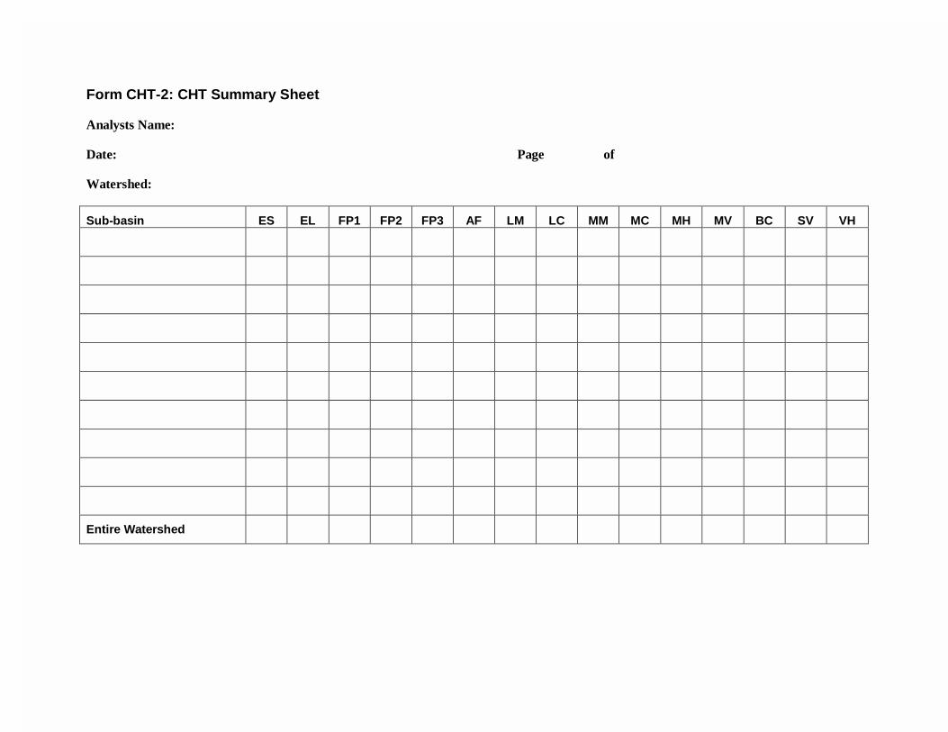
Form CHT-2: CHT Summary Sheet
Analysts Name:
Date: Page of
Watershed:
Sub-basin ES EL FP1 FP2 FP3 AF LM LC MM MC MH MV BC SV VH
Entire Watershed

Form CHT-3: Channel Habitat Type Classification Confidence Evaluation
Name: Date:
Technical expertise or relevant experience:
Watershed Name: Subwatershed Name:
Channel types:
Resources used:� Topographic maps � Field verification� ODF stream sizes � Stream surveys
� Other ___________________________
Confidence in base map stream coverage:� Local expert says high / low (circle one) degree of accuracy based on field experience (provide name
of local expert):� High degree of accuracy because stream mapping based primarily on field verification of
presence/absence of streams (provide source of info/mapping):
� No verification; suspect some streams not mapped (explain rationale):
� No verification; suspect many streams not mapped (explain rationale; what types?):
� Additional criteria/relevant information (describe):
Confidence in channel habitat typing:� Low to moderate: Unsure of procedures, didn’t consult expert, didn’t use field surveys, no field
verification� Moderate: Understood and followed procedures, but no field verification
� Moderate: Some field verification, but found range of conditions hard to type
� Moderate to high: Field surveys available and useful for many streams, but no field verification
� Moderate to high: Some field verification on questionable segments only� High: Used field surveys and field-verified many segments of all types
� If none of the above categories fits, describe your own confidence level and rationale:
Recommendations for additional field verification, if any, and why:

Appendix III-ADescriptions of ChannelHabitat TypesTable of Contents
Channel Habitat Typing Background................. 3
Small Estuarine Channel (ES) ............................ 7
Large Estuarine Channel (EL) ............................ 9
Low Gradient Large Floodplain
Channel (FP1) ........................................ 12
Low Gradient Medium Floodplain
Channel (FP2) ........................................ 15
Low Gradient Small Floodplain
Channel (FP3) ........................................ 18
Alluvial Fan Channel (AF)................................. 20
Low Gradient Moderately Confined
Channel (LM).......................................... 22
Low Gradient Confined Channel (LC).............. 25
Moderate Gradient Moderately Confined
Channel (MM)......................................... 28
Moderate Gradient Confined
Channel (MC) ......................................... 31
Moderate Gradient Headwater
Channel (MH) ......................................... 33
Moderately Steep Narrow Valley
Channel (MV) ......................................... 35
Bedrock Canyon Channel (BC) ........................ 37
Steep Narrow Valley Channel (SV)................... 39
Very Steep Headwater (VH) .............................. 39
References ........................................................ 42
Glossary ............................................................ 43

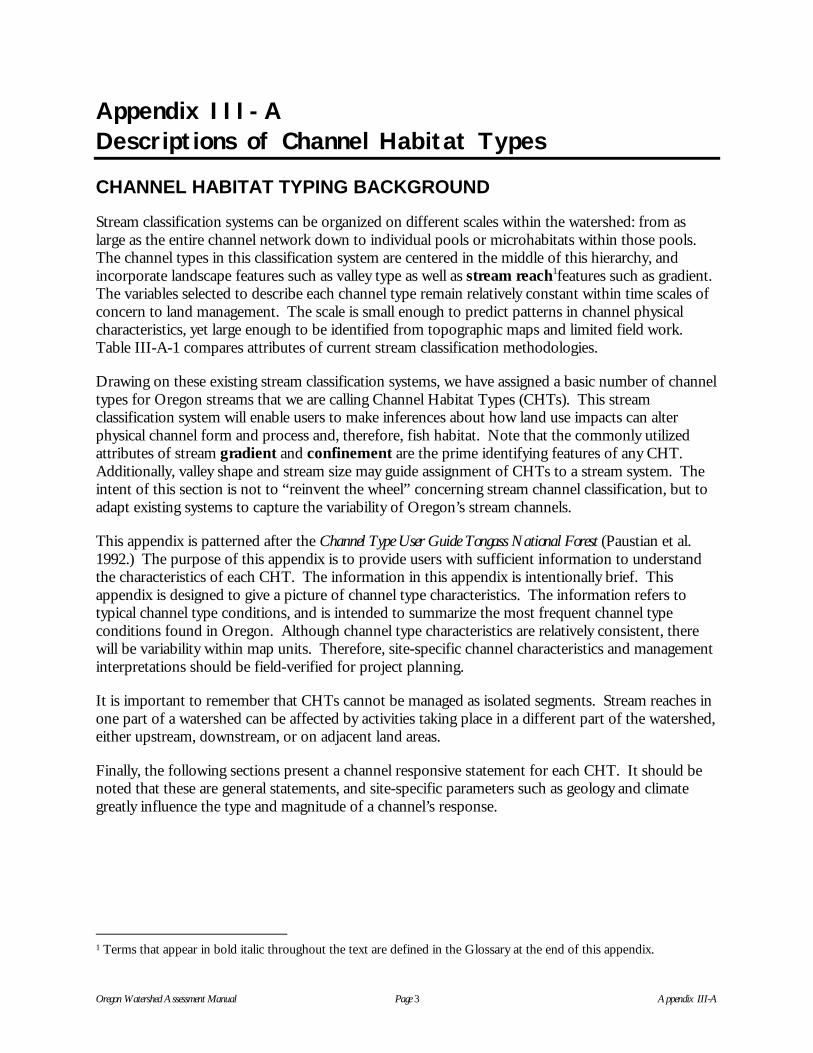
Oregon Watershed Assessment Manual Page 3 Appendix III-A
Appendix III-ADescriptions of Channel Habitat Types
CHANNEL HABITAT TYPING BACKGROUND
Stream classification systems can be organized on different scales within the watershed: from aslarge as the entire channel network down to individual pools or microhabitats within those pools.The channel types in this classification system are centered in the middle of this hierarchy, andincorporate landscape features such as valley type as well as stream reach1features such as gradient.The variables selected to describe each channel type remain relatively constant within time scales ofconcern to land management. The scale is small enough to predict patterns in channel physicalcharacteristics, yet large enough to be identified from topographic maps and limited field work.Table III-A-1 compares attributes of current stream classification methodologies.
Drawing on these existing stream classification systems, we have assigned a basic number of channeltypes for Oregon streams that we are calling Channel Habitat Types (CHTs). This streamclassification system will enable users to make inferences about how land use impacts can alterphysical channel form and process and, therefore, fish habitat. Note that the commonly utilizedattributes of stream gradient and confinement are the prime identifying features of any CHT.Additionally, valley shape and stream size may guide assignment of CHTs to a stream system. Theintent of this section is not to “reinvent the wheel” concerning stream channel classification, but toadapt existing systems to capture the variability of Oregon’s stream channels.
This appendix is patterned after the Channel Type User Guide Tongass National Forest (Paustian et al.1992.) The purpose of this appendix is to provide users with sufficient information to understandthe characteristics of each CHT. The information in this appendix is intentionally brief. Thisappendix is designed to give a picture of channel type characteristics. The information refers totypical channel type conditions, and is intended to summarize the most frequent channel typeconditions found in Oregon. Although channel type characteristics are relatively consistent, therewill be variability within map units. Therefore, site-specific channel characteristics and managementinterpretations should be field-verified for project planning.
It is important to remember that CHTs cannot be managed as isolated segments. Stream reaches inone part of a watershed can be affected by activities taking place in a different part of the watershed,either upstream, downstream, or on adjacent land areas.
Finally, the following sections present a channel responsive statement for each CHT. It should benoted that these are general statements, and site-specific parameters such as geology and climategreatly influence the type and magnitude of a channel’s response.
1 Terms that appear in bold italic throughout the text are defined in the Glossary at the end of this appendix.

Oregon Watershed Assessment Manual Page 4 Appendix III-A
Table III-A-1. Comparison of basic diagnostic features of key stream channel classificationmethods.
Basic Stream ClassificationDiagnostic Features
Frissell et al.1986,
Seg/ReachSystems 1
Cupp19892
Paustian etal. 19923
Montgomery& Buffington
1993Levels II, III, IV
Rosgen 1996Levels I, II
Moore et al.1997
ODFW hab.Survey 4
Valley bottom shape 5 qualitative x x implied x x
Valley bottom slope and/orstream gradient 5
x x x x x x
Side-slope gradient 5 qualitative x x x
Incision depth orentrenchment
x x x
Bankfull width x x x
Active channel width/depth ratio
x
Valley bottom width: activechannel width ratio
x qualitativeconfinement
usesentrenchment
x
Position in the drainagenetwork, stream order6, or
drainage area 5
x x x implied x
Bed features, channelmorphology
x x Inferred x
Plan view channel pattern 5 x x x x unconstrainedchannels only
Stream-adjacent landforms x x
Other criteria lithology,riparian veg.,soil assocs.,
bankcomposition
dominantsubstrate,
bankcomposition
sedimentsupply/sources,
substrate;defines reach
types
substrate substrate, bankcomposition,riparian data,LWD, other
Initial delineation maps aerialphotographs
I-remotesensing, existing
inventories;II-field measure-
ments
field surveys
Number of basic channelgroups 7
5 9 8 9 habitat unitlevel
1 Oriented to small mountain streams in forested environments; provides theoretical framework rather than specific categories.2 Developed for forested lands in Washington State.3 Developed for Tongass National Forest, Alaska.4 Method is more of a habitat survey than channel classification system.5 Those criteria identifiable from maps.6 Montgomery and Buffington believe stream order inappropriate as a foundation for geomorphic channel classification due to
differences in mapping detail, drainage density differences between basins, discharge, and landscape controlling factors.7 Basic Channel Groups:
F - flat cross-section profile, M - moderate gradient sideslopes, V - V-shaped valleys, U - U-shaped valleys, H - headwatertributaries (Cupp 1989), ES - estuarine, PA - palustrine, FP - floodplain, GO - glacial outwash, AF - alluvial fan, LC - largecontained, MM - moderate gradient mixed control, MC - moderate gradient contained, HC - high gradient contained(Paustian et al. 1992) braided, regime, pool-riffle, plane bed, step-pool, cascade, bedrock, colluvial (Montgomery andBuffington 1993)
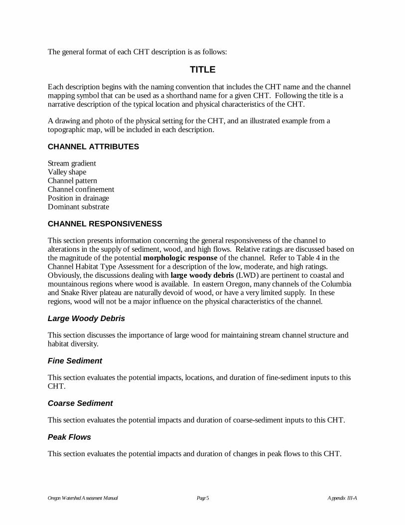
Oregon Watershed Assessment Manual Page 5 Appendix III-A
The general format of each CHT description is as follows:
TITLE
Each description begins with the naming convention that includes the CHT name and the channelmapping symbol that can be used as a shorthand name for a given CHT. Following the title is anarrative description of the typical location and physical characteristics of the CHT.
A drawing and photo of the physical setting for the CHT, and an illustrated example from atopographic map, will be included in each description.
CHANNEL ATTRIBUTES
Stream gradientValley shapeChannel patternChannel confinementPosition in drainageDominant substrate
CHANNEL RESPONSIVENESS
This section presents information concerning the general responsiveness of the channel toalterations in the supply of sediment, wood, and high flows. Relative ratings are discussed based onthe magnitude of the potential morphologic response of the channel. Refer to Table 4 in theChannel Habitat Type Assessment for a description of the low, moderate, and high ratings.Obviously, the discussions dealing with large woody debris (LWD) are pertinent to coastal andmountainous regions where wood is available. In eastern Oregon, many channels of the Columbiaand Snake River plateau are naturally devoid of wood, or have a very limited supply. In theseregions, wood will not be a major influence on the physical characteristics of the channel.
Large Woody Debris
This section discusses the importance of large wood for maintaining stream channel structure andhabitat diversity.
Fine Sediment
This section evaluates the potential impacts, locations, and duration of fine-sediment inputs to thisCHT.
Coarse Sediment
This section evaluates the potential impacts and duration of coarse-sediment inputs to this CHT.
Peak Flows
This section evaluates the potential impacts and duration of changes in peak flows to this CHT.

Oregon Watershed Assessment Manual Page 6 Appendix III-A
RIPARIAN ENHANCEMENT OPPORTUNITIES
This section presents management concerns for in-stream and near-stream management activities, aswell as riparian management opportunities.
The following section begins the CHT descriptions.

Oregon Watershed Assessment Manual Page 7 Appendix III-A
SMALL ESTUARINE CHANNELES
These channels are found at the mouths of drainages along outer coastal beaches or bays. They areintertidal streams that occur exclusively within estuary landforms, usually draining a small, high-relief or moderate-sized watershed. They are associated with saltwater marshes, meadows,mudflats, and deltas.
These streams are predominantly sediment depositional channels associated with low-relief coastallandforms. Stream energy is low due to nearly flat gradients, with substrate material consistingmainly of small gravels, sand, and silt. Channel morphology is strongly influenced by tidal stage.Fine-grained stream banks are highly sensitive to erosion. Beach erosion processes often have adominant influence on deposition and erosion in the outer coastal estuarine streams.
The original boundary of an estuary may be difficult to determinedue to modifications associated with marinas, highways, orreclamation. Many coastal estuaries have been delineatedthrough county, state, or municipal planning processes andmay include the predevelopment boundaries.
The state has produced an excellent reference forestuaries, particularly as it relates to classificationand land use (Oregon Department of LandConservation and Development 1987).
CHANNEL ATTRIBUTES
Stream gradient: ≤1%Valley shape: BroadChannel pattern: Sinuous, single, or multipleChannel confinement: UnconfinedOregon stream size: Small, mediumPosition in drainage: Bottom, mouth of streamDominant substrate: Small gravel, sand
CHANNEL RESPONSIVENESS
These channels are low-energy areas where sediment deposition is a dominant process. Whilechannel sensitivity in estuaries can vary, the unconfined nature of these areas tends to attenuatechanges over space and time. Abandonment and reoccupation of relic channels commonly occurs,but it may be a slow process.
Large Woody Debris: Moderate
Unless in jams, wood often has limited influence on the overall morphology of the channel.Accumulations can be associated with channel shifting. Although wood is often the only roughnesselement present in these channels, the high sedimentation rate limits pool development and gravelsorting. The primary aquatic habitat role of wood may be refuge cover.

Oregon Watershed Assessment Manual Page 8 Appendix III-A
ES – Small Estuary
Scale: Half (1:48,000)Contour Interval: 40 feet
Fine Sediment: Moderateto High
Fine sediment is deposited at arelatively high rate, strongly influencingthe arrangement of channels. In mostsmaller estuaries, an increase in thesediment supply would result in barformation or reoccupation of relicchannels. Localized bank erosion ordowncutting could be expected if thesediment supply were to decrease.
Coarse Sediment: Lowto Moderate
Although these channels can bedeposition zones for coarse sediment,the delivery rate to estuarine channels is usually low due to sedimentation upstream. In some basins,deposits likely influence channel configuration at the upper end of the estuary.
Peak Flows: Low
Estuarine channels are usually capable of transporting high flows with a minimum of alteration tothe primary physical characteristics of the channel. Flows tend to spread out across the valley ratherthan cause streambed scour. Localized bank erosion is expected if new channels are developed.
RIPARIAN ENHANCEMENT OPPORTUNITIES
Many enhancement efforts in estuaries are related to long-term preservation of the area. As thesechannels harbor unique biologic communities, limiting development is a common strategy.Structural enhancement activities often involve dike breaching or removal to reconnect wetlands orsloughs.

Oregon Watershed Assessment Manual Page 9 Appendix III-A
LARGE ESTUARINE CHANNELEL
These channels are most commonly found at the mouths of drainages along outer coastal beaches orbays. They are intertidal streams that occur exclusively within estuary landforms, usually draining ahigh-relief or moderate-sized watershed. They are associated with saltwater marshes, meadows,mudflats, and deltas.
These streams are predominantly depositional channels associated with low-relief coastal landforms;therefore, sediment retention is a dominant process. Stream energy is low due to nearly flatgradients, and substrate material consists mainly of small gravels, sand, and silt. Water flow anddepth are strongly influenced by tidal stage. Fine-grained stream banks are highly sensitive toerosion. Beach erosion processes often have a dominant influence on deposition and erosion in theouter coastal estuarine streams.
The original boundary of an estuary may be difficult to determine due to modifications for marinas,highways, or reclamation. Many coastal estuaries will have been delineated through county, state, ormunicipal planning processes and may include the predevelopment boundaries.
The state has produced an excellent reference for estuaries,particularly as it relates to classification and land use(Oregon Department of Land Conservationand Development 1987).
CHANNEL ATTRIBUTES
Stream gradient: ≤1%Valley shape: BroadChannel pattern: Sinuous, single, or multipleChannel confinement: UnconfinedOregon stream size: LargePosition in drainage: Bottom, mouth of streamDominant substrate: Small gravel, sand
CHANNEL RESPONSIVENESS
These channels are low- to moderate-energy areas where sediment deposition is a dominant process.Although channel sensitivity in estuaries can vary, the unconfined nature of these areas tends toattenuate changes over space and time. Abandonment and reoccupation of relic channelscommonly occurs, but it may be a slow process.
Large Woody Debris: Low to Moderate
Unless in jams, wood often has limited influence on the overall morphology of the channel.Accumulations can be associated with channel shifting. Although wood is often the only roughnesselement present in these channels, the high sedimentation rate limits pool development and gravelsorting. The primary aquatic habitat role of wood may be refuge cover.

Oregon Watershed Assessment Manual Page 10 Appendix III-A
EL – Large Estuary
Scale: Full (1:24,000)Contour Interval: 40 feet
Fine Sediment:Moderate to High
Fine sediment is depositedat a relatively high rate,strongly influencing thearrangement of channels.In most smaller estuaries,an increase in the sedimentsupply would result in barformation or reoccupationof relic channels.Localized bank erosion ordowncutting could beexpected if the sedimentsupply were to decrease.
Coarse Sediment:Low to Moderate
Although these channelscan be deposition zonesfor coarse sediment, thedelivery rate to estuarinechannels is usually low dueto sedimentation upstream.In some basins, depositslikely influence channelconfiguration at the upperend of the estuary.
Peak Flows: Low
Estuarine channels areusually capable oftransporting high flows with a minimumof alteration to the primary physicalcharacteristics of the channel. Flowstend to spread out across the valleyrather than cause streambed scour.Localized bank erosion is expected ifnew channels are developed.
RIPARIAN ENHANCEMENTOPPORTUNITIES
Many enhancement efforts in estuariesare related to long-term preservation of

Oregon Watershed Assessment Manual Page 11 Appendix III-A
the area. As these channels harbor unique biologic communities, limiting development is a commonstrategy. Structural enhancement activities often involve dike breaching or removal to reconnectwetlands or sloughs.

Oregon Watershed Assessment Manual Page 12 Appendix III-A
LOW GRADIENT LARGE FLOODPLAIN CHANNELFP1
FP1 channels are lowland and valley bottom channels of large watersheds. They may also occupyuplifted estuaries along the coast. Normally, these channels have extensive valley floodplains andriver terraces. Sloughs, oxbows, wetlands, and abandoned channels are common in large rivercorridors. Smaller tributary streams may flow through channels abandoned by the main river.Numerous overflow side-channels, extensive gravel bars, avulsions, and log jams in forested basinsare characteristic. They may be bordered on one bank by steep bluffs, marine terraces, or gentleslopes.
These channels function as sediment deposition systems, with short-term storage of fine sediment.Fines are typically mobilized during most high-flow events. Small side-channels dissecting thefloodplain are common. In-channel wood accumulations are less stable than in smaller floodplainchannels due to higher flood flows and greater channel width. Historically, many of these channelsthat drained forested areas contained significantly more wood than observed today.
CHANNEL ATTRIBUTES
Stream gradient: ≤1%Valley shape: Broad valley, floodplainChannel pattern: Sinuous, single to multiple channelsChannel confinement: UnconstrainedOregon stream size: LargePosition in drainage: Bottom, low in drainageDominant substrate: Sand to cobble

Oregon Watershed Assessment Manual Page 13 Appendix III-A
FP1 – Low Gradient Large Floodplain
Scale: Full (1:24,000)`Contour Interval: 40 feet
CHANNEL RESPONSIVENESS
Floodplain channels can be among the mostresponsive in the basin. The limited influence ofconfining terrain features and fine substrateallows the stream to move both laterally andvertically. Although often considered low-energy systems, these larger channels canmobilize large amounts of sediment during highflows. This often results in channel migrationand new channel formation.
Large Woody Debris: Moderate to High
Because of the great stream power, only largepieces or accumulations of pieces are likely toimpact overall channel conditions. The role ofwood and the amount and distribution of piecesis highly variable over time, as high flowsregularly change conditions. Single pieces arelikely to be associated with pools in side-channels and localized sediment depositions.Accumulations of wood are often responsiblefor the creation of midchannel bars and side-channel development.
Fine Sediment: Moderate
Fine sediment is easily mobilized by most of these channels. Increases in the supply of fines maycause temporary storage and pool filling, but moderate to high flows will mobilize the majority ofthe sediment. Deposition may be more permanent in smaller side-channels, and pool filling andminor shifts in side-channel location could occur.

Oregon Watershed Assessment Manual Page 14 Appendix III-A
Coarse Sediment: High
Floodplain channels are generally depositional areas for coarse sediment. When the supply of coarsesediment surpasses the transport capabilities of the stream, the channel is particularly vulnerable towidening, lateral movement, side-channel development, and braiding. Overall aquatic habitatcomplexity is reduced as pools are filled and obstructions such as large boulders or bedrockoutcrops are buried.
Peak Flows: Low to Moderate
Large floodplain channels are usually capable of transporting high flows with a minimum ofalteration to the primary physical characteristics of the channel. Flows tend to spread out across thevalley rather than cause streambed scour. Localized bank erosion is expected as new channels aredeveloped.
RIPARIAN ENHANCEMENT OPPORTUNITIES
Due to the unstable nature of these channels, the success of many enhancement efforts isquestionable. Opportunities for enhancement do occur, however, especially in channels wherelateral movement is slow. Lateral channel migration is common, and efforts to restrict this naturalpattern will often result in undesirable alteration of channel conditions downstream. Smaller side-channels may be candidates for efforts that improve shade and bank stability, but it is likely thatthese efforts may be more beneficial and longer-lived elsewhere in the basin.

Oregon Watershed Assessment Manual Page 15 Appendix III-A
LOW GRADIENT MEDIUM FLOODPLAIN CHANNELFP2
FP2 channels are main-stem streams in broad valley bottoms with well-established floodplains.Alluvial fans, dissected foot slopes, and hill slope and lowland landforms may directly abut FP2floodplains. Channels are often sinuous, with extensive gravel bars, multiple channels, and terraces.These channels are generally associated with extensive and complex riparian areas that may includesuch features as sloughs, side-channels, wetlands, beaver pond complexes, and small groundwater-fed tributary channels.
Sediment deposition is prevalent, with fine-sediment storage evident in pools and point bars, andon floodplains. Bank erosion and bank-building processes are continuous, resulting in a dynamicand diverse channel morphology. Stream banks are composed of fine alluvium and are susceptibleto accelerated bank erosion with the removal or disturbance of stream-bank vegetation and rootmats. Channel gradient is low, and high stream flows are not commonly contained within the activechannel banks, resulting in relatively low stream power.
CHANNEL ATTRIBUTES
Stream gradient: ≤2%Valley shape: Broad, flat, or gentle landformsChannel pattern: Single to multiple channels, sinuousChannel confinement: UnconfinedOregon stream size: Large to mediumPosition in drainage: Middle to lower end of drainage basinDominant substrate: Sand to cobble

Oregon Watershed Assessment Manual Page 16 Appendix III-A
FP2 – Low Gradient MediumFloodplain
Scale: Full (1:24,000)Contour Interval: 40 feet
CHANNEL RESPONSIVENESS
Floodplain channels can be among themost responsive in the basin. Thelimited influence of confining terrainfeatures and fine substrate allows thestream to move both laterally andvertically. Although often consideredlow -energy systems, these channelscan mobilize large mounts of sedimentduring high flows. This often results inchannel migration and new channelformation.
Large Woody Debris: High
Because of the high sedimentation rates, only large pieces oraccumulations of smaller pieces are likely to impact overallchannel conditions. The role of wood, as well as the amountand distribution of pieces, is variable over time, as high flowsand stream power regularly change conditions. Single piecesare likely to be associated with pools in side-channels andlocalized sediment depositions. Accumulations of wood areoften responsible for the creation of midchannel bars andside-channel development.
Fine Sediment: Moderate
Increases in the supply of fines may cause temporary storageand pool filling, but moderate to high flows will mobilize themajority of the sediment. Deposition may be morepermanent in smaller side-channels, and pool filling andminor shifts in side-channel location could occur.
Coarse Sediment: High
Floodplain channels are generally depositional areas forcoarse sediment. When the supply of coarse sedimentsurpasses the transport capabilities of the stream, the channelis particularly vulnerable to widening, lateral movement, side-channel development, and braiding. Overall aquatic habitatcomplexity is reduced, as pools are filled and obstructionssuch as large boulders or bedrock outcrops are buried.

Oregon Watershed Assessment Manual Page 17 Appendix III-A
Peak Flows: Low to Moderate
These floodplain channels are usually capable of transporting high flows with a minimum ofalteration to the primary physical characteristics of the channel. Flows tend to spread out across thevalley rather than cause streambed scour. Localized bank erosion is expected as new channels aredeveloped, especially if the sediment supply has been increased.
RIPARIAN ENHANCEMENT OPPORTUNITIES
Due to the unstable nature of these channels, the success of many enhancement efforts isquestionable. Opportunities for enhancement do occur, however, especially in channels wherelateral movement is slow. Lateral channel migration is common, and efforts to restrict this naturalpattern will often result in undesirable alteration of channel conditions downstream. Side-channelsmay be candidates for efforts that improve shade and bank stability.

Oregon Watershed Assessment Manual Page 18 Appendix III-A
LOW GRADIENT SMALL FLOODPLAIN CHANNELFP3
FP3 streams are located in valley bottoms and flat lowlands. They frequently lie adjacent to the toeof foot slopes or hill slopes within the valley bottom of larger channels, where they are typically fedby high-gradient streams. They may be directly downstream of a small alluvial fan and containwetlands. FP3 channels may dissect the larger floodplain. These channels are often the most likelyCHT to support beavers, if they are in the basin. Beavers can dramatically alter channelcharacteristics such as width, depth, form, and most aquatic habitat features.
These channels can be associated with a large floodplain complex and may be influenced by floodingof adjacent main-stem streams. Sediment routed from upstream high- and moderate-gradientchannels is temporarily stored in these channels and on the adjacent floodplain.
CHANNEL ATTRIBUTES
Stream gradient: ≤2%Valley shape: BroadChannel pattern: Single to multiple channelsChannel confinement: Moderate to unconfinedOregon stream size: Small to mediumPosition in drainage: VariableDominant substrate: Sand to small cobble
CHANNEL RESPONSIVENESS
Floodplain channels can be among the most responsive in the basin. The limited influence ofconfining terrain features and fine substrate allows the stream to move both laterally and vertically.Although often considered low-energy systems, these channels can mobilize large amounts ofsediment during high flows. This often results in channel migration and new channel formation.
Large Woody Debris: High
In forested basins, these channels are likely to have relatively high wood counts. Those located atthe foot of high-gradient channels or along the margin of a large floodplain channel are especiallysubject to wood availability. Wood can readily affect channel pattern, location, and dimension.Wood is likely to be a major channel roughness element, often associated with pools or spawninggravel distribution.
Fine Sediment: Moderate to High
The location of these channels often dictates a high sediment input to the stream. These channelsare sediment deposition zones, with side-channels particularly vulnerable to aggradation andshifting. If a large and persistent source of sediment is available, pool filling and channel migrationcould result.

Oregon Watershed Assessment Manual Page 19 Appendix III-A
FP3 – Low Gradient Small Floodplain
Scale: Full (1:24,000)Contour Interval: 40 feet
Coarse Sediment: High
Floodplain channels are generallydepositional areas for coarse sediment.When the supply of coarse sedimentsurpasses the transport capabilities of thestream, the channel is particularly vulnerableto widening, lateral movement, side-channeldevelopment, and braiding. Overall aquatichabitat complexity is reduced as pools arefilled and obstructions such as largeboulders or bedrock outcrops are buried.
Peak Flows: Low
Floodplain channels are usually capable oftransporting high flows with a minimum ofalteration to the primary physicalcharacteristics of the channel. Flows tendto spread out across the valley rather thancause streambed scour. Localized bankerosion is expected as new channels aredeveloped.
RIPARIAN ENHANCEMENT OPPORTUNITIES
Floodplain channels are, by their nature, prone to lateral migration, channel shifting, and braiding.While they are often the site of projects aimed at channel containment (diking, filling, etc.), it shouldbe remembered that floodplain channels can exist in a dynamic equilibrium between stream energyand sediment supply. As such, the active nature of the channel should be respected, with restorationefforts carefully planned.
The limited power of thesestreams offers a betterchance for success ofchannel enhancementactivities than the largerfloodplain channels. Whilethe lateral movement of thechannel will limit the successof many efforts, localizedactivities to provide bankstability or habitatdevelopment can besuccessful.

Oregon Watershed Assessment Manual Page 20 Appendix III-A
ALLUVIAL FAN CHANNELAF
Alluvial fans are generally tributary streams that are located on foot-slope landforms in a transitionalarea between valley floodplains and steep mountain slopes. Alluvial fan deposits are formed by therapid change in transport capacity as the high-energy mountain-slope stream segments spill onto thevalley bottom. Channel pattern is highly variable, often dependent on substrate size and age of thelandform. Channels may change course frequently, resulting in a multibranched stream network.Channels can also be deeply incised within highly erodible alluvial material. Smaller alluvial fanfeatures may be difficult to distinguish from FP3 channels.
CHANNEL ATTRIBUTES
Stream gradient: 1-12%Valley shape: Where hill slopes open into broad valleyChannel pattern: Single to multiple channels spread across the fan surfaceChannel confinement: VariableOregon stream size: Small to mediumPosition in drainage: Lower end of small tributariesDominant substrate: Fine gravel to large cobble
CHANNEL RESPONSIVENESS
The response of alluvial fans to changes in input factors is highly variable. Response is dependenton gradient, substrate size, and channel form. Single-thread channels confined by high banks arelikely to be less responsive than an actively migrating multiple-channel fan. The moderate-gradientand alluvial substrate of many fans results in channels with a moderate to high overall sensitivity.

Oregon Watershed Assessment Manual Page 21 Appendix III-A
AF – Alluvial Fan
Scale: Full (1:24,000)Contour Interval: 40 feet
Large Woody Debris: Variable
In forested basins, these channels arelikely to have relatively high woodcounts. Those located at the foot ofhigh-gradient channels are especiallysubject to wood availability. Wood canreadily affect channel pattern, location,and dimension. Wood is likely to be amajor channel roughness element,although the high sediment supplylimits development of pools.
Fine Sediment: Moderate toHigh
The location of these channels oftendictates a high sediment input to thestream. These channels are sediment deposition zones for larger particles, although a significantportion of the fine sediment will be transported through higher-gradient fans. In lower-gradientfans, or those with heavy sediment input loads, the fine- and coarse-sediment deposition promoteschannel migration and the development of multiple channels.
Coarse Sediment: High
Alluvial fans are depositionalareas for coarse sediment. Whenthe supply of coarse sedimentsurpasses the transportcapabilities of the stream, thechannel is vulnerable towidening, lateral movement, side-channel development, andbraiding.
Peak Flows: Moderate toHigh
The capability of alluvial fans to pass large flows is highly variable. As the channel is bedded inalluvial material, high flows are capable of moving the channel bed, particularly in the higher-energyregions at the head of the fan. This often results in downcutting or creation of multiple channels.
RIPARIAN ENHANCEMENT OPPORTUNITIES
As many alluvial fans are actively moving at a rate greater than most channels, they are generally notwell-suited to successful enhancement activities. Although they are considered responsive channels,long-term success of enhancement activities is questionable. High sediment loads often limit thesuccess of efforts to improve habitat complexity such as wood placement for pool development.
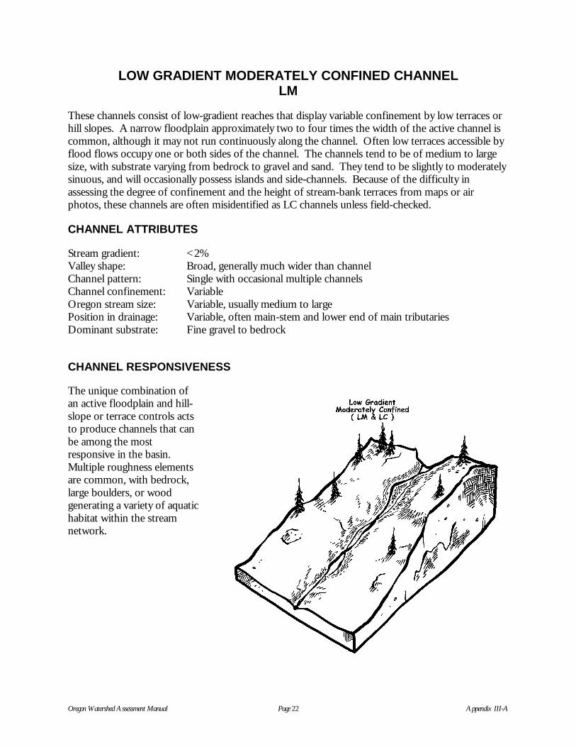
Oregon Watershed Assessment Manual Page 22 Appendix III-A
LOW GRADIENT MODERATELY CONFINED CHANNELLM
These channels consist of low-gradient reaches that display variable confinement by low terraces orhill slopes. A narrow floodplain approximately two to four times the width of the active channel iscommon, although it may not run continuously along the channel. Often low terraces accessible byflood flows occupy one or both sides of the channel. The channels tend to be of medium to largesize, with substrate varying from bedrock to gravel and sand. They tend to be slightly to moderatelysinuous, and will occasionally possess islands and side-channels. Because of the difficulty inassessing the degree of confinement and the height of stream-bank terraces from maps or airphotos, these channels are often misidentified as LC channels unless field-checked.
CHANNEL ATTRIBUTES
Stream gradient: <2%Valley shape: Broad, generally much wider than channelChannel pattern: Single with occasional multiple channelsChannel confinement: VariableOregon stream size: Variable, usually medium to largePosition in drainage: Variable, often main-stem and lower end of main tributariesDominant substrate: Fine gravel to bedrock
CHANNEL RESPONSIVENESS
The unique combination ofan active floodplain and hill-slope or terrace controls actsto produce channels that canbe among the mostresponsive in the basin.Multiple roughness elementsare common, with bedrock,large boulders, or woodgenerating a variety of aquatichabitat within the streamnetwork.

Oregon Watershed Assessment Manual Page 23 Appendix III-A
LM – Low Gradient Moderately Confined
Scale: Full (1:24,000)Contour Interval: 40 feet
Large Woody Debris: Moderate to High
In forested basins, wood alone or incombination with other elements is associatedwith pool formation and maintenance, barformation, and, occasionally, side-channeldevelopment. These channels may haverelatively low wood numbers due to pastmanagement activities.
Fine Sediment: Moderate to High
The location of these channels often dictates ahigh sediment input to the stream. Thesechannels can be sediment deposition zones forlarger particles, although a significant portion ofthe fine sediment may be transported,particularly in bedrock channels. Increases infine-sediment supply will likely result in filling ofmargin pool and bed-fining of side-channels andlow-velocity areas. Decreases in sedimentsupply may induce scour in nonbedrockchannels or localized bank erosion.
Coarse Sediment: Moderate to High
These channels are depositional areas for coarse sediment. When the supply of coarse sedimentsurpasses the transport capabilities of the stream, pools are filled, and the influence of largeboulders, wood, and bedrock control structures is lessened. If significant amounts of large sedimentare added, the channel is particularly vulnerable to widening, lateral movement, side-channeldevelopment, and localized scour.
Oregon Watershed Assessment Manual Page 24 Appendix III-A
Peak Flows: Moderate
These channels are capable of passing most high flows without adjustments to the overalldimensions of the channel. Development of point or medial bars is likely in basins with highsediment loads, as is side-channel development. Localized bed or bank scour is possible on bends inthe main channel.
RIPARIAN ENHANCEMENT OPPORTUNITIES
Like floodplain channels, these channels can be among the most responsive of channel types.Unlike floodplain channels, however, the presence of confining landform features often improvesthe accuracy of predicting channel response to activities that may affect channel form. Additionally,these controls help limit the destruction of enhancement efforts common to floodplain channels.Because of this, LM channels are often good candidates for enhancement efforts.
In forested basins, habitat diversity can often be enhanced by the addition of roughness elementssuch as wood or boulders. Pool frequency and depth may increase, and side-channel developmentmay result from these efforts. Channels of this type in nonforested basins are often responsive tobank stabilization efforts such as riparian planting and fencing. Beavers are often present in thesmaller streams of this channel type, and fish habitat in some channels may benefit from beaverintroduction through side-channel and scour pool development. Introduction of beavers, however,may have significant implications for overall channel form and function, and should be thoroughlyevaluated by land managers as well as biologists as a possible enhancement activity.

Oregon Watershed Assessment Manual Page 25 Appendix III-A
LOW GRADIENT CONFINED CHANNELLC
LC channels are incised or contained within adjacent, gentle landforms or incised in volcanic flowsor uplifted coastal landforms. Lateral channel migration is controlled by frequent bedrock outcrops,high terraces, or hill slopes along stream banks. They may be bound on one bank by hill slopes andlowlands on the other, and may have a narrow floodplain in places, particularly on the inside ofmeander bends. Stream-bank terraces are often present, but they are generally above the currentfloodplain. The channels are often stable, with those confined by hill slopes or bedrock less likely todisplay bank erosion or scour thanthose confined by alluvial terraces.
High-flow events are well-containedby the upper banks. High flows inthese well-contained channels tendto move all but the most stablewood accumulations downstream orpush debris to the channel margins.Stream banks can be susceptible tolandslides in areas where steep hillslopes of weathered bedrock, glacialtill, or volcanic-ash parent materialsabut the channel.
CAUTION: Some degree of cautionshould be exercised in evaluatingchannels that have downcut intoalluvial material set in a wide flatvalley. If the stream banks are highenough to allow a floodplain widthless than two times the bankfull width, then the stream meets the definition of confined. However,some streams meeting this definition may have recently downcut, effectively reducing floodplainwidth as the channel deepens. It is beyond the scope of this manual to deal with technical issuessuch as rate of channel incision. The analyst, however, should note channels that display evidenceof recent downcutting, low channel banks, and evidence of abandoned floodplain. For whateverreason, these channels may be transitioning from LM to LC channels, and should receive additionalscrutiny before assigning the proper CHT.
CHANNEL ATTRIBUTES
Stream gradient: <2%Valley shape: Low- to moderate-gradient hill slopes with limited floodplainChannel pattern: Single channel, variable sinuosityChannel confinement: Confined by hill slopes or high terracesOregon stream size: Variable, usually medium to largePosition in drainage: Variable, generally mid to lower in the larger drainage basinDominant substrate: Boulder, cobble, bedrock with pockets of sand/gravel/cobble

Oregon Watershed Assessment Manual Page 26 Appendix III-A
CHANNEL RESPONSIVENESS
The presence of confining terraces or hill slopes and control elements such as bedrock limit the typeand magnitude of channel response to changes in input factors. Adjustment of channel features isusually localized and of a modest magnitude.
Large Woody Debris: Low to Moderate
In larger forested basins, wood numbers are oftenlow in this channel type. This may be in part due toland management activities, but these channelsusually display sufficient energy to route wooddownstream. Also, limited lateral movement of thechannel reduces the recruitment of wood frombank erosion. Wood is often present in jams or aslarge single pieces capable of withstanding high-energy flows. Even in streams of this channel typethat are smaller and display less energy, wood maybe routed or retained above the elevation of thebankfull channel, where it has limited impact onaquatic habitat.
Fine Sediment: Low
The confining nature of the landforms that define this channel type tends to focus enough streamenergy to route most introduced fine sediment downstream. In basins with high backgroundsediment levels, such as sand and siltstone-bedded channels in the Coast Range, supply mayapproach or surpass transport capacity, resulting in pool filling and bed fining.
Coarse Sediment: Moderate
These channels can bedepositional areas for coarsesediment. When the supply ofcoarse sediment surpasses thetransport capabilities of thestream, pools are filled, and theinfluence of large boulders,wood, and bedrock controlstructures is lessened. Ifsignificant amounts of largesediment are added, the channelis particularly vulnerable towidening, lateral movement, side-channel development, or scour.
LC – Low Gradient Confined
Scale: Full (1:24,000)Contour Interval: 20 feet

Oregon Watershed Assessment Manual Page 27 Appendix III-A
Peak Flows: Low to Moderate
These channels have limited floodplain, and are capable of passing most high flows withoutadjustments to the overall dimensions of the channel. Development of point or medial bars is likelyin basins with high sediment loads. Localized bed or bank scour is possible on bends in the mainchannel.
RIPARIAN ENHANCEMENT OPPORTUNITIES
These channels are not highly responsive, and in channel enhancements may not yield intendedresults. In basins where water-temperature problems exist, the confined nature of these channelslends itself to establishment of riparian vegetation. In nonforested land, these channels may bedeeply incised and prone to bank erosion from livestock. As such, these channels may benefit fromlivestock access control measures.

Oregon Watershed Assessment Manual Page 28 Appendix III-A
MODERATE GRADIENT MODERATELY CONFINED CHANNELMM
This group includes channels with variable controls on channel confinement. Alternating valleyterraces and/or adjacent mountain-slope, foot-slope, and hill-slope landforms limit channelmigration and floodplain development. Similar to the LM channels, a narrow floodplain is usuallypresent, and may alternate from bank to bank. Bedrock steps with cascades may be present.
CHANNEL ATTRIBUTES
Stream gradient: Generally 2-4%Valley shape: Narrow valley with floodplain or narrow terrace developmentChannel pattern: Usually single channel, low to moderate sinuosityChannel confinement: VariableOregon stream size: Variable, usually medium to largePosition in drainage: Mid to lower portion of drainage basinsDominant substrate: Gravel to small boulder
CHANNEL RESPONSIVENESS
The unique combination of a narrow floodplain and hill-slope or terrace controls acts to producechannels that are often the most responsive in the basin. The combination of higher gradients andthe presence of a floodplain set the stage for a dynamic channel system. Multiple roughnesselements such as bedrock, large boulders, or wood may be common, resulting in a variety of aquatichabitats within the stream network.
Large Woody Debris: High
In forested basins, wood alone or incombination with other elements isassociated with pool formation andmaintenance, bar formation and gravelsorting, and, occasionally, side-channeldevelopment. LWD may be the primaryfactor responsible for forming pools inforested systems. Due to the moderategradient, smaller pieces are transporteddownstream or form jams. A change inthe wood supply would likely havesignificant impact on pool condition,sediment movement, bar development,and, possibly, side-channel condition.
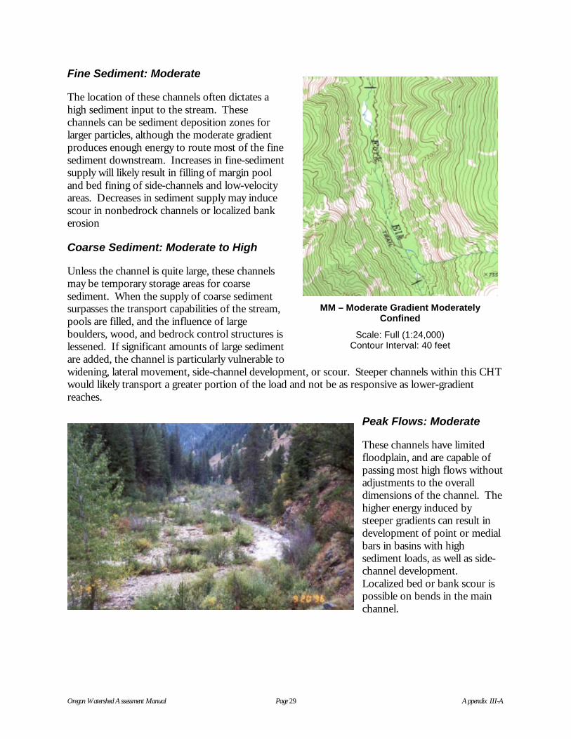
Oregon Watershed Assessment Manual Page 29 Appendix III-A
Fine Sediment: Moderate
The location of these channels often dictates ahigh sediment input to the stream. Thesechannels can be sediment deposition zones forlarger particles, although the moderate gradientproduces enough energy to route most of the finesediment downstream. Increases in fine-sedimentsupply will likely result in filling of margin pooland bed fining of side-channels and low-velocityareas. Decreases in sediment supply may inducescour in nonbedrock channels or localized bankerosion
Coarse Sediment: Moderate to High
Unless the channel is quite large, these channelsmay be temporary storage areas for coarsesediment. When the supply of coarse sedimentsurpasses the transport capabilities of the stream,pools are filled, and the influence of largeboulders, wood, and bedrock control structures islessened. If significant amounts of large sedimentare added, the channel is particularly vulnerable towidening, lateral movement, side-channel development, or scour. Steeper channels within this CHTwould likely transport a greater portion of the load and not be as responsive as lower-gradientreaches.
Peak Flows: Moderate
These channels have limitedfloodplain, and are capable ofpassing most high flows withoutadjustments to the overalldimensions of the channel. Thehigher energy induced bysteeper gradients can result indevelopment of point or medialbars in basins with highsediment loads, as well as side-channel development.Localized bed or bank scour ispossible on bends in the mainchannel.
MM – Moderate Gradient ModeratelyConfined
Scale: Full (1:24,000)Contour Interval: 40 feet

Oregon Watershed Assessment Manual Page 30 Appendix III-A
RIPARIAN ENHANCEMENT OPPORTUNITIES
Like floodplain channels, these channels are among the most responsive of channel types. Unlikefloodplain channels, however, the presence of confining landform features improves the accuracy ofpredicting channel response to activities that may affect channel form. Additionally, these controlshelp limit the destruction of enhancement efforts, a common problem in floodplain channels. Theslightly higher gradients impart a bit more uncertainty as to the outcome of enhancement effortswhen compared to LM channels. MM channels, however, are often good candidates forenhancement efforts.
In forested basins, habitat diversity can often be enhanced by the addition of roughness elementssuch as wood or boulders. Pool frequency and depth may increase as well as side-channeldevelopment as the result of these efforts. Channels of this type in nonforested basins are oftenresponsive to bank stabilization efforts such as riparian planting and fencing.
Beavers are often present in the smaller streams of this channel type, and fish habitat in somechannels may benefit from beaver introduction through side-channel and scour pool development.Introduction of beavers, however, may have significant implications for overall channel form andfunction, and should be thoroughly evaluated by land managers as well as biologists as a possibleenhancement activity.

Oregon Watershed Assessment Manual Page 31 Appendix III-A
MODERATE GRADIENT CONFINED CHANNELMC
MC streams flow through narrow valleys with little river terrace development, or are deeply incisedinto valley floors. Hill slopes and mountain slopes composing the valley walls may lie directlyadjacent to the channel. Bedrock steps, short falls, cascades, and boulder runs may be present; theseare usually sediment transport systems. Moderate gradients, well-contained flows, and large-particlesubstrate indicate high stream energy. Landslides along channel side slopes may be a majorsediment contributor in unstable basins.
CHANNEL ATTRIBUTES
Stream gradient: 2-4%, may vary between 2 to 6%Valley shape: Gentle to narrow V-shaped valley, little to no floodplain
developmentChannel pattern: Single, relatively straight or conforms to hill-slope controlChannel confinement: ConfinedOregon stream size: VariablePosition in drainage: Middle to lowerDominant substrate: Coarse gravel to bedrock
CHANNEL RESPONSIVENESS
The presence of confining terraces or hill slopesand control elements such as bedrock substrateslimits the type and magnitude of channelresponse to changes in input factors.Adjustment of channel features is usuallylocalized and of a modest magnitude.
Large Woody Debris: Low
In larger forested basins, wood numbers areoften low in this channel type. This may be, inpart, due to past land management activities, butthese channels usually display sufficient energyto route wood downstream. Also, limited lateralmovement of the channel reduces therecruitment of wood from bank erosion. Woodis often present in jams or as large single piecescapable of withstanding high-energy flows.Even in streams of this channel type that are smaller and display less energy, wood may be routed orretained above the elevation of the bankfull channel, where it has limited impact on aquatic habitat.

Oregon Watershed Assessment Manual Page 32 Appendix III-A
Fine Sediment: Low
The confining nature of the landforms and the moderategradient combine to produce enough stream energy to routemost introduced fine sediment downstream. Localized poolfilling and bed fining may occur if a large and persistent sourceexists.
Coarse Sediment: Moderate
These channels can be both a transport or deposition area forcoarse sediment. When the supply of coarse sedimentsurpasses the transport capabilities of the stream, pools arefilled, and the influence of large boulders, wood, and bedrockcontrol structures is lessened. If significant amounts of largesediment are added, the channel is particularly vulnerable towidening, limited lateral movement, or scour.
Peak Flows: Moderate
These channels have limited floodplain, and are capable ofpassing most high flows without adjustments to the overalldimensions of the channel. Development of point or medialbars is likely in basins with high sediment loads. Localized bedor bank scour is possible on bends in the main channel.
RIPARIAN ENHANCEMENT OPPORTUNITIES
These channels are not highly responsive, and in-channelenhancements may not yield intended results. Althoughchannels are subject to relatively high energy, they areoften stable. In basins where water-temperature problemsexist, the stable banks generally found in these channelslend themselves to establishment of riparian vegetation.In nonforested land, these channels may be deeply incisedand prone to bank erosion from livestock. As such, thesechannels may benefit from livestock access controlmeasures.
MC – Moderate GradientConfined
Scale: Full (1:24,000)Contour Interval: 40 feet

Oregon Watershed Assessment Manual Page 33 Appendix III-A
MODERATE GRADIENT HEADWATER CHANNELMH
These moderate-gradient headwater channels are common to plateaus in Columbia River basalts,young volcanic surfaces, or broad drainage divides. They may be sites of headwater beaver ponds.These channels are similar to LC channels, but occur exclusively in headwater regions. They arepotentially above the anadromous fish zone.
These gentle to moderate headwater streams generally have low streamflow volumes and, therefore,low stream power. The confined channels provide limited sediment storage in low-gradient reaches.Channels have a small upslope drainage area and limited sediment supply. Sediment sources arelimited to upland surface erosion.
CHANNEL ATTRIBUTES
Stream gradient: 1-6%Valley shape: Open, gentle V-shape valley
Channel pattern: Low sinuosity to straightChannel confinement: ConfinedOregon stream size: SmallPosition in drainage: Upper, headwaterDominant substrate: Sand to cobble, bedrock; boulders may be present from
erosion of surrounding slopes and soils
CHANNEL RESPONSIVENESS
The low stream power and presence ofconfining terraces or hill slopes and controlelements such as bedrock substrates limit thetype and magnitude of channel response tochanges in input factors. Adjustment ofchannel features is usually localized and of amoderate magnitude.
Large Woody Debris: Moderate
Wood numbers and influence is quite variablein these channels. While the low streamenergy may limit the magnitude of responseassociated with wood, wood numbers can behigh and wood may be the dominantroughness element. In these cases, wood iscritical for pool and cover habitat formationand maintenance.
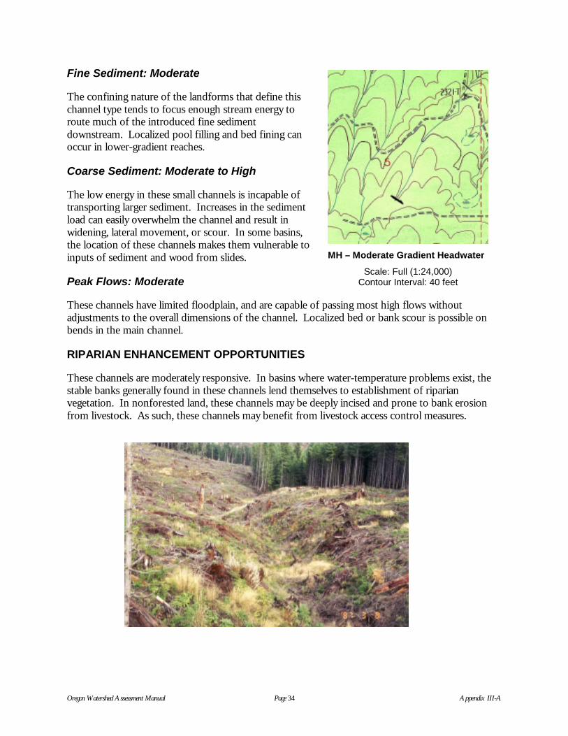
Oregon Watershed Assessment Manual Page 34 Appendix III-A
Fine Sediment: Moderate
The confining nature of the landforms that define thischannel type tends to focus enough stream energy toroute much of the introduced fine sedimentdownstream. Localized pool filling and bed fining canoccur in lower-gradient reaches.
Coarse Sediment: Moderate to High
The low energy in these small channels is incapable oftransporting larger sediment. Increases in the sedimentload can easily overwhelm the channel and result inwidening, lateral movement, or scour. In some basins,the location of these channels makes them vulnerable toinputs of sediment and wood from slides.
Peak Flows: Moderate
These channels have limited floodplain, and are capable of passing most high flows withoutadjustments to the overall dimensions of the channel. Localized bed or bank scour is possible onbends in the main channel.
RIPARIAN ENHANCEMENT OPPORTUNITIES
These channels are moderately responsive. In basins where water-temperature problems exist, thestable banks generally found in these channels lend themselves to establishment of riparianvegetation. In nonforested land, these channels may be deeply incised and prone to bank erosionfrom livestock. As such, these channels may benefit from livestock access control measures.
MH – Moderate Gradient Headwater
Scale: Full (1:24,000)Contour Interval: 40 feet

Oregon Watershed Assessment Manual Page 35 Appendix III-A
MODERATELY STEEP NARROW VALLEY CHANNELMV
MV channels are moderately steep and confined by adjacent moderate to steep hill slopes. Highflows are generally contained within the channel banks. A narrow floodplain, one channel width ornarrower, may develop locally.
MV channels efficiently transport both coarse bedload and fine sediment. Bedrock steps, bouldercascades, and chutes may be common features. The large amount of bedrock and boulders createstable streambanks; however, steep side slopes may be unstable. Large woody debris is foundcommonly in jams that trap sediment in locally low-gradient steps.
CHANNEL ATTRIBUTES
Stream gradient: 4-8%, may vary between 3 to 10%Valley shape: Narrow, V-shaped valleyChannel pattern: Single channel, relatively straight similar to valleyChannel confinement: ConfinedOregon stream size: Small to mediumPosition in drainage: Mid to upperDominant substrate: Small cobble to bedrock
CHANNEL RESPONSIVENESS
The gradient and presence of confining terraces or hill slopes and control elements such as bedrocksubstrates limit the type and magnitude of channel response to changes in input factors. Adjustmentof channel features is localized and of a minor magnitude.
Large Woody Debris: Moderate
In larger forested basins, wood numbers are often high in this channel type. Wood is present injams or as single pieces capable of withstanding high-energy flows. Large woody debris may be theprimary element responsible for pool formation and development. In bedrock systems, wood hasless influence, and is often transported downstream.
Fine Sediment: Low
The confining nature of the landforms and the higher gradients combine to produce enough streamenergy to route most introduced fine sediment downstream. Filling of lateral pools and lower-energy areas may result from increases in the sediment supply.
Coarse Sediment: Moderate
These channels are usually transport reaches for coarse sediment, although lower-energy sectionscan retain sediment and adjust channel dimensions. When the supply of coarse sediment surpassesthe transport capabilities of the stream, pools are filled, and the influence of large boulders, wood,and bedrock control structures is lessened.

Oregon Watershed Assessment Manual Page 36 Appendix III-A
Peak Flows: Moderate
These channels have limited floodplain, and arecapable of passing most high flows withoutadjustments to the overall dimensions of thechannel. Development of point or medial barsis likely in basins with high sediment loads.Localized bed or bank scour is possible onbends in the main channel.
RIPARIAN ENHANCEMENTOPPORTUNITIES
These channels are not highly responsive, and in channel enhancements may not yield intendedresults. Although channels are subject to relatively high energy, they are often stable. In basinswhere water-temperature problems exist, the stable banks generally found in these channels lendthemselves to establishment of riparian vegetation. In nonforested land, these channels may bedeeply incised and prone to bank erosion from livestock. As such, these channels may benefit fromlivestock access control measures.
MV – Moderately Steep Narrow Valley
Scale: Full (1:24,000)Contour Interval: 40 feet

Oregon Watershed Assessment Manual Page 37 Appendix III-A
BEDROCK CANYON CHANNELBC
BC channels are associated with valley bottom gorge landforms typically cut through bedrock withlong, steep, side-slope walls. Channel features include cascades, rapids, and major falls, althoughlong pools may exist.
CHANNEL ATTRIBUTES
Stream gradient: >4%, can be locally lowerValley shape: Canyons, gorges, very steep mountain side slopesChannel pattern: Single channel, straightChannel confinement: Tightly confined by bedrock slopesOregon stream size: VariablePosition in drainage: VariableDominant substrate: Bedrock, large boulders
CHANNEL RESPONSIVENESS
The bedrock side slopes and channel bed severely limit the sensitivity of these channels to change.They are the least responsive of the identified channel types.
Large Woody Debris: Low
Wood is generally transported out of these reaches, although jams can develop in lower-gradientcanyons. Bedrock is the defining roughness element, with wood playing a minor role.
Fine Sediment: Low
The confining nature of the landform produces enough stream energy to route most introduced finesediment downstream. Temporary storage of fines in low-gradient pools may occur.
Coarse Sediment: Low
These channels are usually transport reaches for coarse sediment, although lower-energy sectionscan retain sediment for a limited time.
Peak Flows: Low
These channels have no floodplain, and are capable of passing high flows without adjustments tothe overall dimensions of the channel.

Oregon Watershed Assessment Manual Page 38 Appendix III-A
RIPARIAN ENHANCEMENTOPPORTUNITIES
These channels are not responsive,and are generally a poor site forenhancement efforts.
BC – Bedrock Canyon
Scale: Full (1:24,000)Contour Interval: 20 feet

Oregon Watershed Assessment Manual Page 39 Appendix III-A
STEEP NARROW VALLEY CHANNELSV
VERY STEEP HEADWATERVH
These two channel types are very similar, except that VH channels are steeper. Because of thissimilarity, they are presented together. SV channels are situated in a constricted valley bottombounded by steep mountain or hill slopes. Vertical steps of boulder and wood with scour pools,cascades, and falls are common. VH channels are found in the headwaters of most drainages or sideslopes to larger streams, and commonly extend to ridge-tops and summits. These steep channelsmay be shallowly or deeply incised into the steep mountain or hill slope. Channel gradient may bevariable due to falls and cascades.
CHANNEL ATTRIBUTES
Stream gradient: SV 8-16%, VH >16%Valley shape: Steep, narrow V-shaped valleyChannel pattern: Single, straightChannel confinement: Tightly confinedOregon stream size: Small, small-medium transitionPosition in drainage: Middle upper to upperDominant substrate: Large cobble to bedrock
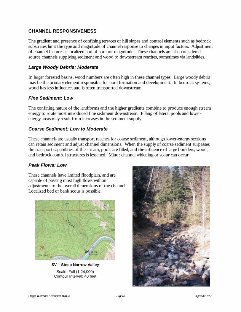
Oregon Watershed Assessment Manual Page 40 Appendix III-A
CHANNEL RESPONSIVENESS
The gradient and presence of confining terraces or hill slopes and control elements such as bedrocksubstrates limit the type and magnitude of channel response to changes in input factors. Adjustmentof channel features is localized and of a minor magnitude. These channels are also consideredsource channels supplying sediment and wood to downstream reaches, sometimes via landslides.
Large Woody Debris: Moderate
In larger forested basins, wood numbers are often high in these channel types. Large woody debrismay be the primary element responsible for pool formation and development. In bedrock systems,wood has less influence, and is often transported downstream.
Fine Sediment: Low
The confining nature of the landforms and the higher gradients combine to produce enough streamenergy to route most introduced fine sediment downstream. Filling of lateral pools and lower-energy areas may result from increases in the sediment supply.
Coarse Sediment: Low to Moderate
These channels are usually transport reaches for coarse sediment, although lower-energy sectionscan retain sediment and adjust channel dimensions. When the supply of coarse sediment surpassesthe transport capabilities of the stream, pools are filled, and the influence of large boulders, wood,and bedrock control structures is lessened. Minor channel widening or scour can occur.
Peak Flows: Low
These channels have limited floodplain, and arecapable of passing most high flows withoutadjustments to the overall dimensions of the channel.Localized bed or bank scour is possible.
SV – Steep Narrow Valley
Scale: Full (1:24,000)Contour Interval: 40 feet

Oregon Watershed Assessment Manual Page 41 Appendix III-A
RIPARIAN ENHANCEMENT OPPORTUNITIES
These channels are not highly responsive, and in channel enhancements may not yield intendedresults. Although channels are subject to relatively high energy, they are often stable. In basinswhere water-temperature problems exist, the stable banks generally found in these channels lendthemselves to establishment of riparian vegetation. This may also serve as a recruitment effort forLWD in the basin.
VH – Very Steep Headwater
Scale: Full (1:24,000)Contour Interval: 40 feet

Oregon Watershed Assessment Manual Page 42 Appendix III-A
REFERENCES
Cupp, C.E. 1989. Stream Corridor Classification for Forested Lands of Washington. State ofWashington, Timber/Fish/Wildlife Ambient Monitoring Program, Olympia.
Frissell, C.A., W.J. Liss, C.E. Warren, and M.D.Hurley. 1986. A Hierarchical Framework forStream Habitat Classification: Viewing Streams in a Watershed Context. EnvironmentalManagement 10(2):199-214.
Montgomery, D.R., and J.M. Buffington. 1993. Channel Classification, Prediction of ChannelResponse, and Assessment of Channel Condition. Washington State Timber/Fish/WildlifeReport TFW-SH10-93-002, Olympia.
Moore, K., K. Jones, and J. Dambacher. 1997. Methods for Stream Habitat Surveys. AquaticInventory Project, Natural Production Program: Oregon Department of Fish and Wildlife.
Oregon Department of Land Conservation and Development. 1987. Estuary Plan Book.
Paustian, S.J. (editor), et al. 1992. Channel Type Users Guide for the Tongass National Forest,Southeast Alaska. US Department of Agriculture Forest Service, Alaska Region, R10 TechnicalPaper 26.
Rosgen, D.L. 1996. Applied River Morphology. Wildland Hydrology, Pagosa Springs, CO.
Oregon Watershed Assessment Manual Page 43 Appendix III-A
GLOSSARY
aggradation: Raising of the channel bed elevation due to sediment deposition.
alluvial fan: An area where large amounts of sediment are deposited by a stream as the streamgradient rapidly decreases.
anadromous fish: Fish that move from the sea to fresh water for reproduction.
bed fining: An increase in the amount of fine sediment (<2 mm) in the stream channel bed.
braiding: Branching of a stream into many channels.
channel confinement: Ratio of bankfull channel width to width of modern floodplain. Modernfloodplain is the flood-prone area and may correspond to the 100-year floodplain. Typically,channel confinement is a description of how much a channel can move within its valley before it isstopped by a hill slope or terrace.
delta: At a river’s mouth, the sediment deposits found between the diverging channels.
estuary: Area of a river mouth where the fresh water of a river mixes with ocean water.
foot slope: Area located at the bottom of a hill slope.
gradient: Channel gradient is the slope of the channel bed along a line connecting the deepestpoints (thalweg) of the channel.
intertidal: The shore region between high and low tide.
large woody debris (LWD): Logs, stumps, or root wads in the stream channel, or nearby. Thesefunction to create pools and cover for fish, and to trap and sort stream gravels.
medial bar: Sediment deposit in a river that protrudes above the water surface and is not connectedto shore.
morphologic response: In stream channels, the response or change in the characteristics thatdefine the channel.
morphology: A branch of science dealing with the structure and form of objects. Geomorphologyas applied to stream channels refers to the nature of landforms and topographic features.
mudflat: Intertidal zone whose substrate consists primarily of silt and clay and is usuallyunvegetated.
oxbow: A bow-shaped river bend.
point bar: A sediment deposit in a river that protrudes above the water surface and is locatedprimarily on the inside of bends in the channel.

Oregon Watershed Assessment Manual Page 44 Appendix III-A
relic channel: A channel historically occupied by a river, but that currently does not convey flow.
riparian area: The area adjacent to the stream channel that interacts and is dependent on the streamfor biologic integrity.
scour: Removal of sediment from the bed or banks of a river by the energy of moving water.
side-channel: A channel that is separated from the main channel, usually by an island.
single-thread channel: A stream channel that has no side channels, braiding, or islands.
slough: A side channel within an estuary.
stream reach: A section of stream possessing similar physical features such as gradient andconfinement.

Component IVHydrology and Water UseTable of Contents
Introduction.....................................................IV-3
Linkages to Other Components .....................IV-3
Section I: Hydrology .......................................IV-4
Critical Questions............................................. IV-4
Assumptions..................................................... IV-4
Materials Needed............................................. IV-5
Necessary Skills............................................... IV-6
Final Products of the Hydrology Section ......... IV-6
Hydrologic Condition Characterization ............ IV-7
Hydrologic Condition Assessment................... IV-8
Section II: Water Use .................................... IV-20
Critical Questions........................................... IV-20
Assumptions................................................... IV-20
Materials Needed........................................... IV-20
Final Products of the Water Use Section ...... IV-20
Water Use Characterization........................... IV-21
Water Use Assessment ................................. IV-21
Confidence in Assessments ........................ IV-22
Further Analyses........................................... IV-23
References .................................................... IV-24
Glossary ........................................................ IV-27
Appendix IV-A: Forms and Worksheets
Form H-1: General Watershed
Characteristics
Form H-2: Land Use Summary Form
Form H-3: Annual Peak Flow Summary
Form
Form H-4: Forestry Worksheet
Form H-5: Agriculture and Range-Land
Worksheet
Form H-6: Forest and Rural Road
Worksheet
Form H-7: Urban and Residential Area
Worksheet

Table of Contents (continued)
Form H-8: Hydrologic Issue Identification
Summary
Form WU-1. Water Rights Summary
Form WU-2: Water Availability Summary
Form WU-3. Consumptive Use Summary
Form HW-1. Confidence Evaluation
Appendix IV-B: Reference Tables
Table B-1. Runoff Curve Numbers for
Cultivated Agricultural Lands
Table B-2: Runoff Curve Numbers for
Other Agricultural Lands
Table B-3: Runoff Curve Numbers for Arid
and Semiarid Range Lands
Table B-4: Runoff Depth for Selected
Curve Numbers and Rainfall Amounts
Appendix IV-C: Resources for Data
Aquisition
Resources for Data Acquisition
USGS
Publications
Regional Offices of OWRD
Appendix IV-D: Background Hydrologic
Information
Land Use Impacts on Hydrology
Water Law and Water Use Background

Oregon Watershed Assessment Manual Page IV-3 Hydrology and Water Use
Component IVHydrology and Water Use
INTRODUCTION
The Watershed Fundamentals component of this manual presents an overview of the naturalhydrologic cycle and potential impacts of human activities. Alterations to the natural hydrologiccycle potentially cause increased peak flows1 and/or reduced low flows resulting in changes towater quality and aquatic ecosystems. The degree to which hydrologic processes are affected by landuse depends on the location, extent, and type of land use activities. When potential impacts arerecognized, best management practices (BMPs) can be followed to minimize some of thepotential hydrologic impacts; mitigation will be necessary to address other impacts.
Evaluating potential impacts from land and water use on the hydrology of a watershed is the focusof this component. It is important to recognize that hydrologic processes are complicated; we haveattempted to provide enough direction for you to identify how land uses may be affecting yourwatershed’s hydrology. Figure 1 provides an overview of the steps you will be following tocomplete the Hydrology and Water Use Assessment component. This assessment does not attemptto address every hydrologic process potentially affected; the goal is to gain an understanding of themajor potential impacts.
The assessment process is separated into two sections (Figure 1). Section I characterizes thehydrology of the watershed and assesses the locations and type of potential impacts. Section IIevaluates the consumptive water uses and identifies locations and types of potential impactsassociated with water use. Each section may be completed independently by different people whocollaborate at the end to complete a map of potential hydrologic impacts and reaches of water useconcerns. Appendix IV-A contains all the forms necessary to complete both sections of theassessment. Appendix IV-B includes reference tables to help complete the forms. Appendix IV-Cprovides information on resources to obtain necessary data. Finally, Appendix IV-D providesadditional background information on how land uses can impact the hydrologic function of awatershed, and information on water rights law.
LINKAGES TO OTHER COMPONENTS
Information on peak-flow history in the watershed (Step 3) will be used in the Historical ConditionsAssessment component. Withdrawal of water from a stream during the driest and hottest times ofthe year potentially stresses aquatic organisms. Information from the Fish and Fish HabitatAssessment component will be required to determine specific stream reaches that are sensitive towater use impacts. The Water Quality and Riparian/Wetlands assessments require an understandingof the hydrology and water use in the watershed.
During the Watershed Condition Evaluation component, subwatersheds where potential hydrologicimpacts are identified will be evaluated for evidence of channel response (i.e., widening, loss ofcomplexity, etc.) to changes in flow.
1 Terms that appear in bold italic throughout the text are defined in the Glossary at the end of this component.

Oregon Watershed Assessment Manual Page IV-4 Hydrology and Water Use
SECTION I: HYDROLOGY
Critical Questions
1. What land uses are present in your watershed?2. What is the flood history in your watershed?3. Is there a probability that land uses in the basin have a significant effect on peak flows?4. Is there a probability that land uses in the basin have a significant effect on low flows?
Assumptions
• Urbanization (including industrial use), agriculture, range-land use, and forestry are theprimary land uses that may impact hydrology.
Figure 1. The screen for potential forestry impacts on hydrology focuses on timber harvest inthis step and follows the pathways shown in this flow chart. Subwatersheds that end up in theshaded box at the bottom left have the potential for peak-flow impacts from forestry.

Oregon Watershed Assessment Manual Page IV-5 Hydrology and Water Use
• Peak flows and low flows are the hydrologic processes most significantly impacted by landuse activities.
• Hydrologic soil condition is an indicator of infiltration rate.
• Groundwater impacts are implicitly addressed through the changes in infiltration rates.
• In forested basins, the greatest potential for peak-flow increases over background conditionsare due to road rerouting of water and changes in snow accumulation and melt in harvestedareas during rain-on-snow events.
• The decreased evaporation and transpiration from tree removal more than offset thereduced infiltration; therefore, low flows tend to increase in the short-term due to forestharvesting.
• BMPs to mitigate peak-flow impacts will also mitigate low-flow impacts from agriculturaland urban land uses.
• Impervious surfaces and roads are good indicators of urbanization and subsequent impactsto the hydrology of a watershed.
Materials Needed
• Watershed Base Map (from Start-Up and Identification of Watershed Issues component)
• Refined Land Use Map with subwatersheds identified (from Start-Up and Identification ofWatershed Issues component)
• Ecoregion map for the watershed (from Start-Up and Identification of Watershed Issuescomponent)
• Aerial photographs and/or orthophoto quadrangle maps (most recent)
• Mean annual precipitation map, available from one of the sources listed in the box below
• Map of 2-year, 24-hour precipitation (Miller et al. 1973). This map is available on line at theDesert Research Institute, Western Regional Climate Center (see list in the box below forInternet address), or can be ordered (for a cost of $9) from National Weather Service Officeof Hydrology, W/OH2 Station 7144, 1325 East-West Highway, Silver Spring, MD 20910;(301) 713-1669.
Oregon Climate ServiceStrand Hall, Room 326Oregon State UniversityCorvallis, OR 97331-2209(541) 737-5705
Internet address:http://www.ocs.orst.edu/
Desert Research InstituteWestern Regional Climate CenterP.O. Box 60220Reno, NV 89506-0220(702) 677-3143
Internet address:http://www.wrcc.dri.edu/
State Service Center for GISDept. of Administrative Services155 Cottage Street NESalem, OR 97310(503) 378-2166
Internet address:http://www.sscgis.state.or.us/

Oregon Watershed Assessment Manual Page IV-6 Hydrology and Water Use
• Daily average and peak streamflow data and map of streamflow collection sites. Availablefrom the sources listed at the top of this page.
• Natural Resources Conservation Service (NRCS) county soil survey. Your local library orcounty extension agent will probably have copies. If not, order a copy from the StateConservationist, Federal Building Room 1640, 1220 SW 3rd Avenue, Portland, OR97204-3221; (503) 414-3201s; Internet address http://www.statlab.iastate.edu/soils/nssc/
• Other relevant published reports and/or unpublished documents from city, county, state, orfederal agencies or private consultants (local, regional, or statewide), such as Basin Planswritten by the Oregon Water Resources Department (OWRD) and others.
Necessary Skills
Characterization of watershed hydrology requires mathematical, statistical, and technical tools. Theanalyst would benefit from a familiarity with computer spreadsheets and/or use of a calculator, aswell as an understanding of simple statistics such as the mean (or average) and ratios. Internetaccess will provide the analyst with more readily available sources of data.
Final Products of the Hydrology Section
Form H-1: General Watershed CharacteristicsForm H-2: Land Use SummaryForm H-3: Annual Peak Flow SummaryForm H-4: Forestry WorksheetForm H-5: Agriculture and Range Land WorksheetsForm H-6: Forest and Rural Road WorksheetForm H-7: Urban and Rural Residential WorksheetForm H-8: Hydrologic Issue Identification SummaryMap H-1: Potential Risks of Land Use on Hydrology
STREAMFLOW DATA SOURCES
USGS Portland District Office10615 SE Cherry Blossom DrivePortland, OR 97216(503 ) 251-3265
Internet address:http://wwworegon.wr.usgs.gov/
• Digital data available at Web site
• US Geological Survey, Open-File Report 90-118,“Statistical Summaries of Streamflow Data inOregon: Volume 1: Monthly and AnnualStreamflow, and Flow-Duration Values”
• US Geological Survey, Open-File Report 93-63,“Statistical Summaries of Streamflow Data inOregon: Volume 2: Annual Low and High Flow,and Instantaneous Peak Flow” Prepared incooperation with the Oregon Water ResourcesDepartment (OWRD, 1993).
Oregon Water Resources Department158 12th Street NESalem, OR 97310(503) 378-8455
Internet address:http://www.wrd.state.or.us/
• Digital data available at Web site

Oregon Watershed Assessment Manual Page IV-7 Hydrology and Water Use
Hydrologic Condition Characterization
Step 1: Identify General Watershed Characteristics (Form H-1)
For each subwatershed, fill in the information requested on Form H-1. This form is designed tohelp you compile watershed-specific information that relates to the local hydrology. You willidentify basic watershed features such as drainage area, minimum and maximum elevations, andmean annual precipitation. If you have Geographic Information System (GIS) support, some ofthe information can be calculated using GIS. Otherwise, use the Watershed Base Map or USGeological Survey (USGS) topographic maps and a map of mean annual precipitation to find theinformation. Subwatershed drainage areas can be estimated by using GIS, a planimeter, or the gridmethod described in the Start-Up and Identification of Watershed Issues component.
Step 2: Summarize Land Uses in the Watershed (Form H-2)
Enter the estimated areas of each land use in each subwatershed onto Form H-2. Consult theRefined Land Use Map from the Start-Up component to identify the different land uses present inthe watershed and subwatersheds. The areas in each land use can be either estimated using GIS, aplanimeter, or the grid method.
Step 3: Characterize Peak Flows (Form H-3)
The purpose of this step is to identify the peak-flow-generating processes within your watershed andto graph the peak-flow history over time. Identification of the peak-flow-generating processes areneeded to complete the hydrologic condition assessment (page 8), and will help you understand thetype of conditions that generate peak flows in your watershed. Compiling and graphing informationon flood history will provide context for understanding the extent of channel disturbance found inyour watershed, help you to understand the cycles of flooding in the watershed, and confirm ordispel public perceptions about flood history.
Identifying Peak-Flow-Generating Processes
The Ecoregion Appendix provides information on peak-flow-generating processes by elevation zonewithin each ecoregion of Oregon. For watersheds located in western Oregon you can also check tosee if any stream gage(s) in your watershed were analyzed in the hydrologic process identificationstudy conducted by Greenberg and Welch (1998). Using the ecoregion map and the base map(showing subwatersheds), estimate the acres and percent area in each subwatershed that fall into oneof the following peak-flow-generating processes categories: rain (including thunderstorms),rain-on-snow, spring snowmelt. Record this information on Form H-3.
Graphing Peak-Flow History
Identify the USGS streamflow gage(s) that are in or near your watershed (see streamflow datasources in the Materials Needed section and Appendix IV-C). Some watersheds in Oregon containone or more stream gages while many unfortunately have none. If no gage is or was present in yourwatershed, find the closest gages in adjacent watersheds in the same ecoregion. Gages located inadjacent watersheds will not necessarily be representative of conditions in your watershed (seeCriteria sidebar at the top of page 8). The USGS Web site is a good starting point to find streamgages in your area. (Gages are listed by county and river basin, and close-up maps can be viewed
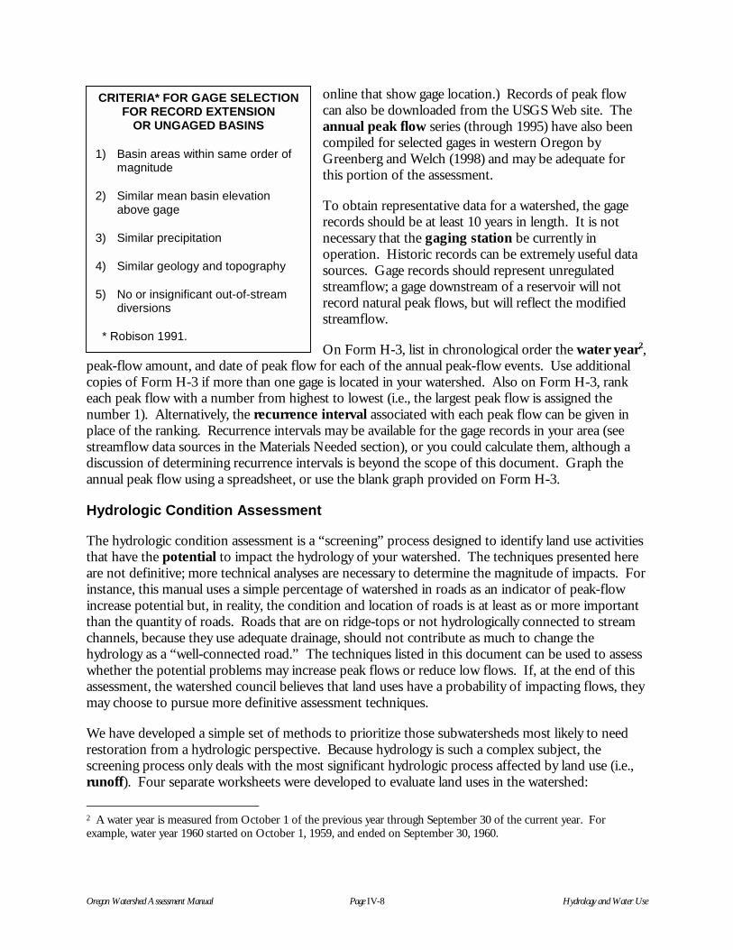
Oregon Watershed Assessment Manual Page IV-8 Hydrology and Water Use
CRITERIA* FOR GAGE SELECTIONFOR RECORD EXTENSION
OR UNGAGED BASINS
1) Basin areas within same order ofmagnitude
2) Similar mean basin elevationabove gage
3) Similar precipitation
4) Similar geology and topography
5) No or insignificant out-of-streamdiversions
* Robison 1991.
online that show gage location.) Records of peak flowcan also be downloaded from the USGS Web site. Theannual peak flow series (through 1995) have also beencompiled for selected gages in western Oregon byGreenberg and Welch (1998) and may be adequate forthis portion of the assessment.
To obtain representative data for a watershed, the gagerecords should be at least 10 years in length. It is notnecessary that the gaging station be currently inoperation. Historic records can be extremely useful datasources. Gage records should represent unregulatedstreamflow; a gage downstream of a reservoir will notrecord natural peak flows, but will reflect the modifiedstreamflow.
On Form H-3, list in chronological order the water year2,peak-flow amount, and date of peak flow for each of the annual peak-flow events. Use additionalcopies of Form H-3 if more than one gage is located in your watershed. Also on Form H-3, rankeach peak flow with a number from highest to lowest (i.e., the largest peak flow is assigned thenumber 1). Alternatively, the recurrence interval associated with each peak flow can be given inplace of the ranking. Recurrence intervals may be available for the gage records in your area (seestreamflow data sources in the Materials Needed section), or you could calculate them, although adiscussion of determining recurrence intervals is beyond the scope of this document. Graph theannual peak flow using a spreadsheet, or use the blank graph provided on Form H-3.
Hydrologic Condition Assessment
The hydrologic condition assessment is a “screening” process designed to identify land use activitiesthat have the potential to impact the hydrology of your watershed. The techniques presented hereare not definitive; more technical analyses are necessary to determine the magnitude of impacts. Forinstance, this manual uses a simple percentage of watershed in roads as an indicator of peak-flowincrease potential but, in reality, the condition and location of roads is at least as or more importantthan the quantity of roads. Roads that are on ridge-tops or not hydrologically connected to streamchannels, because they use adequate drainage, should not contribute as much to change thehydrology as a “well-connected road.” The techniques listed in this document can be used to assesswhether the potential problems may increase peak flows or reduce low flows. If, at the end of thisassessment, the watershed council believes that land uses have a probability of impacting flows, theymay choose to pursue more definitive assessment techniques.
We have developed a simple set of methods to prioritize those subwatersheds most likely to needrestoration from a hydrologic perspective. Because hydrology is such a complex subject, thescreening process only deals with the most significant hydrologic process affected by land use (i.e.,runoff). Four separate worksheets were developed to evaluate land uses in the watershed: 2 A water year is measured from October 1 of the previous year through September 30 of the current year. Forexample, water year 1960 started on October 1, 1959, and ended on September 30, 1960.

Oregon Watershed Assessment Manual Page IV-9 Hydrology and Water Use
1. Forestry2. Agriculture and range lands3. Forest and rural roads4. Urban and/or rural residential development
Figure 1 illustrates the steps to work through depending on the land uses in your basin. You neednot fill out the worksheets for those land uses not present in your watershed. The potential risksfrom land uses on hydrology will be summarized on Form H-8. Form H-8 can be used, inconjunction with other assessments in this manual, to determine potential restoration opportunities.Special attention should be made to connecting the hydrologic information to the ChannelModification Assessment component. If potential peak-flow problems are identified in asubwatershed, the first step would be to cross-reference with the Channel Modification analyst todetermine whether there is corroborating evidence of channel changes in the stream. Hydrologicimpacts to aquatic resources are, to a large degree, a function of the Channel Habitat Type (CHT).Some CHTs can withstand large changes in flow without substantial change to the hydrauliccharacteristics, whereas others are very susceptible to peak-flow changes. If low-flow problems areidentified, corroborating evidence of channel dewatering should be obtained.
Step 4: Complete Forestry Worksheet (Form H-4)
The screen for potential forestry impacts on hydrology focuses on timber harvest in this step andfollows the pathways shown in the flow chart presented in Figure 2. Record your answers on FormH-4. Any subwatersheds that end up in the shaded box at the bottom left of the flow chart have thepotential for peak-flow impacts from forestry. Timber harvest in the Rocky Mountains has beenfound to produce increased spring snowmelt peak flows (Troendle and King 1985); however, it isunknown if the underlying processes would be the same in the moister, more maritime conditionsthat are found in Oregon. If your watershed is in an area in which spring snowmelt produces theannual maximum flows, you may wish to consider some alternative analysis beyond the scope of thismethodology.
Before starting the forestry worksheet, first read through the tasks listed below. This will helpyou be more efficient in answering all the questions found in the flow chart in Figure 2. Refer backto the flow chart to gain an overall perspective on where these steps are leading you. Use theinformation you collected on earlier forms (where available) to help you with the tasks. Also haveForm H-8 handy.
Task 1: Identify the peak-flow-generating processes for each subwatershed. Using Form H-3, notethe percent area in each subwatershed that is in the rain, rain-on-snow, and spring snowmeltcategories. If more than 75% of any subwatershed is in the rain category mark Column 5 on FormH-4 as low potential risk of peak-flow enhancement (WFPB 1997). If all subwatersheds are morethan 75% in the rain category, skip the remainder of this step and go on to Step 5. If more than75% of any subwatershed is in the spring snowmelt category, mark Column 5 on Form H-4 asunknown potential risk of peak-flow enhancement. If all subwatersheds are more than 75% in thespring snowmelt category, skip the remainder of this step and go on to Step 5.

Oregon Watershed Assessment Manual Page IV-10 Hydrology and Water Use
Task 2: For the subwatersheds that have not been eliminated in the previous task, estimate thehistoric crown closure for the portions of each subwatershed that are in the rain-on-snow areas,and record this information on Form H-4. (You may need to sketch the boundaries of the rain,rain-on-snow, and/or spring snowmelt areas on your base map. See the Ecoregion Appendix forguidance on how to define these areas). The Ecoregion Appendix includes historic crown closureestimates for each ecoregion in Oregon. Other possible sources to consult include US ForestService (USFS) plant association documents or watershed analyses, or a local forester or fireecologist (Oregon Department of Forestry [ODF] or private timber landowner) familiar with thelands in your watershed. If any subwatershed had less than 30% historic crown closure, markColumn 5 on Form H-4 as low potential risk of peak-flow increases. If all subwatersheds had lessthan 30% historic crown closure, skip the remainder of this step and go on to Step 5.
Task 3: For the subwatersheds that have not been eliminated in previous tasks, estimate the percentof the rain-on-snow areas that currently have less than 30% crown closure, and record thisinformation on Form H-4. Use published information if possible, such as USFS watershed analysesor other watershed studies. If published information is not available, contact the forester (ODFand/or private timber companies) in charge of lands in the watershed of interest and request crownclosure data; it is preferable that this information be derived from aerial photo coverage or groundinventory and not LANDSAT data. If crown closure coverage is not available from the landowners
Timber Harvest Assessment Tasks
Figure 2. Overview of the steps you will be following to complete the Hydrology and Water UseAssessment component.

Oregon Watershed Assessment Manual Page IV-11 Hydrology and Water Use
in the watershed, you will need to determine these areas by examining aerial photographs. If you arenot familiar with viewing aerial photographs, consult with a technical specialist who can assist youwith this step.
Task 4: Using the information you have entered on Form H-4, and Figure 3, estimate the risk ofpeak-flow enhancement for the remaining subwatersheds, and record this information on FormH-4. Also enter the results from Columns 4 and 5 onto Form H-8 Column 2.
The graph in Figure 3 is adapted from the Washington State Department of Natural Resources(1991) Interim Rain-on-Snow Rules. Although the graph was derived for Washington State, it wasdeveloped using rules of thumb applicable to the Pacific Northwest. For the purpose of screeningforested areas of hydrologic concern in Oregon, the risk classes used in the Washington graph wereaggregated from three classes to two classes: low risk and potential risk. The boundary between thetwo classes was set at a lower threshold of concern, based on personal communication with theoriginal author of the Washington graphs (Brunengo, personal communication, 1998). The lineswere also tested using the Washington State Forest Practices Board rain-on-snow model for awatershed in the Rogue Basin and a watershed on the western slope of the Cascades in northernOregon. The line appears to roughly represent peak-flow increases of 8 to 10%, which representsthe lower boundary of detectability; the accuracy of good streamflow measurements are within 10%of the true value (USGS 1997) (WFPB 1997).
Figure 3. This graph is used to help you estimate the risk of peak-flow enhancement tosubwatersheds from forestry-related impacts during rain-on-snow events.

Oregon Watershed Assessment Manual Page IV-12 Hydrology and Water Use
Step 5: Complete Agriculture and Range-Land Worksheet (Form H-5)
The agricultural and range-land screening procedure (Figure 4) is designed to first identifyhydrologic soil groups (HSG), cover types, and treatments occurring on agricultural lands andrange lands in your watershed. Secondly, using tables from the US Department of AgricultureNatural Resources Conservation Service (NRCS) (formerly Soil Conservation Service) methods(USDA 1986), runoff curve numbers are assigned to each combination of three parameters: soilgroup, cover type, and treatment. The hydrologic response will be bracketed using both goodhydrologic condition and poor hydrologic condition curve numbers. Comparisons between theserunoff values and “background conditions” will serve as the basis for highlighting watersheds thatmay require further analysis of agricultural impacts.
Three reference tables providing runoff curve numbers are located in Appendix IV-B (Tables B-1through B-3). The first two tables are for use in humid regions and the third table is for use in aridand semiarid range lands. There is one reference table (B-4) providing runoff depths for thecombination of a curve number and a rainfall amount.
For more background information of agricultural and range-land impacts, please refer to AppendixIV-D. Before starting the worksheet, first read through the tasks listed below. Also have FormH-8 handy.
Task 1: Using the NRCS soil survey for your county, identify the hydrologic soil groups that arecurrently being farmed or grazed in your watershed and enter in Column 3 on Table 1 (Form H-5).Fill in Columns 1 and 2 on Table 1 (Form H-5) from Form H-2.
Task 2: Select the subwatershed with the highest percent in agricultural use or utilization of rangelands. Complete Task 3 through Task 15 for each hydrologic soil group in this subwatershed.
Task 3: Identify the cover types and treatment practices for the primary hydrologic soil groupoccurring in the subwatershed selected in Task 2. Use soil survey maps and aerial photos,orthophotos, and anecdotal information from discussions with NRCS or Conservation Districtpersonnel (See Tables B-1 through B-3 in Appendix IV-B) to complete this task. Enter the resultsin Column 1 of Table 2 (Form H-5). (Use a separate Table 2 for each hydrologic soil group in eachsubwatershed.)
Task 4: The NRCS has defined hydrologic condition classes of good, fair, and poor. Determine thehydrologic condition of each cover type and treatment practice by referring to the footnotes inTables B-1 through B-3. If conditions are unknown, the hydrologic response can be bracketed byusing good and poor categories. Enter the results in Column 2 of Table 2 on Form H-5.
Task 5: Select a curve number using Tables B-1 through B-3 (Appendix IV-B) for the combinationof information in Columns 1 and 2 of Table 2 of Form H-5. Enter the selected curve number inColumn 3 of Table 2 of Form H-5.

Oregon Watershed Assessment Manual Page IV-13 Hydrology and Water Use
Task 6: Backgroundcurve numbers can bedetermined from TablesB-1 and B-2 for humidregions and Table B-3 forarid/semiarid regions.The background curvenumber for humidregions may, in manycases, have been“woods” in “good”condition (see shadedrow in Table B-2). If thisis the case for yoursubwatershed, select thecurve number for theproper hydrologic soilgroup. If the land wasnot historically wooded,select the appropriatecover type and associatedcurve number for theproper hydrologic soilgroup. Enter the resultsin Column 4 of Table 2on Form H-5.
Task 7: Estimate the2-year, 24-hourprecipitation (i.e., annualmaximum 24-hourprecipitation with arecurrence interval of 2years or 50% probabilityof occurring in any givenyear) for eachsubwatershed. Thisinformation can beobtained from the map inMiller et al. (1973). Seethe Materials Needed section for information on how to obtain this map. Enter the results inColumn 5 of Table 2 on Form H-5.
Task 8: Using the current curve number in Column 3 and rainfall depth in Column 5, read therunoff depth from Table B-4 for each cover type/treatment combination. Interpolate the valuesshown to obtain runoff depths for curve numbers or rainfall amounts not shown. Enter the resultsin Column 6 of Table 2 on Form H-5.
Figure 4. The agricultural and range-land screening procedure, whichyou will perform following these steps, helps you identify watershedsthat may require further analysis of agricultural impacts.
Agriculture/Range-Land Assessment Tasks

Oregon Watershed Assessment Manual Page IV-14 Hydrology and Water Use
Task 9: Using the background curve number in Column 4 and rainfall depth in Column 5, read therunoff depth from Table B-4. Enter the results in Column 7 of Table 2 on Form H-5.
Task 10: Calculate the change in runoff depth from background conditions to current conditionsusing the following formula:
Column 8 = Column 6 – Column 7
Task 11: Calculate the average change from background for all the combinations of covertype/treatment and hydrologic condition. Add up Column 8 and divide by the number of rows.Enter the result in Column 3 of Table 3 on Form H-5. For that same row, transfer the percentagefrom Table 1 Column 3 A, B, C, or D to Column 2 of Table 3. If only one dominant hydrologic soilgroup is present in your subwatershed, go to Task 15 and disregard Columns 4, 5, and 6 on Table 3.
Task 12 (optional): If more than one hydrologic soil group is dominant in your subwatershed,repeat Tasks 3 through 11 and enter the result in Column 5 of Table 3. For that same row, transferthe percentage from Column 3 A, B, C, or D to Column 4 of Table 3.
Task 13 (optional): Compute the weighted average and enter the result in Column 6 of Table 3.For instance, if approximately 45% of agriculture occurs on hydrologic soil group A and 55% occurson C, then the resultant averages will need to be weighted as follows:
Weighted average = (0.45 x average change from background on HSG A soils) + (0.55 x average change from background on HSG C soils)
Task 14: Using the subwatershedaverage change from background(Table 3, Column 3) or the weightedaverage (Table 3, Column 6), select thepotential hydrologic risk from the tableto the right and enter it into Column 7of Table 3 on Form H-5.
Task 15: Enter the results in Columns6 and 7 of Table 3 onto Form H-8Columns 3 and/or 4. If the results forthis subwatershed indicate a lowpotential for peak-flow enhancementand the distribution of HSGs is similarin the other subwatersheds, assume lowpotential in those subwatersheds.If the other subwatersheds showsubstantial differences in thedistribution of HSGs then completethese steps for the next subwatershed withsignificant agriculture land use.
Potential Risk of Agriculture and/or Range Lands1
Change in RunoffFrom Background
(inches)
Relative Potential forPeak-Flow Enhancement
Westside watersheds
0 to 0.5 Low
0.5 to1.5 Moderate
>1.5 High
Eastside watersheds
0 to 0.25 Low
0.25 to 0.75 Moderate
>0.75 High
1 Personal Communication (NRCS 1999)

Oregon Watershed Assessment Manual Page IV-15 Hydrology and Water Use
Step 6: Complete Forest and Rural Road Worksheet (Form H-6)
The assessment of forest and rural roads relies on research from several small basins (39 to 750acres) in the Oregon Coastal Range that documented significant increases (~20%) in peak flows (ofsmaller floods) after road building when roads occupied greater than 12% of the watershed (Harr etal. 1975). This study also found that in watersheds where roads occupied <5% of the basin,peak-flow changes due to roads were small, inconsistent, and statistically nonsignificant. Recentresearch from the University of Washington (Bowling and Lettenmaier 1997) documented that roadnetworks in two western Washington watersheds significantly increased the channel network densityand tended to show a corresponding increase in peak flows. This study revealed that roads canbegin to impact streamflow (~ increase peak of 11%) at lower percent roaded area (estimated 3 to4% of basin) than the 12% value found in Harr et al. (1975). Based on the range of roaded areas(4% and 12%) and associated peak-flow increases (11% and 20%) documented in these two studies,three categories have been established for the purpose of screening for road impacts to basinhydrology. This assessment assigned a threshold of concern (high potential for peak-flowenhancement) of 8% roaded area in order to screen for potential hydrologic impacts prior to apeak-flow increase of 20%. In other words, when the percent roaded area in a subwatershedexceeds 8%, road issues may cause hydrologic impacts and further investigation is warranted. Amoderate category of potential hydrologic impact was established when roaded area occupies from4 to 8% of a subwatershed, and a low potential was assigned to watersheds with roaded areas lessthan 4% of the total area of the subwatershed.
The focus of the road assessment is to determine the quantity of roads within the watershed butdoes not account for the condition of the roads. A more refined scale to separate out well-builtroads that do not accelerate the delivery of water or sediment to the channel from roads that arepoorly constructed is beyond the scope of this section. For example, extension of the surface-waterdrainage network by roadside ditches is often a major influence of increased flows. Roads withproper culvert placement and frequency may alleviate some of these impacts.
This worksheet is designed to guide you in determining what area of the forestry-designated portionof each subwatershed is occupied by roads, as well as by rural roads in agricultural or range-landareas, and to rate subwatersheds for potential hydrologic impacts. Before starting the worksheet,first read through the tasks listed below and review Figure 5, which outlines the process.Also have Form H-8 handy.
Task 1: Using the information from Form H-2, fill in Columns 1 through 3 of Tables 1 and 2 onForm H-6.
Task 2: From the Sediment Sources Assessment component, enter the total linear distance of forestroads in Column 4 of Table 1, Form H-6, and the linear distance of rural roads in Column 4, Table 2of Form H-6.
Task 3: Determine the area of each subwatershed occupied by roads by multiplying Column 4 bythe width of the road (in miles) on Tables 1 and 2. The average width can be determined bymeasurement of several sites in the field, or determine the width from recent aerial photographs oruse a default width of 25 feet (0.0047 miles) for forest roads and 35 feet (0.0066 miles) for ruralroads.

Oregon Watershed Assessment Manual Page IV-16 Hydrology and Water Use
Potential Risk for Peak-Flow Enhancement
Percent of ForestedArea in Roads
Potential RiskFor Peak-Flow Enhancement
Less than 4% Low
4% to 8% Moderate
Greater than 8% High
Task 4: Compute the percent of thesubwatershed in roads by dividing theroaded area value in Column 5 by theforested or rural area in Column 3 andthen multiply by 100 for both Tables 1and 2. Enter the result in Column 6 ofTables 1 and 2, respectively, whichrepresents the percent of thesubwatershed occupied by roads.
Task 5: Assign a relative potential forforest and rural road impacts to eachsubwatershed using the table at lowerright. Enter the risk into Column 7 ofTables 1 and 2, Form H-6. Watershedswith a high risk warrant furtherinvestigation of road issues.
Task 6: Enter the results in Columns 6and 7 of Tables 1 and 2 onto Form H-8,Column 5 (Forest Roads) and Column 6(Rural Roads).
Step 7: Complete Urban andRural Residential Worksheet(Form H-7)
The urban assessment relies on theresults from several studies in which thepercent of imperviousness in awatershed was related to stream quality.Research has identified that the alteredhydrologic regime of a watershed underurban conditions is the leading cause of physical habitat changes (May et al. 1997). Schueler (1994)reviewed key findings from 18 urban stream studies relating urbanization to stream quality andconcluded that stream degradation occurs at relatively low levels of imperviousness, around 10%Total Impervious Areas (TIA). May et al. (1997) recommends that for Puget Sound lowland streamsin Washington, imperviousness must be limited (<5 to 10% TIA) to maintain stream quality, unlessextensive riparian buffers are in place.
Estimating the area in eachsubwatershed that is impervious willbe the basis for determining potentialhydrologic impacts fromurbanization. For the purpose ofscreening these urban impacts, thisassessment assigns a high potentialfor impact to a subwatershed
Forest/Rural Road Assessment Tasks
Figure 5. This procedure is designed to guide you indetermining what area of the forestry-designatedportion of each subwatershed is occupied by roads,as well as by rural roads in agricultural or range-landareas, and to rate subwatersheds for potentialhydrologic impacts.

Oregon Watershed Assessment Manual Page IV-17 Hydrology and Water Use
exceeding 10% TIA; when the percent impervious area in a subwatershed exceeds 10%, furtherinvestigation is warranted. A moderate potential for impact is assigned to subwatersheds withimpervious percentages between 5 and 10%.
Imperviousness is the most common measure of watershed development; however, it can be atime-consuming exercise and costly to calculate percent TIA. If difficulties arise in estimatingimperviousness, the extent of development can be expressed in terms of road density. May et al.(1997) established a relationship between watershed urbanization (in % TIA) and sub-basin roaddensity (in mi/mi2) which can be used to represent the percent imperviousness. Choose eitherMethod 1: Impervious Area Calculation, or Method 2: Urban Road Density Calculation, andproceed to the appropriate table below. First read through the tasks listed below and reviewFigure 6, which outlines the process. Also have Form H-8 handy.
Urban/Residential Land Use Assessment Tasks
Figure 6. Urban and residential land use can be assessed through one of two screeningmethods, as described in this flow chart.
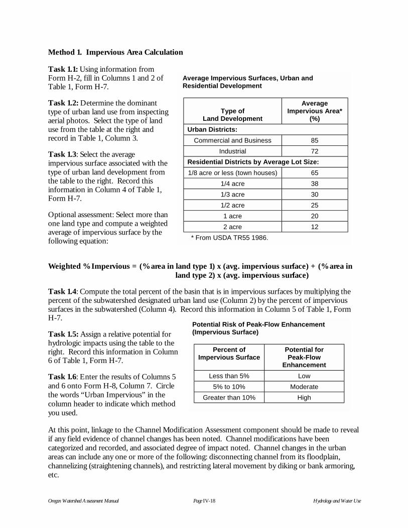
Oregon Watershed Assessment Manual Page IV-18 Hydrology and Water Use
Potential Risk of Peak-Flow Enhancement(Impervious Surface)
Percent ofImpervious Surface
Potential forPeak-Flow
Enhancement
Less than 5% Low
5% to 10% Moderate
Greater than 10% High
Average Impervious Surfaces, Urban andResidential Development
Type ofLand Development
AverageImpervious Area*
(%)
Urban Districts:
Commercial and Business 85
Industrial 72
Residential Districts by Average Lot Size:
1/8 acre or less (town houses) 65
1/4 acre 38
1/3 acre 30
1/2 acre 25
1 acre 20
2 acre 12
* From USDA TR55 1986.
Method 1. Impervious Area Calculation
Task 1.1: Using information fromForm H-2, fill in Columns 1 and 2 ofTable 1, Form H-7.
Task 1.2: Determine the dominanttype of urban land use from inspectingaerial photos. Select the type of landuse from the table at the right andrecord in Table 1, Column 3.
Task 1.3: Select the averageimpervious surface associated with thetype of urban land development fromthe table to the right. Record thisinformation in Column 4 of Table 1,Form H-7.
Optional assessment: Select more thanone land type and compute a weightedaverage of impervious surface by thefollowing equation:
Weighted % Impervious = (% area in land type 1) x (avg. impervious surface) + (% area in land type 2) x (avg. impervious surface)
Task 1.4: Compute the total percent of the basin that is in impervious surfaces by multiplying thepercent of the subwatershed designated urban land use (Column 2) by the percent of impervioussurfaces in the subwatershed (Column 4). Record this information in Column 5 of Table 1, FormH-7.
Task 1.5: Assign a relative potential forhydrologic impacts using the table to theright. Record this information in Column6 of Table 1, Form H-7.
Task 1.6: Enter the results of Columns 5and 6 onto Form H-8, Column 7. Circlethe words “Urban Impervious” in thecolumn header to indicate which methodyou used.
At this point, linkage to the Channel Modification Assessment component should be made to revealif any field evidence of channel changes has been noted. Channel modifications have beencategorized and recorded, and associated degree of impact noted. Channel changes in the urbanareas can include any one or more of the following: disconnecting channel from its floodplain,channelizing (straightening channels), and restricting lateral movement by diking or bank armoring,etc.

Oregon Watershed Assessment Manual Page IV-19 Hydrology and Water Use
Potential Risk of Peak-Flow Enhancement(Road Density)
Road Density(mi/mi²)
Potential Risk for PeakFlow Enhancement
Less than 4.2 Low
4.2 to 5.5 Moderate
Greater Than
5.5
High
Method 2. Urban Road Density
May et al. (1997) established a relationship between watershed urbanization (in % TIA) andsub-basin road density (in mi/mi2) which can be used to represent the percent imperviousness. Theregression equation developed by May et. al. (1997) was used to determine the road density thatwould be expected to correspond to 5% TIA and 10% TIA; the thresholds used in Method 1. Inurban areas, when road densities equal or exceed 5.5 mi/mi2, percent TIA probably exceeds 10%TIA (May et al. 1997). Road densities of 4.2 mi/mi2 were associated with a percent TIA in thesubwatershed of approximately 5%.
Task 2.1: Using information from Form H-2, fill in Columns 1, 2, and 3, Table 2 (Form H-7).
Task 2.2: From the Sediment Sources component, enter the road length in urban and/or ruralresidential areas in Column 4 of Table 2, Form H-7.
Task 2.3: Divide the road length in Column 4 by the urban area in Column 3. Enter the resultingroad density into Column 5.
Task 2.4: Assign a relative potential for peak-flowenhancement to each subwatershed. Watershedswith a road density of greater than 5.5 mi/mi2(associated with 10% TIA) should be assigned ahigh probability of peak-flow enhancement andfurther investigation of urban issues is warranted.Subwatersheds in which road densities are in therange of 4.2 to 5.5 mi/mi2 would be expected tohave between 5% to 10% TIA and thereforeshould be assigned a moderate risk as inMethod 1. Enter results in Column 6.
Task 2.5: Enter the results in Columns 5 and 6 onto Form H-8, Column 7, and circle the words“Urban Roads” in the column header to indicate which method you used.
Step 8: Summarize Potential Risk of Land Use on Hydrology (Form H-8)
Steps 4 through 7 have required you to work through a series of tasks and fill out a series ofcorresponding tables. The last task in each step is to insert the results into the appropriate columnon Form H-8. This table now provides an overview of potential peak-flow enhancement from landuse activities. Using a new copy of the Base Map, or a Mylar overlay, color-code each subwatershedby the potential risks determined above. Label this Map H-1: Potential Risks of Land Use onHydrology.

Oregon Watershed Assessment Manual Page IV-20 Hydrology and Water Use
WATER RIGHTS INFORMATION
Oregon Water ResourcesDepartment (OWRD)158 12th Street NESalem, OR 97310(503) 378-8455 phone(503) 378-2496 fax
Internet address:http://www.wrd.state.or.us
For assistance with access to theWater Rights Information System(WRIS) or the Water AvailabilityReports System (WARS), contact:
Manager of Information SystemsOregon Water Resources Department158 12th Street, NESalem, OR 97310(800) 624-3100(503) 378-8455 phone(503) 378-2496 fax
SECTION II: WATER USE
Water use is generally defined by beneficial use categories such as municipal, industrial, irrigatedagriculture, etc. Background on these different types of water uses and their associated impacts on astream system can be found in Appendix IV-D. In this section you will summarize the water rightsin your basin and gain an understanding of what beneficial uses these water withdrawals are serving.The assessment of water use is primarily focused on low-flow issues. While low-flow issues can beextremely important, they are difficult to characterize at the screening level. Water use activities canimpact low flows, yet the low flows can be enhanced through adopting water conservation measuresto keep more water in the stream system.
Critical Questions
• For what beneficial use is water primarily used in your watershed?• Is water derived from a groundwater or surface-water source?• What type of storage has been constructed in the basin?• Are there any withdrawals of water for use in another basin (interbasin transfers)? Is any
water being imported for use in the basin?• Are there any illegal uses of water occurring in the basin?• Do water uses in the basin have an effect on peak flows?• Do water uses in the basin have an effect on low flows?
Assumptions
• Water use most significantly impacts low flows,with the exception of storage, which can reducepeak flows downstream of the structure.
Materials Needed
• Tabulation of water rights information from theOregon Water Resources Department (OWRD;see contact information in the Water RightsInformation sidebar)
• Map of surface and groundwater right locations,amounts, and priorities (from the OWRD)
Final Products of the Water Use Section
• Form WU-1: Water Rights Summary• Form WU-2: Water Availability Summary• Form WU-3: Consumptive Use Summary• Map WU-1: Water Rights and In-Stream Flow
Rights

Oregon Watershed Assessment Manual Page IV-21 Hydrology and Water Use
Water Use Characterization
Step 1. Summarize Surface- and Groundwater Rights (Form WU-1 and Map WU-1)
The best way to characterize water use in your watershed is to tabulate both the surface-water andgroundwater rights that are on file with OWRD. This can be accomplished by either (1) contactingyour local Watermaster, or (2) using the OWRD Web page (see Water Rights Information sidebar)to download the data.
Tabulate water rights on Form WU-1 (or use printout from OWRD), and obtain a map showing thepoints of diversion of the water rights from OWRD. Also, identify where in-stream flow rightsexist. Label this Map WU-1.
Water Use Assessment
Potential channel dewatering (zero flow in the channel) can present problems for spawning and fishpassage. Typically, the spawning period that coincides with the lowest flow begins on approximatelySeptember 1 and extends through October. Rearing habitat in the summer also requires flow levelsto be maintained. While these are the critical times of year, flow levels throughout the year need tobe maintained to cover all life stages of all species present in a watershed.
The basis for the water use assessment will be the output from the Water Availability ReportsSystem (WARS) and other data provided by the OWRD. Their system has accounted forconsumptive use and presents the best available information at this time. You will assess the dataand gain an understanding of the location and magnitude of low-flow problems in the watershed.
Step 2. Determine Water Availability (Form WU-2)
Task 1: Obtain the water availability reports at the 50% exceedance level for each month for eachwater availability basin (WAB) in your watershed. These will correspond to the 5th and/or 6th fieldHydrologic Unit Codes (HUCs). However, not all subwatersheds will be a designated WAB, souse the WABs rather than the subwatersheds in this task.
The water availability reports can be obtained directly from the OWRD via your local Watermasteror can be retrieved from the OWRD Web site on the Internet (http://www.wrd.state.or.us). SelectWater Availability Reports System (WARS) and when a login ID is requested, type “wars.” Followthe menu to acquire the information desired. Select the 50% exceedance streamflow from thisdatabase/model for review of water availability at this level.
Task 2: Identify on your map the WABs for which water availability has been calculated.Determine which subwatersheds coincide with or are situated within the WABs.
Task 3: Column 8 of the WARS report lists the net available flow. Enter the net water available foreach month onto Form WU-2 for each WAB and highlight the WABs that do not have wateravailable. If the “net water available” column is negative or zero, water is not available at thisexceedance level. The streamflow in these WABs is insufficient to meet the demand for allin-stream and out-of-stream uses; conservation measures may help mitigate low-flow problems.

Oregon Watershed Assessment Manual Page IV-22 Hydrology and Water Use
Task 4: Compute the percentage of consumptive use (CU) for each monthly natural streamflow andenter the result onto Form WU-3. From the Water Availability Reports System, Columns 3 and 5,report consumptive use before and after 1993. Column 2 of WARS reports the natural streamflow.Use the following formula to compute %CU:
%CU = (Column 3 + Column 5) x 100Column 2
Task 5: Highlight the CU values on Form WU-3 that are greater than 10%.
Step 3. Flow-Restoration Priority Areas
If your watershed is not located in one of the following five regions: North Coast, Mid Coast, SouthCoast, Umpqua, or Rogue, call OWRD to determine if the flow restoration prioritization has beencompleted.
Task 1: Determine if any of the subwatersheds are within priority WABs for flow restoration. Theinformation can be found through ODFW’s Web page. Look for the box entitled “StreamflowRestoration Priorities.” Find the location of your watershed: North Coast, South Coast, Mid Coast,Umpqua or Rogue.
Task 2: Highlight the WABs on Form WU-3 that are designated flow-restoration priority basins.
Task 3: Of the WABs that are designated as flow-restoration priorities, the ones with the highestconsumptive use (>10%) present the greatest opportunity for flow restoration through conservationmeasures, increased efficiency of use, and/or best management practices. Based on thisinformation, rank the WABs from greatest to least flow-restoration potential.
CONFIDENCE IN ASSESSMENTS
The confidence in the work performed up to this point will be largely a function of the datalimitations and/or your confidence in the methods used. For example, were difficulties encounteredwhen estimating the acreage within each land use or clearcut? Was the type of urban land use andassociated percent imperviousness difficult to determine?
You must assess the data limitations associated with the work performed up to this point (completeform HW-1). The most obvious data limitation will arise if a stream gage is not located in the basin.Using streamflow records from a nearby similar gage, while appropriate in the absence ofbasin-specific data, does incorporate error.
The assessment approach was designed to be conservative in that a referral for further analysiswould ideally be triggered before the existence of significant hydrologic impacts. Hydrologicprocesses are complex, and the interaction of several variables makes assigning screening thresholdsdifficult. You can gain more confidence that your assessment has identified the problematicsubwatersheds if you sought technical assistance as questions arose, and if you obtainedcorroborative evidence from other components of this process.

Oregon Watershed Assessment Manual Page IV-23 Hydrology and Water Use
FURTHER ANALYSES
If the qualitative assessment identified that a specific land use or uses are potentially problematic insome subwatersheds, further study is warranted. All of the compilation of data you have done up tothis point will provide the basic building blocks for any additional analyses. Although it is fairlystraightforward to identify the potential existence of a problem, attempting to quantitatively assessthe magnitude of the problem or the change in streamflow is complex. Technical users of thismanual understand the myriad of hydrologic techniques available for use. The following listattempts to identify a few techniques appropriate for analyzing the issues at hand; it by no meansconstitutes a definitive list, because many options exist.
• Washington State Forest Practices Board Watershed Analysis MethodsWashington Forest Practices Board Manual: Standard Methodology for ConductingWatershed Analysis Under Chapter 222-22 WAC, Version 4.0, November 1997.
• Antecedent Precipitation Index (API) ModelFedora, M.A. 1987. Simulation of Storm Runoff in the Oregon Coast Range. BLMTechnical Note 378, US Department of the Interior, Bureau of Land Management.
• Continuous models (Hydrologic Simulation Program in Fortran [HSPF], DistributedHydrologic Soil and Vegetation Model [DHSVM], etc.)Bicknell, B.R., J.C. Imhoff, J.L. Kittle, A.S. Donigian Jr., and R.C. Johanson. 1993.Hydrological Simulation Program FORTRAN (HSPF): User's Manual for Release 10.EPA-600/R-93/174. US Environmental Protection Agency, Athens, GA.DHSVM – Dennis Littenmeier, University of Washington
• Water Resources Evaluation of Nonpoint Silvicultural Sources ModelUS Department of Agriculture, Forest Service. 1980. An Approach to Water ResourcesEvaluation of Non-Point Silvicultural Sources (A Procedural Handbook). Published byEPA: EPA-600/8/80-012, August 1980.
• Kendall Trend AnalysisMaidment, D.R. 1993. Handbook of Hydrology. McGraw-Hill, New York.
• Double Mass AnalysisLinsley, R.K. Jr., M.A. Kohler, and J.L.H. Paulhus. 1975. Hydrology for Engineers.McGraw-Hill, Inc.
• Gage Correlation AnalysisRobison, E.G. 1991. Methods for Determining Streamflows and Water Availability inOregon. Hydrology Report #2, Oregon Water Resources Department, October 1991.
• TR55 Methods (USDA 1986)United States Department of Agriculture, Natural Resources Conservation Service. 1986.Urban Hydrology for Small Watersheds. Technical Release-55, June 1986.
• Santa Barbara Unit Hydrograph Methods• Oregon Departments of Environmental Quality and Land Conservation and Development.
Nonpoint Source Pollution Control Guidebook for Local Government. 1994. Availablefrom ODEQ: (503) 229-6893.

Oregon Watershed Assessment Manual Page IV-24 Hydrology and Water Use
REFERENCES
Agee, J.K. 1994. Fire and Weather Disturbances in Terrestrial Ecosystems of the Eastern Cascades.US Department of Agriculture Forest Service, Pacific Northwest Research Station, GeneralTechnical Report PNW-GTR-320, Portland, Oregon.
Belt, G.H. 1995. Recovery of Enhanced Rain-On-Snow Melt Caused By Harvesting: A Review ofScientific Literature. Professor of Forest Resources, College of Forestry, Wildlife, and RangeSciences, University of Idaho.
Black, P.E. 1991. Watershed Hydrology. Prentice-Hall, Inc., Englewood Cliffs, New Jersey.
Bowling, L.C., and D.P. Lettenmaier. 1997. Evaluation of the Effects of Forest Roads onStreamflow in Hard and Ware Creeks, Washington. TFW-SH20-97-001, Water Resources SeriesTechnical Report No. 155, University of Washington, Seattle.
Branson, F.A., G.F. Gifford, K.G. Renard, and R.F. Hadley. 1981. Rangeland Hydrology. RangeScience Series No. 1, October 1972, Second Edition 1981. Society for Range Management,Denver Colorado. Kendall/Hunt Publishing Co., Dubuque, Iowa.
Coastal Salmon Restoration Initiative. 1997. The Oregon Plan, Restoring an Oregon legacythrough cooperative efforts. Submitted to National Marine Fisheries Services. 160 StateCapitol, Salem, Oregon. March 1997.
Chow, V.T., D.R. Maidment, and L.W. Mays. 1988. Applied Hydrology. McGraw-Hill Inc., NewYork.
Coffin, B.A. and R.D. Harr, 1992. Effects of forest cover on volume of water delivery to soil duringrain-on-snow. Timber/Fish/Wildlife Report No. SH1-92-001. Washington Department ofNatural Resources. 118 pp.
Dunne, T., and L.B. Leopold. 1978. Water in Environmental Planning. W.H. Freeman and Co.,New York.
Gifford, G.F., and R.H. Hawkins. 1979. Deterministic Hydrologic Modeling of Grazing SystemImpacts on Infiltration Rates. Water Resources Bulletin 15(4):924-934.
Gilmor Cooper, C. 1996. Hydrology Effects of Urbanization on Puget Sound Lowland Streams. Athesis submitted in partial fulfillment of the requirements for the degree of Master of Science inCivil Engineering, University of Washington, Seattle.
Greenberg, J. and K.F. Welch. 1998. Hydrologic Process Identification for Western Oregon.Prepared for Boise Cascade Corp., Boise, Idaho.
Harr, D.R., W.C. Harper, J.T. Krygier, and F.S. Hsieh. 1975. Changes in Storm Hydrographs AfterRoad Building and Clear-Cutting in the Oregon Coast Range. Water Resources Research 11(3).

Oregon Watershed Assessment Manual Page IV-25 Hydrology and Water Use
Harr, R.D., R.L. Fredriksen and J. Rothacher. 1979. Changes in streamflow following timberharvest in southwestern Oregon. USDA Forest Service Research Paper PNW-249, PacificNorthwest Forest and Range Experiment Station, Portland, Oregon, 22pp.
Harr, R.D. 1981. Some characteristics and consequences of snowmelt during rainfall in WesternOregon. Journal of Hydrology 53:277-304.
Harr, R.D. 1983. Potential for Augmenting Water Yield Through Forest Practices in WesternWashington and Western Oregon. Water Resources Bulletin 19(3):383.
Harr, R.D. 1986. Effects of clearcutting on rain-on-snow runoff in western Oregon: A new look atold studies. Water Resources Research 22(7): 1095-2000.
Jones, J.A. and G.E. Grant. 1996. Peak Flow Responses to Clear-Cutting and Roads in Small andLarge Basins, Western Cascades, Oregon. Water Resources Research, Volume 32, Number 4,pp 959-974.
Kattelmann, R.C., N.H. Berg, and R. Rector. 1983. The Potential for Increasing Streamflow fromSierra Nevada Watersheds. Water Resources Bulletin 19(3):395.
MacDonald, L.H., with A.W. Smart and R.C. Wissmar. 1991. Monitoring Guidelines to EvaluateEffects of Forestry Activities on Streams in the Pacific Northwest and Alaska. EPA910/9-91-001. Published jointly by the US Environmental Protection Agency, Seattle,Washington and the Center for Streamside Studies in Forestry, Fisheries, and Wildlife,University of Washington, Seattle.
Maidment, D.R. 1993. Handbook of Hydrology. McGraw-Hill, New York.
May, C.W., E.B. Welch, R.R. Horner, J.R. Karr, and B.W. Mar. 1997. Quality Indices forUrbanization Effects in Puget Sound Lowland Streams. Final Report Prepared for WashingtonDepartment of Ecology, Centennial Clean Water Fund Grant, Water Resources Series TechnicalReport No. 154.
May, C.W., R.R. Horner, J. Karr, B.W. Mar, and E.B. Welch. 1997. Effects of Urbanization onSmall Streams in the Puget Sound Lowland Ecoregion. Watershed Protection Techniques2(4):483-493.
Miller, J.F., R.H. Frederick, and R.J. Tracey. 1973. Precipitation-Frequency Atlas of the WesternUnited States, Volume X – Oregon. National Oceanic and Atmospheric Administration,NOAA Atlas 2.
Robison, E.G. 1991. Water Availability for Oregon’s Rivers and Streams: Volume 1 – Overview.Oregon Water Resources Department. Hydrology Report #1.
Robison, E.G. 1991. Water Availability for Oregon’s Rivers and Streams: Volume 2 – TechnicalGuide and Appendices. Oregon Water Resources Department. Hydrology Report #1.
Robison, E.G. 1991. Methods for Determining Streamflows and Water Availability in Oregon.Oregon Water Resources Department. Hydrology Report #2.
Oregon Watershed Assessment Manual Page IV-26 Hydrology and Water Use
Schueler, T. 1994. The Importance of Imperviousness. Watershed Protection Techniques1(3):100-111.
Schwab, G.O., D.D. Fangmeier, W.J. Elliot, R.K. Frevert. 1993. Soil and Water ConservationEngineering. John Wiley & Sons, Inc., New York.
Thomas, R.B. and W.F. Megahan. In press. Peak Flow Responses to Clear-Cutting and Roads inSmall and Large Basins, Western Cascades, Oregon: A Second Opinion. Water Resources
Troendle, C.A., 1983. The Potential for Water Yield Augmentation from Forest Management in theRocky Mountain Region. Water Resources Bulletin 19(3):359.
Troendle, C.A., and R.M. King. 1985. The Effect of Timber Harvest on the Fool Creek Watershed,30 Years Later. Water Resources Research 21(12):1915-1922.
USDA (US Department of Agriculture) Natural Resources Conservation Service. Oregon AnnualData Summary, Water Year 19xx.
USDA (US Department of Agriculture) Soil Conservation Service. 1985. National EngineeringHandbook, Section 4, Hydrology.
USDA (US Department of Agriculture) Soil Conservation Service. 1986. Urban Hydrology forSmall Watersheds. Technical Release 55.
USGS (US Geological Survey). 1979. Magnitude and Frequency of Floods in Western Oregon.Open-File Report 79-553. Prepared in cooperation with the Oregon Department ofTransportation, Highway Division, Portland, Oregon.
USGS (US Geological Survey). 1990. Statistical Summaries of Streamflow Data in Oregon: Volume1: Monthly and Annual Streamflow, and Flow-Duration Values. Open-File Report 90-118.Prepared in cooperation with the Oregon Water Resources Department.
USGS (US Geological Survey). 1993. Statistical Summaries of Streamflow Data in Oregon: Volume2: Annual Low and High Flow, and Instantaneous Peak Flow. Open-File Report 93-63.Prepared in cooperation with the Oregon Water Resources Department.
USGS (US Geological Survey). Water Resources Data-Oregon, Water Year 1997.
Viessman, W., Jr., and G.L. Lewis. 1996. Introduction to Hydrology. Harper Collins CollegePublishers, New York.
Washington State Forest Practices Board. 1997. Standard Methodology for Conducting WatershedAnalysis Under Chapter 222-22 WAC. Version 4.0. Olympia, Washington.
Washington State Department of Natural Resources. 1991. Implementation of Rain-on-SnowEmergency Rule WAC 222-16-046 (7). Unpublished interorganizational memorandum fromJack Hulsey to regional managers.

Oregon Watershed Assessment Manual Page IV-27 Hydrology and Water Use
GLOSSARY
adjudication: A court proceeding to determine all rights to the use of water on a particular streamsystem or groundwater basin.
annual maximum 24-hour precipitation: The largest amount of precipitation that has occurred ina 24-hour period over the course of 1 year.
annual minimum flows: The lowest daily flows that have occurred within a given water year.
annual peak flow: The highest streamflow or discharge recorded at a stream gage during eachwater year. Annual peak flows are reported on a water-year basis, defined as October 1 throughSeptember 30.
aspect: Aspect of a slope is the direction toward which the slope faces.
best management practice (BMP): Structural, nonstructural, and managerial techniquesrecognized to be the most effective and practical means to reduce surface- and groundwatercontamination while still allowing the productive use of resources.
canopy cover: The overhanging vegetation in a given area.
Channel Habitat Type (CHT): Groups of stream channels with similar gradient, channel pattern,and confinement. Channels within a particular group are expected to respond similarly to changesin environmental factors that influence channel conditions. In this process, CHTs are used toorganize information at a scale relevant to aquatic resources, and lead to identification of restorationopportunities.
consumptive use: The quantity of water absorbed by the crop and transpired or used directly in thebuilding of plant tissue, together with the water evaporated from the cropped area.
crown closure: The amount of canopy cover in a given area.
discharge: Outflow; the flow of a stream, canal, or aquifer.
elevation: The vertical reference of a site location above mean sea level, measured in feet or meters.
ephemeral: A stream that is dry for a portion of the year and most often contains water during andimmediately after a rainfall event.
evaporation: As water is heated by the sun, its surface molecules become sufficiently energized tobreak free of the attractive force binding them together; they evaporate and rise as invisible vapor inthe atmosphere.
evapotranspiration: The amount of water leaving to the atmosphere through both evaporation andtranspiration.
gaging station: A selected section of a stream channel equipped with a gage, recorder, or otherequipment for determining stream discharge.

Oregon Watershed Assessment Manual Page IV-28 Hydrology and Water Use
Geographic Information System (GIS): A set of tools for modeling virtually all physical andbiological components of natural or cultural resources. A system that can integrate informationfrom diverse sources. Comprised of four subsystems 1) data input subsystems; 2) data storage andretrieval; 3) data manipulation and analysis and; 4) data reporting system. GIS databases can usuallyhave a spatial component in the storage of the data; potential to store and create map-like products;and potential for performing multiple analyses or evaluations of scenarios of model simulations.
groundwater: Water stored in the earth that occupies pores, cavities, cracks, and other spaces in thecrustal rocks and soil.
hydraulic continuity: The connection between groundwater and surface water such thatwithdrawal from an underground aquifer affects the streamflow level in the channel (surface water).
hydrograph: A graph of runoff rate, inflow rate, or discharge rate, past a specific point of a riverplotted over a predefined time period (annual, storm, etc.).
hydrologic soil group (HSG): Soil classification to describe the minimum rate of infiltrationobtained for bare soil after prolonged wetting.
Hydrologic Unit Code (HUC): US Geological Survey designations that correspond to specificwatersheds, and are expressed in a hierarchical scale.
hydrology: The science of the behavior of water in the atmosphere, on the surface of the earth, andunderground.
impervious surface: An area that is made impenetrable by water, such as paved roads, rooftops,and parking lots.
infiltration: The rate of movement of water from the atmosphere into the soil.
lag time: The interval between the center of mass of the storm precipitation and the peak flow ofthe resultant runoff. It is the delay between upstream production of flow and its arrival at adownstream location.
low flow: The minimum rate of flow for a given period of time.
nonpoint source pollution: Variable, unpredictable, and dispersed pollution sources fromagriculture, silviculture, mining, construction, saltwater intrusion, waste disposition and disposal, andpollution from urban-industrial development areas. (“Point sources” are steady, predictable, andconcentrated through “end of pipe” discharges from manufacturing or water treatment plants.)
orthophotograph: A combined aerial photograph and planimetric (no indications of contour) mapwithout image displacements and distortions.
peak flow: The maximum instantaneous rate of flow during a storm or other period of time.
percolation: The act of surface water moving downwards, or percolating, through cracks, joints,and pores in soils and rocks.

Oregon Watershed Assessment Manual Page IV-29 Hydrology and Water Use
planimeter: An instrument for measuring the area of a plane (2-dimensional) figure by tracing itsboundary line.
precipitation: The liquid equivalent (inches) of rainfall, snow, sleet, or hail, collected byprecipitation storage gages.
Prior Appropriation Doctrine: A water law based on the principle of prior appropriation, whichmeans the first person to obtain a water right on a stream is the last to be shut off in times of lowstreamflows.
rain-on-snow event: When snowpacks are melted by warm rains, causing peak-flow events wherethe melted snow augments the runoff derived from rainfall. Rain-on-snow events usually occurwithin an elevation zone in which transient snowpacks occur.
recurrence interval: The frequency of hydrologic events can be discussed in terms of eitherprobability or recurrence interval (also called the return period or frequency of occurrence).Exceedance probability refers to the chance that the annual-maximum event of any year will equal orexceed some given value.
return flow: The portion of a diversion that returns to the river system via subsurface pathways.The rest of the diversion is lost to crop consumptive use.
runoff: Surface runoff is water that moves overland across the surface into creeks, ponds, lakes, andrivers that eventually take the water back to the ocean.
runoff curve number: An empirical rating of the hydrologic performance of a large number ofsoils, vegetative covers, and land use practices throughout the United States.
spring snowmelt: The time in spring when the seasonal snowpack melts out.
transpiration: The process by which water vapor is emitted from plant leaves. Every day, anactively growing plant transpires 5 to 10 times as much water as it can hold at once.
water table: The water table marks the change in the groundwater zone between the zone ofaeration, where some pores are open, and the underlying zone of saturation, in which water fills allthe spaces in the soil and rocks.
water year: The water year in North America is referred to as the 12-month period beginningOctober 1 in one year and ending September 30 of the following year. The water year is designatedby the calendar year in which it ends. For instance, the annual peak flow for water year 1996 wouldbe the highest flow recorded from October 1, 1995, through September 30, 1996.


Appendix IV-AForms and Worksheets


FORM H-1: GENERAL WATERSHED CHARACTERISTICS
Name of Analyst: Date: Watershed Name: Subwatershed information:
SubwatershedName
SubwatershedArea (mi2)
MeanElevation
(feet)
MinimumElevation
(feet)
MaximumElevation
(feet)
Mean AnnualPrecipitation
(inches)
1
2
3
4
5
6
7
8
9
10
Total Watershed
• Mean Annual Precipitation can be estimated from the Mean Annual Precipitation Map (from NOAA)• Minimum and Maximum Elevations can be estimated from the Base Map or USGS quad maps.• The State Service Center for GIS may also be able to provide the above information.
Describe the type and extent of natural storage (lakes, wetlands, etc.) in the watershed: What watershed changes have occurred that will affect streamflows (i.e., dams, major diversions forurban water supply, irrigation diversions, industrial use etc.)? Information on stream gages in basin: (Note: if more than one gage, fill out additional forms.)Gage #: Gage Name: Gage Elevation: Drainage Area to Gage: Storage or regulation upstream of gage (yes or no)? If yes, describe on back of sheet

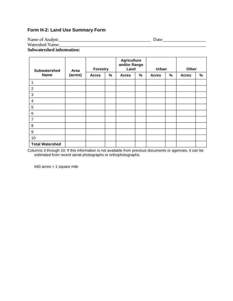
Form H-2: Land Use Summary Form
Name of Analyst: Date: Watershed Name: Subwatershed information:
Forestry
Agricultureand/or Range
Land Urban OtherSubwatershedName
Area(acres) Acres % Acres % Acres % Acres %
1
2
3
4
5
6
7
8
9
10
Total Watershed
Columns 3 through 10: If this information is not available from previous documents or agencies, it can beestimated from recent aerial photographs or orthophotographs.
640 acres = 1 square mile


Form H-3: Annual Peak Flow Summary Form
Name of Analyst: Date: Watershed Name: Subwatershed information:
Rain Rain-on-SnowSpring
SnowmeltSubwatershedName
Area(acres) Acres % Acres % Acres %
1
2
3
4
5
6
7
8
9
10
Total Watershed
Peak flows by water year (use additional sheets if more than one gage in watershed):
Station Name: Station #: Drainage Area = Period of Record: Gage is in watershed? (circle one): Yes No
(Continue from Column to left) (Continue from Column to left)
WaterYear
(10/1-9/30)
Peakflow
amount(cfs)
Date ofPeakFlow
Rank orRecurr.interval
WaterYear
(10/1-9/30)
Peaklow
amount(cfs)
Date ofPeakFlow
Rank orRecurr.Interval
WaterYear
(10/1-9/30)
Peaklow
amount(cfs)
Date ofPeakFlow
Rank orRecurr.Interval

Form H-3: page 2.
Water Year
Pe
ak
Dis
ch
arg
e (
cir
cle
on
e)
CF
S o
r C
FS
/sq
.mil
e


Form H-4: Forestry Worksheet
Name of Analyst: Date: Watershed Name:
1
SubwatershedName orNumber
2
Historic CrownClosure in
Rain-on-SnowAreas
(%)
3
Percent ofsubwatershed
inRain-on-Snow
Areas(%)
4Percent of
Rain-on-Snowareas with <30%Current Crown
Closure(%)
5
Risk of Peak-FlowEnhancement
(either“Potential,”“Low,” or
“Unknown”)
1
2
3
4
5
6
7
8
9
10
Entire Watershed


Form H-5: Agriculture and Range-Land Worksheet
Name of Analyst: Date: Watershed Name:
Table 1. Agricultural Land Use and Range-Land Use Summary
3Hydrologic Soil Groups in Agricultural
Lands or Grazed Range Lands(by approximate percentage)
1
SubwatershedName
2
Area ofSubwatershed in
Agriculture orRange-Land Use A B C D
Entire Watershed

Form H-5: page 2.
Table 2. Curve Number and Runoff-Depth Summary Table for Primary Hydrologic Soil Group
Subwatershed Name: Primary Hydrologic Soil Group:1
Cover Type/Treatment
2
HydrologicCondition
3
CurveNumber
4Background
CurveNumber
5RainfallDepth
(in)
6Current Runoff
Depth(in)
7BackgroundRunoff Depth
(in)
8Change fromBackground
Col. 6 - 7
Subwatershed average change from background:
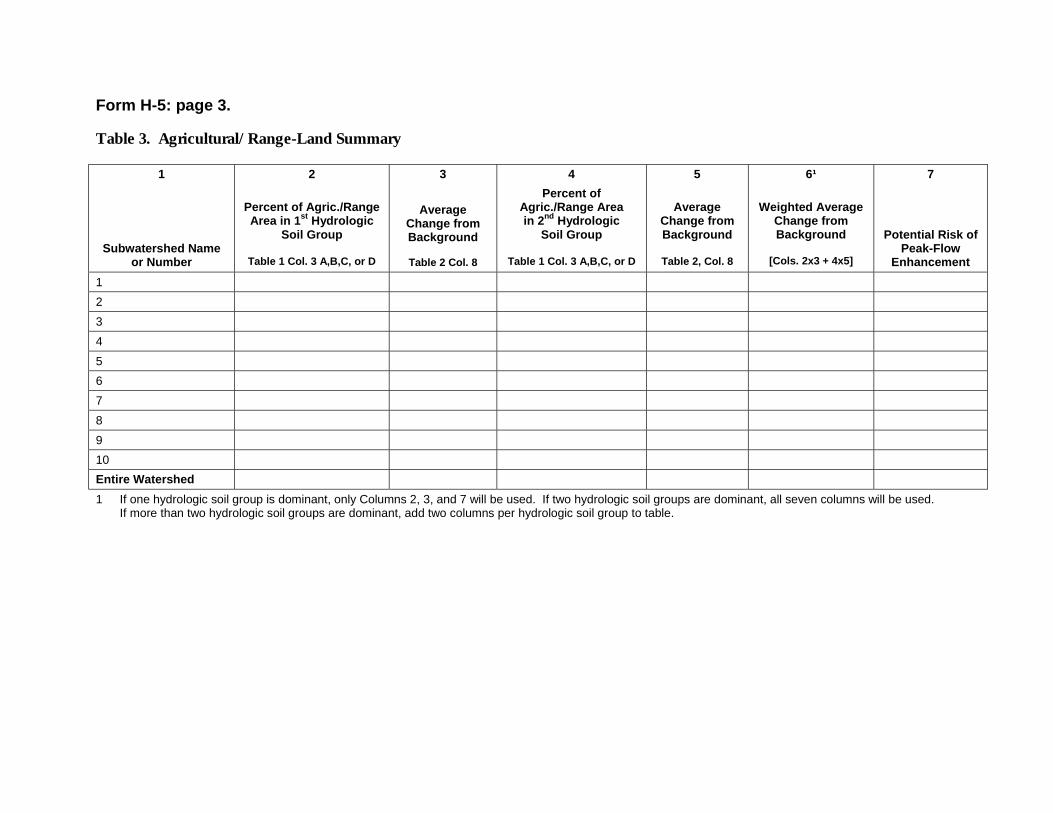
Form H-5: page 3.
Table 3. Agricultural/Range-Land Summary
1
Subwatershed Nameor Number
2
Percent of Agric./RangeArea in 1st Hydrologic
Soil Group
Table 1 Col. 3 A,B,C, or D
3
AverageChange fromBackground
Table 2 Col. 8
4
Percent ofAgric./Range Areain 2nd Hydrologic
Soil Group
Table 1 Col. 3 A,B,C, or D
5
AverageChange fromBackground
Table 2, Col. 8
6¹
Weighted AverageChange fromBackground
[Cols. 2x3 + 4x5]
7
Potential Risk ofPeak-Flow
Enhancement
1
2
3
4
5
6
7
8
9
10
Entire Watershed
1 If one hydrologic soil group is dominant, only Columns 2, 3, and 7 will be used. If two hydrologic soil groups are dominant, all seven columns will be used.If more than two hydrologic soil groups are dominant, add two columns per hydrologic soil group to table.


Form H-6: Forest and Rural Road Worksheet
Name of Analyst: Date: Watershed Name:
Table 1. Forest Road Area Summary
1
SubwatershedName
2
Area(mi2)
3
AreaForested
(mi2)
4
Total LinearDistance of
ForestRoads(miles)
5Roaded Area
Column 4 x std.width(ft2)
std. width = 25feet = .0047 miles
6
PercentArea inRoads
Col. 5/3
7
RelativePotential for
Impact
1
2
3
4
5
6
7
8
9
10
Entire Watershed
Table 2. Rural Road Area Summary
1
SubwatershedName
2
Area(mi2)
3
Rural Area(Agric. + Range)
(mi2)
4
Total LinearDistance ofRural Roads
(miles)
5Roaded Area
Column 4 x std.width(ft2)
std. width =35 feet =
.0066 miles
6
PercentArea inRoads
Col. 5/3
7
RelativePotential forPeak-Flow
Enhancement
1
2
3
4
5
6
7
8
9
10
Entire Watershed


Form H-7: Urban and Residential Area Worksheet
Name of Analyst: Date: Watershed Name:
Table 1. Method 1: Urban and Rural Residential Land Use Summary
1
SubwatershedName
2
Percent of AreaUrbanized/
RuralResidential
3
DominantType of Urban
Land Use
4
AveragePercent
Impervious
5Estimate of
Percent TotalImpervious Area
Col. 2 x Col. 4
6
RelativePotential forPeak-Flow
Enhancement
Table 2. Method 2: Urban Road Density Summary
1
SubwatershedName
2
Area(mi2)
3
Area Urban(mi2)
4Total LinearDistance of
Roads(miles)
5Road
DensityCol. 4/3(mi/mi2)
6Relative
Potential forPeak-Flow
Enhancement
Entire Watershed


Form H-8: Hydrologic Issue Identification Summary
Name of Analyst: Date: Watershed Name:
Summary of Potential Risks from Land Use Impacts on Hydrology
2
Timber Harvest
Form H-4Table
3
Agriculture
Form H-5Table 3
4
Range Lands
Form H-5Table 3
5
Forest Roads
Form H-6Table 1
6
Rural Roads
Form H-6Table 2
7Urban
Impervious orUrban Roads*
Form H-7Table 1 or
Table 2
1
Subwatershed Nameor Number Result Risk Result Risk Result Risk Result Risk Result Risk Result Risk
1
2
3
4
5
6
7
8
9
10
Entire Watershed
* Circle the method used.


Form WU-1. Water Rights Summary
Name of Analyst: Date: Watershed Name:
Water Rights on Record with OWRD
Watershed Name: County:
Permitor
Certificate# Status
PriorityDate
FlowRate(cfs)
Time ofDiversion
Type of Use(Irrigation
StockWatering
Domestic) Location WAB #


Form WU-2: Water Availability Summary
Name of Analyst: Date: Watershed Name: County:
Monthly Net Water Available by Water Availability Basin (cfs)
Water AvailabilityBasins Jan Feb Mar Apr May Jun Jul Aug Sep Oct Nov Dec


Form WU-3. Consumptive Use Summary
Name of Analyst: Date: Watershed Name: County:
Consumptive Use as a Percentage of 50% Exceedance Streamflow
Water AvailabilityBasins Jan Feb Mar Apr May Jun Jul Aug Sep Oct Nov Dec


Form HW-1. Confidence Evaluation
Name of Analyst: Date: Watershed: Area:
Technical expertise or relevant experience:
Resources used:
� USGS Web site � Oregon Climate Service Web site� Hydrodata or Earthinfo CD-ROM � NRCS Web site� USGS Open File Report 90-118 � USGS Water Supply Papers, Oregon� USGS personnel � OWRD Web site� NRCS personnel � OWRD local Watermaster� OWRD regional personnel
Confidence in hydrology assessment
� Low: Unsure of procedures and/or used minimal resources.� Low to moderate: Understood and followed most of the procedures, but minimal resources
available and/or used.� Moderate: Understood and followed procedures, and used adequate number of resources, but
had moderate understanding of outcome.� Moderate to high: Understood and followed procedures, used adequate number of resources,
and had high understanding of outcome.� High: Understood and followed procedures, used numerous resources, and had high
understanding of outcome.� If none of the above categories fit, describe your own confidence level and rationale:
Recommendations for further assessment or analysis:


Appendix IV-BReference Tables


Oregon Watershed Assessment Manual Page 1 Appendix IV-B
Table B-1. Runoff Curve Numbers for Cultivated Agricultural Lands1
Curve Numbers for HydrologicSoil Group
Cover Type Treatment2HydrologicCondition3
A B C D
Bare Soil --- 77 86 91 94
Poor 76 85 90 93
Fallow
Crop Residue Cover
Good 74 83 88 90
Poor 72 81 88 91Straight Row
Good 67 78 85 89
Poor 71 80 87 90Straight Row +Crop Residue Cover Good 64 75 82 85
Poor 70 79 84 88Contoured
Good 65 75 82 86
Poor 69 78 83 87Contoured +Crop Residue Cover Good 64 74 81 85
Poor 66 74 80 82Contoured and Terraced (C&T)
Good 62 71 78 81
Poor 65 73 79 81
Row Crops
Contoured and Terraced +Crop Residue Cover Good 61 70 77 80
Poor 65 76 84 88Straight Row
Good 63 75 83 87
Poor 64 75 83 86Straight Row +Crop Residue Cover Good 60 72 80 84
Poor 63 74 82 85Contoured
Good 61 73 81 84
Poor 62 73 81 84Contoured +Crop Residue Cover Good 60 72 80 83
Poor 61 72 79 82Contoured and Terraced
Good 59 70 78 81
Poor 60 71 78 81
Small Grain
Contoured and Terraced +Crop Residue Cover Good 58 69 77 80
Poor 66 77 85 89Straight Row
Good 58 72 81 85
Poor 64 75 83 85Contoured
Good 55 69 78 83
Poor 63 73 80 83
Close-Seeded orBroadcast LegumesRotation Meadow
Contoured and Terraced
Good 51 67 76 801 Average runoff condition and Ia = 0.2 S2 Crop Residue Cover applies only if residue is on at least 5% of the surface throughout the year.3 Hydrologic condition is based on a combination of factors that affect infiltration and runoff, including
(a) density and canopy of vegetative areas, (b) amount of year-round cover, (c) amount of grass orclose-seeded legumes in rotations, (d) percent of residue cover on the land surface (good > 20%), and(e) degree of surface roughness.
Poor: Factors impair infiltration and tend to increase runoff.Good: Factors encourage average and better-than-average infiltration and tend to decrease runoff.
From USDA Soil Conservation Service, TR55 (2nd edition, June 1986); Table 2-2a, page 2-5.

Oregon Watershed Assessment Manual Page 2 Appendix IV-B
Table B-2: Runoff Curve Numbers for Other Agricultural Lands1
Curve Numbers for HydrologicSoil Group
Cover TypeHydrologicCondition A B C D
Poor 68 79 86 89
Fair 49 69 79 84
Pasture, grassland, or range – continuous foragefor grazing2
Good 39 61 74 80
Meadow – continuous grass; protected fromgrazing and generally mowed for hay
--- 30 58 71 78
Poor 48 67 77 83
Fair 35 56 70 77
Brush – brush-weed-grass mixture with brush themajor element3
Good 304 48 65 73
Poor 57 73 82 86
Fair 43 65 76 82
Woods – grass combination (orchard or treefarm)5
Good 32 58 72 79
Poor 45 66 77 83
Fair 36 60 73 79
Woods6
Shaded area can be used as background if theland was originally wooded Good 304 55 70 77
Farmsteads – buildings, lanes, driveways, andsurrounding lots
--- 59 74 82 86
1 Average runoff condition and Ia = 0.2 S
2 Poor: <50% ground cover or heavily grazed with no mulch.
Fair: 50 to 75% ground cover and not heavily grazed.
Good: >75% ground cover and lightly or only occasionally grazed.
3 Poor: <50% ground cover.
Fair: 50 to 75% ground cover.
Good: >75% ground cover.
4 Actual curve number is less than 30; use curve number = 30 for runoff computations.
5 Curve numbers shown were computed for areas with 50% woods and 50% grass (pasture) cover.Other combinations of conditions may be computed from the curve numbers for woods and pasture.
6 Poor: Forest litter, small trees, and brush are destroyed by heavy grazing or regular burning.
Fair: Woods are grazed but not burned, and some forest litter covers the soil.
Good:Woods are protected from grazing, and litter and brush adequately cover the soil.
From USDA Soil Conservation Service, TR55 (2nd edition, June 1986); Table 2-2b, page 2-6.

Oregon Watershed Assessment Manual Page 3 Appendix IV-B
Table B-3: Runoff Curve Numbers for Arid and Semiarid Range Lands
Curve Numbers for HydrologicSoil Group
Cover TypeHydrologicCondition A3 B C D
Poor 80 87 93
Fair 71 81 89
Herbaceous – mixture of grass, weeds, andlow-growing brush, with brush the minor element
Good 62 74 85
Poor 66 74 79
Fair 48 57 63
Oak-aspen – mountain-brush mixture of oakbrush, aspen, mountain mahogany, bitter brush,maple, and other brush
Good 30 41 48
Poor 75 85 89
Fair 58 73 80
Pinyon-juniper – pinyon, juniper or both; grassunderstory
Good 41 61 71
Poor 67 80 85
Fair 51 63 70
Sagebrush with grass understory
Good 35 47 55
Poor 63 77 85 88
Fair 55 72 81 86
Desert shrub – major plants include saltbush,greasewood, creosotebush, blackbrush, bursage,palo verde, mesquite, and cactus
Good 49 68 79 84
1 Average runoff condition and Ia = 0.2 S.
2 Poor: <30% ground cover (litter, grass, and brush overstory).
Fair: 30 to 70% ground cover.
Good:>70% ground cover.
3 Curve numbers for Group A have been developed only for desert shrub.
From USDA Soil Conservation Service, TR55 (2nd edition, June 1986); Table 2-2c, page 2-7. For rangein humid regions, use table 2-2c of TR55.

Oregon Watershed Assessment Manual Page 4 Appendix IV-B
Table B-4: Runoff Depth for Selected Curve Numbers and Rainfall Amounts1
Runoff Depth for Curve Number of…
Rainfall 40 45 50 55 60 65 70 75 80 85 90 95 98
1.0 0.00 0.00 0.00 0.00 0.00 0.00 0.00 0.03 0.08 0.17 0.32 0.56 0.79
1.2 0.00 0.00 0.00 0.00 0.00 0.00 0.03 0.07 0.15 0.27 0.46 0.74 0.99
1.4 0.00 0.00 0.00 0.00 0.00 0.02 0.06 0.13 0.24 0.39 0.61 0.92 1.18
1.6 0.00 0.00 0.00 0.00 0.01 0.05 0.11 0.20 0.34 0.52 0.76 1.11 1.38
1.8 0.00 0.00 0.00 0.00 0.03 0.09 0.17 0.29 0.44 0.65 0.93 1.29 1.58
2.0 0.00 0.00 0.00 0.02 0.06 0.14 0.24 0.38 0.56 0.80 1.09 1.48 1.77
2.5 0.00 0.00 0.02 0.08 0.17 0.30 0.46 0.65 0.89 1.18 1.53 1.96 2.27
3.0 0.00 0.02 0.09 0.19 0.33 0.51 0.71 0.96 1.25 1.59 1.98 2.45 2.77
3.5 0.02 0.08 0.20 0.35 0.53 0.75 1.01 1.30 1.64 2.02 2.45 2.94 3.27
4.0 0.06 0.18 0.33 0.53 0.76 1.03 1.33 1.67 2.04 2.46 2.92 3.43 3.77
4.5 0.14 0.30 0.50 0.74 1.02 1.33 1.67 2.05 2.46 2.91 3.40 3.92 4.26
5.0 0.24 0.44 0.69 0.98 1.30 1.65 2.04 2.45 2.89 3.37 3.8 8 4.42 4.76
6.0 0.50 0.80 1.14 1.52 1.92 2.35 2.81 3.28 3.78 4.30 4.85 5.41 5.76
7.0 0.84 1.24 1.68 2.12 2.60 3.10 3.62 4.15 4.69 5.25 5.82 6.41 6.76
8.0 1.25 1.74 2.25 2.78 3.33 3.89 4.46 5.04 5.63 6.21 6.81 7.40 7.76
9.0 1.71 2.29 2.88 3.49 4.10 4.72 5.33 5.95 6.57 7.18 7.79 8.40 8.76
10.0 2.23 2.89 3.56 4.23 4.90 5.56 6.22 6.88 7.52 8.16 8.78 9.40 9.76
11.0 2.78 3.52 4.26 5.00 5.72 6.43 7.13 7.81 8.48 9.13 9.77 10.39 10.76
12.0 3.38 4.19 5.00 5.79 6.56 7.32 8.05 8.76 9.45 10.11 10.76 11.39 11.76
13.0 4.00 4.89 5.76 6.61 7.42 8.21 8.98 9.71 10.42 11.10 11.76 12.39 12.76
14.0 4.65 5.62 6.55 7.44 8.30 9.12 9.91 10.67 11.39 12.08 12.75 13.39 13.76
15.0 5.33 6.36 7.35 8.29 9.19 10.04 10.85 11.63 12.37 13.07 13.74 14.39 14.76
1 Interpolate the values shown to obtain runoff depths for curve numbers or rainfall amounts not shown.
From USDA Soil Conservation Service, TR55 (2nd edition, June 1986); Table 2-1, page 2-3.


Appendix IV-CResources forData Acquisition

Oregon Watershed Assessment Manual Page 1 Appendix IV-C
RESOURCES FOR DATA ACQUISITION
USGS
Contact Information
Information OfficerUS Department of the Interior, Geological Survey10615 SE Cherry Blossom DrivePortland, OR 97216Telephone: (503) 251-3201Fax: (503) 251-3470Office hours: 7:30 a.m. to 4:30 p.m. Pacific TimeInternet address: http://waterdata.usgs.gov/nwis-w/OR
Internet Instructions
Access the Internet site referenced above. When you enter the State Surface Water Data RetrievalPage for Oregon, select the gage for which you want information, or, if you don’t yet know the gagenumber, select the county list or the map from which to select the county. Select the gage from thecounty list. Summary information will appear and below that Data Types Available. Select Peak FlowData; then select Annual Peaks and Tab-Delimited Text Data File. The largest instantaneousstreamflow recorded for each year will be displayed along with the date of that peak flow. This datacan be downloaded into a spreadsheet by saving it as a text file. The most recent peak flows will notbe on the Internet and must be requested from the state USGS office.
CD-ROM
Hydrosphere and Earthinfo, both located in Boulder, Colorado, produce and distribute CD-ROMscontaining USGS streamflow data. These CD-ROMs can be found in some libraries, especially atuniversities. If you wish to purchase a CD for use with your computer, you can order one directlyfrom either of the above-mentioned businesses.
Publications
Frank, F.J., and A. Laenen. 1977. Water Resources of Lincoln County Coastal Area, Oregon.Prepared in cooperation with the Oregon Water Resources Department. US Geological Survey,Water Resources Investigations 76-90, Portland, Oregon.
Greenberg, J. and K.F. Welch. 1998. Hydrologic Process Identification for Western Oregon.Prepared for Boise Cascade Corp., Boise, Idaho.
Harris, D.D., L.L. Hubbard, and L.E. Hubbard. 1979. Magnitude and Frequency of Floods inWestern Oregon. Prepared in cooperation with the Oregon Department of Transportation,Highway Division. US Geological Survey, Open File Report 79-553, Portland, Oregon.
Harris D.D., and L.E. Hubbard. 1983. Magnitude And Frequency Of Floods In Eastern Oregon.US Geological Survey WRIR 82-4078.
Oregon Watershed Assessment Manual Page 2 Appendix IV-C
Moffatt, R.L., R.E. Wellman, and J.M. Gordon. 1990. Statistical Summaries of Streamflow Data inOregon: Volume 1: Monthly and Annual Streamflow, and Flow-Duration Values. Prepared incooperation with the Oregon Water Resources Department. US Geological Survey, Open-FileReport 90-118, Portland, Oregon. Maps are located in the appendix of this document showing thelocation of streamflow gaging sites.
Wellman, R.E., J.M. Gordon, and R.L. Moffatt. 1993. A Statistical Summaries of Streamflow Datain Oregon: Volume 2: Annual Low and High Flow, and Instantaneous Peak Flow. Prepared incooperation with the Oregon Water Resources Department. US Geological Survey, Open-FileReport 93-63, Portland, Oregon.
Regional Offices of Oregon Water Resources Department (OWRD)
Northwest Region North Central Region158th 12th Street, NE 3920 WestgateSalem, OR 97310 Pendleton, OR 97801(503) 378-8455, ext. 281 (541) 278-5456Fax: (503) 378-8130 Fax: (541) 278-0287
Southwest Region Eastern RegionGrants Pass Municipal Building Baker County Courthouse942 SW 6th Street Suite E 1995 3rd StreetGrants Pass, OR 97526 Baker City, OR 97814(541) 471-2886; ext. 86 (541) 523-8224Fax: (541) 471-2876 Fax: (541) 523-7866
South Central Region1340 NW Wall Street, Suite 100Bend, OR 97701(541) 388-6669Fax: (541) 388-5101
Oregon State Department of Forestry2600 State StreetSalem, OR 97301(503) 945-7469Fax: (503) 945-7490


Appendix IV-DBackground HydrologicInformation

Oregon Watershed Assessment Manual Page 1 Appendix IV-D
BACKGROUND HYDROLOGIC INFORMATION
Land Use Impacts on Hydrology
Land use practices can modify the amount of water available for runoff, the routing of water to thestreams, the lag time 1 (delay between rainfall and peak streamflow), the flow velocity, or the traveldistance to the stream. Figure D-1 demonstrates how urbanization causes the peak flow (highestpoint on the curve) to increase and to occur sooner (the lag time has decreased). The same conceptsare shown in Figure D-2, in which two streams respond differently to the same rainstorm: Onestream drains a forested watershed and the other drains an urbanized watershed. Agricultural landwould produce a similar but less pronounced response than the urban response shown in bothFigures D-1 and D-2.
Land use practices that affect the rate of infiltration and/or the ability of the soil surface to storewater are typically most influential in affecting the watershed’s hydrology. Using this as an indicatorfor comparison among the land uses, forest harvesting produces the smallest change in theinfiltration rate, thereby producing the smallest impacts to the hydrologic regime of a basin. Forestharvest practices have evolved such that land compaction can be minimized; however, roads andgrazing in these watersheds decrease the infiltration rate. In contrast to forest harvest, agriculturalpractices, range-land utilization for grazing purposes, and urban development can all involvecompaction of the soils and/or paved surfaces, resulting in substantial alteration of the infiltrationrate. Agricultural practices and urban development directly involve altering the shape of thedrainage system by ditching, channelizing, or using piped stormwater networks which decrease theinfiltration and the travel time of subsurface flow to reach the channel. This effect can beexacerbated in high-flow conditions. Forest harvest, although not always practiced at a sustainablerate, is a temporary conversion of the vegetation, and the hydrologic effects diminish as vegetative
1 Terms that appear in bold italic in this appendix are defined in the Glossary of the main text of this component.
Figure D-1. Hypothetical unit hydrographs Figure D-2. Streamflow comparison ofillustrating urbanization impacts on peak urban versus forested watersheds.flows.

Oregon Watershed Assessment Manual Page 2 Appendix IV-D
regrowth occurs. Conversion of lands to agriculture or urbanization produces generallylonger-lasting effects. Road construction, associated with all land uses, alters the rate of infiltrationon the road surface and replaces subsurface flow pathways with surface pathways resulting inquicker travel time to the channel network.
Forestry
The potential effects of forest practices on hydrology include changes in peak flows, water yield, andlow flows. There are two primary mechanisms by which forest practices in Pacific Northwestwatersheds impact hydrologic processes: (1) the removal and disturbance of vegetation, and (2) theroad network and related harvesting systems.
Removal of vegetation reduces interception and evapotranspiration, both of which allow additionalwater to reach the soil surface during rainstorms. Additionally, open areas accumulate moresnowpack. The additional snowpack can potentially produce an increase in water yield (volume ofwater) that, in arid and semiarid regions, is viewed as a net benefit for water supply. The area with adecrease in canopy cover due to tree removal is subject to increased exposure to solar radiation andwind that can cause faster melting rates, potentially causing an increase in peak flows occurringearlier in the melt season. Harvest practices can also affect low flows, especially in spring snowmeltregimes. The quicker melting of the snowpack reduces the opportunities for groundwater recharge,the primary supply for baseflow conditions (streamflow during the driest part of the year).However, this decrease may be offset by the decreased evapotranspiration resulting from thereduction in canopy cover.
The size and structure of forest vegetation varies throughout the state primarily as a function ofclimatic variables, aspect, and elevation. In the eastern regions of the state, crown closure orvegetative cover was historically less dense than the thick forests of western Oregon. In some areasin eastern Oregon, the once-sparse forests now tend to be denser due to the prevention and controlof forest fires. The suppression of fire on the landscape, in areas that historically experiencedfrequent fire, has led to the following general conditions: increased stand densities and canopyclosure, smaller average stand diameter, changes in vegetative composition (i.e., fir or juniperinvasion), decreased shrub/herb growth, increased litter/duff layer, and increased large woodydebris and overall fuel loading (Agee 1994). Consequently, peak flows produced from undisturbedhistoric forests may have been higher compared to forests in which fires have been controlled. Dueto this probable condition, potential hydrologic impacts in these regions may be minor.
The forestry-related effects on peak flows may be a function not only of harvest and vegetativecover issues, but also of the type of hydrologic process that occurs in a basin (MacDonald andHoffman 1995). The greatest likelihood of causing problems from timber harvest is throughincreases in peak flows associated with rain-on-snow events (Harr 1981, 1986; Coffin and Harr1992; and Washington Forest Practices Board 1997). While rain-on-snow conditions can occur atalmost any elevation, given a specific combination of climatic variables, the probability ofrain-on-snow enhancement of peak flows differs with elevation and, to a lesser degree, aspect. Thehighest probability of encountering rain-on-snow conditions occurs at mid-elevations wheretransient snowpacks develop but do not get too deep. The lowest probability occurs in thelowlands, where snowpack rarely occurs and, at the higher elevations, where winter temperatures aretoo cold to melt the snow. The elevation of the lower boundary of the rain-on-snow zone will varygeographically and often by ecoregion. For some portions of Oregon, the boundary has been

Oregon Watershed Assessment Manual Page 3 Appendix IV-D
defined systematically (Greenberg and Welch 1998), whereas for other portions of the state, you willneed to contact a local hydrologist.
Agriculture
Agricultural practices have most often been implemented along valley bottoms, floodplains, andother adjacent low-gradient lands. An often long-lasting change in the vegetative cover has occurredfrom the conversion of the landscape from forested woodlands, prairie grasslands, or other naturalenvirons. Clearing for pasture or crop production has also entailed landleveling or topographicchanges of the landscape. Leveling and field drainage has resulted in the elimination of manywetlands and depressions that previously attenuated flood peaks by providing detention storage.Without wetlands and depressions, surface and subsurface runoff move more quickly to the channelnetwork. In addition, extensive nonpoint source pollution often accompanies agricultural land usepractices (see Water Quality component).
Ditches have been constructed to drain the land and streams have been channelized to maximizeagricultural land use. These practices result in increased velocities of surface and subsurface flowsthat correspondingly decrease infiltration opportunities. Decreased infiltration produces increasedrunoff and subsequent decreased baseflows during the low-flow season.
The impact of agriculture on hydrology is dependent on specific practices such as the type of coverand management treatments, as well as the characteristics of the soil being farmed. The practicesthat alter the rate of infiltration are most influential in causing a change in the hydrologic regime.The infiltration rates of undisturbed soils vary widely. Agriculture has a greater affect on runoff inareas where soils have a high infiltration rate compared to areas where soils are relativelyimpermeable in their natural state (USDA 1986).
The Natural Resources Conservation Service (NRCS) has characterized and mapped the soilsthroughout the state. As part of the mapping process, soils are classified into one of four hydrologicsoil groups (Table D-1) primarily as a function of their minimum infiltration rate on wetted bare soil.As part of the NRCS methods (USDA 1986), runoff curve numbers are assigned to areas for each ofthe combination of three parameters: (1) soil group, (2) cover type, and (3) treatment or farmingpractice.
Runoff curve numbers are used as part of a simplified procedure for estimating runoff in smallagricultural and urban watersheds (USDA 1986). Curve numbers are assigned based on factors suchas soils, plant cover, and impervious area. Rainfall is converted to runoff using Curve numbers.
Certain soil conditions can make farming difficult, so amending the soil structure by adding organicmatter becomes a way in which farmers can maximize the use of their land. This practice canactually change the hydrologic soil group from, say, a C to a B. In this example, it is possible toreduce the runoff rather than increase it. To detect these changes at this screening level ofassessment will be difficult. Voluntary actions and implementation of best management practices toimprove soil texture and water holding capacity can be a benefit to the farmer as well as to thehydrology of the watershed.
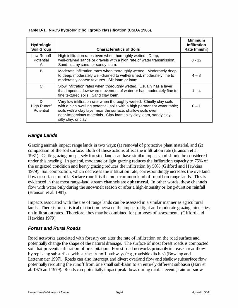
Oregon Watershed Assessment Manual Page 4 Appendix IV-D
Table D-1. NRCS hydrologic soil group classification (USDA 1986).
HydrologicSoil Group Characteristics of Soils
MinimumInfiltration
Rate (mm/hr)
Low RunoffPotential
A
High infiltration rates even when thoroughly wetted. Deep,well-drained sands or gravels with a high rate of water transmission.Sand, loamy sand, or sandy loam.
8 - 12
B Moderate infiltration rates when thoroughly wetted. Moderately deepto deep, moderately well-drained to well-drained, moderately fine tomoderately coarse textures. Silt loam or loam.
4 – 8
C Slow infiltration rates when thoroughly wetted. Usually has a layerthat impedes downward movement of water or has moderately fine tofine textured soils. Sand clay loam.
1 – 4
DHigh Runoff
Potential
Very low infiltration rate when thoroughly wetted. Chiefly clay soilswith a high swelling potential; soils with a high permanent water table;soils with a clay layer near the surface; shallow soils overnear-impervious materials. Clay loam, silty clay loam, sandy clay,silty clay, or clay.
0 – 1
Range Lands
Grazing animals impact range lands in two ways: (1) removal of protective plant material, and (2)compaction of the soil surface. Both of these actions affect the infiltration rate (Branson et al.1981). Cattle grazing on sparsely forested lands can have similar impacts and should be consideredunder this heading. In general, moderate or light grazing reduces the infiltration capacity to 75% ofthe ungrazed condition and heavy grazing reduces the infiltration by 50% (Gifford and Hawkins1979). Soil compaction, which decreases the infiltration rate, correspondingly increases the overlandflow or surface runoff. Surface runoff is the most common kind of runoff on range lands. This isevidenced in that most range-land stream channels are ephemeral. In other words, these channelsflow with water only during the snowmelt season or after a high-intensity or long-duration rainfall(Branson et al. 1981).
Impacts associated with the use of range lands can be assessed in a similar manner as agriculturallands. There is no statistical distinction between the impact of light and moderate grazing intensitieson infiltration rates. Therefore, they may be combined for purposes of assessment. (Gifford andHawkins 1979).
Forest and Rural Roads
Road networks associated with forestry can alter the rate of infiltration on the road surface andpotentially change the shape of the natural drainage. The surface of most forest roads is compactedsoil that prevents infiltration of precipitation. Forest road networks primarily increase streamflowby replacing subsurface with surface runoff pathways (e.g., roadside ditches) (Bowling andLettenmaier 1997). Roads can also intercept and divert overland flow and shallow subsurface flow,potentially rerouting the runoff from one small sub-basin to an entirely different subbasin (Harr etal. 1975 and 1979). Roads can potentially impact peak flows during rainfall events, rain-on-snow

Oregon Watershed Assessment Manual Page 5 Appendix IV-D
events, or spring snowmelt; therefore, the determination of percent of basin occupied by roadsprovides useful information regardless of the way in which peak flows are generated.
Rural roads associated with either agriculture or range lands can also affect streamflow and will becharacterized in a similar manner as forest roads. Roadside ditches are more structured andmaintained along rural roads and can significantly extend the stream network density, because theirpresence is additional to the natural channel. However, if natural channels are altered throughstraightening or channelizing, the stream network length may decrease. Channelizing streams resultsin increased velocities and potentially increases erosion rates of the banks and bed.
Roads along stream channels restrict lateral movement and can cause a disconnection between thestream or river and its floodplain. Restricting lateral movement can result in downcutting of thechannel and decreased accessibility of flood waters to overbank storage, resulting in decreased floodpeak attenuation.
Urban and Rural Residential
Urbanization has the highest impact on hydrology of the land uses addressed. In urban settings, alarge portion of the land surface becomes impervious from roads, parking lots, shopping malls,buildings, sidewalks, etc. The streamflow regime is significantly altered from decreases in infiltrationrates and recharge rates, corresponding increases in peak flows and volume of runoff, and a decreasein watershed response time (time to peak). Rainfall striking the ground surface moves more quicklyfrom streets and roofs than from naturally vegetated areas; conveyance systems such as stormsewers and lined open channels increase the flow velocities, thereby decreasing the lag time or thetime it takes for water to enter the stream channel. Low flows are affected by reduced groundwaterrecharge resulting from the increase in impervious surfaces. In addition, pervasive nonpoint sourcepollution often accompanies stormwater runoff in urbanized areas (see Water Quality component).As with agriculture, urbanization has a greater affect on runoff where soils have a high infiltrationrate than in areas where soils are relatively impermeable in their natural state (USDA 1986).
Water Law and Water Use Background
Water law in the State of Oregon is based on the prior appropriation doctrine or “first in time,first in right,” subject to the physical availability of water and the ability to put it to beneficial usewithout waste. The most senior appropriator (the right with earliest date) has a right to divert waterprior to any junior water right (a later date). The most senior right is the last one to be shut off fromdiverting water during low streamflows. Any person or entity withdrawing water from a stream orriver must have a water right from the Oregon Water Resources Department (OWRD). Thesewater rights are in various levels of use and certification or adjudication. For example, there arecertificates, applications for certificates, water rights on record and not being used, and rights notusing their full entitlement. Each water right has an instantaneous flow amount (the maximum rateat which water can be withdrawn at any point in time), an annual volume restriction (water duty),and a designated beneficial use, including agriculture, domestic, urban, industrial, commercial, fishand wildlife, power, recreation, etc.
In general, agriculture places the greatest demand on our water resources compared to other uses.Water is required for irrigation of crop lands, pasture, stock watering, and/or washdown. In mostcases, the period of high demand for irrigation coincides with the period of low streamflow; crop
Oregon Watershed Assessment Manual Page 6 Appendix IV-D
water requirements tend to peak in August, when streamflows are usually the lowest. Waterwithdrawals are applied to the crop lands for irrigation, and part of that water is used by the crop(evapotranspiration), a portion percolates to deep groundwater, and a portion may be returned toanother watershed; the total portion not returned to the river is called consumptive use. Theportion of the diversion that returns to the stream system through subsurface avenues at pointsdownstream is called the return flow.
Urban water supply can provide for residential, commercial, and some industrial uses. Water isdiverted, treated, and then distributed throughout a municipality. Subsequently, the wastewater isdelivered to a sewage treatment facility where it is treated to a “primary” or “secondary” level anddischarged to a stream or bay at a distinct location. Much of the residential urban water isnonconsumptive, with the exception of lawn watering, and is returned to the stream network fromthe wastewater facilities. Lawn-irrigation return flow occurs through subsurface avenues.
Stormwater runoff from urban areas is generally not treated and discharged directly to thestormwater conveyance facilities that often deliver directly to the stream channel.
Industrial water uses can demand large quantities of water for operation of their facilities. Somehave on-site treatment facilities and all are subject to discharge quantity and quality restrictionsthrough National Pollution Discharge Elimination System (NPDES) permits.
National forests, national parks, US Bureau of Land Management lands, Indian reservations, etc., arefederal reservations. These entities maintain federal reserved rights for the purposes for which thereservations were established. Their priority date is the date the reservation was created. In manycases, reservations were established in the mid- to latter part of the 19th century. Many of the federalreservation water rights have been tried in the courts of law, and, more often than not, case law hasset the precedent of adjudicating federally reserved water rights (Winters Doctrine).
Water Rights
There are three primary types of surface water rights: (1) out-of-stream rights, (2) storage rights, and(3) in-stream rights. Out-of-stream rights are also called “direct flow” or “run of the river”diversions. These rights entail withdrawing water directly from the channel with subsequentapplication for a specific beneficial use such as irrigation, domestic or urban water supply, industrialuse, etc. Storage rights can be for on-stream or off-stream reservoirs. On-stream reservoirs capturewater as it flows into the reservoir. Water is stored until it is needed for the specified beneficial use,at which time it is released either into the channel and withdrawn downstream or released intoconveyance facilities for delivery to the point of use. Off-stream reservoirs require diversion fromthe river to the storage site, and subsequent release and conveyance to the point of use. In-streamrights are those that require a designated quantity of water to remain in the stream or river for aspecific beneficial use, most often for aquatic resources, wildlife, or aesthetics.
Water withdrawals reduce streamflows, potentially resulting in a negative impact on the biologicresources, particularly during the low-flow season. In recent years, in-stream rights have becomemore common as a means of protecting the biologic resources. In-stream water rights did not existin Oregon prior to 1955. Minimum flows were established by administrative rule in 1955, but theydid not carry the full weight of a water right. Between 1955 and 1980, the Oregon Department ofFish and Wildlife (ODFW) conducted basin investigations from which minimum flows were

Oregon Watershed Assessment Manual Page 7 Appendix IV-D
recommended and adopted by rule. In 1987, the legislature changed the administrative rulemakinginto an application process for a water right. OWRD holds the water right, but ODFW,Department of Environmental Quality, and State Parks can apply for an in-stream right. Minimumflows were changed into in-stream rights, and the date minimum flows were adopted became thepriority date. The in-stream rights can have the value up to but not exceeding the median flow.In-stream rights tend to be junior to the majority of the out-of-stream water rights; this reduces theirability to maintain effective streamflows in the channel. If federal reserved rights for in-stream flowshave been adjudicated, they would usually have the most senior right in the basin, because federalreservations were established before the implementation of the Prior Appropriation Doctrine.
Water users with large demands generally have storage rights, because reservoirs provide morecertainty of supply during low-streamflow conditions. The ability to capture streamflow during thehigh flows and use it during low flows can be a significant benefit to water users. In some instances,reservoirs are constructed as flood control facilities to provide attenuation of the peak flows andreduce downstream flooding and damage.
Groundwater rights are those attached to the withdrawal of water from a well. With someexceptions, all water users extracting groundwater as the source of supply must have a water rightfor the legal use of the water. There are exempt uses that do not require a right. The mostsignificant of these is rural residential water users; these users are limited to 15,000 gallons per dayfor noncommercial use and irrigation of less than 0.5 acres.
Groundwater has the potential to influence surface water by what is called hydraulic continuity.Depending on the location of the well and the geology in the area, water withdrawn can have acorresponding effect on the streamflow. In other words, it is possible for the extraction ofgroundwater to dry up a nearby stream during low flows. Consequently, the State of Oregonmanages surface- and groundwater rights conjunctively, which means there are times at whichgroundwater withdrawals will be shut down due to low flows in the channel.
Storage
Man-made storage facilities such as water supply reservoirs, flood control reservoirs, ormultipurpose reservoirs impact the peak flows downstream of the impoundment. Each reservoirhas its unique operating scheme, and therefore will requires more detailed hydrologic investigations,often including release schedules, reservoir routing, etc. If you have a reservoir in your watershed,further technical analyses will be required for the portion of your basin below the dam, while someof these exercises can be completed for the portion of the basin above the dam.
Water Availability
The OWRD has developed a computer model, Water Availability Reports System (WARS), whichcalculates water availability for any of their designated water availability basins (WABs) in the state.Water availability, as defined by the OWRD, refers to the natural streamflow minus the consumptiveuse from existing rights. If water is available, additional in-stream or out-of-stream rights may beissued. This value is dynamic and is often updated to account for issuance of new water rights. The80% level of exceedance is that which OWRD uses to determine whether additional water rights can beissued in a basin. The 80% exceedance flow is the streamflow that is in the river 80% of the timeover a designated 30-year period, which accounts for wet- and dry-year cycles. In other words, that
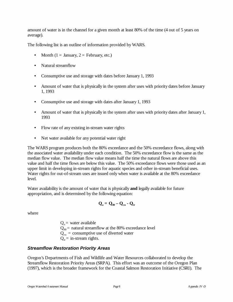
Oregon Watershed Assessment Manual Page 8 Appendix IV-D
amount of water is in the channel for a given month at least 80% of the time (4 out of 5 years onaverage).
The following list is an outline of information provided by WARS.
• Month (1 = January, 2 = February, etc.)
• Natural streamflow
• Consumptive use and storage with dates before January 1, 1993
• Amount of water that is physically in the system after uses with priority dates before January1, 1993
• Consumptive use and storage with dates after January 1, 1993
• Amount of water that is physically in the system after uses with priority dates after January 1,1993
• Flow rate of any existing in-stream water rights
• Net water available for any potential water right
The WARS program produces both the 80% exceedance and the 50% exceedance flows, along withthe associated water availability under each condition. The 50% exceedance flow is the same as themedian flow value. The median flow value means half the time the natural flows are above thisvalue and half the time flows are below this value. The 50% exceedance flows were those used as anupper limit in developing in-stream rights for aquatic species and other in-stream beneficial uses.Water rights for out-of-stream uses are issued only when water is available at the 80% exceedancelevel.
Water availability is the amount of water that is physically and legally available for futureappropriation, and is determined by the following equation:
Qa = Q80 – Qcu - Qir
where
Qa = water availableQ80 = natural streamflow at the 80% exceedance levelQcu = consumptive use of diverted waterQir = in-stream rights.
Streamflow Restoration Priority Areas
Oregon’s Departments of Fish and Wildlife and Water Resources collaborated to develop theStreamflow Restoration Priority Areas (SRPA). This effort was an outcome of the Oregon Plan(1997), which is the broader framework for the Coastal Salmon Restoration Initiative (CSRI). The

Oregon Watershed Assessment Manual Page 9 Appendix IV-D
CSRI mission is to restore coastal salmon populations and fisheries to sustainable levels. Threemajor factors were identified in CSRI as exacerbating the loss of fish populations: (1) fish resources,(2) fish habitat, and (3) loss of streamflow. The loss of streamflow is the focus of the SRPAanalysis.
The identification of priority areas was based on a combination of biological factors and water use.ODFW identified priority areas to enhance fish populations. A rank was assigned to threecategories under fisheries: (1) fish resources; (2) habitat integrity; and (3) risk factors such as a listingunder the Endangered Species Act, in-stream flow protection, or natural low-flow problems.OWRD identified areas in which an opportunity existed to enhance in-channel flows. Concurrently,OWRD identified areas in which an opportunity existed to enhance in-channel flows, situationsunder which water could be saved through conservation, efficiency of use, etc. The criteria forwater resources was assigned to two categories: (1) consumptive use by percentage of the median(50% exceedance) streamflow, and (2) number of months an in-stream water right is not met. Apriority was established based on the combination of the two resulting factors: “need” (fisheries) and“optimism” (water resources). For example, in the Mid Coast Region (Table D-2), if the need isgiven a rank of 2 by ODFW and the optimism is given a rank of 1 by OWRD, the basin would notbe selected as a priority for flow restoration. In the need and optimism column, 1 is the lowest rankand 4 is the highest.
Table D-2. Initial state restoration priority.
Flow-Restoration
Basin Need Optimism Priority
North Coastand Rogue
1 or 23 or 4
1 or 23 or 4
NoYes
Umpqua Any 12, 3, 4
NoYes
South Coast 1 or 23 or 4
12, 3, 4
NoYes
Mid Coast 12, 3, 4
12, 3, 4
NoYes
References
Bowling, L.C., and D.P. Lettenmaier. 1997. Evaluation of the Effects of Forest Roads onStreamflow in Hard and Ware Creeks, Washington. TFW-SH20-97-001, Water Resources SeriesTechnical Report No. 155, University of Washington, Seattle.
Branson, F.A., G.F. Gifford, K.G. Renard, and R.F. Hadley. 1981. Rangeland Hydrology. RangeScience Series No. 1, October 1972, Second Edition 1981. Society for Range Management,Denver Colorado. Kendall/Hunt Publishing Co., Dubuque, Iowa.
Coffin, B.A.. and R.D. Harr. 1992. Effects of Forest Cover on Volume of Water Delivery to SoilDuring Rain on Snow. Final Report TFW-Sh1-92-001.

Oregon Watershed Assessment Manual Page 10 Appendix IV-D
Gifford, G.F., and R.H. Hawkins. 1979. Deterministic Hydrologic Modeling of Grazing SystemImpacts on Infiltration Rates. Water Resources Bulletin 15(4):924-934.
Greenberg, J. and K.F. Welch. 1998. Hydrologic Process Identification for Western Oregon.Prepared for Boise Cascade Corp., Boise, Idaho.
Harr, R.D. 1981. Some Characteristics and Consequences of Snowmelt During Rainfall in WesternOregon. Journal of Hydrology 53:277-304.
Harr, R.D. 1986. Effects of Clearcutting on Rain-on-Snow Runoff in Western Oregon: A NewLook at Old Studies. Water Resources Research 22 (7):1095-1100.
Harr, D.R., W.C. Harper, J.T. Krygier, and F.S. Hsieh. 1975. Changes in Storm Hydrographs AfterRoad Building and Clear-Cutting in the Oregon Coast Range. Water Resources Research 11(3).
Harr, R.D., R.L. Fredriksen, and J. Rothacher. 1979. Changes in Streamflow Following TimberHarvest in Southwestern Oregon. Research Paper PNW-249. February 1979. PacificNorthwest Forest and Range Experiment Station, U.S. Department of Agriculture, ForestService, Portland, Oregon.
Logan, R.S. and R.A. Fletcher. 1996. Forest Ecosystem Stewardship. Montana State UniversityPublications, Bozeman, Montana.
MacDonald, L.H. and J.A. Hoffman. 1995. Causes of Peak Flows in Northwestern Montana andNortheastern Idaho. American Water Resources Association, Water Resources Bulletin 31(1):79-95.
Oregon, State of. 1996. Oregon Plan for Salmon and Watersheds including Oregon's CoastalSalmon Restoration Initiative (OCSRI) and Steelhead Supplement.http://www.oregon-plan.org/
USDA (US Department of Agriculture) Soil Conservation Service. 1986. Urban Hydrology forSmall Watersheds. Technical Release 55.
Washington State Forest Practices Board. 1997. Standard Methodology for Conducting WatershedAnalysis Under Chapter 222-22 WAC. Version 4.0. Olympia, Washington.

Oregon Watershed Assessment Manual Page 1 Appendix VIII-A
WATERSHED CHARACTERIZATION OF TEMPERATURE –UMPQUA BASIN1
The screening procedure described in the Water Quality Assessment component will often raisefurther questions about the spatial distribution of temperature exceedances in the watershed. Amore detailed watershed characterization, such as described here, can be used to answer thesequestions. The Elk Creek Temperature Study (Umpqua Basin Watershed Council 1998) provides agood example of how to conduct and interpret data from a more comprehensive study.
The Oregon temperature criteria is measured as the 7-day moving average of the maximum dailytemperatures. The reason for using a moving average in the water quality standards is to decreasethe effect of a single peak temperature on data interpretation. Aquatic organisms are affected moreby exposure to high temperature over an extended period than to a single excursion over the criteria.As noted in this study, the seasonal maximum temperature was, for this particular watershed andseason, consistently about 3°F higher than the 7-day moving average. This finding shows the utilityof using the simpler daily maximum of 64°F as a screening tool, as described in the watershedassessment manual.
Study Area
The Elk Creek Watershed is located in southwestern Oregon in Douglas County. The watershed isapproximately 350 square miles in size and is primarily in private ownership: 40% private ownership,40 % private commercial forestland, and 20% federal. Elevation ranges from 90 feet at the mouthto 2,000 feet at the top of the watershed. The vegetation is typical of southwest Oregon: the forestlands are dominantly Douglas fir; the riparian areas contain alder, willow, and cottonwood.Vegetative recovery of disturbed areas is relatively rapid in the form of woody brush and grass.
Objectives
The objectives of the study were to provide an understanding of how temperature varies spatiallythroughout the watershed, provide data for the evaluation of aquatic habitat, and develop a databasefor development of a Temperature Management Plan for the watershed.
Methods
The Elk Creek study used an intensive monitoring approach during one field season to eliminate thebetween-year variability. Twenty-eight sites were chosen to obtain a representative sample ofvarious stream types and conditions throughout the watershed. Continuous temperature dataloggers were set to record data every 20 minutes from July 1 through the end of September. Qualitycontrol procedures included the following: (1) calibration of each unit against a referencethermometer at two different temperatures both before deployment and after retrieval of the units,(2) photo documentation of each site saved in digital format, (3) standardized field data sheets, and(4) field verification of data logger temperature against the reference thermometer. The accuracyassessments indicated that all data loggers remained within 0.3°F of the reference temperatureduring the study period.
1 Elk Cr. Temperature Study. Courtesy of Umpqua Basin Watershed Council and Insight Consultants, Roseburg, Oregon.

Oregon Watershed Assessment Manual Page 2 Appendix VIII-A
Results
Figure 1 is an example monitoring site data sheet from the report. It contains relevant informationabout the site as well as a chart of the raw temperature data. These charts are useful in findinganomalies in the data and making general comparisons between stations.
The second chart (Figure 2) shows a summary of some useful statistics for all the stations whichincludes the seasonal maximum temperature, the 7-day average maximum temperature, and the dailychange in temperature.
Project Name: ELK CREEK TEMPERATURE 1998
Temperature Logger ID: 6048 Site Name: 4 Elk Ck abv Brush Ck
Logger Type: Vemco River Basin: Umpqua - Main Stem
Data File Name: Elk Creek 98 Watershed: Elk Creek
Deployment Date: 7/8/98 Site Latitude: 43° 39.698
Sample Interval: 20 Minutes Site Longitude: 123° 29.463
Unit Retrieval Date: 9/22/98 Elevation: 178 ft
Distance to Mouth: 11.90 Miles
Distance to Headwater: 32.7 Miles
Collected by: InSight
Start Date: 7/11/1998 Day # Stop Date: 9/21/1998
Key Statistics: [Produced by DEQ "Tempture" Program ]
Date Day # Value Checks: Date Status
Seasonal Maximum: 7/27/98 16 86.7 Pre-deployment: 7/3/98 OK
Seasonal Minimum: 9/10/98 61 58.9 Audit: 8/15/98 OKMaximum ∆∆∆∆T: 8/31/98 51 13.6 Post-deployment: 9/25/98 OK
Max 7-Day Average: 7/26/98 15 83.4
Location Details:
4 Elk Ck abv Brush Ck
50
60
70
80
90
0 10 20 30 40 50 60 70 80
° F
Channel width about 60 feetcobble /gravel channel bedcontinuous riffleUnit depth 1 ft.
Figure 1. Example data sheet and chart of temperature in degrees Fahrenheit.

Oregon Watershed Assessment Manual Page 3 Appendix VIII-A
Discussion
This study provides data to better understand how stream temperature varies both seasonally anddaily at various points within a watershed. This information, when tied to observations on channelconditions, shade, canopy, and riparian vegetation, can be used to make viable recommendations fordeveloping a temperature management strategy. The study identified tributaries that consistentlycontributed cooler water to Elk Creek: These tributaries may be important in moderatingtemperature and providing cool water refuges for fish. The downstream change in temperature alsoshowed areas of significant heating or cooling. Areas with temperature gain can be furtherinvestigated to identify the specific reason for higher temperatures (e.g., wide shallow channels,reduced canopy) and potential site-specific solutions. The areas of cool water may serve asimportant holding areas for juvenile and adult fish, and can be identified for protection as part of thewatershed restoration plan.
The database associated with this project provides an opportunity to develop other statistics and teststream temperature modeling efforts. For example, there may be an interest in the average dailytemperature for a site. This statistic could be calculated from the data and used to calibratetemperature models such as SSTEMP, which predicts mean daily temperature for differentconditions.
p y
0
10
20
30
40
50
60
70
80
90
100
1 2 2.1
3 4 5 6 7 8 9 10 11 12 13 14 15 16 17 18 19 20 21 22 22.1
23
Site Number
° F
Seasonal Maximum Value
7-Day averages Maximum
Seasonal Max DT
Figure 2. Station summary of maximum seasonal temperature, 7-day moving average of maximumdaily temperatures, and maximum daily change in temperature.

Component IXFish and Fish HabitatAssessmentTable of Contents
Introduction.....................................................IX-3
Critical Questions ........................................IX-3
Assumptions................................................IX-4
Materials Needed ........................................IX-4
Necessary Skills ..........................................IX-4
Final Products of the Fish and Fish
Habitat Component................................IX-5
Assessment Methodology..............................IX-5
Step 1: Identify Fish Species and
Populations............................................IX-5
Step 2: Create Fish Distribution Maps .........IX-8
Step 3: Complete Habitat Condition
Summary............................................. IX-11
Step 4: Migration Barrier Identification....... IX-13
Step 5: Evaluate Confidence in the
Assessment......................................... IX-16
References .................................................... IX-16
Glossary ........................................................ IX-16
Appendix IX-A: ODFW Habitat
Benchmarks
Appendix IX-B: Example Habitat
Condition Summary Forms
Example Form F-2a: Pool Habitat
Condition Summary Big Elk
Watershed
Example Form F-2b: Riffle and Woody
Debris Habitat Condition Summary
Example Form F-2c: Riparian Habitat
Condition Summary.
Appendix IX-C: Example Form F-3: Fish
Passage Evaluation

Table of Contents (continued)
Appendix IX-D: Blank Forms
Form F-1: Fisheries Information
Summary
Form F-2a: Pool Habitat Condition
Summary
Form F-2b: Riffle and Woody Debris
Habitat Condition Summary
Form F-2c: Riparian Habitat Condition
Summary
Form F-3: Fish Passage Evaluation
Form F-4: Fish Passage Field
Assessment
Form F-5: Fish Assessment Confidence
Evaluation

Oregon Watershed Assessment Manual Page IX-3 Fish and Fish Habitat Assessment
Component IXFish and Fish Habitat Assessment
INTRODUCTION
This component of the Oregon Watershed Assessment Manual helps the user compile and evaluateavailable information on fish populations, in-stream habitat, and migration barriers through thefollowing four-step process:
1. Document the temporal distribution and abundance of fish species within the watershed.
2. Identify potential interactions between species of concern, such as those species listed under theEndangered Species Act (ESA).
3. Compile existing Oregon Department of Fish and Wildlife (ODFW) and other habitat data thathave been collected on the watershed, and compare them with established ODFW benchmarksto provide an evaluation of in-stream habitat conditions.
4. Identify and prioritize human-caused barriers to fish passage in the watershed.
The information gathered in this component is then integrated into the Watershed ConditionEvaluation, where users evaluate impacts to important areas of current fish use and habitat.
Critical Questions
1. What fish species are documented in the watershed? Are any of these currently state- orfederally listed as endangered or candidate species? Are there any fish species thathistorically occurred in the watershed which no longer occur there?
2. What is the distribution, relative abundance, and population status of salmonid 1species inthe watershed?
3. Which salmonid species are native to the watershed, and which have been introduced to thewatershed?
4. Are there potential interactions between native and introduced species?
5. What is the condition of fish habitat in the watershed (by sub-basin) according to existinghabitat data?
6. Where are potential barriers to fish migration?
1 Terms found in bold italic throughout the text are defined in the Glossary at the end of this component.

Oregon Watershed Assessment Manual Page IX-4 Fish and Fish Habitat Assessment
Assumptions
• Salmonid fish are typically the most sensitive fish species occurring within a stream network.If habitat conditions are suitable for salmonid fish, then they reflect “good” habitatconditions for the watershed.
• Fish distribution is a function of the quantity and quality of habitat types available in thewatershed. Channel Habitat Types (CHTs) have predictable habitat conditions thatinfluence the potential fish use within a stream reach. The distribution of fish species in awatershed is a function of the distribution and condition of the CHTs found there.
Materials Needed
This assessment relies on finding and compiling existinginformation to develop distribution maps for residentand anadromous salmonid fish. You will need to havethe following items handy:
• Any available fisheries information for thewatershed, including basin plans, data reports, etc.
• A copy of historical fish information from theHistorical Conditions Assessment component
• Forms found in Appendix IX-D
• A copy of the CHT map (from the ChannelHabitat Type Classification component)
• Two or three copies of watershed base maps(from Start-Up and Identification of Issuescomponent) (two copies for watersheds with onlyresident fish, three copies if watershed hasresident and anadromous fish)
• Habitat survey data from ODFW, US ForestService (USFS), Bureau of Land Management(BLM), Oregon Forest Industry Council (OFIC)or others
The Fish Information sidebars on this page and the nextwill help you gather information.
Necessary Skills
This assessment does not require any specialized skills. Itis helpful to have a persistent nature to track down and
FISH INFORMATION CONTACTS
Oregon Department of Fishand Wildlife
General Information:(503) 229-5222
Home Page:http://www.dfw.state.or.us
Regional Offices:Northwest Region, Corvallis(541) 757-4186
Southwest Region, Roseburg(541) 440-3353
Central Region, Bend(503) 388-6363
Northeast Region, LaGrande(541) 963-2138
Southwest Region, Ontario(541) 573-6582
Marine Region, Newport(541) 867-4741
Columbia Region, Clackamas(503) 657-2000
Oregon Department of Forestry
Northwest Area, Forest Grove(503) 357-2192
Southern Area, Roseburg(541) 440-3412
Eastern Area, Prineville(541) 447-5658

Oregon Watershed Assessment Manual Page IX-5 Fish and Fish Habitat Assessment
sort through information from a wide variety ofsources.
Field evaluations of road crossings require thephysical ability to scramble down potentially steeproad embankments and take measurements. Fieldwork also will require use of a level and stadiarod to measure culvert elevations.
Final Products of the Fish and FishHabitat Component
This assessment will result in the followingcompleted forms and maps:
• Form F-1: Fisheries Information Summary
• Form F-2: Habitat Condition Summary
• Form F-3: Fish Passage Evaluation
• Form F-4: Fish Passage Field Assessment(optional)
• Form F-5: Confidence Evaluation
• Map F-1a: Resident Fish Distribution(current and historical)
• Map F-1b: Anadromous Fish Distribution(current and historical)
• Map F-2: Migration Barrier Identification
ASSESSMENT METHODOLOGY
Step 1: Identify Fish Species andPopulations (Form F-1)
The goal of this step is to compile all availableinformation on fish that are documented to occurin the watershed, and to evaluate the status of thefish populations. With this information, you canstart thinking about the habitat needs of thewatershed’s fish species, document whenanadromous fish occur in the watershed, and helpidentify which species have the lowest population
FISH POPULATION AND DISTRIBUTIONINFORMATION
• Oregon Plan: Anadromous fish core areaand distribution information is available in theOregon Plan (Chapter 15). This can beaccessed through the ODFW Web site.http://www.dfw.state.or.us/
• ODFW Basin Plans: These reports are invarious stages of completion and some plansmay be outdated. Nevertheless, these areoften the most accessible source ofinformation relevant to fish management.ODFW District Offices should have copies ofthe plans as appropriate to their basins, orcontact ODFW, Basin Planning Coordinator at(503) 872-5252, x 5421.
• Biennial Report on the Status of Wild Fishin Oregon: This report includes informationon all wild freshwater and estuarine fishspecies in Oregon. Most of the report comesfrom ODFW files, particularly annual reportsfiled by ODFW district biologists or fromresearch projects. This report can beaccessed through the ODFW home page athttp://www.dfw.state.or.us under Researchand Reports. These reports also containsome information on historic abundance anddistribution.
• Bull Trout Distribution: This information isavailable on GIS and can be accessedthrough the ODFW Web site. This informationwill not apply to coastal watersheds or privatelands. Contact ODFW at (503) 872-5252x 5602.
• Other Trout and Steelhead Distribution:Contact ODFW at (503) 872-5252, x 5412.
• Stocking History: The records from 1983 arein a database. The codes they used toidentify the location of stocking are unique tothe hatchery; it may be difficult to access allinformation specific to your watershed.Contact ODFW at (503) 872-5252, x 5415.
• Migration Barriers and Culverts: This datais in several places and you will have to makemultiple phone calls to locate what if anythingis available for your watershed. For fishpassage information, contact (503) 872-5252x 5582; for culvert information, (503) 872-5252x 5590; for ODFW Coho Spawning Project,(541) 737-7636.

Oregon Watershed Assessment Manual Page IX-6 Fish and Fish Habitat Assessment
numbers or may be the most sensitive.
The sources listed in the sidebar on page 5 will provide a good start toward compiling theinformation you need. They may also be able to point you to other sources. Find as muchinformation as you can, then sit down and complete Form F-1 with as much detail as possible. Theform may collect duplicate information, so be sure to note if the information recorded on the formcan be found in multiple sources. Make notes of any conflicting information. Where you do nothave any information, you may need to interview local OFDW and other agency (i.e., USFS, BLM,etc.) fish biologists.
Form F-1: Species of Concern, Fish Presence, and Population Status
Item 1 in Form F-1 asks for information on species of concern, including ESA and ODFW status,and population trends. Item 2 documents whether any species that historically occurred in thewatershed are no longer found. Various sources listed in the sidebar contain current and historicfish distribution information. Usually, ODFW basin plans are the best source of this information.Your local ODFW fish biologist should able to help acquire and sort through the data.
Consult with the assessment team member performing the Start-Up and Identification of WatershedIssues component for a list of species in the watershed compiled using the Natural HeritageDatabase. In addition, look for the ODFW’s comprehensive review of threatened, endangered, andsensitive (TES) species (terrestrial and aquatic). This ODFW project is no longer active, but copiesof the report are available from the ODFW’s Fish Conservation Program Leader, (503) 872-5242,extension 5405.
Form F-1: Stocking History
The goal of Item 3, Form 1 is to summarize what species have been stocked in the watershed andhow extensive the stocking efforts were/are. This information will help identify potentialinteractions between native and stocked species, and help you understand if hatchery fish have aninfluence on current population trends. ODFW basin plans are usually the best source for this typeof summary information, although such information may not be up-to-date. Table 1 provides anexample of a completed stocking history summary.
Form F-1: Life History Patterns, Important Habitat Areas
Items 4 and 5 of Form 1 ask for information about the timing of anadromous and resident fishspawning and migration. Again, this information can be found in the local basin plan or otherODFW documents. This information will help you understand how and when fish use specificportions of the watershed. This knowledge may be important when planning the timing of specificdevelopment or enhancement activities. Table 2 provides an example record of fish life historypatterns from Big Elk Watershed in the Yaquina Basin.

Oregon Watershed Assessment Manual Page IX-7 Fish and Fish Habitat Assessment
Table 1. Example of a completed stocking history summary.
Species Stocking Notes Native orExotic?
Source
Chinook Historically 1902–1990 Yaquina River Basin Plan
Coho Historically 1902–1990 Yaquina River Basin Plan
Steelhead 1905–1939Average 31,000 smolts/year since 1978
Yaquina River Basin Plan
Cutthroat Historically 1925-1960 Yaquina River Basin Plan
Pink Salmon Historically 1977–1982 (OSU Experiment) Exotic Yaquina River Basin Plan
Rainbow Trout Historically 1950– 58, no resident rainbowspresent
Yaquina River Basin Plan
Brook Trout Historically stocked in 1904, no longerpresent
Exotic Yaquina River Basin Plan
American Shad Stocked in Columbia 1800s, later becameestablished in Yaquina
Exotic Yaquina River Basin Plan
Notes: Hatchery at Elk City 1902–1950, OreAqua Hatchery 1974 – 1990
Table 2. Example summary of fish life history patterns.
SpeciesA-AnadromousR-Resident Location Spawning Outmigration
Chinook A – fall Mainstem, lowerreaches of largetributaries
Oct. to Jan.,peak in Nov.
June/July to estuary
Summer/fall to ocean asunder-yearling smolts
Coho A – fall Low-gradienttributaries
Nov. to Feb. 2nd spring after hatching,peak in May; limited estuarytime
Steelhead A – winter Low-/moderate-gradient tributaries
Oct. to March,peak Dec. andJan.
2 to 3 years in freshwater,outmigrate in March to June*
Cutthroat A – summer/fall
R
Fluvial
1st and 2nd ordertributaries
Dec., peaks inFeb.*
Age 1+ and 2+ fishoutmigrate April or May toestuary/tidewater
Age 3 fish go to ocean in May
Adults overwinter in estuariesof origin*
* Based on information from Alsea Watershed; local data not available.
Form F-1: Known Migration Barriers
The initial data compilation and search will likely turn up some information on known migrationbarriers. Indicate these in item 7 of Form F-1 and mark them on the draft fish distribution maps.
Oregon Watershed Assessment Manual Page IX-8 Fish and Fish Habitat Assessment
During the assessment of potential migration barriers, you will work with the Sediment Sourcesanalyst to map and identify potential fish passage barriers.
Form F-1: Species Interactions
Did you answer yes to question 7 on Form F-1? If so the following species interactions may beoccurring. Consult with the regional ODFW fisheries biologist to determine the potential extent ofthe following species interactions.
• Brook trout/bull trout (competition, interbreeding)• Rainbow/cutthroat (competition/ interbreeding)• Hatchery/wild-stock interactions
Step 2: Create Fish Distribution Maps
After you’ve collected all the pertinent information for Form F-1, you are ready to create the fishdistribution maps. These color-coded maps will visually document where fish are known to occur inthe watershed and where areas of important habitat occur. This information will help the watershedcouncil evaluate how potential impacts may or may not affect fish habitat, and will help visuallyillustrate where enhancement activities may have the greatest benefit. If your watershed hasanadromous and more than one species of resident fish, you may want to make one map foranadromous fish distributions (Map F-1a) and one for resident fish (Map F-1b). Typically, the basemap you are using will be the Oregon Department of Forestry (ODF) stream classification maps,which show the upstream extent of fish utilization. Be aware that these maps are not always basedon current data, and you may want to ask local ODFW or ODF staff if any recent data collectionhas been performed to validate the mapped information. In addition, these maps do not identifyfish species; look for fish species information in the raw data or talk to local fish biologists and makean educated guess about which fish species potentially occur.
Not only may data sources be outdated or inaccurate, you may find that specific distributioninformation is simply not available. Creating a fish distribution map will help you identify such datagaps. As a first cut, look at all available information and indicate what is known on the draft maps.It is often useful to take a copy of the map to local fish biologists and ask them to indicate what theyknow about the fish distributions. Typically, the upstream extent of fish utilization by species hasnot been identified or mapped, but you can make an educated guess at where these fish may occur inthe watershed by using the CHT map and general information about the species occurring in thewatershed (see Introduction). Table 3 summarizes potential fish use within each CHT. Thisinformation can help you make decisions on potential fish distributions within the watershed.
Once you have developed a draft map you will probably have numerous questions to ask localODFW, USFS, or other agency fish biologists who have worked in the watershed. They can helpreview the data you have compiled, and make the necessary judgment calls in developing the fishdistribution maps. They can also provide insight on locations of important spawning and rearingareas. Usually it is more effective to develop a draft map before asking for help; it is easier todiscuss key locations with a map in front of you. If the information on current and historical fishdistributions is significantly different, place a footnote on the map explaining the reasons. Figure 1shows an example of a completed map from a coastal watershed.

Oregon Watershed Assessment Manual Page IX-9 Fish and Fish Habitat Assessment
Table 3. Potential fish utilization of Channel Habitat Types.
Channel Habitat Type GradientRange
OregonStream Size
Additional Description Fish Use
Low gradient largefloodplain ( FP1)
1% Large Lowland and valley bottom channels;can include small adjacent wetlands
Anadromous1: Important2 spawning, rearing, and migration corridor
Resident:3: Important spawning, rearing, and overwintering
Low gradient mediumfloodplain ( FP2)
<2% Large tomedium
Mainstem streams in broad valleybottoms
Anadromous: Important spawning, rearing, and migration corridor
Resident: Important spawning, rearing, and overwintering
Low gradient smallfloodplain (FP3)
<2% Small tomedium
Low-gradient floodplain channelsoccupy the floodplains of largerstreams
Anadromous: Important spawning, rearing, and migration corridor
Resident: Important spawning, rearing, and overwintering
Alluvial fan ( AF) 1-12% Small tomedium
Transition from steep mountain slopesto valley floor
Anadromous: Important rearing, migration corridor; potential4 spawning in lowergradientsResident: Important spawning and rearing
Low gradient moderatelyconfined (LM)
<2% Usuallymedium tolarge
Alternating hillslopes and terraces limitfloodplain
Anadromous: Potential spawning and rearing
Resident: Potential spawning, rearing, and overwintering
Low gradient confined(LC)
<2% Usuallymedium tolarge
Relatively straight channel, limitedfloodplain; partial or complete barriersmay occur at bedrock knickpoints
Anadromous: Potential spawning and rearing
Resident: Potential spawning, rearing, and overwintering
Moderate gradientmoderately confined (MM)
2-4% Usuallymedium tolarge
Limited floodplain; bedrock steps withcascades may form partial or completebarriers
Anadromous: Potential steelhead and coho spawning and rearing; limited5
chinookResident: Potential spawning, rearing, and overwintering
Moderate gradientconfined (MC)
2-4, 6% Variable Narrow open to moderate V-shapedvalley; hillslope or terrace confined
Anadromous: Potential steelhead and coho spawning and rearing; limitedchinookResident: Potential spawning, rearing, and overwintering
Moderate gradientheadwater (MH)
1-6% Small Common to plateaus or broaddrainage divides; sites of headwaterbeaver ponds
Anadromous: Potential steelhead and coho spawning and rearing; limitedchinook
Resident: Potential spawning, rearing, and overwintering
Moderately steep narrowvalley (MV)
4-8% Small tomedium
Narrow valley Anadromous: Potential steelhead, coho, sea-run cut spawning and rearing
Resident: Potential spawning, rearing, and overwintering
Bedrock canyon (BC) >4% Variable Very narrow V-shaped channel;migration barriers, may be anywhere
Anadromous: Lower-gradient areas provide limited rearing (if accessible)
Resident: Limited resident spawning and rearing
Steep narrow valley (SV) 8-16% Small Anadromous: Lower-gradient areas provide limited rearing (if accessible)
Resident: Limited resident spawning and rearing
Very steep headwatertributaries (VH)
>16% Small Resident: Very limited rearing
1 Anadromous refers to chinook, coho, steelhead, and sea-run cutthroat trout unless specifically stated.2 Important designates CHTs that potentially contain large areas of preferred habitat conditions.3 Resident refers to native redband, cutthroat trout and/or bull trout.4 Potential designates CHTs that may have suitable habitat conditions depending on site-specific factors.5 Limited designated CHTs that may have pockets of suitable habitat conditions depending on site-specific factors.

Oregon Watershed Assessment Manual Page IX-10 Fish and Fish Habitat Assessment
Figure 1. An example of a completed map from a coastal watershed.

Oregon Watershed Assessment Manual Page IX-11 Fish and Fish Habitat Assessment
Step 3: Complete Habitat Condition Summary (Form F-2)
In this step, you will compile existing ODFW fish habitat data. The ODFW has developed astandard stream habitat survey methodology (Moore et al. 1997). ODFW, ODF, and large privatelandowners have used this methodology to collect extensive amounts of fish habitat data. Datacollected in cooperation with ODFW is available in Geographic Information Systems (GIS)format from the ODFW Web site, or can be obtained in a spreadsheet format by calling the HabitatDivision of ODFW at (541) 757-4263. The assessment will be most straightforward if you requestthe data summary files, and the maps showing the locations of sampled segments.
The approach presented here provides a format for organizing the data and determining how habitatconditions vary throughout the watershed, and for comparing watershed conditions with“benchmark” conditions for the State of Oregon. This comparison allows you to look for patternsin habitat conditions throughout the watershed or to identify specific portions of the watershedwhere problems may exist. For example, in the Big Elk watershed habitat condition summary(Appendix IX-B) there are low numbers of large wood throughout the watershed, a condition whichalso appears to contribute to a lack of complex pools. In addition, in the Wolf Creek sub-watershed reach #4 pool conditions ranked as undesirable conditions, indicating a need to revisitthat stream reach and determine if there are site-specific conditions to explain this data.
CAUTION: Stream survey data is like a single photograph of a dynamic system. Streamchannel conditions may change drastically between years, especially if there has been a high-flow flood event. Also, the survey methodology has evolved, and older data may have beencollected using slightly different methodologies. It is important to be aware of changes thatmay have occurred in the stream system; the analysts of the Hydrology and Water Use,Riparian/Wetlands, and Sediment Sources assessment components can provide insights. Inaddition, some surveyed stream reaches have been found to be inconsistently sampled, andthe summary data do not necessarily reflect actual conditions. If the condition evaluationsbased on comparisons to benchmark conditions do not seem to fit with observedconditions, then those reaches and parameters should be identified for field verification.
Also remember that the CHT breaks may not correspond with ODFW reaches. If a reachincludes more than one of your preliminary segment breaks, or extends beyond an obviouschange in channel gradient or confinement, then you can report the summary informationfor the combined CHT classifications. If you are comfortable with doing spreadsheetanalyses, you can consult the line-by-line field data for the stream and break it at the CHTbreaks, then resummarize the data.
Forms F-2a, b, and c are organized to follow the general format of the ODFW data summary filesand use the same column headings as you will find in the ODFW files. Form F-2a summarizes poolconditions, F-2b summarizes riffle and woody debris conditions, and Form F-2c summarizesriparian conditions. If you collect extensive data, you may wish to fill out a separate set of formsfor each subwatershed. You will need to provide an overall pool rating: Using the most currentbenchmark values for your area, indicate whether the sampled conditions fall into the undesirable(U), desirable (D), or in-between range (B) (Appendix IX-A). The overall condition rating isdeveloped using the following criteria:

Oregon Watershed Assessment Manual Page IX-12 Fish and Fish Habitat Assessment
• Desirable (D): All parameters rated desirable or in-between• Between (B): Parameter ratings were mixed• Undesirable (U): Most of the parameters rated undesirable• ND: No data
After you have completed a summary for a watershed or subwatershed, you can examine the datafor trends. Is there one parameter that consistently rates undesirable or desirable? Is there onereach that has consistently good or bad conditions? Make notes of any general trends orconclusions you see in the data (see guidelines in ODFW Habitat Benchmarks sidebar). Thissummary will be used in the Watershed Condition Evaluation. Appendix IX-B provides examplesof completed summary forms and illustrates the types of general conclusions that can be drawnfrom the data.
If you use data that was not collected using the ODFW protocol (i.e., from USFS or BLM), you willneed to look at the collection methods and decide if the parameters are comparable. You may needto enlist the local ODFW fish biologist for assistance in determining how to complete an evaluationof habitat conditions for other data sets.
ODFW HABITAT BENCHMARKS
The ODFW habitat benchmark values (Appendix IX-A) are designed to provide an initial contextfor evaluating measures of habitat quality. While the natural regime of a stream depends onclimate, geology, vegetation, and disturbance history, it is useful to know whether a value of ahabitat feature in a reach of stream is high or low. For example, knowing whether a reach has alot of large woody debris (LWD) or fine sediments is useful for understanding the condition ofaquatic habitat and its influence on the life history of fishes. The determination of whether the“value” of a habitat feature is “good” or “bad” depends on the natural regime of the stream andthe fish species of interest. The habitat benchmark values for desirable and undesirableconditions are derived from a variety of sources. Values for specific parameters were derived forappropriate stream gradient, and regional and geologic groupings of reach data (see Moore et al.1997). This assessment is designed to look at combinations of features rather than to single outindividual values. This approach should help identify patterns within these features that can thenbe interpreted in a broader watershed context.
The benchmark values of habitat features are listed as desirable or undesirable, but weemphasize that the values should be viewed on a sliding scale, and that the watershed contextshould be considered. For example, eight pieces of LWD per 100 meters may be very low for astream in the Cascade Mountains, but extremely high for a stream in the high desert of southeastOregon. The stream must be viewed within its natural environment. Similarly, a reach in theCascade Mountains may have eight pieces of LWD per 100 meters, but neighboring reachesmay have 25 pieces of LWD per 100 meters. Variability within a watershed may reflect normaldisturbance and hydrologic cycles in addition to management history. The assessment of habitatconditions should look to other components of the watershed assessment to find if there arehistoric or current activities influencing these measures. This provides the basis for linking thefindings from the broader assessments of upslope and upstream activities and impacts to actualin-channel conditions.

Oregon Watershed Assessment Manual Page IX-13 Fish and Fish Habitat Assessment
Step 4: Migration Barrier Identification (Forms F-3 and F-4)
Stream channel crossings by roads have been the cause of serious losses of fish habitat due toimproperly designed culverts. Assessment of migration barriers is important, because anadromoussalmonids migrate upstream and downstream during their lifecycles; in addition, many residentsalmonids and other fish move extensively upstream and downstream to seek food, shelter, betterwater quality, and spawning areas. Where these barriers occur, fish can no longer reach suitablehabitats. By reducing the amount of accessible habitat in a watershed, fish populations may belimited.
Culvert road crossings can create barriers to fish migration in the following ways (Figure 2):
• Culvert is too high for the fish to jump into.
• The water velocity in the culvert is too fast for the fish to swim against.
• The water in the culvert is not deep enough for the fish to swim, or has a disorienting turbulentflow pattern, making it difficult for fish to find their way through.
• There is no pool below the culvert for the fish to use for jumping and resting, so they cannotmake it into the culvert, or there are no resting pools above the culvert, so the fish are washedback downstream.
A combination of these conditions may also impede fish passage. It is not always clear when aculvert blocks fish passage. Some culverts may be velocity barriers during high flows but pass fishsuccessfully during low flows. Other culverts may not be deep enough during summer low flows topass fish, but fish can pass successfully during higher flows. Large, adult anadromous fish may beable to pass through culverts that are total barriers to smaller juvenile or resident fish. For thesereasons it is important to understand what fish species occur in the watershed and when they will bemigrating.
In this step of the fish assessment, you will map and document what is known about the roadcrossings in the watershed. This information will provide the basis for evaluating where fish passagebarriers potentially occur, and will help prioritize efforts to survey and/or replace problem culverts.
Create Stream Crossing Map
The Sediment Sources Assessment component will create an updated road map that identifies allknown road crossings of streams. Obtain a copy of the this map from the Sediment Sources analystand label is Map F-2: Migration Barriers. The Sediment Sources analyst also may have developed aspreadsheet numbering system for all road crossings. This spreadsheet will be a good tool to helpconsistently compile data on road crossings. All road crossings should be considered potential fishpassage barriers until field-verified. Develop a color-coding system to identify bridges and culverts,and then classify the culvert crossings as definitive barriers, potential barriers, passable, or unknown.

Oregon Watershed Assessment Manual Page IX-14 Fish and Fish Habitat Assessment
The ODFW data on stream crossings andculverts may note which crossings havebeen field-verified; however, these data arenot typically available for an entirewatershed. The Sediment Sources analystmay have compiled information fromprivate landowners or other sources onthe condition of road crossings. Checkwith other analysts to see what they havefound on the condition of road crossings.From the information summarized onForm F-1 and compiled from otheranalysts, mark the locations of all knownfish passage barriers (natural and man-made) and all crossings that have beenchecked and are passable on Map F-2.Incorporate this information into yourcrossing summary database on Form F-3,Fish Passage Evaluation.
Determine Crossing Status
Culverts come in round, square, elliptical,and other shapes. Culverts can be madeof various materials, including concrete,but metal pipe is the most commonmaterial. Because of the variability inculvert type and design, it is often difficultto definitively determine if a culvert blocksfish passage. Table 4 summarizes basiccriteria for determining fish passage basedon ODF guidance (Robison 1997). Table
4a lists the culvert conditions that would block passage of juvenile salmonid fish, defined by ODF as“impeding fish passage.” Table 4b lists the culvert conditions that would block passage of mostadult fish. It is important to remember that these criteria are not minimum values; they describe theconditions in which passage of most fish is blocked. Other conditions may still prevent some fishfrom passing through a specific culvert.
Comparing these criteria to culvert conditions summarized on Form F-3 and using the fishdistribution map, rate each road crossing as a juvenile barrier (JB), adult barrier (AB), potentialpartial/seasonal barrier (PB), passable (P), or unknown (U). You will also list on Form F-3 whichspecies are blocked.
If time allows, you may field-verify those road crossings for which no data exist. Form F-4 providesa form for field verification of road crossings; this form is based on the ODFW Culvert EvaluationForm. Any field effort should start with a check of road crossings that are in the lower portion ofthe stream network, and then continue upstream.
Figure 2. Culverts under roads can block fishpassage through a number of factors, includingexcessive water velocity, insufficient depth,excessively high jumps, or a combination of thesefactors.

Oregon Watershed Assessment Manual Page IX-15 Fish and Fish Habitat Assessment
Table 4. Criteria for determining fish passage through culverts.
a. Impeding Fish Passage Criteria (blocking juvenile salmonid fish passage)
• Velocity < 2 feet per second• Outlet perching < 6 inches with little or no inlet constriction or drop• Flow depth > 12 inches, or streambed conditions similar to the natural channel• Free from debris that may concentrate flows and increase velocities
Bare(nonembedded culverts) Embedded Culverts Baffled Culverts
Slope < 0.5% (unlessbackwatered – seeRobison 1997).
At grade – with materialsimulating naturalchannel. Materialshould be > 1 foot deep.
See Robison 1997 forspecific design criteria.
Outlet Drop < 6 inches, with residualpool 1.5 times deeper thanthe jump.
None. < 6 inches, with residualpool 1.5 times deeper thanthe jump.
InletCondition
Diameter >1/2 bankfullchannel width; no inletdrop.
Width 2/3 bankfullchannel width, withtapering material, not asudden drop.
Little or no inlet drop. Topwier should backwater intoupstream natural channel.
Length < 100 feet long.
OutletBackwatering
Minimum 8 inches deep atbaseflows.
b. Fish-Blockage Criteria
• Velocity < 10 feet per second• Outlet perching < 4 feet with adequate jump pool• Outlet perching < 1 foot without adequate jump pool• Severe inlet constriction or drop• Flow depth > 8 inches, or streambed conditions similar to the natural channel
Bare(nonembedded culverts) Embedded Culverts Baffled Culverts
Slope < 4% (unless backwateredor less than 50 ft long–seeRobison 1997).
At grade – with materialsimulating naturalchannel. Materialshould be > 1 foot deep.
See Robison 1997 forspecific design criteria.
Outlet Drop < 4 feet, with residual pool1.5 times deeper than thejump or 2 feet deep.
None. < 4 feet, with residual pool1.5 times deeper than thejump.
InletCondition
Width 2/3 bankfullchannel width.
Little or no inlet drop. Topwier should backwater intoupstream natural channel.
Length < 200 feet long.

Oregon Watershed Assessment Manual Page IX-16 Fish and Fish Habitat Assessment
The final task in the assessment will be to estimate the length of potential fish habitat upstream ofthe barriers. You can use a map wheel to measure the upstream extent of potential fish habitat;record this in the last column of Form F-3 (see example of completed form in Appendix IX-C). Ifyou have been working with a spreadsheet program, it will be simple to sort the road crossingsidentified as barriers by the amount of habitat blocked. Prioritize remediation opportunities bylisting those barriers that block the largest areas of fish habitat, and incorporate this priority list intothe Watershed Condition Evaluation
Step 5: Evaluate Confidence in the Assessment (Form F-5)
You can evaluate the strength of your fish use and habitat assessment by considering the resourcesused, whether information was field-verified, and so on. Form F-5 provides criteria for theevaluation. If the type or quality of information used to map the fish distributions differssignificantly from area to area, fill out one form for each general area.
REFERENCES
Moore, K.M.S., K.K. Jones, and J.M. Dambacher. 1997. Methods for stream habitat surveys.Oregon Department of Fish and Wildlife, Portland, Oregon.
Robison, G.E. 1997. Interim fish passage and culvert/bridge sizing guidance for road crossings.Oregon Department of Forestry Memorandum, Salem, Oregon.
GLOSSARY
anadromous fish: Fish that move from the sea to fresh water for reproduction.
Channel Habitat Types (CHT): Groups of stream channels with similar gradient, channelpattern, and confinement. Channels within a particular group are expected to respond similarly tochanges in environmental factors that influence channel conditions. In this process, CHTs are usedto organize information at a scale relevant to aquatic resources, and lead to identification ofrestoration opportunities.
channel pattern: Description of how a stream channel looks as it flows down its valley (forexample, braided channel or meandering channel).
complex pool: Portion of stream with reduced velocity, a smooth surface, and deeper water; usuallywith undercut banks, thick bank vegetation and/or associated with large woody debris.
channel confinement: Ratio of bankfull channel width to width of modern floodplain. Modernfloodplain is the flood-prone area and may correspond to the 100-year floodplain. Typically,channel confinement is a description of how much a channel can move within its valley before it isstopped by a hill slope or terrace.
Geographic Information System (GIS): A computer system designed for storage, manipulation,and presentation of geographical information such as topography, elevation, geology etc.

Oregon Watershed Assessment Manual Page IX-17 Fish and Fish Habitat Assessment
resident fish: Nonmigratory fish that remain in the same stream network their entire lives.
riffle: Shallow section of stream or river with rapid current and a surface broken by gravel, rubble,or boulders.
riparian vegetation: Vegetation growing on or near the banks of a stream or other body of water insoils that are wet during some portion of the growing season. Includes areas in and near wetlands,floodplains, and valley bottoms. (from Meehan 1991)
salmonid: Fish of the family Salmonidae, including salmon, trout, char, whitefish, ciscoes, andgrayling. Generally, the term refers mostly to salmon, trout, and char.
stadia rod: Surveying rod used for measuring changed in elevation from one point to another.
stream reach: A section of stream possessing similar physical features such as gradient andconfinement; usually the length of stream between two tributaries.


Appendix IX-AODFW Habitat Benchmarks


Oregon Watershed Assessment Manual Page 1 Appendix IX-A
APPENDIX IX-A: ODFW HABITAT BENCHMARKS
UNDESIRABLE DESIRABLEPOOLSPool Area (% total stream area) <10 >35Pool Frequency (channel widths between pools) >20 5-8Residual Pool Depth
Small Streams (<7-m width) <0.2 >0.5Medium Streams (>7-m & <15-m width)
Low Gradient (slope <3%) <0.3 >0.6High Gradient (slope >3%) <0.5 >1.0
Large Streams (>15-m width) <0.8 >1.5Complex Pools (pools w/wood complexity >3 km) <1.0 >2.5RIFFLESWidth/Depth Ratio (active-channel based)
East Side >30 <10West Side >30 <15
Gravel (% area) <15 >35Silt-Sand-Organics (% area)
Volcanic Parent Material >15 <8Sedimentary Parent Material >20 <10Channel Gradient <1.5% >25 <12
SHADE (reach average %)Stream Width <12 m
West Side <60 >70Northeast <50 >60Central-Southwest <40 >50
Stream Width >12 mWest Side <50 >60Northeast <40 >50Central-Southeast <30 >40
LARGE WOODY DEBRIS* (15 cm X 3 m min. size)Pieces/100-m Stream Length <10 >20Volume/100-m Stream Length <20 >30“Key” Pieces (>60-cm and 10-m long)/100 m <1 >3RIPARIAN CONIFERS (30 m from both sides)Number >20-in dbh/1,000-ft Stream Length <150 >300Number >35-in dbh/1,000-ft Stream Length <75 >200
* Values for streams in forested basins


Appendix IX-BExample Habitat ConditionSummary Forms


Oregon Watershed Assessment Manual Page 1 Appendix IX-B
Example Form F-2a: Pool Habitat Condition Summary Big Elk Watershed
Name: Karen Kuzis Date: September 1998 Data Sources: ODFW Data Dates: Elk Creek & Spout Creek 1992, Devils Well 1995, Wolf Creek 1994 Rating Codes: D: Desirable, U: Undesirable, B: Between
Site
LengthSampled(Prichnll)
LaneUse
(Luse1)
Gradient
CHT
Width
Pool Area
Pool Frequency
Residual Pool Depth
Complex Pools
Overall Pool
Rating
Pctpool Bench-mark
CWpool Bench-mark
Residpd Bench-mark
Compool_km Bench-mark
Elk Creek 1 5687 ST 0.8 LC 18.7 16.2 B 16.2 B 1.6 D 0 U B
Elk Creek 2 2420 ST 0.3 LC 12.6 75.8 D 15.7 B 1.3 D 0 U D Elk Creek 3 7719 MT 0.4 LC 15.6 57.7 D 8.4 B 1.2 B 0 U B Elk Creek 4 4082 HG 0.3 LC 16.7 47.7 D 9.1 B 1.3 B 0 U B Elk Creek 5 7628 MT 0.3 LC 15 56.2 D 6.2 D 1.3 B 0 U D Elk Creek 6 9861 LG 0.2 LC/LM 11 53 D 7.2 D 1.1 D 0 U D Spout Creek 1 2945 TH 1.3 LC 6.2 60.7 D 4.4 D 0.4 B 0 U D Spout Creek 2 1161 TH 0.8 LC 4.8 68.8 D 4.2 D 0.4 B 0 U D Spout Creek 3 1279 ST 1.1 LM 4.1 62.8 D 5.6 D 0.3 B 0 U D Spout Creek 4 1509 AG 0.5 LM 4.2 88.6 D 10.4 B 0.3 B 0 U B Spout Creek 5 1056 MT 1.8 LM 4.2 55.6 D 5.4 D 0.3 B 0 U D Spout Creek 6 1152 MT 0.4 LM/MV 5.4 92.4 D 5 D 0.2 B 0 U D Devils Well 1081 ST 4.1 MV 1.3 30.2 B 40.9 U 0.5 D 0 U B Wolf Creek 1 412 ST 1.1 LM/FP3 4.4 26 B 4.3 D 0.4 B 0 U B Wolf Creek 2 1060 LT 1.4 FP3 4.7 32.4 B 5.1 D 0.5 D 0 U B Wolf Creek 3 1059 OG 1.8 FP3 6.2 73.7 D 3.2 D 0.5 D 0 U D Wolf Creek 4 678 OG 3.1 FP3/LM 1.7 1.6 U 78.8 U 0.3 B 0 U U Wolf Creek Trib a 1 590 ST 3.3 LM 2.7 37.8 D 9.1 B 0.4 B 0 U B Wolf Creek Trib a 2 1716 ST 5.6 MC/MV 2.2 25.8 B 36.3 U 0.5 D 0 U B
Conclusions:• 60% of the sampled reaches are in the LC category.• 54% of the sampled reaches have desirable pool conditions.• 45% of the sampled reaches have in-between conditions.• Complex pools were low in all reaches– related to general lack of large woody debris.• Wolf Creek #4 is the only reach with undesirable conditions– may want to revisit data or field-verify site.

Oregon Watershed Assessment Manual Page 2 Appendix IX-B

Oregon Watershed Assessment Manual Page 3 Appendix IX-B
Example Form F-2b: Riffle and Woody Debris Habitat Condition Summary
Site
Width/Depth Ratio
Gravel (% area)
Silt-sand-organics
(% area)
OverallRiffle
Rating
LWD Pieces/100 m
Volume LWD/100m
Key Pieces/100 m
Overall LWD
Rating
WDratio Bench-mark
Pctgravel Bench-mark
Pctsndoc Bench-mark
LWDpiece1 Bench-mark
LWDvol1 Bench-mark
KeyLWD1
Bench-mark
Elk Creek 1 90.5 U 15 B 22 B B 4.1 U 2.8 U 0 U U
Elk Creek 2 52.5 U 17 B 27 U U 4 U 1.8 U 0 U U Elk Creek 3 45 U 9 U 12 D U 3.1 U 2.7 U 0 U U Elk Creek 4 67.5 U 8 U 9 D U 3.6 U 1.4 U 0 U U Elk Creek 5 78.5 U 8 U 11 D U 5.4 U 2.9 U 0 U U Elk Creek 6 54 U 16 B 22 B B 5.8 U 3.1 U 0 U U Spout Creek 1 51 U 10 U 16 B U 7.7 U 4 U 0 U U Spout Creek 2 48 U 22 B 33 U U 9 U 11.4 U 0 U U Spout Creek 3 31 U 14 U 29 U U 7.2 U 3 U 0 U U Spout creek 4 22 B 26 B 53 U B 4.3 U 2.3 U 0 U U Spout Creek 5 32 U 17 B 28 U U 12.3 B 7.1 U 0 U U Spout Creek 6 11 B 18 B 74 U B 8 U 5.8 U 0 U U Devils Well 32.2 U 27 B 51 U U 6.8 U 8.4 U 0.2 U U Wolf Creek 1 20.9 B 34 B 44 U B 7.5 U 5.8 U 0 U U Wolf Creek 2 0 ? 21 B 37 U U 15.5 B 9.8 U 0 U U Wolf Creek 3 24.8 B 15 U 82 U U 9.5 U 7.8 U 0 U U Wolf Creek 4 0 ? 48 D 18 B B 4.9 U 8.2 U 0 U U Wolf Creek Trib a 1 28.4 B 18.0 B 23.0 U B 5.8 U 3.7 U 0.00 U U Wolf Creek Trib a 2 20.2 B 29.0 B 42.0 U B 7.4 U 7.1 U 0.20 U U
Conclusions:• All sampled reaches in all CHTs are deficient in LWD.• Width:depth ratios are higher than anticipated throughout the watershed.• The percent area of gravel is low everywhere except Wolf Creek #4 (which was the site deficient in pools). High flow event in 1996 may
have cleaned gravel – may want to spot-check.• The percent of sand-silt-organics is higher than desirable in all reaches.

Oregon Watershed Assessment Manual Page 4 Appendix IX-B

Oregon Watershed Assessment Manual Page 5 Appendix IX-B
Example Form F-2c: Riparian Habitat Condition Summary.
Site CHT Width
Conifers# >20-in dbhCon_20plus
Conifers# > 35-in dbhCon_36plus
Bench-mark Opensky
Shade = 180-Open sky Benchmark
OverallRiparian
Benchmark
BankErosion
Bankerosi*
PercentSecondaryChannels
Pctscchnls*Elk Creek 1 LC 18.7 0 0 U 49 131 D * 5.3 0
Elk Creek 2 LC 12.6 0 0 U 35 145 D * 14 1.3
Elk Creek 3 LC 15.6 0 0 U 30 150 D * 11.3 0.1
Elk Creek 4 LC 16.7 0 0 U 35 145 D * 12.3 12.9
Elk Creek 5 LC 15 0 0 U 30 150 D * 7.2 0.5
Elk Creek 6 LC/LM 11 0 0 U 30 150 D * 45.7 1.4
Spout Creek 1 LC 6.2 0 0 U 9 171 D * 28.8 0.7
Spout Creek 2 LC 4.8 0 0 U 12 168 D * 38.8 0.5
Spout Creek 3 LM 4.1 0 0 U 3 177 D * 54.6 2.1
Spout creek 4 LM 4.2 0 0 U 7 173 D * 76.3 0.3
Spout Creek 5 LM 4.2 0 0 U 5 175 D * 24.1 1
Spout Creek 6 LM/MV 5.4 0 0 U 11 169 D * 5.7 33.5
Devils Well MV 1.3 0 0 U 26 154 D * 0 0
Wolf Creek 1 LM/FP3 4.4 0 0 U 31 149 D * 37.6 0.6
Wolf Creek 2 FP3 4.7 42 0 U 14 166 D * 17.4 1.1
Wolf Creek 3 FP3 6.2 30.1 30.1 U 33 147 D * 4.3 9
Wolf Creek 4 FP3/LM 1.7 121 181 U 1 179 D * 5.2 0.4
Wolf Creek Trib a 1 LM 2.7 0.0 0 U 3.0 177 D * 22.3 1.6
Wolf Creek Trib a 2 MC/MV 2.2 0.0 0 U 15.0 165 D * 1.1 0.5
* Benchmarks do not exist for these parameters; however they provide some interesting information on general observed conditions.
Conclusions:• Low numbers of riparian conifers – check Riparian assessment to verify.• Plenty of shade in all sampled reaches – check Riparian map.• Spout Creek reaches have high bank erosion, Elk Creek #6 and Wolf Creek #1 (USFS notes recent bank erosion Elk Creek 1995, Lower
Savage with high proportion of unstable banks).
• Spout Creek #6 and Elk Creek #4 have >10% secondary channels, indicating good complex habitat.


Appendix IX-CExample Fish PassageEvaluation


Oregon Watershed Assessment Manual Page 1 Appendix IX-C
Example Form F-3: Fish Passage Evaluation
RoadCrossingNumber
CrossingType1
CrossingSlope
OutletDrop
OutletPool
ResidualDepth
InletDrop
InletDiameter
StreamBankfull
WidthCrossingLength
CrossingRating2
SpeciesBlocked
EstimatedHabitatBlocked
LBC01 B na na na na na 40' na P 0 0
LBC 02 A na na na na na 38' na P 0 0
LBC03 C 1% 10' 1.8' 0 72" 8' 50' AB Coho 2 miles
CC01 EC 4% 0 10" 0 18' 21' 60' P 0 0
CC02 C 1% 3' 0 0 72" 7.5' 40' AB Cutthroat 0.25miles
CC003 C 2% 1' 1'7" 0 8' 8' 15' JB Cutthroat 0.2 miles
1 Crossing Types: B-Bridge, A- Arch, BC-Bare Culvert, EC-Embedded Culvert, BC-Baffled Culvert
2 Crossing Ratings: JB-Juvenile Barrier, AB-Adult Barrier, PB-Potential Partial/Seasonal Barrier, P-Passable, U-Unknown


Appendix IX-DBlank Forms

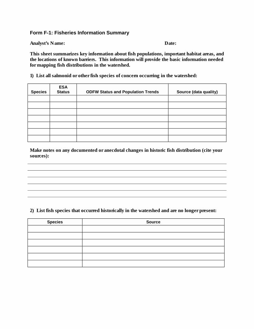
Form F-1: Fisheries Information Summary
Analyst’s Name: Date:
This sheet summarizes key information about fish populations, important habitat areas, andthe locations of known barriers. This information will provide the basic information neededfor mapping fish distributions in the watershed.
1) List all salmonid or other fish species of concern occurring in the watershed:
SpeciesESA
Status ODFW Status and Population Trends Source (data quality)
Make notes on any documented or anecdotal changes in historic fish distribution (cite yoursources):
2) List fish species that occurred historically in the watershed and are no longer present:
Species Source

Form F-1: page 2
3) List species that have been or are currently stocked in the watershed:
Species Stocking NotesNative orExotic? Source
4) Identify life history patterns of key fish species:
SpeciesA-Anadromous
R-Resident Location Spawning Timing Outmigration Timing
Notes:
5) Identify important locations for adult holding, spawning, summer, and winter rearing:
Location Species/Purpose Source
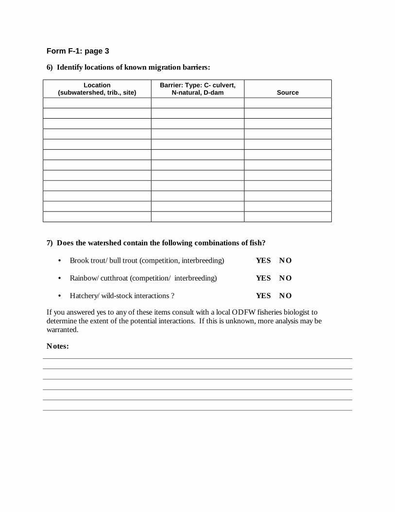
Form F-1: page 3
6) Identify locations of known migration barriers:
Location(subwatershed, trib., site)
Barrier: Type: C- culvert,N-natural, D-dam Source
7) Does the watershed contain the following combinations of fish?
• Brook trout/bull trout (competition, interbreeding) YES NO
• Rainbow/cutthroat (competition/ interbreeding) YES NO
• Hatchery/wild-stock interactions ? YES NO
If you answered yes to any of these items consult with a local ODFW fisheries biologist todetermine the extent of the potential interactions. If this is unknown, more analysis may bewarranted.
Notes:


Form F-2a: Pool Habitat Condition Summary
This form will be filled out for each subwatershed where ODFW or other comparable habitat data exist. Measured values are recordedand compared to rating criteria.
Analyst’s Name: Date Page of
Subwatershed: Data Sources: Data Dates:
Site
LengthSampled(Prichnll)
Land Use(Luse1) Gradient CHT Width Pool Area Pool Frequency
Residual PoolDepth Complex Pools
OverallPool
Rating
Pctpool Bench-mark
CWpool Bench-mark
Residpd
Bench-mark
Compool_km
Bench-mark
Conclusions:


Form F-2b: Riffle and Woody Debris Habitat Condition Summary
This form will be filled out for each subwatershed where ODFW or other comparable habitat data exist. Measured values are recordedand compared to rating criteria.
Analyst’s Name: Date Page of
Subwatershed: Data Sources: Data Dates:
SiteWidth/Depth
Ratio Gravel (% area)Silt-sand-organics
(% area)
OverallRiffle
Rating LWD Pieces/100 m Volume LWD/100 m Key Pieces/100 m
OverallLWD
Rating
WDratioBench-mark Pctgravel
Bench-mark Pctsndor
Bench-mark LWDpiece1
Bench-mark LWDvol1
Bench-mark KeyLWD1
Bench-mark
Conclusions:

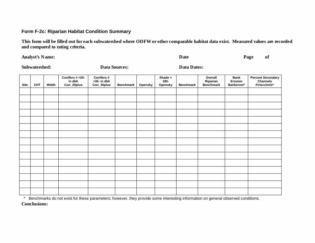
Form F-2c: Riparian Habitat Condition Summary
This form will be filled out for each subwatershed where ODFW or other comparable habitat data exist. Measured values are recordedand compared to rating criteria.
Analyst’s Name: Date Page of
Subwatershed: Data Sources: Data Dates:
Site CHT Width
Conifers # >20-in dbh
Con_20plus
Conifers #>35- in dbhCon_35plus Benchmark Opensky
Shade =180-
Opensky Benchmark
OverallRiparian
Benchmark
BankErosion
Bankerosi*
Percent SecondaryChannels
Pctscchnls*
* Benchmarks do not exist for these parameters; however, they provide some interesting information on general observed conditions.
Conclusions:


Form F-3: Fish Passage Evaluation
Analysts Name:
Date: Page of
Subwatershed:
RoadCrossingNumber
CrossingType¹
CrossingSlope
OutletDrop
OutletPool
ResidualDepth
InletDrop
InletDiameter
StreamBankfull
WidthCrossingLength
CrossingRating²
SpeciesBlocked
EstimatedHabitatBlocked
1- Crossing Types: B-Bridge, A- Arch, BC-Bare Culvert, EC-Embedded Culvert, BC-Baffled Culvert
2- Crossing Ratings: JB-Juvenile Barrier, AB-Adult Barrier, PB- Potential Partial/Seasonal Barrier, P-Passable, U-Unknown


Form F-4: Fish Passage Field Assessment.
Watershed:
Analyst’s Name: Date:
Crossing Number:
The culvert height measurements are taken to calculate culvert slope. These measurements requirethat a level be set up on the road crossing between the upstream and downstream end of the culvert.The upstream and downstream measurements are made by placing a stadia rod on the end of theculvert and reading the measurement through the level. As an alternative, culvert slope can bemeasured using a string attached to the culvert inlet. Level the string and measure the height of thestring above the outlet (rise). The culvert slope can be calculated by dividing the rise by the lengthof the culvert (run).
Hike down to the culvert and take the illustrated measurements and fill in the measured values:
Measurement Units
Length of Culvert Feet
Culvert Diameter Inches
Outlet Drop (height above stream surface) Inches
Pool Depth (outlet pool residual depth) Feet
Culvert Gradient/Crossing Slope Drop in inches or % slope
Culvert Inlet Width Inches
Culvert Inlet Drop inches
Stream Gradient Above Culvert % slope
Stream Gradient Below Culvert % slope
Stream Bankfull Width Above the Culvert feet

Form F-4: page 2
Culvert Material (circle one):
galvanized steel tarred galvanized steel concrete
wood aluminum other
Describe any internal baffles, weirs, or bedload materials:
Who owns/maintains the culvert?
Is the culvert in good physical condition?
Fish species present above culvert?
Fish species present below culvert?
Describe upstream adult or juvenile passage problems, if any:
In your opinion, what improvements may be needed:

Form F-4: page 3
Other comments, observations:
Photo:


Form F-5: Fish Assessment Confidence Evaluation
Watershed:
Analyst’s Name:
Technical expertise or relevant experience:
Resources used:
! ODFW personnel (list):! ODF personnel (list):! federal (USFS, BLM, NMFS) (list):! stream surveys (list):"! newspaper archives! private landowners (list):! others (list):
Published surveys or reports: (examples: ODFW stream surveys for ___ miles of stream in the ([sub]watershed,or USFS/BLM watershed analysis report for [sub]watershed):
Confidence in distribution maps:
! Local expert says high / low (circle one) degree of accuracy based on field experience (providename of local expert):
! High degree of accuracy as field verification of fish presence/absence were available (providesource of info/mapping):
! No verification; map based on recommendations of local professional (provide name):! No verification; map based on personal judgement! Additional criteria/relevent information (describe):

Form F-5: page 2
Confidence in habitat assessment:
! Low: Unsure of procedures; didn’t consult expert; no field verification! Low to moderate: Understood and followed procedures; no field verification! Moderate: Some field verification and found field conditions different from data descriptions! Moderate to high: Field surveys available and useful for many streams; no field verification! Moderate to high: Some field verification on questionable segments only! High: Used field surveys and field-verified many segments! If none of above categories fits, describe your own confidence level and rationale:
Confidence in barrier identification:
! Low: Unsure of procedures; didn’t consult expert; no field verification! Low to moderate: Understood and followed procedures; no field verification! Moderate: Some field verification! Moderate to high: Some field verification; few unknowns! High: Field-verified most crossings or good data available! If none of above categories fits, describe your own confidence level and rationale:
Recommendations for additional field verification, or habitat or fish population surveys, ifany, and why:

Component VRiparian/WetlandsAssessmentTable of Contents
Introduction......................................................V-1
Section I: Riparian Zone Condition.................V-1
Critical Questions .........................................V-1
Assumptions.................................................V-1
Materials Needed .........................................V-2
Time Needed................................................V-2
Necessary Skills ...........................................V-3
Final Products of the Riparian Zone
Condition Section ...................................V-3
Methods .......................................................V-3
Section II: Wetland Characterization and
Functional Assessment .....................V-13
Purpose......................................................V-13
Critical Questions .......................................V-13
Assumptions...............................................V-13
Materials Needed .......................................V-14
Necessary Skills .........................................V-16
Final Products of the Wetland
Characterization Section.......................V-16
Wetland Characterization Methods.............V-16
References .....................................................V-28
Glossary .........................................................V-30
Appendix V-A: Blank Forms
Form R-1: Riparian Condition Units
Form R-2: Riparian Recruitment
Situation Description
Form R-3: Riparian Conditions
Confidence Evaluation
Form W-1: Table of Wetland Attributes
Form W-2: Wetland Confidence
Evaluation
Appendix V-B: Field Measurement of
Stream Shading


Oregon Watershed Assessment Manual Page V-1 Riparian/Wetlands Assessment
Component VRiparian/Wetlands Assessment
INTRODUCTION
The interactions between riparian/wetland 1 areas, streams, and fisheries habitats are discussed inthe Introduction section of this manual. The focus of this Riparian/Wetlands component is todescribe the assessment techniques for these areas. This portion of the manual is broken into twoassessment sections. Section I describes the methods to assess current riparian vegetationconditions, and their impacts on recruitment of large wood and shade. Section II describes themethods to characterize wetland conditions in the analysis area. After the wetland section is a list ofreferences for further reading and background information on riparian/wetland characterization. InAppendix A are all of the necessary forms for completing each of these assessments.
SECTION I: RIPARIAN ZONE CONDITION
Critical Questions
1. What are the current conditions of riparian areas in the watershed?
• To determine conditions, users will examine riparian area width, vegetation types, andvegetation density, stream shading, and the continuity or interruption of the riparianzone from road crossings, streamside roads, and other land uses.
2. How do the current conditions compare to those potentially present or typically present forthis ecoregion?
• Users will use Level IV ecoregion vegetation descriptions to complete this comparison.
3. How can the current riparian areas be grouped within the watershed to increase ourunderstanding of what areas need protection and what the appropriaterestoration/enhancement opportunities might be?
• Using information from the riparian evaluation, users will group riparian areas by sourcesof impact.
Assumptions
1. The riparian vegetation descriptions developed for Level IV ecoregions will provide insighton the most likely vegetation found in riparian zones, and vegetation types with the highestpotential to become established in a riparian zone.
2. The vegetation likely to occur in a given riparian zone can be defined by the ChannelHabitat Type (CHT) and ecoregion, which together integrate important site characteristicsi.e., moisture, disturbance, influence of beavers, etc.).
1 Terms that appear in bold italic are defined in the Glossary at the end of this component.

Oregon Watershed Assessment Manual Page V-2 Riparian/Wetlands Assessment
3. Large wood (sometimes referred to as large woody debris) is an important component ofin-stream habitat in ecoregions that historically were forested, or had forested riparian areas.The importance of large wood for in-stream habitat will vary in ecoregions with sparselyforested riparian areas, and those where trees do not naturally occur.
4. Well-stocked riparian stands, often dominated by conifers, will provide adequate long-termsupplies of large wood to a stream channel. In some situations, riparian stands dominatedby hardwoods will contribute important amounts of large wood.
5. Recruitment distance of in-channel large wood will vary by ecoregion, and is a function ofpotential tree height. The majority of wood recruitment will come from riparian forestswithin 100 feet of the stream (horizontal distance) or less.
Materials Needed
• 1:24,000-scale Oregon Department of Forestry (ODF) base maps (from Start-Up andIdentification of Watershed Issues component).
• CHT maps from the Channel Habitat Type Classification analyst
• Recent stereo aerial photographs covering the entire assessment area (from Start-Up andIdentification of Watershed Issues component).
• Stereoscope for 3-D viewing of aerial photographs. Although a mirrored stereoscope (withmagnification) is preferable, a simple lens stereoscope is adequate.
• Aerial photo scale for measuring riparian area widths, etc. Scale should be the same as theaerial photographs used.
• Map wheel for measuring lengths of riparian areas.
• Land use maps (optional). May be useful in determining land use associated with ripariandisturbance.
• Level IV ecoregion map and descriptions of ecoregions occurring in the watershed.
• Stream survey summaries from the Fish and Fish Habitat Assessment that describe riparianvegetation composition and shade summaries (if available).
• Paper copies of Riparian Assessment Forms or a spreadsheet set up in the same format.(Note: spreadsheet templates for the various forms needed for the assessment may beavailable on the Internet; check http://www.state.or.us/agencies.ns/69000/00070/)
Time Needed
Aerial photo assessment time will vary depending on the size of the assessment area, the type ofvegetation present, the amount of disturbance in riparian areas, and, most importantly, the skill ofthe person doing the interpretation. In a test of the methodology, a skilled assessment person was

Oregon Watershed Assessment Manual Page V-3 Riparian/Wetlands Assessment
able to interpret riparian conditions at the rate of approximately 11 minutes/mile of stream, or 18hours/100 miles of stream. The use of a computer spreadsheet rather than paper forms will greatlyspeed up summarizing and analyzing riparian conditions.
Necessary Skills
Ability to interpret vegetation type, size and density are the most important skills needed for thisportion of the assessment. Although a person with no prior experience in aerial photointerpretation could complete this assessment, they should plan on spending considerable timelearning the skills needed, and allow ample time to field-verify their initial estimates of riparianconditions (see Start-Up and Identification of Watershed Issues component for listing of referenceson aerial photo interpretation). Many watershed councils have members or land owners in thewatershed with staff who are skilled in aerial photo interpretation, and who should be contacted toeither perform the assessment or assist in training others to perform the assessment. Other skillsneeded include the ability to make measurements from aerial photographs, the ability to read andinterpret topographic maps, and the ability to use a computer spreadsheet.
Final Products of the Riparian Zone Condition Section
This assessment will result in the following forms (Appendix A) and maps:
• Form R-1: Riparian Condition Unit Information• Form R-2: Riparian Recruitment Situation Description• Form R-3: Riparian Conditions Confidence Evaluation• Map R-1: Riparian Condition Unit Map• Map R-2: Riparian Recruitment Situations Map• Map R-3: Riparian Shade Map
Methods
Overview
This portion of the assessment is conducted using aerial photographs—with field verification astime and interest permits—and produces a database and maps of riparian characteristics. Thefundamental mapping unit, for which all information in this portion of the assessment is collected, isdefined here as the Riparian Condition Unit or RCU. An RCU is a portion of the riparian area forwhich riparian vegetation type, size, and density remain approximately the same. When ripariancharacteristics change a new RCU is defined. Each RCU occurs on only one side of the stream (i.e.,riparian areas on the opposite side of the stream are separate RCUs).
Information for each RCU is collected on Form R-1 (a separate row for each RCU), and mapped onMap R-1. As a rule of thumb, the minimum length for an RCU should be approximately 1,000 feet;however, there will be situations where a shorter length may be required. Information from FormR-1 will be used to group RCUs into similar Riparian Recruitment Situations (i.e., groups ofRCUs that have similar characteristics and that may be treated similarly for the purposes ofrestoration/enhancement) on Map R-2. Finally, information from Form R-1 will be used to groupRCUs into similar shade categories and mapped on Map R-2. Use of a computer spreadsheet willgreatly facilitate these summaries and groupings.

Oregon Watershed Assessment Manual Page V-4 Riparian/Wetlands Assessment
WHERE TO BEGIN
All of the materials have been gathered together, abase map is laid out on a large table, aerial photos areclose at hand, and the daunting task of looking at eachstream in the watershed is ahead of you. Where tobegin! Although there is no “rule” about where to startor which order to proceed, it is suggested that youbegin at the outlet of a small subwatershed and moveupstream along the primary stream, picking up eachtributary as you go. From there, try looking at a fewmiles of the largest river in the watershed. Try to picksome areas that are easily accessible from a road sothat you can go out and field-check your initial work.
Step 1: Prepare
All of the items listed in the Materials section should first be gathered. The boundaries of thewatershed and subwatersheds should be drawn on the base maps that were completed in the Start-Up and Identification of Watershed Issues component. Consult the Ecoregions appendix of thismanual for a listing of potential streamside vegetation types found within the ecoregion(s) withinthis watershed. The Ecoregions appendix will list potential streamside vegetation by three channelconstraint groups: constrained, semiconstrained, and unconstrained. Keep this table handy.
Step 2: Map Riparian Condition Units
Choose a Starting Point
As mentioned previously, the fundamental mapping unit, for which all information in this portion ofthe assessment is collected, is the Riparian Condition Unit (RCU). Beginning at a logical startingpoint on the aerial photographs (seeWhere to Begin sidebar for suggestions),follow along the stream until youencounter changes in any of the followingcharacteristics:
• Vegetation (type, size, density)• Stream size or other changes• CHT• Ecoregion• Subwatershed
Mark each end of the RCU with a pencilmark perpendicular to the stream, andassign it a number (see Note RCU Number subsection below for suggestions on developing anumbering system). Try to keep each RCU no less than 1,000 feet in length. Remember that eachRCU occurs on only one side of the stream (i.e., riparian areas on the opposite side of the stream areseparate RCUs).
Note Which CHT the RCU is in
Note on Form R-1 what CHT the RCU is in. If the RCU boundaries that you have tentativelyselected overlap more than one CHT, than split the RCU into two (or more) RCUs at the CHTboundary(ies). Information about CHTs is necessary to estimate potential vegetation condition(which varies by CHT), as well as to prioritize restoration efforts when completing the WatershedCondition Evaluation component (some CHTs are more responsive to large wood than others).
Note Riparian Assessment Width(s)
The Ecoregion appendix contains tables of Potential Streamside Vegetation for each ecoregion.Although recruitment has the potential to come from as far away from the stream as the sitepotential tree height, the majority of functional wood is recruited within 100 feet (horizontaldistance) or less (depending on ecoregion) of the stream’s edge (e.g., McDade et al. 1990). Riparian

Oregon Watershed Assessment Manual Page V-5 Riparian/Wetlands Assessment
areas in some ecoregions will have distinct characteristics within this normal zone of large woodrecruitment (e.g., a band of red alder or other hardwoods from 0 to 25 feet [horizontal distance]from the stream edge, and conifers from 25 to 100 feet). Look-up the Potential StreamsideVegetation for ecoregion(s) your watershed is in to determine the assessment width of the riparianarea closest to the stream (referred to in the table as Riparian Area 1 or RA1), and the distance forthe remainder of the recruitment zone (RA2). The widths of RA1 and RA2 will also changedepending on which Channel Constraint Group (Table 1) the RCU falls into. Write down the widthof RA1 on Form R-1. Some ecoregions or CHTs will have only one assessment width.
Note Riparian Vegetation Characteristics
Locate RA1 and RA2 on the aerial photos, using an aerial photo scale to identify the widths of eachRA if necessary. For both RA1 and RA2 note the riparian vegetation characteristics on Form R-1using a three-letter code that describes vegetation type (first letter), vegetation size (second letter),and vegetation density (third letter). Choices are given in Table 2. For example, “CSD” wouldmean a riparian stand that is predominantly conifer, small in size, and dense.
Using the aerial photographs you will be able to detect the relative height of riparian stands, and therelative size of the tree crowns. Relating these characteristics to average stand size is a skill that canonly be developed by field-verifying your initial estimates. If any survey information is available forstreams in the assessment area, it may also be possible to find descriptions of riparian vegetation thatmay help to verify estimates that you have made from aerial photos.
Sometimes stand conditions will not be uniform with respect to tree size. An example would besituations where large individual trees (left from an earlier timber harvest) are interspersed within anotherwise small stand. This condition should be noted on Form R-1. If these anomalies occurfrequently it may be desirable to define these stands as a separate Riparian Recruitment Situation(discussed below), because enhancement opportunities may be different for these stands.
Table 1. CHTs found in Channel Constraint Groups
Channel ConstraintGroup Channel Habitat Types
Constrained channels LC Low Gradient ConfinedMC Moderate Gradient ConfinedMH Moderate Gradient HeadwaterMV Moderately Steep Narrow ValleyBC Bedrock CanyonSV Steep Narrow ValleyVH Very Steep Headwater
Semiconstrainedchannels
ES Small EstuaryEL Large EstuaryAF Alluvial FanLM Low Gradient Moderately ConfinedMM Moderate Gradient Moderately Confined
Unconstrained channels FP1 Low Gradient Large FloodplainFP2 Low Gradient Medium FloodplainFP3 Low Gradient Small Floodplain

Oregon Watershed Assessment Manual Page V-6 Riparian/Wetlands Assessment
Table 2. Codes to describe vegetation type (modified from WFPB 1997).
Vegetation Type
C Mostly conifer trees (>70% of area)
H Mostly hardwood trees (>70% of area)
M Mixed conifer/hardwoods
B Brush species
G Grass/meadow
N No riparian vegetation
Tree Size Classes
R Regeneration (<4-inch average diameter at breast height (DBH)
S Small (4- to 12-inch average DBH)
M Medium (>12- to 24-inch average DBH)
L Large (>24-inch average DBH)
N Nonforest (applies to vegetation Types B, G, and N)
Stand Density
D Dense (<1/3 ground exposed)
S Sparse (>1/3 ground exposed)
N Nonforest (applies to vegetation Types B, G, and N)
Note RCU Number
For each RCU recorded on Form R-1, assign a unique number (RCU#) that links it to the RCUmapped on Map R-1. Write the RCU number on Map R-1 as well.
Complicated systems to number RCUs can be devised; however, it is suggested to simply start withthe number “1” and number RCUs sequentially from that point. The additional informationcollected for each RCU (described below), and the use of a computer spreadsheet to organize thedata, will allow you to easily extract information about a particular stream, sub-basin, etc., and willeliminate the need for a complicated numbering system.
Note Stream Bank
On Form R-1 note which stream bank the RCU lies on (R for right bank looking downstream or Lfor left bank looking downstream). This information is useful for locating the RCU on the map orout in the field.
Measure and Note Length of RCU
Using a map wheel, measure the length of the RCU in feet and note it on Form R-1. Thisinformation will be used to summarize the various condition categories of riparian stands.

Oregon Watershed Assessment Manual Page V-7 Riparian/Wetlands Assessment
Note the Name of the Stream (or lake)
Find the name of the stream or lake on the base map and note it on Form R-1. Unnamed tributariescan be numbered sequentially staring with the first unnamed tributary working in an upstreamdirection. For example, the first unnamed tributary to “Madeline Creek” can be named “MadelineCk Unn Trib #1,” the second can be named “Madeline Ck Unn Trib #2,” etc. Unnamed tributariesentering other unnamed streams can be named using the same convention (e.g., the first unnamedtributary entering Bear Creek can be named “Bear Ck Unn Trib #1,” the first tributary entering thatstream can be named “Bear Ck Unn Trib #1, Unn Trib #1”, etc.). This information is useful forextracting data about a stream of interest.
Note the Name of the Subwatershed
Note the name of the subwatershed on Form R-1. This information is used to summarize riparianconditions by sub-basin.
Note the Ecoregion
Note on Form R-1 the ecoregion that the RCU is in. (If the entire watershed is in the sameecoregion, this column can be left blank).
Note the Stream Size
Note on Form R-1 the stream size (L-large, M-medium, S-small) from the ODF base map.Additionally, if a stream is noted on the ODF base map as being non-fish-bearing, note this onForm R-1 with an “N” suffix. (For example, a small stream that is non-fish-bearing would be notedas “SN”). All RCUs must be split at stream-size breaks. This information is used in the WatershedCondition Evaluation to prioritize restoration projects.
Note Permanent Discontinuities
In some situations the vegetation characteristics of an RCU may be broken up, and recruitmentlimited by permanent discontinuities. For example, there may be a road within the RCU along theentire length, severely limiting riparian recruitment. If any permanent discontinuity exists within theRCU, and it covers more than 30% of the total area of the RCU, the source of the discontinuityshould be noted on Form R-1 (e.g., “Road”). This information will be used to define RiparianRecruitment Situations where permanent discontinuities exist, and will also be used in the WatershedCondition Evaluation to prioritize restoration projects.
Note Stream Shading
RCUs each occur on only one side of the stream, but the amount of shade that the streamexperiences is a result of conditions on both sides of the stream. Nevertheless, it is reasonable forour purposes to estimate the amount of shade that each RCU provides independent of conditionson the opposite bank. Using the aerial photographs and Table 3, which provides indicators ofstream shading, estimate the shade category (H, M, or L) for each RCU and record it on Form R-1.This information will be used to produce Map R-3, and in the Watershed Condition Evaluation.

Oregon Watershed Assessment Manual Page V-8 Riparian/Wetlands Assessment
Table 3. Shade estimation criteria (modified from WFPB 1997).
Indicator Shade Code
Stream surface not visible, slightly visible, or visible in patches >70% H
Stream surface visible but banks are not visible 40-70% M
Stream surface visible; banks visible or visible at times <40% L
If any survey information is available for streams in the assessment area, it may be possible to finddescriptions of stream shading that may help to verify estimates that you have made from aerialphotos.
If you are unfamiliar with estimating shade from aerial photographs, you may wish to field-verifysome of your initial estimates. A methodology for measuring shade in the field is given inAppendix B.
Additional Notes
The final item of information gathered for each RCU is any additional notes that might be helpful indefining the Riparian Recruitment Situations (described in Step 4). For example, you might considerrecording information on types of land use associated with riparian disturbance, sources ofdiscontinuity, presence of beaver ponds, etc.
At this point, Map R-1 is completed and shows all of the RCUs in the watershed. Form R-1 is alsocomplete, with the exception of the Riparian Recruitment Situations column.
Step 3: Perform Field Verification
Field visits can greatly enhance the understanding of riparian conditions. However, it is understoodthat all watershed councils may not have the time or resources available to do this. It is possible togenerate a basic RCU map without field visits, but the accuracy of the information will greatlyimprove with field verification. Field verification early in the process (i.e., after a few initialestimates of riparian conditions in a few parts of the watershed) may be the most useful, as it willhelp you “calibrate” your eye, and give you an understanding of what the aerial photos look likecompared to on-the-ground conditions.
Visit a sampling of RCUs to evaluate conditions in the field. Use the following list to guide yourfield sample selection. Consider visiting those areas where you experienced one or more of thefollowing situations:
• You were unable to determine information required to complete Form R-1 from the mapsand photos.
• The information on the map did not match your recollection or data collected in the area.
• The information on different maps or photos conflict with each other.
In addition, sample a range of RCUs scattered throughout the watershed.

Oregon Watershed Assessment Manual Page V-9 Riparian/Wetlands Assessment
Based on the time available, determine a goal for the number of RCUs you will be able to visit.Make a list of areas to be visited using the guidelines above, and refine it to meet your goal. It isdifficult to give useful estimates for the time a field visit will take, but be aware that in manywatersheds, the travel time to an area will be the most time-consuming step of the field work. Onceyou are at the site, the RCU can usually be evaluated in less than an hour; sometimes substantiallyless.
Plan your field day and assemble your materials before visiting the field. The following steps willassist you in this process.
1. Plan an efficient route, and try to determine the most likely spots from which to access or atleast view the area. If necessary, contact the property owner and request permission to visitthe area. If you do not contact landowners ahead of time, you may wish to carry a letter ofexplanation to give to landowners. If gaining access to an area is a problem, it may benecessary to view the area from public roadways with binoculars.
2. Generate a field form by either printing the spreadsheet or photocopying Form R-1. Oncein the field, evaluate the accuracy of each item in Form R-1.
3. For each area to be visited, assemble a packet that includes a photocopy of the relevantportion of the base map, field form, and aerial photograph.
In addition to field work, data collected from other sampling efforts can be used to validate themapping. Stream surveys have been completed by a variety of agency and private entities (OregonDepartment of Fish and Wildlife [ODFW], US Forest Service, US Bureau of Land Management,tribes, county or local municipalities, etc.). Depending on when the survey was completed and theprotocol that was used, the survey may describe riparian vegetation composition and contain shadesummaries. The Fish and Fish Habitat Assessment component will help you compile andsummarize this survey data. The fisheries analyst will be able to provide available data and a copy ofcompleted Form F-2, which summarizes riparian conditions in stream reaches that have beensurveyed.
Step 4: Define and Map Riparian Recruitment Situations
Determining Where Current Recruitment Potential is Adequate
At this point you want to decide, for each RCU, if current riparian conditions provide adequate orinadequate recruitment potential. This task requires comparing current conditions to the potentialvegetation descriptions for that ecoregion (see Ecoregions appendix for descriptions; note thatpotential vegetation descriptions vary by channel confinement classes), using the decision treeshown in Figure 1. If current conditions are as good or better (i.e., conifers are better thanhardwoods; large trees are better than medium trees; dense stands are better than sparse stands) thanthe potential conditions for both RA1 and RA2, then current recruitment potential is considered tobe adequate. If current conditions are not as good as potential conditions, then recruitment isconsidered to be inadequate. Note in the Riparian Recruitment Situations column on Form R-1 allthe RCUs that have adequate current recruitment potential, and go on to the next step.

Oregon Watershed Assessment Manual Page V-10 Riparian/Wetlands Assessment
Defining Riparian Recruitment Situations
You have now determined which RCUs have adequate current recruitment potential, and which donot. You could simply stop at this point; however, you do not know the underlying reasons whyrecruitment is inadequate, nor do you have any way to logically group RCUs for restorationpurposes. Riparian Recruitment Situations are a way to group the RCUs into several categories thatmay respond to similar restoration treatments, and to summarize the major riparian impacts in thewatershed.
At this point you need to define a set of Riparian Recruitment Situations that are appropriate for thewatershed in question. The first Situation will always be those stands where current recruitmentpotential is adequate (determined in the previous step). You now need to go through the notescollected during the aerial photo interpretation and decide on several Situations that make sense forthe watershed. Questions to consider when developing Riparian Recruitment Situations for yourwatershed include the following: What are the land uses that limit recruitment potential? What arethe primary stand types (e.g., small conifer plantations, stands of large hardwoods, narrow buffers ofhardwoods between agricultural fields and the stream, etc.)? What are the areas where wetlands,residential development, etc., limit tree growth? What are the sources of permanent discontinuitiesin riparian areas (e.g., roads, power lines, etc.)?
Figure 1. This decision tree will help you determine if current riparian conditions provideadequate or inadequate recruitment potential in a Riparian Condition Unit, by comparingcurrent conditions to the potential vegetation descriptions for that ecoregion.

Oregon Watershed Assessment Manual Page V-11 Riparian/Wetlands Assessment
A description of each Situation should be filled out on Form R-2 (one sheet for each Situation), andthe Riparian Recruitment Situation noted for each RCU on Form R-1. Examples of RiparianRecruitment Situations from a Coast Range watershed assessment are provided in Table 4.
Mapping Riparian Recruitment Situations
Now all RCUs have been assigned a Riparian Recruitment Situation type on Form R-1, and eachSituation has been described on Form R-2. The next step is to assign a mapping color to eachSituation and map them on Map R-2. There are two possible approaches to take. The firstapproach is to overlay a large piece of drafting vellum (a semitransparent material, so the RCUboundaries and numbers can be viewed) on Map R-1 and color all RCUs that are in the sameRiparian Recruitment Situation the same color. The second approach is to make a large photocopyof Map R-1 and color-code the Riparian Recruitment Situations. In either case, having Form R-1 ina computer spreadsheet will allow you to sort RCUs and create a list by Riparian RecruitmentSituation. A wide felt-tip marking pen works well in coloring the Riparian Recruitment Situations(Figure 2, page V-12).
Step 5: Produce Shade Map
Assign a mapping color to each of the three shade categories described in Table 3. Then, usingeither a new piece of drafting vellum or a new photocopy of Map R-1, color-code all RCUs that arein the same shade category to produce Map R-3. Again, having Form R-1 in a computerspreadsheet will allow you to sort RCUs and create a list by shade categories.
Table 4. Riparian Recruitment Situations: An example from a Coast Range watershed.
Riparian Recruitment Situation Description
Adequate No enhancement needed (dense stands of large-sized conifers).
Small stands Stands that are generally too small to provide recruitment undercurrent conditions. The land use associated with these stands isforestry.
Large hardwood stands These stands are also associated with forestry land use. Thesestands are primarily areas of large hardwoods.
Agriculture The land use associated with these stands is agriculture. Theseareas that have no or very narrow buffers between agriculturalland and the streams.
Development The land use associated with these stands is residentialdevelopment. Buffers are either absent, small hardwoods, orlawns.
Infrastructure Areas where roads and power lines have created permanentdiscontinuities in riparian conditions.
Beaver These are areas where beaver ponds are limiting riparianrecruitment.
Wet/meadow Wetland conditions limit riparian recruitment.

Oregon Watershed Assessment Manual Page V-12 Riparian/Wetlands Assessment
Step 6: Evaluate Confidence in Riparian Assessment
Using the Riparian Conditions Confidence Evaluation Form (R-3), describe your level of confidencein this assessment. This can include a discussion of the limits of available information, of theamount of field verifying that was possible, and identification of areas where further investigation ordata collection might yield either better results or more confidence in the assessment.
Review the critical questions. Are there any questions that it was not possible to answer, for anyreason? Can the reason be identified? Does this affect your confidence in one of the areas ofanalysis? If so, and if the topic of concern has not already been identified on one of the evaluationforms, use the back of the form to describe the situation, and your resulting confidence level.
Figure 2. In this portion of a Riparian Recruitment Situation map, similar RCUs (numberedin the figure) are grouped by Riparian Recruitment Situation and color-coded on the map.(Colors are depicted with textures in the figure.)
Oregon Watershed Assessment Manual Page V-13 Riparian/Wetlands Assessment
SECTION II: WETLAND CHARACTERIZATION AND FUNCTIONALASSESSMENT
Purpose
Wetlands are protected by federal, state, and local regulations. In order to plan for growth anddevelopment in a watershed, it is necessary to know where these resources are. In addition,wetlands can contribute to critical functions in the health of a watershed, as discussed in theIntroduction section of this manual. Determining the approximate location and extent of wetlandsmay be essential in solving problems within the watershed.
The purpose of the wetland characterization is to gain specific information on the location andattributes of wetlands in the watershed, including (but not limited to) size, habitat type, surroundingland use, connectivity, and opportunities for restoration. This process will also assist indetermining the relationship between wetlands and problems in the watershed that are identifiedthrough other assessments conducted in the watershed analysis process. In addition, the methodwill help watershed councils determine whether it is appropriate or necessary to collect additionaldata on wetland function.
Critical Questions
1. Where are the wetlands in this watershed?
• Wetland locations will be identified and mapped using National Wetland Inventory(NWI) maps, aerial photos, and other resources.
2. What are the general characteristics of wetlands within the watershed?
• The characteristics or attributes of known wetlands will be documented.
3. What opportunities exist to restore wetlands in the watershed?
• Restoration opportunities that are obvious from aerial interpretation, such as presence offill, clearing, grazing, or ditching in wetlands, are identified in the wetlandcharacterization, which results in a list of possible restoration sites.
Assumptions
1. Wetlands are protected by federal, state, and local regulations. In order to plan for growthand development in a watershed, it is necessary to know where these resources are. Inaddition, wetlands can contribute to critical functions in the health of a watershed, asdiscussed in the Watershed Fundamentals component of this document. Determining theapproximate location and extent of wetlands may be essential in solving problems within thewatershed.
2. Although there is no definitive correlation between readily observable wetland conditions,such as size, habitat type, etc., and the functions the wetland provides, this information canoffer some indications. As examples, a wetland connected to a stream has a high likelihood

Oregon Watershed Assessment Manual Page V-14 Riparian/Wetlands Assessment
of providing winter fish habitat, while a large wetland in the middle elevation of thewatershed may contribute significantly to flood control.
3. Some restoration opportunities are obvious from aerial interpretation. However, wetlandrestoration is complex, and the process outlined in this document will only provide a first-cut at identifying restoration opportunities.
Materials Needed
A number of existing resources may be available to assist in identifying wetlands in the watershed.Although all of these may not be available, assemble as many of these as possible before beginning.The following list presents these resources in descending order of usefulness for this project.
• Local wetland inventory. Several (45 at the time of this printing) of the communities inOregon have completed local wetland inventories. Most of these have focused on urbanareas. To determine what is available for your watershed, contact the Oregon Division ofState Lands at (503) 378-3805.
• National Wetland Inventory (NWI) maps. NWI maps are available for the most ofOregon. These maps are produced by the US Fish and Wildlife Service. Using USGeological Survey (USGS) quadrangle maps as a base, NWI maps indicate the location, size,and habitat type of wetlands. Maps may be purchased either through the Oregon Divisionof State Lands at (503) 378-3805, or from the USGS at (800) USA-MAPS.
These maps are also available digitally, which will be extremely valuable if maps for theproject will be produced on a Geographic Information System (GIS). NWI digital datacan be purchased through the agencies listed above, and are also available free of charge viathe Internet. The NWI’s World Wide Web server can be accessed athttp://www.nwi.fws.gov/. This web site is organized by 1:250,000-scale quadrangle maps.Each of the folders listed is the name of a 1:250,000-scale map. Determine the names of the1:250,000-scale maps for your area, and look for that folder; within each folder is data foreach 7.5-minute quadrangle map in that area. Figure 3 presents the status of NWI maps inOregon.
• Aerial photos. Information on how to obtain aerial photographs for the project is providedin the Start-Up and Identification of Watershed Issues component of this manual. Thesephotos can be invaluable at verifying and updating information from other resources,viewing the entire wetland when areas are not accessible, looking at how wetlands may beconnected to streams, and determining the dominant vegetation type, surrounding land use,and disturbances.
• Soil survey maps. Soil survey maps are prepared by the Natural Resource ConservationService (NRCS; formerly the Soil Conservation Service). In some instances, wetlands can beidentified by comparing the mapped soil type with the list of hydric soils for the State ofOregon. However, in order to meet the federal and state wetland definitions, wetlandvegetation and hydrology must also be present; hydric soils alone do not definitely indicatewetlands. Hydric soils can also be used to identify areas that were formerly wetlands—if anarea is mapped as having hydric soils but is not currently a wetland, it may be that a wetland

Oregon Watershed Assessment Manual Page V-15 Riparian/Wetlands Assessment
was present that has been drained or otherwise eliminated. Soil surveys are usually availablefree of charge. To order, contact NRCS at: State Conservationist, Federal Building, Room1640, 1220 SW 3rd Avenue, Portland, OR 97204-3221; (503) 414-3201. The hydric soils listfor the State of Oregon is available on the Internet at:http://www.statlab.iastate.edu/soils/hydric/sslists.html.
• USGS topographic maps. These maps will have been gathered for other portions of theassessment. These maps show lakes, ponds, and some wetlands, in addition to other helpfulfeatures such as topography, roads, and other landmarks.
Figure 3. National Wetland Inventory (NWI) maps are available for the most all of Oregon.Produced by the US Fish and Wildlife Service, these maps indicate the location, size, andhabitat type of wetlands.

Oregon Watershed Assessment Manual Page V-16 Riparian/Wetlands Assessment
Necessary Skills
The analyst for this assessment must be able to do the following:
1. Interpret aerial photographs.2. Read maps.3. Organize information in a spreadsheet (recommended but not required).
Final Products of the Wetland Characterization Section
• Map W-1: Wetland Locations• Form W-1: Wetland Attributes• Form W-2: Confidence Evaluation• Form W-3: Wetland Functions Table (optional)
Wetland Characterization Methods
The flow chart provided in Figure 4 presents the general steps necessary to complete the wetlandcharacterization and assessment. Each of those steps are explained in greater detail in the followingpages. Before beginning this process, it is strongly urged that you read through each of the steps.Although each step is laid out in a separate, sequential fashion, it may be most efficient to beworking various steps concurrently. For example, you may wish to be developing the Table ofWetland Attributes (Step 5) at the same time that you are creating the Wetland Locations Map(Step 2).
Step 1. Gather and Evaluate Existing Resources
Obtain as many of the maps identified in the Materials required section as are available. Review themaps you have gathered to identify which is the most complete starting point for the wetlandinventory. Select the most detailed wetland map available to be the base map.
Step 2. Integrate Resources to Create Preliminary Wetland Map
If the project will not be using GIS, generate a wetland base map by using the most complete of themaps gathered in Step 1. If you will not be using GIS, and your area does not have a local wetlandinventory for the entire watershed (this will be true in most cases), the most useful base map will bethe NWI map(s). Draw the watershed boundary on the base map(s) using the startup map provided.(See the Start-Up and Identification of Watershed Issues component of this document for moreinformation on how to generate a base map.) If a portion of the watershed has a wetland inventory,you can transfer that information to the NWI map, and consider it to be more accurate than theNWI maps.
Use personal knowledge, other maps, and aerial photographs to modify the base map with theaddition of wetlands. If you will be using NWI maps as a base, look at only the area greater than200 feet from the channel. This is to avoid having to examine the very complex NWI mapping thatcan occur near the channels. If the map for your area is not complex and difficult to interpret, youmay choose to include the channel areas in the assessment at this time. Do not include NWI-mapped wetlands that begin with the letter “R” (for riverine). For the purpose of this project, the

Oregon Watershed Assessment Manual Page V-17 Riparian/Wetlands Assessment
characterization will not include most rivers as wetlands (with the exceptions identified in Step 3). Ifmapping near the channel is complex, ignore the channels at this time. Wetlands near the channelwill be added during Step 3.
Step 3. Add Wetlands Identified in Riparian Evaluation and CHT Analyses
Interview the people doing the Riparian and Channel Habitat Type Classification evaluations togather information about wetlands within 200 feet of the channel. Add any areas that they haveidentified in their work near the channel to your wetland base map.
Figure 4. This flow chart presents the general steps necessary to complete the wetlandcharacterization and assessment. Although each step is laid out in a sequential fashion, it maybe most efficient to be working various steps concurrently.

Oregon Watershed Assessment Manual Page V-18 Riparian/Wetlands Assessment
Include anything identified by the riparian analyst as potentially wetland. This may include wetmeadows, shrub areas, or forests. To confirm these wetlands, examine NWI maps, aerialphotographs, and soil survey maps. If the area is indeed a wetland, the other sources should supportthat finding. If it is not clear, add it to the map, and tag it for field verification (Step 6).
Wetland areas may also be present in riparian areas mapped with the following channel habitat types:
• FP1—Low Gradient Large Floodplain• FP2—Low Gradient Medium Floodplain• FP3—Low Gradient Small Floodplain• LM—Low Gradient Moderately Confined• MM—Moderate Gradient Moderately Confined• AF—Alluvial Fan• ES—Estuary, Small• EL—Estuary, Large
These areas should also be confirmed by examining maps and photos to determine whether or notthey are wetlands. If they are or are likely to be wetland, they should be added to the map.
Step 4. Identify Restoration Opportunities
Add potential restoration areas to the map. Restoration areas would include disturbed wetlands orwetland buffers, or areas that were formerly wetland but have been converted to other land uses.These can be located on the maps and photos by looking for the following situations:
1. Areas show up as wetland in one source, but recent aerial photographs or personalknowledge indicate filling, clearing, grading, ditching/draining, or diking in the same area.
2. One of the following modifiers is indicated on the NWI map:d = partially drained/ditchedf = farmedh = diked/impounded
3. The soil survey indicates hydric soils, but the area does not appear to be wetland currently,based on other sources.
NOTE: This is only a first-cut at identifying possibilities, and does not indicate that these areas arenecessarily appropriate or feasible sites to restore. If, later on in this process, wetland restoration isidentified as a goal, a more thorough analysis of restoration potential should be conducted byindividuals with expertise in wetland restoration.
Step 5. Generate Preliminary Table of Wetland Attributes
Use Form W-1, or create a spreadsheet with similar columns. If you have more than a few wetlands,it may be extremely helpful to use a spreadsheet instead of the form provided, because it will allowyou to tabulate summary information in various ways with ease, should you wish to do that in thefuture.

Oregon Watershed Assessment Manual Page V-19 Riparian/Wetlands Assessment
HOW TO CALCULATE WETLAND ACREAGE
1. Determine the scale of your map or photo (e.g.,1 inch = 2,000 feet)
2. Measure the approximate length and width of thesubject wetland.
3. Multiply the length in inches times the scale of themap, and do the same for the width.
4. Multiply the resulting numbers by each other.
5. Divide the result by 43,560. The answer will be thewetland area, in acres, of the wetland.
Example:
Map scale: 1 inch = 2,000 feetWetland on map = 0.5 inches by 1.0 inches.Formula: [(0.5 x 2000) x (1 x 2000)] ÷ 43560 = 45.9 acres
Gather and enter the following information into the form or spreadsheet:
• Wetland ID: Assign anidentifying number to eachwetland. A suggested formatfor the ID number isTownship, Range, Section,and then a consecutivenumber. For example, 13-20N-4E-1, 13-20N-4E-2,refer to two different wetlandswithin Section 13, Township20 North, Range 4 East.Update your map and dataform concurrently by addingthe identifying number to thebase map.
• Sub-basin. Enter theappropriate sub-basin. Thiscan be useful later on if aparticular sub-basin isidentified as having a unique issue. Sub-basin information should be provided on the basemap provided for the project.
• Size. Estimate the size of each wetland in acres (see the sidebar above). Sources for thisinformation include NWI maps and aerial photographs. Use the source that offers the best(largest) scale on which to measure wetland size.
• Connected. If possible, determine whether there is a surface-water connection between thewetland and a stream. This is often difficult to do without field verification. A wetland isconnected if some part of it has a surface-water connection to a seasonal or perennialsurface water, including natural and man-made channels, lakes, or ponds. If there is anobvious stream inlet or outlet shown on the map, enter “Y” (yes) in this column. If thewetland appears to be isolated, (meaning no surface connection to a stream or ditch), enter“N” (no). If you are uncertain, enter “U” (unknown). If wetlands are connected, they aremore likely to provide fish habitat. Sources for this information include NWI maps, aerials,and USGS topographic maps.
• Cowardin Classification Code: (From NWI map). Each wetland shown on the NWI mapwill have a code that provides some information about the wetland. Generally, the firstthree letters are the most important for this purpose. This will indicate the class (e.g.palustrine, riverine, etc.) and the subclass (e.g. forested, emergent, etc.). Use the legendprovided on the map (Table 5 provides a summary) to interpret the remaining codes. If theNWI map indicates more than one code, list all codes in separate columns in the form orspreadsheet. Note that these NWI codes may be helpful in identifying restorationopportunities, as described in Step 4.

Oregon Watershed Assessment Manual Page V-20 Riparian/Wetlands Assessment
• Buffer: Using the aerial photographs, list the dominant land use within 500 feet of thewetland edge. Use the following codes: Fo = forest or open space, Ag = agriculture(pasture, crops, orchards, range land), R = rural (mix of small-scale agriculture, forest,and/or rural residential), or D = developed (residential, commercial, industrial). If morethan one of these exists, list the dominant (>50% of the area) land use. If two land uses arefairly equally represented in the buffer, list them both.
Table 5. NWI map legend.
LetterCode Definition Comment Subcategories
M =Marine
Consists of the open ocean overlying thecontinental shelf and its associated high-energy coastline. Marine habitats areexposed to the waves and currents of theopen ocean and the water regimes aredetermined primarily by the ebb and flow ofoceanic tides.
These will normallybe outside of thewatershedassessment areas.
1 = subtidal
2 = intertidal
E =Estuarine
Deepwater tidal habitats and adjacent tidalwetlands that are semi-enclosed by landsbut have open, partially obstructed, orsporadic access to the open ocean, and inwhich open water is at least occasionallydiluted by freshwater runoff from the land.
These areas are onlyalong the coast.
1 = subtidal
2 = intertidal
R =Riverine
Includes all wetlands and deepwater habitatscontained within a channel, except: (1)wetlands dominated by trees, shrubs,persistent emergents, emergent mosses, orlichens, and (2) areas with water containingocean-derived salts in excess of 0.5 partsper thousand.
Rivers will beaddressed in theCHT component ofthis manual. Onlymap those CHTslisted in Step 3 aswetlands.
1 = tidal
2 = lower perennial
3 = upper perennial
4 = intermittent
5 = unknown perennial
L =Lacustrine
Includes wetlands and deepwater habitatswith all of the following characteristics: (1)situated in a topographic depression or adammed river channel; (2) lacking trees,shrubs, persistent emergents, mosses, orlichens with greater than 30% arealcoverage; and (3) total area exceeds 8hectares (20 acres).
Include lacustrinehabitats on thewetland map.
1 = limnetic
2 = littoral
P =Palustrine
Includes all nontidal wetlands dominated bytrees, shrubs, persistent emergents,emergent mosses, or lichens, and all suchwetlands that occur in tidal areas wheresalinity due to ocean-derived salts is below0.5 parts per thousand.
The majority ofwetlands in awatershed willusually fall into thiscategory.
EM = Emergent: Dominatedby rooted herbaceous plants,such as cattails and grass.
FO = Forested: Dominated bytrees taller than 20 feet.
OW = Open Water: Novegetation evident at thewater surface.
SS = Scrub-shrub: Dominatedby shrubs and saplings lessthan 20 feet tall.
UB = Unconsolidated Bottom:Mud or exposed soils.
Source: Cowardin, L.M., V. Carter, F.C. Golet, and E.T. LaRoe. 1979. Classification of Wetlands and Deepwater Habitatsof the United States. US Fish and Wildlife Service, FWS/OBS-79-31, Washington DC.

Oregon Watershed Assessment Manual Page V-21 Riparian/Wetlands Assessment
• Position in Watershed: Using the USGS topographic maps, divide the watershed into thirds,and determine where the wetland falls: highest, middle, or lowest third. To divide thewatershed into thirds, locate the highest and lowest elevations in the watershed and subtractthe lowest from the highest. Divide the result by three. The resulting number represents thechange in elevation that will occur within each third of the watershed. Add this number tothe lowest elevation. Any wetlands that fall between the lowest elevation and the numberyou derived are in the lowest third of the watershed. Continue calculating in the same wayto determine the middle and highest thirds. It is not uncommon for the lowest third of thewatershed to contain a disproportionate amount of land area. In other words, this processdivides the watershed into thirds topographically, but will probably not result in equal areasof land in each third.
• Field Visit. In this column, indicate whether a field visit would be especially helpful toclarify conditions at the wetland.
• Restoration/Enhancement Potential. Identify obvious recent impacts, such as clearing,grading, or filling, in or near the wetland. In addition, add any areas to the table that are notcurrently wetland, but you suspect were wetland in the recent past. For these areas, enter“Possible Former Wetland” in the wetland identifier column (instead of a number), and fillin as much of the attribute information as possible. In these instances, add the Township,Section, and Range to the comments column so that you can readily locate the area.
• Source. Identify the source of the information so that you can readily go back to the originaldata if needed.
• Comments. You may wish to add comments to indicate other information that you havelearned about the wetland, or questions you would like to answer during field work.
Step 6. Conduct Field Visits
Field visits can greatly enhance the understanding of the watershed. However, it is understood thatall watershed councils may not have the time or resources available to do this. It is possible togenerate a basic wetland map without field visits, but the accuracy of the information will greatlyimprove with field verification. If you willnot be doing any field work, go to Step 8and continue from that point forward. Ifyou will be visiting the wetlands, you maychoose to also conduct a limitedfunctional assessment. Read Step 6Option A before you make this decision.
Visit a sampling of wetlands to evaluateconditions in the field. To guide your fieldsample selection, consider visiting thosewetlands for which one of the followingsituations is true:
WHY DETERMINE WATER SOURCEFOR A WETLAND?
Determining the source of water for a particularwetland can be helpful in determining the role of thewetland in the watershed as well as its sensitivity todisturbance. In addition, this information will be usefulif wetlands will later be classified per thehydrogeomorphic approach
[For more information, see page 26, Hydrogeomorphic(HGM) Approach for Oregon]

Oregon Watershed Assessment Manual Page V-22 Riparian/Wetlands Assessment
• You were unable to determine information required to complete the Table of WetlandAttributes from the maps and photos.
• The information on the map does not match your recollection of the area.
• The information on different maps or photos conflict with each other.
In addition, sample a range of wetland classes types (from the Cowardin codes, such as palustrineforested, palustrine emergent, and palustrine scrub-shrub), wetland sizes, and wetlands scatteredthroughout the watershed.
Based on the time available, determine a goal for the number of wetlands you will be able to visit.Make a list of wetlands to be visited using the guidelines above, and refine it to meet your goal. It isdifficult to give useful estimates for the time a field visit will take, but be aware that in manywatersheds, the travel time to a wetland will often be the most time-consuming step of the fieldwork. Once you are at the site, a small or medium-sized wetland (less than 5 acres) can usually beevaluated in less than 1 hour, sometimes substantially less time.
Plan your field day and assemble your materials before visiting the field. The following steps willassist you in this process.
1. Plan an efficient route, and try to determine the most likely spots from which to access or atleast view the wetland. If necessary, contact the property owner and request permission tovisit the wetland. If you do not contact landowners ahead of time, you may wish to carry aletter of explanation to give to landowners. If gaining access to an area is a problem, eitherbecause of landowner opposition or remote location, it may be necessary to assess thewetland from public roadways with binoculars, or to eliminate those wetlands from thesample and replace them with other accessible sites.
2. Generate a field form by either printing the spreadsheet or photocopying Form W-1, andusing the two columns labeled “Water Source” and “Outlet.”
3. For each wetland to be visited, assemble a packet that includes a photocopy of the relevantportion of the wetland map, newly generated field form, and aerial photograph.
Once in the field, evaluate the accuracy of each item in the Table of Wetland Attributes, and the sizeand location of the wetland shown on your map. If possible, determine the water sources(groundwater, sheetflow, channel, overbank flooding, precipitation), and the presence and conditionof the outlet (none, culvert, channel). See Table 6 for more information on how to determine watersource. Many wetlands may have more than one water source; indicate all that apply.

Oregon Watershed Assessment Manual Page V-23 Riparian/Wetlands Assessment
Table 6. Guidance on determining water source.
Water Source Indicators
Channel Wetland will have well-defined inlet and outlet. Water flows through the wetland.
Overbankflooding
Wetland is within the 100-year floodplain of a river or stream.
Precipitation All wetlands will have this as one of the water sources, but in some unique situations, itwill be the only source. These wetlands will be on topographic high points, and arelikely to support bog communities.
Sheetflow These wetlands receive water from the surrounding lands. Water does not enter thewetland through a defined channel, but flows downhill from surrounding lands across abroad area. These wetlands are lower than the surrounding landscape and have nodefined inlet.
Groundwater This is often very difficult to determine from field assessment. Two obvious situationsin which groundwater plays a key role are springs or hillside seeps, where water isactually observed emerging from the ground. Other situations may require moredetailed studies to determine whether groundwater is a major water source. If you areuncertain, indicate this on the field form.
Tidal flow These wetlands can be either freshwater or saltwater, but are subject to tidal flows.Estuarine wetlands are included in this category.
Option A. Conduct Limited OFWAM Evaluation of Wetlands
The Oregon Freshwater Assessment Methodology (OFWAM; Roth et al. 1996) was developedspecifically for use in Oregon. It is intended to be used by planners and others who are not wetlandspecialists for general planning and educational uses. The benefits of this approach are that it israpid, usable by nontechnical individuals, and is locally relevant. One of the primary drawbacks toOFWAM is that it does not provide resolution between wetlands that provide a certain function.For example, the method may lead to a conclusion that eight wetlands in the watershed have intactwater quality functions, but it will not help to assess whether any of these are more important thanothers at improving water quality. Conducting an OFWAM assessment will assist in developing ageneral overview of the wetlands and their functions in the watershed, but it will not rank orprioritize them.
OFWAM assesses six wetland functions:
1. Wildlife habitat2. Fish habitat3. Water quality4. Hydrologic control5. Education6. Recreation
and assesses three wetland conditions:
1. Sensitivity to impacts2. Enhancement potential3. Aesthetics.

Oregon Watershed Assessment Manual Page V-24 Riparian/Wetlands Assessment
Each watershed council should make the decision as to whether information gained by an OFWAMevaluation is useful. If you will already be visiting a wetland, this step would take approximately 30additional minutes per wetland. This time estimate will vary considerably with the expertise of theobserver, familiarity with the method, and complexity and size of the wetland. It is expected thatthe first few wetlands will take considerably longer to assess than subsequent wetlands, as youbecome more familiar with the questions. Additional time will be required to organize the data andassemble a summary table.
To complete this step, obtain the OFWAM manual from: Wetlands Program, Oregon Division ofState Lands, 775 Summer Street NE, Salem OR 97310; (503) 378-3805. Follow the instructionsprovided in the manual.
The final step in completing a limited OFWAM Evaluation is to assemble and finalize all data sheetsprepared during the field assessment. Prepare a summary table per the example below.
Example of Function Summary Table
WL IDWildlifeHabitat
FishHabitat
WaterQuality
Hydro-logicControl
Sensitivity toImpact
Enhance-mentPotential
Educa-tion
Recrea-tion
AestheticQuality
13-4w-7e Intact Intact Impactedordegraded
Notpresent
Potentiallysensitive
Moderate Notassessed
Notassessed
Notassessed
Step 7. Refine Table of Wetland Attributes and Wetland Map
After the field work is complete, it will likely be necessary to correct the map and Table of WetlandAttributes. Enter any changes into the spreadsheet or, if you are not using a spreadsheet, update theform. Redraw the size, shape, and location of wetlands on the base map if necessary.
Step 8. Determine if Wetlands Play a Key Role in Watershed Issues and Problems
Wetlands can play a significant role in the watershed issues identified during the other assessmentcomponents. Determining the role and function of wetlands can be very complex and related to avariety of factors in the watershed. During the Watershed Condition Evaluation step, allparticipants in the watershed assessment should be present, and will provide information regardingtheir findings. Usually, a few key issues will surface as problems affecting the health of thewatershed. Table 7 is provided as a general guide to some of the more common wetland-relatedissues this can be used to help identify if wetlands may play a key role in specific watershedfunctions.
Step 9. Determine if Additional Data Collection is Appropriate
The confidence in the data depends on a number of factors, including the analyst’s skill andknowledge of the watershed, the tools (such as photos, maps, etc.) available, expertise of the analyst,and the degree of field verification of the data. Form W-2 provides a general guide to help evaluateconfidence. This form will also assist in identifying ways in which to improve confidence in the dataand to identify where additional data may be the most useful.

Oregon Watershed Assessment Manual Page V-25 Riparian/Wetlands Assessment
Table 7. Relationship between watershed issues and wetlands.
WatershedIssue
Relationship toWetlands
Indicators that Wetland MayPerform Function
Possible AdditionalData Needs
Insufficientwinter salmonidrearing habitat
Wetlands adjacent andconnected to thechannel can providethis.
Wetland must have direct,passable connection to astream with anadromous fish.
Assess wetlands in keylocations (connected orlikely connected tochannel) for opportunitiesand constraints.
Frequentflooding
Wetlands can help toreduce flooding bytemporarily retainingwater upslope.
Positioned in the middle of thewatershed; topographicdepression; outletconstrained.
Identify whether importantwetlands have been filledor drained. Evaluatepossibilities forrestoration.
Insufficient flowsfor fish duringdry months
Wetlands can be sitesof groundwaterdischarge.
Groundwater seeps that flowyear round; wetlands thatstore surface water yearround.
Locate and protectwetlands that mayprovide this function.
Sedimentationin streams
Wetlands can filtersediments fromsurface-water runoff.
Wetland receives degradedrunoff that ultimately entersthe channel; wetland denselyvegetated.
Identify degraded (e.g.,cleared, graded, ditched/drained) wetlands in keylocations that could bereplanted to restore waterquality functions.
If confidence in the assessment is low, you may want to take steps to improve the confidence. Thiswill be especially important if a watershed issue that has a direct link to wetlands (see Table 7) isidentified. To improve confidence, it may be desirable to conduct a functional assessment ofwetlands. Functional assessment is also recommended if wetland restoration has been identified as agoal by the watershed council. Understanding what functions are being performed, and to whatdegree, will help prioritize restoration goals.
Option B: Wetland Functional Assessment
The wetland functional assessment step should be undertaken when issues identified during Step 9have a strong link to wetlands. However, the functional assessment is beyond the capabilities ofmost watershed councils; therefore, this manual provides only general information about wetlandfunctional assessment, but detailed step-by-step instructions are not offered here. Final productswill vary based on the approach selected and the goals of the watershed council.
Besides the OFWAM, which is discussed above (Option A. Conduct Limited OFWAM Evaluationof Wetlands), a number of different functional assessment methods currently exist, and others areunder development. Brief descriptions of a few of the available tools are provided below, and Table8 summarizes information about where the different functional assessment tools may be used. It isrecommended that technical expertise be employed to conduct this step, and that the expert assist indetermining an appropriate method.

Oregon Watershed Assessment Manual Page V-26 Riparian/Wetlands Assessment
Table 8. Summary of Wetland Functional Assessment Methods by Habitat Types.
MethodUse for Palustrine
Wetlands? Use for Estuaries?
Process for Assessing ProperFunctioning Condition for LenticRiparian/Wetland Areas
Yes No
Hydrogeomorphic Approach for Oregon(HGM)
Yes Yes
Indicator Value Approach (IVA) Yes Yes
Wetland Evaluation Technique (WET) Yes Yes
Oregon Freshwater AssessmentMethodology
Yes No
Note: This table does not include marine, lacustrine, or riverine habitats, because theseare not likely to be assessed as wetlands during this process.
Process for Assessing Proper Functioning Condition for Lentic Riparian/Wetland Areas
This method (from US Department of the Interior Bureau of Land Management 1994) provides aprocess for assessing proper functioning condition for lentic riparian/wetland areas. Lenticriparian areas have standing water, such as lakes, ponds, seeps, bogs, and meadows. This approachrequires a multidisciplinary team that would include vegetation, soil, hydrology, fish, and wildlifespecialists. After an area is assessed, a summary determination is made that includes a functionalrating (proper functioning condition, functional–at risk, nonfunctional, or unknown) and a trend forfunctional–at risk rating of upward, downward, or not apparent. One of the drawbacks of thismethod is that many of the terms used in the assessment are subjective, and therefore, this methodmay produce variable results. For example, the method asks the user to determine whether“favorable microsite condition is maintained by adjacent site characteristics,” or “fluctuation ofwater is not excessive,” but the document provides little guidance on how to interpret these terms.This method does not address biological requirements. In other words, a wetland can bedetermined to be in proper functioning condition, but may not support a species of interest.
Hydrogeomorphic (HGM) Approach for Oregon
The hydrogeomorphic approach (Adamus in progress) classifies wetlands based on threecharacteristics: geomorphic setting, water source and transport vector, and hydrodynamics. Themethod relies on using a set of reference wetlands in each wetland class to establish “attainablefunctions” for each region. The selected sample of wetlands in the watershed is then compared tothe reference set. This method is currently under development for Oregon, and is not available foruse or review; therefore, benefits and drawbacks are not addressed here. However, as it becomesavailable, it is expected to be an excellent tool to meet the needs of a watershed-scale functionalassessment. Development of this tool was recommended in a document that provides strategies forwetland restoration in Oregon (Good and Sawyer 1997). That report also recommends the use ofHGM by watershed councils.

Oregon Watershed Assessment Manual Page V-27 Riparian/Wetlands Assessment
Indicator Value Approach (IVA)
The IVA method (Hruby et al. 1995) assigns a numeric score to wetland function based onindicators of performance. The method is based on the assumption that wetlands having specificenvironmental indicators perform a wetland function better than those that do not have thoseindicators. The approach is to identify specific indicators of each function and assign additive,multiplicative, and fractional scores to each indicator. The benefits of IVA are that it provides ahigh degree of resolution between wetlands, can address unique watershed issues and concerns(because the set of questions are developed specifically for each watershed), and leads to numericscores, which can be valuable if a goal is to prioritize wetlands for a specific purpose. The primarydrawback to the method is that it requires specific development of the models for each function foreach project, which increases the start-up time, and requires a time commitment of technical expertsto assist in development of the model.
Wetland Evaluation Technique (WET)
WET (Adamus et al. 1991) is a method that evaluates 11 functions and assigns high, moderate, orlow probabilities that a given function is performed. The benefits of this approach are that it isfairly rapid to use. The drawbacks are that it does not distinguish the level of performance of afunction between wetlands which perform that particular function. It would probably not meet theneeds of a watershed council if the goal is to prioritize wetlands for protection or restoration.
Conclusion
Selection of a method for a wetland functional assessment will be key in determining whether thedata gathered is useful to address data gaps or meet other goals of a watershed council. Be sure thatyou understand the implications and limitations of the method that is selected for functionalassessment. Also be sure that the experts assisting the watershed council with this step understandyour goals for using the data. This will ensure that a technically sound and useful product isgenerated.

Oregon Watershed Assessment Manual Page V-28 Riparian/Wetlands Assessment
REFERENCES
Adamus, P.R., L.T. Stockwell, E.J. Clairain Jr., M.E. Morrow, L.T. Rozas, and R.D. Smith. 1991.Wetland Evaluation Technique (WET). Wetlands Research Program Technical Report WRP-DE-2. US Army Corps of Engineers, Waterways Experiment Station, Vicksburg, Mississippi.
Avery, T.E., and G.L. Berlin. 1985. Fundamentals of Remote Sensing and Photo Interpretation.Fifth edition. MacMillan Publishing Co., New York.
Castelle, A., A.W. Johnson, and C. Conolly. 1994. Wetland and Stream Buffers Size Requirements:A review. Journal of Environmental Quality 23:878-882.
Cowardin, L.M., V. Carter, F. Golet, and E.T. LaRoe. 1979. Classification of Wetlands andDeepwater Habitats of the United States, US Fish and Wildlife Service, FWS/OBS-79/31,Washington, DC.
Dunne, T., and L.B. Leopold, 1978. Water in Environmental Planning. W.H. Freeman and Co.,San Francisco, California.
Good, J., and C. Sawyer. 1997. Recommendations for a Nonregulatory Wetland RestorationProgram for Oregon: Final Report. Prepared for Oregon Division of State Lands and the USEnvironmental Protection Agency.
Gregory, S.V., and P.A. Bisson. 1997. Degradation and Loss of Anadromous Salmonid Habitat inthe Pacific Northwest. Pages 277-314 in Stouder, D.J., P.A. Bisson, and R.J. Naiman, eds.Pacific Salmon and Their Ecosystems: Status and Future Options. Chapman and Hall, NewYork.
Hruby, T., W.E. Cesanek, and K.E. Miller. 1995. Estimating Relative Wetland Values for RegionalPlanning Purposes. Wetlands Vol. 15, No. 4.
Li, J.V., and S.V. Gregory. 1995. Effects of forest practices on aquatic biota. In Beschta, R.L., J.R.Boyle, C.C. Chambers, W.P Gibson, S.V. Gregory, J. Grizzel, J.C. Hagar, J.L. Li, W.C. McComb,T.W. Parzybok, M.L. Reiter, G.H. Taylor, and J.E. Warila. Cumulative Effects of ForestPractices in Oregon: Literature and Synthesis. Prepared for Oregon Department of Forestry,Salem.
May, C.W., R.R. Horner, J.R. Karr, B.W. Mar and E.B. Welch. 1997 (draft). The CumulativeEffects of Urbanization on Small Streams in the Puget Sound Lowland Ecoregion. University ofWashington, Seattle.
McDade, M.H., F.J. Swanson, W.A. McKee, J.F. Franklin, and J. Van Sickle. 1990. SourceDistances for Coarse Woody Debris Entering Small Streams in Western Oregon andWashington. Canadian Journal of Forestry Research 20:326-330.
Meehan, W.H., ed. 1991. Influences of Forest and Rangeland Management on Salmonid Fishes andTheir Habitats. American Fisheries Society Special Publication 19, Bethesda, Maryland.
Mitsch, W.J., and J.G. Gosselink. 1986. Wetlands. Van Nostrand Reinhold, New York.

Oregon Watershed Assessment Manual Page V-29 Riparian/Wetlands Assessment
Moore, K.M.S., and K.K. Jones. 1997 (in prep.). Analysis and Application of Stream Survey Datafor Restoration Planning and Quantification of Change at the Watershed Scale. ODFWResearch Section, Corvallis.
Oregon Department of Environmental Quality. 1995. Temperature: 1992-1994 Water QualityStandards Review, Final Issue Paper. Portland.
Roth, E., R. Olsen, P. Snow, and R. Sumner. 1996. Oregon Freshwater Assessment Methodology.Second edition. Oregon Division of State Lands, Salem.
Schuett-Hames, D., A. Pleus, L. Bullchild, and S. Hall. 1994. Ambient Monitoring ProgramManual. Washington State Department of Natural Ressources, TFW-AM9-94-001, Olympia.
WFPB (Washington Forest Practices Board). 1997. Standard Methodology for ConductingWatershed Analysis, Version 4.0: Riparian Function Module. Washington State Department ofNatural Resources, Forest Practices Division, Olympia.
Oregon Watershed Assessment Manual Page V-30 Riparian/Wetlands Assessment
GLOSSARY
channel confinement: Ratio of bankfull channel width to width of modern floodplain. Modernfloodplain is the flood-prone area and may correspond to the 100-year floodplain. Typically,channel confinement is a description of how much a channel can move within its valley before it isstopped by a hill slope or terrace.
Channel Habitat Types (CHT): Groups of stream channels with similar gradient, channelpattern, and confinement. Channels within a particular group are expected to respond similarly tochanges in environmental factors that influence channel conditions. In this process, CHTs are usedto organize information at a scale relevant to aquatic resources, and lead to identification ofrestoration opportunities.
channel pattern: Description of how a stream channel looks as it flows down its valley (forexample, braided channel or meandering channel).
conifer: Cone-bearing tree, generally evergreen (although certain exceptions occur; for examplelarch is a deciduous conifer), having needle-like leaves. Examples include pines, Douglas fir, cedar,and hemlock.
connectivity: The physical connection between tributaries and the river, between surface water andgroundwater, and between wetlands and these water sources.
ecoregion: Land areas with fairly similar geology, flora and fauna, and landscape characteristics thatreflect a certain ecosystem type.
Geographic Information System (GIS): A computer system designed for storage, manipulation,and presentation of geographical information such as topography, elevation, geology etc.
hydric soil: A soil that is saturated, flooded, or ponded long enough during the growing season todevelop anaerobic conditions in the upper part.
hydrology: The science of the behavior of water from the atmosphere into the soil.
large woody debris (LWD): Generally defined as pieces of wood (either tree trunks, stumps, orlarge branches) greater than 6 feet long and greater than 4 inches in diameter. LWD is important inthe formation of channel shape, and consequently, in creating and enhancing fish habitat.Sometimes referred to as coarse woody debris.
lentic riparian/wetland area: Lentic riparian areas have standing water, such as lakes, ponds,seeps, bogs, and meadows.
perennial surface water: Surface water that persists all year.
recruitment: In the context of riparian function, recruitment refers to adding new LWD pieces to astream channel. It is the physical movement of LWD into the stream channel.
riparian area: The area adjacent to the stream channel that interacts and is dependent on the streamfor biologic integrity.

Oregon Watershed Assessment Manual Page V-31 Riparian/Wetlands Assessment
Riparian Condition Unit (RCU): A portion of the riparian area for which riparian vegetation type,size, and density remain approximately the same.
Riparian Recruitment Situation: Groups of RCUs that have similar characteristics and that maybe treated similarly for the purposes of restoration and/or enhancement.
seasonal surface water: Surface water that is normally only present during a portion of the year.
stereo aerial photo: Pairs of photos taken from the air that can be viewed through a stereoscope toreveal three-dimensional features of the landscape.
stereoscope: An instrument used to observe stereo aerial photographs in three dimensions.
wetland vegetation: Plants that are adapted to living in saturated or inundated conditions for atleast part of the growing season.


Appendix V-ABlank Forms


Form R-1: Riparian Condition Units
Name of Watershed: Name of Analyst: Date: Page of
RCU # BankLength
(ft)Stream/
Lake
Sub-water-shed
Eco-region CHT
StreamSize
RA1Width
(ft)RA1Code
RA2Code
Permdiscondue to:
Shade(%)
Riparianrecruitment
situation Notes
TERMS
RA1 Riparian Area 1
RA2 Riparian Area 2


Form R-2: Riparian Recruitment Situation Description
Analyst: Date: Page of
Watershed:
Riparian Recruitment Situation Name:
Description:


Form R-3: Riparian Conditions Confidence Evaluation
Watershed:
Analyst’s Name: Date Page of
Resources used:
! ODF base maps! Topographic maps! CHT maps! Land use maps! Ecoregion map! Ecoregion descriptions! Aerial photographs
! Black & white! Color! Color infraredScale: 1: Source:
! Description of riparian vegetation and/or shade from stream surveysSource: RCU #s:
! Field verification of riparian vegetationRCU #s:
! Field verification of stream shadingRCU #s:
Confidence in riparian condition assessment:
! Low: Unskilled/unsure of procedure, didn’t consult expert, no field-verification, no surveyinformation used, potential for conditions to have changed since aerial photos taken
! Moderate: Some confidence in assessment procedure and personal skills, access to expert forhelp and/or review, some areas field-verified and/or covered by existing surveys, low potentialfor conditions to have changed since aerial photos taken
! High: Confident in using assessment procedure and/or personal skills, access to expert for helpand/or review, extensive field-verification
Recommendation for additional field assessment; unanswered questions (if any) and why (completeon back of form):


Form W-1: Table of Wetland Attributes
Name of Analyst: Watershed:
Date: Page of
WetlandID Sub-basin Size (ac.) Connected Cowardin Code Cowardin Code Cowardin Code Buffer
WatershedPosition
RestorationPotential Field? Source Comments


Form W-2: Wetland Confidence Evaluation
Watershed:
Analyst’s Name: Date Page of
Analyst’s wetland experience:
! Low: No prior experience! Moderate: Some experience! High: Extensive experience.Analyst’s overall familiarity with watershed during different seasons:
! Low: Unfamiliar! Moderate: Somewhat familiar! High: Very familiar (live and/or work in the watershed)Origin of wetland base map:! Low: NWI map based on photos 1980 or earlier! Moderate: NWI map based on photos 1981 or later! High: Other recent wetland inventory information availableAerial photo interpretation:! Low: No aerial photos used! Moderate: Photos greater than 5 years old were used! High: Recent (within 5 years) photos were used.Seasonality of photos:! Low: Photos taken during July, August, or September! Moderate: Photos taken October through February! High: Photos taken March through JuneLevel of field verification:! Low: None! Moderate: Some field verification (50% or fewer of wetlands visited)! High: Extensive (Greater than 50% of wetlands verified)Conditions in watershed:! Low: Greater than 50% of watershed forested! High: Less than 50% of watershed forested
Recommendations for additional field assessment; unanswered questions (if any) and why (completeon back of form):


Appendix V-BField Measurement ofStream Shading


Oregon Watershed Assessment Manual Page 1 Appendix V-B
FIELD MEASUREMENT OF STREAM SHADING
(Note: The following description is modified from Schuett-Hames et al. 1994).
Shade measurements should be taken approximately every 50 to 100 feet along the channel. Shadeshould be measured at a minimum of 5 points for each RCU. The measurement at each point is anaverage of four systematic canopy closure readings taken in the middle of the channel.
Use a spherical densiometer to estimate shade to the stream channel at each point. To take adensiometer reading, hold the densiometer 12 to 18 inches in front of you at elbow height. Use thecircular bubble-level to ensure that it is level. Look down on the surface of the densiometer, whichhas 24 squares etched into its reflective face. The reflection of the top of your head should justtouch the outside of the grid (see figure below). Imagine that each square is subdivided into fouradditional squares, so that there are 96 smaller quarter-squares. Envision a dot in the center of eachquarter-square. Count the total number of quarter-square dots covered by the reflection ofvegetation (see figure below).
Four readings are made at each point. Begin with a reading facing directly upstream (Up); then turnclockwise 90 degrees and take a reading facing the left bank (LB); then turn another 90 degreesclockwise and take a reading facing downstream (Dn); and finally turn clockwise another 90 degreesand take a reading facing the right bank (RB). To determine shade, sum the number of quarter-square dots obscured with vegetation for all four readings, multiply the result by 1.04 (correctionfactor), and divide this result by 4. The result is the average percent shade at that point. Averagethe percent shade at all points to get the average percent shade for the RCU. View into a convexspherical densiometer showing placement of head reflection and bubble-level. Visualize four spaceddots in each square and count the number covered by vegetation.

Component VISediment SourcesAssessmentTable of Contents
Introduction.....................................................VI-3
Critical Questions ........................................VI-4
Assumptions................................................VI-4
Materials Needed ........................................VI-4
Necessary Skills ..........................................VI-7
Final Products of the Sediment Sources
Component............................................VI-7
Methods ...........................................................VI-7
Step 1: Update Roads on Watershed
Base Map ..............................................VI-7
Step 2: Identify Potential Sediment
Sources .................................................VI-8
Step 3: Evaluate Sediment Sources ..........VI-10
Step 4: Evaluate Confidence in
Assessment.........................................VI-43
References ....................................................VI-44
Glossary ........................................................VI-45
Appendix VI-A: Examples of Finished
Sediment - Source Maps
Appendix VI-B: Blank Forms
Form S-1: Screen for Sediment Sources
in a Watershed
Form S-2: Information on Existing Road-
Related Instability
Form S-3: Culvert Capacity and Risk of
Large Amounts of Sediment
Entering Stream
Form S-4: High-Risk Road Segments for
Existing Roads
Form S-5: Summary of Information on
Road Instability
Form S-6: Current Landslides not
Related to Roads

Table of Contents (continued)
Form S-7: Potential for Debris Flows
Form S-8: Summary of Information on
Slope Instability (not related to
roads)
Form S-9: Basic Information on Road
Segments Close to Streams with
Steep Slopes
Form S-10: Summarized Runoff-Related
Information for a Single Road
Form S-11: Summary of Information on
Road Runoff—Basic Assessment
Form S-12: Information on Urban Runoff
Polygons
Form S-13: Database for Tracking Field
Observation and Mapped
Information on Crop Land and
Range Land
Form S-14: Summary of Crop Land
and/or Range Land, Grazing Erosion
Observations
Form S-15: Database Tracking Field
Observations and Mapped
Information on Burned Areas
Form S-16: Summary of Areal Extent of
Erosion Classes Within Burns
Form S-17: Confidence Evaluation

Oregon Watershed Assessment Manual Page VI-3 Sediment Sources Assessment
Component VISediment Sources Assessment
INTRODUCTION
Erosion that occurs near streams and on surrounding slopes is a natural part of any watershed. Fishand other aquatic organisms in a region are adapted to deal with a range of sediment amounts thatenter streams. The amount of erosion in a watershed and the sediment load in the streams varyconsiderably during the year, with most sediment moving during the few days that have the highestflows. The most significant land-forming events may occur during precipitation or snowmelt eventsthat happen only once every decade or more.
In addition to natural levels of erosion, human-induced erosion can occur. Separating human-induced erosion from natural erosion can be difficult because of the highly variable nature of naturalerosion patterns. Furthermore, human-caused erosion may also be highly variable in timing andspatial pattern. While it is nearly impossible to specify when a human-induced change in sediment istoo much for a local population of fish and other aquatic organisms to handle, in general, the greatera stream deviates from its natural sediment levels the greater the chance that the fish and otheraquatic organisms are going to be affected. Sediment in streams can have a human dimension, too.High sediment levels can increase the cost of treating drinking water, can be aesthetically displeasing,and can decrease fish angling success.
A watershed assessment of erosion and sediment within a watershed requires three steps. First, aninventory of visible signs of erosion is needed . This exercise may include locating and mappinglandslide scars, road washouts, or areas with extensive gullying. The second step is to identify andmap areas or situations for which erosion and movement of sediment into streams is likely to occurin the near future. This exercise may include such tasks as locating and mapping high-risk sectionsof road, undersized but still-intact culverts at stream crossings, or areas where inappropriatecropping techniques occur on highly erodible soil. The third step is to summarize information in away that allows identification of human-caused erosion problems for which there is a high priorityfor developing remedies.
One thing to keep in mind is that both the intensity and density of an erosion process needs to beconsidered for the sediment assessment to be useful. For example, grossly undersized road culvertsthat have a high potential of causing road washouts during floods may be a minor sediment problemif only a limited number exist in a watershed, but a major concern if many of these culverts exist.
Methods for assessing erosion and sediment in streams vary with the nature of the human activityand the landscape. Therefore, this sediment assessment is broken into eight modules, each of whichaddresses the following critical questions.

Oregon Watershed Assessment Manual Page VI-4 Sediment Sources Assessment
Critical Questions
1. What are important current sediment sources in the watershed?
• To determine this, use information on current slope and rural road instability; urban andrural road runoff; surface erosion from crop lands, range lands, and burned lands; andother discrete sources.
2. What are important future sources of sediment in the watershed?
• Using field observations and road inventory data, compile information on combinationsof site factors that have a high probability of becoming important sediment sources.
3. Where erosion problems are most severe and qualify as high priority for remedyingconditions in the watershed?
• Restoration opportunities are identified in the summary tables, which indicate locationswhere human-caused sediment increases are most severe.
Assumptions
• Sediment is a normal and critical component of stream habitat for fish and other aquaticorganisms. The more that sediment levels deviate (either up or down) from the naturalpattern in a watershed, the more likely that aquatic habitat conditions will be altered.
• Human-caused increases in sediment commonly occur at a limited number of locationswithin the watershed and can be identified using a combination of site characteristics andland use practices.
• Sediment movement is often episodic, with most erosion and downstream soil movementoccurring during infrequent and intense runoff events.
Materials Needed
The first step in the assessment will be to identify potential sediment sources in the watershed thatare high priority for further investigation. A number of existing resources may be available to assistin this preliminary identification and are identified in the Materials Needed to Start SedimentSources Assessment, below. After you have identified which sediment sources will be evaluated(and thus, which of the eight modules you will follow), refer to Table 1. This table lists whichmaterials are needed to complete each sediment source module.
Materials Needed to Start Sediment Source Assessment
• Watershed Base Map (from Start-Up and Identification of Watershed Issues component)
• Aerial photos (from Start-Up and Identification of Watershed Issues component)
• Refined Land Use Map (from Start-Up and Identification of Watershed Issues component)
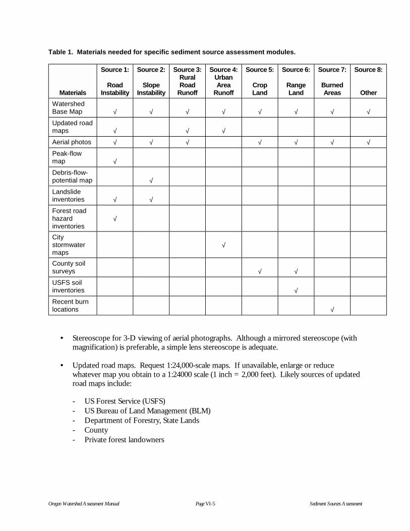
Oregon Watershed Assessment Manual Page VI-5 Sediment Sources Assessment
Table 1. Materials needed for specific sediment source assessment modules.
Materials
Source 1:
RoadInstability
Source 2:
SlopeInstability
Source 3:RuralRoad
Runoff
Source 4:UrbanArea
Runoff
Source 5:
CropLand
Source 6:
RangeLand
Source 7:
BurnedAreas
Source 8:
Other
WatershedBase Map √ √ √ √ √ √ √ √
Updated roadmaps √ √ √
Aerial photos √ √ √ √ √ √ √
Peak-flowmap √
Debris-flow-potential map √
Landslideinventories √ √
Forest roadhazardinventories
√
Citystormwatermaps
√
County soilsurveys √ √
USFS soilinventories √
Recent burnlocations √
• Stereoscope for 3-D viewing of aerial photographs. Although a mirrored stereoscope (withmagnification) is preferable, a simple lens stereoscope is adequate.
• Updated road maps. Request 1:24,000-scale maps. If unavailable, enlarge or reducewhatever map you obtain to a 1:24000 scale (1 inch = 2,000 feet). Likely sources of updatedroad maps include:
- US Forest Service (USFS)- US Bureau of Land Management (BLM)- Department of Forestry, State Lands- County- Private forest landowners

Oregon Watershed Assessment Manual Page VI-6 Sediment Sources Assessment
• Other supplies:
- Transparency overlays- Thin permanent markers (six or more colors)- Engineer’s ruler (English units, not metric) or map wheel for measuring lengths- Calculator- Dot grid templates (provided with this manual) or map wheel for measuring area- Computer spreadsheet software- Worksheet diskette with spreadsheets
Materials Needed for Specific Sediment Source Modules
The materials listed in Table 1 are described in the following list:
• Peak-flow map (50-year recurrence interval 1 for peak flows in forest streams). The mapcan be downloaded from the Oregon Department of Forestry (ODF) Web site athttp://www.odf.state.or.us/FP/DEFAULT.HTM. It is also available in hard copy bycalling the ODF hydrologist at (503) 378-3589.
• Debris-flow-potential maps. ODF is in the process of mapping debris flow potential formany parts of western Oregon. These maps are scheduled to be available June 1999 fromthe ODF landslide specialist at (541) 945-7481.
• Landslide inventories. These can be obtained from the same sources as updated road maps(see previous section).
• Forest road hazard inventories. Many forest landowners have recently completedinventories of their road systems using a standard protocol that is also used on state forestlands by the ODF. These inventories include information about recent landslides nearroads, road surface condition, and stream crossings. The USFS and BLM may also haveroad inventory information, but it will not be the same format.
• City stormwater maps. Request these maps from city public works departments. Thesemaps should show roads, streams, lakes, and the stormwater network (pipes, detentionfacilities, and any processing plants). Make several large-format copies and laminate themfor work maps.
• County soil survey books (from Riparian/Wetlands Assessment component)
• USFS soil resources inventories. Obtain these inventories from your local USFS districtoffice if range land managed by the USFS is to be assessed.
• Locations of recent burns
1 Terms that appear in bold italic throughout the text are defined in the Glossary at the end of this component.

Oregon Watershed Assessment Manual Page VI-7 Sediment Sources Assessment
Area calculations can be done using Geographic Information System (GIS) software instead ofthe dot grids or map wheel if available. In addition, GIS support allows for better-quality final mapsand provides more options for summarizing results.
Necessary Skills
The minimum skills necessary to conduct this assessment include the ability to read topographicmaps and basic experience in operating a computer spreadsheet program. Electronic spreadsheetsversions of all forms have been created; in many cases the data analysis will be much easier if thesediment source information is directly entered into a spreadsheet (referred to as worksheetsthroughout this document). Sediment source identification relies on aerial photo interpretation, soexperience reading aerial photos will help complete the assessment. At a minimum you should havesomeone experienced with aerial photo interpretation help you get started to “train” your eye onhow to read photo features.
Final Products of the Sediment Sources Component
Final products include maps showing points, road segments, or areas of low to high sediment riskfor up to eight of the potential sediment sources. In addition, you will end up with spreadsheetdatabases of erosional features or areas of erosional risk. From these databases, you will be able toconstruct summary tables indicating relative sediment-severity ratings for subwatersheds within thewatershed. Specific final products will be discussed within each of the eight modules.
METHODS
In this assessment you will be able to evaluate potential contributions of sediment from thefollowing eight sources, with a module devoted to each source: (1) road instability, (2) slopeinstability, (3) rural road runoff, (4) urban area runoff, (5) sediment from crop land, (6) sedimentfrom range or pasture lands, (7) sediment from burned areas, and (8) sediment from other identifiedsources. The assessment is conducted using aerial photographs, topographical maps, databaseinventories, and field verification as time and interest permits. It produces a database and maps thatidentify sediment sources. Use of a computer spreadsheet will help you complete these summariesand groupings. Each module may be completed by different users with experience or informationon that specific source.
Step 1: Update Roads on Watershed Base Map
Before accurate information can be gathered about road-related sediment sources, the WatershedBase Map should be updated to include all roads. The 7.5-minute topographic maps or ODF streammaps used as the Watershed Base Map will probably display only two-thirds of the roads. Roadsconstructed since the map was made (or updated) will be missing. If you have obtained 1:24,000-scale maps from other sources that show the missing roads, transfer them onto the Watershed BaseMap. If a 1:24000-scale map from other sources is unavailable, enlarge or reduce what map youhave to achieve a 1:24000 scale (1 inch = 2,000 feet) and transfer roads onto the Watershed BaseMap. You can transfer new roads onto the Base Map by placing the road or sub-basin map on alight table or window, overlaying the Base Map, taping both down, and transferring changes to theBase Map.

Oregon Watershed Assessment Manual Page VI-8 Sediment Sources Assessment
New roads can also be located on recent aerial photographs and transferred to the maps, but this isoften a frustrating and time-consuming task. To do this, first enlarge or reduce color copies of theaerial photographs to match the 1:24000 scale, then follow the procedure described above fortransferring roads to the Base Map. This is made more difficult by the variation of scale within eachaerial photograph, both in elevation (objects on ridges look larger than objects in valleys) and inproximity to the photo edges. To minimize these problems, use a photo that puts the road in thecenter of the photo and adjust the position of the photograph underneath the map as needed to getthe best fit with other landmarks. See the Start-Up and Identification of Watershed Issuescomponent for more information on working with aerial photographs.
Once the new roads have been added to the Base Maps, assign sequential numbers to points whereroads cross streams. These stream-crossing identification numbers will be used later for analysis ofsediment sources and the passage of fish through culverts.
Next, make about a dozen, large-format copies of your map. You will want at least one copy tocomplete each sediment source assessment, it is often useful to have a working copy and a finalcopy. In addition, the Fish and Fish Habitat analyst will need a copy for the passage barrierassessment. For extra convenience, have your Base Maps laminated to allow easy changes as youmark the maps with the locations of sediment sources. All sediment source features will be labeledwith a unique identifying number.
Step 2: Identify Potential Sediment Sources
A first step in evaluating sediment sources in your watershed is to determine which sediment topicsare important to the watershed council. You could compile information on all eight of the sedimenttopics, but this would take quite a bit of time and you would eventually see that some sedimentsources are rather insignificant in your watershed. For example, sediment topics for a watershed inthe Coast Range with little urban or grazed land could probably be limited to an assessment ofsediment from road runoff, road instability, and slope instability (not related to roads). For awatershed in the foothills of the Blue Mountains in eastern Oregon, a watershed council might focusits assessment on sediment from crop land, range land, and road runoff.
Your selection of priority sediment topics may depend, in part, on whether or not there is enoughinformation about your watershed to get started on a topic. For example, if you cannot find aerialphotographs for your watershed and major portions of the watershed are inaccessible to themembers of the watershed council, you may not get very far addressing the topic of slope instability.
The questions listed in Form S-1, Screen for Sediment Sources in a Watershed, may be useful forhelping you to determine which sediment topics should be included in the assessment. As youdiscuss these issues among yourselves, you can keep track of your progress by filling in Form S-1.
Many of these questions can be answered by the following method:
• Use the updated Watershed Base Map to identify areas of high rural road density.
• Use the Refined Land Use map to identify the presence of specific land uses.

Oregon Watershed Assessment Manual Page VI-9 Sediment Sources Assessment
• Your own experience and interviews with landowners who live in the watershed and agencystaff working in the watershed.
As an example of this process, Table 2 indicates that a watershed council decided that rural roadrunoff and instability were the most important sediment sources to be addressed in their assessment.Urban runoff within some tributaries and slope instability (not related to roads) were of lesserimportance. They chose not to expend effort on the remainder of the sediment source modules.
Table 2. Example of Form S-1: Screen for sediment sources in a watershed.
Watershed Name: The River Why Observations Priority
Source 1: Road instability
Are rural roads common in watershed?
Do many road washouts occur following high rainfall?
Are many new roads or road reconstruction planned?
Yes
Some
Yes
2nd
Source 2: Slope instability (not related to roads)
Are landslides common in watershed?
Many high-sediment, large-scale landslides?
Yes
None
4th
Source 3: Rural road runoff
Is sediment-laden runoff from rural roads and turbidity instreams common?
Is there a high density of rural roads?
Yes
Yes
1st
Source 4: Urban runoff
Are many portions of the watershed urbanized?
Importance of these tributaries to watershed council:
Some
High
3rd
Source 5: Surface erosion from crop land
Is there much crop land in watershed?
Is there much evidence of sediment in streams flowingthrough crop land?
Low
Little
Topic not highpriority
Source 6: Surface erosion from range land
Is there much range land in the watershed?
Is there evidence of sediment in streams flowing throughrange land?
Low
Little
Topic not highpriority
Source 7: Surface erosion from burned land
Have many burns occurred recently (last 5 years),especially hot fires?
Was there much sediment created by these burns?
Few
Low
Topic not highpriority
Source 8: Other discrete sources of sediment
List or identify any other suspected sources of sediment: None
Topic not highpriority

Oregon Watershed Assessment Manual Page VI-10 Sediment Sources Assessment
Step 3: Evaluate Sediment Sources
The next step describes how to evaluate each of the eight potential sediment sources. Remember,you will probably not be doing all eight of the modules described herein; only the ones identified inthe previous step as important to you.
Source 1. Road Instability
The stability of a rural road depends on how well the road was built and the inherent stability of theland it traverses. In general, roads are most stable if built along ridges, especially where slopes arenot steep. Less stable locations include steep terrain at the middle of slopes and near streams. Largeamounts of subsurface water cause soils to lose much of their strength, so most road failures occurduring high-intensity rainstorms or snowmelt periods that produce saturated soils.
The type of road construction influences the stability of the road. Sidecast roads are constructed bydigging into the hillside to form the inside of the road and using the excavated soil to build up theoutside of the road (Figure 1). This works well in moderate terrain but can lead to problems onsteep slopes. Excavated material used to build up the outer side of the road (the fill slope) on asteep slope can be unstable. This unstable wedge of soil may be transformed into a landslidesometime in the future (Figure 1). Alternatively, when full-bench road construction is used, soil isexcavated to a stable location rather than using it as the outer edge of the road. This type of roadconstruction is more stable but the cost is considerably higher.
Figure 1. The type of road construction influences the stability of the road. Sidecast roads, builtby digging into the hillside to form the inside of the road and using the excavated soil to build upthe outside of the road, can cause failure on steep slopes. In full-bench road construction, soil isexcavated to a stable location rather than using it as the outer edge of the road.

Oregon Watershed Assessment Manual Page VI-11 Sediment Sources Assessment
Road cut slopes, the inside slope of the road, may also become unstable, and sections of the cutslope can fall or creep into the road during wet weather. Small cut-slope failures can end updiverting ditch water onto the road surface or fill slope, creating gullies or triggering a landslide. Aninherently unstable section of hill slope can be made even less stable when a road is excavated intothe base of the unstable area.
Finally, road crossings with culverts that fail can cause large pulses of sediment to enter channels.Culverts that are inadequate to pass a flood flow or get plugged with floating wood can wash out theroad or divert it down the road, thereby creating gullies.
Understanding rural road instability in a watershed involves two investigations. One involvescollecting information about recent road washouts and possible factors that caused their failure, andthe other involves identifying high-risk situations within the watershed that are likely to lead to roadwashouts in the future.
Gather Information
Road Inventory Databases
Information about road conditions and recent road-related landslides in your watershed may comefrom a number of sources. Forest landowners are good potential sources. Many have recentlycompleted inventories of their road systems using a standard protocol also used on state forest landsby the ODF. These inventories include information about recent landslides near roads, road surfacecondition, and stream crossings. The protocol for these road inventories can be obtained from theODF Web site at http://www.odf.state.or.us/FP/DEFAULT.HTM. Road inventory informationmay also be available from the USFS and BLM, but it will not be the same format. Remember,private landowners are under no obligation to share inventories. Allow extra time to obtaininformation from public agency databases; while they are required to provide their information uponrequest, they are often understaffed and may be slow to respond.
Road inventory databases have several weaknesses:
• Database features are sometimes difficult to match with a map location. Since the locationsof features are usually determined in the field by measuring the distance from the last roadjunction, base map errors and field measurement errors may cause the landslide to be plottedin the wrong place. To confirm the accuracy of inventory site locations, use other nearbyfeatures noted in the inventory that also appear on the map. For example, if major streamcrossings bracket a landslide, the distance to the landslide may be checked by comparing thenoted distances with distances measured on the map.
• The database may not be up-to-date; recent road repairs may not be noted in the inventory.And, of course, road problems that developed after the inventory was completed will bemissing. The database originator will know if the database is updated as road problems arefixed.

Oregon Watershed Assessment Manual Page VI-12 Sediment Sources Assessment
Aerial Photographs
Recent aerial photographs can be very useful for also identifying existing road-related landslidesthroughout the watershed. However, you will find that denser stands of trees greater than 30 yearsold will conceal landslides on aerial photographs.
Field surveys made by driving around the watershed are a good source of information and helpfulfor verifying the information compiled from other road inventories and aerial photographs.However, this activity is time-consuming, and some areas may be inaccessible due to locked gates ordenial of permission to enter the area by the landowner.
Map and Compile Existing Road Instability Information
Compile information on existing road-related instability by marking landslide locations on the BaseMap, and recording landslide information on Form S-2, Information on Existing Road-RelatedInstability. Locations are recorded where a landslide either appears in the aerial photographs, isdescribed in a road hazard inventory, or is noted during a field visit.
Use Form S-2, or the ROADLAND Worksheet, to compile information on the subwatershed, andon the landslide type, whether or not it reached a stream, what distance it traveled, and roadposition. After marking the landslide on the Base Map, assign it a unique number and enter theinformation into the worksheet. Table 3 provides an example of information gathered on existingroad-related instability.
Table 3. Example Form S-2: Information on existing road-related instability.
Number Subwatershed Landslide TypeReachedStream?
DistanceTraveled (ft) Road Location
101 Deer Debris flow Yes 2,200 Mid-slope
102 Deer Debris flow No 1,000 Near ridge
103 Elk Road prismfailure
No 200 Mid-slope
104 Skunk Culvert washout Yes - Near stream
Number: Unique identification number.
Subwatershed: Subwatershed in which landslide occurs.
Landslide Type: Debris flow = initiates as shallow landslide in steep area and then flows down achannel, picking up additional soil, logs, and water. Road prism failure = downhill movement of theroad cut or road fill; does not initiate a debris flow. Culvert washout = road fill partially or completelymissing where the road crosses a stream.
Reached Stream?: Whether or not the landslide material ended up in the stream.
Distance traveled: The distance from initiation point to where the landslide stopped (not applicableto culvert washouts).
Road Location: General location of road: near ridge, mid-slope, near stream.

Oregon Watershed Assessment Manual Page VI-13 Sediment Sources Assessment
Map and Compile Potential Road Instability Information
Identifying the location of potential high-risk landslides or road washouts in the watershed allows acouncil to focus on preventing road instability. This information can be obtained from roadinventory data and road surveys. In this portion of the assessment you will identify locations where(1) water is flowing over the road surface and fill slopes, (2) large cracks or slumps in the fill portionof the road, and/or (3) stream crossings that have undersized culverts. Culverts sizes are evaluatedusing a method adapted from the ODF in which you first document the current culvert capacity andthen you compare this to the capacity needed.
Use Form S-3, Culvert Capacity and Risk of Large Amounts of Sediment Entering Stream, or theCULVERT Worksheet, to determine if the existing culvert is appropriately sized. First enter thesubwatershed name and the unique number for each culvert (Columns 1 and 2). Identify the ownerof the road in Column 3, if known. Then enter the current culvert size (from field information orroad inventory data) in Column 4. Fill in current culvert capacity (Column 5) with values fromTable 4. This table shows the flow capacity of both round culverts and of pipe-arch culverts ofvarious standard sizes (pipe arches are wider than they are tall).
You will use the peak-flow map (50-year recurrence interval for peak flows in forest streams) fromODF to determine how large a culvert is needed for a stream crossing; enter the information inColumn 6. In western Oregon and some of eastern Oregon, this map shows lines of equal value ofpeak flow associated with 50-year recurrence interval ranging from 50 to 600 cubic feet per second
Table 4. Capacity of culverts of various sizes.
Round Culverts Pipe-Arch Culverts
Diameter(inches) Capacity (cfs) Span x Height Capacity (cfs)
15
18
21
24
27
30
33
36
42
48
54
60
72
84
96
108
120
132
3.5
5.5
8
12
16
20
26
32
47
67
88
115
180
260
370
500
670
840
22" x 13"
25" x 16"
29" x 18"
36" x 22"
43" x 27"
50" x 31"
58" x 36"
65" x 40"
72" x 44"
6'-1" x 4'-7"
7'-0" x 5'-1"
8'-2" x 5'-9"
9'-6" x 6'-5"
11-'5" x 7'-3"
12'-10" x 8'-4"
15'-4" x 9'-3"
4.5
7
10
16
26
37
55
70
90
130
170
240
340
470
650
930

Oregon Watershed Assessment Manual Page VI-14 Sediment Sources Assessment
(cfs) per square mile of drainage area. In much of eastern Oregon you will see areas that have aregional average value. Culverts installed on nonfederal forest roads are required to at least pass apeak flow of the magnitude shown for your location on the map. For example, if your watershed isin the central Coast Range and the 200 line runs through it, culverts need to be sized to handle atleast 200 cfs of flow for each square mile of drainage area upstream of the site.
You can measure the drainage area of a site using the Base Map. Starting from the culvert site,delineate the drainage boundary by drawing a line that is always perpendicular to the elevationcontours (see method for delineating watersheds in the Start-Up and Identification of WatershedIssues component). Measure the area bounded by the line using a map grid or map wheel (seemethod for calculating drainage area in Start-Up component) and enter the value in Column 7.Multiply the drainage area (Column 7) times the peak flow value (Column 6). For example, a sitethat has a design criteria of 200 cfs per square mile and a drainage area of 0.65 square miles needs aculvert that passes 131 cfs (200 x 0.65 = 131). Enter the multiplied value in Column 8.
To determine the appropriate culvert size corresponding to the design flow, refer to Table 4. Findthe culvert size required to pass the calculated peak flow value (from Column 7) and enter the valuein Column 9. In the above example, the minimum culvert size is a 72-inch circular culvert or a 7'-x-5'1" pipe arch. Now, look up the capacity of the current culvert in Table 4 and write it down inColumn 5. If the current culvert was 48 inches in diameter, the capacity would be 67 cfs. Next,calculate a ratio (Column 10) of the 50-year flow (Column 6) divided by the current culvert’scapacity (Column 5). In the example above, this ratio would be 131/67= 2.0.
The height of the fill at the stream is important information for evaluating the consequences of aroad washout. If a culvert washes out, the amount of soil entering the stream can be low if the fill issmall or large if the fill is high. Enter fill height (estimated at the outside edge of the road surface) inColumn 11. Next, assign culverts to various risk classes (low through extreme) as shown at thebottom of Form S-3. The risk class goes in Column 12. An example of an inventory of culvertinformation is shown in Table 5.
Identify Road Segments at Risk
The three risk factors used to identify potential road instability are cracks and slumps in roads(cracks/slumps), water running down a road or onto an unstable fill (water/fill), and undersizedculverts in high fills at stream crossings (culvert). Use information within road surveys or your ownknowledge of the watershed to identify locations where cracks and slumps in roads exist. Do thesame for locations where water is running down a road or onto an unstable fill. Assign each locationa unique identification number and mark on the Base Map the location of each site and theidentification number.
Combine information about all three risk factors into Form S-4, High-Risk Road Segments forExisting Roads, or the ROADRISK Worksheet (including only culverts with a hazard rating of high,very high, or extreme). Table 6 provides an example of what information to include.

Oregon Watershed Assessment Manual Page VI-15 Sediment Sources Assessment
Table 5. Example Form S-3: Culvert capacity and risk of large amounts of sediment entering stream.
1Sub-
watershed2
Num.
3Road
Owner-ship
4CurrentCulvert/
Pipe-ArchSize
5CurrentCulvert
Capacity(cfs)
6ODF
Peak-FlowValue
(cfs/mi²)
7Drainage
Area(mi²)
850-Year
PeakFlow(Col.6x7)(cfs)
9Culvert/
Pipe-ArchSize
Needed for50-Year
Peak Flow
10Ratio of
50-YrFlow toCurrentCapacity
11Fill
Height(ft)
12HazardRating *
Deer 201 USFS 30" 20 200 0.65 131 72" 6.5 20 Extreme
Elk 202 County 30"+30" 40** 200 0.44 88 54" 2.2 18 Very high
Elk 203 Un-known
9'-6"x6'-5"
340 200 2.73 545 12'-10"x8'-4" 1.6 3 Moderate
Skunk 204 County 60" 115 200 0.38 75 54" 0.7 35 Low
Skunk 205 State 72" 180 200 0.60 119 72" 0.7 3 Very low
* Hazard rating:
Very low Fill height is 15 feet or less and ratio is less than 1.25.
Low Fill height is greater than 15 feet and ratio is less than 1.25.
Moderate Fill height is 15 feet or less and ratio is between 1.25 and 1.75.
High Fill height is greater than 15 feet and ratio is between 1.25 and 1.75; or, fill height is 15 feet or less and ratio is between1.76 and 3.
Very high Fill height is greater than 15 feet and ratio is between 1.76 and 2.99; or, fill height is 15 feet or less and ratio is greater than 3.
Extreme Fill height is greater than 15 feet and ratio is greater than 3.**Stream crossing had two 30"-diameter culverts.

Oregon Watershed Assessment Manual Page VI-16 Sediment Sources Assessment
Table 6. Example Form S-4: High-risk road segments for existing roads.
Sub-Watershed Num.
FeatureType
Hazard Ratingof Culvert
RoadOwnership
Deer 201 Culvert Extreme Forest Service
Deer 251 Water/fill - Forest Service
Deer 252 Water/fill - Private landowner
Elk 202 Culvert Very high County
Elk 253 Cracks/slumps - Private landowner
Skunk 254 Water/fill - Private landowner
Skunk 255 Cracks/slumps - Private landowner
Map 1 in Appendix VI-A provides an example of a finished map showing information compiled forboth existing and potential road instability sites.
Summary: Road Instability
A final step in this process is to create summary tables (Form S-5, Summary of Information on RoadInstability, or the ROADINST Worksheet) that allow subwatersheds and/or land ownership classesto be compared. Existing road instability (from Form S-2) and high-risk areas for future instability(from Form S-4) are both entered into the table but are evaluated separately. The number of sites ina subwatershed are divided by the subwatershed area and displayed on a per-unit basis. Table 7provides an example of the summary table. An expanded version can be constructed by breakingdown each subwatershed summary into road ownership classes.
This example highlights several issues that should be examined and discussed, including: a highdensity of landslides in the Deer and Eagle subwatersheds; a high density of high-risk culverts in theEagle subwatershed; and a high density of road cracks, slumps, and road water in the Skunk andBear subwatersheds. Note in what locations within these subwatersheds the landslides areoccurring. Examine the Base Map to see if landslides are more common nearest streams or nearestridge-tops. Does slope steepness explain the variation in landslide clusters? Check if landslidesoccur in clumps along only a few roads or are evenly spread out. Examine the map and see iflandslides tend to clump according to land ownership. Such examination will help you determinelandslide causes.
The example also highlights another issue: the high density of high-risk culverts in onesubwatershed. Refer to the Base Map to determine why. Does the road mostly follow streams,thereby requiring many stream crossings? Do a high percentage of these high-risk culverts occur ona certain land ownership? Do the high-risk culverts occur mainly within one size class of stream?Answers to these questions may require the help of a road engineer to help unravel the spatialvariability of high-risk culverts and suggest remedies.

Oregon Watershed Assessment Manual Page VI-17 Sediment Sources Assessment
Table 7. Example Form S-5: Summary of information on road instability.
Subwater-shed
Area(mi²)
Road Failures thatReached Streams
Sites with High-Risk Culverts
Sites withCracks and
Slumps
Sites with WaterFlowing Over
Fills
#Density(#/mi².) #
Density(#/mi².) #
Density(#/mi².) #
Density(#/mi².)
Deer 4.6 13 2.8 3 0.7 0 0.0 0 0.0
Elk 6.5 2 0.3 4 0.6 2 0.3 5 0.8
Skunk 8.3 15 1.8 10 1.2 18 2.2 20 2.4
Bear 2.1 3 1.4 2 1.0 4 1.9 4 1.9
Eagle 10.1 21 2.1 15 1.5 9 0.9 3 0.3
Total 31.6 54 1.7 34 1.1 33 1.0 32 1.0
Table 7 also highlights the high density of road segments with cracks, slumps, or areas where runoffwater flows onto road fills in the Skunk and Bear subwatersheds. In this case, it will take additionalevaluation to determine if this is related to side-slope steepness, position on the hill slope, or road-building practices and maintenance on the part of the landowner.
Other information can be brought in to help decipher road instability questions, such as geologicalinformation, road age, and rainfall patterns. A geological map of the area may provide informationon general rock types; landslides can be more common at the contact zone between two rock types.The era in which the road was built may explain why some are stable and some are unstable. Youmay be able to assign ages to road segments by estimating the age of the oldest harvest units in thegeneral area. Finally, you should consider when the last sustained and high-intensity rainfalloccurred and how it might have varied across the watershed. Road instability is seldom noticeableuntil the road is tested by severe storms.
Source 2. Slope Instability (not related to roads)
Slopes can be unstable for reasons other than roads. Landslides can be a natural part of thelandscape, especially where slopes are steep and rainfall is abundant. Landslides include bothshallow slope failures that go a short distance and those that travel down a channel, gathering upsoil, water, and wood and creating a debris flow (Figure 2). Landslides also include deep-seatedfailures that creep or ooze downhill at slow rates. A combination of the two can occur when theover-steeped face of a deep-seated landslide becomes the site of shallow slope failures.
Shallow landslides typically occur in very steep terrain. There is some evidence that removal of treeson steep slopes (greater than about 80%) makes an area vulnerable to shallow landslides and canlead to a temporary acceleration of the landslide rate. This window of vulnerability begins whenmany of the finer roots of the harvested trees become rotten (about 4 years) and ends once the

Oregon Watershed Assessment Manual Page VI-18 Sediment Sources Assessment
replacement stand has developed a dense root network (about 30 years for wet portions of thestate).
Most deep-seated landslides are natural. The only times when human-activities seem to influencethese landslides is when a road or other feature undercuts the base of the slide or adds weight to thetop of the slide. A deep-seated landslide area can also be triggered by road runoff water divertedonto an unstable slope. Deep-seated landslides are not restricted to steep slopes. Some of the mostactive and extensive landslides can occur on moderate slopes with weak soils. Deep-seatedlandslides add sediment to streams by pinching off stream channels. When a stream is constrictedby an encroaching landslide, the stream carves away at the base of the landslide, causing the slope tobe further destabilized.
Slope instability (unrelated to roads) is evaluated by collecting information about recent landslidesand high-risk areas in the watershed that are likely to move in the future. This is done using recentaerial photographs, referring to federal or state agency aerial photograph landslide inventories ofportions of the basin, and asking landowners, local fishermen, and fisheries biologists wherelandslides are located. Deep-seated landslides next to streams can cause chronic turbidity, but areoften difficult to identify on aerial photos unless they have bare surfaces.
Finding information on existing landslides will probably be frustrating. You can use recent aerialphotographs to detect some landslides but you will seldom be able to observe landslides amongdense trees older than about 30 years. You might find that a federal or state agency has already donesome aerial photography or ground-based landslide inventories of portions of the basin, but theymay not be recent surveys. In many cases, it will probably be better to conduct your own inventoryfrom recent photos so that you can cover the entire watershed, have a current inventory, and be ableto gather other information that is useful in this assessment.
Figure 2. Some landslides travel down a channel, gathering up soil, water, and wood andcreating a debris flow. Landslides also include deep-seated failures that creep or ooze downhillat slow rates.

Oregon Watershed Assessment Manual Page VI-19 Sediment Sources Assessment
Recent Landslides
Begin the mapping of existing landslides by locating landslides seen in the aerial photographs,skipping those that initiate at roads. At first glance, some features may appear similar to a landslide.Skid trails, cable yarding scars, landings, borrow pits, and rock pits can leave patches of baresoil that appear similar to the scar left by a landslide. You can usually resolve these uncertainties byexamining the aerial photographs using a stereoscope. A stereoscope will allow you to see thefeature in three dimensions. If necessary, take the photos to the field and verify what you see on theground and what you see in the photographs. Assign a unique number to each landslide located onthe aerial photographs and mark the location on the Base Map. Use roads, timber harvestboundaries, and streams for orientation. Observing the landslide in stereo will show its locationwith respect to nearby ridges and draws, which show up on the Base Map. Enter the subwatershedname, unique number, and type of landslide on Form S-6, Current Landslides Not Related to Roads,or the LANDCUR Worksheet. Table 8 provides an example of this.
From the aerial photograph, estimate the age of the vegetation at the landslide’s initiation point (seethe Start-up Component for guidance on how to read aerial photos). Also determine the distancethe landslide traveled from the initiation point and whether or not it reached a stream. Enter thisinformation in the appropriate columns on Form S-6. From the Base Map, determine slopesteepness at the initiation point by measuring the distance between 5 contour intervals using the20-scale of an engineer’s scale. Multiply the vertical distance represented by a single contour (usually40 feet) by 5, divide by the distance between 5 contour intervals, and then multiply by 100, as shownbelow:
Slope (%) = 5 x 40 feet/distance x 100
If the contour interval of the Base Map happens to be 20 feet, then substitute 20 for 40 in the aboveequation. Figure 3 provides an example of a landslide in an aerial photo and the measured sitecharacteristics. Map 2 in Appendix VI-A provides an example of a finished map showinginformation compiled on slope instability not related to roads.
Table 8. Example Form S-6: Current landslides not related to roads.
Sub-watershed Num.
Type ofLandslide
Age ofVegetation
(years)
LandslideReachedStream?
DistanceLandslide
Traveled (feet)
Slope Steepnessat InitiationPoint (%)
Deer 301 Shallow 10 Yes 1,700 110
Deer 3702 Deep-seated
20 Yes 200 50
Elk 303 Shallow 5 Yes 1,600 100
Elk 304 Shallow 10 No 900 75
Skunk 305 Unknown 30 No 300 80
Skunk 306 Shallow 5 Yes 800 95
Skunk 307 Deep-seated
10 No 100 45

Oregon Watershed Assessment Manual Page VI-20 Sediment Sources Assessment
High-Risk Areas for Debris Flows
The ODF is in the process of finishing debris-flow-hazard maps for forested regions of Oregon.These maps will indicate areas prone to landslides and will provide a rating of the degree of landslidehazard. Since the maps are not yet available it is not possible to predict how the final maps willindicate the landslide hazard or hazard delineations. The maps will probably consist of polygonsof high- and extreme-hazard delineations. The remainder of the area in the watershed will not bemarked. To include this information on your Base Map, transfer the outlines of the high- andextreme-hazard polygons using a light table or window. Determine the area of these polygons usinga grid or map wheel and compile the information, as demonstrated in Form S-7, Potential for DebrisFlows, or the LANDPOT Worksheet. Table 9 provides an example of a completed Form S-7.
Table 9. Example Form S-7: Potential for debris flows.
Subwatershed Areas Predicted to be High Risk for Debris Flows (mi²)
High Hazard Extreme Hazard Combined
Deer 0.5 0.2 0.7
Elk 1.1 0.4 1.5
Skunk 0.4 0.1 0.5
Bear 0.2 0 0.2
Eagle 1.2 0.5 1.7
Total 3.4 1.2 4.6
Land
ing
Road
Shallow landslides,debris flows
Figure 3. From the aerial photograph, you can estimate the age of the vegetation at a landslide’sinitiation point, and determine the distance the landslide traveled.
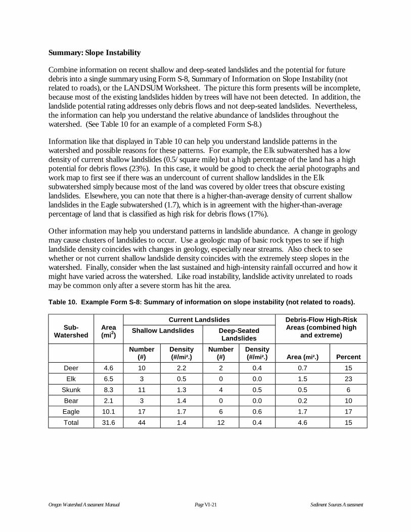
Oregon Watershed Assessment Manual Page VI-21 Sediment Sources Assessment
Summary: Slope Instability
Combine information on recent shallow and deep-seated landslides and the potential for futuredebris into a single summary using Form S-8, Summary of Information on Slope Instability (notrelated to roads), or the LANDSUM Worksheet. The picture this form presents will be incomplete,because most of the existing landslides hidden by trees will have not been detected. In addition, thelandslide potential rating addresses only debris flows and not deep-seated landslides. Nevertheless,the information can help you understand the relative abundance of landslides throughout thewatershed. (See Table 10 for an example of a completed Form S-8.)
Information like that displayed in Table 10 can help you understand landslide patterns in thewatershed and possible reasons for these patterns. For example, the Elk subwatershed has a lowdensity of current shallow landslides (0.5/square mile) but a high percentage of the land has a highpotential for debris flows (23%). In this case, it would be good to check the aerial photographs andwork map to first see if there was an undercount of current shallow landslides in the Elksubwatershed simply because most of the land was covered by older trees that obscure existinglandslides. Elsewhere, you can note that there is a higher-than-average density of current shallowlandslides in the Eagle subwatershed (1.7), which is in agreement with the higher-than-averagepercentage of land that is classified as high risk for debris flows (17%).
Other information may help you understand patterns in landslide abundance. A change in geologymay cause clusters of landslides to occur. Use a geologic map of basic rock types to see if highlandslide density coincides with changes in geology, especially near streams. Also check to seewhether or not current shallow landslide density coincides with the extremely steep slopes in thewatershed. Finally, consider when the last sustained and high-intensity rainfall occurred and how itmight have varied across the watershed. Like road instability, landslide activity unrelated to roadsmay be common only after a severe storm has hit the area.
Table 10. Example Form S-8: Summary of information on slope instability (not related to roads).
Current LandslidesSub-
WatershedArea(mi2)
Shallow Landslides Deep-SeatedLandslides
Debris-Flow High-RiskAreas (combined high
and extreme)
Number(#)
Density(#/mi².)
Number(#)
Density(#/mi².) Area (mi².) Percent
Deer 4.6 10 2.2 2 0.4 0.7 15
Elk 6.5 3 0.5 0 0.0 1.5 23
Skunk 8.3 11 1.3 4 0.5 0.5 6
Bear 2.1 3 1.4 0 0.0 0.2 10
Eagle 10.1 17 1.7 6 0.6 1.7 17
Total 31.6 44 1.4 12 0.4 4.6 15

Oregon Watershed Assessment Manual Page VI-22 Sediment Sources Assessment
Source 3. Rural Road Runoff
The water draining from roads can move considerable amounts of sediment from the insidedrainage ditch and unpaved road surfaces. The road ditch is filled in with sediment from ravel,sliding, and erosion of the road cut slope. Usually, roads are designed so water flowing through theditch picks up this sediment as it flows into streams or small draws. However, some land managershave now adopted a technique whereby roads are designed to divert ditch water onto a stable slopeusing a cross-drain culvert at a site adjacent to but before the stream enters the stream. When thesediment-laden water is diverted onto stable and well-drained slopes, the sediment is filtered out asthe ditch water goes subsurface.
The condition and amount of sediment coming from the surface of an unpaved road depends onthe quality of the surface rock, road maintenance, weather conditions, and the weight and frequencyof traffic. The break-up of the road surface is most rapid during wet weather and when heavy trucktraffic is frequent. Poor-quality surface rock quickly breaks down into fine material and developspotholes. If the road is not maintained, ruts then begin to develop.
The amount of sediment potentially contained in runoff from any single road is difficult to estimatebecause road conditions can change so rapidly. A road surfaced with high-quality rock can bequickly reduced to a quagmire if water is allowed to pool during wet weather and there is heavytruck traffic. Conversely, a road with a poor-quality surface may not degrade much at all if it is usedmainly during dry weather.
In this section, you will compile information about road segments in the watershed and assign anoverall hazard rating that indicates the general propensity of that road segment to deliver sedimentto streams. Two different assessments are described. The first, a basic assessment, simply identifiessite conditions that are conducive for high amounts of sediment in road runoff to enter streams.The second assessment is detailed, and requires much more time but yields more useful informationabout the road systems in your watershed.
This section covers road runoff from rural roads. Rural roads are all roads except those that arewithin cities and towns and are hooked up to a stormwater drainage system.
Basic Rural Road Runoff Assessment
Some basic information about roads and the likelihood of sediment delivery to streams can beobtained by reviewing base maps and aerial photographs. From the maps, you can identify sectionsof road that are within 200 feet of a stream, either laterally or longitudinally (see Figure 4).Throughout the watershed, these are the road segments more likely to have ditches that flow directlyinto the stream and are the most difficult to keep sediment-laden runoff water from enteringstreams. You can also identify on the topographic maps where these road segments close to thestreams also have steep slopes (greater than 50%) uphill of the road. Roads with steep side slopesusually have more soil accumulating in the road ditches than roads with less steep side slopes.Plugged road ditches are common cause of road surfaces breaking down. Also, you can gather someroad information from the aerial photographs. Use the color of the road to determine whether thesurface is paved, rock, or dirt. Finally, local experience by landowners and land managers canprovide information on whether or not a road is a high-use road. By combining all these sources ofinformation you can identify where in the watershed higher-risk situations exist for road runoff.

Oregon Watershed Assessment Manual Page VI-23 Sediment Sources Assessment
On the Base Map, identify and highlight road segments (400 feet or longer) within 200 feet of astream, either laterally or longitudinally (see Figure 4). Assign the road segment a unique numberand measure its length. Record this information on Form S-9, Basic Information on Road SegmentsClose to Streams with Steep Slopes, or the RUNOFF Worksheet. For each of the road segments,also determine which segments have a side slope greater than 50%.
You can identify 50% slopes by examining the spacing between contour lines. The contour lines ona topographic map (1:24000) with a contour interval of 40 feet are spaced slightly closer than thesmallest units on the 20-scale of an engineer’s scale where the slope is 50%. Measure the length ofthose portions of the road segment that have slopes greater than 50%. Finally, use the color of theroad on aerial photographs to determine whether the surface is paved, rock, or dirt. By combiningthis information, higher-risk situations for road runoff can be identified. Table 11 provides anexample of a completed Form S-9, and Map 3 in Appendix VI-A provides an example of a finishedmap showing basic information compiled on rural road runoff.
Table 11. Example Form S-9: Basic information on road segments close to streams withsteep slopes.
Subwatershed Num.Distance <200'
from Stream (feet)
Distance <200' fromStream and Slope >50%
(feet)Road
SurfaceRoadUse
Deer 401 1,800 600 Paved High use
Deer 402 2,200 0 Rock Low use
Deer 403 1,200 400 Rock Low use
Deer 404 900 800 Dirt High use
Elk 405 1,400 300 Rock High use
Elk 406 3,100 1,700 Rock Low use
Elk 407 600 0 Rock Low use
Elk 408 1,500 300 Rock Low use
200 feet
Stream
Road
200 feet
200 feet200 feet
200 feet200 feet
Portion of road within 200 feet of a stream
Stream
Stream
Figure 4. From maps, you can identify sections of road that are within 200 feet of a stream, whichmay help you determine the likelihood of sediment delivery to streams.

Oregon Watershed Assessment Manual Page VI-24 Sediment Sources Assessment
Detailed Rural Road Runoff Assessment
The mileage of road within in a watershed is usually too great for a watershed council to gatherdetailed information on each road section; however, in some areas of the watershed this informationmay have already been gathered by private forest landowners and state forest land managers. Mostof these inventories use a standard protocol so information can be shared and combined. Thisinformation may be added to your assessment if you are willing to deal with difficulties matchingdatabase records to Base Map locations; be prepared for the process to take a long time.
Table 12 provides an example of information collected on road runoff that is included in a typicalroad inventory database. You will be taking information from tables such as these and summarizingthem for inclusion in a summary table. You will also be adding the location of each road to the BaseMap. The variables are listed below the table. Descriptions for ditch condition, cut-slope condition,surface condition, surface material, and road use are the average conditions for the road sectionbeginning at the previous feature noted and extending to the current feature. See the ODF ForestRoad Hazard Inventory Protocol (available from the hydrologist at the ODF, 503-378-3589) formore information.
Raw inventory data may be summarized (on Form S-10, Summarized Runoff-Related Informationfor a Single Road, or the SEDROADS Worksheet; see Table 13 for an example) for a single road byadding up road lengths or occurrences for each classification that a variable takes. Features for allroads within a subwatershed can then be summed as illustrated later in this section.
Summary: Basic Assessment
Summarize information on road segments near streams by subwatershed using Form S-11, Summaryof Information on Road Runoff—Basic Assessment, or the RUNOFF Worksheet. Table 14provides an example of a completed form. For each of the various categories (Roads <200' from aStream; also with Steep Slopes, also with High Use, and also with Low Use), the lengths of road aresummed and a density value calculated by dividing road length by subwatershed area. A variationcould be constructed by including information about the road surface in the summary, yielding 26rather than 10 columns and making it a more detailed table.
Summary information like this can help you identify areas where high-risk roads are common. Forexample, both the Skunk and Eagle subwatersheds have an unusually high density of roads within200 feet of a stream. The situation in Skunk is likely to be of more concern because it also has thehighest density of these segments that have steep slopes uphill of the road. Furthermore, the Skunksubwatershed has the greatest density of high-use roads.
Patterns like these should lead you to examine the base maps again and note where in the Skunksubwatershed these conditions are most prevalent. The Skunk subwatershed would be a highpriority for a site visit (pick a very rainy day when the road is being used) to see whether or not theseindicators of high sediment in runoff water coincide with actual conditions.
A variation of Table F14 could be constructed by including information about the road surface inthe summary. As you can imagine, the introduction of the variable, Road Use, with its threecategories (paved, rock, dirt) makes for a messier table. With the addition of Road Use you will endup with 26 columns rather than the 10 shown in Table F14.

Oregon Watershed Assessment Manual Page VI-25 Sediment Sources Assessment
Table 12. Example of runoff-related information in a road inventory database.
Eagle Creek Road
Stationing(feet) Feature
%Grade(+/-)
DitchCondtn.
Cut-Slope
Condtn.SurfaceCondtn.
SurfaceMaterial
CulvertCondtn.
FilteringOpportun.
RoadUse
0 Start rd. 0
231 Grade Break 5 Good Good Good Rock Active
641 X drainculvert
3 Good Good Good Rock Good Active
1191 Grade Break 7 Good Ravel Good Rock Active
1708 X drainculvert
-7 Good Good Good Rock Good Active
2263 Roadjunction
-9 Good Good Good Rock Active
2619 X drainculvert
16 Good Ravel Good Rock Good Active
3004 Streamcrossing
10 Good Ravel Good Rock Good No Active
3520 X drainculvert
11 Good Good Good Rock Damaged
Active
3667 X drainculvert
9 Good Ravel Good Rock Good Active
4093 X drainculvert
11 Good Ravel Good Rock Good Active
4570 X drainculvert
11 Good Ravel Good Rock Good Active
4870 Streamcrossing
7 Good Ravel Good Rock Good No Active
5623 Streamcrossing
7 Good Good Good Rock Good No Active
5778 Streamcrossing
12 Good Good Good Rock Good No Active
6129 X drainculvert
9 Full Good Rutted Dirt Plugged Inactive
Stationing (feet): Distance from the starting point of the survey to the beginning of the roadsegment.
Feature: Grade breaks; cross-drain culverts; stream crossings; road junctions.% Grade: The gradient of the road in percent.Ditch Condition: Good; downcutting, diverted onto road; full of sediment.Cut-Slope Condition: Good; ravel problems; sloughed into road.Surface Condition: Good; rutted; bermed; eroded.Surface Material: Rock; dirt; pavement.Culvert Condition: Good; damaged; plugged by sediment.Filter Opportunity: Yes; no; possibly (whether or not site conditions would allow diversion of ditch
water onto a stable slope before it enters a stream).Road Use: Active; inactive.

Oregon Watershed Assessment Manual Page VI-26 Sediment Sources Assessment
Table 13. Example Form S-10: Summarized runoff-related information for a single road.
Road Name Variable ClassificationLength(feet)
Occurrences(#)
Eagle Creek Road Overall road length - 7,742 -
Eagle Creek Road Ditch condition Good 5,778 -
Eagle Creek Road Ditch condition Full 1,964 -
Eagle Creek Road Cut-slope condition Good 5,101 -
Eagle Creek Road Cut-slope condition Ravel 2,641 -
Eagle Creek Road Surface condition Good 5,778 -
Eagle Creek Road Surface condition Rutted 1,964 -
Eagle Creek Road Surface material Rock 5,778 -
Eagle Creek Road Surface material Dirt 1,964 -
Eagle Creek Road # Culverts - - 15
Eagle Creek Road Culvert condition Good - 12
Eagle Creek Road Culvert condition Plugged / Damaged - 3
Eagle Creek Road # Stream crossings - - 6
Eagle Creek Road # Stream crossings Ditch water can be filtered - 0
Eagle Creek Road Road use Active 5,778 -
Eagle Creek Road Road use Inactive 1,964 -
Table 14. Example Form S-11: Summary of information on road runoff—basic assessment.
Sub-watershed
Area(mi2)
Roads < 200'from Stream
Roads < 200' fromStream andSlope > 50%
Roads < 200' fromStream and High Use
Roads < 200' fromStream and Low Use
Length(mi.)
Density(mi./mi².)
Length(mi.)
Density(mi./mi².)
Length(mi.)
Density(mi./mi².)
Length(mi.)
Density(mi./mi².)
Deer 4.6 2.5 0.5 1.5 0.3 0.5 0.1 2.0 0.4
Elk 6.5 3.3 0.5 0.6 0.1 2.0 0.3 1.3 0.2
Skunk 8.3 9.6 1.2 8.0 1.0 7.5 0.9 2.1 0.3
Bear 2.1 0.0 0.0 0.0 0.0 0.0 0.0 0.0 0.0
Eagle 10.1 14.5 1.4 5.5 0.5 1.5 0.2 13.0 1.3
Total 31.6 29.9 0.9 15.6 0.5 11.5 0.4 18.4 0.6
Summary: Detailed Assessment
The detailed information from the road inventories that was compiled for each subwatershed (Table13) offers many options for summarizing the data. There are too many variables for you toconstruct a single table. Instead, combine several variables in a way that allows you to look at oneaspect of road runoff. Table 15 provides an example of how the condition of road ditches and ofculverts could be combined to examine road maintenance issues.

Oregon Watershed Assessment Manual Page VI-27 Sediment Sources Assessment
Table 15. Example summary of some of a road-runoff detailed assessment.
Roads withDitches in Good
Condition
Roads with DitchesFilled withSediment
Culverts in GoodCondition Culverts Plugged
SubwatershedArea(mi²) Length
(mi.)Density(mi./mi²)
Length(mi.)
Density(mi./mi²)
Length(mi.)
Density(mi./mi²)
Length(mi.)
Density(mi./mi²)
Deer 4.6 21.0 4.6 5.2 1.1 65 14.1 26 5.7
Elk 6.5 12.0 1.9 1.0 0.2 112 17.2 21 3.2
Skunk 8.3 9.5 1.1 6.0 0.7 71 8.6 39 4.7
Bear* - - - - - - - - -
Eagle 10.1 35.5 3.5 2.0 0.2 154 15.3 24 2.4
Total 29.5 78.0 2.6 14.2 2.2 402 13.6 110 3.7
* No road inventories were completed for this subwatershed.
In this example, the Deer subwatershed has the highest density of sediment-filled ditches that nolonger convey water on the inside of the road. In addition, this subwatershed has the highest densityof plugged culverts. This suggests that roads are not being maintained as well as roads elsewhere inthe watershed. Refer to the Base Map and, after sketching in land ownership on the map, check tosee if the problems are confined to one or more groups of land managers. You might also check thegeology and Base Maps to see if there is anything different about the terrain in that area. The depthof your investigation into road surface runoff may be limited only by the time you have to work thenumbers.
Source 4. Runoff From Urban Areas
Sediment in urban areas enters streams differently than elsewhere in the watershed. In cities andtowns, most sediment is delivered to streams via the stormwater system. The stormwater system isthe maze of underground pipes and ditches that convey runoff from streets, other paved areas, androofs to a nearby stream, river, or lake. The sediment within stormwater can come from a numberof sources, including wind-deposited soil, degrading pavement, sand applied to roads during icyconditions, and erosion from yards and from construction sites. The sediment within stormwateralso includes a large component of organic matter.
Different types of land within an urban setting produce different amounts of sediment. Residentialneighborhoods produce the least amount of sediment per square mile. Commercial areas producemoderate loads of sediment, and heavy industrial areas produce even higher amounts. The highestamounts occur in areas that are actively being developed. Earth disturbances and bared surfacesusually makes sediment production the highest within a town, albeit the sediment production usuallydecreases once the construction is complete.
A particular problem with sediment from urban areas is that pollutants are often attached to thesediment particles. Many heavy metals, toxic compounds, nutrients, and bacteria readily attach tosediment particles derived from urban sources. Of major concern are zinc, copper, oil and grease,yard pesticides, and phosphorus. These compounds are known to be harmful to fish and otheraquatic life at high concentrations. A number of innovative ways have been developed to removeurban sediments and their attached pollutants before they reach streams or lakes. One simple
Oregon Watershed Assessment Manual Page VI-28 Sediment Sources Assessment
method for removing sediment is to simply allow much of the sediment to settle in a detentionpond or underground basin before bypassing the water to a stream or lake. Well-designed detentionponds can remove about one-half of the sediment in stormwater. A more expensive but veryeffective solution is to temporarily store the stormwater, and then process it at the sewage treatmentplant during nonpeak periods.
Regular street cleaning can make quite a difference in how much sediment ends up in stormwater.Normal mechanical sweeping does a moderately good job of reducing sediment in curbs and parkinglots. Vacuum-assisted cleaning following mechanical sweeping removes an even larger portion ofthe surface sediments, especially those sediments that are small and do not readily settle out indetention ponds. Table 16 provides a summary of the factors that influence stormwater sedimentloads within urban areas.
Work Maps
Use work maps acquired from the public works department to evaluate sediment from a city in yourwatershed. The maps should show roads, streams, lakes, and the stormwater network (pipes,detention facilities, and any processing plants). Take the map to a photocopy shop and make severallarge-format copies. Delineate the stormwater watershed boundary or boundaries on the maps.These boundaries may not be the same as the natural drainage boundaries, because stormwater pipesmay shuttle water from one sub-basin to another. Create separate stormwater subwatersheds if oneset of pipes drain to one stream and another set to another stream. Using the streets on the mapand aerial photographs as a guide, along with your knowledge of the city, further classify thestormwater watersheds into urban area types (residential, commercial, heavy industrial, anddeveloping urban). Mark these boundaries on the map.
Next, meet with the person at the public works department most familiar with the stormwatersystem, and ask about city street-cleaning practices for various portions of the city. Add boundariesto your map that show where the street-cleaning activities indicated in Table 16 are performed. Askabout sediment removal efforts such as detention ponds or basins that were constructed to settle outsome of the sediment load and highlight these features on the map. Ask how effective the detentionfacilities have been for trapping sediment. Also, ask if any of the stormwater is being conveyed tothe sewer treatment plant for processing. Add boundaries to the map showing these sedimentremoval zones (Table 16). Finally, ask about any areas within the urban growth boundary that willbe developed within the next 5 years. Highlight these areas on the map and label them “developingurban.”

Oregon Watershed Assessment Manual Page VI-29 Sediment Sources Assessment
Table 16. Factors that influence sediment loads within urban stormwater.
Classification Rating Code
1. Urban area type:
Relative sediment production per unitarea of land
Residential
Commercial
Heavy industrial
Developing urban
Low
Moderate
High
Very high
L1
M1
H1
VH1
2. Street cleaning:
Amount of curbside and parking-lotsediment eliminated
None or infrequent
Frequent mechanical
Vacuum-assisted
Small
Moderate
Large
S2
M2
L2
3. Sediment removal:
Amount of sediment removed fromstormwater
None
Detention ponds/basins
Treatment plant processing
None
Moderate
High
N3
M3
H3
Summary: Urban Runoff
Transfer information from the work map to a final map. Using various colors and styles, redraw theboundaries for the information you collected. Assign a unique number to each polygon on the map.Next, assign a code for each polygon on the map that represents the combination of conditions forthat polygon (Table 16). The code will have three parts. The first part indicates the urban area type,the second indicates street-cleaning methods, and the third indicates any processes for removingsediment from the stormwater before it enters the stream.
An example of a code for a polygon would be L1/M2/N3. This code would indicate:
• L1- Area has a relatively low amount of sediment production (residential housing).
• M2 - Sediment removal from streets and parking lots is moderate (regularly cleaned withmechanical sweeping).
• N3- Sediment removal from stormwater does not occur.
Use a grid or map wheel to determine the area of each of the polygons within each stormwaterwatershed, and calculate the percentage of total area that falls within each polygon. Enter thisinformation on Form S-12, Information on Urban Runoff Polygons, or in the URBAN Worksheet.Table 17 provides an example of polygon attributes and their area. Map 4 in Appendix VI-Aprovides an example of a finished map showing basic information compiled on urban runoff.

Oregon Watershed Assessment Manual Page VI-30 Sediment Sources Assessment
Table 17. Example Form S-12: Information on urban runoff polygons.
StormwaterSubwatershed
Polygon#
PolygonArea (acres)
Area as aPercentage
of Total1. SedimentProduction
2. StreetCleaning
3. SedimentRemoval
Oak Creek 501 2,555 79 L1 M2 N3
Oak Creek 502 250 8 VH1 M2 N3
Oak Creek 503 360 11 M1 M2 M3
Oak Creek 504 50 2 H1 M2 M3
Total 3,215 100
Johnson Creek 506 1,550 69 L1 M2 M3
Johnson Creek 507 120 5 VH1 M2 M3
Johnson Creek 508 420 19 M1 M2 M3
Johnson Creek 509 160 7 H1 M2 M3
Total 2,250 100
This analysis can help identify opportunities for minimizing the sediment that enters urban streamsand lakes. For example, 87% of the Oak Creek subwatershed has no sediment removalinfrastructure (N3). Oak Creek is mostly residential (L1), with some developing areas (VH1); inJohnson Creek, detention basins (M3) service all of the residential and developing areas (69% oftotal). One could then assume that, all else being equal, Oak Creek suffers from a much higher loadof urban sediment than does Johnson Creek. If the construction of detention basins is not anoption, an alternative worth considering is the use of better street cleaning (L2) in those areaswithout detention basins (M3).
A detailed engineering study would be required to assign actual sediment amounts to each of therelative ratings shown in Table 16. If such a study is completed, you would be able calculateestimated sediments loads (tons of sediment per acre per year) for each polygon.
Source 5 Sediment from Crop Land
Evaluating soil erosion for crop land is complicated, since erosion from crop land is related to manyfactors, such as the types of crops planted, soil type, farming practices, steepness of the land, and thetiming of erosion-causing events. Most erosion and sediment movement occurs during unusualevents such as summer thunderstorms, quick snowmelt, or high-intensity rainfall. For much soilmovement to occur, these unusual events must coincide with the crop land being vulnerable toerosion. When a field is covered by vegetation with thick roots, a high-intensity rainfall will notcreate much erosion. Yet, when that same field is freshly plowed, a high-intensity rainfall may causeextensive erosion.
Erosion on crop land is often difficult to spot. Rills that form during a runoff event may disappearonce a field is tilled or the crop begins to grow and cover the soil, or soil eroded from the top of aslope may simply be deposited at the bottom of the slope in an even layer. The best place to lookfor signs of excessive erosion is along draws and streams, especially if the land is relatively flat nextto the channel. Here, you would expect to find thick mounds of newly deposited soil near the banksfollowing a severe runoff event that caused much erosion.

Oregon Watershed Assessment Manual Page VI-31 Sediment Sources Assessment
An approach used in this manual for evaluating the potential for soil erosion makes use ofinformation about the susceptibility of the soil to erosion, the slope of the land, the type of cropplanted, and general farming practices. You will classify areas according to these factors and useyour own experience and observations by others to determine which combinations of these factorshave low, medium, or high soil erosion potential in your watershed. The decision process is set upas follows:
If: erodibility class of the soil is W, and slope steepness class is X, and
crop type is Y, and the farming practice is Z,
Then: soil erosion rating is V.
You will map information about soil erodibility class, slope steepness class, crop type, and farmingpractice on a site-specific basis and then use site observations of actual erosion to assign a relativeerosion rating (low, moderate, high). You will track combinations of site characteristics that lead tohigh erosion rates, and apply this information across the watershed.
Task 1
Use county soil survey books to determine the soil erodibility class. All of the county soil surveys,except some that have not been updated since 1970, will have a table about the physical andchemical properties of soils. The table includes a column called “Erosion Factors.” Here, you willfind that each soil type has been assigned a value for K. The erosion factor K indicates thesusceptibility of a soil to sheet erosion and rill erosion by water. The higher the value, the moresusceptible the soil is to erosion. Some soil surveys provide a K value for various soil depths; usethe K value associated with about the top 12 inches of soil. Many soil types have roughly the sameK values. To simplify this assessment, aggregate the soils into three K value classes: low (<.20),moderate (.20 to .40) and high (>.40), and compile information in a three-column table. Anexample of this is shown for a set of soils in Umatilla County in Table 18.
Task 2
Transfer K classes to the topographic base maps. Make photocopies of the soil maps (those in thewatershed with crop lands, and those with range lands if they also will be assessed) in the soil surveybook. Reduce the soil maps by 20% (or 80% of the original size) when photocopied to achieve1:24000 scale (the soil map scale is 1:20000). Although more expensive, you can make color copiesin order to retain the aerial photograph backdrop in the soils maps. This is helpful whentransferring the field boundaries to the Base Map.
Use a colored marker to highlight the boundaries of the three K classes on the soils maps. Keepyour table of soil types and K classes (like Table 18) handy to determine where the boundariesshould go, and label the K-value zones as Low, Medium, or High. Transfer these boundaries andlabels to the Base Map using a light table or window, adjusting the soil map as needed to ensurealignment.
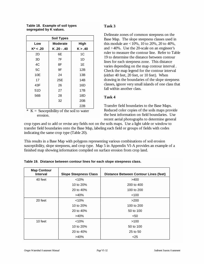
Oregon Watershed Assessment Manual Page VI-32 Sediment Sources Assessment
Task 3
Delineate zones of common steepness on theBase Map. The slope steepness classes used inthis module are <10%, 10 to 20%, 20 to 40%,and >40%. Use the 20-scale on an engineer’sruler to measure the contour line. Refer to Table19 to determine the distance between contourlines for each steepness zone. This distancevaries depending on the map contour interval .Check the map legend for the contour interval(either 40 feet, 20 feet, or 10 feet). Whendrawing in the boundaries of the slope steepnessclasses, ignore very small islands of one class thatfall within another class.
Task 4
Transfer field boundaries to the Base Maps.Reduced color copies of the soils maps providethe best information on field boundaries. Userecent aerial photographs to determine general
crop types and to add or revise any fields not on the soils maps. Use a light table or window totransfer field boundaries onto the Base Map, labeling each field or groups of fields with codesindicating the same crop type (Table 20).
This results in a Base Map with polygons representing various combinations of soil erosionsusceptibility, slope steepness, and crop type. Map 5 in Appendix VI-A provides an example of afinished map showing information compiled on surface erosion from crop land.
Table 18. Example of soil typessegregated by K values.
Soil Types
Low
K* < .20
Moderate
K .20 - .40
High
K > .40
2D
3D
4C
5C
10E
17
43F
51D
56B
6E
7F
8F
9F
24
25E
26
27
28
32
1C
1D
1E
12B
13B
14B
16D
17B
18D
20B
22B
* K = Susceptibility of the soil to watererosion.
Table 19. Distance between contour lines for each slope steepness class.
Map ContourInterval Slope Steepness Class Distance Between Contour Lines (feet)
40 feet <10% >400
10 to 20% 200 to 400
20 to 40% 100 to 200
>40% <100
20 feet <10% >200
10 to 20% 100 to 200
20 to 40% 50 to 100
>40% <50
10 feet <10% >100
10 to 20% 50 to 100
20 to 40% 25 to 50
>40% <25

Oregon Watershed Assessment Manual Page VI-33 Sediment Sources Assessment
Task 5
Next, create a database of observationson how combinations of site factors andfarming practices influence erosion inyour watershed. This is the mostdifficult but perhaps the mostinformative task. Observations are bestmade immediately after a high-runoffperiod and during the time when fieldsare most vulnerable to erosion. Forwheat, this may be when the field isfallow. Christmas tree farms may bemost vulnerable the first winter after thesite has been prepared for a newplanting. For a grass field, this may beduring the fall rains immediately after anew planting.
Site observations are meant to be acollaborative process that includes not only the analysts but also farmers and others with knowledgeof farming practices in the watershed. During a site observation you will be noting several items.First, examine the area for signs of moderate or high erosion. Erosion severity classes for crop landare defined as follows:
• High: Deep rills or gullies. Extensive deposits of sediment on flatter areas near or in streamsand draws. Deep sediment deposits at culvert inlets or at the uphill sides of elevated roads.
• Moderate: Shallow but numerous rills. Shallow deposits of sediment on flatter areas nearstreams and draws. Shallow sediment deposits at culvert inlets or at the uphill of elevatedroads.
• Low: Otherwise.
You will also want to note the condition of the field previous to recent runoff events (e.g., freshlyplowed, fallow, early stage of crop growth, crop removed, crop occupies site), as well as the cropplanted or to be planted. Next, look for evidence of soil conservation measures used by the farmer,or better yet, contact the farmer and ask about any soil conservation measures used on that field.Mark the location where the field was observed and assign it a unique number. Soil conservationmeasures for crop land include:
• Crop rotation: Cover crops are planted for the winter in order to prevent erosion and runoffwhen winter rains or spring snowmelt arrives.
• Contour cultivation: On gently sloping land, fields are tilled on the contour rather than upand down the slopes in order to retard the velocity of overland flow of water. Not effectiveon steep slopes.
Table 20. General crop types.
Crop Type Label
Wheat W
Other grain G
Grass seed GS
Hay H
Corn C
Other row crops R
Berries B
Orchards O
Vineyards V
Christmas trees CT
Nursery operations N
Poplar plantations P
Other Oth

Oregon Watershed Assessment Manual Page VI-34 Sediment Sources Assessment
• Strip cropping: A cropping technique in which alternate strips of different crops are plantedin the same field, usually on the contour.
• Conservation tillage: Any tillage system that reduces tillage and leaves at least 30% of thefield surface covered with crop residue after planting is completed.
• Riparian strips: Establishment of buffers or grass, shrubbery, and trees along channels toslow runoff and prevent scouring of the channel banks and bottom.
Enter the information from the Base Map with that obtained from field observations in Form S-13,Database for Tracking Field Observation and Mapped Information on Crop Land and Range Land,or the CROP Worksheet. Table 21 provides an example of a completed Form S-13 for crop land.
Summary: Crop Land
After a number of observations have been included in the database, you may start to see patternsdeveloping. For example, combinations of the soil K factor, slope steepness, and field conditionsmay result in moderate erosion when normal wheat-farming practices are used but low when certainconservation practices are used. Enter summary information in Form S-14, Summary of Crop Landand/or Range Land, Grazing Erosion Observations, or in the CROPSUM Worksheet. Table 22provides an example of a completed Form S-14. The various combinations of site and farmingpractices are listed and the number of observations with low, medium, or high erosion aresummarized.
The information gained from a data set like the one shown in Table 22 provides insight intocombinations of site factors where an improved farming practice would yield the greatest reductionin incidences of moderate to high soil erosion. One of the main benefits of this approach is that theinformation is tailored to your watershed. From observations made by the watershed council andfarmers, you can begin to develop rules-of-thumb that apply to the watershed.
Source 6. Sediment from Range Land and Pasture
Soil erosion on range land and pasture (referred to as range land in the remainder of this section) isusually more subtle than on cropped areas. Like crop land, sediment movement from range landoccurs during infrequent and unusual runoff events, such as summer thunderstorms, quicksnowmelt, or high-intensity rainfall. However, the grass itself is a significant barrier to soilmovement. Dense grass and the associated root mass present reduces soil movement when unusualrunoff events occur. Large-scale gullying and rilling usually occur only on the most heavilyovergrazed lands. Few people witness these periods of soil movement, and in steeper terrain, theremay be no clear evidence that soil erosion has occurred.
Grazing often occurs on steeper slopes where natural sediment movement is relatively high, whichmakes it difficult to separate natural erosion from grazing-caused erosion. In addition, areas nearstreams are often most vulnerable to erosion. These areas are usually green into late summer andfall. Animals are attracted to the green vegetation. When intense grazing occurs in the late summerand fall, these streamside areas are left with sparse foliage and root mass during potential high-flowperiods in winter and spring.
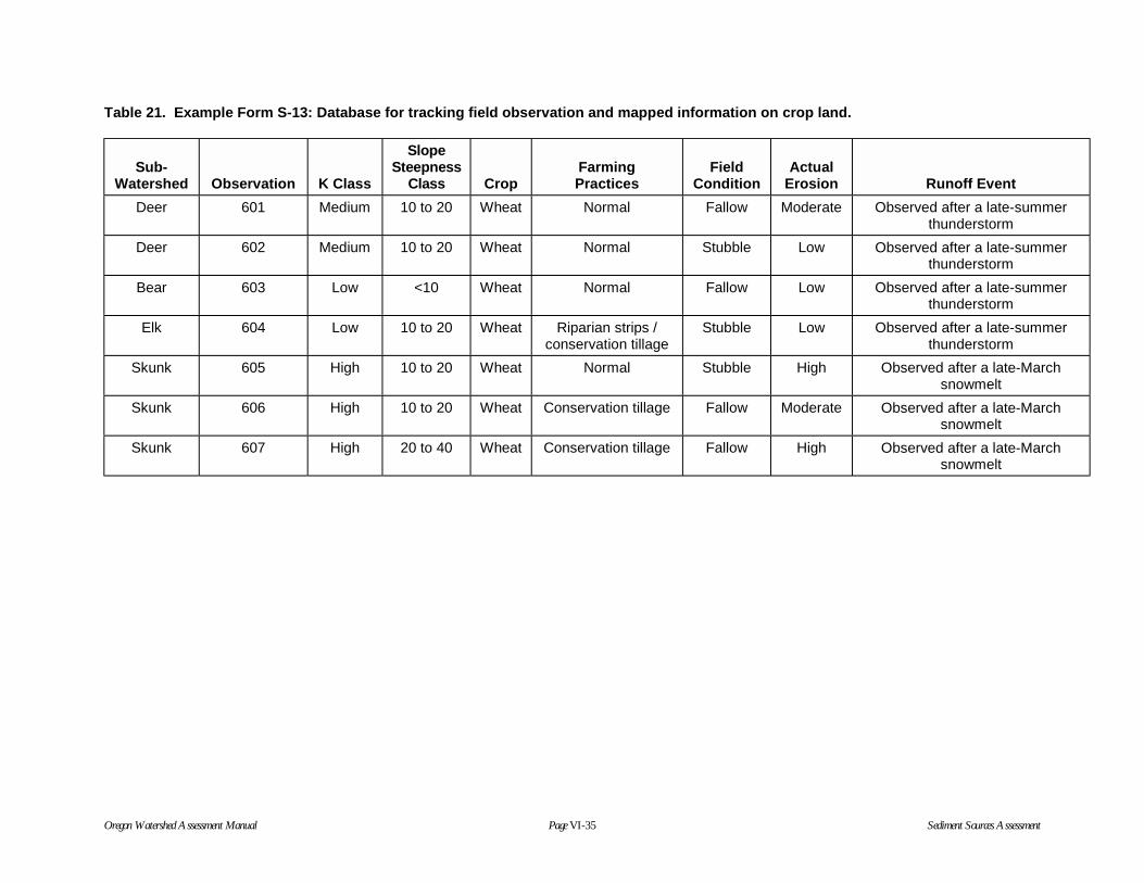
Oregon Watershed Assessment Manual Page VI-35 Sediment Sources Assessment
Table 21. Example Form S-13: Database for tracking field observation and mapped information on crop land.
Sub-Watershed Observation K Class
SlopeSteepness
Class CropFarmingPractices
FieldCondition
ActualErosion Runoff Event
Deer 601 Medium 10 to 20 Wheat Normal Fallow Moderate Observed after a late-summerthunderstorm
Deer 602 Medium 10 to 20 Wheat Normal Stubble Low Observed after a late-summerthunderstorm
Bear 603 Low <10 Wheat Normal Fallow Low Observed after a late-summerthunderstorm
Elk 604 Low 10 to 20 Wheat Riparian strips /conservation tillage
Stubble Low Observed after a late-summerthunderstorm
Skunk 605 High 10 to 20 Wheat Normal Stubble High Observed after a late-Marchsnowmelt
Skunk 606 High 10 to 20 Wheat Conservation tillage Fallow Moderate Observed after a late-Marchsnowmelt
Skunk 607 High 20 to 40 Wheat Conservation tillage Fallow High Observed after a late-Marchsnowmelt

Oregon Watershed Assessment Manual Page VI-36 Sediment Sources Assessment
Table 22. Example Form S-14: Summary of crop-land erosion observations for wheat.
Crop: wheat
Number of Observations byErosion Class
KClass Slope Class Farming Practice Field Condition Low
Mod-erate High Total
Low <10 Normal Fallow 4 2 0 6
Low <10 Normal Stubble 8 0 0 8
Low <10 Conserv. tillage Fallow 9 0 0 9
Low <10 Conserv. tillage Stubble 7 0 0 7
Low 10 to 20 Normal Fallow 3 3 0 6
Low 10 to 20 Normal Stubble 4 3 0 7
Low 10 to 20 Conserv. tillage Fallow 5 2 0 7
Low 10 to 20 Conserv. tillage Stubble 6 2 0 8
Moderate <10 Normal Fallow 4 5 0 9
Moderate <10 Normal Stubble 4 2 0 6
Moderate <10 Conserv. tillage Fallow 5 4 1 10
Moderate <10 Conserv. tillage Stubble 6 2 0 8
Moderate 10 to 20 Normal Fallow 1 2 3 6
Moderate 10 to 20 Normal Stubble 1 3 1 5
Moderate 10 to 20 Conserv. tillage Fallow 1 4 3 8
Moderate 10 to 20 Conserv. tillage Stubble 3 6 0 9
Some of the best places to detect sediment movement on range land is along draws and streams.Here, the runoff water slows down and deposits some of its load of sediment. Another place tolook for signs of high sediment movement is at culvert inlets and the uphill side of elevated roads.
Potential soil erosion from range land is evaluated much like crop-land potential erosion. Grazingareas are first subdivided by slope class and the erodibility class of the soil (K). Then you makeobservations of soil erosion following high-runoff events during the time of year that the soil ismost vulnerable to movement. Areas are classified according to site factors and observed soilerosion, and ultimately, rules-of-thumb will be developed that apply to your watershed. Thedecision process is set up as follows:
If: erodibility class of the soil is X, and slope steepness class is Y, and
grazing practice is Z,
Then: soil erosion potential is W.
You will map soil erodibility class and slope steepness class ahead of time. Information aboutgrazing practices and soil erosion is gathered during site observations. The erodibility class of soils

Oregon Watershed Assessment Manual Page VI-37 Sediment Sources Assessment
(K) you will use for range land is the same that was developed for crop land. Use county soilsurveys and the techniques described in the crop-land section (Task 5) to determine the erodibilityclass of soils. County soil surveys do not include soil typing on USFS land, so if USFS lands are tobe assessed, use the soil resources inventory for the local district office. USFS soil inventories arenot the same as county soil surveys and seldom contain the K values for each soil type, but most willat least have a low, moderate, and high erodibility rating for each soil. Assume that the USFS lowrating corresponds with soils for which K is <.20, moderate corresponds with soils for which K isbetween .20 and .40, and high corresponds with soils for which K is >.40.
The soil steepness classes do not have to be as detailed for range land as for crop land, so soilsteepness is compressed into two classes; 40% or less, or >40%. Use the same procedures describedin Tasks 1 through 4 to record K class and slope steepness information on the Base Map, or simplydisplay range-land information on the crop-land map. Map 6 in Appendix VI-A provides anexample of a finished map showing information compiled on surface erosion potential for rangeland.
After mapping range-land information, create a database of observations on how combinations ofsite factors and grazing practices influence erosion patterns. Factors to note include erosionseverity, plant condition, and soil conservation measures employed (methods described in the nextfew paragraphs). Observations are meant to be a collaborative process that includes not only yourobservations but ranchers and others with knowledge of grazing practices in the watershed. Assigna unique number to each field observation and mark and label the location on the map. Then, enterthe information on Form S-13, Database for Tracking Field Observation and Mapped Informationon Crop Land and Range Land, or the RANGE Worksheet. Table 23 provides an example of howsite information and erosion observations are compiled for range land. Site observations are bestconducted immediately after a high-runoff period and during the time of year when the land is morevulnerable to erosion. In regions that experience thunderstorms and rapid snowmelt, this time isfrom summer to spring; however, in some areas this window of vulnerability is probably during thewinter. During a site observation, assign the area an erosion severity class, and record areas withmoderate or high erosion severity as defined in the crop-land section.
Also note plant conditions and soil conservation measures used. Record the foliage and root masscondition of the plants as dense, moderate, or sparse. Examine evidence of soil conservationmeasures used by the rancher, and contact the rancher to determine these measures. Some soilconservation measures used for range land include:
• Rest rotation: The land is periodically not grazed during the growing season so plants have achance to replace reserves.
• Controlled stocking: The number of animals is controlled so that forage is at least 4 to 6inches after grazing and more than 50% of current growth is left intact.
• Distribution control: Animals are moved or excluded by fences so that certain areas do notbecome degraded (especially streamside areas).
• Plant improvement: The health of browsed plants is enhanced using combinations of fire,seeding, scarification, or fertilization.

Oregon Watershed Assessment Manual Page VI-38 Sediment Sources Assessment
Table 23. Example Form S-13: Database for tracking field observations and mapped information on crop land and range land.
Sub-Watershed Observation K Class
SlopeSteepness
Class
PlantCover
ConditionGrazing
PracticesActual
Erosion Runoff Event
Deer 701 Medium <40 Dense Normal low Observed after a late-summer thunderstorm
Deer 702 Medium >40 Dense Normal moderate Observed after a late-summer thunderstorm
Bear 703 Low <40 Moderate Rest rotation low Observed after a late-summer thunderstorm
Elk 704 Low <40 Sparse Controlledstocking
moderate Observed after a late-summer thunderstorm
Skunk 705 High <40 Sparse Normal moderate Observed after a late-March snowmelt
Skunk 706 High >40 Moderate Plantimprovement(2 years ago)
moderate Observed after a late-March snowmelt
Skunk 707 High <40 Sparse Plantimprovement(3 years ago)
low Observed after a late-March snowmelt

Oregon Watershed Assessment Manual Page VI-39 Sediment Sources Assessment
Summary: Range Land
After a number of observations have been included in the database, patterns may develop. Forexample, combinations of the soil K factor, slope steepness, and plant condition may result inmoderate erosion when normal grazing practices are used, but low erosion when certain soilconservation measures are added. Compile site observations on Form S-14, Summary of Crop Landand/or Range Land, Grazing Erosion Observations. Table 24 provides an example showing acomparison of soil erosion under normal grazing practices to soil erosion under controlled stocking.You may wish to construct other tables focusing on other combinations of grazing practices and siteconditions. Each table will include various combinations of site conditions and grazing practices,and the number of sites with low, medium, or high erosion. The number of sites can also beexpressed as a percentage of the row total to provide a clearer picture of how combinationscompare. These tables may be used to target combinations of site factors that indicate sites whereimproved grazing practices would yield the greatest reduction in moderate to high soil erosion. Thisapproach tailors the information to your watershed; from your own observations, you can begin todevelop rules-of-thumb that work for your watershed.
Source 7. Surface Erosion from Burned Areas
Recently burned areas can have a high potential for erosion within the first year or two following thefire. The removal of surface organic matter by fire can release soil that has collected uphill of the
Table 24. Example Form S-14: Summary of range-land erosion observations.
Number of Observations byErosion Class
KClass
SlopeClass Grazing Practice Plant Condition Low
Mod-erate High Total
Moderate <40 Normal sparse 4 2 0 6
Moderate <40 Normal mod./dense 8 0 0 8
Moderate <40 Controlled stocking sparse 8 1 0 9
Moderate <40 Controlled stocking mod./dense 7 0 0 7
Moderate >40 Normal sparse 3 4 0 7
Moderate >40 Normal mod./dense 4 2 0 6
Moderate >40 Controlled stocking sparse 4 3 0 7
Moderate >40 Controlled stocking mod./dense 5 2 0 7
High <40 Normal sparse 2 5 2 9
High <40 Normal mod./dense 3 4 0 6
High <40 Controlled stocking sparse 2 7 1 10
High <40 Controlled stocking mod./dense 3 6 0 9
High >40 Normal sparse 0 6 2 8
High >40 Normal mod./dense 0 6 0 6
High >40 Controlled stocking sparse 2 6 0 8
High >40 Controlled stocking mod./dense 3 2 0 5

Oregon Watershed Assessment Manual Page VI-40 Sediment Sources Assessment
organic matter. It also leaves the surface vulnerable to rain-splash erosion. Under someconditions, the burned soil surface will actually temporarily repel water. This leads to more of therunoff occurring along the soil surface, thereby causing surface soil movement. Water-repelling soilconditions usually disappear after a few runoff events in Oregon. Fires can also bare the banks ofdraws and streams. Soil raveling from those bared and steep slopes immediately adjacent to thechannel can cause them to partially fill with loose sediment. These sediments are then vulnerable todownstream movement during runoff events.
Fire containment activities such as the construction of temporary access roads and fire lines cansometimes lead to significant inputs of sediment into streams. Access road and fire lines are oftenbuilt in a hurry and sometimes without much consideration to where excavated soil is placed.Unless these temporary roads and fire lines are carefully obliterated or rehabilitated after the fire,they can also become sources of sediment. Erosion is usually caused by water running down thesurfaces of the roads or trails, and is made worse if the fire area later attracts motorcyclists, all-terrain-vehicles, or 4-wheel-drive operators.
Not all fires cause significant increases in stream sediment. Cool fires that consume only part of thesurface organic matter may not be a source of accelerated erosion. Fires that skip over streamchannels also may have little effect on soil erosion.
In some areas, the forests are now intentionally burned at a frequent interval in order to decrease thelikelihood of a catastrophic wildfire that would kill large trees or harm the soil. For many decades,intentional burns have also been used to remove slash and brush following the harvest of timber, totreat fields in anticipation of the next crop, or to manage range-land plant health and composition.Nevertheless, recent air quality control measures are making it hard for landowners to find windowsof opportunity to burn. The main goal of these air quality control measures is to keep smoke out ofpopulated areas. The incidence of intentional burns has decreased substantially in some parts of thestate as a result of the air quality control measures.
Evaluation of surface erosion from burned areas in the watershed will be limited to identifying thepresence of recent burns, if any. Your assessment will result in mapping of recently burned areasand combining of various site factors with observations on obvious evidence of erosion.
Task 1
The first step for compiling information on recently burned areas is to determine the boundaries ofthe fire and transfer them to a topographic base map. You may be able to do this simply by drivingthrough the burned area and noting the relationship of the fire boundary to roads, streams, andridges. You may also want to use aerial photographs for large burned areas and especially areas thatdid not burn uniformly. The ODF, USFS, or BLM will sometimes have aerial photographs flownimmediately after large-scale fires, so check with them first.
Task 2
Segregate the burn area into two slope steepness classes (40% or less, >40%) and two K factorclasses (.40 or less, >.40), as described in the sections on surface erosion from crop land and rangeland. Add information about fire intensity to the map. This is best done using a combination of siteobservations and aerial photographs, although you may be able to complete this without aerial
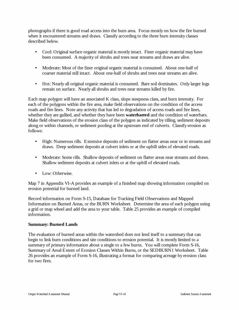
Oregon Watershed Assessment Manual Page VI-41 Sediment Sources Assessment
photographs if there is good road access into the burn area. Focus mostly on how the fire burnedwhen it encountered streams and draws. Classify according to the three burn intensity classesdescribed below.
• Cool: Original surface organic material is mostly intact. Finer organic material may havebeen consumed. A majority of shrubs and trees near streams and draws are alive.
• Moderate: Most of the finer original organic material is consumed. About one-half ofcoarser material still intact. About one-half of shrubs and trees near streams are alive.
• Hot: Nearly all original organic material is consumed. Bare soil dominates. Only larger logsremain on surface. Nearly all shrubs and trees near streams killed by fire.
Each map polygon will have an associated K class, slope steepness class, and burn intensity. Foreach of the polygons within the fire area, make field observations on the condition of the accessroads and fire lines. Note any activity that has led to degradation of access roads and fire lines,whether they are gullied, and whether they have been waterbarred and the condition of waterbars.Make field observations of the erosion class of the polygon as indicated by rilling, sediment depositsalong or within channels, or sediment pooling at the upstream end of culverts. Classify erosion asfollows:
• High: Numerous rills. Extensive deposits of sediment on flatter areas near or in streams anddraws. Deep sediment deposits at culvert inlets or at the uphill sides of elevated roads.
• Moderate: Some rills. Shallow deposits of sediment on flatter areas near streams and draws.Shallow sediment deposits at culvert inlets or at the uphill of elevated roads.
• Low: Otherwise.
Map 7 in Appendix VI-A provides an example of a finished map showing information compiled onerosion potential for burned land.
Record information on Form S-15, Database for Tracking Field Observations and MappedInformation on Burned Areas, or the BURN Worksheet. Determine the area of each polygon usinga grid or map wheel and add the area to your table. Table 25 provides an example of compiledinformation.
Summary: Burned Lands
The evaluation of burned areas within the watershed does not lend itself to a summary that canbegin to link burn conditions and site conditions to erosion potential. It is mostly limited to asummary of primary information about a single to a few burns. You will complete Form S-16,Summary of Areal Extent of Erosion Classes Within Burns, or the SEDBURN1 Worksheet. Table26 provides an example of Form S-16, illustrating a format for comparing acreage by erosion classfor two fires.

Oregon Watershed Assessment Manual Page VI-42 Sediment Sources Assessment
Table 25. Example Form S-15: Database tracking field observations and mapped information onburned areas.
Burn name: Sow Creek fire
Date area burned: 8/98
Date evaluated: 6/99 and 7/99
Years between evaluation and fire: 1.2
Type of fire: Wildfire
Land cover prior to fire: Forested with some meadows on south slopes
ObservationK
Class
SlopeSteepness
ClassBurn
IntensityCondition of AccessRoads and Fire Lines
ErosionClass
Area(acres)
801 <.40 <40 Low Good condition; allwaterbarred
low 1,250
802 <.40 >40 Moderate Good condition; allwaterbarred
moderate 510
803 <.40 <40 Low Good condition; allwaterbarred
moderate 450
804 <.40 <40 Moderate Deeply rutted; 4WDactivity
moderate 1,100
805 >.40 <40 Moderate Deeply rutted; 4WDactivity
high 970
806 >.40 >40 Hot Deeply rutted; 4WDactivity
high 410
807 >.40 <40 Hot Good condition; allwaterbarred
moderate 960
Table 26. Example Form S-16: Summary of areal extent of erosion classes within burns.
Area and % of Total Area by Erosion Class
Low ErosionModerateErosion High Erosion Total
Burn Name Acres % Acres % Acres % Acres %
Sow Creek fire 1,250 22 3,020 53 1,380 25 5,650 100
Little Pig Creekfire
420 17 1,120 44 980 39 2,520 100

Oregon Watershed Assessment Manual Page VI-43 Sediment Sources Assessment
Source 8. Other Discrete Sources
Other discrete sources of accelerated soil erosion and stream sedimentation may be present in yourwatershed. This manual does not include procedures for evaluating these sources, but they shouldbe documented during this assessment process. Your documentation should include not only thosesources that currently are a source of sediment, but also those that have strong potential to becomea source in the future. A partial listing of other discrete sediment sources and their potentialinfluence on streams follows:
• In-channel gold mining: Periods of chronic turbidity; deposition of fine sediments.
• Mining spoil piles: Calving-off of piles or surface erosion into nearby streams; turbidity anddeposition of fine sediments.
• Gravel pit drainage: Chronic turbidity.
• Winter animal holding areas near streams: Trampling of banks—surface runoff overcompacted soils; chronic turbidity; deposition of fine sediments.
• Road sanding: Chronic turbidity; deposition of fine sediments.
• Wind erosion: Chronic turbidity; deposition of fine sediments.
Step 4: Evaluate Confidence in Assessment
Rate your confidence in the quality and completeness of information you compiled for yourwatershed assessment of sediment sources (Form S-17, Confidence Evaluation). For each source,rate the quality of information (where it existed for the watershed) as Good, Fair, or Poor; rate thecompleteness of the information (Not Missing, Partially Missing, Mostly Missing). Explain thefactors that prevented you from compiling good information for the entire watershed. Skip sourcesthat you did not include in your assessment.

Oregon Watershed Assessment Manual Page VI-44 Sediment Sources Assessment
REFERENCES
Alt, D.D., and D.W. Hyndman. 1996. Roadside Geology of Oregon. Mountain Press PublishingCo. Missoula, Montana.
Anderson, H.W. 1954. Suspended Sediment Discharge as Related to Streamflow, Topography, Soil,and Land Use. Transactions of the American Geophysical Union 35(2):268-281.
Benda, L., and T. Dunne. 1987. Sediment Routing by Debris Flow. Pages 213-224 in: Erosion andSedimentation in the Pacific Rim. IAHS Publication No. 165.
Bilby, R.E. 1985. Contributions of Road Surface Sediment to a Western Washington Stream.Forest Science 31(4):827-838.
Bilby, R.E., K. Sullivan, and S.H. Duncan. 1989. The Generation and Fate of Road-SurfaceSediment in Forested Watersheds in Southwestern Washington. Forest Science 35(2):453-468.
Bisson, P.A., and R.E. Bilby. 1982. Avoidance of Suspended Sediment by Juvenile Coho Salmon.North American Journal of Fisheries Management 2:371-374.
Booth, D. 1991. Urbanization and the Natural Drainage System—Impacts, Solutions, andPrognosis. Northwest Environmental Journal 7(1):93-118.
Duncan, S.H., R.E. Bilby, J.W. Ward, and J.T. Heffner. 1987. Transport of Road-Surface SedimentThrough Ephemeral Stream Channels. Water Resources Bulletin 23(1):113-119.
Lisle, T.E. 1987. Channel Morphology and Sediment Transport in Steepland Streams. Pages 287-298 in: Erosion and Sedimentation in the Pacific Rim. IAHS Publication No. 165.
Megahan, W. F. 1987. Increased Sedimentation Following Helicopter Logging and PrescribedBurning on Granitic Soil. Pages 259-260 in: Erosion and Sedimentation in the Pacific Rim.IAHS Publication No. 165.
Newcombe, C.P., and D.D. MacDonald. 1991. Effects of Suspended Sediments on AquaticSystems. North American Journal of Fisheries Management 11:72-82.
Sessions, J., J.C. Balcom, and K. Boston. 1987. Road Location and Construction Practices: Effectson Landslide Frequency and Size in the Oregon Coast Range. Western Journal of AppliedForestry 2(4):119-124.
Tasker, G.D., and N.E. Driver. 1988. Nationwide Regression Models for Predicting Urban RunoffWater Quality at Unmonitored Sites. Water Resources Bulletin 24(5):1091-1101.

Oregon Watershed Assessment Manual Page VI-45 Sediment Sources Assessment
GLOSSARY
borrow pit: An area where rock or soil is excavated from the hillside.
cable yarding scar: An area within a timber harvest unit that is bare due to logs dragging on theground as they are being moved by cables to the road.
calving-off: The rapid movement of soil from the steep leading edge of a large landslide.
cross-drain culvert: A culvert that drains water which collects within the inside ditch of a road tothe outside slope of the road.
cut slope: The sloping excavated surface on the inside of a road.
detention pond: A pond constructed to temporarily store water, thereby allowing sediment to settleout of the water.
draw: A very small stream that may have flowing water only during the wet season.
fill slope: The outer edge of a road that extends downhill of the road surface.
full-bench construction: A practice of constructing a road on steeper slopes whereby excessexcavated soil or rock is hauled away in trucks to a stable storage area rather than disposed of bypushing it downhill of the road.
Geographic Information System (GIS): A computer system designed for storage, manipulation,and presentation of geographical information such as topography, elevation, geology etc.
harvest unit: An area from which trees have been harvested.
hazard delineation: Mapping the boundaries of areas with inherently unstable slopes.
landing: An area adjacent to a road where logs accumulate and are loaded onto trucks duringtimber harvesting.
pipe-arch culvert: A corrugated pipe that is wider than it is tall.
ravel: Erosion caused by gravity, especially during rain, frost, and drying periods. Often seen onsteep slopes immediately uphill of roads.
recurrence interval(s) (return interval): Determined from historical records. The average lengthof time between two events (rain, flooding) of the same size or larger. Recurrence intervals areassociated with a probability. (For example, a 25-year flood would have a 4% probability ofhappening in any given year.)
rills: Very shallow gullies that can develop on a hillslope that is eroding.
rock pit: An area where rock is excavated from a hillside and is usually processed as road-surfacingmaterial.

Oregon Watershed Assessment Manual Page VI-46 Sediment Sources Assessment
scarification: The mechanical loosening of compacted soil usually using subsoilers attached to acrawler tractor.
sheet erosion: Soil erosion caused by surface water that occurs somewhat uniformly across a slope.
skid trail: Trail that develops when logs are hauled by ground-based machinery to a landing.
slash: Detached tree limbs, branches, and other woody material that is left on the ground after atimber harvest is completed.
stereoscope: An instrument used to observe stereo aerial photographs in three dimensions.
waterbar: A deep trough in a skid trail or road that is excavated at an angle to drain surface waterfrom the skid trail or road to an adjacent area that is not compacted.

Appendix VI-AExamples of FinishedSediment-Source Maps


Oregon Watershed Assessment Manual Page 1 Appendix VI-A
APPENDIX VI-A: EXAMPLES OF FINISHEDSEDIMENT - SOURCE MAPS
Existing shallow landslides: reached stream did not reach stream
Existing deep-seated landslides: reached stream did not reach stream
Potential for shallow landslides: High Extreme
Slope Instability (not related to roads)
301
302303
304
305
306
307
308
310
309
312
311
313
314
315317
316
Map 2. Example of a finished map showing information compiled on slope instability not relatedto roads.
Stream culvert; very low to moderate high to extremely high
Road failure; reached stream id not reach stream
Cracks and slumpsWater flowing over fill
Road Instability
201
202
203
204
205
206
207
208
210
209
212211
213
214
215
217
218
219
216
Map 1. Example of a finished map showing information compiled for both existing andpotential road instability sites.

Oregon Watershed Assessment Manual Page 2 Appendix VI-A
City limit
Stream
Stormwaterwatershed
Generalstormwater flow direction
Urban area type
Street cleaningmethod
#501L1/M2/N3
#502L1/M2/N3
#503M1/M2/N3
#504M1/M2/N3
#505M1/L2/N3
#506L1/L2/N3
#507L1/M2/N3
#508L1/M2/N3
#509VH1/M2/N3
#510L1/L2/N3
#511L1/L2/N3
#512L1/M2/N3
Su
cker
Riv
er
Ditch Cr.
Tunnel Cr.
Dairy Cr.
Map 4. Example of a finished map showing basic information compiled on urban runoff.
Road within 200 feet of stream Road within 200 feet of stream and slope greater than 50%
Rural Road Runoff
401
402
403
404
405
Low use,gravel
High use,gravel
High use, gravel
Map 3. Example of a finished map showing information compiled on rural road runoff.

Oregon Watershed Assessment Manual Page 3 Appendix VI-A
Crop Land
>40%
20-40%
>40%
>40%
0-20%
20-40%
20-40%
Slope steepness boundaries
>40%
K class
Low Low
High
Medium
Medium
Low
High
Low
Observations #xxx
#601
CTCT
V
V
V
CT
GS
GS
Field boundary
10-20% 10-20%
20-40%
>40% >40%
20-40%
0-20%
>40%
20-40%
20-40%
20-40%
20-40%
20-40%
#602
#603
#604
#607
#606
#605
#608
#609
#610
#611
#612
#614#615
#616
Map 5. Example of a finished map showing information compiled on surface erosion fromcrop land.
Range Land
Range Land
>40%
>40%
>40%
<40%
>40%>40%
>40%
<40%
<40%<40%
<40%
<40%
<40%
<40%
>40%
>40%
Slope steepness boundaries
<40%
<40%
<40%
>40%
>40%
>40%
K class
Low
Medium
Low
HighMedium
High
Medium
Low
High
Low
Observations #xxx
#701
#702
#703
#704
#707
#705
#706
#708
#709
#710
#711
#712
#713
#714#715
#716
#717
#718
#719
#720
#721
#722
#723
#724
#725 #726
Map 6. Example of a finished map showing information compiled on surface erosion potentialfor range land.

Oregon Watershed Assessment Manual Page 4 Appendix VI-A
Burn boundaries
Burned Areas
Burn intensity boundaries
Cool
Cool
Moderate
Hot
>40%
>40%
>40%
<40%
>40%>40%
>40%
<40%
<40%<40%
<40%
<40%
<40%
<40%
>40%
>40%
Slope steepness boundaries Erosion class (post-fire)
Low
ModerateHigh
Low
Moderate
Moderate
Low Low
Low
Low
#802
#801<40%
#803
#804
#805
#806
#807
#808
#809
#810
#811 #812
#813
#814
#815
#816 #817
#818
#819
#820#821
#822#823
#824 #825
#826#827
#828
#829
#830
#831
#832
#833
#834
#835#836
#837
#838#839
#840
#810
Map 7. Example of a finished map showing information compiled on erosion potential forburned land.


Appendix VI-BBlank Forms


Form S-1: Screen for Sediment Sources in a Watershed
Watershed:
Analyst’s Name:
Watershed Name: The River Why Observations Priority
Source 1: Road instability
Are rural roads common in watershed?
Do many road washouts occur following high rainfall?
Are many new roads or road reconstruction planned?
Source 2: Slope instability (not related to roads)
Are landslides common in watershed?
Many high-sediment, large-scale landslides?
Source 3: Rural road runoff
Are sediment-laden runoff from rural roads and turbidity instreams common?
Is there a high density of rural roads?
Source 4: Urban runoff
Are many portions of the watershed urbanized?
Importance of these tributaries to watershed council:
Source 5: Surface erosion from crop land
Is there much crop land in the watershed?
Is there much evidence of sediment in streams flowingthrough crop land?
Source 6: Surface erosion from range land
Is there much range land in watershed?
Is there evidence of sediment in streams flowing throughrange land?
Source 7: Surface erosion from burned land
Have many burns occurred recently (last 5 years),especially hot fires?
Was there much sediment created by these burns?
Source 8: Other discrete sources of sediment
List or identify any other suspected sources of sediment:


Form S-2: Information on Existing Road-Related Instability
Watershed:
Analyst’s Name:
Num. Subwatershed Landslide TypeReachedStream?
DistanceTraveled (ft) Road Location
Number: Unique identification number.
Subwatershed: Subwatershed in which landslide occurs.
Landslide Type: Debris flow = initiates as shallow landslide in steep area and then flows down achannel, picking up additional soil, logs, and water. Road prism failure = downhill movement of theroad cut or road fill; does not initiate a debris flow. Culvert washout = road fill partially or completelymissing where the road crosses a stream.
Reached Stream?: Whether or not the landslide material ended up in the stream.
Distance traveled: The distance from initiation point to where the landslide stopped (not applicableto culvert washouts).
Road Location: General location of road: near ridge, mid-slope, near stream.


Form S-3: Culvert Capacity and Risk of Large Amounts of Sediment Entering Stream
Watershed:
Analyst’s Name:
1Sub-
watershed2
Num.
3Road
Owner-ship
4CurrentCulvert/
Pipe-ArchSize
5CurrentCulvert
Capacity(cfs)
6ODF
Peak-FlowValue
(cfs/mi²)
7Drainage
Area(mi²)
850-Year
PeakFlow(Col.6x7)(cfs)
9Culvert/
Pipe-ArchSize
Needed for50-Year
Peak Flow
10Ratio of
50-YrFlow toCurrentCapacity
11Fill
Height(ft)
12HazardRating *
* Hazard rating:
Very low Fill height is 15 feet or less and ratio is less than 1.25.
Low Fill height is greater than 15 feet and ratio is less than 1.25.
Moderate Fill height is 15 feet or less and ratio is between 1.25 and 1.75.
High Fill height is greater than 15 feet and ratio is between 1.25 and 1.75; or, fill height is 15 feet or less and ratio is between1.76 and 3.
Very high Fill height is greater than 15 feet and ratio is between 1.76 and 2.99; or, fill height is 15 feet or less and ratio is greater than 3.
Extreme Fill height is greater than 15 feet and ratio is greater than 3.


Form S-4: High-Risk Road Segments for Existing Roads
Watershed:
Analyst’s Name:
Sub-Watershed Num.
FeatureType
Hazard Ratingof Culvert
RoadOwnership


Form S-5: Summary of Information on Road Instability
Watershed:
Analyst’s Name:
Subwater-shed
Area(mi²)
Road Failures thatReached Streams
Sites with High-Risk Culverts
Sites withCracks and
Slumps
Sites with WaterFlowing Over
Fills
#Density(#/mi².) #
Density(#/mi².) #
Density(#/mi².) #
Density(#/mi².)
Total


Form S-6: Current Landslides not Related to Roads
Watershed:
Analyst’s Name:
Sub-watershed Num.
Type ofLandslide
Age ofVegetation
(years)
LandslideReachedStream?
DistanceLandslide
Traveled (feet)
Slope Steepnessat InitiationPoint (%)


Form S-7: Potential for Debris Flows
Watershed:
Analyst’s Name:
Subwatershed Areas Predicted to be High Risk for Debris Flows (mi²)
High Hazard Extreme Hazard Combined


Form S-8: Summary of Information on Slope Instability (not related to roads)
Watershed:
Analyst’s Name:
Current LandslidesSub-
WatershedArea(mi2)
Shallow Landslides Deep-SeatedLandslides
Debris-Flow High-RiskAreas (combined high
and extreme)
Number(#)
Density(#/mi².)
Number(#)
Density(#/mi².) Area (mi².) Percent
Total


Form S-9: Basic Information on Road Segments Close to Streams withSteep Slopes
Watershed:
Analyst’s Name:
Subwatershed Num.Distance <200'
from Stream (feet)
Distance <200' fromStream and Slope >50%
(feet)Road
SurfaceRoadUse


Form S-10: Summarized Runoff-Related Information for a Single Road
Watershed:
Analyst’s Name:
Road Name Variable ClassificationLength(feet)
Occurrences(#)


Form S-11: Summary of Information on Road Runoff—Basic Assessment
Watershed:
Analyst’s Name:
Sub-watershed
Area(mi2)
Roads < 200'from Stream
Roads < 200' fromStream andSlope > 50%
Roads < 200' fromStream and High Use
Roads < 200' fromStream and Low Use
Length(mi.)
Density(mi./mi².)
Length(mi.)
Density(mi./mi².)
Length(mi.)
Density(mi./mi².)
Length(mi.)
Density(mi./mi².)


Form S-12: Information on Urban Runoff Polygons
Watershed:
Analyst’s Name:
StormwaterSubwatershed
Polygon#
PolygonArea (acres)
Area as aPercentage
of Total1. SedimentProduction
2. StreetCleaning
3. SedimentRemoval
Total


Form S-13: Database for Tracking Field Observation and Mapped Information on Crop Land and Range Land
Watershed:
Analyst’s Name:
Sub-Watershed Observation K Class
SlopeSteepness
Class
Crop/PlantCoverCond-ition
Farming/GrazingPractices
FieldCondition
ActualErosion Runoff Event


Form S-14: Summary of Crop Land and/or Range Land, Grazing ErosionObservations
Watershed:
Analyst’s Name:
Number of Observations byErosion Class
KClass Slope Class
Farming/GrazingPractice
FieldCondition/Plant
Condition LowMod-erate High Total


Form S-15: Database Tracking Field Observations and Mapped Information onBurned Areas
Watershed:
Analyst’s Name:
Burn name:
Date area burned:
Date evaluated:
Years between evaluation and fire:
Type of fire:
Land cover prior to fire:
ObservationK
Class
SlopeSteepness
ClassBurn
IntensityCondition of AccessRoads and Fire Lines
ErosionClass
Area(acres)


Form S-16: Summary of Areal Extent of Erosion Classes Within Burns
Watershed:
Analyst’s Name:
Area and % of Total Area by Erosion Class
Low ErosionModerateErosion High Erosion Total
Burn Name Acres % Acres % Acres % Acres %


Form S-17: Confidence Evaluation
Rate your confidence in the quality and completeness of information you compiled for yourwatershed assessment of sediment sources. For each source, rate the quality of information (whereit existed for the watershed) as Good, Fair, or Poor; rate the completeness of the information (NotMissing, Partially Missing, Mostly Missing). Explain the factors that prevented you from compilinggood information for the entire watershed. Skip sources that you did not include in yourassessment.
1. Rural road instability
Quality: Good _____ Fair _____ Poor _____
Completeness: Not Missing _____ Partially Missing _____ Mostly Missing ______
Factors that prevented compilation of good information for the entire watershed:______________________________________________________________________________________________________________________________________________________________________________________________________________________________________________________________________________________________________________________________________________________________________________________________________
2. Rural road runoff
Quality: Good _____ Fair _____ Poor _____
Completeness: Not Missing _____ Partially Missing _____ Mostly Missing ______
Factors that prevented compilation of good information for the entire watershed:______________________________________________________________________________________________________________________________________________________________________________________________________________________________________________________________________________________________________________________________________________________________________________________________________
3. Slope instability (not related to roads)
Quality: Good _____ Fair _____ Poor _____
Completeness: Not Missing _____ Partially Missing _____ Mostly Missing ______
Factors that prevented compilation of good information for the entire watershed:______________________________________________________________________________________________________________________________________________________________________________________________________________________________________________________________________________________________________________________________________________________________________________________________________

Form S-17: page 2.
4. Urban runoff
Quality: Good _____ Fair _____ Poor _____
Completeness: Not Missing _____ Partially Missing _____ Mostly Missing ______
Factors that prevented compilation of good information for the entire watershed:______________________________________________________________________________________________________________________________________________________________________________________________________________________________________________________________________________________________________________________________________________________________________________________________________
5. Surface runoff from crop land
Quality: Good _____ Fair _____ Poor _____
Completeness: Not Missing _____ Partially Missing _____ Mostly Missing ______
Factors that prevented compilation of good information for the entire watershed:______________________________________________________________________________________________________________________________________________________________________________________________________________________________________________________________________________________________________________________________________________________________________________________________________
6. Surface runoff from range land
Quality: Good _____ Fair _____ Poor _____
Completeness: Not Missing _____ Partially Missing _____ Mostly Missing ______
Factors that prevented compilation of good information for the entire watershed:______________________________________________________________________________________________________________________________________________________________________________________________________________________________________________________________________________________________________________________________________________________________________________________________________
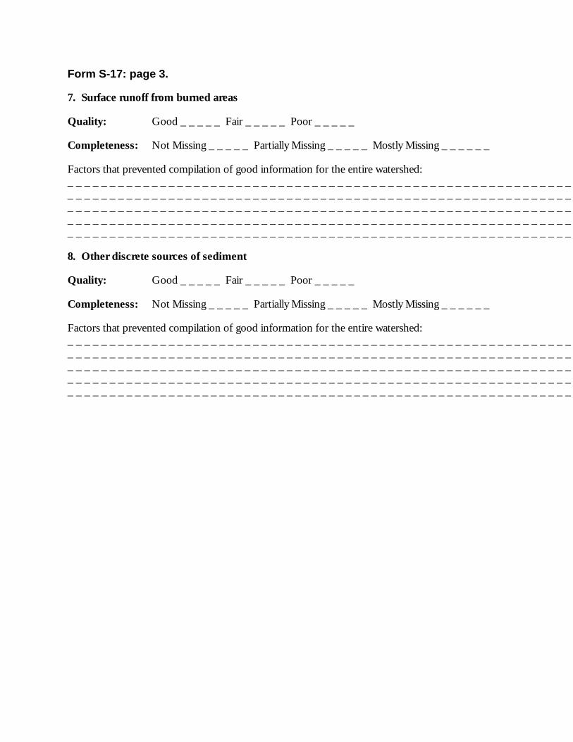
Form S-17: page 3.
7. Surface runoff from burned areas
Quality: Good _____ Fair _____ Poor _____
Completeness: Not Missing _____ Partially Missing _____ Mostly Missing ______
Factors that prevented compilation of good information for the entire watershed:______________________________________________________________________________________________________________________________________________________________________________________________________________________________________________________________________________________________________________________________________________________________________________________________________
8. Other discrete sources of sediment
Quality: Good _____ Fair _____ Poor _____
Completeness: Not Missing _____ Partially Missing _____ Mostly Missing ______
Factors that prevented compilation of good information for the entire watershed:______________________________________________________________________________________________________________________________________________________________________________________________________________________________________________________________________________________________________________________________________________________________________________________________________

Component VIIChannel ModificationAssessmentTable of Contents
Introduction....................................................VII-3
Critical Questions .......................................VII-3
Assumptions...............................................VII-3
Materials Needed .......................................VII-4
Necessary Skills .........................................VII-4
Final Products of the Channel
Modification Assessment ......................VII-4
Channel Modification Mapping
Procedures..........................................VII-5
Step 1: Gather Available Information..........VII-5
Step 2: Map Channel Modifications ............VII-6
Step 3: Evaluate Impact of Modifications....VII-8
Step 4: Identify Affected CHTs ...................VII-9
Step 5: Evaluate Confidence in the
Assessment..........................................VII-9
Glossary .......................................................VII-11
Appendix VII-A: Blank Forms
Form CM-1: Channel Modification
Inventory
Form CM-2: Channel Modification
Summary
Form CM-3: Confidence Evaluation in
Channel Modification Assessment


Oregon Watershed Assessment Manual Page VII-3 Channel Modification Assessment
Component VIIChannel Modification Assessment
INTRODUCTION
In-channel structures and activities such as damming and dredging or filling hinder fish migration,alter the physical character of streams, and change the composition of stream biota.1 The degree ofimpact to habitat will depend on the type of channel and the type and magnitude of channelmodification. Channels are dynamic systems that modify themselves in response to changes inphysical watershed features regardless of human involvement. This section identifies how humanactivities have directly changed channel morphology and aquatic habitat. This information is thensynthesized with information from the other components to assess overall watershed health andfunction.
In this portion of the watershed assessment, you will map and categorize current channelmodifications and incorporate historic channel modification information from the HistoricConditions Assessment component. During the final part of this assessment, you will overlay thechannel modification map with the Channel Habitat Type (CHT) Map (from the Channel HabitatType Classification component) to identify which CHTs have been directly impacted by theseactivities.
Critical Questions
1. Where are channel modifications located?
2. Where are historic channel disturbances, such as dam failures, splash damming, hydraulicmining, and stream cleaning, located?
3. What CHTs have been impacted by channel modification?
4. What are the types and relative magnitude of past and current channel modifications?
Assumptions
• Channel modifications and historic land use and in-channel activities may have altered thequality and/or quantity of aquatic resources in the basin.
• In the absence of documentation on pre-European settlement conditions, the impact toaquatic resources from the channel modification can be inferred from the type ofmodification or historic disturbance and the CHT affected.
• Channel disturbances, such as channel widening, extensive bank erosion, or large graveldeposits, with no apparent adjacent cause, are response indicators of changes in upstreamchannel input factors that may or may not be related to human activities; channels do modifytheir form through natural disturbance events. Conversely, channel gradient can be used to
1 Terms that appear in bold italic throughout the text are defined in the Glossary at the end of this component.

Oregon Watershed Assessment Manual Page VII-4 Channel Modification Assessment
predict zones of potential channel impacts due to declining transport ability and sedimentdeposition.
Materials Needed
• 7.5-minute US Geological Survey (USGS) topographic maps of the watershed (from theStart-Up and Identification of Watershed Issues component)
• Project base map (from the Start-Up and Identification of Watershed Issues component)
• Sharp pencil, colored pencils, thin permanent markers (optional: colored adhesive dots)
• USGS topographic map symbol legend
• Data and information on channel modification (see Step 1 below for list of potentialsources)
• Federal Emergency Management Agency (FEMA) floodplain maps (if available)
• National Wetland Inventory (NWI) maps
• A map wheel (or an engineer’s ruler with inches marked in 10ths so you can easily entermeasurements into a calculator will work if you measure carefully)
• Aerial photos of the basin (from the Start-Up and Identification of Watershed Issuescomponent)
Necessary Skills
The minimum skills necessary to produce the Channel Modification Map include (1) the ability toread and use topographic maps, (2) the ability to accurately transfer information between maps ofdifferent scales, and (3) an ability to search for and compile information from many sources. Theability to use aerial photographs will aid this task, but is not required.
Final Products of the Channel Modification Assessment
1. Channel Modification Map (CM-1)
2. Channel Modification Inventory (Form CM-1) corresponding to numbered sites on the map
3. Channel Modification Summary (Form CM-2), a summary by subwatershed of the amountof channel modified by each activity
4. Confidence Evaluation (Form CM-3) assessing your confidence in the accuracy andcomprehensiveness of the overall mapping

Oregon Watershed Assessment Manual Page VII-5 Channel Modification Assessment
CHANNEL MODIFICATION MAPPING PROCEDURES
Step 1: Gather Available Information
Ideally, you would obtain the Historical Channel Modifications Map (from the Historical ConditionsAssessment component) showing locations where historic activities affect stream channels shown.It is likely, however, that this map will be in preparation and not available at the onset of this task. Ifthis is the case, you will prepare a map of current channel modifications and combine that map withthe historic impacts map at a later date. To begin mapping, obtain a copy of the project base map.It is also possible to do the initial mapping on topographic maps, or on a Mylar overlay of the basemap or topographic maps.
A number of sources are available to gather information concerning current channel modifications,such as the following.
Topographic Maps
Many channel modifications are shown on topographic maps. Most notably are impoundments,dikes, roads along streams, and channel straightening. Structures in or immediately adjacent to thechannel may also be apparent. Note the date of the map and the presence of updated features,usually shown in a violet color.
Aerial Photographs
Depending on the quality of the photos and the skill of the reviewer, aerials can be one of the mostuseful tools in evaluating channel modifications and their potential impacts to the channel andaquatic habitat. Many modifications are quite obvious on photos, and are readily identified bypeople with limited photo interpretation experience. Again, noting the date and scale of the photoswill aid in assessing the condition of the channel and the modification. Because time will be limited,start by reviewing the photos of the largest channels in the watershed. Modifications to smallerchannels may not be visible on the photos.
Agency Records and Personnel
While not all of the agencies listed in Table 1 will have information concerning channelmodifications, contact any agency that has jurisdiction over waterways and riparian areas in yourwatershed. It is prudent to make inquiries as early as possible, because information may take sometime to reach you.
As a start, two agencies, the US Army Corps of Engineers (Corps) and the Oregon Department ofState Lands (DSL), have jurisdiction over activities in “Waters of the State,” including wetlands.The Portland office of the Corps (503-808-5150) can be contacted concerning the federal CleanWater Act Section 404 permits dealing with fills and in-stream structures. Contact the Salem officeof DSL (503-378-3805) concerning Fill and Removal permits in the watershed.
Other agencies such as the Oregon Department of Fish and Wildlife (ODFW), County PublicWorks, Oregon Department of Transportation (road maintenance issues), diking districts, the USBureau of Land Management (BLM), or local port authorities may also have useful information.
Oregon Watershed Assessment Manual Page VII-6 Channel Modification Assessment
In addition, NWI maps display some channel modifications. Consult with the Riparian/WetlandAssessment component analyst concerning the date and accuracy of the maps.
Floodplain Mapping
There are two purposes in identifying the location of the 100-year floodplain within the watershed.The first is to identify areas where channel diking and levees have disconnected the river from itsfloodplain. The second is to provide information for the decision process regarding floodprotection versus restoration potential that will follow the completion of the Watershed ConditionEvaluation component. Recognize that determining the 100-year floodplain for many streams maybe unnecessary (confined channels in narrow valleys). Field verification and assistance fromprofessionals may be needed if extensive floodplains and/or flooding issues are important in thebasin.
FEMA floodplain maps are available for most large rivers as a requirement for qualification offederal flood insurance. They can be ordered directly from FEMA or are available for copying atmost county planning or public works departments. Some counties and cities may have fundedadditional river or stream studies. Check with your local county or city planners to find out whatfloodplain mapping they use to best reflect potential flooding conditions. It is important to notethat many floodplain maps are outdated or contain erroneous information. Verify to the extentpossible the accuracy of the mapping with knowledgeable personnel. If floodplains are extensive, itmay be worthwhile to transfer the location of the floodplain to the Channel Modification Map.
Land Owners/Field Work
Land owners may be a valuable source for information concerning activities in or near the channel.Inventories of activities may be available in basins with large industrial land owners such as timbercompanies. Local residents may also be able to provide information. Obviously, the more time theanalyst can spend in the field mapping and assessing the magnitude of any modifications, the higherthe quality of the final products.
Step 2: Map Channel Modifications
The following steps apply to mapping all types of channel modifications.
1. Investigate all probable and likely sources of information on channel modification activitieswithin your watershed.
2. Draw each modification site onto the Channel Modification Map using the appropriatenumber to tie to Form CM-1 containing information about the activity. Where more thanone modification activity overlaps, draw both mapping symbols. Where you are unsure ofthe exact beginning or end of a feature, put a question mark at the beginning and/or end ofthe map symbol.
3. Mark small features with an X or brightly colored dot.
4. Label each channel modification/disturbance site with a number. Fill out the first threecolumns on the Channel Modification Inventory (Form CM-1) for each site.

Oregon Watershed Assessment Manual Page VII-7 Channel Modification Assessment
5. Create a map legend. If appropriate, include the 100-year floodplain and allnumbers/symbols used to depict the various channel modifications or disturbance sites.Sign and date the map.
Step 2a: Map Current Modifications
Table 1 lists potential channel modification activities that may be present in your watershed andlikely sources of information. The list of potential channel modification activities is not inclusive.When inquiring about the presence of projects or past activities, be sure to ask about any otheractivities that may have taken place.
Table 1. Potential channel modifications.
Channel Modification Activity Sources of Information
Hydroelectric and irrigation dams Topo maps, Corps, Bureau of Reclamation
Reservoirs and artificialimpoundments
Same as above, NWI maps
Small agriculturalimpoundments, cattle ponds, fireponds
Topo maps, irrigation districts, local farmers and ranchers,forestry landowners, fire-protection district maps, NWI maps
Dikes, levees (usually for floodcontrol)
County engineering or public works department, Corps, localdiking districts, NWI maps
Channelization (channelstraightening, hardening, orrelocation)
County/city planning or public works departments, localconservation districts, comparisons with historic maps
Dredged channels Port authorities, Corps, county engineering department
Stream-bank protection (riprap,pilings, bulkheads)
Local and state hydraulic permit officials, county engineering orpublic works departments, Corps, DSL permits
Built-up areas in floodplains,in/near estuaries, wetlands, andchannels
USGS topo maps, comparisons with maps or photos predatingthe fill (assessor’s photos), engineering reports on fill materials,project environmental impact statements
Roads next to streams County road maps; ODFW, US Forest Service (USFS), BLM andother forestry road maps; fire-protection district maps
Extensive fill associated withroad crossings (~250+ feet)
County road maps; ODFW, USFS, BLM and other forestry roadmaps; fire-protection district maps
Tide gates Local officials, residents, diking and water control districts
Water withdrawals State Water Resource Department, State Department ofEnvironmental Quality 303(d) (1)-listed streams, local officials
Push-up dams State Water Resource Department, local officials
Sand and gravel mining in/nearchannels, tailings deposits
DOGAMI (Department of Geology and Mineral Industries),county land use/zoning, DSL permits

Oregon Watershed Assessment Manual Page VII-8 Channel Modification Assessment
Be aware that interpretation of some channel modifications will be a judgment call. For example,roads are frequently located in the flat-lying valleys and encroach into the floodplains of channels.To protect the road from inundation and erosion, roadbeds are elevated and the banks of streamsoften armored. Such roads will effectively act as dikes or levees, preventing the stream frommeandering and eliminating refuge sites for fish during flood flows. You will need to exercise somejudgment concerning whether the road does potentially infringe into the channel or floodplain. Ifthe road falls within the FEMA floodplain or the floodplain clearly stops artificially at the base ofthe road grade, then the road should be mapped.
Step 2b: Incorporate Historic Conditions Information
The final products for the Channel Modification Assessment component will meld the informationfrom the Historical Conditions component regarding channel modifications with identified currentmodifications. As such, it is important that there be a high degree of coordination between thepeople performing these two assessments. While it is important that the final products display bothsets of information, the precise timing regarding merging of information is not critical.
It may be difficult to categorize some activities as either historic or current. For example, old dikesystems that are sporadically maintained or expanded could be considered either a historic or currentmodification. Another example may be a 100-year-old road that affects channel migration patterns.In general, consider historic those activities that are not ongoing or maintained. Often, theseactivities will have ceased over 30 years ago.
It is not critical whether a specific modification be deemed historic or current; only that the activitybe documented and some assessment be made as to the type and magnitude of channel impactresulting from the activity.
The product of this portion of the assessment will be a map displaying channel modifications (MapCM-1), and Form CM 1 with sites cross-referenced to the map.
Step 3: Evaluate Impact of Modifications
Once the location and type of channel modifications (both historic and current) have beeninventoried, you can make an assessment of their impact on channel conditions. The goal is toidentify the type of impact and assign a relative degree of impact. This task may involve somejudgment calls, but your focus is to identify those modifications that have the greatest impact onchannel characteristics and aquatic habitat. Table 2 lists channel modifications and their probableimpact. The presented information is meant as a guide, and not all possible impacts can beidentified and listed. You are encouraged to query knowledgeable fish biologists as to possibleimpact type and degree.
In order to identify a general degree or magnitude of impact, you need to assign each identifiedchannel modification activity a rating of low, moderate, or high. Although subjective, this ratingidentifies those activities most likely to affect channel characteristics and aquatic habitat. Obviously,field verification of modifications greatly increases the accuracy of the impact assessment. Thefollowing guidelines will help you for assign ratings. Consider the type of impact, the geographicextent, age, and longevity of the modification when assigning a degree. Enter the type and degree ofimpact data for each channel modification on Form CM-1.

Oregon Watershed Assessment Manual Page VII-9 Channel Modification Assessment
• Low
- Channel impacts are not readily apparent.
- Impacts likely affect only a small (~<1% of channel or wetland) area.
- Channel characteristics such as pattern, width, substrate type, bank erosion, poolfeatures, and large wood distribution are largely unchanged.
• Moderate
- Impacts are localized but apparent.
- Changes to channel characteristics such as pattern, width, substrate type, bank erosion,pool features, and large wood distribution are detectable but not obvious.
• High
- Impacts are obvious: gross changes in channel characteristics such as pattern, width,substrate, and bank erosion.
- A significant length of the channel is affected.
- A significant portion of a wetland is affected (drained, filled).
Step 4: Identify Affected CHTs
Overlay the Channel Modification Map on the Channel Habitat Type Map to determine whichhabitat types have been most affected. Enter this information in Form CM-1. Summarize thelength of channel affected within each sub-basin and enter this information into Form CM-2.
Step 5: Evaluate Confidence in the Assessment
You can evaluate the strength of your channel modification assessment by considering the resourcesused, whether information was field-verified, and so on. Form CM-3 provides criteria for theevaluation. If the type or quality of information used to map the watershed differs significantly fromarea to area, fill out a form that evaluates each general area.

Oregon Watershed Assessment Manual Page VII-10 Channel Modification Assessment
Table 2. Probable impacts from channel modifications.
Channel Modification Activity Probable Impact
Hydroelectric and irrigationdams
Migration barrier, loss of spawning and rearing habitat, non-nativefish introduction
Reservoirs and artificialimpoundments
Flow alteration, loss of spawning gravels
Small agriculturalimpoundments, cattle ponds,fire ponds
Migration barrier, loss of spawning and rearing habitat, non-nativefish introduction, water quality impacts
Dikes, levees (usually for floodcontrol)
Loss of side-channels and floodplain function, decrease in channellength, and reduction of habitat complexity
Channelization (channelstraightening, hardening, orrelocation)
Reduction in key habitat features such as pools and sorted gravel
Dredged channels Decrease of habitat complexity
Stream-bank protection (riprap,pilings, bulkheads)
Decrease in lateral scour pools; likely to incite bank erosiondownstream
Built-up areas in floodplains,in/near estuaries, wetlands,and channels
Loss of side-channels, flood attenuation, and food-chain support
Tide gates Loss of off-channel rearing areas and food-chain support
Roads next to streams Loss of side-channels, lateral pools, and riparian function
Extensive fill associated withroad crossings (~250+ feet)
Loss of habitat complexity, downstream erosion
Push-up dams Migration barrier, habitat loss, flow alteration
Sand and gravel mining in/nearchannels, tailings deposits
Pool filling, decreased habitat complexity

Oregon Watershed Assessment Manual Page VII-11 Channel Modification Assessment
GLOSSARY
100-year floodplain: That area adjacent to the channel which has a 1 in 100 chance of beingflooded in any given year.
biota: Living matter.
channel confinement: Ratio of bankfull channel width to width of modern floodplain. Modernfloodplain is the flood-prone area and may correspond to the 100-year floodplain. Typically,channel confinement is a description of how much a channel can move within its valley before it isstopped by a hill slope or terrace.
Channel Habitat Types (CHT): Groups of stream channels with similar gradient, channelpattern, and confinement. Channels within a particular group are expected to respond similarly tochanges in environmental factors that influence channel conditions. In this process, CHTs are usedto organize information at a scale relevant to aquatic resources, and lead to identification ofrestoration opportunities.
channel pattern: Description of how a stream channel looks as it flows down its valley (forexample, braided channel or meandering channel).
gradient: Channel gradient is the slope of the channel bed along a line connecting the deepestpoints (thalweg) of the channel.
impoundment: A structure meant to dam or hold back water.
morphology: A branch of science dealing with the structure and form of objects. Geomorphologyas applied to stream channels refers to the nature of landforms and topographic features.
riparian area: The area adjacent to the stream channel that interacts and is dependent on the streamfor biologic integrity.
riprap: Material (usually boulders) placed along a stream bank to prevent erosion of the bank.
splash damming: Historical practice where a small dam was built across a stream to impoundwater and logs. The dam was then removed (usually with explosives) to release the impounded logsand water, causing scour downstream.
stream cleaning: The removal of large wood or fine organic matter (i.e., branches, twigs, leaves,etc.) from stream channels. Historically, this practice was used to remove debris jams that werethought to block fish passage, or to remove fine organic matter that was thought to cause waterquality problems such as reducing aquatic oxygen levels. Because stream cleaning was found todamage fish habitat, it is currently not a common practice.
tailings: Washed or milled rock that has been processed for ore removal.
Waters of the State: Those water bodies over which the State of Oregon has regulatory authority.


Appendix VII-ABlank Forms


Form CM-1: Channel Modification Inventory
Watershed: Page_____of_____
Name: Date:
SiteNo.
Channel ModificationActivity Description
Data/InformationSource
ChannelHabitatType
ChannelLength
(mi)
Degreeof
ImpactType ofImpact


Form CM-2: Channel Modification Summary
Watershed: Page_____of_____
Name: Date:
Miles of Channel Modified
Sub-basinDredging Diking Road Along
StreamRiprap Etc.
Total Miles
Total Miles


Form CM-3: Confidence Evaluation in Channel Modification Assessment
Watershed:
Name of Mapper(s):
Technical expertise or relevant experience:
Resources used:
! Topographic maps ! Field verification! ODFW ! Newspaper archives! FEMA flood maps/county maps ! Army Corp. Engineers personnel/documents! Local irrigation/diking district ! Forestry landowners (all / some)! Historical records ! Long-time residents, old-timers! Local officials/records ! Bureau of Rec. personnel/documents! Road maps: county/ODF/USFS/BLM/forestry landowners/fire-protection district! DOGMI mining records ! County/city zoning maps! Local knowledge/personal knowledge ! Port authorities! Others (list)
Confidence in channel modification mapping:
! Low to moderate: Unsure of procedures and/or used minimal resources; no fieldverification.
! Moderate: Understood and followed procedures; used at least one resource for allcategories mapped; no field verification; suspect some modification activities not known.
! Moderate to high: Understood and followed procedures; used many resources formapping; some field verification; suspect some modification activities not known.
! High: Used many resources; historical activities in area well-documented; field-verified allquestionable locations; suspect few modification activities not known.
! If none of the above categories fits, describe your own confidence level and rationale:

Component VIIIWater Quality AssessmentTable of Contents
Introduction...................................................VIII-3
Critical Questions ......................................VIII-4Assumptions..............................................VIII-4Materials Needed ......................................VIII-5Necessary Skills ........................................VIII-5Final Products of the Water Quality
Assessment.........................................VIII-5Assessment Overview ..................................VIII-6
Step 1: Identify Sensitive BeneficialUses in the Watershed ........................VIII-6
Step 2: Identify Water Quality CriteriaApplicable to the Sensitive BeneficialUses ....................................................VIII-9
Step 3: Assemble Existing Water QualityInformation ........................................VIII-10
Step 4: Evaluate Water QualityConditions Using Available Data........VIII-11
Step 5: Draw Inferences from the WaterQuality Assessment...........................VIII-15
Additional Resources .................................VIII-16EPA Publications.....................................VIII-17US Geological Survey .............................VIII-18The Oregon Plan.....................................VIII-18
References ..................................................VIII-19Glossary ......................................................VIII-20Appendix VIII-A: Watershed
Characterization of Temperature—Umpqua Basin
Appendix VIII-B: Data AssessmentAppendix VIII-C: Blank Forms
Form WQ-1. Beneficial Uses and WaterQuality Issues
Form WQ-2. Summary of PercentExceedance Criteria
Form WQ-3. Summary of Water QualityImpairment
Form WQ-4. Confidence Evaluation

Oregon Watershed Assessment Manual Page VIII-3 Water Quality Assessment
Component VIIIWater Quality Assessment
INTRODUCTION
The term “water quality” includes the water column and the physical channel required to sustainaquatic life. The goal of the federal Clean Water Act, “to protect and maintain the chemical, physical, andbiological integrity of the nation’s waters,” establishes the importance of assessing both water quality andthe habitat required for maintaining fish and other aquatic organisms. Although water qualitypotentially encompasses a wide range of topics, it is necessary in a watershed assessment to focus oncritical issues and partition the evaluation into components.
The purpose of the Oregon watershed assessment manual is to complete a screening-level 1
assessment The screening level is used to flag obvious areas of water quality impairment in thewatershed. This is accomplished by comparing selected measurements of water quality to evaluationcriteria. A more rigorous approach would use detailed statistical assessments to evaluate seasonalfluctuations, to evaluate trends over time, or to evaluate the specific sources of pollution by using anupstream/downstream set of stations. Watershed councils will need to conduct detailed waterquality studies to fill data gaps or investigate the sources of pollutants: see Appendix VIII-A and theWatershed Condition Evaluation and Monitoring components of this manual for examples andfurther discussion. The council should obtain the services of a water quality specialist for thesekinds of projects. The Additional Resources section at the end of this component provides moreresource information on finding help to conduct a water quality analysis.
Water quality is evaluated by comparing key indicators against evaluation criteria. Indicators areselected water quality measures that are representative of a pollution category. For example, totalphosphorus is used as the single indicator for the effect of phosphorus as a plant nutrient in water.In a more detailed analysis, as may be required for a Total Maximum Daily Load (TMDL) plan,an analyst would evaluate the biological availability of the phosphorus by examining dissolved andother forms of phosphorus. The decision to pursue more detailed analysis will depend on theimportance of the issue in the watershed and the potential costs of pollutant load reduction versusresource benefits.
Because water quality is such a broad topic, some aspects of water quality are addressed in othercomponents. Fine sediments are evaluated in the Fish and Fish Habitat Assessment component; thesource of sediment is addressed in the Sediment Sources component; the processes that affecttemperature are addressed in the Riparian/Wetlands Assessment component (riparian continuity andshade), and in the Hydrology (low flows) and Water Use component. The Water QualityAssessment component addresses water quality issues that are not evaluated elsewhere in themanual: temperature, dissolved oxygen, pH, nutrients, bacteria, chemical contaminants, andturbidity.
1 Terms that appear in bold italic throughout the text are defined in the Glossary at the end of this component.

Oregon Watershed Assessment Manual Page VIII-4 Water Quality Assessment
Critical Questions
1. What are the designated beneficial uses of water for the stream segment?
The beneficial uses of water, identified in the Oregon Water Quality Standards, provide thebasis for selecting criteria used to assess water quality.
2. What are the water quality criteria that apply to the stream reaches?
Water quality rules contain both narrative and numeric standards. Values for narrativestandards may be based on local conditions and are derived from the literature. Thisassessment suggests default values for the narrative standards. These two sources of criteriaare combined and used as “evaluation criteria” for the purposes of this assessment.
3. Are the stream reaches identified as water quality limited segments on the 303(d) list by thestate?
Stream reaches that are on the 303(d) list have already been targeted for development ofnonpoint source management plans or TMDL plans by the state. The TMDL process hasidentified water quality issues that should be addressed in the assessment.
4. Are any stream reaches identified as high-quality waters or Outstanding Resource Waters?
Designation as Outstanding Resource Water indicates a stream of high quality or importantecological value. These stream segments have already been identified as a high priority forprotection.
5. Do water quality studies or evaluations indicate that water quality has been degraded or islimiting the beneficial uses?
The water quality analysis will evaluate existing data for temperature, dissolved oxygen, pH,nutrients, bacteria, chemical contaminants, and turbidity.
Assumptions
• The assessment will focus on water quality parameters encountered most frequently as anissue in Oregon watersheds. These issues include temperature, dissolved oxygen, pH,nutrients, bacteria, turbidity, organic contaminants, and metal contaminants.
• Evaluation criteria are derived from the Oregon Water Quality Standards. Evaluationcriteria are based on an interpretation of narrative and numeric standards in the OregonWater Quality Standards. Where numerical criteria are not provided in the state standards,we have indicated evaluation indicators that are based on the literature. These evaluationcriteria could be modified to fit watershed conditions based on local technical knowledgewith concurrence from the Oregon Department of Environmental Quality (ODEQ).
• Sensitive beneficial uses such as salmonid fish serve as surrogate measures for otherbeneficial uses of water in characterization and assessment of water quality.
Oregon Watershed Assessment Manual Page VIII-5 Water Quality Assessment
• The scope of parameters is limited to evaluation indicators or criteria that are representativeof the type of pollution. For example, although there are many forms of phosphorus thatcan be measured, we use total phosphorus as the indicator for phosphorus enrichment.
• Organic contaminants are screened by tallying the number of “detections” above minimumdetection levels. This does not constitute an evaluation of harm to beneficial uses; it simplyserves as a screening tool. A more detailed evaluation of effects is required where organiccontaminants are an issue or the number of detections indicate potential risk to beneficialuses.
• The limited list of metal contaminants (six) is based on their occurrence in Oregon asreported in the ODEQ Statewide Water Quality Status Reports.
• At decision points where one interprets water quality data, a conservative approach is taken.The screening-level assessment is designed to detect patterns of impairment. Whencombined with information from other components of the watershed assessment manual,these patterns help identify potential problem areas spatially within the watershed. Moredetailed evaluation may be needed before any restoration actions are undertaken.
Materials Needed
• Refined Land Use Map (from the Start-Up and Identification of Watershed Issuescomponent)
• Watershed Base Map (from the Start-Up and Identification of Watershed Issues component)
• ODEQ Water Quality Standards for the basin
• ODEQ 303(d) list and decision matrix
• State reports on water quality (from ODEQ and Oregon Department of Fish and Wildlife[ODFW
• Land management reports (from US Forest Service [USFS], US Bureau of LandManagement [BLM], and corporate landowners)
• Calculator
• Spreadsheet program (recommended) (e.g., Excel, Lotus, Quattro Pro)
Necessary Skills
Performing this assessment involves dealing with numeric data and averages. The analyst should bewilling to perform basic math functions.
Final Products of the Water Quality Assessment
• Beneficial Uses and Water Quality Issues form (Form WQ-1) (Step 1 result)

Oregon Watershed Assessment Manual Page VIII-6 Water Quality Assessment
• Summary of Percent Exceedance Criteria (Form WQ-2) (Step 4 result)• Summary of Water Quality Impairment (Form WQ-3) (Step 5 result)• Confidence Evaluation (Form WQ-4)
ASSESSMENT OVERVIEW
The water quality assessment is based on a process which identifies the beneficial uses that occurwithin the watershed, identifies the evaluation criteria which apply to these uses, and evaluates waterquality conditions by comparison of existing data with these criteria. This conceptual framework isconsistent with the guidelines established by the US Environmental Protection Agency (EPA) underauthority of the federal Clean Water Act and the water quality programs of the ODEQ.
The assessment is completed in a step-wise procedure illustrated in Figure 1. The first three stepsaddress the following questions: (1) What are the beneficial uses of concern? (2) What criteriaapply? (3) What do we know about water quality conditions? In Steps 4 through 6, we comparecurrent conditions to the evaluation criteria and determine if there is a water quality problem.Determining the potential cause of water quality decline is completed during the WatershedCondition Evaluation component when information from the other components are combined andsynthesized.
Step 1: Identify Sensitive Beneficial Uses in the Watershed
The requirements for in-stream water quality are based on protection of recognized uses of water.The term “beneficial uses” is legally defined in the Oregon Water Quality Standards and refers touses such as drinking water, aquatic life, swimming, and boating. In practice, the sensitive beneficialuses drive the evaluation of water quality and are the basis for establishing best managementpractices (Table 1).
The list of beneficial uses are found in the Oregon Water Quality Standards for the 19 hydrologicbasins in Oregon. The official list of beneficial uses for a waterbody are determined by consultingthe basin-specific list. In most waterbodies the sensitive beneficial uses shown in Table 1 apply, andthese are the uses that should be carefully evaluated. Exceptions to these general assumptions canbe identified by examining the basin tables in the Oregon Water Quality Rules (OregonAdministrative Rules 340.41). See the Water QualityInformation Resources sidebar to find out how toidentify beneficial uses in your watershed.
Aquatic species, particularly salmonid fish, are oftenconsidered the most sensitive beneficial uses in awatershed. Salmonid species—the pacific salmon, char,and whitefish—are adapted to cold-water, high-gradienthabitats where temperatures are cool and dissolvedoxygen is high. Salmonids have highly variable lifehistories (see Watershed Fundamentals component ofthis manual for a description of salmonid life histories),but display similarity in laying eggs in gravels and havefry and juveniles that rear close to where they hatch
Table 1. Sensitive beneficial uses ofwater applicable to this assessment
Beneficial Uses
Aesthetic quality
Fishing
Domestic water supply
Resident fish and aquatic life
Salmonid fish rearing
Salmonid fish spawning
Water contact recreation

Oregon Watershed Assessment Manual Page VIII-7 Water Quality Assessment
from the egg. These early life stages are particularly sensitive to changes in water quality.
At this step, also determine if the stream is on the 303(d) list and, if so, identify for whichparameters the stream segment is listed. See the Water Quality Information Resources sidebar (nextpage) to find out where to get information on the 303(d) list. Also, the assessment team may alreadyhave obtained this information in the Start-Up and Identification of Watershed Issues component.If so, transfer the information to the Beneficial Uses and Water Quality Issues form (Form WQ-1),and pat yourself on the back for a job well done!
Figure 1. The water quality assessment is performed using a step-wise procedure thatidentifies the beneficial uses which occur within the watershed, identifies the evaluationcriteria which apply to these uses, and evaluates water quality conditions by comparison ofexisting data with these criteria.
Oregon Watershed Assessment Manual Page VIII-8 Water Quality Assessment
WATER QUALITY INFORMATION RESOURCES
Oregon Division of Environmental Quality Web SiteODEQ home page: http://www.DEQ.state.or.us
Information on beneficial uses, water quality criteria, and 303(d) listings are available on the ODEQInternet site. The information can be obtained by following the hypertext links starting with the ODEQhome page address listed above. Several pathways and the information found by following them aredescribed in the following sections:
http://waterquality.deq.state.or.us/wq [Select “Water Quality Program Rules” from the menu.]Beneficial UsesThe water quality rules are organized by river basins, which are shown in the Basin Index Map.Download the figure for the specific river basin which shows the stream segments located in thebasin. Download the basin table which lists the beneficial uses in the basin.
Table 20 – Water Quality Criteria SummaryThis table provides criteria for toxins such as pesticides and heavy metals. Download this tableonly if toxic chemicals are an issue in the basin.Table 21 – Dissolved Oxygen CriteriaDownload this table only where dissolved oxygen has been identified as a water quality issue inthe basin and a more detailed analysis is required.
OAR 340 – Oregon Administrative Rules, Chapter 340These rules provide the official list of water quality standards for the basin. This section is verylengthy and is generally not needed for the screening-level assessment. Refer to these rules only ifthere is question about the application of a specific water quality standard. Download a summary ofthe water quality criteria contained in the 303(d) list site.
http://waterquality.deq.state.or.us/wq [Select “Water Quality Limited Streams (303d)” from the menu.]Listing Criteria for 1998 303(d) ListThe listing criteria provide a summary of the Oregon Water Quality Standards. This list alsoprovides the rationale for deciding what information is needed to place streams on the 303(d) list.Oregon’s Water Quality Limited Waterbodies - Section 303(d) ListThis list shows the parameters, basis, and supporting data for including a waterbody on the streamsegment. Query the list only for the specific stream segments of interest and download thisinformation.More 303(d) InformationThe 303(d) List site contains additional information about water quality limited streams and TMDLs.Refer to this site for information on TMDL schedules, priorities, 303(d) database, fact sheets,guidance, and examples of TMDLs.
http://www.DEQ.state.or.us/lab/lab.htmThe ODEQ laboratory home page provides information on water quality and biological monitoring.The Water Quality Index basin summary provides a summary of types of pollution and theirpotential severity in the basin.
Phone Numbers(800) 452-4011 ODEQ Public Information(503) 229-5279 Water Quality Division(503) 229 5983 ODEQ Laboratory regional water quality monitoring coordinators

Oregon Watershed Assessment Manual Page VIII-9 Water Quality Assessment
Step 2: Identify Water Quality Criteria Applicable to the Sensitive Beneficial Uses
The Oregon Water Quality Standards are several hundred pages in length, so the brief summary ofwater quality criteria discussed here and listed in Table 2 should be used with caution. In general,the values summarized in the table apply to the majority of stream and river systems and aresufficient for the purposes of this assessment. The official state standards for the basin should beconsulted where a key issue relative to water quality is under consideration.
Evaluation criteria are based on an interpretation of narrative and numeric standards in the OregonWater Quality Standards. Where numerical criteria are not provided in the state standards, we haveindicated evaluation indicators that are based on the literature. These are useful for evaluating waterquality conditions, but do not have any regulatory standing.
Step 2 result: Highlight the criteria in Table 2 that are applicable to the watershed assessment. Noteany modifications based on local water chemistry.
Table 2. Water quality criteria and evaluation indicators.
Water Quality Attribute Evaluation Criteria
Temperature Criteria: Daily maximum of 64°F (7-day moving average)
Dissolved Oxygen Criteria: 8.0 mg/l
pH Criteria: 6.5 to 8.5 units
Nutrients No statewide numeric criteria. See state standards for waterquality criteria established in specific basins.
Total Phosphorus Indicator: 0.05 mg/l
Total Nitrate Indicator: 0.30 mg/l
Bacteria Water-contact recreation (criteria)126 E. coli/100 ml (30-day log mean—minimum 5 samples)406 E. coli/100 ml (no single sample can exceed the criteria)
Marine waters and estuarine shellfish growing area14 fecal coliform/100 ml (median)43 fecal coliform /100 ml (not more than 10% of samples)
Turbidity Indicator: 50 NTU maximum above background
Contaminants, Organic Indicator: Above detection limits
Contaminants, Metal Chronic toxicity for freshwater aquatic life:
Hardness 100 mg/l 25 mg/l
Arsenic 190.0 µg/l
Cadmium 1.1 µg/l 0.4 µg/l
Chromium (Hex) 11.0 µg/l
Copper 12.0 µg/l 3.6 µg/l
Lead 3.2 µg/l 0.5 µg/l
Mercury 0.012 µg/l
Zinc 47.0 µg/l 32.7 µg/l

Oregon Watershed Assessment Manual Page VIII-10 Water Quality Assessment
Step 3: Assemble Existing Water Quality Information
Now that the potential pollutants, beneficial uses, and water quality criteria have been identified, youneed to search for applicable information on water quality regarding your watershed.
Water quality information may be accessed in different forms—raw data, reports, and professionaljudgement. These sources of information all start with some form of data—the “raw material” ofan assessment. This raw material must be processed in a technically sound manner. Water qualitydata is turned into information by comparing data against criteria or comparing data betweencollection sites.
Consider beginning your search with the following data sources:
• Raw data. Data in tabular format from agency or private-company files. Data is commonlystored on spreadsheet programs, such as Quattro Pro, Excel, or Lotus. Raw data isprocessed using the procedure described in Appendix VIII-B.
• Reports. The most common sources of information are state and federal agencies, such asODEQ, ODFW, USFS, BLM, and the US Geological Survey (USGS). Studies are alsocompleted by private corporations, universities, private contractors, and municipal waterproviders. In urban areas, local public works agencies may have collected water quality data.Reports should summarize water quality conditions in the Conclusion section. Thisinformation may be directly transferable to the Watershed Condition Evaluation component.
• Professional judgement. Local specialists in hydrology, fisheries, water quality, and otherprofessions that are familiar with a watershed can provide some useful insight intoconditions. Although this professional expertise can provide valuable information,professional judgement is not a substitute for assessments based on data.
An inventory of available information should answer the following questions:
• Who collected the information?• What data were collected?• At which locations were the data collected?• Was data analyzed?• Was a report filed?• Were conclusions made?
You also need to evaluate and record the applicability and reliability of available information.Criteria to consider when evaluating information includes:
1. How old is the information?
2. Have watershed conditions changed since the evaluation was completed?
3. Was the data coverage (over time and geographic extent) sufficient to assess conditions?

Oregon Watershed Assessment Manual Page VIII-11 Water Quality Assessment
4. Is the information based on inventory methods (primarily observations) or on more rigorousstudies (primarily measurements)?
Step 4: Evaluate Water Quality Conditions Using Available Data
This procedure is an initial data evaluation; more rigorous statistical procedures may be required todraw conclusions confidently from the data set. The analysis can be completed using a hand-heldcalculator; however, using spreadsheet software will help speed up data analysis and organize theinformation.
The same general procedure is used for each pollutant category. The procedure is illustrated inAppendix VIII-B using nutrients as an example. The purpose of the analysis is to:
1. Describe the existing condition of the stream under study.
2. Compare the existing condition to reference sites where available (upstream sites or adjacentwatersheds).
3. Compare existing condition to water quality criteria.
Temperature
Cool water temperatures are a basic requirement for native salmon, trout, amphibians, and otheraquatic life. Growth and reproduction are adversely affected when water temperature is outside ofthe range to which these organisms were adapted. There is continuous debate about the actualnumerical values that should be used for setting the temperature criterion. This is because thetemperature cycle varies daily and seasonally, and different life stages and species of fish exhibitdifferent tolerances.
The following temperature criteria are established in the Oregon Water Quality Standards (OAR340-41-[basin][2][b]) for the protection of resident fish and aquatic life, and salmonid spawning andrearing.
Seven (7) day moving average of the daily maximum shall not exceed the following valuesunless specifically allowed under a Department-approved basin surface water temperaturemanagement plan:
• 64°F (17.8°C);
• 55°F (12.8°C) during times and in waters that support salmon spawning, egg incubationand fry emergence from the egg and from the gravels;
• 50°F (10°C) in waters that support Oregon Bull Trout:
• 68°F (20°C) in the Columbia River (mouth to river mile 309);
• 68°F (20°C) in the Willamette River (mouth to river mile 50);

Oregon Watershed Assessment Manual Page VIII-12 Water Quality Assessment
[except when air temperature during the warmest 7-day period of the year exceeds the 90th
percentile of the 7-day average daily maximum air temperature calculated in a yearly seriesover the historical record]
Water Quality Limited Criteria: Rolling seven(7) day average of the daily maximum exceedsthe appropriate standard listed above. In the cases where data was not collected in a mannerto calculate the rolling seven (7) day average of the daily maximum, greater than 25 percent(and an minimum of at least two exceedances) of the samples exceed the appropriatestandard based on multi-year monitoring programs that collect representative samples onseparate days for the season of concern (typically summer) and time of day of concern(typically mid to late afternoon).
The screening-level assessment bypasses these complexities by using the daily maximumtemperature of 64oF as the evaluation criterion. Because temperature is such an important waterquality issue in Oregon, you may find it useful to complete a more exacting evaluation by calculatingthe 7-day moving average as described in the state standards. See Appendix VIII-A, which providesan example of a more detailed temperature analysis.
Action: For this level of assessment, tally the number of days that the maximum temperatureexceeds 64oF. Follow the procedure described in Appendix VIII-B to summarize results, and recordthe result in the Summary of Percent Exceedance Criteria (Form WQ-2).
Dissolved Oxygen
Like temperature, high dissolved oxygen is characteristic of watersheds throughout the PacificNorthwest that support cold-water organisms such as native salmon and trout. These species areadapted to waters with high dissolved oxygen. Developing salmon and trout embryos are especiallysensitive to dissolved oxygen. The Oregon Water Quality Standards, therefore, have specifiedhigher dissolved oxygen for salmonid spawning. The standards also specify a standard for oxygen inthe gravel when salmon and trout eggs are developing.
Oxygen is dissolved in running water in equilibrium with the atmosphere. The water temperatureand pressure determine the percent oxygen saturation from the atmosphere. Oxygen solubilityvaries inversely with temperature, colder water containing a higher concentration of oxygen.Dissolved oxygen fluctuates on a daily cycle that is tied to the daily change in temperature and thephotosynthesis and respiration of aquatic organisms. Dissolved oxygen generally reaches a high inthe afternoon due to photosynthesis from algae, and a low at night, shortly before dawn, due to theuptake of oxygen by all the organisms in the stream, including algae.
The requirement for measuring dissolved oxygen appropriately is therefore very similar totemperature. Dissolved oxygen must be measured over a 24-hour period to be useful. Data basedon single grab samples of oxygen are fairly useless in characterizing the actual oxygen levels thatinfluence aquatic organisms. Devices for measuring dissolved oxygen over a daily cycle are moreexpensive and require more expertise than the simple temperature data loggers. For this reason,there are likely very few adequate existing data records for dissolved oxygen.
The Oregon Water Quality Standards contain a number of dissolved oxygen criteria. Morerestrictive criteria are specified for dissolved oxygen during the period that salmonid fish are
Oregon Watershed Assessment Manual Page VIII-13 Water Quality Assessment
spawning (11 mg/l). Also, the standards specify a dissolved oxygen concentration (8 mg/l) in thegravel used by spawning fish. Additional specific language addresses the difference between cold-water, cool-water, and warm-water fish.
For the purposes of the screening-level assessment, the evaluation criterion is set at a minimum of 8mg/l in the water column for cold-water fish. Because the criterion is a minimum, tally themeasurements found below the criterion.
Action: Use the criterion of 8 mg/l for dissolved oxygen. Follow the procedure described inAppendix VIII-B to summarize results and record the result in Form WQ-2. Where dissolvedoxygen is identified as a critical issue in the watershed, consult the water quality standards for thespecifics of the water quality standards.
pH
The pH is a measure of the hydrogen ion concentration of water. pH is measured in a logarithmicscale, with pH below 7 indicating acidic conditions and pH above 7 indicating alkaline conditions.pH of water is important in determining the chemical form and availability of nutrients and toxicchemicals. Measurement of pH is especially important in mining areas because there is potential forboth generation of heavy metals and a decrease in pH. Metal ions shift to a more toxic form atlower pH values. The pH of waters varies naturally across Oregon due to the chemical compositionof the rock type in the watershed and the amount of rainfall. Eastside basins generally will havemore alkaline water than westside and coastal basins.
The Oregon Water Quality Standards specify the expected pH range for all the basins in Oregon.The pH criteria is generally 6.5 to 8.5 for westside basins, and 7.0 to 9.0 for eastside desert basins. Itshould be recognized that, like dissolved oxygen, pH also varies in streams naturally throughout theday due to the photosynthesis and respiration cycles of attached algae.
Action: To simplify the statewide screening-level assessment, use a pH range of 6.5 to 8.5. Followthe procedure described in Appendix VIII-B to summarize results and record the result in FormWQ-2. If the screening assessment shows values outside of this range, consult the specific basinstandards.
Nutrients
Total phosphorus measures primarily phosphates in the water column and phosphorus insuspended organic material. Total nitrate (commonly measured as nitrite plus nitrate) provides ameasure of the majority of nitrogen present in surface waters. Evaluation criteria are based onliterature values that have been identified as causing excessive plant growth. Local watershed orbasin-specific values should be used if they have been identified through a state-approved planningprocess.
Excess algae and aquatic plant growth can create a problem in slow-moving streams and rivers, andin still waters such as ponds and lakes. The excessive growth can result in low or no dissolvedoxygen, can interfere with recreation, and with certain algae can produce chemicals that are toxic tolivestock and wildlife. Phosphorus and nitrogen, the major growth-limiting nutrients in water, are

Oregon Watershed Assessment Manual Page VIII-14 Water Quality Assessment
the focus of the water quality evaluation. Although aquatic scientists measure nutrients in manyforms, these are two primary chemical forms limit plant growth.
Action: Where TMDLs have not been established, use the evaluation criteria of 0.05 mg/l for totalphosphorus and 0.30 mg/l for total nitrates. Follow the procedure described in Appendix VIII-B tosummarize results and record the result in Form WQ-2.
Bacteria
Bacteria in the coliform group are used as indicators to test the sanitary quality of water for drinking,swimming, and shellfish culture. For the purpose of screening bacterial contamination, bacterialnumbers can be compared to a single sample criterion: 406 E. coli/100 ml in fresh waters and 43fecal coliform/100 ml in marine waters. This approach provides an appropriate red flag forbacterial contamination and maintains simplicity for the watershed assessment. Where bacterial datahave been collected for a specific study (e.g., in public bathing beaches or below waste treatmentfacilities), the analysis and the conclusions should be available in agency reports.
Action: Follow the procedure described in Appendix VIII-B to evaluate bacterial numbers using thesingle sample criterion. Transfer the results to Form WQ-2.
Contaminants: Organic Compounds, Pesticides, and Metals
The term “contaminants” refers to chemicals that may cause toxicity in aquatic organisms. Organiccompounds are man-made chemicals that are used for a variety of industrial purposes and aspesticides and herbicides. Because of the wide variety of organic chemicals it is not feasible to listthe criterion for each chemical in a screening assessment. Establishing the “safe” level for thesechemicals is the subject of continuing debate among scientists.
For organic compounds, the suggested assessment is to count the number of “detections” or “hits”in a data set that are above minimum detection levels. The detection level for these chemicals isusually reported in the parts per billion range, and the detection limit varies by compound. A highpercentage of observed detections should be considered a red flag, and a more detailed evaluation ofthe data should be completed by a water quality specialist or toxicologist.
Criteria for metals are expressed as acute and chronic values. Chronic values are intended to protectthe organism from sublethal effects such as physiological stress, growth inhibition, and decreasedreproduction. Toxicity for most metals is based on the hardness of the receiving water, andtherefore the regulatory criterion is expressed as a formula. To simplify the process, the chroniccriterion for freshwater aquatic life is listed for only two hardness levels, 25 and 100 mg/l ofhardness. As hardness decreases, the toxicity of the metal increases. Request assistance from theODEQ in adapting the criteria to the local water chemistry conditions if hardness levels are outsideof this range.
Action: For organic compounds, count the number of detections and express this count as apercentage of measurements taken. For metals, compare the values to the evaluation criteria in Table2 and use the data analysis procedure described in Appendix VIII-B. Transfer the results of theassessment to Form WQ-2.

Oregon Watershed Assessment Manual Page VIII-15 Water Quality Assessment
Turbidity/Suspended Sediment
Turbidity is a measure of the clarity of water. In most cases water is cloudy due to runoff ofsediment, and therefore turbidity is a useful surrogate for measuring suspended sediment.Turbidity can also be caused by other sources of suspended material such as algae or fine materialsfrom glaciers, so the assumed relationship to suspended sediment should be verified by checkingwith local experts. Suspended sediment can directly affect fish by damaging their gills and reducingthe feeding ability of sight-feeding fish such as salmonids. Suspended sediment is a carrier for otherpollutants (nutrients, pesticides, and bacteria) and is therefore a concern for water quality in general.In addition, suspended sediment interferes with recreational uses and the aesthetic quality of water.State tourism bureaus like to advertise the gin-clear mountain streams—those waters with lowsuspended sediment and turbidity.
Turbidity is measured optically by passing a light beam through a sample. With increased suspendedmaterial, less light passes through the sample and a higher turbidity value is recorded. The unit ofmeasure, an NTU (nephelometric turbidity unit), is based on the original measurement device andhas no direct meaning.
Turbidity varies naturally with the soil type in a landscape. The small particle sizes, silts and clays,will stay suspended for long periods and cause turbidity. Soils that break down into sand-sizefractions will settle to the bottom and result in comparatively low turbidity values. Turbidity in astream will increase naturally during storm and runoff events. This high variability makes it difficultto establish a simple, meaningful criterion.
The Oregon Water Quality Standards specify a criterion that compares an activity relative tobackground. This criterion is only useful in comparison to a specific pollutant source where pairedsamples have been collected; finding this information in routine data collections would be rare. Forthis assessment we recommend using an evaluation criteria of 50 NTU. Turbidity at this levelinterferes with sight-feeding of salmonids and therefore provides a direct indicator of biologicaleffect. Turbidity at this level is not lethal to fish, but, it does provide a useful red flag for screeningturbidity and suspended sediment.
Action: Compare turbidity values to the 50 NTU evaluation criteria using the procedure inAppendix VIII-B and transfer the results to Form WQ-2.
Step 5: Draw Inferences from the Water Quality Assessment
The data assessments completed in Step 4 result in a percentage of criteria exceedance. The nextstep is to make an inference about water quality conditions based on the assessment and summarizethe information. Because water quality data are normally very limited, the forms are set up to recordwater quality by subwatershed rather than by Channel Habitat Type (CHT). If there is sufficientinformation to break the subwatershed into smaller units, then the segment breaks should be attransitions between CHTs.
Water quality varies seasonally as the watershed experiences the process of erosion and pollutanttransport associated with rain and snowmelt events. Aquatic biota integrate the variability in waterquality over time. If water quality conditions are unfavorable during critical periods then thepopulation will either be reduced or eliminated from the waterbody. For this reason, it is not useful

Oregon Watershed Assessment Manual Page VIII-16 Water Quality Assessment
to evaluate water quality on an average annual condition; this would tend to mask the effect on theaquatic life. Instead, you need to consider how seasonal extremes or short-duration events effect theorganisms living in the stream.
To capture this concept of seasonal effects, we suggest using a fairly conservative assessment of thedata. However, the procedure provides some allowance for limited excursions above the criteriathat may be attributed to natural variability and to which aquatic organisms are adapted. Thesefactors are balanced by setting a low percentage of criteria exceedance (15%) as the criterion forimpairment. Analysts should recognize that these are subjective breakpoints.
To apply the information from the Water Quality Assessment component to the WatershedCondition Evaluation component, summarize water quality using the last column (Summary ofMiles Impaired) in Form WQ-3, Summary of Water Quality Impairment. If any water qualitycategory is rated “Moderately Impaired” or “Impaired” (Table 3), the summary should be recordedas “Impaired.” This approach is based on the concept of limiting factor: If one water quality factoris limiting the beneficial use, then this needs to be noted in Form WQ-3 so that the condition can beaddressed in stream restoration.
Finally, the information is summarized by number of miles impaired. The number of miles eachwater quality station represents is evaluated based on the land use and stream course maps. Awater quality station represents stream miles between stations. Where only one station is located atthe mouth of the tributary, the distance represented by the station is a judgement call. If the landuse is uniform within the subwatershed, then the station could be considered representative of theentire length. Where there is an obvious land use change, (e.g., from crop land to forest land), thenthat distance to the change in land use should be used.
ADDITIONAL RESOURCES
The Water Quality Assessment component describes a screening-level procedure that accomplishesthe purpose of flagging potential problem areas in the watershed. In many situations, this cursoryanalysis may not be sufficient for making critical decisions about restoration projects, and additionaldata collection or data analysis may be desired. Information on more detailed analytical methods aremaintained by state and federal agencies that have generally made an effort to provide thisinformation via the Internet. The information detailed on the following pages provides links tomore detailed analytical procedures and further reading on cause-and-effect relationships.
Table 3. Criteria for evaluating water quality impairment.
Percent Exceedance of Criteria Impairment Category
(<15%) No Impairment
No or few exceedances of criteria.
(15-50%) Moderately Impaired
Criteria exceedance occurs on a regular basis.
(>50%) Impaired
Exceedance occurs a majority of the time.
Date lacking/insufficient Unknown

Oregon Watershed Assessment Manual Page VIII-17 Water Quality Assessment
EPA Publications
EPA publications can be ordered on the Internet(http://www.epa.gov/OWOW/info/PubList/comments.html) by filling in an on-line PublicationOrder Form. The order form requires the EPA document number. Publication requests can also bemade by mail, fax, or phone (see NCEPI address below). EPA Region 10, Seattle, maintains a toll-free number (800-424-4372) for requesting documents that are available at the Seattle office. Mostdocuments are available to the public at no cost.
NCEPI (National Center for Environmental Publications and Information)11029 Kenwood Road, Building 5Cincinnati, OH 45242(800) 490-9198Fax: (513) 489-8695
Monitoring Guidance for Determining the Effectiveness of Nonpoint Source Controls, EPA 841-B-96-004 (EPA1997) provides detailed guidance on developing nonpoint-source monitoring plans, biologicalmonitoring, data analysis, quality assurance, and reporting. This publication replaces several otherdocuments that were previously available from EPA, and is therefore a valuable desktop reference.
Environmental Indicators of Water Quality in the United States – Fact Sheet, EPA 841-F-96-001. (EPA1996) describes in detail the set of core water environmental indicators used by EPA to track waterquality progress. The document is useful as a more detailed introduction to understanding theindicators used in this assessment manual. It is also available on line athttp://www.epa.gov/OW/indic.
Volunteer Stream Monitoring: A Methods Manual, EPA-841-B-97-003, EPA (1997) provides step-by-stepmethods for use by volunteer programs for monitoring biological health, water quality conditions,and habitat in wadeable streams. The document includes a chapter on watershed surveys. Similarmanuals are available on volunteer monitoring for lakes and estuaries. See the Publications OrderForm Internet address listed above.
BASINS (Better Assessment Science Integrating Point And Nonpoint Sources) (EPA 1998) is a softwarepackage that evaluates water quality at a watershed level using national databases, water quality andpoint-source loading, GIS data layers, and water quality models. BASINS uses GIS ArcView tointegrate spatial information on the watershed with water quality data. This is a tool for theadvanced watershed assessment with emphasis on pollutant load evaluation. BASINS is availablefor downloading at http://www.epa.gov/OST/BASINS.
Ecological Restoration: A Tool to Manage Stream Quality, EPA 841-F-95-007 (EPA 1996) provides a goodexplanation of the relationship between restoration techniques and water quality parameters– alteredstream geomorphology, sedimentation, flow alteration, nuisance algal growth, dissolved oxygen, pH,and toxic elements. It includes a chapter on cost-effectiveness and case studies.
Nonpoint Pollution of Surface Waters with Phosphorus and Nitrogen (Carpenter et al. 1997) provides thescientific foundation for the nontechnical reader on phosphorus and nitrogen input, output, andtransport processes in a watershed. This is one of a series of papers in the EPA WatershedAcademy, an on-line information series, that provide basic technical information useful to watershed

Oregon Watershed Assessment Manual Page VIII-18 Water Quality Assessment
councils. You can download the publication athttp://www.epa.gov/OWOW/watershed/wacademy/acad2000.html or order from NCEPI.
US Geological Survey
The USGS is a primary source for water quality and quantity data collection and analysis techniques.Reports can be requested via the addresses listed below. Current prices can be obtained whencontacting Information Services.
US Geological SurveyBranch of Information ServicesBox 25286, Federal CenterDenver, CO 80225(303) 202-4700Fax: (303) 202-4693http://wwworegon.wr.usgs.gov/pubs_dir/twri-list.html
The following three manuals are examples of the technical documents that are in the Techniques ofWater-Resources Investigation Series. The manuals describe detailed procedures for collecting andanalyzing data from surface- and groundwater for the advanced technical user.
• Wilde, F.D., and D.B. Radtke. 1998. Field Measurements. TWRI Book 9, Chapter A6.• Myers, D.N., and F.D. Wilde. 1997. Biological Indicators. TWRI Book 9, Chapter A7.• Britton, L. J., and P.E. Greeson. 1989. Methods for Collection and Analysis of Aquatic
Biological and Microbiological Samples. TWRI Book 5, Chapter A4.
The USGS operates two national water quality networks. The Hydrologic Benchmark Networkcollects data on small, minimally disturbed watersheds, and provides information on water qualityand quantity under natural conditions. The National Stream Quality Accounting Network trackstrends in water quality in larger watersheds. Nearby stations can be useful in understandingreference or benchmark conditions at the river basin scale. Refer to Data From Selected USGS NationalStream Water-Quality Monitoring Networks; information available athttp://wwwvares.er.usgs.gov/wqn96cd/
The Oregon Plan
This water quality analysis evaluates water quality based on existing data and reports. One of thepotential outcomes of the analysis is that information is lacking on an important water quality issue.Watershed councils will likely wish to initiate a monitoring program to fill data gaps identified duringthe assessment.
Fortunately, a state interagency group has developed a guidebook (Water Quality Monitoring GuideBook, Oregon Plan for Salmon and Watersheds [Water Quality Monitoring Team 1998]) that will assistwatershed councils in developing a monitoring program for water quality. The council shouldobtain a copy of the document and contact one of the mentors listed in the document for assistancein developing a monitoring plan. Also, refer to the Monitoring Plan component of this documentfor general guidance on developing a monitoring program.

Oregon Watershed Assessment Manual Page VIII-19 Water Quality Assessment
REFERENCES
Boyd, M. and D. Sturdevant. 1998. The Scientific Basis for Oregon’s Stream TemperatureStandard: Common Questions and Straight Answers. Oregon Department of EnvironmentalQuality, Water Quality Bureau, Portland.
Dissmeyer, G.E. 1994. Evaluating the Effectiveness of Forest Best Management Practices inMeeting Water Quality Goals or Standards. Misc. Publication 152. USDA Forest Service,Atlanta, Georgia.
EPA (US Environmental Protection Agency). 1997. Monitoring Guidance for Determining theEffectiveness of Nonpoint Source Controls. US EPA, Nonpoint Source Control Branch,EPA/841-B-96-004. Washington, D.C. EPA. [Comprehensive technical guide for monitoringplans, data analysis, and quality assurance.]
Helsel, D.R., and R.M. Hirsh 1995. Statistical Methods in Water Resources. Studies inEnvironmental Science 49, Elsevier Science Publishing, New York. [Applied statistical methodsfor professional hydrologists.]
Hansen, R.N., H.M. Babcock, and E.H. Clark. 1988. Controlling Nonpoint Source Pollution: ACitizen’s Handbook. Conservation Foundation, Washington, DC. [An overview of nonpointsource pollution, assessment, and management for the citizen.]
MacDonald, L.H., A.W. Smart, and R.C. Wissmar. 1991. Monitoring Guidelines to EvaluatingEffects of Forestry Activities on Streams in the Pacific Northwest and Alaska. U.S.Environmental Protection Agency, EPA 910/9-91-001, Region 10, Seattle, Washington.

Oregon Watershed Assessment Manual Page VIII-20 Water Quality Assessment
GLOSSARY
beneficial uses: Uses of water specified in Oregon Water Quality Standards.
channel confinement: Ratio of bankfull channel width to width of modern floodplain. Modernfloodplain is the flood-prone area and may correspond to the 100-year floodplain. Typically, channelconfinement is a description of how much a channel can move within its valley before it is stoppedby a hill slope or terrace.
Channel Habitat Types (CHT): Groups of stream channels with similar gradient, channelpattern, and confinement. Channels within a particular group are expected to respond similarly tochanges in environmental factors that influence channel conditions. In this process, CHTs are usedto organize information at a scale relevant to aquatic resources, and lead to identification ofrestoration opportunities.
channel pattern: Description of how a stream channel looks as it flows down its valley (forexample, braided channel or meandering channel).
criteria: Elements of Oregon Water Quality Standards expressed as concentrations or narrativestatements representing a quality of water that supports a particular use.
dissolved oxygen: Oxygen present in water. Dissolved oxygen is absorbed by fish and otheraquatic organisms through gills and membranes.
E. coli: The Escherichia coli bacterium is an indicator of human or animal feces.
evaluation indicator: A numerical value used to judge water quality impairment. The numericalvalue is based on the literature and is not a water quality standard.
exceedance: When a measure of water quality exceeds the criteria. The exceedance needs to beevaluated with respect to natural or human causes.
fecal coliform: Bacteria group used as an indicator of human or animal feces.
fry: The early life stage of salmon and trout after the yolk sac is absorbed.
hardness: A measure of the calcium and magnesium concentrations in water; used to select theappropriate criteria for heavy metals.
impairment: An interpretation of criteria exceedance which indicates that the beneficial use isharmed.
juvenile: The early life stage of salmon and trout, usually the first and second years.
nonpoint source: Sources of pollution from diffuse sources such as storm runoff from farming,logging, and roads.
NTU: nephelometric turbidity unit. A unit of turbidity measurement that is defined by itsrelationship to an original measurement method. Synonymous with JTU and FTU.

Oregon Watershed Assessment Manual Page VIII-21 Water Quality Assessment
pH: A measure of the relative acidity or alkalinity of water.
salmonid: Fish of the family Salmonidae, including salmon, trout, char, whitefish, ciscoes, andgrayling. Generally, the term refers mostly to salmon, trout, and char.
screening-level assessment: An initial evaluation of information using simplified methods.
stream reach: A section of stream possessing similar physical features such as gradient andconfinement; usually the length of stream between two tributaries.
stream segment: Contiguous stream reaches that possess similar stream gradient and confinement,and which can be used for analysis.
surrogate measure: An indirect measure of a pollutant; for example, the use of turbidity tomeasure suspended sediment.
suspended sediment: Fine soil particles (e.g., silts and clays) that do not readily settle out.Compare to “fine sediment” – which is sand-sized particles that readily settle to the bottom of astream and fill in the substrate.
Total Maximum Daily Load (TMDL) plan: A TMDL is a plan for pollutant reduction requiredunder the authority of Section 303(d) of the Clean Water Act for waters designated as water qualitylimited. See the Start-Up component for further information.
total nitrate: A measurement form of nitrogen in surface- and groundwater that is composed ofnitrate and nitrite.
total phosphorus: A commonly used measurement of phosphorus that includes most forms ofphosphorus which are biologically available (or can be readily converted to available forms) to algaeand aquatic plants.
turbidity: An optical measure of the murkiness of water. An indirect measure of the affect ofsuspended sediment in water.
mg/l: Milligrams per liter. Unit of chemical concentration that is essentially equivalent to parts permillion (ppm).
µµµµg/l: Micrograms per liter. Unit of chemical concentration that is essentially equivalent to parts perbillion (ppb).
water quality station: A designated location on a stream at which water samples are collected
.


Appendix VIII-AWatershed Characterizationof Temperature—UmpquaBasin


Appendix VIII-BData Assessment

Oregon Watershed Assessment Manual Page 1 Appendix VIII-B
Median T. Phosphorus (mg/l)
0
0.01
0.02
0.03
0.04
0.05
0.06
Stream A Stream B
DATA ASSESSMENT
1. List the data by collection date.
2. Rank the data from the lowest to thehighest number.
3. Calculate summary statistics and compareto water quality criteria.
4. Compare stations where appropriate andinterpret results.
Example: Total Phosphorus (µµµµg/l)Situation: This data is based on a real examplethat illustrates the value of comparingstations. An allotment is grazed by cattle in asection of an industrial private forest.Grazing is season-long within the allotment,but is restricted in an adjacent subwatershed.Data from Stream A within the grazingallotment is compared to Stream B, whereforestry is the predominant land use.
1. Data are listed by collection date.
Date Stream A Stream BMar 10 24 45Apr 11 37 51Apr 24 30 47May 08 34 51May 24 23 32Jun 08 24 43Jul 05 30 76Aug 01 32 74Sep 12 37 78Oct 10 31 52
2. Data are ranked in order form lowest to highest.
Stream A Stream B23 3224 4324 4530 4730 5131 5132 5234 7437 7637 78
3. Calculate summary statistics and compare towater quality criteria.
Number: The count of data points.
Minimum: The lowest data point in the list.
Maximum: The highest data point in the list.
Median: The middle number in the rankedlist. In this example, the medianfor Stream A is between the 5thand 6th number in the list -between 30 and 31 - the medianis therefore 30.5.
The evaluation criteria for total phosphorus is0.05 mg/l or 50 µg/l. The number of datapoints that exceed 50 µg/l are counted andthe percent of exceedance is calculated. E,g.,six values exceeded 50 in Stream B; therefore,the percent exceedance is equal to 6 out of 10,or 60 percent.
Statistic Stream A Stream BNumber 10 10Min 23 32Max 37 78Median 30.5 51Number (> 50) 0 6% exceedance 0 60
A bar chart of the median values provides avisual illustration of the results.


Appendix VIII-CBlank Forms


Form WQ-1: Beneficial Uses and Water Quality Issues
Watershed:
Analyst’s Name:
Beneficial Uses in Watershed:
Beneficial Uses Check Uses that Apply
Aesthetic quality
Fishing
Domestic water supply
Resident fish and aquatic Life
Salmonid fish rearing
Salmonid fish spawning
Water contact recreation
Other (list)
Other (list)
303(d) Stream Segment: (Y/N) _____
Parameters 303(d) List Details from 303(d) List
Temperature (e.g., summer)
Dissolved oxygen (e.g., salmonid spawning)
pH
Nutrients (e.g., phosphorus summer)
Bacteria
Toxics (e.g., tissue pesticides)
Turbidity/suspended sediment
Habitat modification Refer to Fish and Fish Habitatcomponent
Flow modification Refer to Hydrology and WaterUse component


Form WQ-2: Summary of Percent Exceedance Criteria
Subwatershed:
Analyst’s Name:
Percent Exceedance of Water Quality Evaluation Criteria:
MonitoringSite Temp.
DissolvedOxygen pH Nutrients Bacteria Turbidity Toxics
(Example)Hill Creek #1
no data 0 % 0 % 60% 50% no data no data

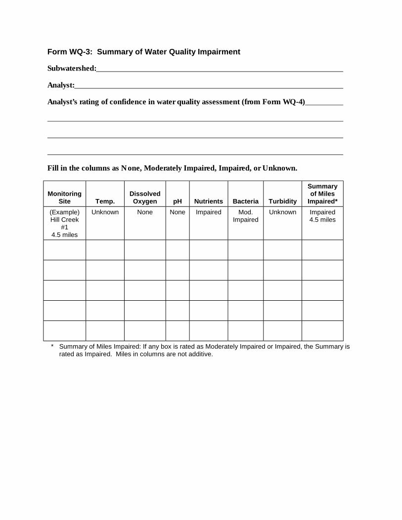
Form WQ-3: Summary of Water Quality Impairment
Subwatershed:
Analyst:
Analyst’s rating of confidence in water quality assessment (from Form WQ-4)
Fill in the columns as None, Moderately Impaired, Impaired, or Unknown.
MonitoringSite Temp.
DissolvedOxygen pH Nutrients Bacteria Turbidity
Summaryof Miles
Impaired*
(Example)Hill Creek
#14.5 miles
Unknown None None Impaired Mod.Impaired
Unknown Impaired4.5 miles
* Summary of Miles Impaired: If any box is rated as Moderately Impaired or Impaired, the Summary israted as Impaired. Miles in columns are not additive.


Form WQ-4: Confidence Evaluation
Watershed:
Analyst’s Name:
Analyst’s Experience/Expertise
Note: Where the availability or quality of information varies by subwatershed, fill out aseparate form for each subwatershed.
Use the following table to summarize your confidence in the conclusions about waterquality conditions.
CategoryPotential issue?1
(Yes, No, Unsure)
Informationsufficient?2
(Yes, No, Unsure)
Confidence inconclusions?3
(High, Moderate, Low)
Temperature
Dissolved Oxygen
pH
Nutrients
Bacteria
Toxics – Organic
Toxics – Metals
Turbidity
Overall Evaluation
1 Potential issue? Answer this question based on the Start-Up and Identification of Watershed Issuescomponent.
2 Information sufficient? Evaluate data or conclusions of reports by considering the followingquestions.
a) How old, or how applicable, is the information to the current watershed condition?
b) Have watershed conditions changed in a significant way since the data was collected?
c) Was the data coverage (over time and geographic extent) sufficient to assess conditions?
d) Is the information based on observations or on more rigorous studies (primarily measurement)?
3 Confidence in conclusions? This conclusion is based on the analyst’s opinion regarding thesufficiency of the information and the analyst’s confidence in completing the evaluation.
Recommendations for additional water quality monitoring:

Component XWatershed ConditionEvaluationTable of Contents
Introduction......................................................X-3
Critical Questions .........................................X-3Assumptions.................................................X-4Materials Needed .........................................X-4Necessary Skills ...........................................X-4Final Products of the Watershed
Condition Evaluation...............................X-5Methods ............................................................X-5
Step 1: Review Summary Data andIdentify Missing Pieces ...........................X-6
Step 2: Gather Assessment Productsand Produce Channel Habitat–FishUse Map.................................................X-6
Step 3: Organize Watershed ConditionEvaluation Meetings ...............................X-7
Step 4: Summarize Historical andCurrent Watershed Conditions................X-7
Step 5: Identify Watershed Protectionand Restoration Opportunities ................X-8
Step 6: List Action Issues and MapWatershed Protection andRestoration Opportunities .....................X-10
References .....................................................X-12Appendix X-A: Blank Forms
Form CE-1: Checklist of AssessmentComponent Summary Products
Form CE-2: Summary of Key Findingsby Assessment Component
Form CE-3: Identification of WatershedIssues and Action Opportunities
Appendix X-B: Examples of WatershedIssues and Action Opportunities
Example Form CE-3: Identification ofWatershed Issues and ActionOpportunities


Oregon Watershed Assessment Manual Page X-3 Watershed Condition Evaluation
Component XWatershed Condition Evaluation
INTRODUCTION
The Watershed Condition Evaluation will help you summarize the information collected in the othercomponents of the assessment process. Using the process outlined in this component, you willaccomplish all of the following:
1. Identify missing or unavailable information.
2. Summarize information collected for each of the manual components.
3. List issues that may require additional assessment or data-gathering.
4. Evaluate the condition of the aquatic–riparian system, fish populations, and water quality.
5. Describe watershed areas and issues that should be the focus for action, including habitatrestoration/protection opportunities.
The condition evaluation process links summaries from each assessment component to the fishdistribution and Channel Habitat Type (CHT) information. The final products will include a tablesummarizing key findings from each of the manual components and a map showing the distributionof factors limiting productive aquatic habitat, fish populations, and water quality. Appendix X-Bprovides an example of products from a completed watershed conditions evaluation.
The watershed condition evaluation process will help the watershed council understand how pastand current resource management and land uses are impacting aquatic resources. This process willconclude with a list of general issues and specific areas in the watershed that should be priorities foraction, including protecting key areas and restoring areas of degraded habitat. For example, actionsthat will protect existing healthy fish populations or high-quality habitat will typically be ranked as ahigher priority than activities to restore degraded habitats in other portions of the watershed.
Critical Questions
1. What are the information and data gaps identified in the assessment process?
2. What were the historical conditions of the aquatic–riparian areas within the watershed?
3. What are the historical changes (legacies), and land uses and resource management trends,that have contributed to impacts in habitat quality, and fish presence and abundance?
4. What ongoing resource management/land use activities are contributing to continuedimpacts on the watershed resources?
5. What are important issues and key aquatic–riparian areas that need to be addressed torestore and protect watershed resources?
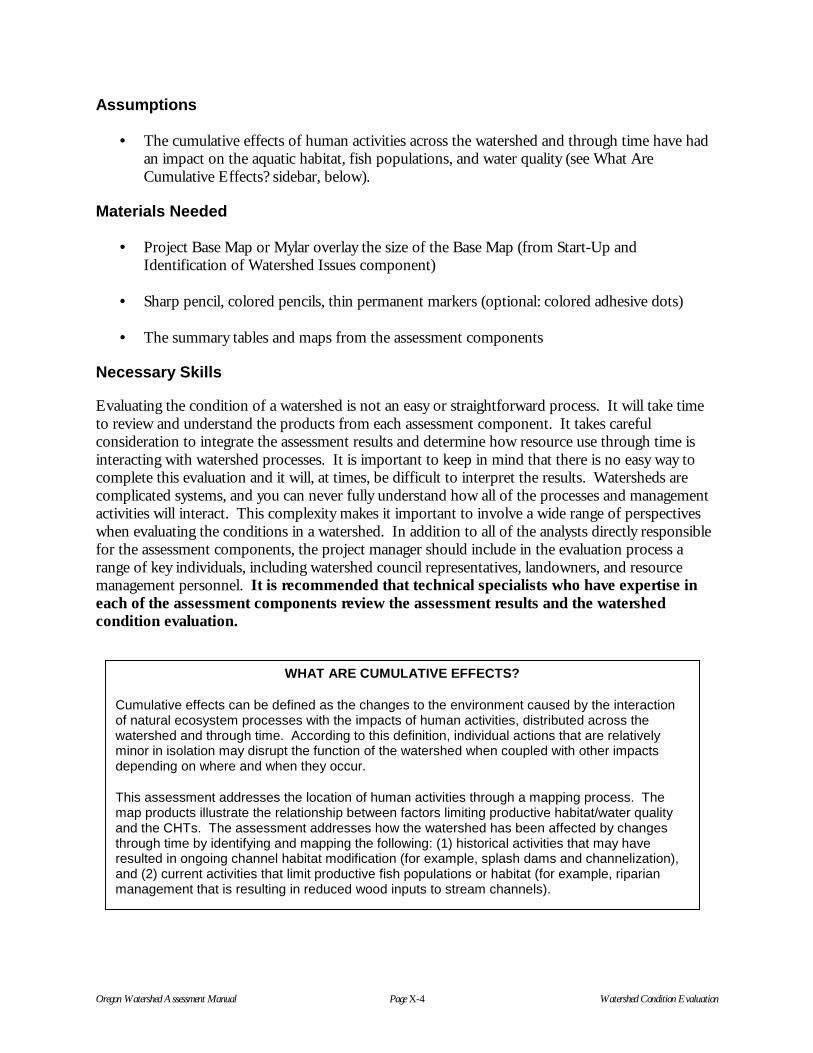
Oregon Watershed Assessment Manual Page X-4 Watershed Condition Evaluation
Assumptions
• The cumulative effects of human activities across the watershed and through time have hadan impact on the aquatic habitat, fish populations, and water quality (see What AreCumulative Effects? sidebar, below).
Materials Needed
• Project Base Map or Mylar overlay the size of the Base Map (from Start-Up andIdentification of Watershed Issues component)
• Sharp pencil, colored pencils, thin permanent markers (optional: colored adhesive dots)
• The summary tables and maps from the assessment components
Necessary Skills
Evaluating the condition of a watershed is not an easy or straightforward process. It will take timeto review and understand the products from each assessment component. It takes carefulconsideration to integrate the assessment results and determine how resource use through time isinteracting with watershed processes. It is important to keep in mind that there is no easy way tocomplete this evaluation and it will, at times, be difficult to interpret the results. Watersheds arecomplicated systems, and you can never fully understand how all of the processes and managementactivities will interact. This complexity makes it important to involve a wide range of perspectiveswhen evaluating the conditions in a watershed. In addition to all of the analysts directly responsiblefor the assessment components, the project manager should include in the evaluation process arange of key individuals, including watershed council representatives, landowners, and resourcemanagement personnel. It is recommended that technical specialists who have expertise ineach of the assessment components review the assessment results and the watershedcondition evaluation.
WHAT ARE CUMULATIVE EFFECTS?
Cumulative effects can be defined as the changes to the environment caused by the interactionof natural ecosystem processes with the impacts of human activities, distributed across thewatershed and through time. According to this definition, individual actions that are relativelyminor in isolation may disrupt the function of the watershed when coupled with other impactsdepending on where and when they occur.
This assessment addresses the location of human activities through a mapping process. Themap products illustrate the relationship between factors limiting productive habitat/water qualityand the CHTs. The assessment addresses how the watershed has been affected by changesthrough time by identifying and mapping the following: (1) historical activities that may haveresulted in ongoing channel habitat modification (for example, splash dams and channelization),and (2) current activities that limit productive fish populations or habitat (for example, riparianmanagement that is resulting in reduced wood inputs to stream channels).
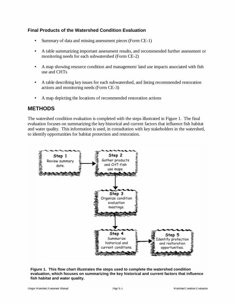
Oregon Watershed Assessment Manual Page X-5 Watershed Condition Evaluation
Final Products of the Watershed Condition Evaluation
• Summary of data and missing assessment pieces (Form CE-1)
• A table summarizing important assessment results, and recommended further assessment ormonitoring needs for each subwatershed (Form CE-2)
• A map showing resource condition and management/land use impacts associated with fishuse and CHTs
• A table describing key issues for each subwatershed, and listing recommended restorationactions and monitoring needs (Form CE-3)
• A map depicting the locations of recommended restoration actions
METHODS
The watershed condition evaluation is completed with the steps illustrated in Figure 1. The finalevaluation focuses on summarizing the key historical and current factors that influence fish habitatand water quality. This information is used, in consultation with key stakeholders in the watershed,to identify opportunities for habitat protection and restoration.
Figure 1. This flow chart illustrates the steps used to complete the watershed conditionevaluation, which focuses on summarizing the key historical and current factors that influencefish habitat and water quality.

Oregon Watershed Assessment Manual Page X-6 Watershed Condition Evaluation
Step 1: Review Summary Data and Identify Missing Pieces
The project manager will be responsible for compiling and reviewing all of the assessmentinformation. Form CE-1 (Appendix X-A) lists the summary products from each assessmentcomponent, which are necessary to complete the watershed condition evaluation. Check that eachform from the assessment has been completely filled out, and then check off the form in thechecklist. If there are notes on any of the forms, be sure to read these and determine if there are anyproblems or circumstances that need to be considered in this overall evaluation. Pay specialattention to the Confidence Evaluation forms—these should identify data gaps, additionalinformation that may be collected, and recommended monitoring. Information gaps andrecommendations for further analysis/monitoring will be summarized and used in the MonitoringPlan component. Complete Form CE-2, which summarizes the assessment results, data gaps, andmonitoring recommendations. This information will help you develop a monitoring plan.
Step 2: Gather Assessment Products and Produce Channel Habitat–Fish Use Map
The completed assessment provides two types of information that will be used to evaluate thecondition of the watershed. Sort out the information gathered from the assessment componentsinto these two categories:
1. A characterization of resources and human uses that describes the watershed, how it functions,asnd how it has changed through time.
2. An assessment of the current status of important watershed resources.The characterization and assessment products are as follows:
Characterization Products
• Watershed Setting—ecoregion information• Watershed Description—land uses, tributaries, stream miles, watershed hydrology• Channel Habitat Types and Distribution• Historical Characterization• Channel Modification Map• Location of Wetlands• Fish Distribution• Road Network• Landslide Maps

Oregon Watershed Assessment Manual Page X-7 Watershed Condition Evaluation
Assessment Products (listed on Form CE-1)
• Channel Modification—degree of impact interpretation• Riparian Conditions• Fisheries Habitat Data Summaries• Fish Migration Barriers• Water Quality Status• Water Use Impacts• Land Use Impacts on Hydrology• Sediment Sources
It is important to come to the watershed condition evaluation meeting with all of the results fromthe assessment components, including summary tables and maps. Maps will help illustrate the issuesin the watershed and show where possible impacts may be associated with areas of fish use andimportant aquatic–riparian habitat.
To provide an overview of channel habitat and fish use associations, combine the information fromthe Channel Habitat Type and Fish Use Distribution maps on the Base Map. This “ChannelHabitat–Fish Use Map” will provide the base for mapping issues that are impacting fishhabitat/water quality, and will show proposed watershed action opportunities.
Step 3: Organize Watershed Condition Evaluation Meetings
The assessment information and maps will be used to summarize the condition of the watershed.The final evaluation of the watershed’s condition should be done through extensive consultationwith key stakeholders, including all of the individuals responsible for the assessment, councilmembers, landowners, resource managers, and government agency personnel. It is suggested thatthe assessment team organize a meeting (or series of meetings) at which the assessment results canbe discussed. These meetings provide an interactive opportunity for analysts to tell what theylearned about the watershed, for them to ask questions of each other, and for others who live andwork in the watershed to provide their insights. These meetings will take one to several days; besure to keep the meeting format informal and allow plenty of time for discussion.
Step 4: Summarize Historical and Current Watershed Conditions
The condition evaluation meetings will provide the information to fill out Form CE-2. This table isused to concisely summarize the results from each assessment component, including informationgaps that will require further assessment or monitoring. You should make copies of this form andfill it out for each subwatershed; in this way you will obtain information on how one subwatersheddiffers from other subwatersheds in the entire watershed. The form includes the questions fromeach assessment component to help guide the discussions and highlight areas that should besummarized.
The questions on Form CE-2 provide guidance on issues that should be placed on the ChannelHabitat–Fish Use Map. The condition evaluation meetings will provide a forum for participants todiscuss and map historical resource management and land use issues that are impacting aquatic–riparian habitat, fish populations, and water quality. Placing these impacts on the Channel Habitat

Oregon Watershed Assessment Manual Page X-8 Watershed Condition Evaluation
Type–Fish Use Map provides an overview of where and how activities through time may be limitinghabitat quality, fish productivity and ranges, and the maintenance of water quality.
The watershed condition evaluation process will provide information that will characterizeconditions that are not conducive to supporting native fish and the maintenance of water quality. Itis important to examine the different subwatersheds to identify the range of issues. For example,some subwatersheds will have limited fish use and water quality, while other subwatersheds willsupport a high diversity of fish species and high water quality. While it is important to examine allareas in the watershed, special emphasis should be placed on stream channels that are responsive toinputs of sediment and wood (See the Channel Habitat Type Classification component). Forexample, low-gradient stream channels with floodplains provide critical habitat for salmonids; thesehabitats are sensitive to watershed-wide disturbance.
Step 5: Identify Watershed Protection and Restoration Opportunities
The summarized watershed conditions are used to identify issues and areas in the watershed thatshould be priorities for action. By using the guidance outlined below, you will be able to place thewatershed condition evaluation results into three groupings:
1. Areas with relatively high-quality aquatic–riparian habitat, fish populations, or water qualityconditions
2. Areas with low-quality aquatic–riparian habitat, limitations on fish presence or production,or water quality concerns; the impacts and sources are identified
3. Areas where the aquatic–riparian condition, fish populations, or water quality cannot beaccurately determined and/or the links to impacts are not clear
All of this information can be used in the development of a watershed action plan that describeshow your council will address issues identified in the assessment. The following guidance provides aframework that can help you plan for watershed restoration actions. The assessment results will giveyou an idea of the issues that are important in your watershed and general areas in which to focusprojects. Implementing watershed protection or restoration projects will require more detailedevaluation, usually involving field investigations.
Action Opportunity 1
Protect stream reaches that are in relatively good condition.
Protecting aquatic–riparian habitat that is supporting good habitat, healthy fish populations, and hasgood water quality is an excellent strategy. It is usually much more efficient and less costly toprotect an area that is functioning in a healthy way than it is to restore conditions once they havebeen degraded. Protection of watershed resources can be accomplished through many differentapproaches, including encouraging good stewardship of private lands. Other methods thatwatershed councils have employed to protect high-quality habitat include conservation easementsand land acquisitions.

Oregon Watershed Assessment Manual Page X-9 Watershed Condition Evaluation
Determining what portions of the watershed warrant protection is based on a synthesis ofinformation on water quality, fish populations, and channel habitat condition, and requiresanswering a number of questions. Is the area of interest:
1. Meeting or exceeding water quality standards?2. Supporting healthy populations of native fish?3. Characterized by high-quality channel and/or riparian habitat?4. Protected by existing planning or regulatory requirements?
Action Opportunity 2
Restore stream reaches with habitat or fish populations that are currently in degradedcondition but have the potential to support high-quality habitat and fish populations.
This category provides a working list of stream reaches for which passive and active restorationshould be considered. Passive restoration involves stopping an action that is contributing to limitedfish populations (such as using culverts that do not support fish passage) or poor channel habitat, oris linked to water quality problems. An example of a passive restoration strategy is limiting grazingin a riparian area where there are obvious impacts on the vegetation and the stream reach haselevated water temperatures. Over time, with the removal or reduction of grazing, the riparianvegetation should recover. Active restoration involves manipulating or modifying stream or riparianhabitat. An example of an active restoration strategy is planting riparian trees to increase shade andplacing logs in the channel to improve habitat complexity.
Determining the type of restoration project for each watershed location requires answering somekey questions:
1. Where is the location of the stream reach with fish population limitations, or degradedhabitat or water quality?
Information on the location should include important data for interpreting the potentialquality of the site, such as CHT.
2. What is the habitat or water quality issue for the reach?
Issues can include, for example, one or a combination of factors, such as high-quality fishhabitat that is blocked by barriers, high water temperatures, limited wood in the channel,limited riparian shade, excessive sediment, and others.
3. What are the factors that are contributing to degraded habitat or water quality?
Factors can include, for example, culverts, streamside roads, vegetative removal,urbanization, and others. It is important to note whether the issue contributing to theimpact is adjacent to the area, upstream (for example, water pollution contributed by asource several miles upstream), or up the hill slope (for example, a road that is contributingexcessive sediment to the stream).
4. What is the best strategy for addressing the factors that are contributing to the problem?

Oregon Watershed Assessment Manual Page X-10 Watershed Condition Evaluation
For example, the restoration strategy should evaluate whether to pursue passive or activerestoration, or some combination of the two. Whether to adopt a passive or activerestoration approach requires that you think about the rates of recovery for the system. Forexample, a riparian area impacted by grazing may recover in a decade, while a stream channelthat has lost boulders from log drives and blasting will probably take centuries to recoverhabitat-forming structures. There will be conditions (e.g., some urban situations) in whichthe factors contributing to the problem are so severe and pervasive (e.g., extensive pavementof riparian areas) that restoration should not be pursued in that area, especially if there areother opportunities for restoration in the watershed.
Action Opportunity 3
Survey stream reaches where there is insufficient data to assess stream habitat quality or fishpopulation status.
It is important to identify those areas where more investigation is necessary to provide a clearpicture of fish population limitations, habitat conditions, or water quality for a stream reach.Additional information should be collected for those stream reaches where conditions are knownbut the factors contributing to the problem are not. For example, information should be collectedfor those stream reaches that have potentially high-quality habitat (for example, low-gradient,unconstrained reaches) but where there are no data on fish populations and/or habitat quality.
Identifying portions of the watershed with limited information can help in developing a plan forimplementing monitoring projects and field assessments.
Step 6: List Action Issues and Map Watershed Protection andRestoration Opportunities
The information from Step 5 should be used—in consultation with technical specialists, thewatershed council, and key stakeholders—to help guide the initial listing of issues and restorationaction opportunities for your watershed. Use Form CE-3, Identification of Watershed Issues andAction Opportunities, to describe watershed issues and list protection and restoration needs for eachsubwatershed. The form also includes space for listing areas that require field monitoring orassessment in order to gage aquatic–riparian habitat quality, fish populations, or water quality.Appendix X-B contains examples of completed forms describing watershed issues and actionopportunities.
Use the following guidance when filling out Form CE-3.
Subwatershed: Name of the subwatershed.
Location: Describe the location of the area or steam segment that is the focus of the summary.
Map symbol: It is important to locate and draw the action opportunity area on a base map for thewatershed. This map will provide a general overview of action opportunities in the watershed andcan be used for guiding the field investigations that are necessary for developing the detailed projectplan.

Oregon Watershed Assessment Manual Page X-11 Watershed Condition Evaluation
Channel Habitat Type: If appropriate, list the Channel Habitat Type (or types) for the stream areasummarized in the form.
Stream size: If appropriate, list the stream size (or sizes) for the stream area summarized in theform.
Fish use: If appropriate, list the resident and anadromous fish use for the stream area summarizedin the form.
Summary: In one sentence, concisely summarize the watershed issue or opportunity.
Habitat/water quality concerns: Concisely describe the issues and concerns for the area or streamreach summarized by the table. Describe all of the relevant factors, such as resource managementover time, characteristics of the hydrology, erosion and sediment sources and impacts, floodplainand riparian conditions, historical fish use, fish passage issues, channel habitat quality, waterquantity, water quality, and others.
Contributing factors: List the factor (or factors) that are limiting fish production, aquatic/riparianhabitat, or the maintenance of water quality. If the factors are not known, list “unknown,” whichwill provide guidance for further investigation.
Recommendation: Describe any recommended actions that will address the factors limiting fishproduction, aquatic–riparian habitat, or the maintenance of water quality. If there is insufficientinformation to make a recommendation on a protection or restoration approach, then describe theneed for further investigation.
Monitoring/assessment needs: Describe any field monitoring or assessment work that should becompleted to understand the nature of the issue or contributing factors. This information will beused to plan field investigations necessary to guide detailed project planning, or to providebackground information that will be used in the Monitoring Plan component.

Oregon Watershed Assessment Manual Page X-12 Watershed Condition Evaluation
REFERENCES
Anonymous. 1998. Oregon Aquatic Habitat Restoration and Enhancement Guide. Oregon StateGovernment, Salem.
Kauffman, J.B., R.L. Beschta, N. Otting, and D. Lytjen. 1997. An Ecological Perspective ofRiparian and Stream Restoration in the Western United States. Fisheries 22(5):12-24.
Federal Interagency Stream Restoration Working Group. 1999. Stream Corridor Restoration:Principals, Processes, and Practices. USDA, Natural Resources Conservation Service,Washington, DC Pacific Rivers Council. 1996. A Guide to the Restoration of Watersheds andNative Fish in the West. 2nd edition. Pacific Rivers Council, Eugene, Oregon.
Williams, J.E., C.A. Wood, and M.P. Dombeck, editors. 1997. Watershed Restoration: Principlesand Practices. American Fisheries Society, Bethesda, Maryland.

Appendix X-ABlank Forms


Form CE-1: Checklist of Assessment Component Summary Products
Form/ Map Title √√√√Historic Conditions
Historical Condition Report
CHT Classification
Form CHT-1 Channel Habitat Type Field Verification
Form CHT-2 CHT Summary Sheet
Form CHT-3 Confidence Evaluation for the CHT Classification
Map CHT-1 Channel Segments
Map CHT-1 Preliminary Channel Habitat Types
Map CHT-1 Final Channel Habitat Types
Hydrology and Water Use
Form H-1 General Watershed Characteristics
Form H-2 Land Use Summary
Form H-3 Annual Peak Flow Summary
Form H-4 Forestry Worksheet
Form H-5 Agriculture and Range Land Worksheet
Form H-6 Forest and Rural Road Worksheet
Form H-7 Urban and Rural Residential Worksheet
Form H-8 Hydrologic Issue Identification Summary
Map H-1 Potential Risks of Land Use on Hydrology
Form WU-1 Water Rights Summary
Form WU-2 Water Availability Summary
Form WU-3 Consumptive Use Summary
Map WU-1 Water Rights and In-Stream Flow Rights
Form HW-1 Confidence Evaluation for Hydrology and Water Use
Riparian/Wetland Conditions
Form R-1 Riparian Condition Unit Information: This will be most helpful at thispoint of the process if it is in a spreadsheet format that can be queriedas the team develops the Watershed Condition Evaluation Summary.
Form R-2 Riparian Recruitment Situation Description
Form R-3 Confidence Evaluation for Riparian Conditions
Map R-1 Riparian Condition Unit map
Map R-2 Riparian Recruitment Situations Map
Map R-3 Riparian Shade Map
Form W-1 Wetland Attributes
Form W-2 Confidence Evaluation for Wetlands Assessment
Form W-3 Wetland Functions Table (optional)
Map W-1 Wetland Locations
Sediment Sources*
Form S-1 Screen or Sediment Topic Sources in a Watershed
Form S-2 Information on Existing Road-Related Instability* Review the sediment source screen to determine which potential sources were evaluated in
the sediment source assessment; also obtain the associated maps.
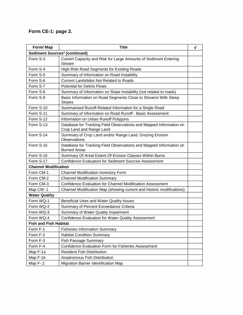
Form CE-1: page 2.
Form/ Map Title √√√√Sediment Sources* (continued)
Form S-3 Culvert Capacity and Risk for Large Amounts of Sediment EnteringStream
Form S-4 High-Risk Road Segments for Existing Roads
Form S-5 Summary of Information on Road Instability
Form S-6 Current Landslides Not Related to Roads
Form S-7 Potential for Debris Flows
Form S-8 Summary of Information on Slope Instability (not related to roads)
Form S-9 Basic Information on Road Segments Close to Streams With SteepSlopes
Form S-10 Summarized Runoff-Related Information for a Single Road
Form S-11 Summary of Information on Road Runoff - Basic Assessment
Form S-12 Information on Urban Runoff Polygons
Form S-13 Database for Tracking Field Observations and Mapped Information onCrop Land and Range Land
Form S-14 Summary of Crop Land and/or Range Land, Grazing ErosionObservations
Form S-15 Database for Tracking Field Observations and Mapped Information onBurned Areas
Form S-16 Summary Of Areal Extent Of Erosion Classes Within Burns
Form S-17 Confidence Evaluation for Sediment Sources Assessment
Channel Modification
Form CM-1 Channel Modification Inventory Form
Form CM-2 Channel Modification Summary
Form CM-3 Confidence Evaluation for Channel Modification Assessment
Map CM- 1 Channel Modification Map (showing current and historic modifications)
Water Quality
Form WQ-1 Beneficial Uses and Water Quality Issues
Form WQ-2 Summary of Percent Exceedance Criteria
Form WQ-3 Summary of Water Quality Impairment
Form WQ-4 Confidence Evaluation for Water Quality Assessment
Fish and Fish Habitat
Form F-1 Fisheries Information Summary
Form F-2 Habitat Condition Summary
Form F-3 Fish Passage Summary
Form F-4 Confidence Evaluation Form for Fisheries Assessment
Map F-1a Resident Fish Distribution
Map F-1b Anadromous Fish Distribution
Map F- 2 Migration Barrier Identification Map

Form CE-2: Summary of Key Findings by Assessment Component
Watershed: Page _____of_____
Analyst’s Name: Date:
Assessment Component Questions
Summary of Key Findings(impacts/changes in ecosystem,
processes affecting habitatquality/quantity, fish populations,
water quality)Missing or Incomplete
Information
Locations of ImpactsCurrently ConstrainingHabitat, Populations,
or Water Quality(add locations to map)
Historical Conditions
• What were the characteristics of thewatershed’s resources at the time ofEuropean exploration/settlement?
• What are the historical trends and locationsof land use and other management impactsin the watershed?
• What are the historical accounts of fishpopulations and distribution?
• Where are the locations of historicfloodplain, riparian area, channel, andwetland modifications, and what was thetype and extent of the disturbance?

Form CE-2: page 2.
Assessment Component Questions
Summary of Key Findings(impacts/changes in ecosystem,
processes affecting habitatquality/quantity, fish populations,
water quality)Missing or Incomplete
Information
Locations of ImpactsCurrently ConstrainingHabitat, Populations,
or Water Quality(add locations to map)
Channel Habitat Type Classification
• What is the distribution of CHTs throughoutthe watershed?
• What is the location of CHTs that are likelyto provide specific aquatic habitat features,as well as those areas which may be themost sensitive to changes in watershedcondition?

Form CE-2: page 3.
Assessment Component Questions
Summary of Key Findings(impacts/changes in ecosystem,
processes affecting habitatquality/quantity, fish populations,
water quality)Missing or Incomplete
Information
Locations of ImpactsCurrently ConstrainingHabitat, Populations,
or Water Quality(add locations to map)
Hydrology and Water Use
• What land uses are present in yourwatershed?
• What is the flood history in your watershed?
• Is there a probability that land uses in thebasin have a significant effect on peakflows?
• Is there a probability that land uses in thebasin have a significant effect on low flows?For what beneficial use is water primarilyused in your watershed?
• Is water derived from a groundwater orsurface-water source?
• What type of storage has been constructedin the basin?
• Are there any withdrawals of water for usein another basin (interbasin transfers)? Isany water being imported for use in thebasin?
• Are there any illegal uses of water occurringin the basin?
• Do water uses in the basin have an effecton peak flows?
• Do water uses in the basin have an effecton low flows?

Form CE-2: page 4.
Assessment Component Questions
Summary of Key Findings(impacts/changes in ecosystem,
processes affecting habitatquality/quantity, fish populations,
water quality)Missing or Incomplete
Information
Locations of ImpactsCurrently ConstrainingHabitat, Populations,
or Water Quality(add locations to map)
Riparian/Wetlands
• What are the current conditions of riparianareas in the watershed?
• How do the current conditions compare tothose potentially present or typically presentfor this ecoregion?
• How can the current riparian areas begrouped within the watershed to increaseour understanding of what areas needprotection and what the appropriaterestoration/enhancement opportunitiesmight be?
• Where are the wetlands in this watershed?
• What are the general characteristics ofwetlands within the watershed?
• What opportunities exist to restore wetlandsin the watershed?

Form CE-2: page 5.
Assessment Component Questions
Summary of Key Findings(impacts/changes in ecosystem,
processes affecting habitatquality/quantity, fish populations,
water quality)Missing or Incomplete
Information
Locations of ImpactsCurrently ConstrainingHabitat, Populations,
or Water Quality(add locations to map)
Sediment Sources
• What are important current sedimentsources in the watershed?
• What are important future sources ofsediment in the watershed?
• Where are erosion problems most severeand qualify as high priority for remedyingconditions in the watershed?

Form CE-2: page 6.
Assessment Component Questions
Summary of Key Findings(impacts/changes in ecosystem,
processes affecting habitatquality/quantity, fish populations,
water quality)Missing or Incomplete
Information
Locations of ImpactsCurrently ConstrainingHabitat, Populations,
or Water Quality(add locations to map)
Channel Modification
• Where are channel modifications located?
• Where are historic channel disturbances,such as dam failures, splash damming,hydraulic mining, and stream cleaning,located?
• What CHTs have been impacted by channelmodification?
• What are the types and relative magnitudeof past and current channel modifications?

Form CE-2: page 7.
Assessment Component Questions
Summary of Key Findings(impacts/changes in ecosystem,
processes affecting habitatquality/quantity, fish populations,
water quality)Missing or Incomplete
Information
Locations of ImpactsCurrently ConstrainingHabitat, Populations,
or Water Quality(add locations to map)
Water Quality
• What are the designated beneficial uses ofwater for the stream segment?
• What are the water quality criteria that applyto the stream reaches?
• Are the stream reaches identified as waterquality limited segments on the 303(d) listby state?
• Are any stream reaches identified ashigh-quality waters of OutstandingResource Waters?
• Do water quality studies or evaluationsindicate that water quality has beendegraded or is limiting the beneficial uses?

Form CE-2: page 8.
Assessment Component Questions
Summary of Key Findings(impacts/changes in ecosystem,
processes affecting habitatquality/quantity, fish populations,
water quality)Missing or Incomplete
Information
Locations of ImpactsCurrently ConstrainingHabitat, Populations,
or Water Quality(add locations to map)
Fish and Fish Habitat
• What fish species are documented in thewatershed? Are any of these currentlystate- or federally listed as endangered orcandidate species? Are there any fishspecies that historically occurred in thewatershed which no longer occur in thewatershed?
• What is the distribution, relative abundance,and population status of salmonid speciesin the watershed?
• Which salmonid species are native to thewatershed, and which have been introducedto the watershed?
• Are there potential interactions betweennative and introduced species?
• What is the condition of fish habitat in thewatershed (by sub-basin) according toexisting habitat data?
• Where are potential barriers to fishmigration?

Form CE-3: Identification of Watershed Issues and Action Opportunities
Watershed: Page ____of_____
Analyst’s Name: Date:
Subwatershed:
Location:
Map symbol:
Channel habitattype:
Stream size:
Fish use:
Summary
Habitat/waterquality concerns
Contributingfactors
Field observations
Recommendation
Monitoring/
assessment needs


Appendix X-BExamples of WatershedIssues and ActionOpportunities


Oregon Watershed Assessment Manual Page 1 Appendix X-B
EXAMPLES OF WATERSHED ISSUES AND ACTION OPPORTUNITIES
The Big River watershed is a 60,000-acre watershed characterized by forest management in theheadwaters and agricultural land uses along the river and the lower tributary valleys. The valley areasalong Big River and most of the larger tributaries were cleared of trees in the 1880s when the areawas homesteaded. There is one small town, Elk City, in the upper portion of Big River and somegrowing suburban developments in the lower watershed. Most of the stream channels start in steepheadwater areas, with the tributary streams occupying low-gradient narrow valleys with limitedfloodplain development. Anadromous fish use in the watershed includes chinook salmon in the BigRiver and lower tributaries, coho salmon, and steelhead trout in most of the larger tributaries.Resident fish include rainbow and cutthroat trout.
Figure X-1 (page 2) is a map illustrating the Big River watershed, including subwatersheds, channelhabitat types, and example stream segments used to illustrate watershed issues and opportunities (seethe Example Form CE-3).

Oregon Watershed Assessment Manual Page 2 Appendix X-B
Figure X-1. This example map illustrates the Big River watershed, including its subwatershedsand CHTs. Example stream segments show watershed issues and opportunities.

Oregon Watershed Assessment Manual Page 3 Appendix X-B
Example Form CE-3: Identification of Watershed Issues and Action Opportunities
Watershed: Big River Page 1 of 8
Analyst’s Name: Steve Jones Date: 3/19/99
Subwatershed: Elk Creek
Location: Cedar Creek upstream from FS road 1292
Map symbol: EC2
Channel habitattype:
MV: Moderately steep narrow valley channel
Stream size: Small
Fish use: Cutthroat trout
Summary Impassable culvert is preventing upstream movement of cutthroat trout.
Habitat/waterquality concerns
The culvert has a 3-foot drop onto bedrock with no jump pool. It appears that fishcannot move upstream, although there is a population (perhaps isolated) of cutthroattrout above the culvert. The stream above the culvert has about 0.25 miles ofmarginal fish habitat (shallow pools, little wood) and then the gradient of the streamincreases to 10 percent and fish use ends. The culvert appears to be adequatelysized to pass peak flows.
Contributingfactors
Culvert on FS Road 1292 is a fish passage barrier.
Field observations Culvert information, including fish habitat data above and below, were collected by aforest service crew on Aug. 23, 1996. The upper-extent fish use information wascollected by an ODFW crew on May 2, 1997.
Recommendation Because there is very little fish habitat above this culvert, this is not a high priority forcouncil action at this time. The council should encourage the landowner to replacethe culvert next time there is forest management in the area.
Monitoring/assessment needs
None

Oregon Watershed Assessment Manual Page 4 Appendix X-B
Example Form CE-3: Identification of Watershed Issues and Action Opportunities
Watershed: Big River Page 2 of 8
Analyst’s Name: Steve Jones Date: 3/19/99
Subwatershed: Big Bear Creek
Location: Upstream from county road 33
Map symbol: BBC1
Channel habitattype:
FP3: Low gradient small floodplain, unconfined channel
Stream size: Medium
Fish use: Cutthroat trout and sculpin, potential coho
Summary Impassable culvert is preventing passage of coho salmon into this section ofstream.
Habitat/waterquality concerns
The culvert has a 3 foot drop onto bedrock with no jump pool. It appears that fishcannot move upstream, although there is a population (perhaps isolated) ofcutthroat trout above the culvert. The stream above the culvert has about 0.25miles of marginal fish habitat (shallow pools, little wood) and then the gradient ofthe stream increases to 10 percent and fish use ends. The culvert appears to notbe adequately sized to pass peak flows.
Contributingfactors
Impassable culvert on county road 33 at mile post 14.
Field observations Culvert information, including fish habitat data above and below, were collected bya county crew on Sept. 10, 1997.
Recommendation Consider consulting with agency personnel to replace this culvert with a bridge oranother culvert that is appropriate for peak flows and fish passage.
Monitoring/assessment needs
If possible, monitor fish passage after the culvert is replaced.

Oregon Watershed Assessment Manual Page 5 Appendix X-B
Example Form CE-3: Identification of Watershed Issues and Action Opportunities
Watershed: Big River Page 3 of 8
Analyst’s Name: Steve Jones Date: 3/19/99
Subwatershed: Elk Creek
Location: Lower 2 miles
Map symbol: EC1
Channel habitattype:
LM: low gradient moderately confined channel
Stream size: Large–medium
Fish use: Steelhead and rainbow trout
Summary Large amounts of sediment have been deposited on the channel bottomthroughout this section.
Habitat/waterquality concerns
Elk Creek passes through farms for the first mile and then drains private forestlands. In comparison to similar streams in this area, there appears to be largeamounts of fine sediments deposited on the channel bottom, sometimes filling upshallow pools. Historically, this was a very productive steelhead stream, withpopulation counts decreasing dramatically over the last 10 years. This section ofstream has fair fish habitat, though somewhat entrenched. It is not known wherethe sediments are coming from; the increase in sediments has been noted tocorresponded to the increased truck traffic over the last two years. There may beincreased turbidity associated with the sedimentation.
Contributingfactors
Not know at this time, although road-related sediment is suspected.
Field observations Sediment deposits were noted in the 1997 ODFW stream habitat survey.
Recommendation Assess the roads in the area to determine if they are contributing fine sediments.
Monitoring/assessment needs
Monitor turbidity levels, especially during wet-weather truck traffic on the roads.Assess roads for delivery of sediment. (See turbidity parameter in Appendix XI-A,Component XI.)

Oregon Watershed Assessment Manual Page 6 Appendix X-B
Example Form CE-3: Identification of Watershed Issues and Action Opportunities
Watershed: Big River Page 4 of 8
Analyst’s Name: Steve Jones Date: 3/19/99
Subwatershed: Oak Creek
Location: Lower 2 miles
Map symbol: OC1
Channel habitattype:
LM-FP3: low gradient moderately confined, and small floodplain, unconfined
Stream size: Large–medium
Fish use: Cutthroat trout and juvenile chinook salmon rearing
Summary Land uses in the area contribute to lack of wood in the channel and increases inpeak flows, which is resulting in channel entrenchment.
Habitat/waterquality concerns
This section of Oak Creek passes through a suburban area, with many homesbordering the stream. Channel simplification due to the channel incision causedby the various land uses (suburban along the stream and urban in the tributaries)and lack of wood in the channel have resulted in this section being very sensitiveto increases in peak flows. The channel cannot dissipate stream flow energyduring storms, resulting in further confinement of the channel. Historically, thischannel was moderately confined. Planned housing developments in thewatershed will result in further increases in peak flows more removal of riparianvegetation.
Contributingfactors
Lack of wood in the channel due to removal of riparian trees and increases in peakflows resulting in channel incision.
Field observations Channel entrenchment, stream wood counts, and riparian vegetation noted in 1998student survey.
Recommendation Work with the city to control future storm water discharges; identify areas forriparian improvement projects.
Monitoring/assessment needs
None

Oregon Watershed Assessment Manual Page 7 Appendix X-B
Example Form CE-3: Identification of Watershed Issues and Action Opportunities
Watershed: Big River Page 5 of 8
Analyst’s Name: Steve Jones Date: 3/19/99
Subwatershed: Coyote Creek
Location: Lower 1.5 miles
Map symbol: CC1
Channel habitattype:
FP3: Low gradient small floodplain, unconfined channel
Stream size: Large–medium
Fish use: Coho salmon, cutthroat and steelhead trout
Summary There is very little information on the habitat quality and fish use for this streamsection.
Habitat/waterquality concerns
According to 1939 Fish Commission reports, Coyote Creek supported largenumbers of spawning coho salmon and some steelhead. There are no recentsurveys of stream habitat or fish use in this stream. The assessment information,based on maps and aerial photographs, appears to indicate the potential for high-quality fish and wildlife habitat: low-gradient channel, with a small floodplain andsome large riparian conifers. This area was recently proposed for a recreationaldevelopment, including building small cabins in potential floodplain habitat.
Contributingfactors
No information.
Field observations There are no recent fish or habitat surveys of the area. Floyd Jones, a landowneron Big Bottom Creek, said that he saw spawning coho in this section of thestream in 1997.
Recommendation This area should be a high priority for field assessments of habitat quality and fishuse.
Monitoring/assessment needs
Assess channel and riparian habitat using ODFW protocols.
Determine the upper extent of fish use and conduct snorkel surveys to assessuse by salmonids, including juvenile coho and steelhead.

Oregon Watershed Assessment Manual Page 8 Appendix X-B
Example Form CE-3: Identification of Watershed Issues and Action Opportunities
Watershed: Big River Page 6 of 8
Analyst’s Name: Steve Jones Date: 3/19/99
Subwatershed: Big River
Location: Lower 10 miles between the mouth and Elk City
Map symbol: Red line along lower Big River
Channel habitattype:
Variable
Stream size: Large
Fish use: Cutthroat trout, rainbow trout, steelhead, coho and chinook salmon
Summary There are indications that of E. coli bacteria levels may exceed state standards.
Habitat/waterquality concerns
During a rainstorm in 1996, the high school collected water quality grab samplesfrom Big River at the mouth and just above Elk City. All of the water qualityparameters were normal with the exception of E. coli bacteria. The E. coli countswere 30/100 ml above Elk City and 800/100 ml at the mouth. No other sampleshave been collected. The land uses in the watershed, especially below Elk City,are primarily farms and pastures with livestock. There are increasing numbers ofhomes and hobby farms. A recent Council of Government study found that thesoils in the lower watershed have a high potential for septic tank failure andrecommended limits on new septic tanks.
Contributingfactors
Not determined at this time, although a combination of septic tanks and farmanimals may contribute to the increased E. coli counts.
Field observations The only known E. coli samples were collected in 1996.
Recommendation Monitor E. coli counts and assess possible causal factors such as leaky septictanks and/or contributions from livestock.
Monitoring/assessment needs
Using DEQ protocols, monitor E. coli counts during rain events at a range of sitesalong Big River and at key tributaries to assess major source areas.(See E. coli parameter in Appendix XI-A, Component XI.)

Oregon Watershed Assessment Manual Page 9 Appendix X-B
Example Form CE-3: Identification of Watershed Issues and Action Opportunities
Watershed: Big River Page 7 of 8
Analyst’s Name: Steve Jones Date: 3/19/99
Subwatershed: Horse Creek
Location: The 1-mile section between Fly Creek and Knot Creek
Map symbol: HC1
Channel habitattype:
FP3: Low gradient small floodplain, unconfined channel
Stream size: Medium
Fish use: Cutthroat trout and coho salmon
Summary This section, which has the potential for high quality habitat, lacks habitatcomplexity, especially wood in the channel.
Habitat/waterquality concerns
Horse Creek supports relatively large numbers of spawning coho salmon, withmost of the production in the upper watershed on Forest Service land.Historically (based on a 1939 Fish Commission survey), this section of the streamhad good habitat, with a low-gradient channel, abundant side-channels, and largeamounts of wood in the stream. Wood was removed from this section of channelin repeated operations between 1946 to 1972. Aerial photos from this periodshow that almost all of the trees along the stream were removed, which limitedrecruitment of wood to the stream. Information from recent habitat surveys in thissection show that there is very little complex habitat, with few deep pools andalmost no side-channels, which limits winter rearing habitat for juvenile cohosalmon. The riparian trees are mostly 25-year-old conifers, so there is littleriparian vegetation improvement potential.
Contributingfactors
Wood removal from the channel and little potential for short-term recruitment oflarge trees into the channel.
Field observations Stream and riparian habitat information is from a 1995 ODFW survey. There areannual spawning surveys on the Forest Service land in the upper portion of thewatershed.
Recommendation Investigate, in consultation with ODFW and other agencies, the potential forplacing large wood in the channel to improve habitat.
Monitoring/assessment needs
Field assessments will be necessary to assess restoration potential.

Oregon Watershed Assessment Manual Page 10 Appendix X-B
Example Form CE-3: Identification of Watershed Issues and Action Opportunities
Watershed: Big River Page 8 of 8
Analyst’s Name: Steve Jones Date: 3/19/99
Subwatershed: Nonsense Creek
Location: Lower 1.3-mile section
Map symbol: NC1
Channel habitattype:
FP3: Low gradient small floodplain, unconfined channel
Stream size: Large – medium
Fish use: Cutthroat and rainbow trout
Summary There is very little riparian vegetation along this section and high watertemperatures have been observed.
Habitat/waterquality concerns
This portion of Nonsense Creek flows through farm lands, with a mixture of cropsand grazing. The upper watershed is forested. This stream has a good populationof rainbow trout. Historical information indicates that the lower watershed wasdensely forested until land was cleared for homesteads in the 1880s. Informationfrom current aerial photos and a recent stream habitat survey all indicate that thereis very limited cover over the stream and few riparian trees. The stream habitatsurvey noted water temperatures in this section of stream as high as 72 degrees Fin August. There is no other water temperature information. As far as can bedetermined, there is limited water removal from the stream, with most of the waterrights in the lower 0.5 miles of the stream.
Contributingfactors
Not determined at this time, but limited riparian cover over the stream (andpossibly water removal) may be contributing to increases in water temperatures.
Field observations Stream and riparian habitat information and water temperature data are from a1997 ODFW survey.
Recommendation Characterize current water temperature patterns in the watershed and assessriparian canopy cover over the stream. Assess possible grazing and othermanagement impacts on riparian vegetation. Use this information and data on todetermine the potential for riparian restoration projects with willing landowners.The riparian projects can use, where appropriate, riparian fencing and treeplanting.
Monitoring/assessment needs
Using DEQ monitoring protocol, monitor water temperatures at key locations in thewatershed and assess water use patterns. (See temperature parameter inAppendix XI-A, Component XI.)

Component XIMonitoring PlanTable of Contents
Introduction.....................................................XI-3
Necessary Skills ..........................................XI-3
Final Products of the Monitoring
Component............................................XI-4
Filling Data Gaps.........................................XI-4
Identifying Data Gaps .....................................XI-6
Developing a Monitoring Plan........................XI-7
Stage 1: Objectives .....................................XI-7
Stage 2: Resources.....................................XI-9
Stage 3: Monitoring Details .........................XI-9
Stage 4: Pilot Project...................................XI-9
Stage 5: Review and Revise .......................XI-9
Written Monitoring Plan................................XI-10
Monitoring Protocols ....................................XI-11
Additional Resources for Developing
Monitoring Plans ...............................XI-11
References ....................................................XI-14
Appendix XI-A: Monitoring Outline for
Selected Issues


Oregon Watershed Assessment Manual Page XI-3 Monitoring Plan
Component XIMonitoring Plan
INTRODUCTION
The primary purpose of this Monitoring component is to describe approaches for collectinginformation to answer questions that may arise during the watershed assessment. A secondobjective is to briefly discuss ways to measure success of restoration efforts that may come out ofthe assessment. The Monitoring component is intended to address the questions of What and Whyto monitor, not to describe detailed monitoring procedures. Monitoring procedures are beingdeveloped by an interagency team of the Oregon Plan for Salmon and Watersheds (OPSW). Todate, the OPSW monitoring team has completed a Water Quality Monitoring Guidebook (OPSW 1999).We refer the reader to this guidebook and other monitoring documents being prepared by this teamfor specific monitoring procedures.
This component will focus on the approach to filling data gaps discovered during the watershedassessment, because this will be the type of monitoring activity that watershed councils will mostlikely be involved in. The second objective of monitoring, measuring the success of restorationefforts, is discussed briefly in the sidebar, Monitoring Restoration Activities. This sidebar alsobriefly reviews the various types of monitoring to acquaint the reader with the terminology that iscommonly encountered in monitoring guidebooks. The main portion of this component willpresent the following information:
1. A description of the process of cataloging data gaps identified during the watershed assessment
2. A description of the stages to follow in developing a monitoring plan
3. An outline of a written monitoring plan
4. A list of the sources of potential monitoring methods and other resources that may be used toimplement the monitoring plan
The stages in developing a monitoring plan and the monitoring methods apply as well to measuringthe success of restoration actions. The emphasis of this component is on linkages to more detailedprocedures rather than a self-contained methods manual. Guidance on monitoring is contained in anumber of good references that should be consulted when developing a monitoring program (seeReferences section).
Necessary Skills
Developing a monitoring plan requires specific knowledge of the monitoring techniques related tothat issue, data analysis, statistics, and quality assurance. Once a plan and data collection protocolare established, trained volunteers can often implement the field work (the fun part!) under thedirection of professionals or agency mentors. Watershed councils should obtain help whendeveloping a monitoring program from agency resource specialists, monitoring consultants, oruniversity faculty.

Oregon Watershed Assessment Manual Page XI-4 Monitoring Plan
Final Products of the Monitoring Component
The monitoring component provides linkages between the watershed assessment and monitoringprograms being developed by the OPSW. An outcome of the watershed assessment is a list ofinformation needs that are the basis for developing a watershed monitoring program. This list ofneeds can then be used in communications with state and federal agencies that may be able to fillthese data gaps or to develop monitoring initiatives at the watershed council level. A secondpotential outcome of this component is the development of a monitoring plan to address specificdata gaps or to evaluate the success of restoration activities.
Filling Data Gaps
Typical monitoring activities that watershed councils may use to follow up the watershed assessmentare categorized as filling data gaps. As a part of the watershed assessment, data gaps and otherinformation needs are identified. These information needs should be addressed before pursuingmore costly restoration activities (see sidebar, Monitoring Restoration Activities). The potential mixof data-gap monitoring and field-verification activities varies for each component of the watershedassessment. Some components such as assessing riparian condition or verifying the location ofwetlands are best completed using field observations. Other components, such as water qualitymonitoring, require collection of samples with an emphasis on standard operating procedures andquality control. Lastly, other components, such as evaluation of hydrologic impacts, cannot bereadily monitored and rely on use of models that require a high degree of professional expertise.
Since the watershed assessment was primarily designed to use existing data, field studies to verifyassumptions are an excellent follow-up activity to watershed assessment. Field verification is a typeof follow-up activity that primarily uses visual observation with few measurements. In many casesobservers can be trained by a resource professional to use standard methods and collect informationthat will be very useful to the watershed improvement goal. To be useful, the field verificationneeds to be completed using standard protocols and documentation. Potential field-verificationactivities are listed in Table 1 for the Channel Habitat Type Classification, Riparian/Wetlands,Sediment Sources, Channel Modification, and Fish and Fish Habitat assessment components.
Intensive monitoring activities that include collection of field samples are more costly and requiremore detailed planning to be successful. Monitoring activities may be undertaken for a number ofpurposes. Some common purposes are to: (1) evaluate the existing condition or status of theresource, (2) identify the cause-and-effect relationships, and (3) determine trends in water quality orhabitat conditions in response to specific actions. The first objective is undertaken if little or noinformation exists about an important issue or to evaluate a series of potential causative agents at acursory level. The second objective, cause-and-effect studies, are designed to pinpoint the majorcause of an impact or geographic focus to be able to prioritize restoration. For example, it may beknown that nutrients are high in a mixed land use watershed, but no specific source has beenidentified. A cause-and-effect study would try to identify the relative contribution from agriculturalrunoff from urban runoff by bracketing these land use areas with monitoring sites. The third type,trend studies, requires intensive monitoring over a long time period because of the natural change inconditions that may occur from year to year or decade to decade.
It is important to be very clear about the objective for intensive monitoring before planning data-collection efforts. The monitoring objective ultimately determines the location, duration, and

Oregon Watershed Assessment Manual Page XI-5 Monitoring Plan
frequency for sample collection. Evaluating current conditions may be accomplished by makingmeasurements during one season, and constitutes a snapshot in time. (For an example, seeAppendix VIII-A in the Water Quality component). Trying to evaluate a trend over time requires agreater level of effort and a commitment of resources over several years or decades. For thesereasons, watershed councils should focus on monitoring efforts that address specific data gaps inwatershed assessment rather than long-term monitoring efforts.
MONITORING RESTORATION ACTIVITIES
Once restoration actions are taken, the council will want to know if they were installed correctly (if theaction involves structures) and if they are going to be successful. Monitoring methods that evaluaterestoration activities have been described as implementation and effectiveness monitoring.Documents that describe monitoring methods often refer to these terms, so it will be useful tounderstand this terminology.
Implementation monitoring asks: Was the management practice or restoration activityimplemented properly? This monitoring should be a part of every project and is normally performedduring or shortly after restoration. Monitoring during the project can lead to mid-course correctionsthat save the project from failure. Implementation monitoring after the project is necessary to reportthe success of the restoration effort to the watershed council and the funding agency. Implementationmonitoring can be as simple as counting the number of structures installed and evaluating if thestructures were installed as designed. The actual monitoring activity consists of visual inspections,field notes, and photographs. For example, if improved road maintenance was the restoration action,implementation monitoring would consist of checking to see if ditches and culverts were cleaned andfunctional, and if cut and fill slopes were seeded, or to determine if seasonal road closures wereinstalled in time.
Implementation monitoring is simple, and it is a cost-efficient form of monitoring. This essential part ofany monitoring effort is often taken for granted: assuming that the best management practice (BMP)was undertaken and completed as planned. Before we measure the effectiveness of the restorationactivity, we must ensure that the planned action was completed as designed. Although this may seemto be an obvious part of restoration, taking the time to document what was completed is easilyoverlooked.
Effectiveness Monitoring asks: Were restoration actions effective in meeting the restorationobjectives and in attaining the desired outcome? This kind of monitoring is more complex thanimplementation monitoring because we need to connect some action with an outcome in the riparianarea or stream channel. In the road maintenance example, we may want to determine if ditches andculverts plugged during a storm, if the vegetation seeded on the slope was established in time toprevent erosion, and if the road closures prevented rills on the road surface. With stream restorationprojects, some actual evidence of an improved condition may not be become evident until severalcycles of high flows or after many years.
Other types of monitoring that are commonly described include validation, baseline, and trendmonitoring. Validation monitoring is a research level of monitoring that addresses basic scientificquestions about watershed processes and will generally not be undertaken by watershed councils.Baseline monitoring is undertaken to establish conditions prior to management activities or in a pairedwatershed or reference site. Baseline monitoring in a less-disturbed drainage is important to calibratethe effects of natural disturbance such as mass wasting, floods, and fire. Trend monitoring tracksconditions in streams and watersheds over years and requires a long-term commitment of resources.While all types of monitoring might be used, watershed councils will likely focus on filling data gapsand on the implementation and effectiveness of restoration activities.

Oregon Watershed Assessment Manual Page XI-6 Monitoring Plan
IDENTIFYING DATA GAPS
The first stage in developing a monitoring program is to identify the list of data gaps and prioritizethe potential list of monitoring studies. The potential list of information needs is compiled from thewatershed assessment and should be completed as part of the Watershed Condition Evaluation.Based on this list we might categorize the potential list of monitoring activities as field-verificationactivities, short-term monitoring activities, and long-term monitoring activities. The secondconsideration at this stage is to determine which of these activities are within the jurisdiction ofother entities and should be completed by them. For example, you may want to encourage anagency to add new stations to its monitoring program, request a major landowner to take the lead ina study, or recruit the interest of a research organization at a state or federal agency. An example ofa potential list of data gaps and monitoring activities is provided in Table 1.
Table 1. Examples of data gaps identified from the watershed assessment.
Manual Component Potential Data Gaps
Channel Habitat TypeClassification
Field verification of channel habitat typesgradient, cross-sectional shape, or valleyshape
Hydrology & Water Use Streamflow gaging stationsLand use mapping
Riparian Field verification of recruitment condition andshadeField measure of stream shade and canopyRiparian plant communitiesWidth of riparian areasBreaks in riparian areas and causes
Wetlands Type, location, and size of wetlandsWetland functions and conditionsConnectivityRestoration opportunities
Sediment Sources Field verification of sourcesRoad stabilityCulvert surveyErosion – crop-land areasErosion – range conditions
Channel Modification Field verification of channel modifications
Water Quality Temperature and dissolved oxygenpH and heavy metalsNutrientsTurbidity and suspended sedimentBacterial sources and impacts
Fisheries Distribution of fish in the watershedLocation and severity of migration barriersCondition of spawning and rearing habitatFine-sediment impacts

Oregon Watershed Assessment Manual Page XI-7 Monitoring Plan
Data gaps can be listed and compared to watershed issues and their influence on future actions.Follow-up monitoring activities should be prioritized on the basis of moving forward on potentialrestoration options. For example, temperature and riparian conditions are often a major issue in awatershed. The watershed assessment may have indicated that temperatures at the mouth oftributaries were in excess of state water quality standards. Riparian conditions based on aerialphotographs indicated potential areas of insufficient shade. A 1-year intensive data-collection effortof temperature data loggers (monitoring activity) and riparian condition (field-verificationobservations) may answer landowners’ questions about specifically where the canopy cover isinsufficient and how it is affecting temperature.
DEVELOPING A MONITORING PLAN
Once the data gaps and monitoring needs are identified, a monitoring plan can be developed toanswer specific questions. A written monitoring plan is a necessary tool to conduct any monitoringprogram. The monitoring plan is like a set of blueprints for building a new home. Once finalized,the blueprints and materials list provide the basis for a contract between the homeowner, thebuilder, and subcontractors to ensure that there is always a basis for clear communication. Themonitoring plan performs the same function—it lays out the objectives, identifies the people andequipment needed, and describes what and where the monitoring activities will take place. Like a setof blueprints, the monitoring plan will need to go through several drafts and peer reviews beforethere is agreement that the plan makes sense and can be completed with the resources available.
The process that should be followed to complete a monitoring plan is illustrated in Figure 1. Werefer to these as stages, because they are part of a decision process and may vary depending on thetype of monitoring; they are not steps in a to-do list as described in other components. Themonitoring plan should be viewed as an iterative process. The best-designed monitoring programmay not work for a variety of reasons, such as access limitations, unanticipated high flows,inadequate equipment, or higher variability than anticipated. For that reason, data should beevaluated frequently and the monitoring plan revised as needed to ensure a successful project.
Stage 1: Objectives
The first stage in developing a monitoring program is to establish a clear set of objectives. Theseobjectives start with a statement of the data gap or the question to be answered. Examples of datagaps are listed in Table 1. Examples of questions are: “Does this stream meet the OregonDepartment of Environmental Quality water quality standards for temperature and dissolvedoxygen?”; and “Are BMPs effective at reducing sediment inputs to the stream channel?”. Data gapsand questions such as these are the beginning point for developing the set of monitoring objectives.
Once the data gap or question is identified, a helpful procedure is to briefly outline the potentialstudy design as shown in Table 2. Briefly specify the objective, the question to be addressed,parameters to be sampled, monitoring method, study design, potential sample locations, duration,and sample frequency. This brief outline connects the objective to the other stages in developing amonitoring plan and should raise critical implementation questions. What resources are needed?What kind of expertise is needed? And specifically, what potential monitoring equipment, methods,and funding will be needed?

Oregon Watershed Assessment Manual Page XI-8 Monitoring Plan
Three of the Watershed Issues and Action Opportunities discussed in the Watershed Condition Evaluation(Component X) can be used to illustrate this initial stage in developing a monitoring plan. Pleaserefer to Appendix XI-A for an outline of these examples. The three examples address temperature,bacterial contamination, and fine-sediment sources. The temperature study is designed initially as aone-season study to evaluate where potential problem areas are and if they are related to lack ofshade. The bacterial contamination study combines storm-event monitoring to locate the sources ofbacteria and a 1-year-long study to evaluate the severity and duration of the bacterial contamination.The sediment source study is planned for completion in a few weeks or months by monitoringturbidity during several runoff events.
Figure 1. The process that should be followed to complete a monitoring plan isdescribed in stages. The plan should be considered an iterative process, and the stagesmay vary depending on the type of monitoring.

Oregon Watershed Assessment Manual Page XI-9 Monitoring Plan
Table 2. Example of initial monitoring strategy.
Outline Example
Question/Data Gap Does the stream meet state standards for temperature and dissolvedoxygen?
Objective Measure temperature and oxygen during critical seasonal periods andtimes during the day to detect exceedance of criteria.
Parameters Temperature, dissolved oxygen
Methods Continuous temperature data loggers, dissolved oxygen meter
Study Design Upstream/downstream of major canopy openings, reference sites, etc.
Locations Based on study design, access, vandalism.
Study Duration At least one season
Sample Frequency Data loggers—hourly
Stage 2: Resources
After an initial monitoring outline is completed, the next stage is to evaluate resources to carry outthe project. This includes the people that are needed, the budget, the field equipment, laboratoryanalysis, and supplies. If the program is too ambitious, as is often the case, it is better to pare downexpectations at this stage than have to deal with problems later. This is a good time to contact amonitoring specialist or mentor and determine if all the resource bases are covered.
Stage 3: Monitoring Details
Identify the specific set of parameters, the methods to be used, the sample frequency required, andthe location of potential monitoring sites. This process should provide feedback on costs,equipment needs, and level of skill needed. Equipment and supplies for water quality studies such astemperature are listed in the OPSW Water Quality Monitoring Guidebook.
Stage 4: Pilot Project
Conduct field reconnaissance of all monitoring sites to be sure that access is secured and thatconditions are safe throughout the monitoring period. It is a good idea to plan on conducting apilot project for a short period or complete some trial runs prior to committing to a long-termmonitoring program.
Stage 5: Review and Revise
Review the data collected after a short pilot period to determine if the information being collectedwill answer the overall monitoring objective, and that it meets the quality assurance objectives. Anybugs in the monitoring program can be worked out before more effort is expended. Fortemperature data loggers, for example, a standard procedure is to check the data logger against astandardized thermometer before installation in the stream.
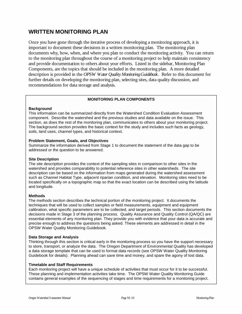
Oregon Watershed Assessment Manual Page XI-10 Monitoring Plan
WRITTEN MONITORING PLAN
Once you have gone through the iterative process of developing a monitoring approach, it isimportant to document these decisions in a written monitoring plan. The monitoring plandocuments why, how, when, and where you plan to conduct the monitoring activity. You can returnto the monitoring plan throughout the course of a monitoring project to help maintain consistencyand provide documentation to others about your efforts. Listed in the sidebar, Monitoring PlanComponents, are the topics that should be included in the monitoring plan. A more detaileddescription is provided in the OPSW Water Quality Monitoring Guidebook. Refer to this document forfurther details on developing the monitoring plan, selecting sites, data quality discussion, andrecommendations for data storage and analysis.
MONITORING PLAN COMPONENTS
BackgroundThis information can be summarized directly from the Watershed Condition Evaluation Assessmentcomponent. Describe the watershed and the previous studies and data available on the issue. Thissection, as does the rest of the monitoring plan, communicates to others about your monitoring project.The background section provides the basic context for the study and includes such facts as geology,soils, land uses, channel types, and historical context.
Problem Statement, Goals, and ObjectivesSummarize the information derived from Stage 1 to document the statement of the data gap to beaddressed or the question to be answered.
Site DescriptionThe site description provides the context of the sampling sites in comparison to other sites in thewatershed and provides comparability to potential reference sites in other watersheds. The sitedescription can be based on the information from maps generated during the watershed assessmentsuch as Channel Habitat Type, adjacent riparian condition, and elevation. Monitoring sites need to belocated specifically on a topographic map so that the exact location can be described using the latitudeand longitude.
MethodsThe methods section describes the technical portion of the monitoring project. It documents thetechniques that will be used to collect samples or field measurements, equipment and equipmentcalibration, what specific parameters are to be collected, and target periods. This section documents thedecisions made in Stage 3 of the planning process. Quality Assurance and Quality Control (QA/QC) areessential elements of any monitoring plan. They provide you with evidence that your data is accurate andprecise enough to address the questions being asked. These elements are addressed in detail in theOPSW Water Quality Monitoring Guidebook.
Data Storage and AnalysisThinking through this section is critical early in the monitoring process so you have the support necessaryto store, transport, or analyze the data. The Oregon Department of Environmental Quality has developeda data storage template that can be used to format data records (see OPSW Water Quality MonitoringGuidebook for details). Planning ahead can save time and money, and spare the agony of lost data.
Timetable and Staff RequirementsEach monitoring project will have a unique schedule of activities that must occur for it to be successful.These planning and implementation activities take time. The OPSW Water Quality Monitoring Guidecontains general examples of the sequencing of stages and time requirements for a monitoring project.

Oregon Watershed Assessment Manual Page XI-11 Monitoring Plan
MONITORING PROTOCOLS
Typical monitoring activities and methods that may be anticipated to fill data gaps identified in eachsection of the watershed assessment are shown in Tables 3 and 4. The potential activities cover atechnical range from field verification of assumptions made in the office to running hydrologic anderosion models. This range of technical expertise reflects the complexity of natural systems and isnot intended to suggest that watershed councils undertake all these activities. Natural resourceprofessionals should guide the selection of potential monitoring activities that can be undertaken.
Some monitoring protocols have been designed for watershed volunteers. These monitoringprograms are very useful in increasing involvement from the local community and in providingeducational opportunities. Information from these less-specialized procedures may provide valuableinformation on the watershed. However, it is important to carefully evaluate what can beaccomplished by a volunteer program versus what is needed to answer critical questions about thewatershed. The US Environmental Protection Agency (EPA) has completed Volunteer MonitoringGuides for estuaries, lakes, and streams (EPA 1991, 1993, and 1997).
ADDITIONAL RESOURCES FOR DEVELOPING MONITORING PLANS
This watershed assessment manual cannot anticipate all the types of restoration activities thatwatershed councils may undertake. There are, however, some good guidance documents thatprovide detailed direction in developing monitoring programs for implementation and effectivenessmonitoring. The article by Kershner (1998) in Watershed Principles and Practices provides a brief reviewof what is needed in a monitoring plan for restoration activities. The guidance documents byMacDonald et al. (1991) and Dissmeyer (1994) provide detailed monitoring guidelines for assessingforestry activities, and the guidance document by Bauer and Burton (1993) provides specificprotocols for assessing effects of grazing management on water quality. The EPA (1997) document,Monitoring Guidance for Determining the Effectiveness of Nonpoint Source Controls, is an excellent referencedocument available at no cost that addresses the development of monitoring plans, data analysis andstatistics, and quality assurance procedures.

Oregon Watershed Assessment Manual Page XI-12 Monitoring Plan
Table 3. Monitoring methods for watershed characterization and source assessment.
ManualComponent
Monitoring Follow-Up Monitoring Method
Channel HabitatType Classification(Component III)
Field verification of CHTs
Detailed verification method
Reference channel sections
Described in Channel Habitat TypeClassification component (Component III).
Rosgen 1996.
Harrelson et al. 1994.
TFW Ambient Monitoring Program Manual(Shuett-Hames et al. 1994).
Hydrology andWater Use(Component IV)
See Hydrology (Component IV) section forlist of further hydrologic analyses.
Riparian(Component V)
Field verification of recruitmentsituation and shade
Field measure of stream shade
Riparian plant community
Riparian evaluation procedure
Urban riparian inventory
Riparian physical processes
Described in Riparian section, Component V.
Described in Riparian section.
Riparian Area Management: GreenlineRiparian-Wetland Monitoring (Cagney 1993).
Integrated Riparian Evaluation Guide (USDAForest Service 1992).
Oregon Urban Riparian Inventory andAssessment Guide (1998)
Users Guide to Assessing Proper FunctioningCondition (Bureau of LandManagement 1998).
Wetlands(Component V)
Field verification ofwetland attributes
Intensive methods
Limited OFWAM Evaluation (Option A)described in Wetland section, Component V.
Wetland Functional Assessment (Option B)described in Wetland section.
Sediment Sources(Component VI)
Field verification of sources
Rural road instability
Erosion—crop land
Erosion—range land
Forest management practices
Described in Sediment Sources component(Component VI).
Forest Road Hazard Inventory Protocol(Oregon Department of Forestry [ODF]).
Universal Soil Loss Equation (USDAAgricultural Handbook #703).
Monitoring Primer for Rangeland Watersheds(Bedell and Buckhouse 1994).
Evaluating the Effectiveness of ForestryBMPs (Dissmeyer 1994).
ChannelModification(Component VII)
Field verification Described in Channel Modificationcomponent (Component VII).

Oregon Watershed Assessment Manual Page XI-13 Monitoring Plan
Table 4. Water quality and fisheries monitoring methods.
Manual Component Monitoring Follow-Up Monitoring Method
Intensive monitoring methods Described in Oregon Water QualityMonitoring Guidebook (OPSW 1999)
• Temperature—continuous recorders
• Dissolved oxygen—Winkler Method ordissolved oxygen meter
• Intergravel dissolved oxygen—fieldsampling protocol
• pH and conductivity meters
• Nitrogen and phosphorus—laboratory analysis
• Turbidity—field meter or laboratoryanalysis
• Macro-invertebrates—identificationand counts
• Fecal bacteria—laboratory analysis
• Pesticides and toxins—laboratoryanalysis
Water quality effects of grazing Monitoring Protocols to Evaluate WaterQuality Effects of Grazing Management inWestern Riparian Areas (Bauer andBurton 1993)
Water Quality(Component VIII)
Water quality effects of forestry Monitoring Guidelines to Evaluate Effectsof Forestry Activities on Streams in thePacific Northwest and Alaska (MacDonaldet al. 1991)
Fish distribution Surveying Forest Streams for Fish Use(ODF)
Migration barriers Oregon Road/Stream CrossingRestoration Guide (GWEB 1998)
Pool habitat condition survey ODFW Stream Habitat Surveys(Moore et al. 1997)
Fish and Fish Habitat(Component IX)
Large woody debris, spawninggravel, habitat units
TFW Ambient Monitoring Program Manual(Shuett-Hames et al. 1994)

Oregon Watershed Assessment Manual Page XI-14 Monitoring Plan
REFERENCES
Bauer, S.B. and T.A. Burton. 1993. Monitoring Protocols to Evaluate Water Quality Effects ofGrazing Management of Western Rangeland Streams. US EPA, Region 10, Water Division,Surface Water Branch. EPA 910/R-93-017.
Bedell, T.E., and J.C. Buckhouse. 1994. Monitoring Primer for Rangeland Watersheds. USEnvironmental Protection Agency. EPA 908-R-94-001.
Bureau of Land Management, Oregon Division of State Lands. 1998. Urban Riparian Inventoryand Assessment Guide.
Cagney, J. 1993. Riparian Area Management, Greenline Riparian-Wetland Monitoring. Bureau ofLand Management. Tech. Ref. 1737-8.
Dissmeyer, G.E. 1994. Evaluating the Effectiveness of Forestry Best Management Practices inMeeting Water Quality Goals and Standards. US Department of Agriculture Forest Service,Southern Region, Atlanta Georgia.
Governor’s Watershed Enhancement Board (GWEB). 1998. Oregon Road/Stream CrossingRestoration Guide: Summer 1998 Draft.
Harrelson, C.C., C.L. Rawlins, and J.P. Potyondy. 1994. Stream Channel Reference Sites: AnIllustrated Guide to Field Technique. US Department of Agriculture Forest Service: Gen. Tech.Report RM-245.
Kershner, J.L., 1997. Monitoring and Adaptive Management. Chapter 8 in J.E. Williams, C.A.Wood, and M.P. Dombeck, editors. Watershed Restoration: Principals and Practices.American Fisheries Society, Bethesda, Maryland.
MacDonald, L.H., A.W. Smart, and R.C. Wissmar. 1991. Monitoring Guidelines to EvaluateEffects of Forestry Activities on Streams in the Pacific Northwest and Alaska. USEnvironmental Protection Agency, Region 10, Water Division, Seattle, Washington.EPA/910/9-91-001.
Moore, K.M.S., and K.K. Jones. 1997 (in prep.) Analysis and Application of Stream Survey Datafor Restoration Planning and Quantification of Change at the Watershed Scale. OregonDepartment of Fish and Wildlife Research Section, Corvallis.
Moore, K.M.S., K.K. Jones, and J.M. Dambacher. 1997. Methods for Stream Habitat Surveys.Oregon Department of Fish and Wildlife, Portland.
National Resource Conservation Service. Revised Universal Soil Loss Equation (RUSLE).Agricultural Handbook #703. US Department of Agriculture.
Oregon Plan for Salmon and Watersheds. 1999. Water Quality Monitoring Guide Book.
Oregon Department of Forestry. Forest Road Hazard Inventory Protocol.

Oregon Watershed Assessment Manual Page XI-15 Monitoring Plan
Oregon Department of Forestry and Oregon Department of Fish and Wildlife. Surveying ForestStream for Fish Use.
Rosgen, D. 1996. Applied River Morphology. Wildland Hydrology, Pagosa Springs, Colorado.
Shuett-Hames D., A. Pleus, L. Bullchild, and S. Hall. 1994. Ambient Monitoring Program Manual.Washington State Department of Natural Resources, TFW-AM9-94-001, Olympia.
US Department of Agriculture Forest Service. 1992. Integrated Riparian Evaluation Guide,Intermountain Region. Ogden, Utah.
US Environmental Protection Agency. 1993. Volunteer Estuary Monitoring: A Methods Manual.EPA842-B-93-004. http://www.epa.gov/owow/monitor/estusrvm.html
US Environmental Protection Agency. 1991. Volunteer Lake Monitoring: A Methods Manual.EPA440-4-91-002. http://www.epa.gov/owow/monitor/lakevm.html
US Environmental Protection Agency. 1996. The Volunteer Monitor’s Guide to Quality AssuranceProject Plans. EPA440-4-91-002.http://www.epa.gov/owow/monitoring/volunteer/gappcovr.html
US Environmental Protection Agency. 1997. Volunteer Stream Monitoring: A Methods Manual.EPA841-B-97-003.
US Environmental Protection Agency. 1997. Monitoring Guidance for Determining theEffectiveness of Nonpoint Source Controls. US EPA, Region 10, Water Division, SurfaceWater Branch. EPA 910/R-93-017.


Appendix XI-AMonitoring Outline forSelected Issues


Oregon Watershed Assessment Manual Page 1 Appendix XI-A
APPENDIX XI-A: MONITORING OUTLINE FOR SELECTED ISSUES
Primary MonitoringIssue
Temperature
Subwatershed:Location:Map Symbol:
Nonsense Creek (see Watershed Issue description in Component X).Lower 1.3 mile sectionNC1
Background The condition evaluation indicates that water temperatures in late summerare as high as 72°F in the lower portion of Nonsense Creek. Land uses inthe lower section of the watershed are farm lands, composed of a mixtureof crops and grazing. There is currently very little riparian vegetationalong this section of the stream. There is limited water removal from thestream. The upper watershed is forested and has a good population ofrainbow trout. The water temperature data was observed during a streamhabitat survey; there is no other water temperature information.
MonitoringQuestion/Data Gap to beAddressed
Are high temperatures impacting fish populations in the lower section ofthe stream? If so, are these high temperatures related to lack of ripariancanopy cover, water withdrawals, or both?
Study Objectives 1. Identify temperature patterns in the mainstem of the creek and keytributaries.
2. Verify riparian cover findings identified from aerial photos.Parameters Primary: Temperature; Secondary: Canopy coverMethods Temperature data loggers, (Guidebook for Water Quality Monitoring,
OPSW 1998). Densiometers for canopy cover (See Appendix V-B in thismanual).QA/QC Issues: Verify accuracy of data loggers prior to field installation;install loggers according to protocols to avoid effects of local warming.
Study Design(& critical period)
Use upstream-downstream approach to bracket areas of high and lowcanopy cover. Locate data loggers in upper watershed in areas of knownfish occurrence to determine temperature zones in which fish appear tobe thriving.Install data loggers with sufficient time prior to and after expected warmperiod (June – August) to document the duration of high temperatures.
Station Locations Locate stations at mouth of tributaries to document temperature regime inthese sub-basins. Locate stations above and below canopy openings,and at land use breaks.
Study Duration A study during one season provides comparison between locations toidentify areas of warming or cooling. Annual monitoring may be neededto verify these results, to note differences between years, or as a follow-up to restoration actions.
Sample Frequency Temperature data loggers should be set to short intervals (e.g., 15-20minutes) to capture the daily extremes in temperature accurately.
Analyses Graphical: Plot the temperature on the X axis against time in days on theY axis. Look for periods of exceedance of the Oregon water qualitycriteria of 64°F. (Data logger software usually provides these plots andcalculates daily maximum, minimum, and mean.) Evaluate anyexceedance of temperature criteria against the canopy cover evident inaerial photos and compared with canopy measurements if these werecollected. Other: Calculate the number of days that temperature exceedsthe 7-day moving average (64°F) in the Oregon Water Quality Standards.

Oregon Watershed Assessment Manual Page 2 Appendix XI-A
Primary MonitoringIssue
Bacterial Contamination
Subwatershed:
Location:
Map Symbol:
Big River (see Watershed Issue description Component X).
Lower 10 miles between the mouth and Elk City
Red line along lower Big River
Background The Big River summary indicates that bacterial numbers increase alongthe reach of stream from Elk City to the mouth of the river. Potentialsources of bacterial contamination along this reach includeurban/suburban runoff; runoff from pastures, confined animal feedingareas and other livestock and pet wastes; and failing septic systems.
MonitoringQuestion/Data Gap to beAddressed
What are the contributing sources and severity of bacterial contaminationto Big River below Elk City?
Study Objectives 1. Confirm the degree of severity of the bacterial pollution in Big River. Isthere a consistent problem or was the initial finding an anomaly?
2. Locate specific contributing sources of E. coli to identify problem areasand potential solutions.
Parameters E. coli bacteria samples
Methods Grab samples for analysis at certified laboratory
QA/QC Issues: Sterilized sample containers, store on ice, transport to labwithin specified holding time.
Study Design(& critical period)
To address the first objective, a few selected index stations will besampled on a monthly basis to determine the severity and duration of theproblem.
For the second objective, a set of intensive stations will be monitoredduring representative storm events at key tributaries and river locations tobracket land use areas.
Station Locations Determined by location of sources, land use, and accessibility. Stationsare located above and below major land uses on tributaries and tosegregate regions along the river.
Study Duration Measure index stations over a 6-12 month period to represent both highand low periods. Monitor intensive survey stations 3-4 times during thisperiod.
Sample Frequency Index stations–monthly basis. Intensive survey stations as needed tosample storm events.
Analyses Graphical: Plot results of storm-event monitoring with bacterial numberson X axis and stream miles along the Y axis. Look for a consistentpattern of increases to identify bacterial sources. (Note: Bacterial countsoften need to be converted to a different scale such as a logarithmicscale).
Other: Tally the percent exceedance of water quality criteria to identifyareas that exceed water quality standards.

Oregon Watershed Assessment Manual Page 3 Appendix XI-A
Primary MonitoringIssue
Fine Sediment (turbidity)
Subwatershed:
Location:
Map Symbol:
Elk Creek (see Watershed Issues description in Component X).
Lower 2 miles
EC1
Background Elk Creek passes through farms for the first mile and then drains privateforest lands. In comparison to similar streams in this area, there appearsto be large amounts of fine sediments deposited on the channel bottom,sometimes filling up shallow pools. It is not known where the sedimentsare coming from; the increase in sediments has been noted to correspondto the increased truck traffic over the last 2 years. There may beincreased turbidity associated with the sedimentation.
MonitoringQuestion/Data Gap to beAddressed
What are the contributing source(s) of sediment to this section of ElkCreek?
Are roads and truck traffic the primary source of fine sediment?
Study Objectives 1. Determine the severity of fine sediment inputs to Elk Creek.
2. Identify the sources of sediment delivery.
3. Specifically, assess the condition of the adjacent roads during periodsof sediment runoff.
Parameters Turbidity (as a surrogate for suspended sediments. Note that turbidity isuseful for very fine soil particles – silts and clays – but, is not generallyuseful for sand-sized particles.)
Road condition
Methods Turbidity: Portable turbidimeter provides ability to process samplesquickly in the field. Samples can also be taken to a laboratory.
Road Condition: Detailed Rural Road Runoff Survey (See Component VIfor description, Table 12).
Study Design(& critical period)
Sample turbidity at locations along the stream and incoming sourcesduring the wet weather period. Repeated surveys should show a patternof obvious source areas. The road survey provides a detailedassessment by section which will link the sources to road segmentsneeding improvement.
Station Locations Identify potential source areas prior to sample collection such as road fillthat is adjacent to the stream, cross-drain outlets, and other drainagesources. Flag and record these on a map as sample locations.
Study Duration Several repeated visits should be adequate to identify source areas. Thesurvey can be repeated after road improvements are made (duringcomparable conditions) to evaluate effectiveness of the treatments.
Sample Frequency As described above.
Analyses The turbidity levels during a survey can be plotted on a detailed map inrelation to road features and other sources. Areas of higher turbidity maybe linked to specific source areas using the Road Runoff Survey.

Watershed Professionals Network (WPN) is an association of waterresource consultants. WPN was formed to use the diverse skills ofindependent consultants to complete complex projects.
CONTRIBUTORS
Karen Kuzis—Project Management,Fisheries
Stephen Bauer—WaterQuality, Monitoring
John Runyon—HistoricalConditions, ConditionEvaluation
Bob Denman—ChannelHabitat Typing, ChannelModifications
Joanne Greenberg—Hydrology and Water Use
Ed Salminen—RiparianConditions
Betsy MacWhinney—Wetland Conditions
Chip Andrus—Sediment Sources,Ecoregion Descriptions
Jean Caldwell—EcoregionDescriptions
Mary Raines—Sediment Sources
Kent Smith—WatershedFundamentals
Kathy Sitchin, PentecEnvironmental, Inc. —Technical Editing
Darrel Weiss, PentecEnvironmental, Inc. —WordProcessing
Mike Flinn—Original Artwork
ACKNOWLEDGEMENTS
We have enjoyed the challenge of developing this document and couldnot have done it without the help and support of numerous people. KenBierly of the Governor’s Watershed Enhancement Board (GWEB)provided outstanding project management and kept the task on track.GWEB staff was always available to answer questions or help obtaininformation. The Technical Oversight Committee sat through numerousmeetings while developing and testing the approach used in this manual.A special thanks goes to the Watershed Council members who attendedthe technical committee meetings, listened to our technical discussions,and helped ground us in their real-world issues and problems. Finally,thanks to the Mid Coast Watershed Council for taking time to participatein the test assessment. Our experience actually completing an on-the-ground assessment and working with a Watershed Council helped improve the manual.
PUBLICATION CITATION
This document should be referenced as Watershed Professionals Network. 1999. OregonWatershed Assessment Manual. June 1999. Prepared for the Governor’s Watershed EnhancementBoard, Salem, Oregon.

ACRONYMS USED IN THIS MANUAL
3-D three-dimensionalBLM US Bureau of Land ManagementBMPs best management practicescfs cubic feet per secondCHT Channel Habitat TypeCorps US Army Corps of EngineersCSRI Coastal Salmon Restoration InitiativeCWA federal Clean Water ActDBH diameter at breast heightDSL Oregon Department of State LandsDHSVM Distributed Hydrologic Soil and Vegetation ModelEPA US Environmental Protection AgencyESA Endangered Species ActET evapotranspirationFEMA Federal Emergency Management AgencyGIS Geographic Information SystemGWEB Governor’s Watershed Enhancement BoardHGM hydrogeomorphicHSG hydrologic soil groupsHSPF Hydrologic Simulation Program in FortranHUC Hydrologic Unit CodeIVA Indicator Value ApproachLWD large woody debrisNCEPI National Center for Environmental Publications and InformationNMFS National Marine Fisheries ServiceNPS Nonpoint Source Control programNRCS Natural Resources Conservation ServiceNTU nephelometric turbidity unitNWI National Wetland InventoryODA Oregon Department of AgricultureODEQ Oregon Department of Environmental QualityODF Oregon Department of ForestryODFW Oregon Department of Fish and WildlifeOFWAM Oregon Freshwater Assessment MethodologyONHP Oregon Natural Heritage ProgramOPSW Oregon Plan for Salmon and WatershedsOWRD Oregon Water Resources DepartmentRCU Riparian Condition UnitSCS USDA Soil Conservation ServiceSWCD Soil and Water Conservation DistrictSRPA Streamflow Restoration Priority AreaSSCGIS State Service Center for Geographic Information SystemsTIA Total Impervious AreaTMDL Total Maximum Daily LoadUSFS US Forest Service

Acronym List (continued)
USFWS US Fish and Wildlife ServiceUSGS US Geological SurveyWAB water availability basinWARS Water Availability Reports SystemWET Wetland Evaluation TechniqueWRIS Water Rights Information System