Central Forces

Corinne A. Manoguewith Tevian Dray, Kenneth S. Krane, Jason Janesky

Department of Physics

Oregon State University

Corvallis, OR 97331, USA

corinne@physics.oregonstate.edu

c©2007 Corinne Manogue

March 1999, last revised February 2009

Abstract

The two body problem is treated classically. The reduced mass isused to reduce the two body problem to an equivalent one body prob-lem. Conservation of angular momentum is derived and exploited tosimplify the problem. Spherical coordinates are chosen to respect thissymmetry. The equations of motion are obtained in two different ways:using Newton’s second law, and using energy conservation. Kepler’slaws are derived. The concept of an effective potential is introduced.The equations of motion are solved for the orbits in the case thatthe force obeys an inverse square law. The equations of motion arealso solved, up to quadrature (i.e. in terms of definite integrals) andnumerical integration is used to explore the solutions.

1

2 INTRODUCTION

In the Central Forces paradigm, we will examine a mathematically tractableand physically useful problem - that of two bodies interacting with eachother through a force that has two characteristics: (a) it depends only onthe separation between the two bodies, and (b) it points along the line con-necting the two bodies. Such a force is called a central force. Perhaps themost common examples of this type of force are those that follow the 1

r2

behavior, specifically the Newtonian gravitational force between two pointmasses or spherically symmetric bodies and the Coulomb force between twopoint or spherically symmetric electric charges. Clearly both of these exam-ples are idealizations - neither ideal point masses or charges nor perfectlyspherically symmetric mass or charge distributions exist in nature, exceptperhaps for elementary particles such as electrons. However, deviations fromideal behavior are often small and can be neglected to within a reasonableapproximation.

These notes discuss two solutions to the central force problem—classicalbehavior exemplified by the gravitational interaction and quantum behaviorexemplified by the Coulomb interaction. In this way, we will be able toexplore the strong similarities and the important differences between classicaland quantum physics. Notice the difference in length scale: the archetypalgravitational example is planetary motion—at astronomical length scales,the archetypal Coulomb example is the hydrogen atom—at atomic lengthscales. We will also consider forces that depend on r in other ways and thekinds of motion they produce.

One of the unifying themes of this topic is the importance of angular

momentum. You should have covered angular momentum in your introduc-tory physics course. Before starting these notes, you might find it helpfulto review the definition of angular momentum, how it enters into dynamicalequations (Newton’s laws and kinetic energy, for example), and the law ofconservation of angular momentum.

You should read these notes in conjunction with the assigned readingsin your textbooks. You should note that the development of the classicalcentral force problem in other textbooks may use a formulation based on La-grangians, which you will not cover until the Classical Mechanics Capstone.We will use a different approach in these notes. You are not responsible forlearning the Lagrangian formalism for this course, but your reading in otherbooks will be clearer if you know that the Lagrangian is defined simply as the

2

difference between kinetic energy and potential energy: L = T − U . And besure you don’t confuse the various symbols. Some books use L to representthe Lagrangian instead of L, L to represent the angular momentum vector,and l to represent the magnitude of the angular momentum. We will alsouse Lu (u = x, y, z) to represent the components of the angular momentumvector. Some authors use K to represent kinetic energy or V to representpotential energy.

We will obtain the equations of motion in two equivalent ways, 1) usingNewton’s second law and 2) using energy conservation. The second approachis slightly more sophisticated in that it exploits more of the symmetries fromthe beginning.

3 Systems of Particles

Consider a system of n different masses mi, interacting with each other andbeing acted on by external forces. We can write Newton’s second law for thepositions ri of each of these masses with respect to a fixed origin O, therebyobtaining a system of equations governing the motion of the masses.

m1d2r1

dt2= F 1 + 0 + f 12 + f 13 + . . . + f 1n

m2d2r2

dt2= F 2 + f 21 + 0 + f 23 + . . . + f 2n (1)

...

mnd2rn

dt2= F n + fn1 + fn2 + . . .+ fn(n−1) + 0

Here, we have chosen the notation F i for the net external forces acting onmass mi and f ij for the internal force of mass mj acting on mi.

In general, each internal force f ij will depend on the positions of theparticles ri and rj in some complicated way, making (1) a set of coupleddifferential equations. To solve (1), we first need to decouple the differentialequations, i.e. find an equivalent set of differential equations in which eachequation contains only one variable.

The weak form of Newton’s third law states that the force f 12 of m2

on m1 is equal and opposite to the force f 21 of m1 on m2. We see thateach internal force appears twice in the system of equations (1), once with a

3

positive sign and once with a negative sign. Therefore, if we add all of theequations in (1) together, the internal forces will all cancel, leaving:

n∑

i=1

mid2ri

dt2=

n∑

i=1

F i (2)

Notice what a surprising equation (2) is. The right-hand side directs usto add up all of the external forces, each of which acts on a different mass;something you were taught never to do in introductory physics.

The left-hand side of (2) directs us to add up (the second derivatives of)n “weighted” position vectors pointing from the origin to different masses.We can simplify the left-hand side of (2) if we multiply and divide by thetotal mass M = m1 +m2 + . . . +mn and use the linearity of differentiationto “factor out” the derivative operator:

n∑

i=1

mid2ri

dt2= M

n∑

i=1

mi

M

d2ri

dt2(3)

= Md2

dt2

(

n∑

i=1

mi

Mri

)

(4)

= Md2R

dt2(5)

We recognize (or define) the quantity in the parentheses on the right-handside of (4) as the position vector R from the origin to the “center of mass”of the system of particles.

R =n∑

i=1

mi

Mri (6)

With these simplifications, equation (2) becomes:

Md2R

dt2=

n∑

i=1

F i (7)

which has the form of Newton’s 2nd Law for a fictitious particle with massM sitting at the center of mass of the system of particles and acted on byall of the external forces from the original system.

4

We can define the momentum of the center of mass as the total masstimes the time derivative of the position of the center of mass:

P = MdR

dt(8)

If there are no external forces acting, then the acceleration of the center ofmass is zero and the momentum of the center of mass is constant in time(conserved).

Md2R

dt2=dP

dt= 0 (9)

Notice that the entire discussion above applies even if all of the internalforces are zero f ij = 0, i.e. none of the particles have any way of knowingthat the others are even present. Such particles are called non-interacting.The position of the center of mass of the system will still move according toequation (7).. . . . . . . . . . . . . . . . . . . . . . . . . . . . . . . . . . . . . . . . . . . . . . . . . . . . . . . . . . . . . . . . . . . . . . . . . . .

1 Problems

1. (TM 9.6) Consider two particles of equal mass m. The forces on theparticles are F 1 = 0 and F 2 = F0ı. If the particles are initially at restat the origin, find the position, velocity, and acceleration of the centerof mass as functions of time. Solve this problem in two ways, with orwithout theorems about the center of mass motion and write a shortdescription comparing the two solutions.)

. . . . . . . . . . . . . . . . . . . . . . . . . . . . . . . . . . . . . . . . . . . . . . . . . . . . . . . . . . . . . . . . . . . . . . . . . . .

4 REDUCED MASS

So far, we have found one decoupled equation to replace ( 2.1 ). What aboutthe other n − 1 equations? It turns out that, in general, there is no way todecouple and solve the other equations. Physicists often say, “The n-bodyproblem can not be solved in general.” Whenever you are stuck trying tosolve a general problem, it often pays to start with simpler examples to buildup your intuition. We will make several assumptions to simplify this problemand keep track of them in a list.

5

1. Assume that there are no external forces acting.

2. Assume that there are only two masses.

The system of equations ( 2.1 ) reduces to:

m1d2r1

dt2= −f 21

(10)

m2d2r2

dt2= f 21

Because we added the two equations of motion to find the equation ofmotion for the center-of-mass, we are led now to consider subtracting theequations so as to get r = r2 − r1. Figure 1 shows the basic geometry ofour problem. r1 and r2 are the position vectors of the two masses measuredwith respect to an arbitrary coordinate origin O. We call the displacement

2

1r

r

1

x

y

z

r

m 2

m

Figure 1: The position vectors for m1 and m2 and the displacement vectorbetween them.

between the two masses r. The magnitude of this displacement is r and thedirection is r. These quantities can be found from r1 and r2 by:

r = r2 − r1 (11)

r = |r| = |r2 − r1| (12)

r =r

r(13)

6

We see that before we subtract, we should multiply the first equation in(11) by m2 and the second equation by m1 so that the factors in front ofthe second derivative are the same. Subtracting the first equation from thesecond and regrouping, we obtain:

m1m2d2

dt2(r2 − r1) = m1m2

d2

dt2(r) = (m1 +m2) f 21 (14)

or rearranging:m1m2

m1 +m2

d2r

dt2= µ

d2r

dt2= f 21 (15)

The combination of masses

µ =m1m2

m1 +m2

(16)

is called the reduced mass. This equation is in the same form as Newton’slaw for a single fictitious mass µ, with position vector r, moving subject tothe force f 21. For the rest of these notes, we will talk about “the mass”,meaning this fictitious particle. Note that to solve the original two massproblem we started with, we will need to transform the solutions for r backto r1 and r2. See Problem 1.1.. . . . . . . . . . . . . . . . . . . . . . . . . . . . . . . . . . . . . . . . . . . . . . . . . . . . . . . . . . . . . . . . . . . . . . . . . . .

1 Problems

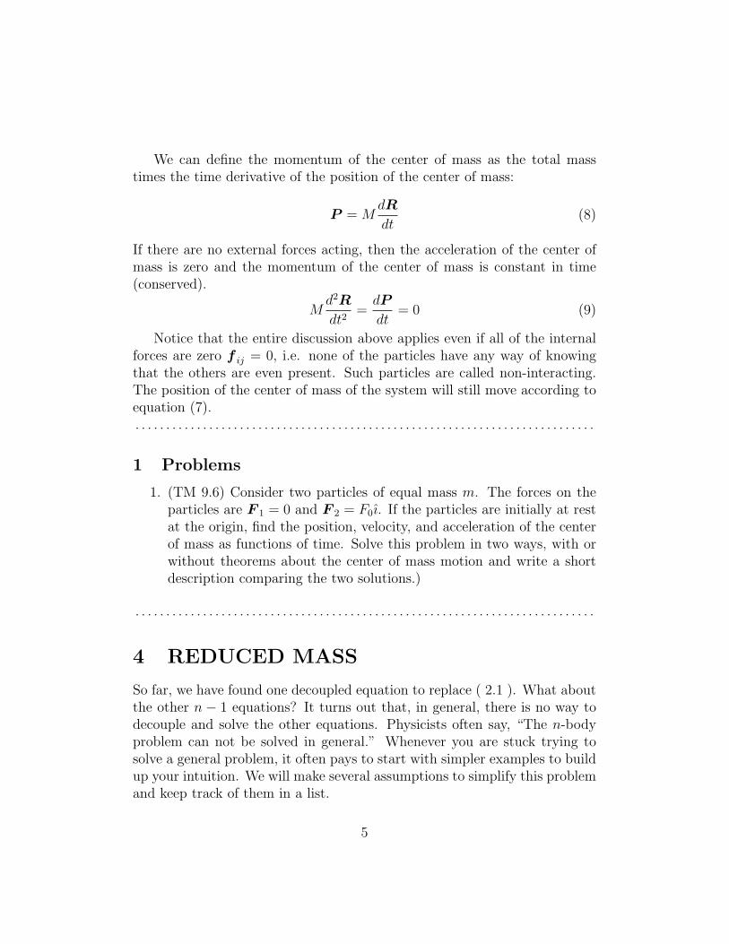
1. The figure below shows the orbit of a “fictitious” reduced mass, µ,traveling around the center-of-mass at the origin. The position vector rlocates the particle at a particular instant t. Assume that m2 = m1 anddraw on the figure the position vectors for m1 and m2 corresponding tor. Also sketch the orbits for m1 and m2. Give an example of a physicalsituation that might produce this type of motion. (NOTE: Do thisproblem “by hand.” Do not use MAPLE or a graphing calculator.)

7

r

Repeat this problem for m2 > m1 and m2 >> m1.

2. Find rsun − rcm and µ for the Sun–Earth system. Compare rsun − rcm

to the radius of the Sun and to the distance from the Sun to the Earth.Repeat the calculation for the Sun–Jupiter system.

. . . . . . . . . . . . . . . . . . . . . . . . . . . . . . . . . . . . . . . . . . . . . . . . . . . . . . . . . . . . . . . . . . . . . . . . . . .

5 CENTRAL FORCES

Our ultimate goal is to solve the equations of motion for two masses m1 andm2 subject to a central force acting between them. When you considered thisproblem in introductory physics, you assumed that one of the masses was solarge that it effectively remained at rest while all of the motion belonged tothe other object. This assumption works fairly well for the Earth orbitingaround the Sun or for a satellite orbiting around the Earth, but in generalwe are going to have to solve for the motion of both objects.

In the introduction, we defined a central force to satisfy two character-istics. We can now write turn these descriptions of the characteristics intoequations:

(a) a central force depends only on the separation between the two bodies

f 21 = −f 12 = f(r2 − r1) (17)

8

(b) it points along the line connecting the two bodies

f 21 = −f 12 = f(r2 − r1) = f(r) r (18)

. . . . . . . . . . . . . . . . . . . . . . . . . . . . . . . . . . . . . . . . . . . . . . . . . . . . . . . . . . . . . . . . . . . . . . . . . . .

1 Problems

1. If a central force is the only force acting on a system of two masses (i.e.no external forces), what will the motion of the center of mass be?

2. Which of the forces which we found in the Static Fields Paradigm (i.e.

~g, q ~E, q~v × ~B) can be central forces? which cannot?

. . . . . . . . . . . . . . . . . . . . . . . . . . . . . . . . . . . . . . . . . . . . . . . . . . . . . . . . . . . . . . . . . . . . . . . . . . .

6 ANGULAR MOMENTUM

Consider the angular momentum of the reduced mass system L = r × p =r × µv. How does L change with time? We have:

dL

dt=

d

dt(r × µv) (19)

= r × µv + v × µv (20)

= r × µa (21)

= r × F (22)

= rr × f(r)r (23)

= 0 (24)

(To get from (19) to (20), use the product rule, which is valid for crossproducts as long as you don’t change the order of the factors. The secondterm in (20) is zero since v×v = 0.) Recall that r×F which occurs in (22)is called the torque τ . We have shown that in the case of central forces thetime derivative of the angular momentum, and hence the torque, are zero.Therefore:

τ =dL

dt= 0 ⇒ L = constant (25)

i.e. the angular momentum is conserved.

9

The force F (r) depends only on the distance of the reduced mass fromthe center of mass and not on the orientation of the system in space. There-fore, this system is spherically symmetric; it is invariant (unchanged) underrotations. Noether’s theorem states that whenever the laws of physics areinvariant under a particular motion or other operation, there will be a cor-responding conserved quantity. In this case, we see that the conservationof angular momentum is related to the invariance of the physical systemunder rotations. Noether’s theorem, in general, is most easily discussed us-ing Lagrangian techniques. You will see this again the Classical MechanicsCapstone.. . . . . . . . . . . . . . . . . . . . . . . . . . . . . . . . . . . . . . . . . . . . . . . . . . . . . . . . . . . . . . . . . . . . . . . . . . .

1 Problems

1. Which of the equations in the derivation of (19)–(24) are valid only forcentral forces, and which are true more generally?

2. (Challenging) What invariances of physics are related to conservationof linear momentum and conservation of energy?

. . . . . . . . . . . . . . . . . . . . . . . . . . . . . . . . . . . . . . . . . . . . . . . . . . . . . . . . . . . . . . . . . . . . . . . . . . .

7 COORDINATES

The time has come to choose a coordinate system. We have argued thatthe problem is spherically symmetric in nature. Therefore, it will be to ouradvantage to use spherical coordinates, defined by:

x = r sin θ cosφ (26)

y = r sin θ sinφ (27)

z = r cos θ (28)

(see Figure 2), rather than the more comfortable Cartesian coordinates x, y,and z.

In fact, in the present classical mechanics context, we can do even better.For a central force:

F = f(r) r (29)

10

φ

θ

x

z

r

r

Spherical Coordinates

y

x=r sin θ cos φy=r sin θ sin φz=r cos θ

(r, , )θ φφ

θ

Figure 2: Spherical Coordinates.

the force, and hence the acceleration, are in the radial direction. Therefore,the path of the motion (orbit) will be in the plane determined by the positionvector r and velocity vector v of the reduced mass at any one moment oftime. Since there is never a component of force out of this plane, the sub-sequent motion must remain in the plane. In this plane, choose plane polarcoordinates:

x = r cosφ (30)

y = r sinφ (31)

Notice that many textbooks choose to call the angle of plane polar coordi-nates θ. See Practice Problem 1.3 for the reason that we choose to call theangle φ.. . . . . . . . . . . . . . . . . . . . . . . . . . . . . . . . . . . . . . . . . . . . . . . . . . . . . . . . . . . . . . . . . . . . . . . . . . .

11

1 Problems

1. Convince yourself that the plane of the orbit is perpendicular to theangular momentum vector L.

2. Show that a central force is always conservative. Find the scalar po-tential U corresponding to the central force F = f(r) r and show thatit depends only on the distance from the center of mass U = U(r).

3. Show that the plane polar coordinates we have chosen are equivalentto spherical coordinates if we make the choices:

(a) The direction of z in spherical coordinates is the same as thedirection of L.

(b) The θ of spherical coordinates is chosen to be π/2, so that theorbit is in the equatorial plane of spherical coordinates.

Some textbooks argue that you can obtain plane polar coordinates interms of r and the polar angle θ by taking spherical coordinates (26)–(28) and making the choice dφ = 0. Why is this choice actually mis-leading? Hint: In spherical coordinates, what is the range of θ? Thesetextbooks label the angle θ because this is the most common conventionfor polar coordinates alone. However, if you do this, polar coordinatesdo not correspond in any nice way to spherical coordinates. BecauseI want you to see the relationship between classical and quantum me-chanics and because the quantum version of central forces will requirethe use of spherical coordinates, we will call the polar coordinate angleφ.)

. . . . . . . . . . . . . . . . . . . . . . . . . . . . . . . . . . . . . . . . . . . . . . . . . . . . . . . . . . . . . . . . . . . . . . . . . . .

8 VELOCITY & ACCELERATION

Newton’s Laws require a knowledge of velocity and acceleration. With ourchoice of polar coordinates:

x = r cosφ (32)

y = r sinφ (33)

12

we must deal with the problem of how to compute velocity and accelerationas time derivatives of the position vector r in terms of the coordinates r andφ. A difficulty arises because r and φ are not independent of position andtherefore are not independent of time. This problem does not present itselfin Cartesian coordinates because ı, , and k are independent of position. Wecan exploit this Cartesian independence to help us in polar coordinates. r

and φ are given, in terms of ı and , by

r = cosφ ı + sinφ (34)

φ = − sinφ ı + cosφ (35)

j

r

φ

φ

x

y

ri

Figure 3: The relationship between unit vectors in polar coordinates (r, φ)and unit vectors in Cartesian coordinates (ı, ).

You should recognize this basis change as a rotation performed on the ı,

basis. As Figure 3 shows:(

r

φ

)

=

(

cosφ sinφ− sinφ cosφ

)(

ı

)

= R(φ)

(

ı

)

(36)

Using the chain rule, the general velocity vector is given by:

v =dr

dt=

d

dt(rr) =

dr

dtr + r

dr

dt(37)

To evaluate (37), we need the derivatives of r (and φ) with respect to time.Using the definitions in (36) above, we obtain:

dr

dt=

d

dt(cosφı + sinφ) = − sinφ

dφ

dtı + cosφ

dφ

dt =

dφ

dtφ (38)

13

dφ

dt=

d

dt(− sinφı + cosφ) = − cosφ

dφ

dtı − sinφ

dφ

dt = −dφ

dtr (39)

Combining this with equation (37) gives:

v = rr + rφ φ (40)

Notice that we have used the convenient notation of putting a dot over asymbol to denote time derivative.

Taking another derivative of (40) with respect to time shows that theacceleration is given by:

a = v = r =(

r − rφ2)

r +(

rφ+ 2rφ)

φ (41)

(40) can be used to show that the kinetic energy T of the reduced mass inpolar coordinates is given by:

T =1

2µ v2 =

1

2µv · v =

1

2µ (r2 + r2φ2) (42)

Similarly, the magnitude of the angular momentum L of the reduced massµ is given in polar coordinates by:

|L| = |r × µv| = l = µr2φ (43)

Since the angular momentum is a constant in central force problems, it’smagnitude l is also constant. Therefore (43) can be used to rewrite differentialequations, getting rid of φ’s in favor of the variable r and the constant l.

Kepler’s second law says that the areal velocity of a planet in orbit isconstant in time. This is equivalent to equation (43). To see why, read insection 8.3 of Marion and Thornton, page 294, from equation 8.10 to thebottom of the page.. . . . . . . . . . . . . . . . . . . . . . . . . . . . . . . . . . . . . . . . . . . . . . . . . . . . . . . . . . . . . . . . . . . . . . . . . . .

1 Practice Problems

1. Work through the steps deriving equations (41), (42), and (43) from(40).

. . . . . . . . . . . . . . . . . . . . . . . . . . . . . . . . . . . . . . . . . . . . . . . . . . . . . . . . . . . . . . . . . . . . . . . . . . .

14

9 EQUATIONS OF MOTION: F = µa

The problem is now to the point where we can write the equations of motionin a form we can solve. However, the importance of the preceding sectionscannot be stressed enough. The strategies that we used are important to thesuccess of problem solving in many complicated physics situations. Drawinga picture, exploiting symmetries, choosing a convenient origin, and using themost appropriate coordinate system all combine to make the analysis as easyas possible. These and other tricks should always be regarded as a goodbeginning to any problem.

Newton’s second law, reduced and modified for our specific problem is:

f(r)r = µ r = µ(

(r − rφ2)r + (rφ+ 2rφ)φ)

(44)

The vector equation breaks up, in polar coordinates, into two coupled differ-ential equations for r(t) and φ(t):

f(r) = µ (r − rφ2) (45)

0 = µ (rφ+ 2rφ) (46)

Equation (46) is just the polar coordinate statement of angular momen-tum conservation, which we have already discussed, i.e.:

0 = r µ (rφ+ 2rφ) =d

dt

(

µ r2φ)

=dl

dt(47)

(To derive verify the equalities in (47) it is easiest to work from right to left!)Therefore

µr2φ = l = constant (48)

(48) can be solved for φ and used in (45) to obtain a messy, second orderODE for r(t):

r =l2

µ2r3+

1

µf(r) (49)

In principle, we could now insert the particular form of f(r) we are con-cerned with, solve equation (49) for r as a function of t, and insert thisvalue in (48) and solve for φ(t). We would then have solved the equations ofmotion for r, and φ, parameterized by the time t. In practice, for any butthe simplest forms of f(r), it is impossible to solve the differential equationsanalytically. Computers to the rescue! On Day 4, you will use a Maple work-sheet which will allow you to explore numerical solutions for some importantphysical examples.

15

10 SHAPE OF THE ORBIT

If we are only interested in the shape of the orbit, we can do somethingsimpler than solving the equations of motion for r and φ as functions of t;we can solve for the shape of the orbit, i.e. instead of using the variable t asa parameter in (49), we will use the variable φ and solve for r(φ). To do this,we need to change the time derivatives into φ derivatives.

d

dt=dφ

dt

d

dφ= φ

d

dφ=

ℓ

µr2

d

dφ(50)

It turns out that the differential equation which we obtain will be mucheasier to solve if we also change independent variables from r to

u = r−1 (51)

(There is no way that you could guess this, yourself.) Therefore,

dr

dt=

ℓ

µr2

dr

dφ= − ℓ

µ

d r−1

dφ= − ℓ

µ

du

dφ(52)

(To verify the second equality, work from right to left.) Then the secondderivative is given by

d2r

dt2=

d

dt

dr

dt=ℓ

µu2 d

dφ

(

− ℓ

µ

du

dφ

)

= − ℓ2

µ2u2 d

2u

dφ2(53)

Plugging (51) and (53) into (49), dividing through by u2, and rearranging,we obtain the orbit equation

d2u

dφ2+ u = − µ

ℓ21

u2f

(

1

u

)

(54)

For the special case of inverse square forces f(r) = −k/r2 (sphericalgravitational and electric sources), it turns out that the right-hand side of(54) is constant so that the equation is particularly easy to solve. Firstsolve the homogeneous equation (with f(r) = 0), which is just the harmonicoscillator equation with general solution

uh = A cos(φ+ δ) (55)

16

Add to this any particular solution of the inhomogeneous equation (withf(r) = −k/r2). By inspection, such a solution is just

up =µ k

ℓ2(56)

so that the general solution of (54) for an inverse square force is

r−1 = u = uh + up = A cos(φ+ δ) +µ k

ℓ2(57)

Then solving for r in (57) we obtain

r =1

µkℓ2

+ A cos(φ+ δ)=

ℓ2

µk

1 + A′ cos(φ+ δ)(58)

You can explore how the graph of this equation depends on the variousparameters using the Maple worksheet conics.mws

. . . . . . . . . . . . . . . . . . . . . . . . . . . . . . . . . . . . . . . . . . . . . . . . . . . . . . . . . . . . . . . . . . . . . . . . . . .

1 Practice Problems

1. Go through all the steps in the derivation of (54) from (49). (49)is the same as equation 8.18 in section 8.4 on page 296 of Marionand Thornton; an alternative derivation of (54) can be found followingequation 8.18. Use whichever technique is easiest for you to follow, butmake sure you understand at least one. This kind of change of variablesis very common in physics.

2. How do the physical constants in (58) correspond to the mathematicalconstants: amplitude α, phase δ, and the eccentricity ǫ, from the Mapleworksheet conics.mws?

. . . . . . . . . . . . . . . . . . . . . . . . . . . . . . . . . . . . . . . . . . . . . . . . . . . . . . . . . . . . . . . . . . . . . . . . . . .

11 EQUATIONS OF MOTION: E = T + U

Another theoretical tool we can use to arrive at an equation for the orbitis conservation of energy. The central force F is conservative and can be

17

derived from a potential U(r) which depends only on the distance from thecenter of mass (see practice problem 1.2):

F = −∇U = −∂U(r)

∂r(59)

The statement of energy conservation:

E = T + U (60)

becomes, using (42), (43), and (59):

E =1

2µ r2 +

1

2

l2

µr2+ U(r) (61)

(61) can be solved for r to give:

r = ±√

2

µ(E − U(r)) − l2

µ2r2(62)

(62) is an equivalent alternative to (49) as an equation of motion for r(t).You might be surprised that (62) is a first order differential equation, whereas(49) is second order. This means that only one initial condition is requiredfor the solution of (62) whereas two are needed for the solution of (49).There is nothing surprising going on here. We have already provided theextra information (the extra initial condition) by specifying the constanttotal energy E.. . . . . . . . . . . . . . . . . . . . . . . . . . . . . . . . . . . . . . . . . . . . . . . . . . . . . . . . . . . . . . . . . . . . . . . . . . .

1 Practice Problems

1. (Challenging) Show that the equation of motion derived from Newton’sLaw (49) is equivalent to the equation of motion derived from energyconservation (62). Hint: Multiply (49) by 2r dt and integrate bothsides.

. . . . . . . . . . . . . . . . . . . . . . . . . . . . . . . . . . . . . . . . . . . . . . . . . . . . . . . . . . . . . . . . . . . . . . . . . . .

18

12 EVERYTHING ELSE

You should now work through sections 8.4-8.7 of Taylor. Pay particularattention to the concept of the effective potential.

There are many areas left to explore if you are interested: questions ofthe stability of orbits under perturbations, the precession of the orbit, andwhether it is open or closed. There are many interesting examples, evenwithin our solar system, that show the varied and unique outcomes of cen-tral force interactions: Lagrange points, resonant orbits, horseshoe orbits,to name a few. There are also other types of central forces. The repul-sive inverse square force was very important to early atomic experiments.Rutherford bombarded a lattice of gold with alpha particles (helium nuclei).The repulsive electrostatic interaction can be handled easily by our preced-ing analysis. The theory fit experiment well until the alpha particle energiesbecame high enough to overcome the effective potential and hit the nucleushead-on.

Many of the ideas in our analysis are handled nicely by the Lagrangianformalism which you will study in the Classical Mechanics Capstone. La-grangian mechanics provides yet another starting point for obtaining theequations of motion. The ideas of symmetry and conservation are moreeasily recognized and handled within that context, which proves to be verypowerful in more complicated situations. When you reach that point, remem-ber some of the techniques we used here and then appreciate the simplicityand beauty provided by the new viewpoint.

19

QUANTUM CENTRAL FORCES

Abstract

The Schrodinger equation in a central potential is examined. Theseparation of variables procedure is used to turn this partial differentialequation into a set of ordinary differential equations. The angularequations are solved, first for a particle confined to a ring and then fora particle confined to a sphere, thereby building up, one dimension ata time, toward the eigenstates of the hydrogen atom. Special attentionis paid to linear combinations of states and time-dependent states.

The properties of the spherical harmonics are explored, includinga brief introduction to angular-momentum raising and lowering op-erators. The relationship of spherical harmonics to spin 1 systems isdiscussed. The eigenstates on the surface of a sphere are shown to bethe same as the rigid rotor problem and the properties of rotationalspectra are discussed.

The radial equation is solved and the properties of the eigenstatesof the (unperturbed) hydrogen atom are explored.

13 INTRODUCTION

We now begin our analysis of the central force problem in quantum mechan-ics. We will find that there are some similarities and some differences betweenthe handling of this problem in classical mechanics and quantum mechanics.Concepts such as acceleration or Newton’s third law have no counterpart inquantum physics. However, we shall find that reduction of the two-bodyproblem to a fictitious one-body problem is also a characteristic of the quan-tum analysis. And we will again find that angular momentum is a criticalaspect of our description of the motion of the system, related to sphericalsymmetry.

As we did in analyzing our classical central force problem, we again as-sume a two-particle system in which the only interaction is the mutual in-teraction of the two particles. We assume that this interaction depends onlyon the separation distance between the particles and not on any angle ororientation in space. In this case, as in the classical problem, we will findthat the angular momentum is a constant of the motion, but in quantummechanics angular momentum (like energy) is quantized.

20

As always in quantum mechanics, we begin with Schrodinger’s equation

HopΨ = ih∂Ψ

∂t

14 Reduced Mass

It is helpful to consider briefly how the quantum two-body problem separatesinto an equation governing the center of mass and an equation describing thesystem around the center of mass, comparing this process to the classicalproblem. The quantum two-body problem in three dimensions is very messy,but all the essential features of the calculation show up in a simple one-dimensional model. So, for simplicity, let’s consider a system of two particles,m1 and m2, lying on a line at positions x1 and x2, and let the interactionbetween the particles be represented by a potential energy U that dependsonly on x = x1 − x2, the separation distance between the particles. Don’tworry about how the particles can get past each other on the line—this is asimple toy model; just imagine that they can pass right through each other.

Our first job, as always, is to identify the Hamiltonian Hop for the system.Because energies are additive, the kinetic part of the Hamiltonian is just thesum of the kinetic parts for two individual particles and the potential U(x)describes the interaction between them. Therefore the Hamiltonian is

Hop = − h2

2m1

∂2

∂x21

− h2

2m2

∂2

∂x22

+ U(x) (63)

and the wave function Ψ is a function of the positions of both particles (andof course time) Ψ = Ψ(x1, x2, t).

Inspired by our experience with classical two-body systems, we will tryrewriting the Hamiltonian (63) in terms of the center-of-mass coordinate X,given by

X =m1x1 +m2x2

m1 +m2

(64)

and the relative coordinate x. We will use the chain rule of calculus totransform the partial derivatives in equation (63) to derivatives with respectto x and X. (Please see Appendix A , especially the worked example onplane polar coordinates.) The transformations for first derivatives are:

∂

∂x1

=∂x

∂x1

∂

∂x+∂X

∂x1

∂

∂X=

∂

∂x+

m1

m1 +m2

∂

∂X(65)

21

∂

∂x2

=∂x

∂x2

∂

∂x+∂X

∂x2

∂

∂X= − ∂

∂x+

m2

m1 +m2

∂

∂X(66)

It is important to note that we cannot simply write equations (65–66) for thesecond derivative, which is what we need for the Hamiltonian (63). To findthe second derivative, we must apply the first derivative rules (65–66) twice:

∂2

∂x21

Ψ =∂

∂x1

∂

∂x1

Ψ (67)

=

(

∂

∂x+

m1

m1 +m2

∂

∂X

)(

∂

∂x+

m1

m1 +m2

∂

∂X

)

Ψ (68)

=∂2

∂x2Ψ +

2m1

m1 +m2

∂2

∂x∂XΨ +

(

m1

m1 +m2

)2∂2

∂X2Ψ (69)

∂2

∂x22

Ψ =∂

∂x2

∂

∂x2

Ψ (70)

=

(

∂

∂x+

m1

m1 +m2

∂

∂X

)(

∂

∂x+

m1

m1 +m2

∂

∂X

)

Ψ (71)

=∂2

∂x2Ψ − 2m1

m1 +m2

∂2

∂x∂XΨ +

(

m1

m1 +m2

)2∂2

∂X2Ψ (72)

Substituting into the Hamiltonian (63), we obtain for Schrodinger’s equation

{

− h2

2µ

∂2

∂x2− h2

2(m1 +m2)

∂2

∂X2+ U(x)

}

Ψ(X, x, t) = ih∂

∂tΨ(X, x, t) (73)

By transforming to these coordinates, the middle terms in equations (69)and (72) have canceled, enabling us to separate the dependence on x fromthe dependence on X. We can now write

Ψ(x,X, t) = ψM(X)ψµ(x)T (t) (74)

After a separation of variables procedure (see Appendix B ) on equation (74),we find that the ordinary differential equation governing the variable X hasa simple, recognizable form (see Problem 14.3b). The solution has the sameform as the free-particle solution to the Schrodinger equation (also called theplane-wave solution to the equation)

ψM(X) = eiPXX/h (75)

22

where PX represents the momentum associated with the motion of the cen-ter of mass. All observables in quantum mechanics involve the probabilitydensity, i.e. terms of the form Ψ∗Ψ, so if we are evaluating observables associ-ated with the relative motion, the pure phase contribution from the center-ofmass has no effect. We can therefore ignore the center-of-mass motion andconcentrate only on the relative motion.

We have arrived at a conclusion in the quantum analysis of the two-body problem that is similar to our analysis of the classical problem (but fordifferent reasons). We have again replaced the more complicated two-bodysystem with a fictitious one-body system, involving the relative coordinateand the reduced mass. Once we have solved the problem and found ψµ(x)and T (t), we can then reverse the procedure in this section to find the wavefunction Ψ(x1, x2, t) describing the original two-body system. The analysisin three dimensions is the same, except that we must do the calculation threetimes, once for each of the rectangular coordinates.. . . . . . . . . . . . . . . . . . . . . . . . . . . . . . . . . . . . . . . . . . . . . . . . . . . . . . . . . . . . . . . . . . . . . . . . . . .

1 Problems

1. Work through the steps of the chain rule to show that equation (73)follows from equation (63)

2. Where does the mass of a particle appear in Schrodinger’s equation?In equation (73), what is the mass associated with the center-of-masscoordinate X? what is the mass associated with the relative positioncoordinate x? Does this make sense?

3. Use the separation of variables procedure in Appendix B to break equa-tion (73) up into three ordinary differential equations.

(a) How many separation constants do you have? Is this the numberyou expect? Explain.

(b) Solve the equations for ψM(X). What are the possible eigenval-ues?

(c) Give an appropriate name to the eigenvalues of the (unsolved)equation for ψµ(x).

(d) Solve the equation for T (t). Discuss how the energy E of thesystem depends on the separation constants.

23

. . . . . . . . . . . . . . . . . . . . . . . . . . . . . . . . . . . . . . . . . . . . . . . . . . . . . . . . . . . . . . . . . . . . . . . . . . .

15 SCHRODINGER’S EQUATION IN SPHER-

ICAL COORDINATES

Schrodinger’s equation is

HopΨ = ih∂Ψ

∂t(76)

For one-dimensional waves, the Hamiltonian is

Hop = − h2

2µ

∂2

∂x2+ U(x) (77)

In a central potential the role of the second derivative with respect to x isplayed by the Laplacian operator ∇2 and the potential energy is a functiononly on the separation variable U = U(r), making the Hamiltonian:

Hop = − h2

2µ∇2 + U(r) (78)

Because of the parameter r, this problem is clearly asking for the use ofspherical coordinates, centered at the origin of the central force.

In rectangular coordinates, we know that the Laplacian ∇2 is given by:

∇2 =∂2

∂x2+

∂2

∂y2+

∂2

∂z2(79)

What is the Laplacian in spherical coordinates? Since ∇2 def= ~∇ · ~∇, we can

combine the spherical coordinate definitions of gradient and divergence

~∇V =∂V

∂rr +

1

r

∂V

∂θθ +

1

r sin θ

∂V

∂φφ (80)

~∇ · ~v =1

r2

∂

∂r(r2vr) +

1

r sin θ

∂

∂θ(sin θvθ) +

1

r sin θ

∂vφ

∂φ(81)

to obtain:

∇2 =1

r2

∂

∂r

(

r2 ∂

∂r

)

+1

r2 sin θ

∂

∂θ

(

sin θ∂

∂θ

)

+1

r2 sin2 θ

∂2

∂φ2(82)

24

For convenience, we will give the combination of angular derivatives whichappears in (82) a new name:

L2op

def= −h2

[

1

sin θ

∂

∂θ

(

sin θ∂

∂θ

)

+1

sin2 θ

∂2

∂φ2

]

(83)

Notice the conventional factor of −h2. h is a constant, 1.05459 × 10−27 erg-sec = 6.58217 × 10−16 eV-sec. Notice that the dimensions of h are those ofangular momentum. With this definition, (82) becomes:

∇2 =1

r2

∂

∂r

(

r2 ∂

∂r

)

− 1

h2r2L2

op (84)

. . . . . . . . . . . . . . . . . . . . . . . . . . . . . . . . . . . . . . . . . . . . . . . . . . . . . . . . . . . . . . . . . . . . . . . . . . .

1 Practice Problems

1. Review the definition of spherical coordinates. Remember that in ourconventions θ is always the angle measured from the z axis and rangesfrom 0 to π. φ is the angle in the x-y plane measured from the x axistowards the y axis and ranges from 0 to 2π.

2. Review the definition of gradient and divergence in spherical coordi-nates. See Griffiths E&M, Appendix A, for a nice derivation. What isthe fastest place to look-up expressions for gradient, etc. in sphericaland cylindrical coordinates?

3. Using the definition of gradient (80) and divergence (81) in sphericalcoordinates, derive equation (82).

. . . . . . . . . . . . . . . . . . . . . . . . . . . . . . . . . . . . . . . . . . . . . . . . . . . . . . . . . . . . . . . . . . . . . . . . . . .

16 SEPARATION OF VARIABLES

We will use the “separation of variables” procedure (see Appendix B ) onthe Schrodinger equation in a central potential. Most of the calculation willinvolve using this procedure on the Laplacian operator. Since the Laplaciancomes up in almost all physics problems with spherical symmetry, you willfind yourself using the results of this section many times in your career.

25

Because there are several spatial dimensions, the procedure requires anumber of rounds, each consisting of the same set of six steps. In the firstround, we will separate out an ordinary differential equation in the timevariable.

Step 1: Write the partial differential equation in appropriate coordinatesystem. For Schrodinger’s equation in any potential we have:

HopΨ = ih∂Ψ

∂t(85)

Step 2: Assume that the solution Ψ can be written as the product offunctions, at least one of which depends on only one variable, in this case t.The other function(s) must not depend at all on this variable, i.e. assume

Ψ(r, θ, φ, t) = ψ(r, θ, φ)T (t) (86)

Plug this assumed solution (255) into the partial differential equation(85). Because of the special form for Ψ, the partial derivatives each act ononly one of the factors in Ψ.

(Hopψ)T = ihψdT

dt(87)

Any partial derivatives that act only on a function of a single variable maybe rewritten as total derivatives.

Step 3: Divide by Ψ in the form of (255).

1

ψ(Hopψ) = ih

dT

dt

1

T(88)

Step 4: Isolate all of the dependence on one coordinate on one side ofthe equation. Do as much algebra as you need to do to achieve this. In ourexample, notice that in (257), all of the t dependence is on the right-handside of the equation while all of the dependence on the spatial variable is onthe other side. In this case, the t dependence is already isolated, without anyalgebra on our part.

Step 5: Now imagine changing the isolated variable t by a small amount.In principle, the right-hand side of (257) could change, but nothing on theleft-hand side would. Therefore, if the equation is to be true for all valuesof t, the particular combination of t dependence on the right-hand side mustbe constant. By convention, we call this constant E.

1

ψ(Hopψ) = ih

dT

dt

1

Tdef= E (89)

26

In this way we have broken our original partial differential equation up into apair of equations, one of which is an ordinary differential equation involvingonly t, the other is a partial differential equation involving only the threespatial variables.

1

ψHopψ = E (90)

ihdT

dt

1

T= E (91)

The separation constant E appears in both equations.Step 6: Write each equation in standard form by multiplying each equa-

tion by its unknown function to clear it from the denominator.

Hopψ = Eψ (92)

dT

dt= − i

hET (93)

Notice that (261) is an eigenvalue equation for the operator Hop. You maynever have thought of the derivation of this “time independent version of theSchrodinger equation” from the Schrodinger equation as just a simple exam-ple of the separation of variables procedure. At the moment, the eigenvalueE could be anything. Much of the rest of the Paradigm will be directedtoward finding the possible values of E!

Now we must repeat the steps until each of the variables has been sepa-rated out into its own ordinary differential equation. In the next round, wewill isolate the r dependence.

Step 1: Since we want to isolate the r dependence, we must rewrite Hop

to show the r dependence explicitly using (84)

− h2

2µ

[

1

r2

∂

∂r

(

r2 ∂

∂r

)

− 1

h2r2L2

op

]

ψ + U(r)ψ = Eψ (94)

Step 2: Assume ψ(r, θ, φ) = R(r)Y (θ, φ).

− h2

2µ

[

1

r2

d

dr

(

r2dR

dr

)

Y − 1

h2r2R(L2

opY )

]

+ U(r)RY = ERY (95)

Step 3:

− h2

2µ

[

1

r2

d

dr

1

R

(

r2dR

dr

)

− 1

h2r2

1

Y(L2

opY )

]

+ U(r) = E (96)

27

Step 4: To isolate the r dependence we must first clear the r dependencefrom the angular term (involving angular derivatives in Lop and angularfunctions in Y ). To do this, we need to multiply (96) by r2 to clear thisfactor out of the denominators of the angular pieces. Further rearranging(96) to get all of the r dependence on the right-hand side, we obtain:

− 1

h2

1

Y(L2

opY ) = − d

dr

(

r2dR

dr

)

1

R− 2µ

h2 (E − U(r))r2 (97)

Step 5: In this case, I have called the separation constant A.

− 1

h2

1

Y(L2

opY ) = − d

dr

(

r2dR

dr

)

1

R− 2µ

h2 (E − U(r))r2 def= A (98)

In principle, A can be any complex number.Step 6: Rearranging (98) slightly, we obtain the radial and angular

equations in the more standard form:

d

dr

(

r2dR

dr

)

+2µ

h2 (E − U(r))r2R + AR = 0 (99)

L2opY + h2AY = 0 (100)

Notice that the only place that the central potential enters the set of differ-ential equations is in the radial equation (99). (99) is not yet in the formof an eigenvalue equation since it contains two unknown constants E and A.(100) is an eigenvalue equation for the operator L2

op with eigenvalue h2A; itis independent of the form of the central potential.

In the last round, we must separate the θ dependence from the φ de-pendence. I will leave this as an important Practice Problem. The answeris:

sin θd

dθ

(

sin θdP

dθ

)

− A sin2 θP −BP = 0 (101)

d2Φ

dφ2+BΦ = 0 (102)

(102) is an eigenvalue equation for the operator d2/dφ2 with eigenvalue B.(101) is not yet in the form of an eigenvalue equation since it contains twounknown constants A and B.

28

We started with a partial differential equation in four variables and weended up with four ordinary differential equations (262), (99), (101), (102)by introducing three separation constants (E, A, and B). You should al-ways get one fewer separation constant than the number of variables youstarted with; each separation constant should appear in two of the final setof equations.. . . . . . . . . . . . . . . . . . . . . . . . . . . . . . . . . . . . . . . . . . . . . . . . . . . . . . . . . . . . . . . . . . . . . . . . . . .

1 Practice Problems

1. Work carefully through all of the derivations in this section.

2. Use the separation of variables procedure on (100) to obtain (101) and(102).

3. Consider the problem of the motion of a quantum particle of mass µconfined to move on a ring of radius r0. Redo the separation of variablesprocedure in this section, assuming that r = r0 is a constant and θ = π

2

is a constant so that Ψ = T (t)Φ(φ) only. How do the equations youget differ from the equations of this section? The solutions of theseequations will be the subject of the next section.

. . . . . . . . . . . . . . . . . . . . . . . . . . . . . . . . . . . . . . . . . . . . . . . . . . . . . . . . . . . . . . . . . . . . . . . . . . .

29

17 Motion on a Ring

To begin our study of the angular properties of the solutions of Schrodinger’sequation, we consider the motion of a quantum particle of mass µ confinedto move on a ring of constant radius r0. As with classical orbits, let’s assumethat the ring lies in the x, y plane, so that in spherical coordinates θ =π2

=const. Then, since Ψ is independent of r and θ, derivatives with respectto those variables give zero and Schrodinger’s equation reduces to

HopΨ = − h2

2µ

1

r20

∂2

∂φ2Ψ + U(r0)Ψ = ih

∂Ψ

∂t(103)

Redoing the separation of variables procedure of the last section (seePractice Problem 1.3), and assuming that Ψ = T (t)Φ(φ) only, we obtain thefollowing separated ordinary differential equations

d2Φ

dφ2= −2I

h2 (E − U(r0)) Φ (104)

dT

dt= − i

hET (105)

where we have used the substitution µr20 = I, in which I would be the

moment of inertia of a classical particle of mass µ traveling in a ring aboutthe center-of-mass.

Alternatively, we could have obtained equations (104) and (105) from theresults of our original separation of variables procedure (262), (99), (101),(102), by restricting the variables r and θ to the equator, noticing that thefunctions R and P are therefore constant, and that equation (99) reduces to:

A =2µ

h2 (E − U(r0)) r20

and equation (101) then reduces to:

B = −2µ

h2 (E − U(r0)) r20

Since the coefficient of Φ on the right-hand-side of (104) is a constant

√

2I

h2 (E − U(r0)) = constant (106)

30

the solutions of the Φ equation (104), are

Φm(φ)def= N eimφ (107)

where

m = ±√

2I

h2 (E − U(r0)) (108)

and N is a normalization constant.There is no ”boundary” on the ring, on which we can impose bound-

ary conditions. However, there is one very important property of the wavefunction that we can invoke: it must be single-valued. The variable φ isgeometrically an angle, so that φ + 2π is physically the same point as φ. Ifwe go once around the ring and return to our starting point, the value of thewave function must remain the same. Therefore the solutions must satisfythe periodicity condition Φm(φ+ 2π) = Φm(φ). This is impossible unless mis real so that the solutions are oscillatory, i.e. E − U(r0) > 0. Furthermore,the solutions must have the correct period, i.e.

m ∈ {0,±1,±2, . . .} (109)

The quantum numberm is called the azimuthal or magnetic quantum number.Note that the solution permits both positive and negative values of m as wellas zero.

Solving (108) for the possible eigenvalues of energy, we obtain

Em =h2

2Im2 + U(r0) (110)

For this simplified ring problem, we can choose the potential energy U(r0)to be zero, but we will have to remember that we should not make thischoice when we are working on the full hydrogen atom problem. There isa degeneracy that arises in this calculation. Note that the wave functionscorresponding to +|m| and −|m| have the same energy but represent (as wewill see) different states of the motion.

As usual, we choose the normalization N in (107) so that, if the particle isin an eigenstate, the probability of finding it somewhere on the ring is unity.

1 =

∫ 2π

0

Φ∗m(φ) Φm(φ) r0dφ =

∫ 2π

0

N∗e−imφNeimφ r0dφ = 2πr0|N |2 (111)

⇒ N =1√2πr0

(112)

31

This is a one-dimensional problem, just like the problem of a particle-in-a-box which you solved in the Waves Paradigm (now in φ instead of x) andthe solutions have the same oscillatory form. Everything that you learnedin that Paradigm is immediately applicable here. As in that problem, theenergy eigenvalues are discrete because of a boundary condition. The onlydifference is that the boundary condition appropriate to this problem is pe-riodicity, since φ is a physical angle, rather than Ψ(x) = 0 at the boundaries,appropriate to an infinite potential.. . . . . . . . . . . . . . . . . . . . . . . . . . . . . . . . . . . . . . . . . . . . . . . . . . . . . . . . . . . . . . . . . . . . . . . . . . .

1 Practice Problems

1. Show that (107) and (108) are solutions of (104).

2. Why is there a factor of r0 in the integral in (111)?

. . . . . . . . . . . . . . . . . . . . . . . . . . . . . . . . . . . . . . . . . . . . . . . . . . . . . . . . . . . . . . . . . . . . . . . . . . .

18 ANGULAR MOMENTUM OF THE PAR-

TICLE ON A RING

Classically, a particle moving in a circle has an angular momentum perpen-dicular to the plane of the circle, which for a ring in the x, y–plane would bein the z direction. Since angular momentum is defined by ~L = ~r×~p, we haveLz = xpy − ypx. To make the transition to quantum mechanics, we replacepx and py by their operator equivalents:

Lz = xpy − ypx ⇒ xh

i

∂

∂y− y

h

i

∂

∂x(113)

Using a straightforward application of the chain rule (see Practice Problems,below) to replace the Cartesian partial derivatives with their polar represen-tations, we obtain

Lz =h

i

∂

∂φ(114)

The effect of operating on the ring eigenfunctions with this operator is:

32

h

i

∂

∂φ

(

1√2π

eimφ

)

= mh

(

1√2π

eimφ

)

(115)

The energy eigenfunctions Φm(φ) are thus also eigenfunctions of Lz witheigenvalues mh . Because the Φm(φ) are eigenfunctions of both energy andangular momentum, we can make simultaneous determinations of the eigen-values of energy and angular momentum.

Considering the angular momentum helps us understand the degeneracyof the eigenfunctions with respect to energy. The ±m degeneracy of theenergy eigenstates corresponds to Lz = +mh and Lz = −mh. That is,the two degenerate states represent particles rotating in opposite directionsaround the ring.

For a classical particle rotating in a circular path in the x, y-plane, thekinetic energy is T = 1

2Iω2 = L2

z/2I , where I is the rotational inertia(moment of inertia). The rotational inertia of a single particle of mass µmoving in a circle of radius r0 is I = µr2

0. The Hamiltonian for the systemis thus

H = T + U =L2

z

2I+ U = − h2

2µr20

∂2

∂φ2+ U0 (116)

It is apparent from this approach that the energy and the angular momen-tum have simultaneous eigenvalues because they are commuting operators.Clearly [L2

z, Lz] = 0, so that E and Lz have the same eigenfunctions. There-fore, we see that (104) and (115) are the position-space representations ofthe eigenvalue equations

H |m〉 = Em|m〉 (117)

Lz |m〉 = hm |m〉 (118)

Because the Φm are simultaneous eigenstates of both H and Lz, it is possibleto make simultaneous measurements of both the energy and the z-componentof angular momentum.

In setting up the problem of the particle on the ring, we constrained themotion to the x, y-plane, so that the angular momentum vector is in thez direction. However, according to quantum mechanics (yet another formof the Heisenberg uncertainty relationships) it is not possible to know thedirection of the angular momentum vector. Our knowledge of the angularmomentum vector is limited to its length and any one component. If the

33

vector lies along the z-axis, then we would know all three of its components(the x and y components being zero). We’ll see how the three-dimensionalproblem solves this contradiction.. . . . . . . . . . . . . . . . . . . . . . . . . . . . . . . . . . . . . . . . . . . . . . . . . . . . . . . . . . . . . . . . . . . . . . . . . . .

1 Practice Problems

1. Using a the chain rule for partial derivatives, show that (113) is indeedthe same as (114), thereby showing that this operator is the quantumanalogue of the z-component of angular momentum.

. . . . . . . . . . . . . . . . . . . . . . . . . . . . . . . . . . . . . . . . . . . . . . . . . . . . . . . . . . . . . . . . . . . . . . . . . . .

19 TIME DEPENDENCE OF RING STATES

We know, from the theory of Fourier series, that we can write any initialprobability distribution, which is necessarily periodic, as a sum of the energyeigenstates.

Φ(φ) =∞∑

m=−∞

cm Φm(φ) =∞∑

m=−∞

cm

(

1√2π r0

eimφ

)

(119)

where, for the probability distribution to be normalized, we must have:

∞∑

m=−∞

|cm|2 = 1 (120)

To find the time evolution of the eigenstates Φm(φ), we must solve thet equation (105). Since, for each Φm, we have now found the value of theconstant E = Em, given by (110), we can solve (105) trivially.

T (t) = e−i

hEmt (121)

A deep theorem in the theory of partial differential equations states that ifyou have found an expansion of the initial probability density in terms of theeigenstates of the Hamiltonian, then the time evolution of that probability

34

density is simply obtained by multiplying each eigenstate individually by theappropriate time evolution.

Φ(φ, t) =∞∑

m=−∞

cm Φm(φ) e−i

hEmt (122)

BE CAREFUL! There are an infinite number of different values for the en-ergy, depending on the eigenstate of the Hamiltonian. It is incorrect tomultiply the initial state (119) by a single over-all exponential time factor.Each term in the series gets its own time evolution.

20 Motion on a Sphere

We will now relax the restriction that the mass be confined to the ring,and instead, let it range over the surface of a sphere of radius r0. Theresults of this analysis yield predictions that can be successfully comparedwith experiment for molecules and nuclei that rotate more than they vibrate.For this reason, the problem of a mass confined to a sphere is often calledthe rigid rotor problem. Furthermore, the solutions that we will find forequations (101) and (102), called spherical harmonics, will occur wheneverone solves a partial differential equation that involves spherical symmetry.

For homework, you will write down the Schrodinger equation for a particlerestricted to a sphere and use the separation of variables procedure to obtainan equivalent set of ordinary differential equations. One of the equations youobtain will be (102), with solutions exactly as we found them for the ring.The other equation will be (101) with slightly different labels for the unknownconstants. So, to solve either Schrodinger’s equation for the hydrogen atomor for a particle restricted to a sphere, we need to solve (101). This will bethe job of the next five sections.

21 Change of Variables

Since we have solved the φ equation (102) and found the possible values ofthe separation constant

√B = m ∈ {0,±1,±2, . . .}, the θ equation becomes

an eigenvalue/eigenfunction equation for the unknown separation constantA and the unknown function P (θ).

35

(

sin θ∂

∂θ

(

sin θ∂

∂θ

)

− A sin2 θ −m2

)

P (θ) = 0 (123)

We start with a change of independent variable z = cos θ where z is theusual rectangular coordinate in three-space. As θ ranges from 0 to π, z rangesfrom 1 to −1. We see from Figure 4 that:

θ1

z

1-z 2

Figure 4: Relationship between z and θ.

√1 − z2 = sin θ (124)

Using the chain rule for partial derivatives, we have:

∂

∂θ=∂z

∂θ

∂

∂z= − sin θ

∂

∂z= −

√1 − z2

∂

∂z(125)

Notice, particularly, the last equality: we are trying to change variables fromθ to z, so it is important to make sure we change all the θ’s to z’s. Multiplyingby sin θ we obtain:

sin θ∂

∂θ= −

(

1 − z2) ∂

∂z(126)

Be careful finding the second derivative; it involves a product rule:

sin θ∂

∂θ

(

sin θ∂

∂θ

)

=(

1 − z2) ∂

∂z

(

(

1 − z2) ∂

∂z

)

=(

1 − z2)2 ∂2

∂z2− 2z

(

1 − z2) ∂

∂z(127)

Inserting (124) and (127) into (123), we obtain a standard form of theAssociated Legendre’s equation:

(

(

1 − z2) ∂2

∂z2− 2z

∂

∂z− A− m2

(1 − z2)

)

P (z) = 0 (128)

36

In §22 and §25, we will solve this equation. After we have found theeigenfunctions P (z), we will substitute z = cos θ everywhere to find theeigenfunctions of the original equation (123).

22 SERIES SOLUTIONS OF ODE’S

The simplest possible φ–dependence on the ring is, of course, Φ(φ) = constant,which corresponds in equation (123) to m = 0. We will first find solutionsfor this special case, which is known as Legendre’s equation.

(

(

1 − z2) ∂2

∂z2− 2z

∂

∂z− A

)

P (z) = 0 (129)

Let’s use series methods to find a solution of (129), i.e. let’s assume thatthe solution can be written as a Taylor series

P (z) =∞∑

n=0

an zn (130)

and solve for the coefficients an. Then we have

dP

dz=

∞∑

n=0

an n zn−1 (131)

d2P

dz2=

∞∑

n=0

an n(n− 1) zn−2 (132)

and then plug (130)–(132) into (129) to obtain

0 =∞∑

n=0

an n(n−1) zn−2−z2

∞∑

n=0

an n(n−1) zn−2−2z∞∑

n=0

an n zn−1−A

∞∑

n=0

an zn

(133)In (133), the summation variable n is a dummy variable (just like a

dummy variable of integration). Therefore, in the first sum, we can shiftn→ n+ 2.

∞∑

n=0

an n(n− 1) zn−2

37

→∞∑

n=−2

an+2(n+ 2)(n+ 1)zn

= a−2(−2 + 2)(−2 + 1)z−2 + a−1(−1 + 2)(−1 + 1)z−1 +∞∑

n=0

an+2(n+ 2)(n+ 1)zn

=∞∑

n=0

an+2(n+ 2)(n+ 1)zn

Pay special attention to what happened to the lower limit of the sum. Thenew sum would start at n = −2, but since the factor of (n + 2) in the firstterm and the factor of (n+1) in the second term means that these terms arezero and we can eliminate them from the sum. At the same time, bring anyoverall factors of z into the corresponding sums. Finally, since each sum nowhas a factor of zn and runs over the same range, group the sums together.

∞∑

n=−2

an+2 (n+ 2)(n+ 1) zn −∞∑

n=0

an n(n− 1) zn − 2∞∑

n=0

an n zn − A

∞∑

n=0

an zn(134)

=∞∑

n=0

[an+2 (n+ 2)(n+ 1) − an n(n− 1) − 2 an n− Aan] zn = 0(135)

Now comes the MAGIC part. Since (135) is true for all values of z, thecoefficient of zn for each term in the sum must separately be zero, i.e.

an+2 (n+ 2)(n+ 1) − an n(n− 1) − 2 an n− Aan = 0 (136)

and therefore we can solve for an+2 in terms of an

an+2 =n(n+ 1) +A

(n+ 2)(n+ 1)an (137)

By plugging successive even values of n into the recurrence relation (137)allows us to find a2, a4, etc. in terms of the arbitrary constant a0 and suc-cessive odd values of n allow us to find a3, a5, etc. in terms of the arbitraryconstant a1. Thus, for the second order differential equation (129) we obtaintwo solutions as expected. a0 becomes the normalization constant for a solu-tion with only even powers of z and a1 becomes the normalization constantfor a solution with only odd powers of z. For example:

a2 =A

2a0 (138)

38

a4 =6 + A

12a2 =

(

6 + A

12

)(

A

2

)

a0 etc. (139)

a3 =2 + A

6a1 (140)

a5 =12 + A

20a2 =

(

12 + A

20

)(

6 + A

12

)

a0 etc. (141)

so that

P (z) = a0

[

A

2z0 +

(

6 + A

12

)(

A

2

)

z2 + . . .

]

(142)

+ a1

[

2 + A

6z1 +

(

12 + A

20

)(

2 + A

6

)

z3 + . . .

]

(143)

In general, the solutions of an ordinary linear differential equation canblow-up only where the coefficients of the equation itself are singular, in thiscase at z = ±1, which correspond to the north and south poles θ = 0, π.But there is nothing special about physics at these points, only the choice ofcoordinates is special there. Therefore, we want to choose solutions of (129)which are regular (non-infinite) at z = ±1. This is an important example ofa problem where the choice of coordinates for a partial differential equationend up imposing boundary conditions on the ordinary differential equationwhich comes from it. Therefore, the infinite series (130) could possibly blowup at the endpoints z = ±1, but a polynomial could not. So if we choosethe special values for the separation constant A to be A = −ℓ(ℓ + 1) whereℓ is a non-negative integer, we see from (137) that for n ≥ ℓ the coefficientsbecome zero and the series terminates in a polynomial. The solutions forthese special values of A are polynomials of degree ℓ, denoted Pℓ, and calledLegendre polynomials.

23 LEGENDRE POLYNOMIALS

It turns out that the Legendre polynomials can also be found from Rodrigues’formula

Pℓ(z) =1

2ℓℓ!

dℓ

dzℓ

(

z2 − 1)ℓ

(144)

(The proof is lengthy, but beautiful. Ask!) Rodrigues’ Formula can be usedto generate solutions quickly. To do this, write

(

z2 − 1)ℓ

= (z − 1)ℓ(z + 1)ℓ = aℓbℓ (145)

39

and use the product rule

dℓ

dzℓ

(

z2 − 1)ℓ

=

(

dℓaℓ

dzℓ

)

bℓ + ℓ

(

dℓ−1aℓ

dzℓ−1

)(

dbℓ

dz

)

(146)

+ℓ(ℓ− 1)

2!

(

dℓ−2aℓ

dzℓ−2

)(

d2bℓ

dz2

)

+ ...+ aℓ

(

dℓbℓ

dzℓ

)

where the coefficient of the ith term in the product rule is the binomialcoefficient

(

ℓ

i

)

=

(

ℓ

ℓ− i

)

=ℓ!

(ℓ− i)! i!(147)

The first few Legendre polynomials are:

P0(z) = 1 (148)

P1(z) = z (149)

P2(z) =1

2(3z2 − 1) (150)

P3(z) =1

2(5z3 − 3z) (151)

P4(z) =1

8(35z4 − 30z2 + 3) (152)

P5(z) =1

8(63z5 − 70z3 + 15z) (153)

There are several useful patterns to the Legendre polynomials:

• The overall coefficient for each solution is conventionally chosen so thatPℓ(1) = 1. As discussed in the next section, this is an inconvenient

convention that we are stuck with!

• Pℓ(z) is a polynomial of degree ℓ.

• Each Pℓ(z) contains only odd or only even powers of z, depending onwhether ℓ is even or odd. Therefore, each Pℓ(z) is either an even or anodd function.

• Since the differential operator in (129) is Hermitian (unproven), weare guaranteed by a deep theorem of mathematics that the Legendre

40

polynomials are orthogonal for different values of ℓ (just as with Fourierseries) 1 , i.e.

1∫

−1

P ∗k (z)Pℓ(z) dz =

δkℓ

ℓ+ 12

(154)

The “squared norm” of Pℓ is just 1/(ℓ+ 12). To normalize each Pℓ(z) it

should be multiplied by√

ℓ+ 12.

Notice that the differential equation

∂2P

∂z2− 2z

1 − z2

∂P

∂z+ℓ(ℓ+ 1)

1 − z2P = 0 (155)

is a different equation for different values of ℓ. For a given value of ℓ, youshould expect two solutions of (155). Why? We have only given one. It turnsout that the “other” solution for each value of ℓ is not regular (i.e. it blowsup) at z = ±1. In cases where the separation constant A does not have thespecial value l(l + 1) for non-negative integer values of ℓ, it turns out thatboth solutions blow up. We discard these irregular solutions as unphysicalfor the problem we are solving.. . . . . . . . . . . . . . . . . . . . . . . . . . . . . . . . . . . . . . . . . . . . . . . . . . . . . . . . . . . . . . . . . . . . . . . . . . .

1 Practice Problems

1. Use Rodrigues’ formula, by hand, to find the first 5 Legendre polyno-mials.

2. Go through the worksheet legendre.mws. You do not need to turnanything in. However, there are two things you should get out of thisworksheet:

(a) Get a feel for what the Legendre polynomials look like. There aresome questions in the worksheet to help guide your exploration.

(b) Learn the syntax for writing a “loop” in Maple. There is a dis-cussion of this in the worksheet. Loops are one of the most usefulof all computer programming techniques.

. . . . . . . . . . . . . . . . . . . . . . . . . . . . . . . . . . . . . . . . . . . . . . . . . . . . . . . . . . . . . . . . . . . . . . . . . . .1One shows this using Rodrigues’ Formula and repeated integration by parts, noting

that the “surface terms” always vanish.

41

24 LEGENDRE POLYNOMIAL SERIES

There is a very powerful mathematical theorem which says that any suffi-ciently smooth function f(z), defined on the interval −1 < z < 1, can beexpanded as a linear combination of Legendre polynomials

f(z) =∞∑

ℓ=0

cℓ Pℓ(z) (156)

(This theorem is the analogue of the theorem which says that any sufficientlysmooth periodic function can be expanded in a Fourier series.) You willhave several occasions in physics to expand functions in Legendre polynomialseries, so we will explore the technique in this section.

We can find the coefficients cℓ by taking the inner product of both sidesof (156) in turn with each “basis vector” Pk and using (154). This yields

1∫

−1

P ∗k (z) f(z) dz =

1∫

−1

P ∗k (z)

∞∑

ℓ=0

cℓ Pℓ(z) dz (157)

=∞∑

ℓ=0

cℓ

1∫

−1

P ∗k (z)Pℓ(z) dz (158)

=∞∑

ℓ=0

cℓδkℓ

ℓ+ 12

(159)

=ck

k + 12

(160)

or equivalently

ck =

(

k +1

2

)

1∫

−1

P ∗k (z) f(z) dz (161)

This expression should be compared with the exponential version of a Fourierseries for f(z) on the same interval −1 ≤ z ≤ 1, namely

f(z) =∞∑

n=−∞

Cn einπz (162)

42

where

Cn =1

2

1∫

−1

e−inπzf(z) dz (163)

Note the analogous role played by the normalization constants k + 12

and 12.

If we had made an unconventional, but more convenient, choice for the nor-malization for the Legendre polynomials such that the value of the integralsin (154) were simply δkℓ, then we would not need to carry around the extrafactor of k + 1

2in (161).

1 Example: Legendre Expansion of ε(z)

Consider the step function

ε(z) = 2 Θ(z) − 1 =

{

+1 (z > 0)−1 (z < 0)

(164)

where Θ is the Heaviside step function; note that ε(z) is an odd function ofz. Using (161) leads to

cℓ =

(

ℓ+1

2

)

1∫

−1

P ∗ℓ (z) ε(z) dz (165)

= −(

ℓ+1

2

)

0∫

−1

P ∗ℓ (z) dz +

(

ℓ+1

2

)

1∫

0

P ∗ℓ (z) dz (166)

and each integral in the final expression is an elementary integral of a poly-nomial. Furthermore, it is easily seen that these two integrals cancel if ℓ iseven, and add if ℓ is odd, so that

cℓ =

0 (ℓ even)

2

(

ℓ+1

2

)

1∫

0

P ∗ℓ (z) dz (ℓ odd)

(167)

These coefficients are easily evaluated on Maple for as many values of ℓ asdesired.

43

25 ASSOCIATED LEGENDRE FUNCTIONS

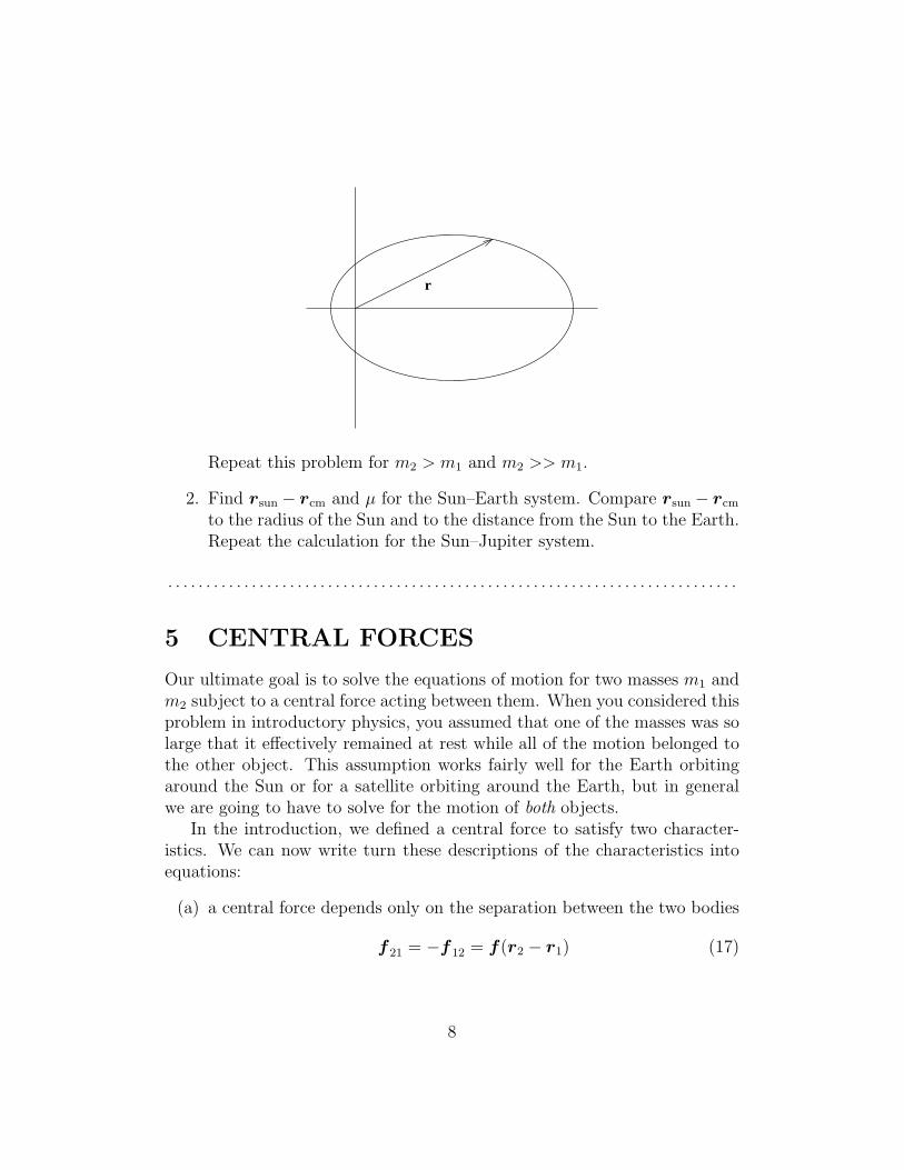
We now return to equation (128) to consider the cases with m 6= 0. Wecan solve these equations with (a slightly more sophisticated version of) theseries techniques from them = 0 case. We would again find solutions that areregular at z = ±1 whenever we choose A = −ℓ(ℓ+ 1) for ℓ ∈ {0, 1, 2, 3, . . .}.With this value for A, we obtain the standard form of Legendre’s associatedequation, namely

(

∂2

∂z2− 2z

1 − z2

∂

∂z+ℓ(ℓ+ 1)

1 − z2− m2

(1 − z2)2

)

P (z) = 0 (168)

Recall that this equation was obtained by separating variables in sphericalcoordinates. Solutions of this equation which are regular at z = ±1 are calledassociated Legendre functions, and turn out to be given by

Pmℓ (z) = P−m

ℓ (z) = (1 − z2)m/2 dm

dzm(Pℓ(z)) (169)

= (1 − z2)m/2 dm+ℓ

dzm+ℓ

(

(z2 − 1)ℓ)

(170)

where m ≥ 0. 2 Note that if z = cos θ, then Pℓ(z) is a polynomial in cos θ,while

(1 − z2)m/2 = (sin2θ)m/2 = sinmθ (171)

so that Pmℓ (z) is a polynomial in cos θ times a factor of sinmθ. Some other

properties of the associated Legendre functions are

• Pmℓ (z) = 0 if |m| > ℓ

• P−mℓ (z) = Pm

ℓ (z)

• Pmℓ (±1) = 0 for m 6= 0 (cf. factor of (1 − z2)m/2)

• Pmℓ (−z) = (−1)ℓ−mPm

ℓ (z) (behavior under parity)

•1∫

−1

Pmℓ (z)Pm

q (z) dz =2

(2ℓ+ 1)

(ℓ+m)!

(ℓ−m)!δℓq

The last property shows that for each given value ofm, the Associated Legen-dre functions form an orthonormal basis on the interval −1 ≤ z ≤ 1. Anyfunction on this interval can be expanded in terms of anyone of these bases.

2Some authors define P−m

ℓ(z) with a different phase.

44

26 SPHERICAL HARMONICS

We have found that normalized solutions of the φ equation (102) satisfyingperiodic boundary conditions are

Φ(φ) =1√2π

eimφ (m = 0,±1,±2, ...) (172)

and normalized solutions of the θ equation (101 which are regular at thepoles are given by

P (cos θ) =

√

(2ℓ+ 1)

2

(ℓ− |m|)!(ℓ+ |m|)! P

mℓ (cos θ) (173)

Combining these yields via multiplication (we assumed solutions of this typewhen we first did the separation of variables procedure), we obtain the spher-

ical harmonics

Y mℓ (θ, φ) = (−1)(m+|m|)/2

√

(2ℓ+ 1)

4π

(ℓ− |m|)!(ℓ+ |m|)! P

mℓ (cos θ) eimφ (174)

where the somewhat peculiar choice of phase is conventional.The spherical harmonics are orthonormal on the unit sphere:

2π∫

0

π∫

0

(

Y m1

ℓ1

)∗Y m2

ℓ2sin θ dθ dφ = δℓ1ℓ2δm1m2

(175)

since dz = sin θ dθ. They are complete in the sense that any sufficientlysmooth function f on the unit sphere can be expanded in a Laplace series as

f(θ, φ) =∞∑

ℓ=0

ℓ∑

m=−ℓ

aℓm Ymℓ (θ, φ) (176)

where

aℓm =

2π∫

0

π∫

0

(Y mℓ )∗ f(θ, φ) sin θ dθ dφ (177)

45

1 Example

Suppose you want a function of (θ, φ) which satisfies

f(θ, φ) ={

sin θ 0 < θ < π2

0 otherwise(178)

Then f takes the form (176), and the constants aℓm can be determined from(177), yielding

aℓm =

2π∫

0

π/2∫

0

(Y mℓ )∗ sin2θ dθ dφ (179)

= Nℓm

2π∫

0

e−imφ dφ

π/2∫

0

Pmℓ (cos θ) sin2θ dθ (180)

where

Nℓm = (−1)(m+|m|)/2

√

(2ℓ+ 1)

4π

(ℓ− |m|)!(ℓ+ |m|)! (181)

Thus,

aℓm =

0 (m 6= 0)

√

(2ℓ+ 1)π

π/2∫

0

Pℓ(cos θ) sin2θ dθ (m = 0)(182)

For m = 0, the integral is most easily computed with the substitutionz = cos θ; the first few coefficients are:

a00 =π

8a10 =

1

2a20 = −5π

64

a30 = − 7

12a40 = − 9π

512a50 =

77

240(183)

(each of which should be multiplied by√

4π/(2ℓ+ 1) ). As you can checkby graphing, however, it requires at least twice this many terms to obtain agood approximation.

46

27 ANGULAR MOMENTUM

1 Classical Angular Momentum

Consider the angular momentum of the reduced mass system L = r × p =r × µv. We have:

dL

dt=

d

dt(r × µv) (184)

= r × µv + v × µv (185)

= r × µa (186)

= r × F (187)

= rr × f(r)r (188)

= 0 (189)

(The second term in (185) is zero since v × v = 0.) r × F which occurs in(187) is called the torque. We have shown that in the case of central forcesthe time derivative of the angular momentum, and hence the torque, arezero. Therefore:

τ =dL

dt= 0 ⇒ L = constant (190)

i.e. the angular momentum is conserved.The force F (r) depends only on the distance of the reduced mass from

the center of mass and not on the orientation. Therefore, this system isspherically symmetric; it is invariant (unchanged) under rotations. Noether’stheorem states that whenever the laws of physics are invariant under a par-ticular motion or other operation, there will be a corresponding conservedquantity. In this case, we see that the conservation of angular momentum isrelated to the invariance of the physical situation under rotations. Noether’stheorem, in general, is most easily discussed using Lagrangian techniques.You will see this again the Classical Mechanics Capstone.. . . . . . . . . . . . . . . . . . . . . . . . . . . . . . . . . . . . . . . . . . . . . . . . . . . . . . . . . . . . . . . . . . . . . . . . . . .

Practice Problem

1. (Challenging) Can you guess what invariances of physics are related toconservation of linear momentum and conservation of energy?

47

. . . . . . . . . . . . . . . . . . . . . . . . . . . . . . . . . . . . . . . . . . . . . . . . . . . . . . . . . . . . . . . . . . . . . . . . . . .

2 Quantum Angular Momentum

In quantum mechanics, momentum p becomes the differential operator hi∇.

Under this correspondence, the components of L = r × p become the oper-ators

Lx = ypz − zpy 7−→ h

i

(

y∂

∂z− z

∂

∂y

)

(191)

Ly = zpx − xpz 7−→ h

i

(

z∂

∂x− x

∂

∂z

)

(192)

Lz = xpy − ypx 7−→ h

i

(

x∂

∂y− y

∂

∂x

)

= −ih ∂∂φ

(193)

which we also call Lx, etc. Direct computation, which you will verify forhomework, shows that

[Lx, Ly]f = ihLzf (194)

and cyclic permutations. But the operator

L2 = L · L = L2x + L2

y + L2z

= −h2

[

1

sin θ

∂

∂θ

(

sin θ∂

∂θ

)

+1

sin2θ

∂2

∂φ2

]

(195)

does commute with L, that is

[L2, Lz] = 0 (196)

and so forth.This (Lie) algebra is the same as the algebra of the spin matrices

Sx =h

2

(

0 11 0

)

Sy =h

2

(

0 −ii 0

)

Sz =h

2

(

1 00 −1

)

(197)

that is[Sx, Sy] = ihSz (198)

and cyclic permuations.

48

3 Eigenvalues

What are the eigenvalues and eigenfunctions of the angular momentum op-erators? As you will show for homework,

L2Yℓm = h2ℓ(ℓ+ 1)Yℓm (199)

LzYℓm = hmYℓm (200)

(201)

28 The Radial Equation

So far we have obtained solutions to the angular (θ and φ) parts of theSchrodinger equation. The Ylm(θ, φ)’s describe the spatial variation of thewave function on the surface of a sphere. Now we turn to the radial equation(99), plugging in the value of the separation constant A = −ℓ(ℓ+ 1) that weobtained when solving the θ equation.

d

dr

(

r2dR

dr

)

+2µ

h2 (E − U(r))r2R− ℓ(ℓ+ 1)R = 0 (202)

The solution to equation (99) will depend on the potential energy U(~r);for central forces, the potential energy U depends only on r and is indepen-dent of θ and φ. As a result, the Ylm(θ, φ)’s are solutions to the angular partfor any central force.

We can rewrite equation(202) as:

d2R

dr2+

2

r

dR

dr+

2µ

h2

[

E − U(r) − h2l(l + 1)

2µr2

]

R = 0 (203)

which resembles the one-dimensional Schrodinger equation corresponding toan effective potential energy Ueff :

Ueff(r) = U(r) +h2l(l + 1)

2µr2(204)

The term h2ℓ(ℓ + 1)/2µ r2 is the centrifugal contribution to the effectivepotential energy. It behaves like a repulsive force, and it increases with ℓ inexact analogy with classical mechanics.

49

We will solve the radial equation for a potential energy characteristic ofan atom consisting of a single electron interacting with a nucleus of charge+Ze (H, He+, Li++, etc.):

U(r) = − Ze2

4πε0r(205)

**Insert Graph**Practice Question:

As l increases, do you think the expectation value of r will increase ordecrease? Later we will use the radial wave functions to calculate the expec-tation value of r, and we will see if the calculated value is consistent withyour expectation.

With this choice of U(r), we can write the radial equation as:

d2R

dr2+

2

r

dR

dr+

2µ

h2

[

E +k

r− h2l(l + 1)

2µr2

]

R = 0 (206)

where k = Ze2/4πε0.

29 ASYMPTOTIC SOLUTIONS TO THE RA-

DIAL EQUATION

At first glance there seems to be no obvious direct approach to solving equa-tion (206), so let’s see if we can get some clues to the form of the solution bylooking at the limiting behavior of the solutions for large r and for small r.

For large r, the terms in equation (206) involving r−1 and r−2 can beneglected, so equation (206) becomes approximately

d2R

dr2+

2µE

h2 R = 0 (207)

It is helpful to remind ourselves that E < 0 by writing equation (207) as

d2R

dr2=

2µ |E|h2 R (208)

which has the familiar exponential solutionsR(r) = e±br with b =√

2µ|E|/h2.

Note the ± symbol in the exponential, which is there because equation(208) involves the second derivative of R. Can we eliminate one of these

50

signs? As r goes to infinity, e+br blows up. We will eventually want oursolutions for the wave functions to give us reasonably behaved probabilitydensities (that is, they must be finite everywhere), and we must thereforediscard any solution that leads to an infinite probability. Our solution forthe radial wave function in this limit then becomes:

R(r) ∼ e−br (larger) (209)

Now let’s look at the behavior of the solutions when r is small. In thislimit, the r−2 term will dominate and we can neglect the other terms in thesquare brackets in equation (206). In this case, we obtain

d2R

dr2+

2

r

dR

dr− l(l + 1)

r2R = 0 (210)

Practice Question: The solution to this equation apparently doesn’t de-pend on h. Don’t all quantum-mechanical results depend in some way onPlanck’s constant?

By inspection, you can see that a solution of the form R(r) = rq can bemade to satisfy equation (210) - note that for this choice of R(r) each termin equation (210) will then depend on rq−2 and the three terms can sum tozero. With this substitution, we obtain

q(q − 1)rq−2 +2

rqrq−1 − l(l + 1)

r2rq = 0 (211)

orq(q + 1) − l(l + 1) = 0 (212)

This quadratic equation for q yields two solutions: q = l and q = l − 1. Forsmall r, r − l − 1 blows up, so we discard this solution. We then have

R(r) ∼ rl (smallr) (213)

Combining equations (209) and (213), we expect the radial solution tolook something like R(r) ∼ rle−br. Note that we have not violated the properbehavior at the limits by combining these two solutions; R(r) remains well-behaved for r = 0 and r → ∞. What else do we need to complete thesolution? Perhaps an additional function H(r), which gives the remainingradial dependence and is well-behaved by not blowing up at r = 0 (or blowing

51

up more slowly than r−l) nor as r → ∞ (or blowing up more slowly thanebr). Let us therefore seek solutions of the radial equation of the form

R(r) = rle−brH(r) (214)

Our next goal is to determine H(r).Practice Question:

Other than its asymptotic behavior, what other properties do you expectfor R(r)? If we expect R(r) to be a radial WAVE function, what type ofbehavior is missing from the other parts of R(r) that H(r) must provide?

30 SOLVING THE RADIAL EQUATION

Before we begin substituting into equation (206), we’ll need the first twoderivatives of R(r).

dR

dr= lrl−1e−brH(r) − brle−brH(r) + rle−brH ′(r) (215)

where H ′(r) = dH/dr, and

d2R

dr2= l(l − 1)rl−2e−brH(r) − 2blrl−1e−brH(r) + 2lrl−1ebrH ′(r)(216)

+ b2rle−brH(r) − 2brle−brH ′(r) + rle−brH ′′(r) (217)

Substituting equations (215) and (217) into equation (206) and clearingterms, the result is

rH ′′ + [2(l + 1) − 2br]H ′ +

[

−2b(l + 1) +2µ

h2 k

]

H = 0 (218)

It is convenient at this point to re-write this equation in terms of the dimen-sionless variables ρ = 2br and λ = µk/h2b:

ρd2H

dρ2+ (2l + 2 − ρ)

dH

dρ+ (λ− l − 1)H(ρ) = 0 (219)

In analogy with our solution to the θ equation, equation (101), we’ll usea power series expansion to find the solution to equation (219):

H(ρ) =∞∑

j=0

cjρj (220)

52

Taking derivatives, we obtain

H ′(ρ) =∞∑

j=1

jcjρj−1 and H ′′(ρ) =

∞∑

j=2

j(j − 1)cjρj−2 (221)

and substituting into equation (219 we find

∞∑

j=2

j(j − 1)cjρj−1 + (2l + 2)

∞∑

j=1

jcjρj−1 −

∞∑

j=1

jcjρj + (λ− l − 1)

∞∑

j=0

cjρj = 0

(222)Expanding each of the sums gives a power series in ρ. For all terms of

the series to add to zero for any and all values of ρ, the coefficient of eachpower of ρ must be zero. Before we develop the solution, let’s write out thefirst few terms of equation (222):

[(2l + 2)c1 + (λ− l − 1)c0]ρ0 + [(4l + 6)c2 (223)

+ (λ− l − 2)c1]ρ1 + [(6l + 12)c3 + (λ− l − 3)c2]ρ

2 + . . . = 0 (224)

Each term in square brackets must be zero for this equation to be valid for anyvalue of ρ. From the first term in square brackets, we obtain a relationshipbetween c1 and c0, from the second term in square brackets, we obtain arelationship between c2 and c1, from the third term in square brackets, weobtain a relationship between c3 and c2, and so forth. The value of c0 thusdetermines the values of all of the remaining cj.

Now let’s find the complete solution to equation (222). It is convenientto begin by rewriting equation (222) so that all sums are given in terms ofpowers of ρj. We can accomplish this by replacing j with j + 1 in the firsttwo sums:

∞∑

j=1

(j + 1)(j)cj+1ρj + (2l + 2)

∞∑

j=0

(j + 1)cj+1ρj (225)

−∞∑

j=1

jcjρj + (λ− l − 1)

∞∑

j=0

cjρj = 0 (226)

Once again, the coefficient of each term in the sum must vanish. The coeffi-cient of the general term ρj is

(j + 1)(j)cj+1 + (2l + 2)(j + 1)cj+1 − jcj + (λ− l − 1)cj = 0 (227)

53

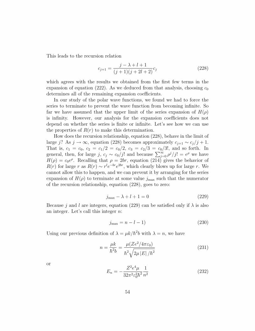
This leads to the recursion relation

cj+1 =j − λ+ l + 1

(j + 1)(j + 2l + 2)cj (228)

which agrees with the results we obtained from the first few terms in theexpansion of equation (222). As we deduced from that analysis, choosing c0determines all of the remaining expansion coefficients.

In our study of the polar wave functions, we found we had to force theseries to terminate to prevent the wave function from becoming infinite. Sofar we have assumed that the upper limit of the series expansion of H(ρ)is infinity. However, our analysis for the expansion coefficients does notdepend on whether the series is finite or infinite. Let’s see how we can usethe properties of R(r) to make this determination.

How does the recursion relationship, equation (228), behave in the limit oflarge j? As j → ∞, equation (228) becomes approximately cj+1 ∼ cj/j + 1.That is, c1 = c0, c2 = c1/2 = c0/2, c3 = c2/3 = c0/3!, and so forth. Ingeneral, then, for large j, cj ∼ c0/j! and because

∑∞j=0 ρ

j/j! = eρ we haveH(ρ) = c0e

ρ. Recalling that ρ = 2br, equation (214) gives the behavior ofR(r) for large r as R(r) ∼ rle−bre2br, which clearly blows up for large r. Wecannot allow this to happen, and we can prevent it by arranging for the seriesexpansion of H(ρ) to terminate at some value jmax such that the numeratorof the recursion relationship, equation (228), goes to zero:

jmax − λ+ l + 1 = 0 (229)

Because j and l are integers, equation (229) can be satisfied only if λ is alsoan integer. Let’s call this integer n:

jmax = n− l − 1) (230)

Using our previous definition of λ = µk/h2b with λ = n, we have

n =µk

h2b=

µ(Ze2/4πε0)

h2√

2µ |E| /h2(231)

or

En = − Z2e4µ

32π2ε20h

2

1

n2(232)

54

This is the quantization condition on the energy levels of the hydrogenicatom, which agrees with the semi-classical condition of the Bohr model. Notethat E depends only on n and not on l (even though R(r) depends on bothn and l). For Z = 1 and µ = me (the electron mass), the numerical factorsin equation (232) evaluate to 13.6 eV.Practice Question: What property did we impose on the radial wave func-tions that ultimately resulted in energy quantization?

It is also convenient at this point to define the quantity

a0 =4πε0h

2

µe2(233)

a0 has the dimension of length and provides a convenient length scale foratomic systems. When µ = me, a0 is known as the Bohr radius and has thevalue 0.0529 nm = 52.9 pm. In terms of a0, the parameter b can be written

b =

√

2m |E|h2 =

µZe2

4πε0h2n

=Z

a0n(234)

Before we discuss the general results for H(ρ), let’s look at the form ofsome of the solutions for particular values of n.

n=1:In this case, equation (230) gives jmax = −l, and since neither j nor l can

be negative, the only possible solution is j = l = 0. In this case, H(ρ) = c0and R(r) becomes

R10(r) = c0e−Zr/a0 (235)

We have labeled the radial wave functions as Rnl using the indices n and l.The constant c0 can be determined from the normalization condition.

n=2:In this case, jmax = 1 − l. The possible l values are l = 0 (in which

case jmax = 1) and l = 1 (in which case jmax = 0). For l = 1, only j = 0contributes and H(ρ) = c0. We then have

R21(r) = c0re−Zr/2a0 (236)

For l = 0, jmax = 1 and thus H(ρ) = c0 + c1 . We can use the recursionformula, equation (228), to determine c1 in terms of c0:

c1 =0 − 2 + 0 + 1

(1)(0 + 0 + 2)c0 = −1

2c0 (237)

55

so that H(ρ) = c012c0ρ = c0(1− 1

2ρ) or H(r) = c0(1−Zr/2a0). We thus have

R20(r) = c0e−Zr/2a0(1 − Zr/2a0) (238)

Practice problems:Continue this process for n = 3 and show

R30(r) = c0

[

1 − 2Zr

3a0

+2

27

(

Zr

a0

)2]

e−Zr/3a0 (239)

R31(r) = c0r

(

1 − Zr

6a0

)

e−Zr/3a0 (240)

R32(r) = c0r2e−Zr/3a0 (241)

31 THE COMPLETE RADIAL SOLUTION

The general solution of equation (219) is the associated Laguerre polynomial.First let’s look at the ordinary Laguerre polynomials of degree q, which areobtained from the generating function

Lq(ρ) = eρ dq

dρq

(

ρqe−ρ)

(242)

The associated Laguerre polynomials are then defined as

Lpq(ρ) =

dp

dρpLq(ρ) (243)

which is a polynomial of degree q−p. The general solution of equation (219)is the associated Laguerre polynomial:

H(ρ) = L2l+1n+l (ρ) (244)

a polynomial of degree (n+l)−(2l+1) = n−l−1, as expected correspondingto the value of jmax given by equation (230).

The complete solution for R(r) is then

Rnl(r) = Nnlrle−Zr/na0L2l+1

n+l (2Zr/na0) (245)

56

where Nnl is a normalization constant. Because the Y ml (θ, φ) are separately

normalized, the normalization of ψ(r, θ, φ) = Rnl(r)Yml (θ, φ) then requires

that the Rnl(r) be normalized:∫ ∞

0

r2 dr [Rnl(r)]2 = 1 (246)

Following a tedious but straightforward calculation,

Nnl =

{

(

2Z

na0

)3(n− l − 1)!

2n[(n+ l)!]3

}1/2(

2Z

na0

)l

(247)

so that the complete solution for R(r) is then

Rnl(r) =

{

(

2Z

na0

)3(n− l − 1)!

2n[(n+ l)!]3

}1/2

e−Zr/na0

(

2Zr

na0

)l

L2l+1n+l (2Zr/na0)

(248)The solution to the Schrodinger equation for the hydrogenic atom is

ψnlm(r, θ, φ) = Rnl(r)Yml (θ, φ) (249)

The solution to the time-dependent equation is

Ψnlm(r, θ, φ, t) = Rnl(r)Yml (θ, φ)e−iEnt/h (250)

where En are the energy eigenvalues given in equation (232).As is always the case for quantum systems, it is possible for the atom

to exist in mixed states that are not pure eigenstates. These states can bedescribed by appropriate linear combinations of the eigenfunctions given inequation (250):

Ψ(r, θ, φ, t) =∑

n,l,m

cnlmRnl(r)Yml (θ, φ)e−iEnt/h (251)

Given any arbitrary (but mathematically well-behaved) function f(r, θ, φ)that represents the state of the atom at t = 0, we can expand f(r, θ, φ) interms of the eigenfunctions:

f(r, θ, φ) =∞∑

n=1

n−1∑

l=0

l∑

m=−l

cnlmRnl(r)Yml (θ, φ) (252)

where

cnlm =

∫ ∞

0

r2dr

∫ π

0

sin θdθ

∫ 2π

0

dφR∗nl(r)Y

m∗l (θ, φ) (253)

57

32 Appendix A: CHAIN RULE

Please see Riley, Hobsen, & Bence, 2nd edition, section 5.5-5.6 (The ChainRule and Change of Variables), especially the worked example on plane polarcoordinates.

33 Appendix B: SEPARATION OF VARI-

ABLES

“Separation of variables” is a procedure that can turn a partial differentialequation (i.e. a differential equation in several variables) into a system ofordinary differential equations (i.e. a set of differential equations, each in onlya single variable). The procedure only works in very special cases involvinga high degree of symmetry. Remarkably, the procedure works for manyimportant physics examples. Here, we will use the procedure on the waveequation, as a simple example that illustrates the basic steps.

Step 1: Write the partial differential equation in an appropriate coordi-nate system. For the wave equation in one-dimension, we have:

∂2

∂x2Ψ(x, t) =

1

v2

∂2

∂t2Ψ(x, t) (254)

Step 2: Assume that the solution Ψ(x, t) can be written as the productof functions, at least one of which depends on only one variable, in this caset; the other function(s) must not depend at all on this variable, i.e. assume

Ψ(x, t) = X(x)T (t) (255)

This is a very strong assumption. Not all solutions will be of this form.However, it turns out that all of the solutions can be written as linear com-binations of solutions of this form. The study of when and why this works iscalled Sturm-Liouville theory.

Plug this assumed solution (255) into the partial differential equation(254). Because of the special form for Ψ, the partial derivatives each act ononly one of the factors in Ψ = X(x)T (t).

d2X(x)

dx2T (t) =

1

v2X(x)

d2T (t)

dt2(256)

58

Notice that the partial derivatives ∂2

∂x2 and ∂2

∂t2have turned into total deriv-

atives d2

dx2 and d2

dt2. Any partial derivatives that act only on a function of a

single variable may be rewritten as total derivatives.Step 3: Divide by Ψ in the form of (255). The rest of the procedure

doesn’t work if you omit this step. Many, many students forget. Don’t beone of them!

1

X(x)

d2X(x)

dx2=

1

v2

1

T (t)

d2T (t)

dt2(257)

Step 4: Isolate all of the dependence of one coordinate on one side ofthe equation. Do as much algebra as you need to do to achieve this. In ourexample, notice that in (257), all of the t dependence is on the right-handside of the equation while all of the dependence on the spatial variable x ison the other side. In this case, the t dependence is already isolated, withoutany algebra on our part.

Step 5: Now imagine changing the isolated variable t by a small amount.In principle, the right-hand side of (257) could change, but nothing on theleft-hand side would. (This argument is the magic of the separation of vari-ables procedure–make sure that the logic is clear to you.) Therefore, if theequation is to be true for all values of t, the particular combination of tdependence on the right-hand side must be constant.

1

X(x)

d2X(x)

dx2=

1

v2

1

T (t)

d2T (t)

dt2def= A (258)

In this way we have broken our original partial differential equation up into apair of equations, one of which is an ordinary differential equation involvingonly x, the other is an ordinary differential equation involving only t.

1

X(x)

d2X(x)

dx2

def= F (259)

1

v2

1

T (t)

d2T (t)

dt2def= F (260)

The separation constant F appears in both equations.Step 6: Write each equation in standard form by multiplying each equa-

tion by its unknown function to clear it from the denominator.

d2X(x)

dx2

def= F X(x) (261)

d2T (t)

dt2def= F T (t) (262)

59

Notice that (261) is an eigenvalue equation for the operator d2

dx2 . At themoment, all we have done is mathematics and the eigenvalue F could beanything. Next we need to solve the system of ordinary differential equationsand use physical information to find the possible values of F . In general thesolution to the X equation will be

X(x) = A cos(−√Fx) +B sin(−

√Fx) = A cos kx+B sin kx

where k is a conventional name for the constant −√F and the allowed values

of k are determined by the boundary conditions. We can then plug this valueof F into the equation for T . Since we now know the value of F , the equationfor T is not an eigenvalue equation. The solutions for T are, of course

T (t) = C cos(−√Fvt) +D sin(−

√Fvt) = C cos kvt+D sin kvt

If the original partial differential equation had had more than two vari-ables, we could have repeated the steps until each of the variables had beenseparated out into its own ordinary differential equation.

60