the impact of microcredit on poverty and women's

THE IMPACT OF MICROCREDIT ON POVERTY AND WOMEN’S

EMPOWERMENT:

A CASE STUDY OF BANGLADESH

By

SAYMA RAHMAN

A Thesis Submitted in Fulfilment of the Requirements

For the Award of the Degree

of

Doctor of Philosophy

School of Economics and Finance

College of Law and Business

University of Western Sydney

Sydney Australia

March 2007

ii

THE IMPACT OF MICROCREDIT ON POVERTY AND WOMEN’S

EMPOWERMENT: A CASE STUDY OF BANGLADESH

Abstract

The microcredit program in Bangladesh is a unique innovation of credit delivery

designed to enhance the income generating activities of the poor. Its uniqueness is

reflected in its collateral-free group-based lending strategy. The program extends

small loans to poor people, mainly women, for self-employment activities thus

allowing clients to achieve a better quality of life. This program is regarded as a very

exciting anti-poverty tool for the poorest, especially for women.

This study investigates the impact of microcredit on economic indicators as well as

consumption behaviour of the borrowers. It further analyses the impact of

microcredit on women’s empowerment. Primary data has been collected from the

borrowers of two major microcredit institutions in Bangladesh. Alongside the

borrowers, data have also been collected from non-borrowers of the same village to

compare the impact between borrowers and control group. The empirical work has

used sophisticated econometric techniques. Five different econometric methods -

OLS, 2SLS, Probit, Tobit and SURE estimators - have been applied to the sample

data of this study.

The most important finding indicates that microcredit programs are effective in

increasing borrowers’ income, assets and consumption but it is more pronounced

towards high income borrowers than low income borrowers. It further finds that

microcredit programs are empowering for women.

iii

STATEMENT OF AUTHENTICATION

I, Sayma Rahman, declare that this thesis has not been submitted, either in whole or

in part, for a degree at this university or any other academic institution. I also certify

that the work presented in this thesis is, to the best of my knowledge and belief, my

own work and original except as acknowledged in the text.

Sayma Rahman

------------------------------

Signature of Candidate

iv

DEDICATION

TO MY MOTHER, SISTERS AND BROTHERS

FOR YOUR FAITH IN ME

TO AWAB

FOR ENCOURAGING AND SUPPORTING ME

WITH MY LOVE…

v

ACKNOWLEDGEMENTS

Thank you, to the following people who assisted me and made it possible for me to

complete this thesis by offering their support, encouragement and professional

consultation in different ways:

First of all, to Professor P N (Raja) Junankar, my principal supervisor, thank you so

much for all the valuable advice and encouragement that I have received from you

for your professional support and for entrusting me with this work. Thank you for all

the confidence and generosity you showed me during my PhD study, especially in

the last few months.

To my co-supervisor, Dr Girijasankar Mallik, thank you for your supervision and

discussions, and for your interest and comments throughout this study. I would like

to express my gratitude to you for your time and encouragement that you have

provided me throughout this study. Thank you for helping me with data entry and

compilation.

I also express my sincere gratitude to Professor Anis Chowdhury for providing me

with updates on the issue of my research whenever he found any. My appreciation

goes to Dr Sudhir Lodh for his comments at different stages of my thesis. Special

thanks and appreciation go to Muhammad Arifur Rahman for providing me

comments and support. Many thanks to all my friends and colleagues for their

friendly assistance and encouragement in many matters during my PhD study. I also

wish to thank Angela Damis for proof reading my thesis and all the academic and

vi

administrative staff in the School of Economics and Finance at the University of

Western Sydney for necessary support and help.

Thank you all; without your support, this study would have not been possible.

Sayma Rahman

vii

TABLE OF CONTENTS

-----------------------------------------------------------------------------------------------------

Abstract ii

Statement of Authentication iii

Dedication iv

Acknowledgements v

List of Tables and Figures xi

Chapter One: Scope and Framework of the Study………………………….…....1

1.1 Introduction………………………….…….…………………............1

1.2 How Far the Grameen Bank Differs from BRAC……………………3

1.3 Research Problem and Question……….….………..…………….......4

1.4 Why is the Problem Worthy of Research?...........................................6

1.5 Data and the Econometric Approach…………………………………8

1.6 Thesis Outline…………………………………………...……………9

Chapter Two: Survey of Literature: Rural Credit Market and the Bangladesh

Economy …………………………………………………………………………...12

2.1 Relevant Theories on Rural Credit Market (Part A)………………..12

2.1.1 The Rural Credit Market……………………………………14

2.1.2 The Monopolistic Nature of the Rural Credit Market………15

2.1.3 Interlinked Factor Markets………………………………….19

2.1.4 Potential Risk………………………………………………..22

2.1.5 Significance of Credit Policy in the Rural Areas…………...23

2.1.6 Conclusion of Part A………………………………………….24

2.2 The Bangladesh Economy: Pre-Microcredit (Part B)……..……......25

2.2.1 Inception of Microcredit Institutions……………………….27

2.2.2 Background of the Grameen Bank……………...………….28

2.2.3 Growth and Expansion of the Grameen Bank.......................29

2.2.4 Savings Mobilisation by the Grameen Bank……………….32

2.2.5 Background of BRAC………….…………………………..33

2.2.6 Growth and Development of BRAC………….……………35

2.2.7 Savings Mobilisation by BRAC………...…….……...…….37

viii

2.3 The Bangladesh Economy and Recent Development………………39

2.3.1 Conclusion of Part B………………………………………..42

2.4 Introduction to Review of Literature (Part C)………………………43

2.4.1 Impact of Microcredit on Poverty ………………………….45

2.4.2 Women’s Empowerment……………………………………54

2.4.3 Household Consumption …………………………………...58

2.4.4 Conclusion of Part C………………………………………….61

Chapter Three: Assessment of Income and Asset Accumulation of Microcredit

Borrowers…………….………………………………………….………....63

3.1 Introduction…………………………………………………………63

3.2 Previous Studies on Impact Assessment…………………………....65

3.2.1 Data …………………………………………………….…..…66

3.2.2 The Selectivity Problem……………………………………....67

3.2.3 Research Questions…………………………………….……..69

3.2.4 Hypotheses……………………………………………………69

3.3 Model Specification…………………………………………………70

3.3.1 Endogeneity of Credit Program……………………………..72

3.3.2 Methodology………………………………………………...72

3.4 Specification of the Instruments and Variables……………………..73

3.4.1 Description of the Variables…………………………...……...74

3.4. 2 Specification of the Variables…………………………..……75

3.5 Estimation Results and Discussion………………………………….78

3.5.1 Descriptive Statistics of the Variables………………… ……78

3.5.2 Impact of Microcredit on Household Outcomes…………...…80

3.5.3 Impact of Microcredit based on Different Income Levels……85

3.5.4 Estimating Censored Regression Problem …………………...89

3.5.5 Censored Problem on different Income levels………………..93

3.6 Conclusion…………………………………………………………..95

ix

Chapter Four: Assessment of Consumption of Microcredit Borrowers

Compared to Non-borrowers………………………………………………….…97

4.1 Introduction……………………………………………………………..97

4.2 Literature Review on Expenditure Elasticity………………………….100

4.3 Introduction to Relevant Theories…………………………..…………104

4.3.1 Theory of Mixed Demand…………………………………...105

4.3.2 An Almost Ideal Demand System…………………………...107

4.3.3 Specification of the AIDS model……………………………108

4.4 Model Specification……………………………………………………112

4.5 Empirical Results……………………………………………………....118

4.5.1 Percentage and Mean Consumption ……………………….118

4.5.2 Preliminary Findings of the Descriptive Table…………...…121

4.5.3 Estimation Results and Discussion…………………………..125

4.5.4 Test of Significant Difference……………………………….134

4.5.5 Testing for Uncorrelated Error Terms…………………….....138

4.6 Conclusion……………………………………………………………..143

Chapter Five: Factors Affecting Women’s Empowerment in Microcredit

Programs...………………………………………………………..148

5.1 Introduction………………...………………………………………….148

5.2 Defining Women’s Empowerment……………………………….……154

5.3 Towards Development of Empowerment Index……………….………156

5.4 Calculation of Empowerment Index…………………………………...159

5.4.1 Economic Security Index……………………………………159

5.4.2 Purchase Decision Index…………………………………….160

5.4.3 Control over Asset Index…………………………………….161

5.4.4 Mobility Index……………………………………………….161

5.4.5 Awareness Index…………………………………………….162

5.4.6 Empowerment Index……………………………………..….163

5.5 Summary Table of the Indices…………………………………………164

5.6 What Causes Women to be Empowered?..............................................170

5.6.1 Research Questions...………………………………… ……171

5.6.2 Hypotheses…………………………………………………..171

5.6.3 Specification of the Variables…………………………….....172

x

5.7 Model Specification…………………….………………..……………172

5.7.1 Model of the Study………………………………………….173

5.8 Estimation Results and Discussion……………………………..……..173

5.8.1 Factors Affecting Empowerment…................................... ....174

5.8.2 Factors Affecting Empowerment for both Groups………..…176

5.8.3 Factors Affecting Empowerment: Different Groups…...…....179

5.8.4 Do Microcredit Programs Empower Women?.........…..…….181

5.9 Conclusion…………………………………………………………......185

Chapter Six: Conclusion and Future Research….……….…………………….188

6.1 Introduction…………………………………………….……………...188

6.2 Summary of the Study………………………………….……………...189

6.3 Key Findings of the Study……………………………………………..192

6.4 Policy Implications………………………………………..…………...200

6.5 Study Limitations………………………………………………..…….201

6.6 Avenues for Future Research………………………………….…..…..202

6.7 Concluding Notes……………………………………………………...203

APPENDICES……………………………………………………………………205

7.1 Appendix A: Global Poverty Figure…………………………….…….205

7.2 Appendix B: The Sixteen Decisions of the Grameen Bank……...……206

7.3 Appendix C: Household Survey Questionnaire………………….……208

7.4 Appendix D: Map of Bangladesh……………………………………..225

7.5 Appendix E: List of the Village……………………………………….226

7.6 Appendix F: Descriptive Tables of Consumption Patterns…………....227

7.7 Appendix G: Experiences from Field Trip…………………………….236

7.8 Appendix H: Abstract of the Paper Published in the FIBR Conference

Proceedings……………………………………………………...…249

7.9 Appendix I: Abstract of the Paper accepted for publication in a

forthcoming issue in the Journal of Development Areas……….…250

7.10 Appendix J: Abstract of the Paper published in the Conference

Proceedings……………………………………………………….251

REFERENCES…………………………………………………………………..252

xi

List of Tables and Figures

List of Tables:

Table 2.1 Number of Schools, Students and Graduates from BRAC 36

Table 2.2 Job Creation by BRAC 36

Table 2.3 Comparing BRAC with the Grameen Bank 38

Table 2.4 Major Socio-Economic Conditions: 1975-2005 40

Table 2.5 Sectoral GDP Growth Rates: 1979/80-1999/00 41

Table 3.1 Correlation Matrix of the Variables 77

Table 3.2 Descriptive Statistics of Dependent and Independent Variables 79

Table 3.3 2SLS Estimation of Amount of Borrowing on

Household Outcome: Log of Total Expenditure 81


Household Outcome: Log of Assets 82


Different Income Level: Log of Total Expenditure 86


Different Income Level: Log of Assets 87

Table 3.7 Tobit Estimation of Amount of Credit Using Censored Data 90

Table 3.8 OLS Estimation of Household Outcomes Using Estimated Value

Of Amount of Credit from Tobit Estimation 92

Table 3.9 OLS Estimation of Household Outcomes Based on Different Income

Level Borrowers: Expenditure (Income) 93


Level Borrowers: Assets 94

Table 4.1 Average Consumption of Borrowers and Non-Borrowers

Of three Districts 120

Table 4.1a T-test Results of Mean Expenditure and Budget Share of Different

items Consumed by Borrowers and Non-Borrowers 121

Table 4.2 OLS Estimation of the AIDS Model 127

Table 4.3 Testing for Differential Slope Coefficient 136

Table 4.4 Seemingly Unrelated Regression Estimates 140

xii

Table 4.5 Testing for Different Slope Coefficients Using SURE 141

Table 4.5a Estimation of Income Elasticity for Borrowers and non-borrowers141

Table 4.6 Comparing and Contrasting OLS and SURE 142

Table 5.1 Defining Women’s Empowerment 151

Table 5.2 Borrowers’ and Non-Borrowers all indices according to Districts 165

Table 5.3 Empowerment Index of Borrowers and Non-Borrowers

According to Districts 166

Table 5.4 Probit Model: Factors Affecting Empowerment Index

Borrowers and Non-Borrowers Separately 175


Pooling Full Data Set 178


Based on Different Data Set 181

Table 5.7 OLS Estimation of the Equations 183

Table 5.8 Probit Estimation: Using the Estimated Value of the

Amount of Credit 184

List of Figures:

Figure 2.1 Monopoly Market 17

Figure 2.2 Number of Branches 31

Figure 2.3 Number of Borrowers 31

Figure 4.1 Consumption Tree . 99

1

Chapter One

SCOPE AND FRAMEWORK OF THE STUDY

1.1 Introduction

This research explores the impact of microcredit organisations in the Bangladesh

economy. It is one of the first comprehensive studies that analyses the impact of

microcredit in a broader spectrum. This is an original study not only in terms of use

of a new data set but also in terms of use of econometric techniques1 that have not

been used by other researchers in this area. The academic discourse in this research

is quite relevant and goes a long way to contributing to the existing literature. This

study touches on wide-ranging theoretical issues related to this field and highlights

the developments in the literature on the subject area. Microcredit is not only a very

topical issue the founder of the Grameen Bank has just been awarded the 2006 Nobel

Peace Prize but it has also been a topic of interest to researchers since its inception in

early 1970s. In this research we have analysed the impact of microcredit programs

on the borrowers of two large microcredit institutions in Bangladesh − the Grameen

Bank and the Bangladesh Rural Advancement Committee (BRAC).

The Grameen Bank is the largest moneylending institution in the world, measured in

terms of numbers of borrowers. In 2005 alone, Grameen Bank’s borrower count rose

from 4 to 5 million. Microcredit programs have created a revolution not only in

Bangladesh but also through out the world for their novelty. Microcredit is a unique

1 This is the first study that uses An Almost Ideal Demand System (AIDS) model to analyse the consumption behaviour of the microcredit borrowers, Tobit estimations to analyse the impact of microcredit on household outcomes and Two Stage Least Square estimation to analyse the impact of microcredit on women’s empowerment.

2

innovation in credit delivery techniques that enhances income generating activities.

Its uniqueness is reflected in its collateral-free group-based lending strategies, high

repayment rates and also a special focus on women. A microcredit program2 extends

small loans to poor people, mainly women, for self-employment activities thus

allowing clients an opportunity to achieve a better quality of life. It is the most

sensational anti-poverty tool for the poor people, especially women (Microcredit

Summit 1997, World Bank). For these reasons, microcredit programs in Bangladesh

have drawn the attention of academics, researchers, international agencies and policy

makers throughout the world. The Grameen Bank the largest microcredit institution

and BRAC the largest non-governmental organisation (NGO) – have been the

pioneers of microcredit in Bangladesh for almost three decades.

There are more than a thousand microcredit institutions providing financial and

social development services in Bangladesh (Khalily, Imam and Khan, 2000 p. 105).

The Grameen Bank and BRAC are the major contributors to this credit market.

About 94 % of the borrowers in this market are female. Bangladesh’s microcredit

program is widely known as a ‘lending program to the poor without any collateral’.

The main focus of this endeavour is to eliminate poverty and empower women in

rural country areas in Bangladesh (Khandker, 2003).

2 According to Khalily, Imam and Khan (2000), “program” is synonymously used with “institution.” Program encompasses those microcredit or micro-finance institutions that are providing micro-financial services.

3

1.2 How Far the Grameen Bank Differs from BRAC

In order to achieve the main objective of delivering credit the Grameen Bank and

BRAC both provide various support programs including social services3 and social

development programs along with financial discipline. As part of such initiatives the

Grameen Bank sets out guidelines and codes of conduct for the borrowers promoting

social and financial discipline (see Appendix B). To develop social awareness among

borrowers, BRAC provides skills training, adult literacy and primary health care etc.

BRAC’s social development approach is more extensive (integrated program)

compared to the Grameen Bank’s minimalist (credit only) approach.

One of the central concerns of both the Grameen Bank and BRAC is to support the

poor - making productive use of their credit and income. It should be mentioned that

although there are differences between the Grameen Bank and BRAC in their

approaches to loan provision, both institutions adopt a credit based poverty

alleviation approach in rural Bangladesh.

The credit delivery model developed by the Grameen Bank does not require tangible

collateral. The “group liability” may be interpreted as intangible collateral in the

sense that, in case of default, a member loses its opportunity for future loans. The

model developed by the Grameen Bank has been replicated in many parts of the

world (Khandker et al., 1995, p. 2). Malaysia, Guinea, Malawi, Colombia, the

Philippines and Nigeria are some less developed countries (LDCs) that have

replicated the Grameen model. In developed countries, the Women’s Self-

3 These include providing free education, awareness development for using proper sanitation, pure drinking water, plantation and birth control measures.

4

employment Project of Chicago, Illinois, the Good Faith Fund in Pine Bluff

Arkansas, in the United States and the Native Self-employment Loan Fund of

Toronto, Ontario in Canada are noteworthy (Wahid, 1993).

1.3 Research Problem and Questions

The founder of the Grameen Bank, Professor Muhammad Yunus, won the Nobel

Peace Prize in 2006 for waging a war against poverty with a revolutionary

microcredit system. He was praised by the Nobel Committee as “a leader who has

managed to translate visions into practical action for the benefit of millions of

people, not only in Bangladesh, but also in many other countries”. This signifies the

importance of a critical examination of the microcredit program.

Although there have been quite a number of studies on various aspects of

microcredit4, none of those studies has comprehensively analysed whether programs

are successful in bringing about an improvement in the quality of life of the

borrowers. On the other hand, the impact assessment studies often show

contradictory results. This study, therefore, analyses the impact of microcredit on

various household outcomes. It examines the consumption patterns of borrowers

compared to non-borrowers and assesses the impact of microcredit on women’s

empowerment.

4 Stiglitz (1993) and Varian (1990) in their theoretical paper have used the principal-agent framework to explain group-based lending. Hossain’s study (1988) is one of the authoritative studies on the impact of credit programs. Gonzalez-Vega and Chavez (1993) and Yaron (1992) have examined the subsidy issue in the context of financial viability of credit programs.

5

This study raises a number of critical questions that need to be addressed by

economists.

Question One: Do microcredit programs in Bangladesh improve various household

outcomes such as income and asset accumulation?

Question Two: Do microcredit programs in Bangladesh provide improved

consumption for borrowers compared to that of the non-borrowers?

Question Three: Do microcredit programs in Bangladesh empower women?

In the existing literature there are two general hypotheses about the impact of

microcredit programs.

First Hypothesis: Microcredit programs are successful in improving the standard of

living of the rural people5 and improving their consumption behaviour.

Second Hypothesis: Microcredit programs are successful for empowering women.

This study answers these questions and examines the hypotheses by using

econometric techniques such as the Ordinary Least Square estimation (OLS), Two-

stage Least Square estimation (2SLS), Tobit, Probit and Seemingly Unrelated

Regression Estimates (SURE). It compares the performance of borrowers with a

control group, non-borrowers to find out if borrowers are better off compared to non-

borrowers.

5 Khandker et al. (1998) showed credit programs have a positive impact on income, production and employment particularly in non-farm sector. Mustafa et al. (1996) showed that not all money borrowed is invested but some portions are used for consumption. Hashemi et al. (1996) and Zaman, (1998) showed that credit programs are empowering for women.

6

The existing literature does not provide a comprehensive study, that is, one covering

all the goals that the credit programs claim to achieve. This study incorporates the

major issues such as impact assessment and conducts a thorough analysis of the

impact of credit on consumption and on women’s empowerment. It uses a new

approach to measure consumption and integrates some new explanatory variables in

the general model specification. In particular this study does not look at the impact

of microcredit on poverty reduction in Bangladesh overall.

1.4 Why is the Problem Worthy of Research?

The success stories of microcredit are fading nowadays as the programs are drawing

increasing amount of attention as well as inevitable criticism. The evidence from the

literature shows that the impact of microcredit on poverty in Bangladesh is

contradictory. There is research to suggest that the access to credit has the potential

to reduce poverty significantly (Hossain, 1988; Khandker, 1998a; Wahid, 1994); on

the other hand, there are studies, that argue that microcredit has a minimal impact on

poverty reduction (Morduch, 1999 and 2000; Weiss and Montgomery, 2005). In

spite of their recent fame, microcredit programs are facing criticism, on the grounds

that they charge very high rates of interest and the poor have not benefited from the

programs. As micro finance transactions are very small in volume, they are unlikely

to have a sustained aggregate impact on poverty reduction. Also, there is concern

that funding for microcredit programs could have been used for other much needed

programs such as health, water, and education. Credit programs may enable poor

people to improve their conditions, but they do not eliminate the need for other basic

social and infrastructure services. Some studies even claim that the benefits from

microcredit are so small that borrowers often borrow from other informal sources to

7

repay loans (Matin, 1999). The very purpose of the micro-finance movement as a

lending instrument for the poor is thus questioned.

In spite of rigorous involvement of world development organisations to reduce

poverty, world poverty has been increasing over the last decade6. This implies that in

many countries the existing policies may not be effective in reducing poverty.

Professor Yunus’ Nobel Peace award reinforces the fact that the world’s

development planners are considering microcredit as one of the key anti-poverty

tools for poorest people. World development organisations such as the World Bank

are planning to replicate the model widely to eradicate poverty from the world.

Since, on the one hand, the impact of microcredit programs on poverty eradication is

still a controversial issue and on the other, world development organisations are

considering microcredit as a key solution to eradicate world’s poverty, it is

extremely important to conduct a thorough analysis of the impact of microcredit

programs in a LDC such as Bangladesh. It is also important to find an answer to the

controversy as well as to find out the extent of the poverty reduction effect of


Even though there is a broad consensus about credit objectives, program outreach

and high repayment rates, it is not clear how far credit programs benefit the poor and

whether the poor are utilising the loans in a proper way. It is necessary to investigate

how far microcredit programs are successful in (1) increasing income and asset

accumulation (alleviating poverty) via increasing the standard of living of the poor,

6 Even though the Global Poverty figures between 1990 to 1999 shows an overall reduction in poverty in the world, but in some part such as Europe and Central Asia, Latin America and the Caribbean, Sub-Saharan Africa and in China poverty has increased. Please refer to Appendix A.

8

(2) increasing the consumption of borrowers, and (3) empowering rural women to

whom they are delivering loans. It is imperative to investigate the programs with

first-hand information collected from the beneficiaries to find out the actual benefit

received by the microcredit clients, the extent of clients’ awareness and the extent of

poverty reduction as a result of the intervention of the microcredit programs.

This study analyses the impact of microcredit in terms of poverty reduction and

women’s empowerment using primary data. A detailed questionnaire7 with a series

of questions has been administered to 571 usable respondents out of which 387 are

borrowers and 184 are non-borrowers. Appropriate econometric methods are used to

analyse the responses. Some existing models that have been used by other

researchers are also used after modifying the model specification and/or the

estimation methods.

1.5 Data and the Econometric Approach

Primary data have advantages over secondary data as there is less possibility of

biased estimation caused by omitted variables. On the other hand, the World Bank

and other international agencies have already used secondary data extensively.

Therefore, we have collected primary data during July-August 2004 for the purpose

of our analysis. A well-organised questionnaire is prepared for data collection. Our

study draws the sample from three major districts in Bangladesh, viz., Gazipur,

Dinajpur and Chokoria. The districts have been chosen on the basis of different agro-

7 Please refer to Appendix C

9

climatic and economic conditions. From each district, five villages8 have been

selected in a cluster. Forty households has been selected using multistage stratified

random sampling from each of these five villages. The samples of the households’

have been randomly selected without replacement from the list of households

available from the program’s local office of each village. The non-borrowers data

has been collected from the same cohort to make a proper comparison. Finally the

total sample size eventually was approximately 600.

These cross-section data are estimated firstly, using the basic methods of Ordinary

Least Squares (OLS), secondly, the instrumental variable method Two Stage Least

Square (2SLS), thirdly, censored Tobit estimation, binary Probit estimation and

Seemingly Unrelated Regression Estimates (SURE) to estimate multiple equation

models.

1.6 Thesis Outline

This study provides a comprehensive body of theoretical and empirical work on

microcredit. It outlines theoretical considerations of the monopolistic nature of the

rural credit market on the basis of which microcredit programs have been developed.

The study presents an extensive analysis of the theory of rural credit as well as an

empirical examination. It is organised in six chapters which are as follows:

8 The map of Bangladesh showing the areas from which data has been collected and the list of the villages are provided in Appendix D and E respectively.

10

Chapter Two outlines the relevant theories on the rural credit market. It then

discusses the inception of microcredit institutions in Bangladesh, provides an overall

picture of the Bangladesh economy before and after the introduction of the

microcredit movement. Finally the chapter provides review of a wide range of

literature on microcredit.

Chapter Three provides an empirical analysis of the impact of microcredit on

various household aspects such as income and asset accumulation. This chapter

closely follows the model of Pitt and Khandker (1996) but extends the analysis by

introducing new variables. It examines the impact of microcredit on various

household outcomes using Two-Stage Least Squares estimation. It further analyses

the impact on household outcomes for different income level borrowers. Finally,

after pooling the data for both borrowers and non-borrowers, Tobit estimation is

undertaken for the censored data.

Chapter Four presents an empirical analysis of the consumption patterns of

borrowers compared to non-borrowers using the AIDS model. Ordinary Least

Squares (OLS) estimation as well as Seemingly Unrelated Regression Estimate

(SURE) is used for the model and results are compared. We allow for differences

between borrowers and non-borrowers in their consumption patterns in this chapter.

Chapter Five provides an empirical analysis of women’s empowerment. Firstly, the

chapter considers alternative definitions of empowerment that has appeared in the

literature. Secondly, the chapter defines empowerment from a new perspective and

develops an empowerment index based on this definition. Thirdly, it finds out the

11

difference between borrowers and non-borrowers in terms of various empowerment

correlates. Fourthly, it studies the factors that affect women’s empowerment. Finally,

the chapter shows whether credit programs are effective in empowering women.

Finally, Chapter Six summarises the results of the study together with policy

implications and provides some suggestions for further research.

12

Chapter Two

SURVEY OF LITERATURE: RURAL CREDIT MARKET AND

THE BANGLADESH ECONOMY

This chapter is organised in three parts. Part A outlines relevant theories on rural

credit market. Part B discusses the historical perspective leading to the inception of

microcredit institutions in Bangladesh. It also examines the scope of the activities

undertaken by these credit institutions. Further, it makes an informal attempt to

understand the ways in which microcredit programs may have contributed towards

the development of the Bangladesh economy. The chapter further examines the

broad trends in socio-economic developments that have taken place over recent

decades in Bangladesh and endeavours to relate these to the activities of the

microcredit institutions. Finally, Part C provides a review of literature on

microcredit.

Part A

2.1 Relevant Theories on the Rural Credit Market

Prior to the introduction of microcredit institutions, the debate in development

economics literature centred on the availability of rural financing in developing

countries (Reserve Bank of India, 1977). Several previous studies on rural financing

show the existence of large interest rate differentials between rural and urban regions

in developing countries (Wharton, 1962; Bailey, 1964; Rahman, 1979). However,

these studies suggest that such interest rate differentials may be of existence for a

temporary period. Basu (1997) suggests that arbitrage across regions on such

13

financing may take place because it is possible to borrow from low interest regions

and then lend the sum to high interest regions (p. 268). Basu further states that

according to standard comparative static analysis this process will continue until

market forces eliminate interest rate differentials between urban and rural regions.

Saleem (1987) argues that the existence of high interest rate differentials can only be

explained by the segmentation of regional funds through risk or monopolistic

barriers.

As well, the existence of such relatively high interest rates in rural regions may be

caused by an inherent and known higher risk default factor to recover the principal

from the borrowers (Tun Wai, 1958; Raj, 1979). While this is an attractive

proposition, research evidence suggests that it may only be a partial explanation of

rural-urban interest rate differentials (Bottomley, 1975). Another explanation for

such differentials may be caused by high transaction costs in channelling finance

from urban to rural areas. These high transaction costs ultimately act as a barrier for

formal commercial banking institutions entering the rural funds market. One of main

foci of rural financing is that the size of rural loans is generally smaller than urban

loans. Rural loans are more disparate requiring relatively higher administrative and

overhead costs when undertaken by established commercial banks (Lipton, 1976). In

contrast, local lenders have a cost advantage with local knowledge leading to lower

information search costs in providing loans. Bottomley (1964) argues that the

administrative costs of collecting a large number of local small loans are less for

local lenders specialising in specific rural regions. Thus, cost differentials based on

this asymmetric information leads to high entry barriers and local monopolies in

rural fund markets.

14

It should be noted that in the past (that is, prior to the introduction of microcredit

institutions in Bangladesh) small informal lenders (mostly local merchants, large

landowners and moneylenders) dominated rural funds markets in many developing

countries (Bhaduri, 1977). In general, these informal lenders find it profitable to

invest their surplus capital (funds) in local small loans that have higher returns,

instead of depositing the surplus with formal commercial banks. According to

standard market theory (as has been stated earlier), such high entry barriers leading

to local monopolies will result in an under-allocation of funds to rural regions.

2.1.1 The Rural Credit Market

Prior to the introduction of microcredit in Bangladesh, credit was not widely

available in the rural economy. Informal lenders (as in most developing countries),

were the sole providers of rural credit (Adams and Fitchett, 1992; Ghate, 1992).

These informal lenders (who are commonly known as “moneylenders”) had an

information advantage about their clients, which helped them to monitor their

activities in an easier and cheaper way. These moneylenders used to charge high

interest rates. For example, Hossain (1988 p. 23) argues that in the case of

Bangladesh interest rate charged by these moneylenders were about 10% per month.

These moneylenders basically provide loans only to the people who worked for them

or over whom they have some sort of control. The nature of operation of these

moneylenders may be described in terms of a monopolist or duopolistic market. The

following section provides the relevant theoretical explanation of the monopolist

market.

15

2.1.2 The Monopolistic Nature of the Rural Credit Market

It is a common practice in rural areas that moneylenders lend to people over whom

they have some control. For example, a merchant lends only to those who buy/sell

regularly from their shop or business. The rural credit market is defined as

“fragmented”9 (Basu, 1997). This credit market is further characterised by a whole

array of interest rates differentials. The theoretical relevance of this fragmented rural

economy is demonstrated here in terms of a monopolistic market.

The personalised relationship between the borrower and the lender determines most

often the terms and conditions of rural lending. In general, it is observed that each

lender lends to the person in whom they have greater personal confidence. That is,

according to Bottomley (1964), the monopoly power of the rural moneylender is

dependent on the intimate knowledge of the borrower’s circumstances.

The monopolistic rural credit market as analysed by Basu (1997) is discussed below.

Following Basu’s (1997) model the demand function is derived, assuming the

borrower can get loans only from one moneylender and the borrower is a price taker,

as follows:

)1.2(0)(),( ' <= iLiLL

where L is the amount of credit and i the interest rate.

The inverse function of Equation (2.1), according to Basu, is just another way of

looking at the same relation, as follows:

9 A fragmented rural credit market means that each moneylender with a potential client becomes a small “Credit Island” and the credit market effectively becomes broken up into small fragments (Basu 1997).

16

)2.2(0)(),( ' <= LiLii

This relationship is shown in Figure 2.1, where the line AD shows the demand

function and AM represents the marginal revenue curve. The personalised relation

ensuring there is no default, the moneylender chooses L amount of loan with i

interest to maximise his/her interest earnings.

Now assuming that the lender has the option of investing money elsewhere and

earning an interest r on the lending, the lender’s objective function, according to

Basu, is derived, as follows:

LrLLiL

−)(max}{

The first-order condition of this problem is shown as follows:

)3.2()()( ' LLiLir +=

The left-hand side of this equation represents the marginal cost of giving loans and

the right-hand side is the marginal revenue. Hence, Equation 2.3 depicts the standard

equilibrium in a monopolistic market where MC=MR. This relationship is shown in

Figure 2.1, as having equilibrium level of amount of loan and interest rate which is

indicated by *L and *i respectively.

17

A

i

*i

r C E

O *L M F D L

B

Figure 2.1 Monopoly Market

According to Basu, “the rural financial market is fragmented into little monopolistic

islands … the rural economy itself will be characterised by a whole array of interest

rates” (p. 270). Basu also states that this model is not without limitations. Firstly,

Basu argues, “The analysis presumes that the borrower always has enough money to

repay a loan”. In reality, given the widespread poverty of rural borrowers, this is

unrealistic (p. 271). The second criticism, according to Basu, is that “monopoly

analysis is general” (p. 271).

In Figure 2.1, it is shown that the urban interest rate r is lower than i* (rural interest

rate) when the moneylender has access to the urban market. Here it is presumed that

the borrower always has enough money to repay the loan. In reality, however,

18

according to Basu, the borrowers often face a liquidity crisis and, therefore,

sometimes use alternative mode of repayments including personal labour; mortgage

land and personal belongings.

According to Basu (1997, p. 271), the demand function of the borrower (Equation

2.2) is treated as “primitive” It is derived assuming that the borrower takes loans

only in order to invest. Let R denote the total earnings from investment and L denote

the amount of loan; the function is derived, as follows (p. 272):

0)0(,0)(,0)(),( "' =<>= RLRLRLRR

Basu (1997) advocates that in the case of a producer who employs workers up to the

point where wage equals marginal product of labour, given i, the borrower chooses L

so that 1+i equals marginal earnings from L. Thus, according to Basu,

“The marginal earnings curve represents the demand curve for loans and the area

under this curve is equal to the total earnings of the borrower” (p. 272). Therefore,

the demand curve for loans put forward by Basu is as follows:

)(1 ' LRi =+

This is the equation of the curve AD in Figure 2.1.

If the moneylender-monopolist considers lending a certain amount *OL , according to

Basu the maximum amount the borrower is willing to pay for this is *OABL . Basu

shows that, according to Figure 2.1, the lender has the option of earning an interest

of r elsewhere; the lender’s net income will be ABCr.

19

If the lender adopts this strategy of extracting the maximum the borrower is willing

to pay, according to Basu the lender does best by giving loans equal to OF, for a net

income of AEr. Since AEr> *BCri Basu argues that, “by this strategy the monopolist

earns a larger profit than he would by behaving like a textbook monopolist” (p. 272).

This finding of Basu (1997) is consistent with that of Bardhan (1976 and 977) where

he uses a model that shows the equilibrium percentage of revenue is higher, other

things remaining the same for the monopolistic landlord.

2.1.3 Interlinked Factor Markets

The rural credit market is not only dominated by moneylenders who are

monopolistic in nature as discussed above. The landlord-tenant relationship is also

an important characteristic of the rural market. The relationship described in the

literature is master-serf in nature. A widely noted theoretical paper on the interlinked

factor markets in an agrarian economy is by Bhaduri (1973) where he shows that the

landlord who is a provider of consumption loans to a tenant may have no incentive to

adopt yield increasing innovations, if the landlord’s interest income from their loans

to the tenant goes down (because the tenant will borrow less as they shares the

increase in yield) sufficiently to offset his share of the increased yield. Bhaduri’s

(1973) four prominent features of the agricultural economy make it easy to

understand the theory on rural credit market. Bhaduri portrays the agricultural

market as “semi-feudal” because the existing relations of production have more in

common with classical feudalism of the master-serf type than with industrial

capitalism. The features are as follows:

20

(1) Sharecropping: Sharecropping is a common form of land tenure used in the

agricultural sector. According to Bhaduri (1973) “The landlord leases out his land

for at least one full production cycle and the net harvest10 is shared between tenant

and the landlord on some legally stipulated basis” (p. 121). He further mentioned

that this tenancy system may have enormous complications as the tenant may have

some land of his own or working on fixed capital or the entire amount is supplied by

the landlord.

(2) Perpetual Indebtedness: “The tenant is always heavily indebted. A substantial

portion of the tenant’s legal share of the harvest is taken away immediately after the

harvest as repayment of past debt with interest, thus reducing his actual availability

balance of the harvest well below his legal share of the harvest” (Bhaduri 1973, p.

122). According to Bhaduri (1973) this does not leave enough food for the tenant to

survive from this harvest to the next harvest. The only way of survival is to borrow

for consumption. This actually perpetuates the indebtedness of the tenant.

(3) Landowner as the Lender of Consumption-loans: “This perpetual indebtedness of

the tenant is combined with another important factor which lends the whole system

the definite character of semi-feudalism the lender of the consumption-loan is also

typically the tenant’s landlord” (Bhaduri, 1973 p. 122). Thus the tenant leases their

land from the same man to whom they are perpetually indebted and this reduces

them virtually to the state of a traditional serf. The tenant is more or less tied to their

landlord. According to Bhaduri (1973), this semi-feudal landlord exploits the tenant

both through their traditional property rights in land and through usury and both

10 Net harvest as defined by Bhaduri (1973) is the gross harvest minus seed required for the next harvest.

21

these modes of exploitation are important features of the agricultural market in

LDCs.

(4) Inaccessibility to the Market: “The semi-feudal economic relationship between

the tenant and his landlord works with full severity when the rate of interest on

consumption-loans is extraordinarily high. The tenant is usually not credit-worthy in

any commercial banking sense because he has no asset to borrow against. His only

lender is usually his landlord, who lends against the future harvest and the tenant has

to borrow on terms which the latter dictates” (Bhaduri, 1973, p. 122).

These four types of landlord-tenant relationship appeared in the theory of

agricultural economy in different ways. Bardhan (1980) shows that a monopolistic

landlord does land rationing at a fixed rental share. Bardhan (1980) argues that “the

tenant is dependent on the landlord for credit to finance a given subsistence

consumption in the lean season11 and he pays back the loan along with interest at the

end of the harvest” (p. 89). According to Bardhan (1980), “since the interest rates are

high, it matters a great deal as to how long one has to wait until income comes. The

tenant knows that as a wage labourer he can get some wage income immediately in

lean season, whereas as a tenant he has to wait until the crop is harvested in peak

season” (p. 89).

In the model developed by Bardhan (1976 and 1977) the landlord has three sources

of income, rental income from leased-out land, income from self-operated land net of

wages paid in lean and peak seasons, and interest income. They maximise their total

11 In agricultural production there are two seasons lean and peak. Lean is the preparation season and peak is the harvest season.

22

income with respect to their two decision variables, the amount of land to lease out

and the amount of labour to use on their self-operated farm. According to Bardhan

1980, “the tenant considers his income from cultivating the leased-in area and from

wage income net of interest payment on lean-season consumption credit and

maximises it with respect to his only decision variable, labour-intensity per acre on

his leased-in area.” Bardhan (1980) shows in his comparative static parametric

variations model that the equilibrium percentage of area under tenancy will be higher

for the monopolistic landlord.

2.1.4 Potential Risk

The Interlinked rural credit market characterised by Basu (1997) is when the

landlord agrees to take on a tenant at a fixed rent and also agrees to provide the

tenant with credit at a certain interest rate. According to Basu (1997) there is some

risk associated with a loan on part of the landlord. There is always a probability that

certain portion of loans will not be repaid. According to Basu (1997), “if a debtor is

the lender’s tenant or has some historical ties with the lender, it is very unlikely that

the debtor will get away with defaulting. If, on the other hand, a debtor has no

dealings, nor any prior ties, with the lender, it is likely that the debtor will not repay,

there being hardly any legal machinery in backward regions to enforce repayment”.

It is not unrealistic that for every moneylender among all potential borrowers there is

a set of people from whom the lender can recover money and there is another set

over whom the landlord has no control. Therefore, according to Basu (1997) if a

landlord does not discriminate between potential borrowers, he will attract all

“lemons” and eventually become bankrupt. The landlord in general provides loans to

23

those over whom they have some control and where there is no ‘potential risk’ of

default.

2.1.5 Significance of Credit Policy in the Rural Areas

The monopolistic nature of the rural credit market has become a concern for policy

makers in understanding the nature and depth of the market. In the case of LDCs,

credit policy is a great worry for policy makers because the moneylenders are the

only credit providers and they charge exorbitant interest rates.

For over a century official policy has been directed at replacing traditional

moneylenders with formal institutions such as cooperatives, rural development bank,

and commercial bank branches. However, these institutions may not cater for the

needs of rural borrowers due to the lack of securities, which is a pre-requisite for

formal borrowing. The government of LDC and the relevant global institutions such

as the World Bank and IMF are always concerned to improve the condition of poor

people in the rural areas. Since there is always an unsatiated demand for rural

finance in rural areas, the governments of LDCs take various initiatives. The major

concern for rural people is how to survive. If they (rural people) could obtain

affordable long-term credit for investment as well as for consumption, then they

could improve their living conditions.

Since 1976 in Bangladesh the microcredit institutions such as the Grameen Bank

have made a remarkable achievement in rural lending. They have set their objective

to reduce poverty by mobilising resources and targeting credit and non-lending

services to poor rural households for the purpose of setting up new enterprises

24

(Yunus, 1984; Hossain, 1984; Getubig, 1992; and Khandker, 1996). Much has been

written about this new class of “banks for the poor”, and there have been enthusiastic

replications in a number of countries including the United States (Ravallion and

Wodon, 2000). Several nations are now trying to emulate the Grameen Bank model.

2.1.6 Conclusion of Part A

Earlier theoretical discussion shows that the landlords can prevent a tenant from

renting other land or from working for wages. Landlords can include these

restrictions in the contract or they can enforce them. The landlord also has an extra

control instrument by means of contract terms that limit the tenant to their wage

rate12 (reservation utility) (Binswanger and Rosenzweig, 1984, p 17).

Some interesting observations may be derived about the microcredit programs of

Bangladesh based on the above mentioned theoretical discussion of interlinked rural

factor markets. The microcredit movement that has been initiated in Bangladesh is a

breakthrough in the history of rural financing in developing countries. Its operating

style is in many ways different from the traditional moneylenders, who lend to rural

borrowers, as well as landlords, who make tenants work for them. It has already been

mentioned earlier that the traditional moneylenders are monopolistic in nature. Thus,

microcredit programs do not reveal such characteristics. Unlike traditional

moneylenders that make their tenants work for them, the borrowers of microcredit

are allowed to choose the activities in which they are willing to invest. The credit

delivery mechanism is very different from traditional lending systems. This does not

12 Bardhan and Srinivasan (1971) developed a similar model where the landlord is not allowed to control tenancy size.

25

allow a master-serf relationship as portrayed by Bhaduri between the loan providers

(microcredit institutions) and their borrowers. It is exciting to see that the programs

are now trying to change the traditional rural lending system and trying to make rural

financing available and affordable for everyone. One very interesting observation

about the microcredit programs are that they do not distinguish between clients’

“potential risk”, rather they provide loans to everyone. It has removed the

moneylenders to some extent and is trying to save the rural economy from very high

interest rates. The popularity of the programs is demonstrated by their outreach and

high recovery rate. The features that attracted most attention are their use of “peer

monitoring” which has substituted the need for collateral. Although lending is

provided to individuals, borrowers are formed into groups of four or five. According

to the Grameen Bank model, each of these groups is held jointly accountable for the

behaviour of its members. If one member is in default to repay the credit then the

likelihood of obtaining credit by the other members becomes remote. That is, one

member’s non-repayment can cause all other members to be denied future credit.

This collective microcredit model creates peer pressure and also encourages the

development of mutual help within groups.

Part B

2.2 The Bangladesh Economy: Pre-Microcredit

Bangladesh became an independent nation in 1971 after a brutal civil war with

Pakistan that lasted about nine months. The government of Bangladesh has faced the

difficult task of reconstructing and rehabilitating the fragile economy since then.

Bangladesh’s economy was forced through a very vulnerable period followed by

26

several natural calamities including the devastating flood of 1974. The War and

natural calamities combined took a heavy toll on mainly the agriculture-based

economy of Bangladesh. Consequently, the production of rice, which is the staple

food, faced a major setback (Hossain, 1988). Soon after independence the economy

had to rely quite heavily on imported food. For example, Bangladesh’s imported

food was worth13 Tk14 500, Tk 870 and Tk 1,310 million at constant prices in the

years 1973-74, 1974-75 and 1975-76 respectively.

In the face of a growing population, the agricultural sector of the economy could not

expand sufficiently. This sector also failed to create more jobs and absorb additional

people joining the labour force every year due to the high population growth (Wahid,

1993). In contrast, the manufacturing sector had an even a bleaker image with poor

structure as well as small size during the 1970s. The major manufacturing industries

were nationalised by the government soon after liberation but they proved to be

liabilities rather than assets due to widespread mismanagement and corruption.

Overall, the economy was characterised by low economic growth, high population

growth and inequality in distribution of resources during 1970s. Khandker (1998a)

identified landlessness15 in rural areas as a major contributor to poverty in the

country at that time. Along with landlessness, lack of human and physical capital

among the poorer population in the rural areas prevented the economy from

productive investment. Coleman (1999) rightly argues that the poor often find

13 Bangladesh Bank Economic Trends, vol. XV (5), (1990), p. 18. 14 Tk. stands for taka, the currency of Bangladesh. 15 In Bangladesh, households with less than 0.5 acre are considered functionally landless, since the amount of land they own cannot be a significant source of income (Hossain, 1988, p.15).

27

themselves in a vicious circle: they are producing at a subsistence level, which in

turn makes it harder for them either to invest in productive resources or to gain

access to formal credit market.

2.2.1 Inception of Microcredit Institutions

In the post-independence period, state owned commercial banks and specialised

agricultural banks such as the Bangladesh Krishi Bank (BKB) could not cater to the

needs of the rural people in the country for several reasons. Firstly, these banks

required collateral for providing loans, which rural poor people found difficult to

arrange. Secondly, the loan sanctioning procedures and other related formalities were

too cumbersome for mainly less educated rural people. Thirdly, these financial

institutions preferred handling large loans rather than small loans. Finally, another

problem was the high transaction costs for the banks that include cost of obtaining

information about the rural borrowers to access their creditworthiness, monitoring

the use of loans and ensuring repayments.

For the reasons outlined above the commercial and other formal banks could not

operate successfully in the rural financial market of Bangladesh. Due to non

availability of credit from the formal sources the rural people had to rely heavily on

informal money lenders who used to charge exorbitant interest rates. All these

factors taken together effectively opened up an opportunity for a new type of

financial institution to come into existence which is called the “microcredit

28

institution”16 (most recently these microcredit institutions are also often called

microfinance institutions).

Nobel laureate Professor Muhammad Yunus, the founder of the largest microcredit

institution in Bangladesh – Grameen Bank was convinced that the poor people were

more capable of taking care of themselves than what was and currently is portrayed

in traditional literature (Yunus, 1999, p. 69). He observed that poor villagers with

virtually no assets worked hard at a variety of crafts and service jobs and in the

absence of any major shocks could somehow manage to survive (Yunus 1999, p.

71). Unfortunately, they could not accumulate any capital because firstly, their

income was quite low and secondly, out of this income, after deducting for

sustenance, whatever insignificant surplus they gathered was going to the local

moneylenders from whom they had to borrow (a small amount of ) capital. Thus, if

the poor villagers were to succeed, according to Yunus, (1999) “credit” was the key.

2.2.2 Background of the Grameen Bank

The Grameen Bank of Bangladesh is one of the largest microcredit institutions in

Bangladesh. In 1976, Professor Yunus tried an experimental research project in a

village near Chittagong University. In his experimental project, he started

lending the equivalent of $26 to a group of 42 workers. Borrowers invested this

16 Microcredit is defined as a credit provided to “poor” free of collateral through institutionalised

mechanism (the only collateral is the “peer” collateral). This credit is made available as and when needed, at the doorstep of the client (Bajwa, 2001). On the other hand, microfinance is inclusive of savings and other services. As a matter of fact, this concept has been used and applied in variety of contexts and used interchangeably with microfinancing - such examples include Badan Kredit Kecamatan (BKK) Indonesia, Agriculture Cooperation, and Banks Rakyat Indo Unit Desa.

29

small amount in craft making and repaid the loan on time. From this small

experiment, he realised lending to the poor had a future.

In March 1978, the project developed an appropriate mechanism for delivering

credit to the poor. In June 1979, the Grameen Bank project was launched in a

wider area with assistance from the Bangladesh Bank (Central Bank of

Bangladesh). Within a year 24 branches were set up. It ensured 98 % recovery of

loans by the due date. With assistance from ‘International Funds for Agricultural

Development (IFAD)’ the project expanded its activities to other districts besides

Dhaka. In 1982-83, 50 branches were set up in five districts. A government

ordinance in September 1983 transformed the project into a “bank”, a specialised

financial institution for the rural poor.

2.2.3 Growth and Expansion of the Grameen Bank

The Grameen Bank has reversed conventional banking practice by removing the

need for collateral and created a banking system based on mutual trust,

accountability, participation and creativity (a group-base lending strategy). The bank

focused its market mainly on the rural areas where population density is very high.

Prior to the introduction of microcredit institutions, a large number of rural people

could not get access to formal credit. Microcredit institutions have taken the risk of

lending to mainly rural people who had been neglected in the past. In the past these

borrowers were classified as high risk borrowers. Most interestingly, through the

introduction of microcredit these so-called “high-risk” borrowers were allowed to

30

borrow collateral-free loans17 and the recovery rate of these loans is considered to be

very high, that is about 95%18 (Yunus 1999, p. 114).

The Grameen Bank is not only the largest rural finance institution in Bangladesh; it

is also the largest moneylending institution in the world in terms of number of

clients. In 2005, the bank’s borrower count rose from 4 to 5 million. 94% of

borrowers are women. With 2,345 branches, the Grameen Bank provides services in

75,359 villages, covering 90% of the total number of villages in Bangladesh. At

present the bank disburses general, seasonal, housing and other types of loan under

the categories of Processing and Manufacturing, Agriculture and Forestry, Livestock

and Fisheries, Service, Trading, and Peddling and Shopkeeping. Since its inception,

the Grameen Bank has sanctioned 290.03 billion taka19 (The Grameen Bank, Annual

Report, 2006).

Figures 2.2 and Figure 2.3 shows the expansion of Grameen Bank membership and

branches over 12 years. It is observed from the figure that the membership has

increased by approximately 150% and the number of branches have grown by more

than 50% in 12 years.

17 Although the Grameen Bank does not require any tangible collateral in giving loans, but the “group liability” may be interpreted as intangible collateral in the sense that, in case of default, a member loses its opportunity for future loans. 18 In 1999, the recovery rate was 95 %which has gone up to 98 % in 2006. 19 One taka is $US 0.017 (approximately).

31

Figure 2.2 Number of Branches

Number of Branches

0

500

1000

1500

2000

2500

1994

1995

1996

1997

1998

1999

2000

2001

2002

2003

2004

2005

Years

Branches

Source: The Grameen Bank, Annual Report (2006).

Figure 2.3 Number of Borrowers

Number of Borrowers

0

100000

200000

300000

400000

500000

600000

1994

1995

1996

1997

1998

1999

2000

2001

2002

2003

2004

2005

Years

Borrowers

Source: The Grameen Bank, Annual Report (2006).

32

In addition to its financial services, the Grameen Bank implements diverse programs

to promote social development. It encourages members to open nursery schools at its

centres, distribute seeds and seedlings to encourage gardening and plantation, and it

helps members and their families to improve their health and nutrition. The bank has

opened 14,804 schools by 2003. The total number of children enrolled in these

schools grew from 71,467 in 1985 to 396,289 by 1994 which is a remarkable

increase of 454.5% from 1985 to 1994. Children’s enrolment at schools is still

increasing at a reasonable rate with the expansion of the banks branches (The

Grameen Bank Annual Report, 2003).

2.2.4 Savings Mobilisation by the Grameen Bank

The Grameen Bank mobilises savings by requiring members to make deposits of

different types. The objectives in doing so are to overcome market imperfections and

promote financial security for members/borrowers. These savings are alternative

sources of credit for borrowers and help to gradually minimise the bank’s

dependence on outside borrowing.

The Grameen Bank’s members are required to contribute one taka weekly to the

group fund as savings. These contributions are held as individual savings that are

refundable when members drop out. Individual members are also required to

contribute 5% of the principal amount borrowed to the group fund. Unlike their

individual savings, group members cannot reclaim this group fund contribution, but

they are allowed to borrow from this fund with the approval of other members.

33

There are two other types of loan, from the “emergency fund” and “welfare fund”.

The emergency fund offers protection against debt or liability when a member dies,

or when theft, loss and damage to property (including livestock and crops) of

members/borrowers occurs. The children’s welfare fund was designed to provide

education for members’ children in schools managed and run by the Grameen Bank

members, and to support children’s involvement in small-scale income earning-

projects.

Although the Grameen Bank initiated microcredit programs, subsequently several

other institutions have started providing microcredit in Bangladesh. At this stage, the

major microcredit institutions in Bangladesh include the Grameen Bank, Bangladesh

Rural Advancement Committee (BRAC), which is the biggest non-government

organisation (NGO),20 Rural Development Project-12 (RD-12), Bangladesh Rural

Development Board (BRDB), Association of Social Advancement (ASA) and

Proshika Manobik Unnayan Kendra (PROSHIKA).

Since we have confined our analysis in the study to the Grameen Bank and BRAC,

the following section discusses BRAC.

2.2.5 Background of BRAC

The Bangladesh Rural Advancement Committee (BRAC), the largest non-

governmental organisation in Bangladesh, was formed in 1972 as a relief

20 Non-government organisations provide help to those who fail to accumulate sufficient resources to survive. In its most ambitious form, an NGO is a private, not for profit institution dedicated to influencing the working structure of government and ensuring the greater welfare of all citizens (Mustafa et al. 2000)

34

organisation for the post-war period. The founder of BRAC, Mr Fazle Hasan Abed

realised that pervasive poverty could not be addressed with short-term relief

measures. Thus in 1973, BRAC shifted its focus from relief to long-term community

development. It started its operation with the objective of improving the economic

and social status of the rural poor. Since then BRAC has operated as an NGO, but its

journey has not always been very smooth. It faced many challenges from different

corners of society including the rural communities and the village elites who

controlled many of the social and economic opportunities of the poor, but these

could not stop the activities of BRAC.

BRAC realised that rural people lack the skills and opportunities to derive benefit

from their own labour. The organisation presently delivers both social services and

credit to its members through its two major programs, the rural development

program (RDP) and the rural credit program (RCP). The RDP was started in 1986,

the RCP in 1990. Both programs have evolved over time through the process of

learning by doing with the objective of poverty reduction and empowering women.

Women in the rural areas of Bangladesh play a vital and unacknowledged role in

production both within and outside the household. Women are often the sole

providers for their households due to the death of a spouse, divorce, desertion or the

migration of men looking for paid labour. Recognising these factors and the low

status of women in Bangladeshi society, BRAC targeted women in its programs and

made women’s empowerment a pillar of its programming. The RDP addresses the

socio-economic development of underprivileged rural women through access to

35

credit, capacity development, savings mobilisation, institution building and

awareness raising.

2.2.6 Growth and Development of BRAC

BRAC’s social development programs are aimed partly at alleviating poverty and

partly at supporting government organisations. BRAC also emphasises the role of

women in development by mobilising more women than men. It has helped improve

women’s social status by increasing their economic role in the family. BRAC

intervenes in education, health care, legal activities, vulnerable group development,

and skill development. Its non-formal primary education program and its oral

dehydration therapy are widely known.

BRAC has developed two primary school models the non-formal primary education

program and the primary education program for older children. In addition, BRAC

assists the government in expanding primary education throughout the country.

BRAC’s primary education models aim to reduce mass illiteracy, ensure women’s

education and involve communities in their own socio-economic development.

The non-primary education program, begun in 1985, is a three-year program for 8 to

10 year-old boys and girls. These children, who have never attended school, are

enrolled in the fifth grade of the formal primary school system after graduating from

this program. The primary education for older children program, begun in 1988 is a

three-year program for 11 to 16 year-olds who have never attended school. Books

and other materials are provided free for the students.

36

Table 2.1 Number of BRAC Schools, Students and Graduates

Bangladesh Rural Advancement Committee (BRAC) (as at June 2006

Number of Primary Schools 3,200

Number of Students 1 million

Number of Graduates 3.49 million

Number of Pre-Primary School 20,168

Number of Students 0.54 million

Source: Bangladesh Rural Advancement Committee, Annual Report (2006).

Table 2.2 Job Creation21

by BRAC

Job Creation by BRAC (as at June 2006)

Poultry 1,708,145

Livestock 570,266

Agriculture 853,390

Forestry 79,062

Fisheries 2,772,330

Sericulture 25,549

Horticulture 184,031

Handicraft Product 15,223

Small Enterprise 136,159

Small Trade 2,635,212

TOTAL 63,53,482

Source: Bangladesh Rural Advancement Committee, Annual Report (2006).

21 Job creation here does not refer to traditional textbook definition. Rather it refers to the number of people who have invested in different sectors.

37

Table 2.1 shows, recent figures for the number of students who have graduated from

BRAC schools since BRAC’s inception. It also shows the number of schools and

pre-primary schools established by BRAC and the number of students enrolled.

Table 2.2 shows job creation by BRAC at the sectoral level since BRAC’s inception

until June 2006.

2.2.7 Savings Mobilisation by BRAC

Savings mobilisation is an integral part of BRAC’s lending process. In addition to

depositing two taka per week as individual savings, borrowers must pay 10% of the

principal loan amount. Out of this, 5% is transformed into individual savings, 1% is

kept for a group insurance fund, and 4% is given to a group fund. The basic objective

of the group insurance scheme is to provide financial support, a maximum of Tk

5,000 to the family of the deceased member so that the family is not displaced and

does not suffer financial hardship. BRAC pays 9% interest on both individual

savings and group funds. This rate is higher than that offered by commercial banks

(BRAC Annual Report, 2004).

Table 2.3 provides some basic statistics in respect of the Grameen Bank and BRAC.

Though we do not directly compare these two institutions in this study, as is evident

from the table both the institutions are quite comparable (similar) in terms of many

indicators.

38

Table 2.3 Comparing BRAC with the Grameen Bank

Items BRAC Grameen Bank

Number of Borrowers 4.51million 6.61million

Number of Branches 1172 2226

Villages Covered 65,000 71,371

Loan Disbursement Tk. 185,580 million

(US$ 3385million)

Tk. 290.03 billion

(US$ 5.72 billion)

Repayment Rate 98.85% 98.85%

Interest Rate Charged 15% 20%

Source: 2006 Annual Reports of the Grameen Bank and BRAC.

39

2.3 The Bangladesh Economy and Recent Developments

Even though the Bangladesh economy went through a very difficult time in the

period following independence, it has recovered substantially in the last two decades

and has shown its potential for becoming an example of success. The UNDP Human

Development Report (2000) referred Bangladesh as “a case that stood out as a

potential instructive story of development”. Philip Browning, the former editor of the

Far Eastern Economic Review, wrote in a very recent article in the International

Herald Tribune on 7th May 2005:

“Bangladesh is a paradox. It lacks good governance and is beset by natural calamities, corruption and self-destructive political infighting. Yet its gross national product persistently maintains a growth rate of 6%, well above average for developing countries. It has overtaken India on several social indicators. Its aid dependence has fallen from 6% to 1.8% of gross domestic product…...Of course this is still a desperately poor, overpopulated country, where 50% of children are underweight. But India is no better on that score. Bangladesh has made much more progress than its neighbours over the past 10 years, becoming self-sufficient in food. Social progress has been even more marked. Educational standards may be poor, but primary school education is even more striking. There are now more girls than boys at secondary level. Gender equality also seems reflected in the fall in fertility rate, which has halved from 6.0 to 3.0 in two decades the steepest fall almost anywhere other than China. It is now below India’s and far below Pakistan’s. The lowest birth rate is linked to a steep fall in child mortality, and to the enhanced economic role of women as small-scale village entrepreneurs and as garment workers. Economic advancement has been underpinned by the individual initiative of hundreds and thousands of Bangladeshis working overseas. Their remittances exceed the net earnings of the garment industry, amounting to more than $3.5 billion a year, mostly from Britain, the United States and Middle East…..”

Despite many obstacles some man-made and some natural Bangladesh experienced

moderately accelerated growth in the 1990s, compared to the previous decades. Its

economic growth rate has increased from 2% in 1975 to 6% in 2005. Bangladesh has

become successful in reducing population growth which has decreased from 3% to

1.48% in last 30 years. The life expectancy of both males and females has increased

40

and the infant mortality rate has fallen dramatically. The country has demonstrated

striking progress in primary and secondary school enrolment for both males and

females. Bangladesh’s poverty has fallen steeply in last three decades. The

accelerated economic and social development of the country is summarised in Table

2.4.

According to the Human Development Index (HDI) developed by UNDP,

Bangladesh has made significant progress. Its HDI increased from 0.345 in 1975 to

0.520 in 2005. The HDI ranking shows that Bangladesh has done better than what

was expected given its GDP level.

Table 2.4 Major Socio-Economic Conditions in Bangladesh 1974-2005

Indicator 1974-75 1984-85 1994-95 2005

Real GDP Growth (%) 2.00 3.72 5.21 6.04 Annual Population Growth Rate 3.00 2.07 1.95 1.48 Infant Mortality Rate 140 112 94 58 (below I year, per '000 live births Life Expectancy at Birth (years) Female 47 56 56.7 59 Male 49 55 56.5 58 Adult Literacy (%) 20 33 37 59.2 Primary School Enrolment (% of school age population) Male 50 63 77 96.5 Female 40 43.8 70 94.5 Child Malnutrition 78 70 68 55 Population below poverty Line 70 55 47 44.7

Sources: Asian Development Bank, Bangladesh Bureau of Statistics,

Ministry of Finance, and United Nations Development Program

41

Sources of Growth

Bangladesh has seen an emergence of progressive entrepreneurs, and good

macroeconomic management has kept inflation in single digits (6% in 2004

according to The World Factbook). Recent reforms in fiscal management,

governance, state-owned enterprises, banking, telecommunications and energy have

also shown encouraging results. Foreign direct investment flows have supported

infrastructure, energy and export-oriented manufacturing.

Bangladesh’s accelerated economic growth has occurred in all broad economic,

agricultural, industry, and services sectors. Table 2.5 shows sectoral GDP growth

rate from the early 1980s to 2000. The agricultural sector accelerated from 2.68% to

3.22% industrial output from 5.70% to 6.96% and service sector GDP from 3.83% to

4.48% over this period.

Table 2.5 Sectoral GDP Growth Rates: 1979/80 – 1999/00

Five-yearly average Decadal average Sector

1980/81-1984/85

1985/86-1988/89

1990/91-1994/95

1995/96-1999/00

1980/81-1999/00

1990/91-1999/00

Agriculture 2.68 2.40 1.55 4.89 2.54 3.22

Crop production 2.69 2.69 -0.43 3.86 2.69 1.72

Fisheries 3.06 1.64 7.86 8.56 2.35 8.21

Others 2.40 2.21 2.53 3.30 2.31 2.92

Industry 5.70 5.80 7.47 6.44 5.75 6.96

Manufacturing 4.69 5.27 8.20 5.59 4.98 6.90

Large and Medium 4.44 5.43 8.41 5.49 4.94 6.95

Small scale 5.41 4.89 7.69 5.87 5.15 6.78

Construction 6.44 5.59 6.27 8.80 6.02 7.54

Others 11.50 10.68 6.43 4.90 11.09 5.67

Services 3.83 3.58 4.14 4.81 3.71 4.48

TOTAL GDP 3.72 3.74 4.15 5.23 3.73 4.69

(Annual average; in constant 1995/96 producer prices)

Source: Osmani et al. (2003)

42

2. 3.1 Conclusion of Part B

We can make an important observation from our discussion in this chapter. The

socio-economic indicators that have shown notable achievements of Bangladesh

over the past two decades are all related, directly or indirectly, to some areas in

which microcredit institutions have had an operational involvement. We have seen

that the two major micro finance institutions chosen for this study are involved not

only in delivering credit but also in providing some important social services such as

mass literacy program, population control, proper sanitation etc. Their credit delivery

service is directly associated with entrepreneurial skills development and job

creation which has direct implications for economic growth. In addition, the social

services provided by these institutions are expected to underpin the overall

development process indirectly. Therefore, it would not be an exaggeration to call

these institutions “development partners” of the government of Bangladesh. With

this backdrop, the relevance of an objective analysis of the contributions of

microcredit programs in the development process of Bangladesh cannot be ignored.

Despite considerable improvement in Bangladesh’s socio-economic scenario over

the past decades, an all-out effort of both government and non-government

organisations is still extremely important to help the country meet several daunting

challenges lying ahead. For example, Bangladesh’s poverty rate remains very high,

with nearly half of its 146 million people living below the poverty line. Bangladesh

still has the highest incidence of poverty in South Asia and the third highest number

of poor people living in a single country after India and China (Bangladesh Country

Brief, World Bank, September 2004). The challenges are magnified by a population

density of more than 800 people per square kilometre one of the highest in the world.

43

These challenges further stress the importance of this study. By providing a thorough

analysis of the performance of these institutions in relation to their major objectives,

this study will uncover the areas in which these institutions should pay careful

attention so that they play a meaningful role in tackling future challenges as active

development partners of the government.

Part C

2.4 Introduction to Review of Literature

The literature on poverty research in Bangladesh is wide-ranging. A significant body

of research on various aspects of poverty in Bangladesh and erstwhile East Pakistan

can be found in economics and development studies literature. Before the emergence

of an independent Bangladesh in 1971, poverty literature about this region appears to

have mainly focused on inequality in income, consumption and wealth between the

then East and West Pakistan. Emphasis was generally placed on economic disparity

between the two regions while such disparity used to be generally cited as the

principal reason causing inequalities in income and wealth of the two regions.

The post-independence literature on poverty in Bangladesh can be generally

characterised as positive and descriptive studies (Rahman and Hossain, 1996;

Osmani, 1978). Attempts have been made to measure and analyse poverty mostly

from a positivist perspective. Within the broad definition of poverty, research has

been undertaken to examine cross-section and time series patterns of poverty

(Rahman and Islam, 1987, 1988). A major part of poverty research is occupied with

the agricultural sector mainly focusing rural poverty (Quesem, 1991; Nahar, 2004;

Osmani, 1989). Urban poverty has drawn the attention of poverty researchers mainly

44

since the 80s when the number of slums and slum dwellers in Dhaka city (the capital

city of Bangladesh) started to rise almost exponentially. Until such time, poverty

used to be generally seen as a rural phenomenon. However, research on urban

poverty ushered a new era of poverty research by revealing the nature, extent,

dimensions and possible consequences of urban poverty. Most of these researches

find a link between rural-urban migration and rise in urban poverty (Rahman, 1978).

While rural poverty, caused by landlessness, unemployment (due mainly to rise in

labour supply in the agricultural sector) and flood and river erosion, is seen as one of

the main causes of rural-urban migration, it is found to be causing urban poverty as

well (Muqtada, 1981).

Another important area of poverty research attempts to determine whether poverty

has a gender bias. In other words, this category of poverty literature looks to examine

whether poor women are poorer than poor men. Some of these researches have found

an association between gender and poverty. Occupational distribution of poverty has

been the focus of some researchers. Notable work on this issue mainly concentrates

on poverty among garment workers (Khan, 1985).

A major part of the poverty research is dedicated to measuring the success or

effectiveness of various poverty alleviation measures undertaken by government and

non-government agencies. Such research includes measuring the success of food for

work programs, agricultural subsidies, agricultural credit and microcredit and other

interventionist programs undertaken by the government and NGOs on different

occasions (Rahman and Razzaque, 2000). Initiatives of several NGOs, particularly

those of the Grameen Bank, BRAC, Proshika Manobik Unnaya Kendra

45

(PROSHIKA), Association of Social Advancement (ASA) and others have been the

focus of a number of studies. Keeping pace with the growth in coverage and volume

of microcredit, the body of such research has also grown to cover various aspects of

microcredit including its role in poverty alleviation, empowerment of the poor

especially poor women, and comparative evaluation of government and NGO


Three major dimensions: are under consideration in this study: impact of credit on

household outcomes, impact of credit on women’s empowerment and impact of

credit on household consumption. The literature on these three broad topics is

studied in this chapter. Since not enough literature is found on the impact of

microcredit on consumption patterns a review of literature on consumption (overall

not specific to microcredit) patterns is provided.

2.4.1 The impact of Microcredit on Poverty (Household Outcomes) in

Bangladesh

Microcredit has appeared in the literature as a popular source of financing that

provides small loans in rural and remote regions of developing countries (Bornstein,

1998; Johnson and Rogaly, 1997; Zeller and Sharma, 2000). As far as developing

countries are concerned, Bangladesh may be considered as the pioneer, having

started this financial innovation that provides loans to the poor especially to women

engaged in self-employment projects that allow them to generate income and in

many cases, begin to build wealth and eliminate poverty (Hulme and Mosley, 1996;

Yunus, 1983; World Bank, 1994).

46

The World Bank (Microcredit Summit, 1997) classified the microcredit program in

Bangladesh as one of the most effective anti-poverty tools for the poorest people.

The program extends small loans to unemployed poor people who are not

creditworthy. These individuals lack collateral, and stable employment and therefore

cannot meet even the most minimum qualifications to gain access to formal credit.

The microcredit (or known as microfinance) program, provides collateral-free small

loans to extremely impoverished people (mostly women) for income-generating

activities thereby reducing poverty (Hossain, 1988; Rahman, 1995; Khandker,

1998a).

Since loans are provided in a group, according to Stiglitz (1993), Varian (1990), and

Ghatak (1999) and Besley and Coate (1995) the members in a group are well placed

to umpire the creditworthiness and scrutinise the actions of their peers, as a

consequence mitigating the problems of adverse selection and moral hazard. Group

lending also gives incentives to members to avoid excessively risky projects

(Stiglitz, 1993). It also provides insurance to other members in the event their

projects fail (Coleman, 1999). Mutual trust among group members created by their

long association with each other provides strong inducement to self-monitoring

which reduces the monitoring cost down to zero.

Many studies have attempted to measure the impact of microcredit on poverty,

income, employment, contraceptive use and fertility (Hossain, 1988; Hulme and

Mosley, 1996; Hashemi and Schuler, 1996). One of the limitations of these studies is

that they fail to address whether improvement in the quality of life is due to program

participation or not.

47

Existing literature on the impact of microcredit on poverty in Bangladesh provides a

controversial picture. Apart from the studies that suggest access to credit has the

potential to significantly reduce poverty (as mentioned above) others argue that

microcredit has a minimal impact on poverty reduction (Morduch, 1999 and 2000;

Weiss and Montgomery, 2005). However, one issue is beyond controversy: everyone

agrees that the “vulnerability22” of the poor has been reduced due to microcredit

programs.

On the issue of vulnerability it is worth mentioning, the study conducted by

Montgomery, Bhattacharya and Hulme (1996), which found an improvement in

household income, is higher for third time borrowers compared to first time

borrowers. There is also a study by Mustafa et al. (1996) that showed the older

members’ asset valuation is 112% higher compared to those of the newer members.

The study further showed that the average weekly expenditure of the household is

higher for the older members than for the newer ones.

Another interesting finding of the study is that it shows 80% of the credit is invested

and the rest is used for consumption. Money is fungible23 and often the cash obtained

from the microfinance institutions24 is used to meet immediate consumption needs.

Several empirical studies support that the view that credit market involvements

improve both consumption and production of the poor via smoothing consumption

and reducing constraints in production (Feder et al., 1988 and Foster, 1995). Even

22 The term “vulnerability” appeared in the literature as the crisis-coping mechanisms of the poor especially when there are natural disasters (Hashemi et al. 1996; Montgomery et al. 1996; Morduch, 2000; Husain, 1998). 23 The dictionary meaning of fungible is something that is exchangeable or substitutable. 24 Synonymously used for microcredit programs.

48

though it is evident from the literature that not all money borrowed is invested by the

households, a portion of it is used for consumption. Therefore, it may be assumed

that microcredit may benefit households in terms of income as well as consumption.

However, there are costs associated with joining the program. The explicit cost is the

interest payment and the implicit cost is the opportunity cost of attending meetings

etc. Rural women in Bangladesh are preoccupied with household work and

producing non-market products which makes the opportunity cost of wage

employment higher for women. This issue is addressed by Khandker (1998b) where

he shows that households would benefit from withdrawing labour from the wage

market if funds are made available to buy the minimum capital needed to initiate

home-based marketable products.

It is observed that the credit program makes a borrower switch from wage

employment to self-employment in farm or non-farm sectors. This process may

increase self-employment, but wage employment will reduce. However, Khandker et

al. (1998) show that wage employment may have declined, but the increases in self-

employment are large enough to offset a reduction in wage employment at the

village level. It has also been suggested in the literature that rural wages have

increased (as there is a reduction in labour supply) at the expense of wage

employment due to the microcredit program. The study further shows that the

Grameen Bank’s credit program has induced about 13.5% increase in the rural wage

and that is due to a reduction in wage employment. In another study, Rahman and

Khandker (1994) show that male and female employment in the Grameen Bank

villages are 14 and 39% higher respectively than those in non-program areas.

49

It has been argued in the literature that, the marginal gain from micro borrowing to

participants may be large, but the accrued total benefits from microfinance in

reducing poverty are likely to be small, as microfinance transactions are often too

small in volume to have a sustained aggregate impact on poverty reduction. Yaron et

al. (1998) have argued that absence of appropriate methodology prevents to find out

the welfare impact or the poverty level in the presence of the microcredit program.

It has been argued that the microcredit program may not be the only way to alleviate

poverty. There may be other non-credit ways such as “food for work” and “targeted

wage employment schemes” to eradicate poverty. Also the grants or donations

received by the government may have alternative uses. Even if clients benefit from

program participation, it may hurt others in the society. It is therefore important to

know the externality effect of the program. It may happen that the benefit accruing to

the poor are generated at the cost of others in the society, so that the program

intervention is not Pareto efficient.25 The World Bank (1994) says Pareto efficiency

is likely to be achieved in areas of economic growth that permits new development

of activities benefiting the participants without hurting anyone else. On the other

hand, Khandker (1998b) argues; that since subsidised funds have alternative uses

through which the poor can benefit, program evaluation of microfinance institutions

must be made based on the cost-effectiveness of alternative anti-poverty programs.

Another issue suggested in the literature is state intervention in alleviating poverty

(Besley, 1997). However, Besley recognises that, there are sections of the poor that

the government does not reach; therefore asking for government intervention

25 Program participation will be Pareto efficient when it benefits at least one person while leaving everyone else at least as well off as before (World Bank 1994).

50

becomes unrealistic in practice. In Bangladesh, the formal financial system has

limited success in targeting the poor with the notable exception of Bangladesh Rural

Development Board’s (BRDB) RD-12 project (Khandker, 1998a).

Researchers have used “program outreach” as a measure of microcredit program

evaluation (Yaron, McDonald and Piperk, 1997; Chaves and Gonzalez-Vega, 1996).

Poverty outreach is important for the governments, policymakers and the donors in

order to know the extent to which microfinance institutions serve the poor in

disadvantaged locations. It may happen that branches of microfinance institutions are

established in locations with better access to transport and communication

infrastructure. Research has showed that microcredit services are geared more

towards the poor who reside in relatively well-developed areas rather than the poor

in more remote and less developed regions. This may not be consistent with the

client density of existing branches that shows more clients in less favourable and

more distressed locations of the rural economy. However, microcredit programs may

be effective in reaching target clients and may generate benefits that are marginal

that do not result in growth of the economy.

Along with outreach there is another issue that has concerned the researchers. It is

well known that all microcredit organisations in Bangladesh are dependent on grants,

soft loans as well as subsidies (Adams and Von Pischke, 1992). Questions such as

“How much subsidy those institutions enjoy”? “Are they able to survive in the long

run if subsidies are withdrawn and if so, how?” (Yaron, 1992b; Yaron, 1994;

McNamara, 1998; Rahman, 1999; Buckland, 1998)’. “Who benefits from

51

microcredit program and program outreach?” (Yaron, 1992a; Sharma and Zeller,

1999)’are posed in the literature.

In the case of microfinance, fixed and transaction costs associated with branch

establishment in rural areas make credit delivery programs expensive ventures to

administer. A large proportion of the literature on microfinance addresses the

financial viability of the targeted credit programs. The literature has covered issues

such as cost efficiency of microcredit programs, where a primary concern is to see

the amount of cost to deliver the services.

In a comparative study among the major small-scale credit programs in Bangladesh

that provide productive credit and other services to the poor such as those provided

by the Grameen Bank, BRAC, and RD-12 project of BRDB, Khandker et al. (1998)

using housing survey data collected by the World Bank and Bangladesh Institute of

Development Studies (BIDS) in 1991-92, attempted to quantify the village-level

impact. Their econometric analysis shows that these programs have positive impacts

on income, production and employment particularly in the non-farm sector.

In a separate study, Pitt and Khandker (1998) evaluated the effect of same group-

based credit programs (again the Grameen Bank, BRAC, and BRDB’s RD-12

programs) on a variety of household behaviours and on the intra-household

distribution of resources. The study estimated the impact of participation, by gender,

in each of the three group-based credit programs on women and men’s labour

supply, boys’ and girls’ schooling, expenditure, and assets using the “Weighted

Exogenous Sampling Maximum Likelihood-Limited Information Maximum

52

Likelihood-Fixed Effects” (WESML-LIML-FE) approach. They found that credit is

a significant determinant of many outcomes such as household expenditure, non-land

assets held by women, male and female labour supply and boys’ and girls’

schooling. Furthermore, credit provided to women is more likely to influence these

behaviours than credit provided to men. The impact of credit on these six outcomes

provided to women is found significant at the 5% level. Annual household

consumption expenditure, the most comprehensive measure available of program

impact, increased 18 taka for every 100 additional taka borrowed by women from

these credit programs, compared with 11 taka for men. These findings suggest that

credit is not perfectly fungible within a household.

An extension of Pitt and Khandker’s (1998) study is conducted by Khandker (2003)

where he estimated the long-run impacts of microfinance on household consumption

and poverty in Bangladesh, based on panel data. The household survey data was

collected in 1992-93 and 1998-99. Pitt and Khandker (1998) showed that the

endogeneity of both microcredit program placement and program participation is a

serious issue and findings could be misleading if this endogeneity is not taken into

consideration while estimation. The method used by Pitt and Khandker (1998) is

based on cross-section data but they employed a quasi-experimental survey design to

resolve the problems of endogeneity associated with non-random program placement

and self-selected program participation. In the study, Khandker used panel data

analysis, which helped measure the program effects on long-term household or

individual welfare.

53

Morduch (1998) using the same data as used by Pitt and Khandker (1998), (BIDS-

World Bank data, 1992-93) but employing a different technique (difference-in-

difference method), finds that program effects are either non-existent or are very

small. Morduch found no evidence of an increase in consumption (and therefore

reduction in poverty) using the same data. Therefore, the contradictory results in

findings provide scope for further study in the area of impact of credit in poverty

reduction.

It appears from the literature that the impact assessment on microcredit provides a

contradictory result. Therefore it is justifiable to assess the impact of microcredit on

various household indicators. It also appears from the literature that many

researchers have used ‘savings’ as an indicator that may reduce poverty. There may

be other indicators that may also contribute to reduce poverty. As far as poverty

alleviation of the borrowers are concerned it is necessary to analyse how these credit

programs may influence in bringing higher income and assets for the borrowers.

Therefore, in this study we have considered “assets” and “income” as poverty

reduction indicators instead of “savings” alone. Some researchers have analysed the

impact of credit on savings using instrumental variable or Two-Stage Least Square

(2SLS) estimation. However, using Tobit estimation along with 2SLS is also a

possible alternative to determine the impact of credit on income and assets using

non-borrowers data as the censored observation. This is a unique idea that has not

been found so far in the literature. Analysing the impact of microcredit on economic

indicators and comparing it as between borrowers and non-borrowers (where the

non-borrowers are the “control group”) is another interesting dimension of research.

54

2.4.2 Women’s Empowerment

The term “women’s empowerment” is an important topic appearing throughout the

literature, but the number of studies in this context is limited. Women’s

empowerment is a subjective issue and is defined by researchers based on their

perception on the issue. In terms of an appropriate methodology, it is a difficult issue

to measure. Some researchers have used a comparison sample as a methodology but

again it is sometimes impossible to find two villages identical in all attributes

making empowerment measurement even harder.

“Women’s empowerment” has been defined by different authors in different ways26.

Rao and Kelleher (1995) define women’s empowerment as the “capacity of women

to become economically self-reliant with control over decisions affecting their lives

and freedom from violence.” Holcombe (1995) defines “empowerment” as “the

sharing of control, and the entitlement and ability to participate in influencing

decisions regarding the allocation of resources”. Hashemi and Schuler (1996) have

argued that a woman’s empowerment is reflected in her relative physical mobility,

economic security, ability to buy things on her own, freedom from domination by the

family, political and legal awareness and participation in public protests and political

campaigning. Sen (1997) has stated, “empowerment is about changes in favour of

those who previously exercised little control over their lives”.

The literature reveals that the impact of credit programs on women’s empowerment

contradicts to each other. Goetz and Sengupta (1996) have found 18% of women

26 Women’s empowerment as defined by this study is discussed in detail in Chapter Five. Chapter Five also provides a table comparing definitions of the term as defined by different researchers.

55

have full control over the loans while 39% of the loans are controlled by the men

even though loans are issued in a woman’s name. According to Goetz and Sengupta

(1996) the credit program is not empowering. They have measured women’s

empowerment in terms of women’s managerial control over loan use. They have

found that the degree of control over loan use increases steadily for a while but

decreases as membership length increases. The findings of this study may not be

dependable because the sample of the study is very small.27

Hashemi et al. (1996) on the other hand, have found that the Grameen Bank and

BRAC have had significant positive effects on women’s empowerment. They argue

that minimalist28 credit programs empower women. They collected data through

participant observation and informal interviews. They chose six villages where both

the Grameen Bank and BRAC operate. They used a combination of sample survey

data and case study approach to argue that the success of the Grameen Bank in

empowering women is due to its strong central focus on credit, and its skilful use of

rules and rituals to make the loan program function.

Hashemi et al. (1996) created an “empowerment index” composed of eight indicators

The indicators are mobility, economic security, ability to make small purchases,

ability to make larger purchases, involvement in major decisions, relative freedom

from domination by the family, political and legal awareness, participation in public

protests and political campaigning. They arbitrarily chose a cut-off point of five and

27 Goetz and Sengupta (1996) have used a sample of 253 female borrowers covering four rural credit providers in Bangladesh. 28 There are group of economist who believe that credit programs would still be helping the poor fight poverty by giving credit to any poor person who is able to repay a loan without dictating to that person how the loan should be used (Mustafa et al., 2000).

56

said if someone scores five points out of eight categories the person is empowered

and not empowered otherwise. To avoid selection bias they used respondents’

demographic and socio-economic characteristics such as age, education, relative

wealth, religion, geographic division and number of surviving children, which may

create heterogeneity problems. The unobserved heterogeneity problem is not

considered in the study. This could have been minimised by dividing the sample into

some strata according to age, education and wealth. The problem of having a small

sample size (after stratifying) could be resolved by using dummies.

Mizan (1993) has used a similar approach as Hashemi et al. (1996). He has used an

index called the Household Decision Making (HHDM) Scale, which is composed of

questions on matters such as decisions of food purchase, education and marriage of

children, expenses on medical for self and husband, the woman’s business earnings,

purchase and sale of land, hiring of outside labour, purchase of agricultural inputs,

the provision of financial support to husband’s family and purchase of clothes for

self and other household members. Mizan has found that the number of years of

borrowing from the Grameen Bank has a positive and significant effect on the

HHDM score. Since only HHDM is used as the indicator of empowerment, this may

be considered as a limitation of the study.

In a recent paper Ashraf et al. (2006) have defined women’s empowerment as

women’s decision making power. In the study they have used randomised controlled

trials and examined whether access to product leads to an increase in women’s

decision-making power within the household. Using data from the Philippines they

have found a positive impact, of access to product and women’s decision making

57

power. The study has suggested that this leads to a shift towards female-oriented

durables goods purchased in the household.

To assess women’s empowerment, Zaman (1998) first divided the questions into

three sections “women’s ownership and control over assets”, “women’s general and

legal knowledge” and “knowledge on fertility and mobility of the women”.

In terms of ownership and control over resources a list of common household assets

is presented and respondents are asked whether they own the items themselves, and

if so whether they could sell them of their own accord, whether they could keep the

proceeds from sale and whether the latter actually ever happened. The legal and

political knowledge section has focused on women’s awareness regarding dowry,

marital age, divorce and “union parishad” chairman’s (local elected representative)

name. The “fertility” section has probed into issues such as whether the woman has

decided to have a child (in conjunction with her husband) or whether it is due

entirely to her husband’s, or even her mother-in-law’s will. The mobility section lists

a number of sites in the locality such as the marketplace and questions whether the

respondent has visited these places in the last four months and if so whether they

went alone or not.

All of these “empowerment correlates” are binary variables29 with the value one for

“yes” and zero for “no”. Zaman (1998) has decided not to construct “empowerment

indices” of any sort due to the problem of assigning subjective weights to different

responses.

29 The responses are transformed into binary variables where necessary; for instance “general knowledge” example discussed above, the “incorrect” and “don’t know” responses are merged into one category.

58

It is clear from the above literature that women’s empowerment has drawn attention

of the researchers, and it is always an interesting issue. It is thus necessary to explore

the idea further and redefine women’s empowerment from a different perspective. It

is also important to find out the factors that affect women’s empowerment. Further,

it is necessary to find out the difference between borrowers and non-borrowers in

terms of women’s empowerment and finally to see if credit programs make

borrowers more empowered or not. To do so, we need to measure “women’s

empowerment”. Since it is a subjective issue this may be measured through index by

using binary variables, which may also eliminate the problem of assigning subjective

weights.

The next section considers the literature on consumption patterns and the

methodology used to measure consumption behaviour as studied in the context of

developed and developing countries.

2.4.3 Household Consumption Behaviour

Studies of consumption behaviour have been pioneered by Stone (1953), and are

carried out by estimation of systems of demand equations explicitly derived from

consumer theory. The availability of household survey data from developed

countries explains the huge empirical literature that has attempted to estimate

systems of demand equations for different consumption categories. The estimation of

the consumption-income relationship or Engel relationship from cross-section data

has been paid considerable attention in the literature on developed countries.

59

Blundell and Ray (1984) have studied the Engel curve analysis on demand system,

while Giles and Hampton (1985) have studied the same on household expenditure

using New Zealand data. Beneito (2003) has estimated income elasticity using Engel

curve analysis in relation to the Spanish economy using Seemingly Unrelated

Regressions Estimator (SURE) and Three-Stage Least Squares Estimates (3SLS).

Sawtelle (1993), on the other hand, has estimated two linear Engel functions for

household total expenditure and 15 aggregate classification of consumer durable,

non-durable and service expenditures using United State’s cross-section data. Each

expenditure equation is estimated using OLS and the 95 %level of significance is

applied in testing all regression results for the models. Using data from the United

States, Lee and Brown (1986) examine food expenditure on household data.

Apart from Engel model, Deaton and Muellbauer (1978) have introduced An Almost

Ideal Demand System (AIDS) model, which has been subsequently adopted by Ray

(1980). Moschini and Vissa (1993) have used the alternative of using direct

approximation to mixed demands with an application to meat demand in Canada.

The number of studies on consumption in the context of developing countries is not

overwhelming. In this regard it is worth mentioning the study conducted by

Weiskoff (1971), on demand elasticity in the developing economy. Ray (1980)

added family size to the AIDS model and applied it to Indian budget data to estimate

expenditure, price, and size elasticity. The usual mean-variance assumptions are

made about the stochastic error term, and F-tests are carried out to investigate the

hypotheses. Ray has estimated single equations using OLS estimates in the absence

60

of cross-equation or non-linear restrictions. In another study, Meenakshi and Ray

(2002) combine the expenditure and demographic information contained in the unit

records of nearly 70,000 households to analyse rural poverty in India. In the presence

of non-linearity and cross-equation restrictions of the parameters appearing in each

equation the study estimated the model as a system of equations using non-linear

Full Information Maximum Likelihood (FIML) estimation using SHAZAM 8.0

computer package.

Dey (2000) has analysed the demand for fish in Bangladesh. The adding-up

conditions imply a singular variance-covariance matrix for the disturbances if all the

“n” demand relations of the equations are estimated jointly. The study has employed

the Iterative Nonlinear Seemingly Unrelated Regression (ITSR) method of

SYSNLIN procedure of SAS (SAS1984) to estimate the share equations.

Hendriks and Lyne (2003) have used panel data on two villages of Africa. They have

used OLS estimates on absolute budget share (ABS) as well as marginal budget

share (MBS). The ABS is the consumption on each item divided by the total

expenditure while MBS is the changes in consumption on each item divided by the

changes in total expenditure.

Ferdous (1997 and 1999) uses the AIDS model on household consumption using

secondary data from the Bangladesh Bureau of Statistics. She has estimated each

single equation using OLS estimates after applying the Breusch-Pagan test for

heteroscedasticity.

61

There appears to be no literature found on the impact of microcredit on consumption

using the AIDS model. Since it is a new idea, it needs to be explored. It is thus

important to find out the impact of microcredit on household consumption using the

AIDS model. It is also important to find out the difference between borrowers and

non-borrowers in terms of consumption.

2.4.4 Conclusion of Part C

Part A introduces the relevant theories on the rural credit market; Part B describes

Bangladesh economy before and after microcredit movement and Part C provides a

review of the wide range of literature on microcredit research. It is not feasible here

to look at all the broad areas carefully and identify every gap from the literature for

research. We have thus confined our study to three areas such as: the impact of credit

on household outcomes, the impact of credit on women’s empowerment and the

impact of credit on household consumption. The most appropriate way to conduct

such particular type of research is through primary data.

At this stage we have developed models30 focusing on these three issues. We have

also developed a detailed questionnaire composed of all the questions necessary to

find out the relevant answers to the problems. Apart from the basic questions of the

respondents the questionnaire is composed of three sections. These three sections

consist of specific questions designed to conduct research on the three issues of

interest (that is the impact of credit on income and assets; the consumption patterns

of both borrowers and non-borrowers; and the extent of women’s empowerment). A

30 Models are developed and selected to analyse the basic problems identified by the study. Models corresponding to each problem are provided in relevant chapters.

62

sample questionnaire used for collecting primary data is provided in Appendix C and

the data collection procedure is described in Chapter Three.

63

Chapter Three

ASSESSMENT OF INCOME AND ASSET ACCUMULATION OF

MICROCREDIT BORROWERS31

3.1 Introduction

Microcredit programs that were initially introduced in Bangladesh have become

popular worldwide. This initiative to provide small finance has not only been

adopted by developing countries (for example, Bangladesh, Malaysia, Guinea,

Malawi, Colombia, the Philippines and Nigeria), but it also has been introduced by

developed nations (for example, United States and Canada). The microcredit

programs in Bangladesh have become successful mainly because of their high

recovery rate, group-based lending strategy and focus on women.

As already stated these programs provide small loans to rural people especially to the

poor with the aim of eradicating poverty. In particular, one of the main objectives of

these programs, that of “credit to the poor” is intended to stimulate the rural

economy and boost the rural financial market (Rahman and Khandker, 1994, p. 50).

However, the impact of microcredit has so far been found contradictory. Several

studies have found that the credit programs have a positive impact in eradicating

poverty (Hossain, 1988; Khandker, 1998b; Yaron, 1994) while others have found the

impact to be negative (Morduch, 2000: Weiss and Montgomery, 2005). To

substantiate the truth of the controversy it is important to assess the impact of these

31 A research paper based on the findings of this chapter has been presented and published in the conference proceedings (refereed) for the Fourth International Business Research Conference. The abstract of the paper is provided in Appendix H.

64

credit programs on household income and asset accumulation of the microcredit

borrowers in Bangladesh. In so doing, it is necessary, firstly, to identify factors that

are essential measures/indicators of poverty and, secondly, to find out whether these

factors are ultimately affected by these credit programs as they aim to eradicate

poverty.

Khandker (2000) considers household savings as an indicator and found that this

factor has an influence on eradicating poverty. Khandker argues that credit

programs32 do stimulate savings as microcredit borrowers are compelled to save

money every week, which they are entitled to withdraw at the end of their

membership. In addition, Khandker (2000) has found that credit programs have a

positive impact in generating not only voluntary savings (mandatory under credit

programs) but also additional savings among the borrowers. Apart from savings, it

can be argued that there are other factors that may contribute to eradicate such

poverty. For example, income and accumulation of assets of the household may be

considered as additional determining factors. It is likely that with the introduction of

microcredit programs, borrowers will have better income as well as more assets. It is

therefore necessary to analyse how these credit programs can influence higher

income and assets for borrowers. In so doing, Two-Stage Least Square and Tobit

estimation are used to determine the impact of microcredit on borrowers’ income and

assets.

This chapter is organised as follows. Section 3.2 begins previous research on the

impact of microcredit on poverty, elaborates the sources of data, and develops

32 By credit programs we are referring only to microcredit programs.

65

hypotheses. Section 3.3 specifies the model for the analysis. Section 3.4

demonstrates the necessary instruments and the variables for the analysis. Section

3.5 analyses the results and findings. A conclusion is drawn is the final section.

3.2. Previous Studies on Impact Assessment

Khandker et al. (1998) have used data from the three most important microcredit

programs in Bangladesh namely, the Grameen Bank, Bangladesh Rural

Advancement Committee (BRAC) and RD-12 project run by the Bangladesh Rural

Development Board (BRDB). Khandker et al. have attempted to quantify the village-

level impacts of these programs using OLS estimation. The econometric analysis

shows that these programs have positive impacts on income, production and

employment particularly in the rural non-farm sector.

Pitt and Khandker (1998) in a study have estimated the impact of participation by

gender in each of the three group-based credit programs in Bangladesh on women

and men’s labour supply, boys and girls schooling, and expenditure and assets using

Weighted Exogenous Sampling Maximum Likelihood-Limited Information

Maximum Likelihood-Fixed Effects (WESML-LIML-FE). They have used housing

survey data collected in 1991-92 by the World Bank and Bangladesh Institute of

Development Studies (BIDS). Their findings suggest that credit is a significant

determinant of many outcomes such as household expenditure, non-land assets held

by women, male and female labour supply and boys’ and girls’ schooling.

Furthermore, credit provided to women is more likely to influence these behaviours

than credit provided to men.

66

Morduch (1998), using the same data set, has obtained a very different result. Instead

of using regression discontinuity design to estimate marginal impacts (as used by Pitt

and Khandker), Morduch has used average impacts. He has made an assumption that

there is no spill over from program clients to non-participants. With no spill over, the

average impact per participant is calculated by dividing the impact per eligible

household by the proportion of eligible households that participate. Morduch used

difference-in-difference estimates and indicates that program participants do not

benefit in terms of greater consumption levels, but they participate because they

benefit from risk reduction.

Khandker (2003) has estimated the long-run impacts of microfinance on household

consumption and poverty in Bangladesh. Montgomery et al. (1996) have used

retrospective questioning to calculate changes in household income. They have

found that improvements in household income are greater for third-time borrowers

compared to the first-time borrowers. Mustafa et al. (1996) have found that older

members’ gross household asset values are greater than those of newer members.

3. 2.1 Data

In order to determine the impact of microcredit on income and asset accumulation,

data are collected from primary sources. As well, a detailed questionnaire (see

Appendix C) was prepared. Appropriate econometric methods are used to analyse

the collected data and test the hypotheses. Modification of existing models used by

prior researchers by adding new variables and dummies to estimate the equation is

carried out for the development of hypotheses and analysis.

67

The sample is drawn from the three major districts of Bangladesh. These are

Gazipur, Dinajpur and Chokoria where both the Grameen Bank and BRAC operate.

The districts are chosen on the basis of different agro-climatic and socio-economic

conditions. From each district five villages33 are chosen at random. The borrowers

are selected in a cluster from each village. Non-borrowers are selected from the same

village sharing the same socio-economic and cultural background as the borrowers.

Data of non-borrowers are collected from the same cohort to provide a control group

for comparison. The sample of borrowers and non-borrowers are randomly selected

without replacement from the list of households available from the programs’ local

office in each village. From all three districts 387 borrowers and 184 non-borrowers

were interviewed through a questionnaire.

3.2.2 The Selectivity Problem

One frequently observed source of bias in cross-sectional data is that the sample may

not be randomly drawn from population. This may cause selection bias. This bias

can be corrected through Heckman’s two-step correction procedure. The problem

with the Heckman procedure is to identify suitable instruments. The first equation is

used to construct a selectivity term called the “Mills ratio” which is added to the

second stage outcome equation.

The term “selectivity problem” appeared in the literature in different ways. Khandker

(1996) addressed the “selectivity problem” using an econometric technique that had

as its basis the assumption that households with more than 0.5 acres of land are not

33 Location of the districts is shown in the map of Bangladesh in Appendix D, list of the villages is provided in Appendix E.

68

included in microcredit programs. Khandker argues due to non-availability of

suitable identifying instruments Heckman’s corrections cannot be used. His view has

been criticised as “half an acre restriction” has its limitations given that a sizeable

proportion of credit programs in Bangladesh include members who do not fulfil this

land criterion (Zaman, 1998; Mustafa et al., 1996; Montgomery et al., 1996).

Reilly (1990) mentions the possibility of obtaining identification by exploiting the

fact that the Mills ratio term is a non-linear function of the exogenous variables used

in the first stage equation. Hence, all the variables in the first stage equation can

enter the second stage, along with the Mills ratio term, in order to identify the

selectivity effect. This “identification on functional form” procedure is normally

used to test for the sensitivity of the estimates from the Heckman procedure to the

particular identification variable used. This identification is obtained “technically”

instead of being “theoretically-based”.

According to theory as stated by Hsiao (2003), when the truncation is based on some

variables and these variables are used as dependent variables in the estimation

process, such estimation will often create what is commonly referred to as selection

bias.

In this study we have, therefore, estimated the models carefully for dependent

variables that do not cause selection biases. We have used household “assets”, and

“incomes”, in Chapter Three, “consumption” in Chapter Four and “the

empowerment index” in Chapter Five as our dependent variables.

69

There is another type of selectivity problem which is called the self-selection

problem. “Self-selection” is a term used to indicate any situation in which

individuals select themselves into a group. We know that the decision to participate

in a microcredit program is self-selective. This type of self-selection problem may be

corrected through Heckman’s two stage correction procedure. The problem with the

Heckman procedure is to identify suitable instruments. Since no suitable instruments

have been identified which would permit the use of techniques such as the Heckman

procedure to correct this self-selection bias, we did not look at the causal impact of

program participation in this study.

3.2.3. Research Questions

(1) Does the microcredit program increase various household outcomes such as:

income and asset accumulation of borrowers?

(2) Are there any differences in income and asset accumulation between different

income level borrowers?

3.2.4. Hypotheses

First Hypothesis: Microcredit programs improve the living standards of rural

households via better household outcomes.

Second Hypothesis: High income level borrowers are better off in term of

income and asset accumulation.

70

3.3 Model Specification

The primary concern of this chapter is to estimate the impact of microcredit on

household outcomes such as income and asset accumulation in the context of

Bangladesh’s major microcredit institutions, namely, the Grameen Bank and

Bangladesh Rural Advancement Committee (BRAC).

To analyse the impact of microcredit using data from borrowers of these two

institutions, we have adapted the model used by Pitt and Khandker (1996).

Pitt and Khandker (1996) considered the credit programs C ij which is the amount of

borrowing of i-th borrower in j-th village depends on some household characteristics,

some village specific characteristics and some other variables. Thus the model used

by Pitt and Khandker (1996) is as follows:

)1.3(C

ijijijcijcij ZVXC επγβα ++++=

where X ij is the vector of exogenous household characteristics (for example, some

demographic factors of the household); ijV is the vector of village characteristics

(community infrastructure); Z ij is also a vector of a set of household or village

characteristics which are different from the Xs and Vs in that they affect C ij . cβ ,

cγ and π are unknown parameters, and c

ijε is a random error composed of three

components. The random error is composed of the following:

71

)2.3(c

ijjjc

ij e++= μηε

where jη and jμ are an unobserved household-specific effect and village-specific

effects respectively, and c

ije is a non-systematic error uncorrelated with the other

error components or the regressors.

According to Pitt and Khandker (1996), the household outcome ijY (we have used

“income” and “assets” whereas Pitt and Khandker used “savings” alone) depends on

the amount of C ij as well, which may be explained as:

)3.3(y

ijijjiyijyij CVXY εδγβα ++++=

where ,yβ yγ and δ are unknown parameters and y

ijε is the error term.

Equation 3.1 shows that amount of borrowing depends on some demographic,

village-specific and some other variables. On the other hand, Equation 3.3 shows

that the dependent variable (we used income and assets separately) depends on the

same demographic, village-specific factors and also amount of borrowings. Amount

of borrowings may be denoted here as a jointly dependent variable (as it appears as a

dependent variable in Equation 3.1 while as an independent variable in Equation 3.3)

making Equations 3.1 and 3.3 a simultaneous equations model. In the language of

simultaneous equations models this type of jointly dependent variables is called an

endogenous variable.

72

3.3.1 Endogeneity of Credit Programs

In the above simultaneous equations model the “amount of borrowing” is an

endogenous variable. The following reasons are provided by Pitt and Khandker

(1996) for “amount of borrowing” to be treated as an endogenous variable.

1. Non-random placement of credit programs

Credit programs are not randomly allocated across the villages of Bangladesh; rather

they are often placed in poorer and more-flood-prone areas.

2. Village attributes may affect both credit demand and household outcomes ( ijY )

Village infrastructural attributes may not be well measured in the data and are likely

to affect both demand for credit and the household outcomes.

3. Household attributes affect both credit demand and household outcomes

Since the households are heterogeneous, household attributes are likely to affect both

credit program and household outcomes.

3.3.2 Methodology

Models containing simultaneous equations are estimated using “Instrumental

Variables” in general. Maximum Likelihood Estimates could also be a possible

alternative, which provides an efficient result. However, if the equations are

73

members of simultaneous equations, OLS estimates will provide biased estimates. In

this chapter we have used Two-Stage Least Squares (2SLS) to estimate the above-

mentioned simultaneous equation model.

Along with 2SLS we have also used Tobit estimation using data from both

borrowers and non-borrowers. Tobit estimation is appropriate for a sample in which

information on the regressand is available only for some observations (known as a

“censored sample”) and not for the rest. Data of “amount of credit” is available for

borrowers only and obviously not for non-borrowers. Therefore, “amount of credit”

will be zero for a group of people (non-borrowers) and contain values for another

group (borrowers). In such cases of censored data the most appropriate estimation

method is Tobit estimation. Tobit estimation is often called a “Limited Dependent

Variable Regression model” because of the restriction put on the values taken by the

regressand (Gujarati, 1995, p. 572).

3.4 Specification of the Instruments and the Variables

In the above-mentioned model, the exogenous regressors Z ij are the instrumental

variables. General norms of choosing instruments are to use variables, which are

uncorrelated with the error term but correlated with the explanatory variables

(independent variables). We have used number of earners in the household and types

of houses as instruments.

74

We have adapted the above-mentioned simultaneous equations model for the

purpose of analysis. Vectors of the dependent and independent variables, as well as

the instrumental variables used in the model, are specified below.

3.4.1 Description of the Variables

We have considered that “the amount of borrowing” depends on demographic

variables such as the “age of the female (borrower)” and the “age of the male

(husband of the borrower)” in the household. It may also depend on the “education

of the female” as well as the “education of the male” in the household. Education of

the male/female is measured as years of schooling. Unlike Pitt and Khandker (1996),

we have considered in this study the number of adult males/females as a percentage

of family size (MAPFS/FAPFS) instead of the number of adult male/female

(ADMALE/ADFEM). The variables MAPFS and FAPFS are measured as the

number of adult male/female divided by the total family size times one hundred.

Since family size is likely to vary, we have considered MAPFS/FAPFS as a better

measure compared to ADMALE/ADFEM. We have also considered in this chapter

“gender of the household head” as a determining factor of amount of borrowing. In a

traditional Bangladeshi society, it is likely that families are male headed. There may

be situations where the female is a widow or abandoned by the husband, or the

husband has migrated to another place for making a living in such circumstances we

may expect a family to be female-headed.

In terms of the village specific variables, we have considered that the amount of

borrowing depends on infrastructural facilities of the village such as electricity, and

paved roads. Dummy variables are used to identify these variables.

75

The instrumental variables used in the study are the “number of earners” and “types

of houses”. The variable “types of houses” is expressed in terms of a dummy, where

the dummy is one for brick and/or tin (roofs and wall) houses and zero for non-brick

and non-tin houses.

For 2SLS estimation we have used borrowers’ data only. In this study we have used

“total expenditure34” (proxy for income) as one of the dependent variables. Not all

the surveyed households used in this study are on a fixed salary. We have therefore,

decided to consider total monthly expenditure as a more appropriate measure than

self-reported monthly income. People are more likely to give accurate answers for

expenditures than for their incomes. They are likely to become sensitive about

declaring incomes as it may not have been reported for taxation purposes. We have

also used “assets of the households” as another dependent variable. We have

preferred in this study to use assets instead of savings as savings are self-reported

and poorly measured. On the other hand, “assets” are physical assets measured in

market value. Therefore, assets of the households such as furniture, television, radio

and other household items other than land and houses are considered for estimation.

3.4.2 Specification of the Variables

Xij = vector of demographic characteristics are:

• Number of males as percentage of family size (MAPFS)

• Number of females as a percentage of family size (FAPFS)

• Age of the female-borrower (AFEM)

34 Total expenditure is measured from the total food and non-food items consumed by the households in a month. Detailed description of all the food and non-food items as well as their average consumption is provided in Chapter Four.

76

• Age of the male-husband of the borrower (AM)

• Education of the female-borrower (EFEM)

• Education of the male-husband of the borrower (EM)

• Gender of the household head (GHH = 1 for male, and zero otherwise).

Vij = vector of village level characteristics (community infrastructure) are:

• Village has electricity (V1 = 1, if there is electricity and zero otherwise)

• Village has paved roads (V2 = 1, if there are paved roads and zero

otherwise).

ijY = dependent variables are the sets of outcomes such as:

• Total expenditure of the households (TE)

• Assets of the households excluding land (ASE).

ijZ = the instruments are the sets of variable other than X’s and V’s such as:.

• Number of earners in the household (NOE) • Types of houses (TYH = 1 for household with tin/brick roofs and/or walls,

and zero otherwise).

C ij = the endogenous variable;

• The amount of credit (CRE).

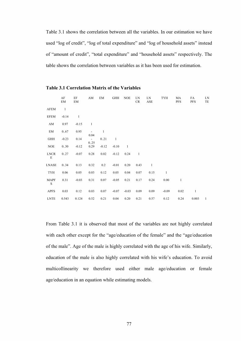
77

Table 3.1 shows the correlation between all the variables. In our estimation we have

used “log of credit”, “log of total expenditure” and “log of household assets” instead

of “amount of credit”, “total expenditure” and “household assets” respectively. The

table shows the correlation between variables as it has been used for estimation.

Table 3.1 Correlation Matrix of the Variables

AF EM

EF EM

AM EM GHH NOE LN CR

LN ASE

TYH MA PFS

FA PFS

LN TE

AFEM

1

EFEM

-0.14 1

AM

0.97 -0.15 1

EM

0..67 0.95 -0.04

1

GHH

-0.23 0.14 -0..25

0..21 1

NOE

0..30 -0.12 0.29 -0.12 -0.10 1

LNCRE

0..27 -0.07 0.28 0.02 -0.12 0.24 1

LNASE

0..34 0.13 0.32 0.2 -0.01 0.20 0.43 1

TYH

0.06 0.05 0.03 0.12 0.05 0.04 0.07 0.15 1

MAPFS

0.31 -0.03 0.31 0.07 -0.05 0.21 0.17 0.24 0.00 1

APFS

0.03 0.12 0.03 0.07 -0.07 -0.03 0.09 0.09 -0.09 0.02 1

LNTE

0.543 0.124 0.52 0.21 0.04 0.20 0.21 0.57 0.12 0.24 0.003 1

From Table 3.1 it is observed that most of the variables are not highly correlated

with each other except for the “age/education of the female” and the “age/education

of the male”. Age of the male is highly correlated with the age of his wife. Similarly,

education of the male is also highly correlated with his wife’s education. To avoid

multicollinearity we therefore used either male age/education or female

age/education in an equation while estimating models.

78

3.5 Estimation Results and Discussion

The descriptive statistics of the dependent variables and the independent variables

are provided in Table 3.2. Tables 3.3 and Table 3.4 show the estimation results of the

impact of microcredit on household outcomes on total expenditure (income) and

assets respectively. Due to multicollinearity we do not consider age/education of

male and female together in the same equation. We have divided borrowers into

three equal groups (33.33 %) based on their income level. The groups are identified

as high, middle and low income level borrowers. Tables 3.5 and 3.6 provide

estimation results of different income level borrowers. Finally, data have been

pooled from the full set (borrowers and non-borrowers) and Tobit estimation is used

for the censored data. The STATA 8.0 statistical package is used to estimate the data

and White corrected standard errors are used to allow for heteroscedasticity. The

Hansen-Sargan test for over identifying restrictions is allowed for exogeneity of the

instruments.

3.5.1 Descriptive Statistics of Dependent and Independent Variables

Table 3.2 provides the summary statistics of the variables. Average age of females in

the study is 37 years with maximum age of 75 years and a minimum of 16 years.

Average education of the female is 4 years of schooling with the highest education to

the level of a bachelor degree (14 years of schooling). Average age of males is 43

years with a maximum of 80 and a minimum of 20 years.

79

Table 3.2 Descriptive Statistics of Dependent and Independent Variables

Variables Mean Standard Deviation

Minimum Maximum

Age of the female (Years)

36.88 10.28 16 75

Education of the female (Years of schooling)

3.82 3.28 0 14

Age of the male (Years)

43.02 10.43 20 80

Education of the male (Years of schooling)

4.60 3.90 0 16

Gender of the household head (%)

0.91 0.27 0 1

Number of males as a percentage of family size (%)

29.48 16.77 - -

Number of females as a percentage of family size (%)

27.18 13.78 - -

Number of earners in the household

1.73 0.70 1 5

Family size

5.4 1.95 2 15

Amount of borrowing (Taka)

8017.51 10268 4000 100,000

Total Expenditure(Taka)

6743.89 4289.02 1300 27000

Assets (Taka)

7126 68931 504 1,625,000

Type of houses

0.52 0.49 0 1

Average education of the male is approximately 5 years of schooling with the

maximum of a master’s degree (16 years of schooling). 91% of the households are

male-headed the rest by a female. Average number of adult males as a percentage of

family size is 29% while for females it is 27%. Average number of earners in a

80

family is 1.73 and the average family size is 5.4. Average amount of borrowing is

8017 taka35 and 51 paisa36 with the highest of 100,000 taka. Average monthly total

expenditure of the household is found to be 6,743 taka with the highest 27,000 taka.

Average accumulated assets are 7126 taka with a maximum of 1,625,000 taka and a

minimum of 504 taka. 52% of the houses are found to have tin or brick roofs and/or

walls and the rest are built with other local housing materials such as straw, mud etc.

3.5.2 Impact of Microcredit on Household Outcomes: Income and Asset

In this study we have estimated simultaneous equations model to determine the

impact of borrowing on household outcomes such as total expenditure (income) and

assets using 2SLS estimation. Equations 3.1 and 3.3 of Section 3.3 are estimated

separately for total expenditure and assets as the dependent variables. Variables such

as amount of credit, total expenditure and assets are log transformed. Table 3.3 and

3.4 show the estimated results for total expenditure and assets respectively. Table 3.1

shows high correlation between age and education of male and female. Two separate

equations for male and female (age and education) are estimated. Results of these

two equations are shown as Equation 1 and 2 (columns 1 and 2) in Table 3.3 and 3.4.

35 Taka is the currency of Bangladesh. 36 Paisa is the lowest denominator of currency.

81

Table 3.3 2SLS Estimation of Amount of Borrowing on Household Outcome:

Log of Total Expenditure/Income

Explanatory Variables Log of

Total Expenditure (Income)

Equation 1 Equation 2

Constant 4.35***

(2.58)

3.72***

(2.12)

Log of Amount of Borrowing 0.95***

(3.74)

1.94***

(3.66)

Age of the Female 0.56**

(2.07)

-

Age-squared (female) -0.28***

(-2.58)

-

Education of the Female 0.38*

(1.82)

-

Age of the Male - 0.55**

(2.06)

Age-squared (male) - -0.46***

(-2.78)

Education of the Male - 0.22**

(2.28)

Gender of the Household Head 0.31***

(3.87)

0.29***

(3.41)

Number of Males as a

Percentage of Family Size

-0.001

(-0.73)

-0.001

(-0.71)

Village has Electricity 0.01

(0.12)

0.04

(0.39)

Village has Paved Roads -0.03

(-0.62)

-0.008

(-0.16)

2R

0.25 0.14

F-statistic (8,379)

Prob. > F

23.33

0.0000

22.14

0.0000

Number of Observations 387 387

(***) significant at 1% level, (**) significant at 5% level, (*) significant at 10% level and figures in the parentheses show the t-values using White corrected standard errors.

82

Table 3.4 2SLS Estimation of Amount of Borrowing on Household Outcome:

Log of Assets

Explanatory Variables Log of Assets


Constant -3.72**

(-2.12)

-7.37*

(-1.68)

Log of Amount of

Borrowing

1.41***

(2.72)

1.51***

(2.74)


(2.05)

-

Education of the Female 0.02**

(2.28)

-

Age of the Male -

0.56**

(2.07)

Education of the Male -

0.04**

(2.67)

Gender of the Household

Head

0.41*

(1.72)

0.48*

(1.69)

Number of Males as a

Percentage of Family Size

0.003

(0.52)

0.003

(0.54)

Village has Electricity 0.56**

(2.07)

0.48

(1.69)

Village has Paved Roads -0.12

(-0.90)

-0.07

(-0.52)

2R 0.16

0.17

F-statistic (7, 379)

Prob. >F

25.52

0.0000

22.29

0.0000

Number of Observations 387 387


83

Table 3.3 shows that coefficient of total expenditure (income) is significant and

positive. This implies incomes of the households are affected positively by the

amount of credit. As amount of credit increases expenditure (income) of the

households also increase. Age of the female as well as male is found significant and

positive. That tells us that as age of both male and female increases, income of the

household also increases.

To see the effect of age we have further estimated the equation using age-squared.

We have found negative and significant coefficient of age-squared for both male and

female. This implies that as age increases income of the household increases but

after certain level it starts dropping. This is a realistic finding as in real life people’s

income increases as they grow older but falls after a certain level when they stop

working.

Table 3.3 also shows a positive coefficient for education of both male and female.

That means education has a positive role in providing higher income for the

households. The coefficient of education for female and male is found significant at

5% and 10% level respectively. In our sample most of the households are male-

headed. Our estimation results from Table 3.3 suggest that the male-headed

households have a larger expenditure (income) for the family.

Table 3.4 shows the 2SLS estimation results of the simultaneous equations model as

discussed in Section 3.3 of this chapter using “assets” as one of the dependent

variables. We have used log transformed assets and credit to estimate our model. As

mentioned earlier, to avoid multicollinearity we have estimated two separate

84

equations for male/female age and education. These are shown separately in columns

1 and 2 of Table 3.4 as Equations 1 and 2 respectively.

Table 3.4 shows that the microcredit program affects household assets significantly

and positively. The positive coefficient of assets implies that as credit increases,

assets of the households also increase. This could be interpreted as one of the

achievements of microcredit programs. Table 3.4 also shows a positive and

significant coefficient for age of the male and female. That means as age of the male

increases, household assets also increase. We also could conclude that education

contributes to better quality of life through enhancing household assets for both male

and female. Education enlightens everyone and plays an important role in bringing

better assets for the households. Table 3.4 also shows that gender of the household

head is positive and significant at the 10% level. The positive and significant

coefficient of electricity implies that having electricity in villages may facilitate

household assets.

Summarising Tables 3.3 and 3.4 we may conclude that microcredit programs are

facilitating households to have better income as well as assets. We therefore accept

the null hypothesis that the microcredit programs improve household outcomes. Our

results suggest that the microcredit programs are successful in improving the quality

of life of borrowers through accumulation of assets and income. These results are

consistent with the findings of Pitt and Khandker (1996).

85

3.5.3 Impact of Microcredit on Household Outcomes Based on Different Income

Level Borrowers

Since we have found a positive impact of microcredit on household outcomes, now

we want to see how this impact varies among different income level borrowers. We

have therefore divided the borrowers into three equal groups according to their

income levels. Each group contains 33.33% borrowers and are classified as high,

middle and low income groups. As we know 94% of microcredit borrowers are

female at the same time there is a high correlation between age and education of

male and female. We have therefore, decided to focus only on female age and

education in our following estimations.

Tables 3.5 and 3.6 show the 2SLS estimation of the effects of microcredit programs

on household outcomes (total expenditure and assets) based on different income

level borrowers. The results of total expenditure and assets are shown in Table 3.5

and 3.6 respectively.

The findings of Tables 3.5 and 3.6 are very interesting. We have found positive and

significant coefficient of income for high income level borrowers. For middle

income level borrowers’ income is positive but significant at the 10% level. The

table also shows that the age of the female is positive and significant across all

income levels.

86

Table 3.5 2SLS Estimation of Amount of Borrowing on Different Income Level

Borrowers: Log of Total Expenditure

Explanatory

Variables

High Income

Level Borrowers

Middle Income

Level Borrowers

Low Income

Level Borrowers

Constant 5.00*** (3.69)

6.69***

(3.99)

5.31***

(2.94)

Log of Amount of Borrowing

0.455*** (2.86)

0.12* (1.68)

0.23

(1.17)


(2.56)

0.13***

(3.11)

0.3***

(3.21)

Education of the

Female

0.024*

(1.90)

0.01*

(1.86)

0.01

(0.08)

Gender of the

Household Head

0.33**

(2.23)

0.04

(0.50)

0.32**

(2.54)

Male as Percentage

of Family Size

-0.004

(-1.17)

-0.001

(-0.55)

-0.001

(-0.39)

Village has

Electricity

0.001

(0.01)

0.07

(1.24)

0.59***

(3.71)

Village has Paved

Roads

-0.11

(-0.88)

-0.06

(-0.82)

-0.02

(0.27)

2R .25 .29 .27

F-statistic (7, 121) Prob. > F

23.22

0.0000

24.31

0.0000

23.21

0.0000

Number of observations

129 129 129


87

Table 3.6 2SLS Estimation of Amount of Borrowing on Different Income Level

Borrowers: Log of Assets

Explanatory

Variables

High Income

Level Borrowers

Middle Income

Level Borrowers

Low Income

Level Borrowers

Constant 6.60*** (4.28)

5.31***

(3.60)

4.35***

(2.58)

Log of Amount of Borrowing

1.69*** (2.85)

0.12* (1.68)

1.99

(1.30)

Age of the Female 0.18*** (3.17)

0.01**

(2.40)

0.02***

(2.40))

Education of the

Female

0.003***

(2.58)

0.19

(1.21)

0.001

(1.09)

Gender of the

Household Head

-0.16

(-1.42)

-0.65

(-1.09)

-0.18

(-1.07)

Male as Percentage

of Family Size

0.008***

(2.89)

0.18**

(2.58)

0.33**

(2.23)

Village has

Electricity

0.03**

(2.00)

0.18

(1.07)

0.008

(0.81)

Village has Paved

Roads

-0.20

(-1.49)

-0.001

(0.05)

-0.12

(-0.72)

2R .21 .26 .31

F-statistic (7, 121) Prob. > F

20.68

0.0000

23.99

0.0000

21.19

0.0000


129 129 129


88

Table 3.5 further shows that as age increases income of the households increase for

all income level borrowers. Education of the female is positive and significant at the

10% level for high and middle income level borrowers. Male-headed households

provide better income for high and low income level households. From Table 3.5 we

have found that having electricity in the village increases income for the low income

level borrowers.

Table 3.6 shows the results of the impact of microcredit on household assets on

different income level borrowers. It is interesting to see from the significant and

positive coefficient that as amount of borrowing increases, assets increase only for

the higher income level borrowers. The coefficient is positive and significant at 10%

level for the middle income level borrowers. Age of the female is positive and

significant across all income level borrowers. This implies that as age of the female

increases, households possess more assets. However as education of the female

increases household assets increase for higher income level borrowers only.

Households with more adult males provide better assets across all income groups.

Having electricity in the village, increases assets only for the higher income level

borrowers.

Summarising the results of Tables 3.5 and 3.6, our findings suggest that the high-

income group borrowers are better off compared to middle and low income group

borrowers. We therefore accept the null hypothesis that the high income group is

better off compared to low and middle income group borrowers. The tables further

show that, as the amount of credit increases, income and assets of high income group

borrowers increase. This is interesting to see as education of the female increases

89

household assets increases only for the higher income level borrowers. Electricity in

the village expedites income for the low income level borrowers only.

3.5.4 Estimating Censored Regression Problem on Household Outcomes

So far in our 2SLS estimation we used only the borrowers’ data to determine the

impact of microcredit on household outcomes. Now we want to pool the whole data

set including borrowers and non-borrowers to determine the impact of microcredit

on household outcomes. We have thus used Tobit estimation to estimate the

censored data. Amount of credit contains some values for the borrowers and zeros

for the non-borrowers. Tobit estimation is normally used for this type of censored

data. Tobit estimation provides the best estimation for model containing censored

observation. Zero values of the dependent variable correspond to censored

observations while positive values correspond to actual transactions. James Tobin

proposes the Tobit model37 for analysing the censored regression problem. To fit in

the same simultaneous equations model used earlier in this chapter we used Tobit

estimation on Equation 3.1 of Section 3.3 containing censored data for amount of

borrowers. Thus predicted rather than actual borrowing is used in Equation 3.3 to

estimate the impact of borrowing on various household outcomes using OLS

estimation. In the following estimation we have used variables without logs such as

“amount of credit”, “assets” and “income”. Table 3.7 shows the results of Tobit

estimation and Table 3.8 shows OLS estimation of household outcomes using the

estimated value of amount of borrowing obtained from Tobit estimation.

37“Estimation of Relationships for Limited Dependent Variables”, Econometrica, January 1958.

90

Table 3.7 Tobit Estimation of Amount of Credit Using Censored Data

(***) significant at 1% level, (**) significant at 5% level, (*) significant at 10% level and figures in the parentheses show the t-values.

In our previous estimations we overruled the possibility that the village that has

electricity may also have paved roads. The coefficient of the dummy variable for

“paved roads” was not found significant in our previous estimations. We have,

therefore, used only “electricity” in the following estimations as one of the

community infrastructure factors.

In our Tobit estimation as shown in Table 3.7 we see that out of 571 observations

there are 183 left-censored observations, 1 right-censored observation and 386

uncensored observations. That leaves us with 570 observations.

Constant 2.47* (1.77)


Education of the Female 0.44*** (2.48)

Gender of the Household Head -.23 (-1.42)

Number of Earners in the Family 1.13*** (3.16)

Types of Houses 0.13 (0.28)

Village has electricity 1.73*** (2.28)

Number of Males as a Percentage of Family Size

0.04*** (2.86)

Number of Observations 570

Pseudo 2R 0.045

LR χ 2 (7)

Prob.> χ 2

76.63 0.0000

91

Table 3.7 shows the Tobit estimation results of the amount of credit (not log

transformed) using censored data. From the table we see that the credit programs are

positively and significantly affected by the age of the female. The microcredit

programs are also affected positively and significantly by the education of the

female. It is good to see that females’ education helps them to manage credit

properly. It is also interesting to see a positive and significant coefficient of “the

number of earners” in the family. That means if a family has more earning members

that helps them to have quick repayment as well as obtain more credit. The positive

and significant coefficient of the variable “electricity” suggests that having

electricity in the village facilitates borrowing by the households. Number of adult

males in the family also facilitates credit programs. This may be concluded from the

positive and significant coefficient of the variable (MAPFS). Tobit estimation results

show that the credit program is also affected by infrastructural facilities such as a

village having electricity.

Table 3.8 shows OLS estimation results of household outcomes: expenditure

(income) and assets using the estimated values of amount of credit obtained from

Tobit estimation. Using censored data provides us slightly better results than the

2SLS estimation. This could be due to having more observations in censored

estimation.

From Table 3.8 we see that the impact of microcredit on household income is

positive and significant. This implies that the income of the household increases with

respect to amount of credit. This is one of the achievements of the microcredit

programs. Table 3.8 further shows age of the female is significant and positive. This

92

implies that as age of the female increases, income of the household increases. In

real life we see people’s income increase with age. Education of the female in the

household is positive and significant. It implies that as the female becomes more

educated, income of the household increases. This is also another realistic finding.

Table 3.8 further shows having electricity in the village enhances household income.

From Table 3.8 we see that the microcredit program enhances household assets. It

also shows that age and education of the female in the household as well as having

better infrastructural facilities in the village facilitates household assets.

Table 3.8 OLS Estimation of Household Outcomes Using Estimated Value of

Amount of Credit from Tobit Estimation

Explanatory variables Income Assets

Constant 6.86*** (9.51)

7.28*** (9.54)

Estimated Value of Amount of Credit

0.72*** (2.40)

0.69*** (2.69)


0.54*** (2.96)


0.06*** (2.82)

Gender of the Household Head

-0.86 (-0.16)

-0.088 (-0.97)

Village has Electricity 0.72** (2.39)

0.14** (2.40)

2R 0.13 0.15

F ( 5, 563) Prob. > F

19.31 0.0000

17.31 0.0000


570 570


93

3.5.5 Estimating Censored Regression Problem of Different Income Level

Households

To be consistent with our previous 2SLS analysis we have decided to determine the

impact of credit based on different income levels of borrowers using the censored

data in Tobit estimation. We have thus divided the total sample into three equal

groups containing 33.33% in each group. The groups are classified as high, middle

and low income group. We have used the estimated value of the amount of credit

obtained in Tobit estimation and estimated Equation 3.3 using OLS estimation for all

three groups.


Level Borrowers: Total Expenditure (Income)

Explanatory

variables

High Income

Group

Middle Income

Group

Low Income

Group

Constant 3.12*** (3.58)

3.09*** (3.98)

3.59*** (4.99)


0.10*** (2.67)

0.59** (2.21)

0.08 (1.10)


0.42** (2.25)

0.52** (2.26)

Education of the Female

0.57*** (2.77)

0.65*** (2.51)

0.61** (2.09)

Gender of the Household Head

-0.33 (-0.58)

-0.54 (-0.89)

-0.65 (-0.61)

Village has electricity

2.47*** (2.58)

1.48** (2.26)

2.43** (2.25)

2R 0.15 0.16 0.13

F ( 5, 184) Prob. > F

6.80 0.0000

5.52 0.0000

5.43 0.0000


190 190 190


94

Table 3.10: OLS Estimation of Household Outcomes Based on Different Income

Level Borrowers: Assets

Explanatory

variables

High Income

Group

Middle Income

Group

Low Income

Group

Constant 2.15*** (2.78)

2.09*** (3.05)

3.56*** (2.58)


0.015*** (2.98)

0.07** (2.40)

0.03 (1.55)


0.01** (2.32)

0.15** (2.24)

Education of the Female

0.02*** (2.71)

0.06*** (2.55)

0.05** (2.22)

Gender of Household Head

-0.55 (-0.51)

-0.45 (-0.75)

-0.02 (-0.63)

Village has electricity

0.81*** (2.22)

0.71*** (2.61)

0.21 (1.09)

2R 0.14 0.13 0.17

F ( 5, 184) Prob. > F

5.66 0.0000

6.54 0.0000

5.51 0.0000


190 190 190


Tables 3.9 and 3.10 show the OLS estimation of household outcomes based on

different income level borrowers using the estimated value of amount of credit

obtained from Tobit estimation. Interestingly the results as shown in Table 3.9 and

3.10 reveal that the impact of microcredit are more pronounced for high income and

middle income group households compared to low income group households. The

results from Table 3.9 and 3.10 are consistent with the results obtained from 2SLS

estimation. They show that age and education of female affect income as well as

assets positively and significantly. The tables further show that having electricity in

the village expedites household outcomes such as income and assets.

95

3.6 Conclusion

In this chapter we have analysed the impact of microcredit on household outcomes

such as income and assets. We have modified the simultaneous equations model

suggested by Pitt and Khandker (1996) by assessing the impact of microcredit

separately on household expenditure (income) and assets. We have further

differentiated the impact of credit on different income level borrowers. In addition

we have also used some refined and log transformed variables to estimate the model

compared to previous studies.

From the estimation it may be concluded that the microcredit programs are effective

in generating higher income and assets for borrowers. This is a very important

finding as it confirms the claims made by the microcredit providers. We may

conclude from this finding that microcredit is providing better quality of life for its

borrowers. We know from experience that people’s income increases as they grow

older. Our estimation results suggest that age of the female as well as male has a

significant and positive impact on income and assets. As someone grows older their

income also grows. We also wanted to see what happens to someone’s income as the

person grows even older. To do so, we have added “age-squared” in the equation and

estimated the model. The negative and significant co-efficient tells us someone’s

income increases as the person grows older but income starts to decline after a

certain level when they stop working. Our results also suggest that education of the

female as well as male are an important factor in affecting income and assets

positively. Education helps people to be more enlightened. According to this finding,

education enhances borrowers’ income and assets. We have also found from this

96

analysis that infrastructural facilities in the village facilitates borrowers’ income and

assets.

This study also suggests that as the number of earners increases in a household,

amount of borrowing also increases. This could be due to the fact that having more

earning members increases the ability to repay loans quickly as well as obtain more

loans. Male-headed households are able to enhance household income and assets. It

is interesting to see that even though microcredit facilitates household outcomes the

impact varies between different income level borrowers. Our results suggest that

microcredit programs help bring better outcomes for high income group borrowers

compared to medium and low income group borrowers.

In general it may be concluded that microcredit has a pronounced positive effect on

income and assets of borrowers. However, microcredit seems to be more effective

for the high income group borrowers compared to middle and low income group

borrowers. Microcredit is more effective for educated borrowers compared to less

educated borrowers. Infrastructural facilities facilitate the household outcomes. It is

also found that families having more earning members enjoy better household

outcomes. Overall this study suggests that even though microcredit is an attractive

tool for producing better outcomes in terms of income and assets, it is more effective

for relatively wealthier borrowers compared to non-wealthy borrowers. It would be a

good research question to pursue in the future, to uncover in the future why this is

the case. At the same time, our results suggest that there should be some adjustment

to the existing microcredit programs to achieve the intended outcome, that is, to

serve the purpose of those who are at the bottom of the society.

97

Chapter Four

ASSESSMENT OF CONSUMPTION OF MICROCREDIT

BORROWERS COMPARED TO NON-BORROWERS38

4.1 Introduction

This chapter investigates the consumption behaviour of borrowers in the microcredit

program and compares it with that of non-borrowers of the same village. To capture

the essence of the consumption behaviour of the borrowers, various food and non-

food items, which are commonly used in the rural households, are considered as an

indicator of their consumption pattern. Total expenditure is used as a proxy for

income as it is simply the sum of the expenditure items. It is common to use total

expenditure in place of income as an explanatory variable in the expenditure

relationship because of the conceptual and measurement errors associated with

observations on income. With total expenditure as a proxy for income, one can use

income as an instrumental variable to obtain consistent estimates. Household

expenditure is used in this chapter as a proxy for income as suggested by Alderman

(1993), Devereux (1993), Puetz, (1993) and Hazell and Röell (1983).

Over a period of time microcredit provides collateral free loans to rural people, and it

is argued that there would be a significant difference in the expenditure patterns of

borrowers compared to non-borrowers. The underlying hypothesis in this regard is:

38 Part of this chapter has been accepted for publication in a forthcoming issue of the Journal of Developing Areas. Please refer to Appendix I for the abstract of the paper.

98

“Are the borrowers in the microcredit program better off in terms of consumption

behaviour than the non-borrowers”?

We use budget share of the items consumed by borrowers and non-borrowers and the

items are classified as food and non-food. Budget share is defined as: when a dollar

of a consumer’s budget is selected randomly, the possibility of that money spent on

the ith commodity is yqpw iii /= where ip is the price and iq is the quantity

bought of that commodity and y is the income or total expenditure. When the budget

share is used, the value shares like probabilities should be non-negative and add up

to one. For the purpose of calculation, budget share is calculated for each item

consumed by the households. The basic items that are commonly consumed by the

households are selected to find out the consumption pattern. Figure 4.1 illustrates the

items consumed by the households as a consumption tree.

99

Fig 4.1 Consumption Tree of Food and Non-food Items Consumed by

Borrowers and Non-borrowers

Food

Total Expenditure

Food

Non-Food

Cereal

Lentils Cigarette

s and

betel leaf

Protein Vege-

tables

Sugar

Spices Cooking

Oil

Milk and

Eggs

Fuel

Clothing Education

Health

Travel

Entertain

-ment

Electricity

100

Food items are classified as follows: Cereals (rice, wheat and products of similar

type); lentils (pulses of various kinds); vegetables (includes fruit); meat and fish

(includes, chicken, beef, mutton and fish of all types); milk and eggs and cigarettes,

betel-leaf and betel nuts.

Non-food items are considered as follows: Fuel (includes wood, kerosene and

similar items used for cooking); electricity, cloth, education (includes tutor’s fee and

books and stationery etc); and health (includes medicines, doctor’s bills and hospital

bills).

The rest of this chapter is structured as follows: Section 4.2 provides a literature

review. Section 4.3 discusses the relevant theories. Section 4.4 specifies the

econometric model. Interpretations of the results are provided in Section 4.5. A

conclusion is drawn in the final section.

4. 2 Literature Review on Expenditure Elasticity

The method of Ordinary Least Squares (OLS) is a classical approach to the problem

of estimating the coefficients of a regression equation. However, if the equation is a

member of simultaneous equations, OLS estimates will provide biased estimates

(Summers, 1959). In estimating household expenditure elasticities, total expenditure

is quite often used as a proxy for income while budget share of the item consumed is

used as the dependent variable. In Engel curve analysis, income or total expenditure

is used as the independent variable in OLS analysis. According to Liviatan (1961),

neither of these variables is a satisfactory index of the true economic position of the

family. This results in biased estimates of the income elasticities of the various

101

consumption categories. The bias can, however, be eliminated in large samples by

using both income and total expenditures in the estimation procedure. This can be

accomplished by applying the method of “instrumental variables” to Engel curve

analysis, with recorded income serving as the instrumental variable.

On the other hand, Prais and Houthakker (1955) have estimated budget shares using

OLS estimates. They have stated, “So long as the item of expenditure is a small

proportion of the budget it is not to be expected that serious biases will result….”

According to Summers (1959), if income data are available, the parameters of each

equation could be estimated directly by Least Squares applied to each equation

individually. For brevity, this procedure will be called Single Equation Least

Squares.

Massell (1969) has expressed the expenditure relationship as:

ijkjk

kijijijiiij uDRNXX +++++= ∑=4

1

*

3

*

2

*

10

* γββββ (4.1)

where ijX = expenditure by household j on item i, ∑=i

ijj XX total expenditure

by household j, N = household size, R = the ratio of subsistence to total expenditure,

1 4,.....D D are district dummy variables, iju is the disturbance, and an asterisk denotes

a logarithm. The 'sβ and 'sγ in the equation are the parameters to be estimated. In

addition, the model has used double log relationship and has found to provide a good

fit to satisfy the assumption of homoscedastic residuals.

102

After using additional instruments as “cash income” and “farm size”, the equation

becomes:

)2.4(..... 4714

*

3

*

2

*

10

*

jjjjjjj vDDNTYX +∂++∂+∂+∂+∂+∂=

)3.4(....... 4714

*

3

*

2

*

10 jjjjjjj wDDNTYR +++++++= ξξξξξξ

where Y = cash income, T = land size of the j-th individual, v and w are the

disturbances, an asterisk denotes a logarithm. Since the above two equations are a set

of simultaneous equations, Massell (1969) has used Two-Stage Least Squares

(2SLS). The evidence of heteroscedasticity or non-linearity has been tested for each

individual consumable item in his paper.

As has been established by the theory of consumption, the demand functions that are

derived from the maximisation problem of the consumer make the quantity

demanded of a good or service dependent on the income level of the individual and

on prices. To be consistent with the microeconomic theory (that is that the consumer

is a utility maximiser) it is required that the restrictions such as (1) homogeneity of

degree zero in prices (that is the consumers have no money illusion, or that they react

to relative, not nominal prices); (2) symmetry or that the effect of a change in the

price of good i on the demand for good j is same as the effect of a change in the price

of good j on the demand for good i for constant income, and (3) a restriction for

adding up or that all the budget shares add up to one. The demand functions should

meet the above-mentioned adding-up restriction, the homogeneity and symmetry

conditions. However, when prices are constant, one obtains the specification

corresponding to the Engel curve, where the demand of goods is dependent only on

103

the income of the individual. In such a case, the only condition to be met is the

adding-up restriction since all the others are derived from the consideration of prices

(Beneito, 2003).

There are quite a number of properties, which a “good” Engel curve should have.

These properties stem from considerations on economic, statistical and practical

questions in demand analysis, but unfortunately there is no general agreement to the

above properties in the literature. Therefore, there is no a priori reason to trust in and

use one certain algebraic formulation of Engel curve only. It is well known that

income elasticities for the same commodity and estimated for the same set of

household budget data can differ widely when they are derived from different

functional types of Engel curves (Dax, 1987).

Ray (1980) has used an extension of an Almost Ideal Demand System (AIDS)

model, which was introduced by Deaton and Muellbauer (1978). Ray has used

restrictions such as adding up, homogeneity, symmetry and concavity in the model.

He has used family size and applied AIDS model to Indian budget data to estimate

expenditure, prices and size elasticities. The usual mean-variance assumptions are

made about the stochastic error term, and F-tests are carried out to investigate the

hypotheses. Ray has estimated single equations using OLS estimates in the absence

of cross-equation or non-linear restrictions, while Beneito (2003) has estimated

income elasticities using Engel curve analysis using Seemingly Unrelated

Regressions Estimator (SURE) and Three Stages Least Square Estimates (3SLS).

104

Based on the above-mentioned literature, in this chapter we have firstly estimated

single equations using heteroscedasticity corrected OLS estimation and then have

used iterative Seemingly Unrelated Regression Estimates (SURE) to analyse the

model containing multiple equations.

4.3 Introduction to Relevant Theories

Empirical studies in applied demand analysis using system of demand equations

typically rely on one of two assumptions: either prices are assumed to be

predetermined or quantities are assumed to be predetermined. These assumptions

lead to quantity-dependent or direct demand systems, such as the (direct) translog

(Christensen, Jorgenson and Lau, 1975), the AIDS (Deaton and Muellbauer, 1980),

or the (direct) differential or Rotterdam model (Theil, 1975). Direct demands are the

usual representation of preferences for the individual consumer, who is typically

taken as making optimal consumption decisions for given prices and income. Its use

at the aggregate level is equivalent to assuming that supplies are perfectly elastic and

that demands adjust to clear the market. The alternative of assuming that quantities

are predetermined and that prices adjust to clear the market leads to price-dependent

or inverse demand systems, such as the (inverse) translog (Christensen, Jorgenson

and Lau, 1975) or (inverse) Rotterdam model (Theil, 1975; Barten and Bettendorf,

1989).

In addition to the two polar cases of direct and inverse demand functions, another

class of models allows one to sidestep estimation of both demand and supply

functions in a simultaneous equations framework. This class is the case of “mixed

105

demand” function (Chavas, 1984) where prices of some goods are predetermined

such that the respective quantities demanded adjust to clear the market. However, for

the remaining set of goods quantities supplied are predetermined and prices must

adjust to clear the market.

The following section will discuss the theory of mixed demands and AIDS model

The mixed demand systems needs the knowledge of both direct and indirect utility

functions to characterise the demand properties whereas the Translog and AIDS

model cannot be used to specify a mixed demand system because the flexible

functional forms do not have a close form dual representation.

4.3.1 Theory of Mixed Demands

The mixed demand theory as described by Moschini and Vissa (1993)

assumes mA xxxx ,....,( 21= ) the vector of commodities chosen optimally and

),....,( 21 nmmB xxxx ++= the vector or commodities in fixed quantity whose price is

optimally determined. According to Moschini and Vissa if ip denote the nominal

price of good i, and y is total expenditure on Ax and Bx (income, for short), then

ypv ii /≡ is the corresponding normalised price, and Av and Bv are the vectors of

normalised prices of the two subsets of goods. Mixed demands are then derived from

the constrained optimisation problem (Samuelson, 1965; Chavas, 1984):

BA

BBAABABA

vx

xvxvvvVxxU )4.4(}1.|),(),(max{ =+−

106

where U (.,.) and V (.,.) are direct and indirect utility functions, quasi-concave and

quasi-convex in their respective arguments. The solution to Equation (4.4) gives

Marshallian mixed demands )1,,( BAA xvx and )1,,( BAA xvv . Evidently, at the

optimum,

[ ] [ ] ),1,,()1,,(),1,,( , BABABABBAA xvVxvvvVxxvxU ≡= where V is the mixed utility

function.

The mixed demand functions )1,,( BAA xvx and )1,,( BAB xvv as stated by Moschini

and Vissa (1993) satisfies the typical restrictions of consumer theory. Firstly, they

satisfy the adding-up condition 1.. =+ BBBA xvxv implied by the budget constraint.

Secondly, the homogeneity condition implies that )1,,( bAA xvx is homogeneous of

degree zero in nominal prices and income, that is )1,,( BAA xvx = ),,( yxpx BAA .

Similarly, the optimal nominal prices of group B are homogeneous of degree one in

),,( ypA implying that )1,,( BAB xvv is homogeneous of degree zero in ),( ypA .

According to Moschini and Vissa (1993), ),,((.). yxppvyp BABBB ≡= follows that

the mixed utility function is homogeneous of degree zero in Ap and y, which

implies, ).,,()1,,( yxpVxvV BABA =

As stated by Moschini and Vissa (1993), the symmetry restrictions can be illustrated

in terms of the compensated mixed demand functions. According to Chavas (1984),

the compensated mixed demands are the same as the compensated demands under

rationing, although mixed demands should be carefully distinguished from rationed

demands (in the case of the latter, some markets do not clear). Moschini and Vissa

107

(1993) further stated that the compensated rationed demand can be characterised in

terms of the restricted cost function defined by Gorman, (1976) and Deaton, (1981).

The authors (Moschini and Vissa, 1993) mentioned that a possible reason for the

scarcity of applications of mixed demand systems is that the knowledge of both

direct and indirect utility functions required that characterises the demand properties.

4.3.2 An Almost Ideal Demand System

Stone (1953) has estimated a system of demand equations derived explicitly from

consumer theory. There has been a continuing search for alternative specifications

and functional forms. Many models have been proposed, but perhaps the most

important one is the linear expenditure system, the Rotterdam model (Theil, 1965

and 1976) and Translog model (Christensen, Jorgenson and Lau 1975). Another type

of model has been introduced by Deaton and Muellbauer; the AIDS model which is

comparable to Rotterdam and translog models but has considerable advantages over

both. The advantages of AIDS model are as follows:

• It gives an arbitrary first-order approximation to any demand system.

• It satisfies the axioms of choice exactly.

• It aggregates perfectly over consumers without invoking parallel linear Engel

curves.

• It has a functional form which is consistent with known household-budget

data.

• It is simple to estimate, largely avoiding the need for non-linear estimation.

108

• It can be used to test the restrictions of homogeneity and symmetry through

linear restrictions on fixed parameters.

Although many of these desirable properties are possessed by one or other of the

Rotterdam or translog models, neither possesses all of them simultaneously.

4.3.3 Specification of the AIDS model

In most of the literature on systems of demand equations, the starting point has been

the specification of a function, which is general enough to act as a second-order

approximation to any arbitrary direct or indirect utility function or, more rarely, a

cost function. Alternatively, it is possible to use a first-order approximation to the

demand functions themselves as in the Rotterdam model (Theil, 1965 and 1976).

Deaton and Muellbauer (1980) followed these approaches in terms of generality but

started not from some arbitrary preference ordering, but from a specific class of

preferences, which by the theorems of Muellbauer (1975 and 1976) permit exact

aggregation over consumers: the representation of market demands as if they were

the outcome of decisions by a rational representative consumer. These preferences,

known as PIGLOG39 class, are represented via the cost or expenditure function,

which defines the minimum expenditure necessary to attain a specific utility level at

given prices. The underlying assumption is to maximise utility subject to a budget

39 The cost function underlying both the Engel curves and the Tornqvist type of indexes has been constructed based on the PIGLOG functional form (Deaton and Muellbauer, 1980). The PIGLOG model was developed to treat aggregate consumer behaviour as if it were the outcome of a single maximising consumer. This problem of how to treat aggregate consumer behaviour as if it was the outcome of a single maximising consumer exists because it is neither necessary nor desirable for a macroeconomic relationship to perfectly mimic its microeconomic foundation. Therefore, the market demand functions that are being estimated may not have the desirable properties of micro-demand functions. This is known in economics as the aggregation problem.

109

constraints. Deaton and Muellbauer denoted this function c(u,p) for utility u and

price vector p, and define the PIGLOG class by

{ } { } )5.5()(log)(log)1(),(log pbupaupuc +−=

With some exceptions, u lies between 0 (subsistence) and 1 (bliss) so that the

positive linearly homogeneous functions a(p) and b(p) can be regarded as the costs

of subsistence and bliss, respectively.

As mentioned by Deaton and Muellbauer (1980), the specific functional forms are

taken for log a(p) and log b(p). For the resulting cost function to be a flexible

functional form, it must possess enough parameters so that at any single point its

derivatives 2222 /,/,/,/,/ ucandpucppcucpc ijii ∂∂∂∂∂∂∂∂∂∂∂∂ can be set

equal to those of an arbitrary cost function as shown by Deaton and Muellbauer

(1980). Therefore, according to Deaton and Muellbauer the cost function takes the

following form:

)6.4(loglog2

1log)(log *

0 jkk j

kjkk

k pppaapa ∑∑∑ ++= γ

)7.4()(log)(log ∏+=k

ikppapb ββ

From the above-mentioned equation the AIDS cost function may be written as:

)8.4(loglog2

1log),(log 0

*

0 ∏∑∑∑ +++=k

kkjk

k jkjk

kk puppppuc ββγαα

110

where *,, ijii and γβα are parameters. As mentioned by Deaton and Muellbauer it

can easily be checked that c(u, p) is linearly homogeneous in p (as it must be a valid

representation of preferences) provided that:

.0,1 ==== ∑∑∑∑ j jk ijj iji i βγγα

Deaton and Muellbauer showed that it is also straightforward to check that Equation

4.8 has enough parameters for it to be a flexible functional form. Since utility is

ordinal, Deaton and Muellbauer (1980) chosen a normalisation such that, at a point,

.0/log 22 =∂∂ uc According to Deaton and Muellbauer the choice of the functions

a(p) and b(p) in Equations 4.6 and 4.7 is governed partly by the need for a flexible

functional form. However, as mentioned by Deaton and Muellbauer, the main

justification is that this particular choice leads to a system of demand functions with

the desirable properties, which are demonstrated below.

Deaton and Muellbauer (1980) further mentioned that the demand functions can be

derived directly from Equation 4.8. It is a functional property of the cost function

(Shephard, 1953 and 1970) that its price derivatives are the quantities

demanded: ii qppuc =∂∂ /),( . Multiplying both sides by ),(/ pucpi gives:

)9.4(),(log

),(logi

ii

i

wpuc

qp

p

puc ==∂∂

where iw is the budget share of good i. Hence, logarithmic differentiation of

Equation 4.8 gives the budget shares as a function of prices and utility:

111

)10.4(log 0∏∑ ++= kki

jjijii pupw βββγα

where:

)11.4()(2

1jiijij γγγ +=

Again, as mentioned by Deaton and Muellbauer (1980), for a utility-maximising

consumer total expenditure x is equal to c(u,p) and this equality can be inverted to

give u as a function of p and x, the indirect utility function. According to Deaton and

Muellbauer if this is done for Equation 4.8 and substituted the result into Equation

4.10 the budget shares is obtained as a function of p and x. These are the AIDS

demand function in budget share form:

{ } )12.4(/loglog pxpw ijj

ijii βγα ++= ∑

where P is price index defined by

)13.4(loglog2

1loglog 0 j

j kkkjk

kk pppP ∑∑∑ ++= γαα

The restrictions on the parameters of Equation 4.8 plus Equation 4.11 imply

restrictions on the parameters of the AIDS Equation 4.12. These are taken in three

sets:

112

)14.4(001111

=== ∑∑∑ −==

n

ii

n

iij

n

ii βγα

)15.4(0=∑j

ijγ

)16.4(jiij γγ =

According to Deaton and Muellbauer (1980), provided Equations 4.14, 4.15 and 4.16

hold, Equation 4.12 represents a system of demand functions that add up to one.

However, as stated by Deaton and Muellbauer the total expenditure ),1( =∑ iw is

homogeneous of degree zero in prices which satisfies Slutsky symmetry conditions.

Deaton and Muellbauer have further showed that in the absence of changes in

relative prices and “real” expenditure (x/P) the budget shares are constant and this is

the natural starting point for predictions using the model. Nevertheless, the changes

in relative prices work through the terms ijγ ; each ijγ represents 10 2 times the effect

on the ith budget share of a 1 % increase in the jth price with (x/P) held constant

(Deaton and Muellbauer 1980). Yet the changes in real expenditure operate through

the iβ coefficient; these add to zero and are positive for luxuries and negative for

necessities.


The AIDS model has been used by Ray (1980). It is originated from Engel curve

analysis, and it is the time series counterpart of Engel function as suggested by Leser

(1976) is as follows:

113

)17.4(log CXB iii ++= βα

where iB and X are the budget shares of the i-th item and total household

expenditure respectively and iα and iβ are the parameters. The model allows

negative coefficients for necessary items and positive for luxury and inferior goods.

AIDS as obtained from the PIGLOG cost function corresponding to the PIGL (Price

Independent Generalised Linearity) after the choice of appropriate functional form is

given by:

nji

CPP

XB jijiii

,.....2,1,

)18.4(loglog

=++⎟⎠

⎞⎜⎝⎛+= ∑γβα

where ,i iα β and ijγ are the parameters and P is an overall price index defined in

terms of individual prices by:

)19.4(loglog2

1loglog 0 j

i jiijii PPPP ∑∑∑ +∂+∂= γ

These functions should meet the well-known adding-up restrictions and the

homogeneity, symmetry and non-negativity conditions. However, when prices are

constant (as in this case40) one obtains the specification corresponding to the Engel

40 In this study cross-section data is collected from three districts of Bangladesh over a period of time. There is insignificant difference in prices found between districts. Therefore, prices are assumed to be constant over the period.

114

curve, where the demand for goods is dependent only on the income of the

individual. In such a case, the only condition to be met is the adding-up restrictions

since all the others are derived from the consideration of prices (Beneito, 2003). The

adding-up restrictions are:

)20.4(001111

=== ∑∑∑ −==

n

ii

n

iij

n

ii βγα

The price formulation Equation 4.18 makes Equation 4.19 a non-linear system of

equations. To avoid non-linear estimation Deaton and Muellbauer (1978) used the

Stone (1954) index as a convenient approximation:

)21.4(logloglog 0

*

ii

i PPp ∑+=≅ βα

Using the utility basis of the PIGLOG model as cost function at the reference year

(p=1) for an individual the linear equation model will take the following form:

)22.4(log.)log(log 00 jj

ijii

iii PPXB ∑∑ +−−+= γβαβα

Ray (1980) incorporated the family size in the above model by using the Barten

(1964) type household utility function and deflating total household expenditure by

family size following Houthakker (1957), Weiskoff (1971) and Sener (1977). The

model takes this form:

115

)23.4(log.)/log( *

0 fPPxB ijj

ijii φγβα +++= ∑

where f, x =(X/f), ijγ and φ denote family size, per capita household expenditure and

the effect of prices and the effect of family size respectively.

As there are no price data (as mentioned above) we have assumed that all the

households face the same prices. This assumption follows Ferdous (1997). So

Equation 4.23 becomes:

*

'

'

loglog

,

)24.4(log

log

PPc

cwhere

fxBor

cfxB

iji

ij

ii

iiii

iiii

βγαα

φβαφβα

−=+=

++=+++=

∑

However, the dependent variable may not only be influenced by variables that can be

quantified on some well-defined scale but also by variables that are basically

qualitative in nature. Such qualitative variables usually indicate the presence or

absence of a “quality” or an attribute. One method of quantifying these attributes is

by constructing dummy variables that take on values of one or zero, where one

indicates the presence and zero indicates the absence of the attribute.

Since the objective of this chapter is to see if there is a significant difference in the

consumption behaviour of the borrowers and non-borrowers of microcredit, a

116

dummy variable called BD (borrower dummy41) is therefore introduced in the model,

where BD = 1 for the borrowers and zero otherwise. However, district dummies are

also included to see if there is any significant difference in consumption between

districts. As the sample data have been collected from three different districts of

Bangladesh, two district dummies are introduced, where DD 1 = 1, for Gazipur and 0

otherwise, and DD 2 = 1 for Dinajpur and zero otherwise. After adding the dummy

variables the model becomes:

12.......2,1

)25.4(log 21

=∀++++++=

i

iiiiiiii DDDDBDfxB εχπγδβα

In the above equation:

BD = 1 for borrowers

= 0 otherwise (that is, non-borrowers)

DD 1 = 1 for Gazipur

= 0 otherwise (that is, Dinajpur and Chokoria)

DD 2 = 1 for Dinajpur

= 0 otherwise (that is, Gazipur and Chokoria)

Mean of non-borrowers:

)0()0|( iii BDBE γα +==

41 We know that the decision to participate in a microcredit program is self-selective. This type of

self-selection problem may be corrected through Heckman’s two stage correction procedure. The problem with the Heckman procedure is to identify suitable instruments. Since no suitable instruments have been identified which would permit the use of Heckman procedure to correct self-selection bias, we did not look at the causal impact of program participation in this study.

117

iα=

Mean of borrowers:

)1()1|( iii BDBE γα +==

ii γα +=

From these regressions it is seen that the intercept term iα gives the mean

consumption of the non-borrowers and ii γα + gives the mean consumption of

borrowers. The coefficient iγ tells the degree of difference in consumption of

borrowers from non-borrowers.

A test of the null hypothesis that the consumption by borrowers is the same as non-

borrowers (that is, 0=iγ ) can easily be made by running regression of Equation 4.25

in the usual Ordinary Least Squares (OLS) manner and finding out whether or not

the basis of the t-statistics and the computed coefficient is statistically significant. In

a similar way, a null hypothesis can be developed for the district dummies to tell

how far Gazipur and Dinajpur are different from the third district.

Equation 4.25 has been estimated using heteroscedasticity corrected OLS estimates

applying the method suggested by White corrected standard errors. To see the

direction as well as the magnitude of changes in consumption between different

income groups, the samples are divided into three groups according to their income

per capita. Samples are classified according to their income per capita instead of

incomes only because it is found that there are wide variations in incomes in the

sample.

118

4.5 Empirical Results

This section will provide empirical results with the interpretation of the estimates. A

brief discussion of the summary statistics is provided here to give an idea of average

consumption of the items in each district.

4.5.1 Percentage and Mean Consumption of the Items by Districts

Before estimating the above mentioned Equation 4.25 it is worthwhile to look at the

average consumption of various food and non-food items in all three districts for

both the borrowers and non-borrowers. Table 4.1 shows the average consumption of

food and non-food items for both borrowers and non-borrowers in all three districts.

The percentage consumption of each item is shown in parentheses. Percentage

consumption of each item is calculated by dividing the mean consumption by the

total expenditure multiplied by hundred.

According to Table 4.1, the percentage consumption of staple food such as cereals,

pulses and vegetables, of non-borrowers of all three districts are higher than

borrowers. On the other hand, percentage consumption of protein items such as meat

and fish and milk and eggs are higher for borrowers in all districts. Percentage

consumption of the total non-food items is higher for borrowers and percentage

consumption of the total food items is higher for non-borrowers in Gazipur and

Dinajpur district but not in Chokoria district. Cigarette consumption of non-

borrowers is also higher in all three districts. Two conclusions may be derived from

119

the above discussion. Firstly, borrowers spend more of their budget on protein than

on cereals and secondly, non-borrowers spend more on food than on non-food items.

While looking at the non-food data, Table 4.1 shows fuel consumption is higher for

borrowers in Gazipur and Dinajpur districts; electricity consumption is higher for

non-borrowers in all districts. Again the clothing consumption is higher for the

borrowers of Gazipur and Dinajpur but not in Chokoria district.

Expenditure on education is higher for the borrowers in all three districts but

expenditure on health does not reveal a pattern. Finally by looking at the total non-

food items, it may be concluded that the spending on non-food items is higher for the

borrowers in Gazipur and Dinajpur districts and cumulatively in all districts for the

borrowers.

Table 4.1a shows the t-test results of different items consumed by borrowers and

non-borrowers. T-test assesses whether the means of treatment group (borrowers) are

statistically different from the control group (non-borrowers). Our t-test results show

that there are significant differences at 1% level in all food items except for

cigarettes between borrowers and non-borrowers. There are significant differences

between borrowers and non-borrowers in terms of all non-food items as well but for

health, education and electricity the difference is significant at 5% level only.

120

Table 4.1 Average Consumption of Borrowers and Non-Borrowers of Three

Districts

(Figures are in taka)

Gazipur Dinajpur Chokoria Total

B NB B NB B NB B NB

Cereal

835.80 (13.68)

743.02 (16.07)

874.78 (19.91)

919.65 (22.99)

725.59 (15.11)

716.12 (16.93)

812.05 (16.23)

792.93 (18.66)

Pulses 196.74 (3.22)

195.55 (4.23)

191.78 (4.37)

199.53 (4.98)

197.99 (4.12)

190.16 (4.49)

95.50 (3.90)

195.08 (4.57)

Vegetables 559.13 (9.15)

509.77 (11.02)

520.84 (11.85)

503.01 (12.57)

450.00 (9.37)

390.29 (9.23)

510 (10.12)

467.69 (10.94)

Meat & Fish

1317.34 (21.56)

732.35 (15.84)

1003.43 (22.84)

848.65 (21.21)

1166.85 (24.30)

837.04 (19.80)

1162.54 (22.9)

806.01 (18.95)

Milk & Eggs

293.81 (4.81)

198.72 (4.29)

174.54 (3.97)

152.47 (3.81)

214.7 (4.47)

209.29 (4.95)

227.8 (4.42)

186.82 (4.35)

Cigarette 245.40 (4.02)

239.15 (5.17)

130.91 (2.98)

138.25 (3.45)

197.42 (4.11)

173.58 (4.10)

191.24 (3.70)

183.66 (4.24)

Cooking Oil

202.65 (3.31)

182.96 (3.95)

165.07 (3.75)

172.81 (4.32)

168.39 (3.50)

148.09 (3.50)

178.0 (3.52)

167.95 (3.92)

Spices 228.19 (3.73)

205.45 (4.44)

169.44 (3.85)

153.33 (3.83)

160.88 (3.35)

139.25 (3.29)

186.17 (3.64)

166.01 (3.85)

Sugar 119.49 (1.95)

91.22 (1.97)

49.71 (1.13)

43.39 (1.08)

53.86 (1.12)

42.74 (1.01)

74.35 (1.4)

69.11 (1.35)

Total Food 3998.56 (65.45)

3098.21 (67.02)

3280.53 (74.69)

3131.12 (78.28)

3335.61 (69.48)

2846.69 (67.33)

3538.23 (69.87)

3025.34 (70.87)

Fuel 175.96 (2.88)

131.54 (2.85)

134.23 (3.05)

111.80 (2.79)

168.61 (3.51)

179.61 (4.24)

159.6 (3.15)

140.98 (3.29)

Electricity 194.74 (3.19)

167.26 (3.61)

63.34 (1.44)

62.69 (1.56)

131.00 (2.72)

117.53 (2.78)

129.69 (2.45)

115.82 (2.65)

Clothing 225.64 (3.69)

129.81 (2.80)

177.40 (4.03)

149.52 (3.78)

181.65 (3.78)

175.67 (4.15)

194.90 (3.83)

151.66 (3.57)

Education 250.74 (4.10)

97.55 (2.11)

92.92 (2.11)

55.55 (1.38)

141.53 (2.95)

99.70 (2.35)

161.73 (3.05)

84.266 (1.95)

Health 247.31 (4.05)

187.79 (4.06)

153.71 (3.50)

131.58 (3.29)

205.62 (4.28)

186.04 (4.40)

202.21 (3.94)

168.47 (3.92)

Travel 574.80 (9.40)

485.47 (10.5)

323.48 (7.36)

232.53 (5.81)

373.84 (7.78)

364.17 (8.61)

424.04 (8.18)

360.72 (8.3)

Entertain

ment

9.90 (0.16)

5.56 (0.12)

2.72 (0.05)

13.49 (0.33)

0 0 12.62 (.07)

19.05 (0.15)

Other 431.53 (7.06)

319.15 (6.9)

164.24 (3.73)

111.26 (2.78)

262.76 (5.47)

258.2 (6.1)

286.17 (5.42)

229.53 (5.26)

Total Non-

food 2110.64 (34.55)

1524.25 (32.98

1111.57 (25.31)

868.47 (21.72)

1465.03 (30.52)

1380.95 (32.67)

1562.41 (30.12)

1257.89 (29.12)

TOTAL

6109.2 (100)

4622.46 (100)

4392.1 (100)

3999.59 (100)

4800.64 (100)

4227.64 (100)

5100.64 (100)

4283.23 (100)

Note: B and NB stands for borrowers and non-borrowers respectively.

The figures in parentheses show the percentage of consumption in terms of total expenditure.

121

Table 4.1a T-test Results of Mean Expenditure and Budget Share of Different

items Consumed by Borrowers and Non-Borrowers

Cereal 3.85***

(0.00)

Fuel 1.16***

(0.00)

Pulses 4.29***

(0.00)

Electricity 1.61**

(0.05)

Vegetable 2.97***

(0.00)

Clothing 5.63***

(0.00)

Meat & Fish 11.17***

(0.00)

Education 2.10**

(0.02)

Milk & Eggs 4.67***

(0.00)

Health 1.67**

(0.04)

Cigarette 0.35

(0.3 6)

Travel 2.75***

(0.00)

Oil 4.65***

(0.00)

Others 2.28***

(0.01)

Spices 2.53***

(0.00)

Total Non-Food 2.29***

(0.01)

Sugar 8.30***

(0.00)

Total Food 3.39***

(0.00)

(***) significant at 1%level (**) significant at 5%level (*) significant at 10%level and the p-values are shown in the parentheses.

4.5.2 Preliminary Findings from the Descriptive Table

The descriptive table is provided in Appendix F which gives the mean, median,

maximum, minimum, standard deviation, normality, skewness and kurtosis of all the

items consumed by the borrowers and non-borrowers and also their family size,

family income, total expenditure and total production of all three districts. Tables are

122

provided separately for the borrowers and non-borrowers and also for both groups as

a whole.

Average cereal consumption is highest in Dinajpur than for the two other districts.

The standard deviation of cereal consumption in Dinajpur is also the highest. In

Gazipur and Chokoria the average consumption of cereal among borrowers are

higher than non-borrowers. The average pulses consumption is almost same in all

three districts. Vegetable consumption is lowest in Chokoria than in the two other

districts.

Average protein consumption is observed as higher for borrowers than non-

borrowers, compared to the average cereal consumption. The standard deviations for

protein items for borrowers in all three districts are higher than the standard

deviation of cereal. It may be concluded here that borrowers are better off in terms of

protein consumption than non-borrowers in all three districts. When comparing all

the districts, the households (both borrowers and non-borrowers) of Gazipur

appeared to have highest average consumption of protein than the other two districts.

Since Gazipur is close to the capital city Dhaka, people may have more opportunities

to make better earnings to have better consumption. It may also be due to better

transportation around the capital that creates a better availability of food.

By looking at the mean value of total food and comparing with total non-food, it

appears that the mean consumption of total food always exceeds the mean of total

non-food in all districts for both borrowers and non-borrowers. In all three districts it

is observed that the average food and non-food consumption is higher for borrowers

123

than non-borrowers. Among the districts, Gazipur is better off in terms of

consumption for both food and non-food items.

From Table 4.1 it is clear that the average income is higher for borrowers in all three

districts. While comparing the districts it appears that the average income is higher

for both borrowers and non-borrowers in Gazipur district. In terms of income,

Chokoria lies in the second position followed by Dinajpur. Even though the average

income of both borrowers and non-borrowers of Gazipur are higher than other two

districts, the dispersion between the incomes of the two groups is also higher in that

district which can be revealed by the higher standard deviation.

In terms of average family size Gazipur has the lowest family size followed by

Chokoria and then Dinajpur. However, the ranking of average total production is

Gazipur (highest), Dinajpur and then Chokoria.

The people of Gazipur spend more on education than the people of the other two

districts. The ranking from high to low is Gazipur, Chokoria and Dinajpur. Again

among borrowers and non-borrowers of all districts it appears that borrowers spend

more on education than non-borrowers in all districts. The same conclusion may be

derived for the consumption on health and clothing in all three districts. It is

surprising to notice that even consumption on cigarettes, betel leaf and entertainment

are also found higher in Gazipur than in the other two districts. However, overall

consumption on entertainment is very poor in all three districts. (Entertainment is

considered here as going to the cinemas and going to theatres).

124

It is remarkable that the total production of non-borrowers of Dinajpur and Chokoria

are higher than borrowers. In contrast, the total production of borrowers in Gazipur

is higher than non-borrowers. However, as with consumption total production is also

highest in Gazipur compared to the other districts.

The result of the Jarque-Bera test shows that the items consumed by both the groups

are not normally distributed in all districts. The concept of skewness and kurtosis of

a probability density function (PDF) tell us something about the shape of the PDF.

Skewness is a measure of asymmetry and kurtosis is a measure of tallness or flatness

of a PDF. In most of the cases items consumed are positively skewed, some are low

in value but very few were found negatively skewed among both borrowers and non-

borrowers. On the other hand, the value of kurtosis is found to be over three in most

of the cases.

It is interesting to see that, in all three districts among both borrowers and non-

borrowers there are some people who do not spend any money on items such as

education, health, travel and entertainment as well as milk and eggs, sugar and

cigarettes. This null expenditure on items may be explained separately. Since

primary education is free in rural Bangladesh some people may not spend money on

education (that is tutorial fee). Some people may be too poor to afford to spend on

items such as health, travel and entertainment. The same logic may apply for some of

the food items as well. The non-expenditure may also be possible due to the fact that,

on that particular month when the survey was conducted, some people may not have

spent any money on that item (the problem of purchase infrequency). While

estimating the model the null expenditure has been taken care of by deleting the

125

entire observation from the estimation procedure for each item. We have not

estimated the equations for travel and entertainment as the sample size become too

small after omitting the null expenditure.

4.5.3 Estimation Results and Discussion

The AIDS model as specified in Equation 4.25 has been estimated by OLS in the

absence of cross-equation and non-linear restrictions. In the absence of price data42,

we assume that all the households experience the same price. However, when prices

are constant, the demand of goods is dependent only on the income of the individual.

In that case, the only condition to be met is the adding-up restriction since all the

other restrictions are derived from consideration of prices (Beneito, 2003). It is worth

mentioning that in this chapter we have considered adding-up restriction by

estimating (n-1) number of equations.

The heteroscedasticity corrected OLS estimates are then obtained using the STATA

8.0 statistical package by applying White corrected Standard errors which is

particularly suitable for cross-section data of family budgets. Twelve items that are

commonly consumed in rural areas are used for the purpose of estimation.

The households are divided into three groups according to their per capita incomes to

see the sign as well as the magnitude of difference in consumption between different

groups. As income increases, it is expected that the consumption of staple food item

(necessary good) will decrease. By dividing the samples into different income groups

42 Since we use cross-section data over a period of time it is assumed that the price of the items has not changed during that period among the districts.

126

we wanted to see the magnitude of changes in consumption between groups. The

reason for grouping the sample according to per capita income instead of income is

due to the fact that there is wide variation in income among the households. Samples

are divided into three equal groups each containing 33.33% of total size and termed

as low, medium and high income group.

Table 4.2 shows OLS estimates of the AIDS model as represented by Equation 4.25.

White corrected standard errors are used to correct for heteroscedasticity.

The t-statistics are shown in the parentheses.

127

Table 4.2 OLS Estimation of the AIDS Model for All Districts.

Constant Log of Total

Expenditure

per capita

(LNTEPC)

Family

Size

Borrower

Dummy

District

Dummy

1

District

Dummy

2

2R No.

of

Obs

Cereals Low income per capita

1.25*** (15.93)

-0.16*** (-13.90)

0.0002 (0.11)

-0.001 (-0.26)

0.04*** (4.00)

0.06*** (8.33)

0.34 190

Medium income per capita

1.08*** (15.47)

-0.13*** (-13.07)

-0.004***

(-2.81)

0.002 (0.49)

0.03*** (6.13)

0.04*** (9.01)

0.35 190

High income per capita

0.80*** (19.21)

-0.09*** (-16.05)

-0.001 (-1.35)

-0.013** (-2.31)

0.02*** (4.49)

0.02*** (4.24)

0.31 191

Pulses Low income per capita

0.21*** (6.06)

-0.02*** (-4.43)

-0.0007 (-1.31)

-0.001 (-0.60)

0.002 (0.54)

0.008*** (2.93)

0.17 189


0.15*** (4.00)

-0.02*** (-2.67)

-0.0009 (-1.38)

-0.002 (-0.73)

-0.007** (-2.49)

-0.0002 (-0.11)

0.10 183


0.16*** (9.27)

-0.02*** (-6.53)

-0.001***

(-2.67)

-0.008*** (-3.10)

-0.0002 (-0.12)

0.003 (1.22)

0.29 195

Vegetables Low income per capita

0.59*** (8.98)

-0.07*** (-6.53)

-0.006***

(-5.12)

-0.001 (-0.29)

0.02 (0.10)

0.03*** (6.83)

0.37 190


0.42*** (6.51)

-0.04*** (-4.37)

-0.007***

(-6.32)

0.0008 (0.25)

0.01*** (2.61)

0.03*** (7.18)

0.36 190


0.49*** (18.71)

-0.05*** (-14.92)

-0.005***

(-7.80)

0.004 (1.46)

0.02*** (5.29)

0.02*** (4.09)

0.33 191

Sugar Low income per capita

-0.07*** (-2.92)

0.01*** (3.63)

0.002*** (4.80)

0.009*** (4.51)

-0.009***

(-2.69)

-0.01*** (-4.91)

0.32 184


-0.05 (-1.10)

0.01 (1.61)

0.002*** (3.53)

0.01*** (3.66)

-0.003 (-0.96)

-0.01*** (-3.67)

0.20 184


0.05* (1.75)

-0.002 (-0.54)

0.0003 (0.49)

0.01*** (3.96)

-0.004 (-1.54)

-0.01*** (-3.70)

0.133 183

Protein (Meat and Fish) Low income per capita

-0.29*** (-3.63)

0.05*** (4.55)

0.006*** (4.48)

0.03*** (6.06)

-0.009 (-1.09)

-0.008 (-1.50)

0.32 189


-0.39*** (-3.85)

0.06*** (4.40)

0.02*** (6.05)

0.03*** (5.63)

0.00007 (0.01)

0.005 (0.95)

0.31 191


-0.17** (-2.31)

0.04*** (3.61)

0.01*** (4.68)

0.05*** (4.77)

0.009 (1.29)

-0.004 (-0.42)

0.34 190

128

Table4.2 (cont’d) Constant Log of Total

Expenditure

Per Capita

(LNTEPC)

Family

Size

Borrower

Dummy

District

Dummy

1

District

Dummy

2

2R No.

of

Obs

Protein (Milk and Eggs) Low income per capita

-0.03 (1.05)

0.01*** (2.84)

-0.0001 (-0.31)

-0.002 (-0.92)

-0.02*** (-4.98)

-0.009***

(-3.28)

0.15 189


-0.009 (-0.23)

0.006 (0.99)

0.003*** (3.90)

0.0007 (0.30)

-0.007 (-1.99)

-0.006** (-2.06)

0.14 183


-0.07** (-2.04)

0.02*** (3.24)

0.002*** (3.25)

0.007 (0.30)

-0.007** (-1.99)

-0.006** (-2.06)

0.14 183

Cigarettes Low income per capita

0.07 (1.64)

0.0002 (0.04)

-0.003*** (-4.71)

-0.008** (-2.42)

-0.002 (-0.38)

0.011*** (3.46)

0.19 166


0.03 (0.69)

0.002 (0.24)

0.0009 (0.98)

0.0008 (0.31)

0.006** (2.16)

0.0009 (0.23)

0.02 166


0.16*** (4.58)

-0.01*** (-3.03)

-0.002** (-2.21)

0.006 (1.49)

0.004 (1.32)

-0.008** (-2.47)

0.11 165

Total Food Low income per capita

1.73*** (16.91)

-0.16*** (-10.08)

-0.004** (-2.13)

0.02** (2.08)

0.009 (0.75)

0.08*** (8.03)

0.30 190


1.59*** (9.42)

-0.14*** (-5.87)

0.005 (1.57)

0.03*** (3.00)

0.02** (2.20)

0.06*** (5.21)

0.31 190


1.65*** (11.60)

-0.14*** (-7.46)

0.003 (0.91)

0.05*** (3.15)

0.05*** (3.74)

0.01 (0.64)

0.29 191

Fuel Low income per capita

0.18*** (3.36)

-0.02** (-2.07)

-0.004*** (-4.21)

0.001 (0.28)

-0.03*** (-4.81)

-0.02 (-4.60)

0.24 190


0.16*** (3.93)

-0.02*** (-2.72)

-0.002** (-2.42)

-0.006*** (-2.72)

-0.01*** (-4.42)

-0.008***

(-3.06)

0.19 190


0.10*** (3.25)

-0.008* (-1.90)

-0.002*** (-2.96)

0.003 (1.15)

-0.01*** (-4.57)

-0.009***

(-2.98)

0.21 191

Electricity Low income per capita

0.25*** (8.97)

-0.03*** (-6.90)

-0.003*** (-6.22)

-0.004* (-1.71)

-0.001 (-0.30)

-0.008***

(-3.35)

0.35 134


0.17*** (4.15)

-0.02*** (-2.77)

-0.003*** (-4.36)

0.0005 (0.26)

-0.003 (-1.26)

-0.003 (-0.84)

0.23 134


0.13*** (5.38)

-0.01*** (-3.59)

-0.002*** (-5.43)

-0.004** (-2.07)

-0.0002 (-0.14)

-0.002 (-0.97)

0.23 133

129

Table 4.2 (cont’d) Constant Log of Total

Expenditure

Per Capita

(LNTEPC)

Family

Size

Borrower

Dummy

District

Dummy

1

District

Dummy

2

2R No.

of

Obs

Education Low income per capita

0.07 (1.33)

0.001 (0.14)

-0.004***

(-3.69)

-0.005 (-1.24)

-0.02** (-2.22)

-0.01 (-3.31)

0.18 94


0.02 (0.34)

0.006 (0.67)

-0.003***

(-2.83)

-0.003 (-0.66)

-0.005 (-0.99)

0.0002 (0.06)

0.06 94


-0.15** (-2.26)

0.02*** (2.98)

-0.001 (-1.65)

0.003 (0.44)

0.005 (0.90)

0.01* (1.84)

0.14 94

Cloth Low income per capita

-0.01 (-0.52)

0.006 (1.66)

0.0002 (0.58)

0.002 (1.59)

-0.004 (-1.44)

0.004 92.35)

0.07 190


0.06*** (2.84)

-0.005 (-1.46)

0.0004 (0.71)

0.003** (2.30)

-0.005*** (-3.12)

0.004 (2.17)

0.20 190


0.05** (2.16)

-0.001 (-0.43)

-0.0001 (-0.29)

0.004 (1.71)

-0.002 (-1.35)

0.008** (2.16)

0.14 191

Health Low income per capita

-0.02 (-0.74)

0.01** (2.22)

0.0003 (0.67)

-0.003 (-1.27)

0.005 (0.66)

-0.006** (-2.31)

0.11 185


0.0009 (0.02)

0.006 (0.70)

-0.0007 (-0.82)

0.003 (0.71)

-0.004 (-0.78)

-0.007** (-2.59)

0.02 185


0.09** (2.47)

-0.003 (-0.79)

-0.003***

(-3.83)

-0.002 (-0.48)

-0.005 (-1.31)

-0.002 (-0.51)

0.08 186

Total non-Food Low income per capita

-0.73*** (-7.16)

0.16*** (10.08)

0.004** (2.13)

-0.02** (-2.08)

-0.009 (-0.75)

-0.08*** (-8.03)

0.44 190


-0.59*** (-3.51)

0.14*** (5.87)

-0.005 (-1.57)

-0.03*** (-3.00)

-0.03** (-2.20)

-0.05*** (-5.21)

0.31 190


-0.65*** (-4.58)

0.14*** (7.46)

-0.003 (-0.91)

-0.05*** (-3.15)

-0.05*** (-3.74)

-0.01 (-0.64)

0.29 191

(***) significant at 1%level (**) significant at 5%level (*) significant at 10%level and the t-statistics are shown in the parentheses.

130

The R 2 values suggest that the model fits better for items such as cereals, vegetables,

total food and total non-food. Low R 2 is a common observation for the consumer

demand behaviour while analysing survey data. The reason may partly be the

absence of some factors in the model, which are unobservable and difficult to

include. A negative value of expenditure coefficient for any item indicates a

necessity and a positive value indicates a non-necessity item.

From Table 4.2 cereals consumption expenditure is found significant and it is a

necessity item for all income groups, as the sign of the coefficient is found negative.

This implies that consumption of cereal is more responsive to changes in income for

all income groups. A small change in income will cause bigger change in cereal

consumption for lower income group people than middle and higher income group

people.

Family size is found statistically significant for middle income group. Borrower

dummy is found statistically significant for higher income group, which implies that

the higher income group borrowers are better off in terms of cereal consumption. We

therefore reject the null hypothesis that borrowers’ consumption is same as for non-

borrowers. District dummy is also found significant which implies that there are

variations among districts in cereal consumption; we therefore reject the null

hypothesis that the consumption is same across districts.

Pulses and vegetables are necessity for all income groups. The coefficient of pulses

and vegetables are also found significant for all income groups. Sugar is found to be

a necessity only for the higher income groups. Family size is found significant for

pulses consumption only for the higher income group, while, family size is found

131

significant for vegetable consumption for all income groups. In case of sugar

consumption, family size is significant only for low and middle income group

people. As family size increases sugar consumption will also increase for low and

medium income group people. Borrower dummy is found significant for pulses

consumption for the higher income group. This implies that the higher income group

borrowers are better off in terms of pulses consumption. Borrower dummy is found

significant for all income groups in case of sugar consumption. Significant district

dummy shows that there is a variation in consumption of vegetables, pulses and

sugar between districts.

Protein consumption is divided into two categories. Beef, mutton, chicken and fish

of all types are estimated separately than milk and eggs. For all income groups’

protein is found to be a significant and non-necessary item. Protein consumption is

found responsive to changes in income for all income groups. For the higher income

group bigger changes in income will cause smaller changes in protein consumption.

This implies the higher income group is more saturated in protein consumption. In

terms of protein consumption family size is found significant and positive. This

implies that as family size increases, protein consumption will also increase. District

dummy is found significant in case of milk and eggs consumption across different

income levels.

Borrower dummy43 is found significant for all income groups in case of meat and

fish consumption. This implies that there is a difference in consumption of meat and

fish between borrowers and non-borrowers. Protein (meat and fish) is considered as

43 The coefficient of the variable (borrower dummy) may be little higher in the absence of Heckman’s two-stage procedure.

132

an expensive food item compared to other food items in rural Bangladesh. Our

results suggest that the microcredit borrowers are better off in terms of protein

consumption. From these results we may conclude that the microcredit programs are

doing well in providing better consumption for borrowers. We have emphasised this

point since we found significant borrower dummy for all income groups. If borrower

dummy was significant, only for the higher income group borrowers, a question may

arise regarding whether only higher income group people are microcredit borrowers.

Cigarettes, betel leaf and betel nuts are found significant and necessary for higher

income group people. Demand for total food is found significant in all income

groups and more responsive to changes in income. For the lower-income group it

decreases at a higher rate than the higher-income group. Significant district dummy

shows there is a difference in total food consumption across districts.

Borrower dummy is found significant for all income groups for total food

consumption. This implies that there is a difference in total food consumption

between borrowers and non-borrowers. This further implies that borrowers are better

off in terms of total food consumption. This result reinforces our previous suggestion

that the microcredit programs are successful in bringing better consumption for

borrowers.

Fuel and electricity are found significant and necessity items. Family size is

significant for both fuel and electricity consumption. District dummies are found

significant for fuel consumption but not for electricity. In case of fuel consumption

borrower dummy is significant only for the middle income group people while the

133

same dummy is significant for low and high income group people in case of

electricity consumption.

Education is found non-necessary but significant for higher income group people.

This may be due to free primary education in rural Bangladesh. Clothing is found

necessary for middle and higher income group people, but not for the poor people.

On the other hand expenditure on health is found to be a necessary item only for the

higher income group but not necessary for the lower and middle income group.

Total non-food items are found non-necessary for all income group people. Borrower

dummy is found significant only for the total non-food item but not for education,

clothing or health (that compose total non-food). This implies there is no difference

between borrowers and non-borrowers in terms of consumption on education,

clothing and health. The significant coefficient of total non-food item for borrowers

may be due to more spending on electricity by borrowers.

On the other hand, district dummy is found significant for items such as clothing,

education at the 10% and 5% levels respectively, and health at the 5% level. The

district dummy is found significant for total non-food item implies that there is

difference in consumption of these items among districts.

Budget share on food items especially meat, fish and eggs are found significant

which is consistent with Deaton’s result based on British data and Ray’s result based

on Indian data on rural areas. The absence of a significant coefficient for clothing,

contrasts with Deaton and Ray both.

134

To examine the robustness of these results an alternative model has been estimated

here where the samples are not divided into groups but income dummies are used

instead.

The model is as follows:

12.......2,1

)26.4(loglog 2121

=∀++++++++=

i

iiiiiiii DDDDDDBDfxB εχπγδβα

where D 1 = 1 for the low income group and zero otherwise,

D 2 = 1 for the middle income group and zero otherwise.

Similar results are obtained from this model so we are not reporting the results here.

4.5.4 Test for Significant Difference between Borrowers and Non-borrowers

The model that has been estimated in the previous section assumes that the

qualitative variables (dummy variables) affect the intercept but not the slope

coefficient of the various subgroup regressions. But what if the slopes are also

different? If the slopes are in fact different, testing for differences in the intercepts

may be of little practical significance. Therefore, it is necessary to develop a general

methodology to find out whether two regressions are different, where the difference

may be in the intercepts or the slopes or both.

In so doing, the following equation is estimated:

12.......2,1

)27.4(*log 21

=∀+++++++=

i

iiiiiiiii DDDDBDXBDfXB εχπλγδβα

135

To see the implications of model and assuming that 0)( =iuE , we obtain the

following from Equation 4.27:

XXBDBE i 11),0|( βα +==

XXBDBE i )()()1|( 1111 λβγα +++==

These are respectively the mean consumption functions for the regression model.

The intercept coefficient as well as the slope coefficient is different as the dummy

takes the value of zero and one. It is worth mentioning that the introduction of the

dummy variable BD in the multiplicative form (D multiplied by X) enables us to

differentiate between the slope coefficient of borrowers and non-borrowers, just as

the introduction of the dummy variable in the additive form enables us to distinguish

between the intercepts of the two groups.

136

Table 4.3: Testing for Differential Slope Coefficient

(***) significant at 1%level, (**) significant at 5%level, (*) significant at 10%level. The t-statistics are shown in the parentheses and probabilities are shown in the square brackets.

Table 4.3 shows the OLS estimation using the differential slope coefficient. It has

also been tested whether the coefficient of the borrower dummy and the

multiplicative term are jointly zero through coefficient tests of Wald coefficient

restrictions.

Constant

Log of Total

Expenditure

Per capita

(LNTEPC)

Family

Size

Borrower

Dummy

(BD)

LNTEPC

*BD

District

Dummy

1

District

Dummy

2

Test of

Restriction

Vector

0== ii λγ

(F-statistics)

2R

Cereal 1.10*** (21.38)

-0.13*** (-17.59)

-0.02*** (-2.85)

-0.08 (-1..62)

0.01* (1.65)

0.03*** (7.80)

0.05*** (11.12)

1.41 [0.24]

0.30

Pulses 0.16*** (7.38)

-0.02*** (-4.97)

-0.004** (-2.15)

0.03 (1.25)

-0.004 (-1.39)

-0.001 (-0.88)

0.004*** (2.72)

3.98 [0.02]

0.38

Vegetables 0.60*** (16.38)

-0.06*** (-12.91)

-0.035*** (-9.35)

-0.03 (-0.85)

0.004 (0.91)

0.02*** (6.26)

0.03*** (10..38)

0.89 [0.41]

0.3 4

Sugar -0.08*** (-5.18)

0.02*** (6.78)

0.01*** (4.70)

0.03* (1.86)

-0.003 (-1.21)

-0.005*** (-2.85)

-0.01*** (-8.01)

32.48*** [0.00]

0.33

Protein (meat and

fish)

-0.48*** (-9.33)

0.07*** (10.44)

0.06*** (9.89)

-0.01 (-0.29)

0.007 (1.00)

0.001 (0.35)

-0.0002 (-0.07)

55.053*** [0.00]

0.39

Protein (milk and

eggs)

-0.03 (-1.52)

0.01*** (3.67)

0.009*** (3.43)

-0.08*** (-3.81)

0.01*** (4.01)

-0.007*** (-3.59)

-0.007*** (-3.75)

11.23*** [0.00]

0.26

Cigarettes 0.11*** (3.77)

-0.006 (-1.58)

-0.009*** (-3.03)

-0.05* (-1.86)

0.008* (1.87)

0.006*** (2.66)

0.003* (1.68)

1.76 [0.17]

0.05

Total food 1.53*** (16.64)

-0.13*** (-9.56)

-0.002 (-0.23)

-0.18** (-1.98)

0.03** (2.39)

0.04*** (4.57)

0.05*** (8.95)

22.60*** (0.00)

0.45

Fuel 0.18*** (7.18)

-0.01*** (-4.62)

-0.01*** (-6.60)

-0.03* (-1.76)

0.005* (1.82)

-0.01*** (-8.12)

-0.01*** (-5.92)

1.94 [0.14]

0.23

Electricity 0.21*** (9.99)

-0.02*** (-7.58)

-0.02*** (-8.65)

-0.02 (-1.16)

0.003 (1.17)

-0.002* (-1.81)

-0.005*** (-3.09)

0.69 [0.50]

0.38

Education 0.09** (2.37)

-0.004 (-0.72)

-0.01*** (-3.49)

-0.11*** (-2.74)

0.02*** (2.67)

-0.003 (-0.94)

-0.001 (-0.50)

4.22** [0.02]

0.08

Cloth -0.001 (-0.08)

0.005*** (2.61)

-0.0002 (-0.17)

-0.01 (-0.78)

0.002 (1.10)

-0.005*** (-4.33)

0.004*** (4.36)

11.04*** [0.00]

0.15

Health 0.05** (2.16)

-0.0001 (-0.02)

-0.007*** (-2.65)

0.003 (0.14)

-0.0009 (-0.22)

-0.004* (-1.88)

-0.007*** (-4.44)

0.79 [0.45]

0.04

Total

non-food

-0.53*** (-5.80)

0.13*** (9.56)

0.002 (0.23)

0.18** (1.98)

-0.03** (-2.39)

-0.04*** (-4.57)

-0.05*** (-8.95)

22.60*** [0.00]

0.35

137

From Table 4.3 it is observed that the intercept coefficient for all food items except

for milk and eggs and all non-food items except for clothing are statistically

significant. By looking at the slope coefficient it is evident that items such as cereals,

protein (both types) fuel, education, total food and total non-food are statistically

significant. The income elasticity of items such as cereals, vegetables, sugar, fuel,

electricity, total food and non-food items for non-borrowers are found steeper than

borrowers, which implies small changes in income will cause a bigger change in

consumption for non-borrowers. This inelastic function implies that cereals,

vegetables, sugar, fuel, electricity, total food and non-food items are necessary items

for non-borrowers.

On the contrary, it is observed that items such as pulses, meat, fish, eggs, milk and

clothes reveals a more inelastic (steeper) function for borrowers. Therefore, it can be

concluded that for borrowers’ items such as pulses, meat, fish, eggs, milk and clothes

are necessary items. It is worth mentioning here that these are relatively expensive

items compared to other food and non-food items in rural Bangladesh. According to

our findings, once borrowers find such items (pulses, meat, fish, eggs, milk and

clothes) as necessary, it can be concluded that microcredit programs must be doing

well in providing better consumption for borrowers. Thus the findings from Table

4.3 are consistent with the results of Table 4.2.

From Table 4.3 it is observed that the intercepts as well as the slopes of the demand

functions are different for both food and non-food items. Therefore, the result

strongly indicates that there are significant difference between borrowers and non-

borrowers in terms of consumption of the items. For testing the values of the

138

coefficient whether jointly zero or not we develop the null hypothesis 0== ii λγ .

The coefficient test result shows statistically significant coefficient for items such as

sugar, protein, education, clothing, total food and total non-food. We therefore reject

the null hypothesis that the coefficients are jointly zero.

4.5.5 Testing for Uncorrelated Error Terms44

The model we have used in this chapter contains multiple equations. Since we used

budget share as the dependent variable, it would be unrealistic to expect that the

equation errors would be uncorrelated. A set of equations that has contemporaneous

cross- equation error correlation is called Seemingly Unrelated Regression Estimates

(SURE) system. The SURE model of Zellner, (1962) consists of m regression

equations, each of which satisfies the assumptions of the standard regression model.

It may appear that each single equation used in the model is unrelated but the

equations could be correlated through the errors terms since budget share is

considered in the model which contains multiple equations. We therefore, have

estimated Equation 4.25 again using Iterated Seemingly Unrelated Regression

estimates using the STATA 8.0 statistical package.

We have estimated 12 equations earlier covering food and non-food items. Some of

the equations are added together to reduce the number of equations to make it

suitable for the SURE estimation in the STATA statistical package. Twelve

44 A paper based on the results of this section has been published in the Conference Proceedings

(refereed), November 7, 2005, ISBN 0-7326-2283-2, Department of Management, Monash University Australia. Please refer to Appendix J for the abstract of the paper.

139

equations are reduced to seven by adding some items together (such as cereals with

pulses, protein of both types together, fuel with electricity, health with education,

and finally fruits with vegetables). Now, six equations are estimated instead of seven

to consider adding-up restriction. Table 4.4 provides the results from iterated SURE

analysis. The figures in parentheses show the Z-statistics at 95 % confidence

interval.

To be consistent with our OLS estimation, we also have added the multiplicative

dummy variable in the model and estimated Equation 4.27 using iterated SURE. The

results are provided in Table 4.5. The results of the SURE estimation are consistent

with our OLS estimation. Table 4.5 shows steeper income elasticities for items such

as protein and clothing for the borrowers. That implies that a large change in income

will bring smaller changes in consumption of protein and clothing for the borrowers.

This result also reinforces the conclusion that borrowers are better off in terms of

consumption of expensive items compared to non-borrowers.

We have calculated the income elasticity for the items consumed by households. The

results are derived from Table 4.5 and produced in Table 4.5a. We have found

income elasticity greater than one for items such as protein, clothing and health and

education. These results are justifiable as rural Bangladeshi people are quite poor. To

find out the difference in income elasticity between borrowers and non-borrowers it

is observed that, there is no difference between the groups in terms of consumption

of all items except for protein.

140

Finally, Table 4.6 provides a comparison between the results from OLS (Table 4.2)

with SURE (Table 4.4).

Table 4.4 Seemingly Unrelated Regression Estimates

Cereals

and Pulses

Protein Fruits and

Vegetables

Fuel and

Electricity

Clothing Health and

Education

Constant

1.18***

(44.89)

-0.57***

(-18.53)

0.55***

(32.63)

0.19***

(13.97)

-0.014*

(-1.92)

-0.07***

(-3.18)

Log of Total Expenditure Per Capita (LNTEPC)

-0.14***

(-38.44)

0.10***

(23.33)

-0.06***

(-26.00)

-0.02***

(-7.70)

0.007***

(6.75)

0.02***

(6.41)

Family Size -0.001*

(-1.83)

0.01***

(10.79)

-0.006***

(-10.06)

-0.003***

(-6.26)

0.00001

(0.06)

0.0006

(0.81)

Borrower dummy (BD)

-0.003

(-0.88)

0.04***

(9.94)

0.0002

(0.10)

-0.003

(-1.46)

0.004***

(4.34)

-0.002

(-0.85)

District

Dummy 1

0.03***

(7.01)

-0.007

(-1.29)

0.02***

(6.67)

-0.006***

(-2.83)

-0.005***

(-4.19)

-0.009**

(-2.43)

District

Dummy 2

0.05***

(12.7)

-0.007

(-1.51)

0.03***

(11.65)

-0.02***

(-11.77)

0.004***

(4.31)

-0.013***

(-3.79)

No of

Observations

571 571 571 571 571 571

R 2 0.31 0.30 0.34 0.27 0.15 0.11

Χ 2 2424.53 885.16 1058.14 210.30 106.97 73.17

(***) significant at 1% level, (**) significant at 5% level, (*) significant at 10% level and the Z-statistics are shown in the parentheses.

141

Table 4.5: Testing for Differential Slope Coefficient Using SURE Estimation

Cereals

and Pulses

Protein Fruits and

Vegetables

Fuel and

Electricity

Clothing Health and

Education

Constant

1.21*** (25.28)

-0.44*** (-7.99)

0.56*** (18.67)

0.19*** (7.79)

-0.001 (-0.12)

-0.04 (-0.97)

Log of Total Expenditure Per Capita (LNTEPC)

-0.15*** (21.02)

0.08*** (10.16)

-0.06*** (-14.55)

-0.01*** (-4.21)

0.005*** (2.63)

0.01*** (2.61)

Family Size -0.002* (-1.94)

0.011*** (10.15)

-0.006*** (-10.06)

-0.003*** (-6.18)

-0.00 (-0.15)

0.00 (0.62)

Borrower Dummy (BD)

-0.041 (-0.84)

-0.11* (-1.93)

-0.02 (-0.91)

-0.006 (-0.26)

-0.01 (-0.79)

-0.04 (-0.99)

District

Dummy 1

0.03*** (7.02)

-0.006 (-1.28)

0.01*** (11.56)

-0.006*** (-2.83)

-0.005*** (-4.18)

-0.009** (-2.42)

District

Dummy 2

0.05*** (12.62)

-0.008* (-1.71)

0.03*** (11.56)

-0.02*** (-11.75)

0.004*** (4.23)

-0.01*** (-3.85)

LNTEPC*BD 0.005 (0.77)

0.02*** (2.68)

0.004 (0.92)

0.0006 (0.16)

0.002 (1.12)

0.006 (0.93)

No of

Observations

571 571 571 571 571 571

R2

0.30 0.31 0.35 0.26 0.26 0.11

Χ 2 2427.67 903.41 1060.54 210.33 210.33

74.15

(***) significant at 1% level, (**) significant at 5%level, (*) significant at 10% level and the Z-statistics are shown in the parentheses.

Table 4.5a: Estimation of Income Elasticity for Borrowers and Non-borrowers

Cereals

and

Pulses

Protein Fruits and

Vegetables

Fuel and

Electricity

Clothing Health

and

Education

Income

Elasticities 0.85 1.08 0.94 0.99 1.005 1.01

Results are derived from Table 4.5.

142

Table 4.6: Compare and Contrast Between OLS and SURE Results

Ordinary Least Square

Estimation

Seemingly Unrelated

Regression Estimation

Cereal -As income increases consumption of cereal decreases, which makes cereal a necessary item. - - Borrower dummy is found significant for the high income group borrowers. This implies there is difference in cereal consumption between the borrowers and non-borrowers in the high income group. -Both the district dummies are found significant, which implies there is difference in consumption of cereal between districts.

-As income increases consumption of cereal decreases, which makes cereal a necessary item. - We found negative co-efficient for the family size. - Borrower dummy is not found significant, which implies there is no difference between the borrowers and non-borrowers in terms of cereal consumption. -Both the district dummies are found significant, which implies there is difference in consumption of cereal between districts.

Protein - -Co-efficient of family size is found positive and significant. -Borrower dummy is found significant for all income groups especially in case of meat and fish. -District dummy is found significant for milk and eggs.

-The co-efficient of protein is non-negative and significant which makes protein a non-necessary item. -Co-efficient of family size is found positive and significant. -Borrower dummy is found significant. -

Fruits and

Vegetables

-Vegetable is found necessary item -Family size is found significant. -There is no difference between vegetable consumption of borrowers and non-borrowers. -District dummies are found significant.

-Vegetable is found necessary item. -Family size is found significant. -There is no difference between vegetable consumption of borrowers and non-borrowers. -District dummies are found significant.

Fuel and -Fuel and electricity is found necessary item. -There is no difference

-Fuel and electricity is found necessary item. -There is no difference

143

electricity between borrowers and non-borrowers in terms of fuel consumption. -District dummies are found significant.

between borrowers and non-borrowers in terms of fuel consumption. -District dummies are found significant.

Clothing -Clothing is found necessary for middle and high-income group people. - -District dummy is only found significant high income group.

-Clothing is found non- necessary item. -Borrower dummy is found significant. -District dummy is found significant.

Health and

Education

-Health and education is a non-necessary item. - -Borrower dummy found not significant. -District dummies are found significant.

-Health and education is a non-necessary item. -As family size increases expenditure on health and education will also increase. -Borrower dummy found not significant. -District dummies are found significant.

4.6 Conclusion

This chapter has investigated the consumption behaviour of borrowers in the

microcredit programs compared to non-borrowers of the same category using

primary data collected through a structured questionnaire circulated in three major

districts of Bangladesh. In order to investigate the impact of per capita monthly

expenditure on budget share of different items consumed by borrowers and non-

borrowers AIDS (An almost Ideal demand System) model has been considered.

We have considered a model that consists of a borrower dummy as well as district

dummies to determine the difference between borrowers and non-borrowers and as

well as between districts. Twelve consumable items commonly used in rural

Bangladesh are used for the purpose of estimation. The samples are divided into

144

three equal groups according to their income per capita to determine the difference in

consumption between different income groups. A test of significant difference

between borrowers and non-borrowers is considered along with the coefficient test.

Finally to test for the uncorrelated error terms, Seemingly Unrelated Regression

Estimation (SURE) has also been used using the STATA 8.0 statistical package.

From the analysis it is observed that cereals, pulses, vegetables, fuel and electricity

are found to be necessity items for all income groups. Sugar, cigarettes, clothing and

health are found to be a necessity only for the high income group people but not for

the low or middle income group people. Meat, fish, milk and eggs are found

significant for all income groups which is consistent with Deaton’s result based on

British data, and Ray’s result based on Indian data. Total food is found statistically

significant for the borrowers and the coefficient becomes smaller with respect to the

higher income level.

It may be derived from the analysis that there is a difference in consumption between

different income group people. Consumption of cereals is more responsive to

changes in income for all income groups, but for the lower income group cereals

consumption falls at a faster rate with respect to income than for the middle and

higher income group. A small change in income will cause bigger change in cereals

consumption for the lower income group people than the middle and higher income

group people. Protein consumption is found responsive to changes in income for all

income groups. For the higher income group bigger changes in income will cause

smaller changes in protein consumption. This implies that the higher income group is

more saturated in protein consumption. The statistically significant coefficient of

145

total food for borrowers (which is also smaller with respect to higher income group)

implies that as income increases, the proportion of expenditure on total food

becomes smaller for the higher income group compared to the lower income group.

Similar results are obtained from total non-food items.

Borrower dummy is found significant in case of cereals, pulses and electricity for the

high income group. From this it may be concluded that borrowers are better off in

terms of food and non-food consumption and higher income borrowers are better off

in some items than the low income borrowers. Borrower dummy is also found

significant for sugar, protein, total food and total non-food for all income groups.

This result suggests that borrowers of all income levels are better off in terms of

consumption of such (relatively expensive) items. Our results further suggest that

microcredit programs are making it possible for borrowers to consume

comparatively expensive food and non-food items and have a better quality of life.

In most of the food items except for meat and fish district dummies are found

significant. Significant coefficients are found in case of all non-food items except for

education, health and clothing. This suggests that there is difference in consumption

in terms of most of the items between different districts.

From the results of the differential slope coefficient test, it is found from the inelastic

demand curve that items such as cereals, vegetables, sugar, fuel, electricity, total

food and non-food are necessary for non-borrowers. On the other hand, for

borrowers, items such as pulses, meat, fish, eggs, milk and cloth are found necessary,

which is demonstrated from the inelastic demand curve of the items.

146

From the result of the joint coefficient test, it is evident that there is a difference in

consumption between borrowers and non-borrowers. Borrowers as a whole are better

off in terms of consumption of all food items and some non-food items such as fuel

and electricity. Interestingly, higher income group borrowers are found statistically

significant and better off in terms of consumption of few food items and total non-

food items.

The results of the SURE estimation are not different from the results of the OLS

estimation. We found that there is no difference between borrowers and non-

borrowers in terms of cereals (staple food) consumption. In terms of protein

consumption borrowers are better off than the non-borrowers. Borrowers consider

protein as a necessary item whereas non-borrowers consider protein as a non-

necessary item. This is a significant difference between borrowers and non-

borrowers.

In terms of vegetables, fuel and electricity consumption there is no difference

between borrowers and non-borrowers while in terms of clothing consumption it is

found that borrowers are better off. In terms of expenditure on health and education,

we found no difference between borrowers and non-borrowers but there is difference

between districts in terms of expenditure on education and health.

In summary we may conclude that borrowers are better off in terms of consumption

of most of the food and non-food items compared to non-borrowers. Borrowers of all

income levels are better off in consumption of expensive food items. These results

suggest that microcredit programs are successful in bringing better consumption for

147

borrowers. The programs are able to make borrowers afford relatively expensive

food and non-food items. Our results further suggest that microcredit programs are

doing well enough to produce better quality of life for borrowers by providing better

consumption. Since borrowers of all income levels are demonstrating better

consumption on most of the expensive food items, show the positive impact of

microcredit programs on consumption. We can not conclude that the higher income

borrowers are better off as we have found significant coefficient of two items

(cereals and pulses) only for that group. Apart from credit, we do not have enough

information to identify other factors that may have impacted better consumption on

borrowers.

148

Chapter Five

FACTORS AFFECTING WOMEN’S EMPOWERMENT IN

MICROCREDIT PROGRAMS

5.1 Introduction

According to a study conducted by the United Nations (2004), more than one billion

people around the world live below the poverty line45. It is argued that women and

children of developing countries represent most of these people. This study further

argues that women’s empowerment is a critical factor in eradicating women’s

poverty. In Bangladesh, non-government organisations (NGOs) and microcredit

institutions have been contributing to break the cycle of poverty. Abed (2000) argues

that women’s economic emancipation is pivotal for alleviating poverty. In so doing,

many microcredit institutions in Bangladesh have launched various credit programs

in providing credit mainly to rural women.

The fundamental principles of the microcredit institutions and NGOs in Bangladesh

are based on poverty alleviation and women’s empowerment. These institutions put

forward a view that if a poor woman is given an opportunity she would build up her

assets i.e. financial security (Abed, 2000). These institutions have also realised that

destitute women would perhaps adopt any new opportunity quicker than men (Write,

2000). There could be many reasons for such behaviour: firstly, women may not

waste money on gambling, drinking alcohol, cinemas or cigarettes like men.

45 The poverty line is the level of income below which one cannot afford to purchase all the resources one requires to live. People who have an income below the poverty line have by definition no discretionary disposable income (Sen, 1976).

149

Secondly, women give more emphasis on the well being of their children. That is

money managed by a woman’s hand in a household will bring more benefit to the

family as a whole than money spent by men. Thirdly, women may be better savers

and good at repaying loans on time. Men, on the other hand, have different priorities,

which do not give the family the top position (Yunus, 1999). In relation to

Bangladesh’s traditional social structure, of which gender discrimination is a

fundamental characteristic, Yunus, (1999 p. 88) argues:

A poor woman in our society is totally insecure; she is insecure in her

husband’s house because he can throw her out any time he wishes… She

cannot read and write, and generally she has never been allowed out of her

house to earn money, even if she has wanted to. She is insecure in her in-

law’s house, for the same reason as she was in her parents’ house: they are

just waiting to get her out so they will have one less mouth to feed.

As well, it cannot be assumed that Bangladeshi women in the formal sector are

liberated from discrimination, as it may be apparent when one examines the

formal banking sector. In relation to Bangladesh, where there is a power

distance46 between men and women, Yunus (1999 p. 87) argues that the formal

procedures of obtaining loans are more difficult for women compared to men, as

the bank require approval from the male spouse and/or male guardian.

46 Power distance is a cultural index derived by sociologist Geert Hofstede, (2001). It measures how much a culture has respect for authority. The Arabic-speaking nations, Latin America, Russia and nearly all of Asia are high in power distance. Most of Europe, Canada, Australia and Israel are low in power distance. Japan and Mediterranean Europe fall in the middle. In a high power distance culture, its acceptable for a supervisor to display his authority, while in a low power distance culture, supervisors are expected to treat employees respectfully.

150

There are general views that less educated, rural women are likely to be loyal

and faithful. This is a reason why the microcredit institutions in Bangladesh have

targeted women to provide loans. Of course, the ultimate objective for such a

strategy is to alleviate women’s poverty in order to empower them. In

Bangladesh, 94% of microcredit borrowers are women and the recovery rate of

loans is 98%. Since 1985, the Grameen Bank has been channelling credit to

women. It is also evidenced from the literature that household consumption

increases by 18% when lending to women compared to 11% when lending to

men (Khandker, 1998b).

There exist different views on the impact of microcredit on women’s empowerment.

Although some researchers are sceptical about the positive effects of a credit

program towards such an empowerment, most of the extant studies put forward a

view that microcredit contributes towards women’s empowerment (Amin et al.,

1994; Naved, 1994; Hashemi et al., 1996; White, 1992). However, Goetz et al.

(1996) argue that there is an inverse relationship between the loan amount and

control (used as proxy for empowerment). They have found that control on loans

diminishes beyond a threshold level of membership. Montgomery et al. (1996) have

also expressed some reservations about the empowering effect of credit programs.

They argue that microcredit reinforces the existing gender discrimination and

inequalities and contributes little to alter the social status of women.

This chapter attempts to examine the factors that affect women’s empowerment, the

difference between borrowers and non-borrowers in terms of empowerment and also

151

the effects of credit programs on women’s empowerment in Bangladesh. It is

therefore necessary to elaborate further on how such empowerment can be defined.

Table 5.1 followed by Section 5.2 provides an examination of the literature on how

various researchers have defined the term in carrying out research in Bangladesh.

Based on this literature on women’s empowerment as outlined here, it will then be

necessary to construct the concept of women’s empowerment to be used in the

study. The following sections are devoted to this end.

Table 5.1: Defining Women’s Empowerment

Authors

(& Dates)

Definition of Women’s

Empowerment (Extract)

Research

Framework Used

Programs

Under

Study

Results

Hashemi et al. (1996)

Women’s empowerment is reflected in her relative physical mobility, economic security, ability to buy things on her own, freedom from domination by the family, political and legal awareness and participation in public protests and political campaigning.

Empirical study based on ethnographic data collected through participant observation and informal interviews.

Grameen Bank and BRAC47

Credit program is empowering and it reduces incidence of violence against women due to women’s involvement in the program.

Zaman (1998, 2001)

Ownership and control over assets, general and legal knowledge and knowledge about fertility and mobility of women.

Empirical study based on primary data collected from borrowers.

BRAC Credit program is empowering

Banu et al. (2001)

The capacity of women to reduce their socio-economic vulnerability and their dependency on their husbands or other male counterparts, in terms of their ability to become involved in income-

Study used Chen and Mahmud’s (1995) conceptual framework as well as a scoring method based on study findings. Both quantitative

BRAC Credit program is empowering – husbands learnt how to value wives, as they are the

47 BRAC stands for Bangladesh Rural Advancement Committee, largest non-government organisation (NGO) of Bangladesh.

152

generating activities and freely spend the income thus generated; to accumulate assets over which they can have right of sale and profit; increase their contribution to household expenditure and thereby acquire a greater role in household decision-making and finally, increase their self confidence and awareness of social issues.

and qualitative data were used.

avenues to bring loans into the household for capital investment.

Amin and Pebley (1994)

Woman’s household decision-making power, her control over household resources, physical mobility outside the home and autonomy and attitudes and aspirations.

Qualitative information was gathered through semi-structured interviews. Multiple logistic regressions were used to estimate the impact of group membership and program effect.

BRAC Credit program is empowering - involvement in micro-credit program reduces their chances of abandonment by the husband. Husbands consider themselves as worthy as they can bring credit to the family.

Mustafa et al. (1996)

Opportunities to generate income and control over their income.

Field survey. BRAC Credit program is empowering.

Ackerly (1995)

Used knowledge of accounting for loan activity as a proxy of empowerment.

Different organisation’s effectiveness in achieving the goal of empowerment was compared through the variable called ‘knowledge of accounting.’

Save the Children (NGO), Grameen Bank and BRAC

Credit program is empowering.

Mizan (1993)

Household decision-making index (HHDM) used as a proxy for empowerment: decision of food purchase, education and marriage of children, medical expenses, earnings and business, purchase of agricultural inputs, financial support to husband’s family, etc.

Uni-dimensional variable was used to identify decision-making power of borrowers and non-borrowers.

Grameen Bank

Number of years of borrowing has positive and significant effect on HHDM score.

Goetz and Sen Gupta

Women’s continued high demand for loan and their

Qualitative investigation of

Safe the Children’s

An inverse relationship

153

(1996) manifestly high propensity to repay is taken as a proxy indicator for control and empowerment.

loan histories. A sample 253 female borrowers from four rural credit providers in Bangladesh was used.

Fund, RD 12 (government funded NGO), Grameen Bank and BRAC

between loan amount and control exits. Women’s high repayment rate and sustained high demand for loans is assumed to reflect effective loan investment strategies by women. The paper has raised the issue of women’s loss of direct control over the loan.

Montgomery et al. (1996)

Control over asset is considered as a proxy for empowerment.

Secondary source and small field survey of 67 borrowers.

BRAC This study has reservations about the empowering effect of microcredit.

Kabeer, N. (2001)

Conceptualised women’s empowerment in an understanding of the relationships of dependence, interdependence and autonomous way.

Qualitative methodology.

The Small Enterprise Development Project (SEDP)

Access to loans enhanced women’s role in minor decisions only.

From Table 5.1 it is evident that there is no coherent definition and/or measurement

index of empowerment. It is apparent from the table that the definitions of

empowerment include: control over assets (Goetz and Sen Gupta, 1996;

Montgomery et al., 1996); women’s relative physical mobility, economic security,

freedom from domination, political and legal awareness and participation in public

protests and political campaigns (Hashemi et al., 1996; Banu et al.; 2001; Zaman,

1998 and 2001); control over household resources (Amin and Pabley, 1994);

154

opportunity to generate income and control over income (Mustafa et al., 1996);

handling of loan applications (Ackerly, 1995); and participation in household

decision-making (Kabeer, 2001; Mizan, 1993).

5.2 Defining Women’s Empowerment

United Nations Population Information Network (POPIN)48 has defined women’s

empowerment based on five components, which are as follows:

• women's sense of self-worth;

• their right to have access to opportunities and resources;

• their right to have the power to control their own lives, both within and

outside the home;

• their right to have and to determine choices;

• their ability to influence the direction of social changes to create a better

social and economic order, nationally and internationally.

Rao and Kelleher (1995) define women’s empowerment as the “capacity of women

to become economically self-reliant with control over decisions affecting their lives

and freedom from violence”. Holcombe (1995) defines empowerment as “the

sharing of control, and the entitlement and ability to participate in influencing

decisions regarding the allocation of resources”. Hashemi and Schuler (1996) have

argued that women’s empowerment is reflected in her relative physical mobility,

economic security, ability to buy things on her own, freedom from domination by the

family, political and legal awareness and participation in public protests and political

48 See http://www.un.org/popin/

155

campaigning. Sen (1997) has stated that, “Empowerment is about changes in favour

of those who previously exercised little control over their lives”.

From these definitions we may visualise an empowered woman. An empowered

woman is confident in her ability, she is capable of leading her life independently,

she is socially as well as economically independent, she is opinionated, enlightened

and has freedom from all sorts of domination and finally she is someone who is

capable of standing for her own rights. Now we may formulate a new definition of

women’s empowerment based on the above definitions:

Women’s empowerment comprises women’s education and

knowledge to enhance her understanding about her surroundings, her

ability to control her life, freedom from domination by not depending

on anyone else’s income, her ability to participate in decision-making

process, her capability to make independent decisions and finally her

independence in terms of mobility.

These subjective attributes are difficult to measure. We have therefore used some

proxies to measure different attributes of women’s empowerment. From the

definition we have identified the key features that represent women’s empowerment.

In the definition of women’s empowerment the key elements are: women’s

economic security, her ability to participate in decision-making processes, her

control over assets, her mobility and finally her knowledge and awareness about her

surroundings. In this study we used proxies for each type of attribute to define

women’s empowerment as well as to formulate an empowerment index.

156

Based on the above definition, proxies are used to define women’s empowerment. In

this study we have used proxies such as “Economic Security Index” (ESI), “Purchase

Decision Index” (PDI), “Control over Assets Index” (COAI), “Mobility Index” (MI)

and finally “Awareness Index” (AI) to develop an “Empowerment Index”. Detailed

derivations of each individual index are discussed below.

5.3 Towards Development of a Women’s Empowerment Index

An attempt has been made in this study to extend the definition of empowerment

from a different perspective. In this study empowerment is defined as women’s

holding of her own assets (not family assets), her ability to participate in the buying

and selling process, her control over the sales proceeds, her independence in terms of

mobility (that is, her ability to visit a place unaccompanied by anyone), and her

awareness around general knowledge questions.

Definitions developed in previous studies have not considered women’s individual

ownerships on various assets such as land, house, domestic productive assets (e.g.

cattle, ducks and chickens), savings, jewellery, poultry farm, business enterprises

(e.g. shops). It is important to consider these individual ownership factors while

measuring empowerment proxies. In addition, it can be argued that the

empowerment factor may be caused by women’s participation in the decision-

making process of buying and selling of her assets. We have therefore asked the

question, “Whether the woman participates in the decision-making process of buying

or selling of her assets only if she possesses any assets in her own name”. That

157

means in the case where the answer of the ownership question is negative the

following decision-making question is considered irrelevant.

Like other studies, we also have considered “control over assets” as an empowering

factor. We further have considered that the woman has control over the asset if she is

allowed to keep the proceeds from the sale of her asset. It should be noted that

control over the proceeds of the disposed assets is also an important variable for

women’s empowerment. That is, the sale proceeds are handled by women without

any intervention by the spouse or male guardian.

It is also assumed that women’s “mobility” is an important factor in calculating

women’s empowerment. In other words, whether a woman is able to visit

(occasionally or often) local markets, urban areas (sub-district town), and her

parent’s place; and whether the woman can visit these places by herself or

accompanied by someone (e.g. sons, daughters, friends, husband, neighbours).

A further factor considered in this study is women’s general knowledge. This general

knowledge is measured based on the following questions: (1) whether the concerned

woman knows the name of the local council (Union Parishad) chairman; (2) whether

the woman knows the name of the Prime Minister of the country; (3) whether the

woman knows the minimum marital age of a bride; (4) whether the woman is aware

of divorce procedures; (5) whether the woman has any reservations about other

women working outside (or going out of the house); (6) whether the woman uses

contraceptives and participates in the decision of birth control with her husband; (7)

whether the woman is aware of the AIDS disease; (8) whether the woman knows

158

anyone who has taken or given a dowry in her village; and (9) whether the woman

has received training from the Grameen Bank and BRAC. Although these general

knowledge attributes are not exhaustive, they are taken to measure women’s general

knowledge.

While collecting data it was observed that there was no one in the village who had

not given a dowry for their daughter’s wedding or received a dowry in their son’s

wedding. Therefore, in calculating the awareness index we have not considered

question (8). Similarly, since all the borrowers from both the Grameen Bank and

BRAC have training from their respective organisations, again question (9) is deleted

while calculating the index. Therefore, the remaining seven questions directly

relevant to general knowledge are considered to calculate the awareness index.

The questions asked to both borrowers and non-borrowers are binary in nature.

Therefore there are only two possible answers to all these questions, either

“affirmative” or “negative”.

We have developed a few indices for each category that contribute towards the

development of the Empowerment Index (EI). We have assigned a cut off point49 for

every index to calculation the EI. The following section provides a detailed

description of calculation of the EI.

49 The cut of points of each category are described in the following pages of this chapter.

159

5.4 Calculation of the Empowerment Index

The above-mentioned categories are the Economic Security Index (ESI), Purchase

Decision Index (PDI), Control over Asset Index (COAI), Mobility Index (MI), and

Awareness Index (AI). Calculations of these small indices are described below.

5.4.1 Economic Security Index (ESI)

To find out the ESI of a woman (either a borrower or non-borrower) we ask

questions such as whether she possesses any assets in her own name such as land,

house, domestic productive assets (e.g. cattle, duck, chicken), savings50, jewellery, a

poultry farm or a business enterprise, (e.g. shop). Assets are categorised into four

groups. The first category of asset consists of land and house (valuable assets), the

second category consist of cows, goats, ducks and chickens (productive assets), the

third one consists of cash, savings and jewellery and the final one consists of poultry

or shops in her own name. Jewellery is not taken into the calculation of the index as

it is assumed that females are most likely to have some sort of jewellery, such as

bangles, chains, rings or at least a nose pin. Therefore, we do not take into

consideration that having jewellery is empowering. To find out the ESI, women

owning any of the above-mentioned assets on her own from any of the above

categories scored one point and zero otherwise. Therefore, out of four categories if

someone scored two she is considered empowered in terms of ESI. Therefore, the cut

off point is considered two in this case. That means anyone scoring two or more will

be scored one in the second step to calculate the EI, zero otherwise.

50 Savings is defined here as money saved in the banks or cash saved at home. These figures are self-reported.

160

5.4.2 Purchase Decision Index (PDI)

Some studies have defined “empowerment” as participating in decision-making

processes (Mizan, 1993). Other studies such as Mahmood (2003) and Kabeer (1998)

have considered women’s joint decision-making with her husband as empowering.

We do not consider joint decision-making as empowering. However, if someone

owns any of the above-mentioned assets in her own name, only then it is relevant to

ask if she participates in the decision-making process of buying or selling of her

assets. If she does not possess any of the assets, it is assumed irrelevant to ask such a

question. If she takes her own decision she is considered empowered in terms of

PDI.

One may possess three or four assets categorised above but participate in the

purchase or selling decision of one or two only. The reason for considering PDI in

such a way is to see whether she really has the ability to participate in the decision-

making process (buy/sell) of her asset. Out of the four groups of assets, we have

considered the cut off point to be two. So if she scores two or more, she is

considered empowered in terms of the PDI. That means anyone scoring two or more

will be scored one in the second step to calculate the EI, zero otherwise.

If she possesses no assets in her own name we have assumed it is irrelevant to ask if

she participates in the decision-making process of the item. In that case she scored

zero in PDI as well.

161

5.4.3 Control over Asset Index (COAI)

To calculate COAI, questions are asked such as “Are you allowed to keep the money

from the sale of your asset or do you spend from your own pocket to buy the asset?”

In the ESI if there is a positive answer (she owns some assets in her own name) only

then will she answer this section. Otherwise, it is irrelevant to ask such a question.

She scores one for a positive answer and zero otherwise.

5.4.4 Mobility Index (MI)

To find out the mobility of a female we ask questions such as “Do you visit places

(such as local markets, sub-district town, parent’s place, court, BRAC, and/or

Grameen Bank), generally, occasionally, on your own or with someone?” Out of the

above-mentioned places visiting court, BRAC, and the Grameen Bank is not

considered in MI calculation. A very poor response has been found for visiting court,

so it is ignored in the MI calculation. Further, it is observed that every member has

to attend meetings with their respective organisations; therefore, the other question is

not also considered.

Visiting a place may depend on necessity. In that case it does not matter if someone

visits a place frequently or rarely. For that reason we consider visiting a place both

generally and occasionally is empowering as long as she can visit the place on her

own. It is worth mentioning here that visiting a place accompanied by someone is

not considered in this study.

162

To calculate each mobility indicators such as local markets, sub-district town and

parent’s place we have considered four dummies such as D 1 , D 2 , D 3 , and D 4 where

D 1 is the woman visits a place generally and on her own. D 2 = she visits a place

occasionally and on her own. D 3 = she visits a place generally but accompanied by

someone. D 4 = she visits a place occasionally but with someone. Even though four

dummies are derived but for the purpose of calculating MI index we only consider

first two dummies out of four. That is, if a woman visits a place by herself, not

accompanied by anyone, generally or occasionally she is considered empowered.

Therefore, we have not considered D 3 , or D 4 , where she is visiting a place

accompanied by someone. The cut off point decided here is two. If a woman scores

two or more out of three places (such as local markets, sub-district town and parent’s

place) she is considered empowered in terms of mobility index and is scored one in

the second step to calculate the EI, or zero otherwise.

5.4.5 Awareness Index (AI)

To find out the AI, seven general knowledge questions are asked to the female

(either borrowers or non-borrowers). The questions are (1) Do you know the name of

the Union Parishad’s chairman? (2) Do you know the name of the Prime Minister of

the country? (3) Do you know the legal minimum marital age of a bride? (4) Are you

aware of the divorce procedures? (5) Do you have any reservation about female

working outside the house? (6) Do you use contraceptives and participate in the

decision of birth control with your husband? (7) Are you aware of the disease AIDS?

There were two other questions in the questionnaire which are not considered while

determining the AI. The questions are on “dowry” and on training from the Grameen

163

Bank and BRAC office. For both the questions the response found100%, so these

two questions are ignored from the calculation of awareness index. We therefore,

have considered seven questions out of nine questions to calculate the AI. These

seven questions are directly relevant to general knowledge. The cut off point

estimated here is five. If someone scored five or more out of seven questions, she is

considered empowered and scored one in the second step of calculating EI and zero

otherwise.

5.4.6 Empowerment Index (EI)

The latent variable empowerment (E) is measured through an index called

Empowerment Index (EI). To calculate the EI, all indices such as ESI, PDI, COAI,

MI and AI are added. The cut off point decided here is three. If someone scores three

or more out of five indices is considered empowered and scored one, zero otherwise.

This may be symbolically written as:

Empowerment (E) = (ESI + PDI + COAI + MI + AI) ≥ 3

Empowerment Index (EI) = 1 if E ≥ 3

= 0 otherwise.

In this study we have calculated the EI for both borrowers’ and non-borrowers’,

investigated the factors affecting women’s empowerment, identified any difference

in terms of empowerment between borrowers and non-borrowers and, finally,

examined whether a credit program has any empowering effect on women.

164

5.5 Summary Table of the Indices

Tables 5.2 and 5.3 provide the mean and percentages of all the indices used to

calculate the EI. Table 5.2 shows the average and percentage of all ownership items,

items related to participation in decision-making process, control over assets and

mobility indicators of all borrowers and non-borrowers of all three districts.

Out of the 125 borrowers in Gazipur it is found that only 31 borrowers own land in

their own name. This comprises 25% of the borrowers of Gazipur owning land or

houses in their own name51. The borrowers of Dinajpur own the second highest

percentage of houses or land. Out of total borrowers only 11% of those sampled

possess land or houses in their own name and only 0.5% of non-borrowers possess

their own land.

In terms of owning productive assets it is observed that the non-borrowers of

Gazipur are the highest in percentage ownership. In case of Dinajpur and Chokoria,

borrowers own more productive assets than non-borrowers. The difference between

borrowers and non-borrowers in terms of owning productive assets are quite low in

Gazipur and Dinajpur but quite high in Chokoria.

51 The reason for borrowers having land or houses in their own name could be due to the new rule introduced by the Grameen Bank that, if a person has to take a loan for housing or purchasing a piece of land, his wife’s name has to be included in the property. In general almost all loans are granted towards female.

165

Table 5.2 Borrowers’ and Non-Borrowers’ Ownership, Purchase Decision,

Control, Mobility and Awareness Indices according to Districts

Gazipur Dinajpur Chokoria Total

Indices Classification

of the indices

Bor.

Non-

bor.

Bor.

Non-

bor.

Bor.

Non-

bor.

Bor.

Non-

bor

House/Land 31 (25)

1 (2)

9 (7)

0 (0)

3 (2)

0 (0)

43 (11)

1 (0.5)

Productive Asset

76 (61)

37 (69)

80 (61)

36 (57)

71 (55)

22 (33)

227 (58)

95 (52)

Savings 78 (62)

22 (41)

71 (54)

36 (57)

79 (61)

33 (49)

228 (59)

91 (49)

Economic

Security

Index

(ESI)

Poultry/Shop 2 (2)

0 (0)

5 (4)

0 (0)

0 (0)

0 (0)

7 (2)

0 (0)

House/Land 26 (21)

0 (0)

9 (7)

0 (0)

3 (2)

0 (0)

38 (10)

0 (0)

Productive Asset

43 (34)

18 (33)

26 (20)

15 (24)

31 (24)

11 (16)

100 (26)

44 (24)

Savings 39 (31)

9 (17)

25 (19)

16 (25)

32 (25)

16 (24)

96 (25)

41 (22)

Purchase

Decision

Index

(PDI)

Poultry/Shop 2 (2)

0 (0)

5 (4)

0 (0)

0 (0)

0 (0)

7 (2)

0 (0)

Control

over Asset

Index

(COAI)

75 (60)

21 (39)

38 (29)

17 (27)

47 (36)

23 (34)

160 (27)

61 (33)

Generally on Her Own

25 (20)

4 (7.5)

18 (14)

6.3 (10)

17 (16.8)

5 (7.4)

60 (15)

15 (8)

Occasionally on Her Own

24 (19)

10 (18)

40 (30)

22 (35)

41 (39.4)

17 (25.3)

105 (27)

49 (27)

Generally Accompanied by Others

21 (17)

8 (15)

35 (26)

15 (24)

37 (35.9)

22 (32.3)

93 (24)

45 (24)

Mobility

Index (MI)

Occasionally Accompanied by Others

38 (30)

15 (28)

23 (17)

14 (22)

24 (23.3)

17 (25)

85 (22)

46 (25)

Awareness

Index (AI)

Affirmative Responses from the Questions

84 (68)

34 (63)

81 (61)

40 (63)

81 (78)

43 (64)

246 (64)

117 (64)

Listens to

News

(Radio/TV

)

94 (75)

34 (63)

75 (57)

39 (62)

68 (52)

37 (55)

237 (61)

110 (59)

Number of

Observatio

ns

125 54 132 63 130 67 387 184

(Figures in the parentheses show the percentage)

166

Table 5.3 Empowerment Index of Borrowers’ and Non-Borrowers’ According

to Districts

Districts Gazipur Dinajpur Chokoria Indexes Bor. Non-

bor. Bor. Non-

bor. Bor. Non-

bor. Economic

Security

Index (ECI)

68 (54.4)

17 (31.5)

58 (44)

23 (37)

41 (32)

9 (13)

Purchase

Decision

Index (PDI)

63 (50.4)

24 (44.4)

52 (39)

25 (40)

49 (38)

26 (39)

Control over

Asset Index

(COAI

75 (60)

21 (38.9)

38 (29)

17 (27)

47 (36)

23 (34)

Mobility

Index (MI) 43

(34.4) 13

(24) 54

(41) 31

(49) 60

(46) 23

(34)

Awareness

Index

(AI)

84.5 (68)

33.8 (63)

81 (61)

40 (63)

81 (78)

42.7 (63.8)

Empowerme

nt Index

(EI)

81 (64.8)

28 (51.6)

73 (55)

39 (62)

78 (60)

39 (58)

(Figures in the parentheses show the percentage)

In Gazipur and Chokoria borrowers have more savings than in Dinajpur. In Dinajpur

the savings of borrowers and non-borrowers are not too far apart. It is observed that

only two out of 125 borrowers possess a business or poultry in their own name. No

non-borrowers are found with any business in their own name. When we summarise

the ownership indicators it is observed that the borrowers as a whole are better off

compared to non-borrowers. In terms of districts borrowers of Gazipur are better off

compared to two other districts.

In Gazipur, borrowers and non-borrowers participate more in the decision-making of

their property. Again the borrowers of Gazipur are better managers52 of their savings

by themselves. This savings management ability is also found highest in Gazipur in

52 By the term managing savings we considered that the female can save her money by her own will and spend from the savings if necessary without consulting her male counterpart.

167

percentage terms compared to the two other districts. In Dinajpur non-borrowers

manage more of their savings compared to the borrowers and in Chokoria savings

management by both the groups are pretty much the same.

Sixty per cent borrowers of Gazipur are likely to keep by themselves the proceeds of

the sale of their property (this is how “control over assets” is measured). Both

borrowers and non-borrowers of Gazipur have more control over their assets

compared to the two other districts. Since Gazipur is close to Dhaka, there may be a

capital city influence for women having more control over assets. In Dinajpur and

Chokoria borrowers have more control over assets than non-borrowers.

In terms of women’s mobility it is observed that borrowers of all three districts visit

places on their own compared to non-borrowers. Among borrowers, females of

Gazipur are more independent in terms of mobility than the other two districts. The

mobility ranking from high to low is Gazipur, Chokoria then Dinajpur. Visiting

places either generally or occasionally depends on someone’s need. Therefore we do

not distinguish women’s mobility based on frequency of visiting. It is observed from

Table 5.2 that most women (both borrowers and non-borrowers) are more

comfortable visiting places accompanied by someone. This may be a cultural norm.

Finally from Table 5.2 it is observed that from the sample over 50% women of all

categories are politically conscious and listen to radio/television news regularly. This

information is gathered but not used in the analysis.

168

Table 5.3 shows the summary of Table 5.2 in terms of various indices. It shows the

calculation of EI derived from all other indices in terms of districts. From the table it

is observed that borrowers of all districts are more empowered in terms of ESI

compared to non-borrowers.

Table 5.3 shows that among all districts, borrowers of Gazipur are more empowered

in terms of ESI. The economic security ranking (high to low) is Gazipur, Dinajpur

and then Chokoria for borrowers while for non-borrowers it is Dinajpur, Gazipur and

then Chokoria.

In terms of PDI, both borrowers and non-borrowers of Gazipur take a larger part in

the decision-making process than the two other districts. This may be due to better

facilities available in Gazipur (near the capital city, Dhaka) compared to the two

other districts. This made both borrowers and non-borrowers more empowered in

terms of decision-making in Gazipur. However, in Dinajpur and Chokoria the

difference between borrowers and non-borrowers is very small in terms of PDI and it

seems that non-borrowers are slightly better off compared to borrowers in these two

districts.

It is observed from Table 5.3 that borrowers of all districts have more control over

assets compared to non-borrowers. It is further observed that the difference in terms

of control over assets between borrowers and non-borrowers is quite low in Dinajpur

and Chokoria district while it is quite high in Gazipur district.

169

As mentioned earlier, the analysis considered women’s mobility only if they are

capable of travelling independently to places. Women dependent on someone for

visiting places are not considered empowering in the study. From Table 5.3 it is

observed that non-borrowers of Dinajpur are the most mobile of all. We could not

find any convincing explanation for such a result. It is interesting to see that the

women (both borrowers and non-borrowers) of Dinajpur and Chokoria are more

mobile compared to Gazipur. While comparing borrowers with non-borrowers, it is

observed that borrowers of Gazipur and Chokoria are more mobile compared to non-

borrowers. In Dinajpur non-borrowers are more mobile than borrowers. It is further

observed that the difference between borrowers and non-borrowers in terms of

mobility is higher in Chokoria than two other districts.

It is observed from Table 5.3 that, over 60% of women (both borrowers and non-

borrowers) is politically aware and has better general knowledge. The borrowers of

Chokoria are the most empowered in terms of the AI. Table 5.3 shows that

borrowers of Gazipur and Chokoria are more empowered in terms of the AI

compared to non-borrowers of the same district. It is further observed that non-

borrowers of Dinajpur have better general knowledge compared to borrowers of the

same district.

Finally, Table 5.3 provides the EI. It is observed from the table that, over 64% of

borrowers and 52% of non-borrowers in Gazipur are empowered. The table further

shows, non-borrowers of Dinajpur are more empowered than borrowers in the same

district. This finding may be explained through a casual observation that Dinajpur is

culturally more advanced compared to two other districts. In Chokoria, 60% of

170

borrowers and 58% of non-borrowers are empowered. The ranking of empowerment

from high to low for borrowers is Gazipur, Chokoria and Dinajpur while for non-

borrowers it is Dinajpur, Chokoria and Gazipur.

5.6 What Causes Women to be Empowered?

Once the EI is calculated it is worth exploring the effect of various factors that may

cause women to be empowered. Before identifying the factors we have considered

some questions. The questions are: 1) Does age of the female matter? 2) Does her

education matter? 3) Does the spouse’s age and education make any difference in

terms of empowerment? 4) Does income of the household have any effect? 5) Can

asset accumulation make a woman empowered? 6) Does women’s empowerment

depend on the locality where she resides?

After careful consideration of the aforementioned questions, we have identified

factors that may affect women’s empowerment. The factors are: age of the female,

age of the husband, education of the female, education of the husband, income of the

household, assets of the household and the location where she resides.

According to theory, it is expected that younger women are more empowered; it is

also expected that a young man would encourage his wife to be more empowered.

We may therefore expect a negative coefficient of age of both male and female when

regressed against the binary variable empowerment index. Similarly, theory tells us

that education has a positive impact on woman’s empowerment. We may expect a

positive coefficient for education of both male and female. We may also expect a

171

positive coefficient of income and assets. In terms of location we expect a positive

coefficient of DD 1 (Gazipur) as Gazipur is close to the capital city Dhaka.

Based on the factors as discussed above we have developed research questions and

hypotheses. Research questions, hypotheses and descriptions of the variables are

provided below:

5.6.1 Research Questions

(1) Is a younger woman more empowered than an older woman?

(2) Are there any differences between the borrowers and non-borrowers in

terms of empowerment?

5.6.2 Hypotheses

First Hypothesis: Microcredit borrowers are more empowered than the non

borrowers.

Second Hypothesis: Microcredit programs are empowering for the women.

172

5.6.3 Specification of the Variables53

The specification of variables is as follows:

Demographic Factors (DF)

• Age of the female (borrower/non-borrower) (AFEM)

• Age of the male (husband of the borrower/non-borrower) (AM)

• Education of the female (borrower/non-borrower) (EFEM)

• Education of the male (husband of the borrower/non-borrower) (EM).

Economic Factors (EF)

• Income of the households (YH)

• Assets of the household (ASE). .

Dummy Variables (DV) • Borrower dummy (BD=1 for borrowers and 0 otherwise)

• District dummy (DD 1 =1 for Gazipur and 0 otherwise)

• District dummy (DD 2 =1 for Dinajpur and 0 otherwise).


Recapping the whole story, we may now develop a model from above-mentioned

variables and dummies. The latent variable “empowerment” is measured by an index

that is binary in nature. This index takes the value of one and zero only. Therefore

53 Summary statistics of the variables are provided in Chapter Four in Table 4.2.

173

the probability of someone being empowered as denoted by P(EI) is shown by the

following model.

5.7.1 Model of the Study

)1.5(

)(

21 iiiii

iiiiiii

DDDDBDASE

YHEMEFEMAMAFEMEIP

εϕθφπμλγδβα

++++++++++=

where ϕθφπμλγδβ ,,,,,,,, are the parameters of the variables age of the female,

age of the male(husband), education of the female, education of the male (husband),

household income (total expenditure is taken as a proxy for income), household

assets54, borrower dummy and both district dummies respectively of the i-th female.

And iε is the error term.

5.8 Estimation Results and Discussion

From the correlation matrix provided in Table 3.1 of Chapter Three, we see that

some variables such as age of the male, age of the female, education of the male and

education of the female are highly correlated. We have, therefore, estimated the

model using male age/education and female age/education in separate equations.

Equation 5.1 is estimated using Probit55 estimation. Since the EI is binary in nature

Probit estimation is used to regress the derived index on various factors. It is

assumed that the estimation error term of the Probit model is normally distributed.

54 Assets are physical assets such as furniture, radio, television and other household items except land and houses valued at market price. 55 An alternative to logistic regression analysis is Probit analysis. The term "Probit' was introduced in

the 1930s by Chester Bliss and stands for probability unit. Probit estimation uses the cumulative

normal probability distribution (Gujarati 1992 p. 356).

174

The STATA 8.0 statistical package is used to estimate the model. White corrected

standard errors56 are used to allow for heteroscedasticity.

5.8.1 Factors Affecting Empowerment - for Borrowers and Non-borrowers

Separately

To find out the factors affecting empowerment, we have divided firstly, the total

sample according to two groups - borrowers57 and non-borrowers to see if these two

groups are different in terms of empowerment. We also want to determine if there is

any difference between women of different districts in terms of empowerment. We

have therefore considered district dummy in the equation. Along with that we have

used the quadratic term of income to see if the quadratic term fits better for the

model. To be consistent with the previous chapters we have used total monthly

expenditure as a proxy for income. After adding the quadratic term and district

dummies the model is as follows:

)2.5()()( 21

2

iiiiiiiii DDDDYHYHEFEMAFEMEIP εϕθνμγβα +++++++=

56 White (1980) has derived a heteroscedasticity consistent covariance matrix estimator that provides correct estimates of the coefficient covariance in the presence of heteroscedasticity of unknown form (Gujarati 1992, p. 449). 57 We know that the decision to participate in a microcredit program is self-selective. This type of

self-selection problem may be corrected through Heckman’s two stage correction procedure. The problem with the Heckman procedure is to identify suitable instruments. Since no suitable instruments have been identified which would permit the use of Heckman procedure to correct this self-selection bias, we did not look at the causal impact of program participation in this study.

175

We have estimated Equation 5.2 separately for borrowers and non-borrowers. Table

5.4 shows the estimation results of the two groups separately. White corrected

standard errors are used to allow for heteroscedasticity and goodness of fit is

measured by the Wald Chi-square test. The output from the Logistic Regression

model provides the pseudo R – square (which is a measure of improvement to fit in a

model due to the independent variables) and is also reported in the table.

Table 5.4: Probit model: Factors Affecting Empowerment Index (Borrowers

and Non-Borrowers)

Borrowers Non-borrowers

Constant 1.46*** (3.82)

1.89*** (2.87)

Age of the Female -0.03*** (-4.81)

-0.03 (-3.20)


0.02 (0.59)

Household Income -0.00 (-0.07)

-0.00 (-0.83)

Income Squared 0.00 (0.43)

0.00 (0.79)

District Dummy 1 0.11 (0.67)

-0.07 (-0.08)

District Dummy 2 -0.18 (-1.06)

-0.02 (-0.08)

No. of Observation 387

184

Wald χ 2 47.74

19.24

Pseudo R2

0.11

0.09

(***) significant at 1% level, (**) significant at 5% level and (*) significant at 10% level. Figures in the parentheses show the z-values.

From Table 5.4 it is observed that the age of the borrowers is significant and

negative. It is a significant factor in determining women’s empowerment but it

affects empowerment negatively. The sign of the coefficient for both borrowers and

176

non-borrowers is found negative. In other words, the estimation results suggest that

younger women are more empowered. Further, education of the borrowers is found

significant and positive. This implies that education of the borrower affects

empowerment in a positive way. This is a reflection that the education plays an

important role in making borrowers empowered.

Since the quadratic term is not found significant we dropped the variable “income-

squared” in our following estimation. We used log transformed “income” and

“assets” variable instead to see if the model fits better. Now instead of separating the

sample into two groups (borrowers and non-borrowers) we would like to determine

the affect of factors for the total sample as a whole. We have therefore considered

borrower dummy as well as district dummy to determine if there is any difference

between borrowers and non-borrowers and the districts respectively. District dummy

is calculated as DD 1 = 1 for Gazipur and 0 otherwise, and DD 2 = 1 for Dinajpur and

zero otherwise. Table 5.5 shows the estimation results of Equation 5.1 for the total

data set using log transformed variables for income and assets.

5.8.2 Factors Affecting Empowerment: Total Data Set Borrowers and Non-

borrowers

We pooled the whole data set to estimate Equation 5.1. Table 5.5 shows the

estimated results of Equation 5.1 considering all the variables. Due to the

multicollinearity problem we do not consider age/education of male and female

together in the same equation.

177

The first column of Table 5.5 shows the estimation result of Equation 5.1

considering all the variables. The results are shown as Equation 1 (column 1 in Table

5.5). The estimation result as shown in Equation 1 shows that age of the female is

significant and it affects empowerment negatively. Education of the female is

significant and affects empowerment positively.

Equation 1 of Table 5.5 further shows that Gazipur is significantly different from the

two other districts. Since Gazipur is close to Dhaka the capital city, it may be

perceived that there may be some capital city influence in Gazipur that makes

women more empowered in that district. It may be that the people of Gazipur have

better access to all facilities that may bring a higher standard of living as well as

empowering the female in that district.

From the estimation results of Equation 1 in Table 5.5 we see that the borrower

dummy is not significant. We therefore have decided to drop this variable and

estimate the model keeping age/education of male and female in separate equations.

Equations 2 and 3 are estimated using female and male age/education separately

after dropping borrower dummy. The results of Equations 2 and 3 are provided in the

second and third columns of Table 5.5 respectively.

Table 5.5 further shows that the coefficient of the age of the male is significant and

negative. This is an interesting finding. This may be interpreted as a younger male

(male counterpart could be husband or father) encouraging the female to be

empowered. The table also shows that the male partner’s education affects women’s

empowerment significantly and positively. There could be a different interpretation

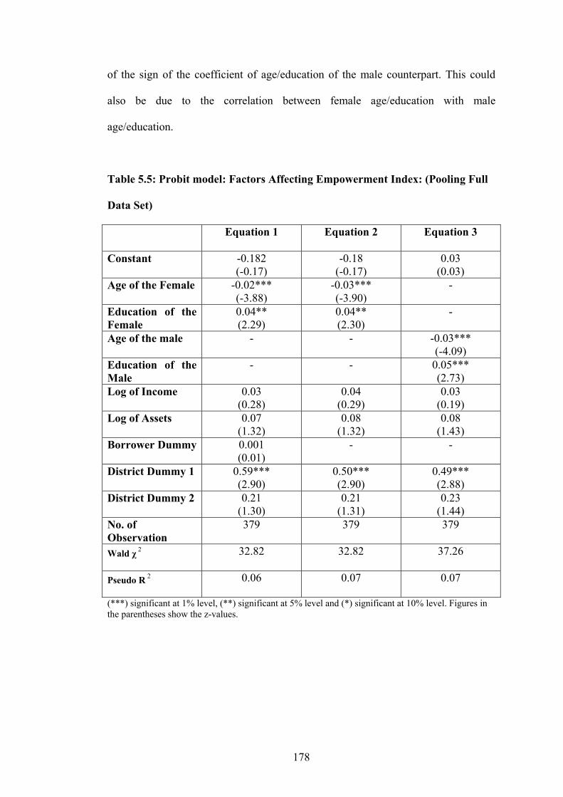
178

of the sign of the coefficient of age/education of the male counterpart. This could

also be due to the correlation between female age/education with male

age/education.

Table 5.5: Probit model: Factors Affecting Empowerment Index: (Pooling Full

Data Set)

Equation 1 Equation 2 Equation 3

Constant -0.182 (-0.17)

-0.18 (-0.17)

0.03 (0.03)


-0.03*** (-3.90)

-

Education of the

Female

0.04** (2.29)

0.04** (2.30)

-

Age of the male -

- -0.03*** (-4.09)

Education of the

Male

- - 0.05*** (2.73)

Log of Income 0.03 (0.28)

0.04 (0.29)

0.03 (0.19)

Log of Assets 0.07 (1.32)

0.08 (1.32)

0.08 (1.43)

Borrower Dummy 0.001 (0.01)

- -

District Dummy 1 0.59*** (2.90)

0.50*** (2.90)

0.49*** (2.88)

District Dummy 2 0.21 (1.30)

0.21 (1.31)

0.23 (1.44)

No. of

Observation

379

379 379

Wald χ 2 32.82

32.82 37.26

Pseudo R2

0.06

0.07 0.07

(***) significant at 1% level, (**) significant at 5% level and (*) significant at 10% level. Figures in the parentheses show the z-values.

179

5.8.3 Factors Affecting Empowerment: Considering Different Income Level

Households

From Tables 5.4 and Table 5.5 we have observed that the coefficient of the variables

“income” or “log of income” are not found significant. We have overlooked so far

the possibility that the variables income and assets could be correlated. We have

therefore dropped the income variable from Equation 5.1 and estimated the model

considering log transformed assets alone as an economic variable. We have used

age/education for male and female in separate equations. We have divided the

households into three equal groups based on their income level to determine if their

income level has any impact towards women’s empowerment. We used two income

dummies such as 1DY and 2DY . 1DY = 1 for low income group and zero otherwise.

2DY = 1 for middle income group and zero otherwise. After adding the dummies the

model is as follows:

)3.5()( 21 iiiiiiii DYDYLnASEEFEMAFEMEIP εϕθλγβα ++++++=

We have estimated Equation 5.3 for the whole group (borrowers and non-

borrowers). Equations 3 and 4 (columns 1 and 2 of Table 5.6) show the estimation

results of Equation 5.3 for female and male respectively. From Table 5.6 we found

that the age of female is significant. Education of the female is significant at the 10%

level. The coefficient of age of the male is found negative and significant. This

implies that a younger male also encourages a woman’s empowerment. The

coefficient of education for both male and female is found positive. This reinforces

180

the importance of education for both male and female in bringing women’s

empowerment.

Table 5.6 further shows that after dropping the income variable (as one of the

economic factors) we found the coefficient of assets is positive and significant at the

5% and 10% levels. Families with more assets are definitely privileged which may

contribute towards better facilities to empower the female in the family.

Furthermore, it is observed that the middle income group household is significantly

different (at the 5% and 10% level) from low and high income group household.

There is no plausible explanation for the negative coefficient of this income dummy.

There may be some data discrepancies (one of the limitations of primary data) which

prevent a reasonable explanation here.

181

Table 5.6: Probit Model: Factors Affecting Empowerment Index: Based on

Different Income Level Households


Constant 0.28 (0.55)

0.38 (0.72)


-

Education of the Female 0.04* (1.75)

-

Age of the Male -

-0.03*** (-4.07)

Education of the Male -

0.04** (2.33)

Log of Assets 0.11* (1.94)

0.11** (1.97)

Low Income Dummy 0.02 (0.11)

0.04 (0.21)

Middle Income Dummy -0.33** (-2.01)

-0.32* (-1.94)

No. of Observations 387 387

Wald χ 2 26.94

34.63

Pseudo R2

0.06

0.07

(***) significant at 1% level, (**) significant at 5% level and (*) significant at 10%level. Figures in the parentheses show the z-values.

5.8.4 Do Microcredit Programs Empower Women?

In this section we want to determine the effect of microcredit program on women’s

empowerment. We have therefore considered only the borrowers’ sample (as non-

borrowers do not have credit). We have used the simultaneous equations model as

presented in Chapter Three with some modification for the purpose of estimation.

182

As in Chapter Three we first assume “credit” depends on “Demographic Factors”

(DF), “Economic Factors” (EF) and unknown factors different from DF and EF.

These unknown factors are the “instrumental variables” used in the model. The

model takes the following form:

)4.5(C

iiicicici ZDDEFDFC επδγβα +++++=

where iC is the amount of credit of i-th individual, iDF is the vector of some

demographic variables (age, education, husband’s age, husband’s education) of i th

borrower, iEF is the vector of some economic variables (household assets,

household income) of i-th household, iDD is the district dummy of i-th district and Z

represents the instrumental variable, which is different from DF, EF and DD. In this

equation we have used “types of houses” and “number of earners” as instruments.

πγβ ,, are the parameters and icε is the error term. In our estimation we used log

transformed variables for amount of credit as well as for the economic variables.

Women’s empowerment may also depend on credit. We have therefore; formulate

the following equation which shows that the EI may also depend on the same

demographic factors, economic factors and also on “credit”. Therefore, the equation

takes the following form:

)5.5()(E

iiiEiEi CEFDFEIP εδγβα ++++=

where, P( iEI )is the probability of i-th borrower to be empowered. δγβ ,, are the

parameters and iEε is the error term. To solve these two simultaneous equations

183

models, we first estimate Equation 5.4 using OLS estimation. We then estimate

Equation 5.5 using the estimated value of amount of credit using Probit estimation.

The results of OLS estimation of Equation 5.4 is provided in Table 5.7. White

corrected standard errors are used to allow for heteroscedasticity.

Table 5.7: OLS Estimation of Equation 5.4

Constant 5.92*** (12.68)


Education of the Female -0.002 (-0.24)

Log of Income 0.26*** (4.75)

District Dummy 1 0.46*** (5.51)

District Dummy 2 -0.08 (-1.19)

Types of Houses 0.07 (1.23)

Number of Earners 0.06 (1.44)


R-Squared 0.32

(***) significant at 1%level, (**) significant at 5% level and (*) significant at 10% t level. Figures in the parentheses show the t-values.

From Table 5.7 we see that credit programs are significantly and positively affected

by the age of borrowers. It also is affected positively by income. The district dummy

for Gazipur shows that Gazipur is significantly different from the two other districts

in terms of program intervention.

184

Table 5.8: Probit Estimation: Using the Estimated Value of Amount of Credit

Constant -2.69* (-1.56)



Estimated Value of Log of Credit 0.55* (1.94)

Log of Income -0.11 (-0.68)

Gender of the Household Head 0.36 (1.54)


Wald χ 2

28.50

Pseudo R2

0.06

(***) significant at 1% level, (**) significant at 5% level and (*) significant at 10%. (Figures in the parentheses show the z-values)

Estimated value of amount of credit obtained from Table 5.7 is used to estimate

Equation 5.5. The results are shown in Table 5.8. We see from Table 5.8 that

woman’s age affect woman’s empowerment significantly. We also see that woman’s

education is significant and positive for woman’s empowerment. Finally we also see

that the coefficient of amount of credit is significant at the 10% level. We may

therefore conclude that microcredit programs affect women’s empowerment

positively. As the amount of credit increases borrowers become more empowered.

This finding reinforces the claim made by the microcredit providers that programs

help in making women empowered.

185

5.9 Conclusion

In this chapter first of all we have introduced “women’s empowerment” as defined

by different researchers. A comparison of the definitions provided by different

researchers is presented in a tabular form. Based on the formal definitions we have

derived our own definition from a different perspective. We then used proxies to

measure women’s empowerment (a subjective term) to quantify it. Detail derivation

of all proxies (termed as indices) are provided in this chapter.

In this chapter we have tried to find out if there is any significant difference between

borrowers and non-borrowers in terms of empowerment. We therefore divided the

sample into two groups and have estimated the equation separately for the two

groups. In this chapter we have also determined factors that may have effect on

women’s empowerment. Finally we have tried to find out whether microcredit

programs have any affect on women’s empowerment. We have used modified

version of the model used by Pitt and Khandker (1996) as presented in Chapter

Three and estimated the simultaneous equations model using 2SLS estimation.

It is observed from the analysis that in terms of ownership of houses, land and

businesses, borrowers of Gazipur are better off compared to non-borrowers as well

as of other districts. It further observed that the borrowers as a whole are better off in

terms of Economic Security Index (ESI) in all districts. However, by looking at the

individual figures it appears that non-borrowers of Dinajpur and Gazipur have more

savings and productive assets respectively compared to the borrowers. There is no

plausible explanation for such a result. In terms of decision-making the overall

186

picture shows that borrowers are better off. In terms of mobility it appears that

female of all districts are more comfortable going out with someone instead of by

themselves. This could be a cultural norm. From careful observation it appears that

borrowers of Chokoria are most mobile. In Dinajpur it appears that non-borrowers

are more mobile compared to borrowers.

The overall picture shows that in terms of awareness there is no difference between

borrowers and non-borrowers. However, the individual depiction shows that

borrowers of Gazipur and Chokoria are more empowered in terms of general

knowledge compared to non-borrowers but not in Dinajpur.

In terms of the Empowerment Index (EI) it is observed that borrowers of Gazipur are

the most empowered compared to non-borrowers as well as other districts. When

comparing borrowers with non-borrowers of all districts, it appears that the

borrowers of Gazipur and Chokoria are more empowered than non-borrowers

whereas in Dinajpur non-borrowers are more empowered than borrowers.

In this study we have tried to find out the factors that may affect women’s

empowerment. Factors are divided in terms of demographic and economic criteria.

Some dummy variables (borrower, district, income) are considered to estimate the

model. It is observed from the analysis that age of the female affects empowerment

negatively. That implies younger women are more empowered. We also have found

that education of the female affects empowerment positively which shows the

importance of education in bringing about women’s empowerment. The most

interesting finding is the age and education of the male partner. It appears that young

187

and educated male encourages women to be more empowered. We further have

observed that assets are positively related to women’s empowerment.

In this study we have found that Gazipur is significantly different from two other

districts in terms of empowerment and also middle income group borrowers are

different from low and high income groups.

We have separated borrowers and non-borrowers to find out if there is any

significant difference between the groups. We also have estimated the full data set

using the borrower dummy. The estimation result (insignificant borrower dummy)

shows that there is no difference between the two groups in terms of empowerment.

This could be due to demonstration effect that non-borrowers are equally empowered

as borrowers. We therefore reject the null hypothesis that borrowers are better off in

terms of empowerment than non-borrowers.

Finally, we have tried to find out the impact of microcredit on women’s

empowerment. 2SLS estimation is used in a simultaneous equations model. It is

observed from the analysis that microcredit places an important role in bringing

women’s empowerment. The positive coefficient shows that as credit increases

woman becomes more empowered. This reinforces the claim made by the

microcredit providers. This result is consistent with Hashemi et al. (1996), Zaman

(1998), Amin and Pabley (1994) and Ackerly (1995). We may conclude that even

though microcredit programs are empowering we cannot say with confidence that

this is only due to microcredit program intervention.

188

Chapter Six

CONCLUSION AND FUTURE RESEARCH

6.1 Introduction

This is an impact assessment study on microcredit organisations in Bangladesh. This

study does not examine the overall poverty level in Bangladesh. Instead it examines

the impact of microcredit programs on household outcomes, income (expenditure)

consumption and women’s empowerment. This is an original and comprehensive

study. The uniqueness of the study is reflected not only in its use of primary source

data, but also in the extent of research performed in the study. Different issues are

addressed in separate chapters. Individual attention has been given to each issue.

Each analytical chapter has addressed new topics and ideas in order to add a new

dimension to the existing research.

The study provides a comprehensive theoretical consideration of rural credit markets

and relates the theory to the performance of microcredit programs in Bangladesh. It

also shows how these programs have overcome the shortcomings of rural financial

markets. The study further establishes the link between the program’s involvement

and the recent socio-economic development of Bangladesh.

The study is conducted using primary data collected from borrowers of two major

microcredit institutions of Bangladesh - the Grameen Bank and Bangladesh Rural

Advancement Committee (BRAC).

189

The impact of microcredit on various household outcomes has been chosen for

study, since such a wide-ranging study has not been conducted previously. The

existing impact assessment studies often provide contradictory results. Such an

intensive study on consumption using microcredit data has not been found in the

prevailing literature. Therefore the consumption behaviour of borrowers compared to

non-borrowers has been considered for analysis in this study. Women’s

empowerment is an important topic. This study defines women’s empowerment in a

different perspective and measures the latent variable “empowerment” through an

index as well as assessing the impact of microcredit on women’s empowerment.

This concluding chapter summarises the study in Section 6.2. Main findings and the

contribution of this study to the existing literature are provided in Section 6.3. Policy

implications are suggested in Section 6.4. Study limitations and suggestions for

further research are provided in Section 6.5 and 6.6 respectively. Concluding notes

are provided in Section 6.7.

6.2 Summary of the Study

The introductory chapter has outlined the framework of this study. It has pointed out

the general hypotheses about the links between microcredit and poverty. Given the

importance of microcredit in the economic emancipation of rural people, the

question arises in the study: “Do microcredit programs in Bangladesh improve

various household outcomes such as income and assets?” To examine the study’s

hypotheses and to answer the question, a comprehensive range of theoretical and

empirical models has been considered.

190

Chapter Two is of fundamental importance. It has presented a broad theoretical

consideration of how the rural financial market developed and worked especially

prior to the microcredit period. Microcredit institutions have reversed the system to

some extent and made rural financing available and affordable for everyone instead

of having a master subordinate relationship in the rural economy. The program has

eliminated potential risk which is a remarkable contribution in rural financial

markets.

Chapter Two also provides an overview of the Bangladesh economy mainly before

the inception of microcredit institutions. It has further discussed the journey of the

two microcredit institutions under study in the past 30 years. It has also shown the

growth and development of these institutions and highlighted their involvement in

social development. The chapter has established a link between the contribution of

these institutions and the recent socio-economic development of Bangladesh.

The last part of Chapter Two has reviewed a wide range of literature on the impact of

microcredit on poverty, women’s empowerment and consumption behaviour. Since

no literature has been found on the impact of microcredit on consumption, an overall

literature on consumption in the context of developed as well as developing countries

have been presented in Chapter Two.

Chapters Three, Four and Five are the core chapters of the study. The three chapters

have been designed in three different ways. They differ in terms of use of

econometric techniques as well as use of models. In Chapter Three we have assessed

the impact of microcredit on various household outcomes such as income (total

191

expenditure is used as a proxy for income) and assets. The chapter has adapted a

modified version of the model used by Pitt and Khandker (1996). In the

simultaneous equations model we have divided the independent variables in terms of

demographic as well as community infrastructure.

We used Two-Stage Least Squares estimation (2SLS) to determine the impact of

credit on the log transformed variables (total expenditure and asset accumulation).

The borrowers are divided into three categories according to their income levels. We

have estimated the impact of credit on different income level borrowers. We have

used Tobit estimation using non-borrowers as the censored group.

Chapter Four has presented a comparative analysis of microcredit borrowers with

non-borrowers in terms of consumption. We have considered consumable food and

non-food items that are commonly used by the rural people. The chapter has

introduced the relevant theories such as mixed demand theory and an Almost Ideal

Demand System (AIDS) and then it has specified the model that has been used for

analysis.

In Chapter Four we have divided the households into three groups based on their

income level. In this chapter we have estimated each equation in the model using

OLS to see the difference in consumption between different income level

households. We have then tested for significant differences between borrowers and

non-borrowers. To test for robustness we have introduced an interactive variable in

the model to see the difference between the two groups in terms of the intercept as

192

well as the coefficient terms. Joint coefficient tests have also been undertaken in this

chapter.

The model that has been estimated in Chapter Four contains multiple equations; OLS

estimation estimates each equation in the model one at a time. Seemingly Unrelated

Regression (SURE) analysis estimates all the equations in the model as a set

allowing for covariance of error terms. Therefore, we have estimated the multiple

equations model using SURE in this study.

Chapter Five is on women’s empowerment. Women’s empowerment has been

defined from a different perspective and an index is developed to measure the latent

variable “empowerment”. In the development of an empowerment index we have

discussed five empowerment correlates that have been used to define empowerment

in this study. These small correlates are used to develop the EI. Since EI is a binary

variable Probit estimation is used to analyse the model. Finally in this chapter we

have used the same simultaneous equations model as used in Chapter Three to find

out the impact of credit on women’s empowerment.

6.3 Key Findings of the Study

The 2SLS estimation in Chapter Three shows that the amount of credit has a positive

impact in bringing higher income and assets for borrowers. This is a very important

finding as it confirms the claims made by the microcredit providers. This is an

indication that microcredit programs are helping borrowers to achieve better quality

of life through higher income and assets. Age of both male and female is important

193

in bringing higher income and assets. Our results suggest that income and assets

accumulation increases as people gets older. Education plays an important role to

enhance borrowers’ income and assets. Number of adult males as a percentage of

family size is also a significant factor that brings higher income and assets. The

analysis further shows that male-headed households benefit from microcredit

programs. Infrastructural facilities such as having electricity are important factors for

credit programs to be effective in producing household outcomes. However, when

these borrowers are divided into different income levels it gives an interesting

picture. The findings of this study show that even though microcredit is improving

overall household income and assets it is more effective for higher income level

borrowers. As the amount of credit increases, income of only the high income level

borrowers increases. It may be concluded from these findings that microcredit

programs are effective only for the high income group borrowers in producing better

household outcomes. Tobit estimation is used considering non-borrowers as the

censored data. The estimation results are no different than the 2SLS estimation.

To estimate the consumption of different income group borrowers and non-

borrowers we have divided the households into three groups in Chapter Four. The

AIDS model is initially estimated using OLS. From the estimation cereal is found to

be a necessary item for all income group households. Small changes in income will

cause bigger changes in cereal consumption for low income group households. That

means cereal is income elastic for low income group households. It is found that

higher income group borrowers are better off in terms of cereal consumption. The

estimation result shows that there is difference in consumption between districts in

terms of cereal consumption.

194

Lentils (pulses) and vegetables are found to be necessary items for all income group

households. It is also found that the high income level borrowers are better off in

terms of pulses consumption. The test result suggests that there is a variation in

consumption of vegetables, pulses and sugar consumption between districts.

Protein (beef, mutton, chicken, fish, milk and eggs) are found to be non-necessary

items for all income group households. Borrower dummy is found significant for all

income groups in case of meat and fish consumption. This implies that there is a

difference in consumption of meat and fish between borrowers and non-borrowers.

Our results suggest that microcredit borrowers are better off in terms of protein

consumption. From these results we may conclude that the microcredit programs

improve consumption for borrowers.

Cigarette, betel leaf and betel nuts are found significant and necessary for high

income group households. Demand for total food for the low income group

household decreases at a higher rate compared to the high income group when there

is a decrease in income. Borrower dummy is found significant for all income groups

for total food consumption. This implies that there is a difference in total food

consumption between borrowers and non-borrowers. This further implies that

borrowers are better off in terms of total food consumption. This result strengthens

our previous suggestion that the microcredit programs are successful in improving

consumption for borrowers.

Education expenses are found non-necessary but significant for the high income

group. However, expenditure on health is found necessary only for high income

195

group households. Total non-food items are found non-necessary for all income

levels. Significant borrower dummy implies that there is difference between

borrowers and non-borrowers in terms of consumption of total non-food items.

The test of robustness indicates that the interactive variable is significant for cereal,

protein, cigarettes, total food, education, fuel and total non-food. It is observed that

items such as pulses, meat, fish, eggs, milk and cloth are more inelastic (steeper)

function for the borrowers. Therefore, it can be concluded that for borrowers’ pulses,

meat, fish, eggs, milk and cloth are essential items.

It is observed from the test result that for both groups, the intercepts as well as the

slopes are different for both food and non-food items. Therefore, the result strongly

suggests that there are significant differences between borrowers and non-borrowers

in terms of consumption of items. The coefficient test result shows statistically

significant coefficients for items such as sugar, protein, education, clothing, total

food and total non-food. Similar results are obtained from SURE estimation.

Chapter Five estimates the EI using Probit model. From the summary table it is

observed that out of 125 borrowers in Gazipur district only 31 borrowers own land in

their own name. The borrowers of Dinajpur own the second highest percentage of

houses or land. Out of total borrowers only 11% of the sample possesses land or

houses in their own name and only 0.5% of non-borrowers possess their own land.

The productive assets are classified as cattle, ducks and chickens. It is observed that

in terms of productive assets the non-borrowers of Gazipur are highest in percentage

196

ownership. However, in Dinajpur and Chokoria districts borrowers own more

productive assets compared to non-borrowers. It is interesting to see that the

differences in ownership in productive assets are quite low between borrowers and

non-borrowers in all districts. This may be due to the fact that these are common

items in rural Bangladesh.

In Gazipur and Chokoria borrowers have more savings than in Dinajpur. Our study

further shows that only two borrowers of Gazipur and five borrowers of Dinajpur

possess business or poultry in their own name. None of the non-borrowers are found

to have any such businesses in their own names. When summarising the Economic

Security Index (ESI) it is found that the borrowers as a whole are better off in terms

of ownership of assets and in particular the borrowers of Gazipur are better off

compared to two other districts.

In Gazipur district borrowers and non-borrowers both participate more in the

decision-making process. Both the borrowers and non-borrowers of Gazipur have

more control over assets compared to two other districts. Since Gazipur is close to

Dhaka, there may be a capital city influence in women having more control over

assets. In Dinajpur and Chokoria borrowers have more control over assets than non-

borrowers.

In terms of women’s mobility it is observed that the borrowers of all three districts

are more comfortable to visit places on their own compared to the non-borrowers.

Among the borrowers, the females of Gazipur are more independent in terms of

197

mobility, than the female of the other two districts. The mobility ranking from

highest to lowest is Gazipur, Chokoria and then Dinajpur.

The above findings are summarised as indices and used to develop the EI. The

economic security index (ESI) ranking from highest to lowest is Gazipur, Dinajpur

and Chokoria. However, for non-borrowers it is Dinajpur, Gazipur and Chokoria. In

terms of the Purchase Decision Index (PDI), both borrowers and non-borrowers of

Gazipur take a greater part in decision-making process compared to the two other

districts. However, in Dinajpur and Chokoria the difference between borrowers and

non-borrowers is less in terms of PDI, and it appears that the non-borrowers are

slightly better off compared to the borrowers in these two districts.

The analysis further shows that borrowers of all districts have more control over

assets compared to non-borrowers. It is observed that the difference in terms of

control over assets between borrowers and non-borrowers is low in Dinajpur and

Chokoria district while it is quite high in Gazipur district.

It is interesting to see that the women (both borrowers and non-borrowers) of

Dinajpur and Chokoria are more mobile compared to Gazipur. However, comparing

borrowers with non-borrowers, it is observed that borrowers of Gazipur and

Chokoria are more mobile compared to non-borrowers. In Dinajpur, non-borrowers

are more mobile than borrowers. It is further observed that the difference between

borrowers and non-borrowers in terms of mobility is higher in Chokoria than two

other districts.

198

The analysis further shows that over 60% of women (both borrowers and non-

borrowers) are politically aware and have better general knowledge. Borrowers of

Chokoria are the most empowered in terms of the Awareness Index (AI). The table

shows that borrowers of Gazipur and Chokoria are more empowered in terms of AI

compared to non-borrowers of the same district. It is further observed that non-

borrowers of Dinajpur have better general knowledge compared to borrowers of the

same district.

In estimating factors affecting the EI, the test result shows that age of the female is

significant and facilitates women’s empowerment. It further shows that younger

women are more empowered compared to older women. Education of the female is

also a significant factor in facilitating women’s empowerment. It is interesting to see

that the age and education of the male is also significant in facilitating women’s

empowerment.

Assets are other factors that enhance women’s empowerment. However, the

estimation result further suggests that there is no difference between borrowers and

non-borrowers in terms of empowerment. This could be due to demonstration effects

that non-borrowers are equally empowered as borrowers. It is also found that

Gazipur is significantly different from the two other districts. Finally, the 2SLS

estimation result shows that microcredit programs are significant and positive in

bringing women’s empowerment. We may therefore conclude from the results of this

study that microcredit facilitates women’s empowerment.

199

By summarising the results of all the aforementioned analytical chapters we may

conclude that microcredit programs are helping to create higher income and asset

acquisition for borrowers as a whole. From our results it may be concluded that the

microcredit programs provide better quality of life for its borrowers. Our findings

confirm the claims made by microcredit providers. However, when we segregate the

borrowers into groups it appears that microcredit programs are not as effective for

the low and middle income group borrowers as they are for high income group

borrowers.

In terms of consumption, it is observed that borrowers of all income levels are better

off in terms of consumption of relatively expensive food items compared to non-

borrowers. While comparing borrowers of different income levels our results suggest

that high income level borrowers are better off in terms of consumption of few items.

We may conclude that microcredit borrowers are better off in terms of consumption

of most items compared to non-borrowers and high income borrowers are slightly

better off compared to low and middle income level borrowers.

It is found that borrowers as a whole are better off in terms of holding assets

(measured by ESI) compared to non-borrowers. In terms of PDI the results are

mixed. It is found that borrowers of Gazipur and Chokoria are more mobile

compared to non-borrowers while borrowers of Gazipur and Chokoria are more

empowered compared to non-borrowers. However, non-borrowers of Dinajpur are

more empowered compare to borrowers. This finding may be explained through a

casual observation that the district of Dinajpur is culturally more advanced compared

to the two other districts.

200

Our results further suggest that age, education of both female and male as well as

assets of the household facilitates women’s empowerment. It is interesting to find

more than 50% empowered borrowers and non-borrowers in all districts. Finally, it

is found that microcredit programs are positively and significantly facilitating

women’s empowerment. Therefore, we may say that microcredit programs are

successful in empowering its borrowers. We further suggest that microcredit may

also be successful in making non-borrowers (those who are not members of credit

programs) empowered through a demonstration effect.

6.4 Policy Implications

The stated goals of the microcredit institutions are generally consistent with the

development objectives of the government of Bangladesh. Our findings suggest that

credit programs administered by two of these leading institutions are effective in

increasing borrowers’ assets and income. This study also suggests that their

programs are facilitating the empowerment of women, who constitute almost half of

the potential labour force of the country. Therefore, the government should take note

of these findings and try to integrate microcredit institutions like the Grameen Bank

and BRAC to make a coordinated effort to overcome major hindrances to the

economic development of Bangladesh.

One incidental finding of this study deserves special attention. Though the overall

evidence of this study tends to suggest that microcredit is an attractive tool to

produce better outcomes in terms of income, assets and consumption we have also

found that such favourable outcomes often accrue to the relatively wealthy

201

borrowers compared to the non-wealthy borrowers. We interpret this finding as an

apparent weakness of the present programs. Therefore, some adjustment to existing

microcredit programs should be made to achieve the intended outcome of such

programs, which is to assist those at the bottom of the society.

6.5 Study Limitations

There are some limitations in this study. The theory does not provide a unique model

to guide the empirical research for examining the impact of microcredit on various

household outcomes. In this respect, economists and researchers have applied

different econometric methodologies and techniques to establish the possible link

between microcredit program and household outcomes.

More precisely, there is no comprehensive theoretical framework in terms of rural

financial market and/or microcredit programs that are required for microcredit and

its economic impact on household outcomes. In addition, many of the empirical

studies suffer from model misspecification and are also sensitive to data coverage.

This study is based on survey data with limited observations. Since this study is

based on primary data, we could not estimate the impact over time and there may be

some data discrepancies. Income, asset accumulation and consumption expenditure

are self-reported and measured only over a relatively short period in the absence of

time series or panel data.

202

However, given these limitations our study has used sophisticated econometric

techniques on consistent cross-section data collected from three different districts of

Bangladesh from both borrowers and non-borrowers of both the Grameen Bank and

BRAC. Appropriate econometric analyses along with related diagnostics are

provided so as to ensure the rigor of economic interpretations of the results.

6.6 Avenues for Future Research

Microcredit is an attractive tool to produce better outcomes in terms of income and

assets but some of our results suggest that it is more effective for relatively wealthy

borrowers compared to non-wealthy borrowers. It would be a good research question

to pursue in future to uncover why this is the case.

From this discussion it may be concluded that borrowers of microcredit are better off

in terms of consumption patterns compared to non-borrowers. But this does not

necessarily tell us that borrowers are better off only due to microcredit intervention.

It may be the fact that the well-off sections of the society are the borrowers of

microcredit program. It would be a good research question to pursue in the future

through panel data estimation to determine whether this is the case.

203

6.7 Concluding Notes

Microcredit programs in Bangladesh represent a breakthrough for rural financial

markets. Two particularly attention-grabbing features of these programs are their

high recovery rates and the heavy emphasis that they place on women. The unique

credit delivery methods have mitigated the problems of moral hazard and adverse

selection. The founder of the Grameen Bank Professor Yunus, has won the 2006

Nobel Peace Prize for waging war against poverty. This event has strengthened the

importance of microcredit. On paper these eye-catching features may sound too good

to be true, so a comprehensive investigation conducted at this stage would prove to

be invaluable in uncovering the truth. Therefore an examination was crucial from

borrowers’ point of view in understanding the effectiveness of the program.

This study examines the impact of microcredit programs on its borrowers through

the collection and compilation of primary source data. Every attempt has been made

to cover all the economic aspects affecting borrowers in order to make this analytical

study as thorough and comprehensive as possible. Attempts have also been made to

substantiate the claims made by microcredit providers with real world evidence.

An interesting finding of this study is that microcredit has been successful in creating

a better quality of life for borrowers, through enhancing their income, consumption

and assets. Our findings strongly suggest that borrowers are better off in terms of

consumption of most of the food and non-food items. Most importantly this study

shows that microcredit programs are successful in empowering women. It is also

clear from the findings that the intensive credit intervention in the rural economy is

204

creating a demonstration effect among everyone including non-borrowers. There is

no doubt from the results that microcredit has continued to have a revolutionary

effect on the rural economy of Bangladesh. This study has already highlighted how

the programs have spurred the continual growth and development of the people

living in rural areas. The continued success of microcredit in Bangladesh has created

an exemplary template for the rest of the world to adopt.

205

Appendices

7.1 Appendix A: Global Poverty Figures

Global Poverty in 1990 and 1999*

Number of people living on less than $1 per day (millions)

Region 1990 1999

East Asia and Pacific 486 279

Excluding China 110 57

Europe and Central Asia 6 24

Latin America and the Caribbean

48 57

Middle East and North Africa

5 6

South Asia 506 488

Sub-Saharan Africa 241 315

Total 1,292 1,169

Excluding China 917 945

Source: Global Economic Prospects 2003, World Bank.

* The poverty figures have not been updated since 1999.

206

7.2 Appendix B: The Sixteen Decisions of the Grameen Bank

1. The four principles of Grameen Bank-discipline, unity, courage, and hard

work-we shall follow and advance in all walks of our lives.

2. We shall bring prosperity to our families.

3. We shall not live in dilapidated houses. We shall repair our houses and

work towards constructing new houses as soon as possible.

4. We shall grow vegetables all the year round. We shall eat plenty of them

and sell the surplus.

5. During the planting seasons, we shall plant as many seedlings as possible.

6. We shall plan to keep our families small. We shall minimize our

expenditures. We shall look after our health.

7. We shall educate our children and ensure that they can earn enough to

pay for their education.

8. We shall always keep our children and the environment clean.

9. We shall build and use pit latrines.

207

10. We shall drink tube well water. If it is not available, we shall boil water

or use alum.

11. We shall not take any dowry in our son’s weddings; neither shall we give

any dowry in our daughter’s weddings. We shall not practice child

marriage.

12. We shall not inflict any injustice on anyone; neither shall we allow

anyone to do so.

13. For higher income, we shall collectively undertake bigger investments.

14. We shall always be ready to help each other. If anyone is in difficulty,

we shall all help.

15. If we come to know of any breach of discipline in any centre, we shall all

go there and help restore discipline.

16. We shall introduce physical exercise in all our centres. We shall take part

in all social activities collectively.

208

7.3 Appendix C: Household Survey Questionnaire

Household Survey Questionnaire

(This survey questionnaire will only be used for academic purposes)

Identification:

Village Name:--------------------------------------- ---- Bari Name:------------------------------------------ ---- DSS Household (Family) Number:-------------- ------ BRAC eligible Household: Yes NO BRAC VO Member Household: Yes NO Name of Respondent: ------------------------------------------ Name of Household Head: ------------------------------------ Gender of Household Head: ---------------------Male Female

Date of Interview: DD MM YY Interviewed by: Name ------------------------------------------ Signature----------------------------------------

209


Village specific questions

This section will be filled up by any village representatives

Questions

1) Village has Grameen Bank Yes No

2) Village has BRAC Yes No

3) Village has Commercial Bank Yes No

4) Village has electricity Yes No

5) Village has paved road Yes No

6) Village has development program

Yes No

7) How far is the thana headquarter?

Within 1-5 kms Within 6-10 kms More than 10 kms

8) How far is the nearest town? Within 1-5 kms Within 6-10 kms More than 10 kms

9) How far is the commercial bank?

Within 1-5 kms Within 6-10 kms More than 10 kms

10) Access to Primary School. In the village Within 1-5 kms Within 6-10 kms More than 10 kms

11) Access to Secondary/Higher Secondary School.

In the village Within 1-5 kms Within 6-10 kms More than 10 Kms

12) Access to Degree college. In the village Within 1-5 kms Within 6-10 kms More than 10 Kms

210

13) Access to water Tube Well Well River Pond/Lake

14)

How far is the medical centre?

In the village Within 1-5 kms Within 6-10 kms More than 10 Kms

15) Is doctor available? In the village Within 1-5 kms Within 6-10 kms More than 10 Kms

16)

What is the average female wage per month?

17) What is the average male wage?

18) Prices of the items of HSQ258

19) Percentage of Hindu population

20) Proportion of village households owing land of 50 decimals or less

58 Household Survey Questionnaire 2

211


Section 1.1

Individual specific questions

a) Marital Status Single Married Sec (b) Widow Separated Divorced b) If married, do you live in a Single family? Extended family? Sec (c) c) If you live in an extended family, how many generations are living together? Section 1.2

Household specific questions

Relationship

with the

borrower

Sex Age Education

Year of

Schooling

Source of

Income59

Income

Per

month

Land

ownership.

(1) (2) (3) (4) (5) (6) (7)

Borrower 1

Others 2

3

4

5

6

7

8

9

59 income from farming, wage labourer etc.

212

Members if not residing with the household

Sex Age Education Source

of

Income60

Income

Per

month

Land

ownership.

(1) (2) (3) (4) (5) (6) (7)

Father of

the

household

head

Mother of

the

household

head

Father of

the

spouse

Mother of

the

spouse

Brother

of the

household

head

Sister of

the

household

head

Brother

of the

spouse

Sister of

the

spouse

60 wage labourer, farming etc.

213

Section 1. 3 Loan Specification

a) Do you have any loans at present Yes No b) If yes, please answer the following questions Source Use of loans

Cash Kind Land Agri Business Con. Wed. Other

Type Value

(1) (2) (3) (4) (5) (6) (7) (8) (9) (10) (11)

Loan1

Loan2

Loan3

Loan4

Friend/relatives =1, Moneylender =2, BRAC =3, GB = 4, Commercial Bank =5, Other =6. Con. Stands for Consumption and Wed. stands for daughter’s wedding

Section 1.4

Borrower specific information (BRAC/GB)

a) How many times did you borrow money from BRAC/GB b) Please specify the following

No.of

loans

Date

started

Date

ended

(contract)

Date

ended

(actual)

Instalment

(Amount) No. of

Instalments PurposeAmount

(Total)

(1) (2) (3) (4) (5) (6) (7) (8)

1

2

3

4

Sec 1.5

214

Section 1.5

Household current savings

Type Amount

(1) (2)

Cash in hand

BRAC

Grameen Bank

Other Banks

Other

Section 1.6

Income from different sources of the family members (Last month)

Income

Generating

Activities

Name

of the

family

membe

rs

No. of

hours

worked

Income from sales Expenditure

Cas

h

In kind Cash In kind

Goods Value

Taka

Goods Value

Taka

(1) (2) (3) (4) (5) (6) (7) (8)

Wage

Agriculture

Langgol chalano

Ropon

Nirano

Kata

Processing

Other

Daily labour other than Agriculture

Net making

Katha salai

Madur tairi

Bamboo and cane work

Egg selling

Milk selling

Chuckles Selling

Veg. garden

215

Mudir dokan

Biri making

Brick breaking

Jogan dai

Poultry

Nursing

Food for work

Overseas

Section 1.7

Assets

Items Land size/

number

Value of the

Items

(1) (2) (3)

1) Type of houses Brick

Tin

Mud

Other

2) Chair

3) Table

4) Cycle

5) Bed

6) Mosquito net

7) Radio

8) TV

9) Fishing net

10) Rickshaw

11) Tube well

12) Sanitary toilet

13) Duck

14) Chicken

15) Cow

16) Goat

17) Mudi shop

18) Mobile phone

19) Other assets: List

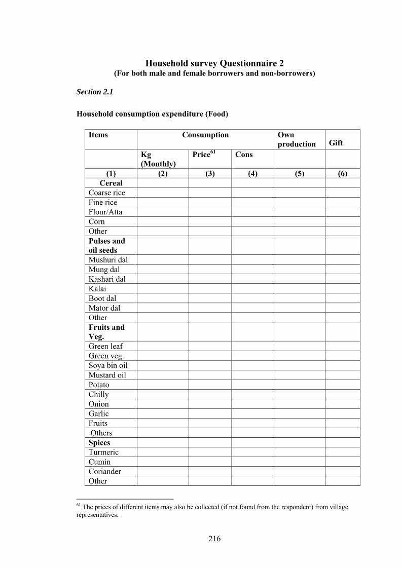
216

Household survey Questionnaire 2 (For both male and female borrowers and non-borrowers)

Section 2.1

Household consumption expenditure (Food)

Items Consumption Own

production Gift

Kg

(Monthly)

Price61

Cons

(1) (2) (3) (4) (5) (6)

Cereal

Coarse rice

Fine rice

Flour/Atta

Corn

Other

Pulses and

oil seeds

Mushuri dal

Mung dal

Kashari dal

Kalai

Boot dal

Mator dal

Other

Fruits and

Veg.

Green leaf

Green veg.

Soya bin oil

Mustard oil

Potato

Chilly

Onion

Garlic

Fruits

Others

Spices

Turmeric

Cumin

Coriander

Other

61 The prices of different items may also be collected (if not found from the respondent) from village representatives.

217

Protein

Big fish

Items Consumption

Own

production Gift

Kg

(Monthly)

Price62

Cons

(1) (2) (3) (4) (5) (6)

Small fish

Chicken

Beef

Mutton

Eggs

Cow’s milk

Powder milk

Sugar/Molasses

Others

Tea

Cigarette/Biri

62 The prices of different items may also be collected (if not found from the respondent) from village representatives.

218

Section 2.2

Household consumption expenditure (Non-food)

Items Unit Own

Production

Gift

(1) (2) (3) (4) (5) (6)

Fuel Monthly

Kerosene

Wood

Gas

Electricity

Other

Clothes Yearly

Women’s wear

Men’s wear

Kid’s wear

Education Yearly

Books

School fees

Tutor’s fees

Other

Health Yearly

Medicine

Doctor

Travel to doctor /Hospital

Other

Other

expenditure

Yearly

Utensils

Bedding

Furniture

House repair

Cycle

TV

Radio

Other

219

Items

Unit Own

Production

Gift

(1) (2) (3) (4) (5) (6)

Travel Monthly

Bus

Train

Rickshaw

Entertainment

Cinema

Theatres

Circus

Other

220

Household survey questionnaire 3

(For female borrowers and non-borrowers only)

Section 3.1

General Questions

(This section will only be filled if HSQ1 has not been filled) Identification:

Village Name: -------------------------------------- ----- Bari Name: ------------------------------------------ ---- DSS Household (Family) Number: ------------- ------- BRAC eligible Household: Yes NO BRAC VO Member Household: Yes NO Name of Respondent: ------------------------------------------ Age of the Respondent: ----------------------------------------- Name of Household Head: ------------------------------------ Gender of Household Head: ---------------------Male Female

Date of Interview: DD MM YY Interviewed by: Name ------------------------------------------ Signature----------------------------------------

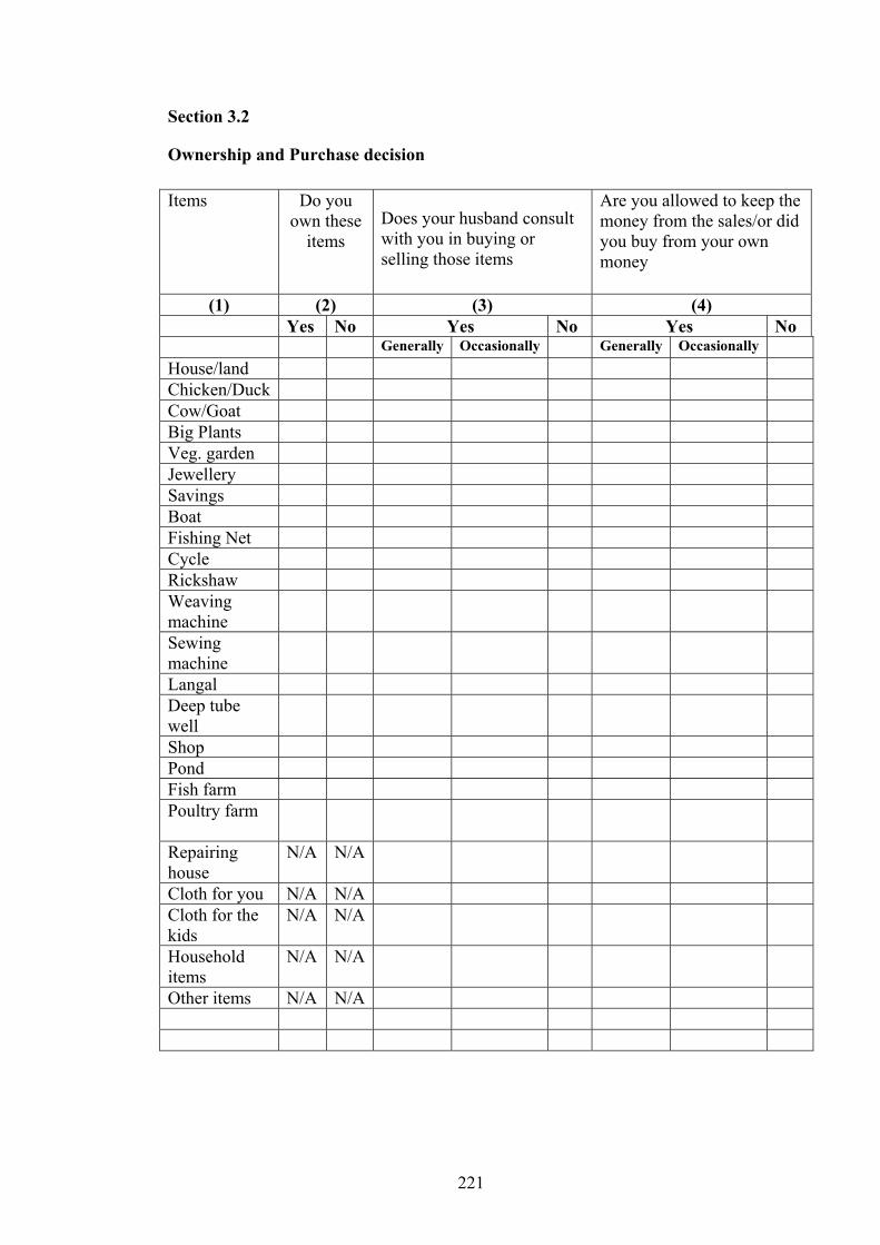
221

Section 3.2

Ownership and Purchase decision

Items Do you own these

items

Does your husband consult with you in buying or selling those items

Are you allowed to keep the money from the sales/or did you buy from your own money

(1) (2) (3) (4)

Yes No Yes No Yes No

Generally Occasionally Generally Occasionally

House/land

Chicken/Duck

Cow/Goat

Big Plants

Veg. garden

Jewellery

Savings

Boat

Fishing Net

Cycle

Rickshaw

Weaving machine

Sewing machine

Langal

Deep tube well

Shop

Pond

Fish farm

Poultry farm

Repairing house

N/A N/A

Cloth for you N/A N/A

Cloth for the kids

N/A N/A

Household items

N/A N/A

Other items N/A N/A

222

Section 3.3

Mobility

In last four months

did you visit these

places

Yes No If yes

Generally Occasionally On

your

own

Accompanied

by others

(1) (2) (3) (4) (5) (6)

Local Market

Sub divisional town

Father’s place

BRAC office

ICDDR,B office

Court

Health centre

Govt. Office

Other Places

Section 3.4

Family issues

Items Between you and your

Husband

Between you and your in-

laws

(1) (2) (3)

Yes No Yes No

Your money has been taken away from you against your will

Your land/Jewellery/Cow has been taken away from you against your will

You have been forbidden to visit your father’s place

You have been physically abused

223

Section 3.5

General knowledge and use of contraceptives

Items Yes No

(1) (2) (3)

Do you know the name of the local Union Parishad Chairman? (Interviewer must know all the answers before hand)

Do you know the name of the Prime Minister of the Country?

Do you know anybody who has taken or given dowry in their son/daughter’s wedding in your village?

Do you know that dowry is illegal?

Do you know the minimum marriage age for a girl?

Do you know the procedure of divorce?

Women are working outside house now; do you think it is good?

Do you use any contraceptives

Do you take the decision of using it in consultation with your husband?

224

Section 3.6

Some additional questions

Items

(1) (2) (3)

What is the ideal family size in your view?

If you were given another chance how many kids would you have?

What should be the time gap between two kids in your opinion?

What is the number of your surviving children

What is the age of your youngest child?

How old are you?

How old were you when you got married?

How many years of schooling did your parents do?

Do you watch NEWS from TV/Radio or both?

Are you aware of AIDS? Yes No

In your assessment are you in good health

Yes No

In your assessment what is the general condition of your children

Good Not good

How many times have you visited your parent’s house in last year

If you do not visit quite often, is it because of

1. Due to security reason

2. You are unable to go on your own

3. You do not have any one to go with

4. Your husband does not allow you to go

Did you receive any training from BRAC/GB?

Yes No

225

7.4 Appendix D: Map of Bangladesh

Map of Bangladesh

RED = Areas in which data was collected

226

7.5 Appendix E: List of the Villages

The following list shows villages from which data have been collected.

Bangladesh Gazipur 1. Bagia 2. Meghlal 3. Kholapara 4. Borabo 5. Ambagh Dinajpur 1. Sheikh hati 2. Ramjiban pur 3. Paschim Shibrampur 4. Bangshi pur 5. Kamalpur Chokoria 1. Bharamuhuri 2. Binamara 3. Nishpan khali 4. Lakharchar 5. Kahariaghona

227

7.6 Appendix F: Descriptive Tables of consumption patterns Table 1

Descriptive table (borrowers of Gazipur district)

Number of observations 125

Mean Median Max. Min. St. dv. Norm. Skew. Kurt.

Cereal 835.881 755 2200 450 288.23 237.08 (0.00)

1.98 8.42

Pulses 197.12 192 650 0 101.51 42.21 (0.00)

1.00 5.04

Vegetables 561.16 552.5 1130 134 186.22 0.83 (0.65)

0.18 3.13

Meat & Fish 1385.65 1080 5500 165 1028.01 29.64 (0.00)

1.07 3.99

Milk & Eggs 444.23 287.5 1750 18 336.67 16.50 (0.00)

0.87 3.33

Cigarette 363.88 310 1200 0 234.21 191.89 0.00()

0.41 2.94

Cooking Oil 203.07 198 450 36 91.17 6.69 (0.033)

0.55 2.75

Spices 228.34 220 450 58 96.11 6.72 (0.039)

0.54 2.68

Sugar 299.05 280 700 0 170.07 4.58 (0.020)

0.33 2.35

Total Food 4518.41 4001 12745 1308 2275.92 14.21 (0.00)

0.81 3.12

Fuel 176.12 144.5 890 11 110.19 963.61 (0.00)

2.51 15.58

Electricity 194.81 200 800 60 114.17 756.80 (0.00)

2.86 13.54

Clothing 236.43 210 560 50 142.92 11.37 (0.0033)

0.58 2.10

Education 252.32 100 1500 0 363.03 117.11 (0.00)

1.89 5.83

Health 247.46 210 1000 0 207.03 81.86 (0.00)

1.50 5.55

Travel 572.02 400 3100 0 647.64 429.32 (0.00)

2.71 10.23

Entertainment 10 0 500 0 58.88 10893.8 (0.00)

6.44 46.87

Other 427.48 295 2500 0 533.87 280.89 (0.00)

2.37 8.51

Total non-

food 2116.60 1622 9030 231 1835.52 275.58

(0.00) 2.34 8.52

Total expenditure

6635.01 5484 18912 1539 3803.14 37.02 (0.00)

1.21 4..07

Total Production

880.90 765 3200 0 742.04 10.64 (0.006)

0.71 3.06

Family size 4.61 4 10 2 1.32 87.31 (0.00)

1.20 6.29

Family Income

8877.81 6750 27000 2000 5579.32 43.40 (0.00)

1.29 4.13

The figures in the parentheses represent probability.

228

Table 2

Descriptive table (non-borrowers of Gazipur district)


Mean Median Max. Min. St. dv. Norm. Skew

.

Kurt.

Cereal 745.28 695 2500 450 291.65 1345.37 (0.00)

4.26 26.41

Pulses 195.53 194 420 0 79.10 1.38 (0.50)

0.35 3.38

Vegetables 507.82 543 950 185 138.28 2.64 (0.30)

0.21 4.02

Meat & Fish 624.71 550 2600 100 469.15 97.18 (0.00)

2.07 8.25

Milk & Eggs 193.17 187.5 555 30 102.40 26.29 (0.88)

1.20 5.51

Cigarette 265.48 250 600 0 131.67 0.18 (0.63)

0.13 3.12

Cooking Oil 182.81 184 380 56 68.58 3.78 (0.15)

0.63 3.35

Spices 206.03 205 350 90 57.63 0.023 (0.98)

0.04 2.94

Sugar 137.07 115 350 0 83.43 2.75

(0.25)

0.50 2.48

Total Food 3057.23 3078.5 7956 1085 1168.32 63.58 (0.00)

1.59 7.3

Fuel 131.40 125 282 22 49.13 5.59 (0.06)

0.50 4.21

Electricity 166.63 192.5 250 50 45.10 5.50 (0.04)

-0.76 2.56

Clothing 123.75 102.5 310 20 71.47 14.13 (0.02)

1.24 3.57

Education 95.57 30 400 0 118.26 8.46 (0.014)

0.97 2.74

Health 189.28 130 1000 20 163.06 303.67 (0.00)

2.81 13.41

Travel 488.07 450 1200 100 256.00 4.09 (0.13)

0.68 3.04

Entertainment 5.55 0 200 0 30.19 2575.62 (0)

5.66 34.88

Other 325.28 300 700 0 182.60 0.69 (0.70)

0.21 2.64

Total non-

food

1525.67 1445 2608 430 484.80 0.42 (0.78)

0.18 2.74

Total

expenditure

4582.90 4386 9230 1515 1407.26 4.89 (0.06)

0.58 3.93

Total

Production

632.98 600 1660 0 471.38 2.40 (0.27)

0.31 2.15

Family size 4.38 4 9 2 1.23 25.99 (0.00)

1.11 5.65

Family

Income

4450.81 4000 11667 1400 1755.04 56.50 (0.00)

1.57 6.89


Table 3

229

Descriptive table (Both borrowers and non-borrowers of Gazipur district)



Cereal 809.41 750 2500 450 291.35 902.23 (0.00)

2.57 12.75

Pulses 196.65 192 650 0 95.09 56.22 (0.00)

0.92 5.05

Vegetables 545.58 550 1130 134 174.90 3.62 (0.15)

0.28 3.40

Meat & Fish 1163.35 750 5500 100 964.45 83.45 (0.00)

1.38 4.87

Milk & Eggs 370.88 242 1750 0 310.12 63.40 (0.00)

1.29 4.37

Cigarette 335.14 300 1200 0 213.88 12.89 (000)

0.61 3.47

Cooking Oil 196.94 196 450 36 85.54 12.15 (0.00)

0.63 3.03

Spices 221.83 210 450 58 86.87 12.47 (0.001)

0.64 3.17

Sugar 251.73 220 700 0 167.00 13.84 (0.000)

0.66 2.69

Total Food 4091.55 3318 12745 1085 2120.22

44.41 (0.00

1.12 3.96

Fuel 163.02 135 890 11 98.56 2048.11 (0.00)

2.76 18.66

Electricity 186.58 200 800 50 99.78 1855.43 (0.00)

3.20 17.46

Clothing 203.51 150 560 20 136.15 25.03 (0)

0.90 2.70

Education 206.53 100 1500 0 319.78 349.55 (0.00)

2.30 8.08

Health 230.47 200 1000 0 196.56 198.29 (0.00)

1.77 6.75

Travel 547.5 400 3100 0 562.64 1048.01 (0.00)

3.03 13.21

Entertainment 8.65 0 500 0 51.87 22281.22 (0)

6.94 55.86

Other 397.62 300 2500 0 461.58 763.22 (0.00)

2.75 11.51

Total non-

food 1943.97 1512.5 9030 231 1587.1

28 832.01 (0.00)

2.84 11.93

Total expenditure

6035.52 5103.5 18912 1515 3415.24

119.71 (0.00)

1.57 5.49

Total Production

808.47 705 3200 0 682.39 22.46 (0.00001)

0.83 3.52

Family size 4.54 4 10 2 1.29 116.03 (0.00)

1.18 6.16

Family Income

7592.85 5875 27000 1400 5188.71

116.03 (0.00)

1.67 6.16


230

Table 4

Descriptive table (borrowers of Dinajpur district)



Cereal 874.78 797.5 2450 350 344.35 231.91 (0.00)

1.96 8.16

Pulses 191.78 177 540 0 82.30 35.62 (0.00)

0.84 4.91

Vegetables 520.84 500 1200 200 168.95 37.53 (0.00)

0.97 4.74

Meat & Fish 719.68 450 3000 120 644.73 40.29 (0.00)

1.48 4.52

Milk & Eggs 227.15 150 950 0 220.95 107.71 (0.00)

1.80 5.55

Cigarette 185.66 200 680 0 171.88 16.67 (0.05)

0.85 3.28

Cooking Oil 165.07 144 550 48 76.34 116.42 (0.00)

1.30 6.78

Spices 169.43 165 560 50 75.13 155.66 (0.00)

1.44 7.46

Sugar 147.18 99.5 650 0 153.40 87.19 (0.00)

1.62 5.2

Total Food 3201.61 2733 9510 1070 1687.62 78.24 (0.00)

1.54 5.217

Fuel 143.19 120 480 11 88.55 57.67 (0.00)

1.28 4.97

Electricity 68.03 0 320 0 89.69 23.86 (0.00)

1.04 2.96

Clothing 182.11 120 750 20 148.29 134.50 (0.00)

1.84 6.28

Education 92.91 0 1250 0 203.88 1160.30 (0.00)

3.37 15.86

Health 153.71 120 550 0 112.14 66.07 (0.00)

1.38 5.08

Travel 323.48 200 2000 0 426.93 272.95 (0.00)

2.21 8.47

Entertainment 2.27 0 200 0 19.40 41462.64 (0.00)

9.08 87.90

Other 164.20 100 2000 0 274.09 2247.43 (0.00)

3.78 21.74

Total non-

food

1129.93 876.5 6290 64 1086.26 374.64 (0.00)

2.34 9.78

Total

expenditure

4331.54 3631 15460 1415 2672.75 161.47 (0.00)

1.87 6.92

Total

Production

217.42 95.5 1060 0 276.34 50.42 (0.00)

1.40 4.14

Family size 5.8 5 12 3 1.92 14.58 (0.00)

0.80 3.25

Family

Income

5257.62 4500 20000 1500 3089.17 178.12 (0.00)

1.81 7.39

The figures in the parentheses represent the probability.

231

Table 5

Descriptive table (non-borrowers of Dinajpur district)


Mean Median Max. Min. St. dv. Norm. Ske. Kurt.

Cereal 926.09 780 2300 450 454.42 44.04 (0.00)

1.72 5.27

Pulses 201.33 188 660 44 109.35 82.26 (0.00)

1.68 7.53

Vegetables 505.48 477.5 1250 200 168.70 87.98 (0.00)

1.63 7.83

Meat & Fish 461.61 240 3000 65 557.22 198.36 (0.00)

2.57 10.09

Milk & Eggs 166.17 118 1100 15 160.71 837.21 (0.02)

3.45 19.62

Cigarette 153.70 150 650 0 143.86 15.62 (0.20)

1.02 4.36

Cooking Oil 173.27 167.5 450 50 72.87 23.34 (.00)

1.03 5.17

Spices 154.19 145 330 50 62.52 5.38 (0.05)

0.72 3.03

Sugar 101.37 36 650 0 132.93 143.11 (0.00)

2.37 8.73

Total Food 2843.25 2356.5 9780 1159 1556.78 122.23 (0.00)

2.10 8.43

Fuel 114.06 104 380 12 72.96 32.41 (0.00)

1.31 5.37

Electricity 63.87 0 280 0 83.43 10.10 (0.01)

0.98 2.82

Clothing 133.82 100 550 20 111.36 121.58 (0.00)

2.22 8.22

Education 56.45 0 500 0 95.43 153.67 (0.00)

2.26 9.24

Health 132.5 100 500 0 106.35 51.02 (0.00)

1.64 5.99

Travel 229.83 200 3000 0 406.91 2946.01 (0.00)

5.20 35.35

Entertainment 13.49 0 600 0 81.42 5134.88 (0.00)

6.47 45.29

Other 109.83 0 1000 0 180.89 225.00 (0.00)

2.43 10.96

Total non-

food

854.09 592 6780 184 937.11 1674.09 (0.00)

4.28 26.97

Total

expenditure

3697.35 3002.5 16560 11412

2413.12 429.00 (0.00)

2.88 14.52

Total

Production

410.69 300 2928 0 508.58 223.61 (0.00)

2.34 11.02

Family size 6.66 6 15 3 2.78 19.19 (0.00)

1.26 4.03

Family

Income

3862.14 3100 20333 1000 2814.65 874.98 (0.00)

3.44 19.90


232

Table 6

Descriptive table (both borrowers and non-borrowers of Dinajpur district)


Mean Median Max. Min. St. dv. Norm. Skew Kurt.

Cereal 889.27 785 2450 350 382.46 259.39 (0.00)

1.93 7.12

Pulses 194.29 178 660 0 91.70 197.94 (0.00)

1.35 7.13

Vegetables 515.08 500 1250 200 168.57 102.90 (0.00)

1.18 5.65

Meat & Fish 634.78 350 3000 65 627.65 147.76 (0.00)

1.72 5.50

Milk & Eggs 207.85 135 1100 0 204.70 326.23 (0.00)

2.15 7.93

Cigarette 175.83 180 680 0 163.42 30.98 (0.01)

0.92 3.60

Cooking Oil 167.57 155 550 48 74.98 138.81 (0.00)

1.22 6.33

Spices 164.23 150 560 50 71.54 186.41 (0.00)

1.34 6.96

Sugar 132.05 72 650 0 148.16 181.44 (0.00)

1.81 6.02

Total Food 3080.99 2595 9780 1070 1649.37 165.34 (0.00)

1.69 5.96

Fuel 133.77 113 480 11 84.97 100.32 (0.00)

1.33 5.27

Electricity 67.13 0 320 0 87.52 33.65 (0.00)

1.02 2.92

Clothing 166.33 110 750 20 138.84 262.53 (0.00)

1.99 7.05

Education 80.84 0 1250 0 176.79 2824.26 (0.00)

3.74 20.07

Health 146.56 100 550 0 110.32 113.69 (0.00)

1.46 5.32

Travel 294.10 200 3000 0 421.68 1534.24 (0.00)

3.05 15.31

Entertainment 5.89 0 600 0 48.99 108135 (0.00)

10.20 116.54

Other 147.10 0 2000 0 248.34 3891.4 (0.00)

3.81 23.50

Total non-

food

1033.03 822 6490 94 986.72 1159.08 (0.00)

2.79 13.55

Total

expenditure

4122.74 3450 16560 1412 2597.98 404.91 (0.00)

2.13 8.62

Total

Production

278.89 120 2928 0 375.55 1429.55 (0.00)

2.64 15.16

Family size 6.07 6 15 3 2.26 81.42 (0.00)

1.27 4.88

Family

Income

4806.77 4000 20333 1000 3066.58 495.42 (0.00)

2.14 9.52


233

Table 7

Descriptive table (borrowers of Chokoria district)



Cereal 724.17 685 1375 310 213.34 12.18 (0.002)

0.68 3.57

Pulses 196.97 200 410 45 80.27 4.49 (0.099)

0.44 2.83

Vegetables 448.71 450 1200 150 149.40 96.62 (0.00)

1.06 6.62

Meat & Fish 875.37 595 2675 0 706.50 27.79 (0.000)

1.12 3.12

Milk & Eggs 296.70 200 975 0 230.42 32.09 (0.00)

1.18 3.49

Cigarette 269.42 200 850 10 184.52 23.79 (0.00)

1.00 3.57

Cooking Oil 167.51 170 360 50 55.34 2.88 (0.17)

0.28 3.55

Spices 160.19 150 350 50 57.37 7.42 (0.021)

0.55 3.35

Sugar 247.97 210 680 16 169.33 16.72 (5.213)

0.87 2.91

Total Food 3387.05 2998 7889 935 1304.63 19.00 (0.000075)

0.87 3.65

Fuel 168.61 156 360 20 71.17 2.21 (0.32)

0.20 2.50

Electricity 131 150 500 0 105.86 2.66 (0.26)

0.35 3.03

Clothing 181.65 165 500 20 92.26 19.28 (0.000)

0.90 3.54

Education 141.53 120 600 0 149.82 20.43 (0.000)

0.95 3.33

Health 205.61 200 600 0 128.26 25.23 (0.000)

1.02 3.67

Travel 373.84 300 2000 0 333.59 293.66 (0.00)

2.06 9.09

Entertainment 0 0 0 0 0 - - -

Other 262.76 200 1500 0 295.63 189.83 (0.00)

1.85 7.61

Total non-

food

1465.03 1297.5 5120 175 927.72 88.35 (0.00)

1.48 5.74

Total

expenditure

4800.7 4324 11666 1175 2053.77 20.88 (0.000)

0.91 3.68

Total

Production

156.32 0 1590 0 284.25 303.91 (0.00)

2.27 8.94

Family size 5.64 6 11 2 1.49 3.69 (0.15)

0.16 3.76

Family

Income

6150.19 5500 17000 1300 2862.91 51.75 (0.00)

1.19 4.96

The figures in the parentheses represent the probability

234

Table 8

Descriptive table (non-borrowers of Chokoria district)



Cereal 718.78 667.5 1565 425 219.27 36.00 (0.00)

1.37 5.39

Pulses 192.06 180 350 72 83.17 5.61 (0.06)

0.36 1.76

Vegetables 391.96 365 650 200 106.38 2.29 (0.28)

0.38 2.50

Meat & Fish 485.68 382.5 1750 125 332.85 97.56 (0.000016)

2.00 7.39

Milk & Eggs 209.29 200 500 0 87.43 25.99 (0.00002)

0.81 5.57

Cigarette 201.89 200 650 15 110.76 33.19 (0.66)

1.06 5.74

Cooking Oil 149.42 135 260 90 47.33 4.95 (0.08)

0.54 2.05

Spices 140.30 130 240 80 46.93 5.09 (0.077)

0.37 1.86

Sugar 141.65 94 550 12 120.62 21.13 (0.00)

1.27 4.09

Total Food 2637.95 2356 5935 1379 969.88 19.97 (0.000046)

1.61 5.49

Fuel 181.19 177.5 320 32 73.47 1.84 (0.3587)

0.02 2.18

Electricity 117.53 150 250 0 89.48 6.29 (0.0431)

-0.23 1.56

Clothing 130.84 105 320 50 63.27 18.67 (0.2759)

1.24 3.79

Education 101.21 0 400 0 129.31 8.68 (0.0109)

0.75 2.06

Health 188.25 200 500 50 78.85 31.07 (0.000001)

1.18 5.37

Travel 368.18 300 1500 0 250.02 108.28 (0.00)

1.73 8.22


Other 262.12 200 1000 0 211.88 9.86 (0.00721)

0.80 3.98

Total non-

food

1348.93 1276.5 4040 395 619.52 61.42 (0.00)

1.38 6.83

Total

expenditure

3986.89 3658 9975 1911 1455.60 45.82 (0.00011)

1.51 6.3

Total

Production

289.51 0 1480 0 393.32 16.02 (0.000537)

1.19 3.38

Family size 5.86 5 11 2 2.30 4.43 (0.1134)

0.41 2.03

Family

Income

4498.23 4100 10000 2000 1612.33 11.16 (0.00513)

0.88 3.95


235

Table 9

Descriptive table (both borrowers and non-borrowers of Chokoria district)



Cereal 722.37 685 1585 310 215.00 40.11 (0.00)

0.92

4.21

Pulses 195.32 200 410 45 81.07 8.07 (0.01)

0.41 2.44

Vegetables 429.70 430 1200 150 138.94 155.45 (0.00)

1.09 6.76

Meat & Fish 744.81 550 2675 0 633.88 90.48 (0.00)

1.50 4.37

Milk & Eggs 269.72 200 975 0 203.31 101.57 (0.00)

1.51 4.77

Cigarette 246.80 200 850 10 166.35 67.17 (0.00)

1.22 4.49

Cooking Oil 161.45 150 360 50 53.77 5.32 (0.06)

0.38 3.22

Spices 153.52 150 350 50 55.02 12.04 (0.002429)

0.58 3.29

Sugar 212.35 180 680 12 162.40 37.05 (0.00)

1.04 3.39

Total Food 3136.08 2659 7675 922 1459.78 76.69 (0.00)

1.21 3.69

Fuel 196.16 165 650 20 113.82 155.55 (0.128)

1.53 6.07

Electricity 126.42 150 500 0 100.38 2.017 (0.3645)

0.24 2.88

Clothing 163.22 120 600 20 101.89 128.88 (0.000001)

1.50 5.57

Education 127.30 100 600 0 144.10 29.99 (0.00)

0.94 3.24

Health 198.95 200 600 0 114.40 61.26 (0.00)

1.16 4.42

Travel 370.55 300 2000 0 307.17 492.97 (0.00)

2.06 9.55


Other 261.21 200 1500 0 269.52 287.01 (0.00)

1.74 7.77

Total non-

food 1443.86 1275 5450 175 903.62 225.96

(0.00) 1.71 6.67

Total expenditure

4579.94 3934 12135 1115 1856.07 51.81 (0.00)

1.33 4.48

Total Production

209.26 0 1590 0 335.65 162.94 (0.00)

1.76 5.71

Family size 5.72 6 11 2 1.80 5.71 (0.057)

0.41 3.06

Family Income

5575.67 5000 17000 1300 2632.89 133.20 (0.00)

1.40 5.88

The figures in the parentheses represent the probability. Max., Min., Stdy., Norm., Skew., and Kurt., are respectively the abbreviation for maximum, minimum, standard deviation, normality, skewness and Kurtosis used in here.

236

7.7 Appendix G: Experiences from Field Trip

My experience from fieldwork

Sampling Procedure

Throughout the course of our fieldwork study, my team and I interviewed six

hundred and ninety-five borrowers and non-borrowers from all over Bangladesh.

The study drew upon the population from four major districts of Bangladesh. These

were based on different agro climatic and economic conditions. The districts were

Gazipur, Dinajpur, Khulna and Chittagong. A cluster of villages from each district

was selected. The household samples were selected using multistage stratified

random sampling from each village in each district. The data collection took place in

July 2004. During this period, nearly two-thirds of the country was under water.

Before leaving for Bangladesh, I had anticipated that I would encounter problems

associated with the monsoon season. However, I did not expect to experience

flooding during my stay. Nevertheless, this was the only time that I could manage to

go for fieldwork between semesters.

My research team consisted of three girls and two boys from Jahangirnagar

University, who assisted me in conducting the fieldwork. We visited several villages

in order to conduct our research. These included Gazipur, located near Dhaka,

Dinajpur, which covers the Northern area, Chokoria, situated near the coast and

Khulna, which lies near south-west of Bangladesh (appendix 1). Interestingly

enough, we only found seven male borrowers in our total surveyed sample as the

vast majority were female.

237

2. My experience from fieldwork

I underwent several exciting experiences as I visited the numerous villages of

Bangladesh. The villagers assumed that we represented the “Sarker63” (Bangladesh

Government). They were convinced that we were collecting information to pass on

to the Government, because we kept asking questions about their assets, incomes and

expenditures.

We repeatedly mentioned that the information that we were gathering would be used

strictly for academic purposes. However, the villagers were not at all convinced by

our remarks. They believed that our research would somehow reach the Government,

who would in turn take care of their problems. In the Chokoria district, one village

representative took me to visit a few of the poorest families and suggested that I

videotape their poor living conditions in order to show the Government. They

expected that I would return with grants, some time in the future. In almost all cases,

the villagers inquired about how they would be reimbursed for their time and service

to us.

The experience was very different in Gazipur. The majority of locals harboured

suspicions regarding our work and were thus unwilling to talk to us. They believed

that we were income tax people, because we wanted information related to their

financial situation.

63 “Sarker” is the Bengali term for the Government.

238

In Gazipur, we were easily able to determine which people were borrowers, because

their clothes, furniture and home accessories provided us with a clear indication of

their present financial situation. We observed that the borrowers were relatively

wealthy and vice versa. All the villages in the Gazipur district were equipped with

electricity, proper toilets, as well as a large range of electrical equipment. These

included colour televisions, stereos, mobile phones and even personal computers.

Gazipur appeared to be the richest place that we had surveyed in terms of health and

wealth of the residents. We noted that the infant mortality rate was much lower in

Gazipur than the other areas that we visited.

Since Gazipur is situated so close to Dhaka, we observed a certain ‘capital-city

influence’ reflected in the attitudes of the local villagers We experienced several

difficulties while trying to get people to talk about personal aspects of their lives,

such as their incomes and expenses. Getting an exclusive interview with borrowers

proved to be an impossible task for us. This was primarily due to husbands of female

borrowers forbidding their wives to disclose private matters to ‘outsiders’.

The district of Dinajpur appeared to be significantly poorer than Gazipur. Villages in

Dinajpur did not have electricity or sanitary toilets. Borrowers were mostly factory

workers, daily labourers and blacksmiths. The crop fields in the villages did not

belong to any of the borrowers. We found the people of Dinajpur to be very friendly,

approachable and down to earth. They took us inside the house offered us a variety

of food items including cow’s milk, rice crisps, jackfruit and other home-grown

fruits. They possessed very few material items, but appeared to be very content with

what they had. The local people were very excited, because they were being filmed.

239

One particular elderly woman even went to the trouble of putting on her best blouse

in order to be captured on film.

One of our most interesting memories of Dinajpur was being able to witness girls

riding bicycles. This scene was unique to the area and would rarely be found

elsewhere in the country. The intervention of Non-Government Organisations

(NGOs) such as BRAC64, led to the introduction of bicycles for the female field-

workers. Even more unusual was our witnessing of girls that were wearing “hijab”65,

riding bikes in the same area. The significance of such seemingly simple scenarios

may not be obvious to everyone, so one must keep the conservative nature and

culture of the locals in mind to fully grasp their importance.

Among the many villages that we visited in the Chokoria district, we came across a

certain village resided by Muslim majority. It was a beautiful village surrounded by

coconut trees. We found a number of NGOs working together at this particular

village. Every household had borrowers from the NGOs. Sometimes, they borrowed

from more than one NGO at the same time.

In the same village, two of our male co-workers found it exceedingly difficult to

interview the female borrowers, because the villagers were very strict Muslims.

According to Islam, females are not allowed to see non-family members without

“parda”66. The female borrowers spoke to the male interviewers from behind doors

64 BRAC stands for Bangladesh Rural Advancement Committee 65 ‘Hijab’ is the head cover used by Muslim women. 66 “Parda” is used to define restrictions in Islam that separate females from males other than their relatives.

240

or fences. The replies to the questions that they were asked were conveyed back to

the interviewers via their husbands.

Some female borrowers told us not to take their photographs, as they did not seek

permission from their husbands. We spoke to one of the schoolteachers working for

BRAC in this village. He mentioned that they always encounter these type of

problems when foreign donors come to visit this village, because the borrowers do

not talk to strangers.

We also visited some villages resided by Hindu and Buddhist majority in the

Chokoria district. The villagers took us to some of their temples and requested that

we videotape the experience. Throughout our journey through the various villages of

the Chokoria district, we witnessed people using water from ponds that was

extremely dirty. They said that they possessed just one tube-well, which was arsenic

free and usable for drinking water.

The Buddhist village that we visited was called “Borua para”. The main occupation

of the villagers was to catch crabs that would ultimately be sold in the international

market. Loans from the Grameen Bank enabled these people to establish such

business.

2.1 Problems in collection data

The time that we had selected for data collection was not at all congenial for

fieldwork. We walked mile after mile through rain, mud and even through flood-

241

water. We realised that carrying out such intensive fieldwork requires an enormous

amount of dedication and perseverance. When we interviewed people we tried to

avoid interrupting their daily routines. Thus, we spoke to them while they cooked,

milked their cows or washed their clothes.

We encountered a number of problems while we were collecting data. Firstly we

wanted to investigate typical household expenses in a certain amount of detail. This

proved to be exceedingly hard for them to explain, as the villagers did not live by a

fixed budget and did not keep track of their daily expenses. Some people felt

uncomfortable when we asked questions about their monthly expenditure. Others

were unable to reply because they could not remember their previous month’s

expenditure. Certain items such as milk, eggs, chicken and fish were produced at

home. This made it difficult for them to estimate their average consumption. We

therefore, had to cross-question them in order to find out the actual amount. We

faced similar problems with the use of cooking wood, as villagers often gathered dry

leaves and wood from neighbours. We also had difficulties with peoples’ incomes.

Not all of them were wage earners, so they were unable to provide details about their

incomes. In many cases the figure that we received would be an over or under-

estimation of the actual figure. We tried calculating the figures from other questions.

In our questionnaires, we included a number of items, which we expected that the

villagers would consume, but in reality, we observed that they consume only a small

variety of common items.

In almost all the cases, the female villagers were unable to provide their husband’s

age or even their own age. We tried finding that from their eldest child’s age and the

242

age at which they were married. Surprisingly, they were also unable to provide us

with general information about their village such as the approximate distance from

one place to another.

Apart from the previously stated difficulties, we also encountered problems relating

to effective communication. We found it difficult to understand various regional

dialects that were specific to various parts of Bangladesh. Although the entire

country speaks a single language (Bengali), these dialects are significantly different

from each other.

My inexperience relating to village life is now very apparent to me and I feel that

this is reflected in the questionnaire, which I prepared prior to my arrival. To record

the type of the houses, I listed four categories: brick, tin, mud and straw houses in

the questionnaire. In reality, we found that most houses were made up of different

combinations of products. Notable features included straw roofs, mud walls and mud

floors. I now realise that I could have asked questions about the type of roof, walls

and floor separately. This in turn, would have greatly assisted me in gathering

information from the locals.

3. Beyond credit program

Do micro credit programs really help the poor? This question cannot be answered in

a single sentence. The impact that micro credit programs have had on the rural

economy has produced mixed results. I spoke to many female borrowers who were

satisfied with the program. Most of them had been borrowers for around ten to

243

fifteen years. It made them extremely happy to be given the opportunity to borrow

money in order to gather assets. They were glad to have tin roofs, tube wells and

land, which would not be possible without the financial assistance received from the

micro credit program. They were also content with the fact that they were now able

to posses a number of cows, goats and chicken. In addition, they stated that they

would not be able to save up to own properties unless they were offered these types

of loans.

We observed that the relatively wealthy families were the ones who were benefited

by the program. Similarly, the long-term borrowers also appeared to be in better

financial condition.

An interesting observation that we made was that although NGOs lend money to

women, in most cases this money is used and managed by the male members of the

family. Generally, the female borrowers borrowed money while their husbands

invested in businesses. The ratio of women whose money was managed by someone

other than themselves to those that handled their own finances was roughly 9:1. As a

result, one may ask why NGOs still continue to lend money to women. This question

needs to be investigated further.

However, there were still some cases where women had successfully borrowed and

managed money. Two such examples included a woman that I met in Gazipur and

one that we met in Dinajpur. Both these women had invested their money wisely and

were thus able to accumulate assets on their own. Such experiences proved to be

244

very empowering for women as they gained confidence in their abilities as

individuals.

The micro credit program has been proven to be highly successful in terms of

recovery. We did not find a single person that had become a defaulter at any time,

because the Grameen Bank takes every measure to ensure that nobody misses his or

her weekly instalment. The field workers who collect the weekly instalments do not

leave until the person pays the money that is owed. They often spend the entire day

focusing on a single debtor. According to borrowers, the debt collectors make sure to

count every single paisa67 and do not express any leniencies or make exceptions for

anyone. Field workers are accountable for the recovery, so at times they may behave

harshly or act rude towards borrowers. In some cases, there were even reports about

fighting breaking out among the field workers and borrowers. It has also been

reported that if the borrowers were unable to pay the money, field workers even took

the tin off the roofs. Poorer borrowers often sold their cows or their jewellery in

order to repay the money. Sometimes other members of the group lent money to the

borrowers in order to help them out. It was also reported that the borrowers

frequently borrowed money from moneylenders so that they could pay off their loan.

Even more interesting was the fact that these moneylenders were also borrowers

from the Grameen Bank, who lend money to people in need. They do not invest the

money borrowed from the Grameen Bank but use it for lending to others. The

interest rate that they charge varies according to peoples’ needs. They charge higher

interest rates when the necessity of the situation is too extreme. Judging from this

67 Paisa is the lowest denomination of Bangladeshi currency.

245

example, one could question whether the Grameen Bank patronises moneylenders

instead of removing them.

One of the new schemes offered by the Grameen Bank is to lend money for buying

mobile phones that will be used commercially. The borrower places the phone in a

shop nearby and people are allowed to use it in case of necessity. Although this

scheme may sound appealing several borrowers in Gazipur expressed their

dissatisfaction with the program. According to the contract, the Grameen Bank lends

25,000 Taka68 to the borrowers in order to buy a mobile phone. However, for the

first three months they are not allowed to keep any profit earned. All revenue earned

from the phone would have to be returned to the bank. They are allowed to keep

profits, three months after paying the weekly instalment. The lady that we spoke to

did not have any problems with this program, because she had other income from her

family to support her. However, she expressed concern about others who sought to

support themselves from such investments. She felt that poor people could not

possibly get through the three months if banks did not allow them to keep any of the

profit.

3.1 Savings and lending mechanism

Grameen Bank and the BRAC borrowers save a certain amount of their money apart

from their weekly instalment. These savings are kept in the bank. Recently the

Grameen Bank has introduced the Deposit Pension Scheme (DPS), which matures in

five to ten years. BRAC also has some long-term savings schemes. The BRAC

borrowers reported that BRAC does not allow them to withdraw their savings even

68 Taka is the currency of Bangladesh. One US Dollar is equivalent to approximately sixty Taka.

246

after they mature. On the other hand, most Grameen Bank borrowers do not

experience such troubles. Many borrowers are now withdrawing membership from

BRAC because of this. There are several NGOs such as ASA, PROSHIKA,

KARITAS, ANSAR and VDP working within the same villages. People are

therefore moving from BRAC to other NGOs. These NGOs are trying to overcome

the problems that the old NGOs have had in the past. Villagers reported that the new

NGOs are much more relaxed about making repayments. They allow a few days to

repay the money and are not as strict as the Grameen Bank and BRAC.

Both the Grameen Bank and BRAC allow people to take out an additional loan when

their first loan is almost repaid. The Grameen Bank waives all debt during the event

of a borrower’s death. As mentioned earlier, in most cases, the husbands of female

borrowers generally manage their money. Thus, attempts are being made to

introduce a similar debt-waiver in the event of a husband’s death.

Interestingly, many borrowers reported that the field workers were very persuasive in

their attempts to convince them to take out loans. However their attitudes changed

when the borrowers had trouble making repayments. It has also been reported that

the Grameen Bank field workers always try to convince people to borrow money and

thus remain indebted at all times. Once a loan has been repaid, they relentlessly

attempt to convince the borrower to take out yet another loan. The field workers

informed my co-workers that the administrative and overhead costs are the same

whether people are borrowing money or not. They therefore prefer to provide more

loans so that the bank can make more money.

247

3.2 Physical abuse

Rural Bangladesh is not free from physical abuse towards women. Our

questionnaires included a question, which asked whether the female interviewee had

ever been physically abused by her husband, in-laws or other relatives. We were

surprised to find out how many women answered “yes” to the question. In some

cases they even told us how they are being abused. Once, while we were visiting the

village of “Shibrampur” in the Dinajpur district, my co-workers and I noticed that we

were being followed by a very beautiful young lady with watery eyes. She told us

that her husband physically abused her all the time. She could not give us a reason to

explain why she was being abused. Furthermore, she mentioned that whenever her

brother came over, her husband told him to take her back. Being a traditional Hindu,

she was not permitted to get divorced as it was against her religion. She therefore,

has to stay with him forever and accept her fate.

3.3 Dowry

Dowry is also another interesting issue. The Grameen Bank has “sixteen decisions69”

that each borrower must recite at every meeting. One of these decisions was that “we

will not give or take dowry in our daughter’s/son’s marriage”. Unfortunately the

dowry custom is still widely common in rural Bangladesh. We asked borrowers

whether they had heard of anyone in the local community who had either given or

taken dowry. The usual reply that we received was that the wedding could not have

even taken place without a dowry. A typical situation is that a man with no education

69 Please see Appendix B.

248

and no job asks for a dowry of at least fifty to a hundred thousand Taka from the

poor girl’s father. This figure increases with the groom’s educational qualifications

and wealth. To marry off their daughters, parents must sometime sell the last of their

assets or borrow from the Grameen Bank.

In Dinajpur, we met a borrower who was at the time working as a daily labourer.

She never worked outside her own house before. She used the borrowed money to

pay the dowry for her daughter’s wedding. Her new son in-law demanded more

money, so she had to take out a new loan in order to pay him off. The borrower had

to start working outside the house so that she could pay off the debt. She mentioned

that she and her husband could barely afford a single meal per day after paying off

the weekly instalment and they still had several years left to pay off the debt.

In every village, we saw borrowers working hard to pay off the debts. Many villagers

borrowed money for investment but in the end this money was used for

consumption. In most of these cases, the money was spent on dowry. As a result they

must do extra work in order to gather money to pay off their debts. Being trapped in

debt has had been very detrimental to the health and well-being of the borrowers.

Mental anxiety and stress have led to villagers reporting that they were unable to

sleep at night. One village representative reported that the general health of the

women has deteriorated since they became borrowers. The same representative

stated that, like so many others, he wished that the dowry was removed from society.

249

7.8 Appendix H: Paper Published in the Fourth International Business and

Research Conference Proceedings

Microcredit Programs and Economic Indicators: Are the Higher Income

Borrowers Better Off? Evidence from Bangladesh

Sayma Rahman

School of Economics &Finance University of Western Sydney

Locked Bag 1797, Penrith South DC NSW 1797, Australia Tel +61 2 9831 8020 Fax +61 2 4620 3787

Email: [email protected]

Abstract

The microcredit program in Bangladesh provides small loans to rural people especially to the poor with the purpose of eradicating poverty. This study investigates the impact of microcredit on economic indicators of the borrowers and compares if the impact is the same across borrowers having different income levels. Household savings, assets and income are considered as causal factors that may contribute towards eradicating poverty. To estimate the impact of microcredit on such indicators we have used simultaneous equations model. Primary data has been collected from the Grameen Bank and the Bangladesh Rural Advancement Committee (BRAC) borrowers of some selected villages from three major districts in Bangladesh. The Two-Stage Least Squares (2SLS) estimation results show that the microcredit programs is effective in generating higher income, assets and savings for the borrowers in general. However, that impact is not found to be uniform across income levels of the borrowers and higher income borrowers seem to be better off compared to the middle and lower income borrowers. This study further shows that the age and education of the household head and his/her partner in the family are significant in bringing about better household impact.

I would like to thank Professor P. N. (Raja) Junankar and Dr. Girijasankar Mallik for their comments on earlier drafts of the paper. Any errors are my responsibility.

250

7.9 Appendix I: Paper accepted for publication in the Journal of Developing Areas in a forthcoming issue

Is there a significant difference between the consumption behaviour of the

borrowers of microcredit programs compared to the non-borrowers? A

Bangladesh experience

Sayma Rahman*

School of Economics &Finance University of Western Sydney

Locked Bag 1797, Penrith South DC NSW 1797, Australia Tel +61 2 9831 8020 Fax +61 2 4620 3787

Email: [email protected]

Abstract

This paper investigates the consumption behaviour of the borrowers of two

major microcredit institutions in Bangladesh and compares that with the non-borrowers. Primary data has been collected from the borrowers of the Grameen Bank and Bangladesh Rural Advancement Committee (BRAC) operating in three major districts of Bangladesh. Along with the borrowers, data has also been collected from the non-borrowers of the same village to compare the differences in consumption patterns between the two groups. This study analyses the impact of per capita monthly expenditure and other household characteristics on the budget share of eleven items (food and non-food) consumed by the borrowers and non-borrowers. Results from the estimation on linear and quadratic model suggest that borrowers of microcredit programs are better off in terms of consumption than the non-borrowers.

JEL Classification: C81, D19

Keywords: Microfinance, elasticity

* I would like to thank Professor P. N. (Raja) Junankar and Dr. Girijasankar Mallik for their comments on earlier drafts of the paper. Any errors are my responsibility.

251

7.10 Appendix J: Paper published in the Conference Proceedings, Monash

University

Comparing the Consumption Pattern of Micro-credit Borrowers and Non-

borrowers: Evidence from Bangladesh

Sayma Rahman*

School of Economics & Finance University of Western Sydney

Locked Bag 1797 Penrith South

DC NSW 1797 Australia

Tel +61 2 9831 8020 Fax +61 2 4620 3787

Email:[email protected]

Abstract

This paper investigates the consumption behaviour of the borrowers of two

major micro-credit institutions in Bangladesh and compares this with that of the non-borrowers. Primary data has been collected from the Grameen Bank and the Bangladesh Rural Advancement Committee (BRAC) borrowers of some selected villages from three major districts in Bangladesh. Alongside the borrowers, data has also been collected from the non-borrowers of the same village to compare the differences in consumption patterns between the two groups. In investigating the impact of per capita monthly expenditure and other household characteristics on the budget share of the items consumed by the borrowers and non-borrowers, the study relies on the AIDS (An Almost Ideal Demand System) framework. The study analyses the monthly budget share of twelve household consumables (food and non-food items) and finds that the borrowers of micro-credit are better off in terms of consumption than the non-borrowers.

JEL Classification: C81, D19

Key words: Microcredit, consumption pattern, budget share, AIDS model.

* I would like to thank Professor P. N. (Raja) Junankar and Dr. Girijasankar Mallik for their comments on earlier drafts of the paper. Any errors are my responsibility.

252

REFERENCES

Abed, F. H. 2000, Microfinance NGO’s in Bangladesh Growth, Impact and Challenges, paper presented at the Asian Regional Conference, Dhaka, Bangladesh (November). Ackerly, B.A. 1995, Testing the Tools of Development: Credit Programs, Loan involvement and Women’s Empowerment, IDS Bulletin 26: (3), 56-68. Adams, D.W. and D. A. Fitchett, 1992, Informal Finance in Low-income Countries. Boulder, Colo, West View Press. Adams, D. W. and J. D. Von Pischke, 1992, Micro Enterprise Credit Programs: Déjà Vu. World Development 20, 1463-70. Alderman, H. 1993, Obtaining Useful Data on Household Incomes from Surveys, in Von Braun, J & Puetz, D. (eds.), Data Needs for Developing Countries: New Directions for Household Surveys, International Food and Policy Research Institute, Washington, DC, 193-201. Amin, S. and A. R. Pebley, 1994, Gender Inequality within Households: The Impact of a Women’s Development Program in 36 Bangladeshi Villages, The Bangladesh Development Studies XXII (2&3). Ashraf, N., D. Karlan, and W. Yin, 2006, Female Empowerment: Impact of a Commitment Savings Product in the Philippines, Yale University Economic Growth Centre Discussion Paper No. 949. Asian Development Bank, www.asiandevelopment Bailey, F. G. 1964, Capital, Saving and Credit in Highland Orissa (India), Chicago: The Aldine Press. Bajwa, R. 2001, Talk Given to the Participants of 75th National Management Course, held at Pakistan Administrative Staff College, Lahore. Bangladesh Bank, 1990: Economic Trends, XV: (5):17-18 Bangladesh Country Brief, The World Bank, September, 2004, www.worldbank.org Bangladesh Bureau of Statistics, http://www.bbs.gov.bd/ Banu, D., F. Farashuddin, A. Hossain and S. Akhter, 2001, Empowering Women in Rural Bangladesh: Impact of Bangladesh Rural Advancement Committee’s (BRAC’s) Program. Bardhan, P. K. 1976, Variatins in Extent and Forms of Agricultureal Tenancy: Analysis of Indian Data across Regions and over Time, Economic and Political Weekly 11, 1505-11 and 1541-46.

253

Bardhan, P. K. 1980, Interlocking Factor Markets and Agrarian Development: A Review of Issues, Oxford Economic Papers, 32: (1), 82-98. Bardhan, P. K. 1977, Variation in the Form of Tenancy in a Peasant Economy, Journal of Development Economies, 4, 105-18. Bardhan, P. K and T. N. Srinivasan, 1971, Crop-sharing tenancy in agriculture: A Theoretical and Empirical Analysis, American Economic Review 61, 48-64. Barten, A. P. 1964, Family Consumption, Prices and Expenditure Patterns, in P.E. Hart, G. Mills and J. Whitaker (eds.). London, Butterworth. Barten, A. P. and. L. J. Bettendorf, 1989, Price Formation of Fish: an Application of an Inverse Demand System, European Economic Review, 33: 1509-1525. Basu, K. 1997, Analytical Development Economics: The Less Developed Economy, Massachusetts; London, The MIT Press. Beneito, P. 2003, A Complete System of Engel Curves in the Spanish Economy, Applied Economics 35, 803-816. Besley, T. and. S. Coate, 1995, Group Lending Repayment Incentives and Social Collateral, Journal of Development Economics, 46, 1-18. Besley, T. 1997, Political Economy of Alleviating Poverty: Theory and Institutions, World Bank Research Observer. Washington, D.C. The World Bank: 117-134. Bhaduri, A. 1977, On the Formation of Usurious Interest Rates in Backward Agriculture, Cambridge Journal of Economics 1, 341-52. Bhaduri, A. 1973, A Study in Agricultural Backwardness under Semi-Feudalism, Economic Journal, 83, 120-37. Binswanger, H. P., and M. R. Rosenzweiz, 1984, Contractual Arrangements, Employment and Wages in Rural Labour Markets in Asia, Yale University Press. Blundell, R. and R. Ray, 1984, Testing for linear Engel curve and additively separable preferences using a new flexible demand system, The Economic Journal 94, 800-11.

Bornstein, D. 1998, The Microcredit Movement is Revolutionising International Development. www.civnet.org/journal/issue6/erpdborn.htm. Bottomley, A. 1964, Monopoly Profit as a Determinant of Interest Rates in Underdeveloped Rural Areas, Oxford Economic Papers, 16, 431-437. Bottomley, A. 1975, Interest Rate Determination in Underdeveloped Rural Areas, American Journal of Agricultural Economics, 57, 279-291. Browning, P. 2005, The Puzzle of Bangladesh, International Herald Tribune, Far

254

Eastern Economic Review, 7th May. BRAC Annual Reports (2004 and 2006), www.brac.net/ Buckland, J. 1998, Social Capital and Sustainability of NGO Intermediated Development Projects in Bangladesh, Community Development Journal, 33, 236-248. Chavas, J. P. 1984, The Theory of Mixed Demand Functions, European Economic Review 24, 321-344. Chaves, R. A. and C. Gonzalez-Vega, 1996, The Design of Successful Rural Finance Intermediaries: Evidence from Indonesia, World Development, 24, 65-78. Christensen, L. R., D. W. Jorgenson and L. J. Lau, 1975, Transcendental Logarithmic Utility Functions, American Economic Review 65, 367-383. Coleman, B.E. 1999, The Impact of Group Lending in Northeast Thailand, Journal of Development Economics 60, 105-141. Dax, P. 1987, Estimation of Income Elasticities from Cross-Section Data, Applied Economics 19, 1471-1482. Deaton, A. and. J. Muellbauer, 1978, An Almost Ideal Demand System, University of Bristol. Deaton, A., and. J. Muellbauer, 1980, An Almost Ideal Demand System. American Economic Review 12, 152-163. Deaton, A. 1981, Theoretical and Empirical Approaches to Consumer Demand under Rationing, in A Deaton (ed.) Essays in the Theory and Measurement of Consumer Behaviour in Honour of Sir Richard Stone, Cambridge, Cambridge University Press,. Devereux, S. 1993, Collection of Production and Income Data: A Commentary Analysis, International Food and Policy Research Institute, Washington, DC. Dey, M. M. 2000, Analysis of Demand for Fish in Bangladesh, Aquaculture Economic and Management 4: (12), 65-83. Feder, G., T. Onchan, Y. Chalamwong and C. Hongladarom, 1988, Land Policies and Farm Productivity in Thailand, Baltimore, Johns Hopkins University Press. Ferdous, R. 1997, Consumer Demand Behaviour in Rural Bangladesh, Dhaka University Journal of Science, 45(1), 109-119. Ferdous, R. 1999, Investigating Gender inequality in Our Family Budgets, Dhaka University Journal of Science, 47(1), 109-117.

255

Foster, A. D. 1995, Prices, Credit Markets and Child Growth in Low Income Rural Areas, The Journal of the Royal Economic Society, 105, 551-70. Getubig, I. P. Jr., 1992, The Role of Credit in Poverty Alleviation: The Asian Experience, Economic Development Institution, The World Bank, Washington, DC. Ghate, P. 1992, Informal Finance: Some Findings from Asia, London: Oxford University Press. Ghatak, M. 1999, Group lending, local information and peer selection, Journal of Development Economics, 60, 27-50.

Giles D. E. A. and P. Hampton, 1985, An Engel Curve Analysis of Household Expenditure in New Zealand, The Economic Record, 61, 450-62. Goetz, A. and R. Sengupta, 1996, Who Takes the Credit? Gender, Power, and Control over Loan Use in Rural Credit Programs in Bangladesh, World Development 24(1), 45-63. Gonzalez-Vega and R.A. Chaves, 1993, Indonesian Rural Financial Markets (Mimeo). Gorman, W. M. 1976, Tricks with Utility Functions, Cambridge: Cambridge University Press. Gujarati, D. N. 1995, Basic Econometrics, McGraw- Hill, New York. Gujarati, D. N. 1992, Essentials of Econometrics, McGraw Hall, New York. Hashemi, S. M., S. R. Schuler and A.P. Riley, 1996, Rural Credit Programs and Women's Empowerment in Bangladesh, World Development 24(4), 635-653. Hazell, P. and. A. Röell, 1983, Rural Growth Linkages: Household Expenditure Patterns in Malaysia and Nigeria, International Food and Policy Research Institute. Hendriks, S. L., and. M. C. Lyne, 2003, Expenditure Patterns and Elasticities of Rural Households Sampled in two Communal Areas of Kwa Zulu-Natal, Development Southern Africa 20(1), 105-127. Hofstede, G. H. 2001, Culture’s consequences: Comparing values, behaviours, institutions and Organisations across nations, Thousand Oaks, Calif, Sage. http://www.un.org/popin/ Holcombe, S. 1995, Managing to empower: the Grameen Bank's experience of poverty alleviation NJ Zed Books, 36-37. Hossain, M. 1984, Credit for the Rural Poor: The Grameen Bank in Bangladesh, Bangladesh Institute of Development Studies, Dhaka.

256

Hossain, M. 1988, Credit for Alleviation of Rural Poverty: The Grameen Bank in Bangladesh, IFPRI Research Report 65, International Food Policy Research Institute, Washington, D.C. Houthakker, S. H. 1957, An International Comparison of Household Expenditure Patterns Commemorating the Centenary of Engel's law, Econometrica, 25, 532-551. Hsioa, C. 2003, Analysis of Panel Data, Cambridge University Press, U.K, 09-10. Hulme, D. and P. Mosley, 1996, Finance against poverty, London, Routledge Int. Publishing Company. Hussain, A. M. 1998, Poverty Alleviation and Empowerment: The Second Impact Assessment Study of BRAC’s, Rural Development Program, BRAC, Dhaka. Johnson, S., and B. Rogaly 1997, Microfinance and Poverty Reduction, London, Oxford; OXFAM. Kabeer, N. 1998, Money Can’t Buy Me Love, Re-Evaluating Gender, Credit and Empowerment in Rural Bangladesh, Discussion Paper 363 IDS, Sussex. Kabeer, N. 2001, Conflicts over Credit: Re-Evaluating the Empowerment Potential of Loans to Women in Rural Bangladesh, World Development, 29, 63-64. Khalily, B.A., M. O. Imam, and S. A. Khan, 2000, Efficiency and Sustainability of Formal and Quasi-formal Microfinance Programs – An Analysis of Grameen Bank and ASA, The Bangladesh Development Studies, XXVI (2&3). Khan, M. M. 1985, Labour Absorption and Unemployment in Rural Bangladesh, Bangladesh Development Studies, XIII, 3 & 4, 67-88. Khandker, S. R. 1998a, Fighting Poverty with Microcredit Oxford University Press. Washington, D.C. Khandker, S. R., B. Khalily and Z. Khan, 1995, Grameen Bank, Performance and Sustainability, World Bank Discussion Papers 306. Khandker, S. R., 1998b, Micro-credit Program evaluation: A critical review, IDS Bulletin 29(4), 11-20. Khandker, S. R. 1996, Grameen Bank: Impact, Costs and Program Sustainability, Asian Development Review, 14, 97-130. Khandker, S. R. 2000, Savings, Informal Borrowing, and Microfinance, Bangladesh Development Studies XXVI: (2 &3), 49-78. Khandker, S. R. 2003, Micro-finance and Poverty: Evidence Using Panel Data from Bangladesh, World Bank Policy Research Working Paper 2945.

257

Khandker, S. R., H. A. Samad, et al., 1998, Income and Employment Effects of Micro-credit Programs; Village-level Evidence from Bangladesh, Journal of Development Studies 35(2), 96-124.

Lee,J. Y. and M. Brown, 1986, Food Expenditures at Home and Away Home in the United States: A Switching Regression Analysis, The Review of Economics and Statistics, 68, 142-47. Leser, C. E. V.1976, Income, Household Size and Price Changes, Oxford Bulletin of Economics and Statistics 38, 1-10. Lipton, M. 1976, Agricultural Finance and Rural Credit in Poor Countries, World Development, 4. Liviatan, N. 1961, Errors in Variables and Engel Curve Analysis, Econometrica, 29(3). Massell, B. F. 1969, Consistent Estimation of Expenditure Elasticities from Cross-Section data on Households Producing Partly for Subsistence, Review of Economics and Statistics 5: (12), 136-142. Matin, I. 1999, Rapid Credit Deepening and A Few Concerns: A Study of Grameen Bank in Madhupur, Unpublished Manuscript. McNamara, N. and S. Morse, 1998, Donors and Sustainability in Provision of Financial Services in Nigeria, IDS Bulletin, 29, 91-101. Meenakshi, J. V., and. R. Ray, 2002, Impact of Household Size and Family composition on Poverty in Rural India, Journal of Policy Modelling 24, 539-559. Mizan A. N. 1993, Women’s Decision Making Power in Rural Bangladesh: A Case study of Grameen, in Abu Wahid (ed) The Grameen Bank: The Poverty Relief in Bangladesh, West View press, Dhaka, Bangladesh 97-126. Montgomery, R., D. Bhattacharya and D. Hulme, 1996, Credit for the Poor in Bangladesh: The BRAC Rural Development Program and the Government Thana Resource Development and Employment Program' in Hulme, D. and Mosley, P. Finance against Poverty, 1 and 2, Routledge, London. Morduch, J. 2000, The Microfinance Schism, World Development, 28: (4), 617-29. Morduch, J. 1998, Does Microfinance Really Help the Poor? New Evidence from Flagship Programs in Bangladesh, Harvard-Institute for Development, Department of Economics and HIID, Harvard University. Morduch, J. 1999, The Microfinance Promise, Journal of Economic Literature, 37: (4), 1569-1614. Moschini, G. and. A. Vissa, 1993, Flexible Specification of Mixed Demand System, American Journal of Agricultural Economics 75, 1-9.

258

Muellbauer, J. 1975, Aggregate, Income, Distribution and Consumer Demand, Review of Economic Studies 62, 525-543. Muellbauer, J. 1976, Community Preferences and the Representative Consumer, Econometrica 44, 979-999. Mustafa, K., Z. Ahmed and T. Azid, 2000, NGOs, Micro-finance and poverty alleviation: Experience of the rural poor in Pakistan, The Pakistan Development Review. 39: (4), 771-792. Mustafa, S., I. Ara, D. Banu, A. Hossain, A. Kabir, M. Mohsin, A. Yusuf and S. Jahan, 1996, Beacon of Hope: An Impact Assessment Study of BRAC’s Rural Development Program, Dhaka, BRAC. Muqtada, M. 1981, Poverty and Famines in Bangladesh, Bangladesh Development Studies, IX (1), 1-34. Nahar, N. 2004, Concepts and Different Poverty Measures in Rural Bangladesh, AIUB Journal of Business and Economics (AJBE) 1: (5), 57-72. Naved, R. 1994, Empowerment of Women: Listening to the Voices of Women, in the Bangladesh Development Studies, ‘Special Issue on Women, Development and Change, XXII, (2 &3), edited by S. Amin, BIDS, Dhaka. Osmani, S. R. 1989, Limits to the Alleviation of Poverty through Non-Farm Credit, Bangladesh Development Studies XVII: (4) 1-20. Osmani, S. R. 1978, On the Normative Measurement of inequality, The Bangladesh Development Studies 6: (4), 417-442. Osmani, S.R., W. Mahmud, B. Sen, H. Dagdeviren, and A. Seth, 2003, Pro-Poor Policies in Bangladesh, Asia and the Pacific Regional Workshop on Macroeconomics of Poverty Reduction, UNDP. Pitt, M. and S.R. Khandker, 1996, Household and Intra-household Impacts of the Grameen Bank and Similar Targeted Credit Programs in Bangladesh, World Bank Discussion Papers 320, Washington, DC. Pitt, M. and S. Khandker, 1998, The Impact of Group-Based Credit Programs on Poor Households in Bangladesh: Does Gender of the participant Matter? Journal of Political Economy 106, 958-996. Prais, J. S. and. H. S. Houthakker, 1955, The Analysis of Family Budget, Cambridge University Press. Puetz, D. 1993, Improving Data Quality in Household Surveys. Washington, DC: International Food and Policy Research Institute. Quasem, M. A. 1991, Limits to the Alleviation of Poverty through Non-Farm Credit: A Comment, Bangladesh Development Studies XIX: (3) 129- 134.

259

Raj, K. N. 1979, Keynesian Economics and Agrarian Economies, Delhi, Allied Press. Rahman, A. 1999, Microcredit Initiatives for Equitable and Sustainable Development: Who Pays? World Development 27, 67-82. Rahman, A. and R. Islam, 1987, An Empirical Account of Hired Labour Market in Rural Bangladesh, The Bangladesh Development Studies XV: (1) 129-142. Rahman, A. and R. Islam, 1988, Labour use in Bangladesh – An Empirical Analysis, The Bangladesh Development Studies XVI: (4) 1-40. Rahman, H. 1995, Mora Kartik: Seasonal Deficits and the Vulnerability of the Rural Poor, in H. Rahman, and M. Hossain (eds.), Rethinking rural poverty Bangladesh, Dhaka, University Press Limited (UPL). Rahman, H. Z. and M. Hossain, 1996, Rethinking Rural Poverty: Bangladesh as a case study, University Press Limited, Dhaka, Bangladesh. Rahman, R. I. 1978, Measurement of Rural Unemployment: A Dis-aggregative Approach, Bangladesh Development Studies 6: (1) 101-110. Rahman, R. I. and S. R. Khandker, 1994, Role of Targeted Credit Programs in Promoting Employment and Productivity of the Poor in Bangladesh, The Bangladesh Development Studies, XXII (2&3), 50-92. Rahman, A. 1979, Usury Capital and Credit Relations in Bangladesh Agriculture: Some Implications for Capital Formation and Capitalist Growth, Bangladesh Development Studies, 7, 1-46. Rahman, A. and A. Razzaque, 2000, On Reaching the Hardcore Poor: Some Evidence on Social Exclusion in NGO Programs, The Bangladesh Development Studies, XXVI, (1), 1-36. Rao, A., and D. Kelleher, 1995, Engendering Organisation Change: The BRAC Case in Getting Institution Right for Women Development, IDS Bulletin 29 (3). Ravallion, M. and Q. Wodon, 2000, Banking on the Poor? Branch Location and Non-farm Rural Development in Bangladesh, Review of Development Economics 4(2), 121-139. Ray, R. 1980, Analysis of a Time Series of Household Expenditure Surveys for India, Review of Economics and Statistics, 595-602. Reilly, B. 1990, Occupational Endogeneity and Gender Wage Differentials for Young Workers: An Empirical Analysis Using Irish Data, The Economic and Social Review, 21 (3), 311-328. Reserve Bank of India, 1977, Indebtedness of Rural Households and the Availability of International Finance, All-Indian Debt and Investment survey 1971-2, Bombay.

260

Saleem, S. T. 1987, On the Determination of Interest Rates in Rural Credit Markets: A Case Study from Sudan, Cambridge Journal of Economics 11, 65-72. Samuelson, P. A. 1965, Using Full Duality to Show that Simultaneously Additive Direct and Indirect Utilities Implies Unitary Price Elasticity of Demand. Econometrica 33, 781-796. Sawtelle, B. A. 1993, Income Elasticities of Household Expenditure: A US Cross-Section Perspective, Applied Economics 25, 635-644. Sen, G. 1997, Empowerment as an Approach to Poverty, Human Development Report, Background Paper (New York: The UNDP) 96-97. Sen, A. K. 1976, Poverty: an Ordinal Approach to Measure, Econometrica, 44 (2), 219-231 Sener, T.1977, An International Comparison of Demand Elasticities: Empirical Analysis of Consumption Patterns, Studies in Development 15, 124-159. Shephard, R. W. 1970, Theory of Cost and Production Functions, Princeton, N.J. Shephard, R. W. 1953, Cost and Production Functions, Princeton, N. J. Squillace, S. 2004, The Palli Karma-Sahayak Foundation as a Regulator of Microfinance Institutions in Bangladesh, Master of Arts in Law and Diplomacy Thesis, The Fletcher School, Tufts University. Stiglitz, K. 1993, Peer Monitoring and Credit Markets: Oxford University Press. Stone, J. R. N. 1953, The Measurement of Consumers ' Expenditure and Behaviour in the United Kingdom, 1920-1938, (Vol. 1): Cambridge University Press. Stone, J. R. N. 1954, Linear Expenditure Systems and Demand Analysis: An Application to the Pattern of British Demand, Economic Journal 64, 511-527. Summers, R. 1959, A Note on Least Squares Bias in Household Expenditure Analysis, Econometrica 27(1), 121-126. The Grameen Bank Annual Reports (2003 and 2006), http://www.grameen-info.org/ The Microcredit Summit, 1997, The Microcredit Summit: Declaration and plan of action. Washington, D.C. The World Fact Book, http://www.bartleby.com/151. Theil, H. 1965, The Information Approach to Demand Analysis, Econometrica 33, 67-87. Theil, H. 1975-1976, The Theory and Measurement of Consumer Demand (Vol. I and II,), Amsterdam, North-Holland.

261

Tobin, J. 1958, Estimation of Relationship for Limited Dependent Variables, Econometrica, 26(1). Tun Wai, U. 1958, Interest Rates outside the Organised Money Markets of Underdeveloped Countries. IM F. Staff Paper (6). United Nations, 2004, Women and Poverty http://topics.developmentgateway.org/gender. United Nations, Development Program, www.undp.org/ UNDP, Human Development Report, 2000, http://hdr.undp.org/report Varian, H. R. 1990, Monitoring Agents with Other Agents, Journal of Institutional and Theoretical Economics 146, 153-174. Wahid, A. N.W. 1993, The Grameen Bank Poverty Relief in Bangladesh, West View Press. Wahid, A. N. M. 1994, The Grameen Bank and Poverty Alleviation in Bangladesh: Theory, Evidence and Limitations, The American Journal of Economics and Sociology, 53(1). Weiskoff, R. 1971, Demand Elasticities for a Developing Economy, Cambridge: Harvard University Press. Weiss, J. and H. Montgomery, 2005, Great Expectations: Microfinance and Poverty Reduction in Asia and Latin America, Oxford Development Studies, 33(3/4):391-416. Wharton, C. 1962, Marketing, Merchandising and Money Lending: A note on Middlemen Monopsony in Malaya, Malaysian Economic Review, 7, 24-44. White S.C. 1992, Arguing with the Crocodile: Gender and Class in Bangladesh, Zed Books, London. Write, A. N. Graham, 2000, Micro-Finance Systems- Designing Quality Financial Services for the Poor, The University Press Limited, Dhaka, Bangladesh. World Bank, 1994, The World Bank's Strategy for Reducing Poverty and Hunger, Environmentally Sustainable Development Studies, Monograph series 4. Yaron, J. 1994, What Makes Rural Finance Institute Successful? The World Bank Research Observer. 9: (1), 49-70 Yaron, J. 1992a, Assessing Development Finance Institutions: A Public Interest Analysis, The World Bank Discussion Paper, Washington, D. C. Yaron, J. 1992b, Successful Rural Finance Institutions. Washington, D.C., World Bank Discussion Papers 150. Monograph series 4.

262

Yaron, J., B. McDonald and G. Piprek 1997, Rural Finance: Issues, Design and Best Practices, Environmentally Sustainable Development Studies and Monographs Series, No.14, The World Bank, Washington D. C. Yaron, J. et al. 1998, Promoting Efficient Rural Financial Intermediation, The World Bank Research Observer 13(2), 147-70. Yunus, M. 1983, Group -based Savings and Credit for the Rural Poor: Grameen Bank in Bangladesh. Group-based Savings and Credit for the Rural Poor, Papers and Proceedings of a workshop, Bogra (Bangladesh), Geneva: ILO. Yunus, M. 1984, Group-Based Savings and Credit for the Rural Poor: The Grameen Bank in Bangladesh, in Group-Based Savings and Credit for the Rural Poor, International Labour Office, Geneva. Yunus, M. 1999, Banker to the Poor, The Autobiography of Muhammad Yunus, Founder of the Grameen Bank. Aurum press limited. London. Zaman, H. 1998, Who Benefits and to What Extent? An evaluation of BRAC's Microcredit Program University of Sussex, D.Phil Zaman, H. 2001, Assessing the Poverty and Vulnerability Impact of Microcredit in Bangladesh: A case study of BRAC, World Bank.

Zeller, M. and M. Sharma, 2000, Many Borrow, More Save, and All Insure: Implications for Food and Microfinance Policy, Food Policy 25, 143-167. Zeller, M. and M. Sharma, 1999, Placement and Outreach of Group-Based Credit Organisation: The Cases of ASA, BRAC, and PROSHIKA in Bangladesh, World Development, 12: 2123-36. Zellner, A. 1962, An Efficient Method of Estimating Seemingly Unrelated Regressions and Tests of Aggregation Bias, Journal of the American Statistical Association, 57, 500-509.

.

the impact of microcredit on poverty and women's

Documents

Transcript of the impact of microcredit on poverty and women's