Water vapor density and turbulent fluxes from three ...

1

Water vapor density and turbulent fluxes from three generations of infrared gas analyzers Seth Kutikoff1, Xiaomao Lin1, Steven R. Evett2, Prasanna Gowda3, David Brauer2, Jed Moorhead2, Gary Marek2, Paul Colaizzi2, Robert Aiken1, Liukang Xu4, and Clenton Owensby1

1Department of Agronomy, Kansas State University, Throckmorton Plant Sciences Center, Manhattan, KS, 66506, USA 5 2USDA-ARS Conservation & Production Research Lab, 300 Simmons Road, Unit 10, Bushland, TX, 79012, USA 3USDA-ARS 141 Experiment Station Road, Stoneville, MS, 38776, USA 4LI-COR Bioscience, 4647 Superior Street, Lincoln, NE, 68504, USA

Correspondence to: Xiaomao Lin ([email protected])

Abstract. Fast-response infrared gas analyzers (IRGAs) have been widely used over three decades in many ecosystems for 10

long-term monitoring of water vapor fluxes in the surface layer of the atmosphere. While some of the early IRGA sensors are

still used in these national and/or regional eco-flux networks, optically-improved IRGA sensors are newly employed in the

same networks. The purpose of this study was to evaluate the performance of water vapor density and flux data from three

generations of IRGAs – LI-7500, LI-7500A, and LI-7500RS (LI-COR Bioscience, Inc., Nebraska, USA) – over the course of

a growing season in Bushland, Texas, USA in an irrigated maize canopy for 90 days. The energy balance ratio, which is the 15

sum of turbulent fluxes divided by the sum of surface available energy, was used to assess systematic biases of the IRGA

sensors for evapotranspiration (ET). Water vapor density measurements were in generally good agreement, but temporal drift

occurred in different directions and magnitudes. Means exhibited mostly shift changes that did not impact the flux magnitudes,

while variances of water vapor density fluctuations were occasionally in poor agreement, especially following rainfall events.

LI-7500 variances were largest compared to recent LI-7500RS and LI-7500A results manifesting in widened cospectra, 20

especially under unstable and neutral static stability. Agreement among the sensors was best under the typical irrigation-cooled

boundary layer, with a 14% interinstrument coefficient of variability under advective conditions. Generally, the smallest

variances occurred with the LI-7500RS, and high-frequency spectral corrections were larger for these measurements resulting

in similar fluxes between the LI-7500A and LI-7500RS. Fluxes from the LI-7500 were best representative of growing season

ET based on a world-class lysimeter reference measurement but using the energy balance ratio as an estimate of systematic 25

bias corrected most of the differences among measured fluxes.

1 Introduction

The eddy covariance (EC) method is a standard way to monitor water vapor flux between the surface and atmosphere at most

spatial scales and environments, including marine (Honkanen et al., 2018; Takahashi et al., 2005), forest (Novick et al., 2013; 30

Zhang et al., 2012), grassland (Haslwanter et al., 2009; Hirschi et al., 2017), and cropland (Ding et al., 2013; Kochendorfer

https://doi.org/10.5194/amt-2020-302Preprint. Discussion started: 27 August 2020c© Author(s) 2020. CC BY 4.0 License.

2

and Paw, 2011). In water-limited regions, the need to conserve a subsurface source, such as the U.S. Ogallala Aquifer, serves

as motivation for agricultural producers to estimate the crop water use for daily irrigation scheduling (Xue et al., 2017). Current

crop production involves innovative water saving measures, such as variable rate irrigation management, requiring high quality

evapotranspiration (ET) data to supplement efforts to calculate the correct amount of water to apply to crops (O'Shaughnessy 35

et al., 2016). In ecosystem networks both large (FLUXNET Baldocchi et al., 2001), and small (e.g., Delta-Flux see Runkle et

al., 2017), as well as at individual research fields in Texas (Evett et al., 2012a) and California (Oncley et al., 2007), the IRGAs

built by LI-COR Biosciences, Inc. (Lincoln, Nebraska, USA) have been widely used for over two decades to monitor water

vapor fluxes. The accuracy of ET measurements relative to a reference system can be assessed to investigate potential

systematic problems with instrumentation (Mauder et al., 2006). Based on this analysis, an open-path, nondispersive infrared 40

gas analyzer (IRGA) has long been selected as the standard fast-response hygrometer for decades after the era of Lyman-alpha

and krypton hygrometer absorption sensors (absorption of ultraviolet radiation by water vapor, e.g., Kaimal and Finnigan,

1994). The optical sensor of the IRGA detects water vapor through differential or ratio measurement of infrared transmittance

at two adjacent wavelengths with one located in a region of large water vapor absorption and the other where absorption is

negligible (Kaimal and Finnigan, 1994). The transmitting path is typically 0.2-1.0 m long, and beams are usually modulated 45

by a mechanical chopper to permit high-gain amplification of the detected signal. Generally, such an optical approaching

device is unreliable when air humidity reaches saturation (rainfall or dew) because of liquid water present in optical pathways.

The ratio detecting technique used to improve the signal-noise ratio of water vapor signals and also removes the common noise

in the absorption path length. For water vapor detected in all LI-COR 7500 models, the ratio of these measurements determines

an estimate of vapor absorptance, which is converted to a concentration or density (absolute humidity), 𝜌", using a third-order 50

calibration polynomial. Any biases occurring in this absorption, therefore, propagate to 𝜌" measurement errors. Fratini et al.

(2014) described contributing factors to this error, including the magnitude of absorptance fluctuations, and showed that zero

drift in 𝜌", or in other words, the change in bias over time, tends to occur in steps rather than in a continuous fashion.

The IRGA specifications for water vapor density measurement 𝜌",$, including accuracy, precision, and drift have been

unchanged over three models of sensors: LI-7500, LI-7500A, and LI-7500RS. The LI-7500 was first introduced in 1999, 55

followed by the LI-7500A in 2010 and LI-7500RS in 2016. The differences between the LI-7500 and LI-7500A reported by

LI-COR primarily address electrical power requirements in cold climate conditions and ease of use. Progressing from the LI-

7500A to the LI-7500RS, while no physical differences are evident, optical changes were made to improve the stability of

measurements in the presence of window contamination which can cause systematic bias (Heusinkveld et al., 2008). LI-COR

reported that 𝜌",$ drift was more than an order of magnitude smaller in the LI-7500RS than the original LI7500A and was 60

accompanied by reduced interinstrument variability (Burba et al., 2018). They also found that after rainfall, LI-7500A and LI-

7500RS measurements were similar but agreement lessened after approximately one week. As the duration of IRGA

deployment increases from weeks to months and years, calibration becomes more important to ensure accuracy for fast-

response water vapor measurements since their measurement stability is relatively low (Iwata et al., 2012). The factory

calibration procedure, resulting in span and zero coefficients, consists of measured water vapor density being compared to the 65


3

absorption of water vapor from a dewpoint generator over a range of temperatures from 17 to 41°C. Based on the manufacturer

calibration and re-calibration sheets (after a certain period the IRGA is returned to the manufacturer for re-calibration), the

span drift is primarily a function of temperature, whereas the zero drift is chiefly influenced by the measurement range of water

vapor density.

In addition to the IRGA, a sonic anemometer is necessary to determine water vapor flux. This pair of instruments 70

introduces systematic error due to their physical separation, which is a source of high frequency turbulent signal loss

(Massman, 2000). The magnitude of flux attenuation is enhanced by lighter wind speed and a greater ratio of horizontal

separation to sensing height (Horst and Lenschow, 2009). The expected cospectra, or eddy flux in the spectral domain, can be

estimated analytically with a series of transfer functions (Massman, 2000; Moncrieff et al., 1997) that account for signal loss

at low and high frequencies. A spectral correction factor can often be determined based on how this modeled cospectrum 75

departs from the measured cospectrum, indicating the degree of flux loss for a given observation period and EC system.

To address offset errors of water vapor density from an IRGA, data are typically compared to another type of sensor. In a

comparison to the enclosed-path EC155 system (Campbell Scientific, Logan, UT, USA), errors in water vapor density were

generally between -3 and 3 g m-3 (Novick et al., 2013). Such errors were largest in early to mid-morning hours coinciding with

the likely formation of dew and fog, and after bias correction, the linear regression slope and offset were 1.01 and 1.68 g m-3, 80

respectively. In a study involving an LI-7500 and Krypton hygrometer in a semi-arid climate where rainfall is irregular (34.6

mm in three events from approximately three weeks of data), flux comparisons were made using simple linear regression

(Martínez-Cob and Suvočarev, 2015). With the Krypton hygrometer being unable to measure absolute concentration of water

vapor, comparisons of 𝜌" data were not made. In this case, 𝜌" can be calibrated to a sensor explicitly designed to determine

absolute humidity. This calibration should be stable (avoid short timescale error) and not drift (avoid long timescale error). In 85

an environment prone to contamination, the measurement timeframe could be 1–2 weeks (Iwata et al., 2012). Accurate water

vapor determination is also crucial in flux processing procedures, specifically to account for air density fluctuations which

complicate the effect of error propagation into water vapor flux (Fratini et al., 2014).

Due to the high expense of infrared gas analyzers (IRGA), there is little research intercomparing multiple instruments

except by the manufacturer itself. Historically, instrumentation errors from EC systems average 10–20%, with additional 90

contributions from random errors and a smaller, non-negligible amount from systematic bias (Alfieri et al., 2011). Gas

analyzers from the same manufacturer have been shown to differ in short-term drifts (Moncrieff et al., 2004). Here, we assess

three generations of LI-7500 instruments in advective field conditions over 90 days by evaluating differences in water vapor

density measurements and how those differences impact the estimation of the turbulent exchange of water vapor compared

with that measured using a large weighing lysimeter. Flux characteristics and how they deviate over the course of the growing 95

season are also analyzed to determine any advantages a newer water vapor analyzer may have over earlier models.


4

2 Data and Methods

2.1 Site description and measurements

The field study was conducted between 16 June [day of the year (DOY) 168] and 13 September 2016 (DOY 257) on the

lysimeter field at the USDA-ARS Conservation & Production Research Laboratory, Bushland, Texas, located in the Texas 100

panhandle (35.19° N, 102.09° W, 1170 m elevation above sea level). Corn (Zea mays L.) was planted on 10 May, with

emergence eleven days later, and thereafter crop height grew steadily during the first part of the study period. From 20 June to

19 July, crop height hc increased nearly linearly from 0.85 m to its peak of 2.30 m. After this point, plants were in their

reproductive stage with a decreasing leaf area index trend ensuing. The high ET demand of corn during its development is well

known and necessitated irrigation to complement precipitation. Both in intensity and frequency, precipitation was erratic (Evett 105

et al., 2019) as typical for a semi-arid climate, which is mostly in the range of 250–350 mm (Gowda et al., 2009; Tolk et al.,

2013) during the corn growing season at Bushland.

The EC experiment included three systems consisting of IRGA models LI-7500, LI-7500A, and LI-7500RS, with a sonic

anemometer (CSAT3, Campbell Scientific, Inc., Logan, UT, USA), sampling at 20 Hz. Each IRGA outputs CO2, H2O,

barometric pressure, and a diagnostic value indicating signal strength and statuses of optical wheel rotation rate, detector 110

temperature, and chopper temperature. The gas analyzers were mounted at a height of 4.6 m above the ground (≥ 2 hc), facing

southward with the anemometers situated west of the gas analyzers perpendicular to the dominant (southerly) wind direction.

Two systems (EC1 and EC2) were at a tower instrumented with an LI-7500RS, LI-7500A, and CSAT3. The horizontal

separation between gas analyzer and sonic anemometer was approximately 10 cm and 20 cm, respectively. This spacing on

the same tower is comparable to a recent intercomparison of fluxes from two open-path IRGAs (Polonik et al., 2019). The 115

third system (EC3) affixed on a tower 26 m to the south, had an LI-7500 and CSAT3 separated by 10 cm horizontally. All gas

analyzers were approximately 10 cm lower than the sonic anemometers and angled slightly downward in accordance with the

manufacturer’s recommendation to reduce collection of water droplets and contamination on the lens. Both towers had

reference 𝜌" data from an air temperature-humidity probe (HMP 155A, Vaisala, Helsinki, Finland) containing a capacitive-

type humidity sensor (HUMICAP 180R, Vaisala, Helsinki, Finland). Ancillary data were taken of net radiation Rn (NR-LITE2, 120

Kipp & Zonen, Delft, The Netherlands) at 2.6 m above ground, soil heat flux G (HFT-3.1, Radiation and Energy Balance

Systems, Seattle, WA, USA) at 8 cm below ground, and thermistors and water-content reflectometers (CS655, Campbell

Scientific, Inc., Logan, Utah, USA) at 2 and 6 cm below ground, which were used to estimate soil heat storage (Kutikoff et al.,

2019).

2.2 Data processing and statistical analysis 125

Water vapor density data among the three infrared open–path IRGAs were compared in a fashion similar to Mauder et al.

(2006). The following characteristics of variance ( 𝜌"′𝜌"′'''''''') and covariance (𝑤′𝜌"′'''''''') were of interest: regression intercept (a),


5

slope (b), and coefficient of determination (r2); root mean square deviation (rmsd); and bias (d). Comparability between LI-

7500RS and the other two models was found using rmsd, defined as:

𝑟𝑚𝑠𝑑 = .∑(𝑥2,3 − 𝑥56,3)8, (1) 130

where 𝑥2,3 is the ith observation for the LI-7500/A and 𝑥56,3 is the ith observation for the LI-7500RS. Interinstrument variability

was also determined, which is like rmsd except the mean of the EC systems is the reference value. For fluxes, interinstrument

variability was expressed relative to flux magnitude using the coefficient of variation (CVI-I). Implausible values of 20 Hz data,

defined as greater than 30 g m-3 or less than 2 g m-3, were removed prior to taking half-hourly means. Additionally, while the

LI-7500A and LI-7500 were calibrated in 2014 and 2015, a correction to these data was made based on a factory calibration 135

after data was collected. Otherwise, no additional conditioning was performed on the raw data. Given the interest in sensor

sensitivity, comparisons were also made between collocated HMP155A and IRGA(s) at each tower, which were assumed to

be sensing identical air parcels containing equal water vapor density.

To further ascertain the performance of IRGAs, (co)spectral density of 𝜌" (𝑤𝜌") measurements were calculated for each

of three EC systems using Welch’s periodogram method (Blanken et al., 2003). The distribution of power across frequencies, 140

particularly signal loss at high frequencies, can indicate differences in flux characteristics with an expectation that latent heat

would be underestimated. Of particular interest are results from an advective environment in which high frequency variation

is enhanced (Prueger et al., 2012). Data were conditioned by linear detrending on half-hour (36,000 points) segments (Zhang

et al., 2010). Spectral density (𝑆:;) was calculated across these segments with a Hamming window length of 360 and overlap

of 180 observations. Then the spectra were averaged into 100 evenly spaced bins on the logarithmic scale. The same procedure 145

was repeated for the cospectra of vertical velocity and water vapor density, indicating the behavior of water vapor flux in the

spectral domain. Finally, ogives were calculated to summarize differences in cospectra across wavelengths by integrating the

cospectra from low-frequency energy to high-frequency energy on a scale from 0 to 1. The (co)spectra and ogives were

multiplied by the frequency and normalized by mean (co)variance to make the data dimensionless.

After examining raw variances and covariances, water vapor fluxes (E) were processed using Eddypro (v6.2.0) software 150

(LI-COR Bioscience, Lincoln, Nebraska, USA) for half-hour averaging periods when availability of data exceeded 90% (𝑤

and 𝜌" were recorded for at least 32,400 of 36,000 possible observations). Prior to computing fluxes, a statistical screening of

time series data was implemented. Spikes were detected using the median absolute deviation for each half-hour (Mauder et al.,

2013) and replaced with the half-hour mean of non-outlier observations. Then data was detrended by block average and

corrections were made to account for sensor separation, tilt of the sonic anemometer via double rotations (Fratini and Mauder, 155

2014), and spectral energy loss in both low (Moncrieff et al., 2004) and high (Moncrieff et al., 1997) frequency ranges. Based

on spectral losses and other corrections, E was calculated iteratively. The original water vapor flux was multiplied by the

spectral correction factor of 𝑤<𝜌"<'''''' before adding WPL density fluctuation terms (Kaimal and Finnigan, 1994). Sensible heat

(H) was then corrected for humidity effects that arise from using sonic temperature in place of air temperature (Van Dijk et

al., 2004). Finally, this corrected H was multiplied by its spectral correction factor, and the WPL term was added to the 160


6

corrected water vapor flux to create a final E or λE. Approximately 13.5% of available data were removed through results of

steady-state and fully developed turbulence tests (Mauder and Foken, 2004). The acquisition ratio of each half-hour was

obtained by dividing the count of non-filtered fluxes by the maximum number of observations (Kim et al., 2015).

Intercomparison of λE and its systematic error (d) and random uncertainty (e) components was conducted on half-hourly

and daily timescales. The measured λE is assumed to be the difference between the actual flux and these errors (Lasslop et al., 165

2008). Systematic error can be evaluated in the context of surface energy balance, such that d is zero when turbulent flux

equals the available energy measured through solar radiation, ground heat flux, and heat storage during a given period (Mauder

et al., 2013). The estimate of systematic error is then

d = 𝜆𝐸( ?@A5

− 1), (2)

and 170

𝐸𝐵𝑅 = EFG@HIJKJL

, (3)

where the terms in the numerator are independent (H is sensible heat flux, and 𝜆𝐸 is latent heat flux) for each EC system and

those in the denominator are shared among the EC systems. J was calculated as the sum of soil and photosynthesis heat storage

since the other components of heat storage contribute negligibly to instantaneous energy balance in this ecosystem (Kutikoff

et al., 2019). Random error associated with sampling was quantified with the method of Finkelstein and Sims (2001), which 175

calculates the variance of the covariance using the raw timeseries data for each averaging period. Together, error quantification

can indicate if half-hour fluxes from the three EC systems statistically differ for half-hours in which turbulent flux

measurements are reliable.

Water vapor flux was compared using the equivalent total water depth ET for daily totals. Gap filling, following Reichstein

et al. (2005), was done for half-hours that were flagged for any of the three EC systems based on steady–state and developed 180

turbulence tests (Mauder and Foken, 2004), occurrence of precipitation, and high relative humidity (RH > 95%). Total gap-

filled ET was close to the sum of the half-hour observations, with approximately a 3% greater flux for each EC system. Flux

accuracy of the three EC systems was assessed in relation to a large weighing lysimeter, which has an accuracy of 0.05 mm

hr-1 (Evett et al., 2012b). Located within 30 m of the EC system, lysimeter ET was computed using a soil water balance

approach from a subsection of the same field. Briefly, the mass change of water measured by the weighing lysimeter was 185

calculated and converted into a flux based on the surface area of the lysimeter and density of water. Description of the lysimeter

data can be found in Moorhead et al. (2017).

3 Results

The findings of the study are presented in three subsections, including water vapor density mean and fluctuations, spectra and

cospectra, and fluxes. All were influenced by irrigation and precipitation events. Water added to the field included 498 mm 190

from 33 separate subsurface drip irrigations (SDI) (Evett et al., 2019) and 238 mm of precipitation (Evett et al., 2018),


7

consistent with an average growing season (Gowda et al., 2009; Tolk et al., 2013). However, much of that rainfall (88%)

occurred after 1 August, and combined with crop maturity, eliminated the need for irrigation after 18 August.

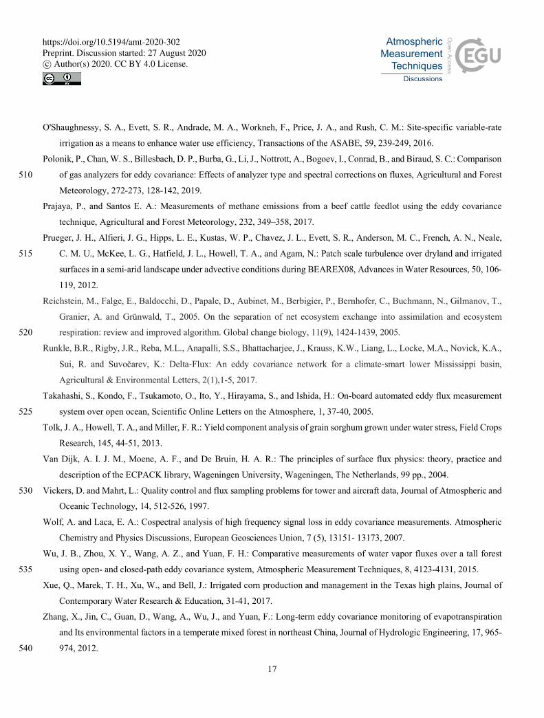
Data filtering also impacted all comparisons. After all threshold and precipitation screenings, 3,577 out of a possible

4,320 half-hour observations are available for analysis. The acquisition ratio was comparable to similar studies (Wu et al., 195

2015). Between 9:00 AM and 9:00 PM (LST), the ratio exceeded 92%, whereas EC system issues reduced availability in the

predawn hours to as low as 61% for the half-hour ending at 7:00 AM (Fig. 1).

3.1 Water vapor density validation

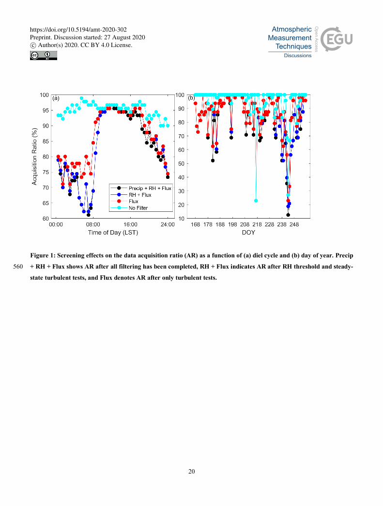
The long-term zero drift of water vapor density for the three IRGAs was evaluated as the three-month change in bias D𝜌". As

the study period began, the reference value of water vapor density 𝜌",M ranged from 3 to 18 g m-3. Accordingly, the measured 200

values 𝜌",$ for the LI-7500 and LI-7500RS were biased low and the LI-7500A was biased high. After applying the post-

correction to the LI-7500 and LI-7500A data, all 𝜌",$were between 0.11 and 1.31 less than 𝜌",N (Fig. 2). At the end of the

study period, all IRGAs clearly showed an increased bias relative to the HMP155. Interestingly, the LI-7500 and LI-7500A

had moved towards larger values, whereas the LI-7500RS moved towards smaller values (Fig. 2). That resulted in the LI-7500

D𝜌" decreasing, whereas the other two newer analyzers ended with greater D𝜌". The magnitude of bias was larger for the LI-205

7500 and LI-7500A than the LI-7500RS and a similar degree of day/night variability (sensitivity to solar radiation) was

apparent among the IRGAs regardless of 𝜌"'''. These temporal patterns may indicate a low frequency modulated signal hidden

in the instruments.

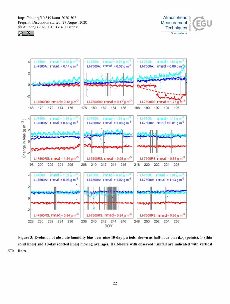
The divergence of 𝜌",$ between early and late times in the study period is the result of many short-term changes in bias.

To assess short-term drift Δ𝜌", half-hour differences between LI-7500s and HMP155s were calculated, with each timeseries 210

bias corrected to set the initial value to zero (Fig. 3). The magnitude of daily drift averaged 0.09 g m-3 for the LI-7500RS, 0.1

g m-3 for the LI-7500A, and 0.13 g m-3 for the LI-7500. Over 10-day periods, this increased to 0.36, 0.27, and 0.29, respectively.

Rainfall contributed to the bulk of changes in drift. Rain-free periods as noted over the initial 10 days, gave the best insight

into the stability of the sensors, and suggested that the LI-7500RS performed best. However, the extended dry period between

DOY 186 and DOY 196 suggested the opposite, when the LI-7500RS suffered from large short-term drift. After this time, the 215

LI-7500RS appeared to be more stable, with steady rmsd over the final 50 days compared to the other two instruments.

According to Figs. 2 and 3, analyzer performance differed between day and night. This diel cycle is indicative of a solar

radiation-induced error (Mauder et al., 2006; Miloshevich et al., 2009) and although amplitude varies, it appeared most

prominently for the LI-7500 and least substantially for the LI-7500A. Periods with more instrument drift were coincident

mainly with larger cycles, but the sudden performance change of the LI-7500RS on DOY 191 did not reflect this tendency. 220

Accidental window contamination may explain this observation, with typical behavior of absolute humidity from the LI-

7500RS resuming from DOY 192 onward.


8

To investigate the unexpected large drift exclusive to the LI-7500RS on DOY 191, biometeorological data were assessed.

Light southerly winds and moderately humid conditions were observed when Δ𝜌",56 increased from -0.96 to -2.45 between

8:30 and 9:30 PM LST. While nothing unusual occurred meteorologically, a 3°C drop in temperature and 10% increase in RH 225

accompanying the loss of daytime heating was noted. It was instructive to look at the variation in RH as estimated using vapor

and ambient pressure from the IRGAs and sonic temperature from the CSAT3. While the magnitude of RH did vary slightly

among the sensors, the increase in RH was similar for the LI-7500 and LI-7500A while being less than half for the LI-7500RS.

In the hours immediately prior and after, the slopes of Δ𝜌",56among the IRGAs and HMPs are nearly in lockstep. Unlike other

deviations that exist on a subdaily timescale, this new offset continued until DOY 197. Step changes are a dominant feature in 230

the linear regression between 𝜌",OP/2 and 𝜌",OP56.

Differences between the means and fluctuations of 𝜌" are summarized in Fig. 4 as a function of day of year. Since variance

of the 𝜌" time series reflects the mean of squared fluctuations 𝜌"< 8'''', greater variance in the half-hourly data reflects larger

fluctuations 𝜌"< . While the LI-7500 tended to have consistently greater 𝜌"< 8'''' values, the comparison between the LI-7500A and

LI-7500RS was more complicated. For example, the LI-7500A initially had slightly larger or the same fluctuations as the LI-235

7500RS for most daytime observations. After noon on DOY 196, the LI-7500RS consistently began to have larger fluctuations.

Then from midday on DOY 226 to DOY 232 noon, the pattern flipped again. Following DOY 232, agreement was consistently

close until DOY 254, and greater fluctuations from the LI-7500A were again found through the remainder of the study period.

Even when the LI-7500RS fluctuations tended to be relatively large, it did not have the large overestimation of fluctuations

observed periodically with the LI-7500A, such as noted on DOY 184, 190, 193, 211, 216, and 253. While the stochastic nature 240

of turbulence is partially responsible for the large scatter in 𝜌"< 8''''shown in Fig. 4, the degree of variance in the older sensors

exceeded that of the LI-7500RS.

Agreement between 𝜌"''' of the LI-7500RS and the older IRGAs was generally strong and stable despite occasional large

errors. In the first week of the study, regardless of the absolute error, linear regression parameters indicated well-calibrated

measurements for the purpose of eddy covariance, in which offset has no effect on the statistic. During the middle 30 days of 245

the study, agreement was also high, reflected by r2 values of 0.94 and 0.97 and slopes of 0.98 and 0.93, respectively for LI-

7500 and LI-7500A. Little change from those parameters occurred across a wide range of 𝜌" during the final 30 days of the

study, when lower temperature and higher relative humidity reduced evaporative demand. As expected, greater comparability

in 𝜌"''' was accompanied by a small 𝜌"< error. However, while step changes in 𝜌"''' occurred, 𝜌"< did not change over time.

Variance of water vapor density 𝜌"< 8'''' was compared using the LI-7500RS as reference, for the entire dataset including 250

daytime and advective periods only (Table 1). Nighttime estimates were particularly prone to overestimation by the LI-7500.

Advective periods were prone to greater errors while having reduced interinstrument variability.


9

3.2 Spectra and cospectra

Since the three analyzers had the same specifications and were configured to measure turbulence in the same fashion, any

deviations in spectral characteristics would be an indication of possible drift. Returning to the distinct LI-7500RS error on 255

DOY 191, spectra were examined during the interval from 8:00-9:30 PM (LST), which consisted of three spectra corresponding

to consecutive flux averaging periods. Overall, as evident from Fig. 5a–c, the shapes of spectra were in close agreement during

the daytime, whereas the nighttime peak frequency was shifted to lower frequencies indicating the predominance of large

eddies after sunset. At 8 PM, the three spectra were nearly identical and matched the predicted -2/3 slope (Fig. 5d). In the

following hour, the spectra of the LI-7500A and LI-7500 remained nearly identical, whereas the LI-7500RS spectra were 260

greatly modified. Based on the 20 Hz timeseries, air humidity began to decrease suddenly at roughly 8:40 PM in concert with

a doubling of fluctuation amplitude. As the other two IRGAs and HMPs continued to indicate increasing air humidity,

𝛥𝜌",STJOPUU56 steadily rose for nearly one hour until 𝜌",STJOPUU56 again agreed with the other instruments. Because only the

averaging period between 9 and 9:30 PM is affected by increased variance water vapor, the spectrum corresponding to that

half-hour is the period with a shift towards higher frequencies. 265

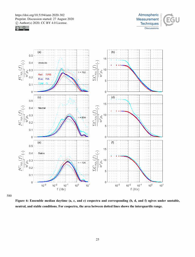
Cospectra were viewed through the lens of atmospheric stability because it predicts their shape according to Monin-

Obukhov similarity theory (Kaimal and Finnigan, 1994). For all cospectra, the LI-7500 tends to have greater energy in the

production and dissipation spectral regions while being nearly identical in the inertial subrange, and these differences translate

into higher latent heat fluxes (Fig. 6). Lower frequency components of flux were clearly greater, especially in unstable and

neutral conditions, as observed by the LI-7500 (the oldest version), compared to the LI-7500A and LI-7500RS. While the two 270

newer sensors exhibited similar behavior and relatively smaller fluxes than the LI-7500, under unstable conditions the LI-

7500RS showed a difference in performance from the LI-7500A at high frequencies. For all three IRGA, co-spectra dipped at

2.5 Hz, which should not occur in any desired instruments (Kaimal and Finnigan, 1994). Strong turbulent motions were likely

captured more by the LI-7500A within the surface layer. These cospectra were shifted towards lower frequency compared to

those in neutral and stable conditions, favoring larger eddy sizes with a smaller percentage of energy accumulated in the inertial 275

subrange (Fig. 6b). This middle frequency range is where the IRGAs were most similar. Regardless of sensor, unstable

conditions featured a flattened peak and more energy towards lower frequencies, as expected for various scalar fluxes measured

with the same instrumentation (Wolf and Laca, 2007). However, in an irrigated cropland environment, the surface layer is

prone to become stable more often than the surrounding area due to a temperature inversion forced by the relatively wetter,

cooler canopy. A previous study demonstrated this effect by using simultaneous sensing over adjacent irrigated cotton and 280

non-irrigated winter wheat fields, where energy production as depicted by 𝑆:;was two orders of magnitude smaller for the

irrigated field than the non-irrigated field (Prueger et al., 2012). Accordingly, in the present study, variability among cospectra

was small under these conditions with relatively few large eddies (Fig. 6e). In contrast, under neutral and unstable conditions,

the LI-7500 departed largely from the other two sensors with energy contribution from low frequency eddies.


10

3.3 Water vapor fluxes 285

For much of the study period, lE from the LI-7500RS and LI-7500A were similar with slightly larger magnitude than the LI-

7500. Overall interinstrument variability CVI-I of lE was 20%, about that of the underlying water vapor variance, and errors

on average were less during daytime hours than nighttime (Table 2). For an average diel cycle, the largest CVI-I occurred

during the middle of the night, rapidly declined after sunrise, reached its smallest value of 10% at 4 PM, and then increased at

a relatively slow rate after sunset. On a seasonal basis, there was a slight, nonlinear increase in CVI-I over time, with mean 290

values increasing from approximately 16% to 24%. Overall, the LI-7500 measured a 15% greater flux than the LI-7500RS

both on average and during only daytime hours. Meanwhile, LI-7500A and LI-7500RS fluxes were nearly identical, with 0.5%

less flux measured by the LI-7500A and an additional 0.2% difference during the daytime. While the daily bias was as equally

positive as negative, the LI-7500A tended to underestimate flux through the first and last third of the study period although

possible rainfall effects exist. Greater flux was observed on 27 of the 41 days from DOY 196 – 226, which coincided with 295

greater accumulated ET (Fig. 7). Relative error varied little by time of day. An increase in variability during advective

conditions was due to greater mean (co)variance. Under advective conditions, the coefficient of determination was particularly

small (see Table 2), but this coincided with large turbulent fluxes including downward sensible heat that was also slightly

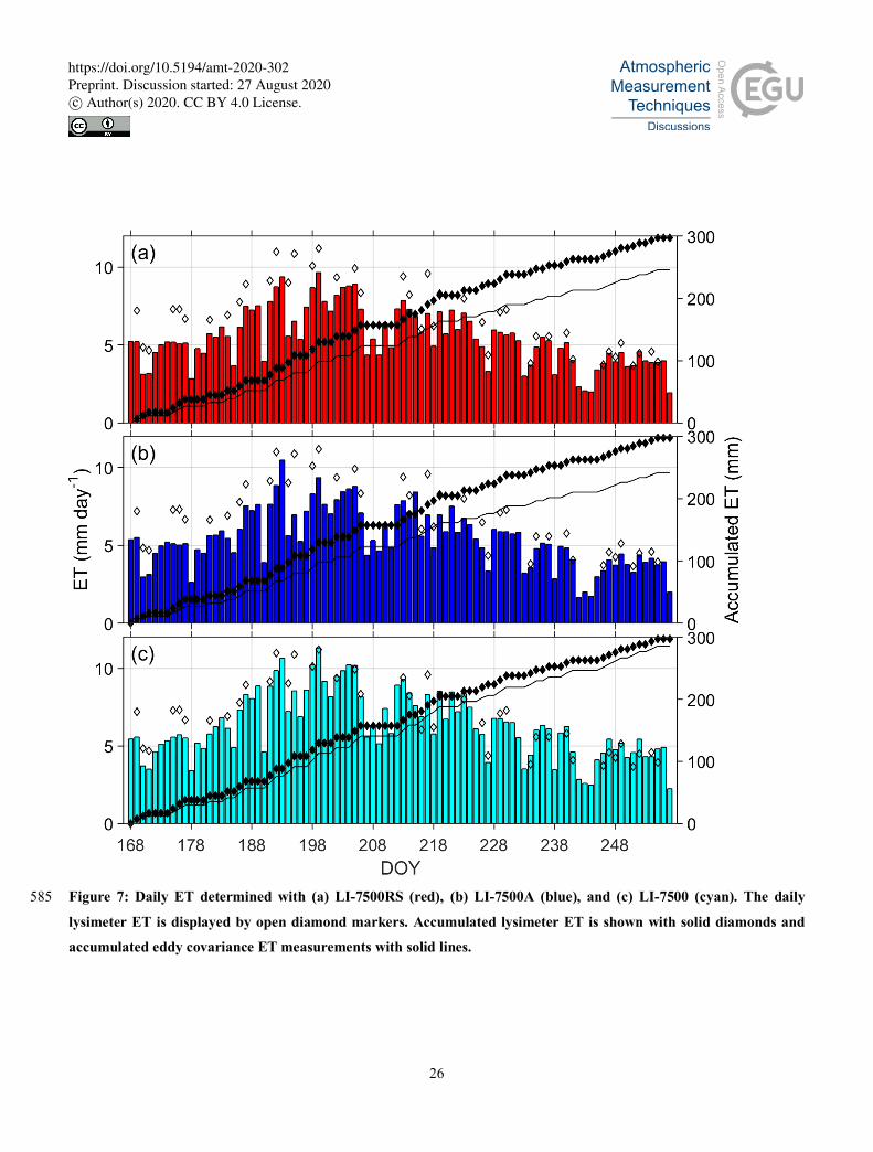
biased towards increased magnitude.

The 90–day ET (Fig. 7) was in good agreement among the three IRGAs, with slightly greater seasonal flux from the LI-300

7500, consistent with the larger variance in the timeseries of 𝜌". Systematic underestimation of ET for all IRGAs is consistent

with advective conditions, especially in the earlier part of the growing season where the gap in daily ET is particularly large

for a similar magnitude of ET (Fig. 7). Even if all spectral loss is corrected for, based on the conservation of water vapor and

eddy covariance theory, the measured EC flux should be less than the true flux under advective conditions. Approximately

16% of accumulated ET was underestimated from LI-7500A or LI-7500RS relative to the accumulated lysimeter ET at the end 305

of the growing season (Fig. 7). However, only less than 5% of accumulated ET was underestimated from the oldest LI-7000

analyzer (Fig. 7). Furthermore, the EC and lysimeter should differ more with increasing mean ET because the advective

component of ET, not captured by EC systems, is more likely to be elevated (Alfieri et al., 2012).

The greater flux from the LI-7500 occurs nearly symmetrically on a diel basis, with relative differences smallest during

the day. The mean daytime error of measured flux λE between the LI-7500A and LI-7500RS systems was 4.5%, with the LI-310

7500A estimating greater ET than the LI-7500RS on approximately three out of every four days. Systematic error d averaged

0.08 mm for the LI-7500RS system, which is rather large considering the mean measuring flux of 0.2 mm. Larger systematic

error is typically associated with greater flux underestimation due to failure to capture all low frequency signals, consistent

with the observed cospectra (Vickers and Mahrt, 1997). In contrast, daily λE differed by 18.6% between LI-7500 and LI-

7500RS systems and the magnitude from the LI-7500RS only exceeded that of the LI-7500 on a single day. Comparing daily 315

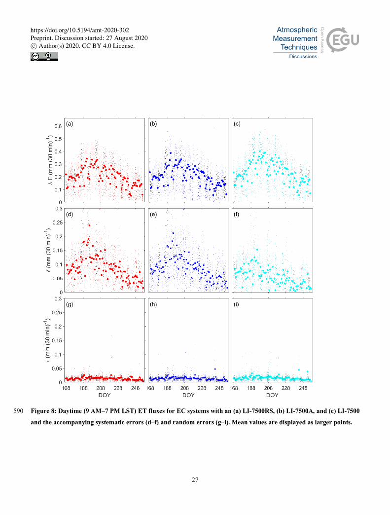
ET as a function of error, systematic error d calculated as shown in Eq. (2), decreases during the study period consistent with


11

declining ET (Fig. 8). Random error e was overwhelmingly similar among the sensors, indicating that uncertainty due to

sampling has little effect on differences in estimated ET.

4 Discussion

4.1 Water vapor variance errors 320

Water vapor variance and flux were compared from three similar eddy covariance systems yielding similar results in rain-free

periods. Large 𝜌"''' errors occurred under relatively small flux conditions, primarily with the LI-7500A systems. A pattern of

increasing flux error corresponding with greater water vapor density error as observed by Fratini et al. (2014) was not found.

This is encouraging despite demonstrated substantial errors in the water vapor density measurements. More important for flux

is the (co)variance of the water vapor density. Despite screening the data for quality, several outliers were observed in the ρW< 8'''' 325

which contributed to deflated r2 values and notable discrepancies in water vapor fluxes. Overestimation of water vapor variance

could contribute to overestimated flux but is not necessarily the case (Mauder et al., 2006). At noon on DOY 190, LI-7500A

overestimated ρW< 8'''' by 5.9 g2 m-6; while corresponding values were only 0.63 and 0.11 for LI-7500 and LI-7500RS, respectively.

The overestimation was accompanied by an uptick in flux of 180 W m-2, whereas values were 138 and 88 for LI-7500 and LI-

7500RS, respectively. In contrast, for the half-hour beginning at 3:00 PM LST on DOY 181, LI-7500 underestimated flux by 330

approximately 20 W m-2 despite an overestimation of ρW< 8'''' (3.5 g2 m-6 and 0.84 g2 m-6 greater relative to LI-7500A and LI-

7500RS). However, in a vast majority of cases, large ρW< 8'''' was observed with both the LI-7500 and LI-7500A relative to the

LI-7500RS and were associated with a recent rainfall event. For instance, a large discrepancy in ρW< 8'''' among the three IRGAs

occurred an hour after light rain on DOY 211, which suggests that thick water droplets may have been still evaporating from

the mirror surface. Antecedent conditions were dry and with the cessation of precipitation, a sudden increase in mean wind 335

speed from under 3 to 5 m s-1 and a wind shift from east to south enabled sensible heat advection as clouds began to dissipate.

Although air humidity decreased by the end of the half-hour for all IRGAs, the magnitude measured by the LI-7500 was much

smaller at the start of the averaging period than at the end, in contrast to observations by the LI-7500A and LI-7500RS. Further,

we observed that the LI-7500A air humidity began decreasing within the first 15 minutes, suddenly increased by approximately

5 g m-3, and then began a rapid decrease. This pattern is different than what was observed by the LI-7500RS, which initially 340

increased and then quickly decreased at an earlier time than for the LI-7500A (not shown). Large variability of air humidity in

time and space caused large errors of water vapor density. The LI-7500 𝜌"'''' decreased to 7.01 g m-3 while the LI-7500A 𝜌"''''

increased to 17.92 g m-3. These corresponded to Δ𝜌"of 8.83 g m-3 and 1.95 g m-3, respectively. While the LI-7500RS

performance during this time was markedly better than that of the other two sensors, the -1.13 g m-3 bias was still different

from its long-term offset. Resulting water vapor fluxes were smallest for the LI-7500A and largest for the LI-7500, with 345

sampling by the LI-7500RS seeming to best reflect the variations in eddies during a period of substantial air mass change. A

similar event occurred on DOY 196. However, for the half-hour of interest, a relatively small difference in ρW< 8''''of the LI-7500


12

and LI-7500A resulted in a larger flux difference, in which a large, likely overestimated flux was measured by the LI-7500.

Interestingly, 20 Hz fluctuations for all systems were dampened during roughly the first half of this averaging period, showing

signs of low frequency atmospheric motion. Once turbulence became more typical of a well-mixed boundary layer, the 350

amplitude of 𝜌"< then grew with a larger variance noted in the LI-7500A and LI-7500 compared to the LI-7500RS. This is

exactly what was observed on DOY 211 during its relevant averaging period. The effect of rainfall may linger depending on

its timing. All the sensors exhibited some degree of non-stationarity in the 𝜌" timeseries from late night on DOY 224 into the

early morning of DOY 225. However, only the LI-7500A continued to exhibit this behavior for several more hours while the

other two sensors showed constant flux. Because 𝜌" was so similar between the LI-7500 and LI-7500RS, it seems that the LI-355

7500A was uniquely sensitive to the intermittent turbulence during this calm period. Based on the combination of high relative

humidity and light winds, these observations were subject to increased random error as expected.

4.2 Water vapor flux errors

In the context of ET measurement, total daily magnitude is of prime importance for practical applications. Therefore, flux

errors during the daytime, roughly between 09:00 and 17:00 LST, contribute to the vast majority of ET variation. The similarity 360

between the LI-7500A and LI-7500RS fluxes is reflected by the lack of scatter in covariance data. As expected, errors were

larger during advective periods than for other times, but overall correlation between ρW< 8'''' and λE errors was weak. Highly

advective conditions have been associated with large interinstrument variability (Alfieri et al., 2011).

Uncorrected fluxes were assessed to assure that the data processing steps did not appreciably affect our findings. Post-

processing of turbulent fluxes could increment fluxes while causing greater error (Irmak et al., 2014). The magnitudes of a, d, 365

and rmsd were slightly smaller for all comparisons, and b and r2 were nearly identical, indicating that the corrections

contributed little to measurement uncertainty. For instance, the rmsd decreased by 6.8% and 7.3% for daytime fluxes against

the LI-7500 and LI-7500A, respectively. Among the corrections, sensor separation and frequency response were of most

interest for the LI-7500RS and LI-7500A pair since they are newer different optical analyzers. This may be why among the

three generations of IRGAs, the LI-7500RS consistently had a larger spectral correction factor by approximately 2 to 4%, but 370

again, this served to only slightly decrease flux error. Its midday mean value of 1.11, though slightly larger than for the LI-

7500 and LI7500A, was still less than reported in a feedlot for an LI-7500 and CSAT-3 EC system (Prajapati and Santos,

2017). This suggests that high frequency attenuation was relatively minor when turbulent intensity was large, and any missing

flux was more attributable to low frequency. While the LI-7500 high frequency energy compared more favorably to the LI-

7500A than the LI-7500RS, a large departure from the LI-7500A and LI-7500RS pattern was clearly observed at low 375

frequencies (Fig. 6).

It has previously been shown that turbulent flux error partitions into primarily random error, with daytime systematic error

only as large as 0.018 mm (30 min-1) (Alfieri et al., 2011). In contrast, Sect. 3.3 demonstrated that the magnitudes of systematic

error were generally large in response to daytime energy balance residuals. The different findings are based on different


13

assumptions of what is true latent heat. In the prior study, the mean of multiple EC measurements was considered the true flux, 380

and the systematic error was the variance of residuals between predicted and true flux. Following that approach, daytime error

was comparable and ranged from 0.014 (LI-7500RS) to 0.024 (LI-7500) mm (30 min-1). Also, the prior study was conducted

during the period of rapid LAI increase of a cotton crop, while the present study was performed during both the period of rapid

LAI increase and crop maturation.

5 Conclusion 385

The guidelines written by Fratini et al. (2014) can be used to avoid water vapor concentration errors. Even in the event that

absorptances are not output via datalogger code, and detection of contamination in real time is not done, the water vapor

concentration errors will not adversely affect accuracy of eddy covariance on a growing season timescale. Instead, larger fluxes

were found from the older LI-7500 system. Our study indicates that the LI-7500 outperformed newer LI7500A and 7500RS

sensors in terms of accumulated ET comparison with lysimeter observations. While it was paired with a different sonic 390

anemometer than the other two IRGAs, flux differences were attributed to differences in variance of turbulent fluctuations of

water vapor rather than sonic anemometer error.

Differences in the response from the same model sensor measuring presumably the same air parcel were identified. In this

study, the growth and maturation of corn crop drove a change in turbulent flux partitioning. Increases in interinstrument

variation for both water vapor variance and flux were observed when conditions were advective during the period of peak 395

canopy development. Following precipitation, while performance characteristics were consistent in well-mixed turbulent air,

larger interinstrument variation was observed under light winds that could cause variation in effects on the IRGA. Adjusting

measured fluxes by the systematic error, which tended to be larger at one EC tower compared to the other, brought the water

vapor fluxes into strong agreement.

Data availability 400

The associated data are available upon request.

Author contribution

SK conducted experiment, collected data, data analysis, and write the manuscript. XL and SK conceptualized the research and

developed the methodology. XL and RA were responding for funding acquisition, project supervision, and writing the

manuscript. All USDA authors were responding for helping calibrations, installation, and site maintenance. LX and CO 405

provided infrared analysers and sonic anemometers. All authors reviewed and edited the manuscript throughout the publication

process.

Competing interests


14

The authors declare that they have no conflict of interest.

Acknowledgements 410

We thank the collaborative scientists and staff in Bushland for their courtesy in allowing access to the experimental site. This

work was supported by the Ogallala Aquifer Program which is funded by a USDA ARS research initiative (USDA-ARS 58-

3090-5-009), as well as the National Institute of Food and Agriculture under award number 2016-68007-25066.

References

Alfieri, J. G., Kustas, W. P., Prueger, J. H., Hipps, L. E., Chávez, J. L., French, A. N., and Evett, S. R.: Intercomparison of 415

nine micrometeorological stations during the BEAREX08 field campaign, Journal of Atmospheric and Oceanic

Technology, 28, 1390-1406, 2011.

Alfieri, J. G., Kustas, W. P., Prueger, J. H., Hipps, L. E., Evett, S. R., Basara, J. B., Neale, C. M. U., French, A. N., Colaizzi,

P., Agam, N., Cosh, M. H., Chavez, J. L., and Howell, T. A.: On the discrepancy between eddy covariance and lysimetry-

based surface flux measurements under strongly advective conditions, Advances in Water Resources, 50, 62-78, 2012. 420

Baldocchi, D., Falge, E., Gu, L., Olson, R., Hollinger, D., Running, S., Anthoni, P., Bernhofer, C., Davis, K., Evans, R. and

Fuentes, J.: FLUXNET: A new tool to study the temporal and spatial variability of ecosystem-scale carbon dioxide, water

vapor, and energy flux densities, Bulletin of the American Meteorological Society, 82(11), 2415-2434, 2001.

Blanken, P. D., Rouse, W. R., and Schertzer, W. M.: Enhancement of evaporation from a large northern lake by the entrainment

of warm, dry air, Journal of Hydrometeorology, 4, 680-693, 2003. 425

Burba, G. G., Begashaw, I., and Kathilankal, J.: New open-path low-power standardized automated CO2/H2O flux

measurement system, European Geosciences Union, Vienna, Austria, 2018.

Ding, R., Kang, S., Vargas, R., Zhang, Y., and Hao, X.: Multiscale spectral analysis of temporal variability in

evapotranspiration over irrigated cropland in an arid region, Agricultural Water Management, 130, 79-89, 2013.

Evett, S. R., Schwartz, R. C., Casanova, J. J., and Heng, L. K.: Soil water sensing for water balance ET and WUE, Agricultural 430

Water Management, 104, 1–9, 2012b.

Evett, S. R., Agam, N., Kustas, W. P., Colaizzi, P. D., and Schwartz, R. C.: Soil profile method for soil thermal diffusivity,

conductivity and heat flux: Comparison to soil heat flux plates. Advances in Water Resources, 50, 41–54, 2012a.

Evett, S. R., Marek, G. W., Copeland, K. S., and Colaizzi, P. D.: Quality management for research weather data: USDA-ARS,

Bushland, TX, Agrosystems, Geosciences & Environment, 1, 180036, 2018. 435

Evett, S. R., Brauer, D. K., Colaizzi, P.D., Tolk, J.A., Marek G. W., and O’Shaughnessy S. A.: Corn and sorghum ET, E,

Yield and CWP as affected by irrigation application method: SDI versus mid-elevation spray irrigation. Trans. ASABE

62(5), 1377-1393, 2019.


15

Finkelstein, P. L. and Sims, P. F.: Sampling error in eddy correlation flux measurements, Journal of Geophysical Research:

Atmospheres, 106, 3503-3509, 2001. 440

Fratini, G. and Mauder, M.: Towards a consistent eddy-covariance processing: an intercomparison of EddyPro and TK3,

Atmospheric Measurement Techniques, 7, 2273-2281, 2014.

Fratini, G., McDermitt, D. K., and Papale, D.: Eddy-covariance flux errors due to biases in gas concentration measurements:

origins, quantification and correction, Biogeosciences, 11, 1037-1051, 2014.

Gowda, P. H., Senay, G. B., Howell, T. A., and Marek, T. H.: Lysimetric evaluation of simplified surface energy balance 445

approach in the Texas High Plains, Applied Engineering in Agriculture, 25, 665-669, 2009.

Haslwanter, A., Hammerle, A., and Wohlfahrt, G.: Open- vs. closed-path eddy covariance measurements of the net ecosystem

carbon dioxide and water vapour exchange: a long-term perspective, Agric For Meteorol, 149, 291-302, 2009.

Heusinkveld, B, Jacob, A, Hotslag, A: Effect of open-path gas analyzer wetness on eddy covariance flux measurements: A

proposed solution, Agricultural and Forest Meteorology, 148, 1563-1573, 2008. 450

Hirschi, M., Michel, D., Lehner, I., and Seneviratne, S. I.: A site-level comparison of lysimeter and eddy covariance flux

measurements of evapotranspiration, Hydrology and Earth System Sciences, 21, 1809-1825, 2017.

Honkanen, M., Tuovinen, J.-P., Laurila, T., Mäkelä, T., Hatakka, J., Kielosto, S., and Laakso, L.: Measuring turbulent CO2

fluxes with a closed-path gas analyzer in a marine environment, Atmospheric Measurement Techniques, 11, 5335-5350,

2018. 455

Horst, T. W. and Lenschow, D. H.: Attenuation of scalar fluxes measured with spatially-displaced sensors, Boundary-Layer

Meteorology, 130, 275-300, 2009.

Irmak, S., Payero, J. O., Kilic, A., Odhiambo, L. O., Rudnick, D., Sharma, V., and Billesbach, D.: On the magnitude and

dynamics of eddy covariance system residual energy (energy balance closure error) in subsurface drip-irrigated maize

field during growing and non-growing (dormant) seasons, Irrigation Science, 32, 471-483, 2014. 460

Iwata, H., Harazono, Y., and Ueyama, M.: Sensitivity and offset changes of a fast-response open-path infrared gas analyzer

during long-term observations in an Arctic environment, Journal of Agricultural Meteorology, 68, 175-181, 2012.

Kaimal, J. C. and Finnigan, J. J.: Atmospheric Boundary Layer Flows: Their Structure and Measurement, Oxford University

Press, 1994.

Kim, W., Miyata, A., Ashraf, A., Maruyama, A., Chidthaisong, A., Jaikaeo, C., Komori, D., Ikoma, E., Sakurai, G., Seoh, H.-465

H., Son, I. C., Cho, J., Kim, J., Ono, K., Nusit, K., Moon, K. H., Mano, M., Yokozawa, M., Baten, M. A., Sanwangsri,

M., Toda, M., Chaun, N., Polsan, P., Yonemura, S., Kim, S.-D., Miyazaki, S., Kanae, S., Phonkasi, S., Kammales, S.,

Takimoto, T., Nakai, T., Iizumi, T., Surapipith, V., Sonklin, W., Lee, Y., Inoue, Y., Kim, Y., and Oki, T.: FluxPro as a

realtime monitoring and surveilling system for eddy covariance flux measurement, Journal of Agricultural Meteorology,

71, 32-50, 2015. 470

Kochendorfer, J. and Paw, U.: Field estimates of scalar advection across a canopy edge, Agricultural and Forest Meteorology,

151, 585-594, 2011.


16

Kutikoff, S., Lin, X., Evett, S., Gowda, P., Moorhead, J., Marek, G., Colaizzi, P., Aiken, R., and Brauer, D.: Heat storage and

its effect on the surface energy balance closure under advective conditions, Agricultural and Forest Meteorology, 265, 56-

69, 2019. 475

Lasslop, G., Reichstein, M., Kattge, J., and Papale, D.: Influences of observation errors in eddy flux data on inverse model

parameter estimation, Biogeosciences, 5, 1311-1324, 2008.

Martínez-Cob, A. and Suvočarev, K.: Uncertainty due to hygrometer sensor in eddy covariance latent heat flux measurements,

Agricultural and Forest Meteorology, 200, 92-96, 2015.

Massman, W. J.: A simple method for estimating frequency response corrections for eddy covariance systems, Agricultural 480

and Forest Meteorology, 104, 185-198, 2000.

Mauder, M. and Foken, T.: Documentation and instruction manual of the eddy covariance software package TK2,

Mikrometeorologie, 2004.

Mauder, M., Oncley, S. P., Vogt, R., Weidinger, T., Ribeiro, L., Bernhofer, C., Foken, T., Kohsiek, W., De Bruin, H. A. R.,

and Liu, H.: The energy balance experiment EBEX-2000. Part II: Intercomparison of eddy-covariance sensors and post-485

field data processing methods, Boundary-Layer Meteorology, 123, 29-54, 2006.

Mauder, M., Cuntz, M., Drüe, C., Graf, A., Rebmann, C., Schmid, H. P., Schmidt, M., and Steinbrecher, R.: A strategy for

quality and uncertainty assessment of long-term eddy-covariance measurements, Agricultural and Forest Meteorology,

169, 122-135, 2013.

Miloshevich, L.M., Vömel, H., Whiteman, D.N. and Leblanc, T.: Accuracy assessment and correction of Vaisala RS92 490

radiosonde water vapor measurements, Journal of Geophysical Research: Atmospheres, 114(D11), 2009.

Moncrieff, J., Massheder, J. M., De Bruin, H. A. R., Elbers, J., Friborg, T., Heusinkveld, B. G., Kabat, P., Scott, S. L., Soegaard,

H., and Verhoef, A.: A system to measure surface fluxes of momentum, sensible heat, water vapour and carbon dioxide,

Journal of Hydrology, 188-189, 589-611, 1997.

Moncrieff, J., Clement, R., Finnigan, J. J., and Meyers, T.: Averaging, detrending and filtering of eddy covariance time series. 495

In: Handbook of micrometeorology: a guide for surface flux measurements Lee, X., Massman, W. J., and Law, B. E.

(Eds.), Kluwer Academic, Dordrecht, 2004.

Moorhead, J. E., Marek, G. W., Colaizzi, P. D., Gowda, P. H., Evett, S. R., Brauer, D. K., Marek, T. H., and Porter, D. O.:

Evaluation of sensible heat flux and evapotranspiration estimates using a surface layer scintillometer and a large weighing

lysimeter, Sensors (Basel), 17, 2017. 500

Novick, K. A., Walker, J., Chan, W. S., Schmidt, A., Sobek, C., and Vose, J. M.: Eddy covariance measurements with a new

fast-response, enclosed-path analyzer: Spectral characteristics and cross-system comparisons, Agricultural and Forest

Meteorology, 181, 17-32, 2013.

Oncley, S.P., Foken, T., Vogt, R., Kohsiek, W., DeBruin, H.A., Bernhofer, C., Christen, A., Van Gorsel, E., Grantz, D.,

Feigenwinter, C. and Lehner, I.: The energy balance experiment EBEX-2000. Part I: overview and energy balance, 505

Boundary-Layer Meteorology, 123, 1-28, 2007.


17

O'Shaughnessy, S. A., Evett, S. R., Andrade, M. A., Workneh, F., Price, J. A., and Rush, C. M.: Site-specific variable-rate

irrigation as a means to enhance water use efficiency, Transactions of the ASABE, 59, 239-249, 2016.

Polonik, P., Chan, W. S., Billesbach, D. P., Burba, G., Li, J., Nottrott, A., Bogoev, I., Conrad, B., and Biraud, S. C.: Comparison

of gas analyzers for eddy covariance: Effects of analyzer type and spectral corrections on fluxes, Agricultural and Forest 510

Meteorology, 272-273, 128-142, 2019.

Prajaya, P., and Santos E. A.: Measurements of methane emissions from a beef cattle feedlot using the eddy covariance

technique, Agricultural and Forest Meteorology, 232, 349–358, 2017.

Prueger, J. H., Alfieri, J. G., Hipps, L. E., Kustas, W. P., Chavez, J. L., Evett, S. R., Anderson, M. C., French, A. N., Neale,

C. M. U., McKee, L. G., Hatfield, J. L., Howell, T. A., and Agam, N.: Patch scale turbulence over dryland and irrigated 515

surfaces in a semi-arid landscape under advective conditions during BEAREX08, Advances in Water Resources, 50, 106-

119, 2012.

Reichstein, M., Falge, E., Baldocchi, D., Papale, D., Aubinet, M., Berbigier, P., Bernhofer, C., Buchmann, N., Gilmanov, T.,

Granier, A. and Grünwald, T., 2005. On the separation of net ecosystem exchange into assimilation and ecosystem

respiration: review and improved algorithm. Global change biology, 11(9), 1424-1439, 2005. 520

Runkle, B.R., Rigby, J.R., Reba, M.L., Anapalli, S.S., Bhattacharjee, J., Krauss, K.W., Liang, L., Locke, M.A., Novick, K.A.,

Sui, R. and Suvočarev, K.: Delta-Flux: An eddy covariance network for a climate-smart lower Mississippi basin,

Agricultural & Environmental Letters, 2(1),1-5, 2017.

Takahashi, S., Kondo, F., Tsukamoto, O., Ito, Y., Hirayama, S., and Ishida, H.: On-board automated eddy flux measurement

system over open ocean, Scientific Online Letters on the Atmosphere, 1, 37-40, 2005. 525

Tolk, J. A., Howell, T. A., and Miller, F. R.: Yield component analysis of grain sorghum grown under water stress, Field Crops

Research, 145, 44-51, 2013.

Van Dijk, A. I. J. M., Moene, A. F., and De Bruin, H. A. R.: The principles of surface flux physics: theory, practice and

description of the ECPACK library, Wageningen University, Wageningen, The Netherlands, 99 pp., 2004.

Vickers, D. and Mahrt, L.: Quality control and flux sampling problems for tower and aircraft data, Journal of Atmospheric and 530

Oceanic Technology, 14, 512-526, 1997.

Wolf, A. and Laca, E. A.: Cospectral analysis of high frequency signal loss in eddy covariance measurements. Atmospheric

Chemistry and Physics Discussions, European Geosciences Union, 7 (5), 13151- 13173, 2007.

Wu, J. B., Zhou, X. Y., Wang, A. Z., and Yuan, F. H.: Comparative measurements of water vapor fluxes over a tall forest

using open- and closed-path eddy covariance system, Atmospheric Measurement Techniques, 8, 4123-4131, 2015. 535

Xue, Q., Marek, T. H., Xu, W., and Bell, J.: Irrigated corn production and management in the Texas high plains, Journal of

Contemporary Water Research & Education, 31-41, 2017.

Zhang, X., Jin, C., Guan, D., Wang, A., Wu, J., and Yuan, F.: Long-term eddy covariance monitoring of evapotranspiration

and Its environmental factors in a temperate mixed forest in northeast China, Journal of Hydrologic Engineering, 17, 965-

974, 2012. 540


18

Zhang, Y., Liu, H., Foken, T., Williams, Q. L., Liu, S., Mauder, M., and Liebethal, C.: Turbulence spectra and cospectra under

the influence of large eddies in the Energy Balance EXperiment (EBEX), Boundary-Layer Meteorology, 136, 235-251,

2010.


19

Figures and Tables

Table 1: Performance characteristics of LI-7500A and LI-7500 with reference to the LI-7500RS for water vapor 545

variance 𝛒𝐯< 𝟐'''''. These include regression offset value (a), regression slope (b), coefficient of determination (r2), mean

absolute bias (d), and comparability (rmsd).

𝝆𝒗< 𝟐''''' a (g2 m-6) b (–) r2 d (g2 m-6) rmsd (g2 m-6)

75

All 0.04 1.17 0.42 0.09 0.88

Daytime 0.06 1.08 0.49 0.10 0.75

Advective 0.22 1.02 0.57 0.24 1.33

75A

All 0.02 1.07 0.56 0.04 0.60

Daytime 0.02 1.03 0.79 0.03 0.36

Advective 0.08 1.02 0.83 0.09 0.63

550

Table 2: Performance characteristics of LI-7500A and LI-7500 with reference to the LI-7500RS for corrected latent

heat fluxes (lE). These include regression offset value (a), regression slope (b), coefficient of determination (r2), mean

absolute bias (d), and comparability (rmsd).

555

lE a (W m-2) b (–) r2 d (W m-2) rmsd (W m-2)

75

All 6.20 1.12 0.96 27.13 54.31

Daytime 23.91 1.08 0.92 49.42 73.66

Advective 47.07 1.05 0.87 69.80 97.94

75A

All -1.48 1.00 0.99 -0.87 16.69

Daytime 2.34 0.99 0.99 0.34 14.53

Advective 2.04 1.00 0.98 -0.10 21.67


20

Figure 1: Screening effects on the data acquisition ratio (AR) as a function of (a) diel cycle and (b) day of year. Precip

+ RH + Flux shows AR after all filtering has been completed, RH + Flux indicates AR after RH threshold and steady-560

state turbulent tests, and Flux denotes AR after only turbulent tests.


21

Figure 2: Absolute humidity 𝛒𝐯 (top) magnitude and (bottom) difference D𝛒𝐯 between paired IRGA and HMP

instruments (HMP155-N is paired with the LI-7500RS and LI-7500A; HMP155-S is paired with the LI-7500) during 565

the first and last three days of the study. Shaded areas indicate daytime.


22

Figure 3: Evolution of absolute humidity bias over nine 10-day periods, shown as half-hour bias D𝛒𝐯 (points), 1- (thin

solid lines) and 10-day (dotted lines) moving averages. Half-hours with observed rainfall are indicated with vertical

lines. 570


23

Figure 4: Intercomparison of absolute humidity 𝛒𝐯 means and standard deviations for (a, b) the LI-7500 and LI-

7500RS and (c, d) the LI-7500A and LI-7500RS.


24

575 Figure 5: Binned spectra of absolute humidity on DOY 191 are shown for 45 half-hour observations from (a) LI-

7500RS, (b) LI-7500A, and (c) LI-7500 as a function of normalized frequency. A close-up comparison of the

performance of the three gas analyzers is illustrated in (d) for three half-hours.


25

580 Figure 6: Ensemble median daytime (a, c, and e) cospectra and corresponding (b, d, and f) ogives under unstable,

neutral, and stable conditions. For cospectra, the area between dotted lines shows the interquartile range.


26

Figure 7: Daily ET determined with (a) LI-7500RS (red), (b) LI-7500A (blue), and (c) LI-7500 (cyan). The daily 585

lysimeter ET is displayed by open diamond markers. Accumulated lysimeter ET is shown with solid diamonds and

accumulated eddy covariance ET measurements with solid lines.


27

Figure 8: Daytime (9 AM–7 PM LST) ET fluxes for EC systems with an (a) LI-7500RS, (b) LI-7500A, and (c) LI-7500 590

and the accompanying systematic errors (d–f) and random errors (g–i). Mean values are displayed as larger points.


Water vapor density and turbulent fluxes from three ...

Documents

Transcript of Water vapor density and turbulent fluxes from three ...