Instructions for use

Title Biogeochemical fluxes through mesozooplankton

Author(s)Buitenhuis, Erik; Le Quere, Corinne; Aumont, Olivier;Beaugrand, Gregory; Bunker, Adrian; Hirst, Andrew; Ikeda,Tsutomu; O'Brien, Todd; Piontkovski, Sergey; Straile, Dietmar

Citation Global biogeochemical cycles, 20(2): GB2003

Issue Date 2006-04-08

DOI

Doc URL http://hdl.handle.net/2115/13694

Right An edited version of this paper was published by AGU.Copyright 2006 American Geophysical Union.

Type article (author version)

AdditionalInformation

FileInformation buitenhuis_etal2005GB002511.pdf

Hokkaido University Collection of Scholarly and Academic Papers : HUSCAP

Biogeochemical fluxes through mesozooplankton.

Buitenhuis, Erik1,10,11

, Corinne Le Quéré1,10

, Olivier Aumont2, Grégory Beaugrand

3, Adrian

Bunker4, Andrew Hirst

5, Tsutomu Ikeda

6, Todd O’Brien

7, Sergey Piontkovski

8, Dietmar Straile

9

1 Max Planck Institute for Biogeochemistry, P.O. box 100164, Jena, Germany

2 Laboratoire d’Oceanographie Dynamique et de Climatologie, Paris, France

3 Sir Alistar Hardy Foundation for Ocean Science, Plymouth, United Kingdom, now at University

of Lille, Wimereux, France 4 Heriot-Watt University, Edinburgh, United Kingdom 5 British Antarctic Survey, Cambridge, United Kingdom

6 Hokkaido University, Hakodate, Japan

7 National Marine Fisheries Service, Silver Spring, Maryland, USA

8 Stony Brook University, New York, USA

9 University of Konstanz, Konstanz, Germany

10 now at University of East Anglia, Norwich, and British Antarctic Survey, Cambridge, United

Kingdom 11

corresponding author: e031@uea.ac.uk

Submitted to Global Biogeochemical Cycles 2005GB002511.

Abstract

Mesozooplankton are significant consumers of phytoplankton, and have a significant

impact on the oceanic biogeochemical cycles of carbon and other elements. Their contribution to

vertical particle flux is much larger than that of microzooplankton, yet most global

biogeochemical models have lumped these two plankton functional types together. In this paper

we bring together several newly available data syntheses on observed mesozooplankton

concentration and the biogeochemical fluxes they mediate, and perform data synthesis on flux

rates for which no synthesis was available. We update the equations of a global biogeochemical

model with an explicit representation of mesozooplankton (PISCES). We use the rate

measurements to constrain the parameters of mesozooplankton, and evaluate the model results

with our independent synthesis of mesozooplankton concentration measurements. We also

perform a sensitivity study to analyse the impact of uncertainty in the flux rates. The standard

model run was parameterised based on the data synthesis of flux rates. The results of

mesozooplankton concentration in the standard run are slightly lower than the independent

databases of observed mesozooplankton concentrations, but not significantly. This shows that

structuring and parameterising biogeochemical models based on observations without tuning is a

strategy that works. The sensitivity study showed that by using a maximum grazing rate of

mesozooplankton that is only 30% higher than the poorly constrained fit to the observations, the

model mesozooplankton concentration gets closer to the observations, but mesozooplankton

grazing becomes higher than what is currently accounted for. This is an indication that food

selection by mesozooplankton is not sufficiently quantified at present. Despite the amount of

effort that is represented by the data syntheses of all relevant processes, the good results that were

obtained for mesozooplankton indicates that this effort needs to be applied to all components of

marine biogeochemistry. The development of ecosystem models that better represent key

plankton groups and are more closely based on observations should lead to better understanding

and quantification of the feedbacks between marine ecosystems and climate.

Index terms: 1615, 1635, 4806, 4842, 4855

Key words: mesozooplankton, export production, synthesis of observations, global ocean

biogeochemical model

1. Introduction Mesozooplankton are a group of multicellular organisms (size range: 200 µm to 2 mm) that

feed on phytoplankton, microzooplankton, other mesozooplankton and detritus. Together with the

specialised filter feeders (salps, pteropods), they are the largest organisms that still have a

significant feedback interaction with primary production. Thus, they are the largest organisms

that are of primary interest for global biogeochemical models of the marine carbon cycle.

One of the main impacts of ecosystem functioning on biogeochemistry is the distinction

between microzooplankton grazing (associated with the microbial loop and regenerated

production), and mesozooplankton grazing (associated with the classical food chain and export

production). Global biogeochemical models tend to represent all zooplankton as one state

variable, and until recently also represented all phytoplankton as one state variable. These NPZD

models (Nutrient Phytoplankton Zooplankton Detritus), and the current Earth system models that

incorporate these models, underestimate interannual variability of chlorophyll a as observed by

satellite (Le Quéré et al., 2005). This suggests that these biogeochemical models will also

underestimate sensitivity to decadal to century scale climate variability. Our working hypothesis

is that building models that more closely represent our current understanding of the marine

ecosystem will help to solve this problem (Prentice et al., 2004).

The explicit representation of mesozooplankton in models should also improve the

representation of algal blooms. The preferred prey size of copepods (the most abundant

mesozooplankton) is larger than the preferred prey size of microzooplankton (Hansen et al.,

1994). The combination of different maximum growth rates for the two zooplankton size classes

and the different preferred prey sizes leads to an effective control of small phytoplankton by

microzooplankton, so that phytoplankton blooms are predominantly made up of large cells. This

positive correlation between cell size and primary production, and the higher sinking rate of

mesozooplankton fecal pellets also lead to a positive correlation between primary production and

export efficiency. From this, glacial/interglacial differences in the marine ecosystem have been

shown to influence the atmospheric CO2 concentration (Bopp et al., 2003).

Unlike microzooplankton (Sherr and Sherr, 2002), mesozooplankton have a maximum

growth rate (Hirst and Bunker, 2003) that is considerably lower than that of phytoplankton

(Eppley, 1972). Thus, they tend to dampen biomass increases of both phytoplankton and

microzooplankton on a timescale of their doubling time (with a minimum of 2 days at 30 °C to 9

days at 0 °C, Hirst and Bunker, 2003). For a biogeochemical model this presents advantages. The

closing term in biological models is the mortality term of the highest represented trophic level.

Using mesozooplankton as the highest represented trophic level has the advantages of including

their small, but significant direct grazing of primary production (about 10%, Calbet, 2001), and

of representing the grazing mortality of microzooplankton in a dynamical way, rather than as a

closure term, which would ignore significant trophic interactions. The lower growth rate of

mesozooplankton suggests that representing mesozooplankton mortality as the model closure

term, and thus ignoring the variability in mesozooplankton mortality caused by higher trophic

levels, would have a smaller impact on the variability of phytoplankton and microzooplankton

production.

Given the potential importance of mesozooplankton for the export efficiency (Honjo and

Roman, 1978) in global biogeochemical cycles, we have reviewed the available data on

mesozooplankton biogeochemistry. In recent years, several data syntheses of measurements have

been generated for both mesozooplankton concentration (O’Brien et al., 2002; Finenko et al.,

2003; Piontkovski and Landry, 2003; Beaugrand et al., 2003) and flux rates (Straile, 1997, Ikeda

et al., 2001; Hirst and Kiørboe, 2002; Hirst and Bunker, 2003). In addition, we present a new

compilation of individual research papers for the other mesozooplankton flux rates (Kremer,

1977; Copping and Lorenzen, 1980; Torres et al., 1982; Small, 1983; Torres and Childress,

1983; Buskey, 1998; Steinberg et al., 2000; Besiktepe and Dam, 2002). With these observations

we obtain all mesozooplankton equations and parameters except food preferences in the PISCES

global biogeochemical model. This is part of an ongoing effort to improve the representation of

ecosystem processes in global biogeochemical models that are more closely based on

observations, both for model formulation and evaluation (Le Quéré et al., 2005).

2. Model

In this section we describe two versions of the biogeochemical model PISCES (Aumont et

al., 2003). Both versions contain some changes relative to the last published version of Bopp et

al. (2003). We will refer to the version with only those changes as PISCES, and the version that

contains additional changes in the parameterisation and equations of the biogeochemical fluxes

through mesozooplankton as PISCES-T.

2.1 PISCES

In the PISCES model, there are two phytoplankton size classes (diatoms and

nanophytoplankton) and two zooplankton size classes (micro- and mesozooplankton).

Phytoplankton nutrient limitation is calculated as the minimum of the potential growth rates on

PO4, Fe, and SiO3 for diatoms. Nutrient limitation is multiplied by light limitation. Both

zooplankton types eat both phytoplankton types, but microzooplankton prefer nanophytoplankton

and mesozooplankton prefer diatoms. The model has 24 state variables. There are eight dissolved

/ nutrient components: dissolved inorganic carbon (DIC), Alkalinity, O2, PO4, SiO3, Fe, DI13

C,

and 18

O2. There are seven phytoplankton components: Nanophytoplankton (NAN), Diatoms

(DIA), the iron content of the two phytoplankton, the chlorophyll content of the two

phytoplankton, and the silica content of diatoms. There are two zooplankton components:

Microzooplankton (MIC), and Mesozooplankton (MES). And there are seven dead particulate /

detritus components: small particulate organic carbon (POCs), large particulate organic carbon

(POCl), dissolved organic carbon (DOC), CaCO3, particulate silica, and the iron content of the

two size classes of POC. The model is forced by river input of PO4 and SiO3, and dust input of Fe

and SiO3.

Since the last published version, the particulate organic matter was split into two size

classes, small POC (POCs) and large POC (POCl). The losses from nanophytoplankton and

microzooplankton go to POCs, while losses from diatoms and mesozooplankton go to POCl. This

helps the model to distinguish between a predominantly recycling microbial loop and a classical

food chain with a higher ratio of export production to primary production. Both micro- and

mesozooplankton feed on POCs.

The model has variable Chl a /C ratios for the algae, variable Si/C ratios for diatoms and

POCl, variable Fe/C ratios for the algae and the two size classes of POC, and constant C/P and

C/O ratios.

The model also has a full implementation of the penalty scheme of André (1990) when the

mixed layer depth (MLD) is deeper than the euphotic depth (EuD). This is a parameterisation for

the mortality that some algal groups suffer when they spend part of the time below the

compensation light intensity. The penalty is 0 when MLD < EuD, maximum when the MLD >

2*EuD, and intermediate by linear interpolation in-between. The maximum penalty is set to 0.5

for nanophytoplankton and 0 for diatoms. This reflects their differing sensitivities to darkness,

which possibly reflects a lower need for maintenance in diatoms because their silica frustule and

lack of flagella lowers the energy needed to maintain the osmotic gradient across the plasma

membrane (R. Geider, pers. comm.).

2.2 Mesozooplankton equations in PISCES-T

The change in the concentration of mesozooplankton (Figure 1) is calculated with the

following equation:

δMES/δt = ΣgrazingFmes

× model growth efficiency - basal respiration - mortality (1)

where MES is the mesozooplankton concentration. The food sources F for mesozooplankton are

diatoms (DIA), microzooplankton (MIC), nanophytoplankton (NAN) and small particulate

organic carbon (POCs).

2.2.1 Grazing

The mesozooplankton grazing rate on any one food is described by the following equation:

pFmesF

grazingFmes =

G0°Cmes × b^T

×

K½mes

+ ΣpFmes

F × MES (2)

Where G0°Cmes

is the maximum grazing rate at 0 °C, b is the temperature dependence of growth

rate (b^10

≡ Q10), T is the temperature, pFmes

is the preference for food F, and K½mes

is the half

saturation constant for grazing.

2.2.2 Partitioning of grazing

In field and laboratory experiments, net mesozooplankton growth is given by:

net growth = grazing - egestion - respiration

= grazing × GGE (3)

where GGE (gross growth efficiency) is the part of grazing that is incorporated into biomass,

egestion is partitioned between particulate egestion to POCl and dissolved egestion to DOC, and

respiration produces dissolved nutrients and DIC. During experiments in which net growth

occurs, egestion and respiration are typically proportional to grazing, which makes it possible to

formulate a dimensionless partitioning of grazing:

GGE + unass + diss + resp = 1 (4)

where GGE, unass, diss and resp are the fractions of grazing that are partitioned to MES, POCl,

DOC and DIC. However, zooplankton also respire when they don’t feed, which makes it

necessary to introduce a term that is independent of grazing: basal respiration. During net growth,

basal respiration is part of respiration. It would be computationally inefficient to evaluate at every

time and place if net growth is occurring. Therefore, we split respiration into feeding respiration

and basal respiration, in which feeding respiration is proportional to grazing. The model always

subtracts basal respiration from mesozooplankton biomass, and the fraction of grazing that is

partitioned to mesozooplankton is made proportionally larger and respiration proportionally

smaller:

model growth efficiency + unass + diss + feeding resp = 1 (5)

model growth efficiency = GGE + basal respiration / ΣgrazingFmes (6)

Further details of the partitioning were chosen based on the available experimental

measurements and are given in Section 3.1.2 on the parameterisation.

2.2.3 Basal respiration

The basal respiration was calculated as:

basal respiration = resp0°Cmes

× d^T

× MES (7)

where resp0°Cmes is the respiration rate at 0 °C, and d is the temperature dependence of respiration

(d^10 ≡ Q10)

2.2.4 Mortality

The mortality rate was calculated as:

mortality = mort0°Cmes

× c^T

× MES (8)

where mort0°Cmes

is the mortality rate at 0 °C, and c is the temperature dependence of mortality

(c^10

≡ Q10). Most of the mortality of mesozooplankton is believed to be due to predation (Hirst

and Kiørboe, 2002), but for lack of higher trophic levels in the model, the mortality is added to

POCl. We also tested a mesozooplankton concentration dependent mortality rate:

mort0°Cmes

mortality =

MESave^power × c

^T × MES

^1+power (9)

where MESave is the average mesozooplankton concentration. We will refer to Equation 8 as

linear mortality and to Equation 9 with power = 1 as squared mortality.

2.2.5 Other fluxes

The other mesozooplankton mediated fluxes are:

δDOC/δt = (1 -inorg) × (1 -unass -model growth efficiency) × ΣgrazingFmes

× MES (10)

δPOCl/δt = unass × ΣgrazingFmes

× MES + mort0°Cmes

× c^T

× MES (11)

δPO43-/δt = inorg × (1 -unass -model growth efficiency) × ΣgrazingF

mes × MES

+ resp0°Cmes

× d^T

× MES (12)

where inorg controls the partitioning between respiration to DIC, PO4 & Fe, and dissolved

egestion to DOC.

2.3 Differences between PISCES and PISCES-T

In PISCES-T the basal respiration rate is density dependent. In the observations, there is no

indication that respiration rate is a function of mesozooplankton concentration (Ikeda, 1985;

Ikeda et al., 2001). In PISCES-T the respiration rate is only temperature dependent, and

respiration is the respiration rate times the mesozooplankton concentration.

In the standard simulation of PISCES-T, the mortality rate was changed to be independent

of mesozooplankton concentration and an exponential function of temperature, so that the

mortality flux becomes a linear function of mesozooplankton concentration. From the data it is

obvious that copepod mortality is a function of temperature (Figure 2D). Since the dataset of

Hirst and Kiørboe (2002) does not include mesozooplankton biomass (it is a steady-state

mortality estimate), there is no direct way to derive a squared mortality function as used in

PISCES. We have therefore used a linear mortality function. In the sensitivity study we

calculated mortality as a function of the square of the mesozooplankton concentration, in which

the rate parameter was divided by the average observed mesozooplankton concentration (0.54

µM, Equation 9).

The POC degradation (both size classes) was changed to be an exponential function of

temperature. We used the phytoplankton growth temperature dependence for this (Q10 = 1.9).

The sinking speed was changed to be independent of the nutrient concentration in the top

100 m.

These changes were made to make use of recently compiled databases of mesozooplankton

flux rates. We did not add any significant computational complexity. Therefore, we will not

address the issue of how much more complexity we may need to be able to match climate

sensitivity of ocean biology in global biogeochemical models. This issue is explored in Le Quéré

et al., 2005.

The parameters in PISCES-T were adjusted to give a reasonable ocean-atmosphere CO2

flux (2.3 Pg·y-1

in the 1980s and 2.4 Pg·y-1

in the 1990s). This was done by increasing the POC

degradation rate at 0°C to 0.18 d-1

(PISCES 0.05 d-1

), increasing the sinking rates of POCs to 6

m·d-1

(PISCES 3 m·d-1

) and of POCl to 100 m·d-1

(PISCES 50 m·d-1

), and decreasing the half

saturation constant for microzooplankton grazing to 6 µM (PISCES 18 µM). This PISCES-T

simulation without nutrient restoring (see Section 2.5) will be presented in Carr (in press) and

McKinley (in press).

2.4 Physical model

We use the OPA8.2 global general circulation model (Madec et al., 1999) with a

horizontal resolution of 2° in longitude and on average 1.1° in latitude, and a vertical resolution

of 10 m in the top 100 m, increasing to 500 m at 5 km depth. Since the model cannot calculate a

meeting of the meridians on the north pole, the grid has been distorted in the northern hemisphere

to have two “north poles” over northern Eurasia and North America (Timmermann et al., 2005).

The model has a free surface height (Roullet and Madec, 2004), and is coupled to a

thermodynamic sea ice model (Fichefet and Morales Maqueda, 1999). The vertical mixing is

calculated at all depths using a turbulent kinetic energy model (Gaspar et al., 1990).

2.5 Model forcing

The model was forced by daily wind and precipitation from NCEP reanalysis (Kalnay et

al., 1996) from 1993 to 2002. Sensible and latent heat fluxes are calculated with a bulk formula,

using the temperature difference between the modeled sea surface temperature and the daily air

temperature from NCEP reanalysis. The latent heat flux also provides evaporation. At the end of

each year the water balance is calculated. From this balance, a water flux correction is calculated

that is applied over the course of the next year.

The model simulation was initialized with observations for DIC, Alkalinity, PO43-

, SiO3-

and O2 as in Le Quéré et al. (2003). Other tracers were initialised with the output of the previous

model version. To keep the modeled nutrient distribution close to the observed distribution and

facilitate the comparison of the results for mesozooplankton, chlorophyll a and export at 100 m.

to the evaluation data, we used nutrient restoring below the mixed layer depth. I.e., modeled

PO43- and SiO3

- were forced towards the seasonal World Ocean Atlas datasets (WOA01,

Conkright et al. 2002) below the mixed layer depth, with a relaxation time of 30 days, both in the

PISCES and the PISCES-T model. The WOA nutrient fields were linearly interpolated on a daily

basis. Independent of the mixed layer depth, nutrients were never restored above 50 m depth and

always restored below 100 m depth.

3. Data synthesis of mesozooplankton flux rates and concentrations

3.1 Parameterisation of the biogeochemical model The parameters in the model were taken from several data syntheses or individual research

papers (Table 1). If more than one paper was used, the model parameter was calculated as the

weighted average, with the weight being the number of replicates that were measured in each

paper.

3.1.1 Grazing

The grazing rate was calculated as the net growth rate divided by the gross growth

efficiency. We calculated the net growth rate of the mesozooplankton using the extensive data

compilation of Hirst and Bunker (2003). The data were refitted to the Michaelis and Menten

(1913) kinetic equation with an exponential increase in growth rate with temperature (Figure 2A,

B):

Chl a

µmes

=

µ0°Cmes

× b^T

×

K½,chlmes

+ Chl a (13)

This gave µ 0°Cmes

= 0.081 d-1

, b = 1.059 and K½,chlmes

= 0.057 µg Chl·L-1

. The K½ for food was

converted to carbon units by using the average C/Chl ratio of 54.8 [g/g] taken from the model.

We found no consistent observations of food preferences. From the data compilation of

Straile (1997) on predator/prey size ratios we can conclude that mesozooplankton would prefer

diatoms over nanophytoplankton. Likewise, Broglio et al. (2004) show that most copepods and

half of the cladocerans prefer algae >5 µm over algae <5 µm. Neither database is structured in a

way that allowed us to calculate preferences according to Equation 14. Preferences are typically

chosen to add up to one. Doing this results in an effective K½ that is much higher than the value

of K½ that is used in the grazing equation. This problem can be prevented (data not shown) by

using preferences with a phytoplankton biomass weighted mean of 1:

(pdiames

× biomassdia

+ pnanmes

× biomassnan

)

Σbiomassphytoplankton

=1

(14)

pdiames

= pnanmes

× relative preference (15)

The relative mesozooplankton preference for diatoms was 5 times that for nanophytoplankton.

The phytoplankton biomasses were taken from a database based on accessory pigments over the

world ocean (Uitz et al., pers. comm.). Since the K½ was based on chlorophyll concentration, the

preferences were calculated based on the phytoplankton biomass. The same preference was used

for microzooplankton as for diatoms, and for small POC as for nanophytoplankton.

3.1.2 Partitioning of grazed food

The grazed material is partitioned between unassimilated fecal material, biomass increase,

respiration that is associated with feeding (that is, which covers the cost of searching for and

digesting food) to inorganic nutrients, and dissolved egestion to DOC. The unassimilated fraction

was taken from Besiktepe and Dam (2002). As they note, their average is very close to the

average of the extensive database compiled by Conover (1978). We did not use the database of

Conover because it is based on a wide variety of older methods and various units that are often

energy based rather than matter based, and it includes freshwater mesozooplankton. The GGE

was taken from the metazoan GGE in Straile (1997, Figure 2C). This database includes

freshwater mesozooplankton. The measurements we could find on dissolved egestion did not

express this as a fraction of grazing, but as a fraction of respiration (Steinberg et al., 2000;

Kremer, 1977; Copping and Lorenzen, 1980; Small et al., 1983). We did not convert this fraction

to a fraction of grazing, but used it as measured. In the model, this results in a decrease of

dissolved egestion when grazing decreases faster than basal respiration, due to an increase in the

model growth efficiency (Equations 6, 10). There is some evidence to suggest that this is what

happens (Ikeda and Dixon, 1982).

3.1.3 Basal respiration

We calculated basal respiration as routine respiration times the ratio between basal and

routine respiration. We calculated routine respiration based on the database of Ikeda (Ikeda,

1985; Ikeda et al., 2001). The results were fit to Equation 7 (Figure 2E). In the respiration

experiments, mesozooplankton were incubated without food for periods from 2.5 to 24 hours

(references in Ikeda, 1985, and Ikeda et al., 2001). The respiration rate thus measured is expected

to be close to the routine respiration rate that mesozooplankton show in their normal environment

with intermittent swimming / feeding current activity (Ikeda et al., 2001). We consider swimming

/ generating a feeding current to be part of the feeding respiration, and have used the ratio

between respiration at normal swimming speed and the respiration extrapolated to no swimming

to represent the ratio between routine and basal respiration. From measurements of zooplankton

respiration as a function of swimming speed the basal respiration rate was calculated by

extrapolating to no swimming. The ratio between basal respiration and routine respiration of

zooplankton with average swimming speeds was estimated to be 2/3 (most measurements were

done on euphausiids, Torres et al., 1982; Torres and Childress, 1983; Buskey, 1998).

3.1.4 Mortality

We calculated mortality based on the database of Hirst and Kiørboe (2002). The mortality

rates of broadcast spawners were estimated using the same equation as for sac spawners

(equation 1 in Hirst and Kiørboe, 2002) to derive a mortality rate for the total life history. The

results for both spawning types together were fit to Equation 8 (Figure 2D).

3.2 Calculation of parameter uncertainties

The standard error that was calculated by the curve fitting program (Table 1) is not a

realistic measure of the spread in the flux measurements (Figure 2A,B,D,E). Therefore, we

calculated upper and lower bounds of the parameters by dividing each dataset in two parts. The

high (low) part was taken as those flux measurements that were higher (lower) than the model

equation fit to all the observations (the thick lines in Figure 2). We then fit the model equations to

each low and high part of the datasets, which gives the parameters used in the sensitivity study in

Table 2, and the thin lines in Figure 2. The K½ calculated in the high part of the database for

growth rate is lower than for the whole database, which is logical because it gives rise to higher

growth rates at low food concentrations. Also note that the model equation for gross growth

efficiency (GGE) does not include food concentration, which by definition gives horizontal lines

in Figure 2C (when GGE is calculated as a linear function of food concentration, this explains

only 1% of the variation in GGE). In a meta-analysis of the GGE of metazoans, GGE was found

to be highly variable between < 10 and > 80 %, i.e. the measured range in GGE was as large as

its theoretically possible range (Straile, 1997). GGE was neither strongly related to temperature,

nor to predator-prey size ratio and food concentration. However, there is evidence that GGE

decreases at high food concentrations due to a decrease in assimilation efficiency (Landry et al.,

1984).

The uncertainty in the flux measurement data is highest for mesozooplankton growth rate

(Figure 2A). The high estimate of net grazing at 0 °C is 8.8 times higher than the low estimate.

This will have been influenced by using chlorophyll as a measure of the food concentration.

Chlorophyll is the most widely available measure of food concentration (Hirst and Bunker,

2003), but a variable chlorophyll/C ratio in algae and a variable contribution of algae to total food

concentration is probably the main contributor to the uncertainty. For further details on sources of

variability see Hirst and Bunker, 2003. Respiration and GGE are better constrained than growth

rate, but still show considerable uncertainty, with the high estimate of respiration at 0 °C being

3.3 times higher than the low estimate, and the high estimate of GGE being 3.2 times higher than

the low estimate. The uncertainty in mortality is relatively low, with the high estimate being 1.6

times higher than the low estimate. An exponential increase with temperature fits the data better

than a linear increase (Figure 2D).

3.3 Mesozooplankton concentration evaluation databases

To evaluate the model we compiled a dataset of mesozooplankton concentration by

combining three datasets (Table 3). These three evaluation datasets are independent of the rate

measurements that were used to calculate the model parameters. Both the measurements that

were used to calculate the model parameters and the evaluation data were sampled within the top

200 meters of the ocean.

3.3.1 NMFS dataset

The first dataset is the Coastal and Oceanic Plankton Ecology, Production Observation

Database (COPEPOD) from the National Marine Fisheries Service (NMFS). It has a global

coverage and includes samples that were sampled over the top 200m. (O’Brien et al., 2002,

http://www.st.nmfs.noaa.gov/plankton, with an update over the 2001 version, hereafter referred

to as the NMFS dataset). Mesozooplankton were collected with nets of 200-333 µm mesh size

(the majority were 300 µm nets, with 200 µm nets used primarily in the Antarctic region ). The

NMFS dataset was composed primarily of total wet mass and total displacement volume

measures of mesozooplankton concentration, with lesser amounts of total dry mass. While

different methods of sample preservation were used, they were most often applied after the total

sample mass or volume was measured. The different concentration types were converted to µg

C·L-1

according to Cushing et al., (1958), and then divided by 12 g·mol-1

. This set of conversion

factors was used in preference over newer ones because it was based on 330 µm mesh nets, and

because it provides a set of conversion factors that is consistent between the different measures of

mesozooplankton concentration present (see also Postel, 2000).

3.3.2 FSU dataset

The second dataset is from cruises by the Former Soviet Union in the tropical and

subtropical Atlantic Ocean. Samples were quantified in two ways: total seston (Finenko et al.,

2003) and species level measurements (Piontkovski and Landry, 2003). The combined data will

hereafter be referred to as the FSU dataset. For the total seston data, mesozooplankton were

collected over the top 100 m with vertical hauls, predominantly with 112- to 142-µm mesh size

nets. Samples were stored in 4 % buffered formalin. The total seston data were based on night

time (18:00 – 04:00) net hauls from 1968 to 1992. Most were subsequently analyzed for wet

weight biomass or by displacement volume. Both measures were converted to µM C by

multiplying 0.16 g dry weight/ g wet weight (Vinogradov and Shushkina, 1987), 0.31 g C/ g dry

weight (Wiebe, 1988) and 1/12 mol/g C = 0.0042.

For the species level data, mesozooplankton were collected over various depth ranges (see

below) with vertical or oblique hauls of 178 and 200 µm mesh size nets. Samples were stored in

4 % buffered formalin. For copepods, the biomass of individuals was based on the measured

length of cephalotorax plus abdomen. This length was converted to weight using four conversion

factors based on shape (between 0.017 mg ·length [mm]3.056 and 0.088 ·length2.715, Gruzov and

Alekseyeva, 1970). Other mesozooplankton were converted based on species specific conversion

factors.

Some of the hauls for the species level data were over a shallower depth range than 0-100

m (on average to 67 m). Since mesozooplankton concentration decreases with depth, it might be

expected that these concentrations would be higher. However, for the times and places where

both total seston and species level samples were taken, the latter were on average 65% of the

former. This might be due to the inclusion of net-phytoplankton and detritus in the total seston

samples and/or uncertainties in the abundance to biomass conversion in the species level samples.

We therefore included the species level samples in the comparison to the model results from 0-

100 m without an additional depth range correction, and used the average between seston and

species level data where both were available. The average contribution of copepods to the total

mesozooplankton was 52% in the Caribbean and 66% in the open ocean between 25°S and 25°N.

3.3.3 CPR dataset

The third dataset is from the Continuous Plankton Recorder survey in the North Atlantic

Ocean (Beaugrand et al., 2003, hereafter referred to as the CPR dataset). Plankton was sampled

on a continuously moving band of silk with an average mesh size of 270 µm, and preserved in

4% formalin. Data for the period 1958-1999 were used in this study. Total calanoid copepod

biomass per CPR sample was calculated from the mean size of each calanoid copepod (minimum

size of female, 108 species or taxonomic groups), their abundance (assuming a sampled volume

of 3 m3 per sample, Warner and Hays, 1994), and an allometric relationship (Legendre and

Michaud, 1998): MES [µM C] = 0.08 [kg] ·length[m]2.1

/12[g/mol]. The minimum size of

females as adult females or copepodite stage V was chosen as they represent the majority of

copepods caught in the samples. The contribution of copepods to mesozooplankton biomass

decreases from about 70% in polar regions to about 50% in temperate regions (Longhurst, 1998).

No correction was made for this varying contribution, and the estimated copepod concentration

was compared to modeled mesozooplankton concentration.

3.3.4 Combined evaluation data

Because of the different (ranges of) sampling depths for the evaluation data, we calculated

the model/data ratio separately over the relevant depth ranges: for the NMFS dataset from 0-200

m, for the FSU dataset from 0-100 m, and for the CPR dataset at 0-10 m. Some of the species

level FSU data were submitted to the NMFS dataset. These values were removed from the NMFS

dataset we used. Where more than one evaluation concentration was available at the same

location, each concentration was included and compared to the appropriate model depth range.

The model protects mesozooplankton from extinction by setting a minimum concentration of

0.01 µM. For the data analysis, the evaluation data were also set to this minimum. The combined

evaluation dataset contains 6260 mesozooplankton concentrations on the model grid.

3.3.5 Consistency among the mesozooplankton biomass evaluation databases

The average observed mesozooplankton concentration is 0.54 ± 0.75 µM C (Table 2). We

calculated the relative consistency between the three datasets. To perform this comparison we

need to correct for the different sampling ranges in the evaluation data. We calculate this

correction factor from the model at the places where the three paired datasets overlap, using the

appropriate depth ranges in the model (Table 3). To prevent the outliers from dominating the

results, the data were log transformed, that is:

ratio = 10^average(log(shallow observations/deep observations * deep model/shallow model)).

The FSU and CPR datasets are considerably lower than the NMFS dataset (Table 3, comparison

corrected). In the case of the FSU / NMFS comparison, this is apparently due to the lower

conversion factors in the seston data, which forms the largest part of the FSU dataset. In the case

of the CPR / NMFS comparison, this could be due to the fact that the CPR database only contains

copepod biomass, while the FSU and NMFS datasets contain all mesozooplankton. In the case of

the CPR / FSU comparison, these two issues seem to cancel out against each other. To calculate

how well the three datasets agree, we calculated

10^average(ABS(log(shallow observations/deep observations * deep model/shallow model)))

for the three datasets together. On average, the three datasets differ 5.6 fold.

3.4 Data – model comparison

To compare the model results to the evaluation data for mesozooplankton concentration,

we calculated both the average modeled mesozooplankton concentration (Table 2), and the

average point by point match among the three evaluation datasets (Section 3.3.5) and between the

evaluation data and the model (see Sections 4.2 and 5.2). Since the observations are spatially

biased towards the coast we only used the model results at the locations and depth ranges for

which evaluation data was available.

To calculate the variability of the evaluation data, the standard deviation was calculated,

using all data irrespective of the depth range of sampling. Since most of the evaluation data is

based on only a few measurements in time for each location, it would be misleading to compare

the variability to the variability of the model after averaging at every timestep for 5 years.

Therefore, we calculated variability after sampling each point for which evaluation data is

available at a random time step over the same depth range as the evaluation data.

4. Model results

4.1 Standard simulation

By implementing all fluxes as derived from our compilation of in situ measurements into

PISCES-T we get a standard simulation, the results of which match the evaluation data of

mesozooplankton concentration fairly well. On average, the model underestimates

mesozooplankton concentration (Table 2), particularly in the equatorial regions (Figure 3C,D,

4A,D).

The PISCES-T model can also reproduce the SeaWiFS measured chlorophyll a field

fairly well (Figure 5A, D), except for the coastal zone. On the other hand, the SeaWiFS protocol

has been derived for open ocean or case 1 waters, and overestimates chlorophyll a in coastal or

case 2 waters due to the presence of Gelbstoff and suspended particulate matter (IOCCG, 2000).

This is confirmed by lower concentrations in the coastal regions in the map of in situ chlorophyll

a measurements (Figure 5B). Relative to PISCES, the modeled chlorophyll a in the standard

simulation is lower and not as close to the observations (Figures 4A,B, 5C,D).

4.2 Sensitivity analysis

We performed a sensitivity analysis of the mesozooplankton rate parameters with the

standard model. In addition, we have also calculated the impact of using squared mortality on

mesozooplankton concentration, and the impact of POC degradation on sinking export at 100 m.

depth (see below).

The sensitivity study showed that at a first approximation, the impact of changing the

parameters that affect mesozooplankton concentration is consistent with how well they are

constrained by the observations, that is, in the order of growth rate, GGE and mortality (Table 2).

However, there are two exceptions to this general trend: the simulation with the high grazing rate

and the simulations with changed respiration. The mesozooplankton concentration is not highest

at the high grazing rate. At low grazing rate the mesozooplankton concentration increases with

the grazing rate. As expected, this trend does not continue indefinitely, because eventually the

mesozooplankton concentration decreases due to a decrease in phytoplankton (see model

optimization below, Figure 6).

Respiration is less constrained than mortality, but the impact of changes in respiration rate

on the yearly averages is very small. This is because the model growth efficiency is corrected for

basal respiration, since the measured GGE includes basal respiration (Equation 6 in Section

2.2.2), so that basal respiration only has an impact when it is higher than grazing. On a seasonal

scale, though, the simulations with no basal respiration (in which case model growth efficiency

equals GGE) can be quite different from the standard simulation (both higher and lower). This is

due to mismatches in seasonal variation of respiration with temperature and variation of grazing

with food concentration (see the additional material, link given in Acknowledgements).

In most simulations of the sensitivity analysis (Table 2), the chlorophyll concentration is

lower when grazing and mesozooplankton concentration are lower. This is probably due to a

trophic cascade, in which lower mesozooplankton grazing on microzooplankton leads to higher

microzooplankton grazing on phytoplankton. A trophic cascade becomes apparent when

microzooplankton grazing on phytoplankton increases faster with a reduction in

mesozooplankton grazing on microzooplankton than the concomitant reduced direct impact of

mesozooplankton grazing on phytoplankton. On the other hand, the chlorophyll concentration is

also lower when grazing is higher, which could be due to an increased direct impact of

mesozooplankton grazing on phytoplankton, and/or due to increased export of nutrients from the

surface ocean.

4.3 Model optimization

To bring the model closer to the evaluation data we optimised the least constrained

parameter: the grazing rate. The grazing rate was changed between the low and high estimates

that were used in the sensitivity analysis (Table 2), but without changing the K½ or the Q10

(Figure 6). Given the large range of grazing rates that is spanned by these low and high estimates,

the optimum grazing rate lies quite close to the best fit to the observations (Figure 2A,B). At the

optimum grazing rate, the model is closest to the observations of mesozooplankton concentration

(Figure 6, Table 2). The agreement between the optimised model and the evaluation data of

mesozooplankton concentration was calculated as 10^average(absolute(log(model/data))). On

average, the optimized model differed 2.9 fold from the evaluation data. The exact grazing rate

for the optimum depends on which rate is optimised: at a grazing rate of 0.37 d-1

the

mesozooplankton concentration is highest, at 0.4 d-1

the grazing rate is highest and at 0.43 d-1

the

difference is smallest. The differences are really small, though. The results we show are for a

grazing rate of 0.4 d-1

(Table 2, Figures 3 & 4B).

4.4 Temperature dependence of POC degradation

Since bacterial activity is temperature dependent, we added a temperature dependence of

POC degradation. To test the impact of using this temperature dependence, we compared it to a

model run in which POC degradation was independent of temperature, and adjusted the

degradation rate to give the same global export (Table 2). With the temperature dependence the

model differs 2.3 fold from the evaluation data, while without the temperature dependence the

difference was 2.4 fold. Although this is not a large difference, it is as good as the PISCES model

(see also Figures 3E, F and 7B, C). PISCES used a sinking speed that depends on the nutrient

concentration in the top 100 m. This reproduces the low export : primary production ratio in

oligotrophic regions without representing the mechanism that connects the nutrient concentration

to sinking speed, and therefore was a rather unrealistic parameterisation.

5. Discussion

5.1 Flux and biomass measurements

It has long been known that zooplankton fecal pellets can form a large part of the vertical

material flux to the deep sea (e.g. Honjo and Roman, 1978), but the relative contribution to total

export is still unresolved (Turner, 2002). The correlation between the mesozooplankton biomass

databases and POC export at 100 m. (NMFS: r=0.30, n=5324; CPR: r=0.35, n=1568; FSU:

r=0.31, n=763) is about the same as the correlation between SeaWiFS and export over the region

where NMFS data is available (r=0.29, n=4885). Thus, we cannot make any a priori statement

about the contribution of mesozooplankton to total export based on the mesozooplankton

observations alone.

5.2 Data / model comparison The area weighted average mesozooplankton concentration in the model (at the locations

where evaluation data is available) could be brought into close agreement with the evaluation

data (Table 2) by increasing the grazing rate by 30%, and otherwise using model parameters that

were derived from independent flux rate measurements (Figure 2, Table 1). The point by point

difference in average mesozooplankton concentration between the standard model and the

evaluation data is 4.3 fold, while after optimization it decreases to 2.9 fold (Figure 6). This is

smaller than the average point by point difference between the three evaluation datasets, which is

5.9 fold (Section 4.1). Thus, we cannot expect to have enough information to significantly

improve the model further by trying to minimize the data / model difference. This suggests that

although at this point already several thousand measurements were used for both

parameterisation and evaluation of the model, further improvement could be achieved by

extending these databases. This is also suggested by the model / data ratio for the CPR data,

which shows the highest differences at the edges of the sampled region (data not shown), where

the number of observations is smallest.

5.3 The relative impact of simplifying mesozooplankton traits into model equations

As shown in the previous section, the difference between the standard model simulation

and the evaluation data falls within the uncertainty range of the evaluation data, and can be

further decreased by optimising the grazing rate within the uncertainty range of the observations.

It is also possible that the mismatch in mesozooplankton concentration in the standard model is

due to lacking processes and mesozooplankton behaviour, such as vertical migration, diapausing,

different functional responses between the various taxonomic groups within the

mesozooplankton, and reduced swimming activity during food shortage. For instance, the

respiration rate of mesozooplankton (mostly Calanus and Neocalanus copepods) diapausing at

depth (>500m) is 20-30% of that at the surface (Ikeda et al., 2005).

In the model, the elemental ratios of mesozooplankton are fixed. For respiration, there is a

substantial amount of data for C, N and P specific rates (Ikeda, 1985; Ikeda et al., 2001). The

Q10s for the three elements are 2.5, 6 and 3.1, respectively. The rates for C and N are the same at

about 30 °C, while for C and P they are the same at about 15 °C (data not shown). To calculate

the model parameters, we used the specific rates of the three elements together (Figure 2E). At

present, there is not enough data for all flux rates to simulate variable elemental stoichiometries

of mesozooplankton.

The model also does not simulate the body mass of individuals, which can explain an

important part of the variability in the flux rates for copepods (Ikeda, 1985; Hirst and Bunker,

2003). Copepods form a large fraction of the mesozooplankton biomass, and in some cases

parameters are exclusively based on measurements of copepods (Table 1). Body mass of

individual copepods shows an increasing trend towards the poles, so that some of this poleward

trend will be attributed to temperature in the data fits we used. The spatial distribution of copepod

species follows trends in SST (Beaugrand and Reid, 2003). Therefore, this (partial) attribution of

body weight variability in the ocean to temperature variability in the model should be robust in

the face of global change. If we were to assume that both the concentration observations and the

flux rate observations are accurate, then the mismatch between the standard simulation and the

evaluation data would be an indication of the relative importance of the missing processes in the

model.

5.4 Sensitivity analysis

Grazing rate is the least constrained parameter of mesozooplankton. Possibly the main

contributing factor to this is that there is no consistent data on the relationship between grazing

and food quality. In the database we used, food concentration was expressed as chlorophyll a

concentration. However, POC concentration would have been a better basis for defining material

fluxes through mesozooplankton. Of the 2743 data points in the growth rate database, only 68

include a measurement of POC/N. In addition to variable chlorophyll/C ratios, the relative

proportions of different species of live food and POC are important contributors to variability in

grazing. Some studies have investigated the food selectivity of key dominant mesozooplankton

and its influence on rates (e.g. Broglio et al., 2004; Koski et al., 1998), but no common

denominator is apparent from these studies, nor do they cover the full diversity of food items that

is found in the ocean. This issue of food preference and grazing rate as a function of food quality

is the single most important topic that needs to be quantified before we can make significant

further progress in modeling mesozooplankton in global biogeochemical models.

The spatial distribution of export in the standard simulation is slightly better than without

temperature dependence of POC degradation. It is as good as in the PISCES model, which has no

temperature dependence, but a sinking rate of POC that depends on the nutrient concentration in

the top 100m. This is not entirely surprising, as the most nutrient poor regions are found in the

warm tropical gyres, so that in PISCES export is low because of the low sinking speed and in

PISCES-T export is low because of the high degradation rate. Using a temperature dependence is

a more reasonable mechanism though, that directly represents the increase of bacterial

degradation with temperature.

5.5 Mortality as a square function of mesozooplankton concentration?

By using the average observed mesozooplankton concentration in Equation 9, the

mortality in the simulation with squared mortality is decreased below the average observed

mesozooplankton concentration and increased above it. Thus, modeled and observed

mesozooplankton concentration are not independent in the simulation with squared mortality.

Therefore, the fact that modeled mesozooplankton concentration in the simulation with squared

mortality is closer to these same observations than the standard simulation (Table 2) can’t be used

to decide whether Equation 9 is better than Equation 8.

In biogeochemical models it is common practice to use a mortality term for zooplankton

that is a square function of their concentration. PISCES also used this approach. The numerical

reasoning behind this is that the model becomes more stable by having a higher mortality rate at

high zooplankton concentration and vice versa. In NPZD models it may serve to represent

mesozooplankton grazing on microzooplankton. The ecological reasoning behind this is that

carnivory becomes more important as the zooplankton concentration increases. Out of five tested

sites, two showed evidence of carnivory of adults on eggs (Ohman et al., 2004). This suggests

that the threshold for this to become significant is at or higher than typical densities found in the

ocean. In addition to this uncertainty and the absence of life stages in our model (eggs, adults and

all stages in between are treated as one biomass), there are a number of reasons why we chose to

use a linear mortality function:

1) The variability of the model is closer to the observed variability when linear mortality is used:

the standard deviation of the observations is 0.75 µM, whereas the standard deviation using

the linear mortality term is 0.26 µM and using the squared mortality term it is 0.12 µM.

2) The mortality rate was calculated with a database that does not include mesozooplankton

concentration (Hirst and Kiørboe, 2002). Therefore, we calculated the squared mortality by

dividing by the average mesozooplankton concentration in the evaluation data (Equation 9),

which is biased towards high productivity regions.

3) There is so little data even on egg and nauplii mortality from grazing by adults (e.g. Bonnet et

al., 2004) that it is impossible to constrain the value of power in Equation 9.

4) There was no noticeable effect on model stability.

However, the mesozooplankton to chlorophyll a ratio decreases with chlorophyll on a log

/ log plot, both for the evaluation data (Figure 8A) and for lakes (Figure 2B in Leibold et al.,

1997). This negative correlation is not evident in the standard simulation (Figure 8D), but is

shown in the simulation with a squared mortality (Figure 8C). When using squared mortality, the

mortality rate increases with the mesozooplankton concentration. Due to the correlation between

mesozooplankton concentration and chlorophyll concentration, this results in a negative

correlation between the mesozooplankton to chlorophyll a ratio and the chlorophyll a

concentration. This does not constitute proof that the negative correlation is caused by squared

mortality in the evaluation data. Several other simulations in the sensitivity analysis with a linear

mortality also show a negative correlation, most clearly so in the simulation at low

mesozooplankton growth efficiency (Figure 8B). In the latter case, the total food to chlorophyll a

ratio decreases with chlorophyll a.

Another mechanism that could result in a negative slope is that average size of

phytoplankton tends to increase with productivity, which probably leads to an increase in the

body mass of mesozooplankton. Since mesozooplankton growth rate decreases with body mass

(Hirst and Bunker, 2003) this could also lead to a negative correlation between chlorophyll a and

the mesozooplankton to chlorophyll a ratio in the ocean, while this process is not included in the

model.

5.6 Optimization towards evaluation data

From a statistical point of view there is little to choose between the standard simulation

that is based on flux measurements and the optimised simulation that is based on concentration

measurements. The simulated global mesozooplankton grazing rate in the optimised simulation is

considerably higher than the standard simulation (Table 2). Hernández-León and Ikeda (2005)

estimated a global grazing rate of 26 Pg C·yr-1

, which they argue is a conservative estimate. This

estimate is based on the respiration data of Ikeda et al. (1985), which is the largest component of

the respiration dataset we used in the model (Figure 2E), and thus is not a completely

independent estimate.

The only other estimate of global mesozooplankton grazing that we are aware of reported

only mesozooplankton grazing on phytoplankton (5.5 Pg C·yr-1

, Calbet, 2001). From literature

data it is also possible to estimate microzooplankton production on phytoplankton.

Microzooplankton production on phytoplankton was estimated to be 8.7 - 11.4 Pg C·yr-1

. This

was calculated as the ratio of microzooplankton grazing to phytoplankton growth (57-75 %,

Calbet and Landry, 2004) times the microzooplankton growth efficiency (30 %, Straile, 1997)

times the primary production (50.7 Pg C·yr-1

, the average of the primary production estimates

from Antoine et al., 1996; Behrenfeld and Falkowski, 1997; and Behrenfeld et al., 2005). There

are two reasons why this estimate would be an optimistic estimate of the flux from phytoplankton

through microzooplankton to mesozooplankton. First, Dolan and McKeon (2004) have reviewed

the method that is used to determine the ratio of microzooplankton grazing to phytoplankton

growth, and show evidence that at low chlorophyll concentrations phytoplankton loss rates are

overestimated. And second, part of this microzooplankton prodution would be grazed by other

microzooplankton. Leaving aside these uncertainties, mesozooplankton grazing on phytoplankton

and on microzooplankton eating phytoplankton would be 14-17 Pg C·yr-1. At this moment we

know of no global estimates of mesozooplankton grazing on POC and mesozooplankton grazing

on microzooplankton eating POC and bacteria.

The standard simulation gives a mesozooplankton concentration that is lower than the

evaluation data (Table 2). In the optimised simulation it was possible to simulate an average

mesozooplankton concentration that is much closer to the evaluation data for mesozooplankton

concentration without an unreasonable change in the grazing rate. In this simulation

mesozooplankton grazing constitutes 77 % of primary production, compared to the conservative

estimate of 51 % of primary production that is calculated by Hernández-León and Ikeda, (2005).

The sensitivity runs with a high GGE or a low mortality share this same feature of getting an

average mesozooplankton concentration that is close to the evaluation data but at relatively high

grazing fluxes. To reconcile the grazing flux in our optimized model of 43 Pg C·y-1

with the

estimated grazing rates on phytoplankton plus microzooplankton production on phytoplankton of

about 15 Pg C·y-1

, direct and indirect grazing on POC and bacteria would have to make up the

largest part of mesozooplankton grazing. A more detailed global data synthesis of

mesozooplankton grazing would be another significant step forward in constraining

biogeochemical fluxes through mesozooplankton.

6. Conclusion

Analysis of decadal scale observations of mesozooplankton species distribution has

shown a significant correlation with climate variability (Beaugrand and Reid, 2003). To represent

such ecosystem responses and their feedbacks on greenhouse gases, NPZD models are not

adequate. Thus, biogeochemical models will need to be developed to include more complete

representations of the marine food web. This will increase the number of model parameters to the

point where they can no longer be constrained by fitting models only to those observations that

constrain the overall behaviour of the marine food web, such as air-sea gas exchange. Here, we

show that it is possible to constrain models to give results that are consistent with observations of

chlorophyll a, mesozooplankton biomass and export by using databases of independent

measurements of flux rates to calculate model parameters. Since the responses and feedbacks

between marine ecosystems and climate change are largely unknown, we feel it is imperative that

models are built that rely on and are evaluated by as full a complement of observations as is

available, and that show an adequate response to observable climate variability. Here, we have

suggested that the representation of mesozooplankton would benefit most from addressing two

additional issues: (1) food preference of mesozooplankton and grazing rate as a function of food

quality, including the relative importance of phytoplankton and microzooplankton, and (2) a

detailed, georeferenced, global data synthesis of mesozooplankton grazing rates.

Acknowledgements We thank the staff at DKRZ for their excellent and friendly support for the use of the

NEC-SX6 computer. We thank Keith Rodgers for providing the forcing files. We thank the

Laboratoire d’Oceanographie Dynamique et de Climatologie for making the code of the OPA

model available. And we thank the members of the Dynamic Green Ocean Project, especially

Colin Prentice and Sandy Harrison, for their input throughout this project. EB thanks the EU for

financial support under contracts HPMD-CT-2000-00038 & EVK2-CT-2001-00134. The FSU

database assembly was supported by the NSF grant # DEB-0203622 (to SP). We thank the

reviewers for their comments. For details on the model equations, flux rate and mesozooplankton

concentration observations, simulation results, and general model documentation see the

additional information at: http://lgmacweb.env.uea.ac.uk/green_ocean/meso.html. Submissions of

additional data to the databases are very welcome, also for microzooplankton and phytoplankton

to EB: martinburo@email.com.

Literature

André, J. M. (1990), Télédétection spatiale de la couleur de la mer: Algorithme d’inversion des

measures du Coastal Zone Color Scanner, Aplication à l’étude de la Méditerrannée

occidentale, Ph. D. Thesis, Université Marie et Pierre Curie, Paris, France.

Antoine, D., J.-M. André, and A. Morel (1996), Oceanic primary production. 2. Estimation at

global scale from satellite (coastal zone color scanner) chlorophyll, Global Biogeochem.

Cycles, 10(1), 57-69.

Aumont, O., E. Maier-Reimer, S. Blain, and P. Monfray (2003), An ecosystem model of the

global ocean including Fe, Si, P colimitations, Global Biogeochem. Cycles, 17(2), 1060,

doi:1010.1029/2001GB001745.

Beaugrand, G., K. M. Brander, J. A. Lindley, S. Souissi, P. C. Reid (2003), Plankton effect on

cod recruitment in the North Sea. Nature, 426, 661-664.

Beaugrand, G., and P. C. Reid (2003), Long-term changes in phytoplankton, zooplankton and

salmon related to climate, Global Change Biol., 9(6), 801-817.

Behrenfeld, M. J., and P. G. Falkowski (1997), Photosynthetic rates derived from satellite-based

chlorophyll concentration, Limnol. Oceanogr., 42(1), 1-20.

Behrenfeld, M. J., E. Boss, D. A. Siegel, and D. M. Shea (2005), Carbon-based ocean

productivity and phytoplankton physiology from space. Global Biogeochem. Cycles, 19,

GB1006, doi:10.1029/2004GB002299.

Besiktepe, S., and H. G. Dam (2002), Coupling of ingestion and defecation as a function of diet

in the calanoid copepod Acartia tonsa, Mar. Ecol. Prog. Ser., 229, 151-164.

Bonnet, D., J. Titelman, and R. Harris (2004) Calanus the cannibal, J. Plankton Res. 26 (8) 937-

948.

Bopp, L., K. E. Kohfeld, C. Le Quéré, and O. Aumont (2003), Dust impact on marine biota and

atmospheric CO2 during glacial periods, Paleoceanography, 18(2), 1046,

doi:1010.1029/2002PA000810.

Broglio, E., E. Saiz, A. Calbet, I. Trepat, M. Alcaraz (2004) Trophic impact and prey selection by

crustacean zooplankton on the microbial communities of an oligotrophic coastal area

(NW Mediterranean Sea), Aquat. Microb. Ecol., 35, p. 65-78.

Buskey, E. J. (1998), Energetic costs of swarming behavior for the copepod Dioithona oculata,

Mar. Biol., 130(3), 425-431.

Calbet, A. (2001), Mesozooplankton grazing effect on primary production: A global comparative

analysis in marine ecosystems. Limnol. Oceanogr., 46, 1824-1830.

Calbet, A., and M. R. Landry (2004), Phytoplankton growth, microzooplankton grazing, and

carbon cycling in marine systems. Limnol. Oceanogr., 49, 51-57.

Carr, M.-E., M. A. M. Friedrichs, D. Antoine, B. Gentili, A. Morel, K. R. Arrigo, T. Reddy, I.

Asanuma, M. Behrenfeld, B. Bidigare, A. Ciotti, H. Dierssen, M. Dowell, J. Dunne, W.

Esaias, K. Turpie, N. Hoepffner, F. Melin, J. Ishizaka, T. Kameda, C. Le Quéré, O.

Aumont, E. Buitenhuis, S. Lohrenz, J. Marra, K. Moore, J. Ryan, M. Scardi, T. Smyth, S.

Groom, G. Holdcroft Tilstone, K. Waters, Y. Yamanaka, M. Noguchi Aita, J. Campbell,

and R. Barber, A comparison of marine primary production estimates from ocean color:

global fields. Deep Sea Research, in press.

Conkright, M. E. (2002), World Ocean Database 2001. Volume 1: Introduction. NOAA Atlas

NESDIS, 42, U.S. Government Printing Office, Washington, D. C..

Conover, R. J. (1978), Transformation of organic matter, Marine Ecology: A Comparative,

Integral Treatise on Life in Oceans and Coastal Waters, O. Kinne (Ed.), 221-499, Wiley

& Sons, London.

Copping, A. E., and C. J. Lorenzen (1980), Carbon budget of a marine phytoplankton-herbivore

system with carbon-14 as a tracer, Limnol. Oceanogr., 25(5), 873-882.

Cushing, D. H., G. F. Humphrey, K. Banse, and T. Laevastu (1958), Report of the committee on

terms and equivalents. Rapports et procès-verbaux des Réunions, 144, 15-16.

Dolan, J. R., and K. McKeon (2004), The reliability of grazing rate estimates from dilution

experiments: Have we over-estimated rates of organic carbon consumption? Ocean

Science Discussions, 1, 21-36.

Eppley, R. W. (1972), Temperature and phytoplankton growth in sea, Fish. Bull., 70(4), 1063-

1085.

Fichefet, T., and M. A. Morales Maqueda (1999), Modelling the influence of snow accumulation

and snow-ice formation on the seasonal cycle of the Antarctic sea-ice cover. Clim. Dyn.,

15, 251-268.

Finenko, Z. Z., S. A. Piontkovski, R. Williams, and A. V. Mishonov (2003), Variability of

phytoplankton and mesozooplankton biomass in the subtropical and tropical Atlantic

Ocean, Mar. Ecol. Prog. Ser., 250, 125-144.

Gaspar P., Y. Gregoris, J. M. Lefèvre (1990) A simple eddy kinetic energy model for simulations

of the oceanic vertical mixing : Tests at station Papa and Long-Term Upper Ocean Study

site. J. Geophys. Res., 95 (16), 179-193.

Gruzov, L. N., and L. G. Alekseyeva (1970), Weight characteristics of copepods from the

equatorial Atlantic. Oceanology, 10, 871-879.

Hansen, B., P. K. Koefoed Bjørnsen and P. J. Hansen (1994), The size ratio between planktonic

predators and their prey. Limnol. Oceanogr., 39 (2), 395-403.

Hernández-León, S., and T. Ikeda (2005), A global assessment of mesozooplankton respiration in

the ocean. Journal of Plankton Research, 27, 153-158.

Hirst, A. G., and A. J. Bunker (2003), Growth of marine planktonic copepods: Global rates and

patterns in relation to chlorophyll a, temperature, and body weight, Limnol. Oceanogr.,

48(5), 1988-2010.

Hirst, A. G., and T. Kiørboe (2002), Mortality of marine planktonic copepods: global rates and

patterns, Mar. Ecol. Prog. Ser., 230, 195-209.

Honjo, S., and M. R. Roman (1978), Marine copepod fecal pellets: production, preservation and

sedimentation, J. Mar. Res., 36(1), 45-57.

Ikeda, T. (1985), Metabolic rates of epipelagic marine zooplankton as a function of body mass

and temperature. Mar. Biol., 85(1), 1-11.

Ikeda, T., and P. Dixon (1982), Body shrinkage as a possible over-wintering mechanism of the

Antarctic krill, Euphausia Superba Dana. J. Exp. Mar. Biol. Ecol., 62, 143-151.

Ikeda, T., Y. Kanno, K. Ozaki, and A. Shinada (2001), Metabolic rates of epipelagic marine

copepods as a function of body mass and temperature. Mar. Biol., 139(3), 587-596.

Ikeda, T., F. Sano, and A. Yamaguchi (2005), Metabolism and body composition of a copepod

Neocalanus cristatus (Crustacea) from the bathypelagic zone of the Oyashio region,

western subarctic Pacific. Mar. Biol., 145(6), 1181-1190

Kalnay, E., M. Kanamitsu, R. Kistler, W. Collins, D. Deaven, L. Gandin, M. Iredell, S. Saha, G.

White, J. Woollen, Y. Zhu, M. Chelliah, W. Ebisuzaki, W. Higgins, J. Janowiak, K. C.

Mo, C. Ropelewski, J. Wang, A. Leetmaa, R. Reynolds, R. Jenne, and D. Joseph (1996),

The NCEP/NCAR 40-year reanalysis project, Bull. Am. Meteorol. Soc., 77(3), 437-471.

Key, R. M., A. Kozyr, C. L. Sabine, K. Lee, R. Wanninkhof, J. L. Bullister, R. A. Feely, F. J

Millero, C. Mordy, and T.-H. Peng (2005), A global ocean carbon climatology: Results

from GLODAP, Global Biogeochem. Cycles, 19, doi:10.1029/2004GB002247.

Koski, M., W. Klein Breteler, N. Schogt (1998) Effect of food quality on rate of growth and

development of the pelagic copepod Pseudocalanus elongatus (Copepoda, Calanoida).

Mar. Ecol. Prog. Ser., 170, 169-187

Kremer, P. (1977), Respiration and excretion by ctenophore Mnepiopsis leidyi, Mar. Biol., 44(1),

43-50.

Landry, M. R., P. Hassett, V. Fagerness, J. Downs, and C. J. Lorenzen (1984), Effect of food

acclimation on assimilation efficiency of Calanus pacificus, Limnol. Oceanogr., 29(2),

361-364.

Laws, E. A., P. G. Falkowski, W. O. Smith Jr., H. Ducklow, and J. J. McCarthy (2000),

Temperature effects on export production in the open ocean, Global Biogeochem. Cycles,

14, 1231-1246.

Le Quéré, C., O. Aumont, P. Monfray, J. C. Orr (2003), Propagation of climatic events on ocean

stratification, marine biology and CO2: case studies over the 1979-1999 period, J.

Geophys. Res., 108, doi:10.1029/2001JC000920.

Le Quéré, C., S. P. Harrison, I. C. Prentice, E. T. Buitenhuis, O. Aumont, L. Bopp, H. Claustre, L.

Cotrim da Cunha, R. Geider, X. Giraud, C. Klaas, K. E. Kohfeld, L. Legendre, M.

Manizza, T. Platt, R. B. Rivkin, S. Sathyendranath, J. Uitz, A. J. Watson, D. Wolf-

Gladrow (2005) Ecosystem dynamics based on plankton functional types for global ocean

biogeochemistry models. Global Change Biol., 11, 1-25.

Legendre, L., and J. Michaud (1998), Flux of biogenic carbon in oceans: size-dependent

regulation by pelagic food webs. Mar. Ecol. Prog. Ser., 164, 1-11.

Leibold, M. A., J. M. Chase, J. B. Shurin, and A. L. Downing (1997), Species turnover and the

regulation of trophic structure, Ann. Rev. Ecol. System., 28, 467-494.

Longhurst, A. (1998), Ecological Geography of the Sea, 398 pp., Academic Press, San Diego.

Madec, G., Delecluse, P., Imbard, M., and Lévy, C. (1999), OPA 8.1. Ocean General Circulation

Model Reference Manual, Notes du Pôle de Modélisation n°X, Institut Pierre-Simon

Laplace.

McKinley, G.A., T. Takahashi, E. Buitenhuis, F. Chai, J.R. Christian, S.C. Doney, M.-S. Jiang,

C. Le Quéré, I. Lima, K. Linday, J. K. Moore, R. Murtugudde, L. Shi and P. Wetzel.

North Pacific carbon cycle response to climate variability on seasonal to decadal

timescales, Journal of Geophys. Res. , in press, doi:10.1029/2005JC003173

Michaelis, L., and M. L. Menten (1913), Die Kinetik der Invertinwirkung, Biochem. Zeitschrift,

49, 333-369.

O'Brien, T. D., M. E. Conkright, T. P. Boyer, C. Stephens, J. I. Antonov, R. A. Locarnini, and H.

E. Garcia (2002), World Ocean Atlas 2001, Volume 5: Plankton, NOAA Atlas NESDIS 53,

S. Levitus (Ed.), U.S. Government Printing Office, Washington, D.C., 95 pp. Available

at: http://www.nodc.noaa.gov/OC5/indpub.html#pub2002

Ohman, M. D., K. Eiane, E. G. Durbin, J. A. Runge, and H.-J. Hirche (2004), A comparative

study of Calanus finmarchicus mortality patterns at five localities in the North Atlantic.

ICES J. Mar. Sci., 61, 687-697.

Piontkovski, S. A., and M. R. Landry (2003), Copepod species diversity and climate variability in

the tropical Atlantic Ocean, Fish. Oceanogr., 12(4-5), 352-359.

Postel, L., H. Fock, and W. Hagen (2000) Biomass and abundance. ICES Zooplankton

Methodology Manual, R. Harris, H.R. Skjoldal, J.Lenz, P. Wiebe and M. Huntley (Ed.), p.

83 – 192, Academic Press.

Prentice I. C., C. Le Quéré, E. T. Buitenhuis, J. I. House, C. Klaas, and W. Knorr (2004)

Biosphere dynamics: challenges for Earth system models, The state of the planet:

frontiers and challenges, C. J. Hawkesworth and R. S. J. Sparks (Eds.) 269-278, AGU.

Roullet, G., and G. Madec (2000), Salt conservation, free surface, and varying levels: a new

formulation for ocean general circulation models, J. Geophys. Res., 105(C10), 23927-

23942.

Schlitzer, R. (2004), Export production in the equatorial and North Pacific derived from

dissolved oxygen, nutrient and carbon data, J. Oceanogr., 60, 53-62.

Sherr, E. B., and B. F. Sherr (2002), Significance of predation by protists in aquatic microbial

food webs, Antonie van Leeuwenhoek, 81, 293-308.

Small, L. F., S. W. Fowler, S. A. Moore, and J. Larosa (1983), Dissolved and fecal pellet carbon

and nitrogen release by zooplankton in tropical waters, Deep-Sea Res., Part A, 30(12),

1199-1220.

Steinberg, D. K., C. A. Carlson, N. R. Bates, S. A. Goldthwait, L. P. Madin, and A. F. Michaels

(2000), Zooplankton vertical migration and the active transport of dissolved organic and

inorganic carbon in the Sargasso Sea, Deep-Sea Res., Part I, 47(1), 137-158.

Straile, D. (1997), Gross growth efficiencies of protozoan and metazoan zooplankton and their

dependence of food concentration, predator-prey weight ratio, and taxonomic group,

Limnol. Oceanogr., 42, 1375-1385.

Timmermann, R., H. Goosse, G. Madec, T. Fichefet, C. Ethe, and V. Dulière (2005), On the

representation of high latitude processes in the ORCA-LIM global coupled sea ice-ocean

model, Ocean Modelling, 8, 175-201.

Torres, J. J., and J. J. Childress (1983), Relationship of oxygen consumption to swimming speed

in Euphausia pacifica. 1. Effects of temperature and pressure, Mar. Biol., 74(1), 79-86.

Torres, J. J., J. J. Childress, and L. B. Quetin (1982), A pressure vessel for the simultaneous

determination of oxygen consumption and swimming speed in zooplankton, Deep-Sea

Res., Part A, 29(5), 631-639.

Turner, J. T. (2002), Zooplankton fecal pellets, marine snow and sinking phytoplankton blooms,

Aquat. Microbial Ecol., 27(1), 57-102.

Vinogradov, M. E., E. L. Shushkina (1987), Functioning of the Plankton Communities of the

Ocean Epipelagic ("Funktcionirovanie Planktonnyih Soobchestv Epipelagiali Okeana"),

240 pp., Nauka, Moscow, (in Russian).

Warner, A. J., and G. C. Hays (1994), Sampling by the Continuous Plankton Recorder survey,

Progress in Oceanography, 34, 237-256.

Wiebe, P. H. (1988), Functional regression equations for zooplankton displacement volume, wet

weight, dry-weight, and carbon: a correction, Fish. Bull., 86, 833-835.

Tables Table 1. Mesozooplankton and POC degradation rate parameters in the standard model

flux rate

parameter

(Figure 1)

rate st.err. organisms references

grazing G0°mes

0.31 d-1

0.03 copepods 1,2

Q10 grazing b^10

1.77 3% * copepods 1

half saturation grazing K½mes

0.26 µM 0.02 copepods 1

gross growth efficiency GGE 0.26 0.18 copepods, cladocerans, rotifers 2

particulate egestion unass 0.31 copepod 3

inorganic fraction of excretion inorg 0.68 meso- and macrozooplankton 4,5,6,7

preference for nanophytoplankton pnanmes

0.63 13

preference for diatoms pdiames

3.1 13

mortality mor0°mes

0.053 d-1

0.001 copepods 8

Q10 mortality c^10

1.99 1% * copepods 8

routine respiration 0.012 d-1

0.003 mesozooplankton 9

basal respiration / routine resp. resp0°

mes

0.67 0.13 + euphausiids, copepods 10,11,12

Q10 routine respiration d^10

3.16 10% * mesozooplankton 9

POCl & POCs degradation 0.18 d-1

13

Q10 POCl & POCs degradation 1.89 13

* estimated as 10 times the standard errors in the temperature dependencies b, c, and d. + estimated from the within experiment errors in the O2 measurements.

1) Hirst and Bunker 2003, n=2743

2) Straile 1997, n=382

3) Besiktepe and Dam 2002, n=272

4) Steinberg et al. 2000, n=46, fraction=0.76

5) Kremer 1977, n=37, fraction=0.62

6) Copping and Lorenzen 1980, n=7, fraction=0.55

7) Small et al. 1983, n=3, fraction=0.62

8) Hirst and Kiørboe 2002, n=1051

9) Ikeda 1985, Ikeda et al. 2001, n=2962

10) Buskey 1998, n=7, ratio = 0.54

11) Torres and Childress 1983, n=271, ratio = 0.77

12) Torres et al. 1982, n=28, ratio = 0.62

13) This paper

Table 2. Model evaluation and sensitivity analysis

changed

rate

parameter

values

chlorophyll�

µg·L-1

mesozooplankton�

µM C

PP§

Pg C·y-1

export§

Pg C·y-1

grazing§

Pg C·y-1

data 0.35 0.54 37-67● 9.6-11.1

¶

▼

PISCES

Aumont et al.

2003 0.21 0.16 69.7 9.9 5.9

standard Table 1

0.16 0.26 67.4 8.2 19.0

grazing high

0.97 d-1

K½=0.18µM C

Q10=1.61

0.08 0.31 36.8 11.3 34.3

grazing low

0.13 d-1

K½=2.2µM C

Q10=2.23

0.12 0.01 55.2 2.2 0.2

GGE high 0.42 0.11 0.58 44.8 16.8 39.2

GGE low 0.13 0.12 0.02 58.4 2.7 2.8

mortality

high

0.064 d-1 0.14 0.09 63.0 4.5 7.8

mortality low 0.041 d-1 0.15 0.54 56.5 15.2 42.2

resp high 0.019 d

-1

Q10=3.19 0.16 0.26 67.8 8.2 19.0

sensitivity

(thin lines

in Fig. 2)

resp zero# 0 d

-1 0.16 0.26 67.1 8.2 19.0

square

mortality mortality 0.098

(d·µM C)-1 0.16 0.41 57.5 13.6 37.0

POC degr. no T dep. 0.72 d

-1

Q10=1 0.18 0.30 69.0 8.2 20.3

optimized grazing rate 0.4 d-1 0.15 0.44 55.7 15.4 42.8

� From SeaWiFS, area-weighted as Σ(concentration*area)/Σarea � Model sampled where evaluation data is available, area-weighted like chlorophyll. See Section

3.3 for details. § Total calculated as Σ(flux*area) ● Range of estimates of primary production from Antoine et al. (1996), Behrenfeld and Falkowski

(1997), and Behrenfeld et al. (2005). ¶ Range of estimates of export at 100 m from Schlitzer (2004), and Laws et al. (2000). ▼

See section 5.5 # Low respiration: 0.0057 d

-1, Q10=2.71

Table 3. Mesozooplankton concentration datasets

Dataset number

of data

number of

data

regridded

region depth

[m]

intercomparison

corrected

see Section 4.1

intercomparison

uncorrected

see Section 4.1 NMFS 5834♠ 4804♥ World 0-200 0.39

(n=258)

0.72 FSU 1666 795 (Sub)tropical

Atlantic

0-100 0.65

0.91

(n=50)

0.24

(n=196) 1.04

CPR 176778 661 North

Atlantic

7

♠ including the species level data in the FSU dataset ♥ excluding the species level data in the FSU dataset

Dataset filter size

µm

maximum

size

sample

handling

measured

quantity

Conversion

to µM C

references

NMFS 200-333 5-10 mm various displacement

volume [ml]

wet weight [mg]

dry weight [mg]

8

0.01

0.05

O’Brien et al. 2002

FSU

seston

112-142 30 mm,

no jellies

4% buffered

formalin

displacement

volume [ml]

wet weight [mg]

4.2

0.0042

Finenko et al. 2003

FSU

species

178-200 10 mm 4% buffered

formalin

countings,

length [mm]

1.4·L3.056

-

7.3·L2.715

Piontkovski and

Landry 2003

CPR ~270 7 mm 4% formalin countings,

length [mm]

3.3·L2.1 Beaugrand et al. 2003

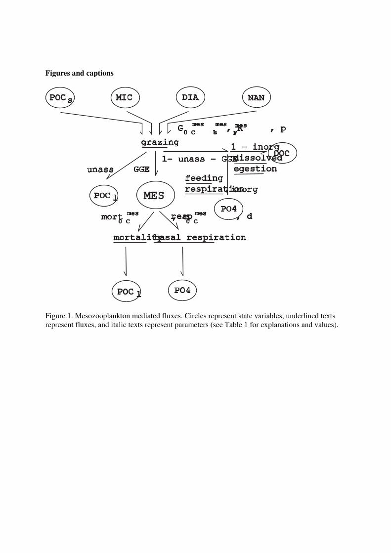
Figures and captions

MES

DOC

PO4

inorg

POC

MICPOC

grazing

DIA NAN

GGEfeeding

respiration

1- unass - GGE

unass

POC

mort , cresp , d

G , K , p

l

s

l

‰0°C

mesmes

1 - inorg

mortalitybasal respiration

PO4

mes

F

dissolved

egestion

0°C

mes

0°C

mes

Figure 1. Mesozooplankton mediated fluxes. Circles represent state variables, underlined texts

represent fluxes, and italic texts represent parameters (see Table 1 for explanations and values).

0

0.2

0.4

0.6

0.8

1

1.2

1.4

0 5 10 15 20Chlorophyll [µg·L-1]

gro

wth

ra

te [

d -1

]

0

0.5

1

1.5

2

2.5

3

0 10 20 30Temperature [°C]

gro

wth

ra

te [

d -1

]

0

0.1

0.2

0.3

0.4

0.5

0.6

0.7

0.8

0.9

1

0.001 0.01 0.1 1 10 100

Food concentration [µM·L-1

]

GG

E

0

0.1

0.2

0.3

0.4

0.5

0.6

-5 0 5 10 15 20 25 30T [°C]

mo

rta

lity

ra

te [

d-1

]

0

0.5

1

1.5

2

2.5

-5 0 5 10 15 20 25 30

Temperature [°C]

res

pir

ati

on

ra

te [

d-1

]

Figure 2. Databases used for calculating parameter values. Bold lines are fit to all measurements.

Thin lines are fit to the data that lie above and below the fit to all measurements, approximately

corresponding to the high and low halves of the data. The dashed line in panels A & B is the net

growth rate used in the optimised simulation. A) Copepod growth rate as a function of chlorophyll a

concentration corrected to a constant temperature of 15 °C (Hirst and Bunker, 2003). Some high

values (up to 321 µg·L-1) are not shown but were included in the data fits. B) Copepod growth rate as

a function of temperature corrected to a constant chlorophyll a concentration of 3.7 µg·L-1 (Same data

as A, the uncorrected data was fit to Equation 13). C) Gross growth efficiency. Horizontal lines are

averages, not calculated as a function of food concentration (Straile, 1997). D) Copepod mortality as

a function of temperature (Hirst and Kiørboe, 2002). E) Unfed routine mesozooplankton respirationsp

as a function of temperature (Ikeda, 1985; Ikeda et al., 2001).

Atlantic Pacific + Indian

A B

C D

E F

Figure 3. Zonal averages. Black lines) Observations, Green lines) PISCES, Red lines) PISCES-T

standard simulation, Blue lines) PISCES-T optimised simulation, Shaded grey areas) range of

simulations in sensitivity analysis (excluding PISCES). A, B) surface chlorophyll, C, D) surface

mesozooplankton, E, F) export at 100 m.. A, C, E) Atlantic Ocean B, D, F) Pacific and Indian

Oceans.

Ex

po

rt [

Pg

·y-1

] M

eso

zoo

pla

nk

ton

[µ

M]

Ch

loro

ph

yll

[µ

g·L

-1]

Observed PISCES-T optimized

PISCES PISCES-T standard

PISCES-T standard / observed

Figure 4. Mesozooplankton concentration [µM C] A) observed (NMFS, FSU (roughly delimited

by white line) & CPR (delimited by black line)), B) PISCES-T optimised simulation, C) PISCES,

D) PISCES-T standard simulation, E) PISCES-T standard simulation (y-axis) vs. observed (x-

axis) +: NMFS (18 values between 5 and 9 µM are not shown), □: FSU, ×: CPR. Model results

are integrated over the same depth ranges as the observations (Table 3), and over the top 200m

where no observations are available.

SeaWiFS WOA

PISCES PISCES-T standard

Figure 5. Surface chlorophyll a concentration. The scale is irregular. A) satellite observed

(SeaWiFS), B) measured in situ (WOA database averaged from 1955-1998), C) PISCES, D)

PISCES-T standard simulation, (A, C & D averaged from 1998-2002).

00.10.20.30.40.5

0 0.2 0.4 0.6 0.8 1grazing rate [d

-1]

con

cen

tra

tio

n

0

5

10

15

20

25

dif

fere

nc

e

010203040506070

0 0.2 0.4 0.6 0.8 1grazing rate [d

-1]

rate

[P

g/y

]

A B

Figure 6. Sensitivity analysis and optimization of the grazing rate. Arrow down: standard

simulation, Arrow up: optimised simulation. A) left y-axis: Filled circles) mesozooplankton

concentration [µM C], grey triangles) chlorophyll a concentration [µg·L-1

], right y-axis: open

squares) point by point difference between model mesozooplankton concentration and evaluation

data, (10^average(absolute(log(model/observation)))); B) Filled circles) mesozooplankton

grazing, grey triangles) primary production, open circles) export at 100 m.

Schlitzer PISCES-T no T dep.

PISCES PISCES-T standard

Figure 7. Export at 100 m. depth [mol·m-2·year-1]. A) Results from the inverse model of Schlitzer

(2004), based on geochemical observations. B) no temperature dependence of POC degradation

C) PISCES. D) PISCES-T standard simulation.

Observed PISCES-T low GGE

PISCES-T squared mortality PISCES-T standard

Figure 8. LOG(mesozooplankton/chlorophyll a [µM C·(µg Chl)-1

]) vs. LOG(chlorophyll a [µg

Chl]) A) observed (using World Ocean Atlas Chlorophyll a, integrated over the appropriate depth

ranges) B) PISCES-T low GGE simulation, surface concentrations C) PISCES-T squared

mortality simulation, surface concentrations D) PISCES-T standard simulation, surface

concentrations.