Analysis of Turbulent Flows with Computer Programs

Analysis of TurbulentFlows with Computer

Programs

THIRD EDITION

Tuncer Cebeci

Formerly Distinguished Technical Fellow,Boeing Company, Long Beach, California

horizonpublishing.net

AMSTERDAM � BOSTON � HEIDELBERG � LONDON

NEW YORK � OXFORD � PARIS � SAN DIEGO

SAN FRANCISCO � SINGAPORE � SYDNEY � TOKYO

Butterworth-Heinemann is an Imprint of Elsevier

http://horizonpublishing.net

Butterworth-Heinemann is an imprint of Elsevier

The Boulevard, Langford Lane, Kidlington, Oxford OX5 1GB, UK

225 Wyman Street, Waltham, MA 02451, USA

First edition 1974

Second edition 2004

Third edition 2013

Copyright � 2013 Elsevier Ltd. All rights reserved

No part of this publication may be reproduced, stored in a retrieval system or transmitted

in any form or by any means electronic, mechanical, photocopying, recording or otherwise

without the prior written permission of the publisher

Permissions may be sought directly from Elsevier’s Science & Technology Rights

Department in Oxford, UK: phone (+44) (0) 1865 843830; fax (+44) (0) 1865 853333;

email: [email protected]. Alternatively you can submit your request online by

visiting the Elsevier web site at http://elsevier.com/locate/permissions, and selecting

Obtaining permission to use Elsevier material

Notice

No responsibility is assumed by the publisher for any injury and/or damage to persons or

property as a matter of products liability, negligence or otherwise, or from any use or operation

of any methods, products, instructions or ideas contained in the material herein. Because of

rapid advances in the medical sciences, in particular, independent verification of diagnoses and

drug dosages should be made

British Library Cataloguing in Publication Data

A catalogue record for this book is available from the British Library

Library of Congress Cataloging-in-Publication Data

A catalog record for this book is availabe from the Library of Congress

ISBN: 978-0-08-098335-6

For information on all Elsevier publications

visit our web site at books.elsevier.com

Printed and bound in United States of America

13 14 15 16 17 10 9 8 7 6 5 4 3 2 1

mailto:[email protected]

http://elsevier.com/locate/permissions

http://books.elsevier.com

Dedication

This book is dedicated to the memory of my beloved wife, Sylvia Holt Cebeci, my

best friend of many years. She will always be with me, in my heart, in my memories

and in all the loving ways she touched my life each day.

I will always remember her note to me on my birthday in 2011 prior to her death

on May 4, 2012:

Dear TC,

The twilight times bring you automatic admission to a special club; to share the

game of special 50’s, 60’s music; remembering your friends and death of a special

friend; being a historian simply because you live long enough. You and I have been

so fortunate to share a golden life everyday.

Love, Sylvia

iii

Preface to the Third Edition

The first edition of this book, Analysis of Turbulent Boundary Layers, was written in

the period between 1970 and early 1974 when the subject of turbulence was in its

early stages and that of turbulence modeling in its infancy. The subject had advanced

considerably over the years with greater emphasis on the use of numerical methods

and an increasing requirement and ability to calculate turbulent two- and three-

dimensional flows with and without separation. The tools for experimentation were

still the traditional Pitot tube and hot wire-anemometer so that the range of flows that

could be examined was limited and computational methods still included integral

methods and a small range of procedures based on the numerical solution of

boundary layer equations and designed to match the limited range of measured

conditions. There have been tremendous advances in experimental techniques with

the development of non-intrusive optical methods such as laser-Doppler, phase-

Doppler and particle-image velocimetry, all for the measurement of velocity and

related quantities and of a wide range of methods for the measurement of scalars.

These advances have allowed an equivalent expansion in the range of flows that have

been investigated and also in the way in which they could be examined and inter-

preted. Similarly, the use of numerical methods to solve time-averaged forms of the

Navier-Stokes equations, sometimes interactively with the inviscid-flow equations,

has expanded, even more so with the rise and sometimes fall of Companies that

wished to promote and sell particular computer codes. The result of these devel-

opments has been an enormous expansion of the literature and has provided a great

deal of information beyond that which was available when the first edition was

written. Thus, the topics of the first edition needed to be re-examined in the light of

new experiments and calculations, and the ability of calculation methods to predict

a wide range of practical flows, including those with separation, to be reassessed.

The second edition, entitled Analysis of Turbulent Flows, undertook the neces-

sary reappraisal, reformulation and expansion, and evaluated the calculation methods

more extensively but also within the limitations of two-dimensional equations

largely because this made explanations easier and the book of acceptable size. In

addition, it was written to meet the needs of graduate students as well as engineers

and so included homework problems that were more sensibly formulated within the

constraints of two independent variables. References to more complex flows, and

particularly those with separation, were provided and the relative merits of various

turbulence models considered. xi

The third edition, entitled Analysis of Turbulent Flows with Computer Programs,

keeps the structure of the first and second editions the same. It expands the solution

of the boundary-layer equations with transport-equation turbulence models,

considers the solution of the boundary-layer equations with flow separation and

provides computer programs for calculating attached and separating flows with

several turbulence models.

The second edition and the contents of this new edition should be viewed in the

context of new developments such as those associated with large-eddy simulations

(LES) and direct numerical solutions (DNS) of the Navier-Stokes equations. LES

existed in 1976 as part of the effort to represent meteorological flows and has been

rediscovered recently as part of the recognition of the approximate nature of solu-

tions of time-averaged equations as considered here. There is no doubt that LES has

a place in the spectrum of methods applied to the prediction of turbulent flows but we

should not expect a panacea since it too involves approximations within the

numerical method, the filter between time-dependent and time-average solutions and

small-scale modeling. DNS approach also has imperfections and mainly associated

with the computational expense which implies compromises between accuracy and

complexity or, more usually, restriction to simple boundary conditions and low

Reynolds numbers. It is likely that practical aerodynamic calculations with and

without separation will continue to make use of solutions of the inviscid-flow

equations and some reduced forms of the Navier-Stokes equations for many years,

and this book is aimed mainly at this approach.

The first and second editions were written with help from many colleagues. AMO

Smith was an enthusiastic catalyst and ideas were discussed with him over the years.

Many colleagues and friends from Boeing, the former Douglas Aircraft Company

and the McDonnell-Douglas Company, have contributed by discussion and advice

and included K. C. Chang and J. P. Shao. Similarly, Peter Bradshaw, the late Herb

Keller of Cal Tech and the late Jim Whitelaw of Imperial College have helped in

countless ways.

Indian Wells

Tuncer Cebeci

xii Preface to the Third Edition

Computer Programs Available from horizonpublishing.net

1. Integral Methods.

2. Differential Method with CS Model for two-dimensional flows with

and without heat transfer and infinite swept-wing flows.

3. Hess-Smith Panel Method with and without viscous effects.

4. Zonal Method for k-ε Model and solution of k-ε Model equations with and

without wall functions.

5. Differential Method for SA Model and for a Plane Jet.

6. Differential Method for inverse and interactive boundary-layer flows with

CS Model.

xiii

http://horizonpublishing.net

Introduction

Chap

ter1

Chapter Outline Head

1.1 Introductory Remarks 1

1.2 Turbulence – Miscellaneous Remarks 3

1.3 The Ubiquity of Turbulence 7

1.4 The Continuum Hypothesis 8

1.5 Measures of Turbulence – Intensity 11

1.6 Measures of Turbulence – Scale 14

1.7 Measures of Turbulence – The Energy Spectrum 19

1.8 Measures of Turbulence – Intermittency 22

1.9 The Diffusive Nature of Turbulence 23

1.10 Turbulence Simulation 26

Problems 29

References 31

1.1 Introductory Remarks

Turbulence in viscous flows is described by the Navier–Stokes equations, perfected

by Stokes in 1845, and now soluble by Direct Numerical Simulation (DNS).

However, computing capacity restricts solutions to simple boundary conditions and 1

Analysis of Turbulent Flows with Computer Programs. http://dx.doi.org/10.1016/B978-0-08-098335-6.00001-X

Copyright � 2013 Elsevier Ltd. All rights reserved.

http://dx.doi.org/10.1016/B978-0-08-098335-6.00001-X

moderate Reynolds numbers and calculations for complex geometries are very

costly. Thus, there is need for simplified, and therefore approximate, calculations for

most engineering problems. It is instructive to go back some eighty years to remarks

made by Prandtl [1] who began an important lecture as follows:

What I am about to say on the phenomena of turbulent flows is still far from

conclusive. It concerns, rather, the first steps in a new path which I hope will

be followed by many others.

The researches on the problem of turbulence which have been carried on at

Gottingen for about five years have unfortunately left the hope of a thorough

understanding of turbulent flow very small. The photographs and

kineto-graphic pictures have shown us only how hopelessly complicated

this flow is .

Prandtl spoke at a time when numerical calculations made use of primitive

devices – slide rules and mechanical desk calculators. We are no longer ‘‘hopeless’’

because DNS provides us with complete details of simple turbulent flows, while

experiments have advanced with the help of new techniques including non-obtrusive

laser-Doppler and particle-image velocimetry. Also, developments in large-eddy

simulation (LES) are also likely to be helpful although this method also involves

approximations, both in the filter separating the large (low-wave-number) eddies and

the small ‘sub-grid-scale’ eddies, and in the semi-empirical models for the latter.

Even LES is currently too expensive for routine use in engineering, and

a common procedure is to adopt the decomposition first introduced by Reynolds for

incompressible flows in which the turbulent motion is assumed to comprise the sum

of mean (usually time-averaged) and fluctuating parts, the latter covering the whole

range of eddy sizes. When introduced into the Navier–Stokes equations in terms of

dependent variables the time-averaged equations provide a basis for assumptions for

turbulent diffusion terms and, therefore, for attacking mean-flow problems. The

resulting equations and their reduced forms contain additional terms, known as the

Reynolds stresses and representing turbulent diffusion, so that there are more

unknowns than equations. A similar situation arises in transfer of heat and other

scalar quantities. In order to proceed further, additional equations for these unknown

quantities, or assumptions about the relationship between the unknown quantities

and the mean-flow variables, are required. This is referred to as the ‘‘closure’’

problem of turbulence modeling.

The subject of turbulence modeling has advanced considerably in the last seventy

years, corresponding roughly to the increasing availability of powerful digital

computers. The process started with ‘algebraic’ formulations (for example, algebraic

formulas for eddy viscosity) and progressed towards methods in which partial

differential equations for the transport of turbulence quantities (eddy viscosity, or the

Reynolds stresses themselves) are solved simultaneously with reduced forms of the

2 Analysis of Turbulent Flows with Computer Programs

Navier–Stokes equations. At the same time numerical methods have been developed

to solve forms of the conservation equations which are more general than the two-

dimensional boundary layer equations considered at the Stanford Conference of

1968.

The first edition of this book was written in the period from 1968 to 1973 and was

confined to algebraic models for two-dimensional boundary layers. Transport

models were in their infancy and were discussed without serious application or

evaluation. There were no similar books at that time. This situation has changed and

there are several books to which the reader can refer. Books on turbulence include

those of Tennekes and Lumley [2], Lesieur [3], Durbin and Petterson [5]. Among

those on turbulence models the most comprehensive is probably that of Wilcox [6].

The second edition of this book had greater emphasis on modern numerical

methods for boundary-layer equations than the first edition and considered turbu-

lence models from advanced algebraic to transport equations but with more emphasis

on engineering approaches. The present edition extends this subject to encompass

separated flows within the framework of interactive boundary layer theory.

This chapter provides some of the terminology used in subsequent chapters,

provides examples of turbulent flows and their complexity, and introduces some

important turbulent-flow characteristics.

1.2 Turbulence – Miscellaneous Remarks

We start this chapter by addressing the question ‘‘What is turbulence?’’ In the 25th

Wilbur Wright Memorial Lecture entitled ‘‘Turbulence,’’ von Karman [7] defined

turbulence by quoting G. I. Taylor as follows:

Turbulence is an irregular motion which in general makes its appearance in

fluids, gaseous or liquid, when they flow past solid surfaces or even when

neighboring streams of the same fluid flow past or over one another.

That definition is acceptable but is not completely satisfactory. Many irregular

flows cannot be considered turbulent. To be turbulent, they must have certain

stationary statistical properties analogous to those of fluids when considered on the

molecular scale. Hinze [8] recognizes the deficiency in von Karman’s definition and

proposes the following:

Turbulent fluid motion is an irregular condition of flow in which the various

quantities show a random variation with time and space coordinates, so that

statistically distinct average values can be discerned.

In addition turbulence has a wide range of wave lengths. The three statements

taken together define the subject adequately.

Introduction 3

What were probably the first observations of turbulent flow in a scientific sense

were described by Hagen [9]. He was studying flow of water through round tubes and

observed two distinct kinds of flow, which are now known as laminar (or Hagen-

Poiseuille) and turbulent. If the flow was laminar as it left the tube, it looked clear

like glass; if turbulent, it appeared opaque and frosty. The two kinds of flow can be

generated readily by many household faucets. Fifteen years later, in 1854, he pub-

lished a second paper showing that viscosity as well as velocity influenced the

boundary between the two flow regimes. In his work he observed the mean* velocity

�u in the tube to be a function of both head and water temperature. (Of course,

temperature uniquely determines viscosity.) His results are shown in Fig. 1.1 for

several tube diameters. The plot contains implicit variations of �u, r0, and n, the

velocity, the tube radius, and the kinematic viscosity, respectively. This form of

presentation displays no orderliness in the data. About thirty years later, Reynolds

[11] introduced the parameter Rr h �ur0 /n an example of what is now known as the

Reynolds number (with velocity and length scales depending on the problem). It

collapsed Hagen’s data into nearly a single curve. The new parameter together with

Fig. 1.1 Relation between �u, (expressed in Rhineland inches per second) and thetemperature (expressed in degrees Reaumur) for various pipe diameters and heads h(in Rhineland inches), after tests by G. Hagen. d 0.281 cm diam.; – – – 0.405 cmdiam.; - - - 0.596 cm diam. [10].

*For now, let ‘‘mean’’ denote an average with respect to time, over a time long compared with the lowest

frequencies of the turbulent fluctuations. In Section 2.3 we will give more details of this and other kinds

of averaging.


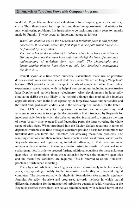
the dimensionless friction factor l, defined such that the pressure drop

Dp ¼ lð9�u2=2Þ ðl=r0Þ, transforms the plot of Fig. 1.1 to that of Fig. 1.2. The

quantity l is tube length; the other quantities have the usual meaning. Thus was born

the parameter, Reynolds number. The term ‘‘turbulent flow’’ was not used in those

earlier studies; the adjective then used was ‘‘sinuous’’ because the path of fluid

particles in turbulent flow was observed to be sinusoidal or irregular. The term

‘‘turbulent flow’’ was introduced by Lord Kelvin in 1887.

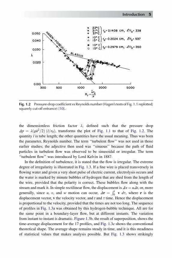
In the definition of turbulence, it is stated that the flow is irregular. The extreme

degree of irregularity is illustrated in Fig. 1.3. If a fine wire is placed transversely in

flowing water and given a very short pulse of electric current, electrolysis occurs and

the water is marked by minute bubbles of hydrogen that are shed from the length of

the wire, provided that the polarity is correct. These bubbles flow along with the

stream and mark it. In simple rectilinear flow, the displacement isDx¼ uDt, or, more

generally, since u, y, and w motion can occur, Dr ¼ R t0 v ds, where r is the

displacement vector, v the velocity vector, and t and s time. Hence the displacement

is proportional to the velocity, provided that the times are not too long. The sequence

of profiles in Fig. 1.3a was obtained by this hydrogen-bubble technique. All are for

the same point in a boundary-layer flow, but at different instants. The variation

from instant to instant is dramatic. Figure 1.3b, the result of superposition, shows the

time-average displacement for the 17 profiles, and Fig. 1.3c shows the conventional

theoretical shape. The average shape remains steady in time, and it is this steadiness

of statistical values that makes analysis possible. But Fig. 1.3 shows strikingly

Fig. 1.2 Pressure-drop coefficient vs Reynolds number (Hagen’s tests of Fig. 1.1 replotted;squarely cut-off entrance) [10].

Introduction 5

that the flow is anything but steady; it is certainly not even a small-perturbation type

of flow.

The Reynolds-number parameter has a number of interpretations, but the most

fundamental one is that it is a measure of the ratio of inertial forces to viscous forces.

It is well known that inertial forces are proportional to 9V2. Viscous forces are

proportional to terms of the type mvu/vy, or approximately to mV/l, for a given

geometry. The ratio of these quantities is

9V2=ðm V=lÞ ¼ 9Vl=mh Rl; (1.2.1)

which is a Reynolds number. Whenever a characteristic Reynolds number Rl is high,

turbulent flow is likely to occur. In the tube tests of Fig. 1.2, the flow is laminar for all

conditions where Rr is below about 1000, and it is turbulent for all conditions where

Rr is greater than about 2000. Between those values of Rr is the transition region.

Accurate prediction of the transition region is a complicated and essentially unsolved

problem.

Fig. 1.3 Instantaneous turbulent boundary-layer profiles according to the hydrogen-bubble technique. Measurements were made at Rx z 105 on a flat plate 5 ft aft ofleading edge. The boundary layer was tripped. (a) A set of profiles, all obtained at thesame position from 17 runs. (b) The same set superimposed. (c) A standard mean profileat the same Rx. (d) Photograph of one of the hydrogen-bubble profiles. (e) A laminarprofile on the opposite side of the plate.


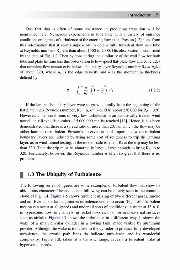
One fact that is often of some assistance in predicting transition will be

mentioned here. Numerous experiments in tube flow with a variety of entrance

conditions or degrees of turbulence of the entering flow exist. Preston [12] notes from

this information that it seems impossible to obtain fully turbulent flow in a tube

at Reynolds numbers Rr less than about 1300 to 2000. His observation is confirmed

by the data of Fig. 1.2. Then by considering the similarity of the wall flow for both

tube and plate he transfers this observation to low-speed flat-plate flow and concludes

that turbulent flow cannot exist below a boundary-layer Reynolds number Rq h ueq/n

of about 320, where ue is the edge velocity and q is the momentum thickness

defined by

q ¼Z N

0

u

ue

�1� u

ue

�dy (1.2.2)

If the laminar boundary layer were to grow naturally from the beginning of the

flat plate, the x Reynolds number, Rx ¼ uex/n, would be about 230,000 for Rq ¼ 320.

However, under conditions of very low turbulence in an acoustically treated wind

tunnel, an x Reynolds number of 5,000,000 can be reached [13]. Hence, it has been

demonstrated that there is a spread ratio of more than 20:1 in which the flow may be

either laminar or turbulent. Preston’s observation is of importance when turbulent

boundary layers are induced by using some sort of roughness to trip the laminar

layer, as in wind-tunnel testing. If the model scale is small, Rq at the trip may be less

than 320. Then the trip must be abnormally large – large enough to bring Rq up to

320. Fortunately, however, the Reynolds number is often so great that there is no

problem.

1.3 The Ubiquity of Turbulence

The following series of figures are some examples of turbulent flow that show its

ubiquitous character. The eddies and billowing can be clearly seen in the cumulus

cloud of Fig. 1.4. Figure 1.5 shows turbulent mixing of two different gases, smoke

and air. Even at stellar magnitudes turbulence seems to occur (Fig. 1.6). Turbulent

motion can occur at all speeds and under all sorts of conditions: in water at M z 0,

in hypersonic flow, in channels, in rocket nozzles, or on or near external surfaces

such as airfoils. Figure 1.7 shows the turbulence in a different way. It shows the

wake of a small circular cylinder in a towing tank, made visible by aluminum

powder. Although the wake is too close to the cylinder to produce fully developed

turbulence, the erratic path lines do indicate turbulence and its wonderful

complexity. Figure 1.8, taken at a ballistic range, reveals a turbulent wake at

hypersonic speeds.

Introduction 7

1.4 The Continuum Hypothesis

The Navier–Stokes equations and their reduced forms leading to Euler (Chapter 2)

and boundary-layer (Chapter 3) equations are derived by considering flow and forces

about an element of infinitesimal size, with the flow treated as a continuum.

Fig. 1.5 Turbulent motion in a smoke trail generated to indicate wind direction forlanding tests.

Fig. 1.4 Turbulent motion in a cumulus cloud.


Although turbulent eddies may be very small, they are by no means infinitesimal.

How well does the assumption of continuity apply?

Avogadro’s number states that there are 6.025 � 1023 molecules in a gram

molecular weight of gas, which at standard temperature (0�C) and pressure

(760 Torr) occupies 22,414 cm3, which means 2.7 � 1019 molecules/cm3. Hence

Fig. 1.6 Solar granulations – a highly magnified section of the sun’s surface. Thisappears to be a random flow, a form of turbulence. The pattern changes continuously.It becomes entirely different after about ten minutes. Photo courtesy of HaleObservatories.

Fig. 1.7 The turbulent motion in the wake of a circular cylinder in water. Motion ismade visible by aluminum powder.

Introduction 9

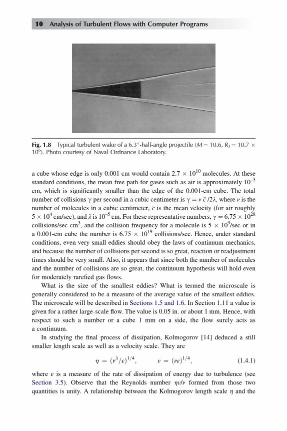
a cube whose edge is only 0.001 cm would contain 2.7 � 1010 molecules. At these

standard conditions, the mean free path for gases such as air is approximately 10–5

cm, which is significantly smaller than the edge of the 0.001-cm cube. The total

number of collisions g per second in a cubic centimeter is g ¼ n �c /2l, where n is the

number of molecules in a cubic centimeter, �c is the mean velocity (for air roughly

5� 104 cm/sec), and l is 10–5 cm. For these representative numbers, g¼ 6.75� 1028

collisions/sec cm3, and the collision frequency for a molecule is 5 � 109/sec or in

a 0.001-cm cube the number is 6.75 � 1019 collisions/sec. Hence, under standard

conditions, even very small eddies should obey the laws of continuum mechanics,

and because the number of collisions per second is so great, reaction or readjustment

times should be very small. Also, it appears that since both the number of molecules

and the number of collisions are so great, the continuum hypothesis will hold even

for moderately rarefied gas flows.

What is the size of the smallest eddies? What is termed the microscale is

generally considered to be a measure of the average value of the smallest eddies.

The microscale will be described in Sections 1.5 and 1.6. In Section 1.11 a value is

given for a rather large-scale flow. The value is 0.05 in. or about 1 mm. Hence, with

respect to such a number or a cube 1 mm on a side, the flow surely acts as

a continuum.

In studying the final process of dissipation, Kolmogorov [14] deduced a still

smaller length scale as well as a velocity scale. They are

h ¼ ðn3=εÞ1=4; y ¼ ðnεÞ1=4; (1.4.1)

where ε is a measure of the rate of dissipation of energy due to turbulence (see

Section 3.5). Observe that the Reynolds number hy/n formed from those two

quantities is unity. A relationship between the Kolmogorov length scale h and the

Fig. 1.8 Typical turbulent wake of a 6.3�-half-angle projectile (M ¼ 10.6, Rl ¼ 10.7 �106). Photo courtesy of Naval Ordnance Laboratory.


mean free path l can be obtained by writing the definition of kinematic viscosity,

namely, n¼ 0.499 c l. Making use of that relationship, from Eq. (1.4.1) we can write

h=l ¼ �c=2y: (1.4.2)

A representative value of ε is given in Fig. 4.6b in dimensionless form as ðεd=u3sÞ.Let us use the value 20. For the tests, us=ue was about (0.0015)

1/2 ¼ 0.04. For these

test conditions, it follows that ε is approximately

ε z 12� 10�4u3e=d: (1.4.3)

With Eq. (1.4.3), we can write Eq. (1.4.2) as

h=lz 3R1=4d =ðue=cÞ; (1.4.4)

where Rd ¼ ued/n. Now a turbulent boundary layer has a thickness roughly equal to

ten times the momentum thickness. Hence, with the value 320 presented in Section

1.1, the minimum value of Rd is about 3000. Then according to Eq. (1.4.4) h is small,

but it too is substantially larger than the mean free path. Note that Mach number has

effectively been brought in by the term ue/ �c. Accordingly, only if the Mach number

becomes quite large will any question arise as to the continuum hypothesis.

1.5 Measures of Turbulence – Intensity

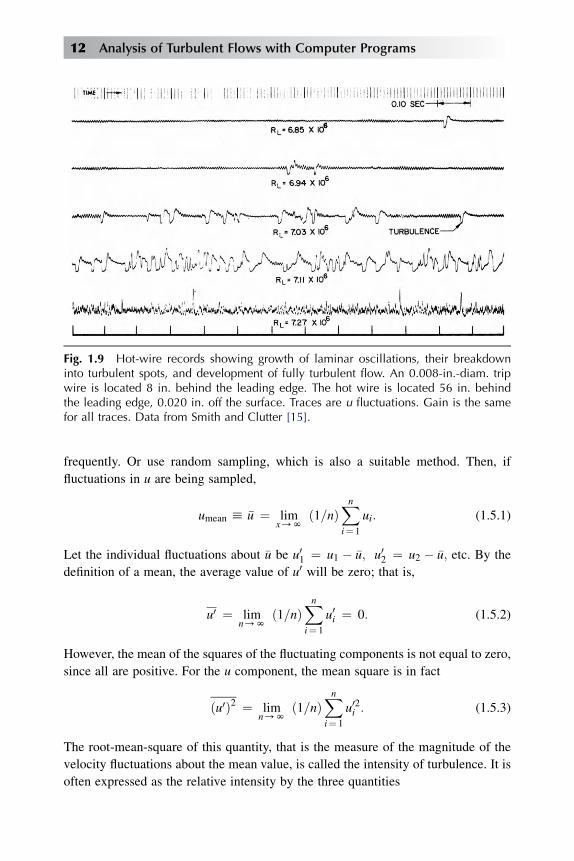
Figure 1.9 shows the evolution of turbulence at a particular point on a 108-in.-

chord plate as the tunnel speed, and hence chord Reynolds number, was

increased. In the sequence, the transition position was moved relative to the hot

wire by changing tunnel speed which is often a more convenient method than

moving the hot wire through the transition region while holding tunnel speed

constant. Until the last or fully-developed turbulent trace is reached, it is ques-

tionable that the fluctuations meet Hinze’s requirement (Section 1.2) for

discernment of statistically distinct average values. Certainly the traces are not

long enough to indicate any statistical regularity. But the last trace seems to

indicate that the fully turbulent state has arrived. Some features visible to the eye

are: (1) average value of the velocity fluctuations; (2) range of magnitudes, or

distribution, of these fluctuations, and (3) some sort of frequency or wave length,

or distribution thereof (thousands of oscillations in 0.1 second or just a few?); (4)

the shortest wave length; (5) the average wave length, etc. A number of useful

measures have been developed, and it is our purpose here to acquaint the reader

with a few of the more important ones.

Consider the bottom trace in Fig. 1.9 and work out a time average by taking

samples periodically without bias, say at every 0.1 or 0.01 sec, or even more

Introduction 11

frequently. Or use random sampling, which is also a suitable method. Then, if

fluctuations in u are being sampled,

umean h �u ¼ limx/N

ð1=nÞXni¼ 1

ui: (1.5.1)

Let the individual fluctuations about �u be u01 ¼ u1 � �u; u02 ¼ u2 � �u; etc. By the

definition of a mean, the average value of u0 will be zero; that is,

u0 ¼ limn/N

ð1=nÞXni¼ 1

u0i ¼ 0: (1.5.2)

However, the mean of the squares of the fluctuating components is not equal to zero,

since all are positive. For the u component, the mean square is in fact

ðu0Þ2 ¼ limn/N

ð1=nÞXni¼ 1

u02i : (1.5.3)

The root-mean-square of this quantity, that is the measure of the magnitude of the

velocity fluctuations about the mean value, is called the intensity of turbulence. It is

often expressed as the relative intensity by the three quantities

Fig. 1.9 Hot-wire records showing growth of laminar oscillations, their breakdowninto turbulent spots, and development of fully turbulent flow. An 0.008-in.-diam. tripwire is located 8 in. behind the leading edge. The hot wire is located 56 in. behindthe leading edge, 0.020 in. off the surface. Traces are u fluctuations. Gain is the samefor all traces. Data from Smith and Clutter [15].


ðu02Þ1=2=u; ðy02Þ1=2=u; ðw02Þ1=2=u; (1.5.4)

A ‘‘stationary’’ turbulent flow is characterized by a constant mean velocity �u (with

y ¼ �w ¼ 0 for suitable axes) and constant values of u02; y02; w02. The true velocityat any instant is never known, but at least certain average properties can be specified.

One such measure is the relative level of turbulence s in a stream whose average

velocity is �u:

s ¼ ð1=uÞ ��u02 þ y02 þ w02�=3�1=2: (1.5.5)

If the turbulence is isotropic, u02 ¼ y02 ¼ w02. Isotropic turbulence can be devel-

oped in a wind tunnel by placing a uniform grid across the duct. A few mesh lengths

downstream, the flow becomes essentially isotropic in its turbulence properties. The

quantity s is about 1.0% in a poor wind tunnel, 0.2% in a good general purpose

tunnel, and as low as 0.01–0.02% in a well-designed low-turbulence tunnel.

The quantity s is directly related to the kinetic energy of the turbulence, as

will now be shown. Consider a flow whose mean velocity is �u, that is, �y ¼ �w ¼ 0.

Its instantaneous velocity can be represented by

V ¼ ð�uþ u0Þiþ y0jþ w0k:

The instantaneous kinetic energy per unit mass is

1

2½ð�uþ u0Þ2 þ y02 þ w02�;

and the mean kinetic energy per unit mass is

1

2�u2:

To get the kinetic energy of the turbulence, we subtract the mean kinetic energy from

the instantaneous kinetic energy and obtain

1

2ð2u0 �uþ q2Þ

where q2 ¼ u0j u0j with j¼ 1, 2, 3. The mean kinetic energy of the turbulence per unit

mass, k, can be obtained by taking the mean of the above expression. This gives

k ¼ 1

2q2: (1.5.6)

With the relation given by Eq. (1.5.5), we can also write Eq. (1.5.6) as

k ¼ 3

2�u2s2: (1.5.7)

Introduction 13

Until now, we have considered only the mean intensity of the fluctuations. Let us now

consider the distribution of the velocity fluctuations. Are the velocity fluctuations all

about the same, or are some large and some small? The lowest trace in Fig. 1.9 shows

a considerable variation. At least in homogeneous turbulence, for which the question

has been studied in some detail, the distribution is nearly Gaussian. A typical result is

shown in Fig. 1.10.

Even in two-dimensional mean flows, the turbulent fluctuations are three

dimensional. That should be fairly evident from the appearance of turbulent water

flow, cloud motion, smoke flow, etc. Figure 1.11 shows some typical measurements

made in a thick two-dimensional boundary layer. The three fluctuating components

differ of course, but not greatly. Observe that the fluctuations reach as much as 10%

of the base velocity �u, which is consistent with the indications of Fig. 1.3.

1.6 Measures of Turbulence – Scale

The oscilloscope trace of a hot wire placed in a stream flowing at 100 mph would

surely show a far more gradual fluctuation if the average eddy were 3 ft in diameter

than it would if the average eddy were ½ in. in diameter. Hence, both scale and

magnitude are parameters. For a stationary random-time series such as this is

presumed to be, a statistical method has been developed to establish well-defined

scales. Consider a stationary time series as in the sketch of Fig. 1.12, which could be

the kind supplied by the experiment just mentioned. Suppose one reads base values at

Fig. 1.10 Probability density function for the occurrence of various magnitudes ofvelocity fluctuations u 0 in a turbulent flow generated by a wire grid. Measurementwas made 16 mesh widths downstream. Mesh Reynolds number �uM /n ¼ 9600.Crosses represent measurements; dashed line represents a Gaussian or normal distri-bution [16].


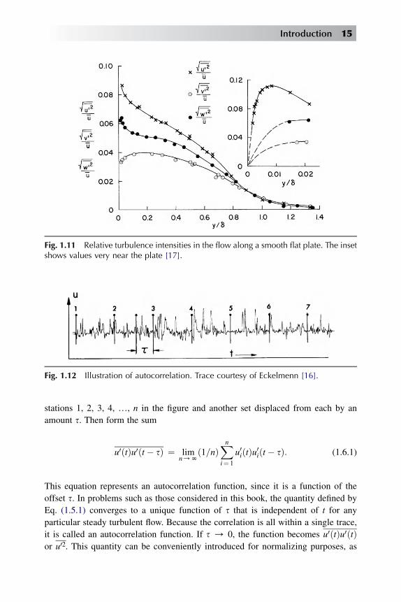
stations 1, 2, 3, 4, ., n in the figure and another set displaced from each by an

amount s. Then form the sum

u0ðtÞu0ðt � sÞ ¼ limn/N

ð1=nÞXni¼ 1

u0iðtÞu0iðt � sÞ: (1.6.1)

This equation represents an autocorrelation function, since it is a function of the

offset s. In problems such as those considered in this book, the quantity defined by

Eq. (1.5.1) converges to a unique function of s that is independent of t for any

particular steady turbulent flow. Because the correlation is all within a single trace,

it is called an autocorrelation function. If s / 0, the function becomes u0ðtÞu0ðtÞor u02. This quantity can be conveniently introduced for normalizing purposes, as

Fig. 1.12 Illustration of autocorrelation. Trace courtesy of Eckelmenn [16].

Fig. 1.11 Relative turbulence intensities in the flow along a smooth flat plate. The insetshows values very near the plate [17].

Introduction 15

in the following equation, to form what is known as an Eulerian time-correlation

coefficient:

REðsÞ ¼ u0ðtÞu0ðt � sÞ= u02: (1.6.2)

The function RE(s) may have a wide variety of shapes; the one sketched in Fig. 1.13

is typical.

The correlation shown in Fig. 1.13 was obtained from a trace produced by

a single instrument. In wind-tunnel tests two hot wires are offen placed abreast of

each other with the distance between them varied in order to obtain transverse

correlations, which provide measures of the transverse dimensions of eddies. In such

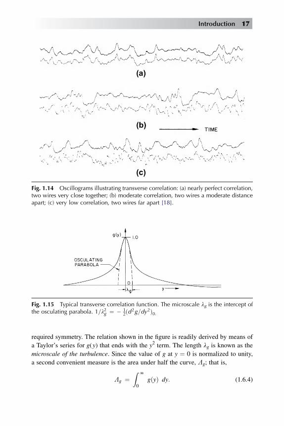
cases, simultaneous traces may have the general appearance shown in Fig. 1.14.

Correlations now are formed by taking readings of a pair of traces at matched time

instants to form quantities similar to Eq. (1.6.1), but now the variable is the sepa-

ration distance r, rather than s. If a pure transverse correlation is sought, the general

distance r reduces to y. With hot wires, a pure longitudinal correlation or x corre-

lation cannot be taken, because the downstream hot wire is in the wake of the

upstream wire. Longitudinal correlation is then obtained by the process leading to

Eq. (1.6.1). An example is shown in Fig. 1.12. An (x, t) relation is supplied by the

equation

v=vt ¼ ��uðv=vxÞ; (1.6.3)

which is known as Taylor’s hypothesis. The hypothesis simply assumes that the

fluctuations are too weak to induce any significant motion of their own, so that

disturbances are convected along at the mean stream velocity. It is quite accurate so

long as the level of turbulence is low, for example, less than 1%. It is not exact, and

has appreciable errors at high levels of turbulence [8].

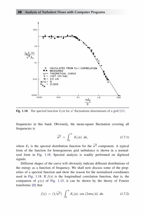
In homogeneous turbulence, a transverse correlation coefficient appears as in

Fig. 1.15, although the coefficient does not always become negative. The curvature at

the vertex is determined by the smallest eddies. Hence, a measure of the smallest

eddies is provided by the intercept of the osculating parabola. Theory shows that the

correlation begins as a quadratic function; a linear term would of course destroy the

Fig. 1.13 Plot of a typical correlation function.


required symmetry. The relation shown in the figure is readily derived by means of

a Taylor’s series for g(y) that ends with the y2 term. The length lg is known as the

microscale of the turbulence. Since the value of g at y ¼ 0 is normalized to unity,

a second convenient measure is the area under half the curve, Lg; that is,

Lg ¼Z N

0gðyÞ dy: (1.6.4)

Fig. 1.14 Oscillograms illustrating transverse correlation: (a) nearly perfect correlation,two wires very close together; (b) moderate correlation, two wires a moderate distanceapart; (c) very low correlation, two wires far apart [18].

Fig. 1.15 Typical transverse correlation function. The microscale lg is the intercept ofthe osculating parabola. 1=l2g ¼ � 1

2ðd2g=dy2Þ0:

Introduction 17

That area is a well-defined measure of the approximate size of the largest eddies. For

obvious reasons, it is called the integral scale. Figure 1.16 shows a number of

transverse correlation coefficients measured in a thick boundary layer on a large

body having a pressure distribution similar to that of a thick airfoil. By inspection –

because the peaks of the correlation curves are so pointed – it is evident that lg is

rather small. However, Lg is rather large, as much as an inch, apparently. Longitu-

dinal correlations were measured in the same investigation; their scales are

considerably greater.

Obviously, a wide variety of correlations can be measured; u0, y0, or w0 may be the

quantity measured. In the next chapter, the term y0u0 will emerge as a very important

quantity, which when multiplied by – 9 is known as a Reynolds shear-stress term. It

is a correlation between two velocities at a point. It could be computed from

oscilloscope traces, but two hot wires arranged in the form of an x can yield

instantaneous u0, y0 directly. If y0 were not related to u0, the correlation would be zero.Actually, it is physically related to u0. The transverse correlations just discussed are

known as double correlations. Correlations involving three or more measurements

can be made; they are of importance in attempts to develop further the statistical

theory of turbulence.

The rates of change of ðu02Þ1=2=�u and lg downstream of a grid are of interest both

from a practical standpoint and from the standpoint of the general theory of turbu-

lence. Figure 1.17 shows typical results downstream of a grid at both large and small

Fig. 1.16 Transverse correlation coefficients Ry measured in the boundary layer of

a large airfoil-like body. At the 1712 -ft station the edge velocity was 160 ft/sec. Ry ¼u 01u

02; ðu 0

1Þ1=2ðu 01Þ1=2 [19].


distances. At a short distance downstream of the grid, l2g has a slope 10nM/�u; at large

distances, the slope is 4nM/�u, whereM is the mesh size. In the initial stages of decay,

�u2=u02 varies as t5/2. A parameter that often arises is the Reynolds number of

turbulence Rl ¼ ðu02Þ1=2lg=n. In initial stages of decay, ðu02Þ1=2w t�1=2 and lg w t1/

2. Hence Rl remains constant in this region because the t terms cancel. Since the data

of Fig. 1.17 pertain to isotropic turbulence, the figure also provides information on

the decay of the kinetic energy of turbulence.

1.7 Measures of Turbulence – The Energy Spectrum

Since turbulence has fluctuations in three directions, any complete study of the

energy spectrum must necessarily involve a three-dimensional spectrum, or more

specifically a correlation tensor involving nine spectrum functions. But our purpose

here is only to introduce the general concept of a spectrum, and so we shall confine

our discussion to the one-dimensional case. Just as with light, where the different

colors (wave lengths or frequencies) may have different degrees of brightness, so

may the signal in a turbulent flow have different strengths for different frequencies.

For instance, the low-frequency portion of a u0 trace might have little energy and

the high-frequency portion much, or vice versa. The spectrum of turbulence relates

the energy content to the frequency. Consider the band of frequencies between n

and n þ dn. Then define E1 such that E1(n) dn is the contribution to u02 of the

Fig. 1.17 Variations of ðu02=�u2Þ and lg downstream of a grid in a wind tunnel [20].

Introduction 19

frequencies in this band. Obviously, the mean-square fluctuation covering all

frequencies is

u02 ¼Z N

0E1ðnÞ dn; (1.7.1)

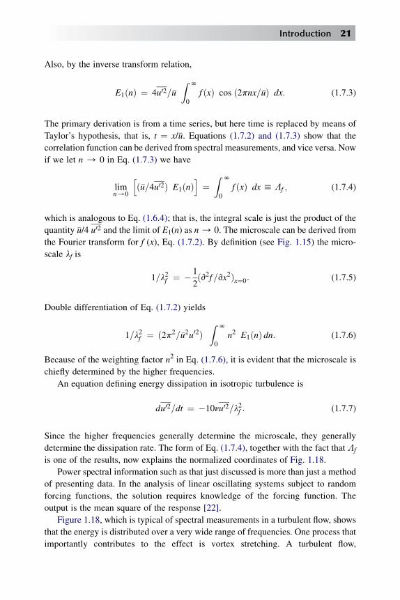
where E1 is the spectral distribution function for the u02 component. A typical

form of the function for homogeneous grid turbulence is shown in a normal-

ized form in Fig. 1.18. Spectral analysis is readily performed on digitized

signals.

Different shapes of the curve will obviously indicate different distributions of

the energy as a function of frequency. We shall now discuss some of the prop-

erties of a spectral function and show the reason for the normalized coordinates

used in Fig. 1.18. If f (x) is the longitudinal correlation function, that is, the

companion of g (y) of Fig. 1.15, it can be shown by the theory of Fourier

transforms [8] that

f ðxÞ ¼ ð1=u02ÞZ N

0E1ðnÞ cos ð2pnx=�uÞ dn: (1.7.2)

Fig. 1.18 The spectral function E1(n) for u0 fluctuations downstream of a grid [21].


Also, by the inverse transform relation,

E1ðnÞ ¼ 4u02=�uZ N

0f ðxÞ cos ð2pnx=�uÞ dx: (1.7.3)

The primary derivation is from a time series, but here time is replaced by means of

Taylor’s hypothesis, that is, t ¼ x/�u. Equations (1.7.2) and (1.7.3) show that the

correlation function can be derived from spectral measurements, and vice versa. Now

if we let n / 0 in Eq. (1.7.3) we have

limn/0

hð�u=4u02Þ E1ðnÞ

i¼Z N

0f ðxÞ dx h Lf ; (1.7.4)

which is analogous to Eq. (1.6.4); that is, the integral scale is just the product of the

quantity �u/4 u02 and the limit of E1(n) as n/ 0. The microscale can be derived from

the Fourier transform for f (x), Eq. (1.7.2). By definition (see Fig. 1.15) the micro-

scale lf is

1=l2f ¼ � 1

2ðv2f=vx2Þx¼0: (1.7.5)

Double differentiation of Eq. (1.7.2) yields

1=l2f ¼ ð2p2=�u2u02ÞZ N

0n2 E1ðnÞ dn: (1.7.6)

Because of the weighting factor n2 in Eq. (1.7.6), it is evident that the microscale is

chiefly determined by the higher frequencies.

An equation defining energy dissipation in isotropic turbulence is

du02=dt ¼ �10nu02=l2f : (1.7.7)

Since the higher frequencies generally determine the microscale, they generally

determine the dissipation rate. The form of Eq. (1.7.4), together with the fact that Lf

is one of the results, now explains the normalized coordinates of Fig. 1.18.

Power spectral information such as that just discussed is more than just a method

of presenting data. In the analysis of linear oscillating systems subject to random

forcing functions, the solution requires knowledge of the forcing function. The

output is the mean square of the response [22].

Figure 1.18, which is typical of spectral measurements in a turbulent flow, shows

that the energy is distributed over a very wide range of frequencies. One process that

importantly contributes to the effect is vortex stretching. A turbulent flow,

Introduction 21

particularly shear layers, is a large array of small vortices. Not only because of their

own interaction but also because of the mean velocity distribution in the boundary

layer, vortices may find themselves convected into the regions of higher velocity. If

so, they become stretched and their vorticity is intensified. Hence, more vorticity can

be generated at higher wave number. Thus there is such a complicated interaction

that vorticity of a wide variety of scales and strengths is generated. Batchelor [23] has

a good introductory discussion of this phenomenon, together with the descriptive

equations.

1.8 Measures of Turbulence – Intermittency

A laminar flow velocity profile asymptotes into the surrounding flow rapidly but

continuously. In fact, the disturbance due to a laminar flow such as a boundary layer

decays at least as fast as exp (–ky2), where k is near unity. Hence, although it decays

rapidly, the boundary layer has no distinct edge. The situation is quite different in

turbulent flows. There is a distinct edge, although it wanders around in random

fashion. Clouds show the effect well. A cumulus cloud is just a well-marked

turbulent flow on a giant scale. The line of demarcation between clear sky and cloud,

which shows as visible turbulent eddies, is quite sharp. There is no gradual

fading into the clear blue sky. Figure 1.4 is a picture of such a cloud, showing the

sharp but irregular boundaries. The ambient air can be thought of as being

contaminated by adjacent turbulence. The phenomenon is evident in any markedly

turbulent flow – clouds, smokestack plumes, exhaust steam, dust storms, muddy

water in clear water, etc.

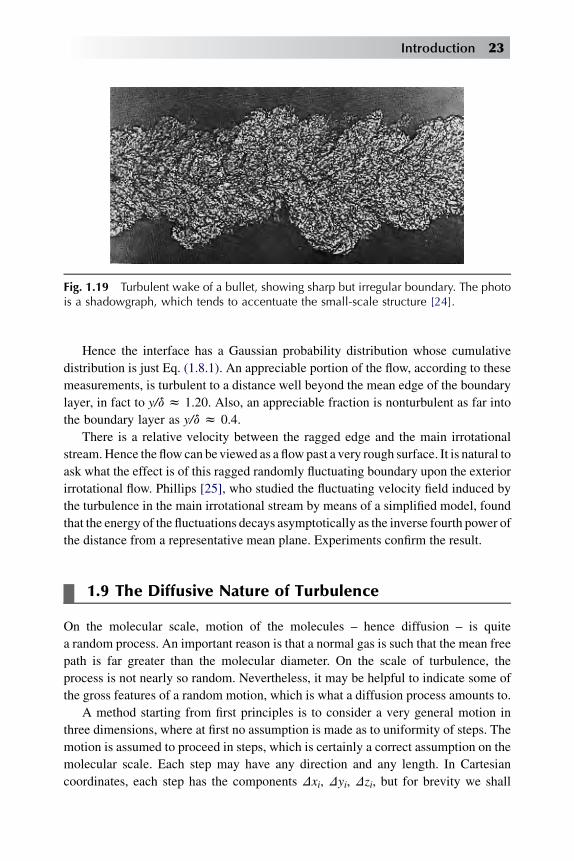
Figure 1.19 shows the same basic phenomenon, in this case due to the wake of

a bullet. If the wake were in motion as in a wind tunnel, it is clear that a hot wire or

another sensor would be either entirely in the turbulence or out of it; and, judging by

the appearance of the wake, the fraction of time the hot wire sees turbulence is

a statistical function of the distance from the center of the wake. The fraction is

called g, the intermittency, a term introduced by Corrsin and Kistler [24]. Entirely

outside a turbulent flow g ¼ 0, and entirely inside g ¼ 1.

Corrsin and Kistler appears to have first noticed the effect in 1943, during studies

of a heated jet. Two important early specific studies of the phenomenon as it occurs

in ordinary turbulent flows of air were conducted by Corrsin and Kistler [24] and

Klebanoff [17]. Klebanoff made such measurements for a boundary-layer flow on

a flat plate. He found that the intermittency was accurately described by the

following equation, where d is the mean thickness of the boundary layer:

g ¼ 1

2ð1� erfzÞ; where z ¼ 5½ðy=dÞ � 0:78�: (1.8.1)


Hence the interface has a Gaussian probability distribution whose cumulative

distribution is just Eq. (1.8.1). An appreciable portion of the flow, according to these

measurements, is turbulent to a distance well beyond the mean edge of the boundary

layer, in fact to y/d z 1.20. Also, an appreciable fraction is nonturbulent as far into

the boundary layer as y/d z 0.4.

There is a relative velocity between the ragged edge and the main irrotational

stream.Hence the flow can beviewed as a flowpast a very rough surface. It is natural to

ask what the effect is of this ragged randomly fluctuating boundary upon the exterior

irrotational flow. Phillips [25], who studied the fluctuating velocity field induced by

the turbulence in the main irrotational stream by means of a simplified model, found

that the energy of the fluctuations decays asymptotically as the inverse fourth power of

the distance from a representative mean plane. Experiments confirm the result.

1.9 The Diffusive Nature of Turbulence

On the molecular scale, motion of the molecules – hence diffusion – is quite

a random process. An important reason is that a normal gas is such that the mean free

path is far greater than the molecular diameter. On the scale of turbulence, the

process is not nearly so random. Nevertheless, it may be helpful to indicate some of

the gross features of a random motion, which is what a diffusion process amounts to.

A method starting from first principles is to consider a very general motion in

three dimensions, where at first no assumption is made as to uniformity of steps. The

motion is assumed to proceed in steps, which is certainly a correct assumption on the

molecular scale. Each step may have any direction and any length. In Cartesian

coordinates, each step has the components Dxi, Dyi, Dzi, but for brevity we shall

Fig. 1.19 Turbulent wake of a bullet, showing sharp but irregular boundary. The photois a shadowgraph, which tends to accentuate the small-scale structure [24].

Introduction 23

leave out the D’s. Then after n steps the total distance traveled in the x, y, and z

directions is

x ¼Xn0

xi; y ¼Xn0

yi; z ¼Xn0

zi; (1.9.1)

Obviously, the square of the total distance traveled after n steps is

r2n ¼ Xn

0

xi

!2

þ Xn

0

yi

!2

þ Xn

0

zi

!2

: (1.9.2)

Now consider in detail the first, of x term, which may be written x0 þ x1 þ x2 þ x3 þ$$$. Its square is

ðx0 þ x1 þ x2 þ x3 þ/Þ2ðx20 þ x21 þ x22 þ x23 þ/Þ þ 2x0ðx1 þ x2 þ x3 þ/Þ

þ2x1ðx2 þ x3 þ/Þ þ 2x2ðx3 þ/Þ þ/:

(1.9.3)

The expressions for displacements y and z are similar. The first term on the right is

a series of squares and hence always positive, but the remaining terms all contain

simple sums of displacements. If the number of steps is great and if the motion has

a high degree of randomness, there will be nearly as many negative steps as positive.

The cross-product quantities therefore become negligible in comparison with the first

term. Therefore, as n becomes large

r2n ¼ limn/N

Xn0

x2i þ y2i þ z2i : (1.9.4)

This is a fully general result quite independent of step length. It states that the square

of the distance traveled is equal to the sum of the squares of the displacements in the

three coordinate directions. In any random motion, as in molecular motion, the ith

path between collisions has a total length li which is exactly

l2i ¼ x2i þ y2i þ z2i : (1.9.5)

Hence Eq. (1.9.4) can be written more compactly, but with the same generality, as

r2n ¼ limn/N

Xn0

l2i : (1.9.6)

If all paths are of equal length l, we can write

r2n ¼ limn/N

nl2 or rn ¼ lðnÞ1=2: (1.9.7)


If motion is at a uniform mean speed �c as in molecular motion, the number of

collisions or steps can be eliminated by the relation

�ct ¼ nl; (1.9.8)

giving

rðtÞ ¼ ð�cltÞ1=2: (1.9.9)

But according to kinetic-gas theory, �c lz 2v, where l now is the molecular mean free

path and v the kinematic viscosity. Therefore,

rðtÞ z ð2vtÞ1=2: (1.9.10)

That is, the mean distance reached by some kind of random-motion process is

proportional to v1/2 and t1/2. The product (vt)1/2 is fundamental to all diffusion

processes. If v is large, diffusion will be much greater than when v is small.

Although the relations just derived are properly applicable only to molecular

motion in gases, they still exhibit some of the gross behavior of turbulence,

especially the high diffusivity. The development assumed that there was negligible

correlation between the successive steps. However, when eddies are large, there

must be some correlation at first, if the steps l are small. In fact, at the very

beginning, before any changes of path occur, we obviously can write, starting from

time t ¼ 0,

rðtÞ ¼ �ct: (1.9.11)

Compare that with Eq. (1.9.9). The relations together show that a random motion

where scales are large starts out as a linear function of time, but after correlation is

lost, it becomes a square-root function of time and velocity. Our discussion considers

only the very beginning of a random process and the final fully developed phases.

Expansions of the type given in Eq. (1.9.3) bring in the notion of correlation. In an

important paper on the subject of diffusion by continuous movements, Taylor [26]

presented a method for analyzing the complete problem instead of just its limits.

Correlation functions are a key feature of the analysis.

In turbulent flow, the process of transfer of momentum and other quantities is

sufficiently similar to the molecular process to suggest the use of fictitious or eddy

viscosity. It is interesting to compare values. For gases on the molecular scale, as was

mentioned earlier, v ¼ 0.499 cl. For turbulent flow in the outer parts of the boundary

layer, a formula that gives good results is εm ¼ 0.0168ued*, where d* is the

displacement thickness. Typical values are shown in Table 1.1.

The effective viscosity in the example is 400 times the true viscosity. Hence the

diffusion rate [Eq. (1.9.10)] is 20 times as great. The primary reason for the large

difference is the great difference in characteristic length – the mean free path. In the

Introduction 25

table the ratio is about 105. When allowance for the effective length is made, the ratio

is still greater than 104. The large ratio is due to the fact that eddies are being dealt

with, rather than molecules. In many cases, the characteristic velocities are not

substantially different. In the table they are, but at 2000 ft/sec, a moderate supersonic

velocity, cwould exceed the molecular value of c. Since a boundary layer at full scale

may have a displacement thickness much larger than 1 cm, it is apparent that the two

types of viscosity can easily differ by a thousand-fold. The strong diffusiveness helps

turbulent flows to withstand much stronger adverse pressure gradients than laminar

flows without separation.

The rise of smoke from a cigarette in quiet air has certain similarities to the

random walk just discussed. The smoke first rises as a slender filament with very

little diffusion, because the flow is laminar. Then transition takes place and the

diffusion is greatly increased. If any one element of smoke is traced, it can be seen

that it wanders back and forth as it rises, in much the random way just visualized.

The strong difference in diffusion rate can be put to good use as an indicator of

transition. A filament of gas injected into a laminar boundary layer will not diffuse

much, but it will diffuse rapidly when it encounters turbulent flow. Reynolds [11],

in his classic experiments with flow of water and transition in pipes, made use of

the phenomenon. He located transition beautifully, by introducing a filament of

dyed water into the pipe. When the transition was reached, the filament suddenly

diffused.

1.10 Turbulence Simulation

By convention, turbulence ‘‘modeling’’ is the development and solution of empirical

equations for the Reynolds stresses that result when the Navier-Stokes equations are

averaged, with respect to time or otherwise. Various models developed for this

purpose will be discussed in this book, but this is a convenient point to introduce

TABLE 1.1 Comparison of typical molecular and turbulent viscosities

Flow

Characteristic

velocity (cm/sec)

Characteristic

length (cm)

Kinematic

viscosity (cm2/sec)

Molecular(laminar)(v ¼ 0.499 �cl )

�c ¼ 54,000 (0�C) 9.4 � 10–6 0.25

Turbulenta

(εm ¼ 0.0168ued*)

�c ¼ 6000 (200 ft/sec) 1 100

aThe quantities ue and d* prove to be successful reference quantities, but the effective velocity and length are about1/30 and 1/2 as much, respectively.


turbulence ‘‘simulation’’. Turbulence simulation is the solution of the complete

three-dimensional time-dependent Navier–Stokes equations, either for the complete

range of eddy sizes (‘‘full simulation’’) or for the large, long-wavelength eddies only,

with a model for the small eddies (‘‘large eddy simulation’’), see flow chart, Fig. 2.1.

Turbulence covers a very wide range of wavelengths; a full simulation must be

carried out in a volume (the domain of integration) large enough to enclose the

largest eddies, with a finite-difference grid spacing, or equivalent, small enough to

resolve the smallest eddies.

The ratio of the length scale l (h k3/2/c) of the large, energy-containing eddies

to the length scale of the smallest, viscous-dependent eddies, Eq. (1.4.1), is of the

order of (k1/2/v)3/4, so the number of finite-difference points in the domain of

integration must be somewhat larger than (k1/2l/v)9/4. Even for low Reynolds

number flows, such as a boundary layer at a momentum-thickness Reynolds

number of 1000, several million grid points are needed. Therefore, full simulation

is restricted to low Reynolds numbers: enormous increases in computer memory

and processing speed will be needed before full simulations at flight Reynolds

numbers become possible. At present, full analysis turbulence simulations are

a research technique rather than a design tool. After a period during which some

experimentalists and others had doubts about the realism of the simulations on the

grounds that the results of gross numerical instability look rather like turbulence,

simulation results now have about the same status as experimental data. That is,

errors due to poor numerical resolution (or other causes) may occur, but in prin-

ciple, solutions of the exact equations describing a phenomenon are equivalent to

measurements of the phenomenon. Simulations not only can give information on

a much finer mesh than could be achieved in an experiment, but can also include

the pressure fluctuations within the fluid. These pressure fluctuations cannot

currently be reliably measured but play a vital part in the behavior of the Reynolds

stresses. Therefore, simulation results are now a very useful source of information

in the development of turbulence models.

Particularly at large Reynolds numbers, the statistics of the small-scale motion

are almost independent of the details of the large-scale motion that produces most

of the Reynolds stresses. At a high enough Reynolds number, the small-scale

statistics depend only on the rate of transfer of turbulent kinetic energy from the

large scales to the small scales, which is equal to the eventual rate of dissipation

of turbulent energy into thermal internal energy by fluctuating viscous stresses in

the smallest eddies. Therefore, acceptable predictions of the large-scale eddies in

high Reynolds number flows can be obtained by modeling the small-scale eddies;

the wavelength which defines the boundary between ‘‘large’’ and ‘‘small’’ eddies

is just twice the finite-difference grid size. In principle it is chosen small enough

to ensure that the contribution of the sub-grid-scale eddies to the Reynolds

stresses (or turbulent heat-flux rates) is negligible. Calculations for turbulent wall

Introduction 27

flows are made more difficult by the fact that the Reynolds stresses near a solid

surface are produced entirely by small eddies, which requires a fine grid near the

surface unless the whole of the near-surface region can be modeled.

An indirect disadvantage of the large number of points needed is the high cost of

performing calculations in complicated geometries, since coordinate-transformation

metrics must be computed or stored at each mesh point. To date few simulations have

been done with fine resolution in complex geometries, although a great deal of

ingenuity has been shown in choosing simple geometries to represent complex flow

behavior.

Much of the early work on simulations was done using ‘‘spectral’’ codes in which

the computations are done in wave-number space. An advantage is that spectral

codes can represent spatial derivatives exactly for all wavelengths down to twice the

effective grid spacing, whereas finite-difference derivative formulas become seri-

ously inaccurate at wavelengths smaller than 4 or 6 grid spacings. (A factor of two on

grid spacing means a factor of 8 on the total number of grid points in three-

dimensional space.) However, spectral codes are almost impossible to use in general

geometries (simple analytically-specified coordinate stretching in one dimension is

the most that is ever attempted in practice) and higher-order finite-difference codes

are now coming into more general use.

Models for the sub-grid-scale motion yield apparent turbulent stresses, applied

instantaneously by the sub-grid-scale motion to the resolved eddies. That is, the sub-

grid-scale effects are averaged over the length and time scales of sub-grid-scale

motion but are seen by the resolved motion as fluctuating stresses, in the same way

that real turbulence sees fluctuating viscous stresses. Sub-grid-scale models are

usually quite simple, partly because the computing cost of complicated models

would be unacceptable and partly because imposing a sharp boundary between

resolved and modeled wavelengths is unphysical. Specifically, turbulent eddies,

however defined, are not simple Fourier modes, so a given eddy with a size near the

cutoff wavelength would make contributions to both the resolved and the sub-grid-

scale fields. Indeed, the most common sub-grid-scale model was developed forty

years ago for use in atmospheric calculations [27]; it relates the total sub-grid-scale

contribution to a given turbulent stress to the rate of strain in the resolved motion. It

is closely equivalent to a ‘‘mixing length’’ formula (see Section 4.3) in which the

mixing length is proportional to the grid spacing (i.e. proportional to the size of the

larger sub-grid-scale eddies, which is plausible in principle). Several alternative

suggestions have been made: a recent proposal which avoids rather than solves the

problem is the scaling technique of Germano [28], in which the influence of sub-

grid-scale eddies in a grid of size D (minimum resolvable wavelength D) is deduced

from the resolved-scale motion in the range of wavelengths 2D to 4D (say).

It is possible for even full simulations to give poor results for the higher-order

statistics of the smallest-scale eddies. In real life the smallest-scale eddies adjust


themselves so that fluctuating viscous stresses dissipate the turbulent kinetic energy

handed down to them by the larger eddies. In a simulation this dissipation is carried

out partly by real viscosity and partly by ‘‘numerical viscosity’’, arising from finite-

difference errors and generally proportional to the mesh size. That is, the total

dissipation is correct (or the intensity of the smallest eddies would decrease or

increase without limit), but the actual statistics of the smallest eddies may be

incorrect to some extent. Mansour et al. [29] report an 8% discrepancy in the

dissipation-equation balance in the viscous wall region: this is satisfactorily small.

Simulations of heat transfer or other scalar transfer simply involve adding

transport equations for thermal energy or species concentration, at the expense of

greater storage and longer computing times but without other special difficulties.

However, if the Prandtl number (ratio of viscosity to thermal conductivity) is large,

the smallest scales in the temperature field may be much less than those in the

velocity field, so the grid size must be reduced; cost considerations currently limit

simulations to Prandtl numbers (or Schmidt numbers for scalar transfer) near unity.

Turbulent combustion is obviously a very difficult phenomenon to study experi-

mentally and is an active topic in simulation work. Even the simplest reactions have

many intermediate steps, ignored in elementary chemical formulas, and concentration

equations must be solved for each intermediate species together with rate equations

for each step. Simulations have so far been confined to instantaneously two-

dimensional flow (w0 ¼ 0). Since chemical reactions depend on mixing at a molecular

level, full simulations covering the whole range of eddy sizes are essential.

Numerical methods for simulations are in principle the same as for any other

three-dimensional time-dependent Navier-Stokes solution, but are in practice

simpler because they are confined to simple geometries. Most of the spectral codes

are based on the work of Rogallo [30] (see also Kim and Moin [31] and finite-

difference methods discussed by Moin and Rai [32]).

Detailed analysis of simulation results can take as much computer time as the

simulation itself, and a good deal more human time. Like the analysis of experi-

mental data, it falls into two categories: (1) studies of eddy structure and behavior in

which statistics are used as an adjunct to a computerized form of flow visualization

(inspection of computer graphics views of the flowfield), and (2) the study of

contributions to the Reynolds-stress transport equations (Chapter 6) and other

equations that are the subject of Reynolds-averaged turbulence modeling.

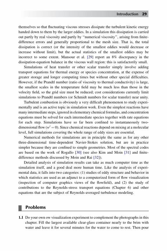
Problems

1.1 Do your own ow visualization experiment to complement the photographs in this

chapter. Fill the largest available clear-glass container nearly to the brim with

water and leave it for several minutes for the water to come to rest. Then pour

Introduction 29

in a small quantity of colored liquid (a teaspoonful at most: very strong instant

coffee seems to be best, but milk or orange juice also work quite well). Some

experimenting will be needed to adjust quantity and ow rate, but it should be

possible to see a cloud-like boundary to the descending jet, and possibly some

of the internal structure as the colored liquid is gradually diluted. The liquid

will mostly collect near the bottom of the container. If possible, leave it over-

night and see how very slow molecular diffusion is compared to turbulent mix-

ing (in liquid mixtures, the diffusivity is usually very small compared to the

viscosity or thermal conductivity but even molecular diffusion of heat is small

compared to turbulent heat transfer).

1.2 A 3/400 water pipe will pass a ow of about one U.S. gallon (8 lb) of water per

minute. Show that the ow is almost certainly turbulent.

1.3 A Boeing 747 is 230 ft long and cruises at 33,000 ft (10,000 m) at a speed of

880 ft/sec. (Mach number 0.9) The International Standard Atmosphere, using

metric units, gives the density at this altitude as 0.413 kg/m3 and the molec-

ular viscosity as 0.0000146 N sec/m2, so that the kinematic viscosity is 3.53 �10–5 m2/sec. (Note that a Newton, symbol N, is the force required to accel-

erate a mass of 1 kg at 1 m/sec2 and therefore has units of kg m–1sec2.) Calcu-

late the Reynolds number based on body length. Note that it would be more

logical to evaluate the viscosity at the wall temperature than at the free-stream

temperature, because the direct effect of viscosity on turbulent stresses and

skin friction is felt only very close to the wall. In this case the absolute

temperature at the wall will be about 1.15 times that in the free stream, about

60 � F greater.

1.4 Using the ‘‘representative’’ value of dissipation given in Eq. (1.3.3) and

assuming that ue/vz 80,000 as in Klebanoff’s experiments (see the cited figures

in Chapter 4) show that h/d z 1,1 � 10–5. The thickness of Klebanoff’s

boundary layer was about 3 in, so that h was about 30 m in. The smalles signif-

icance wavelength in the flow are roughly 5h and the wavelengths that contribute

most to the dissipation are roughly 50h.

1.5 The ‘‘theoretical’’ (strictly, empirical) fit to the frequency spectral function data

in Fig. 1.19 has an asymptotic form at high frequency proportional to n–2.

Show, using the formulas in Sect. 1.6, that the corresponding microscale is

zero and the dissipation infinite. Using Eq. (1.6.5) and referring to to

Fig. 1.14, explain what is wrong with the data fit. Note that a best fit to the

data obviously has a negative slope that increases all the way up to the highest

frequency resolved.

1.6 Use Eq. (1.9.4) to show that, in two-dimensional incompressible flow with ueindependent of x, the displacement thickness is indeed the distance by which

the external streamlines are displaced outwards by the reduction in flow rate

within the boundary layer.


References

[1] L. Prandtl, Turbulent flow. NACA Tech. Memo, 435, originally delivered to 2nd Int, Congr. Appl.

Mech. Zurich (1926).

[2] H.Tennekes, J.L. Lumley, A First Course in Turbulence, MIT Press, Cambridge, MA.

[3] M. Lesieur, La Turbulence, Press Universitaires de Grenoble, 1994.

[4] S.B. Pope, Turbulent Flows, Cambridge Univ. Press, 2000.

[5] P.A. Durbin, B.A. Petterson, Statistical Theory and Modeling of Turbulent Flows, John Wiley and

Sons, New York, 2001.

[6] W.C. Wilcox, Turbulence Modeling for CFD, DCW Industries, La Canada, CA, 1998.

[7] T. von Karman, Turbulence. Twenty-fifth Wilbur Wright Memorial Lecture, J. Roy. Aeronaut. Soc.

41 (1937) 1109.

[8] J.O. Hinze, Turbulence, an Introduction to Its Mechanism and Theory, McGraw-Hill, New York,

1959.

[9] G. Hagen, On the motion of water in narrow cylindrical tubes (German), Pogg. Ann. 46 (1839) 423.

[10] L. Prandtl, O.G. Tietjens, Applied Hydro- and Aeromechanics, Dover, New York, 1934, p. 29.

[11] O. Reynolds, An experimental investigation of the circumstances which determine whether the

motion of water will be direct or sinuous and the law of resistance in parallel channels, Phil. Trans.

Roy. Soc. London 174 (1883) 935.

[12] J.H. Preston, The minimum Reynolds number for a turbulent boundary layer and selection of

a transition device, J. Fluid Mech 3 (1957) 373.

[13] C.S. Wells, Effects of free-stream turbulence on boundary-layer transition, AIAA J 5 (1967) 172.

[14] A.M. Kolmogorov, Equations of turbulent motion of an incompressible fluid. Izvestia Academy of

Sciences, USSR, Physics 6 (1 and 2) (1942) 56–58.

[15] A.M.O. Smith, D.W. Clutter, The smallest height of roughness capable of affecting boundary-layer

transition in low-speed flow, Douglas Aircraft Co (1957). Rep. ES 26803, AD 149 907.

[16] G.K. Batchelor, The Theory of Homogeneous Turbulence, Cambridge Univ. Press, London

New York, 1953.

[17] P.S. Klebanoff, Characteristics of turbulence in a boundary layer with zero pressure gradient, NACA

Tech. Note 3178 (1954).

[18] H. Eckelmann, Experimentelle Untersuchungen in einer turbulenten Kanalstromung mit starken

viskosen Wandschichten, Mitt. No. 48, Max-Planck-Inst. for Flow Res., Gottingen (1970).

[19] G.B. Schubauer, P.S. Klebanoff, Investigation of separation of the turbulent boundary layer, NACA

Tech. Note No. 2133 (1950).

[20] G.K. Batchelor, A.A. Townsend, Decay of turbulence in the final period, Proc. Roy Soc. 194A

(1948) 527.

[21] A. Favre, J. Gaviglio, R. Dumas, Quelques mesures de correlation dans le temps et l’espace en

soufflerie, Rech. Aeronaut 32 (1953) 21.

[22] H.W. Liepmann, On the application of statistical concepts to the buffeting problem, J. Aeronaut Sci.

19 (1952) 793.

[23] G.K. Batchelor, An Introduction to Fluid Dynamics, Cambridge Univ. Press, London New York,

1967.

[24] S. Corrsin, A.L. Kistler, The free-stream boundaries of turbulent flows, NACATech. Note No. 3133

(1954).

[25] O.M. Phillips, The irrotational motion outside a free turbulent boundary layer, Proc. Camb. Phil.

Soc. 51 (1955) 220.

[26] G.I. Taylor, Diffusion by continuous movements, Proc. London Math. Soc. 20 (1921) 196.

Introduction 31

[27] J. Smagorinsky, General Circulation Experiments with the Primitive Equations, I. The Basic

Experiment. Monthly Weather Review 91 (1963) 99.

[28] M. Germano, U. Piomelli, P. Moin, W.H. Cabot, A Dynamic Subgrid-Scale Eddy-Viscosity Model,

Phys. Fluids A3 (1991) 1760.

[29] N.N. Mansour, J. Kim, P. Moin, Reynolds-Stress and Dissipation-Rate Budgets in a Turbulent

Channel Flow, J. Fluid Mech. 194 (1988) 15.

[30] R.S. Rogallo, Numerical Experiments in Homogeneous Turbulence, NASA TM 81315 (1981).

[31] J. Kim, P. Moin, Application of a Fractional Step Method to Incompressible Navier-Stokes Equa-

tion, J. Comp. Phys. 59 (308) (1985). 1985 and NASA TM85898, N8422328.

[32] M.M. Rai, P. Moin, Direct Simulations of Turbulent Flow Using Finite-Difference Schemes,

J. Comp. Phys. 96 (1991) 15.


ConservationEquations forCompressibleTurbulent Flows

Chap

ter2


2.1 Introduction 33

2.2 The Navier–Stokes Equations 34

2.3 Conventional Time-Averaging and Mass-Weighted-Averaging Procedures 35

2.4 Relation Between Conventional Time-Averaged Quantities and

Mass-Weighted-Averaged Quantities 39

2.5 Continuity and Momentum Equations 41

2.6 Energy Equations 41

2.7 Mean-Kinetic-Energy Equation 42

2.8 Reynolds-Stress Transport Equations 44

2.9 Reduced Forms of the Navier–Stokes Equations 48

Problems 51

References 51

2.1 Introduction

In this chapter we consider the Navier-Stokes equations for a compressible fluid and

show how they can be put into a form more convenient for turbulent flows. We follow 33

Analysis of Turbulent Flows with Computer Programs. http://dx.doi.org/10.1016/B978-0-08-098335-6.00002-1


http://dx.doi.org/10.1016/B978-0-08-098335-6.00002-1

the procedure first introduced by Reynolds in incompressible flows: we regard the

turbulent motion as consisting of the sum of the mean part and a fluctuating part,

introduce the sum into the Navier–Stokes equations, and time1 average the resulting

expressions. The equations thus obtained give considerable insight into the character

of turbulent motions and serve as a basis for attacking mean-flow problems, as well

as for analyzing the turbulence to find its harmonic components. However, before

these governing conservation equations for compressible turbulent flows are

obtained, it is appropriate to write down the conservation equations for mass,

momentum, and energy.

In the following sections we shall discuss the conservation equations and their

reduced forms in terms of rectangular coordinates, and for convenience we shall use

the summation notation. For a discussion of the conservation equations in terms of

another coordinate system, the reader is referred to [1].

2.2 The Navier–Stokes Equations

The well-known Navier–Stokes equations of motion for a compressible, viscous,

heat-conducting, perfect gas may be written in the following form [2]:

Continuity

v9

vtþ v

vxj

�9uj

� ¼ 0; (2.2.1)

Momentum

v

vtð9uiÞ þ v

vxjð9uiujÞ ¼ � vp

vxiþ vsi;j

vxj; (2.2.2)

Energy

v

vtð9HÞ þ v

vxjð9ujHÞ ¼ vp

vtþ v

vxjðujsij � qjÞ; (2.2.3)

where the stress tensor sij, heat-flux vector qj, and total enthalpy H are given by

sij ¼ ldijvulvxl

þ m

�vuivxj

þ vujvxi

�; (2.2.4)

qj ¼ �kvT

vxj; (2.2.5)

1See Section 2.3 for a discussion of various kinds of averaging.


H ¼ hþ 1

2uiui: (2.2.6)

In these equations, l is the bulk viscosity (¼ –2/3m), m the dynamic viscosity, k the

thermal conductivity, and h the static enthalpy. In Eq. (2.2.4), dij is the Kronecker

delta, having the value 1 for i ¼ j and 0 for i s j. A summation is understood for

repeated indices.

Sometimes it is more convenient to express the energy equation in terms of static

enthalpy h, rather than total enthalpy H. Then using Eqs. (2.2.1) and (2.2.2) Eq.

(2.2.3) becomes

v

vt

�9h�þ v

vxj

�9huj

� ¼ vp

vtþ uj

vp

vxjþ sij

vuivxj

� vqjvxj

; (2.2.7)

where sijvui=vxj is the dissipation function.

Equations (2.2.1)–(2.2.7) apply to laminar as well as to turbulent flows. For the

latter, however, the values of the dependent variables are to be replaced by their

instantaneous values. A direct approach to the turbulence problem, namely the

solution of the full time-dependent Navier–Stokes equations, then consists in solving

the equations for a given set of boundary or initial values and computing mean values

over the ensemble for solutions, as discussed in Section 1.10. Even for the most

restricted problem – turbulence of an incompressible fluid that appears to be

a hopeless undertaking, because of the nonlinear terms in the equations. Thus, the

standard procedure is to average over the equations rather than over the solutions.

The averaging can be done either by the conventional time-averaging procedure or

by the mass-weighted averaging procedure. Both are discussed in the next section.

2.3 Conventional Time-Averaging andMass-Weighted-Averaging Procedures

In order to obtain the governing conservation equations for turbulent flows, it is

convenient to replace the instantaneous quantities in the equations of Section 2.2 by

their mean and their fluctuating quantities. In the conventional time-averaging

procedure, for example, the velocity and pressure are usually written in the following

forms:2

ui�xi; t

� ¼ uiðxiÞ þ u00i�xi; t

�; (2.3.1)

p�xi; t

� ¼ p�xi�þ p00

�xi; t

�; (2.3.2)

2The usual single prime on fluctuating quantities, for example, u0, p0, is reserved for later use.

Conservation Equations for Compressible Turbulent Flows 35

where uiðxiÞ and pðxiÞ are the time averages of the bulk velocity and pressure,

respectively, and ui00 (xi, t) and p00 (xi, t) the superimposed velocity and pressure

fluctuations, respectively. The time average or ‘‘mean’’ of any quantity q (t) is

defined by

�q ¼ limDt/N

ð1=DtÞZ t0þDt

t0

qðtÞ dt: (2.3.3)

In practice, N is taken to mean a time that is long compared to the reciprocal of the

predominant frequencies in the spectrum of q; in wind-tunnel experiments, aver-

aging times of a few seconds to a minute are usual. Clearly, the time average is useful

only if it is independent of t0; a random process whose time averages are all inde-

pendent of t0 is called ‘‘statistically stationary.’’ A nonstationary process (e.g., an air

jet from a high-pressure reservoir of finite size) must be analyzed by means of

‘‘ensemble averages.’’ The ensemble average q is the average of a large number of

instantaneous samples of q, of which one sample is taken during each run of the

process at time t0 after the process starts. A process with periodicity imposed on

turbulence, like the flow in a turbomachine, can be analyzed by phase averages – take

averages at a given point in space over many events in which a blade is at a given

position relative to that point. For further discussions, see [3].

For a fluctuating quantity q00 (t), the average, q00 ðtÞ, is zero, that is,

q00ðtÞ ¼ limDt/N

ð1=DtÞZ t0þDt

t0

q00ðtÞ dt ¼ 0: (2.3.4)

Average values similar to Eqs. (2.3.1) and (2.3.2) can be written for the other flow

quantities, such as density, temperature, and enthalpy, as follows:

9�xi; t

� ¼ 9ðxiÞ þ 900�xi; t

�; (2.3.5)

h�xi; t

� ¼ hðxiÞ þ h00�xi; t

�; (2.3.6)

H�xi; t

� ¼ HðxiÞ þ H00�xi; t�; (2.3.7)

T�xi; t

� ¼ TðxiÞ þ T 00�xi; t�; (2.3.8)

where 900 ¼ h00 ¼ H00 ¼ T 00 ¼ 0:

As an example, let us consider the continuity and the momentum equations in the

forms given by Eqs. (2.2.1) and (2.2.2), respectively, and show how they can be

obtained by using the conventional time-averaging procedure for compressible

turbulent flows. If we substitute the expressions given by Eqs. (2.3.1), (2.3.2), and

(2.3.5) into (2.2.1) and (2.2.2) and take the time average of the terms appearing in the


resulting equations, we obtain the mean continuity and the mean momentum

equations in the following forms:

v�9

vtþ v

vxj

��9 �uj þ 900u00j

�¼ 0; (2.3.9)

v

vt

��9 �ui þ 900u00i

�þ v

vxj

��9 �ui�uj þ ui900u00j

�

¼ � v�p

vxiþ v

vxj

��sij � �uj900u00i � 9u00i u00j � 900u00i u00j

�:

(2.3.10)

For incompressible flows, d9 ¼ 0. As a result Eqs. (2.3.9) and (2.3.10) can be

simplified considerably; they become

v�ujvxj

¼ 0; (2.3.11)

9v�uivt

þ 9v

vxj

��ui�uj

� ¼ � v�p

vxiþ v

vxj

��sij � 9u00i u00j

�: (2.3.12)

We see from Eqs. (2.3.9)–(2.3.12) that the continuity and the momentum equa-

tions obtained by this procedure contain mean terms that have the same form as the

corresponding terms in the instantaneous equations. However, they also have terms

representing the mean effects of turbulence, which are additional unknown quanti-

ties. For that reason, the resulting conservation equations are undetermined.

Consequently, the governing equations in this case, continuity and momentum, do

not form a closed set. They require additional relations, which have to come from

statistical or similarity considerations. The additional terms enter the governing

equation as turbulent-transport terms such as �9u00i u00j and as density-generated terms

such as 900u00j and 900u00i u00j . In incompressible flows, the density-generated terms

disappear, as is shown in Eqs. (2.3.11) and (2.3.12). In compressible flows, the

continuity equation (2.3.9) has a source term, ðv=vxjÞ900u00j , which indicates that

a mean mass interchange occurs across the mean streamlines defined in terms of �ui. It

also indicates that the splitting of ui according to Eq. (2.3.1) is not convenient; it is

not consistent with the usual concept of a streamline. For that reason, we shall

replace the conventional time-averaging procedure by another procedure that is well

known in the studies of gas mixtures, themass-weighted-averaging procedure, which

was used by Van Driest [4], Favre [5], and Laufer and Ludloff [6]. Mass-weighted

averaging eliminates the mean-mass term 900u00j and some of the momentum transport

terms such as �ui900u00j and 900u00i u00j across mean streamlines. We define a mass-

weighted mean velocity

~ui ¼ 9ui=~9; (2.3.13)


where the bar denotes conventional time averaging and the tilde denotes mass-

weighted averaging. The velocity may then be written as

ui�xi; t

� ¼ �ui�xi�þ u0i

�xi; t

�; (2.3.14)

where u0i (xi, t) is the superimposed velocity fluctuation. Multiplying Eq. (2.3.14) by

the expression for 9(xi, t) given by Eq. (2.3.5) gives

9ui ¼ ð�9þ 900Þð~ui þ u0iÞ ¼ �9~ui þ 900~ui þ 900u0i þ �9u0i:

Time averaging and noting the definition of 9(xi, t), we get

9ui ¼ �9~ui þ 9u0i:

From the definition of ~ui, given by Eq. (2.3.13) it follows that

9u0i ¼ 0: (2.3.15)

Note the important differences between the two averaging procedures. In the

conventional time averaging, u00i ¼ 0 and 9u00i s 0; in the mass-weighted averaging,

u0i s 0 and 9u0i ¼ 0.

Similarly, we can define the static enthalpy, static temperature, and total enthalpy

thus:

h�xi; t

� ¼ ~h�xi�þ h0

�xi; t

�; (2.3.16)

T�xi; t

� ¼ ~T�xi�þ T 0�xi; t�; (2.3.17)

H�xi; t

� ¼ ~H�xi�þ H0�xi; t�; (2.3.18)

where

~T ¼ 9T=�9; ~h ¼ 9h=�9; ~H ¼ ~hþ 1

2~ui~ui þ 1

29u0iu0i=�9;

H0 ¼ h0 þ ~uiu0i þ

1

2u0iu

0i �

1

29u0iu0i=�9:

(2.3.19)

Also,

9T 0 ¼ 9h0 ¼ 9H0 ¼ 0: (2.3.20)

The expressions for ~H and H0 in Eq. (2.3.19) follow from the definitions of H, ui,

and ~H. Multiplying both sides of Eq. (2.2.6) by 9, and introducing the definition of uigiven by Eq. (2.3.14) into the resulting expression, we can write

9H ¼ 9hþ 1

29~ui~ui þ ~ui9u

0i þ

1

29u0iu

0i:


Mass averaging the above expression gives

9H ¼ 9hþ 1

29~ui~ui þ 1

29u0iu0i: (2.3.21)

Since

9H ¼ 9 ~H and 9h ¼ �9~h;

Eq. (2.3.21) can be written as

~H ¼ ~hþ 1

2~ui~ui þ 1

29u0iu0i=�9:

Also,

H ¼ �H þ H0 ¼ �hþ h0 þ 1

2

��ui þ u0i

�2¼ hþ h0 þ 1

2uiui þ uiu

0i þ

1

2u0iu

0i:

Substituting the expression for �H into the above expression, we get

H0 ¼ h0 þ �uiu0i þ

1

2u0iu

0i �

1

29u0iu0i=�9:

The definitions given by Eqs. (2.3.14)–(2.3.21) are also convenient for turbulence

measurements because in hot-wire anemometry, the quantities measured at low speeds

are the fluctuations of 9ui, and of T, and those measured at supersonic speeds are the

fluctuations of 9ui, and of a quantity that is very close to the total enthalpy. Mean

pressure is directly measurable. For that reason, the conventional time average of

pressure is convenient; we shall use the definition given by Eq. (2.3.2). Furthermore,

we shall also use the conventional time-averaging procedures for the stress tensor sijand for the heat-flux vector qj as given by Eqs. (2.2.4) and (2.2.5), respectively.

2.4 Relation Between Conventional Time-AveragedQuantities and Mass-Weighted-Averaged Quantities

A relationship between �ui and ~ui can be established as follows. Using Eq. (2.3.5), we

can write Eq. (2.3.15) as

9u0i ¼ ð~9þ 900Þu0i ¼ 0:

That expression can also be written as

u0i ¼ �900u0i=~9: (2.4.1)


Taking the mean value of Eq. (2.3.14) and rearranging, we get

~ui � �ui ¼ �u0i: (2.4.2)

Hence,

~ui � �ui ¼ 900u0i=9: (2.4.3a)

It follows from the definitions of ui (xi, t) that for i ¼ 1

u1ðxi; tÞ ¼ uðx; tÞ ¼ ~uþ u0 ¼ �uþ u00:

Multiplying both sides of that expression by 9 and averaging, we get

~9~uþ 9u0 ¼ ~9uþ 9u00:

If we note that 9u0 ¼ 0 by definition and that 9u00 can be written as

ð~9þ 900Þu00 ¼ 900u00, we can combine the above expression and Eq. (2.4.3a) as

~u� �u ¼ 900u0=�9 ¼ 900u00=�9: (2.4.3b)

Similar relationships between �h and ~h, �T and ~T , �H and ~H, etc., can be established

by a similar procedure. For example, in order to find the relation �T and ~T , we rewrite

the first term in Eq. (2.3.20) in the form

9T 0 ¼ ð�9þ 900ÞT 0 ¼ 0: (2.4.4)

Taking the mean value of Eq. (2.3.17), rearranging, and substituting the value of 9T 0from Eq. (2.4.4) into the resulting expression, we get

~T � �T ¼ 900T 0=9: (2.4.5a)

It follows from the definition of T (xi, t) that

T�xi; t

� ¼ ~T þ T 0 ¼ �T þ T 00: (2.4.5b)

Multiplying both sides of Eq. (2.4.5b) by 9 and averaging, we get

�9 ~T þ 9T 0 ¼ �9 �T þ 9T 00: (2.4.5c)

If we note that 9T 0 ¼ 0 and that 9T 00 ¼ 900T 00 and if we make use of

Eqs. (2.4.5a)–(2.4.5c), we can write

~T � �T ¼ T 00 � T 0 ¼ 900 T 00=�9 ¼ 900 T 0=�9: (2.4.6)

From Eqs. (2.4.3) and (2.4.5) we see that the difference between the two

average velocities depends on the density–velocity correlation term 900u0i or 900u00i .Similarly, the difference between the two average temperatures depends on the


density–temperature correlation term 900T 0 or 900T 00. A discussion of the magnitude of

these quantities will be given later, in subsection 3.2.2.

2.5 Continuity and Momentum Equations

If we substitute the expressions given by Eqs. (2.3.2), (2.3.5), and (2.3.14) into Eqs.

(2.2.1) and (2.2.2), we obtain

v

vt

��9þ 900

�þ v

vxj

�9~uj þ 9u0j

� ¼ 0; (2.5.1)

v

vt

�9~ui þ 9u0i

�þ v

vxj

�9~ui~uj þ 9u0j~ui þ 9u0i~uj þ 9u0iu

0j

�

¼ � v�p

vxi� vp00

vxiþ vsij

vxj:

(2.5.2)

Taking the time average of the terms appearing in these equations, we obtain the

mean continuity and mean momentum equations for compressible turbulent flow:

v�9

vtþ v

vxj

��9~uj

� ¼ 0; (2.5.3)

v

vt

��9~ui

�þ v

vxj

��9~ui~uj

� ¼ � vp

vxiþ v

vxj

��sij � 9u0iu0j

�: (2.5.4)

A comparison of the continuity equation (2.5.3) and the momentum equation

(2.5.4) obtained by the mass-weighted averaging with those obtained by the

conventional time averaging, namely, Eqs. (2.3.9) and (2.3.10), shows that with

mass-weighted averaging the final equations have simpler form. In fact, with the

mass-weighted averaging, they have the same form, term by term, as those for

incompressible flows, with two exceptions: The viscous stresses sij and the so-calledReynolds stresses �9u0iu0j include fluctuations in viscosity and in density,

respectively.

2.6 Energy Equations

If we substitute the expressions given by Eqs. (2.3.2), (2.3.5) and (2.3.14)–(2.3.20)

into Eqs. (2.2.3) and (2.2.7), we obtain

v

vt

�9 ~H þ 9H0�þ v

vxj

�9 ~H ~uj þ 9H0~uj þ 9u0j ~H þ 9H0u0j

�

¼ v

vt

��pþ p00

�þ v

vxj

�uisij � qj

�;

(2.6.1)


v

vt

�9~hþ 9h0

�þ v

vxj

�9~h�uj þ 9h0�uj þ 9u0j �hþ 9u0jh

0�

¼ v

vt

��pþ p00

�þ �~uj þ u0j

� v

vxj

��pþ p00

�þ sijvuivxj

� vqjvxj

:

(2.6.2)

In those equations, it is convenient not to replace ui, by its average and fluctuating

component when it or its derivative vui/vxj is multiplied by sij. By taking the time

average of the terms appearing in the equations, we obtain the mean energy equa-

tions in terms of total enthalpy, Eq. (2.6.1),

v

vt

��9 ~H

�þ v

vxj

�9 ~H~uj

�

¼ v�p

vtþ v

vxj

�� qj � 9H0u0j þ ~uisij þ u0isij�;

(2.6.3)

and static enthalpy, Eq. (2.6.2),

v

vt

��9~h�þ v

vxj

��9~h~uj

�

¼ v�p

vtþ ~uj

v�p

vxjþ u0j

vp

vxjþ v

vxj

�� qj � 9h0u0j�þ sij

vuivxj

:

(2.6.4)

2.7 Mean-Kinetic-Energy Equation

The equation for kinetic energy of the mean motion can be obtained by

considering the scalar product of ~uj and the mean momentum equation for ~ui [see

Eq. (2.5.4)],

~uj

�v

vt

��9~ui

�þ v

vxk

��9~ui~uk

� ¼ ~uj

�� v�p

vxiþ v

vxk

��sik � 9u0iu

0k

�; (2.7.1a)

and the scalar product of ~ui and the mean momentum equation for ~uj;

~ui

�v

vt

��9~uj

�þ v

vxk

��9~uj~uk

� ¼ ~ui

�� v�p

vxjþ v

vxk

��sjk � 9u0ju0k

�; (2.7.1b)


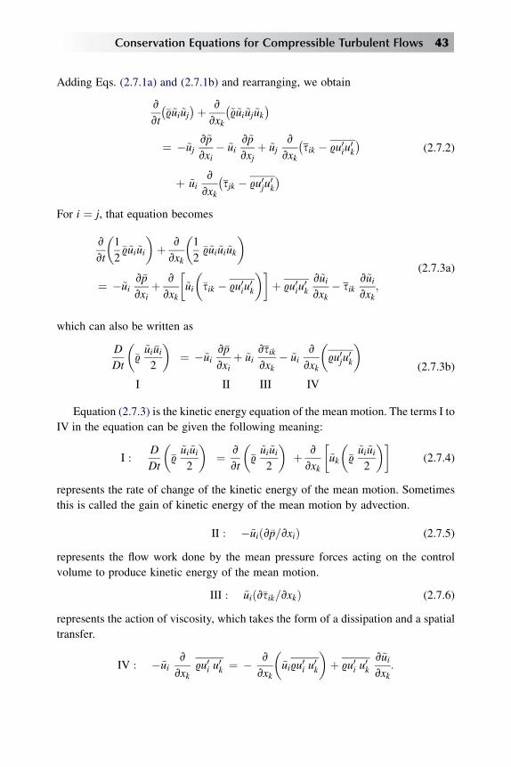
Adding Eqs. (2.7.1a) and (2.7.1b) and rearranging, we obtain

v

vt

��9~ui~uj

�þ v

vxk

�~9~ui~uj~uk

�

¼ �~ujv~p

vxi� ~ui

v~p

vxjþ ~uj

v

vxk

�sik � 9u0iu0k

�

þ ~uiv

vxk

�sjk � 9u0ju0k

�(2.7.2)

For i ¼ j, that equation becomes

v

vt

�1

2�9~ui~ui

�þ v

vxk

�1

2�9~ui~ui~uk

�

¼ �~uiv�p

vxiþ v

vxk

�~ui

��sik � 9u0iu

0k

�þ 9u0iu

0k

v~uivxk

� sikv~uivxk

;

(2.7.3a)

which can also be written as

D

Dt

��9~ui�ui2

�¼ �~ui

v�p

vxiþ ~ui

vsikvxk

� ~uiv

vxk

�9u0ju0k

�I II III IV

(2.7.3b)

Equation (2.7.3) is the kinetic energy equation of the mean motion. The terms I to

IV in the equation can be given the following meaning:

I :D

Dt

��9~ui~ui2

�¼ v

vt

��9~ui~ui2

�þ v

vxk

�~uk

��9~ui~ui2

�(2.7.4)

represents the rate of change of the kinetic energy of the mean motion. Sometimes

this is called the gain of kinetic energy of the mean motion by advection.

II : �~uiðv�p=vxiÞ (2.7.5)

represents the flow work done by the mean pressure forces acting on the control

volume to produce kinetic energy of the mean motion.

III : ~uiðv�sik=vxkÞ (2.7.6)

represents the action of viscosity, which takes the form of a dissipation and a spatial

transfer.

IV : �~uiv

vxk9u0i u

0k ¼ � v

vxk

�~ui9u0i u

0k

�þ 9u0i u

0k

v~uivxk

:


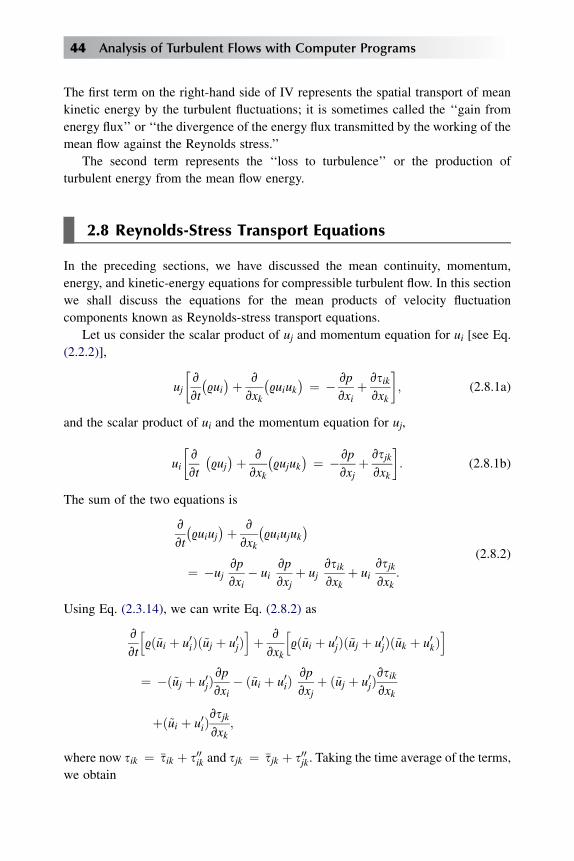
The first term on the right-hand side of IV represents the spatial transport of mean

kinetic energy by the turbulent fluctuations; it is sometimes called the ‘‘gain from

energy flux’’ or ‘‘the divergence of the energy flux transmitted by the working of the

mean flow against the Reynolds stress.’’

The second term represents the ‘‘loss to turbulence’’ or the production of

turbulent energy from the mean flow energy.

2.8 Reynolds-Stress Transport Equations

In the preceding sections, we have discussed the mean continuity, momentum,

energy, and kinetic-energy equations for compressible turbulent flow. In this section

we shall discuss the equations for the mean products of velocity fluctuation

components known as Reynolds-stress transport equations.

Let us consider the scalar product of uj and momentum equation for ui [see Eq.

(2.2.2)],

uj

�v

vt

�9ui

�þ v

vxk

�9uiuk

� ¼ � vp

vxiþ vsik

vxk

; (2.8.1a)

and the scalar product of ui and the momentum equation for uj,

ui

�v

vt

�9uj

�þ v

vxk

�9ujuk

� ¼ �vp

vxjþ vsjk

vxk

: (2.8.1b)

The sum of the two equations is

v

vt

�9uiuj

�þ v

vxk

�9uiujuk

�

¼ �ujvp

vxi� ui

vp

vxjþ uj

vsikvxk

þ uivsjkvxk

:

(2.8.2)

Using Eq. (2.3.14), we can write Eq. (2.8.2) as

v

vt

h9ð~ui þ u0iÞð~uj þ u0jÞ

iþ v

vxk

h9ð~ui þ u0jÞð~uj þ u0jÞð~uk þ u0kÞ

i

¼ �ð~uj þ u0jÞvp

vxi� ð~ui þ u0iÞ

vp

vxjþ ð~uj þ u0jÞ

vsikvxk

þð~ui þ u0iÞvsjkvxk

;

where now sik ¼ �sik þ s00ik and sjk ¼ �sjk þ s00jk. Taking the time average of the terms,

we obtain


v

vt

��9~ui~uj þ 9u0iu0j

�

þ v

vxk

��9~ui~uj~uk þ ~uk9u

0iu

0j þ ~ui9u0ju0k þ ~uj9u0iu0k þ 9u0iu0ju0k

�

¼ �~ujv�p

vxi� u0j

vp

vxi� ~ui

v�p

vxj� u0i

vp

vxjþ ~uj

vsikvxk

þ u0jvs00ikvxk

þ ~uiv�sjkvxk

þ u0ivs00jkvxk

: (2.8.3)

If we subtract Eq. (2.7.2) from that equation and rearrange, we obtain the equations

for the components of the Reynolds stress, �9u0iu0j,

D

Dt

�9u0iu

0j

�þ v

vxk

�9u0iu

0ju

0k

�

¼ �u0jvp

vxi� u0i

vp

vxjþ u0j

vs00ikvxk

þ u0ivs00jkvxk

�9u0iu0k

v~ujvxk

� 9u0ju0k

v~uivxk

; (2.8.4)

where

D

Dt

�9u0iu0j

�¼ v

vt

�9u0iu0j

�þ v

vxk

�~uk9u

0iu

0j

�:

Equation (2.8.4) is the transport equation for the Reynolds stress�9u0iu0j ; it expressesthe rate of change of the Reynolds stress along the mean streamline as the balance of

generation by interaction between the turbulence and the mean flow, the gain or loss

by convective movements of the turbulence and by the action of pressure gradients,

and destruction by viscous forces. It is clear that the six independent components of

Eq. (2.8.4), when taken together with Eqs. (2.5.3) and (2.5.4) form a set with more

unknowns than equations. By itself, Eq. (2.8.4) does not lead to a knowledge of the

distribution of the Reynolds stress and so to a solution of the mean-flow problem; its

value lies in the restrictions it puts on the nature of turbulent transfer processes.

The meaning of the terms in Eq. (2.8.4) will be discussed later. First, we shall

discuss the meaning of these terms for i ¼ j.

For i ¼ j, Eq. (2.8.4) becomes the mean-kinetic-energy equation of the fluctua-

tions, often called the ‘‘turbulent-energy’’ equation:

D

Dt

1

29u0iu0i þ

v

vxku0k

�1

29u0iu0i

�¼ �u0i

vp

vxiþ u0j

vs00ikvxk

� 9u0iu0kv~uivxk

:

I II III IV V

(2.8.5a)


Sometimes the equation is written in the form

D

Dt

1

29u0iu0i

¼ �u0ivp

vxi� s00ik

vu0ivxk

þ v

vxk

�u0i

�s00ik �

1

29u0iu0k

�� 9u0iu0k

v~uivxk

:

(2.8.5b)

The meanings of the terms in Eq. (2.8.5a) are as follows:

I :D

Dt

1

29u0iu

0i ¼

v

vt

1

29u0iu

0i þ

v

vxk~uk

�1

29u0iu

0i

�(2.8.6)

represents the rate of change of the kinetic energy of the turbulence. The term

v

vt

1

29u0i u0i (2.8.7)

represents the unsteady growth of turbulent energy, and the term

v

vxk~uk

�1

29u0i u0i

�

represents the kinetic energy of the fluctuation motion that is convected by the mean

motion. That term is also often called the ‘‘advection’’ or gain of energy by mean

stream advection (gain following the mean flow).

II :v

vxku0k

�1

29u0iu

0i

�

represents the kinetic energy of the fluctuations convected by the fluctuations, that is,

the diffusion of the fluctuation energy.

III : �u0ivp

vxi(2.8.8)

represents the work due to turbulence.

IV : u0ivs00ikvxk

¼ v

vxku0is00ik � s00ik

vu0ivxk

(2.8.9)

represents the work of viscous stresses due to the fluctuation motion. The term

v

vxk

�u0is00ik

�(2.8.10)

represents the spatial transport of turbulent energy by viscous forces, and the term

�s00ikvu0ivxk

(2.8.11)


represents the viscous ‘‘dissipation’’ by the turbulent motion.

V : �9u0iu0kv~uivxk

(2.8.12)

represents the product of a turbulent stress and mean rate of strain. That term links

the mean flow to the turbulent fluctuations through the ‘‘Reynolds stresses’’

�9u0iu0k: It is generally called the ‘‘production of turbulent energy’’ term. Of

course, all the terms on the right-hand side of Eq. (2.8.5a) except the transport

terms act to produce or to destroy (depending upon their sign) the kinetic energy

of the turbulence in the control volume. Any term expressible as the spatial

gradient of a time-averaged quantity is a transport term (its integral over the flow

volume must be zero). Terms not so expressible are source/sink terms. The

distinction between term V and the other terms on the right-hand side of Eq.

(2.8.5a) is that V is the only one containing the mean velocity gradient; the others

contain only the fluctuation quantities. Thus, only term V can act to take energy

from the mean motion.

Let us now turn our attention to the meaning of the terms appearing in the

Reynolds-stress transport equation, Eq. (2.8.4). From the previous discussion of the

meaning of each term for i ¼ j, it is apparent that the meanings of the terms in Eq.

(2.8.4) for i s j are similar to the ones for i ¼ j. For example, the first term on the

left-hand side of Eq. (2.8.4),

�D=Dt

� �9u0iu0j

�(2.8.13)

represents the variation of the correlation 9u0iu0j as the fluid element moves along

a streamline, rather than the variation of the kinetic energy of the fluctuations, 12 9u0iu

0i.

The first two terms on the right-hand side of Eq. (2.8.4) deserve special attention.

If we write them in the form

�"u0j

vp

vxiþ u0i

vp

vxj

#

¼ ��v

vxi

�u0jp

�þ v

vxj

�u0jp

�þ p

�vu0jvxi

þ vu0jvxj

�;

(2.8.14)

the terms

v

vxi

�u0jp

�þ v

vxj

�u0jp

�(2.8.15)

represent the so-called general pressure-diffusion terms. The second term on the

right-hand side of Eq. (2.8.14),


p

�vu0jvxi

þ vu0ivxj

�(2.8.16)

is sometimes called the ‘‘redistribution’’ or ‘‘return-to-isotropy’’ term. It describes

the redistribution of energy among the terms u2i (i ¼ 1, 2, 3) that approaches the

statistically most probable state, in which all of the components of u2i are equal.

2.9 Reduced Forms of the Navier–Stokes Equations

The solution of the complete three-dimensional time dependent Navier–Stokes

equations for turbulent flows, Eqs. (2.2.1)–(2.2.3), is rather difficult due to the wide

range of length and time scales that the turbulent flows posses (see Section 1.5).

Analytical solutions to even the simplest turbulent flows do not exist. A complete

description of turbulent flow, where the flow variables (e.g. velocity, temperature and

pressure) are known as a function of space and time can therefore only be obtained

by numerically solving the Navier–Stokes equations. These numerical solutions are

termed direct numerical simulations (DNS).

The instantaneous range of scales in turbulent flows increases rapidly with the

Reynolds number. As a result most engineering problems, e.g. the flow around

a wing, have too wide a range of scales to be directly computed using DNS. The

engineering computation of turbulent flows therefore relies on simpler descriptions:

instead of solving for the instantaneous flow field, the statistical evolution of the flow

is sought. Approaches based on the Reynolds averaged Navier–Stokes (RANS)

equations, (2.5.3), (2.5.4) and on their reduced forms (see Fig. 2.1) are the most

prevalent. Another approximation, large eddy simulation (LES), is intermediate in

complexity between DNS and RANS (see Fig. 2.1). Large eddy simulation (see

Section 1.10) directly computes the large energy-containing scales, while modeling

the influence of the small scales.

For both laminar and turbulent flows, the Navier–Stokes equations can be

reduced to simpler forms by examining the relative magnitudes of the terms in the

equations. In the application of this procedure, known as ‘‘order-of-magnitude’’

analysis, it is common to introduce length and velocity scales in order to estimate the

relative magnitudes of the mean and fluctuating components as described, for

example, in [7]. Figure 2.1 shows the hierarchy of the simplification of the Navier–

Stokes equations.

Since the momentum equation expresses a balance among inertia forces, pressure

forces, and viscous forces (in formulating the equations, the body forces were

neglected), one such simplifications arises when some of the relative magnitudes of

these forces are small in comparison with others. For example, at Reynolds numbers

much smaller than unity, the inertia accelerating terms in Eq. (2.5.4) become small in


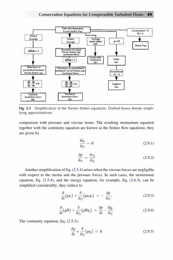
comparison with pressure and viscous terms. The resulting momentum equation

together with the continuity equation are known as the Stokes flow equations; they

are given by

vujvxj

¼ 0 (2.9.1)

vp

vxi¼ vsij

vxj(2.9.2)

Another simplification of Eq. (2.5.4) arises when the viscous forces are negligible

with respect to the inertia and the pressure forces. In such cases, the momentum

equation, Eq. (2.5.4), and the energy equation, for example, Eq. (2.6.3), can be

simplified considerably; they reduce to

v

vt

�9ui

�þ v

vxj

�9uiuj

� ¼ � vp

vxi; (2.9.3)

v

vt

�9H

�þ v

vxj

�9Huj

� ¼ vp

vt� vqj

vxj: (2.9.4)

The continuity equation, Eq. (2.5.3),

v9

vtþ v

vxj

�9uj

� ¼ 0 (2.9.5)

Fig. 2.1 Simplification of the Navier–Stokes equations. Dashed boxes denote simpli-fying approximations.


can be used to simplify Eqs. (2.9.3) and (2.9.4) further, to the forms

vuivt

þ ujvujvxj

¼ � 1

9

vp

vxi; (2.9.6)

vH

vtþ uj

vH

vxj¼ 1

9

vp

vt� 1

9

vqjvxj

: (2.9.7)

These equations are known as the Euler equations. As discussed in [7], for example,

for incompressible irrotational flows, they reduce to the Laplace equation.

In some three-dimensional flows, the viscous terms

v

vx1

�si1 � 9u0iu

01

�in Eq. (2.5.4) can be omitted and can be written as

v

vt

�9~ui

�þ v

vxj

��9~ui~uj

�¼ � v�p

vxiþ v

vx2

��si2 � 9u0iu02

�þ v

vx3

�si3 � 9u0iu

03

�: (2.9.8)

Similarly, the energy equation, Eq. (2.6.4), it can be written as

v

vt

��9~h�þ v

vxj

��9~h~uj

�¼ vp

vtþ ~uj

vp

vxjþ u0j

vp

vxj

þ v

vx2

�� q2 � 9h0u02

�þ v

vx3

�� q3 � 9h0u03

�

þ si2vuivx2

þ si3vuivx3

(2.9.9)

The momentum and energy equations resulting from this approximation, Eqs. (2.9.8)

and (2.9.9) together with the continuity equation, Eq. (2.5.3), are known as the

parabolized Navier–Stokes equations.

In other flows, the Navier–Stokes equations can be simplified further by retaining

only the viscous terms with derivatives in the coordinate direction normal to the body

surface x2 or, for free shear flows, the direction normal to the thin layer. Momentum

and energy equations become

v

vt

�9~ui

�þ v

vxj

��9~ui~uj

�¼ � v�p

vxiþ v

vx2

�si2 � 9u0iu02

�(2.9.10)

v

vt

�9~h�þ v

vxj

�9~h~uj

�¼ � v�p

vtþ ~uj

v�p

vxjþ u0j

vp

vxjþ v

vx2

�� q2 � 9h0u02

�

þ si2vuivx2

(2.9.11)


The above equations together with Eq. (2.5.3) are known as the thin-layer Navier–

Stokes equations.

Another simplification of the Navier–Stokes equations occurs at high Reynolds

number. The resulting equations are known as the boundary-layer equations. They

are discussed in the next chapter.

Problems

2.1 Show that the continuity equation (2.2.1) can be regarded as a ‘‘transport’’ equa-

tion for the density, in the same sense that Eq. (2.2.2) is a transport equation for

the momentum per unit volume, 9ui.

2.2 Take the xi derivative of Eq. (2.2.2), i.e. ‘‘take the divergence’’ of the set of equa-

tions for the three components of momentum, and show that if 9 is constant the

result is nominally a transport equation for the divergence vui/vxi. Further show

that if vui/vxi is set to zero (which Eq. (2.2.1) shows is the correct value in

constant-density flow) the transport equation reduces to a Poisson equation for

the pressure.

2.3 Show that the rate of viscous dissipation given in Eq. (2.8.11) is the mean

product of the fluctuating viscous stress and the fluctuating rate of strain,

vu0i=vxk þ vu0k=vxiÞ=2. Show that this is the mean rate at which the turbulance

does work against viscous stresses, and that the first law of thermodynamics

confirms that this is truly the rate at which turbulent kinetic energy is converted

into thermal internal energy.

References

[1] L.H. Back, Conservation equations of a viscous, heat-conducting fluid in curvilinear orthogonal

coordinates. Published in Handbook of Tables for Applied Engineering Science. 415, in: R.E. Boze,

G.L. Tuve (Eds.), Chem. Rubber Co., Cleveland, Ohio, 1970.

[2] H.W. Liepmann, A. Roshko, Elements of Gas Dynamics. 332, Wiley, New York, 1952.

[3] P. Bradshaw, An Introduction to Turbulence and Its Measurement, Pergamon, Oxford, 1971.

[4] E.R. Van Driest, Turbulent Boundary Layer in Compressible Fluids, J. Aeronaut. Sci. 18 (1951) 145.

[5] A. Favre, Statistical equations of turbulent gases. SIAM Problems of Hydrodynamics and Continuum

Mechanics (Sedov 60th birthday volume). Also, Equations des gaz turbulents compressibles, J. Mec.

4 (1969). 361(part I), 391 (part II).

[6] J. Laufer, K.G. Ludloff, Conservation equations in a compressible turbulent fluid and a numerical

scheme for their solution, McDonnell Douglas Paper WD 1355 (1970).

[7] T. Cebeci, J. Cousteix, Modeling and Computation of Boundary-Layer Flows, Horizons Publ, Long

Beach and Springer-Verlag, Berlin, 1998.


Boundary-LayerEquations

Chap

ter3


3.1 Introduction 54

3.2 Boundary-Layer Approximations for Compressible Flows 54

3.2.1 Laminar Flows 55

3.2.2 Turbulent Flows 59

3.3 Continuity, Momentum, and Energy Equations 64

3.3.1 Two-Dimensional Flows 64

3.3.2 Axisymmetric Flows 69

3.3.3 Three-Dimensional Flows 71

3.4 Mean-Kinetic-Energy Flows 73

3.5 Reynolds-Stress Transport Equations 74

3.6 Integral Equations of the Boundary Layer 78

3.6.1 Momentum Integral Equation 79

3.6.2 Mean Energy Integral Equation 80

3.6.3 Turbulent Energy Integral Equation 81

3.6.4 Energy Integral Equation 82

Problems 84

References 87

53



http://dx.doi.org/10.1016/B978-0-08-098335-6.00003-3

3.1 Introduction

Another important simplification of the Navier-Stokes equations arises when the

flow of a fluid past a solid at high Reynolds number is considered. In such cases,

there is a very narrow region close to the surface in which the fluid velocity and

possibly the temperature (or enthalpy) deviate considerably from their values far

away from the surface. For example, the velocity of a fluid flowing past a stationary

body changes rapidly from zero velocity at the surface to its value in the body of the

fluid (except for very-low-pressure gases, when the mean free path of the gas

molecules is large relative to the body). In that narrow region, the velocity gradient

may be so large that, even if the fluid viscosity is small, the viscous forces may be of

the same order as the inertia forces. That region is called the boundary region, and the

layer of affected fluid is called the boundary layer. There, because gradients

perpendicular to the surface are much larger than gradients parallel to the surface,

some of the terms in the Navier-Stokes equations can be neglected, which simplifies

the equations considerably. It is on this basis that Prandtl, in 1904, proposed his

boundary-layer theory. According to that theory, the flow field may be separated into

two regions: the main, inviscid flow, which is described by Eqs. (2.9.5)–(2.9.7), and

the boundary region described by the simplified momentum and energy equations,

called boundary-layer equations. The simplifications are discussed in the next

section.

3.2 Boundary-Layer Approximations for CompressibleFlows

For simplicity, we consider a two-dimensional, unsteady, compressible turbulent

flow. The external flow has one velocity component, ue, that depends on the time

coordinate t (unsteady flow) and on one coordinate x in the wall surface. The flow

within the boundary layer possesses two velocity components, u and y, that depend

on t and two space coordinates, x and y. As is standard in boundary-layer theory, x is

taken to be the distance measured along the surface (which may be curved) and y is

the distance normal to the surface. The turbulence is three dimensional, with velocity

components u0, y0, and w0 in the x, y, and z directions, respectively. The total enthalpywithin the boundary layer H is a function of x, y, and t. The conservation equations

for mass, momentum, and energy as given by Eqs (2.5.3), (2.5.4), and (2.6.3),

respectively, become

Continuity

v�9

vtþ v

vx

�9~u�þ v

vy

��9~y� ¼ 0; (3.2.1)


x Momentum

v

vt

��9~u�þ v

vx

��9~u~u�þ v

vy

��9~u~y�

¼ � v�p

vxþ v

vx

��sxx � 9u0u0

�þ v

vy

��sxy � 9u0y0

�;

(3.2.2)

y Momentum

v

vt

��9~y�þ v

vx

��9~y~u�þ v

vy

��9~y~y�

¼ � v�p

vyþ v

vx

��syx � 9u0y0

�þ v

vy

��syy � 9y0y0

�;

(3.2.3)

Energy (Total Enthalpy)

v

vt

��9 ~H�þ v

vx

��9 ~H~u

�þ v

vy

��9 ~H~y

�

¼ v�p

vtþ v

vx

�� qx � 9H0u0 þ usxx þ ysyx�

þ v

vy

�� qy � 9H0y0 þ usxy þ ysyy�

(3.2.4)

where

sxx ¼ 2mvu

vx; syy ¼ 2m

vy

vy; sxy ¼ �syx ¼ m

�vu

vyþ vy

vx

�; (3.2.5a)

and

�qx ¼ �kvT

vx; �qy ¼ �k

vT

vy: (3.2.5b)

Note that in Eq. (3.2.5) we have neglected the product of the second viscosity

coefficient l and the divergence term vul/vxl given in Eq. (2.2.4), which is permis-

sible within the boundary-layer approximations. As shown by the discussions that

follow in the next sections, the stress term l(vul/vxl) is of the order of d2 and is small

compared with some of the other stress terms.

3.2.1 LAMINAR FLOWS

The conservation equations given by Eqs. (3.2.1)–(3.2.4) can be simplified consider-

ably by using Prandtl’s boundary-layer approximations, often referred to as thin-shear-

layer approximations. They are applicable to both wall shear layers and free shear

Boundary-Layer Equations 55

layers, provided that the layers are thin. By convention x is taken as the distance along

the solid surface, or along the axis of a free shear layer, and the layer is ‘‘thin’’ in the

y-direction. The approximations are made by estimating the order of magnitude of the

various principal mean quantities, such as ~u, ~y, ~T , ~H, and p, and the order of magnitude

of various statistical averages of fluctuating quantities, such as u02; y02; 9u0y0; 9H0y0,etc. Before we discuss the Prandtl approximations for turbulent flow and apply them to

Eqs. (3.2.1)–(3.2.4), we shall first discuss the boundary-layer approximations for

laminar flow. Since the fluctuating quantities are zero for laminar flow, the bars are not

needed. Equations (3.2.1)–(3.2.4) can be written as

Continuity

v9

vtþ v

vxð9uÞ þ v

vyð9yÞ ¼ 0; (3.2.6)

x Momentum

v

vtð9uÞ þ v

vxð9uuÞ þ v

vyð9yuÞ ¼ � vp

vxþ v

vx

�sxx�þ v

vy

�sxy�; (3.2.7)

y Momentum

v

vtð9yÞ þ v

vxð9uyÞ þ v

vyð9yyÞ ¼ � vp

vyþ v

vx

�syx�þ v

vy

�syy�; (3.2.8)


v

vtð9HÞ þ v

vxð9uHÞ þ v

vyð9yHÞ

¼ vp

vtþ v

vx

�� qx þ usxx þ ysyx�þ v

vy

�� qy þ usxy þ ysyy�:

(3.2.9)

In essence, Prandtl’s boundary-layer approximations depend on the assumption

that gradients of quantities such as u and H across a ‘‘principal flow direction’’ y, i.e.

in the y-direction, are at least an order of magnitude larger than gradients along x.

That assumption permits the neglect of some terms in the governing differential

equations. In accordance with the boundary-layer approximations, we assume that

9 ¼ Oð1Þ; u ¼ Oð1Þ; H ¼ Oð1Þ; T ¼ Oð1Þ; h ¼ Oð1Þ;v=vt ¼ Oð1Þ; v=vx ¼ Oð1Þ; v=vy ¼ O

�d�1�:

(3.2.10)

In Eq. (3.2.10), d, the thickness of the boundary layer, is a function of x and t only. It

is assumed to be small relative to a reference length L, that is, d/L� 1.

Let us first consider the continuity equation (3.2.6). Introducing the appropriate

orders of magnitude in Eq. (3.2.10) into (3.2.6), we see that the velocity component

normal to the surface, y, is of O (d). Since d is small, y is also small.


We next consider the x-momentum equation (3.2.7). Clearly, the left-hand side

of Eq. (3.2.7) is ofO (1). Since v/vy¼O (d–1) and vsxy/vy is ofO (1) at most, sxymust

be of O (d). From the definition of sxy, it can then follow that m is of O (d2) and that,

since vy/vx is small compared to vu/vy, sxy z m (vu/vy). From the definition of sxxand from the fact that m,¼O (d2), we see that sxx is small compared to sxy and is

of O (d2).

At the edge of the boundary layer, the viscous terms are zero. Equation (3.2.7),

with the continuity equation (3.2.6), reduces to the well-known Euler equation,

9evuevt

þ 9euevuevx

¼ � vp

vx: (3.2.11)

From Eq. (3.2.11) we see that the streamwise pressure-gradient term vp/vx is of

O (1).

With these approximations, the x-momentum equation (3.2.2) becomes

v

vtð9uÞ þ v

vxð9uuÞ þ v

vyð9uyÞ ¼ � vp

vxþ v

vy

�sxy�: (3.2.12a)

With the use of Eq. (3.2.6), we can also write Eq. (3.2.12a) as

9vu

vtþ 9u

vu

vxþ 9y

vu

vy¼ � vp

vxþ v

vy

�sxy�; (3.2.12b)

where sxy¼ m(vu/vy).

Turning our attention to the y-momentum equation (3.2.8), we see that the left-

hand side is of O (d). On the right-hand side, the larger stress term (v/vy)(syy) is alsoof O (d) and (v/vx)(syx) is of O (d2). Therefore vp/vy is also of O (d). Thus the

pressure variation across the boundary layer is of O (d2) and can be neglected within

the boundary-layer approximations. Then Eq. (3.2.8) reduces to

p ðx; y; tÞzpðx; tÞ: (3.2.13)

According to that expression, pressure is a function of only x and t. Hence, for

steady flows the pressure-gradient term in Eq. (3.2.12) becomes an ordinary deriv-

ative rather than a partial derivative.

We now consider the energy equation for total enthalpy, Eq. (3.2.9). According to

Eq. (3.2.10), the left-hand side of the equation is of O (1). Also,

usxy[ usxx; ysyy; ysyx:

Since v/vy¼O (d–1) and vqy/vy is at most of O (1), qy is of O (d). Then because

vT/vy is of O (d–1), the thermal-conductivity coefficient k is of O (d2). It follows

from the definition of qx that the streamwise heat transfer is ofO (d2), which is small

compared to the heat transfer normal to the main flow, qy.


With those approximations, the energy equation (3.2.9) becomes

v

vtð9HÞ þ v

vxð9uHÞ þ v

vyð9yHÞ ¼ vp

vtþ v

vy

�� qy þ usxy�: (3.2.14a)

Again making use of Eq. (3.2.6), we can write Eq. (3.2.14a) as

9vH

vtþ 9u

vH

vxþ 9y

vH

vy¼ vp

vtþ v

vy

�� qy þ usxy�; (3.2.14b)

where qy¼ –k (vT/vy) and usxy¼ um(vu/vy).

At the edge of the boundary layer, the heat transfer normal to the main flow, qy,

and the work done by the viscous forces, usxy, are zero. Equation (3.2.14b) then

reduces to the unsteady inviscid energy equation

9evHe

vtþ 9eue

vHe

vx¼ vp

vt: (3.2.15)

From the definitions of total enthalpy H¼ cpTþ u2/2, Prandtl number Pr¼ mcp/k,

and heat transfer normal to the flow qy, we can write

vH

vy¼ v

vy

�cpT�þ u

vu

vy¼ � Pr

mqy þ u

vu

vy:

Solving for qy, we get

�qy ¼ m

Pr

vH

vy� m

Pruvu

vy¼ m

Pr

vH

vy� 1

Prusxy: (3.2.16)

Substitution of that expression for qy into Eq. (3.2.14b) gives

9vH

vtþ 9u

vH

vxþ 9y

vH

vy

¼ vp

vtþ v

vy

�usxy

�1� 1

Pr

�þ m

Pr

vH

vy

:

(3.2.17)

For air, the value of the Prandtl number Pr does not vary much with temperature, and

a constant value of about 0.72 has generally been assumed. But considerable

simplification results if Pr is assumed to be unity and many theories have been

developed on that basis.

We can easily see from Eq. (3.2.17) that for steady state when Pr¼ 1 the total-

enthalpy energy equation always has a solution.

H ¼ const;

which corresponds to the case of an adiabatic wall whose temperature is

constant. For the case of steady state and of zero pressure gradient, (dp/dx¼ 0),


we see further, by comparison of Eqs. (3.2.12b) and (3.2.17), that Eq. (3.2.17) always

has a solution

H ¼ ðconstÞu ðPr ¼ 1Þ;

provided that the wall has a uniform temperature. The general solution is then

H ¼ Aþ Bu:

Since H¼Hw and u¼ 0 when y¼ 0, and since H¼He and u¼ ue as y / N, the

general solution becomes

H ¼ Hw � ½ðHw � HeÞ=ue�u: (3.2.18)

Equation (3.2.18) is often referred to as the Crocco integral.

Equation (3.2.18) is very important, because when Pr¼ 1, the solution of the

total-enthalpy energy equation (3.2.17) is given by Eq. (3.2.18) for the case of zero

pressure gradient, and there remains only to solve Eq. (3.2.12) for u.

3.2.2 TURBULENT FLOWS

We now discuss the boundary-layer approximations for turbulent flows. Although

turbulent shear flows generally spread more rapidly than the corresponding laminar

flows at the same Reynolds number, it is found empirically that Prandtl’s boundary-

layer approximations are also fairly good in turbulent cases and become better as

Reynolds number increases. The approximations involve principal mean quantities

and mean fluctuating quantities. For the principal mean quantities, we use the same

approximations we have used for laminar flows, that is, the relations given by

Eq. (3.2.10), except that now the quantities such as 9, u, etc. are averaged quantities,

for example, �9 and ~u.

Relationship between Temperature and Velocity Fluctuations. According to

experimental data – for example, Kistler [1] and Morkovin [2] – the Crocco integral

also holds true for turbulent flows. However, it is acceptable only for adiabatic walls

and for flows with small heat transfer. Figure 3.1 shows the measured total-

temperature (T0) profiles in non-dimensional coordinates for adiabatic compressible

turbulent flows at four Mach numbers. The measurements were made by Morkovin

and Phinney, as cited in Morkovin [2], and by Kistler [1]. The experimental results

show that a large fraction of the total temperature variation through the boundary

layer occurs quite close to the wall and that, remarkably, the total temperature

remains nearly constant in the rest of the boundary layer.

For convenience, we now use conventional time averages. In accordance with the

definition of total enthalpy, H¼ hþ 12 u

2, we can write


�H þ H00 ¼ �hþ h00 þ 1

2

�uþ u00

�2¼ �hþ h00 þ 1

2ðuÞ2þuu00 þ 1

2

�u00�2:

Then the mean total enthalpy �H is

�H ¼ �hþ 1

2ðuÞ2 (3.2.19a)

and fluctuating total enthalpy H00 is

H00 ¼ h00 þ uu00 þ 1

2ðu00Þ2: (3.2.19b)

Since experiments have shown that for an adiabatic turbulent flow total temperature,

or total enthalpy, is constant or nearly constant, total fluctuating enthalpy must be

small and can be neglected, that is,

H00 ¼ h00 þ uu00 þ 1

2ðu00Þ2z 0:

The second-order term (u00)2 in the above expression is small compared to �uu00 andcan be neglected. With cp¼ constant, the resulting expression can be written as

T 00= �T ¼ ��g� 1��M2�u00=�u

�; (3.2.20)

where �M ¼ �u=ðmR �TÞ1=2 is the local Mach number within the boundary layer.

Experiments carried out in supersonic boundary layers and wakes by Kistler [1]

and by Demetriades [3] support the assumption that H00 z 0. Figure 3.2 shows the

distribution of total-temperature fluctuations at three Mach numbers for an adiabatic

Fig. 3.1 Mean total-temperature distribution across adiabatic turbulent boundarylayers.


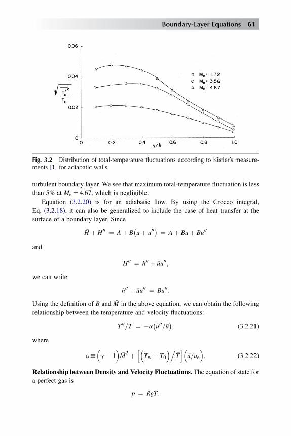
turbulent boundary layer. We see that maximum total-temperature fluctuation is less

than 5% at Me¼ 4.67, which is negligible.

Equation (3.2.20) is for an adiabatic flow. By using the Crocco integral,

Eq. (3.2.18), it can also be generalized to include the case of heat transfer at the

surface of a boundary layer. Since

�H þ H00 ¼ Aþ B��uþ u00

� ¼ Aþ B�uþ Bu00

and

H00 ¼ h00 þ �uu00;

we can write

h00 þ �uu00 ¼ Bu00:

Using the definition of B and �M in the above equation, we can obtain the following

relationship between the temperature and velocity fluctuations:

T 00= �T ¼ �a�u00=�u

�; (3.2.21)

where

ahg� 1

��M2 þ

hTw � T0

�.�Ti

�u=ue

�: (3.2.22)

Relationship between Density and Velocity Fluctuations. The equation of state for

a perfect gas is

p ¼ R9T:

Fig. 3.2 Distribution of total-temperature fluctuations according to Kistler’s measure-ments [1] for adiabatic walls.


In terms of mean and fluctuating quantities, that relation can be written as

�pþ p00 ¼ R��9þ 900

��T þ T 00� ¼ R

��9 �T þ T 009þ 900 �T Þ; (3.2.23)

where we have assumed the second-order term 900T 00 to be negligible. According to

Eq. (2.4.6), such an assumption leads to the relationship ~T ¼ �T . As we shall see

later, in accordance with the boundary-layer assumptions, the 900T 00 term is small and

can be neglected. Using the relation �p ¼ RT9, we can write Eq. (3.2.23) as

p00= �p ¼ �T 00= �T

�þ �900=�9�: (3.2.24)

From Eq. (3.2.24) we see that in order to find a relationship between density and

velocity fluctuations [since the relationship between temperature and velocity fluc-

tuations is given by Eq. (3.2.22)], it is necessary to estimate the order of magnitude of

pressure fluctuations. The pressure field is indicated to the unaided observer by both

the sound field associated with the turbulence and the fluctuating force on a solid

surface in contact with the turbulence. It is important to know the fluctuating pressure

field on material surfaces, since, for example, when flight vehicles are operated in

regimes of large dynamic pressures, the pressures can have significant effects. The

random forces can even cause fatigue failure in a structure, as well as undesirable

levels of structural vibration. In addition, these forces can produce sound within

a structure through the intermediate step of forcing the solid surface into motion.

According to the experimental results of Kistler [1], the temperature fluctuations

are essentially isobaric for adiabatic flows with Mach numbers less than 5. Conse-

quently, Eq. (3.2.24) can be written as

T 00= �Tz� 900=�9: (3.2.25)

Unfortunately, in the flow range above Mach 5, no detailed measurements of

turbulent fluctuations have as yet been reported. It is therefore not possible to provide

quantitative information on the subject. There is convincing experimental evidence,

however, that inflows in thevicinity ofMe¼ 5, appreciable pressurefluctuations exist in

the boundary layer. Kistler and Chen [4] reported rms pressure fluctuations of 8-10% of

the mean static pressure at the wall for Me¼ 5. Under the same conditions, Laufer’s

measurement [5] of the value just outside the boundary layer was ðp002Þ1=2=�pz1%).

In our discussion, we shall assume the pressure fluctuations to be negligible and

make the order-of-magnitude estimates of the fluctuating quantities on that basis.

Substitution from Eq. (3.2.25) into Eq. (3.2.21) gives the desired relationship

between density and velocity fluctuations,

900=�9 ¼ aðu00=�uÞ: (3.2.26)

According to experiment, that relation is justified for compressible turbulent

boundary layers at Mach numbers up to approximately 5 [2].


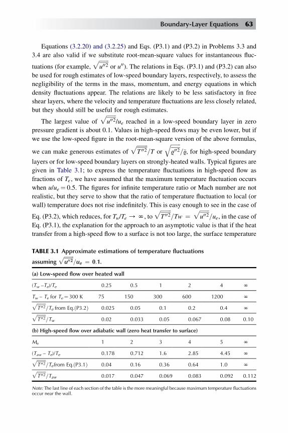
Equations (3.2.20) and (3.2.25) and Eqs. (P3.1) and (P3.2) in Problems 3.3 and

3.4 are also valid if we substitute root-mean-square values for instantaneous fluc-

tuations (for example,ffiffiffiffiffiffiffiu002

por u00). The relations in Eqs. (P3.1) and (P3.2) can also

be used for rough estimates of low-speed boundary layers, respectively, to assess the

negligibility of the terms in the mass, momentum, and energy equations in which

density fluctuations appear. The relations are likely to be less satisfactory in free

shear layers, where the velocity and temperature fluctuations are less closely related,

but they should still be useful for rough estimates.

The largest value offfiffiffiffiffiffiffiu002

p/ue reached in a low-speed boundary layer in zero

pressure gradient is about 0.1. Values in high-speed flows may be even lower, but if

we use the low-speed figure in the root-mean-square version of the above formulas,

we can make generous estimates offfiffiffiffiffiffiffiffiT 002

p=T or

ffiffiffiffiffiffiffi9002

q=�9, for high-speed boundary

layers or for low-speed boundary layers on strongly-heated walls. Typical figures are

given in Table 3.1; to express the temperature fluctuations in high-speed flow as

fractions of Te , we have assumed that the maximum temperature fluctuation occurs

when u/ue¼ 0.5. The figures for infinite temperature ratio or Mach number are not

realistic, but they serve to show that the ratio of temperature fluctuation to local (or

wall) temperature does not rise indefinitely. This is easy enough to see in the case of

Eq. (P3.2), which reduces, for Tw/Te /N, toffiffiffiffiffiffiffiffiT 002

p=Tw ¼

ffiffiffiffiffiffiffiu002

p=ue, in the case of

Eq. (P3.1), the explanation for the approach to an asymptotic value is that if the heat

transfer from a high-speed flow to a surface is not too large, the surface temperature

TABLE 3.1 Approximate estimations of temperature fluctuations

assumingffiffiffiffiffiffiffiffiu002

p=ue ¼ 0:1.

(a) Low-speed flow over heated wall

(Tw –Te)/Te 0.25 0.5 1 2 4 N

Tw – Te for Te¼ 300 K 75 150 300 600 1200 NffiffiffiffiffiffiffiffiT 002

p=Te from Eq:ðP3:2Þ 0.025 0.05 0.1 0.2 0.4 Nffiffiffiffiffiffiffiffi

T 002p

=Tw 0.02 0.033 0.05 0.067 0.08 0.10

(b) High-speed flow over adiabatic wall (zero heat transfer to surface)

Me 1 2 3 4 5 N

(Taw – Te)/Te 0.178 0.712 1.6 2.85 4.45 NffiffiffiffiffiffiffiffiT 002

p=Te from Eq:ðP3:1Þ 0.04 0.16 0.36 0.64 1.0 Nffiffiffiffiffiffiffiffi

T 002p

=Taw 0.017 0.047 0.069 0.083 0.092 0.112

Note: The last line of each section of the table is the more meaningful because maximum temperature fluctuationsoccur near the wall.


is not much less than the total temperature of the external stream and therefore rises

rapidly with Mach number. Values given in Table 3.1(b) are for the ‘‘recovery’’

temperature, the temperature reached by an insulated (adiabatic) surface, Taw(see Section 4.7, Eq. (4.7.3)).

Approximations Involving the Molecular-Transport Terms. For a perfect gas,

the fluid properties m and k are functions only of temperature for a wide range of

pressures. In order to express their variation with temperature fluctuations, we write

them as

m ¼ �mþ m00 ¼ �m�1þ �m00=�m��; k ¼ �k þ k00 ¼ �k

�1þ �k00=�k ��: (3.2.27)

If it is assumed that m and k are proportional to temperature, Eq. (3.2.27)

becomes

m ¼ �m�1þ �T 00= �T

��; k ¼ �k

�1þ �T 00= �T

��: (3.2.28)

3.3 Continuity, Momentum, and Energy Equations

3.3.1 TWO-DIMENSIONAL FLOWS

Let us first consider the continuity and the x-momentum equations given by Eqs.

(3.2.1) and (3.2.2). Since 9 ¼ �9þ 900 and m ¼ �mþ m00, the three terms 9u0u0, 9u0y0,and sxy in Eq. (3.2.2) can be written as

9u0u0 ¼ �9u0u0 þ 900u0u0 ; 9u0y0 ¼ �9u0y0 þ 9009u0y0: (3.3.1a)

�sxy ¼ mvu

vy¼ �m

�1þ m00

�m

�v

vy~u

�1þ u0

~u

�; (3.3.1b)

Since v=vy ¼ Oðd�1Þ, the term 9u0y0 is of O(d) at most. Furthermore,

m00ðvu0=vyÞmðv~u=vyÞ � 1 and

900u0y0

�9u0y0� 1: (3.3.2)

In each case, those ratios can be assumed to be less than 5% for Mach numbers less

than 5, if the coefficients of correlation between viscosity and velocity gradient and

between density and u0y0 fluctuation are at most 0.3.

Let us now estimate the order of magnitude of 900y0. Multiplying both sides of Eq.

(3.2.26) by y, rearranging, and assuming that u00 ¼ u0, we get

900y0 z a��9=�u�u0y0: (3.3.3)


For moderate Mach numbers and heat-transfer rates, a is of O(1). Since u0y0 ¼ OðdÞand �9=�u¼O(1), we see that 900y0 ¼ OðdÞ. If we assume that y0 is proportional to u0,then 900u0 ¼ OðdÞ. Therefore, from Eq. (2.4.3b) we have

~u� �u ¼ 900u0=�9 ¼ 900u00=�9 or ~u ¼ �u (3.3.4a)

and

~y� �y ¼ 900y0=9 ¼ 900y00=9 or ~y ¼ �yþ 900y00=�9; (3.3.4b)

since ~u ¼ Oð1Þ and ~y ¼ OðdÞ: That means that we can interchange tildes and bars

on u with the boundary-layer approximations but cannot do so on y. Also, from the

definition of u0, that is,

u0 ¼ �900u00=�9 ;

we see that u0 is of O(d). As a result, ~uð1þ u0=~uÞ in Eq. (3.3.1b) is approximately

equal to ~u. Furthermore, �sxy[�sxx and 9u0y0[900u0u0.With those approximations, the continuity and x-momentum equations given by

Eqs. (3.2.1) and (3.2.2), respectively, become:

Continuity

v�9

vtþ v

vx

��9�u�þ v

vy

�9y� ¼ 0; (3.3.5)

x Momentum

v

vt

��9�u�þ v

vx

��9�u�u�þ v

vy

�9y �u� ¼ � v�p

vxþ v

vy

��mv�u

vy� 9u0y0

�: (3.3.6a)

With the use of Eq. (3.3.5), we can write Eq. (3.3.6) as

�9v�u

vtþ �9�u

v�u

vxþ 9y

v�u

vy¼ � v�p

vxþ v

vy

��mv�u

vy� 9u0y0

�; (3.3.6b)

where

9y ¼ 9 yþ 900y00 ¼ �9~y: (3.3.7)

Following the same line of order-of-estimate study, the y-momentum equation

(3.2.3) becomes

� v�p

vy� v

vy

�9y0y0

�¼ 0: (3.3.8)

We see from Eq. (3.3.8) that for laminar flows v�p=vy is of O(d) but that for turbulent

flows it is of O(1). Consequently, the pressure variation across the boundary layer is


of O(d), so that in comparison with the streamwise pressure variation p(x, t) it is still

small and can be neglected within the boundary-layer approximations.

For incompressible flows, Eqs. (3.3.5), (3.3.6), and (3.3.8) can be simplified

further, as follows:

Continuity

v�u

vxþ v�y

vy¼ 0; (3.3.9)

Momentum

v�u

vtþ �u

v�u

vxþ �y

v�u

vy¼ � 1

9

v�p

vxþ n

v2�u

vy2þ v

vy

�u0y0

�: (3.3.10)

We next consider the energy equation. According to the approximations dis-

cussed above, we have shown that the double-correlation terms involving u0, y0, 90,such as u0y0, 90y0, etc., are ofO(d) at most, and that the triple correlation terms such as

900u0y0 are small3 compared to �9u0y0. We have also shown that within the boundary-

layer approximations, ~u¼ �u and 9y ¼ �9~y ¼ �9�yþ 900y00. Before we discuss the

boundary-layer simplifications for the total-enthalpy energy equation, let us first

show that within the boundary-layer approximations, ~H ¼ �H.

From the definitions of H (xi, t), ~H, and H, we can write (see Section 2.4)

~H � �H ¼ H00 � H0 ¼ 900H0=9 ¼ 900H00=�9: (3.3.11)

Since

9H00 ¼ 9h00 þ �u9u00 ¼ 900h00 þ u900u00; (3.3.12)

and the two terms on the right-hand side of Eq. (3.3.12) are all of O(d), we see that

9H00, which is also equal to 900H00, is of O(d). Consequently, ~H ¼ �H from

Eq. (3.3.11).

By extending the boundary-layer approximations discussed in the previous

sections, we can write the total-enthalpy energy equation (3.2.4) as

�9v �H

vtþ �9�u

v �H

vxþ 9y

v �H

vy

¼ vp

vtþ v

vy

��u�m

v�u

vy� �qy � 9y0H0

�;

(3.3.13)

where �qy ¼ ��kðv �T=vyÞ.

3It is generally assumed that the triple correlation terms are of O(d2). Since 900y0 ¼O(d) and u0 ¼O(d),

their product must be of O(d2).


From the definitions of mean total enthalpy �H, qy, and Prandtl number, the second

term in parentheses on the right-hand side of Eq. (3.3.13) can be rewritten in

a slightly different form. The resulting expression becomes

�9v �H

vtþ �9�u

v �H

vxþ 9y

v �H

vy

¼ v�p

vtþ v

vy

�m u

v�u

vy

�1� 1

Pr

�þ �m

Pr

v �H

vy� �9H0y0

:

(3.3.14)

Sometimes it is more convenient to express 9y0H0 in terms of static enthalpy fluc-

tuation h0, which can easily be done by recalling the definition of H0. Neglecting the

second- and higher-order terms in Eq. (2.3.19), we can write the fluctuating total

enthalpy H0 as

H0 ¼ h0 þ �uu0;

where we have replaced ~u by �u, which is permissible within the boundary-layer

approximations. Multiplying both sides of that expression by �9y0 and averaging,

we get

�9H0y0 ¼ �9h0y0 þ �9�uu0y0:

Substituting that expression into Eq. (3.3.14) and replacing the second term on the

right-hand side of Eq. (3.3.13) by the resulting expression, we get

�9v �H

vtþ �9�u

v �H

vxþ 9y

v �H

vy

¼ v�p

vtþ v

vy

m

Pr

v �H

vy� �9h0y0 þ u

�1� 1

Pr

��mv�u

vy� �9u0y0

�:

(3.3.15)

For an incompressible flow, the total-enthalpy equation simplifies considerably.

Noting that

�m

Pr

v �H

vy¼ �m

Pr

�v�h

vyþ v

vy

��u2

2

�;

we can rewrite the total energy equation (3.3.15) as

�9v �H

vtþ �9�u

v �H

vxþ 9y

v �H

vy

¼ v�p

vtþ v

vy

��m

Pr

v�h

vy� 9h0y0 þ u

��mv�u

vy� �9u0y0

�:

(3.3.16)


Substituting �hþ �u2=2 for �H in Eq. (3.3.15) and using Eqs. (3.3.6b) and (3.3.16), we

get the energy equation in terms of static enthalpy,

�9v�h

vtþ �9�u

v�h

vxþ 9y

v�h

vy

¼ v�p

vtþ u

v�p

vxþ v

vy

��m

Pr

v�h

vy� �9h0y0

�þ��mv�u

vy� �9u0y0

�v�u

vy:

(3.3.17)

That equation, like Eq. (3.3.13), is still for a compressible flow. For an incom-

pressible flow, the fluid properties, �9, �k, Pr, and m are constant. In addition, the

pressure-work term �uðv�p=vxÞ and the dissipation term ½�mðv�u=vyÞ � �9u0y0� ðv�u=vyÞare small and can be neglected. Their negligibility can be easily shown by expressing

Eq. (3.3.17) in terms of dimensionless quantities defined by

t ¼ tuN=L; x ¼ x=L; y ¼ y=L; u* ¼ u=uN; ð9yÞ*¼ 9y=9NuN;�u0y0�* ¼ u0y0=u2N;

�y0h0�* ¼ y0h0=uN

�hw � hN

�; p* ¼ p=9Nu2N;

9* ¼ 9=9N; h* ¼ �h� hN

�=�hw � hN

�; m* ¼ m=mN;

(3.3.18)

where the bars on independent variables, t, x, and y denote dimensionless quantities.

Using the definitions of Eq. (3.3.18) and then simplifying, we can write the static-

enthalpy energy equation (3.3.17) in terms of dimensionless quantities in the

following form:

9*vh*

vtþ 9*u*

vh*

vxþ ð9yÞ*vh

*

vy

I

¼ E

vp*

vtþ u*

vp*

vx

!þ 1

RL

v

vy

(m*

Pr

vh*

vy� RL9

*ðh0y0Þ*)

II III IV

þ E

RL

m*

vu*

vy� RL9

*ðu0y0Þ*!

vu*

vy:

V VI

(3.3.19)

Like the Prandtl number (Pr h mcp/k), the quantities RL and E are dimensionless

quantities; they are known as Reynolds number and Eckert number, respectively, and

are defined as

RLh uN9NL=mN; E h u2N=hw � hN: (3.3.20)


Since for a perfect gas cp¼ gR/(g – 1), it follows from the definition of Eckert

number that

E ¼ u2Ncp�Tw � TN

�¼ u2N

cpTN

�TN

Tw � TN

�¼ �

g� 1�M2

N

�TN

Tw � TN

�:

(3.3.21)

From Eq. (3.3.21) we see that if the temperature difference is of the same order of

magnitude as the free-stream temperature, the Eckert number becomes equivalent to

the free-stream Mach number. Thus Eckert number becomes important only for

small temperature differences at high Mach numbers. The Eckert number is quite

small in incompressible flows (M z 0), and since RL, is large within the boundary-

layer approximations, the ratio E/RL, is also small. Consequently, pressure-work and

dissipation terms are negligible. For incompressible flows, the energy equation

(3.3.17) then becomes

v�h

vtþ �u

v�h

vxþ �y

v�h

vy¼ a

v2 �h

vy2� v

vy

�h0y0�; (3.3.22)

where a is the thermal diffusivity, a h n/Pr.

That equation can be written in terms of static temperature T as

v �T

vtþ �u

v �T

vxþ y

v �T

vy¼ a

v2 �T

vy2� v

vy

�T 0y0

�: (3.3.23)

3.3.2 AXISYMMETRIC FLOWS

In principle, the governing boundary-layer equations for axisymmetric flows do not

differ much from those of two-dimensional flows. Again, the external potential

velocity is a function of only one space coordinate, and the velocity within the

boundary region has two components. Typical examples of such flows are a flow over

a body of revolution, a wake behind an axially symmetrical body, and a jet issuing

from an axisymmetric body. The extent of the region in the radial direction is of the

order of the thickness of the boundary layer d and is usually much smaller than both

the extent of the region in the axial direction L and the radius of the body r0.

The boundary-layer equations of a steady, compressible fluid for both laminar

and turbulent axisymmetric flows for the coordinate system shown in Fig. 3.3 can be

written in a form similar to those of Eqs. (3.3.5), (3.3.6b), (3.3.13), and (3.3.15). The

steady continuity, momentum, and energy (total enthalpy) equations are


Continuity

v

vx

�r k�9�u

�þ v

vy

�rk9y

� ¼ 0; (3.3.24)

Momentum

9�uv�u

vxþ 9y

v�u

vy¼ � d�p

dxþ 1

rkv

vy

�rk��mv�u

vy� �9u0y0

�; (3.3.25)


�9�uv �H

vxþ 9y

v �H

vy

¼ 1

rkv

vy

rk��m

�1� 1

Pr

��uv�u

vyþ �m

Pr

v �H

vy� �9H0y0

�:

(3.3.26)

The right-hand side of Eq. (3.3.26) can also be written as [see Eq. (3.3.15)]

¼ 1

r kv

vy

�r k �m

Pr

v �H

vy� �9h0y0 þ �u

��1� 1

Pr

��mv�u

vy� 9u0y0

�: (3.3.27)

where k¼ 1 for axisymmetric flows, k¼ 0 for two-dimensional flows and, from

Fig. 3.3,

rðx; yÞ ¼ r0ðxÞ þ y cosa : (3.3.28)

Although for most axisymmetric flows the boundary-layer thickness d is gener-

ally small compared with, say, body radius r0, there are some flows – for example,

flows over very slender cylinders or flow over the tail of a streamlined body of

revolution – in which the boundary-layer thickness can be of the same order of

magnitude as the radius of the body. In such cases, the so called transverse-curvature

(TVC) effect must be accounted for, since such an effect strongly influences the skin

Fig. 3.3 Coordinate system for an axisymmetric flow.


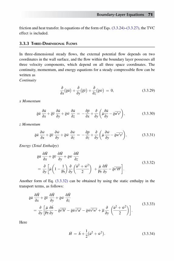
friction and heat transfer. In equations of the form of Eqs. (3.3.24)–(3.3.27), the TVC

effect is included.

3.3.3 THREE-DIMENSIONAL FLOWS

In three-dimensional steady flows, the external potential flow depends on two

coordinates in the wall surface, and the flow within the boundary layer possesses all

three velocity components, which depend on all three space coordinates. The

continuity, momentum, and energy equations for a steady compressible flow can be

written as

Continuity

v

vx

��9�u�þ v

vy

�9y�þ v

vz

��9�w� ¼ 0; (3.3.29)

x Momentum

�9�uv�u

vxþ 9y

v�u

vyþ �9�w

v�u

vz¼ � v�p

vxþ v

vy

��mv�u

vy� �9u0y0

�; (3.3.30)

z Momentum

�9�uv�w

vxþ 9y

v�w

vyþ 9�w

v�w

vz¼ � v�p

vzþ v

vy

��mv�w

vy� �9w0y0

�; (3.3.31)


�9�uv �H

vxþ 9y

v �H

vyþ �9�w

v �H

vz

¼ v

vy

��m

�1� 1

Pr

�v

vy

��u2 þ �w2

2

�þ �m

Pr

v �H

vy� 9y0H0

:

(3.3.32)

Another form of Eq. (3.3.32) can be obtained by using the static enthalpy in the

transport terms, as follows:

�9�uv �H

vxþ 9y

v �H

vyþ �9�w

v �H

vz

¼ v

vy

��m

Pr

v�h

vy� �9y0h0 � �9�u y0u0 � �9�wy0w0 þ m

v

vy

��u2 þ �w2

2

�:

(3.3.33)

Here

�H ¼ �hþ 1

2

��u2 þ �w2

�: (3.3.34)


Again, the pressure gradients vp=vx and vp=vz in Eqs. (3.3.30) and (3.3.31) are

known from the potential flow. At the edge of the boundary layer, the two momentum

equations reduce to

uevuevx

þ wevuevz

¼ � 1

9e

v�p

vx; (3.3.35)

uevwe

vxþ we

vwe

vz¼ � 1

9e

v�p

vz: (3.3.36)

A special case of a three-dimensional flow arises when the external potential flow

depends only on x and not on z, that is,

ue ¼ ueðxÞ; we ¼ const:

For a steady compressible flow, the governing equations follow from Eqs. (3.3.29)–

(3.3.33).

v

vx

��9�u�þ v

vy

�9y� ¼ 0; (3.3.37)

�9�uvu

vxþ 9y

v�u

vy¼ � v�p

vxþ v

vy

��mv�u

vy� �9u0y0

�; (3.3.38)

�9�uv�w

vxþ 9y

v�w

vy¼ v

vy

��mv�w

vy� 9w0y0

�; (3.3.39)

�9�uv �H

vxþ 9y

v �H

vy

¼ v

vy

��m

�1� 1

Pr

�v

vy

��u2 þ �w2

2

�þ �u

Pr

v �H

vy� �9y0H0

:

(3.3.40)

�9�uv �H

vxþ 9y

v �H

vy

¼ v

vy

��m

Pr

v�h

vy� �9y0h0 � �9�uy0u0 � �9�wy0w0 þ �m

v

vy

��u2 þ �w2

2

�:

(3.3.41)

The above equations are known as the boundary-layer equations for laminar and

turbulent flows over infinite swept wings.


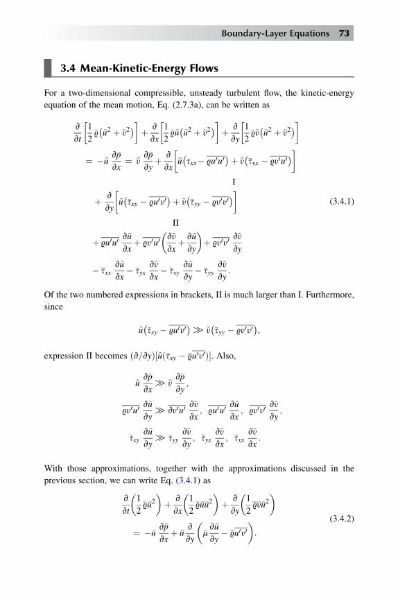
3.4 Mean-Kinetic-Energy Flows

For a two-dimensional compressible, unsteady turbulent flow, the kinetic-energy

equation of the mean motion, Eq. (2.7.3a), can be written as

v

vt

�1

2�9�~u2 þ ~y2

�þ v

vx

�1

2�9~u�~u2 þ ~y2

�þ v

vy

�1

2�9~y�~u2 þ ~y2

�

¼ �~uv�p

vx¼ ~y

v�p

vyþ v

vx

�~u�sxx� 9u0u0

�þ ~y��syx � 9y0u0

�I

þ v

vy

�~u��sxy � 9u0y0

�þ ~y��syy � 9y0y0

�II

þ 9u0u0v~u

vxþ 9y0u0

�v~y

vxþ v~u

vy

�þ 9y0y0

v~y

vy

��sxxv~u

vx� �syx

v~y

vx� �sxy

v~u

vy� �syy

v~y

vy:

(3.4.1)

Of the two numbered expressions in brackets, II is much larger than I. Furthermore,

since

~u��sxy � 9u0y0

�[~y

��syy � 9y0y0

�;

expression II becomes ðv=vyÞ½~uð�sxy � �9u0y0Þ�. Also,

~uv�p

vx[~y

v�p

vy;

9y0u0v~u

vy[ vy0u0

v~y

vx; 9u0u0

v~u

vx; 9y0y0

v~y

vy;

�sxyv~u

vy[�syy

v~y

vy; ~syx

v~y

vx; �sxx

v~y

vx:

With those approximations, together with the approximations discussed in the

previous section, we can write Eq. (3.4.1) as

v

vt

�1

2�9�u2�þ v

vx

�1

2�9�u�u2

�þ v

vy

�1

29y�u2

�

¼ ��uv�p

vxþ �u

v

vy

��mv�u

vy� �9u0y0

�:

(3.4.2)


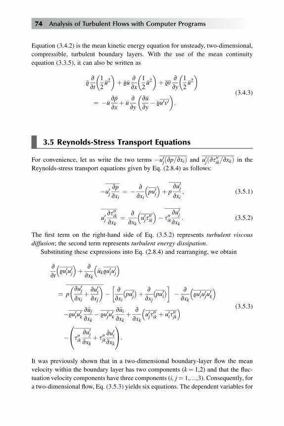
Equation (3.4.2) is the mean kinetic energy equation for unsteady, two-dimensional,

compressible, turbulent boundary layers. With the use of the mean continuity

equation (3.3.5), it can also be written as

�9v

vt

�1

2�u2�þ �9�u

v

vx

�1

2�u2�þ 9y

v

vy

�1

2�u2�

¼ ��uv�p

vxþ �u

v

vy

�v�u

vy� �9u0y0

�:

(3.4.3)

3.5 Reynolds-Stress Transport Equations

For convenience, let us write the two terms �u0jðvp=vxiÞ and u0jðvs00ik=vxkÞ in the

Reynolds-stress transport equations given by Eq. (2.8.4) as follows:

�u0jvp

vxi¼ � v

vxi

pu0j�þ p

vu0jvxi

; (3.5.1)

u0jvs00ikvxk

¼ v

vxk

u0js00ik

�� s00ik

vu0jvxk

: (3.5.2)

The first term on the right-hand side of Eq. (3.5.2) represents turbulent viscous

diffusion; the second term represents turbulent energy dissipation.

Substituting these expressions into Eq. (2.8.4) and rearranging, we obtain

v

vt

9u0iu0j

�þ v

vxk

~uk9u

0iu

0j

�

¼ p

�vu0jvxi

þ vu0ivxj

��v

vxi

�pu0j�þ v

vxj

�pu0i� � v

vxk

9u0iu0ju0k

�

�9u0iu0kv~ujvxk

� 9u0ju0kv~uivxk

þ v

vxk

u0js00ik þ u0is00jk

�

�0@s00ik

vu0jvxk

þ s00jkvu0ivxk

1A:

(3.5.3)

It was previously shown that in a two-dimensional boundary-layer flow the mean

velocity within the boundary layer has two components (k¼ 1,2) and that the fluc-

tuation velocity components have three components (i, j¼ 1,.,3). Consequently, for

a two-dimensional flow, Eq. (3.5.3) yields six equations. The dependent variables for


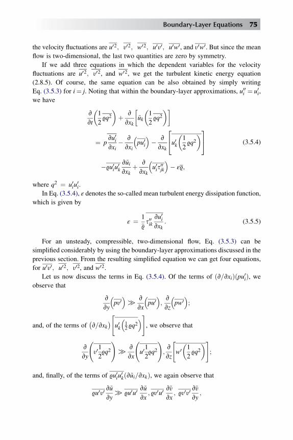
the velocity fluctuations are u02; y02; w02; u0y0; u0w0, and y0w0. But since the mean

flow is two-dimensional, the last two quantities are zero by symmetry.

If we add three equations in which the dependent variables for the velocity

fluctuations are u02; y02, and w02, we get the turbulent kinetic energy equation

(2.8.5). Of course, the same equation can be also obtained by simply writing

Eq. (3.5.3) for i¼ j. Noting that within the boundary-layer approximations, u00i ¼ u0i,we have

v

vt

�1

29q2�þ v

vxk

�~uk

�1

29q2�

¼ pvu0ivxi

� v

vxi

pu0i�� v

vxk

24u0k�1

29q2�35

�9u0iu0k

v~uivxk

þ v

vxk

u0is

00jk

�� ε9;

(3.5.4)

where q2 ¼ u0iu0i:In Eq. (3.5.4), ε denotes the so-called mean turbulent energy dissipation function,

which is given by

ε ¼ 1

�9s00ik

vu0ivxk

: (3.5.5)

For an unsteady, compressible, two-dimensional flow, Eq. (3.5.3) can be

simplified considerably by using the boundary-layer approximations discussed in the

previous section. From the resulting simplified equation we can get four equations,

for u0y0; u02; y02, and w02.Let us now discuss the terms in Eq. (3.5.4). Of the terms of ðv=vxiÞðpu0iÞ, we

observe that

v

vy

py0�[

v

vx

pu0�;v

vz

pw0�;

and, of the terms of�v=vxk

�"u0k12 9q

2�#

, we observe that

v

vy

y01

29q2

![

v

vx

u01

29q2

!;v

vz

"w0�1

29q2�#

;

and, finally, of the terms of 9u0iu0kðv~ui=vxkÞ, we again observe that

9u0y0v~u

vy[ 9u0u0

v~u

vx; 9y0u0

v~y

vx; 9y0y0

v~y

vy;


With the definition of s00ik, we can write u0is00ik as

u0is00ik ¼ �m

�v

vxk

�1

2q2�þ v

vxi

�u0iu

0k

�� u0kvu0ivxi

:

Of the terms of�v=vxk

�hmðv=vxkÞ

�12 q

2�i, we observe that

v

vy

��mv

vy

�1

2q2�

[v

vx

��mv

vx

�1

2q2�

;

and, of the nine terms of ðv=vxkÞhmðv=vxiÞðu0iu0kÞ

i, we again observe

v

vy

��mv

vyðy0y0Þ

[

v

vx

��mv

vx

�u0u0�

;v

vy

��mv

vx

�u0y0�; etc:

Making use of the above relations, assuming that the divergence of the velocity

fluctuations vu0i=vxi is negligible, and noting the relationship given in Eq. (3.3.4), wecan now write the turbulent kinetic energy equation (3.5.4) for a two-dimensional,

unsteady, compressible boundary-layer flow as

v

vt

9q2

2

!

local rate of change

of turbulent energy

þ v

vx

"�9�u

q2

2

!#þ v

vy

"�9�y

q2

2

!#turbulent energy convection

¼ � 9u0y0v�u

vyturbulent

energy production

þ v

vy

��mv

vy

�1

2q2 þ y02

�turbulent viscous diffusion

� v

vy

y01

29q2

!

turbulent kinetic

diffusion

� v

vy

�py0�

turbulent

pressure diffusion

� ε�9:turbulent

energy dissipation

(3.5.6a)

In Eq. (3.5.6a) we have assumed that 9q2[900q2.Multiplying the continuity equation by� 1

2q2 and adding the resulting expression

to Eq. (3.5.6a), we obtain

�9v

vt

q2

2þ �9�u

v

vx

0@q2

2

1Aþ 9y

v

vy

0@q2

2

1A

¼ ��9u0y0v�u

vyþ v

vy

��mv

vy

�1

2q2 þ y02

�� v

vy

�y0�1

2�9q2 þ p

�� ε�9;

(3.5.6b)


where ε, which is given by Eq. (3.5.5), can also be written as

εh1

�9�m

�vu0ivxk

þ vu0kvxi

�vu0ivxk

¼ n

242 �vu0

vx

�2

þ 2

�vy0

vy

�2

þ 2

�vw0

vz

�2

þ�vu0

vyþ vy0

vx

�2

þ�vu0

vzþ vw0

vx

�2

þ�vy0

vzþ vw0

vy

�235; (3.5.7)

if the likðvu0l=vxlÞ term in the stress tensor is neglected.

The boundary-layer approximations for Eq. (3.5.3) are quite similar to those for

Eq. (3.5.4). For i¼ j¼ 1, Eq. (3.5.3) becomes

v

vt

9u02

�þ v

vxk

~uk9u02

�

¼ 2pvu0

vx� 2

v

vx

�pu0�� v

vxk

�u0k9u02

�

�29u0u0kv~u

vxkþ 2

v

vxk

"mu0�vu0

vxkþ vu0k

vx

�#:

(3.5.8)

Let us now define the operator D/Dt on any function g by

Dg

Dt¼ vg

vtþ v

vx

�g�u�þ v

vy

�g~y�:

In accordance with the boundary-layer approximations discussed for the turbulent

kinetic-energy equation, Eq. (3.5.8) simplifies to

D

Dt9u02 ¼ 2p

vu0

vx� v

vyy09u02 � 29u0y0

v�u

vy

þ v

vy

��mv

vy

�u02�� 2�m

vu0

vxk

vu0

vxk:

(3.5.9)

Similarly, we can write an equation for each of the turbulent energies y02 and w02

by letting i¼ j¼ 2 and i¼ j¼ 3 in Eq. (3.5.3), and we can write a single equation for

shear stress by letting i¼ 1, j¼ 2 in Eq. (3.5.3). After the application of boundary-

layer approximations to these equations, we get


D

Dt9y02 ¼ 2p

vy0

vy� 2

v

vy

�py0�� v

vy

�y09y02

�

þ v

vy

��mv

vy

�y02�� 2�m

vy0

vxk

vy0

vxk;

(3.5.10)

D

Dt9w02 ¼ 2p

vw0

vz� v

vy

y09w02

�þ v

vy

��mv

vy

�w02�� 2�m

vw0

vxk

vw0

vxk

!; (3.5.11)

D

Dt9u0y0 ¼ p

�vu0

vyþ vy0

vx

�� v

vy

9u0y02

�� 9y0y0

v�u

vy

þ v

vy

��mv

vy

�u0y0�� v

vy

�pu0�� 2�m

vu0

vxk

vy0

vxk

!:

(3.5.12)

For incompressible flows, since the flow properties are constant, Eqs. (3.5.6) and

(3.5.10)–(3.5.12) can be simplified considerably.

For example, the turbulent kinetic-energy equation becomes

v

vt

q2

2

!þ u

v

vx

q2

2

!þ y

v

vy

�q2

2

�

¼ �u0y0vu

vyþ v

v2

vy2

q2

2þ y02

!� v

vy

y0q2

2þ py0

9

!� ε:

(3.5.13)

3.6 Integral Equations of the Boundary Layer

Although the differential equations of the boundary layer discussed in the previous

sections have been greatly simplified from the general differential equations of fluid

flow, they are still difficult to solve, since they are nonlinear partial differential

equations. Considerable simplification arises when these equations are integrated

across the boundary layer. Then they are no longer partial differential equations, but

just ordinary differential equations. However, they are still exact equations, at

least within the boundary-layer approximations. These equations, known as the

integral equations of the boundary layer, provide a basis for many approximate

methods of boundary-layer prediction. They will now be discussed for steady two-

dimensional flows.


3.6.1 MOMENTUM INTEGRAL EQUATION

The momentum integral equation for a two-dimensional steady compressible

flow can be obtained by integration from the boundary-layer equations (3.3.5)

and (3.3.6b).4 If we multiply Eq. (3.3.5) by (ue–u), multiply Eq. (3.3.6b) by –1,

add and subtract 9uðdue=dxÞ from Eq. (3.3.6b), and add the resulting continuity

and momentum equations, we can arrange the resulting expression in the

form

v

vx

�9u�ue � u

��þ v

vy

�9y�ue � u

��þ duedx

�9eue � 9u

� ¼ � v

vy

�mvu

vy� 9u0y0

�:

Nondimensionalizing and integrating with respect to y from zero to infinity,

we get

d

dx

�9eu

2e

Z N

0

9u

9eue

�1� u

ue

�dy

þ due

dx9eue

� Z N

0

�1� 9u

9eue

�dy

� 9wywue

¼�mvu

vy

�w

h sw;

(3.6.1)

since (vu=vy) and u0y0 / 0 as y / N and since u0y0 / 0 as y / 0. It is more

convenient to express Eq. (3.6.1) in terms of boundary-layer thicknesses d* and q.

Equation (3.6.1) then becomes

d

dx

9eu

2eq�þ 9eued*

duedx

� 9wywue ¼ sw;

or, in nondimensional form,

dq

dxþ q

ueðH þ 2Þdue

dxþ q

9e

d9edx

� 9w9e

yw

ue¼ sw

9eu2e

; (3.6.2)

where H denotes the ratio d*/q, which is known as the shape factor. For an ideal gas

undergoing an isentropic process, we can write

1

9e

d9edx

¼ �M2e

ue

duedx

: (3.6.3)

4For simplicity, we shall drop the bars from the principal mean quantities.


Substituting from that equation into Eq. (3.6.2) and rearranging, we obtain the

momentum integral equation of the boundary layer for a two-dimensional

compressible flow:

dq

dxþ q

ue

�H þ 2�M2

e

�duedx

� 9wde

yw

ue¼ sw

9eu2e

hcf2; (3.6.4)

where cf is the local skin-friction coefficient. Note that in the case of zero mass

transfer the normal velocity component at the wall yw is zero. Then Eq. (3.6.4)

becomes

dq

dxþ q

ue

H þ 2�M2

e

�duedx

¼ cf2: (3.6.5)

For an incompressible flow with no mass transfer, that equation reduces to

dq

dxþ q

ueðH þ 2Þdue

dx¼ cf

2: (3.6.6)

Equations (3.6.4)–(3.6.6) are also known as the first momentum integral equa-

tions. They are applicable to both laminar and turbulent boundary layers.

3.6.2 MEAN ENERGY INTEGRAL EQUATION

The derivation of the mean energy integral equation is similar to that of the

momentum integral equation. We multiply Eq. (3.3.5) by ( u2e– u2), and Eq. (3.3.6b)

by – 2u. After the resulting expressions are added and rearranged, we obtain

1

2

v

vx

9eu

3e

�9u

9eue

�1� u2

u2e

��þ 1

2

v

vy

h9yu2e � u2

�i

þ9eu2e

�u

ue

�1� 9

9e

�duedx

¼ �u

v

vy

�mvu

vy� 9u0y0

�:

(3.6.7)

The right-hand side of Eq. (3.6.7) can also be written as

�uvsvy

¼ svu

vy� v

vy

�us�; (3.6.8)

where

s ¼ m�vu=vy

�� 9u0y0: (3.6.9)

Substituting from Eq. (3.6.8) into Eq. (3.6.7), integrating the resulting expression

with respect to y from zero to infinity, and using the definition of energy thickness d**

given by


d** ¼Z N

0

9u

9eue

�1� u2

u2e

�dy (3.6.10)

we get

1

2

d

dx

9eu

3ed

**�� 1

29wywu

2e

þ9eu2e

duedx

� Z N

0

u

ue

�1� 9

9e

�dy

¼ D;

(3.6.11)

since both 9yðu2e � u2Þ and s / 0 as y / N. In Eq. (3.6.11), D is defined by

D ¼Z N

0

�mvu

vy� 9u0y0

�vu

vydy

and is called the dissipation integral or the shear work integral. It denotes the

viscous work done in the boundary layer by the two shearing stresses m( vu=vy)

and –9u0y0.For an incompressible flow with no mass transfer, Eq. (3.6.11) simplifies

considerably, becoming

d

dxðu3ed**Þ ¼ 2D

9: (3.6.12a)

In dimensionless form, that equation becomes

1

u3e

d

dxðu3ed**Þ ¼ 2D

9u3e¼ 2CD; (3.6.12b)

where CD is called the dissipation integral coefficient.

3.6.3 TURBULENT ENERGY INTEGRAL EQUATION

Integrating Eq. (3.5.6a) with respect to y from zero to infinity, for steady state we get

d

dx

24Z N

09u

q2

2dy

35¼ Z N

0�9u0y0

�vu

vy

�dy�

Z N

09ε dy; (3.6.13a)

since, in accordance with the boundary conditions, the diffusion terms drop out.

Equation (3.6.13a) is often written in the form

d

dx

�1

2IQ2

�¼ P� d; (3.6.13b)


where IQ2 is an integral scale for the turbulence, defined by

IQ2 ¼Z N

09uq2dy; (3.6.14)

and P and d represent the production and dissipation, respectively, of turbulent

energy within the boundary layer, that is,

P ¼Z N

0�9u0y0

�vu

vy

�dy (3.6.15)

and

d ¼Z N

09ε dy: (3.6.16)

3.6.4 ENERGY INTEGRAL EQUATION

To derive the energy integral equation for two-dimensional compressible flows

without body force, we start with the total enthalpy equation, Eq. (3.3.27). Using the

continuity equation, Eq. (3.3.24), we can write Eq. (3.3.27) as

v

vx

�9uH

�þ v

vy

�9yH

� ¼ v

vy

�� _qþ us�: (3.6.17)

where

sh mvu

vy� 9u0y0 � 90u0y0; (3.6.18a)

_qh� kvT

vyþ cp9T 0y0 þ cp90T 0y0 (3.6.18b)

We now integrate the above equation with respect to y from y¼ 0 to y¼ h> d

to get

Z h

0

v

vx

�9uH

�dyþ 9hyhHe ¼ _qw: (3.6.19)

As in the derivation of the momentum integral equation, we substitute for 9hyh from

the continuity equation and write Eq. (3.6.19) as

Z h

0

v

vx

�9u�He � H

��dy ¼ � _qw (3.6.20)


and then as

d

dx

�9eue

Z N

0

9u

9eue

�1� H

He

�dy

¼ � _qw

He; (3.6.21)

using reasoning similar to which led to the writing of Eq. (3.6.1). Since He – H¼ 0

(to sufficient accuracy) for y � h, the integrand of Eq. (3.6.21) contributes only for

y< h, and so the result is independent of h.

Equation (3.6.21) shows that the rate of increase of total-enthalpy deficit per unit

span (in the z direction) is equal to the rate of heat transfer from the fluid to a unit area

of the surface. Comparing this equation with Eq. (3.6.1), we see that the rate of

increase of deficit in each case is affected by transfer into the surface (enthalpy

transfer – _qw, momentum transfer sw); the momentum integral equation contains an

additional term depending on pressure gradient, but the total enthalpy is unaffected

by pressure gradients as such.

If we introduce qH by

qH ¼Z h

0

9u

9eue

�H � He

Hw � He

�dy; (3.6.22)

then we can write the total-enthalpy integral equation (3.6.20) for a two-dimensional

compressible laminar or turbulent flow as

d

dx

�9eue

�Hw � He

�qH

¼ _qw: (3.6.23)

In Eq. (3.6.22), qH is a measure of total-enthalpy-flux surplus caused by the presence

of the thermal boundary layer. For an incompressible flow, where H is equal to the

static enthalpy h, the total-enthalpy thickness qH is equal to the static-enthalpy

thickness.

qh ¼Z N

0

9u

9eue

�h� hehw � he

�dy; (3.6.24)

where h can be replaced by cpT if cp is constant. Noting this and taking 9 constant, we

can write Eq. (3.6.23) for an incompressible flow as

d

dx

�ue�Tw � Te

�qT

¼ _qw

9cp: (3.6.25)

When the wall temperature is uniform, Eq. (3.6.25) can be written as

1

ue

d

dx

�ueqT

� ¼ St (3.6.26a)


or as

dqTdx

þ qT

ue

duedx

¼ St: (3.6.26b)

Here St denotes the Stanton number befined by

St ¼ _qw9cp�Tw � Te

�ue; (3.6.27)

and

qT ¼Z h

0

u

ue

�T � TeTw � Te

�dy: (3.6.28)

Problems

3.1 Show that in a laminar flow with heat transfer the ‘‘compression work’’ term u vpvx

in Eq. (3.3.17) is small compared to the heat-flux term vvy

�mPr

vhvy

�if the tempera-

ture difference across the shear layer, DT, is large compared toPr u2ecp

.

3.2 Show that in a compressible turbulent flow the condition for the neglect of the

‘‘compression work’’ term u vpvx in Eq. (3.3.17) – compared to the ‘‘heat transfer’’

term vvy

��9h0y0

�or cp

v

vy

��9T 0y0

�, say – is

M2e � 1

10

1

g� 1

DT

Te:

[Hint: The factor 10 is an approximation to d/q in a turbulent boundary layer.]

3.3 Show that for high-speed flows

900

9y ðg� 1Þ �M2 u

00

u(P3.3.1)

3.4 In low-speed boundary layers on heated walls, the velocity and temperature fluc-

tuations again tend to have opposite signs. However, since the driving tempera-

ture difference Tw – Te is imposed separately from the velocity difference ueinstead of being related to it as in high-speed flow, Eq. (P3.3.1) does not hold.

Instead, if the analogy between heat transfer and momentum transfer were exact

and the effect of departure of Pr from unity were small, show that we would have

T 00

Tw � Te¼ � u00

ue(P3.4.1)


or

900

9¼ �T 00

T¼�Tw � Te

T

�u00

ue: (P3.4.2)

3.5 Consider the momentum equation, Eq. (3.3.5) and show that in a highspeed

boundary layer,

900y00 ¼ �g� 1

�M29

900y00

u¼ 9y

24�g� 1

�M29

00y00

uy

35: (P3.5.1)

3.6 By using the arguments used to derive a typical value of 900y00 in Eq. (P3.5.1)

show that a typical value for 900u00 in a nearly-adiabatic highspeed shear layer is

9�g� 1

�M2u

002

u(P3.6.1)

where M is the Mach number.

3.7 Show that in a boundary layer of thickness d on a surface of longitudinal

curvature radius R below a stream of Mach number Me, the ratio of the pressure

difference across the layer to the absolute pressure at the edge is of order

gM2ed=R:

3.8 Show that in a turbulent boundary layer the ratio of the pressure change induced

by the Reynolds normal stress to the absolute pressure at the edge is of order

gM2e cf =2, where cf is the skin-friction coefficient. [Hint: Assume that 9y002 is

of the same order as the shear stress – �9u00y00.]3.9 Show that if in the decelerating turbulent boundary layer in an expanding

passage (a diffuser) the skin-friction term in the momentum-integral equation,

Eq. (3.6.6), is negligible and H can be taken as constant. Equation (3.6.6) gives

q

q0¼�

ueue;0

��ðHþ2Þ

where subscript 0 denotes initial conditions.

3.10 Show that for an incompressible zero-pressure gradient flow over a wall at

uniform temperature, Eq. (3.6.26b) can be written as

dqTdx

¼ St: (P3.10.1)

3.11 Since the governing equations for two-dimensional and axisymmetric flows

differ from each other only by the radial distance r(x,y), the axisymmetric flow

equations, Eqs. (3.3.24) to (3.3.26) can be placed in a nearly two-dimensional


form by using a transformation known as the Mangler transformation. In the

case of flow over a body of revolution of radius r0 (a function of x), we find

that if the boundary-layer thickness is small compared with r0, so that

r (x, y)¼ r0(x), this transformation puts them exactly in two-dimensional

form. We define the Mangler transformation by

d�x ¼r0L

�2Kdx; d�y ¼

rL

�Kdy (P3.11.1)

to transform an axisymmetric flow with coordinates (x, y), into a two-dimen-

sional flow with coordinates ð�x; �yÞ. In Eq. (P3.11.1) L is an arbitrary reference

length. If a stream function in Mangler variables ð�x; �yÞ is related to a stream

function j in (x, y) variables by

�j�x; y� ¼

�1

L

�K

j�x; y�;

then

(a) show that the relation between the Mangler transformed velocity compo-

nents �u and �y in ð�x; �yÞ variables and the velocity components u and y in

(x,y) variables is:

u ¼ �u

y ¼�L

r

�K�r0L

�2K�y� v�y

vx�u

:

(P3.11.2)

(b) By substituting from Eqs (P3.11.2) into Eqs. (3.3.24)–(3.3.26), show that for

laminar flows the Mangler-transformed continuity momentum and energy

equations are:

v�u

v�xþ v�y

vy¼ 0

�uv�u

vxþ �y

v�u

v�y¼ � 1

9

dp

d�xþ n

v

v�y

�ð1þ tÞ2Kv�u

v�y

(P3.11.3)

�uvT

v�xþ �y

vT

v�y¼ k

9cp

v

v�y

�ð1þ tÞ2KvT

vy

(P3.11.4)

where

t ¼ �1þ 1þ 2l cosf

r20y

!1=2

: (P3.11.5)


Note that for t¼ 0, Eqs. (P3.11.3) and (P3.11.4) in the ( �x; �y) plane are exactly in

the same form as those for two-dimensional flows in the (x, y) plane.

3.12 As discussed in Section 8.2, transformed coordinates employing similarity

variables are often used in the solution of the boundary-layer equations.

A convenient transformation is the Falkner-Skan transformation given by

Eq. (8.2.5) for two-dimensional flows. With minor changes, this transformation

can also be used for axisymmetric flows.

With the transformation defined by

h ¼uenx

�12y (P3.12.1)

�j��x; �y� ¼ ðuen�xÞ

12 f��x; h

�(P3.12.2)

show that Mangler-transformed continuity and momentum equations and their

boundary conditions can be written as

�bf 00�0þ mþ 1

2f f 00 þ m

h1� ð f 0Þ2

i¼ �x

�f 0vf 0

v�x� f 00

vf

v�x

�(P3.12.3)

h ¼ 0; f 0 ¼ 0; f��x; 0�h fw ¼ � 1

ðuenxÞZ0

�x

�ywd �x (P3.12.4a)

h ¼ he; f 0 ¼ 1 (P3.12.4b)

where

b ¼ ð1þ tÞ2k; m ¼ �x

ue

dued �x

; (P3.12.5a)

t ¼ �1þ�1þ

�L

r0

�22 cos f

L

�n�x

ue

�12

h

12

(P3.12.5b)

References

[1] A.L. Kistler, Fluctuation measurements in a supersonic turbulent boundary layer, Phys. Fluids 2

(1959) 290.

[2] M.V. Morkovin, W.S. Chen, Effects of compressibility on turbulent flows. The Mechanics of

Turbulence, Gordon and Breach, New York, 1961, p. 367.

[3] A. Demetriades, Turbulence measurements in an axisymmetric compressible wake, Phys. Fluids 11

(1841) 1968.

[4] A.L. Kistler, W.S. Chen, The fluctuating pressure field in a supersonic turbulent boundary layer, J.

Fluid Mech. 16 (1963) 41.

[5] J. Laufer, Some statistical properties of the pressure field radiated by a turbulent boundary layer,

Phys. Fluids 7 (1964) 1191.


General Behaviorof TurbulentBoundary Layers

Chap

ter4


4.1 Introduction 90

4.2 Composite Nature of a Turbulent Boundary Layer 90

4.3 Eddy-Viscosity, Mixing-Length, Eddy-Conductivity and Turbulent

Prandtl Number Concepts 99

4.4 Mean-Velocity and Temperature Distributions in Incompressible

Flows on Smooth Surfaces 104

4.4.1 Viscous and Conductive Sublayers 107

4.4.2 Fully Turbulent Part of the Inner Region 108

4.4.3 Inner Region 109

4.4.4 Outer Region 112

4.4.5 Equilibrium Boundary Layers 116

4.4.6 Velocity and Temperature Distributions for the Whole Layer

Velocity Profile 117

4.5 Mean-Velocity Distributions in Incompressible Turbulent Flows

on Rough Surfaces with Zero Pressure Gradient 123

4.6 Mean-Velocity Distribution on Smooth Porous Surfaces with Zero

Pressure Gradient 129

4.7 The Crocco Integral for Turbulent Boundary Layers 131

89



http://dx.doi.org/10.1016/B978-0-08-098335-6.00004-5

4.8 Mean-Velocity and Temperature Distributions in Compressible Flows

with Zero Pressure Gradient 135

4.8.1 The Law-of-the-Wall for Compressible Flows 135

4.8.2 Van Driest Transformation for the Law of the Wall 139

4.8.3 Transformations for Compressible Turbulent Flows 140

4.8.4 Law of the Wall for Compressible Flow with Mass Transfer 143

4.9 Effect of Pressure Gradient on Mean-Velocity and Temperature

Distributions in Incompressible and Compressible Flows 145

Problems 146

References 150

4.1 Introduction

The development and the presentation of the governing equations of turbulent flows

has been discussed in Chapter 2. In Chapter 3 we have shown that the governing

conservation equations can be simplified considerably for thin shear layers. In this

chapter and in the following chapters we shall discuss the solution of the thin-shear-

layer equations for two-dimensional and axisymmetric turbulent boundary layers for

both incompressible and compressible flows.

In this chapter we shall discuss the general behavior of turbulent boundary layers.

We shall consider certain special classes of flows and discuss various empirical laws

based on dimensional analysis such as ‘‘the law of the wall,’’ ‘‘the defect law’’ for

predicting mean velocity distribution, and similar empirical laws for predicting the

mean temperature distribution in such flows.

4.2 Composite Nature of a Turbulent Boundary Layer

According to experimental data, a turbulent boundary layer can be regarded

approximately as a composite layer made up of inner and outer regions. The exis-

tence of the two regions is due to the different response to shear and pressure gradient

by the fluid near the wall. The reason for identifying two regions in a turbulent

boundary layer can best be explained by examples.

Consider an incompressible flow past a flat plate. For a laminar boundary-layer

flow, the velocity profiles are geometrically similar and reduce to a single curve if

u/ue is plotted against a dimensionless y coordinate, h¼ (ue/vx)1/2y. This is the

well-known Blasius profile. The geometrical similarity is maintained, regardless of

the Reynolds number of the flow or of the local skin friction. In a turbulent boundary


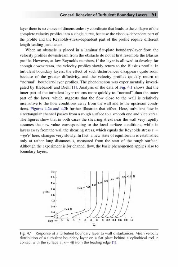
layer there is no choice of dimensionless y coordinate that leads to the collapse of the

complete velocity profiles into a single curve, because the viscous-dependent part of

the profile and the Reynolds-stress-dependent part of the profile require different

length-scaling parameters.

When an obstacle is placed in a laminar flat-plate boundary-layer flow, the

velocity profiles downstream from the obstacle do not at first resemble the Blasius

profile. However, at low Reynolds numbers, if the layer is allowed to develop far

enough downstream, the velocity profiles slowly return to the Blasius profile. In

turbulent boundary layers, the effect of such disturbances disappears quite soon,

because of the greater diffusivity, and the velocity profiles quickly return to

‘‘normal’’ boundary-layer profiles. The phenomenon was experimentally investi-

gated by Klebanoff and Diehl [1]. Analysis of the data of Fig. 4.1 shows that the

inner part of the turbulent layer returns more quickly to ‘‘normal’’ than the outer

part of the layer, which suggests that the flow close to the wall is relatively

insensitive to the flow conditions away from the wall and to the upstream condi-

tions. Figures 4.2a and 4.2b further illustrate that effect. Here, turbulent flow in

a rectangular channel passes from a rough surface to a smooth one and vice versa.

The figures show that in both cases the shearing stress near the wall very rapidly

assumes the new value corresponding to the local surface conditions, while in

layers away from the wall the shearing stress, which equals the Reynolds stress s ¼�9u0y0 here, changes very slowly. In fact, a new state of equilibrium is established

only at rather long distances x, measured from the start of the rough surface.

Although the experiment is for channel flow, the basic phenomenon applies also to

boundary layers.

Fig. 4.1 Response of a turbulent boundary layer to wall disturbances. Mean velocitydistribution of a turbulent boundary layer on a flat plate behind a cylindrical rod incontact with the surface at x¼ 4ft from the leading edge [1].

General Behavior of Turbulent Boundary Layers 91

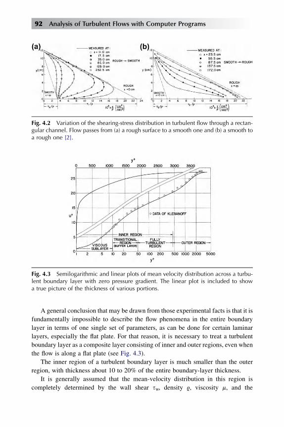
A general conclusion that may be drawn from those experimental facts is that it is

fundamentally impossible to describe the flow phenomena in the entire boundary

layer in terms of one single set of parameters, as can be done for certain laminar

layers, especially the flat plate. For that reason, it is necessary to treat a turbulent

boundary layer as a composite layer consisting of inner and outer regions, even when

the flow is along a flat plate (see Fig. 4.3).

The inner region of a turbulent boundary layer is much smaller than the outer

region, with thickness about 10 to 20% of the entire boundary-layer thickness.

It is generally assumed that the mean-velocity distribution in this region is

completely determined by the wall shear sw, density 9, viscosity m, and the

Fig. 4.2 Variation of the shearing-stress distribution in turbulent flow through a rectan-gular channel. Flow passes from (a) a rough surface to a smooth one and (b) a smooth toa rough one [2].

Fig. 4.3 Semilogarithmic and linear plots of mean velocity distribution across a turbu-lent boundary layer with zero pressure gradient. The linear plot is included to showa true picture of the thickness of various portions.


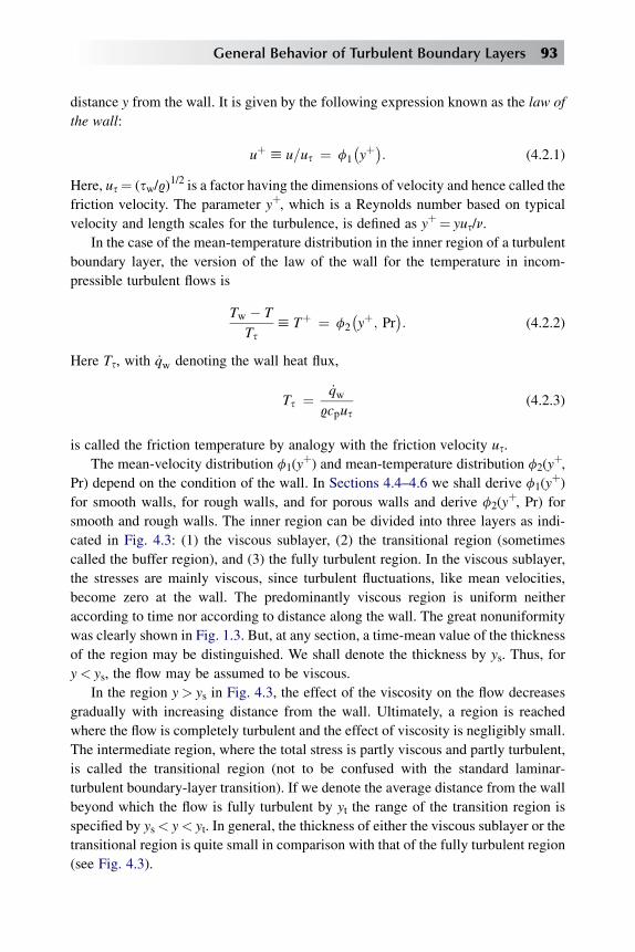
distance y from the wall. It is given by the following expression known as the law of

the wall:

uþ h u=us ¼ f1

�yþ�: (4.2.1)

Here, us¼ (sw/9)1/2 is a factor having the dimensions of velocity and hence called the

friction velocity. The parameter yþ, which is a Reynolds number based on typical

velocity and length scales for the turbulence, is defined as yþ¼ yus/n.

In the case of the mean-temperature distribution in the inner region of a turbulent

boundary layer, the version of the law of the wall for the temperature in incom-

pressible turbulent flows is

Tw � T

Tsh Tþ ¼ f2

�yþ; Pr

�: (4.2.2)

Here Ts, with _qw denoting the wall heat flux,

Ts ¼ _qw9cpus

(4.2.3)

is called the friction temperature by analogy with the friction velocity us.

The mean-velocity distribution f1(yþ) and mean-temperature distribution f2(y

þ,Pr) depend on the condition of the wall. In Sections 4.4–4.6 we shall derive f1(y

þ)for smooth walls, for rough walls, and for porous walls and derive f2(y

þ, Pr) forsmooth and rough walls. The inner region can be divided into three layers as indi-

cated in Fig. 4.3: (1) the viscous sublayer, (2) the transitional region (sometimes

called the buffer region), and (3) the fully turbulent region. In the viscous sublayer,

the stresses are mainly viscous, since turbulent fluctuations, like mean velocities,

become zero at the wall. The predominantly viscous region is uniform neither

according to time nor according to distance along the wall. The great nonuniformity

was clearly shown in Fig. 1.3. But, at any section, a time-mean value of the thickness

of the region may be distinguished. We shall denote the thickness by ys. Thus, for

y< ys, the flow may be assumed to be viscous.

In the region y> ys in Fig. 4.3, the effect of the viscosity on the flow decreases

gradually with increasing distance from the wall. Ultimately, a region is reached

where the flow is completely turbulent and the effect of viscosity is negligibly small.

The intermediate region, where the total stress is partly viscous and partly turbulent,

is called the transitional region (not to be confused with the standard laminar-

turbulent boundary-layer transition). If we denote the average distance from the wall

beyond which the flow is fully turbulent by yt the range of the transition region is

specified by ys< y< yt. In general, the thickness of either the viscous sublayer or the

transitional region is quite small in comparison with that of the fully turbulent region

(see Fig. 4.3).


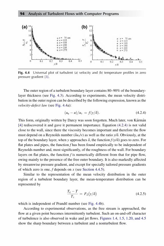
The outer region of a turbulent boundary layer contains 80–90% of the boundary-

layer thickness (see Fig. 4.3). According to experiments, the mean velocity distri-

bution in the outer region can be described by the following expression, known as the

velocity-defect law (see Fig. 4.4a):

ðue � uÞ=us ¼ f ðy=dÞ: (4.2.4)

This form, originally written by Darcy was soon forgotten. Much later, von Karman

[4] rediscovered it and gave it permanent importance. Equation (4.2.4) is not valid

close to the wall, since there the viscosity becomes important and therefore the flow

must depend on a Reynolds number (dus/v) as well as the ratio y/d. Obviously, at the

top of the boundary layer, when y approaches d, the function f (y/d) goes to zero. For

flat plates and pipes, the function f has been found empirically to be independent of

Reynolds number and, most significantly, of the roughness of the wall. For boundary

layers on flat plates, the function f is numerically different from that for pipe flow,

owing mainly to the presence of the free outer boundary. It is also markedly affected

by streamwise pressure gradient, and except for specially tailored pressure gradients

of which zero is one, f depends on x (see Section 4.4.5).

Similar to the representation of the mean velocity distribution in the outer

region of a turbulent boundary layer, the mean-temperature distribution can be

represented by

Te � T

Ts¼ F2

�y=d�

(4.2.5)

which is independent of Prandtl number (see Fig. 4.4b).

According to experimental observations, as the free stream is approached, the

flow at a given point becomes intermittently turbulent. Such an on-and-off character

of turbulence is also observed in wake and jet flows. Figures 1.4, 1.5, 1.20, and 4.5

show the sharp boundary between a turbulent and a nonturbulent flow.

Fig. 4.4 Universal plot of turbulent (a) velocity and (b) temperature profiles in zeropressure gradient [3].


Although the behavior of turbulent flow in the inner and the outer regions of the

layer is quite different, those regions are strongly coupled by the shear-stress profile

and the general diffusivity of the turbulence.

In order to see how the interference takes place, it is useful to study the transport

of energy in a turbulent boundary layer. That can be done by considering the

mean-kinetic-energy equation (3.4.3) and the turbulent-kinetic-energy equation

(3.5.6b). For a steady, two-dimensional, incompressible flow with zero pressure

gradient, they can be written as follows:

Mean-Kinetic-Energy Equation

uv

vx

�u2

2

�þ y

v

vy

�u2

2

�

¼ 1

9

v

vy

�u

�mvu

vy� 9u0y0

��þ u0y0

vu

vy;

(4.2.6)

Turbulent-Kinetic-Energy Equation

uv

vx

0@q2

2

1A þ y

v

vy

0@q2

2

1A

¼ �u0y0vu

vyþ n

v2

vy2

0@q2

2þ y02

1A � v

vy

0@y0q2

2þ py0

9

1A� ε:

(4.2.7)

Here, for simplicity we have again omitted the bars from the mean quantities. We

note that the mean-dissipation term m(vu/vy)2 does not appear in Eq. (4.2.6), since in

incompressible flows the term is small compared to the rest of the terms. Further-

more, except for the turbulence-dissipation term ε, the two viscosity terms (v/vy)

[um(vu/vy)] and v(v2/vy2) ½ðq2=2Þ þ y02� in Eqs. (4.2.6) and (4.2.7), respectively, are

small outside the sublayer and can therefore be neglected. Then for y> ds where ds is

the sublayer thickness, Eq. (4.2.6) reduces to

uv

vx

�u2

2

�þ y

v

vy

�u2

2

�� u0y0

vu

vyþ v

vy

�uu0y0

� ¼ 0; (4.2.8)

and Eq. (4.2.7) reduces to

uv

vx

0@q2

2

1Aþ y

v

vy

0@q2

2

1Aþ u0y0

vu

vyþ v

vy

24y0�q2

2þ p

9

�35þ ε ¼ 0: (4.2.9)

Figure 4.6a shows the distribution of the three terms of Eq. (4.2.8). The exper-

imental data are due to Klebanoff [5]. The figure shows that the loss of mean kinetic


energy is considerable, except in the region close to the wall, where turbulent energy

production is most intense. The kinetic energy lost by the mean flow in the outer

region is transferred by the working of the mean flow against the Reynolds stress to

the inner region, where it appears as energy of the turbulent motion.

Figure 4.6b shows the variation of the four terms of Eq. (4.2.9), in dimensionless

quantities, as calculated from the measurements of Klebanoff [5]. It is seen from the

experimental plots that, in the inner region close to the wall, the dominant terms in

Eq. (4.2.9) are the one that corresponds to the production of kinetic energy due to

turbulence through action of the Reynolds stresses ðdu0y0=u3sÞ (vu/vy) and the one

Fig. 4.5 Sketch of the turbulent boundary layer. At times the uncontaminated potentialflow may extend far into the boundary layer, as shown [5].

Fig. 4.6 (a) Balance of the kinetic energy of the mean flow in the boundary layer inzero pressure gradient according to Eq. (4.2.8), from the experimental data of Klebanoff[5]. (b) Balance of turbulent energy in the boundary layer according to Eq. (4.2.9), fromthe experimental data of Klebanoff [5]. The left-hand ordinate denotes the scale for theinner region of the boundary layer, the right-hand ordinate denotes that for the outerregion.


that corresponds to the dissipation of energy due to viscosity, εd=u3s . The contribu-

tions for the total energy balance are nearly equal and opposite. In addition, it may be

observed that, in general, throughout the boundary layer the absolute values of these

two terms are greater than the values of other contributions, except near the edge.

Consequently it is apparent that, within the inner region of the boundary layer, the

energy-exchange processes are in a state of near equilibrium, with the result that the

local production of energy and the local dissipation of energy are almost compen-

sating. For that reason, the flow in the inner region is governed essentially by the

local conditions.

In the outer region of the boundary layer, however, the dominant terms are those

due to convection and those due to dissipation – both of which have the same sign –

and the balancing contribution for the diffusion term. In that region, the turbulent-

flow phenomena depend not only on the local conditions but also on the whole

history of events in the flow upstream of the point in question.

Figure 4.7 shows the variation of dimensionless turbulent kinetic energy kþ

ðh k=u2sÞ with yþ according to the data compiled by Coles [6] and the data of El

Telbany and Reynolds [7] as reported in [8]. In spite of the larger scatter, we see that

kþ becomes maximum around yþ¼ 15 which corresponds to the location of the

maximum production of k [9]. A representative peak value for kþ is 4.5. In the

interval 60< yþ< 150, kþ becomes nearly constant with a value of 3.3. Since in

the log law region of a flat-plate boundary layer, the shear stress �u0y0fu2s , the data

suggest a value of around 0.30 for the ratio �u0y0=k.The variation of k in the immediate vicinity of the wall can be deduced from the

continuity equation and the no-slip condition. Following [10], the variation of u0, y0

and w0 with distance from the wall can be written in the form

u0 ¼ a1yþ b1y2 þ/ (4.2.10a)

Fig. 4.7 Near-wall variation of kþ with yþ. The equation is Eq. (4.2.11) with Aþ¼ 0.05.


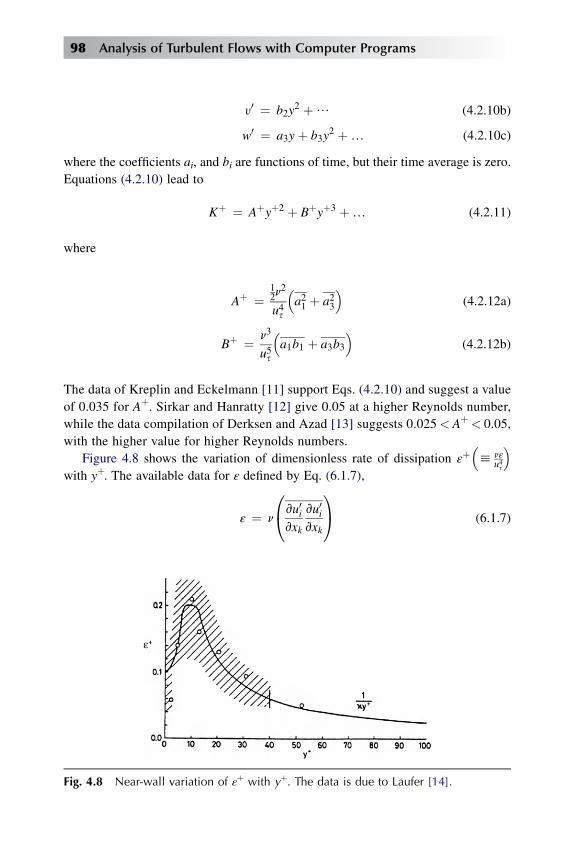
y0 ¼ b2y2 þ/ (4.2.10b)

w0 ¼ a3yþ b3y2 þ. (4.2.10c)

where the coefficients ai, and bi are functions of time, but their time average is zero.

Equations (4.2.10) lead to

Kþ ¼ Aþyþ2 þ Bþyþ3 þ. (4.2.11)

where

Aþ ¼12n

2

u4s

�a21 þ a23

(4.2.12a)

Bþ ¼ n3

u5s

�a1b1 þ a3b3

(4.2.12b)

The data of Kreplin and Eckelmann [11] support Eqs. (4.2.10) and suggest a value

of 0.035 for Aþ. Sirkar and Hanratty [12] give 0.05 at a higher Reynolds number,

while the data compilation of Derksen and Azad [13] suggests 0.025< Aþ< 0.05,

with the higher value for higher Reynolds numbers.

Figure 4.8 shows the variation of dimensionless rate of dissipation εþ�h nε

u4s

with yþ. The available data for ε defined by Eq. (6.1.7),

ε ¼ n

0@vu0ivxk

vu0ivxk

1A (6.1.7)

Fig. 4.8 Near-wall variation of εþ with yþ. The data is due to Laufer [14].


are quite limited and are subject to a large measurement uncertainty, especially in

the region 0< yþ< 40. Very close to the wall, the variation of εþ can be approxi-

mated by

εþ ¼ 2

�Aþ þ 2Bþyþ þ/

�(4.2.13)

indicating a finite εþ at the wall value equal to 2Aþ. Experimental values of Aþ

quoted earlier then indicate 0.05< εþw < 0.10, with a preference for the higher value

at larger Reynolds numbers. If Bþ¼ 0 is assumed, Eq. (4.2.13) indicates

yþ ¼ 0;vεþ

vy¼ 0 (4.2.14)

which can be used as a boundary condition for ε as will be discussed in Chapter 6.

4.3 Eddy-Viscosity, Mixing-Length, Eddy-Conductivityand Turbulent Prandtl Number Concepts

In order to predict the mean-velocity distribution or the mean-temperature distri-

bution across a turbulent boundary layer, it is necessary to make an assumption for

or find a model for the Reynolds stresses. Over the years, several empirical

hypotheses have been used. Eddy-viscosity and mixing-length concepts are among

the more popular and extensively used concepts. All these concepts relate the

Reynolds stress to the local mean-velocity gradient, as will be shown in this section

and later more extensively in Chapters 5 and 6. The main objection to the eddy-

viscosity and mixing-length concepts is that they lack generality – they are based

on local equilibrium ideas that assume the transport terms in the governing equa-

tions to be small. A more general approach, which will be discussed in Chapter 6, is

to use ideas that consider the rate of change of the Reynolds stress in the governing

equations. The prediction methods that use these ideas are referred to as transport-

equation methods. They reduce to the methods that use eddy-viscosity or mixing-

length ideas when the transport terms are small. For a detailed discussion, see

Chapters 6 and 9.

Boussinesq [15] was the first to attack the problem of finding a model for the

Reynolds shear stress by introducing the concept of eddy viscosity. He assumed that

the turbulent stresses act like the viscosity stresses, which implies that the turbulent

stresses are proportional to the velocity gradient. The coefficient of proportionality

was called the ‘‘eddy viscosity’’ and was defined by

�9u0y0 ¼ 9εm�vu=vy

�: (4.3.1)


Here, εm like the kinematic viscosity v, is assumed to be the product of a velocity and

a length, that is,

εmwlength� velocity: (4.3.2)

The mixing-length concept was first proposed by Prandtl [16]. According to this

concept the Reynolds shear stress is to be calculated from

�9u0y0 ¼ 9l2vuvy vu

vy: (4.3.3)

The basis of Prandtl’s mixing length hypothesis is an analogy with the kinetic theory

of gases, based on the assumption that turbulent eddies, like gas molecules, are

discrete entities that collide and exchange momentum at discrete intervals.

By Eq. (4.3.1) we can write a relationship between eddy viscosity and mixing

length:

εm ¼ l2vuvy: (4.3.4)

The length l defined by Eq. (4.3.3) is, of course, a quantity whose value is yet to be

found. According to von Karman’s hypothesis [4], l is given by

l ¼ k

vu=vyv2u=vy2

(4.3.5)

where k is an empirical constant known as von Karman’s constant.

Equations (4.3.1) and (4.3.3) merely represent the definitions of εm and l: the

assumption is that they will vary more slowly or simply than the shear stress and

therefore be easier to correlate empirically. The use of eddy viscosity to predict the

complete Reynolds-stress tensor is discussed later. When the characteristic length

scale is readily identified and defined, for example in a jet or wall boundary layer

with a moderate pressure gradient, the simplicity of the mixing-length or eddy-

viscosity approach is commendable and, since it can readily be specified in algebraic

form, the equations for continuity and momentum can be written with the same

number of unknowns as equations. In more complex, or rapidly-changing flows, the

algebraic correlations are inadequate. One alternative is to use the transport equation

for l or εm. In the so-called ‘‘one-equation’’ models, εm is expressed as

εm ¼ Cmk1=2l (4.3.6)

where l is a length scale, still related to the shear layer thickness, and k is the

turbulent kinetic energy for which a modeled partial-differential ‘‘transport’’


equation is solved. A more general and more popular approach requires a transport

equation for l, often in the form of the rate of turbulence dissipation

ε ¼ k3=2

l: (4.3.7)

The solution of an equation for ε, together with a transport equation for k and the

eddy-viscosity expression, Eq. (4.3.6), forms the basis of the ubiquitous two-

equation models suggested by, for example, Jones and Launder [17] as we shall

discuss in Chapter 6. Note that this procedure simply serves to define

cmh�u0y0vuvy

ε

k2: (4.3.8)

However, the k-εmodel is sufficiently realistic that cm¼ constantx 0.09 gives good

predictions in many flows as we shall see in Chapter 9.

Analogous quantities can be defined for turbulent heat-transfer rates. Again using

Boussinesq’s eddy conductivity concept, we can write the transport of heat due to the

product of time mean of fluctuating enthalpy h0 and fluctuating velocity y0 in the form

�9y0h0 ¼ 9εhvh

vy(4.3.9a)

or for a perfect gas

�9cpT 0y0 ¼ 9cpεhvT

vy: (4.3.9b)

Note that a minus sign still appears; in heat transfer, as in momentum transfer, we

expect transport down the gradient of the quantity in question. The eddy conductivity

has the same dimensions as the eddy viscosity, namely, velocity� length.

Sometimes it has been found to be convenient to introduce a ‘‘turbulent’’ Prandtl

number Prt defined by

Prt hεm

εh¼

u0y0=vuvy

T 0y0=vTvy

: (4.3.10)

Each of the relations given by Eqs (4.3.1), (4.3.3) and (4.3.9) requires some

empirical values if it is to be used for quantitative calculations. In other words, it is

necessary to make assumptions for the distribution of eddy viscosity and conduc-

tivity. We shall postpone the discussion on the distribution of eddy conductivity to

Chapter 5 and here concentrate on the distributions of eddy-viscosity and mixing-

length.


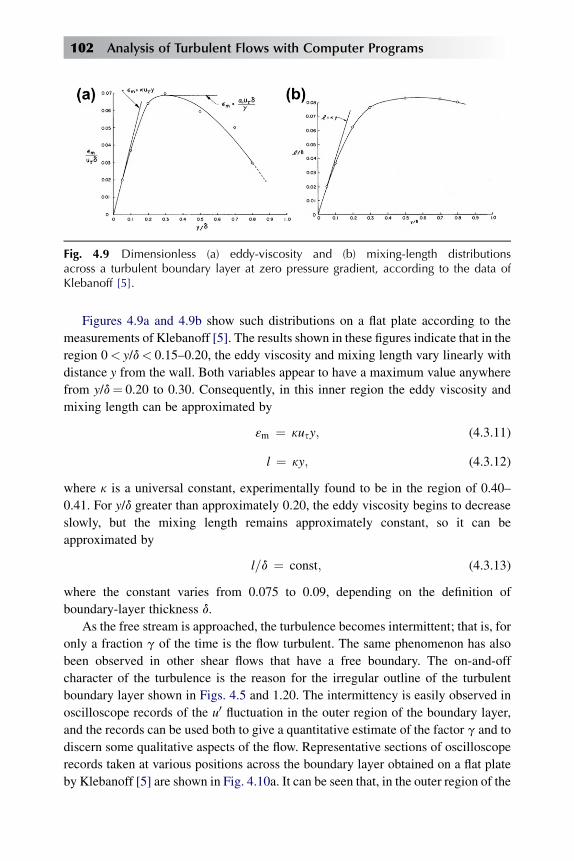
Figures 4.9a and 4.9b show such distributions on a flat plate according to the

measurements of Klebanoff [5]. The results shown in these figures indicate that in the

region 0< y/d< 0.15–0.20, the eddy viscosity and mixing length vary linearly with

distance y from the wall. Both variables appear to have a maximum value anywhere

from y/d¼ 0.20 to 0.30. Consequently, in this inner region the eddy viscosity and

mixing length can be approximated by

εm ¼ kusy; (4.3.11)

l ¼ ky; (4.3.12)

where k is a universal constant, experimentally found to be in the region of 0.40–

0.41. For y/d greater than approximately 0.20, the eddy viscosity begins to decrease

slowly, but the mixing length remains approximately constant, so it can be

approximated by

l=d ¼ const; (4.3.13)

where the constant varies from 0.075 to 0.09, depending on the definition of

boundary-layer thickness d.

As the free stream is approached, the turbulence becomes intermittent; that is, for

only a fraction g of the time is the flow turbulent. The same phenomenon has also

been observed in other shear flows that have a free boundary. The on-and-off

character of the turbulence is the reason for the irregular outline of the turbulent

boundary layer shown in Figs. 4.5 and 1.20. The intermittency is easily observed in

oscilloscope records of the u0 fluctuation in the outer region of the boundary layer,

and the records can be used both to give a quantitative estimate of the factor g and to

discern some qualitative aspects of the flow. Representative sections of oscilloscope

records taken at various positions across the boundary layer obtained on a flat plate

by Klebanoff [5] are shown in Fig. 4.10a. It can be seen that, in the outer region of the

Fig. 4.9 Dimensionless (a) eddy-viscosity and (b) mixing-length distributionsacross a turbulent boundary layer at zero pressure gradient, according to the data ofKlebanoff [5].


layer, y/d> 0.4, there are intervals of time when the flow is not turbulent and that

these intervals become longer with increasing distance from the wall. Thus, the outer

region is divided into a turbulent part and a relatively nonturbulent free-stream part,

and the hot wire at a given position responds to alternate turbulent and nonturbulent

flow as the pattern is swept downstream.

Intermittency factors have been obtained by Klebanoff [5] and by Corrsin and

Kistler [18]. Figure 4.10b shows the distribution of intermittency factor g according

to Klebanoff’s measurements for a flat-plate flow. It can be fitted approximately by

the expression (see Section 1.7)

g ¼ 1

2

�1� erf 5

��y=d�� 0:78

�: (4.3.14)

If the distribution of eddy viscosity is corrected for the effect of intermittency, the

dimensionless eddy viscosity εm/usd becomes nearly constant across the main outer

part, as is shown in Fig. 4.9a. It can be approximated by

εm ¼ a1usd; (4.3.15a)

where a1 is an experimental constant between 0.06 and 0.075.

It should be pointed out that the length and the velocity scales used to normalize

the eddy viscosity in Fig. 4.9a are not the only possible characteristic scales. Other

length and velocity scales such as d* and ue, respectively, can also be used. Equation

(4.3.15a) then can also be written in the form

εm ¼ aued*; (4.3.15b)

where a is a constant between 0.016 and 0.02. For equilibrium boundary layers (see

Section 4.4.5), the two expressions for εm can be shown to be the same.

Fig. 4.10 (a) Instantaneous velocity u in a boundary layer, ue¼ 50 ft/sec, timing dots60/sec and (b) intermittency distribution across a turbulent boundary layer. Data repre-sent three different techniques of measurement.


In Fig. 4.11 we show the mixing-length distribution in pipe flow according to the

measurements of Nikuradse [19]. From those distributions we see that although at

low Reynolds number the mixing-length distribution across the pipes varies, at high

Reynolds numbers it does not. For high Reynolds numbers, the mixing-length

distribution can be expressed with good approximation by the following equation:

l=r0 ¼ 0:14� 0:08½1� ðy=r0Þ�2�0:06½1� ðy=r0Þ�4; (4.3.16a)

where y denotes the distance from the wall and r0 the radius of the pipe. Developing l

as a series gives

l ¼ 0:4y� 0:44�y2=r0

�þ.: (4.3.16b)

Figure 4.12 shows the eddy-viscosity distribution in pipe flow according to the

measurements of Laufer [14] and Nunner [20]. The experimental data indicate that

for the core region of the pipe flow the distribution of the eddy viscosity resembles,

both qualitatively and quantitatively, the corresponding distribution for the fully

turbulent portions of the outer region of the boundary-layer flow. The eddy viscosity

first increases linearly with y/r0, then reaches a maximum at about y/r0¼ 0.3, and

finally decreases slightly, becoming nearly constant at y/r0¼ 0.5.

4.4 Mean-Velocity and Temperature Distributionsin Incompressible Flows on Smooth Surfaces

The momentum equation for a two-dimensional, incompressible, turbulent boundary

layer with zero pressure gradient can be written as [see Eq. (3.3.10)]

Fig. 4.11 Mixing-length distribution in a tube for (a) moderate Reynolds numbers and(b) high Reynolds numbers, Rd> 105� 103 according to the measurements of Nikur-adse [19].


uvu

vxþ y

vu

vy¼ 1

9

vsvy

; (4.4.1)

where s is the total shear stress,

s ¼ sl þ st ¼ mvu

vy� 9u0y0: (4.4.2)

For a nonporous surface, (vs/vy)w¼ 0, since u and y are zero at the wall. Further-

more, by using the equation of continuity and the no-slip condition uw¼ 0, and by

differentiating Eq. (4.4.1) with respect to y, it can be shown that (v2s/vy2)w¼ 0.

Hence for some small distance from the wall we can write

vs=vyz 0: (4.4.3)

That equation shows that the total shear stress s is constant. Experiments support that

relationship. Figure 4.13a shows the distribution of dimensionless Reynolds shear-

stress term, 2st=9u2e ¼ �2u0y0=u2e, across the boundary layer for a flat-plate flow, as

measured by Klebanoff [5]. From a point very close to the wall to y/d¼ 0.1–0.2, the

turbulent shear stress is approximately constant. As the wall is approached, the

turbulent shear stress goes to zero, as shown by the experimental data of Schubauer

[21] in Fig. 4.13b. In the region where turbulent shear stress begins to decrease,

however, the laminar shear stress begins to increase in such a way that the total shear-

stress distribution is still constant in the region 0 � y< 0.1–0.2, which is as it should

Fig. 4.12 Eddy-viscosity distribution in pipe flow according to the measurements ofLaufer [14] (B) and Nunner [20] (,).


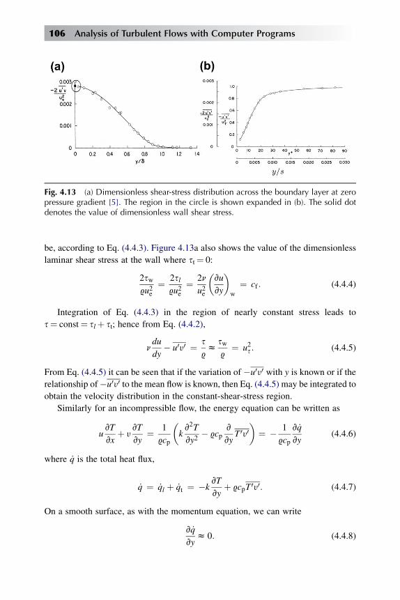
be, according to Eq. (4.4.3). Figure 4.13a also shows the value of the dimensionless

laminar shear stress at the wall where st¼ 0:

2sw9u2e

¼ 2sl9u2e

¼ 2n

u2e

�vu

vy

�w

¼ cf : (4.4.4)

Integration of Eq. (4.4.3) in the region of nearly constant stress leads to

s¼ const¼ slþ st; hence from Eq. (4.4.2),

ndu

dy� u0y0 ¼ s

9z

sw9

¼ u2s : (4.4.5)

From Eq. (4.4.5) it can be seen that if the variation of �u0y0 with y is known or if therelationship of�u0y0 to the mean flow is known, then Eq. (4.4.5) may be integrated to

obtain the velocity distribution in the constant-shear-stress region.

Similarly for an incompressible flow, the energy equation can be written as

uvT

vxþ y

vT

vy¼ 1

9cp

�kv2T

vy2� 9cp

v

vyT 0y0

�¼ � 1

9cp

v _q

vy(4.4.6)

where _q is the total heat flux,

_q ¼ _ql þ _qt ¼ �kvT

vyþ 9cpT 0y0: (4.4.7)

On a smooth surface, as with the momentum equation, we can write

v _q

vyz 0: (4.4.8)

Fig. 4.13 (a) Dimensionless shear-stress distribution across the boundary layer at zeropressure gradient [5]. The region in the circle is shown expanded in (b). The solid dotdenotes the value of dimensionless wall shear stress.


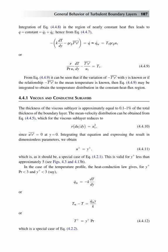
Integration of Eq. (4.4.8) in the region of nearly constant heat flux leads to

q¼ constant¼ _ql þ _qt; hence from Eq. (4.4.7),

��kdT

dy� 9cpT 0y0

�¼ _qz _qw ¼ Ts9cpus

or

n

Pr us

dT

dy� T 0y0

us¼ Ts: (4.4.9)

From Eq. (4.4.9) it can be seen that if the variation of �T 0y0 with y is known or ifthe relationship �T 0y0 to the mean temperature is known, then Eq. (4.4.9) may be

integrated to obtain the temperature distribution in the constant-heat-flux region.

4.4.1 VISCOUS AND CONDUCTIVE SUBLAYERS

The thickness of the viscous sublayer is approximately equal to 0.1–1% of the total

thickness of the boundary layer. The mean-velocity distribution can be obtained from

Eq. (4.4.5), which for the viscous sublayer reduces to

n�du=dy

� ¼ u2s ; (4.4.10)

since u0y0 ¼ 0 at y¼ 0. Integrating that equation and expressing the result in

dimensionless parameters, we obtain

uþ ¼ yþ; (4.4.11)

which is, as it should be, a special case of Eq. (4.2.1). This is valid for yþ less than

approximately 5 (see Figs. 4.3 and 4.13b).

In the case of the temperature profile, the heat-conduction law gives, for yþ

Pr< 3 and yþ< 3 (say),

_qw ¼ �kdT

dy

or

Tw � T ¼ _qwy

k

or

Tþ ¼ yþ Pr (4.4.12)

which is a special case of Eq. (4.2.2).


4.4.2 FULLY TURBULENT PART OF THE INNER REGION

In the part of the inner region where the flow is fully turbulent, the laminar shear

stress sl is small compared to st and can be neglected. According to Fig. 4.13b, that

assumption applies approximately when yþ> 50. Consequently, in the fully turbu-

lent part of the inner region, Eq. (4.4.5) reduces to

st=9 ¼ �u0y0 ¼ u2s : (4.4.13)

Substituting the expression (4.3.1) into Eq. (4.4.13) and using the eddy-viscosity

relation (4.3.11), we get

kusy�du=dy

� ¼ u2s : (4.4.14)

Integration yields

uþ ¼ �1=k�ln yþ þ c; (4.4.15)

where c is a constant whose value is between 4.9 and 5.5. Equation (4.4.15), called

the logarithmic law for velocity, can also be derived by substituting the mixing-

length formula (4.3.10), with l given by Eq. (4.3.12), in Eq. (4.4.13) and integrating

the resulting expression.

Equation (4.4.15) can also be derived from Eq. (4.2.1) without using the mixing-

length concept. From Eq. (4.2.1) we can write

du

dy¼ u2s

n

df1

dyþ:

Since the right-hand side must be independent of the viscosity, it follows that

df1

dyþ¼ 1

kyþor

du

dy¼ us

ky:

Integration of this expression gives Eq. (4.4.15).

An expression similar to Eq. (4.4.15) can also be derived for the temperature

profile by using the eddy conductivity relations discussed in Section 4.3. It can also

be obtained from Eq. (4.2.2) by writing it as

d

dy

�Tw � T

� ¼ Tsusn

df2

dyþ

or as

d

dy

�Tw � T

� ¼ Tskhy

: (4.4.16)


Here kh is an absolute constant around 0.44. Integration of Eq. (4.4.16) gives

Tw � T

Ts¼ 1

khln

usy

nþ ch

or

Tþ ¼ 1

khln yþ þ ch (4.4.17)

where ch is a function of Pr.

4.4.3 INNER REGION

In the transition region (buffer layer) both components of the total shear stress,

namely, sl and st, are important. Prandtl’s mixing-length theory and Boussinesq’s

eddy-viscosity concept in their original form apply to fully turbulent flows. The flow

in the buffer layer is in a state of transition. As the laminar sublayer is approached

from above, the magnitude of the velocity fluctuations u0, y0 and, consequently, thatof the turbulent shear stress, �9u0y0, approaches zero. As the region of fully

turbulent flow is approached from below, the magnitude of the velocity

fluctuations approaches the levels of the velocity fluctuations in the fully turbulent

flow. So far, various assumptions have been made for the turbulent shear-stress term

in Eq. (4.4.5) in order to describe the mean-velocity distribution there. Of the many

proposed, one has enjoyed a remarkable success. It is the expression proposed by

Van Driest [22], who assumed the following modified expression for Prandtl’s

mixing-length theory:

l ¼ ky½1� expð�y=AÞ�; (4.4.18)

where A is a damping-length constant defined as 26v(sw/9)–1/2. In the form given by

Eq. (4.4.18), A is limited to incompressible turbulent boundary layers with negligible

pressure gradient and zero mass transfer. In Chapter 5 we shall discuss its extension

to turbulent boundary layers with pressure gradient and with heat and mass transfer.

If we now use Prandtl’s mixing-length formula (4.3.5), together with the mixing-

length expression given by Eq. (4.4.18), we can write Eq. (4.4.5) as

n�du=dy

�þ ðkyÞ2½1� expð� y=AÞ�2 ðdu=dyÞ2¼ u2s :

In terms of dimensionless quantities, that equation can be written as

a�yþ� �

duþ=dyþ�2þb

�duþ=dyþ

�� 1 ¼ 0


or

duþ

dyþ¼ �bþ �b2 þ 4a

�1=22a

;

where a(yþ)¼ (kyþ)2 [1 – exp(–yþ/Aþ)]2, Aþ ¼ 26, and b¼ 1. Multiplying both

numerator and denominator of the duþ/dyþ expression by [bþ(b2þ 4a)1/2] and

formally integrating the resulting expression, we obtain

uþ ¼Z yþ

0

2

bþ ½b2 þ 4aðyþÞ�1=2dyþ; (4.4.19)

since uþ ¼ 0 at yþ¼ 0.

Equation (4.4.19) defines a continuous velocity distribution in the inner region of

the turbulent boundary layer and applies to the viscous sublayer, to the transition

region, and to the region of fully turbulent flow. For example, in the viscous sublayer,

a¼ 0. Then Eq. (4.4.19) reduces to the viscous-sublayer expression given by Eq.

(4.4.11). In the fully turbulent region, b¼ 0 and a¼ (kyþ)2, and Eq. (4.4.19) reducesto Eq. (4.4.15), with c¼ 5.24.

Figure 4.14 shows that the mean velocity distribution calculated by Eq. (4.4.19)

agrees quite well with the experimental data of Laufer [14] (,) and with the flat-

plate data of Klebanoff [5] (B) and of Wieghardt [23] (6).

Equation (4.4.17), like Eq. (4.4.15) can also be extended to include the

(conductive) sublayer by using a procedure similar to that used for the velocity

Fig. 4.14 Mean-velocity distribution in the inner region as calculated by Eq. (4.4.19).


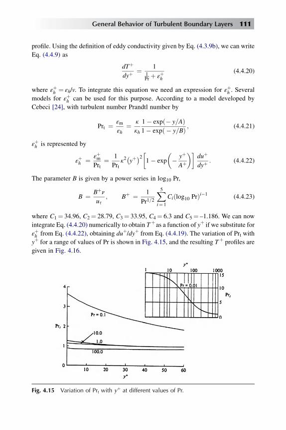
profile. Using the definition of eddy conductivity given by Eq. (4.3.9b), we can write

Eq. (4.4.9) as

dTþ

dyþ¼ 1

1Pr þ ε

þh

(4.4.20)

where εþh ¼ εh/v. To integrate this equation we need an expression for εþh . Several

models for εþh can be used for this purpose. According to a model developed by

Cebeci [24], with turbulent number Prandtl number by

Prt ¼ εm

εh¼ k

kh

1� expð� y=AÞ1� expð � y=BÞ ; (4.4.21)

εþh is represented by

εþh ¼ ε

þm

Prt¼ 1

Prtk2�yþ�2�

1� exp

�� yþ

Aþ

��duþ

dyþ: (4.4.22)

The parameter B is given by a power series in log10 Pr,

B ¼ Bþnus

; Bþ ¼ 1

Pr1=2

X5i¼ 1

Ciðlog10 PrÞi�1 (4.4.23)

where C1¼ 34.96, C2¼ 28.79, C3¼ 33.95, C4¼ 6.3 and C5¼ –1.186. We can now

integrate Eq. (4.4.20) numerically to obtain Tþas a function of yþ if we substitute for

εþh from Eq. (4.4.22), obtaining duþ/dyþ from Eq. (4.4.19). The variation of Prt with

yþ for a range of values of Pr is shown in Fig. 4.15, and the resulting Tþ profiles are

given in Fig. 4.16.

Fig. 4.15 Variation of Prt with yþ at different values of Pr.


4.4.4 OUTER REGION

In obtaining the relation leading to Eq. (4.4.19), we have approximated the

momentum equation (4.4.1) by Eq. (4.4.3), by making the assumption that u and y

are small close to the wall. In other words, we have neglected the convective term in

Eq. (4.4.1). According to experiments, the assumption is good only close to the wall,

within approximately 20% of the boundary-layer thickness for zero-pressure-

gradient flows. Since the convective term is of the same order of magnitude as the

shear-stress gradient term at a greater distance from the wall, the left-hand side of the

momentum equation must be accounted for.

In the outer region, sl is quite small compared to st, and can be neglected. Then

the momentum equation (4.4.1) becomes

uvu

vxþ y

vu

vy¼ 1

9

vstvy

; y0 � y � d: (4.4.24)

where st ¼ �9u0y0 and y0 is at some distance from the wall. We see from Eq. (4.4.24)

that the momentum equation for the outer region of a turbulent boundary layer has

the same form as the momentum equation for a laminar boundary layer. The

resemblance between the two equations can be better illustrated by using the eddy-

viscosity concept.

We first assume an eddy viscosity εm independent of y in the outer region and call

it ε0. Substituting the eddy viscosity defined by Eq. (4.3.1) into Eq. (4.4.24), we get

uvu

vxþ y

vu

vy¼ v

vy

�ε0vu

vy

�¼ ε0

v2u

vy2: (4.4.25)

Fig. 4.16 Mean-temperature distribution across the layer as a function of Pr.


Equation (4.4.25) is identical to the laminar boundary-layer equation if we replace

the kinematic eddy viscosity ε0 by the kinematic molecular viscosity n. The fact that

the momentum equation for the outer region of a turbulent layer is similar to that for

a laminar layer enables one to extract valuable information about the behavior of the

mean velocity distribution of the turbulent layer from the known behavior of the

laminar layer. If proper scaling variables are chosen, a close similarity between

laminar and turbulent velocity profiles in the outer region can be shown to exist, as

demonstrated by Clauser [25].

To illustrate, let us introduce the transformation

z ¼ yðue=ε0xÞ1=2; (4.4.26)

together with the definition of stream function j(x, y) and the dimensionless stream

function F(zhj(x, y) (ε0ue x)1/2 into Eq. (4.4.25). That gives the well-known

Blasius equation for laminar flows, namely,

F000 þ 1

2FF00 ¼ 0; (4.4.27)

where the primes on F denote differentiation with respect to z. Equation (4.4.27) is

subject to the following boundary conditions:

Fð0Þ ¼ 0; F0ð0Þ ¼ const; limz/0

F0ðzÞ ¼ 1: (4.4.28)

We note that in Eq. (4.4.26) the usual kinematic molecular viscosity n is replaced by

the kinematic eddy viscosity ε0, which is assumed to be constant.

Figure 4.17a shows the solutions of Eq. (4.4.27) for various values of F0(0) asobtained by Clauser [25]. In that form of presentation, the velocity profiles do not

Fig. 4.17 (a) Solutions of the Blasius equation for various slip velocities and (b) replotof the solutions of the Blasius equation given in (a) in terms of new coordinates.


collapse into a single ‘‘universal’’ curve. However, if the solutions are to be used in

describing the mean-velocity distribution in the outer region of a turbulent boun-

dary layer, they must collapse into a universal (or nearly universal) curve, as was

shown by the discussion in Section 4.2, where the velocity profiles for turbulent layers

were seen to collapse into a universal curve when they were plotted as (ue – u)/usversus y/d.

To put the ‘‘laminar’’ solutions in the universal form, we use (ue – u)/ue and y/d as

variables and divide them by factors that will bring the curves of Fig. 4.17a into

coincidence. The factor for y/d is elected to make the areas above the curves equal.

Two choices are available for the factor for (ue – u)/ue. Here we discuss only one. See

Clauser [25] for a further discussion. By choosing the variables

ue � u

ue

h�d*=ue

� ðdu=dyÞwi1=2and y

�1

ued*

�du

dy

�w

�1=2; (4.4.29)

the ‘‘laminar’’ curves of Fig. 4.17a can almost be reduced to one universal curve.

Recalling the definition of d* and using the transformation in Eq. (4.4.26) and the

fact that F 0(z)¼ u/ue, we can write Eq. (4.4.29) as

1� F0ðzÞnF00ð0Þ½zðNÞ � FðNÞ�

o1=2 and z

�F00ð0Þ

zðNÞ � FðNÞ�1=2

: (4.4.30)

The ‘‘laminar’’ curves replotted in the new coordinate system are shown in

Fig. 4.17b.

We shall now compare the experimental velocity profiles for turbulent boundary

layers (zero pressure gradient) with the ‘‘laminar’’ curves of Fig. 4.17a. The

experimental data considered are due to Smith and Walker [26]. Here, from the

experiment we know the velocity profile u/ue, the displacement thickness d*, and the

local skin-friction coefficient cf defined as

cf ¼ 2sw=9u2e ¼ 2u2s=u

2e :

Since we are interested only in the outer region, we see from Eq. (4.4.25) that

ðdu=dyÞw ¼ ðst=9Þw�1=ε0

� ¼ u2s=ε0; (4.4.31)

which with the definition of cf can be written as

ðdu=dyÞw ¼ �cf=2

� �u2e=ε0

�:


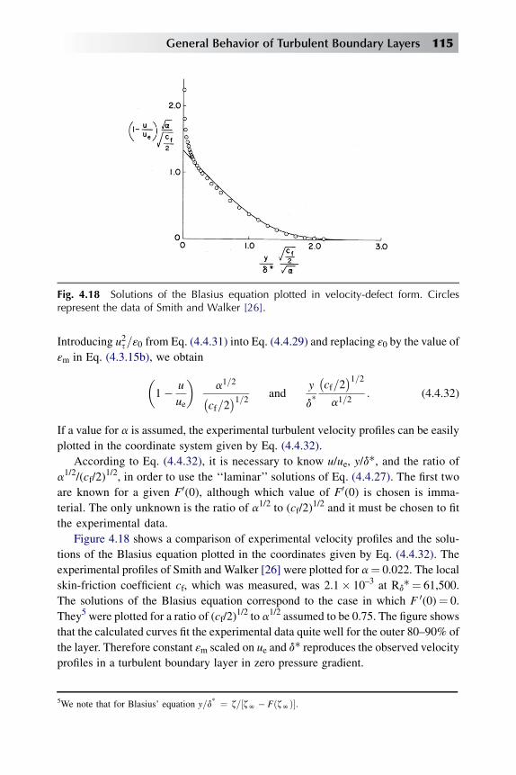
Introducing u2s=ε0 from Eq. (4.4.31) into Eq. (4.4.29) and replacing ε0 by the value of

εm in Eq. (4.3.15b), we obtain

�1� u

ue

�a1=2�

cf=2�1=2 and

y

d*

�cf=2

�1=2a1=2

: (4.4.32)

If a value for a is assumed, the experimental turbulent velocity profiles can be easily

plotted in the coordinate system given by Eq. (4.4.32).

According to Eq. (4.4.32), it is necessary to know u/ue, y/d*, and the ratio of

a1/2/(cf/2)1/2, in order to use the ‘‘laminar’’ solutions of Eq. (4.4.27). The first two

are known for a given F0(0), although which value of F0(0) is chosen is imma-

terial. The only unknown is the ratio of a1/2 to (cf/2)1/2 and it must be chosen to fit

the experimental data.

Figure 4.18 shows a comparison of experimental velocity profiles and the solu-

tions of the Blasius equation plotted in the coordinates given by Eq. (4.4.32). The

experimental profiles of Smith and Walker [26] were plotted for a¼ 0.022. The local

skin-friction coefficient cf, which was measured, was 2.1� 10–3 at Rd*¼ 61,500.

The solutions of the Blasius equation correspond to the case in which F 0(0)¼ 0.

They5 were plotted for a ratio of (cf/2)1/2 to a1/2 assumed to be 0.75. The figure shows

that the calculated curves fit the experimental data quite well for the outer 80–90% of

the layer. Therefore constant εm scaled on ue and d* reproduces the observed velocity

profiles in a turbulent boundary layer in zero pressure gradient.

Fig. 4.18 Solutions of the Blasius equation plotted in velocity-defect form. Circlesrepresent the data of Smith and Walker [26].

5We note that for Blasius’ equation y=d* ¼ z=½zN � FðzNÞ�:


4.4.5 EQUILIBRIUM BOUNDARY LAYERS

Equilibrium boundary layers constitute a class of boundary layers in which the

mainstream velocity distribution is characterized by a constant value of the

parameter

b ¼ �d*=sw

� �dp=dx

�; (4.4.33)

which represents the ratio of pressure forces to shear forces in a section of the

boundary layer. These flows, which are called equilibrium or self-preserving flows,

were first obtained experimentally by Clauser [27] for two adverse-pressure-gradient

flows, both analogous to the Falkner-Skan flows in laminar layers. A zero-pressure-

gradient flow is a special case of an equilibrium boundary layer. In Clauser’s equi-

librium-flow experiments, long sections of two-dimensional turbulent boundary

layers were subjected to various adverse pressure gradients, and by trial and error the

pressure distributions were adjusted to give similar boundary-layer profiles when

plotted on the basis of the velocity-defect laws. For example, at first a trial pressure

distribution was adopted, and the velocity profiles at a number of x stations were

measured and from them the skin-friction coefficients determined. When the results

were plotted in terms of velocity-defect coordinates, that is, (ue – u)/us versus y/d, the

profiles were not similar. Thus it was necessary to alter the pressure distribution

a number of times before similar profiles were obtained. When a pressure distribu-

tion was obtained for which the profiles were similar at all stations, it was found that

the function f in the defect law, Eq. (4.2.4), was different from that for zero-pressure-

gradient flow and was also different for each separate pressure distribution. However,

the function f was the same for an arbitrary number of stations for one pressure

distribution. Furthermore, it was observed that for each pressure distribution or for

each equilibrium flow the parameter b remained approximately constant. From these

experiments, Clauser determined that the outer part of an equilibrium boundary layer

can be analyzed by assuming an eddy viscosity given by Eq. (4.3.15b).

Figure 4.19 shows the velocity profiles for the two different pressure distributions

considered by Clauser [27], as well as the velocity profile for zero pressure gradient.

There is a marked difference between the velocity profiles with pressure gradient and

those with no pressure gradient. Furthermore, the difference increases with

increasing pressure-gradient parameter b.

Equilibrium boundary layers with pressure gradient have also been measured by

Bradshaw [28] and Herring and Norbury [29]. Bradshaw [28] measured equilibrium

boundary layers in mild positive pressure gradient. In his experiment, the external

free stream velocity varied with x as

uewx�0:15 and uewx�0:255:


Herring and Norbury [29] conducted two separate experiments, both for flows having

mild negative pressure gradients. In the first experiment, the flow had a mild negative

pressure gradient for which b was – 0.35. In the second, the flow had a relatively

strong negative pressure gradient for which b was – 0.53.

4.4.6 VELOCITY AND TEMPERATURE DISTRIBUTIONS FOR THE WHOLE LAYERVELOCITY PROFILE

We shall now discuss a useful velocity-profile expression that can be used to predict

the mean-velocity distributions in both the inner and outer regions. The expression,

which was proposed by Coles [30], is

uþ ¼ f1

�yþ�þ �PðxÞ=k w�y=d�: (4.4.34)

It is applicable to flows with and without pressure gradient. If we exclude the viscous

sublayer and the buffer layer, the law-of-the-wall function f1(yþ) is given by

f1

�yþ� ¼ �

1=k�ln yþ þ c; yþ � 50: (4.4.35)

The constants k and c, which are independent of pressure gradient, are taken to be

0.41 and 5.0, respectively. The quantity P is a profile parameter that is in general

Fig. 4.19 Velocity-defect profiles for three incompressible equilibrium turbulentboundary layers. The data for b¼ 1.8 and 8.0 are due to Clauser [27].


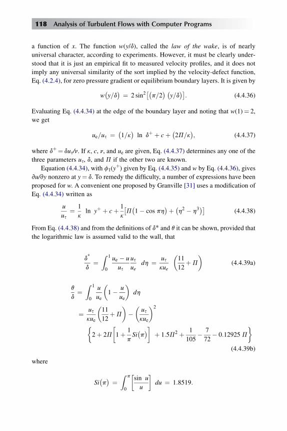
a function of x. The function w(y/d), called the law of the wake, is of nearly

universal character, according to experiments. However, it must be clearly under-

stood that it is just an empirical fit to measured velocity profiles, and it does not

imply any universal similarity of the sort implied by the velocity-defect function,

Eq. (4.2.4), for zero pressure gradient or equilibrium boundary layers. It is given by

w�y=d� ¼ 2 sin2

��p=2

� �y=d� : (4.4.36)

Evaluating Eq. (4.4.34) at the edge of the boundary layer and noting that w(1)¼ 2,

we get

ue=us ¼ �1=k�ln dþ þ cþ �2P=k

�; (4.4.37)

where dþ¼ dus/n. If k, c, n, and ue are given, Eq. (4.4.37) determines any one of the

three parameters us, d, and P if the other two are known.

Equation (4.4.34), with f1(yþ) given by Eq. (4.4.35) and w by Eq. (4.4.36), gives

vu/vy nonzero at y¼ d. To remedy the difficulty, a number of expressions have been

proposed for w. A convenient one proposed by Granville [31] uses a modification of

Eq. (4.4.34) written as

u

us¼ 1

kln yþ þ cþ 1

k

�P�1� cos ph

�þ �h2 � h3�

(4.4.38)

From Eq. (4.4.38) and from the definitions of d* and q it can be shown, provided that

the logarithmic law is assumed valid to the wall, that

d*

d¼Z 1

0

ue � u

us

usue

dh ¼ uskue

�11

12þP

�(4.4.39a)

q

d¼Z 1

0

u

ue

�1� u

ue

�dh

¼ uskue

�11

12þP

��uskue

�2

�2þ 2P

�1þ 1

pSi�p�� þ 1:5P2 þ 1

105� 7

72� 0:12925 P

�(4.4.39b)

where

Si�p� ¼

Z p

0

�sin u

u

�du ¼ 1:8519:


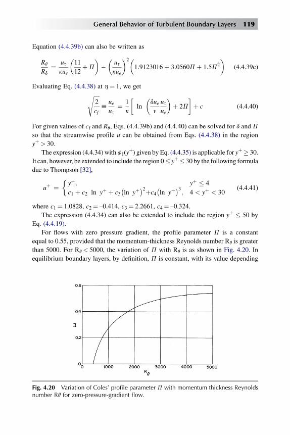
Equation (4.4.39b) can also be written as

Rq

Rd

¼ uskue

�11

12þP

��uskue

�2�1:9123016þ 3:0560Pþ 1:5P2

�(4.4.39c)

Evaluating Eq. (4.4.38) at h¼ 1, we getffiffiffiffi2

cf

sh

ueus

¼ 1

k

�ln

�duev

usue

�þ 2P

�þ c (4.4.40)

For given values of cf and Rq, Eqs. (4.4.39b) and (4.4.40) can be solved for d andP

so that the streamwise profile u can be obtained from Eqs. (4.4.38) in the region

yþ> 30.

The expression (4.4.34) withf1(yþ) given by Eq. (4.4.35) is applicable for yþ� 30.

It can, however, be extended to include the region 0� yþ� 30 by the following formula

due to Thompson [32],

uþ ¼�yþ; yþ � 4

c1 þ c2 ln yþ þ c3�ln yþ

�2þc4�ln yþ

�3; 4 < yþ < 30

(4.4.41)

where c1¼ 1.0828, c2¼ –0.414, c3¼ 2.2661, c4¼ –0.324.

The expression (4.4.34) can also be extended to include the region yþ � 50 by

Eq. (4.4.19).

For flows with zero pressure gradient, the profile parameter P is a constant

equal to 0.55, provided that the momentum-thickness Reynolds number Rq is greater

than 5000. For Rq< 5000, the variation of P with Rq is as shown in Fig. 4.20. In

equilibrium boundary layers, by definition, P is constant, with its value depending

Fig. 4.20 Variation of Coles’ profile parameter P with momentum thickness Reynoldsnumber Rq for zero-pressure-gradient flow.


on the strength of the pressure gradient. In nonequilibrium boundary layers, P

depends on x.

Temperature Profile

A form analogous to Eq. (4.4.34) can be derived for the temperature profile in

a boundary layer in zero pressure gradient with uniform wall temperature or wall

heat-flux rate. Again Eq. (4.4.36) provides an adequate fit to the wake function; so

combining Eqs. (4.2.2) and (4.4.34), we can write

Tþ hTw � T

Ts¼ f2

�yþ; Pr

þPh

khw�yd

(4.4.42)

where Ph is a constant differing slightly between the cases of uniform wall

temperature and uniform wall heat-flux rate but in either case different from P

because Prt s k/kh in the outer layer. Ph is independent of Prt and Reynolds

number if the Reynolds number is high. Since P depends on Reynolds number for

ueq/n< 5000, we must expect Ph to do so as well, because if viscous effects on

the turbulence change the fluctuating velocity field, they will affect heat transfer

as well as momentum transfer. In principle, Ph may depend on the thermal

conductivity if the Peclet number (ueq/n)Pr is less than roughly 5000, according to

the usual argument about the analogy between heat transfer and momentum

transfer, but current experimental data are not sufficient to define the low-

Reynolds-number and low-Peclet-number behaviors, and indeed the high-

Reynolds-number value of Ph is not known very accurately; it is about 0.3.

Outside the viscous and conductive sublayers, Eq. (4.4.42) becomes

Tþ hTw � T

Ts¼ 1

khln

usy

nþ ch þPh

khw�yd

(4.4.43)

in analogy with Eq. (4.4.34); recall that ch depends on Pr.

The above formulas for velocity and temperature profiles can all be used in fully

developed flow in circular pipes or two-dimensional ducts, again with uniform wall

heat-flux rate or uniform differences between the wall temperature and the bulk-

average temperature of the stream. The boundary-layer thickness is replaced by the

radius of the pipe or the half-height of the duct. Values P and Ph are smaller than

in the boundary-layer – indeed P for a pipe flow is so small that it is often

neglected. Low-Reynolds-number effects on P and Ph in pipe or duct flow seem to

be negligible, implying that the effects in boundary layers are associated with the

irregular interface between the turbulent and nonturbulent flow, the ‘‘viscous

superlayer’’.

In arbitrary pressure gradients, Eqs. (4.4.34) and (4.4.42) are usually still good

fits to experimental data but P and Ph depend on the pressure distribution for all


positions upstream. Equation (4.4.42) is not necessarily a good fit to temperature

profiles with arbitrary wall temperature or heat-flux distributions. Consider the case

where a region of uniform wall heat-flux rate, in which Eq. (4.4.42) holds, is fol-

lowed by a region of lower wall heat-flux rate, so that Ts changes discontinuously

while the temperature profile does not. Even the inner-layer formula for Tw – T,

Eq. (4.2.2), breaks down at a step change in _qw; it recovers fairly quickly, but the

outer layer takes much longer.

Shear Stress Distribution

Once the velocity distribution is known, the shear-stress distribution across the

boundary layer can be calculated as follows. For generality, consider a zero-pressure-

gradient flow with mass transfer. First, multiply the continuity equation by u and add

the resulting expression to Eq. (4.4.1) to get

v

vx

�u2�þ v

vy

�uy� ¼ 1

9

vsvy

: (4.4.44)

Integration of Eq. (4.4.44) with respect to y yields

Z y

0

v

vx

�u2�dyþ uy ¼ 1

9

�s� sw

�; (4.4.45)

and integration of the continuity equation also with respect to y yields

y ¼ yw �Z y

0

vu

vxdy: (4.4.46)

With Eq. (4.4.46) we can write Eq. (4.4.28) in nondimensional form asZ y

0

vg2

vxdyþ gyw � g

Z y

0

vg

vxdy ¼ 1

9u2e

�s� sw

�; (4.4.47)

where g¼ u/ue and yw ¼ yw=ue. Next, let h ¼ y=d. Then, since v/vy¼ (v/vh)

(vh/vx)¼ – (h/d) (dd/dx) (v/vh), we can write two of the terms in Eq. (4.4.47) as

follows:

Z y

0

vg2

vxdy ¼ � dd

dx

Z h

0gg0h dh;

Z y

0

vg

vxdy ¼ � dd

dx

Z h

0g0h dh:

(4.4.48)


Integration by parts yields

Z y

0

vg2

vxdy ¼ �dd

dx

g2h�

Z h

0g2dh

!;

Z y

0

vg

vxdy ¼ �dd

dx

gh�

Z h

0g dh

!:

(4.4.49)

Substituting the relations given by Eq. (4.4.49) into Eq. (4.4.47) and rearranging, we

get the dimensionless shear-stress distribution

ssw

¼ 1þ�2

cf

�"gyw þ dd

dx

Z h

0g2dh� g

Z h

0g dh

!#: (4.4.50)

Equation (4.4.50) also applies to incompressible boundary layers with pressure

gradient, provided that the term – (dh/ue)(due/dx) is included in the bracketed

expression.

To obtain an approximate expression for dd/dx, we use a power-law assumption

for the velocity profiles and write the following relation, which is exact for an

asymptotic layer with suction:

d=q ¼ const: (4.4.51)

Taking the derivative of Eq. (4.4.51) with respect to x gives

dd

dx¼ dq

dx

�q

d

��1

: (4.4.52)

But, by definition,

q

d¼ 1

d

Z d

0

u

ue

�1� u

ue

�dy ¼

Z 1

0gð1� gÞdh: (4.4.53)

Evaluating Eq. (4.4.47) at y¼ d yields the momentum integral equation

dq

dx¼ yw þ sw

9u2e¼ yw þ cf

2¼ cf

2

�1þ B

�; (4.4.54)

where Bh 2yw=cf . With Eqs. (4.4.53) and (4.4.54), we can write Eq. (4.4.52) as

dd

dx¼ cf

2

�1þ B

�" Z 1

0gð1� gÞdh

#�1

: (4.4.55)


Substitution of the expression (4.4.55) into Eq. (4.4.50) gives

ssw

¼ 1þ Bgþ �1þ B� Z 1

0gð1� gÞdh

!�1 Z h

0g2dh� g

Z h

0g dh

!: (4.4.56)

Let us now calculate the velocity-defect and shear-stress distributions by using

Coles’ expression (4.4.34) and then compare them with experiment for no mass-

transfer flow. Subtracting Eq. (4.4.37) from Eq. (4.4.34), we obtain the velocity

defect distribution

ðue � uÞ=us ¼ �ð1=kÞ ln ðy=dÞ þ ðP=kÞ½2� wðy=dÞ�: (4.4.57)

Figure 4.21 shows the calculated distributions and the experimental values of

Klebanoff [5]. In both cases, the agreement is excellent.

4.5 Mean-Velocity Distributions in IncompressibleTurbulent Flows on Rough Surfaces with ZeroPressure Gradient

In the previous section, we have described the mean-velocity and shear-stress

distributions on smooth surfaces with zero pressure gradient. In this section, we shall

discuss the effect of wall roughness on mean-velocity distribution. As was discussed

in Section 4.2, the velocity-defect law, Eq. (4.2.4), is valid for both smooth and rough

surfaces. Roughness affects only the inner region, and hence we shall direct the

discussion to that region. It is of course impossible to make a surface absolutely

Fig. 4.21 (a) The velocity-defect law according to Coles’ expression. The solid line isthe calculation from Eq. (4.4.57); (b) the shear-stress distribution obtained by usingColes’ velocity-profile expression. The solid line denotes the dimensionless Reynoldsshear stress; the dashed line denotes the dimensionless total shear stress; circled datapoints are from Klebanoff [5].


smooth, but the wall is aerodynamically smooth for a turbulent boundary layer if the

height of the roughness elements k is much less than the thickness of the viscous

sublayer. Since in most cases the viscous sublayer is extremely thin, the roughness

elements must be very small if the surface is to be aerodynamically smooth. On

a given surface, as the boundary-layer thickens and its Reynolds number changes, the

surface may change from effectively rough to aerodynamically smooth.

According to experiments and dimensional analysis, the law of the wall for

a surface with uniform roughness is given by

uþ ¼ f2

�yþ; kþ

�: (4.5.1)

Here kþ is a roughness Reynolds number defined by

kþ ¼ kus=n: (4.5.2)

On a given surface, the surface may change from being effectively rough to aero-

dynamically smooth as us decreases downstream.

In the fully turbulent part of the inner region, the law of the wall for a uniform

rough surface is similar to that for a smooth surface except that the additive constant

c in Eq. (4.4.15) is a function of the roughness Reynolds number kþ. In that region,

the law of the wall can be written as

uþ ¼ �1=k�ln yþ þ B1ðkþÞ; (4.5.3)

where we expect k to be the same as for smooth surfaces. Therefore, we can write

Eq. (4.5.3) as

uþ ¼ �1=k�ln yþ þ c� ��1=k� ln kþ þ c� B2

;

where c is constant for a smooth surface and B2¼ (1/k) ln kþ þ B1 (kþ). Then we

can write

uþ ¼ �1=k�ln yþ þ c� Duþ; (4.5.4)

where

Duþ hDu=us ¼ �1=k�ln kþ þ B3: (4.5.5)

Here B3, which is equal to c – B2, is a function of roughness geometry and density.

The relation between Duþ and kþ has been determined empirically for various

types of roughness. The results are shown in Fig. 4.22.

We see from Eq. (4.5.4) that, since for a given roughness Duþ is known, the sol-

e effect of the roughness is to shift the intercept c –Duþ as a function of kþ. For valuesof kþ below approximately 5, the vertical shiftDuþ approaches zero, except for those

roughnesses having such a wide distribution of particle sizes that there are some


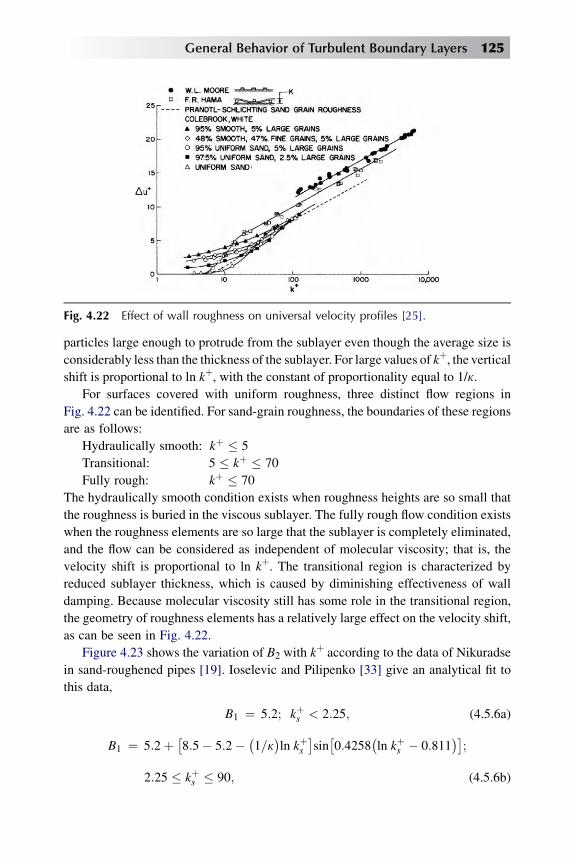
particles large enough to protrude from the sublayer even though the average size is

considerably less than the thickness of the sublayer. For large values of kþ, the verticalshift is proportional to ln kþ, with the constant of proportionality equal to 1/k.

For surfaces covered with uniform roughness, three distinct flow regions in

Fig. 4.22 can be identified. For sand-grain roughness, the boundaries of these regions

are as follows:

Hydraulically smooth: kþ � 5

Transitional: 5 � kþ � 70

Fully rough: kþ � 70

The hydraulically smooth condition exists when roughness heights are so small that

the roughness is buried in the viscous sublayer. The fully rough flow condition exists

when the roughness elements are so large that the sublayer is completely eliminated,

and the flow can be considered as independent of molecular viscosity; that is, the

velocity shift is proportional to ln kþ. The transitional region is characterized by

reduced sublayer thickness, which is caused by diminishing effectiveness of wall

damping. Because molecular viscosity still has some role in the transitional region,

the geometry of roughness elements has a relatively large effect on the velocity shift,

as can be seen in Fig. 4.22.

Figure 4.23 shows the variation of B2 with kþ according to the data of Nikuradse

in sand-roughened pipes [19]. Ioselevic and Pilipenko [33] give an analytical fit to

this data,

B1 ¼ 5:2; kþs < 2:25; (4.5.6a)

B1 ¼ 5:2þ �8:5� 5:2� �1=k�ln kþs sin�0:4258�ln kþs � 0:811� ;

2:25 � kþs � 90; (4.5.6b)

Fig. 4.22 Effect of wall roughness on universal velocity profiles [25].


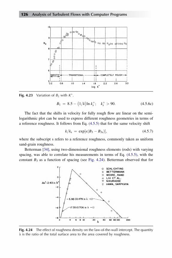
B1 ¼ 8:5� �1=k�ln kþs ; kþs > 90: (4.5.6c)

The fact that the shifts in velocity for fully rough flow are linear on the semi-

logarithmic plot can be used to express different roughness geometries in terms of

a reference roughness. It follows from Eq. (4.5.5) that for the same velocity shift

k=ks ¼ exp½kðB3 � B3sÞ�; (4.5.7)

where the subscript s refers to a reference roughness, commonly taken as uniform

sand-grain roughness.

Betterman [34], using two-dimensional roughness elements (rods) with varying

spacing, was able to correlate his measurements in terms of Eq. (4.5.5), with the

constant B3 as a function of spacing (see Fig. 4.24). Betterman observed that for

Fig. 4.23 Variation of B2 with Kþ.

Fig. 4.24 The effect of roughness density on the law-of-the-wall intercept. The quantityl is the ratio of the total surface area to the area covered by roughness.


a certain spacing of the rods the measured value of Duþ was a maximum and that as

the spacing was increased or decreased Duþ decreased. In another series of exper-

iments, Liu et al. [35] made the same observations.

Betterman found that in the density range 1 � l � 5, where l is the ratio of the

total surface area to the area covered by roughness, the variation of Duþ with

roughness could be specified by

Duþ ¼ 2:43 ln kþ þ 17:35�0:706 ln l� 1

�; (4.5.8)

which is plotted in Fig. 4.24.

The extension of the function Duþ to roughness densities greater than 5 was

accomplished by Dvorak [36] from Fig. 4.24, which is based on the single set of data

by Bettermann in this region and on the data obtained by Schlichting [37]. The

correlation has been biased toward the two-dimensional roughness data of Better-

mann, with the slope of the curve determined in conjunction with Schlichting’s

measurements. Dvorak’s expression for Duþ in this region is given by the following

formula:

Duþ ¼ 2:43 ln kþ � 5:95�0:479 ln l� 1

�: (4.5.9)

Numerically, Eqs. (4.5.8) and (4.5.9) are equal when the value of the density

parameter l is 4.68. It should be noted that Eq. (4.5.9), which applies only for fully

rough flows, requires further verification before it can be used with confidence.

The relation given by Eq. (4.4.19) can also be extended to the prediction of the

mean velocity distribution in the inner region of the boundary layer on a rough

surface by using the following model discussed by Rotta [9].

In this model, the effect of roughness is considered to be equivalent to a change in

the velocity jump across the viscous sublayer. Hence, it can be represented by a shift

of the smooth-flow velocity profile. For rough flow, the reference plane (wall) is

shifted downward by an amount Dy, and the reference plane moves with the velocity

DU in a direction opposite to that of the main flow. Figure 4.25a shows the coordinate

systems for the two flows, the smooth (y,u) and the shifted (Y,U). With the

assumption that the universal law of the wall is valid for the shift, the mean-velocity

distribution for the rough flow in the Y, U coordinate system is

Uþr ¼ f1

�Yþ�; (4.5.10)

where the function f1 is given by the right-hand side of Eq. (4.4.19).

With the relationships u¼U – DU and Y¼ yþDy, we can write the velocity

distribution for rough flow in the physical plane as

uþr ¼ Uþr � DUþ ¼ f1

�Yþ�� f1

�Dyþ

� ¼ f1�yþ þ Dyþ

�� f1�Dyþ

�: (4.5.11)


Obviously, the term f1(Dyþ) in Eq. (4.5.11) is a constant for a given Dyþ. TO

determine Dyþ, we observe that for yþ[Dyþ; f ðyþ þ DyþÞzf ðyþÞ: Hence,

from Fig. 4.25b,

uþs � uþr ¼ Duþ z f�Dyþ

�: (4.5.12)

For a given roughness, the quantity Duþ is determined from experimental data as

a function of kþ (e.g., see Fig. 4.22). Our problem then is to establish a relationship

between Dyþ and kþ. For that purpose, Eq. (4.4.19) is integrated from zero to an

unknown limit for a given Duþ, thus

Z Dyþ

0

2

bþ ½b2 þ 4aðyþÞ�1=2dyþ � Duþ ¼ 0: (4.5.13)

The calculated results for the case of sand-grain roughness, can be approximated by

the following formula:

Dyþ ¼ 0:9h�kþ�1=2�kþexp

�� kþ=6

i: (4.5.14)

Once the shift parameter Dyþ is known, the mean-velocity distribution for rough-

wall flows can be calculated by using the relationship given by Eq. (4.5.11).

If we designate the integrand in Eq. (4.4.19) by f1(yþ), we can write Eq.

(4.5.11) as

uþr ¼Z yþþDyþ

0f1ðyþÞdyþ �

Z Dyþ

0f1

�yþ�dyþ

¼Z yþþDyþ

Dyþf1

�yþ�dyþ:

(4.5.15)

Fig. 4.25 Mean velocity distribution on smooth and rough surfaces (a) illustrating Duand Dy shift, and (b) uþ, y

þ plot.


If we introduce the transformation

yþ ¼ �y þ þ Dyþ (4.5.16)

into Eq. (4.5.15), we can write

uþr ¼Z �yþ

0f1

��yþ þ Dyþ

�d�yþ: (4.5.17)

Comparison of Eq. (4.5.17) with the right-hand side of Eq. (4.4.19) shows that the

velocity profile for rough flow can also be obtained from the smooth-flow condition

by shifting the independent variable in Van Driest’s formulation by Dyþ, or

uþr ¼Z yþ

0

2 dyþ

1þ�1þ ½2kðyþ þ DyþÞ�2f1� exp½ � ðyþ þ DyþÞ=26�g2

1=2 :(4.5.18)

The approach outlined above is limited to small values of Dyþ, say less than 10,

because the integrated velocity profile is slow in gaining the expected logarithmic

variation for large values of Dyþ.

4.6 Mean-Velocity Distribution on Smooth PorousSurfaces with Zero Pressure Gradient

Consider an incompressible turbulent flow on a smooth porous flat surface with zero

pressure gradient. Close to the wall, vu/vx is small and can be neglected. The

momentum equation then becomes

ywdu

dy¼ 1

9

dsdy

; (4.6.1)

where s ¼ sl þ sl: Integrating Eq. (4.6.1) and using the wall boundary condition,

sð0Þ ¼ sw; uð0Þ ¼ 0; we obtain

s ¼ sw þ 9ywu: (4.6.2)

In the fully turbulent part of the inner region, sl z 0. If st is replaced by Prandtl’s

mixing-length expression given by Eqs. (4.3.3) and (4.3.12), integration of Eq.

(4.6.2) gives

�2=yþw

��1þ yþwu

þ�1=2¼ �1=k�ln yþ þ c1; (4.6.3)


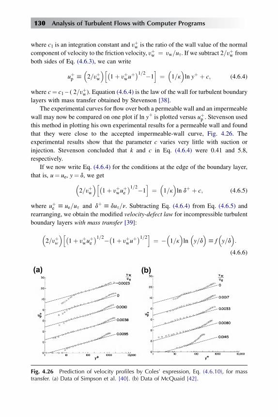
where c1 is an integration constant and yþw is the ratio of the wall value of the normal

component of velocity to the friction velocity, yþw ¼ yw=us. If we subtract 2=yþw from

both sides of Eq. (4.6.3), we can write

uþp h�2=yþw

h�1þ yþwu

þ�1=2�1i¼�1=kln yþ þ c; (4.6.4)

where c¼ c1 – ( 2=yþw). Equation (4.6.4) is the law of the wall for turbulent boundary

layers with mass transfer obtained by Stevenson [38].

The experimental curves for flow over both a permeable wall and an impermeable

wall may now be compared on one plot if ln yþ is plotted versus uþp . Stevenson usedthis method in plotting his own experimental results for a permeable wall and found

that they were close to the accepted impermeable-wall curve, Fig. 4.26. The

experimental results show that the parameter c varies very little with suction or

injection. Stevenson concluded that k and c in Eq. (4.6.4) were 0.41 and 5.8,

respectively.

If we now write Eq. (4.6.4) for the conditions at the edge of the boundary layer,

that is, u¼ ue, y¼ d, we get�2=yþw

h�1þ yþwu

þe

�1=2�1i¼�1=kln dþ þ c; (4.6.5)

where uþe h ue=us and dþ h dus=n. Subtracting Eq. (4.6.4) from Eq. (4.6.5) and

rearranging, we obtain the modified velocity-defect law for incompressible turbulent

boundary layers with mass transfer [39]:

�2=yþw

h�1þ yþwu

þe

�1=2��1þ yþwuþ�1=2i ¼ �

�1=kln�y=dh f

�y=d:

(4.6.6)

Fig. 4.26 Prediction of velocity profiles by Coles’ expression, Eq. (4.6.10), for masstransfer. (a) Data of Simpson et al. [40]. (b) Data of McQuaid [42].


The results in Fig. 4.26 show that the function f (y/d) in the equation of the modified

velocity defect law, Eq. (4.2.4), is independent of yw and us in the outer region of the

boundary layer.

According to Stevenson’s law of the wall, the parameter c in Eq. (4.6.4), like the

parameter k, is essentially unaffected by mass transfer. Simpson et al. [39] carried

out extensive new measurements on flat plates with both blowing and suction, as

a result of which they proposed a different condition, namely, that the curve of

Eq. (4.6.4) always passes through the point uþ¼ yþ¼ K¼ 11, regardless of the

value of yw. Here the parameter K represents the intersection of the logarithmic

profile with the linear sublayer when yw¼ 0; that is,

uþ ¼ yþ ¼ �1=k�ln yþ þ c0 (4.6.7)

or

K ¼ ð1=kÞln K þ c0: (4.6.8)

Simpson’s condition for c, which is purely empirical, implies that

c ¼ c0 þ�2=yþw

h�1þ Kyþw

�1=2�1i� K: (4.6.9)

Using the above expression for c, Coles [41] has shown that his profile expression

(4.4.34), when generalized to the form�2=yþw

h�1þ yþwu

þ�1=2�1i¼�1=kln yþ þ cþ

�P=k

w�y=d; (4.6.10)

with c0¼ 5 and K¼ 10.805, describes the experimental data for zero-pressure-

gradient flows with mass transfer very well. As in flows with zero mass transfer, the

profile parameter P has the variation with Reynolds number given by Fig. 4.20.

Figure 4.26 shows, for two sets of experimental data, the excellent prediction of

pseudo-velocity profiles, uþp , by Eq. (4.6.10).

4.7 The Crocco Integral for Turbulent Boundary Layers

As was discussed in Chapter 3, the Crocco integral, Eq. (3.2.18),

ðH � HwÞ=ðHe � HwÞ ¼ u=ue; (4.7.1)

provides a good approximation for adiabatic, zero-pressure-gradient flows, both

incompressible and compressible. For the compressible flow of a perfect gas, Eq.

(3.2.18) can be written as

T

Te¼ Tw

Te��TwTe

� 1

�u

ueþ g� 1

2M2

e

u

ue

�1� u

ue

�: (4.7.2a)


Obviously, for incompressible flows it reduces to

T

Te¼ Tw

Te��TwTe

� 1

�u

ue: (4.7.2b)

According to experiments, the Crocco relationship does not apply in either

laminar or turbulent flows with heat transfer and pressure gradient, even if the wall is

isothermal and the molecular or the eddy diffusivities for momentum and heat

transfer are equal or nearly equal. Instead, the relationship between total temperature

and velocity is generally expected to depend upon the degree of flow acceleration (or

deceleration) and the amount of wall cooling (or heating), and may be influenced to

some extent by the flow speed, that is, the compressibility effect when the molecular

or the eddy diffusivities for momentum are not the same (e.g., see Bertram et al. [43];

Back and Cuffel [44,45]).

Figure 4.27 shows the relationship between measured temperature and velocity

profiles for an accelerating, turbulent-boundary-layer flow of air through a cooled,

convergent-divergent nozzle. The data are due to Back and Cuffel [43,44].

Boundary-layer measurements were made upstream, along the convergent section,

and near the end of the divergent section where the flow is supersonic. These

measurements span a relatively large flow-speed range, with inlet and exit Mach

Fig. 4.27 Relationship between measured total temperature and velocity profiles for anaccelerating turbulent boundary-layer flow of air through a cooled convergent-divergentnozzle [44].


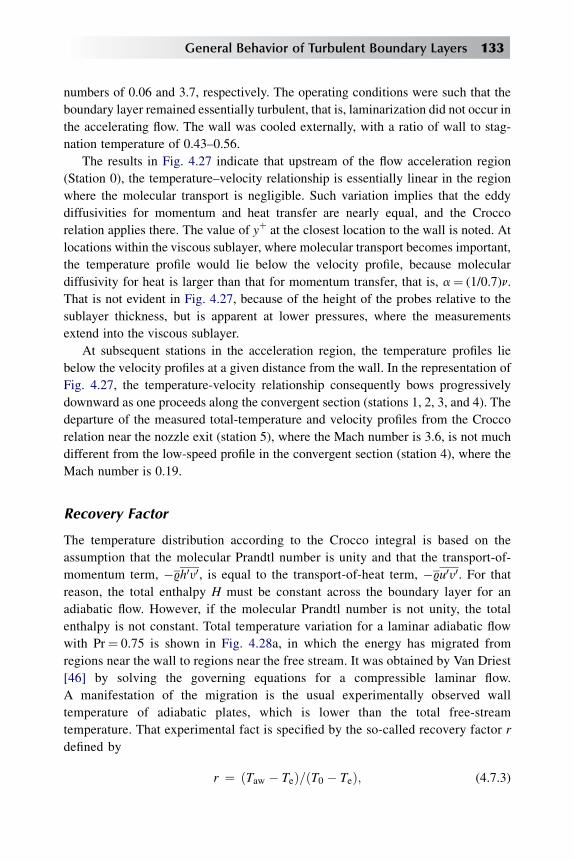
numbers of 0.06 and 3.7, respectively. The operating conditions were such that the

boundary layer remained essentially turbulent, that is, laminarization did not occur in

the accelerating flow. The wall was cooled externally, with a ratio of wall to stag-

nation temperature of 0.43–0.56.

The results in Fig. 4.27 indicate that upstream of the flow acceleration region

(Station 0), the temperature–velocity relationship is essentially linear in the region

where the molecular transport is negligible. Such variation implies that the eddy

diffusivities for momentum and heat transfer are nearly equal, and the Crocco

relation applies there. The value of yþ at the closest location to the wall is noted. At

locations within the viscous sublayer, where molecular transport becomes important,

the temperature profile would lie below the velocity profile, because molecular

diffusivity for heat is larger than that for momentum transfer, that is, a¼ (1/0.7)n.

That is not evident in Fig. 4.27, because of the height of the probes relative to the

sublayer thickness, but is apparent at lower pressures, where the measurements

extend into the viscous sublayer.

At subsequent stations in the acceleration region, the temperature profiles lie

below the velocity profiles at a given distance from the wall. In the representation of

Fig. 4.27, the temperature-velocity relationship consequently bows progressively

downward as one proceeds along the convergent section (stations 1, 2, 3, and 4). The

departure of the measured total-temperature and velocity profiles from the Crocco

relation near the nozzle exit (station 5), where the Mach number is 3.6, is not much

different from the low-speed profile in the convergent section (station 4), where the

Mach number is 0.19.

Recovery Factor

The temperature distribution according to the Crocco integral is based on the

assumption that the molecular Prandtl number is unity and that the transport-of-

momentum term, �9h0y0, is equal to the transport-of-heat term, �9u0y0. For thatreason, the total enthalpy H must be constant across the boundary layer for an

adiabatic flow. However, if the molecular Prandtl number is not unity, the total

enthalpy is not constant. Total temperature variation for a laminar adiabatic flow

with Pr¼ 0.75 is shown in Fig. 4.28a, in which the energy has migrated from

regions near the wall to regions near the free stream. It was obtained by Van Driest

[46] by solving the governing equations for a compressible laminar flow.

A manifestation of the migration is the usual experimentally observed wall

temperature of adiabatic plates, which is lower than the total free-stream

temperature. That experimental fact is specified by the so-called recovery factor r

defined by

r ¼ ðTaw � TeÞ=ðT0 � TeÞ; (4.7.3)


where Taw and T0 are the adiabatic wall and the reservoir (isentropic-stagnation)

temperatures, respectively. From the steady-state energy equation for an inviscid

perfect-gas flow, we can write

T0 � Te ¼ u2e=2cp:

Substituting that expression into Eq. (4.7.3) and rearranging, we get

Taw ¼ Te�lþ r

��g� 1

��2 M2

e

�: (4.7.4)

With laminar boundary layers, the recovery factor rlam is approximately equal to

(Pr)1/2 for incompressible flows.

In the case of the adiabatic fully turbulent boundary layer, the recovery factor rt is

somewhat larger than it is in laminar boundary layers. According to experiments

(see Fig. 4.28b), its value is between 0.875 and 0.90 for air. It is given approximately

by (Pr)1/3.

From the Crocco integral, Eq. (4.7.1a), after rearranging we can write

T

Tw¼ 1þ

��1þ g� 1

2M2

e

�TeTw

� 1

�u

ue� g� 1

2M2

e

TeTw

�u

ue

�2

: (4.7.5)

Replacing the relation 1þ ½ðg� 1Þ=2�M2e by T0/Te in Eq. (4.7.5) and rearranging, we

obtain

T ¼ Tw þ ðT0 � TwÞ ðu=ueÞ þ ðTe � T0Þ ðu=ueÞ2: (4.7.6)

Fig. 4.28 (a) Variation of stagnation-temperature ratio across the laminar boundarylayer at Me¼ 3 [46] and (b) variation of recovery factor with Reynolds number [47].


That expression is another form of Crocco integral. It can be extended to Prandtl

numbers differing from unity by replacing the stagnation temperature T0 by the

adiabatic wall temperature Taw. Then Eq. (4.7.6) can be written as

T ¼ Tw þ ðTaw � TwÞ ðu=ueÞ þ ðTe � TawÞ ðu=ueÞ2: (4.7.7)

In that equation, Taw should be calculated from Eq. (4.7.3). A commonly used value

for r is 0.89. For zero-pressure-gradient flows with small heat transfer, Eq. (4.7.7) can

be used quite satisfactorily to calculate the static-temperature distribution for flows

both with and without mass transfer [48,49].

4.8 Mean-Velocity and Temperature Distributions inCompressible Flows with Zero Pressure Gradient

For two-dimensional unsteady compressible boundary layers, both laminar and

turbulent, the continuity, momentum, and energy equations are given by Eqs. (3.3.5),

(3.3.6), and (3.3.14), respectively. For laminar layers, the equations are coupled

through the variation of density and the transport properties of the gas, such as m, k,

and cp. Although reliable experiments in variable-density flows are still few in

number, there is reasonable evidence that the structure of the turbulent velocity field

is not altered significantly in the presence of moderate density or temperature

fluctuations. This suggests that interaction between the velocity and the temperature

fluctuations is probably not strong, even in flows of moderate Mach numbers [50].

Indeed, Chu and Kovasznay [51] have shown theoretically that in a homogeneous

field the interactions are second order. Thus for compressible turbulent shear flows,

the main coupling between the equations occurs through the density variation only.

In this section we shall discuss the mean-velocity and temperature distributions in

compressible turbulent boundary layers with zero pressure gradient, and we shall

show how the various expressions developed for incompressible flows can be

modified to account for the variation of density in such flows.

4.8.1 THE LAW-OF-THE-WALL FOR COMPRESSIBLE FLOWS

In compressible turbulent flows, the velocity profile and temperature profile in the

inner part of the boundary layer depend on all the quantities that affect the velocity or

temperature profile in compressible flows (Section 4.4), and in addition the absolute

temperature (at the wall, say) must be included since, by definition, the temperature

differences in compressible flows are a significant fraction of the absolute temper-

ature. Also, if the Mach number of the flow is not small compared with unity, the

speed of sound, a, and the ratio of specific heats, g, will appear; in a perfect gas


a ¼ ffiffiffiffiffiffiffiffiffigRT

p ¼ ffiffiffiffiffiffiffiffiffiffiffiffiffiffiffiffiffiffiffiffiffiffiffiðg� 1ÞcpTp

, so that either a or T or both may be used as a varia-

ble. With these additions, from dimensional analysis with us ¼ ffiffiffiffiffiffiffiffiffiffiffiffiffisw=9w

p, we can

write

u

us¼ f3

�usy

vw;

_qw9cpusTw

;usaw

;g; Prw

�; (4.8.1)

T

Tw¼ f4

�usy

vw;

_qw9cpusTw

;usaw

;g ; Prw

�: (4.8.2)

In Eq. (4.8.2) we have used T Tw= instead of ðTw � TÞ Tw= for convenience, and the

speed of sound at the wall, aw, is used instead of the dimensionally correct but less

meaningful quantityffiffiffiffiffiffiffiffiffifficpTw

p. The quantity us/aw is called the friction Mach number,

Ms. The evaluation of fluid properties at the wall is adequate if, for example, n/nw can

be expressed as a function of T/Tw only (the pressure being independent of y in any

case); this is the case if nf T u for some u, which is a good approximation for

common gases over a range of, say, 2:1 in temperature.

The arguments that led to the law-of-the-wall formulas for velocity and

temperature in incompressible flows (Section 4.2) can be applied again to the

compressible case if we are satisfied that the effects of viscosity are again small for

usy/nw [ 1 and that the effects of thermal conductivity are again small for (usy/vw)

Pr [ 1. Provided that the effects of fluctuations in viscosity and thermal conduc-

tivity are small and that v and 9 do not differ by orders of magnitude from their values

at the wall so that usy=nw is still a representative Reynolds number, molecular

diffusion should indeed be small compared with turbulent diffusion if usy/nw is large.

Since density varies in compressible flows, the local value of ðs=9Þ1=2 would providea better velocity scale than the wall value us; it therefore seems logical to use the

local value in compressible flows also, and in the simplest case when only 9 and not

s, varies with y, the appropriate velocity scale is ðsw=9Þ1=2. Analogously we use _q/9,

rather than _qw=9w, in the mixing-length formula for temperature; we shall see below

that _q always varies with y in high-speed flows. The elimination of nw and Pr from the

lists of variables and the use of dimensional analysis on vu=vy and vT=vy instead of u

and T give, instead of Eqs. (4.8.1) and (4.8.2)

vu

vy¼ ðs=9Þ1=2

kyfu

"_q

9cpTðs=9Þ1=2;ðs=9Þ1=2

a;g

#; (4.8.3)

vT

vy¼ � _q=9cp

ðs=9Þ1=2khyfT

"_q

9cpTðs=9Þ1=2;ðs=9Þ1=2

a;g

#(4.8.4)

where we have consistently used local variables in the arguments of the f functions,

even for s. The analysis below will be restricted to the case of a constant-stress layer,


s¼ sw , which, as was discussed in Section 4.2, is a good approximation to the inner

20 percent of a boundary layer in a small pressure gradient.

In order to equate the f functions to unity and recover effectively incompressible

versions of the mixing-length formulas, we need to neglect the effect of density

fluctuations discussed in Section 3.2. With this assumption, the heat-transfer

parameter _q=9cpðs=9Þ1=2T and the friction Mach number ðs=9Þ1=2=a – representing

the two sources of density (temperature) fluctuations – do not appear in formulas

(4.8.3) and (4.8.4) for the gradients of u and T ; they will, however, remain in the full

formulas for u and T, Eqs. (4.8.1) and (4.8.2), because they affect the temperature

gradient in the viscous sublayer. Formulas for vu=vy and vT=vy in the viscous

sublayer would nominally contain all the variables on the right-hand sides of Eq.

(4.8.1) or (4.8.2). The assumption that turbulence processes are little affected by

density fluctuations implies, that g, which is a measure of the difference between

adiabatic and isothermal processes, would have a negligible effect even in the

viscous sublayer, but there are not enough data to check this. With the assumption

that fu and fT are constant outside the viscous sublayer, we can now write

vu

vy¼ ðs=9Þ1=2

ky; (4.8.5)

vT

vy¼ � _q=9cp

ðs=9Þ1=2khy: (4.8.6)

Now Eq. (4.8.6) still retains the local value of _q, and in a high-speed flow this will

differ from the wall value, even if s¼ sw , because of viscous dissipation of mean and

turbulent kinetic energy into heat. The rate at which kinetic energy is extracted from

a unit volume of the mean flow by work done against viscous and turbulent stresses is

svu/vy; the part corresponding to the viscous shear stress represents direct viscous

dissipation into heat, and the part corresponding to the turbulent shear stress

represents production of the turbulent kinetic energy. We cannot immediately equate

turbulent energy production to viscous dissipation of that turbulent energy into heat

because turbulence processes include transport of turbulent kinetic energy from one

place to another. However, this transport is negligible in the inner layer (outside the

viscous sublayer), so that we can write a degenerate version of the energy equation,

with all transport terms neglected and only y derivatives retained, as

v _q

vy¼ sw

vu

vy; (4.8.7)

which simply states that the net rate of (y-component) transfer of heat leaving

a control volume in the inner layer is equal to the rate at which the fluid in the control

volume does work against (shear) stress. Integrating this equation, we get

_q ¼ _qw þ usw: (4.8.8)


In a low-speed flow the work done is negligible, and _q¼ _qw, corresponding to s¼ sw.If we divide Eq. (4.8.6) by Eq. (4.8.5), we obtain

vT

vu¼ �ðk=khÞ _q

cpsw; (4.8.9)

where k/kh is the turbulent Prandtl number. Substituting for _q from Eq. (4.8.8) and

integrating with respect to u, we get

T ¼ � ðk=khÞ _qwucpsw

��k=kh

�u2

2cpþ const: (4.8.10)

Here the constant of integration is not exactly equal to Tw because the formulas

(4.8.5) and (4.8.6) are not valid on the viscous or conductive sublayers, but it is

conventionally written as c1Tw , where c1 is close to unity and is a function of

_qw=9wcpusTw; us=aw, and the molecular Prandtl number Pr. That is,

T ¼ c1Tw � ðk=khÞ _qwucpsw

��k=kh

�u2

2cp: (4.8.11)

Noting that 9 ¼ 9wTw=T , we can use Eq. (4.8.11) to eliminate 9 from Eq. (4.8.5).

The integral required to obtain u as a function of y from Eq. (4.8.5) then becomes

Zdy

k y¼Z

du=us�c1 �

�k=kh

�_qwu=cpTwsw � �k=kh�u2=2cpTw 1=2 (4.8.12)

Replacing cpTw by a2w/(g – 1) and integrating Eq. (4.8.12), we obtain the law of the

wall for compressible turbulent flows:

u

us¼

ffiffiffiffiffic1

pR

sin

�Ru*

us

�� H

�1� cos

�Ru*

us

��; (4.8.13)

where

R ¼ usaw

�ðg� 1Þk2kh

�1=2; H ¼ _qw

swush

1

ðg� 1Þ_qw

9wcpusTw

�awus

�2

; (4.8.14a)

u* ¼ 1

kln yþ const: (4.8.14b)

Recalling from Eq. (4.8.1) that y appears in the group usy/vw, we rewrite

u*

us¼ 1

kln

usy

nwþ c: (4.8.14c)


If _qw ¼ 0 and us/aw / 0, then H¼ 0, R / 0, and

u

us¼ ffiffiffiffiffi

c1p u*

us: (4.8.15)

It can be shown that if us/aw is small, then c1¼ 1 – O( _qw), for compatibility with the

logarithmic law for temperature in incompressible flows, Eq. (4.4.17), so that u¼ u*

for small _qw ; thus the constant c in Eq. (4.8.14c) can be identified with the additive

constant c in the logarithmic law for constant property wall layers. In general c, like

c1, is a function of the friction Mach number Ms and of Bq defined by

Bq ¼ _qw9wcpusTw

: (4.8.16)

The above analysis is originally due to Rotta [9] and is an extension of that of Van

Driest [46].

4.8.2 VAN DRIEST TRANSFORMATION FOR THE LAW OF THE WALL

Simpler versions of Eq. (4.8.13) and the accompanying temperature profile Eq.

(4.8.11) have been proposed by many authors. Van Driest [46] assumed c1¼ 1 and

k/kh¼ 1 (recall that k/kh is a turbulent Prandtl number in the fully turbulent part of

the flow, and note that c1¼ 1 implies that the effective Prandtl number in the viscous

and conductive sublayers is unity). Van Driest presented the inverse of Eq. (4.8.3)

giving u* in terms of u. In our more general notation this is

u*

us¼ 1

R

sin�1 Rðu=us þ HÞ

ðc1 þ R2H2Þ1=2� sin�1 RH

ðc1 þ R2H2Þ1=2

!: (4.8.17)

This formula is called the Van Driest transformation; it can be regarded as trans-

forming the inner-layer part of the compressible boundary-layer profile u(y) to an

equivalent incompressible flow u*(y) that obeys the logarithmic formula, Eq.

(4.8.14c). However, it is simpler to regard Eq. (4.8.13), with Eq. (4.8.14) as direct

prediction of inner-layer similarity theory for the compressible boundary layer.

If there is no heat transfer through the surface, H is zero, the second term on the

right of Eq. (4.8.13) disappears, and Eq. (4.8.17) reduces to

u*

us¼ 1

Rsin�1

�Rffiffiffiffiffic1

p u

us

�; (4.8.18)

which is easy to identify as the inverse of Eq. (4.8.13) without the second term on the

right and of course reduces to u*¼ u as R / 0 and c1 / 1.

The basic assumptions imply that k and kh are the same as in incompressible flow.

As we have seen, c1 and c, which are constants of integration in Eqs. (4.8.9) and


(4.8.12), respectively, must be expected to be functions of the friction Mach number

and the heat transfer parameter. Experimental data reviewed in great detail by

Fernholz and Finley [52] support the extension of inner-layer similarity to

compressible flow but fail to provide definite evidence about the variation of c and c1.

The low-speed values c¼ 5.0 and c1¼ 1 fit the data as a whole to within the rather

large scatter, but Bradshaw [53] presents formulas for variable c and c1 based on

a selection of the more reliable data.

If we replace H by the expressions given in Eq. (4.8.14a) and (4.8.11), use the

definition of Mach number, Me¼ ue /ae, take c1¼ 1 and k /kh¼ 1 following Van

Driest [46], and note that 9w/9e¼ Te/Tw, then Eq. (4.8.17) can be written as

u*

us¼ 1

Affiffiffiffiffiffiffiffiffiffiffiffiffiffiffiffiffiffiffiffiffiffiffiffiffiffiffiffiffiffi�cf =2

��Tw=Te

�q sin�1

Affiffiffiffiffiffiffiffiffiffiffiffiffiffiffiffiffiffiffiffiffiffiffiffiffiffiffiffiffiffi�cf =2

��Tw=Te

�q �u=us

�� B=2A

1þ ðB=2AÞ2

þ sin�1 B=2Affiffiffiffiffiffiffiffiffiffiffiffiffiffiffiffiffiffiffiffiffiffiffiffiffi1þ ðB=2AÞ2

q! (4.8.19)

or as

u* ¼ ueA

sin�1 2A2

�u=ue

�� B

ðB2 þ 4A2Þ1=2þ sin�1 B

ðB2 þ 4A2Þ1=2

!(4.8.20)

where

A2 ¼ g� 1

2

M2e

Tw=Te; B ¼ 1þ �g� 1

��2M2

e

Tw=Te� 1: (4.8.21)

Note that the above relations assume that the recovery factor rh ðTaw=Te � 1Þ½ðg� 1Þ=2M2

e �;where Taw is the temperature of an adiabatic wall, is 1. To account for

the fact that r is less than unity (about 0.89) we rewrite Eqs. (4.8.21) as

A2 ¼��g� 1

��2 M2

eg

Tw=Te; B2 ¼ 1þ ��g� 1

��2 M2

eg

Tw=Te� 1: (4.8.22)

4.8.3 TRANSFORMATIONS FOR COMPRESSIBLE TURBULENT FLOWS

The Van Driest Transformation for the Whole Layer

The Van Driest transformation, Eq. (4.8.17), applied to the fully turbulent part of the

inner (constant-stress) layer of a compressible boundary layer produces the loga-

rithmic profile, Eq. (4.8.14c). Applying the transformation to the outer layer of


a constant-pressure compressible boundary layer, we obtain a profile that looks

qualitatively like that of a constant-pressure constant-density boundary layer. In

particular, the transformed profile u*(y) can be described, more or less as accurately

as an incompressible profile, by the wall-plus-wake formula given by Eqs. (4.4.34)–

(4.4.36),

u*

us¼ 1

kln

usy

vwþ cþP

k

�1� cos p

y

d

: (4.8.23)

However, this convenient data correlation is a consequence of the strong constraint

on the wake profile, which has to have zero slope and zero intercept at y¼ 0, whereas

the profile as a whole has zero slope at y¼ d also, the ‘‘wake parameter’’ P and the

boundary-layer thickness d are constants that can be adjusted to optimize the fit of

Eq. (4.8.23) to any real or transformed profile. We must, therefore, not claim that the

success of Eq. (4.8.23) proves the validity of Van Driest’s inner-layer analysis in the

outer layer.

As was discussed in subsection 4.4.6, P is constant in incompressible constant-

pressure flows at high Reynolds number and equal to about 0.55. The value ofP that

best fits a transformed profile is expected to be a function of the friction Mach

number Ms (h us/aw) and of the heat-transfer parameter Bq (h _qw=9cpusTw).

Evaluation of this function from experimental data is hampered by the low Reynolds

number of most of the compressible-flow data and uncertainty about the definition of

Reynolds number that should be used in correlating low-Reynolds-number effects on

the velocity-defect profile. If it is accepted that these originate at the irregular

interface between the turbulent fluid and the nonturbulent ‘‘irrotational’’ fluid, then

the fluid properties in the Reynolds number should be evaluated at freestream

conditions. Now the largest-scale interface irregularities seen in flow-visualization

pictures have a length scale of order d, being the result of the largest eddies that

extend across the full thickness of the shear layer. Therefore d is the appropriate in-

terface scale and, since it is found that the shear-stress profile plotted as s/sw¼ f (y/d)

has nearly the same shape at any Reynolds number, we can use sw as a shear-stress

scale and (sw/9e)1/2 – evaluated using the freesteam density – as a velocity scale.

Therefore the appropriate Reynolds number is (sw/9e)1/2d/ne h (usd/ne)$ (9w/9e)

1/2

rather than the Reynolds number usd/nw that arises naturally in the Van Driest

transformation. However, Fernholz [54] has shown that the Reynolds number 9eueq/

mw gives excellent correlations of data over a wide range of Mach numbers and

Reynolds numbers.

If the physics of low-Reynolds-number effects is the same in compressible flow

as in incompressible flow, then the wake parameter P of the transformed profile

should be independent of Reynolds number for (sw/9e)1/2d/ne> 2000 approximately

(corresponding to ueq/n> 5000 in the case of a low-speed boundary layer). Since P

is nominally a function of Ms and Bq, it is not possible to predict the trend with


Reynolds number explicitly, but it is probably adequate to assume that the ratio ofP

to its high-Reynolds-number asymptotic value is the same function of the chosen

Reynolds number as in incompressible flow. In fact, although the data are rather

scattered by low-speed standards, it appears that P decreases only very slowly with

increasing Mach number [55] in adiabatic-wall boundary layers ( _qw ¼ 0) and

therefore that P¼ 0.55 is an adequate high-Reynolds number value for all Ms.

If c and c1 are known as functions ofMs and Bq, and ifP is known as a function of

Ms, Bq, and Reynolds number, then putting y¼ d and u¼ ue in Eq. (4.8.17) and using

Eq. (4.8.23) to substitute for u*, we obtain ue /us as a function of usd/yw . In practicewe

require the skin-friction coefficient sw=129eu2e as a function of ueq/ve or Fernholz’s

variable 9eueq/mw given Me (and Te) and either _qw or Tw. This requires iterative

calculation, starting with an estimate of sw . Also, the velocity profile of the

compressible flow has to be integrated at each iteration to obtain q/d for conversion

from the ‘‘input’’ Reynolds number ueq/ve to the Reynolds number usd/vw that appears

in the transformation [53]. Skin-friction formulas are discussed in subsection 7.2.3.

The Van Driest transformation could be regarded as a solution of the

compressible-flow problem only if the coefficients c, c1 and P were independent of

Mach number and heat-transfer parameter. However, we can use the transformation,

plus compressible-flow data for c, c1 and P, to correlate the mean properties of

constant-pressure compressible boundary layers. As noted above the change in the

coefficients is almost within the (large) experimental scatter.

In pressure gradients the transformed boundary-layer profile still fits Eq. (4.8.23)

as does its true low-speed equivalent, but, as at low speeds, there is no simple formula

to relate the shape parameter P to the Iocal pressure gradient. Moreover, the vari-

ation of us,P, and d with x will not generally correspond to any realizing low-speed

boundary layer; that is, it may not be possible to choose a pressure distribution p(x)

for a low-speed flow that will reproduce at each x, the same velocity profile as in the

compressible flow. The spirit of Van Driest’s transformation, although not its details,

would be retained if compressible boundary layers were calculated using the mixing-

length formula to predict the shear stress and the assumption of constant turbulent

Prandtl number to predict the heat transfer. We consider such calculation methods in

Chapter 8.

Other Transformations

While the transformations between compressible and incompressible laminar

boundary layers are rigorous but limited in application, transformations for turbulent

flow are necessarily inexact because our knowledge of the time-averaged properties

of turbulent motion is inexact. As in the case of laminar flow the need for trans-

formation has decreased as our ability to do lengthy numerical calculations has

increased, and the assumption that density fluctuations have negligible effect on


turbulence has permitted low-speed models to be cautiously extended to

compressible flow. The Van Driest transformation relies on the application of this

assumption to the inner-layer (mixing-length) formula. In the outer layer where the

mixing length departs from its inner-layer value ky, the Van Driest analysis is not

exact and the transformation will not eliminate compressibility effects though it

certainly reduces them, apparently within the scatter of current experimental data.

The transformations between compressible and incompressible flow fall into two

classes: (1) transformations for the complete velocity profile (and by implication the

shear stress profile) and (2) transformations for integral parameters only (specifically,

skin-friction formulas). It is generally recognized that transformations for

compressible flows in pressure gradient do not necessarily lead to realizable low-

speed flows, and we will discuss only constant-pressure flows here.

The paper by Coles [56] is a useful review of previous work and presents one of

the most general transformations so far proposed. The two main assumptions are that

suitably defined ratios of coordinates in the original (high-speed) and transformed

(low-speed) planes are functions only of x and not of y, and that the ratio of the

stream functions in the transformed and original flows is equal to the ratio of the

(constant) viscosity in the transformed flow to the viscosity evaluated at an,

‘‘intermediate temperature’’ somewhere between Tw and Te in the compressible flow.

The justification for the latter assumption is carefully discussed by Coles, but the

choice of intermediate temperature is necessarily somewhat arbitrary. Coles chooses

the temperature at the outer edge of the viscous sublayer, but in order to fit the

experimental data for skin friction it is necessary to locate the sublayer edge at

usy/v¼ 430 in the transformed flow, whereas the thickness of the real sublayer is

only about one-tenth of this. Coles conjectures that the relevant region is perhaps not

the viscous sublayer as such but the whole turbulent boundary layer at the lowest

Reynolds number at which turbulence can exist; this boundary layer indeed has usd/y

of the order of 430. Coles’ transformation should not be confused with the simpler

intermediate-temperature assumption that any low-speed skin friction formula can

be applied to a high-speed flow if fluid properties are evaluated at a temperature Tisomewhere between Tw and Te [57].

4.8.4 LAW OF THE WALL FOR COMPRESSIBLE FLOW WITH MASS TRANSFER

Stevenson’s law-of-the-wall expression, Eq. (4.6.4), discussed in Section 4.6, has

also been extended to compressible turbulent boundary layers with mass transfer by

Squire [58]. Again assuming that derivatives in the x direction are negligible

compared to derivatives in the y direction, one can integrate the continuity equation

to give

9y ¼ const ¼ 9wyw; (4.8.24)


and with that result, the momentum equation can be integrated to give

9wywu ¼ s� sw: (4.8.25)

By means of Prandtl’s mixing-length formula, Eq. (4.8.25) can be formally inte-

grated to give Z u

u0

ð9Þ1=2du0ð9wywu0 þ swÞ1=2

¼ 1

kln

�y

y0

�; (4.8.26)

where the subscript a designates values at the inner edge ot the fully turbulent region.

Equation (4.8.26) may be rearranged to give

Z u

0


¼ 1

kln

yusvw

� 1

kln

y0usvw

þZ u0

0


¼ 1

kln

yusvw

þ c:

(4.8.27)

Before the left-hand side of that equation can be integrated, it is necessary, as

before, to know the density or the temperature. That can be obtained from Eq. (4.7.6)

since 9w=9 ¼ T=Tw.

With Eq. (4.7.6), the left-hand side of Eq. (4.8.27) may be written

�TeTw

�1=2Z f

0

�9wyw

9euef0 þ 1

2cf

��1=2

��1þ Taw � Tw

Twf0 þ Te � Taw

TwðfÞ02

��1=2

df0h uþp ;(4.8.28)

where f¼ u/ue. Thus the law of the wall for compressible turbulent boundary layers

with mass transfer is

uþp ¼�1=k

ln�yus=vw

þ c: (4.8.29)

For incompressible, constant-temperature flows, uþp reduces to

Z f

0

�yw

uef0 þ 1

2cf

��1=2

df0 ¼ 2ueywz

��1þ ywuz

2

u2e

�1=2

�1

�:

Thus the law of the wall for incompressible flows with mass transfer can be written as�2=yþw

h�1þ yþwu

þ�1=2�1i¼ �

1=k�ln yþ þ c;

the law of the wall obtained by Stevenson [38] [see Eq. (4.6.4)].


According to Stevenson’s study [38], which was discussed earlier, the parameters

k and c were virtually independent of the mass-transfer velocity yw/ue . However,

when Danberg [48] evaluated uþp for his experimental data atMe¼ 6.5, he found that

the parameter c fell with increase in blowing rate, with the result that, for a blowing

rate of 9wyw/9eue¼ 0.0012, c was 2.5, as compared to a value of 10 for the solid wall

at the same Mach number and with the same ratio of Tw/Te. According to Squire’s

study, the mixing-length constant k in a compressible turbulent boundary layer with

mass transfer is independent of Mach number and mass-transfer rate. However, the

additive parameter c in the law of the wall varies with both Mach number and

injection, and the value depends critically on the measured skin friction. In general,

the additive parameter decreases with increasing injection rate at fixed Mach

number, and the rate of fall increases with increase in Mach number. Figure 4.29

shows the variation of uþp with yþ(¼ yus/nw) at Me¼ 3.55 for several blowing rates,

F h 9wuw/9eue.

4.9 Effect of Pressure Gradient on Mean-Velocityand Temperature Distributions in Incompressibleand Compressible Flows

In Sections 4.4–4.8, we have discussed the mean-velocity distributions in flows with

zero pressure gradient. Here, we shall discuss the effect of the pressure gradient on

the mean-velocity and temperature distributions. We shall not consider rough

surfaces. If the roughness is reasonably small compared to the boundary-layer

thickness, it will just have the effect of a velocity shift in the sublayer, according to

the analysis presented in Section 4.5. Therefore, nothing unusual will happen to the

mean-velocity distribution since the inner region is not much affected by the pressure

gradient. For that reason, the discussion for smooth surfaces also applies for rough

surfaces, except for the velocity shift.

Although it is useful and important to study special flows such as equilibrium

flows, in most flows with pressure gradient, the external velocity distribution does

not generally vary with x in a special way, and the parameter b [see Eq. (4.4.33)] does

not remain constant. Flows with arbitrary external velocity distribution are of great

interest and it is best to determine the effect of pressure gradient on mean-velocity

and temperature distributions by obtaining solutions of turbulent boundary-layer

equations by differential methods or by Navier-Stokes methods. Integral methods

can also be used for this purpose (see Section 7.3) but they are restricted to boundary

and flow conditions and their accuracy is not comparable to differential methods

discussed in Chapters 8 and 9.

For a given two-dimensional or three-dimensional body, which implies that

the external velocity distribution can be determined and that the surface


boundary condition is known, the momentum- and heat-transfer properties of the

flow can be obtained by solution of the continuity, momentum and energy

equations with accuracy sufficient for most engineering purposes. A general

computer program for this purpose is presented and discussed in Chapter 10 for

two-dimensional flows; it utilizes the eddy-viscosity formulation of Cebeci and

Smith and the so-called Box scheme. This and other similar methods (Chapters

9, 10) allow the calculation of turbulent boundary layers, including free shear

layers, for a wide range of boundary conditions. For more complicated flows or

configurations, it may be more appropriate and necessary to use Navier-Stokes

methods.

Problems

4.1 The process of dimensional analysis discussed for the law of the wall, Eq.

(4.2.1), can be performed more rigorously with the ‘‘matrix elimination’’

method discussed by E. S. Taylor [59]; its advantage over other methods is

that dimensionless groups that are already known can be inserted easily, making

the analysis much shorter than in methods that start from a position of total igno-

rance. For an example of its use, let us apply it to the inner-layer velocity profile.

We first identify all the relevant variables, namely u, y, sw, 9, and m, and construct

Fig. 4.29 Variation of uþp with yþ at Me¼ 3.55 [58].


a matrix whose columns give the mass, length, and time dimensions of the vari-

ables in each row:

uyswm9

M L T0 1 �10 1 01 �1 �20 �1 �10 �3 0

The dimensions of sw, for example, are those of pressure or stress and can be constructed

by noting that 9m2 has the same dimensions as pressure, which are thereforeML–3(L2T –

2). We now eliminate the mass dimension by dividing all but one of the variables

containing the mass dimension by the remaining variable containing mass; our

knowledge of fluid dynamics prompts us to choose the density 9 as the dividingvariable:

u

ysw9

m

9

9

M L T

0 1 �1

0 1 0

0 2 �2

0 2 �1

1 �3 0

Obviously the density cannot appear in any dimensionless group in this problem

except as sw/9 of m/9 – there is no other way of canceling its mass dimension, and we

can therefore drop it from the matrix.

Next we eliminate the time dimension, simply because in this case the T (time)

column contains more zeros than the L (length) column. Again using our knowledge

of fluid flow to choose physically useful combinations of variables, we get

uffiffiffiffiffiffiffisw=9

pyu=9ffiffiffiffiffiffiffisw=9

p

L T0 01 01 0

By inspection, the length dimension can be eliminated by forming y

ffiffiffiffiffiffiffiffiffiffisw=9

p=ðm=9Þ:

No other independent dimensionless groups can be constructed: so we have

f

"uffiffiffiffiffiffiffiffiffiffisw=9

p ;yffiffiffiffiffiffiffiffiffiffisw=9

pm=9

#¼ 0:

which, with our usual notation, is equivalent to Eq. (4.2.1).


Derive the ‘‘law of the wall’’ for temperature, Eq. (4.2.2), by using the matrix

elimination procedure discussed above. Start by deriving the matrix shown below, in

which the rows represent the exponents of mass, length, time and temperature (M, L,

T and q) in the dimensions of the variables shown at the left

Tw � Tysw_qw9

m

kcp

M L T q

0 0 0 10 1 0 01 �1 �2 01 0 �3 01 �3 0 01 �1 �1 01 1 �3 �10 2 �2 �1

4.2 Using the matrix elimination procedure, show that the law of the wall for

velocity on a rough surface is

uþ ¼ f�yþ; kþ

�: (P4.1)

4.3 For the inner region of a turbulent boundary layer, Reichardt [60] used the eddy-

viscosity formula given by Eq. (4.3.11) and modified it to account for the viscous

sublayer,

εm ¼ kusy

�1�

�yly

�tanh

�y

yl

��(P4.2)

Here yl denotes the viscous sublayer thickness. Show that εm is proportional to y3 for

(y/yl) � 1.

4.4 Show that the continuity equation requires that u0y0 should vary as at least the

third power of y in the viscous sublayer, whereas the Van Driest formula for mix-

ing length, Eq. (4.4.18) implies u0y0wy4 for small y.

4.5 Show that the ‘‘kinematic heating’’ parameter 9u3s= _qw is equal to

ðg� 1Þðus=awÞ2_qw=�9cpusTw

where aw ¼ ffiffiffiffiffiffiffiffiffiffiffiffigRTw

p:

4.6 Show that Eq. (4.6.3) reduces to Eq. (4.4.15) as yw / 0.

4.7 Show that the viscous shear stress at yþ¼ 50 is about 5% of the wall shear stress.

4.8 If the expression for the whole velocity profile, Eq. (4.4.34) with f1(yþ) given

by Eq. (4.4.35), is evaluated at y¼ d, the profile parameter P can be related


to the local skin-friction coefficient cf ¼ 2sw=9u2e and to boundary-layer

thickness d by ffiffiffiffi2

cf

sh

ueus

¼ 1

kln

dusn

þ cþ 2P

k: (P4.3)

Show that it can also be related to the displacement thickness d* and to the

momentum thickness q by

kd*uedus

� 1þP (P4.4)

and

k2

�d*� q

�u2e

du2s¼ 2þ 2

�1þ 1

pSiðpÞ

�Pþ 3

2P2 (P4.5)

Also show that

P

P� 1

uskue

h1

kG¼ FðPÞ (P4.6a)

FðPÞ ¼ 1þP

2þ 2�1þ 1=p Si

�p� Pþ 3=2P2

(P4.6b)

where Si(p)¼ R p

0[sin u/u] du¼ 1.8519 and G is the Clauser shape parameter.

G ¼Z N

0

�u� ueus

�2

d

�y

D

�;

D ¼ �Z N

0

�u� ueus

�dy:

4.9 Using Eq. (P4.3), find the skin-friction coefficient in a constant pressure

boundary layer at ued*/n¼ 15,000 and then use Eq. (P4.6) to calculate ueq/n.

Take k¼ 0.41 and c¼ 5.0.

4.10 Find the velocity profile in the inner layer but outside the viscous layer if

s¼ swþ ay, where a is a constant. On what dimensionless parameter does

the final constant of integration depend?

4.11 Determine the equivalent sand-grain height of the square-bar roughness

distribution tested by Moore and shown in Fig. 4.22. Assume fully rough

conditions.


4.12 Consider the flat-plate problem in Problem 4.11, that is, a flat plate covered

with square-bar roughness distribution. Compute the local skin-friction coeffi-

cient at x¼ 1 m for ue/n¼ 107 m–1 and k (the roughness height)¼ 0.1 cm.

4.13 A thin flat plate is immersed in a stream of air at atmospheric pressure and at

25 �C moving at a velocity of 50 m s–1. Calculate the momentum thickness,

boundary-layer thickness, local skin-friction coefficient, and average skin-

friction coefficient at x¼ 3 m. Assume that v¼ 1.5�10–5 m2 s–1 and

Rxcr ¼ 3� 106:

4.14 Consider the flat-plate problem in Problem 4.13, but assume that (a) the plate

surface is covered with camouflage paint (see Table P4.1) applied in mass

production conditions and (b) the plate surface is a dip-galvanized metal

surface. Calculate the momentum thickness, boundary-layer thickness, local

skin-friction coefficient, and average skin-friction coefficient at x¼ 3 m. As

a simplification assume that roughness causes the transition to be at the leading

edge so that we can neglect the contribution of laminar flow.

References

[1] P.S. Klebanoff, Z.W. Diehl, Some features of artificially thickened fully developed turbulent

boundary layers with zero pressure gradient, NACA Rep. 1110 (1952).

[2] W. Jacobs, Umformung eines turbulenten Geschwindigkeitsprofils, Z. Angew. Math. Mech. 19

(1939) 87.

[3] P.H. Hoffmann, A.E. Perry, The development of turbulent thermal layers on flat plates, Int. J. Heat

Mass Transfer. 22 (1979) 39.

TABLE P4.1 Equivalent sand roughness for several types of surfaces.

Type of surface ks, cm

Aerodynamically smooth surface 0

Polished metal or wood 0.05–0.2� 10–3

Natural sheet metal 0.4� 10–3

Smooth matte paint, carefully applied 0.6� 10–3

Standard camouflage paint, average application 1� 10–3

Camouflage paint, mass-production spray 3� 10–3

Dip-galvanized metal surface 15� 10–3

Natural surface of cast iron 25� 10–3


[4] T. van Karman, Mechanical similitude and turbulence, NACA Tech. Memo No. 611 (1931).

[5] P.S. Klebanoff, Characteristics of turbulence in a boundary layer with zero pressure gradient. NACA

Tech. Note 3178 (1954).

[6] D. Coles, A Model for Flow in the Viscous Sublayer. Proceedings of the Workshop on Coherent

Structure of Turbulent Boundary Layers, Lehigh University, Bethlehem, Pa, 1978.

[7] M.M.M. El Telbany, A.J. Reynolds, Turbulence in Plane Channel flows, Journal of Fiuid Mechanics

111 (1981) 283–318.

[8] V.C. Patel, W. Rodi, G. Scheuerer, Turbulence models for near-wall and low Reynolds number

flows: A Review, AIAA J. 23 (No. 9) (1985) 1308–1319.

[9] J.C. Rotta, Turbulent Boundary Layers in Incompressible Flow, Progress in the Aeronautical

Sciences 2 (1962) 1–219.

[10] B.E. Launder, Second Moment Closure: Methodology and Practice. Proceedings of the Ecole d’Ete

d’Analyse Numerique – Modelisation Numerique de la Turbulence, Clamart, France (1982).

[11] H.-P. Kreplin, H. Eckelmann, Behaviour of the Three Fluctuating Velocity Components in the Wall

Region of a Turbulent Channel Flow, Physics of Fluids 22 (1979) 1233–1239.

[12] K.K. Sirkar, T.J. Hanratty, The Limiting Behaviour of the Turbulent Transverse Velocity Component

Close to a Wall, J. Fluid Mech. 44 (1970) 605–614.

[13] R.W. Derksen, R.S. Azad, Behaviour of the Turbulent Energy Equation at a Fixed Boundary, AIAA

J. 19 (1981) 238–239.

[14] L. Laufer, The Structure of Turbulence in Fully Developed Pipe Flow, NACA Rept. 1174 (1954).

[15] J. Boussinesq, Theorie de l’ecoulement tourbillant, 46, Mem. Pres. Acad. Sci. XXIII, Paris, 1877.

[16] L. Prandtl, Turbulent flow. NACA Tech. Memo, 435. Originally delivered to 2nd, Internat. Congr.

Appl. Mech. Zurich (1926).

[17] W.P. Jones, B.E. Launder, The prediction of laminarization with a two-equation model of turbu-

lence. Int. J. Heat. Mass. Transfer 15 (1972) 301.

[18] S. Corrsin, A.L. Kistler, The free-stream boundaries of turbulent flows, NACATech Note No. 3133

(1954).

[19] J. Nikuradse, Law of flow in rough pipes, Tech. Memo. NACA (1955). No. 1292.

[20] W. Nunner, Warmeubertragung und Druckabfall in rauhen Rohren, VDI-Forschungsheft No. 455

(1956).

[21] G.B. Schubauer, Turbulent processes as observed in boundary layer and pipe, J. Appl. Phys. 25

(1954) 188.

[22] E.R. Van Driest, On turbulent flow near a wall, J. Aeronaut. Sci. 23 (1956).

[23] K. Wieghardt, Zum Reibungswiderstand rauher Platten. Kaiser-Wilhelm-Institut fur Stromungs-

forschung, Gottngen, UM 6612 (1944).

[24] T. Cebeci, A model for eddy conductivity and turbulent Prandtl number, J. Heat Transfer 95 (1973)

227.

[25] F.H. Clauser, The turbulent boundary layer, Advan. Appl. Mech. 4 (1956) 1.

[26] D.W. Smith, J.H. Walker, Skin friction measurements in incompressible flow, NASA Tech. Rep.

R-26 (1959).

[27] F.H. Clauser, Turbulent boundary layers in adverse pressure gradient, J. Aero. Sci. 21 (1954) 91.

[28] P. Bradshaw, The turbulence structure of equilibrium boundary layers. NPL Aero. Rep. 1184

(1967).

[29] T.F. Herring, J. Norbury, Some experiments on equilibrium turbulent boundary layers in favorable

pressure gradients, J. Fluid Mech. 27 (1967) 541.

[30] D. Coles, The law of the wake in the turbulent boundary layer, J. Fluid Mech. 1 (1956) 191.

[31] P.S. Granville, A modified law of the wake for turbulent shear layers, J. Fluids Engineering

(Sept. 1976) 578–579.


[32] B.G.J. Thompson, A Near Two-parameter Family of Mean Velocity Profiles for Incompressible

Boundary layers on Smooth Walls, ARC R&M 3463 (1965).

[33] V.A. Ioselevich, V.I. Pilipenko, Logarithmic Velocity Profile for Flow at a Weak Polymer Solution

Near a Rough Surface, Sov. Phys. Dokl. 18 (1974) 790.

[34] D. Betterman, Contribution a l’atude de la couche limite turbulente le long de plaques regueuses.

Rapport, Centre Nat. de la Rech. Sci. Paris. France, 1965. 65–6.

[35] C.K. Liu, S.J. Kline, J.P. Johnston, An experimental study of turbulent boundary layers on rough

walls. Rep. MD-15, Stanford Univ., Dept. of Mech. Eng. Stanford, California, 1966.

[36] F.A. Dvorak, Calculation of turbulent boundary layers on rough surfaces in pressure gradient, AIAA

J. 7 (No. 9) (1969) 1752.

[37] H. Schlichting, Boundary-Layer Theory, McGraw-Hill, New York, 1968.

[38] T.N. Stevenson, A law of the wall for turbulent boundary layers with suction or injection, The

College of Aeronautics, Cranfield Rep. Aero. No. 166. (1963). Also N64–19323.

[39] T.N. Stevenson, A modified velocity defect law for turbulent boundary layers with injection, The

College of Aeronautics, Cranfield Rep. Aero. No. 170. (1963). Also N64–19324.

[40] R.L. Simpson, W.M. Kays, R.J. Moffat, The turbulent boundary layer on a porous plate: An

experimental study of the fluid dynamics with injection and suction. Rep. No. HMT-2, Stanford

Univ., Mech. Eng. Dept, Stanford, California, 1967.

[41] D. Coles, A survey of data for turbulent boundary layers with mass transfer, AGARD Conf. Proc.

No. 93 on Turbulent Shear Flows, London, 1975. Also AD738–102.

[42] J. McQuaid, Experiments on incompressible turbulent boundary layers with distributed injection,

British ARC 28735, HMT 135 (1967). Also N69–21334.

[43] M. Bertram, A. Cary, A. Whitehead, Experiments with hypersonic turbulent boundary layers on flat

plates and wings. Proc. AGARD Specialists Meeting Hypersonic Boundary Layers Flow Fields,

London, AGARD-CP-30 1 (1) (1968). Also N69–10186.

[44] L.H. Back, R.F. Cuffel, P.F. Massier, Effect of wall cooling on the mean structure of a turbulent

boundary layer in low-speed gas flow, Int. J. Heat Mass Transfer 13 (1970) 1029.

[45] L.H. Back, R.F. Cuffel, P.F. Massier, Laminarization of a turbulent boundary layer in a nozzle

flow-boundary layer and heat transfer measurements with wall cooling, J. Heat Transfer Ser. G. 92

(1970) 333.

[46] E.R. Van Driest, Turbulent boundary layer in compressible fluids, J. Aeronaut. Sci. 18 (1951) 145.

[47] L.B. Mack, An experimental investigation of the temperature recovery-factor. Jet Propulsion Lab.,

Rep, California, California Inst. Technol. Pasadena, 1954. 20–80.

[48] J.E. Danberg, Characteristics of the turbulent boundary layer with heat and mass transfer atM¼ 6.7.

Naval Ord. Rep. NOLTR (1964) 64–99. Also AD 452–471.

[49] L.O.F. Jeromin, Compressible turbulent boundary layers with fluid injection. Ph.D. thesis,

Cambridge Univ. England, 1966.

[50] J. Laufer, Thoughts on compressible turbulent boundary layers. Rand Rep. RM-5946-PR,

California, Santa Monica, 1969. Also N69–31803.

[51] B.T.C. Chu, L.S.G. Kovasznay, Nonlinear interactions in a viscous heat-conducting compressible

gas, J. Fluid Mech. 3 (1958) 494.

[52] H.H. Fernholz, P.J. Finley, A critical compilation of compressible turbulent boundary-layer data,

AGARDographs 223 (253) (1977) 263.

[53] P. Bradshaw, An improved Van Driest skin-friction formula for compressible turbulent boundary

layers, AIAA J. 15 (1977) 212.

[54] H.H. Fernholz, Ein halbempirisches Gesetz fur die Wandreibung in kompressiblen

turbulenten Grenzschichten bei isothermer und adiabater Wand, Z. Angew. Math. u. Mech. 51

(1971) T146.


[55] D.G. Mabey, Some observations on the wake component of the velocity profiles of turbulent

boundary layers at subsonic and supersonic speeds, Aero. Quart. 30 (1979) 590.

[56] D. Coles, The turbulent boundary layer in a compressible fluid, Phys. Fluids 7 (1964) 1403.

[57] E.J. Hopkins, M. Inouye, An evaluation of theories for predicting turbulent skin friction and heat

transfer on flat plates at supersonic and hypersonic Mach numbers, AIAA J. 9 (1971) 993.

[58] L.C. Squire, A law of the wall for compressible turbulent boundary layers with air injection,

J. Fluid Mech. 37 (1969) 449.

[59] E.S. Taylor, Dimensional Analysis for Engineers, Clarendon, Oxford, 1973.

[60] H. Reichardt, On a theory of free turbulence, J. Roy. Aero Soc. 47 (1943) 167.


AlgebraicTurbulence Models

Chap

ter5


5.1 Introduction 156

5.2 Eddy Viscosity and Mixing Length Models 156

5.3 CS Model 160

5.3.1 Effect of Low Reynolds Number 161

5.3.2 Effect of Transverse Curvature 165

5.3.3 Effect of Streamwise Wall Curvature 166

5.3.4 The Effect of Natural Transition 168

5.3.5 Effect of Roughness 172

5.4 Extension of the CS Model to Strong Pressure-Gradient Flows 175

5.4.1 Johnson–King Approach 175

5.4.2 Cebeci-Chang Approach 178

5.5 Extensions of the CS Model to Navier–Stokes Methods 181

5.6 Eddy Conductivity and Turbulent Prandtl Number Models 185

5.7 CS Model for Three-Dimensional Flows 194

5.7.1 Infinite Swept Wing Flows 196

5.7.2 Full Three-Dimensional Flows 199

5.8 Summary 203

Problems 204

References 205155



http://dx.doi.org/10.1016/B978-0-08-098335-6.00005-7

5.1 Introduction

It was shown in Chapter 4 that an accurate calculation of velocity and temperature

boundary layers in turbulent flows is complicated by the fact that the governing

equations contain fluctuation terms that are at present impossible to relate correctly

to the dependent variables in the equations. As discussed in Chapter 1, direct

numerical solution (DNS) of the instantaneous Navier-Stokes equations for turbulent

flows offers exciting possibilities. The computer requirements of DNS, however, are

large, and it is unlikely that this approach can be used for turbulent flow calculations

on complex bodies in the near future. For this reason, in order to proceed, it is

necessary to use time-averaged equations and introduce some empiricism to them.

Over the years, several approaches have been taken, and various models for the

Reynolds stresses have been proposed. Algebraic turbulence models based on

Prandtl’s mixing-length and Boussinesq’s eddy-diffusivity concepts are typical

examples of such models. They are mostly justified for local equilibrium flows.

Although the expressions obtained from those models do not necessarily either

describe the microscopic details of a turbulent flow or provide basic information

about the turbulence mechanism, they are very useful engineering tools.

In this chapter, we discuss algebraic turbulence models suitable for calculating

turbulent boundary layers, transport coefficients that account for various effects such

as pressure gradient and heat and mass transfer. They have been used in many

calculations methods based on the solutions of the boundary-layer and Navier-Stokes

equations and found to give results that usually agree well with experiment. Other

turbulence models based on the solution of transport equations such as Reynolds

stresses, turbulent kinetic energy, dissipation of equations will be discussed in the

following chapter. The calculation methods employing these models are more

general than those that employ algebraic models because they can handle a larger

class of flows than algebraic models.

5.2 Eddy Viscosity and Mixing Length Models

The conservation equations for a compressible turbulent flow were derived in

Chapter 2. Let us now consider an incompressible flow and write the continuity and

momentum equations for it. From Eqs. (2.5.3) and (2.5.4) we can write

v�uj=vxj ¼ 0; (5.2.1)

9

�v�uivt

þ ujv�uivxj

�¼ �vp

vxiþ v

vxjðsij þ RijÞ; (5.2.2)


where Rij is the Reynolds stress tensor defined by

�Rij ¼ �9u0iu

0j: (5.2.3)

With Boussinesq’s eddy-viscosity concept discussed in the previous chapter we can

write the Reynolds stress tensor as

�Rij ¼ 9ε*m

�vuivxj

þ vujvxi

�; (5.2.4)

which is similar to sij defined in Eq. (2.2.4), that is,

sij ¼ m

�vuivxj

þ vujvxi

�:

Equation (5.2.4) is a definition ε*m, but see Eq. (5.2.5).

According to Boussinesq’s concept, the eddy viscosity ε*m has a scalar value.

Originally, Boussinesq assumed directional constancy, but in the application of the

theory to turbulent flow through channels, he assumed that ε*m was spatially

constant also. Such a constant value can be expected to occur only if the turbulent

flow field is at least homogeneous. In a few cases of free shear flows that are not

homogeneous and show a pronounced velocity gradient and a shear stress in one

direction, it is possible to describe the overall flow field in a satisfactory way on the

assumption of a constant eddy viscosity. However, a constant value cannot be

expected as a general rule. For example, as was discussed in Section 4.3, in

turbulent flows near walls, ε*m is not a constant in the boundary layer, but varies

approximately linearly with y.

If the concept of a scalar eddy viscosity is to be used, a more accurate procedure

would be to extract the average turbulence pressure from the turbulence stresses as

a separate term and write the Reynolds stress tensor as

Rijh�Rij

9¼ 2

3kdij þ εm

�vuivxj

þ vujvxi

�(5.2.5)

where k ¼ q2/2.

Another closure approach to model the Reynolds stress tensor is the ‘‘mixing

length’’ approach, in which Eq. (5.2.5) is written in the form

Rij ¼ 2

3kdij þ l2

�vuivxj

þ vujvxi

� �vuivxj

þ vujvxi

�: (5.2.6)

Algebraic Turbulence Models 157

Occasionally the approaches are mixed. Comparison of Eq. (5.2.6) with Eq. (5.2.5)

shows that

εm ¼ l2�vuivxj

þ vujvxi

�; (5.2.7)

where l is a turbulence length scale.

For a two-dimensional, incompressible, steady flow, the boundary-layer forms of

Eqs. (5.2.1) and (5.2.2) are

vu

vxþ vy

vy¼ 0; (5.2.8)

uvu

vxþ y

vu

vy¼ �1

9

dp

dxþ v

v2u

vy2� v

vyu0y0: (5.2.9)

The relation between Reynolds shear stress and mean velocity gradient is

�u0y0 ¼ εmvu

vy¼ l2

�vu

vy

�2

: (5.2.9b)

For the sake of simplicity, we have neglected the bars over the mean quantities in

these equations. For convenience, we shall call �u0y0 the Reynolds shear stress

(actually �9u0y0 is the shear stress).Information on the distribution of l and εm in turbulent flows comes from

experimental data. The distribution of l across a boundary layer can conveniently

be described by two separate empirical functions. In the fully turbulent part of the

inner region, l is proportional to y, and in the outer region it is proportional to d.

Therefore,

li ¼ ky y0 � y � yc; (5.2.10a)

l0 ¼ a1d yc � y � d; (5.2.10b)

where y0 is a small distance from the wall and yc is obtained from the continuity of l.

The empirical parameters k and a1 vary slightly, according to the experimental data.

Here, we shall take them to be 0.40 and 0.075, respectively. Later, we shall discuss

the universality of these parameters (see subsection 5.3.1).

Similarly, according to experiments with equilibrium boundary layers, εm also

varies linearly with y in the inner region and is nearly constant (except for the


intermittency) in the outer region (see Section 4.3). Its variation across the boundary

layer can conveniently be described by the following formulas:

ðεmÞi ¼ l2��vu=vy�� y0 � y � yc; (5.2.11a)

ðεmÞ0 ¼ aued*kg yc � y � d: (5.2.11b)

Here d*k is defined by

d*k ¼Z d

0

�1� u

ue

�dy

and g is given by Eq. (4.3.14) which can be approximated by

g ¼�1þ 5:5

�y

d0

�6��1

where d0 is defined as the location where u/ue ¼ 0.995.

Although it varies somewhat with Reynolds number when Rq < 5000,

the parameter a in Eq. (5.2.11b) is generally assumed to be a constant equal to

0.016–0.0168. Later, we shall also discuss its universality (see Section 5.4).

The mixing-length and eddy-viscosity expressions given by Eqs. (5.2.10) and

(5.2.11) apply in the fully turbulent part of the boundary layer, excluding the

sublayer and buffer layer close to the wall. They can be modified, in order to make

them applicable over the entire boundary layer, by using various empirical expres-

sions. Here, we use the expression proposed by Van Driest [1] and write the mixing

length as

L ¼ l½1� expð � y=AÞ�: (5.2.12)

where

A ¼ Aþvðsw=9Þ�1=2: (5.2.13)

Here Aþis a dimensionless constant. The parameter A is often referred to as the Van

Driest damping parameter.

For the inner region of the boundary layer, where the law of the wall applies, the

mixing length l is proportional to the distance y from the wall: l ¼ ky. Taking

k¼ 0.40 and comparing his model with experimental data at high Reynolds number

(Rq > 5000), Van Driest empirically determined the constant Aþ in Eq. (5.2.13) to

be 26. With those assumptions and constants, the eddy viscosity for the inner region

becomes

ðεmÞi ¼ ðkyÞ2½1� expð�y=AÞ�2��vu=vy��: (5.2.14)


Over the years several algebraic eddy viscosity and mixing-length models have

been developed and their accuracy have been explored for a range of turbulent shear

flows: the Cebeci-Smith (CS), Mellor-Herring (MR), Patankar-Spalding (PS) and

Michel-Quemard-Durant (MQD) models are typical examples. The CS [2] and MH

[3] models use the eddy viscosity approach and the PS [4] and MQD [5] models use

the mixing-length approach. All four treat the boundary layer as a composite layer

characterized by inner and outer regions and use separate expressions for εm or l in

the two regions. The main differences lie in the numerical method used to solve the

equations. Also the treatment of the empirical functions εm or l2 in the inner region

very close to the wall and in the outer region differ.

Of these algebraic turbulence models, the CS model has been extended and tested

for a wide-range of turbulent flows, mostly for boundary-layer flows, and is dis-

cussed here in some detail for momentum and heat transfer.

5.3 CS Model

The CS model is based on a two-layer eddy-viscosity formulation given by Eqs.

(5.2.11), (5.2.12) and (5.2.13) and contains several modifications to the inner and

outer expressions. For example, the expression (5.2.13) was obtained for a flat-plate

flow with no mass transfer and should not be used for a turbulent boundary layer with

strong pressure gradient and heat and mass transfer. That there must be no strong

pressure gradient is quite obvious, since for a flow with an adverse pressure gradient,

sw may approach zero (flow separation), in which case the inner eddy viscosity

predicted by the Van Driest formula will be zero.6 For that reason the expression was

extended by Cebeci [6,7] to flows with pressure gradient, mass transfer, and heat

transfer. According to this extension, the damping-length constant A in Eq. [5.2.13]

is given by

A ¼ Aþ v

N

�sw9w

��1=2�9

9w

�1=2

; (5.3.1)

where

N ¼�m

me

�9e9w

�2 pþ

yþw

�1� exp

�11:8

mw

myþw

��þ exp

�11:8

mw

myþw

��1=2

(5.3.2a)

6Writing the ratio of y/A in the exponential term as yþ/Aþ, we see that, if sw ¼ 0, [1 – exp(–y/A)] will be

zero. Hence (εi)m ¼ 0.


pþ ¼veue=u

3s

due=dx

; yþw ¼ yw=us; us ¼ ðsw=9wÞ1=2: (5.3.2b)

For flows with no mass transfer, N can be written as

N ¼h1� 11:8ðmw=meÞð9e=9wÞ2pþ

i1=2: (5.3.2c)

5.3.1 EFFECT OF LOW REYNOLDS NUMBER

After an extensive survey of mean-velocity-profile measurements in flows with zero

pressure gradient, Coles [8] showed that the mean-velocity distribution across an

incompressible boundary layer outside the sublayer at low Reynolds number can

accurately be described by the expression

uþ ¼ �1=k

�ln yþ þ cþ �

P=k�w�y=d

�; (4.4.23)

with k ¼ 0.41 and c ¼ 5.0, provided that the profile parameter P varies with Rq

according to the curve of Fig. 4.20. There, it can be seen that for Rq > 5000, P is

a constant equal to 0.55. The variation of P with Rq can be approximated by

P ¼ 0:55h1� exp

� 0:243z

1=21 � 0:298z1

i; (5.3.3)

where z1 ¼ (Rq/425 – 1).

There has been a number of studies conducted to see whether the parameters k

and c in Eq. (4.4.23) were not constant. On the basis of his experimental data,

Simpson [9] reported that for values of Rq < 6000, they varied with Rq by the

following empirical formulas:

k ¼ 0:40ðRq=6000Þ�1=8; (5.3.4a)

c ¼ R1=8q ½7:90� 0:737 ln jRqj�: (5.3.4b)

Furthermore, the parameter a1 in the outer mixing-length formula (5.2.10b) and the

parameter a in the outer eddy-viscosity formula (5.2.11b) were not constant; for

values of Rq < 6000, they varied with Rq.

Simpson approximated the variation of a with Rq by the following expression:

a ¼ 0:016R�1=4q : (5.3.5)

In their eddy-viscosity method for calculating compressible turbulent boundary

layers, Herring and Mellor [3] observed that, if kwas kept constant and a varied with

Reynolds number as


a ¼ 0:016h1þ ð1100=RsÞ2

i; (5.3.6)

the calculated results agreed much better with experiment than those obtained with

constant a (¼ 0.016). In Eq. (5.3.6), Rs is defined by

Rs ¼ ued*k=ns; (5.3.7)

where vs is the kinematic viscosity at the edge of the sublayer.

Cebeci and Mosinskis [10] varied k and the damping-length constant Aþ and

showed that when Eq. (5.2.11b) (with a ¼ 0.0168) and Eq. (5.2.14) were used as the

eddy-viscosity formulation in the solution of the boundary-layer equations by the CS

method, the agreement with experiment was improved. The variation of k and Aþ

were related to Reynolds number by the following interpolation formulas:

k ¼ 0:40þ 0:19

1þ 0:49z22; Aþ ¼ 26þ 14

1þ z22; (5.3.8)

where z2 ¼ Rq � 10–3 > 0.3.

Huffman and Bradshaw [11] obtained a correlation in terms of Aþ and vsþ=vyþ

that is valid for a number of flows ranging from axisymmetric wall jets to two-

dimensional boundary layers. They concluded that the von Karman constant k in the

mixing-length formula is a universal constant.

Bushnell and Morris [12] analyzed measurements in hypersonic turbulent

boundary layers at low Reynolds numbers. They observed variations with Reynolds

number of the parameters k and a in the inner and the outer eddy-viscosity formulas

similar to those in Eqs. (5.3.5) and (5.3.8).

The universality of the parameters k and a was also studied by Cebeci [13]. The

study showed that a is not a universal constant at low Reynolds numbers, but that it

varies with Reynolds number. According to his study, a is given by

a ¼ a0ð1þP0Þ=ð1þPÞ; (5.3.9)

where P0 ¼ 0.55, a ¼ 0.0168 and P is given by Eq. (5.3.3).

Figure 5.1 shows a comparison of calculated local skin-friction values for a flat

plate for a range of Rq of 425 to 10,000. The calculations were made by using the

eddy-viscosity formulation given by Eqs. (5.2.11b), (5.2.14), and (5.3.9) with

k¼ 0.40, Aþ ¼ 26. In one set of calculations, a was kept constant (¼ 0.0168), and in

another set a was varied according to Eq. (5.3.9). The results in Fig. 5.1 show that

when a is constant, the calculated skin-friction values differ considerably from those

given by Coles [8]. However, when a varies according to Eq. (5.3.9), the calculated cfvalues are in very close agreement with those of Coles.

Figure 5.2a shows the calculated Rq andH values as functions of Rx obtained with

the same values of a as in Fig. 5.1. As can be seen, the value of a has an important


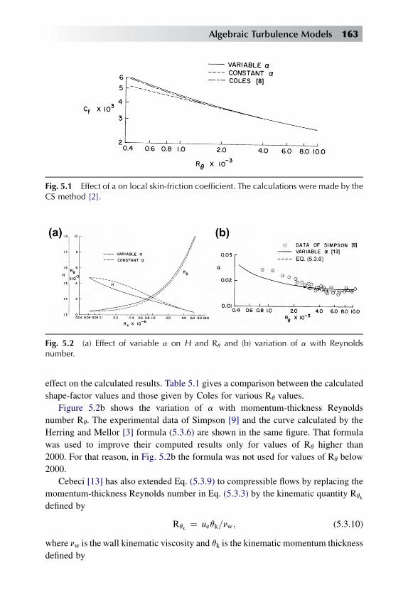
effect on the calculated results. Table 5.1 gives a comparison between the calculated

shape-factor values and those given by Coles for various Rq values.

Figure 5.2b shows the variation of a with momentum-thickness Reynolds

number Rq. The experimental data of Simpson [9] and the curve calculated by the

Herring and Mellor [3] formula (5.3.6) are shown in the same figure. That formula

was used to improve their computed results only for values of Rq higher than

2000. For that reason, in Fig. 5.2b the formula was not used for values of Rq below

2000.

Cebeci [13] has also extended Eq. (5.3.9) to compressible flows by replacing the

momentum-thickness Reynolds number in Eq. (5.3.3) by the kinematic quantity Rqk

defined by

Rqk ¼ ueqk=nw; (5.3.10)

where nw is the wall kinematic viscosity and qk is the kinematic momentum thickness

defined by

Fig. 5.1 Effect of a on local skin-friction coefficient. The calculations were made by theCS method [2].

Fig. 5.2 (a) Effect of variable a on H and Rq and (b) variation of a with Reynoldsnumber.


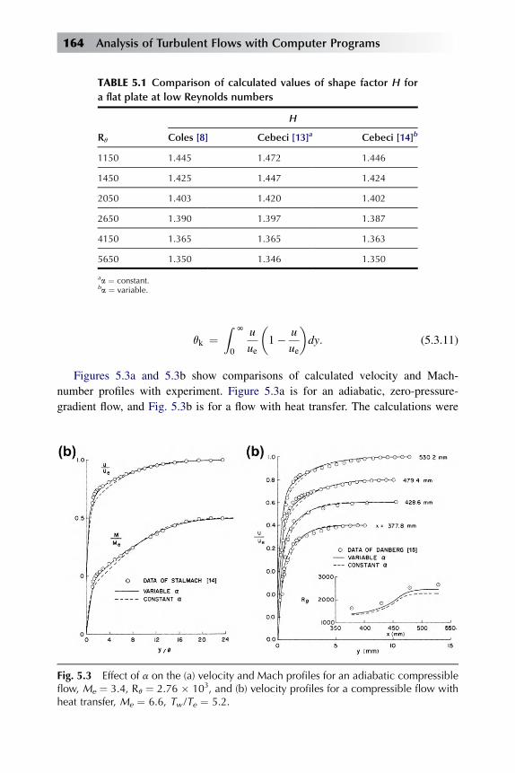
qk ¼Z N

0

u

ue

�1� u

ue

�dy: (5.3.11)

Figures 5.3a and 5.3b show comparisons of calculated velocity and Mach-

number profiles with experiment. Figure 5.3a is for an adiabatic, zero-pressure-

gradient flow, and Fig. 5.3b is for a flow with heat transfer. The calculations were

TABLE 5.1 Comparison of calculated values of shape factor H for

a flat plate at low Reynolds numbers

Rq

H

Coles [8] Cebeci [13]a Cebeci [14]b

1150 1.445 1.472 1.446

1450 1.425 1.447 1.424

2050 1.403 1.420 1.402

2650 1.390 1.397 1.387

4150 1.365 1.365 1.363

5650 1.350 1.346 1.350

aa ¼ constant.ba ¼ variable.

Fig. 5.3 Effect of a on the (a) velocity and Mach profiles for an adiabatic compressibleflow, Me ¼ 3.4, Rq ¼ 2.76 � 103, and (b) velocity profiles for a compressible flow withheat transfer, Me ¼ 6.6, Tw /Te ¼ 5.2.


made by the CS method. In one set of calculations, the parameter awas held constant

(¼ 0.0168); in the other, it varied according to Eq. (5.3.9), with Rqk given by

Eq. (5.3.10). Clearly, in all cases the agreement with experiment is better if a is

varied.

5.3.2 EFFECT OF TRANSVERSE CURVATURE

First-order boundary-layer theory is based on the assumption that the boundary-layer

thickness d is small in comparison with a characteristic length L. There are some

flows for which this assumption fails. Typical examples are long, slender bodies of

revolution with slender tails. In flows past these bodies, the thickness of the boundary

layer may be of the same order as, or larger than, a characteristic length, for example,

the body radius r0. As an example, consider an axial flow at zero incidence along

a cylinder. If the radius of the cylinder is large in comparison with the thickness of

the boundary layer d, the flow is essentially two-dimensional and is not significantly

different from flow past a flat plate. However, if the radius of the cylinder is small in

comparison with d, we may expect the flow to differ from the two-dimensional case,

since in that case the flow tends to wrap itself around the body. The effect, called the

transverse curvature (TVC) effect, strongly influences the skin-friction and heat-

transfer characteristics and must be taken into consideration in calculating the flow.

If thick axisymmetric turbulent boundary layers are to be calculated by means of

an eddy-viscosity concept, the question of the applicability of the two-dimensional

eddy-viscosity distribution immediately arises. If that distribution is not applicable,

how can the proper distribution for such flows be found?

The question was considered by Cebeci [16]. According to his study, the inner

eddy-viscosity distribution in such layers differs from the two-dimensional eddy-

viscosity distribution, but the outer eddy-viscosity distribution does not change, that

is, it is given by Eqs. (5.2.11b), (5.3.9), and (5.3.10). For thick axisymmetric

turbulent boundary layers, the inner eddy-viscosity formula is

ðεmÞi ¼ L2r0r

du

dy; (5.3.12)

where

L ¼ 0:4r0 ln ðr=r0Þ�1� exp

�� r0

Aln

�r

r0

��: (5.3.13)

As before, the damping length parameter, A, in Eq. (5.3.13) is given by Eq. (5.3.1).

Figures 5.4a and 5.4b show the comparison of calculated and experimental

velocity and Mach-number profiles. The experimental data are due to Richmond

[17]. The calculations were made by the CS method with the two-dimensional


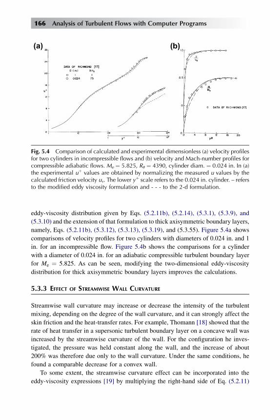
eddy-viscosity distribution given by Eqs. (5.2.11b), (5.2.14), (5.3.1), (5.3.9), and

(5.3.10) and the extension of that formulation to thick axisymmetric boundary layers,

namely, Eqs. (5.2.11b), (5.3.12), (5.3.13), (5.3.19), and (5.3.55). Figure 5.4a shows

comparisons of velocity profiles for two cylinders with diameters of 0.024 in. and 1

in. for an incompressible flow. Figure 5.4b shows the comparisons for a cylinder

with a diameter of 0.024 in. for an adiabatic compressible turbulent boundary layer

for Me ¼ 5.825. As can be seen, modifying the two-dimensional eddy-viscosity

distribution for thick axisymmetric boundary layers improves the calculations.

5.3.3 EFFECT OF STREAMWISE WALL CURVATURE

Streamwise wall curvature may increase or decrease the intensity of the turbulent

mixing, depending on the degree of the wall curvature, and it can strongly affect the

skin friction and the heat-transfer rates. For example, Thomann [18] showed that the

rate of heat transfer in a supersonic turbulent boundary layer on a concave wall was

increased by the streamwise curvature of the wall. For the configuration he inves-

tigated, the pressure was held constant along the wall, and the increase of about

200% was therefore due only to the wall curvature. Under the same conditions, he

found a comparable decrease for a convex wall.

To some extent, the streamwise curvature effect can be incorporated into the

eddy-viscosity expressions [19] by multiplying the right-hand side of Eq. (5.2.11)

Fig. 5.4 Comparison of calculated and experimental dimensionless (a) velocity profilesfor two cylinders in incompressible flows and (b) velocity and Mach-number profiles forcompressible adiabatic flows. Me ¼ 5.825, Rq ¼ 4390, cylinder diam. ¼ 0.024 in. In (a)the experimental uþ values are obtained by normalizing the measured u values by thecalculated friction velocity us. The lower yþ scale refers to the 0.024 in. cylinder. – refersto the modified eddy viscosity formulation and - - - to the 2-d formulation.


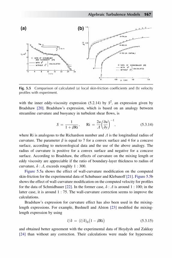
with the inner eddy-viscosity expression (5.2.14) by S2, an expression given by

Bradshaw [20]. Bradshaw’s expression, which is based on an analogy between

streamline curvature and buoyancy in turbulent shear flows, is

S ¼ 1

1þ bRi; Ri ¼ 2u

L

�vu

vy

��1

; (5.3.14)

where Ri is analogous to the Richardson number and L is the longitudinal radius of

curvature. The parameter b is equal to 7 for a convex surface and 4 for a concave

surface, according to meteorological data and the use of the above analogy. The

radius of curvature is positive for a convex surface and negative for a concave

surface. According to Bradshaw, the effects of curvature on the mixing length or

eddy viscosity are appreciable if the ratio of boundary-layer thickness to radius of

curvature, d : L, exceeds roughly 1 : 300.

Figure 5.5a shows the effect of wall-curvature modification on the computed

skin-friction for the experimental data of Schubauer and Klebanoff [21]. Figure 5.5b

shows the effect of wall-curvature modification on the computed velocity for profiles

for the data of Schmidbauer [22]. In the former case, d : L is around 1 : 100; in the

latter case, it is around 1 : 75. The wall-curvature correction seems to improve the

calculations.

Bradshaw’s expression for curvature effect has also been used in the mixing-

length expressions. For example, Bushnell and Alston [23] modified the mixing-

length expression by using

l=d ¼ ðl=dÞ0�1� bRi

�(5.3.15)

and obtained better agreement with the experimental data of Hoydysh and Zakkay

[24] than without any correction. Their calculations were made for hypersonic

Fig. 5.5 Comparison of calculated (a) local skin-friction coefficients and (b) velocityprofiles with experiment.


turbulent boundary layers. In Eq. (5.3.15), (l /d)0 represents the mixing-length

distribution given by Eq. (5.2.10b).

5.3.4 THE EFFECT OF NATURAL TRANSITION

In most practical boundary-layer calculations, it is necessary to calculate a complete

boundary-layer flow. That is, for a given pressure distribution and for a given tran-

sition point (natural), it is necessary to calculate laminar, transitional, and turbulent

boundary layers by starting the calculations at the leading edge or at the forward

stagnation point of the body. In most boundary-layer prediction methods, however,

the calculation of transitional boundary layers is avoided by assuming the transi-

tional region to be just a switching point between laminar and turbulent regions. In

general, especially at low Reynolds numbers, that is not a good procedure, and it can

lead to substantial errors. The point can best be described by an example. Consider

the flow past a turbine or compressor blade and assume two blade Reynolds numbers,

Rb ¼ 105 and 106. The extent of the transitional region on the blade at each of those

two Reynolds numbers can be estimated by using a correlation given by Chen and

Thyson [25]:

RDx ¼ Rxt � Rxtr ¼ CR2=3xt

; (5.3.16)

where RDx is the extent of the transition region, Rxtr is the Reynolds number based on

the distance to the start of the transition, and Rxt is the Reynolds number based on the

completion of transition. C is an empirical expression given by

C ¼ 60þ 4:86M1:92e 0 < Me < 5: (5.3.17)

The expressions (5.3.16) and (5.3.17) are based on the correlation of incompressible

and compressible adiabatic data for Mach numbers less than 5. If we assume that

transition starts at two points, namely, at the 10% and 50% chord points, the extents

of the transitional Reynolds number RDx for two blade Reynolds numbers Rb,

according to Eq. (5.3.16), are shown in Table 5.2.

The tabulated values of RDx clearly show that the transitional region is very

important and that it must be accounted for in order to make accurate boundary-layer

calculations. For example, for Rb ¼ 1 � 105 and transition starting at x/c ¼ 0.5, the

transition region is 0.81c in length, which means that the flow on the body from the

start of transition right up to the trailing edge is in a transitional state.

Naturally developing transition does not occur as a sharp, continuous front.

Instead, random spots of turbulence arise. Outside of these spots, the flow is still fully

laminar. The spots grow because fluid in contact with them is contaminated. While

growing, they are carried along by the flow. The net result is that they sweep out

wedges of about 8 or 9� half angle. As more and more spots are formed throughout


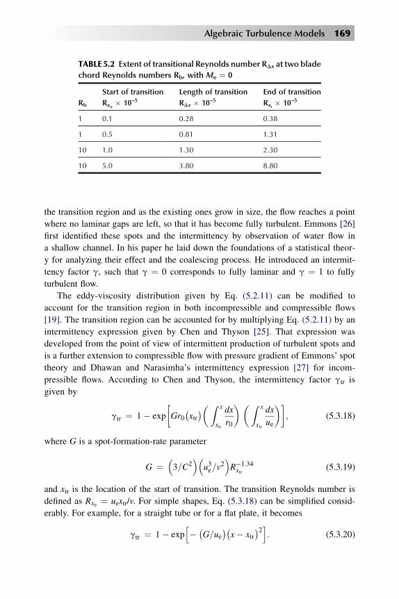
the transition region and as the existing ones grow in size, the flow reaches a point

where no laminar gaps are left, so that it has become fully turbulent. Emmons [26]

first identified these spots and the intermittency by observation of water flow in

a shallow channel. In his paper he laid down the foundations of a statistical theor-

y for analyzing their effect and the coalescing process. He introduced an intermit-

tency factor g, such that g ¼ 0 corresponds to fully laminar and g ¼ 1 to fully

turbulent flow.

The eddy-viscosity distribution given by Eq. (5.2.11) can be modified to

account for the transition region in both incompressible and compressible flows

[19]. The transition region can be accounted for by multiplying Eq. (5.2.11) by an

intermittency expression given by Chen and Thyson [25]. That expression was

developed from the point of view of intermittent production of turbulent spots and

is a further extension to compressible flow with pressure gradient of Emmons’ spot

theory and Dhawan and Narasimha’s intermittency expression [27] for incom-

pressible flows. According to Chen and Thyson, the intermittency factor gtr is

given by

gtr ¼ 1� exp

�Gr0

�xtr��Z x

xtr

dx

r0

� �Z x

xtr

dx

ue

��; (5.3.18)

where G is a spot-formation-rate parameter

G ¼3=C2

u3e=v

2R�1:34xtr

(5.3.19)

and xtr is the location of the start of transition. The transition Reynolds number is

defined as Rxtr ¼ uextr/v. For simple shapes, Eq. (5.3.18) can be simplified consid-

erably. For example, for a straight tube or for a flat plate, it becomes

gtr ¼ 1� exph� �

G=ue��x� xtr

�2i: (5.3.20)

TABLE 5.2 Extent of transitional Reynolds number RDx at two blade

chord Reynolds numbers Rb, with Me ¼ 0

Rb

Start of transition

Rxtr � 10–5Length of transition

RDx � 10–5End of transition

Rxt � 10–5

1 0.1 0.28 0.38

1 0.5 0.81 1.31

10 1.0 1.30 2.30

10 5.0 3.80 8.80


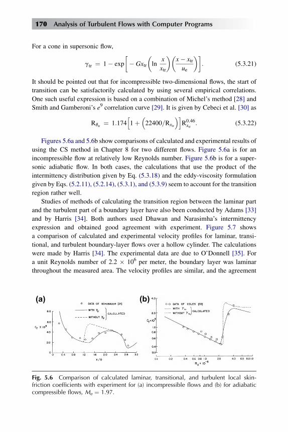
For a cone in supersonic flow,

gtr ¼ 1� exp

�� Gxtr

�ln

x

xtr

��x� xtrue

��: (5.3.21)

It should be pointed out that for incompressible two-dimensional flows, the start of

transition can be satisfactorily calculated by using several empirical correlations.

One such useful expression is based on a combination of Michel’s method [28] and

Smith and Gamberoni’s e9 correlation curve [29]. It is given by Cebeci et al. [30] as

Rqtr ¼ 1:174h1þ

22400=Rxtr

iR0:46xtr

: (5.3.22)

Figures 5.6a and 5.6b show comparisons of calculated and experimental results of

using the CS method in Chapter 8 for two different flows. Figure 5.6a is for an

incompressible flow at relatively low Reynolds number. Figure 5.6b is for a super-

sonic adiabatic flow. In both cases, the calculations that use the product of the

intermittency distribution given by Eq. (5.3.18) and the eddy-viscosity formulation

given by Eqs. (5.2.11), (5.2.14), (5.3.1), and (5.3.9) seem to account for the transition

region rather well.

Studies of methods of calculating the transition region between the laminar part

and the turbulent part of a boundary layer have also been conducted by Adams [33]

and by Harris [34]. Both authors used Dhawan and Narasimha’s intermittency

expression and obtained good agreement with experiment. Figure 5.7 shows

a comparison of calculated and experimental velocity profiles for laminar, transi-

tional, and turbulent boundary-layer flows over a hollow cylinder. The calculations

were made by Harris [34]. The experimental data are due to O’Donnell [35]. For

a unit Reynolds number of 2.2 � 106 per meter, the boundary layer was laminar

throughout the measured area. The velocity profiles are similar, and the agreement

Fig. 5.6 Comparison of calculated laminar, transitional, and turbulent local skin-friction coefficients with experiment for (a) incompressible flows and (b) for adiabaticcompressible flows, Me ¼ 1.97.


between the calculated results and experiment is very good (see Fig. 5.7a). For unit

Reynolds numbers of 9.45 � 106 per meter, laminar, transitional, and turbulent flow

occurred. Again the agreement between the calculated results and experiment is very

good, as is shown in Fig. 5.7b.

Separation-Induced Transition

The length of the transition region is also susceptible to the degree of freestream

turbulence, especially of large scale, flow separation and surface roughness,

decreasing rapidly as these features of the flow become more pronounced. While

these features are difficult to incorporate into expressions like Eq. (5.3.18), or to

correlate with data, in the case of two-dimensional low Reynolds-number flows, Eq.

(5.3.18) was extended by Cebeci [36] to model the transition region in separation

bubbles. The parameter C in Eq. (5.3.19) was expressed in terms of Rxtr and its

variation with Rxtr, with the onset of transition obtained from the en-method [38], is

shown in Fig. 5.8a, together with the experimental data obtained for four airfoils. The

data encompass a typical low Reynolds number range from chord Reynolds Rc ¼ 2.4

� 105 to 2� 106. They fall conveniently on a straight line on a semilog scale and can

be represented by the equation

C2 ¼ 213�log Rxtr � 4:7323

�: (5.3.23)

Figure 5.8b shows the results obtained with this modification to the CS model for the

ONERA-D airfoil examined by Cousteix and Pailhas [37] in a wind tunnel with

a chord Reynolds number, Rc, of 3 � 105 at zero angle of attack. The calculations

were made by using the interactive boundary layer method described in [38], with the

onset of transition calculated with the en-method.

Fig. 5.7 Comparison of calculated and experimental velocity profiles for laminar, tran-sitional, and turbulent boundary flows over a hollow cylinder. The calculations weremade by Harris [34]; L ¼ 2.54cm. (a) Laminar flow, R/m ¼ 2.2 � 106. (b) Laminar, tran-sitional, and turbulent flow, R/m ¼ 9.45 � 106.


The airfoil and mean velocity profiles shown in Fig. 5.8b indicate excellent

agreement between the measured and calculated results. For this flow, transition

occurred within the separated flow region and caused reattachment shortly

thereafter. The calculations revealed transition at x/c ¼ 0.81 with the en-method

in comparison with measurement which revealed transition at x/c ¼ 0.808.

Additional comparisons between calculations and experimental data are given

in [38].

5.3.5 EFFECT OF ROUGHNESS

The CS model discussed in the previous subsections was also extended by Cebeci

and Chang [39] to represent flow over rough walls without and with pressure

gradients. This was done by modifying the inner eddy viscosity formula with the help

of Rotta’s model [40] which recognized that the velocity profiles for smooth and

rough walls can be similar, provided that the coordinates are displaced; we rewrite L

in Eq. (5.2.12) with l given by Eq. (5.2.10a) as

L ¼ 0:4ðyþ DyÞ½1� expf � ðyþ DyÞ=Ag� (5.3.24)

and express Dy as a function of an equivalent sand-grain roughness parameter

kþs ðhksus=vÞ, i.e.

Dy ¼ 0:9�v=us

�� ffiffiffiffiffiffikþs

q� kþs exp

�� kþs =6

��

Fig. 5.8 (a) Variation of C2/3 with Rxtr and (b) comparison of calculated (solid lines) andmeasured (symbols) velocity profiles for the ONERA-D airfoil for a ¼ 0�, Rc ¼ 3.0 � 105.


given by Eq. (4.5.14) which is valid for

4:535 < kþs < 2000

with the lower limit corresponding to the upper bound for hydraulically smooth

surface.

It remains to provide a link between kþs and the geometry of a particular rough

surface. As was discussed in Section 4.5, Schlichting determined experimentally

equivalent sand roughness for a large number of roughnesses arranged in a regular

fashion. Dvorak established a correlation between the velocity shift Du and the

roughness density from which the equivalent sand roughness can be determined [41].

For the roughness elements other than the ones investigated by Schlichting and

Dvorak, the equivalent sand roughness must be determined experimentally or by

some empirical methods.

As we shall discuss later, for turbulent flows, it is sometimes more convenient to

use ‘‘wall’’ boundary conditions at some distance y0 away from the wall. Usually this

y0 is taken to be the distance, given by

y0 ¼ �v=us

�yþ0

with yþ0 given by 50 for smooth surfaces. In that case, the ‘‘wall’’ boundary

conditions for u and v can be represented by

u0 ¼ us

�1

kln

y0usv

þ c

�(5.3.25a)

y0 ¼ �u0y0us

dusdx

: (5.3.25b)

Here c is a constant equal to 5.2. Equation (5.3.25b) results from integrating the

continuity equation with u given by Eq. (4.2.1). The shear stress at y0, namely s0, isobtained from

s ¼ sw þ dp

dxyþ v

dusdx

Z yþ

0

�u

us

�2

dyþ (5.3.26)

In the viscous sublayer and in the buffer layer (yþ � 30), u/us can be obtained from

Thompson’s velocity profile given by Eq. (4.4.41). For yþ > 30 we can use the

logarithmic velocity formula, Eq. (9.3.1a). See subsection 9.3.1.

The above equations are also applicable to flows over rough walls provided we

replace c in Eq. (5.3.25a) with B, given by Eq. (4.5.6). The use of these boundary

conditions are especially advantageous for fully rough flow conditions because they

do not directly require ‘‘low Reynolds number’’ modifications.


Cebeci and Chang modification to the CS model to account for wall roughness

has been investigated for several flows by using the differential boundary layer

method described in Chapter 8 and in [38]. Here, of the several flows considered in

that study, two are presented below to demonstrate the accuracy of this model for

flows over rough walls.

Figure 5.9 presents measured values of momentum thickness, displacement

thickness, and skin-friction coefficients, reported by Betterman [42], together with

lines corresponding to the Cebeci-Chang calculations. The measurements corre-

spond to values of roughness density of 2.65 to 4.18 and roughness height between

2.4 and 4.0 mm. The equivalent sand roughness heights were calculated as described

in Section 4.5 based on the correlated results presented by Dvorak [41]. The

measured cf and Rq at the 0.4-m station, where initial perturbations have died down,

were used to generate initial data. As can be seen, the agreement is generally very

good, with the maximum discrepancy in skin-friction coefficient and integral

thicknesses amounting to approximately 5% and corresponding to the results

obtained with the longest roughness height.

Fig. 5.9 Results for Bettermann’s data (d computed, � 6 B data): (a) k ¼ 3 mm,l ¼ 2.65, ks ¼ 1.26 mm; (b) k ¼ 3 mm, l ¼ 3.30, ks ¼ 3.8 mm; (c) k ¼ 2.4 mm,l ¼ 4.13, ks ¼ 9.26 mm; (d) k ¼ 4.0 mm, l ¼ 4.18, ks ¼ 14.0 mm. In all cases,ue ¼ 30 m/s, v ¼ 1.44 � 10–5 m2/s.


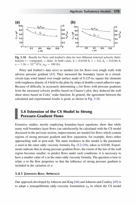
Perry and Joubert’s data serve as another test for flows over rough walls with

adverse pressure gradient [43]. They measured the boundary layers in a closed-

circuit-type wind tunnel over rough surface made of 0.125-in.-square bar elements

with roughness density of 4 held to the plate by strips of double-coated adhesive tape.

Because of difficulty in accurately determining cf for flows with pressure gradients

from the measured velocity profiles based on Clauser’s plot, they deduced the wall

shear stress based on Coles’ wake function. In general, the agreement between the

calculated and experimental results is good, as shown in Fig. 5.10.

5.4 Extension of the CS Model to StrongPressure-Gradient Flows

Extensive studies, mostly employing boundary-layer equations, show that while

many wall boundary-layer flows can satisfactorily be calculated with the CS model

discussed in the previous section, improvements are needed for flows which contain

regions of strong pressure gradient and flow separation, for example, flows either

approaching stall or post-stall. The main weakness in this model is the parameter

a used in the outer eddy viscosity formula, Eq. (5.2.11b), taken as 0.0168. Experi-

ments indicate that in strong pressure gradient flows, the extent of the law of the wall

region becomes smaller; to predict flows under such conditions, it is necessary to

have a smaller value of a in the outer eddy viscosity formula. The question is how to

relate a to the flow properties so that the influence of strong pressure gradient is

included in the variation of a.

5.4.1 JOHNSON–KING APPROACH

One approach developed by Johnson and King [44] and Johnson and Coakley [45] is

to adopt a nonequilibrium eddy-viscosity formulation εm in which the CS model

Fig. 5.10 Results for Perry and Joubert’s data for two different external velocity distri-butions (d computed, B data). In both cases, k ¼ 0.0104 ft, l ¼ 4.0, ks ¼ 0.0346 ft,v ¼ 1.56 � 10–4 ft2/s, uref ¼ 100 ft/s.


serves as an equilibrium eddy viscosity (εm)eq distribution. An ordinary differential

equation (ODE), derived from the turbulence kinetic energy equation, is used to

describe the streamwise development of the maximum Reynolds shear stress,

�ð9u0y0Þm, or ð�u0y0Þm for short, in conjunction with an assumed eddy-viscosity

distribution which hasffiffiffiffiffiffiffiffiffiffiffiffiffiffiffið�u0y0Þ

qm as its velocity scale. In the outer part of the

boundary layer, the eddy viscosity is treated as a free parameter that is adjusted to

satisfy the ODE for the maximum Reynolds shear stress. More specifically, the

nonequilibrium eddy-viscosity distribution is defined again by separate expressions in

the inner and outer regions of the boundary layer. In the inner region, (εm)i is given by

ðεmÞi ¼ ðεmiÞ1�1� g2

�þ �εmi

�J � Kg2 (5.4.1)

where (εmi)1 is given either by (ky)2vu/vy or usy. The expression (εmi

) J – K is

�εmi

�J�K

¼ D2kyum (5.4.2)

where

um ¼ max

�us;

ffiffiffiffiffiffiffiffiffiffiffiffiffiffiffiffiffiffi��u0y0�m

q �(5.4.3a)

and D is a damping factor similar to that defined by Eq. (5.2.12)

D ¼ 1� exp

� ffiffiffiffiffiffiffiffiffiffiffiffiffiffiffiffiffiffi��u0y0�m

qy

vAþ

�(5.4.3b)

with the value of Aþ equal to 17 rather than 26, as in Eq. (5.2.12). The parameter g2in Eq. (5.4.1) is given by

g2 ¼ tanh

�y

L0c

�(5.4.3c)

where, with ym corresponding to the y-location of maximum turbulent shear stress,

(�u0y0)m,

L0c ¼ usus þ um

Lm (5.4.4)

with

Lm ¼�0:4ym ym � 0:225d0:09d ym > 0:225d:

(5.4.5)

In the outer region, (εm)o is given by

ðεmÞo ¼ s�0:0168ued*g

�(5.4.6)


where s is a parameter to be determined. The term multiplying s on the righthand

side of Eq. (5.4.6) is the same as the expression given by Eq. (5.2.11b) without gtrand with a ¼ 0.0168.

The nonequilibrium eddy viscosity across the whole boundary-layer is computed

from

εm ¼ ðεmÞo tanh�ðεmÞiðεmÞo

�: (5.4.7)

The maximum Reynolds shear stress (�u0y0)m is computed from the turbulence

kinetic energy equation using assumptions similar to those used by Bradshaw et al.

(see subsection 6.3.1). After the modeling of the diffusion, production and dissipa-

tion terms and the use of �� u0y0�m

km¼ a1 ¼ 0:25

the transport equation for (�u0y0)m with um now denoting the streamwise velocity at

ym, is written as

d

dx

�� u0y0�m

¼ a1�� u0y0

�m

Lmum

�� u0y0�1=2m;eq

� �u0y0

�1=2m

�� a1um

Dm (5.4.8)

where, with cdif ¼ 0.5, the turbulent diffusion term along the path of maximum

(�u0y0) is given by

Dm ¼ cdifa1d

�� u0y0�3=2m�

0:7� ðy=dÞm�(1�

" �� u0y0�m�� u0y0

�m;eq

#1=2): (5.4.9)

To use this closure model, the continuity and momentum equations are first

solved with an equilibrium eddy viscosity (εm)eq distribution such as in the CS

model, and the maximum Reynolds shear stress distribution is determined based on

(εm)eq, which we denote by (�u0y0)m,eq. Next the location of the maximum Reynolds

shear stress is determined so that ym and um can be calculated. The transport equation

for (�u0y0)m is then solved to calculate the nonequilibrium eddy-viscosity distribu-

tion εm given by Eq. (5.4.7) for an assumed value of s so that the solutions of the

continuity and momentum equations can be obtained. The new maximum shear

stress term is then compared with the one obtained from the solution of Eq. (5.4.8).

If the new computed value does not agree with the one from Eq. (5.4.8), a new value

of s is used to compute the outer eddy viscosity and eddy-viscosity distributions

across the whole boundary-layer so that a new (�u0y0)m can be computed from the

solution of the continuity and momentum equations. This iterative procedure of


determining s is repeated until (�u0y0)m is computed from the continuity and

momentum equations agrees with that computed from the transport equation, Eq.

(5.4.8).

5.4.2 CEBECI-CHANG APPROACH

Cebeci and Chang used another approach in order to improve the predictions of the

CS model for flows with strong adverse pressure gradient and separation [46]. They

related the parameter a to a parameter F, according to the suggestion of Simpson

et al. [47] by

a ¼ 0:0168

F1:5: (5.4.10)

Here (1 – F) denotes the ratio of the production of the turbulence energy by normal

stresses to that by shear stress, evaluated at the location where shear stress is

maximum, that is

F ¼ 1�24�u02 � y02

�vu=vx

�u0y0vu=vy

35m

: (5.4.11)

Before Eq. (5.4.10) can be used in Eq. (5.2.11b), an additional relationship between

ðu02 � y02Þ and ð�u0y0Þ is needed. For this purpose, the ratio in Eq. (5.4.11)

b ¼24u02 � y02

�u0y0

35m

(5.4.12)

is assumed to be a function of Rt ¼ sw=ð�9u0y0Þm which, according to the data of

Nakayama [48], can be represented by

b ¼ 6

1þ 2Rtð2� RtÞ (5.4.13a)

for Rt < 1.0. For Rt � 1.0, b is taken to be

b ¼ 2Rt

1þ Rt(5.4.13b)

Introducing the above relationships into the definition of F and using Eq. (5.4.7)

results in the following expression for a

a ¼ 0:0168

½1� bðvu=vxÞ=ðvu=vyÞ�1:5m

(5.4.14)

where b is given by Eq. (5.4.13).


Separation-Induced Transition

Another improvement to the CS model was made by replacing the intermittency

parameter g in Eq. (5.2.11b) by another intermittency expression recommended by

Fiedler and Head [49]. According to the experiments conducted by Fiedler and Head,

it was found that the pressure gradient has a marked effect on the distribution of

intermittency. Their experiments indicated that in the boundary-layer proceeding to

separation, the intermittent zone decreased in width and moved further from the

surface as shape factor H increased. The reverse trend was observed with decreasing

H in a favorable pressure gradient.

In the improved CS model the intermittency expression of Fiedler and Head is

written in the form

g ¼ 1

2

�1� erf

y� Yffiffiffi2

ps

�(5.4.15)

where Y and s are general intermittency parameters with Y denoting value of

y for which g ¼ 0.5 and s, the standard deviation. The dimensionless inter-

mittency parameters Y/d*, s/d* and d/d* expressed as functions of H are shown in

Fig. 5.11.

The predictions of the original and modified Cebeci-Smith turbulence models

were investigated for several airfoils [46] by using the interactive boundary-layer

Fig. 5.11 Variation of Y/d*, s/d* and d/d* with H according to the data of Fiedler andHead [49].


(IBL) method of Cebeci [38]. For each airfoil, the onset of the transition location

was computed with Michel’s correlation [28], and the calculated lift coefficients

were compared with data for a range of angles of attack, including stall and

post-stall.

Figures 5.12a and 5.12b show a sample of results obtained with the original and

modified CS models, the latter corresponding to the one in which a is computed

according to Eq. (5.4.14) and the intermittency factor due to Fiedler and Head. The

experimental data in Fig. 5.12a were obtained by Carr et al. [50] and in Fig. 5.12b by

Omar et al. [51].

As can be seen, the calculated results obtained with the modified CS model are

significantly better than those obtained with the original CS model. In both cases,

the calculated maximum lift coefficients with the original CS model are much

higher than those measured ones; in Fig. 5.12b, the clmaxis not predicted at all. The

modified CS model, on the other hand, in both cases, predicts the clmaxand produces

lift coefficients for post stall which are in agreement with the trend of measured

values.

Figures 5.13a and 5.13b show a comparison between the calculated and

experimental results in which the calculated ones were obtained by using the

modified CS and Johnson-King (JK) models. In both cases, the predictions of

the modified CS model are better than the JK model. For example, for the

NACA 0012 airfoil, Fig. 5.13a, the modified CS model predicts clmaxmore

accurately than the JK model. For the Boeing airfoil, the modified CS model

appears to predict post stall better than the JK model. For additional comparisons,

see [38].

Fig. 5.12 IBL results for the (a) NACA 0012 airfoil and (b) Boeing airfoil, MN ¼ 0.3.


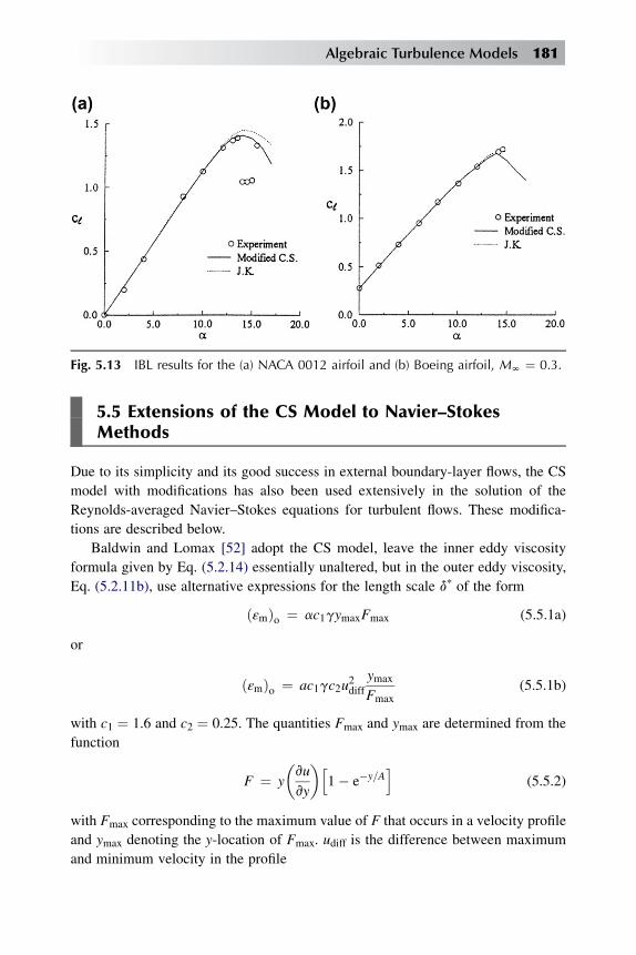
5.5 Extensions of the CS Model to Navier–StokesMethods

Due to its simplicity and its good success in external boundary-layer flows, the CS

model with modifications has also been used extensively in the solution of the

Reynolds-averaged Navier–Stokes equations for turbulent flows. These modifica-

tions are described below.

Baldwin and Lomax [52] adopt the CS model, leave the inner eddy viscosity

formula given by Eq. (5.2.14) essentially unaltered, but in the outer eddy viscosity,

Eq. (5.2.11b), use alternative expressions for the length scale d* of the form

ðεmÞo ¼ ac1gymaxFmax (5.5.1a)

or

ðεmÞo ¼ ac1gc2u2diff

ymax

Fmax(5.5.1b)

with c1 ¼ 1.6 and c2 ¼ 0.25. The quantities Fmax and ymax are determined from the

function

F ¼ y

�vu

vy

�h1� e�y=A

i(5.5.2)

with Fmax corresponding to the maximum value of F that occurs in a velocity profile

and ymax denoting the y-location of Fmax. udiff is the difference between maximum

and minimum velocity in the profile

Fig. 5.13 IBL results for the (a) NACA 0012 airfoil and (b) Boeing airfoil, MN ¼ 0.3.


udiff ¼ umax � umin (5.5.3)

where umin is taken to be zero except in wakes.

In Navier–Stokes calculations, Baldwin and Lomax replace the absolute value of

the velocity gradient vu/vy in Eqs. (5.2.14) and (5.5.2) by the absolute value of the

vorticity juj,��u�� ¼

��vuvy � vy

vx

�� (5.5.4a)

and the intermittency factory g in Eq. (5.2.11b) is written as

g ¼�1þ 5:5

�c3y

ymax

�6��1

(5.5.4b)

with c3 ¼ 0.3. The studies conducted by Stock and Haase [53] clearly demonstrate

that the modified algebraic eddy viscosity formulation of Baldwin and Lomax is not

a true representation of the CS model since their incorporation of the length scale in

the outer eddy viscosity formula is not appropriate for flows with strong pressure

gradients.

Stock and Haase proposed a length scale based on the properties of the mean

velocity profile calculated by a Navier–Stokes method. They recommend computing

the boundary-layer thickness d from

d ¼ 1:936ymax (5.5.5)

where ymax is the distance from the wall for which yjvu=vyj or F in Eq. (5.5.2) has its

maximum. With d known, ue in the outer eddy viscosity formula, Eq. (5.2.11b) is the

u at y ¼ d, and g is computed from

g ¼h1þ 5:5

yd

6i�1(5.5.6)

based on Klebanoff’s measurements on a flat plate flow and not from Eq. (5.5.4b).

The displacement thickness d* for attached flows is computed from its definition,

d* ¼Z d

0

�1� u

ue

�dy (5.5.7a)

and, for separated flows from

d* ¼Z d

yu¼0

�1� u

ue

�dy (5.5.7b)


either integrating the velocity profile from y ¼ 0, or y ¼ yu¼0 to d, or using the Coles

velocity profile. The results obtained with this modification to the length scale in the

outer CS eddy viscosity formula improve the predictions of the CS model in Navier–

Stokes methods as discussed in Stock and Haase [53].

A proposal which led to Eq. (5.5.5) was also made by Johnson [54]. He rec-

ommended that the boundary-layer thickness d is calculated from

d ¼ 1:2y1=2 (5.5.8)

where

y1=2 ¼ y atF

Fmax¼ 0:5: (5.5.9)

The predictions of the original and modified CS models were also investigated by

Cebeci and Chang by using the Navier-Stokes method of Swanson and Turkel [55] as

well as by the interactive boundary-layer method of Cebeci (see subsection 5.4.2).

The models considered include the original CS model, BL model, modifications to

the BL model and the JK model.

Figures 5.14a and 5.14b show the results obtained with the original CS and BL

models. In the former case, the length scale d* in the outer eddy-viscosity formula

was computed based on the definition of the boundary-layer thickness d given by

Stock and Haase [53] and Johnson [54].

Fig. 5.14 Navier–Stokes results for the (a) NACA 0012 airfoil and (b) Boeing airfoil,MN ¼ 0.3.


Figures 5.15a and 5.15b show similar comparisons with turbulence models

corresponding to the original CS and modified CS models. In the latter case the

boundary-layer thickness was computed from

d ¼ 1:5y1=2

or from

d ¼ ym

if 1.5y1/2 > ym, with ym corresponding to the location where streamwise velocity u is

maximum. Figures 5.16a and 5.16b show results obtained with turbulence models

based on modified CS and BL-JK models. In the latter case, the parameter a in the

BL method was taken as a variable computed by the JK method.

A comparison of results presented in Figures 5.14 and 5.15 shows that for the

airfoil flows considered here, the results obtained with the original CS model

(Fig. 5.14) with d defined by Stock and Haase [53] and Johnson [54] are slightly

better than those given by the BL model and the results with the modified CS model

(Fig. 5.15) are much better than all the other modified versions of the original CS

model.

A comparison of the results obtained with the modified CS model and with the

BL-JK model (Fig. 5.16) show that both models essentially produce similar results.

Finally, Fig. 5.17 shows a comparison between the predictions of the IBL and NS

methods. In both methods, the turbulence model used is the modified CS model. As

can be seen, the predictions of both methods are identical at low and moderate angles



of attack. At higher angles, especially near stall and post stall, while there are some

differences, both methods predict the stall angle well. The requirements for the

computer resources for the IBL method, however, are considerably less than those

provided by the Navier–Stokes method.

5.6 Eddy Conductivity and Turbulent PrandtlNumber Models

Using Boussinesq’s eddy-conductivity concept, we can write the transport of heat

due to the product of time mean of fluctuating enthalpy h0 and fluctuating velocity y0

in the form

�9y0h0 ¼ 9εh�vh=vy

�: (5.6.1)

Sometimes it has been found to be convenient to introduce a ‘‘turbulent’’ Prandtl

number Prt defined by

Prt ¼ εm=εh: (5.6.2)

It is obvious from Eq. (5.6.1) that in order to predict temperature distribution within

a boundary layer, it is necessary to describe the distribution of εh in the layer. For that

reason, various assumptions have been made and several models have been proposed

for εh. One assumption that has been used extensively is due to Reynolds [56].

According to his assumption, heat and momentum are transferred by the same



process, which means that the eddy coefficients for momentum and heat transport are

the same. That assumption leads to a turbulent Prandtl number of unity. The literature

discusses the relationship between those coefficients at great length (see, e.g., Kestin

and Richardson [57]) without definite conclusions. According to mercury experi-

ments in pipes, Prt > 1; according to gas experiments in pipes, Prt < 1. From the

experiments, it is not clear whether or not the eddy conductivity and, consequently,

the turbulent Prandtl number are completely independent of the molecular Prandtl

number.

One of the first proposals for a modification of the Reynolds analogy was made

by Jenkins [58], who took into consideration the heat conduction to or from an

element of an eddy during its movement transverse to the main flow. He assumed that

if the temperature of the eddy did not change in transit, the definition of mixing

length, l ¼ us (vu/vy)–1, and the definition of eddy conductivity, Eq. (5.6.1), would

give εh ¼ ly0, since T 0 ¼ l(vT/vy). However, if heat were lost during transit, the

fluctuation temperature T 0 would actually be less than that, because of molecular

thermal conductivity. Then the eddy conductivity would be

εh ¼ ly0Tf � TilðvT=vyÞ ; (5.6.3)

where Tf and Ti are the final and the initial eddy mean temperatures, respectively. In

order to obtain an expression for (Tf – Ti)/l(vT/vy), Jenkins assumed that the eddies

were spheres of radius l, the mixing length, with the surface temperature of the

particles varying linearly with time during their movement. The interval of time

between an eddy’s creation and its destruction was taken to be l/v0. Using Carslaw

Fig. 5.17 Comparison of NS and IBL results obtained with the modified CS model forthe (a) NACA 0012 airfoil and (b) Boeing airfoil, MN ¼ 0.3.


and Jaeger’s formula for the average temperature of a sphere under those conditions,

he obtained an expression for Eq. (5.6.3).

Treating the effects of molecular viscosity on an eddy in movement in the same

way as the effects of molecular thermal conductivity, Jenkins obtained the following

expression for the ratio of eddy conductivity to eddy viscosity:

εh

εmh

1

Prt

¼ 1

Pr

8><>:

2

15��12=p6

�εþm

nXN

n¼1

�1=n6

��1� exp

�� n2p2=εþm��o

2

15��12=p6

�Prεþm

nXN

n¼1

�1=n6

��1� exp

�� n2p2=Prεþm��o

9>=>;:

(5.6.4)

The variation of εh/εm with Pr for various values of εþmðhεm=vÞ according to Eq.

(5.6.4) is shown in Fig. 5.18. Calculations made at low Prandtl numbers with the data

of Fig. 5.18 for the relationship between εh and εm are in fair agreement with

experiment [59], although the more recent experimental data for liquid metals

suggest that the loss of heat by an eddy in transit is not as great as that predicted by

Jenkins. Furthermore, according to the experimental data of Page et al. [60] for air at

Pr ¼ 0.7, the eddy conductivity is greater than the eddy viscosity. Jenkins’ result

Fig. 5.18 Variation of reciprocal of turbulent Prandtl number with molecular Prandtlnumber for various values of εþm, according to Eq. (5.6.4).


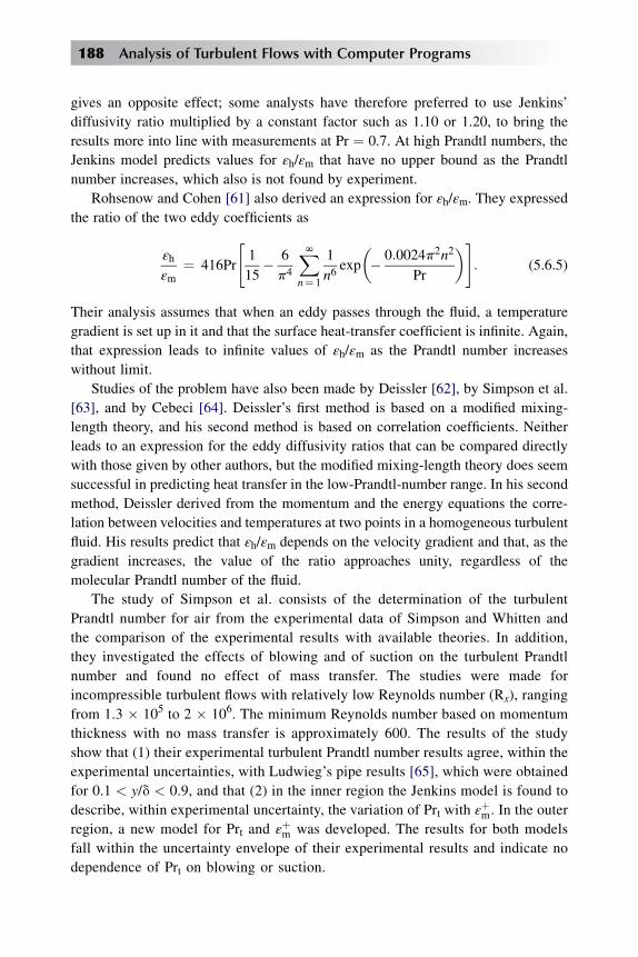
gives an opposite effect; some analysts have therefore preferred to use Jenkins’

diffusivity ratio multiplied by a constant factor such as 1.10 or 1.20, to bring the

results more into line with measurements at Pr ¼ 0.7. At high Prandtl numbers, the

Jenkins model predicts values for εh/εm that have no upper bound as the Prandtl

number increases, which also is not found by experiment.

Rohsenow and Cohen [61] also derived an expression for εh/εm. They expressed

the ratio of the two eddy coefficients as

εh

εm¼ 416Pr

"1

15� 6

p4

XNn¼ 1

1

n6exp

�� 0:0024p2n2

Pr

�#: (5.6.5)

Their analysis assumes that when an eddy passes through the fluid, a temperature

gradient is set up in it and that the surface heat-transfer coefficient is infinite. Again,

that expression leads to infinite values of εh/εm as the Prandtl number increases

without limit.

Studies of the problem have also been made by Deissler [62], by Simpson et al.

[63], and by Cebeci [64]. Deissler’s first method is based on a modified mixing-

length theory, and his second method is based on correlation coefficients. Neither

leads to an expression for the eddy diffusivity ratios that can be compared directly

with those given by other authors, but the modified mixing-length theory does seem

successful in predicting heat transfer in the low-Prandtl-number range. In his second

method, Deissler derived from the momentum and the energy equations the corre-

lation between velocities and temperatures at two points in a homogeneous turbulent

fluid. His results predict that εh/εm depends on the velocity gradient and that, as the

gradient increases, the value of the ratio approaches unity, regardless of the

molecular Prandtl number of the fluid.

The study of Simpson et al. consists of the determination of the turbulent

Prandtl number for air from the experimental data of Simpson and Whitten and

the comparison of the experimental results with available theories. In addition,

they investigated the effects of blowing and of suction on the turbulent Prandtl

number and found no effect of mass transfer. The studies were made for

incompressible turbulent flows with relatively low Reynolds number (Rx), ranging

from 1.3 � 105 to 2 � 106. The minimum Reynolds number based on momentum

thickness with no mass transfer is approximately 600. The results of the study

show that (1) their experimental turbulent Prandtl number results agree, within the

experimental uncertainties, with Ludwieg’s pipe results [65], which were obtained

for 0.1 < y/d < 0.9, and that (2) in the inner region the Jenkins model is found to

describe, within experimental uncertainty, the variation of Prt with εþm: In the outer

region, a new model for Prt and εþm was developed. The results for both models

fall within the uncertainty envelope of their experimental results and indicate no

dependence of Prt on blowing or suction.


The approach taken by Cebeci [64] is based on the mixing-length concept. It

differs from others in that his eddy-conductivity expression (1) provides a continuous

temperature distribution across the boundary layer, (2) accounts for the mass transfer

and the pressure gradient, and (3) accounts for both low-and-high-Prandtl-number

fluids. According to this model, the turbulent Prandtl number is given by

Prt ¼ k½1� expð� y=AÞ�kh½1� expð� y=BÞ�: (5.6.6a)

At the wall,

Prt ¼ k

kh

B

A¼ k

kh

Bþ

Aþ: (5.6.6b)

Note that as y becomes larger, the exponential terms in Eq. (5.6.6a) approach zero.

The turbulent Prandtl number then becomes

Prt ¼ k=kh: (5.6.6c)

We also note from Eq. (5.6.6) that the molecular Prandtl number plays a strong role

in Prt close to the wall, since Bþ ¼ Bþ(Pr), and has no effect on Prt away from the

wall.

The damping constant in Eq. (5.6.6) is for air, whose Prandtl number is

approximately 0.7. For fluids other than air it varies since Bþ is a function of the

molecular Prandtl number. If we assume that k, kh, and Aþ are 0.40, 0.44, and 26,

respectively, Bþ can be calculated from Eq. (5.6.6b), provided that the Prt is known at

the wall. Following that procedure and using the experimental values of Prt, Na and

Habib [66] expressed the variation of Bþwith Pr, for a range of Pr from 0.02 to 15, by

B ¼ Bþvus

; Bþ ¼ Bþþ=ðPrÞ1=2; (5.6.7)

where Bþþ is represented by the following formula:

Bþþ ¼X5i¼ 1

Ciðlog10 PrÞi�1; (5.6.8)

with C1 ¼ 34.96, C2 ¼ 28.79, C3 ¼ 33.95, C4 ¼ 6.33, and C5 ¼ –1.186.

To account for the low Reynolds number effects (Rq < 5000) for air with Pr ¼ 1,

kh and Bþ are represented by

kh ¼ 0:44þ 0:22

1þ 0:42z22;Bþ ¼ 35þ 25

1þ 0:55z22; (5.6.9)

where z2hRq � 10�3 � 0:3.


Equation (5.6.6) with B and A given by (5.6.7) and (5.2.13) is restricted to

incompressible flows without pressure gradient. It can easily be extended to

compressible flows by replacing A by Eq. (5.3.1) with N given by Eq. (5.3.2c) and by

replacing B by

B ¼ Bþ v

N

�sw9w

��1=2�9

9w

�1=2

: (5.6.10)

The expression for the turbulent Prandtl number given by Eq. (5.6.6) has been

evaluated for flows with and without mass transfer by comparing its predictions with

experiment and with other predictions.

For an incompressible flow with no mass transfer, Figures 5.19a and 5.19b show

the variation of the turbulent Prandtl number with yþ and εþm respectively, according

to the Cebeci model for Rq ¼ 1000 and 4000 and according to Jenkins’ model. Also

shown is the uncertainty envelope and the variation of the mean turbulent Prandtl

number determined by Simpson et al. [63] from their experimental data. We note that

the values of Prt calculated by Eq. (5.6.6) show a slight Reynolds-number effect for

Rq < 4000, an effect that was also observed by Simpson et al. The predicted results

fall within the uncertainty envelope and agree well in both inner and outer regions,

with the predictions of Jenkins in the inner region (yþ < 102), and with the exper-

imental data of Simpson et al.

Figure 5.20a shows the variation of turbulent Prandtl number with y/d for Rq

values of 1000 and 4000. It also shows the uncertainty envelope of Simpson et al. and

the experimental data of Johnson [67] and of Ludwieg [65]. The experimental data of

Johnson are for flat-plate flow at high Reynolds numbers. Johnson studied the

temperature distribution downstream of an unheated starting length where

the thermal boundary layer was contained at all times in an inner fraction of the

momentum boundary layer, which provided no information about the outer region.

He compared the turbulent shear stress and the heat flux obtained by hot-wire

Fig. 5.19 Variation of turbulent Prandtl number (a) with yþ and (b) with εþm:


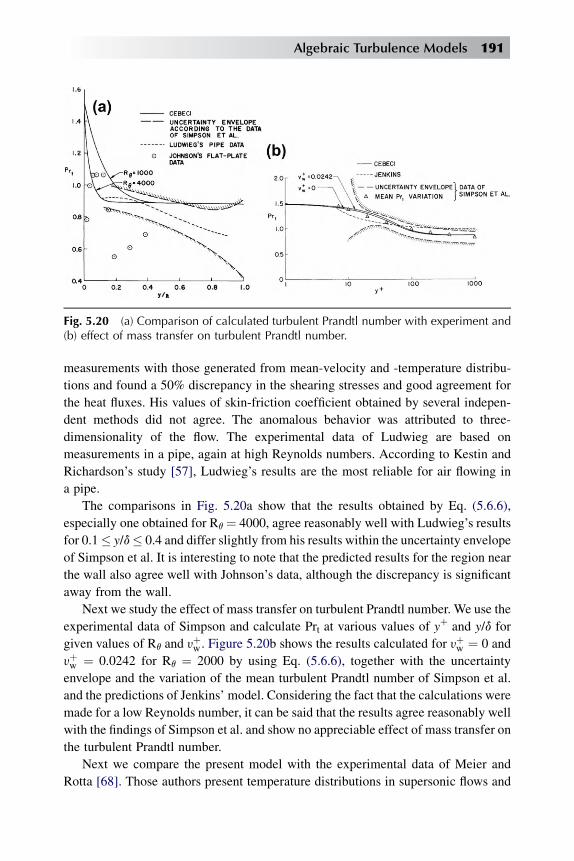
measurements with those generated from mean-velocity and -temperature distribu-

tions and found a 50% discrepancy in the shearing stresses and good agreement for

the heat fluxes. His values of skin-friction coefficient obtained by several indepen-

dent methods did not agree. The anomalous behavior was attributed to three-

dimensionality of the flow. The experimental data of Ludwieg are based on

measurements in a pipe, again at high Reynolds numbers. According to Kestin and

Richardson’s study [57], Ludwieg’s results are the most reliable for air flowing in

a pipe.

The comparisons in Fig. 5.20a show that the results obtained by Eq. (5.6.6),

especially one obtained for Rq ¼ 4000, agree reasonably well with Ludwieg’s results

for 0.1� y/d� 0.4 and differ slightly from his results within the uncertainty envelope

of Simpson et al. It is interesting to note that the predicted results for the region near

the wall also agree well with Johnson’s data, although the discrepancy is significant

away from the wall.

Next we study the effect of mass transfer on turbulent Prandtl number. We use the

experimental data of Simpson and calculate Prt at various values of yþ and y/d for

given values of Rq and yþw. Figure 5.20b shows the results calculated for yþw ¼ 0 and

yþw ¼ 0.0242 for Rq ¼ 2000 by using Eq. (5.6.6), together with the uncertainty

envelope and the variation of the mean turbulent Prandtl number of Simpson et al.

and the predictions of Jenkins’ model. Considering the fact that the calculations were

made for a low Reynolds number, it can be said that the results agree reasonably well

with the findings of Simpson et al. and show no appreciable effect of mass transfer on

the turbulent Prandtl number.

Next we compare the present model with the experimental data of Meier and

Rotta [68]. Those authors present temperature distributions in supersonic flows and

Fig. 5.20 (a) Comparison of calculated turbulent Prandtl number with experiment and(b) effect of mass transfer on turbulent Prandtl number.


turbulent Prandtl number distributions obtained from their experimental data. They

point out that the results of their turbulent-Prandtl-number distribution for such flows

are in excellent agreement with those of Simpson et al. [63], who carried out

measurements at low subsonic speeds on a porous plate. They further point out that if

they express Prandtl’s mixing-length expression in the form written by Van Driest,

that is,

lh ¼ khyh1� exp

� yðsw9Þ1=2=mBþ

i; (5.6.11)

and use the restrictions

y ¼ 0; Prt ¼�k

kh

Bþ

Aþ

�2

y/d; Prt ¼�k

kh

�2

; (5.6.12)

then the calculated temperature distributions are in excellent agreement with their

experimental data, provided that they choose the constants in Eqs. (5.6.11) and

(5.6.12) as k ¼ 0.40, kh ¼ 0.43, Aþ ¼ 26, and Bþ ¼ 33.8, four empirical constants

that compare reasonably well with those used in Eq. (5.6.6). Figures 5.21a and 5.21b

show the experimental Prt variation for Meier and Rotta’s experiment, together with

calculated and experimental temperature distributions taken from Meier and Rotta

[68].

We now show the heat-transfer results obtained for pipe flow by using the Cebeci

model. The calculations were made by Na and Habib [66] for fluids with low,

medium, and high Prandtl numbers (Pr ¼ 0.02�15). Figure 5.22 shows comparisons

of calculated and experimental values of Nusselt number Nu, defined as

Nu ¼ hd=k; (5.6.13)

Fig. 5.21 (a) Prt variation in the boundary layer and (b) effect of variable Prt on thecalculated temperature distributions [68].


for various values of Peclet number Pe, defined as

Pe ¼ Rd Pr; (5.6.14)

for two different fluids. Figure 5.22a shows the results for mercury and Figure 5.22b

for air. In Eq. (5.6.13) h is the heat-transfer-film coefficient, d is the pipe diameter,

and k is the thermal conductivity of the fluid. In Eq. (5.6.14) Rd is the Reynolds

number defined as

Rd ¼ ud=v; (5.6.15)

where u is the mean velocity.

Figure 5.23a shows comparisons of calculated and experimental Stanton numbers

St, defined as

St ¼ Nu=ðRd PrÞ: (5.6.16)

Fig. 5.22 Comparison of calculated and experimental values of Nusselt number fora turbulent pipe flow at different values of (a) Peclet number and (b) Reynolds number.

Fig. 5.23 Comparison of calculated and experimental values of (a) Stanton number and(b) static-enthalpy profiles for a turbulent pipe flow at different values of Reynoldsnumber and Prandtl number.


and Fig. 5.23b shows comparisons of calculated and experimental dimensionless

static-enthalpy profiles hþ

hþ ¼ hw � h

hs; hs ¼ qw

9

1

us(5.6.17)

for Prandtl numbers of 0.72 and 0.02. Again the agreement with experiment is very

good.

5.7 CS Model for Three-Dimensional Flows

With the eddy viscosity concept, the boundary-layer equations for three-dimensional

turbulent flows can be expressed in the same form as those for laminar flows,

�9u0y0 ¼ 9εmvu

vy; �9w0y0 ¼ 9εm

vw

vy(5.7.1)

Here �9u0y0 denotes the shear stress acting in the x-direction on a plane parallel to

the xz-plane, and �9w0y0, usually written as �9y0w0, the shear stress acting in the

z-direction on the same plane. Almost all workers have inferred, from the fact that

the choice of direction of the axes in the xz-plane is arbitrary, that the assumptions

made for �9y0w0 should be closely analogous to those made for �9u0y0. Mathe-

matically, they assume that the turbulence model equation for �9y0w0 should be

obtainable from that for �9u0y0 by cyclic interchange of symbols. However, it is not

so obvious that the equations for �9u0y0 can be simply derived from models used for

a two-dimensional flow. The argument commonly used is that turbulence, being

instantaneously three-dimensional, should not be seriously affected by moderate

three-dimensionality of the mean flow. There is, of course, a loss of symmetry, for

instance, y0w0 is zero in a two-dimensional flow but not in a three-dimensional flow,

and Rotta [69] has shown that the asymmetry can noticeably affect the modeling of

the shear-stress equations.

The law of the wall [Eq (4.2.1)] and the mixing-length formula

vu

vy¼ ðs=9Þ1=2

ky(5.7.2)

are the foundations of most methods for two-dimensional flows. Clearly, Eq. (5.2.11)

requires modification since the velocity now has an extra component. The local

equilibrium arguments suggest that it should still be valid in a three-dimensional flow

if the x-axis is taken to coincide with the direction of the shear stress at height y. The

assumption of local equilibrium between the magnitudes of s and vu/vy that leads to


Eq. (5.7.2) implies, when it is taken at face value, that there should be local equi-

librium, that is, coincidence between their directions. This leads to

vu

vy¼ �u0y0

ðs=9Þ1=2ky(5.7.3a)

vw

vy¼ �y0w0

ðs=9Þ1=2ky(5.7.3b)

where

s ¼h�9u0y0

�2þ�9y0u0�2i1=2

The argument is not, of course, very convincing – the local equilibrium is an

approximation whose limits of validity need further investigation by experiment.

Experiments in three-dimensional flows, particularly measurements of y0w0, aredifficult, and there is evidence both for and against Eq. (5.7.3). A safe position to take

is that local equilibrium concepts are not likely to fail catastrophically as soon as the

mean flow becomes slightly three-dimensional, and indeed the calculation methods

that use Eq. (5.7.3) seem to agree acceptably with most of the experimental data not

too near separation, as we shall see in this section.

An undeniable difficulty in treating three-dimensional wall layers is that the

viscous sublayer is not a local-equilibrium region; there is a transfer of turbulent

energy toward the wall by the turbulent fluctuations themselves to compensate for

viscous dissipation. Therefore, conditions at one value of y depend on conditions at

the other values of y, and although the directions of velocity gradient and of shear

stress coincide at the surface (Reynolds stresses negligible) and, according to Eq.

(5.7.3), again coincide outside the sublayer, they may differ within the sublayer. As

a result, the direction of the velocity outside the sublayer may differ from that of the

shear stress or velocity gradient. In practical terms, the constant of integration in any

velocity profile derived from Eq. (5.7.3), or the damping length constant, A in Eq.

(5.2.12), will have two components. The effect will be significant only if the

direction of the shear stress changes significantly across the sublayer. Since at the

surface, vsx=vy ¼ vp=vx and vsz=vy ¼ vp=vz, this will occur only if there is

a significant pressure gradient normal to the wall-stress vector, as for example in

a boundary layer flowing into a lateral bend ðvwe=vxs0Þ. Van den Berg [70] has

proposed a dimensionally correct empirical correlation taking the x-axis in the

direction of the wall shear stress, the z-component velocity at the outer edge of the

sublayer is 12usðv=9u3sÞvp=vz.The outer layer, like the sublayer, is not a local equilibrium region, and the

direction of the shear stress will lag behind the direction of the velocity gradient if


the latter changes with x. Several experiments have shown that angles between the

shear stress and velocity gradient vectors are of the same order as that of the cross-

flow (i.e., the angle between the external velocity and the surface shear stress).

However, the accuracy of prediction of the boundary-layer thickness and the surface

shear-stress vector does not depend critically on the shear-stress direction in the

outer layer, and good agreement has been obtained between the available data and

an extension of the CS eddy-viscosity formulation for two-dimensional flows in

which the velocity defect used in Eq. (5.2.11b) is just taken as the magnitude of the

vector (ute – ut) at given y. The same eddy viscosity is used in Eq. (5.7.2) so that the

directions of shear stress and velocity gradient are equated. According to [71],

a generalization of the CS eddy-viscosity formulation for three-dimensional

boundary layers is

ðεmÞi ¼ l2��

vu

vy

�2

þ�vw

vy

�2�12

0 � y � yc (5.7.4a)

ðεmÞo ¼ a

��Z d

0ðute � utÞdy

�� yc � y � d (5.7.4b)

with a ¼ 0.0168 for small adverse pressure gradient flows. Its variation with strong

pressure gradient flows can again be expressed by a generalization of Eq. (5.4.14),

but this has not been attempted yet.

In Eq. (5.7.4a), the mixing length l is given by Eq. (5.2.12) with A and N defined

by Eqs. (5.3.1) and (5.3.2a) except that now

us ¼�st9

�12

max

;

�st9

�max

¼ v

��vu

vy

�2

þ�vw

vy

�2�12

max

(5.7.5)

In Eq. (5.7.4b), ute and ut are the total edge and local velocites defined by

ute ¼ �u2e þ w2

e

�1=2(5.7.6a)

ut ¼ �u2 þ w2

�1=2: (5.7.6b)

In the following subsections we present an evaluation of this turbulence model

with experimental data for three-dimensional incompressible flows.

5.7.1 INFINITE SWEPT WING FLOWS

The accuracy of the CS turbulence model of this section and other models has been

investigated for several infinite swept wing flows, as discussed in [71]. Here we


present a sample of results taken from those studies and discuss first the results

for the data of Bradshaw and Terrell [72] and then for the data of Cumpsty and

Head [73].

Data of Bradshaw and Terrell

This experiment was set up especially to test the outer-layer assumptions made in

extending the boundary-layer calculation method of Bradshaw et al. [74] from two

dimensions to three [75]. Measurements were made only on the flat rear of the wing

in a region of nominally zero pressure gradient and decaying cross flow. See the

sketch in Fig. 5.24a. Spanwise and chordwise components of mean velocity and

shear stress, and all three components of turbulence intensity, were measured at

a number of distances x 0 ¼ 0, 4, 10, 16 and 20 in. from the start of the flat portion of

the wing (Fig. 5.24). The surface shear stress, measured with a Preston tube, was

constant along a generator to the start of the flat part of the wing, except for a few

inches at each end and except for small undulations of small spanwise wavelength

caused by residual nonuniformities in the tunnel flow.

Fig. 5.24 Results for the relaxing flow of Bradshaw and Terrell: (a) wall cross-flowangle and local skin friction, (b) velocity profiles, (c) cross-flow angle distributions.The symbols denote the experimental data, the solid line the numerical solutions ofCebeci [76] and the dashed line the numerical solutions of Bradshaw et al. [74].


Figure 5.24 shows the calculated results (solid lines) with experimental results

(symbols) and those obtained by Bradshaw’s method [74] (dashed lines). The cross-

flow angle b which represents the departure of the velocity vector within the

boundary-layer from the freestream velocity vector was computed from

bhtan�1wu

(5.7.7a)

The above formula becomes indeterminate at y ¼ 0; however, with the use of

L’Hopital’s rule, it can be written as

bw ¼ tan�1

��vw

vy

�w

�vu

vy

��1

w

�(5.7.7b)

The streamwise component of the local skin-friction coefficient cfs was calculated

from

cfs ¼ sws

129U

2s

(5.7.8)

with swsand Us given by

sws¼swxcosfþ swz

sinf (5.7.9a)

Us ¼ uecosf

; f ¼ tan�1

�we

ue

�(5.7.9b)

Here swxand swz

denote the wall shear values in the x- and z-directions, respectively,

obtained from the solution of the infinite swept wing equations.

Data of Cumpsty and Head

In this experiment [73] the boundary-layer development was measured on the rear of

a wing swept at 61.1�. The boundary-layer separated at about 80% chord. The

measured profiles were affected by traverse gear ‘‘blockage,’’ probably because of

upstream influence of disturbance caused to the separated flow by the wake of the

traverse gear.

Figure 5.25 shows a comparison of calculated and measured streamwise velocity

profiles us/Us and streamwise momentum thickness q11 defined by

q11 ¼Z d

0

usUs

�1� us

Us

�dy (5.7.10)

where us/Us is calculated from

usUs

¼ u

uecos2 fþ w

wesin2 f (5.7.11)


The results in Fig. 5.25 show good agreement with experiment at two x-stations.

However, with increasing distance they begin to deviate from experimental values

and at x ¼ 0.650 ft, the agreement becomes poor.

The above results indicate what was already observed and discussed in relation to

the shortcomings of the Cebeci-Smith algebraic eddy-viscosity formulation, that is,

it requires improvements for strong adverse pressure gradient flows. As discussed

in subsection 5.4.2, the improvements to this formulation were made for two-

dimensional flows by allowing a in the outer eddy-viscosity formula to vary. A

similar improvement is needed to the formulation for three-dimensional flows.

5.7.2 FULL THREE-DIMENSIONAL FLOWS

To illustrate the evaluation of the CS model for full three-dimensional flows, we

consider two flows corresponding to an external flow formed by placing an

obstruction in a thick two-dimensional boundary-layer (data of East and Hoxey) and

an external flow on a prolate spheroid at an incidence angle of 10� (data of Meier and

Kreplin).

Data of East and Hoxey

Figure 5.26 shows a schematic drawing of East and Hoxey’s test setup in which

a wing is placed in a thick two-dimensional boundary layer [77]. The strong pressure

gradients exposed by the obstruction caused the boundary layer to become three-

dimensional and to separate. The measurements were made in the three-dimensional

boundary layer upstream of and including the three-dimensional separation.

Fig. 5.25 Comparison of calculated (solid lines) and experimental (symbols) results forthe data of Cumpsty and Head on the rear of a swept infinite wing.


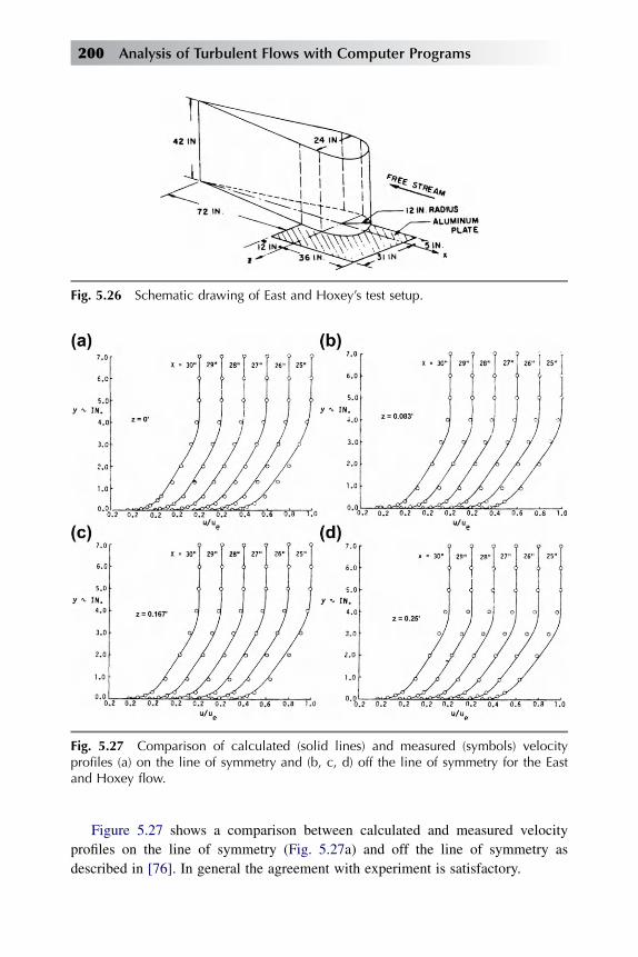
Figure 5.27 shows a comparison between calculated and measured velocity

profiles on the line of symmetry (Fig. 5.27a) and off the line of symmetry as

described in [76]. In general the agreement with experiment is satisfactory.

Fig. 5.26 Schematic drawing of East and Hoxey’s test setup.

Fig. 5.27 Comparison of calculated (solid lines) and measured (symbols) velocityprofiles (a) on the line of symmetry and (b, c, d) off the line of symmetry for the Eastand Hoxey flow.


Data of Meier and Kreplin

Meier and Kreplin’s data correspond to laminar, transitional and turbulent flow on

a prolate spheroid with a thickness ratio of 6 for a Reynolds number of 6.6 � 106

[78–80]. As discussed in [81], the calculations for this flow were made for freestream

velocities of 45 and 55 m/s corresponding to natural and imposed transition. To

account for the transitional region between a laminar and turbulent flow, the right-

hand sides of Eqs. (5.7.4) are multiplied by the intermittency factor gtr, defined by

Eqs. (5.3.18) and (5.3.19). Since detailed and corresponding correlation formulas for

three-dimensional transitional flows are lacking, the same expression was used for

three-dimensional flows by using the local similarity assumption with ue in Eqs.

(5.3.18) and (5.3.19) replaced by the total velocity.

The experimental data of Meier et al. consists of surface shear stress magnitude

and direction vectors and velocity profiles over a range of angles of attack.

Figure 5.28a shows a comparison of calculated surface shear stress vectors in laminar

flow at a ¼ 10�. The magnitude of the shear stress vector is proportional to the shear

intensity. The agreement between the calculation and measurements on the wind-

ward side is generally good, although there are some differences that are partly due to

the use of inviscid potential flow in the calculations, whereas the measured pressure

distribution shows viscous-inviscid interaction effects. It is clear that the laminar

flow is separated on the leeward side of the body at some distance aft of the nose. The

origin or nature of the high shear intensities leeward of the separation line cannot be

determined from calculations because calculations based on external flow that is

purely inviscid is not expected to account for strong interactions.

Fig. 5.28 (a) Measured (/) and calculated (/) distributions of wall shear stressvectors

�cfhsw=12 9u

2a

�for laminar flow and (b) for laminar, transitional and turbulent

flow on a prolate spheroid at a ¼ 10� [81].


Figure 5.28b shows wall shear vectors for laminar, transitional and turbulent

flow with natural transition. In general, the calculated and measured results are in

agreement with discrepancies (which are small) confined to the region close to the

specified transition. More quantitative comparison with the imposed transition

Fig. 5.29 Measured (dashed line) and calculated (solid line) resultant wall shear stressvalues on the prolate spheroid at a ¼ 10� [81].

Fig. 5.30 Comparison of calculated (solid lines) and measured (symbols) streamwiseus /Us and crossflow us /Us velocity profiles [81].


experiment is afforded by Fig. 5.29 which displays circumferential distributions

of wall shear stress at four axial locations. The calculated results display the

correct trends and are within 15% of the measured values with discrepancies

tending to diminish with downstream distance. A sample of the velocity profiles

is shown in Fig. 5.30 and corresponds to x/2a of 0.48 and 0.73, and again the

agreement is within or very close to the error bounds of the measurements,

except in the regions where the inviscid velocity distribution differed from the

measured one. Additional comparisons of calculated and experimental data are

given in [81].

5.8 Summary

In the previous sections we have discussed coefficients for transport of momentum

and heat suitable for calculating two- and three-dimensional turbulent boundary-

layer flows. We have shown how effects such as mass transfer, heat transfer, pressure

gradient, etc., can be included in the empirical relations in order to calculate

turbulent flows for a wide range of conditions. Although these relations lack rigor

and do not improve any fundamental understanding of turbulence, they provide

results that are very useful in engineering calculations.

On the basis of comparisons presented in this chapter and those in Chapter 8,

we recommend the following eddy-viscosity formulation for calculating two-

dimensional and axisymmetric and three-dimensional turbulent boundary layers:

The turbulent Prandtl number distribution is given by Eqs. (5.6.6), (5.6.7)

and (5.6.8).

Two-Dimensional Flows

Inner Region

ðεmÞi ¼ L2��vuvy

��gtr; 0 � y � yc; (5.8.12)

Outer Region

ðεmÞo ¼ a

Z N

0ðue � uÞdy gtrg yc � y � d: (5.8.13)

For flows on smooth surfaces L is given by Eq. (5.2.12), A by Eq. (5.3.1), gtr by Eq.

(5.3.18), a by Eq. (5.4.10) and g by Eq. (5.4.15). For flows over surfaces with

roughness, L is given by Eq. (5.3.24).


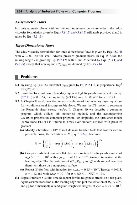
Axisymmetric Flows

For axisymmetric flows with or without transverse curvature effect, the eddy

viscosity formulation given by Eqs. (5.8.12) and (5.8.13) still apply provided that L is

given by Eq. (5.3.13).

Three-Dimensional Flows

The eddy viscosity formulation for three-dimensional flows is given by Eqs. (5.7.4)

with a ¼ 0.0168 for small adverse-pressure gradient flows. In Eq. (5.7.4a), the

mixing length l is given by Eq. (5.2.12) with A and N defined by Eqs. (5.3.1) and

(5.3.2a) except that now us and (s/9)max are defined by Eqs. (5.7.6).

Problems

5.1 By using Eq. (4.4.18), show that (εm)i given by Eq. (5.2.11a) is proportional to y4

for (y/d) � 1.

5.2 Show that for equilibrium boundary layers at high Reynolds numbers, if a in Eq.

(5.2.11b) is 0.0168, then a1 in Eq. (4.3.15a) must be 0.0635 for k ¼ 0.41.

5.3 In Chapter 8 we discuss the numerical solution of the boundary-layer equations

for two-dimensional incompressible flows. We use the CS model to represent

the Reynolds shear stress, �9u0y0. In Chapter 10 we describe a computer

program which utilizes this numerical method, and the accompanying

CD-ROM presents the computer program. For simplicity, the turbulence model

(subroutione EDDY) is limited to flows over smooth surfaces with pressure

gradient.

(a) Modify subroutine EDDY to include mass transfer. Note that now for incom-

pressible flows, the definition of N, [Eq. 5.3.2a)], becomes

N ¼�pþ

yþw

�1� exp

�11:8yþw

��þ exp

�11:8yþw

��1=2

(b) Compute turbulent flow on a flat plate with suction for a Reynolds number of

uNc/v ¼ 3 � 106 with vw/uN ¼ –0.15 � 10–4. Assume transition at the

leading edge. Plot the variation of d*/c, Rq, cf and f 00w with x/c and compare

them with those on a nonporous surface.

(c) Repeat (b) for flow with injection for yw/uN ¼ 0.15� 10–4. Take h1 ¼ 0.015,

k ¼ 1.12 and with Dx/c ¼ 10–2 for 0 � x/c � 1, NXT ¼ 101.

5.4 Repeat Problem 5.3, this time to acount for the roughness effects on a flat plate.

Again assume transition at the leading edge and plot the variation of Rq, cf, d*/c,

and f 00w for dimensionless sand-grain roughness heights of ks/c ¼ 0.25 � 10–3,


0.50� 10–3, 1� 10–3, 1.50 � 10–3 and compare your results with those given in

the accompanying CD-ROM.

5.5 Repeat Problem 5.3, this time to acount for the transverse curvature effect on

a circular cylinder. Remember that this flow is an axisymmetric flow; in addi-

tion to making changes in the EDDY viscosity subroutine, it is necessary to

redefine b.

(a) Compute cf with the modified eddy viscosity model, [Eqs. (5.3.12) and

(5.3.13)], for r0/c ¼ 0.15 � 10–2 and 0.5 � 10–4 for Rc ¼ 10 � 106. Assume

(x/c)tr at 0.075. Plot the variation of d/r0, cf and Rq with x/c and compare the

results with those obtained with the 2d eddy viscosity model [no changes to

the subroutine EDDY for TVC effect].

(b) Plot the variation of d/r0 with x/c with calculations made by using the orig-

inal and modified eddy viscosity formulas.

References

[1] E.R. Van Driest, On Turbulent Flow Near a Wall, J. Aeronaut. Sci. 23 (1956).

[2] T. Cebeci, A.M.O. Smith, Computation of Turbulent Boundary Layers – 1968, in: S.J. Kline,

M.V. Morkovin, G. Sovran, D.S. Cockrell (Eds.), AFOSR-IFP-Stanford Conf, 1, Stanford Univ.

Press, Stanford, California, 1968, p. 346.

[3] G.L. Mellor, H.J. Herring, Computation of Turbulent Boundary Layers – 1968, in: S.J. Kline,

M.V. Morkovin, G. Sovran, D.S. Cockrell (Eds.), AFOSR-IFP-Stanford Conf, 1, Stanford Univ.


[4] S.V. Patankar, D.B. Spalding, Computation of Turbulent Layers – 1968, in: S.J. Kline,

M.V. Morokovin, G. Sovran, D.S. Cockrell (Eds.), AFOSR-IFP-Stanford Conf, 1, Stanford Univ.


[5] R. Michel, C. Quemard, R. Durant, Application d’un schema de longueur de melange a l’etude des

couches limites d’equilibre, ONERA Note Technique No. 154 (1969).

[6] T. Cebeci, Behavior of Turbulent Flow Near a Porous Wall With Pressure Gradient, AIAA J. 8

(1970).

[7] T. Cebeci, Calculation of Compressible Turbulent Boundary Layers With Heat and Mass Transfer,

AIAA J. 9 (1971) 1091.

[8] D. Coles, The Turbulent Boundary Layer in a Compressible Fluid. Rep. R-403-PR, Rand Corp,

California, Santa Monica, 1962. Also AD 285–651.

[9] R.L. Simpson, Characteristics of Turbulent Boundary Layers at Low Reynolds Numbers with and

without Transpiration, J. Fluid Mech. 42 (1970) 769.

[10] T. Cebeci, G.J. Mosinskis, Computation of Incompressible Turbulent Boundary Layers at Low

Reynolds Numbers, AIAA J. 9 (1971).

[11] D.G. Huffman, P. Bradshaw, A Note on Van Karman’s Constant in Low Reynolds Number

Turbulent Flows, J. Fluid Mech. 53 (1972) 45.

[12] D.M. Busnell, D.J. Morris, Shear-Stress Eddy-Viscosity and Mixing Length Distributions

in Hypersonic Turbulent Boundary Layers, NASA Tech. Memo No. X-2310 (1971). Also

N71–31310.

[13] T. Cebeci, Kinematic Eddy Viscosity at Low Reynolds Numbers, AIAA J. 11 (1973) 102.


[14] T. Cebeci, Variation of the Van Driest Damping Parameter with Mass Transfer, AIAA J. 9 (1968)

1973.

[15] J.E. Danberg, Characteristics of the Turbulent Boundary Layer with Heat and Mass Transfer at

M ¼ 6.7, Naval Ord. Rep. NOLTR (1964) 64–99. Also AD 452–471.

[16] T. Cebeci, Eddy Viscosity Distribution in Thick Axisymmetric Turbulent Boundary Layers, J. Fluids

Eng. 95 (1973) 319.

[17] R. Richmond, Experimental Investigation of Thick Axially Symmetric Boundary Layers On

Cylinders at Subsonic and Hypersonic Speeds. Ph.D. Thesis, California Inst. Technology, Pasadena,

California, 1957.

[18] H. Thomann, Effect of Streamwise Wall Curvature on Heat Transfer in a Turbulent Boundary Layer,

J. Fluid Mech. 33 (1968) 283.

[19] T. Cebeci, Curvature and Transition Effects in Turbulent Boundary Layers, AIAA J. 9 (1968) 1971.

[20] P. Bradshaw, The Analogy Between Streamline Curvature and Buoyancy in Turbulent Shear Flow, J.

Fluid Mech. 36 (1969) 177.

[21] G.B. Schubauer, P.S. Klebanoff, Investigation of Separation of the Turbulent Boundary Layer,

NACA Tech. Note No. 2133 (1956).

[22] H. Shmidbauer, Turbulent Friction Along Convex Surfaces, NACA Tech. Memo 791 (1936).

[23] D.M. Bushnell, D.W. Alston, On the Calculation of Transitional Boundary-Layer Flows, AIAA J. 10

(1972) 229.

[24] W.G. Hoydysh, V. Zakkay, An Experimental Investigation of Hypersonic Turbulent Boundary

Layers in Adverse Pressure Gradient. Rep. F-67-5, New York Univ., Bronx. New York, 1967.

[25] K.K. Chen, N.A. Thyson, Extension of Emmons Spot Theory to Flows on Blunt Bodies, AIAA J. 5

(1971) 821.

[26] H.W. Emmons, The Laminar-Turbulent Transition in a Boundary Layer – Part 1, J. Aeronaut. Sci.

18 (1951) 490.

[27] S. Dhawan, R. Narasimha, Some Properties of Bounday-Layer Flow During the Transition from

Laminar to Turbulent Motion, J. Fluid Mach. 3 (1958) 418.

[28] R. Michel, Resultants sur la couche limite turbulent aux grandes vitesses, Memo Tech 22 (1961).

Office Nat. d’Etudes et de Rech. Aeronaut.

[29] A.M.O. Smith, N. Gamberoni, Transition, In: Pressure Gradient and Stability Theory, 4, Proc. Int.

Congr. Appl. Mech., 9th, Brussels, Belgium, 1956. 234. Also AD 125 559m.

[30] T. Cebeci, G.J. Mosinskis, A.M.O. Smith, Calculation of Viscous Drag and Turbulent Boundary-

Layer Separation on Two-dimensional and Axisymmetric Bodies in Incompressible Flows. Rep. No.

MDC J0973–01, Douglas Aircraft Co, Long Beach, California, 1970. Also N71-25868.

[31] G.B. Schubauer, Air Flow in the Boundary Layer of an Elliptic Cylinder, NACA Rep. No. 652

(1939).

[32] D. Coles, Measurements in the Boundary Layer on a Smooth Flat Plate in Supersonic Flow. III.

Measurements in a Flat-Plate Boundary Layer at the Jet Propulsion Lab. Rep. No. 20–71, Jet

Propulsion Lab., California Inst. Technol, Pasadena, California, 1953.

[33] J.C. Adams Jr., Implicit Finite-Difference Analysis of Compressible Laminar, Transitional and

Turbulent Boundary Layers Along the Windward Streamline of a Sharp Cone at Incidence. Rep.

AEDC-TR-71–235, Arnold Eng. Develop. Center, Tennessee, 1971. Also N72-19346.

[34] J.E. Harris, Numerical Solution of the Equations for Compressible Laminar, Transitional and

Turbulent Boundary Layers and Comparisons with Experimental Data, NASA Tech. Rep (1971).

No. R-368. Also N71–32164.

[35] R.M. O’Donnell, Experimental Investigation at a Mach Number of 2.41 of Average Skin-Friction

Coefficients and Velocity Profiles for Laminar and Turbulent Boundary Layers and on Assessment

of Probe Effects, NACA Tech. Note No. 3122 (1954).


[36] T. Cebeci, Essential Ingredients of a Method for Low Reynolds-Number Airfoils, AIAA J. 27

(1983) 1680–1688.

[37] J. Cousteix, G. Pailhas, Etude Exploratorie d’un Processus de Transition Laminair-Turbulent au

Voisinage du Decollemente d’une Couche Limite Laminaire, T. P. No (1979-86) 213–218. Also

LeRecherche Aerospatiale No. 1979-3.

[38] T. Cebeci, An Engineering Approach to the Calculation of Aerodynamic Flows, Horizons

Publishing, Long Beach and Springer-Verlag, Heidelberg, 1999.

[39] T. Cebeci, K.C. Chang, Calculation of Incompressible Rough-Wall Boundary-Layers Flows, AIAA

J. 16 (1978) 730.

[40] J.C. Rotta, Turbulent Boundary Layers in Incompressible Flows, Progr. Aeronaut. Sci. 2

(1962) 1.

[41] F.A. Dvorak, Calculation of Turbulent Boundary Layers on Rough Surfaces in Pressure Gradient,

AIAA J. 7 (No. 9) (1969). 1752.

[42] D. Betterman, Contribution a l’etude de la couche limite turbulente le long de plaques regueuses,

Rapport 65–6, Centre Nat. de la Rech. Sci, Paris, France, 1965.

[43] A.E. Perry, P.N. Joubert, Rough-Wall Boundary Layers in Adverse Pressure Gradients, J. Fluid

Mech. 17 (1963) 193–211.

[44] D.A. Johnson, L.S. King, Mathematically Simple Turbulence Closure Model for Attached and

Separated Turbulent Boundary Layers, AIAA J. 23 (No. 11) (1985) 1684–1692.

[45] D.A. Johnson, T.J. Coakley, Improvement to a Nonequilibrium Algebraic Turbulence Model, AIAA

J. 28 (No. 11) (1990). 2000–2003.

[46] T. Cebeci, K.C. Chang, An Improved Cebeci-Smith Turbulence Model for Boundary-Layer and

Navier-Stokes Methods, 20th Congress of the International Council of the Aeronautical Sciences,

Sorrento, Italy, 1996, paper No. ICAS-96–1.7.3.

[47] R.L. Simpson, Y.T. Chew, B.G. Shivaprasad, The Structure of a Separating Turbulent Boundary

Layer, Part 1, Mean Flow and Reynolds Stresses, J. Fluid Mech. 113 (1981) 23–51.

[48] A. Nakayama, Measurements in the Boundary Layer and Wake of Two Airfoil Models. Report No,

MDC J2403, Douglas Aircraft Co. (1982).

[49] H. Fiedler, M.R. Head, Intermittency Measurements in the Turbulent Boundary Layer, J. Fluid

Mech., 25, Part 4 (1966). 719–535.

[50] Carr, L. W., McCroskey, W. J., McAlister, K. W., Pucci, S. L., and Lambert, O.: An Experimental

Study of Dynamic Stall on Advanced Airfoil Sections, 3, Hot-Wire and Hot-Film Measurements,

NASA TM 84245.

[51] E. Omar, T. Zierten, M. Hahn, E. Szpiro, A. Mahal, Two-Dimensional Wind-Tunnel Tests of

a NASA Supercritical Airfoil with Various High-Lift Systems, 2, Test Data, NASA CR-2215

(1977).

[52] B.S. Baldwin, H. Lomax, Thin Layer Approximation of Algebraic Model for Separated Turbulent

Flows, AIAA paper No (1978) 78–257.

[53] H.W. Stock, W. Haase, Determination of Length Scales in Algebraic Turbulence Models for Navier-

Stokes Methods, AIAA J. 27 (No. 1) (1989) 5–14.

[54] D.A. Johnson, Nonequilibrium Algebraic Turbulence Modeling Considerations for Transonic

Airfoils and Wings, AIAA paper No (1992). 92–0026.

[55] R.C. Swanson, E. Turkel, A Multistage Time-Stepping Scheme for the Navier-Stokes Equations,

AIAA paper No (1985). 85–0035.

[56] O. Reynolds, On the Extent and Action of the Heating Surface for Steam Boilers, Proc. Manchester

Lit. Phil. Soc. 14 (1874) 7.

[57] J. Kestin, P.D. Richardson, Heat Transfer Across Turbulent Incompressible Boundary Layers, Int. J.

Heat Mass Transfer 6 (1963) 147.


[58] R. Jenkins, Variation of Eddy Conductivity with Prandtl Modulus and Its Use in Prediction of

Turbulent Heat Transfer Coefficients, Inst. Heat Transfer Fluid Mech. 147 (1951).

[59] W.M. Kays, Convective Heat and Mass Transfer, McGraw-Hill, New York, 1966.

[60] F. Page, W.G. Schlinger, D.K. Breaux, B.H. Sage, Point Values of Eddy Conductivity and Viscosity

in Uniform Flow Between Parallel Plates, Ind. Eng. Chem. 44 (1952) 424.

[61] W.M. Rohsenow, H.Y. Choi, Heat, Mass and Momentum Transfer, Prentice-Hall, Englewood Cliffs,

New Jersey, 1961.

[62] R.G. Deissler, Turbulent Heat Transfer and Temperature Fluctuations in a Field with Uniform

Velocity and Temperature Gradients, Int. J. Heat Mass Transfer 6 (1963) 257.

[63] R.L. Simpson, D.C. Whitten, R.J. Moffat, An Experimental Study of the Turbulent Prandtl Number

of Air with Injection and Suction, Int. J. Heat Mass Transfer 13 (1970) 125.

[64] T. Cebeci, A Model for Eddy Conductivity and Turbulent Prandtl Number, J. Heat Transfer 95

(1973) 227.

[65] H. Ludweig, Bestimmung des Verhaltnisses der Austauschkoeffizienten fur Warme und Impuls bei

turbulenten Grenzschichten, Z. Flugwiss. 5 (1956) 73.

[66] T.Y. Na, I.S. Habib, Heat Transfer in Turbulent Pipe Flow Based on a New Mixing Length Model,

Appl. Sci. Res. 28 (4/5) (1973).

[67] D.S. Johnson, Velocity and Temperature Fluctuation Measurements in a Turbulent Boundary Layer

Downstream of a Stepwise Discontinuity in Wall Temperature, J. Appl. Mech. 26 (1959) 325.

[68] Meier, H. U. and Rotta, J. C.: Temperature Distributions in Supersonic Turbulent Boundary Layers.

AIAA J., 9, 2149, 1971.

[69] J. Rotta, C., A Family of Turbulence Models for Three-Dimensional Thin Shear Layers, DFVLR-

AVA Gottingen (1977). IB251–76A25.

[70] B. Van den Berg, A Three-Dimensional Law of the Wall for Turbulent Shear Flows, J. Fluid Mech.

70 (1975) 149.

[71] T. Cebeci, J. Cousteix, Modeling and Computation of Boundary-Layer Flows, Horizons Publishing,

Long Beach, California and Springer-Verlag, Heidelberg, 1998.

[72] P. Bradshaw, M.G. Terell, The Response of a Turbulent Boundary Layer on an ‘‘Infinite’’

Swept Wing to the Sudden Removal of Pressure Gradient, NFL Aero. Rept. 1305, ARC 31514

(1969).

[73] N.A. Cumpsty, M.R. Head, The Calculation of Three-Dimensional Turbulent Boundary-Layers, Part

IV: Comparison of Measurements with Calculations on the Rear of a Swept Wing. C. P. 1077, Aero

Research Council, London, England, 1970.

[74] P. Bradshaw, D.H. Ferriss, N.P. Atwell, Calculation of Boundary-Layer Development Using the

Turbulent Energy Equation, J. Fluid Mech. 23 (1967) 593.

[75] T. Cebeci, Calculation of Three-Dimensional Boundary Layers, Part 2, Three-Dimensional Flows in

Cartesian Coordinates, AIAA J. 13 (1975) 1056.

[76] P. Bradshaw, G. Mizner, K. Unsworth, Calculation of Compressible Turbulent Boundary Layers on

Straight-Tapered Swept Wings, AIAA J. 14 (1976) 399.

[77] L.F. East, R.P. Hoxey, Low-Speed Three-Dimensional Turbulent Boundary-Layer Data. Pt. I, TR

69041, Royal Aircraft Establishment, Farnborough, England, 1969.

[78] H.U. Meier, H.P. Kreplin, Experimental Investigation of the Boundary Layer Transition and

Separation on a Body of Revolution, Zeitschrift fur Flugwissenschaften und Weltraumforschung 4

(March-April 1980) 65–71.

[79] H.U. Meier, H.P. Kreplin, A. Landhausser, D. Baumgarten, Mean Velocity Distributions in

Three-Dimensional Boundary Layers, Developing on a 1:6 Prolate Spheroid with Natural Transition

(a ¼ 10�, UN ¼ 45 m/s, Cross Sections x0/2a ¼ 0.56; 0.64 and 0.73), German Aerospace Research

Establishment, Gottingen, Germany, March 1984. Rept. IB 222-84 A 10.


[80] H.U. Meier, H.P. Kreplin, A. Landhausser, D. Baumgarten, Mean Velocity Distributions in

Three-Dimensional Boundary Layers, Developing on a 1:6 Prolate Spheroid with Natural Transition

(a ¼ 10�, UN ¼ 55 m/s, Cross Sections x0/2a ¼ 0.48; 0.56; 0.64 and 0.73), German Aerospace

Research Establishment, Gottingen, Germany, March 1984. Rept. IB 222-84 A 11.

[81] T. Cebeci, H.U. Meier, Turbulent Boundary Layers on a Prolate Spheroid, AIAA paper (June 1987)

87–1299.


Transport-EquationTurbulence Models

Chap

ter6



6.2 Two-Equation Models 215

6.2.1 k-ε Model 215

6.2.2 k-u Model 221

6.2.3 SST Model 224

6.3 One-Equation Models 226

6.3.1 Bradshaw’s Model 227

6.3.2 Spalart-Allmaras Model 228

6.4 Stress-Transport Models 230

Problems 233

References 235

6.1 Introduction

While the zero-equationmodels discussed inChapter 5 are useful and accurate formost

boundary-layer flows, thesemodels lack generality. For turbulent shear flows other than

wall boundary-layers, they require different expressions for mixing length and eddy 211



http://dx.doi.org/10.1016/B978-0-08-098335-6.00006-9

viscosities. For example, for a plane jet, round jet and plane wake l¼ 0.09d, l¼ 0.07d,

l¼ 0.16d, respectively, with d denoting the shear layer thickness. Transport equation

models have less limitations than the zero-equation models for modeling Reynolds

stresses. Beforewe discuss several of thesemethods that are popular and inwide use, let

us consider the Reynolds-stress transport equation (3.5.3) and the kinetic energy

equation (2.8.5) which these models use. For convenience, we again call Rij ðh�u0iu0jÞthe Reynolds stress tensor, rather than the actual one, �Rij ðh�9u0iu0jÞ, and also consideran incompressible flow. Beforewe rewrite Eq. (3.5.3), let us divide the last two terms in

Eq. (3.5.3) by 9. If we denote these two terms Vij, that is,

Vij ¼ 1

9

v

vxk

�u0j s00ik þ u0is00jk

�� 1

9

s00ik

vu0jvxk

þ s00jkvu0ivxk

!; (6.1.1)

then from the definition of the stress tensor we can write the first term as

1

9

v

vxk

�u0js00ik þ u0is00jk

�

¼ vv

vxk

24u0j�vu0ivxk

þ vu0kvxi

�þ u0i

�vu0jvxk

þ vu0kvxj

�35

¼ vv

vxk

�v

vxk

�u0iu

0j

��þ v

v

vxk

0@u0j

vu0kvxi

þ u0ivu0kvxj

1A:

(6.1.2)

Now we write the second term in Eq. (6.1.1) as

�1

9

0@s00ik

vu0jvxk

þ s00jkvu0ivxk

1A

¼ �v

�vu0ivxk

þ vu0kvxi

�vu0jvxk

� n

�vu0jvxk

þ vu0kvxj

�vu0ivxk

¼ �v

0@2

vu0ivxk

vu0jvxk

þ vu0kvxi

vu0jvxk

þ vu0kvxj

vu0ivxk

1A:

(6.1.3)

Combining Eqs. (6.1.2) and (6.1.3), we get

Vij ¼ �nv2Rij

vx2k� 2n

vu0ivxk

vu0jvxk

(6.1.4)


since for an incompressible flow u0jðv2u0k=vxkvxiÞ and u0iðv2u0k=vxkvxjÞ are zero.

With Eq. (6.1.4) and with the continuity equation (2.5.3), Eq. (3.5.3) can be

written as

D Rij

Dt¼ v

vxk

�nv Rij

vxk

�� Rik

v�ujvxk

� Rjkv�uivxk

þ 2nvu0ivxk

vu0jvxk

þ v

vxk

0@u0iu0ju0k þ

p0

9u0idjk þ

p0

9u0jdik

1A

� p0

9

�vu0jvxi

þ vu0ivxj

�(6.1.5)

where

D Rij

Dt¼ v Rij

vtþ uk

vRij

vxk:

A contraction of Eq. (6.1.5), i¼ j and with k ¼ � Rii

2 gives the following equation for

the turbulence kinetic energy discussed in Section 2.8:

Dk

Dt¼ v

vxk

0@n

vk

vxk� p0

9u0idik � u0k

u0iu0i2

1Aþ Rik

v�uivxk

� ε (6.1.6)

where

Dk

Dt¼ vk

vtþ �uk

vk

vxk

ε ¼ n

�vu0ivxk

vu0ivxk

� (6.1.7)

The left-hand side of Eq. (6.1.6) represents the rate of change of turbulence kinetic

energy. The first term on the right-hand side is called molecular diffusion and repre-

sents the diffusion of turbulence energy caused by the molecular transport process of

the fluid. The second term is called pressure diffusion and the triple velocity corre-

lation term which represents the rate at which turbulence energy is transported through

the fluid by turbulent fluctuations, is called turbulent transport. The fourth term is

known as production and represents the rate at which turbulence kinetic energy is

transferred from the mean flow to the turbulence. Finally the last term may be called

‘‘isotropic dissipation’’, since the actual dissipation ε is given by Eq. (3.5.5),

ε ¼ 1

9s00ik

vu0ivxk

(3.5.5)

Transport-Equation Turbulence Models 213

Another equation that is employed in most transport-equation turbulence models is

the rate of dissipation of turbulent energy which is obtained from a transport equation

for ε derived by Harlow and Nakayama [1],

Dε

Dt¼ v

vxk

�nvε

vxk

�� 2n

v�uivxk

0@vu0ivxl

vu0kvxl

þ vu0lvxi

vu0lvxk

1A

�2nvu0ivxk

vu0ivxl

vu0kvxl

� 2

24n v2u0i

vxkvxl

352

� v

vxku0kε0 �

n

9

v

vxi

24vp0vxl

vu0ivxl

35 :

(6.1.8)

The following closure assumptions are made for the terms on the right-hand side of

this equation.

The second term on the right-hand side, the generation term, is modeled by

2n

0@vu0ivxl

vu0kvxl

þ vu0lvxi

vu0lvxk

1A ¼

0@cε1

u0iu0kk

þ ~cε1dik

1A

ε (6.1.9)

where cε1 and ~cε1 are constants. In fact, the term containing ~cε1 vanishes when Eq.

(6.1.1) is multiplied by vui=vxk; thus it need not be considered further.

The third and fourth terms on the right-hand side of Eq. (6.1.8) are combined into

one term, modeled by

2

8<:n

vu0ivxk

vu0ivxl

vu0kvxl

þ0@n

v2u0ivxkvxl

1A

29=; ¼ cε2

ε2

k: (6.1.10)

In two-equation models, the fifth term, which accounts for the diffusion of ε from

velocity fluctuations, is modeled by

�u0kε0 ¼εm

sε

vε

vxk(6.1.11)

which is different than the modeling used in stress-transport models, see Eq. (6.4.7).

The last term, which represents the diffusional transport of ε by pressure fluc-

tuations, is neglected.

With these closure assumptions, the final form of the rate of dissipation of

turbulent energy may be written as

Dε

Dt¼ v

vxk

�nvε

vxk

�þ cε1

ε

kRik

v�uivxk

� cε2ε2

kþ v

vxk

�εm

sε

vε

vxk

�(6.1.12)


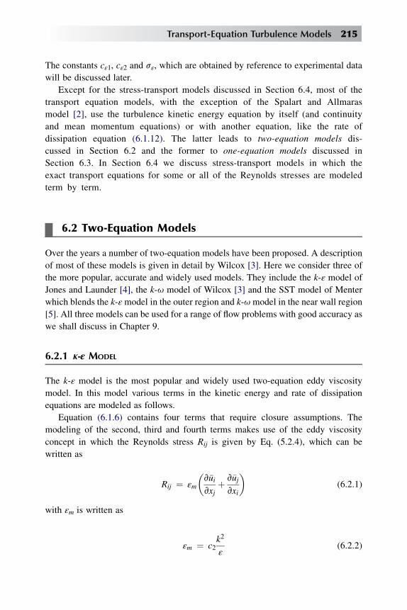
The constants cε1, cε2 and sε, which are obtained by reference to experimental data

will be discussed later.

Except for the stress-transport models discussed in Section 6.4, most of the

transport equation models, with the exception of the Spalart and Allmaras

model [2], use the turbulence kinetic energy equation by itself (and continuity

and mean momentum equations) or with another equation, like the rate of

dissipation equation (6.1.12). The latter leads to two-equation models dis-

cussed in Section 6.2 and the former to one-equation models discussed in

Section 6.3. In Section 6.4 we discuss stress-transport models in which the

exact transport equations for some or all of the Reynolds stresses are modeled

term by term.

6.2 Two-Equation Models

Over the years a number of two-equation models have been proposed. A description

of most of these models is given in detail by Wilcox [3]. Here we consider three of

the more popular, accurate and widely used models. They include the k-ε model of

Jones and Launder [4], the k-u model of Wilcox [3] and the SST model of Menter

which blends the k-εmodel in the outer region and k-umodel in the near wall region

[5]. All three models can be used for a range of flow problems with good accuracy as

we shall discuss in Chapter 9.

6.2.1 K-ε MODEL

The k-ε model is the most popular and widely used two-equation eddy viscosity

model. In this model various terms in the kinetic energy and rate of dissipation

equations are modeled as follows.

Equation (6.1.6) contains four terms that require closure assumptions. The

modeling of the second, third and fourth terms makes use of the eddy viscosity

concept in which the Reynolds stress Rij is given by Eq. (5.2.4), which can be

written as

Rij ¼ εm

�v�uivxj

þ v�ujvxi

�(6.2.1)

with εm is written as

εm ¼ c2k2

ε

(6.2.2)


Here c2 is a constant at high Reynolds number. The second and third terms in Eq.

(6.1.6), namely the pressure diffusion and turbulent transport terms are related to the

gradients of k,

�0@u0k

p0

9þ u0k

u0iu0i2

1A ¼ εm

sk

vk

vxk(6.2.3)

where sk is a constant or a specified function. Substituting Eqs. (6.2.1) and (6.2.3)

into Eq. (6.1.6) we obtain the modeled form of the turbulence kinetic energy

equation

Dk

Dt¼ v

vxk

��nþ εm

sk

�vk

vxk

�þ εm

�v�uivxj

þ v�ujvxi

�v�uivxj

�ε (6.2.4)

Similarly, with the relation given by Eq. (6.2.1), the dissipation equation (6.1.12)

becomes

Dε

Dt¼ v

vxk

��nþ εm

sε

�vε

vxk

�þ cε1

ε

kεm

�v�uivxj

þ v�ujvxi

�v�uivxj

� cε2ε2

k(6.2.5)

The first term on the right-hand side of Eq. (6.2.5) represents molecular and turbulent

diffusion of dissipation, and the sum of the second and third terms represent the

production and dissipation. The parameter sε is a parameter to be specified.

For boundary-layer flows at high Reynolds number and with Eq. (6.2.2) now

written as

εm ¼ cmk2

ε

(6.2.6)

Eqs. (6.2.4) and (6.2.5) can be written as

uvk

vxþ y

vk

vy¼ v

vy

�εm

sk

vk

vy

�þ εm

�vu

vy

�2

�ε (6.2.7)

uvε

vxþ y

vε

vy¼ v

vy

�εm

sε

vε

vy

�þ cε1

ε

kεm

�vu

vy

�2

�cε2ε2

k(6.2.8)

The parameters cm, cε1 , cε2 , sk and sε are given by

cm; ¼ 0:09; cε1 ¼ 1:44; cε2 ¼ 1:92; sk ¼ 1:0; sε ¼ 1:3 (6.2.9)

These equations apply only to free shear flows. For wall boundary-layer flows, they

require modifications to account for the presence of the wall. Without wall functions,

it is necessary to replace the true boundary conditions at y¼ 0 by new ‘‘boundary

conditions’’ defined at some distance y0 outside the viscous sublayer to avoid


integrating the equations through the region of large y gradients near the surface.

Usually this y0 is taken to be the distance given by

y0 ¼�n

us

�yþ0 ;

y0þ being a constant taken as about 50 for smooth surfaces. For the velocity

field, the boundary conditions at y¼ y0 use the law of the wall, Eq. (4.2.1), and

require that

u0 ¼ us

�1

kln

y0usn

þ c

�; (6.2.10a)

y0 ¼ �u0y0us

dusdx

(6.2.10b)

Here c is a constant around 5 to 5.2. Equation (6.2.10b) results from integrating the

continuity equation with u given by Eq. (4.2.1). We also use relations for the changes

in shear stress between y ¼ 0 and y¼ y0 in order to calculate us from

u2s ¼ s09� ay0 (6.2.11a)

where s0 is calculated from

s0 ¼��nþ εm

vu

vy

�y0

with a semiempirically given by

a ¼ 0:3du20dx

� ueduedx

(6.2.11b)

The friction velocity us is obtained from

s ¼ sw þ dp

dxyþ n

dusdx

Z yþ

0

�u

us

�2

dyþ (6.2.12)

In the viscous sublayer and in the buffer layer (yþ � 30), u/us can be obtained from

Thompson’s velocity profile given by Eq. (4.4.41). For yþ> 50, we can use the

logarithmic velocity formula, Eq. (9.3.1a). See subsection 9.3.1.

There are several ways to specify the ‘‘wall’’ boundary conditions for k and ε.

A common one for k makes use of the relation between shear stress s and k [see

Eq. (6.3.2)],

y ¼ y0; k0 ¼ s0a1

(6.2.13a)


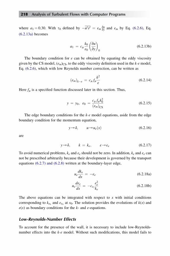
where a1¼ 0.30. With s0 defined by �u0y0 ¼ εmvuvy and εm by Eq. (6.2.6), Eq.

(6.2.13a) becomes

a1 ¼ cmk0ε0

�vu

vy

�0

(6.2.13b)

The boundary condition for ε can be obtained by equating the eddy viscosity

given by the CS model, (εm)CS, to the eddy viscosity definition used in the k-εmodel,

Eq. (6.2.6), which with low Reynolds number correction, can be written as

ðεmÞk�ε¼ cm fm

k2

ε

(6.2.14)

Here fm is a specified function discussed later in this section. Thus,

y ¼ y0; ε0 ¼ cm fmk20

ðεmÞCS(6.2.15)

The edge boundary conditions for the k-ε model equations, aside from the edge

boundary condition for the momentum equation,

y/d; u/ueðxÞ (6.2.16)

are

y/d; k ¼ ke; ε/εe (6.2.17)

To avoid numerical problems, ke and εe should not be zero. In addition, ke and εe can

not be prescribed arbitrarily because their development is governed by the transport

equations (6.2.7) and (6.2.8) written at the boundary-layer edge,

uedkedx

¼ �εe (6.2.18a)

uedεedx

¼ �cε2ε2e

ke(6.2.18b)

The above equations can be integrated with respect to x with initial conditions

corresponding to ke0 and εe0 at x0. The solution provides the evolutions of k(x) and

ε(x) as boundary conditions for the k- and ε-equations.

Low-Reynolds-Number Effects

To account for the presence of the wall, it is necessary to include low-Reynolds-

number effects into the k-ε model. Without such modifications, this model fails to


predict the sharp peak in turbulence kinetic energy close to the surface for pipe and

channel flow as well as fails to predict a realistic value of the additive constant c in

the law of the wall.

There are several approaches that can be used to model Eqs. (6.2.7) and (6.2.8)

near the wall region. For an excellent review of these models, see Wilcox [3] and

Patel et al. [6].

Patel et al. [6] reviewed eight models and evaluated them against test cases,

which involved a flat-plate boundary layer, an equilibrium adverse pressure gradient

boundary layer, strong favorable pressure gradient (relaminarizing) boundary layers,

and sink boundary layers. Their study indicated that not all of the available low

Reynolds number models reproduced the most basic feature of a flat-plate boundary

layer. Only the more promising versions of Launder and Sharma, LS, [7], Chien, CH,

[8], Lam and Bremhorst, LB, [9] will therefore be discussed here in the context of

reviewing models for low Reynolds number effects. These models, LS, CH and LB

all gave comparable results and performed considerably better than the other low

Reynolds number turbulence models considered in Patel et al.’s study. However, it

was pointed out in their study that even these models needed further refinement if

they were to be used with confidence to calculate near-wall and low Reynolds

number flows.

Before we present a brief review of these models as described in [6], it is useful to

write the k-ε model equations in the following general form,

uvk

vxþ y

vk

vy¼ v

vy

��nþ εm

sk

�vk

vy

�þ εm

�vu2

vy

��~εþ D

�(6.2.19)

uv~ε

vxþ y

v~ε

vy¼ v

vy

��nþ εm

sε

�v~ε

vy

�þ cε1 f1

~ε

kεm

�vu2

vy

�� cε2 f2

~ε2

kþ E (6.2.20)

where D and E as well as cε1 , cε2 , f1, f2 are model dependent and

~ε ¼ ε� D (6.2.21)

The parameters D and E for the LS, CH and LB1 models, including those for high

Reynolds, HR, numbers are summarized in Table 6.1 together with their wall

boundary conditions, with εm defined by

εm ¼ cm fmk2

~ε(6.2.22)

Similarly the parameters f1, f2, fm, sk, sε, cε1 and cε2 are summarized in Table 6.2.

Since the review of Patel et al. [6], another low Reynolds number correction to

the k-εmodel was proposed by Hwang and Lin [10] who added an F term to the right


hand side of Eq. (6.2.19) and defined the parameters D, E, F and other parameters in

Table 6.2 by

D ¼ 2n

vffiffiffik

p

vy

!2

; E ¼ � v

vy

�n~ε

k

vk

vy

�

F ¼ � 1

2

v

vy

�n

k

~εþ D

vD

vy

�; fm ¼ 1� exp

�� 0:01yl � 0:008y3l

�

f1 ¼ 1:0; f2 ¼ 1:0; sk ¼ 1:4� 1:1 exp½� ðyl=10Þ�sε ¼ 1:3� exp½ � ðyl=10Þ�; cε1 ¼ 1:44; cε2 ¼ 1:92

(6.2.23)

yl ¼ yffiffiffiffiffiffiffiffiffink=~ε

p

TABLE 6.1 Parameters D and E and the wall boundary conditions for LS, CH, LB1

and HR models

Model D E Boundary Conditions

~ε k

HR 0 0 wall functions

LS2n

vffiffiffik

p

vy

!2

2nεm

�v2u

vy2

�2 0 0

CH2n

k

y2�2n

�~ε

y2

�exp

��1

2yþ�

0 0

LB1 0 0 v~ε

vy¼ 0

0

TABLE 6.2 Parameters f1, f2, fm, sk, sk, cε1 and cε2 for LS, CH, LB1 and HR models.

RT ¼ k2

nε; Ry ¼

ffiffiffik

py=n; yþ ¼ yus=n:

Model f1 f2 fm sk sε

cε1 cε2

HR 1.0 1.0 1.0 1.0 1.3 1.44 1.92

LS 1.0 1 – 0.3exp ð�R2T Þ

exp

"�3:4

ð1þRT =50Þ2

#1.0 1.3 1.44 1.92

CH 1.01 – 0.22exp

��R2

T

36

�1 – exp (–0.0115yþ) 1.0 1.3 1.35 1.8

LB11þ

�0:05fm

�3 1�exp ð�R2T Þ [1 – exp (–0.0165Ry)]

2

��1þ 20:5

RT

� 1.0 1.3 1.44 1.92


The wall boundary conditions for this model are same as those for LS and CH

models. The edge boundary conditions given by Eq. (6.2.18) remain the same.

The application of this model to fully developed channel flows, turbulent plane

Couette-Poisseuille flow and turbulent flow over a backward-facing step show very

good agreement with data. Calculated results with this model show a much better

agreement with measurements than those calculated with the models of CH and LS.

In the methods that use the k-εmodel the coefficient cm in Eq. (6.2.22) is still 0.09,

but in a recent investigation Marvin and Huang [11] propose that to account for

adverse pressure gradient effect, cm should be

cm ¼ 0:09

max

�1; 0:29

��vuvy�� k

ε

��1

(6.2.24)

A preliminary study shows promise but it still needs to be examined further.

Another approach to include the low-Reynolds-number effects in the k-εmodel is

to employ a simple model near the wall (a mixing-length model [12] or a one

equation model [13] which is valid only near the wall region) and a transport

equation model in the outer region of the boundary layer; the two solutions are

matched at a certain point in the boundary layer as discussed by Arnal et al. [12].

This approach, sometimes referred to as the two-layer method or the zonal method

will be discussed in Section 9.2.

Other Extensions of the k-ε Model

Another extension of the k-ε model was developed by Yakhot et al. [14]. With

techniques from renormalization group theory they proposed the so-called RNG k-ε

model. In this model, k and ε are still given by Eqs. (6.2.7) and (6.2.8). The only

different occurs in the definitions of the parameters given by Eq. (6.2.9). In the RNG

k-ε model, they are given by

cε1 ¼ 1:42; cε2 ¼ 1:68þ cml3�1� l=l0

1þ 0:012l3

l ¼ k

ε

ffiffiffiffiffiffiffiffiffiffiffi2sijsji

p; l0 ¼ 4:38; cm ¼ 0:085

sk ¼ 0:72; sε ¼ 0:72; sij ¼ 1

2

�vuivxj

þ vujvxi

�(6.2.25)

6.2.2 K-u MODEL

Like the k-ε model discussed in the previous subsection, k-u model is also very

popular and widely used. Over the years, this model has gone over many changes and


improvements as described in [3]. The most recent model is due to Wilcox [3] and is

given by the following defining equations.

With εm defined by

εm ¼ k

u(6.2.26)

the turbulence kinetic energy and specific dissipation rate equations are

Dk

Dt¼ v

vxk

��nþ εm

sk

�vk

vxk

�þ Rik

v�uivxk

� b*ku (6.2.27)

Du

Dt¼ v

vxk

��nþ εm

su

�vu

vxk

�þ a

u

kRik

v�uivxk

� bu2 (6.2.28)

where Rik is given by Eq. (6.2.1) and

a ¼ 13

25; b ¼ b0fb; b*¼ b*0 fb; sk ¼ 2; su ¼ 2 (6.2.29a)

b0 ¼ 9

125; fb ¼ 1þ 70cu

1þ 80cu; cu ¼

��UijUjkSki�b*0u

3�� (6.2.29b)

b*0 ¼ 9

100; fb ¼

8><>:

1; ck � 01þ 680c2k1þ 400c2k

; ck > 0; ck ¼ 1

u3

vk

vxj

vu

vxj(6.2.29c)

The tensors Uij and Ski appearing in Eq. (6.2.29b) are the mean rotation and

mean-strain-rate tensors, respectively, defined by

Uij ¼ 1

2

�v�uivxj

� v�ujvxi

�; Ski ¼ 1

2

�v�ukvxi

þ v�uivxk

�(6.2.30)

The parameter cu is zero for two-dimensional flows. The dependence of b on cu has

a significant effect for round and radial jets [3]. This model takes the length scale in

the eddy viscosity as

l ¼ffiffiffik

p

u(6.2.31a)

and calculates dissipation ε from

ε ¼ b* uk (6.2.31b)


Wilcox’s model equations have the advantage over the k-εmodel that they can be

integrated through the viscous sublayer, without using damping functions. At the

wall the turbulent kinetic energy k is equal to zero. The specific dissipation rate can

be specified in two different ways. One possibility is to force u to fullfill the solution

of Eq. (6.2.28) as the wall is approached [5]:

u/6n

by2as y/0 (6.2.32)

The other [5] is to specify a value for u at the wall which is larger than

uw > 100Uw

where Uw is the vorticity at the wall.

Menter [5] applied the condition of Eq. (6.2.32) for the first five grid points away

from the wall (these points were always below yþ¼ 5). He repeated some of his

computations with uw¼ 1000Uw and obtained essentially the same results. He points

out that the second condition is much easier to implement and does not involve the

normal distance from the wall. This is especially attractive for computations on

unstructured grids [5].

The choice of freestream values for boundary-layer flows are

uN > luNL; ðεmÞN < 10�2ðεmÞmax ; kN ¼ ðεmÞNuN (6.2.33)

where L is the approximate length of the computational domain and uN is the

characteristic velocity. The factor of proportionality l¼ 10 has been recom-

mended [5].

Free shear layers are more sensitive to small freestream values of uN and

larger values of u are needed in the freestream. According to [5], a value of at

least l¼ 40 for mixing layers, increasing up to l¼ 80 for round jets is

recommended.

According to [5], in complex Navier-Stokes computations it is difficult to exer-

cise enough control over the local freestream turbulence to avoid small freestream u

ambiguities in the predicted results.

For boundary-layer flows, Eq. (6.2.27) reduces to Eq. (6.2.19) with

D ¼ 0; ~ε ¼ 0:09uk (6.2.34)

The specific dissipation rate equation, Eq. (6.2.28), becomes

uvu

vxþ y

vu

vy¼ v

vy

��nþ εm

su

�vu

vy

�þ a

�vu

vy

�2

�b0u2 (6.2.35)


6.2.3 SST MODEL

The SST model of Menter [5] combines several desirable elements of existing two-

equation models. The two major features of this model are a zonal weighting of

model coefficients and a limitation on the growth of the eddy viscosity in rapidly

strained flows. The zonal modeling uses Wilcox’s k-u model near solid walls and

Launder and Sharma’s k-ε model near boundary layer edges and in free shear layers.

This switching is achieved with a blending function of the model coefficients. The

shear stress transport (SST) modeling also modifies the eddy viscosity by forcing the

turbulent shear stress to be bounded by a constant times the turbulent kinetic energy

inside boundary layers. This modification, which is similar to the basic idea behind

the Johnson-King model, improves the prediction of flows with strong adverse

pressure gradients and separation.

In order to blend the k-u model and the k-ε model, the latter is transformed into

a k-u formulation. The differences between this formulation and the original k-u

model are that an additional cross-diffusion term appears in the u-equation and that

the modeling constants are different. Some of the parameters appearing in k-umodel

are multiplied by a function F1 and some of the parameters in the transformed k-ε

model by a function (1 – F1) and the corresponding equations of each model are

added together. The function F1 is designed to be a value of one in the near wall

region (activating the k-u model) and zero far from the wall. The blending takes

place in the wake region of the boundary layer.

The SST model also modifies the turbulent eddy viscosity function to improve

the prediction of separated flows. Two-equation models generally under-predict

the retardation and separation of the boundary layer due to adverse pressure

gradients. This is a serious deficiency, leading to an underestimation of the effects

of viscous-inviscid interaction which generally results in too optimistic perfor-

mance estimates for aerodynamic bodies. The reason for this deficiency is that

two-equation models do not account for the important effects of transport of the

turbulent stresses. The Johnson-King model (subsection 5.4.1) has demonstrated

that significantly improved results can be obtained with algebraic models by

modeling the transport of the shear stress as being proportional to that of the

turbulent kinetic energy. A similar effect is achieved in the SST model by

a modification in the formulation of the eddy viscosity using a blending function

F2 in boundary layer flows [5].

In this model, the eddy viscosity expression, Eq. (6.2.26), is modified,

εm ¼ a1k

max ða1u;U F2Þ (6.2.36)

where a1¼ 0.31. In turbulent boundary layers, the maximum value of the eddy

viscosity is limited by forcing the turbulent shear stress to be bounded by the


turbulent kinetic energy times a1, see Eq. (6.3.2). This effect is achieved with an

auxiliary function F2 and the absolute value of the vorticity U. The function F2 is

defined as a function of wall distance y as

F2 ¼ tanh�arg22

(6.2.37a)

where

arg2 ¼ max

2

ffiffiffik

p

0:09uy;

500n

y2u

!(6.2.37b)

The two transport equations of the model for compressible flows are defined below

with a blending function F1 for the model coefficients of the original u and ε model

equations.

D9k

Dt¼ v

vxk

hðmþ 9εmskÞ vk

vxk

�þ Rik

v�uivxk

� b*9uk (6.2.38)

D9u

Dt¼ v

vxk

hðmþ 9εmsuÞvu

vxk

�þ g

εmRik

v�uivxk

� b9u2

þ2ð1� F1Þ 9su2

1

u

vk

vxk

vu

vxk

(6.2.39)

where

Rik ¼ 9εm

�v�uivxk

þ v�ukvxi

� 2

3

vujvxj

dik

�� 2

39kdik (6.2.40)

The last term in Eq. (6.2.39) represents the cross-diffusion (CD) term that appears in

the transformed u-equation from the original ε-equation. The function F1 is designed

to blend the model coefficients of the original k-u model in boundary layer zones

with the transformed k-ε model in free shear layer and freestream zones. This

function takes the value of one on no-slip surfaces and near one over a larger portion

of the boundary layer, and goes to zero at the boundary layer edge. This auxiliary

blending function F1 is defined as

F1 ¼ tanh ðarg41Þ (6.2.41)

arg1¼ min

"max

ffiffiffik

p

0:09uy;500n

y2u

!;

49su2k

CDkuy2

#(6.2.42)

where CDku is the positive portion of the cross-diffusion term of Eq. (6.2.39):

CDku ¼ max

�29su2

1

u

vk

vxk

vu

vxk; 10�20

�(6.2.43)


The constants of the SST model are

b*¼ 0:09; k ¼ 0:41 (6.2.44)

The model coefficients b, g, sk and su denoted with the symbol f are defined by

blending the coefficients of the original k-u model, denoted as f1, with those of the

transformed k-ε model, denoted as f2.

f ¼ F1f1 þ ð1� F1Þf2 (6.2.45)

where

f ¼ fsk; su; b;ggwith the coefficients of the original models defined as

inner model coefficients

sk1 ¼ 0:85 ; su1¼ 0:5; b1 ¼ 0:075

g1 ¼ b1

b*� su1

k2ffiffiffiffiffib*

q ¼ 0:553(6.2.46)

outer model coefficients

sk2 ¼ 1:0; su2¼ 0:856; b2 ¼ 0:0828

g2 ¼ b2

b*� su2

k2ffiffiffiffiffib*

q ¼ 0:440(6.2.47)

The boundary conditions of the SST model equations are the same as those

described in the previous subsection for the k-u model.

For the numerical implementation of the SST model equations to Navier-Stokes

equations, the reader is referred to [5].

For incompressible boundary-layer flows, Eq. (6.2.38) is same as the kinetic

energy equation given by Eqs. (6.2.19) and (6.2.27). Equation (6.2.39) is same as

Eq. (6.2.35) except that its righthand side contains the cross diffusion term,

þ2�1� F1

su2

1

u

vk

vy

vu

vy(6.2.48)

6.3 One-Equation Models

In this section we discuss one-equation models. Of the several methods that fall in

this group, we only consider two methods due to Bradshaw et al. [15] and Spalart and


Allmaras [2]. The former method has only been used for boundary-layer flows and is

not used much anymore. It has, however, some important features that have been

employed in other methods. The Spalart and Allmaras method employs a single

transport equation for eddy viscosity, is very popular for wall boundary-layer and

free shear flows and is used in both boundary-layer and Navier-Stokes methods.

6.3.1 BRADSHAW’S MODEL

Bradshaw’s model [15] is also based on the turbulent kinetic energy equation, which

for two-dimensional flows without the molecular diffusion term n vkvy can be written as

uvk

vxþ y

vk

vy¼ � v

vyp0y0 � u0y0

vu

vy� ε (6.3.1)

Whereas the two-equation models discussed in Section 6.2 use the turbulent kinetic

energy equation to form an eddy viscosity, Bradshaw’s model uses that equation to

form a relation to the Reynolds shear stress,

a1 ¼ �u0y0

k(6.3.2)

where a1 y 0.30. The pressure diffusion term is written as

p0y0 ¼ G��u0y0

�� u0y0 1=2max

(6.3.3)

The use of ð�u0y0Þ1=2max is suggested by physical arguments about the large eddies that

effect most of the diffusion of turbulent energy.

The dissipation term ε is modeled by

ε ¼�� u0y0

3=2l

(6.3.4)

The parameter G and length scale l are prescribed as functions of the position across

the boundary layer (see Fig. 6.1). With the relations given by Eqs. (6.3.2)–(6.3.4), the

turbulent energy equations becomes

D

Dt

�� u0y0

a1

�¼ � v

vy

�G�� u0y0

�� u0y0 1=2max

�þ �� u0y0

vuvy

�� u0y0

3=2l

(6.3.5)

The ‘‘wall’’ boundary conditions for this equation are given by Eq. (6.2.13a),

(6.2.10) and (6.2.12). The edge boundary conditions are

y/d; u/ue�x ; s�h� u0y0

/0 (6.3.6)


It should be mentioned that the closure assumption, (6.2.3), is of considerable

importance; with this assumption, Eq. (6.2.4) is parabolic, while with Eq. (6.3.3),

Eq. (6.3.5) is hyperbolic with three real characteristic lines. Thus, there is another

important difference between, for example, k-ε method, which uses a system of

parabolic equations, and Bradshaw’s method which uses a system of hyperbolic

equations.

Note that Eq. (6.3.5) could equally well be thought of as a directly modeled

version of the exact u0y0 transport equation, which has terms whose effect is similar

to that of the terms in Eq. (6.3.1). The advantage of this method is that a1, l can all

be measured, except for the term in G, which seems to be small. Although currently

available measurements of turbulence quantities are not as accurate as the

predictions of u0y0 must be, they are much better than nothing. They define the error

band within which a1, l and G can be arbitrarily adjusted and, what is even more

important, they give advance warning of breakdown of the correlations in difficult

cases.

It should also be mentioned that the Johnson and King model discussed in Section

5.4 can be regarded as a simplified version of Bradshaw’s method, using an eddy

viscosity to give the shear stress profile shape but an ordinary differential equations

for ð�u0y0Þmax to specify the shear-stress level. Both models use algebraic correlation

for length scale and are therefore restricted to shear layers with a well behaved

thickness. However, the Johnson and King model as well as the Cebeci-Chang model

have been used successfully for separated flows as described in Section 5.4.

6.3.2 SPALART-ALLMARAS MODEL

Unlike the Cebeci-Smith model which uses algebraic expressions for eddy viscosity,

this model uses a transport equation for eddy viscosity. Unlike most one-equation

Fig. 6.1 Empirical functions used in Bradshaw’s method.


models, this model is local (i.e., the equation at one point does not depend on the

solution at other points), and therefore compatible with grids of any structure and

Navier-Stokes solvers in two or three-dimensions. It is numerically forgiving, in

terms of near-wall resolution and stiffness, and yields fairly rapid convergence to

steady state. The wall and freestream boundary conditions are trivial. The model

yields relatively smooth laminar-turbulent transition at the specified transition

location. Its defining equations are as follows.

εm ¼ ~ntfn1 (6.3.7)

D~ntDt

¼ cb1�1� ft2

�~S~nt �

�cw1

fw � cb1k2

ft2

��~ntd

�2

þ 1

s

v

vxk

��nþ ~nt

v~ntvxk

�þ cb2

s

v~ntvxk

v~ntvxk

(6.3.8)

Here

cb1 ¼ 0:1355; cb2 ¼ 0:622; cn1 ¼ 7:1; s ¼ 2

3(6.3.9a)

cw1¼ cb1

k2þ ð1þ cb2Þ

s; cw2

¼ 0:3; cw3¼ 2; k ¼ 0:41 (6.3.9b)

fn1 ¼ c3

c3 þ c3n1; fn2 ¼ 1� c

1þ cfn1; fw ¼ g

"1þ c6w3

g6 þ c6w3

#1=6(6.3.9c)

c ¼ ~ntn; g ¼ r þ cw2

�r6 � r

; s ¼ ~n

~Sk2d2(6.3.9d)

~S ¼ Sþ ~ntk2d2

fn2 ; S ¼ ffiffiffiffiffiffiffiffiffiffiffiffiffiffiffi2UijUij

p(6.3.9e)

ft2 ¼ ct3e�ct4c

2

; ct3 ¼ 1:1; ct4 ¼ 2 (6.3.9f)

where d is the distance to the closest wall and S is the magnitude of the vorticity,

Uij ¼ 12

�vuivxj

� vujvxi

�.

The wall boundary condition is ~nt ¼ 0. In the freestream and as initial condition

0 is best, and values below n10 are acceptable [2].

For boundary-layer flows, Eq. (6.3.8) can be written as

uv~ntvx

þ nv~ntvy

¼ cb1�1� ft2

~S~nt þ 1

s

v

vy

��nþ ~nt

v~ntvy

�þ cb2

�v~ntvy

�2�

��cw1

fw � cb1k2

ft2� �~nt

d

�2(6.3.10)


where

~S ¼��vuvy�� þ ~nt

k2d2fn2 (6.3.11)

As discussed in Section 9.4, this model not only predicts wall boundary-layer flows

well, but it also predicts free shear flows well.

6.4 Stress-Transport Models

As pointed out by Bradshaw ‘‘it is so obvious that stress-transport models are more

realistic in principle than eddy viscosity models that the improvements they give are

very disappointing and most engineers have decided that the increased numerical

difficulties (complexity of programming, expense of calculation, occasional insta-

bility) do not warrant changing up from eddy-viscosity models at present. Even

stress-transport models often give very poor predictions of complex flows – noto-

riously, the effects of streamline curvature are not naturally reproduced, and

empirical fixes for this have been very reliable’’ [16].

Of the several versions of this approach to turbulence models, we consider the

Launder-Reece-Rodi (LRR) model [17] which is the best known model based on the

ε-equation. Most recent stress-transport models are based on the LRR model and

differ primarily in the modeling of the pressure-strain term. For an excellent review

of versions closure assumptions for the terms appearing in the Reynolds stress-

transport equation (6.1.5), the reader is referred of [3].

In the LRR model, the pressure-strain term is modeled by

p0

9

�vu0jvxi

þ vui0vxj

�hPij ¼ c1

ε

k

�Rij þ 2

3kdij

�

�a

�Pij � 2

3Pdij

�� b

�Dij � 2

3Ddij

�� gksij

��0:125

ε

k

�Rij þ 2

3kdij

�� 0:015ðPij � DijÞ

�k3=2

εn

(6.4.1)

where n denotes distance normal to the surface and

Pij ¼ Rimv�ujvxm

þ Rjmv�uivxm

; Dij ¼ Rimv�umvxj

þ Rjmv�umvxi

P ¼ 12Pkk; D ¼ 1

2Dkk

(6.4.2)


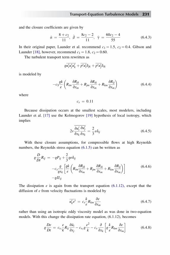
and the closure coefficients are given by

a ¼ 8þ c211

; b ¼ 8c2 � 2

11; g ¼ 60c2 � 4

55(6.4.3)

In their original paper, Launder et al. recommend c1¼ 1.5, c2¼ 0.4. Gibson and

Launder [18], however, recommend c1¼ 1.8, c2¼ 0.60.

The turbulent transport term rewritten as

9u0iu0ju

0k þ p0u0idjk þ p0u0jdik

is modeled by

�cS9k

ε

�Rim

vRjk

vxmþ Rjm

vRik

vxmþ Rkm

vRij

vxm

�(6.4.4)

where

cs ¼ 0:11

Because dissipation occurs at the smallest scales, most modelers, including

Launder et al. [17] use the Kolmogorov [19] hypothesis of local isotropy, which

implies

2vvu0ivxk

vu0jvxk

¼ 2

3εdij (6.4.5)

With these closure assumptions, for compressible flows at high Reynolds

numbers, the Reynolds stress equation (6.1.5) can be written as

9D

DtRij ¼ �9Pij þ 2

39εdij

�cs9

9xk

�9k

ε

�Rim

vRjk

vxmþ Rjm

vRik

vxmþ Rkm

vRij

vxm

��9Pij

(6.4.6)

The dissipation ε is again from the transport equation (6.1.12), except that the

diffusion of ε from velocity fluctuations is modeled by

u0kε0 ¼ cεk

ε

Rkmvε

vxm(6.4.7)

rather than using an isotropic eddy viscosity model as was done in two-equation

models. With this change the dissipation rate equation, (6.1.12), becomes

9Dε

Dt¼ cε1

ε

kRij

v�uivxj

� cε29ε2

k� cε

v

vxk

�9k

ε

Rkmvε

vxm

�(6.4.8)


where

cε ¼ 0:18

With the boundary-layer approximations, the Reynolds-stress transport equations

for twodimensional incompressible flows can be written as

D

Dtu0y0 ¼ �y02

vu

vyþ cs

v

vy

24kε

0@u0y0

vy02

vyþ 2y02

vðu0y0Þvy

1A35

c1ε

ku0y0 þ

�~ay02 þ bu02 � g

2k

�vu

vyþ ðF12Þw

(6.4.9)

D

Dtu02 ¼ �2u0y0

vu

vy� 2

3εþ cs

v

vy

24kε

0@2u0y0

v

vyu0y0 þ y02

vu02

vy

1A35

�c1ε

k

�u02 � 2

3k

�þ�2a� 2

3ðaþ bÞ

�u0y0

vu

vyþ ðF11Þw

(6.4.10)

Dy02

Dt¼ �2

3εþ cs

v

vy

24kε

0@3y02

vy02

vy

1A35� c1

ε

k

�y02 � 2

3k

�

þ�2b� 2

3

�aþ b

��u0y0

vu

vyþ ðF22Þw

(6.4.11)

Dw02

Dt¼ �2

3εþ cs

v

vy

24kε

0@y02

vw02

vy

1A35� c1

ε

k

�w02 � 2

3k

�

þ�� 2

3ðaþ bÞ

�u0y0

vu

vyþ ðF33Þw

(6.4.12)

Here

ðF11Þw ¼ k3=2

εy

�0:125

ε

k

�u02 � 2

3k

�� 0:015

�2u0y0

�vu

vy

�(6.4.13a)

ðF22Þw ¼ k3=2

εy

�0:125

ε

k

�y02 � 2

3k

�� 0:015

�� 2u0y0

�vu

vy

�(6.4.13b)

ðF33Þw ¼ k3=2

εy

�0:125

ε

k

�w02 � 2

3k

��(6.4.13c)


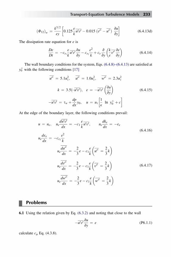
ðF12Þw ¼ k3=2

εy

�0:125

ε

ku0y0 � 0:015 ðy02 � u02Þ vu

vy

�(6.4.13d)

The dissipation rate equation for ε is

Dε

Dt¼ �cε1

ε

ku0y0

vu

vy� cε2

ε2

kþ cε

v

vy

�k

ε

y02vε

vy

�(6.4.14)

The wall boundary conditions for the system, Eqs. (6.4.8)–(6.4.13) are satisfied at

y0þ with the following conditions [17]

u02 ¼ 5:1u2s ; u02 ¼ 1:0u2s ; w02 ¼ 2:3u2s

k ¼ 3:5ð�u0y0Þ; ε ¼ �u0y0�vu

vy

�(6.4.15)

�u0y0 ¼ sw þ dp

dxy0; u ¼ us

�1

kln yþ0 þ c

�

At the edge of the boundary layer, the following conditions prevail:

u ¼ ue; uedu0y0

dx¼ �c1

ε

ku0y0; ue

dkedx

¼ �εe

uedεedx

¼ �cε2ε2

k

(6.4.16)

uedu02

dx¼ �2

3ε� c1

ε

k

�u02 ¼ 2

3k

�

uedy02

dx¼ �2

3ε� c1

ε

k

�y02 ¼ 2

3k

�

uedw02

dx¼ �2

3ε� c1

ε

k

�w02 ¼ 2

3k

�(6.4.17)

Problems

6.1 Using the relation given by Eq. (6.3.2) and noting that close to the wall

�u0y0vu

vy¼ ε (P6.1.1)

calculate cm Eq. (4.3.8).


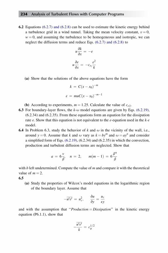
6.2 Equations (6.2.7) and (6.2.8) can be used to estimate the kinetic energy behind

a turbulence grid in a wind tunnel. Taking the mean velocity constant, y¼ 0,

w¼ 0, and assuming the turbulence to be homogeneous and isotropic, we can

neglect the diffusion terms and reduce Eqs. (6.2.7) and (6.2.8) to

uvk

vx¼ �ε

uvε

vx¼ �cε2

ε2

k

(a) Show that the solutions of the above equations have the form

k ¼ Cðx� x0Þ�m

ε ¼ muCðx� x0Þ�m�1

(b) According to experiments, m¼ 1.25. Calculate the value of cε2.

6.3 For boundary-layer flows, the k-u model equations are given by Eqs. (6.2.19),

(6.2.34) and (6.2.35). From these equations form an equation for the dissipation

rate ε. Show that this equation is not equivalent to the ε-equation used in the k-ε

model.

6.4 In Problem 6.3, study the behavior of k and u in the vicinity of the wall, i.e.,

around y¼ 0. Assume that k and u vary as k¼ bym and u¼ ayn and consider

a simplified form of Eqs. (6.2.19), (6.2.34) and (6.2.35) in which the convection,

production and turbulent diffusion terms are neglected. Show that

a ¼ 6v

b; n ¼ 2; mðm� 1Þ ¼ 6

b*

b

with b left undetermined. Compute the value ofm and compare it with the theoretical

value of m¼ 2.

6.5

(a) Study the properties of Wilcox’s model equations in the logarithmic region

of the boundary layer. Assume that

�u0y0 ¼ u2s ;vu

vy¼ us

ky

and with the assumption that ‘‘Production¼Dissipation’’ in the kinetic energy

equation (P6.1.1), show that

�u0y0

k¼ c1=2m


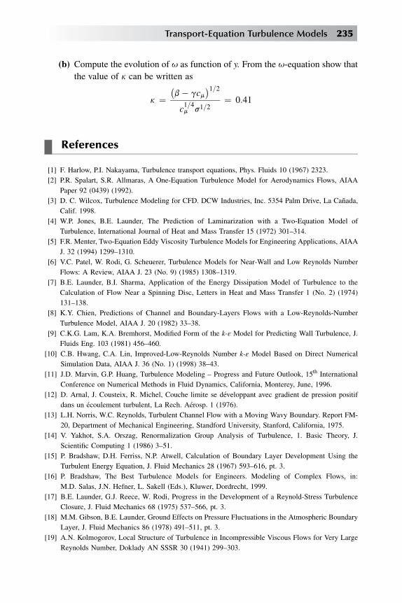
(b) Compute the evolution of u as function of y. From the u-equation show that

the value of k can be written as

k ¼�b� gcm

1=2c1=4m s1=2

¼ 0:41

References

[1] F. Harlow, P.I. Nakayama, Turbulence transport equations, Phys. Fluids 10 (1967) 2323.

[2] P.R. Spalart, S.R. Allmaras, A One-Equation Turbulence Model for Aerodynamics Flows, AIAA

Paper 92 (0439) (1992).

[3] D. C. Wilcox, Turbulence Modeling for CFD. DCW Industries, Inc. 5354 Palm Drive, La Canada,

Calif. 1998.

[4] W.P. Jones, B.E. Launder, The Prediction of Laminarization with a Two-Equation Model of

Turbulence, International Journal of Heat and Mass Transfer 15 (1972) 301–314.

[5] F.R. Menter, Two-Equation Eddy Viscosity Turbulence Models for Engineering Applications, AIAA

J. 32 (1994) 1299–1310.

[6] V.C. Patel, W. Rodi, G. Scheuerer, Turbulence Models for Near-Wall and Low Reynolds Number

Flows: A Review, AIAA J. 23 (No. 9) (1985) 1308–1319.

[7] B.E. Launder, B.I. Sharma, Application of the Energy Dissipation Model of Turbulence to the

Calculation of Flow Near a Spinning Disc, Letters in Heat and Mass Transfer 1 (No. 2) (1974)

131–138.

[8] K.Y. Chien, Predictions of Channel and Boundary-Layers Flows with a Low-Reynolds-Number

Turbulence Model, AIAA J. 20 (1982) 33–38.

[9] C.K.G. Lam, K.A. Bremhorst, Modified Form of the k-ε Model for Predicting Wall Turbulence, J.

Fluids Eng. 103 (1981) 456–460.

[10] C.B. Hwang, C.A. Lin, Improved-Low-Reynolds Number k-ε Model Based on Direct Numerical

Simulation Data, AIAA J. 36 (No. 1) (1998) 38–43.

[11] J.D. Marvin, G.P. Huang, Turbulence Modeling – Progress and Future Outlook, 15th International

Conference on Numerical Methods in Fluid Dynamics, California, Monterey, June, 1996.

[12] D. Arnal, J. Cousteix, R. Michel, Couche limite se developpant avec gradient de pression positif

dans un ecoulement turbulent, La Rech. Aerosp. 1 (1976).

[13] L.H. Norris, W.C. Reynolds, Turbulent Channel Flow with a Moving Wavy Boundary. Report FM-

20, Department of Mechanical Engineering, Standford University, Stanford, California, 1975.

[14] V. Yakhot, S.A. Orszag, Renormalization Group Analysis of Turbulence, 1. Basic Theory, J.

Scientific Computing 1 (1986) 3–51.

[15] P. Bradshaw, D.H. Ferriss, N.P. Atwell, Calculation of Boundary Layer Development Using the

Turbulent Energy Equation, J. Fluid Mechanics 28 (1967) 593–616, pt. 3.

[16] P. Bradshaw, The Best Turbulence Models for Engineers. Modeling of Complex Flows, in:

M.D. Salas, J.N. Hefner, L. Sakell (Eds.), Kluwer, Dordrecht, 1999.

[17] B.E. Launder, G.J. Reece, W. Rodi, Progress in the Development of a Reynold-Stress Turbulence

Closure, J. Fluid Mechanics 68 (1975) 537–566, pt. 3.

[18] M.M. Gibson, B.E. Launder, Ground Effects on Pressure Fluctuations in the Atmospheric Boundary

Layer, J. Fluid Mechanics 86 (1978) 491–511, pt. 3.

[19] A.N. Kolmogorov, Local Structure of Turbulence in Incompressible Viscous Flows for Very Large

Reynolds Number, Doklady AN SSSR 30 (1941) 299–303.


Short Cut Methods

Chap

ter7



7.2 Flows with Zero-Pressure Gradient 238

7.2.1 Incompressible Flow on a Smooth Flat Plate 239

7.2.2 Incompressible Flow on a Rough Flat Plate 248

7.2.3 Compressible Flow on a Smooth Flat Plate 250

7.2.4 Compressible Flow on a Rough Flat Plate 256

7.3 Flows with Pressure Gradient: Integral Methods 257

7.4 Prediction of Flow Separation in Incompressible Flows 264

7.5 Free Shear Flows 268

7.5.1 Two-Dimensional Turbulent Jet 268

7.5.2 Turbulent Mixing Layer Between Two Uniform Streams

at Different Temperatures 273

7.5.3 Power Laws for the Width and the Centerline Velocity of Similar

Free Shear Layers 280

Appendix 7A Gamma, Beta and Incomplete Beta Functions 281

Problems 283

References 291

237



http://dx.doi.org/10.1016/B978-0-08-098335-6.00007-0

7.1 Introduction

Over the years many attempts have been made to calculate turbulent flows and

various approaches have been taken. At first, before high-speed computers became

available, almost all attempts avoided the mathematical difficulties of solving highly

nonlinear Navier-Stokes and boundary-layer equations in their partial-differential

form and, instead, concentrated on the solution of the ‘‘integral’’ forms of the

boundary-layer equations, which yield ordinary differential equations. Such methods

are commonly called integral methods.

The interest in the solution of boundary-layer equations in their differential form

began early in 1960 when computers began to offer the possibility of solving

complicated systems of partial differential equations numerically. As a result, since

about 1960, a number of methods called differential methods have been develop-

ment. At present there are several very efficient and accurate differential methods

such as the one discussed in Chapters 8 and 9 for laminar and turbulent flows. With

increase in computer power, around late 1970, interest next concentrated in the

solution of the Navier-Stokes equations. As a result, at present there are several

powerful methods for solving the Navier-Stokes equations for both laminar and

turbulent flows.

In this chapter we discuss simple methods and formulas for calculating two-

dimensional turbulent flows. These methods, which we have called ‘‘short-cut’’

methods do not have the accuracy of the differential boundary-layer methods dis-

cussed in Chapters 8 and 9. Furthermore, they are restricted to simple two-dimensional

flows with restricted boundary conditions. Their chief advantage and usefulness lies in

their simplicity; unlike differential boundary-layer and Navier-Stokes methods they

either do not require computers or only small computers. They can easily be used in

many practical engineering problems.

Description of short-cut methods for flows with zero-pressure gradient begins in

Section 7.2 and is continued in Section 7.3 with integral methods for flows with

pressure gradient. Section 7.4 discusses the prediction of flow separation in two-

dimensional incompressible flows and Section 7.5 discusses the calculation of

several free shear flows based on similarity concepts.

7.2 Flows with Zero-Pressure Gradient

Short-cut methods discussed here for flows with zero-pressure gradient includes

incompressible flows on a smooth flat plate (subsection 7.2.1), on a rough flat plate

(subsection 7.2.2), compressible flow on a smooth flat plate (subsection 7.2.3) and on

a rough flat plate (subsection 7.2.4).


7.2.1 INCOMPRESSIBLE FLOW ON A SMOOTH FLAT PLATE

Let us consider an incompressible flow over a smooth flat plate. If the Reynolds

number is sufficiently large, we can identify three different flow regimes on such

a surface. Starting from the leading edge, there is first a region (0< Rx< Rxtr ) in

which the flow is laminar. After a certain distance, there is a region (Rxtr < Rx< Rxtr )

in which transition from laminar to turbulent flow takes place. In the third region

(Rx� Rxtr ) the flow is fully turbulent. The transition Reynolds number Rxtr depends

partly upon the turbulence in the free stream; Rxtr may be as low as 5� 104 or as high

as 5� 106.

For laminar flow over a flat plate, the boundary-layer parameters can be obtained

exactly from the solution of the similarity equations and can be expressed in terms of

very useful formulas. For a turbulent flow, the momentum and energy equations do

not reduce to similarity equations. Furthermore, the presence of the Reynolds stress

terms in the equations prevents an exact solution. For that reason, it is necessary to

introduce some empiricism into the equations and check their solutions with

experiment.

Skin Friction Formulas

Over the years, a large number of experiments have been conducted with smooth flat

plates. Velocity profiles and local skin-friction coefficients have been measured at

various Reynolds numbers. The experimental data have been the basis for several

useful formulas for boundary-layer parameters, as well as for several general

prediction methods such as those discussed in Chapters 8 and 9 for calculating

turbulent boundary-layers with and without pressure gradient. Here we shall restrict

our discussion to several approximate formulas that can be used for calculating cf, d*,

q, d, etc. For simplicity, we shall assume that the transition region is a point and that

the transition from laminar to turbulent flow takes place instantaneously, that is

Rxtr ¼ Rxtr .

For zero-pressure-gradient flow, the momentum integral equation (3.6.6) can be

written as

dRq=dRx ¼ cf =2 (7.2.1)

where Rq¼ ueq/n and Rx¼ uex/n. Denoting (2/cf)1/2 by z and using integration by

parts, we can express Eq. (7.2.1) in the form

Rx ¼ z2Rq � 2

Z z

ztr

Rqz dzþ A1; (7.2.2)

where A1 is an integration constant and ztr is the value of the skin-friction parameter z

at transition.

Short Cut Methods 239

The integral in Eq. (7.2.2) can be integrated, provided that Rq is expressed

as a function of z. That can be done by first recalling the definition of q and

writing it as

q ¼ d

Z 1

0

u

ue

�1� u

ue

�dh

¼ d

Z 1

0

�ue � u

ue

�dh� d

Z 1

0

�ue � u

ue

�2

dh;

(7.2.3)

where h¼ y/d. But for equilibrium boundary layers at high Reynolds numbers, c1and c2, defined as

c1h

Z 1

0

�ue � u

us

�dh; c2h

Z 1

0

�ue � u

us

�2

dh; (7.2.4)

are constant (see Fig. 4.4). Substituting from Eq. (7.2.4) into Eq. (7.2.3) and non-

dimensionalizing, we obtain

Rdhued

n¼ Rqz

c1 � c2=z(7.2.5)

Next we consider Coles’ velocity-profile expression evaluated at the edge of the

boundary layer, Eq. (4.4.37), and write it as

z ¼ 1

klnRd

zþ cþ 2P

k: (7.2.6)

With the values of c and P taken as 5.0 and 0.55, respectively, we can now integrate

Eq. (7.2.2) with the relations given by Eqs. (7.2.5) and (7.2.6). This integration

allows the resulting expression to be written as

�Rx � A2

�cf ¼ 0:324 exp

"0:58ffiffiffifficf

p�1� 8:125

ffiffiffifficf

p þ 22:08cf�#

: (7.2.7)

Here A2 is an integration constant that depends on the values of cf and Rx at transition.

Figure 7.1 presents the results for three transition Reynolds numbers, Rxtr ¼ 0,

4.1� 105 and 3� 106, the first being the casewhen transition takes place at the leading

edge. The value ofRx¼ 4� 105 corresponds to the approximate minimum value ofRx

for which the flow can be turbulent. The highest value of Rx is a typical natural

transition Reynolds number on a smooth flat plate in low-turbulence test rigs with no

heat transfer. If the plate is heated, the location of natural transition in a gas flowmoves

upstream, decreasing the value of the transitional Reynolds number, whereas if the

plate is cooled, the location of transitionmoves downstream. The reason is that sincem

rises with gas temperature, the velocity gradient near the wall is reduced by heating,


distorting the profile to a more unstable shape, and for cooling, the converse holds. In

liquid flows m falls with increasing fluid temperature, and the effect is reversed.

Putting A2¼ 0 in Eq. (7.2.7) (i.e., assuming that the turbulent boundary layer

starts at x¼ 0 with negligible thickness), taking logarithms, and making further

approximations lead to formulas like

1ffiffiffifficf

p ¼ aþ b log cf Rx;

where a and b are constants chosen to get the best agreement with experiment. Such

less-rigorous formulas have been derived by many previous workers. Von Karman

[1] took a¼ 1.7 and b¼ 4.15; i.e.

1ffiffiffifficf

p ¼ 1:7þ 4:15 log cf Rx: (7.2.8a)

A formula for the average skin friction �cf (averaged over the distance x) that

makes use of the above equation was obtained by Schoenherr [2]:

1ffiffiffiffi�cf

p ¼ 4:13 log �cf Rx: (7.2.8b)

Power-Law Velocity Profiles

By relating the profile parameter P to the displacement thickness d* and to the

momentum thickness q as well as to the local skin-friction coefficient cf, as is done in

Fig. 7.1 Local skin-friction coefficient on a smooth flat plate with three transition Rey-nolds numbers according to Eq. (7.2.7). The variation of laminar cf with Rx is shown bycf¼ 0.664/

ffiffiffiffiffiffiRx

p:


the analysis leading to Eq. (7.2.8a), we can obtain relations between d, cf, d*, q, and

H. Much simpler but less accurate relations can be obtained by assuming that the

velocity profile can be represented by the ‘‘power law’’

u

ue¼�yd

�1=n: (7.2.9)

Here n is about 7 in zero-pressure-gradient flow, increasing slowly with Reynolds

number. Using Eq. (7.2.9) and the definitions of d*, q, and H, we can show that

d*

d¼ 1

1þ n: (7.2.10a)

q

d¼ n

ð1þ nÞð2þ nÞ ; (7.2.10b)

H ¼ 2þ n

n(7.2.10c)

Other formulas obtained from power-law assumptions with n¼ 7, given by

Schlichting [1] are the following equations valid only for Reynolds numbers Rx

between 5� 105 and 107:

cf ¼ 0:059R�0:20x ; (7.2.11)

�cf ¼ 0:074R�0:20x ; (7.2.12)

d

x¼ 0:37R�0:20

x ; (7.2.13)

q

x¼ 0:036R�0:20

x : (7.2.14)

Equations (7.2.8b) and (7.2.12) assume that the boundary layer is turbulent from

the leading edge onward, that is, the effective origin is at x¼ 0. If the flow is

turbulent but the Reynolds number is moderate, we should consider the portion of

the laminar flow that precedes the turbulent flow. There are several empirical

formulas for �cf that account for this effect. One is the formula quoted by

Schlichting [1]. It is given by

�cf ¼ 0:455

ðlogRxÞ2:58� A

Rx; (7.2.15)

and another is

�cf ¼ 0:047R�0:20x � A

Rx; 5� 105 < Rx < 107: (7.2.16)


Here A is a constant that depends on the transition Reynolds number Rxtr. It is

given by

A ¼ Rxtr

��cftr � �cftr

�; (7.2.17)

where �cft and �cfl correspond to the values of average skin-friction coefficient for

turbulent and laminar flow at Rxtr . We note that although Eq. (7.2.16) is restricted to

the indicated Rx range, Eq. (7.2.15) is valid for a wide range of Rx and has given good

results up Rx¼ 109.

Heat-Transfer Formulas on Smooth Surfaces with SpecifiedTemperature

For a zero-pressure-gradient flow, the energy integral equation (3.6.26b) can be

integrated to obtain the Stanton number St as a function of Reynolds number. This

can be done by inserting the velocity profile expression given by Eq. (4.4.37) and the

similar expression for the temperature profile given by Eq. (4.4.43) into the definition

of qT. Since we already have an expression for cf, however, a simpler procedure

would be to evaluate Eq. (4.4.43) at y¼ d and make use of the relation given by Eq.

(7.2.6). For example, at y¼ d, Eq. (4.4.43) becomes

Tw � TeTs

¼ 1

khlnRd

zþ ch þ 2Ph

kh: (7.2.18)

Using the definition of Ts and the local Stanton number St, the left-hand side of Eq.

(7.2.18) becomes

Tw � TeTs

¼ 1

St

ffiffiffifficf2

r: (7.2.19)

If we equate the two expressions for ln(Rd/z) obtained from Eqs. (7.2.6) and (7.2.5)

and substitute Eq. (7.2.19) in the left-hand side of Eq. (7.2.18), we get, after

rearranging

St

cf =2¼ kh=k

1� ck� chkh þ 2�P�Ph

��k ffiffiffiffiffiffiffiffiffi

cf =2p : (7.2.20)

Because of the scatter in temperature-profile data, it is simplest to choose the value

of the quantity in braces as one that gives the best agreement with St data. For air,

this is

St

cf =2¼ 1:11

1� 1:20ffiffiffiffiffiffiffiffifficf =2

p (7.2.21)

for k¼ 0.40 and kh¼ 0.44. This equation for the Reynolds analogy factor St=ðcf =2Þis quoted in the literature with a wide range of values for the empirical constants. For


cf¼ 3� 10–3, a typical value for a laboratory boundary layer, the constants quoted

here give St/ 11 cf¼ 1.16, whereas at very high Reynolds number, where cf is small,

St/ 12 cf asymptotes to 1.11 [3].

Substituting Eq. (7.2.11) into Eq. (7.2.21) yields

St ¼ 0:0327R�0:20x

1� 0:206R�0:10x

: (7.2.22)

According to an extensive study conducted by Kader and Yaglom [4], the empirical

formula

St ¼ 1

Pr

ffiffiffifficf

p4:3 lnRxcf þ 3:8

(7.2.23)

fits the existing data on air (Pr¼ 0.7) well. For fluids with Pr� 0.7, they recommend

St ¼ffiffiffiffiffiffiffiffifficf =2

p2:12 ln Rxcf þ 12:5 Pr 2=3 þ 2:12 ln Pr� 7:2

: (7.2.24)

Equations (7.2.23) and (7.2.24) utilize Von Karman’s equation (7.2.8a) for cf with

a slightly different constant ahead of the log cf Rx term:

1ffiffiffifficf

p ¼ 1:7þ 4:07 log cf Rx :

For isothermal flat plates, Reynolds et al. [5] recommend the following empirical

formula for Stanton number:

St Pr0:4�TwTe

�0:4

¼ 0:0296R�0:20x (7.2.25)

for 5� 105< Rx< 5� 106 and 0.5� Pr� 1.0.

An approximate expression for Stanton number on an isothermal flat plate

with unheated starting length can be obtained for turbulent flows by making

suitable assumptions for velocity, temperature, and shear-stress profiles and by

using eddy viscosity and turbulent Prandtl number concepts [6]. For example,

from the definition of Stanton number with power-law profiles for velocity and

temperature,

u

ue¼�yd

�1=n;

Tw � T

Tw � Te¼�y

dt

�1=n

; (7.2.26a)

and with a shear-stress profile in the form

ssw

¼ 1��yd

�ðnþ2Þ=n(7.2.26b)


and with s=9 ¼ εmðvu=vyÞ; Prt ¼ 1; we can write

St ¼ cf2

�dt

d

��1=n

: (7.2.27)

Substituting this equation into the energy integral equation (3.3.26b) and using the

momentum integral equation for zero-pressure gradient-flow, the resulting expres-

sion can be written in the form

Z d

dx0

dd

d¼Z dt=d

0

nþ 1

n

ðdt=dÞ2=n1� ðdt=dÞð2þnÞ=n d

�dt

d

�; (7.2.28)

where dx0 denotes the hydrodynamic boundary-layer thickness at x¼ x0 (see

Fig. 7.2).

Integrating Eq. 7.2.28, we obtain

d

dx0¼�1�

�dt

d

�ð2þnÞ=n��ðnþ1Þ=ðnþ2Þ

or

dt

d¼�1�

�dx0d

�ðnþ2Þ=ðnþ1Þ�n=ð2þnÞ: (7.2.29)

In the range 5� 105� Rx� 107, d varies as x4/5 [see Eq. (7.2.13)]. Thus Eq.

(7.2.29) may be written as

dt

d¼h1�

�x0x

�4ðnþ2Þ=5ðnþ1Þin=ð2þnÞ: (7.2.30)

Substituting Eq. (7.2.30) into Eq. (7.2.27) and taking n¼ 7, we get

St ¼ cf2

h1�

�x0x

�9=10i�1=9: (7.2.31)

For a plate heated from the leading edge (x0¼ 0), Eq. (7.2.31) becomes

St ¼ StT ¼ cf2;

Fig. 7.2 Flat plate with an unheated starting length.


where StT denotes the Stanton number of the isothermal flat plate. With this notation,

Eq. (7.2.31) can be written as

St

StT¼h1�

�x0x

�9=10i�1=9; x > x0: (7.2.32)

From the definition of heat-transfer coefficient h and Stanton number St, for an

isothermal flat plate with unheated starting length,

h ¼ 9uecpStT

h1�

�x0x

�9=10i�1=9: (7.2.33)

Similarly, with StT given by Eq. (7.2.25)

St Pr0:4�TwTe

�0:4

¼ 0:0296R�0:20x

h1�

�x0x

�9=10i�1=9: (7.2.34)

For nonisothermal surfaces with arbitrary surface temperature, the heat flux at

some distance x from the leading edge is, by superposition arguments [7],

_qw ¼Z x¼x

x¼0h�x; x�dTw

�x�; (7.2.35)

where, with StT (x) being evaluated at x,

h�x; x� ¼ 9uecpStT

�x��1�

�x

x

�9=10��1=9

: (7.2.36)

The integration of Eq. (7.2.35) is performed in the ‘‘Stieltjes’’ sense rather than in the

ordinary ‘‘Riemann’’ or ‘‘area’’ sense [8]. This must be done because specified

surface temperature may have a finite discontinuity, so that dTw is undefined at some

point. The Stieltjes integral may, however, be expressed as the sum of an ordinary or

Riemann integral and a term that accounts for the effect of the finite discontinuities

[7]. The integral of Eq. (7.2.25) may be written as

_qw�x� ¼

Z x¼x

x¼0h�x; x�dTwðxÞ

dxdx

þXNn¼ 1

h�x0n; x

�hTw�xþ0n�� Tw

�x�0n�i:

(7.2.37)

Here N denotes the number of discontinuities and Twðxþ0nÞ � Twðx�0nÞ denotes the

temperature jump across the nth discontinuity.

As an example, let us consider a plate whose temperature is equal to Tw1from the

leading edge to x¼ x0 and equal to Tw2for x> x0. To find the heat flux for x> x0, we

note that since dTw/dx is zero except at x¼ x0, the first term on the right-hand side is


zero. Therefore, we concentrate our attention on the second term. Since N¼ 2, we

can write

n ¼ 1; h�0; x� ¼ 9uecpStT ½1� 0��1=9;

Tw�0þ�� Tw

�0�� ¼ Tw1

� Te ;

n ¼ 2; h�x0; x

� ¼ 9uecpStT�x�h1�

�x0x

�9=10i�1=9;

Tw�xþ0�� Tw

�x�0� ¼ Tw2

� Tw1:

Thus the heat transfer for x> x0 is given by

_qwðxÞ ¼ 9uecpStTðxÞn�

Tw1� Te

�þ �Tw2� Tw1

�h1�

�x0x

�9=10i�1=9o: (7.2.38)

Note that StT (x) is computed with Tw¼ Tw2.

Heat-Transfer Formulas on Smooth Surfaces with Specified Heat Flux

The analysis of thermal boundary layers on smooth surfaces with specified heat flux

is similar to those with specified temperature. Based on the experiments of Reynolds

et al., the following empirical formula is recommended in [9]:

St Pr0:4 ¼ 0:030R�0:2x ; (7.2.39)

which is nearly identical to the one for specified temperature, Eq. (7.2.25). Note that

the difference in Stanton-number formulas between the constant wall heat-flux case

and the constant wall temperature case is considerably more in laminar flows, where

the difference is 36 percent.

When the plate has an arbitrary heat-flux distribution on the surface and also

includes an unheated section, the difference between the surface temperature and

edge temperature can be calculated from the following formula given by Reynolds

et al. [7]:

Tw�x�� Te ¼

Z x¼x

x¼0gðx; xÞ _qwðxÞ dx; (7.2.40)

where, with G denoting the gamma function (see Appendix 7A),

g�x; x� ¼

910 Pr

�0:6R�0:8x

G�19

�G�89

��0:0287k

��1�

�x

x

�9=10��8=9

:

The nature of the integrated in Eq. (7.2.40) is such that integration is always per-

formed in the usual Riemann sense, including integration across discontinuities. To


illustrate this point further, let us consider a plate that is unheated for a distance x0from the leading edge and is heated at a uniform rate _qw for x> x0. To find the wall

temperature for x> x0, we write Eq. (7.2.40) as

Tw�x�� Te ¼ 3:42 _qw

Pr0:6R0:8x k

Z x

x0

�1�

�x

x

�9=10��8=9

dx: (7.2.41)

The integral can be evaluated in terms of beta functions (see Appendix 7A), and the

resulting expression can be written as

Tw�x�� Te ¼ 33:61 _qwPr

0:4R0:2x

9cpue

brð1=9; 10=9Þb1ð1=9; 10=9Þ

(7.2.42)

or, using the definition of Stanton number, as

St ¼ 0:030Pr�0:4R�0:2x

br�19;

109

��.b1�19;

109

�� ; (7.2.43)

where r¼ 1 – (x0/x)9/10.

7.2.2 INCOMPRESSIBLE FLOW ON A ROUGH FLAT PLATE

The discussion in the previous subsection is valid for smooth surfaces. In practice,

many surfaces are ‘‘rough’’ in the hydraulic sense. It is often desirable to compute cf,

�cf , Rq, H, etc., on such surfaces. Here we show, as an example, how boundary-layer

parameters can be obtained for sand-roughened plates by using an approach similar

to that discussed in subsection 7.2.1.

It was shown in Section 4.5 that the law of the wall for flows with roughness is

given by Eq. (4.5.1). By means of Eq. (4.5.2), it can be written as

uþ ¼ �1=k�ln yþ � �1=k�ln kþ þ B2: (7.2.44)

The functional relationship, which can only be determined from experiments,

also assumes that the slope of the velocity distribution on rough walls is the same as

the slope on smooth surfaces. The best-known roughness configuration – one

frequently used as standard roughness – is that of closely packed uniform sand

grains. According to Nikuradse’s experiments in sand-roughened pipes [10], the

variation of B2 with kþ is that shown in Fig. 7.3. We see from the figure that B2 varies

differently in the three regions discussed in Section 4.5. For example, in the

completely rough regime, B2 is a constant equal to 8.48.


Equation (7.2.44) applies only in the inner region of the boundary layer. For

application to the entire boundary layer, it must be corrected for the wakelike

behavior of the outer region. That can be done by using Coles’ wake expression.

With the correction, Eq. (7.2.44) becomes

uþ ¼ �1=k�ln�y=k�þ B2 þ

�P=k

�w: (7.2.45)

Evaluating that expression at the edge of the boundary layer and rearranging, we can

write

Rd ¼ Rk exp½kðz� fð1Þ�; (7.2.46)

where

Rk ¼ uek=n; fð1Þ ¼ B2 þ ð2P=kÞ:

Since the velocity-defect law is valid for both smooth and rough surfaces, we can still

use the expression for Rq as given by Eq. (7.2.5). From Eqs. (7.2.46) and (7.2.5), we

can write

Rq ¼ ðRk=zÞ½c1 � ðc2=zÞ� exp ½kðz� fð1Þ�: (7.2.47)

As before, the constants c1 and c2 are 3.78 and 25, respectively.

A relation between cf and Rx can now be obtained by using the momentum

integral equation in the form given by Eq. (7.2.1). Before Eq. (7.2.1) is integrated,

however, it is necessary to establish lower limits for Rx and Rq. It is obvious from

Fig. 7.3 Variation of B2 with k*.


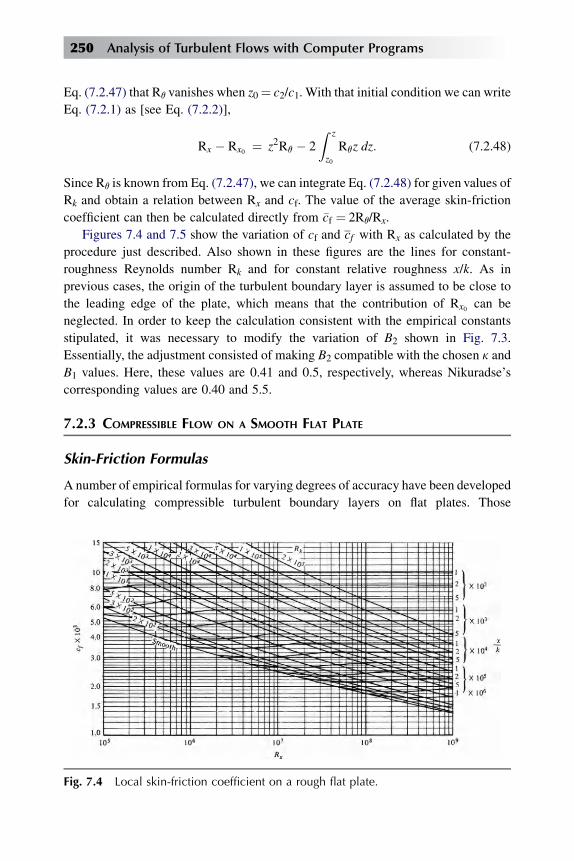
Eq. (7.2.47) that Rq vanishes when z0¼ c2/c1. With that initial condition we can write

Eq. (7.2.1) as [see Eq. (7.2.2)],

Rx � Rx0 ¼ z2Rq � 2

Z z

z0

Rqz dz: (7.2.48)

Since Rq is known from Eq. (7.2.47), we can integrate Eq. (7.2.48) for given values of

Rk and obtain a relation between Rx and cf. The value of the average skin-friction

coefficient can then be calculated directly from �cf ¼ 2Rq/Rx.

Figures 7.4 and 7.5 show the variation of cf and cf with Rx as calculated by the

procedure just described. Also shown in these figures are the lines for constant-

roughness Reynolds number Rk and for constant relative roughness x/k. As in

previous cases, the origin of the turbulent boundary layer is assumed to be close to

the leading edge of the plate, which means that the contribution of Rx0 can be

neglected. In order to keep the calculation consistent with the empirical constants

stipulated, it was necessary to modify the variation of B2 shown in Fig. 7.3.

Essentially, the adjustment consisted of making B2 compatible with the chosen k and

B1 values. Here, these values are 0.41 and 0.5, respectively, whereas Nikuradse’s

corresponding values are 0.40 and 5.5.

7.2.3 COMPRESSIBLE FLOW ON A SMOOTH FLAT PLATE

Skin-Friction Formulas

A number of empirical formulas for varying degrees of accuracy have been developed

for calculating compressible turbulent boundary layers on flat plates. Those

Fig. 7.4 Local skin-friction coefficient on a rough flat plate.


developed by Van Driest [11] and by Spalding and Chi [12] have higher accuracy than

the rest and cover a wide range of Mach number and ratio of wall temperature to total

temperature. These two methods have similar accuracy, although the approaches

followed to obtain the formulas are somewhat different. Both methods define

compressibility factors by the following relation between the compressible and

incompressible values:

cfi ¼ Fccf ; (7.2.49a)

Rqi ¼ FRqRq; (7.2.49b)

Rxi ¼Z Rx

0

FRq

FcdRx ¼ FRx

Rx; (7.2.49c)

Here the subscript i denotes the incompressible values, and the factors Fc, FRq; and

FRx(h FRq

/Fc) defined by Eq. (7.2.49) are functions of Mach number, ratio of wall

temperature, and recovery factor. Spalding and Chi’s method is based on the

postulate that a unique relation exists between cf Fc and FRx Rx. The quantity Fc is

obtained by means of mixing-length theory, and FR is obtained semiempirically.

According to Spalding and Chi,

Fc ¼ Taw=Te � 1

ðsin�1aþ sin�1bÞ2; FRq

¼�TawTe

�0:772�TwTe

��1:474

; (7.2.50)

where, with r denoting the recovery factor (Taw – Te)/(T0e – Te),

Fig. 7.5 Average skin-friction on a rough flat plate.


a ¼ Taw=Te þ Tw=Te � 2hðTaw=Te þ Tw=TeÞ2� 4

�Tw=Te

�i1=2 ;

b ¼ Taw=Te � Tw=TehðTaw=Te þ Tw=TeÞ2� 4

�Tw=Te

�i1=2 ;(7.2.51a)

TawTe

¼ 1þ g� 1

2r M2

e : (7.2.51b)

According to van Driest’s method, which is based entirely on the mixing-length

theory, Fc is again given by the expression defined in Eqs. (7.2.50) and (7.2.51).

However, the parameter FRqis now given by

FRq¼ me

mw: (7.2.52)

The development of Van Driest’s formula for skin friction is analogous to the

solution steps discussed for incompressible flows (see subsection 7.2.1) except that

the derivation is more tedious. The solution requires the expansion of the integral

into a series by means of integration by parts and a simple expression is again

obtained when higher-order terms are neglected. With this procedure and with the

power-law temperature-viscosity relation mf T u, which implies FRq¼ (Te /Tw)

u the

following relation for cf and Rx is obtained for compressible turbulent boundary

layers with and without heat transfer, with xmeasured from the effective origin of the

turbulent flow:

0:242�sin�1aþ sin�1b

�A

ffiffiffiffiffiffiffiffiffiffiffiffiffiffiffiffiffiffiffiffifficf�Tw=Tc

�q ¼ 0:41þ logRxcf ��1

2þ u

�log

TwTe

; (7.2.53)

where A

A2 ¼ g� 1

2

M2e

Tw=Te:

This formula is based on Prandtl’s mixing-length formula l¼ ky. If the procedure

leading to this equation is repeated with the mixing-length expression given by von

Karman’s similarity law

l ¼ k

�� vu=vyv2u=vy2

��;a formula similar to that given by Eq. (7.2.53) is obtained except that 12þu in Eq.

(7.2.53) is replaced by u. This formula is known as Van Driest II, in order to


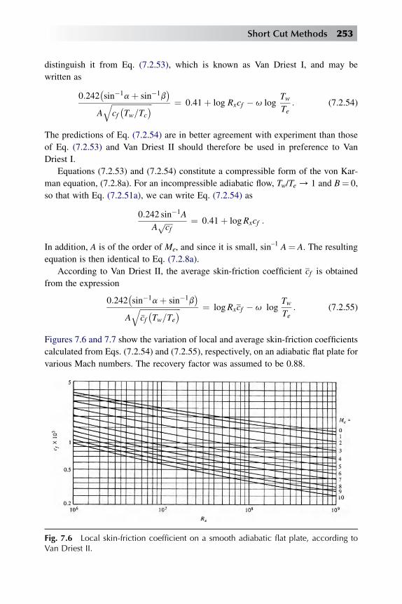
distinguish it from Eq. (7.2.53), which is known as Van Driest I, and may be

written as


�A

ffiffiffiffiffiffiffiffiffiffiffiffiffiffiffiffiffiffiffiffifficf�Tw=Tc

�q ¼ 0:41þ log Rxcf � u logTwTe

: (7.2.54)

The predictions of Eq. (7.2.54) are in better agreement with experiment than those

of Eq. (7.2.53) and Van Driest II should therefore be used in preference to Van

Driest I.

Equations (7.2.53) and (7.2.54) constitute a compressible form of the von Kar-

man equation, (7.2.8a). For an incompressible adiabatic flow, Tw/Te/ 1 and B¼ 0,

so that with Eq. (7.2.51a), we can write Eq. (7.2.54) as

0:242 sin�1A

Affiffiffifficf

p ¼ 0:41þ logRxcf :

In addition, A is of the order of Me, and since it is small, sin–1 A¼ A. The resulting

equation is then identical to Eq. (7.2.8a).

According to Van Driest II, the average skin-friction coefficient cf is obtained

from the expression


�A

ffiffiffiffiffiffiffiffiffiffiffiffiffiffiffiffiffiffiffiffiffi�cf�Tw=Te

�q ¼ logRxcf � u logTwTe

: (7.2.55)

Figures 7.6 and 7.7 show the variation of local and average skin-friction coefficients

calculated from Eqs. (7.2.54) and (7.2.55), respectively, on an adiabatic flat plate for

various Mach numbers. The recovery factor was assumed to be 0.88.

Fig. 7.6 Local skin-friction coefficient on a smooth adiabatic flat plate, according toVan Driest II.


Figure 7.8 shows the effect of compressibility on the local and average skin-

friction coefficients. Here, the skin-friction formulas were solved at a Reynolds

number (Rx¼ 107) as functions of Mach number for fixed values of Tw/Te. In the

results shown in Fig. 7.6, the local skin-friction values for incompressible flows with

heat transfer were obtained from the limiting form of Eq. (7.2.54).

We note that asMe/ 0 and when Tw/Te¼ 1, A/ 0, a/ –1, and b/ 1. It follows

that the term

sin�1aþ sin�1b

A

Fig. 7.7 Average skin-friction coefficient on a smooth adiabatic flat plate, according toVan Driest II.

Fig. 7.8 Effect of compressibility on (a) local skin-friction coefficient and (b)average skin-friction coefficient on a smooth flat plate, according to Van Driest II.Rx¼ 107.


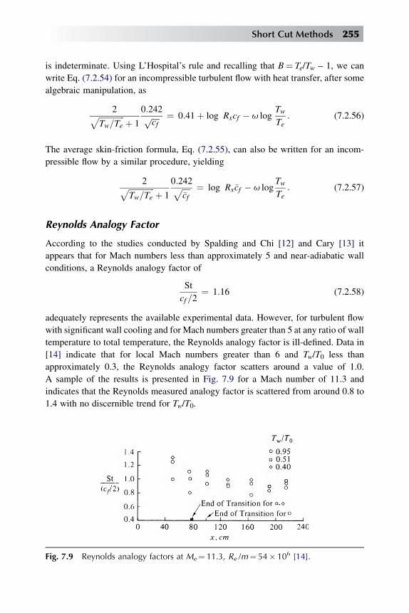
is indeterminate. Using L’Hospital’s rule and recalling that B¼ Te/Tw – 1, we can

write Eq. (7.2.54) for an incompressible turbulent flow with heat transfer, after some

algebraic manipulation, as

2ffiffiffiffiffiffiffiffiffiffiffiffiffiTw=Te

p þ 1

0:242ffiffiffifficf

p ¼ 0:41þ log Rxcf � u logTwTe

: (7.2.56)

The average skin-friction formula, Eq. (7.2.55), can also be written for an incom-

pressible flow by a similar procedure, yielding

2ffiffiffiffiffiffiffiffiffiffiffiffiffiTw=Te

p þ 1

0:242ffiffiffiffi�cf

p ¼ log Rx�cf � u logTwTe

: (7.2.57)

Reynolds Analogy Factor

According to the studies conducted by Spalding and Chi [12] and Cary [13] it

appears that for Mach numbers less than approximately 5 and near-adiabatic wall

conditions, a Reynolds analogy factor of

St

cf =2¼ 1:16 (7.2.58)

adequately represents the available experimental data. However, for turbulent flow

with significant wall cooling and for Mach numbers greater than 5 at any ratio of wall

temperature to total temperature, the Reynolds analogy factor is ill-defined. Data in

[14] indicate that for local Mach numbers greater than 6 and Tw/T0 less than

approximately 0.3, the Reynolds analogy factor scatters around a value of 1.0.

A sample of the results is presented in Fig. 7.9 for a Mach number of 11.3 and

indicates that the Reynolds measured analogy factor is scattered from around 0.8 to

1.4 with no discernible trend for Tw/T0.

Fig. 7.9 Reynolds analogy factors at Me¼ 11.3, Re /m¼ 54� 106 [14].


7.2.4 COMPRESSIBLE FLOW ON A ROUGH FLAT PLATE

The skin-friction formulas for a smooth flat plate, Eqs. (7.2.55) and (7.2.56), can also

be used to obtain formulas for sand-grain-roughened flat plates by assuming a rela-

tion between the compressible and incompressible values such as that given by Eq.

(7.2.49a). According to the experiments of Goddard [15] on adiabatic fully rough flat

plates,

Fc ¼ TawTe

; (7.2.59)

and the experimental values of cf verified the relation (7.2.59) for his chosen

turbulent recovery factor, r¼ 0.86. It should be emphasized that this equation is for

fully rough flow in which the flow on top of the roughness elements remains

subsonic. It is consistent with the observation originally noted by Nikuradse for

incompressible flow, namely, that the skin-friction drag for fully rough flow is the

sum of the form drags of the individual roughnesses.

Fenter [16] also presented a theory for the effect of compressibility on the

turbulent skin friction of rough plates with heat transfer. This gave results that agree

with those of relation (7.2.59) only at Mach numbers close to unity and only for zero

heat transfer. For Tw¼ Te, the value of cf given by this theory is 14 percent less than

that given by Goddard’s relation at Me¼ 2.0 and 45 percent less at Me¼ 4.0. Fenter

presented experimental data forMe¼ 1.0 and 2.0 that agreed well with this theory for

the case of zero heat transfer. The difference in the experimental values of cf of the

two reports is probably within the accuracy to which the roughness heights were

measured. The theory of Fenter is based on assumptions whose validity is ques-

tionable at high Mach numbers, and these assumptions may account for the differ-

ence in cf predicted by Fenter and by Goddard for the case of Tw¼ Te.

Figures 7.10 and 7.11 show the average skin friction distribution for a sand-

roughened adiabatic plate, and Figs. 7.12 and 7.13 show the results for a sand-

roughened plate with a wall temperature equal to the freestream temperature, all at

Me¼ 1 and 2. In all these figures, transition was assumed to take place at the leading

edge.

Figure 7.14 shows the variation of the ratio of the compressible to incompressible

values of skin-friction coefficient with Mach number for the various types of flow on

an adiabatic plate. The variation is much larger for turbulent flow than for laminar

flow and increases as the Reynolds number increases, being largest for a fully rough

wall where viscous effects are negligible. The reason is that the effect of viscosity is

felt mainly near the wall (in the viscous sublayer), and so the relevant Reynolds

number for correlating skin friction is that based on the wall value of viscosity. The

ratio of wall viscosity to freestream viscosity increases as Me increases; so a given

value of ueL/ne corresponds to a smaller value of ueL/nw and thus a larger cf. The


effect on cf decreases as ueL/ne increases because the change of cf associated with RL

is smaller. The effect is absent on fully rough walls.

7.3 Flows with Pressure Gradient: Integral Methods

Integral methods are based on the solution of the integral equations of motion

discussed in Section 3.6. They avoid the complexity of solving the differential form

of the boundary layer equations, and they provide – with very short computation

Fig. 7.11 Average skin-friction coefficient for a sand-roughened adiabatic flat plate atMe¼ 2.

Fig. 7.10 Average skin-friction coefficient for a sand-roughened adiabatic flat plate atMe¼ 1.


times – a solution of the boundary layer equations. There are several integral

methods for calculating momentum transfer in turbulent boundary layers and

a more limited number for heat transfer. This disparity arises because of the

difficulty of incorporating possible rapid changes in wall temperature or heat flux

Fig. 7.12 Average skin-friction coefficient for a sand-roughened adiabatic flat platewith Tw/Te¼ 1, Me¼ 1.

Fig. 7.13 Average skin-friction coefficient for a sand-roughened adiabatic flat platewith Tw /Te¼ 1, Me¼ 2.


into the temperature profiles used in the solution of the energy integral equation. In

the following, we discuss integral methods, first for momentum transfer and then

for heat transfer.

Head’s Method

The momentum integral equation

dq

dxþ q

ue

duedx

�H þ 2

� ¼ cf2

(3.6.6)

contains the three unknowns q, H, and cf, and assumed relationships between these

integral parameters are required. There are several approaches to the achievement of

this objective. One approach that we shall consider here adopts the notion that

a turbulent boundary layer grows by a process of ‘‘entrainment’’ of nonturbulent

fluid at the outer edge and into the turbulent region. It was first used by Head [17],

who assumed that the mean-velocity component normal to the edge of the boundary

layer (which is known as the entrainment velocity yE) depends only on the mean-

velocity profile, specifically on H. He assumed that the dimensionless entrainment

velocity yE/ue is given by

yE

ueh

1

ue

d

dx

Z d

0u dy ¼ 1

ue

d

dxue�d� d*

� ¼ F�H1

�; (7.3.1)

Fig. 7.14 Mach number variation of the ratio of the compressible to incompressiblevalues of local skin-friction coefficient for the various types of air flow on an adiabaticflat plate, for given Reynolds number ueL/ve.


where we have used the definition of d* for two-dimensional incompressible flows. If

we define

H1 ¼ d� d*

q; (7.3.2)

then the right-hand equality in Eq. (7.3.1) can be written as

d

dx

�ueq H1

� ¼ ueF : (7.3.3)

Head also assumed that H1 is related to the shape factor H by

H1 ¼ GðHÞ: (7.3.4)

The functions F andGwere determined from experiment, and a best fit to several sets

of experimental data showed that they can be approximated by

F ¼ 0:0306ðH1 � 3:0Þ�0:6169; (7.3.5)

G ¼�0:8234ðH � 1:1Þ�1:287 þ3:3 H � 1:6 ;

1:5501ðH � 0:6778Þ�3:064 þ3:3 H � 1:6 :(7.3.6)

With F and G defined by Eqs. (7.3.5) and (7.3.6), Eq. (7.3.3) provides a relationship

between q andH. Another equation relating cf to q and/orH is needed, and Head used

the semiempirical skin-friction law given by Ludwieg and Tillmann [18],

cf ¼ 0:246� 10�0:678H R�0:268q ; (7.3.7)

where Rq¼ ueq/n. The system [Eqs. (3.6.6) and (7.3.1)–(7.3.7)], which includes

two ordinary differential equations, can be solved numerically for a specified

external velocity distribution to obtain the boundary-layer development on a two-

dimensional body with a smooth surface [19]. To start the calculations, say x¼ x0,

we note that initial values of two of the three quantities q, H and cf must be

specified, with the third following from Eq. (7.3.7). When turbulent-flow calcu-

lations follow laminar calculations for a boundary layer on the same surface,

Head’s method is often started by assuming continuity of momentum thickness q

and taking the initial value of H to be 1.4, an approximate value corresponding to

flat-plate flow.

This model, like most integral methods, uses a given value of the shape factor

H as the criterion for separation. [Equation (7.3.7) predicts cf to be zero only if

H tends to infinity]. It is not possible to give an exact value of H corresponding to

separation, and values between the lower and upper limits of H makes little

difference in locating the separation point since the shape factor increases rapidly

close to separation.


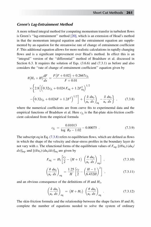
Green’s Lag-Entrainment Method

Amore refined integral method for computing momentum transfer in turbulent flows

is Green’s ‘‘lag-entrainment’’ method [20], which is an extension of Head’s method

in that the momentum integral equation and the entrainment equation are supple-

mented by an equation for the streamwise rate of change of entrainment coefficient

F. This additional equation allows for more realistic calculations in rapidly changing

flows and is a significant improvement over Head’s method. In effect this is an

‘‘integral’’ version of the ‘‘differential’’ method of Bradshaw et al. discussed in

Section 6.3. It requires the solution of Eqs. (3.6.6) and (7.3.1) as before and also

considers the ‘‘rate of change of entrainment coefficient’’ equation given by

q�H1 þ H

�dFdx

¼ F�F þ 0:02

�þ 0:2667cf0F þ 0:01

� 2:8h�

0:32cf0 þ 0:024 Feq þ 1:2F2eq

�1=2�

��0:32cf0 þ 0:024F þ 1:2F2

�1=2�þ�d

ue

duedx

�eq

� d

ue

duedx

�; (7.3.8)

where the numerical coefficients are from curve fits to experimental data and the

empirical functions of Bradshaw et al. Here cf0 is the flat-plate skin-friction coeffi-

cient calculated from the empirical formula

cf0 ¼ 0:01013

log Rq � 1:02� 0:00075 : (7.3.9)

The subscript eq in Eq. (7.3.8) refers to equilibrium flows, which are defined as flows

in which the shape of the velocity and shear-stress profiles in the boundary layer do

not vary with x. The xfunctional forms of the equilibrium values of Feq, [(q/ue) (due/

dx)]eq, and [(d/ue) (due/dx)]eq are given by

Feq ¼ H1

�cf2� �H þ 1

� � q

ue

duedx

�eq

�; (7.3.10)

�q

ue

duedx

�eq

¼ 1:25

H

�cf2��

H � 1

6:432H

�2�; (7.3.11)

and an obvious consequence of the definitions of H and H1,�d

ue

duedx

�eq

¼ �H þ H1

� � q

ue

duedx

�eq

: (7.3.12)

The skin-friction formula and the relationship between the shape factors H and H1

complete the number of equations needed to solve the system of ordinary


differential equations (3.6.6), (7.3.1) and (7.3.8). The skin-friction equation is

given by �cfcf0

þ 0:5

� �H

H0� 0:4

�¼ 0:9 ; (7.3.13a)

where

1� 1

H0¼ 6:55

�cf02

�1=2; (7.3.13b)

so that Eqs. (7.3.9) and (7.3.13) give cf as a function of H and Rq with values close to

Eq. (7.3.7).

The shape-factor relation is

H1 ¼ 3:15þ 1:72

H � 1� 0:01ðH � 1Þ2 (7.3.13c)

and gives values close to Eq. (7.3.6).

Comparisons with experiment show good accuracy in incompressible boundary

layer flows and also in wakes. The method has also been extended to represent

compressible flows [19].

Truckenbrodt’s Method

Two dimensional turbulent boundary layers can also be computed by simple methods

such as Thwaites’ method for laminar flows [19]. Although these methods are limited

and are not as accurate as the differential and integral methods, they are nevertheless

useful to estimating boundary-layer parameters without the use of computers.

According to Truckenbrodt’s method, the momentum thickness is computed from

Q ¼�q

c

�7=6 � ueuN

�7=2

¼ 0:0076

R1=6c

Z x=c

ðx=cÞtr

�ueuN

�10=2

d�xc

�þ c1 : (7.3.14)

Here c1 is a constant determined by the initial values of ue and q at the transition point

xtr. The momentum thickness Reynolds number Rq is defined by ueq/n.

In order to calculate the development of the shape factor H, Truckenbrodt intro-

duced a new shape factor L that can be calculated from the following expression:

L ¼ xtr

xLtr þ ln

�ueðxÞuetr

�

þ 1

x

Z x

xtr

�0:0304 ln Rq � 0:23� ln

�ueðxÞuetr

��dx ; (7.3.15)

where x¼Q4.


The shape factor L is related to H by

L ¼ ln

"0:775ðH � 0:379Þ1:61

H ðH � 1Þ0:61#

: (7.3.16)

Thus once the initial values of q and H are known, one can calculate the initial

value of L by Eq. (7.3.16) and consequently can calculate the development of q, L,

and H around the body.

The local skin friction can be calculated by means of the formula given by

Ludwieg and Tillmann, Eq. (7.3.7).

Ambrok’s Method

The use of integral procedures to predict heat transfer in turbulent boundary

layers generally requires the solution of the integral forms of the energy and

momentum equations, although solutions of the integral form of one equation

and the differential form of the other have, on occasions, been used. Empirical

information is, of course, required to allow the solution of the energy equation,

and this usually involves a relationship between the wall heat flux and known

integral quantities together with an equation to link the thickness of the

temperature and velocity boundary layers. It is difficult to provide empirical

relationships that can be used for more than the simplest flows; as a consequence,

integral procedures are not widely used, and differential methods are generally to

be preferred.

Where an approximate heat-transfer result is required in relation to a simple flow,

expressions derived from integral procedures can be useful. The method of Ambrok

[21], for example, assumes the Reynolds analogy and, with the integral energy

equation, arrives at the approximate equation

St ¼ _qw9cpue

�Tw � Te

� ¼ Pr�0:4R�0:2L ðTw � TeÞ0:25h R x*

0 u*eðTw � TeÞ1:25dx*i0:2 ; (7.3.17)

ue*, and RL denote dimensionless quantities defined by

x* ¼ x

L; u*e ¼ ue

uref; RL ¼ urefL

n:

It is useful to note that Eq. (7.3.17) does represent, albeit approximately, the effect of

variable surface temperature.


7.4 Prediction of Flow Separation in Incompressible Flows

In many problems it is necessary to know the boundary layer whether laminar or

turbulent, will separate from the surface of a specific body and, if so, where the

separation will occur. That is quite important, since in many design problems, such

as those of the design of hydrofoils or airfoils, it is necessary to avoid flow separation

in order to obtain low drag and high lift.

For two-dimensional steady flows, the separation point is defined as the point

where the wall shear stree sw is equal to zero, that is,

ðvu=vyÞw ¼ 0 : (7.4.1)

With high-speed computers, the boundary-layer equations for laminar flow can be

solved exactly, and consequently the laminar separation point can be determined

almost exactly. In addition, there are several ‘‘simple’’ methods that do not require

the solution of the boundary layer equations in their differential form and that can be

used to predict the separation point quite satisfactorily. Thwaites’ method discussed

in [19] and Stratford’s method as cited in [22] are typical examples of two such

methods. According to Thwaites’ method, laminar separation is predicted when

l�h q2

nduedx

� ¼ �0:090. Stratford’s method does not even require the solution of the

laminar boundary-layer equations. For a given pressure distribution, for example,

Cp(x), the expression

C1=2p x

�dCp=dx

�(7.4.2)

is calculated around the body. Separation is predicted when it reaches a value of

0.102. Here Cp is defined as

Cp ¼ 1� ðue=uoÞ2 ; (7.4.3)

where uo is the velocity at the beginning of the adverse pressure gradient.

The location of a separation point can also be calculated by using either

a differential method or an integral method. In differential methods, the parameter

used to predict the separation point is the zero-wall-shear stress. In integral methods,

the shape factor H is usually used in locating the separation point. In integral

methods separation is assumed to occur when H reaches a value between 1.8 and 2.4

for turbulent flows. In some cases, however, the value of H increases rapidly near

separation and then begins to decrease. In each case7 the point corresponding to the

maximum value of H is taken as the separation point.

7Flows for which an experimental pressure distribution is used in the calculations.


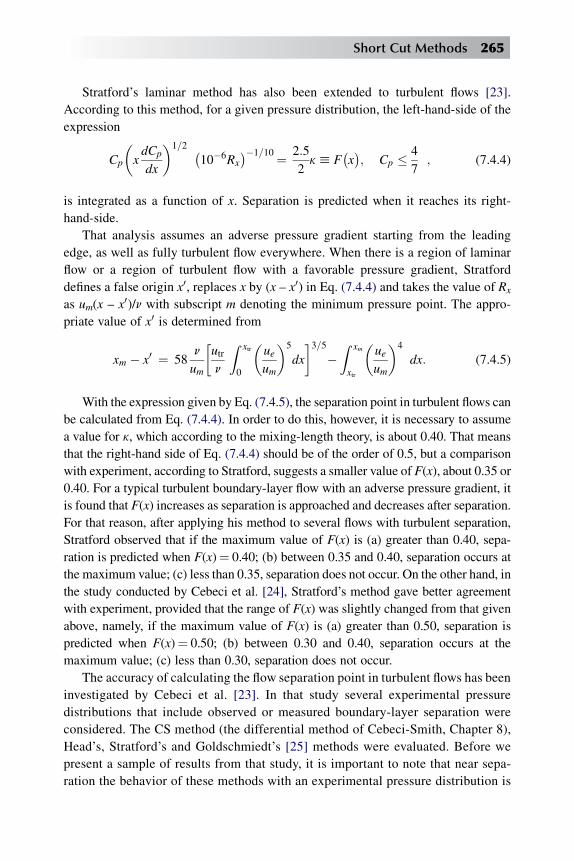
Stratford’s laminar method has also been extended to turbulent flows [23].

According to this method, for a given pressure distribution, the left-hand-side of the

expression

Cp

�xdCp

dx

�1=2 �10�6Rx

��1=10¼ 2:5

2khF

�x�; Cp � 4

7; (7.4.4)

is integrated as a function of x. Separation is predicted when it reaches its right-

hand-side.

That analysis assumes an adverse pressure gradient starting from the leading

edge, as well as fully turbulent flow everywhere. When there is a region of laminar

flow or a region of turbulent flow with a favorable pressure gradient, Stratford

defines a false origin x0, replaces x by (x – x0) in Eq. (7.4.4) and takes the value of Rx

as um(x – x0)/n with subscript m denoting the minimum pressure point. The appro-

priate value of x0 is determined from

xm � x0 ¼ 58n

um

�utrn

Z xtr

0

�ueum

�5

dx

�3=5�Z xm

xtr

�ueum

�4

dx: (7.4.5)

With the expression given by Eq. (7.4.5), the separation point in turbulent flows can

be calculated from Eq. (7.4.4). In order to do this, however, it is necessary to assume

a value for k, which according to the mixing-length theory, is about 0.40. That means

that the right-hand side of Eq. (7.4.4) should be of the order of 0.5, but a comparison

with experiment, according to Stratford, suggests a smaller value of F(x), about 0.35 or

0.40. For a typical turbulent boundary-layer flow with an adverse pressure gradient, it

is found that F(x) increases as separation is approached and decreases after separation.

For that reason, after applying his method to several flows with turbulent separation,

Stratford observed that if the maximum value of F(x) is (a) greater than 0.40, sepa-

ration is predicted when F(x)¼ 0.40; (b) between 0.35 and 0.40, separation occurs at

the maximum value; (c) less than 0.35, separation does not occur. On the other hand, in

the study conducted by Cebeci et al. [24], Stratford’s method gave better agreement

with experiment, provided that the range of F(x) was slightly changed from that given

above, namely, if the maximum value of F(x) is (a) greater than 0.50, separation is

predicted when F(x)¼ 0.50; (b) between 0.30 and 0.40, separation occurs at the

maximum value; (c) less than 0.30, separation does not occur.

The accuracy of calculating the flow separation point in turbulent flows has been

investigated by Cebeci et al. [23]. In that study several experimental pressure

distributions that include observed or measured boundary-layer separation were

considered. The CS method (the differential method of Cebeci-Smith, Chapter 8),

Head’s, Stratford’s and Goldschmiedt’s [25] methods were evaluated. Before we

present a sample of results from that study, it is important to note that near sepa-

ration the behavior of these methods with an experimental pressure distribution is


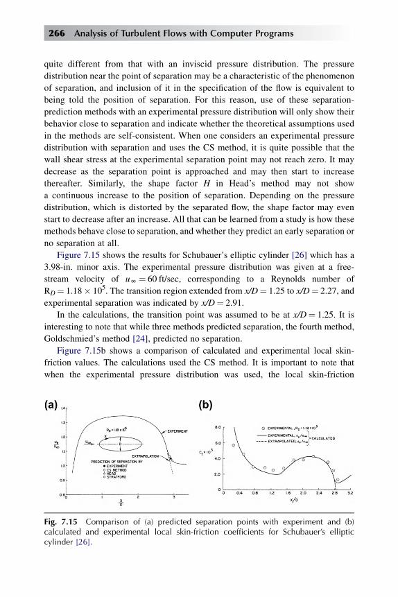
quite different from that with an inviscid pressure distribution. The pressure

distribution near the point of separation may be a characteristic of the phenomenon

of separation, and inclusion of it in the specification of the flow is equivalent to

being told the position of separation. For this reason, use of these separation-

prediction methods with an experimental pressure distribution will only show their

behavior close to separation and indicate whether the theoretical assumptions used

in the methods are self-consistent. When one considers an experimental pressure

distribution with separation and uses the CS method, it is quite possible that the

wall shear stress at the experimental separation point may not reach zero. It may

decrease as the separation point is approached and may then start to increase

thereafter. Similarly, the shape factor H in Head’s method may not show

a continuous increase to the position of separation. Depending on the pressure

distribution, which is distorted by the separated flow, the shape factor may even

start to decrease after an increase. All that can be learned from a study is how these

methods behave close to separation, and whether they predict an early separation or

no separation at all.

Figure 7.15 shows the results for Schubauer’s elliptic cylinder [26] which has a

3.98-in. minor axis. The experimental pressure distribution was given at a free-

stream velocity of uN¼ 60 ft/sec, corresponding to a Reynolds number of

RD¼ 1.18� 105. The transition region extended from x/D¼ 1.25 to x/D¼ 2.27, and

experimental separation was indicated by x/D¼ 2.91.

In the calculations, the transition point was assumed to be at x/D¼ 1.25. It is

interesting to note that while three methods predicted separation, the fourth method,

Goldschmied’s method [24], predicted no separation.

Figure 7.15b shows a comparison of calculated and experimental local skin-

friction values. The calculations used the CS method. It is important to note that

when the experimental pressure distribution was used, the local skin-friction

Fig. 7.15 Comparison of (a) predicted separation points with experiment and (b)calculated and experimental local skin-friction coefficients for Schubauer’s ellipticcylinder [26].


coefficient began to increase near separation because the pressure distribution was

distorted by the flow separation. However, when the calculations were repeated by

using an extrapolated velocity distribution that could be obtained by an inviscid

method, the skin friction went to zero at x/D¼ 2.82.

Figures 7.16 and 7.17 show the results for three airfoils where flow separation

was observed. Figure 7.16 shows the results for the pressure distribution observed

over an airfoil-like body at a Reynolds number per foot of 0.82� 106. The experi-

mental data, which are due to Schubauer and Klebanoff [27] gave the separation

point at 25.7� 0.2 ft from the leading edge. The predictions of all methods are quite

good.

As shown in Fig. 7.17a, agreement between the CS method and experiment is

also very good for Newman’s airfoil [28]. On the other hand, the other methods

predict an early separation.

Fig. 7.16 Comparison of predicted separation points with experiment for the airfoil-like body of Schubauer and Klebanoff [27].

Fig. 7.17 Comparison of predicted separation points with experiment for (a) Newman’sairfoil [28] and (b) the NASA 4412 airfoil section at various angles of attack.


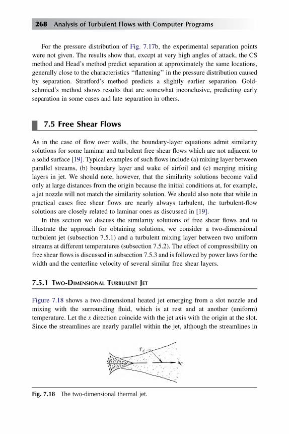
For the pressure distribution of Fig. 7.17b, the experimental separation points

were not given. The results show that, except at very high angles of attack, the CS

method and Head’s method predict separation at approximately the same locations,

generally close to the characteristics ‘‘flattening’’ in the pressure distribution caused

by separation. Stratford’s method predicts a slightly earlier separation. Gold-

schmied’s method shows results that are somewhat inconclusive, predicting early

separation in some cases and late separation in others.

7.5 Free Shear Flows

As in the case of flow over walls, the boundary-layer equations admit similarity

solutions for some laminar and turbulent free shear flows which are not adjacent to

a solid surface [19]. Typical examples of such flows include (a) mixing layer between

parallel streams, (b) boundary layer and wake of airfoil and (c) merging mixing

layers in jet. We should note, however, that the similarity solutions become valid

only at large distances from the origin because the initial conditions at, for example,

a jet nozzle will not match the similarity solution. We should also note that while in

practical cases free shear flows are nearly always turbulent, the turbulent-flow

solutions are closely related to laminar ones as discussed in [19].

In this section we discuss the similarity solutions of free shear flows and to

illustrate the approach for obtaining solutions, we consider a two-dimensional

turbulent jet (subsection 7.5.1) and a turbulent mixing layer between two uniform

streams at different temperatures (subsection 7.5.2). The effect of compressibility on

free shear flows is discussed in subsection 7.5.3 and is followed by power laws for the

width and the centerline velocity of several similar free shear layers.

7.5.1 TWO-DIMENSIONAL TURBULENT JET

Figure 7.18 shows a two-dimensional heated jet emerging from a slot nozzle and

mixing with the surrounding fluid, which is at rest and at another (uniform)

temperature. Let the x direction coincide with the jet axis with the origin at the slot.

Since the streamlines are nearly parallel within the jet, although the streamlines in

Fig. 7.18 The two-dimensional thermal jet.


the entraining flow are more nearly normal to the axis, the pressure variation in the jet

is small and can be neglected. The boundary layer equations can be written as

vu

vxþ vy

vy¼ 0; (7.5.1)

uvu

vxþ y

vu

vy¼ 1

9

vsvy; (7.5.2)

uvT

vxþ vT

vy¼ � 1

9cp

v _q

vy: (7.5.3)

Here in general

s ¼ mvu

vy� 9u0y0; (7.5.4)

_qh _qy ¼ �kvT

vyþ 9cpT 0y0: (7.5.5)

These equations are subject to the symmetry and boundary conditions

y ¼ 0; y ¼ 0;vu

vy¼ 0;

vT

vy¼ 0; (7.5.6a)

y ¼ N; u ¼ 0; T ¼ Te: (7.5.6b)

Because the pressure is constant in the jet and the motion is steady, the total

momentum in the x direction is constant; that is

J ¼ 9

Z N

�Nu2 dyh 29

Z N

0u2 dy ¼ const: (7.5.7)

The heat flux (rate of transport of enthalpy of the mean flow) in the x direction is

independent of x and equal to its value at the orifice; that is

K ¼ 29cp

Z N

0uðT � TeÞ dy ¼ const; (7.5.8)

K being equal to the product of the initial mass flow rate and the mean enthalpy per

unit mass.

To find the similarity solution for the above system, we define dimensionless

velocity and temperature ratios by

f 0�h� ¼ uðx; yÞ

ucðxÞ ; (7.5.9)

g�h� ¼ Tðx; yÞ � Te

TcðxÞ � Te: (7.5.10)


Here uc(x) and Tc(x) denote the velocity and temperature, respectively, along the

centerline y¼ 0, and h denotes the similarity variable defined by

h ¼ y

dðxÞ; (7.5.11)

where d is the shear-layer thickness, to be defined quantitatively below. We assume

that the stream function j(x, y) is related to a dimensionless stream function f(h),

independent of x, by

jðx; yÞ ¼ ucðxÞdðxÞ=f ðhÞ: (7.5.12)

Note that since j(x, y) has the units (length)2/time, and since f(h) is dimensionless,

the product uc(x) d(x) has the same units as j. Our interest here is to find the

functional form of d(x).

Using Eqs. (7.5.9)–(7.5.11), we can write Eqs. (7.5.7) and (7.5.8) as

J ¼ 29M

Z N

0ðf 0Þ2 dh; (7.5.13)

K ¼ 29cpN

Z N

0f 0 g dh; (7.5.14)

where

M ¼ u2cd ; N ¼ ucd�Tc � Te

�: (7.5.15)

We note that since the total momentum J and the heat flux K are constant, thenM and

N must be constant, since the integrals in Eqs. (7.5.13) and (7.5.14) are pure

numbers. By using Eqs. (7.5.9)–(7.5.12) and (7.5.15), together with the chain rule,

we can write Eqs. (7.5.2) and (7.5.3) as

u2c2

dd

dx

�ðf 0Þ2þf f 00

�¼ �s0

9; (7.5.16)

ducdTcdx

�fg�0 ¼ � 1

9cp

�_q�0; (7.5.17)

h ¼ 0; f ¼ f 00 ¼ 0; g0 ¼ 0; (7.5.18a)

h ¼ he; f 0 ¼ 0; g ¼ 0: (7.5.18b)

Equations (7.5.16) and (7.5.17) apply to both laminar and turbulent two-

dimensional jets. For turbulent jets the contributions of the laminar shear stress

and heat transfer to s and _q, defined by Eqs. (7.5.4) and (7.5.5), respectively, are

small, just as they are outside the sublayer in a wall flow, and can be neglected.


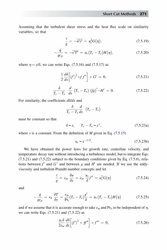
Assuming that the turbulent shear stress and the heat flux scale on similarity

variables, so that

s9¼ �u0y0 ¼ u2cG

�h�; (7.5.19)

� _q

9cp¼ �y0T 0 ¼ uc

�Tc � Te

�H�h�; (7.5.20)

where h¼ y/d, we can write Eqs. (7.5.16) and (7.5.17) as

1

2

dd

dx

�ðf 0Þ2þf f 00

�þ G0 ¼ 0; (7.5.21)

d

Tc � Te

d

dx

�Tc � Te

� �fg�0�H0 ¼ 0: (7.5.22)

For similarity, the coefficients dd/dx and

d

Tc � Te

d

dx

�Tc � Te

�must be constant so that

dwx; Tc � Tewxs; (7.5.23a)

where s is a constant. From the definition of M given in Eq. (7.5.15)

ucwx�1=2: (7.5.23b)

We have obtained the power laws for growth rate, centerline velocity, and

temperature decay rate without introducing a turbulence model, but to integrate Eqs.

(7.5.21) and (7.5.22) subject to the boundary conditions given by Eq. (7.5.6), rela-

tions between f 0 and G 0 and between g and H0 are needed. If we use the eddy-

viscosity and turbulent-Prandtl-number concepts and let

s9¼ εm

vu

vy¼ εm

ucdf 00 ¼ u2cG

�h�

(7.5.24)

and

� _q

9cp¼ εh

vT

vy¼ εm

Prt

�Tc � Te

�g0d

¼ uc�Tc � Te

�H�h�

(7.5.25)

and if we assume that it is accurate enough to take εm and Prt, to be independent of h,

we can write Eqs. (7.5.21) and (7.5.22) as

ucd

2εm

dd

dx

�ðf 0Þ2þ ff 00

�þ f 000 ¼ 0; (7.5.26)


Prtεm

ucd2

Tc � Te

d

dx

�Tc � Te

� �fg�0�g00 ¼ 0: (7.5.27)

If we define d as the y distance where u/uc¼ 12 , then experimental data [1] suggest

εm ¼ 0:037ucd: (7.5.28)

If we write the first relation in Eq. (7.5.23a) as

d ¼ Ax (7.5.29a)

and use Eq. (7.5.28), the coefficient in Eq. (7.5.26) becomes

ucd

2εm

dd

dx¼ const ¼ A

2ð0:037Þ ¼ c1; (7.5.29b)

as required for similar solution of Eq. (7.5.26) and Eq. (7.5.26) can be written as

f 000 þ c1

hðf 0Þ2þf f 00

i¼ 0: (7.5.30)

After integrating it three times and using at first the boundary conditions that at

h¼ he, f0 ¼ f 00 ¼ 0 and then the condition that at h¼ 0, f 0 ¼ 1, f¼ 0, we find the

solution to be

f ¼ffiffiffiffiffi2

c1

rtanh

ffiffiffiffiffic12

rh: (7.5.31)

Requiring that f 0 (¼ u/uc) ¼ 12 at y¼ d, that is, h¼ 1, we find the value of c1 to be

1.5523. Then it follows from Eq. (7.5.29b) that A¼ 0.115. As a result, the similarity

solution for the dimensionless velocity profile of a two-dimensional turbulent jet can

be written as

f 0 ¼ u

uc¼ sech20:881h; (7.5.32)

the dimensionless stream function f can be written as

f ¼ 1:135 tanh 0:881h; (7.5.33)

and Eq. (7.5.29a) for the width of the jet becomes

d ¼ 0:115x: (7.5.34)

We now insert Eq. (7.5.32) into Eq. (7.5.13), and upon integration we get

uc ¼ 2:40

ffiffiffiffiffiffiffiffiJ=9

x

r: (7.5.35)


The mass flow rate _m is

_m ¼ 0:625ffiffiffiffiffiffiffi9Jx

p: (7.5.36)

To obtain the similarity solution of the energy equation (7.5.27), we denote

Prtεm

ucd2

Tc � Te

d

dx

�Tc � Te

�¼ const ¼ �CPrt; (7.5.37)

and we write Eq. (7.5.27) as

g00 þ CPrt�fg�0 ¼ 0: (7.5.38)

Letting C¼ c1 (h 1.5523), we integrate Eq. (7.5.38) to get

g0 þ c1Prt f g ¼ c2: (7.5.39)

Noting that the constant of integration c2¼ 0 according to the centerline boundary

condition imposed on g, and using the relation for f obtained from Eq. (7.5.33), we

integrate Eq. (7.5.39) once more to get

g ¼ T � TeTc � Te

¼ c3

½cosh 0:881h�2Prt ¼ c3½sech 0:881h�2Prt ; (7.5.40)

where c3¼ 1 because g(0)¼ 1.

Clearly, if Prt¼ 1, the velocity profile of Eq. (7.5.32) and the temperature profile

of Eq. (7.5.40) are identical. The profile shapes are also identical with those given

for a laminar jet [19] because the eddy viscosity is assumed to be independent of y.

Since the eddy viscosity εm depends on x, the growth rate is different; the jet width

varies linearly with x in turbulent flow and as x2/3 in laminar flow.

7.5.2 TURBULENT MIXING LAYER BETWEEN TWO UNIFORM STREAMS

AT DIFFERENT TEMPERATURES

Similarity solutions of the momentum and energy equations for a turbulent mixing

layer between two uniform streams that move with velocities u1 and u2 and whose

(uniform) temperatures are T1 and T2 (see Fig. 7.19) can be obtained by the method

Fig. 7.19 The thermal mixing layer.


used for a two-dimensional jet but with different similarity variables. The governing

equations are Eqs. (7.5.1)–(7.5.5). The boundary conditions in Eq. (7.5.6) are

replaced by

y ¼ N; u ¼ u1; T ¼ T1; y ¼ �N; u ¼ u2; T ¼ T2: (7.5.41)

Sometimes the velocity of one uniform stream may be zero. If we use the definition

of stream function j and relate it to a dimensionless stream function f by

jðx; yÞ ¼ u1dðxÞ f ðhÞ (7.5.42)

then we can write

u ¼ u1 f0; y ¼ u1

dd

dx

�f 0h� f

�(7.5.43)

with h¼ y/d(x). Here y¼ 0, defined as the line on which y¼ 0, is not in general

parallel to the splitter plate dividing the two streams for x< 0. The lateral location of

the profile is determined by the boundary conditions applied by the external flow. If

there is a solid boundary, parallel to the splitter plate, at the upper edge of the high-

velocity stream, then y¼ 0 for large positive y (where f 0 ¼ 1, which requires f¼ h for

large h). If we now define a dimensionless temperature by

g�h� ¼ T � T2

T1 � T2; (7.5.44)

then using the definition of h and the definition of dimensionless stream function

given by Eq. (7.5.42), we can write the momentum and energy equations and their

boundary conditions as

u21dd

dxf f 00 ¼ � 1

9s0; (7.5.45)

�T1 � T2

�du1

dd

dxf g0 ¼ 1

9cpq0; (7.5.46)

h ¼ he; f 0 ¼ 1; g ¼ 1; h ¼ �he; f 0 ¼ u2u1

h l; g ¼ 0; (7.5.47a)

h ¼ 0; f ¼ 0 or f 0 ¼ 1

2

�1þ l

�: (7.5.47b)

Equations (7.5.45) and (7.5.46) apply to both laminar and turbulent flows. For

turbulent flows, the contribution of laminar momentum and heat transfer to s and _q

are small and can be neglected. As before, if we use the eddy-viscosity, eddy-

conductivity, and turbulent-Prandtl-number concepts and let

�u0y0 ¼ εmvu

vy¼ εm

u1d

f 00 (7.5.48a)


and

�T 0y0 ¼ εhvT

vy¼ εm

Prt

vT

vy¼ εm

Prt

T0d

g00; (7.5.48b)

where T0¼ T1 – T2, we can write Eqs. (7.5.45) and (7.5.46) as

f 000 þ u1d

εm

dd

dxf f 00 ¼ 0 (7.5.49)

and

g00 þ Prtu1d

εm

dd

dxfg0 ¼ 0: (7.5.50)

For similarity of the velocity field, we must have

u1d

εm

dd

dx¼ const: (7.5.51)

With Prt also assumed to be a constant, this requirement for similarity then applies to

both velocity and temperature fields. If we take the constant in Eq. (7.5.51) to be 12

then Eqs. (7.5.49) and (7.5.50) become

f 000 þ 1

2f f 00 ¼ 0; (7.5.52)

g00 þ 1

2Prt f g

0 ¼ 0: (7.5.53)

As in the case of the jet, these equations, which are subject to the boundary condi-

tions given by Eq. (7.5.47), are identical to those for laminar flows [19] if we replace

Prt by Pr. In fact, if we assume Prt to be, say, 0.9, then the laminar-flow profile for

Pr¼ 0.9 will be the same as the turbulent-flow profile; as usual, if Prt¼ 1.0, the

velocity and temperature profiles will be identical.

The difference between the solutions of (7.5.51) for turbulent flows and the one

for laminar flows is due to the definition of d. For turbulent flows the solution of Eq.

(7.5.51) requires an expression for εm. Several expressions can be used for this

purpose. Here we use the one given by Prandtl. Assuming that εmw d, we expect that

εm will be determined by the velocity and length scales of the mixing layer:

εm ¼ k1dðumax � uminÞ ¼ k1dðu1 � u2Þ; (7.5.54)

where k1 is an empirical factor, nominally dependent on y but usually taken as

constant.

If we assume that �u0 y0 ¼ u21HðhÞ, then from similarity arguments it follows

that d is proportional to x; in laminar flow it is proportional to x1/2. Denoting d by cx,

we can write Eq. (7.5.54), with k1c¼ C, as

εm ¼ C xu1ð1� lÞ: (7.5.55)


For uniformity with the existing literature on turbulent mixing layers, we now

introduce a parameter s used by Gortler and defined by him as

s ¼ 1

2

ffiffiffiffiffiffiffiffiffiffiffiffiffiffiffiffiffiffi1þ l

ð1� lÞC

s: (7.5.56)

This can be written as

C ¼ ð1þ lÞ4s2ð1� lÞ : (7.5.57)

Substituting Eq. (7.5.57) into (7.5.55) and the resulting expression into Eq. (7.5.51)

and taking the constant in Eq. (7.5.51) to be 12, we get

d ¼ x

s

ffiffiffiffiffiffiffiffiffiffiffi1þ l

8

r: (7.5.58)

With d given by this equation, we can now plot the solutions of Eqs. (7.5.52)

and (7.5.53) in terms of f 0 (h u/u1) and g0 [h (T – T2)(T1 – T2)] as a function

of

h ¼ y

xs

ffiffiffiffiffiffiffiffiffiffiffi8

1þ l

r(7.5.59)

for a given value of l. The Gortler parameter s, a numerical constant, must be

determined empirically. For a turbulent ‘‘half jet’’ (mixing layer in still air) for

which l¼ 0, experimental values are mostly between 11 and 13.5. For mixing

layers with arbitrary velocity ratios l, Abramovich [29] and Sabin [30] proposed

that

s ¼ s0

�1þ l

1� l

�(7.5.60)

for flows with and without pressure gradient. In Eq. (7.5.60) s0 is, of course, the

value of s for the half jet, l¼ 0. This relation was later confirmed by Pui and

Gartshore [31] to be a good fit to data.

Figure 7.20 shows a comparison between the numerical solutions of Eq. (7.5.52)

and the experimental data of Liepmann and Laufer [32] for a half jet, with s¼ 12.0

and taking y¼ 0 where u/u1¼ 0.5.

Data for thermal mixing layers are rare but suggest a turbulent Prandtl number

of the order of 0.5. This does not necessarily imply that the temperature profile is

wider than the velocity profile but merely that the two shapes are different.

However, good agreement with experiment near the edges would probably require

Prt to depend on y.


Low-Speed Flows

The interpretation of experimental data obtained in free turbulent shear layers

with large density differences is made difficult by the influence of initial

conditions and the absence of flows that can be regarded as ‘‘fully developed’’.

Indeed, in the case of the mixing layer between two streams of different densities

and unequal (subsonic) speeds, even the direction of the change in spreading rate

with density ratio is uncertain. The measurements covering the widest range of

density ratio appear to be those of Brown and Roshko [33], who varied the ratio

of low-speed stream density 92 to high-speed stream density 91 between 7 and 17.

In the former case the spreading rate was about 0.75 of that of a constant-density

mixing layer, and in the latter case it was about 1.35 times as large as in the

constant-density case. Other experiments over smaller ranges of density ratio are

inconsistent, but it is clear that in most practical cases, such as the mixing of air

and gaseous hydrocarbon fuel, the density ratio will be sufficiently near unity for

the change in spreading rate to be negligible. Furthermore, the effect of density

ratio on the percentage change of spreading rate with velocity ratio u2/u1 is also

small.

In the case of a jet of one fluid emerging into another fluid of different

density, the density ratio has inevitably fallen to a value fairly near unity at the

location where the jet has become fully developed (say, x/d¼ 20), and the change

of jet spreading rate with density ratio is effectively negligible. The case of low-

speed wakes with significant density differences is not of great practical

importance except for buoyant flows in the ocean, and there appear to be no data

available.

Fig. 7.20 A comparison between the numerical solutions of Eq. (7.5.52) for a turbulentmixing layer (shown by solid line) and the experimental data of Liepmann and Laufer[32], for a half jet with s ~ 12.


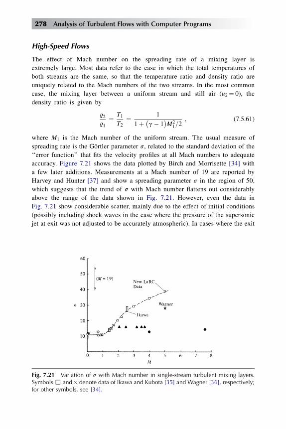
High-Speed Flows

The effect of Mach number on the spreading rate of a mixing layer is

extremely large. Most data refer to the case in which the total temperatures of

both streams are the same, so that the temperature ratio and density ratio are

uniquely related to the Mach numbers of the two streams. In the most common

case, the mixing layer between a uniform stream and still air (u2¼ 0), the

density ratio is given by

9291

¼ T1T2

¼ 1

1þ �g� 1�M2

1=2; (7.5.61)

where M1 is the Mach number of the uniform stream. The usual measure of

spreading rate is the Gortler parameter s, related to the standard deviation of the

‘‘error function’’ that fits the velocity profiles at all Mach numbers to adequate

accuracy. Figure 7.21 shows the data plotted by Birch and Morrisette [34] with

a few later additions. Measurements at a Mach number of 19 are reported by

Harvey and Hunter [37] and show a spreading parameter s in the region of 50,

which suggests that the trend of s with Mach number flattens out considerably

above the range of the data shown in Fig. 7.21. However, even the data in

Fig. 7.21 show considerable scatter, mainly due to the effect of initial conditions

(possibly including shock waves in the case where the pressure of the supersonic

jet at exit was not adjusted to be accurately atmospheric). In cases where the exit

Fig. 7.21 Variation of s with Mach number in single-stream turbulent mixing layers.Symbols , and� denote data of Ikawa and Kubota [35] and Wagner [36], respectively;for other symbols, see [34].


pressure is significantly different from atmospheric pressure, the pattern of shock

waves and/or expansions considerably affects the spreading rate of the mixing

layer.

Equation (7.5.61) implies that the density ratio across a mixing layer at a Mach

number of 5 is roughly equal to the factor of 7 investigated in a low-speed flow by

Brown and Roshko, who found an increase in spreading rate of about 35 percent

compared with the decrease of almost a factor of 3 indicated by Fig. 7.21. Clearly,

the high Mach number implies an effect of compressibility on the turbulence, as well

as on the mean density gradient. Indeed it is easy to show that the Mach-number

fluctuation in a mixing layer is considerably higher than in a boundary layer at the

same mean Mach number. A typical velocity fluctuation can be expressed in terms of

the shear stress, so that a representative maximum root-mean-square (rms) velocity

fluctuation can be written as ffiffiffiffiffism9

r; (7.5.62)

where sm is the maximum shear stress within the layer. The square of the speed of

sound, a2, is gp/9, and we can see that the Mach number based on the above-

mentioned representative velocity fluctuation and the local speed of sound can be

written in terms of the external stream Mach number and a shear-stress coefficient

based on external stream parameters, that is,

M1

ffiffiffiffiffiffiffiffiffism91u

21

r: (7.5.63)

The quantity under the square root sign is of order 0.01 in a mixing layer at low

speeds, whereas it is equal to cf /2, which is of order 0.001, in a boundary layer in

zero pressure gradient (where the maximum shear stress is equal to the wall value).

Thus, the Mach-number fluctuation in a mixing layer at a given freestream Mach

number is approximately 3 times as large as in a boundary layer at the same

freestream Mach number. (This result refers to low Mach number; as the Mach

number increases, the skin-friction coefficient in a boundary layer decreases and, as

we have seen, the spreading rate and turbulence intensity in a mixing layer also

decrease, so that the factor of 3 is at least roughly maintained). We can, therefore,

argue that compressibility effects on the turbulence in a mixing layer at a Mach

number of 1 are as strong as in a boundary layer at a Mach number of 3. The fact

that the spreading rate of a mixing layer does not start to decrease until the Mach

number is greater than unity, and that turbulence models with no explicit

compressibility effects perform well in boundary layers at Mach numbers up to at

least 3, supports this explanation. The implication that significant compressibility

effects on turbulence may occur in boundary layers at Mach numbers in excess of 3


is overshadowed by the effects of the very large heat-transfer rates found in practice

at hypersonic speeds and the fact that the viscous sublayer becomes extremely thick

in hypersonic boundary layers.

No convincing explanation of the compressibility effects exists. Clearly, pres-

sure fluctuations are in some way responsibly because large density differences at

low speeds have very little effect. Pressure fluctuations within a turbulent flow are

of the order of the density multiplied by the mean-square velocity fluctuation,

which, we argued above, is in turn of the same order as the shear stress. In fact the

ratio of the maximum shear stress to the absolute pressure is, except for a factor of

g, equal to the square of the Mach number fluctuation derived above. Since the root

mean square of the Mach number fluctuation in a mixing layer is about 0.1 of the

stream Mach number, this suggests that the ratio of the rms pressure fluctuation to

the absolute pressure is of order 14 at a Mach number of 5. It is not necessary that

these large pressure fluctuations are caused by shock waves, although the latter may

well occur, nor is it necessary to suppose that the main reason for the decrease in

spreading rate with increase in Mach number is the increasing loss of turbulent

kinetic energy by acoustic radiation (‘‘eddy Mach waves’’), although the latter may

have some effect. It is known that pressure fluctuations play a large part in the

generation and destruction of shear stress in turbulent flow, and this effect of

pressure fluctuations is certain to alter if the pressure fluctuations become

a significant fraction of the absolute pressure. However, this approach to the role of

pressure fluctuations does not explain why the spreading rate should decrease with

increasing Mach number.

In jets and wakes, the Mach number based on the maximum velocity difference

between the shear layer and the external flow falls rapidly with increasing distance

downstream, and the density ratio returns rapidly toward unity. As in the case of low-

speed jets and wakes with significant density differences, it is difficult to establish

general effects of compressibility on spreading rate, independent of the initial

conditions. There is considerable interest in the wakes of axisymmetric bodies

moving at high speeds, with reference to the detection of reentering missiles. In this

case, the most important variables are the temperature and the electron density in the

partly ionized gas. Wake data for moderate freestream Mach numbers are given by

Demetriades [38,39].

7.5.3 POWER LAWS FOR THE WIDTH AND THE CENTERLINE VELOCITY OF SIMILAR

FREE SHEAR LAYERS

The variation of the width, d, and the centerline velocity, uc or u1, of several turbulent

shear layers are summarized in Table 7.1.


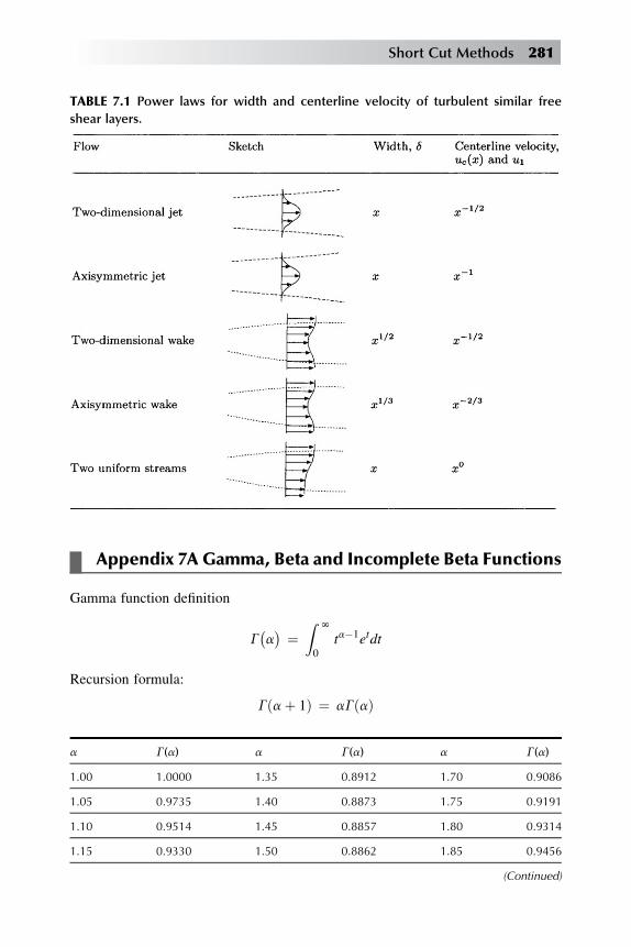
Appendix 7A Gamma, Beta and Incomplete Beta Functions

Gamma function definition

G�a� ¼

Z N

0ta�1etdt

Recursion formula:

Gðaþ 1Þ ¼ aGðaÞ

a G(a) a G(a) a G(a)

1.00 1.0000 1.35 0.8912 1.70 0.9086

1.05 0.9735 1.40 0.8873 1.75 0.9191

1.10 0.9514 1.45 0.8857 1.80 0.9314

1.15 0.9330 1.50 0.8862 1.85 0.9456

(Continued)

TABLE 7.1 Power laws for width and centerline velocity of turbulent similar free

shear layers.


(Continued )

a G(a) a G(a) a G(a)

1.20 0.9182 1.55 0.8889 1.90 0.9618

1.25 0.9064 1.60 0.8935 1.95 0.9799

1.30 0.8975 1.65 0.9001 2.00 1.0000

Beta function definition:

B1

�a; b

� ¼Z 1

0ta�1ð1� tÞb�1dt ¼ GðaÞGðbÞ

Gðaþ bÞ ¼ B1

�b;a

�

Incomplete Beta function definition:

Bx

�a; b

� ¼Z x

0ta�1ð1� tÞb�1dt

Recursion formula:

Bxða; bÞ ¼ B1ða; bÞ � B1�xða; bÞ

The following table [40] gives the functional ratios Ix(a, b)¼ Bx (a, b)/B1(a, b) for

typical combinations of a and b:

Incomplete beta function ratios Ix (a, b)

x a¼ 1/3 a¼ 1/3 a¼ 1/3 a¼ 2/3 a¼ 1/9 a¼ 1/9 a¼ 1/9 a¼ 8/9

b¼ 2/3 b¼ 4/3 b¼ 8/3 b¼ 4/3 b¼ 8/9 b¼ 10/9 b¼ 20/9 b¼ 10/9

0 0 0 0 0 0 0 0 0

0.02 0.2249 0.3068 0.4007 0.0912 0.6346 0.6588 0.7281 0.0342

0.04 0.2838 0.3859 0.5007 0.1443 0.6856 0.7113 0.7845 0.0628

0.06 0.3254 0.4410 0.5684 0.1886 0.7173 0.7439 0.8186 0.0917

0.08 0.3588 0.4845 0.6204 0.2278 0.7407 0.7679 0.8431 0.1174

0.10 0.3872 0.5210 0.6627 0.2636 0.7595 0.7870 0.8622 0.1416

0.20 0.4924 0.6506 0.8008 0.4124 0.8213 0.8490 0.9199 0.2607

0.30 0.5694 0.7377 0.8793 0.5321 0.8603 0.8870 0.9506 0.3715

(Continued)


(Continued )

x a¼ 1/3 a¼ 1/3 a¼ 1/3 a¼ 2/3 a¼ 1/9 a¼ 1/9 a¼ 1/9 a¼ 8/9

b¼ 2/3 b¼ 4/3 b¼ 8/3 b¼ 4/3 b¼ 8/9 b¼ 10/9 b¼ 20/9 b¼ 10/9

0.40 0.6337 0.8038 0.9284 0.6339 0.8895 0.9146 0.9696 0.4765

0.50 0.6911 0.8566 0.9599 0.7225 0.9133 0.9362 0.9820 0.5767

0.60 0.7448 0.8998 0.9796 0.7999 0.9335 0.9538 0.9901 0.6725

0.70 0.7970 0.9352 0.9912 0.8671 0.9515 0.9686 0.9952 0.7640

0.80 0.8501 0.9640 0.9972 0.9244 0.9679 0.9812 0.9982 0.8507

0.90 0.9084 0.9863 0.9996 0.9706 0.9835 0.9917 0.9996 0.9313

1.00 1.0000 1.0000 1.0000 1.0000 1.0000 1.0000 1.0000 1.0000

B1(a, b) 3.6275 2.6499 2.0153 1.2092 9.1853 8.8439 7.9839 1.0206

Problems

7.1 A thin flat plate is immersed in a stream of air at atmospheric pressure and at

25 �C moving at a velocity of 50ms–1. Calculate the momentum thickness,

boundary-layer thickness, local skin-friction coefficient, and average skin-fric-

tion coefficient at x¼ 3 m. Assume that n¼ 1.5� 10–5 m2s–1 and

Rxcr ¼ 3� 106.

7.2 Air at 70 �F and 1 atm flows at 100 ft s–1 past a flat plate of length 15 ft. Assume

Rxtr ¼ 3� 106, take n¼ 1.6� 10–4 ft2s–1.

(a) Find the effective origin x0 of the turbulent boundary layer.

Hint: To estimate x0 neglect the transitional region, assume that the

momentum thickness is continuous at transition, and replace x in Eq.

(7.2.14) by xtr – x0.

(b) With Reynolds number based on the effective origin, calculate the local and

average skin-friction coefficients at x¼ 15 ft.

(c) At x¼ 3 ft, calculate the distances from the surface at which yþ is equal to 5,

50, 100, 500 and 1000.

7.3 (a) If in Problem 7.2 the surface temperature of the plate is maintained at 80 �F,calculate the rate of cooling of the plate per unit width. Use the arithmetic-

mean film temperature Tf to evaluate the fluid properties.

(b) What error is involved if the boundary layer is assumed to be turbulent from

the leading edge?

(c) Repeat (a) and (b) for a velocity of 50 ft s–1 with all the other data remaining

the same. Discuss the results.


7.4 Use Eq. (7.2.37) to obtain an expression for the heat transfer rate on a flat plate

for x> x2 and with Tw¼ Tw1for 0< x< x1, Tw¼ Tw2

for x1< x< x2 and Tw¼ Tw1

for x> x2.

7.5 Air at ue/n¼ 3� 106 m–1 flows past a 3m-long flat plate. Consider the plate: (a)

heated at uniform wall temperature Tw , and (b) the heated portion preceded by

an unheated portion x0 of 1 m. Calculate the Stanton number distribution along

the plate for both cases. What role does the term (Tw/Te)0.4 in Eq. (7.2.34) play in

the results. Assume the flow to be turbulent from the leading edge with Tw/Te¼1.1 and Pr¼ 0.7.

7.6 Use Eq. (7.2.37) to derive an expression for wall heat flux on a flat plate for

which the difference between wall temperature and freestream temperature

varies linearly with x, that is,

Tw � Te ¼ Aþ Bx:

Hint: Note that there is a temperature jump at the leading edge of the plate where

Tw – Te¼ A.

7.7 Use Eq. (7.2.37) to obtain an expression for the heat transfer rate on a flat plate

for x> x2 and with Tw¼ Tw1, for 0< x< x1, Tw¼ Tw2

, for x1< x< x2, and

Tw¼ Tw3, for x> x2.

7.8 Air at ue/n¼ 107 m s–1 flows past a 3 m long plate covered with spanwise

square-bar roughness elements. Determine the local skin-friction coefficient

at x¼ 1 m and the average skin-friction coefficient of the plate. As a simpli-

fication, assume that roughness causes the transition to be at the leading

edge so that the contribution of laminar flow can be neglected, and take

k¼ 0.0005 m.

Hint: First determine the equivalent sand-grain height of the square-bar

roughness distribution tested by Moore (see Problem 4.11) and shown in

Fig. 4.22.

7.9 Consider the flat-plate problem in Problem 7.1, but assume that (a) the plate

surface is covered with camouflage paint (see Table P7.1) applied in mass

production conditions and (b) the plate surface is a dip-galvanized metal

surface. Calculate the momentum thickness, boundary-layer thickness, local

skin-friction coefficient, and average skin-friction coefficient at x¼ 3 m. As

a simplification assume that roughness causes the transition to be at the leading

edge so that we can neglect the contribution of laminar flow.

7.10 Water at 20�C flows at a velocity of 3 ms–1 past a flat plate. Assume

Rxtr ¼ 3� 106 and use Eq. (7.2.15) to determine the average skin-friction

drag of the first 10 m of the plate. Check the contribution of the turbulent

portion by Head’s method, assuming that H¼ 1.5 at the end of the

transition.


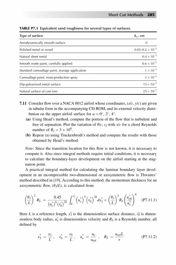
7.11 Consider flow over a NACA 0012 airfoil whose coordinates, (x/c, y/c) are given

in tabular form in the accompanying CD-ROM, and its external velocity distri-

bution on the upper airfoil surface for a¼ 0�, 2�, 4�.(a) Using Head’s method, compute the portion of the flow that is turbulent and

free of separation. Plot the variation of q/c, cf with x/c for a chord Reynolds

number of Rc¼ 3� 106.

(b) Repeat (a) using Truckenbrodt’s method and compare the results with those

obtained by Head’s method.

Note: Since the transition location for this flow is not known, it is necessary to

compute it. Also since integral methods require initial conditions, it is necessary

to calculate the boundary-layer development on the airfoil starting at the stag-

nation point.

A practical integral method for calculating the laminar boundary layer devel-

opment in an incompressible two-dimensional or axisymmetric flow is Thwaites’

method described in [19]. According to this method, the momentum thickness for an

axisymmetric flow, (q3/L), is calculated from

�q3

L

�2

RL ¼ 0:45�u*e�6�

r*0�2kZ x*3

0

�u*e

�5�r*0

�2kdx*3 þ

�q3

L

�2

RL

u*e0u*e

!6

(P7.11.1)

Here L is a reference length, x3* is the dimensionless surface distance, r0* is dimen-

sionless body radius, ue* is dimensionless velocity and RL is a Reynolds number, all

defined by

x*3 ¼ x2L

; r*0 ¼ r0L

; u*e ¼ ueuref

; RL ¼ urefL

n(P7.11.2)

TABLE P7.1 Equivalent sand roughness for several types of surfaces.

Type of surface ks , cm

Aerodynamically smooth surface 0

Polished metal or wood 0.05–0.2� 10–3

Natural sheet metal 0.4� 10–3

Smooth matte paint, carefully applied 0.6� 10–3

Standard camouflage paint, average application 1� 10–3

Camouflage paint, mass-production spray 3� 10–3

Dip-galvanized metal surface 15� 10–3

Natural surface of cast iron 25� 10–3


Tha parameter k is flow index being equal to 0 for two-dimensional flows and 1 for

axisymmetric flows.

For an axisymmetric stagnation point flow,

�q3

L

�2

RL ¼ 0:056�du*e=dx

*3

�0

(P7.11.3)

and for a two-dimensional flow

�q

L

�2

0

RL ¼ 0:075�du*e=dx

*�0

(P7.11.4)

Once q3 is calculated from Eq. (P7.11.3), then the variables d*, H and cf can be

calculated from the following relations with l, cf and Rq defined by

l ¼ q2

n

duedx

;cf2

¼ l

Rq

; Rq ¼ ueq

n(P7.11.5)

For 0� l� 0.1

l ¼ 0:22þ 1:57l� 1:8l2

H ¼ 2:61� 3:75lþ 5:24l2(P7.11.6a)

For –0.1� l� 0

l ¼ 0:22þ 1:402lþ 0:018l

0:107þ l

H ¼ 0:0731

0:14þ lþ 2:088

(P7.11.6b)

A useful method for predicting transition in two-dimensional incompressible

flows is the expression based onMichel’s method and Smith’s e9-correlation [19]. It is

given by

Rqtr ¼ 1:174

�1þ 22; 400

Rxtr

�R0:46xtr

: (P7.11.7)

According to this method, the boundary-layer development on the body is

calculated for a laminar flow starting at the leading-edge of the flow so that both Rq

and Rx can be determined. Usually, the calculated Reynolds numbers are beneath the


curve given by Eq. (P7.11.7). The location where the (Rq, Rx) values intersect this

curve corresponds to the onset of transition location. In some cases, however, before

this happens, flow separation takes place; in those cases, the separation point is

assumed to correspond to the onset of transition location.

In the accompanying CD-ROM, we include the FORTRAN programs for

Thwaites’ and Michel’s method. Their input and output instructions are described in

Section 10.2.

7.12 Consider Problem 7.11 and assume that the airfoil surface temperature, Tw , is at

80 �F and outside temperature, Te , is at 50�F. Taking Pr¼ 0.72 , we wish to

calculate the Stanton number distribution on the airfoil for laminar and turbu-

lent flows.

Note: The Stanton number for turbulent flow can be calculated by using

Ambrok’s method discussed in Sect. 7.3. The Stanton number for laminar flows

can be calculated from the integral method of Smith and Spalding discussed in

[21]. According to this method, Stanton number defined by

St ¼ _qw9cpue

�Tw � Te

� ¼ k

9cpuedc¼ Nux

RxPr(P7.12.1)

is calculated from

St ¼ c1�u*e�c2"Z x*

0

�u*e

�c3dx*

#1=2 1ffiffiffiffiffiffiRL

p : (P7.12.2)

Here c1¼ Pr–1A–1/2, c2¼ B/2 – 1, c3¼ B – 1 (see Table P7.2).

TABLE P7.2 Constants in Eq. (P7.12.2) for various prandtl numbers

Pr c1 c2 c3

0.7 0.418 0.435 1.87

0.8 0.384 0.450 1.90

1.0 0.332 0.475 1.95

5.0 0.117 0.595 2.19

10.0 0.073 0.685 2.37


Smith-Spalding method can also be used for axisymmetric flows. As discussed in

[21], using the Mangler transformation, Eq. (P7.12.2) can be written as

St ¼ c1�r*0�K�

u*e�c2

" Z x*3

0

�u*e

�c3�r*0

�2Kdx*3

#12

R� 1

2

L : (P7.12.3)

Here the constants c1, c2 and c3 are the same as those given in Table P7.2.

The location of transition again can be calculated from Eq. (P7.11.7) if we

assume that heat transfer has negligable effect on transition. Another practical

method for predicting transition with heat transfer is the H-Rx method described in

[21]. Here H and Rx are the shape factor (h d*/q) and the Reynolds number based on

surface distance (h uex/n), respectively. This method is simple to use for two-

dimensional and axisymmetric flows with pressure gradient, suction and wall heating

or cooling. It is given by

logRx

�e9�� ¼ �40:4557þ 64:8066H � 26:7538H2 þ 3:3819H3;

2:1 < H < 2:8:(P7.12.4)

This method is restricted to heating rates where the difference between surface

temperature and freestream temperature, Tw – TN does not exceed about 23�C.

(a) First calculate the laminar boundary-layer development using Thwaites’ method.

(b) Calculate the location of transition using Eqs. (P7.11.7) and (P7.12.3) and

compare the results.

(c) Compute Stanton number distribution up to transition by using Smith-Spalding

method.

(d) Compute Stanton number distribution for turbulent flowusingAmbrok’smethod.

In the accompanying CD-ROM, we include the FORTRAN programs for Smith-

Spalding, Ambrok methods and H-Rx method for predicting transition. Their input

and output instructions are described in Section 10.2.

7.13 The boundary-layer equations and their boundary conditions for a heated

laminar jet can be written as

v

vx

�ur�þ v

vr

�yr� ¼ 0; (P7.13.1)

uvu

vxþ y

vu

vr¼ n

r

v

vr

�rvu

vr

�; (P7.13.2)


uvT

vxþ y

vT

vr¼ n

Pr

1

r

v

vr

�rvT

vr

�; (P7.13.3)

r ¼ 0; y ¼ 0;vu

vr¼ 0;

vT

vr¼ 0 (P7.13.4a)

r/N; u/0; T/Tc: (P7.13.4b)

In addition to the above equations, the total momentum denoted by J, and the heat

flux denoted by K (both in the x-direction) remain constant and are independent of

the distance x from the orifice. Hence

J ¼ 2p9

Z N

0u2r dr ¼ const: (P7.13.5)

K ¼ 2p9cp

Z N

0urðT � TcÞ dr ¼ const: (P7.13.6)

In Eq. (P7.13.6), K is equal to the product of the initial mass flow rate and mean

enthalpy at the orifice.

(a) Using the matrix-elimination procedure discussed in Problem 4.1 show that the

similarity variable h and dimensionless strem function for continuity and

momentum equations are

h ¼ r

x; f

�h� ¼ j

x; (P7.13.7)

Note that the second expression in Eq. (P7.13.7) is dimensionally incorrect. It can

easily be corrected by rewriting it as

j ¼ yxf ðhÞ : (P7.13.8)

(b) From the definitions of h and stream function

ru ¼ vj

vr; ry ¼ �vj

vx

and from Eq. (P7.13.8), show that

u

uc¼ 1

ðucx=nÞf 0

h: (P7.13.9)


Note that the right-hand side of Eq. (P7.13.9) is independent of x by virtue of

ucx ¼ const: (P7.13.10)

As a result we can redefine h as

h ¼�ucx

n

�1=2rx: (P7.13.11)

(c) Use the transformation defined by Eqs. (P7.13.8) and (P7.13.11), observe the

chain-rule and show that Eqs. (P7.13.1) to (P7.13.4) can be written as

�h

�f 0

h

�0�0þf

�f 0

h

�0þðf 0Þ2

h¼ 0; (P7.13.12)

� h

PrG0 þ f G

�0 ¼ 0; (P7.13.13)

h ¼ 0; f ¼ G0 ¼ 0; f 00 ¼ 0 (P7.13.14a)

h ¼ hc; f 0 ¼ G ¼ 0 (P7.13.14b)

where

G�h� ¼ T � Te

Tc � Te:

(d) Note that

limh/N

f 0ðhÞh

/0 and limh/N

f 00�h�/0 (P7.13.15)

and show that the solutions of Eq. (P7.13.12) subject to f(0)¼ 0 are given by

f�h� ¼ 1=2h2

1þ 1=8h2(P7.13.16)

and

f 0ðhÞh

¼ 1

½1þ 1=8h2�2: (P7.13.17)

(e) With f(h) given by Eq. (P7.13.15), show that the solution of Eq. (P7.13.13)

subject to the boundary conditions given by Eq. (P7.13.14) is

G ¼ 1

½1þ h2=8�2Pr: (P7.13.18)


7.14 For the transition location determined in Problem 7.12, compute the location of

flow separation on the NACA 0012 airfoil for a¼ 2� and 4� using Stratford’s

method and compare its predictions with Head’s method.

7.15 Show that the velocity defect in the wake of a tall building, approximating

a two-dimensional cylinder with a diameter of 100 ft (30 m), exceeds 10%

of the wind velocity for a distance of 1 mile downstream of the building.

7.16 Trailing vortices from an airliner can endanger following aircraft. Do the jet

exhausts significantly affect the decay of the trailing vortices by enhancing

turbulent mixing? A simplified version of this question is to ask whether the

jet velocity at the vortex position (say 20 nozzle diameters outboard of the

jet axis) ever exceeds, say, 5%of the exhaust velocity. Answer the question,

assuming that the velocity profile in a circular jet in still air can be approxi-

mated by u/uc¼ 12 (1þ cos pr/2R), where R is the radius at which u/uc¼ 0.5

and the approximation applies for r< 2R only. State the main assumptions

made in simplifying the question and any further assumptions you make.

7.17 Two tubes in a cross-flow heat exchanger can be idealized as parallel circular

cylinders of 1 cm diameter, 10 cm apart. Find the distance downstream at

which the two wakes meet, taking the sectional drag coefficients of each

cylinder as 1.0.

References

[1] H. Schlichting, Boundary-Layer Theory, McGraw-Hill, New York, 1981.

[2] K.E. Schoenherr, Resistance of flat surface moving through a fluid, Trans. Soc. Nav. Architects Mar.

Eng. 40 (1932) 279.

[3] J.C. Simonich, P. Bradshaw, Effect of freestream turbulence on heat transfer through a turbulent

boundary layer, J. Heat Transfer 100 (1978) 671.

[4] B.A. Kader, A.M. Yaglom, Heat and mass transfer laws for fully turbulent wall flows, Int. J. Heat

Mass Transfer 15 (1977) 2329.

[5] W.C. Reynolds, W.M. Kays, S.J. Klime, Heat transfer in the turbulent incompressible boundary

layer, I. Constant wall temperature, NASA MEMO 12-1-58W (1958).


layer, I Step wall-temperature distribution, NASA MEMO 12-22-58W (1958).


layer, III. Arbitrary wall temperature and heat flux, NASA MEMO 12-3-58W (1958).

[8] F.B. Hildebrand, Advanced Calculus for Applications, Prentice-Hall, Englewood Cliffs, NJ, 1962.

[9] W.M. Kays, M.E. Crawford, Convective Heat and Mass Transfer, McGraw-Hill, New York, 1980.

[10] J. Nikuradse, Law of flow in rough pipes, Tech. Memo. NASA No 129 (1955).

[11] E.R. Van Driest, Turbulent boundary layer in compressible fluids, J. Aeronaut. Sci. 18 (1951) 145.

[12] D.B. Spalding, S.W. Chi, The drag of a compressible turbulent boundary layer on a smooth flat plate

with and without heat transfer, J. Fluid Mech. 18 (1964) 117.

[13] A.M. Cary, Summary of available information on Reynolds analogy for zero-pressure gradient,

compressible turbulent-boundary-layer flow, NASA TN D-5560 (1970).


[14] A.M. Cary, M.H. Bertram, Engineering prediction of turbulent skin friction and heat transfer in

high-speed flow, NASA TN D-7507 (1974).

[15] F.E. Goddard Jr., Effect of uniformly distributed roughness on turbulent skin-friction drag at

supersonic speeds, J. Aero/Space Sci. 26 (1959) 1–15.

[16] F.W. Fenter, The effect of heat transfer on the turbulent skin-friction of uniformly rough surfaces in

compressibleflow,TheUniversityofTexas,DefenseResearchLab.Rept,April 1956.DLR-368,CM-839.

[17] M.R. Head, Entrainment in the turbulent boundary layers, ARC R&M 3643 (1969).

[18] H. Ludwieg, W. Tillmann, Investigation of the wall shearing stress in turbulent boundary layers,

NACA Rept. TM 1285 (1949).

[19] T. Cebeci, J. Cousteix, Modeling and Computation of Boundary-Layer Flows, Horizons Pub., Long

Beach, C. A. and Springer-Verlag, Germany, Heidelberg, 1998.

[20] J.E. Green, D.J. Weeks, J.W.F. Brooman, Prediction of turbulent boundary layers and wakes in

incompressible flow by a lag-entrainment method, ARC R&M 3791 (1973).

[21] T. Cebeci, Convective Heat Transfer, Horizons Pub., Long Beach, C. A., 2002. and Springer-Verlag,

Heidelberg, Germany.

[22] L. Rosenhead, Laminar Boundary Layers, Oxford Univ. Press (Clarendon), London and New York,

1963.

[23] B.S. Stratford, The prediction of separation of the turbulent boundary layer,, J. Fluid Mech. 5 (1959) 1.

[24] T. Cebeci, G.J. Mosinskis, A.M.O. Smith, Calculation of separation point in turbulent flows,,

J. Aircraft 9 (1972) 618.

[25] F.R. Goldschmied, An approach to turbulent incompressible separation under adverse pressure

gradients, J. Aircraft 2 (1965) 108.

[26] G.B. Schubauer, Air flow in the boundary layer of an elliptic cylinder, NACA Rep. No. 652 (1939).


Tech. Note No. 2133 (1950).

[28] B.G. Newman, Some contributions to the study of the turbulent boundary layer near separation,

Austr, Dept. Supply Rep. ACA-53 (1951).

[29] G.N. Abramovich, The Theory of Turbulent Jets, M.I.T. Cambridge, Mass (1963).

[30] C.M. Sabin, An analytical and experimental study of the plane, incompressible, turbulent free-shear

layer with arbitrary velocity ratio and pressure gradient, J. Basic Eng. 87 (1965) 421.

[31] N.K. Pui, I.S. Gartshore, Measurement of the growth rate and structure in plane turbulent mixing

layers, J. Fluid Mech. 91 (1979) 111.

[32] H.W. Liepmann, J. Laufer, Investigations of free turbulent mixing, NACA TN 1257 (1947).

[33] G.L. Brown, A. Roshko, On density effects and large structure in turbulent mixing layers, J. Fluid

Mech. 64 (1974) 775.

[34] S.F. Birch, J.M. Eggers, A critical review of the experimantal data for developed free turbulent shear

layers, in Free Turbulent Shear Flows, NASA SP-321 11 (1972).

[35] H. Ikawa, T. Kubota, Investigation of supersonic turbulent mixing layer with zero pressure gradient,

AIAA J. 13 (1975) 566.

[36] R.D. Wagner, Mean flow and turbulence measurements in a Mach 5 free shear layer, NASA TN

D-7366 (1973).

[37] W.D. Harvey, W.W. Hunter, Experimental study of a free turbulent shear flow at Mach 19 with

electron-beam and conventional probes, NASA TN D-7981 (1975).

[38] A. Demetriades, Turbulence measurements in a supersonic two-dimensional wake, Phys. Fluids 13

(1970) 1672.

[39] A. Demetriades, Turbulence correlations in a compressible wake, J. Fluid Mech. 74 (1976) 251.

[40] D.C. Baxter, W.C. Reynolds, Fundamental solutions for heat transfer from non-isothermal flat

plates, J. Aero. Sci. 25 (1958) 403.


DifferentialMethods withAlgebraicTurbulence Models

Chap

ter8



8.2 Numerical Solution of the Boundary-Layer Equations with Algebraic

Turbulence Models 295

8.2.1 Numerical Formulation 297

8.2.2 Newton’s Method 299

8.2.3 Block-Elimination Method 301

8.2.4 Subroutine SOLV3 302

8.3 Prediction of Two-Dimensional Incompressible Flows 305

8.3.1 Impermeable Surface with Zero Pressure Gradient 305

8.3.2 Permeable Surface with Zero Pressure Gradient 307

8.3.3 Impermeable Surface with Pressure Gradient 310

8.3.4 Permeable Surface with Pressure Gradient 312

8.4 Axisymmetric Incompressible Flows 315

8.5 Two-Dimensional Compressible Flows 317

8.5.1 Impermeable Surface with Zero Pressure Gradient 317

8.5.2 Permeable Surface with Zero Pressure Gradient 320

8.5.3 Impermeable Surface with Pressure Gradient 320

8.6 Axisymmetric Compressible Flows 322

293



http://dx.doi.org/10.1016/B978-0-08-098335-6.00008-2

8.7 Prediction of Two-Dimensional Incompressible Flows with Separation 322

8.7.1 Interaction Problem 324

8.8 Numerical Solution of the Boundary-Layer Equations in the Inverse Mode

with Algebraic Turbulence Models 326

8.8.1 Numerical Formulation 328

8.9 Hess-Smith (HS) Panel Method 333

8.9.1 Viscous Effects 340

8.9.2 Flowfield Calculation in the Wake 342

8.10 Results for Airfoil Flows 344

8.11 Prediction of Three-Dimensional Flows with Separation 347

Problems 349

References 354

8.1 Introduction

Differential methods are based on the solution of the boundary-layer equations in

their partial-differential equation form. They vary depending on the numerical

method used to solve the equations and the turbulence model employed to model the

Reynolds stresses. Unlike integral methods, they are general, accurate depending on

the numerical method and turbulence model and can handle various initial and

boundary conditions. The differential methods, which have largely superseded

integral methods with the advent of modern computers, however, require more

computer time than the integral methods.

An accurate and efficient differential method is the method developed by

Cebeci and Smith [1]. It uses the Cebeci-Smith algebraic eddy viscosity formu-

lation discussed in Chapter 5 to model the Reynolds shear stress term in the

momentum equation. In this method, CS method, the boundary-layer equations

are solved for both laminar and turbulent flows by specifying the onset of the

transition location. The laminar flow calculations are performed up to this loca-

tion, and the turbulent flow calculations, including the transition region are

performed.

In Section 8.2 we describe the formulation and the numerical method used in the

CS method. In Section 8.3 and the following sections up to 8.7, we discuss the

prediction of incompressible and compressible, two-dimensional and axisymmetric

flows with the CS method. Section 8.7 describes the so-called standard and inverse

approaches for calculating boundary-layer flows with and without separation and

Section 8.8 extends the standard approach of Section 8.2 to flows with separation.

The results obtained with this approach are described in Sections 8.9 and 8.10 for

two- and three-dimensional flows.


8.2 Numerical Solution of the Boundary-Layer Equationswith Algebraic Turbulence Models

There are several numerical methods for solving the boundary-layer equations in

differential form. The Crank-Nicolson and Keller’s box methods are the most

convenient ones as discussed in some detail in [1,2]. Of the two, Keller’s method has

significant advantages over the other, and in this section it will be used to solve the

boundary-layer equations with algebraic turbulence models and in Sections 9.2 and

9.3 with transport-equation turbulence models for two-dimensional flows.

For two-dimensional incompressible flows, the continuity and momentum

equations given by Eqs. (3.3.24) and (3.3.25) for compressible axisymmetric flows

reduce to the equations given by Eqs. (5.2.8) and (5.2.9), that is,

vu

vxþ vy

vy¼ 0 (8.2.8)

uvu

vxþ y

vu

vy¼ �1

9

dp

dxþ v

v2u

vy2� v

vy

�u0y0�

(8.2.9)

With Bernoulli’s equation, the above momentum equation can be written as

uvu

vxþ y

vu

vy¼ ue

duedx

þ vv2u

vy2� v

vy

�u0y0�

(8.2.1)

The boundary conditions for Eqs. (8.2.8) and (8.2.1) are

y ¼ 0 u ¼ 0 y ¼ ywðxÞ (8.2.2a)

y ¼ d u ¼ ue (8.2.2b)

The above equations can be solved in the form they are expressed or in the form after

they are expressed as a third order equation by using the definition of stream function

j(x, y). Noting that

u ¼ vj

vy; y ¼ �vj

vx(8.2.3)

Eqs. (5.2.8) and (8.2.1), with a prime denoting differentiation with respect to y, and

with an eddy viscosity εm defined by Eq. (5.2.9),

�u0y0 ¼ εmvu

vy(5.2.9)

can be written as ��vþ εm

�j00�0þue

duedx

¼ j0vj0

vx� j00vj

vx(8.2.4)

Differential Methods with Algebraic Turbulence Models 295

In either form, for given initial conditions, say at x¼ x0 and eddy viscosity distri-

bution, these equations can be solved subject to their boundary conditions in the

interval 0 to d at each specified x-location greater than x0. The boundary-layer

thickness d(x), however, increases with increasing downstream distance x for both

laminar and turbulent flows; to maintain computational accuracy, it is necessary to

take small steps in the streamwise direction.

Transformed coordinates employing similarity variables such as the one dis-

cussed in [1] provide another alternative to express the equations in a better form

before solving. Such a choice can reduce the growth of transformed boundary-layer

thickness and thus allow larger steps to be taken in the stream-wise direction.

Furthermore, in some cases, they can also be used to generate the initial conditions

needed in the solution of the boundary-layer equations.

We shall advocate the use of transformed coordinates employing similarity

variables and for two-dimensional flows wewill use the Falkner-Skan transformation

discussed in [1]. With the similarity variable defined by

h ¼ffiffiffiffiffiuevx

ry (8.2.5a)

and the dimensionless stream function f (x, h)

jðx; yÞ ¼ ffiffiffiffiffiffiffiffiffiuevx

pf ðx; hÞ; (8.2.5b)

the continuity and momentum equations, Eq. (8.2.4) and their boundary conditions,

Eqs. (8.2.2), can be written as

�b f 00

�0þmþ 1

2f f 00 þ m

�1� ðf 0Þ2� ¼ x

�f 0vf 0

vx� f 00

vf

vx

�(8.2.6)

h ¼ 0; f ¼ fw ¼ � 1ffiffiffiffiffiffiffiffiffiuevx

pZ x

0ywdx; f 0 ¼ 0 (8.2.7a)

h ¼ he; f 0 ¼ 1 (8.2.7b)

Here, a prime denotes differentiation with respect to h; the parameter b and

pressure gradient parameter m are defined by

b ¼ 1þ εþm ; ε

þm ¼ εm

v; m ¼ x

ue

duedx

: (8.2.8)

To solve Eqs. (8.2.6) and (8.2.7) with Keller’s box method, which is a two-

point finite-difference scheme, we first express them as a first-order system by

introducing new functions to represent the derivatives of f with respect to h


(subsection 8.2.1). The first-order equations are approximated on an arbitrary

rectangular net, Fig. 8.1, with ‘‘centered-difference’’ derivatives and averages at

the midpoints of the net rectangle difference equations. The resulting system of

equations which is implicit and nonlinear is linearized by Newton’s method

(subsection 8.2.2) and solved by the block-elimination method discussed in

subsection 8.2.3.

8.2.1 NUMERICAL FORMULATION

In order to express Eqs. (8.2.6) and (8.2.7) as a system of first-order equations, we

define new variables u(x, h) and y(x, h) by

f 0 ¼ u (8.2.9a)

u0 ¼ y (8.2.9b)

and write them as�by�0þmþ 1

2f yþ m

�1� u2

� ¼ x

�uvu

vx� y

vf

vx

�(8.2.9c)

h ¼ 0; u ¼ 0; f ¼ fwðxÞ; h ¼ he; u ¼ 1 (8.2.10)

We denote the net points of the net rectangle shown in Fig. 8.1 by

x0 ¼ 0; xn ¼ xn�1 þ kn; n ¼ 1; 2;.;Nh0 ¼ 0; hj ¼ hj�1 þ hj; j ¼ 1; 2;.; J

(8.2.11)

and write the difference equations that are to approximate Eqs. (8.2.9) by considering

one mesh rectangle as in Fig. 8.1. We start by writing the finite-difference approx-

imations of the ordinary differential equations (8.2.9a,b) for the midpoint (xn, hj–1/2)

of the segment P1P2, using centered-difference derivatives,

Fig. 8.1 Net rectangle for difference approximations.


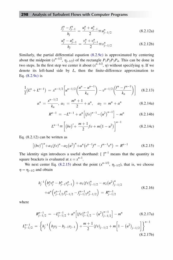
f nj � f nj�1

hj¼ unj þ unj�1

2hunj�1=2 (8.2.12a)

unj � unj�1

hj¼ ynj þ ynj�1

2hynj�1=2 (8.2.12b)

Similarly, the partial differential equation (8.2.9c) is approximated by centering

about the midpoint (xn–1/2, hj–1/2) of the rectangle P1P2P3P4. This can be done in

two steps. In the first step we center it about (xn–1/2, h) without specifying h. If we

denote its left-hand side by L, then the finite-difference approximation to

Eq. (8.2.9c) is

1

2

�Ln þ Ln�1

� ¼ xn�1=2

un�1=2

�un � un�1

kn

�� yn�1=2

�f n � f n�1

kn

�(8.2.13)

an ¼ xn�1=2

kn; a1 ¼ mn þ 1

2þ an; a2 ¼ mn þ an (8.2.14a)

Rn�1 ¼ �Ln�1 þ anhðf yÞn�1��u2�n�1

i� mn (8.2.14b)

Ln�1h

�by�0þ mþ 1

2f yþ m

�1� u2

�n�1

(8.2.14c)

Eq. (8.2.12) can be written as�ðbyÞ0�nþa1ðf yÞn�a2�u2�nþan

�yn�1f n � f n�1yn

� ¼ Rn�1 (8.2.15)

The identity sign introduces a useful shorthand: [ ]n–1 means that the quantity in

square brackets is evaluated at x¼ xn–1.

We next center Eq. (8.2.15) about the point (xn–1/2, hj–1/2), that is, we choose

h¼ hj–1/2 and obtain

h�1j

�bnj y

nj � bnj�1y

nj�1

�þ a1ðf yÞnj�1=2 � a2

�u2�nj�1=2

þan�yn�1j�1=2 f

nj�1=2 � f n�1

j�1=2ynj�1=2

�¼ Rn�1

j�1=2

(8.2.16)

where

Rn�1j�1=2 ¼ �Ln�1

j�1=2 þ anhðf yÞn�1

j�1=2 ��u2�n�1

j�1=2

i� mn (8.2.17a)

Ln�1j�1=2 ¼

h�1j

�bjyj � bj�1yj�1

�þ mþ 1

2ðf yÞj�1=2 þ m

1� �u2�

j�1=2

�n�1

(8.2.17b)


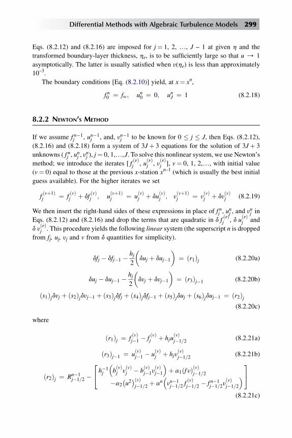
Eqs. (8.2.12) and (8.2.16) are imposed for j¼ 1, 2, ., J – 1 at given h and the

transformed boundary-layer thickness, he, is to be sufficiently large so that u / 1

asymptotically. The latter is usually satisfied when y(he) is less than approximately

10–3.

The boundary conditions [Eq. (8.2.10)] yield, at x¼ xn,

f n0 ¼ fw; un0 ¼ 0; unJ ¼ 1 (8.2.18)

8.2.2 NEWTON’S METHOD

If we assume f n�1j , un�1

j , and, yn�1j to be known for 0 � j � J, then Eqs. (8.2.12),

(8.2.16) and (8.2.18) form a system of 3Jþ 3 equations for the solution of 3Jþ 3

unknowns ( f nj , unj , y

nj ), j¼ 0, 1,.,J. To solve this nonlinear system, we use Newton’s

method; we introduce the iterates [ fðnÞj , u

ðnÞj , y

ðnÞj ], v¼ 0, 1, 2,., with initial value

(v¼ 0) equal to those at the previous x-station xn–1 (which is usually the best initial

guess available). For the higher iterates we set

fðvþ1Þj ¼ f

ðvÞj þ df

ðvÞj ; u

ðvþ1Þj ¼ u

ðvÞj þ du

ðvÞj ; y

ðvþ1Þj ¼ y

ðvÞj þ dy

ðvÞj (8.2.19)

We then insert the right-hand sides of these expressions in place of f nj , unj , and ynj in

Eqs. (8.2.12) and (8.2.16) and drop the terms that are quadratic in d fðnÞj , d u

ðnÞj and

d yðnÞj . This procedure yields the following linear system (the superscript n is dropped

from fj, uj, yj and v from d quantities for simplicity).

dfj � dfj�1 � hj2

�duj þ duj�1

�¼ ðr1Þj (8.2.20a)

duj � duj�1 � hj2

�dyj þ dyj�1

�¼ ðr3Þj�1 (8.2.20b)

ðs1Þjdyj þ ðs2Þjdyj�1 þ ðs3Þjdfj þ ðs4Þjdfj�1 þ ðs5Þjduj þ ðs6Þjduj�1 ¼ ðr2Þj(8.2.20c)

where

ðr1Þj ¼ fðvÞj�1 � f

ðvÞj þ hju

ðvÞj�1=2

(8.2.21a)

ðr3Þj�1 ¼ uðvÞj�1 � u

ðvÞj þ hjy

ðvÞj�1=2

(8.2.21b)

ðr2Þj ¼ Rn�1j�1=2 �

24 h�1j

�bðvÞj y

ðvÞj � b

ðvÞj�1y

ðvÞj�1

�þ a1ðf yÞðvÞj�1=2

�a2�u2�ðvÞj�1=2

þ an�yn�1j�1=2 f

ðvÞj�1=2

� f n�1j�1=2y

ðvÞj�1=2

�35(8.2.21c)


In writing the system given by Eqs. (8.2.20) we have used a certain order for

them. The reason for this choice, as we shall see later, is to ensure that the A0 matrix

in Eq. (8.2.27a) is not singular.

The coefficients of the linearized momentum equation are

ðs1Þj ¼ h�1j b

ðvÞj þ a1

2fðvÞj � an

2f n�1j�1=2 (8.2.22a)

ðs2Þj ¼ �h�1j b

ðvÞj�1 þ

a1

2fðvÞj�1 �

an

2f n�1j�1=2 (8.2.22b)

ðs3Þj ¼a1

2yðvÞj þ an

2yn�1j�1=2 (8.2.22c)

ðs4Þj ¼a1

2yðvÞj�1 þ

an

2yn�1j�1=2 (8.2.22d)

ðs5Þj ¼ �a2uðvÞj (8.2.22e)

ðs6Þj ¼ �a2uðvÞj�1 (8.2.22f)

The boundary conditions, Eq. (8.2.18) become

df0 ¼ 0; du0 ¼ 0; duJ ¼ 0 (8.2.23)

As discussed in [1], the linear system given by Eqs. (8.2.20) and (8.2.23) has

a block tridiagonal structure and can be written in matrix-vector form as

A d!! ¼ r!! (8.2.24)

where

A ¼

��

A0 C0

B1 A1 C1

: : :: : :Bj Aj Cj

: : :BJ�1 AJ�1 CJ�1

BJ AJ

��d!! ¼

��

d!

0

d!

1

::d!

j

::d!

J

��r!! ¼

��

r!0

r!1

::r!j

::r!J

��(8.2.25)

d!

j ¼��dfjdujdyj

�� r!j ¼��ðr1Þjðr2Þjðr3Þj

�� 0 � j � J (8.2.26)


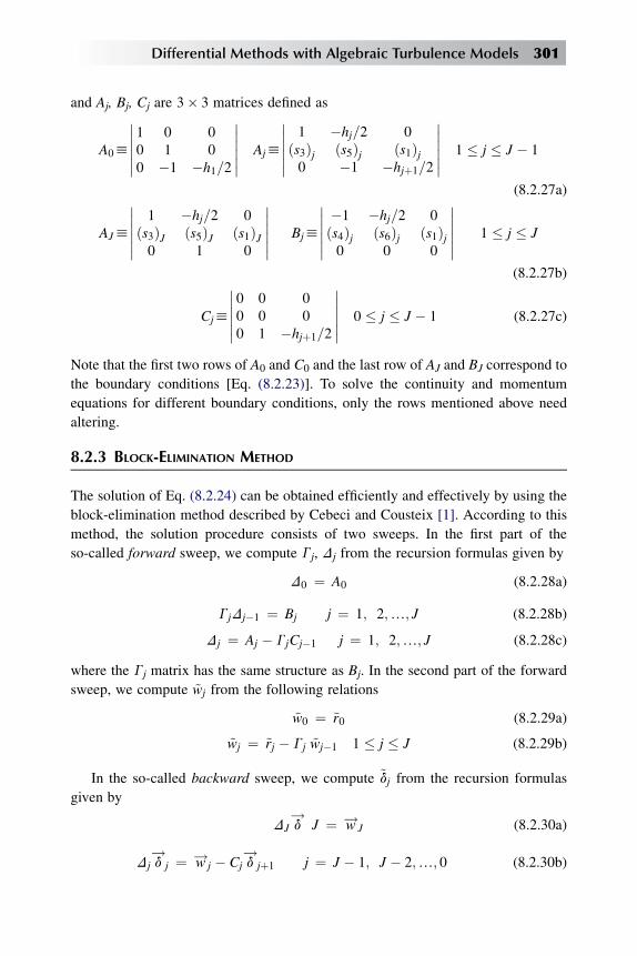
and Aj, Bj, Cj are 3� 3 matrices defined as

A0h

��1 0 00 1 00 �1 �h1=2

�� Ajh

��1 �hj=2 0

ðs3Þj ðs5Þj ðs1Þj0 �1 �hjþ1=2

�� 1 � j � J � 1

(8.2.27a)

AJh

��1 �hj=2 0

ðs3ÞJ ðs5ÞJ ðs1ÞJ0 1 0

�� Bjh

��1 �hj=2 0ðs4Þj ðs6Þj ðs1Þj0 0 0

�� 1 � j � J

(8.2.27b)

Cjh

��0 0 00 0 00 1 �hjþ1=2

�� 0 � j � J � 1 (8.2.27c)

Note that the first two rows of A0 and C0 and the last row of AJ and BJ correspond to

the boundary conditions [Eq. (8.2.23)]. To solve the continuity and momentum

equations for different boundary conditions, only the rows mentioned above need

altering.

8.2.3 BLOCK-ELIMINATION METHOD

The solution of Eq. (8.2.24) can be obtained efficiently and effectively by using the

block-elimination method described by Cebeci and Cousteix [1]. According to this

method, the solution procedure consists of two sweeps. In the first part of the

so-called forward sweep, we compute Gj, Dj from the recursion formulas given by

D0 ¼ A0 (8.2.28a)

GjDj�1 ¼ Bj j ¼ 1; 2;.; J (8.2.28b)

Dj ¼ Aj � GjCj�1 j ¼ 1; 2;.; J (8.2.28c)

where the Gj matrix has the same structure as Bj. In the second part of the forward

sweep, we compute ~wj from the following relations

~w0 ¼ ~r0 (8.2.29a)

~wj ¼ ~rj � Gj ~wj�1 1 � j � J (8.2.29b)

In the so-called backward sweep, we compute ~dj from the recursion formulas

given by

DJ d!

J ¼ w!J (8.2.30a)

Dj d!

j ¼ w!j � Cj d!

jþ1 j ¼ J � 1; J � 2;.; 0 (8.2.30b)


The block elimination method is a general one and can be used to solve any

system of first-order equations. The amount of algebra in solving the recursion

formulas given by Eqs. (8.2.28) to (8.2.30), however, depends on the order of the

matrices Aj, Bj, Cj. When it is small, the matrices Gj, Dj and the vector w!j can be

obtained by relatively simple expressions, as discussed in subsection 8.2.4. However,

this procedure, though very efficient, becomes increasingly tedious as the order of

matrices increases and requires the use of an algorithm that reduces the algebra

internally. A general algorithm, called the ‘‘matrix solver’’ discussed by Cebeci and

Cousteix [1] and also in subsection 10.9.7 can be used for this purpose.

8.2.4 SUBROUTINE SOLV3

The solution of Eq. (8.2.24) by the block-elimination method can be obtained by

using the recursion formulas given by Eqs. (8.2.28) to (8.2.30), and determining the

expressions such as Dj, Gj and w!j and d!

j. To describe the procedure let us first

consider Eq. (8.2.28). Noting that the Gj matrix has the same structure as Bj and

denoting the elements of Gj by gik (i, k¼ 1, 2, 3), we can write Gj as

Gjh

��ðg11Þj ðg12Þj ðg13Þjðg21Þj ðg22Þj ðg23Þj0 0 0

�� (8.2.31a)

Similarly, if the elements ofDj are denoted by aikwe can writeDj as [note that the

third row of Dj follows from the third row of Aj according to Eq. (8.2.28c)]

Djh

��ða11Þj ða12Þj ða13Þjða21Þj ða22Þj ða23Þj0 �1 �hjþ1=2

�� 0 � j � J � 1 (8.2.31b)

and for j¼ J, the first two rows are the same as the first two rows in Eq. (8.2.31b), but

the elements of the third row, which correspond to the boundary conditions at j¼ J,

are (0, 1, 0).

For j¼ 0, D0¼ A0; therefore the values of (aik)0 are

ða11Þ0 ¼ 1 ða12Þ0 ¼ 0 ða13Þ0 ¼ 0ða21Þ0 ¼ 0 ða22Þ0 ¼ 1 ða23Þ0 ¼ 0

(8.2.32a)

and the values of (gik) are

ðg11Þ1 ¼ �1 ðg12Þ1 ¼ �1

2h1 ðg13Þ1 ¼ 0

ðg21Þ1 ¼ ðs4Þ1 ðg23Þ1 ¼ �2

ðs2Þ1h1

ðg22Þ1 ¼ ðs6Þ1 þ ðg23Þ1

(8.2.32b)


The elements of the Dj matrices are calculated from Eq. (8.2.28c). Using the

definitions of Aj, Gj and Cj–1, we find from Eq. (8.2.28c) that for j¼ 1, 2,., J,

ða11Þj ¼ 1 ða12Þj ¼ �hj2� ðg13Þj ða13Þj ¼

hj2ðg13Þj

ða21Þj ¼ ðs3Þj ða22Þj ¼ ðs5Þj � ðg23Þj ða23Þj ¼ ðs1Þj þhj2ðg23Þj(8.2.33a)

To find the elements of the Gj matrices, we use Eq. (8.2.28b). With Dj defined by

Eq. (8.2.31b) and Bj by Eq. (8.2.27b), it follows that for 2 � j � J,

ðg11Þj ¼ ða23Þj�1 þ

hj2

�hj2

�ða21Þj�1 � ða22Þj�1

��D0

ðg12Þj ¼ � hj2

hj2þ ðg11Þj

ða12Þj�1

hj2� ða13Þj�1

��D0

ðg13Þj ¼ðg11Þjða13Þj�1 þ

�g12

�ða23Þj�1

�hj2

ðg21Þj ¼nðs2Þjða21Þj�1 � ðs4Þjða23Þj�1

þhj2

ðs4Þjða22Þj�1 � ðs6Þjða21Þj�1

��D0

ðg22Þj ¼ ðs6Þj

hj2� ðs2Þj þ ðg21Þj

ða13Þj�1 � ða12Þj�1

hj2

��D1

ðg23Þj ¼ ðg21Þjða12Þj�1 þ ðg22Þjða22Þj�1 � ðs6Þj(8.2.33b)

D0 ¼ ða13Þj�1 ða21Þj�1 � ða23Þj�1ða11Þj�1

� hj2

hða12Þj�1 ða21Þj�1 � ða22Þj�1ða11Þj�1

iD1 ¼ ða22Þj�1

hj2� ða23Þj�1

To summarize the calculation of Gj and Dj matrices, we first calculate aik from

Eq. (8.2.31b) for j¼ 0, gik from Eq. (8.2.32b) for j¼ 1, aik from Eq. (8.2.33a) for

j¼ 1, then gik from Eq. (8.2.33b) for j¼ 2, aik from Eq. (8.2.33a) for j¼ 2, then gik

from Eq. (8.2.33b), aik from Eq. (8.2.33a) for j¼ 3, etc.

In the second part of the forward sweep we compute w!j from the relations given

by Eq. (8.2.29). If we denote the components of the vector w!j by

w!jh

��ðw1Þjðw2Þjðw3Þj

�� 0 � j � J (8.2.34)


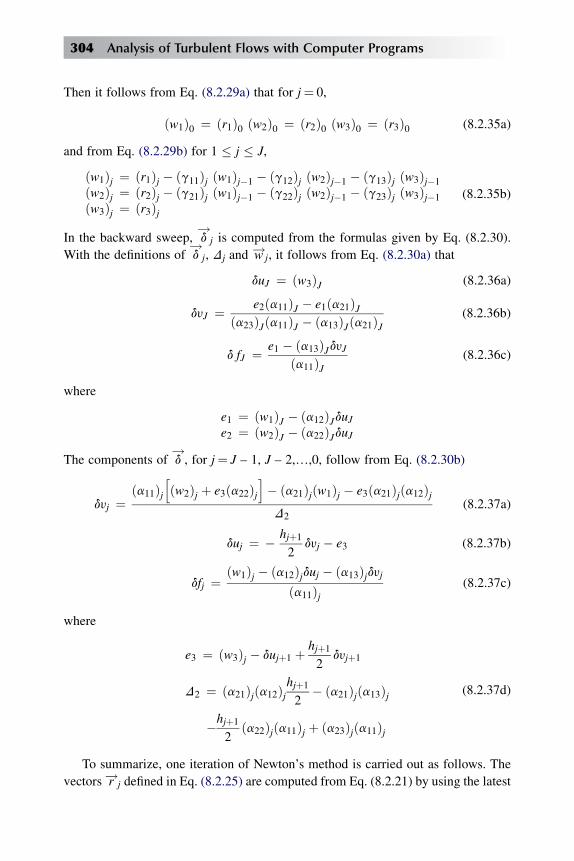
Then it follows from Eq. (8.2.29a) that for j¼ 0,

ðw1Þ0 ¼ ðr1Þ0 ðw2Þ0 ¼ ðr2Þ0 ðw3Þ0 ¼ ðr3Þ0 (8.2.35a)

and from Eq. (8.2.29b) for 1 � j � J,

ðw1Þj ¼ ðr1Þj � ðg11Þj ðw1Þj�1 � ðg12Þj ðw2Þj�1 � ðg13Þj ðw3Þj�1ðw2Þj ¼ ðr2Þj � ðg21Þj ðw1Þj�1 � ðg22Þj ðw2Þj�1 � ðg23Þj ðw3Þj�1ðw3Þj ¼ ðr3Þj

(8.2.35b)

In the backward sweep, d!

j is computed from the formulas given by Eq. (8.2.30).

With the definitions of d!

j, Dj and w!j, it follows from Eq. (8.2.30a) that

duJ ¼ ðw3ÞJ (8.2.36a)

dyJ ¼ e2ða11ÞJ � e1ða21ÞJða23ÞJða11ÞJ � ða13ÞJða21ÞJ

(8.2.36b)

d fJ ¼ e1 � ða13ÞJdyJða11ÞJ

(8.2.36c)

where

e1 ¼ ðw1ÞJ � ða12ÞJduJe2 ¼ ðw2ÞJ � ða22ÞJduJ

The components of d!, for j¼ J – 1, J – 2,.,0, follow from Eq. (8.2.30b)

dyj ¼ða11Þj

hðw2Þj þ e3ða22Þj

i� ða21Þjðw1Þj � e3ða21Þjða12ÞjD2

(8.2.37a)

duj ¼ � hjþ1

2dyj � e3 (8.2.37b)

dfj ¼ðw1Þj � ða12Þjduj � ða13Þjdyj

ða11Þj(8.2.37c)

where

e3 ¼ ðw3Þj � dujþ1 þ hjþ1

2dyjþ1

D2 ¼ ða21Þjða12Þjhjþ1

2� ða21Þjða13Þj

�hjþ1

2ða22Þjða11Þj þ ða23Þjða11Þj

(8.2.37d)

To summarize, one iteration of Newton’s method is carried out as follows. The

vectors r!j defined in Eq. (8.2.25) are computed from Eq. (8.2.21) by using the latest


iterate. The matrix elements of Aj, Bj and Cj defined in Eq. (8.2.24) are next deter-

mined by Eq. (8.2.22a) to (8.2.22f). Using the relations in Eqs. (8.2.27) and (8.2.28),

the matrices Gj and Dj and vectors w!j are calculated. The matrix elements for Gj

defined in Eq. (8.2.31a) are determined from Eq. (8.2.32b) and (8.2.33b).

The components of the vector w!j defined in Eq. (8.2.34) are determined from

Eq. (8.2.35). In the backward sweep, the components of d!

j are computed

from Eqs. (8.2.36) and (8.2.37). A subroutine which makes use of these formulas

and called SOLV3 is given on the companion site, store.elsevier.com/components/

9780080983356.

8.3 Prediction of Two-Dimensional Incompressible Flows

In this section and the following sections up to Section 8.7, we discuss the prediction

of incompressible and compressible, two-dimensional and axisymmetric flows with

the numerical method described in the previous section and the CS algebraic eddy-

viscosity formulation in Chapter 5. These results were all obtained previously

without improvements to the CS model proposed by Cebeci and Chang for strong

pressure-gradient flows as discussed in Section 5.4. The predictions of the CS model

with the Cebeci-Chang improvement are described in Sections 8.7 and 8.8 for two-

dimensional and three-dimensional flows with separation.

8.3.1 IMPERMEABLE SURFACE WITH ZERO PRESSURE GRADIENT

We first examine the accuracy of the momentum equation and compute the local

skin-friction coefficients for a Reynolds number of 106� Rx� 109. We choose a unit

Reynolds number of 1� 106 (ue¼ 160 ft/sec, v¼ 1.6� 10–4 ft2/sec) and specify the

flow as turbulent at x¼ 0.01 ft. The boundary-layer thickness he is calculated in the

program as the calculations proceed downstream.

Figure 8.2 shows the results with two different Dh and Dx spacings (see Section

12.3). Figure 8.2 shows the results with fixed Dh spacing (h1¼ 0.002, K¼ 1.226)

and with variable Dx spacing. The latter was chosen to be such that starting from

Rx¼ 106, the DRx spacing was 2n/2� 106, 2n/4� 106, yielding approximately 20 and

40 x-stations, respectively, at Rx¼ 109. The cf values shown in Fig. 8.2a do not seem

to be very sensitive to Dx spacing. On the other hand, the computed values of

transformed boundary-layer thickness (Fig. 8.2b) show appreciable irregularity. The

number of h points J remains approximately constant.

Figure 8.3 shows a comparison between the calculations obtained with the CS

method (present method) and experimental data for incompressible flows with zero

pressure gradient. Figure 8.3a presents the local skin friction results for the data of


http://store.elsevier.com/components/9780080983356


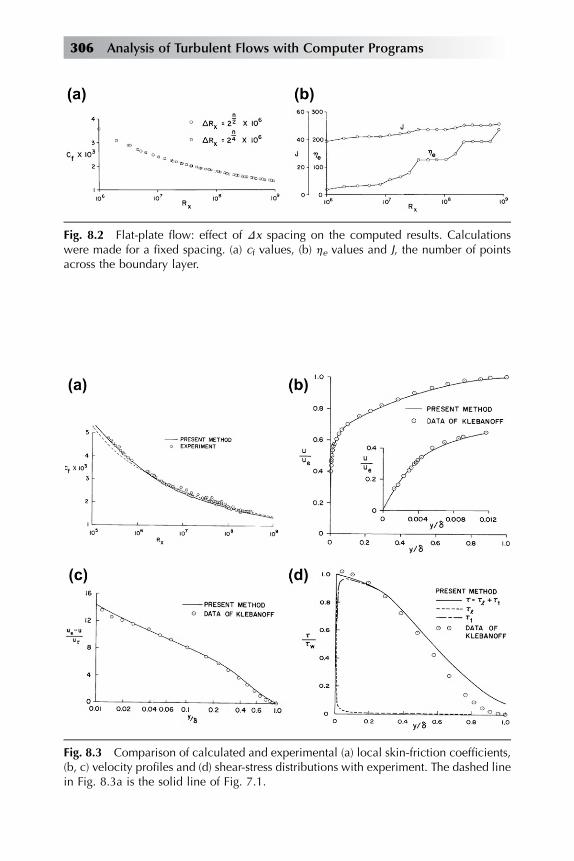
Fig. 8.2 Flat-plate flow: effect of Dx spacing on the computed results. Calculationswere made for a fixed spacing. (a) cf values, (b) he values and J, the number of pointsacross the boundary layer.

Fig. 8.3 Comparison of calculated and experimental (a) local skin-friction coefficients,(b, c) velocity profiles and (d) shear-stress distributions with experiment. The dashed linein Fig. 8.3a is the solid line of Fig. 7.1.


Coles [3], Figs. 8.3b and 8.3c the velocity profiles and Fig. 8.3d the shear stress

profiles, all for the data of Klebanoff [4].

In plotting the velocity profiles in Figs. 8.3b and 8.3c, we have used the definition

of d

�h kðd*ueÞ

us

�1þP

��, which can also be written as (with P¼ 0.55)

d ¼ �2=cf

�1=2�d*=3:78

�¼ 0:375

�d*=c

1=2f

�:

That was necessary because Klebanoff’s experimental data are for a unit Rey-

nolds number of approximately 3� 105. Furthermore, the above relation has the

advantage that it eliminates the difficulty of dealing with an ill-defined quantity d.

We now study the accuracy of the energy equation for smooth impermeable walls

with different wall-temperature distributions, and compare the computed local

Stanton number with experiment. For more comparisons, see [5].

Figure 8.4 shows the results for (a) an isothermal heated plate and (b) step

variation of wall temperature. Similarly Fig. 8.5 shows the results for (a) double-step

and (b) step-ramp wall temperatures.

8.3.2 PERMEABLE SURFACE WITH ZERO PRESSURE GRADIENT

Again we first study the accuracy of the momentum equation, this time for flows with

suction and blowing for a wide range of mass-transfer parameters F defined as

F¼ (9y)w/9eue, which for incompressible flows is simply F¼ yw/ue.

Figure 8.6 shows the computed velocity profiles for the boundary layer measured

by (a) McQuaid [9] for F¼ 0.0046 and (b) Simpson et al. [10] for F¼ 0.00784.

Figure 8.6b also shows a comparison between the calculated local skin-friction

values and the values given by Simpson et al. Simpson’s values were obtained by

Fig. 8.4 Comparison of calculated and experimental Stanton numbers (a) uniform and(b) step variation of wall temperature.


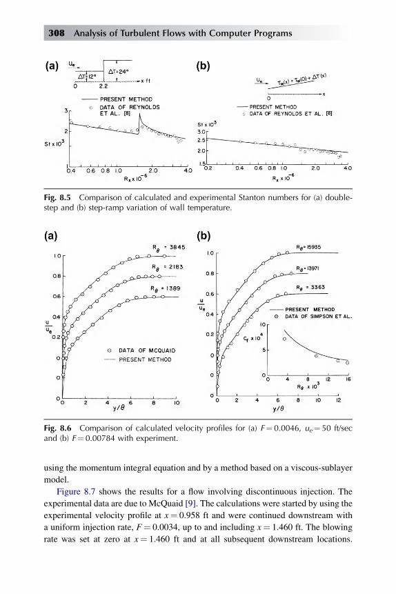
using the momentum integral equation and by a method based on a viscous-sublayer

model.

Figure 8.7 shows the results for a flow involving discontinuous injection. The

experimental data are due to McQuaid [9]. The calculations were started by using the

experimental velocity profile at x¼ 0.958 ft and were continued downstream with

a uniform injection rate, F¼ 0.0034, up to and including x¼ 1.460 ft. The blowing

rate was set at zero at x¼ 1.460 ft and at all subsequent downstream locations.

Fig. 8.5 Comparison of calculated and experimental Stanton numbers for (a) double-step and (b) step-ramp variation of wall temperature.

Fig. 8.6 Comparison of calculated velocity profiles for (a) F¼ 0.0046, ue¼ 50 ft/secand (b) F¼ 0.00784 with experiment.


Results show that the experimental trends are closely followed by the calculations,

including the results for the region after which the mass transfer is zero.

We now investigate the accuracy of calculating local Stanton number for flows

with heat and mass transfer. Figure 8.8 shows the computed results for a wide ran-

ge of the mass-transfer parameter F. The experimental data are due to Moffat and

Kays [11]. As the results show, the agreement with experiment is good for all mass-

transfer rates.

Fig. 8.7 Comparison of calculated velocity profiles for the discontinuous-injectionflow measured by McQuaid [9]. Profiles (a) upstream of discontinuity, (b) downstream.

Fig. 8.8 Comparison of calculated and experimental Stanton numbers for a turbulentboundary layer with suction and blowing.


8.3.3 IMPERMEABLE SURFACE WITH PRESSURE GRADIENT

All of the previous examples were for flows with zero pressure gradient. The utility

of a general method depends on the accuracy of the results it gives for a wide variety

of flow conditions; hence it must be tested on flows with pressure gradient.

The accuracy of the CS method has been very thoroughly studied for a large

number of incompressible turbulent flows with pressure gradient. Here we present

several comparisons taken from the studies in [5,12,13].

Complete Development of the Boundary Layer abouta Streamlined Body

In a general practical problem, it is often necessary to calculate a complete

boundary-layer development from the leading edge of the body to its trailing edge,

which means that it is necessary to calculate the laminar layer, locate the transition

point, and then calculate the turbulent layer. Thus, for example, if one is interested in

calculating the total skin-friction drag of the body, the accuracy of the result depends

on doing each calculation for each region as accurately as possible.

In the studies reported in [12], the laminar layer was calculated by solving the

governing equations up to the transition point. Transition was computed by Smith’s

transition-correlation curve [Eq. (5.3.22)]. Then the turbulent-flow calculations were

started at the transition point by activating the eddy-viscosity expression and were

continued to the trailing edge. However, sometimes the calculations indicated

laminar separation before the transition point was reached. In those cases, the wall

shear became negative and prevented the solutions from converging; the laminar

separation point was then assumed to be tbe transition point, and turbulent flow was

assumed to start at that point.

Figure 8.9 shows the results for the airfoil tested by Newman [14]. The

measurements include pressure distribution, transition-point, turbulent velocity

profiles, and separation point. The calculations were started at the stagnation point of

Fig. 8.9 Comparison of calculated and experimental results for Newman’s airfoil.


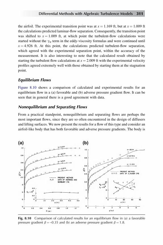
the airfoil. The experimental transition point was at x¼ 1.169 ft, but at x¼ 1.009 ft

the calculations predicted laminar-flow separation. Consequently, the transition point

was shifted to x¼ 1.009 ft, at which point the turbulent-flow calculations were

started without the gtr term in the eddy-viscosity formulas and were continued until

x¼ 4.926 ft. At this point, the calculations predicted turbulent-flow separation,

which agreed with the experimental separation point, within the accuracy of the

measurement. It is also interesting to note that the calculated result obtained by

starting the turbulent flow calculations at x¼ 2.009 ft with the experimental velocity

profiles agreed extremely well with those obtained by starting them at the stagnation

point.

Equilibrium Flows

Figure 8.10 shows a comparison of calculated and experimental results for an

equilibrium flow in a (a) favorable and (b) adverse pressure gradient flow. It can be

seen that in general there is a good agreement with data.

Nonequilibrium and Separating Flows

From a practical standpoint, nonequilibrium and separating flows are perhaps the

most important flows, since they are so often encountered in the design of diffusers

and lifting surfaces. We now present the results for a flow of this type and consider an

airfoil-like body that has both favorable and adverse pressure gradients. The body is

Fig. 8.10 Comparison of calculated results for an equilibrium flow in (a) a favorablepressure gradient b¼ –0.35 and (b) an adverse pressure gradient b¼ 1.8.


two-dimensional and has a sharp nose. It is at a slight angle of attack, which produces

a pressure peak at the leading edge that causes transition. Separation is reported to

have taken place at 25.7�0.2 ft from the leading edge. Figure 8.11 shows some

computed and experimental velocity profiles. The experimental data are due to

Schubauer and Klebanoff [17].

Thermal Boundary Layers

Figure 8.12 shows a comparison of calculated and experimental results for an (a)

accelerating flow and a (b) decelerating flow. In the calculations, the experimental

temperature difference between wall and free stream DT(x) and the velocity distri-

bution ue(x) reported by Moretti and Kays [18] were used. This is the reason for the

small oscillations that show up in the calculated values of Stanton number. For more

comparisons, see [5].

8.3.4 PERMEABLE SURFACE WITH PRESSURE GRADIENT

McQuaid [9] made an extensive series of mean-velocity measurements on smooth

permeable surfaces with distributed injection. He measured boundary-layer devel-

opments for blowing rates F between 0 and 0.008 at free-stream velocities of 50 and

150 ft/sec. He used the momentum integral equation to obtain the local skin-friction

coefficient. As was pointed out by Simpson et al. [19] the reported skin-friction

values of McQuaid are very uncertain for these data. The reasons are that (1) there is

variation in injection velocity over the test surface, (2) the usable test section is short,

and (3) the fact that F is subtracted from the momentum-thickness gradient to obtain

local skin-friction coefficient.

Fig. 8.11 Comparison of calculated and experimental results on a large airfoil-likebody [17].


Figure 8.13a shows experimental and calculated velocity-profile comparisons for

a boundary layer in a favorable pressure gradient with F¼ 0.008. The calculations

were started by using the experimental velocity profile at x¼ 0.958 ft and were

continued downstream with the given blowing rate. Figure 8.13b shows the results for

an adverse pressure gradient withF¼ 0.002. The calculations were started by initially

matching zero-pressure-gradient data for the given blowing rate at x¼ 0.958 ft and

were continued downstream with the experimental velocity distribution. In both of

those figures, skin-friction comparisons were omitted because of the uncertainty in

experimental cf data.

Figure 8.14 shows the results for two highly accelerating flows with mass

transfer. In these cases, the flow starts in zero pressure gradient, then accelerates,

and later ends in zero pressure gradient, all with mass transfer. In both cases, the

acceleration parameter K�h me

9eu2e

duedx

�is not very large. The results in Fig. 8.14a

show that the CS method computes the accelerating boundary layers with blowing

(F¼ 0.006) quite well. Calculated velocity profiles and skin-friction values agree

well with experiment. On the other hand, the results in Fig. 8.14b show that the CS

method does not compute the highly accelerating boundary layers with suction

Fig. 8.12 Comparison of calculated and experimental Stanton numbers for (a) anaccelerating and (b) a decelerating boundary layer, Runs 24 and 36, respectively.


(F¼ –0.004) well. It should be noted, however, that for that suction case the

Reynolds number is quite low and that with acceleration and suction, the boundary

layer, which initially had an already low Reynolds number, has no doubt

laminarized.

Fig. 8.13 Comparison of calculated and experimental velocity profiles for (a) an accel-erating boundary layer with blowing, F¼ 0.008, and (b) a decelerating boundary layerwith blowing, F¼ 0.002.

Fig. 8.14 Comparison of calculated and experimental results for two highly acceler-ating boundary layers with mass transfer: (a) blowing, F¼ 0.006; (b) suction, F¼ –0.004.


8.4 Axisymmetric Incompressible Flows

We first consider flows with zero pressure gradient, namely, flows past slender

cylinders. As was discussed in subsection 5.3.2, in such flows the transverse-

curvature effect plays an important role and causes the boundary-layer development

to be significantly different from those in flat-plate flows. The difference increases

with the slenderness of the cylinder.

Figure 5.4 in subsection 5.3.2 shows the velocity profiles and Table 8.1 presents

the local skin-friction values for two cylinders of diameters d¼ 1 in. and 0.024 in.

The experimental data are due to Richmond [21]. The calculations were made by

Cebeci [22,23] and by White [24]. The values of Richmond, which were estimated

by using the ‘‘streamline hypothesis’’ for the 0.024-in. cylinder, have been pointed

out by Rao [22] to be in error by a factor of 2. White’s values were obtained by

solving the momentum integral equation. They are given by

cf ¼8<:

0:0015þh0:20þ 0:016ðx=r0Þ0:4

iR�1=3x ; 106 � Rx � 109�

4=Rr0

��1=G

�þ �0:5772=G2��

;

�x=r0

��5� 105;

Rr0 � 25 ;

where G¼ ln(4Rx/ R2r0) and Rr0¼ uer0/v. White also gives the following equations

for the average skin-friction coefficient cf :

cf ¼8<:

0:0015þh0:34þ 0:07ðL=r0Þ0:4

iR�1=3L ; 106 � RL � 109�

4=Rr0

��1=G

�þ �0:5772=G2��

;

�L=r0

� � 106

G � 6; Rr0 � 20;

where G¼ ln(4RL/ R2r0) and RL¼ ue/v. Here L is the length of the cylinder.

The values of Cebeci [22,23] were obtained by using the CS method with

a two-dimensional mixing-length expression, Eq. (5.2.12), instead of the expression

given by Eq. (5.2.13). As may be seen from the results in Table 8.1, the Cebeci [23]

values agree closely with White’s values. Furthermore, the value of the local skin

friction for the 1-in. cylinder remains unchanged from that obtained earlier by

TABLE P8.1 Comparison of calculated cf values with other reported values for

incompressible flows on slender cylinders.

cf� 103

d (in.) Rq3–d d/r0 Richmond [21] White [24] Cebeci [22] Cebeci [23]

0.024 2100 75 4.95 7.71 10.73 8.21

1.00 8750 2 2.90 3.18 3.03 3.02


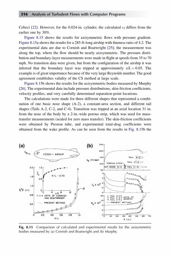
Cebeci [22]. However, for the 0.024-in. cylinder, the calculated cf differs from the

earlier one by 30%.

Figure 8.15 shows the results for axisymmetric flows with pressure gradient.

Figure 8.15a shows the results for a 285-ft-long airship with fineness ratio of 4.2. The

experimental data are due to Cornish and Boatwright [25]; the measurement was

along the top, where the flow should be nearly axisymmetric. The pressure distri-

bution and boundary-layer measurements were made in flight at speeds from 35 to 70

mph. No transition data were given, but from the configuration of the airship it was

inferred that the boundary layer was tripped at approximately x/L¼ 0.05. The

example is of great importance because of the very large Reynolds number. The good

agreement establishes validity of the CS method at large scale.

Figure 8.15b shows the results for the axisymmetric bodies measured by Murphy

[26]. The experimental data include pressure distributions, skin-friction coefficients,

velocity profiles, and very carefully determined separation-point locations.

The calculations were made for three different shapes that represented a combi-

nation of one basic nose shape (A-2), a constant-area section, and different tail

shapes (Tails A-2, C-2, and C-4). Transition was tripped at an axial location 31 in.

from the nose of the body by a 2-in.-wide porous strip, which was used for mass-

transfer measurements (sealed for zero mass transfer). The skin-friction coefficients

were obtained by Preston tube, and experimental total-drag coefficients were

obtained from the wake profile. As can be seen from the results in Fig. 8.15b the

Fig. 8.15 Comparison of calculated and experimental results for the axisymmetricbodies measured by (a) Cornish and Boatwright and (b) Murphy.


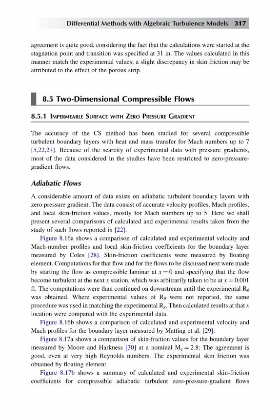
agreement is quite good, considering the fact that the calculations were started at the

stagnation point and transition was specified at 31 in. The values calculated in this

manner match the experimental values; a slight discrepancy in skin friction may be

attributed to the effect of the porous strip.

8.5 Two-Dimensional Compressible Flows

8.5.1 IMPERMEABLE SURFACE WITH ZERO PRESSURE GRADIENT

The accuracy of the CS method has been studied for several compressible

turbulent boundary layers with heat and mass transfer for Mach numbers up to 7

[5,22,27]. Because of the scarcity of experimental data with pressure gradients,

most of the data considered in the studies have been restricted to zero-pressure-

gradient flows.

Adiabatic Flows

A considerable amount of data exists on adiabatic turbulent boundary layers with

zero pressure gradient. The data consist of accurate velocity profiles, Mach profiles,

and local skin-friction values, mostly for Mach numbers up to 5. Here we shall

present several comparisons of calculated and experimental results taken from the

study of such flows reported in [22].

Figure 8.16a shows a comparison of calculated and experimental velocity and

Mach-number profiles and local skin-friction coefficients for the boundary layer

measured by Coles [28]. Skin-friction coefficients were measured by floating

element. Computations for that flow and for the flows to be discussed next were made

by starting the flow as compressible laminar at x¼ 0 and specifying that the flow

become turbulent at the next x station, which was arbitrarily taken to be at x¼ 0.001

ft. The computations were than continued on downstream until the experimental Rq

was obtained. Where experimental values of Rq were not reported, the same

procedure was used in matching the experimental Rx. Then calculated results at that x

location were compared with the experimental data.

Figure 8.16b shows a comparison of calculated and experimental velocity and

Mach profiles for the boundary layer measured by Matting et al. [29].

Figure 8.17a shows a comparison of skin-friction values for the boundary layer

measured by Moore and Harkness [30] at a nominal Me¼ 2.8: The agreement is

good, even at very high Reynolds numbers. The experimental skin friction was

obtained by floating element.

Figure 8.17b shows a summary of calculated and experimental skin-friction

coefficients for compressible adiabatic turbulent zero-pressure-gradient flows


studied by Cebeci et al. [22]. The experimental values of skin friction were all

measured by the floating-element technique. The calculated values cover a

Mach number range of 0.40 to 5 and a momentum-thickness Reynolds number

range of 1.6� 103 to 702� 103. The rms error based on 43 experimental values, all

Fig. 8.16 Comparison of calculated and experimental results for the data of (a) Colesand (b) Matting et al.

Fig. 8.17 Comparison of calculated and experimental local skin-friction values foradiabatic zero-pressure gradient flows (a) data of Moore and Harkness and (b) 43 exper-imental values.


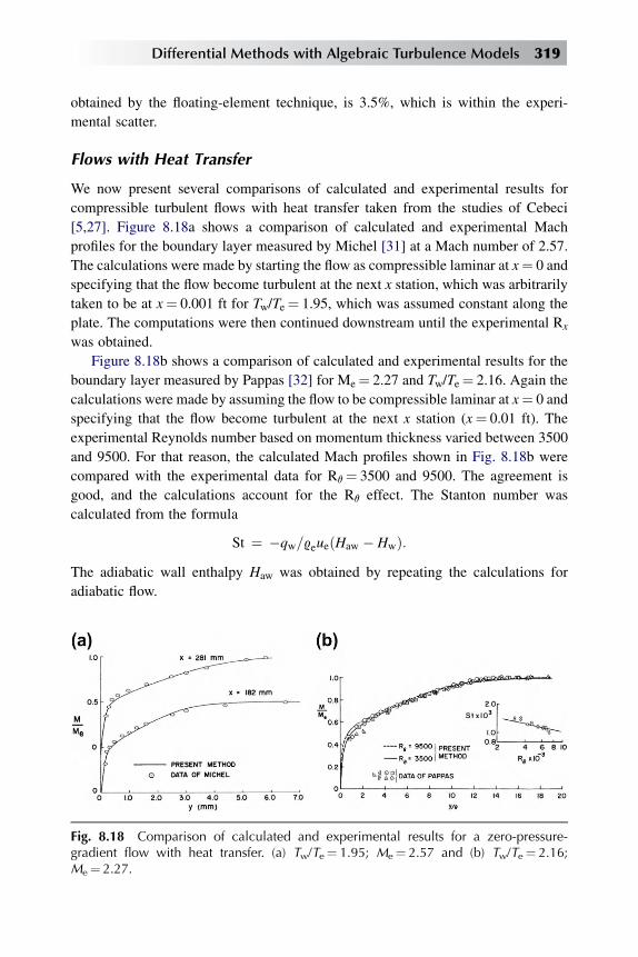
obtained by the floating-element technique, is 3.5%, which is within the experi-

mental scatter.

Flows with Heat Transfer

We now present several comparisons of calculated and experimental results for

compressible turbulent flows with heat transfer taken from the studies of Cebeci

[5,27]. Figure 8.18a shows a comparison of calculated and experimental Mach

profiles for the boundary layer measured by Michel [31] at a Mach number of 2.57.

The calculations were made by starting the flow as compressible laminar at x¼ 0 and

specifying that the flow become turbulent at the next x station, which was arbitrarily

taken to be at x¼ 0.001 ft for Tw/Te¼ 1.95, which was assumed constant along the

plate. The computations were then continued downstream until the experimental Rx

was obtained.

Figure 8.18b shows a comparison of calculated and experimental results for the

boundary layer measured by Pappas [32] for Me¼ 2.27 and Tw/Te¼ 2.16. Again the

calculations were made by assuming the flow to be compressible laminar at x¼ 0 and

specifying that the flow become turbulent at the next x station (x¼ 0.01 ft). The

experimental Reynolds number based on momentum thickness varied between 3500

and 9500. For that reason, the calculated Mach profiles shown in Fig. 8.18b were

compared with the experimental data for Rq¼ 3500 and 9500. The agreement is

good, and the calculations account for the Rq effect. The Stanton number was

calculated from the formula

St ¼ �qw=9eueðHaw � HwÞ:The adiabatic wall enthalpy Haw was obtained by repeating the calculations for

adiabatic flow.

Fig. 8.18 Comparison of calculated and experimental results for a zero-pressure-gradient flow with heat transfer. (a) Tw/Te¼ 1.95; Me¼ 2.57 and (b) Tw/Te¼ 2.16;Me¼ 2.27.


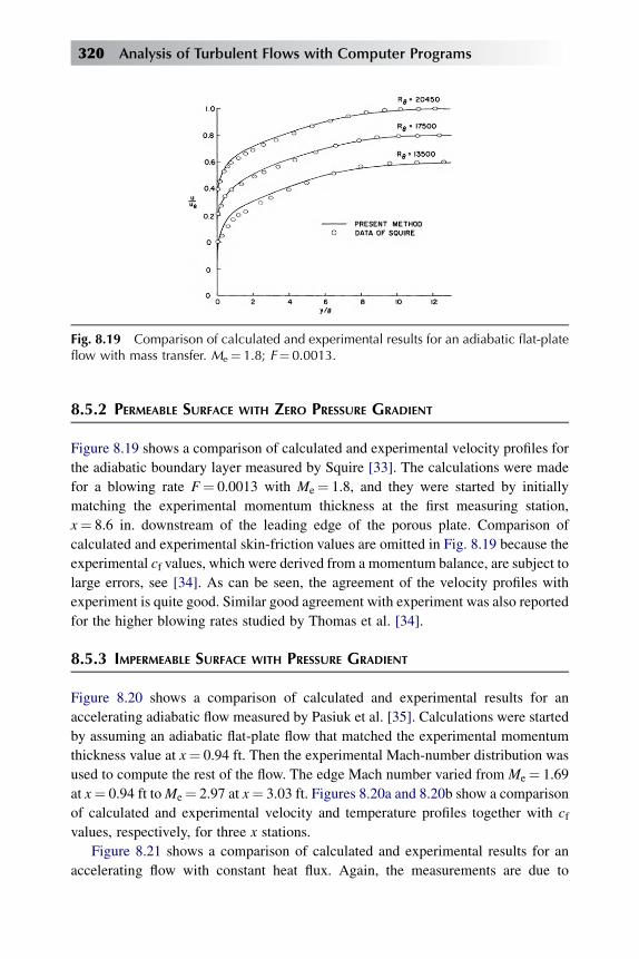
8.5.2 PERMEABLE SURFACE WITH ZERO PRESSURE GRADIENT

Figure 8.19 shows a comparison of calculated and experimental velocity profiles for

the adiabatic boundary layer measured by Squire [33]. The calculations were made

for a blowing rate F¼ 0.0013 with Me¼ 1.8, and they were started by initially

matching the experimental momentum thickness at the first measuring station,

x¼ 8.6 in. downstream of the leading edge of the porous plate. Comparison of

calculated and experimental skin-friction values are omitted in Fig. 8.19 because the

experimental cf values, which were derived from a momentum balance, are subject to

large errors, see [34]. As can be seen, the agreement of the velocity profiles with

experiment is quite good. Similar good agreement with experiment was also reported

for the higher blowing rates studied by Thomas et al. [34].

8.5.3 IMPERMEABLE SURFACE WITH PRESSURE GRADIENT


accelerating adiabatic flow measured by Pasiuk et al. [35]. Calculations were started

by assuming an adiabatic flat-plate flow that matched the experimental momentum

thickness value at x¼ 0.94 ft. Then the experimental Mach-number distribution was

used to compute the rest of the flow. The edge Mach number varied from Me¼ 1.69

at x¼ 0.94 ft toMe¼ 2.97 at x¼ 3.03 ft. Figures 8.20a and 8.20b show a comparison

of calculated and experimental velocity and temperature profiles together with cfvalues, respectively, for three x stations.


accelerating flow with constant heat flux. Again, the measurements are due to

Fig. 8.19 Comparison of calculated and experimental results for an adiabatic flat-plateflow with mass transfer. Me¼ 1.8; F¼ 0.0013.


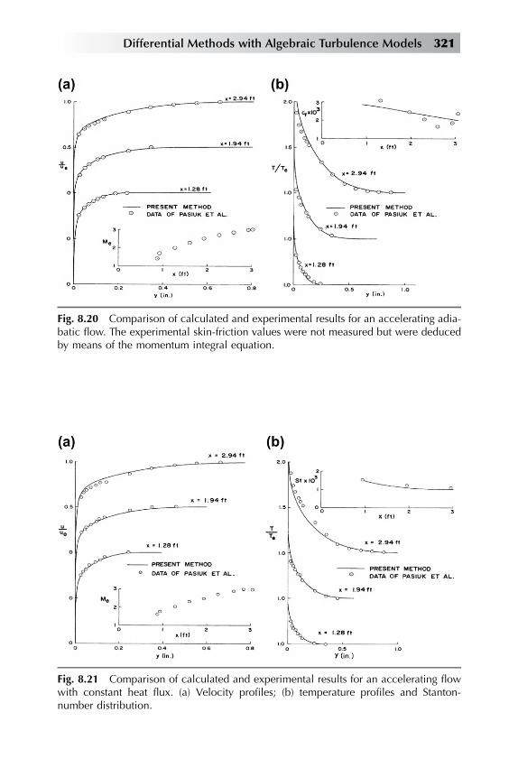
Fig. 8.20 Comparison of calculated and experimental results for an accelerating adia-batic flow. The experimental skin-friction values were not measured but were deducedby means of the momentum integral equation.

Fig. 8.21 Comparison of calculated and experimental results for an accelerating flowwith constant heat flux. (a) Velocity profiles; (b) temperature profiles and Stanton-number distribution.


Pasiuk et al. [35]. The calculations were started by assuming a constant heat flux

with zero pressure gradient that matched the experimental momentum-thickness

value at x¼ 0.94 ft. Then the experimental Mach-number distribution was used to

compute the rest of the flow for constant heat flux. The edge Mach number varied

from Me¼ 1.69 at x¼ 0.94 ft to Me¼ 2.97 at x¼ 3.03 ft. Figure 8.21a shows

a comparison of calculated and experimental velocity profiles for three x stations.

Similarly, Fig. 8.21b shows a comparison of calculated and experimental

temperature profiles, together with a comparison of local Stanton-number values.

Except for one x station, the calculated profiles are in good agreement with

experiment.

8.6 Axisymmetric Compressible Flows

Figure 5.4b in subsection 5.3.2 presented a comparison of calculated and experi-

mental velocity profiles in adiabatic compressible turbulent boundary layers on

slender cylinder. As we discussed in Sects. 5.3.2 and 8.4, in flows past such bodies,

the transverse-curvature effect causes the boundary-layer development to be

significantly different from those in two-dimensional zero-pressure gradient flows. A

modification of the two-dimensional eddy-viscosity distribution for thick axisym-

metric boundary layers improves the calculations.

Figure 8.22 shows the results for a waisted body of revolution for an adiabatic

compressible flow at two Mach numbers. The measurements are due to Winter et al.

[36]. The experimental skin-friction values were obtained by the ‘‘razor blade’’

technique. The calculations in each case were started by using the experimental

velocity profile at X/L¼ 0.4 and by using the Crocco relationship. Calculations were

made with and without the transverse-curvature effect. In general, the calculated

results are in good agreement with experiment.

8.7 Prediction of Two-Dimensional IncompressibleFlows with Separation

The solution of the boundary-layer equations for laminar and turbulent external flows

with prescribed velocity distribution is sometimes referred to as the standard

problem or direct problem [1]. This approach allows viscous flow solutions provided

that boundary-layer separation, which corresponds to vanishing wall shear in two-

dimensional steady flows, does not occur. If the wall shear vanishes at some

x-location, solutions breakdown and convergence cannot be obtained. This is

referred to as the singular behaviour of the boundary-layer equations at separation.


The boundary-layer equations are not singular at separation if the external

velocity or pressure is computed as part of the solution. This procedure is known as

the inverse problem and has been extensively used for airfoil flows. In general two

procedures have been pursued. In the first procedure, developed by Le Balleur [37]

and Carter and Wornom [38], the solution of the boundary-layer equations is

obtained by the standard method, and a displacement-thickness, d*0(x), distribution

is determined. If this initial calculation encounters separation, d*0(x) is extrapolated

to the trailing edge of the airfoil. For the given d*0(x) distribution, the boundary-layer

equations are then solved in the inverse mode to obtain an external velocity uev(x).

An updated inviscid velocity distribution, uei(x), is then obtained from the inviscid

flow method with the added displacement thickness. A relaxation formula is intro-

duced to define an updated displacement-thickness distribution,

d*ðxÞ ¼ d*0ðxÞ 1þ u

uevðxÞueiðxÞ � 1

�(8.7.1d)

Fig. 8.22 Comparison of calculated and experimental results for a waisted body ofrevolution for an adiabatic flow at two Mach numbers: (a) MN¼ 0.6, RL¼ 107; (b)MN¼ 1.4, RL¼ 107 (TVC stands for transverse curvature).


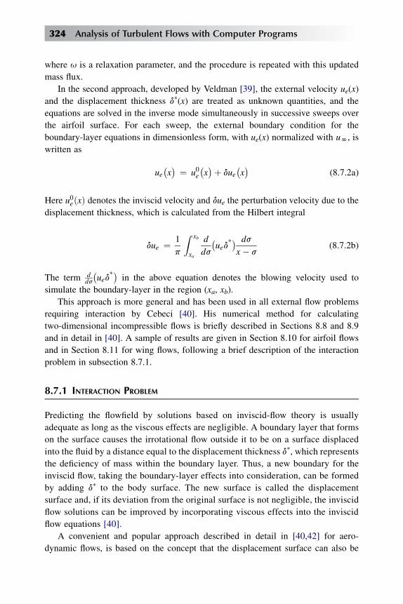
where u is a relaxation parameter, and the procedure is repeated with this updated

mass flux.

In the second approach, developed by Veldman [39], the external velocity ue(x)

and the displacement thickness d*(x) are treated as unknown quantities, and the

equations are solved in the inverse mode simultaneously in successive sweeps over

the airfoil surface. For each sweep, the external boundary condition for the

boundary-layer equations in dimensionless form, with ue(x) normalized with uN, is

written as

ue�x� ¼ u0e

�x�þ due

�x�

(8.7.2a)

Here u0eðxÞ denotes the inviscid velocity and due the perturbation velocity due to the

displacement thickness, which is calculated from the Hilbert integral

due ¼ 1

p

Z xb

xa

d

ds

�ued

*� ds

x� s(8.7.2b)

The term dds

�ued

*�in the above equation denotes the blowing velocity used to

simulate the boundary-layer in the region (xa, xb).

This approach is more general and has been used in all external flow problems

requiring interaction by Cebeci [40]. His numerical method for calculating

two-dimensional incompressible flows is briefly described in Sections 8.8 and 8.9

and in detail in [40]. A sample of results are given in Section 8.10 for airfoil flows

and in Section 8.11 for wing flows, following a brief description of the interaction

problem in subsection 8.7.1.

8.7.1 INTERACTION PROBLEM

Predicting the flowfield by solutions based on inviscid-flow theory is usually

adequate as long as the viscous effects are negligible. A boundary layer that forms

on the surface causes the irrotational flow outside it to be on a surface displaced

into the fluid by a distance equal to the displacement thickness d*, which represents

the deficiency of mass within the boundary layer. Thus, a new boundary for the

inviscid flow, taking the boundary-layer effects into consideration, can be formed

by adding d* to the body surface. The new surface is called the displacement

surface and, if its deviation from the original surface is not negligible, the inviscid

flow solutions can be improved by incorporating viscous effects into the inviscid

flow equations [40].

A convenient and popular approach described in detail in [40,42] for aero-

dynamic flows, is based on the concept that the displacement surface can also be


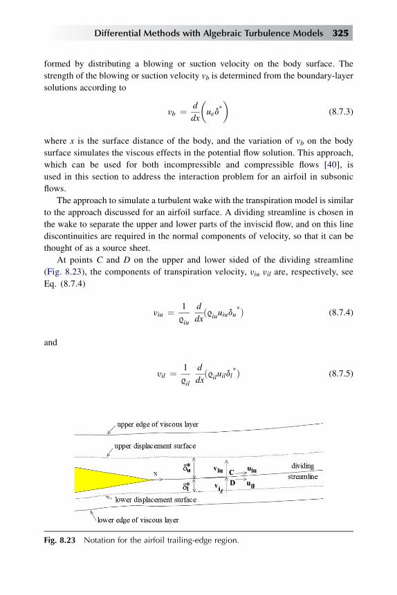
formed by distributing a blowing or suction velocity on the body surface. The

strength of the blowing or suction velocity vb is determined from the boundary-layer

solutions according to

yb ¼ d

dx

�ued

*

�(8.7.3)

where x is the surface distance of the body, and the variation of vb on the body

surface simulates the viscous effects in the potential flow solution. This approach,

which can be used for both incompressible and compressible flows [40], is

used in this section to address the interaction problem for an airfoil in subsonic

flows.

The approach to simulate a turbulent wake with the transpiration model is similar

to the approach discussed for an airfoil surface. A dividing streamline is chosen in

the wake to separate the upper and lower parts of the inviscid flow, and on this line

discontinuities are required in the normal components of velocity, so that it can be

thought of as a source sheet.

At points C and D on the upper and lower sided of the dividing streamline

(Fig. 8.23), the components of transpiration velocity, yiu yil are, respectively, see

Eq. (8.7.4)

yiu ¼ 1

9iu

d

dxð9iuuiudu*Þ (8.7.4)

and

yil ¼ 1

9il

d

dxð9iluildl*Þ (8.7.5)

Fig. 8.23 Notation for the airfoil trailing-edge region.


Here the sign convention has been used the y is measured positive in the direction

of the upward normal to the wake. Hence a jump Dy in the component of velocity

normal to the wake is required; it is given by

Dyih yiu � yil ¼ 1

9iu

d

dxð9iuuiudu*Þ þ

1

9il

d

dxð9iluildl*Þ (8.7.6)

For a given airfoil geometry and freestream flow conditions, the inviscid velocity

distribution is usually obtained with a panel method, then the boundary-layer

equations are solved in the inverse mode as described in Section 8.8. The blowing

velocity distribution, yb(x), is computed from Eqs. (8.7.3–8.7.6) and the displace-

ment thickness distribution d*(x) on the airfoil and in the wake are then used in the

panel method to obtain an improved inviscid velocity distribution with viscous

effects (See Section 8.9). The d*te is used to satisfy the Kutta condition in the panel

method at a distance equal to d*te; this is known as the off-body Kutta condition

(Fig. 8.24). In the first iteration between the inviscid and the inverse boundary-layer

methods, yb(x) is used to replace the zero blowing velocity at the surface. At the next

and following iterations, a new value of yb(x) in each iteration is used as a boundary

condition in the panel method. This procedure is repeated for several cycles until

convergence is obtained, which is usually based on the lift and total drag coefficients

of the airfoil. Studies discussed in [40] show that with three boundary-layer sweeps

for one cycle, convergence is obtained in less than 10 cycles.

8.8 Numerical Solution of the Boundary-Layer Equationsin the Inverse Mode with Algebraic Turbulence Models

We consider a laminar and turbulent flow. We assume the calculations start at the

leading edge, x¼ 0, for laminar flow and are performed for turbulent flow at any

x-location by specifying the transition location. The use of the two-point finite-

difference approximations for streamwise derivatives is proper and does not cause

numerical difficulties if there is no flow separation. If there is one, then it is necessary

to use backward difference formulas [40].

Fig. 8.24 Interactive boundary-layer scheme.


We employ two separate but closely related transformations. The first one is the

Falkner-Skan transformation in which the dimensionless similarity variable h and

a dimensionless stream function f (x, h) are defined by Eqs. (8.2.5).

The resulting equations with this transformation are given by Eqs. (8.2.6) and

(8.2.7).

In the inverse mode, since ue (x) is also an unknown, slight changes are made to

the transformation given by Eq. (8.2.5), replacing ue(x) by uN and redefining new

variables Y and F by

Y ¼ffiffiffiffiffiffiffiuNnx

ry; jðx; yÞ ¼ ffiffiffiffiffiffiffiffiffiffiffi

uNnxp

Fðx; YÞ; x ¼ x

L(8.8.1)

The resulting equation and its wall boundary equations can be written as

ðbF00Þ0 þ 1

2FF00 ¼ x

�F0vF0

vx� F00vF

vx

�� xw

dw

dx(8.8.2)

Y ¼ 0; F0 ¼ 0; F ¼ 0 (8.8.3)

Here primes denote differentiations with respect to Y and w¼ ue/uN.

The edge boundary condition is obtained from Eq. (8.7.2). By applying a

discretization approximation to the Hilbert integral, Eq. (8.7.2b), we can write

ueðxiÞ ¼ u0eðxiÞ þ CiiDi þXi�1

j¼ 1

CijDj þXN

j¼ iþ1

CijDj (8.8.4)

where the subscript i denotes the x-station where the inverse calculations are to be

performed, Cij is a matrix of interaction coefficients obtained by the procedure

described in subroutine HIC, and D is given by D¼ ued*. In terms of transformed

variables, the parameter D becomes

D ¼ D

LuN¼

ffiffiffiffiffiffix

RL

rðYew� FeÞ (8.8.5)

and the relation between the external velocity ue and displacement thickness d*

provided by the Hilbert integral can then be written in dimensionless form as

Y ¼ Ye; F0e

�xi�� l

�YeF

0e

�xi�� Fe

�xi�� ¼ gi (8.8.6)

where

l ¼ Cii

ffiffiffiffiffiffiffiffiffiffiffixi=RL

q(8.8.7a)

gi ¼ u0e�xi�þXi�1

j¼ 1

CijDj þXN

j¼ iþ1

CijDj (8.8.7b)


8.8.1 NUMERICAL FORMULATION

The numerical method for the inverse problem is similar to the numerical method

described for the standard problem in Section 8.2. Since ue(x) must be computed as

part of the solution procedure, we treat it as an unknown. Remembering that the

external velocity w is a function of x only, we write

w0 ¼ 0 (8.8.8)

As in the case of the standard problem, new variables U (x, Y), V (x, Y) are introduced

and Eq. (8.8.2) and its boundary conditions, Eq. (8.8.3) and (8.8.6), are expressed as

a first-order system,

F0 ¼ U (8.8.9a)

U0 ¼ V (8.8.9b)

ðbVÞ0þ 1

2FV ¼ x

�UvU

vx� V

vF

vx

�� xw

dw

dx(8.8.9c)

Y ¼ 0; F ¼ U ¼ 0 (8.8.10a)

Y ¼ Ye; U ¼ w; lF þ ð1� lYeÞw ¼ gi (8.8.10b)

Finite-difference approximations to Eqs. (8.8.8) and (8.8.9) are written in a similar

fashion to those expressed in the original Falkner-Skan variables, yielding

h�1j

�wnj � wn

j�1

�¼ 0 (8.8.11a)

h�1j

�Fnj � Fn

j�1

�¼ Un

j�1=2 (8.8.11b)

h�1j

�Unj � Un

j�1

�¼ Vn

j�1=2 (8.8.11c)

h�1j

�bnj V

nj � bnj V

nj�1

�þ�1

2þ an

�ðFVÞnj�1=2

þ anh�w2�nj�1=2

� FLARE�U2�nj�1=2

iþ an

�Vn�1j�1=2F

nj�1=2 � Fn�1

j�1=2Vnj�1=2

�¼ Rn�1

j�1=2

(8.8.11d)

where

Rn�1j�1=2 ¼ �Ln�1

j�1=2 þ anhðFVÞn�1

j�1=2 � FLARE�U2�n�1

j�1=2

i(8.8.12a)


Ln�1j�1=2 ¼

h�1j

�bjyj � bj�1yj�1

�þ 1

2ðFVÞj�1=2 � an

�w2�j�1=2

n�1

(8.8.12b)

In Eq. (8.8.11d), the parameter FLARE refers to the Flugge-Lotz-Reyhner

approximation [1] used to set uvu

vxequal to zero in the momentum equation whenever

u < 0. As a result, the numerical instabilities that plague attempts to integrate the

boundary-layer equations against the local directions of flow are avoided. In regions

of positive streamwise velocity (uj > 0), it is taken as unity and as zero in regions of

negative streamwise velocity (uj � 0).

The linearized form of Eqs. (8.8.11) and (8.8.10) can be expressed in the form

given by Eq. (8.2.24) or

b.c. 1

–1

0(s4)j (s6)j (s2)j (s3)j (s5)j (s1)j (s7)j

(s4)J (s6)J (s2)J (s8)J

(s8)j

000

0

00

0 0 0 0 00 0 0 00 1 00 0 0 1

00

δFo

δUo

δVo

δwo

δFj

δUj

δVj

δwj

δFJ

δFO

δUO

δVO

δwO

(r1)O

(r2)O

(r3)O

(r4)O

δFj

δUj

δVj

δwj

(r1)j

(r2)j

(r3)j

(r4)j

δFJ

δUJ

δVJ

δwJ

(r1)J

(r2)J

(r3)J

(r4)J

δUJ

δVJ

δwJ

0 0 00 1 0 00 –1 00 0 0 –1

b.c.

b.c.b.c.

–h12

–hj

2 –1

–1 0 0

–1–1

0 0

0

–hj

2

–hJ

2

00 0 0

00 0 000 0 0

(s3)J (s5)J (s1)J (s7)J1 0 0–h

J

2

–10 1 000 0 0

hj+1

2

hj+1

2

0 0 0 00 0 0 00 –1 00 0 0 1

–h12

(8.8.13)

With de j and re j now defined by

de j ¼��dFj

dUj

dVj

dwj

��; re j ¼��ðr1Þjðr2Þjðr3Þjðr4Þj

�� (8.8.14)

and Aj, Bj, Cj becoming 4� 4 matrices defined by

A0 ¼

��1 0 0 00 1 0 0

0 �1 �h12

0

0 0 0 �1

��; Aj ¼

��

1 �hj2

0 0

ðs3Þj ðs5Þj ðs1Þj ðs7Þj0 �1 �hjþ1

20

0 0 0 �1

��; 1 � j � J � 1

(8.8.15a)


AJ ¼

��1 �hJ

20 0

ðs3ÞJ ðs5ÞJ ðs1ÞJ ðs7ÞJg1 0 0 g20 1 0 �1

��; Bj ¼

��1 �hj

20 0

ðs4Þj ðs6Þj ðs2Þj ðs8Þj0 0 0 00 0 0 0

��; 1 � j � J

(8.8.15b)

Cj ¼

��0 0 0 00 0 0 0

0 1 �hjþ1

20

0 0 0 1

��; 0 � j � J � 1 (8.8.15c)

Here the first two rows of A0 and C0 and the last two rows of BJ and AJ correspond to

the linearized boundary conditions,

dF0 ¼ dU0 ¼ 0; dUJ � dwJ ¼ wJ � UJ ; g1dFJ þ g2dwJ ¼ g3 (8.8.16)

where

g1 ¼ l; g2 ¼ 1� lYJ ; g3 ¼ gi � ðg1FJ þ g2wJÞ (8.8.17)

As a result

ðr1Þ0 ¼ ðr2Þ0 ¼ 0 (8.8.18a)

ðr3ÞJ ¼ g3; ðr4ÞJ ¼ wJ � UJ (8.8.18b)

The third and fourth rows of A0 and C0 correspond to Eq. (8.2.20b) and the

linearized form of Eq. (9.2.18a), that is,

dwj � dwj�1 ¼ wj�1 � wj ¼ ðr4Þj�1 (8.8.19)

if the unknows f, u, y are replaced by F, U and V. Similarly, the first and second rows

of Aj and Bj correspond to Eq. (8.2.20a) and (9.2.18a) with two terms added to its

left-hand side,

ðs7Þjdwj þ ðs8Þjdwj�1 (8.8.20a)

with (s7)j and (s8)j defined by

ðs7Þj ¼ anwj; ðs8Þj ¼ anwj�1 (8.8.20b)

The coefficients (s1)j to (s6)j defined by Eqs. (8.2.22) remain unchanged provided

we set


a1 ¼ 1

2þ an; a2 ¼ an (8.8.21)

and define (r2)j by

ðr2Þj ¼ Rn�1j�1=2 �

h�1j

�bjVj � bj�1Vj�1

�þ �12þ an

�ðFVÞj�1=2

þ anh�w2�j�1=2

� FLARE�U2�j�1=2

iþ an

�Vn�1j�1=2Fj�1=2 � Fn�1

j�1=2Vj�1=2

�i (8.8.22)

The remaining elements of the re j vector follow from Eqs. (8.2.21), and (8.8.19) and

(8.8.22) so that, for l � j � J, (r1)j, (r2)j, (r3)j�1 are given by Eqs. (8.2.21a), (8.8.22)

and (8.2.21b), respectively. For the same j-values, (r4)j�1 is given by the right-hand

side of Eq. (8.8.19).

The parameters g1, g2 and g3 in Eq. (8.8.16) determine whether the system given

by the linearized form of Eqs. (8.8.11) and their boundary conditions is to be solved

in standard or inverse form. For an inverse problem, they are represented by the

expressions given in Eq. (8.8.16) and for a standard problem by g1¼ 0, g2¼ 1.0 and

g3¼ 0.

It should be noted that for flows with separation, it is necessary to use backward

differences as discussed for the CS and k-ε models in Sections 10.7 to 10.10.

In that case, the coefficients (s1)j to (s6)j are given by Eq. (9.2.25), and (r2)j by

Eq. (9.2.26) with the relations given by Eq. (8.8.22).

The solution of Eq. (8.2.24), with de j and re j defined by Eq. (8.8.14) and with Aj, Bj

and Cj matrices given by Eqs. (8.8.15), can again be obtained by the block-

elimination of subsection 8.2.3. The resulting algorithm, is similar to SOLV3, and is

called SOLV4.

Numerical Method for Wake Flows

In interaction problems involving airfoils, it is usually sufficient to neglect the wake

effect and perform calculations on the airfoil only, provided that there is no or little

flow separation on the airfoil. With flow separation, the relative importance of

including the wake effect in the calculations depends on the flow separation as shown

in Fig. 8.25 taken from [40]. Figure (8.25a) shows the computed separation locations

on a NACA 0012 airfoil at a chord Reynolds number, Rc of 3� 106. When the wake

effect is included, separation is encountered for angles of attack greater than 10�, andattempts to obtain results without consideration of the wake effect lead to errone-

ously large regions of recirculation that increases with angle of attack, as discussed

in [40]. Figure (8.25b) shows that the difference in displacement thickness at the

trailing edge is negligible for a¼ 10� but more than 30% for a¼ 16� [40].


As discussed in [40], the inverse boundary layer method described here can also be

extended to include wake flows. This requires the specification of a turbulence model

for wake flows and minor modifications to the numerical method.

The extension of the CS model for wall boundary layers to wake flows is given by

the following expressions described in [41]:

εm ¼ ðεmÞw þ �ðεmÞt:e: � ðεmÞw�exp

�ðx� xt:e:Þldt:e:

(8.8.23)

where dt.e. is the boundary layer thickness at the trailing edge, l is an empirical

parameters, (εm)t.e. is the eddy viscosity at the trailing edge, and (εm)w is the eddy-

viscosity in the far wake given by the larger of

ðεmÞlw ¼ 0:064

Z ymin

�Nðue � uÞdy (8.8.24)

and

ðεmÞuw ¼ 0:064

Z N

ymin

ðue � uÞdy (8.8.25)

with ymin denoting the location where the velocity is a minimum.

The studies conducted in [41] indicate that a choice of l¼ 20 is satisfactory for

single airfoils. Calculations with different values of l essentially produced similar

results, indicating that the modeling of wake flows with Eq. (8.8.23) was not too

sensitive to the choice of l. The application of the above model to wake flows with

strong adverse pressure gradient, however, indicated that this was not the case and

the value of the parameter is an important one. On the basis of that study, a value of

l¼ 50 was found to produce best results and is used in the computer program

discussed in Section 10.14.

Fig. 8.25 Wake effect on (a) flow separation and (b) displacement thickness – NACA0012 airfoil. d, with wake:– – – , without wake.


A modification to the numerical method of the previous section arises due to the

boundary conditions along the wake dividing streamline. The new ‘‘wall’’ boundary

conditions on f and u now become

h ¼ 0; f0 ¼ 0; y0 ¼ 0 (8.8.26)

so that the second row of Eq. (8.8.23) can de written as

0 0 1 0 (8.8.27)

Before the boundary-layer equations can be solved for wake flows, the initial

velocity profiles must satisfy the wall and edge boundary conditions. When the

calculations are first performed for wall boundary layer flows and are then to be

extended to wake flows, it is necessary to modify the velocity profiles computed

for wall boundary layers. This is done in subroutine WAKEPR of the computer

program.

8.9 Hess-Smith (HS) Panel Method

For incompressible flows, a panel method is an ideal inviscid method for interactive

boundary layer approach. Of the several panel methods, here we choose the one due

to Hess and Smith [40]. The procedure for incorporating the viscous effects into the

panel method is discussed in Section 8.9.1. Changes required in an inviscid method

to extend the viscous flow calculations into the wake of an airfoil are discussed in

Section 8.9.2. A brief description of the computer program for the HS method with

viscous effects is given in Section 10.4.

We consider an airfoil at rest in an onset flow of velocity VN. We assume that

the airfoil is at an angle of attack, a (the angle between its chord line and the onset

velocity), and that the upper and lower surfaces are given by functions Yu(x) and

Yl(x), respectively. These functions can be defined analytically, or (as is often the

case) by a set of (x, y) values of the airfoil coordinates. We denote the distance of

any field point (x, y) from an arbitrary point, b, on the airfoil surface by r, as shown

in Fig. 8.25. Let n! also denote the unit vector normal to the airfoil surface and

directed from the body into the fluid, and t!a unit vector tangential to the surface,

and assume that the inclination of t!

to the x-axis is given by q. It follows from

Fig. 8.25 that with i!and j

!denoting unit vectors in the x- and y-directions,

respectively,

n! ¼ �sinq i!þ cosq j

!t! ¼ cosq i

!þ sinq j! (8.9.1)


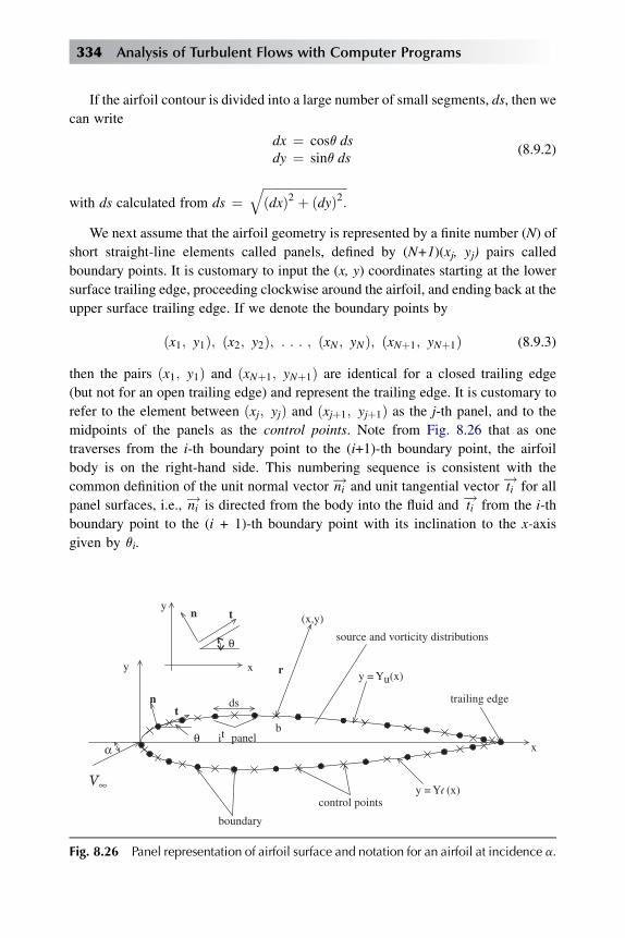
If the airfoil contour is divided into a large number of small segments, ds, then we

can write

dx ¼ cosq dsdy ¼ sinq ds

(8.9.2)

with ds calculated from ds ¼ffiffiffiffiffiffiffiffiffiffiffiffiffiffiffiffiffiffiffiffiffiffiffiffiffiffiffiffiðdxÞ2 þ ðdyÞ2:

qWe next assume that the airfoil geometry is represented by a finite number (N) of

short straight-line elements called panels, defined by (N+1)(xj, yj) pairs called

boundary points. It is customary to input the (x, y) coordinates starting at the lower

surface trailing edge, proceeding clockwise around the airfoil, and ending back at the

upper surface trailing edge. If we denote the boundary points by

ðx1; y1Þ; ðx2; y2Þ; : : : ; ðxN ; yNÞ; ðxNþ1; yNþ1Þ (8.9.3)

then the pairs ðx1; y1Þ and ðxNþ1; yNþ1Þ are identical for a closed trailing edge

(but not for an open trailing edge) and represent the trailing edge. It is customary to

refer to the element between ðxj; yjÞ and ðxjþ1; yjþ1Þ as the j-th panel, and to the

midpoints of the panels as the control points. Note from Fig. 8.26 that as one

traverses from the i-th boundary point to the (i+1)-th boundary point, the airfoil

body is on the right-hand side. This numbering sequence is consistent with the

common definition of the unit normal vector ni! and unit tangential vector ti

!for all

panel surfaces, i.e., ni! is directed from the body into the fluid and ti

!from the i-th

boundary point to the (i + 1)-th boundary point with its inclination to the x-axis

given by qi.

∞

y

y

x

(x,y)

source and vorticity distributions

y = Yu(x)

control points

it panelb

dsnt

r

n t

boundary

αθ

θ

trailing edge

x

Fig. 8.26 Panel representation of airfoil surface and notation for an airfoil at incidence a.


In the HS panel method, the velocity V!

at any point ðx; yÞ is represented by

V! ¼ U

!þ y! (8.9.4)

where U!

is the velocity of the uniform flow at infinity

U! ¼ VN

�cos a i

!þ sin a j!�

(8.9.5)

and y! is the disturbance field due to the body which is represented by two elementary

flows corresponding to source and vortex flows. A source or vortex on the j-th panel

causes an induced source velocity ys! at (x, y) or an induced vortex velocity y!y at (x, y),

respectively, and these are obtained by taking radients of a potential source

fs ¼ q

2pln r (8.9.6)

and a potential vortex

fr ¼ I0

2pq; (8.9.7)

both centered at the origin, so that, with integrals applied to the airfoil surface,

y!ðx; yÞ ¼Z

ys!qjðsÞdsj þ

Zyy!sjðsÞdsj (8.9.8)

Here qjdsj is the source strength for the element dsj on the j-th panel. Similarly, sjdsjis the vorticity strength for the element dsj on the same panel.

Each of the N panels is represented by similar sources and vortices distributed on

the airfoil surface. The induced velocities in Eq. (8.9.8) satisfy the irrotationality

condition and the boundary condition at infinity

u ¼ vf

vx¼ vj

vy¼ VNcosa (8.9.9a)

y ¼ vf

vy¼ �vj

vx¼ VNsina (8.9.9b)

For uniqueness of the solutions, it is also necessary to specify the magnitude of the

circulation around the body. To satisfy the boundary conditions on the body, which

correspond to the requirement that the surface of the body is a streamline of the flow,

that is,

j ¼ constant orvf

vn¼ 0 (8.9.10)

at the surface on which n is the direction of the normal, the sum of the source induced

and vorticity-induced velocities and freestream velocity is set to zero in the direction

normal to the surface of each of the N panels. It is customary to choose the control


points to numerically satisfy the requirement that the resultant flow is tangent to the

surface. If the tangential and normal components of the total velocity at the control

point of the i-th panel are denoted by (Vt)i and (Vn)i, respectively, the flow tangency

conditions are then satisfied at panel control points by requiring that the resultant

velocity at each control point has only (Vt)i, and

ðVnÞi ¼ 0 i ¼ 1; 2;.;N (8.9.11)

Thus, to solve the Laplace equation with this approach, at the i-th panel control point

we compute the normal (Vn)i and tangential (Vt)i, (i ¼ 1, 2, . . . , N) velocity

components induced by the source and vorticity distributions on all panels, j ( j ¼ 1,

2, . . . , N), including the i-th panel itself, and separately sum all the induced

velocities for the normal and tangential components together with the freestream

velocity components. The resulting expressions, which satisfy the irrotationality

condition, must also satisfy the boundary conditions discussed above. Before dis-

cussing this aspect of the problem, it is convenient to write Eq. (8.9.4) expressed in

terms of its velocity components (Vn)i and (Vt)i by

ðVnÞi ¼XNj¼ 1

Anijqj þ

XNj¼ 1

Bnijsj þ VNsinða� qiÞ (8.9.12a)

ðVtÞi ¼XNj¼ 1

Atijqj þ

XNj¼ 1

Btijsj þ VNcosða� qiÞ (8.9.12b)

where Anij , B

nij , A

tij , B

tij are known as influence coefficients, defined as the

velocities induced at a control point ðxmi; ymi

Þ; more specifically, Anij and At

ij

denote the normal and tangential velocity components, respectively, induced at the

i-th panel control point by a unit strength source distribution on the j-th panel, and

Bnij and Bt

ij are those induced by unit strength vorticity distribution on the j-th

panel. The influence coefficients are related to the airfoil geometry and the panel

arrangement; they are given by the following expressions:

Anij ¼

8>><>>:1

2p

sinðqi � qjÞ ln ri; jþ1

ri;jþ cosðqi � qjÞbij

isj

1

2i ¼ j

(8.9.13)

Atij ¼

1

2p

sinðqi � qjÞ bij � cosðqi � qjÞ ln ri; jþ1

ri;j

isj

0 i ¼ j

8><>: (8.9.14)

Bnij ¼ �At

ij Btij ¼ An

ij (8.9.15)


Here

ri;jþ1 ¼hðxmi

� xjþ1Þ2 þ ðymi� yjþ1Þ2

i1=2ri;j ¼

hðxmi

� xjÞ2 þ ðymi� yjÞ2

i1=2xmi

¼ 1

2ðxi þ xjþ1Þ; ymi

¼ 1

2ðyi þ yjþ1Þ

qi ¼ tan�1

�yiþ1 � yixiþ1 � xi

�; qj ¼ tan�1

�yjþ1 � yjxjþ1 � xj

�bij ¼ tan�1

�ymi

� yjþ1

xmi� xjþ1

�� tan�1

�ymi

� yjxmi

� xj

�(8.9.16)

Regardless of the nature of qj(s) and sj(s), Eq. (8.9.12) satisfies the irrotationality

condition and the boundary condition at infinity, Eq. (8.9.9). To satisfy the require-

ments given by Eq. (8.9.11) and the condition related to the circulation, it is necessary

to adjust these functions. In the approach adopted by Hess and Smith [40], the source

strength qj(s) is assumed to be constant over the j-th panel and is adjusted to give zero

normal velocity over the airfoil, and the vorticity strength sj is taken to be constant onall panels (sj¼s) and its single value is adjusted to satisfy the condition associatedwiththe specification of circulation. Since the specification of the circulation renders the

solution unique, a rational way to determine the solution is required.

The best approach is to adjust the circulation to give the correct force on the body

as determined by experiment. However, this requires advance knowledge of that force,

and one of the principal aims of a flow calculation method is to calculate the force and

not to take it as given. Thus, another criterion for determining circulation is needed.

For smooth bodies such as ellipses, the problem of rationally determining the

circulation has yet to be solved. Such bodies have circulation associated with them,

and resulting lift forces, but there is no rule for calculating these forces. If, on the

other hand, we deal with an airfoil havinga sharp trailing edge, we can apply the

Kutta condition [40]. It turns out that for every value of circulation except one,

the inviscid velocity is infinite at the trailing edge. The Kutta condition states

that the particular value of circulation that gives a finite velocity at the trailing edge

is the proper one to choose. This condition does not include bodies with nonsharp

trailing edges and bodies on which the viscous effects have been simulated by, for

example, surface blowing, as discussed [4]. Thus, the classical Kutta condition is of

strictly limited validity. It is customary to apply a ‘‘Kutta condition’’ to bodies

outside its narrow definition, but this is an approximation; nevertheless the calcu-

lations are often in close accord with experiment.

In the panel method, the Kutta condition is indirectly applied by deducing

another property of the flow at the trailing edge that is a direct consequence of the


finiteness of velocity; this property is used as ‘‘the Kutta condition’’. Properties that

have been used in lieu of ‘‘the Kutta condition’’ in panel methods include the

following:

(a) A streamline of the flow leaves the trailing edge along the bisector of the trai-

ling-edge angle.

(b) Upper and lower displacement total velocities approach a common limit at the

trailing edge. The limiting value is zero if the trailing-edge angle is nonzero.

(c) Source and/or vorticity strengths at the trailing edge must satisfy conditions to

allow finite velocity.

Of the above, property (b) is more widely used. At first it may be thought that this

property requires setting both the upper and lower surface velocities equal to zero.

This gives two conditions, which cannot be satisfied by adjusting a single parameter.

The most reasonable choice is to make these two total velocities in the downstream

direction at the 1st and N-th panel control points equal so that the flow leaves the

trailing edge smoothly. Since the normal velocity on the surface is zero according to

Eq. (8.9.11), the magnitudes of the two tangential velocities at the trailing edge must

be equal to each other, that is,

ðVtÞN ¼ �ðVtÞ1 (8.9.17)

Introducingthe flow tangency condition, Eq. (8.9.11), into Eq. (8.9.12a) and noting

that sj¼ s, we get

XNj¼ 1

Anijqj þ s

XNj¼ 1

Bnij þ VNsinða� qiÞ ¼ 0; i ¼ 1; 2;.;N (8.9.18)

In terms of the unknowns, qj ( j ¼ 1, 2, . . . , N) and s, the Kutta condition of

Eq. (8.9.17) and Eq. (8.9.18) for a system of algebraic equations which can be written

in the following form,

A xe ¼ be (8.9.19)

Here A is a square matrix of order (N + 1), that is

A h

��

a11 a12 . a1j . a1N a1;Nþ1

a21 a22 . a2j . a2N a2;Nþ1

« « « « « « «

ai1 ai2 . aij . aiN ai;Nþ1

« « « « « « «

aN1 aN2 . aNj . aNN aN;Nþ1

aNþ1;1 aNþ1;2 . aNþ1;j . aNþ1;N aNþ1;Nþ1

��(8.9.20)


and x!¼ (q1, . . . , qi, . . . , qN, s)T and b ¼ (b1, . . . , bi, . . . , bN, bN+1)

Twith denoting

the transpose. The elements of the coefficient matrix A follow from Eq. (8.9.18)

aij ¼ Anij;

i ¼ 1; 2;.;Nj ¼ 1; 2;.;N

(8.9.21a)

ai;Nþ1 ¼XNj¼ 1

Bnij; i ¼ 1; 2;.;N (8.9.21b)

Anij are given by Eq. (8.9.13) and Bn

ij by Eq. (8.9.15). The relation in Eq. (8.9.20)

follows from the definition of x! where s is essentially xN+1.

To find aN+1,j (J ¼ 1, . . . , N) and aN+1,N+1 in the coefficient matrix A, we use the

Kutta condition and apply Eq. (8.9.17) to Eq. (8.9.12b) and, with s as a constant, wewrite the resulting expression as

XNj¼ 1

At1jqj þ s

XNj¼ 1

Bt1j þ VNcosða� q1Þ

¼ �"XN

j¼ 1

AtNjqj þ s

XNj¼ 1

BtNj þ VNcosða� qNÞ

#

or as

XNj¼ 1

ðAt1j þ At

NjÞqj þ sXNj¼ 1

ðBt1j þ Bt

NjÞ ¼ �VNcosða� q1Þ � VNcosða� qNÞ

(8.9.22b)

so that,

aNþ1;j ¼ At1j þ At

Nj; j ¼ 1; 2;.;N (8.9.23a)

aNþ1;Nþ1 ¼XNj¼ 1

ðBt1j þ Bt

NjÞ (8.9.23b)

where now At1j and At

Nj are computed from Eq. (8.9.14) and Bt1j and Bt

Nj from

Eq. (8.9.15).

The components of b!

again follow from Eqs. (8.9.18) and (8.9.21). From

Eq. (8.9.18),

bi ¼ �VNsinða� qiÞ; i ¼ 1;.;N (8.9.24a)

and from Eq. (8.9.22),

bNþ1 ¼ �VNcosða� q1Þ � VNcosða� qNÞ (8.9.24b)


With all the elements of aij determined from Eqs. (8.9.21) and (8.9.23) and the

elements of b!

from Eq. (8.9.24), the solution of Eq. (8.9.19) can be obtained by the

Gaussian elimination method [42]. The elements of x! are given by

xi ¼ 1

aði�1Þii

�"bði�1Þi �

XNþ1

j¼ iþ1

aði�1Þij xj

#i ¼ N þ 1;.; 1 (8.9.25)

where

aðkÞij ¼ a

ðk�1Þij � a

ðk�1Þik

aðk�1Þkk

aðk�1Þkj ;

k ¼ 1;.;Nj ¼ k þ 1;.N þ 1i ¼ k þ 1;.;N þ 1

að0Þij ¼ aij

(8.9.26a)

bðkÞi ¼ b

ðk�1Þi � a

ðk�1Þik

aðk�1Þkk

bðk�1Þk ;

k ¼ 1;.;Ni ¼ k þ 1;.N þ 1

bð0Þi ¼ bi

(8.9.26b)

8.9.1 VISCOUS EFFECTS

The viscous effects can be introduced into the panel method by (1) replacing the zero

normal-velocity condition, Eq. (8.9.11), by a nonzero normal-velocity condition

Viw(x) and by (2) satisfying the Kutta condition, Eq. (8.9.17), not on the surface of the

airfoil trailing edge but at some distance away from the surface.

Here it will be assumed that the nonzero normal-velocity distribution Viw(x) along

the surface of the airfoil and in its wake is known, together with the distance from the

surface, say displacement thickness d*, where the Kutta condition is to be satisfied.

We now describe how these two new conditions can be incorporated into the panel

method.

To include the nonzero normal-velocity condition into the solution procedure, we

write Eq. (8.9.18) as

XNj¼ 1

Anijqj þ s

XNj¼ 1

Bnijqj þ VNsinða� qiÞ ¼ yiwðxmi

Þ (8.9.27)

To satisfy the Kutta condition at the normal distance d* from the surface of the trailing

edge, called the ‘‘off-body’’ Kutta condition, the total velocities at the N-th and first

off-body control points are again required to be equal. Since the normal velocity

component is not zero, we write the off-body Kutta condition at distance d* as

ðVÞN ¼ �ðVÞ1 (8.9.28)


where V is the total velocity at the two control points. The off-body total velocities

are computed from

V ¼ ðVnÞ2 þ ðVtÞ2V

¼ VnVn

Vþ VtV

t

V¼ Vnsinfþ Vtcosf (8.9.29)

where Vn and Vt are computed by expressions identical to those given by Eqs.

(8.9.12) at the two off-body control points, I ¼ 1, I ¼ N, that is,

ðVnÞI ¼XNj¼ 1

AnIjqj þ s

XNj¼ 1

BnIj þ VNsinða� qIÞ (8.9.30a)

ðVtÞI ¼XNj¼ 1

AtIjqj þ s

XNj¼ 1

BtIj þ VNcosða� qIÞ (8.9.30b)

and where

f ¼ tan�1½ðVnÞI=ðVtÞI � (8.9.31)

With Eqs. (8.9.30), the expression for the total velocity given by Eq. (8.9.29) can be

written as

V ¼XNj¼ 1

ðAnIj$sinfþ At

Ij$cosfÞqj þ sXNj¼ 1

ðBnIj$sinfþ Bt

Ij$cosfÞ

þ VNsinða� qIÞsinfþ VNcosða� qIÞcosf (8.9.32a)

or as

V ¼XNj¼ 1

A0Ijqj þ s

XNj¼ 1

B0Ij þ VNcosða� qI � fÞ (8.9.32b)

where

A0Ij ¼ An

Ij$sinfþ AtIj$cosf; B0

Ij ¼ BnIj$sinfþ Bt

Ij$cosf (8.9.33a)

AnIj ¼

1

2p

sinðqI � qjÞ ln rI;jþ1

rI;jþ cosðqI � qjÞbIj

(8.9.33b)

AtIj ¼

1

2p

sinðqI � qjÞ bIj � cosðqI � qjÞ ln rI;jþ1

rI;j

(8.9.33c)

BnIj ¼ �At

Ij; BtIj ¼ An

Ij (8.9.33d)

If we define

q0I ¼ qI þ f (8.9.34)


then it can be shown that Eq. (8.9.32b) can be written as

V ¼XNj¼ 1

A0Ijqj þ s

XNj¼ 1

B0Ij þ VNcosða� q0IÞ (8.9.35)

where

A0Ij ¼

1

2p

sinðq0I � qjÞ bIj � cosðq0I � qjÞ ln rI;jþ1

rI;j

(8.9.36a)

B0Ij ¼

1

2p

sinðq0I � qjÞ ln rI;jþ1

rI;jþ cosðq0I � qjÞbIj

(8.9.36b)

The off-body Kutta condition can now be expressed in a form similar to that

of Eq. (8.9.22). Applying Eq. (8.9.28) to Eq. (8.9.35), we write the resulting

expression as

XNj¼ 1

A0Njqj þ s

XNj¼ 1

B0Nj þ VNcosða� q0NÞ

¼ �"XN

j¼ 1

A01jqj þ s

XNj¼ 1

B01j þ VNcosða� q01Þ

#(8.9.37a)

or as

XNj¼ 1

ðA01j þ A0

NjÞqj þ sXNj¼ 1

ðB01j þ B0

NjÞ þ VNcosða� q01Þ þ VNcosða� q0NÞ ¼ 0

(8.9.37b)

8.9.2 FLOWFIELD CALCULATION IN THE WAKE

The calculation of airfoils in incompressible viscous flows can be accomplished

without taking into account the wake effect; that is, the viscous flow calculations are

performed up to the trailing edge only and are not extended into the wake. This

procedure, which may be sufficient at low to moderate angles of attack without flow

separation, is not sufficient at higher angles of attack, including post-stall flows.

Additional changes are required in the panel method (and in the boundary-layer

method), as discussed in this section.

The viscous wake calculations usually include a streamline issuing from the

trailing edge of the airfoil. The computation of the location of this streamline is

relatively simple if conformal mapping methods are used to determine the velocity


field. In this case, the stream function j is usually known, and because the airfoil

surface is represented by j(x, y) ¼ const, the calculation of the wake streamline

amounts to tracing the curve after it leaves the airfoil. When the flowfield is

computed by a panel method or by a finite-difference method, however, the results

are known only at discrete points in the field in terms of the velocity components. In

this case, the wake streamline is determined from the numerical integration of

dy

dx¼ y

u(8.9.38)

aft of the trailing edge with known initial conditions. However, some care is

necessary in selecting the initial conditions, especially when the trailing edge is

blunt. As a general rule, the initial direction of the streamline is given to a good

approximation by the bisector of the trailing-edge angle of the airfoil.

The panel method, which was modified only for an airfoil flow, now requires

similar modifications to include the viscous effects in the wake which behaves as

a distribution of sinks. It is divided into nwp panels along the dividing streamline

with suction velocities or sink strengths qi ¼ Dvi (N + 1 � i � N + nwp), distributed

on the wake panels and determined from boundary-layer solutions in the wake by

Eq. (8.9.12). As before, off-body boundary points and ‘‘control’’ points are intro-

duced at the intersections of the d* surface with the normals through panel boundary

points and panel control points, respectively. Summation of all the induced veloci-

ties, separately for the normal and tangential components and together with the

freestream velocity components, produces (Vn)I and (Vt)I at I ¼ 1, 2, . . . , N + nwp.

The wake velocity distribution, as the airfoil velocity distribution, is computed on the

d*-surface, rather than on the dividing streamline.

The total velocities are again computed from Eq. (8.9.29), with (Vn)I and (Vt)Ifrom Eqs. (8.9.30), except that now

ðVnÞI ¼XNþnwp

j¼ 1

AnIjqj þ s

XNj¼ 1

BnIj þ VNsinða� qIÞ (8.9.39a)

ðVtÞI ¼XNþnwp

j¼ 1

AtIjqj þ s

XNj¼ 1

BtIj þ VNcosða� qIÞ (8.9.39b)

As before, the expression for the total velocity is written in the same form as

Eq. (8.9.32a), except that now

V ¼XNþnwp

j¼ 1

ðAnIj$sinfþ At

Ij$cosfÞqj þ sXNj¼ 1

ðBnIj$sinfþ Bt

Ij$cosfÞ

þ VNsinða� qIÞsinfþ VNða� qIÞcosf (8.9.40)


where AnIj, A

tIj, B

nIj and Bt

Ij, are identical to those given by Eq. (8.9.33). Similarly,

Eq. (8.9.35) with AIj and BIj given by Eq. (8.9.36) is

V ¼XNþnwp

j¼ 1

A0Ijqj þ s

XNj¼ 1

B0Ij þ VNcosða� q0IÞ (8.9.41)

and the Kutta condition given by Eqs. (8.9.37a) becomes

XNþnwp

j¼ 1

A0Njqj þ s

XNj¼ 1

B0Nj þ VNcosða� q0NÞ

¼ �" XNþnwp

j¼ 1

A01jqj þ s

XNj¼ 1

B01j þ VNcosða� q01Þ

#(8.9.42a)

or

XNþnwp

j¼ 1

ðA01j þ A0

NjÞqjþ sXNj¼ 1

ðB01j þ B0

NjÞ þ VNcosða� q01Þ þ VNcosða� q0NÞ ¼ 0

(8.9.42b)

In computing the wake velocity distribution at distances d* from the wake

dividing streamline, the velocities in the upper wake are equal to those in the lower

wake for a symmetrical airfoil at zero angle of attack. This is, however, not the case if

the airfoil is asymmetric or if the airfoil is at an angle of incidence. While the

external velocities on the upper and lower surfaces at the trailing edge are equal to

each other, they are not equal to each other in the wake region since the d*-distri-

bution in the upper wake is different from the d*-distribution in the lower wake.

8.10 Results for Airfoil Flows

The interactive boundary-layer method dicussed in subsection 8.8 employing the

improved CS model (subsection 5.4.2) has been extensively tested for single and

multielement airfoils with extensive flow separation. A sample of results were pre-

sented in Fig. 5.8b for an airfoil at low Reynolds number (see subsection 5.3.4) and in

Figs. 5.12 and 5.13 for airfoils at high Reynolds number (see subsection 5.4.2). Here

we present more results for single airfoils and also include multielement airfoils. For

additional results, see [40].

Figure 8.27 shows the variation of the lift and drag coefficients of the NACA

0012 airfoil for a chord Reynolds number of 3� 106. As can be seen from Fig. 8.27a,

viscous effects have a considerable effect on the maximum lift coefficient, (cl)max,


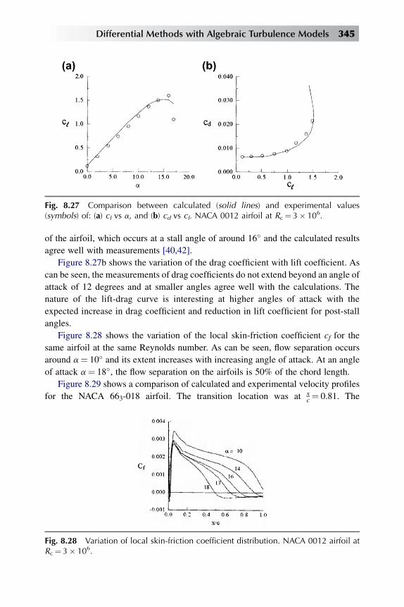
of the airfoil, which occurs at a stall angle of around 16� and the calculated results

agree well with measurements [40,42].

Figure 8.27b shows the variation of the drag coefficient with lift coefficient. As

can be seen, the measurements of drag coefficients do not extend beyond an angle of

attack of 12 degrees and at smaller angles agree well with the calculations. The

nature of the lift-drag curve is interesting at higher angles of attack with the

expected increase in drag coefficient and reduction in lift coefficient for post-stall

angles.

Figure 8.28 shows the variation of the local skin-friction coefficient cf for the

same airfoil at the same Reynolds number. As can be seen, flow separation occurs

around a¼ 10� and its extent increases with increasing angle of attack. At an angle

of attack a¼ 18�, the flow separation on the airfoils is 50% of the chord length.

Figure 8.29 shows a comparison of calculated and experimental velocity profiles

for the NACA 663-018 airfoil. The transition location was at xc¼ 0.81. The

Fig. 8.27 Comparison between calculated (solid lines) and experimental values(symbols) of: (a) cl vs a, and (b) cd vs cl. NACA 0012 airfoil at Rc¼ 3� 106.

Fig. 8.28 Variation of local skin-friction coefficient distribution. NACA 0012 airfoil atRc¼ 3� 106.


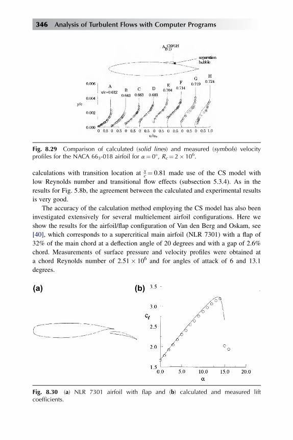
calculations with transition location at xc¼ 0.81 made use of the CS model with

low Reynolds number and transitional flow effects (subsection 5.3.4). As in the

results for Fig. 5.8b, the agreement between the calculated and experimental results

is very good.

The accuracy of the calculation method employing the CS model has also been

investigated extensively for several multielement airfoil configurations. Here we

show the results for the airfoil/flap configuration of Van den Berg and Oskam, see

[40], which corresponds to a supercritical main airfoil (NLR 7301) with a flap of

32% of the main chord at a deflection angle of 20 degrees and with a gap of 2.6%

chord. Measurements of surface pressure and velocity profiles were obtained at

a chord Reynolds number of 2.51� 106 and for angles of attack of 6 and 13.1

degrees.

Fig. 8.29 Comparison of calculated (solid lines) and measured (symbols) velocityprofiles for the NACA 663-018 airfoil for a¼ 0�, Rc¼ 2� 106.

Fig. 8.30 (a) NLR 7301 airfoil with flap and (b) calculated and measured liftcoefficients.


Figure 8.30b shows a comparison between calculated and measured lift coeffi-

cients. While some discrepancies exist at higher angles of attack, the stall is pre-

dicted accurately. It is believed that these discrepancies are due to the merging of the

airfoil shear layer with the boundary-layer on the upper surface of the flap which was

not considered in the calculation method described in [40].

8.11 Prediction of Three-Dimensional Flowswith Separation

The calculation method described in the previous section for airfoils and multiele-

ment airfoils has also been extended and evaluated for wing and multielement wings

as described in [40]. Here again we present results for one wing and two slat-wing-

flap configurations.

Figure 8.31a shows the lift coefficient variation with angle of attack for the RAE

wing tested by Lovell, see [40]. This wing has an airfoil section having a consider-

able rear loading with the maximum thickness of 11.7% occuring at 37.5% chord and

the maximum camber occuring at 75% chord. It has no twist nor dihedral, but has

a quarter-chord sweep angle of 28�, a taper ratio of 1/4 and an aspect ratio of 8.35.

The experiments were conducted at a test Reynolds number of 1.35� 106 with one

set of measurements corresponding to free transition and with another to fixed

transition for a freestream Mach number of 0.223. The wing has a semispan of 1.07

m and a mean aerodynamic chord of 0.26 m.

The calculations for this wing were performed with the Hess panel method [40]

and the inverse boundary-layer method of Cebeci [40] described in Section 8.8.

Initially, the calculations were done with angle of attack increments of 2� until 10�.

Fig. 8.31 (a) Effect of turbulence model on the lift coefficient of the RAE wing and (b)distribution of flow separation along the span at two angles of attack.


The increment in angle of attack is reduced to 1� beyond that point. Results show that

with the original CS turbulence model (see Section 5) the lift coefficient keeps

increasing past the measured stall angle (around 12� with free transition). With the

modified CS turbulence model, on the other hand, the agreement between measured

and calculated lift coefficient is excellent up to 14�. At 15�, the boundary layer

calculations did not converge near the trailing edge due to the large separated flow

region.

Figure 8.31b shows flow separation along the span at angles of attack, a¼ 13�

and 14�. As can be seen, there is a significant increase in the amount of flow

separation with one degree increase in a.

Figures 8.32 and 8.33 present results for the RAE slat-wing-flap configurations

with the slat deflected at 25�, and the flap deflected at 10� and 25�, respectively.Again, the inviscid lift coefficient is included to show how the introduction of the

viscous effects allows obtaining reasonable predictions of lift and drag coefficients.

The discrepancies may be due to the merging of shear layers which was not

accounted for. In addition, the large recirculating flow region in the slat cove – larger

at low angles of incidence – was removed with the fairing and may contribute to the

disagreement at low angles of attack.

Stall is not captured for the configurations tested. However, it is worthwhile to

note that, at the present time, the reliable prediction of stall for slat-wing-flap

configurations still offers significant challenges for two-dimensional flows. Unlike

for single element and wing-flap configurations, stall can occur without flow sepa-

ration on the body but may be due instead to a sudden increase of the wake thickness

thus reducing the circulation on the entire configuration. Therefore, the results of the

calculation method of [40] should be viewed as quite satisfactory.

Fig. 8.32 RAE wing with slat deflected at 25� and flap deflected at 10�, (a) wing cross-section, (b) lift coefficient, and (c) drag coefficient.


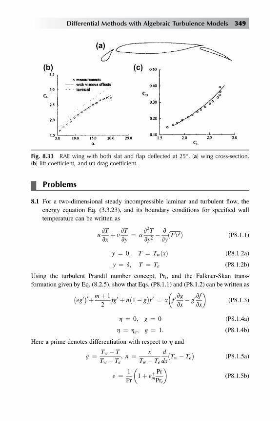
Problems

8.1 For a two-dimensional steady incompressible laminar and turbulent flow, the

energy equation Eq. (3.3.23), and its boundary conditions for specified wall

temperature can be written as

uvT

vxþ y

vT

vy¼ a

v2T

vy2� v

vyðT 0y0Þ (P8.1.1)

y ¼ 0; T ¼ TwðxÞ (P8.1.2a)

y ¼ d; T ¼ Te (P8.1.2b)

Using the turbulent Prandtl number concept, Prt, and the Falkner-Skan trans-

formation given by Eq. (8.2.5), show that Eqs. (P8.1.1) and (P8.1.2) can be written as�eg0�0þmþ 1

2fg0 þ n

�1� g

�f 0 ¼ x

�f 0vg

vx� g0

vf

vx

�(P8.1.3)

h ¼ 0; g ¼ 0 (P8.1.4a)

h ¼ he; g ¼ 1: (P8.1.4b)

Here a prime denotes differentiation with respect to h and

g ¼ Tw � T

Tw � Te; n ¼ x

Tw � Te

d

dx

�Tw � Te

�(P8.1.5a)

e ¼ 1

Pr

�1þ ε

þm

Pr

Prt

�(P8.1.5b)

Fig. 8.33 RAE wing with both slat and flap deflected at 25�, (a) wing cross-section,(b) lift coefficient, and (c) drag coefficient.


8.2 The calculation of convective heat transfer in boundary-layer flows requires

the solution of the continuity, momentum and energy equations. For two-

dimensional incompressible flows, this can be done by either solving Eqs.

(5.2.8), (5.2.9) and (P8.1.1) together or by first solving Eqs. (5.2.8) and

(5.2.9) and then Eq. (P8.1.1) since the energy equation is not coupled to

the momentum equation. Here we will consider the second choice for conve-

nience and seek the solution of the energy equation separately from the solu-

tion of the continuity and momentum equations which is already available.

Solve Eq. (P8.1.3) subject to the boundary conditions given by Eq. (P8.1.4).

Use the procedure similar to the momentum equation discussed in Section

8.2 and outlined below.

1. First reduce the system to first order by defining

g0 ¼ p (P8.2.1)

and using the same definitions of u, y for f 0 and f 00 in the momentum equation,

Eq. (8.2.6).

2. Write difference approximations for the two first-order equations and express

the first-order energy equation in the following form

ðs1Þjpj þ ðs2Þjpj�1 þ ðs3Þj�gj þ gj�1

�¼ ðr1Þj; 1 � j � J (P8.2.2)

3. Write the resulting system in the following form

(P8.2.3)

Note that there is no need for Newton’s method since the energy equation is linear.


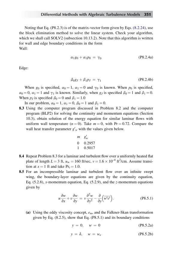
Noting that Eq. (P8.2.3) is of the matrix-vector form given by Eqs. (8.2.24), use

the block elimination method to solve the linear system. Check your algorithm,

which we shall call SOLV2 (subsection 10.13.2). Note that this algorithm is written

for wall and edge boundary conditions in the form

Wall:

a1g0 þ a1p0 ¼ g0 (P8.2.4a)

Edge:

b0gJ þ b1pJ ¼ g1 (P8.2.4b)

When g0 is specified, a0¼ 1, a1¼ 0 and g0 is known. When p0 is specified,

a0¼ 0, a1¼ 1 and g1 is known. Similarly, when gJ is specified b0¼ 1 and b1¼ 0.

When pJ is specified b0¼ 0 and b1¼ 1.0

In our problem, a0¼ 1, a1¼ 0, b0¼ 1 and b1¼ 0.

8.3 Using the computer program discussed in Problem 8.2 and the computer

program (BLP2) for solving the continuity and momentum equations (Section

10.3), obtain solution of the energy equation for similar laminar flows with

uniform wall temperature (n¼ 0). Take m¼ 0, with Pr¼ 0.72. Compare the

wall heat transfer parameter g0w with the values given below.

m g0w0 0:29571 0:5017

8.4 Repeat Problem 8.3 for a laminar and turbulent flow over a uniformly heated flat

plate of length L¼ 3 ft, uN¼ 160 ft/sec, v¼ 1.6� 10–4 ft2/cm. Assume transi-

tion at x¼ 1 ft and take Prt¼ 1.0.

8.5 For an incompressible laminar and turbulent flow over an infinite swept

wing, the boundary-layer equations are given by the continuity equation,

Eq. (5.2.8), x-momentum equation, Eq. (5.2.9), and the z-momentum equations

given by

uvw

vxþ y

vw

vy¼ v

v2w

vy2� v

vy

�w0y0

�: (P8.5.1)

(a) Using the eddy viscosity concept, εm, and the Falkner-Skan transformation

given by Eq. (8.2.5), show that Eq. (P8.5.1) and its boundary conditions

y ¼ 0; w ¼ 0 (P8.5.2a)

y ¼ d; w ¼ we (P8.5.2b)


can be written as �bg00�0þ mþ 1

2f 0g00 ¼ x

�f 0vg0

vx� g00

vf

vx

�(P8.5.3)

h ¼ 0; g0 ¼ 0 (P8.5.4a)

h ¼ he; g0 ¼ 1: (P8.5.4b)

Here a prime again denotes differentiation with respect to h and

b ¼ 1þ εþm ; g0 ¼ w

we(P8.5.5)

(b) Express the eddy-viscosity formulation given by Eqs. (5.7.4) for three-

dimensional flows in terms of Falkner-Skan variables.

8.6 Using the boundary-layer program BLP2 discussed in Section 10.3, develop

a new program to solve the infinite swept wing equations, which, in transformed

variables, are given by Eqs. (8.2.7), (P8.2.3) and (P8.2.4). Follow the steps below.

1. Reduce Eq. (P8.5.3) to second order by defining

g0 ¼ G

and to a system of two first order equations by defining

G0 ¼ P

Use the same definitions of u, y for f 0 and f 00 in the momentum equation,

Eq. (8.2.6).

2. Write difference approximations similar to the procedure used in

Problem 8.2.

3. Solve the resulting linear system with SOLV2.

8.7 As discussed in [1,41], for incompressible flows the external velocity distribu-

tion for an infinite swept wing can be obtained from a panel method for two-

dimensional flows. The streamwise external velocity ue/yN can be calculated

from

ueVN

¼�ueuN

�2D

cos l (P8.7.1a)

and the spanwise velocity we/yN from

we

VN¼ sin l (P8.7.1b)

Here l is the sweep angle and yN is the total velocity,

yN ¼ffiffiffiffiffiffiffiffiffiffiffiffiffiffiffiffiffiffiu2N þ w2

e

q(P8.7.2)


(a)Use

the panel method (HSPM) given in Section 10.4 and calculate ue/VN and ue/VNfor the upper surface of an infinite swept wing having the NACA 0012 airfoil

cross-section (given on the companion website: store.elsevier.com/companions/

9780080983356) and l¼ 30�, a¼ 0�.Note: The identification of upper and lower surface requires the location of the

airfoil stagnation point.

(b) Using the computer program discussed in Problem 8.4, obtain laminar flow

solutions up to flow separation for the external velocity given in (a).

8.8 Repeat Problem 8.7(b) for a laminar and turbulent flow with transition at

x/c¼ 0.20.

8.9 In some problems, it is desirable to start turbulent flow calculations by speci-

fying the initial velocity profiles. A convenient formula for this purpose is to

use Eq. (4.4.41) for yþ � 50 and Eq. (4.4.38) for yþ � 50.

In terms of the Falkner-Skan variables, Eq. (4.4.41) can be written as

f 0ffiffiffiffi2

cf

s¼

8>><>>:e1h h � 4

e1

c1 þ c2 ln�e1h�þ c3 ln ðe1hÞ2þc4ðe1hÞ3 4

e1� h � 50

e1

(P8.9.1)

where c1, c2, c3 and c4 are the coefficients of Eq. (P8.9.1) and

e1 ¼ ffiffiffiffiffiRx

p ffiffiffifficf2

r; Rx ¼ uex

v¼ RLuex; RL ¼ uNL

v(P8.9.2)

Similarly, for h � 50/e1, Eq. (4.4.38) can be written as

f 0ffiffiffiffi2

cf

s¼ 1

kln

e1h

!þ cþ 1

k

P

�1� cosp

h

he

�þ�h

he

�2

��h

he

�3(P8.9.3)

where

he ¼ ffiffiffiffiffiRx

p d

x(P8.9.4)

It is clear that a complete velocity profile for a turbulent boundary-layer can be

obtained from Eqs. (P8.9.1) and (P8.9.3) provided that the boundary-layer thickness

d and the profile parameterP are known. Since they are not known at first, they must

be calculated in a manner they are compatible with Rq and cf.

A convenient procedure is to assume dv (v¼ 0) and, calculateP from Eq. (4.4.38)

evaluated at the boundary-layer edge, h¼ he. The initial estimate of d is obtained

from the power-law relation, Eq. (7.2.10b), which for n¼ 7

q

dw 0:10


http://store.elsevier.com/companions/9780080983356


Here q is calculated from the specified value of Rq,

q ¼ v

ueRq (P8.9.5)

The next values of dv (v¼ 1, 2,.,n) are obtained from

dðvþ1Þ ¼ dðvÞ � f�dfdd

� (P8.9.6)

Where, with f1(h Rq/Rd) given by Eq. (4.4.39c) andwq denoting the momentum

thickness calculated from Eq. (P8.9.3),

f ¼ wq� df1 (P8.9.7a)

df

dd¼ �f1 � d

df1

dP

dP

dd(P8.9.7b)

and with

dP

dd¼ � 1

2d(P8.9.7c)

obtained by differentiating Eq. (4.4.40) with respect to d.

Using the computer program BLP2 (Section 10.3) and the subroutine IVPT, see

subsection 10.13.1, both given on the companion website: store.elsevier.com/

companions/9780080983356, we can perform turbulent flow calculations for

a given external velocity distribution with initial values of Rq and H given at x¼ x0.

(a) Compute turbulent flowonaflat plate of length 20 ft for aReynolds number per

foot, ue/v, equal to 106. Take uniform steps in x (Dx) equal to 1, with h1¼ 0.01,

k¼ 1.14, x0¼ 5 ft with Rq andH at x¼ x0 equal to 6000 and 1.4, respectively.

(b) Repeat (a) with Dx¼ 2 ft.

Note: Experience shows that the calculations which begin with velocity

profiles generated in this way show oscillations in wall shear for x-stations

greater than x0. A convenient procedure is to perform calculations, say

for the first two x-stations x1 and x2, then average the solutions in the

midpoint of x0 and x1, x12 , and x1 and x2, x1

12 and then average the solutions

x 12 and x1

12 at x1 to define a new solution and start the calculations at x¼ x2.

Another useful procedure which is effective in avoiding oscillations is the

use of first-order backward differences for the streamwise derivatives.

References

[1] T. Cebeci, J. Cousteix, Modeling and Computation of Boundary-Layer Flows, Horizons Publishing,

Long Beach, CA, and Springer-Verlag, Heidelberg, Germany, 1998.

[2] P. Bradshaw, T. Cebeci, J.H. Whitelaw, Engineering Calculation Methods for Turbulent Flows,

Academic Press, New York, NY, 1981.




[3] D. Coles, Measurements in the boundary layer on a smooth flat plate in supersonic flow. I. The

problem of the turbulent boundary layer. Rep. A20–69, Jet Propulsion Lab., California Inst.

Technol., Pasadena, CA, 1953.

[4] P.S. Klebanoff, Characteristics of turbulence in a boundary layer with zero pressure gradient, NACA

Tech. Note 3178 (1954).

[5] T. Cebeci, Application of exact turbulent boundary-layer equations as a means of calculating heat

and mass transfer in incompressible and compressible flows. Proc. Int. Heat Transfer Conf. 4th

vol. 2, Elsevier, Amsterdam, 1970.

[6] R.A. Seban, D.L. Doughty, Heat transfer to turbulent boundary layers with variable free-stream

velocity, J. heat Transfer 78 (1956) 217.

[7] W.C. Reynolds,W.M. Kays, S.J. Kline, Heat transfer in the turbulent incompressible boundary layer – II:

step wall-temperature distribution, NASAMemo 12-2-58W (1958).

[8] W.C.Reynolds,W.M.Kays, S.J.Kline,Heat transfer in the turbulent incompressible boundary layer – III:

arbitrary wall temperature and heat flux, NASAMemo 12-3-58W (1958).

[9] J. McQuaid, Experiments on incompressible turbulent boundary layers with distributed injection.

British ARC 28735, HMT 135. Also N69–21334 (1967).

[10] R.L. Simpson, Characteristics of turbulent layers at low Reynolds numbers with and without

transpiration, J. Fluid Mech. 42 (1970) 769.

[11] R.J. Moffat, W.M. Kays, The turbulent boundary layer on a porous plate: experimental heat transfer

with uniform blowing and suction, Int. J. Heat Mass Transfer 11 (1968) 1547.

[12] T. Cebeci, Behavior of turbulent flow near a porous wall with pressure gradient, AIAA J. 8 (1970)

2152.

[13] T. Cebeci, G.J. Mosinskis, Prediction of turbulent boundary layers with mass addition, including

accelerating flows, J. heat Transfer 93 (1971) 271.

[14] B.G. Newman, Some contributions to the study of the turbulent boundary layer near separation,

Austr. Dept. Supply Rep. ACA-53 (1951).

[15] T.E. Herring, J. Norbury, Some experiments on equilibrium turbulent boundary layers in favorable

pressure gradients, J. Fluid Mech. 27 (1967) 541.

[16] F.H. Clauser, Turbulent boundary layers in adverse pressure gradient, J. Aero. Sci. 21 (1954) 91.


Tech. Note No. 2133 (1950).

[18] P.M. Moretti, W.M. Kays, Heat transfer to a turbulent boundary layer with varying free-stream velocity

and varying surface temperature, an experimental study, Int. J. Heat Mass Transfer 8 (1965) 1187.

[19] R.L. Simpson, W.M. Kays, R.J. Moffat, The turbulent boundary layer on a porous plate: An

experimental study of the fluid dynamics with injection and suction. Rep. No. HMT-2, Stanford

Univ., Mech. Eng. Dept., Stanford, California, 1967.

[20] H.L. Julien, W.M. Kays, R.J. Moffat, The turbulent boundary layer on a porous plate: experimental

study of the effects of a favorable pressure gradient. Rep. No. HMT-4, Stanford Univ. Also

N69-34951, NASA-CR-104140, 1969.

[21] R. Richmond, Experimental investigation of thick axially symmetric boundary layers on cylinders at

subsonic and hypersonic speeds. Ph.D. Thesis, California Inst. Technol., Pasadena, California, 1957.

[22] T. Cebeci, Laminar and turbulent incompressible boundary layers on slender bodies of revolution in

axial flow, J. Basic Eng. 92 (1970) 545.

[23] T. Cebeci, Eddy viscosity distribution in thick axisymmetric turbulent boundary layers, J. Fluids

Eng. 95 (1973) 319.

[24] F.M. White, An analysis of axisymmetric turbulent flow past a long cylinder, J. Basic Eng. 94

(1972) 200.

[25] J.J. Cornish III, D.W. Boatwright, Application of full scale boundary layer measurements to drag

reduction of airships. Rep. No. 28, Aerophys. Dept. Mississippi State Univ., Jackson, Mississippi,

1960.


[26] J.S. Murphy, The separation of axially-symmetric turbulent boundary layers. Part I. Preliminary

experimental results on several bodies in incompressible flows. Rep. No. ES 17513, Douglas

Aircraft Co., Long Beach, CA. Also AD 432–666. Part II. Detailed measurements in the boundary

layers on several slender bodies in incompressible flow. Rep. No. ES 17513, Douglas Aircraft Co.,

Long Beach, CA., 1954. Also AD 432–491.

[27] T. Cebeci, Calculation of compressible turbulent boundary layers with heat andmass transfer, AIAA J.

9 (1971) 1091.

[28] D. Coles, Measurements in the boundary layer on a smooth flat plate in supersonic flow. III.

Measurements in a flat-plate boundary layer at the Jet Propulsion Lab. Rep. No. 20–71, Jet Pro-

pulsion Lab., California Inst. Technol., Pasadena, CA, 1953.

[29] F.W. Matting, D.R. Chapman, J.R. Nyholm, A.G. Thomas, Turbulent skin friction at high Mach

numbers and Reynolds numbers in air and helium. NASA TR R-82. Also N62–70506 (1961).

[30] D.R. Moore, J. Harkness, Experimental investigation of the compressible turbulent boundary layer

at very high Reynolds numbers. M¼ 2.8, Rep. No. 0.71000/4R-9, LTV Res. Center. Also

N64–29671 (1964).

[31] R. Michel, Resultants sur la couche limite turbulent aux grandes vitesses, Memo Tech 22 (1961).

Office Nat. d’Utudes et de Rech, Aeronaut.

[32] C.S. Pappas, Measurement of heat transfer in the turbulent boundary layer on a flat plate in

supersonic flow and comparison with skin-friction results, NACA Tech. Note No. 3222 (1954).

[33] L.C. Squire, Further experimental investigation of compressible turbulent boundary layers with an

injection. ARC R&M 3627. Also N71–15789 (1970).

[34] G.D. Thomas, V.K. Verma, L.C. Squire, A comparison of two prediction methods with experi-

ment for compressible turbulent boundary layers with air injection, Aeronaut. Quart. XXIII (4)

(1972) 301.

[35] L. Pasiuk, S.M. Hastings, R. Chatham, Experimental Reynolds analogy factor for a compressible

turbulent boundary layer with a pressure gradient. Naval Ordinance Rep. NOLTR 64–200, White

Oak, Maryland. Also AD610-663 (1965).

[36] K.G. Winter, L. Gaudet, Turbulent boundary-layer studies at high Reynolds numbers at Mach

numbers between 0.2 and 2.8. RAE Tech. Rep. 70251. Also AD890–133 (1970).

[37] J.C. LeBalleur, Couplage visqueux-non visqueux: methode numerique et applications aux ecoulements

bidimensionnels transsoniques et supersoniques, La Recherche Aerospatiale (March-April 1978).

[38] J. Carter, S.F. Wornom, Solutions for incompressible separated boundary layers including viscous-

inviscid interaction,AerodynamicAnalysisRequiringAdvancedComputers (1975) 125.NASASP-347.

[39] A.E.P. Veldman, A numerical method for the calculation of laminar incompressible boundary layers

with strong inviscid interaction, NLRTR 79023L (1979).

[40] T. Cebeci, An Engineering Approach to the Calculation of Aerodynamic Flows, Horizons

Publishing, Long Beach, CA, and Springer-Verlag, Heidelberg, Germany, 1999.

[41] T. Cebeci, K.C. Chang, Compressibility and Wake Effects on the Calculations of Flow over High

Lift Configuration, 48th Annual Conference, Canadian Aeronautics and Space Institute, Toronto,

Canada, April 2001.

[42] T. Cebeci, Turbulence Models and Their Application, Horizons Publishing, Long Beach, CA,

and Springer-Verlag, Heidelberg, Germany, 2003.

[43] C. Gleyzes, J. Cousteix, J.L. Bonnet, A calculation method of leading-edge separation bubbles,

in: T. Cebeci (Ed.), Numerical and Physical Aspects of Aerodynamic Flow, II, Springer-Verlag,

Heidelberg, Germany, 1984.

[44] J.C. LeBalleur, New possibilities of viscous-inviscid numerical techniques for solving viscous flow

equations with massive separation, in: T. Cebeci (Ed.), Numerical and Physical Aspects of Aero-

dynamic Flows, IV, Springer-Verlag, Heidelberg, Germany, 1990.


DifferentialMethods withTransport-EquationTurbulence Models

Chap

ter9



9.2 Zonal Method for k-ε Model 358

9.2.1 Turbulence Equations and Boundary Conditions 359

9.2.2 Solution Procedure 360

9.3 Solution of the k-ε Model Equations with and without Wall Functions 371

9.3.1 Solution of the k-ε Model Equations without Wall Functions 371

9.3.2 Solution of the k-ε Model Equations with Wall Functions 374

9.4 Solution of the k-u and SST Model Equations 375

9.5 Evaluation of Four Turbulence Models 378

9.5.1 Free-Shear Flows 379

9.5.2 Attached and Separated Turbulent Boundary Layers 384

9.5.3 Summary 389

9A Appendix: Coefficients of the Linearized Finite-Difference Equations

for the k-ε Model 392

Problems 397

References 407

357



http://dx.doi.org/10.1016/B978-0-08-098335-6.00009-4

9.1 Introduction

In Sections 9.2 and 9.3 we discuss the numerical solution of the boundary-layer

equations employing transport-equation turbulence models. There are several

models that can be used for this purpose, and there are several approaches that can

be pursued. For example, in one approach the solution of the k-ε model equations

can be obtained with and without the wall functions as discussed in subsection

6.2.1. In the case without wall functions, the usual boundary conditions are replaced

by boundary conditions specified at some distance y¼ y0. In the case with wall

functions, the boundary conditions are specified at y¼ 0. Another approach which

we shall refer to it as the zonal approach, the boundary-layer equations are solved in

two regions with each region employing different turbulence models. In effect this

approach may be regarded as the use of the k-ε model with wall functions. In

Section 9.2 we discuss the numerical solution of the k-ε model equations with this

zonal method; in Section 9.3, the numerical solution of the k-ε model equations

with and without wall functions; and in Section 9.4, the numerical solution of the k-

u and SST model equations.

In Section 9.5 we consider four turbulence models discussed in Sections 6.2

and 6.3 and evaluate their relative performance for free-shear flows and attached

and separated boundary-layers flows. In discussing the performance of these

transport-equation turbulence models, it would be more consistent with this book

to present results obtained from the solution of the boundary-layer equations.

However, such a study is yet to be conducted for a range of flows including

free-shear layer and wall boundary layers with and without separation. For this

reason, we present results obtained from the solution of the Navier-Stokes

equations.

9.2 Zonal Method for k-ε Model

In the zonal method considered here, the boundary-layer is divided into two

zones. The inner zone is identified by y � y0, yþ0 ¼ (y0us/n) z 100, where the

continuity and momentum equations, Eqs. (5.2.8) and (8.2.1), are solved subject

to the wall boundary conditions given by Eq. (8.2.2a), with eddy viscosity εm

given by the inner region of the CS model. In the outer zone, y> y0, the

continuity Eq. (5.2.8), momentum Eq. (8.2.1), turbulent kinetic energy

Eq. (6.2.7) and rate of dissipation Eq. (6.2.8) are solved subject to the inner

boundary condition given by Eqs. (6.2.13) and (6.2.14) and edge boundary

conditions given by Eqs. (6.2.16) and (6.2.18), with eddy viscosity εm computed

from Eq. (6.2.6).


The turbulence equations and boundary conditions for this zonal method are

provided in the following subsection; the finite-difference equations together with

Newton’s method are discussed in the subsequent subsection.

9.2.1 TURBULENCE EQUATIONS AND BOUNDARY CONDITIONS

As with the differential method with algebraic turbulence models, we again express

the turbulence equations in terms of transformed variables. The mean-flow equa-

tions remain the same as those considered in Chapter 8, namely, Eqs. (8.2.6)

and (8.2.7). The turbulent kinetic energy and rate of dissipation equations and

their boundary conditions are also expressed in transformed variables. With the

transformation

j ¼ ffiffiffiffiffiffiffiffiffiuenx

pf ; h ¼

ffiffiffiffiffiuenx

ry; ~k ¼ k

u2e; ~ε ¼ εx

u3e(9.2.1)

and with the definition of stream function, Eq. (8.2.3), they can be written as

�b2k

0�0þ m1fk0 þ ε

þm

�f 00�2� ε� 2mf 0k ¼ x

�f 0vk

vx� k0

vf

vx

�(9.2.2)

�b3ε

0�0þm1f ε0 þ Cε1 f1

ε

kεþmðf 00Þ2�Cε2 f2

ε2

k� �3m� 1

�f 0ε ¼ x

�f 0vε

vx� ε

0vfvx

�(9.2.3)

where the tilde has been dropped from the equations and

b2 ¼ 1þ εþm

sk; b2 ¼ 1þ ε

þm

sε; ε

þm ¼ εm

n; m1 ¼ mþ 1

2(9.2.4)

With the introduction of new variables

f 0 ¼ u; u0 ¼ y; k0 ¼ s; ε0 ¼ q (9.2.5)

Eqs. (8.2.6), (9.2.2) and (9.2.3) can be written as�b1y�0 þm1 f yþ m

�1� u2

� ¼ x

�uvu

vx� y

vf

vx

�(9.2.6)

�b2s�0þm1 fsþ ε

þmy

2 � ε� 2muk ¼ x

�uvk

vx� s

vf

vx

�(9.2.7)

�b3q�0þm1 fqþ Cε1 f1

ε

kεþmy

2 � Cε2 f2ε2

k� �3m� 1

�uε ¼ x

�uvε

vx� q

vf

vx

�(9.2.8)

Differential Methods with Transport-Equation Turbulence Models 359

These equations form a system of seven first-order differential equations with

seven dependent variables (f, u, y, k, s, ε, and q) for the outer zone and three for

the inner zone. The definitions, k0 ¼ 0, s0 ¼ 0, ε0 ¼ 0, and q0 ¼ 0, respectively,

replace the last two expressions in Eq. (9.2.5) and the equations (9.2.7) and (9.2.8)

in the solution algorithm to represent the equations for the inner zone, so there are

seven first-order equations from the wall to the edge of the boundary layer that

require solution subject to the seven boundary conditions given by Eqs. (8.2.2),

(6.2.14)–(6.2.16) and (6.2.18), which in terms of transformed variables can be

written as

h ¼ 0; f ¼ u ¼ 0 (9.2.9a)

h ¼ h0;�εþm

�CS

¼ Rx fmcmk2

ε

; ε ¼ �εþm

�CSy2 (9.2.9b)

h ¼ he; u ¼ 1:0; xvk

vxþ εþ 2m2k ¼ 0;

xvε

vxþ Cε2f2

ε2

kþ �3m� 1

�ε ¼ 0

(9.2.9c)

9.2.2 SOLUTION PROCEDURE

In general, differential methods for turbulent flows require the specification of initial

profiles at x¼ x0. With methods employing algebraic viscosity models, the initial

profiles correspond to streamwise u and normal y velocity profiles. However, when

the calculations are performed for both laminar and turbulent flows, as was discussed

in Chapter 8, the initial velocity profiles may be assumed to correspond to those at

the transition location. With methods employing transport-equation models, since

the calculations are for turbulent flows, it is often necessary to specify initial profiles,

which in the case of k-ε model, correspond not only to u and y profiles, but also to k,

εm and ε profiles.

Experience with the box method discussed in Chapter 8 has shown that when

profiles are used to start the turbulent flow calculations, the solutions at the

subsequent x-locations oscillate. A common cure to this problem is to compute

the first two x-stations equally spaced and take an average of the solutions at the

midpoint of x0 and x1, say xm and x1 and x2, say xe. Then another average of

the solutions is taken at xm and xe defining a new solution at x1. When new calcu-

lations begin at x2 with averaged profiles at x¼ x1, the solutions at x � x2 do not

exhibit oscillations.

While this cure is relatively easy to incorporate into a computer program and in

most cases provides stable solutions in adverse pressure gradient flows, sometimes


the solutions may breakdown due to oscillations. On the other hand, the author and

his colleagues observed that if one uses backward difference approximations for the

x-derivates in the boundary-layer equations, rather than central differences as used

in the box method, the solutions do not oscillate and are more stable. For this

reason, when the box method is used for turbulent flow calculations with initial

profiles, we will represent the x-derivates with backward finite difference

approximations.

As discussed in Section 6.2, the k-ε model equations without wall functions use

‘‘wall’’ boundary conditions specified at some distance y0 outside the viscous sub-

layer. The boundary conditions on u and y are usually represented by Eqs. (6.2.10)

and those for k and ε by Eqs. (6.2.13) and (6.2.14), although in the latter case, there

are other choices. In such cases, the friction velocity us appearing in u and y equa-

tions is unknown and must be determined as part of the solution. One approach is to

assume us, s0 (say from the initial profiles at the previous x-station), solve the

governing equations subject to the ‘‘wall’’ and edge boundary conditions. From the

solution determine s0 at y0,

s0 ¼ 9ðεmÞ0�vu

vy

�0

(9.2.10)

and compute us from Eq. (6.2.11). If the calculated value of us does not agree with

the estimated value within a specified tolerance parameter d1,��unþ1s � uns

�� < d1 (9.2.11)

then a new solution is obtained with the updated values of us and s0. This procedureis repeated until convergence.

This iterative procedure can be replaced with a more efficient one by treating usas an unknown. Since us is a function of x only, we can write

u0s ¼ 0 (9.2.12)

thus increasing the number of first-order equations from seven to eight. Although the

Aj, Bj, Cj matrices now become 8� 8, rather than 7� 7, this procedure does not

increase the storage much and allows the solutions to converge faster, especially for

flows with strong adverse pressure gradient.

In the solution procedure described here, the numerical method is formulated for

eight unknowns, not only for the k-εmodel equations with the zonal method but also

for the k-ε model equations with and without wall functions and with the zonal

method. This choice does not increase the complexity of the solution procedure, and

as we shall discuss in Chapter 10, it paves the way to solve the k-εmodel equations or

others in an inverse mode if the solution procedure is to be extended to flows with

separation (see Section 10.9).


Inner Region

The numerical solution of the k-ε model equations with the zonal method requires

that in the inner region Eq. (8.2.6) is solved subject to the true wall boundary

conditions f¼ 0, u¼ 0. Since, however, the solution procedure is being formulated

for the general case which includes the solution of the k-ε model equations without

wall functions, it is nescessary to specify a boundary condition for us. This can be

done as described below.

From the definition of us

�hue

ffiffiffifficf2

r �, we can write

usue

hw ¼ffiffiffifficf2

r(9.2.13a)

or in transformed variables,

w ¼ffiffiffiffiffif 00w

pR1=4x

(9.2.13b)

The boundary condition for w is

w0 ¼ffiffiffiffiffiy0

p

R1=4x

(9.2.14)

Next the eight first-order equations can be written by letting u0 ¼ n, k0 ¼ 0, s0 ¼ 0,

ε0 ¼ 0, w0 ¼ 0, q0 ¼ 0, f 0 ¼ u and the momentum equation (9.2.6). For j¼ 0, with the

first three equations corresponding to boundary conditions, the equations for the

inner region are ordered as

f0 ¼ 0 (9.2.15a)

u0 ¼ 0 (9.2.15b)

w0 ¼ffiffiffiffiffiy0

p

R1=4x

(9.2.15c)

u0 ¼ y (9.2.15d)

k0 ¼ 0 (9.2.15e)

s0 ¼ 0 (9.2.15f)

ε0 ¼ 0 (9.2.15g)

q0 ¼ 0 (9.2.15h)

With finite-difference approximations and linearization, they become

df0 ¼ ðr1Þ0 ¼ 0 (9.2.16a)

du0 ¼ ðr2Þ0 ¼ 0 (9.2.16b)


dy0 � 2ffiffiffiffiffiffiRx

pw0dw0 ¼ ðr3Þ0 ¼ ffiffiffiffiffiffi

Rx

pw20 � y0 (9.2.16c)


�dyj þ dyj�1

� ¼ ðr4Þj ¼ uj�1 � uj þ hjyj�1=2 (9.2.16d)

dkj � dkj�1 ¼ ðr5Þj ¼ 0 (9.2.16e)

dsj � dsj�1 ¼ ðr6Þj ¼ 0 (9.2.16f)

dεj � dεj�1 ¼ ðr7Þj ¼ 0 (9.2.16g)

dqj � dqj�1 ¼ ðr8Þj ¼ 0 (9.2.16h)

For 1 � j � js, the order of the equations is the same as those above except that the

first three equations are replaced by

w0 ¼ 0 (9.2.17a)

f 0 ¼ u (9.2.17b)

momentum Eq:ð9:2:6Þ (9.2.17c)

In linearized form they can be written as

dwj � dwj�1 ¼ ðr1Þj ¼ 0 (9.2.18a)


�duj þ duj�1

� ¼ ðr2Þj ¼ fj�1 � fj þ hjuj�1=2 (9.2.18b)

ðs1Þjdfj þ ðs2Þjdfj�1 þ ðs3Þjduj þ ðs4Þjduj�1 þ ðs5Þjdyj þ ðs6Þjdyj�1 ¼ ðr3Þj(9.2.18c)

The finite-difference procedure for Eq. (9.2.6) is identical to the procedure

described in subsection 8.2.1. The only difference occurs in the solution of

Eq. (9.2.6) where we use three-point or two-point backward finite-difference

formulas for the x-wise derivatives rather than central differences as we did in

subsection 8.2.1. For this purpose, for any variable V, the derivative of vVvx is

defined by �vV

vx

�n

¼ A1Vn�2 þ A2V

n�1 þ A3Vn (9.2.19)

where for first-order

A1 ¼ 0; A2 ¼ � 1

xn � xn�1; A3 ¼ � 1

xn � xn�1(9.2.20)


and second-order

A1 ¼ ðxn � xn�1Þðxn�2 � xn�1Þ ðxn�2 � xnÞ

A2 ¼ ðxn � xn�2Þðxn�1 � xn�2Þ ðxn�1 � xnÞ

A3 ¼ 2xn � xn�1 � xn�2

ðxn � xn�2Þ ðxn � xn�1Þ

(9.2.21)

Representing the x-derivatives in Eq. (9.2.6) with either two-point or three-point

backward difference approximations at x¼ xn and using central differences in the

h-direction, we can write Eq. (9.2.6) as

h�1j

hðbyÞnj � ðbyÞnj�1

iþ mn

1ðf yÞnj�1=2 þ mnh1� �u2�n

j�1=2

i¼ 1

2xn�v

vx

�u2�n

j�1=2

� xn

2

��yvf

vx

�n

j

þ�yvf

vx

�n

j�1

(9.2.22)

Linearizing we get

h�1j

bnj dyj � bnj�1dyj�1

�þmn

1

2

�f nj dyj þ ynj dfj þ f nj�1dyj�1 þ ynj�1dfj�1

��mn

�ujduj þ uj�1duj�1

�¼ xn

4

�v

vu

�vu2

vx

�n

j

duj þ v

vu

�vu2

vx

�n

j�1

duj�1

� xn

2

��vf

vx

�n

j

dyj þ ynjv

vf

�vf

vx

�n

j

dfj þ�vf

vx

�n

j�1

dyj�1

þynj�1

v

vf

�vf

vx

�n

j�1

dfj�1

(9.2.23)

From Eq. (9.2.19), it follows that

v

vu

�vu2

vx

�n

j

¼ 2A3unj ;

v

vu

�vu2

vx

�n

j�1

¼ 2A3unj�1

v

vf

�vf

vx

�n

j

¼ A3;v

vf

�vf

vx

�n

j�1

¼ A3

(9.2.24)


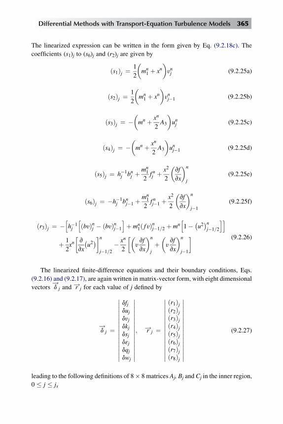
The linearized expression can be written in the form given by Eq. (9.2.18c). The

coefficients (s1)j to (s6)j and (r2)j are given by

ðs1Þj ¼1

2

�mn1 þ xn

�ynj (9.2.25a)

ðs2Þj ¼1

2

�mn1 þ xn

�ynj�1 (9.2.25b)

ðs3Þj ¼ ��mn þ xn

2A3

�unj (9.2.25c)

ðs4Þj ¼ ��mn þ xn

2A3

�unj�1 (9.2.25d)

ðs5Þj ¼ h�1j bnj þ

mn1

2f nj þ x2

2

�vf

vx

�n

j

(9.2.25e)

ðs6Þj ¼ �h�1j bnj�1 þ

mn1

2f nj�1 þ

x2

2

�vf

vx

�n

j�1

(9.2.25f)

ðr3Þj ¼ �hh�1j

hðbyÞnj � ðbyÞnj�1

iþ mn

1ð f yÞnj�1=2 þ mnh1� �u2�n

j�1=2

iiþ 1

2xn�v

vx

�u2�n

j�1=2

� xn

2

��yvf

vx

�n

j

þ�yvf

vx

�n

j�1

(9.2.26)

The linearized finite-difference equations and their boundary conditions, Eqs.

(9.2.16) and (9.2.17), are again written in matrix-vector form, with eight dimensional

vectors d!

j and r!j for each value of j defined by

d!

j ¼

��

dfjdujdyjdkjdsjdεjdqjdwj

��; r!j ¼

��

ðr1Þjðr2Þjðr3Þjðr4Þjðr5Þjðr6Þjðr7Þjðr8Þj

��(9.2.27)

leading to the following definitions of 8� 8 matrices Aj, Bj and Cj in the inner region,

0 � j � js


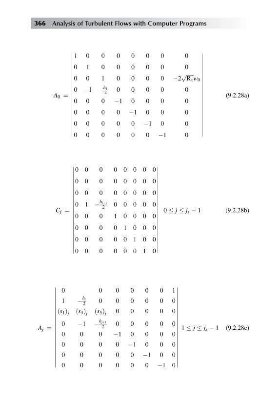
A0 ¼ j 1 0 0 0 0 0 0 0

0 1 0 0 0 0 0 0

0 0 1 0 0 0 0 �2ffiffiffiffiffiffiRx

pw0

0 �1 �h12 0 0 0 0 0

0 0 0 �1 0 0 0 0

0 0 0 0 �1 0 0 0

0 0 0 0 0 �1 0 0

0 0 0 0 0 0 �1 0

j (9.2.28a)

Cj ¼ j 0 0 0 0 0 0 0 0

0 0 0 0 0 0 0 0

0 0 0 0 0 0 0 0

0 1 �hjþ1

2 0 0 0 0 0

0 0 0 1 0 0 0 0

0 0 0 0 1 0 0 0

0 0 0 0 0 1 0 0

0 0 0 0 0 0 1 0

j 0 � j � js � 1 (9.2.28b)

Aj ¼ j 0 0 0 0 0 0 1

1 �hj2 0 0 0 0 0 0

ðs1Þj ðs3Þj ðs5Þj 0 0 0 0 0

0 �1 �hjþ1

2 0 0 0 0 0

0 0 0 �1 0 0 0 0

0 0 0 0 �1 0 0 0

0 0 0 0 0 �1 0 0

0 0 0 0 0 0 �1 0

j 1 � j � js � 1 (9.2.28c)


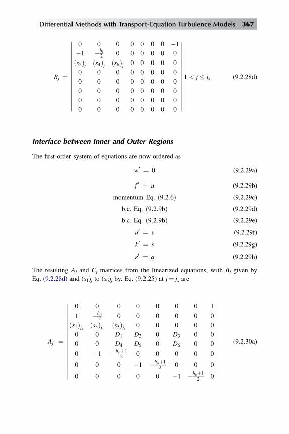
Bj ¼ j 0 0 0 0 0 0 0 �1

�1 �hj2 0 0 0 0 0 0

ðs2Þj ðs4Þj ðs6Þj 0 0 0 0 0

0 0 0 0 0 0 0 0

0 0 0 0 0 0 0 0

0 0 0 0 0 0 0 0

0 0 0 0 0 0 0 0

0 0 0 0 0 0 0 0

j 1 < j � js (9.2.28d)

Interface between Inner and Outer Regions

The first-order system of equations are now ordered as

w0 ¼ 0 (9.2.29a)

f 0 ¼ u (9.2.29b)

momentum Eq: ð9:2:6Þ (9.2.29c)

b:c: Eq: ð9:2:9bÞ (9.2.29d)

b:c: Eq: ð9:2:9bÞ (9.2.29e)

u0 ¼ y (9.2.29f)

k0 ¼ s (9.2.29g)

ε0 ¼ q (9.2.29h)

The resulting Aj and Cj matrices from the linearized equations, with Bj given by

Eq. (9.2.28d) and (s1)j to (s6)j by. Eq. (9.2.25) at j¼ js are

Ajs ¼ j 0 0 0 0 0 0 0 1

1 �hjs2 0 0 0 0 0 0

ðs1Þjs ðs3Þjs ðs5Þjs 0 0 0 0 0

0 0 D1 D2 0 D3 0 0

0 0 D4 D5 0 D6 0 0

0 �1 �hjsþ12 0 0 0 0 0

0 0 0 �1 �hjsþ12 0 0 0

0 0 0 0 0 �1 �hjsþ12 0

j (9.2.30a)


Cjs ¼ j 0 0 0 0 0 0 0 00 0 0 0 0 0 0 00 0 0 0 0 0 0 00 0 0 0 0 0 0 00 0 0 0 0 0 0 00 1 �hjsþ1

2 0 0 0 0 0

0 0 0 1 �hjsþ12 0 0 0

0 0 0 0 0 1 �hjsþ12 0

j (9.2.30b)

Here the fourth and fifth rows of Ajs follow from the boundary conditions, Eq.

(9.2.9b), at h¼ h0. After the application of Newton’s method to the finite-difference

form of these equations, D1 to D6 are given by the following expressions.

D1 ¼ εjs

v

vy

�εþm

�CS; D2 ¼ �2Rxcmkjs ; D3 ¼ �

εþm

�CS

(9.2.31a)

D4 ¼ 2Rxcmk2jsyjs ; D5 ¼ �2Rxcmkjsy

2js; D6 ¼ �2εjs (9.2.31b)

The associated (r4)js and (r5)js are

ðr4Þjs ¼ Rxcmk2js� �εþm�CSεjs (9.2.32a)

ðr5Þjs ¼ ε2js� Rxcm

�kjsyjs

�2(9.2.32b)

Outer Region

The finite-difference approximations for the outer region defined for js þ 1 �j � J are written by using a similar procedure described for the inner region

equations. The system of first-order equations are arranged similar to those given by

Eqs. (9.2.29) except that Eqs. (9.2.29d) and (9.2.29e) are replaced by Eqs. (9.2.7) and

(9.2.8). The resulting matrices from the linearized equations, with Cj matrix

remaining the same as that given by Eq. (9.2.30b) for js< j � J – 1, are

Bj ¼ j 0 0 0 0 0 0 0 �1

�1 �hj2 0 0 0 0 0 0

ðs2Þj ðs4Þj ðs6Þj ðs8Þj 0 ðs12Þj 0 0

ða2Þj ða4Þj ða6Þj ða8Þj ða10Þj ða12Þj 0 0

ðb2Þj ðb4Þj ðb6Þj ðb8Þj 0 ðb12Þj ðb14Þj 0

0 0 0 0 0 0 0 0

0 0 0 0 0 0 0 0

0 0 0 0 0 0 0 0

j js þ 1 < j � J

(9.2.33a)


Aj ¼ j 0 0 0 0 0 0 0 1

1 �hj2 0 0 0 0 0 0

ðs1Þj ðs3Þj ðs5Þj ðs7Þj 0 ðs11Þj 0 0

ða1Þj ða3Þj ða5Þj ða7Þj ða9Þj ða11Þj 0 0

ðb1Þj ðb3Þj ðb5Þj ðb7Þj 0 ðb11Þj ðb13Þj 0

0 �1 �hjþ1

2 0 0 0 0 0

0 0 0 �1 �hjþ1

2 0 0 0

0 0 0 0 0 �1 �hjþ1

2 0

j js þ 1 < j � J � 1

(9.2.33b)

AJ ¼ j 0 0 0 0 0 0 0 1

1 �hJ2 0 0 0 0 0 0

ðs1ÞJ ðs3ÞJ ðs5ÞJ ðs7ÞJ 0 ðs11ÞJ 0 0

ða1ÞJ ða3ÞJ ða5ÞJ ða7ÞJ ða9ÞJ ða11ÞJ 0 0

ðb1ÞJ ðb3ÞJ ðb5ÞJ ðb7ÞJ 0 ðb11ÞJ ðb13ÞJ 0

0 1 0 0 0 0 0 0

0 0 0 E1 0 E2 0 0

0 0 0 E3 0 E4 0 0

j (9.2.33c)

Here (s1)j to (s12)j, (a1)j, to (a12)j and (b1)j to (b14)j given in Appendix 9A correspond

to the coefficients of the linearized momentum (9.2.6), kinetic energy of turbulence

(9.2.7), and rate of dissipation (9.2.8) equations written in the following forms,

respectively,

ðs1Þjdfj þ ðs2Þjdfj�1 þ ðs3Þjduj þ ðs4Þjduj�1 þ ðs5Þjdyjþðs6Þjdyj�1 þ ðs7Þjdkj þ ðs8Þjdkj�1 þ ðs11Þjdεjþðs12Þjdεj�1 ¼ ðr3Þj

(9.2.34)

ða1Þjdfj þ ða2Þjdfj�1 þ ða3Þjduj þ ða4Þjduj�1 þ ða5Þjdyjþða6Þjdyj�1 þ ða7Þjdkj þ ða8Þjdkj�1 þ ða9Þjdsjþða10Þjdsj�1 þ ða11Þjdεj þ ða12Þjdεj�1 ¼ ðr4Þj

(9.2.35)


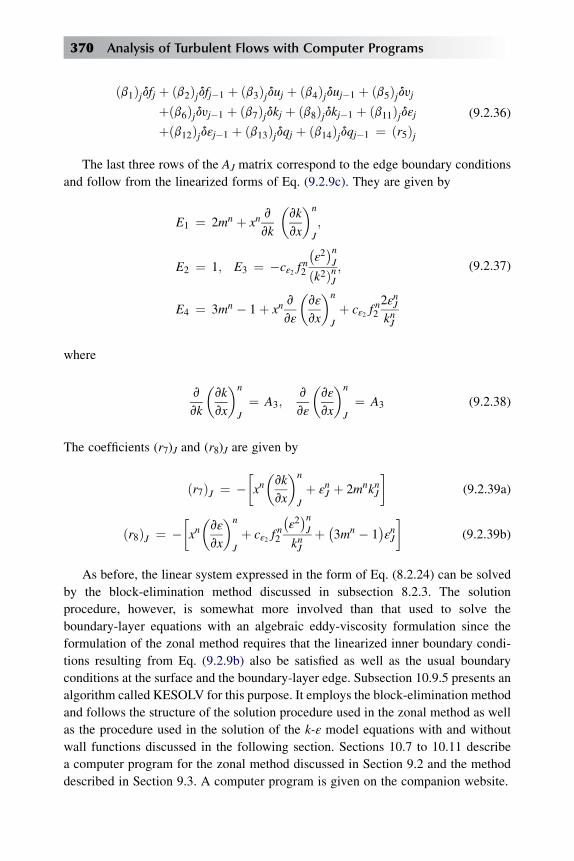
ðb1Þjdfj þ ðb2Þjdfj�1 þ ðb3Þjduj þ ðb4Þjduj�1 þ ðb5Þjdyjþðb6Þjdyj�1 þ ðb7Þjdkj þ ðb8Þjdkj�1 þ ðb11Þjdεjþðb12Þjdεj�1 þ ðb13Þjdqj þ ðb14Þjdqj�1 ¼ ðr5Þj

(9.2.36)

The last three rows of the AJ matrix correspond to the edge boundary conditions

and follow from the linearized forms of Eq. (9.2.9c). They are given by

E1 ¼ 2mn þ xnv

vk

�vk

vx

�n

J

;

E2 ¼ 1; E3 ¼ �cε2 fn2

�ε2�nJ

ðk2ÞnJ;

E4 ¼ 3mn � 1þ xnv

vε

�vε

vx

�n

J

þ cε2 fn2

2εnJknJ

(9.2.37)

where

v

vk

�vk

vx

�n

J

¼ A3;v

vε

�vε

vx

�n

J

¼ A3 (9.2.38)

The coefficients (r7)J and (r8)J are given by

ðr7ÞJ ¼ ��xn�vk

vx

�n

J

þ εnJ þ 2mnknJ

(9.2.39a)

ðr8ÞJ ¼ ��xn�vε

vx

�n

J

þ cε2 fn2

�ε2�nJ

knJþ �3mn � 1

�εnJ

(9.2.39b)

As before, the linear system expressed in the form of Eq. (8.2.24) can be solved

by the block-elimination method discussed in subsection 8.2.3. The solution

procedure, however, is somewhat more involved than that used to solve the

boundary-layer equations with an algebraic eddy-viscosity formulation since the

formulation of the zonal method requires that the linearized inner boundary condi-

tions resulting from Eq. (9.2.9b) also be satisfied as well as the usual boundary

conditions at the surface and the boundary-layer edge. Subsection 10.9.5 presents an

algorithm called KESOLV for this purpose. It employs the block-elimination method

and follows the structure of the solution procedure used in the zonal method as well

as the procedure used in the solution of the k-ε model equations with and without

wall functions discussed in the following section. Sections 10.7 to 10.11 describe

a computer program for the zonal method discussed in Section 9.2 and the method

described in Section 9.3. A computer program is given on the companion website.


9.3 Solution of the k-ε Model Equations withand without Wall Functions

The solution of the k-ε model equations with and without wall functions is similar

to the solution of the k-ε model equations with the zonal method. Their solution

with either one can be accomplished with minor changes to the solution algorithm

described in the previous section. In both cases changes are made to the Ajs matrix,

Eq. (9.2.30a), by modifying or redefining the elements of the first five rows which

in this case correspond to the boundary conditions at y¼ y0 or y¼ 0. In either case,

for j¼ 0, after the five boundary conditions are specified, the next three equations

correspond to those given by Eqs. (9.2.29f) to (9.2.29h). For j � 1, the ordering of

the first-order equations is identical to that used for the outer region, that is, the

equations are ordered according to those given by Eqs. (9.2.29) except that

Eqs. (9.2.29d) and (9.2.29e) are replaced by Eqs. (9.2.7) and (9.2.8), respectively.

In addition of course, the coefficients of the momentum, kinetic energy and rate of

dissipation are different.

9.3.1 SOLUTION OF THE k-ε MODEL EQUATIONS WITHOUT WALL FUNCTIONS

The k-ε model equations without wall functions given by Eqs. (6.2.7) and (6.2.8) for

high Reynolds number together with the continuity and momentum equations are

subject to the four boundary conditions given by Eqs. (6.2.10), (6.2.13) and (6.2.15)

at y¼ y0 and to those at the edge, h¼ d, given by Eqs. (6.2.16) and (6.2.18) together

with the relation given by Eq. (6.2.12). To discuss the solution procedure in terms of

transformed variables, let us consider first the two boundary conditions at h¼ h0. In

terms of transformed variables, Eqs. (6.2.10) become

f00 ¼ w0

�1

kln� ffiffiffiffiffiffi

Rx

pw0h0

�þ c

(9.3.1a)

xvf0vx

þ m1 f0 ¼ f 0h�m1 þ x

w0

dw0

dx

(9.3.1b)

where

Rx ¼ uex

n; c ¼ 5:2; k ¼ 0:41; m1 ¼ mþ 1

2(9.3.2)

with f 0 ¼ u, us/ue¼w0, Eqs. (9.3.1) in linearized form can be written as

du0 þ a8dw0 ¼ ðr1Þ0 (9.3.3)

b1df0 þ b2du0 þ b8dw0 ¼ ðr2Þ0 (9.3.4)


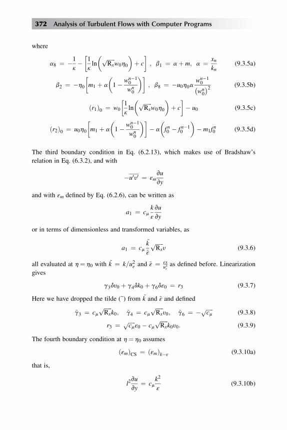
where

a8 ¼ �1

k��1

kln

� ffiffiffiffiffiffiRx

pw0h0

�þ c

; b1 ¼ aþ m; a ¼ xn

kn(9.3.5a)

b2 ¼ �h0

�m1 þ a

�1� wn�1

0

wn0

�; b8 ¼ �u0h0a

wn�10�wn0

�2 (9.3.5b)

ðr1Þ0 ¼ w0

�1

kln


pw0h0

�þ c

� u0 (9.3.5c)

ðr2Þ0 ¼ u0h0

�m1 þ a

�1� wn�1

0

wn0

�� a

�f n0 � f n�1

0

�� m1f

n0 (9.3.5d)

The third boundary condition in Eq. (6.2.13), which makes use of Bradshaw’s

relation in Eq. (6.3.2), and with

�u0y0 ¼ εmvu

vy

and with εm defined by Eq. (6.2.6), can be written as

a1 ¼ cmk

ε

vu

vy

or in terms of dimensionless and transformed variables, as

a1 ¼ cm~k

~ε


py (9.3.6)

all evaluated at h¼ h0 with ~k ¼ k=u2e and ~ε ¼ εxu3eas defined before. Linearization

gives

g3dy0 þ g4dk0 þ g6dε0 ¼ r3 (9.3.7)

Here we have dropped the tilde (~) from ~k and ~ε and defined

~g3 ¼ cmffiffiffiffiffiffiRx

pk0; ~g4 ¼ cm


py0; ~g6 ¼ � ffiffiffiffiffi

cmp

(9.3.8)

r3 ¼ ffiffiffiffifficm

pε0 � cm


pk0y0: (9.3.9)

The fourth boundary condition at h¼ h0 assumes

ðεmÞCS ¼ ðεmÞk�ε(9.3.10a)

that is,

l2vu

vy¼ cm

k2

ε

(9.3.10b)


In terms of dimensionless quantities and transformed variables, in linearized form,

Eq. (9.3.10b) can be written as

q3dy0 þ q4dk0 þ q6dε0 ¼ r4 (9.3.11)

where

q3 ¼ �cyε0; q4 ¼ 2cmffiffiffiffiffiffiRx

pk0; q6 ¼ �cyy0; (9.3.12)

cy ¼ ðkh$dampingÞ2; r4 ¼ cyy0ε0 � cmffiffiffiffiffiffiRx

pk20 (9.3.13)

If y0 is sufficiently away from the wall, i.e. y0þ � 60, then the damping term, such as

the one used in the CS model, is equal to 1.0.

The fifth boundary condition which connects s0 at y¼ y0 and sw at y¼ 0, is

obtained from Eq. (6.2.12). With Thompson’s and log law velocity profiles, it can be

written as

s0 ¼ sw þ a*y0dswdx

þ y0dp

dx(9.3.14)

Here a* is given by

a* ¼ 0:5

�c1ln

�yþ0�2þc2 ln y

þ0 þ c3 þ c4

yþ0

(9.3.15)

where

c1 ¼ 5:9488; c2 ¼ 13:4682; c3 ¼ 13:5718; c4 ¼ �785:20

yþ0 ¼ ffiffiffiffiffiffiRx

push0; y0 ¼ xh0ffiffiffiffiffiffi

Rxp (9.3.16)

In terms of transformed variables, Eq. (9.3.14), after linearization, can be expressed

in the form

d3dy0 þ d4dk0 þ d6dε0 þ d8dw0 ¼ ðr5Þ0 (9.3.17)

where

d3 ¼ cmRxk20ε0

(9.3.18a)

d4 ¼ 2cmRxk0ε0

y0 (9.3.18b)

d6 ¼ �cmRxk20ε20

y0 (9.3.18c)


d8 ¼ �2w0


p þ a*h0�aþ 2m1

� � va*

vw

!0

(a

"�wn0

�2��wn�10

�2#þ 2m1

�wn0

�2) (9.3.18d)

and

ðr5Þ0 ¼ ffiffiffiffiffiffiRx

pw2 þ a*h0

nah�wn0

�2��wn�10

�2iþ 2m1

�wn0

�2o�h0m2 � cmRx

k20ε0

y20

(9.3.19)

With the five boundary conditions defined, the Ajs matrix, which is essentially the

A0 matrix in this case, becomes

A0 ¼ j 0 1 0 0 0 0 0 a8b1 b2 0 0 0 0 0 b80 0 g3 g4 0 g6 0 00 0 q3 q4 0 q6 0 00 0 d3 d4 0 d6 0 d80 �1 �h1

2 0 0 0 0 0

0 0 0 �1 �h12 0 0 0

0 0 0 0 0 �1 �h12 0

j (9.3.20)

9.3.2 SOLUTION OF THE k-ε MODEL EQUATIONS WITH WALL FUNCTIONS

The solution of the k-ε model equations with wall functions is similar to the

procedure described for the case without wall functions. Again the only changes

occur in the first five rows of the Ajs matrix, Eq. (9.2.30a). Of the five boundary

conditions at the wall, the first three are written in the order given by Eqs.

(9.2.15a,b,c) and the fourth and fifth ones are given by

k0 ¼ 0 (9.3.21a)

ε0 ¼ 0 (9.3.21b)

or in linearized form

dk0 ¼ ðr4Þ0 ¼ 0 (9.3.22a)

dε0 ¼ ðr5Þ0 ¼ 0 (9.3.22b)


The structure of the other matrices remain the same, but of course, the coefficients of

the linearized momentum, kinetic energy and dissipation equations, Eqs. (9.2.34),

(9.2.35) and (9.2.36), respectively are different than those for k-ε model equations

without wall functions. These coefficients naturally vary depending on the wall

functions used.

The A0 matrix for the k-εmodel equations with wall functions, with the last three

rows identical to those in Eq. (9.3.20), is

A0 ¼ j 1 0 0 0 0 0 0 0

0 1 0 0 0 0 0 0

0 0 1 0 0 0 0 �2ffiffiffiffiffiffiRx

pu0

0 0 0 1 0 0 0 0

0 0 0 0 0 1 0 0

0 �1 �h12 0 0 0 0 0

0 0 0 �1 �h12 0 0 0

0 0 0 0 0 �1 �h12 0

j (9.3.23)

In some model equations, the boundary conditions on ε¼ 0 is replaced by vεvy ¼ 0;

in that case, the fifth row of A0-matrix becomes

0 0 0 0 0 0 1 0 (9.3.24)

9.4 Solution of the k-u and SST Model Equations

The solution of the k-u model equations is similar to the solution of the k-ε model

equations with wall functions. Again the k-umodel equations, Eqs. (6.2.19), (6.2.23)

and (6.2.28), are expressed in terms of Falkner-Skan variables.

Since the SST model equations make use of the k-ε model equations in the inner

region and the k-ε model equations in the outer region we express them, for the sake

of compactness, in the following form in transformed variables.

��1þ skε

þm

�k0�0�2mf 0k þ m1fk

0 þ εþmðf 00Þ2�b*uk ¼ x

�f 0vk

vx� k0

vf

vx

�(9.4.1)


��1þ suε

þm

�u0�0þ2ð1� F1Þsu2

Rx

uk0u0 þ m1u

0f � ðm� 1Þf 0u

�bu2 þ Rxðf 00Þ2¼ x

�f 0vu

vx� u0vf

vx

� (9.4.2)

where u and k are dimensions, normalized by x/ue and 1=u2e , respectively. Equations

(9.4.1) and (9.4.2) are the equations used in the SST model. To recover Wilcox’s k-u

model equations expressed in transformed variables, we let F1¼ 1 and take

sk ¼ 0:5; su ¼ 0:5; b ¼ 0:075;

b* ¼ 0:09; k ¼ 0:41; g ¼ b

b*� su

k2ffiffiffiffiffib*

q (9.4.3)

In the SST model, the above constants are determined from the relation, Eq. (6.2.45)

f ¼ F1f1 þ ð1� F1Þf2 (6.2.45)

where the constant f1 is determined from Eq. (6.2.46) and the constant f2 from

Eq. (6.2.47). F1 is determined from Eq. (6.2.41), where its arg1 given by Eq. (6.2.42)

can be written us

arg1 ¼ min½maxðl1; l2Þ; l3� (9.4.4)

In terms of transformed quantities, l1 to l3 are

l1 ¼ffiffiffik

p

0:09uy¼

ffiffiffik

p

uh


p0:09

(9.4.5a)

l2 ¼ 500n

y2u¼ 500

h2u(9.4.5b)

l3 ¼ 49su2k

CDcuy2(9.4.5c)

CDcu ¼ max

�29su2

1

u

vk

vy

vu

vy; 10�20

�¼ 2k

max

�1

uk0u0; 10�20

�h2

Wefirst find themaximumof l1 and l2 (say l4), then calculate theminimumof l4 and l3and thus determine arg1 andF1. OnceF1 is calculated, then the constants in Eqs. (9.4.1)

and (9.4.2) are determined from the relation given by Eq. (6.2.45). For example,

su ¼ 0:5F1 þ 0:856ð1� F1Þb� 0:0750F1 þ 0:0828ð1� F1Þetc:


Next we determine the eddy viscosity distribution across the boundary layer. In

terms of transformed variables, Eq. (6.2.36) can be written as ðy ¼ f 00: a1 ¼ 0:31Þ

εþm ¼ εm

n�

8>>><>>>:Rx

k

ua1u > UF2ffiffiffiffiffiffi

Rxp

a1k

jyjF2a1u < UF2

(9.4.6)

where

U ¼��vuvy�� ¼ uejf 00j

ffiffiffiffiffiuenx

r

and F2 is determined from Eq. (6.2.37a) where arg2 is

arg2 ¼ maxð2l1; l2Þ (9.4.7)

In the SST model, once the constants are determined and the distribution of eddy

viscosity is calculated, then Eqs. (9.4.1) and (9.4.2) are solved together with the

continuity and momentum equations; a new arg1, arg2, F1 and F2, new constants and

eddy viscosity distribution are determined. This procedure is repeated until

convergence.

It should be noted that, for F1¼ 1, the whole region is the inner region governed

by the k-u model equations.When F1¼ 0, the whole region is governed by the k-ε

model equations.

Before we discuss the solution procedure for the SST model equations, it is useful

to point out that the structure of the solution algorithm for the k-ε model equations

with wall functions is almost identical to the one for the SST model equations. This

means all the Aj, Bj, Cj matrices have the same structure; the difference occurs in the

definitions of the coefficients of the linearized momentum, kinetic energy and rate-

of-dissipation equations and in the definition of the boundary condition for u which

occurs in the fourth row of A0-matrix.

To describe the numerical method for the k-u model equations, we start with the

kinetic energy equation, Eq. (9.4.1), and write it in the same form as Eq. (9.4.2) by

defining Q and F by

Q ¼ b*uk; F ¼ 0 (9.4.8)

The definition of P remains the same. Next we write Eq. (9.4.2) in the form

ðb3u0Þ0þP1 � Q1 þ E ¼ x

�f 0vu

vx� u0 vf

vx

�þ ðm� 1Þf 0u� m1u

0f (9.4.9)


where

E ¼ 2ð1� F1Þsu2

Rx

uk0u0 (9.4.10)

Q1 ¼ bu2

P1 ¼ gRxðf 00Þ2

With

u0 ¼ q

Equation (9.4.9) can be written as

ðb3qÞ0þP1 � Q1 þ E ¼ x

�uvu

vx� q

vf

vx

�þ ðm� 1Þuu� m1q f (9.4.11)

A comparison of Eq. (9.4.11) with Eq. (9A.10) shows that if we let ε¼u for notation

purposes, then the coefficients of linearized specific dissipation rate equation are

very similar to those given by Eqs. (9A.14a) and (9A.15a). Except for the definitions

of Q and F in the kinetic energy-equation, Eq. (9.4.1), the coefficients of the line-

arized kinetic energy equation are identical to those given by Eqs. (9A.7) and (9A.8).

Appropriate changes then can be easily made to subroutine KECOEF (see Section

11.9) in order to adopt the computer program of Sections 11.7 to 11.10 to solve the

kinetic energy and specific dissipation rate kinetic energy equations in the SST

model. Of course, other changes also should be made, but these are not discussed

here. A good understanding of the computer program for the k-ε model equations is

needed to make the necessary changes.

9.5 Evaluation of Four Turbulence Models

In Sections 8.3 to 8.6 and 8.9, 8.10 we discussed the evaluation of the CSmodel with

a differential method based on the solution of the boundary-layer equations. In this

section we present a similar discussion for transport-equation turbulence models

with a differential method based on the solution of the Navier-Stokes equations. The

discussion is based on the study conducted in [2] where Bardina et al. evaluated the

performance of four higher-order turbulence models. The models were: 1) the k-u

model of Wilcox (subsection 6.2.2), 2) k-εmodel of Launder and Sharma (subsection

6.2.1), 3) the SST model of Menter (subsection 6.2.3) and 4) the SA model

(subsection 6.3.2). The flows investigated were five free shear flows and five

boundary-layer flows consisting of an incompressible and compressible flat plate,

a separated boundary layer, an axisymmetric shock-wave/boundary-layer interac-

tion, and an RAE 2822 transonic airfoil.


In this section we present a sample of results for some of these flows obtained

from this study and discuss a summary of the conclusions regarding the relative

performance of the various models tested. For additional results and discussion, the

reader is referred to [2].

9.5.1 FREE-SHEAR FLOWS

Five free-shear flows corresponding to a mixing layer, plane jet, round jet, plane

wake and a compressible mixing layer were considered in [2], and four eddy

viscosity models were validated for the prediction of these flows. The validation of

each model was mainly based on the ability of the models to predict the mean

velocity profile and spreading rate of each one of these fully developed free-shear

flows. Sensitivity analyses, the validation results to freestream turbulence, grid

resolution and initial profiles were also included in their study. Here, however, we

only present the mean velocity profiles and spreading rate of each flow.

Mixing Layer

Figure 9.1 shows a comparison of the predictions of the mean velocity profile u/u1against h¼ y/x and the experimental data of Liepmann and Laufer [3] for a half jet.

See also Fig. 7.20. The dimensionless coordinate h was defined with its origin

located where the mean velocity ratio was 1/2.

According to the calculations in [2], the results of the k-ε and SST models are

insensitive to freestream turbulence and show good agreement in the middle of the

mixing zone and sharp edge profiles at the boundaries. The small difference between

the predictions of these two models near the edge of the freestream at rest is due to

the different value of their diffusion model constant, sε. The results of the SA model

Fig. 9.1 Predictions of four turbulence models for the mixing layer of Liepmannand Laufer, after [3].


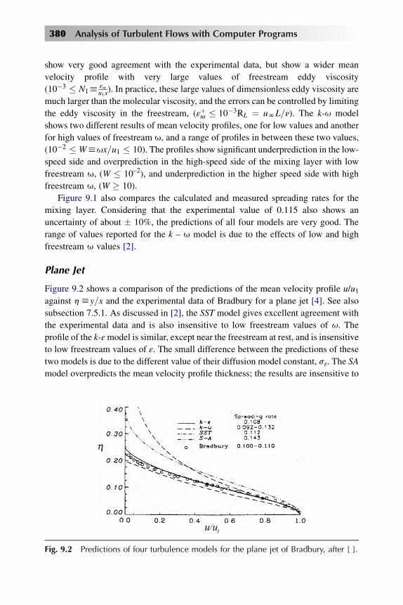
show very good agreement with the experimental data, but show a wider mean

velocity profile with very large values of freestream eddy viscosity

(10�3 � N1hεm

u1x). In practice, these large values of dimensionless eddy viscosity are

much larger than the molecular viscosity, and the errors can be controlled by limiting

the eddy viscosity in the freestream, (εþm � 10�3RL ¼ uNL=n). The k-u model

shows two different results of mean velocity profiles, one for low values and another

for high values of freestream u, and a range of profiles in between these two values,

(10�2 � Whux=u1 � 10). The profiles show significant underprediction in the low-

speed side and overprediction in the high-speed side of the mixing layer with low

freestream u, (W � 10–2), and underprediction in the higher speed side with high

freestream u, (W � 10).

Figure 9.1 also compares the calculated and measured spreading rates for the

mixing layer. Considering that the experimental value of 0.115 also shows an

uncertainty of about � 10%, the predictions of all four models are very good. The

range of values reported for the k – u model is due to the effects of low and high

freestream u values [2].

Plane Jet

Figure 9.2 shows a comparison of the predictions of the mean velocity profile u/u1against hhy=x and the experimental data of Bradbury for a plane jet [4]. See also

subsection 7.5.1. As discussed in [2], the SST model gives excellent agreement with

the experimental data and is also insensitive to low freestream values of u. The

profile of the k-εmodel is similar, except near the freestream at rest, and is insensitive

to low freestream values of ε. The small difference between the predictions of these

two models is due to the different value of their diffusion model constant, sε. The SA

model overpredicts the mean velocity profile thickness; the results are insensitive to

Fig. 9.2 Predictions of four turbulence models for the plane jet of Bradbury, after [ ].


freestream eddy viscosity for Nhεm=u1x � 10�3. Results with larger freestream

eddy viscosities give much larger overpredictions and are not shown in Fig. 9.2. In

practice, these errors can be controlled by limiting the values of the eddy viscosity in

the freestream, εþm � 10�3RL. The results of the k-u model show two predictions;

one largely overpredicts and the other underpredicts the thickness of the mean

velocity profile, corresponding to low and high freestreamW h uxu1values, (W� 10–4

and W � 103), respectively. This model gives a set of intermediate solutions (not

shown in Fig. 9.2) depending on the values of freestream u, (10–4 � W � 103).

Figure 9.2 also compares the calculated and measured spreading rates for the

plane jet. The range of experimental values is reported between 0.10 and 0.11 and is

given only as reference values.

The k-ε and the SST models give close predictions of the experimental spreading

rate, while the SA model overpredicts the spreading rate. The k-u model predicts

a range of values due to the effects of low and high freestream u.

Round Jet

Figure 9.3 shows the comparison of the predictions of the mean velocity profile u/u1against h - y/x and the experimental data of Wygnanski and Fiedler [7]. As discussed

in [2], all models overpredict the thickness of the experimental mean velocity profile.

This classical anomaly is well known in these models that have been fine-tuned with

empirical data of mixing layer, plane jet, and/or far wake experiments.

The results of the k-ε and SST models are closer to the experimental data and are

also insensitive to low freestream values of ε or u, respectively. The small difference

between the predictions of these two models near the edge of the freestream is also

due to the different value of their diffusion model constant, sε. The SA model gives

Fig. 9.3 Prediction of four turbulence models for the round jet of Wygnanski andFiedler, after [2].


a considerably larger overprediction of the mean velocity profile thickness, and the

results are insensitive to freestream eddy viscosity for Nhεm=u1 x � 10�3. Results

with larger freestream eddy viscosities give much larger overpredictions and are not

shown in Fig. 9.3. In practice, these large values of dimensionless eddy viscosity are

much larger than the molecular viscosity, and the errors can be controlled by limiting

the eddy viscosity in the freestream εþm � 10�3RL. The results of the k-umodel show

two overpredictions of the thickness of the mean velocity profile, corresponding to

low and high freestream Whux=u1 values, (W � 10–4 and W � 104), and a set of

intermediate solutions (not shown in Fig. 9.3) depending on the values of freestream

u, (10–4 � W � 104) [2].

The spreading rate is defined as the value of the nondimensional jet radius,

S¼ y/(x – x0), where the mean speed is half its centerline value. This definition of

spreading rate is one of several formulations that have been proposed. The spreading

rate provides an estimate of the thickness of the round jet and is widely used in

turbulence modeling. However, it is only one parameter and it does not provide

information about the shape of the velocity profile.

Figure 9.3 also compares the spreading rates obtained with the turbulence models

and the recommended experimental value. The range of experimental values is

between 0.086 and 0.095. All models overpredict the spreading rate. The range of

values reported for the k-u model is due to the effects of low and high freestream

u values.

Plane Wake

Figure 9.4 shows a comparison of the predictions of the mean velocity profiles u�umin

ue�umin

against the dimensionless coordinate h ¼ yð9uN=mxÞ1=2 compared with the

Fig. 9.4 Predictions of four turbulence models for the plane wake of Fage and Falkner,after [2].


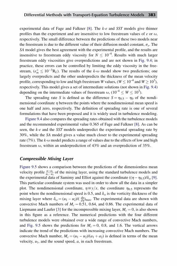
experimental data of Fage and Falkner [8]. The k-ε and SST models give thinner

profiles than the experiment and are insensitive to low freestream values of ε or u,

respectively. The small difference between the predictions of these two models near

the freestream is due to the different value of their diffusion model constant, sε. The

SA model gives the best agreement with the experimental profile, and the results are

insensitive to freestream eddy viscosity for N � 10–4. Results with much larger

freestream eddy viscosities give overpredictions and are not shown in Fig. 9.4; in

practice, these errors can be controlled by limiting the eddy viscosity in the free-

stream, (εþm � 10�3RL). The results of the k-u model show two predictions; one

largely overpredicts and the other underpredicts the thickness of the mean velocity

profile, corresponding to low and high freestreamW values, (W� 10–4 andW� 103),

respectively. This model gives a set of intermediate solutions (not shown in Fig. 9.4)

depending on the intermediate values of freestream u, (10–4 � W � 103).

The spreading rate S is defined as the difference S¼ h0.5 – h0 of the nondi-

mensional coordinate h between the points where the nondimensional mean speed is

one half and zero, respectively. The definition of spreading rate is one of several

formulations that have been proposed and it is widely used in turbulence modeling.

Figure 9.4 also compares the spreading rates obtained with the turbulence models

and the recommended experimental value 0.365 of Fage and Falkner [8]. As can be

seen, the k-ε and the SST models underpredict the experimental spreading rate by

30%, while the SA model gives a value much closer to the experimental spreading

rate (7%). The k-umodel predicts a range of values due to the effects of low and high

freestream u, within an underprediction of 43% and an overprediction of 35%.

Compressible Mixing Layer

Figure 9.5 shows a comparison between the predictions of the dimensionless mean

velocity profile u�u2u1�u2

of the mixing layer, using the standard turbulence models and

the experimental data of Samimy and Elliot against the coordinate ((h – h0.5)/du [9].

This particular coordinate system was used in order to show all the data in a simpler

plot. The nondimensional coordinate, hhy=x; the coordinate h0.5 represents the

point where the nondimensional speed is 0.5, and du is the vorticity thickness of the

mixing layer where du¼ (u1 – u2)/(dudh)max. The experimental data are shown with

convective Mach numbers of Mc¼ 0.51, 0.64, and 0.86. The experimental data of

Liepmann and Laufer [3] for the incompressible mixing layer,Mc¼ 0, is also shown

in this figure as a reference. The numerical predictions with the four different

turbulence models were obtained over a wide range of convective Mach numbers,

and Fig. 9.5 shows the predictions for Mc¼ 0, 0.8, and 1.6. The vertical arrows

indicate the trend of the predictions with increasing convective Mach numbers. The

convective Mach number, Mc¼ (u1 – u2)/(a1þ a2) is defined in terms of the mean

velocity, u1, and the sound speed, a, in each freestream.


All velocity profiles show some degree of agreement with the experimental data

due to the particular coordinate system of the plot. These plot coordinates bound the

range and collapse all data at the midpoint. The results of the k-ε and SST models

show good agreement with the nondimensional shape of the experimental profile.

The results of the SA model also show good agreement with the experimental data,

except for very high freestream eddy viscosity. The mean velocity profiles of the k-u

model show sensitivity to low freestream u values. The relative good agreement of

prediction with data is due to the use of du in the nondimensional plots. The

dimensional profiles and spreading rates show a much stronger dependence on Mach

number, as discussed in detail in [2].

Figure 9.6 shows a comparison of spreading rates predicted with the four

turbulence models with no compressibility corrections and the experimental Langley

data [10]. Here the spreading rate S is defined as dd/dx where d(x) is the thickness of

the mixing layer. The predicted results are shown with lines and the experimental

data are shown with symbols. The most significant result is that all models fail to

predict the experimental data on the decrease of spreading rate with increasing

convective Mach number. This is a well-known weakness of present turbulence

models. For additional details, see [2].

9.5.2 ATTACHED AND SEPARATED TURBULENT BOUNDARY LAYERS

Studies in [2] for attached and separated turbulent boundary layers included the flow

over an adiabatic flat plate of an incompressible flow and a compressible flow at

Mach 5, an adverse pressure gradient flow on an axisymmetric cylinder, a shock/

boundary layer flow on an axisymmetric bump, and a transonic flow on the RAE

2822 airfoil. A brief description of the performance of the four turbulence models for

Fig. 9.5 Comparison of velocity profiles for compressible mixing layer, after [2].


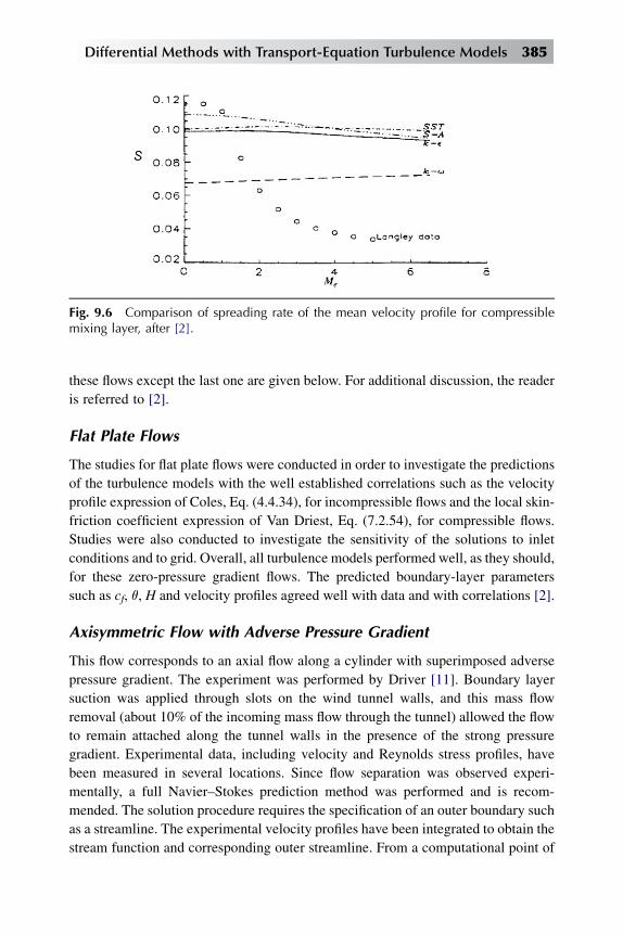
these flows except the last one are given below. For additional discussion, the reader

is referred to [2].

Flat Plate Flows

The studies for flat plate flows were conducted in order to investigate the predictions

of the turbulence models with the well established correlations such as the velocity

profile expression of Coles, Eq. (4.4.34), for incompressible flows and the local skin-

friction coefficient expression of Van Driest, Eq. (7.2.54), for compressible flows.

Studies were also conducted to investigate the sensitivity of the solutions to inlet

conditions and to grid. Overall, all turbulence models performed well, as they should,

for these zero-pressure gradient flows. The predicted boundary-layer parameters

such as cf, q, H and velocity profiles agreed well with data and with correlations [2].

Axisymmetric Flow with Adverse Pressure Gradient

This flow corresponds to an axial flow along a cylinder with superimposed adverse

pressure gradient. The experiment was performed by Driver [11]. Boundary layer

suction was applied through slots on the wind tunnel walls, and this mass flow

removal (about 10% of the incoming mass flow through the tunnel) allowed the flow

to remain attached along the tunnel walls in the presence of the strong pressure

gradient. Experimental data, including velocity and Reynolds stress profiles, have

been measured in several locations. Since flow separation was observed experi-

mentally, a full Navier–Stokes prediction method was performed and is recom-

mended. The solution procedure requires the specification of an outer boundary such

as a streamline. The experimental velocity profiles have been integrated to obtain the

stream function and corresponding outer streamline. From a computational point of

Fig. 9.6 Comparison of spreading rate of the mean velocity profile for compressiblemixing layer, after [2].


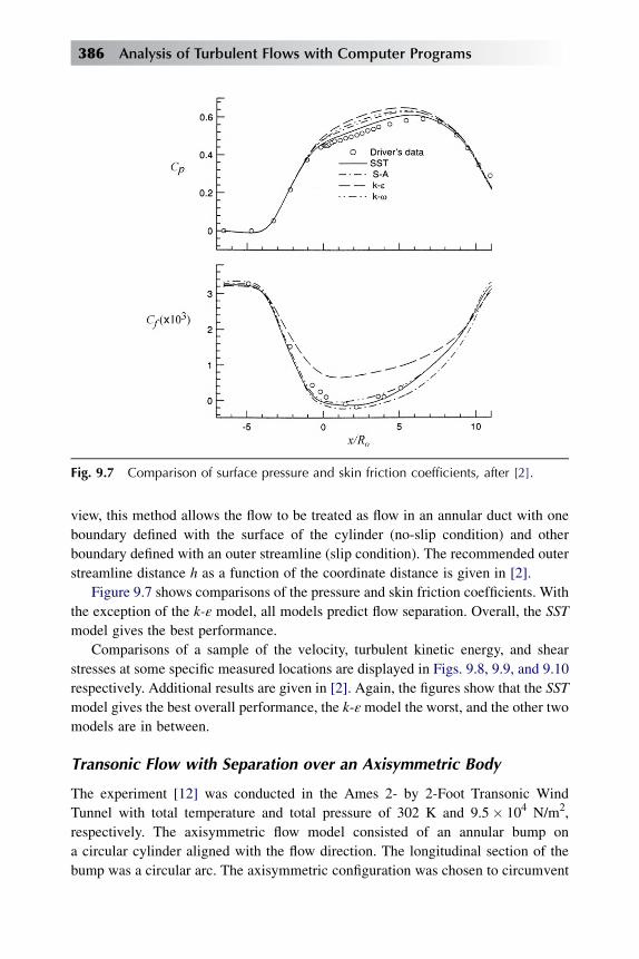
view, this method allows the flow to be treated as flow in an annular duct with one

boundary defined with the surface of the cylinder (no-slip condition) and other

boundary defined with an outer streamline (slip condition). The recommended outer

streamline distance h as a function of the coordinate distance is given in [2].

Figure 9.7 shows comparisons of the pressure and skin friction coefficients. With

the exception of the k-ε model, all models predict flow separation. Overall, the SST

model gives the best performance.

Comparisons of a sample of the velocity, turbulent kinetic energy, and shear

stresses at some specific measured locations are displayed in Figs. 9.8, 9.9, and 9.10

respectively. Additional results are given in [2]. Again, the figures show that the SST

model gives the best overall performance, the k-εmodel the worst, and the other two

models are in between.

Transonic Flow with Separation over an Axisymmetric Body

The experiment [12] was conducted in the Ames 2- by 2-Foot Transonic Wind

Tunnel with total temperature and total pressure of 302 K and 9.5� 104 N/m2,

respectively. The axisymmetric flow model consisted of an annular bump on

a circular cylinder aligned with the flow direction. The longitudinal section of the

bump was a circular arc. The axisymmetric configuration was chosen to circumvent

Fig. 9.7 Comparison of surface pressure and skin friction coefficients, after [2].


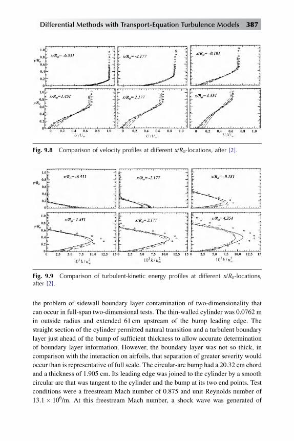
the problem of sidewall boundary layer contamination of two-dimensionality that

can occur in full-span two-dimensional tests. The thin-walled cylinder was 0.0762 m

in outside radius and extended 61 cm upstream of the bump leading edge. The

straight section of the cylinder permitted natural transition and a turbulent boundary

layer just ahead of the bump of sufficient thickness to allow accurate determination

of boundary layer information. However, the boundary layer was not so thick, in

comparison with the interaction on airfoils, that separation of greater severity would

occur than is representative of full scale. The circular-arc bump had a 20.32 cm chord

and a thickness of 1.905 cm. Its leading edge was joined to the cylinder by a smooth

circular arc that was tangent to the cylinder and the bump at its two end points. Test

conditions were a freestream Mach number of 0.875 and unit Reynolds number of

13.1� 106/m. At this freestream Mach number, a shock wave was generated of

Fig. 9.8 Comparison of velocity profiles at different x/R0-locations, after [2].

Fig. 9.9 Comparison of turbulent-kinetic energy profiles at different x/R0-locations,after [2].


sufficient strength to produce a relatively large region of separated flow. The sepa-

ration and reattachment points were at approximately 0.7 and 1.1 chords, respec-

tively. Boundary layer measurements were obtained by the laser velocimeter

technique from upstream of separation through reattachment. These data consist of

profiles of mean velocities, turbulence intensities, and shear stresses in the stream-

wise and normal direction. Separation and reattachment locations were determined

from oil-flow visualizations, and local surface static pressures were obtained with

conventional pressure instrumentation.

Figure 9.11 shows a comparison of the pressure coefficients along the surface of

the axisymmetric ‘‘bump.’’ Both k-ε and k-u models predict a delay of the shock

position and, therefore, underpredict the size of the flow separation. The SST model

provides the best overall performance, and the SA model comes second.

Fig. 9.10 Comparison of shear-stress profiles at different x/R0-locations, after [2].

Fig. 9.11 Comparison of surface pressure coefficient, after [2].


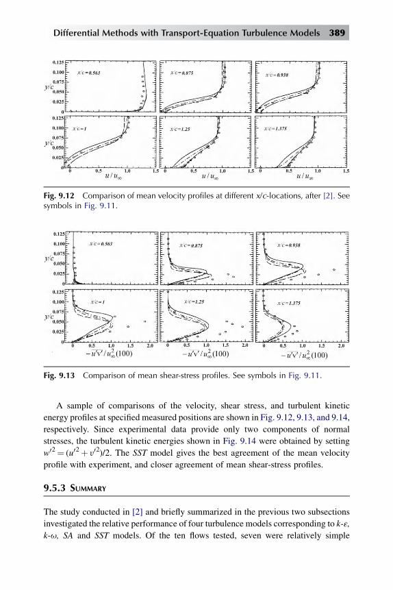
A sample of comparisons of the velocity, shear stress, and turbulent kinetic

energy profiles at specified measured positions are shown in Fig. 9.12, 9.13, and 9.14,

respectively. Since experimental data provide only two components of normal

stresses, the turbulent kinetic energies shown in Fig. 9.14 were obtained by setting

w02¼ (u02þ y02)/2. The SST model gives the best agreement of the mean velocity

profile with experiment, and closer agreement of mean shear-stress profiles.

9.5.3 SUMMARY

The study conducted in [2] and briefly summarized in the previous two subsections

investigated the relative performance of four turbulence models corresponding to k-ε,

k-u, SA and SST models. Of the ten flows tested, seven were relatively simple

Fig. 9.12 Comparison of mean velocity profiles at different x/c-locations, after [2]. Seesymbols in Fig. 9.11.

Fig. 9.13 Comparison of mean shear-stress profiles. See symbols in Fig. 9.11.


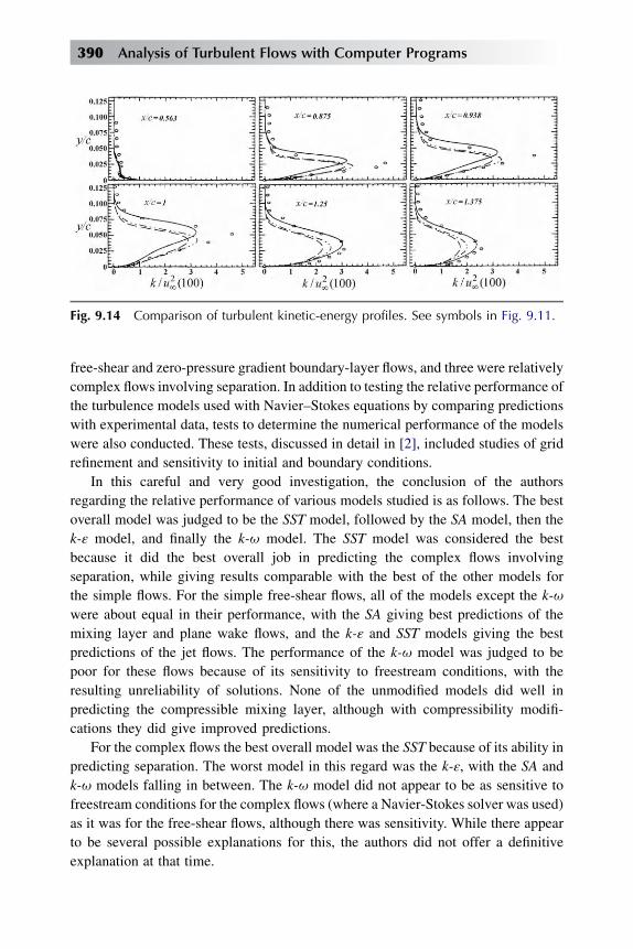
free-shear and zero-pressure gradient boundary-layer flows, and three were relatively

complex flows involving separation. In addition to testing the relative performance of

the turbulence models used with Navier–Stokes equations by comparing predictions

with experimental data, tests to determine the numerical performance of the models

were also conducted. These tests, discussed in detail in [2], included studies of grid

refinement and sensitivity to initial and boundary conditions.

In this careful and very good investigation, the conclusion of the authors

regarding the relative performance of various models studied is as follows. The best

overall model was judged to be the SST model, followed by the SA model, then the

k-ε model, and finally the k-u model. The SST model was considered the best

because it did the best overall job in predicting the complex flows involving

separation, while giving results comparable with the best of the other models for

the simple flows. For the simple free-shear flows, all of the models except the k-u

were about equal in their performance, with the SA giving best predictions of the

mixing layer and plane wake flows, and the k-ε and SST models giving the best

predictions of the jet flows. The performance of the k-u model was judged to be

poor for these flows because of its sensitivity to freestream conditions, with the

resulting unreliability of solutions. None of the unmodified models did well in

predicting the compressible mixing layer, although with compressibility modifi-

cations they did give improved predictions.

For the complex flows the best overall model was the SST because of its ability in

predicting separation. The worst model in this regard was the k-ε, with the SA and

k-u models falling in between. The k-u model did not appear to be as sensitive to

freestream conditions for the complex flows (where a Navier-Stokes solver was used)

as it was for the free-shear flows, although there was sensitivity. While there appear

to be several possible explanations for this, the authors did not offer a definitive

explanation at that time.

Fig. 9.14 Comparison of turbulent kinetic-energy profiles. See symbols in Fig. 9.11.


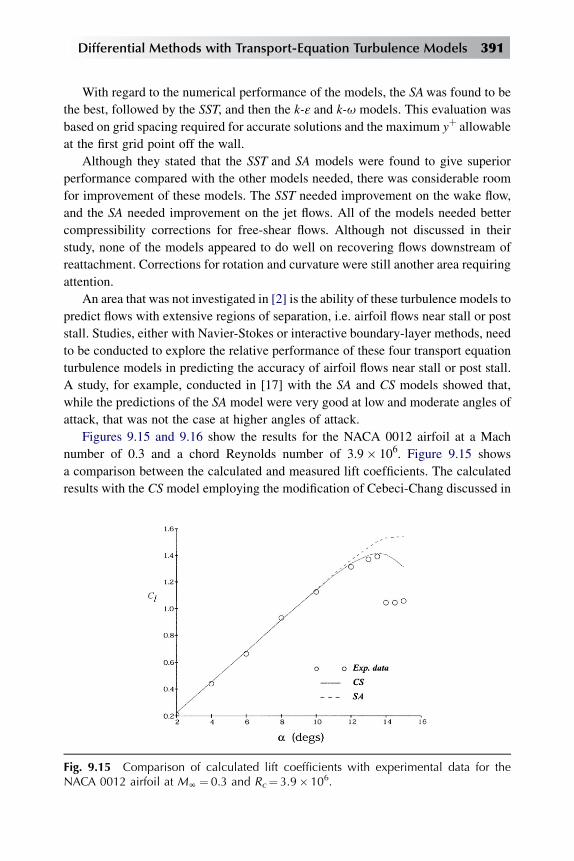
With regard to the numerical performance of the models, the SAwas found to be

the best, followed by the SST, and then the k-ε and k-u models. This evaluation was

based on grid spacing required for accurate solutions and the maximum yþ allowable

at the first grid point off the wall.

Although they stated that the SST and SA models were found to give superior

performance compared with the other models needed, there was considerable room

for improvement of these models. The SST needed improvement on the wake flow,

and the SA needed improvement on the jet flows. All of the models needed better

compressibility corrections for free-shear flows. Although not discussed in their

study, none of the models appeared to do well on recovering flows downstream of

reattachment. Corrections for rotation and curvature were still another area requiring

attention.

An area that was not investigated in [2] is the ability of these turbulence models to

predict flows with extensive regions of separation, i.e. airfoil flows near stall or post

stall. Studies, either with Navier-Stokes or interactive boundary-layer methods, need

to be conducted to explore the relative performance of these four transport equation

turbulence models in predicting the accuracy of airfoil flows near stall or post stall.

A study, for example, conducted in [17] with the SA and CS models showed that,

while the predictions of the SA model were very good at low and moderate angles of

attack, that was not the case at higher angles of attack.

Figures 9.15 and 9.16 show the results for the NACA 0012 airfoil at a Mach

number of 0.3 and a chord Reynolds number of 3.9� 106. Figure 9.15 shows

a comparison between the calculated and measured lift coefficients. The calculated

results with the CS model employing the modification of Cebeci-Chang discussed in

Fig. 9.15 Comparison of calculated lift coefficients with experimental data for theNACA 0012 airfoil at MN¼ 0.3 and Rc¼ 3.9� 106.


subsection 5.4.2 indicate good agreement with data. The predictions of the SAmodel,

while satisfactory at low and moderate angles of attack, are not satisfactory near and

post stall. They resemble those obtained with the CS model with a in Eq. (5.4.14) as

constant equal to 0.0168.

Figure 9.16 shows flow separation calculated with both turbulence models at

a¼ 13.5�, which is near the stall angle. As can be seen, while the CS model predicts

separation at xc ¼ 0:80, the SA model predicts it at x

c ¼ 0:90. Less flow separation

predictedwith the latter model is the reasonwhy the calculated lift coefficient is higher

than the experimental data. The reason for thismay be the ability of the SAmodel not to

decrease the law of thewall region in the presence of strong adverse pressure gradient.

For example, for a zero-pressure gradient flow, a constant value of a (h 0.0168) in

Eq. (5.4.14), predicts roughly 20% inner region and 80% outer region. A variable

a allows the inner region to decrease in the presence of a strong pressure gradient.

For additional comparisons between the CS and SAmodels and data, the reader is

referred to [13].

9A Appendix: Coefficients of the LinearizedFinite-Difference Equations for the k-ε Model

We write the kinetic energy equation Eq. (6.2.19), in the general form

uvk

vxþ y

vk

vy¼ v

vy

��nþ εm

sk

�vk

vy

þ εm

�vu

vy

�2

��~εþ D

�þ F (9A.1)

Fig. 9.16 Flow separation on the NACA 0012 airfoil at MN¼ 0.3 and Rc¼ 3.9� 106 ata¼ 13.5�.


In terms of transformal variables, the above equation becomes

�b2k

0�0þP� Qþ F ¼ 2mnk � m1 f k0 þ x

�uvk

vx� k0

vf

vx

�(9A.2)

where (b2k0)0 denotes the diffusion term, P and Q defined by

P ¼ εþmy

2; Q ¼ ~εþ D (9A.3)

denote the production and dissipation terms, respectively. The right-hand side of

Eq. (9.A.2) represents the convection term.

With k0 ¼ s, Eq. (9.A.2) becomes

�b2s�0þP� Qþ F � 2mnk þ m1fs ¼ x

�uvk

vx� s

vf

vx

�(9A.4)

With x-wise derivation represented either by two- or three-point backward

differences the finite-difference approximations to Eq. (9.A.4) are

h�1j

hðb2sÞnj � ðb2sÞnj�1

iþ mn

1ðf sÞnj�1=2 � 2mnðukÞnj�1=2 þ Pnj�1=2

�Qnj�1=2 þ Fn

j�1=2 ¼ xn�unj�1=2

�vk

vx

�n

j�1=2

� snj�1=2

�vf

vx

�n

j�1=2

(9A.5)

Linearizing, we get

h�1j

�ðb2Þnj dsj þ snj

�vb2vk

�n

j

dkj þ snj

�vb2vε

�n

j

dεj � ðb2Þnj�1dsj�1

�snj�1

�vb2vk

�n

j�1

dkj�1 � snj�1

�vb2vε

�n

j�1

dεj�1

þ1

2

��vP

vk

�n

j

dkj þ�vP

vε

�n

j

dεj þ�vP

vy

�n

j

dyj

þ�vP

vk

�n

j�1

dkj�1 þ�vP

vε

�n

j�1

dεj�1 þ�vP

vy

�n

j�1

dyj�1

þmn1

2

�f nj dsj þ snj dfj þ f nj�1dsj�1 þ snj�1dfj�1

��mn

hunj dkj þ knj duj þ unj�1dkj�1 þ knj�1duj�1

i


�1

2

��vQ

vk

�n

j

dkj þ�vQ

vε

�n

j

dεj þ�vQ

vk

�n

j�1

dkj�1

þ�vQ

vε

�n

j�1

dεj�1

(9A.6)

þ1

2

��vF

vk

�n

j

dkj þ�vF

vε

�n

j

dεj þ�vF

vk

�n

j�1

dkj�1

þ�vF

vε

�n

j�1

dεj�1

¼ xn

2

��duj þ duj�1

��vk

vx

�n

j�1=2

þ unj�1=2

�v

vk

�vk

vx

�n

j

dkj

þ v

vk

�vk

vx

�n

j�1

dkj�1

��dsj þ dsj�1

��vf

vx

�n

j�1=2

�snj�1=2

�v

vf

�vf

vx

�n

j

dfj þ v

vf

�vf

vx

�n

j�1

dfj�1

�þ ðr4Þj

The coefficients of Eq. (9.2.35) can now be written as

ða1Þj ¼mn1

2snj þ

xn

2snj�1=2

v

vf

�vf

vx

�n

j

(9A.7a)

ða2Þj ¼mn1

2snj�1 þ

xn

2snj�1=2

v

vf

�vf

vx

�n

j�1

(9A.7b)

ða3Þj ¼ �mnknj �xn

2

�vk

vx

�n

j�1=2

(9A.7c)

ða4Þj ¼ �mnknj�1 �xn

2

�vk

vx

�j�1=2

(9A.7d)

ða5Þj ¼1

2

�vP

vy

�n

j

(9A.7e)

ða6Þj ¼1

2

�vP

vy

�n

j�1

(9A.7f)

ða7Þj ¼ h�1j snj

�vb2vk

�n

j

þ 1

2

�vP

vk

�j

� mnunj �1

2

�vQ

vk

�n

j

þ1

2

�vF

vk

�n

j

� xn

2unj�1=2

v

vk

�vk

vx

�n

j

(9A.7g)


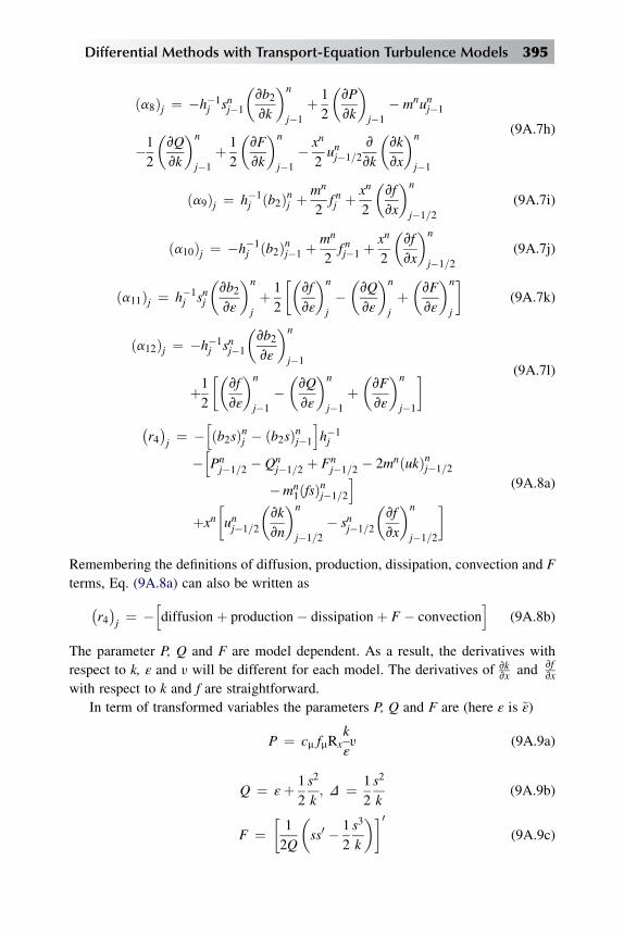
ða8Þj ¼ �h�1j snj�1

�vb2vk

�n

j�1

þ 1

2

�vP

vk

�j�1

� mnunj�1

�1

2

�vQ

vk

�n

j�1

þ 1

2

�vF

vk

�n

j�1

� xn

2unj�1=2

v

vk

�vk

vx

�n

j�1

(9A.7h)

ða9Þj ¼ h�1j ðb2Þnj þ

mn

2f nj þ xn

2

�vf

vx

�n

j�1=2

(9A.7i)

ða10Þj ¼ �h�1j ðb2Þnj�1 þ

mn

2f nj�1 þ

xn

2

�vf

vx

�n

j�1=2

(9A.7j)

ða11Þj ¼ h�1j snj

�vb2vε

�n

j

þ 1

2

��vf

vε

�n

j

��vQ

vε

�n

j

þ�vF

vε

�n

j

(9A.7k)

ða12Þj ¼ �h�1j snj�1

�vb2vε

�n

j�1

þ1

2

��vf

vε

�n

j�1

��vQ

vε

�n

j�1

þ�vF

vε

�n

j�1

(9A.7l)

�r4�j¼ �

hðb2sÞnj � ðb2sÞnj�1

ih�1j

�hPnj�1=2 � Qn

j�1=2 þ Fnj�1=2 � 2mnðukÞnj�1=2

�mn1ðfsÞnj�1=2

iþxn

�unj�1=2

�vk

vn

�n

j�1=2

� snj�1=2

�vf

vx

�n

j�1=2

(9A.8a)

Remembering the definitions of diffusion, production, dissipation, convection and F

terms, Eq. (9A.8a) can also be written as�r4�j¼ �

hdiffusionþ production� dissipationþ F � convection

i(9A.8b)

The parameter P, Q and F are model dependent. As a result, the derivatives with

respect to k, ε and y will be different for each model. The derivatives of vkvx and vf

vx

with respect to k and f are straightforward.

In term of transformed variables the parameters P, Q and F are (here ε is ~ε)

P ¼ cm fmRxk

ε

y (9A.9a)

Q ¼ εþ 1

2

s2

k; D ¼ 1

2

s2

k(9A.9b)

F ¼�1

2Q

�ss0 � 1

2

s3

k

�0(9A.9c)


The rate of dissipation equation is given by Eq. (6.2.20); in terms of transformed

variables it can be written as (ε ¼ ~ε)�b3ε

0�0þP1 � Q1 þ E ¼ x

�uvε

vx� ε

0vfvx

�þ �3m� 1

�uε� m1ε

0f (9A.10)

where (b3ε0)0 denotes the diffusion term, P1 and Q1 defined by

P1 ¼ cε1f1cm fmy2k (9A.11a)

Q1 ¼ cε2 f2ε2=k (9A.11b)

denote the generation and destruction terms, respectively. The right hand side of

Eq. (9.A.10) represents the convective term.

With ε0 ¼ q, Eq. (9.A.10) becomes�

b3q�0þP1 � Q1 þ E þ m1fq�

�3m� 1

�uε ¼ x

�uvε

vx� q

vf

vx

�(9A.12)

Following a procedure similar to the one used for the kinetic energy equation, the

finite-difference approximations for the above equation are

h�1j

hðb3qÞnj � ðb3qÞnj�1

iþ ðP1Þnj�1=2 � ðQ1Þnj�1=2 þ En

j�1=2

þmn1ðfqÞnj�1=2 �

3mn � 1

�ðuεÞn

¼ x

�unj�1=2

�vε

vx

�n

j�1=2

� qnj�1=2

�vf

vx

�n

j�1=2

(9A.13)

After linearization, the resulting expression can be expressed in the form given by

Eq. (9.2.36),

ðb1Þj ¼mn1

2qnj þ

xn

2qnj�1=2

v

vf

�vf

vx

�n

j

(9A.14a)

ðb2Þj ¼mn1

2qnj�1 þ

xn

2qnj�1=2

v

vf

�vf

vx

�n

j�1

(9A.14b)

ðb3Þj ¼ �xn

2

�vε

vx

�n

j�1=2

� 1

2

�3m� 1

�εnj (9A.14c)

ðb4Þj ¼ �xn

2

�vε

vx

�n

j�1=2

� 1

2

�3m� 1

�εnj�1 (9A.14d)

ðb5Þj ¼1

2

�vP1

vy

�n

j

(9A.14e)


ðb6Þj ¼1

2

�vP1

vy

�n

j�1

(9A.14f)

ðb7Þj ¼ h�1j qnj

�vb3vk

�n

j

þ 1

2

�vP1

vk

�n

j

� 1

2

�vQ1

vk

�n

j

(9A.14g)

ðb8Þj ¼ h�1j qnj�1

�vb3vk

�n

j�1

þ 1

2

�vP1

vk

�n

j�1

� 1

2

�vQ1

vk

�n

j�1

(9A.14h)

ðb11Þj ¼ h�1j qnj

�vb3vε

�n

j

� 1

2

�vQ1

vε

�n

j

þ 1

2

�vE

vε

�n

j

�1

2

�3mn � 1

�unj �

xn

2unj�1=2

v

vε

�vε

vx

�n

j

(9A.14i)

ðb12Þj ¼ �h�1j qnj�1

�vb3vε

�n

j�1

� 1

2

�vQ1

vε

�n

j�1

þ 1

2

�vE

vε

�n

j�1

�1

2

�3mn � 1

�unj�1 �

xn

2unj�1=2

v

vε

�vε

vx

�n

j�1

(9A.14j)

ðb13Þj ¼ h�1j ðb3Þnj þ

mn1

2f nj þ xn

2

�vf

vx

�n

j�1=2

(9A.14k)

ðb14Þj ¼ �h�1j ðb3Þnj�1 þ

mn1

2f nj�1 þ

xn

2

�vf

vx

�n

j�1=2

(9A.14l)

ðr5Þj ¼ �h�1j

hðb3qÞnj � ðb3qÞnj�1

iþðP1Þnj�1=2 � ðQ1Þnj�1=2 þ En

j�1=2

þmn1ðfqÞnj�1=2 �

3mn � 1

�ðuεÞnj�1=2

iþxn

�unj�1=2

�vε

vx

�n

j�1=2

� qnj�1=2

�vf

vx

�n

j�1=2

(9A.15a)

Equation (9A.15a) can also be written are

ðr5Þj ¼ �½diffusionþ generation� destruction� convectionþ E� (9A.15b)

Problems

9.1 Consider the SA model discussed in subsection 6.3.2. Using the Falkner-Skan

transformation, Eq. (8.2.5), show that the transport equation for eddy viscosity,

Eq. (6.3.10), can be written as


x

�f 0vnþtvx

� nþtvf

vx

�� m1

�nþt�0f ¼ cb1

�1� ft2

�~s*n*t

�cu1

fu � cb1k2

fb2

� �nþt �2h2

þ1

s

��1þ nþt

��nþt�0�0þcb2

��nþt�0�2�

(P9.1.1)

9.2 The solution of the transformed continuity and momentum equations, Eqs.

(8.2.6) and (8.2.7) and Eq. (P9.1.1) can be obtained with the Box method dis-

cussed in Section 8.2.

(a) Show that Eqs. (8.2.6) and (P9.1.1) can be written as a system of five first-

order equations by defining

g ¼ �nþt�0; u ¼ f 0; y ¼ u0

f 0 ¼ u (P9.2.1a)

u0 ¼ y (P9.2.1b)�nþt�0 ¼ g (P9.2.1c)�

by�0þm1f yþ m

�1� u2

� ¼ x

�uvu

vx� y

vf

vx

�(P9.2.1d)

1

s

��1þ nþt

�g�0þcb2g

2�þ cb1

�1� ft2

�~s*nþt

�cu1

fu � cb1k2

ft2

� �nþt�2

h2 þ �n*w�2 þ m1gf

¼ x

�uvnþtvx

� gvf

vx

�(P9.2.1e)

9.3 For the net rectangle shown in Fig. 8.1, write finite difference approximations to

the equations in Problem 9.2 and check your answer with those given below. Use

backward differences for the streamwise derivatives which are needed to avoid

oscillations when initial conditions are specified for turbulent flow. Also, to keep

the code simple, in Eq. (P9.2.1e) we have defined the diffusion term fm by

1

s

��1þ nþt

�g�0þcb2g

2

(P9.3.1a)

production term ~pr by


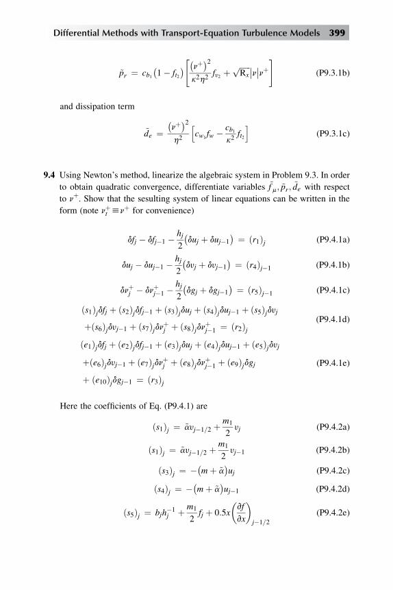
~pr ¼ cb1�1� ft2

�"�nþ�2k2h2

fy2 þffiffiffiffiffiffiRx

p ��n��nþ# (P9.3.1b)

and dissipation term

~de ¼�nþ�2

h2

hcw1

fw � cb1k2

ft2

i(P9.3.1c)

9.4 Using Newton’s method, linearize the algebraic system in Problem 9.3. In order

to obtain quadratic convergence, differentiate variables ~f m; ~pr; ~de with respect

to nþ. Show that the sesulting system of linear equations can be written in the

form (note nþt hnþ for convenience)


�duj þ duj�1

� ¼ ðr1Þj (P9.4.1a)


�dyj þ dyj�1

� ¼ ðr4Þj�1 (P9.4.1b)

dnþj � dnþj�1 �hj2

�dgj þ dgj�1

� ¼ ðr5Þj�1 (P9.4.1c)

ðs1Þjdfj þ ðs2Þjdfj�1 þ ðs3Þjduj þ ðs4Þjduj�1 þ ðs5Þjdyjþðs6Þjdyj�1 þ ðs7Þjdnþj þ ðs8Þjdnþj�1 ¼ ðr2Þj

(P9.4.1d)

ðe1Þjdfj þ ðe2Þjdfj�1 þ ðe3Þjduj þ ðe4Þjduj�1 þ ðe5Þjdyjþðe6Þjdyj�1 þ ðe7Þjdnþj þ ðe8Þjdnþj�1 þ ðe9Þjdgjþ ðe10Þjdgj�1 ¼ ðr3Þj

(P9.4.1e)

Here the coefficients of Eq. (P9.4.1) are

ðs1Þj ¼ ~ayj�1=2 þm1

2yj (P9.4.2a)

ðs1Þj ¼ ~ayj�1=2 þm1

2yj�1 (P9.4.2b)

ðs3Þj ¼ ��mþ ~a�uj (P9.4.2c)

ðs4Þj ¼ ��mþ ~a�uj�1 (P9.4.2d)

ðs5Þj ¼ bjh�1j þ m1

2fj þ 0:5x

�vf

vx

�j�1=2

(P9.4.2e)


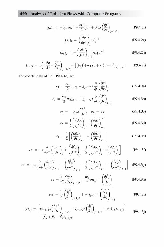
ðs6Þj ¼ �bj�1h�1j þ m1

2fj�1 þ 0:5x

�vf

vx

�j�1=2

(P9.4.2f)

ðs7Þj ¼�

vb

vnþ

�j

yjh�1j (P9.4.2g)

ðs8Þj ¼ ��

vb

vnþ

�j�1

yj�1h�1j (P9.4.2h)

ðr2Þj ¼ x

�uvu

vx� vf

vxy

�j�1=2

� ��by�0þm1 f yþ m�1� u2

��j�1=1

(P9.4.2i)

The coefficients of Eq. (P9.4.1e) are

e1 ¼ m1

2m1gj þ gj�1=2x

d

df

�vf

vx

�j

(P9.4.3a)

e2 ¼ m1

2m1gj�1 þ gj�1=2x

d

df

�vf

vx

�j�1

(P9.4.3b)

e3 ¼ �0:5xvnþ

vx; e4 ¼ e3 (P9.4.3c)

e5 ¼ 1

2

��v~prvy

�j

��v~devy

�j

(P9.4.3d)

e6 ¼ 1

2

��v~prvy

�j�1

��v~devy

�j�1

(P9.4.3e)

e7 ¼ �xv

vnþ

�vnþ

vx

�j

þ v~f mvnþ

!j

þ 1

2

��v~prvnþ

�j

��v~devnþ

�j

(P9.4.3f)

e8 ¼ �xv

vnþ�vnþ

vx

�j�1

þ v~f mvnþ

!j�1

þ 1

2

��v~prvnþ

�j�1

��v~devnþ

�j�1

(P9.4.3g)

e9 ¼ 1

2x

�vf

vx

�j�1=2

þ m1

2m1fj þ

v~f mvg

!j

(P9.4.3h)

e10 ¼ 1

2x

�vf

vx

�j�1=2

þ m1fj�1 þ v~f mvg

!j�1

(P9.4.3i)

ðr3Þj ¼�uj�1=2x

�vnþ

vx

�j�1=2

� gj�1=2x

�vf

vx

�j�1=2

� m1ðfgÞj�1=2

��~f m þ ~pr � ~de

�j�1=2

(P9.4.3j)


Here the diffusion, production and destruction terms, ~f m; ~pr and ~de, respectively, are

given by

~f m ¼ ð1þ cb2Þs

h�1þ nþj

�gj �

�1þ nþj�1

�gj�1

ih�1j � cb2

snþj�1=2

�gj � gj�1

�h�1j

~pr ¼ cb1�1� ft2

�" �nþ�2

k2�h2 þ n2w

�2 fy2 þ ffiffiffiffiffiffiRx

p ��y��nþ#

~de ¼�nþ�2

h2

hcw1

fw � cb1k2

ft2

iand

v~prvy

¼ cb1�1� ft2


p �nþ�nþ

�if y > 0if y > 0

v~devy

¼�nþ�2

h2

�cw1

vfwvy

v~f mvnþ

!j

¼ 1þ cb2s

gjhj� 1

2

cb2s

gj � gj � 1

hj v~f mvnþ

!j�1

¼ �1þ cb2s

gj�1

hj� 1

2

cb2s

gj � gj�1

hj

v~f mvg

¼ 1þ cb2s

1þ nþ

hj� cb2

s

nþj�1=2

hj

v~prvvþ

¼ �cb1

�vft2vnþ

�"�nþ�2

k2h2fy2 þ nþ


p ��y��#

þcb1�1� ft2

�"�nþ�2k2h2

vfv2vnþ

þ vfy2vnþ

þ ffiffiffiffiffiffiRx

p ��y��þ 2vþ

k2h2fy2

vdevnþ

¼�nþ�2

h2 þ �n*w�2�cw1

vfwvnþ

� cb1k2

vft2vnþ

þ 2nþ

h2 þ �n*w�2cw1fw � cb1

k2ft2

�In the above equations, fy1, fy2, fw, ft2 and their variations with respect to n and n

þ are as

follows

ft2 ¼ ct3exph� ct4

�nþ�2i


vft2vnþ

¼ �2ct4nþft2

fy1 ¼�nþ�3

ðnþÞ3þc3y1

vfy1vnþ

¼ 3c3y1�nþ�2h

ðnþÞ3þc3y1

i2fy2 ¼ 1� nþ

1þ nþfy1

vfy2vnþ

¼�vþ�2vfy1vnþ

� 1�1þ nþfy1

�2fw ¼

" 1þ c6w3

�1þ c6w3

g�61

�#1=6

g1 ¼ rr þ cw5

�rr6 � rr

�rr ¼

�nþ�2

h2k2

(nþ


p ��y��þ �nþ�2k2h2

fy2

)�1

vfwvy

¼ vfwvg1

vg1vðrrÞ

vðrrÞvy

vfwvnþ

¼ vfwvg1

vg1vðrrÞ

vðrrÞvnþ

where

vfwvg1

¼ c6w3g�61 fwh

g1

1þ c6w3

g�61

�ivg1vðrrÞ ¼ 1þ cw2

�6rr5 � 1

�vðrrÞvy

¼ ��nþ�2

k2�h2 þ n*2w

�"nþ ffiffiffiffiffiffiRx

p ��y��þ �nþ�2k2h2

fy2

#�2

�� ffiffiffiffiffiffiRx

pnþ�( 1

�1

)if y > 0

if y < 0


vðrrÞvnþ

¼ ��nþ�2

k2�h2 þ n*2w

�"nþ ffiffiffiffiffiffiRx

p ��y��þ �nþ�2

k2�h2 þ n*2w

� fy2#�2

�" �

nþ�2

k2�h2 þ n*2w

� vfy2vnþ

þ ffiffiffiffiffiffiRx

p ��y��þ 2nþ

k2�h2 þ n*2w

� fy2#

þ 2nþ

k2�h2 þ n*2w

� "nþ ffiffiffiffiffiffiRx

p ��y��þ �nþ�2

k2�h2 þ n*2w

� fy2#

9.5 Show that the linear system of equations given by Eqs. (P9.4) subject to the

boundary conditions

h ¼ 0; f ¼ u ¼ nþ ¼ 0h ¼ he; u ¼ 1; nþ ¼ nþe

(P9.5.1)

which in linearized form

du0 ¼ df0 ¼ dnþ0 ¼ 0

duJ ¼ dnþJ ¼ 0(P9.5.2)

can be written in matrix-vector form, given by Eq. (8.2.24) with five-dimen-

sional vectors dej and rej for each value of j defined by

dej ¼0BBBB@

dfjdujdyjdvþjdgj

1CCCCA; rej ¼0BBBB@

ðr1Þjðr2Þjðr3Þjðr4Þjðr5Þj

1CCCCA (P9.5.3)

and the 5� 5 matrices Aj, Bj, Cj given by

A0 ¼ j 1 0 0 0 0

0 1 0 0 0

0 0 0 1 0

0 �1 �h12 0 0

0 0 0 �1 �h12

j (P9.5.4a)


Bj ¼ j 1� �h12 0 0 0

ðs2Þj ðs4Þj ðs6Þj ðs8Þj 0

ðe2Þj ðe4Þj ðe6Þj ðe8Þj ðe10Þj0 0 0 0 0

0 0 0 0 0j; 1 � j � J (P9.5.4b)

Aj ¼

��1 �hj=2 0 0 0

ðs1Þj ðs3Þj ðs5Þj ðs7Þj 0ðe1Þj ðe3Þj ðe5Þj ðe7Þj ðe9Þj0 �1 �hjþ1=2 0 00 0 0 �1 �hjþ1=2

��; 1 � j � J � 1 (P9.5.4c)

Cj ¼

��0 0 0 0 00 0 0 0 00 0 0 0 00 1 �hjþ1=2 0 00 0 0 1 �hjþ1=2

��; 0 � j � J � 1 (P9.5.4d)

Aj ¼ j 1 �hj=2 0 0 0

ðs1Þj ðs3Þj ðs5Þj ðs7Þj 0

ðe1Þj ðs3Þj ðs5Þj ðs7Þj ðs9Þj0 1 0 0 0

0 0 0 1 0

j (P9.5.4e)

9.6 Using the matrix solver, MSA (subsection 10.7.3), write an algorithm for the

linear system in Problem 9.5. Check your code with the one given on the

companion site.

9.7 To develop a computer program to solve the equations using the SA model, it is

necessary to specify initial profiles for fj, uj, vj, yþj and gj. It is also necessary to

generate the boundary layer grid, account for the boundary layer growth, etc.

A convenient procedure is to use the computer program described in Section

10.3 with initial velocity profiles incorporated in a new subroutine IVPT as de-

scribed in Problem 8.9. The initial profiles for yþj and gj can be calculated from

those calculated in subroutine EDDY since yþj ¼ ( εþm)j. Thus with initial profilesspecified in this manner, we can replace subroutine COEF3 and SOLV3 in BLP2

with new subroutines, say COEF5 which contains the coefficients in Problem

9.4, and the algorithm discussed in Problem 9.6. Obviously, we need to


incorporate other changes to the logic of the computations in order to extend the

computer program of Problem 8.6 to solve the SA model equations.

9.8 The properties of a two-dimensional nonsimilar plane jet for a turbulent flow can

also be calculated with an algebraic eddy viscosity formulation using the

computer program described in Section 10.3. As before, we again use trans-

formed variables.

(a) Show that, with the eddy viscosity concept and neglecting the pressure-gradient

term, the continuity and momentum equations given by Eqs. (5.2.8) and (5.2.9)

can be written as �bf 00�0þðf 0Þ2þf f 00 ¼ 3x

�f 0vf 0

vx� f 00

vf

vx

�(P9.8.1)

with the transformation defined by

h ¼ffiffiffiffiffiu0nL

ry

3x2=3; x ¼ x

L; j ¼ ffiffiffiffiffiffiffiffiffiffi

u0nLp

x1=3f�x; h�

(P9.8.2)

Here u0, L denote a reference velocity and length, respectively, and

b ¼ 1þ εm=n ¼ 1þ εþm (P9.8.3)

(b) With

f 0 ¼ u (P9.8.4a)

u0 ¼ y (P9.8.4b)

Eq. (P9.8.1) can be written as�by�0þu2 þ f y ¼ 3x

�uvu

vx� y

vf

vx

�(P9.8.4c)

Write finite difference approximations to the above equations and show that

Eq. (P9.8.4c) can be expressed in the same form as Eq. (8.2.20c) and that the

coefficients (sk)j are identical to those given by Eqs. (8.2.22), provided that we

take m1¼ 1 and m2¼ –1.

(c) With the boundary conditions given by

h ¼ 0; f ¼ y ¼ 0 (P9.8.5a)

h ¼ he; u ¼ 0 (P9.8.5b)

or in linearized form

df0 ¼ 0; dy0 ¼ 0; duJ ¼ 0 (P9.8.6)


the linear system of equations can again be expressed in the form given by

Eq. (8.2.24) and can be solved with minor changes to the computer program

described in Section 10.3. One of the changes occurs in subroutine IVPL that

defines the initial velocity profiles for laminar flows. For either laminar or

turbulent plane jet, this subroutine requires changes. An initial velocity profile

can be generated by assuming the profile to be of the form

u

uc¼ 1

2

h1� tanh b

yh� 2c

�i(P9.8.7)

Here b and 2c are specified constants, and h is the half-width of the duct. This

profile essentially corresponds to a uniform velocity at the exit of the duct. The

fairing given by the above equation is to remove the discontinuity at y/h¼ 1.

Plot the above equation for two values of b equal to 10 and 20 with 2c¼ 1 and

show that in transformed variables, this equation can be written in the form

f 0

2x1=3¼ 1

2

(1� tanh b

"3x

2=30ffiffiffiffiffiffiRL

p �h� hc

�#)(P9.8.8)

Here RL is a dimensionless Reynolds number, u0L/n and x0 is the x-location at

which the initial profiles are specified. The reference length L is usually taken to

be equal to the half-width of the duct.

(d) In addition to subroutine IVPL, we need to make changes in subroutine

EDDYand replace the eddy viscosity formulas in that subroutine with a new

one. There are several formulations that can be used for this purpose.

A simple one is

εm ¼ 0:037ucd (P9.8.9)

where d represents the half-width (taken as the point where u/uc¼ 0.5 and ucis the centerline viscosity.

Show that this equation can be written in transformed variables as

εþm ¼ 0:037

ffiffiffiffiffiffiRL

px1=3h1=2f

0c (P9.8.10)

Here h1/2 is the transformed h-distance where u ¼ 12 uc; and f 0c is the

dimensionless centerline velocity.

(e) Compute the variation of the dimensionless centerline velocity for a turbulent

flow with the revised computer program of Section 10.3. Take RL¼ 5300,

b¼ 20, 2c¼ 1.0 and x0¼ 1. Plot u/u0 as a function of y/L at x¼ 1.054, 1.249,

1.581, 2.976, 4.484, 6.819, 10.

(f) Include the intermittency term g

g ¼ 1

1þ 5:5ðy=dÞ6 (P9.8.11)


in Eq. (P9.8.10) and repeat the calculations in (e) with this modification to εm.

Compare your results with those in (e).

(g) Compare the results in (f) with experimental data given on the companion site.

(h) Repeat (g) with 0.037 in Eq. (P9.8.10) replaced with 0.035, 0.033 to study the

effect of this constant on the solutions.

9.9 Repeat (e) in Problem P9.8 for RL¼ 100.

References

[1] T. Cebeci, Turbulence Models and Their Applications, Horizons Publishing, Long Beach, CA, and

Springer-Verlag, Heidelberg, Germany, 2003.

[2] J.E. Bardina, P.G. Huang, T.J. Coakley, Turbulence Modeling Validation, Testing and Development,

NASA, Tech. Memo. 110446 (April 1997).

[3] H.W. Liepmann, J. Laufer, Investigations of Free Turbulent Mixing, NACA TN-1257 (1947).

[4] L.J.S. Bradbury, The Structure of a Self-Preserving Turbulent Plane Jet,, J. Fluid Mech. 23 (1)

(1965) 31–64.

[5] S.J. Kline, B.J. Cantwell, G.M. Lilley, 1980-81 AFOSR-HTTM-Stanford Conference on Complex

Turbulent Flows, Stanford University, Stanford, Calif, 1981.

[6] S. Birch, Planar Mixing Layer, In 1980-81 AFOSR-HTTM-Stanford Conference on Complex

Turbulent Flows, in: S.J. Kline, B.J. Cantwell, G.M. Lilley (Eds.), Stanford University, Stanford,

Calif., 1981. vol. 1, pp. 170–177.

[7] I. Wygnanski, H.E. Fiedler, Some Measurements in the Self-Preserving Jet, J. Fluid Mech. 38 (3)

(1969) 577–612. Also in Boeing Scientific Research Labs, Flight Science Laboratory, Document

D1-82-0712.

[8] A. Fage, V.M. Falkner, Note on Experiments on the Temperature and Velocity in the Wake of

a Heated Cylindrical Obstacle. London, Proc. Roy. Soc. vol. A135 (1932) 702–705.

[9] G.S. Settles, L.J. Dodson, Hypersonic Turbulent Boundary-Layer and Free Shear Database, NASA

CR-177610, Ames Research Center (Apr. 1993).

[10] S.F. Birch, J.M. Eggers, A Critical Review of the Experimental Data for Developed Free Turbulent

Shear Layers. – Conference Proceedings, Langley Research Center, NASA, Hampton, Va., July

20–21, Free Turbulent Shear Flows vol. 1 (1972) 11–40.

[11] D.M. Driver, Reynolds Shear Stress Measurements in a Separated Boundary Layer Flow, AIAA

Paper (1991) 91–1787.

[12] W.D. Bachalo, D.A. Johnson, Transonic Turbulent Boundary-Layer Separation Generated on an

Axisymmetric Flow Model, AIAA J. 24 (1986) 437–443.

[13] T. Cebeci, K.C. Chang, An Improved Cebeci-Smith Turbulence Model for Boundary-Layer and

Navier-Stokes Methods, paper No. ICAS-96–1.7.3, 20th Congress of the International Council of

the Aeronautical Sciences, Sorrento, Italy, 1996.


CompanionComputer Programs

Chap

ter10



10.2 Integral Methods 412

10.2.1 Thwaites’ Method 412

10.2.2 Smith-Spalding Method 412

10.2.3 Head’s Method 412

10.2.4 Ambrok’s Method 413

10.3 Differential Method with CS Model: Two-Dimensional Laminar

and Turbulent Flows 413

10.3.1 Main 413

10.3.2 Subroutine INPUT 414

10.3.3 Subroutine IVPL 416

10.3.4 Subroutine GROWTH 417

10.3.5 Subroutine COEF3 417

10.3.6 Subroutine EDDY 417


10.3.8 Subroutine OUTPUT 418409



http://dx.doi.org/10.1016/B978-0-08-098335-6.00010-0

10.4 Hess-Smith Panel Method with Viscous Effects 418

10.4.1 MAIN 418

10.4.2 Subroutine COEF 419

10.4.3 Subroutine OBKUTA 419

10.4.4 Subroutine GAUSS 419

10.4.5 Subroutine VPDIS 419

10.4.6 Subroutine CLCM 420

10.4.7 Subroutine VPDWK 420

10.5 Differential Method with CS Model: Two-Dimensional Flows with

Heat Transfer 420

10.6 Differential Method with CS Model: Infinite Swept-Wing Flows 421

10.7 Differential Method with CS and k-ε Models: Components of the

Computer Program Common to both Models 421

10.7.1 MAIN 421


10.7.3 Subroutine IVPT 423

10.7.4 Subroutine GROWTH 423

10.7.5 Subroutine GRID 423

10.7.6 Subroutine OUTPUT 423

10.8 Differential Method with CS and k-ε Models: CS Model 424

10.8.1 Subroutine COEFTR 424


10.8.3 Subroutines EDDY, GAMCAL, CALFA 424

10.9 Differential Method with CS and k-ε Models: k-ε Model 425

10.9.1 Subroutines KECOEF, KEPARM, KEDEF and KEDAMP 425

10.9.2 Subroutine KEINITK 427

10.9.3 Subroutine KEINITG 428

10.9.4 Subroutine KEWALL 428

10.9.5 Subroutine KESOLV 428

10.9.6 Test Cases for the CS and k-ε Models 429

10.9.7 Solution Algorithm 429

10.10 Differential Method with CS and k-ε Models: Basic Tools 431

10.11 Differential Method with SA Model 431

10.12 Differential Method for a Plane Jet 432

10.13 Useful Subroutines 432

10.13.1 Subroutine IVPT 432


10.14 Differential Method for Inverse Boundary-Layer Flows with CS Model 432


10.14.2 Subroutine HIC 434


10.15 Companion Computer Programs 435

10.15.1 Sample Calculations for the Panel Method Without

Viscous Effects 435

10.15.2 Sample Calculations for the Inverse Boundary-Layer Program 438

10.15.3 Sample Calculations with the Interactive Boundary-Layer

Program 439

References 446

10.1 Introduction

In this chapter we describe several computer programs for calculating two-

dimensional laminar and turbulent incompressible flows. In Section 10.2 we first

describe computer programs based on integral methods discussed in Chapter 7 and

present sample calculations. The computer program in Section 10.3 is based on

the differential method discussed in Chapter 8 and is applicable to both laminar

and turbulent flows for a given external velocity distribution and transition loca-

tion. In this section we also present sample calculations for an airfoil with the

external velocity distribution obtained from the panel method discussed in Section

10.4. Sections 10.5 and 10.6 present computer programs for incompressible

laminar and turbulent flows with heat transfer and for infinite-swept wing flows,

respectively. Sections 10.7 to 10.10 present another differential method for two-

dimensional incompressible turbulent flows with CS and k-ε models. The

computer program with the CS model is essentially similar to the one in

Section 10.3 except that the wall boundary conditions for the momentum and

continuity equations are specified at some distance from the wall. The computer

program for the k-ε model includes the zonal method with a combination of the

CS model for the inner region and the k-ε model for the outer region as discussed

in Section 9.2. It also includes the solution of the k-ε model equations with and

without wall functions. Section 10.11 presents a differential method for the SA

model using the numerical procedure discussed in Problems 9.1 to 9.7 and Section

10.12 for a plane jet discussed in Problem 9.8. Section 10.13 presents several

subroutines discussed in Chapters 8 and 9. Section 10.14 presents the differential

method for the inverse boundary-layer discussed in Section 8.8 and subsection

10.15.1 presents sample calculations for the panel method of Section 8.9 without

viscous affects. Sample calculations for the inverse boundary-layer program is

discussed in subsection 10.15.2 and those for the interactive boundary-layer

program in subsection 10.15.3.

All programs, including the three programs in Chapter 5, can be found on the

companion site, store.elsevier.com/companions/9780080983356.

Companion Computer Programs 411


10.2 Integral Methods

In Chapter 7 we discussed integral methods for calculating heat and momentum

transfer in two-dimensional and axisymmetric laminar and turbulent flows. In this

section we describe FORTRAN programs for them and present sample

calculations.

10.2.1 THWAITES’ METHOD

This method is applicable to both two-dimensional and axisymmetric laminar flows

(see Problem 7.11) and has the following input requirements:

NXT Total number of x-stations.

KASE Flow index, 0 for two-dimensional flow, 1 for two-dimensional flow that starts asstagnation-point flow, and 2 for axisymmetric flow.

KDIS Index for surface distance; 1 when surface distance is input, 0 when surface distanceis calculated.

UREF Reference velocity, uref, feet per second or meters per second.

BIGL Reference length, L, feet or meters.

CNU Kinematic viscosity, n, square feet per second or square meters per second.

X Dimensionless chordwise or axial distance, x/L. If KDIS¼ 1, then X is the surfacedistance, s.

UE Dimensionless velocity, ue/uref.

R Dimensionless two-dimensional body ordinate or body of revolution radius; r/L.

Its output includes d*, q, H, cf and Rq¼ ueq/n together with Reynolds mumber,

RS, based on surface distance and external velocity.

10.2.2 SMITH-SPALDING METHOD

This method is for laminar boundary-layer flows with variable ue but uniform surface

temperature. Its input is similar to Thwaites’ method and consists of NXT, KASE,

KDIS, UREF, BIGL, CNU and PR. We again read in X, R and UE.

The output includes X, S, UE and ST (Stanton number).

10.2.3 HEAD’S METHOD

This method is applicable to only two-dimensional incompressible turbulent flows.

Its input consists of the specification of the external velocity distribution, ue/uN,

UE(I), as a function of surface distance x/L, X(I), with uN denoting the reference

freestream velocity and L a reference length. The initial conditions consist of

a dimensionless momentum thickness, q/L, T(1), and shape factor H, H(1), at the first


station. In addition, we specify a reference Reynolds number RL¼ uNL/n, RL and

the total number of x-stations, NXT. In the code, the derivative of external velocity

due/dx, DUEDX(I), is computed by using a three-point Lagrange-interpolation

formula. The output includes X(I), UE(I), DUEDX(I), T(I), H(I), DELST(I), d*/L,

CF(I) and DELTA(I), d, defined by Eq. (7.3.2).

10.2.4 AMBROK’S METHOD

This method is only for two-dimensional turbulent flows. Its input and output

instructions are similar to Head’s method.

10.3 Differential Method with CS Model:Two-Dimensional Laminar and Turbulent Flows

In this section we present the computer program discussed in Chapter 8 for two-

dimensional incompressible laminar and turbulent flows. Its extension to flows with

heat transfer is discussed in Section 10.5 and to infinite-swept wing flows in Section

10.6, to turbulent flows employing the SA model in Section 10.11 and to a plane jet

in Section 10.12.

This computer program, called BLP2, and also described in [1], consists of

a MAIN routine, which contains the logic of the computations, and seven subrou-

tines: INPUT, IVPL, GROWTH, COEF3, SOLV3, EDDY and OUTPUT. The

following subsections describe the function of each subroutine.

10.3.1 MAIN

BLP2 solves the linearized form of the equations. Thus an iteration procedure in

which the solution of Eq. (8.2.24) is obtained for successive estimates of the

velocity profiles is needed with a subsequent need to check the convergence of the

solutions. A convergence criterion based on v0 which corresponds to f 00w is usually

used and the iterations, which are generally quadratic for laminar flows, are stopped

when

jdy0ð¼ DELVð1ÞÞj < ε1 (10.3.1)

with ε1 taken as 10–5. For turbulent flows, due to the approximate linearization

procedure used for the turbulent diffusion term, the rate of convergence is not

quadratic and solutions are usually acceptable when the ratio of jdy0/y0j is less than0.02. With proper linearization, quadratic convergence of the solutions can be

obtained as described in [1].


After the convergence of the solutions, the OUTPUT subroutine is called and the

profiles F, U, V and B, which represent the variables fj, uj, yj and bj are shifted.

10.3.2 SUBROUTINE INPUT

This subroutine prepares data for boundary layer calculations. The data includes grid

in x- and h-directions, dimensionless pressure gradient m(x), mass transfer fw(x)

parameter and calculation of the gtr-term in the CS model which is given by Eqs.

(5.3.18) and (5.3.19).

The streamwise grid is generated by reading the values at xi. In general, the x-grid

distribution depends on the variation of ue with x so that rapid variations in external

velocity distribution and the approach to separation require small Dx-steps (kn). For

laminar flows, it is often sufficient to use a uniform grid in the h-direction. A choice of

transformed boundary-layer thicknesses he equal to 8 often ensures that the dimen-

sionless slope of the velocity profile at the edge, f 00(he), is sufficiently small (< 10–3)

and that approximately 61 grid points are adequate for most flows. For turbulent flows,

however, a uniform grid is not satisfactory because the boundary-layer thickness heand the dimensionless wall shear parameter nw (h f 00w) are much larger in turbulent

flows than laminar flows. Due to the rapid variation of the velocity profile close to the

wall, it is necessary to take much smaller steps in h close to the wall.

The program uses a h-grid which has the property that the ratio of lengths of any

two adjacent intervals is a constant, that is, hj¼ Khj–1 and the distance to the j-th line

is given by

hj ¼ h1KJ � 1

K � 1j ¼ 1; 2;.; J K > 1 (10.3.2)

There are two parameters: h1, the length of the first Dh-step, and K, the variable grid

parameter. The total number of points, J, is calculated from

J ¼ ln½1þ ðK � 1Þðhe=h1Þ�lnK

þ 1 (10.3.3)

In practice, it is common to choose h1 [DETA(1)] and K (VGP) so that, for an

assumed maximum value of he (ETAE), the number of j-points do not exceed the

total number (NPT) specified in the code. For example, for he¼ 50 and h1¼ 0.01, the

number of j-points depends on K. Figure 10.1 can help in the selection of K and

shows that, for example for J¼ 61, the value of the variable grid parameter must be

less than about 1.1.

With velocities known at each x-station, called NX-stations, the pressure gradient

parameters m (P2) and m1 (P1) are computed from their definitions for all x-stations,

except the first one at which m is specified, after the derivative of due/dx (DUDS)


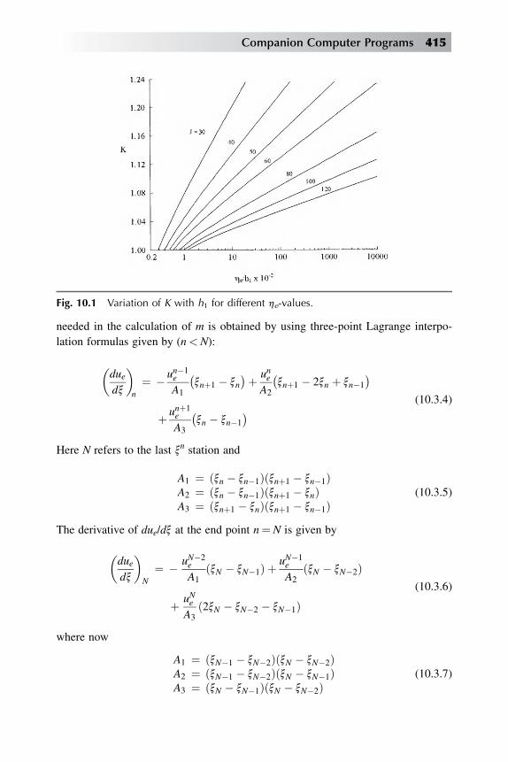
needed in the calculation of m is obtained by using three-point Lagrange interpo-

lation formulas given by (n< N):

�duedx

�n

¼ � un�1e

A1

�xnþ1 � xn

�þ uneA2

�xnþ1 � 2xn þ xn�1

�

þ unþ1e

A3

�xn � xn�1

� (10.3.4)

Here N refers to the last xn station and

A1 ¼ ðxn � xn�1Þðxnþ1 � xn�1ÞA2 ¼ ðxn � xn�1Þðxnþ1 � xnÞA3 ¼ ðxnþ1 � xnÞðxnþ1 � xn�1Þ

(10.3.5)

The derivative of due/dx at the end point n¼ N is given by

�duedx

�N

¼ � uN�2e

A1ðxN � xN�1Þ þ

uN�1e

A2ðxN � xN�2Þ

þ uNeA3

ð2xN � xN�2 � xN�1Þ(10.3.6)

where now

A1 ¼ ðxN�1 � xN�2ÞðxN � xN�2ÞA2 ¼ ðxN�1 � xN�2ÞðxN � xN�1ÞA3 ¼ ðxN � xN�1ÞðxN � xN�2Þ

(10.3.7)

Fig. 10.1 Variation of K with h1 for different he-values.


The gtr-term, which accounts for the transition region between a laminar and

turbulent flow, is calculated as a function of x once the onset of transition is

specified.

In this subroutine we specify he at x¼ 0 and the reference Reynolds number RL

(RL). In addition, the following data are also read in and the total number of j-points

J(NP) is computed from Eq. (10.3.2).

NXT Total number of x-stations

NTR NX-station for transition location xtr

NPT Total number of h-grid points.

DETA(I) Dh-initial step size of the variable grid system. Use Dh¼ 0.01 for turbulent flows. Ifdesired, it may be changed.

ETAE Transformed boundary-layer thickness, he

VGP K is the variable-grid parameter. Use K¼ 1.0 for laminar flow and K¼ 1.12 for turbulentflow. For a flow consisting of both laminar and turbulent flows, use K¼ 1.12.

RL Reynolds number, uNLv

x Surface distance, feet or meters, or dimensionless.

ue Velocity, feet per second or meter per second, or dimensionless.

10.3.3 SUBROUTINE IVPL

At x¼ 0 with b¼ 1, Eq. (8.2.6) reduces to the Falkner-Skan similarity equation

which can be solved subject to the boundary conditions of Eq. (8.2.7). Since the

equations are solved in linearized form, initial estimates of fj, uj and yj are needed in

order to obtain the solutions of the nonlinear Falkner-Skan equation. Various

expressions can be used for this purpose. Since Newton’s method is used, however,

it is useful to provide as good an estimate as is possible and an expression of

the form.

uj ¼ 3

2

hj

he� 1

2

�hj

he

�3

(10.3.8)

usually satisfies this requirement. The above equation is obtained by assuming

a third-order polynomial of the form

f 0 ¼ aþ bhþ ch3

and by determining constants a, b, c from the boundary conditions given by Eq.

(8.2.7) for the zero-mass transfer case and from one of the properties of momentum

equation which requires that f 00 ¼ 0 at h¼ he.


The other profiles fj, yj follow from Eq. (10.3.4) and can be written as

fj ¼ he

4

�hj

he

�2�3� 1

2

�hj

he

�2�(10.3.9)

yj ¼ 3

2

1

he

�1�

�hj

he

�2�(10.3.10)

10.3.4 SUBROUTINE GROWTH

For most laminar-boundary-layer flows the transformed boundary-layer thickness

he(x) is almost constant. A value of he¼ 8 is sufficient. However, for turbulent

boundary-layers, he(x) generally increases with increasing x. An estimate of he(x) is

determined by the following procedure.

We always require that he(xn)� he(x

n–1), and in fact the calculations start with

he(0)¼ he(x1). When the computations on x¼ xn (for any n� 1) have been

completed, we test to see if j ynJ j � εy at he(xn) where, say εy¼ 5� 10–4. This test is

done in MAIN. If this test is satisfied, we set he(xnþ1)¼ he(x

n). Otherwise, we call

GROWTH and set Jnew¼ Joldþ t, where t is a number of points, say t¼ 1. In this

case we also specify values of ( f nj ; unj ; y

nj ; b

nj ) for the new nj points. We take the values

of uj¼ 1, ynj ¼ 0, f nj ¼ ðhj � heÞunJ þ f nJ , and bnj ¼ bnJ . This is also done for the

values of f n�1j , yn�1

j , and bn�1j .

10.3.5 SUBROUTINE COEF3

This is one of the most important subroutines of BLP2. It defines the coefficients of

the linearized momentum equation given by Eqs. (8.2.20) and (8.2.23).

10.3.6 SUBROUTINE EDDY

This subroutine contains the CS algebraic eddy viscosity model in Section 5.8. For

simplicity we do not include the low Reynolds number effect, roughness effect, mass

transfer effect and strong pressure gradient effect (variable a) in this subroutine.

These capabilities, if desired, can easily incorporated into the formula as defined in

this subroutine. The formulas for the inner and outer eddy-viscosity expressions are

given by Eqs. (5.2.11) with each side of equation multiplied by gtr given by Eqs.

(5.3.18) and (5.3.19).

In terms of transformed variables ( εþm)i and ( εþm)o given by Eq. (5.2.11) can be

written as �εþm

�i¼ 0:16R1=2

x ½1� expð� y=AÞ�2h2ygtr (10.3.11a)


�εþm

�0¼ 0:0168R1=2

x

�he � fe

gtrg (10.3.11b)

y

A¼ N

26R1=4x y1=2w h; Rx ¼ uex

n(10.3.12)


This subroutine is used to obtain the solution of Eq. (8.2.24) with the block-elimi-

nation method discussed in subsection 8.2.3 and with the recursion formulas given in

subsection 8.2.4.

10.3.8 SUBROUTINE OUTPUT

This subroutine prints out the desired profiles such as fj, uj, yj, and bj as functions of

hj. It also computes the boundary-layer parameters, cf, d*, q and Rx.

10.4 Hess-Smith Panel Method with Viscous Effects

In this section we present a computer program for the panel method discussed in

Section 8.9. This program can be used interactively with the boundary-layer program

of Section 10.14 so that, as discussed in detail in [2,3] and briefly in Section 8.9,

more accurate solutions of inviscid and viscous flow equations can be obtained by

includingthe viscous effects in the panel method of Section 8.9.

The computer program of the panel method has five subroutines and MAIN, as

described below.

10.4.1 MAIN

MAIN contains the input information which comprises (1) the number of panels

alongthe surface of the airfoil, NODTOT, and the number of panels in the wake, NW.

The code is arranged so that it can be used for inviscid flows with and without viscous

effects. For inviscid flows, NW is equal to zero. (2) The next input data also comprises

airfoil coordinates normalized with respect to its chord c, x/c, y/c, [hX(I),Y(I)]. If

NW s 0, then it is necessary to specify the dimensionless displacement thickness

d*/c (hDLSP(I)), dimensionless blowingv elocity uw /uN (hVNP(I)) distributions

on the airfoil, as well as the wake coordinates XW(I), YW(I) of the dividing-

streamline, the dimensionless displacement thickness distribution on the upper wake

DELW(I,1) and lower wake DELW(I,2) and velocity jump QW(I). It should be noted


that all input data for wake includes values at the trailing edge. The input also in-

cludes angle of attack a (hALPHA) and Mach number MN (hFMACH).

The panel slopes are calculated from Eq. (8.9.2). The subroutine COEF iscalled

to compute A and b!

in Eq. (8.9.19) subroutine OBKUTA to calculate the off-body

Kutta condition, subroutine GAUSS to compute x!, subroutine VPDIS to compute

the velocity and pressure distributions, and subroutine CLCM to compute the airfoil

characteristics correspondingto lift (CL) and pitchingmoment (CM) coefficients.

10.4.2 SUBROUTINE COEF

This subroutine calculates the elements aij of the coefficientmatrixA fromEqs. (8.9.21)

and (8.9.23) and the elements of b!

fromEq. (8.9.24)We note thatNþ 1 corresponds to

KUTTA, and N to NODTOT

10.4.3 SUBROUTINE OBKUTA

This subroutine is used to calculate the body-off Kutta condition.

10.4.4 SUBROUTINE GAUSS

The solution of Eq. (8.9.19) is obtained with the Gauss elimination method described

in Section 8.9.

10.4.5 SUBROUTINE VPDIS

Once x! is determined by subroutineGAUSS so that source strengths qi (i¼ 1, 2, . . . , N)

and vorticity s on the airfoil surface are known, the tangential velocity component ðVtÞat each control point can be calculated. Denoting qiwith Q(I) and swith GAMMA, the

tangential velocities ðVtÞi are obtained with the help of Eq. (8.9.12b). This subroutinealso determines the distributions of the dimensionless pressure coefficient Cp (h CP)

defined by

Cp ¼ p� pNð1=2Þ9V2

N

(10.4.1a)

which in terms of velocities can be written as

Cp ¼ 1��Vt

VN

�2

(10.4.1b)

It is common to use panel methods for low Mach number flows by introdu-

cingcompressibilit y corrections which depend upon the linearized form of the


compressibility velocity potential equation and are based on the assumption of small

perturbations and thin airfoils [4]. A simple correction formula for this purpose is the

Karman-Tsien formula which uses the ‘‘tangent gas’’ approximation to simplify the

compressible potential-flow equations. Accordingto this formula, the effect of Mach

number on the pressure coefficient is estimated from

cp ¼ cpibþ ½M2

N=ð1þ bÞ�ðcpi=2Þ (10.4.2)

and the correspondingv elocities are computed from

V2 ¼ 1þ 1

c6

h1� ð1þ c8cpÞ1=c7

i(10.4.3)

Here cpi denotes the incompressible pressure coefficient, MN the freestream

Mach number and

b ¼ffiffiffiffiffiffiffiffiffiffiffiffiffiffiffiffiffiffi1�M2

N;q

c6 ¼ g� 1

2M2

N; c 7 ¼ g

g� 1; c8 ¼ 1

2gM2

N; g ¼ 1:4

(10.4.4)

In this subroutine we also include this capability in the HS panel method.

10.4.6 SUBROUTINE CLCM

The dimensionless pressure in the appropriate directions is integrated to compute the

aerodynamic force and the coefficients for lift (CL) and pitchingmoment (CM) about

the leading edge of the airfoil.

10.4.7 SUBROUTINE VPDWK

This subroutine calculates the total velocity and pressure coefficient at each

control point alongthe upper and lower wakes separately. The normal and

tangential components of the total velocities are computed from Eqs. (8.9.39a) and

(8.9.39b).

10.5 Differential Method with CS Model:Two-Dimensional Flows with Heat Transfer

The program which for convenience we called BLP2H is the same computer

program BLP2 which now includes the solution of the energy equation. Two

subroutines, COEF2 and SOLV2, are added to BLP2 to calculate incompressible


laminar and turbulent flows with heat transfer (see Problem 8.3). Sample calculations

presented on the companion site, store.elsevier.com/components/9780080983356,

represent the application of this code to Problems 8.4 and 8.5.

10.6 Differential Method with CS Model: InfiniteSwept-Wing Flows

This program, called BLP2ISW, is also the extension of BLP2 to the calculation of

infinite swept-wing equations for incompressible laminar and turbulent flows as

discussed in Problem 8.6. Again two subroutines are added to BLP2 and changes are

made to the eddy viscosity subroutines. Subroutine COEF2 includes the coefficients

of the z-momentum equation and subroutine SOLV2 is the same solution algorithm

used in BLP2H see subsection 10.13.1.

For three-dimensional turbulent flows, the eddy viscosity formulas require

changes to those for two-dimensional flows. Here they are defined according to Eqs.

(5.7.4) and (5.7.5).

Sample calculations for an infinite swept wing having the NACA 0012 airfoil

cross section with a sweep angle of l¼ 30�, an angle of attack of a¼ 2�, chordReynolds number Rc¼ 5� 106 and transition location at x/c¼ 0.10 are presented on

the companion site, store.elsevier.com/components/9780080983356. See also

Problem 8.7.

10.7 Differential Method with CS and k-ε Models:Components of the Computer Program Commonto both Models

This section includes a MAIN routine which contains the logic of the computations

and five subroutines, INPUT, IVPT, GROWTH, GRID and OUTPUT, described

below.

10.7.1 MAIN

Here we first read in input data (subroutine INPUT) and generate the initial turbulent

velocity profile (subroutine IVPT) and the eddy viscosity distribution for the CS

model (subroutine EDDY), k-profile (subroutine KEINITK), ε-profile (subroutine

KEINITG). Since linearized equations are being solved, we use an iteration proce-

dure in which the solutions of the equations are obtained for successive estimates of

velocity, kinetic energy, dissipation profiles with a subsequent need to check the




convergence of the solutions. A convergence criterion based ondy0

y0< 0:02 is used

and the iterations are stopped when��dy0y0�� < 0:02

During this iteration procedure, we introduce an under-relaxation procedure for the

iterations as described in MAIN. This is useful, especially with transport equation

turbulence models.

When the solutions converge, we also check to see whether the boundary-layer

thickness, he, used in the calculations for that x-station is large enough so that the

asymptotic behavior of the solutions is reached. If this is not the case, we call

subroutine GROWH.

After the convergence of the solutions. the OUTPUT subroutine is called and the

profiles which represent the variables such as fj, uj, yj, kj, εj etc. are shifted.


In this subroutine we read in input data and set up the flow calculations according to

the following turbulence models listed below.

Model ¼ 0 CS model1 Huang-Lin k-ε model2 Chien k-ε model

¼ �1 zonal method¼ �2 high Re # k-ε model

In some problems, like airfoil flows, it is convenient to read in the dimensionless

airfoil coordinates x/c, y/c rather than the surface distance required in the boundary-

layer calculations. In all calculations, the external velocity ue(x) either dimensional

or dimensionless, ue=uN, and freestream or reference velocity, uN (uref), kinematic

viscosity n (CNU), reference length c (chord), variable h-grid parameter K (VGP)

discussed in subroutine GRID must be specified together with Rq (RTHA) and cf(CFA) needed to generate the initial turbulent velocity profile with subroutine IVPT.

The input also requires the specification of the first grid point needed in the h-grid

generated by subroutine GRID. This is done by inputting yþ0 (YPLUSW).

defined by

yþ0 usn

where us (UTAU) is the frictionvelocity, ueffiffiffiffiffiffiffiffifficf =2

pand y0 is the variable grid parameter

h1, discussed in subroutine GRID. Its typical values for CS, zonal and high Reynolds


number k-εmodels are around0.5 to 1.0. For lowReynolds number k-εmodel, values of

yþ0 around 0.10 to 0.50 are typical. In the present program, K is set equal to 1.12, yþ0equal to 0.5 for low Reynolds number k-ε model and 1.0 for zonal and CS models.

Since equations use transformed variables where y is given by

y ¼ffiffiffiffiffiffiffiffiffiffiffinx=ue

ph

and since the location of xwhere the turbulent flow calculations are started, x1, can be

an arbitrary distance, in this subroutine we calculate x0 in order to control yþ0 better.

The calculation of the pressure gradient parameter m(x) (P2) in the transformed

momentum equation is achieved from the given external velocity ueðxÞ distributionand from the definition of m.

10.7.3 SUBROUTINE IVPT

This subroutine is used to generate the initial turbulent velocity profile for both

models by specifying a Reynolds number based on momentum thickness,

Rq ¼ ueQ=n and local skin-friction coefficient cf

�h sw=

1

2Qu2e

�. It makes use of Eq.

(4.4.41) for yþ � 50 ; and Eq. (4.4.35) for yþ � 50. See problem 8.9. It is also given

in subsection 10.13.1.

10.7.4 SUBROUTINE GROWTH

This subroutine is similar to the one described in subsection 10.3.4. An estimate of

heðxÞ for turbulent flows is determined by the following procedure.

We always require that heðxnÞ � heðxn�1Þ, and in fact the calculations start with

heðx0Þ ¼ heðx1Þ. When the computations on x ¼ xn (for any n � 1) have been

completed, we test to see if jynJ j � εy at heðxnÞwhere, say εy ¼ 5� 10�4. This test is

done in MAIN. If this test is satisfied, we set heðxnþ1Þ ¼ heðxnÞ Otherwise, we callGROWTH and set Jnew ¼ Jold þ t, where t is a number of points, say t ¼ 1. In this

casewe also specify values of ðf nj ; unj ; ynj ; bnj ; knj ; εjn etc:Þ for the new hj points.We take

the values of unj ¼ 1, ynj ¼ 0; f nj ¼ ðhj�heÞunJ þ f nJ ;knj ¼ knJ ;ε

nj ;s

nj ¼ 0;qj

n ¼ 0:

10.7.5 SUBROUTINE GRID

See subsection 10.3.2

10.7.6 SUBROUTINE OUTPUT

This subroutine prints out the desired profiles of the momentum, kinetic energy and

rate of dissipation equations, such as fj; uj; yj; kj; εj as a function of h. It also

computes the boundary-layer parameters, cf ; d*; q;Rd and Rq.


10.8 Differential Method with CS and k-ε Models:CS Model

This part of the computer program which uses the CS model has five subroutines in

addition to those described in Section 10.7. They include subroutines COEFTR,

SOLV3, EDDY, GAMCAL, and CALFA and are briefly described in the following

subsections.

10.8.1 SUBROUTINE COEFTR

The solution of the momentum equation, Eq. (8.2.6), is much simpler than the

solution of the k-ε model equations. Since this equation is third order, we have three

first-order equations, the first two given by the first two equations in Eqs. (8.2.9a, b)

(2.2.1) and the third by Eq. (8.2.9a). After writing the difference equations for Eqs.

(8.2.9a, b) and linearizing them, we obtain Eqs. (8.2.20a, b) and (8.2.21a, b). The

third equation is given by Eq. (8.2.20c) with (r2) given by Eq. (8.2.21c)

The linearized boundary conditions correspond to Eqs. (8.2.23) at h ¼ 0 and to

duJ ¼ 0 at h ¼ hj. This system of equations is again written in matrix-vector form

given by Eq. (8.2.24) with Aj, Bj and Cj matrices given by Eqs. (8.2.27) and d!

j and

r!j by Eq. (8.2.26).

The solution of Eq. (8.2.24) is again obtained with the block climination method

described in subsection 8.2.3

This subroutine contains the coefficients of the linearized momentum equation

given by Eqs. (8.2.20c), (8.2.20a,b), and (8.2.21c). Since the calculations are for

turbulent flow only, these coefficients for the first two computed x-stations are slightly

different due to the use of two-point backward difference formulas for the streamwise

derivatives in the momentum equation. This is needed to avoid oscillations caused by

the specified initial velocity profiles. At the third x-station, the calculations revert back

to the central differences for the streamwise derivatives described in [1]. In this case

the coefficients ðs1Þj to ðs6Þj and ðr2Þj are given by Eqs. (8.2.22) and (8.2.21c).


This subroutine is the same as the one described in subsection 10.3.7.

10.8.3 SUBROUTINES EDDY, GAMCAL, CALFA

These subroutines use the CS algebraic eddy viscosity formulation discussed in

Section 5.2. In terms of transformed variables, ðεþmÞi and ðεþmÞ0 are given by

�εþm

�i¼ 0:16h2

ffiffiffiffiffiRx

pyn1� exp

�� R1=4

x y1=2w =26=cn

ogtr (10.8.1a)


�εþm

�0¼ �a

ffiffiffiffiffiRx

p ðhJ � fJÞgtrg (10.8.1b)

where

cn ¼ m

R1=4x n

3=4w

(10.8.2)

Subroutine EDDY contains the expressions for the inner and outer regions. The

intermittency expression used in the outer eddy viscosity formula is calculated in

subroutine GAMCAL and the variable a in subroutine CALFA.

10.9 Differential Method with CS and k-ε Models:k-ε Model

The structure of the k-ε model, which includes the zonal method and the model for

low and high Reynolds number flows, is similar to the CS model described above. It

consists of the subroutines described below.

10.9.1 SUBROUTINES KECOEF, KEPARM, KEDEF AND KEDAMP

Again we need a subroutine for the coefficients of the linearized equations for

momentum, turbutlent kinetic energy and rate of dissipation. We also need to

generate initial profiles for the kinetic energy and rate of dissipation equations

for both low and high Reynolds number flows. We do not need to generate the

initial turbulent velocity profile for the momentum equation since it is already

generated by subroutine IVPT discussed in subsection 10.7.3. Then we need an

algorithm, like SOLV3, to solve the linear system of equations for the zonal

method and k-ε model with and without wall functions for low and high Rey-

nolds number flows.

To simplify the coding and discussion and the application of this computer

program to other turbulence models, we use three additional subroutines to define the

coefficients of the linearized equations for momentum, kinetic energy and rate of

dissipation given in subroutine KECOEF. The first of these three subroutines is

subroutine KEPARM, which calculates the parameters b1, b2, b3 and production and

dissipation terms and their linearized terms such as�vb2vk

�n

j

;

�vb3vε

�n

j

;

�vP

vε

�n

j

;

�vQ

vk

�n

j

;

�vP

vn

�n

j

; etc. in the equations for kinetic energy

and rate of dissipation.


The second of these three subroutines is subroutine KEDEF, which calculates

D, E, F terms, (see subsection 6.2.1), and their linearized terms such as�vE

vε

�n

j

;

�vF

vε

�n

j

; etc. in k-ε model associated with low Reynolds number effects,

which in the present program correspond to the models of Huang-Lin and Chien

discussed in Section 6.2.

The third of these subroutine is subroutine KEDAMP, which calculates near-wall

damping terms f1, f2, fm, sk, sε and their linearized terms which are for low Reynolds

numbers and are model dependent.

The linearized coefficients of the momentum equation in subroutine KECOEF

use both two and three point backward finite-difference approximations for the

streamwise derivatives. For j� js, the coefficients (s1)j to (s6)j are given by Eq.

(8.2.22) for the CS model. At j¼ js.

ðεmÞCS ¼ ðεmÞk-εand (s7)j to (s12)j are given by the following equations,

ðs7Þj ¼ h�1j yj

�vb

vk

�j

(10.9.1a)

ðs8Þj ¼ �h�1j yj�1

�vb

vk

�j�1

(10.9.1b)


�vb

vs

�j

(10.9.1c)


�vb

vs

�j�1

(10.9.1d)


�vb

vε

�j

(10.9.1e)


�vb

vε

�j�1

(10.9.1f)

for the k-ε model.

This subroutine also presents the coefficients of the kinetic energy equation, (a1)jto (a12)j and (r4)j in Eq. (9.2.35) and the coefficients of the rate of dissipation

equation, (b1)j to (b14)j (s5)j in Eq. (9.2.36).

To discuss the procedure for obtaining the coefficients of the kinetic energy and

rate of dissipation equations, consider Eq. (9.2.7). With x-wise derivatives repre-

sented either by two- or three-point backward differences, the finite difference

approximations to Eq. (9.2.7) are given by Eq. (9A.5) and linearized Eqs. by (9A.6).


The coefficients of Eq. (9.2.35) are now given by Eqs. (9A.7a) to (9A.7l) and

(9A.8a).

Remembering the definitions of the diffusion, production, dissipation, convention

and F terms. Eq. (9A.8a) can also be written as Eq. (9A.8b)

The parameters P, Q and F are model-dependent. As a result, the derivatives with

respect to k, ε and y will be different for each model. The derivations ofvk

vxand

vf

vxwith respect to k and f are straight forward.

In term of transformed variables the parameters, P, Q and F in Hung and Lin’s

model, for example, are (here ε is ε) given by Eqs. (9A.9a) to (9A.9c)

We now consider the rate of dissipation equation given by Eq. (2.2.4). Following

a procedure similar to the one used for the kinetic energy equation, the finite-

difference approximation for this equation is given by Eq. (9A.13)

After linearization, Eq. (9A.13) can be expressed in the form given by Eq.

(9.2.3b) with (b1)j to (b14)j and (r5)j given by Eqs. (9A.14a) to (9A.15a). The latter

equation, (9A.15a), can also be written in the form given by Eq. (9A.15b).

10.9.2 SUBROUTINE KEINITK

This subroutine generates the initial k-profile for low and high Reynolds numbers as

well as the profile for the zonal method. For high Reynolds number flows, the kinetic

energy profile k is determined by first calculating the shear stress s from

s ¼ ðεmÞCSvu

vy(10.9.2)

and using the relation between s and k,

k ¼ sa1

(10.9.3)

with a1¼ 0.30. The calculation of s is easily accomplished in subroutine IVPT once

the initial velocity profile is generated in that subroutine.

For low Reynolds number flows, we assume that the ratio of sþ/kþ is given by

sþ

kþ¼

8><>:

a�yþ

�2b�yþ

�3yþ � 4:0 ð10:9:4aÞ

c1 þ c2zþ c3z2 þ c4z

3 60 � yþ < 4:0 ð10:9:4bÞ0:30 yþ > 60 ð10:9:4cÞ

where z¼ ln yþ. The constants in Eq. (11.9.4a) are determined by requiring that

at yþ¼ 4.

sþ

kþ¼ 0:054:

�sþ

kþ

�0¼ 0:0145 (10.9.5)


according to the data of [4]

The constants c1 to c4 in Eq. (10.9.4b) are taken as

c1 ¼ 0:080015; c2 ¼ �0:11169c3 ¼ 0:07821; c4 ¼ �0:0095665

(10.9.6)

10.9.3 SUBROUTINE KEINITG

In this subroutine the rate of dissipation profile ε is determined by assuming

ðεmÞCSðεmÞk-ε ¼ fmcmk2

ε

(10.9.7)

or from

ε ¼ fmcmk2

ðεmÞCSwhere (εm)CS is determined from the CS-eddy viscosity model in subroutine EDDY.

Whereas fm is constant for high Reynolds number flows with a typical value of 1.0, it

is not constant for low Reynolds number flows. Its variation differs according to

different models developed close to the wall, say yþ� 60 [4].

10.9.4 SUBROUTINE KEWALL

This subroutine provides the wall boundary conditions for the k-ε model which

includes low (with wall functions) and high Reynolds number (without wall func-

tions) flows as well as the zonal method. For low Reynolds numbers, there are four

physical wall boundary conditions and one ‘‘numerical’’ boundary condition. They

are given by Eqs. (9.2.9)

For high Reynolds numbers, the ‘‘wall’’ boundary conditions are specified at

a distance y0 ¼ ðn=usÞyþ0 . In this case we have a total of five boundary conditions.

10.9.5 SUBROUTINE KESOLV

This subroutine performs both forward and backward sweeps for low and high

Reynolds numbers, including the zonal method, by using the block elimination

method. When the perturbation quantities um (1, j) to um (8, j) are calculated so that

new values of fj, uj, yj, etc., can be calculated, a relaxation parameter rex is used in

order to stabilize the solutions.

In this subroutine, for the zonal method we also reset k, ε in the inner region only.

Since the CS model is used for the inner region, there is no need for these quantities.

For safety, they are arbitrarily defined in this region.


10.9.6 TEST CASES FOR THE CS AND K-ε MODELS

There are five test cases for this computer program. They all use the notation

employed in the Stanford Conference in 1968 [1]. For example, flow 1400 corre-

sponds to a zero-pressure gradient glow. Flow 2100 has favorable, nearly-zero and

adverse-pressure-gradient flow. All calculations are performed for Model¼ 1, 2,�1,

and �2 (see subroutine 10.9.2). The predictions of four models with experimental

data are given for cf, d* and Rq as a function of x in the companion site, store.elsevier.

com/companions/9780080983356.

A summary of the freestream and initial conditions for each flow are summarized

below.

1. Flow 1400: Zero-Pressure-Gradient Flow

NXT¼ 61, ue/uref¼ 1.0, uref¼ 33 ms–1,

cf¼ 3.17� 10–3, Rq¼ 3856, n¼ 1.5� 10–5 m2s–1, REF¼ 1

2. Flow 2100: Favorable, Zero and Adverse-Pressure-Gradient Flow

NXT¼ 81, uref¼ 100 ft s–1

cf¼ 3.10� 10–3, Rq¼ 3770, n¼ 1.6� 10– 4 ft2s–1, REF¼ 1

3. Flow 1300: Accelerating Flow

NXT¼ 81, uref¼ 100 ms–1,

cf¼ 4.61� 10–3, Rq¼ 1010, n¼ 1.54� 10–5 ft2s–1, REF¼ 1

4. Flow 2400: Relaxing Flow

NXT¼ 81, ue/uref¼ tabulated values, uref¼ 1,

cf¼ 1.42� 10–3, Rq¼ 27,391, n¼ 1.55� 10–4 m2s–1, REF¼ 1

5. Flow 2900: Boundary Layor Flow in a Diverging Channel

NXT¼ 81, uc/uref¼ tabulated values, uref¼ 1,

cf¼ 1.77� 10–3, Rq¼ 22.449.2, n¼ 1.57� 10–4ft2s–1, REF¼ 1

The input and output for each flow are given in tabular and graphical form and

are included with the computer program. Figure 10.2 shows a comparison between

the calculated results and experimental data for flow 1400. The calculations for

Model¼ 1, 2, –1 and –2 correspond to low Reynolds number flows with Huang-

Lin and Chien models, zonal method and high Reynolds number flows,

respectively.

10.9.7 SOLUTION ALGORITHM

When the system of first-order equations to be solved with the block elimination

method becomes higher than, say 6, the preparation of the solution algorithm with

the recursion formulas described in subroutine SOLV3 becomes tedious. A matrix-

solver algorithm (MSA) discussed here can be used to perform the matrix operations

required in the block elimination method. This algorithm consists of three




subroutines, namely, subroutines GAUSS, GAMSVand USOLV. To illustrate its use,

we discuss the replacement of SOLV3 with MSA.

(1) Read in

DIMENSIONDUMM(3),BB(2,3),YY(3,81),NROW(3,81),GAMJ(2,3,81).

AA(3,3,,81),CC(2,3,81)

DATA IROW,ICOL,ISROW,INP/3,3,3,81/

Here IROW, ICOL correspond to number of maximum rows and columns

respectively. ISROW denotes the number of ‘‘wall’’ boundary conditions and

INP the total number of j-points in the h-direction, and

BB ¼ Bj; YY ¼ w!j; GAMJ ¼ Gj; AA ¼ Aj; CC ¼ Cj

Thefirst and second numbers in the arguments ofAA,BB,CCandGAMJcorrespond to

the number of nonzero rows and columns in Aj (or Dj), Bj, Cj and Gj matrices, respec-

tively. Note thatBj andGj have the same structure and the last row ofBj and the-first two

rows of Cj are all zero. The index 81 in YY, NROW, GAMJ, AA and CC refers to INP.

(2) Set the elements of all matrices, Aj, Bj, Cj (and Dj) equal to zero.

Fig. 10.2 Comparison of calculated results with the experimental data for flow 1400.


(3) Define the matrices A0 and C0 by reading in their elements. Note that only those

nonzero elements in the matrices are read in since in (2) we set all the elements

equal to zero.

(4) Call subroutine GAUSS.

(5) Read in the elements of Bj and call subroutine GAMSV to compute G1.

(6) Define Aj according to Eq. (9.2.33b), call GAUSS and read in the

elements of Cj.

(7) Recall the elements of Bj and call GAMSV to compare G2.

(8) Repeat (6) and (7) for j < J.

(9) At j¼ J. read in the last row of AJ which is also equal to the last row of DJ.

(10) Compute w!0 according to Eq. (8.2.29a). Here r!0 ¼ RRR (1.81).

(11) Define the right-hand side of Eq. (8.2.29b) and compute w!j according to Eq.

(8.2.29b)

(12) In the backward sweep, with dj corresponding to UM(I.J), compute d!

J accord-

ing to Eq. (8.2.30a) by calling USOLV at INP.

(13) Define the right-hand side of Eq. (8.2.30b) and solve for dj by calling USOLV

for j¼ J – 1, J – 2,.,0.

This algorithm is very useful to solve the linear system for the k-ε model equations.

With all Aj, Bj, Cj matrices and rj nicely defined in subroutine KECOEF, the solution

of Eq. (8.2.24) is relatively easy.

10.10 Differential Method with CS and k-ε Models:Basic Tools

The computer programalso includes basic tools to perform smoothing, differentiation,

integration, and interpolation. For example, subroutine DIFF-3 provides first. second

and third derivatives of the input function at inputs. First derivatives use weighted

angles, second and third derivatives, use cubic fits. Subroutine INTRP3 provides cubic

interpolation. Given the values of a function (F1) and its derivatives at N1 values of the

independent variable (X1), this subroutine determines the values of the function (F2)

at N2 values of the independent variable (X2). Here X2 can be in arbitrary order.

Another subroutine used for interpolation is subroutine LNTP: it performs linear

interpolation.

10.11 Differential Method with SA Model

This computer program called BLPSA is the extension of BLP2 with the procedure

described in Problems 9.1 to 9.7. Many of the subroutines used in BLP2 remain the


same except for some minor changes. Several additional subroutines are added.

Subroutine COEF contains the coefficients of linearized continuity, momentum and

eddy viscosity equations (Problem 9.4), subroutine MSA (subsection 10.10.3) is the

solution algorithm to solve the linear system in Problem 9.4.

The companion site, store.elsevier.com/companions/9780080983356 has two test

cases for this program and also includes another program for this model in which the

continuity, momentum and eddy transport equations are all solved together. This

program is referred to as 5� 5 in contrast to the other onewhich is referred to as 2� 2.

10.12 Differential Method for a Plane Jet

See Problem 9.8.

10.13 Useful Subroutines

In this section we present two subroutines that are useful to solve some of the

problems in Chapters 8 and 9. They are briefly described below and are given in the

companion site, store.elsevier.com/companions/9780080983356.

10.13.1 SUBROUTINE IVPT

This subroutine is for generating initial velocity profiles turbulent flows with the

method discussed in Problem 8.9. It requires the initial values of Reynolds number

based on momentum thickness Rq (h ueq/n) and local skin friction coefficient

cf ðh 2sw=9u2eÞ:


This subroutines is similar to the solution algorithm, SOLV3, in subsection 8.2.4. It is

designed to solve two first-order equations with the block-elimination method

subject to the boundary conditions given by Eq. (P8.2.4). See also Problem 8.2.

10.14 Differential Method for Inverse Boundary-LayerFlows with CS Model

This computer program consists of a MAIN and 15 subroutines, INPUT, IVPL, HIC,

EDDY, SWTCH, COEF, WAKEPR, DIFF1, LNTP, INTEG, AMEAN, SOLVA4,




EDGCHK, CALFA and GAMCAL MAIN, as before, is used to control the logic of

the computations. Here the parameter gi, in Eq. (8.8.7b) is also calculated with

SUM1 ¼Xi�1

j¼ 1

CijDj (10.14.1a)

and

SUM2 ¼XN

j¼ iþ1

CijDj (10.14.1b)

The initial displacement thickness (d*) distribution needed in the calculation of Dj is

computed in subroutine INPUT by assuming a d* distribution flat-plate flow and

given by

d*

x¼ 0:036HR�0:20

x (10.14.2)

with H¼ 1.3.

Of the 15 subroutines, subroutine WAKEPR is used to modify the profiles

resulting from wall boundary layers for wake profiles. Except for this subroutine and

except for subroutines INPUT, IVPL and HIC, the remaining subroutines are similar

to those described in Sections 10.9.2 and 10.9.3. For this reason, only these three

subroutines are described below.


This subroutine is used to generate the grid, calculate gtr in the eddy viscosity

formulas, initial d* -distribution, and pressure gradient parameters m and m1. The

following data are read in and the number of j-points J(NP) is computed from Eq.

(10.3.3)

NXT Total number of x-stations

NXTE Total number of x-stations on the body

NXS NX-station after which inverse calculations begin

RL Reynolds number, uNc=v

XTR x/c value for transition location

ETAE Transformed boundary layer thickness he at x¼ 0, ETAE¼ 8.0 K is the variable-gridparameter. Take K¼ 1.0 for laminar flow and K¼ 1.14 for turbulent flow. For a flowconsisting of both laminar and turbulent regions, take K¼ 1.14

DETA(1) Dh /h1-initial step size of the variable grid system. Take h1¼ 0.01 for turbulent flows

P2(1) m at x¼ 0 (NX¼ 1)

x/c, y/c Dimensionless airfoil coordinates

ue=uN Dimensionless external velocity


10.14.2 SUBROUTINE HIC

This subroutine calculates the coefficients of the Hilbert integral denoted by Cij.

While they can be generated from any suitable integration procedure, we use the

following procedure which is appropriate with the box method [5].

We calculate

Hi ¼Z xL

xiGðsÞ ds

xi � s(10.14.3)

where

GðsÞ ¼ dF

ds

with F denoting any function, so that over each subinterval (xn–1, xn), except the two

enclosing the point x¼ xi, we replace G(s) by its midpoint value:

Z xn

xn�1

GðsÞdsxi � s

¼ Gn�1=2

Z xn

xn�1

ds

xi � s¼ Gn�1=2ln

��xi � xn�1

xi � xn

�� (10.14.4)

Making the further approximation,

Gn�1=2 �Fn � Fn�1

xn � xn�1

we can write

Z xn

xn�1

dF

ds

ds

xi � s¼ Ei

nðFn � Fn�1Þ (10.14.5)

where for ns i or iþ 1

Ein ¼ �

xn � xn�1�ln

��xi � xn�1

xi � xn

�� (10.14.6)

for the two subintervals xi�1 to xi and xi to xiþ1. Because of the cancellation with the

constant term, account should be taken of the linear variation of G from one interval

to the next. Thus, we take the linear interpolation

G ¼Gi�1=2

�xiþ1 � xi

�þ Giþ1=2

�xi � xi�1

�þ 2�Giþ1=2 � Gi�1=2

�s� xi

��xiþ1 � xi�1

�


so that

Z xiþ1

xi�1

G ds

xi � s¼ Gi�1=2

�xiþ1 � xi

�þ Giþ1=2

�xi � xi�1

�xiþ1 � xi�1

ln

��xi � xi�1

xi � xiþ1

��2

�Giþ1=2 � Gi�1=2

(10.14.7)

Replacing the midpoint derivative values by difference quotients, we obtain

Z xiþ1

xi�1

dF

ds

ds

xi � s¼ Ei

iðFi � Fi�1Þ þ Eiiþ1ðFiþ1 � FiÞ (10.14.8)

where

Eii ¼

xiþ1 � xi

xiþ1 � xi�1ln

��xi � xi�1

xi � xiþ1

��þ 2

xi � xi�1(10.14.9a)

Eiiþ1 ¼

xi � xi�1

xiþ1 � xi�1ln

��xi � xi�1

xi � xiþ1

�� 2

xiþ1 � xi(10.14.9b)

Thus

Hi ¼ Ei2ðF2 � F1Þ þ Ei

3ðF3 � F2Þ þ.þ EiL�1ðFL�1 � FL�2Þ þ Ei

LðFL � FÞ¼ �Ei

2F1 þ�Ei2 � Ei

3

�F2 þ.þ �

EiL�1 � Ei

L

�FL�1 þ Ei

LFL

(10.14.10)

so, finally the Cij of Eq. (4.0.6) are given by

Cij ¼ 1

p

�Eij � Ei

jþ1

(10.14.11)

and the Ei given by Eqs. (10.14.9a) and (10.14.9b) with Ei1 ¼ Ei

Lþ1 ¼ 0.

10.15 Companion Computer Programs

10.15.1 SAMPLE CALCULATIONS FOR THE PANEL METHOD WITHOUT

VISCOUS EFFECTS

This test case is for a NACA 0012 symmetrical airfoil, with a maximum thickness of

0.12c: the pressure and external velocity distributions on its upper and lower


surfaces are computed and its section characteristics determined using the panel

method. The airfoil coordinates are given on the companion site store.elsevier.com/

companions/9780080983356 for 184 points in tabular form. This corresponds to

NODTOT ¼ 183. Note that the x=c and y=c values are read in starting on the lower

surface trailing edge (TE), traversing clockwise around the nose of the airfoil to the

upper surface TE. The calculations are performed for angles of attack of a ¼ 0�, 8�

and 16�. In identifying the upper and lower surfaces of the airfoil, it is necessary to

determine the x=c locations where �ueðhue=uNÞ ¼ 0. This location, called the

stagnation point, is easy to determine since the �ue values are positive for the upper

surface and negative for the lower surface. In general it is sufficient to take the

stagnation point to be the x=c location where the change of sign �ue occurs. For

higher accuracy, if desired, the stagnation point can be determined by interpolation

between the negative and positive values of �ue as a function of the surface distance

along the airfoil.

Figures 10.3 and 10.4 show the variation of the pressure coefficient Cp and

external velocity �ue on the lower and upper surfaces of the airfoil as a function of x=c

at three angles of attack starting from 0�. As expected, the results show that the

pressure and external velocity distributions on both surfaces are identical to each

other at a ¼ 0�. With increasing incidence angle, the pressure peak moves upstream

on the upper surface and downstream on the lower surface. In the former case, with

the pressure peak increasing in magnitude with increasing a, the extent of the flow

deceleration increases on the upper surface and, we shall see in the following section,

increases the region of flow separation on the airfoil. On the lower surface, on the

other hand, the region of accelerated flow increases with incidence angle which leads

to regions of more laminar flow than turbulent flow.

Fig. 10.3 Distribution of pressure coefficient on the NACA 0012 airfoil at a ¼ 0�, 8�,and 16�.


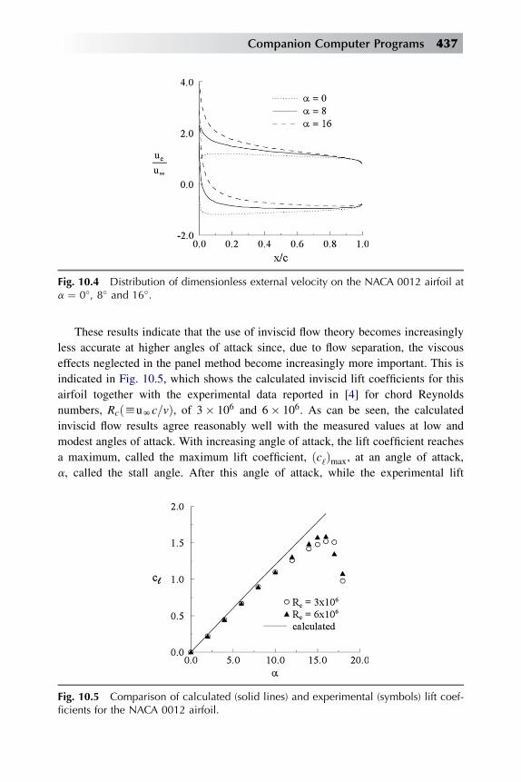
These results indicate that the use of inviscid flow theory becomes increasingly

less accurate at higher angles of attack since, due to flow separation, the viscous

effects neglected in the panel method become increasingly more important. This is

indicated in Fig. 10.5, which shows the calculated inviscid lift coefficients for this

airfoil together with the experimental data reported in [4] for chord Reynolds

numbers, RcðhuNc=vÞ, of 3� 106 and 6� 106. As can be seen, the calculated

inviscid flow results agree reasonably well with the measured values at low and

modest angles of attack. With increasing angle of attack, the lift coefficient reaches

a maximum, called the maximum lift coefficient, ðc‘Þmax, at an angle of attack,

a, called the stall angle. After this angle of attack, while the experimental lift

Fig. 10.4 Distribution of dimensionless external velocity on the NACA 0012 airfoil ata ¼ 0�, 8� and 16�.

Fig. 10.5 Comparison of calculated (solid lines) and experimental (symbols) lift coef-ficients for the NACA 0012 airfoil.


coefficients begin to decrease with increasing angle of attack, the calculated lift

coefficient, independent of Reynolds number, continuously increases with increasing

a. The lift curve slope is not influenced by Rc at low to modest angles of attack, but at

higher angles of attack it is influenced by Rc, thus making ðc‘Þmaxdependent upon Rc.

10.15.2 SAMPLE CALCULATIONS FOR THE INVERSE BOUNDARY-LAYER PROGRAM

This test case is again for the airfoil considered in the previous section. The

boundary-layer calculations are performed only for the upper surface, for laminar

and turbulent flows with transition location specified, at angles of attack of a ¼ 4�,8�, 12�, 14�, 16� and 17�. The airfoil coordinates, x=c, y=c are used to calculate the

surface distance. The calculations are done for a chord Reynolds number of

4� 106.

In practice, it is also necessary to calculate the transition location. Two practical

methods for this purpose are the Michel method and the en-method described, for

example, in [1, 5]. The former is based on a empirical correlation between two

Reynolds numbers based on momentum thickness, Rq, and surface distance Rx. It is

given by Eq. (10.15.1), also Eq. (5.3.22),

Rqtr ¼ 1:174

�1þ 22; 400

Rxtr

�R0:46xtr

(10.15.1)

where

Rq ¼ ueq

v; Rx ¼ uex

v

The accuracy of this method is comparable to the en-method at high Reynolds

number flows on airfoils. The en-method, which is based on the linear stability

theory, is, however, a general method applicable to incompressible and compressible

two- and three-dimensional flows. As discussed in [1, 2], for two-dimensional flows

at low Reynolds numbers, transition can occur inside separation bubble and can be

predicted only by the en-method. For details, see [1, 2].

While the boundary-layer calculations with this program can be performed for

standard and inverse problems, here they are performed for the standard problem,

postponing the application of the inverse method to the following section.

Here we present a sample of the input and output of the calculations. The

format of the inverse boundary-layer program is similar to the format of the

interactive code and is discussed in the following section. Figure 10.6 shows the

distribution of local skin friction coefficient, cf , and dimensionless displacement


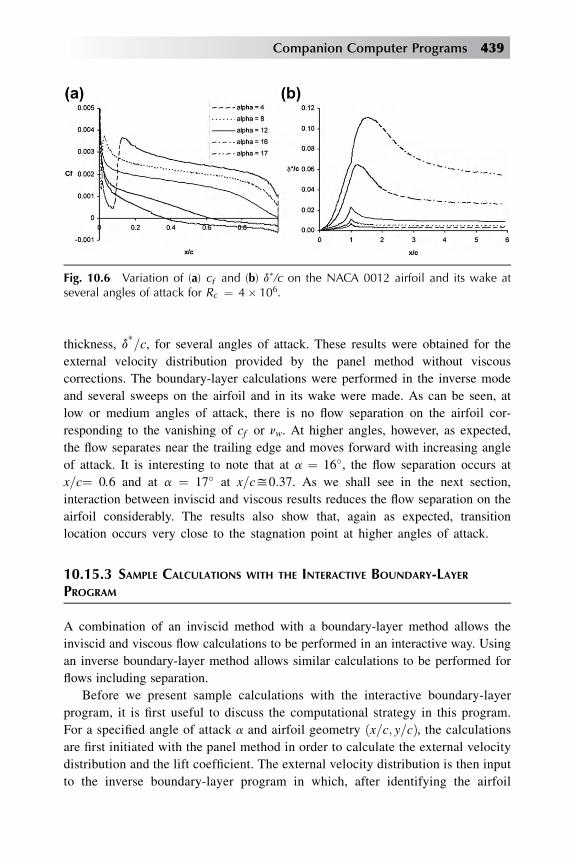
thickness, d*=c, for several angles of attack. These results were obtained for the

external velocity distribution provided by the panel method without viscous

corrections. The boundary-layer calculations were performed in the inverse mode

and several sweeps on the airfoil and in its wake were made. As can be seen, at

low or medium angles of attack, there is no flow separation on the airfoil cor-

responding to the vanishing of cf or nw. At higher angles, however, as expected,

the flow separates near the trailing edge and moves forward with increasing angle

of attack. It is interesting to note that at a ¼ 16�, the flow separation occurs at

x=c¼ 0.6 and at a ¼ 17� at x=cy0:37. As we shall see in the next section,

interaction between inviscid and viscous results reduces the flow separation on the

airfoil considerably. The results also show that, again as expected, transition

location occurs very close to the stagnation point at higher angles of attack.

10.15.3 SAMPLE CALCULATIONS WITH THE INTERACTIVE BOUNDARY-LAYERPROGRAM

A combination of an inviscid method with a boundary-layer method allows the

inviscid and viscous flow calculations to be performed in an interactive way. Using

an inverse boundary-layer method allows similar calculations to be performed for

flows including separation.

Before we present sample calculations with the interactive boundary-layer

program, it is first useful to discuss the computational strategy in this program.

For a specified angle of attack a and airfoil geometry ðx=c; y=cÞ, the calculations

are first initiated with the panel method in order to calculate the external velocity

distribution and the lift coefficient. The external velocity distribution is then input

to the inverse boundary-layer program in which, after identifying the airfoil

Fig. 10.6 Variation of (a) cf and (b) d*/c on the NACA 0012 airfoil and its wake atseveral angles of attack for Rc ¼ 4� 106.


stagnation point, the calculations are performed separately for the upper and

lower surfaces of the airfoil and in the wake. The calculations involve several

sweeps on the airfoil, one sweep corresponding to boundary-layer calculations

which start at the stagnation point and end at some specified x-location in the

wake. In sweeping through the boundary-layer, the right-hand side of Eq. (8.8.4)

uses the values of d* from the previous sweep when j > i and the values from the

current sweep when j < i. Thus, at each x-station the right-hand side of

Eq. (8.8.4) provides a prescribed value for the linear combination of ueðxiÞ and

d*ðxiÞ. After convergence of the Newton iterations at each station, the summations

of Eq. (8.8.4) are updated for the next x-station. Note that the Hilbert integral

coefficients Cij discussed in subsection 10.14.2 are computed and stored at the

start of the boundary-layer calculations.

At the completion of the boundary-layer sweeps on the airfoil and in the wake,

boundary-layer solutions are available on the airfoil and in the wake. The blowing

velocity on the airfoil viw [see Eqs. (8.7.4) and (8.7.5)] and a jump in the normal

velocity component Dvi in the wake [see Eq. (8.7.6)], for which an incompressible

flow are

viw ¼ d

dxðviwd*AÞ (10.15.2)

Dvi ¼ d

dxðuiud*uÞ þ d

dxðuild*‘ Þ (10.15.3)

are calculated and are used to obtain a new distribution of external velocity ueiðxÞfrom the inviscid method. As before, the onset of transition location is determined

from the laminar flow solutions and the boundary-layer calculations are performed

on the upper and lower surfaces of the airfoil and in the wake by making several

specified sweeps. This sequence of calculations is repeated for the whole flowfield

until convergence is achieved.

The format of the input to this interactive boundary-layer (inviscid/viscous)

program is similar to the input required for the inverse boundary-layer described in

subsection 10.14.1. The code is arranged in such a way that it is only necessary to

read in the airfoil geometry, the angles of attack to be calculated, Mach number and

chord Reynolds number. The rest of the input is done internally.

We now present sample calculations for the NACA0012 airfoil for Reynolds

numbers corresponding to 3� 106. In this case, transition locations are calculated

with Michel’s formula. The calculations and the results are given on the

companion site.

Lift, cl, drag, cd, pitching moment, Cm, coefficients for Rc ¼ 3� 106 are

shown in Table 10.1 for a ¼ 2� to 16.5� and MN ¼ 0.1 together with lift

coefficients calculated with the panel method. As can be seen, while at low and


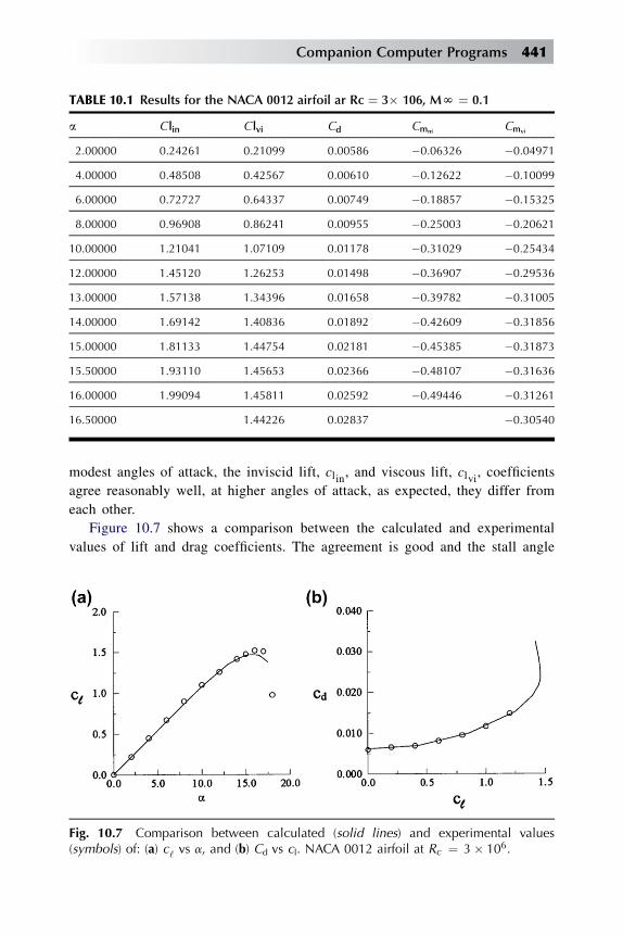
modest angles of attack, the inviscid lift, clin, and viscous lift, clvi, coefficients

agree reasonably well, at higher angles of attack, as expected, they differ from

each other.

Figure 10.7 shows a comparison between the calculated and experimental

values of lift and drag coefficients. The agreement is good and the stall angle

TABLE 10.1 Results for the NACA 0012 airfoil ar Rc ¼ 3� 106, MN ¼ 0.1

a C lin C lvi Cd CmniCmvi

2.00000 0.24261 0.21099 0.00586 �0.06326 �0.04971

4.00000 0.48508 0.42567 0.00610 �0.12622 �0.10099

6.00000 0.72727 0.64337 0.00749 �0.18857 �0.15325

8.00000 0.96908 0.86241 0.00955 �0.25003 �0.20621

10.00000 1.21041 1.07109 0.01178 �0.31029 �0.25434

12.00000 1.45120 1.26253 0.01498 �0.36907 �0.29536

13.00000 1.57138 1.34396 0.01658 �0.39782 �0.31005

14.00000 1.69142 1.40836 0.01892 �0.42609 �0.31856

15.00000 1.81133 1.44754 0.02181 �0.45385 �0.31873

15.50000 1.93110 1.45653 0.02366 �0.48107 �0.31636

16.00000 1.99094 1.45811 0.02592 �0.49446 �0.31261

16.50000 1.44226 0.02837 �0.30540

Fig. 10.7 Comparison between calculated (solid lines) and experimental values(symbols) of: (a) c‘ vs a, and (b) Cd vs cl. NACA 0012 airfoil at Rc ¼ 3� 106.


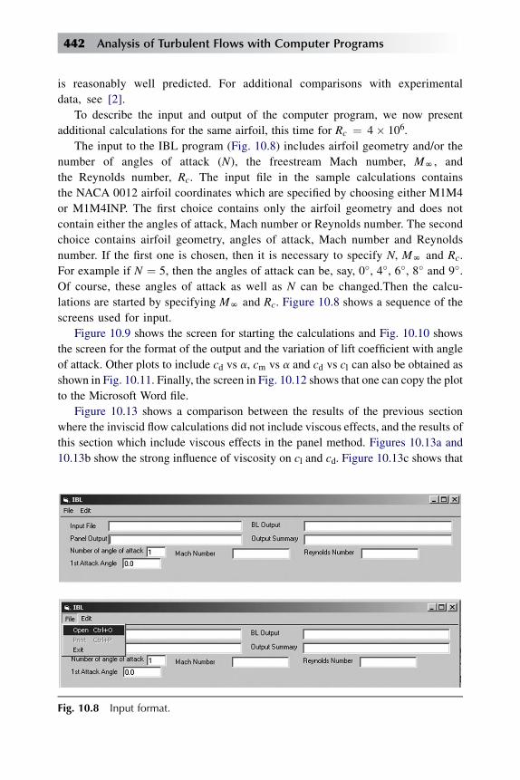
is reasonably well predicted. For additional comparisons with experimental

data, see [2].

To describe the input and output of the computer program, we now present

additional calculations for the same airfoil, this time for Rc ¼ 4� 106.

The input to the IBL program (Fig. 10.8) includes airfoil geometry and/or the

number of angles of attack (N), the freestream Mach number, MN, and

the Reynolds number, Rc. The input file in the sample calculations contains

the NACA 0012 airfoil coordinates which are specified by choosing either M1M4

or M1M4INP. The first choice contains only the airfoil geometry and does not

contain either the angles of attack, Mach number or Reynolds number. The second

choice contains airfoil geometry, angles of attack, Mach number and Reynolds

number. If the first one is chosen, then it is necessary to specify N, MN and Rc.

For example if N ¼ 5, then the angles of attack can be, say, 0�, 4�, 6�, 8� and 9�.Of course, these angles of attack as well as N can be changed.Then the calcu-

lations are started by specifying MN and Rc. Figure 10.8 shows a sequence of the

screens used for input.

Figure 10.9 shows the screen for starting the calculations and Fig. 10.10 shows

the screen for the format of the output and the variation of lift coefficient with angle

of attack. Other plots to include cd vs a, cm vs a and cd vs cl can also be obtained as

shown in Fig. 10.11. Finally, the screen in Fig. 10.12 shows that one can copy the plot

to the Microsoft Word file.

Figure 10.13 shows a comparison between the results of the previous section

where the inviscid flow calculations did not include viscous effects, and the results of

this section which include viscous effects in the panel method. Figures 10.13a and

10.13b show the strong influence of viscosity on cl and cd. Figure 10.13c shows that

Fig. 10.8 Input format.


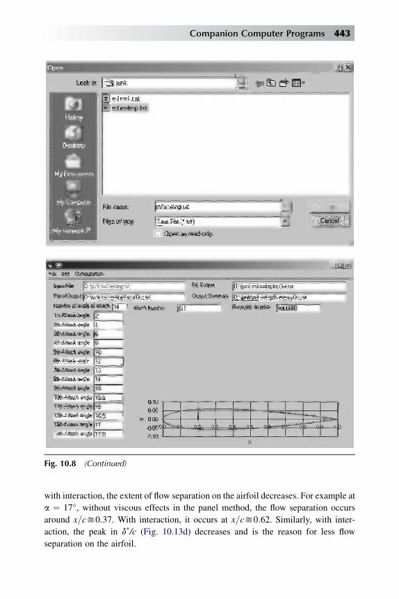
with interaction, the extent of flow separation on the airfoil decreases. For example at

a ¼ 17�, without viscous effects in the panel method, the flow separation occurs

around x=cy0:37. With interaction, it occurs at x=cy0:62. Similarly, with inter-

action, the peak in d*/c (Fig. 10.13d) decreases and is the reason for less flow

separation on the airfoil.

Fig. 10.8 (Continued)


Fig. 10.9 Beginning of calculations.

Fig. 10.10 Output format.


Fig. 10.11 Calculated results for the NACA0012 airfoil, Rc ¼ 4� 106, MN ¼ 0.1.(a) cd vs a, (b) cm vs a.

Fig. 10.12 Instruction for copying plots.


References

[1] T. Cebeci, J. Cousteix, Modeling and Computation of Boundary-Layer Flows, Horizons Pub. Long

Beach, Calif. and Springer, Heidelberg, Germany, 1998.

[2] M.J. Lighthill, ‘‘On Displacement Thickness’’, J. Fluid Mech. vol. 4 (1958) 383.

[3] R.C. Lock, M.C.P. Firmin, ‘‘Survey of Techniques for Estimating Viscous Effects in External

Aerodynamics’’, Royal Aircraft Establishment Tech Memo, AERO (1981) 1900.

[4] N.N. Mansour, J. Kim, P. Moin, Near-Wall k-ε Turbulence Modeling, J. AIAA 27 (1989) 1068–1073.

[5] T. Cebeci, An Engineering Approach to the Calculation of Aerodynamic Flows, Horizons Pub., Long

Beach, Calif., and Springer, Heidelberg, Germany, 1999.

[6] D. Coles, E. A. Hirst, Computation of Turbulent Boundary Layers – 1968 AFOSR-IFP-Stanford

Conference, vol. 2, Thermosciences Division, Stanford University, Stanford, Calif., 1969.

[7] J.H. Abbott, A.E. von Doenhoff, Theory of Wing Sections, Dover, 1959.

Fig. 10.13 Comparison of results between the inverse boundary-layer method and theinteractive method. (a) cl vs a, (b) cd vs a, (c) cf vs x/c, (d) d*/c vs x/c.


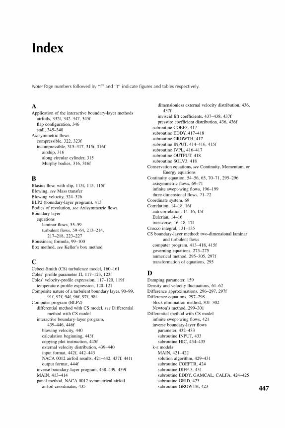
Index

Note: Page numbers followed by ‘‘f’’ and ‘‘t’’ indicate figures and tables respectively.

AApplication of the interactive boundary-layer methods

airfoils, 332f, 342–347, 345fflap configuration, 346stall, 345–348

Axisymmetric flowscompressible, 322, 323fincompressible, 315–317, 315t, 316f

airship, 316along circular cylinder, 315Murphy bodies, 316, 316f

BBlasius flow, with slip, 113f, 115, 115fBlowing, see Mass transferBlowing velocity, 324–326BLP2 (boundary-layer program), 413Bodies of revolution, see Axisymmetric flowsBoundary layer

equationslaminar flows, 55–59turbulent flows, 59–64, 213–214,

217–218, 223–227Boussinesq formula, 99–100Box method, see Keller’s box method

CCebeci-Smith (CS) turbulence model, 160–161Coles’ profile parameter P, 117–123, 123fColes’ velocity-profile expression, 117–120, 119f

temperature-profile expression, 120–121Composite nature of a turbulent boundary layer, 90–99,

91f, 92f, 94f, 96f, 97f, 98fComputer program (BLP2)

differential method with CS model, see Differentialmethod with CS model

interactive boundary-layer program,439–446, 446f

blowing velocity, 440calculation beginning, 443fcopying plot instruction, 445fexternal velocity distribution, 439–440input format, 442f, 442–443NACA 0012 airfoil results, 421–442, 437f, 441toutput format, 444f

inverse boundary-layer program, 438–439, 439fMAIN, 413–414panel method, NACA 0012 symmetrical airfoil

airfoil coordinates, 435

dimensionless external velocity distribution, 436,437f

inviscid lift coefficients, 437–438, 437fpressure coefficient distribution, 436, 436f

subroutine COEF3, 417subroutine EDDY, 417–418subroutine GROWTH, 417subroutine INPUT, 414–416, 415fsubroutine IVPL, 416–417subroutine OUTPUT, 418subroutine SOLV3, 418

Conservation equations, see Continuity, Momentum, orEnergy equations

Continuity equation, 54–56, 65, 70–71, 295–296axisymmetric flows, 69–71infinite swept-wing flows, 196–199three-dimensional flows, 71–72

Coordinate system, 69Correlation, 14–18, 16f

autocorrelation, 14–16, 15fEulerian, 14–16transverse, 16–18, 17f

Crocco integral, 131–135CS boundary-layer method: two-dimensional laminar

and turbulent flowscomputer program, 413–418, 415fgoverning equations, 273–275numerical method, 295–305, 297ftransformation of equations, 295

DDamping parameter, 159Density and velocity fluctuations, 61–62Difference approximations, 296–297, 297fDifference equations, 297–298

block elimination method, 301–302Newton’s method, 299–301

Differential method with CS modelinfinite swept-wing flows, 421inverse boundary-layer flows

parameter, 432–433subroutine INPUT, 433subroutine HIC, 434–435

k-3 modelsMAIN, 421–422solution algorithm, 429–431subroutine COEFTR, 424subroutine DIFF-3, 431subroutine EDDY, GAMCAL, CALFA, 424–425subroutine GRID, 423subroutine GROWTH, 423 447

Differential method with CS model (Continued )subroutine INPUT, 422–423subroutine INTRP3, 431subroutine IVPT, 423subroutine KECOEF, KEPARM, KEDEF and

KEDAMP, 425–427subroutine KEINITG, 428subroutine KEINITK, 427–428subroutine KESOLV, 428subroutine KEWALL, 428subroutine LNTP, 431subroutine OUTPUT, 423subroutine SOLV3, 424test cases, 429, 430f

two-dimensional laminar and turbulent flows,413–418

two-dimensional flows with heat transfer, 420–421Differential method for a plane jet, 432Differential methods

k-3 model, 371–375transport-equation, 358zonal method, 358–370

Diffusive nature of turbulence, see TurbulenceDirect numerical simulation (DNS), 48, 156Dissipation integral coefficient, 80–81Drag

airfoils, 332f, 342–347, 345f

EEckert number, 67–69Eddy viscosity, see Transport coefficientsEnergy equations, 41–42, 54–56, 66, 392–393

axisymmetric flows, 70infinite swept-wing flows, 411three-dimensional flows, 71–72

Energy spectrum, 19–22, 20fFourier transform, 20–21

Entrainment function, 259–262Entrainment velocity, 259–260Equilibrium boundary layers, 116–117, 311, 311fEvaluation of turbulence models

CS model, 295–305transport equation models, 378–392,

379f–382f, 384f–392f

FFalkner–Skan transformation, 296, 326–327Free-shear flows, 268–280, 268f, 273f, 277f, 278f, 281t,

379–384, 379f, 381f, 382f, 384f, 392fFriction temperature, 93Friction velocity, 92–93

HHagen-Poiseuille flow, 4–5Heat-transfer formulas, 243–248Hess–Smith panel method (HSPM)

airfoil coordinates, 333airfoil surface and notation, 333, 334fboundary points, 334coefficient matrix, 339flowfield calculation, 342–344

Gaussian elimination method, 340Kutta condition, 337–340Laplace equation, 336potential vortex, 335viscous effects, 340–342

MAIN, 418–419subroutine CLCM, 420subroutine COEF, 419subroutine GAUSS, 419subroutine OBKUTA, 419subroutine VPDIS, 419–420subroutine VPDWK, 420

IInner region, 109–111, 110f, 111f, 112fIntegral equations of the boundary layer, 78Integral methods, 257–263, 258f–259f, 412–413

Ambrok’s method, 263computer program for Ambrok’s method, 413computer program for Head’s method, 412–413computer program for Smith–Spalding method,

412computer program for Thwaites’ method, 412Green’s ‘‘lag-entrainment’’ method, 261–262Head’s method, 259–260Truckenbrodt’s method, 262

Intensity of turbulence, 11–14Interaction problem, 324–326, 325f

blowing/suction velocity, 324–325displacement surface, 324interactive boundary-layer scheme, 326fKutta condition, 337–340

Interactive boundary-layer theory, 324, 326f, 344Intermittency

edge, 22, 102–103effect on exterior, inviscid stream, 23in transition, 168–169

Intermittency factor, 103

Kk-3 model, 215–221, 220tk-u model, 221–223

SST model equations, 375–378Keller’s box method

difference approximations, 296–297, 297fmomentum equation, 295–296

Kinetic energy balance, 95Kinetic energy of turbulence, 13–14Kolmogorov scale, 10–11

LLarge eddy simulation, 48Law of the wake, 117–118Law of the wall, 92–93, 117–118Ludwieg–Tillmann law, 260

MMangler transformation, 85–87Mass transfer flows

flat plate, 320, 320fheat transfer, 319

448 Index

law of the wall, 129–130compressible, 135–139

pressure gradient effects, 320, 320fvelocity-defect law, 130–131

Mass-weighted averaging, 35–39relation to time averaging, 39–41

Matrix solver algorithm, 302, 429–431Mean-kinetic-energy equation, 42–44, 73–74, 95Mean-velocity and temperature distributions

incompressible flowsporous surfaces, 129–130rough surfaces, 123–129, 125f, 126f, 128fsmooth surfaces, 104–123, 106f,

110f–113f, 115f, 117f, 119f, 123fcompressible flows, 135–145, 146feffect of pressure gradient, 145–146

Mixing layer, 273–280, 273f, 277f, 278fMixing length

concepts, 99–104, 102f, 103f, 104fformulas, 156–160

Momentum equation, 295–296axisymmetric flows, 70infinite swept-wing flows, 350three-dimensional flows, 71

Momentum integral equation, 79–80, 259–260

NNavier–Stokes equations, 34–35

Nusselt number, 192–193Newton’s method, 299–301Numerical solution, 295

box method, 296–297transformed equations, 296

Numerical solution of the boundary-layer equationswith algebraic turbulence models, 295

block elimination method, 301–302Falkner–Skan transformation, 296finite difference approximation, 297–298linear system, 299Newton’s method, 299–301numerical formulation, 297–299similarity variables, 296

Numerical solution of the boundary-layer equationswith transport-equation turbulence models,358

k-3 model equations with and without wall functions,371

solution with wall functions, 374–375solution without wall functions, 371–374

zonal method for k-3 model, 358–360solution procedure, 360–370

OOrder-of-magnitude analysis, 48

laminar flows, 35turbulent flows, 49–50

Outer region, 112–115, 113f, 115f

PPanel method, viscous effectsPeclet number, 192–193

Pipe flow, 4–5, 4fPower law assumptions, 242Power laws for similar free shear layers, 280, 281tPrandtl number

Cebeci’s model, 189–190, 192–194Jenkin’s formula, 186–187turbulent, 185–194, 186f, 187f, 190f, 191f, 192f, 193f

Pressure gradient flows, 310equilibrium flows, 311, 311fnonequilibrium flows, 311–312, 312fseparating flows, 311–312, 312fstreamlined body, boundary layout, 310–311, 310fthermal boundary layers, 312, 313f

Pressure gradient parameter, 116, 296–297

RRandom motion, theory of, 23–25Recovery factor, 133–135, 134fReynolds analogy, 255, 255fReynolds stresses, 27–28, 41Reynolds-stress transport equations, 44–48, 74–78Roughness

shift parameter, 127–128spaced, 125–127uniform, 124–125

SSeparation

prediction of, 264–268, 266f, 267f, 322–325, 325fStratford method, 264–266, 268

Shape factorflat plate, 260

Shear-stress distribution, 121–123, 123fShort-cut methods

free shear flows, 268–280, 268f, 273f, 277f,278f, 281t

prediction of flow separation, 264–268, 266f–267fpressure gradient, 257–263zero-pressure gradient

compressible, 250–255, 253f, 254f, 255fincompressible, 239–248, 241f, 245f

Similarity solutions of turbulent free shear flows,268

mixing layer, 273–280, 273f, 277f, 278ftwo-dimensional jet, 268–273, 268f

Skin-friction formulascompressible, 250–255, 253f, 254f, 255fpower law, 241–243rough plate, 248–250, 249f, 250f, 251fsmooth plate, 239–241, 241fVan Driest, 250–253, 253f–254f

Spectrum, see Energy spectrumStanton number, 243–248Subroutine COEF3, 417Subroutine COEFTR, 424Subroutine DIFF-3, 431Subroutine EDDY, 417–418

GAMCAL, CALFA, 424–425Subroutine GRID, 423Subroutine GROWTH, 417, 423Subroutine INPUT, 409f, 414–416, 422–423Subroutine INTRP3, 431

Index 449

Subroutine IVPL, 416–417initial velocity profiles, 432

Subroutine IVPT, 423, 432Subroutine KECOEF, KEPARM, KEDEF and

KEDAMP, 425–427Subroutine KEINITG, 428Subroutine KEINITK, 427–428Subroutine KESOLV, 428Subroutine KEWALL, 428Subroutine LNTP, 431Subroutine OUTPUT, 418, 423Subroutine SOLV2 and SOLV4, 432Subroutine SOLV3, 418, 424Suction, see Mass transfer flows

TTaylor’s hypothesis, 16Temperature distribution, 133–134Temperature and velocity fluctuations, 59, 60fThermal boundary layers, 312Thwaites’ method, 412Time averaging, 35–39Transformed equations, 296, 359–360Transpiration, see Mass transfer flowsTransport coefficients

eddy conductivity, 100–101, 185–186eddy viscosity, 25, 99–101, 156–160effect of low Reynolds number, 161–165, 163f,

164f, 164teffect of natural transition, 168–172, 169t, 170f,

171f, 172feffect of roughness, 172–175, 174f–175feffect of streamwise curvature, 166–168, 167feffect of transverse curvature, 165–166, 166fmixing length, 99–101recommendations, 203

Transition length, 168–172, 169t, 170f, 171f, 172fTruckenbrodt formulas, 262Turbulence

continuum hypothesis, 8–11convection, 97decay of, 18–19, 22definition, 3diffusion, 97diffusive nature of, 23–26, 26tdissipation, 96–97integral scale, 16–18, 20–21microscale, 16–18, 20–21minimum Reynolds number for, 7miscellaneous properties, 3–7, 4f, 5f, 6forigin of name, 3production, 97Reynolds number of, 18–19shear-stress work, 97

Turbulence modelseddy viscosity, 156–175, 194–203, 197f, 199f, 200f,

201f, 202finverse mode

Falkner–Skan transformation, 326–327

Hilbert integral, 324–327numerical formulation, 328–333, 332f

mixing length, 156–175one-equation

Bradshaw, 227–228, 228fSpalart–Allmaras, 228–230

stress transport, 230–233two-equation

k-3, 215–221, 220tk-u, 221–223SST, 224–226

Turbulence simulation, 26–29Turbulent boundary layer

buffer layer, 93fully-turbulent region, 93outer region, 94viscous sublayer, 93

Turbulent energy equation, see Turbulent-kinetic-energy equation

Turbulent energy integral equation, 81–82Turbulent-kinetic-energy equation, 45–47,

75–78meanings of terms, 45–47

Two-dimensional compressible flows, 317–322flat plate, 320, 320fheat transfer, 319, 319fmass transfer, 320, 320fpressure gradient, 320–322, 321f

Two-dimensional incompressible flowsequilibrium flows, 311flat plate, 305, 306fflat plate, mass transfer, 307–309heat transfer, 309nonequilibrium flows, 311–312, 312fpressure gradient, 310separation, 311–312, 312fthermal boundary layers, 312

UUseful subroutines, 405–406

subroutine IVPT, 432subroutine SOLV2 and SOLV4, 432

VVan Driest mixing length, 159–161

Cebeci’s extension, 160–175, 163f, 164f, 164t,166f–167f, 169t, 170f–172f, 174f–175f

Variable grid system, 414Velocity defect law, 94Velocity distribution, see Mean velocity distributionVelocity profiles

instantaneous, 5–6, 6fpower-law, 241–243transitional, 170–171

WWake flows, 331–333, 332fWake, law of the, see Coles’ profile parameter, PWakes, 7, 9f, 22

450 Index

Analysis of Turbulent Flows with Computer Programs

Documents

Transcript of Analysis of Turbulent Flows with Computer Programs