arX

iv:n

lin/0

4050

22v1

[nl

in.C

D]

11

May

200

4

The Polymer Stress Tensor in Turbulent Shear Flows

Victor S. L’vov, Anna Pomyalov, Itamar Procaccia and Vasil TiberkevichDepartment of Chemical Physics, The Weizmann Institute of Science, Rehovot 76100, Israel

The interaction of polymers with turbulent shear flows is examined. We focus on the structureof the elastic stress tensor, which is proportional to the polymer conformation tensor. We examinethis object in turbulent flows of increasing complexity. First is isotropic turbulence, then anisotropic(but homogenous) shear turbulence and finally wall bounded turbulence. The main result of thispaper is that for all these flows the polymer stress tensor attains a universal structure in the limitof large Deborah number De ≫ 1. We present analytic results for the suppression of the coil-stretchtransition at large Deborah numbers. Above the transition the turbulent velocity fluctuations arestrongly correlated with the polymer’s elongation: there appear high-quality “hydro-elastic” wavesin which turbulent kinetic energy turns into polymer potential energy and vice versa. These wavesdetermine the trace of the elastic stress tensor but practically do not modify its universal structure.We demonstrate that the influence of the polymers on the balance of energy and momentum canbe accurately described by an effective polymer viscosity that is proportional to to the cross-streamcomponent of the elastic stress tensor. This component is smaller than the stream-wise componentby a factor proportional to De2. Finally we tie our results to wall bounded turbulence and clarifysome puzzling facts observed in the problem of drag reduction by polymers.

I. INTRODUCTION

The dynamics of dilute polymers in turbulent flows isa rich subject, combining the complexities of polymerphysics and of turbulence. Besides fundamental ques-tions there is a significant practical interest in the sub-ject, particularly because of the dramatic effect of dragreduction in wall bounded turbulent flows [1–4]. On theone hand the polymer additives provide a channel of dis-sipation in addition to the Newtonian viscosity; this hadbeen stressed in the past mainly by Lumley [5, 6]. Onthe other hand the polymers can store energy in the formof elastic energy; this aspect had been stressed for exam-ple by Tabor and De Gennes [7]. A better understandingof the relative roles of these aspects requires a detailedanalysis of the dynamics of the “complex fluid” obtainedwith dilute polymers in the turbulent flow regime.

Some important progress in the theoretical descriptionof the statistics of polymer stretching in homogeneous,isotropic turbulence of dilute polymer solutions was of-fered in Refs. [8–10]. Here we want to stress the factthat in the practically interesting turbulent regimes, andin particular when there exists a large drag reduction ef-fect, the characteristic mean velocity gradient (say, themean shear, S0), is much larger than the inverse polymerrelaxation time, τp, S0τp ≫ 1. Usually this parameter isreferred to as the Deborah or Weissenberg number:

De ≡ Wi ≡ S0τp . (1.1)

Indeed, the onset of drag reduction corresponds toReynolds number Recr at which De ∼ 1. Large dragreduction corresponds to Re ≫ Recr at which De ≃Re/Recr ≫ 1.

The aim of this paper is to provide a theory of the poly-mer stress tensor Π [defined in Eq. (2.1b)] in turbulentflows in which De ≫ 1. The main result is a relativelysimple form (1.2a) of the mean polymer stress tensor Π0

that enjoys a high degree of universality. Denoting by

x and y the unit vectors in the mean velocity and meanvelocity gradient directions (streamwise and cross-streamdirections in a channel geometry) and by z = x × y thespan-wise direction, we show that tensor Π0 has a uni-versal form:

Π0 ≃ Πyy0

2De2 De 0De 1 00 0 C

for De ≫ 1 . (1.2a)

One sees that in the (x-y)-plane the tensorial structureof Π0 is independent of the statistics of turbulence:

Πxx0 = 2De2Πyy

0 , Πxy0 = Πyx

0 = De Πyy0 . (1.2b)

Due to the to the symmetry of the considered flows withrespect to reflection z → −z, the off-diagonal compo-nents Πxz

0 and Πyz0 vanish identically:

Πxz0 = Πyz

0 = 0 . (1.2c)

The only non-universal entry in Eq. (1.2a) is the dimen-sionless coefficient C. We show that C = 1 for shearflows in which the extension of the polymers is caused bytemperature fluctuations and/or by isotropic turbulence.For anisotropic turbulence the constant C is of the orderof unity.

The universal tensorial structure (1.2) has importantconsequences for the problem of drag reduction in dilutepolymeric solutions. We show that the effect of the poly-mers on the balance of energy and mechanical momentumcan be described by an effective polymer viscosity that isproportional to the cross-stream component of the elasticstress tensor Πyy

0 . According to Eq. (1.2b) this compo-nent is smaller than the stream-wise component Πxx

0 bya factor of 2De2. This finding resolves the puzzle of thelinear increase of the effective polymeric viscosity withthe distance from the wall, while the total elongation ofthe polymers [dominated by the largest component Πxx

0

of the tensor (1.2a)] decreases with the distance from the

2

wall. We show that our results for the profiles of thecomponents Πij

0 are in a good agreement with DNS ofthe FENE-P model in turbulent channel flows.

The paper is organized as follows. In Sec. II A wepresent the basic equations of motion of the problem.In Sec. II B we describe the standard Reynolds decom-position of the equations of motion for the mean andfluctuations of the relevant variables. In Sec. II C we findgeneral solution for Π0 and formulate (the very weak)conditions at which it simplifies to the universal form(1.2).

In Section III we analyze the phenomenon of polymerstretching in shear flows with prescribed turbulent ve-locity fields, either isotropic, Sec. III B, or anisotropic,Sec. III C. We relate the value of C to the level ofanisotropy in the turbulent flow. We also show in thissection that a strong mean shear suppresses the thresh-old value for the coil-stretched transition by a factor De2,see Eqs. (3.10).

Sections IV and V are devoted to the case of strong tur-bulent fluctuations for which the fluctuating velocity andpolymeric fields are strongly correlated. In Sec. IV weconsider the case of homogeneous shear flows. In Sec. Vwe discuss wall bounded turbulence in a channel geom-etry, compare our results with available DNS data andapply our finding to the problem of drag reduction bypolymeric solutions.

Section VI presents summary and a discussion of theobtained results .

Appendix A offers some useful exact relationships forthe energy balance in the system.

II. EQUATIONS OF MOTION AND SOLUTION

FOR SIMPLE FLOWS

A. Equations of motion for dilute polymer

solutions

a. The equation for the velocity field of the complex

fluid reads:

∂ V

∂t+ (V · ∇)V = ν0∆V − ∇P + ∇ · Π ,

∇ · V = 0 . (2.1a)

Here V ≡ V (t, r), P ≡ P (t, r) and ν0 are the fluid ve-locity, the pressure, and Newtonian viscosity of the neatfluid respectively. The fluid is considered incompressible,and units are chosen such that the density is 1. The ef-fect of the added polymer appears in Eq. (2.1a) via theelastic stress tensor Π ≡ Π(t, r).

In this paper we consider dilute polymers in the limitthat their extension due to interaction with the fluidis small compared with their chemical length. In thisregime one can safely assume that the polymer extensionis proportional to the applied force (Hook’s law). Wesimplify the description of the polymer dynamics assum-ing that the relaxation to equilibrium is characterized by

a single relaxation time τp, which is constant at smallextensions. In this case Π can be written as

Π(t, r) ≡ ν0p

τp

R(t, r)R(t, r) , (2.1b)

where ν0p is polymeric viscosity for infinitesimal shear,and R is the polymer end-to-end elongation vector, nor-malized by its equilibrium value (in equilibrium RR =δ). The average in Eq. (2.1b) is over the Gaussian statis-tics of the Langevin random force which describes theinteraction of the polymer molecules with the solventmolecules at a given temprature, but not over the tur-bulent ensemble.

b. The equation for the elastic stress tensor Π hasthe form

∂ Π

∂t+ (V · ∇)Π = S · Π + Π · ST − 1

τp

(Π− Πeq) ,

S ≡ (∇V )T

, Sij = ∂V i/∂xj , (2.1c)

Πeq = Πeqδ , Πeq ≡ ν0p/τp .

Here S ≡ S(t, r) is the velocity gradient tensor and δ isunit tensor.

c. Choice of coordinates. In this paper we considerboth homogeneous and wall bounded shear flows. In bothcases we choose the coordinates such that the mean ve-locity is in the x direction and the gradient is in the y

direction. In wall bounded flows x and y are unit vectorsin the streamwise and the wall normal directions:

V0 ≡ 〈V 〉 = S0 · r , S0 ≡ S0 xy , (2.2)

only V x0 = S0 y 6= 0 and Sxy

0 = S0 6= 0 .

The unit vector orthogonal to x and y (the span-wisedirection in wall bounded cases) is denoted as z.

B. Reynolds decomposition of the basic equations

In the following we need to consider separately themean values and the fluctuating parts of the velocity,V (r, t), the velocity gradient S(r, t), and the elasticstress tensor Π(r, t) fields. We define the fluctuatingparts via

V = V0 + v , S = S0 + s , Π = Π0 + π , . . . (2.3)

All the mean quantities will be denoted with a “0” sub-script (e.g. the mean velocity V0), and all the fluctuatingquantities by the lower-case letters v, p, π, s, etc. Thesemean values are computed with respect to the appropri-ate turbulent ensemble. Note that the mean pressurein a homogeneous shear flow is zero, P0 = 0, and allmean quantities (except the mean velocity V x

0 = S0 y,of course) are coordinate independent and, by definition,time independent.

3

1. Equations for the mean objects

a. The equation for the mean elastic stress tensor

Π0 follows from Eq. (2.1c):(

D

D t+

1

τp

)Π0 = S0 · Π0 + Π0 · ST

0 + Q , (2.4a)

Q ≡ 1

τp

Πeq + QT , (2.4b)

QT ≡ 〈s · π + π · sT〉 , (2.4c)

where Πeq is given by Eq. (2.1c), and 〈· · · 〉 denotes anaverage with respect to the turbulent ensemble. In com-ponents:

( D

D t+

1

τp

)Πij

0 = Sik0 Πkj

0 + Sjk0 Πki

0 + Qij ,

Qij =1

τp

Πeqδij +

⟨sikπkj + sjkπki

⟩. (2.4d)

Here D/Dt is the mean substantial time derivative

D

D t≡ ∂

∂t+ V0 · ∇ =

∂

∂t+ S0 y

∂

∂x. (2.5)

The substantial derivative vanishes in the stationary case,when all the statistical objects are t- and x-independent.

b. The equation for the mean velocity follows fromEq. (2.1a):

∂V0

∂t=

∂

∂y[ν0S0 − W xy + Πxy

0 ] , (2.6)

were W is the Reynolds stress tensor:

W ij ≡⟨vivj

⟩. (2.7)

In the stationary case ∂V0/∂t = 0 and Eq. (2.6) gives

ν0S0 − W xy + Πxy0 = P , (2.8)

where constant of integration P has a physical meaningof the total momentum flux. The three terms on the LHSof Eq. (2.8) describe the viscous, inertial and polymericcontributions to P . In a homogeneous-shear geometryall theses terms are y-independent constants, whereas ina channel geometry they depend on the distance to thewall. Notice, that Eq. (2.8) also can be considered as anequation for the balance of mechanical forces in the flow.

2. Equations for the fluctuations

The equations for the fluctuating parts v and π read:

D v

D t= −S0 · v + ν0∆v − ∇p + ∇ · (π − vv) ,

(2.9a)(D

D t+

1

τp

)π = S0 · π + π · ST

0 + s · Π0 + Π0 · sT

+ Φπ , (2.9b)

where ∇ · v = 0, and

Φπ ≡ (s · π + π · sT) − ∇ · vπ . (2.9c)

Here (. . . ) denotes the “fluctuating part of” (. . . ).

C. Solutions for simple flow configurations

1. Implicit solution for shear flows

Note that the mean shear tensor S0 satisfies, besidesthe incompressibility condition Tr S0 = Sii

0 = 0, oneadditional constraint

Sij0 Sjk

0 = 0 . (2.10)

Remarkably, this property of S0 uniquely distinguishesshear flows from other possibilities (elongational or ro-tational flows): if (2.10) holds, one can always choosecoordinates such that the only nonzero component of S0

is Sxy0 = S0.

Having Eq. (2.10) consider Eq. (2.4a) in the stationarystate:

Π0 = τp (S0 ·Π0 + Π0 · ST

0 + Q) . (2.11)

We can proceed to solve this equation implicitly, treat-ing Q on the RHS as a given tensor, and solve the lin-ear set of equation for Π0. In the considered geometryEq. (2.11) is a system of 4 linear equations, and the so-lution is expected to be quite cumbersome. However,property (2.10) allows a very elegant solution of this sys-tem. Using (2.11) iteratively (i.e., substituting instead ofΠ0 on the RHS of Eq. (2.11) the whole RHS), we get

Π0 = 2τ2pS0 · Π0 · ST

0 + τ2p (S0 · Q + Q · ST

0 ) + τpQ

+τ2p

(S2

0 · Q + Q ·(S2

0

)T

).

One sees that due to Eq. (2.10) the last term in thisequation vanishes. Repeating this procedure once again,we obtain the exact solution of (2.11) in the form of afinite (quadratic) polynomial of the tensor S0:

Π0 = 2 τ3p S0 · Q · ST

0 + τ2p (S0 · Q + Q · ST

0 ) + τpQ .(2.12a)

The individual components of the solution Eq. (2.12a)are given by:

Πxx0 = τp

(2De2 Qyy + 2De Qxy + Qxx

),

Πxy0 = τp (De Qyy + Qxy) , (2.12b)

Πyy0 = τpQyy , Πzz

0 = τpQzz ,

Πxz0 = Πyz

0 = 0 .

Notice that the xz and yz components of Π0 vanish dueto the symmetry of reflection z → −z, which remainsrelevant in all the flow configurations addressed in thispaper.

4

In the limit De ≫ 1 the tensorial structure (2.12b) canbe simplified to the form (1.2) if

Qxy ≪ De Qyy , Qxx ≪ De2 Qyy . (2.13)

Indeed, in this case one can neglect the last two termsin Πxx

0 and the second term in Πxy0 and obtain Eq. (1.2)

with C = Qzz/Qyy.

2. Explicit solution for laminar homogeneous shear flows

The solution (2.12) allows further simplification in thecase of laminar shear flow, in which QT of Eq. (2.4c)vanishes, QT = 0, and thus, according to Eqs. (2.4b) and(2.1c), the tensor Q becomes proportional to the unittensor:

Qij =Πeq

τp

δij . (2.14)

With this relationship Eq. (2.12a) simplifies to

Π0 = Πeq

2De2 + 1 De 0De 1 00 0 1

. (2.15)

Equation (2.15), in which Πeq is given by Eq. (2.1c),is important in itself as an explicit solution for Π0 in thecase of laminar shear flow. But more importantly, thisequation together with Eq. (2.12) gives a hint regard-ing the tensorial structure of Π0 even in the presenceof turbulence, when the coupling between the velocityand the polymeric elongation field, leading to the cross-correlation QT, cannot be neglected.

To see why the simple result (2.15) may be relevantalso for the turbulent case, note first that the non-diagonal elements with z projection, i.e. Πxz

0 and Πyz0 ,

are identically zero in general as long as the symmetryz → −z prevails. Second, for large Deborah numbers,De ≫ 1, the nonzero components in both Eqs. (2.15)and (2.12b) have three different orders of magnitude:Πxx

0 ≫ Πxy0 ≫ Πyy

0 ≃ Πzz . In other words, the tensor Π0

is strongly anisotropic, reflecting a strong preferential ori-entation of the stretched polymers along the stream-wisedirection x. The characteristic deviation angle (from thex direction) is of order O(1/De).

Notice that Eqs. (2.12) relate the polymeric stress ten-sor Π0 to the cross-correlation tensor QT, Eq. (2.4c). Inits turn this tensor depends on the polymeric stretch-ing, which is described by the same tensor Π0. There-fore, generally speaking, Eqs. (2.12) remains an im-

plicit solution of the problem, which in general requiresconsiderable further analysis. However, as we discussedabove, Eq. (2.12a) is more transparent than the start-ing Eq. (2.4). In particular, if the tensor Q is notstrongly anisotropic, the tensorial structure of Π0 is closeto Eq. (2.15) for the laminar case. We will see below thatthis structure is indeed recovered under more general con-ditions.

In the following Sects. III and IV we will find explicitsolutions for the elastic stress tensor in the presence ofturbulence which share a structure similar to Eq. (2.15).Namely, for De ≫ 1 the leading contribution to eachcomponent of Π0 can be presented as Eq. (1.2), in whichC, given by Eqs. (3.13) and (5.8), is some constant of theorder of unity, depending on the anisotropy of turbulentstatistics.

III. POLYMER STRETCHING IN THE

PASSIVE REGIME

A. Cross-correlation tensor QT in Gaussian

turbulence

When De ≫ 1 the characteristic decorrelation time ofturbulent fluctuations, τcor

<∼ 1/S0, is much smaller thanthe polymer relaxation time τp. Accordingly the turbu-lent fluctuations can be taken as δ-correlated in time:

⟨sij(t)si′j′(t′)

⟩= Ξii′,jj′

pas δ(t − t′) . (3.1)

This approximation is valid below the threshold of coil-stretched transition, when the polymers do not affect theturbulent statistics. This regime will be referred to as the“passive” regime. The fourth-rank tensor Ξpas definedby Eq. (3.1) is symmetric with respect to permutations

of the two first and two last indices, Ξii′,jj′

pas = Ξi′i,j′jpas .

Incompressibility leads to the restriction Ξik,jkpas = 0. Ho-

mogeneity implies Ξii′,jj′

pas = Ξii′,j′jpas .

At this point we assume also Gaussianity of the turbu-lent statistics. Then the tensor QT can be found usingthe Furutsu-Novikov decoupling procedure developed in[12, 13] for Gaussian processes:

QijT

= Ξij,kk′

pas Πkk′

0 . (3.2)

The cross-correlation tensor QT is proportional to apresently undetermined stress tensor Π0. To find Π0

one has to substitute Eq. (3.2) into Eq. (2.4) or into itsformal solution (2.15) and to solve the resulting linearsystem of four equations for the non-zero components ofΠ0: Πxx, Πyy, Πzz and Πxy = Πyx.

The resulting equations are quite cumbersome. Thebasic physical picture simplifies however in two lim-iting cases: i) isotropic turbulence, Sec. III B, andii) anisotropic turbulence in the limit of strong shear,Sec. III C.

B. Isotropic turbulence

First we consider the simplest case of isotropic turbu-lence. In this case the tensor Ξpas has the form

Ξii′,jj′

pas = Ξ

[δii′δjj′ − 1

4

(δijδi′j′ + δij′δi′j

)], (3.3)

5

where Ξ is a constant measuring the level of turbulentfluctuations. Using Eq. (3.3) in Eq. (3.2) for QT one gets

QT = Ξ

(Π0δ − 1

2Π0

). (3.4)

Substituting this relationship into (2.4a) one gets a closedequation for Π0:

( D

D t+

1

τp

)Π0 = S0 · Π0 + Π0 · ST

0 (3.5a)

+

(ΞΠ0 +

1

τp

Πeq

)δ ,

1

τp

≡ 1

τp

+Ξ

2. (3.5b)

The stationary solution of Eq. (3.5a) has the form

Π0 = Πyy0

(δ + τp (S0 + ST

0 ) + 2τ2pS0 · ST

0

),

Πyy0 = τp

(ΞΠ0 +

1

τp

Πeq

), (3.6a)

Π0 ≡ Tr Π0 .

In components:

Π0 = Πyy0

2 De2

+ 1 De 0

De 1 00 0 1

, (3.6b)

De ≡ τp S0 < De . (3.6c)

We see that the tensor structure of Π0 has the same formas in the laminar case, but with an increased relaxationfrequency given by Eq. (3.5b).

Taking the trace of Eq. (3.6), one gets the followingequation for Πyy

0 :

Πyy0 =

1

τp

Γ Πeq , (3.7)

Γ ≡ 1

τp

−(

2 De2

+5

2

)Ξ . (3.8)

We see that the effective damping Γ decreases with in-creasing the turbulence level Ξ. At some critical value ofΞ = Ξc, the effective damping goes to zero, Γ → 0, andformally Π0 → ∞. The critical value Ξc corresponds tothe threshold of the coil-stretch transition. SubstitutingEq. (3.6c) into the threshold condition Γ = 0, one gets a3rd-order algebraic equation for X ≡ Ξcτp:

5X3 + 18X2 + 4(3 + 4De2)X = 8 . (3.9)

This equation has one real root Ξc, which we consider intwo limiting cases:

• Small shear S0 ≪ 1/τp (De ≪ 1). In this case thethreshold turbulence level Ξc is proportional to thepolymer relaxation frequency

Ξc ≃ 2

5 τp

(1 − 5De2

9

). (3.10a)

• Large shear S0 ≫ 1/τp (De ≫ 1). In this case thethreshold velocity gradient is much smaller. In-deed:

Ξc ≃ 1

2 τp De2

(1 − 3

4De2

). (3.10b)

Evidently, the strong mean shear decreases the thresh-old of the coil-stretch transition very significantly, by afactor of De2. The important conclusion is that in theentire region below the threshold, Ξ ≤ Ξc, the renormal-ization of the Deborah number can be safely neglected:

De − De ≤ 1

4De≪ 1 . (3.11)

This means that the structure of the elastic stress ten-sor in the passive regime (3.6b) hardly differs from thelaminar case (2.15).

C. The elastic stress tensor in anisotropic

turbulent field

Here we consider the case of strong shear, De → ∞,having in mind that in the passive regime the tensorialstructure of Ξpas [see Eq. (3.3)] is independent of De. Inthis case the leading contributions to each component ofΠ0 in Eq. (2.12b) are:

Πxx0 = 2τp De2 Qyy ,

Πxy0 = τpDe Qyy , (3.12)

Πyy0 = τpQyy , Πzz

0 = τpQzz ,

Πxz0 = Πyz

0 = 0 .

This means that for De ≫ 1 Π0 takes on the form (1.2)with

C ≃Ξyy,xx

pas

Ξzz,xxpas

. (3.13)

The threshold condition for Ξ can be found along thelines of the preceding subsection. The result is that onlyone component of the tensor Ξpas is important:

Ξyy,xxpas,c ≃ 1

2 τp De2. (3.14)

This result coincides to leading order with Eq. (3.10b) inwhich Ξyy,xx

pas ⇒ Ξ according to Eq. (3.3).Finally, we point out that the results presented in

this section remain valid for finite, but small, decor-relation time τcor → 0 in which Ξ can be defined asΞ ≡2 σ02τcor/15, where σ2

0 ≡⟨(∂αuβ)2

⟩= Tr 〈s · sT〉.

Notice that experimental and numerical studies [2, 4,16] show that the level of turbulent activity in turbu-lent polymeric flows is of the same order as in Newto-nian flow at the same conditions. Simple estimationsfor the typical conditions in the MDR regime, when one

6

observes large drag reduction, show that the parameterΞ is far above the threshold value (3.10b). Therefore,polymers in the MDR regime cannot be considered aspassive: there should be some significant correlations be-tween polymers and fluid motion that prevent polymersfrom being infinitely extended despite of supercriticallevel of turbulence. The character of these correlations isclarified in the following Section.

IV. ACTIVE REGIME OF THE POLYMER

STRETCHING

In this Section we continue the discussion of the case ofhomogeneous turbulence with mean shear, but allow forsupercritical levels of turbulent fluctuations, at which thepolymers are strongly stretched. In that case they canno longer be considered as a passive field that does notaffect the turbulent fluctuations. In this active regime

of the polymer stretching one cannot use Eq. (3.2) forthe cross-correlation tensor QT of the turbulent veloc-ity field v(r, t) and polymeric stretching π(r, t). In thepresent Section we reconsider the v −π correlations andshow that in the active regime they are determined by theso-called hydroelastic waves which are involved in trans-forming turbulent kinetic energy into polymer potentialenergy and vice versa. Therefore in order to find QT inthe active regime we need first to study the basic prop-erties of the hydroelastic waves themselves. This is donein Sects. IVA and IVB. In Sec. IVA we demonstratethat the coupled Eqs. (4.3) for v and π give rise to prop-agating hydro-elastic plane waves

vk , bk ∝ exp[i (k · r − ωkt) − γkt] (4.1a)

with the dispersion law ωk and damping γk:

ωk =√

(k ·Π0 · k) , (4.1b)

γk =1

2

(1

τp

+ ν0k2

). (4.1c)

For large shear, De ≫ 1, these waves (with the exceptionof those propagating exactly in the stream-wise directionx) have high quality-factor: ωk ≫ γk. The desired cross-correlation tensor QT is defined by the polarization ofthe hydro-elastic waves, that is the subject of Sec. IVB.In Sec. IVC we derive the following equation for tensorQT

QijT

= Ξij,klact Πkl

0 , (4.2)

that is very similar to the corresponding Eq. (3.2) in thepassive regime. However in Eq. (4.2) the proportionalitytensor Ξact, given by Eq. (4.11a), is very different fromthe corresponding tensor Ξpas in the passive regime.

A. Frequency and damping of hydro-elastic waves

The equations (2.9) for the vector v and tensor π canbe reformulated in terms of a new vector :

b ≡ τp∇ · π , (4.3a)

instead of the tensor π. The new equations read

Dv

D t= −S0 · v + ν0∆v − ∇p + γp b + N v , (4.3b)

Db

D t= − 1

τp

b + S0 · b − τpΩ2 v + N b , (4.3c)

where

Ω2 ≡ −∇ ·Π0 · ∇ , (4.3d)

N v ≡ −∇ · vv , N b ≡ τp∇ ·Φπ . (4.3e)

The linearized version of (4.3) gives rise to hydro-elasticwaves [9, 14] with an alternating exchange between thekinetic energy of the carrier fluid and the potential energyof the polymeric subsystem. In the simplest case of space-homogeneous turbulent media (no mean shear, S0 = 0)the homogeneous Eqs. (4.3) have plane wave solutions cf.Eq. (4.1).

When the mean shear exists it appears in Eqs. (4.3)with a characteristic frequency S0. In the region of pa-rameters that we are interested in, S0 is much smallerthan the wave frequency ωk, but much larger than thewave damping frequency γk. This means that the sheardoes not affect the wave character of the motion, but itcan change the effective damping of the plain wave witha given wave vector k. Indeed, due to the linear inhomo-geneity of the mean velocity (constant shear) the wavevector becomes time dependent according to

dk

dt= −ST

0 · k . (4.4)

This means that in the case S0 ≫ γk the shear frequencyS0 serves as an effective de-correlation frequency insteadof γk:

γk ⇒ γ = bS0 , (4.5)

where b is the dimensionless constant of the order ofunity.

We reiterate that the limit De ≫ 1 is consistent withthe frequency of the hydro-elastic waves ωk being muchlarger than their effective damping.

B. Polarization of hydro-elastic waves

The formal solution of the linear Eq. (4.3c) for b can

be written in terms of the Green’s function Gp:

b = −τp

(Gp + S0 · G2

p

)Ω2 v , (4.6a)

Gp ≡(

D

D t+

1

τp

)−1

. (4.6b)

7

Denoting by Fn(t, r) the result of n-fold action Gnp on

the function f(t, r),

Fn(t, r) ≡ Gnpf(t, r) , (4.7a)

one writes

F1(t, r) =

∞∫

0

dτf(t − τ, r − S0 · rτ) exp

(− τ

τp

),

(4.7b)

Fn(t, r) =

∞∫

0

dτ τn−1

(n − 1)!f(t − τ, r − S0 · rτ) exp

(− τ

τp

).

By straightforward calculations one can show that Gp

satisfies the following commutative relationship

Gp∇ − ∇Gp = ST

0 · G2p∇ . (4.8)

Using this relation in Eq. (4.6a) repeatedly we can rewriteb as

b = τp

[(Gp∇ ·Π0 · ∇

)+ S0 ·

(G2

p∇ · Π0 · ∇)]

v

= τp

[ (∇ ·Π0 · Gp∇

)+

(∇ · S0 · Π0 · G2

p∇

)

+S0 ·(∇ ·Π0 · G2

p∇

)(4.9)

+2S0 ·(∇ · S0 ·Π0 · G3

p∇

)]v .

This is an exact relationship for the polarization of thehydro-elastic waves in the presence of mean shear, and itwill be used in the analysis of the cross-correlation tensorQT.

C. General structure of the cross-correlation tensor

The cross-correlation tensor QT Eq. (2.4c) can berewritten in terms of the vector field b as follows:

QT = − 1

τp

〈vb + bv〉 . (4.10)

Substituting the vector b from Eq. (4.9) into Eq. (4.10)one finds that the cross-correlation tensor QT is pro-portional to the elastic stress tensor Π0, according toEq. (4.2), in which the proportionality tensor Ξact is ex-pressed in terms of the second-order correlation functionsof the velocity gradients, as follows:

Ξijklact = Ξijkl

1 + Ξjikl1 +

(Ξijk′ l

2 + Ξjik′ l2

)Sk′k

0

+(Sjj′

0 Ξij′kl2 + Sii′

0 Ξji′kl2

)(4.11a)

+2(Sjj′

0 Ξij′k′l3 + Sii′

0 Ξji′k′l3

)Sk′k

0 .

Here Ξn are time-integrated tensors defined as follows:

Ξn ≡∫

∞

0

dτ τn−1

(n − 1)!Ξ(τ) exp

(− τ

τp

)(4.11b)

Ξijkl(τ) ≡⟨

∂vi(t, r)

∂rk

∂vj(t − τ, r′)

∂r′l

⟩(4.11c)

and r′ = r − τ S0 · r.In order to estimate the relative importance of Ξ1,

Ξ2, and Ξ3 in Eq. (4.11a) notice that the integrals inEq. (4.11b) are dominated by contributions from thelongest hydro-elastic waves in the system. These longestk-vectors have a decorrelation time γ [which is estimatedin Eq. (4.5)], and are characterized by a frequency ω thatwe will be specified below. Using these estimates we canapproximate the time dependence of Ξijkl(τ) as follows

Ξijkl(τ) ⇒ σijklf(τ) , σ ≡ Ξ(0) (4.12a)

f(τ) = cos (ω τ) exp (−γτ) . (4.12b)

Note that the assumption here is that ω and γ do notdepend on the tensor indices. This is a simplifying as-sumption that does not carry heavy consequences for thequalitative analysis.

Under these assumptions the tensors Ξn in Eq. (4.11a)can be estimated as follows

Ξijkln = fnσijkl , (4.13a)

fn =

∫∞

0

dτ τn−1

(n − 1)!f(τ) exp

(− τ

τp

)

≃ Re(γ + iω)n

(γ2 + Ω2)n , (4.13b)

f1 ≃ γ

Ω2, f2 ≃ − 1

Ω2, f3 ≃ −3 γ

ω4. (4.13c)

At this point we need to estimate ω. From Eq. (4.1b) wesee that we need to take the largest of component of Π0,and smallest available k vector which will be denoted askmin. Since we expect the xx component of Π0 to be thelargest component we write

ω ≃√

Πxx0 kmin . (4.14)

We should note at this point that homogeneous turbu-lence has no inherent minimal k vector, since there is nonatural scale. In reality there is always an outer scalewhich is determined by external constraints. For fur-ther progress in the analysis of the structure of the cross-correlation tensor one need to specify the outer scale ofturbulence. To this end we will consider in the next Sec-tion homogeneous turbulence with a constant shear asan approximation to wall bounded turbulence of poly-meric solution in the region of logarithmic mean velocityprofile.

V. POLYMER STRETCHING IN WALL

BOUNDED TURBULENCE

In this section we consider turbulent polymeric solu-tions in wall bounded flows, and show that the elastic

8

stress tensor takes on the universal form (1.2). This im-plies very specific dependence of the components of theelastic stress tensor on the distance from the wall. Thetheoretical predictions will be checked against numericalsimulations and will be shown to be very well corrobo-rated. Since we are interested in drag reduction we mustconsider here the active regime when the polymers aresufficiently stretched to affect the turbulent field. Asmentioned before, large drag reduction necessarily im-plies De ≫ 1. For concreteness we restrict ourselves byconsidering the most interesting logarithmic-law region.Extension of our results to the entire turbulent boundarylayer is straightforward.

A. Cross-correlation tensor in wall bounded

turbulence

In this section we consider in more details tensor QT

for wall bounded turbulent flows. In this case the outerscale of turbulence is estimated as the distance to thewall. Therefore in Eq. (4.14) kmin ∼ 1/y where y is thedistance to the wall.

Also we can use the fact that in the turbulent boundarylayer the mean velocity has a logarithmic profile for bothNewtonian and viscoelastic flows, (with slopes that differby approximately a factor of five). Therefore the meanshear S0 is inversely proportional to the distance to thewall y and can be estimated as

S0 ≃√Py

, (5.1)

where P is the total flux of the mechanical momentum(for example, in the channel of half-width L, equal top′ L, where p′ is the pressure gradient in the streamwisedirection).

Another well established fact is that when the effect ofdrag reduction is large, the momentum flux toward thewall is carried mainly by the polymers. Then, Eq. (2.8)gives

Πxy0 ≃ P ≃ (S0 y)2 . (5.2)

To estimate the frequency (4.14) we need to handlethe other component of the elastic stress tensor. Exam-ining Eqs. (2.12b) in the limit De ≫ 1 we will make theassumption that the inequalities (2.13) hold also in thestrongly active regime. This assumption will be justifiedself-consistently below. It then follows immediately that

Π0 ≃ Πxx0 ≃ De(S0 y)2 , Πyy

0 ≃ Πzz0 ≃ (S0 y)2

De. (5.3)

Now we can estimate the characteristic frequency ofhydro-elastic waves in Eq. (4.14) as follows:

ω = a√De S0 , (5.4)

where the dimensionless parameter a ≃ 1. One sees thatω indeed is much larger than γ = b S0, Eq. (4.5), as weexpected.

Next we can continue the analysis of the cross-correlation tensor in wall bounded turbulence. Using theestimates (4.5), (4.13) and (5.4), we notice that

Ξ1 ≃ S0Ξ2 ≃ S20DeΞ3 ≫ S2

0Ξ3 .

Therefore one can neglect terms with Ξ3 on the RHSof Eq. (4.11a). Moreover, we can further simplifyEq. (4.11a), taking into account that the solution of thesystem of Eqs. (2.4) and (4.11a) preserves the structureof polymer stress tensor (2.12b) in which Πxx

0 ≫ Πxy0 .

This allows one to neglect the two last terms in the firstline of the RHS of Eq. (4.11a), where only Sxy 6= 0. Afterthat the cross-correlation tensor QT, given by Eq. (4.2)in terms of tensor Ξact, Eq. (4.11a), can be representedvia the second order tensor

Bij ≡ σij,klΠkl0 (5.5a)

as follows:

QT =1

a2DeS0

[b (B + BT) − (B · y)x − x(B · y)] .

(5.5b)Recall that we are looking for the tensorial structure of

the cross-correlation tensor QT in order to find the struc-ture of Π0. One sees from Eq. (5.5a) that although thetensor Π0 is strongly anisotropic (its components differby powers of De), once contracted with the tensor σij,kl

of a general form, it gives a tensor B with componentsof the same order in De. Then Eq. (5.5b) implies thatthe cross-correlation tensor QT has components that areall of the same order in De. This result is even strongerthan the assumption (2.13) in our derivation (that weneeded to recapture self-consistently). Having done sowe can conclude that the elastic stress tensor Π0 has theuniversal tensorial structure given by Eq. (1.2).

Armed with this knowledge we observe that the leadingcontribution to B on the RHS of Eq. (5.5a) is given byΠxx

0 = 2De2Πyy0 :

Bij = σij,xxΠxx0 = 2De2 σij,xxΠyy

0 . (5.6a)

According to definition (4.11c) the tensor σij,xx =Ξij,xx(0) can be evaluated as cW ij/y2, where y is theouter scale of turbulence (and distance to the wall), theReynolds stress tensor W was defined by Eq. (2.7) anda new dimensionless constant c is of the order of unity.Thus one has

Bij = 2 cDe2 W ijΠyy0

/y2 . (5.6b)

Now we can write an explicit equation for QT:

QT = dτp

y2Πyy

0

W − 1

2b[(W · y) x + x (W · y)]

,

(5.7)where d ≡ 4b c/a2.

9

B. Explicit solution for the polymeric stress tensor

Having Eq. (5.7) for QT in terms of Π0 and W wecan find an explicit solution for the mean elastic stresstensor Π0 in the presence of intensive turbulent velocityfluctuations and strong shear. As a first step in Eq. (2.4b)for Q we neglect the equilibrium term Πeqδ/τp since it isexpected to be much smaller than QT, which stems fromturbulent interactions. Then we substitute Q = QT intoEq. (2.11) [or into Eq. (2.12a)] and solve the resultingequations. To leading order in De = S0τp ≫ 1 (in eachcomponent) this solution takes the form Eq. (1.2) with

C = W zz/W yy . (5.8)

Notice that in our approach the “constant” shear has tobe understood as a local, y-dependent shear in the tur-bulent channel flow, according to Eq. (5.1). Correspond-ingly, the Deborah number also becomes y-dependent.

De ⇒ De(y) = S0(y)τp ≃√Pτp

y. (5.9)

Now Eqs. (5.2) and (5.3) provide an explicit dependenceof the components of tensor Π0 on the distance from thewall:

Π0 ≃ Πxx0 ≃ P3/2τp

y,

Πxy0 = Πyx

0 ≃ P , (5.10)

Πyy0 ≃ Πzz

0 ≃√P y

τp

.

At this point we can summarize our procedure as fol-lows. First, we assumed that the Q tensor is not stronglyanisotropic such that weak inequalities (2.13) are valid.This allowed us to use the universal form (1.2) of ten-sor Π0 in actual calculations of d the cross-correlationfunction QT. Then we demonstrated that QT indeed

satisfies the required inequalities (2.13). This means thatEq. (1.2) presents a self-consistent solution of the exact

equations in the limit De → ∞. The described proceduredoes not guarantee that Eq. (1.2) is the only solution ofthe problem at hand. However we propose that this solu-tion is the realized one, and we will check it next againstnumerical simulations.

C. Effective polymeric viscosity

Armed with the structure Eq. (1.2) of the polymericstress tensor, we can rewrite the equation of the mechan-ical balance (2.8) as follows:

P = ν0S0 − W xy + τpΠyy0 S0 . (5.11)

This means, that the polymeric contribution to the mo-mentum flux (last term on the RHS of this equation) canbe considered as an “effective polymeric viscosity” νp

ν0 ⇒ ν0 + νp , νp = τpΠyy0 . (5.12a)

Using Eq. (5.10) one gets universal (τp-independent) lin-ear dependence of νp:

νp ≃√P y , (5.12b)

as was suggested in [11] (and see also [15]).The polymeric contribution to the rate of turbulent

energy dissipation has the form:

εTp = Tr 〈s · Π〉 =1

2TrQT , (5.13)

see Eq. (A3e) in Appendix A. Using here Eq. (5.7) onegets

εTp =d τp

2 y2Πyy

0

[2K − 1

bW xy

], (5.14)

where K = 12TrW is the density of the turbulent ki-

netic energy. Having in mind that in the MDR regimeW xy ≃ K, having the same dependence on the distancefrom the wall, Eq. (5.14) can be rewritten in terms of theeffective polymeric viscosity νp, given by Eq. (5.12):

εTp = νp

⟨|∇u|2

⟩, (5.15)

where⟨|∇u|2

⟩was estimated as K/y2.

Notice that the naive estimate for the effective poly-meric viscosity is νp ≃ τpΠ0, that exceeds our re-sult (5.12) by a factor of De2. The reason for this dif-ference is the wave character of the fluid motion; thenaive result is valid for the estimate of the character-istic instantaneous energy flux. As usual in high-qualitywaves or oscillations, the rate of energy exchange betweensubsystems is much larger than the rate of energy dissi-

pation.

D. Comparison with DNS data

The tensorial structure of the polymer stress tensorwas studied in fair detail in DNS for channel flows invarious papers, see [16–20] and references therein. Themain problem is that the large Re regime at which theuniversal MDR [2] is observed is hardly available. Inthese DNS the maximal available De was below 100 atthe wall, decreasing to about 10 in the turbulent sub-layer. For these conditions only up to 50-60 % of thetotal momentum flux is carried by the polymers. Never-theless we can compare our analytical results for De → ∞with DNS at moderate De, at least on a qualitative level.

The most frequently studied object is Π0 ≡ TrΠ0.This object is dominated by the stream-wise componentΠxx

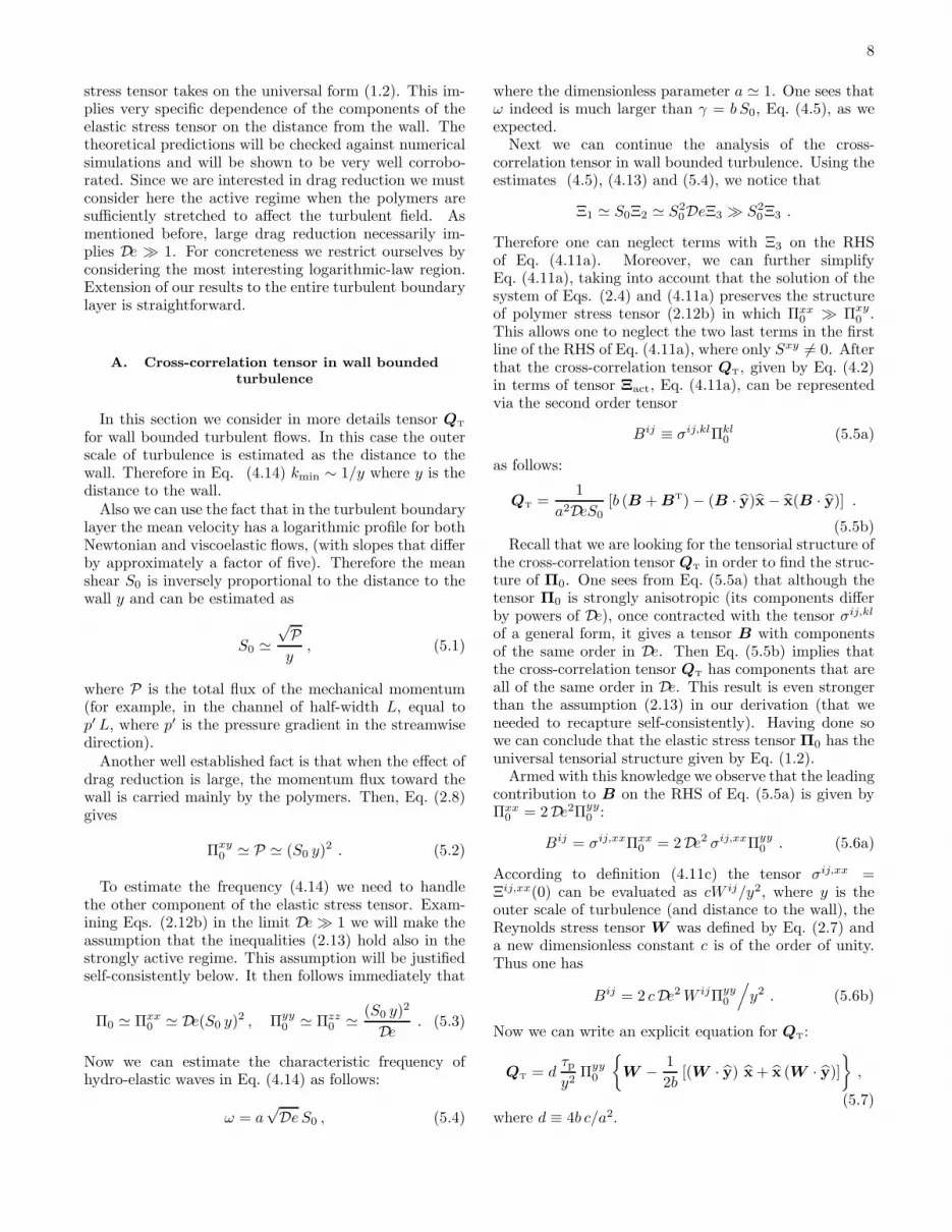
0 , see, Fig. 12 in Ref. [16], Fig. 5.3.1 in Ref. [17], Fig. 6in Ref. [20], etc. The accepted result is that Π0 decreasesin the turbulent layer. Our Eqs. (5.10) predict Π0 ∝ 1/yin this region. This rationalizes the DNS observations inRefs. [16, 17, 19, 20]. As an example, we present in Fig. 1by black squares the DNS data of [19] for the largest,

10

0 40 80 120 1600.00

0.01

0.02

0.03

0.040.0 0.2 0.4 0.6 0.8 1.0

Rij

Ryy x 10Rxx

y/L

y+

FIG. 1: Comparison of the DNS data Ref. [19] for the meanprofiles of the xx and yy components of the elastic stresstensor Πij

0 with analytical predictions. Black squares: DNSdata for streamwise diagonal component Πxx

0 , that accordingto our understanding, Eq. (5.10), has to decrease as 1/y withthe distance to the wall. Black solid line: 1/y+ dependence.Red empty circles: DNS data for the wall-normal componentΠyy

0 , for which we predicted linear increase with y+ in the log-law turbulent region. Red dashed line - linear dependence,∝ y+.

streamwise component Πxx0 and plotted by solid black

line the expected [see Eq. (5.10)] profile ∝ 1/y+. In spiteof the fact that the MDR asymptote with the logarithmicmean velocity profile is hardly seen in that DNS, theagreement between the DNS data and our prediction isobvious.

The effective polymeric viscosity was measured, for ex-ample, in Ref. [16], Fig. 5, and in Ref. [17]. In these Refs.νp(y) was understood as ∆p(y)/S0(y), where ∆p(y) isthe Reynolds stress deficit, which is Πxy

0 according toEq. (2.8). The observations of Refs. [16, 17] is thatνp(y) in the turbulent boundary layer grows linearly withthe distance from the wall. Recent data of DNS of theNavier-Stokes equation with polymeric additives (usingthe FENE-P model) taken from Ref. [19] are presentedin Fig. 1. The wall-normal component Πyy

0 is presentedby the red empty circles. One sees that (in the quitenarrow) region 20 < y+ < 60 (where the mean velocityprofile is close of MDR) the profile Πyy

0 is indeed propor-tional to y+, as represented by the red dashed line. Thisis in agreement with our result, see Eq. (5.12b) and ourRef. [11].

Direct DNS of other components of the polymericstress tensor, see, e.g. Fig. 6 in Ref. [19] also agrees withthe tensorial structure of Π0 given by Eq. (5.10).

VI. SUMMARY AND DISCUSSION

The aim of this paper was the analysis of the poly-mer stress tensor in turbulent flows of dilute polymericsolutions. On the face of it this object is very hard topinpoint analytically, being sensitive to complex interac-tions between the polymer molecules and the turbulentmotions. We showed nevertheless that in the limit ofvery high Deborah numbers, De ≫ 1, this tensor attainsa universal form. Increasing the complexity of our turbu-lent ensemble, from laminar, through homogeneous tur-bulence with a constant shear, and ending up with wallbounded anisotropic turbulence, we proposed a universalform

Π0(y) ≃ Πyy0 (y)

2De2(y) De(y) 0De(y) 1 0

0 0 C(y)

. (6.1)

We rewrite this form here to stress that it remainsunchanged even when the Deborah number, and with itthe components of the tensor, become space dependent.Obviously, this strong result is expected to hold only aslong as the mean properties, including the mean shear,vary in space in a controlled fashion, as for example inthe logarithmic layer near the wall (be it a Karman or aVirk logarithm).

As an important application of these results we consid-ered in Sect. V the important problem of drag reductionby polymers in wall bounded flows. A difficult issue thatcaused a substantial confusion is the relation betweenthe polymer physics, the effective viscosity that is due topolymer stretching, and drag reduction. In recent workon drag reduction it was shown that the Virk logarith-mic Maximum Drag Reduction asymptote is consistentwith a linearly increasing (with y) effective viscosity dueto polymer stretching. This result seemed counter intu-itive since numerical simulations indicated that polymerstretching is decreasing as a function of y. The presentresults provide a complete understanding of this conun-drum. “Polymer stretching” is dominated by Πxx

0 sinceit is much larger than all the other components of thestress tensor. As shown above, this component is indeeddecreasing when y increases, cf. Fig. 1. On the otherhand the effective viscosity is proportional Πyy

0 , and thiscomponent is indeed increasing (linearly) with y, cf. Fig.1. In fact, drag reduction saturates precisely when Πxx

0

and Πyy0 become of the same order.

Acknowledgments

We thank Roberto Benzi for useful discussions. Thiswork had been supported in part by the US-Israel Bina-tional Science Foundation, by the European Commissionvia a TMR grant, and by the Minerva Foundation, Mu-nich, Germany.

11

APPENDIX A: EXACT ENERGY BALANCE

EQUATIONS

In this Appendix we present exact energy balanceequations that are useful in the analysis of turbulence ofthe polymeric solutions. In the present study we employonly one of them, i.e. Eq. (A3e).

Introduce the mean densities of the turbulent kineticenergy ET and polymeric potential energy Ep

ET ≡ 1

2W , W ≡ Tr W , (A1a)

Ep ≡ 1

2Π0 , Π0 ≡ Tr Π0 . (A1b)

Using Eqs. (2.1) one can derive equations for the bal-ance of ET and Ep and for their sum:

DET

Dt= ε+

T− ε−

T− εTp = 0 , (A2a)

DEp

Dt= ε+

p − ε−p + εTp = 0 , (A2b)

D

Dt(ET + Ep) = ε+

T+ ε+

p − ε−T− ε−p = 0 . (A2c)

We denote by ε+T

and ε+p the energy flux from the mean

flow to the turbulent and polymeric subsystem respec-tively:

ε+T

≡ −S0Wxy , (A3a)

ε+p ≡ S0Π

xy0 ; (A3b)

ε−T

describes the dissipation of energy in the turbulentsubsystem, whereas ε−p is the dissipation in the polymeric

subsystem due to the relaxation of the stretched polymersback to equilibrium:

ε−T

≡ ν0Tr 〈s · sT〉 , (A3c)

ε−p ≡ 1

2 τp

Tr (Π0 − Πeq) . (A3d)

The last term on the RHS of Eqs. (A2a) and (A2b) [thatis absent in (A2c)] describes the energy exchange betweenthe polymeric and turbulent subsystems:

εTp ≡ Tr 〈s · π〉 =1

2Tr QT . (A3e)

Using the expression for the momentum flux, we obtainan exact balance equation for the total energy

E = EV + ET + Ep , (A4a)

that in the stationary state reads:

S0P =1

2τp

Tr (Π0 − Πeq) + ν0

(S2

0 + Tr 〈s · sT〉)

.

(A4b)In Eq. (A4a) EV is the density of the kinetic energy of themean flow, defined up to an arbitrary constant, depend-ing on the choice of the origin of coordinates. The LHSof Eq. (A4b) describes the work of external forces neededto maintain the constant mean shear. The first term onthe RHS (∝ 1/τp) describes the energy dissipation in thepolymeric subsystem. The term ν0S

20 represents the vis-

cous dissipation due to the mean shear, while the lastterm on the RHS is responsible for the viscous dissipa-tion caused by the turbulent fluctuations.

[1] B.A. Toms, in Proceedings of the International Congress

of Rheology Amsterdam Vol 2. 0.135-141 (North Holland,1949).

[2] P.S. Virk, AIChE J. 21, 625 (1975).[3] P.G. de Gennes, Introduction to Polymer Dynamics,

(Cambridge, 1990).[4] K. R. Sreenivasan and C. M. White, J. Fluid Mech. 409,

149 (2000).[5] J.L. Lumley, Annu. Rev. Fluid Mech. 1, 367 (1969).[6] J.L. Lumley, Symp. Math 9, 315 (1972).[7] M. Tabor and P.G. de Gennes, Europhys. Lett. 2, 519

(1986).[8] E. Balkovsky, A. Fouxon, and V. Lebedev, ”Turbulent

Dynamics of Polymer Solutions”, Phys. Rev. Lett. 84,4765 (2000).

[9] E. Balkovsky, A. Fouxon, and V. Lebedev,, ”Turbulenceof polymer solutions” Phys. Rev. E 64, 056301 (2001).

[10] M. Chertkov, ”Polymer Stretching by Turbulence”, Phys.Rev. Lett. 84, 4761 (2000).

[11] V.S. L’vov, A. Pomyalov, I. Procaccia and V. Tiberke-vich, Phys. Rev. Lett., in press. Also: nlin.CD/0307034

[12] K. Furutsu, J. Res. NBSD 67, 303, (1963)[13] A.E. Novikov, Soviet Physics, JETP, 47, 1919 (1964).[14] T. Burghelea, V. Steinberg and P.H. Diamond, Europhys.

Lett. 60, 704, (2002).[15] R. benzi, E. de Angelis, V.S. L’vov, I. Procaccia and

V. Tiberkevich, “Maximum Drag Reduction Asymptotesand the Cross-Over to the Newtonian Plug”, J. FluidMech, submitted.

[16] R. Sureshkuar and A.N. Beris, Phys. of Fluids, 9, 743,(1997).

[17] E. de Angelis, PhD thesis, Univ. di Roma “La Saspienza”(2000).

[18] E. de Angelis, C.M. Casciola and R. Piva, CFD Journal,9, 1 (2000).

[19] S. Sibilla and A. Baron, Phys. of Fluids, 14, 1123 (2002).[20] P. K. Ptasinski et. al, J. Fluid Mech., 490, 251 (2003).