Investigation of Turbulent Flame Characteristics via Laser ...
159
Investigation of Turbulent Flame Characteristics via Laser Induced Fluorescence Dem Fachbereich Maschinenbau an der Technischen Universit¨ at Darmstadt zur Erlangung des Grades eines Doktor-Ingenieurs (Dr.-Ing.) genehmigte Dissertation von Dipl.-Ing Sunil Kumar Omar (M.Tech.) aus Sumerpur(U.P.), Indien Berichterstatter Prof. Dr.-Ing. J. Janicka Mitberichterstatter Prof. Dr.-Ing. H.-P. Schiffer Mitberichterstatter Dr.rer.nat.habil. A. Dreizler Tag der Einreichung 08.12.2005 Tag der m¨ undlichen Pr¨ ufung 03.03.2006 Darmstadt 2006 D17 i
-
Upload
khangminh22 -
Category
Documents
-
view
2 -
download
0
Transcript of Investigation of Turbulent Flame Characteristics via Laser ...

Investigation of Turbulent Flame
Characteristics via Laser Induced Fluorescence
Dem Fachbereich Maschinenbau
an der Technischen Universitat Darmstadt
zur Erlangung des Grades
eines Doktor-Ingenieurs (Dr.-Ing.)
genehmigte
Dissertation
von
Dipl.-Ing Sunil Kumar Omar (M.Tech.)
aus Sumerpur(U.P.), Indien
Berichterstatter Prof. Dr.-Ing. J. Janicka
Mitberichterstatter Prof. Dr.-Ing. H.-P. Schiffer
Mitberichterstatter Dr.rer.nat.habil. A. Dreizler
Tag der Einreichung 08.12.2005
Tag der mundlichen Prufung 03.03.2006
Darmstadt 2006
D17
i

Hiermit erklre ich, dass ich die vorleigende Dissertaion selbstndig verfasst und
nur die angegebenen Hilfsmittel verwendet habe. Ich habe bisher noch keinen
Promotionsversuch unternommen.
Sunil Kumar Omar,
Darmstadt im Marz 2006
ii

Acknowledgements
The present work was performed at the Institute of Energy and Power-plant
Technology (EKT) at the Darmstadt University of Technology, Germany.
I wish to express my sincere thanks to the head of the institute, Prof. Dr.-Ing.
Johannes Janicka, for his great support and offer to pursue a PhD. under his
supervision. I am grateful to him for his steady optimism and trust towards my
dissertation work.
My sincere gratitude goes to Prof. Dr.-Ing. Heinz-Peter Schiffer (TU-Darmstadt)
for his willingness to report on my work.
I greatly acknowledge the support and guidance from Dr.rer.nat.habil. Andreas
Dreizler, who was kind and patient enough to assist me through out this work.
His perpetual enthusiasm in the area of combustion and laser diagnostics was
always the source of encouragement and inspiration to me. I also thank him for
his tireless effort and never give-up attitude, which led me finish this work.
I am heartly greatful to my colleagues Rajani Akula, Andreas Ludwig, Mark
Gregor, Dirk Geyer, Cristoph Schneider and Andreas Nauert for many profes-
sional discussion. I wish to thank Andreas Kempf, Markus Klein, Bernhard
Wegner, Elena Schneider for the pleasant working atmosphere during my stay
at EKT. Many thanks to the diplom students Jan Brubach and Axel Sattler
for their kind help in the laser lab. I take my opportunity to thank all EKT
staffs and technical workshop staffs for their kind support and letting me use the
available facilities.
Many thanks to Dr. M.Renfro and V.Krishnan for their help during the col-
laborative project work in turbulent opposed jet flames at the Purdue University,
Indianapolis USA.
I wish to thank Himanshu Verma, Dr. Rahul Harshe, Amit, Santosh, Sidharth
Sekhar and Anita Singh for their moral support and great time we had together.
I owe a great debt of gratitude to my family specially my parents, who have
always been very loving, supportive and believed in my abilities. My heartily
thanks goes to my supportive brother’s Pankaj Omar, Rajendra Gupta, my only
sister Ruchi Omar and sister-in-law Seema Gupta. I could have never came such
far without their support and affection towards me.
iii

To my parents, Shri. Raj Kumar Gupta and Smt. Rani Gupta
Sunil Kumar Omar
Darmstadt, March 2006
iv

Contents
Nomenclature ix
1 Introduction 1
2 Turbulent Reacting Flows 5
2.1 Introduction on Turbulent Combustion . . . . . . . . . . . . . . . 5
2.1.1 Modes of Turbulent Reacting Flows . . . . . . . . . . . . . 7
2.2 Framework to Understand Turbulent Reacting Flows . . . . . . . 9
2.3 Experimental Methods . . . . . . . . . . . . . . . . . . . . . . . . 10
2.3.1 Introduction . . . . . . . . . . . . . . . . . . . . . . . . . . 10
2.3.1.1 Laser Diagnostics . . . . . . . . . . . . . . . . . . 11
2.3.1.2 Multi-dimensional Measurements . . . . . . . . . 12
2.3.1.3 Multi-scalar Measurements . . . . . . . . . . . . 13
2.4 Numerical Modelling Methods . . . . . . . . . . . . . . . . . . . . 14
3 Laser Technique 17
3.1 Introduction . . . . . . . . . . . . . . . . . . . . . . . . . . . . . . 17
3.2 Theory . . . . . . . . . . . . . . . . . . . . . . . . . . . . . . . . . 19
3.3 Criteria for Line Selection . . . . . . . . . . . . . . . . . . . . . . 22
3.4 Quenching Correction in Combustion Flames . . . . . . . . . . . . 23
3.5 Short Pulse Diagnostics (PITLIF) . . . . . . . . . . . . . . . . . . 25
3.5.1 Theory . . . . . . . . . . . . . . . . . . . . . . . . . . . . . 26
3.5.2 Measurement of Exponential Decay . . . . . . . . . . . . . 27
3.5.3 LIFTIME . . . . . . . . . . . . . . . . . . . . . . . . . . . 28
3.5.4 Quantitative time-series . . . . . . . . . . . . . . . . . . . 30
v

Contents
4 Applied Studies on Turbulent Flames 31
4.1 Single Point Measurement . . . . . . . . . . . . . . . . . . . . . . 31
4.1.1 Time-resolved measurement: OH-PITLIF . . . . . . . . . . 31
4.1.1.1 Time-Series . . . . . . . . . . . . . . . . . . . . . 32
4.1.1.2 Autocorrelation and Integral Time Scale . . . . . 33
4.2 Multi-dimensional Investigation: 2D Planar . . . . . . . . . . . . 34
4.2.1 Flame-front Topology . . . . . . . . . . . . . . . . . . . . . 35
4.2.1.1 Visualization of Instantaneous Stoichiometric con-
tour . . . . . . . . . . . . . . . . . . . . . . . . . 36
4.2.1.2 Visualization of Reaction Rate . . . . . . . . . . 38
4.3 Molecules Investigated . . . . . . . . . . . . . . . . . . . . . . . . 40
4.3.1 The Hydroxyl Radical . . . . . . . . . . . . . . . . . . . . 41
4.3.2 Formaldehyde . . . . . . . . . . . . . . . . . . . . . . . . . 42
4.3.2.1 Burner Configuration and Flame Measured . . . 44
4.3.2.2 Spectrum Analysis . . . . . . . . . . . . . . . . . 45
5 Experimental Methods 47
5.1 OH-PITLIF in Opposed Jet Flames . . . . . . . . . . . . . . . . . 47
5.1.1 Introduction . . . . . . . . . . . . . . . . . . . . . . . . . . 47
5.1.2 PITLIF Laser System . . . . . . . . . . . . . . . . . . . . 47
5.1.2.1 OH-Line Selection . . . . . . . . . . . . . . . . . 49
5.1.3 Detection Optics . . . . . . . . . . . . . . . . . . . . . . . 50
5.1.4 PITLIF Photon Counting System . . . . . . . . . . . . . . 51
5.1.5 PITLIF Data Processing and Signal Calibration . . . . . . 54
5.2 OH-PLIF in Opposed Jet Flames . . . . . . . . . . . . . . . . . . 55
5.2.1 Laser System . . . . . . . . . . . . . . . . . . . . . . . . . 55
5.2.2 Optical Set-up . . . . . . . . . . . . . . . . . . . . . . . . . 58
5.2.3 Image Detector . . . . . . . . . . . . . . . . . . . . . . . . 59
5.2.4 Synchronization: OH-PLIF . . . . . . . . . . . . . . . . . . 59
5.3 Multiple Scalar Measurements in Swirl Flames . . . . . . . . . . . 61
5.3.1 Experimental Set-up . . . . . . . . . . . . . . . . . . . . . 62
5.3.2 Optical Set-up . . . . . . . . . . . . . . . . . . . . . . . . . 63
5.3.3 Image Detector and synchronization . . . . . . . . . . . . . 64
5.3.4 HCHO spectrum analysis . . . . . . . . . . . . . . . . . . 65
5.3.4.1 Planar Measurement . . . . . . . . . . . . . . . . 65
vi

Contents
5.3.4.2 Spectrum Measurement . . . . . . . . . . . . . . 67
6 Data Image Processing 69
6.1 Correction . . . . . . . . . . . . . . . . . . . . . . . . . . . . . . . 70
6.1.1 Background Subtraction . . . . . . . . . . . . . . . . . . . 70
6.1.2 Laser Profile Compensation . . . . . . . . . . . . . . . . . 70
6.2 Noise Rejection and Edge Enhancement . . . . . . . . . . . . . . 70
6.2.1 Median Filter . . . . . . . . . . . . . . . . . . . . . . . . . 73
6.2.2 Non-Linear Diffusion method . . . . . . . . . . . . . . . . 73
6.3 Binary Image Generation . . . . . . . . . . . . . . . . . . . . . . . 76
6.4 Algorithms Applied . . . . . . . . . . . . . . . . . . . . . . . . . . 77
6.4.1 Median-Threshold-Majority Method . . . . . . . . . . . . 77
6.4.1.1 Sensitivity Analysis . . . . . . . . . . . . . . . . . 79
6.4.2 Median-Non-Linear Diffusion-Threshold . . . . . . . . . . 80
6.5 Conclusion . . . . . . . . . . . . . . . . . . . . . . . . . . . . . . . 81
7 Opposed Jet Flames 85
7.1 Introduction . . . . . . . . . . . . . . . . . . . . . . . . . . . . . . 85
7.2 Burner Description . . . . . . . . . . . . . . . . . . . . . . . . . . 87
7.3 Flames Measured . . . . . . . . . . . . . . . . . . . . . . . . . . . 89
7.4 Characterization of the Burner . . . . . . . . . . . . . . . . . . . . 90
7.5 Result and Discussion . . . . . . . . . . . . . . . . . . . . . . . . 92
7.5.1 OH-PLIF . . . . . . . . . . . . . . . . . . . . . . . . . . . 92
7.5.1.1 Flame Area . . . . . . . . . . . . . . . . . . . . . 92
7.5.1.2 Flame Length . . . . . . . . . . . . . . . . . . . . 96
7.5.1.3 Position of Stoichiometric Contour . . . . . . . . 99
7.5.1.4 Local Flame Angle . . . . . . . . . . . . . . . . . 103
7.5.1.5 Conclusion . . . . . . . . . . . . . . . . . . . . . 107
7.5.2 OH-PITLIF . . . . . . . . . . . . . . . . . . . . . . . . . . 108
7.5.2.1 Time-averaged Concentration Profiles . . . . . . 109
7.5.2.2 Time-series Statistics . . . . . . . . . . . . . . . . 109
7.5.2.3 Autocorrelation . . . . . . . . . . . . . . . . . . . 115
7.5.2.4 Integral time scale . . . . . . . . . . . . . . . . . 115
7.5.3 Conclusion . . . . . . . . . . . . . . . . . . . . . . . . . . . 119
vii

Contents
8 Swirl Flames 121
8.1 Introduction . . . . . . . . . . . . . . . . . . . . . . . . . . . . . . 121
8.2 Burner Description . . . . . . . . . . . . . . . . . . . . . . . . . . 123
8.3 Results and Discussion . . . . . . . . . . . . . . . . . . . . . . . . 124
8.4 Conclusion . . . . . . . . . . . . . . . . . . . . . . . . . . . . . . . 128
9 Summary and Outlook 129
Bibliography 133
viii

Nomenclature
Latin Symbols
Symbol Dimension Definition
am [s−1] mean strain rate
a [s−1] strain rate
A peak amplitude of exponential decay
AG [mm2] global area
AL [mm2] local area
b12 [s−1] rate constant for stimulated absorption
b21 [s−1] rate constant for stimulated emission
B background signal from exponential decay
c optimized parameter
c0 [ms−1] speed of light
db [mm] bluff-body diameter
dcf [mm] co-flow nozzle diameter for swirl burner
Din [mm] nozzle diameter for opposed jet burner
Dcf [mm] co-flow nozzle diameter for opposed jet burner
E1 [cm−1] upper energy level
E2 [cm−1] lower energy level
Ei,j sensitivity
fst stoichiometric mixture fraction
f mixture fraction
fl [m] focal length
fn f number
h [J s] Plank’s constant
ix

Nomenclature
H [mm] distance between the nozzles
I intermittency
Iνsat [Wm−2] saturation irradiance
Iν [Wm−2] incident laser spectral irradiance
k [J ] turbulent kinetic energy
kb [JK−1] Boltzmann constant
kf rate coefficient
L [mm] integral length scale
Lbottom [m] flame length
m constant in non-linear diffusion filter
n [cm−3] number density of molecule
n1 [cm−3] number density of the molecule in electronic ground state
n2 [cm−3] number density of the molecule in electronic excited state
n01 [cm−3] lower level population prior to laser excitation
Pd photoionization
P [W ] thermal power of the flame
Qgas [lthr−1] flow rate of fuel (Swirl Burner)
Qair [lthr−1] flow rate of air (Swirl Burner)
r [mm] radial flow field co-ordinates (Opposed Jet Burner)
R [mm] radius of the inner nozzle (Opposed Jet Burner)
RR [mollt−1s−1] forward reaction Rate
Re Reynolds number
sl [ms−1] flame velocity
S swirl number
Sc Schmidt number
SiOH lif signal from hydroxyl molecule
SiHCHO lif signal from formaldehyde molecule
tres [ms] residence time of eddy
tov [ms] large eddy turn overtime
u [ms−1] mean velocity
u [ms−1] bulk velocity
u′ [ms−1] velocity fluctuation
W predissociation
Yα mass fraction of element α
Yα,O mass fraction of element α in oxidizer flow
x

Nomenclature
Yα,F mass fraction of element α in fuel flow
z, Z [mm] axial flow field co-ordinates
Greek Symbols
Symbol Dimension Definition
τl, τ [ns] lifetime
τI [ms] integral time scale
ν [Hz] light pulse frequency
Ω [sterad] collection solid angle
ω [nm] light frequency
θ [rad] flame angle
λw [nm] wavelength of laser pulse
λ contrast parameter
λB air-to-fuel ratio
φ, φB equivalence ratio
ηB [mm] Batchelor length scale
ηk [mm] Kolmogorov length scale
ρ autocorrelation function
ρu [kgm3] density of unburned fluid
ρb [kgm3] density of burned fluid
∇ gradient operator
σ gaussian kernel
A Angstrom
Abbreviations
BBO beta borium borate non-linear crystal
CCD charge coupled device
CFD computational fluid dynamics
DCS direct current sampling
xi

Nomenclature
DPR dual pulse resolution
DNS direct numerical simulation
EKT Fachgebiet fur Energie- und Kraftwerkstechnik
(Institute for Energy and Power-Plant Technology)
FWHM full width half maximum
GTI Gires-Tournois interferometer
ICCD intensified charge coupled device
IEO international energy outlook
IR infra-red
LASKIN LASer KINetics
(a simulation program for time-resolved LIF spectra)
LBO lithium tribonate non-linear crystal
LDV laser Doppler velocimetry
LES large eddy simulation
LIF laser induced fluorescence
LII laser induced incandescence
MCA multi-channel analyzer
NIM nuclear instrumentation method pulse
NLDF non-linear diffusion filter
OPPDIF opposed jet diffusion flame
PBP pellin-broca-prism
PDF probability density function
PITLIF pico-second time-resolved laser induced fluorescence
PIV particle image velocimetry
PLIF planar laser induced fluorescence
PMT photomultiplier
PSD power spectral density
RANS Reynolds averaged numerical simulation
RET rotational energy transfer
RLD rapid lifetime determination
SFB Sonderforschungsbereich
SNR signal-to-noise ratio
SPC signal photon counting
TAC time-to-amplitude convertor
TGP turbulence generating plate
xii

Nomenclature
TNF turbulent non-premixed flame
TOJ turbulent opposed jet flame
UV ultra-violet
WEX wavelength extender
WLLS weighted linear least-square method
Molecular Species
CH Methylidyne
CH2O,HCHO Formaldehyde
CH4 Methane
OH Hydroxyl
HCO Formyl
xiii

Nomenclature
xiv

1 Introduction
The world is using an increasing amount of energy. Both the developed and less
developed countries are demanding larger shares of world energy resources. At
the same time, it is fully recognized that such resources are limited. Most are
fossil fuels, formed underneath the surface of the earth millions of years ago.
They will not easily be replenished! The most plentiful source of fossil energy
is coal. This is essentially carbon but contains a number of impurities such as
nitrogen, sulphur, and chlorine. Another group of fuels is the hydrocarbons.
These may be liquid or gaseous and are compounds of hydrogen and carbon in
different proportions. However, coal is well suited to industrial processes such as
power generation, but it is difficult to store and transport. Hydrocarbons provide
convenient automotive power, whether on the road or in the air.
Fossil fuels remain the primary source of energy for domestic heating, power
generation and transportation. Other energy sources such as solar energy, wind
energy or nuclear energy still account for less than 20 percent of total energy
consumption. Therefore combustion of fossil fuels, being humanity’s oldest tech-
nology, remains a key technology today and even in foreseeable future. On the
same token, world energy consumption is projected to increase by 58 percent
over 24-years forecast horizon, from 2001-2025 [IEO2003].
Today, combustion of fossil fuel is the main source of energy for mankind. How-
ever, it is also the major contributor to the pollution in earth’s atmosphere. It
pollutes the earth by emitting exhaust gases from various combustion processes.
If the combustion process of fossil fuel is perfect, the only elements remaining
would be carbon dioxide, water, nitrogen and excess oxygen. Unfortunately,
combustion isn’t perfect, thus emitting pollutants in the process such as car-
bon monoxide, UHC (unburnt hydrocarbons), NOx, sulphur dioxide etc. These
gases effect our local as well as global environment causing air pollution, acid
rain, global warming, forest fire and other hazards. Thus understanding of com-
bustion processes and improvements are necessary to lower the emission, while
1

1 Introduction
maintaining a high efficiency rate. It is thus important to increase the efficiency
of combustion and reduce pollution in order to improve the quality of life and
save all endangered species around the globe.
Turbulent combustion is an important technical process found mostly in all
practical industrial devices, like automotive engines, gas turbines and power
plants (boilers etc). A significant amount of effort is ongoing to improve the
knowledge of combustion under turbulent environment, both experimentally and
numerically. The improvement in terms of efficiency and pollution reduction
in practical combustion systems is an immense task. In addition, it requires
complete understanding of complex processes and interaction involved with tur-
bulent combustion. Understanding of turbulent combustion requires knowledge
on turbulent flow field, combustion chemistry and their interaction with other
processes. One of the interaction is interaction between turbulent flow field and
combustion chemistry known as turbulent-chemistry interaction that occur in
molecular level during combustion. Due to its complexity and insufficient knowl-
edge, it still remains an attractive research topic around the globe.
Improvement in combustor design, its efficiency and to meet future emission
constraints requires the fundamental understanding of turbulent combustion and
its complex interactions. The motivation for understanding turbulent combustion
to design future combustion system arises from two primary reasons: 1) the
systems are too complex to be understood easily, and trial and error techniques
of design simply do not work and 2) the systems are too large that trial and error
techniques are far too expensive to practice. Therefore a better understanding of
combustion is required, which will give an insight into the physical understanding
of the complex behavior and hence significantly reduce the dependence on the
trial and error technique.
Modelling technique is mainly used to design combustors in the industrial envi-
ronment, but there is limitation to these modelling technique. In order to test for
the efficiency and capabilities of these numerical models, relevant experimental
data is required. With increasing computational power and growing importance
of numerical studies, pressure to generate good and useful experimental data
is huge. The assessment and validation of new and improved numerical mod-
els need experimental data, in order to correctly predict the complex physical
phenomenon involved with turbulent combustion. Present work contributes to
increase knowledge on turbulent combustion, that will enable the combustor de-
2

signers to achieve three important targets: to save fossil fuels, to minimize the
formation of pollutants and to reduce the cost of energy produced from fossil
fuels.
More specifically, current work aims to provide experimental information on
various laboratory friendly and technical relevant flames that mainly solve two
purposes: firstly data will allow the numerical simulators to test the efficiency of
existing numerical models and secondly it tries to explain the physics behind the
complex process that is involved with turbulent combustion. Above mentioned
twin-fold importance remains to be the motivation of the thesis.
First part of the thesis illustrates the background and basics of turbulent com-
bustion, various complex interaction involved and the framework adopted to im-
prove on its understanding. It also provides information on turbulence-chemistry
interaction which remains to be the bottleneck unresolved problem among the
researchers around the globe. Importance of experimental studies for validation
purpose and limitation of numerical studies is also detailed in the same chapter.
Third chapter introduces the basic principles on the laser based technique (Laser
Induced Fluorescence) utilized to investigate the flame characteristics in the cur-
rent work. Methods to evaluate quantitative information from the fluorescence
signal is also depicted and available techniques are as well explained.
Chapter four is more specific. It provides the information on important pa-
rameter of interest that has been measured and evaluated during this work.
Information on single point and two-dimensional measurement along with liter-
ature survey on previous work is also described. This chapter will provide the
basic platform on the parameters needed for the study and thereafter, subsequent
chapters will demonstrate its application and show the results obtained during
the measurement of various flames.
Details on experimental set-up and instrumentation utilized to carry out mea-
surements in turbulent flames is provided in chapter five. This chapter is divided
according to the type of flames measured, first two sections detail on experi-
mental methods used in application on turbulent opposed jet flame, whereas last
section details on turbulent swirl flame. Chapter six, talks about the importance
of image processing to evaluate the information from the raw planar image taken
during the experimental measurements. This chapter also lets us to choose the
right filtering and the image processing technique to extract relevant information
from the planar LIF images.
3

1 Introduction
Last three chapters provides the outcome from the experimental measurement
in various flames. Discussion and conclusion is also done to visualize the outcome
and improve our knowledge in these turbulent flames. Future work and impor-
tant conclusion from the present work is provided in the chapter with heading
”Summary and Outlook”.
4

2 Turbulent Reacting Flows
This chapter introduces the concept of turbulent combustion, its processes and
its complex behavior. Typical framework that has been proposed to understand
the turbulent combustion and its complex behavior is also explained. This in-
cludes the importance of combined effort from both numerical and experimental
methods and their current status in the field of turbulent combustion.
2.1 Introduction on Turbulent Combustion
Turbulence phenomenon is still living up to its expectation as Werner Heisenberg
once answered, when he was asked what he would ask God, given the opportunity.
His reply was: ”When I meet God, I am going to ask him two questions: Why
relativity? and why turbulence? I really believe he will have an answer for the
first”.
Turbulent flow is characterized by the complex motion of fluid molecules that
are mainly composed of circular structures (eddies) and moving in a chaotic
manner in all directions. During visualization of such flows, one would observe
complicated instead of simple streamlined patterns in the flow. Flows that are
pseudo-random, three dimensional, unsteady, swirled structured and dissipative
(i.e. kinetic energy is changed into heat as the flow progresses) in nature are
defined as ”turbulent flows”. Turbulence in fluid flow, is encouraged since it
strongly enhances the mixing process between the fluids. Large-scale vortex
motion and mixing at molecular level through diffusion are the cause for mixing
process between the fluids.
Turbulence itself is a very complicated non-linear problem. Turbulent reacting
flows are a step ahead in terms of complications, because it involves strong in-
teraction of several physical and chemical processes such as turbulence, mixing,
mass and heat transfer, radiation and multi-phase flow phenomena [1] (see figure
2.1).
5

2 Turbulent Reacting Flows
Figure 2.1: Structure of integral and sub-models showing various processes andinteraction involved with turbulent combustion
This complicated picture can be reduced, if multi-phase phenomena and radi-
ation effect is opted out in the turbulent reacting flow. Even then, the strong
non-linear coupling between turbulence and chemistry is extremely difficult and
requires understanding at the fundamental level. This is mainly because the
chemical reaction can involve hundreds of species and thousands of elementary
reactions, with a wide range of chemical reaction length and time scales, starting
from a nanometer regime of molecular encounters to combustor dimension of a
few meters. Some of which may overlap with the turbulent flow scales, thus
complicating the flow field structure.
In turbulence-chemistry interaction, initially turbulence causes the mixing of
reactants through large scale vortices in the flow field, small scale molecular
mixing then proceeds the chemical reaction. During chemical reaction heat is
released, which alters the density field thus modifying the turbulent flow field.
This non-linear coupling of turbulent flow and chemical reaction is the most
complex and challenging topic for the researchers working in the field of turbulent
combustion.
This thesis is limited to the critical issue of turbulence-chemistry interaction
in turbulent flames. Almost in all practical combustion systems such as internal
combustion (IC) engines or gas turbines (GT), chemical reactions takes place in a
turbulent flow field. Therefore, in order to develop more efficient and environment
friendly combustion systems, the fundamental knowledge of this interaction and
its reliable prediction in turbulent reacting flow is required.
6

2.1 Introduction on Turbulent Combustion
Figure 2.2: Schematic drawing of a turbulent non-premixed jet flame
2.1.1 Modes of Turbulent Reacting Flows
Fortunately, turbulent reacting flows are classified only into premixed and non-
premixed modes of combustion. This classification has to do with the state
of mixing of the reactants before entering the reaction zone. If the reactants
are separately fed into the reaction zone, the resultant flame is known as non-
premixed flame. Mixing brings reactants into the reaction zone where thin layer
of burnable mixtures at different are formed and combustion takes place. Most
of the mixing in this thin zone occurs mainly by a molecular diffusion process.
On either side of the reaction zone, the mixture is either too lean (oxidiser side)
or too rich (fuel side) for chemical reaction to take place (see figure 2.2). Non-
premixed flames are normally safe and simpler to operate because they are not
mixed prior to the combustion chamber and they do not propagate against the
flow, as their premixed counterpart. Non-premixed flames are of major interest
in gas turbine engines, jet engines, Diesel engines, boiler, furnace etc.
The main disadvantage of pure diffusion flames is their pollutant generation.
This is because the fuel does not get enough oxidant in the right place resulting
in incomplete combustion. In such flames, maximum combustion temperature is
achieved at the location, where the mixture is stoichiometric and this is associated
with increased production of NOx. Stoichiometry is used to refer to the ratio of
7

2 Turbulent Reacting Flows
oxidizer to fuel which just leads to complete product of combustion. One of the
useful qualities related to stoichiometry is equivalence ratio (φ). It is the ratio of
fuel to oxidizer by weight in a given case to that to stoichiometry stated in the
form of an equation 2.1. Thus all stoichiometric mixture have equivalence ratio
of unity. Rich mixtures have φ greater than unity, whereas lean mixture have φ
less than unity.
φ =fuel/air
fuel/air stoichiometry
(2.1)
In a two feed system as shown in figure 2.2, one can introduce a conserved
scalar, mixture fraction, as a dimensionless element mass fraction shown in equa-
tion 2.2
fα =Yα − Yα,O
Yα,F − Yα,O
(2.2)
Where Yα denotes mass fraction of element α. The second subscript, F and
O refers to the fuel and oxidizer in their initially unmixed state and Yα,F , Yα,O
corresponds to the element mass fraction value in the fuel and oxidizer streams
respectively.
In contrary to the diffusion flames considered in last paragraphs, the reactants
in premixed flames are thoroughly premixed homogeneously on the molecular
scale before entering the reaction zone. The reactants in a premixed flame are
mixed before chemical reaction occurs therefore the chemical reaction rate de-
termines the overall reaction rate in such flames. Combustion in such flames
occurs by propagation of a reaction front through the flow. In such flames the
combustion zone is defined mainly by two main zones, i.e. the preheated zone
and the reaction zone. Initially, in the preheated zone the mixed reactants pro-
ceed intensively due to diffusion of heat and mass without any chemical reaction.
Thereafter, the chemical reaction occurs and the reaction rate increases at high
level. At this reaction zone combustion occurs and maximum heat is released.
They are compact in nature and the common application is in Spark-Ignition
engines that are mostly used in cars.
The above mentioned non-premixed and premixed regimes of combustion are
classified according to the mixing condition of the reactants. However, in tech-
nical applications, there are very few situations where one of these combustion
8

2.2 Framework to Understand Turbulent Reacting Flows
regimes appears in their pure form. The combination of non-premixed and pre-
mixed regimes takes place more often to produce so called partially premixed
combustion. Partially premixed phenomenon can be seen in triplet flame. In
particular, triplet flames essentially comprise three flames, namely a rich pre-
mixed flame accompanied by a diffusion flame in the middle and followed by a
lean premixed flame. Similarly, in partially premixed flames the equivalence ratio
of the fresh gas mixture directly in vicinity of the flame front is still within the
flammability limits. If the equivalence ratio φ varies only within the lean region,
the complete fuel consumption occurs in the flame front. But if the mixture in-
cludes rich value of φ, then the premixed flame is accompanied by an additional
diffusion flame in the post flame region where the remaining fuel oxidizes. In
such flames, strong interaction of fluid dynamics, mixing and chemical reaction
is found.
Over the last two decades, significant advances have been made on turbulent
non-premixed combustion. These advances have been closely associated with a
series of international workshops on turbulent non-premixed flames(TNF, 2000).
By the same token, advances in premixed flames have been relatively less in com-
parison with turbulent non-premixed flames. Reason for this sluggish advances
is because premixed turbulent combustion is inherently more complex than non-
premixed and also associated with much stronger coupling between the chemistry
and the turbulence [2].
2.2 Framework to Understand Turbulent Reacting
Flows
Typical framework for turbulent combustion research is through close collabora-
tion between experimental, numerical and theoretical studies with a focus on un-
derstanding the interaction between turbulence and flame chemistry. This close
collaboration has led to the continuous improvement in the measurement tech-
nique and the numerical models (Computational Fluid Dynamics) respectively.
Even after such improvements and numerous advances, turbulent combustion
still remains to be the most challenging topic today.
Numerical model design and development have been increased in past years
due to the availability of increased computer power. While developing future
9

2 Turbulent Reacting Flows
numerical models, the major questions we want to answer is whether we can make
a model to predict the flame physics and utilize this knowledge to design efficient
practical combustion devices. In order to validate and further develop efficient
numerical models, there is continuous need of experimental data. This includes
providing precise and accurate experimental results that is well aligned with the
capabilities of the modelling and simulation techniques. Therefore, researchers
around the world are working in collaboration to generate the required data base
for turbulent flames and further develop innovative modelling and measurement
techniques.
2.3 Experimental Methods
2.3.1 Introduction
Under the above mentioned framework to understand the turbulent reacting
flows, Bray [3] outlined the essential role of experiments in model development
and named several attributes of ideal experiments. The main purpose was to
measure data complete enough that quantitative comparison with model calcu-
lations can be performed without ambiguity. The outcome from the combustion
modelling depends on the quality and quantity of measured data provided by the
experimentalist. Therefore experimental data must meet certain requirements,
which includes accurate initial and boundary conditions, choice of simple flow
configuration, sufficient amount of data and spatially covering whole region of
interest.
The complete data set includes relevant physical properties of turbulent flames
as a function of field variables such as mass fraction of species concentration
(both major species such as fuels and oxidants, the intermediate species such as
flame radicals), as well as flow field velocity, density, temperature, flame front
location and the location of heat release rate [4]. Hassel et al. gives an overview
of data, connected to the different sub-models for turbulent combustion and
common methods to measure them [5]. These measurements are divided into two
different classes, first is represented by single point measurements from which a
large statistical data base can be established. Second is field measurement to
study the flame dynamics and its structural characteristics.
A complete characterization of turbulent flames may require measurement data
10

2.3 Experimental Methods
acquired from a multi-dimensional (2D or ideally 3D) measurement technique.
As the turbulence is also inherently time-dependent the experiment should be
performed with high temporal resolution, and the acquisition time for each data
point must be short enough to freeze the flow. In order to get the detailed insight
on the turbulent combustion phenomenon, multiple quantities must be measured
simultaneously.
2.3.1.1 Laser Diagnostics
Measurements using traditional techniques such as thermocouples and gas sam-
pling probes, while useful for certain applications, are limited by their intrusive-
ness when used in combustion environment. Besides perturbing the flow field they
are often limited in their spatial resolution and temporal response. Several other
limitations are associated with individual sensors for example thermocouples. It
requires radiative corrections which can introduce a large source of uncertainty
in the temperature measurement. Similarly, with species measurements gas sam-
pling probes cannot measure the highly reactive combustion intermediate such as
hydroxyl radical. This molecule is an important intermediate during combustion,
where air as oxidizer is involved.
Therefore, measurements are done preferably with laser diagnostics methods
due to their non-intrusiveness, high repetition rate, high spatial and temporal
resolution. Several individual measurement techniques using laser have been
developed to great accuracy in recent years. Laser based spectroscopic techniques
play an important role in the field of turbulent reacting flows. High spatial
resolution (∼50 µm) can be obtained by focusing the laser beam to a small
point or a narrow sheet. The data can be sampled using an extremely short
measurement time, which is determined by the laser pulse length (∼10 ns), this
effectively freezes all turbulent flows and allows instantaneous measurements. In
most cases the measurements are non-intrusive, which ensures that measurements
are performed in an unperturbed system.
The disadvantages of the laser based spectroscopic techniques are: the need of
optical access on the test rig and measurements close to walls although highly
desirable are generally difficult to perform. This is due to the intense scattering
from the surface.
Common laser based measurement techniques are Laser Induced Fluorescence
11

2 Turbulent Reacting Flows
(LIF) for intermediate species measurement, spontaneous Raman spectroscopy
(SRS) for major species. Temperature can be measured either indirectly through
the gas density by Rayleigh scattering or by probing the spectroscopic state of
atoms or molecules using LIF or coherent anti-stroke Raman scattering (CARS).
Laser Doppler Velocitimetry (LDV) can be used to determine gas velocity field
and its higher moments. Combination of some of the measurement techniques
are common and some are under development. For example, simultaneous Ra-
man/Rayleigh/LIF measurement have been done in a turbulent diffusion jet
flame [6] and simultaneous Raman-LDV scattering measurements have been done
by Dibble et al. [7]. On the same path simultaneous Raman/Rayleigh/LDV
measurement and its application in turbulent flames is under development in
TU-Darmtstadt [1].
2.3.1.2 Multi-dimensional Measurements
Laser spectroscopic techniques can be implemented to register information from
a single point, along a line, in a plane and in some cases even in a volume. Single
point measurement can be performed by focusing the laser beam into a small
point and signal can then be detected using a spatially integrating detector.
Detailed point measurements have proven very useful in order to generate a
comprehensive database. This may include the information on turbulent flow
field [8],[9], turbulence structure [10], scalar fluctuation [11] and the lifetime
of intermediate species [12]. Turbulent flow field information comprises mean
velocity, higher order moments and Reynolds-stresses. Whereas temporal time
scales, spatial length scales and the power spectral density are the information
associated with turbulence structure. All these measurements can only be done
using single point or two-point measurement techniques due to the limitation of
sufficient spatial resolution on the laser based diagnostic methods.
In 1-D measurements the laser beam is formed to a narrow line and the signal
along a portion of the laser beam is imaged onto a 1-D or 2-D array detector.
Such measurements are undertaken, if there is a difficulty in accurately measuring
a parameter in a single-shot basis with sufficient spatial resolution. Multi-scalar
line Raman measurement in a turbulent opposed jet flame is one such example
[13]. Another example is where double pulse line measurements of major species
concentrations and temperature have been performed using Raman and Rayleigh
12

2.3 Experimental Methods
scattering [14].
Two-dimensional measurements are the state of the art techniques that are per-
formed when sufficient signal from the flame is available and can be accurately
detected in a single-shot basis. Such measurement provides detailed understand-
ing of the flame front topology and structural dynamics of the turbulent flames.
2-D measurements are performed by forming the laser beam to a narrow sheet
of high spatial resolution and then focussed into a planar region. Wherein, the
signal is generated and can be detected using a 2-D detector. Several planar
measurements utilizing a wide range of laser diagnostic techniques have been re-
ported in the field of turbulent combustion such as Planar measurement utilizing
LIF [15], Raman [16], Rayleigh [17],[18].
As turbulence is an intrinsically three-dimensional phenomenon, 3-D measure-
ments of relevant flow and flame quantities are highly desirable. 2-D imaging
techniques can be extended to obtain quasi 3-D information by rapidly recording
a stack of closely spaced planar images. This is feasible by sweeping the laser
beam through the measurement volume using a rapidly rotating mirror [19],[20].
2.3.1.3 Multi-scalar Measurements
Several laser spectroscopic techniques can be used in combination to yield si-
multaneous data of two or more parameters and are highly recommended. The
combined information of several flame and flow quantities can be used to study
the structure of turbulent flame fronts. Usually more than one laser and detector
system is needed for this type of experiment where the different laser beams are
overlapped to generate all signals in the same experimental region.
Multi-scalar, time averaged, point measurement of major species concentra-
tion, intermediate radical and temperature have been performed by using com-
bined Raman/Rayleigh/LIF measurements [21]. Simultaneous measurements of
velocity and scalars are of great interest in turbulent combustion because of the
need to validate models for scalar-velocity correlation. In recent years, PIV have
been combined with planar imaging of various scalars, including OH, CH, fuel
and temperature. more recently, joint PDF measurement of velocity and scalar
measurement was done by using simultaneous LDV and PLIF measurement by
Nauert et al. [22].
Simultaneous CH/OH have been used to study the location of stoichiometric
13
2 Turbulent Reacting Flows
contour and flame surface density in non-premixed flames by Donbar et al. [23].
Instantaneous reaction rate and temperature field imaging was done using simul-
taneous measurement of hydroxyl and formaldehyde concentration with Rayleigh
scattering in a turbulent flame [24]. In the present work, multiple-scalar mea-
surement laser based techniques are utilized to identify the location of peak heat
release rate in a turbulent swirl flame.
2.4 Numerical Modelling Methods
Characterization, modelling and numerical simulation of turbulent combustion
requires the understanding and modelling of complex turbulent flows, the chem-
ical reactions of fuel and oxidizer, including the generation of pollutants, energy
transfer via radiation and the interaction of all these aspects, complicating mat-
ters by far. Until now the most challenging part is the treatment of turbulent
reacting flows. This phenomenon is partly understood, and its complete numer-
ical handling requires immense computer processing time and storage.
In turbulent combustion, the description and modelling is based on the system
of a large number of coupled partial differential equations describing both fluid
flow and chemistry. These equations need to be solved in space and time domain.
These full and general set of differential equations governing the motion of a
fluid is referred as Navier-Stokes Equation. In the final analysis, these equation
comprise the equations expressing conservation of mass, linear momentum, and
energy for general motions. An overview of different approaches to solve or
model these equations are found for example in [25],[4] and will not be discussed
in detail. The main idea of this section is to provide information on available
numerical methods for the treatment of turbulent flows.
Numerical investigation of turbulent combustion can be classified into three
major groups: direct numerical simulation (DNS), Reynolds averaged Navier-
Stokes modelling (RANS), and large eddy simulation (LES).
A full description of the turbulence in flames is carried out in DNS. For given
chemistry and transport models, all the scales (time and length) are solved di-
rectly with the Navier-Stokes equations for reacting flows. Due to the huge
computational cost and processing time involved, its application is restricted to
the low Reynolds number flows only. Due to Reynolds number limitations, DNS
14

2.4 Numerical Modelling Methods
does not allow calculations of real combustion chamber configurations or char-
acterization of high turbulent combustion flames. As computational power is
increased in recent years, DNS may be able to resolve the combustion flame of
technical relevance.
Improvement and development of the design of technical devices in the indus-
trial application has been widely done with RANS modelling. Useful information
on time-averaged quantities such as fuel consumption or pollutant formation at
an affordable computational cost is the main attraction of this modelling tech-
nique. It is done by formulating time-independent equations that describes the
mean quantities.
Large eddy simulation (LES) stands in the middle of the range of turbulent
flow prediction tools, between direct numerical simulation (DNS), in which all
scales of turbulence are numerically resolved, and Reynolds-averaged Navier-
Stokes (RANS) calculations, in which all scales of turbulence are modeled. In
LES, the large, energy- containing scales of motion are simulated numerically (as
in DNS), while the small, unresolved sub-grid scales and their interactions with
the large scales are modelled. The large scales, which usually control the behavior
and statistical properties of a turbulent flow, tend to be geometry and flow de-
pendent. This dependence is difficult to capture in Reynolds average models and
makes LES well suited for studies of combustion instabilities. The explicit calcu-
lation of large structures also allows a better description of turbulence chemistry
interactions.
Main aim of the current work is to provide experimental data, which assists
in the development of such modelling technique. The development of above
mentioned modelling techniques have been highly dependent on the experimental
results taken from various diagnostics methods. This collaboration has helped
in developing both experimental and numerical techniques keeping in the mind
to provide better understanding of turbulent reacting flows.
15

2 Turbulent Reacting Flows
16

3 Laser Technique
Flame diagnostics involves detection and identification of the intermediate species
in the flames. Therefore, a measurement technique is required that can provide
the information on the intermediate species and important radicals occurring
during the combustion. Here in this section, a well-known minor-species detection
technique known as laser induced fluorescence(LIF), is presented.
This technique is of a great importance in combustion studies due to its species
specific property, non-intrusiveness, high temporal and spatial resolution. It is
one of the most successful and a frequently used method for minor-species de-
tection in combustion flames. Almost 20 percent of all published experimental
papers in twenty-seventh symposium on combustion utilized LIF as a experi-
mental technique, shows its popularity [26]. All the experimental measurement
undertaken in this work utilizes LIF as laser diagnostic method.
3.1 Introduction
Any substance that emits light, is a luminescent substance and the phenomenon
is known as luminescence. Luminescence occurs when a substance is excited by
an external energy source from a ground state to an unstable energy state. While
returning back to the stable ground state, it emits energy in the form of light.
If the excitation is due to the chemical reaction, it is called chemiluminescence.
Moreover, if a light pulse is used as a external source for excitation and the
emission that follows the excitation lasts only for a short duration, then the
phenomenon is known as fluorescence.
Fluorescence is the spontaneous emission of radiation by which the molecule
or atom relaxes from an upper energy level to the ground level. The optical
excitation is normally through a laser pulse that is carefully tuned to a transition
from a lower to an upper state of the targeted species. If the target molecule
is resonantly excited by the laser source, then a photon of energy hν will be
17

3 Laser Technique
absorbed, bringing the molecule from a ground state to a certain rotational and
vibrational level in a higher electronic state. Where h is the Plank’s constant and
ν is the tuned frequency. Such a state is unstable and the population is rapidly
redistributed by the rotational energy transfer (RET), as illustrated in the figure
3.1. This redistribution results in populating of the neighboring rotational sub-
levels, as well as spontaneously emitting another photon of energy hν before it
decays to the rotational and vibrational sub-levels in the ground electronic state.
Figure 3.1: Full model for laser-induced fluorescence. Subscript GS represents
ground state and ES excited state. V represents vibrational level, E electronic
level and R rotational level. RET is rotational energy transfer, P loss due to
ionization, W loss due to dissociation.
The fluorescence photons are emitted in all directions with an equal probability
and are the source of the LIF signal. These emitted photons can be collected
with the help of a CCD camera or a photomultiplier, thereby giving information
about the chemical and physical properties of the species.
Although an atom or molecule at a higher energy level may not necessarily emit
radiation, as several other pathways for this loss compete with the fluorescence
18

3.2 Theory
(see figure 3.1). Some of these are dissociation, energy transfer to nearby species
through collision, other internal energy states and chemical reaction. Among all
losses, electronic quenching (Q21) of potential molecules will reduce the significant
amount of fluorescence and is caused due to the collision between the molecules.
Colliding molecule may transfer a part or all of its energy to the collision partner,
without emitting a photon and hence contributes to the lost of signal. Quenching
depends upon the pressure, temperature and on intermolecular characteristics of
individual colliders.
W corresponds to predissociation and P to photoionization. Predissociation is
the probability of the specific excited states, to decay without emitting radiation
into fragments like neutral atoms. The fluorescence process can be easily under-
stood by considering a simple two-level model and will be detailed in the next
section.
There have been several reviews published on LIF from time to time. A histor-
ical perspective on the development of this technique and its application can be
found from the book by Eckbreth [27]. More recently, two articles published in
the Progress in Energy and Combustion Sciences provide the outlook on recent
advancement on LIF [28],[29].
Laser-induced fluorescence is the technique of choice, if a strong signal from
one specific molecular species is needed. Each atom or molecule has a specific
absorption line and emission pattern that makes LIF species selective. It is an
attractive technique with its application in several fields such as medical research,
applied physics, chemical detection etc., other than its significant use in the field
of combustion. Using LIF in the combustion environment, it has been possible
to detect flame radicals, reaction intermediates and pollutants at, or even below,
ppm (parts per million) levels.
3.2 Theory
The simplest two-level model of LIF is depicted, in which the medium is described
by two electronic energy levels. In figure 3.2 the rate constants for the different
optical and collisional processes connecting the upper and lower energy levels E1
and E2, are shown. Parameter A is the rate constant for spontaneous emission,
given by the Einstein A coefficient. Variable b12 and b21 are, respectively, the
19

3 Laser Technique
Figure 3.2: Simple two energy level diagram of LIF with the energy transferprocesses
rates for absorption and stimulated emission and are related to the Einstein
coefficients for stimulated emission, B, through
b =BIν
c, (3.1)
where Iν is the incident laser spectral irradiance and c, the speed of light.
Q21 corresponds to collisional quenching (dash line in figure 3.2), which is energy
transfer without emission of light due to collision of molecules. The rate equations
for the population densities of the two energy levels, n1 and n2, based on a simple
two-level model with weak (unsaturated) excitation can be written as:
dn1/dt = n1 = −n1b12 + n2(b21 + A21 + Q21) (3.2)
and
dn2/dt = n2 = −n1b12 − n2(b21 + A21 + Q21) (3.3)
Where n1 is the number density of the molecule in electronic ground state and
n2 is the number density of the molecule in electronic excited state. Number
density is defined as the number of the molecule in a specific volume. The
population conservation equation may be written as:
20

3.2 Theory
n01 = n1 + n2 (3.4)
where n01 is the lower level population prior to laser excitation. Combining
equations 3.2 and 3.3 and solving for n2 gives:
n2(t) =b12n
01
r(1− e−rt) (3.5)
Where r = b12 + b21 + A21 + Q21. As long as rt 1, there is continuous rise
of population in upper state with time,
n2(t) = b12n01t (3.6)
for rt > 1, stable condition is achieved
n2 =b12n
01
r(3.7)
where the first factor gives the excited population at steady state, which is
reached after a short delay called the pumping time, τ = 1/(b12+b21+A21+Q21) =
1/r. At atmospheric pressure τ is much shorter than the duration of the laser
pulse (<1 ns compared to 10 ns for a typical laser pulse), and the steady state
population is given by:
n2 = n01
b12
b12 + b21
1
1 + A21+Q21
b12+b21
(3.8)
Where Iνsat is the saturation irradiance:
Iνsat =
(A21 + Q21)c
B12 + B21
(3.9)
After replacing Iνsat in equ 3.8 and simplifying in a new form:
n2 = n01
B12
B12 + B21
1
1 +Iνsat
Iν
(3.10)
The fluorescence signal power F is proportional to n2A21 and can be expressed
as:
F = hνn2A21Ω
4πV ∝ n0
1
B12
B12 + B21
A21
1 +Iνsat
Iν
(3.11)
21

3 Laser Technique
At low laser irradiance, Iν Iνsat. Thus, substituting for Iν
sat and n2 in equation
3.11 will result in simplified form shown in equation 3.13.
where n2 (upper state population) is given by,
n2 = n01
Iν
c
B12
A21 + Q21
(3.12)
F = hνB12Ω
4πV n0
1
Inu
c
A21
A21 + Q21
(3.13)
Where hν is the photon energy, Ω is the collection solid angle and V the in-
teraction volume. The fluorescence signal is linearly proportional on the number
of molecule in the focal volume n01V and the laser irradiance Inu. Additionally,
it depends on the Einstein coefficient for stimulated absorption B12 and on the
quenching rate Q21. The term A21/(A21 + Q21) can be interpreted as a fluo-
rescence efficiency, it is generally much smaller than 1 as A21 Q21. In order
to quantify the signal from laser induced fluorescence, all the parameter in the
equation 3.14 should be correctly predicted.
F ∝ B12A21n01τl (3.14)
where τl is the lifetime and equal to (A21 + Q21)−1.
It is important to perform the global calibration of the set-up for quantita-
tive measurement. Factors like the laser energy, an effective probe volume, the
fluorescence detection solid angle and detection sensitivity must be known prior
to measurements. Careful calibration measurement is the only way to minimize
measurement errors and thus great care must be taken to ensure that the calibra-
tion measurement is performed under similar conditions as the actual measure-
ment. Calibration object such as McKenna burner or Wolfhard-Parker burner
can be used as a object for calibration of flames.
3.3 Criteria for Line Selection
In reality, each of the two electronic states is distributed over several vibrational
and rotational sub-levels as illustrated in figure 3.1. After excitation to a partic-
ular sub-level in the upper state the population is redistributed to neighboring
sub-levels, before returning to a sub-level in the ground state. The global fluores-
22

3.4 Quenching Correction in Combustion Flames
cence intensity detected over a large band is also dependent on the concentration
at the lower sub-levels. The ratio of the number density of molecules in the lower
rovibronic level to the total number density, n, is defined by the Boltzmann frac-
tion which is a function of temperature (see equation 3.15).
If the fluorescence intensity is to be proportional to the total concentration of
the species and independent of temperature it is necessary to pump a sub-level
for which the relative population is nearly constant over the temperature range
expected in the measurement volume. This is important in the combustion flame
as the temperature ranges from 300K in the incoming fluid to as large as 3000K
within the flame. Thus, with proper selection of the transition, the Boltzmann
fraction will be nearly constant over the range of temperatures encountered in
the focal volume, making the number of photons captured by the detector pro-
portional to the total number density and the lifetime only.
nj ∝ ngje
−εj/kT∑j gje−εj/KT
(3.15)
where nj is the number density of particles in the jth energy level j; n , the
total number density; k, Boltzmann’s constant; T, the temperature; and gj, the
degeneracy of the jth energy state.
3.4 Quenching Correction in Combustion Flames
The main challenges in obtaining reliable quantitative LIF measurements are cali-
bration of the optical detection system, fluorescence quantum yield determination
and assessment of various radiative and non-radiative processes associated with
LIF. In order to determine the concentration from the fluorescence signal, the
dependence of the fluorescence signal on collisional quenching must be eliminated
i.e by evaluating the lifetime term (”τl”) in the equation 3.14. It is the quenching
rate ”term Q21” that complicates quantitative LIF measurements in flames: it de-
pends heavily on the collision environment, the state of the probed quantum level
and the temperature. The fluorescence signal can be corrected from collisional
quenching either by monitoring the quenching environment, measurement in a
calibration flame and by computing the correction term from available literature
for a given species.
Among above mentioned ways to acquire the quench-free fluorescence signal,
23

3 Laser Technique
the calibration method is very common and attractive. Calibration issues have
been solved by:
• simultaneously measuring LIF signal from the same molecule at known
concentration CH2O [30]
• comparing the LIF with that from a different molecule with similar prop-
erties and known concentration
• the measurement of major species via simultaneous measurement of single-
shot Raman/Rayleigh/LIF provides the necessary information on local
quenching environment for OH and NO molecule, and hence number den-
sity of the radicals can be evaluated [31], [32]
• measuring the column density by absorption and combining it with the
path length to normalize the LIF signal [33]
Other techniques such as laser saturated fluorescence [34] and pre-dissociative
LIF with Raman scattering [35] were also used to quantify LIF signal.
Numerical modelling of the lifetime can be applied to correct the LIF signal for
recovering species-concentration information. One such simulation model based
on a kinetic-rate equation model for detailed energy transfer known as LASKIN
[36] may be used to describe the collision dynamics for the OH molecule [37].
Other simulation techniques are also available, which help in approximating the
signal intensities for several combustion-relevant species [38]. Modelling of life-
times requires knowledge of the local temperature, all major species concentra-
tions (the primary collision partners), and species and temperature-dependent
quenching cross sections. Lifetime better than ±20 percent can be estimated
from the literature available for hydroxyl molecule at flame temperatures. In-
sufficient information on collision partners and other information result in worse
estimation for molecules such as CH and HCO [29].
Short pulse diagnostics offers attractive alternative: If LIF is excited with a
laser pulse of a duration of less than typical collision times ( 100ps) and an ap-
propriate fast detection system is used, quench free measurement can be realized
[26]. After interaction with a laser pulse of duration τ , n02(τl) molecules are ex-
cited into the upper state. After the excitation the upper state population and
therefore the fluorescence signal F will change temporally according to:
24

3.5 Short Pulse Diagnostics (PITLIF)
N2(t) = n02(τ)e−(A21+Q21)t (3.16)
By observing this exponential decay of the fluorescence signal using a suitable
rapid detection system and extrapolating it backward to t=0, it is possible to
determine the lifetime and the initial number density of the excited molecule
that is not effected by quenching.
3.5 Short Pulse Diagnostics (PITLIF)
As mentioned above, short pulse diagnostics is an attractive method to realize a
quench-free LIF measurement in combustion environment. In application to low
pressure flames, the exponential decay of the fluorescence can be deduced from
the nanosecond pulses because the pumping time of the species can be longer
than the duration of the laser pulse.
Although in atmospheric flames where the natural lifetime of the species is of
the order of several tens or even a hundred nanosecond, a nanosecond laser pulse
does not provide sufficient resolution. Typical collision times in atmospheric
flame is of order of 10-100 ps and with a nanosecond pulse excitation, many
collisions occur before the photons are emitted. Collision between the species
adds to the loss in fluorescence signal because of the emission less transfer of
energy [39].
This can be resolved by using a picosecond laser pulse which has a tempo-
ral width significantly shorter than the lifetime of the molecule at the excited
state. Detailed information and characterization of short pulse laser is provided
in several reviews [26]. After excitation from the picosecond laser pulse, the
fluorescence signal that decays exponentially must be sampled fast enough. Pho-
tomultiplier tubes (PMT’s) are inexpensive, easy to use and reliable detection
systems normally used that can resolve such fast fluorescence decays.
One such facility based on a short pulse diagnostics known as picosecond time-
resolved laser-induced fluorescence (PITLIF) was developed at the Purdue Uni-
versity (U.S.A) [40]. Picosecond time-resolved laser-induced fluorescence is a
technique that combines time-series measurements of the fluorescence signal with
simultaneous quenching measurements to construct a quantitative concentration
time series from the minor species such as Hydroxyl [OH], Methylidyne [CH],
25

3 Laser Technique
Nitric Oxide [NO], etc. in laminar and turbulent flames. The information on the
development of this technique is available in the thesis of [41], [42],[43]. This work
utilized this experimental set-up to measure the scalar fluctuation in turbulent
flames and its statistics.
3.5.1 Theory
The equation of LIF evaluated in section(3.1) still holds, as the fluorescence
process via laser excitation is same. Specific knowledge of the PITLIF laser can
now simply be introduced to the equation 3.3. In particular, the laser used is
a high repetition rate, picosecond duration pulsed laser. This implies that the
fluence (J/cm2) per pulse is low (since pulse energy and repetition rate cannot
both be high). As a result of this low pulse energy, the number density within
the excited level will remain small and the product n2b21 will be especially small;
thus, it can be neglected relative to the terms n2A21 and n2Q21. Moreover, since
the duration of the laser pulse is very short compared to the typical time required
for excited state decay via spontaneous emission and electronic quenching, the
excitation process and the decay process can be separated into two differential
equations. The result of this analysis is equation 3.6 and equation 3.17.
n2(t) = n02exp(−t(A21 + Q21)) (3.17)
where equation 3.6 describes the excited state number density just following
the laser pulse (of duration t). Finally, the rate at which fluorescence photons
are collected at the detector, dF/dt, is derived from the spontaneous emission
rate and the excited state number density [see equation 3.13]
While the excitation process is essentially monochromatic, RET causes the flu-
orescence signal to occur over approximately 20-30 nm (the spectral width of the
vibrational band)[see figure 3.1]. If all of this fluorescence is not captured, the
measured lifetime can differ from its actual value and the SNR will decrease be-
cause of a lower photon count. If the entire vibrational band is collected, then the
simplified two-level model adequately describes the fluorescence process. Next
section will describe the method to calculate the lifetime and number density
from a single exponential decay.
26

3.5 Short Pulse Diagnostics (PITLIF)
3.5.2 Measurement of Exponential Decay
One of the easiest methods to capture the exponential decay is Direct Current
Sampling (DCS), that involves direct sampling the current from the PMT. If
the sampling device is fast enough, individual decays can be resolved. Once the
decay is captured from the PMT output, a fitting curve could be generated from
the sampled results. This fitted function will provide the information on total
number density that is not effected by quenching. This method has been used
for the previous PITLIF measurements of [44]. However, the temporal resolution
is limited by the maximum sampling rate of the detection system. Thus the pri-
mary limitation of this technique is its inability to collect such data long enough
to recover any useful turbulence statistics. Inability to resolve the decay with
good temporal resolution remains to be the major drawback for above mentioned
detection technique. In other words, application to turbulent condition with the
DCS detection scheme is restricted.
Time-correlated single photon counting (SPC) is perhaps the most popular
technique [42],[45] for lifetime measurement from the registered exponential de-
cay. The signal-to-noise ratio from the detection system is excellent, the temporal
resolution is superb, and the data reduction is fairly straightforward. The com-
plete exponential decay is registered by building the histogram from the pulses
that are sorted out according to their height. Each pulse height is proportional
to the delay between the start pulse (often output from photodiode in laser path)
and stop pulse (output from photomultiplier).
For SPC measurements, the output of the PMT that is able to capture single
photon event, is usually directed into a time-to-amplitude converter(TAC). The
TAC also receives a start pulse from a photodiode in the laser path and outputs
a pulse of which the amplitude is proportional to the delay between the start
and PMT (stop) pulse. These pulses are then counted with pulse-height discrim-
inators and are sorted into a multi-channel analyzer (MCA) according to their
height (which corresponds to the photon arrival time after the laser pulse). The
resulting array represents the PDF of first-photon arrival times [45].
Gated photon counting techniques share many similarities to time-correlated
single photon counting in that the photon counts from the PMT are distributed
into bins which build up the fluorescence decay [see figure 3.3]. The main differ-
ence lies in the fact that single photon counting technique is assumed of regis-
27
3 Laser Technique
tering a single photon per laser pulse, which is not the case with gated photon
counting technique. This is because time-to-amplitude converter is replaced by
a double-balance mixer (DBM) and a trombone delay line placed in line of the
laser photodiode path.
Both the PMT output and the photodiode output are applied to the DBM,
which will only output the pulse if both pulses are present. This effectively gates
the fluorescence photons based on the arrival of the laser PD pulse. By scanning
the trombone line and recording the delay along with the DBM output pulse
rate, the fluorescence decay can be constructed. This technique is not limited to
only one collected photon per pulse [40]. Alfano [46] describe a system for gated
photon counting and discuss many of the advantages over SPC.
Photon counting system captures the decay signal from LIF into a set of bins
that are temporarily delayed with the help of coaxial delay cables of varying
length as can be seen from figure 3.3. A fit is generated from total number of
photons stored into separate bins to reproduce fluorescence decay and properties
such as total number density and lifetime is evaluated from the rapid lifetime
determination (RLD) algorithm. The instrumentation based on gated photon
counting technique that captures the complete decay is detailed in the chapter
5. The line diagram of the photon path inside the instrumentation and also the
method the photons are stored into the each individual delayed bins is explained
in the section(5.1.4) of the same chapter.
3.5.3 LIFTIME
The novel technique LIFTIME was modelled based on the algorithm from ash-
worth’s rapid lifetime determination (RLD) technique. The RLD method deter-
mines the peak decay amplitude and the fluorescence lifetime by calculating the
ratio of two integrated areas under the fluorescence decay. This method com-
putes the lifetime from algebraic equations based on this fluorescence ratio has
advantage of being faster and using less computational power. This technique
exploits the fact that a fluorescence decay is often a well-defined system, so only
two points on the decay are necessary to describe the lifetime completely [47].
These two points often are referred as the storage bin for the incoming photons.
Therefore in RLD technique only two bins were used to register the incoming
photons.
28

3.5 Short Pulse Diagnostics (PITLIF)
Lytle et al. [47] used this algorithm for on-the-fly correction of fluorescence
lifetime from two-point decay measurement. They used a two-channel sampling
oscilloscope to acquire simultaneously two values on a fluorescence decay gen-
erated by pulsed laser excitation. The error analysis of this technique and its
comparison with weighted linear least-square (WLLS) method was determined
by Richard.et.al [48]. Precision of the RLD was undertaken in the same study by
two independent methods, error propagation and numerical (Monto Corlo) sim-
ulation. RLD was found to be tens to hundreds of times faster than the WLLS
method, depending upon how the data are taken. RLD with two integrated bin
system cannot be used without significant errors, given an signal background.
This restricts the application of RLD technique in combustion flames, because
flame environment often consists of large flame-emission background.
The LIFTIME improves on the RLD method by adding a third integrated bin
capable of directly monitoring the background. This improvement permits the
application of LIFTIME in combustion flames, without additional losses. Figure
3.3 depict the three-bin arrangement for LIFTIME.
If the widths of the three areas are chosen to be the same (a condition that
is easily attained in the experiment), the fluorescence lifetime, peak amplitude,
and background can be found from
τl =∆t
ln[ (D2−D3)(D3−D4)
](3.18)
B =D2C
2 −D4
∆t(C2 − 1(3.19)
A =D2 −B∆t
τl(1− C)(3.20)
where τl is the fluorescence lifetime, B is the background, A is the amplitude
of the fluorescence signal, t is the width of each integrated bin, and C is defined
as C = exp(−∆t/τ l) for convenience. These equations have been derived by
pack. et al. [42] by neglecting the instrumentation response from the PMT and
by assuming that the background is constant (i.e., not correlated with the laser
pulse). Figure 3.3 shows the measured impulse response for the PMT.
29

3 Laser Technique
Figure 3.3: PMT impulse response function as compared to a typical fluorescencedecay. The areas D2, D3, and D4 represent integrated measurements of the gatedphoton-counting system. D1 represents the total integrated fluorescence signal (0to 12.5 ns). The background, B, is typical of flame emission, and the amplitude,A, is proportional to concentration
3.5.4 Quantitative time-series
The photon counting system summed the counts in each bin for a specific period
of time, the inverse of the sampling rate. This results in recording of separate
time-series of these three accumulated counts from each individual bins. The
system is capable of sampling rates up to 500Hz and can record up to 8192
sequential points in a single time-series.
All our measurements were carried at sampling rates of 2 KHz and 4096 points
were recorded in a single time-series. The bin counts were also used to determine
the fluorescence lifetime, flame emission background and species concentration
at each point from the software [40].
30

4 Applied Studies on Turbulent
Flames
This chapter provides the introduction and mathematical description of impor-
tant flame characteristics that have been investigated in this work. Significance
of investigated physical properties for the description of flame physics under
turbulent environment, are also discussed. Flame characteristics are catalogued
and distributed according to the type of laser induced fluorescence measurements
(single-point or planar measurement).
Initial sections are devoted to the parameters that are investigated using single-
point LIF and planar LIF measurements respectively. More specifically, first
section describes information on single-point quantitative scalar time-series mea-
surement using time-resolved pico-second laser induced fluorescence (PITLIF)
on turbulent opposed jet flame. Next section elaborates the flame characteristics
evaluated from 2D planar LIF measurement on turbulent opposed jet flame and
swirl jet flame measurements. Last section provides information on investigated
molecule and their significance as a suitable flame front marker in the reacting
flow.
4.1 Single Point Measurement
4.1.1 Time-resolved measurement: OH-PITLIF
Minor-species concentration measurement in turbulent flames have been of great
interest, owing to their importance in pollutant chemistry and their use as a
flame front marker. Normally, accurate predictions of scalar single-time statis-
tics (mean, variance and PDF) are sufficient for most engineering applications.
However in turbulent applications, more information extracted simultaneously
in short temporal and spatial scale are important for the better understanding
31

4 Applied Studies on Turbulent Flames
of turbulent flames and the behavior associated with the turbulence-chemistry
interaction. Simultaneous measurement of minor-species concentration and its
fluctuations (time-resolved data) would be more beneficial. Such measurements
will help in providing detailed insight on the flame front dynamics, minor-species
concentration fluctuation and the information on extinction phenomenon. Addi-
tionally, the outcome may be used to test the numerical models capability, which
are normally limited to predict only the average values of the scalar or limited
to higher moments of the scalar distribution [49].
Fluorescence concentration of a scalar, when measured at high repetition rate
with respect to time can provide the simultaneous information on its intensity
fluctuation and concentration at the measured location. Additionally, scalar
time-series can be constructed from such measurements that can provide insight
on concentration correlation and power spectra of the fluctuating scalar in tur-
bulent flames.
Time-resolved information can be provided by scalar time-series when mea-
surement repetition rates are sufficiently fast to resolve turbulent fluctuations.
For that purpose a laser with a high repetition rate, or alternatively a contin-
uous laser, is needed. However, high repetition rate lasers generally have low
laser pulse energy, which limits their use to point measurement techniques. For
measurements in a point, where low laser energies are sufficient, measurement
of temporal correlations in turbulent flames have been demonstrated for velocity
[50] and many scalars, including temperature [51], chemiluminescence [52], and
minor-species have been reported [53],[54].
In the current study, PITLIF (Pico-second time resolved LIF) have been used
for the hydroxyl time series measurements for the first time in turbulent opposed
jet flames. This technique seeks to combine LIF measurements with the capa-
bility for on-the-fly quenching corrections, yielding a time series of quantitative
concentration measurement [40]. These measurements were done in collaboration
with Mechanical Engineering Department of Purdue University (USA).
4.1.1.1 Time-Series
Registering the flame emission or any specific species as a function of time will
result in time series. It provides an idea on the dependency of the next mea-
surement, with the one which is measured before. For example, time series of
32

4.1 Single Point Measurement
a constant signal will result in a straight line, when the signal value is plotted
with respect to time. This means that the measured signal at any specific time
for the above condition will have a same value as the previous measured value.
This may be the case when the time series from flame emission or any excited
scalar is detected from a laminar flame. However, in turbulent environment the
time series may be very fluctuating and the measurement made may not have
the same value as measured before. In other words, the two measurements taken
at any instant of time may not show self-correlation.
Minor-species quantitative time series measurement in turbulent flames nor-
mally involves averaging of the instantaneous concentration over a period of time
that is smaller than the smallest temporal scale, and reporting this average con-
tinuously for a period of time sufficient to capture the largest scale of the fluid
flow. At single location, fifty time-series of 60 sec were collected at random to
produced clean statistics from the turbulent opposed jet flame. Each time-series
consists of 4096 points.
4.1.1.2 Autocorrelation and Integral Time Scale
The autocorrelation function reveals how correlations between any two values
in the corresponding time-series change with temporal separation. The general
formula for two point spatial and temporal correlation term in a three dimensional
turbulent flow, is formally defined by (eq.4.1).
Ri,j(−→x , t, ∆−→x , ∆t) = u′i(
−→x , t)u′j(−→x + ∆−→x , t + ∆t) (4.1)
Where i and j are the dimensions of the vector that varies from 1 to 3 and
u is the velocity term. If the temporal correlation is considered, that means
correlation equation for same spatial location (−→∆x = 0). The equation is reduced
to:
Ri,j(−→x , t, ∆t) = u′i(
−→x , t)u′j(−→x , t + ∆t) (4.2)
Normally autocorrelation is normalized by the mean fluctuation component.
And, if it considered for a single point measurement and only a function of time
difference. Then the eq.4.2 can be rewritten as:
33

4 Applied Studies on Turbulent Flames
ρ(∆t) =u′(t)u′(t + ∆t)
(u′rms)2
(4.3)
and Integral time scale τI , which represents approximately the largest time
over which fluctuations are correlated is given by eq.4.4.
τI =
∫ ∞
0
ρ(∆t)d∆t. (4.4)
If fluctuation from a scalar is considered, as in our case where the hydroxyl
molecule is the investigated scalar, the velocity fluctuation term is replaced by
[COH ] resulting in a new set of equation for single-point auto-correlation and
the integral time scale (eq.4.5)-(eq.4.6). Where [COH ] is the concentration of
detected molecule, in our case it is hydroxyl.
ρ(∆t) =[COH ]′(t)[COH ]′(t + ∆t)
([COH ]′rms)2
(4.5)
τI =
∫ ∞
0
ρ(∆t)d∆t. (4.6)
Where [COH ]′ = [COH ] − [COH ] is the fluctuating part of the time series, and
root mean square value [COH ]′rms =√
[COH ]′2.
4.2 Multi-dimensional Investigation: 2D Planar
For viewing effects of turbulence-chemistry interaction and to provide structural
data on the flame sheet in the view of LES validation, wrinkling and location
of the mean reaction zone, spatial extension of the reaction zone and of regions
containing hot combustion products are some of the most important parameters.
Two applications of flame front topology using the two-dimensional planar tech-
nique have been identified, first is to visualize the location of instantaneous stoi-
chiometric contour in turbulent opposed jet partially-premixed and non-premixed
flames. And secondly, to visualize the position of peak heat release rate in more
technical relevant swirl stabilized lean premixed flame. Other flame front char-
acteristics were also evaluated and studied in these flames in order to build a
data base for numerical model validation.
34

4.2 Multi-dimensional Investigation: 2D Planar
4.2.1 Flame-front Topology
The flame-front or the reaction zone in turbulent reacting flows is defined as
the region where chemical reactants involving fuel and oxidizer reacts to form
combustion product, thereby releasing maximum energy. Several studies have
been motivated in the past decade on visualizing and identifying the accurate
location of reaction zone in combustion. Research in this field was fuelled by the
identification and detection of several intermediate species that occur near the
reaction zone.
It is known that direct measurement of the instantaneous flame-front location
is difficult, rather flame-front detection has been relied upon identification of
species existing near flame reaction zone. Such measurement were difficult due
to the reason that no single species can mark the entire fuel decomposition zone,
which depends on all of the relevant radicals (CH3, CH2, CH, HCO, etc.). Thus
proper choice of the species for the flame-front identification is an important task
for the success of such measurement. Various chemical (chemiluminescence, LIF
etc.) and physical quantities (dilatation rate) were used to localize the flame-
front in unsteady reacting flows and have been documented. Various flame-front
markers include OH, CH, HCO, HCHO, OH*, CH*, C2* and dilatation rate
represented by ∆.v.
In non-premixed flames the reaction zone is identified as region existing be-
tween fuel and oxidizer. In such flames, the location of reaction rate is attached
with the zone of stoichiometric condition. Therefore, most of the time reaction
rate have been predicted just by imaging the species that accurately predict the
location of stoichiometric contour. Simultaneous scalar imaging of OH/CH PLIF
[23] or OH/CO LIF [18] was used to study the reaction rate in a piloted CH4/air
jet flame. Same paper also utilized polarized Rayleigh scattering to register field
image of temperature, which was used to correlate the results with reaction rate
location.
In premixed flames the reaction zone is the area differentiating between burned
and unburned region. Also, the location of reaction zone is no longer attached
with the zone of stoichiometric condition and combustion occurs by the prop-
agation of reaction front through the turbulent flow. Therefore to identify the
location of reaction zone, a different approach was proposed by Paul et al. [55],
which will be detailed later in this section.
35

4 Applied Studies on Turbulent Flames
Very less research have been done for the partial-premixed flames in terms
of predicting the location of reaction zone. Studying partially-premixed flames
is important regarding the fact, that it could provide insight on the transition
between partially-premixed and non-premixed flames. This information could
be useful to understand the physical behavior of such flames. Present work
tries to extract the position of stoichiometric contour from planar laser induced
fluorescence (PLIF) measurements that are applied to the turbulent opposed jet
flames ranging from premixed to partially-premixed mode.
4.2.1.1 Visualization of Instantaneous Stoichiometric contour
Information on the location of instantaneous stoichiometric contour in turbulent
opposed jet flames (section: 7.5.1.3) is of special importance, because along this
contour it is useful to know the value of certain quantities such as scalar dissipa-
tion rate and the strain rate. Such measurements are complex to pursue due to
the fact that the reaction zone remains thin and rarely exceeds 1 mm. Simulta-
neous measurement of two or more species that occur near the reaction zone is
another complex procedure, time consuming and costly.
The molecules, namely CH and OH were previously simultaneously imaged
in turbulent jet flames by Donbar et al. [23], for the purpose to visualize the
instantaneous stoichiometric contour. It was found that the boundary between
OH layer (lean side) and CH layer (rich side) was found to be a very good
marker for visualizing stoichiometric contour. However, they proposed some
caution during interpretation of CH and OH images, especially in high turbulent
flames and the locations where the flame is locally extinguished. This is because
CH yields erroneous results near the locally extinction zone and it is not known
if the entire flame is extinguished or if only the reactions involving CH have
extinguished.
In non-premixed jet flames, CH is helpful in complicated flow environments
for a distinction between the OH formed in the reaction zone itself and regions
of hot combustion products where OH exists because of the thermo-chemical
equilibrium with water. In contrast to co-flowing jet flames and more complicated
flows, in the counter-flow configuration oxidizer and fuel approach the shear
layer with opposed flow directions, allowing a definite discrimination between
the flame contour and reaction products. The OH surface on its own is therefore
36

4.2 Multi-dimensional Investigation: 2D Planar
a reasonable marker to identify the structure of the stoichiometric contour in
counter-flow configuration.
Figure 4.1: Profiles of OH and CH mole fractions calculated from laminar op-
posed jet flames using flamelet theory. Results are shown for strain rates of 100
and 350 s−1, respectively. Solid lines denote a = 100s−1, dashed lines a = 350s−1.
CH is represented by additional symbols. Vertical lines denote the location of
stoichiometric mixture fraction (fst) and f is the mixture fraction. The stagnation
plane for this counter-flow configuration lies at z = 15 mm.
This statement is even more supported by the calculation of spatial hydroxyl
profile of laminar opposed-jet flames using flamelet theory. I am much obliged
Prof. J.Y.Chen for providing data on laminar opposed jet calculation. Hydroxyl
profiles were computed for a partially premixed fuel with φ = 2.0 and strain rates
of 100 and 350s−1respectively, are shown in figure 4.1. Strain rate is calculated
as the ratio velocity to the distance between the nozzles. Corresponding stoi-
chiometric positions (fst) are marked by the vertical lines and f is the mixture
fraction. For this configuration, z equal to 15 mm is the location of the horizontal
stagnation plane between the opposed nozzles. The lower nozzle (fuel side) is
situated at z equal to 0, whereas the upper nozzle (air side) is located at z equals
30 mm.
37

4 Applied Studies on Turbulent Flames
For a = 100s−1, the onset of the OH slope (mole fraction ≥ 1 × 10⁻³) on the
fuel rich side is 0.57 mm displaced from the stoichiometric point. With increasing
strain this displacement reduces remarkably. For a = 350s−1 the displacement is
less than 0.25 mm. Thereby, the lower contour of the hydroxyl profile only is a
reasonable marker of the stoichiometric contour. Notice that in the experimental
set up described in chapter 7, this OH onset corresponds to the fuel side contour
line monitored experimentally. In turbulent opposed flames the OH maximum
is believed to be a marker less reliable than the onset because super-equilibrium
concentrations [6] of OH due to turbulent transport might affect the contour of
the maximum rather than the onset of the OH concentration.
In turbulent opposed jet flames, parameter of interest also includes measure-
ment of instantaneous spatial structures. Information on flame-front characteris-
tics such as flame front wrinkling, area, length, spatial extension of the reaction
zone and of regions containing hot combustion products were also investigated.
These measurements were applied on turbulent opposed jet flames ranging from
combustion mode of partially-premixed to premixed.
4.2.1.2 Visualization of Reaction Rate
Another and more recent application of flame-front topology was to predict
the location of peak heat release rate in turbulent premixed flames. Studies
showed that the peak heat release rate correlates well with the destruction rate
of methane. Several species can be utilized to either correlate or track the de-
struction rate of methane during combustion. As can be seen from the reaction
chain in the figure 4.2, destruction rate of methane can be determined by the
formation rate of formaldehyde molecule in the stoichiometric methane-air flame
(taken from [25]). Even the reaction rate of methyl radicals and oxygen atoms
may be used to predict the heat release rate.
Finally, Najm [56] presented detailed chemical kinetic computations and ex-
perimental measurements in premixed methane/air flame, and studied the utility
of several other species as the indicator of heat release rate. Signal from species∗ such as OH*, C2*, CH*, CO2*, OH and CH PLIF imaging were investigated.
In the same paper, it was found that the formyl radical (HCO) concentration is
also dependent on formaldehyde formation rate which correlates well with the
∗”X*” indicates the chemiluminescence signal from molecule ”X”
38

4.2 Multi-dimensional Investigation: 2D Planar
Figure 4.2: Reaction mechanism of methane/air stoichiometric premixed flame atP=1 bar and T=298 K. Production rate of formyl molecule [CHO] is associatedwith reduction of formaldehyde [CH2O] and hydroxyl molecule [OH].
heat release rate. But, due its low abundance in the reacting flows, single-shot
measurement of the HCO distribution using laser induced fluorescence is not fea-
sible. Thus results have to be averaged in order to achieve good signal-to-noise
ratio. The two photon excitation scheme of HCO molecules further increase the
complexity for its easy detection.
Instead, Paul [55] showed that the product of hydroxyl (OH) and formaldehyde
(HCHO) concentration is directly proportional to the reaction rate HCHO +
OH → H2O + HCO and, therefore, yields an estimate for the production
rate of HCO. This reaction proceeds at a forward rate proportional to RR ∝nOHnHCHOkf (T ), where n is the number density and kf is a rate coefficient.
Same paper revealed that the product of hydroxyl [OH] and formaldehyde
[HCHO] LIF signals taken at the same spatial location may be written as SiOHSiHCHO ∝nHCHOnOH g(T), where g(T) is a known function of temperature. Over a limited
temperature range, transitions can be properly selected such that g(T) sufficiently
39

4 Applied Studies on Turbulent Flames
mimics kf (T). Due to the high abundance of HCHO and OH molecules near the
flame front region and their large fluorescence cross-sections, this approach en-
ables single-shot measurements in the highly turbulent reactive flows.
Recently, Fayoux et al. [57] also confirmed that the product of the molecule
yields a result closely related to the heat release in counter-flow laminar flame.
Stefan [24] applied the simultaneous single-pulse imaging technique of OH, HCHO
and temperature in a bunsen burner and a turbulent swirl flame. It was shown
in the same work that the product of OH and HCHO LIF signal closely follows
iso-lines within the temperature field. Which justifies the neglect of the influence
of temperature on the fluorescence intensities and the direct use of the product
of the LIF intensities instead of the product of concentration [55]. All above
mentioned comparison lead to the conclusion that the experimental imaging of
simultaneous OH and HCHO molecule via planar laser induced fluorescence,
seemed to be a reasonable tool for the identification of peak heat release location
in the turbulent flame.
A part of the thesis is motivated from the work from Paul.et.al and thus,
reaction zone imaging using simultaneous OH/HCHO PLIF on technical rele-
vant turbulent swirl premixed flame was realized in the Institute for Energy and
Powerplant Technology (EKT).
4.3 Molecules Investigated
Theoretically, there are approximately 180 intermediate species taking part in
combustion process but only few are accessible and can be detected using modern
techniques. In turbulent combustion, selection of molecules to be investigated is
driven by the following criteria:
• Its presence in significant amount during combustion
• Possibility of single-shot detection and state of art planar measurement (2D
or 3D measurement)
• Its presence over a very large temperature range
• It should be easily accessible with existing and cheap laser systems
• Detection scheme must not be very complex
40

4.3 Molecules Investigated
Figure 4.3: Oxidation of methane, showing the significance of hydroxyl molecule
in the combustion process.
4.3.1 The Hydroxyl Radical
Hydroxyl is an important and most common intermediate species in combustion
where oxygen as oxidizer is involved [58], as can be seen from figure 4.3. Same
figure, as well depicts that the hydroxyl radical is involved in many reaction
pathways, and also causes propagation in the oxidation process of methane. OH
is formed by fast two-body reactions, such as the attack of H radicals on O2
molecules, and is then consumed by slower three body recombination reactions.
Such reactions are the primary sources of energy and involves three reacting
species to successfully carry out the reaction. The probability of a three-body
collision is small, therefore, recombination reactions are much slower than other
41
4 Applied Studies on Turbulent Flames
flame reactions. Radicals such as hydroxyl, therefore, relatively long-lived in a
flame and may diffuse significant distance before they undergo reaction.
This long-living behavior was successfully utilized previously for analyzing tur-
bulent flame structures, where a clear detection from pre- and post flame region is
required. Additional properties such as occurring near the flame front, high con-
centration [ppm range] and high signal intensity in a flame makes it a favourable
flame front marker. Also sufficient contrast (good signal-to-noise ratio) from
higher spatial (2D or even 3D) topological measurement thus undoubtedly makes
it a good choice for extracting information on spatial structures in a turbulent
flame.
4.3.2 Formaldehyde
Formaldehyde is another important intermediate in the hydrocarbon combustion
and has experienced growing interest in the recent years as an important molecu-
lar species to monitor combustion events. This interest is due to several reasons,
on the one hand CH2O is formed by oxygen attack on primary fuel radicals (e.g.
CH3) and, therefore is indicative as a center for the occurrence of oxidation re-
action. It is destroyed by the hydrogen abstraction resulting in the production
of HCO, another intermediate species that correlates best with the peak reaction
rate in methane-air combustion [56].
In combustion, LIF measurement of native HCHO in the laminar Wolfhard-
Parker slot burner flame was first reported by Harrington and Smyth [59]. This
was followed by several studies for the detection of formaldehyde molecule (HCHO)
using point and planar measurement techniques in combustion flames, both ex-
perimentally [60]-[66] and numerically [55],[67].
Also, formaldehyde is chemically very active species and spectroscopically ac-
cessed with ease in the near-UV spectral region using existing laser sources. At
excitation wavelengths shorter than 290 nm, the dissociation phenomenon be-
comes so fast that the fluorescence is undetectable. Because of pre-dissociation,
the lowest energy vibronically allows one-photon transition. A − X410, is the
strongest fluorescence band. This band is well suited for diagnostics applications,
extending from about 352 to 357 nm in the absorption spectrum [see figure 4.4]
[68]. Some literature have also accessed the electronic band at 339 nm, which
can be easily accessible from state-of-the-art tunable laser system.
42

4.3 Molecules Investigated
Figure 4.4: Emission spectrum of formaldehyde CH20 taken from literature.
Two-dimensional imaging of HCHO in an spark-ignition engine has been re-
ported by Bauerle et al. [60] and Graf et al. [63]. In both cases, excitation via
band A1A2 − X1A1 (near 353 nm) was chosen. Other excitation wavelength at
338 nm [30], or at 370 nm [64] were also used for various application in flames.
These transition was accessed with a tunable dye laser pumped either by a XeCl
excimer or an Nd:Yag pulsed laser. Not many literature have reported an ex-
citation wavelength of 355nm, due to its weak excitation scheme. Even though
the laser light at this wavelength is easily accessible using a non-linear crys-
tal that generates 3rd harmonic from an Nd:Yag laser. Recently, Fayoux et al.
have measured planar laser induced fluorescence of formaldehyde molecule in a
counter-flow premixed laminar flame by exiting it using laser light at wavelength
of 355 nm [57]. We have also chosen this 355 nm weak excitation scheme for
formaldehyde detection in the turbulent flames.
The emission spectrum of the formaldehyde molecule was determined in a lam-
inar flame and compared with the available literature spectrum. The measured
spectrum was found to match well with the literature spectrum. The details of
the burner configuration, flame parameter and the location of measurement is
provided in the next section. The emission spectrum from the flame was regis-
tered using point laser induced fluorescence and the signal was detected using a
detected that was attached to the spectrometer.
43

4 Applied Studies on Turbulent Flames
Figure 4.5: Schematic figure of EKT standard burner.
4.3.2.1 Burner Configuration and Flame Measured
Investigation and confirmation for the formaldehyde molecule was done in a
laminar methane-air premixed flame from EKT standard burner. As can be seen
from the figure 4.2, most of the carbon in the flame chemistry reduce through
single C species and not through C2 species at the stoichiometric mixture [25].
Also, the approximation that the simultaneous measurement of HCHO and OH
molecule compares well with the local temperature gradient, is valid between
λB = 1.0 to λB = 1.2 [55]. Therefore, flame with an λB = 1.2 was chosen for
testing purpose.
A schematic of EKT standard burner with nozzle diameter of 11 mm, is de-
picted in the figure 4.5. A mixture of fuel and air flows through the center tube
of 500 mm in length and the fluid exits at the nozzle end of 11 mm in diameter.
The flame chosen was a laminar flame with Re=500, φ = 0.88. The mass flow of
surrounding co-flow (air) was 4800 lt/hr. The locations above the burner, where
44

4.3 Molecules Investigated
the formaldehyde spectrum was taken using the point laser induced fluorescence
technique are shown in the figure 4.6.
Figure 4.6: Location of point measurement for the formaldehyde spectrum in
the standard burner, h is the height in mm and r is the radial distance from the
center burner axis. h3r0 indicates center point at height 3 mm above the nozzle.
4.3.2.2 Spectrum Analysis
Figure 5.11 shows the result from the spectrum measurement of the formalde-
hyde molecule excited through a Nd:Yag laser beam at an excitation wavelength
of 355 nm in a methane/air laminar premixed flame. A spectrum between 405-515
nm was captured through a two-dimensional charge coupled intensifier located
at the exit of the spectrometer. The details on the experimental set-up and
the equipment used for spectrum measurements are provided in chapter 5. The
formaldehyde spectrum is reproduced very well in comparison with the litera-
ture spectrum shown in figure 4.4. The resultant profile is the result from the
accumulation of 1500 single-shot spectrums acquired by the detector (ICCD).
45

4 Applied Studies on Turbulent Flames
Figure 4.7: Measured spectrum from the formaldehyde in Methane/Air premixed
flame at the locations given in figure [4.6]. Comparison of measured spectrum
(lower) is shown with the literature spectrum (upper).
46

5 Experimental Methods
This chapter outlines the experimental methods utilized for the application of
laser induced fluorescence (both point and planar technique) in the turbulent
flame diagnostics. A detailed description is provided on the experimental set-up
and the instrumentation required for the successful completion of experimental
measurement.
5.1 OH-PITLIF in Opposed Jet Flames
5.1.1 Introduction
The PITLIF system consisted of a mode-locked laser and a photon counting
system that records the individual fluorescence decay, with temporal resolution
and bandwidth sufficient for time series measurement in turbulent flames. The
PITLIF technique in combination with the time-resolved instrumentation, facili-
tates the registering of the exponential decay from the hydroxyl molecule during
the emission process of laser induced fluorescence.
5.1.2 PITLIF Laser System
The lasers used in the PITLIF system are a large-frame Spectra-Physics argon-
ion laser and a Ti:Sapphire ∗ laser from Spectra-Physics. The Ti:Sapphire laser
is pumped by the argon-ion laser and the output beam power of the argon-ion
laser is tunable upto 25 W. A simplified detailed sketch of the laser system and
the experimental set-up is illustrated in figure 5.1.
The Tsunami (Ti:Sapphire laser) is characterized by a typical laser cavity
composed of Brewster windows, a two- or three-plate birefringent filter, a Gires-
Tournois Interferometer (GTI) and a host of high precision mirrors and lenses.
∗a regeneratively mode-locked
47

5 Experimental Methods
Figure 5.1: Experimental set-up of OH-PITLIF in opposed jet flames: DO, de-tection optics; PMT, photomultiplier.
To change the repetition rate of the laser, the cavity length can be adjusted
by translating a mirror on a piezoelectric mount through a photodiode feedback
loop. This controller can be locked to an input reference frequency, so that the
repetition rate of the laser can be matched with that of any other laser or a
characteristic frequency of the desired measurements. This controller can also
be turned off and the laser repetition rate can be allowed to vary. The repetition
rate of the laser during our measurements was set at 80 MHz.
The birefringent filter can be adjusted to give continuously tunable, low-IR
radiation from 840 to 1000 nm. The cavity of the Tsunami laser is sealed and
a nitrogen purge is constantly applied to reduce internal contaminants. Conse-
quently, frequent cleaning is avoided and water vapour (with strong absorption
lines around 940 nm) is continuously removed from the cavity. The typical out-
put power of the Tsunami is 1.0-3.5 W for argon-ion pump powers of 12-25 W.
The GTI provides an output temporal pulse width of 2 pico-second.
After leaving the Tsunami, the infra-red beam frequency is tripled to 306.5
nm for OH excitation via a CSK SuperTripler (Model 8312). The SuperTripler
48
5.1 OH-PITLIF in Opposed Jet Flames
consists of an LBO∗ doubling crystal and a BBO† tripling crystal. A polarization
rotator is used after the Tsunami to ensure horizontal polarization before the
beam enters the doubling crystal. To achieve a highly efficient tripled beam, the
doubled beam from the LBO crystal and the residual fundamental beam must
be focused and overlapped, in both space and time in the BBO crystal. The
conversion process is non-linear and is proportional to square of the peak power
in the doubling crystal and cubed for the beam from the BBO crystal. Hence a
small change in the temporal pulse width of the laser beam can cause a very large
change in the required UV. The beam from the SuperTripler is re-collimated by
a pair of UV lenses, and focused by a 200 mm focal length, 50 mm diameter UV
lens, through the probe volume. The focused beam was tilted at 20
angle from
the horizontal plane to avoid beam steering. The laser beam is then dumped onto
a photodiode (Thor-Labs DET −200), which records the average laser power. A
2 pico-second GTI was used for all measurements of OH reported. For this GTI,
the average power at the probe volume varied from about 18 mW to 30 mW.
5.1.2.1 OH-Line Selection
Figure 5.2 illustrates a simulated excitation scan using the spectral code devel-
oped by Seitzmann for the actual spectral width of the Tsunami laser beam.
This code accounts for all rovibronic lines in the (0, 0) vibrational band of the
X2Π - A2Σ+ system of OH up to ′′
= 90. For each ground level, several transi-
tions are available (Q-branch, P-branch, R-branch). Figure 5.2 depicts that the
chosen transition R1(11) was selected for excitation of hydroxyl molecule. The
ground level for this transition is properly chosen to minimize any dependence
of the fluorescence signal on temperature fluctuations. For minimal temperature
dependence, the Boltzmann fraction should be constant over the range of tem-
peratures present in the flame. It can be seen from the figure that the variation
of the chosen transition with temperature is negligible. Thus, fluorescence signal
can provide the information on the number density of the investigated species.
The best of these transitions is selected based on the strength of each transition
and their isolation from possible interferences. The wavelength of the chosen
excitation line is 306.5nm.
∗Lithium Triborate, nonlinear crystal†Beta Barium Borate, nonlinear crystal
49

5 Experimental Methods
Figure 5.2: Simulated OH absorption spectrum as a function of temperature.
The selected transition R1(11) is insensitive to the temperature range between
1500 K to 2500 K. Wavelength is depicted in Angstrom, visible light covers the
range of 4000 to 8000 Angstrom. For hydroxyl molecule wavelength of 3065 was
chosen, which corresponds to 306.5 nm.
5.1.3 Detection Optics
The arrangement of the detection optics for the PITLIF system is shown in figure
5.3. Fluorescence from the excited molecules was collected by a lens tilted at a
20
angle from the burner axis, which was at 90
to the incident laser beam.
This was done to avoid viewing through the complete flame and hence reduce
the background emission. The optimized detecting angle would be at 0
angle to
the burner axis (bottom of the flame), but this was impossible. The focal length
and diameter of the lens (L1) are 150 mm and 51 mm, respectively. A pair of
mirrors reflect the collimated fluorescent rays onto a focusing lens. The diameter
of the collimating and focussing mirrors was 51 mm.
50

5.1 OH-PITLIF in Opposed Jet Flames
The fluorescent rays were then focused onto the slit of a PTI 0.25−m monochro-
mator using a lens (L2) with a focal length of 200 mm. An adjustable slit at the
entrance to the monochromator allows the probe volume in the flame to be lim-
ited to specific dimensions. For the current measurements, the spatial resolution
was 100 × 100 × 60 µm3 based on the beam diameter and the monochromator
entrance slit width. The slit was aligned vertically to define the probe volume
dimension along the laser beam path. The laser beam diameter itself defines the
other two probe volume dimensions. The monochromator grating was blazed
at 400 nm, 1200 lines/mm and can be rotated to scan the spectrum. For the
hydroxyl measurements reported in this investigation, the slit was set to result
in total bandwidth of 10 nm centered at 306.5 nm.
Figure 5.3: Detection side of the PITLIF set-up. FV is the focal volume and
the location of measurement and L1, L2 are the detecting and focusing lenses
respectively.
5.1.4 PITLIF Photon Counting System
This section describes the instrumentation that was designed after the success
of gated photon counting technique that is explained in section(3.5.3). In or-
der to register the fluorescence decay from the OH molecule in flames that is
excited by the pico-second laser pulse, a novel photon-counting system and a
fast PMT capable of monitoring single-photon events in the exit plane of the
monochromator, is utilized. The detection scheme is based on the three-bin ar-
rangement temporarily apart, that act as the detecting window for registering
51

5 Experimental Methods
the complete decay [see figure 3.3]. Decay from the radiating molecule is saved
in these three bins and a fitting routine is applied to achieve the exponential
function, which is further evaluated to get the total number density and lifetime
of the molecule. Total counts in each bin, when registered with time, provides
time-series measurement of the fluctuating molecule from the measured location.
A Hamamatsu HS5321 photomultiplier tube attached at the exit of the monochro-
mator detected the fluorescence. The PMT was powered by a high-voltage power
supply from Stanford Research Systems (Model PS325), which was set at -2500
volts. The HS5321 PMT has a rise-time of 700 ps and a transit time spread of
160 ps.
The wire schematic for the designed photon counting system is illustrated in
figure 5.4 [42]. The output of this designed photon counting system is the infor-
mation stored in three sperate bins delayed temporarily apart. The electronics
from photon-counting system consists of two LeCroy model 4608C octal discrim-
inators connected to four EGG Ortec logic-pulse counting boards. These two
discriminators decide whether the pulse from the PMT is above the threshold
and is detectable, whereas counting boards counts the incoming pulses and store
in three separate bins temporarily delayed apart.
Figure 5.4: PITLIF photon-counting system. N is the NIM input from the
discriminator, I is the start signal input, O is the start signal output, CI is the
channel advance input, and CO is the channel advance output. Unused signals
are 50-ohm terminated while 10.0, 6.5, and 3.0 ns represent the delays placed in
each line.
The output from the photomultiplier tube (PMT) is directed to one of the
discriminator channels and the output from photodiode (PD) of the laser is
52

5.1 OH-PITLIF in Opposed Jet Flames
directed to another that act as a trigger (start pulse) for the whole system.
For each current pulse from the PMT, the discriminator emits a 5 ns nuclear
instrumentation methods (NIM) pulse. Likewise, each cycle in the laser PD
signal produces a 9 ns NIM pulse.
There are three NIM outputs for each discriminator channel. One of the three
outputs is rerouted to the first photon counting board(A). The second output is
terminated (50Ω) and the third is rerouted to yet another discriminator chan-
nel(B). This re-discrimination allows the NIM pulse to be amplified and split into
three identical NIM pulses without causing any timing error. The three outputs
are delayed separately (10 ns, 6.5 ns, 3 ns) with 50-ohm delay cables and are
directed to three separate discriminator channels on the second octal discrimi-
nator. These delays cause the fluorescence decay signal to arrive at the chosen
times so as to be gated simultaneously.
Figure 5.5: PITLIF Timing diagram. This shows the typical distribution of
photons that arrive from the PMT and the way they are gated by the photon
counting system. D1, D2, D3, D3 are the integrated temporal bins.
The second octal discriminator is gated by a VETO input. The VETO input
is the 9 ns NIM pulse generated from the laser photodiode. The VETO line is
delayed 11.5 ns to account for the difference in the PMT and laser photodiode
cable lengths. This delay must be changed when the optical path length of the
laser changes. The VETO input allows the second octal discriminator to output
NIM pulses for only 3.5 ns.
53

5 Experimental Methods
The outputs of these gated channels are sent to the photon-counting boards
and thus represent the integrated counts D2, D3, and D4 as can be seen from
figure 3.3. The first photon-counting board (D1) is triggered to start the counting
process. Once the first board is initiated, it sends a start signal to the second
board. Likewise, the second board sends a start signal to the third and so on.
D1 is the total decay which is the sum of D2, D3 and D4 respectively.
Figure 5.5 shows an outlined diagram for the timing of the PITLIF system. The
PMT emits a pulse for every photoelectron detected. The pulse height typically
is 20 mV but with obvious shot-to-shot variations. The arrival time of successive
photons is not equal. Typically, a photon arrives at the PMT every six or seven
laser pulses. In some cases, two photons may arrive at the same time. As a result,
the discriminator counts them as a single pulse thereby reducing potential counts
in the corresponding bin. Sometimes, the pulse height of the incoming photon
may also be less than the threshold limit. In this case, the discriminator does not
recognize this pulse and thus it goes uncounted by either of the bins. The analog
PMT pulses are passed through the first discriminator, which converts them into
TTL pulses ∗ with a 6.5ns ’dead’ time. The discriminator operates against a
threshold voltage, detects and converts PMT pulses above that particular voltage.
5.1.5 PITLIF Data Processing and Signal Calibration
The conversion of the measured bins D1-D4 to fluorescence lifetime, concentra-
tion, and flame emission background, is a time consuming process. Because of
the dual pulse resolution (DPR) of the discriminators, photon pile-up can occur
in the discriminators and pulse counters, causing the measured bins to be non-
linear with signal. Hence, a detailed consideration of pile-up statistics must be
undertaken to account for saturation effects at large fluorescence signals and for
accurate recovery of decay parameters. Renfro et al. [69] presents a derivation of
the pileup statistics, which iterate to a solution based on the measured bin counts
and a simulated saturated fluorescence decay based on a Poisson distribution of
photon arrivals and on the DPR of the discriminators.
The result of this derivation is an iterative ”saturate-and-compare” solution to
recover the fluorescence decay parameters from the measured data. A program
which encompasses this solution was written in FORTRAN [40]. The time-series
∗Transistor-Transistor Logic Pulse
54

5.2 OH-PLIF in Opposed Jet Flames
stored in each bins are then converted into a single time-series and the code
typically requires 2-5 minutes for conversion of a 4096 point time series when
using a 200 MHz PC with 32 MB of memory.
After pulse pile-up corrections by the ”saturate and compare program”, the re-
sulting time series were calibrated with the known environment to obtain quanti-
tative results and to decrease the uncertainty in the experiment. For the OH mea-
surements investigated here, the quenching-corrected fluorescence measurements
are calibrated against an opposed-flow, laminar diffusion flame with 35%CH4 /
65% N2, a strain rate of 40 s−1 and the the Reynolds number of 800. Reynolds
number is calculated from the ratio between inertia force with the viscous force of
the flowing fluid. Measurements were taken at various axial locations along the
jet centerline and the calibration factor was determined by equating this mea-
surement to the concentration profile recovered from the OPPDIF code using the
GRI 3.01 kinetic mechanism [70]. The measured and computed axial OH profiles
for the calibration flame are shown in figure 5.6. The measured OH profile has
a FWHM (full width half maximum) of 2.0mm in comparison to a FWHM of
1.4mm predicted by OPPDIF. The peak [OH] value predicted by OPPDIF is
2.57× 10⁻⁸mol/cm3. All turbulent flames were then calibrated by comparing to
this extracted value from the OPPDIF code.
5.2 OH-PLIF in Opposed Jet Flames
This section details on the experimental set-up and instrumentation required to
successfully accomplish PLIF measurements in a turbulent opposed jet flame.
The importance of hydroxyl molecule in topological studies of the turbulent
flames was detailed in the last chapter (see section 4.2.1). To provide a sound
basis for statistical analysis, 3000 single-shot OH distributions were monitored
for each flame configuration.
5.2.1 Laser System
The laser system for experimental measurements includes following components:
Nd:Yag laser (Quanta Ray GCR-4), dye laser (Spectra Physics, PDL-3) and
a wavelength extender (WEX). For the two-dimensional excitation of the OH
molecule laser pulses of high peak power, high temporal and spatial resolution
55

5 Experimental Methods
Figure 5.6: Measured and simulated axial OH profiles for a counter-flow flamewith SR = 40s−1andRe = 800. Stagnation plane for the opposed jet geometryis at z equal to 15 mm. Full width at half maximum (FWHM) is shown with thearrows.
and at fixed absorption transition are required. Conventional Nd:Yag laser sys-
tem in combination with dye laser is used mostly for OH excitation, even though
transition of hydroxyl molecule could also be excited by excimer laser. High
peak power permits wavelength conversion through several nonlinear processes,
such as: frequency doubling, frequency mixing, or dye laser pumping. For these
experiments, the heart of the laser system was an Nd:Yag laser with a repetition
rate of 10 Hz, pulse duration of 10 ns FWHM and an energy per pulse of approx-
imately 900 mJ at a wavelength of 1064 nm. This Nd:Yag laser acts as a laser
light source to pump a dye laser.
A infra-red pulse from the Nd:Yag laser was frequency-doubled with the help of
a nonlinear crystal situated in a harmonic generator module. The output beam
from the harmonic generator contains both fundamental∗ and second harmonics†
laser beams. A high energy laser mirror (R > 99%) splits the pump beam (532
∗IR beam = λwat 1064 nm)†Pump beam = λwat532nm)
56

5.2 OH-PLIF in Opposed Jet Flames
nm) after the harmonic generator module, whereas the infra-red was blocked
with a beam dump situated outside the Nd:Yag laser. A small fraction of pump
beam, after the beam splitter was sent to excite the dye∗ that is flowing through
oscillator cuvette and the remainder excites the dye flowing through the amplifier.
The oscillator cuvette is the part of a precision monochromator that consists of
output coupler, a six-prism beam expander and a grating. In the oscillator, the
grating disperses the light, allowing only a narrow wavelength to be reflected back
to the oscillator cavity. The laser beam from the oscillator was passed through
amplifier cuvette leading to the augmentation in energy of the laser beam.
Figure 5.7: Schematic diagram of the OH-PLIF set-up. P: prism, WEX: wave-
length extender, P-B P: pellin-brocca prism, T: telescope, PS: periscope, CL:
cylindrical lens, F:filter, LS1: focusing lens, BD: beam dump.
The wavelength of the laser beam from the output window of the dye laser was
tuned to 562.6 nm. The output beam from the dye laser is then steered into the
∗Dye = Rhodamine 6G
57

5 Experimental Methods
wavelength extender (WEX) with the help of a fused silica prism. This beam
was frequency-doubled with the help of nonlinear crystal (KD*P crystal) situated
inside the WEX. The resultant output UV beam (λw∼= 281.3nm) from the WEX
was used to excite the OH radical in the test section. The UV beam was tuned
to the R1(8) line of the A2Σ+ (ν ′ = 1) ←− X2Π (ν ′′ = 0) band of OH with the
help of counter that is attached to the precision motor that drives the tilt of
the grating situated inside the dye laser. This choice ensures lowest population
distribution variation in the pumped energy level with respect to temperature.
5.2.2 Optical Set-up
The output beam from the WEX mainly consists of UV (281.3 nm). In order to
achieve the pure UV laser beam, the output UV laser beam from the WEX was
passed through a pellin-broca-prism that disperses the incoming laser beams. In
order to cover the complete flame height centered between the burner nozzles,
the height of the laser beam was expanded to a factor of 1.8 with the help of a
telescope optics. The telescope assembly includes the combination of a negative
lens (f1 = -100 mm) and a convex lens (f2 = 180 mm). The height difference
between the measurement volume and the laser beam was about half a meter.
Therefore, the laser beam was brought to an adjustable height between the burner
nozzles with the help of a periscope that consists of two high energy laser mirrors.
The laser energy was found to be reduced to 0.8 mJ before the measurement
volume, which was due to the use of high reflecting mirrors in the periscope that
were meant specifically for excimer laser beam (designed wavelength at 248 nm).
A laser sheet was formed with the help of a cylindrical lens (f=250 mm).
This cylindrical lens focused the laser sheet to the investigated volume without
altering the height. The dimensions defined by the laser sheet focused in the
measurement volume was 27 mm (L) X 9 mm (H) X 0.25 mm (W). Extra height
from the laser sheet was blocked by the circular mask placed at 100 mm before
the focussing cylindrical lens. The fluorescence from the A-X (1,1) and (0,0)
bands (λw = 307 − 330nm) was collected and imaged by a detector located
perpendicular to the laser sheet (see figure 5.7). A dichroic filter was used in
front of the detector to avoid detection of flame luminosity and spurious light
scattering. The recorded area of OH fluorescence is 9 mm high, limited by the
laser sheet.
58
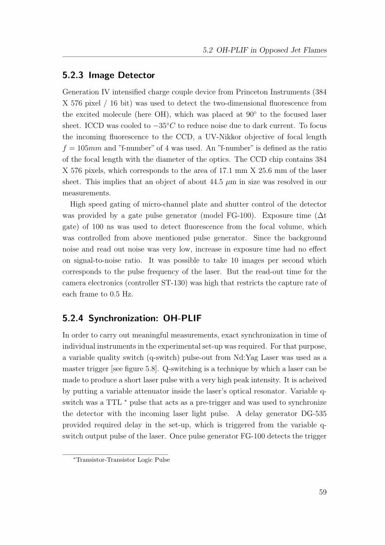
5.2 OH-PLIF in Opposed Jet Flames
5.2.3 Image Detector
Generation IV intensified charge couple device from Princeton Instruments (384
X 576 pixel / 16 bit) was used to detect the two-dimensional fluorescence from
the excited molecule (here OH), which was placed at 90 to the focused laser
sheet. ICCD was cooled to −35C to reduce noise due to dark current. To focus
the incoming fluorescence to the CCD, a UV-Nikkor objective of focal length
f = 105mm and ”f-number” of 4 was used. An ”f-number” is defined as the ratio
of the focal length with the diameter of the optics. The CCD chip contains 384
X 576 pixels, which corresponds to the area of 17.1 mm X 25.6 mm of the laser
sheet. This implies that an object of about 44.5 µm in size was resolved in our
measurements.
High speed gating of micro-channel plate and shutter control of the detector
was provided by a gate pulse generator (model FG-100). Exposure time (∆t
gate) of 100 ns was used to detect fluorescence from the focal volume, which
was controlled from above mentioned pulse generator. Since the background
noise and read out noise was very low, increase in exposure time had no effect
on signal-to-noise ratio. It was possible to take 10 images per second which
corresponds to the pulse frequency of the laser. But the read-out time for the
camera electronics (controller ST-130) was high that restricts the capture rate of
each frame to 0.5 Hz.
5.2.4 Synchronization: OH-PLIF
In order to carry out meaningful measurements, exact synchronization in time of
individual instruments in the experimental set-up was required. For that purpose,
a variable quality switch (q-switch) pulse-out from Nd:Yag Laser was used as a
master trigger [see figure 5.8]. Q-switching is a technique by which a laser can be
made to produce a short laser pulse with a very high peak intensity. It is acheived
by putting a variable attenuator inside the laser’s optical resonator. Variable q-
switch was a TTL ∗ pulse that acts as a pre-trigger and was used to synchronize
the detector with the incoming laser light pulse. A delay generator DG-535
provided required delay in the set-up, which is triggered from the variable q-
switch output pulse of the laser. Once pulse generator FG-100 detects the trigger
∗Transistor-Transistor Logic Pulse
59

5 Experimental Methods
from DG535, it sends the high voltage pulse that opens the internal shutter of
the detector (ICCD).
The detector was left open for a defined exposure and the incoming light was
registered in the CCD. After the detector had finished registering photons, the
captured light in the CCD wells were transferred to the analog-to-digital con-
verter for the read-out process. During the read-out process the camera con-
troller sends the not-scan pulse to the pulse generator FG-100, which restricts
the detector to register new images during read-out process. Once the read-out
was done, camera controller frees the pulse generator to send the high voltage
pulse to the detector and the next image is taken. The schematic of the trigger
system is depicted below.
Figure 5.8: Schematic showing the trigger system used for PLIF measurement.
DG535: delay generator, FW: flame watcher, A: logical AND, FG-100: High volt-
age pulse generator, ICCD: Intensified charge couple device (detector), ST130:
controller for the detector.
Normally DG535 and pulse generator were triggered at 10 Hz, similar as
Nd:Yag laser. However, time required during read-out process was long, which
lets the detector to register at the rate of half the frames per second. For the
60

5.3 Multiple Scalar Measurements in Swirl Flames
measurement of extinguishing flames, a flame watcher was installed in the set-up
that triggers an output TTL signal only when it detects flame. This was required
since some of the high turbulent flames extinguished every 10 sec, thus making
experiments almost impossible without flame watcher. A flame-monitoring de-
vice F-150 in combination with a flame sensor FFS 05 from LAMTEC Leipzig
GmbH & Co. KG was used as a flame watcher. It detected the flame emission
within the spectral range of 210-400 nm. To remain in the ”flame in” stage the
sensor required a pulse amplitude of ≥ 30mV by viewing to the flame.
The flame monitoring device, which was connected in series with the flame
sensor is able to distinguish between the ”flame in” and ”flame out” states of the
flame. It also outputs the TTL signal that can be used to synchronies the flame
ignition system which is controlled with LABVIEW software. Logical ”AND”was
used in between DG535 and the pulse generator FG-100. The output of DG535
delay generator was connected to the one end of the logical ”AND”, whereas the
other end was connected to the TTL output from the flame watcher. Trigger
to the pulse generator is initiated once the high peak of TTL signal from both
delay generator and the flame watcher was detected. Pulse generator then sends
high voltage signal to the detector for initializing frame capturing process. The
high peak of TTL from flame watcher corresponds to the ”flame on” condition
and therefore, image was captured only when flame watcher detected signal.
5.3 Multiple Scalar Measurements in Swirl Flames
This section elaborates the experimental set-up for simultaneous measurement
of radicals [OH][HCHO] in turbulent premixed swirl jet flames. Most of the
previous reports have chosen separate laser systems to excite individual molecules
in order to extract meaningful single-shot planar images [57]. We have used a
single Nd:Yag laser system to excite both molecules for our measurement. Several
literature have been reported that used a laser wavelength of 338 nm [30] and
353.4 nm [60], but only few have used a laser wavelength of 355 nm to excite
the formaldehyde molecule for point and planar measurement in combustion
flames [57]. This is because the excitation wavelength of 355 nm lies on the
weak transition, which results in bad signal to noise ratio and does not permit
single-shot measurements. We have been able to successfully carry out planar,
61

5 Experimental Methods
single-shot measurements inside the turbulent flame with sufficient contrast to
identify the formaldehyde molecule.
5.3.1 Experimental Set-up
Figure 5.9: Schematic of experimental set-up for multiple scalar measurement. P:
prism, WEX: wavelength extender, P-B P: pellin-brocca prism, CL: cylindrical
lens, BS: beam splitter, M,M’: mirror, FS1,FS2: filter set, BD: beam dump,
EKT-SB: EKT-Swirl Burner.
The laser system for multiple scalar measurements was similar to that used in
[OH]-PLIF, except an additional non-linear crystal (3rd harmonics) was used to
generate a laser pulse at wavelength 355nm from the same laser system. Har-
monic generator module inside the laser for multi-scalar measurements contained
two non-linear crystal that outputs laser light at 2ω (532 nm) and 3ω (355 nm)
from the laser system. Where ω is the natural frequency of the laser light and
62

5.3 Multiple Scalar Measurements in Swirl Flames
higher values are its harmonics. The green laser beam at wavelength 532nm was
used to pump the dye laser to generate 568 nm, which is then frequency doubled
using another non-linear crystal inside wavelength extender to generate 283.1
nm.
The output beam from wavelength extender was used to excite the A-X band
(transition) of the hydroxyl radical inside the flame. Laser beam generated from
third harmonics was reflected with the help of high energy laser mirrors with a
reflection greater than 99.5 % situated just before the entrance of dye laser. This
beam was redirected to the measurement volume and was used to excite the weak
transition of the formaldehyde radical in the targeted flame. An schematic of the
experimental set-up used for this measurement can be seen in figure 5.9. The
hydroxyl molecule was excited with the laser beam generated from wavelength
extender at 281.5nm.
5.3.2 Optical Set-up
As shown in figure 5.9, a laser beam 355 nm and 532 nm is generated inside the
harmonic generator with the help of non-linear crystals. UV laser beam at 355
nm was reflected using a beam splitter BS just before the dye laser. An IR laser
beam was blocked and a laser beam at 532 nm was used to pump the dye laser
[Rodamine 6G], that generates laser at 563 nm. The output laser beam from
the dye laser is reflected with the help of a prism to the entrance of wavelength
extender. Laser beam at 563 nm is then frequency doubled with the help of
*KDP crystal inside the WEX generated laser beam at 281.5 nm, which is then
filtered with the help of Pellin-Brocca prism. This laser beam at 281.5 nm is
used to excite R1(8) band of OH molecule. Before required laser beams at 355
nm and 281.5 nm is launched to the focal volume, they are transformed to laser
sheets with the help of cylindrical lens with focal distance of 1000 mm.
The emission was collected at 90 of the laser sheet, and imaged on a gated
intensified ccd camera with an UV-Nikkor objective lens of focal length f =
105mm and a ”f” number 4. Suitable spectral band-pass filters were interposed
in front of the individual detector to reject elastic scattering (Rayleigh scattering)
at the laser wavelength and to select the suitable fluorescence. Filter set [FS1] on
the hydroxyl detection side includes dichroic short pass filter(T ≥ 95% between
305-330 nm). Whereas, filter set [FS2] on the formaldehyde consists of GG-
63

5 Experimental Methods
420 and CP-AB-505-2X. The transmission curves for FS2 filters are checked till
800 nm because no laser induced emission was detected from the combustion
flame beyond this limit. In short, hydroxyl ICCD can only detect laser-induced
emission ranging from 305 nm to 320 nm, whereas formaldehyde ICCD is made
to detect the light within the wavelengthrange 420 nm to 500 nm.
5.3.3 Image Detector and synchronization
Image detector for OH molecule was used as mentioned in the starting of this
chapter. For detecting signal from formaldehyde molecule, a similar intensifier
CCD device as the OH molecule was used.
Figure 5.10: Schematic diagram showing delay between laser and detector trigger
pulse for simultaneous measurement. laser pulse(1064nm): laser pulse out, laser
pulse(355 nm): laser pulse at focal volume (D1=150 ns), laser pulse(281.5 nm):
laser pulse at focal volume (D2= 650 ns).
Trigger system looked very similar to the one that was used during the OH-
PLIF measurement, except one extra detector and its controller was added and
that was also controlled with the same delay generator DG535 mentioned in OH-
trigger schematic. Laser trigger was used as a master trigger for the complete
experimental set-up, other electronics utilized was a delay generator DG535,
64

5.3 Multiple Scalar Measurements in Swirl Flames
pulse generators for intensifier charge couple devices (ICCD’s) and computer for
data acquisition that captures and stores the captured images. A pre-trigger
pulse from the laser triggered the delay generator, that controls the delay of
H.V.pulse to the individual ICCD detector. A pulse generator FG-100 was used
to pulse the ICCD detector [OH-side] once a TTL pulse from DG535 is detected.
Another pulse generator from Stanford instruments was used to pulse the other
detector[HCHO-side]. Both delays were controlled from the DG535.
As shown in figure 5.10, there is a small delay between D1 and D2. This delay
was about 500ns and since the smallest scale of turbulence (Kolmogorov scale)
in the flame was much larger than this value, these measurements can be still
called as simultaneous measurements.
5.3.4 HCHO spectrum analysis
Initially a planar image of the flame was captured in order to get an idea on
the location of excited molecules inside the laminar flame by the laser light at
355 nm. In order to confirm for the formaldehyde molecule, emission spectrum
at the high intensity location was registered using a spectrometer and a two
dimensional detector array. This measured spectrum was then compared with
the spectrum available in the literature [68] (see figure 4.7). The combination of
Planar measurement and spectrum analysis confirmed us that we were exciting
and detecting the formaldehyde molecule.
5.3.4.1 Planar Measurement
Formaldehyde molecule was excited using a laser light at 355 nm that can be
easily accessible by using a 3rd harmonic non-linear crystal before the funda-
mental beam (1064 nm) from an Nd:Yag laser. Details on the laser system used
for these measurement are provided in the section(5.2.1).
An ICCD detector of chip size 384 X 576 pixels was used and each pixel size was
equal to 44.5 µm X 44.5 µm, which means that the whole chip thus corresponds
to 17.1 mm X 25.6 mm approximately. This detector was gated with the help of
a pulse generator FG100, and was set at 50 ns opening time, which was enough
for fluorescence signal to be captured. This gated time was kept low in order to
reject the unwanted stray light from the reflecting surfaces near the measurement
space. Synchronization of such experimental set-up was done, which was almost
65

5 Experimental Methods
similar to the trigger system used in OH-PLIF measurements in opposed jet
burner.
As can be seen from the figure 5.11 (a), the output beam from the harmonic
generator was redirected with the help of dichroic mirror and was turned into a
laser sheet with the help of a cylindrical lens of focal length 1000 mm, which is
then focused to the focal volume above the burner nozzle. The two-dimensional
fluorescence signal was captured by the detector placed 90to the incoming beam.
Rayleigh signal from the laser beam was rejected using a long-pass filter GG-420
[Schott glass filter] in front of the detector.
Figure 5.11: Side(a): Experimental setup for HCHO-PLIF measurement in EKT
standard burner. Side(b): Experimental setup for point measurement for HCHO
emission spectrum in EKT standard burner. FO: focussing optics, DO: detection
optics, F: filter, M: mirror, BS: beam splitter, BD: beam dump.
66

5.3 Multiple Scalar Measurements in Swirl Flames
5.3.4.2 Spectrum Measurement
For spectrum measurement, the laser beam was focused to the single point in
the measurement volume by a spherical convex lens of focal length 500 mm.
Fluorescence signal from a point was collected with the help of collecting lens
(L1) of 200 mm. The collimated beam was then focused to the entrance slit of the
spectrometer with another lens (L2) of 250 mm. This combination confirms the
f-number of the collection system is less than the f-number of the spectrometer,
which is important to capture the maximum signal inside the spectrometer. The
grating of the spectrometer was having the resolution of 600 line/mm and had
the spectral dispersion of 2.64 nm/mm. The signal from the grating was then
redirected to the exit of the spectrometer and then to the ICCD detector as can
be seen in figure 5.11(b).
67

5 Experimental Methods
68

6 Data Image Processing
Image processing can be understood as the transformation of the ”raw image”to a
meaningful ”processed image”. An image is defined as a function u on <2 raster,
where u(x,y) represents the gray value or intensity at point (x,y). Accurate
detection of relevant object accurately and extraction of required data has a
central importance in image processing. This relevant object must be clearly
distinguished from background or other interfering objects.
This assumption is however seldom met in real world application due to fac-
tors like limited dynamic range of detectors, dark noise etc. Therefore, correction
procedures should be implemented to compensate for these experimental defects.
Introduction on image processing for scientific application is available from a well
known handbook from Jahne [71]. In this chapter, details on post-processing
algorithms that include correction, noise rejection and image enhancement of
structures are described. Strategy applied for the image post-processing is di-
vided into following steps:
1. Correction
a) Background correction
b) Correction of the intensity of laser profile
2. Noise reduction
3. Edge enhancement
4. Binary image generation
5. Evaluation of topological flame characteristics (flame area, flame length
etc.)
69

6 Data Image Processing
6.1 Correction
6.1.1 Background Subtraction
Experimental images have to be compensated for the background noise. It con-
sists of constant positive level accumulated during read out process from the
detector and experimental background intensity level. The background noise
was determined by taking the images without any illumination, which was ap-
prox. 350 counts on the detector of 16 bit resolution. Background image was
subtracted from acquired raw flame and laser intensity images to compensate for
the background noise.
6.1.2 Laser Profile Compensation
Every laser based techniques requires normalizing of the data with the laser pro-
file, in order to correct for the laser inhomogeneities. Therefore, the background
corrected flame images were normalized by the average laser sheet to correct for
the effect of laser fluctuations and inhomogeneities. Since hardly any change was
observed in long term fluctuation of laser profile, the average over 50 accumu-
lated images was used for compensating this defect. An averaged laser profile
was captured between every 500 flame images.
Figure 6.1 shows the raw image, the laser sheet and corrected normalized
image. Ideally after background subtraction of the acquired flame image, the
intensity where molecules are not present should be zero. That would result in
no surrounding noise spikes after laser profile compensation (normalization). But
practically non-zero values lead to the noise spikes which can be clearly seen in
normalized image. For eliminating these noises, further image post-processing
techniques such as suitable filtering and edge enhancement was applied to this
normalized image.
6.2 Noise Rejection and Edge Enhancement
Improving signal-to-noise ratio and reducing spurious pixel intensity values in
unprocessed image is an important step in image processing. Normalized images
(mentioned above) suffer from bad signal-to-noise ratio and require smoothing
70
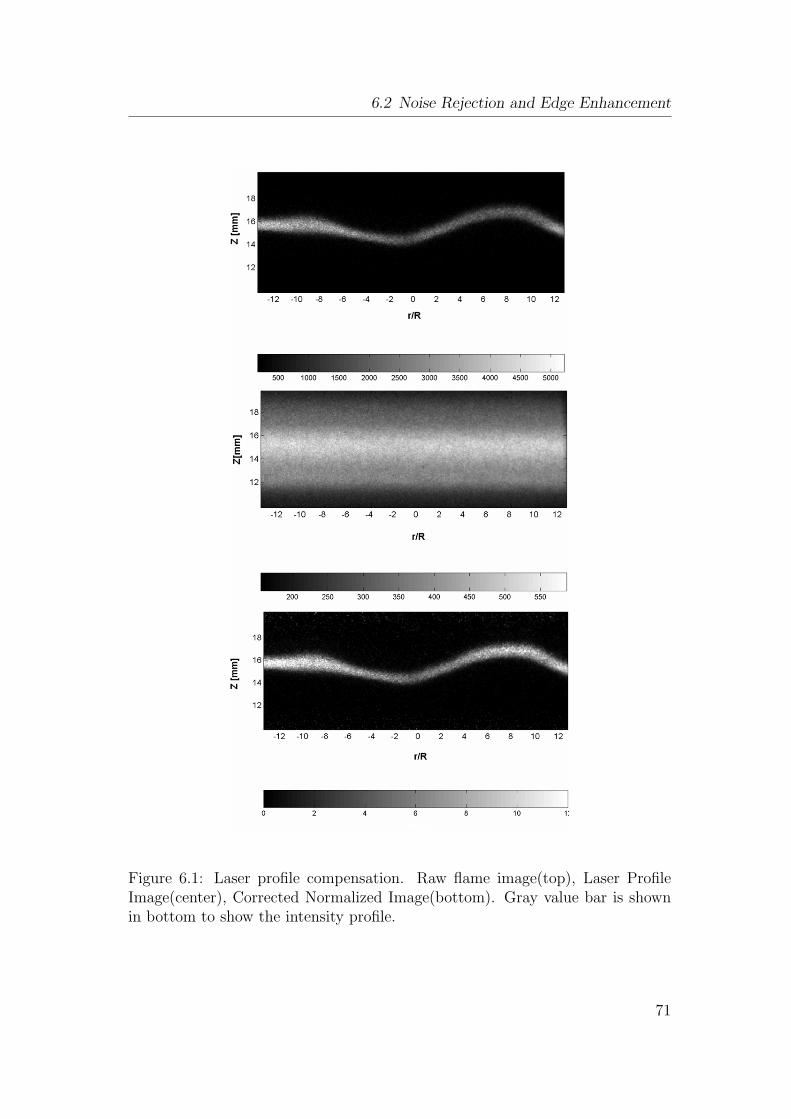
6.2 Noise Rejection and Edge Enhancement
Figure 6.1: Laser profile compensation. Raw flame image(top), Laser ProfileImage(center), Corrected Normalized Image(bottom). Gray value bar is shownin bottom to show the intensity profile.
71

6 Data Image Processing
of high frequency noise as well as enhancing of relevant structures before any
topological studies are made. Several linear and nonlinear filters are available,
but their application is restricted to the type of distortion in the given image.
While linear filters work well within flat regions, they are questionable near the
gradients. They tend to smooth all types of gradients independent, if they carry
useful information or noise. Thus, applications of such filters are restricted to
the images where the issue of gradient preservation and edge enhancement is not
critical.
Figure 6.2: Graph displaying the profile filtered with two dimensional median
method with mask size [5x5].
Non-linear filters can overcome such problem if user defined parameters are
suitably applied to the given image. Objective choice of user defined parameters
relies upon sensitivity analysis which will be discussed in the later part of this
chapter. In this work only nonlinear filters were used for noise reduction since
gradient preservation and edge enhancement is critical for detection of the flame
front.
72

6.2 Noise Rejection and Edge Enhancement
6.2.1 Median Filter
Experimental LIF images contained several high amplitude single-distorted pixels
near gradient of intensity ”u” of the detected species, which require smoothing
before relevant information is extracted. Median filter was found as well-known
approach to smooth out such pixels. In the case of median filter, the pixels of a
sub-area defined by the neighborhood are sorted for their amplitudes. The value
of the central pixel of the sub-area is then re-defined by the amplitude, which
is in the middle of this arrangement. In this process, it efficiently removes the
solitary pixels with highest and lowest amplitudes emerging near the gradient
without altering the gradient itself. The effect of median filter in a test profile is
depicted in figure 6.2.
6.2.2 Non-Linear Diffusion method
Next step of image processing after unwanted noise is diminished, is to enhance
the relevant structures. This is best done by using an edge enhancement routine.
Here, non-linear operation based on partial differential equation known as nonlin-
ear diffusion method was applied. Non-Linear diffusion has deservedly attracted
much attention in the field of image processing for its ability to smooth noise
locally, within regions defined by boundaries. Smoothing stops as the disconti-
nuity such as boundaries are reached, which leads to amplification of boundaries
or edges in the given image.
It is adapted from an approach originally formulated by Perona and Malik
[72][73]. A good introduction to nonlinear diffusion can be found in lecture
notes of J.Weickert of Dept. of Computer Science. Weickert [74][75] also gives a
comprehensive survey of the literature. Malm [76] applied NLDF filtering in the
images taken from planar laser induced fluorescence spectroscopy.
To apply a diffusion process to an image, we regard the gray value u as the
concentration of a chemical species. Equation 6.1 shows the solution of the linear
diffusion equation, where D is a scalar constant known as diffusion coefficient.
Perona & Malik (1987) proposed to exchange this diffusion coefficient D in eq.
6.1 with a scalar-valued function g of the gradient ∇u of the gray values in the
image [eq. 6.2]. This non-linear equation is solved iteratively till the desired
result is achieved.
73

6 Data Image Processing
∂tu = div(D∇u) (6.1)
∂tu = div[g(∇u)∇u] (6.2)
The diffusion coefficient is made dependent on the edge strength as given by
the magnitude of the gradient, thus making diffusion process non-linear. The
function g is required to be smooth and non-increasing with g(0)=1 and g(s)→0 for s →∞, where s is equal to ∇u. We used the diffusivity function proposed
by Weickert. Figure 6.3 shows comparison of Weickert’s and Perona & Malik
diffusivity function. Weickert’s diffusivity function reads as:
g(s) = 1− exp[−cm/(s/λ)m] (6.3)
where m is a positive integer and a constant. It is a process specific constant
which governs the shape of the function ”g”. Big values of ’m’ make the flux
of the function change quickly. The constant cm is calculated to make the flux
function (s∗g(s)) ascending for s < λ and descending for s ≥ λ. That means the
diffusion in the direction across the edges will be a forward diffusion when ∇u <
λ and a backward diffusion when ∇u > λ. Lambda is the contrast parameter,
that separates regions where forward diffusion occurs from those where backward
diffusion takes place. In other words, if the gradient is inferior to lambda the
flux is increasing with the gradient and if the gradient is larger then lambda the
flux decreases as the gradient grows.
Figure 6.3 shows the three different diffusivity function formulated by Perona
& Malik and Weickert. The solid curve corresponds to Perona & Malik, the
dotted (m=2) and dash-dot (m=8) curve corresponds to diffusivity function of
Weickert. The flux rises to its maximum at λ=1, then falling again for increasing
gradient ∇u. Parameter selection for edge detection was done in such a way that
maximum diffusion occurred for the gradient exhibited by noisy features and
minimum for the edges. This selection helps in clearly distinguishing the regions
across the gradients. Weickert diffusivity function with greater m shows sharper
peaks in the flux, which directly means less iteration required for desirable results.
It also has a drawback that the function becomes sensitive to proper choice of λ.
Influence of various critical user defined parameters used in non-linear diffusion
74
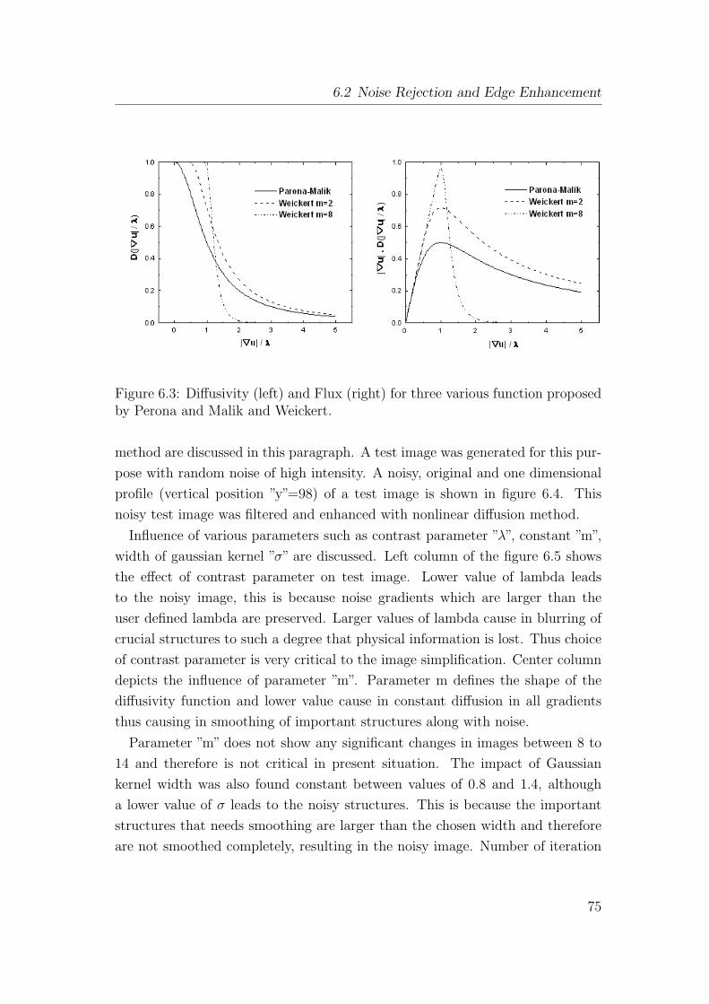
6.2 Noise Rejection and Edge Enhancement
Figure 6.3: Diffusivity (left) and Flux (right) for three various function proposedby Perona and Malik and Weickert.
method are discussed in this paragraph. A test image was generated for this pur-
pose with random noise of high intensity. A noisy, original and one dimensional
profile (vertical position ”y”=98) of a test image is shown in figure 6.4. This
noisy test image was filtered and enhanced with nonlinear diffusion method.
Influence of various parameters such as contrast parameter ”λ”, constant ”m”,
width of gaussian kernel ”σ” are discussed. Left column of the figure 6.5 shows
the effect of contrast parameter on test image. Lower value of lambda leads
to the noisy image, this is because noise gradients which are larger than the
user defined lambda are preserved. Larger values of lambda cause in blurring of
crucial structures to such a degree that physical information is lost. Thus choice
of contrast parameter is very critical to the image simplification. Center column
depicts the influence of parameter ”m”. Parameter m defines the shape of the
diffusivity function and lower value cause in constant diffusion in all gradients
thus causing in smoothing of important structures along with noise.
Parameter ”m” does not show any significant changes in images between 8 to
14 and therefore is not critical in present situation. The impact of Gaussian
kernel width was also found constant between values of 0.8 and 1.4, although
a lower value of σ leads to the noisy structures. This is because the important
structures that needs smoothing are larger than the chosen width and therefore
are not smoothed completely, resulting in the noisy image. Number of iteration
75

6 Data Image Processing
Figure 6.4: Original test image, random noisy test image and its one dimensionalprofile is shown.
for evaluation of these images was taken as 100. Contrast parameter ”λ” is the
only critical parameter and is the weakness of this method. Edge enhancement
of this method is the advantage of this method, which leads to better distinguish
between important structures and noise. Figure 6.6 shows a noisy intensity profile
and its gradient. Corresponding filtered intensity profile and its gradient is also
depicted. Also gradient enhancement can be clearly seen in the same figure.
6.3 Binary Image Generation
For the identification of structural quantities the amplitude information of the
images is of no importance. Therefore, the gray scale images might be trans-
formed into binary images without basic loss of information. Within the binary
image, information is reduced to ’pixel inside the gradient’ or ’pixel outside the
gradient’. For this distinction, a simple threshold method is applied. Pixels with
amplitude below a user set threshold are defined as OFF pixels and those with
amplitude above the threshold are defined as ON pixels. Naturally, the settings
of the threshold influence the results.
A threshold value which is too low generally implies inclusion of noise in the
result, whereas a threshold too high results in a loss of relevant information by
cutting away locations with lower signal intensities. Thus, the threshold derived
from the objective analysis was chosen to meet both requirements i.e. noise
rejection and information preservation.
76

6.4 Algorithms Applied
Figure 6.5: Influence of various parameters on test image after nonlinear diffusionmethod is depicted. Left column shows the effect of contrast parameter ”λ” ontest image. Middle column shows the effect of parameter ”m” and the rightcolumn the gaussian kernel ”σ”.
6.4 Algorithms Applied
In qualitative topological studies, results are strongly dependent on the selection
of filters and edge enhancement routines. Algorithm selection depends upon
various factors such as computational speed, sensitivity to noise and user defined
parameter. Therefore two algorithms are discussed that comprises suitable filter,
edge enhancing routine and routine that generates binary image marking the
flame front. Firstly median-threshold-majority method and secondly median-
nonlinear diffusion-threshold method were tested. Both algorithms and there
impact on results will be discussed later.
6.4.1 Median-Threshold-Majority Method
This algorithm includes two dimensional median filtering in LIF images, which
is then followed by binary image generation. Median filter worked well to re-
move surrounding noise in the given image but was partially able to remove high
77

6 Data Image Processing
Figure 6.6: Figure shows Edge enhancement property of nonlinear diffusionmethod in a test profile. Top: Noisy profile from the test image and corre-sponding gradient of the intensity. Bottom: The filtered profile using non-lineardiffusion method and the corresponding gradient of the intensity from filteredprofile. Clearly edge enhancement of the profile can be seen from the gradientplot after the application of NLDF method.
frequency components attached to the edges. They are later removed by the
application of an iterative process known as majority method. This method is
an edge smoothing algorithm and is applied directly to the binary image.
Figure 6.7 shows the noisy contour after median filtering, which is smoothed by
majority method. If the majority of the surrounding pixels defined by the kernel
widths (defined as mask) possess the value 1 the central pixel, which undergoes
the transformation process, is set to 1, otherwise it is set to 0. In this process,
noise attached to the edges of a large structure becomes isolated and thus diffused
78

6.4 Algorithms Applied
via iterative procedure.
Figure 6.7: An example showing the removal of noise attached to the edges of
the flame front via majority method
6.4.1.1 Sensitivity Analysis
An appropriate set of user defined parameters−→k (like filter kernel widths and sig-
nal intensity threshold) must be defined before applying algorithms to the given
image. The choice of an optimized parameter set is crucial for the discrimination
between noise and structural information and thereby for the identification of the
topological flame characteristics −→c = −→c (−→k ). One possible way to quantify the
influence of these parameters on the result is a sensitive analysis. This analysis
yields the sensitivity E(−→c ,−→k ) in dependence of topological flame characteristics
with respect to the variation of each of the parameters, as shown in eq. 6.4.
Ei,j = ∆ci/∆kj (6.4)
If the selected quantity is insensitive to the variation of the parameter the
sensitivity is small, which means the choice of the parameter is non-critical for
the flame characteristics. The optimal parameter is located where the transition
from a low to a high sensitivity is found. This is a point of maximum bending,
or the maximum of the 2nd derivative of ci with respect to kj.
Naturally, this method is only applicable if ci is not linearly dependent on the
parameter k. Figure 6.8 shows the result of a sensitivity analysis. In this example
the quantity ci is the flame area that is defined as the total number of ”on”pixels
in the binary image. Both median kernel size k1 and the threshold for binary
image generation k2 is varied. It is obvious that kernel size k1 does not influence
the results, whereas for k2<1 a high sensitivity and for k2>1 a small sensitivity
79

6 Data Image Processing
Figure 6.8: Sensitivity of flame area with threshold is depicted. Flame areaverses threshold, also included is the 2nd derivative of the OH area with respectto threshold.
is observed.
An optimal choice of k2 is obviously approximately 1, slightly above the value
where the second derivative of ci shows a maximum. This maximum marks the
transition from low to high sensitivity, as visible in figure 6.8. Notice, that the
sensitivity analysis in this case additionally shows that k1 and k2 are statistically
independent. From sensitivity analysis, it was concluded that threshold of value
1 is the proper choice for our [OH] PLIF images. Also kernel width is insensitive
to the parameter of interest therefore, mask size 5x5 was chosen.
6.4.2 Median-Non-Linear Diffusion-Threshold
Figure 6.9 shows the LIF image before and after the application of nonlinear
diffusion filter. Parameter that are not critical for LIF images are the parameter
”m” (8 ≤ m ≤ 12), width of gaussian kernel ”σ” (0.8 ≤ σ ≤ 1.4) and number of
iteration (> 75 iteration). These limits of the user-defined parameter can also be
concluded from the test images from figure 6.5. The set of parameter chosen for
80

6.5 Conclusion
Figure 6.9: OH-LIF image before and after application of nonlinear diffusionmethod. Gray value bar is shown in bottom to show the intensity profile.
OH-LIF images from opposed jet burner were λ=0.2, m=8, no. of iteration=100,
σ=0.8. Important features such as flame boundaries are clearly enhanced after
nonlinear fusion filter as shown below.
6.5 Conclusion
It is always hard to say, which algorithm is best in image processing. It totally
depends upon the features one has to preserve and unwanted noise. The worst
case is when the noise are similar and distributed throughout the image along
81

6 Data Image Processing
with the important gradients that needs to be preserved. It is well known that it
is impossible to define a single algorithm, which is suited for all types of features.
Comparison of various algorithms for image post processing is discussed in details
by Schiessl.et.al [77].
Figure 6.10: Global area extracted using two different algorithms of image post-
processing from OH-LIF images. φ represents the equivalence ratio, AG is global
area and Amax is the mean global area value for flame with φ = 1.2 and with
algorithm ”Med-Th-Maj”.
Figure 6.10 shows the effect of different post-processing strategies to extract
global flame area defined by OH molecule. Global area (AG) is calculated as
the total number of ”on” pixels in the binary image, which is generated from
the OH-PLIF raw images by applying a threshold. Statistics have been gener-
ated from 3000 instantaneous binary images. All global area values have been
normalized with the mean global area value for flame with equivalence ratio 1.2
and algorithm type ”median-threshold-majority”. The results evaluated from two
82

6.5 Conclusion
different algorithms applied in image processing of images is also depicted. The
trend remains the same for both the algorithms but the mean values are differ-
ent. However, qualitatively trends and shapes of the results are important. Thus
similar trend from both algorithms shows that the global area is insensitive to
the type of algorithm applied.
For our LIF images, we have chosen the second algorithm (Median-nonlinear
diffusion-threshold) because of its better efficiency in noise reduction, even in the
presence of severe noise levels. Also it promises gradient enhancement, which
is important for clear distinction between the burned and unburned regions of
the flame. Although this method is time consuming and harder to implement
numerically than the first algorithm (Median-threshold-majority method).
83

6 Data Image Processing
84

7 Opposed Jet Flames
The main results obtained on the turbulent opposed jet flames using laser in-
duced fluorescence is presented. Chapter starts with the review on literature
survey on stagnation point stabilized flames. Which is then followed by the de-
tailed description of the EKT opposed jet burner and properties of the flames
that have been measured in this work. Thereafter, characterization of the EKT
opposed jet burner is provided, that includes survey and plots from the previ-
ous measurements using various non-intrusive techniques. Last section provides
the outcome of the measurement and discussion on the major findings from the
current study.
7.1 Introduction
The reasons for investigating counter-flow stagnated flames are manifold. Firstly
these flames are relatively easy to control in the laboratory. Secondly with the
same burner set-up, flames from the diffusion to the premixed limit can be studied
while varying parameters like Reynolds numbers, strain rates, turbulence inten-
sities and length scales, which is convenient from the experimentation point of
view. Advantages for the modelers from using this configuration are the absence
of pilots or flame holders, any contact of the flame to walls and the simplicity of
its geometry. Therefore, for development and validation of various sub-models, a
counter-flow geometry is ideally suited. Due to the rotational symmetry and the
limited extension of the flow field, even complex phenomena such as turbulent-
chemistry interaction can be explored by using advanced chemistry models or
more sophisticated models of the turbulent flow like LES [78],[13].
Turbulent flames stabilized in a counter-flow geometry have been studied to
gain insight into two major issues i.e. turbulent mixing and flame stabilization.
In non-premixed flames, it is important in order to keep the combustion chamber
compact and light in weight. Fast mixing between the two fluids is important
85

7 Opposed Jet Flames
to restrict the flame length and enabling a more intense combustion. Premixed
as well as non-premixed configurations have been investigated in the opposed jet
geometry with various experimental methods for example by [79]-[96] and with
numerical techniques, such as [78],[97],[98],[13].
Investigation on flame stabilization or the understanding of extinction mech-
anism is one of the fundamental issue in turbulent non-premixed flames. There-
fore, most of the literature have been focussed on the understanding of the ex-
tinction events and the properties influencing it. Parameters like flow structure,
flow properties, scalar dissipation rate, high strain rate etc. have been found to
be influencing extinction events in such flames.
Kitajima et al. attempted to deduce the effects on extinction limits by varying
turbulent characteristics of the air and fuel stream individually. This was done by
the means of a laser tomographic technique [82],[83] and later more accurately by
planar Rayleigh imaging. Kostiuk et al. [99] introduced the effects of small-scale
eddies to the extinction of turbulent counter-flow premixed flames. It was shown
that the extinction occurred when the sum of the bulk flow stretch rate and
small-scale stretch rate caused by Kolmogorov scale exceeded a certain limit.
Where flame stretch is defined as the fractional rate-of-change of flame area
and expressed exactly as the sum of tangential strain rate and flame curvature.
Similar criteria was applied for the extinction of partially premixed and non-
premixed flames of opposed jet burner by Mastorakos et al. [87].
Mastorakos et al. [88] also confirmed another criteria initially proposed by
Peters and Williams for the extinction of turbulent non-premixed flame. They
identified the scalar dissipation rate as the central parameter controlling turbu-
lent reactive flows and their extinction. It was also shown that the mean scalar
dissipation rate increases with increasing bulk and/or turbulent strain rates,
which implies that both strain rates have to be low to ensure non-premixed
flame stability in the counter-flow geometry.
Thermocouple measurements of temperature, and its radial and axial dissi-
pation, by Sardi et al. [93] demonstrated that scalar residence times in the
mixing layer are shorter than large-eddy turn-over times and that fluctuations
are strongly correlated with scalar dissipation rate. Results in the current thesis
indicate the presence of ”young turbulence” or in other words, turbulent flow
is not fully developed during the mixing process. Also large scale motions are
found to be the driving factor for extinction events in the investigated turbulent
86

7.2 Burner Description
opposed jet flames. Which implies that the flame stability is compromised by
total flame stretching and not by small-scale wrinkling.
Recently, information on velocity field, scalars, and scalar dissipation of turbu-
lent reacting and non-reacting opposed jets were obtained using 1D Raman/Rayleigh
scattering and LDV in two dimensional flow field [13]. These experimental re-
sults were supported and accessed by results from numerical modelling (LES).
Mixture-fraction and scalar dissipation rates were represented very well along the
center-line. Same group also estimated the performance of mixing models on tur-
bulent opposed jet flames similar to above [80]. These models were validated with
the experimental results obtained from scalar and velocity field measurements.
The numerical results were extracted from one-dimensional Monte Carlo PDF
simulations with a 12-step reduced chemistry and reduced chemistry. Simulation
in general showed a very good agreement for scalar and flow field properties in
the physical space. However, extinction limits computed with the mixing models
were overestimated by a factor of more than 2 in terms of bulk strain rates [80].
Laser tomography has been applied to study spatial flame structures of pre-
mixed [100] and non-premixed flames [82], but no studies exist with emphasis
on turbulent partially-premixed flames. Furthermore, flame fronts detected by
tomography are ambiguous since non-uniform distributions of seeding spray, size
and spatial distribution of the spray have an impact on structural information.
Thus, in analogy to extensive studies on turbulent jet flames [23],[101], there is
a need of comprehensive data sets on counter-flow configurations especially for
combustion LES validation.
7.2 Burner Description
The flow configuration in the EKT opposed jet burner ∗ consists of two identical
opposed nozzles, each surrounded with a annular section. A schematic diagram
of the burner assembly is shown in figure 7.1 [81]. Each contoured nozzle, is
profiled with a contraction ratio of 9:1 and is followed by a straight tube of
50 mm length. The inner nozzle with a diameter of Din=30mm is surrounded
by a concentric co-flow (Dcf=60mm) of N2, which provides a flame stabilizing
curtain in order to prevent pre-reaction of partially premixed fuel upstream of
∗©Dirk Geyer(TU-Darmstadt)
87

7 Opposed Jet Flames
the stagnation plane. For these measurements nozzle separation distance is kept
constant, which is equal to Din.
Figure 7.1: Schematic diagram of the Darmstadt Turbulent Opposed Jet Burner.
Z is the burner axis, lower and upper nozzles are located at Z equal to 0 and
30 mm respectively. The burner stagnation plane Zst is situated at the center
between the nozzles, Zst equal to 15.
A rich fuel-air flow exiting from the lower nozzle impinges on a pure air flow
coming from the upper nozzle, resulting in the stabilization of a turbulent flame
in the vicinity of half the distance between the burner nozzles. The nozzles are
separated by a distance H=30 mm resulting in a ratio H/Din=1.0. The fluid
flows through perforated plates located at 50 mm upstream of the nozzle exit
and acting as turbulence generators. They consist of hexagonally arranged round
88

7.3 Flames Measured
holes with a blockage ratio of 45 % and a hole diameter of 4.0 mm. Contoured
nozzles upstream of the perforated plates ensure uniform inflow condition at the
perforated plates.
7.3 Flames Measured
Premixed and partially premixed methane/air mixtures at different equivalence
ratios (i.e. φ=3.18, 2.0, 1.6, and 1.2) are used as fuel. Without additional mixing
with air from the upper nozzle these mixtures are outside the flammability limits,
except for the φ=1.2 case, and therefore burning is similar to non-premixed
flames. Using an equal momentum for the flow rates of the two opposing flows
the stagnation plane is established half way between the nozzle.
Reynolds numbers (Re), based on the bulk velocity at the oxidizer nozzle exit
and the nozzle diameter Din are varied between 3300 and 7200 as shown in table
7.1. The highest Re-number for the respective equivalence ratios φ=3.18 and 2.0
correspond to flames that do not burn for a time duration longer than 30 seconds
in 100 subsequent runs. These flames are described as extinguishing.
Reair am(1/s) φ≡3.18 φ≡2.0 φ≡1.6 φ≡1.2
3300 115 TOJ1A - - -
4500 158 TOJ1B TOJ2B - -
5000 175 TOJ1C TOJ2C TOJ3C TOJ4C
6650 235 TOJ1D TOJ2D - -
7200 255 - TOJ2E - -
Table 7.1: Progression of turbulent opposed jet flames (TOJ) investigated in this
study. The mean strain rate am is based on bulk velocity of the air side.
Table 7.2 shows flow field parameters for flame TOJ2D. Integral time scales
are deduced from hot-wire anemometry measurements performed at the nozzle
exits. Since the momenta of the two opposing jets were equal the stagnation
plane was established at the half nozzle distance H/2. Accordingly, the bulk
strain rate, ab = (Ub,Ox +Ub,Fu)/H, estimated with the bulk velocities Ub of both
89

7 Opposed Jet Flames
Integral turbulent Integral turbulent Turbulent Reynolds Kolmogorov
time scale τI length scale l0 number Ret length scale ηk
l0=uτI Ret =√
kl0/ν ηk = l0/Ret0.75
1.1 ms 3.8 mm 95 0.13 mm
Bachelor Length scale ηB Resident time tres Large eddy turn over time tov
ηB=ηk/Sc−0.5 tres=am−1 tov=l0/(2k)0.5
0.15 mm 4.3 ms 7 ms
Table 7.2: Flow field quantities for configuration TOJ2D.
gas streams was 231 1/s and the residence time in the mixing layers, tres= a−1m ,
was 4.3 ms. The integral time scale τI=1.1 ms of the turbulent flow field 1 mm
above the nozzle exit was computed from the autocorrelation function of hot-
wire anemometry data. Utilizing Taylor’s hypothesis the integral length scale,
l0, was calculated as 3.8 mm, which agrees favorably with the hole diameter of
the perforated plates.
The turbulent Reynolds number, Ret, for the air stream at the centerline is 95
based on l0 and the turbulent kinetic energy, k = 12(u′2 + 2 ∗ v′2), where u’ and
v’ are the axial and radial velocity fluctuations respectively, by assuming that
radial fluctuations in both directions are similar. Note that velocity fluctuations
in both directions double until the flow reaches the stagnation plane. Since the
large-eddy turnover time, tov = l0 /(2k)12 , (tov = 7ms) is distinctly larger than
the residence time in the mixing layers tres, a ’young turbulence’ emerges where
the large eddies have not lost a significant part of their kinetic energy, which
in turn leads to states of ’unmixedness’. Based on the Reynolds number and
the integral length scale a Kolmogorov length scale, ηk, of 0.13 mm and the
corresponding Batchelor length scale, ηB, was estimated as ηB = ηk Sc−12 ≈ 0.15
mm (Sc Schmidt number).
7.4 Characterization of the Burner
A comprehensive experimental data set of turbulent partially premixed methane-
air flames stabilized on a counter-flow geometry were investigated under project
90

7.4 Characterization of the Burner
Figure 7.2: Axial velocity profile at nozzle exit (left side) and along centerline(right side) for Re=6650, φ = 2.0. Upper part shows mean velocity, lower partnormalized rms velocity [102].
SFB 568 in EKT [102]. This data set comprises information of the flow field, tem-
perature, main species concentrations, scalar dissipation rate (in axial direction)
and turbulent time scales. For these measurements a variety of diagnostic tech-
niques have been used, including single-shot one-dimensional spatially resolved
Raman/Rayleigh-scattering, Laser-induced Fluorescence and laser Doppler ve-
locimetry.
Mean velocity flow field both at nozzle exit and along centerline along with
normalized rms. velocity for flame TOJ2D are depicted in figure 7.2. Radial
symmetry has been verified for both nozzles. Mean mixture fraction f and tem-
perature T along center line is shown in figure 7.3. Experimental data set evalu-
ated from this burner via various non-intrusive laser-based techniques serves as
a basis for numerical validation.
91

7 Opposed Jet Flames
Figure 7.3: Mean and fluctuation of the mixture fraction f and temperature Talong center line. Temperature fluctuations are normalized by the maximumtemperature T = 1289K [102].
7.5 Result and Discussion
7.5.1 OH-PLIF
Figure 7.4 shows an example of processed flame image in a stable and extinguish-
ing mode of combustion, that has been acquired during these measurements. Sev-
eral flame characteristics have been evaluated to get an idea on the interaction
of turbulence in a reacting scalar field.
7.5.1.1 Flame Area
Information about flame properties such as global and local areas of the spatial
OH distribution, were obtained. Transient information about turbulent struc-
tures were obtained from the binary image, which was generated from a pro-
92

7.5 Result and Discussion
Figure 7.4: An example of typical two-dimensional images acquired from hy-droxyl molecule from a opposed jet flames. Left column shows the flame definedby hydroxyl molecule in a stable configuration, whereas the effect of high turbu-lence that lead to flame extinction, can be seen in the right columned images.
Figure 7.5: Processing of a binary image and contour of the OH layer from anintensity image. Threshold value applied is Ith = 1. Contour image shows bothlower and upper OH contour
cessed image by applying a suitable threshold value on gray scale (see figure
7.5). Global flame area is calculated by counting all the ”on” (pixel with value
1) pixels which are inside the flame front boundary.
The effect of Reynolds number variation for the case φ = 3.18 and φ = 2.0
is shown in figure 7.6(a). With increasing Reynolds number the global OH area
decreases as expected, this is due to the increase in strain rate due to bulk
93

7 Opposed Jet Flames
Figure 7.6: (a) Global OH area for varying Re-number at φ = 2.0 and 3.18.Standard deviations are assigned by vertical bars (b) Global OH area for variousflame configurations at Re = 5000.
94

7.5 Result and Discussion
velocity that results in compressing of the reaction zone and hence OH detection
area. Taking φ = 3.18 and Re =5000 and 7200 as an example, this decrease
is approximately 20 %. In analogy to laminar opposed flames, the strain rate
based on the bulk velocity increases with Reynolds number, in this example from
am = 175s−1 to 255s−1, compare table 7.1. Increasing strain rates stretches the
turbulent flame and thereby increases scalar gradients, as exemplarily shown for
laminar flamelets in figure 4.1.
Figure 7.6(b) shows the effect of different fuel compositions for a fixed Reynolds
number of 5000 on the global OH area for a radial extension of 26 mm. The
effect of premixing on global flame areas of partially-premixed flames was not
pronounced. Only a small increase from 40 mm2 for φ = 3.18 to around 60mm2
for φ = 1.6 was found, demonstrating that the last flame, that is still inside
the rich flammability limit, shows a similar behavior compared to the partially
premixed ones. Evidently, this effect can be attributed to short resident times due
to mean strain rate as well as turbulent mixing. In contrast to this observation,
a sharp increase in global flame area to approximately 105mm2 was found for
the flame with the equivalence ratio of φ = 1.2. That increase clearly indicates
the transition from the regime where flame burns similar to non-premixed ones
to the premixed regime. Two reaction zones exist where OH is created, first a
rich premixed branch that supplies unburned hydrocarbons as fuel for a second
non-premixed branch.
Standard deviations of global flame area are similar for all partially premixed
flames (the configuration with φ = 1.6 was also assigned to partially premixed),
while again a significant increase is found for the premixed flames. It might
be speculated that high transient strain rates of the turbulent flow occasionally
cause a merging of the described two reaction branches to a single one, which
would result in more extended OH distribution. Naturally, a broader distribution
of the post flame gases will also contribute to the increased standard deviation
and the flame itself.
To investigate the effect of flame stretching in more details, figure 7.7(a) shows
local areas of the OH distribution that assign areas of hot combustion products.
Local distribution was calculated using the progressing technique in horizontal
direction of the PLIF images. First value of the distribution was calculated by
taking a window of 4 column and averaging the pixel values (on pixels), this
window was then shifted by a single pixel every step and the next averaged value
95

7 Opposed Jet Flames
was generated. Various sizes of windows were tested for this case and the analysis
showed that the results were not sensitive to the window size. The width of the
window in terms of number of columns averaged was chosen as 5, 11, 15 and 25.
This progressing procedure provides the complete local area distribution along
the horizontal axis and provides the knowledge on flame front distribution.
For φ = 2.0 and φ = 3.18, figure 7.7 presents radial profiles for various Reynolds
numbers. For all flame configurations an axisymmetric distribution was observed.
This indicates radial symmetry of the flames and the burner. For all cases a
local minimum was observed at r/R=0 and an increase of the local areas up
to r/R=0.4. This spatial modulation in general was more pronounced for lower
Reynolds numbers.
It can be concluded that the small increase of local flame area from the center-
line outwards is most likely caused by the transport of hot combustion products
in radial direction. Notice, that for φ = 2.0 switching from Re= 6650 to 7200
the OH thickness at the centerline is nearly constant but for increasing radial
position the Re= 6650 case shows increasing values. At higher strain rates the
assumed transport process of the hot reaction products seems to be of less im-
portance at larger radial positions for both fuel compositions, probably due to
the decreasing overall width of the reaction layer. However, in order to verify
these assumptions and in particular to explore the sharp drop for the φ = 2.0, Re
= 6650 configuration a simultaneous examination of the 2-D velocity and scalar
field must be investigated.
The variances of local OH areas are spatially independent and only marginally
influenced by the Reynolds number. By varying the equivalence ratio from φ =
3.18 to φ = 2.0 the variance is increased by the small factor of 1.5 that was
already found for the global area and explained above. For a fixed Reynolds
number of 5000, figure 7.8 exhibits local OH areas for equivalence ratio ranging
from φ = 1.2 to φ = 3.18. A similar trend as presented for global OH areas in
figure 7.6(b) was observed.
7.5.1.2 Flame Length
The position of the flame front is derived directly from binary images by an edge
finding algorithm. The output of the algorithm is the contour of separate flame
fronts from the binary image. Flame length in radial direction was calculated by
96

7.5 Result and Discussion
Figure 7.7: (a) Local area distribution in radial direction for varying Re-numberat φ = 2.0. (b) Local area distribution in radial direction for varying Re-numberat φ = 3.18.
97

7 Opposed Jet Flames
Figure 7.8: Variation of local area distribution in radial direction for differentequivalence ratios at Re = 5000
counting the connecting pixel along the contour generated from the binary image.
The algorithm used for this purpose is well known as matrix counting method.
An example for counting the length of the flame front with this algorithm is
depicted in figure 7.9.
This algorithm starts from the one edge and finds the position of the start pixel.
In the next step it finds the connecting pixel by checking all the neighboring pixels
in a clockwise direction as depicted and the length between the two connecting
pixel is counted. Once it has located the connecting pixel, it fills the old pixel
with the value that is not recognized in the forward step. This procedure assures
that the algorithm counts only in forward direction. In addition, it avoids the
algorithm routine to track and count reverse path. This algorithm progresses till
the other edge of the frame is reached thereby giving the total length counted
during the process.
For the total length of the stoichiometric contour line within the 26 mm wide
monitored region the average length increases from 31.5 mm for Re=4500 to 33
98

7.5 Result and Discussion
Figure 7.9: Matrix counting method for extracting length of the OH contour.
mm for Re=7200 respectively, using fuel with φ = 2.0 (figure 7.10). Increasing
the Reynolds number by a factor of 1.6 enhances global length of the contour line
by only ∼ 5 %. This observation is noticeable, because flame stability changed
drastically from stable to extinguishing.
This result, however, indicates that flame stability is decreased not by small
wrinkling but by the total flame stretching. Consequently, large scale eddies
are the reason of flame extinguishing rather than small eddies that disrupt the
reaction zone. This finding is in agreement with the time ratio tres/tov < 1
indicating ”young turbulence”. For the φ = 3.18 case very similar results are
observed.
7.5.1.3 Position of Stoichiometric Contour
As discussed in chapter 3, the lower flame front defined by OH molecule can
be used as a good approximation for predicting the location of stoichiometric
contour. Therefore in this work, the mean stoichiometric contour as defined by
lower flame front was extracted from OH-PLIF images. This is done by plotting
all the perimeters of the lower flame front from instantaneous images on top of
each other.
In contrast to the local area distribution (see figure 7.7 and 7.8), the averaged
99

7 Opposed Jet Flames
Figure 7.10: Mean flame length evaluated from a window of 26 mm in radialdirection for (a)Various Reynolds number for equivalence ratio at 2.0 and 3.18,(b)different equivalence ratios at Re = 5000.
100
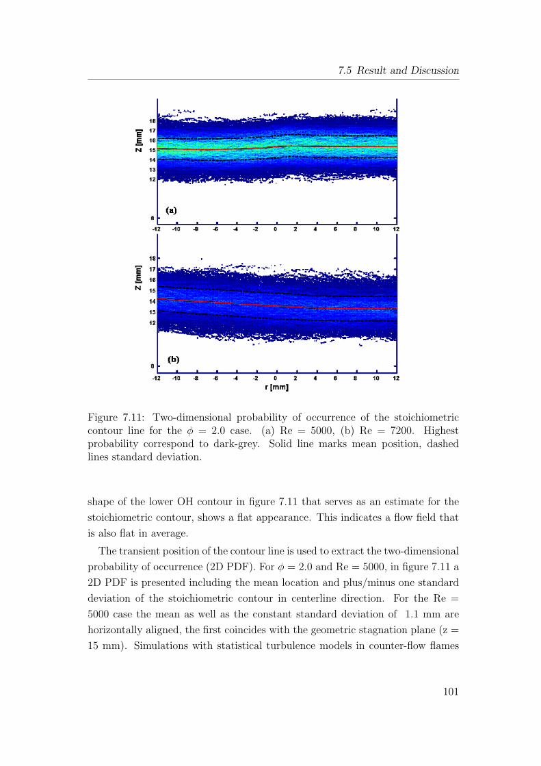
7.5 Result and Discussion
Figure 7.11: Two-dimensional probability of occurrence of the stoichiometriccontour line for the φ = 2.0 case. (a) Re = 5000, (b) Re = 7200. Highestprobability correspond to dark-grey. Solid line marks mean position, dashedlines standard deviation.
shape of the lower OH contour in figure 7.11 that serves as an estimate for the
stoichiometric contour, shows a flat appearance. This indicates a flow field that
is also flat in average.
The transient position of the contour line is used to extract the two-dimensional
probability of occurrence (2D PDF). For φ = 2.0 and Re = 5000, in figure 7.11 a
2D PDF is presented including the mean location and plus/minus one standard
deviation of the stoichiometric contour in centerline direction. For the Re =
5000 case the mean as well as the constant standard deviation of 1.1 mm are
horizontally aligned, the first coincides with the geometric stagnation plane (z =
15 mm). Simulations with statistical turbulence models in counter-flow flames
101

7 Opposed Jet Flames
Figure 7.12: Two-dimensional probability of occurrence of the stoichiometriccontour line for the φ = 3.18 case. (a) Re = 3300, (b) Re = 6500.
are based on the assumption of a flow and scalar field that is only a function of
the centerline coordinate [89],[97]. This assumption is in excellent agreement for
the whole radial range of OH distributions shown in figure 7.11(a). Even if the
OH distribution is slightly tilted for the configuration with Re = 7200 (figure
7.11(b)), the flame is at the extinction limit, the distribution of OH around the
mean position is again parallel aligned for the whole radial range.
Compared to the upper figure, an increase of the turbulence level is reflected by
a wider distribution of the OH contour around the mean position, the standard
deviation is about 10 % higher. The finding that strain caused by transient large
scale eddies as the most important reason for extinction in the presented counter-
102

7.5 Result and Discussion
Figure 7.13: Two-dimensional probability of occurrence of the stoichiometriccontour line for the Re = 5000. (a)φ = 3.18, b)φ = 2.0, c)φ = 1.6, d)φ = 1.2
flow configuration is thereby supported, since only large scale eddies will be able
to enforce the motion of the stoichiometric contour, for instance by compressive
straining. This enforced motion leads to increased strain rates and gradients of
the mixture fraction causing local and global flame extinction.
As the length of the stoichiometric contour line is nearly independent of the
Reynolds number and the equivalence ratio, the results indicate that the mecha-
nism of flame extinction is driven by strain effects rather than severe wrinkling.
This finding is supported by the fact that residence times are relatively small
compared to large eddy turn over times. Therefore, turbulence is not fully de-
veloped.
7.5.1.4 Local Flame Angle
Instantaneous flamelet orientation angles have been previously calculated from
the OH-PLIF images by Lachaux et al. and I.G. Shepherd in the turbulent
premixed methane-air flames [103] [94] [104]. This angle is defined as the angle
between the normal to the flame front surface and the plane tangent to the
103

7 Opposed Jet Flames
Figure 7.14: A schematic figure representing the flame angle at a point on aflame contour
contoured surface. In these measurements flame orientation angle is taken as
the angle between the fixed laser horizontal sheet and local tangent of the flame
front as can be seen from the figure 7.14. Additionally, the mean contour of the
stoichiometric contour defined by the lower OH layer of the current flame are
horizontally flat for the flames measured, which can be well concluded from the
previous sub-section.
The local tangent of the instantaneous flame front was obtained in the following
manner:
1. A window was chosen in the bottom flame front contour
2. Flame front was checked for any discontinuity
3. Parameterizing the points chosen in the flame front
4. Fitting and interpolating with B-Spline curve
5. Calculating the tangent angle from the first derivative of fitting curve
Once the window is chosen for the fitting routine and the check for the broken
flame front is made, second-order parameterizations of the flame front was done
along the distance s. Parameterizations includes the extraction of x(s) and y(s)
for more than 100 points along the flame front, where s is the distance along
the flame front. More points were taken in order to get the better fit with the
evaluated points.
104

7.5 Result and Discussion
Figure 7.15: An example of fitting function applied on the bottom contour of theOH-PLIF image.
A step-wise B-spline fitting routine was applied to the single values in x(s)
and y(s) direction’s. The choice of B-spline was made as fitting functions for two
reason, firstly the B-spline remains smooth along the edge points in contrary to
other polynomials thus adding to the error in calculation. Secondly the B-spline
is not biased towards any offset single point but follows the path of the chosen
points since it is a stepwise and progressing fitting function. Once the function
is defined, angle at a point in the function is defined by (eq.7.1).
θ = tan−1(df(s)
ds) (7.1)
where f(s) is the fitted function for the given set of data points x(s) and y(s)
105

7 Opposed Jet Flames
Figure 7.16: PDF of angle distribution at the burner center-line for varyingReynolds number for φ = 2.0
directions. Since we were interested in calculating the angle at the center-line
of the burner axis, no further smoothing of the profile other than non-linear
filtering was done. The flame front in the region of the center-line was more
wrinkled than the flame region radially outwards. Therefore, it was presumed
that small structure were smoothed out by the application of non-linear diffusion
filtering and the stable situation was reached.
Figure 7.15 shows an example of the data points and the fitting routine applied
to it. Angle results were highly dependent on the fitting routine. The flame angle
for the fuel side flame contour at the point along the burner axis was calculated.
The angle PDF was found to be symmetrical for all flames and centered around
0 [figure 7.16, figure 7.17]. Flame angle was also calculated at the distance of
1 mm offset from the burner center-axis and similar symmetry was found [figure
7.18] (see page 100-102).
106

7.5 Result and Discussion
Figure 7.17: PDF of angle distribution at the burner center-line for varyingReynolds number for φ = 3.18
7.5.1.5 Conclusion
Investigating local and global flame front characteristics yielded insight to the
flame symmetry, its extinction properties, flame location and flame length. The
results indicate that with increasing equivalence ratio the global and local OH
area decrease. Decreasing OH areas are showing a higher sensitivity with respect
to flame extinction. Results here also shows that flame length alone can provide
the qualitative information on the stage of turbulence. As these results show that
the diminished influence of small eddies in flame front indicated by no drastic
change in flame length, confirms the presence of ”young turbulence”.
As the length of the stoichiometric contour line is nearly independent of Reynolds
number and equivalence ratio, the results indicate that the mechanism of flame
extinction is driven by strain effects rather than severe wrinkling. This finding
is supported by the fact that residence times are relatively small compared to
large eddy turn over time. Therefore, it reconfirms that the turbulence is not
107

7 Opposed Jet Flames
Figure 7.18: PDF of angle distribution at 1mm offset from burner center-axis forvarying Reynolds number for φ = 3.18
fully developed.
Similarly local area distribution provides the information on radial symmetry
and spatial distribution of the flames. All these information can be very useful for
model validation purposes, which indirectly can be used to optimize the burner
design. These flame front characteristics results have been useful to confirm the
good design of the opposed jet burner, which could be used as a standard burner
for investigating various phenomenon associated with turbulent combustion such
as flame extinction and flame stabilization.
7.5.2 OH-PITLIF
In OH-PITLIF study, time-series measurements are utilized to determine tem-
poral scales for hydroxyl fluctuations in a series of stable and extinguishing tur-
bulent methane/air counter-flow partially premixed flames as listed in table 7.1.
The time-series measurements are facilitated by picosecond time-resolved laser-
108

7.5 Result and Discussion
induced fluorescence (PITLIF), which directly accounts for potential variations
in both the quenching rate coefficient and background flame emission.
Since OH is present in the high-temperature regions of the flame, the measured
fluctuations in the OH layer represent those of the flame front inside and outside
of the probe volume. Time-series statistics are presented that highlight the effects
of multiple parameters on the dynamics of flame motion. Flame front crossings
are suitably characterized by the OH intermittency, but instead highlights the
presence or absence of OH. The presence of successive bursts in the time series
can be interpreted as successive flame-let crossings, while the OH intermittency
can be used to quantify the percentage of such crossings. The influences of bulk
Reynolds number and fuel-side equivalence ratio on fluctuation time scales are
then examined using the OH integral time scales.
7.5.2.1 Time-averaged Concentration Profiles
Figure 7.19 shows axial turbulent and laminar profiles of [OH], for different fuel-
air compositions, obtained along the opposed-flow axis (z axis). The laminar
profiles in mentioned figure are axially shifted to match their peak [OH] locations
with the corresponding turbulent profiles. For all these PITLIF measurements
the stagnation point is situated at value z−zst/(H/2) = 0, lower nozzle and upper
nozzle are located at z − zst/(H/2) = −1 and z − zst/(H/2) = 1 respectively.
Table 7.3 shows the axial location of peak [OH] measured in the turbulent
flames and, the profile full-width at half-maximum (FWHM). For the highest
degree of premixing (TOJ4C, φB =1.2), the computed laminar profile indicates
the presence of two reaction zones corresponding to two OH peaks, as opposed to
a single OH peak for the corresponding turbulent profile. For similar flames (φB
= 3.18-1.60), PLIF measurements indicate that premixing has very little effect
on global flame area. However, a sharp increase occurs in global flame area for
φB = 1.2 (TOJ4C), consistent with the measured axial [OH] region in figure 7.19
and table 7.3.
7.5.2.2 Time-series Statistics
Figure 7.20 shows the first 1s of time-series data collected for three φB = 2.0
flames with different Reynolds numbers, ranging from stable to extinguishing, at
the axial location of peak OH. These time series, collected at random, are typical
109

7 Opposed Jet Flames
Figure 7.19: Axial profile of time-averaged [OH] for fuel-side equivalence ratiosat Re = 5000, as compared with corresponding laminar profiles calculated fromlaminar code ”OPPDIF”. H represents the distance between the opposed nozzles.The accuracy for each measured concentration is ±18% (95% confidence intervalof the mean). The stagnation point is situated at value Z/(H/2) = 0, lowerand upper nozzle are located at z − zst/(H/2) = −1 and z − zst/(H/2) = 1respectively.
110

7.5 Result and Discussion
Figure 7.20: A snapshot of time series from flame with φB=2.0 (a) Re= 3300 (b)Re= 5000 (c) Re= 7200.
111

7 Opposed Jet Flames
Table 7.3: Time-series statistics at axial location of peak [OH] for different par-tially premixed flames. FWHMs are determined by Gaussian fits to the meanaxial [OH] profiles, intermittency parameter (I) represents the probability of [OH]= 0 occurrences.
of the full 60 seconds of data obtained at each location and are normalized
using the maximum [OH] from TOJ2C. The normalized [OH] for the TOJ2A
flame typically exists for a longer duration in comparison to the TOJ2C flame.
Similarly, the intermittent periods are also longer for the flame at lower Re.
Hence, as the Reynolds number rises, the time-series bursts representing OH
fluctuations become more rapid with reduced burst duration. Bursts in the OH
time series are defined as those regions whose OH intensity values are greater
than 15% of the peak intensity. The number of OH bursts per second increases
from 26 at Re = 3300 to 43 at Re = 7200.
Time-series statistics for the different flame configurations at the axial location
of peak OH are tabulated in table 7.3. The influence of turbulence on hydroxyl
fluctuations can be studied by defining an intermittency parameter (I) which
represents the probability of [OH] = 0 occurrences, i.e. for IOH = 1 [OH]=0
and for IOH = 0 high probability of OH occurrence. Intermittency equal to 1
represents the fully turbulent flow and with intermittency equal to 0 represents
112

7.5 Result and Discussion
Figure 7.21: Sample time series of OH fluorescence for different φB at constantRe = 5000. These time series were measured at peak [OH] locations along thejet axis.
laminar flow. Because the time series is affected by shot noise and imperfections
in background subtractions, a threshold value of 15% of the peak intensity was
set below which the [OH] was assumed to be zero.
The OH intermittency (I) was found to be nearly constant despite a factor of
1.5 increase in Re (see table 7.3). The changes in intermittency parameter and
OH profile FWHM, at the location of peak [OH], for various fuel-side equivalence
ratios are shown in figure 7.22. Hydroxyl intermittency rises with increasing fuel-
113
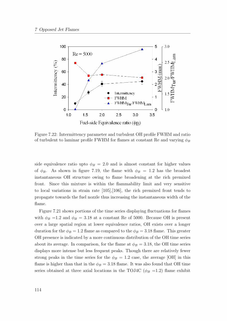
7 Opposed Jet Flames
Figure 7.22: Intermittency parameter and turbulent OH profile FWHM and ratioof turbulent to laminar profile FWHM for flames at constant Re and varying φB
side equivalence ratio upto φB = 2.0 and is almost constant for higher values
of φB. As shown in figure 7.19, the flame with φB = 1.2 has the broadest
instantaneous OH structure owing to flame broadening at the rich premixed
front. Since this mixture is within the flammability limit and very sensitive
to local variations in strain rate [105],[106], the rich premixed front tends to
propagate towards the fuel nozzle thus increasing the instantaneous width of the
flame.
Figure 7.21 shows portions of the time series displaying fluctuations for flames
with φB =1.2 and φB = 3.18 at a constant Re of 5000. Because OH is present
over a large spatial region at lower equivalence ratios, OH exists over a longer
duration for the φB = 1.2 flame as compared to the φB = 3.18 flame. This greater
OH presence is indicated by a more continuous distribution of the OH time series
about its average. In comparison, for the flame at φB = 3.18, the OH time series
displays more intense but less frequent peaks. Though there are relatively fewer
strong peaks in the time series for the φB = 1.2 case, the average [OH] in this
flame is higher than that in the φB = 3.18 flame. It was also found that OH time
series obtained at three axial locations in the TOJ4C (φB =1.2) flame exhibit
114
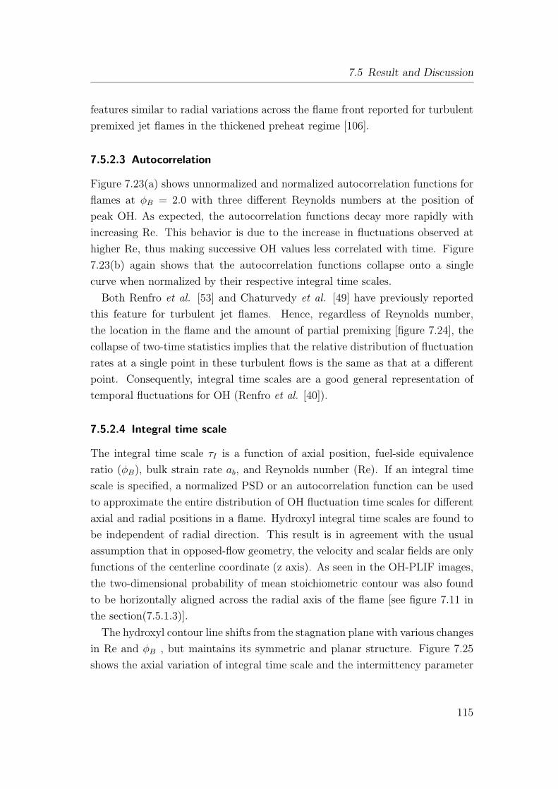
7.5 Result and Discussion
features similar to radial variations across the flame front reported for turbulent
premixed jet flames in the thickened preheat regime [106].
7.5.2.3 Autocorrelation
Figure 7.23(a) shows unnormalized and normalized autocorrelation functions for
flames at φB = 2.0 with three different Reynolds numbers at the position of
peak OH. As expected, the autocorrelation functions decay more rapidly with
increasing Re. This behavior is due to the increase in fluctuations observed at
higher Re, thus making successive OH values less correlated with time. Figure
7.23(b) again shows that the autocorrelation functions collapse onto a single
curve when normalized by their respective integral time scales.
Both Renfro et al. [53] and Chaturvedy et al. [49] have previously reported
this feature for turbulent jet flames. Hence, regardless of Reynolds number,
the location in the flame and the amount of partial premixing [figure 7.24], the
collapse of two-time statistics implies that the relative distribution of fluctuation
rates at a single point in these turbulent flows is the same as that at a different
point. Consequently, integral time scales are a good general representation of
temporal fluctuations for OH (Renfro et al. [40]).
7.5.2.4 Integral time scale
The integral time scale τI is a function of axial position, fuel-side equivalence
ratio (φB), bulk strain rate ab, and Reynolds number (Re). If an integral time
scale is specified, a normalized PSD or an autocorrelation function can be used
to approximate the entire distribution of OH fluctuation time scales for different
axial and radial positions in a flame. Hydroxyl integral time scales are found to
be independent of radial direction. This result is in agreement with the usual
assumption that in opposed-flow geometry, the velocity and scalar fields are only
functions of the centerline coordinate (z axis). As seen in the OH-PLIF images,
the two-dimensional probability of mean stoichiometric contour was also found
to be horizontally aligned across the radial axis of the flame [see figure 7.11 in
the section(7.5.1.3)].
The hydroxyl contour line shifts from the stagnation plane with various changes
in Re and φB , but maintains its symmetric and planar structure. Figure 7.25
shows the axial variation of integral time scale and the intermittency parameter
115

7 Opposed Jet Flames
Figure 7.23: Autocorrelation functions for various Re at φB = 2.0 (a) unnormal-ized and (b) normalized by their respective integral time scales.
116

7.5 Result and Discussion
Figure 7.24: Autocorrelation functions for various φB at Re = 5000 (a) unnor-malized and (b) normalized by their respective integral time scales.
117

7 Opposed Jet Flames
Figure 7.25: Axial variation of integral time scale and OH intermittency forflames with (a)φB = 1.2 and (b)φB = 3.18, at constant Re = 5000.
for flames at different Re. The hydroxyl intermittency and integral time scale
reach a minimum near the axial location of peak OH. The lower value of OH
intermittency at the location of peak OH indicates a high probability of OH oc-
currence. The axial variation in both OH integral time scale and intermittency
for opposed-flow flames is similar to radial variations across the flame front re-
ported for jet diffusion flames [53]. However, across the OH layer, the gradient
of integral time scale for opposed-flow flames increases with decreasing fuel-side
equivalence ratio. In fact, for the flame having the lowest fuel-side equivalence
ratio (φB =1.2), the integral time scale exhibits a sinusoidal variation along the
jet centerline.
118

7.5 Result and Discussion
7.5.3 Conclusion
Instantaneous OH layer thickness is smaller for flames having higher fuel-side
equivalence ratios as shown by OH-PLIF results. The extent of spatial movement
of the partially premixed flame front drops with enhanced premixing. For a
flame with a equivalence ratio of 1.2, hydroxyl time series at peak [OH] exhibit
very little scalar intermittency. This behavior is consistent with the presence
of a broad instantaneous OH layer for this rich mixture. For the same flame,
the intermittency at peak OH remains almost constant in going from stable to
extinguishing flame. It was also found that OH time series obtained at three
axial locations in the TOJ4C (φB =1.2) flame exhibit features similar to radial
variations across the flame front reported for turbulent premixed jet flames in
the thickened preheat regime.
Hydroxyl integral time scales are found to be independent of radial direction.
The hydroxyl integral time scale reaches a minimum at the axial location of peak
OH, consistent with measurement in jet diffusion flame.
119

7 Opposed Jet Flames
120
8 Swirl Flames
This chapter presents realization of Paul’s [55] work on imaging flame heat re-
lease rate in turbulent flames. This requires simultaneous measurement of two
species namely hydroxyl and formaldehyde in the targeted flame. Current chap-
ter is arranged in the similar way as the previous chapter on opposed jet burner.
Introduction that includes literature survey on swirl-stabilized flames is followed
by the burner description and the properties of the flame measured. Last section
contains the results and discussion on the current measurement.
8.1 Introduction
Swirl flows are found in nature and are utilized in a very wide range of applica-
tions. In nature, the vortex shedding from the wings of an aircraft is the best
example. In the reacting flows, most technical systems of practical interest such
as gas turbine engine combustors, boilers, gasoline and diesel engines, industrial
furnaces etc. involves large regions of recirculating flows. Swirled reacting flow
has multi-fold advantages: it increases the efficiency of the combustion by ac-
celerating the mixing of two flows (having different densities), it provides the
reduced velocity necessary for flame stabilization and it also reduces the flame
height which helps in the compact design of technical combustors. Therefore,
above mentioned reasons are important enough to improve the understanding of
such flows at various operating conditions.
Most of the research in the field to optimize the modern gas turbine engine
is fuelled by the concept of lean premixed combustion, which demands a high
ignition stability even in the mixtures of high air to fuel ratios. This can only be
realized using swirl stabilization. A proper design of future low-NOx combustors
depends on more reliable numerical simulations of turbulent premixed combus-
tion processes [107]. Although a variety of models for premixed flames exist such
as Bray-Moss-Libby (BML) model, the thickened flame model, the linear eddy
121

8 Swirl Flames
model, or the G-equation approach, there is still an ongoing scientific debate on
ways to model turbulent premixed flame. The numerical simulation for studying
the effect of swirl on flow development and flame dynamics in a lean premixed
swirl flame was recently done by Huang et al. [108]. This study showed a signifi-
cant impact of the swirl number on the flame dynamics and the recirculation zone
within such flames. Same study also showed a substantial turbulence-chemistry
interaction involved in the turbulent flames on a swirl stabilized burner.
Because turbulence is considered to be mainly responsible for flame stabiliza-
tion in swirl burners, extensive measurement of mean and fluctuating velocity
components were performed before using laser based diagnostics [109],[8],[10].
Raman measurements were carried by W.Meier to investigate on the temper-
ature and major species concentration in the same swirled natural gas flames.
Several other groups have carried out velocity measurements and investigated
time-mean and fluctuating temperatures and the concentration of stable species
within the program ”Arbeitsgemeinshaft TECFLAM”. For these investigations a
water-cooled combustion chamber with a variable swirl burner was used. These
studies included research on the stability limits, pollutant formation, measure-
ment techniques and numerical investigation of swirling flames [110].
Figure 8.1: Schematic diagram of EKT swirl burner
122

8.2 Burner Description
These studies also aimed to provide a database of a swirl stabilized turbulent
flame for validation of numerical simulation. More recently, turbulent-chemistry
interaction was studied using a joint velocity/scalar measurement in the same
target burner and natural gas as fuel [22].
Experimental investigation of heat release rate imaging on a non-premixed
swirl flame was successfully carried by Bockle et al. [111]. This was done by mea-
suring the flame flow field via simultaneous single-shot imaging of formaldehyde
and OH molecule using PLIF. Present work also utilizes the planar technique in
order to provide a snap shot of instantaneous reaction rate in a swirling flow field
under the lean premixed mode.
8.2 Burner Description
Experiments were carried out with a burner that is designed with well-known
Moveable-Block swirl generators. These generators are situated upstream of the
nozzle and allow the adjustment of the theoretical swirl number S0,th ranging
from 0 to 2.0. The theoretical swirl number is calculated using axial and circum-
ferential momentum [22]. The fluid flow enters the moveable block in a radial
direction and is injected radially upstream of the moveable block through eight
nozzles, as can be seen from the arrows in the figure 8.2. This moveable block
consists of upper and lower segments and each segment has a angular bend in ra-
dial direction. Turning the lower segment of the moveable block allows the burner
to be operated at various swirl numbers. If the moveable segment is turned in
such a way that the opposite edges of the radial bends of both segments lie on
top of each other, then the S0,th = 1.98 is reached.
The schematic diagram of the burner is shown in figure 8.1. This burner
consists of a 15 mm wide annular duct that encloses a central bluff body with
db = 30 mm. The premixed combustion mixture of fuel and air exits into the
ambient atmosphere from this annular duct. About 70 mm upstream of the
moveable block, a mixture of methane and air was injected into the air flow
at 300 K using a perforated ring line. The co-flow fluid (N2) surrounds the
flame which provides the defined boundary condition and the protection from
the particles. The co-flow exits through a duct with a diameter of dcf = 168 mm
diameter and a with the mean velocity of 0.5 m/s.
123

8 Swirl Flames
Figure 8.2: Configuring the swirl number from swirl generators situated in theburner. Left showing the configuration at no swirl (S=0) and right with S=1.98.
The investigated flame was operated close to the stability limit with S0,th =
0.75 because theoretical swirl number S0,th exceeding 0.8 resulted in flash back.
The operating conditions for the investigated flame are listed in table 8.1. PSF-
30 represents the premixed swirl flame with power of 30 KW. Parameters ρu and
ρu represents fluid density of unburned mixture and burned mixture respectively.
Reynolds number is calculated using the bulk velocity of the fluid exiting through
the nozzle and the hydraulic diameter.
8.3 Results and Discussion
The single shot images of the instantaneous [OH] and [HCHO] concentration were
normalized to correct for the laser beam profile prior to any further analysis for
results. Post-processing of images were also carried out which included filtering
and smoothing as discussed in chapter-6. Image processing of the individual
single-shot images of OH and HCHO was done separately.
Using images of the reference mask (grids) from both ICCD cameras, the
field of view was carefully adjusted. After post-processing the camera matching
was done. Camera matching included the spatial overlapping in horizontal and
vertical direction of the images, so that the field of view for both the camera
124

8.3 Results and Discussion
Table 8.1: Details of flame configuration measured on turbulent premixed swirlburner
remains the same and also the tilt of the images. However, deviation in tilt
was found to be in the sub-pixel range. These images were normalized by their
maximum intensity before they were multiplied to generate the heat release rate
intensities.
Figure 8.3 shows the single-shot images of OH, HCHO and multiplied inten-
sity image from [OH][HCHO], these images were recorded simultaneously with
separate detection systems in the lower part of the flame at a height ranging
from 9-14mm. Hydroxyl molecule in the inner zone indicate the position of hot
burnt gases that have been recirculated back to the burner center due to the
recirculation zone formed by high intensity swirling motion. The position of the
formaldehyde molecules indicate the fresh cold gases in the preheated zone and
is formed near the shear layer between the high temperature burned gases in the
recirculation zone and the outer fresh gases. The overlap area is the indicator
of the location of a optimal reaction zone, where most of the chemical reaction
is taking place. Typical formaldehyde concentration layer evaluated from our
images was found to be around 1.5-2.5 mm. A profile is indicated in the fig-
ure 8.4 showing the overlapping of hydroxyl and formaldehyde. The intensity of
125
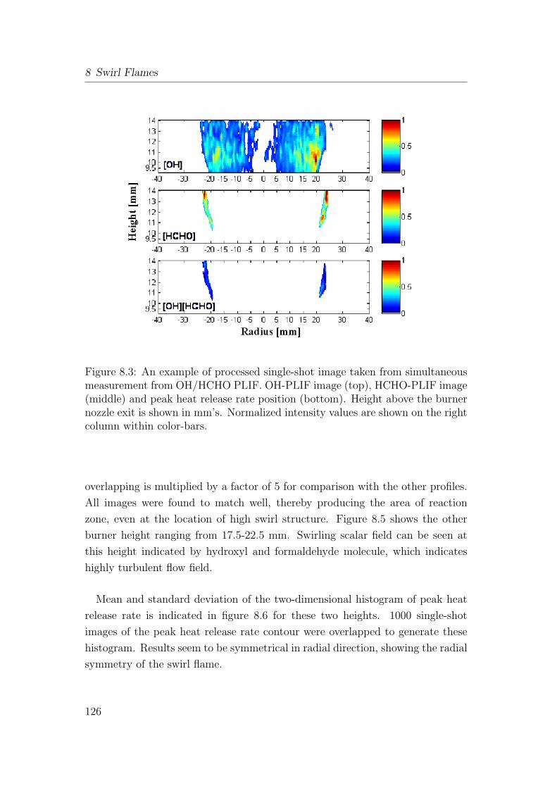
8 Swirl Flames
Figure 8.3: An example of processed single-shot image taken from simultaneousmeasurement from OH/HCHO PLIF. OH-PLIF image (top), HCHO-PLIF image(middle) and peak heat release rate position (bottom). Height above the burnernozzle exit is shown in mm’s. Normalized intensity values are shown on the rightcolumn within color-bars.
overlapping is multiplied by a factor of 5 for comparison with the other profiles.
All images were found to match well, thereby producing the area of reaction
zone, even at the location of high swirl structure. Figure 8.5 shows the other
burner height ranging from 17.5-22.5 mm. Swirling scalar field can be seen at
this height indicated by hydroxyl and formaldehyde molecule, which indicates
highly turbulent flow field.
Mean and standard deviation of the two-dimensional histogram of peak heat
release rate is indicated in figure 8.6 for these two heights. 1000 single-shot
images of the peak heat release rate contour were overlapped to generate these
histogram. Results seem to be symmetrical in radial direction, showing the radial
symmetry of the swirl flame.
126
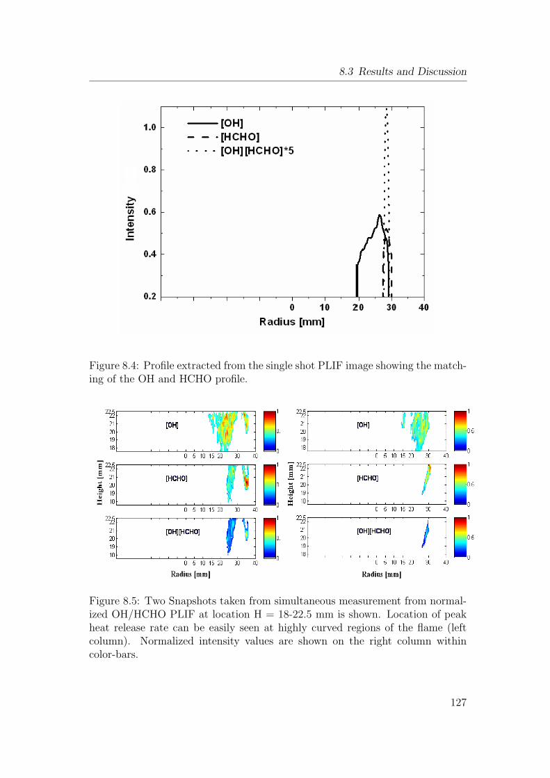
8.3 Results and Discussion
Figure 8.4: Profile extracted from the single shot PLIF image showing the match-ing of the OH and HCHO profile.
Figure 8.5: Two Snapshots taken from simultaneous measurement from normal-ized OH/HCHO PLIF at location H = 18-22.5 mm is shown. Location of peakheat release rate can be easily seen at highly curved regions of the flame (leftcolumn). Normalized intensity values are shown on the right column withincolor-bars.
127

8 Swirl Flames
Figure 8.6: Two-dimensional histogram of the mean location of peak heat re-lease rate evaluated from 1000 single-shot images at two different location of theburner. Solid lines shows the mean location and their standard deviation.
8.4 Conclusion
A turbulent premixed flame was measured using simultaneous laser induced flu-
orescence of hydroxyl and formaldehyde molecule. Such measurement provided
insight into the flame front location of turbulent flames and also the position of
peak heat release rate. We have used a single laser system for excitation of both
molecule and also showed that the signal to noise ratio was high enough to ex-
tract information on a single-shot basis, which is important in turbulent flames.
The complete flame was not captured from a single sheet due to the limitation
in height of the laser sheet. The increase in height of the laser sheet reduced our
signal to noise ratio drastically and the signal from the formaldehyde molecule
was hardly detectable on a single shot basis. Our measurement have shown that
it is possible to measure simultaneously hydroxyl and formaldehyde molecules
in a highly turbulent lean-premixed swirled flame. Such measurement can be
very useful in locating optimal reaction zone of an opposed jet flame where the
reaction zone is restricted between the center of the nozzles [57].
128

9 Summary and Outlook
Flame front characteristics in various turbulent flames reaching from premixed to
partially-premixed and non-premixed have been investigated using well known
laser induced fluorescence technique. This work also provides insight into the
flame front dynamics as a function of turbulent flow field. Turbulent flames
from two different combustion devices have been investigated, namely the EKT
turbulent opposed jet burner and the EKT swirl burner respectively.
The potential of extracting both, quantitative and qualitative information from
the chosen combustion devices were huge. From the same setup, flames from dif-
fusion to the premixed limit were studied, will varying parameters like Reynolds
number, turbulent intensities and strain rate. Additionally, the extracted infor-
mation could be used to validate and test the capability of the numerical model
for the prediction of complex phenomenon. This will indirectly help in no longer
relying on trial and error technique for designing combustion devices.
Investigated molecules were selected according to their presence near the re-
action zone and formed in abundance during combustion processes under highly
turbulent conditions. They were also checked for the possibility of single-shot
detection and state of the art planar measurement. The hydroxyl and formalde-
hyde molecule were used as flame front marker as they are important intermediate
species in combustion using fossil fuels. Investigation of formaldehyde molecules
in flame was done by comparing the literature emission spectrum with the spec-
trum taken in this study.
Advanced image processing have been applied to the raw planar images to ex-
tract relevant information. This included normalizing the laser intensity, series
of filtering, smoothing and binary image extraction. Various filtering methods
ranging from median to non-linear diffusion filtering was applied to obtain the
important gradients of intensity thereby removing attached unwanted noise. Sen-
sitivity analysis was carried to choose the set of parameters applied to the images
and different algorithms were checked for compatibility with the images.
129
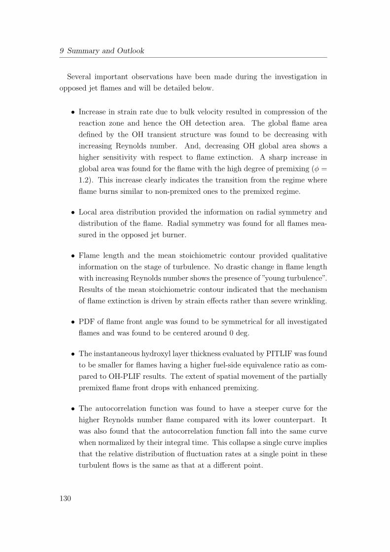
9 Summary and Outlook
Several important observations have been made during the investigation in
opposed jet flames and will be detailed below.
• Increase in strain rate due to bulk velocity resulted in compression of the
reaction zone and hence the OH detection area. The global flame area
defined by the OH transient structure was found to be decreasing with
increasing Reynolds number. And, decreasing OH global area shows a
higher sensitivity with respect to flame extinction. A sharp increase in
global area was found for the flame with the high degree of premixing (φ =
1.2). This increase clearly indicates the transition from the regime where
flame burns similar to non-premixed ones to the premixed regime.
• Local area distribution provided the information on radial symmetry and
distribution of the flame. Radial symmetry was found for all flames mea-
sured in the opposed jet burner.
• Flame length and the mean stoichiometric contour provided qualitative
information on the stage of turbulence. No drastic change in flame length
with increasing Reynolds number shows the presence of ”young turbulence”.
Results of the mean stoichiometric contour indicated that the mechanism
of flame extinction is driven by strain effects rather than severe wrinkling.
• PDF of flame front angle was found to be symmetrical for all investigated
flames and was found to be centered around 0 deg.
• The instantaneous hydroxyl layer thickness evaluated by PITLIF was found
to be smaller for flames having a higher fuel-side equivalence ratio as com-
pared to OH-PLIF results. The extent of spatial movement of the partially
premixed flame front drops with enhanced premixing.
• The autocorrelation function was found to have a steeper curve for the
higher Reynolds number flame compared with its lower counterpart. It
was also found that the autocorrelation function fall into the same curve
when normalized by their integral time. This collapse a single curve implies
that the relative distribution of fluctuation rates at a single point in these
turbulent flows is the same as that at a different point.
130

• Hydroxyl integral time scales are found to be independent of radial direc-
tion. The hydroxyl integral time scale reaches a minimum at the axial
location of peak OH.
The list of important conclusion are detailed below from the swirl jet flames.
• Insight into the reaction zone location in a swirled stabilized turbulent
flame was provided using multi-scalar PLIF measurement.
• Usage of single laser system for excitation of both molecules showed that
signal-to-noise ratio was good enough to extract the information on single-
shot basis.
• Height of the laser sheet was limited and the complete capture of the flame
does not look feasible with the current setup.
131

9 Summary and Outlook
132

Bibliography
[1] Dreizler, A. and Janicka, J. ”Diagnostic challenges for gas turbine com-
bustor model validation, ”Applied Combustion Diagnostics” (edited by K.
Kohse-Hoinghaus and J. Jeffries)”. New York: Taylor and Francis, 2002.
[2] Bilger, B.W., Pope, S.B., Bray, K.N.C., and Driscoll, J.F. ”Paradigms of
turbulent combustion research”. Proceedings of the Combustion Institute,
30:pp. 21–42, 2005.
[3] Bray, K.N.C. ”The challenge of turbulent combustion”. Proceedings of the
Combustion Institute, 26:pp. 1–26, 1996.
[4] Bilger, B.W. ”Future progress in turbulent combustion research”. Prog.
Energ. Comb. Sci., 26:pp. 367–380, 2000.
[5] Hassel, E.P. and Linow, S. ”Laser diagnostics for studies of turbulent
combustion”. Measurement Science and Technology, 11:R37–R57, 2000.
[6] Barlow, R.S., Dibble, R.W., Chen, J.-Y., and Lucht, R.P. ”Effect of
Damkohler number on superequilibrium OH concentrations in turbulent
nonpremixed jet flames”. Combustion and Flame, Vol. 82:pp. 235–251,
1990.
[7] Dibble, R.W., Hartmann, V., Schefer, R.W., and Kollmann, and W. ”Con-
ditional sampling of velocity and scalars in turbulent flames using simul-
taneous LDV-Raman scattering”. Experiments in Fluids, 5:pp. 103–113,
1987.
[8] Landenfeld, T., Kremer, A., Hassel, E.P., Janicka, J., Schafer, T., Kazen-
wadel, J., Schulz, C., and Wolfrum, J. ”Laser-diagnostic and numerical
133

Bibliography
study of strongly swirling natural gas flames”. Proceedings of the Combus-
tion Institute, 27:pp. 1023–1029, 1998.
[9] Janus, B., Dreizler, A., and Janicka, J. ”Flow field and structure of swirl
stabilized non-premixed natural gas flames at elevated pressure”. Proceed-
ings of ASME Turbo Expo 2004 Power for Land, Sea, and Air, GT-2004-
53340:pp. 1–10, June 14-17, 2004.
[10] Schneider, C., Dreizler, A., and Janicka, J. ”Fluid dynamical analysis of
atmospheric reacting and isothermal swirling flows”. Flow, Turbulence and
Combustion, 74:pp. 103–127, 2005.
[11] Renfro, M.W., King, G.B., and Laurendeau, N.M. ”Quantitative hydroxyl
concentration time-series measurements in turbulent nonpremixed flames”.
Applied Optics, Vol.38(21):pp. 4596–4608, 1999.
[12] Brockhinke, A., Bulter, A., Rolon, J.C., and Kohse-Hoinghaus, K.
”Picosecond-LIF measurements of minor species concentration in a coun-
terflow diffusion flame interacting with a vortex”. Applied Physics B, pages
pp. 491–496, 2001.
[13] Geyer, D., Kempf, A., Dreizler, A., and Janicka, J. ”Scalar dissipation rates
in isothermal and reactive turbulent opposed-jets: 1-D Raman/Rayleigh
experiments supported by LES”. Proceedings of the Combustion Institute,
30:pp. 681–689, 2005.
[14] Brockhinke, A., Kohse-Hoinghaus, K., and Andresen, P. ”Double-pulse one
dimensional Raman and Rayleigh measurements for the detection of tem-
poral and spatial structures in a turbulent H2-air diffusion flame”. Optics
Letters, 21:pp. 2029–2031, 1996.
[15] Hult, J. ”Development of time resolved laser imaging technique for studies
of turbulent reacting flows”. PhD thesis, Lund University of Technology,
Lund, 2002.
[16] Long, B.L., Fourgette, D.C., Escoda, M.C., and Layne, C.B. ”Instanta-
neous Ramanography of a turbulent diffusion flame”. Optics Letters, 8:pp.
244–246, 1983.
134

Bibliography
[17] Fielding, J., Schaffer, A.M., and Long, M.B. ”Three-scalar imaging in
turbulent non-premixed flames of methane”. Proceedings of the Combustion
Institute, Vol.27:pp. 1007–1014, 1998.
[18] Frank, J.H., Kaiser, S.A., and Long, M.B. ”Reaction-rate, mixture fraction
and temperature imaging in turbulent methane/air jet flames”. Proceedings
of the Combustion Institute, Vol 29:pp. 2687–2694, 2002.
[19] Hult, J., Omrane, A., Nygren, J., Kaminski, C.F., Axelsson, B., Collin, R.,
Hult, J., P.-E.Bengtsson,, and Alden, M. ”Quantitative three-dimensional
imaging of soot volume fraction in turbulent non-premixed flames”. Exper-
iments in Fluids, 33:pp. 265–269, 2002.
[20] Nygren, J., Hult, J., Richter, M., Alden, M., Christensen, M., Hultqvist,
A., and Johansson, B. ”Three-dimensional laser induced fluorescence of fuel
distributions in an HCCI engine”. Proceedings of the Combustion Institute,
Vol.29:pp. 679–685, 2002.
[21] Barlow, R.S., Carter, C.D., and Pitz, R.W. ”Multi-species diagnostics
in turbulent flames”. in Kohse-Hoinghaus, K and Jeffries, J.B. (Eds.):
Applied Combustion Diagnostics, Taylor and Francis, New York, pages
pp. 384–407, 2002.
[22] Nauert, A. and Dreizler, A. ”Conditional velocity measurements by simul-
taneously applied laser doppler velocimetry and planar laser-induced fluo-
rescence in a swirling natural gas/air flame”. Journal of Physical Chemistry,
219:pp. 635–648, 2005.
[23] Donbar, J.M., Driscoll, J.F., and Carter, C.D. ”Reaction zone structure in
turbulent non-premixed jet flames-from CH-OH PLIF images”. Combustion
and Flame, Vol.122:pp. 1–19, 2000.
[24] Bockle, S., Kazenwadel, J., Kunzelmann, T., Shin, D.I., Schulz, C., and
Wolfrum, J. ”Simultanous single-shot laser-based imaging of formaldehyde,
OH and temperature in turbulent flames”. Proceedings of the Combustion
Institute, Vol.28:pp. 279–286, 2000.
135
Bibliography
[25] Warnatz, J., Maas, U., and Dibble, R.W. ”Combustion: physical and
chemical fundamentals, modeling and simulation, experiments, pollutant
formation”. 3rd Ed. Springer-Verlag, ISBN 3-540-67751-8, 1996.
[26] Kohse-Hoinghaus, K. and Jeffries, B.J. ”Applied Combustion Diagnostics”.
Combustion: An International Series, 2002.
[27] Eckbreth, A.C. ”Laser Diagnostics for Combustion Temperature and
Species”. 2nd Ed., Gordon and Breach, 1996.
[28] Daily, J.W. ”Laser Induced Fluorescence Spectroscopy in Flames”. Progr.
Energy Combustion Sci., 23:pp. 133–199, 1997.
[29] Kohse-Hoinghaus, K. ”Laser techniques for the quantitive detection of
reactive intermediates in combustion systems”. Progr. Energy Combustion
Sci., 20:pp. 203–279, 1994.
[30] Shin, D.I., Dreier, T., and Wolfrum, J. ”Spatially resolved absolute concen-
tration and fluorescence lifetime determination of HCHO in atmospheric
pressure methane/air flames”. Applied Physics B, 72:pp. 257–261, 2001.
[31] Nguyen, Q.V., Dibble, R.W., Carter, C.D., Fiechtner, G.J., and Barlow,
R.S. ”Raman-LIF measurement of temperature, major species, OH, and
NO in a methane-air bunsen flame”. Combustion and Flame, Vol.105:pp.
499–510, 1996.
[32] Carter, C.D. and Barlow, R.S. ”Simultaneous measurements of NO, OH,
and the major species in turbulent flames”. Optics Letters, Vol.19(4):pp.
299–301, 1999.
[33] Heard, D.E., Jeffries, J.B., Smith, G.P., and Crosley, D.R. ”Laser-Induced
fluorescence measurements in methane/air flames of radicals important in
prompt-NO formation”. Combustion and Flame, Vol.88:pp. 137, 1992.
[34] Lucht, R.P., Sweeney, D.W., and Laurendeau, N.M. ”Laser saturated flu-
orescence of OH concentration in flames”. Combustion and Flame, 50:pp.
189–205, 1983.
136

Bibliography
[35] Cheng, T.S., Wehrmeyer, J.A., and Pitz, R.W. ”Simultaneous tempera-
ture and multispecies measurement in a lifted hydrogen diffusion flame”.
Combustion and Flame, 91:pp. 323–345, 1992.
[36] Rahmann, U., Bulter, A., Lenhard, U., Dusing, R., Markus, D., Brock-
hinke, A., and Kohse-Hoinghaus, K. ”LASKIN- A simulation program for
time-resolved LIF spectra”. Internal Report, University of Bielefeld, 2003.
[37] Rahmann, U., Kreutner, W., and Kohse-Hoinghaus, K. ”Rate-equation
modeling of single- and multiple-quantum vibrational energy transfer of
OH (A2Sigma+, v’=0 to 3)” . Applied Physics B, 69:pp. 61–70, 1990.
[38] Luque, J. and Crosley, D.R. ”LIFBASE”. MP-99-0099, SRI International,
1999.
[39] Renfro, M.W. ”Fluorescence-lifetime measurements in atmospheric-
pressure flames using nanosecond-pulsed lasers”. Applied Physics B, 74:pp.
167–174, 2002.
[40] Renfro, M.W. ”Quantitative time series for minor-series concentrations:
measurements and modeling in turbulent nonpremixed flames”. PhD thesis,
Purdue University, USA, 2000.
[41] Thompson, B.D. ”Flame measurements using picosecond time-resolved
laser-induced fluorescence”. MS thesis Purdue University West Lafayette
IN, 1992.
[42] Pack, S.D., Renfro, M.W., King, G.B., and Laurendeau, N.M. ”Photon-
counting technique for rapid fluorescence-decay measurement”. Optics Let-
ters, Vol. 23(15):pp. 1215–1217, 1998.
[43] Reichardt, T.A. ”Minor-species number density measurements using pi-
cosecond time-resolved laser-induced fluorescence”. MS thesis Purdue Uni-
versity West Lafayette IN, 1994.
[44] Reichardt, T.A., Klassen, M.S., King, G.B., and Laurendeau, N.M. ”Real-
time acquisition of laser-induced fluorescence decays”. Applied Optics,
34:pp. 973–976, 1995.
137

Bibliography
[45] O’Connor, D.V. and Phillips, D. ”Time-correlated single photon counting”.
Academic Press London, 1984.
[46] Alfano, A.J., Fong, F.K., and Lytle, F.E. ”High repetition rate subnanosec-
ond gated photon counting”. Rev. Sci. Instrum., 54:pp. 967–972, 1983.
[47] Desilets, D.J., Coburn, J.T., Lantrip, A.D., Kissinger, P.T., and Lytle,
F.E. ”On-the-fly determination of fluorescence lifetime from two-point de-
cay measurements”. Analytical Chemistry, Vol.58(6):pp. 1123–1128, 1986.
[48] Ballew, R.M. and Demas, J.N. ”An error analysis of the rapid lifetime de-
termination method for the evaluation of single exponential decays”. Ana-
lytical Chemistry, (61):pp. 30–33, 1989.
[49] Chaturvedy, A., King, G.B., Laurendeau, N.M., Renfro, M.W., Kempf, A.,
Dreizler, A., Sadiki, A., and Janicka, J. ”Comparision of OH time-series
measurements and large-eddy simulations in H2 jet flames”. Combustion
and Flame, 139:pp. 142–151, 2004.
[50] Gokalp, I., Shepherd, I.G., and Cheng, R.K. ”Spectral behaviour of velocity
fluctuation in premixed turbulent flames”. Combustion and Flame, 71:pp.
313–323, 1988.
[51] McQuay, M.Q. and Cannon, S.M. ”Time-resolved temperature measure-
ment in the developing region of an elliptic, jet diffusion flame at Reynolds
number of 6000”. Combustion and Flame, 119:pp. 13–33, 1996.
[52] Ikeda, Y., Kojima, J., Nakajima, T., Akamatsu, F., and Katsuki, M. ”Mea-
surement of local flame-front structure in turbulent premixed flame”. Pro-
ceedings of the Combustion Institute, 28:pp. 343, 2000.
[53] Renfro, M.W., Guttenfelder, W.A., King, G.B., and Laurendeau, N.M.
”Scalar time-series measurements in turbulent CH4/H2/N2 non-premixed
flames: OH”. Combustion and Flame, Vol. 123:pp. 389–401, 2000.
[54] Renfro, M.W., King, G.B., and Laurendeau, N.M. ”Scalar time-series mea-
surements in turbulent CH4/H2/N2 non-premixed flames: CH”. Combus-
tion and Flame, 122:pp. 139–150, 2000.
138

Bibliography
[55] Paul, P.H. and Najm, H.N. ”Planar laser-induced fluorescence imaging of
flame heat release rate”. Proceedings of the Combustion Institute, pages pp.
43–50, 1998.
[56] Najm, H.N., Paul, P.H., Mueller, C.J., and Wyckoff, P.S. ”On the adequacy
of certain experimental observables as measurements of flame burning rate”.
Combustion and Flame, Vol.113:pp. 312–332, 1998.
[57] Fayoux, A., Zahringer, K., Gicquel, O., and Rolon, J.C. ”Experimental and
numerical determination of heat release in counterflow premixed laminar
flame”. Proceedings of the Combustion Institute, 30:pp. 251–257, 2005.
[58] Tobai, J. ”Pikosekunden pump-probe DFWM spektroskopie-methoden von
NH und OH in atmospharendruckflammen: untersuchung des relaxations-
prozesses bei elektronischer anregung und im grundzustand”. Dissertation:
Ruprecht-Karls-Universitat Heidelberg, 2000.
[59] Harrington, J.E. and Smith, K.C. ”Laser-induced fluorescence measure-
ments of formaldehyde in a methane/air diffusion flame”. Chemical Physics
Letters, Vol. 202(3-4):pp. 196–202, 1993.
[60] Bauerle, B., Warnatz, J., and Behrendt, F. ”Time-resolved investigation
of hot spots in the end gas of an S.I engine by means of 2-D double pulse
LIF of formaldehyde”. Proceedings of the Combustion Institute, pages pp.
2619–2626, 1996.
[61] Bockle, S., Kazenwadel, J., Kunzelmann, T., Shin, D.I., and Schulz, C.
”Single-shot laser-induced fluorescence imaging of formaldehyde with XeF
excimer excitation”. Applied Physics B, Vol.70:pp. 733–735, 2000.
[62] Burkert, A., Grebner, D., Muller, D., Triebel, W., and Konig, J. ”Single-
shot imaging of formaldehyde in hydrocarbon flames by XeF excimer laser-
induced fluorescence”. Proceedings of the Combustion Institute, Vol.28:pp.
1655–1661, 2000.
[63] Graf, N., Gronki, J., Schulz, C., Baritaud, T., Cherel, J., Duret, P., and
Lavy, J. ”In-cylinder combustion visualization in an auto-igniting gasoline
engine using fuel tracer- and formaldehyde-LIF imaging”. SAE, 2001-01-
1924, 2001.
139
Bibliography
[64] Klein-Douwel, R.J.H., Luque, J., Jeffries, J.B., Smith, G.P., and Crosley,
D.R. ”Laser-induced fluorescence of formaldehyde hot bands in flames”.
Applied Optics, Vol.39(21):pp. 3712–3715, 2000.
[65] Tobai, J. and Dreier, T. ”Effective A-state fluorescence lifetime of formalde-
hyde in atmospheric pressure methane/air flames”. Applied Physics B,
74(1):pp. 101–104, 2002.
[66] Tolocka, M.P. and Miller, J.H. ”Measurement of formaldehyde concentra-
tions and formation rates in a methane-air, non-premixed flame and their
implication for heat release rate”. Proceedings of the Combustion Institute,
pages pp. 663–640, 1998.
[67] Najm, H.N., Knio, O.M., Paul, P.H., and Wyckoff, P.S. ”A study of flame
observable in premixed methane-air flame”. 17th International Colloquium
on the Dynamics of Explosion and Reactive System, 119, July 25-30, 1999.
[68] Mohlmann, G.R. ”Formaldehyde detection in air by laser induced fluores-
cence”. Society of Applied Spectroscopy, Vol. 39(No.1):pp. 98–101, 1985.
[69] Renfro, M.W., Pack, S.D., King, G.B., and Laurendeau, N.M. ”A pulse-
pileup correction procedure for rapid measurements of hydroxyl concentra-
tions using picosecond time resolved laser-induced fluorescence”. Applied
Physics B, 69:pp. 137–146, 1999.
[70] Lutz, A.E., Kee, R.J., Grcar, J.F., and Rupley, F.M. ”OPPDIF: A fortran
program for computing opposed-flow diffusion flames, Scandia National
Laboratories”. Report No. SAND96-8243, 1996.
[71] Jahne, B. ”Practical handbook on image processing for scientific applica-
tions”. Book Published by CRC Press (1997).
[72] Perona, P. and Malik, J. ”Scale-space and edge detection using anistropic
diffusion”. IEEE Comp. Soc. Workshop on Computer Vision, pages pp.
16–22, 1987.
[73] Perona, P. and Malik, J. ”Scale-space and egde detection using anistropic
diffusion”. IEEE Transactions on Pattern Analysis and Maschine Intelli-
gence, Vol. 12(7):pp. 629–639, 1990.
140

Bibliography
[74] Weickert, J. ”Nonlinear diffusion filtering”. Handbook of Computer Vision
and Application, Vol. 2:pp. 423–450.
[75] Weickert, J. ”A review of nonlinear diffusion filtering”. Scale-Space Theory
in Computer Vision, Lecture Notes in Computer Science, Vol. 1252:pp.
3–28, 1997.
[76] Malm, H., Sparr, G., Hult, J., and Kaminski, C.F. ”Nonlinear diffusion
filtering of images obtained by planar laser induced fluorescence spec-
troscopy”. Journal of Optical Society of America, A 17:pp. 2148–2156,
2000.
[77] Schiessl, R., Dreizler, A., and Mass, U. ”Comparison of different ways for
image post-processing: Detection of flame fronts”. Society of Auto. Eng.,
441(8):pp. 151–189, 1999.
[78] Kempf, A., Forkel, H., Chen, J.-Y., Sadiki, A., and Janicka, J. ”Large-eddy
simulation of a counterflow configuration with and without combustion”.
Proceedings of the Combustion Institute, 28:pp. 35–40, 2000.
[79] Geyer, D., Nauert, A., Dreizler, A., and Janicka, J. ”Flow and scalar field
properties of a turbulent opposed jet burner”. Proceedings of Externes
TECHFLAM Seminar, Karlsruhe, 2002.
[80] Geyer, D., Nauert, A., Dreizler, A., and Janicka, J. ”Finite-rate chemistry
effects in turbulent opposed flows: comparison of Raman/Rayleigh mea-
surements and Monte Carlo PDF simulations”. Proceedings of the Com-
bustion Institute, 30:pp. 711–718, 2005.
[81] Geyer, D. ”1D-Raman/Rayleigh experiments in turbulent-opposed jet
flows”. PhD thesis, Technische Universitat Darmstadt, 2004.
[82] Kitajima, A., Ueda, T., Matsuo, A., and Mizomoto, M. ”A comprehen-
sive examination of the structure and extinction of turbulent non-premixed
flames formed in a counterflow”. Combustion and Flame, Vol.121:pp. 301–
311, 2000.
[83] Kitajima, A., Ueda, T., Matsuo, A., and Mizomoto, M. ”Experimental
investigation of the flame structure and extinction of turbulent counterflow
141

Bibliography
non-premixed flames”. Proceedings of the Combustion Institute, 26:pp. 137–
143, 1996.
[84] Kitajima, A., Torikai, H., Takeuchi, M., and Oya, M. ”Experimental study
of extinction and its quantification in laminar and turbulent counterflow
CH4-N2/O2-N2 nonpremixed flames”. Combustion and Flame, 137:pp. 93–
108, 2004.
[85] Korusoy, E. and Whitelaw, J.H. ”Extinction and relight in opposed flames”.
Experiments in Fluids, Vol. 33:pp. 75–89, 2002.
[86] Luff, D., Korusoy, E., Lindstedt, P., and Whitelaw, J.H. ”Counterflow
flames of air and methane, propane and ethylene with and without periodic
forcing”. Experiments in Fluids, Vol. 35:pp. 618–626, 2003.
[87] Mastorakos, E., Taylor, A.M.K.P., and Whitelaw, J.H. ”Extinction and
temperature characteristics of turbulent counterflow diffusion flames with
partial premixing”. Combustion and Flame, 91:pp. 40–54, 1992.
[88] Mastorakos, E., Taylor, A.M.K.P., and Whitelaw, J.H. ”Scalar dissipa-
tion rate at the extinction of turbulent counterflow non-premixed flames”.
Combustion and Flame, 91:pp. 55–64, 1992.
[89] Mastorakos, E. ”Turbulent combustion in opposed jet flows”. Phd thesis,
Imperial College, University of London, 1993.
[90] Mounaim-Rouselle, C. and Gokalp, I. ”Strain effects on the structure of
counterflowing turbulent flames”. Proceedings of the Combustion Institute,
Vol. 25:pp. 1199–1205, 1994.
[91] Sardi, K., Taylor, A.M.K.P., and Whitelaw, J.H. ”Exinction of turbulent
counterflow flames under periodic strain”. Combustion and Flame, 120:pp.
265–284, 2000.
[92] Sardi, E. ”Turbulent flame extinction in unforced and periodically forced
counterflows”. Ph.D. thesis, Imperial College of Science, Technology and
Medicine, University of London, 1997.
142

Bibliography
[93] Sardi, K., Taylor, A.M.K.P., and Whitelaw, J.H. ”Conditional scalar dissi-
pation statistics in a turbulent counterflow”. Journal of Fluid Mechanics,
Vol. 361:pp. 1–24, 1998.
[94] Shepherd, I.G. ”Flame surface density and burning rate in premixed tur-
bulent flames”. Proceedings of the Combustion Institute, 26:pp. 373–379,
1996.
[95] Tsuji, H., Yoshida, A., and Endo, and N. ”Effect of turbulence on extinction
of counterflow diffusion flame”. Proceedings of the Combustion Institute,
pages pp. 1191–1197, 1994.
[96] Yoshida, A., Igarashi, T., and Kotani, Y. ”Extinction of turbulent diffusion
flames by Kolmogorov microscale turbulence”. Combustion and Flame, Vol.
109(4):pp. 669–681, 1997.
[97] Bray, K.N.C., Champion, M., and Libby, P.A. ”Premixed flame in stag-
nation turbulence part IV: a new theory for the Reynolds stresses and
Reynolds fluxes applied to impinging flows”. Combustion and Flame, Vol.
120:pp. 1–18, 2000.
[98] Jones, W.P. and Prasetyo, W. ”Probability density function modeling of
premixed turbulent opposed jet flames”. Proceedings of the Combustion
Institute, 26:pp. 275–282, 1996.
[99] Kostiuk, L.W., Bray, K.N.C., and Chew, T.C. ”Premixed turbulent com-
bustion in counterflowing streams”. Combustion Science and Technology,
64:pp. 233–241, 1989.
[100] Kostiuk, L.W., Bray, K.N.C., and Cheng, R.K. ”Experimental study of pre-
mixed turbulent combustion in opposed streams. Part III - Spatial structure
of flames”. Combustion and Flame, Vol. 118:pp. 129–139, 1999.
[101] Gulder, O.L., Smallwood, G.J., Wong, R., Snelling, D.R., Smith, R., Small-
wood, G.J., Deschamps, B.M., and Sautet, J-C. ”Flame front surface char-
acterisitics in turbulent propane/air combustion”. Combustion and Flame,
Vol. 120(No. 4):pp. 407–416, 2000.
143

Bibliography
[102] Geyer, D., Omar, S., Nauert, A., Ludwig, A., Dreizler, A., and Janicka,
J. ”A Comprehensive characterization of a turbulent opposed jet flame
by 1D-Raman/Rayleigh, 2D-LIF, and LDV”. 1st International SFB-568
Workshop Darmstadt, 2002.
[103] Lachaux, T., Halter, F., Chauveau, C., Gokalp, I., and Shepherd, I.G.
”Flame front analysis of high-pressure turbulent lean premixed methane-
air flames”. Proceedings of the Combustion Institute, 30:pp. 819–826, 2005.
[104] Soika, A., Dinkelacker, F., and Leipertz, A. ”Pressure influence on the
flame front curvature of turbulent premixed flames: comparision between
experiment and theory”. Combustion and Flame, 132:pp. 451–462, 2003.
[105] Blevins, L.G. and Gore, J.P. ”Computed structure of low strain rate par-
tially premixed CH4/air counterflow flames: implications for NO forma-
tion”. Combustion and Flame, 116:pp. 546–566, 1999.
[106] Tanoff, M.A., Smooke, M.D., Osborne, R.J., Brown, T.M., and Pitz, RW.
”The sensitive structure of partially premixed methane-air vs. air counter-
flow flames”. Proceedings of the Combustion Institute, 26:pp. 1121–1128,
1996.
[107] Syred, D.G. and Beer, J.M. ”Combustion in swirling flows”. Combustion
and Flame, 23:pp. 143–201, 1974.
[108] Huang, Y. and Yang, V. ”Effect of swirl on combustion dynamics in a
lean-premixed swirl-stabilized combustor”. Proceedings of the Combustion
Institute, 30:pp. 1775–1782, 2005.
[109] Kremer, A., Hassel, E.P., and Janicka, J. ”Velocity measurements in a
strongly swirling natural gas flame”. Engineering Research, 63, 1997.
[110] Schafer, T., Kazenwadel, J., Schulz, C., and Wolfrum, J. ”Multi-
dimensional imaging of temperature, OH and NO in the techflam swirl
burner”. PCI data archive.
[111] Bockle, S., Kazenwadel, J., Kunzelmann, T., Shin, D.I., Schulz, C., and
Wolfrum, J. ”Simultaneous single-shot laser-based imaging of formalde-
hyde, OH, and temperature in turbulent flames”. Proceedings of the Com-
bustion Institute, 28:pp. 279–286, 2000.
144

Resume of Sunil Kumar Omar Personal Birth (dd.mm.yyyy) 10.12.1977 Banda (UP), India Education Secondary School 1992-1993 MP Board of Education, India Higher Secondary School 1994-1995 MP Board of Education, India Batchalor of Engineering 1995-1998 The Aeronautical Society of India (A.M.Ae.S.I) New Delhi, India Master of Technology 1998-2000 The Indian Institute of Technology (M-Tech Aerospace) Madras, India Supervision: Dr. S. R. Chakravarthy
“Development of an Experimental setup for the Combustion of Solid Propellant under high pressure oscillatory condition”
PhD Studies 2001-2005 TU-Darmstadt (Mechanical Engineering) Supervision: Prof. Dr.-Ing. J. Janicka
“Investigation of Turbulent Flame Characteristics via Laser Induced Fluorescence”
Scholarships Gate Scholarship 1998-2000 The Indian Institute of Technology Madras, India CTES, British Chevening 2004-2005 Imperial College, London, UK Scholarship Research Projects
2002 Department of Mechanical Engineering, Purdue University, US
Collaboration with Dr. M. Renfro 2004-05 Imperial College, London
Project with Dr. A. L. Heyes and Dr. J.P.Feist