University of Groningen

International fund flows: surges, sudden stops, and cyclicalityLi, Suxiao

IMPORTANT NOTE: You are advised to consult the publisher's version (publisher's PDF) if you wish to cite fromit. Please check the document version below.

Document VersionPublisher's PDF, also known as Version of record

Publication date:2017

Link to publication in University of Groningen/UMCG research database

Citation for published version (APA):Li, S. (2017). International fund flows: surges, sudden stops, and cyclicality. University of Groningen, SOMresearch school.

CopyrightOther than for strictly personal use, it is not permitted to download or to forward/distribute the text or part of it without the consent of theauthor(s) and/or copyright holder(s), unless the work is under an open content license (like Creative Commons).

The publication may also be distributed here under the terms of Article 25fa of the Dutch Copyright Act, indicated by the “Taverne” license.More information can be found on the University of Groningen website: https://www.rug.nl/library/open-access/self-archiving-pure/taverne-amendment.

Take-down policyIf you believe that this document breaches copyright please contact us providing details, and we will remove access to the work immediatelyand investigate your claim.

Downloaded from the University of Groningen/UMCG research database (Pure): http://www.rug.nl/research/portal. For technical reasons thenumber of authors shown on this cover page is limited to 10 maximum.

Download date: 02-06-2022

Chapter 2

Surges of

International Fund Flows

2.1 Introduction In general, a surge refers to exceptionally large capital inflows (Ghosh et al., 2014). Surges

appear to contribute to asset price bubbles, credit booms and more volatile economic

cycles (Reinhart and Reinhart, 2009; Cardarelli et al., 2010; Forbes and Warnock, 2012;

Tillmann, 2013). Therefore, many studies investigate the characteristics and drivers of

surges of (net or gross) capital flows (Forbes and Warnock, 2012; Ghosh et al., 2014;

Burger and Ianchovichina, 2014; Calderon and Kubota, 2014). In this chapter, we focus on

the surges of international fund flows, which are defined as investments in equity or bond

markets by global funds, such as mutual funds, exchange traded funds (ETFs), closed-end

funds, insurance-linked funds and hedge funds.

International fund flow is an increasingly important component of international capital

12 Chapter2

flows. According to the IMF’s BPM6 classification, they are mainly cross-boarder

portfolio investments. The volume and volatility of international fund flows increased

dramatically during the last decades (see Figure 2.1). The volume of equity flows

increased by more than forty times between 1996 and 2013 to reach a level of 62.8 USD

billion. The volume of bond flows reached an unprecedented level of 62.9 USD billion in

2012. Fund flows are more volatile than other types of capital flows and they play an

increasingly important role in international financial markets and the transmission of

shocks (Borensztein and Gelos, 2003; Gelos, 2013; Raddatz and Schmukler, 2012). Surges

of international fund flows may trigger and prolong asset price bubbles and amplify

financial fragility (Tillmann, 2013).

Figure 2.1 Fund flows into advanced and emerging markets (USD billion)

Data source: EPFR Global

In view of the size and volatility of fund flows, it is worthwhile to investigate surges

of international fund flows. So far, limited research has been done on the characteristics

and determinants of surges of international fund flows, which is the focus of this chapter.

Issues addressed include: How many waves of surges can be identified during the last

decades? Are global (push) factors or domestic (pull) factors driving surges of fund flows?

-80

-60

-40

-20

0

20

40

60

29/02/1996

30/09/1996

30/04/1997

30/11/1997

30/06/1998

31/01/1999

31/08/1999

31/03/2000

31/10/2000

31/05/2001

31/12/2001

31/07/2002

28/02/2003

30/09/2003

30/04/2004

30/11/2004

30/06/2005

31/01/2006

31/08/2006

31/03/2007

31/10/2007

31/05/2008

31/12/2008

31/07/2009

28/02/2010

30/09/2010

30/04/2011

30/11/2011

30/06/2012

31/01/2013

31/08/2013

EquityFlows

-80

-30

20

70

31/01/2002

31/07/2002

31/12/2002

31/05/2003

31/10/2003

31/03/2004

31/08/2004

31/01/2005

30/06/2005

30/11/2005

30/04/2006

30/09/2006

28/02/2007

31/07/2007

31/12/2007

31/05/2008

31/10/2008

31/03/2009

31/08/2009

31/01/2010

30/06/2010

30/11/2010

30/04/2011

30/09/2011

29/02/2012

31/07/2012

31/12/2012

31/05/2013

31/10/2013

BondFlows

AllDevelopedMarkets AllEmergingMarkets

SurgesofInternationalFundFlows 13

And are these factors also the drivers of the magnitude of surges? Are the drivers of the

occurrence and magnitude of surges different across developing and developed countries?

Related research on fund flows has been done by Fratzscher (2012), Gauvin et al.

(2014) and Puy (2016). Fratzscher (2012) investigates the drivers of international fund

flows to 50 countries during and after the global financial crisis. He concludes that global

common shocks exert a larger effect on fund flows than country-specific factors. Gauvin et

al. (2014) find that increases in US policy uncertainty significantly reduce international

fund flows into emerging markets. Puy (2016) studies the dynamics and geography of

investments made by international mutual funds located in advanced markets. His results

suggest that push effects from advanced market investors affect developing countries and

expose them to sudden stops and surges. In contrast to these studies, we examine surges of

international fund flows, which is regarded as one risk source of fund flows.

We use monthly data of international fund flows for 55 countries from January 1996

to June 2013 from the EPFR Global Database, which tracks the flows and allocations of

more than 33,735 equity funds and 21,716 bond funds (as of February 2014). We first

build a database of surge episodes for equity flows and bond flows and then compare the

differences between countries in different income and regional groups. Similar to net

capital flows (Cardarelli et al., 2010; Ghosh et al., 2014), surges of fund flows tend to be

synchronized globally and there are three waves of equity fund flow surges during 1996 to

2013: one in the 1990s (which ended before the East Asia financial crisis), one in the early

2000s (which ended with the global financial crisis in 2008) and one in the late 2000s. We

identify two waves of bond flow surges between 2004 and 2013, which coincide with

waves of surges of equity flows.

Following Ghosh et al. (2014), we investigate the determinants of surges of

international fund flows as well as the magnitude of surges, distinguishing between global,

contagion, and domestic variables. Specifically, global variables capture global economic

and financial shocks, and policy uncertainty. Contagion variables capture the contagion

effects through geography and trade linkages. Domestic variables include economic and

policy variables. We use probit models to identify the determinants of the occurrence of

surges and OLS models to investigate the drivers of the magnitude of surges. Our results

suggest that especially global factors (such as US industrial production, US equity returns,

the TED spread, the VIX index and policy uncertainty) and contagion factors drive the

occurrence of fund flow surges. However, notably domestic factors (such as industrial

14 Chapter2

production, inflation, equity returns, the expected real exchange rate depreciation,

capitalization as percentage of GDP, the exchange rate regime, and financial openness

index) affect the magnitude of surges. Several sensitivity analyses suggest that these

findings are fairly robust.

Overall, our findings provide a better understanding of surges of international funds

flows, which have never been studied before. From a policy perspective, we conclude that

a country can reduce the probability of a surge by enhancing trade and financial openness.

Policy makers can also influence the magnitude of surges, e.g. by maintaining price

stability, keeping moderate credit growth, enlarging their stock market capitalization. In

particular, developing countries can opt for a more flexible exchange rate regime to

control surges.

The remainder of this chapter is organized as follows. Section 2.2 discusses studies on

the characteristics, determinants, and consequences of surges. Section 2.3 describes the

data used and identifies surge episodes in fund flows. Section 2.4 introduces the models

we use and outlines the global, contagion and domestic factors used in the models.

Sections 2.5 and 2.6 present the results for the determinants of the occurrence and the

magnitude of these surges, respectively. Section 2.7 concludes.

2.2 Related literature Several studies have examined the characteristics, determinants, and consequences of large

increases in capital inflows (Forbes and Warnock, 2012; Ghosh et al., 2014; Tillmann,

2013; Burger and Ianchovichina, 2014; Calderón and Kubota, 2014), frequently referred to

as capital flow ‘surges’ (Ghosh et al., 2014) or ‘bonanzas’ (Reinhart and Reinhart, 2009).

We refer to “surges” in this book. Ghosh et al. (2014) conclude that the association

between net capital flows and push and pull factors depends significantly on the

magnitude of the flow so that it makes sense to focus on large inflows.

There are multiple measures to identify capital surges. Several papers use the

threshold method to identify surges (Ghosh et al., 2014). For instance, Reinhart and

Reinhart (2009) employ the 20th percentile of net capital flows as percentage of GDP to

identify surges in 181 countries from 1980 to 2007. They find that surges occurred

frequently in the early 1980s (in the run-up of the ‘Mexico crisis’) and the early 1990s

(caused by a decline in US interest rates). Similarly, Ghosh et al. (2014) identify a surge if

capital inflows are both in the top 30th percentile of the country’s own distribution of net

SurgesofInternationalFundFlows 15

capital flows as percentage of GDP and in the top 30th percentile of the whole sample. In

contrast, Cardarelli et al. (2010) identify surges based on the deviation of net private

capital inflows to GDP from trend, determined by an HP filter. Employing annual data for

52 countries over 1985 to 2007, they identify 109 surges which are concentrated in two

waves. The first wave began in the early 1990s and ended with the Asian Crisis of 1997,

and the second wave started in 2002 and ended with the global financial crisis of 2008.

Similarly, Forbes and Warnock (2012) and Calderón and Kubota (2014) define surges as

an annual increase in gross capital inflows that is more than one standard deviation above

the 5-year rolling average and at least two standard deviations above this average in at

least one quarter. Based on quarterly data for 71 countries from 1975Q1 to 2010Q4,

Calderón and Kubota (2014) identify 198 surges; 68 percent of these are dominated by

debt inflows while 32 percent are dominated by equity inflows. Burger and Ianchovichina

(2014) investigate surges of gross foreign direct investment and find that greenfield-led

surges are more frequent and more likely in low-income and resource-rich countries.

Several studies analyze the determinants of surges considering push and pull factors.

For instance, Calderón and Kubota (2014) examine the drivers of surges in net and gross

capital flows by estimating panel probit and complementary log-log models. The pull

factors in their study include macroeconomic variables (e.g. growth in real GDP, inflation,

the exchange rate regime, and the current account balance), financial sector variables (e.g.

credit growth in excess of GDP growth and real exchange rate overvaluation), while the

push factors consist of trade and financial relations. They conclude that for industrial

countries both pull and push factors are significant, while for developing countries, pull

factors play a larger role than push factors.

Apart from push and pull factors, many studies include contagion effects to explain

the behavior of capital flows (Forbes and Warnock, 2012; Ghosh et al., 2014; Calderón

and Kubota, 2014). For instance, Calderón and Kubota (2014) use a regional dummy,

which takes the value one if another country in the same region experiences a surge, and

find that this dummy is statistically significant. Forbes and Warnock (2012) employ three

measures to capture contagion, namely geographic proximity, trade linkages, and financial

linkages. Their results suggest that all contagion measures are important in explaining

surges.

Employing data on net capital flows for 56 emerging market economies from 1980 to

2011, Ghosh et al. (2014) not only examine the determinants of the occurrence of surges,

16 Chapter2

but also the magnitude of capital flows during surges. Their results suggest that global

push factors are significantly related to the occurrence of a surge episode, while they tend

to play a much more limited role in determining the magnitude of surges.

As to the consequences of surges, Reinhart and Reinhart (2009) compare the

probability of a crisis conditional on a ‘bonanza’ and they find that capital inflow

‘bonanzas’ increase the likelihood that a crisis will occur. In addition, several studies

conclude that large capital inflows tend to be associated with real exchange rate

appreciations and current account deteriorations. Surges also appear to contribute to asset

price bubbles, credit booms, and more volatile economic cycles (Reinhart and Reinhart,

2009; Cardarelli et al., 2010; Forbes and Warnock, 2012; Calderón and Kubota, 2014).

Cardarelli et al. (2010) analyze the policy responses to surges and conclude that capital

controls cannot protect the economy from sudden changes in capital flows. Forbes and

Warnock (2012) come to this conclusion as well. As policymakers do not control most

factors causing extreme changes in capital flows, the best strategy is to focus on

strengthening the country’s ability to withstand volatilities and risks.5

As illustrated, most studies focus on surges of net or gross capital flows. As far as we

know, there is hardly research on surges of international fund flows. The paper that comes

closest to our research is Puy (2016) who calculates a diffusion index to measure the

cyclicality of mutual funds flows. He defines periods of at least two consecutive month

inflows (outflows) as “surge phase” (“retrenchment phase”). Using a diffusion index to

measure the share of countries experiencing the same phase each month, Puy (2016)

concludes that international portfolio flows exhibit strong cyclical behavior at the world

level. In this chapter, we want to identify the determinants of the occurrence and

magnitude of surges of fund flows.

2.3 Identifying surges of fund flows We will identify surge episodes of fund flows in this section. First, we describe the data

employed. Next, two methods based on Ghosh et al. (2014) and Reinhart and Reinhart

(2009) are used to identify surges. Finally, we compare the characteristics of surges in

different time periods and country groups. 5The authors differentiate between surges (a sharp increase in gross capital inflows), stops (a sharp

decreaseingrosscapitalinflows),flights(asharpincreaseingrosscapitaloutflows)andretrenchments(a

sharpdecreaseingrosscapitaloutflows).

SurgesofInternationalFundFlows 17

2.3.1 Data on fund flows We use the EPFR Global database to investigate surges of fund flows. Some previous

studies have employed this database as well (cf. Kaminsky et al., 2001; Hsieh et al., 2011;

Fratzscher, 2012; Jotikasthira et al., 2012; Raddatz and Schmukler, 2012; Puy, 2016). The

database aggregates global fund investments into specific countries. Positive values

indicate fund inflows and negative values indicate fund outflows. As the database

distinguishes the equity funds and bond funds, we analyze the equity flows and bond

flows separately. The volume and volatility of fund flows increased significantly in recent

decades. As shown in Figure 2.1, for equity flows, the volume and volatility of flows into

developed markets are higher than those flowing into developing countries. For bond

flows, this difference is even larger.

We scale fund flows by assets under management of each receiving country (cf.

Fratzscher, 2012; Puy, 2016). Monthly data is employed and some data cleaning has been

done. Firstly, we excluded countries with less than 24 observations. Secondly, we

excluded all countries with an estimated allocation of bond or equity investments of less

than 100 million US dollars. Thirdly, we winsorized the data at the 1% and 99% level. As

a result, our sample consists of 55 countries, including 32 developed countries and 23

developing countries.6 The time span is from January 1996 to June 2013 for equity flows

and from January 2004 to June 2013 for bond flows. We also divide our sample according

to regions as shown in Appendix A.1 (cf. Puy, 2016).

2.3.2 Identifying surges We identify surges of fund flows with both the threshold method suggested by Ghosh et al.

(2014) – henceforth the GQK method – and the threshold approach suggested by Reinhart

and Reinhart (2009) – henceforth the RR method. Under the GQK method, a surge

episode occurs when the fund flows scaled by assets under management lies both in the

top 30th percentile of a specific country’s distribution of fund flows and in the top 30th

percentile of the entire sample’s distribution. Thus, the definition is as follows:

!!,! = 1, !" !!,! ∈ !"# 30!! !"#$"%&'(" !!,! !!!! ∩ !"# 30!! !"#$"%&'(" !!,! !!!,!!!

!,!

0, !"ℎ!"#$%! (2.1),

6 Low-income and middle-income economies are referred to as developing economies. High-income

economies are referred to as developed economies. Economies are divided according to their GNI per

capitain2012followingtheWorldBankatlas.Weprovidealistofthe55countriesinAppendixA.1.

18 Chapter2

where !!,! is the indicator of a surge episode for country i at time t and !!,! is the fund

flows scaled by assets under management. If consecutive months meet the criteria, each

month is labeled as a surge episode. In order to check the robustness of our findings, we

also define surges of fund flows based on the RR method, under which the threshold to

identify a surge is set at the 20th percentile of fund flows (as percentage of assets under

managements) of a country’s own distribution.

Applying the GQK method and the RR method to equity and bond flows we arrive at

the following stylized facts. First, as shown in Figure 2.2, the results based on the GQK

method are very similar to those of the RR method. That is why in the remainder of our

analysis we focus on the surges identified using the GQK method. There are three waves

of equity flows during 1996 to 2013. The first wave ended before the East Asia financial

crisis and the Russian default. The second wave started in 2002 and ended with the global

financial crisis in 2008. The third wave started in the recovery period after the financial

crisis. These fund flow surge periods are fairly similar to those based on net capital flows

(cf. Cardarelli et al., 2010; Ghosh et al., 2014), but the surge peaks of fund flows are

earlier than those of net capital flows. For example, in the second wave, fund flows surges

peak between 2003-2005, while net capital flow surges peak in 2006. For bond flows, we

identify two waves of surges between 2004 and 2013. Similar to equity flows, the first

wave ended with the global financial crisis in 2008, and the second one started in the

recovery period afterwards, especially in 2009 and 2010. For bond flows there are more

surges in the recovery period than for equity flows.

Figure 2.2 Number of surge episodes (months) in each year

0

200

400 EquityFlows

GQKmethod RRmethod

0

500

2004 2005 2006 2007 2008 2009 2010 2011 2012 2013(halfyear)

BondFlows

GQKmethod RRmethod

SurgesofInternationalFundFlows 19

Second, there is considerable time-series and cross-sectional variation in different

country groups and different regions during surges, as shown by Figure 2.3 and Figure 2.4.

For equity flows, developing countries experienced more surges than developed countries

in the first wave, among which Middle East and Africa (MEA), Latin America, Emerging

Asia, and Eastern Europe experienced large amount of surges7. However, in the second

wave more surges can be detected in developed countries. Especially Western European

countries dominated the wave of equity surges during 2002 to 2007, followed by

developed Asia. In the recovery period after the global financial crisis, equity flows mainly

went to developing countries including Middle East and Africa (MEA), Latin America,

and Emerging Asia, which may be due to the better economic perspectives in emerging

economies at the time.

Third, different from equity flows, especially developing countries experienced surges

during the 2004-2007 period, while bond flows went especially into developed countries

after the crisis. For the number of months with bond surges, more surges occurred during

the 2009-2013 wave than during the 2004-2008 wave, with the highest proportion in

Western Europe, MEA, Latin America, and Emerging Asia in the latest surge wave.

Figure 2.3 Number of surge episodes (months) by country groups

Note: Economies are divided according to their GNI per capita in 2012 following the World Bank atlas.

7Thisresultmaybeduetothefactthatthedataformostdevelopedeconomiesisonlyavailableafter2001.

0

50

100

150

200EquityFlows

0

100

200

300

2004 2005 2006 2007 2008 2009 2010 2011 2012 2013(halfyear)

BondFlows

developedcountries developingcountries

20 Chapter2

Figure 2.4 Number of surge episodes (months) by year and region

Note: The classification in regions follows Puy (2016).

2.4 Methodology Next, we examine the determinants of the occurrence as well as the magnitude of the

surges (cf. Ghosh et al., 2014; Calderón and Kubota, 2014). First, we introduce the probit

model used to investigate the factors associated with the likelihood of surges and the

pooled OLS model which will be used to estimate the determinants of the magnitude of

international fund flows. Then, we describe the definition of the drivers of surges,

including global, domestic and contagion factors. In the regression model, we delete

Taiwan due to a lack of macro-economic data. The United States is excluded in the

regression model because we use the macro economic data from the US as our proxy for

global variables. Therefore, we have 53 countries for the regression model.

2.4.1 Models In line with Ghosh et al. (2014) and Calderón and Kubota (2014), we estimate the

following probit model for the occurrence of surges:

Pr (!!,!!!) = !(!!! !!!"#$%" + !!!!!,!!!"#$%&!" + !!! !!,!!!!"#$%&'() (2.2),

0

100

200

300

400

WesternEurope

EasternEurope

DevelopedAsia

EmergingAsia

MEA La:nAmerica

NorthAmerica

EquityFlows

1996-2001 2002-2007 2008-2013

0

100

200

300

WesternEurope

EasternEurope

DevelopedAsia

EmergingAsia

MEA La:nAmerica

NorthAmerica

BondFlows

2004-2008 2009-2013

SurgesofInternationalFundFlows 21

where !!,! is a dummy variable which takes value 1 when a surge occurs in county i at

time t. !!!"#$%" , !!,!!!"#$%&!"!"# !!,!!!!"#$%&'(are vectors of global, contagion and domestic

factors, respectively. To mitigate potential endogeneity, lagged values of domestic factors

are employed; the global factors are considered to be exogenous (Ghosh et al., 2014).

!! ,!! ,!! are the estimated coefficients. F(∙) is the cumulative distribution function of the

standard normal distribution. We first estimated the model with random effects, but the

likelihood-ratio test shows that the panel estimator is no different from the pooled

estimator. Therefore, we estimate the equation using pooled probit.

To explore the determinants of the magnitude of surges, we estimate a pooled OLS

model over the sample of surge months (Ghosh et al., 2014). The estimated equation is as

follows:

!!,!/!!,!!! = !!! !!!"#$%" + !!!!!,!!!"#$%&!" + !!! !!,!!!!"#$%&'( + !!,! (2.3),

where !!,!/!!,!!! is fund flows scaled by assets under management for country i at

time t, conditional on the surge episode defined by the GQK method.

!!!"#$%" , !!,!!!"#$%&!"!"# !!,!!!!"#$%&'(are vectors of global factors, contagion variable and

domestic factors, respectively, while !!,! is the error term.

2.4.2 Definition of variables Several studies have investigated the determinants of capital flows. For example,

Fernandez-Arias (1996) examines whether capital flows are “pushed” by adverse

conditions in developed countries or “pulled” by attractive conditions in developing

countries. Based on a sample of middle-income countries after 1989, he concludes that

push factors are more important in most countries. It appears that most studies focus on

the factors associated with net or gross capital flows (De Santis and Lührmann, 2009;

Milesi Ferretti and Tille, 2011; Ghosh et al., 2014; Calderón and Kubota, 2014; Sarno et

al., 2016). Only a few papers study the determinants of fund flows. Based on weekly fund

flows to 50 economies, Fratzscher (2012) examines the factors influencing fund flows and

the determinants of heterogeneity across countries, including macro fundamentals,

institutional conditions, policy interventions and exposure to international markets. He

finds that common shocks have a large effect on fund flows, while country heterogeneity

appears to be related to the quality of domestic institutions, country risk and domestic

macroeconomic fundamentals. Based on a Bayesian dynamic latent factor model, Puy

22 Chapter2

(2016) decomposes equity and bond flows into world, regional, and idiosyncratic

components. He concludes that push factors from advanced market investors have a strong

impact on funds flows to emerging economies. Therefore, drawing on previous studies, we

consider the following factors, which can be classified as global, domestic, and contagion

variables.

Global variables

The global variables in our model capture the economic factors, financial factors, and

policy uncertainty factors. We use the macro economic data from the US as proxy for

global variables. They include the annual growth rate of US industrial production

(Fratzscher, 2012) and the US real interest rate (3-month US Treasury bill rate deflated by

US inflation; see also Ghosh et al., 2014 and Gauvin et al., 2014). As capital will flow

from low-return countries to high-return countries, capital flows will increase when global

interest rates decrease. Financial variables include equity market performance (Fratzscher,

2012), global liquidity (Fratzscher, 2012; Gauvin et al., 2014), and global risk (Fratzscher,

2012; Gauvin et al., 2014). As global funds may also invest in commodities, we include

commodity prices in our model. Similar to Ghosh et al. (2014), we calculate the log

difference between the actual commodity prices (Goldman Sachs Commodity Index) and

their trend8 to capture shocks in commodity prices. The monthly return of US equity

markets is used as proxy for global equity market performance. Following Fratzscher

(2012), the TED spread9 is our proxy for global liquidity. The CBOE Volatility Index

(VIX), which is constructed using the implied volatilities of a wide range of S&P 500

index options, captures overall financial risks and investor risk aversion (Forbes and

Warnock, 2012). In addition, we consider the influence of macroeconomic policy

uncertainty in the US and the EU separately. The policy uncertainty index is drawn from

Baker et al. (2015). It is based on the newspaper coverage of policy-related economic

uncertainty and disagreement among economic forecasters about policy relevant variables.

Domestic variables

Our domestic variables are divided into two groups: economic fundamentals (industrial

8ThetrendisderivedusingaHodrick-Prescottfilterwithlambdasetat14,400.9TheTEDspread is thedifferencebetweenthe interest rateson interbank loans (LIBOR)andtherateon

short-termUSgovernmentdebt(T-bills).

SurgesofInternationalFundFlows 23

production, interest rates and inflation, equity returns, exchange rate depreciation, trade

openness, credit growth and stock market capitalization), and policy variables (financial

openness index and the exchange rate regime). Regarding the economic fundamentals, a

higher annual growth rate of domestic industrial production may indicate better economic

prospects and therefore attracts more fund flows (Fratzscher, 2012). Higher real interest

rates also attract more fund investments (Gauvin et al., 2014). The CPI inflation rate is

included as a proxy for monetary stability (Fratzscher, 2012). Trade openness, which is

measured as the sum of exports and imports scaled by GDP, is also included in our model.

We also take economic variables related to financial markets into consideration. First,

we include domestic equity returns (Fratzscher, 2012; Gauvin et al., 2014) as a proxy for

the performance of equity markets. A better performance of equity markets tends to attract

more fund flows. In addition, we include the expected real exchange rate depreciation

among the financial fundamentals (Ghosh et al., 2014; Calderón and Kubota, 2014), which

is calculated by subtracting each country’s REER from its long-term trend by applying the

HP filter.10 Domestic credit growth is included to capture credit conditions. Finally, we

include stock market capitalization as a percentage of GDP as a proxy for financial

development (Ghosh et al., 2014).

The policy variables considered are financial openness index and the exchange rate

regime. We include the KAOPEN index developed by Chinn and Ito (2008) to capture

financial openness. The exchange rate regime is also taken into consideration (see also

Lambert et al., 2011; Forbes and Warnock, 2012) and proxied by the classification of

exchange rate regimes as developed by Reinhart and Rogoff (2004) and updated by

Ilzetzki et al. (2008). The exchange rate regimes are coded on a 6-point scale where a

higher value indicates a more flexible exchange rate.

Contagion variables

Two measures are used to capture contagion effects, namely geography and trade linkages

(cf. Forbes and Warnock, 2012). To capture the geographic contagion effects, a dummy

variable is included which equals one if at least 50% of the countries in the same region

are experiencing a surge at the same time.11 To check the robustness of our results, we also

10ThetrendisderivedusingaHodrick-Prescottfilterwithlambdasetat14,400.11We exclude the country itself when calculating the share of the countries experiencing a surge in a

region.

24 Chapter2

construct a dummy variable which equals one if at least one country in the same region is

experiencing surges. Contagion effects trough trade – henceforth trade linkage – is

calculated as export-weighted average of rest-of-the-world surge episodes. The equation

is !"!,! = (!"#$%&!,!,!!"#!,!∗ !urge!,!)!

!!! , where !"#$%&!,!,! is exports from country x to

country i in month t (scaled by GDP), !urge!,! takes the value one if country i experiences

a surge in month t. !"!,! is calculated for each country x in each month t. If a country’s

trade partners experience a surge, the likelihood of this country experiencing a surge tends

to increase. All the variables are winsorized at 1% and 99% in the regression. Appendix

A.2 presents the definition, data sources, and references for all variables used.

2.5 Occurrence of surges This section presents the result for the determinants of the occurrence of surges. Section

2.5.1 reports the results for the baseline model and examines differences between equity

flows and bond flows. Section 2.5.2 compares the driving factors of surges in developing

and developed countries. Section 2.5.3 offers a sensitivity analysis.

2.5.1 Baseline model Table 2.1 reports probit estimates of equation 2.2 using the GQK method to identify

surges. Columns (1) to (4) present the estimation results for the determinants of equity

flow surges and Columns (5) to (8) show the results for the determinants of bond flow

surges. We start with only global variables and then add the vectors for contagion,

domestic economic, and policy variables one by one in the model.12 Table 2.1 makes the

following observations.

Firstly, the occurrence of fund flow surges is more strongly related to global factors

than to domestic factors, which is consistent with the findings of previous studies for net

capital flows (Forbes and Warnock, 2012; Ghosh et al., 2014). The probability of an equity

flow surge is positively related with US industrial production and US real equity returns,

which suggests that better global economic conditions lead to more international fund

flows. A higher TED spread reduces the likelihood of an equity flow surge, which

indicates that global equity flows shrink with worsening liquidity conditions. A higher 12We perform a robustness check for the order in which variables are included in the model. The

qualitativefindingsaresimilar;seeAppendixA.3fordetails.

SurgesofInternationalFundFlows 25

level of the VIX is associated with a higher probability of an equity flow surge, which is

different from the findings of Ghosh et al. (2014) for surges of net capital flows. As

financial volatility increases, investors tend to invest more in global funds to diversify

their risks. This implies that international funds behave differently from net capital flows

regarding global financial volatility. Greater policy uncertainty in the US leads to a lower

probability of surges, perhaps because institutional investors tend to decrease their

investments in case of high policy uncertainty. This result is consistent with the findings of

Gauvin et al. (2014), who find that increases of US policy uncertainty tend to reduce the

fund portfolio investments into emerging market economies significantly. Calderón and

Kubota (2014) also find that the probability of surges of net capital inflows tends to

decrease with higher policy uncertainty. Commodity price appears to have no impact on

the surges of equity flows. Although most global factors are significant, their explanatory

power is limited. The pseudo R-squared is 7.44% and the fraction of surges correctly

predicted is only 6.28.

Secondly, the contagion effects are significant for both equity flows and bond flows.

The pseudo R-squared rises to 43.4% and 55.5% after adding the contagion factors. Both

the geographic and the trade linkage contagion variables are positively related to the

likelihood of a surge. If at least half of the countries within the same geographical area are

experiencing a surge, the probability that a surge will occur in another country in that

region is significantly higher. Likewise, a country is more likely to experience a surge if its

trading partners are experiencing a surge too.

Thirdly, domestic economic fundamentals have less impact on the occurrence of

surges than global factors, except for domestic equity returns and trade openness. Higher

domestic equity returns increase the probability of a surge, while higher trade openness

tends to decrease the likelihood of a surge. This result differs from the findings reported by

Ghosh et al. (2014), who find that domestic economic fundamentals play an important role

in determining net capital flows surges, such as real domestic interest rate and expected

REER depreciation. This result implies that fund flow surges are mainly driven by global

factors, whereas net capital flow surges are driven both by global factors and by domestic

factors.

Domestic policy variables are significant. The exchange rate regime is significantly

negatively associated with the likelihood of surges, especially for bond flows, which

indicates that a more flexible exchange rate regime tends to reduce the likelihood of

26 Chapter2

surges. Likewise, a higher degree of financial openness reduces the probability of fund

flow surges. So, although domestic factors play a less significant role than global and

contagion factors in driving surges, a country can reduce the probability of a surge by

enhancing exchange rate flexibility and financial openness.

The behavior of bond flows is similar to that of equity flows with a few exceptions. A

rise in the TED spread increases the likelihood of a surge of bond inflows. As liquidity

conditions worsen and higher counterparty risks increase, investors tend to invest more in

bond funds to diversify their risks. The likelihood of bond flow surges is significantly

negatively correlated with commodity prices, whereas it is not significant for equity flow.

One possible reason could be that decreasing commodity prices are associated with a

worsening investment environment for global funds. Therefore, institutional investors tend

to invest more in bonds, which are generally regarded as a safer asset class than

commodities and equity.

The percentage of correctly predicted surges in our model is more than 92% for both

equity and bond flow surges, which is higher than in the model of Ghosh et al. (2014) who

find a percentage correctly predicted surges of almost 80%.

SurgesofInternationalFundFlows 27

Table 2.1 Occurrence of surges: baseline model Equity flows Bond flows (1) (2) (3) (4) (5) (6) (7) (8) US industrial production

0.024*** 0.017*** 0.017** 0.027*** 0.047*** 0.020*** 0.018** 0.023** (6.84) (3.97) (2.56) (3.7) (10.73) (3.37) (2.4) (2.56)

US real interest rate 0.036*** 0.046*** 0.009 -0.030 -0.182*** -0.009 -0.036 -0.050 (4.48) (4.31) (0.46) (-1.34) (-13.58) (-0.49) (-1.56) (-1.61) US equity returns 0.111*** 0.041*** 0.043*** 0.036*** 0.126*** 0.056*** 0.049*** 0.046*** (20.68) (5.78) (4.07) (3.22) (15.94) (5.10) (3.88) (3.00) TED spread -0.344*** -0.089 -0.420*** -0.420*** 0.066 0.172 0.235* 0.322** (-5.73) (-1.17) (-3.50) (-3.47) (0.84) (1.59) (1.85) (2.36) VIX 0.045*** 0.020*** 0.020* 0.017 0.091*** 0.042*** 0.035*** 0.034** (8.44) (2.88) (1.89) (1.38) (11.79) (3.93) (2.91) (2.17) Policy uncertainty -0.003*** -0.003*** -0.003* -0.004** -0.004*** -0.002* -0.003** -0.004** (-3.93) (-2.69) (-1.85) (-2.24) (-4.36) (-1.80) (-2.07) (-2.03) Commodity prices -0.001 0.001 -0.001 -0.001 -0.012*** -0.003*** -0.003** -0.004** (-1.46) (0.56) (-1.13) (-1.45) (-15.46) (-2.82) (-2.28) (-2.40) Geography contagion 2.017*** 1.867*** 1.851*** 2.422*** 2.257*** 2.572*** (47.44) (30.11) (26.89) (40.36) (29.87) (24.42) Trade linkage 1.426*** 2.487*** 2.627*** 1.118*** 1.485*** 0.873***

(8.84) (8.62) (8.19) (6.35) (6.01) (2.94) Dom. industrial production

0.011** 0.003 0.002 -0.000 (2.54) (0.6) (0.43) (-0.05)

Dom. interest rate 0.011 0.014 0.009 0.005 (1.14) (1.26) (0.74) (0.32) Dom. inflation 0.010 -0.006 0.003 -0.0192 (0.84) (-0.48) (0.24) (-1.02) Dom. equity returns 0.033*** 0.029*** 0.020*** 0.017*** (7.43) (6.07) (3.94) (2.81) Exp. REER depreciation

-0.004 -0.007 -0.018* -0.009 (-0.47) (-0.81) (-1.90) (-0.73)

Trade openness -0.415*** -0.405*** -0.201*** -0.105 (-5.40) (-4.63) (-2.79) (-1.16) Credit growth -0.001 -0.001 0.001 -0.002 (-0.50) (-0.44) -0.4 (-0.55) Stock market cap. 0.000 0.000 0.001* 0.001

(0.36) (0.19) (1.95) (0.9) Exchange rate regime

-0.043 -0.071* (-1.33) (-1.65)

KAOPEN -0.096*** -0.107*** (-3.52) (-2.88) Constant -0.778*** -1.456*** -1.470*** -1.145*** -0.996*** -1.706*** -1.744*** -1.359*** � (-45.84) (-58.39) (-19.21) (-8.92) (-36.57) (-43.61) (-20.53) (-8.09) N 9444 8669 4898 3722 5390 5329 3931 2755 Pseudo R-squared 0.074 0.434 0.481 0.487 0.105 0.555 0.551 0.634 Percent correctly predicted

72.79 88.96 89.89 89.09 75.44 92.21 91.76 93.65 Sensitivity 6.28 75.99 77.72 79.83 12.76 84.26 84.63 88.09 Specificity 96.95 93.62 93.9 92.83 97.15 94.95 94.28 95.85

Note: Dom., exp., cap. are short for domestic, expected, and capitalization, respectively. The dependent variable is a binary variable which equals one if a surge occurs according to the GQK method. All equations are estimated using a probit model. t statistics in parentheses; *, ** and *** indicate significance at respectively 10%, 5% and 1% level. Sensitivity (specificity) gives the fraction of surges (non-surges) that are correctly predicted. Domestic factors are lagged one period. See Appendix A.2 for a detailed description of the variables used.

28 Chapter2

2.5.2 Developed versus developing countries Eijffinger and Karataş (2012) point out that the vulnerabilities of emerging markets and

advanced markets may be different during crisis periods. We investigate their differences

in driving factors of surges by focusing separately on developed countries and developing

countries. Table 2.2 shows the estimation results of equity flows for developed and

developing countries. As to global factors, economic shocks (e.g. US industrial production

and real US interest rate) play an important role in equity flow surges in developed

countries, while global financial factors (e.g. US equity returns and VIX index) are

important drivers of surges in developing countries. As to domestic factors, the expected

REER depreciation has a different effect in both samples as well. The probability of an

equity flow surge is positively associated with the expected REER depreciation in

developed countries, while this relationship is negative for developing countries. This is

because, on the one hand, for developing countries, expected REER appreciation (lower

value in expected REER depreciation) will attract more international fund investments and

therefore lead to a higher likelihood of surges. On the other hand, expected REER

depreciation of the currency in developed countries is usually associated with global

negative economic shocks, and global funds (which are mainly domiciled in developed

countries) tend to withdraw money from developing countries to decrease risks (‘flight-to-

safety’). A flexible exchange rate system reduces the probability of a surge in developing

countries, but this variable appears to be not significant for developed countries.

For bond flows, we report the results in Appendix A.4. There are few differences

between developed and developing countries, except for the influence of policy

uncertainty and financial openness index. Policy uncertainty in the US has a significantly

negative impact on the probability of a surge in developing countries, whereas it has little

influence on bond investments in industrialized countries. The possible reason is that

assets in developing countries are regarded with higher risk compared to the assets in

developed countries. With policy uncertainty shocks, investors tend to withdraw more

money from developing countries. More financial openness is helpful to reduce the

likelihood of bond flow surges, especially in industrialized countries.

SurgesofInternationalFundFlows 29

Table 2.2 Occurrence of surges: developed versus developing countries (equity flows) Developed countries Developing countries

� (1) (2) (3) (4) (5) (6) (7) (8) US industrial production

0.040*** 0.034*** 0.027*** 0.029*** 0.009* 0.004 0.010 0.025** (7.91) (5.27) (2.73) (2.69) (1.75) (0.61) (0.98) (2.34)

US real interest rate 0.089*** 0.103*** 0.047* 0.013 -0.015 -0.009 -0.012 -0.085** (7.42) (6.74) (1.69) (0.43) (-1.29) (-0.58) (-0.41) (-2.47) US equity returns 0.0849*** 0.019* 0.013 0.003 0.138*** 0.062*** 0.082*** 0.083*** (10.94) (1.9) (0.87) (0.22) (18.16) (6.07) (4.83) (4.59) TED spread -0.262*** -0.058 -0.526*** -0.501*** -0.448*** -0.119 -0.353* -0.377** (-3.11) (-0.56) (-3.26) (-3.09) (-5.18) (-1.07) (-1.88) (-1.99) VIX 0.035*** 0.012 0.002 -0.006 0.054*** 0.029*** 0.037** 0.041** (4.55) (1.18) (0.11) (-0.34) (7.24) (2.79) (2.24) (2.17) Policy uncertainty -0.004*** -0.004** -0.001 -0.004 -0.003** -0.002 -0.005** -0.006** (-3.51) (-2.48) (-0.64) (-1.44) (-2.10) (-1.35) (-2.21) (-2.02) Commodity prices -0.000 0.002** -0.001 -0.002 -0.001 -0.002* -0.001 -0.002 (-0.62) (2.56) (-0.68) (-1.24) (-1.55) (-1.87) (-0.89) (-1.09) Geography contagion 1.929*** 1.790*** 1.790*** 2.045*** 1.851*** 1.881*** (30.81) (20.4) (18.78) (33.98) (19.62) (17.61) Trade linkage 1.401*** 2.880*** 3.146*** 2.340*** 2.336*** 1.941***

(7.48) (7.95) (7.72) (6.51) (4.04) (3.13) Dom. industrial production

0.020*** 0.019** -0.003 -0.014* (3.14) (2.53) (-0.43) (-1.84)

Dom. interest rate 0.021 0.023 -0.018 -0.009 (0.95) (0.94) (-1.38) (-0.60) Dom. inflation -0.009 -0.033 0.014 0.012 (-0.45) (-1.35) (0.92) (0.69) Dom. equity returns 0.043*** 0.036*** 0.026*** 0.026*** (6.08) (4.63) (4.31) (4.02) Exp. REER depreciation

0.035*** 0.035** -0.036*** -0.040*** (2.62) (2.42) (-3.21) (-3.30)

Trade openness -0.471*** -0.502*** -0.451*** -0.468*** (-4.78) (-4.46) (-3.04) (-2.76) Credit growth 0.002 0.007 -0.001 -0.002 (0.47) (1.26) (-0.52) (-0.81) Stock market cap. -0.000 -0.000 0.002 0.002

(-0.51) (-0.27) (1.36) (1.17) Exchange rate regime -0.018 -0.187*** (-0.45) (-2.75) KAOPEN -0.080 -0.015 (-1.15) (-0.36) Constant -0.843*** -1.474*** -1.464*** -1.244*** -0.693*** -1.458*** -1.222*** -0.685*** � (-35.28) (-42.64) (-15.14) (-5.03) (-28.19) (-38.55) (-6.97) (-2.74) N 4944 4657 3125 2432 4500 4012 1773 1290 Pseudo R-squared 0.071 0.419 0.496 0.509 0.095 0.463 0.476 0.473 Percent correctly predicted

75.95 89.05 91.01 90.5 71.49 88.88 88.16 86.9 Sensitivity 3.66 72.02 75.23 78.21 20.25 79.6 80.29 81.84

Note: See note to Table 2.1. Low-income and middle-income economies are referred to as developing economies. High-income economies are referred to as developed economies. Economies are divided according to 2012 GNI per capita, calculated using the World Bank Atlas method.

30 Chapter2

2.5.3 Sensitivity analysis We perform a range of sensitivity tests to check the robustness of our estimation results.

Firstly, as surges are extreme episodes and occur irregularly, the distribution of the

cumulative distribution function (cdf), F(.), is asymmetric. Therefore, we estimate

equation 2.2 using the complementary logarithmic framework, which assumes that F(.) is

the cdf of the extreme value distribution, where (Forbes and Warnock,

2012; Calderón and Kubota, 2014). Secondly, we estimate equation 2.2 with regional

dummies to include region-specific effects. Thirdly, we estimate the model with

alternative surge definitions: the alternative dependent variable is a binary variable, which

equals one if a surge is identified under the RR method. Finally, we employ alternative

specifications of some explanatory variables. We use another contagion variable which

equals one if at least one of the countries in the same area is experiencing a surge. In

addition, macroeconomic policy uncertainty in the EU instead of the US is used to test for

the influence of policy uncertainty in different areas.

All the sensitivity tests suggest that our results are fairly robust, as shown in Table 2.3

and Appendix A.5. Specifically, as to the estimation framework, the outcomes using the

logarithmic framework estimation (as shown in Appendix A.5) are very similar to those

reported in Table 2.1. Adding regional dummies to control for regional-fixed effects does

not affect the main results, as shown in column (1) in Table 2.3. When we use the RR

method to identify surge episodes, the outcome is highly similar to those based on the

GQK method, but some factors become significant (e.g. capitalization as percentage of

GDP, and the exchange rate regime) as shown in column (2) in Table 2.3.

Also the alternative specifications of some of the variables do not lead to very

different results. If the contagion variable equals one if at least one of the countries in the

same region is experiencing a surge, the contagion effect is still significant, although the

coefficient is a little bit lower (column (3) in Table 2.3). The policy uncertainty of the EU

is insignificant for the probability of surges, while the influence of policy uncertainty of

the US is negative, which indicates that international fund flows appear to be more

sensitive to the US policy uncertainty (column (4) in Table 2.3).

exp( )( ) 1 exp zF z −= −

SurgesofInternationalFundFlows 31

Table 2.3 Sensitivity analysis for surge episode and surge magnitude (equity flows) Surge episode Surge magnitude (1) (2) (3) (4) (5) (6) (7)

Region dummy

RR surge

Contagion EU policy uncertainty

Region dummy

Contagion EU policy uncertainty

US industrial production

0.027*** 0.034*** 0.025*** 0.026*** 0.041** 0.033* 0.030* (3.69) (4.75) (3.58) (3.65) (2.37) (1.88) (1.71)

US real interest rate -0.019 -0.004 -0.000 -0.026 -0.102* -0.123** -0.124** (-0.83) (-0.16) (-0.02) (-1.18) (-1.85) (-2.27) (-2.27) US equity returns 0.033*** 0.028** 0.045*** 0.040*** 0.029 0.038 0.047* (2.91) (2.47) (4.14) (3.46) (1.11) (1.40) (1.75) TED spread -0.436*** -0.290** -0.455*** -0.475*** 0.222 0.327 0.319 (-3.54) (-2.36) (-3.71) (-3.95) (0.61) (0.89) (0.87) VIX 0.015 0.016 0.006 0.016 0.039 0.048* 0.057** (1.18) (1.30) (0.51) (1.34) (1.40) (1.71) (2.01) Policy uncertainty -0.004** -0.002 -0.001 0.001 0.004 0.004 0.006** (-2.27) (-1.07) (-0.62) (1.42) (0.97) (0.95) (2.14) Commodity prices -0.001 -0.001 -0.001 -0.001 -0.002 -0.003 -0.003 (-0.82) (-0.96) (-1.03) (-1.23) (-0.76) (-1.13) (-1.12) Geography contagion 1.874*** 1.568*** 1.369*** 1.843*** -0.011 -0.230 -0.000 (26.40) (22.41) (18.72) (26.70) (-0.06) (-0.75) (-0.00) Trade linkage 2.710*** 2.833*** 4.966*** 2.625*** 0.853 0.694 0.556

(8.30) (9.02) (16.19) (8.17) (1.44) (1.28) (0.96) Dom. industrial production

0.002 -0.009* 0.004 0.003 -0.050*** -0.043*** -0.041*** (0.43) (-1.81) (0.73) (0.57) (-4.34) (-3.67) (-3.53)

Dom. interest rate 0.013 0.009 0.024** 0.014 -0.005 0.009 0.006 (1.08) (0.76) (2.19) (1.24) (-0.21) (0.39) (0.25) Dom. inflation -0.023 -0.008 -0.007 -0.005 0.050 0.129*** 0.132*** (-1.56) (-0.61) (-0.53) (-0.35) (1.57) (4.42) (4.53) Dom. equity returns 0.027*** 0.025*** 0.026*** 0.029*** 0.036*** 0.039*** 0.038*** (5.68) (5.21) (5.63) (6.10) (3.39) (3.59) (3.49) Exp. REER depreciation

-0.006 -0.002 0.002 -0.006 -0.062*** -0.070*** -0.067*** (-0.73) (-0.21) (0.20) (-0.74) (-3.07) (-3.46) (-3.31)

Trade openness -0.436*** -0.775*** -0.882*** -0.403*** 0.029 0.232 0.259 (-4.48) (-7.78) (-10.08) (-4.61) (0.13) (1.19) (1.27) Credit growth -0.003 0.002 -0.004 -0.001 -0.004 -0.007 -0.006 (-1.09) (0.91) (-1.63) (-0.54) (-0.77) (-1.24) (-1.14) Stock market cap. 0.000 0.002*** -0.000 0.000 -0.001 -0.002* -0.002*

(0.64) (2.81) (-0.24) (0.14) (-0.99) (-1.76) (-1.73) Exchange rate regime -0.060 -0.118*** 0.038 -0.042 -0.348*** -0.161** -0.162** (-1.46) (-3.66) (1.25) (-1.32) (-3.96) (-2.22) (-2.22) KAOPEN -0.117*** 0.016 -0.118*** -0.095*** -0.446*** -0.261*** -0.255*** (-3.09) (0.58) (-4.53) (-3.45) (-5.52) (-4.43) (-4.32) Constant -0.691*** -1.146*** -1.453*** -1.143*** 3.222*** 2.053*** 1.810*** (-2.83) (-8.69) (-10.59) (-8.91) (4.45) (5.06) (5.82) N 3722 3722 3722 3711 1071 1071 1067

Note: For surge episodes, the dependent variable is a binary variable, which equals one if a surge occurs according to the GQK method or RR method. For the surge magnitude, the dependent variable is the fund flows scaled by assets under management conditional on surge episodes defined by GQK method. Column (1) to column (4) are estimated using a probit model. Column (5) to column (7) are estimated using OLS. t statistics in parentheses; *, ** and *** indicate significance at respectively 10%, 5% and 1% level. The sensitivity tests are as follows: “Region dummy” indicates that model estimated with region dummies. “RR

32 Chapter2

method” means that employing surges identified with RR method. “Contagion” indicates that contagion variable takes value one if at least one of the countries in the same area is experiencing surge. “Policy uncertainty of EU” indicates changing variable policy uncertainty in US to policy uncertainty in EU. These sensitivity analyses are based on equity flows, the outcomes for bond flows are available upon request.

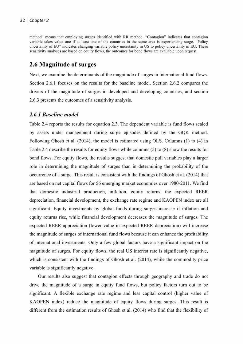
2.6 Magnitude of surges Next, we examine the determinants of the magnitude of surges in international fund flows.

Section 2.6.1 focuses on the results for the baseline model. Section 2.6.2 compares the

drivers of the magnitude of surges in developed and developing countries, and section

2.6.3 presents the outcomes of a sensitivity analysis.

2.6.1 Baseline model Table 2.4 reports the results for equation 2.3. The dependent variable is fund flows scaled

by assets under management during surge episodes defined by the GQK method.

Following Ghosh et al. (2014), the model is estimated using OLS. Columns (1) to (4) in

Table 2.4 describe the results for equity flows while columns (5) to (8) show the results for

bond flows. For equity flows, the results suggest that domestic pull variables play a larger

role in determining the magnitude of surges than in determining the probability of the

occurrence of a surge. This result is consistent with the findings of Ghosh et al. (2014) that

are based on net capital flows for 56 emerging market economies over 1980-2011. We find

that domestic industrial production, inflation, equity returns, the expected REER

depreciation, financial development, the exchange rate regime and KAOPEN index are all

significant. Equity investments by global funds during surges increase if inflation and

equity returns rise, while financial development decreases the magnitude of surges. The

expected REER appreciation (lower value in expected REER depreciation) will increase

the magnitude of surges of international fund flows because it can enhance the profitability

of international investments. Only a few global factors have a significant impact on the

magnitude of surges. For equity flows, the real US interest rate is significantly negative,

which is consistent with the findings of Ghosh et al. (2014), while the commodity price

variable is significantly negative.

Our results also suggest that contagion effects through geography and trade do not

drive the magnitude of a surge in equity fund flows, but policy factors turn out to be

significant. A flexible exchange rate regime and less capital control (higher value of

KAOPEN index) reduce the magnitude of equity flows during surges. This result is

different from the estimation results of Ghosh et al. (2014) who find that the flexibility of

SurgesofInternationalFundFlows 33

the exchange rate regime and capital account openness tend to amplify the magnitude of

surges of net capital inflows.

Table 2.4 Magnitude of surges: baseline model Equity flows Bond flows (1) (2) (3) (4) (5) (6) (7) (8) US industrial production

-0.008 -0.009 0.013 0.031* 0.053*** 0.052*** 0.019** 0.026*** (-0.91) (-0.96) (0.81) (1.81) (7.28) (7.34) (2.32) (2.82)

US real interest rate

0.003 -0.002 -0.010** -0.127** -0.113*** -0.057** -0.115*** -0.186*** (0.14) (-0.07) (-2.08) (-2.34) (-4.17) (-2.09) (-3.94) (-5.42) US equity returns

0.016 0.021 0.024 0.035 0.076*** 0.073*** 0.089*** 0.110*** (1.19) (1.39) (0.98) (1.32) (5.36) (5.27) (6.49) (7.04) TED spread -0.291* -0.148 0.264 0.320 0.575** 0.531** 0.591** 0.062 (-1.67) (-0.79) (0.76) (0.87) (2.51) (2.31) (2.33) (0.22) VIX 0.020 0.024 0.042 0.048* 0.094*** 0.092*** 0.092*** 0.111*** (1.34) (1.49) (1.63) (1.69) (6.62) (6.61) (6.84) (7.01) Policy uncertainty

0.006** 0.005* 0.006 0.005 -0.001 -0.001 -0.000 -0.003 (2.35) (1.90) (1.48) (0.97) (-0.62) (-0.53) (-0.16) (-1.38) Commodity prices

-0.000 0.0001 -0.006** -0.003 -0.016*** -0.011*** -0.013*** -0.002 (-0.16) (0.01) (-2.50) (-1.18) (-10.06) (-6.90) (-7.72) (-0.74) Geography contagion

0.232** 0.125 0.004 0.555*** 0.491*** 0.493*** (2.54) (0.79) (0.02) (5.88) (4.85) (3.61) Trade linkage -0.165 0.431 0.604 1.048*** 0.616*** 0.735**

(-0.89) (0.85) (1.04) (6.90) (2.61) (2.41) Dom. industrial production

-0.023** -0.042*** 0.027*** 0.009* (-2.30) (-3.64) (6.21) (1.66)

Dom. interest rate

0.004 0.008 0.021* 0.011 (0.21) (0.34) (1.65) (0.70) Dom. inflation 0.167*** 0.131*** 0.011 -0.010 (6.84) (4.50) (0.80) (-0.57) Dom. equity returns

0.038*** 0.038*** 0.0237** 0.017*** (3.84) (3.53) (3.91) (2.59) Exp. REER depreciation

-0.062*** -0.070*** 0.003 0.001 (-3.32) (-3.46) (0.30) (0.07)

Trade openness 0.206 0.248 0.172* 0.309** (1.13) (1.22) (1.83) (2.53) Credit growth -0.002 -0.007 0.006** 0.007** (-0.38) (-1.26) (2.29) (2.19) Stock market cap.

-0.002* -0.002* 0.001 -0.000 (-1.80) (-1.71) (0.91) (-0.42)

Exchange rate regime

-0.160** 0.084* (-2.20) (1.93) KAOPEN -0.257*** -0.168*** (-4.37) (-4.83) Constant 1.913*** 1.760*** 0.847*** 1.828*** 2.990*** 2.434*** 1.887*** 2.212*** (39.75) (21.84) (4.23) (5.87) (52.47) (27.10) (15.92) (10.95) N 2517 2291 1212 1071 1387 1366 1028 781

Note: Dom., exp., cap. are the short for domestic, expected, and capitalization, respectively. The dependent variable is fund flows scaled by asset under management conditional on surge episodes defined by the GQK method. All equations are estimated using OLS. t statistics in parentheses; *, ** and *** indicate significance at respectively 10%, 5% and 1% level.

34 Chapter2

Our findings imply that policy makers can influence the magnitude of surges of equity

fund flows by maintaining price stability, enhancing financial development, making the

exchange rate more flexible, and exerting less capital control.

When it comes to bond flows, both global push factors and domestic pull factors are

important in determining the magnitude of surges. As to global push factors, all the

variables are significant except for policy uncertainty. The magnitude of bond surges tends

to increase with lower US real interest rates, higher US equity returns, a higher TED

spread, as well as higher financial market volatility. One possible reason is that with

worsened liquidity conditions and higher market volatility, investors tend to invest in bond

funds to reduce risk, because bond assets are assumed to be safer than equity assets. The

contagion factors are also significantly positive, which indicates that the surge magnitude

of receiving countries is influenced by the occurrence of surges in the region and in

trading partners. Regarding domestic pull factors, the results are similar to those for equity

flows with a few exceptions. Inflation and the expected REER depreciation are not

significantly related to the magnitude of bond surges, while trade openness and credit

growth rate become more significant, which indicates that more trade openness and higher

credit growth tend to attract more bond investments once the surge episodes occurred.

2.6.2 Developed versus developing countries The results for developed and developing countries regarding the magnitude of equity

surges are highly similar, with a few exceptions. For equity flows, as shown in Table 2.5,

the differences are as follows. Firstly, the contagion effects are more significant for

developed countries. Secondly, the magnitude of surges in developed countries is

positively related with commodity prices, while the relationship is negative for developing

countries. Thirdly, the exchange rate regime variable has a significant positive coefficient

in the case of developed countries, but a significantly negative one for developing

countries. This indicates that for developing countries more flexible exchange rate regime

tends to reduce the magnitude of surge episodes.

For bond flows, the comparison results are shown in Appendix A.6. The magnitude of

bond flow surges is more sensitive to global factors than the magnitude of equity flow

surges, especially for developing countries. For example, the magnitude of bond flow

surges in developing countries is more influenced by US industrial production and the

TED spread. In addition, contagion through geography is more significant for developing

SurgesofInternationalFundFlows 35

countries.

Table 2.5 Magnitude of surges: developed versus developing countries (equity flows) Developed countries Developing countries

(1) (2) (3) (4) (5) (6) (7) (8) US industrial production

-0.002 0.000 0.001 0.013 -0.005 -0.007 0.012 0.032 (-0.21) (0.01) (0.13) (1.53) (-0.38) (-0.48) (0.40) (0.96)

US real interest rate 0.067*** 0.078*** -0.045** -0.023 -0.054 -0.056 -0.150 -0.285** (3.23) (3.70) (-2.21) (-1.09) (-1.52) (-1.35) (-1.50) (-2.40) US equity returns 0.000 0.002 -0.004 -0.013 0.014 0.022 0.048 0.093 (0.04) (0.18) (-0.43) (-1.22) (0.62) (0.85) (0.90) (1.60) TED spread -0.165 0.012 -0.045 0.004 -0.396 -0.272 0.492 0.238 (-1.05) (0.08) (-0.32) (0.03) (-1.33) (-0.83) (0.67) (0.31) VIX -0.000 -0.004 -0.003 -0.010 0.033 0.045* 0.073 0.105* (-0.02) (-0.29) (-0.25) (-0.82) (1.39) (1.70) (1.42) (1.87) Policy uncertainty 0.004 0.002 0.002 0.003 0.007 0.007 0.008 0.003 (1.58) (0.81) (1.43) (1.56) (1.61) (1.52) (1.07) (0.38) Commodity prices 0.007*** 0.008*** 0.000 0.001 -0.005** -0.005* -0.008* -0.006 (4.42) (5.16) (0.05) (0.91) (-2.15) (-1.85) (-1.79) (-1.21) Geography contagion 0.269*** 0.279*** 0.227*** 0.092 -0.106 0.150 (3.56) (4.38) (3.32) (0.55) (-0.31) (0.36) Trade linkage -0.072 0.436** 0.608*** 1.245** 1.683 1.023 (-0.56) (2.40) (3.11) (2.24) (1.07) (0.58) Dom. industrial production

0.004 -0.009 -0.035* -0.061*** (0.88) (-1.64) (-1.89) (-2.73)

Dom. interest rate 0.016 -0.021 -0.024 0.008 (1.13) (-1.28) (-0.63) (0.19) Dom. inflation 0.050*** 0.039** 0.227*** 0.225*** (3.82) (2.34) (5.07) (4.28) Dom. equity returns 0.022*** 0.022*** 0.049*** 0.049*** (4.04) (3.76) (2.85) (2.66) Exp. REER depreciation

-0.024** -0.023** -0.083** -0.093** (-2.44) (-2.24) (-2.45) (-2.52)

Trade openness 0.013 0.081 0.030 -0.103 (0.19) (1.12) (0.06) (-0.17) Credit growth -0.004 -0.001 -0.005 -0.016* (-1.31) (-1.00) (-0.56) (-1.81) Stock market cap.

-0.001 -0.001*** -0.002 0.001 (-1.36) (-2.72) (-0.52) (0.24)

Exchange rate regime 0.058** -0.926*** (2.15) (-4.50) KAOPEN -0.217*** -0.144 (-4.67) (-1.20) Constant 1.712*** 1.527*** 0.911*** 1.415*** 2.107*** 1.923*** 1.032* 3.129*** (39.12) (23.17) (12.16) (8.16) (25.24) (12.86) (1.70) (3.80) N 1174 1090 654 592 1343 1201 558 479

Note: See note to Table 2.4. Low-income and middle-income economies are referred to as developing economies. High-income economies are referred to as developed economies. Economies are divided according to 2012 GNI per capita, calculated using the World Bank Atlas method.

36 Chapter2

2.6.3 Sensitivity analysis We also do some robustness tests for the determinants of the magnitude of surges, mainly

focusing on some alternative specifications of global, contagion and domestic factors (see

Table 2.3). First, we include region dummies to control for regional-fixed effects. The

results remain stable and this too suggests that domestic factors are more important than

global factors in determining surge magnitude (column (5)). Next, when the geography

dummy equals one if at least one country in the same region is experiencing a surge, the

geographic contagion effect is still insignificant for the magnitude of surges (column (6)).

Finally, similar to the case of US policy uncertainty, EU policy uncertainty has a positive

effect on surge magnitude (column (7)).

2.7 Conclusions Based on the monthly data of 55 countries, this study investigates surges in international

fund flows. Employing a threshold method proposed by Ghosh et al. (2014), we identify

surge episodes for equity flows and bond flows. We identify three surge episodes for

equity flows during 1996 to 2013 and two surges in bond flows from 2004 to 2013.

Following Ghosh et al. (2014), we investigate the drivers of the occurrence and

magnitude of surges. Our results suggest that surges of international fund flows are

especially driven by global push factors (such as US industrial production, US equity

returns, TED spread, VIX index and policy uncertainty) and contagion factors. Better

global economic conditions lead to higher likelihood of fund flow surges. One country is

more prone to surges if their neighbors or trader partners also experience surges. Different

from the findings of Ghosh et al. (2014) for surges of net capital flows, we find that as

financial volatility increases, investors tend to invest more in global funds to diversify

their risks. The magnitude of surges primarily depends on domestic factors (such as

industrial production, inflation, equity returns, expected REER depreciation, stock market

capitalization, the exchange rate regime and KAOPEN index). The magnitude of surges

will increase in the period of high inflation and high equity returns in domestic countries.

Overall, our findings are consistent with, but go beyond, the empirical results of

previous studies. We provide a better understanding of surges of international funds flows,

which have not been studied before. From a policy perspective our results are also

important. A country can reduce the probability of a surge by enhancing trade openness

SurgesofInternationalFundFlows 37

and financial openness. Policy makers can also influence the magnitude of surges, e.g. by

maintaining price stability, keeping moderate credit growth, enlarging their stock market

capitalization. In particular, developing countries can opt for a more flexible exchange rate

regime to control surges. Besides, our results suggest that although trade openness is

helpful to decrease the likelihood of surges, it tends to make the surges more severe once

they occur. Capital controls are not helpful to control fund flow surges.

In this chapter, we focus on whether push or pull factors are important in driving fund

flow surges instead of the influence of one or two specific factors. Therefore, the role of

each explanatory variable may not be sufficiently discussed. Future research can focus on

the role of one specific variable in determining surges, e.g. whether trade/financial

openness makes a country more prone or less prone to surge risks. In next chapter, we will

discuss the counterpart risk of surges – sudden stops.

38 Chapter2