Ultimate Strength of Ship Plating - A Proof of Capacity under ...
261
SCHRIFTENREIHE SCHIFFBAU Richard C. Hayward 699 | November 2016 Ultimate Strength of Ship Plating - A Proof of Capacity under Combined In-Plane-Loads
-
Upload
khangminh22 -
Category
Documents
-
view
3 -
download
0
Transcript of Ultimate Strength of Ship Plating - A Proof of Capacity under ...

SCHRIFTENREIHE SCHIFFBAU
Richard C. Hayward
699 | November 2016
Ultimate Strength of Ship Plating -A Proof of Capacity under Combined In-Plane-Loads
SCH
RIF
TEN
REI
HE
SCH
IFFB
AU
699


Ultimate Strength of Ship PlatingA Proof of Capacity under Combined In-Plane Loads
Vom Promotionsausschuss derTechnischen Universität Hamburg-Harburg
zur Erlangung des akademischen Grades
Doktor-Ingenieur (Dr.-Ing.)
genehmigte Dissertation
vonRichard C. Hayward
ausToronto, Kanada
2016

1. Gutachter: Prof. Dr.-Ing. Dr.-Ing. E.h. Dr. h.c. Eike Lehmann2. Gutachter: Prof. D.Sc. (Tech.) Claude Daley3. Gutachter: Prof. D.Sc. (Tech.) Sören Ehlers
Tag der mündlichen Prüfung: 18.10.2016

Ultimate Strength of Ship Plating - A Proof of Capacity under Combined In-Plane Loads, Richard C. Hayward, 1. Auflage, Hamburg, Technische Universität Hamburg, 2016, ISBN 978-3-89220-699-6
© Technische Universität Hamburg Schriftenreihe Schiffbau Am Schwarzenberg – Campus 4 D-21073 Hamburg
http://www.tuhh.de/vss


Abstract
The present work addresses the need for a proof of plate capacity under combined in-planeloads, a need recently highlighted by the loss of the post-panamax container ship MOLComfort. Towards this end, an extensive series of numerical studies based on the finiteelement method have been performed covering all load combinations and plating configura-tions relevant for the shipbuilding industry. These studies have been used to investigate themechanics of plating collapse (including the effects of plate slenderness and aspect ratio)under longitudinal, transverse and shear loads in isolation and in combination. Numericalstudies have also been used to quantitatively evaluate existing proofs of plate capacityfound in both literature and the shipbuilding industry. In this regard, quantitative ac-ceptance criteria have been developed with which to judge whether a proof is (1) precise,(2) accurate and (3) robust. Similarly, qualitative criteria have been defined which requirean acceptable proof to be (1) concise, (2) physically-based and (3) directly solvable. Be-cause no existing proof was found to satisfy all quantitative and qualitative acceptancecriteria, a hypothetical proof has been postulated using a generalised form of the von Misesequation (in order to satisfy qualitative acceptance criteria), where the exponents andinteraction coefficient have been derived on the basis of observations made in the inves-tigation of plating collapse mechanisms. To satisfy all quantitative acceptance criteria,the exponents and interaction coefficient of the hypothetical proof have subsequently beenredefined on the basis of additional numerical studies (in case of biaxial compression only).Design application of the resulting proof has subsequently been explained and demon-strated. Because the new proof is based on numerical studies of simply-supported plates,uniform in-plane loads and idealised initial imperfections, the validity of its application hasbeen demonstrated in case of other boundary conditions, additional load components andmore realistic initial imperfections. Moreover, the marginal effect of out-of-plane loads (i.e.lateral pressure) on the in-plane capacity of plating has also been investigated. Finally,two examples of design application have been provided wherein the capacity of stiffenedpanels in the bottom shell and side shell of a double hull VLCC have been calculated bothnumerically and according to the new proof. Although the focus of the present work ison the capacity of plane plates, a new proof of curved plate capacity has been addition-ally presented. In terms of practical application in the shipbuilding industry, both proofsof plate capacity have been included in the newly harmonised IACS Common StructuralRules for Bulk Carriers and Oil Tankers, the new IACS Longitudinal Strength Standard forContainer Ships as well as the new DNVGL Rules for Classification which are applicableto all ship types.
i


Acknowledgements
It would not have been possible to write this doctoral dissertation without the helpand support of the kind people around me, only some of whom it is possible to here giveparticular mention.
Firstly, I would like to express my sincere gratitude to my academic advisors ProfessorEike Lehmann and Professor Claude Daley for their continuous support and guidance. Theunending enthusiasm which they exude is indeed infectious.
I also would like to thank my IACS HPT02 colleagues as well as my colleagues atGermanischer Lloyd (now DNV·GL) for their cooperation and valuable feedback. In par-ticular I would like to thank my former supervisor Hans-Joachim Schulte who so kindlymentored me on the buckling and ultimate strengths of ship structures.
Last but not least, I would like to thank my parents and sister for their long-distancesupport and encouragement. I would especially like to thank my wife Patricia. If kindnessand patience are truly virtues then she is without doubt the most virtuous person I know.
iii


Nomenclature
Common notation
a plate length or frame span [mm]b plate breadth or frame spacing [mm]c stress ratio σy/σx [ - ]t nominal plate thickness [mm]
E modulus of elasticity [N/mm2]K elastic buckling factor [ - ]P axial force [N]R normalised axial or shear stress [ - ]
α plate aspect ratio [ - ]β plate slenderness parameter [ - ]γ shear strain [ - ]δ deflection [ - ]ε axial strain [ - ]η utilisation factor [ - ]κ plate reduction factor [ - ]λ reference degree of slenderness [ - ]µ stress multiplier factor at failure [ - ]ν Poisson’s ratio [ - ]σ axial stress [N/mm2]τ shear stress [N/mm2]ψ edge stress ratio [ - ]
Γ ratio of (stress) vector magnitudes [ - ]
Subscripts
cr critical (elastic) stresse reference stresseq equivalent stressi internal stressm effective breadth/lengthproof quantity based on proof of capacityrc residual compressive stressrt residual tensile stressult ultimate strengthx quantity in the x-directionxy quantity in the xy-plane
v

y quantity in the y-directionz quantity in the z-direction
FEA quantity based on finite element analysesY yield strength
0 initial quantity1, 2, 3 directions of principal stress
Acronyms
ABS American Bureau of ShippingALS Accidental Limit StateBV Bureau VeritasClassNK Nippon Kaiji KyokaiCSR-BC IACS Common Structural Rules for Bulk CarriersCSR BC & OT IACS Common Structural Rules for Bulk Carriers and Oil TankersCSR-OT IACS Common Structural Rules for Oil TankersDIN Deutsches Institut für Normung (German Institute for Standardization)DnV Det norske VeritasFLS Fatigue Limit StateGL Germanischer LloydHPT02 IACS CSR Harmonisation Project Team 02 (Buckling)IACS International Association of Classification Societies Ltd.KPI Key Performance IndicatorLR Lloyd’s RegisterPULS Panel Ultimate Limit StateSLS Serviceability Limit StateULS Ultimate Limit StateUR Unified Requirement (IACS)
vi

Contents
1. Introduction 11.1. Purpose . . . . . . . . . . . . . . . . . . . . . . . . . . . . . . . . . . . . . . 11.2. Scope and outline . . . . . . . . . . . . . . . . . . . . . . . . . . . . . . . . . 2
2. Mechanics of Plating Collapse 52.1. Uniaxial compression . . . . . . . . . . . . . . . . . . . . . . . . . . . . . . . 5
2.1.1. Ideal plates . . . . . . . . . . . . . . . . . . . . . . . . . . . . . . . . 62.1.2. Effective width concept . . . . . . . . . . . . . . . . . . . . . . . . . 102.1.3. Effects of initial deflections . . . . . . . . . . . . . . . . . . . . . . . 132.1.4. Effective width formulae used in shipbuilding . . . . . . . . . . . . . 18
2.2. Biaxial loads . . . . . . . . . . . . . . . . . . . . . . . . . . . . . . . . . . . 212.2.1. Ideal plates - compressive secondary stress . . . . . . . . . . . . . . . 212.2.2. Ideal plates - tensile secondary stress . . . . . . . . . . . . . . . . . . 262.2.3. Internal stress distributions . . . . . . . . . . . . . . . . . . . . . . . 312.2.4. Capacity curves . . . . . . . . . . . . . . . . . . . . . . . . . . . . . . 35
2.3. In-plane shear . . . . . . . . . . . . . . . . . . . . . . . . . . . . . . . . . . . 382.3.1. Ideal plates . . . . . . . . . . . . . . . . . . . . . . . . . . . . . . . . 382.3.2. Tension field analysis . . . . . . . . . . . . . . . . . . . . . . . . . . . 432.3.3. Effects of initial deflections . . . . . . . . . . . . . . . . . . . . . . . 472.3.4. Formulae for plate reduction factors . . . . . . . . . . . . . . . . . . 482.3.5. Reduction in uniaxial/biaxial capacity due to shear . . . . . . . . . . 51
2.4. Effects of plate aspect ratio . . . . . . . . . . . . . . . . . . . . . . . . . . . 592.4.1. Uniaxial loads . . . . . . . . . . . . . . . . . . . . . . . . . . . . . . . 592.4.2. Biaxial loads . . . . . . . . . . . . . . . . . . . . . . . . . . . . . . . 682.4.3. In-plane shear . . . . . . . . . . . . . . . . . . . . . . . . . . . . . . . 73
3. Existing Proofs 773.1. Quantitative evaluation scheme . . . . . . . . . . . . . . . . . . . . . . . . . 77
3.1.1. Precision and bias . . . . . . . . . . . . . . . . . . . . . . . . . . . . 773.1.2. Robustness . . . . . . . . . . . . . . . . . . . . . . . . . . . . . . . . 80
3.2. Proofs from literature . . . . . . . . . . . . . . . . . . . . . . . . . . . . . . 833.2.1. Paik . . . . . . . . . . . . . . . . . . . . . . . . . . . . . . . . . . . . 843.2.2. Ueda et al. . . . . . . . . . . . . . . . . . . . . . . . . . . . . . . . . 88
3.3. Proofs from shipbuilding practice . . . . . . . . . . . . . . . . . . . . . . . . 923.3.1. Elastic analyses with plasticity correction (DnV and GL) . . . . . . . 943.3.2. PULS (DnV) . . . . . . . . . . . . . . . . . . . . . . . . . . . . . . . 1013.3.3. Amended DIN 18800 (GL) . . . . . . . . . . . . . . . . . . . . . . . . 1053.3.4. Provisional CSR BC & OT (BV) . . . . . . . . . . . . . . . . . . . . 111
vii

Contents
4. New Proof 1154.1. Problem statement . . . . . . . . . . . . . . . . . . . . . . . . . . . . . . . . 115
4.1.1. Quantitative Criteria . . . . . . . . . . . . . . . . . . . . . . . . . . . 1164.1.2. Qualitative Criteria . . . . . . . . . . . . . . . . . . . . . . . . . . . . 117
4.2. Evaluation of existing proofs . . . . . . . . . . . . . . . . . . . . . . . . . . . 1194.3. Development and evaluation of new proof . . . . . . . . . . . . . . . . . . . 122
4.3.1. Framework of new proof . . . . . . . . . . . . . . . . . . . . . . . . . 1234.3.2. Hypothetical Proof of Plate Capacity . . . . . . . . . . . . . . . . . . 1274.3.3. Exponent e0 (Quadrant 1) . . . . . . . . . . . . . . . . . . . . . . . . 1314.3.4. Interaction Coefficient B (Quadrant 1) . . . . . . . . . . . . . . . . . 1364.3.5. Quantitative evaluation . . . . . . . . . . . . . . . . . . . . . . . . . 139
4.4. CSR BC & OT proof . . . . . . . . . . . . . . . . . . . . . . . . . . . . . . . 1424.4.1. Quantitative evaluation . . . . . . . . . . . . . . . . . . . . . . . . . 144
5. Design Application 1485.1. Proof of stiffened panel strength . . . . . . . . . . . . . . . . . . . . . . . . . 148
5.1.1. Proof of sufficient plate capacity . . . . . . . . . . . . . . . . . . . . 1505.1.2. Proof of sufficient stiffener capacity . . . . . . . . . . . . . . . . . . . 165
5.2. Examples of design application . . . . . . . . . . . . . . . . . . . . . . . . . 1685.2.1. Bottom shell plating (σx-σy) . . . . . . . . . . . . . . . . . . . . . . 1705.2.2. Side shell plating (σx-τxy) . . . . . . . . . . . . . . . . . . . . . . . . 171
6. Conclusions 1726.1. Summary of results and conclusions . . . . . . . . . . . . . . . . . . . . . . . 1726.2. Summary of contributions . . . . . . . . . . . . . . . . . . . . . . . . . . . . 1756.3. Future research . . . . . . . . . . . . . . . . . . . . . . . . . . . . . . . . . . 177
7. References 178
Appendices 184
Appendix A. Proof of Curved Plate Capacity 185A.1. Evaluation of proof under two stress components . . . . . . . . . . . . . . . 185A.2. Evaluation of proof under three stress components . . . . . . . . . . . . . . 190
Appendix B. Numerical Studies 192B.1. Description of finite element analyses . . . . . . . . . . . . . . . . . . . . . . 192
B.1.1. General . . . . . . . . . . . . . . . . . . . . . . . . . . . . . . . . . . 192B.1.2. Model extent . . . . . . . . . . . . . . . . . . . . . . . . . . . . . . . 192B.1.3. Element type and meshing . . . . . . . . . . . . . . . . . . . . . . . . 193B.1.4. Material properties and real constants . . . . . . . . . . . . . . . . . 193B.1.5. Boundary conditions and load application . . . . . . . . . . . . . . . 194B.1.6. Initial imperfections . . . . . . . . . . . . . . . . . . . . . . . . . . . 196B.1.7. Solution algorithm . . . . . . . . . . . . . . . . . . . . . . . . . . . . 196
B.2. Validation of procedure . . . . . . . . . . . . . . . . . . . . . . . . . . . . . 197B.2.1. Comparison with stiffened panel tests . . . . . . . . . . . . . . . . . 197B.2.2. Comparison with unstiffened plate tests . . . . . . . . . . . . . . . . 199
viii

Contents
Appendix C. Evaluation Data 202C.1. Tabular Results . . . . . . . . . . . . . . . . . . . . . . . . . . . . . . . . . . 203C.2. Graphical Results . . . . . . . . . . . . . . . . . . . . . . . . . . . . . . . . . 216
Appendix D. Calibration Data 223D.1. Tabular Results . . . . . . . . . . . . . . . . . . . . . . . . . . . . . . . . . . 224D.2. Graphical Results . . . . . . . . . . . . . . . . . . . . . . . . . . . . . . . . . 237
ix


1. Introduction
On 17 June 2013 the post-panamax container ship MOL Comfort (8,000 TEU class) suf-fered a fracture amidships during inclement weather en route from Singapore to Jeddah,Saudi Arabia, eventually breaking into two halves. Fortunately all 26 crew members wereable to take to lifeboats and thereafter rescued by another ship in the area [1]. Althoughboth halves remained intact and afloat for several days after breaking apart, the aft sectionsank on 27 June 2013 together with about 1,700 containers and 1,500 metric tons of fueloil [2]. The bow section, while under tow, caught fire on 06 July 2013 and sank on 11July 2013 together with another 2,400 containers and 1,600 metric tons of fuel oil [3, 4].The total loss of ship and cargo (4,382 containers) was evaluated by the insurer Allianz at83m USD and 440m USD, respectively [5]. Moreover, additional financial claims are beingmade by the operator against the shipbuilder which include the renovation of sister shipsas a safety precaution.
An interim investigative report into the loss of MOL Comfort stated that water ingresswas first detected by an alarm in the duct keel (i.e. near the centreline of the ship) anda few minutes later in No. 6 cargo hold. Photos of the damaged ship showed a fracturepropagating up through the side shell from the bottom of the ship, leading investigators toconclude that the crack which triggered the fracture originated amidships in the bottomshell plating below No. 6 cargo hold [6]. Subsequent surveys of the bottom shell platingof sister ships revealed large buckling deformations in the same area. Based on elasto-plastic analyses using 3-hold finite element models, it was shown that the loss of platingstrength led to a reduction in effective breadth of the double bottom girders which in turnled to collapse of the double bottom and subsequently the hull girder [7]. Moreover, itwas concluded that the double bottom structure of the MOL Comfort and sister ships wasrelatively weak out-of-plane compared to ships of similar size. The resulting increase inbiaxial stresses due to deflection of the double bottom under sea pressure, superimposedon and magnified by axial stresses due to hull girder bending and transverse stresses dueto side compression, created an extreme biaxial stress state in the bottom shell plating.Accordingly, although accident investigators struggled to explain the apparent gap betweenstructural demand and capacity, it was concluded with some confidence that the loss ofMOL Comfort initiated with collapse of the ship’s bottom shell plating under biaxialcompression.
1.1. Purpose
Although the foregoing is certainly not a singular example of catastrophic failure when theultimate strength of ship plating is exceeded, it is one of the more recent examples whichserves to illustrate the need for a proof of plate capacity under combined in-plane loads.Only with such a proof can ship plating be reliably and efficiently designed so that the de-mands on structure are met over the service life of a ship without incurring a needless weightpenalty. However, five years before the sinking of MOL Comfort, the International Associ-
1
2 1. Introduction
ation of Classification Societies (IACS) had already established a project team (HPT02) toharmonise the disparate buckling strength rules applied at that time to bulk carriers andoil tankers. With respect to the proof of plate capacity under combined in-plane loads, ithad become apparent in 2012 that the proof of plate capacity used provisionally by theproject team was too non-conservative in case of plating under biaxial compression andtoo conservative in case of stress states with a tensile component. For this reason, theauthor of the present work was tasked during the 10th meeting of HPT02 to develop a newproof of plate capacity for inclusion in the newly harmonised IACS Common StructuralRules for Bulk Carriers and Oil Tankers. As this proof is intended for use in the designand classification of ships, it was determined that it needs not only to be based on theultimate strength concept, but needs as well to satisfy certain qualitative and quantitativecriteria. In qualitative terms, the proof needs to be (1) concise, (2) physically-based and(3) directly solvable. In quantitative terms, the proof needs to be (1) precise, (2) accurateand (3) robust. The purpose of the present work is to develop a proof of plate capacitywhich satisfies all of these criteria.
In addition to inclusion in the IACS Common Structural Rules for Bulk Carriers andOil Tankers, the proof presented herein has also been included in the new IACS Longi-tudinal Strength Standard for Container Ships (UR S11A) as well as the new DNVGLRules for Classification which are applicable to all ship types. As a consequence of the lossof MOL Comfort, the IACS Longitudinal Strength Standard for Container Ships includesadditional requirements for the buckling strength assessment of large container ships (i.e.breadth B > 32.26m) for which "(a)ll in-plane stress components (i.e. bi-axial and shearstresses) induced by hull girder loads and local loads are to be considered" [8]. Of course,most classification societies have for many years already considered all in-plane stress com-ponents and lateral loads in their assessments of buckling strength for all ship types as amatter of good engineering practice.
1.2. Scope and outline
The present work addresses the need for a proof of plate capacity under combined in-planeloads. Towards this end, an extensive series of numerical studies based on the finite elementmethod have been performed covering all load combinations and plating configurationsrelevant for the shipbuilding industry. Because the new proof is based on numerical studiesof simply-supported plates, uniform in-plane loads and idealised initial imperfections, thevalidity of its application in case of other boundary conditions, additional load componentsand more realistic initial imperfections has been demonstrated as is its application tostiffened panels. However, the effects of strain hardening are largely ignored and theplating is assumed to remain ductile throughout loading, i.e. no brittle or fatigue fracture.Finally, although the present work is focussed on a proof of plane plate capacity, the DIN18800 proof of curved plate capacity (already used extensively in the shipbuilding industry)has also been revised, the technical background of which is documented in Appendix A.
In Chapter 2 the development of a proof of plate capacity under combined in-planeloads begins with a detailed investigation of the mechanics of plating collapse. Here thecollapse of plates are examined under longitudinal, transverse and shear stresses, in isola-tion and in combination. In this regard, the first three sections of the chapter address the

1.2. Scope and outline 3
capacity of plating under uniaxial compression, biaxial loads and in-plane shear (includingthe reduction in uniaxial/biaxial capacity due to shear). In each of these sections squareplating is used to isolate the effects of plate aspect ratio which are subsequently discussedin the last section of the chapter. The purpose of Chapter 2 is to lay the groundwork fora physically-based solution and to thoroughly examine the ultimate strengths of platingunder single stress components which are used as reference stresses in most proofs of platecapacity under combined in-plane loads. Accordingly, because the accuracy and precisionof these proofs depend extensively on those of the reference stresses, formulations found inliterature and the shipbuilding industry for defining the characteristic strength of plates(under single stress components) are thoroughly discussed and compared to numericalresults.
In Chapter 3 existing proofs of plate capacity found in literature and the shipbuildingindustry are described and quantitatively evaluated over a wide range of load combinationsand plating configurations. In this regard, an evaluation scheme is firstly presented whichmeasures bias (or accuracy) and precision (including measures of conservatism and non-conservatism) in terms of five key performance indicators. Each proof is evaluated overa design space consisting of 360 evaluation points and a design subspace consisting of 56evaluation points. The former covers load combinations and plating configurations relevantfor all ship structures while the latter covers those combinations and configurations largelyrelevant for cargo hold structures, i.e. those critical to the ultimate strength of the hullgirder.
In Chapter 4 a new proof of plate capacity under combined in-plane loads is developed.Towards this end, the problem to be solved is stated quite precisely using quantitativeand qualitative criteria which define an acceptable proof of plate capacity. On the basis ofthese criteria, the existing proofs discussed in Chapter 3 are evaluated. Because no existingproof is found to satisfy all quantitative and qualitative acceptance criteria, a hypotheticalproof of plate capacity under combined in-plane loads is postulated which well reflects themechanics of plating collapse described in Chapter 2 and the strengths of existing proofsinvestigated in Chapter 3. In order to satisfy qualitative acceptance criteria, the proof isbased on a generalised form of the von Mises equation
(σx
κx · σY
)e0
+
(σy
κy · σY
)e0
−B·(
σx
κx · σY
)e0/2
·(
σy
κy · σY
)e0/2
+
(τxy
κτ · τY
)e0
= 1.0 (1.1)
where the exponent e0 and interaction coefficient B are derived on the basis of observa-tions made in the investigation of plating collapse mechanisms. Because the hypotheticalproof falls just short of satisfying all quantitative acceptance criteria, a new proof of platecapacity is subsequently developed where the exponent e0 and interaction coefficient B areredefined on the basis of additional numerical studies (in case of biaxial compression only).This new proof is then evaluated followed by a description and evaluation of the proof ofplate capacity implemented in the newly harmonised IACS Common Structural Rules forBulk Carriers and Oil Tankers for which the interaction coefficient B is slightly revisedwhen used together with newly harmonised load models.
In Chapter 5 the design application of the newly developed proof as used in the IACSCommon Structural Rules for Bulk Carriers and Oil Tankers is discussed. In the first sec-tion of the chapter, an overview of the proof of stiffened panel capacity is presented wherethe decoupling of plate strength and stiffener strength is explained and presented. Regard-

4 1. Introduction
ing the former, the new proof of plate capacity is based on numerical studies of simply-supported plates, uniform in-plane loads and idealised initial imperfections. Accordingly,as noted above, the validity of its application in case of other boundary conditions (i.e.free edges and edge pull-in), additional load components (i.e. in-plane bending and lateralpressure) and more realistic initial imperfections (i.e. residual deflections and stresses basedon measurements) is demonstrated. The marginal effect of out-of-plane loads (i.e. lateralpressure) on the in-plane capacity of plating is also investigated. The section concludeswith a discussion of the proof of stiffener capacity. In the second section of the chapter,two examples of design application are presented where the capacity of stiffened panels inthe bottom shell and side shell of a double hull VLCC are calculated both numerically andaccording to the new proof, the former stiffened panel being particularly relevant to thehull girder collapse of MOL Comfort.

2. Mechanics of Plating Collapse
In this chapter the mechanics of plating collapse is examined in detail. Once the behaviourof plating under in-plane loads is thoroughly understood, a physically-based proof of platecapacity is then possible. In §2.1 the simplest case of collapse under uniaxial compressionis examined. This is followed in §2.2 by analyses of collapse under biaxial loads and in §2.3under in-plane shear. In each of these sections square plates are used to isolate the effectsof aspect ratio which are discussed in §2.4. Numerical analyses are used throughout thischapter, the description and validation of which are included in Appendix B. All analysesare based on simply-supported plates with edges forced to remain straight, but otherwisefree to move in-plane. As explained in Chapter 5, this means that the loads are strain-basedrather than stress-based. Strain-based loads are representative of those arising from hullgirder bending where the in-plane displacement of plating is directly proportional to theradius of curvature. Furthermore, in all analyses the loads are uniformly applied and theplates are free of residual welding stresses with initial deflections based on their eigenmodes.In Chapter 5 the effects of other boundary conditions, additional load components and morerealistic initial imperfections are investigated. Finally, the concepts of effective width andplate reduction factors are thoroughly discussed throughout this chapter. Although theseconcepts only apply to single load types (i.e. σx, σy or τxy), they are used to define thecharacteristic strength of plates in several capacity formulations such that their accuracyis a prerequisite for avoiding inaccuracy under combined loading.
2.1. Uniaxial compression
In this section the collapse of square plates under a single compressive load is examined.For plating under single, in-plane loads, "collapse" is best defined using load-displacementcurves. These curves delineate the relationship between the magnitude of a single appliedload and the relative axial or shear displacement of the plate edges. When this rela-tionship is expressed in terms of internal quantities, reference is instead made to averagestress-average strain curves1, hereinafter referred to simply as stress-strain curves (wherethe expressions of both stress and strain are usually normalised against yield quantities).The stress and strain corresponding to the peak of the stress-strain curve represents thegreatest load which the plate can resist and is therefore referred to as the collapse strength(or ultimate strength) of the plating2.
1 Here the term strain does not refer to true material strain, but rather nominal or engineering strain,i.e. the displacement of plate edges relative to the extent of the undeformed plate.
2 Here the term strength refers to both stress and strain.
5
6 2. Mechanics of Plating Collapse
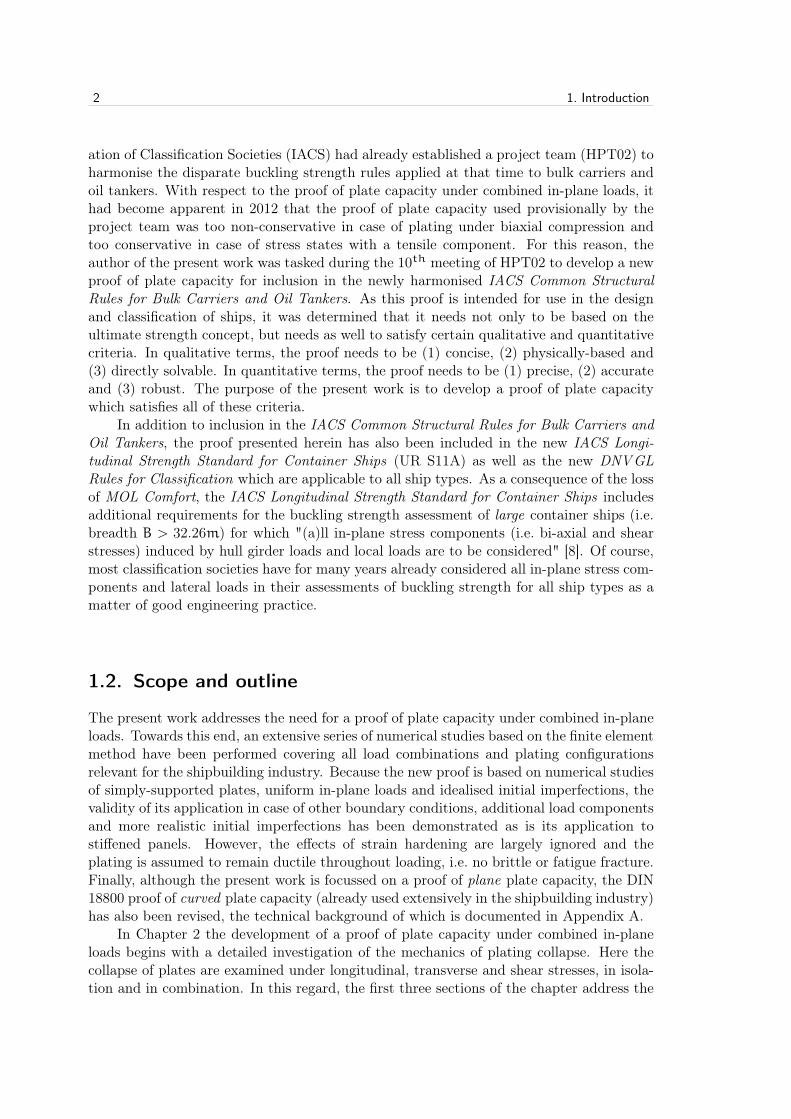
2.1.1. Ideal plates
Pre-buckling
A typical stress-strain curve is shown in Figure 2.1 for a square plate without any initialdeflections and an elastic buckling stress σx,cr well below its yield stress σY and collapsestrength σx,ult. With the initial application of a uniaxial load, stresses and strains areuniform throughout the plate with a linear relationship between them defined by the mod-ulus of elasticity, E = σx/εx. This linear elastic behaviour is referred to as the pre-bucklingportion of the stress-strain curve and in theory applies only to ideal plates (although inpractice the behaviour is also exhibited by plates with large elastic buckling stresses). Forthe load corresponding to point A on the curve (σx/σY = 0.3), the principal stresses in themiddle plane of the plate (normalised against the principal stress of greatest magnitude)are plotted in Figure 2.2(a). No Poisson effects are evident in these stresses since the edgesof the plate, although straight, are otherwise able to move freely in-plane.
A (Pre-buckling)
Buckling strength
B (Post-buckling)
Yield strength C (Post-yield)
Collapse strength
D (Post-collapse)
0.0
0.1
0.2
0.3
0.4
0.5
0.6
0.7
0.8
0.0 0.2 0.4 0.6 0.8 1.0 1.2 1.4 1.6 1.8 2.0 2.2 2.4 2.6 2.8 3.0
Nor
mal
ised
str
ess,
σx/σ
Y
Normalised strain, εx/εY
a
b σx
y
x
1
XYZ
run id 9930
-2350
235500
MAR 25 201519:10:42
PLOT NO. 3
Figure 2.1.: Stress-strain curve of ideal plate under uniaxial compression.
Buckling strength
As the load is increased, the linear relationship between stress and strain continues untilthe buckling strength of the plate is reached. At this point, there exists an alternative(out-of-plane) deflection shape for which the elastic strain energy is equal to that of thecompressed, plane plate. In mathematical terms, the critical buckling load is equal to the1st eigenvalue and the deformed shape is defined by the 1st eigenmode. Under the slightestof perturbations, the resulting out-of-plane deflection in the central region of the plate

2.1. Uniaxial compression 7
leads to a redistribution of stresses towards its edges and a lower axial stiffness3.1
X
Y
Z
run id 9930
JUN 3 201421:41:22
PLOT NO. 7
VECTOR
STEP=1SUB =31TIME=.310053SMIDDLE
PRIN1PRIN2PRIN3
(a) Pre-buckling (Point A)
1
X
Y
Z
run id 9930
JUN 3 201421:41:49
PLOT NO. 8
VECTOR
STEP=1SUB =520TIME=.522289SMIDDLE
PRIN1PRIN2PRIN3
(b) Post-buckling (Point B)
1
X
Y
Z
run id 9930
JUN 3 201421:42:10
PLOT NO. 9
VECTOR
STEP=1SUB =878TIME=.667575SMIDDLE
PRIN1PRIN2PRIN3
(c) Post-yield (Point C)
1
X
Y
Z
run id 9930
JUN 3 201421:42:37
PLOT NO. 10
VECTOR
STEP=1SUB =1414TIME=.618375SMIDDLE
PRIN1PRIN2PRIN3
(d) Post-collapse (Point D)
Figure 0.1: ——-CROP!——–CROP!——–CROP!——–CROP!——–CROP!———CROP!——-
1
Figure 2.2.: Principle stresses in middle plane of ideal plate.
Post-buckling
Accordingly, the post-buckling portion of the stress-strain curve is characterised by a re-duced slope (E ′ ' 0.49 · E). In Figure 2.2(b) the principal stresses associated with point
3 Plates with or without out-of-plane deflections store about the same amount of membrane strain energy(although this energy is distributed more so towards the edges in plates with out-of-plane deflections).The principle difference is that plates with out-of-plane deflections have additional bending strainenergy in the middle region of the plate. This bending strain energy comes from additional externalwork and accounts for the greater distance over which the load must act, i.e. lower axial stiffness.

8 2. Mechanics of Plating Collapse
B (σx/σY = 0.5) are shown. Here the redistribution of longitudinal stresses towards theedges of the plate (i.e. y = 0, y = b) is clearly evident as is the emergence of stresses in thetransverse direction4. With respect to the latter, tensile stresses form around mid-lengthof the buckled plate due to the out-of-plane deflection. As a consequence of its straightsides5, compressive stresses arise along the edges of the plate (i.e. x = 0, x = a)to balancein-plane forces in the transverse direction.
Yield strength
As the load is increased further, the out-of-plane deflections are magnified such that thecentral region of the plate sheds even more load, leading to an increase in stresses at theedges of the plate (i.e. y = 0, y = b) until the yield stress in the middle plane is eventuallyreached. Although stresses along the edges of the plate are approximately equal over itslength (increasing slightly in the corners of the plate with increasing slenderness), yieldinginitiates at the mid-length edges of the plate, i.e. x = a/2 (see corner inset in Figure 2.1),due to the aforementioned tensile stresses. Here the (compressive) longitudinal stressesand (tensile) transverse stresses are "working together" to deform the plate material. Inmaterial failure theory, the opposite signs of these stresses result in a higher equivalentstress σeq,i as reflected, for instance, in the positive interaction term (−σx,i ·σy,i) definedin the von Mises failure criterion6
σeq,i =√σx,i2 − σx,i · σy,i + σy,i2 = σY (2.1)
Although plasticity first appears at the compression surface of the plate (due primarily tobending strains in the central region), yielding in the middle plane of the plate is indicativeof through-thickness plasticity (due primarily to in-plane strains at the edges of the plate)and is typically a precursor to collapse.
Post-yield
With further increases in axial load, plastic flow begins to spread throughout the mid-dle plane, leading to progressive losses in stiffness at the edges of the plate (i.e. y = 0,y = b) such that the post-yield portion of the stress-strain curve is characterised by arapidly decreasing slope. In Figure 2.2(c) the principal stresses associated with point C(εx/εY = 1.0) in the post-yield response are shown. Here it can be seen that the axialstresses at the edges of the plate (i.e. y = 0, y = b) are approximately twice the magnitudeof axial stresses in the central region (i.e. y = b/2) due to the ever increasing out-of-planedeflection in the buckled plate. This deflection is also reflected in the increased magnitudeof transverse stresses.
4 As a matter of convention, the term longitudinal refers to quantities in the x-direction and the termtransverse refers to quantities in the y-direction. Moreover, plate length a is measured locally in thex-direction and plate breadth b in the y-direction such that a > b.
5 As explained in Appendix B, plate edges remain straight due to reciprocal actions in adjacent platefields. The effects of pull-in at free edges are discussed in Chapter 5.
6 To avoid confusion with externally applied (average) stresses, e.g. σx, internal stresses distributedthroughout the plate are additionally denoted with the subscript i, e.g. σx,i.

2.1. Uniaxial compression 9
Collapse strength
Once the slope of the stress-strain curve reaches zero (i.e. the peak of the curve), thecollapse strength or ultimate strength of the plate has been reached. In Figure 2.1 thenormalised collapse stress is seen to be approximately σx,ult/σY = 0.64 which representsa 2.8% increase in stress compared to initial yield. In the nomenclature of ultimate limitstate (ULS) design, this value is referred to as the characteristic measure of capacity Ck(referred to above as the characteristic strength of plates). Alternatively, this capacity maybe expressed in terms of strain. In the present example the normalised collapse strain isapproximately εx,ult/εY = 1.09 which is an increase of approximately ∆εx ' 0.20·εY com-pared to initial yield. In the ultimate strength analysis of hull girders, the ultimate strainvalue may be of particular importance since the applied loads are strain-based. The ratioof σx,ult and εx,ult is referred to as the secant modulus, Es = σx,ult/εx,ult, an analogousterm to the elastic modulus E. The significance of the secant modulus is explained in §2.1.3.
Post-collapse
After collapse there is, by definition, a reduction in the load resistance of the plate underfurther straining. This is referred to as the post-collapse, post-ultimate or unloading portionof the stress-strain curve. The last of these terms may lead to some confusion since the plateis certainly not unloaded in the "unloading" portion of the curve. Indeed the strain loadingis increasing even if some of the force previously carried by the plate is now "unloaded"onto adjacent structure, without which large axial displacements would ensue. The effectsof further post-collapse straining are shown in Figure 2.2(d) for the load associated withpoint D of the stress-strain curve (εx/εY = 2.0). Here the development of large axialand transverse stresses spread across the plate at mid-length (i.e. x = a/2) is evidenceof a plastic mechanism which facilitates large axial straining. Hughes [9] refers to thismechanism as a "pitched roof" configuration, but it is also recognisable as the double-Yplastic formation from hinge line theory. In any case, a plot of this plastic mechanismis shown in Figure 2.1 for εx/εY = 3.0. This plastic collapse mechanism has also beenobserved in experiments of stiffened plates carried out by Egge [10], as shown in Figure2.3, as well as in experiments reported by Faulkner [11].
7
Fig
. 5
: fa
ilu
re m
od
e m
od
el I
I
Fig
. 6
: fa
ilu
re m
od
e m
od
el I
II
(a) Panel II
7
Fig. 5: failure mode model II
Fig. 6: failure mode model III
(b) Panel III
1
Figure 2.3.: Plastic collapse mechanisms (reproduced from reference [10] with permission of E.D.Egge and Germanischer Lloyd).
10 2. Mechanics of Plating Collapse
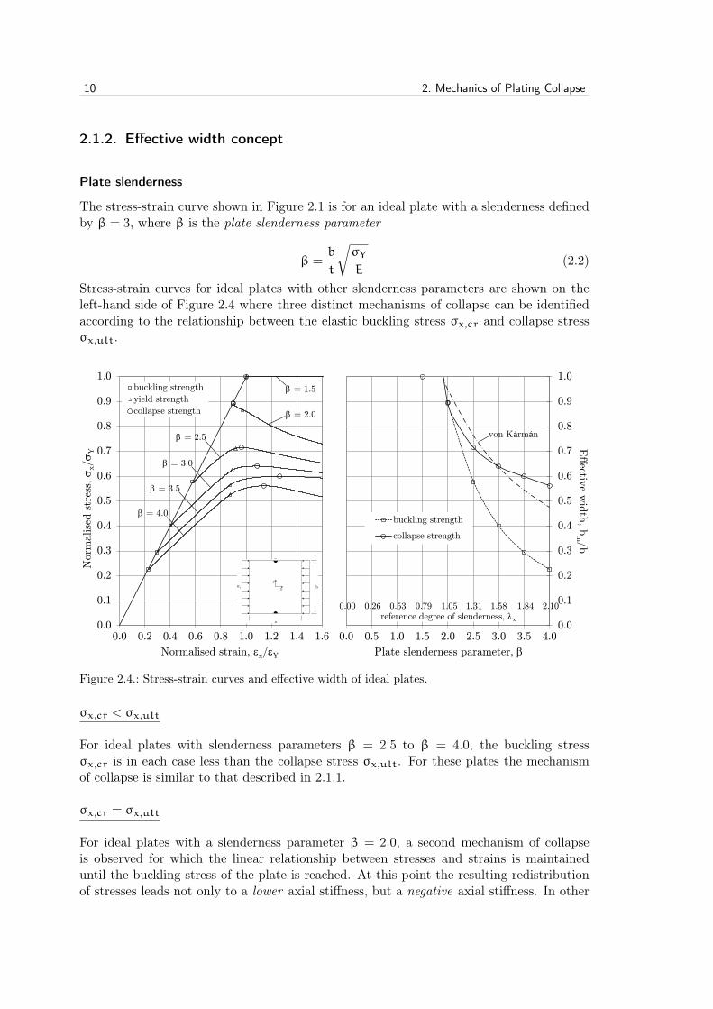
2.1.2. Effective width concept
Plate slenderness
The stress-strain curve shown in Figure 2.1 is for an ideal plate with a slenderness definedby β = 3, where β is the plate slenderness parameter
β =b
t
√σYE
(2.2)
Stress-strain curves for ideal plates with other slenderness parameters are shown on theleft-hand side of Figure 2.4 where three distinct mechanisms of collapse can be identifiedaccording to the relationship between the elastic buckling stress σx,cr and collapse stressσx,ult.
β = 1.5
β = 2.0
β = 2.5
β = 3.0
β = 3.5
β = 4.0
0.0
0.1
0.2
0.3
0.4
0.5
0.6
0.7
0.8
0.9
1.0
0.0 0.2 0.4 0.6 0.8 1.0 1.2 1.4 1.6
Nor
mal
ised
str
ess,
σx/σ
Y
Normalised strain, εx/εY
buckling strength
yield strength
collapse strength
0,32 cm 13,8 cm
13,15 cm
23,42 cm
0.00 0.26 0.53 0.79 1.05 1.31 1.58 1.84 2.10
von Kármán
0.0
0.1
0.2
0.3
0.4
0.5
0.6
0.7
0.8
0.9
1.0
0.0 0.5 1.0 1.5 2.0 2.5 3.0 3.5 4.0
Effectiv
e wid
th, b
m/b
Plate slenderness parameter, β
buckling strength
collapse strength
reference degree of slenderness, λx
0,32 cm 13,8 cm
13,15 cm
23,46 cm
a
b σx
y
x
Figure 2.4.: Stress-strain curves and effective width of ideal plates.
σx,cr < σx,ult
For ideal plates with slenderness parameters β = 2.5 to β = 4.0, the buckling stressσx,cr is in each case less than the collapse stress σx,ult. For these plates the mechanismof collapse is similar to that described in 2.1.1.
σx,cr = σx,ult
For ideal plates with a slenderness parameter β = 2.0, a second mechanism of collapseis observed for which the linear relationship between stresses and strains is maintaineduntil the buckling stress of the plate is reached. At this point the resulting redistributionof stresses leads not only to a lower axial stiffness, but a negative axial stiffness. In other

2.1. Uniaxial compression 11
words, for such plates the collapse stress σx,ult is defined by their buckling stress σx,cr,whereupon the plate begins to unload. Whether or not the yield strain of the plate isreached depends on the stiffness of the adjacent supporting structure.
σx,cr > σx,ult = σY
For ideal plates with a slenderness parameter β = 1.5, yet a third mechanism of col-lapse is seen for which the elastic buckling stress σx,cr is greater than the collapse stressσx,ult. Here the linear relationship between stresses and strains continues until the yieldstress (and yield strain) of the plate is reached, without any buckling whatsoever. Ne-glecting strain hardening effects, no further increase in stress is possible beyond this pointsuch that the collapse stress of the plate is defined by its yield stress. Because the fullcross-section of the plate is yielded at collapse, the post-collapse portion of the stress-straincurve is characterised entirely by plastic flow (i.e. an elastic-perfectly plastic stress-straincurve).
von Kármán
Similar stress-strain curves to those shown on the left-hand side of Figure 2.4 were first de-termined experimentally in the context of aeronautical research. The seminal work in thisregard was carried out in 1930 by Schuman and Back [12] in order to better understand thepost-buckling behaviour of thin plates. Simply-supported plates of four different materialswere tested to failure under uniaxial compression loads. The plates were a ∼ 600 mm inlength with widths varying between b ∼ 100 mm and b ∼ 600 mm (∆b ∼ 100 mm incre-ments) and thicknesses between t ∼ 0.38 mm and t ∼ 2.41 mm (∆t ∼ 0.38 mm increments).When plotting the maximum load (i.e. force) carried by each of the plates against theirwidths, the tests revealed that the loads generally reached a maximum for the b ∼ 200 mmor b ∼ 300 mm widths without significant increases in maximum load for larger widths(i.e. for those plates which buckled elastically prior to collapse). As noted by Schumanand Back "(i)t appears that after buckling, the wide plate acts as though it were a narrowplate of a width corresponding to that of the side portions which are taking most of theload".
Indeed, it was precisely this concept of post-buckling behaviour which led von Kár-mán [13] in 1932 to derive the first effective width expression for thin plates in compression.The sketch used in von Kármán’s paper to illustrate this concept is shown in Figure 2.5.As can be seen, it is assumed that the entire axial force P is carried uniformly by two edgestrips of width w. For simplicity, von Kármán then assumes "that the deflection is suchthat horizontal tangents at the inner edges of the two load-supporting strips are parallelto the X-direction, Fig. 2(a). Then the center of the sheet can be disregarded and the twostrips can be handled as if they were together".
Accordingly, denoting the effective width of the plating as bm = 2 · w, the critical(elastic) buckling stress of the actual plate
σx,cr = Kx ·π2 · E
12(1− ν2)
(t
b
)2
(2.3)
can be rewritten for a fictitious plate of width bm as

12 2. Mechanics of Plating Collapse
σx,cr,m = Kx ·π2 · E
12(1− ν2)
(t
bm
)2
(2.4)
where Kx is the elastic buckling factor.
Figure 2.5.: Sketch of effective width concept from von Kármán’s paper (reproduced from refer-ence [13] with permission of the American Society of Mechanical Engineers).
However, because the edges of the plate do not buckle elastically before yielding (i.e.σx,cr,m > σY), von Kármán is able to define failure of the plate as
σY = Kx ·π2 · E
12(1− ν2)
(t
bm
)2
(2.5)
or, in terms of effective width bm
bm =
√Kx ·
π2 · E12(1− ν2)
t2
σY(2.6)
which in the modern treatment of the effective width concept is normalised against theactual width of the plating b
bm
b=
√Kx ·
π2 · E12(1− ν2)
(t2
σY · b2
)=
√σx,cr
σY(2.7)
2.1. Uniaxial compression 13
In present-day nomenclature, the inverse ratio of the term on right-hand side of Equation(2.7) is known as the reference degree of slenderness, λx:
λx =
√σYσx,cr
=
√σY
Kx · σe(2.8)
Here the critical buckling stress σx,cr is alternatively expressed as the product Kx · σe,where σe is a reference stress equal to the Euler buckling stress for a wide column or platewith an infinite aspect ratio (i.e. α =∞)
σe =π2 · E
12(1− ν2)
(t
b
)2
(2.9)
Accordingly, the plate slenderness parameter β is related to the reference degree of slen-derness λx as
λx = β
√12(1− ν2)
π2 · Kx(2.10)
and related to the effective width as
bm
b=
1λx
=1β
√π2 · Kx
12(1− ν2)' 1.9β
(2.11)
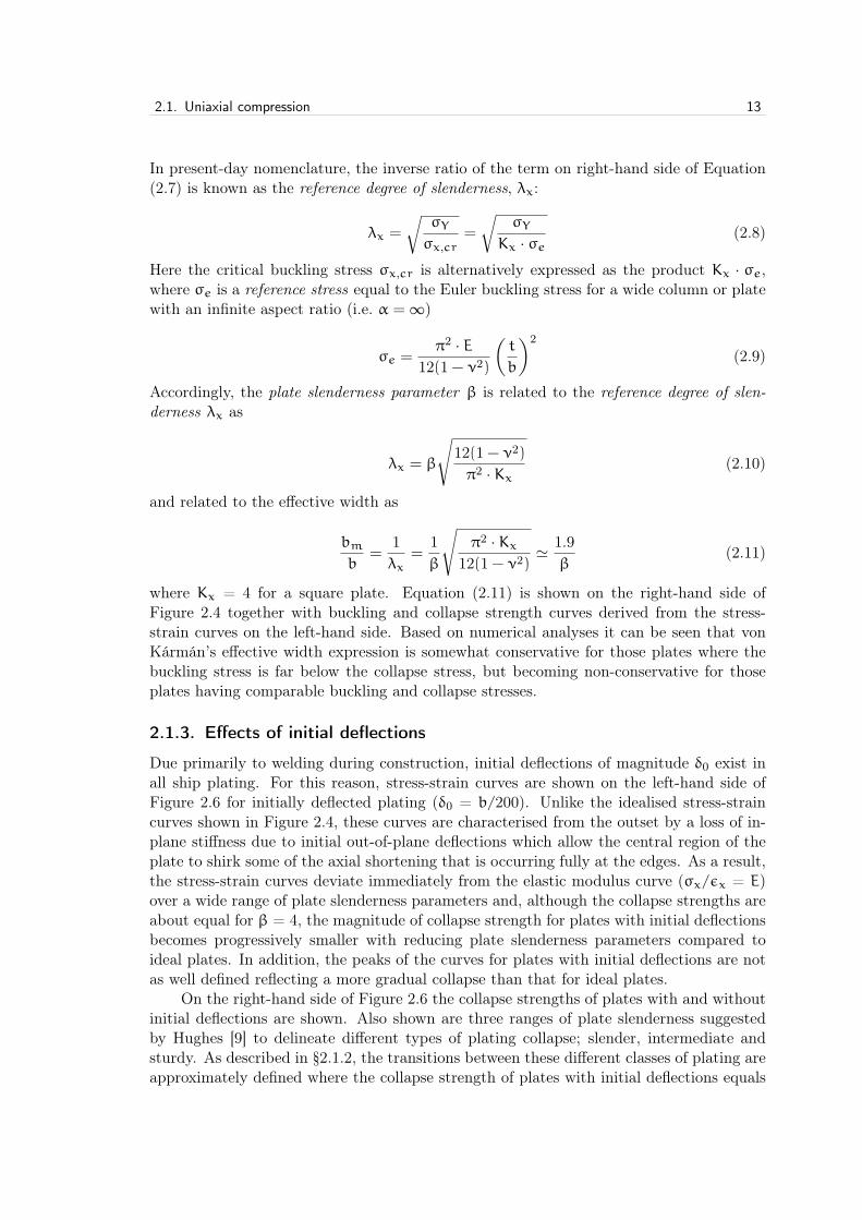
where Kx = 4 for a square plate. Equation (2.11) is shown on the right-hand side ofFigure 2.4 together with buckling and collapse strength curves derived from the stress-strain curves on the left-hand side. Based on numerical analyses it can be seen that vonKármán’s effective width expression is somewhat conservative for those plates where thebuckling stress is far below the collapse stress, but becoming non-conservative for thoseplates having comparable buckling and collapse stresses.
2.1.3. Effects of initial deflections
Due primarily to welding during construction, initial deflections of magnitude δ0 exist inall ship plating. For this reason, stress-strain curves are shown on the left-hand side ofFigure 2.6 for initially deflected plating (δ0 = b/200). Unlike the idealised stress-straincurves shown in Figure 2.4, these curves are characterised from the outset by a loss of in-plane stiffness due to initial out-of-plane deflections which allow the central region of theplate to shirk some of the axial shortening that is occurring fully at the edges. As a result,the stress-strain curves deviate immediately from the elastic modulus curve (σx/εx = E)over a wide range of plate slenderness parameters and, although the collapse strengths areabout equal for β = 4, the magnitude of collapse strength for plates with initial deflectionsbecomes progressively smaller with reducing plate slenderness parameters compared toideal plates. In addition, the peaks of the curves for plates with initial deflections are notas well defined reflecting a more gradual collapse than that for ideal plates.
On the right-hand side of Figure 2.6 the collapse strengths of plates with and withoutinitial deflections are shown. Also shown are three ranges of plate slenderness suggestedby Hughes [9] to delineate different types of plating collapse; slender, intermediate andsturdy. As described in §2.1.2, the transitions between these different classes of plating areapproximately defined where the collapse strength of plates with initial deflections equals

14 2. Mechanics of Plating Collapse
β = 1.0
β = 1.5
β = 2.0
β = 2.5
β = 3.0
β = 3.5
Es
β = 4.0
0.0
0.1
0.2
0.3
0.4
0.5
0.6
0.7
0.8
0.9
1.0
0.0 0.2 0.4 0.6 0.8 1.0 1.2 1.4 1.6
Nor
mal
ised
str
ess,
σx/σ
Y
Normalised strain, εx/εY
yield strength
collapse strength
13,15 cm
0,32 cm
23,42 cm
13,8 cm
0.00 0.26 0.53 0.79 1.05 1.31 1.58 1.84 2.10
0.0
0.1
0.2
0.3
0.4
0.5
0.6
0.7
0.8
0.9
1.0
0.0 0.5 1.0 1.5 2.0 2.5 3.0 3.5 4.0
Effectiv
e wid
th, b
m/b
Plate slenderness parameter, β
buckling strength
collapse strength
collapse strength (ideal plates)
sturdy slender intermediate
reference degree of slenderness, λx
13,15 cm
13,8 cm 0,32 cm
23,46 cm
secant modulus, Es/E
a
b σx
y
x
Figure 2.6.: Stress-strain curves and effective width of plates with initial deflections.
the yield strength (i.e. sturdy to intermediate plating) and where the collapse strengthequals the elastic buckling strength (i.e. intermediate to slender plating).
Sturdy plating
For sturdy plating (β 6 1.0) the elastic buckling stress is so large that the magnification ofinitial deflections is minimal. Accordingly, the stress-strain curves of sturdy plates closelyfollow the elastic modulus curve and then the yield limit defined by σY , i.e. elastic-perfectlyplastic behaviour. This behaviour is evident in the distributions of principal stresses atcollapse as shown in Figure 2.7(a) for plating with a slenderness parameter β = 1.0. Thenegligible presence of transverse σy stresses is due to the (near) absence of out-of-planedeflections. Accordingly, as noted in §2.1.1, sturdy plates (i.e. even those with initial de-flections) also exhibit the linear elastic behaviour of pre-buckled, ideal plates and do sountil the yield stress is reached.
Slender plating
Conversely, slender plating (2.3 < β) buckles elastically before either the yield or collapsestresses are reached. However, since the plate continues to support the load after elasticbuckling, this is in general acceptable provided serviceability limit state (SLS) and fatiguelimit state (FLS) criteria are satisfied (limit states are discussed in §5.1). The elastic buck-ling behaviour which precedes collapse is clearly evident in the distributions of principalstresses shown in Figures 2.7(c) and 2.7(d) for plating with slenderness parameters β = 3.0and β = 4.0, respectively. These distributions are characterised by a transfer of longitudi-nal load to the edges of the plate and by significant transverse stresses due to out-of-planedeflections.

2.1. Uniaxial compression 151
X
Y
Z
run id 9910
AUG 20 201418:19:58
PLOT NO. 3
VECTOR
STEP=1SUB =141TIME=.920212SMIDDLE
PRIN1PRIN2PRIN3
(a) β = 1.0
1
X
Y
Z
run id 9920
AUG 20 201418:14:58
PLOT NO. 2
VECTOR
STEP=1SUB =130TIME=.628524SMIDDLE
PRIN1PRIN2PRIN3
(b) β = 2.0
1
X
Y
Z
run id 9930
AUG 20 201418:07:08
PLOT NO. 1
VECTOR
STEP=1SUB =128TIME=.638516SMIDDLE
PRIN1PRIN2PRIN3
(c) β = 3.0
1
X
Y
Z
run id 9940
AUG 20 201417:37:49
PLOT NO. 4
VECTOR
STEP=1SUB =83TIME=.5256SMIDDLE
PRIN1PRIN2PRIN3
(d) β = 4.0
Figure 0.1: ——-CROP!——–CROP!——–CROP!——–CROP!——–CROP!———CROP!——-
1
Figure 2.7.: Principle stresses at collapse in middle plane of plates with initial deflections.
Intermediate plating
Between these two extremes, intermediate plating (1.0 < β 6 2.3) is typical of that usedin longitudinal strength members and has a collapse stress below both the elastic bucklingand yield stresses. Looking at the collapse strength data points on the right-hand side ofFigure 2.6, an inflection point can be discerned within the range of slenderness parametersfor intermediate plating which marks the steepest portion of the effective width curve,thereby indicating that the collapse strength of intermediate plating is the most sensitiveto slenderness under a uniaxial load. As can be seen in Figure 2.7(b), the distribution

16 2. Mechanics of Plating Collapse
of principal stresses displays moderate or "intermediate" levels of both load shedding andtransverse stresses.
Plate secant modulus
As illustrated on the left-hand side of Figure 2.6 (for the stress-strain curve associatedwith plate slenderness β = 4), a secant intersecting a stress-strain curve at its origin anda point associated with collapse is referred to as the plate secant stiffness or plate secantmodulus Es. On the left-hand side of Figure 2.6, the yield strain εx/εY = 1.0 has beenchosen as the point associated with collapse. Chatterjee and Dowling [14] showed that ifthe plate secant modulus Es is normalised against the plate elastic modulus E, the result-ing quantity Es/E is approximately equal to the normalised ultimate stress σx,ult/σY lessthe magnitude of residual (compressive) stress σx,rc/σY [9]. For the stress-strain curvesshown on the left-hand side of Figure 2.6, the residual stresses are zero. Accordingly, onthe right-hand side of Figure 2.6 the secant modulus curve defined by Es/E is shown toclosely approximate the ultimate stress curve defined by σx,ult/σY7. In general, Chatter-jee and Dowling suggest the secant be drawn to the peak of the load-shortening curve ora point on the curve corresponding to an arbitrary strain limit in case there is no clearpeak or in case it occurs at a level of strain far beyond yield (e.g. the stress-strain curvefor plate slenderness β = 3.5 shown on the left-hand side of Figure 2.6). On the basis ofthis procedure, Chatterjee and Dowling have provided curves of secant modulus for plateswith and without residual stresses [14].
Winter
Contrary to the foregoing approach, steel-plated structures are generally designed usingeffective width formulae based on experimental and numerical results. On the left-handside of Figure 2.8, von Kármán’s effective width expression
bm = 1.9
√E
σY· t (2.12)
is plotted as bm/b together with the collapse strength of plates with and without initialdeflections. Unsurprisingly, the detrimental effect of initial deflections on the capacity ofplates reveals von Kármán’s equation to be even more non-conservative than shown in Fig-ure 2.4 for ideal plates. Nevertheless, this does not diminish von Kármán’s effective widthconcept. As noted by Sechler and Donnell in the Appendix to von Kármán’s derivation ofeffective width, the purpose of von Kármán’s derivation was to prove that the capacity ofthe plate was proportional to the square roots of E and σY as well as the square of platethickness
Px,ult = C√E · σY · t2 (2.13)
7 A useful way to conceptualise this approach is to consider the buckled plate with an elastic modulus Ereplaced by a plane (unbuckled) plate with a reduced elastic modulus Es. The collapse strength of theplate is then defined by σx,ult = σY · Es/E.
2.1. Uniaxial compression 17
where Px,ult = bm · t ·σY and the proportionality constant C accounts for existing bound-ary conditions.
Accordingly, von Kármán’s effective width equation can be rewritten in a more generalform as
bm = C
√E
σY· t (2.14)
According to Sechler and Donnell, "(i)n making his analysis, Dr. von Kármán, forsimplicity, assumed somewhat artificial conditions, and hence it is not to be expectedthat the value of C given above is exactly correct even for the case of simply supportedsides". In fact, Sechler and Donnell show that for a "perhaps more likely assumption"about the deflected shape (i.e. "Fig. 2(b)" shown in Figure 2.5), the value of C is foundto be approximately 1.24. Indeed, Sechler [15] went on to conduct a number tests on thinplates of various metals8 where he found that the value of C = 1.9 is only approachedfor extremely wide and thin plates, i.e. slender plates. Moreover, Sechler showed that theexperimentally determined values of C were not constant, but rather dependent on theparameter
√E/σY · (t/b), i.e. 1/β.
von Kármán
Winter
0.00 0.26 0.53 0.79 1.05 1.31 1.58 1.84 2.10
0.0
0.1
0.2
0.3
0.4
0.5
0.6
0.7
0.8
0.9
1.0
0.0 0.5 1.0 1.5 2.0 2.5 3.0 3.5 4.0
Effec
tive
wid
th, b
m/b
Plate slenderness parameter, β
collapse strength
collapse strength (ideal plates)
reference degree of slenderness, λx
13,8 cm 0,32 cm
23,42 cm
13,15 cm
Figure 2.8.: Von Kármán and Winter curves.
0.00 0.26 0.53 0.79 1.05 1.31 1.58 1.84 2.10
Johnson-Ostenfeld
Euler Hyperbola
Frankland
Winter
DIN 18800
0.0
0.1
0.2
0.3
0.4
0.5
0.6
0.7
0.8
0.9
1.0
0.0 0.5 1.0 1.5 2.0 2.5 3.0 3.5 4.0
Plate red
uction
factor, κ
x
Plate slenderness parameter, β
collapse strength
buckling strength
reference degree of slenderness, λx
0,32 cm 13,8 cm
13,15 cm
23,46 cm
Figure 2.9.: Plate reduction curves.
Building on the work of Sechler, Winter [17] performed additional tests on 25 U-beamsto see if von Kármán’s effective width concept for individual plates could be applied equallyto thin compression plates representing component parts of structural members. Winterconcluded that the agreement between the results of the two investigations were "remark-ably close" and therefore fit a straight line through the values of C for both sets of tests
8 Results of these tests are also reported by Timoshenko [16].

18 2. Mechanics of Plating Collapse
C = 1.9− 1.09
√E
σY
(t
b
)(2.15)
in which the intercept of the ordinate is equal to von Kármán’s initial value of C = 1.9.Substituting this equation for C in Equation (2.14), Winter obtained the following equationfor effective width
bm = 1.9
√E
σY· t
1− 0.574(t
b
)√E
σY
(2.16)
where the second term within the square brackets is used to modify von Kármán’s originalequation. Winter’s equation was initially used in the first edition (1946) of the specificationfor the design of light gage steel structural members published by the American Iron andSteel Institute (AISI) [18], but has since been used widely throughout civil engineering,albeit with modifications over the years to the constant used in the expression for correctingvon Kármán’s original equation. Today it is most commonly expressed in terms of thereference degree of slenderness as
bm
b=
1λx
−0.22λ2x
(2.17)
and is used to calculate the effective width of compressed plates in Eurocode 3(EN 1993-1-5) [19]. Accordingly, Winter’s equation is also plotted on the left-hand side ofFigure 2.8. As expected, Winter’s curve lies below that of von Kármán’s original curve andis more representative of the collapse strength of intermediate and sturdy plating (β 6 2.3).
2.1.4. Effective width formulae used in shipbuilding
Plate reduction factors
In the particular case of the classification of ships, three effective width formulae havebecome prevalent, where the ratio of the collapse stress σx,ult and the material yield stressσY of the plate is alternatively referred to as the plate reduction factor κ. In general thereis a plate reduction factor corresponding to each stress component,
κx = σx,ult/σY κy = σy,ult/σY κτ = τxy,ult ·√3/σY
Not only do plate reduction factors represent the characteristic strength of plates undersingle stress components, but (as will be seen) they are as well used as reference stressesin interaction equations which define the capacity of plates under multiple stress compo-nents. In addition, plate reduction factors are used to define the effective width of platingin proofs of stiffener buckling strength9.
9 Generally, the extent of attached plating used in proofs of stiffener buckling strength is the minimumof the effective width due to plate buckling and the effective breadth due to shear lag effects associatedwith bending of the plate-stiffener combination (as discussed in §5.1.2).

2.1. Uniaxial compression 19
1. Johnson-Ostenfeld
The Johnson-Ostenfeld correction is used to adjust the (elastic) buckling strength curvesshown on the right-hand sides of Figures 2.4 and 2.6 to account for plasticity, i.e. mate-rial non-linearity, not geometric non-linearity. It was developed in the context of columnbuckling, but has also been used for plating since 1989 in the IACS Longitudinal StrengthStandard UR S11 [20]. In terms of the former, material properties over the cross-sectionof a column are rarely uniform due to the presence of residual stresses in rolled sections.Those areas under compressive residual stresses σx,rc will begin to yield when the (com-pressive) axial stress reaches σx = σY - σx,rc, while those areas under tensile residualstresses σx,rt will not yield until the (compressive) axial stress reaches σx = σY + σx,rt.However, by assuming an elastic-perfectly plastic material, the reduction in the averagemodulus of elasticity over the cross-section, referred to as the structural tangent modulusEts, becomes linearly proportional to the extent of yielding. On the basis of this assump-tion, the Ostenfeld-Bleich [21] parabola describes the relationship between the axial stressσx and the structural tangent modulus Ets
Ets = Eσx (σY − σx)
σspl(σY − σspl
) (2.18)
where σspl = σY - σx,rc is the structural proportional limit which determines where thematerial stress-strain curve departs from the linear stress-strain relationship defined by theelastic modulus E, i.e. Ets = E when σx 6 σspl [9].
Substituting Ets from Equation (2.18) for E in Equation (2.3) yields the followingcritical buckling stress corrected for plasticity
σcr,p = Kx ·π2 · E
12(1− ν2)
(t
b
)2 σcr,p(σY − σcr,p
)σspl
(σY − σspl
) (2.19)
which, when taken as the ultimate stress of the plate, becomes
σx,ult =σYλ2x
σx,ult(σY − σx,ult
)σspl
(σY − σspl
) (2.20)
If residual compressive stresses σx,rc are assumed to be 50% of yield stress thenσspl = ½·σY such that
κx =σx,ult
σY=
1−
λ2x
4λx <
√2
1λ2x
λx >√2
(2.21)
where κx = 1/λ2x is commonly referred to as the Euler hyperbola and defines collapse as
the critical buckling stress σx,cr (see Equation (2.8)). Equation (2.21) is plotted in Figure2.9 where the transition from elastic to inelastic buckling occurs at κx = 0.5 (i.e. λx =
√2)
as defined by the (assumed) structural proportional limit σspl = ½·σY . Not surprisingly,the portion of the reduction curve defined by the Euler hyperbola is rather conservativesince it does not take the post-buckling strength of the plate into account. The portionof the reduction curve defined by the Johnson-Ostenfeld correction (i.e. κx = 1 - λ2
x/4) isalso conservative, but generally within 5% of numerical analyses.

20 2. Mechanics of Plating Collapse
2. Frankland
In parallel to the previously referenced experiments by the aircraft industry, similar investi-gations were undertaken at the U.S. Navy Yard in Washington D.C. Since late 1932 the U.S.Experimental Model Basin conducted strength tests on longitudinally-stiffened plating un-der in-plane compressive loads (here the unloaded edges of the plate were simply-supportedand free to pull in). The results of these tests were documented in a series of confidentialreports. However, in a published review of the experimental work written by Frankland in1940 [22], a figure summarising the buckling and ultimate strength of plates in terms of κxand β is reproduced from a report by Vasta (formerly of the Experimental Model Basinstaff), together with a fitted curve of "reasonable accuracy". This curve has the equation
κx =2.25β
−1.25β2 (2.22)
and is included in Figure 2.9. In terms of λx, the equation is
κx =1.18λx
−0.35λ2x
(2.23)
However, Frankland points out that there is a considerable amount of scatter in the dataat the high stress end of the curve due to inaccuracies in estimating the compressive yieldstrength of the plates from tensile tests. More importantly, Frankland acknowledges theabsence of in-plane restraint, without which the depths of plate buckles increase such thatthe effective width of plates decrease. However, Frankland concludes that this effect is onlyappreciable for plates with a slenderness β > 2.5.
Not surprisingly, the U.S. Navy Yard’s equation has found its way into commercialshipbuilding as well. In particular, it is used in the hull girder ultimate strength require-ments of the CSR BC & OT [23]. Furthermore, it is also used to determine the effectivewidth of the compression flange of corrugations in the IACS unified requirements for theevaluation of corrugated transverse watertight bulkheads (UR S18 [24] and UR S19 [25]).
3. DIN 18800
Using an approach similar to that of the U.S. Navy Yard, ultimate plate strength formula-tions were also developed in the late 1980’s for inclusion in the German construction stan-dard DIN 18800 [26]. The standard was prepared jointly by the Normenausschuß Bauwesen(Building and Civil Engineering Standards Committee) and the Deutscher Ausschuß fürStahlbau (German Committee for Structural Steelwork). In Part 3 of DIN 18800, equa-tions for reduction factors are provided for buckling cases classified according to boundaryconditions and stress types. For a simply-supported plate under longitudinal compres-sion, the equation for κx = σx,ult/σY was determined on the basis of 705 experimentallyand numerically derived buckling strength results. However, following critical evaluation ofthese results, 213 were considered unreliable and discarded (e.g. due to errors/uncertaintiesconcerning boundary conditions, material properties, loading rate etc.) [27]. The resultingequation for the reduction factor κx is equal to Winter’s Equation (2.17) multiplied bya factor c = 1.25 − 0.12 · ψx 6 1.25, where ψx = σx,max/σx,min is the ratio of edgestresses. Since ψx = 1.0 for the case of a uniform in-plane load (i.e. no in-plane bending),the resulting equation for the plate reduction factor is

2.2. Biaxial loads 21
κx = 1.13(
1λx
−0.22λ2x
)=
1.13λx
−0.25λ2x
(2.24)
This equation is also plotted in Figure 2.9. In terms of β, the equation is
κx =2.15β
−0.9β2 (2.25)
which is not too dissimilar from an equation proposed by Faulkner [28] [29] in 1964 on thebasis of his own analysis of the tests carried out at the U.S. Navy Yard
κx =2β−
1β2 (2.26)
The DIN 18800 formulations were first implemented in the buckling strength require-ments of the German classification society Germanischer Lloyd (GL) in 1997 [30], buthave since been implemented in the buckling strength requirements of the IACS CommonStructural Rules for Bulk Carriers (CSR BC) [31], the IACS Common Structural Rules forDouble Hull Oil Tankers (CSR OT) [32], CSR BC & OT [23], UR S11A [8] as well as thenew DNVGL Rules for Classification [33] which are applicable to all ship types.
2.2. Biaxial loads
In general ship plating is subjected to combined in-plane stresses (as well as lateral pres-sure). Usually one of the in-plane stress components governs the collapse of the plating(primary stress) with another of the in-plane stress components affecting this collapse tosome discernible extent (secondary stress). A third in-plane stress component may alsoexist (tertiary stress), but often has only a negligible effect on plating collapse. In thissection the collapse of square plates under pure biaxial in-plane stresses is examined. Sucha stress state is approached, for instance, in the shell and inner bottom plating of doublebottom structures due to hull girder bending, transverse compression and double bottombending10. Of sufficient magnitude, either of the axial stresses in isolation would lead tocollapse of square plating as described in the preceding section. With the presence of asecondary stress, however, there is an extensive interaction which affects the distributionof stresses and strains within the plate and thereby its collapse strength.
2.2.1. Ideal plates - compressive secondary stress
Loading sequence
In Figure 2.1 a stress-strain curve was shown for a square plate of slenderness β = 3.0. Theplate was without any initial deflections and subjected to a uniaxial load. In Figure 2.10two stress-strain curves are shown for the same (ideal) plate under a biaxial load σy = σx.For one curve σy and σx are applied simultaneously. This is referred to as proportionalloading. For the other curve σy is applied first, followed by σx11. This is referred to as
10 The aspect ratio of plating in the shell and inner bottom plating of double bottom structures is typicallybetween α = 3 and α = 5, although square plates are sometimes found outside the parallel midbody.The effect of plate aspect ratio is examined in §2.4.
11 In case of σy = σx the stress-strain curve for a square plate remains unchanged regardless of whichstress is applied first.

22 2. Mechanics of Plating Collapse
sequential loading. In the latter case, the negative strain in the x-direction following theapplication of σy is evidence of the Poisson effect
εx
εY= −ν · σy,ult
σY= −0.3 · 0.38 = −0.11 (2.27)
where ν = 0.3 is Poisson’s ratio and σy,ult/σY = 0.38 is the (normalised) ultimate stress inthe y-direction for the biaxial compression case σy = σx. With the subsequent applicationof σx, the slope of the stress-strain curve is lower, but the load is acting over a greaterrange of strain. Accordingly, in the present case of a square plate, the two stress-straincurves coincide at the collapse strength. As shown by Valsgård [34] for plates with anaspect ratio α = 3, proportional loading leads to lower plate capacity for plates with anaspect ratio greater than α = 1. Accordingly, following this subsection, only the criticalcase of proportional loading will be considered.
σy = 0
A (Pre-buckling)
Buckling strength
B (Post-buckling)
Yield strength
C (Post-yield)
Collapse strength
D (Post-collapse)
0.0
0.1
0.2
0.3
0.4
0.5
0.6
0.7
0.8
-0.2 0.0 0.2 0.4 0.6 0.8 1.0 1.2 1.4 1.6 1.8 2.0 2.2 2.4 2.6 2.8 3.0
Nor
mal
ised
str
ess,
σx/σ
Y
Normalised strain, εx/εY
σy = σx (sequential loading)
σy = σx (proportional loading)
a
b σx
σy
y
x
1
XYZ
run id 99304
-2350
235500
MAR 25 201518:01:37
PLOT NO. 1
Figure 2.10.: Stress-strain curve of ideal plate under biaxial compression (σy = σx, β = 3).
Pre-buckling
Due to symmetry, the stress-strain curve σy-εy under proportional loading has the sameshape and height as the σx-εx curve. With the initial application of the biaxial load,stresses and strains in each direction are uniform throughout the plate. However, unlikethe uniaxial load case, the linear relationship between them is no longer defined solely bythe modulus of elasticity, E = σx/εx. Rather, due to the presence of the secondary stressσy, strain in the x-direction is reduced according to Poisson’s equation
εx =σx
E− ν · σy
E(2.28)
2.2. Biaxial loads 23
When σy = σx (as it does in Figure 2.10), this equation can be rewritten as
εx =σx
E− ν · σx
E= (1− ν) · σx
E(2.29)
Rearranging in terms of σx/εx
σx
εx=
E
(1− ν)(2.30)
Accordingly, when ν = 0.3, the pre-buckling behaviour of the plate is such that its effectivemodulus of elasticity is equal to E ′ ' 1.43 · E, as reflected in the pre-buckling portion ofthe curve in Figure 2.10. Again, this linear elastic behaviour applies only to ideal plates orto plates with large elastic buckling stresses. For the load corresponding to point A on thecurve (σx/σY = 0.1), the principal stresses in the middle plane of the plate are plotted inFigure 2.11(a). As in the uniaxial load case, no Poisson effects are evident in these stressessince the edges of the plate are able to move freely in-plane.
Buckling strength
As the biaxial load σy = σx is increased, the linear relationship between stress and straincontinues until the buckling strength of the plate is reached. Again, with the slightestof perturbations, the resulting out-of-plane deflection in the central region of the platingleads to a redistribution of stresses towards its edges and a lower axial stiffness (in boththe x- and y-directions). For a square plate, the 1st eigenmode of the buckled plate undera biaxial load is similar to that under a uniaxial load, although the magnitude of its 1st
eigenvalue is lower. In fact, for the biaxial load σy = σx, the magnitude of the criticalbuckling stress is exactly half of the critical buckling stress σx,cr in the uniaxial load case(compare the buckling strength in Figure 2.10 to that in Figure 2.1). This is because theelastic strength interaction equation for a square plate has the linear form
σx
σx,cr+
σy
σx,cr= 1 (2.31)
when the stresses in both x- and y-directions are compressive.
Post-buckling
Accordingly, the post-buckling portion of the stress-strain curve is again characterised bya reduced slope (E ′ ' 0.36 · E) which is considerably less compared to the post-bucklingportion of the curve in the uniaxial load case. In Figure 2.11(b) the principal stressesassociated with point B (σx/σY = 0.3) are shown. Here the redistribution of appliedstresses towards the edges is clearly evident. However, unlike the uniaxial load case, theredistribution of stresses occurs equally in both the x- and y-directions due to the equalmagnitudes of σx and σy. While the stresses parallel and adjacent to the edges of the plateare dominated by the applied compressive stresses, the reduced magnitude of stresses in

24 2. Mechanics of Plating Collapse1
X
Y
Z
run id 99304
MAR 25 201517:21:51
PLOT NO. 5
VECTOR
STEP=1SUB =1TIME=.01SMIDDLE
PRIN1PRIN2PRIN3
(a) Pre-buckling (Point A)
1
X
Y
Z
run id 99304
MAR 25 201516:18:11
PLOT NO. 2
VECTOR
STEP=1SUB =1229TIME=.52231SMIDDLE
PRIN1PRIN2PRIN3
(b) Post-buckling (Point B)
1
X
Y
Z
run id 99304
MAR 25 201517:11:11
PLOT NO. 1
VECTOR
STEP=1SUB =1805TIME=.651108SMIDDLE
PRIN1PRIN2PRIN3
(c) Post-yield (Point C)
1
X
Y
Z
run id 99304
MAR 25 201517:14:23
PLOT NO. 2
VECTOR
STEP=1SUB =3052TIME=.562818SMIDDLE
PRIN1PRIN2PRIN3
(d) Post-collapse (Point D)
Figure 0.1: ——-CROP!——–CROP!——–CROP!——–CROP!——–CROP!———CROP!——-
1
Figure 2.11.: Principle stresses in middle plane of ideal plate (σy = σx, β = 3).
the middle of the buckled plate is evidence of tensile stresses caused by the out-of-planedeflections. Accordingly, the magnitude of compressive stresses perpendicular and adjacentto the edges of the plate decrease towards mid-length and mid-breadth.
Yield strength
As the biaxial load is increased further, greater out-of-plane deflections again lead to addi-tional load shedding which results in a further increase in the magnitude of stresses alongthe edges. In the uniaxial load case, the resulting combination of compressive stresses (dueto the applied load) and perpendicular tensile stresses (due to out-of-plane deflections)
2.2. Biaxial loads 25
leads to initial yielding in the middle plane at the mid-length edges of the plate (see cornerinset in Figure 2.1). However, due to the presence of the secondary compressive stress,the tensile stresses at the mid-length edges of the biaxially loaded plate are considerablysmaller. Accordingly, initial yielding under the biaxial load σy = σx does not occur at themid-length edges of the plate, but instead in the corners of the plate where the (magnified)applied stresses σx and σy coalesce (see corner inset in Figure 2.10). In other words, the(compressive) axial and (tensile) transverse stresses at the mid-length edges of the plateare still "working together" to deform the plate material, but the contribution of the tensilestresses is relatively small such that compression-tension yielding at the mid-length edgesof the plate is preceded by compression-compression yielding in the corners of the plate.With this sort of mechanism, yielding in the middle plane initiates at a considerably lowerlevel of axial strain compared to the uniaxial load case. Nevertheless, as in the case of auniaxial load, yielding in the middle plane of the plate is indicative of through-thicknessplasticity and is a precursor to collapse.
Post-yield
With further increases in the biaxial load σy = σx, plastic flow begins to gradually spreadfrom the corners of the plate leading to progressive losses in stiffness. Accordingly, the post-yield portion of the stress-strain curve is characterised by a gradually decreasing slope. InFigure 2.11(c) the principal stresses associated with point C (εx/εY ' 0.75) in the post-yield response are shown. At this point it can be seen that the central portion of the plateis approaching a (relatively) stress free state where the compressive stresses due to theapplied load and tensile stresses due to out-of-plane deflections are almost equal. Further-more, the load shedding caused by out-of-plane deflections leads to uniaxial compressivestresses along the sides of the plate with biaxial compressive stress states remaining onlyin the corners.
Collapse strength
As noted previously, once the slope of the stress-strain curve reaches zero the collapsestrength of the plate has been reached. In Figure 2.10 the normalised collapse stress isseen to be approximately σx,ult/σY = 0.38 which represents a 1.7% increase in stresscompared to initial yield. Compared to the uniaxial load case (σx,ult/σY = 0.64), thiscollapse stress represents a 41% reduction in σx,ult. Since σy,ult = σx,ult for the biaxialload case σy = σx, this reduction represents the maximum decrease of the primary col-lapse stress due to the presence of a secondary stress (i.e. for β = 3). As will be shown in§2.2.4, the maximum reduction in the primary collapse stress due to the presence of a sec-ondary stress is 50% for a very slender, square plate. In terms of displacement, the collapsestrain has an approximate magnitude of εx,ult/εY = 0.81 which is an additional strain of∆εx ' 0.12 · εY compared to initial yield. Furthermore, compared to the collapse strainunder a uniaxial load (εx,ult/εY = 1.09), the collapse under the biaxial load σy = σxoccurs at a significantly smaller strain (∆εx ' −0.28 · εY). As mentioned previously, theultimate strain value may be of particular importance in the ultimate strength analysis ofhull girders since the applied loads are strain-based. For instance, when calculating theultimate capacity of hull girders according to IACS requirements (e.g. CSR BC & OT),

26 2. Mechanics of Plating Collapse
the stress-strain curves of all elements are assumed to reach ultimate capacity at a strainof εx,ult/εY = 1.0. Accordingly, for plate elements this assumption may be either conser-vative or non-conservative depending on the stress state.
Post-collapse
Following collapse the unloading portion of the stress-strain curve is quite similar to thatfor a uniaxial load. The effects of further post-collapse straining are shown in Figure2.11(d) for the load associated with point D of the stress-strain curve (εx/εY = 2.0). Herethe development of the stress state in the pre-collapse portion of the stress-strain curve, i.e.negligible stresses in the central portion of the plate, uniaxial compressive stresses along thesides of the plate and biaxial compressive stresses in the corners, is further intensified. Thisleads to fully plastified material in the corners of the plate which facilitates its transitioninto a developable surface. A plot of this plastic mechanism is shown in Figure 2.10 forεx/εY = εy/εY = 3.0, where a gradient exists from the yield stresses in the plastifiedcorners to near zero stresses in the middle of the plate.
2.2.2. Ideal plates - tensile secondary stress
Eigenmodes
Before examining the collapse of an (ideal) square plate under a compressive-tensile biaxialload, it is useful to understand something about the elastic buckling of square plates. InFigure 2.12 the elastic buckling interaction curve for a square plate (β = 3) is shown basedon the following equation [9, 35]
m2
a2 σx +n2
b2 σy −π2 ·Dt·(m2
a2 +n2
b2
)2
= 0 (2.32)
where m and n are the buckling half-wave numbers in the x- and y-directions, respectively,and D is the flexural rigidity of the plate
D =E · t3
12 · (1− ν2)(2.33)
The elastic buckling interaction curve shows the combinations of σx and σy underwhich an ideal plate buckles elastically. When σx and σy are both compressive (i.e. Quad-rant 1), the plate buckles into a mode characterised by a single half-wave in each direction.However, when either σx or σy is tensile, the plate may buckle into a mode characterisedby a single half-wave in the direction of the tensile stress and two half-waves in the direc-tion of the compressive stress. This transition in mode shape occurs at the discontinuitiesin the elastic buckling interaction curve (i.e. in Quadrants 2 and 4). Also shown in Figure2.12 is the von Mises ellipse. For the combinations of σx and σy which lie on this ellipse,a plane plate yields according to the von Mises failure criterion provided it does not firstbuckle elastically. Accordingly, for the stress ratio σy/σx = −1/4, the plate buckles atpoint A into an eigenmode characterised by a single half-wave in each direction. However,for the stress ratio σy/σx = −1/2, the plate buckles at point B into an eigenmode whichis characterised by two half-waves in the (compressive) x-direction. This mode shape isshown on the right hand side of Figure 2.12 together with the eigenmode of the plate at

2.2. Biaxial loads 27
Quadrant 1 Quadrant 2
von Mises ellipse
Quadrant 3 Quadrant 4
C
B
A
elastic buckling interaction curve
B'
-1.2
-0.8
-0.4
0.0
0.4
0.8
1.2
-1.2 -0.8 -0.4 0.0 0.4 0.8 1.2
Norm
alise
d s
tres
s, σ
y/σ Y
Normalised stress, σx/σY
1
XYZ
run id 993023599
APR 5 201522:44:13
PLOT NO. 1
1
XYZ
run id 993023599
APR 5 201522:52:14
PLOT NO. 7
Eigenmode at points B and C
Eigenmode at points A and B‘
Eigenmode at points B and C
Eigenmode at points A and B‘
Figure 2.12.: Elastic buckling interaction curve and eigenmodes of ideal square plate.
point B’. This latter eigenmode is a more likely shape for an initially deflected plate, butthe biaxial stress combination at which it occurs for an ideal plate (assuming that theeigenmode at point B fails to develop) lies outside the von Mises ellipse such that the platewould fail in yielding before the stresses required for this eigenmode could develop. For thestress ratio σy/σx = −1, the eigenmode of the plate is also characterised by two half-wavesin the (compressive) x-direction (point C). However, as can be seen, the plate would alsofail in yielding before reaching the stresses required for this eigenmode to develop.
Loading sequence
On the basis of the foregoing, the stress-strain curve shown in Figure 2.13 is for an idealsquare plate (β = 3.0) under proportional loading with a secondary stress σy = −σx/4.A second curve for sequential loading is shown for comparison where σy is again appliedfirst, followed by σx. Here the positive strain in the x-direction following the applicationof σy,ult is again evidence of the Poisson effect
εx
εY= −ν · σy,ult
σY= ν · σx
4 · σY= 0.3 · 0.7
4= 0.0525 (2.34)
In this case, the resulting initial strain is compensated by a greater slope in the stress-straincurve with the subsequent application of σx. Accordingly, the two stress-strain curves co-incide at the yield strength with the post-yield portion of the curve similar to that forproportional loading. For the sake of comparison, the stress-strain curve for the uniaxialload case (σy = 0) is also shown.

28 2. Mechanics of Plating Collapse
σy = 0
A (Pre-buckling)
B (Post-buckling)
Yield strength
Buckling strength
C (Post-yield)
Collapse strength
D (Post-collapse)
0.0
0.1
0.2
0.3
0.4
0.5
0.6
0.7
0.8
0.0 0.2 0.4 0.6 0.8 1.0 1.2 1.4 1.6 1.8 2.0 2.2 2.4 2.6 2.8 3.0
Nor
malise
d s
tres
s, σ
x/σ
Y
Normalised strain, εx/εY
σy = -σx/4 (proportional loading)
σy = -σx/4 (sequential loading)
a
b σx
y
x
σy
1
XYZ
run id 993024
-2350
235500
APR 8 201511:55:14
PLOT NO. 5
Figure 2.13.: Stress-strain curve of ideal plate under biaxial compression (σy = −σx/4, β = 3).
Pre-buckling
With the proportional application of the biaxial load, the linear relationship betweenstresses and strains is again defined according to Poisson’s equation
εx =σx
E− ν · σy
E(2.35)
When σy = −σx/4, this equation can be rewritten as
εx =σx
E+ ν · σx
4 · E =σx
E· (1+ ν
4) (2.36)
Rearranging in terms of σx/εx
σx
εx=
E
(1+ ν4 )
(2.37)
Accordingly, for a Poisson’s ratio of ν = 0.3 the pre-buckling behaviour of the plate issuch that its effective modulus of elasticity is equal to E ′ ' 0.93 · E, as reflected in thepre-buckling portion of the curve in Figure 2.13. For the load corresponding to point Aon the curve (σx/σY = 0.4), the principal stresses in the middle plane of the plate areplotted in Figure 2.14(a). Unsurprisingly, these stresses are uniform throughout the plate,reflecting the magnitudes of the applied stresses, i.e. σy = −σx/4. As in previous cases,

2.2. Biaxial loads 29
no Poisson effects are evident in these stresses since the edges of the plate are able to movefreely in-plane.1
X
Y
Z
run id 993024
APR 8 201511:03:17
PLOT NO. 1
VECTOR
STEP=1SUB =47TIME=.470095SMIDDLE
PRIN1PRIN2PRIN3
(a) Pre-buckling (Point A)
1
X
Y
Z
run id 993024
APR 8 201511:03:51
PLOT NO. 2
VECTOR
STEP=1SUB =395TIME=.705182SMIDDLE
PRIN1PRIN2PRIN3
(b) Post-buckling (Point B)
1
X
Y
Z
run id 993024
APR 8 201511:04:10
PLOT NO. 3
VECTOR
STEP=1SUB =621TIME=.820616SMIDDLE
PRIN1PRIN2PRIN3
(c) Post-yield (Point C)
1
X
Y
Z
run id 993024
APR 8 201511:04:29
PLOT NO. 4
VECTOR
STEP=1SUB =1257TIME=.705336SMIDDLE
PRIN1PRIN2PRIN3
(d) Post-collapse (Point D)
Figure 0.1: ——-CROP!——–CROP!——–CROP!——–CROP!——–CROP!———CROP!——-
1
Figure 2.14.: Principle stresses in middle plane of ideal plate (σy = −σx/4, β = 3).
Buckling strength
As the biaxial load σy = −σx/4 is increased, the linear relationship between stress andstrain continues until the buckling strength of the plate is reached. Again, with the slightestof perturbations, the resulting out-of-plane deflection in the central region of the platingleads to a redistribution of stresses towards its edges and a lower axial stiffness in thex-direction. As shown by point A in Figure 2.12, the magnitude of the critical buckling
30 2. Mechanics of Plating Collapse
stress σx,cr is greater than that for the case σy = 0 with the plate buckling into a modecharacterised by a single half-wave in each direction.
Post-buckling
Accordingly, the post-buckling portion of the stress-strain curve is again characterised bya reduced slope (E ′ ' 0.54 · E). However, this slope is still greater than that for thepost-buckling portion of the curve in the uniaxial load case. This is due to the tensilestresses applied in the y-direction which restrain the out-of-plane deflections of the buck-led plate, thereby making the plate effectively stiffer in the x-direction. Accordingly, thepost-buckling effects are not as pronounced as in the uniaxial load case. In Figure 2.14(b)the principal stresses associated with point B (σx/σY = 0.6) confirm this effect (i.e. com-pared to Figure 2.2(b)). Similar to the uniaxial load case, the out-of-plane deflectionscause load shedding of compressive stresses in the x-direction towards the edges of theplate and induce tensile stresses in the y-direction around mid-length of the buckled platewith associated compressive stresses at the ends of the plate to balance in-plane forces, i.e.tensile stresses in the y-direction still exist in the corners of the plate, but they are lessthan those at mid-length. However, redistribution of both compressive stresses towardsthe edges and tensile stresses towards mid-length is generally mitigated compared to theuniaxial load case, again due to restrained out-of-plane deflections.
Yield strength
As the load is increased further, greater out-of-plane deflections again lead to additionalload shedding which results in a further increase in the magnitude of stresses along theedges. As in the uniaxial load case, the resulting combination of compressive stresses (dueto the applied load) and perpendicular tensile stresses (due to out-of-plane deflections)leads to initial yielding in the middle plane at the mid-length edges of the plate (see cornerinset in Figure 2.13). However, because the restrained out-of-plane deflections mitigate theredistribution of stresses, the (applied) axial stress σx at which the plate yields is greaterthan that in the uniaxial load case although yielding in the middle plane initiates at a com-parable level of axial strain εx. As in the case of a uniaxial load, yielding in the middleplane of the plate is indicative of through-thickness plasticity and is a precursor to collapse.
Post-yield
With further increases in the biaxial load σy = −σx/4, plastic flow begins to spreadthroughout the middle plane, leading to progressive losses in stiffness at the edges of theplate such that the post-yield portion of the stress-strain curve is again characterised by arapidly decreasing slope. In Figure 2.14(c) the principal stresses associated with point C(εx/εY = 0.92) in the post-yield response are shown. Here it can be seen that the axialstresses at the edges of the plate are greater than those in the central region due to theever increasing out-of-plane deflection in the buckled plate. This deflection is also reflectedin the increased magnitude of transverse stresses. However, it can be seen that the redis-tribution of stresses is clearly less than that in the uniaxial load case (see Figure 2.2(c)).

2.2. Biaxial loads 31
Collapse strength
As noted previously, once the slope of the stress-strain curve reaches zero the collapsestrength of the plate has been reached. In Figure 2.13 the normalised collapse stress is seento be approximately σx,ult/σY = 0.70 which represents a 1.5% increase in stress comparedto initial yield. Compared to the uniaxial load case (σx,ult/σY = 0.64), this collapse stressrepresents a 9.2% increase in σx,ult. In terms of displacement, the collapse strain hasan approximate magnitude of εx,ult/εY = 0.95 which is an additional ∆εx ' 0.078 · εYcompared to initial yield. Furthermore, compared to the collapse strain under a uniaxialload (εx,ult/εY = 1.09), collapse under the biaxial load σy = −σx/4 occurs at a smallerstrain (∆εx ' −0.13 · εY).
Post-collapse
Following collapse the unloading portion of the stress-strain curve is very similar to that fora uniaxial load. The effects of further post-collapse straining are shown in Figure 2.14(d)for the load associated with point D of the stress-strain curve (εx/εY = 2.0). Here thedevelopment of large axial and transverse stresses spread across the plate at mid-lengthis the same as that for the uniaxial load case. This growth of plasticity again leads to aplastic mechanism which facilitates large axial straining. A plot of this plastic mechanismis shown in Figure 2.13 for εx/εY = 3.0.
2.2.3. Internal stress distributions
Hot spots
In Figure 2.12 the elastic buckling interaction curve was shown for an ideal square plate(β = 3) together with the von Mises ellipse. As explained, whether elastic buckling pre-cedes gross yielding depends on the stress ratio designated hereafter as c = σy/σx. Forplates with a slenderness β < 3, the elastic buckling interaction curve lies outside thatshown in Figure 2.12 (i.e. further from the origin). Accordingly, for very sturdy plateswhere the elastic buckling curve lies completely outside the von Mises ellipse, failure oc-curs by gross yielding for all values of c.
In addition to the foregoing, the stress ratio c = σy/σx also determines the locationof initial yield in plates (i.e. in case of buckling). So far initial yielding in a plate has beenshown for two sets of locations; yielding at the mid-length edges in the x-direction (c = 0and c = −0.25) and yielding in the corners of the plate (c = 1.0). Each of these locationsets, or "hot spots", are shown in Figure 2.15(a) and Figure 2.15(b), respectively. Thehot spots shown in Figure 2.15(c) (i.e. mid-breadth edges) are analogous to those shownin Figure 2.15(a) where σy is the primary stress, i.e. σy > σx. As noted previously, initialyielding in the middle plane of the plate is a precursor to collapse. Accordingly, the mech-anism of collapse depends on where yielding initiates which in turn depends on the stressratio c = σy/σx.

32 2. Mechanics of Plating Collapse
y
x
y
x
(b) corners (a) mid-length edges (c) mid-breadth edges
x
y
Figure 2.15.: Location of plasticity "hot spots".
Qualitatively there are two basic types of effects on the distribution of stresses withina plate due to the presence of a secondary stress σy. There are, of course, the first ordereffects of changes to the internal stresses as a result of the stress application, i.e. directeffect on internal stresses σy,i and an indirect effect on internal stresses σx,i due to thePoisson effect. In addition, there is the second order effect of load shedding towards theedges in both directions associated with the magnitude of out-of-plane deflections.
c . −0.6
In order to obtain a better understanding of how the stress ratio c = σy/σx affects thelocation of initial yielding (and therefore the collapse mechanism), Figure 2.16(a) showsthe normalised equivalent stresses at the point of initial yield for each of the hot spotsshown in Figure 2.15 for an ideal square plate of slenderness β = 3 (based on numericalanalyses). As can be seen, when c . −0.6, the normalised equivalent stress σeq,i/σY = 1.0at each of the hot spots. This is indicative of gross yielding and is in approximate agree-ment with Figure 2.12. Evidence of gross yielding can also be seen in Figure 2.16(b) andFigure 2.16(c) which show the normalised internal stresses (σx,i/σY and σy,i/σY) and nor-malised applied stresses (σx/σY and σy/σY), respectively, for various values of c = σy/σx.In the former, it can be seen that σx,i/σY and σy,i/σY are the same in each of the hotspots and that the relationship between them is defined by c. Furthermore, it can be seenthat σx,i/σY = σx/σY and σy,i/σY = σy/σY . This shows that no stress redistribution isoccurring and is further evidence of gross yielding. The absence of any stress redistributionis explained by the lack of out-of-plane deflections. This is shown in Figure 2.17 wherethe maximum out-of-plane deflections are normalised against a representative magnitudeof initial deflections δ0 = b/200 for real plates.
−0.6 . c 6 0
When the stress ratio is between −0.6 . c 6 0, Figure 2.16(a) shows that the equiv-alent stress σeq,i is critical at the mid-length edges of the plate. Accordingly, yieldinginitiates at these locations. As already discussed in §2.1.1 (i.e. the uniaxial load casec = 0), yielding in the middle plane of the plate initiates at the mid-length edges due tocompressive stresses in the x-direction combined with tensile stresses in the y-direction.Here out-of-plane displacements magnify the compressive stresses due to load sheddingand induce the tensile stresses. In case of tensile secondary stresses (i.e. c < 0), the out-of-plane deflections are smaller compared to those in the absence of tensile stresses (i.e.c = 0) as shown in Figure 2.17. This means that the degree of load shedding is lessened

2.2. Biaxial loads 33
0.00.10.20.30.40.50.60.70.80.91.0
-1.0 -0.8 -0.6 -0.4 -0.2 0.0 0.2 0.4 0.6 0.8 1.0
Equiv
alen
t st
ress
es
Stress ratio, σy/σx
corners
mid-length edges
mid-breadth edges
23,46 cm
(a) Normalised equivalent stresses, σeq,i/σY
-0.6-0.4-0.20.00.20.40.60.81.01.2
-1.0 -0.8 -0.6 -0.4 -0.2 0.0 0.2 0.4 0.6 0.8 1.0
Inte
rnal st
ress
es
Stress ratio, σy/σx
corners
mid-length edges
mid-breadth edges
23,46 cm
σx,i/σY
σy,i/σY
(b) Normalised internal stresses, σx,i/σY , σy,i/σY
-0.6
-0.4
-0.2
0.0
0.2
0.4
0.6
0.8
-1.0 -0.8 -0.6 -0.4 -0.2 0.0 0.2 0.4 0.6 0.8 1.0
Applied
str
esse
s
Stress ratio, σy/σx
23,46 cm
σx/σY
σy/σY
(c) Normalised applied stresses, σx/σY , σy/σY
Figure 0.1: ——-CROP!——–CROP!——–CROP!——–CROP!——–CROP!———CROP!——-Figure 2.16.: Stress distributions at initial yield (α = 1, β = 3).
which effectively retards the development of plasticity at the mid-length edges. This canbe seen in the decreasing ratios of σx,i/σx at the mid-length edges with increasing tensilestresses (i.e. with decreasing values of c as shown in Figures 2.16(b) and 2.16(c)). It isthis increase in the effective width of plating which permits greater applied compressivestresses in the x-direction under applied tensile stresses in the y-direction, i.e. compared

34 2. Mechanics of Plating Collapse
0.0
0.5
1.0
1.5
2.0
2.5
3.0
3.5
4.0
-1.0 -0.8 -0.6 -0.4 -0.2 0.0 0.2 0.4 0.6 0.8 1.0
Max
imum
def
lect
ions,
δ/δ
0
Stress ratio, σy/σx
23,46 cm
Figure 2.17.: Normalised maximum (out-of-plane) deflections at initial yield, δ/δ0 (α = 1, β = 3).
to the uniaxial load case σy = 0. Here the second order effect of tensile stresses is moresignificant than their first order effect.
0 < c . 0.25
When the stress ratio is between 0 < c . 0.25, Figure 2.16(a) shows that the equiva-lent stress σeq,i remains critical at the mid-length edges of the plate (this is contrary tothe widely held assumption that yielding always initiates in the corners of a plate wheneverc > 0). In this case the out-of-plane deflections are larger compared to those in the absenceof tensile stresses (i.e. c = 0) as shown in Figure 2.17. This means that the degree of loadshedding is increased which effectively promotes the development of plasticity at the mid-length edges. This can be seen in the increasing ratios of σx,i/σx at the mid-length edgeswith increasing compressive stresses (i.e. with increasing values of c as shown in Figures2.16(b) and 2.16(c)). It is this decrease in the effective width of plating which prohibitshigher applied compressive stresses in the x-direction under applied compressive stressesin the y-direction, i.e. again compared to the uniaxial load case σy = 0. Here the secondorder effect of compressive stresses is again more significant than their first order effect.
0.25 . c 6 1.0
In the presence of a (significant) compressive secondary stress, both its first and secondorder effects increase the magnitude of equivalent stress σeq,i in the corners of the plate. Inthis regard, the internal (compressive) stresses σx,i remain above yield such that plasticityis only prevented in the corners of the plate by the contrary action of internal (compressive)stresses σy,i. Accordingly, the increase in the equivalent stresses in the corners of the plateis such that they become the critical hot spots for stress ratios 0.25 . c 6 1.0 (for valuesc > 1.0, σy becomes the primary stress such that c > 1/0.25 = 4.0 is the stress ratio wherethe mid-breadth edges in the y-direction become the critical hot spots). For stress ratios inthis range the out-of-plane displacements remain (relatively) constant as shown in Figure2.17. Accordingly, as can be seen in Figures 2.16(b) and 2.16(c), the rate of decreasinginternal stress σx,i is rather similar to the rate of decreasing applied stresses σx. Only thevalues of σy,i increase markedly due to the direct effects of increasing σy. Finally, since a
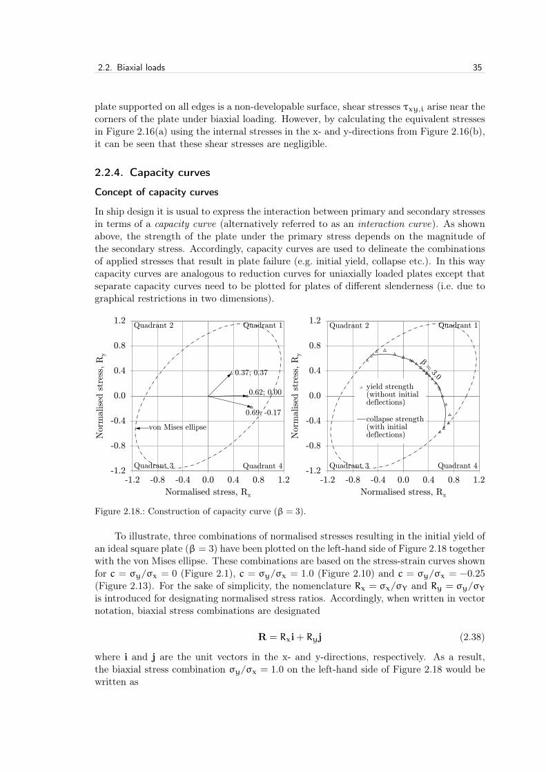
2.2. Biaxial loads 35
plate supported on all edges is a non-developable surface, shear stresses τxy,i arise near thecorners of the plate under biaxial loading. However, by calculating the equivalent stressesin Figure 2.16(a) using the internal stresses in the x- and y-directions from Figure 2.16(b),it can be seen that these shear stresses are negligible.
2.2.4. Capacity curves
Concept of capacity curves
In ship design it is usual to express the interaction between primary and secondary stressesin terms of a capacity curve (alternatively referred to as an interaction curve). As shownabove, the strength of the plate under the primary stress depends on the magnitude ofthe secondary stress. Accordingly, capacity curves are used to delineate the combinationsof applied stresses that result in plate failure (e.g. initial yield, collapse etc.). In this waycapacity curves are analogous to reduction curves for uniaxially loaded plates except thatseparate capacity curves need to be plotted for plates of different slenderness (i.e. due tographical restrictions in two dimensions).
Quadrant 1 Quadrant 2
von Mises ellipse
Quadrant 3 Quadrant 4
0.62; 0.00
0.37; 0.37
0.69; -0.17
-1.2
-0.8
-0.4
0.0
0.4
0.8
1.2
-1.2 -0.8 -0.4 0.0 0.4 0.8 1.2
Norm
alise
d s
tres
s, R
y
Normalised stress, Rx
Quadrant 1 Quadrant 2
Quadrant 3 Quadrant 4 -1.2
-0.8
-0.4
0.0
0.4
0.8
1.2
-1.2 -0.8 -0.4 0.0 0.4 0.8 1.2
Norm
alise
d s
tres
s, R
y
Normalised stress, Rx
yield strength(without initialdeflections)
collapse strength(with initialdeflections)
Figure 2.18.: Construction of capacity curve (β = 3).
To illustrate, three combinations of normalised stresses resulting in the initial yield ofan ideal square plate (β = 3) have been plotted on the left-hand side of Figure 2.18 togetherwith the von Mises ellipse. These combinations are based on the stress-strain curves shownfor c = σy/σx = 0 (Figure 2.1), c = σy/σx = 1.0 (Figure 2.10) and c = σy/σx = −0.25(Figure 2.13). For the sake of simplicity, the nomenclature Rx = σx/σY and Ry = σy/σYis introduced for designating normalised stress ratios. Accordingly, when written in vectornotation, biaxial stress combinations are designated
R = Rxi+ Ryj (2.38)
where i and j are the unit vectors in the x- and y-directions, respectively. As a result,the biaxial stress combination σy/σx = 1.0 on the left-hand side of Figure 2.18 would bewritten as
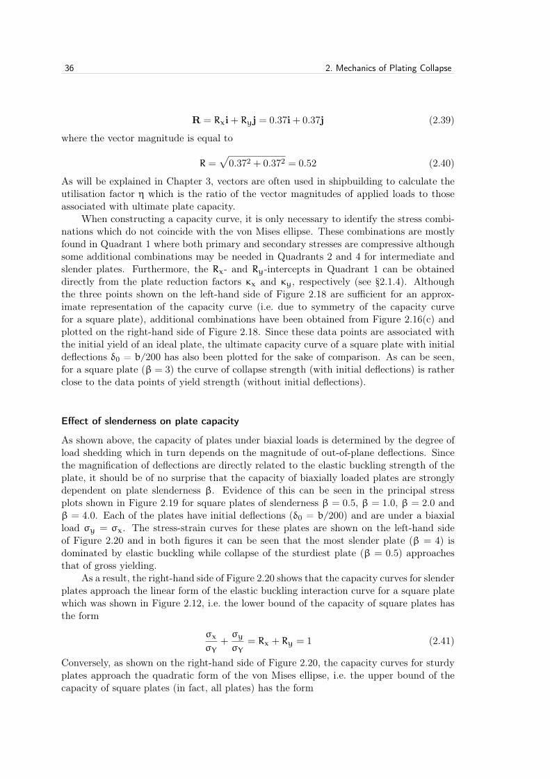
36 2. Mechanics of Plating Collapse
R = Rxi+ Ryj = 0.37i+ 0.37j (2.39)
where the vector magnitude is equal to
R =√
0.372 + 0.372 = 0.52 (2.40)
As will be explained in Chapter 3, vectors are often used in shipbuilding to calculate theutilisation factor η which is the ratio of the vector magnitudes of applied loads to thoseassociated with ultimate plate capacity.
When constructing a capacity curve, it is only necessary to identify the stress combi-nations which do not coincide with the von Mises ellipse. These combinations are mostlyfound in Quadrant 1 where both primary and secondary stresses are compressive althoughsome additional combinations may be needed in Quadrants 2 and 4 for intermediate andslender plates. Furthermore, the Rx- and Ry-intercepts in Quadrant 1 can be obtaineddirectly from the plate reduction factors κx and κy, respectively (see §2.1.4). Althoughthe three points shown on the left-hand side of Figure 2.18 are sufficient for an approx-imate representation of the capacity curve (i.e. due to symmetry of the capacity curvefor a square plate), additional combinations have been obtained from Figure 2.16(c) andplotted on the right-hand side of Figure 2.18. Since these data points are associated withthe initial yield of an ideal plate, the ultimate capacity curve of a square plate with initialdeflections δ0 = b/200 has also been plotted for the sake of comparison. As can be seen,for a square plate (β = 3) the curve of collapse strength (with initial deflections) is ratherclose to the data points of yield strength (without initial deflections).
Effect of slenderness on plate capacity
As shown above, the capacity of plates under biaxial loads is determined by the degree ofload shedding which in turn depends on the magnitude of out-of-plane deflections. Sincethe magnification of deflections are directly related to the elastic buckling strength of theplate, it should be of no surprise that the capacity of biaxially loaded plates are stronglydependent on plate slenderness β. Evidence of this can be seen in the principal stressplots shown in Figure 2.19 for square plates of slenderness β = 0.5, β = 1.0, β = 2.0 andβ = 4.0. Each of the plates have initial deflections (δ0 = b/200) and are under a biaxialload σy = σx. The stress-strain curves for these plates are shown on the left-hand sideof Figure 2.20 and in both figures it can be seen that the most slender plate (β = 4) isdominated by elastic buckling while collapse of the sturdiest plate (β = 0.5) approachesthat of gross yielding.
As a result, the right-hand side of Figure 2.20 shows that the capacity curves for slenderplates approach the linear form of the elastic buckling interaction curve for a square platewhich was shown in Figure 2.12, i.e. the lower bound of the capacity of square plates hasthe form
σx
σY+σy
σY= Rx + Ry = 1 (2.41)
Conversely, as shown on the right-hand side of Figure 2.20, the capacity curves for sturdyplates approach the quadratic form of the von Mises ellipse, i.e. the upper bound of thecapacity of square plates (in fact, all plates) has the form

2.2. Biaxial loads 371
X
Y
Z
run id 15104
APR 14 201516:40:15
PLOT NO. 1
VECTOR
STEP=1SUB =137TIME=.847331SMIDDLE
PRIN1PRIN2PRIN3
(a) β = 0.5
1
X
Y
Z
run id 11104
APR 14 201516:44:29
PLOT NO. 2
VECTOR
STEP=1SUB =189TIME=.850811SMIDDLE
PRIN1PRIN2PRIN3
(b) β = 1.0
1
X
Y
Z
run id 12104
APR 14 201516:47:35
PLOT NO. 3
VECTOR
STEP=1SUB =197TIME=.701386SMIDDLE
PRIN1PRIN2PRIN3
(c) β = 2.0
1
X
Y
Z
run id 14104
APR 14 201516:49:54
PLOT NO. 4
VECTOR
STEP=1SUB =97TIME=.621948SMIDDLE
PRIN1PRIN2PRIN3
(d) β = 4.0
Figure 0.1: ——-CROP!——–CROP!——–CROP!——–CROP!——–CROP!———CROP!——-
1
Figure 2.19.: Principle stresses at collapse in middle plane of plates with initial deflections (c = 1).
(σx
σY
)2
−
(σx
σY
)·(σy
σY
)+
(σy
σY
)2
= R2x − Rx · Ry + R2
y = 1 (2.42)
In between these two limits, the interaction is a mixture of elastic buckling and yielding(i.e. inelastic buckling). Based on this observation, Hughes [9] developed the followinginteraction equation for square plates
R2x − Rx · Ry + R2
y +
(β−
49 · β
)· (Rx + Ry − 1) = 1 (2.43)
As can be seen, this equation employs a weighting factor

38 2. Mechanics of Plating Collapse
β = 1.0
β = 0.5
β = 2.0
β = 4.0
0.0
0.1
0.2
0.3
0.4
0.5
0.6
0.7
0.8
0.9
1.0
0.0 0.2 0.4 0.6 0.8 1.0 1.2 1.4 1.6
Nor
malise
d s
tres
s, σ
x/σ
Y
Normalised strain, εx/εY
collapse strength
13,15 cm
0,32 cm
23,42 cm
13,8 cm
Quadrant 2
Quadrant 3 Quadrant 4 -1.2
-0.8
-0.4
0.0
0.4
0.8
1.2
-1.2 -0.8 -0.4 0.0 0.4 0.8 1.2N
orm
alise
d s
tres
s, R
y
Normalised stress, Rx
Hughes
Figure 2.20.: Capacity curves under biaxial compression (c = 1).
(β−
49 · β
)(2.44)
which determines where the capacity lies between the upper and lower bounds as a func-tion of plate slenderness β, i.e. based on the assumption that gross yielding occurs whenthe plate slenderness β 6 2/3. For the sake of comparison, data points based on Equa-tion (2.43) are plotted on the right-hand side of Figure 2.20 and show reasonably goodagreement with numerical analyses. Other interaction equations suitable for square platesunder biaxial loads will be presented in Chapter 3.
2.3. In-plane shear
If plating is subjected to large shear loads, collapse may occur whether axial stresses arepresent or not. In such cases, shear stress is designated the primary stress. High shearloads generally exist in the webs of ship structures whether that be the web of a hull girder(e.g. side shell plating, longitudinal bulkheads etc.) or the web in a more local structure(e.g. floors, longitudinal girders etc.). In this section the collapse of square plates under apure shear load is examined as well as the capacity reduction in plating due to shear as asecondary or tertiary stress. In case of the former, collapse under pure shear is still best de-fined using stress-strain curves which delineate the relationship between the applied shearstress and the resulting angular strain. Once again the stress and strain corresponding tothe peak of the stress-strain curve represents the greatest shear load which the plate canresist and is therefore referred to as the collapse (or ultimate) strength of the plating.
2.3.1. Ideal plates
For pre-buckled plates subjected to a pure shear load τxy, in-plane principal stresses areoriented ±45◦ to the x-axis with magnitudes σ1 = τxy (compression) and σ2 = −τxy

2.3. In-plane shear 39
(tension). Accordingly, with the stabilising influence of a tensile stress perpendicular tothe compression stress (and of equal magnitude), it is not surprising that the bucklingstrength of plates under pure shear is generally higher than that under a uniaxial load forwhich σ1 = σx and σ2 = 0. This is reflected in the elastic buckling factor of plates undershear, Kτ = 5.34 + 4/α2, compared to that under a uniaxial load, Kx ' 4. Accordingly,the shear buckling stress for a square plate is greater than that under a uniaxial load by afactor of 9.34/4 ' 2.3. Moreover, while the shear buckling strength of plating is relativelyhigh compared to its uniaxial buckling strength, the shear yield strength is relatively low.Given that the (von Mises) equivalent stress in terms of principal in-plane stresses is equalto
σeq =√σ2
1 + σ22 − σ1 · σ2 (2.45)
it can be seen from the above quantities for σ1 and σ2 that a plate under a uniaxial loadyields when σeq = σ1 = σx = σY while under a pure shear load the plate yields whenσeq =
√3 ·σ1 =
√3 · τxy = σY , i.e. τY = σY/
√3. Consequently, although the square plate
shown in Figure 2.1 buckles well before yield under a uniaxial load (β = 3), as shown inFigure 2.21 the same plate under pure shear is characterised by elastic-perfectly plasticbehaviour (at least for γxy/γY < 2). In case of a square plate with slenderness β = 4,there is an immediate unloading of the plate once it buckles elastically such that the ul-timate shear stress τxy,ult equals the elastic buckling stress τxy,cr. Accordingly, in orderto obtain an illustrative stress-strain curve under pure shear, the slenderness of an (ideal)square plate needs to be more than that permitted in the shipbuilding industry.
Pre-buckling
Given the foregoing, the stress-strain curve for a square plate of slenderness β = 5 is shownin Figure 2.21. The plate is without initial deflections and subjected to a pure shear load.With the initial application of the load, stresses and strains are uniform throughout theplate with a linear relationship between them defined by the shear modulus of elasticity
G =E
2 · (1+ ν) (2.46)
This linear elastic behaviour is referred to as the pre-buckling portion of the stress-straincurve and theoretically applies only to ideal plates. For the load corresponding to pointA on the curve (τxy/τY = 0.5), the principal stresses in the middle plane of the plateare plotted in Figure 2.22(a). As noted above, the tensile stresses are oriented 45◦ to thex-axis and the compressive stresses −45◦ to the x-axis with both tensile and compressivecomponents having the same magnitude as the applied shear stress12.
Buckling strength
As the shear load is increased, the linear relationship between stress and strain continuesuntil the buckling strength of the plate is reached. At this point, due to the compressive12 The orientation of the principal stresses are reversed in case the shear load is applied in the opposite
direction.

40 2. Mechanics of Plating Collapse
Collapse strength
Yield strength
Buckling strength
A (Pre-buckling)
B (Post-buckling)
C (Post-yield) D (Post-collapse)
strength
Yield/collapse strength
Buckling/collapse
Yield strength
0.0
0.1
0.2
0.3
0.4
0.5
0.6
0.7
0.8
0.9
1.0
0.0 0.2 0.4 0.6 0.8 1.0 1.2 1.4 1.6 1.8 2.0 2.2 2.4 2.6 2.8 3.0
Nor
malise
d s
tres
s, τ
xy/τ
Y
Normalised strain, γxy/γY
β = 3
β = 5
β = 4
a
b
y
x
τxy
1
XYZ
run id 25107
-2340
234500
APR 17 201518:17:55
PLOT NO. 1
Figure 2.21.: Stress-strain curves of ideal plates under shear.
stresses, a shear buckle develops (under the slightest of perturbations) with its axis ori-ented 45◦ to the x-axis, i.e. from plate corner to plate corner. Shear buckling of an idealplate causes a redistribution of stresses which marks the beginning of a distinctly differentphase of its response to the shear load.
Post-buckling
The post-buckling portion of the stress-strain curve is characterised by a constantly reduc-ing slope. In Figure 2.22(b) the principal stresses associated with point B (τxy/τY = 0.7)are shown. As can be seen, these principal stresses are no longer comprised of pure (in-ternal) shear stresses, i.e. axial stresses are now present as evidenced by changes in therelative magnitude of principal stresses and slight changes in their orientation. Despitethese changes, stresses remain symmetric about an axis oriented 45◦ to the x-axis. Thisnewly formed stress distribution marks the emergence of a stable arrangement of stressescalled the tensile field or tension band. The development of such a field or band is onlypossible if the plate is bounded by structure of sufficient in-plane stiffness which enablesthe plate to carry additional (post-buckling) shear load. Within the tension band the mag-nitude of tensile stresses increase with their proximity to the axis of symmetry while theopposite is true for compressive stresses due to out-of-plane deflections in the plate.

2.3. In-plane shear 41
X
Y
Z
(a) Pre-buckling (Point A)X
Y
Z
(b) Post-buckling (Point B)
X
Y
Z
(c) Post-yield (Point C)X
Y
Z
(d) Post-collapse (Point D)
Figure 0.1: ——-CROP!——–CROP!——–CROP!——–CROP!——–CROP!———CROP!——-
1
X
Y
ZZZ
Y
Figure 2.22.: Principle stresses in middle plane of ideal plate (β = 5).
Yield strength
As the shear load is increased further, the out-of-plane deflections are magnified (albeitmitigated by the tensile stresses) leading to an increase in the polarisation of tensile andcompressive stresses. Yielding in the middle plane of the plate eventually initiates in thecentre of the plate, i.e. x = a/2, y = b/2. Because the centre of the plate is located withinthe tension band, the stress state is dominated by tensile stresses although the magnitudeof compressive stresses remain significant (about 73% of the tensile stress). Accordingly,similar to the mid-length edges of the plate under a uniaxial load, tensile and compressivestresses at the centre of the plate are "working together" to deform the plate material. Asalways, yielding in the middle plane of the plate is indicative of through-thickness plasticity

42 2. Mechanics of Plating Collapse
and is typically a precursor to collapse.
Post-yield
With further increases in shear load, plastic flow begins to spread throughout the middleplane as evidenced by the near-zero slope of the stress-strain curve following yield (seeFigure 2.21). In particular, plasticity begins to appear in the central portion of the tensionband, all four corners of the plate and near the mid-length and mid-breadth edges of theplate. In Figure 2.22(c) the principal stresses associated with point C (γxy/γY = 1.2) inthe post-yield response are shown. Here the polarisation of tensile and compressive stressesis more pronounced as is the formation of the tension band. Corresponding to the latter,the edges of the plate begin to take on a role similar to compression posts of a Pratt trussas reflected in the magnitude and orientation of stresses, i.e. except in the corners of theplate, the magnitude of angles between the x-axis and compressive principal stresses at theedges of the plate are markedly more than 45◦.
Collapse strength
With a small increase in shear load the slope of the stress-strain curve reaches zero. InFigure 2.21 the normalised collapse stress is seen to be approximately τxy,ult/τY = 0.77which represents a 2.9% increase in shear stress compared to initial yield. In terms ofdisplacement, the normalised collapse strain is approximately γxy,ult/γY = 1.37 which isan increase of approximately ∆γxy ' 0.40 · γY compared to initial yield. This increaseis twice that compared to the uniaxial load case and is due to the near-zero (post-yield)stiffness of the plate.
Post-collapse
After collapse the load resistance of the plate under further shear straining is reducedthrough the spread of plasticity throughout the tension band. The effects of post-collapsestraining on principal stresses are shown in Figure 2.22(d) for the load associated withpoint D of the stress-strain curve (γxy/γY = 2.0). Here the redistribution of stresseswhich initiated under buckling are further accentuated. Accordingly, tensile stresses inthe tension band continue to grow as do compressive stresses along the edges of the plate.A plot of the plastic collapse mechanism which permits large shear straining is shown inFigure 2.21 for γxy/γY = 3.0. Photos of collapse mechanisms under pure shear are shownby Rockey et al. in reference [36] and reproduced in Figure 2.23. In case of both girdersevidence of finite in-plane edge restraint can be seen. In Figure 2.23(a) neither of the shearbuckles are anchored in the corners of the plate and in Figure 2.23(b) a well-developedplastic mechanism in the compression flange is clearly evident.

2.3. In-plane shear 43
Dow
nloa
ded
By:
[Zha
ng, S
.] A
t: 16
:57
30 M
ay 2
008
S. Zhang, P. Kumar and S. E. Rutherford
Figure 1 Collapse of a stiffened panel under shear.
Figure 2 Illustration of ultimate strength curve.
comparisons are made with results from ABAQUS non-
linear FE analysis software.
In Application to the Side Shell Structure in Damaged
Situation, application of the proposed method to a collision
damaged side shell structure is performed and again the
results are compared with those derived from ABAQUS
software.
A SEMI-EMPIRICAL APPROACH FOR THE ULTIMATE
SHEAR STRENGTH OF A PLATE
The ultimate strength of a structure is defined as the point
beyond which an additional increment of applied load-
ing cannot be supported, as illustrated in Figure 2. A
structure could collapse under axial loads, lateral pres-
sure, shear loads or a combination of these actions. Ulti-
mate strength under pure edge shear is the subject of this
article.
Figure 3 Simply supported plate under edge shear.
The scenario considered is a simply supported plate sub-
jected to pure shear loading along its edges, as illustrated
in Figure 3. The edges are assumed to remain straight dur-
ing load application and an average magnitude of initial
imperfection in the shape of the critical elastic buckling
mode is assumed. Residual stress is not considered. Under
pure shear loading, the plate supports tension in one diag-
onal direction and compression in the other. For a typical
structure, the plating may first buckle elastically and then,
with increased loading, additional capacity will be devel-
oped through an increase in diagonal tension. The shear
capability of the plate is finally reached when the capacity
of the diagonal tension zone is exhausted. For a single plate
with edges constrained to remain straight, this occurs when
the diagonal reaches tensile yield.
As discussed by Paik and Thayamballi (2003), the de-
formation of plates under edge shear is quite complex and
pure analytical approaches are not straightforward to de-
velop. Thus, many authors employ curve fitting to derive
empirical formulae from numerical results. While this ap-
proach can produce reasonable prediction tools for a spec-
ified range of structural parameters, the physical meaning
can be lost. A format which more closely resembles estab-
lished expressions for ultimate compressive strength pre-
diction would be beneficial. Faulkner’s (1975) well-known
formula for the ultimate strength of plates under uni-axial
compression has been useful to the industry, in that it is
simple to apply and shows good agreement with extensive
experimental data. Through analyses and application of en-
gineering experience, the following similarly constructed
simple formula is now proposed for the ultimate strength
of a plate under pure edge shear:
τu
τy
=
1 for βτ < 12
√βτ
−1
βτ
for βτ ≥ 1(1)
where
βτ =β
1 + (b/a)3/2,
β =b
t
√
σy
Eis the plate slenderness,
τy = σy/√
3 is the shear yield strength,
106SAOS 2008 Vol. 3 No. 2 Copyright C© 2008 Taylor & Francis
(a) Girder SH1 (b) Girder 1AS1-5
1
Figure 2.23.: Collapse mechanism under pure shear (reproduced from reference [36] with permissionof the Institution of Civil Engineers).
2.3.2. Tension field analysis
In parallel to the early work being carried out to study plating under pure axial loads, theaeronautical industry was also studying the collapse of plating under pure shear loads. Apioneer in this regard was Wagner who in 1931 described the post-buckling capacity of aplate under pure shear in terms of the tension band13 [37]. Wagner explained his conceptusing a square truss comprised of four perfectly rigid members and two cross diagonals(pinned at the corners) as shown in Figure 2.24(a). Under low levels of shear the two crossdiagonals D1 and D2 carry equal and opposite stresses. However, at a critical level ofshear the cross diagonal under compression D2 will buckle such that it is unable to carryfurther increases in stress. Accordingly, with further increases in the applied shear stress,Wagner writes "we can assume that the stress in the buckled D2 remains constant butthat thereby the tension in D1 raises twice as fast, so that finally the tension diagonal D1transmits the principal portion of the cross stress". By analogy, the same state of stressresults when shear resistance is provided by a thin plate instead of the cross diagonals D1and D2 (although Wagner acknowledges that the buckling of the plate under compressionstress σ2,i will be somewhat delayed by the presence of the tensile stress σ1,i). When thetensile stress σ1,i is so large that the compression stress σ2,i can be neglected, the plate issaid to be in a state of pure diagonal tension.
Accordingly, there are two analytical models describing two separate states of internalstress in a plate under an applied shear load. One model is of a state of pure shear (seeFigure 2.24(b)) and the other a state of pure (diagonal) tension (see Figure 2.24(c)). Ofcourse, in reality the state of stress in plating under pure shear lies somewhere between thesetwo limits. For this reason, Wagner suggested to include the effects of buckling stiffness inhis tension field analysis of curved plates [38] (i.e. due to their increased buckling strengthcompared to plane plates). However, this idea was subsequently adopted by others forplane plates and further refined by Kuhn et al. [39] in their theory of incomplete diagonal
13 To be precise, 1931 was the publication year of Wagner’s technical memorandums for the NationalAdvisory Committee for Aeronautics. However, he had previously published his work under the title"Ebene Blechwandträger mit sehr dünnem Stegblech" in the German language publication Zeitschriftfür Flugtechnik und Motorluftschiffahrt (Vol. 20, No. 8, 29 April 1929, pp. 200-207 and Vol. 20, No. 9,14 May 1929, pp. 227-231).
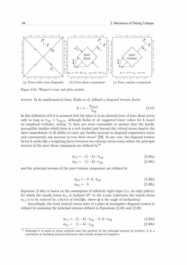
44 2. Mechanics of Plating Collapse
𝐴𝐴 = 𝜋𝜋𝑟𝑟2
y
x
τxy
D1
D2
(a) Truss with cross diagonals
𝐴𝐴 = 𝜋𝜋𝑟𝑟2
y
x
τxy
σ2,i
σ1,i
π 4
𝜎𝜎1,𝑖𝑖 = −(1 − 𝑘𝑘) ∙ 𝜏𝜏𝑥𝑥𝑥𝑥 𝜎𝜎2,𝑖𝑖 = (1 − 𝑘𝑘) ∙ 𝜏𝜏𝑥𝑥𝑥𝑥
pure shear
(b) Pure shear component
𝐴𝐴 = 𝜋𝜋𝑟𝑟2
y
x
τxy
σ1,i
π 4
𝜎𝜎1,𝑖𝑖 = −2 ∙ 𝑘𝑘 ∙ 𝜏𝜏𝑥𝑥𝑥𝑥 𝜎𝜎2,𝑖𝑖 = 0
pure tension
(c) Pure tension component
Figure 0.1: ——-CROP!——–CROP!——–CROP!——–CROP!——–CROP!———CROP!——-
1
Figure 2.24.: Wagner’s truss and plate models.
tension. In its mathematical form, Kuhn et al. defined a diagonal tension factor
k = 1−τxy,cr
τxy(2.47)
In this definition of k it is assumed that the plate is in an internal state of pure shear stressonly so long as τxy < τxy,cr, although Kuhn et al. suggested lower values for k basedon empirical evidence, noting "it does not seem reasonable to assume that the hardlyperceptible buckles which form in a web loaded just beyond the critical stress deprive thesheet immediately of all ability to carry any further increase in diagonal compressive stressand consequently any increase in true shear stress" [39]. In any case, the diagonal tensionfactor k works like a weighting factor between two extreme stress states where the principalstresses of the pure shear component are defined by14
σ1,i = −(1− k) · τxy (2.48a)σ2,i = (1− k) · τxy (2.48b)
and the principal stresses of the pure tension component are defined by
σ1,i = −2 · k · τxy (2.49a)σ2,i = 0 (2.49b)
Equation (2.49a) is based on the assumption of infinitely rigid edges (i.e. no edge pull-in)for which the tensile stress σ1,i is inclined 45◦ to the x-axis (otherwise the tensile stressσ1,i is to be reduced by a factor of sin(2φ), where φ is the angle of inclination).
Accordingly, the total (mixed) stress state of a plate in incomplete diagonal tension isdefined by summing the principal stresses defined in Equations (2.48) and (2.49)
σ1,i = −(1− k) · τxy − 2 · k · τxy (2.50a)σ2,i = (1− k) · τxy (2.50b)
14 Although it is usual in stress analyses that the greatest of the principal stresses be positive, it is aconvention in buckling analyses literature that tensile stresses be negative.

2.3. In-plane shear 45
which can be rewritten as
σ1,i = −(1+ k) · τxy (2.51a)σ2,i = (1− k) · τxy (2.51b)
Substituting Equation (2.51) into that defining the (von Mises) equivalent stress
σeq,i =√σ2
1,i + σ22,i − σ1,i · σ2,i (2.52a)
= τxy ·√
3+ k2 (2.52b)
As a result, if the ultimate shear strength of the plate τxy,ult is defined by initial yield,i.e. σeq,i = σY ,
τxy,ult =σY√3+ k2
(2.53)
As a result,
τxy,ult =σY√3
(= τY) (2.54)
for relatively thick plates where k→ 0 (pure shear) and
τxy,ult =σY2
(2.55)
for very thin plates where k → 1 (pure tension). This means that the minimum ultimateshear capacity of a very thin plate under pure diagonal tension is about 87% of that fora thick "shear resistant" plate, i.e.
√3/2 ∼ 0.866, such that 0.866 · τY 6 τxy,ult 6 τY
according to tension field theory for plating with perfect in-plane edge restraint.In the case of the square plate shown in Figure 2.21 (β = 5), the development of
internal stresses obtained using tension field theory (for plating with perfect in-plane edgerestraint) will now be compared to that obtained using finite element analysis. In thisregard, the growth of internal stresses σx,i, σy,i, τxy,i and σeq,i with the application ofthe applied shear stress τxy is shown on the left-hand side of Figure 2.25 and in terms ofprincipal stresses on the right-hand side of Figure 2.2515. Also shown on the right-hand sideof Figure 2.25 is the growth of principal stresses according to tension field theory. On bothsides of Figure 2.25 the elastic buckling stress for the plate (τxy,cr ' 0.59 ·τY) is indicated.As noted above, the magnitudes of principal stresses σ1,i and σ2,i in the pre-buckled stateare equal to σ1,i = −τxy and σ2,i = τxy. In the post-buckled state, ∆σ1,i = −2 ·∆τxy and∆σ2,i = 0. Therefore, according to tension field theory, the plate yields under an appliedshear stress of τxy = 0.97 · τY , where σ1,i = −(0.59+ 2 · (0.97− 0.59)) · τY = −0.78 · σYand σ2,i = 0.59 · τY = 0.34 · σY . Here the applied shear stress τxy = 0.97 · τY initiat-ing yield in plating of slenderness β = 5 is near the upper limit of the above condition0.866 · τY 6 τxy,ult 6 τY for tension field theory.
However, as can be seen in Figure 2.21, yielding occurs under an applied shear stressof τxy = 0.75 · τY according to finite element analysis. Here it is important to reiterate
15 For the purpose of representation the first principal stress σ1 is plotted as |σ1|.
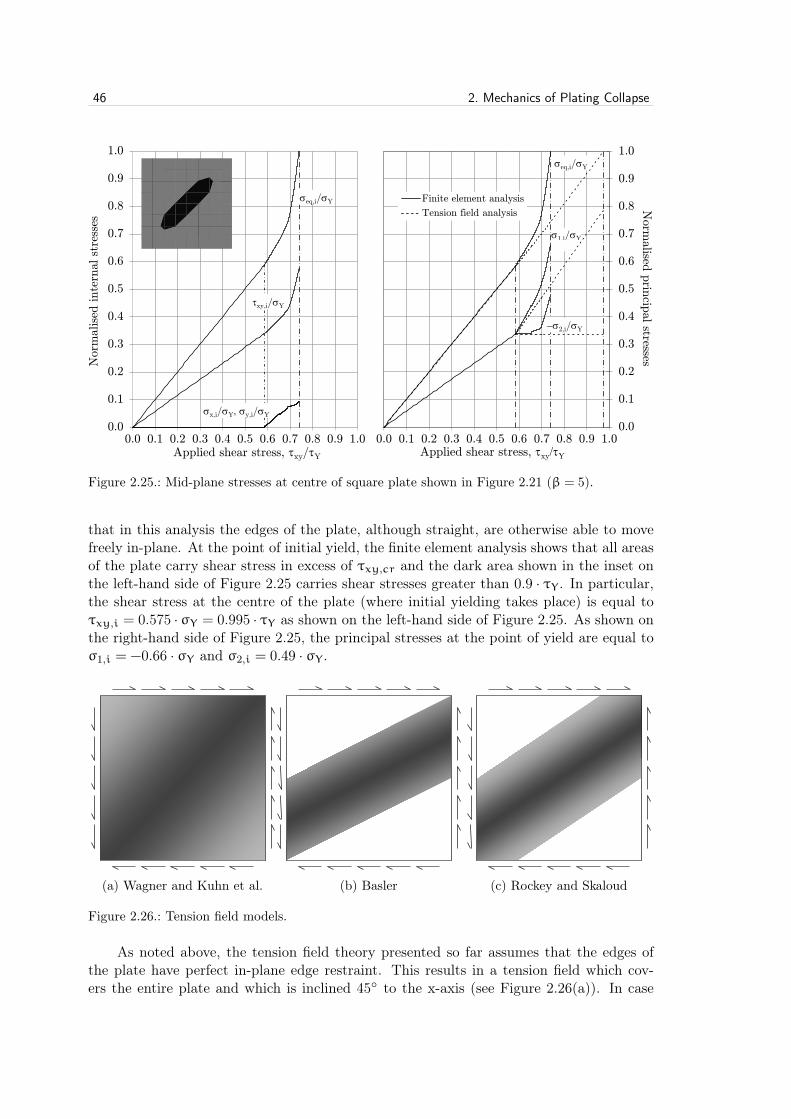
46 2. Mechanics of Plating Collapse
σx,i/σY, σy,i/σY
τxy,i/σY
σeq,i/σY
0.0
0.1
0.2
0.3
0.4
0.5
0.6
0.7
0.8
0.9
1.0
0.0 0.1 0.2 0.3 0.4 0.5 0.6 0.7 0.8 0.9 1.0
Nor
mal
ised
inte
rnal
str
esse
s
Applied shear stress, τxy/τY
13,15 cm
0,32 cm
23,42 cm
13,8 cm
−σ2,i/σY
σeq,i/σY
0.0
0.1
0.2
0.3
0.4
0.5
0.6
0.7
0.8
0.9
1.0
0.0 0.1 0.2 0.3 0.4 0.5 0.6 0.7 0.8 0.9 1.0
Norm
alised p
rincip
al stresses
Applied shear stress, τxy/τY
Finite element analysis
Tension field analysis
13,15 cm
13,8 cm 0,32 cm
23,46 cm
σ1,i/σY
JUL 31 201515:53:16 plate_ulsPLOT NO. 10NODAL SOLUTIONTIME=.67437 SXY (AVG) MIDDLE RSYS=0DMX =10.872 SMN =93.3108 SMX =135.271
1
ZV =1 DIST=467.5 XF =425 YF =425 ZF =.245E-03 VUP =Z A-ZS=90 PRECISE HIDDENEDGE
-122 0 122 135.7
run id 25107
1
Figure 2.25.: Mid-plane stresses at centre of square plate shown in Figure 2.21 (β = 5).
that in this analysis the edges of the plate, although straight, are otherwise able to movefreely in-plane. At the point of initial yield, the finite element analysis shows that all areasof the plate carry shear stress in excess of τxy,cr and the dark area shown in the inset onthe left-hand side of Figure 2.25 carries shear stresses greater than 0.9 · τY . In particular,the shear stress at the centre of the plate (where initial yielding takes place) is equal toτxy,i = 0.575 · σY = 0.995 · τY as shown on the left-hand side of Figure 2.25. As shown onthe right-hand side of Figure 2.25, the principal stresses at the point of yield are equal toσ1,i = −0.66 · σY and σ2,i = 0.49 · σY .
y
x
τxy
(a) Wagner and Kuhn et al.
y
x
τxy
(b) Basler
y
x
τxy
(c) Rockey and Skaloud
Figure 0.1: ——-CROP!——–CROP!——–CROP!——–CROP!——–CROP!———CROP!——-
1
Figure 2.26.: Tension field models.
As noted above, the tension field theory presented so far assumes that the edges ofthe plate have perfect in-plane edge restraint. This results in a tension field which cov-ers the entire plate and which is inclined 45◦ to the x-axis (see Figure 2.26(a)). In case

2.3. In-plane shear 47
of aeronautical engineering, this assumption may well be valid given the high strengthaluminium alloys used in aircraft structure which lead to thin webs and relatively strongflanges [40, 41]. However, in the case of steel plate girders used in civil engineering applica-tions, the bending stiffness of flanges is usually insufficient to prevent in-plane displacementof the plate edges. If this displacement is of an extent that the tensile stresses in the diago-nal of the plate are appreciably relieved, then both the width and inclination of the tensionfield are affected. In this regard, Basler (as referenced in [40]) assumed that the flangesof most plate girders were too flexible to withstand the lateral load caused by a perfectlydiagonal tension field. Accordingly, he postulated an off diagonal tension field which isnot anchored to any part of the flange (see Figure 2.26(b)). Rockey and Skaloud (as refer-enced in [40]) subsequently showed the foregoing assumption to be overly conservative andpostulated tension fields which took into explicit account the stiffness of the flanges (seeFigure 2.26(c)). Such models may be more appropriate for ship structures such as floorsand longitudinal girders where in-plane edge restraint is negligible.
2.3.3. Effects of initial deflections
In order to study the effect of welding distortions, stress-strain curves are shown on theleft-hand side of Figure 2.27 for initially deflected plating (δ0 = b/200). Here the nomen-clature of the plate reduction factor κτ = τxy,ult ·
√3/σY = τxy,ult/τY is reintroduced
(see §2.1.4). Unlike the uniaxial load case (see the left-hand side of Figure 2.6), thesecurves deviate only slightly from the shear modulus curve (G = τxy/γxy) due to themitigating influence of tensile stresses on out-of-plane deflections. Accordingly, the mag-nitudes of collapse strength normalised against yield are clearly higher in the case of shearloading. Furthermore, regardless of plate slenderness, the stress-strain curves approachelastic-perfectly plastic behaviour where plasticity is defined by the ultimate stress τxy,ultrather than the yield stress τY . This stable response is again due to the presence of thetension field.
Ranges of plate slenderness
On the right-hand side of Figure 2.27 the collapse strengths of plates with and withoutinitial deflections are shown. Also shown are the ranges of the plate slenderness parameterβ defined by Hughes to delineate different types of plating collapse (because the shearbuckling factor Kτ is a function of the plate aspect ratio α, the reference degrees of slen-derness λτ shown in Figure 2.27 are only valid for α = 1). Here it may be recalled thatthe transitions between these different classes of plating are approximately defined wherethe collapse strength equals the yield strength (i.e. sturdy to intermediate plating) andwhere the collapse strength equals the elastic buckling strength (i.e. intermediate to slen-der plating). Applying these same criteria to square plates under a pure shear load, it canbe seen that there is no "slender" plating for the range of plate slenderness parameterstypically found in shipbuilding since the elastic buckling strength always exceeds the ulti-mate strength. Moreover, the transition between sturdy and intermediate plating occursnot in the vicinity of β = 1 but rather β = 2. As can be seen in Figure 2.28, there islittle evidence of buckling behaviour in the principal stress plots at collapse for plating ofslenderness β = 2.
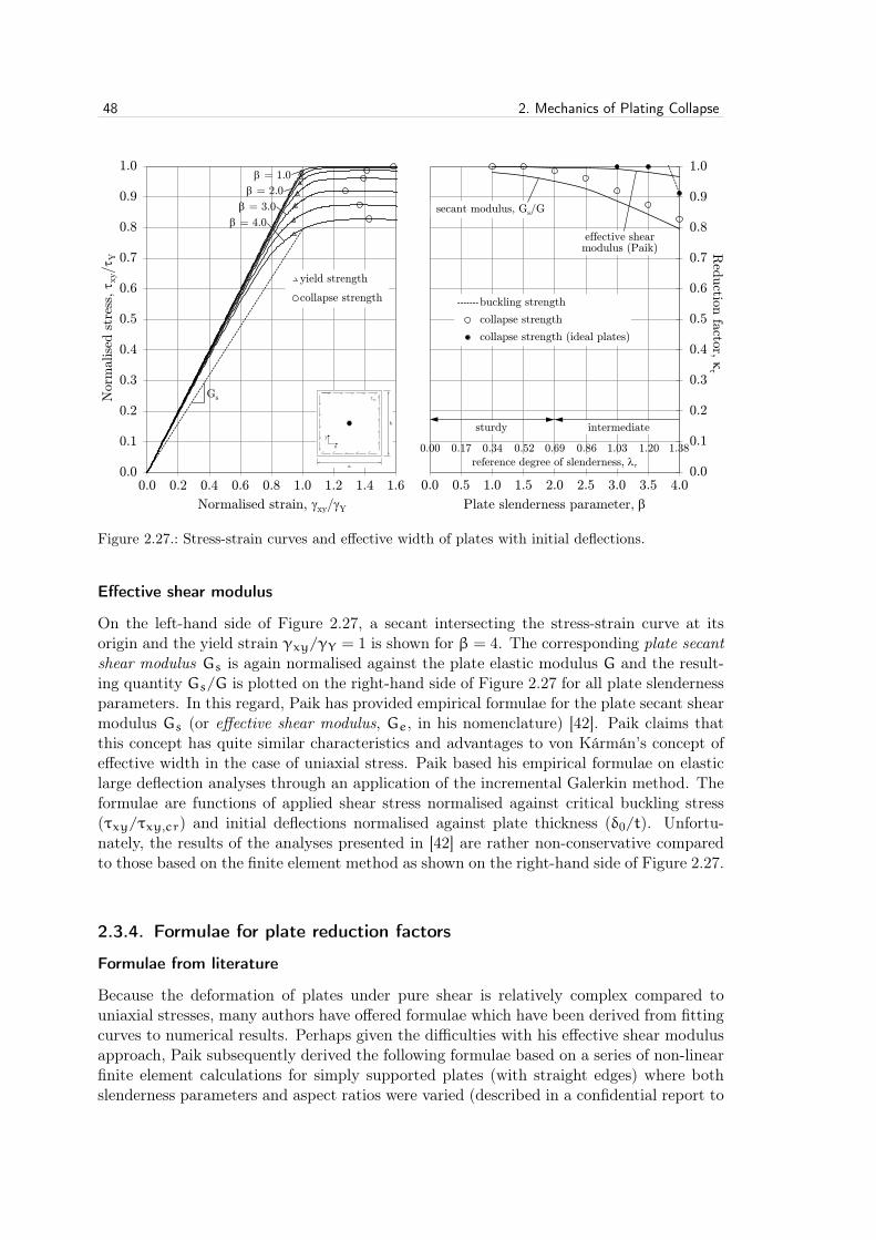
48 2. Mechanics of Plating Collapse
β = 1.0
β = 2.0
β = 3.0
Gs
β = 4.0
0.0
0.1
0.2
0.3
0.4
0.5
0.6
0.7
0.8
0.9
1.0
0.0 0.2 0.4 0.6 0.8 1.0 1.2 1.4 1.6
Nor
mal
ised
str
ess,
τxy/τ
Y
Normalised strain, γxy/γY
yield strength
collapse strength
13,15 cm
0,32 cm
23,42 cm
13,8 cm
0.00 0.17 0.34 0.52 0.69 0.86 1.03 1.20 1.38
effective shear modulus (Paik)
0.0
0.1
0.2
0.3
0.4
0.5
0.6
0.7
0.8
0.9
1.0
0.0 0.5 1.0 1.5 2.0 2.5 3.0 3.5 4.0
Red
uction
factor, κτ
Plate slenderness parameter, β
buckling strength
collapse strength
collapse strength (ideal plates)
sturdy intermediate
reference degree of slenderness, λτ
13,15 cm
13,8 cm 0,32 cm
23,46 cm
secant modulus, Gs/G
a
b
y
x
τxy
Figure 2.27.: Stress-strain curves and effective width of plates with initial deflections.
Effective shear modulus
On the left-hand side of Figure 2.27, a secant intersecting the stress-strain curve at itsorigin and the yield strain γxy/γY = 1 is shown for β = 4. The corresponding plate secantshear modulus Gs is again normalised against the plate elastic modulus G and the result-ing quantity Gs/G is plotted on the right-hand side of Figure 2.27 for all plate slendernessparameters. In this regard, Paik has provided empirical formulae for the plate secant shearmodulus Gs (or effective shear modulus, Ge, in his nomenclature) [42]. Paik claims thatthis concept has quite similar characteristics and advantages to von Kármán’s concept ofeffective width in the case of uniaxial stress. Paik based his empirical formulae on elasticlarge deflection analyses through an application of the incremental Galerkin method. Theformulae are functions of applied shear stress normalised against critical buckling stress(τxy/τxy,cr) and initial deflections normalised against plate thickness (δ0/t). Unfortu-nately, the results of the analyses presented in [42] are rather non-conservative comparedto those based on the finite element method as shown on the right-hand side of Figure 2.27.
2.3.4. Formulae for plate reduction factors
Formulae from literature
Because the deformation of plates under pure shear is relatively complex compared touniaxial stresses, many authors have offered formulae which have been derived from fittingcurves to numerical results. Perhaps given the difficulties with his effective shear modulusapproach, Paik subsequently derived the following formulae based on a series of non-linearfinite element calculations for simply supported plates (with straight edges) where bothslenderness parameters and aspect ratios were varied (described in a confidential report to

2.3. In-plane shear 491
X
Y
Z
run id 21107
APR 18 201501:09:10
PLOT NO. 1
VECTOR
STEP=1SUB =129TIME=.90447SMIDDLE
PRIN1PRIN2PRIN3
(a) β = 1
1
X
Y
Z
run id 22107
APR 18 201501:12:15
PLOT NO. 2
VECTOR
STEP=1SUB =149TIME=.892213SMIDDLE
PRIN1PRIN2PRIN3
(b) β = 2
1
X
Y
Z
run id 23107
APR 18 201501:25:32
PLOT NO. 6
VECTOR
STEP=1SUB =172TIME=.832793SMIDDLE
PRIN1PRIN2PRIN3
(c) β = 3
1
X
Y
Z
run id 24107
APR 18 201501:28:04
PLOT NO. 7
VECTOR
STEP=1SUB =178TIME=.749401SMIDDLE
PRIN1PRIN2PRIN3
(d) β = 4
Figure 0.1: ——-CROP!——–CROP!——–CROP!——–CROP!——–CROP!———CROP!——-
1
Figure 2.28.: Principle stresses at collapse in middle plane of plates with initial deflections.
the American Bureau of Shipping (ABS) [43], but referenced in [44])
κτ =τxy,ult
τY=
1.324/λ2
τ λτ >√2
0.039/λ6τ − 0.274/λ4
τ + 0.676/λ2τ + 0.388
√2 > λτ >
√0.5
0.956 λτ <√0.5
(2.56)
where λτ =√τY/τcr. In Paik’s solution, τcr is calculated for a plate aspect ratio α = 1
because he found that the ultimate shear strength of plates decreases only slightly withaspect ratios α > 1. Similarly, Nara et al. (referenced in [35] and [45]) proposed thefollowing which was also obtained by fitting a curve to non-linear finite element results

50 2. Mechanics of Plating Collapse
κτ =τxy,ult
τY=
(0.486λτ
) 13
6 1.0 (2.57)
and which is valid for λτ 6 2.0. Results obtained with the proofs of Paik and Nara et al.are compared in Figure 2.29 to those obtained by finite element analyses.
Because formulae based on curve fitting can be devoid of physical meaning, Zhanget al. sought a format which more closely resembled established expressions for ultimatecompressive strength. Towards this end, Faulkner’s well-known Equation (2.26) for theultimate strength of plates under a uniaxial load was considered both accurate and simpleto apply. Accordingly, "(t)hrough analyses and application of engineering experience",Zhang et al. [45] proposed the following similarly constructed formula
κτ =τxy,ult
τY=
2√βτ
−1βτ
βτ > 1
1 βτ < 1(2.58)
where βτ = β/(1+ (b/a)3/2
). Results obtained with the proof of Zhang et al. are also
shown in Figure 2.29.
Nara et al.
0.00 0.17 0.34 0.52 0.69 0.86 1.03 1.20 1.38
Zhang et al.
0.0
0.1
0.2
0.3
0.4
0.5
0.6
0.7
0.8
0.9
1.0
0.0 0.5 1.0 1.5 2.0 2.5 3.0 3.5 4.0
Red
uct
ion fact
or,
κ τ
Plate slenderness parameter, β
collapse strength
collapse strength (ideal plates)
reference degree of slenderness, λτ
13,15 cm
13,8 cm 0,32 cm
23,46 cm
Paik
Figure 2.29.: Formulae from literature.
0.00 0.17 0.34 0.52 0.69 0.86 1.03 1.20 1.38
DIN 18800
0.0
0.1
0.2
0.3
0.4
0.5
0.6
0.7
0.8
0.9
1.0
0.0 0.5 1.0 1.5 2.0 2.5 3.0 3.5 4.0
Red
uction
factor, κτ
Plate slenderness parameter, β
collapse strength
collapse strength (ideal plates)
reference degree of slenderness, λτ
13,15 cm
13,8 cm 0,32 cm
23,46 cm
Johnson-Ostenfeld
Figure 2.30.: Formulae used in shipbuilding.
Formulae used in shipbuilding
In terms of the classification of ships, two proofs for the ultimate shear strength of platesare widely used in the shipbuilding industry. The first proof is again based on the Johnson-Ostenfeld correction which is used to adjust the elastic shear buckling curve to account forplasticity (as presented in §2.1.4. for the uniaxial load case)
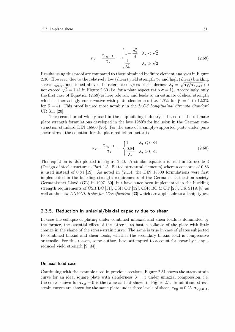
2.3. In-plane shear 51
κτ =τxy,ult
τY=
1−
λ2τ
4λτ <
√2
1λ2τ
λτ >√2
(2.59)
Results using this proof are compared to those obtained by finite element analyses in Figure2.30. However, due to the relatively low (shear) yield strength τY and high (shear) bucklingstress τxy,cr mentioned above, the reference degrees of slenderness λτ =
√τY/τxy,cr do
not exceed√2 = 1.41 in Figure 2.30 (i.e. for a plate aspect ratio α = 1). Accordingly, only
the first case of Equation (2.59) is here relevant and leads to an estimate of shear strengthwhich is increasingly conservative with plate slenderness (i.e. 1.7% for β = 1 to 12.3%for β = 4). This proof is used most notably in the IACS Longitudinal Strength StandardUR S11 [20].
The second proof widely used in the shipbuilding industry is based on the ultimateplate strength formulations developed in the late 1980’s for inclusion in the German con-struction standard DIN 18800 [26]. For the case of a simply-supported plate under pureshear stress, the equation for the plate reduction factor is
κτ =τxy,ult
τY=
1 λτ 6 0.840.84λτ
λτ > 0.84(2.60)
This equation is also plotted in Figure 2.30. A similar equation is used in Eurocode 3(Design of steel structures - Part 1-5: Plated structural elements) where a constant of 0.83is used instead of 0.84 [19]. As noted in §2.1.4, the DIN 18800 formulations were firstimplemented in the buckling strength requirements of the German classification societyGermanischer Lloyd (GL) in 1997 [30], but have since been implemented in the bucklingstrength requirements of CSR BC [31], CSR OT [32], CSR BC & OT [23], UR S11A [8] aswell as the new DNVGL Rules for Classification [33] which are applicable to all ship types.
2.3.5. Reduction in uniaxial/biaxial capacity due to shear
In case the collapse of plating under combined uniaxial and shear loads is dominated bythe former, the essential effect of the latter is to hasten collapse of the plate with littlechange in the shape of the stress-strain curve. The same is true in case of plates subjectedto combined biaxial and shear loads, whether the secondary biaxial load is compressiveor tensile. For this reason, some authors have attempted to account for shear by using areduced yield strength [9, 34].
Uniaxial load case
Continuing with the example used in previous sections, Figure 2.31 shows the stress-straincurve for an ideal square plate with slenderness β = 3 under uniaxial compression, i.e.the curve shown for τxy = 0 is the same as that shown in Figure 2.1. In addition, stress-strain curves are shown for the same plate under three levels of shear, τxy = 0.25 · τxy,ult,

52 2. Mechanics of Plating Collapse
τxy = 0
τxy = 0.25∙τxy,ult
τxy = 0.5∙τxy,ult
τxy = 0.75∙τxy,ult
0.0
0.1
0.2
0.3
0.4
0.5
0.6
0.7
0.8
0.0 0.2 0.4 0.6 0.8 1.0 1.2 1.4 1.6 1.8 2.0 2.2 2.4 2.6 2.8 3.0
Nor
malise
d s
tres
s, σ
x/σ
Y
Normalised strain, εx/εY
applied shear stress
adjusted yield stress (no shear load)
a
y
x
τxy
σx b
Figure 2.31.: Stress-strain curves under influence of shear (σy = 0, β = 3).
τxy = 0.5 · τxy,ult and τxy = 0.75 · τxy,ult. Compared to the ultimate strength underuniaxial compression only, there is a non-linear decrease in the capacity of the plate withincreasing levels of shear, i.e. 5.4%, 21.7% and 49.7%, respectively. However, there islittle change in the shape of the stress-strain curves, except for the shear dominant caseτxy = 0.75 · τxy,ult (the stress-strain curve of which resembles that for pure shear). Ac-cordingly, also shown in Figure 2.31 are stress-strain curves for a uniaxially loaded plateusing a reduced yield stress σ ′Y in lieu of applied shear loads. The reductions in yield stressare calculated according to the following commonly used equation
σ ′Y =√σ2Y − 3 · τ2
xy (2.61)
However, as can be seen, this approach generally overestimates the collapse strengthof the plate with errors increasing with levels of shear, i.e. 3.3%, 15.1% and 49.7% forτxy = 0.25 · τxy,ult, τxy = 0.5 · τxy,ult and τxy = 0.75 · τxy,ult, respectively.
To better understand the collapse of plating under combined uniaxial and shear loads,Figure 2.32 shows principal stresses in the middle plane of an ideal plate at the point ofcollapse under various levels of shear. In Figure 2.32(a) the principal stresses are shown forcollapse in the absence of shear. As noted in §2.1.1, although longitudinal stresses alongthe edges of the plate are approximately equal over its length, yielding initiates at themid-length edges of the plate (i.e. x = a/2), because of transverse tensile stresses whicharise due to out-of-plane deflections. As noted previously, the (compressive) longitudinalstresses and (tensile) transverse stresses are here "working together" to deform the platematerial. This is reflected in Figure 2.33 which shows the internal equivalent stresses atthe mid-length edges, mid-breadth edges, corners within the tension band and centre ofthe plate under various levels of shear. As can be seen, equivalent stresses in the corners

2.3. In-plane shear 531
X
Y
Z
run id 9930
OCT 16 201518:00:26
PLOT NO. 4
VECTOR
STEP=1SUB =943TIME=.669117SMIDDLE
PRIN1PRIN2PRIN3
(a) Rτ = 0
1
X
Y
Z
run id 9930
OCT 16 201518:09:05
PLOT NO. 5
VECTOR
STEP=1SUB =812TIME=.711731SMIDDLE
PRIN1PRIN2PRIN3
(b) Rτ = 0.25 · κτ
1
X
Y
Z
run id 9930
OCT 16 201518:15:55
PLOT NO. 6
VECTOR
STEP=1SUB =499TIME=.589684SMIDDLE
PRIN1PRIN2PRIN3
(c) Rτ = 0.5 · κτ
1
X
Y
Z
run id 9930
OCT 16 201518:24:45
PLOT NO. 7
VECTOR
STEP=1SUB =222TIME=.378372SMIDDLE
PRIN1PRIN2PRIN3
(d) Rτ = 0.75 · κτ
Figure 0.1: ——-CROP!——–CROP!——–CROP!——–CROP!——–CROP!———CROP!——-
1
Figure 2.32.: Principle stresses at collapse in middle plane of ideal plate (σy = 0, β = 3).
of the plate are about 82% of those at the mid-length edges (where yielding initiates) inthe absence of shear. However, in the presence of a shear stress τxy = 0.25 · τxy,ult, thetensile stresses which develop are such that yielding initiates instead in the corners of theplate within the tension band. As the level of shear increases, the principal stresses shownin Figure 2.32 progressively approach those shown in Figure 2.22 ((c) and (d)) for the pureshear case. In other words, as the level of shear increases, the locations of initial yieldgradually move from the mid-length edges of the plate, to the corners of the plate (withinthe tension band) to the centre of the plate. This transition is reflected in the internalequivalent stresses shown in Figure 2.33. Moreover, as discussed in §2.3.1, Figure 2.33 con-firms that collapse of an ideal (square) plate (β = 3) under pure shear (τxy/τxy,ult = 1.00)

54 2. Mechanics of Plating Collapse
0.0
0.2
0.4
0.6
0.8
1.0
0.00 0.25 0.50 0.75 1.00Equiv
ale
nt
stre
sses
, σ e
q,i/σ
Y
Stress ratio, τxy/τxy,ult
mid-length edges
mid-breadth edges
plate corners within tension band
plate centre
23,46 cm
Figure 2.33.: Internal equivalent stresses at collapse (σy = 0, β = 3).
occurs by gross yielding.
Compressive secondary stress, c = 1
Continuing further with the example used in previous sections, Figure 2.34 shows the stress-strain curve for an ideal square plate with slenderness β = 3 under biaxial compressionwhere σy = σx, i.e. the curve shown for τxy = 0 is the same as that shown in Figure 2.10.In addition, stress-strain curves are again shown for the same plate under three levels of
τxy = 0.25∙τxy,ult
τxy = 0.5∙τxy,ult
τxy = 0.75∙τxy,ult
0.0
0.1
0.2
0.3
0.4
0.5
0.6
0.7
0.8
0.0 0.2 0.4 0.6 0.8 1.0 1.2 1.4 1.6 1.8 2.0 2.2 2.4 2.6 2.8 3.0
Nor
mal
ised
str
ess,
σx/σ
Y
Normalised strain, εx/εY
τxy = 0
y
x
τxy
σx b
σy
a
Figure 2.34.: Stress-strain curves under influence of shear (σy = σx, β = 3).

2.3. In-plane shear 55
shear, τxy = 0.25 · τxy,ult, τxy = 0.5 · τxy,ult and τxy = 0.75 · τxy,ult. Compared to theultimate strength under biaxial compression alone (i.e. σy = σx), there is again a non-linear decrease in the capacity of the plate with increasing levels of shear, i.e. 8.8%, 25.2%and 52.9%, respectively. Likewise, there is again little change in the shape of the stress-strain curves, except for the shear dominant case τxy = 0.75 · τxy,ult (the stress-straincurve of which again resembles that for pure shear).1
X
Y
Z
run id 99304
OCT 17 201521:01:44
PLOT NO. 1
VECTOR
STEP=1SUB =1887TIME=.653306SMIDDLE
PRIN1PRIN2PRIN3
(a) Rτ = 0
1
X
Y
Z
run id 99304
OCT 17 201521:16:03
PLOT NO. 2
VECTOR
STEP=1SUB =1690TIME=.596046SMIDDLE
PRIN1PRIN2PRIN3
(b) Rτ = 0.25 · κτ
1
X
Y
Z
run id 99304
OCT 17 201521:36:13
PLOT NO. 3
VECTOR
STEP=1SUB =647TIME=.439725SMIDDLE
PRIN1PRIN2PRIN3
(c) Rτ = 0.5 · κτ
1
X
Y
Z
run id 99304
OCT 17 201521:48:07
PLOT NO. 4
VECTOR
STEP=1SUB =234TIME=.30779SMIDDLE
PRIN1PRIN2PRIN3
(d) Rτ = 0.75 · κτ
Figure 0.1: ——-CROP!——–CROP!——–CROP!——–CROP!——–CROP!———CROP!——-
1
Figure 2.35.: Principle stresses at collapse in middle plane of ideal plate (σy = σx, β = 3).
To better understand the collapse of plating under combined biaxial (σy = σx) andshear loads, Figure 2.35 shows principal stresses in the middle plane of the plate at thepoint of collapse. In Figure 2.35(a) the principal stresses are again shown for collapse inthe absence of shear. As noted in §2.2.1, initial yielding under a biaxial load σy = σx does

56 2. Mechanics of Plating Collapse
not occur at the mid-length edges of the plate, but rather in the corners of the plate wherethe (magnified) applied stresses σx and σy coalesce. This is reflected in Figure 2.36 whichagain shows the internal equivalent stresses at the mid-length edges, mid-breadth edges,corners in the tension band and centre of the plate under various levels of shear. As can beseen, equivalent stresses in the corners of the plate (within the tension band) are the firstto reach yield under all levels of shear. As the level of shear increases, the principal stressesshown in Figure 2.35 once again progressively approach those shown in Figure 2.22 ((c)and (d)) for the pure shear case. Moreover, Figure 2.36 again confirms that collapse of anideal (square) plate (β = 3) under pure shear (τxy/τxy,ult = 1.00) occurs by gross yielding.
0.0
0.2
0.4
0.6
0.8
1.0
0.00 0.25 0.50 0.75 1.00Equiv
alen
t st
ress
es, σ e
q,i/σ
Y
Stress ratio, τxy/τxy,ult
mid-length edges
mid-breadth edges
plate corners within tension band
plate centre
23,46 cm
Figure 2.36.: Internal equivalent stresses at collapse (σy = σx, β = 3).
τxy = 0.25∙τxy,ult
τxy = 0.5∙τxy,ult
τxy = 0.75∙τxy,ult
0.0
0.1
0.2
0.3
0.4
0.5
0.6
0.7
0.8
0.0 0.2 0.4 0.6 0.8 1.0 1.2 1.4 1.6 1.8 2.0 2.2 2.4 2.6 2.8 3.0
Nor
mal
ised
str
ess,
σx/σ
Y
Normalised strain, εx/εY
τxy = 0
y
x
τxy
σx b
σy
a
Figure 2.37.: Stress-strain curves under influence of shear (σy = −σx/4, β = 3).
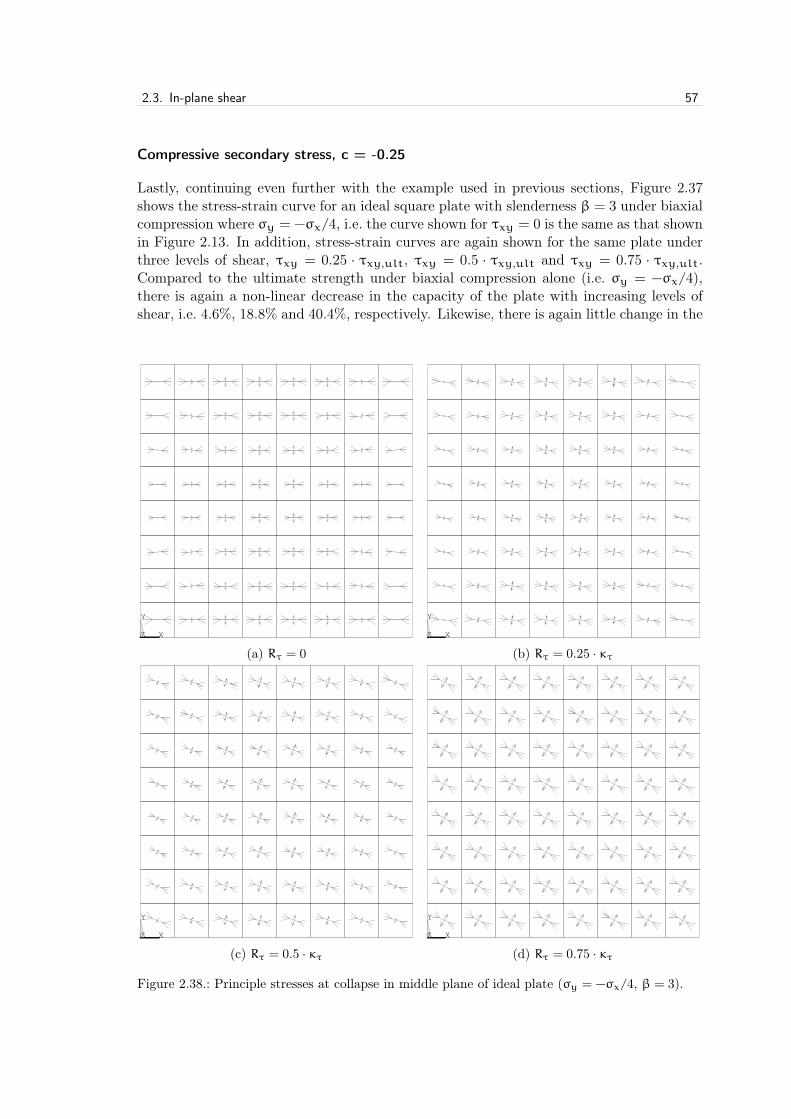
2.3. In-plane shear 57
Compressive secondary stress, c = -0.25
Lastly, continuing even further with the example used in previous sections, Figure 2.37shows the stress-strain curve for an ideal square plate with slenderness β = 3 under biaxialcompression where σy = −σx/4, i.e. the curve shown for τxy = 0 is the same as that shownin Figure 2.13. In addition, stress-strain curves are again shown for the same plate underthree levels of shear, τxy = 0.25 · τxy,ult, τxy = 0.5 · τxy,ult and τxy = 0.75 · τxy,ult.Compared to the ultimate strength under biaxial compression alone (i.e. σy = −σx/4),there is again a non-linear decrease in the capacity of the plate with increasing levels ofshear, i.e. 4.6%, 18.8% and 40.4%, respectively. Likewise, there is again little change in the
1
X
Y
Z
run id 993024
OCT 18 201510:57:19
PLOT NO. 1
VECTOR
STEP=1SUB =661TIME=.822197SMIDDLE
PRIN1PRIN2PRIN3
(a) Rτ = 0
1
X
Y
Z
run id 993024
OCT 18 201511:48:11
PLOT NO. 1
VECTOR
STEP=1SUB =536TIME=.784049SMIDDLE
PRIN1PRIN2PRIN3
(b) Rτ = 0.25 · κτ
1
X
Y
Z
run id 993024
OCT 18 201512:12:19
PLOT NO. 1
VECTOR
STEP=1SUB =386TIME=.667743SMIDDLE
PRIN1PRIN2PRIN3
(c) Rτ = 0.5 · κτ
1
X
Y
Z
run id 993024
OCT 18 201512:36:40
PLOT NO. 1
VECTOR
STEP=1SUB =77TIME=.489907SMIDDLE
PRIN1PRIN2PRIN3
(d) Rτ = 0.75 · κτ
Figure 0.1: ——-CROP!——–CROP!——–CROP!——–CROP!——–CROP!———CROP!——-
1
Figure 2.38.: Principle stresses at collapse in middle plane of ideal plate (σy = −σx/4, β = 3).

58 2. Mechanics of Plating Collapse
shape of the stress-strain curves, except for the shear dominant case τxy = 0.75 · τxy,ult(the stress-strain curve of which again resembles that for pure shear).
To better understand the collapse of plating under combined biaxial (σy = −σx/4)and shear loads, Figure 2.38 shows principal stresses in the middle plane of the plate at thepoint of collapse. In Figure 2.38(a) the principal stresses are again shown for collapse inthe absence of shear. As noted in §2.2.2, the resulting combination of compressive stresses(due to the applied load) and perpendicular tensile stresses (due to out-of-plane deflections)leads to initial yielding in the middle plane at the mid-length edges of the plate. However,because the restrained out-of-plane deflections mitigate the redistribution of stresses, the(applied) axial stress σx at which the plate yields is greater than that in the uniaxial loadcase. This is reflected in Figure 2.39 which once again shows the internal equivalent stressesat the mid-length edges, mid-breadth edges, corners within the tension band and centre ofthe plate under various levels of shear. As can be seen, equivalent stresses in the corners ofthe plate are approximately 85% of those at the mid-length edges (where yielding initiates)in the absence of shear. Moreover, due to the effect of the tensile stress in the y-direction,a shear stress of τxy = 0.5 · τxy,ult is needed before yielding initiates in the corners ofthe plate within the tension band. As the level of shear increases, the principal stressesshown in Figure 2.38 once again progressively approach those shown in Figure 2.22 ((c)and (d)) for the pure shear case. Moreover, Figure 2.39 again confirms that collapse of anideal (square) plate (β = 3) under pure shear (τxy/τxy,ult = 1.00) occurs by gross yielding.
0.0
0.2
0.4
0.6
0.8
1.0
0.00 0.25 0.50 0.75 1.00Equiv
alen
t st
ress
es, σ e
q,i/σ
Y
Stress ratio, τxy/τxy,ult
mid-length edges
mid-breadth edges
plate corners within tension band
plate centre
23,46 cm
Figure 2.39.: Internal equivalent stresses at collapse (σy = −σx/4, β = 3).
Concept of capacity surfaces
In the context of plates under biaxial loads, the concept of capacity curves was introducedin §2.2.4. As noted therein, it is usual in ship design to delineate the combinations ofbiaxial stresses associated with plating collapse in terms of a capacity curve (alternativelyreferred to as an interaction curve). In this section the concept is extended to includethe effects of shear, where separate capacity curves are shown for different levels of shearloads. For example, in Figure 2.40 a stress combination is shown in the x-y plane corre-sponding to collapse of a square plate (β = 3) with initial deflections under a shear loadof τxy = 0.50 · τxy,ult. In terms of vector notation this combination is written as

2.4. Effects of plate aspect ratio 59
R = Rx i+ Ry j+ Rτ k = 0.34 i+ 0.20 j+ 0.46k (2.62)
By developing capacity curves for several values of τxy, the effects of shear can berepresented as shown in Figure 2.41. If each of these capacity curves are plotted on ashear plane, then reference is instead made to a capacity or failure surface. Formulationsor proofs to describe such failure surfaces will be presented in Chapters 3 and 4.
τxy= 0.50∙τxy,ult
-1.2
-0.8
-0.4
0.0
0.4
0.8
1.2
-1.2 -0.8 -0.4 0.0 0.4 0.8 1.2
Norm
alise
d s
tres
s, R
y
Normalised stress, Rx
von Mises ellipse
R = 0.34i + 0.20j + 0.46k
Figure 2.40.: Biaxial capacity vector undershear (β = 3).
τxy=0.0
τxy=0.25∙τxy,ult
τxy=0.50∙τxy,ult
τxy=0.75∙τxy,ult
-1.2
-0.8
-0.4
0.0
0.4
0.8
1.2
-1.2 -0.8 -0.4 0.0 0.4 0.8 1.2
Norm
alise
d s
tres
s, R
y
Normalised stress, Rx
Figure 2.41.: Biaxial capacity curves undershear (β = 3).
2.4. Effects of plate aspect ratio
In order to isolate the effects of plate aspect ratio α, the mechanics of plating collapse inthe preceding sections has been studied using square plates. In this section the effects ofthe plate aspect ratio on the mechanics of collapse under uniaxial, biaxial and shear loadsis now examined. As shown below, the elastic buckling strength of longitudinally-stiffenedplating is up to four times that for transversely-stiffened plating. For this reason, shipstructures are generally made more weight-efficient (i.e. lighter) when plating is stiffenedin the direction of the primary axial stress. Although the aspect ratio of ship platingis usually between the minimum value of α = 1 and a maximum of about α = 8 in(transversely-stiffened) shell plating of single-side skin bulk carriers, the usual range ofaspect ratio for plates in the cargo hold regions of ships is between α = 3 and α = 5.
2.4.1. Uniaxial loads
Ideal plates
A typical stress-strain curve is shown in Figure 2.42 for a plate without any initialdeflections and an aspect ratio of α = 3 (β = 3). For the sake of comparison, plates withaspect ratios α = 1 and α = 5 are also shown. Here the stresses are applied along the

60 2. Mechanics of Plating Collapse
A (Pre-buckling)
Buckling strength
B (Post-buckling)
Yield strength C (Post-yield)
Collapse strength D (Post-collapse)
0.0
0.1
0.2
0.3
0.4
0.5
0.6
0.7
0.8
0.0 0.2 0.4 0.6 0.8 1.0 1.2 1.4 1.6 1.8 2.0 2.2 2.4 2.6 2.8 3.0
Nor
mal
ised
str
ess,
σy/σ
Y
Normalised strain, εy/εY
α = 1
α = 3
α = 5
a
b y
x
σy
1
XYZ
run id 9930
Figure 2.42.: Stress-strain curve of ideal plate under transverse compression (β = 3).
longer edges of the plate, i.e. transverse stresses σy. Once again, the plate has an elasticbuckling stress σy,cr which is well below its yield stress σY and collapse strength σy,ult.When longitudinal stresses σx are applied to the shorter edges, the plate deflects intoα = 3 square buckles with the response within each buckle as described for a square platein §2.1.1. In case the length of the plate is not an exact multiple of its width, then theplate deflects into the number of buckles which minimises the deflection energy. Becausethe energy of nearly square buckles will always be slightly higher than that for perfectlysquare buckles, the ultimate strength of the former under a single longitudinal stress isalways slightly higher. Accordingly, in terms of their longitudinal strength, plates maygenerally be regarded as square. For this reason, only rectangular plates under transversestresses are discussed in this section.
Pre-buckling
With the initial application of a uniaxial (transverse) load, stresses and strains are uniformthroughout the plate with a linear relationship between them defined by the modulus ofelasticity, E = σy/εy. For the load corresponding to point A on the curve (σy/σY = 0.1),the principal stresses in the middle plane of the plate are plotted in Figure 2.43(a). Duringthis phase of the response, the stress-strain curve is exactly the same as for a square plate.Once again, no Poisson effects are evident in these stresses since the edges of the plate,although straight, are otherwise able to move freely in-plane.

2.4. Effects of plate aspect ratio 61
1
X
Y
Z
run id 9930
OCT 20 201516:25:29
PLOT NO. 1
VECTOR
STEP=1SUB =11TIME=.109986SMIDDLE
PRIN1PRIN2PRIN3
(a) Pre-buckling (Point A)
1
X
Y
Z
run id 9930
OCT 20 201516:26:42
PLOT NO. 2
VECTOR
STEP=1SUB =562TIME=.195591SMIDDLE
PRIN1PRIN2PRIN3
(b) Post-buckling (Point B)
1
X
Y
Z
run id 9930
OCT 20 201516:27:25
PLOT NO. 3
VECTOR
STEP=1SUB =1022TIME=.284999SMIDDLE
PRIN1PRIN2PRIN3
(c) Post-yield (Point C)
1
X
Y
Z
run id 9930
OCT 20 201516:28:13
PLOT NO. 4
VECTOR
STEP=1SUB =1515TIME=.270085SMIDDLE
PRIN1PRIN2PRIN3
(d) Post-collapse (Point D)
Figure 0.1: ——-CROP!——–CROP!——–CROP!——–CROP!——–CROP!———CROP!———1Figure 2.43.: Principle stresses in middle plane of ideal plate (α = 3, β = 3).

62 2. Mechanics of Plating Collapse
Buckling strength
As the load is increased, the linear relationship between stress and strain continues un-til the buckling strength of the plate is reached. At this point, as explained in the caseof square plates, there exists an alternative (out-of-plane) deflection shape for which theelastic strain energy is equal to that of the compressed plane plate. Upon buckling (underthe slightest of perturbations), the so-called non-developable deflection seen in §2.1.1 for asquare plate occurs at the ends of rectangular plates. However, the central portion of rect-angular plates is far enough removed from the out-of-plane restraint at the ends to permitdevelopable deflection. This type of deflection is often referred to as beam bending althoughwide column (or cylindrical) bending is more correct since the anticlastic curvature whichoccurs in beam bending (due to Poisson effects) is prevented in continuous plating [9] (itis for this reason that the effective modulus of elasticity for buckled plates is defined asE/(1− ν2)). As the relative amount of developable bending increases, the relative amountof deflection energy decreases. Accordingly, as shown in Figure 2.42, the critical transversebuckling stress of a plate σy,cr decreases with increasing aspect ratio α. This is reflectedin the equation for the buckling factor Ky = (1+ 1/α2)2 under a transverse load which fora plate aspect ratio α =∞ results in an elastic buckling strength which is 25% of that fora square plate or a rectangular plate under a longitudinal load. The resulting out-of-planedeflection in the central region of post-buckled plating leads expectedly to a redistributionof stresses towards its ends and a lower axial stiffness.
Post-buckling
Accordingly, the post-buckling portion of the stress-strain curve is characterised by a re-duced slope which, again due to increased cylindrical bending, decreases with increas-ing plate aspect ratio. In Figure 2.43(b) the principal stresses associated with point B(εy/εY = 0.4) are shown. Here the redistribution of transverse stresses towards the shortedges of the plate is clearly evident as is the emergence of stresses in the longitudinal di-rection. As in the case of square plates, tensile stresses in the longitudinal direction formaround mid-breadth of the buckled plate due to the out-of-plane deflection and compres-sive stresses arise along the long edges of the plate to balance in-plane forces. However,as can be seen, these effects are limited to the ends of the plate (i.e. 0 6 x . b/2 anda− b/2 . x 6 a) where the deflection is non-developable.
Yield strength
As the transverse load is increased further, the out-of-plane deflections are magnified lead-ing to a non-linear increase in stresses at the ends of the plate until the yield stress in themiddle plane is reached. Here again yielding initiates at the mid-breadth edges of the plate,i.e. y = b/2 (see corner inset in Figure 2.42), where the (compressive) transverse stressesand (tensile) longitudinal stresses are working together to deform the plate material. Asalways, yielding in the middle plane of the plate is indicative of through-thickness plastic-ity and is typically a precursor to collapse. In case of very thick plates (e.g. β = 1), theout-of-plane deflections are only slightly magnified (i.e. due to the comparatively high elas-tic buckling stress) such that the (tensile) longitudinal stresses at the mid-breadth edges

2.4. Effects of plate aspect ratio 63
of the plate are quite small. Accordingly, initial yielding may occur towards the cornersof the plate where shear stresses (particularly in the y-z and x-z planes due to rotations)contribute more to the equivalent stresses (i.e. the assumptions of plane stress are no longervalid). However, in such cases the equivalent stress at the mid-breadth edges of the plateis only slightly less than that at the location of initial yield (i.e. approximately 1% in caseof α = 3 and β = 1).
Post-yield
With further increases in transverse load, plastic flow begins to spread throughout themiddle plane, leading to progressive losses in stiffness at the short edges of the plate suchthat the post-yield portion of the stress-strain curve is characterised by a decreasing slope.In Figure 2.43(c) the principal stresses associated with point C (εy/εY = 1.0) in the post-yield response are shown. Here it can be seen that the transverse stresses at the short edgesof the plate are several times the magnitude of transverse stresses in the central region dueto the ever increasing out-of-plane deflection in the buckled plate. This deflection is alsoreflected in the increased magnitude of longitudinal stresses at the short edges of the plate.
Collapse strength
Eventually the slope of the stress-strain curve reaches zero, thereby defining the collapsestrength or ultimate strength of the plate. In Figure 2.42 the normalised collapse stress isseen to be approximately σy,ult/σY = 0.27 which represents a 57% decrease in the collapsestress compared to a plate with an aspect ratio α = 1. For a plate with an aspect ratioα = 5, the normalised collapse stress is seen to be approximately σy,ult/σY = 0.20 whichrepresents a 25% decrease in the collapse stress compared to a plate with an aspect ratioα = 3 and a 68% decrease in the collapse stress compared to a plate with an aspect ratioα = 1.
Post-collapse
After collapse there is of course a reduction in the load resistance of the plate under furtherstraining. As mentioned previously, in this post-collapse phase of plating response someof the load previously carried by plate must now be taken by adjacent structure if large(unrestrained) transverse displacements are to be avoided. The effects of further post-collapse straining are shown in Figure 2.43(d) for the load associated with point D of thestress-strain curve (εy/εY = 2.0) with a plot of the yielded portion of the plate shown inFigure 2.42 for εy/εY = 3.0.
Plates with initial deflections
Influence of plate aspect ratio
On the left-hand side of Figure 2.44, stress-strain curves are shown for initially deflectedplating (δ0 = b/200) with an aspect ratio α = 3. As for the square plates examined in§2.1.3, these curves are characterised from the outset by a loss of in-plane stiffness due to

64 2. Mechanics of Plating Collapse
initial deflections which allow regions away from the short edges of the plate to shirk someof the transverse shortening that is occurring fully at the short edges. As a result, thestress-strain curves deviate immediately from the elastic modulus curve (σy/εy = E) overa wide range of plate slenderness parameters. Corresponding to the peaks of these curves,the curve of effective lengths (or plate reduction factors) is shown on the right-hand sideof Figure 2.44 as a function of the plate slenderness parameter β. Similar curves are alsoshown for α = 1, α = 5 and α =∞, the latter representing 100% cylindrical bending. Herethe influence of aspect ratio on the collapse strength of plates under transverse loads canbe seen (especially for slender plates). As shown, this influence is clearly non-linear withthe influence of plate aspect ratio diminishing rapidly beyond α = 3 as cylindrical bendingbecomes increasingly dominant.
β = 1.0
β = 1.5
β = 2.0
β = 2.5
β = 3.0
β = 3.5
Es
β = 4.0
β = 0.5
0.0
0.1
0.2
0.3
0.4
0.5
0.6
0.7
0.8
0.9
1.0
0.0 0.2 0.4 0.6 0.8 1.0 1.2 1.4 1.6
Nor
mal
ised
str
ess,
σy/σ
Y
Normalised strain, εy/εY
yield strength
collapse strength
13,15 cm
0,32 cm
23,42 cm
13,8 cm
α = ∞
0.0
0.1
0.2
0.3
0.4
0.5
0.6
0.7
0.8
0.9
1.0
0.0 0.5 1.0 1.5 2.0 2.5 3.0 3.5 4.0
Effectiv
e length
, am/a
Plate slenderness parameter, β
13,15 cm
13,8 cm 0,32 cm
23,46 cm
α = 1
α = 5
α = 3
Figure 2.44.: Stress-strain curves (α = 3) and effective length of plates with initial deflections.
Effective length curves from literature
As described in §2.1.3, the plate secant modulus Es has been calculated for each of thestress-strain curves on the left-hand side of Figure 2.44 (as shown for β = 4) and normalisedagainst the plate elastic modulus E. The resulting curves of effective length are shown inFigures 2.45 and 2.46 for α = 3 and α = 5, respectively, based on the approach of Chatterjeeand Dowling [14]. As can be seen, this approach once again yields good results.
Alternative approaches to deriving effective length curves for plates under transverseloading can be found in the literature such as that provided by Faulkner et al. [46], butfor which the French classification society Bureau Veritas (BV) is credited
κy =am
a=
0.9β2 +
1.9α · β
(1−
0.9β2
)(2.63)
Results using this formulation are also shown in Figures 2.45 and 2.46 and are shown to

2.4. Effects of plate aspect ratio 65
be rather non-conservative.However, a more physical approach to deriving effective length curves has been sug-
gested by Valsgård [34]. As shown on the left-hand side of Figure 2.47, Valsgård assumesthat the collapse strength at the ends of a rectangular plate is equal to that of a squareplate (i.e. κx · σY) while the collapse strength of the remaining central portion is equal tothat for cylindrical bending. Accordingly, the normalised difference between plate lengthand width, i.e. ρ = (a−b)/a = 1−b/a, acts as a weighting factor ρ for cylindrical bending
0.0
0.1
0.2
0.3
0.4
0.5
0.6
0.7
0.8
0.9
1.0
0.0 0.5 1.0 1.5 2.0 2.5 3.0 3.5 4.0
Effec
tive
length
, a m
/a
Plate slenderness parameter, β
buckling strength
collapse strength
13,15 cm
13,8 cm 0,32 cm
23,46 cm
secant modulus, Es/E
Valsgård
Bureau Veritas
Figure 2.45.: Effective length curves fromliterature (α = 3).
0.0
0.1
0.2
0.3
0.4
0.5
0.6
0.7
0.8
0.9
1.0
0.0 0.5 1.0 1.5 2.0 2.5 3.0 3.5 4.0
Effectiv
e length
, am/a
Plate slenderness parameter, β
buckling strength
collapse strength
13,15 cm
13,8 cm 0,32 cm
23,46 cm
secant modulus, Es/E
Valsgård
Bureau Veritas
Figure 2.46.: Effective length curves fromliterature (α = 5).
κy =am
a=b
a· κx +
(1−
b
a
)· κwc (2.64)
where κwc equals the normalised collapse stress of a wide column, for which Valsgårdworked backwards from reference solutions based on finite element analyses to obtain
κwc = 0.08 ·(1+
1β2
)2
(2.65)
For the collapse strength of a square plate, Valsgård used Equation (2.26) of Faulkner aspresented in §2.1.4
κx =2β−
1β2 (2.66)
Results based on Valsgård’s approach are shown in Figures 2.45 and 2.46.16 As can beseen, the formulation works well for plating of slenderness 2.5 6 β 6 3.0, but becomes
16 In order to eliminate any errors associated with the collapse strength of plates, the values of κx obtainedwith finite element analyses are here used in lieu of those calculated with Equation (2.66).

66 2. Mechanics of Plating Collapse1
run id 24507
OCT 28 201516:17:41
PLOT NO. 6
DISPLACEMENT
STEP=1SUB =1FREQ=16.3487DMX =1
a
σy,avg
σx,ult
σe
b
ρ2∙a (1-ρ2)∙a/2 (1-ρ2)∙a/2
a
σy,avg
σx,ult
σe
b
ρ∙a (1-ρ)∙a/2 (1-ρ)∙a/2
1
run id 24507
OCT 28 201516:22:11
PLOT NO. 7
DISPLACEMENT
STEP=1SUB =1FREQ=16.3487DMX =.500833
1
run id 24507
OCT 28 201516:25:58
PLOT NO. 8
DISPLACEMENT
STEP=1SUB =1FREQ=16.3487DMX =1 1
run id 24507
OCT 28 201516:26:55
PLOT NO. 9
DISPLACEMENT
STEP=1SUB =1FREQ=16.3487DMX =.500833
plate buckling wide column buckling
plate buckling wide column buckling
plate buckling wide column buckling
a
σy,ult
σx,ult
σe
b
ρ2∙a (1-ρ2)∙a/2 (1-ρ2)∙a/2
a
σy,ult
σx,ult
σe
b
ρ2∙a (1-ρ2)∙a/2 (1-ρ2)∙a/2
Figure 2.47.: Effective length concept for transverse stresses.
non-conservative for more slender plating and conservative for more sturdy plating. Togeneralise the approach of Valsgård for any ratio of plate and wide column collapse, Equa-tion (2.64) can be rewritten as
κy =am
a= (1− ρ) · κx + ρ · κwc (2.67)
as illustrated on the right-hand side of Figure 2.47, where ρ = 1−b/a in case of Valsgård’sapproach.
Effective length formulae used in shipbuilding
In the particular case of the classification of ships, two effective length formulae havebecome prevalent, one based on the Johnson-Ostenfeld correction and the other basedon the German construction standard DIN 18800 [26]. As shown in §2.1.4, the Johnson-Ostenfeld correction is used to adjust the elastic buckling curve to account for plasticity.This approach is most prominently used in the IACS Longitudinal Strength Standard URS11 [20]. The calculation proceeds by obtaining the buckling factor Ky from which thereference degree of slenderness λy can be determined
λy = β
√12(1− ν2)
π2 · Ky(2.68)
The Johnson-Ostenfeld correction is then calculated as described previously
κy =σy,ult
σY=
1−
λ2y
4λy <
√2
1λ2y
λy >√2
(2.69)

2.4. Effects of plate aspect ratio 67
Capacity curves obtained using this approach are shown in Figures 2.48 and 2.49 for plateswith aspect ratios α = 3 and α = 5, respectively, where the shipbuilding nomenclatureplate reduction factor κy is reintroduced. As can be seen, reduction factors obtained withthe Johnson-Ostenfeld correction are rather conservative for slender plates.
0.0
0.1
0.2
0.3
0.4
0.5
0.6
0.7
0.8
0.9
1.0
0.0 0.5 1.0 1.5 2.0 2.5 3.0 3.5 4.0
Red
uct
ion fact
or,
κy
Plate slenderness parameter, β
buckling strength
collapse strength
13,15 cm
13,8 cm 0,32 cm
23,46 cm
Johnson-Ostenfeld
DIN 18800
Figure 2.48.: Reduction factor curves fromshipbuilding industry (α = 3).
0.0
0.1
0.2
0.3
0.4
0.5
0.6
0.7
0.8
0.9
1.0
0.0 0.5 1.0 1.5 2.0 2.5 3.0 3.5 4.0
Red
uctio
n factor, κ
y
Plate slenderness parameter, β
buckling strength
collapse strength
13,15 cm
13,8 cm 0,32 cm
23,46 cm
Johnson-Ostenfeld
DIN 18800
Figure 2.49.: Reduction factor curves fromshipbuilding industry (α = 5).
0.0
0.1
0.2
0.3
0.4
0.5
0.6
0.7
0.8
0.9
1.0
0.0 0.5 1.0 1.5 2.0 2.5 3.0 3.5 4.0
Wei
ghting
fact
or,
ρ
Plate slenderness parameter, β
13,15 cm
13,8 cm 0,32 cm
23,46 cm
Valsgård
DIN 18800
Figure 2.50.: Weighting factors (α = 3).
0.0
0.1
0.2
0.3
0.4
0.5
0.6
0.7
0.8
0.9
1.0
0.0 0.5 1.0 1.5 2.0 2.5 3.0 3.5 4.0
Weigh
ting factor, ρ
Plate slenderness parameter, β
13,15 cm
13,8 cm 0,32 cm
23,46 cm
Valsgård
DIN 18800
Figure 2.51.: Weighting factors (α = 5).
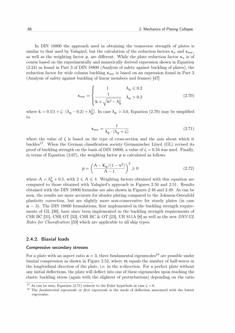
68 2. Mechanics of Plating Collapse
In DIN 18800 the approach used in obtaining the transverse strength of plates issimilar to that used by Valsgård, but the calculation of the reduction factors κx and κwc,as well as the weighting factor ρ, are different. While the plate reduction factor κx is ofcourse based on the experimentally and numerically derived expression shown in Equation(2.24) as found in Part 3 of DIN 18800 (Analysis of safety against buckling of plates), thereduction factor for wide column buckling κwc is based on an expression found in Part 2(Analysis of safety against buckling of linear members and frames) [47]
κwc =
1 λy 6 0.21
k+√k2 − λ2
y
λy > 0.2 (2.70)
where k = 0.5[1+ ζ · (λy − 0.2) + λ2y]. In case λy > 3.0, Equation (2.70) may be simplified
to
κwc =1
λy · (λy + ζ)(2.71)
where the value of ζ is based on the type of cross-section and the axis about which itbuckles17. When the German classification society Germanischer Lloyd (GL) revised itsproof of buckling strength on the basis of DIN 18800, a value of ζ = 0.34 was used. Finally,in terms of Equation (2.67), the weighting factor ρ is calculated as follows
ρ =
(Λ− Ky/(1− ν2)
Λ− 1
)2
> 0 (2.72)
where Λ = λ2y + 0.5, with 2 6 Λ 6 4. Weighting factors obtained with this equation are
compared to those obtained with Valsgård’s approach in Figures 2.50 and 2.51. Resultsobtained with the DIN 18800 formulae are also shown in Figures 2.48 and 2.49. As can beseen, the results are more accurate for slender plating compared to the Johnson-Ostenfeldplasticity correction, but are slightly more non-conservative for sturdy plates (in caseα = 3). The DIN 18800 formulations, first implemented in the buckling strength require-ments of GL [30], have since been implemented in the buckling strength requirements ofCSR BC [31], CSR OT [32], CSR BC & OT [23], UR S11A [8] as well as the new DNVGLRules for Classification [33] which are applicable to all ship types.
2.4.2. Biaxial loads
Compressive secondary stresses
For a plate with an aspect ratio α = 3, three fundamental eigenmodes18 are possible underbiaxial compression as shown in Figure 2.52, where m equals the number of half-waves inthe longitudinal direction of the plate, i.e. in the x-direction. For a perfect plate withoutany initial deflections, the plate will deflect into one of these eigenmodes upon reaching theelastic buckling stress (again with the slightest of perturbations) depending on the ratio
17 As can be seen, Equation (2.71) reduces to the Euler hyperbola in case ζ = 0.18 The fundamental eigenmode or first eigenmode is the mode of deflection associated with the lowest
eigenvalue.

2.4. Effects of plate aspect ratio 69
of stresses in the x- and y-directions (c = σy/σx). In case of real plates (which alwayshave some level of initial deflections), the plate may snap into its fundamental eigenmodeprovided the magnitude of initial deflection is sufficiently small. With initial deflections ofgreater magnitude, the energy required for this to occur may be too great for any modechange to occur. This in turn leads to a higher plate capacity than if the plate deflectsaccording to its fundamental eigenmode, a fact which has implications for choosing initialdeflection shapes and magnitudes in finite element analyses (as discussed in Appendix B).
1
XYZ
run id 13399
NOV 9 201518:42:10
PLOT NO. 2
DISPLACEMENT
STEP=1SUB =1FREQ=38.9238DMX =1
(a) m = 1
1
XYZ
run id 13399
NOV 9 201518:45:45
PLOT NO. 3
DISPLACEMENT
STEP=1SUB =1FREQ=297.135DMX =1
(b) m = 2
1
XYZ
run id 13399
NOV 9 201518:38:38
PLOT NO. 1
DISPLACEMENT
STEP=1SUB =1FREQ=125.4DMX =1
(c) m = 3
Figure 0.1: ——-CROP!——–CROP!——–CROP!——–CROP!——–CROP!———CROP!———
1
Figure 2.52.: Fundamental eigenmode shapes.
0.00
0.05
0.10
0.15
0.20
0.25
0.30
0.0 0.1 0.2 0.3 0.4 0.5 0.6 0.7
Nor
malise
d s
tres
s, σ
y/σ
Y
Normalised stress, σx/σY
critical mode shape change
c = 0.372
c = 0.161
m = 2
m = 3
m = 1
ultimate capacity curve
buckling capacity curve
m = 1
m = 2
m = 3
Figure 2.53.: Ultimate capacity curve for rectangular plate (α = 3, β = 3).
In Figure 2.53 the tangent c = σy/σx = 0.161 indicates the transition ratio be-tween eigenmodes with m = 1 half-wave and m = 2 half-waves. Similarly, the tangentc = σy/σx = 0.372 indicates the transition ratio between eigenmodes with m = 2 half-waves and m = 3 half-waves. These transition values of c remain constant for all plateswith an aspect ratio α = 3, regardless of the plate slenderness parameter β. This is evidentin the following condition provided by Paik and Thayamballi [35] with which to determinethe buckling half-wave number, m

70 2. Mechanics of Plating Collapse
(m2/a2 + 1/b2)2
m2/a2 + c/b2 6[(m+ 1)2/a2 + 1/b2]2
(m+ 1)2/a2 + c/b2 (2.73)
For a plate of slenderness β = 3, Figure 2.53 also shows the buckling capacity curve aswell as segments of the capacity curves using initial deflection shapes based on the threefundamental eigenmodes shown in Figure 2.52 (δ0 = b/200). As can be seen, for an idealplate (or plate with small initial deflections), the plate will buckle into three half-waves inthe x-direction when c 6 0.161, which is then the critical deflection shape at collapse. Sim-ilarly, an ideal plate (or plate with small initial deflections) will buckle into one half-wavein the x-direction when c > 0.372, which is then the critical deflection shape at collapse.However, although an ideal plate (or plate with small initial deflections) will buckle intotwo half-waves in the x-direction when 0.161 < c < 0.372, this is not the critical deflectionshape at collapse. Rather, the critical deflection shape is either m = 1 or m = 3 dependingon the value of c. Here the change in critical mode shape at collapse (i.e. between m = 3and m = 1) occurs at c = σy/σx = 0.167. Accordingly, whereas the ultimate capacitycurve for square plates are always symmetric (see the right-hand side of Figure 2.18), plateswith an aspect ratio α >
√2 (according to Equation (2.73) when c = 0) will in general
have a discontinuity in the ultimate capacity curve where the critical mode shape changes.Plates with irregular initial deflections of large magnitudes will be discussed in Chapter 5.
-1.0
-0.8
-0.6
-0.4
-0.2
0.0
0.2
0.4
0.6
-1.2 -1.0 -0.8 -0.6 -0.4 -0.2 0.0 0.2 0.4 0.6 0.8 1.0 1.2
Nor
mal
ised
str
ess,
σy/σ
Y
Normalised stress, σx/σY
ultimate capacity curve
von Mises ellipse
κx = 0.611
κy = 0.262
Quadrant 2
Quadrant 4
von Mises ellipse
a
b y
x
σy
σx
a
b y
x σx
σy
Figure 2.54.: Capacity curves for rectangular plate under tension (α = 3, β = 3).
Tensile secondary stresses
In case of tensile secondary stresses, the capacity curves of plates with an aspect ratioα = 3 are shown in Figure 2.54 where the ultimate capacity curve shown in Figure 2.53

2.4. Effects of plate aspect ratio 71
is extended beyond Quadrant 1 to show the effects of tensile stresses. To help illustratethe effect of tensile stresses, reference lines are drawn for the capacity of the plate underuniaxial compressive loads (i.e. κx = 0.611 and κy = 0.262). Under a uniaxial compressiveload in the y-direction, as explained in §2.4.1, yielding initiates at the mid-breadth edgesof the plate (i.e. y = b/2, see inset in Figure 2.54), where the (compressive) transversestresses σy,i and (tensile) longitudinal stresses σx,i are working together to deform theplate material. With the application of a tensile secondary stress in the x-direction, thefirst order effect is an increase of tensile stresses σx,i in the middle plane of the plate.However, in terms of plate capacity, the more significant second order effect of appliedtensile stresses in the x-direction is to restrain out-of-plane deflections, thereby mitigat-ing the redistribution of compressive stresses σy,i towards the short edges of the plate,i.e. increasing the effective length am of the plate.
1
X
Y
Z
run id 13307
NOV 11 201523:26:21
PLOT NO. 3
VECTOR
STEP=1SUB =56TIME=.235967SMIDDLE
PRIN1PRIN2PRIN3
(a) Rx = 0
1
X
Y
Z
run id 133115
NOV 15 201517:05:19
PLOT NO. 2
VECTOR
STEP=1SUB =91TIME=.415389SMIDDLE
PRIN1PRIN2PRIN3
(b) Rx = −0.40
Figure 0.1: ——-CROP!——–CROP!——–CROP!——–CROP!——–CROP!———CROP!———
1
Figure 2.55.: Principle stresses in middle plane of rectangular plate (α = 3, β = 3) - Quadrant 2.
This can be seen in the distribution of principal stresses in the middle plane of theplate at collapse. In Figure 2.55(a), these stresses show that the transverse load is takenby an effective length of plating concentrated at the short edges of the plate. For the plateunder consideration (α = 3, β = 3), capacity increases with tensile stresses applied in thex-direction, reaching a maximum at about σx ∼ −0.40 · σY . For this stress combination,the distribution of principal stresses in the middle plane of the plate at collapse are shownin Figure 2.55(b). As can be seen in the distribution of principal stresses (normalised
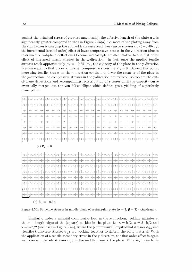
72 2. Mechanics of Plating Collapse
against the principal stress of greatest magnitude), the effective length of the plate am issignificantly greater compared to that in Figure 2.55(a), i.e. more of the plating away fromthe short edges is carrying the applied transverse load. For tensile stresses σx < −0.40 ·σY ,the incremental (second order) effect of lower compressive stresses in the y-direction (due torestrained out-of-plane deflections) become increasingly smaller relative to the first ordereffect of increased tensile stresses in the x-direction. In fact, once the applied tensilestresses reach approximately σx = −0.65 · σY , the capacity of the plate in the y-directionis again equal to that under a uniaxial compressive stress, i.e. σx = 0. Beyond this point,increasing tensile stresses in the x-direction continue to lower the capacity of the plate inthe y-direction. As compressive stresses in the y-direction are reduced, so too are the out-of-plane deflections and accompanying redistribution of stresses until the capacity curveeventually merges into the von Mises ellipse which defines gross yielding of a perfectlyplane plate.
1
X
Y
Z
run id 13301
NOV 11 201522:50:13
PLOT NO. 2
VECTOR
STEP=1SUB =107TIME=.55027SMIDDLE
PRIN1PRIN2PRIN3
(a) Ry = 0
1
X
Y
Z
run id 133235
NOV 15 201517:01:08
PLOT NO. 1
VECTOR
STEP=1SUB =136TIME=.965204SMIDDLE
PRIN1PRIN2PRIN3
(b) Ry = −0.35
Figure 0.1: ——-CROP!——–CROP!——–CROP!——–CROP!——–CROP!———CROP!———
1
Figure 2.56.: Principle stresses in middle plane of rectangular plate (α = 3, β = 3) - Quadrant 4.
Similarly, under a uniaxial compressive load in the x-direction, yielding initiates atthe mid-length edges of the (square) buckles in the plate, i.e. x = b/2, x = 3 · b/2 andx = 5 ·b/2 (see inset in Figure 2.54), where the (compressive) longitudinal stresses σx,i and(tensile) transverse stresses σy,i are working together to deform the plate material. Withthe application of a tensile secondary stress in the y-direction, the first order effect is againan increase of tensile stresses σy,i in the middle plane of the plate. More significantly, in

2.4. Effects of plate aspect ratio 73
terms of plate capacity, the second order effect of applied tensile stresses in the y-directionis to restrain out-of-plane deflections, thereby mitigating the redistribution of compressivestresses σx,i towards the long edges of the plate (i.e. increasing the effective width bm ofthe plate). In fact, because transverse tensile stresses are more effective at restraining out-of-plane deflections (i.e. acting along the entire length of the plate and across its relativelyshort breadth), the second order effects in Quadrant 4 are even greater than those inQuadrant 2. Accordingly, as shown in Figure 2.54, the corresponding increase in capacityis markedly greater with the maximum increase under a tensile stress of σy ∼ −0.35 · σYoccurring comparably close to the von Mises ellipse.
The foregoing effects of tensile secondary stresses can again be seen in the distributionof principal stresses in the middle plane of the plate at collapse. In the absence of tensilesecondary stresses, the redistribution of compression stresses σx,i towards the long edgeof the plate is clearly visible in Figure 2.56(a). Moreover, the out-of-plane deflectionsassociated with a buckled plated are clearly reflected in the redistribution of transversestresses σy,i. Conversely, in the presence of tensile secondary stresses (σy ∼ −0.35 · σY),the mitigation of out-of-plane deflections is such that the distribution of principal stressesin the middle plane of the plate look similar to those of a plate which has collapsed undergross yielding without any buckling. Accordingly, in Quadrant 4 the capacity of platingin the x-direction is generally greater under tensile secondary stresses, excluding thosestress combinations lying on the von Mises ellipse. As will be shown in Chapter 4, thisdemonstrable increase of capacity under tensile loads enables an approach to calculatingultimate plate capacity in Quadrants 2 and 4 which has heretofore not been used in theshipbuilding industry.
2.4.3. In-plane shear
Description of collapse
As in the case of ideal square plates, the principal in-plane stresses of ideal (pre-buckled)rectangular plates under a pure shear load τxy are again oriented ±45◦ to the x-axis withmagnitudes σ1 = −τxy (tension) and σ2 = τxy (compression). Although the stabilising in-fluence of a tensile stress perpendicular to the compression stress (and of equal magnitude)again ensures that the elastic buckling strength of plates under pure shear is generallyhigher than that under a uniaxial load, it does decrease with the plate aspect ratio αaccording to the equation for the buckling factor Kτ = 5.34 + 4/α2. As in the case ofrectangular plates under transverse compression, this loss of strength reflects the dimin-ishing effect of the out-of-plane restraint at the short edges of the plate, i.e. a function ofthe plate aspect ratio α. Once the shear buckling strength is exceeded, the post-buckleddeflection shape of rectangular plates is generally characterised by multiple shear bucklesrather than a single shear buckle as in the case of square plates. The number of shearbuckles depends on the plate aspect ratio α, where shear buckles with an aspect ratio of1.25 generally minimise the internal strain energy of the plate [9]. Accordingly, as shownin Figure 2.57, plates with an aspect ratio of α = 3 develop 3/1.25 ∼ 2 buckles while plateswith an aspect ratio of α = 5 develop 5/1.25 = 4 buckles.
Therefore, because rectangular plates under pure shear behave as a series of plateswith an aspect ratio α = 1.25, the post-buckling, post-yield and post-collapse phases ofthe response are similar to that for a square plate (as described in §2.3), including thedevelopment of influential tension bands. Initial yield of rectangular plates again occurs in

74 2. Mechanics of Plating Collapse
1
XYZ
run id 23107
NOV 16 201516:05:55
PLOT NO. 1
DISPLACEMENT
STEP=1SUB =1FREQ=271.449DMX =.996539
1
XYZ
run id 23107
NOV 16 201517:21:36
PLOT NO. 6
DISPLACEMENT
STEP=1SUB =1FREQ=455.457DMX =1
1
XYZ
run id 23107
NOV 16 201517:02:15
PLOT NO. 5
DISPLACEMENT
STEP=1SUB =1FREQ=286.562DMX =.988642
α = 1
α = 3
α = 5
α = 1
α = 3
α = 5
α = 1
α = 3
α = 5
Figure 2.57.: Eigenmodes under pure shear.
0.0
0.1
0.2
0.3
0.4
0.5
0.6
0.7
0.8
0.9
1.0
0.0 0.5 1.0 1.5 2.0 2.5 3.0 3.5 4.0
Red
uctio
n factor, κ
τ
Plate slenderness parameter, β
13,15 cm
13,8 cm 0,32 cm
23,46 cm
α = 1
α = 5
α = 3
α = 10
Figure 2.58.: Reduction factor curves.
1
X
Y
Z
run id 23307
NOV 17 201510:00:12
PLOT NO. 1
VECTOR
STEP=1SUB =131TIME=.769238SMIDDLE
PRIN1PRIN2PRIN3
XXXX
Figure 2.59.: Principle stresses at collapse in middle plane of rectangular plate under pure shear(α = 3, β = 3).
the centre of these bands where tensile stresses are dominant and working together with(perpendicular) compressive stresses to deform the material. With further increases inshear load, plastic flow again begins to spread throughout the middle plane of the plate,particularly in the central portion of the tension band, until the collapse strength of theplate is reached. The influence of aspect ratio α on this strength is shown in Figure 2.58 forplates with initial deflections (δ0 = b/200). As reflected in the buckling factor Kτ, it canbe seen that the effect of the plate aspect ratio α diminishes exponentially (as in the caseof rectangular plates under pure transverse loads). For a plate with an aspect ratio α = 3and slenderness β = 3 (indicated by the marker in Figure 2.58), the principal stresses inthe middle plane of the plate at collapse are shown in Figure 2.59. Here the tension bands

2.4. Effects of plate aspect ratio 75
which develop throughout plating response are again highlighted.
Formulae for reduction factors from literature
In §2.3.4 formulae for deriving plate reduction factors associated with pure shear were de-scribed and compared to numerical results for square plates. In terms of formulae found inthe literature, those of Paik (Equation (2.56)), Nara et al. (Equation (2.57)) and Zhang etal. (Equation (2.58)) are compared in Figures 2.60 and 2.61 to numerical results for plateswith aspect ratios α = 3 and α = 5, respectively. As noted previously, Paik’s solution isalways calculated for a plate aspect ratio α = 1 such that results using his solution becomeprogressively non-conservative with increasing plate aspect ratios. Conversely, whereas thesolution of Nara et al. is rather conservative for square plates, results using this solutiongradually approach those of the numerical results with increasing values of the plate as-pect ratio α. Similarly, results using the solution of Zhang et al. also approach those of thenumerical results for plate aspect ratios α > 1, although the slope of the reduction curveis somewhat low (compared to that of the numerical results) such that results for slenderplates tend to become non-conservative.
Nara et al.
Zhang et al.
0.0
0.1
0.2
0.3
0.4
0.5
0.6
0.7
0.8
0.9
1.0
0.0 0.5 1.0 1.5 2.0 2.5 3.0 3.5 4.0
Red
uct
ion fact
or,
κτ
Plate slenderness parameter, β
collapse strength
13,15 cm
13,8 cm 0,32 cm
23,46 cm
Paik
Figure 2.60.: Reduction factor curves fromliterature (α = 3).
Nara et al.
Zhang et al.
0.0
0.1
0.2
0.3
0.4
0.5
0.6
0.7
0.8
0.9
1.0
0.0 0.5 1.0 1.5 2.0 2.5 3.0 3.5 4.0
Red
uction
facto
r, κτ
Plate slenderness parameter, β
collapse strength
13,15 cm
13,8 cm 0,32 cm
23,46 cm
Paik
Figure 2.61.: Reduction factor curves fromliterature (α = 5).
Formulae for reduction factors used in shipbuilding
In terms of the classification of ships, two proofs for the ultimate shear strength of plateswidely used in the shipbuilding industry were presented in §2.3.4. The first proof is basedon the Johnson-Ostenfeld correction which is used to adjust the elastic shear buckling curveto account for plasticity (Equation (2.59)) and the second proof is based on the ultimate
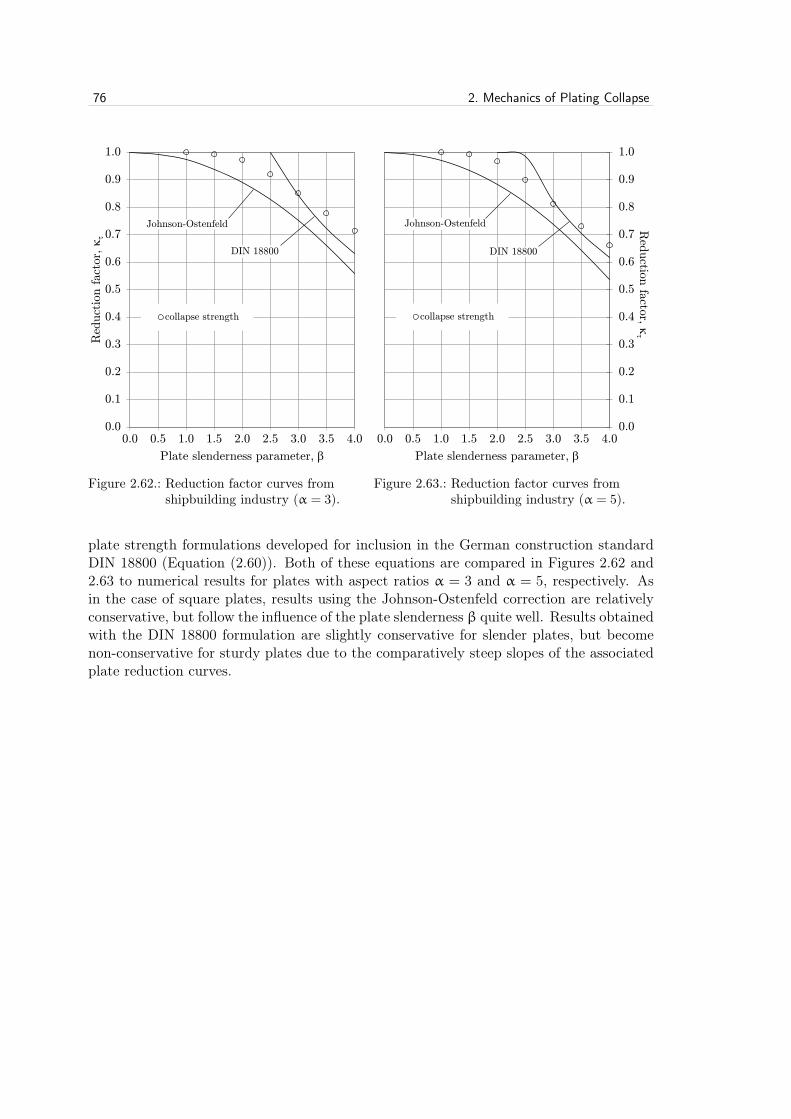
76 2. Mechanics of Plating Collapse
DIN 18800
0.0
0.1
0.2
0.3
0.4
0.5
0.6
0.7
0.8
0.9
1.0
0.0 0.5 1.0 1.5 2.0 2.5 3.0 3.5 4.0
Red
uct
ion fact
or,
κτ
Plate slenderness parameter, β
collapse strength
13,15 cm
13,8 cm 0,32 cm
23,46 cm
Johnson-Ostenfeld
Figure 2.62.: Reduction factor curves fromshipbuilding industry (α = 3).
Johnson-Ostenfeld
0.0
0.1
0.2
0.3
0.4
0.5
0.6
0.7
0.8
0.9
1.0
0.0 0.5 1.0 1.5 2.0 2.5 3.0 3.5 4.0
Red
uction
facto
r, κτ
Plate slenderness parameter, β
collapse strength
13,15 cm
13,8 cm 0,32 cm
23,46 cm
DIN 18800
Figure 2.63.: Reduction factor curves fromshipbuilding industry (α = 5).
plate strength formulations developed for inclusion in the German construction standardDIN 18800 (Equation (2.60)). Both of these equations are compared in Figures 2.62 and2.63 to numerical results for plates with aspect ratios α = 3 and α = 5, respectively. Asin the case of square plates, results using the Johnson-Ostenfeld correction are relativelyconservative, but follow the influence of the plate slenderness β quite well. Results obtainedwith the DIN 18800 formulation are slightly conservative for slender plates, but becomenon-conservative for sturdy plates due to the comparatively steep slopes of the associatedplate reduction curves.

3. Existing Proofs
In Chapter 1 the need for a proof of plate capacity with which to reliably and efficientlydesign ship plating was discussed. The purpose of this chapter is to describe existing proofsof plate capacity found in literature and the shipbuilding industry, as well as to measurethe accuracy and precision of each. With respect to the latter, an evaluation scheme ispresented in §3.1 which measures both accuracy (or bias) and precision over a wide range ofload combinations and plating configurations relevant for the shipbuilding industry. Sinceproofs of plate capacity are normally used for assessing structures anywhere in the ship, itis important that they be robust as well as precise and without bias. Using this evaluationscheme, existing proofs from literature are assessed in §3.2, followed by proofs from theshipbuilding industry in §3.3.
3.1. Quantitative evaluation scheme
In this section the quantitative evaluation scheme used to assess existing proofs of platecapacity in subsequent sections is described. Here the capacity according to the proofs iscompared against the capacity according to finite element analyses. Firstly, the aspectsof bias and precision are discussed (§3.1.1), followed by the aspect of robustness (§3.1.2).The evaluation scheme presented in this section is also used later in Chapter 4 to assessthe accuracy and precision of the new proof of plate capacity.
3.1.1. Precision and bias
As noted in §2.3.5, the capacity of plates under combined axial, transverse and shear loadsis described by a failure surface in three dimensions. Each point on the failure surface isexpressed in terms of a stress vector with three components
R = Rx i+ Ry j+ Rτ k (3.1)
where i, j and k are unit vectors and the magnitude of the stress vector R is normallydefined by
R =√R2x + R
2y + R2
τ (3.2)
However, in the definition of the buckling utilisation factor within the IACS CommonStructural Rules for Bulk Carriers and Oil Tankers [23], stresses are not first normalisedagainst yield before calculating the magnitude of stress vectors. Accordingly, in order tobe consistent with this approach, the magnitude of R in the present work is defined by
R =√R2x + R
2y + R2
τ/3 (3.3)
i.e. since Rτ = τxy/τY =√3 · τxy/σY .
77

78 3. Existing Proofs
Rproof
RFEA Rτ/√3
Ry
Rx
𝑅𝑅 = �𝑅𝑅𝑥𝑥2 + 𝑅𝑅𝑦𝑦2 + 𝑅𝑅𝜏𝜏2/3
Figure 3.1.: Magnitude of stress vectors.
0.0
0.2
0.4
0.6
0.8
1.0
1.2
0.0 0.2 0.4 0.6 0.8 1.0 1.2Norm
alise
d v
ecto
r m
agnitude,
Rpro
of
Normalised vector magnitude, RFEA
95th percentile
5th percentile
“best fit”
Figure 3.2.: Scatter of results.
As shown in Figure 3.1, when comparing the plate capacity according to a proof with theplate capacity according to finite element analyses, the direction cosines of the stress vectorassociated with the proof are defined by those of the stress vector associated with the finiteelement analyses, i.e. both stress vectors have the same unit vector
uR =RR
=Rx
Ri+
Ry
Rj+
Rτ/√3
Rk (3.4)
such that error evaluation can be based solely on the relative magnitudes of the stressvector associated with the proof (Rproof) and the stress vector associated with the finiteelement analyses (RFEA). This ratio of vector magnitudes Γ is used extensively in thequantitative evaluation scheme to measure bias and precision:
Γ =Rproof
RFEA(3.5)
such that a proof is said to be non-conservative if Γ > 1.0.Accordingly, both bias and precision of a given proof can be quantified by evaluating
the ratio of stress vector magnitudes Γ for all load combinations and plating configurations.This is represented graphically in Figure 3.2 by the scatter of Rproof against RFEA. Herethe curve of "best fit" is shown together with curves showing the 5th and 95th percentilesof the ratios Γ . In Figure 3.3, four broad characterisations of precision and bias are shown.On the basis of such plots, five key performance indicators (KPI’s) are used to measureprecision and bias for each proof.
1. Average of the squares of the residuals, Sr/ns
The first KPI is based on the differences between Rproof and RFEA. By taking the averageof the squares of these residuals, a combined measure of precision and bias is obtained

3.1. Quantitative evaluation scheme 79
0.0
0.2
0.4
0.6
0.8
1.0
1.2
0.0 0.2 0.4 0.6 0.8 1.0 1.2
Norm
alise
d v
ecto
r m
agnitude,
Rpro
of
Normalised vector magnitude, RFEA
(a) Precise without bias
0.0
0.2
0.4
0.6
0.8
1.0
1.2
0.0 0.2 0.4 0.6 0.8 1.0 1.2
Norm
alise
d v
ecto
r m
agnitude,
Rpro
of
Normalised vector magnitude, RFEA
(b) Precise with bias
0.0
0.2
0.4
0.6
0.8
1.0
1.2
0.0 0.2 0.4 0.6 0.8 1.0 1.2
Norm
alise
d v
ecto
r m
agnitude,
Rpro
of
Normalised vector magnitude, RFEA
(c) Imprecise without bias
0.0
0.2
0.4
0.6
0.8
1.0
1.2
0.0 0.2 0.4 0.6 0.8 1.0 1.2
Norm
alise
d v
ecto
r m
agnitude,
Rpro
of
Normalised vector magnitude, RFEA
(d) Imprecise with bias
Figure 0.1: ——-CROP!——–CROP!——–CROP!——–CROP!——–CROP!———CROP!——-
1
Figure 3.3.: Precision and bias.
KPI1 = Sr/ns =
ns∑i=1
(Rproof,i − RFEA,i)2
ns(3.6)
where ns is the number of evaluation points (i.e. sample size). For this KPI the targetis to be as close to zero as possible, i.e. Sr/ns → 0. This KPI is not very informative inabsolute terms, but becomes so when compared to those of other proofs.
2. Slope, mlsr
By using least square regression (without an intercept term), the second KPI is definedby the slope of the resulting straight line through the RFEA - Rproof evaluation points,thereby providing a measure of bias

80 3. Existing Proofs
KPI2 = mlsr =
ns∑i=1
(RFEA,i · Rproof,i)ns∑i=1
(RFEA,i)2(3.7)
For this KPI the target is to be as close to unity as possible, i.e. mlsr → 1.
3. Coefficient of determination, R2D
On the basis of the foregoing regression, the third KPI is defined as the coefficient ofdetermination R2
D which provides a measure of precision
KPI3 = R2D = 1−
ns∑i=1
(Rproof,i −mlsr · RFEA,i)2
ns∑i=1
(Rproof,i − Rproof,mean)2(3.8)
For this KPI the target is also to be as close to unity as possible, i.e. R2D → 1.
4. Slope of 95th percentile, m95
Although the preceding KPI’s provide useful information about bias and precision in aproof, neither gives any direct measure of non-conservatism. In shipbuilding it is importantto know the magnitude of any inherent non-conservatism in plate capacity formulations.Accordingly, the fourth KPI is the slope of a straight line through the 95th percentile ofthe RFEA - Rproof evaluation points, m95, which excludes the undue influence of outliers.This measure is useful in the determination of partial safety factors, the target of which isto be as close to unity as possible, i.e. m95 → 1.
5. Slope of 5th percentile, m5
Conversely, in shipbuilding it is also important to know the magnitude of any inherentconservatism in plate capacity formulations. Accordingly, the fifth KPI is the slope of astraight line through the 5th percentile of the RFEA - Rproof evaluation points, m5. Thismeasure is useful in gauging the over-design inherent in a proof of plate capacity whichleads to a weight penalty that must be borne throughout the ship’s service life. The targetof this KPI is again to be as close to unity as possible, i.e. m5 → 1.
3.1.2. Robustness
Measurements of bias and precision are meaningless unless the sample upon which theyare based is representative of the design space. Since proofs of plate capacity are used byshipbuilders for a wide variety of ship structures, it is imperative that they are sufficientlyrobust (unfortunately history is replete with catastrophic structural failures due to theuse of engineering formulae beyond the boundaries of their validity [9]). In the context of

3.1. Quantitative evaluation scheme 81
a capacity equation for ship plating, this design space is defined by the intersection of acontinuous set of load combinations and a continuous set of plating configurations, bothof which need to be delimited and discretised within the quantitative evaluation scheme.
Load combinations
Because axial, transverse and shear stresses combine in an infinite number of ways to forma three-dimensional failure surface, the first step in the discretisation of this surface isto equally divide the surface into four discrete levels of shear; Rτ = 0, Rτ = 0.25 · κτ,Rτ = 0.50 · κτ and Rτ = 0.75 · κτ. The shear value Rτ = κτ is omitted since in this caseRx = Ry = 0, i.e. the capacity of the plate under pure shear is (by definition) directly de-fined by the plate reduction factor κτ. Furthermore, negative values of shear are omittedsince failure surfaces are symmetric about the Rx-Ry plane1.
This discretisation results in four concentric capacity curves in the Rx-Ry plane(i.e. four levels of shear) as shown in Figure 3.4. Accordingly, in the second step of thediscretisation, each capacity curve for a given level of shear is further divided into 12 com-binations of biaxial stresses (Rx-Ry). Four of these combinations coincide with positiveand negative values of the x- and y-axes where Ry = 0 and Rx = 0, respectively. Takencollectively with Rτ = κτ, each set of points at Rx = 0 and Ry = 0 constitute the Ry − Rτand Rx − Rτ capacity curves, respectively.
The foregoing discretisation steps result in 4 x 12 = 48 evaluation points for each plat-ing configuration. However, in order to avoid an artificial increase in the accuracy of theevaluated proofs, the 16 data points representing only yielding behaviour are not includedin the evaluation scheme. The capacity of these data points, shown as open in Figure 3.4,can be calculated using the von Mises failure criterion and are therefore assumed to haveno error. Furthermore, the capacity of the two additional evaluation points representingRx = Rτ = 0 and Ry = Rτ = 0 are also omitted since they can be directly calculated fromthe plate reduction factors κy and κx, respectively (determined in the present work byfinite element analyses). Accordingly, there remain 48 - 16 - 2 = 30 evaluation points foreach plating configuration.
Plating configurations
The configurations of simply-supported, plane and rectangular plating can be describedby two parameters; the plate aspect ratio α and the plate slenderness parameter β. Inshipbuilding the aspect ratios of plates range from α = 1 up to a maximum of aboutα = 10. However, reductions in capacity above α = 5 become increasing small and are, inany case, usually confined to the shell plating of (transversely-framed) single side skin bulkcarriers. Accordingly, three plate aspect ratios are included in the quantitative evaluationscheme used in the present work; α = 1, α = 3 and α = 5.
With respect to plate slenderness, most shipbuilding rules provide minimum slen-
1 For this reason all references to τxy and Rτ throughout the present work are to be understood as |τxy|
and |Rτ|, respectively.
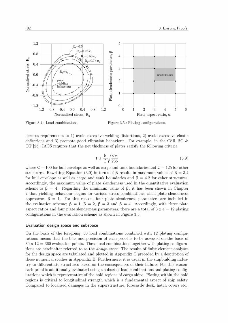
82 3. Existing Proofs
Rτ=0.0
Rτ=0.25∙κτ
Rτ=0.50∙κτ
Rτ=0.75∙κτ
-1.2
-0.8
-0.4
0.0
0.4
0.8
1.2
-1.2 -0.8 -0.4 0.0 0.4 0.8 1.2
Norm
alise
d s
tres
s, R
y
Normalised stress, Rx
pure yielding behaviour
Rτ=κτ
Figure 3.4.: Load combinations.
0
1
2
3
4
5
0 1 2 3 4 5 6P
late
sle
nder
nes
s para
met
er,
β Plate aspect ratio, α
Cargo Hold Regions
Figure 3.5.: Plating configurations.
derness requirements to 1) avoid excessive welding distortions, 2) avoid excessive elasticdeflections and 3) promote good vibration behaviour. For example, in the CSR BC &OT [23], IACS requires that the net thickness of plates satisfy the following criteria
t >b
C
√σY235
(3.9)
where C = 100 for hull envelope as well as cargo and tank boundaries and C = 125 for otherstructures. Rewriting Equation (3.9) in terms of β results in maximum values of β = 3.4for hull envelope as well as cargo and tank boundaries and β = 4.2 for other structures.Accordingly, the maximum value of plate slenderness used in the quantitative evaluationscheme is β = 4. Regarding the minimum value of β, it has been shown in Chapter2 that yielding behaviour begins for various stress combinations when plate slendernessapproaches β = 1. For this reason, four plate slenderness parameters are included inthe evaluation scheme; β = 1, β = 2, β = 3 and β = 4. Accordingly, with three plateaspect ratios and four plate slenderness parameters, there are a total of 3 x 4 = 12 platingconfigurations in the evaluation scheme as shown in Figure 3.5.
Evaluation design space and subspace
On the basis of the foregoing, 30 load combinations combined with 12 plating configu-rations means that the bias and precision of each proof is to be assessed on the basis of30 x 12 = 360 evaluation points. These load combinations together with plating configura-tions are hereinafter referred to as the design space. The results of finite element analysesfor the design space are tabulated and plotted in Appendix C preceded by a description ofthese numerical studies in Appendix B. Furthermore, it is usual in the shipbuilding indus-try to differentiate structures based on the consequences of their failure. For this reason,each proof is additionally evaluated using a subset of load combinations and plating config-urations which is representative of the hold regions of cargo ships. Plating within the holdregions is critical to longitudinal strength which is a fundamental aspect of ship safety.Compared to localised damages in the superstructure, forecastle deck, hatch covers etc.,
3.2. Proofs from literature 83
failure of plating in the cargo hold regions may endanger the structural integrity of theship. Typically, plating in the hold regions is characterised by an aspect ratio betweenα = 3 and α = 5 and a slenderness parameter between β = 2 and β = 3 (see Figure 3.5).Moreover, the critical stress combinations for plating in these regions usually involve com-pressive biaxial stresses (i.e. Quadrant 1). As a result, each proof is additionally assessedfor a subset of load combinations and plating configurations represented by 2 x 2 x 14 = 56evaluation points, hereinafter referred to as the design subspace.
3.2. Proofs from literature
In 1969 the Ship Structure Committee (SSC) released a feasibility study for a programmeof ultimate strength tests on ship structural elements (i.e. unstiffened plates, stiffenedplates and grillages) [48]. Following a detailed review of the state-of-the-art, it was thereinconcluded that there was no published theoretical or experimental material on the ultimatestrength of any structural elements under biaxial compression. In the following year resultsfrom the initial phase of an ensuing SSC project were reported where the compressivestrength of unstiffened plates was addressed (the effects of shear were listed among thetopics to be investigated after the initial phase was completed) [49]. Within this initialphase, compression tests on square tubes were conducted in order to obtain a large amountof experimental data on the ultimate strength of plating under various combinations ofbiaxial loading (sometimes with lateral pressure).
In order to support the experimental data with theoretical explanations, the reportincluded biaxial strength hypotheses. For small b/t ratios (in this case b/t = 30 andb/t = 50), biaxial failure was expected to occur under plastic buckling involving the entireplate. Accordingly, a modified (elastic) buckling interaction curve was used where they-axis was left unchanged (since transverse buckling was assumed to result in failure) andthe x-axis was divided by four (thereby transforming the elastic buckling factor Kx = 4.0into the stress ratio Rx = 1.0). However, on the basis of the test results, a differenthypothesis was required for plates of larger b/t ratios (in this case b/t = 70 and b/t = 90).As noted in §2.4.2, plating with an aspect ratio α >
√2 develops a number of buckle-
induced node or ridge lines in the transverse direction depending on the ratio of σx andσy (acting like "invisible stiffeners" in the words of the authors). The effective breadthof plating on each side of these ridge lines (in addition to that on the ends of the plate)theoretically gives slender plating the post-buckling strength needed to agree with observedtest results. However, the authors concede that "(t)he hypothesis of multiple flange failuremodes represents an attempt to characterize the ultimate load behaviour of a biaxiallycompressed plate in terms of well known phenomena. At present it is an engineeringapproach of a conceptual nature. The evolution of a rigorous solution must be deferred toa subsequent investigation".
Indeed several authors in subsequent years investigated the capacity of plating undercombined in-plane loads with solutions almost always expressed in terms of a generalisedform of the von Mises failure criterion
(σx
κx · σY
)e1
+
(σy
κy · σY
)e2
− B ·(
σx
κx · σY
)·(
σy
κy · σY
)+
(τxy
κτ · τY
)e3
= 1.0 (3.10)

84 3. Existing Proofs
or (Rx
κx
)e1
+
(Ry
κy
)e2
− B ·(Rx
κx
)·(Ry
κy
)+
(Rτ
κτ
)e3
= 1.0 (3.11)
in terms of normalised stresses.Based on the aforementioned compression tests, Faulkner et al. [46] proposed a parabolic
relationship to describe the capacity of plating under compressive biaxial stresses(Rx
κx
)+
(Ry
κy
)2
= 1.0 (3.12)
where e1 = 1, e2 = 2 and B = 0 in terms of Equation (3.11). Typical of earlier efforts, thesolution accounts neither for the effects of shear loading nor tensile stresses. Nevertheless,Valsgård [34] notes that Equation (3.12) was incorporated in the offshore design codeof Det norske Veritas (DnV) [50] (although this could not be confirmed by the author).By choosing various values for B > 0, Valsgård produced skewed variations of Faulkner’sparabolic interaction equation. Comparing these variations to his own numerical resultsfor plates with an aspect ratio α = 3, Valsgård concluded that B = 0.25 fits the numericaldata "reasonably well", i.e.(
Rx
κx
)+
(Ry
κy
)2
− 0.25 ·(Rx
κx
)·(Ry
κy
)= 1.0 (3.13)
When incorporating his interaction equation in a design code formulation, Valsgård ac-counted for the effect of shear loading using a reduced yield stress according to Equation(2.61), i.e.
σ ′Y =√σ2Y − 3 · τ2
xy (3.14)
As noted in §2.3.5, this is a widely used approach whenever plate failure is not dominatedby shear buckling.
In this section one of the most recent attempts to derive a capacity equation basedon the generalised form of the von Mises failure criterion will be examined. In his reportto the American Bureau of Shipping [43], Paik presents a proof that is one of the few todirectly account for both shear loading and tensile stresses. Subsequently, a rather uniqueproof developed by Ueda et al. is also examined [51]. While almost all proofs of platecapacity use a generalised form of the von Mises failure criterion, the proof of Ueda et al.provide so-called stress coefficients which enable the calculation of stresses at each of thehot spots identified in Figure 2.15 (but for plates of any aspect ratio α). Knowing howthe applied stresses are distributed throughout the plate enables direct use of von Misescriterion to calculate yielding (i.e. a precursor to collapse).
3.2.1. Paik
Based on insights gleaned from a series of non-linear finite element analyses where bothload ratios and plate aspect ratios were varied, Paik [43] (as referenced in [44]) proposed aproof based on the generalised form of the von Mises failure criterion shown in Equation(3.11) where e1 = e2 = e3 = 2 and B = 0 when both axial stresses are compressive andB = 1 when either are tensile, i.e.

3.2. Proofs from literature 85
(Rx
κx
)2
+
(Ry
κy
)2
+
(Rτ
κτ
)2
= 1.0 (3.15)
when Rx > 0 and Ry > 0, and(Rx
κx
)2
+
(Ry
κy
)2
−
(Rx
κx
)·(Ry
κy
)+
(Rτ
κτ
)2
= 1.0 (3.16)
when Rx < 0 or Ry < 0.
Bias and Precision
In accordance with the evaluation scheme described in §3.1, Paik’s proof has been used tocalculate the capacity of plating for the 360 evaluation points. The resulting scatter plotsfor both the design space and design subspace are shown in Figure 3.6. The five key per-formance indicators used to measure precision and bias are shown in Table 3.1. Regardingthe overall measure of error (KPI1), the average of the squares of the residuals Sr/ns issomewhat high for the design space (Sr/ns = 0.011), but very low for the design subspace(Sr/ns = 0.001)2. With respect to the measure of bias (KPI2), the least-squares fit ofa straight line through the RFEA − Rproof data points gives a moderately/significantlyconservative slope for the design space (mlsr = 0.91) and a slightly non-conservativeslope for the design subspace (mlsr = 1.03). Concerning the measure of precision (KPI3),the coefficients of determination reflect a high degree of scatter for the design space(RD2 = 0.72), but a very low degree of scatter for the design subspace (RD2 = 0.95).Regarding the extent of non-conservatism (KPI4), a straight line through the 95th per-centile gives a significantly non-conservative slope for both the design space (m95 = 1.18)and design subspace (m95 = 1.13). With respect to the extent of conservatism (KPI5), astraight line through the 5th percentile gives an extremely conservative slope for the designspace (m5 = 0.73) and a slightly/moderately conservative slope for the design subspace(m5 = 0.95).
Design space Design subspace Target
1 Sr/ns 0.011 0.001 0.000
2 mlsr 0.91 1.03 1.00
3 RD2 0.72 0.95 1.00
4 m95 1.18 1.13 1.00
5 m5 0.73 0.95 1.00
KPI
Table 3.1.: Key performance indicators (Paik).
In order to identify any inherent problems within Paik’s proof for specific parameters,the mean and extreme values of the ratio of stress vector magnitudes, Γ = Rproof/RFEA,are shown in Figure 3.7 for each value of plate aspect ratio (α), plate slenderness parameter
2 The adjectives used throughout all descriptions of bias and precision (e.g. "somewhat high", "very low"etc.) reflect relative degrees of bias and precision. These adjectives are based on the total ranges ofbias and precision taken collectively for all existing proofs.

86 3. Existing Proofs
m95
m5
mlsr
0.0
0.2
0.4
0.6
0.8
1.0
1.2
0.0 0.2 0.4 0.6 0.8 1.0 1.2
Norm
alise
d v
ecto
r m
agnitude,
Rpro
of
Normalised vector magnitude, RFEA
(a) Design space (360 evaluation points)
m95
m5
mlsr
0.0
0.2
0.4
0.6
0.8
1.0
1.2
0.0 0.2 0.4 0.6 0.8 1.0 1.2N
orm
alise
d v
ecto
r m
agnitude,
Rpro
of
Normalised vector magnitude, RFEA
(b) Design subspace (56 evaluation points)
Figure 0.1: ——-CROP!——–CROP!——–CROP!——–CROP!——–CROP!———CROP!——-
1
Figure 3.6.: Scatter plots of RFEA - Rproof (Paik).
0.99 0.94 0.92
0.95 0.94 0.94 0.97
1.06
0.88 0.93
0.90 0.95 0.96 0.98
α =
1
α =
3
α =
5
β =
1
β =
2
β =
3
β =
4
Q1
Q2
Q4
Rt =
0
Rτ =
0.2
5∙κ
τ
Rτ =
0.5
0∙κ
τ
Rτ =
0.7
5∙κ
τ
95%
95%
95%
95%
95%
95%
95% 95%
95%
95% 95%
95% 95%
95%
5% 5%
5%
5%
5%
5% 5%
5%
5%
5%
5%
5% 5% 5%
0.0
0.1
0.2
0.3
0.4
0.5
0.6
0.7
0.8
0.9
1.0
1.1
1.2
1.3
1.4
1.5
1.6
1.7
1.8
1.9
2.0
Rat
io o
f st
ress
vec
tor
magn
itudes
, Γ
Figure 3.7.: Evaluation of data subsets (Paik).
(β), quadrants of compressive/tensile load combinations (Q1, Q2 and Q4) and levels ofshear (Rτ). In case of the plate aspect ratios, the mean values of Γ indicate a slightlynon-conservative bias for α = 1 and a moderately conservative bias for α = 3 and α = 5,i.e. increasing conservatism with increasing aspect ratios. The ranges of extreme valuesindicate poor to somewhat poor precision for all plate aspect ratios. In case of the plate

3.2. Proofs from literature 87
-1.2
-0.8
-0.4
0.0
0.4
0.8
1.2
-1.2 -0.8 -0.4 0.0 0.4 0.8 1.2
Norm
alise
d s
tres
s, R
y
Normalised stress, Rx
FEA Proof
(a) α = 1, β = 1, Rτ = 0.5 · κτ
-1.2
-0.8
-0.4
0.0
0.4
0.8
1.2
-1.2 -0.8 -0.4 0.0 0.4 0.8 1.2
Norm
alise
d s
tres
s, R
y
Normalised stress, Rx
FEA Proof
(b) α = 1, β = 4, Rτ = 0
Figure 0.1: ——-CROP!——–CROP!——–CROP!——–CROP!——–CROP!———CROP!——-
1
Figure 3.8.: Comparison plots (Paik).
slenderness parameters, the mean values of Γ indicate a slightly/moderately conservativebias for β = 1, moderately conservative bias for β = 2 and β = 3 and a slightly conservativebias for β = 4. The ranges of extreme values indicate very good precision for β = 1 toquite poor precision for β = 4, i.e. decreasing precision with increasing plate slendernessparameters. In case of the compressive/tensile load combinations, the mean values of Γindicate a moderately non-conservative bias in Q1, a significantly conservative bias in Q2and a moderately conservative bias in Q4. The ranges of extreme values indicate goodto somewhat good precision in all quadrants. In case of shear, the mean values of Γreveal a moderately/significantly conservative bias in the absence of shear and a slightlyto slightly/moderately conservative bias in the presence of shear, i.e. increasing accuracywith increasing levels of shear. The ranges of extreme values indicate poor precision in theabsence of shear and poor (Rτ = 0.25 · κτ) to somewhat good (Rτ = 0.75 · κτ) precisionin the presence of shear, i.e. increasing precision with increasing levels of shear (whenpresent).
In order to obtain an impression of the strengths and weaknesses of Paik’s proof, thelowest and highest values of the squares of the residuals (Sr/ns) for each combination ofplate aspect ratio (α), plate slenderness parameter (β) and level of shear (Rτ) have beencalculated. The lowest value of Sr/ns is for the combination α = 1, β = 1 and Rτ = 0.5·κτ,the capacity curve of which is plotted in Figure 3.8(a)3. Conversely, the highest value ofSr/ns is for the combination α = 1, β = 4 and Rτ = 0, the capacity curve of which is
3 The levels of shear indicated in all Rx-Ry plots are those used in the finite element analyses,i.e. Rτ = 0.25 · κτ, Rτ = 0.50 · κτ or Rτ = 0.75 · κτ. In case of results obtained with the proof,these are nominal levels of shear (except of course when Rτ = 0). This is because the unit vectors usedin the proof are the same as those used in the finite element analyses. In general this leads to platecapacities obtained with the proof having different magnitudes of shear compared to the fixed valuesof shear used in the finite element analyses. However, the degree of departure from the fixed value ofshear depends on the ratio of stress vector magnitudes Γ = Rproof/RFEA and as such can be discernedfrom results plotted in the Rx-Ry plane, i.e. the relative magnitudes of stress vectors of the proof andfinite element analyses projected onto the Rx-Ry plane.

88 3. Existing Proofs
plotted in Figure 3.8(b).
3.2.2. Ueda et al.
In §2.2.3 the distribution of internal stresses within a plate were described as a function ofthe stress ratio c = σy/σx. There it was described how stresses accumulate in three setsof "hot spots" such that yielding initiates at one or more of them (i.e. all "hot spots" incase of gross yielding). Based on the results of theoretical investigations, Ueda et al. [51]developed stress coefficients χx and χy which enable the calculation of internal stresses ateach of the hot spots identified in Figure 2.15 (shown for plates with an aspect ratio α = 1).These coefficients have been determined assuming the plate is without initial deflections.As noted above, knowing how the applied stresses are distributed throughout the plateenables direct use of von Mises criterion to calculate yielding (i.e. a precursor to collapse)
[Rx · (1+ χx)]2 + [Ry · (1+ χy)]2 − Rx · Ry · (1+ χx) · (1+ χy) + R2τ = 1 (3.17)
For a given combination of loads (i.e. a unit stress vector), the elastic buckling strengthof the plate is compared to its material yield strength (i.e. defined by χx = χy = 0). Incase the plate buckles elastically before yielding, the stress coefficients χx and χy take onnon-zero values. In case of a square plate without shear, the equations to determine thepost-buckling stress coefficients reduce to
χx,max = 1+Ry − Rx,cr
Rx(3.18a)
χx,min = −χx,max (3.18b)
χy,max = 1+Rx − Ry,cr
Ry(3.18c)
χy,min = −χy,max (3.18d)
These maximum and minimum values of χx and χy are introduced into Equation(3.17) according to the locations of initial yield
(a) in the case of yielding at mid-length edges of plate buckles; χx,max, χy,min,
(b) in the case of yielding in the corners of plate; χx,max, χy,max,
(c) in the case of yielding at mid-breadth edges of plate buckle; χx,min, χy,max.
These locations of initial yield are shown in Figure 3.9. In Figure 3.10, results obtainedwith the above stress coefficients are compared to the numerical results presented in §2.2.3(α = 1, β = 3). As shown in §2.2.3, it is in fact the value of c = σy/σx which determinesthe location of initial yield and not simply whether Rx and Ry are compressive or tensile.Accordingly, the ultimate strength of the plating is determined by gradually increasingthe applied stresses Rx and Ry until the equivalent stresses in one or more location sets,i.e. (a), (b) or (c), reach yield.

3.2. Proofs from literature 89
y
x
y
x
(b) corners (a) mid-length edges (c) mid-breadth edges
y
x
Figure 3.9.: Locations of initial yield in buckled plate (shown for α = 2)
Bias and Precision
In accordance with the evaluation scheme described in §3.1, the proof of Ueda et al. hasbeen used to calculate the capacity of plating for the 360 evaluation points. The re-sulting scatter plots for both the design space and design subspace are shown in Figure3.11. The five key performance indicators used to measure precision and bias are shownin Table 3.2. Regarding the overall measure of error (KPI1), the average of the squaresof the residuals Sr/ns is high for the design space (Sr/ns = 0.018) and very high forthe design subspace (Sr/ns = 0.038). With respect to the measure of bias (KPI2), theleast-squares fit of a straight line through the RFEA - Rproof data points gives a mod-erately/significantly non-conservative slope for the design space (mlsr = 1.11) and anextremely non-conservative slope for the design subspace (mlsr = 1.35). Concerning themeasure of precision (KPI3), the coefficients of determination reflect a very high degree ofscatter for both the design space (RD2 = 0.62) and the design subspace (RD2 = 0.57). Re-garding the extent of non-conservatism (KPI4), a straight line through the 95th percentilegives an extremely non-conservative slope for both the design space (m95 = 1.61) and de-sign subspace (m95 = 1.91). With respect to the extent of conservatism (KPI5), a straightline through the 5th percentile gives a slope without bias for the design space (m5 = 1.00)and a significantly non-conservative slope for the design subspace (m5 = 1.18).
Design space Design subspace Target
1 Sr/ns 0.018 0.038 0.000
2 mlsr 1.11 1.35 1.00
3 RD2 0.62 0.57 1.00
4 m95 1.61 1.91 1.00
5 m5 1.00 1.18 1.00
KPI
Table 3.2.: Key performance indicators (Ueda et al.).
In order to identify any inherent problems within the proof of Ueda et al. for spe-cific parameters, the mean and extreme values of the ratio of stress vector magnitudes,Γ = Rproof/RFEA, are shown in Figure 3.12 for each value of plate aspect ratio (α), plateslenderness parameter (β), quadrants of compressive/tensile load combinations (Q1, Q2and Q4) and levels of shear (Rτ). In case of the plate aspect ratios, the mean values of Γ in-dicate a moderately/significantly non-conservative bias for α = 1, a significantly/extremelynon-conservative bias for α = 3 and an extremely non-conservative bias for α = 5, i.e. in-

90 3. Existing Proofs
-1.0-0.8-0.6-0.4-0.20.00.20.40.60.81.01.2
-1.0 -0.8 -0.6 -0.4 -0.2 0.0 0.2 0.4 0.6 0.8 1.0
Inte
rnal
str
esse
s
Stress ratio, σy/σx
FEA
Ueda et al.
FEA
Ueda et al.
23,46 cm
σx,i/σY
σy,i/σY
(a) Normalised internal stresses, σx,i/σY , σy,i/σY - mid-length edges
-1.0-0.8-0.6-0.4-0.20.00.20.40.60.81.01.2
-1.0 -0.8 -0.6 -0.4 -0.2 0.0 0.2 0.4 0.6 0.8 1.0
Inte
rnal
str
esse
s
Stress ratio, σy/σx
FEA
Ueda et al.
FEA
Ueda et al.
23,46 cm
σx,i/σY
σy,i/σY
(b) Normalised internal stresses, σx,i/σY , σy,i/σY - corners
-1.0-0.8-0.6-0.4-0.20.00.20.40.60.81.01.2
-1.0 -0.8 -0.6 -0.4 -0.2 0.0 0.2 0.4 0.6 0.8 1.0
Inte
rnal
str
esse
s
Stress ratio, σy/σx
FEA
Ueda et al.
FEA
Ueda et al.
23,46 cm
σx,i/σY
σy,i/σY
(c) Normalised internal stresses, σx,i/σY , σy,i/σY - mid-breadth edges
Figure 0.1: ——-CROP!——–CROP!——–CROP!——–CROP!——–CROP!———CROP!——-Figure 3.10.: Comparisons of stress distributions in buckled plate at initial yield.
creasing non-conservatism with increasing aspect ratios. The ranges of extreme valuesindicate good precision for α = 1 to very poor precision for α = 5, i.e. decreasing precisionwith increasing plate aspect ratios. In case of the plate slenderness parameters, the meanvalues of Γ indicate a moderately/significantly non-conservative bias for β = 1 to an ex-
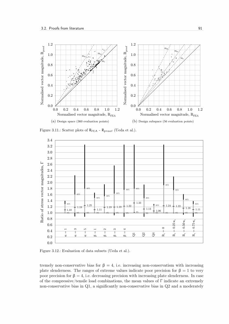
3.2. Proofs from literature 91
m95
m5
mlsr
0.0
0.2
0.4
0.6
0.8
1.0
1.2
0.0 0.2 0.4 0.6 0.8 1.0 1.2
Norm
alise
d v
ecto
r m
agnitude,
Rpro
of
Normalised vector magnitude, RFEA
(a) Design space (360 evaluation points)
m95
m5
mlsr
0.0
0.2
0.4
0.6
0.8
1.0
1.2
0.0 0.2 0.4 0.6 0.8 1.0 1.2
Norm
alise
d v
ecto
r m
agnitude,
Rpro
of
Normalised vector magnitude, RFEA
(b) Design subspace (56 evaluation points)
Figure 0.1: ——-CROP!——–CROP!——–CROP!——–CROP!——–CROP!———CROP!——-
1
Figure 3.11.: Scatter plots of RFEA - Rproof (Ueda et al.).
1.10 1.18
1.25
1.11 1.19 1.19 1.22
1.33
1.13 1.06
1.24 1.22 1.16
1.11
α =
1
α =
3
α =
5
β =
1
β =
2
β =
3
β =
4
Q1
Q2
Q4
Rt =
0
Rτ =
0.2
5∙κ
τ
Rτ =
0.5
0∙κ
τ
Rτ =
0.7
5∙κ
τ
95%
95%
95%
95% 95%
95%
95% 95%
95%
95%
95%
95%
95%
95%
5% 5% 5% 5% 5% 5% 5% 5%
5% 5% 5% 5% 5% 5%
0.0
0.2
0.4
0.6
0.8
1.0
1.2
1.4
1.6
1.8
2.0
2.2
2.4
2.6
2.8
3.0
3.2
3.4
Rat
io o
f st
ress
vec
tor
magn
itudes
, Γ
Figure 3.12.: Evaluation of data subsets (Ueda et al.).
tremely non-conservative bias for β = 4, i.e. increasing non-conservatism with increasingplate slenderness. The ranges of extreme values indicate poor precision for β = 1 to verypoor precision for β = 4, i.e. decreasing precision with increasing plate slenderness. In caseof the compressive/tensile load combinations, the mean values of Γ indicate an extremelynon-conservative bias in Q1, a significantly non-conservative bias in Q2 and a moderately

92 3. Existing Proofs
-1.2
-0.8
-0.4
0.0
0.4
0.8
1.2
-1.2 -0.8 -0.4 0.0 0.4 0.8 1.2
Norm
alise
d s
tres
s, R
y
Normalised stress, Rx
FEA Proof
(a) α = 1, β = 4, Rτ = 0
-1.2
-0.8
-0.4
0.0
0.4
0.8
1.2
-1.2 -0.8 -0.4 0.0 0.4 0.8 1.2N
orm
alise
d s
tres
s, R
y
Normalised stress, Rx
FEA Proof
(b) α = 5, β = 4, Rτ = 0
Figure 0.1: ——-CROP!——–CROP!——–CROP!——–CROP!——–CROP!———CROP!——-
1
Figure 3.13.: Comparison plots (Ueda et al.).
non-conservative bias in Q4. The ranges of extreme values indicate very poor precision inQ1, poor precision in Q2, but good precision in Q4. In case of shear, the mean values ofΓ reveal an extremely non-conservative bias for Rτ = 0 to a significantly non-conservativebias for Rτ = 0.75 · κτ, i.e. decreasing non-conservatism with increasing shear. The rangesof extreme values indicate very poor precision in the absence of shear to good precision forRτ = 0.75 · κτ, i.e. increasing precision with increasing shear.
In order to obtain an impression of the strengths and weaknesses of the proof of Uedaet al., the lowest and highest values of the squares of the residuals (Sr/ns) for each com-bination of plate aspect ratio (α), plate slenderness parameter (β) and level of shear (Rτ)have been calculated. The lowest value of Sr/ns is for the combination α = 1, β = 4 andRτ = 0, the capacity curve of which is plotted in Figure 3.13(a). Conversely, the highestvalue of Sr/ns is for the combination α = 5, β = 4 and Rτ = 0, the capacity curve ofwhich is plotted in Figure 3.13(b).
3.3. Proofs from shipbuilding practice
Almost all ships in the world’s commercial fleet are built according to the constructionstandards of classification societies. Even many non-commercial ships (e.g. navy and othergovernment vessels) are built according to standards developed specially by classificationsocieties. When a ship complies with the construction standards of a classification societyit is assigned a class designation. Regular surveys are carried out to verify that ships inservice remain in compliance with these standards. In principle, classification societiesare independent, self-regulating, externally-audited bodies. To ensure their constructionstandards keep up with the state-of-the-art, classification societies incorporate the results ofongoing, relevant research, tempered by in-service experience gained from the classificationof many types of ships over many years.
Following the International Load Line Convention of 1930 and its recommendation

3.3. Proofs from shipbuilding practice 93
that classification societies ensure "as much uniformity as possible in the application ofthe standards of strength upon which freeboard is based", the first conference of the sevenmajor classification societies was hosted by Registro Italiano Navale (RINA) in 1939 [52].The other societies in attendance were the American Bureau of Shipping (ABS), BureauVeritas (BV), Det norske Veritas (DnV), Germanischer Lloyd (GL), Lloyd’s Register (LR)and Nippon Kaiji Kyokai (ClassNK). In 1955 a second major conference was held whichled to the creation of working parties on specific topics and in 1968 the International Asso-ciation of Classification Societies (IACS) was formed. Today more than 90% of the world’scargo carrying tonnage is covered by the classification rules of IACS member societies [52].Accordingly, the most important proofs of plate capacity in shipbuilding practice can befound in the classification rules of IACS member societies. In 1989 the IACS WorkingParty on Strength (WP/S) delivered the first Unified Requirement (UR) concerning thestrength of ships which contained explicit buckling strength criteria. The IACS Longitudi-nal Strength Standard (UR S11) contains buckling strength requirements for plate panelsand longitudinals subject to hull girder bending and shear stresses based on the Johnson-Ostenfeld plasticity correction discussed in §2.1.4. However, the UR addresses axial andshear loads in isolation and does not include a capacity equation for plates under combinedin-plane loads.
Nevertheless, although IACS Unified Requirements (UR) are minimum requirementsto be incorporated into the rules of all member societies, several members declared "reser-vations" against the UR S11 proof of buckling strength, opting instead for their owncriteria. This led initially to extensive efforts within the WP/S to agree on a harmonisedproof of buckling strength which carried on into the development of the IACS commonstructural rules. Common structural rules are construction standards which are used byall IACS member societies without the possibility of reservations. In 2006 the IACS Com-mon Structural Rules for Bulk Carriers (CSR-BC) and IACS Common Structural Rulesfor Double Hull Oil Tankers (CSR-OT) came into force. Unfortunately, these two rule setswere developed independently by two different groups of IACS member societies such thatthe buckling strength rules in CSR-OT were (for all intents and purposes) based on DnV’scomputerised buckling code PULS (Panel Ultimate Limit State) while in CSR-BC theywere based on the buckling strength rules of GL (in turn based on the German construc-tion standard DIN 18800). Despite extensive efforts to harmonise the proofs of bucklingstrength in CSR-BC and CSR-OT, an agreement on a single proof could not be reached.
Therefore, in 2008 efforts were renewed to harmonise the CSR buckling strength cri-teria within the framework of the IACS Common Structural Rules for Bulk Carriers andOil Tankers (CSR BC & OT). The purpose of CSR BC & OT was to harmonise loadand strength criteria common to both bulk carriers and oil tankers (Part One) and toprovide additional requirements unique to each ship type (Part Two). Included in theformer were the buckling strength criteria for which a dedicated project team (HPT02)was established4. Following six years of discussion and analyses, it was concluded thatthe CSR BC & OT buckling strength criteria would be based on those in the GL rulesfor classification and construction. This decision was not based on accuracy and precisionalone (in this regard PULS would have been an equally acceptable choice), but also be-cause the GL proof of buckling strength possessed qualities suitable for both the printedand programmed versions of CSR BC & OT (i.e. robust, concise, transparent, physically-
4 For the sake of full disclosure, the author represented GL in WP/S, CSR-BC/CSR-OT andCSR BC & OT efforts to harmonise the IACS buckling strength criteria.

94 3. Existing Proofs
based, meaningful and dimensionally consistent quantities, easily programmable, efficientsolutions etc.). However, some changes were made to the GL proof of buckling strengthwithin the development of CSR BC & OT. In particular, in order to improve its accuracyand precision, as well as to remove the need for a Poisson correction (discussed below),the GL proof of plate capacity under combined in-plane loads was revised on the basis ofChapter 4. This revised proof has also been used in the new IACS Longitudinal StrengthStandard for Container Ships (UR S11A) as well as the new DNVGL Rules for Classifi-cation (applicable to all ship types) which were developed after the 2013 merger of DnVand GL.
Accordingly, in this section the proofs of plate capacity prior to CSR BC & OT are ex-amined. In particular, because they formed the basis of the CSR-OT and CSR-BC bucklingstrength criteria, the historical development of the DnV and GL proofs of plate capacity arediscussed. Firstly, the plate capacity proof within DnV Classification Note 30.1 (CN 30.1)will be examined followed by the plate capacity proof of GL based on DIN 4114. Bothproofs are based on elastic buckling strength analyses with a plasticity correction and arethe predecessors to the CSR proofs. Next the CSR proofs themselves will be examinedbeginning with DnV’s PULS (CSR-OT) and followed by the GL proof based on DIN 18800(CSR-BC). Finally, because the latter GL proof is based on beam stresses, modified stressvalues are needed if σx and σy contain Poisson effects (i.e. from finite element calcula-tions). Accordingly, in an attempt to simplify its use, BV developed a modified version ofthe GL proof to eliminate the need for this Poisson correction. This modified proof wasused provisionally in CSR BC & OT development and so is also examined.
3.3.1. Elastic analyses with plasticity correction (DnV and GL)
In §2.1.4 it was shown how an ultimate value of stress can be calculated using Johnson-Ostenfeld formulae to correct the elastic buckling stress of a plate for plasticity, i.e. materialnon-linearity, not geometric non-linearity. There the plate was subjected to a uniaxial stressσx. However, for a plate subjected to combined in-plane stresses (i.e. σx, σy and τxy), itis possible to describe an equivalent stress based on the von Mises equation5
σeq =√σx2 − σx · σy + σy2 + 3 · τxy2 (3.19)
and compare this to an ultimate value of equivalent stress σeq,ult which is equal to anequivalent elastic stress σeq,cr corrected for plasticity.
CN 30.1
In the earlier editions of DnV’s Classification Note 30.1 (1982 and 1984), this comparisonwas made in two steps in case of combined biaxial and shear stresses. A utilisation factorηcs was first calculated for a combination of uniaxial compression and shear and then aseparate utilisation factor ηc for the remaining uniaxial stress component. On the basisof these two utilisation factors, a final utilisation factor for combined biaxial and shearstresses was then calculated
5 This equation is the same as Equation (2.1) except that it is here intended for externally applied stresses(i.e. not internal stresses) and expanded to include shear.
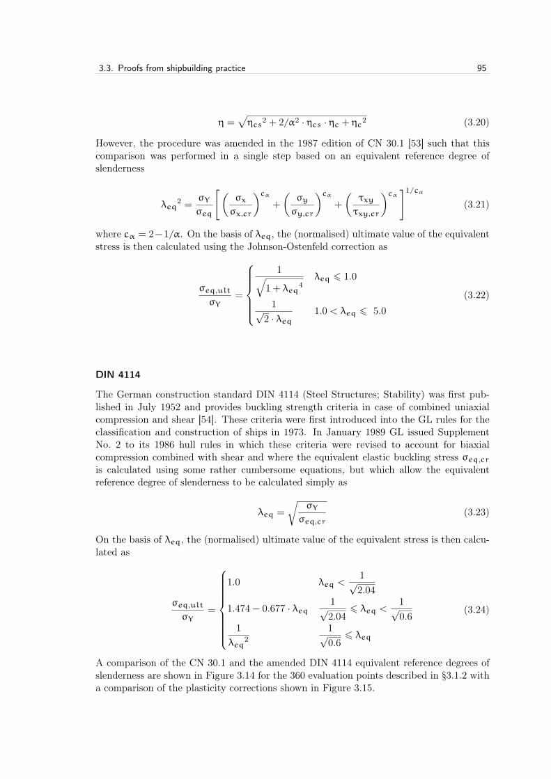
3.3. Proofs from shipbuilding practice 95
η =√ηcs2 + 2/α2 · ηcs · ηc + ηc2 (3.20)
However, the procedure was amended in the 1987 edition of CN 30.1 [53] such that thiscomparison was performed in a single step based on an equivalent reference degree ofslenderness
λeq2 =
σYσeq
[(σx
σx,cr
)cα+
(σy
σy,cr
)cα+
(τxy
τxy,cr
)cα ]1/cα
(3.21)
where cα = 2−1/α. On the basis of λeq, the (normalised) ultimate value of the equivalentstress is then calculated using the Johnson-Ostenfeld correction as
σeq,ult
σY=
1√
1+ λeq4λeq 6 1.0
1√2 · λeq
1.0 < λeq 6 5.0(3.22)
DIN 4114
The German construction standard DIN 4114 (Steel Structures; Stability) was first pub-lished in July 1952 and provides buckling strength criteria in case of combined uniaxialcompression and shear [54]. These criteria were first introduced into the GL rules for theclassification and construction of ships in 1973. In January 1989 GL issued SupplementNo. 2 to its 1986 hull rules in which these criteria were revised to account for biaxialcompression combined with shear and where the equivalent elastic buckling stress σeq,cris calculated using some rather cumbersome equations, but which allow the equivalentreference degree of slenderness to be calculated simply as
λeq =
√σY
σeq,cr(3.23)
On the basis of λeq, the (normalised) ultimate value of the equivalent stress is then calcu-lated as
σeq,ult
σY=
1.0 λeq <1√2.04
1.474− 0.677 · λeq1√2.04
6 λeq <1√0.6
1λeq
21√0.6
6 λeq
(3.24)
A comparison of the CN 30.1 and the amended DIN 4114 equivalent reference degrees ofslenderness are shown in Figure 3.14 for the 360 evaluation points described in §3.1.2 witha comparison of the plasticity corrections shown in Figure 3.15.

96 3. Existing Proofs
0.0
0.5
1.0
1.5
2.0
2.5
3.0
3.5
4.0
0.0 0.5 1.0 1.5 2.0 2.5 3.0 3.5 4.0
Ref
eren
ce d
egre
e of sl
ender
nes
s, λ
eq, D
IN 4
114
Reference degree of slenderness, λeq, CN 30.1
Figure 3.14.: Comparison of equivalent referencedegrees of slenderness, λeq.
DIN 4114
CN 30.1
Johnson-Ostenfeld
0.0
0.1
0.2
0.3
0.4
0.5
0.6
0.7
0.8
0.9
1.0
1.1
0.0 0.5 1.0 1.5 2.0 2.5 3.0 3.5 4.0E
quiv
ale
nt
ult
imate
str
ess,
σeq/σ Y
Reference degree of slenderness, λeq
Figure 3.15.: Comparison of plasticity correc-tions.
Bias and Precision - CN 30.1
In accordance with the evaluation scheme described in §3.1, the CN 30.1 proof has beenused to calculate the capacity of plating for the 360 evaluation points. The resulting scat-ter plots for both the design space and design subspace are shown in Figure 3.16. Thefive key performance indicators used to measure precision and bias are shown in Table 3.3.Regarding the overall measure of error (KPI1), the average of the squares of the residualsSr/ns is very high for the design space (Sr/ns = 0.032), but quite low for the designsubspace (Sr/ns = 0.005). With respect to the measure of bias (KPI2), the least-squaresfit of a straight line through the RFEA - Rproof data points gives a significantly conser-vative slope for both the design space (mlsr = 0.82) and design subspace (mlsr = 0.88).Concerning the measure of precision (KPI3), the coefficients of determination reflect a veryhigh degree of scatter for the design space (RD2 = 0.63), but a low degree of scatter for thedesign subspace (RD2 = 0.85). Regarding the extent of non-conservatism (KPI4), a straightline through the 95th percentile gives a moderately non-conservative slope for the designspace (m95 = 1.08) and a moderately/significantly non-conservative slope for the designsubspace (m95 = 1.10). With respect to the extent of conservatism (KPI5), a straight linethrough the 5th percentile gives an extremely conservative slope for both the design space(m5 = 0.52) and design subspace (m5 = 0.75).
Design space Design subspace Target
1 Sr/ns 0.032 0.005 0.000
2 mlsr 0.82 0.88 1.00
3 RD2 0.63 0.85 1.00
4 m95 1.08 1.10 1.00
5 m5 0.52 0.75 1.00
KPI
Table 3.3.: Key performance indicators (CN 30.1).

3.3. Proofs from shipbuilding practice 97
m95
m5
mlsr
0.0
0.2
0.4
0.6
0.8
1.0
1.2
0.0 0.2 0.4 0.6 0.8 1.0 1.2
Norm
alise
d v
ecto
r m
agnitude,
Rpro
of
Normalised vector magnitude, RFEA
(a) Design space (360 evaluation points)
m95 m5
mlsr
0.0
0.2
0.4
0.6
0.8
1.0
1.2
0.0 0.2 0.4 0.6 0.8 1.0 1.2
Norm
alise
d v
ecto
r m
agnitude,
Rpro
of
Normalised vector magnitude, RFEA
(b) Design subspace (56 evaluation points)
Figure 0.1: ——-CROP!——–CROP!——–CROP!——–CROP!——–CROP!———CROP!——-
1
Figure 3.16.: Scatter plots of RFEA - Rproof (CN 30.1).
0.80 0.81 0.83
1.01
0.87
0.73
0.64
0.89
0.76 0.78 0.83 0.83
0.80 0.80
α =
1
α =
3
α =
5
β =
1
β =
2
β =
3
β =
4
Q1
Q2
Q4
Rt =
0
Rτ =
0.2
5∙κ
τ
Rτ =
0.5
0∙κ
τ
Rτ =
0.7
5∙κ
τ
95% 95%
95% 95%
95%
95% 95%
95%
95% 95%
95%
95%
95% 95%
5% 5% 5%
5%
5%
5%
5%
5%
5% 5%
5% 5% 5% 5%
0.0
0.1
0.2
0.3
0.4
0.5
0.6
0.7
0.8
0.9
1.0
1.1
1.2
1.3
1.4
1.5
1.6
1.7
1.8
1.9
2.0
Rat
io o
f st
ress
vec
tor
mag
nitudes
, Γ
Figure 3.17.: Evaluation of data subsets (CN 30.1).
In order to identify any inherent problems within the CN 30.1 proof for specific parame-ters, the mean and extreme values of the ratio of stress vector magnitudes,Γ = Rproof/RFEA, are shown in Figure 3.17 for each value of plate aspect ratio (α),plate slenderness parameter (β), quadrants of compressive/tensile load combinations (Q1,Q2 and Q4) and levels of shear (Rτ). In case of the plate aspect ratios, the mean values

98 3. Existing Proofs
-1.2
-0.8
-0.4
0.0
0.4
0.8
1.2
-1.2 -0.8 -0.4 0.0 0.4 0.8 1.2
Norm
alise
d s
tres
s, R
y
Normalised stress, Rx
FEA Proof
(a) α = 3, β = 1, Rτ = 0.75 · κτ
-1.2
-0.8
-0.4
0.0
0.4
0.8
1.2
-1.2 -0.8 -0.4 0.0 0.4 0.8 1.2N
orm
alise
d s
tres
s, R
y
Normalised stress, Rx
FEA Proof
(b) α = 1, β = 4, Rτ = 0
Figure 0.1: ——-CROP!——–CROP!——–CROP!——–CROP!——–CROP!———CROP!——-
1
Figure 3.18.: Comparison plots (CN 30.1).
of Γ indicate a significantly to significantly/extremely conservative bias for all values ofα. The ranges of extreme values indicate poor to quite poor precision for all plate aspectratios. In case of the plate slenderness parameters, the mean values of Γ indicate a slightlynon-conservative bias for β = 1 to an extremely conservative bias for β = 4, i.e. increasingconservatism with increasing plate slenderness. The ranges of extreme values indicate quitegood precision for β = 1 to somewhat poor precision for β = 4, i.e. decreasing precisionwith increasing plate slenderness. In case of the compressive/tensile load combinations, themean values of Γ indicate a moderately/significantly conservative bias in Q1, an extremelyconservative bias in Q2 and a significantly/extremely conservative bias in Q4. The rangesof extreme values indicate poor precision in all quadrants. In case of shear, the mean valuesof Γ reveal a significantly to significantly/extremely conservative bias for all levels of shear.The ranges of extreme values indicate very poor precision in the absence of shear to poorprecision for Rτ = 0.75 · κτ, i.e. increasing precision with increasing shear.
In order to obtain an impression of the strengths and weaknesses of the CN 30.1 proof,the lowest and highest values of the squares of the residuals (Sr/ns) for each combinationof plate aspect ratio (α), plate slenderness parameter (β) and level of shear (Rτ) havebeen calculated. The lowest value of Sr/ns is for the combination α = 3, β = 1 andRτ = 0.75 · κτ, the capacity curve of which is plotted in Figure 3.18(a). Conversely, thehighest value of Sr/ns is for the combination α = 1, β = 4 and Rτ = 0, the capacity curveof which is plotted in Figure 3.18(b).
Bias and Precision - Amended DIN 4114
In accordance with the evaluation scheme described in §3.1, the amended DIN 4114 proofhas been used to calculate the capacity of plating for the 360 evaluation points. Theresulting scatter plots for both the design space and design subspace are shown in Figure3.19. The five key performance indicators used to measure precision and bias are shown in

3.3. Proofs from shipbuilding practice 99
Table 3.4. Regarding the overall measure of error (KPI1), the average of the squares of theresiduals Sr/ns is very high for the design space (Sr/ns = 0.039) and quite high for thedesign subspace (Sr/ns = 0.020). With respect to the measure of bias (KPI2), the least-squares fit of a straight line through the RFEA - Rproof data points gives a significantlyconservative slope for the design space (mlsr = 0.84) and an extremely conservative slopefor the design subspace (mlsr = 0.78). Concerning the measure of precision (KPI3), thecoefficients of determination reflect a very high degree of scatter for the design space(RD2 = 0.63) and a quite high degree of scatter for the design subspace (RD2 = 0.69).Regarding the extent of non-conservatism (KPI4), a straight line through the 95th percentilegives a moderately/significantly non-conservative slope for the design space (m95 = 1.10)and a slightly non-conservative slope for the design subspace (m95 = 1.03). With respectto the extent of conservatism (KPI5), a straight line through the 5th percentile gives anextremely conservative slope for both the design space (m5 = 0.36) and design subspace(m5 = 0.45).
m95
m5
mlsr
0.0
0.2
0.4
0.6
0.8
1.0
1.2
0.0 0.2 0.4 0.6 0.8 1.0 1.2
Norm
alise
d v
ecto
r m
agnitude,
Rpro
of
Normalised vector magnitude, RFEA
(a) Design space (360 evaluation points)
m95
m5
mlsr
0.0
0.2
0.4
0.6
0.8
1.0
1.2
0.0 0.2 0.4 0.6 0.8 1.0 1.2
Norm
alise
d v
ecto
r m
agnitude,
Rpro
of
Normalised vector magnitude, RFEA
(b) Design subspace (56 evaluation points)
Figure 0.1: ——-CROP!——–CROP!——–CROP!——–CROP!——–CROP!———CROP!——-
1
Figure 3.19.: Scatter plots of RFEA - Rproof (Amended DIN 4114).
Design space Design subspace Target
1 Sr/ns 0.039 0.020 0.000
2 mlsr 0.84 0.78 1.00
3 RD2 0.63 0.69 1.00
4 m95 1.10 1.03 1.00
5 m5 0.36 0.45 1.00
KPI
Table 3.4.: Key performance indicators (Amended DIN 4114).
In order to identify any inherent problems within the amended DIN 4114 proof forspecific parameters, the mean and extreme values of the ratio of stress vector magnitudes,Γ = Rproof/RFEA, are shown in Figure 3.20 for each value of plate aspect ratio (α), plate

100 3. Existing Proofs
0.83
0.74 0.75
1.06
0.90
0.66
0.47
0.79 0.73
0.82
0.74 0.75 0.77 0.82
α =
1
α =
3
α =
5
β =
1
β =
2
β =
3
β =
4
Q1
Q2
Q4
Rt =
0
Rτ =
0.2
5∙κ
τ
Rτ =
0.5
0∙κ
τ
Rτ =
0.7
5∙κ
τ
95% 95% 95%
95%
95%
95%
95%
95%
95% 95%
95%
95%
95%
95%
5%
5% 5%
5%
5%
5%
5%
5% 5%
5%
5% 5% 5%
5%
0.0
0.1
0.2
0.3
0.4
0.5
0.6
0.7
0.8
0.9
1.0
1.1
1.2
1.3
1.4
1.5
1.6
1.7
1.8
1.9
2.0
Rat
io o
f st
ress
vec
tor
mag
nitudes
, Γ
Figure 3.20.: Evaluation of data subsets (Amended DIN 4114).
-1.2
-0.8
-0.4
0.0
0.4
0.8
1.2
-1.2 -0.8 -0.4 0.0 0.4 0.8 1.2
Norm
alise
d s
tres
s, R
y
Normalised stress, Rx
FEA Proof
(a) α = 5, β = 1, Rτ = 0.75 · κτ
-1.2
-0.8
-0.4
0.0
0.4
0.8
1.2
-1.2 -0.8 -0.4 0.0 0.4 0.8 1.2
Norm
alise
d s
tres
s, R
y
Normalised stress, Rx
FEA Proof
(b) α = 1, β = 4, Rτ = 0
Figure 0.1: ——-CROP!——–CROP!——–CROP!——–CROP!——–CROP!———CROP!——-
1
Figure 3.21.: Comparison plots (Amended DIN 4114).
slenderness parameter (β), quadrants of compressive/tensile load combinations (Q1, Q2and Q4) and levels of shear (Rτ). In case of the plate aspect ratios, the mean values ofΓ indicate a significantly conservative bias for α = 1 and an extremely conservative biasfor α = 3 and α = 5. The ranges of extreme values indicate very poor precision for allplate aspect ratios. In case of the plate slenderness parameters, the mean values of Γ

3.3. Proofs from shipbuilding practice 101
indicate a moderately non-conservative bias for β = 1 to an extremely conservative biasfor β = 4, i.e. increasing conservatism with increasing plate slenderness. The ranges ofextreme values indicate good precision for β = 1 and β = 4, somewhat good precisionfor β = 2 and poor precision for β = 3. In case of the compressive/tensile load combina-tions, the mean values of Γ indicate a significantly/extremely conservative bias in Q1, anextremely conservative bias in Q2 and a significantly conservative bias in Q4. The rangesof extreme values indicate quite poor to very poor precision in all quadrants. In case ofshear, the mean values of Γ reveal an extremely conservative bias in the absence of shearand an extremely to significantly/extremely conservative bias in the presence of shear,i.e. decreasing conservatism with increasing shear. The ranges of extreme values indicatequite poor to very poor precision.
In order to obtain an impression of the strengths and weaknesses of the amended DIN4114 proof, the lowest and highest values of the squares of the residuals (Sr/ns) for eachcombination of plate aspect ratio (α), plate slenderness parameter (β) and level of shear(Rτ) have been calculated. The lowest value of Sr/ns is for the combination α = 5, β = 1and Rτ = 0.75 · κτ, the capacity curve of which is plotted in Figure 3.21(a). Conversely,the highest value of Sr/ns is for the combination α = 1, β = 4 and Rτ = 0, the capacitycurve of which is plotted in Figure 3.21(b).
3.3.2. PULS (DnV)
In October 2002 DnV replaced CN 30.1 with its Recommended Practice DNV-RP-201(Buckling Strength of Plated Structures). As noted in its introduction, DNV-RP-201 de-scribes two different, but equally acceptable, methods for buckling and ultimate strengthassessment of plated structures. The first method is a "conventional" buckling code forplates and stiffeners based on an updated version of CN 30.1 where the proof of platecapacity is based on the BV amendment of the DIN 18800 proof (presented in §3.3.4). Thesecond method is a "computerised, semi-analytical" buckling code called PULS (PanelUltimate Limit State). By means of a description of the advanced buckling assessmentmethod required for the check of plates and stiffened panels subjected to combined stressfields, PULS was ostensibly included in CSR-OT.
Although its (energy) formulations are derived analytically using a variational method,PULS is characterised as semi-analytical because the resulting set of equations are solvedwith a numerical method that is also used for incrementally advancing the solution alongthe load-displacement curve. Variational methods are important techniques of mathemati-cal approximation and are used in the mechanics of materials to solve otherwise intractableboundary value problems. The objective of variational methods is to identify from a set ofadmissible functions that which represents the deflected shape of an elastic body in stableequilibrium [55].
In this regard, the Ritz method6 applies the principle of minimum potential energyto identify the deflected shape (of all shapes that satisfy the boundary conditions) whichminimises the change in the total potential energy Π of the system. When there is nochange in the total potential energy of the system, reference is alternatively made to the
6 Often called the Rayleigh-Ritz method since the methods of Rayleigh and Ritz are the same when onlyone-term expressions are used to describe buckling deflections. An alternative energy formulation canbe obtained by Galerkin’s method wherein the governing differential equation of the plate is used todefine the total potential energy of the system [55].

102 3. Existing Proofs
principle of stationary potential energy
δΠ = δU+ δV = 0 (3.25)
where δU is the change in internal strain energy and δV the change in the potential ofexternal loads. The strain energy U stored in the plate during deformation is found byintegrating the work of internal forces, where the strain energy calculated in PULS hasboth a membrane component Um and a bending component Ub, i.e. U = Um + Ub (thelatter based on the Love-Kirchoff approximation). In calculating the potential of in-planeexternal loads, the displacements at the edges of the plate are calculated using the non-linear plate theory of Marguerre [56] who extended the membrane strain-displacementrelations of von Kármán to plates with geometric imperfections
εx = ux +12w2x +w0,x ·wx (3.26a)
εy = vy +12w2y +w0,y ·wy (3.26b)
γxy = uy + vx +wx ·wy +w0,x ·wy +w0,y ·wx (3.26c)
where w and w0 are the additional and initial out-of-plane deflections of the plate, respec-tively.
Because the lateral buckling deflections are discretised in PULS using a double Fourierseries
w(x,y) =M∑m=1
N∑n=1
Amn · sin(mπax)sin
(nπby)
(3.27)
the principle of stationary potential energy can be alternatively expressed using the Ritzmethod as
∂Π
∂Amn= 0 (3.28)
which reduces the problem of finding the deflected shape of the plate in stable equilibriumto finding the unknown displacement amplitudes Amn in Equation (3.27).
As shown by Byklum and Amdahl [57], in case of large deflections the potential energyΠ of a plate is of the fourth order in the deflection. Therefore, the equations resulting fromEquation (3.28) are of the third order in the displacement amplitudes Amn. In order toavoid solving a set of third order equations, an incremental solution using a numericalperturbation scheme with arc length control is used in PULS to obtain a linear equationsystem. Details pertaining to the application of the perturbation method to plate bucklingproblems are reported by Steen [58].
For each incremental step along the load-displacement curve, stresses are calculatedat the "hot spot" locations (see Figure 3.9), whereby it is normal to assume plane stress

3.3. Proofs from shipbuilding practice 103
conditions for thin plates (i.e. σz = τyz = τzx = 0)
σx =E
1+ ν2 (εx + ν · εy) (3.29a)
σy =E
1+ ν2 (εy + ν · εx) (3.29b)
τxy = G · γxy (3.29c)
from which the equivalent von Mises stress is calculated
σeq =√σ2x + σ
2y − σx · σy + 3 · τ2
xy (3.30)
and compared to the yield stress, i.e. σeq 6 σY . As shown in Chapter 2, yielding withinthe middle plane of the plate is a precursor to collapse.
Bias and Precision
In accordance with the evaluation scheme described in §3.1, PULS has been used to cal-culate the capacity of plating for the 360 evaluation points. Like the proof of Ueda et al.as well as the CN 30.1 and DIN 4114 proofs, it is important to recognise that the platereduction factors κx, κy and κτ are inherently calculated within PULS (unlike the remain-ing proofs of this chapter where these factors are obtained from the finite element analysesand used as input). Accordingly, the bias and precision in this section not only reflectany errors in the shape of the capacity curves, but their endpoints as well, i.e. PULS ismeasured against relatively higher standards of bias and precision together with the above-mentioned proofs. With this in mind, the resulting scatter plots for both the design spaceand design subspace are shown in Figure 3.22. The five key performance indicators usedto measure precision and bias are shown in Table 3.5. Regarding the overall measure oferror (KPI1), the average of the squares of the residuals Sr/ns is very low for both thedesign space (Sr/ns = 0.004) and design subspace (Sr/ns = 0.004). With respect to themeasure of bias (KPI2), the least-squares fit of a straight line through the RFEA - Rproofdata points gives a slightly non-conservative slope for the design space (mlsr = 1.04) anda moderately/significantly non-conservative slope for the design subspace (mlsr = 1.11).Concerning the measure of precision (KPI3), the coefficients of determination reflect avery low degree of scatter for both the design space (RD2 = 0.92) and design subspace(RD2 = 0.94). Regarding the extent of non-conservatism (KPI4), a straight line throughthe 95th percentile gives a significantly/extremely non-conservative slope for both the de-sign space (m95 = 1.20) and design subspace (m95 = 1.21). With respect to the extent ofconservatism (KPI5), a straight line through the 5th percentile gives a slightly conservativeslope for the design space (m5 = 0.96) and a slope without bias for the design subspace(m5 = 1.00).
In order to identify any inherent problems within PULS for specific parameters, themean and extreme values of the ratio of stress vector magnitudes, Γ = Rproof/RFEA,are shown in Figure 3.23 for each value of plate aspect ratio (α), plate slenderness pa-rameter (β), quadrants of compressive/tensile load combinations (Q1, Q2 and Q4) andlevels of shear (Rτ). In case of the plate aspect ratios, the mean values of Γ indicate aslightly/moderately non-conservative bias for all values of α. The ranges of extreme values

104 3. Existing Proofs
m95
m5
mlsr
0.0
0.2
0.4
0.6
0.8
1.0
1.2
0.0 0.2 0.4 0.6 0.8 1.0 1.2
Norm
alise
d v
ecto
r m
agnitude,
Rpro
of
Normalised vector magnitude, RFEA
(a) Design space (360 evaluation points)
m95
m5
mlsr
0.0
0.2
0.4
0.6
0.8
1.0
1.2
0.0 0.2 0.4 0.6 0.8 1.0 1.2N
orm
alise
d v
ecto
r m
agnitude,
Rpro
of
Normalised vector magnitude, RFEA
(b) Design subspace (56 evaluation points)
Figure 0.1: ——-CROP!——–CROP!——–CROP!——–CROP!——–CROP!———CROP!——-
1
Figure 3.22.: Scatter plots of RFEA - Rproof (PULS).
Design space Design subspace Target
1 Sr/ns 0.004 0.004 0.000
2 mlsr 1.04 1.11 1.00
3 RD2 0.92 0.94 1.00
4 m95 1.20 1.21 1.00
5 m5 0.96 1.00 1.00
KPI
Table 3.5.: Key performance indicators (PULS).
indicate good precision for all values of α. In case of the plate slenderness parameters,the mean values of Γ indicate a moderately to slightly non-conservative bias for all valuesof β. The ranges of extreme values indicate good to quite good precision for all plateslenderness parameters. In case of the compressive/tensile load combinations, the meanvalues of Γ indicate a moderately/significantly non-conservative bias in Q1 and a slightlynon-conservative bias in Q2 and Q4. The ranges of extreme values indicate good precision(Q1) to very good precision (Q2 and Q4). In case of shear, the mean values of Γ reveala slightly non-conservative bias in the absence of shear to a moderately non-conservativebias for Rτ = 0.75 ·κτ, i.e. increasing non-conservatism with increasing levels of shear. Theranges of extreme values indicate good to quite good precision for all values of shear.
In order to obtain an impression of the strengths and weaknesses of PULS, the lowestand highest values of the squares of the residuals (Sr/ns) for each combination of plateaspect ratio (α), plate slenderness parameter (β) and level of shear (Rτ) have been calcu-lated. The lowest value of Sr/ns is for the combination α = 5, β = 3 and Rτ = 0.5 · κτ,the capacity curve of which is plotted in Figure 3.24(a). Conversely, the highest value ofSr/ns is for the combination α = 5, β = 1 and Rτ = 0, the capacity curve of which isplotted in Figure 3.24(b).

3.3. Proofs from shipbuilding practice 105
1.05 1.05 1.05 1.06 1.06 1.04 1.04 1.10
1.02 1.01 1.03 1.04 1.05 1.07
α =
1
α =
3
α =
5
β =
1
β =
2
β =
3
β =
4
Q1
Q2
Q4
Rt =
0
Rτ =
0.2
5∙κ
τ
Rτ =
0.5
0∙κ
τ
Rτ =
0.7
5∙κ
τ
95% 95% 95%
95%
95% 95% 95%
95%
95% 95%
95% 95% 95%
95%
5% 5% 5% 5% 5% 5% 5%
5% 5% 5% 5% 5%
5% 5%
0.0
0.1
0.2
0.3
0.4
0.5
0.6
0.7
0.8
0.9
1.0
1.1
1.2
1.3
1.4
1.5
1.6
1.7
1.8
1.9
2.0R
atio
of st
ress
vec
tor
mag
nitudes
, Γ
Figure 3.23.: Evaluation of data subsets (PULS).
-1.2
-0.8
-0.4
0.0
0.4
0.8
1.2
-1.2 -0.8 -0.4 0.0 0.4 0.8 1.2
Norm
alise
d s
tres
s, R
y
Normalised stress, Rx
FEA Proof
(a) α = 5, β = 3, Rτ = 0.5 · κτ
-1.2
-0.8
-0.4
0.0
0.4
0.8
1.2
-1.2 -0.8 -0.4 0.0 0.4 0.8 1.2
Norm
alise
d s
tres
s, R
y
Normalised stress, Rx
FEA Proof
(b) α = 5, β = 1, Rτ = 0
Figure 0.1: ——-CROP!——–CROP!——–CROP!——–CROP!——–CROP!———CROP!——-
1
Figure 3.24.: Comparison plots (PULS).
3.3.3. Amended DIN 18800 (GL)
In November 1990 an updated series of the German construction standard DIN 18800(Structural Steelwork) set out practical rules for engineers based on the philosophy ofdesign and safety formulated in Principles for the Specification of Requirements Relating

106 3. Existing Proofs
to the Safety of Structures [59] (as referenced in [26] and [47]). The updated DIN 18800was developed jointly by the Building and Civil Engineering Standards Committee andthe German Committee for Structural Steelwork (as noted in §2.1.4). The new series ofstandards are based on the ultimate strength concept and replace DIN 4114 from July1952 as well as DASt-Guidelines 012 (Proof of Safety against Buckling of Plates) from1979 which are based on elastic theory (with plasticity corrections). Part 3 of DIN 18800(Analysis of Safety against Buckling of Plates) contains a proof of plate capacity undercombined in-plane loads (Item 504 - Analysis for coexistent edges stresses σx, σy andτxy) [26] (
Rx
κx
)e1
+
(Ry
κy
)e2
− B ·(Rx
κx
)·(Ry
κy
)+
(Rτ
κτ
)e3
= 1.0 (3.31)
where
e1 =1+ κ4x (3.32a)
e2 =1+ κ4y (3.32b)
e3 =1+ κx · κy · κ2τ (3.32c)
and
B =
(κx · κy)6 if σx > 0 and σy > 0σx · σy|σx · σy|
if σx 6 0 or σy 6 0(3.33)
Each term in Equation (3.32) is not to exceed 1.0.As with Paik’s proof, Equation (3.31) is a generalised form of the von Mises failure
criteria as shown in Equation (3.11). In addition to being based on the ultimate strengthconcept, the two most important points of departure for this proof compared to earlierDIN proofs is its relative ease of use and its (normally) conservative results comparedto theoretical and experimental investigations [60]. Because DIN 18800 was developedprincipally for civil engineering applications (e.g. plate girder bridges) these investigationsfocussed primarily on combinations of uniaxial and shear stresses.
In 1997 GL revised its proof of buckling strength on the basis of the ultimate strengthconcept embodied in DIN 18800. However, in order to improve its practical application, thecalculation methodology of DIN 18800 was simplified in some areas and otherwise adaptedto the hull structures of ships [61]. Moreover, results of its own research were incorpo-rated into GL’s new buckling strength requirements. For instance, large-scale tests wereperformed for typical ship structure panels under combined biaxial in-plane compressionand lateral loads [10]. On the basis of such research, three changes were incorporated intothe GL proof of plate capacity.
1. Removal of reduction factors from denominators of interaction terms
Equation (3.31) was redefined to normalise stresses in the interaction term on the basis ofyield stress rather than ultimate (uniaxial) stresses(
Rx
κx
)e1
+
(Ry
κy
)e2
− B · Rx · Ry +
(Rτ
κτ
)e3
= 1.0 (3.34)

3.3. Proofs from shipbuilding practice 107
2. Redefinition of interaction coefficient B
In case σx > 0 and σy > 0, the exponent on the product(κx · κy
)is reduced from six to
five. In case σx 6 0 or σy 6 0, B is set equal to unity.
B =
{(κx · κy)5 if σx > 0 and σy > 0
1.0 if σx 6 0 or σy 6 0(3.35)
3. Introduction of corrected stresses to account for Poisson effects
In general finite element analyses are required to directly assess the strength of shiphull structures. In some cases a global direct strength analysis is required to assess theoverall hull girder response while in other cases a partial ship structural analysis to assessthe strength of hull girder structural members, primary supporting structural membersand bulkheads is sufficient, e.g. a cargo hold analysis [62]. In such cases linear elasticanalyses are usually performed with a b x b mesh size to carry out a yield assessment.Buckling strength assessments are carried out separately on a plate-by-plate basis. Inorder to do so, linearised reference stresses are calculated over the edges of each plate as afunction of the finite element stresses7. Of course, the stresses from finite element analysescontain a Poisson effect which is not present in the beam stresses upon which the exponentsand interaction coefficient in Equation (3.32) and Equation (3.35), respectively, are based.Accordingly, as shown in Figure 3.25, the plates stresses σ∗x and σ∗y obtained from finiteelement analyses need to be converted into beam stresses σx and σy, respectively, for usein Equation (3.34)
σx =(σ∗x − 0.3 · σ∗y)
0.91(3.36a)
σy =(σ∗y − 0.3 · σ∗x)
0.91(3.36b)
where Poisson’s ratio is taken as ν = 0.3.When the compressive stresses fulfil the condition σ∗y < 0.3 · σ∗x, then σy = 0 and
σx = σ∗x. Similarly, when the compressive stresses fulfil the condition σ∗x < 0.3 · σ∗y, thenσx = 0 and σy = σ∗y. No Poisson correction is applied when either σ∗x or σ∗y are tensilestresses. However, from the mechanics of materials, these Poisson corrections should infact be
σx =σ∗x − 0.3 · σ∗y (3.37a)
σy =σ∗y − 0.3 · σ∗x (3.37b)
Accordingly, Equation (3.37) ensures that the plate and beam stresses have the same cor-responding strains, but Equation (3.36) introduces some conservatism (about 10 %) intothe conversion.
7 When necessary, plates with an irregular geometry are idealised as equivalent rectangular plates. In§5.1.1 the idealisation of plate geometries and determination of reference stresses are discussed in detail.

108 3. Existing Proofs
0.65; 0.29
0.74; 0.49
0.0
0.1
0.2
0.3
0.4
0.5
0.6
0.7
0.8
0.9
1.0
0.0 0.1 0.2 0.3 0.4 0.5 0.6 0.7 0.8 0.9 1.0
Norm
alise
d s
tres
s, R
y
Normalised stress, Rx
Uncorrected
Corrected
Stress Limits
Stress LimitsBeam stresses excluding Poisson effect (for buckling strength assessment)
Plate stresses including Poisson effect (from finite element analyses) σx < 0.3 ∙ σy
σy < 0.3 ∙ σx
Beam Stresses
Plate Stresses
Figure 0.1: ——-CROP!——–CROP!——–CROP!——–CROP!——–CROP!———CROP!——-
1
Figure 3.25.: Poisson correction.
Bias and Precision
In accordance with the evaluation scheme described in §3.1, the amended DIN 18800 proof(with Poisson correction) has been used to calculate the capacity of plating for the 360evaluation points. The resulting scatter plots for both the design space and design subspaceare shown in Figure 3.26. The five key performance indicators used to measure precisionand bias are shown in Table 3.6. Regarding the overall measure of error (KPI1), theaverage of the squares of the residuals Sr/ns is high for the design space (Sr/ns = 0.018),but quite low for the design subspace (Sr/ns = 0.005). With respect to the measure of bias(KPI2), the least-squares fit of a straight line through the RFEA - Rproof data points givesa significantly conservative slope for the design space (mlsr = 0.87) and a moderatelyconservative slope for the design subspace (mlsr = 0.93). Concerning the measure ofprecision (KPI3), the coefficients of determination reflect a high degree of scatter for thedesign space (RD2 = 0.73), but somewhat low degree of scatter for the design subspace(RD2 = 0.80). Regarding the extent of non-conservatism (KPI4), a straight line throughthe 95th percentile gives a significantly non-conservative slope for both the design space(m95 = 1.14) and design subspace (m95 = 1.13). With respect to the extent of conservatism(KPI5), a straight line through the 5th percentile gives an extremely conservative slope forboth the design space (m5 = 0.67) and design subspace (m5 = 0.75).
Design space Design subspace Target
1 Sr/ns 0.018 0.005 0.000
2 mlsr 0.87 0.93 1.00
3 RD2 0.73 0.80 1.00
4 m95 1.14 1.13 1.00
5 m5 0.67 0.75 1.00
KPI
Table 3.6.: Key performance indicators (Amended DIN 18800).

3.3. Proofs from shipbuilding practice 109
m95
m5
mlsr
0.0
0.2
0.4
0.6
0.8
1.0
1.2
0.0 0.2 0.4 0.6 0.8 1.0 1.2
Norm
alise
d v
ecto
r m
agnitude,
Rpro
of
Normalised vector magnitude, RFEA
(a) Design space (360 evaluation points)
m95
m5
mlsr
0.0
0.2
0.4
0.6
0.8
1.0
1.2
0.0 0.2 0.4 0.6 0.8 1.0 1.2
Norm
alise
d v
ecto
r m
agnitude,
Rpro
of
Normalised vector magnitude, RFEA
(b) Design subspace (56 evaluation points)
Figure 0.1: ——-CROP!——–CROP!——–CROP!——–CROP!——–CROP!———CROP!——-
1
Figure 3.26.: Scatter plots of RFEA - Rproof (Amended DIN 18800).
0.93 0.86 0.85
0.95
0.87 0.84 0.84
0.97
0.79 0.85
0.93 0.89
0.85 0.84
α =
1
α =
3
α =
5
β =
1
β =
2
β =
3
β =
4
Q1
Q2
Q4
Rt =
0
Rτ =
0.2
5∙κ
τ
Rτ =
0.5
0∙κ
τ
Rτ =
0.7
5∙κ
τ
95%
95% 95%
95% 95%
95%
95% 95%
95% 95%
95%
95%
95% 95%
5% 5%
5%
5%
5%
5% 5%
5%
5%
5% 5% 5% 5%
5%
0.0
0.1
0.2
0.3
0.4
0.5
0.6
0.7
0.8
0.9
1.0
1.1
1.2
1.3
1.4
1.5
1.6
1.7
1.8
1.9
2.0
Rat
io o
f st
ress
vec
tor
magn
itudes
, Γ
Figure 3.27.: Evaluation of data subsets (Amended DIN 18800).

110 3. Existing Proofs
-1.2
-0.8
-0.4
0.0
0.4
0.8
1.2
-1.2 -0.8 -0.4 0.0 0.4 0.8 1.2
Norm
alise
d s
tres
s, R
y
Normalised stress, Rx
FEA Proof
(a) α = 1, β = 1, Rτ = 0.75 · κτ
-1.2
-0.8
-0.4
0.0
0.4
0.8
1.2
-1.2 -0.8 -0.4 0.0 0.4 0.8 1.2N
orm
alise
d s
tres
s, R
y
Normalised stress, Rx
FEA Proof
(b) α = 1, β = 4, Rτ = 0
Figure 0.1: ——-CROP!——–CROP!——–CROP!——–CROP!——–CROP!———CROP!——-
1
Figure 3.28.: Comparison plots (Amended DIN 18800).
In order to identify any inherent problems within the amended DIN 18800 proof (withPoisson correction) for specific parameters, the mean and extreme values of the ratio ofstress vector magnitudes, Γ = Rproof/RFEA, are shown in Figure 3.27 for each value ofplate aspect ratio (α), plate slenderness parameter (β), quadrants of compressive/tensileload combinations (Q1, Q2 and Q4) and levels of shear (Rτ). In case of the plate aspectratios, the mean values of Γ indicate a moderately conservative bias for α = 1 to a sig-nificantly conservative bias for α = 5, i.e. increasing conservatism with increasing aspectratios. The ranges of extreme values indicate poor to somewhat poor precision for allplate aspect ratios. In case of the plate slenderness parameters, the mean values of Γ indi-cate a slightly/moderately conservative bias for β = 1 to a significantly conservative biasfor β = 4, i.e. a general increase in conservatism with increasing plate slenderness. Theranges of extreme values indicate good precision for β = 1 to quite poor precision for β = 4,i.e. decreasing precision with increasing plate slenderness. In case of the compressive/tensileload combinations, the mean values of Γ indicate a slightly conservative bias in Q1, a sig-nificantly/extremely conservative bias in Q2 and a significantly conservative bias in Q4.The ranges of extreme values indicate somewhat poor precision in Q1 but good precisionin Q2 and Q4. In case of shear, the mean values of Γ reveal a moderately conservative biasin the absence of shear to a significantly conservative bias for Rτ = 0.75 ·κτ, i.e. increasingconservatism with increasing levels of shear. The ranges of extreme values indicate quitepoor precision in the absence of shear to somewhat good precision for Rτ = 0.75 · κτ,i.e. increasing precision with increasing levels of shear.
In order to obtain an impression of the strengths and weaknesses of the amended DIN18800 proof (with Poisson correction), the lowest and highest values of the squares of theresiduals (Sr/ns) for each combination of plate aspect ratio (α), plate slenderness param-eter (β) and level of shear (Rτ) have been calculated. The lowest value of Sr/ns is for thecombination α = 1, β = 1 and Rτ = 0.75 · κτ, the capacity curve of which is plotted inFigure 3.28(a). Conversely, the highest value of Sr/ns is for the combination α = 1, β = 4and Rτ = 0, the capacity curve of which is plotted in Figure 3.28(b).

3.3. Proofs from shipbuilding practice 111
3.3.4. Provisional CSR BC & OT (BV)
When CSR-OT was introduced in 2008, it was required that plate buckling under combinedin-plane stresses be assessed with a so-called advanced buckling assessment method. Themethod was required to consider the following effects [32]
1. non-linear geometrical behaviour,
2. inelastic material behaviour,
3. initial deflections - geometrical imperfections/out-of-flatness,
4. welding residual stresses,
5. interactions between buckling modes and structural elements; plates, stiffeners, gird-ers etc.,
6. simultaneous acting loads; biaxial compression/tension, shear and lateral pressure,
7. boundary conditions.
As noted in §3.3.2, this advanced buckling assessment method referred to PULS inall but name (despite the fact that PULS does not consider inelastic material behaviour).However, alternative advanced buckling analysis methods were permitted provided theyconsidered the foregoing effects and compared well with benchmark results obtained withPULS. Towards this end Bureau Veritas introduced the BV Advanced Buckling AssessmentMethod. In fact, this method was based on the GL proof of buckling strength (in turnbased on DIN 18800 and included in CSR-BC), but with a change to the exponents andcoefficients of the plate capacity equation insofar that they implicitly account for Poissoneffects (
Rx
κx
)e1
+
(Ry
κy
)e2
− B ·(Rx
κx
)·(Ry
κy
)+
(Rτ
κτ
)e3
= 1.0 (3.38)
where
e1 = e2 = e3 = 2 (3.39)
and
B =
1−
b
120 · t ifb
t6 120
0 ifb
t> 120
(3.40)
in case σx > 0 and σy > 0, otherwise B = 1 (i.e. in Quadrants 2, 3 and 4). The BV Ad-vanced Buckling Assessment Method was used provisionally as the proof of plate capacityunder combined in-plane loads in initial harmonisation efforts and was included in the firstexternal release of CSR BC & OT in April 2013. However, as shown below, the proof tendsto overestimate plate capacity in Quadrant 1 and underestimate capacity in Quadrants 2
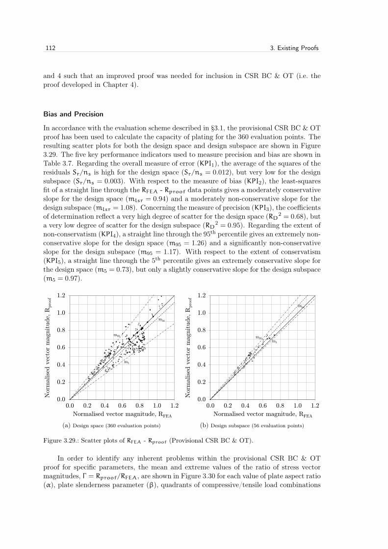
112 3. Existing Proofs
and 4 such that an improved proof was needed for inclusion in CSR BC & OT (i.e. theproof developed in Chapter 4).
Bias and Precision
In accordance with the evaluation scheme described in §3.1, the provisional CSR BC & OTproof has been used to calculate the capacity of plating for the 360 evaluation points. Theresulting scatter plots for both the design space and design subspace are shown in Figure3.29. The five key performance indicators used to measure precision and bias are shown inTable 3.7. Regarding the overall measure of error (KPI1), the average of the squares of theresiduals Sr/ns is high for the design space (Sr/ns = 0.012), but very low for the designsubspace (Sr/ns = 0.003). With respect to the measure of bias (KPI2), the least-squaresfit of a straight line through the RFEA - Rproof data points gives a moderately conservativeslope for the design space (mlsr = 0.94) and a moderately non-conservative slope for thedesign subspace (mlsr = 1.08). Concerning the measure of precision (KPI3), the coefficientsof determination reflect a very high degree of scatter for the design space (RD2 = 0.68), buta very low degree of scatter for the design subspace (RD2 = 0.95). Regarding the extent ofnon-conservatism (KPI4), a straight line through the 95th percentile gives an extremely non-conservative slope for the design space (m95 = 1.26) and a significantly non-conservativeslope for the design subspace (m95 = 1.17). With respect to the extent of conservatism(KPI5), a straight line through the 5th percentile gives an extremely conservative slope forthe design space (m5 = 0.73), but only a slightly conservative slope for the design subspace(m5 = 0.97).
m95
m5
mlsr
0.0
0.2
0.4
0.6
0.8
1.0
1.2
0.0 0.2 0.4 0.6 0.8 1.0 1.2
Norm
alise
d v
ecto
r m
agnitude,
Rpro
of
Normalised vector magnitude, RFEA
(a) Design space (360 evaluation points)
m95 m5
mlsr
0.0
0.2
0.4
0.6
0.8
1.0
1.2
0.0 0.2 0.4 0.6 0.8 1.0 1.2
Norm
alise
d v
ecto
r m
agnitude,
Rpro
of
Normalised vector magnitude, RFEA
(b) Design subspace (56 evaluation points)
Figure 0.1: ——-CROP!——–CROP!——–CROP!——–CROP!——–CROP!———CROP!——-
1
Figure 3.29.: Scatter plots of RFEA - Rproof (Provisional CSR BC & OT).
In order to identify any inherent problems within the provisional CSR BC & OTproof for specific parameters, the mean and extreme values of the ratio of stress vectormagnitudes, Γ = Rproof/RFEA, are shown in Figure 3.30 for each value of plate aspect ratio(α), plate slenderness parameter (β), quadrants of compressive/tensile load combinations
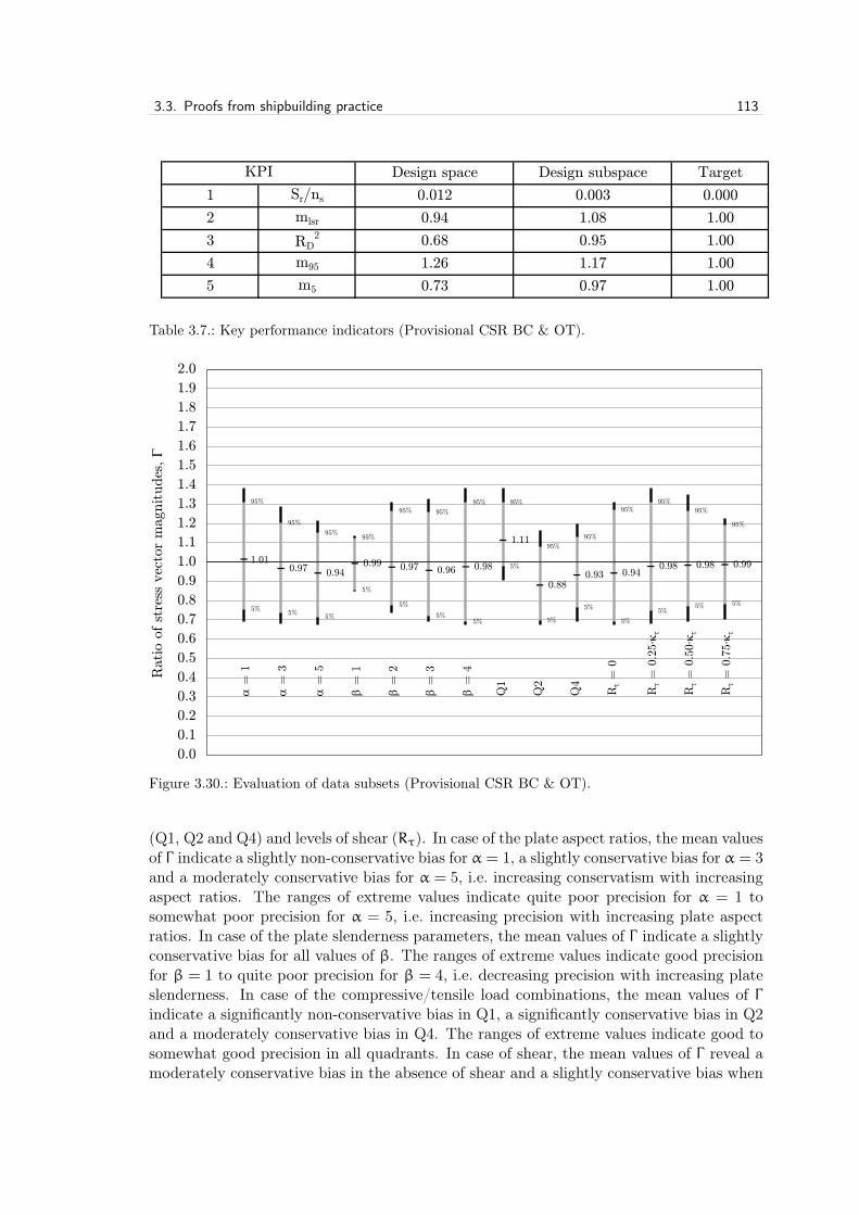
3.3. Proofs from shipbuilding practice 113
Design space Design subspace Target
1 Sr/ns 0.012 0.003 0.000
2 mlsr 0.94 1.08 1.00
3 RD2 0.68 0.95 1.00
4 m95 1.26 1.17 1.00
5 m5 0.73 0.97 1.00
KPI
Table 3.7.: Key performance indicators (Provisional CSR BC & OT).
1.01 0.97 0.94
0.99 0.97 0.96 0.98
1.11
0.88 0.93 0.94
0.98 0.98 0.99
α =
1
α =
3
α =
5
β =
1
β =
2
β =
3
β =
4
Q1
Q2
Q4
Rt =
0
Rτ =
0.2
5∙κ
τ
Rτ =
0.5
0∙κ
τ
Rτ =
0.7
5∙κ
τ
95%
95%
95% 95%
95% 95%
95% 95%
95%
95%
95% 95%
95%
95%
5% 5%
5%
5%
5%
5% 5%
5%
5%
5%
5%
5% 5% 5%
0.0
0.1
0.2
0.3
0.4
0.5
0.6
0.7
0.8
0.9
1.0
1.1
1.2
1.3
1.4
1.5
1.6
1.7
1.8
1.9
2.0
Rat
io o
f st
ress
vec
tor
magn
itudes
, Γ
Figure 3.30.: Evaluation of data subsets (Provisional CSR BC & OT).
(Q1, Q2 and Q4) and levels of shear (Rτ). In case of the plate aspect ratios, the mean valuesof Γ indicate a slightly non-conservative bias for α = 1, a slightly conservative bias for α = 3and a moderately conservative bias for α = 5, i.e. increasing conservatism with increasingaspect ratios. The ranges of extreme values indicate quite poor precision for α = 1 tosomewhat poor precision for α = 5, i.e. increasing precision with increasing plate aspectratios. In case of the plate slenderness parameters, the mean values of Γ indicate a slightlyconservative bias for all values of β. The ranges of extreme values indicate good precisionfor β = 1 to quite poor precision for β = 4, i.e. decreasing precision with increasing plateslenderness. In case of the compressive/tensile load combinations, the mean values of Γindicate a significantly non-conservative bias in Q1, a significantly conservative bias in Q2and a moderately conservative bias in Q4. The ranges of extreme values indicate good tosomewhat good precision in all quadrants. In case of shear, the mean values of Γ reveal amoderately conservative bias in the absence of shear and a slightly conservative bias when

114 3. Existing Proofs
-1.2
-0.8
-0.4
0.0
0.4
0.8
1.2
-1.2 -0.8 -0.4 0.0 0.4 0.8 1.2
Norm
alise
d s
tres
s, R
y
Normalised stress, Rx
FEA Proof
(a) α = 1, β = 1, Rτ = 0.75 · κτ
-1.2
-0.8
-0.4
0.0
0.4
0.8
1.2
-1.2 -0.8 -0.4 0.0 0.4 0.8 1.2N
orm
alise
d s
tres
s, R
y
Normalised stress, Rx
FEA Proof
(b) α = 1, β = 4, Rτ = 0
Figure 0.1: ——-CROP!——–CROP!——–CROP!——–CROP!——–CROP!———CROP!——-
1
Figure 3.31.: Comparison plots (Provisional CSR BC & OT).
shear is present. The ranges of extreme values indicate quite poor precision in the absenceof shear and quite poor to somewhat poor precision when shear is present, i.e. increasingprecision with increasing levels of shear.
In order to obtain an impression of the strengths and weaknesses of the provisionalCSR BC & OT proof, the lowest and highest values of the squares of the residuals (Sr/ns)for each combination of plate aspect ratio (α), plate slenderness parameter (β) and level ofshear (Rτ) have been calculated. The lowest value of Sr/ns is for the combination α = 1,β = 1 and Rτ = 0.75 · κτ, the capacity curve of which is plotted in Figure 3.31(a). Con-versely, the highest value of Sr/ns is for the combination α = 1, β = 4 and Rτ = 0, thecapacity curve of which is plotted in Figure 3.31(b).

4. New Proof
The purpose of this chapter is to develop a new proof of plate capacity under combinedin-plane loads. Towards this end, the problem to be solved is stated quite precisely in§4.1 using quantitative and qualitative criteria which define an acceptable proof of platecapacity. This is followed in §4.2 by an evaluation of the existing proofs presented inChapter 3 which shows that each of these proofs fails to satisfy the defined acceptabilitycriteria. Accordingly, in §4.3 a hypothetical proof of plate capacity under combined in-planeloads is postulated using a generalised form of the von Mises equation where the exponente0 and the interaction coefficient B are derived on the basis of observations made in theinvestigation of plating collapse mechanisms. Because the hypothetical proof falls justshort of satisfying all quantitative acceptance criteria, the exponent e0 and the interactioncoefficient B are redefined on the basis of additional numerical studies (in case of biaxialcompression only). The new proof is then evaluated using the same scheme applied toexisting proofs. The chapter ends with a description and evaluation in §4.4 of the proofused in the newly harmonised IACS Common Structural Rules for Bulk Carriers and OilTankers which is based on the present work.
4.1. Problem statement
As noted in Chapter 1, a proof of plate capacity is needed with which to reliably and effi-ciently design ship plating. As this proof is intended for use in the design and classificationof ships, it needs not only to be based on the ultimate strength concept, but needs as wellto satisfy certain qualitative and quantitative criteria. In qualitative terms, the proof needsto be (1) concise, (2) physically-based and (3) directly solvable. In quantitative terms, theproof needs to be (1) precise, (2) accurate and (3) robust. Certainly some existing proofsin both literature and the shipbuilding industry meet many of these criteria (primarilythe qualitative criteria), only to fail in some important respect, e.g. lack of robustness ordirect solution capability. Without an acceptable proof of plate capacity, ships will eitherbe over-designed with weight penalties which must be borne throughout their service livesor be at risk of serious, sometimes catastrophic, structural failure. As discussed in Chapter1, the ultimate hull girder collapse of MOL Comfort (which reportedly initiated in the bot-tom shell plating under biaxial loading) is one of the more recent and high profile exampleswhich illustrates the need for such a proof. Accordingly, the problem to be solved in thepresent work is to develop a proof of plate capacity under combined in-plane loads whichmeet all of the quantitative and qualitative criteria listed above and which are now definedin detail.
115

116 4. New Proof
4.1.1. Quantitative Criteria
As noted above, an acceptable proof of plate capacity needs to be (1) precise, (2) accurateand (3) robust, where the latter criterion of robustness requires that the results of a proofbe precise and accurate over the full range of load combinations and plating configurationsrelevant for the shipbuilding industry. In other words, the criterion of robustness is metwhen the criteria for precision and accuracy are satisfied over the whole of the design space(i.e. as defined in §3.1.2).
Precision and accuracy
In §3.1.1 the concepts of precision and accuracy (or bias) were presented together withfive key performance indicators (KPI’s) for their measurement. Existing proofs were sub-sequently presented together with their associated KPI’s. In Table 4.1 the best values ofKPI1, KPI2 and KPI3 obtained with these proofs are shown for both the design space andsubspace. As can be seen, the most precise and accurate results are obtained with Paik’sproof, but only for the design subspace. When considering the whole of the design space(i.e. including tensile stresses as well as plates with slenderness parameters of β = 1 orβ = 4 or an aspect ratio of α = 1), the most precise and accurate results are obtained withthe computerised buckling code PULS. This result is not surprising. The proof of Paikis based on a limited set of non-linear finite element results, whereas PULS is based onanalytically derived energy formulations in combination with a numerical method for theirsolution. For this reason, it is to be expected that the results of PULS are more robust.
Target
1 Sr/ns 0.011 0.004 0.001 0.004 0.000
2 mlsr 0.91 1.04 1.03 1.11 1.00
3 RD2 0.72 0.92 0.95 0.94 1.00
Paik PULS Paik PULS
Design SubspaceDesign SpaceKPI
Table 4.1.: Key performance indicators KPI1 to KPI3 for proofs of Paik and PULS.
In terms of precision and accuracy, the goal of the present work is to develop a proofof plate capacity which has at least the same degrees of precision and accuracy for both thedesign space and subspace as the highest degrees obtained with existing proofs for eitherthe design space or subspace. Therefore, based on Paik’s proof in the design subspace,the following acceptance criteria are defined for the KPI’s related to precision and accuracy:
KPI1: Sr/ns 6 0.001
KPI2: 0.97 6 mlsr 6 1.00
KPI3: R2D > 0.95
As can be seen, a 3% deviation from the target slope mlsr = 1.00 is accepted for KPI2based on Paik’s proof. However, contrary to this existing proof, any bias in an acceptableproof must be conservative.

4.1. Problem statement 117
Measures of conservatism and non-conservatism
Further to the foregoing, results for the remaining two KPI’s are shown for the proofs ofPaik and PULS in Table 4.2. As explained previously, the fourth KPI m95 measures theinherent non-conservatism in a proof while the fifth KPI m5 measures conservatism. Ascan be seen, the amount of non-conservatism in PULS and the proof of Paik is ratherhigh, i.e. 5% of the stress vector magnitudes according to these proofs are at least 13% to21% higher than those obtained with finite element analyses. Conversely, the amount ofconservatism of the 5th percentile is at most 5% (except in case of the design space resultsfor Paik’s proof).
Target
4 m95 1.18 1.20 1.13 1.21 1.00
5 m5 0.73 0.96 0.95 1.00 1.00
m95 - m5 0.45 0.24 0.18 0.21 0.00
Paik PULS Paik PULS
KPI Design Space Design Subspace
Table 4.2.: Key performance indicators KPI4 and KPI5 for proofs of Paik and PULS.
Accordingly, because the degrees of conservatism and non-conservatism for these ex-isting proofs are excessively biased towards non-conservatism, the acceptance criteria forthe KPI’s related to measures of conservatism and non-conservatism are instead based onthe smallest spread between KPI4 and KPI5, i.e. Paik’s proof for the design subspace wherem95 −m5 = 0.18. Using the above maximum conservatism of 5% instead for the maxi-mum non-conservatism, the following acceptance criteria are defined for the KPI’s relatedto measures of conservatism and non-conservatism:
KPI4: m95 6 1.05
KPI5: m5 > 0.87
That is, the acceptable degree of conservatism is calculated as m5 > m95 − 0.18 = 0.87.Accordingly, similar to the measures of precision and accuracy, the goal of the presentwork is to develop a proof of plate capacity which has at most the same spread betweenmeasures of conservatism and non-conservatism for both the design space and subspace asthe smallest amount of spread obtained with existing proofs for either the design spaceor subspace, but with a rather significant shift of 8% in bias towards more conservativeresults.
4.1.2. Qualitative Criteria
As noted above, an acceptable proof of plate capacity needs to be (1) concise, (2) physically-based and (3) directly solvable. Although it is sometimes difficult to precisely define anddifferentiate these criteria, each will now be discussed.

118 4. New Proof
Concise
The main reason for a proof of plate capacity to be concise is so that ship designers andplan approval engineers are able to independently verify results obtained with the softwarerule packages which are today normally provided by classification societies. These soft-ware rule packages are provided as an aid for designers and plan approval engineers, butare not intended to be "black box" substitutes for their engineering responsibilities. Forthis reason, designers and plan approval engineers need concise (and transparent) bucklingstrength proofs. A beneficial corollary of this is that almost all "bugs" in software rulepackages are discovered by designers and plan approval engineers through comparison withthe printed rules, where hand calculations are often times involved. Of course, the numberof software "bugs" for a given proof is reduced with increasing conciseness. In addition tothe engineering aspect of the need for a concise proof, there is also a legal aspect insofarthat the (legally binding) rules of classification need to be documented in printed format.
Physically-based
Related to the foregoing, a proof of plate capacity must be physically-based. Designersand plan approval engineers must be able to clearly and immediately understand how thevarious load and plate parameters affect capacity so that ship plating may be reliably andefficiently designed. For example, a designer needs to be able to understand why and whenbuckling stiffeners are a preferred design solution compared to increased plate thickness.This is not possible with proofs riddled with coefficients and devoid of physics. Moreover,a physically-based proof is also important for rule developers. Whenever improvementsare required, e.g. due to in-service experience, the physics of the existing proof must bereadily apparent.
Directly solvable
For the plan approval of a ship, there are normally several dynamic load cases requiredfor the assessment of strength. For instance, in the IACS CSR BC & OT [23] there are22 dynamic load cases related to head, following, beam and oblique seas. These dynamicload cases are in addition to still water load cases corresponding to various departure, ar-rival, seagoing, sheltered/harbour, ballast loading/unloading and cargo loading/unloadingconditions. Accordingly, because most ships usually have thousands of plate fields, thenumber of buckling strength checks which must be performed will generally be immense(for both so-called prescriptive checks and direct strength analyses). For this reason, aproof of plate capacity needs not only to be concise, but must also be solvable withoutthe need for iterations if several hours of calculations are to be avoided for checking eachdesign variation.
In particular, because many rule sets do not always allow the capacity of plating tobe fully utilised, it must be possible to isolate the stress multiplier factor at failure µ inthe proof of capacity. This factor is similar to the ratio of proof and FEA stress vectormagnitudes Γ = Rproof/RFEA used in the quantitative evaluation of proofs except that thestress multiplier factor at failure is defined as the ratio of ultimate and applied stress vectormagnitudes µ = Rult/Rapplied, where Rult is defined by the proof of plate capacity. For

4.2. Evaluation of existing proofs 119
instance, in IACS CSR BC & OT [23] only 80% of plate capacity may be utilised underpurely static loads (e.g. in harbours or sheltered waters), where the degree of utilisation isreflected in a so-called utilisation factor η = 1/µ. Accordingly, in terms of a proof basedon the generalised form of the von Mises failure criterion
(µ · σxκx · σY
)e1
+
(µ · σyκy · σY
)e2
− B ·(µ · σxκx · σY
)·(µ · σyκy · σY
)+
(µ · τxyκτ · τY
)e3
= 1.0 (4.1)
a direct solution is only possible if the stress multiplier factor at failure µ can be isolated.This requires that all terms in Equation (4.1) have the same exponent, i.e.
(µ · σxκx · σY
)e0
+
(µ · σyκy · σY
)e0
−B·(µ · σxκx · σY
)e0/2
·(µ · σyκy · σY
)e0/2
+
(µ · τxyκτ · τY
)e0
= 1.0 (4.2)
or
(µ · Rxκx
)e0
+
(µ · Ryκy
)e0
− B ·(µ · Rxκx
)e0/2
·(µ · Ryκy
)e0/2
+
(µ · Rτκτ
)e0
= 1.0 (4.3)
such that
µe0 ·[(
Rx
κx
)e0
+
(Ry
κy
)e0
− B ·(Rx
κx
)e0/2
·(Ry
κy
)e0/2
+
(Rτ
κτ
)e0]= 1.0 (4.4)
and
µ =
[(Rx
κx
)e0
+
(Ry
κy
)e0
− B ·(Rx
κx
)e0/2
·(Ry
κy
)e0/2
+
(Rτ
κτ
)e0]1/e0
(4.5)
or
η = 1/µ =
[(Rx
κx
)e0
+
(Ry
κy
)e0
− B ·(Rx
κx
)e0/2
·(Ry
κy
)e0/2
+
(Rτ
κτ
)e0]e0
(4.6)
where η must less than or equal to the allowable utilisation factor ηall, e.g. η 6 ηall = 0.80under purely static loads.
4.2. Evaluation of existing proofs
As noted in the introduction to this chapter, none of the existing proofs of plate capacitypresented in Chapter 3 satisfy all of the quantitative and qualitative acceptance criteriadelineated in §4.1.1 and §4.1.2, respectively (in particular the former). With direct refer-ence to Chapter 3, this will now be explained.

120 4. New Proof
Quantitative criteria
In Table 4.3 and Table 4.4 all of the key performance indicators obtained in Chapter3 for the design space and subspace, respectively, are summarised and compared to thequantitative acceptance criteria delineated in §4.1.1. Those measurements which meet theacceptance criteria are highlighted.
KPI Criteria Paik Ueda et al. CN 30.1 DIN 4114 PULS DIN 18800 Prov. CSR BC & OT
1 Sr/ns ≤ 0.001 0.011 0.018 0.032 0.039 0.004 0.018 0.012
2 0.97 ≤ mlsr ≤ 1.00 0.91 1.11 0.82 0.84 1.04 0.87 0.94
3 RD2 ≥ 0.95 0.72 0.62 0.63 0.63 0.92 0.73 0.68
4 m95 ≤ 1.05 1.18 1.61 1.08 1.10 1.20 1.14 1.26
5 m5 ≥ 0.87 0.73 1.00 0.52 0.36 0.96 0.67 0.73
Table 4.3.: Summary of quantitative results for existing proofs in design space.
KPI Criteria Paik Ueda et al. CN 30.1 DIN 4114 PULS DIN 18800 Prov. CSR BC & OT
1 Sr/ns ≤ 0.001 0.001 0.038 0.005 0.020 0.004 0.005 0.003
2 0.97 ≤ mlsr ≤ 1.00 1.03 1.35 0.88 0.78 1.11 0.93 1.08
3 RD2 ≥ 0.95 0.95 0.57 0.85 0.69 0.94 0.80 0.95
4 m95 ≤ 1.05 1.13 1.91 1.10 1.03 1.21 1.13 1.17
5 m5 ≥ 0.87 0.95 1.18 0.75 0.45 1.00 0.75 0.97
Table 4.4.: Summary of quantitative results for existing proofs in design subspace.
As can be seen, only two of the existing proofs (Ueda et al. and PULS) meet evena single acceptance criterion in the design space. This is an unsurprising result since theacceptance criteria are based on the best KPI’s obtained with Paik’s proof in the designsubspace. However, as noted above, all of the precision and accuracy criteria need to bemet in the design space if a proof is to be considered precise, accurate and robust.
With respect to the design subspace, two of the existing proofs meet more than one ofthe acceptance criterion (Paik and the provisional CSR BC & OT proofs). Both of theseproofs (as well as PULS) would probably meet all of the performance criteria (i.e. for thedesign subspace) if the results obtained with each were more conservatively biased. This israther instructive since both the Paik and the provisional CSR BC & OT proofs are basedon a generalised form of the von Mises failure criterion shown in Equation (4.3).
Qualitative criteria
With few exceptions, all of the existing proofs presented in Chapter 3 meet the qualitativecriteria delineated in §4.1.2. The corresponding qualities of these proofs are summarisedin Table 4.5 and discussed below.
Paik Ueda et al. CN 30.1 DIN 4114 PULS DIN 18800 Prov. CSR BC & OT
Criteria
Concise
Physically-based
Directly solvable
Table 4.5.: Summary of qualitative results for existing proofs.

4.2. Evaluation of existing proofs 121
Concise
Regarding the criterion of conciseness, all of the proofs presented in Chapter 3, exceptthe computerised semi-analytical buckling code PULS, are sufficiently concise to be doc-umented in rules for the classification of ships. Certainly this is true of the proofs fromshipbuilding practice since they have been directly obtained from various rule sets (againexcept for PULS). However, Paik’s proof, consisting of two simple equations, is the best interms of conciseness with the provisional CSR BC & OT proof of comparable simplicity.
Conversely, the proof of Ueda et al. is somewhat difficult to document, firstly becausethe equations for the elastic buckling strength of plating under combined loads need to beincluded and secondly because the equations for the stress coefficients are rather cumber-some, especially when the effects of shear are taken into account. Nevertheless, the proofis sufficiently concise to be included in a rule set.
Lastly, because it is obviously not suitable for inclusion in printed rules, PULS hasbeen implemented into a stand-alone software with an "easy and intuitive" interface. Thebuckling code is also available in Microsoft Excel format and for automatic rule checksin the NAUTICUS Hull software. However, in order to offer it as a tool for plan ap-proval, the parameters governing the discretisation of buckling deflections and solution ofthe equilibrium equations are pre-determined and fixed. Furthermore, these parametersare not disclosed to the user. For this reason, some consider PULS to be something of a"black-box". Even if the fundamental theory behind it is transparent, the calculation itselfis not because the user has no knowledge or control of the pre-processing, solution andpost-processing options. In this regard, PULS differs from most commercially-availablefinite element analysis packages.
Physically-based
All of the proofs presented in Chapter 3 are physically-based using the von Mises failurecriterion directly (i.e. PULS and the proof of Ueda et al.) or using some generalised formof the von Mises equation (i.e. the remaining proofs). However, in case of the amendedDIN 18800 proof, some designers and approval engineers find the transformation from plateto beam stresses (in case of finite element analyses), i.e. the so-called Poisson correction,difficult to understand and/or apply.
Notably, in case of the computerised buckling code PULS, the available software offerscolour plots showing capacity curves, eigenmodes, model imperfections, out-of-plane deflec-tions as well as in-plane normal, shear and von Mises stresses at initial yield(i.e. in addition to utilisation factors for buckling strength and ultimate capacity). Thesefeatures provide ship designers and plan approval engineers with some insight into thefailure mechanism of plates and also makes PULS particularly useful for rule developers.
Directly solvable
With respect to the direct solution criterion, those proofs based on a generalised form of thevon Mises equation can be solved directly. The exception to this is the amended DIN 18800proof where the stress multiplier factor at failure µ cannot be isolated in the interactionequation. This is because the exponents e1, e2 and e3 generally take on different values
122 4. New Proof
(the Poisson correction is not a problem in this concern since it depends only on the ratioof σx and σy and not on the magnitude of µ).
Regarding the proof of Ueda et al., obtaining efficient solutions is also not possible sincethe applied loads need to be gradually incremented in order to determine the capacity of theplating. Furthermore, in some cases Equation (3.17) has no real solutions or solutions whichare not unique (i.e. two possible solutions). This could be due to misprints in reference [51]or the author’s own programming errors although the calculation method used has beenvalidated against examples provided in reference [51] for the ultimate strength of squareplates under biaxial loading. Moreover, as a co-author of the Ueda et al. paper [51], it isperhaps telling that Paik focussed his subsequent efforts on a generalised form of the vonMises equation as presented in §3.2.1.
Finally, although PULS is a fundamentally sound proof of plate capacity, calculationtimes are considerably longer compared to closed form solutions. Like the proof of Ueda etal., this is because the applied loads in PULS need to be gradually incremented in order todetermine the capacity of the plating. Increased calculation times are particularly notice-able when many buckling strength checks need to performed, e.g. for cargo hold models.This drawback combined with those described above have made some classification soci-eties reluctant to reference PULS in their rules for the classification of ships.
4.3. Development and evaluation of new proof
On the basis of the foregoing evaluations, a proof based on a generalised form of the vonMises equation appears to hold the most promise for satisfying all of the quantitative andqualitative acceptance criteria outlined in §4.1. In terms of the qualitative criteria, in canbe seen in Table 4.5 that only four of the existing proofs presented in Chapter 3 (i.e. Paik,CN 30.1, DIN 4114 and provisional CSR BC & OT) are concise, physically-based anddirectly solvable. Of these proofs, it can be seen from the results presented in Tables 4.3and 4.4 that proofs based on a generalised form of the von Mises equation (i.e. Paik andprovisional CSR BC & OT) are appreciably more precise and accurate than the proofsbased on elastic analyses with plasticity corrections (i.e. CN 30.1 and DIN 4114). This isshown in Table 4.6 where the rankings for each of the five KPI’s are summarised.
KPI Paik CN 30.1 DIN 4114 Prov. CSR BC & OT Paik CN 30.1 DIN 4114 Prov. CSR BC & OT
1 1 3 4 2 1 3 4 2
2 1 4 3 2 1 3 4 2
3 1 3 3 2 1 3 4 1
4 3 1 2 4 3 2 1 4
5 1 3 4 1 2 3 4 1
Design SubspaceDesign Space
Table 4.6.: Ranking of proofs.
Here the proofs of Paik and provisional CSR BC & OT are ranked 1 and 2 for allKPI’s except KPI 4. This exception is in general the case because the proofs based onelastic analyses with plasticity corrections are comparably conservative while the proofsof Paik and provisional CSR BC & OT are either imprecise with a conservative bias(i.e. for the design space) or precise with a non-conservative bias (i.e. for the design sub-

4.3. Development and evaluation of new proof 123
space). Accordingly, a solution is sought in a more precise and accurate proof based on ageneralised form of the von Mises equation. Again, as noted in §4.1.2, the same exponentsare needed for each term of the equation in order that the stress multiplier at failure µ canbe isolated. Accordingly, the new proof of plate capacity is to be formulated as
(µ · σxκx · σY
)e0
+
(µ · σyκy · σY
)e0
−B·(µ · σxκx · σY
)e0/2
·(µ · σyκy · σY
)e0/2
+
(µ · τxyκτ · τY
)e0
= 1.0 (4.7)
or(µ · Rxκx
)e0
+
(µ · Ryκy
)e0
− B ·(µ · Rxκx
)e0/2
·(µ · Ryκy
)e0/2
+
(µ · Rτκτ
)e0
= 1.0 (4.8)
in terms of normalised stresses (i.e. Equation (4.3)).
4.3.1. Framework of new proof
With the aim of developing a new proof of plate capacity based on Equation (4.8), theframework of the proof will now be built up quadrant by quadrant. Based on the mechan-ics of plating collapse investigated in Chapter 2, this framework is intended to facilitate amore physically-based proof.
Yielding in Quadrant 3
Whenever gross yielding occurs throughout the plate, the capacity equation should ofcourse be that of the von Mises ellipse, as shown in Figure 4.1 (where Rτ = 0). In termsof Equation (4.8), this means that B = 1, e0 = 2 and the plate reduction factors are equalto unity (i.e. κx = κy = κτ = 1.0) such that Equation (4.8) is reduced to
R2x + R
2y − Rx · Ry + R2
τ = 1.0 (4.9)
Here the stress multiplier factor at failure µ is set to unity in order to obtain ultimateplate strength. As shown in Figure 4.2 (again where Rτ = 0), Equation (4.9) defines platecapacity in Quadrant 3 where it is generally assumed that the magnitude of shear stressis either insufficient to induce buckling (i.e. Rτ < Rτ,cr) or that the magnitude of tensilestresses in the x- and/or y-directions is sufficient to prevent shear buckling. Even if shearbuckling were to occur, it is assumed that the presence of tensile stresses Rx and Ry miti-gate the out-of-plane shear deflections to the point where any post-buckling redistributionof internal stresses is negligible. Moreover, as discussed in §2.3, post-buckling effects undershear are not as significant as those under uniaxial loads.
Yielding/buckling in Quadrants 2 and 4
Collapse due to gross yielding
The foregoing absence of post-buckling effects in Quadrant 3 is assumed to continueinto Quadrant 2 for those combinations of normalised stress where Ry 6 κ ′y. Here the

124 4. New Proof
-1.2
-0.8
-0.4
0.0
0.4
0.8
1.2
-1.2 -0.8 -0.4 0.0 0.4 0.8 1.2
Norm
alise
d s
tres
s, R
y
Normalised stress, Rx
von Mises ellipse
τxy = 0.00∙τxy,ult (proof)
τxy = 0.25∙τxy,ult (proof)
τxy = 0.50∙τxy,ult (proof)
τxy = 0.75∙τxy,ult (proof)
τxy = 0.00∙τxy,ult (FEA)
τxy = 0.25∙τxy,ult (FEA)
τxy = 0.50∙τxy,ult (FEA)
τxy = 0.75∙τxy,ult (FEA)
Quadrant 2
Quadrant 4 Quadrant 3
Quadrant 1
von Mises equation
Figure 4.1.: Von Mises ellipse.
-1.2
-0.8
-0.4
0.0
0.4
0.8
1.2
-1.2 -0.8 -0.4 0.0 0.4 0.8 1.2N
orm
alise
d s
tres
s, R
y
Normalised stress, Rx
yield (tau = 0.00)
τxy = 0.00∙τxy,ult (proof)
τxy = 0.25∙τxy,ult (proof)
τxy = 0.50∙τxy,ult (proof)
τxy = 0.75∙τxy,ult (proof)
τxy = 0.00∙τxy,ult (FEA)
τxy = 0.25∙τxy,ult (FEA)
τxy = 0.50∙τxy,ult (FEA)
τxy = 0.75∙τxy,ult (FEA)
Quadrant 3
yielding
Figure 4.2.: Yielding in Quadrant 3.
quantity κ ′y is equal to the reduced uniaxial strength of the plate (in the y-direction)considering shear (i.e. Rx = 0, Rτ > 0). In other words, the quantity κ ′y is a plate reduc-tion factor which takes into account the effects of any shear loads which may be present(i.e. κ ′y = κy in the absence of shear). In particular, when Rx = 0 (and again setting thestress multiplier factor at failure µ to unity), Equation (4.8) is reduced to(
Ry
κy
)e0
+
(Rτ
κτ
)e0
= 1.0 (4.10)
which defines plate capacity in the Ry−Rτ plane. When rearranging this equation in termsof Ry, the quantity κ ′y is obtained
κ ′y = Ry = κy ·[1−
(Rτ
κτ
)e0]1/e0
(4.11)
As shown in Figure 4.3, this means that the von Mises ellipse describes collapse inQuadrant 2 up to the point (Rx,Y , κ ′y) where Rx,Y refers to the value of Rx which whencombined with Ry = κ ′y and Rτ satisfies Equation (4.9), i.e. the von Mises failure crite-rion. Of course, the assumption of gross yielding in Quadrant 2 is more tenuous than inQuadrant 3 due to the presence of compressive stresses in the y-direction. Nevertheless,these compressive stresses are normally secondary stresses (i.e. |Ry| < |Rx| in Quadrant 2)such that the tensile stresses in the x-direction are assumed to be of sufficient magnitudeto inhibit buckling. As shown in Figure 4.3, the same assumptions and treatment applyanalogously in Quadrant 4.
Collapse due to buckling
For those combinations of normalised stress in Quadrant 2 where Rx > Rx,Y , bucklingis assumed to take place. However, as shown in Figure 4.4, for all such values of Rx it isassumed that plate capacity in the y-direction is defined by Ry = κ ′y, i.e. this is the equiv-alent of setting Rx = 0 whenever Rx > Rx,Y . This is normally a conservative assumption

4.3. Development and evaluation of new proof 125
(κ¶x, Ry,Y)
(Rx,Y, κ¶y)
-1.2
-0.8
-0.4
0.0
0.4
0.8
1.2
-1.2 -0.8 -0.4 0.0 0.4 0.8 1.2
Norm
alise
d s
tres
s, R
y
Normalised stress, Rx
yield (tau = 0.00)
τxy = 0.00∙τxy,ult (proof)
τxy = 0.25∙τxy,ult (proof)
τxy = 0.50∙τxy,ult (proof)
τxy = 0.75∙τxy,ult (proof)
τxy = 0.00∙τxy,ult (FEA)
τxy = 0.25∙τxy,ult (FEA)
τxy = 0.50∙τxy,ult (FEA)
τxy = 0.75∙τxy,ult (FEA)
Quadrant 2
Quadrant 4
yielding
Figure 4.3.: Yielding in Quadrants 2 and 4.
(Rx,Y, κ¶y) (0, κ¶y)
(κ¶x, 0)
(κ¶x, Ry,Y)
-1.2
-0.8
-0.4
0.0
0.4
0.8
1.2
-1.2 -0.8 -0.4 0.0 0.4 0.8 1.2
Norm
alise
d s
tres
s, R
y
Normalised stress, Rx
yield (tau = 0.00)
τxy = 0.00∙τxy,ult (proof)
τxy = 0.25∙τxy,ult (proof)
τxy = 0.50∙τxy,ult (proof)
τxy = 0.75∙τxy,ult (proof)
τxy = 0.00∙τxy,ult (FEA)
τxy = 0.25∙τxy,ult (FEA)
τxy = 0.50∙τxy,ult (FEA)
τxy = 0.75∙τxy,ult (FEA)
Quadrant 2
Quadrant 4
buckling
Figure 4.4.: Buckling in Quadrants 2 and 4.
since, as explained in §2.2, tensile stresses in the x-direction will tend to increase platecapacity in the y-direction by restraining the out-of-plane deflections (thereby mitigatingthe redistribution of stresses towards the edges and corners of the plate).
One reason for this conservatism is that the new proof incorporates a design prin-ciple which limits the magnitudes of applied stresses in the x- and y-directions to thosestresses which define the capacity of the plate when applied in the absence of each other,i.e. Rx 6 κ ′x and Ry 6 κ ′y. This design principle was first included in the buckling strengthrules of Germanischer Lloyd, but is there only relevant in Quadrant 1. The reasoningbehind this principle is that the presence of a secondary stress component cannot be anecessary condition for allowing another stress component to exceed its ultimate stress,e.g. Ry > κ ′y. In other words, because the presence of a secondary stress cannot generallybe guaranteed (particularly in the case of independent stresses), stress limits are applied.
Finally, although the capacity of the plate is defined throughout Quadrant 2 by Equa-tion (4.8), i.e. a generalised form of the von Mises equation, it should be noted that theplate reduction factors κx, κy and κτ, as well as the exponent e0 and interaction coefficientB of the von Mises equation, do not remain constant throughout. In particular, for thesegment of the plate capacity curve defined by Ry = κ ′y, the beneficial effects of tensilestresses in mitigating post-buckling effects are reflected in changing values of the platereduction factors, i.e. κx → 1.0, κy → 1.0 and κτ → 1.0, as well as in changing valuesof the exponent and interaction coefficient of the von Mises equation, i.e. e0 → 2.0 andB → 1.0, with increasing magnitudes of tensile stresses. Nevertheless, it is far simplerwhen the segment of the plate capacity curve between Rx = 0 and Rx = Rx,Y is defined byEquation (4.10), rather than explicitly defining (transitioning) values of κx, κy, κτ, e0 andB for use in Equation (4.8). As shown in Figure 4.4, the same assumptions and treatmentapply analogously in Quadrant 4.
Error analysis
Ignoring the beneficial effects of tensile stresses on the capacity of the plate is a

126 4. New Proof
-1.2
-0.8
-0.4
0.0
0.4
0.8
1.2
-1.2 -0.8 -0.4 0.0 0.4 0.8 1.2
Norm
alise
d s
tres
s, R
y
Normalised stress, Rx
finite element analysesnew proofPaik / prov. CSR BC & OT
Quadrant 2
Quadrant 4
point of maximum error
point of maximum error
Figure 4.5.: Comparison of results.
mlsr = 1.03x RD
2 = 0.76
0.0
0.2
0.4
0.6
0.8
1.0
1.2
0.0 0.2 0.4 0.6 0.8 1.0 1.2N
orm
alise
d v
ecto
r m
agnitude,
Rpro
of
Normalised vector magnitude, RFEA
results
Series2
mlsr
Linear (results)
τxy = 0.00∙τxy,ult (proof)
τxy = 0.25∙τxy,ult (proof)
τxy = 0.50∙τxy,ult (proof)
τxy = 0.75∙τxy,ult (proof)
τxy = 0.00∙τxy,ult (FEA)
τxy = 0.25∙τxy,ult (FEA)
τxy = 0.50∙τxy,ult (FEA)
τxy = 0.75∙τxy,ult (FEA)
Figure 4.6.: Maximum errors (96 data points).
source of significant error in the Paik and provisional CSR BC & OT proofs (albeit on theconservative side of results in Quadrants 2 and 4, e.g. see Figures 3.8 (b) and 3.31 (b)).In Quadrants 2 and 4 these proofs describe the capacity of the plate using the von Misesequation, but with the components of applied stresses normalised by ultimate stress ratherthan yield stress (recalling that κx = κy = κτ = 1.0 in case of gross yielding), i.e.(
Rx
κx
)2
+
(Ry
κy
)2
−
(Rx
κx
)·(Ry
κy
)+
(Rτ
κτ
)2
= 1.0 (4.12)
In Figure 4.5 the capacity of plating with an aspect ratio α = 3 and plate slendernessparameter β = 2 is shown for Quadrants 2 and 4. Here the results obtained with finiteelement analyses are compared to results obtained with the Paik and provisional CSR BC &OT proofs. As can be seen, these proofs significantly underestimate the capacity of platingin Quadrants 2 and 4. Conversely, plate capacities obtained with the yielding/bucklingapproach described above is seen to agree well with the results of finite element analyses.This latter approach was intuitively presumed by Smith et al. [63] to be plausible on thebasis of elastic buckling strength in Quadrants 2 and 41, but who cautioned that "bucklingstresses provide useful indicators of behaviour but cannot be used to determine (ultimate)strength (or strength interaction). This is because initial buckling theory takes no accountof the complex redistribution of mid-thickness and surface stresses which occur duringloading. In fact, the limited numerical data available show that tensile stress can resultin some reduction of strength before the yield surface is reached". Indeed, numericalstudies in the present work confirm that there is the potential for some non-conservatismassociated with those stress combinations near the transitions from (inelastic) buckling togross yielding, i.e. where Rx → Rx,Y and Ry → Ry,Y .
In fact, as shown in Figure 4.5, the potential for this non-conservatism is greatestprecisely where the stress limits and the von Mises ellipse intersect in Quadrants 2 and4 (i.e. at Rx,Y , κ ′y and κ ′x,Ry,Y). To investigate the significance of this potential error,
1 The validity of this approach is also supported by the distribution of internal stresses described by Uedaet al. [51].

4.3. Development and evaluation of new proof 127
additional finite element analyses were performed along the stress vector of this intersectionfor 96 combinations of plate aspect ratio α, plate slenderness parameter β and all four levelsof shear Rτ in Quadrants 2 and 4, i.e. 3 x 4 x 4 x 2 = 96 evaluation points. The resultsare shown in Figure 4.6 where a straight line through the RFEA - Rproof evaluation pointshas a slightly non-conservative slope of 1.03 (least square regression without an interceptterm, R2
D = 0.76). In Quadrant 2 the average of maximum errors is about 5.7% (maximum13.2%). However, because transverse tensile stresses are acting over the entire length ofthe plate and therefore more effective in limiting out-of-plane deflections, in Quadrant 4the average of maximum errors is only about 1.0% (maximum 6.5%).
In cases where the design load is realised and the capacity of a plate is slightly ex-ceeded, the additional load will be taken over by the supporting structure and/or strainhardening (which has not been included in the finite element analyses). In practicethe scantlings of plates are normally driven by their capacity under biaxial compression(i.e. Quadrant 1). However, if a proof of plate capacity is so conservative in Quadrants2 and 4 that they govern plate thickness (i.e. even when the critical load combination istruly not in these quadrants), a more precise and accurate proof is needed, if for no otherreason then to allow the thickness of plating to be governed by its capacity under biaxialcompression in Quadrant 1 (i.e. when the critical load combination is truly in this quad-rant).
Buckling in Quadrant 1
The stress limits in Quadrants 2 and 4 which prevent components of applied stress Rx andRy from exceeding (normalised) ultimate stresses κ ′x and κ ′y, respectively, continue intoQuadrant 1. These limits are shown in Figure 4.7 and govern whenever collapse initiatesin the corners of the plate, i.e. in case of sturdy plates2. Unlike yielding along the sides ofthe plate, here the biaxial compressive stresses are working "against each other" to delayyielding as reflected in the interaction term of the von Mises equation. However, whencollapse does not initiate in the corners of the plate, its (inelastic) buckling capacity inQuadrant 1 is described by Equation (4.8) where the values of the exponent e0 and inter-action coefficient B are functions of the plate aspect ratio α and slenderness parameter β.As shown in Figure 4.8, this portion of the capacity curve completes the proof.
4.3.2. Hypothetical Proof of Plate Capacity
Based solely on the mechanics of plating collapse presented in Chapter 2, a hypo-thetical proof without any numerical calibration can now be developed. As reflected inthe framework described above, the capacity of plates in Quadrants 2, 3 and 4 can bedetermined on the basis of ultimate plate strength under single load components (i.e. κx,κy and κτ) and the von Mises failure criterion. For this reason, the task of developing ahypothetical proof of plate capacity is reduced to determining values of the exponent e0
2 As shown in Appendix D, the presence of a secondary (compressive) stress Ry may increase the capacityof the plate under a primary (compressive) stress Rx (and vice versa). This is not the case withcombined axial and shear stresses (as also shown in Appendix D) and explains why no shear stresslimit is required.

128 4. New Proof
(0, κ¶y)
(κ¶x, 0)
-1.2
-0.8
-0.4
0.0
0.4
0.8
1.2
-1.2 -0.8 -0.4 0.0 0.4 0.8 1.2
Norm
alise
d s
tres
s, R
y
Normalised stress, Rx
yield (tau = 0.00)
sx limitτxy = 0.00∙τxy,ult (proof)
τxy = 0.25∙τxy,ult (proof)
τxy = 0.50∙τxy,ult (proof)
τxy = 0.75∙τxy,ult (proof)
τxy = 0.00∙τxy,ult (FEA)
τxy = 0.25∙τxy,ult (FEA)
τxy = 0.50∙τxy,ult (FEA)
τxy = 0.75∙τxy,ult (FEA)
Quadrant 1
stress limits
Figure 4.7.: Stress limits in Quadrant 1.
-1.2
-0.8
-0.4
0.0
0.4
0.8
1.2
-1.2 -0.8 -0.4 0.0 0.4 0.8 1.2N
orm
alise
d s
tres
s, R
y
Normalised stress, Rx
yield (tau = 0.00)
τxy = 0.00∙τxy,ult (proof)
τxy = 0.25∙τxy,ult (proof)
τxy = 0.50∙τxy,ult (proof)
τxy = 0.75∙τxy,ult (proof)
τxy = 0.00∙τxy,ult (FEA)
τxy = 0.25∙τxy,ult (FEA)
τxy = 0.50∙τxy,ult (FEA)
τxy = 0.75∙τxy,ult (FEA)
Quadrant 1
buckling
Figure 4.8.: Buckling in Quadrant 1.
and interaction coefficient B (in Quadrant 1) for Equation (4.8) with the stress multiplierfactor at failure µ set to unity, i.e.(
Rx
κx
)e0
+
(Ry
κy
)e0
− B ·(Rx
κx
)e0/2
·(Ry
κy
)e0/2
+
(Rτ
κτ
)e0
= 1.0 (4.13)
As discussed in §2.2.4, it is to be expected that the collapse of slender plates inQuadrant 1 is dominated by elastic buckling such that the shape of their capacity curvesapproaches the shape of the elastic buckling strength interaction curve (i.e. in the Rx-Ryplane for a given level of shear). Conversely, it is to be expected that the collapse of sturdyplates includes significant yielding such that the shape of their capacity curves approachesthat of the von Mises ellipse (i.e. again in the Rx-Ry plane for a given level of shear).
Accordingly, if it is hypothesised that the effects of plate aspect ratio are secondarycompared to those of plate slenderness and that the shape of the plate capacity curve in theRx-Ry plane is unaffected by shear, then the (linear) elastic buckling interaction equationof a square plate may be used for slender plates. Conversely, in case of sturdy plates,the (quadratic) von Mises equation may be used (where plate aspect ratio already has norole). Accordingly, what remains is to define the limiting values of slenderness for whichthe behaviour of plates is perfectly elastic and perfectly plastic, i.e. nominal definitions ofslender and sturdy plates, respectively. On the basis of the right-hand side of Figure 2.20,these limits are defined as β > 4 for perfectly elastic behaviour and β 6 0.5 for perfectlyplastic behaviour. With reference to Equation (4.13), this means that e0 = 1 and B = 0when β > 4 and that e0 = 2 and B = 1 when β 6 0.5. Linear interpolation will be used todefine the exponent e0 and interaction coefficient B for plate behaviour between these twoextremes, resulting in the following equations
e0 = (7.5− β)/3.5, where 1 6 e0 6 2 (4.14)
B = (4.0− β)/3.5, where 0 6 B 6 1 (4.15)

4.3. Development and evaluation of new proof 129
which are plotted in Figure 4.9. These equations (for use in Quadrant 1), together withthe framework described above, comprise the hypothetical proof based on the mechanics ofplating collapse presented in Chapter 2, i.e. a physically-based proof without any numericalcalibration. Because the proof is based on a generalised form of the von Mises equation(with the same value of e0 for all terms), the qualitative acceptance criteria defined in§4.1.2 are fulfilled. Accordingly, only an evaluation of the hypothetical proof against thequantitative acceptance criteria delineated in §4.1.1 remains.
0.00
0.25
0.50
0.75
1.00
1.25
1.50
1.75
2.00
2.25
2.50
0.0 0.5 1.0 1.5 2.0 2.5 3.0 3.5 4.0 4.5
Exponen
t, e
0
Plate slenderness parameter, β
e_0
τxy = 0.00∙τxy,ult (proof)
τxy = 0.25∙τxy,ult (proof)
τxy = 0.50∙τxy,ult (proof)
τxy = 0.75∙τxy,ult (proof)
τxy = 0.00∙τxy,ult (FEA)
τxy = 0.25∙τxy,ult (FEA)
τxy = 0.50∙τxy,ult (FEA)
τxy = 0.75∙τxy,ult (FEA)
perfectly plastic behaviour
perfectly elastic behaviour
(a) Exponent e0
0.00
0.25
0.50
0.75
1.00
1.25
1.50
1.75
2.00
2.25
2.50
0.0 0.5 1.0 1.5 2.0 2.5 3.0 3.5 4.0 4.5
Inte
ract
ion c
oef
fici
ent, B
Plate slenderness parameter, β
B
τxy = 0.00∙τxy,ult (proof)
τxy = 0.25∙τxy,ult (proof)
τxy = 0.50∙τxy,ult (proof)
τxy = 0.75∙τxy,ult (proof)
τxy = 0.00∙τxy,ult (FEA)
τxy = 0.25∙τxy,ult (FEA)
τxy = 0.50∙τxy,ult (FEA)
τxy = 0.75∙τxy,ult (FEA)
perfectly plastic behaviour
perfectly elastic behaviour
(b) Interaction coefficient B
Figure 0.1: ——-CROP!——–CROP!——–CROP!——–CROP!——–CROP!———CROP!——-
1
Figure 4.9.: Plots of exponent e0 and interaction coefficient B.
Therefore, in accordance with the evaluation scheme described in §3.1, the hypothet-ical proof has been used to calculate the capacity of plating for the 360 evaluation points.The resulting scatter plots for both the design space and design subspace are shown inFigure 4.10. The five key performance indicators used to measure precision and bias areshown in Table 4.7 together with the acceptance criteria. On the basis of these indicators,it can be seen that the hypothetical proof generally performs better than any of the existingproofs. Regarding the overall measure of error (KPI1), the average of the squares of theresiduals Sr/ns is very low for both the design space (Sr/ns = 0.002) and design subspace(Sr/ns = 0.001). With respect to the measure of bias (KPI2), the least-squares fit of astraight line through the RFEA - Rproof data points gives a slightly conservative slope forboth the design space (mlsr = 0.99) and design subspace (mlsr = 0.97). Concerning themeasure of precision (KPI3), the coefficients of determination reflect a very low degree ofscatter for both the design space (RD2 = 0.95) and design subspace (RD2 = 0.94). Regard-ing the extent of non-conservatism (KPI4), a straight line through the 95th percentile givesa moderately non-conservative slope for both the design space (m95 = 1.09) and designsubspace (m95 = 1.09). With respect to the extent of conservatism (KPI5), a straightline through the 5th percentile gives a significantly/extremely conservative slope for thedesign space (m5 = 0.80) and a significantly conservative slope for the design subspace(m5 = 0.84).
In order to identify any inherent problems within the hypothetical proof for spe-cific parameters, the mean and extreme values of the ratio of stress vector magnitudes,

130 4. New Proof
m95
m5
mlsr
0.0
0.2
0.4
0.6
0.8
1.0
1.2
0.0 0.2 0.4 0.6 0.8 1.0 1.2
Norm
alise
d v
ecto
r m
agnitude,
Rpro
of
Normalised vector magnitude, RFEA
(a) Design space (360 evaluation points)
m95
m5
mlsr
0.0
0.2
0.4
0.6
0.8
1.0
1.2
0.0 0.2 0.4 0.6 0.8 1.0 1.2N
orm
alise
d v
ecto
r m
agnitude,
Rpro
of
Normalised vector magnitude, RFEA
(b) Design subspace (56 evaluation points)
Figure 0.1: ——-CROP!——–CROP!——–CROP!——–CROP!——–CROP!———CROP!——-
1
Figure 4.10.: Scatter plots of RFEA - Rproof (hypothetical proof).
Target Design space Design subspace Criteria
1 Sr/ns 0.000 0.002 0.001 Sr/ns ≤ 0.001
2 mlsr 1.00 0.99 0.97 0.97 ≤ mlsr ≤ 1.00
3 RD2 1.00 0.95 0.94 RD
2 ≥ 0.95
4 m95 1.00 1.09 1.09 m95 ≤ 1.05
5 m5 1.00 0.80 0.84 m5 ≥ 0.87
KPI
Table 4.7.: Key performance indicators (hypothetical proof).
Γ = Rproof/RFEA, are shown in Figure 4.11 for each value of plate aspect ratio (α), plateslenderness parameter (β), quadrants of compressive/tensile load combinations (Q1, Q2and Q4) and levels of shear (Rτ). In case of the plate aspect ratios, the mean values ofΓ indicate a slightly to moderately conservative bias for all values of α. The ranges ofextreme values indicate good precision for all plate aspect ratios. In case of the plateslenderness parameters, the mean values of Γ indicate a slightly non-conservative bias forβ = 1 and β = 2, but a slightly/moderately conservative bias for β = 3 and a significantlyconservative bias for β = 4. The ranges of extreme values indicate good precision for β = 2and β = 4, but quite good precision for β = 3 and very good precision for β = 1. In caseof the compressive/tensile load combinations, the mean values of Γ indicate a moderatelyto slightly conservative bias for all quadrants. The ranges of extreme values indicate goodprecision in Quadrants 1 and 2 with very good precision in Quadrant 4. In case of shear,the mean values of Γ reveal a slightly non-conservative bias in the absence of shear and aslightly to moderately conservative bias in the presence of shear. The ranges of extremevalues indicate good precision for all levels of shear.

4.3. Development and evaluation of new proof 131
0.98 0.96 0.94 1.01 1.01
0.95
0.88 0.94 0.96 0.97
1.01 0.98
0.94 0.93
α =
1
α =
3
α =
5
β =
1
β =
2
β =
3
β =
4
Q1
Q2
Q4
Rt =
0
Rτ =
0.2
5∙κ
τ
Rτ =
0.5
0∙κ
τ
Rτ =
0.7
5∙κ
τ
95% 95% 95%
95%
95%
95% 95%
95% 95%
95%
95% 95%
95% 95%
5% 5%
5%
5% 5%
5%
5% 5%
5% 5%
5%
5% 5% 5%
0.0
0.1
0.2
0.3
0.4
0.5
0.6
0.7
0.8
0.9
1.0
1.1
1.2
1.3
1.4
1.5
1.6
1.7
1.8
1.9
2.0R
atio
of st
ress
vec
tor
mag
nitudes
, Γ
Figure 4.11.: Evaluation of data subsets (hypothetical proof).
4.3.3. Exponent e0 (Quadrant 1)
As seen in Table 4.7, the hypothetical proof satisfies or nearly satisfies KPI’s 1, 2 and 3in both the design space and subspace. However, as reflected in KPI’s 4 and 5, the mainproblem with the hypothetical proof is the significant scatter between the 5th and 95th
percentiles, particularly in Quadrant 1. Although the degree of precision in Quadrant 1 is"good" relative to existing proofs, it can be seen in Figure 4.11 that the scatter of resultsin absolute terms is rather high (this can also be seen in comparison to other data subsetswithin Figure 4.11). Accordingly, in an effort to satisfy all of the quantitative acceptancecriteria established in §4.1.1, the next task in developing a new proof of plate capacity isto better capture the effects of plate aspect ratio α and shear Rτ in Quadrant 1 (effectswhich were excluded from the hypothetical proof). Towards this end, equations will nowbe developed numerically with which to calculate more precise values of the exponent e0and interaction coefficient B (i.e. in case of biaxial compression) according to Equation(4.8), i.e.
(Rx
κx
)e0
+
(Ry
κy
)e0
− B ·(Rx
κx
)e0/2
·(Ry
κy
)e0/2
+
(Rτ
κτ
)e0
= 1.0 (4.16)
where the stress multiplier factor at failure µ is again set to unity. Of course, it is not pos-sible to simultaneously derive unique values of e0 and B (i.e. one equation, two unknowns).For this reason, it is necessary in the first step to separate these two quantities. Since thevalue of e0 must remain valid in case Ry = 0 and in case Rx = 0, unique values of e0 canbe derived using either of the following equations

132 4. New Proof
(Rx
κx
)e0
+
(Rτ
κτ
)e0
= 1.0 (4.17)
in case Ry = 0 or (Ry
κy
)e0
+
(Rτ
κτ
)e0
= 1.0 (4.18)
in case Rx = 0.Accordingly, in addition to the 360 evaluation points tabulated and plotted in Ap-
pendix C (i.e. Rx-Ry-Rτ stress combinations in Quadrants 1, 2 and 4), additional finiteelement analyses were performed for stress combinations Rx-Rτ, Ry-Rτ and Rx-Ry in Quad-rant 1 (the latter combinations for use in the following subsection to determine an equationfor the interaction coefficient B). A typical capacity curve from these analyses is shownin Figure 4.12 for plating with an aspect ratio α = 3 and plate slenderness parameterβ = 2. In addition to the plate aspect ratios α = 1, α = 3 and α = 5, analyses were alsoperformed for the plate aspect ratio α = 10. Since plates with aspect ratios greater thanα = 5 are sometimes used, e.g. the side shell plating of single side skin bulk carriers, theseadditional analyses were performed to ensure that the resulting equations for e0 and Bwould also be valid for these plates (even if the equations are not optimised for such largeaspect ratios). Furthermore, additional finite element analyses were performed for platingwith a plate slenderness parameter β = 0.5. As will be seen, this was necessary in orderto accurately characterise (and limit) the resulting equations to take into account grossyielding. A summary of the 19 combinations of plate aspect ratio α and plate slendernessparameter β are shown in Figure 4.13. Because each of these combinations is comprised ofseven stress combinations in terms of Rx-Rτ, Ry-Rτ and Rx-Ry (as shown in Figure 4.12),in total 19 x 7 x 3 = 399 data points are used to determine the exponent e0 and interac-tion coefficient B. Some of the Rx-Ry data points overlap with the 360 evaluation points,i.e. in case Rτ = 0. All results are tabulated and plotted in Appendix D.
0.755; 0.000
0.465; 0.694
0.000; 0.977
0.0
0.2
0.4
0.6
0.8
1.0
1.2
0.0 0.2 0.4 0.6 0.8 1.0 1.2
Norm
alise
d s
tres
s, R
τ
Normalised stress, Rx
Figure 4.12.: Capacity curve (α = 3, β = 2).
0.0
0.5
1.0
1.5
2.0
2.5
3.0
3.5
4.0
4.5
0 1 2 3 4 5 6 7 8 9 10 11
Pla
te s
lender
nes
s para
met
er,
β
Plate aspect ratio, α
Figure 4.13.: Plating configurations.
In order to derive an equation with which to determine the values of e0, corresponding

4.3. Development and evaluation of new proof 133
quantities from the capacity curves are substituted into Equations (4.17) and (4.18) whichare then solved for e0. For example, in case of the capacity curve shown in Figure 4.12(α = 3, β = 2), the plate reduction factors κx and κτ are equal, respectively, to Rx,ultwhen Rτ = 0 (i.e. κx = Rx,ult = 0.755) and Rτ,ult when Rx = 0 (i.e. κτ = Rτ,ult = 0.977).Accordingly, for the data point Rx = 0.465, Rτ = 0.694, Equation (4.17) becomes(
0.4650.755
)e0
+
(0.6940.977
)e0
= 1.0 (4.19)
for which e0 = 1.70. This result is plotted in Figure 4.14(b) where arctangent (Rτ/Rx) = 56◦.This calculation is repeated for each of the five stress combinations comprising the Rx-Rτand Ry-Rτ capacity curves which have non-zero components, i.e. the endpoints of the ca-pacity curves are not included since they involve no interaction of stresses. All results forβ = 1, β = 2, β = 3 and β = 4 are shown in Figure 4.14 for all Rx-Rτ capacity curves andin Figure 4.15 for all Ry-Rτ capacity curves. The results for β = 0.5 are shown separatelyin Figure 4.16.
As can be seen, for each combination of α and β, the derived values of e0 remain fairlyconstant for the Rx-Rτ stress combinations, but not so for the Ry-Rτ stress combinations.Moreover, for each value of β, the average derived values of e0 remain fairly constant for allvalues of α in case of Rx-Rτ stress combinations, but increase with α in case of Ry-Rτ stresscombinations. These average values are plotted separately for Rx-Rτ and Ry-Rτ in Figure4.17 as a function of β (i.e. the average for all values of α). These results show clearly thatthe average (derived) values of e0 are higher for Ry-Rτ stress combinations compared toRx-Rτ stress combinations (due to the presence of higher tensile stresses under shear whereyielding initiates under longitudinal loads, i.e. compared to where yielding initiates undertransverse loads). Nevertheless, in order to isolate the stress multiplier factor at failureµ in Equation (4.8), a single value of the exponent e0 is required for each term in thecapacity equation. The possibilities in this regard are to optimise the values of e0 on thebasis of Rx-Rτ stress combinations, Ry-Rτ stress combinations or some combination thereof.However, the decision in this regard is rather straightforward. Firstly, because the baseof each term in the interaction equation is less than or equal to unity, the lower values ofeo should be taken to limit non-conservative results, e.g. (0.694)2.0 > (0.694)2.1. Secondly,because the capacity of plating under longitudinal stresses Rx is generally greater thanunder transverse stresses Ry, ships are normally longitudinally-framed in order to increasetheir strength under global longitudinal bending moments (combined with global shearforces). For both these reasons, the design equation for e0 is derived on the basis of Rx-Rτstress combinations.
Accordingly, in Figure 4.17 the following power equation of best fit to the derivedvalues of e0 is plotted (i.e. on the basis of Rx-Rτ stress combinations)
e0 = 2.01/β0.275 (4.20)
Therefore, two simplified equations are considered for the proof of capacity
e0 = 2/β0.25 (4.21)
and
e0 = 2/β0.30 (4.22)

134 4. New Proof
α = 1 α = 3
α = 5 α = 10
Eqn. (4.26)
0.0
0.5
1.0
1.5
2.0
2.5
3.0
3.5
0 15 30 45 60 75 90
Exponen
t, e
0
Arctangent (Rτ/Rx) [ deg ]
alpha = 1
alpha = 3
alpha = 5
alpha = 10
Design Equation
Series6
Series7
Series8
Series9
Series10
(a) β = 1
α = 1 α = 3
α = 5 α = 10
Eqn. (4.26)
0.0
0.5
1.0
1.5
2.0
2.5
3.0
3.5
0 15 30 45 60 75 90E
xponen
t, e
0
Arctangent (Rτ/Rx) [ deg ]
alpha = 1
alpha = 3
alpha = 5
alpha = 10
Design Equation
Series6
Series7
Series8
Series9
Series10
(b) β = 2
α = 1 α = 3
α = 5 α = 10
Eqn. (4.26)
0.0
0.5
1.0
1.5
2.0
2.5
3.0
3.5
0 15 30 45 60 75 90
Exponen
t, e
0
Arctangent (Rτ/Rx) [ deg ]
alpha = 1
alpha = 3
alpha = 5
alpha = 10
Design Equation
Series6
Series7
Series8
Series9
Series10
(c) β = 3
α = 1 α = 3
α = 5 α = 10
Eqn. (4.26)
0.0
0.5
1.0
1.5
2.0
2.5
3.0
3.5
0 15 30 45 60 75 90
Exponen
t, e
0
Arctangent (Rτ/Rx) [ deg ]
alpha = 1
alpha = 3
alpha = 5
alpha = 10
Design Equation
Series6
Series7
Series8
Series9
Series10
(d) β = 4
Figure 0.1: ——-CROP!——–CROP!——–CROP!——–CROP!——–CROP!———CROP!——-
1
Figure 4.14.: Derived values of e0 (Rx-Rτ).
with the former resulting in a slightly higher coefficient of determination (as shown below).As can be seen in Figure 4.17, the values of e0 approach a limiting value of 2 when β = 1(this limit is verified by the results for β = 0.5). This is an unsurprising result sincethe plate reduction factors κ and interaction coefficient B all approach unity as the plateslenderness parameters become lower such that the plate capacity equation approachesthat of the von Mises yield equation
R2x + R
2y − Rx · Ry + R2
τ = 1.0 (4.23)
or
R2x + R
2τ = 1.0 (4.24)
when Ry = 0, and

4.3. Development and evaluation of new proof 135
α = 1 α = 3
α = 5 α = 10
Eqn. (4.26)
0.0
0.5
1.0
1.5
2.0
2.5
3.0
3.5
0 15 30 45 60 75 90
Exponen
t, e
0
Arctangent (Rτ/Ry) [ deg ]
alpha = 1
alpha = 3
alpha = 5
alpha = 10
Design Equation
Series6
Series7
Series8
Series9
Series10
(a) β = 1
α = 1 α = 3
α = 5 α = 10
Eqn. (4.26)
0.0
0.5
1.0
1.5
2.0
2.5
3.0
3.5
0 15 30 45 60 75 90
Exponen
t, e
0
Arctangent (Rτ/Ry) [ deg ]
alpha = 1
alpha = 3
alpha = 5
alpha = 10
Design Equation
Series6
Series7
Series8
Series9
Series10
(b) β = 2
α = 1 α = 3
α = 5 α = 10
Eqn. (4.26)
0.0
0.5
1.0
1.5
2.0
2.5
3.0
3.5
0 15 30 45 60 75 90
Exponen
t, e
0
Arctangent (Rτ/Ry) [ deg ]
alpha = 1
alpha = 3
alpha = 5
alpha = 10
Design Equation
Series6
Series7
Series8
Series9
Series10
(c) β = 3
α = 1 α = 3
α = 5 α = 10
Eqn. (4.26)
0.0
0.5
1.0
1.5
2.0
2.5
3.0
3.5
0 15 30 45 60 75 90
Exponen
t, e
0
Arctangent (Rτ/Ry) [ deg ]
alpha = 1
alpha = 3
alpha = 5
alpha = 10
Design Equation
Series6
Series7
Series8
Series9
Series10
(d) β = 4
Figure 0.1: ——-CROP!——–CROP!——–CROP!——–CROP!——–CROP!———CROP!——-
1
Figure 4.15.: Derived values of e0 (Ry-Rτ).
R2y + R2
τ = 1.0 (4.25)
when Rx = 0. Accordingly, the value of e0 is limited to a maximum value of e0,max = 2,i.e.
e0 = 2/β0.25 6 2 (4.26)
The values for e0 resulting from this equation are also plotted in Figures 4.14 to4.16. As expected, these values agree best with Ry-Rτ stress combinations in case α = 1.Using Equation (4.26) for the exponent e0, the magnitudes of stress vectors are calculatedusing Equations (4.17) and (4.18), respectively, for all combinations of Rx-Rτ and Ry-Rτ(i.e. 2 x 19 x 5 = 190 vectors) and compared in Figure 4.18 to the magnitudes of stress

136 4. New Proof
α = 1 α = 3
α = 5 Eqn. (4.26)
0.0
0.5
1.0
1.5
2.0
2.5
3.0
3.5
0 15 30 45 60 75 90
Exponen
t, e
0
Arctangent (Rτ/Rx) [ deg ]
alpha = 1
alpha = 3
alpha = 5
Design Equation
Series6
Series7
Series8
Series10
(a) Rx-Rτ
α = 1 α = 3
α = 5 Eqn. (4.26)
0.0
0.5
1.0
1.5
2.0
2.5
3.0
3.5
0 15 30 45 60 75 90E
xponen
t, e
0
Arctangent (Rτ/Ry) [ deg ]
alpha = 1
alpha = 3
alpha = 5
Design Equation
Series6
Series7
Series8
Series10
(b) Ry-Rτ
Figure 0.1: ——-CROP!——–CROP!——–CROP!——–CROP!——–CROP!———CROP!——-
1
Figure 4.16.: Derived values of e0 (β = 0.5).
1.98
1.72
1.48 1.36
2.29
1.96
1.69
1.46
Rx-Rτ
Ry-Rτ
e0 = 2.01β-0.275 RD
2 = 0.98
0.0
0.5
1.0
1.5
2.0
2.5
0 1 2 3 4 5
Exponen
t, e
0
Plate slenderness parameter, β
sig_x-sig_tau
0.5
sig_y-sig_tau
0.5
sx-txy
Series7
sy-txy
Series9
Series10
max
proof
Power (sig_x-sig_tau)
Figure 4.17.: Design equation for e0.
RD2 = 0.99
0.0
0.2
0.4
0.6
0.8
1.0
0.0 0.2 0.4 0.6 0.8 1.0
Norm
alise
d v
ecto
r m
agnitude,
Rpro
of
Normalised vector magnitude, RFEA
Figure 4.18.: Evaluation of equation for e0.
vectors calculated on the basis of finite element analyses. As can be seen, the coefficient ofdetermination is equal to R2
D = 0.99 (mlsr = 1) with most of the scatter on the conservativeside of results (an ever so slightly higher coefficient of determination R2
D = 0.9902 isobtained for the equation e0 = 2/β0.25 6 2 compared to R2
D = 0.9897 for the equatione0 = 2/β0.30 6 2).
4.3.4. Interaction Coefficient B (Quadrant 1)
Similar to above, an equation with which to determine the value of the interaction coeffi-cient B may be determined numerically by substituting the values of (Rx/κx) and (Ry/κy)obtained by finite element analyses, together with the values of e0 determined by Equation

4.3. Development and evaluation of new proof 137
(4.26), into Equation (4.8) where Rτ = 0 and the stress multiplier factor at failure µ is setto unity, i.e. (
Rx
κx
)e0
+
(Ry
κy
)e0
− B ·(Rx
κx
)e0/2
·(Ry
κy
)e0/2
= 1.0 (4.27)
α = 1
α = 3
α = 5
α = 10
-0.4
-0.2
0.0
0.2
0.4
0.6
0.8
1.0
1.2
1.4
0 15 30 45 60 75 90
Inte
ract
ion C
oef
fici
ent, B
Arctangent (Ry/Rx) [ deg ]
alpha = 1
alpha = 3
alpha = 5
alpha = 10
Design Equation
Series6
Series7
Series8
Series9
Series11
Series12
Series13
Series14
(a) β = 1
α = 1
α = 3
α = 5
α = 10
-0.4
-0.2
0.0
0.2
0.4
0.6
0.8
1.0
1.2
1.4
0 15 30 45 60 75 90
Inte
ract
ion C
oef
fici
ent, B
Arctangent (Ry/Rx) [ deg ]
alpha = 1
alpha = 3
alpha = 5
alpha = 10
Design Equation
Series6
Series7
Series8
Series9
Series11
Series12
Series13
Series14
(b) β = 2
α = 1
α = 3
α = 5
α = 10
-0.4
-0.2
0.0
0.2
0.4
0.6
0.8
1.0
1.2
1.4
0 15 30 45 60 75 90
Inte
ract
ion C
oef
fici
ent, B
Arctangent (Ry/Rx) [ deg ]
alpha = 1
alpha = 3
alpha = 5
alpha = 10
Design Equation
Series6
Series7
Series8
Series9
Series11
Series12
Series13
Series14
(c) β = 3
α = 1
α = 3
α = 5
α = 10
-0.4
-0.2
0.0
0.2
0.4
0.6
0.8
1.0
1.2
1.4
0 15 30 45 60 75 90
Inte
ract
ion C
oef
fici
ent, B
Arctangent (Ry/Rx) [ deg ]
alpha = 1
alpha = 3
alpha = 5
alpha = 10
Design Equation
Series6
Series7
Series8
Series9
Series11
Series12
Series13
Series14
(d) β = 4
Figure 0.1: ——-CROP!——–CROP!——–CROP!——–CROP!——–CROP!———CROP!——-
1
Figure 4.19.: Derived values of B.
which can then be solved for B (the assumption that B is not highly dependent on Rτwill be confirmed in the following subsection). For example, in case of the Rx-Ry capacitycurve for plating with an aspect ratio α = 3 and slenderness parameter β = 2 (i.e. Rτ = 0,see Table D.2 and Figure D.2 in Appendix D), the plate reduction factors κx and κy areequal, respectively, to Rx,ult when Ry = 0 (i.e. κx = 0.755) and Ry,ult when Rx = 0(i.e. κy = 0.371). According to Equation (4.26), e0 = 2/20.25 = 1.68 for a plate ofslenderness β = 2. Therefore, for the data point Rx = 0.441 and Ry = 0.295, Equation

138 4. New Proof
(4.27) becomes(0.4410.755
)1.68
+
(0.2950.371
)1.68
− B ·(0.4410.755
)0.84
·(0.2950.371
)0.84
= 1.0 (4.28)
α = 1 α = 3 α = 5
-0.4
-0.2
0.0
0.2
0.4
0.6
0.8
1.0
1.2
1.4
0 15 30 45 60 75 90
Inte
ract
ion C
oef
fici
ent, B
Arctangent (Ry/Rx) [ deg ]
alpha = 1
alpha = 3
alpha = 5
alpha = 10
Design Equation
Series6
Series7
Series8
Series11
Series12
Series13
Figure 4.20.: Derived values of B(β = 0.5).
α = 1
α = 3
α = 5
α = 10
-0.6
-0.4
-0.2
0.0
0.2
0.4
0.6
0.8
1.0
1.2
0 1 2 3 4 5
Inte
ract
ion C
oef
fici
ent, B
Plate slenderness parameter, β
alpha = 1
alpha = 3
alpha = 5
alpha = 10
legend a = 1
legend a = 3
legend a = 5
legend a = 10
max
alpha = 1
alpha = 3
alpha = 5
alpha = 10
alpha = 1
Figure 4.21.: Curves of best fit for B.
for which B = 0.156. This result is indicated in Figure 4.19(b) wherearctangent (Ry/Rx) = 34◦. This calculation is repeated for each of the five stress com-binations comprising the Rx-Ry capacity curves which have non-zero components, i.e. theendpoints of the capacity curves are again not included since they involve no interactionof stresses. All results for β = 1, β = 2, β = 3 and β = 4 are shown in Figure 4.19. Theresults for β = 0.5 are shown separately in Figure 4.20.
α = 1
α = 3
α = 5
α = 10
-0.6
-0.4
-0.2
0.0
0.2
0.4
0.6
0.8
1.0
1.2
0 1 2 3 4 5
Inte
ract
ion C
oef
fici
ent, B
Plate slenderness parameter, β
alpha = 1
alpha = 3
alpha = 5
alpha = 10
legend a = 1
legend a = 3
legend a = 5
legend a = 10
max
alpha = 1
alpha = 3
alpha = 5
alpha = 10
alpha = 1
Figure 4.22.: Design curves for B.
RD2 = 0.98
0.0
0.2
0.4
0.6
0.8
1.0
1.2
1.4
1.6
0.0 0.2 0.4 0.6 0.8 1.0 1.2 1.4 1.6
Norm
alise
d v
ecto
r m
agnitude,
Rpro
of
Normalised vector magnitude, RFEA
Figure 4.23.: Evaluation of design equation for B.
As can be seen, for each value of β the derived values of B generally decrease with
4.3. Development and evaluation of new proof 139
decreasing values of α and increasing values of Ry/Rx (except in case of the plate aspectratio α = 1 for which the derived values of B remain relatively constant). Furthermore,the derived values of B generally decrease with increasing values of β. For this reason,the equation defining the interaction coefficient B should be a function of α and β (as willbe seen below, B need not be defined as a function of Ry/Rx). Accordingly, to derive anequation for the interaction coefficient B, the average values are plotted in Figure 4.21 asa function of β for each value of α. This plot reflects that the average derived values ofB decrease with decreasing values of α and increasing values of β. On the basis of theseresults, curves of best fit to the derived values of B are also shown in Figure 4.21 based onthe following power equation
B = 2/(2 · β)0.55/α0.35− 1 (4.29)
However, for the purpose of design, Equation (4.29) is slightly amended
B = 2/(2 · β)0.7/√α − 1 6 1 (4.30)
to obtain moderately more conservative results, especially for α = 1 and α = 3. A maxi-mum value of Bmax = 1 is added so that Equation (4.27) (and ultimately Equation (4.8))agrees with the von Mises (yield) equation for sturdy plating, i.e. small plate slendernessparameters. Design curves based on Equation (4.30) are shown in Figure 4.22.
Using Equation (4.30) for the interaction coefficient B (together with Equation (4.26)for e0), the magnitudes of stress vectors are calculated using Equation (4.27) for all combi-nations of Rx-Ry, i.e. 19 x 5 = 95 vectors, and compared in Figure 4.23 to the magnitudesof stress vectors calculated on the basis of finite element analyses. As can be seen, thecoefficient of determination is equal to R2
D = 0.98 (mlsr = 1) with most of the scatteragain on the conservative side of results.
Finally, in order to obtain an impression of the importance of accurately calculating theinteraction coefficient B, the magnitude of the interaction term B·(Rx/κx)e0/2 ·(Ry/κy)e0/2
has been calculated for all 95 Rx-Ry data points, i.e. the absolute value of the interactionterm as a fraction of the plate capacity 1.0. These results show that the contributionof the interaction term is highly dependent on the plate slenderness parameter β. Incase β = 0.5, the average magnitude of the interaction term is about 0.53. For a plateslenderness parameter β = 1, the average magnitude drops to 0.25 and to 0.13 for β = 2.For the remaining plate slenderness parameters β = 3 and β = 4, the average magnitudeof the interaction term is about 0.10. These average values have been obtained with shearRτ = 0 and decrease with increasing values of shear.
4.3.5. Quantitative evaluation
On the basis of the foregoing, the formulation of the new proof is shown in Box 4.1. Ascan be seen, a third stress limit has been added to prevent the shear capacity of the platefrom being exceeded. As noted previously, because the proof is based on a generalisedform of the von Mises equation (with the same value of e0 for all terms), the qualitativeacceptance criteria defined in §4.1.2 are fulfilled. Accordingly, only an evaluation of thenew proof against the quantitative acceptance criteria delineated in §4.1.1 remains.
Therefore, in accordance with the evaluation scheme described in §3.1, the new proofhas been used to calculate the capacity of plating for the 360 evaluation points. The re-sulting scatter plots for both the design space and design subspace are shown in Figure

140 4. New Proof
4.24. The five key performance indicators used to measure precision and bias are shown inTable 4.8. Regarding the overall measure of error (KPI1), the average of the squares of theresiduals Sr/ns is very low for both the design space (Sr/ns = 0.001) and design subspace(Sr/ns = 0.001). With respect to the measure of bias (KPI2), the least-squares fit of astraight line through the RFEA - Rproof data points gives a slightly conservative slope forboth the design space (mlsr = 0.99) and design subspace (mlsr = 0.97). Concerning themeasure of precision (KPI3), the coefficients of determination reflect a very low degree ofscatter for both the design space (RD2 = 0.97) and design subspace (RD2 = 0.98). Re-garding the extent of non-conservatism (KPI4), a straight line through the 95th percentilegives a slightly non-conservative slope for both the design space (m95 = 1.04) and designsubspace (m95 = 1.02). With respect to the extent of conservatism (KPI5), a straightline through the 5th percentile gives a significantly conservative slope for the design space(m5 = 0.87) and a moderately/significantly conservative slope for the design subspace(m5 = 0.90). Nevertheless, all key performance indicators associated with the new proofmeet the quantitative acceptance criteria defined in §4.1.1, as highlighted in Table 4.8.
The capacity of plates under combined in-plane loads is defined by the following equation(Rx
κx
)e0+
(Ry
κy
)e0− B ·
(Rx
κx
)e0/2·(Ry
κy
)e0/2+
(Rτ
κτ
)e0= 1.0
where e0 = 2 / β0.25 6 2 B = 2 / (2 · β)0.7/√α − 1 6 1 for Rx > 0 and Ry > 0
e0 = 2 B = κx = κy = κτ = 1 for Rx < 0 or Ry < 0
and where the following stress limits are to be observed(Rx
κx
)2/β0.25
+
(Rτ
κτ
)2/β0.25
6 1.0 for Rx > 0 (i)
(Ry
κy
)2/β0.25
+
(Rτ
κτ
)2/β0.25
6 1.0 for Ry > 0 (ii)
(Rτ
κτ
)6 1.0 (iii)
Box 4.1.: Formulation of new proof
Target Design space Design subspace Criteria
1 Sr/ns 0.000 0.001 0.001 Sr/ns ≤ 0.001
2 mlsr 1.00 0.99 0.97 0.97 ≤ mlsr ≤ 1.00
3 RD2 1.00 0.97 0.98 RD
2 ≥ 0.95
4 m95 1.00 1.04 1.02 m95 ≤ 1.05
5 m5 1.00 0.87 0.90 m5 ≥ 0.87
KPI
Table 4.8.: Key performance indicators (new proof).
Even so, in order to identify any inherent problems within the new proof for spe-

4.3. Development and evaluation of new proof 141
m95
m5
mlsr
0.0
0.2
0.4
0.6
0.8
1.0
1.2
0.0 0.2 0.4 0.6 0.8 1.0 1.2
Norm
alise
d v
ecto
r m
agnitude,
Rpro
of
Normalised vector magnitude, RFEA
(a) Design space (360 evaluation points)
m95 m5
mlsr
0.0
0.2
0.4
0.6
0.8
1.0
1.2
0.0 0.2 0.4 0.6 0.8 1.0 1.2
Norm
alise
d v
ecto
r m
agnitude,
Rpro
of
Normalised vector magnitude, RFEA
(b) Design subspace (56 evaluation points)
Figure 0.1: ——-CROP!——–CROP!——–CROP!——–CROP!——–CROP!———CROP!——-
1
Figure 4.24.: Scatter plots of RFEA - Rproof (new proof).
0.98 0.98 0.97 1.00 0.99 0.96 0.96 0.98 0.97 0.99 0.99 0.99 0.97 0.97
α =
1
α =
3
α =
5
β =
1
β =
2
β =
3
β =
4
Q1
Q2
Q4
Rt =
0
Rτ =
0.2
5∙κ
τ
Rτ =
0.5
0∙κ
τ
Rτ =
0.7
5∙κ
τ
95% 95% 95% 95%
95% 95% 95%
95% 95%
95%
95% 95%
95% 95%
5% 5% 5%
5% 5%
5% 5%
5% 5%
5%
5% 5% 5%
5%
0.0
0.1
0.2
0.3
0.4
0.5
0.6
0.7
0.8
0.9
1.0
1.1
1.2
1.3
1.4
1.5
1.6
1.7
1.8
1.9
2.0
Rat
io o
f st
ress
vec
tor
magn
itudes
, Γ
Figure 4.25.: Evaluation of data subsets (new proof).
cific parameters, the mean and extreme values of the ratio of stress vector magnitudes,Γ = Rproof/RFEA, are shown in Figure 4.25 for each value of plate aspect ratio (α), plateslenderness parameter (β), quadrants of compressive/tensile load combinations (Q1, Q2and Q4) and levels of shear (Rτ). In case of the plate aspect ratios, the mean values ofΓ indicate a slightly conservative bias for all values of α. The ranges of extreme values

142 4. New Proof
-1.2
-0.8
-0.4
0.0
0.4
0.8
1.2
-1.2 -0.8 -0.4 0.0 0.4 0.8 1.2
Norm
alise
d s
tres
s, R
y
Normalised stress, Rx
FEA Proof
(a) α = 1, β = 2, Rτ = 0
-1.2
-0.8
-0.4
0.0
0.4
0.8
1.2
-1.2 -0.8 -0.4 0.0 0.4 0.8 1.2N
orm
alise
d s
tres
s, R
y
Normalised stress, Rx
FEA Proof
(b) α = 5, β = 4, Rτ = 0.75 · κτ
Figure 0.1: ——-CROP!——–CROP!——–CROP!——–CROP!——–CROP!———CROP!——-
1
Figure 4.26.: Comparison plots (new proof).
indicate quite good to very good precision for all plate aspect ratios. Similarly, in caseof the plate slenderness parameters, the mean values of Γ indicate no bias for β = 1 anda slightly conservative bias for all remaining values of β. The ranges of extreme valuesindicate quite good precision for β = 4 and very good precision for all remaining valuesof β. In case of the compressive/tensile load combinations, the mean values of Γ indicatea slightly conservative bias for all quadrants. The ranges of extreme values indicate quitegood precision in Quadrant 2 and very good precision in Quadrants 1 and 4. In case ofshear, the mean values of Γ reveal a slightly conservative bias for all values of Rτ. Theranges of extreme values indicate very good precision for all levels of shear.
In order to obtain an impression of the strengths and weaknesses of the new proof, thelowest and highest values of the squares of the residuals (Sr/ns) for each combination ofplate aspect ratio (α), plate slenderness parameter (β) and level of shear (Rτ) have beencalculated. The lowest value of Sr/ns is for the combination α = 1, β = 2 and Rτ = 0,the capacity curve of which is plotted in Figure 4.26(a). Conversely, the highest value ofSr/ns is for the combination α = 5, β = 4 and Rτ = 0.75 · κτ, the capacity curve of whichis plotted in Figure 4.26(b). As can be seen, even though this latter combination is "inthe corner" of the design space (see Figure 3.5), quite good accuracy is still achieved withthe new proof. Results obtained using the new proof are tabulated and plotted for all loadcombinations and plating configurations in Appendices C and D.
4.4. CSR BC & OT proof
In 2006 the IACS Common Structural Rules for Double Hull Oil Tankers (CSR-OT) andIACS Common Structural Rules for Bulk Carriers (CSR-BC) came into force with the goalof achieving more robust and safer ships. However, because these two rule sets were inde-pendently developed by two different groups of IACS member societies, there existed someinconsistencies in requirements common to both ship types. For instance, as mentioned in

4.4. CSR BC & OT proof 143
§3.3, the buckling strength rules in CSR-OT were (for all intents and purposes) based onDnV’s computerised buckling code PULS (see §3.3.2) while in CSR-BC they were basedon GL’s amended DIN 18800 buckling strength rules (see §3.3.3). Accordingly, in order toremove these inconsistencies, IACS initiated a project in 2008 to harmonise those aspectsof the rules common to both ship types. This resulted in the new IACS Common StructuralRules for Bulk Carriers and Oil Tankers (CSR BC & OT) comprising harmonised loadand strength criteria common to both bulk carriers and oil tankers (Part One) as well asadditional requirements unique to each ship type (Part Two).
In this regard, an IACS project team designated HPT02 was tasked with harmonisingthe buckling strength requirements for CSR BC & OT. In initial harmonisation efforts theBV Advanced Buckling Assessment Method was used provisionally for the proof of platecapacity under combined in-plane loads and was included in the first external release ofCSR BC & OT in April 2013. As noted in §3.3.4, this method was based on the GL proofof buckling strength (in turn based on DIN 18800 and included in CSR-BC), but with achange to the exponents and interaction coefficient of the plate capacity equation in orderto avoid the need for the Poisson correction. However, as shown (extremely) in Figure3.31(b), the proof tends to overestimate plate capacity in Quadrant 1 and underestimatecapacity in Quadrants 2 and 4 such that an improved proof was needed for inclusion inCSR BC & OT.
The proof of plate capacity ultimately included in CSR BC & OT is a slight variant ofthe new proof developed in the previous section. The single difference in the CSR BC & OTplate capacity formulation compared to the proof shown in Box 4.1 is the definition of theinteraction coefficient B under biaxial compression (i.e. Quadrant 1). One of the greatstrengths of classification societies is their reservoir of successful (and unsuccessful) in-service experience. However, this experience has two inseparable components; capacityand demand. When the new proof of plate capacity was used together with the newlyharmonised load definitions, consequence studies showed that the thickness required forplates under biaxial compression were too conservative compared to that of successfulin-service experience. Accordingly, instead of recalibrating the load formulations, it wasdecided that the easiest solution to this problem would be to increase the values of theinteraction coefficient B, thereby relaxing the required thickness of plates in Quadrant 1
B = 0.7− 0.3 · β/α2 (4.31)It is hoped that this is a short-term solution. In any case, Figure 4.27 shows the result-ing design curves for the interaction coefficient B using Equation (4.31) overlaid on thosepreviously shown in Figure 4.22 based on Equation (4.30). As explained, Equation (4.31)results in higher values of B for almost all combinations of plate aspect ratio α and plateslenderness parameter β (reference is here made to the above analysis regarding the contri-bution of the interaction term to the capacity of the plate, which reduces with increasingplate slenderness).
Using Equation (4.31) for the interaction coefficient B (together with Equation (4.26)for e0), the magnitudes of stress vectors are calculated using Equation (4.27) for all combi-nations of Rx-Ry, i.e. 19 x 5 = 95 vectors, and compared in Figure 4.28 to the magnitudesof stress vectors calculated on the basis of finite element analyses. As can be seen, thecoefficient of determination is equal to R2
D = 0.95 (mlsr = 1) with most of the scatter onthe non-conservative side of results. However, although Equation (4.31) leads to a meannon-conservative bias of 1.03 in Quadrant 1 (as shown below), this remains substantially

144 4. New Proof
α = 1 α = 3
α = 5 α = 10
-0.6
-0.4
-0.2
0.0
0.2
0.4
0.6
0.8
1.0
1.2
0 1 2 3 4 5
Inte
ract
ion C
oef
fici
ent, B
Plate slenderness parameter, β
alpha = 1
alpha = 3
alpha = 5
alpha = 10
legend a = 1
legend a = 3
legend a = 5
legend a = 10
max
alpha = 1
alpha = 3
alpha = 5
alpha = 10
alpha = 1
Figure 4.27.: Design curves for B (CSRBC & OT proof).
RD2 = 0.95
0.0
0.2
0.4
0.6
0.8
1.0
1.2
1.4
1.6
0.0 0.2 0.4 0.6 0.8 1.0 1.2 1.4 1.6N
orm
alise
d v
ecto
r m
agnitude,
Rpro
of
Normalised vector magnitude, RFEA
Figure 4.28.: Evaluation of design equation for B(CSR BC & OT proof).
below the mean non-conservative bias of 1.11 obtained with the provisional CSR BC & OTproof (see Figure 3.30).
4.4.1. Quantitative evaluation
On the basis of the foregoing, the formulation of the CSR BC & OT proof is the same asthat shown in Box 4.1, but using the alternative definition of the interaction coefficient Baccording to Equation (4.31). Because the proof is based on a generalised form of the vonMises equation (with the same value of e0 for all terms), the qualitative acceptance criteriadefined in §4.1.2 are fulfilled. Accordingly, only an evaluation of the CSR BC & OT proofagainst the quantitative acceptance criteria delineated in §4.1.1 remains.
Therefore, in accordance with the evaluation scheme described in §3.1, theCSR BC & OT proof has been used to calculate the capacity of plating for the 360 evalua-tion points. The resulting scatter plots for both the design space and design subspace areshown in Figure 4.29. The five key performance indicators used to measure precision andbias are shown in Table 4.9. Regarding the overall measure of error (KPI1), the average ofthe squares of the residuals Sr/ns is very low for both the design space (Sr/ns = 0.001)and design subspace (Sr/ns = 0.001). With respect to the measure of bias (KPI2), theleast-squares fit of a straight line through the RFEA - Rproof data points gives no bias forthe design space (mlsr = 1.00) and a slightly non-conservative bias for the design subspace(mlsr = 1.03). Concerning the measure of precision (KPI3), the coefficients of determina-tion reflect a very low degree of scatter for both the design space (RD2 = 0.96) and designsubspace (RD2 = 0.93). Regarding the extent of non-conservatism (KPI4), a straight linethrough the 95th percentile gives a moderately/significantly non-conservative slope for thedesign space (m95 = 1.10) and a significantly non-conservative slope for the design subspace(m95 = 1.16). With respect to the extent of conservatism (KPI5), a straight line throughthe 5th percentile gives a significantly conservative slope for the design space (m5 = 0.87)and a moderately/significantly conservative slope for the design subspace (m5 = 0.91).
4.4. CSR BC & OT proof 145
m95
m5
mlsr
0.0
0.2
0.4
0.6
0.8
1.0
1.2
0.0 0.2 0.4 0.6 0.8 1.0 1.2
Norm
alise
d v
ecto
r m
agnitude,
Rpro
of
Normalised vector magnitude, RFEA
(a) Design space (360 evaluation points)
m95
m5
mlsr
0.0
0.2
0.4
0.6
0.8
1.0
1.2
0.0 0.2 0.4 0.6 0.8 1.0 1.2
Norm
alise
d v
ecto
r m
agnitude,
Rpro
of
Normalised vector magnitude, RFEA
(b) Design subspace (56 evaluation points)
Figure 0.1: ——-CROP!——–CROP!——–CROP!——–CROP!——–CROP!———CROP!——-
1
Figure 4.29.: Scatter plots of RFEA - Rproof (CSR BC & OT proof).
Target Design space Design subspace Criteria
1 Sr/ns 0.000 0.001 0.001 Sr/ns ≤ 0.001
2 mlsr 1.00 1.00 1.03 0.97 ≤ mlsr ≤ 1.00
3 RD2 1.00 0.96 0.93 RD
2 ≥ 0.95
4 m95 1.00 1.10 1.16 m95 ≤ 1.05
5 m5 1.00 0.87 0.91 m5 ≥ 0.87
KPI
Table 4.9.: Key performance indicators (CSR BC & OT proof).
Accordingly, the CSR BC & OT proof meets the acceptance criteria in four of five KPI’sfor the design space and two of five KPI’s for the design subspace, as highlighted in Table4.9.
In order to identify any inherent problems within the CSR BC & OT proof for spe-cific parameters, the mean and extreme values of the ratio of stress vector magnitudes,Γ = Rproof/RFEA, are shown in Figure 4.30 for each value of plate aspect ratio (α), plateslenderness parameter (β), quadrants of compressive/tensile load combinations (Q1, Q2and Q4) and levels of shear (Rτ). In case of the plate aspect ratios, the mean values of Γindicate a slightly conservative bias for α = 1, a slightly non-conservative bias for α = 3and no bias for α = 5 . The ranges of extreme values indicate very good precision for α = 1and good precision for the remaining two plate aspect ratios. Similarly, in case of the plateslenderness parameters, the mean values of Γ indicate slightly non-conservative biases forβ = 1 and β = 2 with slightly conservative biases for β = 3 and β = 4. The rangesof extreme values indicate very good precision for β = 1 and β = 2 with good precisionfor the remaining two values of β. In case of the compressive/tensile load combinations,the mean values of Γ indicate a slightly non-conservative bias for Quadrant 1 (due to therevised equation for B) and slightly conservative biases in the remaining two quadrants.The ranges of extreme values indicate good precision in Quadrant 1, quite good precision

146 4. New Proof
0.99 1.01 1.00 1.01 1.01 0.99 0.99 1.03
0.97 0.99 1.03 1.01 0.99 0.98
α =
1
α =
3
α =
5
β =
1
β =
2
β =
3
β =
4
Q1
Q2
Q4
Rt =
0
Rτ =
0.2
5∙κ
τ
Rτ =
0.5
0∙κ
τ
Rτ =
0.7
5∙κ
τ
95%
95% 95%
95% 95%
95%
95% 95%
95%
95%
95%
95%
95% 95%
5% 5% 5%
5% 5%
5% 5%
5%
5% 5%
5% 5% 5%
5%
0.0
0.1
0.2
0.3
0.4
0.5
0.6
0.7
0.8
0.9
1.0
1.1
1.2
1.3
1.4
1.5
1.6
1.7
1.8
1.9
2.0
Rat
io o
f st
ress
vec
tor
mag
nitudes
, Γ
Figure 4.30.: Evaluation of data subsets (CSR BC & OT proof).
in Quadrant 2 and very good precision in Quadrant 4. In case of shear, the mean valuesof Γ reveal a slightly non-conservative bias in the absence of shear which transitions to aslightly conservative bias for Rτ = 0.75 · κτ. The ranges of extreme values indicate goodprecision for Rτ = 0 and Rτ = 0.25 · κτ with quite good precision for Rτ = 0.5 · κτ andRτ = 0.75 · κτ.
-1.2
-0.8
-0.4
0.0
0.4
0.8
1.2
-1.2 -0.8 -0.4 0.0 0.4 0.8 1.2
Norm
alise
d s
tres
s, R
y
Normalised stress, Rx
FEA Proof
(a) α = 1, β = 1, Rτ = 0.75 · κτ
-1.2
-0.8
-0.4
0.0
0.4
0.8
1.2
-1.2 -0.8 -0.4 0.0 0.4 0.8 1.2
Norm
alise
d s
tres
s, R
y
Normalised stress, Rx
FEA Proof
(b) α = 5, β = 4, Rτ = 0.75 · κτ
Figure 0.1: ——-CROP!——–CROP!——–CROP!——–CROP!——–CROP!———CROP!——-
1
Figure 4.31.: Comparison plots (CSR BC & OT proof).

4.4. CSR BC & OT proof 147
In order to obtain an impression of the strengths and weaknesses of theCSR BC & OT proof, the lowest and highest values of the squares of the residuals (Sr/ns)for each combination of plate aspect ratio (α), plate slenderness parameter (β) and level ofshear (Rτ) have been calculated. The lowest value of Sr/ns is for the combination α = 1,β = 1 and Rτ = 0.75 · κτ, the capacity curve of which is plotted in Figure 4.31(a). Con-versely, the highest value of Sr/ns is for the combination α = 5, β = 4 and Rτ = 0.75 · κτ,the capacity curve of which is plotted in Figure 4.31(b). Like the new proof shown in Box4.1, it can be seen that quite good accuracy is still achieved with the CSR BC & OT proof"in the corners" of the design space.

5. Design Application
In the previous chapter a proof of plate capacity under combined in-plane loads was de-veloped where the edges of the plate were simply-supported and forced to remain straight.Neither the effects of in-plane bending nor lateral loads were considered. Moreover, theplate was free of residual stresses, but had an initial deflection shape defined by its eigen-modes and an initial deflection magnitude defined by δ0 = b/200. From a theoreticalpoint of view, the proof is in and of itself informative insofar as it quantifies the influenceof the plate aspect ratio α and plate slenderness parameter β on the collapse strength ofplates under biaxial compression (with and without shear). In addition, the proof pro-vides a more physical treatment of the collapse behaviour of plates under tensile loads.However, as noted previously, the motivation underlying this development is ultimately toobtain a proof of plate capacity for use in the shipbuilding industry. Towards this end, thepresent chapter illustrates in some detail how the proof developed in Chapter 4 may beapplied in practice. In §5.1 an overview of the proof of stiffened panel capacity is presented,explaining how the strengths of plates and stiffeners are decoupled and separately calcu-lated. Regarding the former, it is demonstrated that the proof of plate capacity developedin Chapter 4 remains valid in case of boundary conditions, load components and initialimperfections relevant for the shipbuilding industry, provided the influences of each areaccurately captured in the plate reduction factors. In §5.2 two examples of design applica-tion are presented where the capacity of stiffened panels in the bottom shell and side shellof a double hull VLCC are calculated both numerically and according to the new proof,the former stiffened panel being particularly relevant to hull girder ultimate strength.
5.1. Proof of stiffened panel strength
As shown in Figure 5.1, modern day ship structures are essentially assemblages of stiffenedpanels. In a double bottom construction, for example, the bottom shell and inner bottomare comprised of stiffened panels which are supported by floors in the transverse directionand girders in the longitudinal direction, each of which are also stiffened panels. Platingwhich contributes to the longitudinal bending strength of the ship is almost always stiffenedin the longitudinal direction, although it may sometimes be vertically-framed near the(vertical) neutral axis of the ship’s cross-section where longitudinal bending stresses aresmallest, e.g. in order to provide strengthening against ice loads. Conversely, plating whichcontributes to the transverse strength of the ship is normally stiffened in the transversedirection, although here again some transverse structures may be vertically-framed, e.g.the corrugated transverse bulkheads of bulk carriers where sufficient transverse strengthmay be provided by the upper/lower stools and adjacent structure (see Figure 5.1).
In general, all of these stiffened panels are subject to complex combinations of in-plane and lateral loads arising not only from routine service conditions, but as well fromextreme conditions and/or accidents. In the language of probabilistic design, it is theresponsibility of structural designers and classification societies to ensure that the design
148

5.1. Proof of stiffened panel strength 149
BULK CARRIERS: GUIDELINES FOR SURVEY, ASSESSMENT AND REPAIR OF HULL STRUCTURE 1 INTRODUCTION
INTERNATIONAL ASSOCIATION OF CLASSIFICATION SOCIETIES 1 INTRODUCTION
2
surveyors, and is to be used at the surveyors' discretion. It is recognized that alternative and satisfactory methods are already applied by surveyors. Should there be any doubt with regard to interpretation or validity in connection with particular applications, clarification should be obtained from the Classification Society concerned.
Figure 2 shows a typical cargo hold structural arrangement in way of cargo hold region.
Hoppertank
Double bottomtank
Side shell framesand end brackets
Transversebulkhead
Topside tank
Floor
Watertightbulkhead
Girder
Upper stool
Lower stool
Figure 2 Typical cargo hold configuration for a single skin bulk carrier
Figure 5.1.: Typical cargo hold configuration for a single side skin bulk carrier (reproduced fromreference [64] with permission of the International Association of Classification Soci-eties).
capacity (or characteristic strength) of these stiffened panels is greater than or equal tothe design demand (or characteristic load) throughout the design service life of the ship(with adequate margins of safety against various uncertainties). Of course, capacity maybe defined in a number of ways. Within the approach known as limit state design, fourtypes of limit states are widely recognised [23, 35]:
1. serviceability limit state (SLS)
2. ultimate limit state (ULS)
3. fatigue limit state (FLS)
4. accidental limit state (ALS)
In terms of ship plating, the serviceability limit state (SLS) normally refers to limitsin terms of deflection and vibration behaviour during normal operations. In this regard,

150 5. Design Application
for example, it was already mentioned in §3.1.2 that most shipbuilding rules provide min-imum plate slenderness values to 1) avoid excessive welding distortions, 2) avoid excessiveelastic deflections and 3) promote good vibration behaviour. The ultimate limit state(ULS), however, refers to a limit where the structure collapses due to loss of stiffness whenits ultimate strength is reached (as defined by the peak of the load-displacement curve).Today the strength requirements of classification societies are increasingly based on theultimate limit state, despite the widespread misconception that they are based solely onallowable stress as some fraction of the yield stress. Of course, a necessary condition forattaining its ultimate strength is that plating remain ductile throughout loading. Brittlefracture is a particularly dangerous and sudden form of collapse against which steel graderequirements have been established as a function of plate thickness, tensile strength, tem-perature (if below -20°C) as well as severity of consequences associated with structuralfailure. As noted in §1.2, ductile plating is an assumption of the present work. In additionto brittle fracture, fatigue fracture of structural members refers to the unstable growthof a crack under the combined effects of stress concentration and cyclic loading, i.e. thefatigue limit state (FLS). Classification societies generally invest substantially in the devel-opment of their fatigue strength requirements in order that the fatigue life of ship structures(i.e. their capacity for accumulated damage) is greater than their design life. Finally, theaccidental limit state (ALS) refers to the capacity of ship structures to prevent/limit lossof life, environmental pollution and loss of property (i.e. ship and cargo) in the aftermathof accidents or abnormal events (e.g. collision, grounding, flooding, explosion and/or fire).In this regard, shipbuilding rules typically define loads based on accidental design scenariosand then check to ensure that critical ship structures have adequate redundancy to survivethe event.
In terms of the capacity of stiffened panels, today most shipbuilding rules define a proofbased on ultimate strength (i.e. ULS design) rather than allowable stress, whereby proof ofsufficient capacity is typically separated into distinct proofs for single plate fields and panelstiffeners with the capacity of the panel defined by the lesser of the two. Such decouplingis based on the assumption that plating and attached framing have similar in-plane, post-buckled stiffness (any differences in pre-buckled stiffness will be accounted for in directstrength analyses), otherwise the stiffer of the two would take a disproportionate shareof the load. Nevertheless, the capacities of plating and stiffeners remain interdependentwhereby stiffeners provide boundary conditions for plating which in turn constitutes (inmost cases) the larger of stiffener flanges.
5.1.1. Proof of sufficient plate capacity
As noted in §4.4, the proof of plate capacity developed in Chapter 4 has been imple-mented in the newly harmonised IACS Common Structural Rules for Bulk Carriers andOil Tankers (CSR BC & OT), although its use is generally valid for any such application.Because the capacity of plating is defined by its ultimate strength, the proof belongs tothe ultimate limit state (ULS) design method. As can be seen in Box 5.1, the ratios ofcharacteristic strength and characteristic load under single stress components are criticalelements in the proof of plate capacity. These characteristic values are calculated fromidealisations of plates and loads and their ratios comprise the base components of the ex-ponential terms, i.e. µ · Rx/κx, µ · Ry/κy and µ · Rτ/κτ, where µ is the stress multiplier atfactor at failure which is included to limit utilisation of ultimate plate strength. As shown
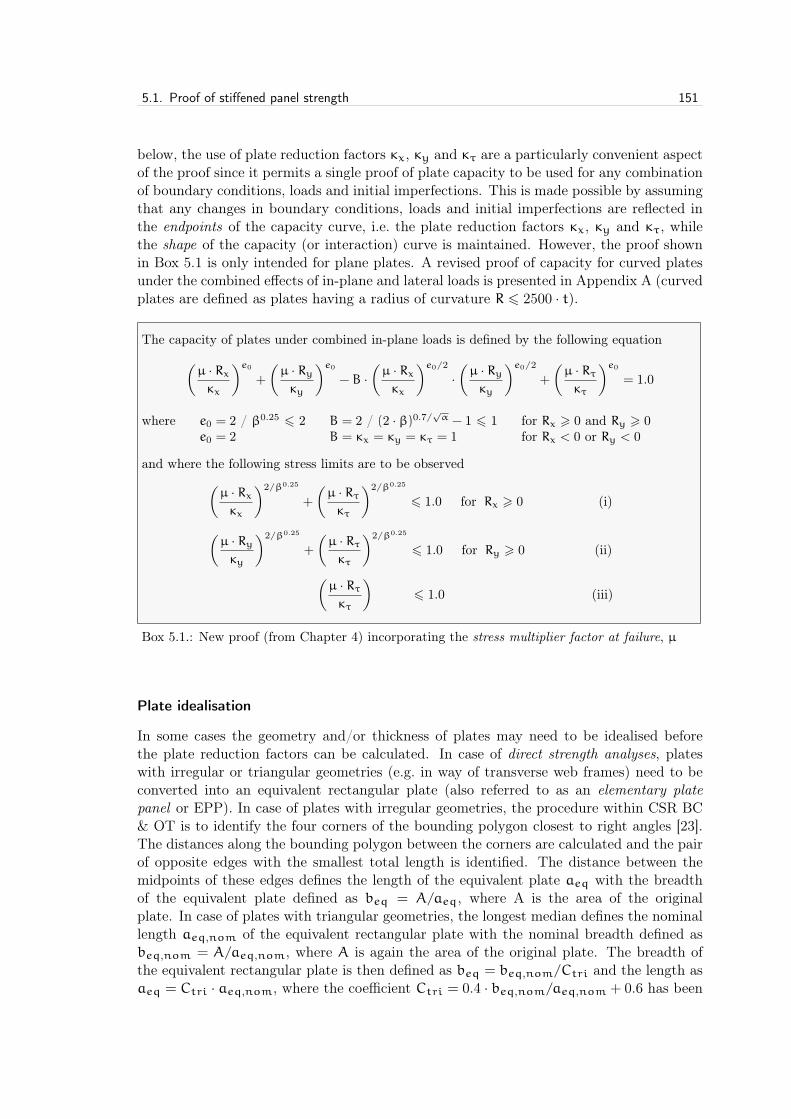
5.1. Proof of stiffened panel strength 151
below, the use of plate reduction factors κx, κy and κτ are a particularly convenient aspectof the proof since it permits a single proof of plate capacity to be used for any combinationof boundary conditions, loads and initial imperfections. This is made possible by assumingthat any changes in boundary conditions, loads and initial imperfections are reflected inthe endpoints of the capacity curve, i.e. the plate reduction factors κx, κy and κτ, whilethe shape of the capacity (or interaction) curve is maintained. However, the proof shownin Box 5.1 is only intended for plane plates. A revised proof of capacity for curved platesunder the combined effects of in-plane and lateral loads is presented in Appendix A (curvedplates are defined as plates having a radius of curvature R 6 2500 · t).
The capacity of plates under combined in-plane loads is defined by the following equation(µ · Rxκx
)e0+
(µ · Ryκy
)e0− B ·
(µ · Rxκx
)e0/2·(µ · Ryκy
)e0/2+
(µ · Rτκτ
)e0= 1.0
where e0 = 2 / β0.25 6 2 B = 2 / (2 · β)0.7/√α − 1 6 1 for Rx > 0 and Ry > 0
e0 = 2 B = κx = κy = κτ = 1 for Rx < 0 or Ry < 0
and where the following stress limits are to be observed(µ · Rxκx
)2/β0.25
+
(µ · Rτκτ
)2/β0.25
6 1.0 for Rx > 0 (i)
(µ · Ryκy
)2/β0.25
+
(µ · Rτκτ
)2/β0.25
6 1.0 for Ry > 0 (ii)
(µ · Rτκτ
)6 1.0 (iii)
Box 5.1.: New proof (from Chapter 4) incorporating the stress multiplier factor at failure, µ
Plate idealisation
In some cases the geometry and/or thickness of plates may need to be idealised beforethe plate reduction factors can be calculated. In case of direct strength analyses, plateswith irregular or triangular geometries (e.g. in way of transverse web frames) need to beconverted into an equivalent rectangular plate (also referred to as an elementary platepanel or EPP). In case of plates with irregular geometries, the procedure within CSR BC& OT is to identify the four corners of the bounding polygon closest to right angles [23].The distances along the bounding polygon between the corners are calculated and the pairof opposite edges with the smallest total length is identified. The distance between themidpoints of these edges defines the length of the equivalent plate aeq with the breadthof the equivalent plate defined as beq = A/aeq, where A is the area of the originalplate. In case of plates with triangular geometries, the longest median defines the nominallength aeq,nom of the equivalent rectangular plate with the nominal breadth defined asbeq,nom = A/aeq,nom, where A is again the area of the original plate. The breadth ofthe equivalent rectangular plate is then defined as beq = beq,nom/Ctri and the length asaeq = Ctri · aeq,nom, where the coefficient Ctri = 0.4 · beq,nom/aeq,nom + 0.6 has been

152 5. Design Application
derived from the eigenvalue analyses of plates with right-angled triangular and isoscelestriangular shapes. Where the thickness of finite elements is not constant over the platefield, a weighted average thickness is to be used in the buckling strength analyses1
t =
∑n1 Ai · ti∑n
1 Ai(5.1)
where n is the number of finite elements defining the plate.In the case of prescriptive analyses where the thickness changes over the breadth b
of a plate field, the plate reduction factor κx is calculated in CSR BC & OT using anequivalent plate defined by the smaller plate thickness t1 and a reduced breadth beq ofthe plate field
beq = b1 + b2
(t1
t2
)1.5
(5.2)
where b1 and b2 are the breadths associated with the smaller plate thickness t1 and largerplate thickness t2, respectively. In case the thickness changes over the length a of a platefield, the smaller plate thickness is to be used for the entire field. Here it may be notedthat the plate thickness upon which ultimate strength calculations are based is generallythe net thickness of the plate, i.e. without corrosion additions or any additional thicknessrequired by the owner (i.e. so-called owner’s extras). In the context of IACS rules andrequirements, this is referred to as the net scantling approach.
Lastly, in case the yield strength changes within a plate field, the lesser of the yieldstrengths is to be used when calculating plate capacity. Although this has no effect onthe plate reduction factor, it is the product of the yield stress and the plate reductionfactor which defines the ultimate strength of the plate under a single stress component,e.g. σx,ult = κx · σY .
Load idealisation
When performing prescriptive analyses of scantlings, stresses are defined on the basis ofsimple beam theory such that their definition is rather straightforward. Conversely, incase of direct strength analyses using the finite element method, the distribution of stressesacting on the plate are rarely uniform. Accordingly, procedures are required for determiningthe so-called reference stresses to be used in the proof of plate capacity. These referencestresses are based on the finite element stresses transformed into the local coordinate systemof an equivalent rectangular plate, i.e. the EPP.
In case of plates with irregular or triangular geometries, the longitudinal, transverseand shear stresses are calculated in CSR BC & OT using a weighted average approach.In this case the edge stress ratios are to be taken as ψx = σx,max/σx,min = 1 andψy = σy,max/σy,min = 1, i.e. no in-plane bending along either edge. In case of regu-lar geometries, the following procedures are included in CSR BC & OT for calculatingstress-based reference stresses along the edges of the plate (an alternative procedure forcalculating displacement-based reference stresses is included in the IACS Common Struc-tural Rules for Bulk Carriers (CSR BC) [31]).
1 Throughout the following discussion of plate and load idealisation, the subscript i is used as a counterof finite elements rather than an indication of internal stress.

5.1. Proof of stiffened panel strength 153
Longitudinal stress σx
In case of longitudinal stress, the distribution of σx(x) over the length of the plateis represented by a second order polynomial curve (to take into account in-plane bendingstresses in the plate due to out-of-plane stiffener deflection)
σx(x) = C1 · x2 + C2 · x+ C3 (5.3)
The curve of best fit is obtained by minimising the square error Π using the area of eachelement Ai as a weighting factor
Π =
ne∑i=1
Ai[σx,i −
(C1 · x2
i + C2 · xi + C3)]2 (5.4)
where ne is the number of finite elements and σx,i is the stress at the centroid of eachfinite element. The unknown coefficients C1, C2 and C3 are obtained by setting to zero thefirst derivatives of the square error Π with respect to each, e.g. ∂Π/∂C1 = 0, and solvingthe resulting set of equations, i.e. a 3 x 3 matrix.
The average longitudinal stresses σx1 and σx2 over b x b areas at each end of theplate as well as the average longitudinal stress σx3 over a b x b area centred at the peakof the computed 2nd order polynomial curve are then calculated and the maximum takento be the magnitude of reference stress in the longitudinal direction
σx = max.(σx1;σx2;σx3) (5.5)
Here the average stress σx3 is only considered if the peak of the computed 2nd order poly-nomial curve is at least b/2 away from the ends of the plate. The edge stress ratio forlongitudinal stresses is taken as ψx = σx,min/σx,max = 1, i.e. no in-plane bending.
Transverse stress σy
In case of transverse stress, the distribution of σy(x) over the length of the plate isassumed to be linear
σy(x) = A+ B · x (5.6)
Once again, the curve of best fit is obtained by minimising the square error Π using thearea of each element as a weighting factor
Π =
ne∑i=1
Ai[σy,i − (A+ B · xi)
]2 (5.7)
where σy,i is again the stress at the centroid of each finite element. Similar to that forlongitudinal stresses, the unknown coefficients A and B are obtained by setting to zero thefirst derivatives of the square error Π with respect to each, e.g. ∂Π/∂A = 0, and solvingthe resulting set of equations, i.e. a 2 x 2 matrix.
The magnitude of transverse stress is then taken as
σy = max.[A,A+ B · a) (5.8)
154 5. Design Application
and the edge stress ratio as
ψy =min.[A,A+ B · a)max.[A,A+ B · a) for σy > 0 (5.9a)
ψy =1 for σy < 0 (5.9b)
Shear stress τxy
In case of shear stress τxy, a weighted average approach is used such that
τxy =
∑ne1 Ai · τxy,i∑ne
1 Ai(5.10)
Here again, τxy,i is the shear stress at the centroid of each finite element.
Poisson correction
Finally, in case of grillage analyses where the stresses are based on beam theory(e.g. scantling check of hatch covers), stresses in the x- and y-directions need first tobe corrected before a capacity check can be performed. This is because stresses whichinclude the Poisson effect are greater than those according to beam theory for a given levelof strain in the structure. Therefore, because stresses used in the proof of plate capacityinclude Poisson effects, stresses based on beam theory are to be corrected as follows
σx =σxb + ν · σyb
1− ν2 (5.11a)
σy =σyb + ν · σxb
1− ν2 (5.11b)
where σxb and σyb are the longitudinal and transverse stresses, respectively, based onbeam theory.
Plate reduction factors
In Chapter 2 the plate reduction factors for rectangular plates under single stress compo-nents (i.e. κx, κy and κτ) were numerically calculated and compared to various formulationsfrom both literature and the shipbuilding industry. Here the plates were simply-supportedon all edges with uniform axial and shear stresses over the length/breadth of the plate.Although these idealised conditions are largely valid for most of the structure contributingto the longitudinal strength of a ship (i.e. the most critical aspect of ship strength), thereis much structure throughout the ship for which these conditions are clearly invalid. Forthis reason, shipbuilding rules normally provide plate reduction factors for several com-binations of other idealised boundary conditions (i.e. free, simply-supported or clampededges) and applied stresses (including in-plane bending). In CSR BC & OT, 25 such casesare provided for plane plates alone (including the variations due to in-plane bending). Itis then the responsibility of designers and plan approval engineers to determine which ide-alised case is most appropriate for a given structure and load. For instance, in case offloors or girders with lightening holes or access openings, the plating between stiffeners is
5.1. Proof of stiffened panel strength 155
decomposed into smaller plate elements which may then be evaluated with the proof ofcapacity taking into account the revised dimensions and relevant boundary conditions, e.g.free edge in case the edge adjacent to an opening is not stiffened. The strength of websand flanges of corrugated bulkheads may also be evaluated using a nominal plate aspectratio (α = 2 in case of CSR BC & OT) and assuming simply-supported edges.
As noted above, plate reduction factors (explicitly) capture the effects of boundaryconditions and stresses over the length/breadth of the plate. In this regard, various defini-tions of plate reduction factors are used for different combinations of boundary conditionsand loads. Moreover, for each of these combinations, plate reduction factors are assumedto (implicitly) capture the effects of lateral pressure and initial imperfections (i.e. residualstresses and deflections) even though, in case of the former, out-of-plane loads are as-sumed to have a negligible effect on the in-plane capacity of the plate (in accordance withDIN 18800 [26]). As mentioned previously, these assumptions conveniently allow a singleproof of plate capacity to be used for any combination of boundary conditions, loads andinitial imperfections, provided the influences of each are accurately reflected in the platereduction factors. Accordingly, although the determination of plate reduction factors isbeyond the scope of the present work, some examples are in order to demonstrate that theproof of plate capacity under combined loads (as shown in Box 5.1) remains valid in caseof other boundary conditions, loads and initial imperfections relevant for the shipbuildingindustry.
Other boundary conditions
Upon first glance of the buckling cases in CSR BC & OT, one of the more obviousvariations in boundary conditions for investigation would seem to be plates with all fouredges clamped against rotation (Case Nos. 13 and 14). Indeed, such boundary conditionsdo result in an interaction curve which is more rectangular in shape (i.e. less interactionbetween the axial stress components) such that the proof shown in Box 5.1 would berelatively conservative. However, in practice such boundary conditions are quite difficultto achieve and have been included in CSR BC & OT more so for the sake of completeness.Under in-plane axial stresses, the internal energy of continuous plating is minimised whenit buckles out-of-plane in opposite directions on each side of its supports (in both the x- andy-directions), a deflection pattern which closely resembles simply-supported edges. Anyeffect of the rotational restraint provided by stiffeners is taken into account by increasingthe elastic buckling factor K which in turn increases the value of the plate reduction factorκ, but essentially the edge conditions of the plating remain simply-supported. Even whena plate is preloaded by an extreme lateral pressure, it has been shown in finite elementanalyses (see below) and observed in tests [10] that the plating snaps out of the deflectionpattern due to the lateral load and into a deflection pattern which minimises the internalenergy under in-plane axial loads (i.e. its eigenmode). However, in a very few cases, it maybe appropriate to consider some edges of the plate clamped against rotation. For instance,in CSR BC & OT the short edges of the shell plating of single side skin bulk carriersmay be considered clamped against rotation due to the substantial restraint provided bythe adjacent wing and hopper tank structures, although the strengthening effects of theseboundary conditions are quite local.
One of the more common variations in boundary conditions found in shipbuilding isthree edges simply-supported with the fourth edge free from any support. As suggested

156 5. Design Application
above and shown in Figure 5.2, this is the case for plating adjacent to lightening holesand access openings (without edge reinforcements) in the floors and girders of the doublebottom structure. Here the plate is subject to axial stresses in the local x-direction (e.g.due to longitudinal bending or transverse compression of the hull girder) combined withshear stresses (e.g. near the ends of floors and girders due to lateral loading of the doublebottom). In Figure 5.3 the capacity curve of a plate with a free edge (α = 1, β = 2)is compared to that with all four edges simply-supported. As can be seen, the capacitycurve for the plate with one free edge takes on the same shape as that for the platesimply-supported on all edges (i.e. a function of the exponent e0, as defined by the plateslenderness parameter β, since Ry = 0). Here a standard access opening of 600 x 800 mmin accordance with SOLAS [65] requirements has been centred in a 2400 x 800 mm platefield in the double bottom2. In practice, the vertical extension of such openings shouldnot exceed one half of the height of the floor/girder. Accordingly, for the standard accessopening 600 x 800 mm in a plate field of 800 mm spacing, it is possible that the remainingplating above/below the opening has an aspect ratio α = 2 (i.e. a double bottom heightof 1600 mm and vertically-centred opening). This of course increases the effect of the freeedge on the capacity of the plate leading to an error which may approach 10%. However,this is something of an upper bound on the error and is at the boundary of practical shipdesign. Moreover, for plating adjacent to lightening holes and access openings, the endsof the "free" edge are not truly free, i.e. they are supported by the plating and snipedstiffeners in line with the longitudinal axis of the opening.
free edge
sniped stiffeners
600 x 800
bottom shell plating
inner bottom plating
Figure 5.2.: Idealisation of plating adjacentto access opening.
0.0
0.1
0.2
0.3
0.4
0.5
0.6
0.7
0.8
0.9
1.0
0.0 0.1 0.2 0.3 0.4 0.5 0.6 0.7 0.8 0.9 1.0
Norm
alise
d s
tres
s, R
τ
Normalised stress, Rx
finite element results
proof of capacity
1
run id 922203
MAR 16 201613:56:03
PLOT NO. 10
DISPLACEMENT
STEP=1SUB =157TIME=.527836DMX =16.9047
1
run id 922203
MAR 16 201613:50:03
PLOT NO. 8
DISPLACEMENT
STEP=1SUB =192TIME=.763311DMX =9.70523
Figure 5.3.: Capacity curve of plate with free edge(α = 1, β = 2).
Yet another common variation in boundary conditions found in shipbuilding is whenone edge is allowed to pull in, i.e. no edge restraint. In fact, preventing the in-planedeflection of plating at the edges of stiffened panels is rarely possible in ship structuressince the restraint would need to come from perpendicular supporting structure which in
2 According to Chapter II-1, Part A-1, Regulation 3-6, Paragraph 5.2 of SOLAS, such a configurationrequires the provision of gratings or other foot holds since the distance of the opening from the bottomshell plating is otherwise not to exceed 600 mm (i.e. to facilitate access).
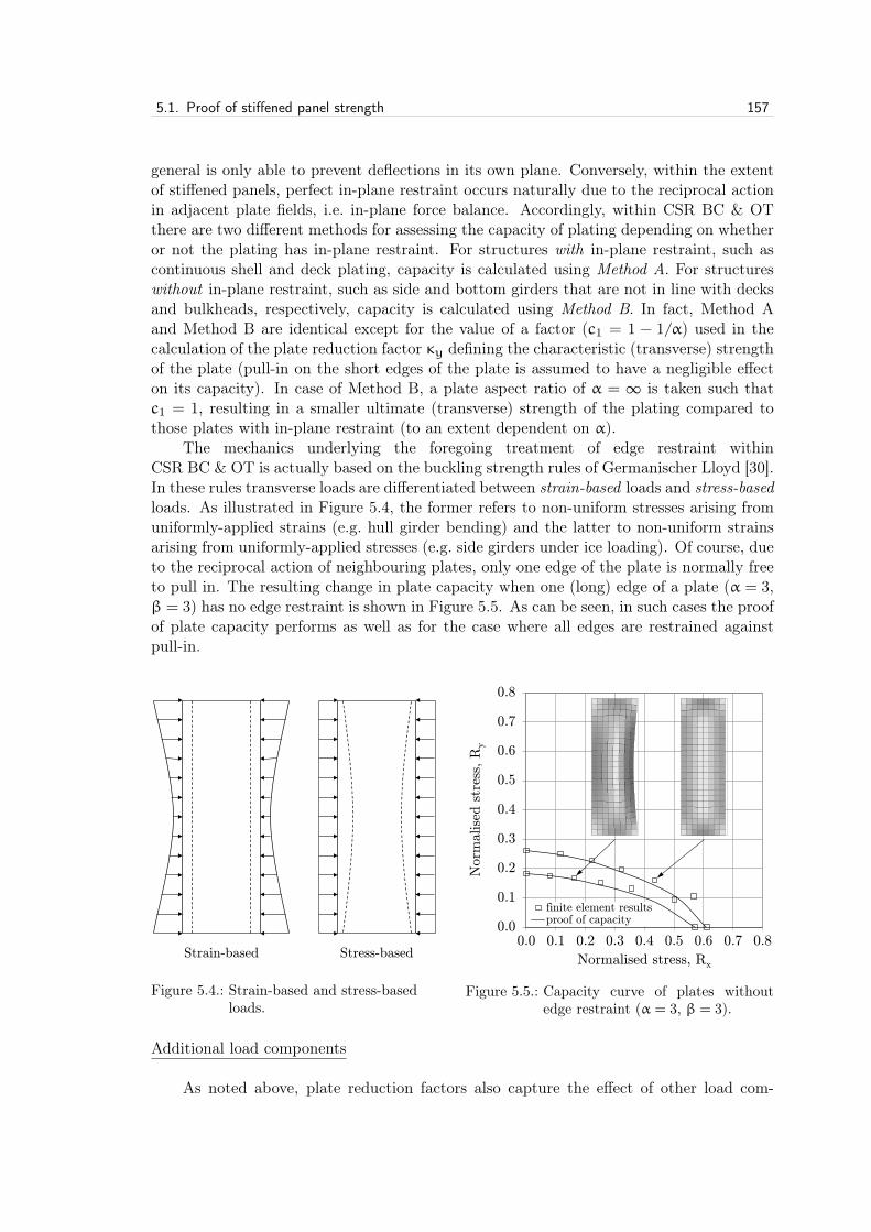
5.1. Proof of stiffened panel strength 157
general is only able to prevent deflections in its own plane. Conversely, within the extentof stiffened panels, perfect in-plane restraint occurs naturally due to the reciprocal actionin adjacent plate fields, i.e. in-plane force balance. Accordingly, within CSR BC & OTthere are two different methods for assessing the capacity of plating depending on whetheror not the plating has in-plane restraint. For structures with in-plane restraint, such ascontinuous shell and deck plating, capacity is calculated using Method A. For structureswithout in-plane restraint, such as side and bottom girders that are not in line with decksand bulkheads, respectively, capacity is calculated using Method B. In fact, Method Aand Method B are identical except for the value of a factor (c1 = 1 − 1/α) used in thecalculation of the plate reduction factor κy defining the characteristic (transverse) strengthof the plate (pull-in on the short edges of the plate is assumed to have a negligible effecton its capacity). In case of Method B, a plate aspect ratio of α = ∞ is taken such thatc1 = 1, resulting in a smaller ultimate (transverse) strength of the plating compared tothose plates with in-plane restraint (to an extent dependent on α).
The mechanics underlying the foregoing treatment of edge restraint withinCSR BC & OT is actually based on the buckling strength rules of Germanischer Lloyd [30].In these rules transverse loads are differentiated between strain-based loads and stress-basedloads. As illustrated in Figure 5.4, the former refers to non-uniform stresses arising fromuniformly-applied strains (e.g. hull girder bending) and the latter to non-uniform strainsarising from uniformly-applied stresses (e.g. side girders under ice loading). Of course, dueto the reciprocal action of neighbouring plates, only one edge of the plate is normally freeto pull in. The resulting change in plate capacity when one (long) edge of a plate (α = 3,β = 3) has no edge restraint is shown in Figure 5.5. As can be seen, in such cases the proofof plate capacity performs as well as for the case where all edges are restrained againstpull-in.
Strain-based Stress-based
Figure 5.4.: Strain-based and stress-basedloads.
0.0
0.1
0.2
0.3
0.4
0.5
0.6
0.7
0.8
0.0 0.1 0.2 0.3 0.4 0.5 0.6 0.7 0.8
Norm
alise
d s
tres
s, R
y
Normalised stress, Rx
finite element resultsproof of capacity
1
run id 913307
DEC 8 201512:33:14
PLOT NO. 6
DISPLACEMENT
STEP=1SUB =56TIME=.235967DMX =19.749
1
run id 913307
DEC 8 201512:41:27
PLOT NO. 11
DISPLACEMENT
STEP=1SUB =69TIME=.163154DMX =31.7568
Figure 5.5.: Capacity curve of plates withoutedge restraint (α = 3, β = 3).
Additional load components
As noted above, plate reduction factors also capture the effect of other load com-

158 5. Design Application
ponents such as in-plane bending. Because individual plate fields are relatively smallcompared to the ship as a whole, the in-plane bending due to global bending of the hullgirder (vertical and horizontal) is normally assumed to result in uniform stress distributionover the length and breadth of plates (one notable exception here is the in-plane bendingof vertical stiffened side shell plating of single side skin bulk carriers which generally haverather large aspect ratios). Accordingly, it is usually local loads such as double bottombending which subject plates to in-plane bending (e.g. floors and girders). In such cases,the effects of in-plane bending are reflected in the elastic buckling factor K which in turnare reflected in the plate reduction factor κ that is used in the proof of capacity. As anexample, a capacity curve is shown in Figure 5.6 for a plate (α = 3, β = 3) subjected simul-taneously to shear stresses and transverse in-plane bending. Here the in-plane bending isdescribed by the edge stress ratio ψ = σy,min/σy,max = 0, where σy,min is the minimumstress along the side and σy,max is the maximum. Such a stress state occurs, for instance,in case of a vertically stiffened plate field at the end of a bottom longitudinal girder,i.e. under lateral loads the girder is effectively clamped against rotation by the supportingstructure of the transverse bulkhead such that pure in-plane bending is superimposed oncompressive stresses (of comparable magnitude) due to hull girder bending. As can beseen, the shape of the capacity curve for in-plane bending (ψ = 0) is similar to the shapeof the capacity curve for the (standard) case of no in-plane bending (ψ = 1), upon whichthe proof of plate capacity is based.
0.0
0.2
0.4
0.6
0.8
1.0
0.0 0.2 0.4 0.6 0.8 1.0
Norm
alise
d s
tres
s, R
τ
Normalised stress, Ry
finite element results
proof of capacity
Figure 5.6.: Capacity curve of plate underin-plane bending (α = 3, β = 3).
0.0
0.1
0.2
0.3
0.4
0.5
0.6
0.7
0.8
0.0 0.1 0.2 0.3 0.4 0.5 0.6 0.7 0.8
Norm
alise
d s
tres
s, R
y
Normalised stress, Rx
finite element results
proof of capacity
1
Run ID 912301
DEC 8 201521:50:46
PLOT NO. 12
ELEMENTS
PRES-NORM.2987
1
Run ID 912301
DEC 8 201521:50:57
PLOT NO. 13
ELEMENTS
Figure 5.7.: Capacity curve of plate under lateralload (α = 3, β = 2).
Another load component not explicitly considered in the development of the platecapacity proof is lateral pressure. As noted above, out-of-plane loads are assumed to havea negligible effect on the in-plane capacity of the plate in accordance with DIN 18800 [26].In this regard, Figure 5.7 compares the capacity curves for typical bottom shell plating(α = 3, β = 2) under biaxial compression with and without lateral pressure. Here theplate was pre-loaded with a lateral pressure of p = 271.0 kN/m2 which is the pressurerequired to initial yield according to the following equation

5.1. Proof of stiffened panel strength 1591
X Y
Z
run id 912301
DEC 8 2015
23:27:17
PLOT NO. 21
(a) Deflection under lateral load
1
X Y
Z
run id 912301
DEC 8 2015
23:26:27
PLOT NO. 17
hot spot
(b) Deflection under lateral and in-plane loads
Figure 0.1: ——-CROP!——–CROP!——–CROP!——–CROP!——–CROP!———CROP!——-
1
Figure 5.8.: Deflection patterns under lateral load (p = 271.0 kN/m2, α = 3, β = 2).
p =2 · σY√
1− ν+ ν2·(t
b
)2
(5.12)
In this case the average loss of capacities (i.e. reduction in magnitude of the ultimate loadvectors) due to the lateral pressure is about 4.8%. Moreover, as shown in Figure 5.7, theshape of capacity curves with and without pressure are the same. Accordingly, the proofof capacity remains valid where any loss in capacity due to the presence of lateral pressureneed only be reflected in the plate reduction factors κx and κy. In case of square plates,Søreide and Czujko [66] alternatively suggest an interactive relationship between biaxialcompression and lateral load of the form
(Rx)e1 − B · Rx · Ry + (Ry)
e2 = (1+ ξ · Rp)e4 (5.13)
where the quantity Rp = p/pult is the lateral load normalised against its defined ultimatevalue (e.g. first yield).
To better understand why lateral pressure has such a small effect on the capacity ofplates under in-plane loads, some insight into the collapse mechanism is required. Towardsthis end, it is noteworthy that the presence of lateral pressure does not prevent deflectionof the plate into a shape which minimises internal energy under compressive loads. This isillustrated in Figure 5.8 which shows the deflection under lateral load alone (Figure 5.8(a))and the deflection at collapse after an in-plane longitudinal load was applied in a secondload step (Figure 5.8(b)). The same is true when transverse loads are applied. Here thefinite element analyses are performed with a symmetric model to correctly capture theeffect of the lateral pressure with the location of stiffeners indicated in Figure 5.8 (a finermesh is also used to better illustrate the patterns of deflection).
Moreover, the locations of collapse initiation are the same with or without lateralpressure. Therefore, in order to study the development of plate collapse, the internalstresses at the mid-length edge "hotspot" identified in Figure 5.8(b) are shown in Figure5.9. Here the tracking of internal stress development begins following application of thelateral pressure, i.e. longitudinal load Rx = 0. Accordingly, as shown in Figures 5.9(a)and 5.9(b), edge hinges develop under the lateral pressure as evidenced by yielding in thetop and bottom fibres of the plate for Rx = 0 (i.e. Re,i ' 1) due to large tensile andcompressive stresses Ry,i, respectively, in the transverse direction. With the application of

160 5. Design Application
Rx,i
Ry,i
Re,i
-1.4-1.2-1.0-0.8-0.6-0.4-0.20.00.20.40.60.81.01.21.4
0.0 0.1 0.2 0.3 0.4 0.5 0.6 0.7 0.8
Norm
alise
d inte
rnal st
ress
es
Applied stress, Rx
(a) Top fibre of plate
Rx,i
Ry,i
Re,i
-1.4-1.2-1.0-0.8-0.6-0.4-0.20.00.20.40.60.81.01.21.4
0.0 0.1 0.2 0.3 0.4 0.5 0.6 0.7 0.8N
orm
alise
d inte
rnal st
ress
es
Applied stress, Rx
(b) Bottom fibre of plate
Rx,i
Ry,i
Re,i
-1.4-1.2-1.0-0.8-0.6-0.4-0.20.00.20.40.60.81.01.21.4
0.0 0.1 0.2 0.3 0.4 0.5 0.6 0.7 0.8
Norm
alise
d inte
rnal st
ress
es
Applied stress, Rx
(c) Middle plane of plate
Re,i (top fibre)
Re,i (middle plane)
Re,i (bottom fibre)
-1.4-1.2-1.0-0.8-0.6-0.4-0.20.00.20.40.60.81.01.21.4
0.0 0.1 0.2 0.3 0.4 0.5 0.6 0.7 0.8
Norm
alise
d inte
rnal st
ress
es
Applied stress, Rx
(d) Equivalent internal stresses
Figure 0.1: ——-CROP!——–CROP!——–CROP!——–CROP!——–CROP!———CROP!——-
1
Figure 5.9.: Internal stresses in plate under lateral pressure and longitudinal in-plane compression.
the longitudinal load Rx (i.e. Ry = 0), the internal stress Rx,i in the x-direction directlyincreases. However, because of changes in Ry,i due to changes in the deflection patternof the plate, the equivalent internal stresses in both the top and fibres remain close toRe,i = 1.0 throughout the application of the longitudinal load.
Conversely, as shown in Figure 5.9(c), the stress levels in the middle plane of theplate under lateral pressure alone are quite small, i.e for Rx = 0. This is because lateralloads are primarily resisted by pure bending in the absence of significant membrane action(i.e. there is little strain in the middle plane of the plate since its edges, although straight,are otherwise able to freely move in-plane). Accordingly, the equivalent stress Re,i in themiddle plane of the plate under lateral pressure alone is only about 6.5% of yield. As themagnitude of the longitudinal load Rx increases, so too does the magnitude of internalstresses Rx,i and Ry,i in the middle plane of the plate, the latter due to the magnifica-

5.1. Proof of stiffened panel strength 161
tion of out-of-plane deflections as shown in Figure 5.8(b).3 This growth of longitudinaland transverse stresses in the middle plane of the plate leads directly to larger equivalentstresses Re,i in this plane. As noted in Chapter 2, through thickness plasticity (alongthe plate edges) is a precursor to collapse under in-plane axial loads. This means thatplate collapse only occurs once the equivalent stresses in all fibres of the plate reach yield,i.e. Re,i = 1 in the top, bottom and middle fibres of the plate. However, as shown inFigure 5.9(d), here yielding in the middle fibres of the plate depends almost exclusively onthe magnitude of applied in-plane loads, although membrane action would be expected toincrease together with plate slenderness (as evident in test results reported by Becker [49]).
Initial imperfections
Within modern day shipbuilding, most steel structures are subjected to time-dependenttemperature gradients during welding and to a lesser extent thermal cutting. As notedby Paik and Thayamballi [35], when steel is heated during welding the molten portionexpands and is compressed by the surrounding steel which remains relatively cool. Oncethe temperature drops in the heated portion, it is subjected to locked in tensile stressesand distortions which may be minimised by proper welding procedures and fabricationmethods, but never eliminated. Accordingly, in addition to boundary conditions and otherload components, plate reduction factors need also to account for the effects of these initialimperfections.
In terms of distortions due to welding, a double Fourier series imperfection shape iswidely used to characterise residual deflections in plating
δ
δ0=
m∑i=1
n∑j=1
siniπ
ax · sinjπ
by (5.14)
where δ0 is the magnitude of initial (out-of-plane) deflection. However, initial imperfec-tion shapes are normally such that they predominantly have one half-wave in the shorterdirection, allowing them to be adequately described by out-of-plane deflection along thecentreline y = b/2 of the plate
δ
δ0=
m∑i=1
siniπx
a(5.15)
The magnitude of initial deflection δ0 is of particular importance since the capacity ofplating is inversely related to this quantity. For this reason, several empirical formulationsare available in the literature for calculating design magnitudes, with one of the more wellknown formulations provided by Smith et al. [63] for three different levels of imperfections
δ0
t=
0.025 · β2 slight
0.100 · β2 average
0.300 · β2 severe
(5.16)
3 The magnification of deflections used in Figure 5.8 are optimised for better illustration. The magnitudeof out-of-plane deflections at collapse under combined lateral and longitudinal loads are about 3.5 timesgreater than under lateral pressure alone.

162 5. Design Application
However, in shipbuilding the magnitudes of initial deflection are unknown beforehandand so are not an explicit parameter in plating design. For instance, the plate reductionfactors used in CSR BC & OT are empirically derived on the basis of experimental andnumerical results. Accordingly, post-construction surveys are carried out to ensure thatplating complies with deflection tolerances. For instance, ships built according to therules of IACS member societies need to comply with tolerances delineated in the IACSShipbuilding and Repair Quality Standard [67] for the hull structure during the newbuildingstage and repair standard when the quality standard is not satisfied.
-1.0
-0.5
0.0
0.5
1.0
0.0 0.1 0.2 0.3 0.4 0.5 0.6 0.7 0.8 0.9 1.0Def
lect
ion δ
/δ0
Longitudinal position, x/a
(a) Eigenmode under σx
-1.0
-0.5
0.0
0.5
1.0
0.0 0.1 0.2 0.3 0.4 0.5 0.6 0.7 0.8 0.9 1.0Def
lect
ion δ
/δ0
Longitudinal position, x/a
(b) Eigenmode under σy
-1.0
-0.5
0.0
0.5
1.0
0.0 0.1 0.2 0.3 0.4 0.5 0.6 0.7 0.8 0.9 1.0Def
lect
ion δ
/δ0
Longitudinal position, x/a
(c) Initial deflection shape #1
-1.0
-0.5
0.0
0.5
1.0
0.0 0.1 0.2 0.3 0.4 0.5 0.6 0.7 0.8 0.9 1.0Def
lect
ion δ
/δ0
Longitudinal position, x/a
(d) Initial deflection shape #2
-1.0
-0.5
0.0
0.5
1.0
0.0 0.1 0.2 0.3 0.4 0.5 0.6 0.7 0.8 0.9 1.0Def
lect
ion δ
/δ0
Longitudinal position, x/a
(e) Initial deflection shape #3
-1.0
-0.5
0.0
0.5
1.0
0.0 0.1 0.2 0.3 0.4 0.5 0.6 0.7 0.8 0.9 1.0Def
lect
ion δ
/δ0
Longitudinal position, x/a
(f) Initial deflection shape #4
Figure 0.1: ——-CROP!——–CROP!——–CROP!——–CROP!——–CROP!———CROP!——-
1
Figure 5.10.: Initial deflection shapes.
With respect to the shape of imperfections, the proof of plate capacity developedin Chapter 4 is based on results using the critical eigenmodes of plates for the initialdeflection shapes (as described in Appendix B). In order to investigate whether the resultingproof remains valid for other types of imperfection shapes, capacities for a plate (α = 3,β = 2) under biaxial compression have been numerically calculated using four typical initialdeflection patterns reported by Paik and Thayamballi [35] (see also Paik and Pedersen [68]).These shapes have been chosen amongst several deflection measurements obtained by Uedaand Yao [69] from 21 bulk carriers and 12 car carriers and are shown in Figure 5.10 togetherwith the critical eigenmodes under longitudinal and transverse compression. A deflectionmagnitude of δ0 = b/200 was used in all analyses which was sufficient to prevent the platefrom snapping into any of its eigenmodes upon load application (i.e. in case of imperfectionshapes #1 to #4). Capacities of the plate based on all imperfection shapes are comparedin Figure 5.11. As can be seen, the shape of the capacity curves delineated by numericalresults may not be the same, but those based on eigenmode deflections provide a goodrepresentation of the critical imperfections.
In addition to initial deflections, plate reduction factors need also to account for resid-ual stresses due primarily to welding. Similar to initial deflections, some authors havedeveloped formulations for plate reduction factors which explicitly account for the level ofresidual welding stresses. For instance, Frieze et al. [70] have developed plate reductioncurves for "unwelded", "lightly welded" and "heavily welded" plates. However, withinthe shipbuilding industry, plate reduction factors implicitly account for welding residual

5.1. Proof of stiffened panel strength 163
0.0
0.1
0.2
0.3
0.4
0.5
0.6
0.7
0.8
0.9
0.0 0.1 0.2 0.3 0.4 0.5 0.6 0.7 0.8 0.9
Norm
alise
d s
tres
s, R
y
Normalised stress, Rx
Proof
Critical eigenmodes
Shape 1
Shape 2
Shape 3
Shape 4
Figure 5.11.: Capacity curve of plates withvarious initial deflection shapes.
0.0
0.1
0.2
0.3
0.4
0.5
0.6
0.7
0.8
0.0 0.1 0.2 0.3 0.4 0.5 0.6 0.7 0.8
Norm
alise
d s
tres
s, R
y
Normalised stress, Rx
finite element results
proof of capacity
σrcx = 0.10∙σY , σrcy = 0.03∙σY
σrcx = σrcy = 0
Figure 5.12.: Capacity curve of plate withresidual stresses.
stresses and where the quality of welds are controlled through classification society rules,welding procedure qualification, welder certification as well as weld monitoring and con-trol [71].
With respect to residual stresses, the proof of plate capacity developed in Chapter 4is based on results for unwelded plates (i.e. without residual stresses) such that some addi-tional numerical calculations are needed to validate the proof for welded plates (i.e. withresidual stresses). As noted above, residual tensile stresses develop due to welding in theso-called heat-affected zone (HAZ) along the edges of the plate, between which compressivestresses develop in order to maintain force equilibrium. Accordingly, the internal stressesin the body of the plate reach yield under the application of a smaller compressive in-planestress compared to stress-free plates, i.e. residual stresses generally reduce the capacityof plates. Because the tensile zones are adjacent to the edges of the plate, Hughes notesthat they have a negligible effect on the stability of the plate [9]. Moreover, as furthernoted by Hughes, the breadth of these zones are relatively small such that the effectiveaspect ratio α’ of the plate is only slightly reduced. In general, residual stresses due towelding develop in both the x- and y-directions of the plate and are normally idealised astensile and compressive blocks as shown in the inset of Figure 5.12. Based on equilibriumconsiderations, the breadth of the tensile block bt in the x-direction is equal to
bt =σrcx
2 · (σrcx − σrtx)· b (5.17)
where σrcx and σrtx are the residual compression and tension stresses, respectively. Asnoted by Hughes [9], the compressive residual stresses in welded plates rarely exceed 0.1·σYand, although tensile residual stresses may well reach yield, stress-relief normally occursdue to the alternating tension and compression of the plate under hull girder bending(referred to as "shakedown") resulting locally in small plastic strains. Accordingly, basedon measurements reported by Cheng et al. in Appendix B of reference [72] (also reportedin reference [35]), −0.7 · σY is considered to be an appropriate value of tensile compressivestresses due to welding.

164 5. Design Application
Accordingly, for residual stresses of σrcx = 0.1 ·σY and σrtx = −0.7 ·σY , the resultingbreadth of the tensile zones in the x-direction according to Equation (5.17) is equal to
bt =σrcx
2 · (σrcx − σrtx)· b =
0.1 · σY2 · (0.1 · σY + 0.7 · σY)
· b =b
16(5.18)
For a finite element model of a plate with 16 square elements of equal size across its breadth,tensile zones in the x-direction would therefore have the breadth of a single element. Usingthe same breadth at = bt = b/16 and magnitude σrty = σrtx = −0.7 · σY of tensilezones along the short edges of a plate, the magnitude of compressive residual stress in they-direction is calculated as σrcy = 0.03 · σY (it is for this reason that residual stresses inthe transverse direction are often neglected). Accordingly, with reference to the inset inFigure 5.12, the following residual stresses are used in the numerical analyses of a weldedplate
σrx =
σrtx for 0 6 y 6 btσrcx for bt 6 y 6 b− btσrtx for b− bt 6 y 6 b
(5.19)
in the x-direction, and
σry =
σrty for 0 6 x 6 atσrcy for at 6 x 6 a− at
σrty for a− at 6 x 6 a
(5.20)
in the y-direction. Using this residual stress state, the capacities of a welded plate underbiaxial compression are compared in Figure 5.12 to that for an unwelded plate (α = 3,β = 2). As can be seen, the loss of capacity due to residual stresses is about 7.0%. However,the shape of both capacity curves is the same such that the results obtained with the proofof plate capacity compare well with both sets of numerical results.
Evaluation
Following the calculation of plate reduction factors (κx, κy and κτ) and reference stresses(Rx, Ry and Rτ), the capacity of the plate can then be evaluated. By substituting thesefactors and stresses into the capacity equation shown in Box 5.1, the equation can thenbe solved in terms of the stress multiplier factor at failure µ. Within CSR BC & OT, autilisation factor is then defined as the reciprocal of the minimum value of µ
η =1
µmin(5.21)
and then compared to an allowable value of the utilisation factor ηall which is defined asa function of the type of structure and load combination, i.e. whether the applied stressesare due to a static load or combined static and dynamic loads
η 6 ηall (5.22)
The utilisation factor is best understood as the ratio of applied loads and the ultimatecapacity of the plate, i.e. the ratio of stress vector magnitudes.

5.1. Proof of stiffened panel strength 165
5.1.2. Proof of sufficient stiffener capacity
As noted above, the ultimate strength of a stiffened panel is defined as the minimum ofthe ultimate strength of the plating and the ultimate strength of the stiffeners. In termsof the latter, CSR BC & OT includes checks for two separate collapse modes
1. overall panel buckling (elastic),
2. lateral buckling (inelastic).
In CSR BC (and legacy GL rules), three additional collapse modes are considered
3. torsional buckling (inelastic),
4. web buckling (inelastic),
5. flange buckling (inelastic).
Analogous to the analysis of plating strength, the mode of collapse associated with theminimum stress multiplier at failure µ is the critical mode which defines stiffener strength.
Overall panel buckling
Regarding the first mode of collapse, overall panel buckling is synonymous with elastic stiff-ener buckling, i.e. lateral or out-of-plane buckling. In this mode of collapse the panel buck-les elastically as if it were a plate. For this reason, the computerised buckling code PULSuses orthotropic plate theory to check for overall panel buckling (orthotropic plate theorywas also used in the GL buckling strength rules prior to 1997). As noted by Hughes [9],overall panel buckling is a sudden mode of collapse requiring adjacent structure to takeover a considerable amount of load. However, the lateral loads carried by most ship pan-els lead to stiffener scantlings which are normally sufficient to prevent this mode of collapse.
Lateral buckling
Contrary to overall panel buckling, collapse under lateral buckling is a relatively gradualprocess whereby the initial out-of-plane deflection of the stiffener is magnified under in-plane loads until the yield stress is reached either in the flange of the stiffener (i.e. stiffenerinduced failure) or in the attached plating (i.e. plating induced failure). In addition to thesesecond order effects, bending stresses due to lateral pressure will either retard or hastenyielding depending on the sign of the resulting bending moment, i.e. whether the pressureis on the plate side or the stiffener side. Although yielding at mid-span of the stiffener maybe considered a precursor to stiffener collapse, there is generally some margin before theultimate strength of the stiffener is reached. The magnitude of this margin depends largelyon the relative magnitude (and sign) of the longitudinal stress which directly increases (ordecreases) internal stress over the entire cross-section of the plate-stiffener combination.

166 5. Design Application
2nd order theory
In CSR BC & OT, capacity checks associated with overall panel buckling and lateralbuckling are performed using 2nd order theory. Provision for the use of 2nd order theory wasinitially included in DIN 18800, but the procedure was first implemented in shipbuildingthrough the 1997 GL buckling strength rules and subsequently in CSR BC. The procedureconsiders the following loads
a. compressive stresses parallel to the stiffener,
b. compressive stresses perpendicular to the stiffener,
c. shear stresses in the plate,
d. lateral loads (e.g. external sea pressure)
and is described in detail in reference [73]. However, the following description is basedclosely on reference [61].
As shown in Figure 5.13, when a stiffener with initial deflection δ0 (at midspan) issubjected to a compressive (axial) force Fx, this initial deflection is magnified such thatthe total deflection δ (at midspan) becomes
δ = δ0 ·Fx,cr
Fx,cr − Fx(5.23)
where
Fx,cr =π2
a2 · E · Izz (5.24)
is the critical buckling force and Fx = µ · σx · Ax, where Ax is the cross-sectional area ofthe plate-stiffener combination. Moreover, the quantity Izz is the moment of inertia of thestiffener with attached plating, the extent of which is equal to the lesser of the effectivewidth considering plate buckling (i.e. κx ·b) and the effective breadth considering shear lageffects under bending (i.e. χ ·b, where χ is the effective breadth coefficient)4. Accordingly,the bending moment Mzz,0(x) caused by the compressive force Fx is
Mzz,0(x) = δ(x) · Fx (5.25)
Fx δ0 Fx δ
a
Figure 5.13.: Magnification of initial deflection.
qz
a
a/2
Figure 5.14.: Equivalent sinusoidal line load.
According to DIN 18800, Part 2, Section 2, this bending moment may be alternativelydefined in terms of an equivalent sinusoidal lateral line load
4 Admittedly, as noted by Faulkner [29], "in many practical structures the two effects occur together andare not separable or additive".

5.1. Proof of stiffened panel strength 167
qz(x) = qz · sin(π · xa
)(5.26)
as shown in Figure 5.14. Through integration, this results in the following bending momentat midspan
Mzz,0 = δ · Fx =qz · a2
π2 (5.27)
By substituting the total deflection δ defined by Equation (5.23) into Equation (5.27), theline load at midspan qz becomes
qz = δ · Fx ·π2
a2 = Fx,cr ·π2
a2 · Fx · δ0Fx,cr − Fx
(5.28)
Accordingly, the bending moment of the stiffener (at midspan) becomes
Mzz,0 =qz · a2
π2 = Fx,cr ·π2
a2 · Fx · δ0π2
a2 · Fx,cr − π2
a2 · Fx= Fx,cr ·
pz,x · δ0cf − pz,x
(5.29)
where pz,x = π2
a2 · Fx is the equivalent lateral pressure caused by the longitudinal force Fxand cf = π2
a2 · Fx,cr is the elastic capacity of the stiffener.Analogously, equations for equivalent lateral pressures can also be derived for trans-
verse stresses µ · σy, i.e. pz,y, and shear stresses µ · τxy, i.e. pz,τ. In case of the latter,shear stresses are transformed into principal stresses and the supporting effect of the tensionstresses are neglected. Accordingly, the total equivalent lateral pressure can be expressedas
pz = pz,x + pz,y + pz,τ (5.30)
such that the total bending moment of the stiffener at midspan due to in-plane forcesbecomes
Mzz,0 = Fx,cr ·pz · δ0cf − pz
(5.31)
Upon inspection of Equation (5.31), it can be seen that the quantity pzcf−pz
is a deflectionmagnification factor. Accordingly, once the total equivalent lateral pressure pz equals theelastic capacity of the stiffener cf, the elastic deflection of the stiffener becomes infinite,i.e. overall panel buckling. Accordingly, the capacity of the panel corresponding to collapsemode 1 (overall panel buckling) may be expressed as
pz/cf = 1 (5.32)
Regarding the second mode of collapse (lateral buckling), the bending moment of thestiffener at midspan due to in-plane stresses Mzz,0 is combined with the bending momentof the stiffener at midspan due to the lateral loadMzz,1 in order to obtain the total bendingstress in the stiffener
σb =Mzz,0 +Mzz,1
Z(5.33)

168 5. Design Application
where Z is the section modulus of the stiffener with attached plating as defined above5.This bending stress is in turn combined with the longitudinal stress σ ′x (corrected to takeinto account the reduced effective width of plating due to buckling) and compared to theyield stress of the plate, resulting in the following capacity equation for lateral stiffenerbuckling (collapse mode 2)
σ ′x + σbσY
= 1 (5.34)
or
µ · σ ′x + σbσY
= 1 (5.35)
when the stress multiplier factor at failure µ is included. Here the quantity σb implicitlycontains the effects of µ applied to each single component of in-plane stress.
Torsional, web and flange buckling
In CSR BC & OT, slenderness requirements (including tripping brackets) are used tocontrol torsional stiffener buckling, as well as buckling of the stiffener web and flange.However, in case of bulb, angle and tee profiles under a compressive longitudinal load, awarping stress σw is also included in the lateral buckling check such that Equation (5.35)becomes
µ · σ ′x + σb + σwσY
= 1 (5.36)
In case of flat bars, the effective web thickness is decreased to account for local lateraldeformation.
5.2. Examples of design application
As noted above, proof that a stiffened panel has sufficient capacity is typically separatedinto distinct proofs for single plate fields and for stiffeners. In the proof of single plates,the plate is idealised as rectangular with the effects of boundary conditions and appliedloads reflected in the plate reduction factors. In CSR BC & OT these conditions and loadsare assumed to be perfect where rotational, out-of-plane and in-plane restraints along theedges of the plate are assumed to be either infinite or zero and applied loads are assumed tobe linearly distributed over the edges of the plate. However, even in finite element analyses,these assumptions are never completely correct when a stiffened panel rather than a singleplate is modelled.
Accordingly, to give some indication of the error inherent in an approach with theabove-mentioned assumptions, this section includes two sample calculations where theplate capacity according to the procedure prescribed in CSR BC & OT is compared tothat of a stiffened panel based on finite element analyses. The first capacity calculation isbased on stiffened bottom plating under biaxial compression together with lateral pressure
5 The section modulus calculated at the stiffener flange is used to check for stiffener-induced failure andthe section modulus calculated at the attached plating is used to check for plate-induced failure.

5.2. Examples of design application 169
(i.e. typical double bottom loading). The second calculation is based on stiffened side shellplating under combined axial and shear stresses together with lateral pressure (typicalloading at/near the lower flange of the hull girder). In both calculations a panel with fivestiffeners is modelled with scantlings as shown in Table 5.1. These scantlings are from a315 metre double hull VLCC (very large crude carrier) as published in the report of theSpecial Task Committee VI.2 of ISSC 2000 [74]6.
frame spacing, b [mm] 830frame span, a [mm] 4980nominal plate thickness, t [mm] 20.5minimum yield stress, σY [N/mm2] 315stiffener T 550 x 12 + 150 x 25
Table 5.1.: Scantlings of double hull VLCC stiffened panel.1
X Y
Z
run id 3443250
NOV 5 2016
10:22:37
PLOT NO. 2
ELEMENTS
U
Copyright © 2013 by DNV GLPOSEIDON 13,0,15,19160 64Bit (Rules:GL Ch.1)
Project : by RICHAY 2015-12-16 00:21Date : File : C:\Users\RicHay\Documents\TUHH\Dissertation_Files (December_15_2015)\Excel_Files\Chapter_5\Section modulus of ISSC 2000 VLCC stiffener.glf 1/1Page :
Section Number: 1
Y
Z
Figure 5.15.: Finite element model and section of stiffened panel in double hull VLCC.
Therefore, the plating in this model has an aspect ratio α = 4980/830 = 6.0 anda slenderness parameter β = 830/20.5 ·
√315/206000 = 1.58. In both calculations, the
plate is pre-loaded with a (constant) lateral pressure before the in-plane loads are applied.Because a VLCC is generally able to pass through the Suez Canal, a static pressure headcorresponding to a draught of 20 metres is used plus a nominal dynamic (head sea) com-
6 The original frame span of a = 4950mm was omitted from the report of the Special Task Committee, butobtained previously from its Chairman (T. Yao, personal communication, 20 January 2003). However,a span of a = 4980mm was used in the present calculations to round off the aspect ratio of the plateto α = 4980/830 = 6.0.

170 5. Design Application
ponent of 10%, i.e. p = (20 + 2) · 9.807 = 215.8 kN/m2. The analyses are carried outin accordance with the procedure developed and agreed within the IACS harmonisationproject team HPT02 for performing non-linear finite element analyses of stiffened pan-els [75]. In accordance with this procedure, a 3-span finite element model (1
2 + 1+ 1+ 12)
is used as shown in Figure 5.15 (with initial deflections magnified 20 times).
5.2.1. Bottom shell plating (σx-σy)
In Figure 5.16 separate capacity curves for plating and stiffeners are compared to finiteelement results for the panel under biaxial compression combined with lateral pressure.Here the capacity curve for stiffeners is based on the proof of lateral buckling strengthincluded in CSR BC & OT. Normally the capacity of the stiffeners is critical when thelongitudinal stress Rx is dominant, but this is not the case for the panel described inTable 5.1, which is indicative of relatively strong stiffeners (i.e. compared to the strengthof plating). In terms of the two plate capacity curves, these have been developed usingthe proof of plate capacity shown in Box 5.1 (µ = 1) with the plate reduction factors κxand κy obtained from finite element analyses of a single plate. However, of the two platecapacity curves, one curve is based on the stresses Rx and Ry applied directly to the panel(applied stresses), while the other is based on the resulting stresses acting on the plating atmid-span as determined by elastic finite element analyses (reference stresses). The platingcapacity curves calculated on the basis of applied stresses are generally non-conservative asthey do not account for the redistribution of stresses which take place within the stiffenedpanel, the most important of which are the additional bending stresses in the attachedplating due to the deflection of the stiffeners under a lateral load (stress redistributionmay take place for other reasons, e.g. due to stiffeners which have a higher/lower in-planestiffness compared to the plating).
For example, the collapse stress of the plating under an applied longitudinal stress(i.e. Ry = 0) is Rx,ult = 0.864. However, this is the collapse stress when the lateral andin-plane loads are applied to the plate in isolation. When the lateral and in-plane loadsare instead applied to a stiffened panel, the former induces mid-span bending stresses ofapproximately Rx = 0.073 in the plating such that collapse stress of the plate under anapplied longitudinal stress is Rx,ult = 0.864 − 0.073 = 0.791, i.e. panel collapse due toplate failure. As can be seen in Figure 5.16, this collapse stress agrees well with the resultof finite element analysis for the panel, i.e. for Ry = 0. Moreover, the ultimate transversestress Ry,ult = 0.369 of the plate also agrees well with the result of finite element analysesfor the panel, i.e. for Rx = 0. As the relative magnitude of transverse stresses increases, thedifferences between the plate capacity curves based on applied and reference stresses arereduced, eventually converging under a purely transverse stress. As can be seen in Figure5.16, although the endpoints of the capacity curve based on (plate) reference stresses agreewell with finite element analyses of the panel, its shape leads to some conservatism withinthe range of biaxial compressive stresses 0.2 < c = σy/σx < 0.7. In other words, thecapacity curve of the panel is more rectangular than that for the plating, suggesting thatthe presence of stiffeners may not be fully accounted for in a proof where the strength ofplates and stiffeners are decoupled. However, given that the balance of strength betweenplating and stiffener is biased towards the latter (i.e. for the panel in question), furtheranalyses are required before any general conclusions can be reached.
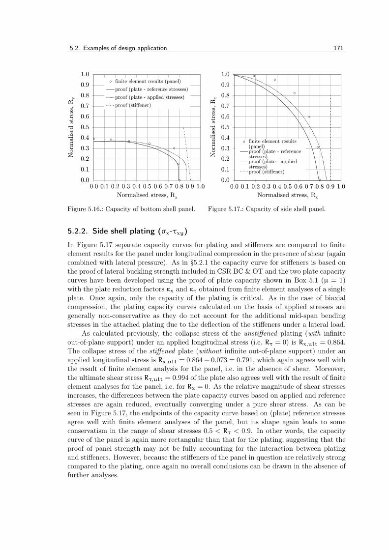
5.2. Examples of design application 171
0.0
0.1
0.2
0.3
0.4
0.5
0.6
0.7
0.8
0.9
1.0
0.0 0.1 0.2 0.3 0.4 0.5 0.6 0.7 0.8 0.9 1.0
Norm
alise
d s
tres
s, R
y
Normalised stress, Rx
finite element results (panel)
proof (plate - reference stresses)
proof (plate - applied stresses)
proof (stiffener)
Figure 5.16.: Capacity of bottom shell panel.
0.0
0.1
0.2
0.3
0.4
0.5
0.6
0.7
0.8
0.9
1.0
0.0 0.1 0.2 0.3 0.4 0.5 0.6 0.7 0.8 0.9 1.0
Norm
alise
d s
tres
s, R
τ
Normalised stress, Rx
finite element results(panel)proof (plate - referencestresses)proof (plate - appliedstresses)proof (stiffener)
Figure 5.17.: Capacity of side shell panel.
5.2.2. Side shell plating (σx-τxy)
In Figure 5.17 separate capacity curves for plating and stiffeners are compared to finiteelement results for the panel under longitudinal compression in the presence of shear (againcombined with lateral pressure). As in §5.2.1 the capacity curve for stiffeners is based onthe proof of lateral buckling strength included in CSR BC & OT and the two plate capacitycurves have been developed using the proof of plate capacity shown in Box 5.1 (µ = 1)with the plate reduction factors κx and κτ obtained from finite element analyses of a singleplate. Once again, only the capacity of the plating is critical. As in the case of biaxialcompression, the plating capacity curves calculated on the basis of applied stresses aregenerally non-conservative as they do not account for the additional mid-span bendingstresses in the attached plating due to the deflection of the stiffeners under a lateral load.
As calculated previously, the collapse stress of the unstiffened plating (with infiniteout-of-plane support) under an applied longitudinal stress (i.e. Rτ = 0) is Rx,ult = 0.864.The collapse stress of the stiffened plate (without infinite out-of-plane support) under anapplied longitudinal stress is Rx,ult = 0.864− 0.073 = 0.791, which again agrees well withthe result of finite element analysis for the panel, i.e. in the absence of shear. Moreover,the ultimate shear stress Rτ,ult = 0.994 of the plate also agrees well with the result of finiteelement analyses for the panel, i.e. for Rx = 0. As the relative magnitude of shear stressesincreases, the differences between the plate capacity curves based on applied and referencestresses are again reduced, eventually converging under a pure shear stress. As can beseen in Figure 5.17, the endpoints of the capacity curve based on (plate) reference stressesagree well with finite element analyses of the panel, but its shape again leads to someconservatism in the range of shear stresses 0.5 < Rτ < 0.9. In other words, the capacitycurve of the panel is again more rectangular than that for the plating, suggesting that theproof of panel strength may not be fully accounting for the interaction between platingand stiffeners. However, because the stiffeners of the panel in question are relatively strongcompared to the plating, once again no overall conclusions can be drawn in the absence offurther analyses.

6. Conclusions
In this chapter the main results, conclusions and contributions to knowledge are sum-marised. A direction for future research is also proposed. In §6.1 results directly related tothe problem stated in Chapter 4 are outlined and conclusions drawn. In §6.2 contributionsto knowledge made in the course of solving the stated problem are delineated. Finally,regarding introduction of the new proof of plate capacity into the rules of classificationsocieties, future research related to the capacity of unstiffened plates and stiffened panelsis proposed in §6.3.
6.1. Summary of results and conclusions
As noted in Chapter 1, a proof of plate capacity under combined in-plane loads is neededwith which to reliably and efficiently design ship plating, i.e. so that the demands onstructure are met over the service life of a ship without incurring a needless weight penalty.In quantitative terms, this proof needs to be (1) precise, (2) accurate and (3) robust. Inqualitative terms, this proof needs to be (1) concise, (2) physically-based and (3) directlysolvable. In Chapter 3 existing proofs were described and subsequently evaluated againstquantitative and qualitative acceptance criteria delineated in Chapter 4. In terms of thelatter, it may be concluded that several of the existing proofs are deemed to be concise,physically-based and directly solvable as summarised in Table 6.1.
Paik Ueda et al. CN 30.1 DIN 4114 PULS DIN 18800 Prov. CSR BC & OT
Criteria
Concise
Physically-based
Directly solvable
Table 6.1.: Summary of qualitative results (existing proofs).
In terms of quantitative criteria, results of plate capacities obtained with each proofwere compared against results obtained from an extensive series of numerical studies basedon the finite element method covering all load combinations and plating configurationsrelevant for the shipbuilding industry. As summarised in Table 6.2 and Table 6.3, respec-tively, it may be concluded from these comparisons that none of the existing proofs satisfyall quantitative acceptance criteria in either the design space or subspace.
Because no existing proof was found to satisfy all quantitative and qualitative accep-tance criteria, a hypothetical proof of plate capacity under combined in-plane loads waspostulated which well reflected the mechanics of plating collapse described in Chapter 2as well as the strengths of existing proofs investigated in Chapter 3. In order to satisfyqualitative acceptance criteria, this proof was based on a generalised form of the von Misesequation
172

6.1. Summary of results and conclusions 173
KPI Criteria Paik Ueda et al. CN 30.1 DIN 4114 PULS DIN 18800 Prov. CSR BC & OT
1 Sr/ns ≤ 0.001 0.011 0.018 0.032 0.039 0.004 0.018 0.012
2 0.97 ≤ mlsr ≤ 1.00 0.91 1.11 0.82 0.84 1.04 0.87 0.94
3 RD2 ≥ 0.95 0.72 0.62 0.63 0.63 0.92 0.73 0.68
4 m95 ≤ 1.05 1.18 1.61 1.08 1.10 1.20 1.14 1.26
5 m5 ≥ 0.87 0.73 1.00 0.52 0.36 0.96 0.67 0.73
Table 6.2.: Summary of quantitative results for existing proofs (design space).
KPI Criteria Paik Ueda et al. CN 30.1 DIN 4114 PULS DIN 18800 Prov. CSR BC & OT
1 Sr/ns ≤ 0.001 0.001 0.038 0.005 0.020 0.004 0.005 0.003
2 0.97 ≤ mlsr ≤ 1.00 1.03 1.35 0.88 0.78 1.11 0.93 1.08
3 RD2 ≥ 0.95 0.95 0.57 0.85 0.69 0.94 0.80 0.95
4 m95 ≤ 1.05 1.13 1.91 1.10 1.03 1.21 1.13 1.17
5 m5 ≥ 0.87 0.95 1.18 0.75 0.45 1.00 0.75 0.97
Table 6.3.: Summary of quantitative results for existing proofs (design subspace).
(Rx
κx
)e0
+
(Ry
κy
)e0
− B ·(Rx
κx
)e0/2
·(Ry
κy
)e0/2
+
(Rτ
κτ
)e0
= 1.0 (6.1)
where the exponent e0 and interaction coefficient B were hypothesised on the basis ofobservations made in the investigation of plating collapse mechanisms. Here the influenceof plate slenderness on the capacity of plates under biaxial compression as well as thebehaviour of plates under secondary tensile loads were particularly important. As shownin Table 6.4, it may be concluded that only some slight deficiencies in precision prevent thehypothetical proof from satisfying all quantitative acceptance criteria in both the designspace and subspace. It is perhaps worth reiterating that this proof is based solely on themechanics of plating collapse presented in Chapter 2, i.e. without any numerically-baseddefinitions of the exponent e0 and interaction coefficient B.
Target Design space Design subspace Criteria
1 Sr/ns 0.000 0.002 0.001 Sr/ns ≤ 0.001
2 mlsr 1.00 0.99 0.97 0.97 ≤ mlsr ≤ 1.00
3 RD2 1.00 0.95 0.94 RD
2 ≥ 0.95
4 m95 1.00 1.09 1.09 m95 ≤ 1.05
5 m5 1.00 0.80 0.84 m5 ≥ 0.87
KPI
Table 6.4.: Key performance indicators for hypothetical proof.
Nevertheless, in order to obtain more precise results, the exponent e0 and interac-tion coefficient B were subsequently redefined on the basis of 399 additional finite elementanalyses to reflect more closely the influences of aspect ratio α and slenderness parameterβ on the capacity of plates in Quadrant 1 (also in the presence of shear). The result-ing proof is shown in Box 6.1 and satisfies all quantitative acceptance criteria in boththe design space and subspace as shown in Table 6.5. Having fulfilled all quantitativeand qualitative acceptance criteria for a proof of plate capacity under combined in-plane

174 6. Conclusions
loads, it may therefore be concluded that this proof solves the problem stated in Chapter 4.
The capacity of plates under combined in-plane loads is defined by the following equation(µ · Rxκx
)e0+
(µ · Ryκy
)e0− B ·
(µ · Rxκx
)e0/2·(µ · Ryκy
)e0/2+
(µ · Rτκτ
)e0= 1.0
where e0 = 2 / β0.25 6 2 B = 2 / (2 · β)0.7/√α − 1 6 1 for Rx > 0 and Ry > 0
e0 = 2 B = κx = κy = κτ = 1 for Rx < 0 or Ry < 0
and where the following stress limits are to be observed(µ · Rxκx
)2/β0.25
+
(µ · Rτκτ
)2/β0.25
6 1.0 for Rx > 0 (i)
(µ · Ryκy
)2/β0.25
+
(µ · Rτκτ
)2/β0.25
6 1.0 for Ry > 0 (ii)
(µ · Rτκτ
)6 1.0 (iii)
Box 6.1.: Formulation of new proof
Target Design space Design subspace Criteria
1 Sr/ns 0.000 0.001 0.001 Sr/ns ≤ 0.001
2 mlsr 1.00 0.99 0.97 0.97 ≤ mlsr ≤ 1.00
3 RD2 1.00 0.97 0.98 RD
2 ≥ 0.95
4 m95 1.00 1.04 1.02 m95 ≤ 1.05
5 m5 1.00 0.87 0.90 m5 ≥ 0.87
KPI
Table 6.5.: Key performance indicators (new proof).
For this reason, the proof of plate capacity included in the newly harmonised IACSCommon Structural Rules for Bulk Carriers and Oil Tankers has been based on the proofshown in Box 6.1. However, when used together with newly harmonised load models, theinteraction coefficient B was recalibrated so that the scantlings of ships from successfulin-service experience remained largely unchanged (i.e. under biaxial compression). Thequantitative evaluation of this recalibrated proof is shown in Table 6.6. Here it may beconcluded that the proof included in the newly harmonised IACS Common Structural Rulesfor Bulk Carriers and Oil Tankers, although not fulfilling all of the quantitative acceptancecriteria, still performs far better than any of the existing proofs presented in Chapter 3.
Finally, the design application of the newly developed proof as used in the IACSCommon Structural Rules for Bulk Carriers and Oil Tankers was subsequently presented.Here it was shown that the effects on plating capacity of other boundary conditions(i.e. free edges and edge pull-in), additional load components (i.e. in-plane bending and lat-eral pressure) and more realistic initial imperfections (i.e. residual deflections and stressesbased on measurements) can be adequately captured in the plate reduction factors κx,

6.2. Summary of contributions 175
Target Design space Design subspace Criteria
1 Sr/ns 0.000 0.001 0.001 Sr/ns ≤ 0.001
2 mlsr 1.00 1.00 1.03 0.97 ≤ mlsr ≤ 1.00
3 RD2 1.00 0.96 0.93 RD
2 ≥ 0.95
4 m95 1.00 1.10 1.16 m95 ≤ 1.05
5 m5 1.00 0.87 0.91 m5 ≥ 0.87
KPI
Table 6.6.: Key performance indicators (CSR BC & OT proof).
κy and κτ, i.e. the endpoints of capacity curves. On the basis of these results, it may beconcluded that the newly developed proof remains valid in case of boundary conditions,loads and initial imperfections relevant for the shipbuilding industry, i.e. these variationshave little effect on the shape of capacity curves. Moreover, on the basis of numericalcalculations performed for the bottom and side shell structures of a double hull VLCC, itmay be concluded that the proof of stiffened panel capacity can be made using decoupledproofs of plate capacity and stiffener capacity (albeit somewhat conservatively in case ofthe panel and load combinations analysed in §5.2).
6.2. Summary of contributions
An extensive series of numerical studies based on the finite element method have beenperformed covering all load combinations and plating configurations relevant for the ship-building industry. Analyses of the results have led to the following contributions to knowl-edge:
1. the mechanics of plating collapse under single and combined in-plane loads havebeen thoroughly investigated resulting in an improved understanding of collapsemechanisms as well as stress redistributions in the post-buckling, post-yield andpost-collapse phases of response. Moreover, because the ultimate strengths of plat-ing under single stress components define the reference stresses used in most proofsof plate capacity, formulations found in literature and the shipbuilding industry fordefining the characteristic strength of plating under single stress components havebeen thoroughly discussed and compared to numerical results.
2. in the presence of primary tensile stresses, it has been shown numerically that grossyielding occurs in plates even under the application of a secondary compressive stress.This contradicts closed-form proofs used heretofore in the shipbuilding industry whichassume that plate buckling ensues under any level of compressive stress. Moreover,it has been shown numerically that the ultimate compressive strength of platingis often higher in the presence of a secondary tensile stress. This is contrary toresults obtained with closed-form proofs used heretofore in the shipbuilding industrywhich generally show a steadily decreasing capacity of plating with increasing tensilestresses.
3. in case of biaxial compressive stresses, it has been shown numerically that the shapeof the interaction curve is highly dependent on the slenderness of the plating, ap-

176 6. Conclusions
proaching a linear elastic curve for slender plating and a quadratic yield ellipse forsturdy plating. Moreover, it has also been shown that the shape of the interactioncurve is dependent on the aspect ratio of the plate, with the capacity of plating gen-erally increasing with decreasing aspect ratio. In this regard, equations have beendeveloped for the exponent e0 and interaction coefficient B of a generalised form ofthe von Mises equation with which the buckling capacity of plating can be determinedunder biaxial compression.
4. for all load combinations and plating configurations relevant for the shipbuilding in-dustry, a proof of plane plate capacity has been developed and shown to be moreprecise, accurate and robust than any existing proof. Moreover, the proof is con-cise, based on the mechanics of plating collapse and solvable without the need foriterations.
5. because the newly developed proof of plate capacity is based on numerical studies ofsimply-supported plates, uniform in-plane loads and idealised initial imperfections,the validity of its application in case of other boundary conditions (i.e. free edges andedge pull-in), additional load components (i.e. in-plane bending and lateral pressure)and more realistic initial imperfections (i.e. residual deflections and stresses basedon measurements) has been demonstrated. In this regard, it has been shown thatthese effects can be adequately captured in the plate reduction factors κx, κy andκτ, thereby validating use of the newly developed proof in case of those boundaryconditions, loads and initial imperfections relevant for the shipbuilding industry.Moreover, the marginal effect of out-of-plane loads (i.e. lateral pressure) on the in-plane strength of plating has been investigated.
6. on the basis of numerical calculations performed for the bottom and side shell struc-tures of a double hull VLCC, it has been shown that the proof of stiffened panelcapacity can be made using decoupled proofs of plate capacity and stiffener capacity.
7. regarding curved plate capacity under combined in-plane and lateral loads, a revisionto the DIN 18800 proof (already used extensively in the shipbuilding industry) hasbeen explained and evaluated. The revised proof of curved plate capacity is seento be more accurate and precise than the DIN 18800 proof, particularly in case ofcombined axial and hoop stresses.
In terms of practical contributions to the shipbuilding industry, the proofs of plane platecapacity and curved plate capacity developed/presented in the present work have bothbeen included in the newly harmonised IACS Common Structural Rules for Bulk Carri-ers and Oil Tankers, the new IACS Longitudinal Strength Standard for Container Ships(UR S11A) as well as the new DNVGL Rules for Classification which are applicable toall ship types. In future, more extensive use of the proofs can be reasonably expectedas classification societies seek to harmonise their own buckling strength rules with thoseincluded in the aforementioned IACS rules and requirements (as noted in §3.3, more than90% of the world’s cargo carrying tonnage is covered by IACS rules and requirements forthe classification of seagoing ships).

6.3. Future research 177
6.3. Future research
In terms of future research, two suggestions are offered regarding introduction of the newproof of plate capacity into the rules of classification societies:
1. As can be seen in Box 6.1, e0 = 2 for β 6 1 and B = 1 for β 6 0.5 in case ofsquare plates under biaxial compression. Accordingly, on the basis of the numericalcalibration, the design capacity equation transitions into the von Mises equation be-tween 0.5 6 β 6 1.0 (provided κx = κy = κτ = 1). This agrees well, for instance,with Hughes [9] whose numerical solution for square plates under biaxial compressionshows that gross yielding takes place for plates of slenderness β 6 0.67 (see Equations(2.43) and (2.44)). As shown in Figure 2.9, this transition range also agrees well withthat for square plates under uniaxial compression (according to finite element anal-yses). However, in the rules of classification societies, it is intended that the platereduction factors (κx, κy and κτ) be obtained using the DIN 18800 formulae. Al-though it was shown in Chapter 2 that these formulae agree reasonably well with thefinite element analyses upon which the derivation of the exponent e0 and interactioncoefficient B are based, the transitions to gross yielding differ slightly. For instance,it can be seen in Figure 2.9, that the DIN 18800 formulae predict yielding behaviourunder uniaxial compression to take place for square plates of slenderness β 6 1.58.Accordingly, using the new proof of plate capacity together with the DIN 18800 for-mulae for plate reduction factors (in general) could benefit from a parametric study toevaluate the significance of any anomalies which may arise (e.g. if κx = κy = κτ = 1,but e0 6= 2 and/or B 6= 1, due to slight discrepancies concerning the onset of yieldingbehaviour).
2. As discussed in §5.1, proof that a stiffened panel has sufficient capacity is typicallyseparated into distinct proofs for single plate fields and stiffeners with the capacity ofthe panel defined by the lesser of the two. However, as evidenced by the conservativeresults presented in §5.2 for some combinations of stresses applied to the panel of adouble hull VLCC, there is most likely some interaction between plating and stiffenerswhich is not fully accounted for in the current procedure for decoupling of capacityproofs. Moreover, the ratios of load carried by plating and stiffeners are themselvesa function of relative in-plane stiffness, which in turn depends on scantlings, initialimperfections and load types (e.g. the in-plane stiffness of a stiffener is a functionof lateral load). Accordingly, it is suggested that the current method of decouplingplate and stiffener strength used by classification societies could benefit from futureresearch. When necessary, better procedures to account for the interaction of plating,stiffeners and loads should be developed.

7. References
[1] Mitsui O.S.K. Lines Press Release. Incident with Containership MOL Comfort. 17June 2013, Tokyo, Japan.
[2] Mitsui O.S.K. Lines Press Release. Incident Involving the Containership MOL Comfort- Urgent Update No. 12. 27 June 2013, Tokyo, Japan.
[3] Mitsui O.S.K. Lines Press Release. Incident Involving the Containership MOL Comfort- Update No. 19. 06 July 2013, Tokyo, Japan.
[4] Mitsui O.S.K. Lines Press Release. Incident Involving the Containership MOL Comfort- Update No. 25. 11 July 2013, Tokyo, Japan.
[5] M. Mitev."MOL Comfort demands as much as $500m against Mitsubishi". VesselFinder Maritime News, 15 December 2014.
[6] Committee on Large Container Ship Safety (Japan’s Ministry of Land, Infrastruc-ture, Transport and Tourism). Interim Report of Committee on Large Container ShipSafety. 2013, Tokyo, Japan.
[7] The Investigative Panel on Large Container Ship Safety (ClassNK). Investigation Re-port on Structural Safety of Large Container Ships. 2014, Tokyo, Japan.
[8] International Association of Classification Societies. Requirements concerning strengthof ships. Unified Requirement S11A; Longitudinal strength standard for containerships, 2015.
[9] O.F. Hughes. Ship Structural Design: A Rationally-Based, Computer-Aided Optimiza-tion Approach. Society of Naval Architects and Marine Engineers, Jersey City, U.S.A.,1988.
[10] E.D. Egge. Untersuchungen zum Festigkeitsverhalten von ebenen versteiften Plat-tenfeldern mit zunehmender Auslastung der Struktur (in German). Technical report,Germanischer Lloyd, Hamburg, Germany, 1995. Abschlußbericht zum Vorhaben MTK0443 A.
[11] D. Faulkner. Compression tests on welded eccentrically stiffened plate panels (pa-per 25, 581-617). In P.J. Dowling J.E. Harding and P.A. Frieze, editors, Steel PlatedStructures: An International Symposium, Crosby Lockwood Staples, London, Eng-land, 1977.
[12] L. Schuman and G. Back. Strength of rectangular flat plates under edge compression.Technical report, National Advisory Committee for Aeronautics, Washington, U.S.A.,1930. Report No. 356.
178

179
[13] T. von Kármán, E.E. Sechler and L.H. Donnell. The strength of thin plates in com-pression. ASME Transactions, 54:53, 1932.
[14] S. Chatterjee and P.J. Dowling. The design of box girder compression flanges (paper8, 196-228). In P.J. Dowling J.E. Harding and P.A. Frieze, editors, Steel Plated Struc-tures: An International Symposium, Crosby Lockwood Staples, London, England,1977.
[15] E.E. Sechler. The ultimate compressive strength of thin sheet metal panels. In par-tial fulfillment of the requirements for the degree of Doctor of Philosophy. CaliforniaInstitute of Technology, Pasadena, U.S.A., 1934.
[16] S. Timoshenko. Theory of Elastic Stability. McGraw-Hill Book Company, New York,U.S.A., 1936.
[17] G. Winter. Strength of thin steel compression flanges. ASCE Transactions, 112:527,1947.
[18] American Iron and Steel Institute. Specification for the design of light gage steelstructural members, New York, U.S.A., 1946.
[19] Eurocode 3; Design of steel structures. Part 1-5: Plated structural elements. EN 1993-1-5, 2006.
[20] International Association of Classification Societies. Requirements concerning strengthof ships. Unified Requirement S11; Longitudinal strength standard (Rev. 7), 2010.
[21] F. Bleich. Buckling Strength of Metal Structures. McGraw-Hill Book Company, NewYork, U.S.A., 1952.
[22] J.M. Frankland. The strength of ship plating under edge compression. Technicalreport, United States Experimental Model Basin, Washington, U.S.A., 1940. ReportNo. 469.
[23] International Association of Classification Societies. Common Structural Rules forBulk Carriers and Oil Tankers (Rev. 1), 2014.
[24] International Association of Classification Societies. Requirements concerning strengthof ships. Unified Requirement S18; Evaluation of scantlings of corrugated transversewatertight bulkheads in non-CSR bulk carriers considering hold flooding (Rev. 9),2014.
[25] International Association of Classification Societies. Requirements concerning strengthof ships. Unified Requirement S19; Evaluation of scantlings of the transverse water-tight corrugated bulkhead between cargo holds nos. 1 and 2, with cargo hold no. 1flooded, for existing bulk carriers (Rev. 5), 2004.
[26] Deutsches Institut für Normung e.V. DIN 18800; Structural steelwork. Part 3: Anal-ysis of safety against buckling of plates. Beuth Verlag, Berlin, Germany, 1990.

180 7. References
[27] J. Scheer U. Peil and G. Fuchs. Auswertung von internationalen Veröffentlichun-gen, Versuchsberichten, Kommissionspapieren u.ä. auf dem Gebiet des Beulens vonPlatten aus Stahl (in German). Technical report, Institutes für Stahlbau, TechnischeUniversität Braunschweig, Braunschweig, Germany, 1987. Report No. 6095.
[28] J.B. Caldwell. Ultimate longitudinal strength (written discussion). RINA Transac-tions, 107:411, 1965.
[29] D. Faulkner. A review of effective plating for use in the analysis of stiffened platingin bending and compression. Journal of Ship Research, 19(1):1–17, March 1975.
[30] Germanischer Lloyd GmbH. Rules for Classification and Construction. I - Ship Tech-nology; Part 1 - Seagoing Ships; Chapter 1 - Hull Structures; Section 3 - DesignPrinciples, 1997.
[31] International Association of Classification Societies. Common Structural Rules forBulk Carriers, 2006.
[32] International Association of Classification Societies. Common Structural Rules forDouble Hull Oil Tankers, 2006.
[33] DNVGL. Class Guideline - Buckling, DNVGL-CG-0128, 2015.
[34] S. Valsgård. Numerical design prediction of the capcity of plates in biaxial in-planecompression. Computers & Structures, 12:729–739, 1980.
[35] J.K. Paik and A.K. Thayamballi. Ultimate Limit State Design of Steel-Plated Struc-tures. John Wiley and Sons Ltd., Chicester, England, 2003.
[36] K.C. Rockey H.R. Evans and D.M. Porter. Ultimate load capacity of stiffened webssubjected to shear and bending (Paper 4, Session B, 45-61). In Proceedings of aninternational conference on steel box girder bridges, Institution of Civil Engineers,London, England, 1973.
[37] H. Wagner. Flat sheet metal girders with very thin metal web. Technical report,National Advisory Committee for Aeronautics, Washington, U.S.A., 1931. TechnicalMemorandum Nos. 604/605/606.
[38] H. Wagner and W. Ballerstedt. Tension fields in originally curved, thin sheets duringshearing stresses. Technical report, National Advisory Committee for Aeronautics,Washington, U.S.A., 1935. Technical Memorandum No. 774.
[39] P. Kuhn J.P. Peterson and L.R. Levin. A summary of diagonal tension, Parts I and II.Technical report, National Advisory Committee for Aeronautics, Washington, U.S.A.,1952. Technical Note Nos. 2661/2662.
[40] P. Dubas and E. Gehri. Behaviour and design of steel plated structures. Technicalreport, ECCS-CECM-EKS, Zürich, Switzerland, 1986. No. 44.
[41] K.C. Rockey. The design of web plates for plate and box girders - a state of the artreport (paper 19, 459-485). In P.J. Dowling J.E. Harding and P.A. Frieze, editors, SteelPlated Structures: An International Symposium, Crosby Lockwood Staples, London,England, 1977.

181
[42] J.K. Paik. A new concept of the effective shear modulus for a plate buckled in shear.Journal of Ship Research, 39(1):70–75, 1995.
[43] J.K. Paik. Ultimate strength design equations of plates and stiffened panels undercombined loads. Final Report to the American Bureau of Shipping, Ship StructuralMechanics Lab, Pusan National University, July 1999.
[44] J.K. Paik A.K. Thayamballi and B.J. Kim. Advanced ultimate strength formulationsfor ship plating under combined biaxial compression/tension, edge shear, and lateralpressure loads. Marine Technology, 38(1):9–25, 2001.
[45] S. Zhang P. Kumar and S.E. Rutherford. Ultimate shear strength of plates andstiffened panels. Ships and Offshore Structures, 3(2):105–112, 2008.
[46] D. Faulkner J.C. Adamchak G.J. Snyder and M.F. Vetter. Synthesis of welded grillagesto withstand compression and normal loads. Computers & Structures, 3:221–246, 1973.
[47] Deutsches Institut für Normung e.V. DIN 18800; Structural steelwork. Part 2: Anal-ysis of safety against buckling of linear members and frames. Beuth Verlag, Berlin,Germany, 1990.
[48] H. Becker. Feasibility study of model tests on ship hull girders. Technical report, ShipStructure Committee, Washington, U.S.A., 1969. SSC-194.
[49] H. Becker R. Goldman and J. Pazerycki. Compressive strength of ship hull girders,Part I - Unstiffened plates. Technical report, Ship Structure Committee, Washington,U.S.A., 1970. SSC-217.
[50] Det norske Veritas. Rules for the Design, Construction and Inspection of OffshoreStructures. Appendix C - Steel Structures, 1977.
[51] Y. Ueda S.M.H. Rashed and J.K. Paik. Buckling and ultimate strength interactionin plates and stiffened panels under combined inplane biaxial and shearing forces.Marine Structures, 8:1–36, 1995.
[52] International Association of Classification Societies. Classification societies - what,how and why? London, England, 2015.
[53] Det norske Veritas. Buckling Strength Analysis. Classification Notes No. 30.1, 1987.
[54] Deutsches Institut für Normung e.V. DIN 4114; Steel structures; Stability. BeuthVerlag, Berlin, Germany, 1952.
[55] R. Szilard. Theory and Analysis of Plates: Classical and Numerical Methods. Prentice-Hall Inc., New Jersey, U.S.A., 1974.
[56] K. Marguerre. The apparent width of the plate in compression. Technical report,National Advisory Committee for Aeronautics, Washington, U.S.A., 1937. ReportNo. 833.
[57] E. Byklum and J. Amdahl. A simplified method for elastic large deflection analysis ofplates and stiffened panels due to local buckling. Thin-Walled Structures, 40:925–953,2002.

182 7. References
[58] E. Steen. Application of the perturbation method to plate buckling problems. Techni-cal report, Mechanics Division, Department of Mathematics, University of Oslo, Oslo,Norway, 1998. Research Report in Mechanics No. 98-1.
[59] Deutsches Institut für Normung e.V. Principles for the specification of requirementsrelating to the safety of structures. Beuth Verlag, Berlin, Germany, 1981.
[60] J. Lindner and W. Habermann. Zur Weiterentwicklung des Beulnachweises für Plattenbei mehrachsiger Beanspruchung (in German). Stahlbau, 57:333–339, 1988.
[61] M. Böckenhauer and H.-J. Schulte. An introduction to the new requirements of Ger-manischer Lloyd for proof of buckling strength. Technical report, Germanischer Lloyd,Hamburg, Germany, 1997.
[62] DNVGL. Class Guideline - Finite element analysis, DNVGL-CG-0127, 2015.
[63] C.S. Smith P.C. Davidson J.C. Chapman and P.J. Dowling. Strength and stiffnessof ships’ plating under in-plane compression and tension (written discussion). RINATransactions, 130:277–296, 1987.
[64] International Association of Classification Societies. Recommendation No. 76; IACSGuidelines for Surveys, Assessment and Repair of Hull Structure - Bulk Carriers (Corr.1), 2007.
[65] International Maritime Organisation. Consolidated text of the International Conven-tion for the Safety of Life at Sea, 1974, and its Protocol of 1988: articles, annexes andcertificates, London, England, 2016.
[66] T. Søreide and J. Czujko. Load carrying capacities of plates under combined lateralload and axial/biaxial compression. The 2nd International Symposiuim on PracticalDesign in Shipbuilding, pages 493–500, 1983.
[67] International Association of Classification Societies. Recommendation No. 47; Ship-building and Repair Quality Standard (Rev. 7), 2013.
[68] J.K. Paik and P.T. Pedersen. A simplified method for predicting ultimate compressivestrength of ship panels. International Shipbuilding Progress, 43(434):139–157, 1996.
[69] Y. Ueda and T. Yao. The influence of complex initial deflection modes on the be-haviour and ultimate strength of rectangular plates in compression. Journal of Con-structional Steel Research, 5(4):265–302, 1985.
[70] P.A. Frieze P.J. Dowling and R.E. Hobbs. Ultimate load behaviour of plates in com-pression (paper 2, 24-50). In P.J. Dowling J.E. Harding and P.A. Frieze, editors, SteelPlated Structures: An International Symposium, Crosby Lockwood Staples, London,England, 1977.
[71] P.L. Moore. The importance of welding quality in ship construction (paper 40, 357-363). In Analysis and design of marine structures: An international symposium. 2ndInternational Conference on Marine Structures (MARSTRUCT 2009) March 16 - 18,2009 Lisbon, Portugal.

183
[72] Q. Chen T.J.E. Zimmerman D.D. DeGeer and B.W. Kennedy. Strength and stabilitytesting of stiffened plate components. Technical report, Ship Structure Committee,Washington, U.S.A., 1997. SSC-399.
[73] J. Lindner J. Sheer and H. Schmidt. Stahlbauten - Erläuterungen zu DIN 18 800 Teil1 bis Teil 4 (in German). Beuth Verlag, Berlin, Germany, 1993.
[74] T. Yao O.C. Astrup P. Caridis Y.N. Chen S.-R. Cho R.S. Dow O. Niho and P. Rigo.Ultimate hull girder strength. Special Task Committee VI.2, 14th International Shipand Offshore Structurees Committee, 2-6 October 2000, Nagasaki, Japan.
[75] International Association of Classification Societies. Validation of non-linear bucklingprocedure. CSR BC & OT - Technical Background Report (Pt. 1, Ch 8, Sec 5), Rev.2, 2014.
[76] International Association of Classification Societies. Curved plate capacity under com-bined loads. CSR BC & OT - Technical Background Report (Pt. 1, Ch 8, Sec 5), Rev.1, 2015.
[77] ANSYS, Element Reference, Release 13.0, I. Element Library.
[78] ANSYS, Theory Reference, Release 13.0, 4. Structures with Material Nonlinearities,4.2. Rate-Independent Plasticity.

Appendices
184

Appendix A. Proof of Curved PlateCapacity
Although the majority of plating used in the construction of ships is plane, curved shellplating is used extensively in the fore and aft regions of the ship as well as the bilge areawithin the parallel midbody. The latter is particularly relevant in terms of hull girderultimate strength. Because the collapse behaviour of curved plating is generally differentfrom that of plane plating (depending on the degree of curvature), an alternate proofof capacity is needed. In this regard, the purpose of this Appendix is to evaluate theDIN 18800 proof of curved plate capacity (based on a generalised form of the von Misesequation) and to show how both accuracy and precision can be improved with the additionof a non-zero interaction term. This evaluation is performed under two stress componentsin the first section of this appendix (§A.1) and under three stress components in the secondsection (§A.2). The resulting correction has been included in the newly harmonised IACSCommon Structural Rules for Bulk Carriers and Oil Tankers, the new IACS LongitudinalStrength Standard for Container Ships (UR S11A)1 as well as the new DNVGL Rules forClassification which are applicable to all ship types.
A.1. Evaluation of proof under two stress components
Within the shipbuilding industry, the DIN 18800 proof was initially implemented in thebuckling strength rules of Germanischer Lloyd and subsequently in the IACS CommonStructural Rules for Bulk Carriers. As mentioned above, the proof is based on a generalisedform of the von Mises equation
(σx
σx,ult
)e1
+
(σθ
σθ,ult
)e2
− B ·(
σx
σx,ult
)·(
σθσθ,ult
)+
(τxθ
τxθ,ult
)e3
= 1.0 (A.1)
where e1 = e2 = 1.25, e3 = 2 and B = 0, i.e. no interaction term. In Equation (A.1), theaxial, hoop and shear stresses are denoted by σx, σθ and τxθ, respectively. Here it shouldbe noted that lateral pressure p on a curved plate induces hoop stresses in the platingaccording to the equation
σθ =p · Rt
(A.2)
where R is the radius of curvature. As in the case of plane plates, Equation (A.1) may beexpressed in terms of normalised stresses
1 In case of (global) axial and shear stresses, the existing and revised proofs are the same. Only whenhoop stresses are considered, e.g. due to local lateral loads, does the correction have any influence oncalculated capacity (see S11A.6.2).
185

186 A. Proof of Curved Plate Capacity
(Rx
κx
)1.25
+
(Rθκθ
)1.25
+
(Rτ
κτ
)2
= 1.0 (A.3)
where Rx = σx/σY , Rθ = σθ/σY and Rτ =√3 · τxθ/σY , respectively, and κx, κθ and κτ
are the corresponding plate reduction factors. In case of tensile stresses, the correspondingaxial or hoop stress is set to zero, i.e. Rx > 0, Rθ > 0. This is consistent with the treatmentof tensile stresses in the proof of capacity for plane plates.
Plate d/t Axial length, d [mm] Thickness, t [mm] Radius, R [mm] Yield stress, σY [N/mm2]
1 75 1200 16.0
2 60 1200 20.0
3 50 1200 24.0
4 150 2400 16.0
5 120 2400 20.0
6 100 2400 24.0
7 300 4800 16.0
8 240 4800 20.0
9 200 4800 24.0
2300 315
Table A.1.: Description of plates used in finite element analyses.
t
σx
σx
σθ
τxθ
R d
σθ
Figure A.1.: Cylinder nomenclature.
1
XYZ
Curved Plate Study
Figure A.2.: Finite element model of cylinder.
In order to evaluate the proof of curved plate capacity, a series of numerical studiesbased on the finite element method were performed for nine plates with a constant radius ofcurvature R = 2300 mm, but different axial length d to thickness t ratios as defined in TableA.1. The nomenclature used in this table is illustrated in Figure A.1 where curved platingis defined as plating with a radius of curvature R 6 2500 · t. The scantlings shown in TableA.1 are representative of those for shell plating in the bilge area of ships. A description

A.1. Evaluation of proof under two stress components 187
0.0
0.1
0.2
0.3
0.4
0.5
0.6
0.7
0.8
0.9
1.0
0.0 0.1 0.2 0.3 0.4 0.5 0.6 0.7 0.8 0.9 1.0
Norm
alise
d s
tres
s, R
τ
Normalised stress, Rx
Finite element analyses
Proof
(a) Rx-Rτ
0.0
0.1
0.2
0.3
0.4
0.5
0.6
0.7
0.8
0.9
1.0
0.0 0.1 0.2 0.3 0.4 0.5 0.6 0.7 0.8 0.9 1.0
Norm
alise
d s
tres
s, R
τ
Normalised stress, Rθ
Finite element analyses
Proof
(b) Rθ-Rτ
Figure 0.1: ——-CROP!——–CROP!——–CROP!——–CROP!——–CROP!———CROP!——-
1
Figure A.3.: Comparison plots for existing proof (Plate 5, d/t = 120).
of the finite element analyses is included in Appendix 1 of reference [76]2. Because thecircumferential length of a curved plate has no effect on its buckling or ultimate strength,cylindrical shells (without stiffening) were modelled in all finite element analyses. A typicaldeformation plot of a cylinder under pure axial stress is shown in Figure A.2.
For each of the nine plates described in Table A.1, the ultimate capacity was deter-mined under ten combinations each of two stress components Rx - Rθ (axial and hoopstresses), Rx - Rτ (axial and shear stresses) and Rθ - Rτ (hoop and shear stresses). Theseresults were then compared to those obtained using Equation (A.3). For stress combi-nations involving shear, i.e. Rx - Rτ and Rθ - Rτ, results of the comparison for Plate 5(d/t = 120) are shown in Figure A.33. Comparison results for all plates are plotted inAppendix 2 of reference [76]. Using the quantitative evaluation scheme presented in §3.1for capacity proofs of plane plates, the results for these two stress combinations are tab-ulated in Table A.2 and plotted in Figure A.4. These results are based on 9 x 8 = 72evaluation points (data points where Rx = 0, Rθ = 0 or Rτ = 0 are omitted since they canbe directly calculated from plate reduction factors) and show that the existing proof basedon DIN 18800 is reasonably accurate and precise for stress combinations Rx - Rτ (axialand shear stresses) and Rθ - Rτ (hoop and shear stresses).
For the stress combination excluding shear, i.e. Rx - Rθ, results of the comparisonfor Plate 5 (d/t = 120) are shown in Figure A.5(a). As noted above, comparison resultsfor all plates are plotted in Appendix 2 of reference [76]. Using again the quantitativeevaluation scheme presented in §3.1 for capacity proofs of plane plates, the results for this
2 Although the author is responsible for the subsequent analyses, the finite element analyses were per-formed by Det norske Veritas (DnV) using the Abaqus finite element code. In this regard, the authorperformed similar analyses using the ANSYS finite element code, but only to establish the boundaryconditions to be used in the models and to verify selected DnV results.
3 As shown in Figures A.3(a) and A.3(b), the ultimate shear stresses for Plate 5 are Rτ,ult = 0.761 andRτ,ult = 0.784, respectively. This discrepancy arises due to differences in the initial imperfection shapesused in the finite element models for each calculation set (as noted in Appendix 1 of reference [76]).

188 A. Proof of Curved Plate Capacity
Target Rx - Rτ Rθ - Rτ Criteria
1 Sr/ns 0.000 0.003 0.000 Sr/ns ≤ 0.001
2 mlsr 1.00 0.99 1.00 0.97 ≤ mlsr ≤ 1.00
3 RD2 1.00 0.80 0.98 RD
2 ≥ 0.95
4 m95 1.00 1.13 1.08 m95 ≤ 1.05
5 m5 1.00 0.86 0.94 m5 ≥ 0.87
KPI
Table A.2.: Key performance indicators for existing proof (Rx - Rτ and Rθ - Rτ).
m95
m5
mlsr
0.0
0.2
0.4
0.6
0.8
1.0
1.2
0.0 0.2 0.4 0.6 0.8 1.0 1.2
Norm
alise
d v
ecto
r m
agnitude,
Rpro
of
Normalised vector magnitude, RFEA
(a) Rx-Rτ
m95
m5
mlsr
0.0
0.2
0.4
0.6
0.8
1.0
1.2
0.0 0.2 0.4 0.6 0.8 1.0 1.2
Norm
alise
d v
ecto
r m
agnitude,
Rpro
of
Normalised vector magnitude, RFEA
(b) Rθ-Rτ
Figure 0.1: ——-CROP!——–CROP!——–CROP!——–CROP!——–CROP!———CROP!——-
1
Figure A.4.: Scatter plots for existing proof (Rx - Rτ and Rθ - Rτ).
stress combination are tabulated in Table A.3 and plotted in Figure A.6(a). Contrary, tothe stress combinations including shear, these results show that the existing proof basedon DIN 18800 is rather conservative for the stress combination Rx - Rθ (axial and hoopstresses), i.e. due to the quasi-rectangular shape of the capacity curve delineated by theresults of finite element analyses.
Target Existing proof Revised proof Criteria
1 Sr/ns 0.000 0.009 0.002 Sr/ns ≤ 0.001
2 mlsr 1.00 0.87 0.98 0.97 ≤ mlsr ≤ 1.00
3 RD2 1.00 0.92 0.95 RD
2 ≥ 0.95
4 m95 1.00 0.97 1.08 m95 ≤ 1.05
5 m5 1.00 0.72 0.85 m5 ≥ 0.87
KPI
Table A.3.: Key performance indicators for existing and revised proofs (Rx - Rθ).

A.1. Evaluation of proof under two stress components 189
0.0
0.1
0.2
0.3
0.4
0.5
0.6
0.7
0.8
0.9
1.0
0.0 0.1 0.2 0.3 0.4 0.5 0.6 0.7 0.8 0.9 1.0
Norm
alise
d s
tres
s, R
θ
Normalised stress, Rx
Finite element analyses
Proof
(a) Rx - Rθ - Existing proof
0.0
0.1
0.2
0.3
0.4
0.5
0.6
0.7
0.8
0.9
1.0
0.0 0.1 0.2 0.3 0.4 0.5 0.6 0.7 0.8 0.9 1.0
Norm
alise
d s
tres
s, R
θ
Normalised stress, Rx
Finite element analyses
Proof
(b) Rx - Rθ - Revised proof
Figure 0.1: ——-CROP!——–CROP!——–CROP!——–CROP!——–CROP!———CROP!——-
1
Figure A.5.: Comparison plots for existing and revised proofs (Plate 5, d/t = 120).
m95
m5
mlsr
0.0
0.2
0.4
0.6
0.8
1.0
1.2
0.0 0.2 0.4 0.6 0.8 1.0 1.2
Norm
alise
d v
ecto
r m
agnitude,
Rpro
of
Normalised vector magnitude, RFEA
(a) Rx - Rθ - Existing proof
m95
m5
mlsr
0.0
0.2
0.4
0.6
0.8
1.0
1.2
0.0 0.2 0.4 0.6 0.8 1.0 1.2
Norm
alise
d v
ecto
r m
agnitude,
Rpro
of
Normalised vector magnitude, RFEA
(b) Rx - Rθ - Revised proof
Figure 0.1: ——-CROP!——–CROP!——–CROP!——–CROP!——–CROP!———CROP!——-
1
Figure A.6.: Scatter plots for existing and revised proofs (Rx - Rθ).
In an effort to correct this conservatism, additional comparisons were made using arevised proof in which an Rx - Rθ interaction term is added to the existing proof. Here aninteraction coefficient equal to B = 0.5 was used(
Rx
κx
)1.25
+
(Rθκθ
)1.25
− 0.5 ·(Rx
κx
)·(Rθκθ
)+
(Rτ
κτ
)2
= 1.0 (A.4)
The rationale behind using an interaction term is to avoid any degradation in the existinglevels of accuracy and precision for stress combinations Rx - Rτ and Rθ - Rτ which mightoccur if the exponents in the capacity equation were changed. For the stress combination

190 A. Proof of Curved Plate Capacity
Rx - Rθ, revised results of the comparison for Plate 5 (d/t = 120) are shown in FigureA.5(b).
Again using the quantitative evaluation scheme presented in §3.1 for capacity proofsof plane plates, the results using Equation (A.4) for the stress combination Rx - Rθ aretabulated in Table A.3 and plotted in Figure A.6(b). Although not all key performanceindicators fall within the ranges of acceptable values, a marked improvement in the accu-racy can be seen (i.e. mlsr = 0.87 → mlsr = 0.98) as well as a moderate improvement inprecision (i.e. R2
D = 0.92→ R2D = 0.95).
A.2. Evaluation of proof under three stress components
For each of the nine plates described in Table A.1, the ultimate capacity was also de-termined under three stress components Rx - Rθ - Rτ for three different levels of shear.These results were then compared to those obtained using Equation (A.3), i.e. the ex-isting proof, and those obtained using Equation (A.4), i.e. the revised proof. Results ofthe comparison for Plate 5 (d/t = 120) are shown in Figure A.7(a) for the existing proofand Figure A.7(b) for the revised proof. Comparison results for all plates are plotted inAppendix 3 of reference [76].
0.0
0.1
0.2
0.3
0.4
0.5
0.6
0.7
0.8
0.9
1.0
0.0 0.1 0.2 0.3 0.4 0.5 0.6 0.7 0.8 0.9 1.0
Norm
alise
d s
tres
s, R
θ
Normalised stress, Rx
Finite element analyses
Proof
decreasing values of shear
(a) Rx - Rθ - Rτ - Existing proof
0.0
0.1
0.2
0.3
0.4
0.5
0.6
0.7
0.8
0.9
1.0
0.0 0.1 0.2 0.3 0.4 0.5 0.6 0.7 0.8 0.9 1.0
Norm
alise
d s
tres
s, R
θ
Normalised stress, Rx
Finite element analyses
Proof
decreasing values of shear
(b) Rx - Rθ - Rτ - Revised proof
Figure 0.1: ——-CROP!——–CROP!——–CROP!——–CROP!——–CROP!———CROP!——-
1
Figure A.7.: Comparison plots for existing and revised proofs (Plate 5, d/t = 120).
Again using the quantitative evaluation scheme presented in §3.1 for capacity proofsof plane plates, the results for three stress components are tabulated in Table A.4 andplotted in Figure A.8. These results are based on ((3 x 3) + 1) x 9 = 90 evaluation points(here only a single evaluation point is used in case Rτ = 0 since the capacity of platingwhere Rx = Rτ = 0 and Rθ = Rτ = 0 can be directly calculated from the plate reductionfactors κθ and κx, respectively). As can be seen, these results reflect a slight increase(albeit non-conservative) in the accuracy (mlsr = 0.97 → mlsr = 1.02) and a markedimprovement in precision (R2
D = 0.84→ R2D = 0.91) when using the revised proof.
It can be concluded from the foregoing that the improvements in accuracy and pre-cision using Equation (A.4) compared to Equation (A.3) are more significant under com-

A.2. Evaluation of proof under three stress components 191
Target Existing proof Revised proof Criteria
1 Sr/ns 0.000 0.004 0.002 Sr/ns ≤ 0.001
2 mlsr 1.00 0.97 1.02 0.97 ≤ mlsr ≤ 1.00
3 RD2 1.00 0.84 0.91 RD
2 ≥ 0.95
4 m95 1.00 1.15 1.16 m95 ≤ 1.05
5 m5 1.00 0.78 0.90 m5 ≥ 0.87
KPI
Table A.4.: Key performance indicators for existing and revised plots (Rx - Rθ - Rτ).
m95
m5
mlsr
0.0
0.2
0.4
0.6
0.8
1.0
1.2
0.0 0.2 0.4 0.6 0.8 1.0 1.2
Norm
alise
d v
ecto
r m
agnitude,
Rpro
of
Normalised vector magnitude, RFEA
(a) Rx - Rθ - Rτ - Existing proof
m95
m5
mlsr
0.0
0.2
0.4
0.6
0.8
1.0
1.2
0.0 0.2 0.4 0.6 0.8 1.0 1.2
Norm
alise
d v
ecto
r m
agnitude,
Rpro
of
Normalised vector magnitude, RFEA
(b) Rx - Rθ - Rτ - Revised proof
Figure 0.1: ——-CROP!——–CROP!——–CROP!——–CROP!——–CROP!———CROP!——-
1
Figure A.8.: Scatter plots for existing and revised proofs (Rx - Rθ - Rτ).
bined axial and hoop stresses, i.e. Rx - Rθ, than under combined axial, hoop and stresses,i.e. Rx - Rθ - Rτ. However, because the former is relevant for shell plating in the bilgearea (i.e. due to dominant axial stresses under hull girder bending and hoop stresses underexternal sea pressure), the IACS harmonisation project team HPT02 decided to includethe interaction term in the IACS Common Structural Rules for Bulk Carriers and OilTankers. As noted above, the revised proof expressed in Equation (A.4) is also included(at least implicitly) in the new IACS Longitudinal Strength Standard for Container Ships(UR S11A) as well as the new DNVGL Rules for Classification which are applicable to allship types.

Appendix B. Numerical Studies
Numerical studies based on the finite element method have been used extensively through-out the present work using the ANSYS software package (Release 13.0). These studieshave been used to better understand the mechanics of plating collapse (Chapter 2), quan-titatively evaluate existing proofs of plate capacity (Chapter 3), develop a new proof ofplate capacity (Chapter 4) and demonstrate the practical application of this proof withinthe shipbuilding industry (Chapter 5). In case of the stiffened panels analysed in Chapter5, the numerical study of bottom shell and side shell structures of a double hull VLCChave been performed in strict adherence to a procedure developed and agreed within theIACS harmonisation project team HPT02 for performing non-linear finite element analysesof stiffened panels [75]. This procedure has been validated against tests of four stiffenedpanels carried out by Germanischer Lloyd [10]. In the present work, this procedure isalso used for the analyses of single plates where stiffeners are modelled by simple supports(in fact, a single batch file has been used with options for switching between the analy-sis of stiffened panels and the analysis of single plates). Because the IACS procedure foranalysing stiffened panels is already in the public domain, only its application to singleplates is here described. In the first section of this appendix (§B.1), the procedure usedfor performing finite element analyses is described. In the second section of this appendix(§B.2), comparisons with test results are used to validate this procedure.
B.1. Description of finite element analyses
B.1.1. General
Non-linear buckling analyses are essentially performed in two steps. When perfectly in-plane loads are applied to a plane plate in the absence of any out-of-plane loads(e.g. lateral pressure), the out-of-plane deflections which are needed to initiate bucklingwill not develop. Accordingly, the first step is to perform a linear eigenvalue analysis inorder to generate an initial deflection shape for the plate. Alternatively, initial deflectionshapes (theoretical or measured) may be modelled directly. In the second step, a non-linearanalysis is performed, the aim being to obtain a stable load-deflection curve, the peak ofwhich defines the ultimate capacity of the plate.
B.1.2. Model extent
The extent of model used in all analyses is a single a x b plate. As noted below, the modelis simply supported on all edges. In case of symmetric deflection patterns, a model without-of-plane support along its centrelines x = a/2 and y = b/2 together with rotationalrestraint along the edges may also be used to represent continuous plating. However, sucha model is precluded in the present study by the asymmetric deflection patterns associatedwith shear loads. As shown in Figure B.1(a), the differences in ultimate plate strength
192

B.1. Description of finite element analyses 193
(α = 3, β = 3) under axial loads using these two models is negligible (although somedifferences in unloading are evident under longitudinal stress σx). In Figure B.1(b), thestress strain-curve under shear for a single plate supported simply on all edges (α = 3,β = 3) is compared to that for continuous plating comprised of nine plate fields (i.e. threeframe spacings by three frame spans). As can be seen, there is only a slight increase(2.16%) in the ultimate strength of continuous plating due to the strengthening effect ofthe asymmetric deflection.
0.0
0.1
0.2
0.3
0.4
0.5
0.6
0.7
0.8
0.9
1.0
0.0 0.2 0.4 0.6 0.8 1.0 1.2 1.4 1.6 1.8 2.0
Norm
alise
d a
xia
l st
ress
, σ/
σ Y
Normalised axial strain, ε/εY
simply-supported plate model
symmetric plate model
σx - εx
σy - εy
(a) Axial loads
0.0
0.1
0.2
0.3
0.4
0.5
0.6
0.7
0.8
0.9
1.0
0.0 0.2 0.4 0.6 0.8 1.0 1.2 1.4 1.6 1.8 2.0
Norm
alise
d s
hea
r st
ress
, τ x
y/τ Y
Normalised shear strain, γxy/γY
1 x 1 plate model
3 x 3 plate model
(b) Shear load
Figure 0.1: ——-CROP!——–CROP!——–CROP!——–CROP!——–CROP!———CROP!——-
1
Figure B.1.: Model comparisons (α = 3, β = 3).
B.1.3. Element type and meshing
In the HPT02 agreed procedure for stiffened panels, 4-node shell elements may be usedwith six elements across the breadth b of the plate. However, in case of a single platemodel, the drastically reduced degrees of freedom allow an 8-node element to be used witheight elements across the breadth b of the plate. Because the length a of a single plateused in the present work is always an exact multiple of the frame spacing b, the edge lengthof elements in the x-direction are exactly equal to those in the y-direction (i.e. b/8 x b/8elements). Plates are modelled using the ANSYS element Shell281 which is an 8-nodeelement with six degrees of freedom at each node. The element is suitable for analysingthin to moderately-thick shell structures [77].
The single exception to the foregoing, is the analysis of plates with residual stresses(§5.1.1). Due to the small width of the tensile zone along plate edges, the size of elementsare here reduced to b/16 x b/16 and the 4-node shell element Shell181 is used (with thefull integration option). Like its 8-node counterpart, Shell181 is also suitable for analysingthin to moderately-thick shell structures [77].
B.1.4. Material properties and real constants
A bi-linear material model including strain-hardening effect is used in all analyses. Inthis regard, the ANSYS option TB, BISO is used for which the von Mises yield criteria

194 B. Numerical Studies
is coupled with an isotropic work hardening assumption (i.e. under progressive yieldingthe yield surface remains centred about its initial centreline and expands in size as theplastic strains develop [78]). The bilinear stress-strain curve is initially defined by theelastic modulus of the material E = 206, 000N/mm2. Once the specified yield stress σYis reached, the curve continues along a slope defined by the strain hardening parameterET = 1000N/mm2. A Poisson’s ratio ν = 0.3 is used in all analyses.
For the analysis of the stiffened panel in Chapter 5, the scantlings and yield stressesare directly provided. However, in all analyses of single plates, the thickness, breadth(i.e. frame spacing) and yield stress is always given in terms of the (non-dimensional) plateslenderness parameter β = b/t ·
√σY/E. For this reason, the corresponding combinations
of plate thickness t and yield stress σY used in the finite element analyses for each valueof β are shown in Table B.1. The frame spacing remains constant at b = 850mm.
β b [mm] t [mm] σY [N/mm2] t [mm] σY [N/mm
2]
0.5 850 57.40 235 57.40 235
1.0 850 28.71 235 28.71 235
1.5 850 - - 19.14 235
2.0 850 16.62 315 14.35 235
2.5 850 - - 11.48 235
3.0 850 11.08 315 9.57 235
3.5 850 - - 8.20 235
4.0 850 8.82 355 7.18 235
5.0 850 - - 5.74 235
Set 1 Set 2
Table B.1.: Combinations of plate thickness t and yield stress σY used in finite element analyses.
All evaluation and calibration data used in Chapters 3 and 4, as well as single plateanalyses performed in Chapter 5 (Design Application), are based on Set 1 combinations.Analyses performed in Chapter 2 (Mechanics of Plating Collapse), where the effects ofplate slenderness are often compared, are based primarily on Set 2 combinations such thatthese effects are studied by changing only the b/t ratios. Differences in the results usingeither of these two sets (i.e. in case of β = 2, β = 3 and β = 4) are negligible.
B.1.5. Boundary conditions and load application
In all analyses, constraint equations are used to force the edges of the model to remainstraight in the plane of the plate. As noted in the HPT02 agreed procedure [75], thisis done to reflect the force balance which exists between adjacent plate fields. As shownin Figure B.2(a), this is achieved in the longitudinal direction by restraining all nodaldisplacements in the x-direction at x = 0 and using the ANSYS CP command to couple allnodal displacements in the x-direction at x = a. In the transverse y-direction, the ANSYScommand CE is used to establish constraint equations which force the edges at y = 0 andy = b to remain parallel to each other, the resulting constraints of which can be seen inFigure B.2(b). For the sake of numerical stability, a single node at x = y = 0 is restrainedagainst displacements in the y-direction. No restraints against rotation about the z-axis

B.1. Description of finite element analyses 195
are applied. The effects of all in-plane constraints can be seen in the magnified deflectionsof a plate under pure shear as shown in Figure B.2(c). For the analyses performed in §5.1.1of a plate with a single free edge (i.e. no in-plane or out-of-plane restraint) as well as aplate with free pull-in on a single edge (i.e. no in-plane restraint), analyses are performedwithout the constraint equations at y = b.
1
X
YZ
run id 9913301
DEC 23 201520:09:14
PLOT NO. 1
ELEMENTS
UCP
(a) Coupled displacements inx-direction
1
X
YZ
run id 9913301
DEC 23 201520:15:36
PLOT NO. 2
ELEMENTS
CE
(b) Coupled displacements iny-direction
1
X
YZ
run id 9913301
DEC 23 201520:34:09
PLOT NO. 4
DISPLACEMENT
STEP=1SUB =10TIME=.098088DMX =1.14622
(c) In-plane displacement underpure shear
Figure 0.1: ——-CROP!——–CROP!——–CROP!——–CROP!——–CROP!———CROP!——-
1
Figure B.2.: In-plane constraints.
1
X Y
Z
run id 9913301
(a) Simply-supported plate model
1
X Y
Z
run id 9913301
(b) Symmetric plate model
Figure 0.1: ——-CROP!——–CROP!——–CROP!——–CROP!——–CROP!———CROP!——-
1
Figure B.3.: Single plate models.

196 B. Numerical Studies
In addition to the foregoing, all edges of the model are restrained against out-of-planedeflections, but are allowed to rotate freely. The exceptions to this are the analyses in§5.1.1 of a plate with a single free edge and of a plate under lateral pressure. In case of thelatter, the edges of the model are restrained against rotation and out-of-plane deflectionsare instead restrained along the centrelines of the model (i.e. x = a/2 and y = b/2). Bothmodels are shown in Figure B.3.
Regarding the application of in-plane loads, this is performed in all cases by applyingforces directly to nodes using the ANSYS F command. For the analysis of lateral pressurein §5.1.1, the pressure is firstly applied directly to elements using the ANSYS SFE com-mand. In a second load step, the pressure is kept constant while the in-plane loads areincrementally applied.
B.1.6. Initial imperfections
In order to account for any residual stresses and deflections due to welding and cutting,initial out-of-plane deflections with a magnitude of δ0 = b/200 are applied to all platemodels. In accordance with the agreed HPT02 procedure, initial deflection shapes arebased on eigenmodes resulting from linear elastic buckling analyses. Because a plate modelmay not snap into the eigenmode associated with minimum internal (strain) energy, allrelevant eigenmodes need to be checked. In accordance with the agreed HPT02 procedure,this means that analyses are performed with initial deflection shapes based on eigenmodesfor each load component in isolation as well as the eigenmode associated with the actualload combination.
For instance, the eigenmodes used in the analyses of a plate under biaxial compressioncombined with shear are shown in Figure B.4. Here the load combination has been chosento illustrate that its associated eigenmode may differ from eigenmodes associated witheither load component in isolation. The critical eigenmode is that resulting in the lowestcapacity of the plate.
The only exceptions to the foregoing are the analyses in Chapter 2 pertaining to idealplates and the analyses in Chapter 5 pertaining to the study of initial imperfections. Incase of the former, initial out-of-plane deflections with an amplitude of 0.0005 mm havebeen used (i.e. b/1700000). In case of the latter, deflection shapes shown in Figure 5.10(c)to 5.10(f) are directly applied to the plate model using the ANSYS D command whichdefines the degree of freedom constraints at nodes (the model geometry is then updatedon the basis of the resulting deflection shape). For the subsequent investigation of residualstresses, elements are pre-stressed using the ANSYS INISTATE command.
B.1.7. Solution algorithm
All analyses have been performed using an arc length solution algorithm in order to capturethe unloading portion of the stress-strain curve, thereby clearly defining its peak. Thereference arc length radius (which defines the initial arc length) has been defined as 1/100of the total load. During solution iteration, any subsequent modification of arc lengthis limited by the default minimum and maximum arc lengths included in the ANSYScode. Non-linear geometric effects are included using the ANSYS NLGEOM command.Following solution, average stress and strain values for the model are calculated and plottedto ensure that plate response is stable and without convergence problems.
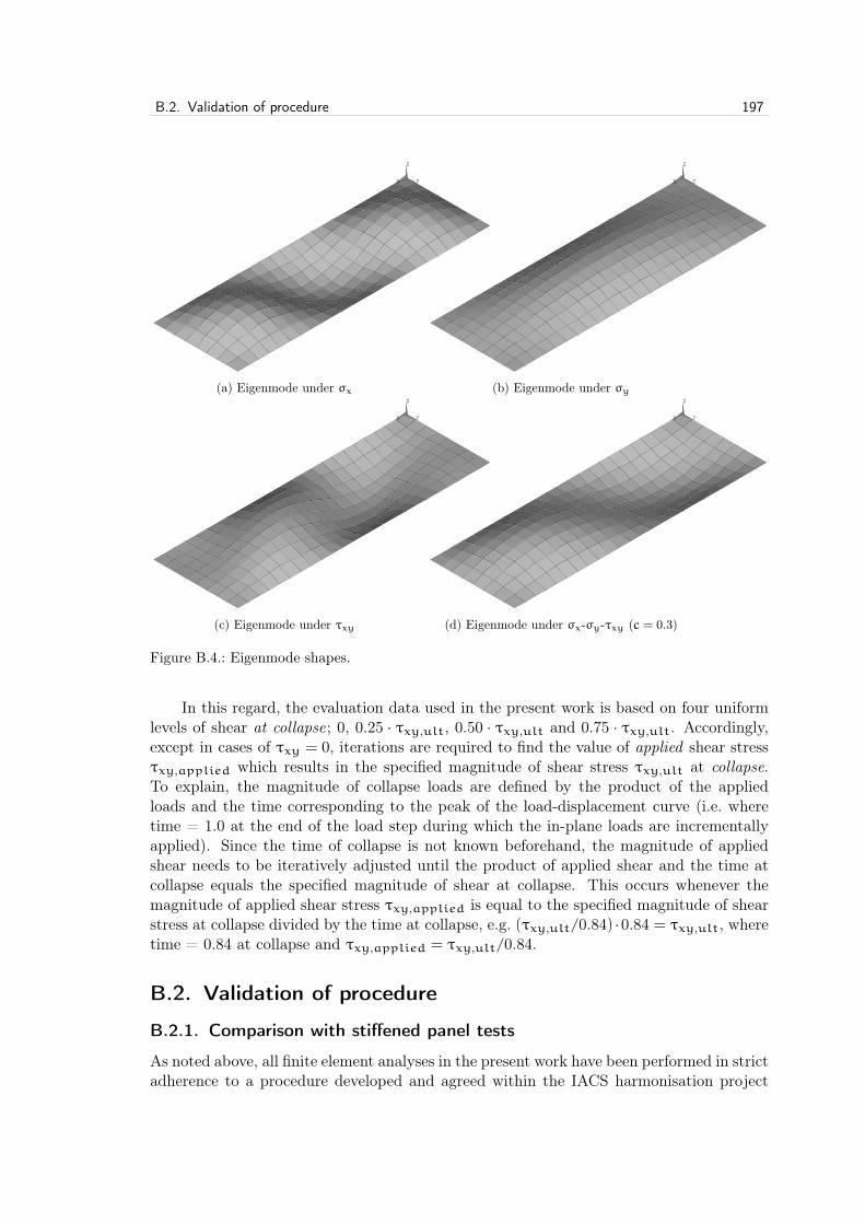
B.2. Validation of procedure 197
1
X Y
Z
run id 9913301
(a) Eigenmode under σx
1
X Y
Z
run id 9913301
(b) Eigenmode under σy1
X Y
Z
run id 9913301
(c) Eigenmode under τxy
1
X Y
Z
run id 9913301
(d) Eigenmode under σx-σy-τxy (c = 0.3)
Figure 0.1: ——-CROP!——–CROP!——–CROP!——–CROP!——–CROP!———CROP!——-
1
Figure B.4.: Eigenmode shapes.
In this regard, the evaluation data used in the present work is based on four uniformlevels of shear at collapse; 0, 0.25 · τxy,ult, 0.50 · τxy,ult and 0.75 · τxy,ult. Accordingly,except in cases of τxy = 0, iterations are required to find the value of applied shear stressτxy,applied which results in the specified magnitude of shear stress τxy,ult at collapse.To explain, the magnitude of collapse loads are defined by the product of the appliedloads and the time corresponding to the peak of the load-displacement curve (i.e. wheretime = 1.0 at the end of the load step during which the in-plane loads are incrementallyapplied). Since the time of collapse is not known beforehand, the magnitude of appliedshear needs to be iteratively adjusted until the product of applied shear and the time atcollapse equals the specified magnitude of shear at collapse. This occurs whenever themagnitude of applied shear stress τxy,applied is equal to the specified magnitude of shearstress at collapse divided by the time at collapse, e.g. (τxy,ult/0.84) ·0.84 = τxy,ult, wheretime = 0.84 at collapse and τxy,applied = τxy,ult/0.84.
B.2. Validation of procedure
B.2.1. Comparison with stiffened panel tests
As noted above, all finite element analyses in the present work have been performed in strictadherence to a procedure developed and agreed within the IACS harmonisation project
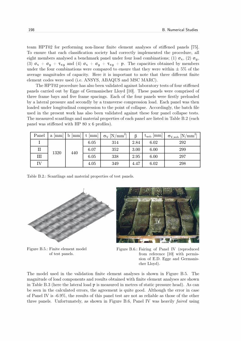
198 B. Numerical Studies
team HPT02 for performing non-linear finite element analyses of stiffened panels [75].To ensure that each classification society had correctly implemented the procedure, alleight members analysed a benchmark panel under four load combinations; (1) σx, (2) σy,(3) σx + σy + τxy and (4) σx + σy + τxy + p. The capacities obtained by membersunder the four combinations were compared to ensure that they were within ± 5% of theaverage magnitudes of capacity. Here it is important to note that three different finiteelement codes were used (i.e. ANSYS, ABAQUS and MSC MARC).
The HPT02 procedure has also been validated against laboratory tests of four stiffenedpanels carried out by Egge of Germanischer Lloyd [10]. These panels were comprised ofthree frame bays and five frame spacings. Each of the four panels were firstly preloadedby a lateral pressure and secondly by a transverse compression load. Each panel was thenloaded under longitudinal compression to the point of collapse. Accordingly, the batch fileused in the present work has also been validated against these four panel collapse tests.The measured scantlings and material properties of each panel are listed in Table B.2 (eachpanel was stiffened with HP 80 x 6 profiles).
Panel a [mm] b [mm] t [mm] σY [N/mm2] β tweb [mm] σY,web [N/mm2]
I 6.05 314 2.84 6.02 292
II 6.07 352 3.00 6.00 299
III 6.05 338 2.95 6.00 297
IV 4.05 349 4.47 6.02 298
1320 440
Table B.2.: Scantlings and material properties of test panels.1
X Y
Z
run id 99993
1
Figure B.5.: Finite element modelof test panels.
8
Fig. 7: failure mode model IV Figure B.6.: Fairing of Panel IV (reproduced
from reference [10] with permis-sion of E.D. Egge and Germanis-cher Lloyd).
The model used in the validation finite element analyses is shown in Figure B.5. Themagnitude of load components and results obtained with finite element analyses are shownin Table B.3 (here the lateral load p is measured in metres of static pressure head). As canbe seen in the calculated errors, the agreement is quite good. Although the error in caseof Panel IV is -6.9%, the results of this panel test are not as reliable as those of the otherthree panels. Unfortunately, as shown in Figure B.6, Panel IV was heavily faired using

B.2. Validation of procedure 199
Panel p [m] σy [N/mm2] σx,test [N/mm
2] σx,FEA [N/mm
2] Error
I 2.65 43.0 187.6 189.9 1.2%
II 5.30 43.0 194.0 199.2 2.7%
III 5.30 69.0 190.0 183.8 -3.3%
IV 2.40 47.0 185.0 172.2 -6.9%
Table B.3.: Applied loads and results.
heat treatment in an effort by the shipyard to reduce the magnitude of large post-weldingdeflections. According to Egge, this resulted in an indeterminate state of initial conditions(i.e. uncontrolled residual stresses and very short-waved pre-deformations).
B.2.2. Comparison with unstiffened plate tests
In addition to the foregoing, an effort has been made to validate the finite element analy-ses used in the present work against full-scale tests of unstiffened plates under combinedloading. Unfortunately, the only publicly-available data which the author could find is ofsmall-scale tests of plates under biaxial compression and lateral pressure [49]. As notedin the introduction to the corresponding test report, experimental data on biaxial com-pression strength was reported there for the first time. The tests were carried out in 1970during a research project sponsored by the Ship Structure Committee [48] and the authorcould find no results from subsequently performed tests.
4.0
00
-49-
-o
n2E 2
YCEXPER) 2))- y2) (b)-o
-O
Ç)
3-
Q
-O
(0.862, 0.555)
Fig. 33. Biaxial Strength Data
Fig. 34. Biaxial Buckle Photographs
'o)
HYPOTHETICALINTERACTIONbit 30CURVE3- b/t 50
Ç) b/t 70
-O b/I 90
Ç)
G-
39, 0.951)G-
3-
2.0
-E
I
0.25 0.50 0.75 1.00O( /O
Figure B.7.: Post-collapse test specimens (reproduced from reference [49] with permission of theShip Structure Committee).
As mentioned, the scale of the above-mentioned tests were small. All test specimenswere square cross-sectional tubes fabricated from flat rectangular plates having a nominal

200 B. Numerical Studies
b/t b [mm] a [mm] t [mm] σY [N/mm2] E [N/mm2] ν β30 22.86 68.58 1.10
50 38.10 114.3 1.84
70 53.34 160.0 2.57
90 68.58 205.7 3.31
270.3 199948 0.280.762
Table B.4.: Scantlings and material properties of test specimens.
thickness of 0.726 mm (0.03 in.) and an aspect ratio α = 3. Four basic specimens weretested as shown in Figure B.7. The scantlings and material properties of all four specimens
0.0
0.1
0.2
0.3
0.4
0.5
0.6
0.7
0.8
0.9
1.0
0.0 0.1 0.2 0.3 0.4 0.5 0.6 0.7 0.8 0.9 1.0
Norm
alise
d s
tres
s, R
y
Normalised stress, Rx
tests without lateral pressure
finite element analyses
(a) β = 1.10
0.0
0.1
0.2
0.3
0.4
0.5
0.6
0.7
0.8
0.9
1.0
0.0 0.1 0.2 0.3 0.4 0.5 0.6 0.7 0.8 0.9 1.0
Norm
alise
d s
tres
s, R
y
Normalised stress, Rx
tests without lateral pressure
tests with lateral pressure
finite element analyses
(b) β = 1.84
0.0
0.1
0.2
0.3
0.4
0.5
0.6
0.7
0.8
0.9
1.0
0.0 0.1 0.2 0.3 0.4 0.5 0.6 0.7 0.8 0.9 1.0
Norm
alise
d s
tres
s, R
y
Normalised stress, Rx
tests without lateral pressure
tests with lateral pressure
finite element analyses
(c) β = 2.57
0.0
0.1
0.2
0.3
0.4
0.5
0.6
0.7
0.8
0.9
1.0
0.0 0.1 0.2 0.3 0.4 0.5 0.6 0.7 0.8 0.9 1.0
Norm
alise
d s
tres
s, R
y
Normalised stress, Rx
tests without lateral pressure
tests with lateral pressure
finite element analyses
(d) β = 3.31
Figure 0.1: ——-CROP!——–CROP!——–CROP!——–CROP!——–CROP!———CROP!——-
1
Figure B.8.: Comparisons between tests and finite element analyses.

B.2. Validation of procedure 201
are summarised in Table B.4. Theoretically, the small scale of the tests should have noeffect on the results, but in practice provided several challenges with respect to fabrication(e.g. fairness, residual stresses) as well as testing (e.g. boundary conditions and load ap-plication).
Nevertheless, plate capacity curves based on finite element analyses are compared inFigure B.8 to all test results of plates under biaxial compression (results from uniaxialcompression tests were often incompatible with biaxial compression test results and sohave been omitted). In general, it can be concluded that the agreement between the testresults and finite element analyses are as good as could be reasonably expected given therelatively high degree of scatter in the test results ("a feature common to all compressiontests on thin plates", according to Winter [17]).

Appendix C. Evaluation Data
202

C.1. Tabular Results 203
C.1. Tabular Results
In this section the results of finite element analyses used in the evaluation of proofs aretabulated. Results obtained with the new proof are also included.
Plate aspect ratio, α Plate slenderness parameter, β Table Page
1 C.1 204
2 C.2 205
3 C.3 206
4 C.4 207
1 C.5 208
2 C.6 209
3 C.7 210
4 C.8 211
1 C.9 212
2 C.10 213
3 C.11 214
4 C.12 215
1
3
5

204 C. Evaluation Data
data point run id Rx,ult Ry,ult Rτ, ult Magnitude Rx,ult Ry,ult Rτ, ult Magnitude
1 11103 0.908 0.524 0.000 1.048 0.894 0.516 0.000 1.032
2 11105 0.524 0.908 0.000 1.048 0.516 0.894 0.000 1.032
3 11109 -0.421 0.721 0.000 0.835 -0.421 0.721 0.000 0.835
4 11111 -0.726 0.415 0.000 0.836 -0.726 0.415 0.000 0.836
5 11121 0.415 -0.726 0.000 0.836 0.415 -0.726 0.000 0.836
6 11123 0.721 -0.421 0.000 0.835 0.721 -0.421 0.000 0.835
7 41101 0.942 0.000 0.250 0.953 0.947 0.000 0.252 0.959
8 41103 0.869 0.502 0.250 1.014 0.865 0.500 0.249 1.010
9 41105 0.502 0.869 0.250 1.014 0.500 0.865 0.249 1.010
10 41107 0.000 0.942 0.250 0.953 0.000 0.947 0.252 0.959
11 41109 -0.407 0.697 0.250 0.820 -0.407 0.698 0.250 0.821
12 41111 -0.702 0.401 0.250 0.821 -0.703 0.402 0.250 0.822
13 41121 0.401 -0.702 0.250 0.821 0.402 -0.703 0.250 0.822
14 41123 0.697 -0.407 0.250 0.820 0.698 -0.407 0.250 0.821
15 51101 0.837 0.000 0.500 0.885 0.845 0.000 0.505 0.894
16 51103 0.756 0.437 0.500 0.920 0.769 0.444 0.509 0.936
17 51105 0.437 0.756 0.500 0.920 0.444 0.769 0.509 0.936
18 51107 0.000 0.837 0.500 0.885 0.000 0.845 0.505 0.894
19 51109 -0.361 0.619 0.500 0.772 -0.363 0.623 0.503 0.778
20 51111 -0.623 0.356 0.500 0.773 -0.627 0.358 0.503 0.779
21 51121 0.356 -0.623 0.500 0.773 0.358 -0.627 0.503 0.779
22 51123 0.619 -0.361 0.500 0.772 0.623 -0.363 0.503 0.778
23 61101 0.636 0.000 0.750 0.770 0.641 0.000 0.756 0.775
24 61103 0.590 0.341 0.749 0.808 0.591 0.341 0.750 0.808
25 61105 0.341 0.590 0.749 0.808 0.341 0.591 0.750 0.808
26 61107 0.000 0.636 0.750 0.770 0.000 0.641 0.756 0.775
27 61109 -0.267 0.457 0.750 0.683 -0.271 0.465 0.764 0.696
28 61111 -0.456 0.261 0.750 0.681 -0.466 0.266 0.767 0.696
29 61121 0.261 -0.456 0.750 0.681 0.266 -0.466 0.767 0.696
30 61123 0.457 -0.267 0.750 0.683 0.465 -0.271 0.764 0.696
New Proof
τ xy =
0τ x
y =
0.2
5∙τ
xy,u
ltτ x
y =
0.5
0∙τ
xy,u
ltτ x
y =
0.7
5∙τ
xy,u
lt
Finite Element Analyses
Table C.1.: α = 1, β = 1.

C.1. Tabular Results 205
data point run id Rx,ult Ry,ult Rτ, ult Magnitude Rx,ult Ry,ult Rτ, ult Magnitude
31 12103 0.585 0.338 0.000 0.676 0.580 0.335 0.000 0.670
32 12105 0.338 0.585 0.000 0.676 0.335 0.580 0.000 0.670
33 12109 -0.461 0.686 0.000 0.827 -0.461 0.686 0.000 0.827
34 12111 -0.755 0.380 0.000 0.845 -0.755 0.380 0.000 0.845
35 12121 0.380 -0.755 0.000 0.845 0.380 -0.755 0.000 0.845
36 12123 0.686 -0.461 0.000 0.827 0.686 -0.461 0.000 0.827
37 42101 0.714 0.000 0.247 0.728 0.709 0.000 0.246 0.723
38 42103 0.542 0.313 0.247 0.641 0.546 0.315 0.249 0.646
39 42105 0.313 0.542 0.247 0.641 0.315 0.546 0.249 0.646
40 42107 0.000 0.714 0.247 0.728 0.000 0.709 0.246 0.723
41 42109 -0.446 0.663 0.247 0.812 -0.447 0.665 0.248 0.814
42 42111 -0.730 0.367 0.247 0.829 -0.731 0.368 0.248 0.831
43 42121 0.367 -0.730 0.247 0.829 0.368 -0.731 0.248 0.831
44 42123 0.663 -0.446 0.247 0.812 0.665 -0.447 0.248 0.814
45 52101 0.612 0.000 0.495 0.675 0.606 0.000 0.490 0.669
46 52103 0.460 0.266 0.495 0.603 0.463 0.268 0.498 0.607
47 52105 0.266 0.460 0.495 0.603 0.268 0.463 0.498 0.607
48 52107 0.000 0.612 0.495 0.675 0.000 0.606 0.490 0.669
49 52109 -0.397 0.591 0.495 0.767 -0.400 0.595 0.498 0.772
50 52111 -0.648 0.326 0.495 0.780 -0.654 0.329 0.499 0.787
51 52121 0.326 -0.648 0.495 0.780 0.329 -0.654 0.499 0.787
52 52123 0.591 -0.397 0.495 0.767 0.595 -0.400 0.498 0.772
53 62101 0.438 0.000 0.742 0.613 0.433 0.000 0.734 0.606
54 62103 0.329 0.190 0.742 0.573 0.329 0.190 0.741 0.572
55 62105 0.190 0.329 0.742 0.573 0.190 0.329 0.741 0.572
56 62107 0.000 0.438 0.742 0.613 0.000 0.433 0.734 0.606
57 62109 -0.300 0.446 0.742 0.687 -0.294 0.438 0.729 0.675
58 62111 -0.482 0.242 0.742 0.689 -0.492 0.247 0.758 0.704
59 62121 0.242 -0.482 0.742 0.689 0.247 -0.492 0.758 0.704
60 62123 0.446 -0.300 0.742 0.687 0.438 -0.294 0.729 0.675
Finite Element Analyses New Proof
τ xy =
0τ x
y =
0.2
5∙τ
xy,u
ltτ x
y =
0.5
0∙τ
xy,u
ltτ x
y =
0.7
5∙τ
xy,u
lt
Table C.2.: α = 1, β = 2.

206 C. Evaluation Data
data point run id Rx,ult Ry,ult Rτ, ult Magnitude Rx,ult Ry,ult Rτ, ult Magnitude
61 13103 0.461 0.266 0.000 0.532 0.431 0.249 0.000 0.497
62 13105 0.266 0.461 0.000 0.532 0.249 0.431 0.000 0.497
63 13109 -0.495 0.652 0.000 0.819 -0.467 0.614 0.000 0.772
64 13111 -0.776 0.353 0.000 0.852 -0.776 0.353 0.000 0.852
65 13121 0.353 -0.776 0.000 0.852 0.353 -0.776 0.000 0.852
66 13123 0.652 -0.495 0.000 0.819 0.614 -0.467 0.000 0.772
67 43101 0.571 0.000 0.232 0.586 0.565 0.000 0.229 0.580
68 43103 0.412 0.238 0.232 0.494 0.397 0.229 0.223 0.477
69 43105 0.238 0.412 0.232 0.494 0.229 0.397 0.223 0.477
70 43107 0.000 0.571 0.232 0.586 0.000 0.565 0.229 0.580
71 43109 -0.474 0.623 0.232 0.794 -0.434 0.571 0.212 0.727
72 43111 -0.754 0.343 0.232 0.838 -0.755 0.343 0.232 0.840
73 43121 0.343 -0.754 0.232 0.838 0.343 -0.755 0.232 0.840
74 43123 0.623 -0.474 0.232 0.794 0.571 -0.434 0.212 0.727
75 53101 0.470 0.000 0.464 0.541 0.466 0.000 0.459 0.536
76 53103 0.340 0.196 0.463 0.475 0.330 0.190 0.450 0.461
77 53105 0.196 0.340 0.463 0.475 0.190 0.330 0.450 0.461
78 53107 0.000 0.470 0.464 0.541 0.000 0.466 0.459 0.536
79 53109 -0.417 0.548 0.464 0.739 -0.372 0.489 0.414 0.659
80 53111 -0.681 0.310 0.463 0.794 -0.686 0.312 0.467 0.800
81 53121 0.310 -0.681 0.463 0.794 0.312 -0.686 0.467 0.800
82 53123 0.548 -0.417 0.464 0.739 0.489 -0.372 0.414 0.659
83 63101 0.303 0.000 0.694 0.502 0.306 0.000 0.701 0.507
84 63103 0.216 0.125 0.695 0.472 0.217 0.125 0.697 0.474
85 63105 0.125 0.216 0.695 0.472 0.125 0.217 0.697 0.474
86 63107 0.000 0.303 0.694 0.502 0.000 0.306 0.701 0.507
87 63109 -0.306 0.403 0.695 0.646 -0.276 0.363 0.626 0.582
88 63111 -0.550 0.250 0.695 0.725 -0.554 0.252 0.700 0.731
89 63121 0.250 -0.550 0.695 0.725 0.252 -0.554 0.700 0.731
90 63123 0.403 -0.306 0.695 0.646 0.363 -0.276 0.626 0.582
τ xy =
0.7
5∙τ
xy,u
ltτ x
y =
0τ x
y =
0.2
5∙τ
xy,u
ltτ x
y =
0.5
0∙τ
xy,u
lt
Finite Element Analyses New Proof
Table C.3.: α = 1, β = 3.

C.1. Tabular Results 207
data point run id Rx,ult Ry,ult Rτ, ult Magnitude Rx,ult Ry,ult Rτ, ult Magnitude
91 14103 0.386 0.223 0.000 0.446 0.365 0.211 0.000 0.421
92 14105 0.223 0.386 0.000 0.446 0.211 0.365 0.000 0.421
93 14109 -0.509 0.628 0.000 0.808 -0.452 0.558 0.000 0.718
94 14111 -0.786 0.340 0.000 0.856 -0.786 0.340 0.000 0.856
95 14121 0.340 -0.786 0.000 0.856 0.340 -0.786 0.000 0.856
96 14123 0.628 -0.509 0.000 0.808 0.558 -0.452 0.000 0.718
97 44101 0.502 0.000 0.208 0.516 0.501 0.000 0.208 0.515
98 44103 0.342 0.197 0.208 0.413 0.330 0.190 0.201 0.398
99 44105 0.197 0.342 0.208 0.413 0.190 0.330 0.201 0.398
100 44107 0.000 0.502 0.208 0.516 0.000 0.501 0.208 0.515
101 44109 -0.456 0.563 0.208 0.734 -0.412 0.509 0.188 0.664
102 44111 -0.768 0.332 0.208 0.845 -0.769 0.332 0.208 0.846
103 44121 0.332 -0.768 0.208 0.845 0.332 -0.769 0.208 0.846
104 44123 0.563 -0.456 0.208 0.734 0.509 -0.412 0.188 0.664
105 54101 0.393 0.000 0.416 0.461 0.397 0.000 0.420 0.466
106 54103 0.277 0.160 0.416 0.400 0.267 0.154 0.401 0.386
107 54105 0.160 0.277 0.416 0.400 0.154 0.267 0.401 0.386
108 54107 0.000 0.393 0.416 0.461 0.000 0.397 0.420 0.466
109 54109 -0.405 0.500 0.416 0.687 -0.350 0.431 0.359 0.593
110 54111 -0.713 0.308 0.416 0.813 -0.715 0.309 0.417 0.815
111 54121 0.308 -0.713 0.416 0.813 0.309 -0.715 0.417 0.815
112 54123 0.500 -0.405 0.416 0.687 0.431 -0.350 0.359 0.593
113 64101 0.232 0.000 0.624 0.429 0.240 0.000 0.644 0.443
114 64103 0.162 0.094 0.624 0.406 0.164 0.095 0.631 0.411
115 64105 0.094 0.162 0.624 0.406 0.095 0.164 0.631 0.411
116 64107 0.000 0.232 0.624 0.429 0.000 0.240 0.644 0.443
117 64109 -0.294 0.362 0.624 0.589 -0.257 0.317 0.545 0.515
118 64111 -0.613 0.265 0.623 0.758 -0.607 0.262 0.617 0.751
119 64121 0.265 -0.613 0.623 0.758 0.262 -0.607 0.617 0.751
120 64123 0.362 -0.294 0.624 0.589 0.317 -0.257 0.545 0.515
Finite Element Analyses New Proof
τ xy =
0.5
0∙τ
xy,u
ltτ x
y =
0.7
5∙τ
xy,u
ltτ x
y =
0.2
5∙τ
xy,u
ltτ x
y =
0
Table C.4.: α = 1, β = 4.

208 C. Evaluation Data
data point run id Rx,ult Ry,ult Rτ, ult Magnitude Rx,ult Ry,ult Rτ, ult Magnitude
121 11303 0.953 0.458 0.000 1.057 0.920 0.442 0.000 1.021
122 11305 0.459 0.646 0.000 0.792 0.477 0.672 0.000 0.824
123 11309 -0.433 0.602 0.000 0.742 -0.481 0.669 0.000 0.824
124 11311 -0.765 0.364 0.000 0.848 -0.767 0.365 0.000 0.849
125 11321 0.415 -0.726 0.000 0.836 0.415 -0.726 0.000 0.836
126 11323 0.721 -0.421 0.000 0.835 0.721 -0.421 0.000 0.835
127 41301 0.946 0.000 0.250 0.957 0.948 0.000 0.251 0.959
128 41303 0.916 0.440 0.250 1.027 0.893 0.429 0.244 1.000
129 41305 0.446 0.627 0.250 0.783 0.461 0.649 0.258 0.810
130 41307 0.000 0.654 0.250 0.670 0.000 0.650 0.249 0.666
131 41309 -0.421 0.586 0.250 0.736 -0.462 0.643 0.274 0.808
132 41311 -0.742 0.353 0.250 0.834 -0.742 0.353 0.250 0.834
133 41321 0.401 -0.702 0.250 0.821 0.402 -0.703 0.250 0.822
134 41323 0.697 -0.407 0.250 0.820 0.698 -0.407 0.250 0.821
135 51301 0.844 0.000 0.500 0.892 0.847 0.000 0.502 0.896
136 51303 0.810 0.389 0.500 0.944 0.800 0.385 0.494 0.933
137 51305 0.415 0.584 0.500 0.772 0.414 0.582 0.498 0.770
138 51307 0.000 0.606 0.500 0.671 0.000 0.587 0.485 0.651
139 51309 -0.385 0.535 0.500 0.719 -0.408 0.567 0.530 0.763
140 51311 -0.663 0.315 0.500 0.789 -0.664 0.316 0.500 0.790
141 51321 0.356 -0.623 0.500 0.773 0.358 -0.627 0.503 0.779
142 51323 0.619 -0.361 0.500 0.772 0.623 -0.363 0.503 0.778
143 61301 0.644 0.000 0.750 0.776 0.646 0.000 0.752 0.778
144 61303 0.625 0.300 0.750 0.818 0.618 0.297 0.741 0.808
145 61305 0.357 0.502 0.750 0.753 0.337 0.474 0.708 0.711
146 61307 0.000 0.514 0.750 0.672 0.000 0.480 0.700 0.627
147 61309 -0.305 0.424 0.750 0.678 -0.310 0.432 0.764 0.691
148 61311 -0.499 0.237 0.750 0.702 -0.502 0.239 0.755 0.707
149 61321 0.261 -0.456 0.750 0.681 0.266 -0.466 0.766 0.696
150 61323 0.457 -0.266 0.750 0.683 0.465 -0.271 0.764 0.696
Finite Element Analyses New Proof
τ xy =
0τ x
y =
0.2
5∙τ
xy,u
ltτ x
y =
0.5
0∙τ
xy,u
ltτ x
y =
0.7
5∙τ
xy,u
lt
Table C.5.: α = 3, β = 1.

C.1. Tabular Results 209
data point run id Rx,ult Ry,ult Rτ, ult Magnitude Rx,ult Ry,ult Rτ, ult Magnitude
151 12303 0.605 0.243 0.000 0.652 0.572 0.230 0.000 0.617
152 12305 0.293 0.331 0.000 0.442 0.298 0.337 0.000 0.450
153 12309 -0.411 0.375 0.000 0.556 -0.407 0.371 0.000 0.551
154 12311 -0.809 0.272 0.000 0.854 -0.831 0.279 0.000 0.877
155 12321 0.380 -0.754 0.000 0.845 0.380 -0.754 0.000 0.845
156 12323 0.686 -0.461 0.000 0.827 0.686 -0.461 0.000 0.827
157 42301 0.721 0.000 0.244 0.735 0.711 0.000 0.241 0.725
158 42303 0.580 0.233 0.244 0.641 0.542 0.218 0.228 0.599
159 42305 0.278 0.314 0.244 0.442 0.280 0.317 0.247 0.447
160 42307 0.000 0.357 0.244 0.384 0.000 0.350 0.240 0.377
161 42309 -0.397 0.362 0.244 0.555 -0.384 0.351 0.237 0.538
162 42311 -0.784 0.263 0.244 0.839 -0.804 0.270 0.251 0.861
163 42321 0.368 -0.730 0.244 0.830 0.368 -0.731 0.245 0.831
164 42323 0.664 -0.446 0.244 0.812 0.666 -0.447 0.245 0.814
165 52301 0.617 0.000 0.488 0.679 0.609 0.000 0.482 0.669
166 52303 0.497 0.200 0.489 0.606 0.470 0.189 0.461 0.572
167 52305 0.250 0.282 0.488 0.471 0.242 0.274 0.474 0.456
168 52307 0.000 0.320 0.489 0.427 0.000 0.304 0.464 0.405
169 52309 -0.358 0.327 0.489 0.561 -0.335 0.306 0.457 0.525
170 52311 -0.705 0.237 0.489 0.796 -0.720 0.242 0.499 0.812
171 52321 0.329 -0.653 0.489 0.784 0.331 -0.657 0.492 0.788
172 52323 0.596 -0.400 0.489 0.772 0.598 -0.402 0.490 0.774
173 62301 0.428 0.000 0.733 0.602 0.428 0.000 0.732 0.601
174 62303 0.338 0.136 0.733 0.558 0.332 0.134 0.721 0.549
175 62305 0.193 0.218 0.733 0.514 0.183 0.206 0.694 0.486
176 62307 0.000 0.265 0.732 0.499 0.000 0.240 0.663 0.452
177 62309 -0.293 0.267 0.733 0.580 -0.264 0.241 0.660 0.523
178 62311 -0.550 0.185 0.733 0.719 -0.557 0.187 0.742 0.727
179 62321 0.248 -0.493 0.733 0.695 0.253 -0.502 0.746 0.708
180 62323 0.458 -0.308 0.733 0.696 0.446 -0.299 0.713 0.676
Finite Element Analyses New Proof
τ xy =
0τ x
y =
0.2
5∙τ
xy,u
ltτ x
y =
0.5
0∙τ
xy,u
ltτ x
y =
0.7
5∙τ
xy,u
lt
Table C.6.: α = 3, β = 2.

210 C. Evaluation Data
data point run id Rx,ult Ry,ult Rτ, ult Magnitude Rx,ult Ry,ult Rτ, ult Magnitude
181 13303 0.434 0.160 0.000 0.462 0.412 0.152 0.000 0.439
182 13305 0.222 0.227 0.000 0.317 0.218 0.223 0.000 0.311
183 13309 -0.411 0.281 0.000 0.498 -0.384 0.262 0.000 0.465
184 13311 -0.829 0.214 0.000 0.856 -0.869 0.224 0.000 0.897
185 13321 0.352 -0.776 0.000 0.852 0.352 -0.776 0.000 0.852
186 13323 0.646 -0.493 0.000 0.813 0.611 -0.467 0.000 0.769
187 43301 0.537 0.000 0.214 0.551 0.558 0.000 0.223 0.573
188 43303 0.403 0.149 0.214 0.447 0.381 0.141 0.202 0.422
189 43305 0.202 0.207 0.214 0.314 0.200 0.205 0.212 0.311
190 43307 0.000 0.246 0.214 0.276 0.000 0.241 0.210 0.270
191 43309 -0.393 0.268 0.214 0.492 -0.357 0.244 0.194 0.447
192 43311 -0.805 0.208 0.214 0.841 -0.847 0.218 0.225 0.884
193 43321 0.343 -0.758 0.214 0.841 0.344 -0.758 0.214 0.842
194 43323 0.598 -0.456 0.214 0.762 0.566 -0.432 0.203 0.721
195 53301 0.450 0.000 0.429 0.513 0.457 0.000 0.436 0.522
196 53303 0.361 0.133 0.429 0.457 0.326 0.120 0.387 0.413
197 53305 0.178 0.181 0.429 0.354 0.169 0.172 0.407 0.337
198 53307 0.000 0.214 0.428 0.327 0.000 0.203 0.407 0.310
199 53309 -0.348 0.238 0.429 0.489 -0.307 0.210 0.378 0.431
200 53311 -0.735 0.190 0.428 0.799 -0.755 0.195 0.440 0.820
201 53321 0.316 -0.697 0.429 0.805 0.318 -0.701 0.431 0.809
202 53323 0.538 -0.410 0.428 0.720 0.485 -0.370 0.386 0.649
203 63301 0.283 0.000 0.643 0.467 0.291 0.000 0.662 0.481
204 63303 0.211 0.078 0.643 0.434 0.210 0.078 0.640 0.432
205 63305 0.112 0.114 0.643 0.404 0.111 0.114 0.639 0.402
206 63307 0.000 0.168 0.643 0.407 0.000 0.153 0.586 0.371
207 63309 -0.277 0.189 0.643 0.500 -0.239 0.163 0.554 0.431
208 63311 -0.611 0.158 0.643 0.732 -0.571 0.147 0.601 0.684
209 63321 0.267 -0.590 0.643 0.746 0.269 -0.593 0.646 0.750
210 63323 0.419 -0.320 0.642 0.645 0.370 -0.282 0.567 0.569
Finite Element Analyses New Proof
τ xy =
0τ x
y =
0.2
5∙τ
xy,u
ltτ x
y =
0.5
0∙τ
xy,u
ltτ x
y =
0.7
5∙τ
xy,u
lt
Table C.7.: α = 3, β = 3.

C.1. Tabular Results 211
data point run id Rx,ult Ry,ult Rτ, ult Magnitude Rx,ult Ry,ult Rτ, ult Magnitude
211 14303 0.345 0.123 0.000 0.366 0.336 0.120 0.000 0.357
212 14305 0.179 0.175 0.000 0.251 0.180 0.176 0.000 0.252
213 14309 -0.415 0.241 0.000 0.480 -0.376 0.219 0.000 0.435
214 14311 -0.843 0.187 0.000 0.864 -0.887 0.197 0.000 0.908
215 14321 0.335 -0.789 0.000 0.858 0.335 -0.789 0.000 0.858
216 14323 0.512 -0.424 0.000 0.665 0.541 -0.448 0.000 0.702
217 44301 0.438 0.000 0.180 0.450 0.479 0.000 0.196 0.492
218 44303 0.315 0.112 0.180 0.350 0.304 0.108 0.173 0.338
219 44305 0.161 0.157 0.180 0.247 0.162 0.158 0.181 0.249
220 44307 0.000 0.193 0.180 0.219 0.000 0.196 0.182 0.223
221 44309 -0.386 0.225 0.180 0.459 -0.344 0.200 0.160 0.409
222 44311 -0.820 0.182 0.180 0.846 -0.870 0.194 0.191 0.899
223 44321 0.329 -0.776 0.180 0.850 0.330 -0.777 0.180 0.850
224 44323 0.499 -0.413 0.180 0.656 0.488 -0.404 0.176 0.641
225 54301 0.361 0.000 0.359 0.416 0.377 0.000 0.376 0.435
226 54303 0.281 0.100 0.360 0.363 0.254 0.090 0.325 0.329
227 54305 0.140 0.136 0.359 0.285 0.133 0.130 0.342 0.271
228 54307 0.000 0.161 0.359 0.263 0.000 0.159 0.353 0.258
229 54309 -0.330 0.192 0.359 0.434 -0.289 0.168 0.315 0.381
230 54311 -0.757 0.168 0.359 0.803 -0.724 0.161 0.344 0.768
231 54321 0.312 -0.735 0.359 0.825 0.313 -0.737 0.360 0.827
232 54323 0.454 -0.376 0.359 0.624 0.410 -0.339 0.325 0.564
233 64301 0.230 0.000 0.538 0.386 0.236 0.000 0.553 0.397
234 64303 0.155 0.055 0.538 0.351 0.155 0.055 0.539 0.352
235 64305 0.080 0.078 0.539 0.331 0.081 0.079 0.545 0.334
236 64307 0.000 0.102 0.538 0.327 0.000 0.102 0.536 0.326
237 64309 -0.251 0.146 0.539 0.426 -0.217 0.126 0.466 0.368
238 64311 -0.643 0.143 0.539 0.728 -0.561 0.125 0.470 0.635
239 64321 0.282 -0.663 0.539 0.785 0.270 -0.635 0.516 0.752
240 64323 0.369 -0.306 0.539 0.572 0.316 -0.261 0.461 0.489
Finite Element Analyses New Proof
τ xy =
0.7
5∙τ
xy,u
ltτ x
y =
0τ x
y =
0.2
5∙τ
xy,u
ltτ x
y =
0.5
0∙τ
xy,u
lt
Table C.8.: α = 3, β = 4.
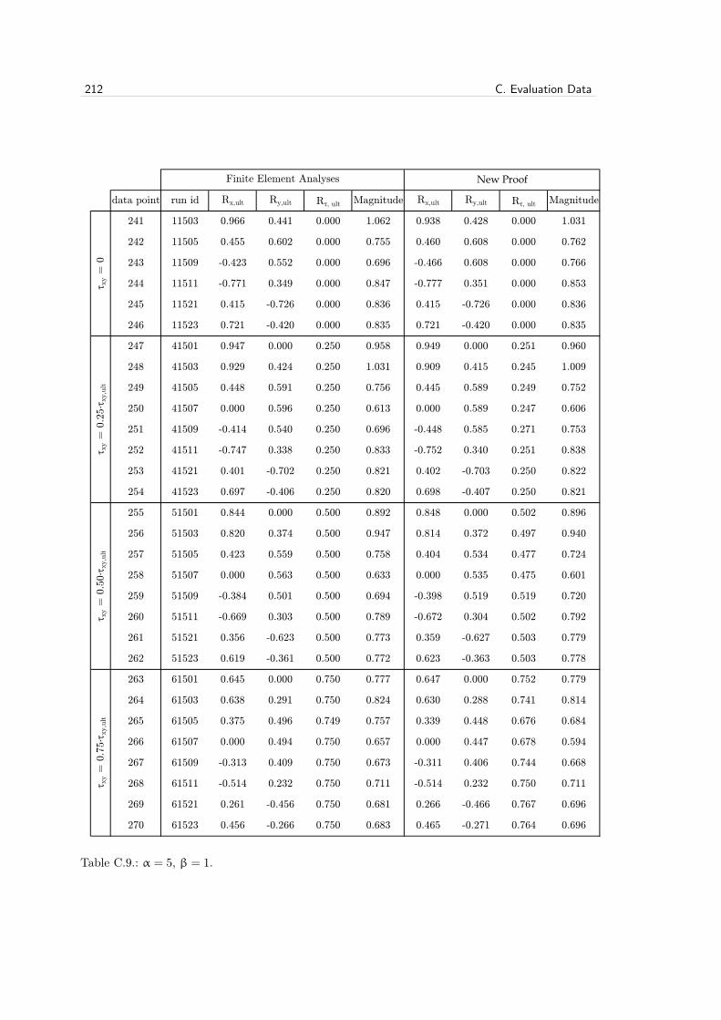
212 C. Evaluation Data
data point run id Rx,ult Ry,ult Rτ, ult Magnitude Rx,ult Ry,ult Rτ, ult Magnitude
241 11503 0.966 0.441 0.000 1.062 0.938 0.428 0.000 1.031
242 11505 0.455 0.602 0.000 0.755 0.460 0.608 0.000 0.762
243 11509 -0.423 0.552 0.000 0.696 -0.466 0.608 0.000 0.766
244 11511 -0.771 0.349 0.000 0.847 -0.777 0.351 0.000 0.853
245 11521 0.415 -0.726 0.000 0.836 0.415 -0.726 0.000 0.836
246 11523 0.721 -0.420 0.000 0.835 0.721 -0.420 0.000 0.835
247 41501 0.947 0.000 0.250 0.958 0.949 0.000 0.251 0.960
248 41503 0.929 0.424 0.250 1.031 0.909 0.415 0.245 1.009
249 41505 0.448 0.591 0.250 0.756 0.445 0.589 0.249 0.752
250 41507 0.000 0.596 0.250 0.613 0.000 0.589 0.247 0.606
251 41509 -0.414 0.540 0.250 0.696 -0.448 0.585 0.271 0.753
252 41511 -0.747 0.338 0.250 0.833 -0.752 0.340 0.251 0.838
253 41521 0.401 -0.702 0.250 0.821 0.402 -0.703 0.250 0.822
254 41523 0.697 -0.406 0.250 0.820 0.698 -0.407 0.250 0.821
255 51501 0.844 0.000 0.500 0.892 0.848 0.000 0.502 0.896
256 51503 0.820 0.374 0.500 0.947 0.814 0.372 0.497 0.940
257 51505 0.423 0.559 0.500 0.758 0.404 0.534 0.477 0.724
258 51507 0.000 0.563 0.500 0.633 0.000 0.535 0.475 0.601
259 51509 -0.384 0.501 0.500 0.694 -0.398 0.519 0.519 0.720
260 51511 -0.669 0.303 0.500 0.789 -0.672 0.304 0.502 0.792
261 51521 0.356 -0.623 0.500 0.773 0.359 -0.627 0.503 0.779
262 51523 0.619 -0.361 0.500 0.772 0.623 -0.363 0.503 0.778
263 61501 0.645 0.000 0.750 0.777 0.647 0.000 0.752 0.779
264 61503 0.638 0.291 0.750 0.824 0.630 0.288 0.741 0.814
265 61505 0.375 0.496 0.749 0.757 0.339 0.448 0.676 0.684
266 61507 0.000 0.494 0.750 0.657 0.000 0.447 0.678 0.594
267 61509 -0.313 0.409 0.750 0.673 -0.311 0.406 0.744 0.668
268 61511 -0.514 0.232 0.750 0.711 -0.514 0.232 0.750 0.711
269 61521 0.261 -0.456 0.750 0.681 0.266 -0.466 0.767 0.696
270 61523 0.456 -0.266 0.750 0.683 0.465 -0.271 0.764 0.696
Finite Element Analyses New Proof
τ xy =
0τ x
y =
0.2
5∙τ
xy,u
ltτ x
y =
0.5
0∙τ
xy,u
ltτ x
y =
0.7
5∙τ
xy,u
lt
Table C.9.: α = 5, β = 1.

C.1. Tabular Results 213
data point run id Rx,ult Ry,ult Rτ, ult Magnitude Rx,ult Ry,ult Rτ, ult Magnitude
271 12503 0.619 0.216 0.000 0.656 0.582 0.203 0.000 0.617
272 12505 0.286 0.273 0.000 0.395 0.296 0.284 0.000 0.410
273 12509 -0.394 0.300 0.000 0.495 -0.391 0.298 0.000 0.492
274 12511 -0.802 0.229 0.000 0.834 -0.855 0.244 0.000 0.890
275 12521 0.380 -0.754 0.000 0.845 0.380 -0.754 0.000 0.845
276 12523 0.687 -0.461 0.000 0.827 0.687 -0.461 0.000 0.827
277 42501 0.721 0.000 0.244 0.734 0.712 0.000 0.241 0.725
278 42503 0.599 0.210 0.244 0.650 0.552 0.193 0.224 0.599
279 42505 0.275 0.263 0.244 0.406 0.279 0.266 0.247 0.411
280 42507 0.000 0.288 0.244 0.321 0.000 0.281 0.237 0.312
281 42509 -0.383 0.291 0.244 0.501 -0.369 0.281 0.235 0.484
282 42511 -0.780 0.223 0.244 0.823 -0.826 0.236 0.258 0.872
283 42521 0.368 -0.731 0.244 0.830 0.369 -0.731 0.244 0.831
284 42523 0.666 -0.447 0.244 0.814 0.666 -0.447 0.244 0.814
285 52501 0.616 0.000 0.487 0.677 0.609 0.000 0.481 0.669
286 52503 0.507 0.177 0.487 0.607 0.478 0.167 0.459 0.572
287 52505 0.254 0.243 0.487 0.450 0.242 0.232 0.465 0.429
288 52507 0.000 0.266 0.487 0.387 0.000 0.246 0.451 0.358
289 52509 -0.353 0.268 0.487 0.525 -0.324 0.247 0.448 0.483
290 52511 -0.709 0.202 0.487 0.789 -0.737 0.210 0.507 0.821
291 52521 0.329 -0.653 0.487 0.784 0.331 -0.657 0.490 0.789
292 52523 0.597 -0.401 0.487 0.772 0.599 -0.402 0.489 0.775
293 62501 0.428 0.000 0.731 0.601 0.428 0.000 0.730 0.601
294 62503 0.327 0.114 0.729 0.545 0.328 0.115 0.732 0.547
295 62505 0.195 0.187 0.730 0.500 0.183 0.175 0.686 0.470
296 62507 0.000 0.231 0.731 0.481 0.000 0.200 0.635 0.418
297 62509 -0.301 0.229 0.731 0.566 -0.262 0.200 0.637 0.494
298 62511 -0.564 0.161 0.731 0.722 -0.573 0.163 0.743 0.734
299 62521 0.249 -0.493 0.731 0.695 0.253 -0.503 0.745 0.709
300 62523 0.461 -0.309 0.731 0.697 0.447 -0.300 0.709 0.676
Finite Element Analyses New Proof
τ xy =
0τ x
y =
0.2
5∙τ
xy,u
ltτ x
y =
0.5
0∙τ
xy,u
ltτ x
y =
0.7
5∙τ
xy,u
lt
Table C.10.: α = 5, β = 2.

214 C. Evaluation Data
data point run id Rx,ult Ry,ult Rτ, ult Magnitude Rx,ult Ry,ult Rτ, ult Magnitude
301 13503 0.436 0.130 0.000 0.455 0.418 0.125 0.000 0.436
302 13505 0.215 0.172 0.000 0.276 0.217 0.173 0.000 0.278
303 13509 -0.393 0.204 0.000 0.443 -0.373 0.193 0.000 0.419
304 13511 -0.818 0.163 0.000 0.834 -0.898 0.179 0.000 0.916
305 13521 0.352 -0.776 0.000 0.852 0.352 -0.776 0.000 0.852
306 13523 0.647 -0.494 0.000 0.814 0.611 -0.467 0.000 0.769
307 43501 0.578 0.000 0.205 0.590 0.563 0.000 0.199 0.575
308 43503 0.412 0.123 0.205 0.446 0.387 0.115 0.192 0.419
309 43505 0.200 0.160 0.205 0.282 0.199 0.159 0.204 0.281
310 43507 0.000 0.184 0.205 0.218 0.000 0.178 0.198 0.211
311 43509 -0.380 0.196 0.205 0.444 -0.346 0.179 0.187 0.404
312 43511 -0.798 0.159 0.205 0.823 -0.875 0.175 0.224 0.902
313 43521 0.344 -0.759 0.205 0.842 0.345 -0.760 0.205 0.843
314 43523 0.614 -0.469 0.205 0.782 0.567 -0.433 0.189 0.722
315 53501 0.474 0.000 0.410 0.530 0.465 0.000 0.402 0.520
316 53503 0.371 0.111 0.409 0.454 0.332 0.099 0.366 0.406
317 53505 0.182 0.145 0.409 0.331 0.169 0.135 0.382 0.309
318 53507 0.000 0.165 0.410 0.288 0.000 0.151 0.376 0.265
319 53509 -0.346 0.179 0.409 0.455 -0.300 0.155 0.355 0.395
320 53511 -0.740 0.148 0.409 0.790 -0.733 0.146 0.405 0.783
321 53521 0.320 -0.705 0.409 0.809 0.321 -0.708 0.411 0.813
322 53523 0.562 -0.429 0.409 0.746 0.491 -0.375 0.357 0.651
323 63501 0.296 0.000 0.614 0.461 0.300 0.000 0.623 0.469
324 63503 0.207 0.062 0.614 0.415 0.209 0.062 0.618 0.418
325 63505 0.124 0.099 0.614 0.388 0.118 0.094 0.587 0.371
326 63507 0.000 0.140 0.614 0.381 0.000 0.120 0.528 0.328
327 63509 -0.294 0.152 0.614 0.485 -0.242 0.125 0.506 0.399
328 63511 -0.638 0.127 0.614 0.741 -0.573 0.114 0.551 0.665
329 63521 0.274 -0.604 0.614 0.752 0.276 -0.609 0.620 0.759
330 63523 0.464 -0.354 0.614 0.683 0.390 -0.298 0.516 0.574
Finite Element Analyses New Proof
τ xy =
0τ x
y =
0.2
5∙τ
xy,u
ltτ x
y =
0.5
0∙τ
xy,u
ltτ x
y =
0.7
5∙τ
xy,u
lt
Table C.11.: α = 5, β = 3.

C.1. Tabular Results 215
data point run id Rx,ult Ry,ult Rτ, ult Magnitude Rx,ult Ry,ult Rτ, ult Magnitude
331 14503 0.342 0.094 0.000 0.354 0.339 0.093 0.000 0.352
332 14505 0.173 0.126 0.000 0.214 0.179 0.130 0.000 0.221
333 14509 -0.398 0.165 0.000 0.430 -0.366 0.152 0.000 0.396
334 14511 -0.832 0.134 0.000 0.843 -0.918 0.148 0.000 0.930
335 14521 0.334 -0.790 0.000 0.858 0.334 -0.790 0.000 0.858
336 14523 0.509 -0.424 0.000 0.662 0.537 -0.447 0.000 0.699
337 44501 0.503 0.000 0.166 0.512 0.485 0.000 0.160 0.494
338 44503 0.318 0.087 0.166 0.343 0.306 0.084 0.160 0.331
339 44505 0.158 0.115 0.166 0.218 0.160 0.117 0.168 0.221
340 44507 0.000 0.137 0.166 0.167 0.000 0.136 0.165 0.166
341 44509 -0.375 0.155 0.166 0.417 -0.335 0.139 0.148 0.372
342 44511 -0.812 0.131 0.166 0.828 -0.842 0.135 0.172 0.858
343 44521 0.329 -0.779 0.166 0.851 0.329 -0.779 0.166 0.851
344 44523 0.497 -0.413 0.166 0.653 0.484 -0.403 0.162 0.637
345 54501 0.406 0.000 0.332 0.449 0.393 0.000 0.321 0.434
346 54503 0.291 0.080 0.333 0.358 0.259 0.071 0.296 0.318
347 54505 0.143 0.104 0.333 0.261 0.133 0.097 0.310 0.244
348 54507 0.000 0.120 0.332 0.226 0.000 0.113 0.312 0.213
349 54509 -0.332 0.137 0.332 0.407 -0.284 0.118 0.285 0.349
350 54511 -0.760 0.122 0.332 0.793 -0.705 0.113 0.308 0.736
351 54521 0.315 -0.744 0.332 0.830 0.315 -0.745 0.333 0.831
352 54523 0.468 -0.389 0.332 0.638 0.412 -0.343 0.293 0.562
353 64501 0.247 0.000 0.498 0.380 0.248 0.000 0.498 0.380
354 64503 0.161 0.044 0.499 0.333 0.159 0.044 0.494 0.329
355 64505 0.094 0.069 0.498 0.310 0.090 0.066 0.475 0.296
356 64507 0.000 0.098 0.499 0.304 0.000 0.086 0.437 0.267
357 64509 -0.275 0.114 0.499 0.414 -0.225 0.093 0.407 0.338
358 64511 -0.674 0.108 0.499 0.741 -0.564 0.091 0.417 0.620
359 64521 0.289 -0.683 0.499 0.795 0.273 -0.646 0.472 0.752
360 64523 0.399 -0.332 0.499 0.593 0.327 -0.273 0.409 0.487
Finite Element Analyses New Proof
τ xy =
0τ x
y =
0.2
5∙τ
xy,u
ltτ x
y =
0.5
0∙τ
xy,u
ltτ x
y =
0.7
5∙τ
xy,u
lt
Table C.12.: α = 5, β = 4.

216 C. Evaluation Data
C.2. Graphical Results
In this section the results of finite element analyses used in the evaluation of proofs areplotted. Results obtained with the new proof are also included.
Plate aspect ratio, α Plate slenderness parameter, β Figure Page
1 C.1
2 C.2
3 C.3
4 C.4
1 C.5
2 C.6
3 C.7
4 C.8
1 C.9
2 C.10
3 C.11
4 C.12
1
3
5
217
218
219
220
221
222
Note: In this appendix all graphical results of the new proof are shown for fixed levelsof shear equal to those of the finite element analyses (i.e. τxy = 0.25 · τxy,ult, τxy =0.50 · τxy,ult or τxy = 0.75 · τxy,ult). Accordingly, any differences between the new proofand finite element analyses are shown fully in the x-y planes, but are therefore magnifiedcompared to tabular results where the unit vectors for the new proof and finite elementanalyses are the same (i.e. the levels of shear are not fixed).
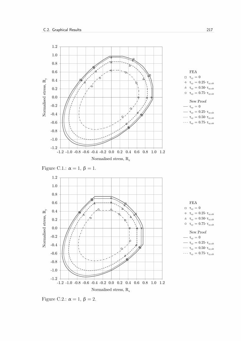
C.2. Graphical Results 217
-1.2
-1.0
-0.8
-0.6
-0.4
-0.2
0.0
0.2
0.4
0.6
0.8
1.0
1.2
-1.2 -1.0 -0.8 -0.6 -0.4 -0.2 0.0 0.2 0.4 0.6 0.8 1.0 1.2
Norm
alise
d s
tres
s, R
y
Normalised stress, Rx
yield (tau = 0.00)
yield (tau = 0.25)
yield (tau = 0.50)
yield (tau = 0.75)
FEA (tau = 0.00)
FEA (tau = 0.25)
FEA (tau = 0.50)
FEA (tau = 0.75)
τxy = 0.00∙τxy,ult (proof)
τxy = 0.25∙τxy,ult (proof)
τxy = 0.50∙τxy,ult (proof)
τxy = 0.75∙τxy,ult (proof)
τxy = 0.00∙τxy,ult (FEA)
τxy = 0.25∙τxy,ult (FEA)
τxy = 0.50∙τxy,ult (FEA)
τxy = 0.75∙τxy,ult (FEA)
Figure C.1.: α = 1, β = 1.
FEA
τxy = 0
τxy = 0.25∙ τxy,ult
τxy = 0.50∙ τxy,ult
τxy = 0.75∙ τxy,ult
New Proof
τxy = 0
τxy = 0.25∙ τxy,ult
τxy = 0.50∙ τxy,ult
τxy = 0.75∙ τxy,ult
-1.2
-1.0
-0.8
-0.6
-0.4
-0.2
0.0
0.2
0.4
0.6
0.8
1.0
1.2
-1.2 -1.0 -0.8 -0.6 -0.4 -0.2 0.0 0.2 0.4 0.6 0.8 1.0 1.2
Norm
alise
d s
tres
s, R
y
Normalised stress, Rx
yield (tau = 0.00)
yield (tau = 0.25)
yield (tau = 0.50)
yield (tau = 0.75)
FEA (tau = 0.00)
FEA (tau = 0.25)
FEA (tau = 0.50)
FEA (tau = 0.75)
τxy = 0.00∙τxy,ult (proof)
τxy = 0.25∙τxy,ult (proof)
τxy = 0.50∙τxy,ult (proof)
τxy = 0.75∙τxy,ult (proof)
τxy = 0.00∙τxy,ult (FEA)
τxy = 0.25∙τxy,ult (FEA)
τxy = 0.50∙τxy,ult (FEA)
τxy = 0.75∙τxy,ult (FEA)
Figure C.2.: α = 1, β = 2.
FEA
τxy = 0
τxy = 0.25∙ τxy,ult
τxy = 0.50∙ τxy,ult
τxy = 0.75∙ τxy,ult
New Proof
τxy = 0
τxy = 0.25∙ τxy,ult
τxy = 0.50∙ τxy,ult
τxy = 0.75∙ τxy,ult

218 C. Evaluation Data
-1.2
-1.0
-0.8
-0.6
-0.4
-0.2
0.0
0.2
0.4
0.6
0.8
1.0
1.2
-1.2 -1.0 -0.8 -0.6 -0.4 -0.2 0.0 0.2 0.4 0.6 0.8 1.0 1.2
Norm
alise
d s
tres
s, R
y
Normalised stress, Rx
yield (tau = 0.00)
yield (tau = 0.25)
yield (tau = 0.50)
yield (tau = 0.75)
FEA (tau = 0.00)
FEA (tau = 0.25)
FEA (tau = 0.50)
FEA (tau = 0.75)
τxy = 0.00∙τxy,ult (proof)
τxy = 0.25∙τxy,ult (proof)
τxy = 0.50∙τxy,ult (proof)
τxy = 0.75∙τxy,ult (proof)
τxy = 0.00∙τxy,ult (FEA)
τxy = 0.25∙τxy,ult (FEA)
τxy = 0.50∙τxy,ult (FEA)
τxy = 0.75∙τxy,ult (FEA)
Figure C.3.: α = 1, β = 3.
FEA
τxy = 0
τxy = 0.25∙ τxy,ult
τxy = 0.50∙ τxy,ult
τxy = 0.75∙ τxy,ult
New Proof
τxy = 0
τxy = 0.25∙ τxy,ult
τxy = 0.50∙ τxy,ult
τxy = 0.75∙ τxy,ult
-1.2
-1.0
-0.8
-0.6
-0.4
-0.2
0.0
0.2
0.4
0.6
0.8
1.0
1.2
-1.2 -1.0 -0.8 -0.6 -0.4 -0.2 0.0 0.2 0.4 0.6 0.8 1.0 1.2
Norm
alise
d s
tres
s, R
y
Normalised stress, Rx
yield (tau = 0.00)
yield (tau = 0.25)
yield (tau = 0.50)
yield (tau = 0.75)
FEA (tau = 0.00)
FEA (tau = 0.25)
FEA (tau = 0.50)
FEA (tau = 0.75)
τxy = 0.00∙τxy,ult (proof)
τxy = 0.25∙τxy,ult (proof)
τxy = 0.50∙τxy,ult (proof)
τxy = 0.75∙τxy,ult (proof)
τxy = 0.00∙τxy,ult (FEA)
τxy = 0.25∙τxy,ult (FEA)
τxy = 0.50∙τxy,ult (FEA)
τxy = 0.75∙τxy,ult (FEA)
Figure C.4.: α = 1, β = 4.
FEA
τxy = 0
τxy = 0.25∙ τxy,ult
τxy = 0.50∙ τxy,ult
τxy = 0.75∙ τxy,ult
New Proof
τxy = 0
τxy = 0.25∙ τxy,ult
τxy = 0.50∙ τxy,ult
τxy = 0.75∙ τxy,ult

C.2. Graphical Results 219
-1.2
-1.0
-0.8
-0.6
-0.4
-0.2
0.0
0.2
0.4
0.6
0.8
1.0
1.2
-1.2 -1.0 -0.8 -0.6 -0.4 -0.2 0.0 0.2 0.4 0.6 0.8 1.0 1.2
Norm
alise
d s
tres
s, R
y
Normalised stress, Rx
yield (tau = 0.00)
yield (tau = 0.25)
yield (tau = 0.50)
yield (tau = 0.75)
FEA (tau = 0.00)
FEA (tau = 0.25)
FEA (tau = 0.50)
FEA (tau = 0.75)
τxy = 0.00∙τxy,ult (proof)
τxy = 0.25∙τxy,ult (proof)
τxy = 0.50∙τxy,ult (proof)
τxy = 0.75∙τxy,ult (proof)
τxy = 0.00∙τxy,ult (FEA)
τxy = 0.25∙τxy,ult (FEA)
τxy = 0.50∙τxy,ult (FEA)
τxy = 0.75∙τxy,ult (FEA)
Figure C.5.: α = 3, β = 1.
FEA
τxy = 0
τxy = 0.25∙ τxy,ult
τxy = 0.50∙ τxy,ult
τxy = 0.75∙ τxy,ult
New Proof
τxy = 0
τxy = 0.25∙ τxy,ult
τxy = 0.50∙ τxy,ult
τxy = 0.75∙ τxy,ult
-1.2
-1.0
-0.8
-0.6
-0.4
-0.2
0.0
0.2
0.4
0.6
0.8
1.0
1.2
-1.2 -1.0 -0.8 -0.6 -0.4 -0.2 0.0 0.2 0.4 0.6 0.8 1.0 1.2
Norm
alise
d s
tres
s, R
y
Normalised stress, Rx
yield (tau = 0.00)
yield (tau = 0.25)
yield (tau = 0.50)
yield (tau = 0.75)
FEA (tau = 0.00)
FEA (tau = 0.25)
FEA (tau = 0.50)
FEA (tau = 0.75)
τxy = 0.00∙τxy,ult (proof)
τxy = 0.25∙τxy,ult (proof)
τxy = 0.50∙τxy,ult (proof)
τxy = 0.75∙τxy,ult (proof)
τxy = 0.00∙τxy,ult (FEA)
τxy = 0.25∙τxy,ult (FEA)
τxy = 0.50∙τxy,ult (FEA)
τxy = 0.75∙τxy,ult (FEA)
Figure C.6.: α = 3, β = 2.
FEA
τxy = 0
τxy = 0.25∙ τxy,ult
τxy = 0.50∙ τxy,ult
τxy = 0.75∙ τxy,ult
New Proof
τxy = 0
τxy = 0.25∙ τxy,ult
τxy = 0.50∙ τxy,ult
τxy = 0.75∙ τxy,ult

220 C. Evaluation Data
-1.2
-1.0
-0.8
-0.6
-0.4
-0.2
0.0
0.2
0.4
0.6
0.8
1.0
1.2
-1.2 -1.0 -0.8 -0.6 -0.4 -0.2 0.0 0.2 0.4 0.6 0.8 1.0 1.2
Norm
alise
d s
tres
s, R
y
Normalised stress, Rx
yield (tau = 0.00)
yield (tau = 0.25)
yield (tau = 0.50)
yield (tau = 0.75)
FEA (tau = 0.00)
FEA (tau = 0.25)
FEA (tau = 0.50)
FEA (tau = 0.75)
τxy = 0.00∙τxy,ult (proof)
τxy = 0.25∙τxy,ult (proof)
τxy = 0.50∙τxy,ult (proof)
τxy = 0.75∙τxy,ult (proof)
τxy = 0.00∙τxy,ult (FEA)
τxy = 0.25∙τxy,ult (FEA)
τxy = 0.50∙τxy,ult (FEA)
τxy = 0.75∙τxy,ult (FEA)
Figure C.7.: α = 3, β = 3.
FEA
τxy = 0
τxy = 0.25∙ τxy,ult
τxy = 0.50∙ τxy,ult
τxy = 0.75∙ τxy,ult
New Proof
τxy = 0
τxy = 0.25∙ τxy,ult
τxy = 0.50∙ τxy,ult
τxy = 0.75∙ τxy,ult
-1.2
-1.0
-0.8
-0.6
-0.4
-0.2
0.0
0.2
0.4
0.6
0.8
1.0
1.2
-1.2 -1.0 -0.8 -0.6 -0.4 -0.2 0.0 0.2 0.4 0.6 0.8 1.0 1.2
Norm
alise
d s
tres
s, R
y
Normalised stress, Rx
yield (tau = 0.00)
yield (tau = 0.25)
yield (tau = 0.50)
yield (tau = 0.75)
FEA (tau = 0.00)
FEA (tau = 0.25)
FEA (tau = 0.50)
FEA (tau = 0.75)
τxy = 0.00∙τxy,ult (proof)
τxy = 0.25∙τxy,ult (proof)
τxy = 0.50∙τxy,ult (proof)
τxy = 0.75∙τxy,ult (proof)
τxy = 0.00∙τxy,ult (FEA)
τxy = 0.25∙τxy,ult (FEA)
τxy = 0.50∙τxy,ult (FEA)
τxy = 0.75∙τxy,ult (FEA)
Figure C.8.: α = 3, β = 4.
FEA
τxy = 0
τxy = 0.25∙ τxy,ult
τxy = 0.50∙ τxy,ult
τxy = 0.75∙ τxy,ult
New Proof
τxy = 0
τxy = 0.25∙ τxy,ult
τxy = 0.50∙ τxy,ult
τxy = 0.75∙ τxy,ult

C.2. Graphical Results 221
-1.2
-1.0
-0.8
-0.6
-0.4
-0.2
0.0
0.2
0.4
0.6
0.8
1.0
1.2
-1.2 -1.0 -0.8 -0.6 -0.4 -0.2 0.0 0.2 0.4 0.6 0.8 1.0 1.2
Norm
alise
d s
tres
s, R
y
Normalised stress, Rx
yield (tau = 0.00)
yield (tau = 0.25)
yield (tau = 0.50)
yield (tau = 0.75)
FEA (tau = 0.00)
FEA (tau = 0.25)
FEA (tau = 0.50)
FEA (tau = 0.75)
τxy = 0.00∙τxy,ult (proof)
τxy = 0.25∙τxy,ult (proof)
τxy = 0.50∙τxy,ult (proof)
τxy = 0.75∙τxy,ult (proof)
τxy = 0.00∙τxy,ult (FEA)
τxy = 0.25∙τxy,ult (FEA)
τxy = 0.50∙τxy,ult (FEA)
τxy = 0.75∙τxy,ult (FEA)
Figure C.9.: α = 5, β = 1.
FEA
τxy = 0
τxy = 0.25∙ τxy,ult
τxy = 0.50∙ τxy,ult
τxy = 0.75∙ τxy,ult
New Proof
τxy = 0
τxy = 0.25∙ τxy,ult
τxy = 0.50∙ τxy,ult
τxy = 0.75∙ τxy,ult
-1.2
-1.0
-0.8
-0.6
-0.4
-0.2
0.0
0.2
0.4
0.6
0.8
1.0
1.2
-1.2 -1.0 -0.8 -0.6 -0.4 -0.2 0.0 0.2 0.4 0.6 0.8 1.0 1.2
Norm
alise
d s
tres
s, R
y
Normalised stress, Rx
yield (tau = 0.00)
yield (tau = 0.25)
yield (tau = 0.50)
yield (tau = 0.75)
FEA (tau = 0.00)
FEA (tau = 0.25)
FEA (tau = 0.50)
FEA (tau = 0.75)
τxy = 0.00∙τxy,ult (proof)
τxy = 0.25∙τxy,ult (proof)
τxy = 0.50∙τxy,ult (proof)
τxy = 0.75∙τxy,ult (proof)
τxy = 0.00∙τxy,ult (FEA)
τxy = 0.25∙τxy,ult (FEA)
τxy = 0.50∙τxy,ult (FEA)
τxy = 0.75∙τxy,ult (FEA)
Figure C.10.: α = 5, β = 2.
FEA
τxy = 0
τxy = 0.25∙ τxy,ult
τxy = 0.50∙ τxy,ult
τxy = 0.75∙ τxy,ult
New Proof
τxy = 0
τxy = 0.25∙ τxy,ult
τxy = 0.50∙ τxy,ult
τxy = 0.75∙ τxy,ult

222 C. Evaluation Data
-1.2
-1.0
-0.8
-0.6
-0.4
-0.2
0.0
0.2
0.4
0.6
0.8
1.0
1.2
-1.2 -1.0 -0.8 -0.6 -0.4 -0.2 0.0 0.2 0.4 0.6 0.8 1.0 1.2
Norm
alise
d s
tres
s, R
y
Normalised stress, Rx
yield (tau = 0.00)
yield (tau = 0.25)
yield (tau = 0.50)
yield (tau = 0.75)
FEA (tau = 0.00)
FEA (tau = 0.25)
FEA (tau = 0.50)
FEA (tau = 0.75)
τxy = 0.00∙τxy,ult (proof)
τxy = 0.25∙τxy,ult (proof)
τxy = 0.50∙τxy,ult (proof)
τxy = 0.75∙τxy,ult (proof)
τxy = 0.00∙τxy,ult (FEA)
τxy = 0.25∙τxy,ult (FEA)
τxy = 0.50∙τxy,ult (FEA)
τxy = 0.75∙τxy,ult (FEA)
Figure C.11.: α = 5, β = 3.
FEA
τxy = 0
τxy = 0.25∙ τxy,ult
τxy = 0.50∙ τxy,ult
τxy = 0.75∙ τxy,ult
New Proof
τxy = 0
τxy = 0.25∙ τxy,ult
τxy = 0.50∙ τxy,ult
τxy = 0.75∙ τxy,ult
-1.2
-1.0
-0.8
-0.6
-0.4
-0.2
0.0
0.2
0.4
0.6
0.8
1.0
1.2
-1.2 -1.0 -0.8 -0.6 -0.4 -0.2 0.0 0.2 0.4 0.6 0.8 1.0 1.2
Norm
alise
d s
tres
s, R
y
Normalised stress, Rx
yield (tau = 0.00)
yield (tau = 0.25)
yield (tau = 0.50)
yield (tau = 0.75)
FEA (tau = 0.00)
FEA (tau = 0.25)
FEA (tau = 0.50)
FEA (tau = 0.75)
τxy = 0.00∙τxy,ult (proof)
τxy = 0.25∙τxy,ult (proof)
τxy = 0.50∙τxy,ult (proof)
τxy = 0.75∙τxy,ult (proof)
τxy = 0.00∙τxy,ult (FEA)
τxy = 0.25∙τxy,ult (FEA)
τxy = 0.50∙τxy,ult (FEA)
τxy = 0.75∙τxy,ult (FEA)
Figure C.12.: α = 5, β = 4.
FEA
τxy = 0
τxy = 0.25∙ τxy,ult
τxy = 0.50∙ τxy,ult
τxy = 0.75∙ τxy,ult
New Proof
τxy = 0
τxy = 0.25∙ τxy,ult
τxy = 0.50∙ τxy,ult
τxy = 0.75∙ τxy,ult

Appendix D. Calibration Data
223

224 D. Calibration Data
D.1. Tabular Results
In this section the results of finite element analyses used in the calibration of the exponente0 and interaction coefficient B are tabulated. Results obtained with the new proof arealso included.
Stress combination Plate aspect ratio, α Table Page
1 D.1 225
3 D.2 226
5 D.3 227
10 D.4 228
1 D.5 229
3 D.6 230
5 D.7 231
10 D.8 232
1 D.9 233
3 D.10 234
5 D.11 235
10 D.12 236
σx-σy
σx-τxy
σy-τxy

D.1. Tabular Results 225
data point run id Rx,ult Ry,ult Rt, ult Magnitude Rx,ult Ry,ult Rt, ult Magnitude
1 15101 1.000 0.000 0.000 1.000 1.000 1.000 0.000 1.000
2 15102 1.115 0.299 0.000 1.155 1.000 1.000 0.000 1.035
3 15103 1.113 0.643 0.000 1.285 1.000 1.000 0.000 1.155
4 15104 0.936 0.936 0.000 1.324 1.000 1.000 0.000 1.414
5 15105 0.643 1.113 0.000 1.285 1.000 1.000 0.000 1.155
6 15106 0.299 1.115 0.000 1.155 1.000 1.000 0.000 1.035
7 15107 0.000 1.000 0.000 0.000 1.000 1.000 0.000 0.000
8 11101 0.979 0.000 0.000 0.979 0.979 0.226 0.000 0.979
9 11102 1.007 0.270 0.000 1.043 0.974 0.261 0.000 1.009
10 11103 0.908 0.524 0.000 1.048 0.894 0.516 0.000 1.032
11 11104 0.736 0.736 0.000 1.041 0.736 0.736 0.000 1.041
12 11105 0.524 0.908 0.000 1.048 0.516 0.894 0.000 1.032
13 11106 0.270 1.007 0.000 1.043 0.261 0.974 0.000 1.009
14 11107 0.000 0.979 0.000 0.000 0.226 0.979 0.000 0.000
15 12101 0.753 0.000 0.000 0.753 0.753 0.000 0.000 0.753
16 12102 0.688 0.184 0.000 0.712 0.679 0.182 0.000 0.703
17 12103 0.585 0.338 0.000 0.676 0.580 0.335 0.000 0.670
18 12104 0.467 0.467 0.000 0.660 0.466 0.466 0.000 0.659
19 12105 0.338 0.585 0.000 0.676 0.335 0.580 0.000 0.670
20 12106 0.184 0.688 0.000 0.712 0.182 0.679 0.000 0.703
21 12107 0.000 0.753 0.000 0.000 0.000 0.753 0.000 0.000
22 13101 0.614 0.000 0.000 0.614 0.614 0.000 0.000 0.614
23 13102 0.554 0.148 0.000 0.574 0.519 0.139 0.000 0.537
24 13103 0.461 0.266 0.000 0.532 0.431 0.249 0.000 0.497
25 13104 0.366 0.366 0.000 0.518 0.343 0.343 0.000 0.485
26 13105 0.266 0.461 0.000 0.532 0.249 0.431 0.000 0.497
27 13106 0.148 0.554 0.000 0.574 0.139 0.519 0.000 0.537
28 13107 0.000 0.614 0.000 0.000 0.000 0.614 0.000 0.000
29 14101 0.558 0.000 0.000 0.558 0.558 0.000 0.000 0.558
30 14102 0.467 0.125 0.000 0.484 0.447 0.120 0.000 0.463
31 14103 0.386 0.223 0.000 0.446 0.365 0.211 0.000 0.421
32 14104 0.307 0.307 0.000 0.434 0.289 0.289 0.000 0.409
33 14105 0.223 0.386 0.000 0.446 0.211 0.365 0.000 0.421
34 14106 0.125 0.467 0.000 0.484 0.120 0.447 0.000 0.463
35 14107 0.000 0.558 0.000 0.000 0.000 0.558 0.000 0.000
β =
0.5
β =
1β
= 2
β =
3β
= 4
Finite Element Analyses New Proof
Table D.1.: σx-σy, α = 1.

226 D. Calibration Data
data point run id Rx,ult Ry,ult Rt, ult Magnitude Rx,ult Ry,ult Rt, ult Magnitude
36 15301 1.000 0.000 0.000 1.000 1.000 0.938 0.000 1.000
37 15302 1.113 0.289 0.000 1.150 1.000 0.938 0.000 1.033
38 15303 1.121 0.627 0.000 1.284 1.000 0.938 0.000 1.146
39 15304 0.934 0.905 0.000 1.301 1.000 0.938 0.000 1.347
40 15305 0.587 0.984 0.000 1.145 1.000 0.938 0.000 1.092
41 15306 0.272 0.983 0.000 1.020 1.000 0.938 0.000 0.973
42 15307 0.000 0.938 0.000 0.000 1.000 0.938 0.000 0.000
43 11301 0.980 0.000 0.000 0.980 0.980 0.343 0.000 0.980
44 11302 1.015 0.230 0.000 1.041 0.980 0.343 0.000 1.004
45 11303 0.953 0.458 0.000 1.057 0.920 0.442 0.000 1.021
46 11304 0.732 0.601 0.000 0.947 0.726 0.596 0.000 0.939
47 11305 0.459 0.646 0.000 0.792 0.501 0.672 0.000 0.824
48 11306 0.221 0.666 0.000 0.702 0.501 0.672 0.000 0.708
49 11307 0.000 0.672 0.000 0.000 0.501 0.672 0.000 0.000
50 12301 0.755 0.000 0.000 0.755 0.755 0.036 0.000 0.755
51 12302 0.709 0.140 0.000 0.723 0.695 0.137 0.000 0.708
52 12303 0.605 0.243 0.000 0.652 0.572 0.230 0.000 0.617
53 12304 0.441 0.295 0.000 0.530 0.439 0.293 0.000 0.528
54 12305 0.293 0.331 0.000 0.442 0.298 0.337 0.000 0.450
55 12306 0.148 0.356 0.000 0.385 0.152 0.364 0.000 0.395
56 12307 0.000 0.371 0.000 0.000 0.074 0.371 0.000 0.000
57 13301 0.611 0.000 0.000 0.611 0.611 0.000 0.000 0.611
58 13302 0.567 0.105 0.000 0.577 0.515 0.096 0.000 0.524
59 13303 0.434 0.160 0.000 0.462 0.412 0.152 0.000 0.439
60 13304 0.324 0.197 0.000 0.379 0.315 0.192 0.000 0.369
61 13305 0.222 0.227 0.000 0.317 0.218 0.223 0.000 0.311
62 13306 0.116 0.251 0.000 0.277 0.114 0.247 0.000 0.272
63 13307 0.000 0.262 0.000 0.000 0.000 0.262 0.000 0.000
64 14301 0.541 0.000 0.000 0.541 0.541 0.000 0.000 0.541
65 14302 0.449 0.081 0.000 0.457 0.427 0.077 0.000 0.434
66 14303 0.345 0.123 0.000 0.366 0.336 0.120 0.000 0.357
67 14304 0.259 0.151 0.000 0.300 0.258 0.150 0.000 0.298
68 14305 0.179 0.175 0.000 0.251 0.180 0.176 0.000 0.252
69 14306 0.096 0.198 0.000 0.219 0.096 0.199 0.000 0.221
70 14307 0.000 0.219 0.000 0.000 0.000 0.219 0.000 0.000
Finite Element Analyses New Proof
β =
0.5
β =
1β
= 2
β =
3β
= 4
Table D.2.: σx-σy, α = 3.

D.1. Tabular Results 227
data point run id Rx,ult Ry,ult Rt, ult Magnitude Rx,ult Ry,ult Rt, ult Magnitude
71 15501 1.000 0.000 0.000 1.000 1.000 0.906 0.000 1.000
72 15502 1.111 0.284 0.000 1.147 1.000 0.906 0.000 1.032
73 15503 1.126 0.619 0.000 1.285 1.000 0.906 0.000 1.141
74 15504 0.941 0.896 0.000 1.299 1.000 0.906 0.000 1.314
75 15505 0.581 0.956 0.000 1.119 1.000 0.906 0.000 1.060
76 15506 0.268 0.951 0.000 0.988 1.000 0.906 0.000 0.941
77 15507 0.000 0.906 0.000 0.000 1.000 0.906 0.000 0.000
78 11501 0.981 0.000 0.000 0.981 0.981 0.371 0.000 0.981
79 11502 1.016 0.221 0.000 1.040 0.981 0.371 0.000 1.004
80 11503 0.966 0.441 0.000 1.062 0.938 0.428 0.000 1.031
81 11504 0.742 0.574 0.000 0.938 0.731 0.566 0.000 0.925
82 11505 0.455 0.602 0.000 0.755 0.598 0.608 0.000 0.762
83 11506 0.216 0.610 0.000 0.647 0.598 0.608 0.000 0.645
84 11507 0.000 0.608 0.000 0.000 0.598 0.608 0.000 0.000
85 12501 0.755 0.000 0.000 0.755 0.755 0.070 0.000 0.755
86 12502 0.715 0.128 0.000 0.726 0.709 0.127 0.000 0.720
87 12503 0.619 0.216 0.000 0.656 0.582 0.203 0.000 0.617
88 12504 0.439 0.251 0.000 0.506 0.442 0.252 0.000 0.509
89 12505 0.286 0.273 0.000 0.395 0.296 0.284 0.000 0.410
90 12506 0.142 0.288 0.000 0.321 0.178 0.298 0.000 0.332
91 12507 0.000 0.298 0.000 0.000 0.178 0.298 0.000 0.000
92 13501 0.611 0.000 0.000 0.611 0.611 0.015 0.000 0.611
93 13502 0.582 0.092 0.000 0.589 0.523 0.083 0.000 0.530
94 13503 0.436 0.130 0.000 0.455 0.418 0.125 0.000 0.436
95 13504 0.320 0.154 0.000 0.355 0.318 0.153 0.000 0.353
96 13505 0.215 0.172 0.000 0.276 0.217 0.173 0.000 0.278
97 13506 0.111 0.187 0.000 0.217 0.111 0.188 0.000 0.219
98 13507 0.000 0.193 0.000 0.000 0.047 0.193 0.000 0.000
99 14501 0.537 0.000 0.000 0.537 0.537 0.002 0.000 0.537
100 14502 0.453 0.067 0.000 0.458 0.429 0.063 0.000 0.434
101 14503 0.342 0.094 0.000 0.354 0.339 0.093 0.000 0.352
102 14504 0.254 0.111 0.000 0.277 0.259 0.114 0.000 0.283
103 14505 0.173 0.126 0.000 0.214 0.179 0.130 0.000 0.221
104 14506 0.091 0.139 0.000 0.166 0.094 0.144 0.000 0.172
105 14507 0.000 0.152 0.000 0.000 0.006 0.152 0.000 0.000
Finite Element Analyses New Proofβ
= 0
.5β
= 1
β =
2β
= 3
β =
4
Table D.3.: σx-σy, α = 5.
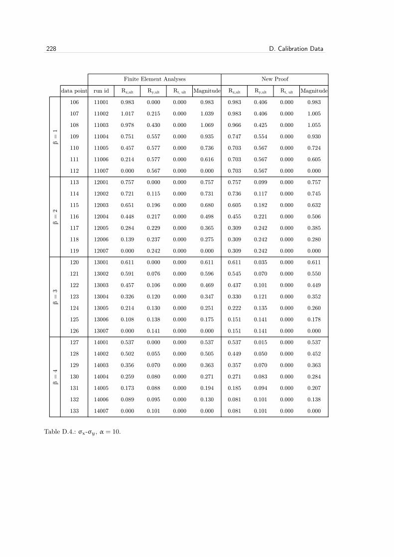
228 D. Calibration Data
data point run id Rx,ult Ry,ult Rt, ult Magnitude Rx,ult Ry,ult Rt, ult Magnitude
106 11001 0.983 0.000 0.000 0.983 0.983 0.406 0.000 0.983
107 11002 1.017 0.215 0.000 1.039 0.983 0.406 0.000 1.005
108 11003 0.978 0.430 0.000 1.069 0.966 0.425 0.000 1.055
109 11004 0.751 0.557 0.000 0.935 0.747 0.554 0.000 0.930
110 11005 0.457 0.577 0.000 0.736 0.703 0.567 0.000 0.724
111 11006 0.214 0.577 0.000 0.616 0.703 0.567 0.000 0.605
112 11007 0.000 0.567 0.000 0.000 0.703 0.567 0.000 0.000
113 12001 0.757 0.000 0.000 0.757 0.757 0.099 0.000 0.757
114 12002 0.721 0.115 0.000 0.731 0.736 0.117 0.000 0.745
115 12003 0.651 0.196 0.000 0.680 0.605 0.182 0.000 0.632
116 12004 0.448 0.217 0.000 0.498 0.455 0.221 0.000 0.506
117 12005 0.284 0.229 0.000 0.365 0.309 0.242 0.000 0.385
118 12006 0.139 0.237 0.000 0.275 0.309 0.242 0.000 0.280
119 12007 0.000 0.242 0.000 0.000 0.309 0.242 0.000 0.000
120 13001 0.611 0.000 0.000 0.611 0.611 0.035 0.000 0.611
121 13002 0.591 0.076 0.000 0.596 0.545 0.070 0.000 0.550
122 13003 0.457 0.106 0.000 0.469 0.437 0.101 0.000 0.449
123 13004 0.326 0.120 0.000 0.347 0.330 0.121 0.000 0.352
124 13005 0.214 0.130 0.000 0.251 0.222 0.135 0.000 0.260
125 13006 0.108 0.138 0.000 0.175 0.151 0.141 0.000 0.178
126 13007 0.000 0.141 0.000 0.000 0.151 0.141 0.000 0.000
127 14001 0.537 0.000 0.000 0.537 0.537 0.015 0.000 0.537
128 14002 0.502 0.055 0.000 0.505 0.449 0.050 0.000 0.452
129 14003 0.356 0.070 0.000 0.363 0.357 0.070 0.000 0.363
130 14004 0.259 0.080 0.000 0.271 0.271 0.083 0.000 0.284
131 14005 0.173 0.088 0.000 0.194 0.185 0.094 0.000 0.207
132 14006 0.089 0.095 0.000 0.130 0.081 0.101 0.000 0.138
133 14007 0.000 0.101 0.000 0.000 0.081 0.101 0.000 0.000
Finite Element Analyses New Proof
β =
1β
= 2
β =
3β
= 4
Table D.4.: σx-σy, α = 10.

D.1. Tabular Results 229
data point run id Rx,ult Ry,ult Rt, ult Magnitude Rx,ult Ry,ult Rt, ult Magnitude
134 25101 1.000 0.000 0.000 1.000 1.000 0.000 0.000 1.000
135 25102 0.939 0.000 0.344 0.960 0.939 0.000 0.344 0.960
136 25103 0.795 0.000 0.606 0.869 0.795 0.000 0.606 0.869
137 25104 0.614 0.000 0.789 0.765 0.614 0.000 0.789 0.765
138 25105 0.416 0.000 0.909 0.670 0.416 0.000 0.909 0.670
139 25106 0.210 0.000 0.978 0.602 0.210 0.000 0.978 0.602
140 25107 0.000 0.000 1.000 0.000 0.000 0.000 1.000 0.000
141 21101 0.979 0.000 0.000 0.979 0.979 0.000 0.000 0.979
142 21102 0.912 0.000 0.339 0.933 0.920 0.000 0.342 0.941
143 21103 0.771 0.000 0.601 0.845 0.778 0.000 0.607 0.853
144 21104 0.595 0.000 0.785 0.748 0.599 0.000 0.791 0.753
145 21105 0.404 0.000 0.908 0.661 0.405 0.000 0.911 0.663
146 21106 0.204 0.000 0.979 0.601 0.204 0.000 0.978 0.600
147 21107 0.000 0.000 1.000 0.000 0.000 0.000 1.000 0.000
148 22101 0.753 0.000 0.000 0.753 0.753 0.000 0.000 0.753
149 22102 0.702 0.000 0.287 0.721 0.696 0.000 0.285 0.716
150 22103 0.597 0.000 0.522 0.668 0.591 0.000 0.517 0.662
151 22104 0.469 0.000 0.706 0.622 0.464 0.000 0.698 0.615
152 22105 0.327 0.000 0.847 0.588 0.324 0.000 0.839 0.583
153 22106 0.170 0.000 0.945 0.571 0.169 0.000 0.941 0.569
154 22107 0.000 0.000 0.990 0.000 0.000 0.000 0.990 0.000
155 23101 0.614 0.000 0.000 0.614 0.614 0.000 0.000 0.614
156 23102 0.566 0.000 0.246 0.584 0.560 0.000 0.243 0.578
157 23103 0.479 0.000 0.448 0.544 0.474 0.000 0.443 0.539
158 23104 0.376 0.000 0.607 0.514 0.376 0.000 0.607 0.514
159 23105 0.263 0.000 0.736 0.500 0.267 0.000 0.746 0.507
160 23106 0.140 0.000 0.843 0.507 0.143 0.000 0.859 0.516
161 23107 0.000 0.000 0.927 0.000 0.000 0.000 0.927 0.000
162 24101 0.558 0.000 0.000 0.558 0.558 0.000 0.000 0.558
163 24102 0.499 0.000 0.216 0.514 0.498 0.000 0.216 0.513
164 24103 0.413 0.000 0.384 0.469 0.416 0.000 0.387 0.473
165 24104 0.322 0.000 0.517 0.439 0.329 0.000 0.528 0.449
166 24105 0.227 0.000 0.630 0.429 0.234 0.000 0.651 0.443
167 24106 0.123 0.000 0.735 0.442 0.127 0.000 0.758 0.456
168 24107 0.000 0.000 0.832 0.000 0.000 0.000 0.832 0.000
Finite Element Analyses New Proofβ
= 0
.5β
= 1
β =
2β
= 3
β =
4
Table D.5.: σx-τxy, α = 1.

230 D. Calibration Data
data point run id Rx,ult Ry,ult Rt, ult Magnitude Rx,ult Ry,ult Rt, ult Magnitude
169 25301 1.000 0.000 0.000 1.000 1.000 0.000 0.000 1.000
170 25302 0.939 0.000 0.344 0.960 0.939 0.000 0.344 0.960
171 25303 0.795 0.000 0.606 0.869 0.795 0.000 0.606 0.869
172 25304 0.614 0.000 0.789 0.765 0.614 0.000 0.789 0.765
173 25305 0.416 0.000 0.909 0.670 0.416 0.000 0.909 0.670
174 25306 0.210 0.000 0.978 0.602 0.210 0.000 0.978 0.602
175 25307 0.000 0.000 1.000 0.000 0.000 0.000 1.000 0.000
176 21301 0.980 0.000 0.000 0.980 0.980 0.000 0.000 0.980
177 21302 0.918 0.000 0.341 0.938 0.921 0.000 0.342 0.942
178 21303 0.776 0.000 0.604 0.851 0.779 0.000 0.606 0.854
179 21304 0.599 0.000 0.788 0.752 0.600 0.000 0.790 0.754
180 21305 0.405 0.000 0.910 0.664 0.406 0.000 0.910 0.664
181 21306 0.204 0.000 0.979 0.601 0.204 0.000 0.978 0.600
182 21307 0.000 0.000 1.000 0.000 0.000 0.000 1.000 0.000
183 22301 0.755 0.000 0.000 0.755 0.755 0.000 0.000 0.755
184 22302 0.708 0.000 0.288 0.727 0.697 0.000 0.283 0.716
185 22303 0.598 0.000 0.520 0.669 0.591 0.000 0.513 0.661
186 22304 0.465 0.000 0.694 0.614 0.464 0.000 0.692 0.612
187 22305 0.323 0.000 0.829 0.577 0.323 0.000 0.830 0.578
188 22306 0.168 0.000 0.927 0.561 0.169 0.000 0.930 0.563
189 22307 0.000 0.000 0.977 0.000 0.000 0.000 0.977 0.000
190 23301 0.611 0.000 0.000 0.611 0.611 0.000 0.000 0.611
191 23302 0.534 0.000 0.225 0.550 0.554 0.000 0.233 0.570
192 23303 0.458 0.000 0.413 0.516 0.466 0.000 0.420 0.525
193 23304 0.362 0.000 0.564 0.487 0.367 0.000 0.571 0.493
194 23305 0.250 0.000 0.672 0.461 0.259 0.000 0.696 0.478
195 23306 0.132 0.000 0.762 0.459 0.138 0.000 0.797 0.480
196 23307 0.000 0.000 0.857 0.000 0.000 0.000 0.857 0.000
197 24301 0.541 0.000 0.000 0.541 0.541 0.000 0.000 0.541
198 24302 0.438 0.000 0.180 0.450 0.478 0.000 0.196 0.492
199 24303 0.376 0.000 0.330 0.422 0.395 0.000 0.348 0.443
200 24304 0.302 0.000 0.456 0.401 0.310 0.000 0.468 0.411
201 24305 0.212 0.000 0.553 0.384 0.219 0.000 0.570 0.396
202 24306 0.113 0.000 0.630 0.381 0.118 0.000 0.659 0.398
203 24307 0.000 0.000 0.719 0.000 0.000 0.000 0.719 0.000
Finite Element Analyses New Proof
β =
0.5
β =
1β
= 2
β =
3β
= 4
Table D.6.: σx-τxy, α = 3.

D.1. Tabular Results 231
data point run id Rx,ult Ry,ult Rt, ult Magnitude Rx,ult Ry,ult Rt, ult Magnitude
204 25501 1.000 0.000 0.000 1.000 1.000 0.000 0.000 1.000
205 25502 0.939 0.000 0.344 0.960 0.939 0.000 0.344 0.960
206 25503 0.795 0.000 0.606 0.869 0.795 0.000 0.606 0.869
207 25504 0.614 0.000 0.789 0.765 0.614 0.000 0.789 0.765
208 25505 0.416 0.000 0.909 0.670 0.416 0.000 0.909 0.670
209 25506 0.210 0.000 0.978 0.602 0.210 0.000 0.978 0.602
210 25507 0.000 0.000 1.000 0.000 0.000 0.000 1.000 0.000
211 21501 0.981 0.000 0.000 0.981 0.981 0.000 0.000 0.981
212 21502 0.918 0.000 0.341 0.939 0.921 0.000 0.342 0.942
213 21503 0.776 0.000 0.604 0.851 0.780 0.000 0.607 0.855
214 21504 0.600 0.000 0.789 0.753 0.601 0.000 0.790 0.754
215 21505 0.406 0.000 0.911 0.664 0.406 0.000 0.910 0.664
216 21506 0.205 0.000 0.979 0.601 0.204 0.000 0.978 0.601
217 21507 0.000 0.000 1.000 0.000 0.000 0.000 1.000 0.000
218 22501 0.755 0.000 0.000 0.755 0.755 0.000 0.000 0.755
219 22502 0.708 0.000 0.287 0.727 0.698 0.000 0.283 0.717
220 22503 0.597 0.000 0.518 0.668 0.591 0.000 0.512 0.661
221 22504 0.465 0.000 0.692 0.613 0.464 0.000 0.690 0.611
222 22505 0.323 0.000 0.828 0.577 0.323 0.000 0.828 0.577
223 22506 0.168 0.000 0.924 0.559 0.169 0.000 0.927 0.561
224 22507 0.000 0.000 0.974 0.000 0.000 0.000 0.974 0.000
225 23501 0.611 0.000 0.000 0.611 0.611 0.000 0.000 0.611
226 23502 0.568 0.000 0.234 0.583 0.552 0.000 0.228 0.567
227 23503 0.470 0.000 0.415 0.528 0.462 0.000 0.408 0.518
228 23504 0.361 0.000 0.549 0.481 0.362 0.000 0.551 0.482
229 23505 0.254 0.000 0.664 0.460 0.255 0.000 0.668 0.463
230 23506 0.133 0.000 0.746 0.450 0.136 0.000 0.763 0.461
231 23507 0.000 0.000 0.819 0.000 0.000 0.000 0.819 0.000
232 24501 0.537 0.000 0.000 0.537 0.537 0.000 0.000 0.537
233 24502 0.489 0.000 0.195 0.502 0.472 0.000 0.188 0.484
234 24503 0.400 0.000 0.340 0.446 0.387 0.000 0.329 0.431
235 24504 0.306 0.000 0.446 0.400 0.302 0.000 0.439 0.394
236 24505 0.211 0.000 0.528 0.371 0.213 0.000 0.532 0.374
237 24506 0.112 0.000 0.601 0.365 0.114 0.000 0.611 0.371
238 24507 0.000 0.000 0.665 0.000 0.000 0.000 0.665 0.000
Finite Element Analyses New Proofβ
= 0
.5β
= 1
β =
2β
= 3
β =
4
Table D.7.: σx-τxy, α = 5.
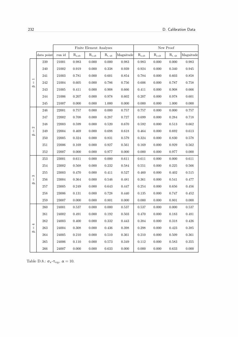
232 D. Calibration Data
data point run id Rx,ult Ry,ult Rt, ult Magnitude Rx,ult Ry,ult Rt, ult Magnitude
239 21001 0.983 0.000 0.000 0.983 0.983 0.000 0.000 0.983
240 21002 0.919 0.000 0.338 0.939 0.924 0.000 0.340 0.945
241 21003 0.781 0.000 0.601 0.854 0.784 0.000 0.603 0.858
242 21004 0.605 0.000 0.786 0.756 0.606 0.000 0.787 0.758
243 21005 0.411 0.000 0.908 0.666 0.411 0.000 0.908 0.666
244 21006 0.207 0.000 0.978 0.602 0.207 0.000 0.978 0.601
245 21007 0.000 0.000 1.000 0.000 0.000 0.000 1.000 0.000
246 22001 0.757 0.000 0.000 0.757 0.757 0.000 0.000 0.757
247 22002 0.708 0.000 0.287 0.727 0.699 0.000 0.284 0.718
248 22003 0.599 0.000 0.520 0.670 0.592 0.000 0.513 0.662
249 22004 0.469 0.000 0.698 0.618 0.464 0.000 0.692 0.613
250 22005 0.324 0.000 0.831 0.579 0.324 0.000 0.830 0.578
251 22006 0.169 0.000 0.927 0.561 0.169 0.000 0.929 0.562
252 22007 0.000 0.000 0.977 0.000 0.000 0.000 0.977 0.000
253 23001 0.611 0.000 0.000 0.611 0.611 0.000 0.000 0.611
254 23002 0.568 0.000 0.232 0.584 0.551 0.000 0.225 0.566
255 23003 0.470 0.000 0.411 0.527 0.460 0.000 0.402 0.515
256 23004 0.364 0.000 0.546 0.481 0.361 0.000 0.541 0.477
257 23005 0.249 0.000 0.643 0.447 0.254 0.000 0.656 0.456
258 23006 0.131 0.000 0.728 0.440 0.135 0.000 0.747 0.452
259 23007 0.000 0.000 0.801 0.000 0.000 0.000 0.801 0.000
260 24001 0.537 0.000 0.000 0.537 0.537 0.000 0.000 0.537
261 24002 0.491 0.000 0.192 0.503 0.470 0.000 0.183 0.481
262 24003 0.400 0.000 0.332 0.443 0.384 0.000 0.318 0.426
263 24004 0.308 0.000 0.436 0.398 0.298 0.000 0.423 0.385
264 24005 0.210 0.000 0.510 0.361 0.210 0.000 0.509 0.361
265 24006 0.110 0.000 0.573 0.349 0.112 0.000 0.583 0.355
266 24007 0.000 0.000 0.633 0.000 0.000 0.000 0.633 0.000
Finite Element Analyses New Proof
β =
1β
= 2
β =
3β
= 4
Table D.8.: σx-τxy, α = 10.

D.1. Tabular Results 233
data point run id Rx,ult Ry,ult Rt, ult Magnitude Rx,ult Ry,ult Rt, ult Magnitude
267 35101 0.000 1.000 0.000 0.000 0.000 1.000 0.000 0.000
268 35102 0.000 0.939 0.344 0.960 0.000 0.939 0.344 0.960
269 35103 0.000 0.795 0.606 0.869 0.000 0.795 0.606 0.869
270 35104 0.000 0.614 0.789 0.765 0.000 0.614 0.789 0.765
271 35105 0.000 0.416 0.909 0.670 0.000 0.416 0.909 0.670
272 35106 0.000 0.210 0.978 0.602 0.000 0.210 0.978 0.602
273 35107 0.000 0.000 1.000 0.000 0.000 0.000 1.000 0.000
274 31101 0.000 0.979 0.000 0.000 0.000 0.979 0.000 0.000
275 31102 0.000 0.912 0.339 0.933 0.000 0.920 0.342 0.941
276 31103 0.000 0.771 0.601 0.845 0.000 0.778 0.607 0.853
277 31104 0.000 0.595 0.785 0.748 0.000 0.599 0.791 0.753
278 31105 0.000 0.404 0.908 0.661 0.000 0.405 0.911 0.663
279 31106 0.000 0.204 0.979 0.601 0.000 0.204 0.978 0.600
280 31107 0.000 0.000 1.000 0.000 0.000 0.000 1.000 0.000
281 32101 0.000 0.753 0.000 0.000 0.000 0.753 0.000 0.000
282 32102 0.000 0.702 0.287 0.721 0.000 0.696 0.285 0.716
283 32103 0.000 0.597 0.522 0.668 0.000 0.591 0.517 0.662
284 32104 0.000 0.469 0.706 0.622 0.000 0.464 0.698 0.615
285 32105 0.000 0.327 0.847 0.588 0.000 0.324 0.839 0.583
286 32106 0.000 0.170 0.945 0.571 0.000 0.169 0.941 0.569
287 32107 0.000 0.000 0.990 0.000 0.000 0.000 0.990 0.000
288 33101 0.000 0.614 0.000 0.000 0.000 0.614 0.000 0.000
289 33102 0.000 0.566 0.246 0.584 0.000 0.560 0.243 0.578
290 33103 0.000 0.479 0.448 0.544 0.000 0.474 0.443 0.539
291 33104 0.000 0.376 0.607 0.514 0.000 0.376 0.607 0.514
292 33105 0.000 0.263 0.736 0.500 0.000 0.267 0.746 0.507
293 33106 0.000 0.140 0.843 0.507 0.000 0.143 0.859 0.516
294 33107 0.000 0.000 0.927 0.000 0.000 0.000 0.927 0.000
295 34101 0.000 0.558 0.000 0.000 0.000 0.558 0.000 0.000
296 34102 0.000 0.499 0.216 0.514 0.000 0.498 0.216 0.513
297 34103 0.000 0.413 0.384 0.469 0.000 0.416 0.387 0.473
298 34104 0.000 0.322 0.517 0.439 0.000 0.329 0.528 0.449
299 34105 0.000 0.227 0.630 0.429 0.000 0.234 0.651 0.443
300 34106 0.000 0.123 0.735 0.442 0.000 0.127 0.758 0.456
301 34107 0.000 0.000 0.832 0.000 0.000 0.000 0.832 0.000
Finite Element Analyses New Proofβ
= 0
.5β
= 1
β =
2β
= 3
β =
4
Table D.9.: σy-τxy, α = 1.

234 D. Calibration Data
data point run id Rx,ult Ry,ult Rt, ult Magnitude Rx,ult Ry,ult Rt, ult Magnitude
302 35301 0.000 0.938 0.000 0.000 0.000 0.938 0.000 0.000
303 35302 0.000 0.893 0.335 0.914 0.000 0.884 0.332 0.905
304 35303 0.000 0.773 0.609 0.849 0.000 0.754 0.594 0.828
305 35304 0.000 0.599 0.800 0.756 0.000 0.585 0.782 0.739
306 35305 0.000 0.402 0.916 0.664 0.000 0.397 0.906 0.657
307 35306 0.000 0.201 0.980 0.600 0.000 0.200 0.977 0.599
308 35307 0.000 0.000 1.000 0.000 0.000 0.000 1.000 0.000
309 31301 0.000 0.672 0.000 0.000 0.000 0.672 0.000 0.000
310 31302 0.000 0.649 0.283 0.670 0.000 0.645 0.281 0.665
311 31303 0.000 0.591 0.554 0.672 0.000 0.568 0.533 0.646
312 31304 0.000 0.489 0.792 0.670 0.000 0.454 0.736 0.622
313 31305 0.000 0.329 0.923 0.626 0.000 0.315 0.883 0.599
314 31306 0.000 0.163 0.983 0.590 0.000 0.161 0.971 0.583
315 31307 0.000 0.000 1.000 0.000 0.000 0.000 1.000 0.000
316 32301 0.000 0.371 0.000 0.000 0.000 0.371 0.000 0.000
317 32302 0.000 0.360 0.212 0.381 0.000 0.355 0.209 0.375
318 32303 0.000 0.333 0.420 0.411 0.000 0.319 0.403 0.395
319 32304 0.000 0.291 0.629 0.466 0.000 0.269 0.582 0.430
320 32305 0.000 0.217 0.800 0.510 0.000 0.203 0.748 0.477
321 32306 0.000 0.117 0.911 0.539 0.000 0.115 0.894 0.529
322 32307 0.000 0.000 0.977 0.000 0.000 0.000 0.977 0.000
323 33301 0.000 0.262 0.000 0.000 0.000 0.262 0.000 0.000
324 33302 0.000 0.251 0.172 0.270 0.000 0.247 0.169 0.266
325 33303 0.000 0.230 0.334 0.300 0.000 0.221 0.322 0.289
326 33304 0.000 0.201 0.495 0.349 0.000 0.189 0.465 0.328
327 33305 0.000 0.154 0.634 0.397 0.000 0.146 0.604 0.378
328 33306 0.000 0.087 0.742 0.437 0.000 0.088 0.746 0.440
329 33307 0.000 0.000 0.857 0.000 0.000 0.000 0.857 0.000
330 34301 0.000 0.219 0.000 0.000 0.000 0.219 0.000 0.000
331 34302 0.000 0.199 0.137 0.214 0.000 0.203 0.140 0.219
332 34303 0.000 0.180 0.263 0.235 0.000 0.180 0.263 0.235
333 34304 0.000 0.156 0.385 0.272 0.000 0.152 0.376 0.265
334 34305 0.000 0.121 0.501 0.313 0.000 0.118 0.489 0.306
335 34306 0.000 0.070 0.600 0.353 0.000 0.072 0.610 0.360
336 34307 0.000 0.000 0.719 0.000 0.000 0.000 0.719 0.000
Finite Element Analyses New Proof
β =
0.5
β =
1β
= 2
β =
3β
= 4
Table D.10.: σy-τxy, α = 3.

D.1. Tabular Results 235
data point run id Rx,ult Ry,ult Rt, ult Magnitude Rx,ult Ry,ult Rt, ult Magnitude
337 35501 0.000 0.906 0.000 0.000 0.000 0.906 0.000 0.000
338 35502 0.000 0.869 0.331 0.890 0.000 0.856 0.326 0.877
339 35503 0.000 0.764 0.613 0.842 0.000 0.733 0.588 0.807
340 35504 0.000 0.590 0.805 0.751 0.000 0.570 0.777 0.725
341 35505 0.000 0.394 0.919 0.661 0.000 0.388 0.904 0.650
342 35506 0.000 0.197 0.980 0.599 0.000 0.196 0.976 0.597
343 35507 0.000 0.000 1.000 0.000 0.000 0.000 1.000 0.000
344 31501 0.000 0.608 0.000 0.000 0.000 0.608 0.000 0.000
345 31502 0.000 0.594 0.271 0.615 0.000 0.585 0.267 0.606
346 31503 0.000 0.554 0.545 0.637 0.000 0.522 0.513 0.600
347 31504 0.000 0.470 0.801 0.659 0.000 0.422 0.719 0.592
348 31505 0.000 0.316 0.934 0.625 0.000 0.296 0.873 0.585
349 31506 0.000 0.155 0.986 0.590 0.000 0.152 0.968 0.579
350 31507 0.000 0.000 1.000 0.000 0.000 0.000 1.000 0.000
351 32501 0.000 0.298 0.000 0.000 0.000 0.298 0.000 0.000
352 32502 0.000 0.291 0.200 0.313 0.000 0.286 0.196 0.307
353 32503 0.000 0.275 0.401 0.359 0.000 0.260 0.379 0.340
354 32504 0.000 0.249 0.615 0.434 0.000 0.223 0.551 0.389
355 32505 0.000 0.198 0.819 0.513 0.000 0.174 0.717 0.449
356 32506 0.000 0.107 0.912 0.537 0.000 0.103 0.874 0.515
357 32507 0.000 0.000 0.974 0.000 0.000 0.000 0.974 0.000
358 33501 0.000 0.193 0.000 0.000 0.000 0.193 0.000 0.000
359 33502 0.000 0.187 0.156 0.208 0.000 0.183 0.152 0.203
360 33503 0.000 0.175 0.308 0.250 0.000 0.165 0.291 0.236
361 33504 0.000 0.158 0.468 0.313 0.000 0.143 0.422 0.283
362 33505 0.000 0.130 0.632 0.388 0.000 0.114 0.552 0.339
363 33506 0.000 0.075 0.717 0.421 0.000 0.073 0.691 0.406
364 33507 0.000 0.000 0.819 0.000 0.000 0.000 0.819 0.000
365 34501 0.000 0.152 0.000 0.000 0.000 0.152 0.000 0.000
366 34502 0.000 0.141 0.120 0.157 0.000 0.142 0.121 0.158
367 34503 0.000 0.130 0.236 0.188 0.000 0.127 0.230 0.184
368 34504 0.000 0.117 0.354 0.236 0.000 0.109 0.330 0.220
369 34505 0.000 0.099 0.490 0.300 0.000 0.087 0.432 0.264
370 34506 0.000 0.059 0.570 0.334 0.000 0.056 0.545 0.320
371 34507 0.000 0.000 0.665 0.000 0.000 0.000 0.665 0.000
Finite Element Analyses New Proofβ
= 0
.5β
= 1
β =
2β
= 3
β =
4
Table D.11.: σy-τxy, α = 5.

236 D. Calibration Data
data point run id Rx,ult Ry,ult Rt, ult Magnitude Rx,ult Ry,ult Rt, ult Magnitude
372 31001 0.000 0.567 0.000 0.000 0.000 0.567 0.000 0.000
373 31002 0.000 0.559 0.262 0.579 0.000 0.548 0.257 0.568
374 31003 0.000 0.530 0.534 0.613 0.000 0.492 0.497 0.570
375 31004 0.000 0.460 0.804 0.653 0.000 0.403 0.704 0.572
376 31005 0.000 0.310 0.937 0.624 0.000 0.286 0.864 0.575
377 31006 0.000 0.151 0.987 0.590 0.000 0.148 0.965 0.577
378 31007 0.000 0.000 1.000 0.000 0.000 0.000 1.000 0.000
379 32001 0.000 0.242 0.000 0.000 0.000 0.242 0.000 0.000
380 32002 0.000 0.239 0.191 0.263 0.000 0.233 0.187 0.257
381 32003 0.000 0.230 0.390 0.322 0.000 0.214 0.362 0.299
382 32004 0.000 0.215 0.612 0.414 0.000 0.186 0.530 0.358
383 32005 0.000 0.179 0.837 0.515 0.000 0.148 0.693 0.427
384 32006 0.000 0.099 0.919 0.540 0.000 0.092 0.857 0.503
385 32007 0.000 0.000 0.977 0.000 0.000 0.000 0.977 0.000
386 33001 0.000 0.141 0.000 0.000 0.000 0.141 0.000 0.000
387 33002 0.000 0.138 0.146 0.162 0.000 0.134 0.142 0.157
388 33003 0.000 0.132 0.295 0.215 0.000 0.122 0.273 0.199
389 33004 0.000 0.123 0.458 0.291 0.000 0.107 0.397 0.253
390 33005 0.000 0.107 0.637 0.383 0.000 0.087 0.520 0.312
391 33006 0.000 0.063 0.708 0.413 0.000 0.058 0.655 0.383
392 33007 0.000 0.000 0.801 0.000 0.000 0.000 0.801 0.000
393 34001 0.000 0.101 0.000 0.000 0.000 0.101 0.000 0.000
394 34002 0.000 0.096 0.110 0.115 0.000 0.095 0.109 0.114
395 34003 0.000 0.091 0.220 0.156 0.000 0.086 0.208 0.148
396 34004 0.000 0.084 0.339 0.213 0.000 0.075 0.300 0.189
397 34005 0.000 0.075 0.479 0.286 0.000 0.061 0.393 0.235
398 34006 0.000 0.046 0.553 0.323 0.000 0.042 0.499 0.291
399 34007 0.000 0.000 0.633 0.000 0.000 0.000 0.633 0.000
Finite Element Analyses New Proof
β =
1β
= 2
β =
3β
= 4
Table D.12.: σy-τxy, α = 10.

D.2. Graphical Results 237
D.2. Graphical Results
In this section the results of finite element analyses used in the calibration of the exponente0 and interaction coefficient B are plotted. Results obtained with the new proof are alsoincluded.
Stress combination Plate aspect ratio, α Figure Page
1 D.1
3 D.2
5 D.3
10 D.4
1 D.5
3 D.6
5 D.7
10 D.8
1 D.9
3 D.10
5 D.11
10 D.12
238
239
240
241
242
243
σx-σy
σx-τxy
σy-τxy

238 D. Calibration Data
0.0
0.1
0.2
0.3
0.4
0.5
0.6
0.7
0.8
0.9
1.0
1.1
1.2
0.0 0.1 0.2 0.3 0.4 0.5 0.6 0.7 0.8 0.9 1.0 1.1 1.2
Norm
alise
d s
tres
s, R
y
Normalised stress, Rx
Figure D.1.: σx-σy, α = 1.
FEA
β = 0.5
β = 1
β = 2
β = 3
β = 4
New Proof
β = 0.5
β = 1
β = 2
β = 3
β = 4
0.0
0.1
0.2
0.3
0.4
0.5
0.6
0.7
0.8
0.9
1.0
1.1
1.2
0.0 0.1 0.2 0.3 0.4 0.5 0.6 0.7 0.8 0.9 1.0 1.1 1.2
Norm
alise
d s
tres
s, R
y
Normalised stress, Rx
Figure D.2.: σx-σy, α = 3.
FEA
β = 0.5
β = 1
β = 2
β = 3
β = 4
New Proof
β = 0.5
β = 1
β = 2
β = 3
β = 4

D.2. Graphical Results 239
0.0
0.1
0.2
0.3
0.4
0.5
0.6
0.7
0.8
0.9
1.0
1.1
1.2
0.0 0.1 0.2 0.3 0.4 0.5 0.6 0.7 0.8 0.9 1.0 1.1 1.2
Norm
alise
d s
tres
s, R
y
Normalised stress, Rx
Figure D.3.: σx-σy, α = 5.
FEA
β = 0.5
β = 1
β = 2
β = 3
β = 4
New Proof
β = 0.5
β = 1
β = 2
β = 3
β = 4
0.0
0.1
0.2
0.3
0.4
0.5
0.6
0.7
0.8
0.9
1.0
1.1
1.2
0.0 0.1 0.2 0.3 0.4 0.5 0.6 0.7 0.8 0.9 1.0 1.1 1.2
Norm
alise
d s
tres
s, R
y
Normalised stress, Rx
Figure D.4.: σx-σy, α = 10.
FEA
β = 1
β = 2
β = 3
β = 4
New Proof
β = 1
β = 2
β = 3
β = 4
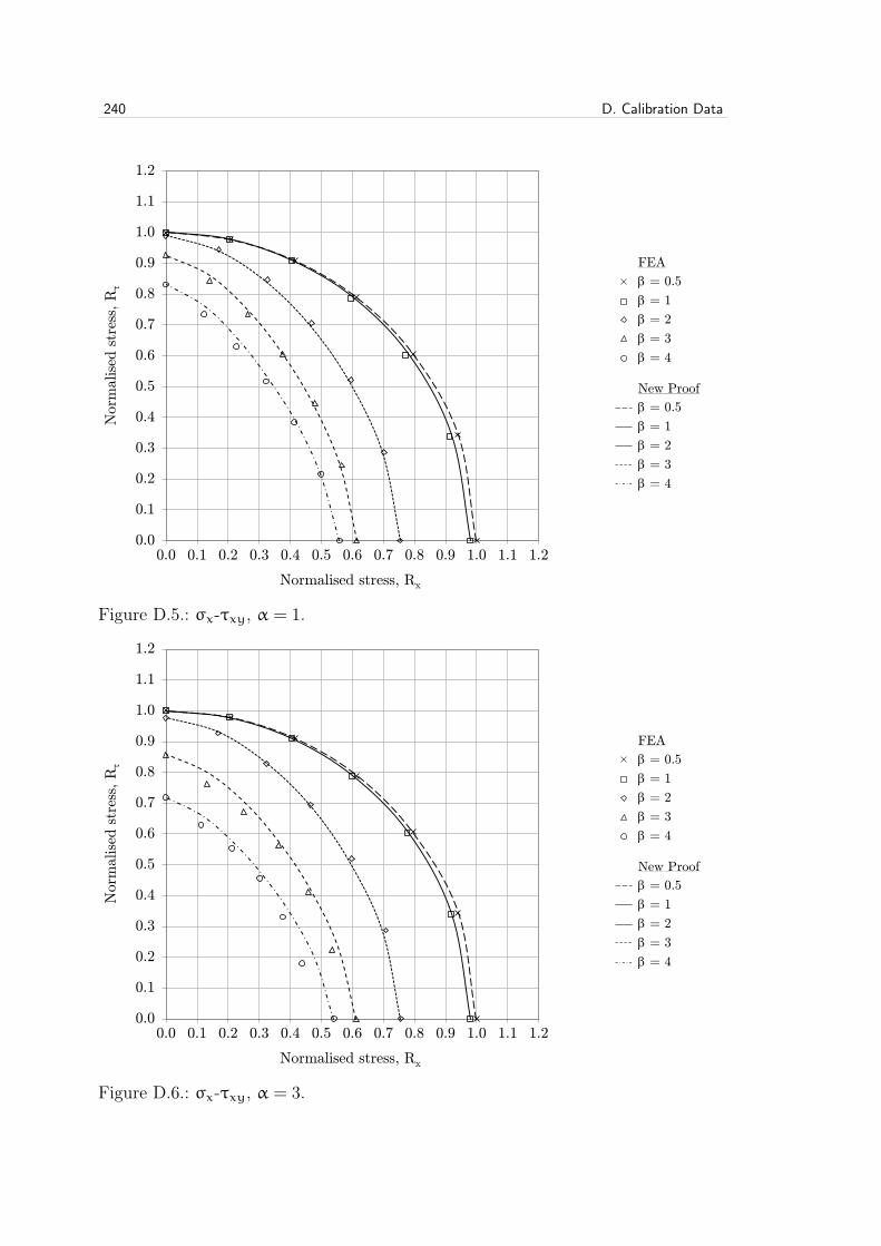
240 D. Calibration Data
0.0
0.1
0.2
0.3
0.4
0.5
0.6
0.7
0.8
0.9
1.0
1.1
1.2
0.0 0.1 0.2 0.3 0.4 0.5 0.6 0.7 0.8 0.9 1.0 1.1 1.2
Norm
alise
d s
tres
s, R
τ
Normalised stress, Rx
Figure D.5.: σx-τxy, α = 1.
FEA
β = 0.5
β = 1
β = 2
β = 3
β = 4
New Proof
β = 0.5
β = 1
β = 2
β = 3
β = 4
0.0
0.1
0.2
0.3
0.4
0.5
0.6
0.7
0.8
0.9
1.0
1.1
1.2
0.0 0.1 0.2 0.3 0.4 0.5 0.6 0.7 0.8 0.9 1.0 1.1 1.2
Norm
alise
d s
tres
s, R
τ
Normalised stress, Rx
Figure D.6.: σx-τxy, α = 3.
FEA
β = 0.5
β = 1
β = 2
β = 3
β = 4
New Proof
β = 0.5
β = 1
β = 2
β = 3
β = 4

D.2. Graphical Results 241
0.0
0.1
0.2
0.3
0.4
0.5
0.6
0.7
0.8
0.9
1.0
1.1
1.2
0.0 0.1 0.2 0.3 0.4 0.5 0.6 0.7 0.8 0.9 1.0 1.1 1.2
Norm
alise
d s
tres
s, R
τ
Normalised stress, Rx
Figure D.7.: σx-τxy, α = 5.
FEA
β = 0.5
β = 1
β = 2
β = 3
β = 4
New Proof
β = 0.5
β = 1
β = 2
β = 3
β = 4
0.0
0.1
0.2
0.3
0.4
0.5
0.6
0.7
0.8
0.9
1.0
1.1
1.2
0.0 0.1 0.2 0.3 0.4 0.5 0.6 0.7 0.8 0.9 1.0 1.1 1.2
Norm
alise
d s
tres
s, R
τ
Normalised stress, Rx
Figure D.8.: σx-τxy, α = 10.
FEA
β = 1
β = 2
β = 3
β = 4
New Proof
β = 1
β = 2
β = 3
β = 4
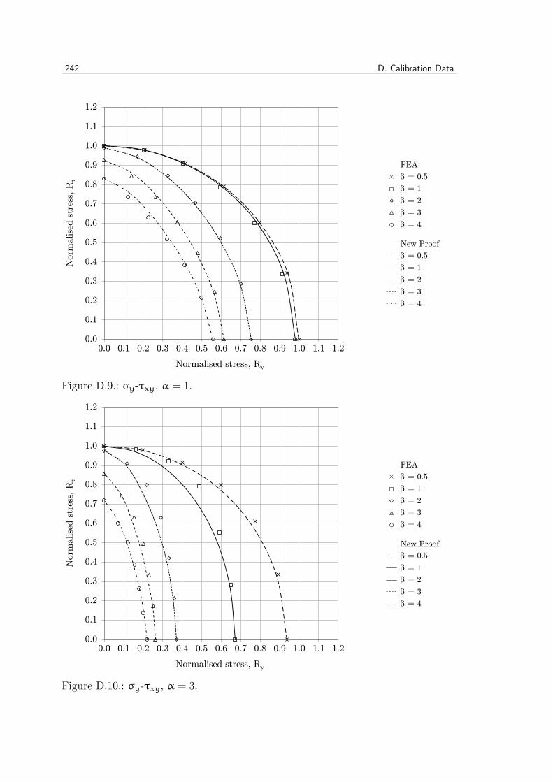
242 D. Calibration Data
0.0
0.1
0.2
0.3
0.4
0.5
0.6
0.7
0.8
0.9
1.0
1.1
1.2
0.0 0.1 0.2 0.3 0.4 0.5 0.6 0.7 0.8 0.9 1.0 1.1 1.2
Norm
alise
d s
tres
s, R
τ
Normalised stress, Ry
Figure D.9.: σy-τxy, α = 1.
FEA
β = 0.5
β = 1
β = 2
β = 3
β = 4
New Proof
β = 0.5
β = 1
β = 2
β = 3
β = 4
0.0
0.1
0.2
0.3
0.4
0.5
0.6
0.7
0.8
0.9
1.0
1.1
1.2
0.0 0.1 0.2 0.3 0.4 0.5 0.6 0.7 0.8 0.9 1.0 1.1 1.2
Norm
alise
d s
tres
s, R
τ
Normalised stress, Ry
Figure D.10.: σy-τxy, α = 3.
FEA
β = 0.5
β = 1
β = 2
β = 3
β = 4
New Proof
β = 0.5
β = 1
β = 2
β = 3
β = 4

D.2. Graphical Results 243
0.0
0.1
0.2
0.3
0.4
0.5
0.6
0.7
0.8
0.9
1.0
1.1
1.2
0.0 0.1 0.2 0.3 0.4 0.5 0.6 0.7 0.8 0.9 1.0 1.1 1.2
Norm
alise
d s
tres
s, R
τ
Normalised stress, Ry
Figure D.11.: σy-τxy, α = 5.
FEA
β = 0.5
β = 1
β = 2
β = 3
β = 4
New Proof
β = 0.5
β = 1
β = 2
β = 3
β = 4
0.0
0.1
0.2
0.3
0.4
0.5
0.6
0.7
0.8
0.9
1.0
1.1
1.2
0.0 0.1 0.2 0.3 0.4 0.5 0.6 0.7 0.8 0.9 1.0 1.1 1.2
Norm
alise
d s
tres
s, R
τ
Normalised stress, Ry
Figure D.12.: σy-τxy, α = 10.
FEA
β = 1
β = 2
β = 3
β = 4
New Proof
β = 1
β = 2
β = 3
β = 4


SCHRIFTENREIHE SCHIFFBAU
ISBN: 978-3-89220-699-6
SCH
RIF
TEN
REI
HE
SCH
IFFB
AU
699