Two-scale dynamics of flow past a partial cross-stream array of tidal turbines

Accepted for publication in J. Fluid Mech. 1

Two-scale dynamics of flow past a partialcross-stream array of tidal turbines

Takafumi Nishino† and Richard H. J. Willden

Department of Engineering Science, University of Oxford, Parks Road, Oxford OX1 3PJ, UK

(Received 19 December 2012; revised 15 May 2013; accepted 25 June 2013)

The characteristics of flow past a partial cross-stream array of (idealised) tidal turbinesare investigated both analytically and computationally to understand the mechanismsthat determine the limiting performance of partial tidal fences. A two-scale analyticalpartial tidal fence model reported earlier is further extended by better accounting forthe effect of array-scale flow expansion on device-scale dynamics, so that the new modelis applicable to short fences (consisting of a small number of devices) as well as to longfences. The new model explains theoretically general trends of the limiting performanceof partial tidal fences. The new model is then compared to three-dimensional Reynolds-averaged Navier-Stokes (RANS) computations of flow past an array of various numbers(up to 40) of actuator disks. On the whole, the analytical model agrees well with theRANS computations, suggesting that the two-scale dynamics described in the analyticalmodel predominantly determines the fence performance in the RANS computations aswell. The comparison also suggests that the limiting performance of short partial fencesdepends on how much of device far-wake mixing takes place within the array near-wakeregion. This factor, however, depends on the structures of the wake and therefore on thetype/design of devices to be arrayed.

Key words: channel flow, coastal engineering, shallow water flows

1. Introduction

Tidal stream/current power generation is one of the emerging technologies in the fieldof renewable energy. Various types of tidal stream devices (the majority can be describedas underwater versions of wind turbines) are currently proposed and tested; however, itis generally recognised that a considerably large number of devices would be requiredto make a meaningful contribution to the future energy supply (regardless of the exactdesign of devices to be employed). The challenge here is how to design efficient tidal powerfarms, i.e., how to array such a large number of devices to maximise their overall powergeneration whilst keeping their impact on the natural environment to an acceptable level.The so-called ‘tidal fences’ (spanwise array of tidal stream devices) are promising on theirown and also as a component of large tidal farms to be deployed in the future.

A series of important theories on the efficiency of tidal fences has been derived duringthe last several years. Garrett & Cummins (2007) have reported an extension of theLanchester-Betz theory (on the efficiency of wind power generation based on the balancesof mass, momentum and energy). An important finding was the significance of the effectof tidal channel blockage; the hydrodynamic limit of power extraction by devices placedin a tidal channel is proportional to (1 − B)−2, where B is the channel blockage (ratio

† Email address for correspondence: [email protected]

2 T. Nishino and R. H. J. Willden

of the frontal-projected area of devices to the channel cross-sectional area). Houlsbyet al. (2008) and Whelan et al. (2009) further extended this theory, explaining thatan ‘effective’ channel blockage may change due to the free-surface effect (the effect ofchanges in water depth that accompany power extraction) and hence the limit of powerextraction may also change, depending on the Froude number of the flow. It should benoted here that the above theories by Garrett & Cummins (2007), Houlsby et al. (2008)and Whelan et al. (2009) are all concerned with the local efficiency of tidal devices; inother words, these theories assume that the installation of devices into a tidal channeldoes not change the amount of flow coming into the channel. In reality, however, thechannel inflow may reduce unless the hydrodynamic drag caused by the installation ofdevices is negligibly small compared to other flow resistances through the channel, e.g.,sea-bed friction (Garrett & Cummins 2005). Vennell (2010, 2011) combined a simplifiedmodel of this effect (namely a channel dynamics model) with the local power extractiontheory of Garrett & Cummins (2007) to estimate the efficiency of a number of devicesarrayed across the cross-sections of various types of tidal channels. Also, Vennell (2012)included the effect of drag acting on device supporting structures in his model.

A drawback to all theories/models described above (regardless of whether the channeldynamics effects are considered or not) is that they are not directly applicable to devicesarrayed across only a part of the channel cross-section. They (explicitly or implicitly)assume that devices are regularly arrayed across the entire channel cross-section, i.e.,they are concerned with ‘full’ (rather than ‘partial’) tidal fences. As will become clearerlater in this paper, this limitation essentially comes from the assumption that the mixingof flow behind devices takes place only in a single ‘far-wake’ region; in this sense, alltheories/models mentioned above can be described as being based on a single-scale wakemixing assumption. Two major examples that highlight the significance of considering‘partial’ tidal fences are: (i) channels where a considerable portion of their cross-sectionneeds to be unblocked in order to allow for navigation of vessels and so forth, and (ii)headland sites, where the channel cross-section is semi-infinitely wide (and may also bedeep) and therefore cannot be fully blocked by the fence. In recognition of this, Nishino &Willden (2012b) have derived another important extension of the Betz theory to explorethe efficiency of a partial tidal fence by introducing an idea of scale separation betweenthe flow around each device and that around the array. One of the key findings from thenew model was the existence of optimal intra-device spacing to maximize the efficiencyof a partial tidal fence; for an infinitely wide channel, for example, the limit of energyextraction significantly increases from the Betz limit of 59.3% (of the kinetic energy ofundisturbed incoming flow) to another limit of 79.8% if the spacing is optimised. Thenew model accounts for the effects of device- and array-scale far-wake mixing separatelyand may therefore be referred to as the first (and presumably the simplest) tidal streampower generation model employing a multi-scale wake mixing concept.

In this paper we present an extension of the partial fence model of Nishino & Willden(2012b) (hereafter NW12) to further investigate the mechanics of flow past a partial tidalfence. Also reported will be three-dimensional Reynolds-averaged Navier-Stokes (RANS)computations of an array of various numbers (up to 40) of actuator disks to support theinvestigation as well as to validate the analytical model. The NW12 model assumes thatthe device-scale wake mixing takes place much faster than the array-scale flow expansion(the two scales are completely separated). This assumption, however, is valid only whenthe number of devices is sufficiently large. In this new study we account for the effect ofarray-scale flow expansion on device-scale mass, momentum and energy balances, so thatthe extended model will be applicable to a short fence (consisting of a small number ofdevices) as well as to a long fence. As with the NW12 model the mass flow through the

Two-scale dynamics of flow past tidal turbines 3

channel is assumed to be constant, i.e., we do not consider channel dynamics effects inthis study. This is because our focus here is on the partial fence flow characteristics thatare independent of the channel dynamics; a combined channel dynamics and partial fencemodel will be reported separately by Willden and Nishino (to be submitted) to discussthe effect of channel mass flow reduction. Assuming a constant mass flow means that thepower extracted by the fence is much smaller than the ‘potential’ of the channel discussedby Garrett & Cummins (2005) (or more generally, the drag caused by the installation ofthe fence is small enough not to change the balance of flow resistance inside and outsidethe entire channel, if we consider that the channel is a part of a large flow system). Seee.g. Vennell (2013) for recent discussion on the efficiency of tidal fences that are largeenough to cause reduction of the entire channel flow. Also neglected in this study are thefree-surface effects, which have recently been examined by Vogel et al. (to be submitted)by extending the NW12 model.

It should be noted that both NW12 model and the new model are essentially based on‘one-dimensional’ flow analysis. This means that these models neglect the non-uniformityof flow across each device area (for the device-scale problem) and that across the fencearea (for the array-scale problem). For the device-scale problem, this assumption seemsreasonable; the non-uniformity does not affect the (device-area-averaged) thrust or powersignificantly (Nishino & Willden 2012a). For the array-scale problem, again this assump-tion seems reasonable if we consider that all turbines in the array are under the sameoperating conditions (constant torque, for example) and subject to a uniform inflow. Aswill be presented later, RANS simulations of a spanwise array of actuator disks showthat the flow through the disks is nearly uniform across most of the array span (providedthat all disks have the same flow resistance). This suggests that one-dimensional analysisis suitable for this partial tidal fence problem.

2. Analytical model

Figure 1 shows a schematic of the extended partial tidal fence model. We consider afinite number (n) of devices arrayed across a part of the cross-section of a wide channel(note that n = 5 in figure 1). Similarly to the NW12 model, three different blockages aredefined, namely the global, local and array blockages. Here we define that the frontal-projected area of each device is AD and the cross-sectional area of the channel is AC ;hence the global blockage BG = nAD/AC . We also define that the cross-sectional area of‘local flow passage’ for each device (at the device location) is AL (which increases as thespacing between each device increases); hence the local blockage BL = AD/AL. Finally,the entire array of devices can be considered (in the array-scale problem to be describedlater) as a single power-extracting fence of area AA = nAL; hence the array blockageBA = nAL/AC . It should be noted that BG = BLBA, i.e. only two of the three blockagesare independent. To determine the full configuration of an array, we need to specify fourparameters: AC , AD, AL and n; however, the relationships among these four parametersare described by any two of the three blockage ratios. See NW12 for further descriptionsof the global, local and array blockages.

Following NW12 we will consider the balances of mass, momentum and energy in twodifferent scales, namely the device and array scales. The difference from NW12, however,is that the present model accounts for the interaction of device- and array-scale problemsa little further. The NW12 model was strictly only applicable to a ‘long’ partial fenceconsisting of a large number of devices since the model was based on the less generalassumption that the two scales were completely separated (and it remained undefinedhow large the number of devices should be for this assumption to be acceptable). In the


p1A

p4A

p5A

k ua1 2A

u

u

u

ua4A

ub4A

ub4A

1A 2 3 4A 5A

1L

4L5L

p1L

p4L p

5L

u

u

u

k ua5 2A

ub2A

ub2A

Device near wake

Array near wake

Figure 1. Schematic of the new partial tidal fence model.

present model, we relax this assumption by better accounting for the effects of array-scale flow expansion on device-scale mass, momentum and energy balances. Hence thepresent model is more generic and provides a new theoretical framework to investigatethe effect of the number of devices in the fence. As shown in figure 1 (and also in figure2, which describes the device-scale problem in more detail), we consider an array-scalestream-tube (dividing the channel flow into two flow passages, namely the array-scalebypass and core flow passages) and device-scale stream-tubes (dividing each local flowpassage into the device-scale bypass and core flow passages); then define the following 8streamwise locations:• 1A: (array-scale) far upstream, where pressure and velocity are uniform across the

channel cross-section;• 1L: (device-scale) far upstream, where pressure and velocity are uniform across the

cross-section of each local flow passage;• 2: immediately upstream of the array/devices;• 3: immediately downstream of the array/devices;• 4L: (device-scale) pressure equilibrium location, where pressure equilibrates between

the device-scale bypass and core flow passages;• 5L: (device-scale) far downstream, where not only pressure but also velocity returns

to be uniform across the cross-section of each local flow passage (due to device-scale wakemixing);• 4A: (array-scale) pressure equilibrium location, where pressure equilibrates between

the array-scale bypass and core flow passages; and• 5A: (array-scale) far downstream, where not only pressure but also velocity returns

to be uniform across the channel cross-section (due to array-scale wake mixing).Stations 1L, 2, 3, 4L and 5L are employed in the device-scale problem, whereas 1A,


k ua1 2A

2 3

1L

4L

5L

p1L

p4L p

5L

k ua5 2Aua a2 2A L k ua a4 2 4A L

k ua b4 2 4A L

k ua b4 2 4A L

ADA = A RL D L

D L 1A R /k

D L 4A R /kD L 5A R /k

TD P =TD D ua a2 2A L

k ua1 2A

k ua1 2A

ua b2 2A L

ua b2 2A L

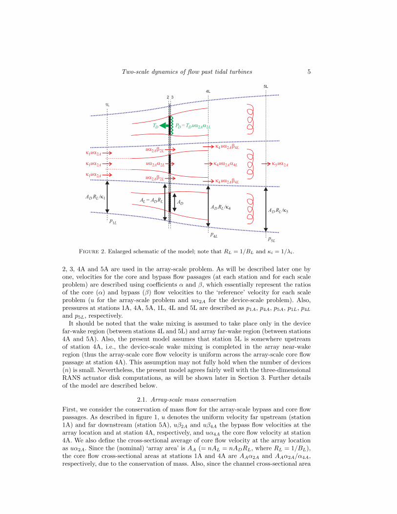
Figure 2. Enlarged schematic of the model; note that RL = 1/BL and κi = 1/λi.

2, 3, 4A and 5A are used in the array-scale problem. As will be described later one byone, velocities for the core and bypass flow passages (at each station and for each scaleproblem) are described using coefficients α and β, which essentially represent the ratiosof the core (α) and bypass (β) flow velocities to the ‘reference’ velocity for each scaleproblem (u for the array-scale problem and uα2A for the device-scale problem). Also,pressures at stations 1A, 4A, 5A, 1L, 4L and 5L are described as p1A, p4A, p5A, p1L, p4Land p5L, respectively.

It should be noted that the wake mixing is assumed to take place only in the devicefar-wake region (between stations 4L and 5L) and array far-wake region (between stations4A and 5A). Also, the present model assumes that station 5L is somewhere upstreamof station 4A, i.e., the device-scale wake mixing is completed in the array near-wakeregion (thus the array-scale core flow velocity is uniform across the array-scale core flowpassage at station 4A). This assumption may not fully hold when the number of devices(n) is small. Nevertheless, the present model agrees fairly well with the three-dimensionalRANS actuator disk computations, as will be shown later in Section 3. Further detailsof the model are described below.

2.1. Array-scale mass conservation

First, we consider the conservation of mass flow for the array-scale bypass and core flowpassages. As described in figure 1, u denotes the uniform velocity far upstream (station1A) and far downstream (station 5A), uβ2A and uβ4A the bypass flow velocities at thearray location and at station 4A, respectively, and uα4A the core flow velocity at station4A. We also define the cross-sectional average of core flow velocity at the array locationas uα2A. Since the (nominal) ‘array area’ is AA (= nAL = nADRL, where RL = 1/BL),the core flow cross-sectional areas at stations 1A and 4A are AAα2A and AAα2A/α4A,respectively, due to the conservation of mass. Also, since the channel cross-sectional area


AC = AARA (= nADRLRA, where RA = 1/BA), the bypass flow cross-sectional areasat stations 1A and 4A are AA(RA − α2A) and AA(RA − α2A/α4A), respectively.

It is also obtained, again from the conservation of mass, that

β2A =RA − α2A

RA − 1(2.1)

and

β4A =RA − α2A

RA − α2A/α4A. (2.2)

It should be noted that α4A is also a function of α2A (and vice versa); the relationshipbetween the two is obtained by considering the momentum balance, as will be describedlater in Section 2.7. Also note that β2A described above is just for completeness of thedescription of the flow system and is not required to solve the model.

2.2. Array-scale flow expansion factors

Next, we attempt to express the array-scale flow expansion between stations 1L and 5Lsystematically so that it can be included in the device-scale problem. In NW12 the cross-sectional area of each local flow passage was constant throughout the passage (AL =ADRL) as we assumed that all device-scale flow events take place much faster than thearray-scale flow expansion. In the present model, each local flow passage expands towarddownstream (i.e. the local cross-sectional area is smaller than ADRL upstream and largerthan ADRL downstream of the device location) due to the array-scale flow expansion.As shown in figure 2, here we introduce array-scale flow expansion factors, λ1, λ4 and λ5(and their inverses, κ1 = 1/λ1, κ4 = 1/λ4 and κ5 = 1/λ5) for stations 1L, 4L and 5L,respectively, so that the local cross-sectional areas are expressed as λ1ADRL, λ4ADRLand λ5ADRL for the three stations. We assume that these flow expansion factors do notchange for all n local flow passages, i.e. all local passages expand equivalently. As willbecome clear later, λ1 and λ4 (or alternatively, κ1 and κ4) need to be specified in orderto solve the device-scale problem.

To specify λ1 and λ4 the following should be taken into account. For λ1 the maximumpossible value is 1, which is the case when the number of devices (n) is so large that thedistance between stations 1L and 2 becomes negligibly small compared to the distancebetween stations 1A and 2 (i.e. the situation considered in NW12), whereas the minimumpossible value (by definition) is α2A, which is the case when n = 1 and thus station 1Lbecomes identical to station 1A (note that the local cross-sectional area at station 1A isAAα2A/n = ADRLα2A). Similarly, for λ4 the minimum possible value is 1 (for n→∞)whereas the maximum possible value (by definition) is α2A/α4A (for n = 1; note thatthe local cross-sectional area at station 4A is ADRLα2A/α4A).

In this study we use simple power-law approximations to model the dependence of λ1and λ4 on 1/n, thereby specify λ1 and λ4 as follows:

λ1 =1

κ1= 1 +

(1

n

)γ1(α2A − 1) (2.3)

and

λ4 =1

κ4= 1 +

(1

n

)γ4 (α2A

α4A− 1

). (2.4)

where γ1 and γ4 are the scaling exponents that determine the dependence of λ1 and λ4on 1/n. Unless specified, γ1 = γ4 = 1 is used in this study as a first order approximation.


As will be discussed later in Section 4, more complex model functions of λ1 and λ4 mayalso be devised and used in future studies.

2.3. Device-scale mass conservation

As the array-scale flow expansion factors have been introduced, now we can consider theconservation of mass flow for the device-scale problem. Since the mean velocity (for eachlocal flow passage) at the array location is uα2A, the velocities at stations 1L and 5L areκ1uα2A and κ5uα2A, respectively, and also the mean velocity at station 4L is κ4uα2A

due to the conservation of mass for each local flow passage.As shown in figure 2, we express the local bypass flow velocities at stations 2 and 4L

as uα2Aβ2L and κ4uα2Aβ4L. Also, we express the local core flow velocities at stations 2and 4L as uα2Aα2L and κ4uα2Aα4L. Due to the conservation of mass for the local coreflow, the local core flow areas at stations 1L and 4L are ADα2L/κ1 and ADα2L/α4Lκ4;therefore the local bypass flow areas at stations 1L and 4L are AD(RL − α2L)/κ1 andAD(RL − α2L/α4L)/κ4, respectively.

It is also obtained from the conservation of mass for the local bypass flow that

β2L =RL − α2L

RL − 1(2.5)

and

β4L =RL − α2L

RL − α2L/α4L. (2.6)

It should be noted that α4L is also a function of α2L (and vice versa); the relationshipbetween the two is obtained by considering the momentum balance, as will be describedlater in Section 2.7. Also note that β2L described above is just for completeness of thedescription of the flow system and is not required to solve the model.

2.4. Device-scale energy balance

Now we derive the device-scale energy balance equations. First, we consider each localbypass flow passage between stations 1L and 4L as a single ‘control-volume’, for whichthe energy equation can be described as(

1

2ρ(κ1uα2A)2 + p1L

)uα2AAD (RL − α2L)

=

(1

2ρ(κ4uα2Aβ4L)2 + p4L

)uα2Aβ4LAD

(RL −

α2L

α4L

), (2.7)

where ρ is the density of fluid and p1L and p4L are the pressures at stations 1L and 4L.By substituting (2.6) the above equation can be simplified to

1

2ρ(uα2A)2

(κ21 − κ24β2

4L

)+ p1L − p4L = 0. (2.8)

Note that this equation (2.8) can also be seen as a Bernoulli equation for a stream-linealong the local bypass flow passage.

Next, we consider each local core flow passage between stations 1L and 4L as a singlecontrol-volume, for which the energy equation can be described as(

1

2ρ(κ1uα2A)2 + p1L

)uα2Aα2LAD

=

(1

2ρ(κ4uα2Aα4L)2 + p4L

)uα2Aα2LAD + PD, (2.9)


where PD = uα2Aα2LTD is the power removed by the device (at the device location) andTD the thrust on the device. Hence the above equation can be simplified to

1

2ρ(uα2A)2

(κ21 − κ24α2

4L

)+ p1L − p4L =

TDAD

. (2.10)

Again, this equation (2.10) can be seen as a Bernoulli equation for a stream-line alongthe local core flow passage.

2.5. Array-scale energy balance

Next, we derive the array-scale energy balance equations. The energy equation for thearray-scale bypass flow passage between stations 1A and 4A can be described as(

1

2ρu2 + p1A

)uAA (RA − α2A)

=

(1

2ρ(uβ4A)2 + p4A

)uβ4AAA

(RA −

α2A

α4A

), (2.11)

where p1A and p4A are the pressures at stations 1A and 4A. By substituting (2.2) theabove equation can be simplified to

1

2ρu2

(1− β2

4A

)+ p1A − p4A = 0. (2.12)

Meanwhile, the energy equation for the array-scale core flow passage between stations1A and 4A can be described as(

1

2ρu2 + p1A

)uα2AAA =

(1

2ρ(uα4A)2 + p4A

)uα2AAA + PA, (2.13)

where PA is the power removed by the array as a single power-extracting fence. In otherwords, PA represents not only the power removed by the devices at the device locationbut also the power lost (to heat) due to the device-scale wake mixing. Since the cross-sectionally averaged velocity across this single power extracting fence is uα2A, PA canbe described as PA = uα2ATA, where TA = nTD is the thrust on the entire array (notethat PD = uα2Aα2LTD; therefore PA = nPD/α2L). Hence (2.13) can be simplified to

1

2ρu2

(1− α2

4A

)+ p1A − p4A =

TAAA

. (2.14)

2.6. Thrust and power coefficients

Similarly to NW12, here we define three different thrust coefficients, namely local (CTL),array (CTA) and global (CTG) thrust coefficients:

CTL =TD

12ρ(uα2A)2AD

= κ24(β24L − α2

4L

); (2.15)

CTA =TA

12ρu

2AA=(β24A − α2

4A

); (2.16)

CTG =nTD

12ρu

2nAD= α2

2ACTL. (2.17)

Note that (2.15) is derived from the device-scale energy balances (2.8) and (2.10), whilst(2.16) is derived from the array-scale energy balances (2.12) and (2.14). Of importanceis that the device- and array-scale problems are linked to each other by TA = nTD and


AA = nAD/BL. This means that CTL obtained from (2.15) and CTA obtained from(2.16) must satisfy the following relationship:

CTA = α22ABLCTL. (2.18)

We also define three different power coefficients, namely local (CPL), array (CPA) andglobal (CPG) power coefficients:

CPL =PD

12ρ(uα2A)3AD

= α2Lκ24

(β24L − α2

4L

); (2.19)

CPA =PA

12ρu

3AA= α2A

(β24A − α2

4A

); (2.20)

CPG =nPD

12ρu

3nAD= α3

2ACPL. (2.21)

It should be reminded that one of our primary objectives in this study is to examinehow the number of devices forming a partial tidal fence affects its optimal local blockage(for a given global blockage) to maximise CPG, which represents the power removed bythe devices at the device location, nPD, relative to the ‘available’ power, i.e. the powerof undisturbed flow passing through the total device area. The power removed at thedevice location, nPD (or alternatively its normalised coefficient, CPG) can be referred toas the hydrodynamic limit of power extraction (for given conditions), in the sense that,in reality, only a part of this power can be extracted as useful power and the rest will bewasted either (i) by generating heat immediately at the device location due to friction,mechanical loss, etc.; or (ii) by generating non-streamwise and/or time-dependent fluidmotion, such as mean swirling, large-scale coherent structures and turbulence, the powerof which is also eventually turned into heat due to (device-scale) wake mixing.

2.7. Momentum balance

So far we have derived (from the balances of mass and energy) that all thrust and powercoefficients are determined by the combination of α2A, α4A, α2L and α4L (and also thenumber of devices, n, to determine κ4 in the present model, cf. (2.4)). As already noted,the relationship between α2A and α4A in the array-scale problem and that between α2L

and α4L in the device-scale problem are obtained by considering the momentum balancein each problem, which will be described below.

First, we consider the entire channel between stations 1A and 4A as a single controlvolume, for which the momentum balance equation can be described as

p1AAARA − p4AAARA − TA = ρ(uα4A)2AAα2A

α4A− ρu2AAα2A

+ρ(uβ4A)2AA

(RA −

α2A

α4A

)− ρu2AA (RA − α2A) , (2.22)

which can be simplified to

(p1A − p4A)RA12ρu

2− CTA = 2α2A(α4A − 1) + 2(RA − α2A)(β4A − 1). (2.23)

Note that the left-hand side of (2.23) represents the (non-dimensionalised) force actingon the channel between stations 1A and 4A, whereas the right-hand side represents thecorresponding momentum change through this control volume. By substituting (2.12)and (2.16) to remove p1A − p4A and CTA from (2.23), we obtain the following equation


to be satisfied:

RA(β24A − 1)− (β2

4A − α24A) = 2α2A(α4A − 1) + 2(RA − α2A)(β4A − 1). (2.24)

Since β4A is a function of α2A, α4A and RA as given by (2.2), the above equation (2.24)provides the relationship between α2A and α4A (for a given RA or BA).

Next, we consider the momentum balance for each local flow passage between stations1L and 4L to derive the relationship between α2L and α4L. A difficulty here is thateach local flow passage expands toward downstream (except for the case with n → ∞);hence pressure along this expanding (non-parallel) stream-tube surface also affects thedevice-scale momentum balance. Using p∗A∗ to denote the (unknown) surface integral ofthe streamwise component of pressure force acting on this stream-tube, the momentumbalance equation can be described as

p1LADRLκ1

+ p∗A∗ − p4LADRLκ4

− TD = ρ(κ4uα2Aα4L)2ADα2L

α4Lκ4− ρ(κ1uα2A)2

ADα2L

κ1

+ρ(κ4uα2Aβ4L)2ADκ4

(RL −

α2L

α4L

)− ρ(κ1uα2A)2

AD(RL − α2L)

κ1. (2.25)

In order to close the model, here we consider the following approximation:

p1LADRLκ1

+ p∗A∗ ≈ p1LADRLκ4

. (2.26)

This physically means that the additional contribution from the expanding stream-tubesurface, p∗A∗, is approximated by the additional force that would be exerted at station1L if the cross-sectional area at station 1L (ADRL/κ1) was increased to that at station4L (ADRL/κ4). (This approximation is exact if the pressure along the stream-tube isconstant at p1L; in reality, the pressure should be higher than p1L upstream of the arrayand lower than p1L downstream of the array. Our RANS computations suggest that thisapproximation tends to somewhat overpredict p∗A∗ as the effect of lower pressure in thedownstream surpasses the effect of higher pressure in the upstream. Note, however, thatthe contribution of p∗A∗ to the momentum balance is minor in the first place unless thenumber of devices n is very small and the difference of κ1 and κ4 is significant.) By using(2.26), (2.25) can be simplified to

(p1L − p4L)RL12ρ(uα2A)2κ4

− CTL = 2α2L(κ4α4L − κ1) + 2(RL − α2L)(κ4β4L − κ1). (2.27)

By substituting (2.8) and (2.15) to remove p1L − p4L and CTL, we obtain the followingequation to be satisfied between α2L and α4L:

RLκ4

(κ24β24L − κ21) − κ24(β2

4L − α24L)

= 2α2L(κ4α4L − κ1) + 2(RL − α2L)(κ4β4L − κ1). (2.28)

In summary, (2.28) and (2.24) are the device- and array-scale momentum equations tobe solved, respectively. For a given set of n, RL (or BL) and RA (or BA), we can obtainα4L as a function of α2L by solving (2.28) and thus CTL from (2.15), whilst we canalso obtain α4A as a function of α2A by solving (2.24) and thus CTA from (2.16). HereCTL and CTA must satisfy (2.18) as already noted in Section 2.6. Since CTA increaseswhilst CTL decreases as α2A decreases from 1, the value of α2A that satisfies (2.18) isuniquely determined for a given set of α2L, RL, RA and n. Eventually, all thrust andpower coefficients are uniquely determined for a given set of α2L, RL, RA and n. Notethat the present model returns to the NW12 model when n→∞ (κ1 = κ4 = 1).


2.8. Wake mixing loss factor

Before presenting results of the new model, we consider another non-dimensional factorrelated to the efficiency of tidal fences, called ‘wake mixing loss factor’. Here we expressthe total power removed from the entire channel flow between stations 1A and 5A asPC . Since the energy equation for the entire channel between stations 1A and 5A can bedescribed as (

1

2ρu2 + p1A

)uAC =

(1

2ρu2 + p5A

)uAC + PC (2.29)

whereas the momentum equation can be described as

p1AAC − p5AAC − nTD = 0, (2.30)

the total power removed from the channel is PC = nTDu. Meanwhile, the power removedby the devices at the device location is nPD as already discussed in Section 2.6; thereforethe power lost to heat due to (device- and array-scale) wake mixing is PW = PC − nPD.The ratio of nPD to PC is sometimes referred to as ‘basin efficiency’ or ‘farm efficiency’in order to distinguish it from the efficiency represented by the global power coefficientCPG, although the same type of efficiency has also been introduced by Corten (2000) forwind turbines, to which the term ‘basin’ is not relevant. In this study, we define the ratioof PW to PC (rather than nPD to PC) as ‘wake mixing loss factor’ of tidal fences:

wake mixing loss factor =PWPC

=nTDu− nPD

nTDu= 1− α2Aα2L. (2.31)

Note that α2Aα2L is the ratio of the velocity through each device to the velocity farupstream of the entire array, u (cf. figures 1 and 2); hence the wake mixing loss factordefined above is identical to the global axial induction factor of each device:

aG = 1− uα2Aα2L

u= 1− α2Aα2L. (2.32)

2.9. Results

Below we present some examples of the solution of the new analytical model to examinedifferences in performance characteristics between short and long partial tidal fences.

First we consider a fixed global blockage (BG = 0.001); hence here we have only threeindependent parameters: the number of devices n, local blockage BL(= 1/RL), and oneof the parameters that determine the operating condition of devices (α2L for example).Figure 3 shows contours of the global power coefficient CPG plotted with respect to BLand the wake mixing loss factor (1 − α2Aα2L) for n = 4 and 16 (representing relativelyshort and long fences). Note that the wake mixing loss factor is identical to the globalinduction factor of each device; hence the loss factor = 0 means that the devices do notdecelerate the flow at all (therefore CPG = 0) whereas the loss factor = 1 means that thedevices completely block the flow (therefore again CPG = 0). For both short and longfence cases, CPG is maximised when the loss factor is around 0.33 to 0.45 (dependingon BL as shown by the white lines in the figure). This means that we can increase theoutput power (for a given array configuration) by reducing the flow through each deviceby up to about 33 to 45% of the undisturbed channel flow, although the wake mixing lossalso increases as the flow through each device is reduced (also note that these results arefor arrays that do not cause reduction of channel inflow, as described earlier). Of furtherinterest is the effect of BL. For the longer fence, the effect is very similar to that predictedby NW12; CPG increases as BL increases up to about 0.3 to 0.4 and then decreases as


Figure 3. Relationship between global power coefficient CPG and wake mixing loss factor asa function of local blockage BL, for two different numbers of devices: n = 4 and 16. Globalblockage BG is fixed at 0.001. White lines represent CPGmax (the maximal CPG for given BL)and ‘x’ indicates the peak of CPGmax.

BL further increases. This means that, even without increasing the wake mixing loss, wecan increase the power by optimising the array configuration. For the shorter fence, theoverall trend is still similar but the decrease in CPG at higher BL is more significant andthe optimal BL decreases compared to the longer fence case.

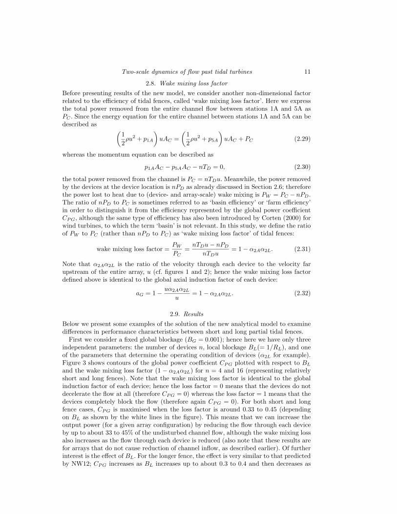
Figure 4 compares the effects of BL on the maximal CPG (hereafter CPGmax) and alsothe values of CPL and α3

2A at the optimal operating condition (that yields CPGmax forgiven BL) for n = 4, 8, 16 and 100. Again the global blockage is fixed at BG = 0.001. Asdiscussed in NW12, the optimal local blockage to maximise the limit of power extractionby a partial tidal fence is determined by the balance between the local blockage effect,represented by CPL, and the array-scale choking (or flow reduction) effect, representedby α3

2A. Note that CPG = α32ACPL as shown in (2.21). Of importance here is the effect

of the number of devices, n, on the local power coefficient, CPL. As can be seen fromfigure 4, the local blockage effect (represented by CPL) diminishes as n decreases; this isbecause the expansion of each local flow passage (due to the array-scale flow expansion,represented by κ1 and κ4) becomes more significant as the number of devices decreases.This results in the decrease in CPGmax and also alters the balance between CPL and α3

2A

in such a way that the optimal BL decreases as the number of devices decreases.

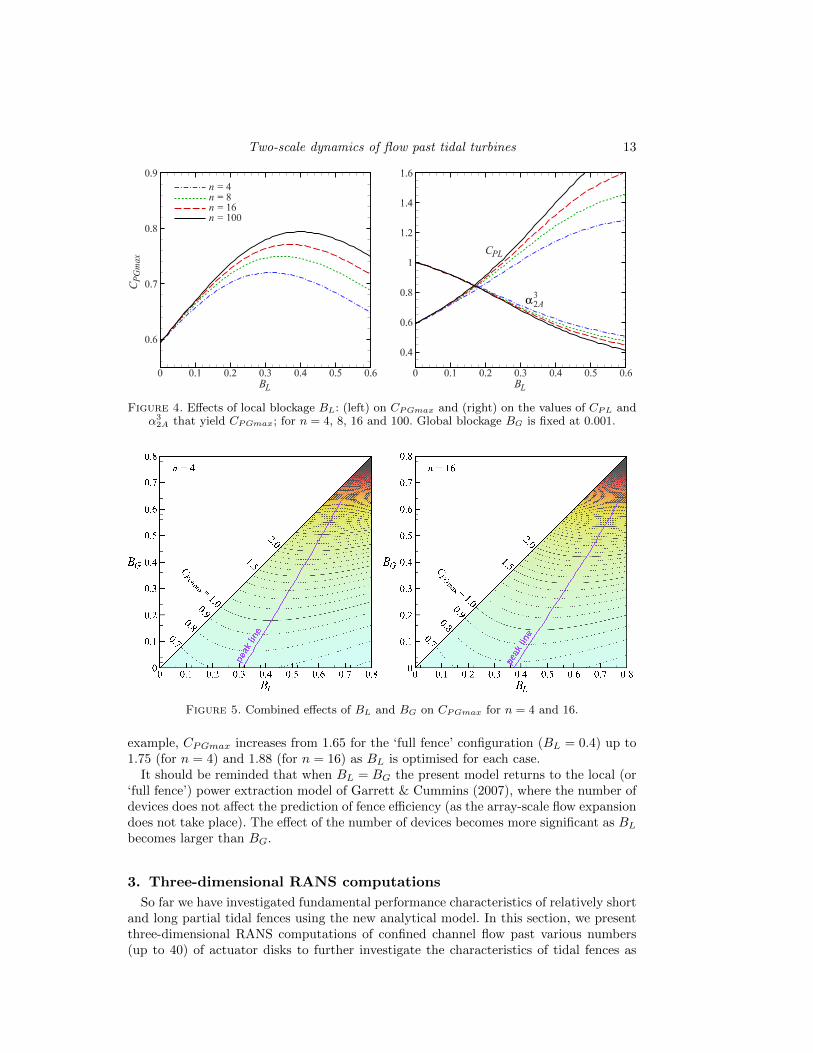
The above effects of the number of devices are important not only for low global block-age cases but also for higher global blockage cases. Figure 5 shows contours of CPGmaxplotted with respect to BL and BG for n = 4 and 16 (again representing relatively shortand long fences). As can be seen from the figure, the optimal BL (to maximise CPGmax)is smaller for the shorter fence than for the longer fence, regardless of the global block-age BG (although the optimal BL for each fence does depend on BG). Note that, forboth short and long fence cases, we can increase the output power by optimising BL (oroptimising the spacing between each device) even when BG is high; at BG = 0.4, for


α

Figure 4. Effects of local blockage BL: (left) on CPGmax and (right) on the values of CPL andα32A that yield CPGmax; for n = 4, 8, 16 and 100. Global blockage BG is fixed at 0.001.

Figure 5. Combined effects of BL and BG on CPGmax for n = 4 and 16.

example, CPGmax increases from 1.65 for the ‘full fence’ configuration (BL = 0.4) up to1.75 (for n = 4) and 1.88 (for n = 16) as BL is optimised for each case.

It should be reminded that when BL = BG the present model returns to the local (or‘full fence’) power extraction model of Garrett & Cummins (2007), where the number ofdevices does not affect the prediction of fence efficiency (as the array-scale flow expansiondoes not take place). The effect of the number of devices becomes more significant as BLbecomes larger than BG.

3. Three-dimensional RANS computations

So far we have investigated fundamental performance characteristics of relatively shortand long partial tidal fences using the new analytical model. In this section, we presentthree-dimensional RANS computations of confined channel flow past various numbers(up to 40) of actuator disks to further investigate the characteristics of tidal fences as


d+s

h

w

Figure 6. Schematic of the channel cross-section for RANS actuator disk computations.

s/d h/d w/nd n BL BG

0.1 2 10 2, 4, 8 0.357 0.0390.25 2 10 2, 4, 8, 16, 24, 32, 40 0.314 0.0390.5 2 10 2, 4, 8 0.262 0.0391 2 10 2, 4, 8 0.196 0.039

Table 1. Summary of flow configuration for RANS actuator disk computations

well as to examine the validity of the analytical model. The present RANS actuatordisk methodology has been previously used by Nishino & Willden (2012a) to investigatethe effect of three-dimensional channel blockage on single actuator disk performance,which agrees very well with the analytical (one-dimensional) model prediction of Garrett& Cummins (2007) when turbulent mixing in the near wake region (modelled in theRANS computations) is not significant. Details of the computations are described below,followed by results compared to the analytical partial fence model.

3.1. Flow configuration

Figure 6 shows a schematic of the cross-section of the channel simulated. We consider nactuator disks of diameter d arrayed regularly but only around the centre of the channelcross-section of height h and width w. The spacing between each disk is s; thereforethe local blockage BL = πd2/4h(d+ s) and global blockage BG = nπd2/4hw. Cartesiancoordinates (x, y, z) are employed, representing the streamwise, vertical and spanwisedirections, respectively.

Table 1 summarises the flow configuration. In this study the channel height h is fixedat 2d whereas the channel width w is set at 10nd (i.e. the channel width is proportionalto the number of disks) so that the global blockage is fixed. The intra-disk spacing s isvaried between 0.1d and 1d; thus the local blockage is varied between 0.357 to 0.196.

For the sake of expedience, here we suppose that the disk diameter d = 20m and thechannel inlet velocity u = 2m/s, resulting in the Reynolds number Re = ρud/µ = 4×107

(where ρ = 1000kg/m3 and µ = 0.001kg/m·s are the density and viscosity of water). Itshould be noted, however, that the flow simulated upstream of the disks is nearly inviscid(as the channel inlet turbulence level is set very low in the present RANS computations,as will be described later) whereas the rate of mixing simulated downstream of the disksis predominantly determined by the turbulence model (as will be discussed later).

3.2. Computational methods

The governing equations to be solved are the three-dimensional incompressible ‘steady’RANS equations (together with the continuity equation). The Reynolds stress terms aremodelled using the k-ε eddy viscosity model of Launder & Spalding (1974). Similarlyto Nishino & Willden (2012a), each power-extracting device (or turbine) is modelled as


a stationary permeable disk; all disks are placed perpendicular to the x-axis and arelocated at x = 0. The effect of each disk on the (Reynolds-averaged or ‘mean’) flow isconsidered as a loss of momentum in the streamwise direction at the disk plane. Thechange in momentum flux (per unit area and per unit density; to be added as ‘source’of momentum to the RANS equation for the streamwise direction at the disk plane) islocally calculated as

SU = K

(1

2U2d

), (3.1)

where Ud(y, z) is the local (rather than disk-averaged) streamwise velocity at the diskplane and K is the so-called momentum loss factor (the parameter that determines the‘operating condition’ of the devices). In this study K is assumed to be uniform acrossthe surface of all n disks. Hence the thrust on each disk is calculated as

Td(i) =

∫disk(i)

ρSUdAd =1

2ρK

∫disk(i)

U2ddAd, (3.2)

where the integration is taken over the area of each disk, Ad, and i denotes the i-th diskin the array of n disks. Hence the total thrust on the n disks is calculated as

n∑i=1

Td(i) =1

2ρK

n∑i=1

Ad〈U2d 〉i =

1

2ρKnAd〈U2

d 〉, (3.3)

where 〈φ〉i indicates the face average of a variable φ over the i-th disk and 〈φ〉 the faceaverage of φ over all n disks. Thus the (n-disk-averaged) global thrust coefficient, 〈CTG〉,is calculated as

〈CTG〉 =

∑ni=1 Td(i)

12ρu

2nAd= K

〈U2d 〉u2

. (3.4)

Similarly, the power removed from the mean flow by the i-th disk at the disk plane iscalculated as

Pd(i) =

∫disk(i)

ρSUUddAd =1

2ρK

∫disk(i)

U3ddAd, (3.5)

hence the (n-disk-averaged) global power coefficient, 〈CPG〉, is calculated as

〈CPG〉 =

∑ni=1 Pd(i)

12ρu

3nAd= K

〈U3d 〉u3

. (3.6)

Also, we define the (n-disk-averaged) global axial induction factor, 〈aG〉, as

〈aG〉 = 1− 〈Ud〉u

. (3.7)

As discussed in detail by Nishino & Willden (2012a), this actuator disk method doesnot account for the effect of turbulence (or time-dependent fluid motion) generated bythe device itself (i.e. wake turbulence is generated solely by the mean wake shear); hencethe wake mixing simulated downstream of the disks tends to be rather weak (comparedto, for example, that of common horizontal-axis turbines). Since the analytical tidalfence model to be compared with the present RANS computations is concerned with thehydrodynamic limit of power extraction (by some ideal devices that do not lose power toheat, turbulence etc., cf. Section 2.6), it might seem to be reasonable to ignore the effect


of turbulence generated by the devices in the RANS computations as well. However, theanalytical tidal fence model assumes that the device-scale wake mixing is completed inthe array near-wake region (i.e. station 5L is somewhere upstream of station 4A), whichmeans that the analytical tidal fence model supposes some form of practical (strong)device-scale wake mixing. Note that nPD in the analytical model represents the powerremoved from the mean flow at the device place, which is indeed the hydrodynamic limitof power extraction, but the analytical model never knows whether the removed poweris actually extracted as useful power or lost to generate heat, turbulence etc.; hence it isnatural to consider that the analytical tidal fence model does implicitly account for thegeneration of turbulence at the devices (or more precisely, time-dependent fluid motionthat enhances the mixing of bypass and core flows only in the device far-wake region,because the present analytical model does not account for the device near-wake mixingbetween stations 3 and 4L; for example, helical tip-vortices from horizontal-axis turbinesmight be close to this type of motion as they seem to significantly enhance the mixingonly after the breakdown of their structures (Nishino & Willden 2012c)).

A possible approach to account for the generation of turbulence at the devices withinthe framework of RANS actuator disk computations has been proposed by Nishino &Willden (2012a), who modelled the additional turbulence (called blade-induced turbu-lence or BIT) based on two physical parameters: (i) ratio of the power converted to BITto the power removed from the mean flow, and (ii) representative length scale for BIT.A difficulty here, however, is that the effect of modelled BIT on the device wake mixingis still rather hypothetical since the wake structure of actuator disks is different fromthat of actual devices; see Nishino & Willden (2012a) for further discussion on the BITapproach. In order to avoid unnecessary complication, in this study we do not employthe BIT approach but simply manipulate one of the empirical model constants in the k-εmodel of Launder & Spalding (1974) to simulate stronger and weaker wake mixing cases.Specifically, we use three different values for the model constant for the production termin the ε-equation, Cε1 (which is denoted by C1 in the original paper by Launder andSpalding): Cε1 = 1.36, 1.44 and 1.52. Unless specified, Cε1 = 1.44 (the ‘standard’ valueproposed by Launder & Spalding) is used in this paper. Note that the smaller Cε1 resultsin stronger wake mixing whereas the larger Cε1 results in weaker wake mixing; however,it should be remembered that these ‘stronger’ and ‘weaker’ cases are just relative to thenominal ‘standard’ case, which itself does not represent anything physically standard interms of simulating wake mixing of unknown devices.

Computations were performed using a second-order finite volume method employing aprocedure similar to Rhie & Chow (1983). The SIMPLE algorithm (Patankar 1980) wasused for pressure-velocity coupling. See Nishino & Willden (2012a) for further details ofthe computational methods.

3.3. Boundary conditions and computational grids

Since the flow configuration to be investigated is symmetric in both vertical and spanwisedirections (as shown earlier in figure 6), computations were performed only for a quarterof the channel cross-section with symmetry boundary conditions applied to y = 0 andz = 0 planes. Note that the centre of the n-disk array is located at (x, y, z) = (0, 0, 0).Inviscid or ‘slip’ wall boundary conditions are applied to the vertical and spanwise ends(y = h/2 and z = w/2 planes). Of importance here is that the computational domainmust be sufficiently long in the streamwise (x) direction so that neither inlet nor outletboundary would alter the flow around the disks (this theoretically means that the regionbetween stations 1A and 4A needs to be contained in the computational domain).

Our preliminary computations suggested that the effect of the computational domain


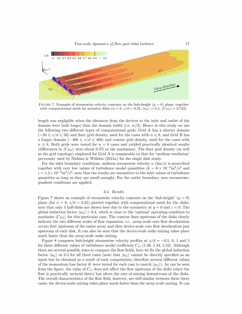
Figure 7. Example of streamwise velocity contours on the hub-height (y = 0) plane, togetherwith computational mesh for actuator disks (n = 8, s/d = 0.25, 〈aG〉 = 0.4, 〈CPG〉 = 0.742).

length was negligible when the distances from the devices to the inlet and outlet of thedomain were both longer than the domain width (i.e. w/2). Hence in this study we usethe following two different types of computational grids: Grid A has a shorter domain(−50 6 x/d 6 50) and finer grid density, used for the cases with n 6 8, and Grid B hasa longer domain (−400 6 x/d 6 400) and coarser grid density, used for the cases withn > 8. Both grids were tested for n = 8 cases and yielded practically identical results(differences in 〈CPG〉 were about 0.5% at the maximum). The finer grid density (as wellas the grid topology) employed for Grid A is comparable to that for ‘medium resolution’previously used by Nishino & Willden (2012a) for the single disk study.

For the inlet boundary conditions, uniform streamwise velocity u (2m/s) is prescribedtogether with very low values of turbulence model quantities (k = 6 × 10−6m2/s2 andε = 1.2×10−9m2/s3; note that the results are insensitive to the inlet values of turbulencequantities as long as they are small enough). For the outlet boundary, zero streamwise-gradient conditions are applied.

3.4. Results

Figure 7 shows an example of streamwise velocity contours on the ‘hub-height’ (y = 0)plane (for n = 8, s/d = 0.25) plotted together with computational mesh for the disks;note that only 4 half-disks are shown here due to the symmetry at y = 0 and z = 0. Theglobal induction factor 〈aG〉 = 0.4, which is close to the ‘optimal’ operating condition tomaximise 〈CPG〉 for this particular case. The contour lines upstream of the disks clearlyindicate the two different scales of flow expansion, i.e., array-scale core flow decelerationoccurs first upstream of the entire array and then device-scale core flow deceleration justupstream of each disk. It can also be seen that the device-scale wake mixing takes placemuch faster than the array-scale wake mixing.

Figure 8 compares hub-height streamwise velocity profiles at x/d = −0.5, 0, 1 and 5for three different values of turbulence model coefficient Cε1 (1.36, 1.44, 1.52). Althoughthere are several possible ways to compare the flow fields, here we fix the global inductionfactor 〈aG〉 at 0.4 for all three cases (note that 〈aG〉 cannot be directly specified as aninput but be obtained as a result of each computation; therefore several different valuesof the momentum loss factor K were tested for each case to match 〈aG〉). As can be seenfrom the figure, the value of Cε1 does not affect the flow upstream of the disks (since theflow is practically inviscid there) but alters the rate of mixing downstream of the disks.The overall characteristics of the flow field, however, are still similar between these threecases; the device-scale mixing takes place much faster than the array-scale mixing. It can


ε1

Figure 8. Effects of turbulence model constant Cε1 on hub-height streamwise velocity profilesat x/d = −0.5, 0, 1 and 5 (for n = 8, s = 0.25, 〈aG〉 = 0.4).

⟨ ⟩

⟨ ⟩

⟨ ⟩

⟨ ⟩

Figure 9. Comparisons of global power and thrust coefficients between RANS computations(4: Cε1 = 1.36; •: Cε1 = 1.44; O: Cε1 = 1.52) and analytical models; for n = 8, s/d = 0.25.

also be seen that the streamwise velocity is nearly uniform across all disks (at x/d = 0);the velocity is slightly lower at the outermost disks as the flow is oblique near the endsof the disk array.

Now we compare the prediction of fence performance between these computations andthe analytical tidal fence model presented in Section 2. Figure 9 shows global power andthrust coefficients obtained from the RANS computations (using the three different Cε1values) and from the analytical model (for n = 8 and s/d = 0.25; hence BL = 0.314 andBG = 0.039 as listed in table 1). Also plotted here for comparison are the predictionsobtained from the local (i.e. single-scale) model of Garrett & Cummins (2007) and theoriginal partial tidal fence model of Nishino & Willden (2012b). Note that for the localmodel of Garrett & Cummins (2007) there are two possible ways to define the blockage


γ = γ =

⟨ ⟩

Figure 10. Effect of the number of devices on the maximal global power coefficient: obtainedfrom RANS computations (4: Cε1 = 1.36; •: Cε1 = 1.44; O: Cε1 = 1.52) and analytical models;for s/d = 0.25.

B for partial tidal fences: using the local blockage (B = BL) or using the global blockage(B = BG), both of which are plotted in the figure. As can be seen from the figure, RANScomputations predict that both 〈CPG〉 and 〈CTG〉 gently increase as the mixing behindthe disks is enhanced (by reducing Cε1). The present analytical model agrees well withthe RANS computations, especially those for the stronger mixing case (Cε1 = 1.36). Theoriginal partial fence model (Nishino & Willden 2012b) slightly overpredicts both 〈CPG〉and 〈CTG〉 but still agrees fairly well with the stronger mixing case.

Figure 10 compares the effect of the number of devices on the maximal global powercoefficient (again for s/d = 0.25; hence BL = 0.314 and BG = 0.039). Here the resultsof the present analytical model are plotted for three different values of γ1 and γ4 (thescaling exponents used in (2.3) and (2.4) to specify the dependence of array-scale flowexpansion factors λ1 and λ4 on the number of devices n). It should be noted that n isinvolved in the present analytical model only through the determination of λ1 and λ4in (2.3) and (2.4); therefore the 〈CPG〉max versus n curve is simply stretched towardlarger n as the scaling exponents γ1 and γ4 are reduced (for example, the prediction forn = 4 and γ1 = γ4 = 1 is identical to that for n = 16 and γ1 = γ4 = 0.5). As can beseen from the figure, the present analytical model using the ‘default’ scaling exponents(γ1 = γ4 = 1) agrees well with the RANS computations for the stronger mixing case(Cε1 = 1.36), although it seems that the agreement in the shape of the curve slightlyimproves if γ1 and γ4 are reduced to about 0.7 for this particular flow configuration; apossible reason for this will be discussed later in Section 4.

Finally, figure 11 compares the effect of the intra-device spacing s/d on the maximalglobal power coefficient (for n = 2, 4 and 8). Note that RANS results are plotted only forthe stronger mixing case (Cε1 = 1.36) for comparison with the analytical model. Overall,RANS results agree fairly well with the analytical model; both indicate the trends that (i)the effect of the number of devices becomes more significant as the intra-device spacingdecreases and (ii) the optimal spacing increases (i.e. optimal local blockage decreases)as the number of devices is reduced. Although not presented here, larger Cε1 cases havealso shown the same trends. It should be noted, however, that the present RANS resultshave shown a somewhat weaker dependence of the maximal power coefficient on s/d. Forn = 4 and 8, for example, the analytical model predicts the maximal power coefficient


⟨ ⟩

γ = γ =

Figure 11. Effect of the intra-device spacing s/d on the maximal global power coefficient:obtained from RANS computations with Cε1 = 1.36 (symbols: black for n = 8, grey for n = 4and white for n = 2) and analytical model (lines).

slightly higher at smaller s/d but lower at larger s/d compared to the RANS results;this suggests that the analytical results would not perfectly match the RANS results bysimply increasing or decreasing the scaling exponents γ1 and γ4. The results could matchbetter if the scaling exponents are given as a function of s/d or BL; however, it shouldbe remembered that there are several reasons why the analytical model does not (andshould not) perfectly match the present RANS results, as will be discussed below.

4. Discussion

In this study we have compared a new two-scale (but still essentially one-dimensional)analytical model and three-dimensional RANS computations of partial tidal fence flows.On the whole, the new model agreed well with the RANS computations, suggesting thatthe two-scale dynamics described in the new analytical model predominantly determinedthe fence performance in the RANS computations as well. Most importantly, the modeland computations have both demonstrated the trend that, for a given global blockage,the limit of power extraction (per device) by a partial tidal fence increases as the numberof devices is increased. This is of importance when a certain number of devices are goingto be installed across a given channel cross-section; for example, if we are going to install8 devices in total, a single spanwise array of 8 devices (with its optimal local blockage)is expected to have a higher limit of power extraction than two spanwisely-separatedspanwise arrays of 4 devices (with their optimal local blockage, which should be slightlysmaller than that for an array of 8 devices).

It should be reminded that this kind of one-dimensional analytical model has a sig-nificant advantage in terms of computational cost compared to three-dimensional RANScomputations, especially when optimising the configuration and operating conditions ofa partial tidal fence at the same time. For example, the power coefficient contours shownin figure 3 (plotted against the local blockage and the wake mixing loss factor) are veryuseful for such an optimisation and can be easily obtained from an analytical model. Toobtain these contours from RANS computations, we would need to consider a number ofcases (for various combinations of array configuration and operating conditions), each ofwhich requires a decent amount of computational resources.


⟨ ⟩

λ

Figure 12. Effect of the number of devices on the horizontal flow expansion factor at x/d = 2:obtained from RANS computations (4: Cε1 = 1.36; •: Cε1 = 1.44; O: Cε1 = 1.52) for s/d = 0.25and 〈aG〉 = 0.4.

The new analytical model and RANS computations, however, still showed some quan-titative discrepancies between them. To examine the causes of discrepancies and also tobetter understand the fence flow mechanisms, here we discuss the following three issues:(i) modelling of array-scale flow expansion factors; (ii) effect of device near-wake mixing;and (iii) effect of device far-wake mixing.

The modelling of array-scale flow expansion factors λ1 and λ4 is an essential (and theonly adjustable) part of the new analytical model. In this study we modelled λ1 and λ4as in (2.3) and (2.4) and used γ1 = γ4 = 1 as the ‘default’ scaling exponents; this meansthat the ratio of the array-scale stream-tube cross-sectional area at station 1L to that atstation 1A linearly decreases down to 1 (and similarly the ratio of the area at station 4Lto that at station 4A linearly increases up to 1) as 1/n increases from 0 to 1. In reality,however, the dependence of λ1 and λ4 on 1/n should be nonlinear mainly because theexpansion of the array-scale stream-tube is nonlinear. Since its expansion rate is higheraround the array than around stations 1A and 4A, it seems reasonable to argue that thedependence of λ1 and λ4 on 1/n should be more significant when 1/n is small than when1/n is large (and hence the scaling exponents γ1 and γ4 should be less than 1). Thisargument can be supported by the results of RANS computations as shown in figure 12.Since it is not straightforward to obtain λ1 or λ4 from the simulated three-dimensionalflow data, here we plot the values of horizontal (two-dimensional) flow expansion factor λat x/d = 2 (where the local pressure appears to approximately equilibrate) obtained fromthe following procedure: (i) extract the hub-height (y = 0) plane from the simulated flowdata; (ii) calculate the two-dimensional stream-tube passing through the edge of ‘fence

area’ (i.e. x = 0, z = n(d+ s)/2); and (iii) calculate λ(x/d=2) as the ratio of the width ofthis two-dimensional stream-tube at x/d = 2 to that at x/d = 0. Note that these values

of λ are not directly comparable to λ4 used in the analytical model; nevertheless, theyshow the nonlinear dependence of array-scale flow expansion factors on 1/n. It shouldalso be noted that λ1 and λ4 are, in reality, expected to depend not only on the numberof devices but also on the local and global blockages (and presumably the aspect ratios,rather than blockages, of local and channel flow passages as well) since they would affectthe expansion rates of device- and array-scale stream-tubes.


Although the modelling of array-scale flow expansion factors λ1 and λ4 is the sourceof uncertainty in the present analytical model, this is not the only cause of discrepanciesbetween the analytical model and RANS computations. In other words, the analyticalmodel would not perfectly agree with the RANS results even if the array-scale flowexpansion factors were accurate. Two other major causes of discrepancies are: (i) devicenear-wake mixing (between stations 3 and 4L), which is neglected in the analytical modelbut not negligible in the RANS computations, and (ii) device far-wake mixing, which isassumed to be completed in the array near-wake region (upstream of station 4A) in theanalytical model but this assumption is not fully satisfied in the RANS computations ifthe number of devices is small and/or the modelled turbulent wake mixing is weak. Asconcerns the effect of device near-wake mixing, Nishino & Willden (2012a) have shownfor single actuator disk cases that the maximal power removed at the disk increases asthe mixing behind the disk is enhanced (and hence RANS actuator disk computationstend to somewhat overpredict the power coefficient compared to the analytical modelof Garrett & Cummins (2007); see Nishino & Willden (2013) for further discussion onthis issue). A similar effect can therefore be expected for the present tidal fence cases aswell, i.e., the RANS computations should have a tendency of overpredicting the powercoefficient (compared to the analytical tidal fence model) as the device near-wake mixingis enhanced. This means that the RANS computations with weaker wake mixing wouldagree better with the analytical tidal fence model than those with stronger wake mixingif the effect of device near-wake mixing was the only cause of discrepancies. On the otherhand, however, the RANS computations with stronger wake mixing tend to satisfy thedevice far-wake mixing assumption (that the mixing is completed in the array near-wakeregion) better than those with weaker wake mixing. Thus, in terms of the effect of devicefar-wake mixing, computations with stronger wake mixing should agree better with theanalytical tidal fence model than those with weaker wake mixing.

To consider the effect of device-scale wake mixing is important not only to explain thediscrepancies between the present model and computations but also to explore how theperformance of partial tidal fences can be improved in practice. Although not presentedhere, our preliminary computations without using any turbulence models (i.e. laminarflow comutations) showed that the maximal power coefficient 〈CPGmax〉 for n = 8 wasinsensitive to s/d and was practically identical to that for n = 1 (for the same globalblockage of BG = 0.039), suggesting the importance of device-scale wake mixing on thefence performance. (In these laminar flow computations the disk wakes were observed tobe stable, presumably due to the symmetry boundary conditions imposed at y = 0 andz = 0.) Analogously to the array-scale flow expansion factor λ4 that essentially representshow much the array-scale stream-tube expands whilst the device-scale bypass and coreflow pressure equilibrates, another influential factor to the fence performance would bethat representing how much of the device-scale wake mixing takes place whilst the array-scale bypass and core flow pressure equilibrates. For a relatively long fence, this factorwould not be of interest since the device-scale wake mixing would always be completedin the array near-wake region (as assumed in the present analytical model). For a shortfence, however, this factor would depend on device wake structures and therefore on thedesign of devices to be arrayed. In other words, the limiting performance of short partialtidal fences could be improved by somehow enhancing the device-scale wake mixing.

5. Conclusions

In this study we analytically and computationally investigated the characteristics offlow past a partial cross-stream array of (idealised) tidal turbines to better understand


the mechanisms that determine the limiting performance of partial tidal fences. A two-scale analytical partial tidal fence model previously proposed by Nishino & Willden(2012b) has been further extended by better accounting for the effect of array-scale flowexpansion on device-scale dynamics, so that the new model is applicable to short partialfences (consisting of a small number of devices, where the two scales are not completelyseparated) as well as to long partial fences.

The new analytical model has explained general trends of the limiting performanceof partial tidal fences. Most importantly the model has explained that, even for a givenglobal blockage (rather than for a given channel cross-sectional area), the limit of powerextraction (per device area) by a partial tidal fence increases as the number of devicesforming the array increases. This is essentially because the local blockage effect is en-hanced as the scale separation between the device- and array-scale flow events becomesmore significant. It has also been shown that, as the number of devices in the arrayincreases, the balance between the (beneficial) effect of local blockage and the (adverse)effect of flow reduction for the entire array is altered in such a way that the optimal localblockage increases. These trends are expected not only for low global blockage cases butalso for high global blockage cases.

The new analytical model has also been compared with three-dimensional RANS ac-tuator disk computations of partial tidal fence flows, where three different levels of wakemixing strength were simulated. On the whole, the new analytical model agrees well withthe RANS computations, suggesting that the two-scale dynamics described in the newanalytical model predominantly determines the partial fence performance in the RANScomputations as well. The present analytical model and RANS computations, however,have still shown some quantitative discrepancies between them. These discrepancies areconsidered to be partly due to the effect of device-scale far-wake mixing, which has beenassumed in the analytical model to be completed within the array near-wake region butin reality this assumption may not fully hold when the number of devices in the ar-ray is small. In addition to the array-scale flow expansion factors considered in the newanalytical model, the rate of device-scale wake mixing (or more precisely, how much ofthe device-scale mixing takes place within the array near-wake region) could be anotherinfluential factor to the limiting performance of short partial tidal fences. This factor,however, depends on device wake structures and therefore on the type/design of devicesto be arrayed.

Finally, it should be noted that this study did not consider any channel-scale dynamics,i.e. we assumed a constant channel mass flow in order to focus on fundamental partialtidal fence flow dynamics (that is independent of the channel-scale dynamics). In a prac-tical tidal channel that is a part of a larger flow system, the channel mass flow shouldchange depending on the configuration and operating conditions of tidal devices unlessthe drag caused by the devices is small enough not to change the balance of flow resis-tance inside and outside the entire channel. Also note that the effects of the channel’sbed friction and vertical shear of the channel flow were neglected in this study; furtherinvestigations are required to understand these effects. Nevertheless, the physical insightinto the characteristics of partial tidal fence flows obtained in this study should remainof fundamental importance.

The authors gratefully acknowledge the support of the Oxford Martin School, Univer-sity of Oxford, who have funded this research.

REFERENCES


Corten, G. P. 2000 Heat generation by a wind turbine. In Proc. 14th IEA Symposium on theAerodynamics of Wind Turbines. NREL, CO, USA.

Garrett, C. & Cummins, P. 2005 The power potential of tidal currents in channels.Proc. R. Soc. A 461, 2563–2572.

Garrett, C. & Cummins, P. 2007 The efficiency of a turbine in a tidal channel. J. Fluid Mech.588, 243–251.

Houlsby, G. T., Draper, S. & Oldfield, M. L. G. 2008 Application of linear momentumactuator disc theory to open channel flow. Tech. Rep.. OUEL 2296/08, Dept. EngineeringScience, University of Oxford.

Launder, B. E. & Spalding, D. B. 1974 The numerical computation of turbulent flows.Comput. Method. Appl. M. 3, 269–289.

Nishino, T. & Willden, R. H. J. 2012a Effects of 3-d channel blockage and turbulent wakemixing on the limit of power extraction by tidal turbines. Int. J. Heat Fluid Flow 37,123–135.

Nishino, T. & Willden, R. H. J. 2012b The efficiency of an array of tidal turbines partiallyblocking a wide channel. J. Fluid Mech. 708, 596–606.

Nishino, T. & Willden, R. H. J. 2012c Low-order modelling of blade-induced turbulencefor rans actuator disk computations of wind and tidal turbines. In Proc. EUROMECHColloquium 528: Wind Energy and the Impact of Turbulence on the Conversion Process.Oldenburg, Germany.

Nishino, T. & Willden, R. H. J. 2013 The efficiency of tidal fences: a brief review and furtherdiscussion on the effect of wake mixing. In Proc. 32nd International Conference on Ocean,Offshore and Arctic Engineering (OMAE2013). Nantes, France.

Patankar, S. V. 1980 Numerical heat transfer and fluid flow . Hemisphere Publishing Corpo-ration.

Rhie, C. M. & Chow, W. L. 1983 Numerical study of the turbulent flow past an airfoil withtrailing edge separation. AIAA J. 21, 1525–1532.

Vennell, R. 2010 Tuning turbines in a tidal channel. J. Fluid Mech. 663, 253–267.Vennell, R. 2011 Tuning tidal turbines in-concert to maximise farm efficiency. J. Fluid Mech.

671, 587–604.Vennell, R. 2012 The energetics of large tidal turbine arrays. Renewable Energy 48, 210–219.Vennell, R. 2013 Exceeding the betz limit with tidal turbines. Renewable Energy 55, 277–285.Whelan, J. I., Graham, J. M. R. & Peiro, J. 2009 A free-surface and blockage correction

for tidal turbines. J. Fluid Mech. 624, 281–291.

Two-scale dynamics of flow past a partial cross-stream array of tidal turbines

Documents

Transcript of Two-scale dynamics of flow past a partial cross-stream array of tidal turbines