Two-dimensional variability in porosity, density, and electrical resistivity of Eckernforde sediment

*Corresponding author:

Continental Shelf Research 18 (1998) 1939—1964

Two-dimensional variability in porosity,density, and electrical resistivityof Eckernforde Bay sediment

Kevin B. Briggs!,*, Peter D. Jackson", Ronald J. Holyer#,Robert C. Flint", J.C. Sandidge#, David K. Young$

!Naval Research Laboratory, Code 7431, Stennis Space Center, MS 39529-5004, USA"British Geological Survey, Engineering Geology and Geophysics Group, Keyworth, Nottingham,

NG12 5GG, UK#Naval Research Laboratory, Code 7341, Stennis Space Center, MS 39529-5004, USA$Naval Research Laboratory, Code 7331, Stennis Space Center, MS 39529-5004, USA

Abstract

Image-based analysis techniques are employed to compare sediment density heterogeneity asinterpreted from X-radiography and electrical resistivity measurements. Assessments of sedi-ment heterogeneity in two dimensions through the use of the two methods, with someexceptions, yield similar results. Autocorrelation functions estimated from density fluctuationsreveal an anisotropy between vertical and horizontal sediment structure indicated by horizontalcorrelation lengths being greater than vertical correlation lengths. In addition to the anisotropy,discrepancies between values of correlation lengths calculated from two statistical methods areindicative of the scale-dependent nature of the sediment structure. This scale dependence is alsoexemplified by the differences between the images of X-radiography and electrical resistivity. Theunequal volume of sediment over which the respective methods are integrated produces resultsdiffering by the amount and type of information included in each image. Electrical microresistiv-ity is more sensitive than X-radiography to many smaller-scale variations in sediment density.Combining the results from X-radiography and microresistivity imaging allows the calculationof Archie’s m parameter, an extremely sensitive indicator of sediment microstructure. Inaddition, electrical microresistivity gives a measurement of sediment tortuosity coincident withsediment porosity and density. ( 1998 Published by Elsevier Science Ltd. All rights reserved

1. Introduction

Sediment density heterogeneity is created through biological, hydrodynamic andchemical processes that are concentrated in the upper 1—30 cm of sediments. Processes

0278—4343/98/$ — See front matter ( 1998 Published by Elsevier Science Ltd. All rights reservedPII: S0278—4343(98)00064—8

of bioturbation, erosion or deposition result in sediment structural patterns that areoften characterized by the predominance or the immediacy of one of these processes.The sediment patterns are exemplified by the fluctuations in sediment density toX-rays depicted in X-radiographs of sediment cores (Howard, 1968; Rhoads et al.,1977). Features prominent in X-radiographs are density discontinuities created by theburrowing, pelletizing and tube building by benthic organisms within the sedimentand by the deposition and subsequent burial of laminae, lenses and flasers viahydrodynamic stress events (Rhoads and Young, 1970; Richardson et al., 1983).

Besides offering information on the sedimentary history of the sea floor, elucidationof sediment density heterogeneity is of great value in modeling the acoustic scatteringfrom the sediment volume. From characterization of fluctuations in sediment densityand sound velocity (the two components of acoustic impedance), significant para-meters employed in predicting sediment volume scattering of sound energy can beestimated. The magnitude of the fluctuations in sediment impedance determines theacoustic scattering intensity whereas the spatial distribution of the sediment fluctu-ations determines the frequency and grazing angle dependence of the scattering(Briggs, 1994). Traditional methodology for determining sediment porosity and den-sity on cores has led to the use of vertical fluctuations of density to model the sedimentvolume inhomogeneity (Lyons et al., 1994; Jackson, D.R., et al., 1996). Yet, there isevidence for anisotropy in horizontal and vertical fluctuations of sediment physicaland acoustic properties (Yamamoto, 1996). Considering the complexity wrought bythe processes at work in surficial sediments, an accurate assessment of sedimentheterogeneity in the horizontal and vertical dimensions is necessary in order to be oflegitimate use in predictive models.

Inhomogeneities within the sediment fabric are manifested as variations in bulkdensity, which is a function of sediment porosity which, in turn, is a significant factordetermining the electrical resistivity of the sediment. Electrical resistivity has beenshown to be applicable to a wide range of sediments and rocks where ionic conductionin the pore fluid is the dominant electrical conduction process (Boyce, 1968; Kermabonet al., 1969). Indeed, Jackson, P.D., et al., (1996) have demonstrated the technique ofmicroresistivity imaging as an effective method for delineating sediment electricalheterogeneity. Combining X-ray and microresistivity imaging offers the possibility ofemploying density and formation factor (microresistivity normalized by pore fluidresistivity) data to assess textural changes caused by changing depositional environ-ments, diagenesis or bioturbation, which would not be possible using one method alone.By employing X-radiography and microresistivity imaging of sediment cores, we havecharacterized the horizontal and vertical fluctuations in sediment density and porosityin the upper 20 cm of silty clay sediments in Eckernforde Bay, southwestern Baltic Sea.With these data we use image textural analysis procedures described by Holyer et al.(1996) to compare the two techniques used in estimating statistics to describe thedensity/porosity fluctuations within the sediment in both the horizontal and verticaldimensions. Furthermore, we combine the density data from X-radiography with theporometric data from microresistivity imagery to examine sedimentological structure.Two-dimensional, high-resolution statistical characterization of sediment density het-erogeneity is a rare and valuable tool in studies of sedimentology and acoustics.

1940 K.B. Briggs et al./Continental Shelf Research 18 (1998) 1939—1964

2. Materials and methods

2.1. Sampling

Microresistivity measurements and X-radiographs were made on 3-cm-thick sedi-ment slabs collected in rectangular diver cores (Jackson, P.D., et al., 1996). The coreswere constructed of 6.4-mm-thick acrylic plastic, 36-cm wide and 44-cm long, witha rectangular acrylic cap lined with cellular neoprene held fast to the bottom bya rubber strap. The cores were X-rayed within a few hours of collection at an exposureof 20 s at 50 kV and 20 mA with a Kramex PX20N portable X-ray unit and KodakAA industrial X-ray film. After development and fixing, the X-radiographs were usedto produce positive prints where the 36-cm width of the exposed area on the X-rayfilm was reduced to approximately 13 cm. The reduced positive prints were digitizedto 8 bits (256 digital levels) at 150 dpi resulting in images of the core that wereapproximately 775 pixels vertically by 870 pixels horizontally. The resolution of thedigital X-radiograph images was, therefore, approximately 0.043 cm/pixel.

Measurements of microresistivity were made within 12—36 h after core collection.Prior to measurements, cores were submerged in tanks with running seawater atambient temperature and salinity. Disturbance was minimized by careful handling ofthe cores. Fortunately, bioturbation of collected sediment was minimal owing to thenatural isolation of burrowing fauna to the top cm of the sediment (D’Andrea et al.,1996). The sample was kept in hydrostatic equilibrium by excluding all air; theorientation was changed slowly; and there was no tendency for fluid to move if thesediment did not slump. Seawater-saturated polyurethane foam was used to supportthe sediment—water interface.

One side of the diver core was removed to expose the sediment slab for insertion ofmicroresistivity electrodes. Fig. 1 shows the arrangement of the electrode arraysresulting in a 2880-electrode grid spaced at 5-mm intervals. Elongated rectangularpads of 576 electrodes were positioned 5 times to cover nearly all of the exposed side ofthe sediment slab. The potential difference between the potential dipoles was loggedby a computer while a current of constant magnitude, but alternating direction, waspassed through the sample. All aspects of the operation were under computer control,enabling the electrode arrays and acquisition parameters to be reconfigured if neces-sary. The fundamental data set from which formation factors and porosities werecalculated was comprised of the resistances converted from the measurements at eachelectrode coordinate. The coordinates of each electrode were established by knowingthe positions of the corner of the electrode pad and the starting position of the firstpad in relation to the core. Of the seven X-radiograph cores on which measurementswere made, two were chosen on the basis of least disturbance and clarity andrepresentativeness of sedimentary features for correlation of microresistivity and bulkproperty measurements.

The basic principles of the resistivity imaging technique for use on split cores arereported elsewhere (Jackson et al., 1990) and its development for use with diver coreshas been detailed by Jackson, P.D., et al., (1996). The design of this technique providesfor 2-D assessments of sediment resistivity at a resolution of 5 mm. Current is injected

K.B. Briggs et al./Continental Shelf Research 18 (1998) 1939—1964 1941

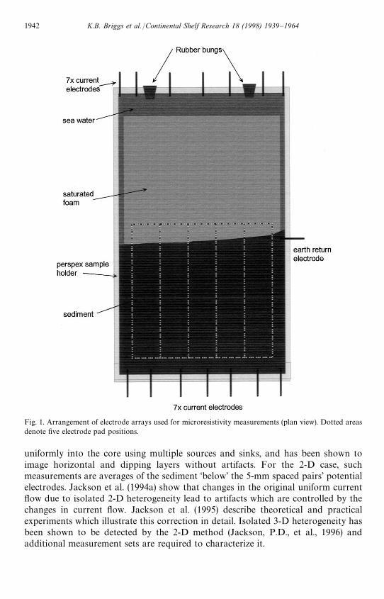
Fig. 1. Arrangement of electrode arrays used for microresistivity measurements (plan view). Dotted areasdenote five electrode pad positions.

uniformly into the core using multiple sources and sinks, and has been shown toimage horizontal and dipping layers without artifacts. For the 2-D case, suchmeasurements are averages of the sediment ‘below’ the 5-mm spaced pairs’ potentialelectrodes. Jackson et al. (1994a) show that changes in the original uniform currentflow due to isolated 2-D heterogeneity lead to artifacts which are controlled by thechanges in current flow. Jackson et al. (1995) describe theoretical and practicalexperiments which illustrate this correction in detail. Isolated 3-D heterogeneity hasbeen shown to be detected by the 2-D method (Jackson, P.D., et al., 1996) andadditional measurement sets are required to characterize it.


2.2. Image analysis

The X-radiographs at 0.043 cm/pixel (0.43 mm/pixel) and the microresistivity dataat 5-mm sample spacing are mismatched in terms of spatial sampling density by morethan a factor of ten. Both data sets were, therefore, transformed to an intermediatescale of 1 mm/pixel. There were two reasons for interpolation of the resistivity to1 mm/pixel. Firstly, presentation of the resistivity data was deemed important. Theoriginal resistivity measurements were made on a grid of approximately 45]55samples. To show these data in image format at 45]55 would have resulted in animage that was too small to be effective in demonstrating the patterns of resistivitywithin the sediment. Therefore, it was necessary to enlarge it for printing as a figure.Enlargement by simple magnification would have created an unsatisfactory ‘blocked’appearance. Secondly, the interpolation was undertaken for convenience. By scalingboth images to 1 mm/pixel, measurements such as correlation length determined fromthe image in units of pixels could be expressed directly in mm without applyingconversion factors. The X-radiographs underwent nearest-neighbor resampling.Structure in the X-radiographs appeared visually to be large relative to samplespacing, so it was assumed that aliasing was not a problem in this procedure.Microresistivity data were formed into 1 mm/pixel images by ‘Kriging’ (Isaaks andSrivastava, 1989), a popular geostatistical gridding method. Kriging was performedwith an isotropic, linear variogram model with no drift and no nugget effect. Theresult was X-radiograph and microresistivity images that were spatially coregisteredto facilitate comparisons using image analysis methods. Both image types as shown inthis paper were, therefore, approximately 250 samples vertically and 350 sampleshorizontally (25]35 cm of core area imaged). The 1 mm/pixel resolution of themicroresistivity images is not real; any property of the microresistivity images ob-served at scales smaller than 5 mm is an artifact of the interpolation method and is notof physical origin.

In contrast to the preceding manipulations used for assessing spatial variability ofX-radiographs and microresistivity imagery, different image processing was used fordirect comparison of the two images. X-ray transmittance values were normalized(scaled to range from 0 to 1) and averaged over a 5 mm grid corresponding to thevolume associated with the resistivity measurements to plot on the same scale as theresistivity values. Microresistivity values were compared with sediment bulk proper-ties of density and porosity once a relationship was established between theX-radiographs and sediment bulk density.

2.3. Relationship between X-radiograph transmittance and bulk density

X-ray transmittance (or image brightness) is a nearly linear function of gravimetricdensity. Orsi (1994), in studies of X-ray computed tomography (CT), demonstrateda very tight linear relationship (r2 "0.992) between the response of their CT scanner(in Hounsfield units) and wet bulk density of the sample. Furthermore, theoreticalconsiderations lead to expectations of a linear relationship between bulk density of thesediment sample and X-radiograph image brightness. Film responds to exposure by


incident light according to the ‘D—log E’ curve which is typically linear over a filmdensity range of approximately 0.8—2.5. Assuming that the photoprocesses leading tothe X-radiograph are confined to this linear range, the film density and exposure arerelated as follows.

D"c log10

E#const. (1)

where D is film density, E is film exposure, and c is the combined sensitivity of the filmand processing. The terms c and const. are parameters that depend on the type of filmand on the details of the exposure and photoprocessing procedures. If

D"!log10

q, (2)

where q is image brightness, then substitution of Eq. (2) into Eq. (1) and subsequentmathematical manipulation leads to the result

q"aE#b, (3)

where a and b are coefficients of a linear relationship. The X-radiograph film has beendigitized to 8-bit resolution for computer analysis. The digital value (0—255) from theA/D converter is linearly related to image brightness and the X-ray exposure of thefilm is linearly related to bulk density of the sample. Therefore, the linear relationshipbetween q and E in Eq. (3) translates to a linear relationship between digital value andbulk density, such that

digital value"a](bulk density)#b. (4)

Eq. (4) describes the image formation process where bulk density and digital value arethe independent and dependent variables, respectively. For analysis purposes, wheredigital value is extracted from the film and bulk density is the derived value, the rolesof independent and dependent variables are reversed. Estimates of bulk density resultfrom

bulk density"c](digital value)#d. (5)

Furthermore, the irradiance of the sample must also be uniform over the area of theX-radiograph for the linear relationship to be maintained. Although exposure timeswere the same for all X-radiographs, the uniformity of illumination over the X-rayfield of view has not been tested. Although a linear relationship may exist for a givenX-radiograph, it is likely that a and b (or c and d ) will vary from image to image due toinconsistencies in photoprocessing, the A/D conversion process, output from theX-ray source, and the illumination by the light source in the A/D converter. In theideal case, the physical sample from which bulk density is determined should coincidespatially with the physical sample imaged in the X-radiograph.

Although gravimetric and X-radiograph samples were not spatially coincident, theuniformity of bulk density of the Eckernforde Bay sediment and the proximity of thesamples to each other should simplify the relationship sufficiently. Fig. 2a shows themean profile and standard deviation of the bulk density profiles as a function of depth(Richardson and Briggs, 1996). Notice that the standard deviation of the horizontalfluctuations of density is small, but not uniform. The figure shows bands of increased


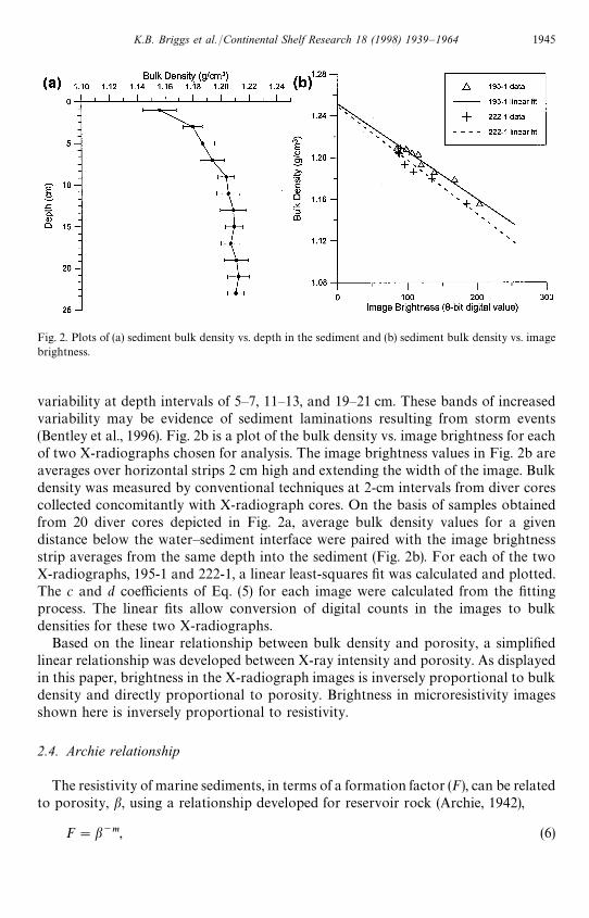
Fig. 2. Plots of (a) sediment bulk density vs. depth in the sediment and (b) sediment bulk density vs. imagebrightness.

variability at depth intervals of 5—7, 11—13, and 19—21 cm. These bands of increasedvariability may be evidence of sediment laminations resulting from storm events(Bentley et al., 1996). Fig. 2b is a plot of the bulk density vs. image brightness for eachof two X-radiographs chosen for analysis. The image brightness values in Fig. 2b areaverages over horizontal strips 2 cm high and extending the width of the image. Bulkdensity was measured by conventional techniques at 2-cm intervals from diver corescollected concomitantly with X-radiograph cores. On the basis of samples obtainedfrom 20 diver cores depicted in Fig. 2a, average bulk density values for a givendistance below the water—sediment interface were paired with the image brightnessstrip averages from the same depth into the sediment (Fig. 2b). For each of the twoX-radiographs, 195-1 and 222-1, a linear least-squares fit was calculated and plotted.The c and d coefficients of Eq. (5) for each image were calculated from the fittingprocess. The linear fits allow conversion of digital counts in the images to bulkdensities for these two X-radiographs.

Based on the linear relationship between bulk density and porosity, a simplifiedlinear relationship was developed between X-ray intensity and porosity. As displayedin this paper, brightness in the X-radiograph images is inversely proportional to bulkdensity and directly proportional to porosity. Brightness in microresistivity imagesshown here is inversely proportional to resistivity.

2.4. Archie relationship

The resistivity of marine sediments, in terms of a formation factor (F), can be relatedto porosity, b, using a relationship developed for reservoir rock (Archie, 1942),

F"b~m, (6)


where the formation factor (F) is the sediment resistivity normalized by the pore waterresistivity, b is the fractional porosity and m is a factor which has been shown to becontrolled by the particle shape or pore style (Atkins and Smith, 1961; Jackson et al.,1978; Focke and Munn, 1987). Archie found that this relationship described hisexperimental data for unconsolidated sands from the Gulf of Mexico, if m had a valueof 1.5. He noted this value increased to over 2 for cemented sandstones. For uncon-solidated marine sediments Jackson et al., (1978) showed that the same relationshipdescribed their experimental results with m being independent of grain size, butincreasing with decreasing sphericity from 1.2 for spheres to 1.4 for rounded sands to1.6 for a platy sand and up to 1.8—2.0 for platy shell fragments. They also showed thatmixtures of two different grain shapes obeyed the Archie relationship with an inter-mediate value of Archie m. Focke and Munn (1987) using an extensive data set froma carbonate reservoir showed m to have values close to 2 for the intergranular porositystyles and in the range 2—5 for the vuggy porosity styles typical for these formations.Other workers have found a similar relationship with m"2 for clay size particles (e.g.Kermabon et al., 1969).

The Archie relationship has been shown to apply to individual samples at differentstates of compaction (e.g. Jackson et al., 1978); more complex relationships have beendeveloped using different samples of the same sediment type (e.g., Winsauer et al.,1952). If grain shape varied substantially between such samples, each sample would bedescribed by the Archie relationship, but any averaged relationship would not.Consequently, the authors consider individual samples of unconsolidated marinesediments to obey the Archie relationship [Eq. (6)].

The shapes and packing of the grains of uncemented marine sediments control themorphology of the fluid-filled pore space through which electric current flows, by ionicconduction, during electrical resistivity measurements. The tortuous nature of thesepaths along which ions flow under the action of an electric field can be assessed directlyusing the Archie relationship if both porosity (b) and formation factor (F) are known.

Early studies of electrical tortuosity assumed the porous medium to be a series ofchannels that were each longer than the sample. On this basis Wyllie and Spangler(1952) derived the following relationships related to electrical tortuosity, q, of porousmedia:

q"(¸a/¸) (7)

F"qb~1 (8)

where ¸a is the average length of the tortuous pore channels and ¸ is the length of thesample. The electrical tortuosity and Archie’s m parameter can be calculated asfollows given the porosity, b, and formation factor, F:

m"

log1/F

logb(9)

q"b~(m~1). (10)

Thus, sediment tortuosity can be directly related to sediment porosity throughArchie’s m parameter.


3. Results and discussion

3.1. Vertical and horizontal variability of sediment structure

Two methods have been used to quantify the scales of variability in X-radiographand microresistivity images with special attention to differences in vertical andhorizontal features. The first method is the autocorrelation function and its associatedcorrelation length. The second method involves conversion of grayscale imagery toblack-and-white (called a binary image) followed by calculation of horizontal andvertical run length statistics both for black and white pixels.

3.1.1. Autocorrelation

The normalized autocorrelation function, /(x,y), of image I(s,l), is given by

/(x, y)"1

+s

+l

I2 (s, l )+s

+l

I (s, l )I (s#x, l#y), (11)

where s and l are sample and line numbers within the image, respectively, and x andy are the correlation ‘lag’ or offset values. In other words, the autocorrelation functionof an image is the product of the image and a spatially offset (by x, y) copy of itself,with the result scaled by the image product at offset (0, 0). The autocorrelationfunction has, by definition, a value of 1 when x"y"0. For nonzero x, y offsets, theautocorrelation function assumes values ranging from 1 to !1. The autocorrelationfunction is of interest because the rate of decline in the correlation value with size ofthe offset gives a correlation length indicating dominant spatial scales in the imagegray-tone features. Furthermore, variation in correlation lengths for x and y offsets isa measure of the anisotropy of the features.

Correlation length, ¸, is defined as that offset length at which the correlation valuehas dropped to 1/e (e"2.7183). For random data, autocorrelation decreases withdistance, x (or y) according to the exponential function exp(x/¸). If the image patternsare structured in some way, e.g., periodic, the autocorrelation function will not showexponential decay with distance and correlation length as defined here would not bea meaningful parameter. If exponential decay is assumed, an exponential curve can befit to the autocorrelation function and correlation length determined. Furthermore,the rms error of the fit of the curve to the autocorrelation function gives an indicationof the validity of the exponential decay assumption.

Fig. 3 shows the autocorrelation functions of the X-radiograph and microresistivityimages from cores 195-1 and 222-1. The autocorrelation image is composed ofcorrelation values corresponding to x, y offsets ranging from !30 to 30 mm. The (0,0)lag autocorrelation value is at the center of the autocorrelation image with othercorrelation values for other x, y lags displayed displaced from the center by distance(x, y). The autocorrelation image is displayed with a value of 1 being white and theminimum value in the image being black. All other values are represented by grayscale linearly spread over the black-to-white (minimum-to-1) range.


Table 2Image-based measures of structure anisotropy

Core ID X-radiographhor./vert.corr. length

Resistivityhor./vert.corr. length

X-radiographhor./vert.run length

Resistivityhor./vert.run length

195-1 2.2 3.2 1.1 1.3222-1 3.2 3.1 1.2 1.1

Table 1Image-based parameterizations of structure scale in cores 195-1 and 222-1

Core ID X-radiographcorr. length (cm)

Resistivitycorr. length (cm)

X-radiographrun length (cm)

Resistivityrun length (cm)

hor. vert. hor. vert. hor. vert. hor. vert.

195-1 32.1 14.8 3.8 1.2 0.9 0.8 2.2 1.7222-1 27.2 8.4 2.8 0.9 0.5 0.4 1.9 1.7

Fig. 4 shows horizontal and vertical ‘slices’ through the autocorrelation images ofFig. 3. The difference between the horizontal and vertical curves is evidence ofanisotropy in the image features. Exponential functions have been fit to the correla-tion slices of Fig. 4 to give correlation lengths. The correlation lengths thus obtainedare presented in Table 1. Anisotropy values, defined as the ratio of horizontal tovertical correlation lengths, are given in Table 2. The rms errors of the fit of theexponential curves were 0.02 or less for six of the eight curve fits performed. Theautocorrelations of resistivity data in the vertical direction resulted in fits with higherrms errors of 0.061 and 0.078. However, these fits were still good enough that theexponential decay assumption is appropriate and the resulting correlation lengths aremeaningful. In all cases the rms error of the fit to the autocorrelation function is largerfor the vertical slice than for the horizontal slice. This result is an indication that thevertical variability of both density and resistivity tends to be more structured than thehorizontal variability.

Greater values of correlation lengths in the horizontal dimension than in thevertical dimension is an expected aspect of layered sediments with little or no biogenicdisturbance to destroy the horizontal, linear features. The smaller values of correla-tion length calculated from microresistivity images (as compared with those cal-culated from X-radiographs) may be due to the ability of the method to discriminatesmall features within layers that are obscured by the superimposing of information inX-ray images. Results from the use of resistivity images closely agree with data fromhigh-resolution CT (computerized tomography) images of Eckernforde Bay sediment,indicating correlation lengths on the order of 1 cm (Lyons, 1995). Thus, use ofX-radiographs in the estimation of correlation lengths may be misleading. Theanisotropy ratios in Table 2, however, are very similar for X-ray and microresistivity


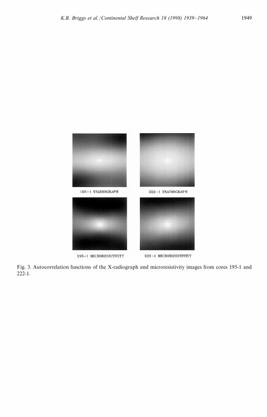
Fig. 3. Autocorrelation functions of the X-radiograph and microresistivity images from cores 195-1 and222-1.


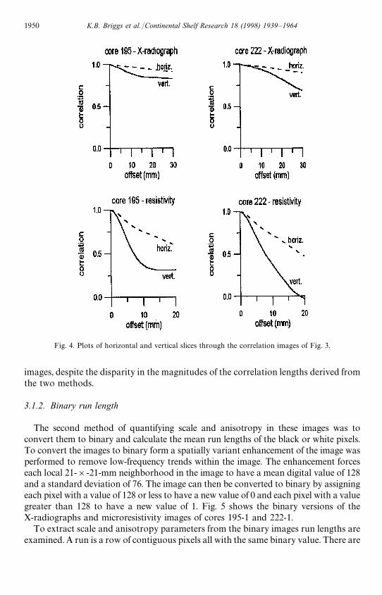
Fig. 4. Plots of horizontal and vertical slices through the correlation images of Fig. 3.

images, despite the disparity in the magnitudes of the correlation lengths derived fromthe two methods.

3.1.2. Binary run length

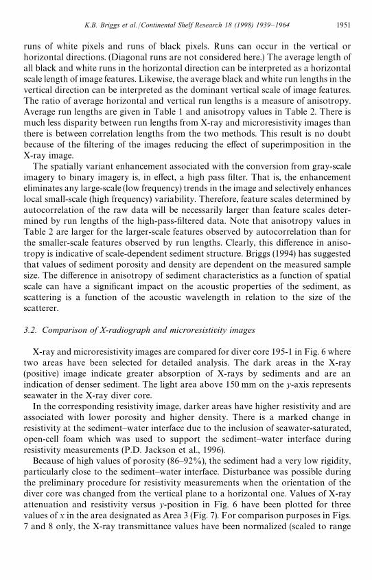
The second method of quantifying scale and anisotropy in these images was toconvert them to binary and calculate the mean run lengths of the black or white pixels.To convert the images to binary form a spatially variant enhancement of the image wasperformed to remove low-frequency trends within the image. The enhancement forceseach local 21-]-21-mm neighborhood in the image to have a mean digital value of 128and a standard deviation of 76. The image can then be converted to binary by assigningeach pixel with a value of 128 or less to have a new value of 0 and each pixel with a valuegreater than 128 to have a new value of 1. Fig. 5 shows the binary versions of theX-radiographs and microresistivity images of cores 195-1 and 222-1.

To extract scale and anisotropy parameters from the binary images run lengths areexamined. A run is a row of contiguous pixels all with the same binary value. There are


runs of white pixels and runs of black pixels. Runs can occur in the vertical orhorizontal directions. (Diagonal runs are not considered here.) The average length ofall black and white runs in the horizontal direction can be interpreted as a horizontalscale length of image features. Likewise, the average black and white run lengths in thevertical direction can be interpreted as the dominant vertical scale of image features.The ratio of average horizontal and vertical run lengths is a measure of anisotropy.Average run lengths are given in Table 1 and anisotropy values in Table 2. There ismuch less disparity between run lengths from X-ray and microresistivity images thanthere is between correlation lengths from the two methods. This result is no doubtbecause of the filtering of the images reducing the effect of superimposition in theX-ray image.

The spatially variant enhancement associated with the conversion from gray-scaleimagery to binary imagery is, in effect, a high pass filter. That is, the enhancementeliminates any large-scale (low frequency) trends in the image and selectively enhanceslocal small-scale (high frequency) variability. Therefore, feature scales determined byautocorrelation of the raw data will be necessarily larger than feature scales deter-mined by run lengths of the high-pass-filtered data. Note that anisotropy values inTable 2 are larger for the larger-scale features observed by autocorrelation than forthe smaller-scale features observed by run lengths. Clearly, this difference in aniso-tropy is indicative of scale-dependent sediment structure. Briggs (1994) has suggestedthat values of sediment porosity and density are dependent on the measured samplesize. The difference in anisotropy of sediment characteristics as a function of spatialscale can have a significant impact on the acoustic properties of the sediment, asscattering is a function of the acoustic wavelength in relation to the size of thescatterer.

3.2. Comparison of X-radiograph and microresistivity images

X-ray and microresistivity images are compared for diver core 195-1 in Fig. 6 wheretwo areas have been selected for detailed analysis. The dark areas in the X-ray(positive) image indicate greater absorption of X-rays by sediments and are anindication of denser sediment. The light area above 150 mm on the y-axis representsseawater in the X-ray diver core.

In the corresponding resistivity image, darker areas have higher resistivity and areassociated with lower porosity and higher density. There is a marked change inresistivity at the sediment—water interface due to the inclusion of seawater-saturated,open-cell foam which was used to support the sediment—water interface duringresistivity measurements (P.D. Jackson et al., 1996).

Because of high values of porosity (86—92%), the sediment had a very low rigidity,particularly close to the sediment—water interface. Disturbance was possible duringthe preliminary procedure for resistivity measurements when the orientation of thediver core was changed from the vertical plane to a horizontal one. Values of X-rayattenuation and resistivity versus y-position in Fig. 6 have been plotted for threevalues of x in the area designated as Area 3 (Fig. 7). For comparison purposes in Figs.7 and 8 only, the X-ray transmittance values have been normalized (scaled to range


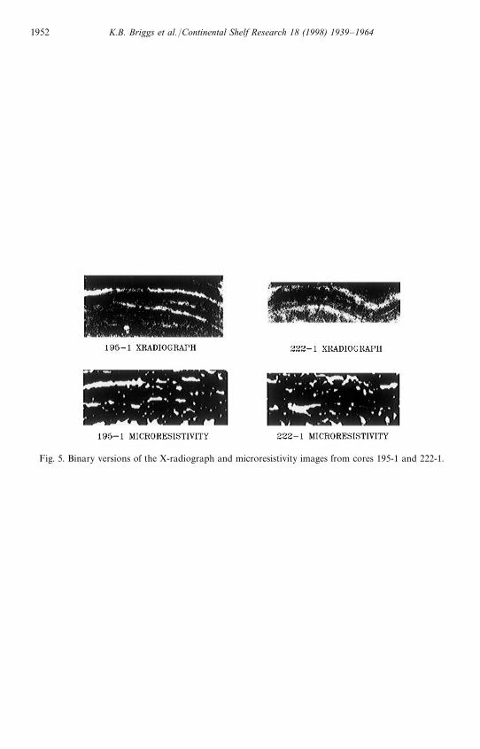
Fig. 5. Binary versions of the X-radiograph and microresistivity images from cores 195-1 and 222-1.


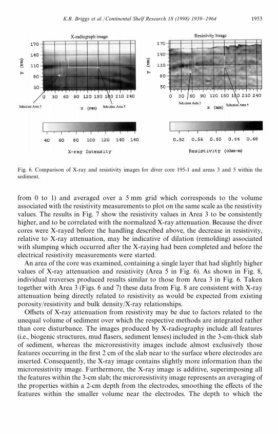
Fig. 6. Comparison of X-ray and resistivity images for diver core 195-1 and areas 3 and 5 within thesediment.

from 0 to 1) and averaged over a 5 mm grid which corresponds to the volumeassociated with the resistivity measurements to plot on the same scale as the resistivityvalues. The results in Fig. 7 show the resistivity values in Area 3 to be consistentlyhigher, and to be correlated with the normalized X-ray attenuation. Because the divercores were X-rayed before the handling described above, the decrease in resistivity,relative to X-ray attenuation, may be indicative of dilation (remolding) associatedwith slumping which occurred after the X-raying had been completed and before theelectrical resistivity measurements were started.

An area of the core was examined, containing a single layer that had slightly highervalues of X-ray attenuation and resistivity (Area 5 in Fig. 6). As shown in Fig. 8,individual traverses produced results similar to those from Area 3 in Fig. 6. Takentogether with Area 3 (Figs. 6 and 7) these data from Fig. 8 are consistent with X-rayattenuation being directly related to resistivity as would be expected from existingporosity/resistivity and bulk density/X-ray relationships.

Offsets of X-ray attenuation from resistivity may be due to factors related to theunequal volume of sediment over which the respective methods are integrated ratherthan core disturbance. The images produced by X-radiography include all features(i.e., biogenic structures, mud flasers, sediment lenses) included in the 3-cm-thick slabof sediment, whereas the microresistivity images include almost exclusively thosefeatures occurring in the first 2 cm of the slab near to the surface where electrodes areinserted. Consequently, the X-ray image contains slightly more information than themicroresistivity image. Furthermore, the X-ray image is additive, superimposing allthe features within the 3-cm slab; the microresistivity image represents an averaging ofthe properties within a 2-cm depth from the electrodes, smoothing the effects of thefeatures within the smaller volume near the electrodes. The depth to which the


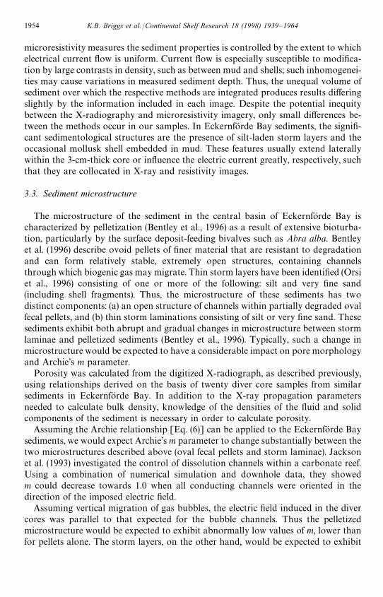
microresistivity measures the sediment properties is controlled by the extent to whichelectrical current flow is uniform. Current flow is especially susceptible to modifica-tion by large contrasts in density, such as between mud and shells; such inhomogenei-ties may cause variations in measured sediment depth. Thus, the unequal volume ofsediment over which the respective methods are integrated produces results differingslightly by the information included in each image. Despite the potential inequitybetween the X-radiography and microresistivity imagery, only small differences be-tween the methods occur in our samples. In Eckernforde Bay sediments, the signifi-cant sedimentological structures are the presence of silt-laden storm layers and theoccasional mollusk shell embedded in mud. These features usually extend laterallywithin the 3-cm-thick core or influence the electric current greatly, respectively, suchthat they are collocated in X-ray and resistivity images.

3.3. Sediment microstructure

The microstructure of the sediment in the central basin of Eckernforde Bay ischaracterized by pelletization (Bentley et al., 1996) as a result of extensive bioturba-tion, particularly by the surface deposit-feeding bivalves such as Abra alba. Bentleyet al. (1996) describe ovoid pellets of finer material that are resistant to degradationand can form relatively stable, extremely open structures, containing channelsthrough which biogenic gas may migrate. Thin storm layers have been identified (Orsiet al., 1996) consisting of one or more of the following: silt and very fine sand(including shell fragments). Thus, the microstructure of these sediments has twodistinct components: (a) an open structure of channels within partially degraded ovalfecal pellets, and (b) thin storm laminations consisting of silt or very fine sand. Thesesediments exhibit both abrupt and gradual changes in microstructure between stormlaminae and pelletized sediments (Bentley et al., 1996). Typically, such a change inmicrostructure would be expected to have a considerable impact on pore morphologyand Archie’s m parameter.

Porosity was calculated from the digitized X-radiograph, as described previously,using relationships derived on the basis of twenty diver core samples from similarsediments in Eckernforde Bay. In addition to the X-ray propagation parametersneeded to calculate bulk density, knowledge of the densities of the fluid and solidcomponents of the sediment is necessary in order to calculate porosity.

Assuming the Archie relationship [Eq. (6)] can be applied to the Eckernforde Baysediments, we would expect Archie’s m parameter to change substantially between thetwo microstructures described above (oval fecal pellets and storm laminae). Jacksonet al. (1993) investigated the control of dissolution channels within a carbonate reef.Using a combination of numerical simulation and downhole data, they showedm could decrease towards 1.0 when all conducting channels were oriented in thedirection of the imposed electric field.

Assuming vertical migration of gas bubbles, the electric field induced in the divercores was parallel to that expected for the bubble channels. Thus the pelletizedmicrostructure would be expected to exhibit abnormally low values of m, lower thanfor pellets alone. The storm layers, on the other hand, would be expected to exhibit


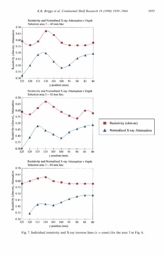
Fig. 7. Individual resistivity and X-ray traverse lines (x"const.) for the area 3 in Fig. 6.


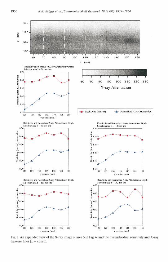
Fig. 8. An expanded view of the X-ray image of area 5 in Fig. 6. and the five individual resistivity and X-raytraverse lines (x"const.).


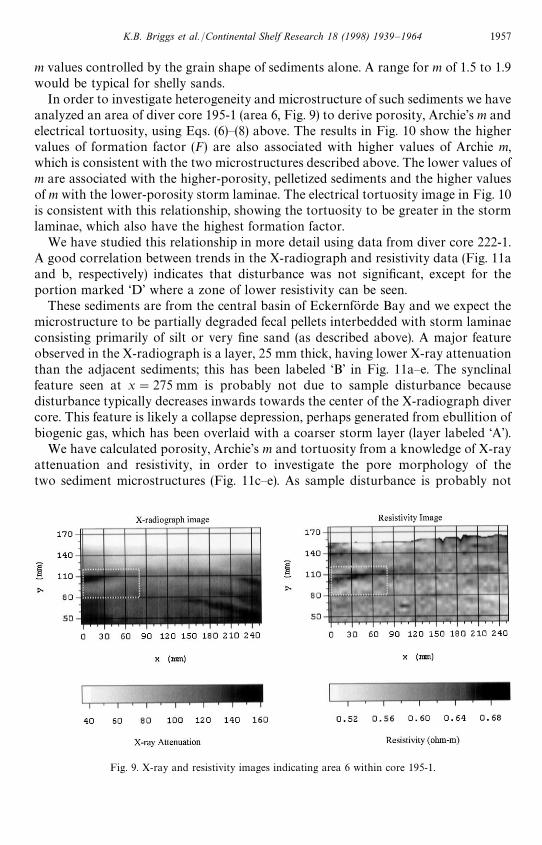
Fig. 9. X-ray and resistivity images indicating area 6 within core 195-1.

m values controlled by the grain shape of sediments alone. A range for m of 1.5 to 1.9would be typical for shelly sands.

In order to investigate heterogeneity and microstructure of such sediments we haveanalyzed an area of diver core 195-1 (area 6, Fig. 9) to derive porosity, Archie’s m andelectrical tortuosity, using Eqs. (6)—(8) above. The results in Fig. 10 show the highervalues of formation factor (F) are also associated with higher values of Archie m,which is consistent with the two microstructures described above. The lower values ofm are associated with the higher-porosity, pelletized sediments and the higher valuesof m with the lower-porosity storm laminae. The electrical tortuosity image in Fig. 10is consistent with this relationship, showing the tortuosity to be greater in the stormlaminae, which also have the highest formation factor.

We have studied this relationship in more detail using data from diver core 222-1.A good correlation between trends in the X-radiograph and resistivity data (Fig. 11aand b, respectively) indicates that disturbance was not significant, except for theportion marked ‘D’ where a zone of lower resistivity can be seen.

These sediments are from the central basin of Eckernforde Bay and we expect themicrostructure to be partially degraded fecal pellets interbedded with storm laminaeconsisting primarily of silt or very fine sand (as described above). A major featureobserved in the X-radiograph is a layer, 25 mm thick, having lower X-ray attenuationthan the adjacent sediments; this has been labeled ‘B’ in Fig. 11a—e. The synclinalfeature seen at x"275 mm is probably not due to sample disturbance becausedisturbance typically decreases inwards towards the center of the X-radiograph divercore. This feature is likely a collapse depression, perhaps generated from ebullition ofbiogenic gas, which has been overlaid with a coarser storm layer (layer labeled ‘A’).

We have calculated porosity, Archie’s m and tortuosity from a knowledge of X-rayattenuation and resistivity, in order to investigate the pore morphology of thetwo sediment microstructures (Fig. 11c—e). As sample disturbance is probably not


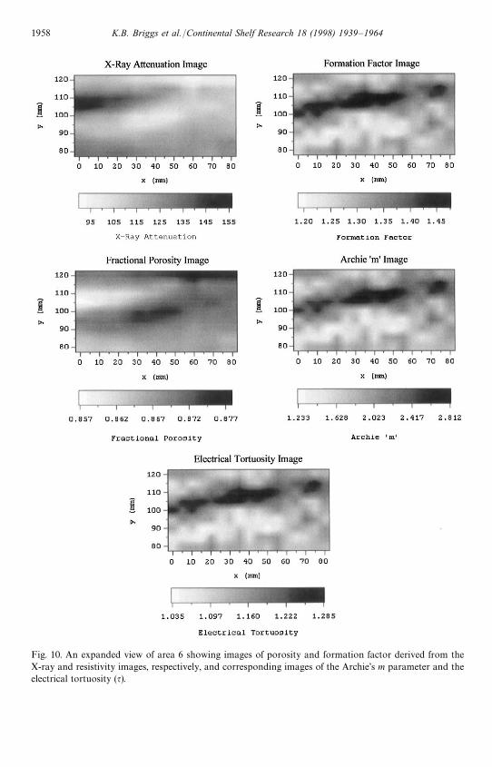
Fig. 10. An expanded view of area 6 showing images of porosity and formation factor derived from theX-ray and resistivity images, respectively, and corresponding images of the Archie’s m parameter and theelectrical tortuosity (q).


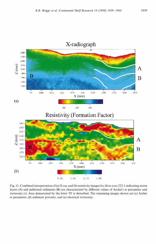
Fig. 11. Combined interpretation of (a) X-ray and (b) resistivity images for diver core 222-1 indicating stormlayers (A) and pelletized sediments (B) are characterized by different values of Archie’s m parameter andtortuosity (q). Area demarcated by the letter ‘D’ is disturbed. The remaining images shown are (c) Archiem parameter, (d) sediment porosity, and (e) electrical tortuosity.


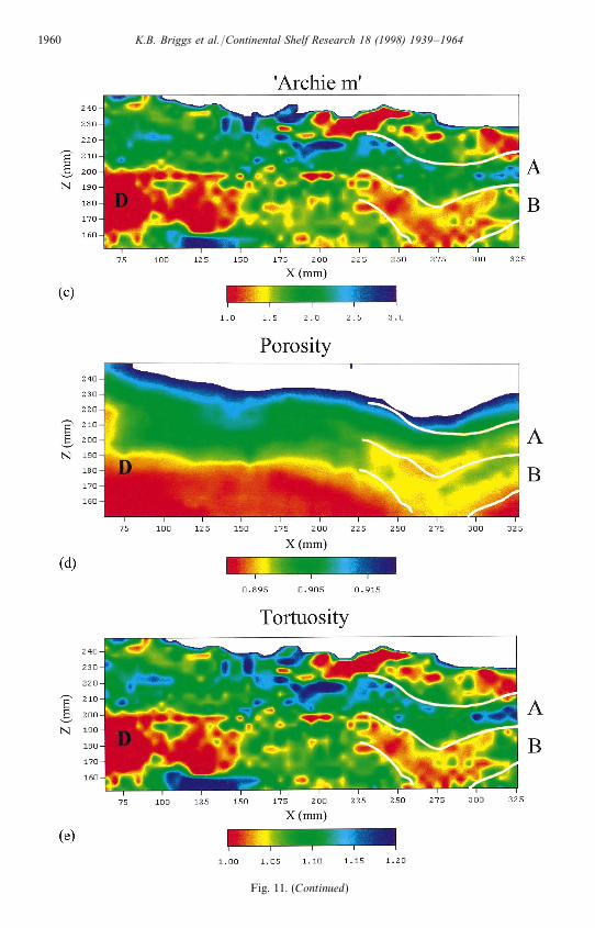
Fig. 11. (Continued)


significant, these petrophysical parameters have been derived for the whole of divercore 222-1. The results depicted in Fig. 11c indicate substantial changes in Archie’sm parameter between layers A and B. Low values of m in layer B are typical of wellconnected pore space and spherical grains (Jackson et al., 1978), such as found in thepelletized sediment microstructure. Conversely, higher values in layer A are consistentwith silt/sand storm laminae. A large proportion of the m values associated with layerA are in the range 1.5—2.0, which is typical of unconsolidated marine sands and muds,whereas layer B has lower values which are consistent with spherical particlesand good connectivity in the direction in which electric currents flowed duringmeasurements.

The pelletized microstructure is known to be extremely open, and to containchannels through which biogenic gas may migrate (Lavoie et al., 1996). Thesechannels may be aligned preferentially in the vertical direction as the result of verticalmigration of gas. During the measurements of resistivity using diver cores, theelectrical currents were constrained to flow in the same vertical direction (Jackson,P.D., et al., 1996). Consequently, the data are fully sensitive to the connected porestructure and values of m close to the lower theoretical limit of 1.0 are to be expectedfor these pelletized sediments.

Whereas there is a marked increase in resistivity below layer B in Fig. 11b, thereis no corresponding increase in the Archie’s m parameter in Fig. 11c, as is the casewith layer A. This observation is consistent with a decrease in porosity withinthe same microstructure (i.e., pelletized sediment) as shown in the X-radiograph (Fig.11a). In general, the porosity (b) changes less, in a fractional sense, than the formationfactor (F). This results in m following resistivity rather than the porosity [Eq. (9)].Thus, we conclude that in these high-porosity sediments, microresistivity measure-ments are more sensitive to changes in microstructure than measurements of bulkporosity.

As we expect Archie’s m parameter to be 1.2 for spherical-, 1.5 for sandy- and 1.8 forplaty-grained, unconsolidated sediments, the joint use of X-ray and resistivity dataenables the sediment to be zoned in terms of m to directly reflect the sedimentmicrostructure. In this case the variation in sphericity of the particles and theconnectivity of the pore space between the two types of microstructure (pelletizedsediment and storm laminae) causes significant changes in m. The electrical tortuosity(q) follows the formation factor because the porosity changes are relatively small [Eq.(10)] and q varies from 1.0 to 1.2 between layers A and B as shown in Fig. 11e.

Values of m greater than 2 are seen to be associated with layer A in Fig. 11c but arenot reported in the literature for fully saturated unconsolidated marine sediments.Such values of m are typical of vuggy (i.e., cavity-filled) carbonates.

4. Conclusions

Correlation lengths of features comprising sediment heterogeneity are anisotropicin Eckernforde Bay sediments, primarily resulting from horizontally orientedstorm laminae. Microresistivity images are sensitive to many smaller-scale variations


in sediment density, which are otherwise obscured by the additive effect of X-radio-graphy, resulting in smaller measured correlation lengths. Because the degree ofanisotropy measured by the two methods is comparable despite differing correlationlengths, it is likely that small variations within the same large features are beingobserved by the microresistivity method.

There is much less anisotropy when smaller-scale features are examined via binaryrun length. When the low-frequency trends in sediment heterogeneity are filtered fromthe imagery, smaller-scale variations in sediment density become apparent in bothX-radiograph and microresistivity images. Sediment inhomogeneities on the scale of1—2 cm, and which are nearly isotropic in their horizontal and vertical dimensions, areelucidated by this type of image processing. Because the size and shape of sedimentinhomogeneities vary with the scale of the measurement, Eckernforde Bay sedimentstructure is scale dependent. Scale dependence of sediment structure is significant tomodelers attempting to predict acoustic scattering from the sediment volume as thescale of the acoustic wavelength will determine the scale of measurement.

The difference in sediment volume over which X-radiography or microresistivitymeasurements are integrated is responsible for slight discrepancies between theimages. The quantity and quality of the information derived from the two methodsdiffer, resulting in slight offsets in image intensity. Because the X-ray method superim-poses rather than averages features, we would expect a much greater disparitybetween methods in highly bioturbated sediments. We observe relatively close agree-ment between X-ray and microresistivity images in Eckernforde Bay sediments wherethere is a relatively homogeneous, pelletized microstructure and the dominant sedi-mentary feature is storm-generated laminae. Biogenic structures such as burrows andfeeding voids are virtually absent from the sediment structure in the central basin ofEckernforde Bay, as the biota are primarily restricted to the top cm of sediment. Thus,the dissimilarity in the quantity (thickness) of sediment measured by the two tech-niques should not be considered as a fatal flaw in methodology, but rather as a caveatwhen interpreting the data.

The combination of formation factor (through electrical resistivity) and porosity(through X-ray attenuation) enables Archie’s m parameter to be calculated. Valuesof this parameter are extremely sensitive to sediment structure and are diagnosticof the pelletized sediments and storm laminae typical of Eckernforde Bay. Thisdual microstructure could not be identified from either X-radiography or microresis-tivity imaging alone. Such diversity in the microstructure inhibits the constructionof general relationships between formation factor and porosity for the sedimentsfrom Eckernforde Bay. For these sediments, we consider microstructure to bean independent variable, which may be characterized by Archie’s m parameter.These sediment microstructures exhibit differing tortuosities, as calculated fromconsiderations of the flow of electric current, indicating a link to the sedimenttortuosity used in acoustic modeling (e.g., Biot theory). The combination of resistivityand X-ray data enables zones to be identified in terms of both microstructure andsediment tortuosity.

Optimal use of the microresistivity imagery would employ an additional dimensionover which data could be collected. This approach has been only recently pursued


using an array of microresistivity electrodes positioned upon the sediment—waterinterface that is able to assess the 2-dimensional sediment heterogeneity at variousdepths in sediment box cores.

Acknowledgements

We thank M. Richardson and R. Ray for help with collecting diver cores and thecaptains and crews of the vessel HELMSAND for their cooperation in the field. Thiswork was funded by the Office of Naval Research through the Coastal BenthicBoundary Layer program managed by the Naval Research Laboratory, programelement 0601153N, M. D. Richardson, chief scientist. P.D.J. and R.C.F. publish withthe permission of the Director, BGS (NERC). The NRL contribution number isNRL/JA/7431-97-0001.

References

Archie, G.E., 1942. The electrical resistivity log as an aid in determining some reservoir characteristics.Transactions of the American Institute of Mining and Metallurgical Engineers 146, 54—62.

Atkins, E.R., Smith, G.H., 1961. The significance of particle shape in formation factor porosity relationships.Journal of Petroleum Technology 13, 285—291.

Bentley, S.J., Nittrouer, C.A., Sommerfield, C.K., 1996. Development of sedimentary strata in EckernfordeBay, southwestern Baltic Sea. Geo-Marine Letters 16, 148—154.

Boyce, R.E., 1968. Electrical resistivity of modern marine sediments from the Bering Sea. Journal ofGeophysical Research 73, 4579—4766.

Briggs, K.B., 1994. High-frequency acoustic scattering from sediment interface roughness and volumeinhomogeneities. Ph.D. Dissertation, University of Miami, 143 pp.

D’Andrea, A.F., Craig, N.I., Lopez, G.R., 1996. Benthic macrofauna and depth of bioturbation in Ecker-nforde Bay, southwestern Baltic Sea. Geo-Marine Letters 16, 155—159.

Focke, J.W., Munn, D., 1987. Cementation exponents in Middle Eastern Carbonate Reservoirs. SPEFormation Evaluation 2, 155—162.

Holyer, R.J., Young, D.K., Sandidge, J.C., Briggs, K.B., 1996. Sediment density structure derived fromtextural analysis of cross-sectional X-radiographs. Geo-Marine Letters 16, 204—211.

Howard, J.D., 1968. X-ray radiography for examination of burrowing in sediments by marine invertebrateorganisms. Sedimentology 11, 249—258.

Isaaks, E.H., Srivastava, R.M., 1989. An Introduction to Applied Geostatistics. Oxford University Press,New York, 561 pp.

Jackson, D.R., Briggs, K.B., Williams, K.L., Richardson, M.D., 1996. Tests of models for high-frequencysea-floor backscatter. IEEE Journal of Oceanic Engineering 21, 458—470.

Jackson, P.D., Briggs K.B., Flint, R.C., 1996. Evaluation of sediment heterogeneity using microresistivityimaging and X-radiography. Geo-Marine Letters 16, 219—225.

Jackson, P.D., Jarrard, R.D., Pigram, C.J., Pearce, J.M., 1993. Resistivity porosity velocity relationshipsfrom downhole logs: an aid to the evaluation of pore morphology. Proceedings, ODP, Scientific ResultsVol. 133, College Station, TX (Ocean Drilling Program) pp. 661—686.

Jackson, P.D., Lovell, M.A., Pitcher, C., Green, C.A., Evans, C.J., Flint,R., Forster, A., 1990. Electricalresistivity imaging of core samples. In: Worthington, P.F. (Ed.), Advances in Core Evaluation, Accuracyand Precision in Reserves Estimation. Proceedings of the European Core Analysis Symposium (EurocasI), Society of Core Analysts, Gordon and Breach Science, London, 555pp.


Jackson, P.D., Lovell, M.A., Harvey, P.K., Ball, J.K., Williams, C., Flint, R.C., Ashu, A.P., Meldrum, P.I.,1994. Advances in resistivity core imaging, SPWLA 35th Annual Logging Symposium. Tulsa, OK. II:Paper GG, 5 pp.

Jackson, P.D., Lovell, M.A., Harvey, P.K., Ball, J.K., Williams, C., Flint,R.C., Gunn, D.A., Ashu, A.P.,Meldrum, P.I., 1995. Electrical resistivity core imaging I: a new technology for high resolution investiga-tion of petrophysical properties. Scientific Drilling 5(4), 139—151.

Jackson, P.D., Taylor Smith, D., Stanford, P.N., 1978. Resistivity-porosity-particle shape relationships formarine sands. Geophysics 43, 1250—1268.

Kermabon, A.J., Gehin, C., Blavier, P., 1969. A deep sea electrical resistivity probe for measuring porosityand density of unconsolidated sediments. Geophysics 34, 554—571.

Lavoie, D.M., Lavoie, D.L., Pittenger, H.A., Bennett, R.H., 1996. Bulk sediment properties interpreted inlight of qualitative and quantitative microfabric analysis. Geo-Marine Letters 16, 226—231.

Lyons, A.P., 1995. Acoustic volume scattering from the seafloor and small scale structure of heterogenoussediments. Ph.D. Dissertation, Texas A&M University, 184 pp.

Lyons, A.P., Anderson, A.L., Dwan, F.S., 1994. Acoustic scattering from the seafloor: Modeling and datacomparison. Journal of the Acoustical Society of America 95, 2441—2451.

Mualem, Y., Friedman, S.P., 1991. Theoretical prediction of electrical conductivity in saturated andunsaturated soil. Water Resources Research 27(10), 2771—2777.

Orsi, T.H., 1994. Computed tomography of macrostructure and physical property variability of seafloorsediments. Ph.D. Dissertation, Texas A&M University, 186 pp.

Orsi, T.H., Werner, F., Milkert, D., Anderson, A.L., Bryant, W.R., 1996. Environmental overview ofEckernforde Bay, northern Germany. Geo-Marine Letters 16, 140—147.

Rhoads, D.C., Aller, R.C., Goldhaber, M.B., 1977. The influence of colonizing benthos on physicalproperties and chemical diagenesis of the estuarine seafloor. In: Coull, B.C. (Ed.), Ecology of MarineBenthos, University of South Carolina, Columbia, SC, pp. 113—138.

Rhoads, D.C., Young, D.K., 1970. The influence of deposit-feeding organisms on sediment stability andcommunity trophic structure. Journal of Marine Research 28, 150—178.

Richardson, M.D., Briggs, K.B., 1996. In situ and laboratory geoacoustic measurements in soft mud andhard-packed sand sediments: implications for high-frequency acoustic propagation and scattering.Geo-Marine Letters 16, 196—203.

Richardson, M.D., Young, D.K., Briggs, K.B., 1983. Effects of hydrodynamic and biological processes onsediment geoacoustic properties in Long Island Sound, USA. Marine Geology 52, 201—226.

Winsauer, W.O., Shearin, H.M., Masson, P.H., Williams, M., 1952. Resistivity of brine-saturated sands inrelation to pore geometry. Bulletin of the American Association of Petroleum Geology 36, 253—277.

Wyllie, M.R.J., Spangler, M.B., 1952. Application of electrical resistivity measurements to the problem offluid flow in porous media. Bulletin of the American Association of Petroleum Geology 36, 359—403.

Yamamoto, T., 1996. Acoustic scattering in the ocean from velocity and density fluctuations in thesediments. Journal of the Acoustical Society of America 99, 866—879.


Two-dimensional variability in porosity, density, and electrical resistivity of Eckernforde sediment

Documents

Transcript of Two-dimensional variability in porosity, density, and electrical resistivity of Eckernforde sediment