Turbulent Rayleigh–Bénard convection of water in cubical cavities: A numerical and experimental...

www.elsevier.com/locate/ijhmt

International Journal of Heat and Mass Transfer 50 (2007) 3203–3215

Turbulent Rayleigh–Benard convection of water in cubical cavities:A numerical and experimental study

Leonardo Valencia, Jordi Pallares *, Ildefonso Cuesta, Francesc Xavier Grau

Department of Mechanical Engineering, University Rovira i Virgili, Avinguda dels Paısos Catalans 26, 43007 Tarragona, Spain

Received 31 October 2005Available online 28 March 2007

Abstract

Experimental measurements and numerical simulations of natural convection in a cubical cavity heated from below and cooled fromabove are reported at turbulent Rayleigh numbers using water as a convective fluid (Pr = 6.0). Direct numerical simulations were carriedout considering the Boussinesq approximation with a second-order finite volume code (107

6 Ra 6 108). The particle image velocimetrytechnique was used to measure the velocity field at Ra = 107, Ra = 7 � 107 and Ra = 108 and there was general agreement between thepredicted time averaged local velocities and those experimentally measured if the heat conduction through the sidewalls was consideredin the simulations.� 2007 Elsevier Ltd. All rights reserved.

Keywords: Natural convection; Rayleigh–Benard flow; Partially conducting lateral walls; Numerical simulation; Particle image velocimetry turbulent flow

1. Introduction

Flows in cubical cavities have been extensively used forvalidation of CFD codes because of the geometrical sim-plicity. Despite the advantages of a numerical investiga-tion, ultimately measurements are the only way toestablish the reliability of numerical predictions. Numericalsimulations of natural convection flows have been exten-sively performed and analyzed in the laminar and turbulentregimes. Some authors have identified different flow struc-tures in a cubical cavity heated from below. For example,at low Rayleigh numbers, Ozoe et al. [1], predicted a singleroll structure with ascending and descending flows close totwo opposed lateral walls and Hernandez and Frederick [2]reported the toroidal roll which consists of four ascendingcurrents of flow close to the vertical edges of the cavity anda single descending one along the vertical symmetry axis ofthe cavity. These structures and other two were reportedand classified by Pallares et al. [3]. At turbulent Rayleigh

0017-9310/$ - see front matter � 2007 Elsevier Ltd. All rights reserved.

doi:10.1016/j.ijheatmasstransfer.2007.01.013

* Corresponding author. Tel.: +34 977559682; fax: +34 977559691.E-mail address: [email protected] (J. Pallares).

numbers, Pallares et al. [4] reported the time-averagedvelocity and temperature fields of large-eddy simulationsof Rayleigh–Benard convection of a Boussinesq fluid witha Prandtl number of 0.71 in a perfectly conducting cubicalcavity at Ra ¼ 106 and Ra ¼ 108. Valencia et al. [5] studiedthe non-Boussinesq effects of water [6] in a cubical cavitywith perfectly conducting sidewalls at Ra ¼ 107. Leonget al. [7] measured the averaged Nusselt numbers at thecold plate of a perfectly conducting cubical cavity filledwith air and with isothermal horizontal walls. Theseauthors studied the range 104

6 Ra 6 108 and three anglesof inclination of the cavity but the flow topologies were notreported.

The effect of the thermal boundary conditions of naturalconvection flows confined by walls of finite thickness andthermal conductivity was investigated by Kim and Visk-anta [8]. These authors demonstrated that the use of idealthermal boundary conditions that neglect the interactionbetween the convecting fluid and the thermal conductionacross the walls in numerical simulations was not a goodapproximation to reproduce experimental flows of air incavities with polycarbonate lateral walls. A similar conclu-sion was reported by Salat et al. [9]. Ahlers [10] showed

mailto:[email protected]

Nomenclature

C wall conductanceCp heat capacity (J/kg K)d wall thickness (m)g gravitational acceleration (m/s2)h heat transfer coefficient (W/m2 K)k thermal conductivity (W/m K)L dimension of the cavity (m)N number of grid pointsNu Nusselt number (Nu = hL/k)Pr Prandtl number (Pr = m/a)Ra Rayleigh number ðRa ¼ gbDTL3=maÞt time (s)T temperature (K)u; v; w velocity components (m/s)x; y; z Cartesian coordinates (m)

Greek symbols

a thermal diffusivity (m2/s)b thermal expansion coefficient (1/K)dij Kronecker delta

D incrementk2 second largest eigenvalue of the velocity gradi-

ent tensorl dynamic viscosity (Pa s)m kinematic viscosity (m2/s)s integral time scale (s)

Superscripts and subscripts

– time averaged value* non-dimensional quantity0 reference value at the mean temperatureC cold platef fluidg glassH hot platehw horizontal wallslw lateral wallst total value of integration

X

Z

YHorizontal Hot Plate (TH)

Horizontal Cold Plate (TC)

g

FluidGlass Walls

Fig. 1. Sketch showing the configuration of the cubical cell and thecoordinate system.

3204 L. Valencia et al. / International Journal of Heat and Mass Transfer 50 (2007) 3203–3215

that the experimental method of substraction of the con-ductance of the empty cell to estimate the conductance ofthe sidewalls could lead to errors of 20% in the Nusseltnumber and an important underestimation of the exponentc of the Rayleigh number in a correlation of the formNu / Rac. The numerical results reported by Verzicco[11], who studied the effects of a sidewall with finite thermalconductivity in a cylindrical enclosure, showed that theadditional heat transfer across the lateral fluid/wall inter-face produces an important effect on the flow and Nusseltnumbers.

The objective of the present study is to compare and val-idate the calculated time averaged-velocity field of the tur-bulent Rayleigh–Benard flow structures in a cubical cavitywith partially conducting lateral walls with those measuredexperimentally with the particle image velocimetry (PIV)technique. The experimental setup and the numerical tech-niques are described in Sections 2 and 3, respectively, andthe results are presented and discussed in Section 4.

Table 1Operating conditions of the experiments

Exp. no. Cavity sizeL (m)

DT = TC � TH

(�C)T0

(�C)Ra0 Pr0

1 0.050 4.3 26.0 107 5.952 0.092 5.0 25.5 7 � 107 6.033 0.092 5.8 30.3 108 5.35

2. Experimental

The experimental set-up used in the present work tomeasure the velocity field is similar to that used by Arroyoand Saviron [12] (Fig. 1). Two cubical cavities wereconstructed with 4-mm-thick glass lateral walls and 5-mm-thick horizontal copper plates. Table 1 shows theexperimental conditions used in the experiments for thetwo cavities. The glass lateral walls were glued to the cop-per plates with Loctite 3106. The cubical cells were sand-wiched between 15-mm-thick and 25-mm-thick copperblocks. Semiconductor paste was used to obtain a good

thermal contact between the copper surfaces. The maxi-mum horizontal misalignments of the cavities in the exper-

L. Valencia et al. / International Journal of Heat and Mass Transfer 50 (2007) 3203–3215 3205

iments are estimated to be ±0.1�. The top copper block wascooled by recirculating water from a thermostatic bath andthe bottom block was heated with an electrical resistancecontrolled by a Proportional–Integral-Derivative (PID)digital control.

Three Pt100 temperature sensors were connected andembedded in each block along its diagonal. The mean tem-perature of the copper blocks was calculated using the mea-surements of the corresponding sensors. The differencesbetween the sensors of the same block were within±0.02 �C. During the experiments the 15/25-mm-thick cop-per blocks were kept at constant temperatures within±0.01 �C. The maximum electrical power supplied to theelectric resistance was approximately 12 W. The lateralthermal boundary conditions of the experiments were fixedby the thickness and the thermal conductivity of the glasssidewalls. These conditions can be characterized by the wallconductance defined as

C ¼ kfLkgd lw

¼ 1

k�L�ð1Þ

Eq. (1) indicates that for small thickness ðL� ! 0Þ or smallthermal conductivity of the wall ðk� ! 0Þ insulation is ob-tained ðC !1Þ while values of C close to zero reveal goodthermal conduction along the sidewalls that can be mod-eled with a constant linear temperature profile betweenthe bottom hot wall and the cold top wall (i.e. perfectlyconducting boundary conditions). Under the thermal con-ditions of the experiments the values of conductance areC = 9.6 and C = 17.7 for the cavities with dimensionsL = 0.05 m and L = 0.092 m, respectively. These valuesare not as great/small to consider adiabatic/perfectly con-ducting walls and, consequently, the heat conduction inthe glass walls has been included in the numerical simula-tions of the experiments.

The density of the particles used for the PIV techniquewith a diameter of 10 lm was slightly greater than thatof the distilled water. This produced an important progres-sive decrease of the number of particles in the flow usingwater as a fluid considering the low velocities of the flowof order of several mm/s and the overall duration of someexperiments of about 10 h. In order to increase the densityof water, different salt solutions were tried. The most favor-able results were obtained with 15 g/l of K2SO4 to ensureperfectly neutrally buoyant particles at T0 and avoid chem-ical reactions between the salt solution and the copperplates. The variation of the physical properties of theK2SO4 solution with respect to the properties of water islower than 1%.

In order to start the natural convection flow, the temper-ature of the cold plate was fixed at TC, according to theconditions of the experiment (see Table 1). When TC wasreached and the value was stable, the temperature of thebottom plate was increased to TH to obtain the desiredtemperature increment. Preliminary experimental testswere carried out to measure the time evolution of the veloc-ity in two points of the cavity and typically after 30 min of

constant and stable temperatures in the copper blocks theflow structure could be considered statistically developedand the image recording procedure for the PIV techniquewas initiated.

2.1. Particle image velocimetry

The instantaneous velocity fields were measured with theconventional PIV technique that allows the simultaneousmeasurement of two components of velocity in an illumi-nated plane of the flow. The details about this techniquecan be found in the review of Raffel et al. [13]. The imageprocessing that includes the cross-correlation betweentwo images of the fluid seeded with particles was carriedout with an in-house Matlab code. The images of the fullvertical section of the cavities illuminated with a laser sheetwere acquired with a monochrome digital CCD camera of480 � 420 pixels (Motion Scope PCI 1000 S) running at 10frames per second to obtain maximum particle displace-ments of about 0.8 mm (3–6 pixels) between two consecu-tive images. The images were acquired during periods ofapproximately of 10 s. After this period the images weresaved from the video memory of the camera to the com-puter disk and another acquisition period was started. Thiscontinuous process was carried out during 30 min approx-imately at Ra ¼ 107. At Ra ¼ 7� 107 and Ra ¼ 108, periodsof about 13 and 9 h of acquisition process were requiredbecause of the large wavelengths present in the time evolu-tion of the flow at these Rayleigh numbers. The images ofthe vertical cross-section of the cavities were divided into27 � 27 overlapped interrogation windows of 30 � 30 pix-els (3.57 � 3.57 mm for the cavity with L = 0.05 m and6.57 � 6.57 mm for that with L = 0.092 m). The maximumerrors of the PIV technique used to measure the localinstantaneous velocity components were estimated to beabout 7%. This value was obtained by analyzing syntheticparticle images generated with numerically simulatedinstantaneous velocity fields. A complete description ofthe determination of this error can be found in Valencia[14].

3. Numerical method

The physical model consists in a cubical cavity full ofwater (Pr = 6.0) with rigid lateral glass walls of thicknessdlw = 0.004 m and thermal conductivity kg = 0.78 W/m �C. A sketch of the cell and the coordinate systemadopted is shown in Fig. 1. The two horizontal walls areconsidered isothermal. Radiation heat transfer, compress-ibility effects and viscous dissipation are neglected. Table2 shows the relevant physical properties of the fluid andthe maximum variation of physical properties betweenthe cold and the hot temperatures for the present simula-tions and experiments. It can be seen that the maximumvariation is only 18% for b at Ra = 7 � 107. According toprevious studies [5] at Ra = 107 and Pr = 5.9, the differ-ences in the flow structure and in the averaged Nusselt

Table 2Values of the physical properties at the mean temperature and their variation with temperature expressed as ð%n ¼ ðnT H

� nT CÞ � 100=nT 0

ÞRa b0 [15] %b l0 [16] %l k0 [17] %k Cp0 [17] %Cp q0 [17] %q

107 2.64 � 10�4 15.4 8.7 � 10�4 9.7 0.61 1.2 4160 0.14 996.2 0.103 � 107 2.61 � 10�4 7.6 8.8 � 10�4 4.7 0.61 0.6 4157 0.07 996.3 0.055 � 107 2.61 � 10�4 12.6 8.8 � 10�4 7.9 0.61 1.0 4157 0.11 996.3 0.087 � 107 2.59 � 10�4 18.0 8.8 � 10�4 11.2 0.61 1.4 4160 0.16 996.4 0.11

108 3.04 � 10�4 17.5 8.0 � 10�4 12.1 0.62 1.5 4163 0.17 995.2 0.14

Table 3Minimum and maximum grid spacing of the mesh used in the numericalsimulations at Pr ¼ 6:0 and at Rayleigh numbers 107, 3 � 107, 5 � 107,7 � 107 and 108

Nx Ny Nz Dx�min Dx�max Dy�min ¼ Dz�min Dy�max ¼ Dz�max

81 61 61 0.004 0.028 0.008 0.030


numbers are not significant between a simulation consider-ing the Boussinesq approximation and a simulation carriedout considering the variation of 62%/40% in b/l betweenthe temperatures of the cold and hot plates. Consequently,the Boussinesq approximation has been adopted in thepresent simulations. For the simulations at Ra ¼ 107,Ra ¼ 7� 107 and Ra ¼ 108 the experimental conditionsshown in Table 1 were adopted.

The governing dimensionless equations in Cartesiancoordinates, considering a Boussinesq fluid, are

the continuity equation:

ou�iox�i¼ 0 ð2Þ

the momentum equations:

ou�iot�þ

oðu�j u�i Þox�j

¼ � op�

ox�iþ Pr0

o2u�iox�2jþ Ra0Pr0T �di1 ð3Þ

the thermal energy equation:

oT �

ot�þ oðu�i T �Þ

ox�i¼ o2T �

ox�2ið4Þ

and the thermal energy equation for the walls:

oT �

ot�¼ a�

o2T �

ox�2ið5Þ

In Eq. (5), a� ¼ ag=af , is the ratio between thermal diffusiv-ity of the glass and thermal diffusivity of water(ag ¼ 3:4� 10�7 m2=s and af ¼ 1:4� 10�7 m2=s) [17]. Thescales used for length, velocity, time and pressure are L,a0=L; L2=a0 and a2

0q0=L2, respectively. The non-dimen-sional temperature is defined as T � ¼ ðT � T 0Þ=DT whereDT ¼ ðT H � T CÞ and T0 is the mean temperatureT 0 ¼ ðT H þ T CÞ=2. The six walls are assumed to be rigidand static (u�i ¼ 0) and the thermal boundary conditionsat the hot and cold plates are T �H ¼ 0:5 and T �C ¼ �0:5,respectively. The lateral thermal boundary conditions forthe fluid are fixed by the dimension and the material ofthe lateral vertical walls of the cavities used in the experi-ments. The physical properties of the glass at 20 �Crelevant for the simulations are kg ¼ 0:78 W=m �C, Cpg ¼840 J=kg �C and qg ¼ 2700 kg=m3 [17]. The Rayleigh num-bers of the air around the cavities based on the height andthe maximum temperature difference of the cavities are4 � 107, 3 � 108 and 3.3 � 108 for the experiments 1, 2and 3, respectively (Table 1). In order to set the boundary

condition on the outer surface of the lateral walls the heattransfer coefficient of the outer surface of the lateral wallswas calculated considering a typical heat transfer coeffi-cient for a vertical plate and Ra < 109, h ¼ 1:42½ðT lw�T 0Þ=L�1=4 [17], where Tlw is the temperature of the externalsurface of the wall and L is the vertical dimension of theplate. The lateral heat loses predicted are only 1.0% ofthe heat conduction transferred across the lateral wallsfrom the hot to the cold plate and the heat transfer betweenthe horizontal walls and the convecting fluid. Conse-quently, in the simulations, a perfectly adiabatic boundarycondition was imposed at the outer surface of the sidewalls.

Eqs. (2)–(5) and the corresponding boundary conditionshave been solved numerically with the CFD control vol-ume code 3DINAMICS. In this second-order accuracycode, the diffusive and convective fluxes are discretized ina staggered grid using a central scheme. The code performsthe time-marching procedure with an explicit Adams–Bashforth scheme. The coupling between the pressureand velocity field is computed with the predictor-correctorscheme, which involves the numerical solution of a Poissonequation with a conjugate gradient method. The details ofthe complete mathematical formulation and the descriptionof the numerical methods can be found in Cuesta [18].Numerical simulations at the Rayleigh numbers consideredin this study, were conducted with non-uniform grids ofNx = 81, Ny = 61 and Nz = 61 nodes and the heat transferacross the lateral walls was calculated using 8 additionalnodes in the perpendicular direction of each wall atRa ¼ 107, Ra ¼ 3� 107 and Ra ¼ 5� 107 and 5 additionalnodes at Ra ¼ 7� 107 and Ra ¼ 108. Table 3 shows theminimum and maximum grid spacing of the mesh used inthe numerical simulations. The time steps used range fromDt� ¼ 2� 10�7 at Ra ¼ 108 to Dt� ¼ 5� 10�7 at Ra ¼ 107.

Large-eddy simulations at Ra ¼ 108 and Pr0 ¼ 6 wereinitially carried out with the dynamically localized subgridscale (SGS) model used by Pallares et al. [4] to check thesubgrid scale contribution for the computational condi-tions of the present study. It was found that at Pr0 ¼ 6,the maximum time-averaged ratios between the local sub-

X

Z

Y

Vector Plotof Fig. 5(a)

Vector Plotof Fig. 5(b)

X

Z

Y

u*=300AscendingFluid



u*=-300DescendingFluid

3 3

3 3

Fig. 2. Time averaged flow fields at Ra ¼ 107 for a total integration timeof t�t ¼ 1:61 (7.6 h). (a) Surface of constant value of k2=jk2;maxj ¼ �0:02:(b) Isosurfaces of the vertical velocity component, u� ¼ �300.


grid-scale viscosity and the molecular viscosity in the cavitywere only 0.1% with a standard deviation of 0.2%. Thesesmall contributions agree with those reported by Pallareset al. [4] at lower Prandtl number ðPr ¼ 0:7Þ. The grid res-olution used has at least 3 grid nodes within the time-aver-age thermal boundary layers near the horizontal walls atthe highest Rayleigh number studied ðRa ¼ 108Þ.

4. Results and discussion

In this section the numerical results of the time-averagedflow structures and the averaged Nusselt numbers at thehorizontal cold plate are reported for Ra ¼ 107,Ra ¼ 3� 107, Ra ¼ 5� 107, Ra ¼ 7� 107 and Ra ¼ 108.The measured and numerically predicted time-averagedvelocity field on a vertical mid-plane of the cavity are com-pared at Rayleigh numbers Ra ¼ 107, Ra ¼ 7� 107 andRa ¼ 108. As initial conditions for the simulations, theinstantaneous velocity and thermal field at Ra ¼ 107 andPr ¼ 5:9 in a cavity with perfectly conducting lateral wallscomputed by Valencia et al. [5] was used. The results athigher Rayleigh numbers were obtained from instanta-neous flow fields using a step change of the Ra number.

4.1. Numerical and experimental results at Rayleigh number

107

The time averaged flow structure obtained numericallyat Ra ¼ 107 is shown in Fig. 2 in terms of isosurfaces ofthe second largest eigenvalue of the velocity gradient tensorfollowing the method to detect the occurrence of vortexcores proposed by Jeong and Hussein [19] (Fig. 2a) andin terms of two isosurfaces of the vertical velocity compo-nent (Fig. 2b). The averaged flow and temperature fieldsand the flow statistics at Ra ¼ 107 were obtained by sam-pling the statistically developed velocity and thermal fieldsduring t�t ¼ 1:61 non-dimensional time units (tt ¼ 456 minof dimensional time considering a cavity of L ¼ 0:05 m).This sampling period was started after t�t ¼ 0:7 from theinitial conditions. The time averaged flow topology at thisRayleigh number can also be seen in Fig. 3 in terms of thevelocity vectors field on the vertical mid-planes (z� ¼ 0:5and y� ¼ 0:5) of the cavity. The averaged flow structureat Ra ¼ 107, which is very similar to that reported byValencia et al. [5] at the same Rayleigh number for a cavitywith perfectly conducting lateral walls, consists in twomain counter rotating vortex rings located near the hori-zontal walls and eight small vortex tubes near the verticesof the cavity, as shown in Fig. 2. The vortex rings can beunderstood as a combination of four z-rolls (with vorticityaligned with the z-direction) and four y-rolls (with vorticityaligned with the y-direction), as shown in Fig. 3a and b. Itcan be seen that the time-averaged topology is symmetricwith respect to the horizontal and vertical mid-planes ofthe cavity.

The numerically predicted and the experimentally mea-sured cross section of the y-rolls are shown in Fig. 3b

and c, respectively. These figures show that there is a gen-eral agreement between the calculated and the measuredvelocity fields and the fluctuation intensities of the verticalvelocity (u). It can be seen that, in general, the fluctuationintensities predicted numerically are greater than thosemeasured experimentally. As reported by Lecordier et al.[20] a reduction of a 5% of the fluctuation intensities canbe attributed to the filtering effect of the relatively largeinterrogation windows. The present results, obtained withinterrogation windows of 30 � 30 pixels, show maximumdifferences of the fluctuation intensities between the mea-surements and the simulation of about 10% (see, for exam-ple, Fig. 3b and c).

The first five rows of Table 4 show the values of the inte-gral scale and the number of integral scales sampled (t�t =s

�),at Ra ¼ 107, of the surface averaged Nusselt number on thecold plate (NuC) and u�; v� and T* at the position x� ¼ 0:5,

1.2

1.4

1.6

1.00.5

1.0

z (mm)

x(m

m)

0 10 20 30 40 500

10

20

30

40

50

2

Fig. 6(c)

Fig. 6 )

Fig. 6(b)

0.5

1.0

1.2

1.4

0.8

0.8

z (mm)

x(m

m)

0 10 20 30 40 500

10

20

30

40

50

2

Fig. 6(c)

Fig. 6(a)

Fig. 6(b)

0.51.0

1.2

1.4

1.0 1.6

y (mm)

x(m

m)

0 10 20 30 40 500

10

20

30

40

50

2

4

4

4

4 (b)4

4 (b)

(a

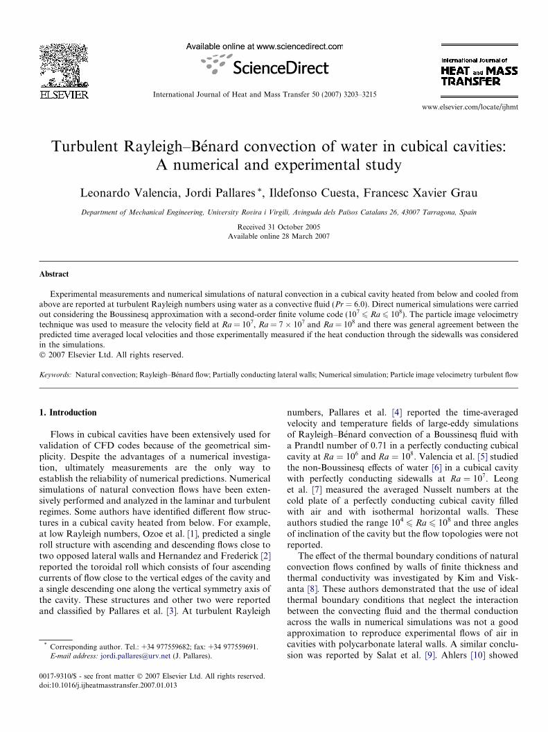
Fig. 3. Velocity fields and RMS values of u at Ra ¼ 107 on the verticalmid-planes. (a) and (b) numerical fields at z ¼ 25 mm and y ¼ 25 mm,respectively, (c) experimental velocity field at y ¼ 25 mm. These planes areindicated in Fig. 2a and b. The reference vectors are depicted near thebottom right corner of each vector plot.

Table 4Integral scale ðs�Þ, number of integral scales sampled ðt�t =s�Þ and statisticalquantities for the averaged Nusselt number at the cold plate ðNuCÞ, and foru*, v* and T* at the point x� ¼ 0:5, y� ¼ 0:75 and z� ¼ 0:5

Integral scale ðs�Þ ðt�t =s�Þ Mean value ðn�Þ RMS

Ra ¼ 107 ðt�t ¼ 1:61ÞNuC 6.2 � 10�4 2595 16.6 0.76u* 8.3 � 10�3 195 25.0 466.1v* 4.9 � 10�3 331 �226.6 233.9T* 8.5 � 10�3 191 �1.3 � 10�4 0.04

Ra ¼ 3� 107 ðt�t ¼ 0:85ÞNuC 4.1 � 10�4 2066 25.1 0.95u* 6.5 � 10�2 13 365.8 926.4v* 3.1 � 10�3 274 �207.2 470.4T* 2.5 � 10�2 35 3.8 � 10�3 0.03

Ra ¼ 5� 107 ðt�t ¼ 0:75ÞNuC 1.2 � 10�3 636 30.7 1.05u* 1.9 � 10�1 4 �511.2 1147.9v* 2.6 � 10�3 285 �264.17 610.4T* 3.5 � 10�2 21 �4.5 � 10�3 0.025

Ra ¼ 7� 107 ðt�t ¼ 0:86ÞNuC 1.4 � 10�3 631 35.0 1.15u* 9.7 � 10�2 9 121.4 1513.8v* 7.7 � 10�4 1111 �266.9 734.2T* 7.9 � 10�2 11 5.5 � 10�4 0.024

Ra ¼ 108ðt�t ¼ 0:56ÞNuC 2.0 � 10�4 2822 40.4 1.19u* 8.1 � 10�2 7 �645.0 1429.5v* 5.0 � 10�4 1116 �329.2 831.5T* 1.2 � 10�2 47 �4.1 � 10�3 0.022


y� ¼ 0:75 and z� ¼ 0:5. It can be seen that the total integra-tion time, at this Rayleigh number, ranges from 191 to

2920 times the integral scale and consequently the numberof data taken is adequate to calculate the time averagedvalues.

At the Rayleigh numbers studied the flow shows largefluctuations in the velocity and temperature fields withrespect to the time averaged values as can be deduced com-paring the time averaged values of the velocity with theircorresponding fluctuation intensities, shown in Fig. 3. Itcan be seen that the RMS values are significantly largerthan the time averaged values near the horizontal midplaneof the cavity indicating an intensive turbulent transfer nearthis region. The mean value and the standard deviation ofthe averaged Nusselt number at the cold plate at Ra ¼ 107

are very similar to those reported by Valencia et al. [5] atthe same Rayleigh number with perfectly conducting lat-eral walls. The mean value/standard deviation is only1.3%/4.2% smaller/larger for the present study.

Fig. 4a and b show the numerical and experimentaltime-averaged velocity profiles along the lines indicated inFig. 3b and c. The maximum differences between the exper-imental and the numerical vertical velocities can beobserved close to the walls (see for example Fig. 4b). Thisdifference can be attributed to the finite size of the interro-gation volumes used in the PIV technique when the velocityis measured in regions with large velocity gradients.

The vertical velocity profile of the time averaged flowstructure in a perfectly conducting cavity at Ra ¼ 107

v_Partially Conducting Walls

v_Experimental Data

w (mm/s)

x(m

m)

-1.0 -0.5 0.0 0.5 1.00

10

20

30

40

50

u_Partially Conducting Wallsu_Experimental Datau_Conducting Walls

z (mm)

u(m

m/s

)

0 10 20 30 40 50

-2.0

-1.5

-1.0

-0.5

0.0

0.5

1.0

1.5

2.0

Fig. 4. Velocity profiles obtained from the simulations and from themeasurements of the time averaged flow topology at Ra ¼ 107. Theseprofiles are indicated in Fig. 3b and c. (a) Horizontal (y) profiles of thevertical velocity component (u), along the line x ¼ 11:1 mm, z ¼ 25 mm(z� ¼ 0:5). (b) vertical (x) profiles of the horizontal velocity component (v)along the lines y ¼ 4:7 mm, z ¼ 25 mm and y ¼ 45:2 mm, z ¼ 25 mm. Thegray squares indicate the size of the interrogation window used in theexperiments.


reported by Valencia et al. [5] is also included in Fig. 4a forcomparison. It can be seen that close to z ¼ 37 mm veloci-ties are about 110% larger for the perfectly conducting cav-ity indicating that the effect of the thermal conductivity ofthe walls is important in the simulations to reproduce theexperimental measurements. Although the averaged Nus-selt number at the horizontal walls in the present studyare very similar to those calculated with perfectly conduct-ing walls, the volume averaged modulus of the velocity vec-

tor is 290 non-dimensional velocity units. This value is 36%smaller for the simulation considering the finite value of thewall thermal conductivity in comparison with the valuereported by Valencia et al. [5] in a perfectly conducting cav-ity. This reduction of the velocities, also shown in Fig. 4a,can be explained with the help of Fig. 5c. This figure showsthe vertical profile ðy� ¼ 1:041Þ of the temperature insidethe wall of the cavity on the mid-plane z� ¼ 0:5, for the sim-ulations with perfectly conducting walls and for the simu-lations considering finite thermal conductivity of thelateral walls. Fig. 5c reveals that in the lower region ofthe cavity ðx� < 0:5Þ, the temperatures for the perfectlyconducting lateral walls are larger than those correspond-ing to simulations with partially conducting walls. Theselarger values of temperature produce an overall increaseof the buoyancy term in the vertical momentum equationin these regions and, consequently, an increase of the mag-nitude of the vertical velocities.

Fig. 5a shows time averaged temperature contours ofthe fluid close to the glass walls on the vertical planesy� ¼ 0:996 and z� ¼ 0:004 at Ra ¼ 107. It can be seen thatthe departure from the linear velocity profile of the per-fectly conducting conditions is found along all the area ofthe lateral walls. The temperature contours on the verticalmid-plane indicated in Fig. 5a are depicted in Fig. 5b. Thisfigure shows that more of the 90% of the volume of thefluid is between the range T � ¼ �0:1 and T � ¼ 0:1 accord-ing to the fact that Pr > 1 and because of the good mixingproduced by the mean flow and the turbulence intensities,that restricts the temperature gradients to the thin thermalboundary layers near the horizontal walls of the cavity. Thetemperature contours in the lateral walls shown in Fig. 5bindicate that the heat transfer in the walls is not only fromthe hot to the cold plates; it can be seen that the heat is alsotransferred from the fluid to the walls in the lower part ofthe cavity and from the walls to the fluid close to the top ofthe cavity.

4.2. Time evolution of the flow structure at Ra = 3 � 107,Ra = 5 � 107, Ra = 7 � 107 and Ra = 108

This section describes the time evolution of the averageflow structure and the averaged Nusselt number at the coldplate at Ra ¼ 3� 107; 5� 107; 7� 107 and 108. Becauseof the similitude of the time averaged flow structures foundin the range 3� 107

6 Ra 6 108, the discussion is centeredin the experimental flow topology measured at Ra ¼7� 107.

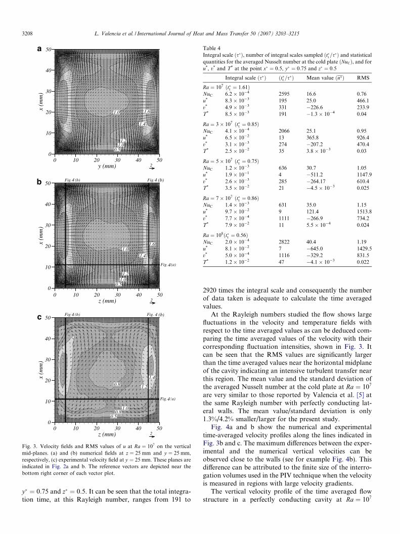
Fig. 6b shows the time evolution of the instantaneousvertical velocity component ðu�Þ at Ra ¼ 7� 107 at the posi-tion x� ¼ 0:5; y� ¼ 0:75 and z� ¼ 0:5. This position insidethe cavity is indicated in Fig. 6a and c. The time evolutionof the vertical velocity component shown in Fig. 6b has verylow frequencies superimposed to a range of higher frequen-cies. It can be seen that the low frequencies produce largeperiods of time of positive instantaneous values (for exam-ple between 0.1 and 0.25 non-dimensional units of time)

X

Z

Y

-0.5

0.3

0.0

-0.1

-0.3

-0.15

0.1

0.05

0.15

-0.05

-0.2

0.2

Contour Plotof Fig. 7(b)

Tw*

x*

-0.4 -0.2 0.0 0.2 0.40.0

0.2

0.4

0.6

0.8

1.0

0.0

0.0

y*

x*

0.0 0.2 0.4 0.6 0.8 1.00.0

0.2

0.4

0.6

0.8

1.0

-0.1

0.1

0.5

Fluid/Glass WallsBoundary

-0.5Fig.7 )

0.2

-0.2

Partiallyconducting walls

Perfectlyconducting walls

5

5(c

Fig. 5. (a) Temperature contours of the time averaged temperature field ofthe fluid close to the glass walls at Ra ¼ 107, (b) temperature contours onthe vertical mid-plane, (c) temperature profile indicated in figure (b) forthe simulations with perfectly conducting walls and considering the finiteconductivity of the lateral walls.


followed by periods in which the values are negative (forexample between 0.3 and 0.5 non-dimensional units oftime). The different time averaged flow fields obtained byaveraging the instantaneous flow during the periods of timecorresponding to the low frequencies have been identified asfour different flow configurations that are denoted as (A),(B), (C) and (D). It can be considered that the low frequencytime evolution corresponds to the periodic oscillation of theflow between these four basic flow configurations.

These four averaged flow configurations were obtainedby averaging the velocity flow field during different periodsof time. Each period of time could contain from 0.03 to0.16 non-dimensional time units. The four possible config-urations of the average flow structure obtained atRa ¼ 7� 107 are depicted in Fig. 6c in terms of the verticalvelocity contours on the horizontal mid-plane x� ¼ 0:5.The period of time in which each configuration occurs inthe time evolution of the vertical velocity of the analyzedpoint is indicated above the horizontal axis of Fig. 6b.

The averaged flow structure of each configuration con-sists in two main descending and ascending flows thatoccur close to two diagonally opposed vertical edges simi-lar to the laminar flow topology named S2 in previousstudies [3]. Fig. 7 shows the averaged flow structure interms of isosurfaces of two values of the vertical velocityfor configuration (C) (i.e. ascending fluid near the cornery ¼ 92 mm, z = 0 mm and descending fluid neary ¼ 0 mm, z ¼ 92 mm). The time averaged flow topologyof this configuration can also be seen in Fig. 8 in termsof the velocity vectors field on the vertical mid-planes(z� ¼ 0:5 and y� ¼ 0:5) of the cavity (see Fig. 8a and b).It can be seen that this combination of main ascendingand descending flows is associated with a single rollingmotion with its axis of rotation horizontally oriented andperpendicular to two diagonally opposed vertical edges ofthe cavity. Fig. 6c shows that the main difference betweenthe flow configurations or positions of the flow topologyis the diagonally opposed pair of corners used by the fluidto ascend from the hot plate and descend from the coldplate. For example, Fig. 6b indicates that the positive meanvertical velocities at the position x� ¼ 0:5, y� ¼ 0:75 andz� ¼ 0:5 are found in configurations (C) and (D) and thenegative mean vertical velocities occur in configurations(A) and (B). The change of the sign of the instantaneousvertical velocity plotted in Fig. 6b agrees with the changesof the configuration of the structure. The changes frompositive to negative velocity values indicate that the meanflow structure evolves from (A) to (D) or from (B) to (C)and the changes from negative to positive values, corre-spond to the inverse evolutions. This change of flow config-uration, which has associated a very low frequency, can beunderstood as a progressive rotation on the horizontalplane of the rotation axis of the single roll flow structure.It can be seen in Fig. 6b that this rotation of the roll axis,or of the overall flow structure, around the vertical axis ofthe cavity that produces the evolution between two flowconfigurations can be clockwise (i.e. from (A) to (D)) or

X

Z

Y

y*=0.75

x*=0.5

z*=0.5

2300

17001000

400

0

-400

400

-400

-1000-1700

-2300

y*

z*

0 0.2 0.4 0.6 0.8 10

0.2

0.4

0.6

0.8

1

-2300

-1700

-1000

-400

0

400

1000

1700

2300

400

-400

y*

z*

0 0.2 0.4 0.6 0.8 10

0.2

0.4

0.6

0.8

1

-2300-1700

-1000-400

0

400

1000

1700

2300

400

-400

y*

z*

0 0.2 0.4 0.6 0.8 10

0.2

0.4

0.6

0.8

1

2000

1700

1000

400

0

-400

-1000-1700

-2000

-400

400

y*

z*

0 0.2 0.4 0.6 0.8 10

0.2

0.4

0.6

0.8

1

Position of thetime series plotted in Fig. 6.b

(A)

(B) (C)

(D)

c

Fig. 6. (a) Sketch of the position of the point used in the analysis of the time evolution of some variables (see figure (b) and Table 4), (b) time evolution ofthe vertical velocity component (u*) at the position indicated in figure (a), the letters (A), (B), (C) or (D) near the x-axis indicate the configuration (seefigure (c)) of the flow structure in the period of time showed by the parenthesis. (c) Contours of the vertical velocity (u*) on the horizontal mid-plane for thefour configurations of the structure at Ra ¼ 7� 107. Continuous/dashed line contours correspond to positive/negative values. The black point indicatesthe position depicted in figure (a).


anticlockwise (i.e. from (A) to (B)). It should be noted thatthe direct transition from (A) to (C), (C) to (A), (B) to (D)or (D) to (B) are not possible, and in fact have notobserved, according to the rotation of the flow structure.The change of orientation of the averaged flow structurealso occurs at Ra ¼ 3� 107, 5� 107 and 108. It has beenobserved that the flow in the range 3� 107

6 Ra 6 108

evolves erratically between the different flow configurationsand it was not possible to found a clear relation between

the Rayleigh number and the time in which the flow main-tains a certain configuration or the time needed by the flowto change between configurations.

The observed evolution of the flow between the differentconfigurations in the range 3� 107

6 Ra 6 108 impliesdifferent statistical properties of the time evolution of thedifferent variables of the flow. Since these flow transi-tions occur at very low frequencies, the statistical proper-ties of the variables that are sensitive to the particular

X

YZ


u*=1000AscendingFluid


u*=-1000DescendingFluid

8 8

Fig. 7. Time averaged flow field at Ra ¼ 7� 107 for the (C) configurationwith a total integration time of t�t ¼ 0:16 (156 min) in terms of theisosurfaces of the vertical velocity component, u� ¼ �1000.

0.6

1.01.1

1.4

0.9

0.9

z (mm)

x(m

m)

0 20 40 60 800

20

40

60

80

3

Fig. 11(a)

Fig. 11(a)

0.81.4

1.61.8

2.5

1.4

z (mm)

x(m

m)

0 20 40 60 800

20

40

60

80

3

Fig. (a)

Fig. 11(a)

1.6

0.81.4

1.82.5 1.4

y (mm)

x(m

m)

0 20 40 60 800

20

40

60

80

3

9

9

9

9

Fig. 8. Velocity fields and RMS values of u at Ra ¼ 7� 107 on the verticalmid-planes. (a) and (b) numerical fields at z ¼ 46 mm and y ¼ 46 mm,respectively (c) experimental velocity field at y ¼ 46 mm. These planes areindicated in Fig. 7. The reference vectors are depicted near the bottomright corner of each vector plot.


configuration of the flow are different from those that aremore insensitive to the flow configuration. Table 4 showsthat at the Rayleigh numbers in which the single roll isobserved ð3� 107

6 Ra 6 108Þ the integral time scales ofthe vertical velocity and temperature on the horizontalmid plane of the cavity are drastically reduced in compari-son with the evolutions of these variables at Ra ¼ 107

because of the important contribution of the low frequenciesassociated with the transition between different flow config-urations in their time evolutions. On the contrary the timeevolution of other quantities, as the horizontal velocity com-ponent or the averaged Nusselt number which are not signi-ficantly affected by the evolution between configurations,show integral time scales of the same order of magnitudeas those at Ra ¼ 107. Table 4 shows that the increase ofthe RMS values as the Rayleigh is increased is more evidentin the variables insensitive to the particular flow configura-tion than in the sensitive quantities. It is important to notethat the influence of the low frequency evolution in the inte-gral time scale of some specific flow quantities should betaken into account to determine adequate sampling periodsfor the calculation of the flow statistics.

The averaging procedure during the experiments atRa ¼ 7� 107 and at Ra ¼ 108 was performed during 13and 8 h, respectively. The time evolution of the verticalvelocity at x� ¼ 0:5, y� ¼ 0:75 and z� ¼ 0:5 does not showlow frequencies. However, the averaged flow structure ofthe vector field showed good agreement with the individualflow configuration obtained numerically (i.e. configura-tions (A), (B), (C) and (D)). This indicates that the timeaveraged flow structure experimentally obtained corre-sponds to only one of the flow configurations obtainednumerically and consequently, it can be concluded thatthe transition between the configurations is not producedin the experiments.


In order to check the influence of the horizontal inclina-tion of the cavity, a simulation at Ra ¼ 7� 107 was carriedout with 0.1� of inclination in the y-direction and 0.2� inthe z-direction. The time averaged flow structure obtainedwith this inclination was perfectly identified as the (D) con-figuration. In this case, the time evolution of the velocitiesdid not show low frequencies and transition between flowconfigurations was not observed. This indicates that therelative stability of the configuration observed experimen-tally can be explained by the small horizontal misalign-ments of the experimental cavities that were estimated tobe of the same order of magnitude than those introducedin this numerical simulation.

Because of the similitude of the time averaged flowstructures found in the range 3� 107

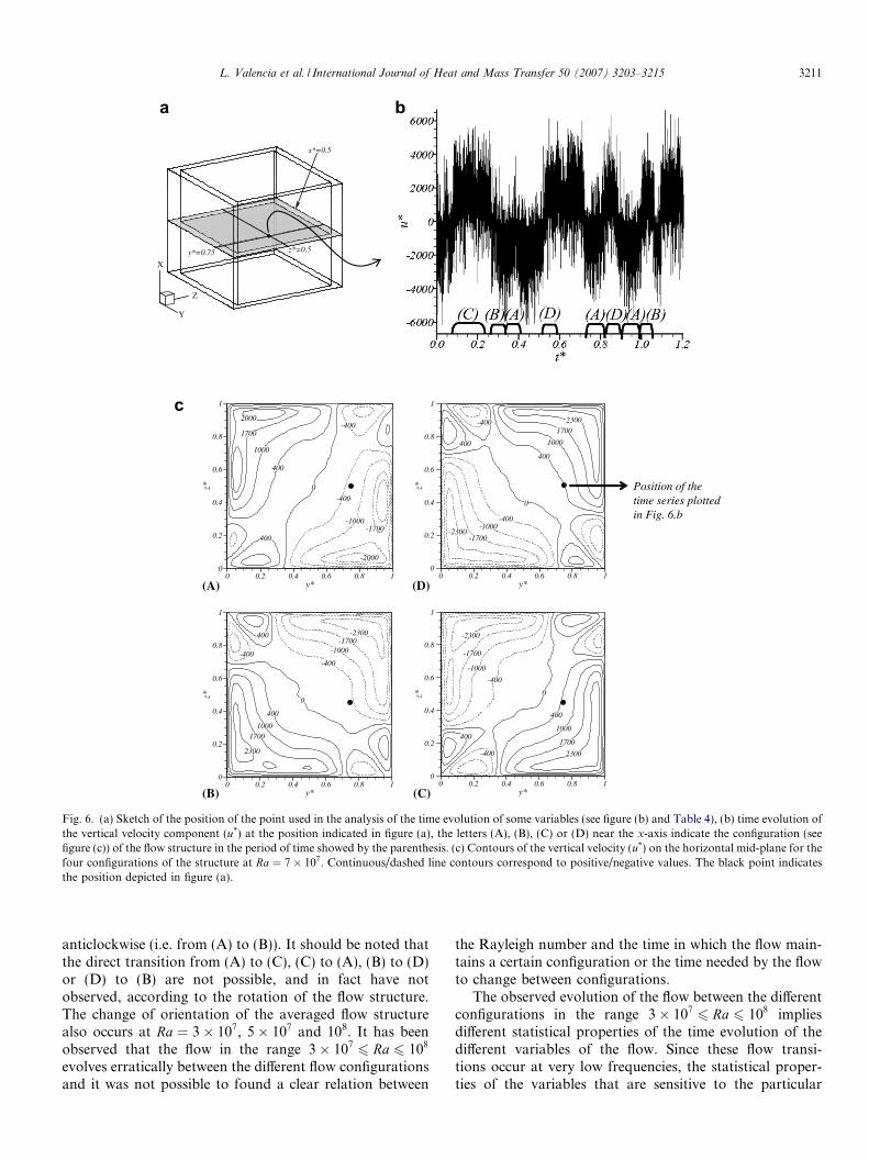
6 Ra 6 108, onlythe flow topologies at Ra ¼ 7� 107 and Ra ¼ 108 obtainednumerically were validated with experiments. Although theaveraging time during the experiments was 13/9 h atRa ¼ 7� 107=Ra ¼ 108 only 3.5 h, 1.5 h, 2.6 h and 1.2 h/2.9 h, 3.9 h and 1.2 h were used for the configurations(A), (B), (C) and (D)/(A), (B) and (C), respectively,obtained numerically (t�t ¼ 0:22, t�t ¼ 0:09, t�t ¼ 0:16 andt�t ¼ 0:08=t�t ¼ 0:19, t�t ¼ 0:25 and t�t ¼ 0:08, respectively).

Fig. 8 shows the velocity fields and the RMS values onthe vertical mid-planes at Ra ¼ 7� 107. In Fig. 8a and bthe (C) configuration is plotted for the numerical simula-tions on the mid-planes z� ¼ 0:5 and y� ¼ 0:5, respectively.The corresponding measured velocity vector field on the

y, z (mm)

w (mm/s)

u(m

m/s

)

x(m

m)

0 20 40 60 80

-4.0 -3.0 -2.0 -1.0 0.0 1.0 2.0

-4.0

-3.0

-2.0

-1.0

0.0

1.0

2.0

3.0

0

20

40

60

80

Ra=7×107

Experim

DNS, ADNS, BDNS, CDNS, D

Fig. 9. Velocity profiles of the four possible configurations obtained numehorizontal/vertical velocity component ðv=uÞ along the line y ¼ 16:5=x ¼ 65:8horizontal axis corresponds to y for the configurations A and B, and to z for throtated in order to obtain comparable velocity profiles and the horizontal axisindicated in Fig. 8a and b. The gray squares indicate the size of the interroga

mid-plane at Ra ¼ 7� 107 is shown in Fig. 8c. It can beseen that there is a good qualitative agreement betweenthe numerical and experimental velocity vectors and theRMS values of u, indicating that the experimental flowstructure is well predicted by the numerical simulation.Fig. 9a shows the velocity profiles along the solid lines indi-cated in Fig. 8b and c for the (C) configuration. Note thatthe profiles corresponding to the other three configurationshave been rotated accordingly to make the profiles compa-rable. Fig. 9b shows the velocity profiles at Ra ¼ 108 alongthe same lines used at Ra ¼ 7� 107 for the three configura-tions obtained at this Rayleigh number ((A), (B) and (C)).It can be seen that, in general, the measured velocities arewithin the numerically predicted velocity profiles for thedifferent flow configurations.

The averaged flow structure obtained from the averag-ing of the different flow configurations at Ra ¼ 7� 107 isshown in Fig. 10, in terms of isosurface of the second larg-est eigenvalue of the velocity gradient tensor [19] (Fig. 10a)and in terms of the velocity vectors field on a vertical mid-plane of the cavity ðz� ¼ 0:5Þ (Fig. 10b). It can be seen thatthe averaging of the different orientations of the single roll,corresponding to the different flow configurations, pro-duces the same overall two-ring flow topology observedat Ra ¼ 107 (see Fig. 2a). This is consistent with the averageflow structure that would be obtained by rotating, forexample, the flow configuration shown in Fig. 8b, withrespect to the vertical axis of the cavity.

y, z (mm)

w (mm/s)

u(m

m/s

)

x(m

m)

0 20 40 60 80

-4.0 -3.0 -2.0 -1.0 0.0 1.0 2.0

-5.0

-4.0

-3.0

-2.0

-1.0

0.0

1.0

2.0

3.0

4.0

0

20

40

60

80

Ra=108

ental results

configurationconfigurationconfigurationconfiguration

rically and measured experimentally. Vertical/horizontal profile of themm, y ¼ 46 mm (y� ¼ 0:5) (a) at Ra ¼ 7� 107 and (b) at Ra ¼ 108. Thee configurations C and D. The configuration D at Ra ¼ 7� 107 had to be

has to be read inversely, from 92 to 0 mm. The profiles at Ra ¼ 7� 107 aretion window used in the experiments.

X

YZ


y*

x*

0 0.2 0.4 0.6 0.8 10

0.2

0.4

0.6

0.8

1

2000

10

Fig. 10. Time averaged flow field calculated using four average data setsof approximately 3:7� 105 time steps of each configuration ((A), (B), (C)and (D)) at Ra ¼ 7� 107 (a) in terms of the isosurface of a constant value(k2=jk2;maxj ¼ �0:036Þ of the second largest eigenvalue of the velocitygradient tensor and (b) in terms of the velocity field in the vertical mid-plane z� ¼ 0:5.


5. Concluding remarks

The time evolving and time average flow structures inthe range 107 < Ra < 108 were studied numerically andexperimentally for water in a cubical enclosure heated frombelow with partially conducting lateral walls. The timeaveraged flow structure obtained at Ra ¼ 107 consisted intwo main counter rotating vortex rings parallel to the hor-izontal walls. In the range 3� 107 < Ra < 108 the flow wascharacterized by a single rolling motion with ascending anddescending currents located close to two diagonallyopposed vertical edges. The time evolution of the verticalvelocity component in one point of the cavity in this range

of Rayleigh numbers shows low frequencies that corre-spond to the progressive rotation of this single roll motionaround the vertical axis of the cavity. For the Rayleighstudied here, it was not possible to found a clear relationbetween the Rayleigh number and the time in which theflow maintains a certain configuration or the time neededby the flow to change between configurations. The timeaveraged flow topologies numerically predicted were alsoobserved experimentally using the PIV technique atRa ¼ 107. At Ra ¼ 7� 107 and Ra ¼ 108 the rotation ofthe orientation of the single roll obtained numericallywas not observed, probably because of the extreme sensi-tivity of this rotation to the horizontal misalignments ofthe cavity, as suggested by numerical simulations of theflow in cavities with small inclinations. The differences ofthe averaged heat transfer rates and the overall flow struc-ture between partially conducting walls and perfectly con-ducting lateral walls at Ra ¼ 107 are not significant butdifferences in velocities can reach 110% indicating thatthe experimental results are better predicted when a finitethermal conductivity is considered in the calculations.Finally, this study shows that the numerical prediction ofRayleigh–Benard convection in a cubical cavity at interme-diate Rayleigh numbers is an excellent benchmark problemfor the study of transitional flows.

Acknowledgement

This study was financially supported by the SpanishMinistry of Science and Technology under projectsDPI2003-06725-C02-01 and VEM2003-20048.

References

[1] H. Ozoe, K. Yamamoto, S.W. Churchill, H. Sayama, Three-dimen-sional, numerical analysis of laminar natural convection in a confinedfluid heated from below, J. Heat Transfer 98 (1977) 202–207.

[2] R. Hernandez, R.L. Frederick, Spatial and thermal features of threedimensional Rayleigh–Benard convection, Int. J. Heat Mass Transfer37 (3) (1994) 411–424.

[3] J. Pallares, I. Cuesta, F.X. Grau, F. Giralt, Natural convection in acubical cavity heated from below at low Rayleigh numbers, Int. J.Heat Mass Transfer 39 (15) (1996) 3233–3247.

[4] J. Pallares, I. Cuesta, F.X. Grau, Laminar and turbulent Rayleigh–Benard convection in a perfectly conducting cubical cavity, Int. J.Heat Fluid Flow 23 (2002) 346–358.

[5] L. Valencia, J. Pallares, I. Cuesta, F.X. Grau, Rayleigh–Benardconvection of water in a perfectly conducting cubical cavity: effects oftemperature – dependent physical properties in laminar and turbulentregimes, Numer. Heat Transfer, Part A: Appl. 47 (5) (2005) 333–352.

[6] D.D. Gray, A. Giorgini, The validity of the Boussinesq approxima-tion for liquids and gasses, Int. J. Heat Mass Transfer 19 (1976) 545–551.

[7] W.H. Leong, K.G.T. Hollands, A.P. Brunger, Experimental Nusseltnumbers for a cubical-cavity benchmark problem in natural convec-tion, Int. J. Heat Mass Transfer 42 (11) (1999) 1979–1989.

[8] D.M. Kim, R. Viskanta, Study of the effects of wall conductance onnatural convection in differently oriented square cavities, J. FluidMech. 144 (1984) 153–176.

[9] J. Salat, S. Xin, P. Joubert, A. Sergent, F. Penot, P. LeQuere,Experimental and numerical investigation of turbulent natural


convection in a large air-filled cavity, Int. J. Heat Fluid Flow 25(2004) 824–832.

[10] G. Ahlers, Effect of sidewall conductance on heat-transport measure-ments for turbulent Rayleigh–Benard convection, Phys. Rev. E 63(2000) 015303/1-4.

[11] R. Verzicco, Sidewall finite-conductivity effects in confined turbulentthermal convection, J. Fluid Mech. 473 (2002) 201–210.

[12] M.P. Arroyo, J.M. Saviron, Rayleigh–Benard convection in a smallbox: spatial features and thermal dependence of the velocity field, J.Fluid Mech. 235 (1992) 325–348.

[13] M. Raffel, C. Willert, J. Kompenhans, Particle Image Velocimetry,first ed., Springer, Berlin, 1998.

[14] L. Valencia, Estudio numerico y experimental del flujo Rayleigh–Benard en cavidades cubicas para regimen transitorio y turbulento,Ph.D. thesis, Universitat Rovira i Virgili, Tarragona, Spain, 2005.

[15] F.P. Incropera, D.P. DeWitt, Fundamentos de Transferencia deCalor, fourth ed., Pearson–Prentice Hall, Mexico, 1996, pp. 846–847.

[16] M.C. Potter, D.C. Wiggert, Mecanica de Fluidos, second ed.,Prentice-Hall, Mexico, 1997, pp. 754.

[17] J.P. Holman, Heat Transfer, fourth ed., Mc Graw-Hill KogakushaLtd., Tokyo, 1976, pp. 253, 499, 507.

[18] I. Cuesta, Estudi Numeric de Fluxos Laminars i Turbulents en unaCavitat Cubica, Ph.D. thesis, Universitat Rovira i Virgili, Tarragona,Spain, 1993.

[19] J. Jeong, F. Hussain, On the identification of a vortex, J. Fluid Mech.285 (1995) 69–80.

[20] B. Lecordier, D. Demare, L.M.J. Vervisch, J. Reveillon, M. Trinite,Estimation of the accuracy of PIV treatments for turbulent flowstudies by direct numerical simulation of multi-phase flow, Measur.Sci. Technol. 12 (2001) 1382–1391.

Turbulent Rayleigh–Bénard convection of water in cubical cavities: A numerical and experimental...

Documents

Transcript of Turbulent Rayleigh–Bénard convection of water in cubical cavities: A numerical and experimental...