Heat transfer and large scale dynamics in turbulent Rayleigh-Bénard convection

Heat transfer and large scale dynamics in turbulent Rayleigh-Bénardconvection

Guenter Ahlers*

Department of Physics and iQCD, University of California, Santa Barbara, California93106, USA

Siegfried Grossmann†

Fachbereich Physik, Philipps-Universität Marburg, D-35032 Marburg, Germany

Detlef Lohse‡

Physics of Fluids Group, Department of Science and Technology, J. M. Burgers Centrefor Fluid Dynamics, and Impact-Institute, University of Twente, 7500 AE Enschede,The Netherlands

�Published 22 April 2009�

The progress in our understanding of several aspects of turbulent Rayleigh-Bénard convection isreviewed. The focus is on the question of how the Nusselt number and the Reynolds number dependon the Rayleigh number Ra and the Prandtl number Pr, and on how the thicknesses of the thermal andthe kinetic boundary layers scale with Ra and Pr. Non-Oberbeck-Boussinesq effects and the dynamicsof the large scale convection roll are addressed as well. The review ends with a list of challenges forfuture research on the turbulent Rayleigh-Bénard system.

DOI: 10.1103/RevModPhys.81.503 PACS number�s�: 47.27.te, 47.55.P�, 47.27.T�

CONTENTS

I. Introduction 503

II. Theories of Global Properties: The Nusselt and

Reynolds Number 506

A. Older theories for Nu�Ra,Pr� and Re�Ra,Pr� 506

B. Grossmann-Lohse theory for Nu�Ra,Pr� and

Re�Ra,Pr� 507

C. Is there an asymptotic regime for large Ra?, and

strict upper bounds 510

III. Experimental Measurements of the Nusselt Number 511

A. Overview 511

B. Sidewall and top- and bottom-plate-conductivity

effects on Nu 512

C. The Nusselt number for Pr�4.38 obtained using

water as the fluid 513

D. The Prandtl-number dependence of the Nusselt

number 513

E. The aspect-ratio dependence of the Nusselt number 514

F. The insensitivity of the Nusselt number to the LSC 514G. The dependence of Nu on Ra at very large Ra 515

IV. Experimental Measurements of the ReynoldsNumbers 518

A. Reynolds numbers based on the large scaleconvection roll 518

B. Reynolds numbers based on plume motion 519V. Nu�Ra,Pr� and Re�Ra,Pr� in Direct Numerical

Simulations 520VI. Boundary Layers 522

A. Relevance of boundary layers and challenges 522B. Thermal boundary layers 522C. Kinetic boundary layers 524

VII. Non-Oberbeck-Boussinesq Effects 526VIII. Global Wind Dynamics 528

A. Experiment 528B. Models 529

IX. Issues for Future Research 530Acknowledgments 531References 531

I. INTRODUCTION

Rayleigh-Bénard �RB� convection—the buoyancydriven flow of a fluid heated from below and cooledfrom above—is a classical problem in fluid dynamics. Itplayed a crucial role in the development of stabilitytheory in hydrodynamics �Chandrasekhar, 1981; Drazinand Reid, 1981� and had been paradigmatic in patternformation and in the study of spatial-temporal chaos�Getling, 1998; Bodenschatz et al., 2000�. From an ap-plied viewpoint, thermally driven flows are of utmostimportance. Examples are thermal convection in the at-mosphere �see, e.g., Hartmann et al. �2001��, in theoceans �see, e.g., Marshall and Schott �1999�� includingthermohaline convection; see, e.g., Rahmstorf �2000��, inbuildings �see, e.g., Hunt and Linden �1999��, in processtechnology, and in metal-production processes �see, e.g.,Brent et al. �1988��. In the geophysical and astrophysicalcontext, we mention convection in the Earth’s mantle�see, e.g., McKenzie et al. �1974��, in the Earth’s outer

*[email protected]†[email protected]‡[email protected]

REVIEWS OF MODERN PHYSICS, VOLUME 81, APRIL–JUNE 2009

0034-6861/2009/81�2�/503�35� ©2009 The American Physical Society503

http://dx.doi.org/10.1103/RevModPhys.81.503

core �see, e.g., Cardin and Olson �1994��, and in starsincluding our Sun �see, e.g., Cattaneo et al. �2003��. Con-vection has been associated with the generation and re-versal of the Earth’s magnetic field �see, e.g., Glatzmaierand Roberts �1995��.

Even if one restricts oneself to thermally driven flowsin a closed box, there are so many aspects that not all ofthem can be addressed in this single review. We focus ondeveloped turbulence when spatial coherence through-out the cell is lost and only on the large scale dynamicsof the flow and aspects intimately connected with it,such as the boundary layer structures. The scaling of thespectra of velocity and temperature fluctuations, or ofthe corresponding structure functions, will not be ad-dressed. These issues had been discussed in the reviewby Siggia �1994�, but meanwhile considerable progresshas been achieved, in particular on the question ofwhether and where in the flow to expect Bolgiano-Obukhov scaling �Bolgiano, 1959; Obukhov, 1959; Mo-nin and Yaglom, 1975� of the structure functions; see,e.g., Calzavarini et al. �2002�; Sun et al. �2006�; Kunnen etal. �2008�. For a very recent review on these issues, werefer to Lohse and Xia �2010�.

The question to be asked about the Rayleigh-Bénardproblem is as follows: For a given fluid in a closed con-tainer of height L heated from below and cooled fromabove, what are the flow properties inside the containerand, in addition, what is the heat transfer from bottomto top? Here spatially and temporally constant tempera-tures are assumed at the bottom and top. In Sec. III wediscuss to what degree this assumption can be justified inreality �Chaumat et al., 2002; Verzicco, 2004; Brown,Funfschilling, et al., 2005�.

The problem is further simplified by the so-calledOberbeck-Boussinesq �OB� approximation �Oberbeck,1879; Boussinesq, 1903; Landau and Lifshitz, 1987� inwhich the fluid density � is assumed to depend linearlyon the temperature,

��T� = ��T0��1 − ��T − T0�� , �1�

with � the thermal expansion coefficient. In addition, itis assumed that the material properties of the fluid suchas �, the viscosity �, and the thermal diffusivity � do notdepend on temperature. The governing equations of theRB problem are then the Oberbeck-Boussinesq equa-tions �Landau and Lifshitz, 1987�

�tui + uj�jui = − �ip + ��j2ui + �g�i3� , �2�

�t� + uj�j� = ��j2� �3�

for the velocity field u�x , t�, the kinematic pressure fieldp�x , t�, and the temperature field ��x , t� relative to somereference temperature. Here and in the following we as-sume summation over double indices; �ij is the Kro-necker symbol. The Oberbeck-Boussinesq equations areassisted by continuity �iui=0 and the boundary condi-tions u=0 for the velocities at all walls, ��z=−L /2�=� /2 for the temperature at the bottom plate,and ��z=L /2�=−� /2 for the temperature at the top

plate. At the sidewalls the condition of no lateral heatflow is imposed. The limitations of the Oberbeck-Boussinesq approximations are discussed in Sec. VII.

Within the OB approximation and for a given cell ge-ometry, the system is determined by only two dimen-sionless control parameters, namely, the Rayleigh num-ber and the Prandtl number,

Ra =�gL3�

��, Pr =

�

�. �4�

The cell geometry is described by its symmetry and oneor more aspect ratios . For a cylindrical cell �d /L,where d is the cell diameter.

The key response of the system to the imposed Ra isthe heat flux H from bottom to top. The dimensionlessheat flux Nu=H /�L−1 is the Nusselt number. Here =cp�� is the thermal conductivity. Within the Oberbeck-Boussinesq approximation one obtains for incompress-ible flow

Nu =�uz��A − ��3��A

��L−1 . �5�

Here �·�A denotes the average over �any� horizontalplane and over time. Correspondingly, �·�V used belowdenotes the volume and time average.

Another key system response is the extent of turbu-lence, expressed in terms of a characteristic velocity am-plitude U, nondimensionalized by �L−1 to define a Rey-nolds number

Re =U

�L−1 . �6�

As we show in Sec. IV, there are various reasonable pos-sibilities to choose a velocity, e.g., the components or themagnitude of the velocity field at different positions, lo-cal or averaged amplitudes, turnover times or frequencypeaks in the thermal spectrum, etc. In some parameterranges these amplitudes differ not only in magnitude buteven show different dependences on Ra and Pr �Brownet al., 2007; Sugiyama et al., 2009�. Mostly we restrictourselves to that Reynolds number which is associatedwith the large scale circulation �LSC�, also called the“wind of turbulence” U �Niemela et al., 2001; Xia et al.,2003; Sun, Xia, and Tong, 2005�. There is discussion inthe literature whether or not the LSC evolves out of thewell-known cellular structures at small Ra. On the onehand, Krishnamurti and Howard �1981� performed ex-periments from which they concluded that the LSC isnot a simple reminder and continuation of the roll struc-ture observed just after the onset of convection. On theother hand, we are not aware that their observationshave been confirmed. Even an explicit search for such amode as Krishnamurti and Howard �1981� reported wasnot successful; see the review by Busse �2003� andHartlep et al. �2005�. They concluded that the LSC atlarge Ra indeed is a reminder of the low Ra structures.The dynamics of the large scale wind, its azimuthal os-cillation, diffusion, reorientation, cessation, and possible

504 Ahlers, Grossmann, and Lohse: Heat transfer and large scale dynamics in …

Rev. Mod. Phys., Vol. 81, No. 2, April–June 2009

breakdown at very large Ra are discussed in detail inSec. VIII.

The key question to ask is: How do Nu and Re de-pend on Ra and Pr? The experimental situation will bethe subject of Sec. III for Nu�Ra,Pr� and Sec. IV forRe�Ra,Pr�. Results from numerical simulations are re-ported in Sec. V. However, first �Sec. II� we summarizeolder theories �Sec. II.A� and then �Sec. II.B� theGrossmann-Lohse �GL� theory �Grossmann and Lohse,2000, 2001, 2002, 2004�. In Sec. II.C we discuss theoriesabout a possible asymptotic regime at very large Ra andstrict upper bounds for Nu.

Section VI is devoted to the structure and width of thethermal and kinetic boundary layers �BLs�. The thermal

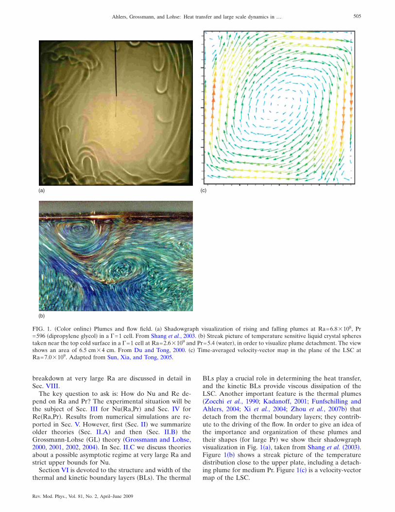
BLs play a crucial role in determining the heat transfer,and the kinetic BLs provide viscous dissipation of theLSC. Another important feature is the thermal plumes�Zocchi et al., 1990; Kadanoff, 2001; Funfschilling andAhlers, 2004; Xi et al., 2004; Zhou et al., 2007b� thatdetach from the thermal boundary layers; they contrib-ute to the driving of the flow. In order to give an idea ofthe importance and organization of these plumes andtheir shapes �for large Pr� we show their shadowgraphvisualization in Fig. 1�a�, taken from Shang et al. �2003�.Figure 1�b� shows a streak picture of the temperaturedistribution close to the upper plate, including a detach-ing plume for medium Pr. Figure 1�c� is a velocity-vectormap of the LSC.

(c)(a)

(b)

FIG. 1. �Color online� Plumes and flow field. �a� Shadowgraph visualization of rising and falling plumes at Ra=6.8�108, Pr=596 �dipropylene glycol� in a =1 cell. From Shang et al., 2003. �b� Streak picture of temperature sensitive liquid crystal spherestaken near the top cold surface in a =1 cell at Ra=2.6�109 and Pr=5.4 �water�, in order to visualize plume detachment. The viewshows an area of 6.5 cm�4 cm. From Du and Tong, 2000. �c� Time-averaged velocity-vector map in the plane of the LSC atRa=7.0�109. Adapted from Sun, Xia, and Tong, 2005.

505Ahlers, Grossmann, and Lohse: Heat transfer and large scale dynamics in …


As mentioned, Sec. VII is devoted to non-Oberbeck-Boussinesq effects and Sec. VIII deals with the globalwind dynamics. In Sec. IX we outline some major issuesin Rayleigh-Bénard convection for future research.

II. THEORIES OF GLOBAL PROPERTIES: THE NUSSELTAND REYNOLDS NUMBER

A. Older theories for Nu(Ra,Pr) and Re(Ra,Pr)

For a detailed discussion of the theories developedprior to the review by Siggia �1994� we refer the readerto that paper and to Chandrasekhar �1981�. These theo-ries predicted power laws

Nu Ra�NuPr Nu, �7�

Re Ra�RePr Re �8�

for the dependences of Nu and Re on Ra and Pr. Asummary of predicted exponents is given in Table I.Early experiments were of limited precision, and wereconsistent with power-law dependences over their lim-ited ranges of Ra and Pr.

The conceptually easiest early theory is Malkus’marginal-stability theory of 1954. It assumed that thethermal BL thickness adjusts itself so as to yield a criti-cal BL Rayleigh number. This immediately gave �Nu=1/3. After the experiments by Chu and Goldstein�1973�, Threlfall �1975� and the later ground-breakingChicago experiments in cryogenic helium �Heslot et al.,1987; Castaing et al., 1989; Wu et al., 1990; Sano et al.,1989; Procaccia et al., 1991� had suggested a smallerpower-law exponent, the Chicago group developed themixing-zone model �Castaing et al., 1989� which laterwas extended by Cioni et al. �1997� to include thePrandtl-number dependences. The central result was�Nu=2/7. The same scaling exponent could also be ob-tained from the BL theory of Shraiman and Siggia�1990�, assuming a turbulent boundary layer. The as-

sumptions of that theory are, however, very differentfrom those of the mixing-layer theory, leading to verydifferent power-law exponents for the dependences onthe Prandtl number; see Table I.

As we show later, the assumption of a fully developedturbulent BL is far from being fulfilled in the parameterregime of the Chicago experiments. That can already beseen from an estimate of the coherence length � of theRB flow. Taking the data from Procaccia et al. �1991� forthe scaling of the velocity fluctuations and of the cross-over frequency to the viscous subrange, Grossmann andLohse �1993� obtained � /L50 Ra−0.32. For the =1/2cell of Procaccia et al. �1991� this implies that only atRa108 the coherence length becomes about 1/3 of thelateral cell width and 1/6 of its height, a pre-requisite forindependent fluctuations to develop in the bulk. Esti-mates based on �10�, where � is the �locally or glo-bally defined� Kolmogorov scale, give similar results.The transition to turbulence in the BL is correspond-ingly expected only at much large Ra, namely, at Ra1014 �at the edge of the achievable regime in the Chi-cago experiments�, as we show in the next section.

In any case, at “large enough” Rayleigh number atransition should occur towards an ultimate Rayleigh-number regime. Such a regime was first suggested byKraichnan �1962�. Spiegel �1971� hypothesized that inthat regime the heat flux and the turbulence intensityare independent of the kinematic viscosity and the ther-mal diffusivity, which leads to �Nu=1/2 �for more details,see Sec. II.C�. Though in those days �1971 and before�no measured power-law exponent was even close to thatvalue, that paper has been extremely influential, perhapsalso because from a mathematical point of view nolower strict upper bound than �Nu=1/2 could be provento exist for finite Pr �see Doering and Constantin�1996��.

As shown in Sec. III and IV, the experiments of thelast decade reveal the limitations of most of these oldertheories.

TABLE I. Power-law exponents for Nu and Re as functions of Ra and Pr predicted by theoriesdeveloped prior to the review by Siggia �1994�. The exponents are defined by Eqs. �7� and �8�.Whereas Re is based on the large scale wind velocity, Refluct is based on the velocity fluctuations.

Reference Pr and Ra range �Nu Nu �Re �Refluct Re

Davis �1922a, 1922b� Ra small 1 /4Malkus �1954� 1/3Kraichnan �1962� Ra ultimate,

Pr�0.151/2 1/2 1/2 −1/2

Ra ultimate,0.15�Pr�1

1/2 −1/4 1/2 −3/4

Spiegel �1971� Ra ultimate 1/2 1/2 1/2 −1/2Castaing et al. �1989� 2/7 1/2 3/7Shraiman and Siggia �1990� Pr�1 2/7 −1/7 3/7 −5/7Yakhot �1992� 5/19 8/19Zaleski �1998� 2/7Cioni et al. �1997� Pr�1 2/7 2/7 3/7 −4/7



B. Grossmann-Lohse theory for Nu(Ra,Pr) and Re(Ra,Pr)

Given the increasing richness and precision of experi-mental and numerical data for Nu�Ra,Pr� �Sec. III� andRe�Ra,Pr� �Sec. IV�, it became clear near the end of thelast decade that none of the theories developed up tothen could offer a unifying view, accounting for all data.In particular, the predicted Prandtl-number depen-dences of Nu �Shraiman and Siggia, 1990; Cioni et al.,1997� are in disagreement with measured and calculateddata. Therefore in a series of papers, Grossmann andLohse �2000, 2001, 2002, 2004� tried to develop a unify-ing theory to account for Nu�Ra,Pr� and Re�Ra,Pr� overwide parameter ranges.

The backbone of the theory is a set of two exact rela-tions for the kinetic and thermal energy-dissipation rates�u and ��, respectively, namely,

�u � ��iuj�x,t��2�V =�3

L4 �Nu − 1�RaPr−2, �9�

�� i��x,t��2�V = ��2

L2Nu. �10�

These relations can easily be derived from the Bouss-inesq equations and the corresponding boundary condi-tions �see, e.g., Shraiman and Siggia �1990��, assumingonly statistical stationarity. The central idea of thetheory now is to split the volume averages of both thekinetic and the thermal dissipation rate into respectivebulk and boundary layer �or rather boundary-layer-like�contributions,

�u = �u,BL + �u,bulk, �11�

�� = ��,BL + ��,bulk. �12�

The motivation for this splitting is that the physics of thebulk and the BL �or BL-like� contributions to the dissi-pation rates is fundamentally different and thus the cor-responding dissipation rate contributions must be mod-eled in different ways. The phrase “BL-like” indicatesthat from a scaling point of view we consider the detach-ing thermal plumes as parts of the thermal BLs. Thusinstead of BL and bulk we could also use the labels pl�plume� and bg �background� for the two parts of thedissipation rates. A sketch of the splitting is shown inFig. 2. Rather than Eq. �12� one therefore could alsowrite

�� = ��,pl + ��,bg, �13�

signaling the contributions from the BL and the plumes�pl�, on the one hand, and from the background �bg�, onthe other hand.

Two further assumptions of the GL theory are indi-cated as well in Fig. 2, namely, that there exists a largescale wind with only one typical velocity scale U �defin-ing a Reynolds number Re=UL /��, and that the kineticBLs are �scalingwise� characterized by a single effectivethickness �u regardless of the position along the platesand walls in the flow. As we show in Sec. IV for the

velocity scales and in Sec. VI for the BL thicknesses,both assumptions are simplifications. In particular, eventhe scaling of the kinetic BL thickness with Ra may bedifferent at the sidewalls as compared to the top andbottom plates �see Xin et al. �1996�, Xin and Xia �1997�,Lui and Xia �1998�, Qiu and Xia �1998b��. Nevertheless,for the sake of simplicity and in view of Occam’s razor—and consistent with the recent experimental results forthe BLs by Sun et al. �2008�—these simplifications havebeen used.

Accepting the splitting �11� and �12� �or Eq. �13��, theimmediate consequence is that there are four main re-

λu

uλBL

bulk

U

� � � � � � � � � � � � � � � � � � �

� � � � � � � � � � � � � � � � � � �

� � � � � � � � � � � � � � � � � � �

� � � � � � � � � � � � � � � � � � �

� � � � � � � � � � � � � � � � � � �

� � � � � � � � � � � � � � � � � � �

� � � � � � � � � � � � � � � � � � �

� � � � � � � � � � � � � � � � � � �

� � � � � � � � � � � � � � � � � � �

� � � � � � � � � � � � � � � � � � �

� � � � � � � � � � � � � � � � � � �

� � � � � � � � � � � � � � � � � � �

� � � � � � � � � � � � � � � � � � ��

� � � � � � � � � � � � � � � � � � ��

� � � � � ��

� � � � ��

� � � � � � ��

� � � � � � �

� � � � � � �

� � � � � � �

� � � � � � �

� � � � � � �

� � � � � � �

� � � � � � �

� � � � � � �

� � � � � � �

� � � � � � �

� � � � � � �

� � � � � � �

� � � � � � �

� � � � � � �

� � � � � � �

� � � � � � �

� � � � � � �

� � � � � � �

� � � � � � �

λθ

λθ

plumebg

U

(a)

(b)

FIG. 2. �Color online� Boundary-bulk partition. Sketch of thesplitting of the kinetic �a� and thermal �b� dissipation rates onwhich the GL theory is based. In both figures the large scaleconvection roll with typical velocity amplitude U is sketched.The typical width of the kinetic BL is �u, whereas the typicalthermal BL thicknesses and the plume thicknesses are ��. Out-side the BL/plume region is the background flow �bg�.



gimes in parameter space: regime I in which both �u and�� are dominated by the BL-plume contribution, regimeII in which �u is dominated by �u,bulk and �� by ��,BL,regime III in which �u is dominated by �u,BL and �� by��,bulk, and finally regime IV in which both �u and �� aredominated by their bulk contributions. It remains to bedetermined where in Ra-Pr parameter space the cross-overs between the different regimes are located.

The next step is to model the individual contributionsto the dissipation rates. We start with the bulk contribu-tions. The turbulence in the bulk is driven by the largescale wind U. The corresponding time scale therefore isL /U, and from Kolmogorov’s energy-cascade picture�see, e.g., Frisch �1995�� the bulk energy dissipation ratescalingwise becomes1

�u,bulk U3

L=�3

L4Re3. �14�

This seems justified because the turbulence in the bulk ismore or less homogeneous and isotropic �Sun et al.,2006; Zhou, Sun, et al., 2008�. The same reasoning canbe applied to the temperature equation; see Frisch�1995�. The bulk thermal dissipation rate then becomes

��,bulk U�2

L= �

�2

L2PrRe. �15�

The scaling of the boundary-layer contributions to thedissipation rates are estimated from their definitions asBL averages �u,BL=��iuj�x�BL, t��2�V and ��,BL=��i��x�BL, t��2�V, namely,

�u,BL �U2

�u2

�u

L�16�

and

��,BL ��2

��2

��

L. �17�

As detailed by Grossmann and Lohse �2004�, the kineticand thermal BL thicknesses �u and �� are obtained fromthe Prandtl-Blasius BL theory �Prandtl, 1905; Blasius,1908; Meksyn, 1961; Schlichting and Gersten, 2000;Cowley, 2001�:

�u

L= a Re−1/2, �18�

where a is a dimensionless prefactor of order 1, and

��

L � Re−1/2Pr−1/2 for Pr� 1, �19�

Re−1/2Pr−1/3 for Pr� 1. �20�

Note that scalingwise laminar BL theory is appliedwhich seems justified because of the low prevailingboundary Reynolds numbers. Further below it will beestimated when this assumption breaks down for in-creasing Re. In the small Pr regimes �Eq. �19�� label l

stands for lower in Fig. 3� the kinetic BL is nested in thethermal one, �u��, whereas in the large Pr regimes�Eq. �20�� u for upper in Fig. 3� the thermal BL is nestedin the kinetic one, ��u. The transition from one re-

1Note that the Bolgiano-Obukhov length scale does not enterhere.

5 10 15log10 Ra

−5

0

5

log 10

Pr

Il

IIlIVl

IVuIu

IIIu

III∞I∞

IIu

IVl’

IVu’

IIl’

(a)

7 9 11 13log10 Ra

−2

−1

0

1

2

log 10

Pr

IVl

IVu

(b)

FIG. 3. �Color online� Phase diagram in Ra-Pr plane. �a� Phasediagram in the Ra-Pr plane according to Grossmann andLohse �2000, 2001, 2002, 2004�: The upper solid line meansRe=Rec; the lower nearly parallel solid line corresponds to�u,BL=�u,bulk; the curved solid line is ��,BL=��,bulk; and alongthe long-dashed line �u=��, i.e., 2aNu=�Re. The dotted lineindicates where the laminar kinetic BL is expected to becometurbulent, based on a critical shear Reynolds number Re

s*

420 of the kinetic BL; cf. Landau and Lifshitz �1987�. Datapoints where Nu has been measured or numerically calculatedhave been included �for aspect ratios 1/2–1�: squares, Cha-vanne et al. �1997�; diamonds, Cioni et al. �1997�; circles,Niemela et al. �2000a�; stars, Ahlers and Xu �2001�; stars,Funfschilling et al. �2005�, Nikolaenko et al. �2005�; trianglesdown, Xia et al. �2002�; triangles down, Sun, Xi, et al. �2005�;triangles right, du Puits, Resagk, Tilgner, et al. �2007�; trianglesup, Verzicco and Camussi �1999� �numerical simulations�;squares, Kerr and Herring �2000� �numerical simulations�; tri-angles up, Amati et al. �2005�, Verzicco and Sreenivasan �2008��numerical simulations�. Note that some of the large Ra dataprobably are influenced by NOB effects. �b� An enlargementof part �a�.



gime to the other is modeled “by hand” through a cross-over function f�x��= �1+x�

4�−1/4 of the variable x�=�u /��=2aNu/Re1/2; see Grossmann and Lohse �2001�. Notethat in the crossover function f��u /�� the thermal BLthickness �� has been replaced by L / �2Nu�. Finally,when Re becomes very small the expression �18� for thekinetic BL thickness diverges, while the physical �u islimited instead by an outer length scale of the order ofthe cell height L. This saturation is happening at somesmall but a priori unknown Reynolds number Rec.The transition towards the saturation regime is againmodeled by hand with the crossover function g�xL�=xL�1+xL

4 �−1/4 with xL=�u�Re� /�u�Rec�=�Rec /Re �seeGrossmann and Lohse �2001� for details�.

When putting the splitting and modeling assumptionstogether with the two exact relations �9� and �10�, onefinally obtains two implicit equations for Nu�Ra,Pr� andRe�Ra,Pr� with six free parameters a, Rec, and ci, i=1,2 ,3 ,4:

�Nu − 1�RaPr−2 = c1Re2

g��Rec/Re�+ c2 Re3, �21�

Nu − 1 = c3 Re1/2 Pr1/2�f 2a Nu�Rec

g��Rec

Re��1/2

+ c4 Pr Re f 2a Nu�Rec

g��Rec

Re�� . �22�

The −1 on the left-hand side of Eq. �22� stems from thecontribution of the molecular transport, which surviveswhen the Peclet number Pe�RePr=UL /� tends tozero, Pe→0; cf. Grossmann and Lohse �2008�. This hap-pens if either the velocity field decreases, ui→0, or if thethermal diffusivity becomes large, �→�. In either casethe time-averaged Oberbeck-Boussinesq equation �3�takes the form �j

2�=0, whose solution with the properboundary conditions is �=−�L−1z. Inserting this solu-tion into the Nusselt number definition �5� giveslimPe→0 Nu=1. Of course the −1 does not matter muchin the turbulent regime with large Nu.

The six parameters in Eqs. �21� and �22� were adjustedso as to provide a fit to 155 data points for Nu�Ra,Pr�from Ahlers and Xu �2001�. These data were in therange 3�107�Ra�3�109 and 4�Pr�34 for a =1 cy-lindrical cell. As elaborated by Grossmann and Lohse�2002�, in order to fix the parameter a one also needs toknow Re for �at least� one pair �Ra,Pr�; Grossmann andLohse �2002� took that value from Qiu and Tong�2001b�. The final results were a=0.482, c1=8.7, c2=1.45, c3=0.46, c4=0.013, and Rec=1.0. With this set thedata of Ahlers and Xu �2001� were described very well.Later these data were adjusted for sidewall and platecorrections. However, the agreement with them as wellas with additional data �Funfschilling et al., 2005� for Raup to 3�1010 and Pr=4.38 �see Fig. 4� is still good �seeSec. III.C�. For the Nu�Ra,Pr� and Re �Ra,Pr� predictedwith these parameters over wide ranges of Ra and Pr werefer the reader to the figures given by Grossmann and

Lohse �2001, 2002�. We mention that in principle oneexpects an aspect-ratio dependence of ci, since the rela-tive contributions of BL and bulk change with aspectratio. However, from experiment it is known that the dependence of Nu�Ra,Pr� is very weak in the exploredrange of Ra and Pr �see Sec. III.E�.

After the determination of these six parameters,Nu�Ra,Pr� and Re�Ra,Pr� are given for all Ra and Pr byEqs. �21� and �22�. In addition, the Ra-Pr parameter-space structure with all transitions from one regime toanother is also determined. The corresponding phasediagram is reproduced in Fig. 3; the respective ‘‘pure’’power laws for Nu and Re of the various regimes aregiven in Table II.

One central assumption of the GL theory is the appli-cability of the scaling of the Prandtl-Blasius laminar BLtheory. For increasing Ra and thus increasing Re thisassumption will ultimately break down; the BLs are ex-pected to become turbulent as well. Grossmann andLohse �2000, 2002� provided an estimate for the Ray-leigh number at which the breakdown occurs, based onthe shear Reynolds number Res=�uU /�=a�Re. For RBexperiments using classical fluids over “typical” Ra andPr ranges Res is not particularly large. This reflects therelatively low degree of turbulence in the interior, whichalso becomes evident from flow visualizations similar tothose by Tilgner et al. �1993�, Xia et al. �2003�, Funfschill-ing and Ahlers �2004�, and Xi et al. �2004�. For example,with Pr�4 one has Res=15 when Ra=108 and Re900, and Res=190 for Ra=1014 and Re140 000. Thedotted line in Fig. 3 is based on the critical value Re

s*

�420. Beyond Res* the kinetic BLs become fully turbu-

lent and the Prandtl-Blasius scaling is no longer appli-cable. It is not totally clear what will happen in this ul-timate regime of thermal convection. That will bediscussed in the next section.

107 108 109 1010 1011 1012

0.06

0.08

Ra

Nu

/Ra1/

3

FIG. 4. Nusselt number versus Rayleigh number. Reduced Nufor =1, obtained using water �Pr4.4� and copper plates, as afunction of Ra. Open symbols, uncorrected data. Solid sym-bols, after correction for the finite plate conductivity. Circles,Funfschilling et al. �2005�. Squares, Sun, Ren, et al. �2005�. Thedownwards and upwards triangles are upper and lower boundson the actual Nusselt number at large Ra; the diamonds origi-nate from an estimate, see the text for details. The solid line isthe GL prediction �Grossmann and Lohse, 2001�.



Note that the notion of laminar kinetic BLs in RBflow should not be confused with time independence orlack of chaotic behavior. The detaching thermal plumesintroduce time dependences and chaotic behavior intothe kinetic BL; but, as shown by Grossmann and Lohse�2004�, the Prandtl-Blasius scaling laws for the thick-nesses of the BLs still hold. Assuming a turbulent BLalready for Ra�1014 as done by Shraiman and Siggia�1990� leads to a dependence of Nu on Pr that disagreeswith experiments and numerical simulations.

A detailed comparison of the GL theory with variousdata is given in Secs. III and IV. Here we stress only thatthe theory has predictive power: The determination ofthe free parameters was done in the limited parameterrange 3�107�Ra�3�109 and 4�Pr�34; see stars inFig. 3. The predictions of the theory, however, hold overa much larger domain in the Ra-Pr parameter space.

We further note that due to Eq. �9� knowledge of theNusselt number allows for an estimate of the volumeaveraged energy dissipation rate and derived quantities.For example, when taking the conditions of the Oregoncryogenic helium experiment �Niemela et al., 2000�, forRa=1010 and Pr=0.7 one obtains either directly fromexperiment or from the GL theory a Nusselt number of120 and with the experimental values L=1 m and �=5�10−6 m2/s an energy dissipation rate of �u=3�10−4 m2/s3. At Ra=1014 and Pr=0.7 one obtains Nu2400 and with �=10−7 m2/s a value of �u=5�10−4 m2/s3. Both of these energy dissipation rates areabout three orders of magnitude smaller than in typicalwind tunnel experiments. From the volume-averagedenergy dissipation rate equation �9� one can also obtainglobal estimates for the spatial coherence length � whichtypically is about ten times the Kolmogorov length scale�=�3/4 /�u

1/4. For example, for cryogenic helium �Pr=0.7� at Ra=107 one obtains � /L10� /L=10Pr1/2 / ��Nu−1�1/4Ra1/4�0.08, which is small enoughto allow for the loss of spatial coherence and the onsetof turbulence in the bulk. In contrast, for the same Ra inwater �at Pr=4� one has � /L0.18 and in glycerol �atPr=2000� even at Ra=109 one only has � /L0.9, so thatthere is no developed turbulence. In glycerol, only at

Ra=1011 one obtains � /L�0.2 and thus developed tur-bulence, according to this GL-model based estimate.

Finally, we note that the GL approach also has beenapplied to other geometries and flows: For example,Eckhardt et al. �2000, 2007a, 2007b� applied it to Taylor-Couette and pipe flow and Tsai et al. �2003, 2005, 2007�to turbulent electroconvection.

C. Is there an asymptotic regime for large Ra?, and strictupper bounds

Kraichnan �1962� later Spiegel �1971� postulated an“ultimate,” or asymptotic, regime in which heat transferand the strength of turbulence become independentof the kinematic viscosity and the thermal diffusivity.The physics of this ultimate regime is that the thermaland kinetic boundary layers, and thus the kinematic vis-cosity � and the thermal diffusivity �, do not play anexplicit role any more for the heat flux. The flow thenis bulk dominated. With proper nondimensionalization,and including logarithmic corrections due to viscoussublayers induced by no-slip boundary conditions,Kraichnan’s predictions for this regime read

Nu Ra1/2�ln Ra�−3/2Pr1/2, �23�

Re Ra1/2�ln Ra�−1/2Pr−1/2, �24�

for Pr�0.15, while for 0.15�Pr�1 he suggested

Nu Ra1/2�ln Ra�−3/2Pr−1/4, �25�

Re Ra1/2�ln Ra�−1/2Pr−3/4. �26�

The Ra-number dependences agree with the depen-dences in regimes VIl and VIl� of the GL theory �Gross-mann and Lohse, 2000, 2001, 2002, 2004�, except for thelogarithmic corrections. The Pr dependence within theGL theory in the ultimate regimes VIl and VIl� is differ-ent:

Nu Ra1/2Pr1/2, �27�

TABLE II. The pure power laws for Nu and Re in the various regimes. From Grossmann and Lohse,2001.

Regime Dominance of BLs Nu Re

Il �u,BL, ��,BL �u�� Ra1/4Pr1/8 Ra1/2Pr−3/4

Iu �u�� Ra1/4Pr−1/12 Ra1/2Pr−5/6

I� �u=L /4�� Ra1/5 Ra3/5Pr−1

IIl �u,bulk, ��,BL �u�� Ra1/5Pr1/5 Ra2/5Pr−3/5

IIu �u�� Ra1/5 Ra2/5Pr−2/3

IIIu �u,BL, ��,bulk �u�� Ra3/7Pr−1/7 Ra4/7Pr−6/7

III� �u=L /4�� Ra1/3 Ra2/3Pr−1

IVl �u,bulk, ��,bulk �u�� Ra1/2Pr1/2 Ra1/2Pr−1/2

IVu �u�� Ra1/3 Ra4/9Pr−2/3



Re Ra1/2Pr−1/2. �28�

Equation �27� was derived first by Spiegel �1971� from amodel for thermal convection in stars.

To illustrate the physical implications of the existenceof the ultimate regime, Acrivos �2008� suggested the fol-lowing gedanken experiment: Consider RB convectionin a very large aspect ratio sample, with the lateral di-mension �say, the diameter D of a cylinder� much largerthan the sample height L. Now fix all dimensional pa-rameters ��, �, �, �, g, and D� and increase the sampleheight L, starting from zero, but such that always stillD�L, i.e., remain in the large aspect ratio limit. Howdoes the dimensional heat flux H=Nu� /L behave?First, HL−1, corresponding to Nu=1. With increasingL, the decrease will become weaker. The regime NuRa1/3 corresponds to the dimensional heat flux H be-ing independent of L. For even further increase of L�with still D�L�, the existence of the ultimate regimeNuRa1/2 would imply that the dimensional heat flux Hwould increase again, namely, with L1/2. This featuremay be considered as counterintuitive. However, our in-terpretation of the ultimate regime �if it exists� is that,with fully developed turbulence in the bulk, the increas-ing sample height L allows for larger and larger eddieswhich thus can transport more and more heat from thebottom to the top plate.

Ever since Kraichnan’s prediction in 1962, researchershave tried to find evidence for this regime. Various ex-perimental efforts are discussed in Sec. III.G.

There are also numerical indications of the ultimateregime: In order to obtain a NuRa1/2 power law, theclassical velocity and temperature boundary conditionsof the RB problem have been modified: Lohse and Tos-chi �2003� and Calzavarini et al. �2005� performed nu-merical simulations for so-called “homogeneous” RBturbulence, in which the top- and bottom-temperatureboundary conditions have been replaced by periodicones, with an unstratified temperature gradient imposed.The idea was to eliminate the BLs in this way. The nu-merical results of Calzavarini et al. �2005�—including thefound Prandtl number dependence—are consistent withthe ultimate scaling equations �27� and �28�, where theReynolds number is that of the velocity fluctuations. Aspointed out by Calzavarini et al. �2006� however, oneshould note that the dynamical equations of homoge-neous RB turbulence allow for exponentially growing�in time� solutions, i.e., homogeneous RB turbulencedoes not have any strict upper bound for Nu.

Such upper bounds do exist for the classical RB prob-lem. Building on Howard’s seminal variational formula-tion �Howard, 1963, 1972�, Busse �1969� could prove thatNu� �Ra/1035�1/2 for any Pr. Later Doering and Con-stantin �1996� derived a strict upper bound given byNu�0.167Ra1/2−1. They employed the so-called “back-ground method” �Doering and Constantin, 1992�. Thehitherto absolute best asymptotic upper bound onNu�Ra� comes from Plasting and Kerswell �2003�, ob-taining Nu�1+0.026 34Ra1/2, which is 20% lower thanBusse’s best estimate. For arbritary Pr no power-law ex-

ponent of Ra smaller than 1/2 could hitherto be ob-tained as an upper bound. However, for infinite Pr Con-stantin and Doering �1999� could prove that Nu�const�Ra1/3�ln Ra�2/3. This result was improved later to Nu�0.644�Ra1/3�ln Ra�1/3 by Doering et al. �2006�. Oteroet al. �2002� obtained a strict upper bound for Nu for RBconvection with constant heat flux through the plates�rather than with constant temperatures of the plates�,namely, Nu�const�Ra1/2 also for this case. We notethat the scaling laws resulting from the GL theory arecompatible with the upper bounds, including those inthe large-Pr limit.

III. EXPERIMENTAL MEASUREMENTS OF THENUSSELT NUMBER

A. Overview

During the last two or three decades measurements ofNu�Ra� as a function of such parameters as , the extentof departures from the OB approximation, the deliber-ate suppression of the large scale circulation �LSC� byinternal obstructions, the roughness of the confiningsolid surfaces, or deliberate misalignment relative togravity have revealed various aspects of the heat-transport mechanisms involved in this system. These ef-forts received a significant boost when it was appreci-ated that liquid or gaseous helium at low temperaturesoffered experimental opportunities not available at am-bient temperatures �Ahlers, 1974, 1975; Threlfall, 1975;Behringer, 1985; Niemela and Sreenivasan, 2006b�. Ex-tensive low-temperature measurements of Nu�Ra� wereinitiated by the Chicago group �Heslot et al., 1987;Castaing et al., 1989; Sano et al., 1989�, followed by theGrenoble group �Chavanne et al., 1996, 1997, 2001;Roche, Castaing, Chabaud, and Hebral, 2001, 2002,2004� and the Oregon-Trieste group �Niemela, Skrbek,Swanson, et al., 2000; Niemela et al., 2000a, 2000b, 2001;Niemela and Sreenivasan, 2003a, 2006a, 2006b�. Amongthe advantages of the low-temperature environment isthe exceptionally small shear viscosity of helium gaswhich, at sufficiently high density, permits the attain-ment of extremely large Ra. Further enhancements ofthe achievable Ra have be attained near the criticalpoints of several fluids, including helium, where the ther-mal expansion coefficient diverges and the thermal dif-fusivity vanishes, yielding a diverging Ra at constant �.Here, however, it must be noted that on average theincrease of Ra is accompanied by an increase of Pr �seeFig. 6, bottom� because Pr diverges as well at the criticalpoint. This makes it difficult to disentangle any influenceof Ra, on the one hand, and of Pr, on the other hand, onthis system. Another unique property of materials at lowtemperatures is the extremely small heat capacity andlarge thermal diffusivity of the confining top and bottomplates which permit the study of temperature fluctua-tions at the fluid-solid interface when the heat current isheld constant and led to the observation of chaos in asystem governed by continuum equations �Ahlers, 1974,1975�. Additional advances in recent times have been



due to the application of precision measurements, usingclassical liquids and gases at ever increasing Ra �Xu etal., 2000; Fleischer and Goldstein, 2002; Roche et al.,2002; Funfschilling et al., 2005; Nikolaenko et al., 2005;Sun, Ren, et al. 2005� and over a wide range of Pr�Ahlers and Xu, 2001; Xia et al., 2002�.

B. Sidewall and top- and bottom-plate-conductivity effects onNu

A serious problem for quantitative measurements ofNu is the influence of the sidewall �Ahlers, 2000; Roche,Castaing, Chabaud, Hebral, and Sommeria, 2001; Ver-zicco, 2002; Niemela and Sreenivasan, 2003a�. The wallis in thermal contact with the convecting fluid and shareswith it, by virtue of the thermal BLs, a large verticaltemperature gradient near the top and bottom and amuch smaller gradient away from the plates. Thus thecurrent entering and leaving the wall is larger for thefilled sample than it is for the empty one. In the wallnear the top and bottom ends there is also a lateral gra-dient that will cause a part of the wall current to enterthe fluid in the bottom half of the sample, and to leave itagain in the top half. This will influence the detailednature of the LSC �Niemela and Sreenivasan, 2003a�.However, the global heat current is determined prima-rily by processes within the top and bottom BLs. Thus itis insensitive to the detailed structure and intensity ofthe LSC and is not influenced much by this complicatedlateral heat flow out of and into the wall. Therefore theproblem reduces primarily to determining the currentthat actually enters the fluid. Approximate models thatprovide a correction for this wall effect have been pro-posed �Ahlers, 2000; Roche, Castaing, Chabaud, Hebral,and Sommeria, 2001�, but these are of limited reliabilitywhen the effect is large. The cryogenic measurementshave a disadvantage because the sample usually is con-tained by steel sidewalls that have a relatively large con-ductivity w�0.2 W/m K, while the fluid itself has anexceptionally small conductivity of order 0.01 W/m K,giving w /�20. In this case the models suggest thatthe correction is about 10% of Nu when Nu�100 �Ra�4�109� and of course larger for smaller Nu. Even forRa�1011 where Nu�280 a correction of about 6% issuggested. The net result is that the measured effectiveexponent of Nu�Ra� is reduced below its true value byabout 0.02 or 0.03 �Ahlers, 2000�. For gases near ambi-ent temperatures with typical thermal conductivitiesnear 0.03 W/m K, such as sulfur hexafluoride �SF6� andethane �C2H6�, confined by a high-strength-steel side-wall with a conductivity of 66 W/m K �Ahlers et al.,2007�, one approaches the case of perfectly conductinglateral boundaries where subtraction of the current mea-sured for the empty cell actually becomes a good ap-proximation. Nonetheless, results for Nu, although veryprecise, cannot be expected to be very accurate. An ex-ceptionally favorable case is that of water confined byrelatively thin plastic walls �Ahlers, 2000�, where w /�0.3. In that case the sidewall correction can be as small

as a fraction of a percent and may safely be ignored formost purposes. An intermediate case, for which reason-ably reliable corrections can be made, is that of organicfluids confined by various plastic walls which typicallyhave w /=O�1� �Ahlers and Xu, 2001�. In the case ofliquid metals, which are of interest because they havevery small Prandtl numbers of order 10−2 or less, w /is small ��2 for Hg and �0.2 for Na as examples� andagain the wall corrections are small or negligible.

A second problem involves the finite conductivity pof the top and bottom plates �Chaumat et al., 2002; Ver-zicco, 2004�. One would like X�pL /eNu to be verylarge �here e is the thickness of one plate�. Else the emis-sion of a plume from the top �bottom� boundary willleave an excess �deficiency� of enthalpy in its former lo-cation, generating a relatively warm �cold� spot near theplate where the probability of the emission of the nextplume is diminished until this thermal “hole” has dif-fused away by virtue of the plate conductivity. This issuewas explored experimentally by Brown, Funfschilling,et al. �2005� by measuring Nu�Ra� with high precisionusing water ��0.6 W/m K� as the fluid and firstAl and then Cu top and bottom plates of identicalshape and size �see Fig. 4�. The conductivities p,Cu�400 W/m K of Cu and p,Al�170 W/m K of Al differby a factor of about 2.3 and thus yield different reduc-tions of Nu�Ra� below the ideal value Nu� for isother-mal boundary conditions. The results permitted the ex-trapolation of Nu to Nu� by the use of the empiricalformula

Nu = f�X�Nu�, f�X� = 1 − exp�− �aX�b� . �29�

The parameters were a=0.275 and b=0.39 for L=0.50 m, and f�X� was closer to unity for smaller L. Atfixed L both a and b �and thus f�X�� were independentof . This plate-conductivity effect is expected to berelatively small for the cryogenic and room-temperaturecompressed-gas experiments because typically p /=O�104� and larger and thus X is very large unless Nubecomes extremely large. At modest Ra, say Ra�3�109, it is small also for Cu plates and organic fluidswhere p /=O�103�. The plate correction is a seriousproblem for measurements with liquid metals where forinstance, p /�50 for Hg and �5 for Na. It has beensuggested that this problem might be overcome using acomposite plate containing a volume partially filled witha liquid of high vapor pressure. In that case the conden-sation and vaporization of this fluid inside the plate canyield an effective plate conductivity much larger thanthat of the metal alone. To our knowledge this idea hasnot yet been implemented.

The influence of the boundary conditions at the topand bottom plates was recently addressed through nu-merical simulations by Amati et al. �2005� and Verziccoand Sreenivasan �2008�. Results for Nu�Ra� obtainedwith constant heat-flux boundary conditions �BCs� at thelower plate and constant-temperature BCs at the upperplate were compared with Nu�Ra� for constant-



temperature BCs at both plates. The results for bothBCs agreed reasonably well with each other and withexperiment up to Ra109. This is also found by com-paring two-dimensional �2D� numerical simulations withconstant temperature and constant flux BCs �Johnstonand Doering �2007, 2009��. Beyond Ra=109, early 3Dnumerical simulations �Amati et al., 2005; Verzicco andSreenivasan, 2008� had suggested differences in the Nus-selt numbers between constant-temperature andconstant-flux BCs, with the former up to 30% largerthan the latter and the experimental results. However,later numerical simulations with greater resolution re-vealed that the Nusselt numbers obtained from the nu-merical simulations with constant-temperature BCs areconsistent with the constant-flux results and with theexperimental data �Stevens, Verzicco, and Lohse, 2009�.The conclusion is that constant-temperature andconstant-flux boundary conditions within the present nu-merical accuracy lead to the same Nu.

C. The Nusselt number for Pr¶4.38 obtained using water asthe fluid

For Pr�4.4 and =1.00 high-accuracy measurementsof Nu �Funfschilling et al., 2005� for 107�Ra�1011 usingwater and copper plates are shown in Fig. 4 as circles.We focus on these data because for them the sidewallcorrections are negligible and top- and bottom-plate cor-rections based on experiments with plates of differentconductivities were made �see Sec. III.B�. The wide Rarange was achieved using three samples with different L.The data before the plate correction are given as opencircles. Corrected data are presented as solid circles.

For =1 and Pr�4 the experiment reaching the larg-est Ra was conducted using Cu plates and a watersample with L=100 cm and reached Ra�1012 �Sun,Ren, et al., 2005�. These data are shown as open squaresin the figure. It is gratifying that they are remarkablyconsistent with the open circles. However, they used anempirical plate correction with a=0.987 and b=0.30which yielded the solid squares in the figure. In an at-tempt to develop an estimate of the uncertainty, we ap-plied a correction using Eq. �29� and the parameters a=0.275 and b=0.39 obtained from the L=0.5 m sample.This yielded the up-pointing triangles. This correction istoo small because measurements with a L=0.25 msample and the L=0.50 m sample by Brown, Funfschill-ing, et al. �2005� revealed that the correction increaseswith L. Arbitrarily assuming a power-law dependencea=a0Lxa and b=b0Lxb, an extrapolation to L=1 myielded a=0.221 and b=0.264, and via Eq. �29� led to thedown-pointing triangles. We consider the up-pointingand down-pointing triangles to be estimates of lowerand upper bounds on the actual Nu�. Arbitrarily adjust-ing a and b to the intermediate values 0.25 and 0.32,respectively, yielded the solid diamonds which are con-sistent with the data from the L=0.5 m sample. New

measurements in this very large cell with Al plates,which together with the Cu-plate data will yield bettervalues of a and b, are anxiously awaited.

The solid line in Fig. 4 is the GL prediction �Gross-mann and Lohse, 2001�. It gives the shape of the experi-mentally found Nu�Ra� very well for Ra�1010. Forlarger Ra the data suggest �eff=1/3 whereas the modelonly reaches such a value for �eff as Ra→� where themodel is no longer expected to be applicable.

A detailed discussion of a number of other measure-ments for Pr=O�1� and =0.5 or 1 �Niemela et al.,2000a; Xu et al., 2000; Ahlers and Xu, 2001; Chavanne etal., 2001; Fleischer and Goldstein, 2002; Roche et al.,2002, 2004; Niemela and Sreenivasan, 2003a; Ni-kolaenko and Ahlers, 2003; Nikolaenko et al., 2005; Sun,Ren, et al., 2005� is beyond the scope of this review,although we re-visit a few of them in Sec. III.G. We referthe reader to publications by Niemela and Sreenivasan�2003a� and Nikolaenko et al. �2005� where many datasets have been compared. There is excellent agreementbetween several of them; however, in the range Ra�1012 there are differences of up to 20% or so betweensome of them. It is not clear whether the origin of thesedifferences is to be found in experimental uncertainties,perhaps associated with wall or plate corrections orother experimental effects, or, as suggested by Niemelaand Sreenivasan �2003a�, in genuine differences of thefluid dynamics of the various samples. We find the latterexplanation somewhat unlikely because, as discussed inSec. III.F, the heat transport is determined primarily byboundary layer instabilities and is relatively insensitiveto the structure of the LSC.

D. The Prandtl-number dependence of the Nusselt number

Fluids with Pr�1 are plentiful in the form of variousliquids, although accurate determinations of Nu�Ra� arein many cases problematic because the required physicalproperties are not known well enough. Typical gases nottoo close to the critical point have Pr=O�1�. The rangePr�0.7 is difficult to access because most ordinary fluidshave Pr greater than or close to the hard-sphere-gasvalue 2/3 �see, for instance, Hirschfelder et al. �1964��.Liquid metals, by virtue of the electronic contribution tothe thermal conductivity, have Pr=O�10−2� or smaller,leaving a wide gap in the range from 10−2 to 0.7. For theliquid metals it is difficult to obtain very large values ofRa because the large thermal conductivity requires largeheat currents and tends to yield small Rayleigh numbersunless very large samples are constructed. Anotherproblem for liquid metals �see Sec. III.B� is the uncer-tainty introduced by a large plate correction; however,sidewall corrections should be negligible.

In spite of these difficulties, several researchers at-tempted low-Pr measurements of Nu, in order to studythe Pr dependence. Measurements with mercury �Pr=0.025� were done by Rossby �1969� �2�104�Ra�5�105�, by Takeshita et al. �1996� and Naert et al. �1997�



�105�Ra�109�, by Cioni et al. �1995, 1996, 1997� �5�106�Ra�2�109�, and by Glazier et al. �1999� �2�105�Ra�8�1010�. Horanyi et al. �1999� made mea-surements with liquid sodium �Pr=0.005, Ra�106�. To-gether with the results for helium gas, air �Pr=0.7�, andwater �4�Pr�7�, these low-Pr data imply a strong in-crease of Nu with Pr at constant Ra, as shown in Fig.5�a�. For Pr larger than about 1 a saturation sets in andNu becomes Pr independent for some Pr range. Recent

results using helium gas at low temperatures �Roche etal., 2002� and covering the range 0.7�Pr�21 suggest avery mild, if any, increase with Pr. Results obtained withvarious organic fluids �Ahlers and Xu, 2001; Xia et al.,2002� for Ra=1.78�109 and 1.78�107 are shown in Fig.5, bottom, and indicate a maximum in Nu�Pr� near Pr�3, followed by a very gradual decrease of Nu with Prthat can be described by Nu�Pr−0.03 over the Pr range ofthe experiments.

One of the successes of the GL model is that it con-tains most of the features of Nu�Pr� observed in experi-ment. When Ra is not too large, it predicts NuPr1/8 atconstant Ra for Pr�1, a maximum near Pr=3, and thevery gradual decline for larger Pr. For large Pr the GLprediction is shown by the solid lines in Fig. 5�b�. Al-though the parameters of the model had been adjustedusing data for Pr up to about 30 �including the opencircles in the figure�, the model agrees with the measure-ments up to Pr�2000. The large Pr behavior resultingfrom the GL theory has been discussed by Grossmannand Lohse �2001� and the small Pr behavior by Gross-mann and Lohse �2008�.

E. The aspect-ratio dependence of the Nusselt number

Several experiments �Wu and Libchaber, 1992; Xu etal., 2000; Ahlers and Xu, 2001; Fleischer and Goldstein,2002; Funfschilling et al., 2005; Nikolaenko et al., 2005;Sun, Ren, et al., 2005; Niemela and Sreenivasan, 2006a�have probed the dependence of Nu at constant Ra andPr on . Using water with Pr�4, it is found for �5that Nu increases, albeit only very slightly, with decreas-ing . For larger the measurements up to =20 sug-gest no further change, indicating that a large- regimemay have been reached. The weak dependence sug-gests an insensitivity to the nature of the LSC �see alsoSec. III.F�, which surely changes as increases well be-yond 1, and is consistent with the determination of Nuby instabilities of the thermal BLs. Theoretical efforts tounderstand the influence of on Nu have been quitelimited; see, e.g., Grossmann and Lohse �2003� andChing and Tam �2006�.

F. The insensitivity of the Nusselt number to the LSC

Several experiments suggest that the Nusselt numberin the Ra range below the transition to the ultimateregime is insensitive to the strength and structure ofthe LSC. Cioni et al. �1996� measured Nu�Ra� with asample of water with Pr�3 in a container of rectangularcross section in which the azimuthal LSC orientationwas more or less fixed. They determined the heat fluxboth of the original water samples and of the same

0.001 0.01 0.1 1 10Pr

3

710

20

Nu

Pr

1 10 100 1000

NuR

a-1/4

0.2

0.3

0.4

(b)

(a)

FIG. 5. �Color online� Nusselt number versus Prandtl number.�a� Nu�Pr� for Ra=6�105 and =1 from numerical simula-tions by Verzicco and Camussi �1999� �circles�, from experi-ments with mercury by Rossby �1969� �diamond�, and from theexperiments with sodium by Horanyi et al. �1999� �square�. Thestraight solid line is a fit to the numerical data with Pr�1�Verzicco and Camussi, 1999�, giving Nu=8.1Pr0.14±0.02. The ex-ponent is in agreement with the low-Pr expectation 1/8 of theGL theory. The upper triangles are the numerical data forRa=107 by Kerr and Herring �2000�, the dark circle resultsfrom the experimental data of Cioni et al. �1997� for the sameRa=107, and the diamonds are numerical results for Ra=106

by Breuer et al. �2004�. The three solid lines are the resultsfrom the GL theory equations �21� and �22� for the three Ray-leigh numbers of the numerical data sets, namely, Ra=6�105,Ra=106, and Ra=107, bottom to top. �b� The reduced Nusseltnumber NuRa−1/4 as a function of the Prandtl number for thetwo Rayleigh numbers 1.78�109 �upper set� and 1.78�107

�lower set� in the large-Pr regime. Open circles, Ahlers and Xu�2001�. Solid symbols, Xia et al. �2002�. Various organic fluidswere used. From Xia et al., 2002.



samples after several vertically positioned screens hadbeen installed within them. In the absence of screensshadowgraph visualizations showed that plumes gener-ated at the bottom boundary layer were swept laterallyjust above the boundary layer by a LSC. The plumesrose vertically in the presence of screens, suggesting adramatically altered and much weaker LSC. For bothcases the heat current was the same within a few per-cent. This experiment suggests that the heat current isdetermined primarily by the conductance and instabilityof the thermal boundary layers which are not influencedsignificantly by the LSC, and that the plumes with theirexcess enthalpy will find their way to the top one way oranother regardless of any LSC. Cioni et al. �1996� alsofound that tilting their cells relative to gravity by anangle as large as 0.06 rad, which enhances the Rey-nolds number of the LSC, had no influence on the heattransport within their resolution of a few percent.

More recently Ahlers, Brown, and Nikolaenko �2006�measured Nu�Ra� for a cylindrical water sample with =1 and Pr=4.4 as a function of the tilt angle with aprecision of 0.1%. They found, for example, a very smallreduction, by about 0.4%, for a tilt angle =0.12 rad. Inthe same experiment the LSC Reynolds number was de-termined and found to increase by about 25% for Ra=109 and by about 12% for Ra=1011. If the Reynoldsnumber had any direct influence on Nu, one would haveexpected an increase of Nu with Re. Again one is led toconclude that the heat transport is independent of thevigor of the LSC and thus presumably determined byLSC-independent boundary layer properties. This find-ing seems to be in conflict with the final GL results equa-tions �21� and �22�, in which Nu and Re are intimatelycoupled to each other.

For a =0.5 water sample Chillà et al. �2004a� mea-sured a reduction of Nu by about 5% when they tiltedtheir system by about 0.03 rad. Samples of this aspectratio are more complex because the LSC can consisteither of a single convection roll or of a more complexstructure approximated by two rolls stacked one abovethe other �Verzicco and Camussi, 2003; Xi and Xia,2008b�. They conjectured that the tilt stabilizes thesingle-roll structure, and that this structure gives asmaller heat transport than the two-roll structure, thusaccounting for the reduction of Nu. However, it seemssurprising to us that for =0.5 the Nusselt numbershould be more sensitive to the LSC than it is for the=1 system.

More evidence for the insensitivity of Nu to changesin the LSC has been given by Xia and Lui �1997�, whoaltered the LSC into an oscillating four-roll flow patternby placing staggered fingers on the sidewall and foundthat Nu changed very little. Xia and Qiu �1999� made aneven stronger perturbation to the system by placing abaffle at the cell’s mid-height, again finding insensitivityof Nu.

In addition to the evidence of the insensitivity ofNu�Ra� to changes in the LSC, there is good evidencefor the sensitivity of Nu�Ra� to the structure of the ther-mal BLs. This is provided by an experiment of Du and

Tong �2000, 2001� who covered the top and bottomplates with triangular grooves that were much deeperthan the BL thickness. They found an enhancement ofNu�Ra� by as much as 76%, with no significant change inthe dependence on Ra �see also Ciliberto and Laroche�1999��. Flow visualization revealed an increase of plumeshedding by the protrusions as the mechanism of the Nuenhancement. Similar results were found by Stringanoand Verzicco �2006� in their numerical simulations of RBconvection over grooved plates.

G. The dependence of Nu on Ra at very large Ra

Below the transition to the ultimate regime the Nus-selt number is determined essentially by properties ofthe top and bottom thermal boundary layers �see Sec.III.F�. As discussed in Secs. II.B and II.C, this is ex-pected to change dramatically in a critical range aroundsome Ra*, defined by the condition that the shear acrossthe laminar �albeit fluctuating� kinetic BL due to theLSC becomes so large that a transition to turbulence isinduced within it. Note that the exact value of Ra* de-pends on the strength and type of the turbulent noisethat perturbs the BLs, but the transition is expectedto happen once the shear Reynolds number Res, basedon the kinetic BL thickness, exceeds Re

s*=O�400�. For

=1 estimates of Ra* based on the GL theory �Gross-mann and Lohse, 2002� and corresponding to Re

s*=440

and 220 are shown in Fig. 6�b� as dotted and dashedlines, respectively �since the parameters of the GLtheory have been determined only for =1, an equiva-lent prediction of Ra* for general unfortunately is notavailable�. These estimates are based on the assumptionthat a LSC continues to exist at these very large Ray-leigh numbers. If it does not, then the transition shouldeventually be triggered by a destruction of the kineticBL by turbulent fluctuations rather than by a laminar�albeit fluctuating� flow across the plates. Understandingthe regime above Ra* is of particular importance be-cause it is believed by many to be the asymptotic regimethat permits, in principle, an extrapolation to arbitrarilylarge values of Ra, including those of astrophysical andgeophysical interest.

Experimentally it should be possible to observe thepredicted transition by a dramatic change in the magni-tude and/or the Rayleigh-number dependence of theNusselt number. For Nu�Ra� one expects a change froman effective power law with �eff�0.32 as observed belowRa* to �eff�0.4, which due to the logarithmic correc-tions is somewhat below the predicted asymptotic value�=1/2 �see Sec. II.C�. Another dramatic change, accord-ing to the theory, should be the dependence on Pr. ForRa�Ra* the Nusselt number is essentially independentof Pr for Pr�1. For Ra�Ra* the Kraichnan predictionis NuPr−1/4 �see Eq. �25��, at least for Pr near 1. How-ever, the GL theory predicts NuPr1/2 �see Eq. �27��, sothere remains some uncertainty on this issue. Nonethe-less, any significant Pr dependence would lead to a



discontinuity of Nu�Ra� of a size that would depend onPr.

From Fig. 6�b�, one sees that the measurements withwater at Pr=4.4 and =1, 0.67, and 0.43 have notreached the regime above Ra* predicted for =1. Asexpected, the measurements for =0.67 and 0.43 shownin Fig. 6�a�, as well as those for =1 shown in Fig. 4, giveno indication of the BL-turbulence transition. Neitherdo other measurements for Pr4, between 0.67 and20, and Ra up to 5�1012 �Sun, Ren, et al., 2005�.

Measurements using cryogenic helium by Niemela etal. �2000a� for =0.5 are shown in Fig. 6, top, as solidcircles. The data were corrected recently by some of theoriginal authors �Niemela and Sreenivasan, 2006a� for

sidewall and plate effects �see Sec. III.B�.2 The data arefor Rayleigh numbers as large as 1017, and for Ra up toabout 1012 they are for Pr�0.7. In the Ra range of over-lap, they are in excellent agreement with the water mea-surements for Pr=4.4 and =0.67 and 0.43, and with theresults for compressed gases �Fleischer and Goldstein,2002� with Pr�0.7, 1��3, and 1�109�Ra�2�1012,demonstrating again the insensitivity of Nu to Pr and in this Ra range, as well as a consistency between thecryogenic and room-temperature experiments. At largeRa the values of Pr for the Niemela et al. �2000a� dataincreased because of the proximity to the critical point.As shown in Fig. 6�b�, the =0.5 data might have beenexpected to cross Ra* somewhere near Ra=1013 or 1014,but apparently did not do so since they reveal no changeof the dependence of Nu on Ra. Two possible explana-tions come to mind. Perhaps the LSC was less vigorousin this experiment than it was for =1. In that case theexpected Re

s*�400 would only be reached at even

higher Ra. Alternatively, at the very high Ra the LSCmay have deteriorated into an unrecognizable entityconsisting essentially only of vigorous fluctuations assuggested by Sreenivasan et al. �2002�. In that case theGL estimate for Ra* would no longer be quantitativelyapplicable.

Within their experimental uncertainty and over thevery wide range 107�Ra�5�1015 the data of Niemelaet al. �2000a� can be described by a single power lawNu=N0 Ra�eff with an effective exponent �eff=0.323 andN0=0.0783. This power law agrees well with a fit to thedata of Fleischer and Goldstein �2002� which �over theirmuch more narrow range of Ra� yielded N0=0.0714 and�eff=0.327. Both sets of measurements are inconsistentwith an exponent of 1/3. However, they are remarkablyconsistent with the prediction of GL, which is shown bythe solid line in the figure. The drop below the powerlaw for Ra�5�1015 is unexplained. One might have at-tributed it to non-Boussinesq effects, but for gases nearthe critical point these would cause an increase of Nuand not a decrease; see Ahlers et al. �2008� and Sec. VII.Alternatively, one might look at the variation of Pr as anexplanation, but in the GL model Nu is essentially inde-pendent of Pr at these large Ra; cf. regime IVu in Sec.II.B.

An earlier set of data using helium at low tempera-tures and =0.5 was obtained by Chavanne et al. �1996,1997, 2001�. It extends up to Ra�1015, and the resultslisted by Chavanne et al. �2001� are shown as opencircles in Fig. 6. In the range 1010�Ra�1011 they agreevery well with the other data shown in the figure. Forsmaller Ra they are higher than the Niemela et al.

2Interestingly, this sidewall correction, which was based onthe model of Roche, Castaing, Chabaud, Hebral, et al. �2001�,yielded corrected data that are nearly identical to those thathad been obtained using model 1 of Ahlers �2000� and shownin Fig. 5 of that reference. The plate-effect corrections arequite small for the cryogenic data and have little influence onthe interpretation of the data.

0.07

0.10

Ra

Nu/Ra0.323

106 108 1010 1012 1014 10161

10

Pr

(a)

(b)

FIG. 6. �Color online� High-precision data comparison of Nus-selt versus Rayleigh numbers. �a� Nu/Ra�eff with �eff=0.323 asa function of Ra. Solid circles, =0.5 �Niemela et al., 2000a�after a correction for plate and sidewall effects �Niemela andSreenivasan, 2006b�. Open circles, =0.5 �Chavanne et al.,2001�. Solid squares, =1 �Niemela and Sreenivasan, 2003a�.Solid diamonds, =0.67 and 0.43 �Nikolaenko et al., 2005�.Open squares, 1��3, Pr=0.7 �Fleischer and Goldstein,2002�. Stars in circles, numerical results for =1/2, Pr=0.7�Stevens et al., 2009� for constant-temperature boundary con-ditions at the plates. Solid �dotted� line, the GL prediction forPr=0.8 �Pr=29�. �b� The Prandtl numbers corresponding to thedata in �a�. In addition, Pr for the measurements for =1 withwater in Fig. 4 are shown as diamonds. The dashed and dottedlines in the bottom figure are estimates of the location of thetransition to the Kraichnan regime for =1, assuming criticalboundary layer Reynolds numbers Re

s*=220 and 440, respec-

tively �since the parameters of the GL theory have been deter-mined only for =1, a prediction of Ra* for smaller is notavailable�.



�2000a� data. A possible reason might be found in a dif-ference of the sidewall correction that was applied.3

More interesting is the difference between the two datasets that evolves as Ra grows beyond 1011. In that re-gime the open circles in the figure can be describedwithin their scatter by a power law with �eff�0.38. Cha-vanne et al. �1997� interpret this result as correspondingto the expected �=1/2 in the Kraichnan regime, modi-fied by the logarithmic corrections that are attributableto a viscous sublayer. Thus they claim to have enteredthe “ultimate,” or asymptotic, regime of turbulent RBconvection �Chavanne et al., 1997�. However, the transi-tion at Ra* just above 1011 is lower than the theoreticalestimates for the shear-flow boundary layer instability.For Pr=1 and Ra=3�1011 the GL model yields �in the=1 case� Res�100, which is too low for a shear-induced transition to turbulence in the boundary layer.An explanation in terms of a shear-induced BL transi-tion would require a more vigorous LSC for the =0.5case than was measured �see Sec. IV� for the =1.0case.4 In any case, the data of Chavanne et al. �2001�, andthe interpretation in terms of a transition to the Kraich-nan regime, differ dramatically from the measurementsof Niemela et al. �2000a� who did not find this transitioneven though their data extend to higher values of Ra,and were done at somewhat lower Pr where the sheartransition should occur at even smaller Ra. The reasonfor this difference remains unresolved at this time, andthe resolution of this apparent conflict between the twodata sets is one of the major challenges in this field ofresearch.

Yet another set of data, shown as solid squares in Fig.6�a�, was obtained with low-temperature helium by Ni-emela and Sreenivasan �2003a�, using the original appa-ratus of the =0.5 measurements by Niemela et al.�2000a�, but with a sample of reduced height that had=1.0. Unfortunately these results do not help to clarifythe situation. They are consistent with other data in theRa range near 1011. At smaller Ra they agree fairly wellwith the Chavanne et al. �2001� data, but differ from thesidewall-corrected Niemela et al. �2000a� data. Hereagain one would be tempted to invoke the sidewall ef-fect as a possible explanation. More difficult to disregardare the data for Ra�1012, where sidewall corrections are

negligible. There the data fall between the two =0.5cryogenic data sets, thus adding to the complexity ofexperimental information about a possible Kraichnantransition.

The Grenoble-Lyon group undertook several investi-gations in an attempt to find an explanation for the dif-ferences between the various data sets for Ra�1012. Forinstance, Chillà et al. �2004b� developed a model thatattempted to explain the difference in terms of a finiteplate-conductivity effect �see Sec. III.B�; but measure-ments with relatively low-conductivity brass plates byRoche et al. �2005� yielded results comparable to thehigh-conductivity copper-plate results. In a separate ex-periment Roche, Castaing, Chabaud, and Hebral �2001�made measurements using helium in a sample cell with=0.5 with walls and plates that were covered com-pletely by grooves. The depth of the grooves was statedto be less than the thermal boundary layer thickness.Such a geometry is asserted to remove the influence ofthe sublayer which is responsible for the logarithmic cor-rections. For Ra�1012 this experiment yielded an expo-nent quite close to 0.5, consistent with the expectedKraichnan value of 1/2. However, Niemela and Sreeni-vasan �2006a� pointed out that the BL thickness de-creases with increasing Ra and becomes comparable tothe groove depth in the Ra range of the measurements.In such a case the measurements of Du and Tong �2000�using a sample with grooves in the plates that weredeeper than the BL thickness indicate that the prefactorof an effective power law describing Nu�Ra� increasesby as much as 76% for deep grooves. Thus it was sug-gested by Niemela and Sreenivasan �2006a� that the re-sults of Roche, Castaing, Chabaud, and Hebral �2001�might possibly be due to a crossover between rough sur-faces with a groove depth less than the BL thickness to aregime where the groove depth is larger than the BLthickness. More work is needed to resolve this issue.

An interesting experiment related to the Kraichnanregime was by Gibert et al. �2006�, taking up earlier ex-periments by Perrier et al. �2002� and experimentally re-alizing the theoretically suggested homogeneous RB tur-bulence �Lohse and Toschi, 2003; Calzavarini et al.,2006�. Gibert et al. �2006� used a vertical channel withwide entrance and exit sections that avoided the influ-ence of the thermal BLs on Nu. They found relation-ships for Nu and Re �based on the velocity fluctuations�consistent with Eqs. �27� and �28� when they redefinedRa in terms of an intrinsic �-dependent length scaleproportional to the ratio of temperature-fluctuation am-plitudes and the vertical thermal gradient, instead of us-ing a sample-geometry-dependent and �-independentlength. The same scaling was also obtained byCholemari and Arakeri �2005, 2009� for buoyancy driventurbulent exchange flow in a vertical pipe. The flow wasdriven by an unstable density difference across the endsof the pipe, created using brine and distilled water.Away from either end, a fully developed region of tur-bulence existed with a linear density gradient. With aRayleigh number based on the local density gradient re-

3In fact, for Ra�109 the data from Niemela et al. �2000a�before their sidewall correction were much closer to the datafrom Chavanne et al. �2001� than after this correction wasmade.

4Chavanne et al. �2001� measured the vertical LSC velocitycomponent vz�r ,z ,�� in the horizontal midplane �z=0� and at aradial position r=L /4 halfway between the center line andsidewall. The significant size found for vz suggests the exis-tence of well developed upflow and/or downflow in the mid-plane, implying that the LSC consisted of a single convectionroll rather than of two rolls one above the other. The measure-ment yielded a Reynolds number that is not very differentfrom that for the =1 case �see Sec. IV�, but it is difficult toknow precisely the corresponding shear across the viscous BLsat the top and bottom plates.



lations consistent with Eqs. �27� and �28� were foundexperimentally.

Also local measurements of the heat flux can result inthe 1/2 exponent predicted by Kraichnan �1962�. Shanget al. �2008�, based on their earlier measurements �Shanget al., 2003, 2004�, determined a time-averaged localNusselt number at fixed positions x and given by

Nu�x� = �u3�x,t��x,t��t /��L−1 �30�

in a 1 cylindrical cell filled with water, in the range108�Ra�2�1010. At half height they found Nu�x�=1.5Ra0.24±0.03 when x was close to the sidewall wherethe heat was primarily transported by plumes, andNu�x�=3.5�10−4Ra0.49±0.03 when x was close to the cellcenter where the plume density was much less.5 Thesetwo different local scaling laws had been predictedby Grossmann and Lohse �2004�; they correspondto the two independent scaling contributions ��,pl=��2L−2Nuside and ��,bg=��2L−2Nucenter to the thermaldissipation rate ��=��2L−2Nu �see Eq. �13��. The theorypredicts that for Ra�1014 the heat transport via the flowclose to the sidewall dominates, but around Ra1014

the heat flux through the center and thus the back-ground fluctuations take over. Interestingly, when ex-trapolating the measured power laws for the local Nus-selt number in the center and close to the sidewalltowards larger Ra, Shang et al. �2008� also obtain acrossover around Ra1014. The spatial inhomogeneityof the local heat flux also has been confirmed by thenumerical simulations of Shishkina and Wagner �2007�.

IV. EXPERIMENTAL MEASUREMENTS OF THEREYNOLDS NUMBERS

A. Reynolds numbers based on the large scale convection roll

The geometrical features and dynamics of the largescale circulation �LSC� depend on the symmetry and as-pect ratio of the sample. Here we focus on cylindricalsamples with �1 because for them the flow geometryis relatively simple, the dynamics is very rich, and theexperimental studies are most extensive. Then the flowoccurs in a near-vertical plane and yields near-ellipticalstream lines, with the long axis of the ellipse slightlytilted relative to gravity �see, for instance, Verzicco andCamussi �1999�, Qiu et al. �2004�, Sun, Xia, et al. �2005��,as shown in the time-average velocity map Fig. 1�c�. De-pending on Ra, two small counter-rotating vortices posi-tioned near the corners close to the minor axis

of the ellipse may be more or less prominent. In the 2Dnumerical simulations of Sugiyama et al. �2009� they canbe very pronounced, depending on Ra.

Often it is said that the large scale convection roll isdriven by the localized volumes of hot or cold fluidknown as plumes that are emitted from the top and bot-tom thermal BLs as a result of a BL instability, and nodoubt these plumes play an important role. But in addi-tion some of the heat current is conducted across theBLs, warming or cooling the fluid adjacent to them. Thisin itself, without the presence of the plume inhomoge-neities, would drive the flow as it does closer to the on-set of convection where there are no plumes. Thus pre-sumably the LSC derives its existence from acombination of these two heat-transport mechanismswith the relative importance of each depending on Prand Ra, and indeed it seems difficult to separate onefrom the other. For Pr�4 it is known that, away fromthe BLs, this heat current leads to a destabilizing time-averaged vertical gradient of the azimuthal average ofthe temperature which is strongest near the sidewallwhile the interior is more nearly isothermal �Brown andAhlers, 2007b�. Superimposed upon this azimuthally av-eraged gradient is the warm upwelling and cold down-welling current of the LSC which, when time averaged,leads to a near-sinusoidal azimuthal temperature varia-tion with period 2� and amplitude � at the side wall�Brown and Ahlers, 2007b�, and a near-linear tempera-ture variation along a diameter �Qiu and Tong, 2001b�.

Although the speed of the flow shown in Fig. 7�a� var-ies considerably with position, one might expect that thelarge central roll can be described by a unique turnovertime T. Using L as a relevant length scale, one can de-fine a Reynolds number

ReLSC �2L2

T�. �31�

We would not expect ReLSC to describe all aspects of theflow field; for instance, the small counter-rotating vorti-ces might require a different Reynolds number whichmight even have a different dependence on Ra; but themain features, for instance, those predicted by the GLmodel, might be related to ReLSC. Further, it has beensuggested that the actual path length of the LSC circu-lation varies with Ra because the shape of the flow fieldchanges; this feature would introduce an additional Radependence of ReLSC because the length scale, set equalto 2L in Eq. �31�, would no longer be a constant �Ni-emela and Sreenivasan, 2003b; Sun and Xia, 2005�.

To our knowledge there are no direct measurementsof T. However, T was inferred from local measurementsof various velocity components �see Fig. 7�a� for an ex-ample� and the assumption of a constant circulation pathlength proportional to L. The time-averaged maximumvertical velocity component vmax �Qiu and Tong, 2001a;Lam et al., 2002� near the region between the viscousboundary layers and the bulk of the system �sometimesknown as the “mixing zone” �Castaing et al., 1989�� gaveRevmax�vmaxL /�. Alternatively, the slope �u in the

5Note that in earlier work by Ching et al. �2004� a less steepscaling of Nu�x� with Ra was derived at the center of the con-vection cell. One possible source of discrepancy is that theassociation of the length scale resulting from balancing buoy-ancy and viscous forces with the thermal boundary layer thick-ness done in that work does not generally hold.



sample interior away from the mixing zone of the time-averaged horizontal component u of the LSC velocity asa function of the vertical position along the sample axis�see Fig. 7�a�� was used to define and determine Reu

=�uL2 /� �Qiu and Tong, 2001a, 2002� �open circles inFig. 7�b��.

An interesting property of the LSC is a torsionalazimuthal oscillation mode with frequency f0=�0 /2��Funfschilling and Ahlers, 2004; Funfschilling et al.,2008� that can be used to define Re��2L2f0 /�. Well be-fore the spatial nature of this mode was known, its fre-quency was measured in numerous single-point determi-nations of the temperature or the velocity �Heslot et al.,1987; Castaing et al., 1989; Ciliberto et al., 1996;Takeshita et al., 1996; Xin et al., 1996; Cioni et al., 1997;Xin and Xia, 1997; Qiu et al., 2000, 2004; Qiu and Tong,2001a, 2001b, 2002; Lam et al., 2002�, both of which havean oscillatory contribution provided the probe is not lo-cated in the horizontal midplane of the sample wherethe amplitude of this mode vanishes �Funfschilling et al.,2008�. Some of the single-point measurements yielded

results for Re� that were equal to Reu within experimen-tal resolution �Qiu and Tong, 2002�, as shown in Fig.7�b�. The reason for this equality is not known at thistime. Some other experimental investigations indicatedthat there is a distinct difference between the Ra depen-dence of Reumax and Re� �Lam et al., 2002� and thatthese Ra dependences change with Pr. Clearly there re-main some unresolved issues.6

B. Reynolds numbers based on plume motion

An estimate of another Re was based on the motionof plumes. When a cold or warm plume passes a localtemperature probe, it produces a positive or negativedeviation of the local temperature from the mean. Thelocal time-averaged vertical plume speed vpl= l / tpl wasthus determined from the peak location tpl of time cross-correlation functions between two temperatures mea-sured with probes separated vertically by a small dis-tance l �Castaing et al., 1989; Sano et al., 1989; Takeshitaet al., 1996; Chavanne et al., 1997, 2001; Niemela et al.,2001�. The measurements yielded Revpl�vplL /�. A simi-lar technique used thermometers mounted in the side-wall at the horizontal midplane. A single temperaturesensor yielded a time autocorrelation �AC� function witha broad peak at a delay time corresponding to the plumeturnover time Tpl �Ahlers, Brown, and Nikolaenko, 2006;Brown et al., 2007�. Similarly, two sensors on oppositesides of the sample yielded time cross-correlation �CC�functions with broad peaks corresponding to half theplume turnover time Tpl /2. These measurements gaveReynolds numbers Repl��2L /Tpl�L /�. Quite remark-ably, measurements indicate over a wide parameterrange that Revmax=Reu=Repl=Revpl within fairly smallexperimental errors. This can be interpreted to meanthat the plume circulation is slaved to the LSC, or viceversa, and that all of these quantities �where they agreewith each other� yield a reliable representation of ReLSC.

The cross-correlation functions for two thermometersat the midplane but on opposite sides had extrema thatwere negative, indicting a correlation between the warmrising plumes on one side and the cold falling plumes onthe other side. This tends to support the ideas of Viller-maux �1995�, who suggested that a plume impinging onthe BL causes an instability and an associated emissionof a new plume of the opposite type. However, the widthof the cross-correlation function extremum, which wasnot very different from Tpl, indicates that this is not aperiodic process as originally suggested. The periodicsignal, when observed in some experiments, presumably

6Evaluation of experiments is complicated by experimental-ists that often slightly tilt their samples so as to obtain a domi-nant LSC orientation for their measurements. Measurementsof Re are sensitive to the sample alignment relative to gravity�Ahlers, Brown, and Nikolaenko, 2006�, and in a tilted samplef0 can be observed even at the horizontal midplane.

(a)

(b)

FIG. 7. Profile and scaling of velocity. �a� Normalized horizon-tal velocity u /umax as a function of the vertical position �z=z /L. The measurements were made at Ra=3.08�107

�circles�, 9.14�107 �triangles�, and 3.7�109 �diamonds�. FromQiu and Tong, 2001b. Note that the data extend only up to�z�0.85; thus the minimum near the sample top is not shown.�b� Reduced Reynolds numbers Reu /Ra1/2 �circles� andRe� /Ra1/2 �solid triangles�, defined in the text, as functions ofRa. The measurements were done in water at Pr5.5. FromQiu and Tong, 2002.



is due to the torsional oscillation discussed above and inSec. VIII.7

For modest Ra, say Ra�3�109 when Pr�4, the GLprediction �Grossmann and Lohse, 2002� is in goodagreement with experimental results �Qiu and Tong,2002; Brown et al., 2007� for Reu�Ra,Pr�, Re��Ra,Pr�,and Repl�Ra,Pr� �see Fig. 8�. In that parameter range allthree measured quantities, so far as they have been de-

termined, agree with each other. In that regime both theprediction and the experiment can be well described bya power law Re�Ra�eff with a very slightly Ra-dependent effective exponent �eff�0.44 �there also aresome notable differences between the predictions andsome other measurements �Lam et al., 2002��. However,for Ra�3�109 the measurements reveal a relativelysudden transition to a new state of the system, with aRepl that is larger than Re�, which in turn is larger thanthe GL prediction. These results agree well with recentexperimental results for Repl obtained by Sun and Xia�2005� in the range 7�1010�Ra�2�1012. If the GLmodel still correctly predicts the Ra dependence ofReLSC in this parameter range, then the experimentalresults for Repl and Re� suggest the existence of a newLSC state in which the plumes and the LSC are nolonger slaved to each other and where the twist oscilla-tion of the LSC is no longer synchronous with the LSCturnover time �see also Xi et al. �2006��. The observationthat Repl�ReLSC would then indicate that the plumesrise and fall more rapidly than the background flow ofthe LSC. However, Niemela and Sreenivasan �2003a�and Sun and Xia �2005� suggested that it is more likelythat the LSC evolves into a more complex flow structurewhere its dynamics can no longer be described quantita-tively by a uniquely defined Reynolds number. It is un-clear at present whether the difference between thisstate and the one at smaller Ra will be found in thegeometry of the flow, in the nature of the viscous bound-ary layers that interact with it, or in the nature and fre-quency of plume shedding by the thermal boundary lay-ers adjacent to the top and bottom plates.

The dependence of Re� on Pr has been investigatedover a wide range of Pr by Lam et al. �2002�. The datafor Ra�3�109 are shown as squares in Fig. 8�c�. Theiragreement with the GL prediction is not as good as onemight wish. However, at Pr�4, they also differ from themeasurements of Repl by Brown et al. �2007�. More workover a wide Pr range is desirable.

V. Nu(Ra,Pr) AND Re(Ra,Pr) IN DIRECT NUMERICALSIMULATIONS

Direct numerical simulations �DNS� of Rayleigh-Bénard flow have several advantages in comparison toexperiments: �i� Any local or global quantity can be“measured” without interfering with the probe or havingrestricted accessibility. �ii� The boundary conditions canbe chosen as in the idealized RB case, i.e., with exactlyzero heat flux through the sidewalls and constant tem-peratures at the top and bottom plates. Therefore amodeling of sidewall and plate corrections �see Sec.III.B� is not necessary. �iii� The material properties ofthe fluid can be chosen at will. One can study fluids, forexample, which exactly obey the Boussinesq approxima-tion, or fluids which show temperature dependence ofone material property only. By doing simulations withsuch fluids, theoretically suggested mechanisms can betested.

7Very recently Xi et al. �2009� observed that the dynamicsof the LSC, in addition to the twisting mode discovered byFunfschiling and Ahlers �2004�, involves also a “sloshingmode,” see Sec. VIII.A. A theoretical explanation of the originof both modes was given recently by Brown and Ahlers �2009�.Rather than coherent plume motion, it is possible that thesloshing mode is responsible for the signal corresponding toRepl. In that case the remarks about plume correlation wouldbe inapplicable.

Ra109 1011

1

3

5

( a )

102

Re

/Ra1/

2

109 10112

3

4

5

( b )

Ra

100 102

0.9

1.0

1.1

Re

/ReG

L

Pr

( c )

FIG. 8. Parameter dependences of Reynolds number. �a�, �b�Reduced Reynolds numbers Re/Ra1/2. �a� Repl for Pr=4.38�circles�, Pr=5.55 �up-pointing triangles�, and Pr=3.32 �down-pointing triangles�, from Brown et al., 2007. Stars, Re� for Pr=28.9, from Brown et al., 2007. Pluses, Reu, from Qiu andTong, 2002, Pr�5.4. Dashed lines �from top to bottom�, GLpredictions for Pr=3.32, 4.38, 5.55, and 28.9. �b� Repl �solidsymbols� and Re� �open symbols� for Pr=4.38 �circles�, Pr=5.68 �up-pointing triangles�, and Pr=3.26 �down-pointing tri-angles�. Dashed lines �from top to bottom�, GL predictions forPr=3.26, 4.38, and 5.68. �c� The ratio of Re to the GL predic-tion as a function of Pr for Ra�3�109. Open circles, Repl,Pr=4.38. Stars, Re�, Pr=29.8. Squares, Re�, from Lam et al.,2002, 5.6�Pr�1206.



However, obviously there are also major disadvan-tages of DNS, the main one being the limitations in theobtainable sizes of Ra and Pr. For fixed Pr1 the re-quired CPU time increases roughly as Ra3/2 ln Ra. Thespatial resolution requirements for thermal convectionhave been defined by Grötzbach �1982, 1983�. In somesimulations good small scale resolution, which is particu-larly crucial in the BLs, is sacrified for higher Ra.

In this DNS part of the review we focus on globalproperties such as Nu and Re and the dynamics of thewind, omitting DNS results for the small scales.

The RB simulations by DeLuca et al. �1990�, Werne etal. �1991�, and Werne �1993� were restricted to two di-mensions and employed free-slip �but impermeable� ve-locity boundary conditions at the sidewalls, to make ef-ficient use of pseudospectral methods. Note that free-slip sidewall BCs lead to a different large scalecirculation �LSC� pattern than no-slip sidewall BCs. Inparticular, the counter rolls in the corners of the cell aresuppressed. With this method, DeLuca et al. �1990� car-ried out simulations up to Ra=1.6�108 for Pr=1, find-ing an effective Nu vs Ra power-law exponent consistentwith 2/7 at the largest Ra. Werne �1993� extended these2D simulations to Pr=7.

3D simulations in the early 1990s—also employingspectral methods—could only achieve relatively smallRa, e.g., Ra=6.5�106 in the work by Balachandar et al.�1989� and Sirovich et al. �1989� or Ra=6.3�105 in thework by Christie and Domaradzki �1992�; both are toosmall to make statements on exponents for power-lawdependences on Ra, and also because there are still co-herent flow structures.

One of the first 3D RB simulations from which suchexponents could be extracted was that by Kerr �1996�.He employed lateral periodic BCs and achieved Ra=2�107 on a 288�288�96 grid. For Pr=0.7 he found aneffective power law NuRa0.28. Later, Kerr and Herring�2000� extended these simulations to Prandtl numbers inthe range 0.07�Pr�7, finding NuRa0.25 for the small-est Pr and effective exponents consistent with 2/7 forPr�0.7. For the Prandtl dependence of Nu at fixed Ra=107 and Pr�0.7 �see Fig. 5, top�, Kerr and Herring�2000� give an effective exponent of 0.12. A more recentexample of a spectral RB code is the work of Hartlep etal. �2003�, achieving Ra=107. In that work the focus wason the flow organization in RB convection with sidewiseperiodic boundary conditions.

A second class of DNS for RB convection is that oflattice-Boltzmann �LB� simulations �Benzi et al., 1994�.In one of the first large LB RB simulations Benzi et al.�1998� achieved Ra3.5�107 and found �Nu=0.283±0.003 for the effective Nu vs Ra power-law ex-ponent �they used Pr=1 and free slip on vertical walls�.

The third class of simulations contains DNS based onfinite difference or finite volume. Verzicco and Camussi�1999�, building on their earlier work �Verzicco and Ca-mussi, 1997; Camussi and Verzicco, 1999�, employedsuch finite-difference simulations to obtain effectivepower-law exponents for both Nu and Re vs Ra for sev-

eral Pr for Ra up to 2�107 �see Fig. 5�a��. The advan-tage of this method is that the correct no-slip BCs at thesidewall can easily be implemented and that simulationscan also be performed efficiently in the cylindrical ge-ometry as used in many experiments, so that a directcomparison with the experimental results is possible.A further advantage of finite-difference or finite-volume methods is that the spatial resolution can easilybe refined at will in the BLs, using a coarser grid in thebulk. For the small Prandtl number Pr=0.025 and =1the effective power law Nu0.119Ra0.25 was found inthe regime 5�104�Ra�106. For Pr=0.7 Verzicco andCamussi �1999� obtained the effective power law NuRa0.285. They also explored the Pr dependence ofNu over the range 0.0022�Pr�15 at fixed Ra=6�105,finding Nu8.5Pr0.14 as an effective power law. For theReynolds number they found RePr−0.73 for Pr�1and RePr−0.94 for Pr�1. Similarly, Breuer et al.�2004� performed finite volume integrations of theBoussinesq equations, finding NuPr0.182±0.012 and RePr−0.607±0.012 for 10−3�Pr�1 and NuPr0.032±0.003 andRePr−0.998±0.014 for 1�Pr�102, for no-slip boundaryconditions and Ra=106.

Verzicco and Camussi �2003� and Stringano and Ver-zicco �2006� extended the earlier simulations to the re-markably high Ra=2�1011 for a slender =1/2 cell andPr=0.7. Beyond Ra=109 the numerical data are consis-tent with NuRa1/3. The focus of those papers is on theflow organization in the =1/2 cell: beyond 1010 and forPr0.7 the single convection roll can break up into twosmaller counter-rotating rolls, each approximately of as-pect ratio 1. Stringano and Verzicco �2006� in additionshowed that the thermal properties of the sidewalls canstabilize the large-scale convection roll.

At present the largest-Ra DNS of RB flow are theones by Amati et al. �2005� and Verzicco andSreenivasan �2008�, achieving Ra=2�1014 for =1/2and Pr=0.7, though, as recently shown by Stevens et al.�2009�, at the prize of under-resolving the fine structuresof the flow, which leads to Nusselt numbers that are toolarge. Sidewall corrections �Verzicco, 2002� and platecorrections �Verzicco, 2004� have been studied, whichwere discussed in Sec. III.B.

Another advantage of finite-difference simulations isthat complicated geometries like those with rough wallscan be treated; see Stringano et al. �2006�. Theresults—an enhanced heat flux consistent with NuRa0.37 over the range 2�109�Ra�2�1011—are inreasonable agreement with the experimental results ofQiu et al. �2005�, who found a power-law exponent of0.35 in the range 108�Ra�1010, but in conflict with theearlier mentioned results by Du and Tong �2000�, whofound unchanged effective power-law exponents for therough wall case, but a larger prefactor. Similarly, Ver-zicco �2003� found that by manipulating the velocity BCat the plates the viscous BL could be affected and alsothe absolute value of Nu, but its power-law exponentwas rather robust against such manipulations. Clearly,more research is necessary to clarify this matter.



The numerical simulations of Shishkina and Wagner�2006, 2007, 2008� also are based on a finite volumescheme; they focus on the role of plumes and the floworganization in RB flow with Pr=0.7 and Pr=5.4 and Raup to 2�109. For Ra=2�1010 large-eddy simulations�LESs� were done. In this subgrid modeling the lengthscales in the dissipative and diffusive regime are under-resolved.

Finally, when full spatial resolution of the turbulencefield was abandoned even further, obviously much largerRa could be achieved. An example for such a calculationis the so-called transient Reynolds averaged Navier-Stokes �RANS� method, which Kenjeres and Hanjalic�2002� applied to RB convection. They found NuRa0.31 between Ra=105 and 1015. For the last two Radecades some reorganization of the plumes and aslightly enhanced Nusselt number were observed, butgiven the progressively decreasing spatial resolution ofthe numerical scheme at these high Ra the implicationsof this finding are presently unclear and a detailed dis-cussion of RANS simulations and LES of RB flow isbeyond the scope of this review.

Given the enormous CPU power needed to achievelarge Ra, one may wonder whether two-dimensionalsimulations would not be sufficient to reflect at leastsome aspects of the dynamics of the three-dimensionalRB problem. This point has been analyzed by Schmalzlet al. �2002, 2004� whose conclusion is that for Pr�1various properties observed in numerical 3D convection�and thus also in experiment� are indeed well reflected in2D simulations. This in particular holds for the BL pro-files and for the Nusselt number. Also Ahlers et al.�2008� and Sugiyama et al. �2007, 2009� employed 2Dnumerics to study the non-Oberbeck-Boussinesq devia-tions of the Nusselt number and of the bulk �central�temperature from that in the Oberbeck-Boussinesqcases; see Sec. VII.

VI. BOUNDARY LAYERS

A. Relevance of boundary layers and challenges

Boundary layers describe the temperatures and flowfields in the vicinity of the plates and walls. They arecharacterized by their time-averaged profiles in the di-rection perpendicular to the respective solid boundary,i.e., in the z direction off the bottom and top plates or inthe x direction off the sidewalls. As the top and bottomboundary layers contribute the main resistance for theheat transfer through the cell and thus dominantly de-termine the Nusselt number, they deserve special atten-tion. Indeed, nearly all theories of Nu�Ra,Pr� in RB con-vection are in essence boundary-layer theories: Thisholds for the now classical mixing-layer theory of Cas-taing et al. �1989�, the turbulent-BL based scaling theoryof Shraiman and Siggia �1990� and extensions thereof�e.g., Ching �1997��, the turbulent BL type theories ofDubrulle �2001, 2002� and Hölling and Herwig �2005,2006�, and the theory of Grossmann and Lohse �2000,2001, 2002, 2004� which scalingwise builds heavily on the

laminar, though time-dependent Prandtl-Blasius BLtheory as elaborated in Sec. II.B. It is therefore of primeimportance to directly study the BLs, to see whether theassumptions on which these theories are based are ful-filled at least to a reasonable approximation.

Unfortunately, directly studying the BLs in thelarge-Ra regime is equally challenging experimentally,numerically, and theoretically. Experimentally, the re-quired spatial resolution is very difficult to achieve.Even for the L6.5 m high Ilmenau RB barrel both thethermal and the kinetic BL thicknesses are only a fewmillimeters when, e.g., Ra1012; see du Puits, Resagk,and Thess �2007� and du Puits, Resagk, Tilgner, et al.�2007�. In addition, both laser-Doppler velocimetry andhot-wire anemometry are difficult to employ in regionswith large temperature fluctuations and a small mean-flow velocity; both complications occur in the BLs. Nu-merically, large Rayleigh numbers are hard to reach, inparticular with sufficient spatial resolution; see Sec. V.Even state-of-the-art DNS such as those of Verzicco andSreenivasan �2008� have only a few grid points in theBLs. Theoretically, no generally accepted BL theory forflow over a strongly heated surface exists. Even in thetruly laminar case an analytic theory for the two-waycoupling of the temperature to the velocity field is miss-ing �i.e., taking the temperature as an active scalar�; see,e.g., Schlichting and Gersten �2000�. And even if thetwo-way coupling is suppressed as done by Ching andLo �2001� and Ching and Pang �2002�, no exact analyti-cal results exist for the thermal BL thickness and thusfor the heat transfer through the shear flow over theheated plate.

The analysis of the BLs is further complicated by theirextreme complexity, not only in time, where there isplume detachment �see Fig. 1�, but also in space. Recentexperimental studies such as those by Lui and Xia�1998�, Wang and Xia �2003�, Maystrenko et al. �2006�,and Sun et al. �2008� and numerical studies such as thoseby Sugiyama et al. �2009� give increasing evidence thatthe BL thicknesses as well as the profiles of the meanquantities and of the fluctuations depend on the positionalong and above the plate�s�, not only relative to thewalls, but also relative to the fluctuating large convec-tion roll �see Sec. IV�. It is this main convection rollwhich creates the viscous BL because of the no-slip con-dition at the top and bottom plates.

The aim of this section is to give an overview of whathas been found experimentally, theoretically, and nu-merically about the BL thicknesses.

B. Thermal boundary layers

The thermal boundary layer thickness can be definedin several ways. From an experimental point of view, it iseasiest to time average the temperature profile at fixedlateral positions �x ,y�=� for various z and to extract athermal boundary layer thickness �� from the result-ing local profile. From the theoretical viewpoint area av-erages on x ,y �in addition to the time averaging� are ofmain interest. Indeed, it is the thickness �� of the area-



averaged temperature profile in the z direction whichenters theory while comparison with experiment so farrefers to locally measured BL thicknesses ��. Notethat strictly speaking the global thickness �� is not equalto ��A in general; the reason is that the thickness isa �nonlinearly defined� property of a given profile. Then�� in particular is a property of the area-averaged profileand not the average of properties �� of the respectivelocal profiles. Along large plates the local BL width maywell represent the area-averaged global one; but for RBsamples with of order 1 one has to expect significantdifferences, even different scaling of the global and localthicknesses, since the area-averaged profiles comprise allinhomogeneities of the temperature and flow fieldsalong the plates, including backflows, the regions be-tween them, and the near wall ranges. These all willlocally have quite different profiles. The more homoge-neous the flow, the more similar the global width will beto the average of the local widths. Experimental analysisof these details is still a big challenge.

The �global� thermal BL thickness �� can be definedin several ways. The most popular way is to define ��through the slope of the area-averaged time-mean tem-perature profile at the plates: Take the tangent of thearea-averaged mean temperature ��z� at the plate. Thatdistance between the plate and the vertical positionwhere this tangent crosses the bulk �or center� tempera-ture Tc is then called ��

sl. The center temperature Tc isequal to the mean temperature Tm= �Tt+Tb� /2 if theOberbeck-Boussinesq approximation holds because ofup-down symmetry. The very notion of Tc already refersto an area-averaged profile.

Locally, i.e., for fixed �x ,y��, the slope of the time-averaged profile, as well as the temperature for z→�

and thus the local width ��sl��, will depend on the hori-

zontal position � where the local time-mean temperatureprofile is taken.

One of the first measurements of temperature andalso velocity profiles in RB cells was by Tilgner et al.�1993�, namely, in water �Pr=6.6� at fixed Ra=1.1�109

and at a fixed lateral position �. Belmonte et al. �1993�extended these measurements to the Ra range 5�105

�Ra�1011 in compressed gas �air� at room temperature�Pr=0.7�, but still at fixed lateral position. Lui and Xia�1998� measured the lateral dependence of ��

sl�� on thepositions x �in the mean LSC direction� and y �perpen-dicular to the preferred LSC direction� in a cylindricalwater filled RB cell with =1 in the regime Ra=2�108–2�1010. They reported variations of the BLwidth by nearly a factor of 2, depending on the laterallocation where the profile was measured. Wang and Xia�2003� found similar results for a cubic cell. Even thescaling exponent of ��

sl�� with Ra depends on the posi-tion and varies between −0.35 and −0.28. Lui andXia �1998� found the thermal BL to be thinnestclose to the center of the plates; there 2��

sl�0,0� /L= �0.23±0.02�Ra−0.285±0.004 holds.

One cannot draw conclusions about the dependenceof Nu on Ra from such measurements of local ��

sl�� at a

particular lateral location. It is the length scale resultingfrom the laterally averaged BL temperature profilewhich is connected with the Nusselt number through thefollowing exact relation:

Nu =��z��x,y,z = 0 or z = L��A�

�L−1 =L

2��sl �32�

which follows from Eq. �5�.A different definition for a thermal boundary-layer

thickness is the one employed by classical �laterally ho-mogeneous� laminar BL theories �Prandtl, 1905; Blasius,1908; see also Meksyn, 1961; Schlichting and Gersten,2000; Cowley, 2001�. This thickness, known as ��

99%, isdefined as the vertical distance from the plate to thepoint where 99% of the temperature difference betweenplate and mean center temperature is achieved. For thebottom plate ��

99% is the distance where the temperaturereaches T=Tb−0.99�b. This definition is in analogy tothe common definition of the thickness � of the kineticBL, defined by the distance where, say, 99% of the maxi-mum bulk velocity is achieved. The profile-based thick-ness ��

99% can be calculated within the truly laminarPrandtl-Blasius BL theory, which implies lateral homo-geneity and thus yields local and area-averaged widthsthat are the same. One obtains

��99%

L=

C�Pr�Re1/2Pr1/3 , �33�

with a function C�Pr� given by Meksyn �1961�. For largePrandtl numbers C�Pr� becomes constant, whereas forsmall Pr one finds C�Pr��Pr−1/6. We note that ��

99% candisplay different scaling behavior than ��

sl, as a functionboth of Ra and of Pr, depending on the parameter-spaceregime. To our knowledge this issue has not yet beenexplored systematically, neither for ��

99% nor for its localcounterpart ��

99%�� which depends on the lateral posi-tion � and refers to the local, only time-averaged, pro-files.

A third way to define a thermal BL thickness, sug-gested by Belmonte et al. �1994�, is to take the positionof the maximal temperature fluctuations at the edge ofthe thermal BL. We call the respective BL thicknessesdefined in this way ��

� and ��. du Puits, Resagk,

Tilgner, et al. �2007� showed that thermal BL thicknessesdefined in this way and measured in the barrel of Il-menau using air at one atmosphere as the fluid behavedifferently from ��

sl. However, since BL thicknesses aredetermined largely by diffusive processes, it cannot beruled out that a mixture like air �where both mass diffu-sion and heat diffusion play a role and where marginalstability depends on both concentration and tempera-ture gradients� might in this respect behave differentlyfrom a pure fluid.

Profile measurements, and thus the determination ofBL thicknesses, are obviously less difficult if the abso-lute length scale L is larger. That is why the about 6.5 mhigh barrel of Ilmenau is particularly suited for thesepurposes. du Puits, Resagk, Tilgner, et al. �2007� mea-



sured local time-averaged temperature profiles up toRa=7.7�1011; for an example see Fig. 9�a�. Outside asmall linear regime near the plate they obtain a powerlaw ��z�z with 0.5, only weakly dependent on Raand . For even larger z the temperature saturated at itsbulk value. The 1/2 power law for intermediate heightssupports neither the logarithmic scaling laws for turbu-lent BL theories nor the temperature profile for a one-way coupled temperature field �i.e., taking the tempera-ture as a passive scalar� predicted by the �laminar�Prandtl-Blasius approach. However, the power law��

sl�� /L�Ra−0.254 found by du Puits, Resagk, Tilgner, etal. �2007� below the center of the top plate is not incon-sistent with what follows from the scalingwise laminarPrandtl-Blasius approach. Sun et al. �2008� obtained��

sl�� /L�Ra−0.33±0.05 from temperature-profile measure-ments above the center of the plate in water with Ra upto 2�1010.

Thermal BL thicknesses also have been determinedfrom DNS. For a =1 RB cell Verzicco and Camussi�1999� obtained for the area-averaged width ��

sl

=3.1Ra−0.29 for Pr=0.7 over the range 5�105�Ra�2�107 and ��

sl=2.8Ra−0.25 for Pr=0.022 in the regime 5�104�Ra�106. When going towards the larger Ra re-gime 2�106�Ra�2�1011 Verzicco and Camussi �2003�found ��

�Ra−0.31 for Pr=0.7 and =1/2. For evenlarger Ra up to 2�1014 Verzicco and Sreenivasan �2008�reported ��

�Ra−1/3.The profiles of the rms temperature fluctuations are

much less settled; see, e.g., Lui and Xia �1998�,Fernandes and Adrian �2002�, Wang and Xia �2003�, duPuits, Resagk, Tilgner, et al. �2007�, Sun et al. �2008�. Thisissue will not be discussed in the present review.

As stated in Sec. II.B, thermal plumes can be viewedas detached pieces of the thermal BL. Since their discov-ery in RB convection by Zocchi et al. �1990� they havebeen studied intensively—experimentally, numerically,and theoretically—that a review of its own on this sub-ject would be justified. A number of recent papers weredevoted to them �Theerthan and Arakeri, 1998, 2000;Zhou and Xia, 2002; Breuer et al., 2004; Funfschillingand Ahlers, 2004; Haramina and Tilgner, 2004; Xi et al.,2004; Puthenveettil and Arakeri, 2005, 2008; Puthen-veettil et al., 2005; Shishkina and Wagner, 2006, 2008;Zhou et al., 2007b� Their nature was discussed most re-cently by Funfschilling et al. �2008�. Here we only makea few remarks. They seem to originate as one-dimensional excitations of the marginally stable BL. Asthey are borne out of the BL, they become oriented bythe LSC with their long axis in the direction of the flow,and then are swept by the LSC toward the sidewall.Along their way they separate from the BL and progressvertically near the wall, developing their famous mush-room top �Zocchi et al., 1990; Xi et al., 2004; Puthenveet-til and Arakeri, 2005; Zhou et al., 2007b� in this process.Although they are often referred to as “sheetlike,” im-plying an extension in two spatial dimensions, the term“linelike” would more appropriately describe theirlength scale of order L in one dimension and of orderthe thermal boundary-layer thickness in the other two.

C. Kinetic boundary layers

The kinetic BL thicknesses �u are determined fromthe velocity profiles or the velocity-fluctuation profiles.Also �u can be defined in various ways, starting fromeither time- and area-averaged quantities or only locallytime-averaged ones. An additional alternative here is toaverage the velocity vectors themselves or to take therms velocities, componentwise or the full magnitude.Given the velocity profile of interest, its thickness maybe defined �i� via the slope of the velocity profile in the zdirection �for the BL above or below the bottom or topplate� at a given position � on the plate, known as �u

sl��,�ii� through the distance �u

m�*� to the local maximalmean velocity, �iii� through the distance �u

��*� to themaximal velocity rms fluctuations, etc. Again, all these

0 2 4 6 8

u/u m

ax

0.0

0.5

1.0

(*)/ sluz λ

0 10 20 30 40 50

0.2

0.4

0.6

�/�

0 10 20 30 40 50

0.05

0.1

0.15

z/��

�rms/�

(a)

(b)

FIG. 9. �Color online� Temperature and velocity profiles. �a�Local, only time-averaged, temperature, and temperature-fluctuation profiles at Ra=7.7�1011 and =1.13 as functionsof the height z �normalized by ��

sl�, measured below the centerof the top plate. The fluid is air at atmospheric pressure, thecell height is 6.3 m. From du Puits, Resagk, Tilgner, et al., 2007.�b� Rescaled mean velocity profiles U�z� above the center ofthe plate for Ra=1.25�109 �shortest data set� up to Ra=2.02�1010 �longest data set� for RB flow in water. u is normalizedby umax and z by the kinetic BL thickness �u

sl��. From Sun etal., 2008.



quantities depend on the lateral position *= �x ,y�, unlessarea averages are considered.

The first direct systematic measurements of velocityprofiles in RB convection as a function of Ra were byXin et al. �1996� and Xin and Xia �1997�, using a novellight-scattering technique in a cylindrical cell. Theyfound �u

sl�*� /LRa−0.16 from the velocity profile abovethe center of the lower plate. At the sidewalls at halfheight as functions of x instead of z they measured�u

sl�*� /LRa−0.25. Qiu and Xia �1998a, 1998b� extendedthese measurements to convection in cubic cells,finding the same scaling exponents as in the cylind-rical case. Using various organic liquids, Lam et al.�2002� could also explore the Pr dependence over therange 6�Pr�1027 and 2�108�Ra�2�1010, finding�u

sl�*� /LPr0.24Ra−0.16 above the center plate position.The small Ra exponent of the effective power law isremarkable, as for a Prandtl-Blasius area-averaged BLprofile one would expect an exponent of −0.25, just asmeasured at the sidewalls, roughly corresponding tothe Prandtl-Blasius scaling �u

sl /LRe−1/2 with �approxi-mately� ReRa1/2. We return to this point later. Notethat these measurements were still done above a singleposition over the plate.

In 2003, particle image velocimetry �PIV� measure-ments revolutionarized the experimental analysis of thevelocity field in thermal convection �Xia et al., 2003; Sun,Xi, and Xia, 2005; Sun, Xia, et al., 2005; Sun et al., 2006�,including the analysis of the kinetic BLs �Sun et al.,2008�. This allowed not only for the direct identificationof various Reynolds numbers, cf. Sec. IV, but also forthat of various kinetic BL thicknesses such as �u

sl�*�,�u

m�*�, or �u��*�, even at different positions � in the cell.

For 109�Ra�1010 and Pr=4.3 in a rectangular cellwith =1, Sun et al. �2008� obtained time-averaged ve-locity profiles in the center above the bottom plate.They found that if the vertical lengths are rescaled by�u

sl�*� and the velocities by the maximal velocity, thenthe shape of the local velocity profile does not dependon Ra; in this sense it is universal in that regime �seeFig. 9�b��. Moreover, Sun et al. �2008� found�u

sl�*� /L�um�*� /LRa−0.27±0.01 �see Fig. 10�a��, in con-

trast to the much weaker Ra dependence reported ear-lier �Xin et al., 1996; Xin and Xia, 1997; Qiu and Xia,1998a, 1998b�. The origin of this discrepancy is not clearat this point. However, we note that the newly foundscaling �u

sl�*� /L�um�*� /LRa−0.27±0.01 is consistent with

the Prandtl-Blasius expectation. As a double check, Sunet al. �2008� plotted �u

sl�*� /L and �um�*� /L against the

independently determined Reynolds number, finding thePrandtl-Blasius scaling �u

sl�*� /L�um�*� /LRe−0.50±0.03;

see Fig. 10�b�. In numerical simulations of RB flowfor Pr=1 and =1 Breuer et al. �2004� found �u

sl /LRe0.44±0.02, but a weaker Re dependence for �u

m /L.Numerical simulations by Verzicco and Camussi �1999�for the same =1 and Pr=0.7 gave an area-averagedprofile thickness exponent consistent with the Prandtl-Blasius BL theory, namely, �u

sl /L=0.95Ra−0.23. For lower

Pr=0.022 Verzicco and Camussi �1999� obtained �usl /L

=0.1Ra−0.18.The PIV BL study of Sun et al. �2008� also yielded the

wall shear stress �w, the viscous sublayer length scaleyw=��z=0� /u�, the skin-friction velocity u�= ��w /��1/2,and the skin-friction coefficient cf=�w /�Umax

2 . �Thesequantities have been measured above the plate center,but here for simplicity we suppress the *= �x ,y� depen-dence in the notation.� They found �w / ��2 /L2�Re1.55,yw /LRe−0.91, u� / �� /L�Re0.80, and cfRe−0.34. Therespective Prandtl-Blasius scaling exponents for a lami-nar BL over a flat plate are 3/2, −1, 3 /4, and −1/2.Apart from the last one all are in fair agreement withthe measurements. It is hard to judge the importance ofthe discrepancy between −0.34 and −0.50 for the scalingof the skin-friction coefficient, in particular because thelast three data points around Re104 show a steeperdependence than −0.34; see Fig. 22�d� of Sun et al.�2008�. Moreover, in the numerical simulations of Ver-zicco and Camussi �2003� �=1/2, Ra up to 2�1011� the

Ra109 1010

λ θsl/L

,λusl

/L,λ

um/L

0.001

0.01

0.1

01.027.0~ ±−Ramuλ

01.027.0~ ±−Rasluλ

05.033.0~ ±−Raslθλ

Re104

λ usl/L

,λum

/L0.01

0.1

02.050.0Re~ ±−muλ

03.050.0Re~ ±−sluλ

(a)

(b)

FIG. 10. Boundary layer thickness. Scaling of the kinetic BLthicknesses �u

sl�� and �um�� as functions of �a� Ra and �b� Re,

taken above the center of the lower plate. From Sun et al.,2008. In �a� the scaling of the thermal BL thickness ��

sl�� isalso shown. It has been deduced from the temperature profileabove the center of the lower plate. The lines are power-lawfits.



friction coefficient cf does show a Reynolds-numberscaling exponent consistent with −1/2. �That work didnot find any scaling for �u

� as function of Ra, presumablybecause of a reorganization of the flow in the =1/2 cellwith increasing Ra.� Also in the hitherto largest numeri-cal RB simulations of Amati et al. �2005� cfRe−1/2 isfound; see Fig. 6�b� of that paper. Next, also the experi-mental analysis of Chavanne et al. �2001� found a −1/2scaling of a surrogate of the friction factor with Re up toRa=1011. However, at Ra=1011, corresponding to Re=8�104, the data of Chavanne et al. �2001� give evi-dence for a transition towards a weaker dependence.Verzicco and Camussi �2003� found the same transitionin this friction factor surrogate, but not in the actualfriction factor cf.

Finally, we mention the interesting numerical study byYu et al. �2007�, who analyzed the heat transfer andboundary-layer thicknesses in laminar and steady con-vection with Ra up to 108, finding basically the sameRa-scaling laws for Nu, �u, and �� as in classical RBconvection. Their conclusion is that turbulence does notplay a decisive role for the heat transfer.

In summary, although some of the various velocity BLprofiles differ from the idealized Prandtl-Blasius trulylaminar profile due to the permanently ongoing plumeemission, the scaling of the kinetic BL thickness withRa, Re, and Pr is consistent with the laminar Prandtl-Blasius theory at least up to Ra=1011, but presumablyalso beyond. There is no indication of any transition to-wards a different kinetic BL thickness scaling even atthe largest Ra realized up to now. Moreover, for Pr�1the thermal BL is nested in the kinetic one, whereas forPr�1 it is the other way around.

The scaling of the rms velocity fluctuations �see, e.g.,du Puits, Resagk, and Thess �2007� and Sun et al. �2008�for recent work on this issue� will not be discussed in thisreview.

VII. NON-OBERBECK-BOUSSINESQ EFFECTS

The problem of RB convection is commonly analyzedwithin the so-called Oberbeck-Boussinesq �OB� ap-proximation �Oberbeck, 1879; Boussinesq, 1903�, inwhich the fluid properties are assumed to be tempera-ture independent, apart from the density for which thelinear temperature dependence equation �1� is assumed.Under normal conditions, i.e., “small” temperature dif-ferences � between the bottom and top plates, this ap-proximation is rather good. However, in order toachieve ever larger values of Ra for given L and fluidproperties �, cp, �, and �, the temperature difference �between top and bottom plates quite frequently was in-creased to such an extent that the OB approximationhad to be expected to fail. Non-Oberbeck-Boussinesq�NOB� effects, i.e., deviations of various properties in-cluding Nu and the center temperature Tc from the OBcase, then had to be expected at the largest Ra in severalexperiments �Castaing et al., 1989; Chavanne et al., 1997;Ashkenazi and Steinberg, 1999; Niemela et al., 2000a;

Niemela and Sreenivasan, 2003a, 2006b�. Particularlyproblematic were measurements in the vicinity of liquid-gas critical points, where Re tends to become exception-ally large but where NOB effects are to be expected atrelatively small �. To be able to interpret these high-Radata—in particular, with respect to the question ofwhether there is an intrinsic large-Ra transition in theflow—it is therefore important to understand the physi-cal nature, the signatures, and the size of the NOB ef-fects. In addition to this practical consideration, there ismuch interesting physics to be learned from their study.

NOB effects in high-Ra convection were measuredand analyzed first using helium gas by Wu and Lib-chaber �1991�, and then using water and glycerol byZhang et al. �1997�. They confirmed experimentally thatthe temperature dependence of the fluid propertiesleads to a symmetry breaking between the top and thebottom of the sample. The temperature drops �b and �tacross the bottom and top boundary layers become dif-ferent, �b��t, and so do the thicknesses of the thermalBLs, ��,b

sl ��,tsl . Both phenomena are associated with a

corresponding shift of the temperature Tc=Tb−�b=Tt+�t in the center �bulk� of the cell away from the arith-metic mean temperature Tm= �Tb+Tt� /2 of the bottomand top plate temperatures Tb and Tt. Moreover, onewould expect NOB observables to include deviations ofNu and Re from their OB values if � becomes large.Surprisingly, Wu and Libchaber �1991� and Zhang et al.�1997� found that Nu is remarkably insensitive to NOBeffects. To our knowledge, NOB effects on Re have yetto be observed experimentally.

In order to assess the validity of the OB approxima-tion, Niemela and Sreenivasan �2003a� suggested thatthe following three measures are basically equivalent:Busse’s weighted sum of fractional deviations �Xt−Xb� /Xm for the relevant material properties X, the ra-tio �=�b /�t �introduced by Wu and Libchaber �1991�� ofthe temperature drops across the bottom and top BLs,and the relative change of the density ��. The last cri-terion is the simplest, and Niemela and Sreenivasan�2003a� suggested on empirical grounds that OB condi-tions can reasonably be expected to prevail when �� isless than about 0.1–0.2. We show that the situation ismore complicated and that there is a plethora of differ-ent NOB effects.

NOB effects for RB convection in water were mea-sured and analyzed systematically by Ahlers, Brown,Fontenele Araujo, et al. �2006�. Of the relevant fluidproperties, the kinematic viscosity � had the largest tem-perature dependence in this case. They compared Nu forthree samples with different L, but the same Ra, all with=1. The same Ra was realized in different ways bykeeping L3� constant while L and � were changed. Onthe one hand, NOB effects were negligible in a cell withlarge L and sufficiently small �. On the other, a cell withrelatively small L but larger � up to 40 K could havestrong NOB effects. For the largest � the deviation ofthe center temperature Tc from the mean temperatureTm was only about 1.8 K �see Fig. 11�c��, corresponding



to ��0.85. Brown, Fontenele Araujo, Ahlers, et al.�2006� calculated the increase of Tc theoretically by de-veloping an extended Prandtl-Blasius BL theory, whichtakes the T dependence of � and � into account.

Surprisingly, for these water measurements the NOBeffects on Nu were small, see Fig. 11�a�: less than 1.4%even for �=40 K. To account for this finding, Ahlers,Brown, Fontenele Araujo, et al. �2006� derived an exten-sion of the exact relation �32� for the Nusselt number tothe NOB case, proving the generally valid exact relation

NuNuOB

=2��,OB

sl

��,bsl + ��,t

sl

�b�b + �t�t

�m�� F�F�. �34�

In each of the two factors F� and F� the symmetry-breaking different bottom and top BL properties enteradditively and thus tend to compensate each other, lead-ing to a cancellation of the linear contributions to theirtemperature dependences. Thus the remaining NOB ef-fects on Nu originate only from the quadratic andhigher-order variations of the material properties withtemperature.

With the help of Eq. �34� Ahlers, Brown, FonteneleAraujo, et al. �2006� could identify the origins of theNOB corrections for water: For this fluid it is mainly thetemperature dependence of the thermal diffusivity �that is responsible for the NOB correction of Nu, whilethe NOB correction of the center temperature Tc has itsmain origin in the temperature dependence of the kine-matic viscosity �. Instead in glycerol, which displays anextreme dependence of � on the temperature, the NOBcorrections for Tc are much larger, both in experiment

�Zhang et al., 1997� and in the two-dimensional numeri-cal simulations of Sugiyama et al. �2007�.

Theoretical calculations of Tc from the extendedPrandtl-Blasius BL theory of Ahlers, Brown, FonteneleAraujo, et al. �2006� for various waterlike fluids with hy-pothetical temperature dependences of the material pa-rameters were in good agreement with the correspond-ing numerical results of Sugiyama et al. �2007, 2009�.Ahlers et al. �2007� applied the extended Prandtl-Blasiustheory of Ahlers, Brown, Fontenele Araujo, et al. �2006�to NOB effects in gases, finding good agreement for Tcwith experiments using pressurized ethane gas, in whichthe material properties strongly depend on temperature.For this case a decrease of Tc relative to Tm and anincrease of Nu in comparison to the OB case was found.Note that both effects are in the opposite directions ascompared to the NOB effects in water or glycerol.

In experiments by Ahlers et al. �2008� the measure-ments using ethane were extended to the region near thecritical point; see Figs. 11�b� and 11�d�. On first sight theresults for Tc seem surprising. NOB effects in liquidlikeethane ��c where �c is the critical density� caused anincrease of Tc relative to Tm, whereas in gaslike ethane��c� NOB effects made Tc smaller than Tm. Thephysical reason for this qualitative difference was foundin the opposite sign of the bottom-top asymmetry of thebuoyancy strength due to the opposite temperature de-pendence of ��T� for the two cases. In the liquidlikecase the buoyancy, proportional to ��T�=��Tm�+ �T−Tm��Tm�, is larger at the bottom and smaller at thetop, supporting the uprising warmer bottom plumesmore than the down-coming colder top plumes. Thisbrings predominantly hotter material into the bulk, lead-ing to Tc�Tm. For gaslike ethane the buoyancy is largerat the cooler top, favoring down-going cold over upris-ing warm plumes. This in turn brings more cooler mate-rial into the bulk, resulting in Tc�Tm. It is the sign ofthe slope �� of � at Tm that is the relevant quantity forthis type of NOB correction.

Of course, the extended Prandtl-Blasius BL theoryfails when the thermal expansion coefficient �, which isdisregarded in that theory by construction as it treats thetemperature as a passive scalar, shows an extreme tem-perature dependence such as close to a criticial point.The above explanation in terms of the strong tempera-ture dependence of �, which leads to broken buoyancysymmetry, as an additional cause of NOB effects on Tcwas verified numerically by Ahlers et al. �2008�.

Even though the two cases ��c and ��c discussedabove had Tc displaced away from Tm in opposite direc-tions, they both yielded an enhancement of Nu abovethe OB value, i.e., in the same direction despite oppositedeviations of Tc from Tm. This insensitiveness to the signof Tc−Tm can be understood from Eq. �34�. Physically,the BLs act as two thermal resistances in series, sinceNusselt number deviations only depend on the sum ofboth, and it does not matter much which of them is re-duced and which one is enhanced.

The flow organization due to NOB effects in water

1.0

1.1

0 2 4 6

–0.4

0.0

0.4

∆ ( Κ )

(d)

0.99

1.00

Nu

/Nu O

B

0 10 20 30 400.0

0.5

1.0

1.5

∆ ( K )

T c−

T m(

K)

(a)

(c)

(b)

FIG. 11. Deviations from the Oberbeck-Boussinesq approxi-mation. �a�, �b� The ratio Nu/NuOB as a function of � for fixedTm. �c�, �d� Tc−Tm as a function of �, also fixed Tm. �a�, �c�Water at Tm=40.0 °C, =1.0. Solid circles, L=49.7 cm. Opencircles, L=24.8 cm. Solid squares, L=9.2 cm. �b�, �d� Ethaneat a pressure of 55.17 bars for =0.5. Open symbols, Tm=35.0 °C below the critical isochore temperature T

=38.06 °C at this pressure. Solid symbols, Tm=41.0 °C, aboveT .



and other liquids was studied numerically by Sugiyamaet al. �2009�, again with 2D RB simulations. It was con-firmed that buoyancy, in particular, the temperaturedependence of the thermal expansion coefficient �, isthe main origin of the NOB effects on the center-roll Reynolds number, which roughly behaves likeRe/ReOB��Tc� /��Tm��1/2. Reynolds-number mea-surements using water �Ahlers, Brown, FonteneleAraujo, et al., 2006� were still unable to resolve NOBeffects within their resolution of 1% or 2% even though� was as large as 38 K.

VIII. GLOBAL WIND DYNAMICS

A. Experiment

For cylindrical samples with =1 the LSC circulationplane breaks the rotational invariance of the cell. Thisleads to interesting dynamics which includes oscillationsof the circulation plane �Heslot et al., 1987; Castaing etal., 1989; Ciliberto et al., 1996; Takeshita et al., 1996;Cioni et al., 1997; Qiu et al., 2000, 2004; van Doorn et al.,2000; Niemela et al., 2001; Qiu and Tong, 2001a, 2001b,2002; Sreenivasan et al., 2002; Xi et al., 2006; Resagk etal., 2006; Xi and Xia, 2007�. These are caused by a tor-sional mode in which the orientation of the upper half ofthe LSC undergoes azimuthal oscillations �Funfschillingand Ahlers, 2004; Resagk et al., 2006� that are out ofphase with those of the lower half �Funfschilling andAhlers, 2004; Funfschilling et al., 2008�. This is shown inthe left part of Fig. 12, which shows the LSC azimuthalorientations �characterized by the angle� �b at the verti-cal position z=−L /4, the azimuthal orientation �0 at z=0, and the azimuthal orientation �t at z= +L /4 �theorigin of the z axis is at the cell center�. These orienta-tions were determined by measuring the azimuthal tem-perature variation of the side wall at the three verticalpositions. Casual inspection shows that �t and �b oscil-late, out of phase with each other and perhaps with ran-dom amplitudes, about �0. Quantitative analysis usingcorrelation functions confirms this qualitative result.

Important insight into the origin of the twisting modeis gained from the probability distribution functionsp��b,t� � shown in the right part of Fig. 12. Here p��b,t� � isthe probability of the azimuthal displacement �b,t� ��b,t−�0, relative to �0, of �b or �t. If the mode had its originin a Hopf bifurcation, then one would expect it to have acharacteristic finite amplitude A which would lead totwo peaks of p��b,t� � at or near ��= ±A. In contrast tothis, the experimental result for p��b,t� � is a near-Gaussian distribution with only one maximum centeredat �t,b� =0. Such a distribution is characteristic of adamped oscillator driven by a broad-band noise source�see, for instance, Gitterman �2005��. This driving is at-tributed to the action of the small scale turbulent fluc-tuations on the large scale flow.

The twisting mode does not influence the LSC orien-tation �0 at z=0 because there it has a node. However,the LSC breaks the rotational symmetry of a cylindricalsample and its circulation plane must somehow choosean azimuthal orientation. This orientation has beenfound to undergo spontaneous diffusive meandering�Sun, Xi, and Xia, 2005; Brown and Ahlers, 2006a,2006b; Xi et al., 2006� in the sense that its mean squareazimuthal displacement is proportional to the elapsedtime. This diffusion is shown in the top of Fig. 13 by along time series of �0�t�. It is also attributed to the actionof the small scale fluctuations on the large scale flow.Measurements of its diffusivity have yielded results forthe intensity of the fluctuating force �Brown and Ahlers,2006a, 2006b�.

Recently Xi et al. �2009� and Zhou, Xi, et al. �2009�discovered a “sloshing” mode in a =1 cylindricalsample that occurs in addition to the torsional mode andthat was missed by the analysis method employed byFunfschilling and Ahlers �2004� and Funfschilling et al.�2008�. This mode consists of an in-phase horizontal dis-placement of the entire LSC. A theoretical explanationof the origin of both modes was given recently by Brownand Ahlers �2009�. The sloshing mode is responsible forthe oscillations seen in some of the local temperature

–0.2 0.0 0.210–2

10–1

100

101

θ’/2π0 500 1000

0.2

0.4

0.6

t (s, arbitrary origin)

(θb,

θ 0,a

ndθ t

)/2

π

p(θ’

/2π)

FIG. 12. Behavior of LSC. Left: The LSC orientation as afunction of time at z=−L /4 ��b, dotted line�, z=0 ��0, tri-angles�, and z=L /4 ��t, solid line�. Right: The probability dis-tribution p�� /2�� as a function of �� /2�. Here ��=�t−�0�open circles� and ��=�b−�0 �solid circles�. Solid line, a Gauss-ian distribution. Adapted from Funfschilling et al., 2008.

θ 0/2

π

0 5.105 1.106

−4−20246

0 100 200 300

0.5

1.0

θ 0/2

π

0 100 2000.0

0.4

time (sec., arb. orig.)

δ(

K)

FIG. 13. Time dependence of LSC orientation. Top: A timeseries of �0�t� spanning about 11 days. Adapted from Brownand Ahlers, 2006b. Bottom left: The LSC orientation �0�t�.Bottom right: The LSC azimuthal temperature amplitude ��t�at the sidewall, during a cessation. Adapted from Brown, Ni-kolaenko, et al., 2005.



measurements that had been attributed by some to pe-riodic plume emission from the thermal boundary lay-ers.

The LSC also undergoes re-orientations both by azi-muthal rotations �Cioni et al., 1997; Brown and Ahlers,2006b� and by cessations in which the LSC slows to astop and restarts in a random new orientation �Brown,Nikolaenko, et al., 2005; Brown and Ahlers, 2006b; Xiand Xia, 2007�. A cessation is shown in the lower part ofFig. 13. The left part reveals a sudden change in orien-tation. The right one shows that the temperature ampli-tude �, and thus presumably the LSC itself, vanishes orcomes close to zero at the time of the cessation. Theangular change ��c during a cessation has a nearly uni-form probability distribution, indicating that once theflow stops it re-organizes itself in a random new orien-tation. The angular change ��r of rotations has a power-law distribution, with small changes more likely thenlarge ones. The time interval �1 between successiveevents for either cessations or rotations is Poisson dis-tributed, showing that successive events are uncorre-lated.

On longer time scales, the Earth’s Coriolis force �at alatitude of 34° in the Northern Hemisphere� was foundto cause a net clockwise �as seen from above� rotation ofthe LSC orientation on average once every 3 days, andto align the LSC in a preferred orientation close to West.The measured probability distribution p��0� agreedquantitatively with a model calculation of the Coriolis-force interaction that involved no adjustable parameters�Brown and Ahlers, 2006a�. The net clockwise rotationwas also consistent with this model.

The LSC in other geometries and aspect ratios adds tothe richness of this phenomenon but is beyond the scopeof this review. We mention briefly that DNS revealedtwo counter-rotating near-circular rolls, stacked verti-cally one above the other �Verzicco and Camussi, 2003�as the dominating feature of the LSC in cylindricalsamples with �0.5. Recent experimental evidence pro-vided by Xi and Xia �2008b� for =0.5 and 0.33 indicatesrandom temporal successions of one-roll and two-rollstates, with the two-roll state becoming more prevalentas is decreased. Xi and Xia �2008a� found a strongaspect ratio dependence when comparing the azimutalmotion, reorientation, cessation, and reversal of thelarge scale circulation in cylindrical RB samples with =2.3, 1, and 0.5. In samples of square or rectangularcross section the LSC is locked in a predominant orien-tation along a diagonal �Daya and Ecke, 2001�. This isnow understood in terms of the pressure gradients thatarise when the rotational invariance of a cylindricalsample is broken �Brown and Ahlers, 2008a�. Zhou et al.�2007a� studied temperature and velocity oscillations ina rectangular cell finding that the temperature oscilla-tions scale differently with Ra than the velocity oscilla-tions, which are affected by the cell geometry. Of greatinterest, but largely unexplored, is the flow structurethat will be found in large- systems where numerousconvection rolls potentially can coexist next to each

other. Recent papers addressing this issue numericallyinclude that by Hartlep et al. �2005�. Recent experimen-tal work going in this direction includes the measure-ments by Niemela and Sreenivasan �2006a�.

B. Models

Stochastic models of flow reversal have been pro-posed by Sreenivasan et al. �2002� and Benzi �2005�.They treated diffusion of the LSC strength in a potentialwell, but there was no physical motivation for the shapeof the potential that was used and the model parameterswere chosen phenomenologically. They also did not ad-dress the azimuthal dynamics of the LSC. Two othermodels describe the LSC with deterministic ordinary dif-ferential equations that have chaotic solutions �Fon-tenele Araujo et al., 2005; Resagk et al., 2006�. Theywere derived by retaining some relevant aspects of theNavier-Stokes equations and making various approxima-tions. The model of Fontenele Araujo et al. �2005� isbased on assumptions about the lifetimes �p of plumes.It is estimated that plumes with a sufficiently large �pwill be carried over by the LSC to the far side wheretheir buoyancy tends to act against the prevailing flow.This physical process can lead to cessations. Since thismodel does not contain an azimuthal mode, it cannotdescribe the rich azimuthal dynamics of the physical sys-tem.

Recently a model consisting of two stochastic ordinarydifferential equations, one each for the circulationstrength U and the azimuthal circulation-plane orienta-tion �0, was developed by Brown and Ahlers �2007a,2008b�. Starting with the Navier-Stokes �NS� equation, itwas argued that U is driven by the buoyancy term andhindered by the dissipation in the viscous boundary lay-ers near the walls. A phenomenological stochastic driv-ing term representing the interaction between the smallscale turbulent fluctuations and the large scale circula-tion is added to the deterministic model. For �0 the onlydriving is the turbulent fluctuations, but the componentof the nonlinear term in the NS equation that describesthe rotational inertia of the LSC provides damping andcouples the two equations. Assuming that the experi-mentally accessible azimuthal temperature amplitude �is proportional to U near the side wall, the model be-comes

�̇ =�

��−�3/2

��0

+ f��t�, �̈0 = −�̇0�

��̇�0+ f�̇�t� �35�

with the coefficients

�0 �18�� Re3/2

R, ��

L2

18� Re1/2 , ��̇ �L2

2� Re.

�36�

The intensities of the stochastic forces f��t� and f�̇�t� areobtained from model-independent measurements of the

diffusivities of � and �̇0.



The potential corresponding to the �̇ equation has a�5/2 rather than the usual quartic nonlinearity. However,this does not change its qualitative structure, which hasan unstable fixed point at �=0 and a stable one at �=�0. The driving will cause diffusion in the vicinity of thestable fixed point, with occasional excursions to �=0 cor-responding to cessations. During a cessation �when � is

small� the damping term on the right hand side of the �̈0equation, and thus the angular momentum of the LSC,become small, and it becomes easy for the stochasticdriving to cause relatively large angular changes ��c.The model agrees well with many experimental resultsfor the LSC dynamics �Brown and Ahlers, 2008b�, in-cluding a time interval between cessations of 1–2 days, anear-uniform distribution p��c� for cessations, and thedependence of �0 on Re and Ra expressed by��0 /��Ra/Pr��Re3/2. There is, however, a significantdisagreement between the model and the measured tailof the probability distribution p�� at small �, for ��0 /2. It has been suggested �Brown and Ahlers, 2008b�that this is caused by the neglect of thermal conductionacross the thermal BLs which is expected to becomeimportant when � is small.

Recently the above model was extended by Brownand Ahlers �2008a� by including various perturbationsthat break the rotational invariance of the sample. Theseinclude �i� the effect of Earth’s Coriolis force, �ii� an el-liptic rather than circular horizontal cross section of thesample, �iii� a tilt of the sample axis relative to gravity,and �iv� a small horizontal temperature gradient at thetop or bottom plate. It turns out that �i� and �ii� only

influence the �̈0 equation and not the �̇ equation. Pertur-bations of this type, although they introduce a preferredorientation of the LSC, leave the Reynolds number andthe frequency of cessations largely unchanged. However,

perturbations like �iii� and �iv� which affect �̇ influenceRe and suppress cessations. A tilt or elliptic eccentricityof sufficient magnitude creates a new oscillatory modeof the LSC which is different from the torsional oscilla-tion in that the phase of the oscillation is uniform alongthe height of the sample. For the tilted sample this modewas found in recent experiments �Brown and Ahlers,2008a�.

IX. ISSUES FOR FUTURE RESEARCH

As shown in this review, since Siggia’s article �1994�tremendous progress in the understanding of the turbu-lent Rayleigh-Bénard system has been achieved by ex-periment, theory, and numerical simulation. However, ithas also become clear that our understanding is far fromcomplete. In the following we summarize what we con-sider as major issues for future research.

Presumably the most important challenge is to clarifywhether and, if so, where in parameter space the ulti-mate state of convection exists. Estimates suggest that�for Pr near 1� a transition to such an ultimate stateshould occur at Rayleigh numbers around 1013–1014. Be-

yond that transition the Nusselt number should increasemore rapidly with Ra than below it. Though theGrenoble experiments suggest such a transition nearRa=1011, neither the Oregon-Trieste experiments nornumerical simulations do so. The reason for the discrep-ancy is unresolved at present. It is important to clarifythis issue in order to allow extrapolations of the heattransfer to the very large Ra regime of geophysical andastrophysical interest. Perhaps related to this issue iswhether a coherent LSC continues to exist at very largeRa, or whether it is totally overwhelmed by fluctuations.Several experimental efforts are planned to try to an-swer these questions.

Rather than focusing on global quantities such as theheat flux, which may be difficult to control in the large-scale setups necessary in an ultimate regime, a promisingcomplementary strategy may be to focus on a detailedanalysis of the top and bottom BLs, whose structureshould reflect such a transition. Here the challenge is theopposite: Extremely small structures must be spatiallyresolved. Even for an about 7-m-high sample �such asthe barrel of Ilmenau� the thermal boundary layer isonly about 1 mm thick when Ra=1014. Helpful strate-gies may be to try to trigger the transition in the BL, bycontrolled roughness or even by moving parts.

Also the three-dimensional dynamics of the largescale convection roll will need further attention andanalysis. As shown in Sec. VIII, it is rather rich, includ-ing torsional modes, rotation, cessation, and sloshing.Here the key question is: What features of the LSC canbe described through a deterministic model somehowbased on the Oberbeck-Boussinesq dynamics or someforce balance and what features need stochastic ele-ments for a description? Routes for further research onthis subject will include experiments and numericalsimulations with modified geometries as, e.g., cylindricalsamples with a horizontal axis.

Another issue for future research is the exploration ofthe aspect-ratio dependence of the flow. Though the dependence of Nu is found experimentally to be weak, afull understanding of the RB system requires furthertheoretical efforts also in that direction. For the charac-terization of the corresponding flow organizations de-tailed PIV measurements could play a crucial role.These will also shed light on the Ra and Pr dependencesof the various Reynolds numbers that one can define,and their connections.

From the theoretical viewpoint, the GL theory hasprovided a good guideline for the understanding ofNu�Ra,Pr� and Re�Ra,Pr� and even allowed various pre-dictions, but the theory has its limitations

• It builds on the Prandtl-Blasius BL theory for thetemperature as a passive scalar. The buoyancy termis skipped by construction in the Prandtl BL equa-tions, but it is of high importance for thermallydriven flow, leading to plume detachment from thethermal BLs. This detachment mechanism as a time-dependent BL separation process needs furtherstudy and analysis of its parameter dependences. The



GL theory only represents the global effect of theplumes and the resulting self-organizing buoyancy-driven flow, namely, the large scale wind.

• The three-dimensional �torsional� dynamics of thelarge scale wind is not taken into consideration bythe GL theory �or any other model�.

• Experiments suggest that Nu and Re are not as inti-mately related as the relations �21� and �22� of theGL theory suggest. For instance, by tilting the systemRe can be enhanced considerably whereas Nuchanges very little.

• Figure 4 implies that there are more sudden transi-tions between the various regimes in reality thanwithin the GL theory.

• Finally, in the Nu�Ra1/3 regime the experimentallyfound coexistence of a measured Reynolds number�Ra1/2, achieved in Santa Barbara, and the GL pre-diction Re�Ra4/9 for the global wind has to be clari-fied and resolved.

More theoretical work is necessary to improve on theGL theory. This unfortunately may only be possible bysacrificing its conceptual appeal and simplicity.

An important further extension of the present theo-retical understanding of RB convection, but of coursealso of the numerical simulations and the experiments,is the extension towards rotating RB convection. Withrotation, the �Ra,Pr� parameter space is extended to�Ra,Pr,Ro�, where the Rossby number Ro is defined asRo= �2!�−1��g� /L, i.e., as the ratio of the time scalegiven by the rotation rate ! and the one given by buoy-ancy. The obvious questions to address are: What is thedependence of the Nusselt number on the control pa-rameters Ra, Pr, and Ro, i.e., what is Nu�Ra,Pr,Ro�?8

And how do the large scale convection roll and theReynolds number react to the rotation, i.e., what isRe�Ra,Pr,Ro�? When will the large scale convection rollbreak down? How are the top-bottom, and sidewall ki-netic and thermal BLs modified through the rotation?Only a small fraction of the parameter space �Ra,Pr,Ro�has hitherto been explored. Given that rotating turbu-lence is known for its counterintuitive features �e.g., theTaylor-Proudman effect�, we expect many surprising re-sults ahead of us. We do not want to give an extensiveliterature review on rotating RB here, but good startingpoints are Greenspan �1990� or the classical article byRossby �1969� himself.

Future developments undoubtedly will also includethe extension of the current state of the art of RB con-vection to complex fluids, to fluids containing bubbles orsuspensions of particles, to fluids undergoing phase tran-sitions, and so on. But these topics are beyond the scopeof the present review.

Fifteen years after Siggia’s article on RB convection�Siggia, 1994�, and inspite of the huge progress achieved

during this time, we close with a similar statement as hedid: The current rate of experimental and numerical ad-vances will again soon antiquate this summary.

ACKNOWLEDGMENTS

We thank all our co-workers and colleagues for theircontributions to our understanding of this great prob-lem, for the many stimulating discussions we had theprivilege to enjoy over the years, and for their manyvaluable comments on this manuscript. The work ofG.A. was supported in part by U.S. National ScienceFoundation Grant No. DMR07-02111 and by the Alex-ander von Humboldt Stiftung. D.L. acknowledges FOMfor the continuous support.

REFERENCES

Acrivos, A., 2008, private communication.Ahlers, G., 1974, “Low temperature studies of the Rayleigh-

Bénard instability and turbulence,” Phys. Rev. Lett. 33, 1185–1188.

Ahlers, G., 1975, in Fluctuations, Instabilities and Phase Tran-sitions, edited by T. Riste �Plenum, New York�, pp. 181–193.

Ahlers, G., 2000, “Effect of sidewall conductance on heat-transport measurements for turbulent Rayleigh-Bénard con-vection,” Phys. Rev. E 63, 015303�R�.

Ahlers, G., E. Brown, F. Fontenele Araujo, D. Funfschilling, S.Grossmann, and D. Lohse, 2006, “Non-Oberbeck-Boussinesqeffects in strongly turbulent Rayleigh-Bénard convection,” J.Fluid Mech. 569, 409–445.

Ahlers, G., E. Brown, and A. Nikolaenko, 2006, “The searchfor slow transients, and the effect of imperfect vertical align-ment, in turbulent Rayleigh-Bénard convection,” J. FluidMech. 557, 347–367.

Ahlers, G., E. Calzavarini, F. Fontenele Araujo, D. Funfschill-ing, S. Grossmann, D. Lohse, and K. Sugiyama, 2008, “Non-Oberbeck-Boussinesq effects in turbulent thermal convectionin ethane close to the critical point,” Phys. Rev. E 77, 046302.

Ahlers, G., F. Fontenele Araujo, D. Funfschilling, S. Gross-mann, and D. Lohse, 2007, “Non-Oberbeck-Boussinesq ef-fects in strongly turbulent Rayleigh-Bénard convection,”Phys. Rev. Lett. 98, 054501.

Ahlers, G., and X. Xu, 2001, “Prandtl-number dependence ofheat transport in turbulent Rayleigh-Bénard convection,”Phys. Rev. Lett. 86, 3320–3323.

Amati, G., K. Koal, F. Massaioli, K. R. Sreenivasan, and R.Verzicco, 2005, “Turbulent thermal convection at high Ray-leigh numbers for a constant-Prandtl-number fluid underBoussinesq conditions,” Phys. Fluids 17, 121701.

Ashkenazi, S., and V. Steinberg, 1999, “High Rayleigh numberturbulent convection in a gas near the gas-liquid criticalpoint,” Phys. Rev. Lett. 83, 3641–3644.

Balachandar, S., M. R. Maxey, and L. Sirovich, 1989, “Numeri-cal simulation of high Rayleigh number convection,” J. Sci.Comput. 4, 219–236.

Behringer, R. P., 1985, “Rayleigh-Bénard convection and tur-bulence in liquid-helium,” Rev. Mod. Phys. 57, 657–687.

Belmonte, A., A. Tilgner, and A. Libchaber, 1993, “Boundarylayer length scales in thermal turbulence,” Phys. Rev. Lett.70, 4067–4070.

Belmonte, A., A. Tilgner, and A. Libchaber, 1994, “Tempera-

8For a very recent reference on this issue we refer to Zhong etal. �2009�, and references therein.



ture and velocity boundary layers in turbulent convection,”Phys. Rev. E 50, 269–279.

Benzi, R., 2005, “Flow reversal in a simple dynamical model ofturbulence,” Phys. Rev. Lett. 95, 024502.

Benzi, R., F. Toschi, and R. Tripiccione, 1998, “On the heattransfer in the Rayleigh-Bénard system,” J. Stat. Phys. 93,901–918.

Benzi, R., R. Tripiccione, F. Massaioli, S. Succi, and S. Cili-berto, 1994, “Scaling behavior of the velocity and tempera-ture correlation-functions in 3D convective turbulence,” Eu-rophys. Lett. 25, 341.

Blasius, H., 1908, “Grenzschichten in Flüssigkeiten mit kleinerReibung,” Z. Math. Phys. 56, 1–37.

Bodenschatz, E., W. Pesch, and G. Ahlers, 2000, “Recent de-velopments in Rayleigh-Bénard convection,” Annu. Rev.Fluid Mech. 32, 709–778.

Bolgiano, R., 1959, “Turbulent spectra in a stably stratifiedatmosphere,” J. Geophys. Res. 64, 2226.

Boussinesq, J., 1903, Theorie Analytique de la Chaleur�Gauthier-Villars, Paris�, Vol. 2.

Brent, A. D., V. R. Voller, and K. J. Reid, 1988, “Enthalpy-porosity technique for modeling convection-diffusion phasechange—Application to the melting of a pure metal,” Numer.Heat Transfer 13, 297–318.

Breuer, M., S. Wessling, J. Schmalzl, and U. Hansen, 2004,“Effect of inertia in Rayleigh-Bénard convection,” Phys. Rev.E 69, 026302.

Brown, E., and G. Ahlers, 2006a, “Effect of the Earth’s Cori-olis force on turbulent Rayleigh-Bénard convection in thelaboratory,” Phys. Fluids 18, 125108.

Brown, E., and G. Ahlers, 2006b, “Rotations and cessations ofthe large-scale circulation in turbulent Rayleigh-Bénard con-vection,” J. Fluid Mech. 568, 351–386.

Brown, E., and G. Ahlers, 2007a, “Large-scale circulationmodel for turbulent Rayleigh-Bénard convection,” Phys. Rev.Lett. 98, 134501.

Brown, E., and G. Ahlers, 2007b, “Temperature gradients, andsearch for non-Boussinesq effects, in the interior of turbulentRayleigh-Bénard convection,” Europhys. Lett. 80, 14001.

Brown, E., and G. Ahlers, 2008a, “A dynamical model of thelarge-scale circulation in turbulent Rayleigh-Bénard convec-tion: azimuthal asymmetries,” Phys. Fluids 20, 105105.

Brown, E., and G. Ahlers, 2008b, “A model of diffusion in apotential well for the dynamics of the large-scale circulationin turbulent Rayleigh-Bénard convection,” Phys. Fluids 20,075101.

Brown, E., and G. Ahlers, 2009, “The origin of oscillations ofthe large-scale circulation of turbulent Rayleigh-Bénard con-vection,” e-print arXiv:0902.4487.

Brown, E., D. Funfschilling, and G. Ahlers, 2007, “AnomalousReynolds-number scaling in turbulent Rayleigh-Bénard con-vection,” J. Stat. Mech.: Theory Exp. 2007, P10005.

Brown, E., D. Funfschilling, A. Nikolaenko, and G. Ahlers,2005, “Heat transport by turbulent Rayleigh-Bénard convec-tion: Effect of finite top- and bottom conductivity,” Phys. Flu-ids 17, 075108.

Brown, E., A. Nikolaenko, and G. Ahlers, 2005, “Reorienta-tion of the large-scale circulation in turbulent Rayleigh-Bénard convection,” Phys. Rev. Lett. 95, 084503.

Busse, F. H., 1969, “On Howard’s upper bound for heat trans-port in turbulent convection,” J. Fluid Mech. 37, 457–477.

Busse, F. H., 2003, “The sequence-of-bifurcations approach to-wards understanding turbulent fluid flow,” Surv. Geophys. 24,

269–288.Calzavarini, E., C. R. Doering, J. D. Gibbon, D. Lohse, A.

Tanabe, and F. Toschi, 2006, “Exponentially growing solu-tions of homogeneous Rayleigh-Bénard flow,” Phys. Rev. E73, 035301�R�.

Calzavarini, E., D. Lohse, F. Toschi, and R. Tripiccione, 2005,“Rayleigh and Prandtl number scaling in the bulk ofRayleigh-Bénard turbulence,” Phys. Fluids 17, 055107.

Calzavarini, E., F. Toschi, and R. Tripiccione, 2002, “Evidencesof Bolgiano-Obhukhov scaling in three-dimensionalRayleigh-Bénard convection,” Phys. Rev. E 66, 016304.

Camussi, R., and R. Verzicco, 1999, “Convective turbulence inmercury: Scaling laws and spectra,” Phys. Fluids 10, 516–527.

Cardin, P., and P. Olson, 1994, “Chaotic thermal convection ina rapidly rotating spherical shell: Consequences for flow inthe outer core,” Phys. Earth Planet. Inter. 82, 235–259.

Castaing, B., G. Gunaratne, F. Heslot, L. Kadanoff, A. Lib-chaber, S. Thomae, X. Z. Wu, S. Zaleski, and G. Zanetti,1989, “Scaling of hard thermal turbulence in Rayleigh-Bénard convection,” J. Fluid Mech. 204, 1–30.

Cattaneo, F., T. Emonet, and N. Weiss, 2003, “On the interac-tion between convection and magnetic fields,” Astrophys. J.588, 1183–1198.

Chandrasekhar, S., 1981, Hydrodynamic and HydromagneticStability �Dover, New York�.

Chaumat, S., B. Castaing, and F. Chilla, 2002, in Advances inTurbulence IX, edited by I. P. Castro, P. E. Hancock, and T.G. Thomas �International Center for Numerical Methods inEngineering, CIMNE, Barcelona�.

Chavanne, X., F. Chilla, B. Castaing, B. Hebral, B. Chabaud,and J. Chaussy, 1997, “Observation of the ultimate regime inRayleigh-Bénard convection,” Phys. Rev. Lett. 79, 3648–3651.

Chavanne, X., F. Chillá, B. Chabaud, B. Castaing, J. Chaussy,and B. Hébral, 1996, “High Rayleigh number convection withgaseous helium at low temperature,” J. Low Temp. Phys. 104,109–129.

Chavanne, X., F. Chilla, B. Chabaud, B. Castaing, and B. He-bral, 2001, “Turbulent Rayleigh-Bénard convection in gas-eous and liquid He,” Phys. Fluids 13, 1300–1320.

Chillà, F., M. Rastello, S. Chaumat, and B. Castaing, 2004a,“Long relaxation times and tilt sensitivity in Rayleigh-Bénardturbulence,” Eur. Phys. J. B 40, 223–227.

Chillà, F., M. Rastello, S. Chaumat, and B. Castaing, 2004b,“Ultimate regime in Rayleigh-Bénard convection: The role ofplates,” Phys. Fluids 16, 2452–2456.

Ching, E. S. C., 1997, “Heat flux and shear rate in turbulentconvection,” Phys. Rev. E 55, 1189–1192.

Ching, E. S. C., H. Guo, X. D. Shang, P. Tong, and K.-Q. Xia,2004, “Extraction of plumes in turbulent thermal convec-tion,” Phys. Rev. Lett. 93, 124501.

Ching, E. S. C., and K. F. Lo, 2001, “Heat transport by fluidflows with prescribed velocity fields,” Phys. Rev. E 64,046302.

Ching, E. S. C., and K. M. Pang, 2002, “Dependence of heattransport on the strength and shear rate of circulating flows,”Eur. Phys. J. B 27, 559–564.

Ching, E. S. C., and W. S. Tam, 2006, “Aspect-ratio depen-dence of heat transport by turbulent Rayleigh-Bénard con-vection,” J. Turbul. 7, 1–10.

Cholemari, M. R., and J. H. Arakeri, 2005, “Experiments and amodel of turbulent exchange flow in a vertical pipe,” Int. J.Heat Mass Transfer 48, 4467–4473.

Cholemari, M. R., and J. H. Arakeri, 2009, “Axially homoge-



neous, zero-mean flow buoyancy driven turbulence in a ver-tical pipe,” J. Fluid Mech. 621, 69.

Christie, S. L., and J. A. Domaradzki, 1992, “Numerical evi-dence for nonuniversality of the soft/hard turbulence classifi-cation for thermal convection,” Phys. Fluids A 5, 412–421.

Chu, T. Y., and R. J. Goldstein, 1973, “Turbulent convection ina horizontal layer of water,” J. Fluid Mech. 60, 141–159.

Ciliberto, S., S. Cioni, and C. Laroche, 1996, “Large-scale flowproperties of turbulent thermal convection,” Phys. Rev. E 54,R5901–R5904.

Ciliberto, S., and C. Laroche, 1999, “Random roughness ofboundary increases the turbulent convection scaling expo-nent,” Phys. Rev. Lett. 82, 3998–4001.

Cioni, S., S. Ciliberto, and J. Sommeria, 1995, “Temperaturestructure functions in turbulent convection at low Prandtlnumber,” Europhys. Lett. 32, 413–418.

Cioni, S., S. Ciliberto, and J. Sommeria, 1996, “Experimentalstudy of high Rayleigh-number convection in mercury andwater,” Dyn. Atmos. Oceans 24, 117–127.

Cioni, S., S. Ciliberto, and J. Sommeria, 1997, “Strongly turbu-lent Rayleigh-Bénard convection in mercury: Comparisonwith results at moderate Prandtl number,” J. Fluid Mech. 335,111–140.

Constantin, P., and C. Doering, 1999, “Infinite Prandtl numberconvection,” J. Stat. Phys. 94, 159–172.

Cowley, S. J., 2001, in Mechanics for a New Millenium,ICTAM2000 (Chicago) Proceedings, edited by H. Aref and J.W. Philips �Kluwer Academic, Dordrecht�, pp. 389–411.

Davis, A. H., 1922a, “Natural convective cooling of wires,”Philos. Mag. 43, 329–339.

Davis, A. H., 1922b, “Natural convective in cooling in fluids,”Philos. Mag. 44, 920–940.

Daya, Z. A., and R. E. Ecke, 2001, “Does turbulent convectionfeel the shape of the container?,” Phys. Rev. Lett. 87, 184501.

DeLuca, E. E., J. Werne, R. Rosner, and F. Cattaneo, 1990,“Numerical simulations of soft and hard turbulence—Preliminary results for two-dimensional convection,” Phys.Rev. Lett. 64, 2370–2373.

Doering, C., and P. Constantin, 1996, “Variational bounds onenergy dissipation in incompressible flows: III. Convection,”Phys. Rev. E 53, 5957–5981.

Doering, C. R., and P. Constantin, 1992, “Energy-dissipation inshear driven turbulence,” Phys. Rev. Lett. 69, 1648–1651.

Doering, C. R., F. Otto, and M. G. Reznikoff, 2006, “Boundson vertical heat transport for inifinite-Prandtl-numberRayleigh-Bénard convection,” J. Fluid Mech. 560, 229–241.

Drazin, P., and W. H. Reid, 1981, Hydrodynamic Stability�Cambridge University Press, Cambridge, England�.

Du, Y. B., and P. Tong, 2000, “Turbulent thermal convection ina cell with ordered rough boundaries,” J. Fluid Mech. 407,57–84.

Du, Y. B., and P. Tong, 2001, “Temperature fluctuations in aconvection cell with rough upper and lower surfaces,” Phys.Rev. E 63, 046303.

Dubrulle, B., 2001, “Momentum transport and torque scalingin Taylor-Couette flow from an analogy with turbulent con-vection,” Eur. Phys. J. B 21, 295.

Dubrulle, B., 2002, “Scaling in large Prandtl number turbulentthermal convection,” Eur. Phys. J. B 28, 361–367.

du Puits, R., C. Resagk, and A. Thess, 2007, “Mean velocityprofile in confined turbulent convection,” Phys. Rev. Lett. 99,234504.

du Puits, R., C. Resagk, A. Tilgner, F. H. Busse, and A. Thess,

2007, “Structure of thermal boundary layers in turbulentRayleigh-Bénard convection,” J. Fluid Mech. 572, 231–254.

Eckhardt, B., S. Grossmann, and D. Lohse, 2000, “Scaling ofglobal momentum transport in Taylor-Couette and pipeflow,” Eur. Phys. J. B 18, 541–544.

Eckhardt, B., S. Grossmann, and D. Lohse, 2007a, “Fluxes andenergy dissipation in thermal convection and shear flows,”Europhys. Lett. 78, 24001.

Eckhardt, B., S. Grossmann, and D. Lohse, 2007b, “Torquescaling in turbulent Taylor-Couette flow between indepen-dently rotating cylinders,” J. Fluid Mech. 581, 221–250.

Fernandes, R. L. J., and R. J. Adrian, 2002, “Scaling of thevelocity and temperature fluctuations in turbulent thermalconvection,” Exp. Therm. Fluid Sci. 26, 355–360.

Fleischer, A. S., and R. J. Goldstein, 2002, “High-Rayleigh-number convection of pressurized gases in a horizontal enclo-sure,” J. Fluid Mech. 469, 1–12.

Fontenele Araujo, F., S. Grossmann, and D. Lohse, 2005,“Wind reversals in turbulent Rayleigh-Bénard convection,”Phys. Rev. Lett. 95, 084502.

Frisch, U., 1995, Turbulence �Cambridge University Press,Cambridge, England�.

Funfschilling, D., and G. Ahlers, 2004, “Plume motion andlarge scale circulation in a cylindrical Rayleigh-Bénard cell,”Phys. Rev. Lett. 92, 194502.

Funfschilling, D., E. Brown, and G. Ahlers, 2008, “Torsionaloscillations of the large-scale circulation in turbulentRayleigh-Bénard convection,” J. Fluid Mech. 607, 119–139.

Funfschilling, D., E. Brown, A. Nikolaenko, and G. Ahlers,2005, “Heat transport by turbulent Rayleigh-Bénard convec-tion in cylindrical cells with aspect ratio one and larger,” J.Fluid Mech. 536, 145–154.

Getling, A. V., 1998, Rayleigh-Bénard Convection: Structuresand Dynamics �World Scientific, Singapore�.

Gibert, M., H. Pabiou, F. Chilla, and B. Castaing, 2006, “High-Rayleigh-number convection in a vertical channel,” Phys.Rev. Lett. 96, 084501

Gitterman, M., 2005, The Noisy Oscillator, The First HundredYears, From Einstein Until Now �World Scientific, Singapore�.

Glatzmaier, G. A., and P. H. Roberts, 1995, “A 3-dimensionalself-consistent computer simulation of a geomagnetic field re-versal,” Nature �London� 377, 203–209.

Glazier, J. A., T. Segawa, A. Naert, and M. Sano, 1999, “Evi-dence against ultrahard thermal turbulence at very high Ray-leigh numbers,” Nature �London� 398, 307–310.

Greenspan, H. P., 1990, The Theory of Rotating Flows �Breu-kelen Press, Brookline, MA�.

Grossmann, S., and D. Lohse, 1993, “Characteristic scales inRayleigh-Bénard convection,” Phys. Lett. A 173, 58.

Grossmann, S., and D. Lohse, 2000, “Scaling in thermal con-vection: A unifying view,” J. Fluid Mech. 407, 27–56.

Grossmann, S., and D. Lohse, 2001, “Thermal convection forlarge Prandtl number,” Phys. Rev. Lett. 86, 3316–3319.

Grossmann, S., and D. Lohse, 2002, “Prandtl and Rayleighnumber dependence of the Reynolds number in turbulentthermal convection,” Phys. Rev. E 66, 016305.

Grossmann, S., and D. Lohse, 2003, “On geometry effects inRayleigh-Bénard convection,” J. Fluid Mech. 486, 105–114.

Grossmann, S., and D. Lohse, 2004, “Fluctuations in turbulentRayleigh-Bénard convection: The role of plumes,” Phys. Flu-ids 16, 4462–4472.

Grossmann, S., and D. Lohse, 2008, in “Thermal convection insmall Prandtl number liquids: strong but ineffective,” Let’s



Face Chaos through Nonlinear Dynamics: Proceedings of the7th International Summer School and Conference, edited byM. Robnik and V. G. Romanovski, AIP Conf. Proc. No. 1076�AIP, Melville, NY�, pp. 68–75.

Grötzbach, G., 1982, “Direct numerical simulation of laminarand turbulent Bénard convection,” J. Fluid Mech. 119, 27–53.

Grötzbach, G., 1983, “Spatial resolution for direct numericalsimulations of Rayleigh-Bénard convection,” J. Comput.Phys. 49, 241–264.

Haramina, T., and A. Tilgner, 2004, “Coherent structures inboundary layers of Rayleigh-Bénard convection,” Phys. Rev.E 69, 056306.

Hartlep, T., A. Tilgner, and F. H. Busse, 2003, “Large scalestructures in Rayleigh-Bénard convection at high Rayleighnumbers,” Phys. Rev. Lett. 91, 064501.

Hartlep, T., A. Tilgner, and F. H. Busse, 2005, “Transition toturbulent convection in a fluid layer heated from below atmoderate aspect ratio,” J. Fluid Mech. 544, 309–322.

Hartmann, D. L., L. A. Moy, and Q. Fu, 2001, “Tropical con-vection and the energy balance at the top of the atmosphere,”J. Clim. 14, 4495–4511.

Heslot, F., B. Castaing, and A. Libchaber, 1987, “Transition toturbulence in helium gas,” Phys. Rev. A 36, 5870–5873.

Hirschfelder, J. O., C. F. Curtiss, and R. B. Bird, 1964, Molecu-lar Theory of Gases and Liquids �Wiley, New York�.

Hölling, M., and H. Herwig, 2005, “Asymptotic analysis of thenear-wall region of turbulent natural convection flows,” J.Fluid Mech. 541, 383–397.

Hölling, M., and H. Herwig, 2006, “Asymptotic analysis ofheat transfer in turbulent Rayleigh-Bénard convection,” Int.J. Heat Mass Transfer 49, 1129–1136.

Horanyi, S., L. Krebs, and U. Müller, 1999, “TurbulentRayleigh-Bénard convection in low Prandtl number fluids,”Int. J. Heat Mass Transfer 42, 3983–4003.

Howard, L. N., 1963, “Heat transport by turbulent convec-tion,” J. Fluid Mech. 17, 405–432.

Howard, L. N., 1972, “Bounds on flow quantities,” Annu. Rev.Fluid Mech. 4, 473–494.

Hunt, G. R., and P. F. Linden, 1999, “The fluid mechanics ofnatural ventilation—Displacement ventilation by buoyancy-driven flows assisted by wind,” Build. Environ. 34, 707–720.

Johnston, H., and C. R. Doering, 2007, “Rayleigh-Bénard con-vection with imposed heat flux,” Chaos 17, 041103.

Johnston, H., and C. R. Doering, 2009, “Comparison of turbu-lent thermal convection between conditions of constant tem-perature and constant flux,” Phys. Rev. Lett. 102, 064501.

Kadanoff, L. P., 2001, “Turbulent heat flow: Structures andscaling,” Phys. Today 54 �8�, 34–39.

Kenjeres, S., and K. Hanjalic, 2002, “Numerical insight intoflow structure in ultraturbulent thermal convection,” Phys.Rev. E 66, 036307.

Kerr, R., 1996, “Rayleigh number scaling in numerical convec-tion,” J. Fluid Mech. 310, 139–179.

Kerr, R., and J. R. Herring, 2000, “Prandtl number depen-dence of Nusselt number in direct numerical simulations,” J.Fluid Mech. 419, 325–344.

Kraichnan, R. H., 1962, “Turbulent thermal convection at ar-britrary Prandtl number,” Phys. Fluids 5, 1374–1389.

Krishnamurti, R., and L. N. Howard, 1981, “Large scale flowgeneration in turbulent convection,” Proc. Natl. Acad. Sci.U.S.A. 78, 1981–1985.

Kunnen, R. P. J., H. J. H. Clercx, B. J. Geurts, L. A. Bokhoven,R. A. D. Akkermans, and R. Verzicco, 2008, “A numerical

and experimental investigation of structure function scalingin turbulent Rayleigh-Bénard convection,” Phys. Rev. E 77,016302.

Lam, S., X. D. Shang, S. Q. Zhou, and K.-Q. Xia, 2002,“Prandtl-number dependence of the viscous boundary layerand the Reynolds-number in Rayleigh-Bénard convection,”Phys. Rev. E 65, 066306.

Landau, L. D., and E. M. Lifshitz, 1987, Fluid Mechanics �Per-gamon, Oxford�.

Lohse, D., and F. Toschi, 2003, “The ultimate state of thermalconvection,” Phys. Rev. Lett. 90, 034502.

Lohse, D., and K.-Q. Xia, 2010, “Small-scale properties of tur-bulent Rayleigh-Bénard convection,” Ann. Rev. Fluid Mech.�to be published�.

Lui, S. L., and K.-Q. Xia, 1998, “Spatial structure of the ther-mal boundary layer in turbulent convection,” Phys. Rev. E 57,5494–5503.

Malkus, M. V. R., 1954, “The heat transport and spectrum ofthermal turbulence,” Proc. R. Soc. London, Ser. A 225, 196–212.

Marshall, J., and F. Schott, 1999, “Open-ocean convection: Ob-servations, theory, and models,” Rev. Geophys. 37, 1–64.

Maystrenko, A., C. Resagk, and A. Thess, 2006, “Structure ofthe thermal boundary layer for turbulent Rayleigh-Bénardconvection of air in a long rectangular enclosure,” Phys. Rev.E 75, 066303.

McKenzie, D. P., J. M. Roberts, and N. O. Weiss, 1974, “Con-vection in the Earth’s mantle: towards a numerical simula-tion,” J. Fluid Mech. 62, 465–538.

Meksyn, D., 1961, New Methods in Laminar Boundary LayerTheory �Pergamon, Oxford�.

Monin, A. S., and A. M. Yaglom, 1975, Statistical Fluid Me-chanics �MIT, Cambridge, MA�.

Naert, A., T. Segawa, and M. Sano, 1997, “High-Reynolds-number thermal turbulence in mercury,” Phys. Rev. E 56,R1302–R1305.

Niemela, J., L. Skrbek, K. R. Sreenivasan, and R. Donnelly,2000a, “Turbulent convection at very high Rayleigh num-bers,” Nature �London� 404, 837–840.

Niemela, J., L. Skrbek, K. R. Sreenivasan, and R. J. Donnelly,2001, “The wind in confined thermal turbulence,” J. FluidMech. 449, 169–178.

Niemela, J., and K. R. Sreenivasan, 2003a, “Confined turbulentconvection,” J. Fluid Mech. 481, 355–384.

Niemela, J., and K. R. Sreenivasan, 2006a, “Turbulent convec-tion at high Rayleigh numbers and aspect ratio 4,” J. FluidMech. 557, 411–422.

Niemela, J., and K. R. Sreenivasan, 2006b, “The use of cryo-genic helium for classical turbulence: Promises and hurdles,”J. Low Temp. Phys. 143, 163–212.

Niemela, J. J., L. Skrbek, K. R. Sreenivasan, and R. Donnelly,2000b, “Turbulent convection at very high Rayleigh num-bers,” Nature �London� 406, 439.

Niemela, J. J., L. Skrbek, C. Swanson, S. Hall, K. R.Sreenivasan, and R. J. Donnelly, 2000, “New results in cryo-genic helium flows at ultra-high Reynolds and Rayleigh num-bers,” J. Low Temp. Phys. 121, 417–422.

Niemela, J. J., and K. R. Sreenivasan, 2003b, “Rayleigh-number evolution of large-scale coherent motion in turbulentconvection,” Europhys. Lett. 62, 829–833.

Nikolaenko, A., and G. Ahlers, 2003, “Nusselt number mea-surements for turbulent Rayleigh-Bénard convection,” Phys.Rev. Lett. 91, 084501.



Nikolaenko, A., E. Brown, D. Funfschilling, and G. Ahlers,2005, “Heat transport by turbulent Rayleigh-Bénard convec-tion in cylindrical cells with aspect ratio one and less,” J.Fluid Mech. 523, 251–260.

Oberbeck, A., 1879, “Über die wärmeleitung der flüssigkeitenbei berücksichtigung der strömungen infolge von temperatur-differenzen,” Ann. Phys. Chem. 7, 271.

Obukhov, A. M., 1959, Sov. Phys. Dokl. 4, 61.Otero, J., R. W. Wittenberg, R. A. Worthing, and C. R. Doer-

ing, 2002, “Bounds on Rayleigh-Benard convection with animposed heat flux,” J. Fluid Mech. 473, 191–199.

Perrier, F., P. Morat, and J. L. LeMouel, 2002, “Dynamics of airavalanches in the access pit of an underground quarry,” Phys.Rev. Lett. 89, 134501.

Plasting, S. C., and R. R. Kerswell, 2003, “Improved upperbound on the energy dissipation rate in plane Couette flow:The full solution to Busse’s problem and the Constantin-Doering-Hopf problem with one-dimensional backgroundfield,” J. Fluid Mech. 477, 363–379.

Prandtl, L., 1905, “Über Flüssigkeitsbewegungen bei sehrkleiner Reibung,” in Verhandlungen des III. Int. Math.Kongr., Heidelberg, 1904 �Teubner, Leipzig�, pp. 484–491.

Procaccia, I., E. S. C. Ching, P. Constantin, L. P. Kadanoff, A.Libchaber, and X. Z. Wu, 1991, “Transition to convective tur-bulence: The role of thermal plumes,” Phys. Rev. A 44, 8091–8102.

Puthenveettil, B. A., G. Ananthakrishna, and J. H. Arakeri,2005, “The multifractal nature of plume structure in high-Rayleigh-number convection,” J. Fluid Mech. 526, 245–256.

Puthenveettil, B. A., and J. H. Arakeri, 2005, “Plume structurein high-Rayleigh-number convection,” J. Fluid Mech. 542,217–249.

Puthenveettil, B. A., and J. H. Arakeri, 2008, “Convection dueto an unstable density difference across a permeable mem-brane,” J. Fluid Mech. 609, 139–170.

Qiu, X. L., X. D. Shang, P. Tong, and K.-Q. Xia, 2004, “Veloc-ity oscillations in turbulent Rayleigh-Bénard convection,”Phys. Fluids 16, 412–423.

Qiu, X. L., and P. Tong, 2001a, “Large scale velocity structuresin turbulent thermal convection,” Phys. Rev. E 64, 036304.

Qiu, X. L., and P. Tong, 2001b, “Onset of coherent oscillationsin turbulent Rayleigh-Bénard convection,” Phys. Rev. Lett.87, 094501.

Qiu, X. L., and P. Tong, 2002, “Temperature oscillations inturbulent Rayleigh-Bénard convection,” Phys. Rev. E 66,026308.

Qiu, X. L., and K.-Q. Xia, 1998a, “Spatial structure of theviscous boundary layer in turbulent convection,” Phys. Rev. E58, 5816–5820.

Qiu, X. L., and K.-Q. Xia, 1998b, “Viscous boundary layers atthe sidewall of a convection cell,” Phys. Rev. E 58, 486–491.

Qiu, X. L., K. Q. Xia, and P. Tong, 2005, “Experimental studyof velocity boundary layer near a rough conducting surface inturbulent natural convection,” J. Turbul. 6, 1–13.

Qiu, X. L., S. H. Yao, and P. Tong, 2000, “Large-scale coherentrotation and oscillation in turbulent thermal convection,”Phys. Rev. E 61, R6075–R6078.

Rahmstorf, S., 2000, “The thermohaline ocean circulation: Asystem with dangerous thresholds?,” Clim. Change 46, 247–256.

Resagk, C., R. du Puits, A. Thess, F. V. Dolzhansky, S. Gross-mann, F. Fontenele Araujo, and D. Lohse, 2006, “Oscillationsof the large scale wind in turbulent thermal convection,”

Phys. Fluids 18, 095105.Roche, P., B. Castaing, B. Chabaud, B. Hebral, and J. Somme-

ria, 2001, “Side wall effects in Rayleigh-Bénard experiments,”Eur. Phys. J. B 24, 405–408.

Roche, P., F. Gauthier, B. Chabaud, and B. Hébral, 2005, “Ul-timate regime of convection: Robustness to poor thermal res-ervoirs,” Phys. Fluids 17, 115107.

Roche, P. E., B. Castaing, B. Chabaud, and B. Hebral, 2001,“Observation of the 1/2 power law in Rayleigh-Bénard con-vection,” Phys. Rev. E 63, 045303�R�.

Roche, P. E., B. Castaing, B. Chabaud, and B. Hebral, 2002,“Prandtl and Rayleigh numbers dependences in Rayleigh-Bénard convection,” Europhys. Lett. 58, 693–698.

Roche, P. E., B. Castaing, B. Chabaud, and B. Hebral, 2004,“Heat transfer in turbulent Rayleigh-Bénard convection be-low the ultimate regime,” J. Low Temp. Phys. 134, 1011–1042.

Rossby, H. T., 1969, “A study of Bénard convection with andwithout rotation,” J. Fluid Mech. 36, 309–335.

Sano, M., X. Z. Wu, and A. Libchaber, 1989, “Turbulence inhelium-gas gree-convection,” Phys. Rev. A 40, 6421–6430.

Schlichting, H., and K. Gersten, 2000, Boundary Layer Theory,8th ed. �Springer-Verlag, Berlin�.

Schmalzl, J., M. Breuer, and U. Hansen, 2002, “The influenceof the Prandtl number on the style of vigorous thermal con-vection,” Geophys. Astrophys. Fluid Dyn. 96, 381–403.

Schmalzl, J., M. Breuer, S. Wessling, and U. Hansen, 2004,“On the validity of two-dimensional numerical approaches totime-dependent thermal convection,” Europhys. Lett. 67,390–396.

Shang, X. D., X. L. Qiu, P. Tong, and K.-Q. Xia, 2003, “Mea-sured local heat transport in turbulent Rayleigh-Bénard con-vection,” Phys. Rev. Lett. 90, 074501.

Shang, X.-D., X.-L. Qiu, P. Tong, and K.-Q. Xia, 2004, “Mea-surements of the local convective heat flux in turbulentRayleigh-Bénard convection,” Phys. Rev. E 70, 026308.

Shang, X. D., P. Tong, and K.-Q. Xia, 2008, “Scaling of thelocal convective heat flux in turbulent Rayleigh-Bénard con-vection,” Phys. Rev. Lett. 100, 244503.

Shishkina, O., and C. Wagner, 2006, “Analysis of thermal dis-sipation rates in turbulent Rayleigh-Bénard convection,” J.Fluid Mech. 546, 51–60.

Shishkina, O., and C. Wagner, 2007, “Local heat fluxes in tur-bulent Rayleigh-Bénard convection,” Phys. Fluids 19, 085107.

Shishkina, O., and C. Wagner, 2008, “Analysis of sheetlikethermal plumes in turbulent Rayleigh-Bénard convection,” J.Fluid Mech. 599, 383–404.

Shraiman, B. I. and E. D. Siggia, 1990, “Heat transport in high-Rayleigh number convection,” Phys. Rev. A 42, 3650–3653.

Siggia, E. D., 1994, “High Rayleigh number convection,”Annu. Rev. Fluid Mech. 26, 137–168.

Sirovich, L., S. Balachandar, and M. R. Maxey, 1989, “Simula-tion of turbulent thermal convection,” Phys. Fluids A 1,1911–1914.

Spiegel, E. A., 1971, “Convection in stars,” Annu. Rev. Astron.Astrophys. 9, 323–352.

Sreenivasan, K. R., A. Bershadski, and J. Niemela, 2002,“Mean wind and its reversals in thermal convection,” Phys.Rev. E 65, 056306.

Stevens, R. J. A. M., R. Verzicco, and D. Lohse, 2009, “Radialboundary layer structure and Nusselt number in Rayleigh-Bénard convection” �unpublished�.

Stringano, G., G. Pascazio, and R. Verzicco, 2006, “Turbulentthermal convection over grooved plates,” J. Fluid Mech. 557,



307–336.Stringano, G., and R. Verzicco, 2006, “Mean flow structure in

thermal convection in a cylindrical cell of aspect-ratio onehalf,” J. Fluid Mech. 548, 1–16.

Sugiyama, K., E. Calzavarini, S. Grossmann, and D. Lohse,2007, “Non-Oberbeck-Boussinesq effects in Rayleigh-Bénardconvection: Beyond boundary-layer theory,” Europhys. Lett.80, 34002.

Sugiyama, K., E. Calzavarini, S. Grossmann, and D. Lohse,2009, “Flow organization in non-Oberbeck-BoussinesqRayleigh-Bénard convection in water,” J. Fluid Mech. �inpress�.

Sun, C., Y. H. Cheung, and K. Q. Xia, 2008, “Experimentalstudies of the viscous boundary layer properties in turbulentRayleigh-Bénard convection,” J. Fluid Mech. 605, 79–113.

Sun, C., L.-Y. Ren, H. Song, and K.-Q. Xia, 2005, “Heat trans-port by turbulent Rayleigh-Bénard convection in 1 m diam-eter cylindrical cells of widely varying aspect ratio,” J. FluidMech. 542, 165–174.

Sun, C., H. D. Xi, and K. Q. Xia, 2005, “Azimuthal symmetry,flow dynamics, and heat transport in turbulent thermal con-vection in a cylinder with an aspect ratio of 0.5,” Phys. Rev.Lett. 95, 074502.

Sun, C., and K.-Q. Xia, 2005, “Scaling of the Reynolds numberin turbulent thermal convection,” Phys. Rev. E 72, 067302.

Sun, C., K. Q. Xia, and P. Tong, 2005, “Three-dimensional flowstructures and dynamics of turbulent thermal convection in acylindrical cell,” Phys. Rev. E 72, 026302.

Sun, C., Q. Zhou, and K. Q. Xia, 2006, “Cascades of velocityand temperature fluctuations in buoyancy-driven thermal tur-bulence,” Phys. Rev. Lett. 97, 144504.

Takeshita, T., T. Segawa, J. A. Glazier, and M. Sano, 1996,“Thermal turbulence in mercury,” Phys. Rev. Lett. 76, 1465–1468.

Theerthan, S. A., and J. H. Arakeri, 1998, “A model for near-wall dynamics in turbulent Rayleigh-Bénard convection,” J.Fluid Mech. 372, 221–254.

Theerthan, S. A., and J. H. Arakeri, 2000, “Planform structureand heat transfer in turbulent free convection over horizontalsurfaces,” Phys. Fluids 12, 884–894.

Threlfall, D. C., 1975, “Free convection in low temperaturegaseous helium,” J. Fluid Mech. 67, 17–28.

Tilgner, A., A. Belmonte, and A. Libchaber, 1993, “Tempera-ture and velocity profiles of turbulence convection in water,”Phys. Rev. E 47, R2253–R2256.

Tsai, P., Z. A. Daya, V. B. Deyirmenjian, and S. W. Morris,2007, “Direct numerical simulation of supercritical annularelectroconvection,” Phys. Rev. E 76, 026305.

Tsai, P., Z. A. Daya, and S. W. Morris, 2003, “Aspect-ratiodependence of charge transport in turbulent electroconvec-tion,” Phys. Rev. Lett. 92, 084503.

Tsai, P., Z. A. Daya, and S. W. Morris, 2005, “Charge transportscaling in turbulent electroconvection,” Phys. Rev. E 72,046311.

van Doorn, E., B. Dhruva, K. R. Sreenivasan, and V. Cassella,2000, “Statistics of wind direction and its increments,” Phys.Fluids 12, 1529.

Verzicco, R., 2002, “Sidewall finite conductivity effects in con-fined turbulent thermal convection,” J. Fluid Mech. 473, 201–210.

Verzicco, R., 2003, “Turbulent thermal convection in a closeddomain: Viscous boundary layer and mean flow effects,” Eur.Phys. J. B 35, 133–141.

Verzicco, R., 2004, “Effect of non-perfect thermal sources inturbulent thermal convection,” Phys. Fluids 16, 1965–1979.

Verzicco, R., and R. Camussi, 1997, “Transitional regimes oflow-Prandtl thermal convection in a cylindrical cell,” Phys.Fluids 9, 1287–1295.

Verzicco, R., and R. Camussi, 1999, “Prandtl number effects inconvective turbulence,” J. Fluid Mech. 383, 55–73.

Verzicco, R., and R. Camussi, 2003, “Numerical experimentson strongly turbulent thermal convection in a slender cylin-drical cell,” J. Fluid Mech. 477, 19–49.

Verzicco, R., and K. R. Sreenivasan, 2008, “A comparison ofturbulent thermal convection between conditions of constanttemperature and constant heat flux,” J. Fluid Mech. 595, 203–219.

Villermaux, E., 1995, “Memory-induced low frequency oscilla-tions in closed convection boxes,” Phys. Rev. Lett. 75, 4618–4621.

Wang, J., and K.-Q. Xia, 2003, “Spatial variations of the meanand statistical quantities in the thermal boundary layers ofturbulent convection,” Eur. Phys. J. B 32, 127–136.

Werne, J., 1993, “Structure of hard-turbulent convection intwo-dimensions: Numerical evidence,” Phys. Rev. E 48, 1020–1035.

Werne, J., E. E. DeLuca, R. Rosner, and F. Cattaneo, 1991,“Development of hard-turbulence convection in twodimensions—Numerical evidence,” Phys. Rev. Lett. 67, 3519–3522.

Wu, X. Z., L. Kadanoff, A. Libchaber, and M. Sano, 1990,“Frequency power spectrum of temperature-fluctuation infree-convection,” Phys. Rev. Lett. 64, 2140–2143.

Wu, X. Z., and A. Libchaber, 1991, “Non-Boussinesq effects infree thermal convection,” Phys. Rev. A 43, 2833–2839.

Wu, X. Z., and A. Libchaber, 1992, “Scaling relations in ther-mal turbulence: The aspect ratio dependence,” Phys. Rev. A45, 842–845.

Xi, H. D., S. Lam, and K.-Q. Xia, 2004, “From laminar plumesto organized flows: The onset of large-scale circulation in tur-bulent thermal convection,” J. Fluid Mech. 503, 47–56.

Xi, H. D., and K. Q. Xia, 2007, “Cessations and reversals of thelarge-scale circulation in turbulent thermal convection,” Phys.Rev. E 75, 066307.

Xi, H. D., and K. Q. Xia, 2008a, “Azimuthal motion, reorien-tation, cessation, and reversal of the large-scale circulation inturbulent thermal convection: A comparison between aspectratio one and one-half geometries,” Phys. Rev. E 78, 036326.

Xi, H. D., and K. Q. Xia, 2008b, “Flow mode transitions inturbulent thermal convection,” Phys. Fluids 20, 055104.

Xi, H.-D., Q. Zhou, and K.-Q. Xia, 2006, “Azimuthal motionof the mean wind in turbulent thermal convection,” Phys.Rev. E 73, 056312.

Xi, H. D., S. Q. Zhou, Q. Zhou, T. S. Chan, and K. Q. Xia,2009, “Origin of the temperature oscillations in turbulentthermal convection,” Phys. Rev. Lett. 102, 044503.

Xia, K.-Q., S. Lam, and S. Q. Zhou, 2002, “Heat-flux measure-ment in high-Prandtl-number turbulent Rayleigh-Bénardconvection,” Phys. Rev. Lett. 88, 064501.

Xia, K.-Q., and S.-L. Lui, 1997, “Turbulent thermal convectionwith an obstructed sidewall,” Phys. Rev. Lett. 79, 5006–5009.

Xia, K.-Q., and X. L. Qiu, 1999, “Turbulent convection with“disconnected” top and bottom boundary layers,” Europhys.Lett. 46, 171–176.

Xia, K.-Q., C. Sun, and S. Q. Zhou, 2003, “Particle image ve-locimetry measurement of the velocity field in turbulent ther-



mal convection,” Phys. Rev. E 68, 066303.Xin, Y. B., and K.-Q. Xia, 1997, “Boundary layer length scales

in convective turbulence,” Phys. Rev. E 56, 3010–3015.Xin, Y. B., K.-Q. Xia, and P. Tong, 1996, “Measured velocity

boundary layers in turbulent convection,” Phys. Rev. Lett. 77,1266–1269.

Xu, X., K. M. S. Bajaj, and G. Ahlers, 2000, “Heat transport inturbulent Rayleigh-Bénard convection,” Phys. Rev. Lett. 84,4357–4360.

Yakhot, V., 1992, “4/5 Kolmogorov law for statistically station-ary turbulence: Application to high Rayleigh number Bénardconvection,” Phys. Rev. Lett. 69, 769–771.

Yu, H., N. Li, and R. E. Ecke, 2007, “Scaling in laminar naturalconvection in laterally heated cavities: Is turbulence essentialin the classical scaling of heat transfer?,” Phys. Rev. E 76,026303.

Zaleski, S., 1998, in Geophysical and Astrophysical Convection,edited by P. Fox, and R. Kerr �Gordon and Breach Science,New York�, pp. 129–143.

Zhang, J., S. Childress, and A. Libchaber, 1997, “Non-Boussinesq effect: Thermal convection with broken symme-try,” Phys. Fluids 9, 1034–1042.

Zhong, J. Q., R. J. A. M. Stevens, H. J. H. Clercx, R. Verzicco,D. Lohse, and G. Ahlers, 2009, “Prandtl-, Rayleigh-, andRossby-number dependence of heat transport in turbulent

rotating Rayleigh-Bénard convection,” Phys. Rev. Lett. 102,044502.

Zhou, S.-Q., C. Sun, and K.-Q. Xia, 2007a, “Measured oscilla-tions of the velocity and temperature fields in turbulentRayleigh-Bénard convection in a rectangular cell,” Phys. Rev.E 76, 036301.

Zhou, Q., C. Sun, and K.-Q. Xia, 2007b, “Morphological evo-lution of thermal plumes in turbulent Rayleigh-Bénard con-vection,” Phys. Rev. Lett. 98, 074501.

Zhou, Q., C. Sun, and K. Q. Xia, 2008, “Experimental investi-gations of homogeneity, isotropy, and circulation of the veloc-ity field in buoyancy-driven turbulence,” J. Fluid Mech. 598,361–372.

Zhou, Q., H. D. Xi, S. Q. Zhou, C. Sun, and K. Q. Xia, 2009,“Oscillations of the large-scale circulations in turbulentRayleigh-Bénard convection: The sloshing mode and its rela-tionship with the torsional mode,” J. Fluid Mech. �to be pub-lished�.

Zhou, S. Q., and K.-Q. Xia, 2002, “Plume statistics in thermalturbulence: Mixing of an active scalar,” Phys. Rev. Lett. 89,184502.

Zocchi, G., E. Moses, and A. Libchaber, 1990, “Coherentstructures in turbulent convection: An experimental study,”Physica A 166, 387–407.



Heat transfer and large scale dynamics in turbulent Rayleigh-Bénard convection

Documents

Transcript of Heat transfer and large scale dynamics in turbulent Rayleigh-Bénard convection