arX

iv:2

004.

1251

7v1

[m

ath.

CO

] 2

7 A

pr 2

020 Relating CAT(0) cubical complexes and flag

simplicial complexes

Rowan Rowlands

April 28, 2020

Abstract

Given a finite CAT(0) cubical complex, we define a flag simplicialcomplex associated to it, called the crossing complex. We show that thecrossing complex holds much of the combinatorial information of the orig-inal cubical complex: for example, hyperplanes in the cubical complexcorrespond to vertex links in the crossing complex, and the crossing com-plex is balanced if and only if the cubical complex is cubically balanced.The most significant result is that the sets of f -vectors of CAT(0) cubi-cal complexes and flag simplicial complexes are equal, up to an invertiblelinear transformation.

1 Introduction

Simplicial complexes are well-known, well-studied objects used in many areas ofmath, from topology to optimisation, and their combinatorial aspects have beenwidely explored. Cubical complexes, while less well-known, are also importantobjects in several areas of math. In this paper, we consider special cases of each,namely flag simplicial complexes and CAT(0) cubical complexes, and exploresome of the many interesting connections between their combinatorial proper-ties. We do this by defining the crossing complex, a flag simplicial complexassociated to each CAT(0) cubical complex.

Flag simplicial complexes arise as the clique complex of a graph, i.e. thesimplicial complex obtained by filling in every clique of a graph with a face.Much research has been done on their combinatorial structure, particularly theirf -vectors and metric properties [2, 4, 13, 16, 17].

Similarly, CAT(0) cubical complexes first arose in metric space theory, wherethey were constructed to provide examples of non-positively curved metricspaces: for cubical complexes, the non-positive curvature condition reducesto a simple combinatorial criterion, according to a theorem by Gromov [18](see Theorem 2.3 below). More recently, CAT(0) cubical complexes are alsocommonly used in group theory, due to research into group actions on cu-bical complexes pioneered by Davis, Niblo, Roller and Sageev, among others[14, 22, 23, 24].

1

In both metric geometry and group theory, the CAT(0) cubical complexesunder consideration are usually infinite, and sometimes even infinite-dimensional.However, finite CAT(0) cubical complexes also have interesting structure andcombinatorics, and often arise from applications, including state complexes ofrobotic systems [1, 6] and spaces of phylogenetic trees [9].

To date, there has been little research into the combinatorics of generalCAT(0) cubical complexes. Two notable exceptions are the work of Hagen[19, 20, 21] and Ardila [5], Ardila et al. [6, 7]. Hagen introduced the contactgraph and crossing graph of a CAT(0) cubical complex (the latter of which willappear as the underlying graph of the crossing complex defined below), andalso the simplicial boundary of a CAT(0) cubical complex; however, Hagen’sresults often only become interesting for infinite complexes. Ardila et al. givea useful bijection between (rooted) CAT(0) cubical complexes and a class ofposets with extra structure, based on Roller and Sageev’s notion of a halfspacesystem [23, 24]: this bijection will form the basis for much of the work in thispaper.

The structure of this paper is as follows. In Section 2, we define the basicnotions, and summarise Ardila et al.’s theorem. In Section 3, we define thecrossing complex of a finite CAT(0) cubical complex, and make some initialobservations about the connections between the f -vectors of the cubical complexand its crossing complex: this section includes our main theorem, that the setsof f -vectors of flag simplicial complexes and CAT(0) cubical complexes are thesame, up to an invertible linear transformation. Section 4 discusses ways ofmaking new CAT(0) cubical complexes by combining old ones, and how thisrelates to the structure of the crossing complex. In Section 5, we take a closerlook at the hyperplanes in CAT(0) cubical complexes: the major result of thissection is that hyperplanes in the cubical complex correspond to vertex linksin the crossing complex. Section 6 gives some results of a topological flavour,using the Nerve Theorem to find the crossing complex living as a subspace ofthe cubical complex, up to homotopy equivalence. Finally, in Section 7, we lookat the special case of balanced complexes, and return to the f -vectors of ourcomplexes.

While some results call upon lemmas in previous sections, most of the sec-tions are fairly independent, and can be read in any order. The exceptions areSections 2 and 3, which introduce important definitions and concepts, so thesesections should be read first.

Acknowledgments

We are grateful to Steve Klee and (especially) Isabella Novik for providinginnumerable helpful comments on drafts of this paper.

This research was partially supported by a graduate fellowship from NSFgrant DMS-1664865.

2

12

3

4

5

6

7

Figure 1: The geometric realisation of the flag simplicial complex ∆ ={∅, {1}, {2}, . . . , {7}, {1, 2}, {1, 5}, {2, 3}, {2, 6}, {3, 4}, {3, 5}, {4, 5}, {3, 4, 5}

}

2 Definitions

We will begin by defining the two main objects of study in this paper: flagsimplicial complexes and CAT(0) cubical complexes. Readers who are familiarwith simplicial complexes may wish to skip ahead to Section 2.2.

2.1 Flag simplicial complexes

Definition 2.1. A simplicial complex consists of a finite set V and a collection∆ of subsets of V , such that:

• ∅ ∈ ∆,

• for each v ∈ V , the set {v} is in ∆, and

• if σ ∈ ∆ and τ is any subset of σ, then τ ∈ ∆.

We usually abuse notation and just refer to ∆ as the simplicial complex.Elements of V are called vertices, and elements of ∆ are called faces. The

dimension of a face σ is dim σ := |σ|−1, and the dimension of ∆ is the maximumdimension of its faces. Faces of dimension 0 are identified with the vertices,and faces of dimension 1 are called edges. Faces of ∆ that are maximal underinclusion are called facets. If all facets of ∆ have the same dimension, then ∆is pure.

The collection of all vertices and edges of ∆ forms a graph, called the under-lying graph of ∆; conversely, any graph (which will always mean a finite, simple,undirected graph) can be thought of as a 1-dimensional (or smaller dimensional)simplicial complex.

The link of a face σ ∈ ∆ is the following set:

link∆ σ := {τ ∈ ∆ : σ ∪ τ ∈ ∆ and σ ∩ τ = ∅}.

We will sometimes just write link σ if the complex ∆ is clear. The link is asimplicial complex. As a poset (ordered by inclusion), it is isomorphic to theopen star of σ:

star∆ σ := {ρ ∈ ∆ : ρ ⊇ σ},

3

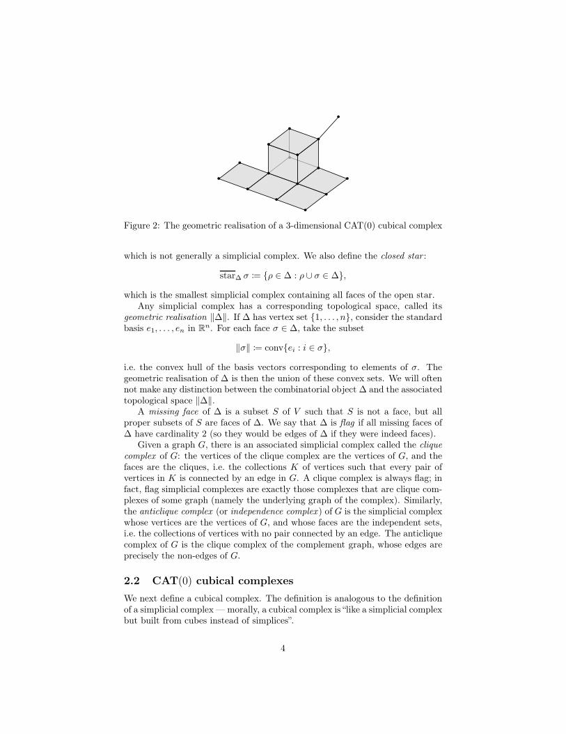
Figure 2: The geometric realisation of a 3-dimensional CAT(0) cubical complex

which is not generally a simplicial complex. We also define the closed star :

star∆ σ := {ρ ∈ ∆ : ρ ∪ σ ∈ ∆},

which is the smallest simplicial complex containing all faces of the open star.Any simplicial complex has a corresponding topological space, called its

geometric realisation ‖∆‖. If ∆ has vertex set {1, . . . , n}, consider the standardbasis e1, . . . , en in Rn. For each face σ ∈ ∆, take the subset

‖σ‖ := conv{ei : i ∈ σ},

i.e. the convex hull of the basis vectors corresponding to elements of σ. Thegeometric realisation of ∆ is then the union of these convex sets. We will oftennot make any distinction between the combinatorial object ∆ and the associatedtopological space ‖∆‖.

A missing face of ∆ is a subset S of V such that S is not a face, but allproper subsets of S are faces of ∆. We say that ∆ is flag if all missing faces of∆ have cardinality 2 (so they would be edges of ∆ if they were indeed faces).

Given a graph G, there is an associated simplicial complex called the cliquecomplex of G: the vertices of the clique complex are the vertices of G, and thefaces are the cliques, i.e. the collections K of vertices such that every pair ofvertices in K is connected by an edge in G. A clique complex is always flag; infact, flag simplicial complexes are exactly those complexes that are clique com-plexes of some graph (namely the underlying graph of the complex). Similarly,the anticlique complex (or independence complex ) of G is the simplicial complexwhose vertices are the vertices of G, and whose faces are the independent sets,i.e. the collections of vertices with no pair connected by an edge. The anticliquecomplex of G is the clique complex of the complement graph, whose edges areprecisely the non-edges of G.

2.2 CAT(0) cubical complexes

We next define a cubical complex. The definition is analogous to the definitionof a simplicial complex — morally, a cubical complex is “like a simplicial complexbut built from cubes instead of simplices”.

4

Definition 2.2. A cubical complex consists of a finite set V and a collectionof subsets of V , such that:

• ∅ is not in ,

• for each v ∈ V , the set {v} is in ,

• if σ and τ are in , then σ ∩ τ is either empty or in , and

• if σ ∈ , then the collection of elements of that are contained in σ isisomorphic as a poset (ordered by inclusion) to the poset of non-emptyfaces of a cube.

This definition might appear different from the definition of a simplicialcomplex. However, note that the condition that σ ∩ τ ∈ ∆ is redundant forsimplicial complexes, and the condition that a simplicial complex is closed undertaking subsets is equivalent to the requirement that for any σ ∈ ∆, the collectionof elements of ∆ that are contained in σ is isomorphic to the face poset of asimplex. The requirement that ∅ 6∈ is a matter of preference — we couldinstead have required that ∅ ∈ and removed the word “non-empty” in thefourth condition. We chose the convention that ∅ 6∈ because the poset ofnon-empty faces of a cube is slightly simpler to describe than the poset of allfaces, and because omitting the empty face makes some enumeration cleaner.

The dimension of σ ∈ is log2|σ| — the definition guarantees that |σ| is apower of 2, so the dimension of σ will always be an integer. Otherwise, all thebasic terminology for simplicial complexes (faces, vertices, edges, dimension of

, facets, pureness, underlying graph) applies unchanged for cubical complexes.We can also define links in cubical complexes, but we base the definition on

the notion of a simplicial open star:

link σ := {ρ ∈ : ρ ⊇ σ}.

Unlike for simplicial complexes, a cubical link is not generally a subcomplex.As a poset (ordered by inclusion), the link of any face of a cubical complex isisomorphic to a simplicial complex. We also define closed stars, analogously tosimplicial closed stars:

star σ := {ρ ∈ : ρ ∪ σ is contained in some face of }.

Like simplicial complexes, cubical complexes also have geometric realisations,although the construction is less clean — in general, the best we can get is aCW complex, rather than a union of convex sets in Euclidean space (althoughwe will see that convex sets do work for CAT(0) complexes, defined below). Foreach i-dimensional face σ ∈ , take ‖σ‖ to be an i-dimensional cube [0, 1]i, andidentify the subfaces of σ with faces of ‖σ‖. To construct ‖ ‖, we topologicallyglue the cubes together along corresponding faces. However, even though thisconstruction does not naturally live in Rn like for simplicial complexes, we cangive a cubical complex the structure of a metric space, by endowing each cube

5

7

v01 2

3

4

56

Figure 3: The CAT(0) cubical complex from Fig. 2 with its hyperplanes and aroot vertex shown

‖σ‖ with the metric of the unit cube in Ri, and choosing the gluings to beisometries.

An arbitrary metric space X is said to be CAT(0) if it has geodesics betweenany two points and it satisfies the “thin triangle” condition (see Bridson andHaefliger [11] for more details). However, we will not need the precise definition,thanks to the following theorem:

Theorem 2.3 (Gromov [18, Section 4]). A cubical complex is CAT(0) if andonly if it is simply connected and all vertex links are flag simplicial complexes.Moreover, any CAT(0) cubical complex is contractible.1

This theorem gives the first inkling of the connections between flag simplicialcomplexes and CAT(0) cubical complexes.

One particularly useful feature of cubical complexes is their hyperplanes.Given any cubical complex , for each cube [0, 1]i in , a subset [0, 1]× · · · ×{ 12} × · · · × [0, 1] is called a midplane of the cube. Two midplanes are adjacent

if their intersection is a midplane of another cube; after taking the transitiveclosure of this relation, the union of all midplanes in any equivalence class iscalled a hyperplane of . The midplanes give the hyperplane its own cubicalcomplex structure. See Fig. 3 for an example.

One reason why hyperplanes are especially nice in CAT(0) cubical complexesis the following lemma:

Lemma 2.4 (Niblo and Reeves [22, Lemma 2.7]). In a CAT(0) complex ,each hyperplane divides into two sides.

2.3 Posets with inconsistent pairs

Ardila et al. [7] gave another, more combinatorial description of CAT(0) cubical

1Adiprasito and Benedetti [3, Corollary II] go even further, and show that CAT(0) cubicalcomplexes are collapsible.

6

1 2

3 4 5

6 7

Figure 4: The Hasse diagram of a poset with inconsistent pairs

complexes which will be much more useful to us. But first, we need some moredefinitions.

Definition 2.5. A poset with inconsistent pairs (or a PIP for short) is a triple(P,≤,=) with the following properties:

• (P,≤) is a finite partially ordered set (poset), and

• = is a relation on P such that:

– a = a is false for all a (that is, = is antireflexive),

– a = b implies b = a (that is, = is symmetric), and

– if a = b, a ≤ a′ and b ≤ b′, then a′ = b′ (that is, = is inheritedupwards).

If a = b, then we say a and b form an inconsistent pair. A subset S ⊆ P isconsistent if it contains no inconsistent pairs.

We can draw the Hasse diagram of a PIP by drawing the usual Hasse diagramof the poset (P,≤) with solid lines, and adding dashed lines for each minimalinconsistent pair, that is, each pair c = d with no other pair c′ = d′ wherec ≥ c′ and d ≥ d′. For example, the PIP shown in Fig. 4 has four inconsistentpairs, namely 3 = 7, 4 = 6, 5 = 6 and 6 = 7.

A definition is no good without examples, and fortunately there are twolarge sources of them. Firstly, if P is any poset, we can think of it as a PIP thathas an order relation but happens to have no inconsistent pairs. Secondly, onthe other extreme, we can construct PIPs with inconsistent pairs but no orderrelation: if G is any (finite, simple, undirected) graph, we can think of it as aPIP whose underlying set is the set of vertices of G, the inconsistent pairs arethe edges of G, and there are no order relations (except the trivial relation a ≤ a

for each a).We will use a lot of standard poset terminology when talking about PIPs.

Given a subset S ⊆ P , an element x ∈ S is said to be maximal in S (respectivelyminimal in S) if there is no other element y ∈ S with x ≤ y (resp. x ≥ y). Theset of maximal elements of S is denoted maxS, and the set of minimal elementsis minS. Every element of P is greater than or equal to some minimal element,and less than or equal to some maximal one.

7

A downset (or order ideal) is a subset I ⊆ P with the property that if a ∈ I

and a′ ≤ a then a′ ∈ I. The downset generated by S ⊆ P is the set

↓S := {x ∈ P : x ≤ s for some s ∈ S}.

An upset (or order filter) is defined similarly with the inequalities reversed, andthe upset generated by S ⊆ P is denoted ↑S.

Two elements a and b of P are said to be comparable if either a ≤ b or b ≤ a.A chain is a subset C ⊆ P such that every two elements of C are comparable;an antichain is a subset A ⊆ P where no two elements are comparable.

We will often discuss consistent downsets and consistent antichains. Thesetwo objects are related by the following lemma:

Lemma 2.6. The map I 7→ max I is a bijection from the set of consistentdownsets of P to the set of consistent antichains, with inverse map given byA 7→ ↓A.

Proof. Apart from the word “consistent”, this is a standard result about finiteposets. Since I is consistent and max I is a subset of I, max I is consistent;the fact that ↓A is consistent follows from the upward-inherited property ofinconsistent pairs.

At this point, the reader may be starting to wonder what PIPs have to dowith cubical complexes. The answer lies in the following construction due toArdila et al. [7], culminating in Theorem 2.9 (see also Ardila [5], Ardila et al.[6]).

Definition 2.7. Given a PIP P , we define an associated cubical complex P

as follows. The vertex set of P is the set of consistent downsets of P . Thereis a face of P for each pair (I,M), where I is a consistent downset and M issome subset of max I: the face is denoted C(I,M), and it contains vertices

C(I,M) := {I \N : N ⊆ M}.

The result is a CAT(0) cubical complex (though this is not obvious). The faceC(I,M) contains 2|M| vertices, one for each subset N ⊆ M , so it is an |M |-dimensional cube. Note that ∅ is always a consistent downset of any PIP, soa cubical complex constructed in this way has a natural choice of distinguishedvertex, the one corresponding to ∅.

There is a natural embedding of P into the unit cube [0, 1]|P |: the verticesof P are associated with some subsets of P , whereas the vertices of [0, 1]|P |

correspond to the set of all subsets of P . The faces of P agree with the faces of[0, 1]|P |, so P is the induced subcomplex of [0, 1]|P | generated by these vertices.Thus P can be realised as a union of convex sets in Rn, faces of a cube.

Definition 2.8. A rooted CAT(0) cubical complex is a CAT(0) cubical complextogether with a choice of distinguished vertex v0.If we are given a rooted CAT(0) cubical complex, there is an associated

PIP P . The underlying set of P is the set of hyperplanes of . If H is a

8

H1

H2

v0

(a) H1 ≤ H2

H1 H2

v0

(b) H1 = H2

H1

H2

v0

(c) H1 and H2 consistentand incomparable

Figure 5: How to turn hyperplanes into a PIP

hyperplane, then the complement of H has two components, by Lemma 2.4: letH− be the component that does not contain the root vertex v0. We declarethat H1 ≤ H2 in P whenever H−

1 ⊇ H−2 , and H1 = H2 when H−

1 and H−2 are

disjoint. Intuitively, “H1 ≤ H2” means that hyperplane H2 is entirely beyondH1, to an observer standing at the root vertex, and “H1 = H2” means thatthis observer can see both hyperplanes without either obscuring any part of theother — see Fig. 5.

These constructions result in a theorem which forms the foundation for muchof the rest of this paper:

Theorem 2.9 (Ardila et al. [7, Theorem 2.5]). The map P 7→ P is a bijectionfrom the set of PIPs to the set of rooted CAT(0) cubical complexes, with inversegiven by 7→ P .

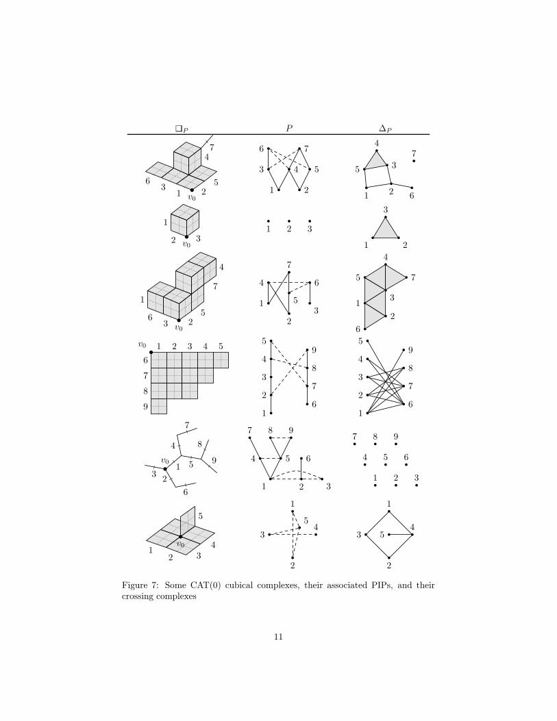
For example, if P is the PIP in Fig. 4, then P is the cubical complex inFigs. 2 and 3, as illustrated in Fig. 6. Several more examples are shown in thefirst two columns of Fig. 7.

3 The crossing complex

At last, we can define the main tool of this paper: the crossing complex.

Definition 3.1. Given a PIP P , the crossing complex ∆P is the simplicialcomplex whose vertex set is the underlying set of P , and whose faces are theconsistent antichains of P .

For example, if P is the running example PIP shown in Figs. 4 and 6, thecrossing complex ∆P is the simplicial complex shown in Fig. 1. This exampleis reprinted in Fig. 7, along with several more examples.

Observe that ∆P is a flag simplicial complex, since it is the anticlique com-plex of the graph whose edges are the comparable or inconsistent pairs in P .Our goal for the rest of this paper is to demonstrate that the crossing complex∆P and the CAT(0) cubical complex P share many properties.

9

1 2

3 4 5

6 7

↔

7

12

3

4

56

∅

2

25

1

12

125

13

123136

1236

124

12451234

12345

12457

Figure 6: The bijection from Theorem 2.9, illustrated with the PIP from Fig. 4.For example: the set I = {1, 2, 3, 6} is a consistent downset of P and thus avertex of P (shown as “1236”), with maximal elements max I = {2, 6}. Theface C({1, 2, 3, 6}, {2, 6}) is the left-most square in the figure, with vertex set{{1, 2, 3, 6}, {1, 2, 3}, {1, 3, 6}, {1, 3}

}; the northwest edge of that square is the

face C({1, 2, 3, 6}, {2}) ={{1, 2, 3, 6}, {1, 3, 6}

}.

For a first connection, observe that hyperplanes h1 and h2 in P intersectif and only if h1 and h2 are consistent and incomparable elements in P . Theunderlying graph of ∆P , which therefore has an edge between two hyperplanesprecisely when they intersect in P , was previously called the “crossing graph”of P by Hagen [21] and the “transversality graph” by Roller [23]. Hagen notesthe following lemma:

Lemma 3.2 ([21, Lemma 3.5]). If h1, . . . , hk are hyperplanes of a CAT(0)

complex with hi ∩ hj 6= ∅ for every i and j, then⋂k

i=1 hi 6= ∅.

In terms of the crossing complex, this means that the faces of ∆P are exactlythe sets of hyperplanes of P with a non-empty intersection. Consequently, wecan compute the crossing complex of P directly from P , and the result doesnot depend on the choice of root vertex of P .

Recall that any graph G can be thought of as a PIP with no order relationsand an inconsistent pair for each edge. In this interpretation, the consistent an-tichains are just the consistent sets of vertices, i.e. the anticliques of G. There-fore, since any flag simplicial complex is the anticlique complex of some graph,we obtain the following lemma:

Lemma 3.3. Every flag simplicial complex is the crossing complex of someCAT(0) cubical complex.

This lemma was also essentially observed by Hagen [21, Proposition 2.15]

10

P P ∆P

7

v01 2

3

4

561 2

3 4 5

6 7

1 2

3

4

5

6

7

1

2 3v0

1 2 3

1 2

3

1

23

4

56

7

v0

1

23

4

5

6

7

1

2

3

4

5

6

7

1 2 3 4 5

6

7

8

9

v0

1

2

3

4

5

6

7

8

9

1

2

3

4

5

6

7

8

9

v01

4

7

5

8

9

2

6

3

1 2 3

4 5 6

7 8 97 8 9

4 5 6

1 2 3

v01

2 34

5

1

2

34

5

1

2

34

5

Figure 7: Some CAT(0) cubical complexes, their associated PIPs, and theircrossing complexes

11

(among others), with a more complicated proof.2 However, note that differentCAT(0) cubical complexes may have the same crossing complex — for example,any tree with n edges is a 1-dimensional CAT(0) cubical complex, and thecrossing complex of such a tree always consists of n isolated points.

Next, we turn our attention to f -vectors.

Definition 3.4. If K is a complex (simplicial or cubical), define fi(K) to bethe number of i-dimensional faces of K.

If ∆ is a (d − 1)-dimensional simplicial complex, the f -vector of ∆ is thetuple

(f−1(∆), . . . , fd−1(∆)

), and the f -polynomial is:

f(∆, t) :=

d∑

i=0

fi−1(∆) ti.

If is a d-dimensional cubical complex, its f -vector is(f0( ), . . . , fd( )

), and

its f -polynomial is:

f( , t) :=

d∑

i=0

fi( ) ti.

Note the difference in conventions between the simplicial and cubical cases! Forinstance, the constant term of f(∆, t) is f−1(∆), which is always 1 to countthe empty face; whereas the constant term of f( , t) is f0( ), the number ofvertices of .

This brings us to the main result of this section.

Theorem 3.5. Let P be a PIP. Then f( P , t) = f(∆P , 1 + t).

Proof. Let “A E P ” mean “A is a consistent antichain of P ”.By construction, the i-dimensional faces of P are in bijection with pairs

(I,M) where I ⊆ P is a consistent downset and M ⊆ max I with |M | = i.Lemma 2.6 says these pairs are in turn in bijection with pairs (A,M) where A

is a consistent antichain of P and M ⊆ A with |M | = i.Therefore, using the convention that fi(K) = 0 if i > dimK,

f( P , t) =

∞∑

i=0

fi( P )ti

=∞∑

i=0

∑

AEP

∑

M⊆A|M|=i

ti

=∑

AEP

∞∑

i=0

(|A|

i

)ti

2Hagen writes: “The fact that every [simple] graph is a crossing graph means that there islittle hope of any general geometric statements about crossing graphs of cube complexes” [19,p. 35]. We disagree.

12

=∑

AEP

(1 + t)|A|

=∞∑

j=0

fj−1(∆P )(1 + t)j

= f(∆P , 1 + t).

This formula has some neat immediate consequences.

Corollary 3.6. dim P = dim∆P + 1.

Proof. The dimension of P is the degree of its f -polynomial, and the dimensionof ∆P is 1 less than the degree of its f -polynomial.

Corollary 3.7. The Euler characteristic χ( P ) of P is 1.

Proof. χ( P ) := f( P ,−1) = f(∆P , 0) = f−1(∆P ) = 1. (Of course, Theorem 2.3says P is contractible, so we already knew this.)

Corollary 3.8. The number of hyperplanes of P is∑d

i=0(−1)i−1ifi( P ).

Proof. The number of hyperplanes is |P | = f0(∆P ), which is the coefficient ofthe linear term in f(∆P , t) = f( P , t− 1).

But the biggest consequence of Theorem 3.5 comes when we combine it withLemma 3.3:

Theorem 3.9. The following sets are equal:

{p(t) : p is the f -polynomial of a d-dimensional CAT(0) cubical complex},

and

{q(t+ 1) : q is the f -polynomial of a (d− 1)-dimensional flag simplicial complex}.

In other words, the sets of f -vectors of CAT(0) cubical complexes and flag sim-plicial complexes are equal, up to the invertible linear transformation by thematrix T whose (i, j)th entry is

(j−1i−1

).

Proof. If p(t) is the f -polynomial of some CAT(0) cubical complex , thenTheorem 2.9 says = P for some P (after choosing a root arbitrarily), sop(t + 1) is the f -polynomial of ∆P . Conversely, if q(s) is the f -polynomial ofsome flag simplicial complex ∆, then Lemma 3.3 says ∆ = ∆P ′ for some P ′,thus q(s− 1) is the f -polynomial of P ′ .

The equivalence of the statement about f -vectors comes from this equality:

d∑

i=0

fi( P )ti =

d∑

j=0

fj−1(∆P )(1 + t)j

=d∑

i=0

d∑

j=0

(j

i

)fj−1(∆P )t

i,

noting that the indexing in T is shifted by 1.

13

We will revisit f -polynomials in Section 7.

4 Combining CAT(0) complexes

In this section, we aim to illustrate how the crossing complex and Ardila et al.’sbijection may be used to study P , by examining some ways of building newcomplexes from old. We begin this section with three definitions.

First, a natural construction for combining cubical complexes is the product.

Definition 4.1. Given two cubical complexes 1 and 2, their product is thecubical complex 1× 2 whose vertices are pairs (v1, v2) with vi a vertex of i

for i = 1, 2, and whose faces are sets of the form σ1 × σ2 for σi ∈ i.

Second, there is a construction for simplicial complexes called the join.

Definition 4.2. If ∆1 and ∆2 are two simplicial complexes with vertex sets V1

and V2 respectively, their join3 is the simplicial complex ∆1 ∗∆2, whose vertexset is V1 ⊔ V2 and whose faces are sets of the form σ1 ⊔ σ2, where σi is a face of∆i for i = 1, 2.

Third, here is a way of combining PIPs.

Definition 4.3. If P and Q are two PIPs, define P ⊔↔

Q to be the PIP where:

• the underlying set is P ⊔Q, the disjoint union of P and Q,

• if p1, p2 ∈ P , then the relations between p1 and p2 in P ⊔↔Q are the same

as in P , and similarly for q1, q2 ∈ Q, and

• if p ∈ P and q ∈ Q, then p and q are incomparable and consistent inP ⊔

↔Q.

In other words, P ⊔↔

Q is the PIP whose Hasse diagram is obtained by simply

placing the Hasse diagrams for P and Q next to each other.

One may wonder what the connection between these constructions is — theanswer is in the following lemma (also observed by Caprace and Sageev [12,Lemma 2.5] and Hagen [20, Proposition 1.3]):

Lemma 4.4. P × Q∼= P ⊔

↔

Q, and ∆P ⊔↔

Q∼= ∆P ∗∆Q.

Proof. The consistent downsets of P ⊔↔

Q are sets of the form I ⊔ J , where I

and J are consistent downsets in P and Q respectively, and the set of maximalelements of I ⊔J is max I ⊔maxJ . Therefore, vertices of P ⊔

↔

Q are in bijection

with pairs (I, J) with I and J as above, which are in bijection with vertices

3Not to be confused with the join of two elements in a poset, x ∨ y. We will not use thistype of join in this paper.

14

of P × Q; and faces of P ⊔↔

Q are in bijection with tuples (I,M, J,N) with

M ⊆ max I and N ⊆ maxJ , which are in bijection with faces of P × Q.Note that the root vertices of P and Q correspond to the empty consistent

downset, and ∅ ⊔∅ = ∅, so this isomorphism respects roots.The consistent antichains of P ⊔

↔Q are sets of the form A⊔B with A and B

consistent antichains of P and Q respectively; the statement about ∆P ⊔↔

Q and

∆P ∗∆Q follows immediately.

Here are some more constructions.

Definition 4.5. Suppose K1 and K2 are two complexes (both simplicial or bothcubical, although the simplicial case will be more useful to us), with vertex setsV1 and V2 respectively. The disjoint union K1 ⊔K2 of the complexes is definedto be the complex whose vertex set is V2 ⊔ V2 and whose face set is the setK1 ∪K2 (which is not quite a disjoint union if K1 and K2 are simplicial, sincethen they share the face ∅).

Definition 4.6. Given two rooted cubical complexes 1 and 2, the wedgesum 1∧ 2 is the cubical complex obtained by taking the disjoint union of 1

and 2 and identifying their root vertices together to make a single new rootvertex.

Definition 4.7. Given two PIPs P and Q, the PIP P ⊔=

Q is defined identically

to P ⊔↔Q, except that each pair p, q with p ∈ P and q ∈ Q is incomparable and

inconsistent in P ⊔=

Q. The Hasse diagram of P ⊔=

Q is obtained by putting the

Hasse diagrams of P and Q next to each other, then adding dotted lines fromminimal element of P to each minimal element of Q.

Lemma 4.8. P ∧ Q = P ⊔=

Q, and ∆P ⊔=

Q = ∆P ⊔∆Q.

Proof. There are three types of consistent downsets in P ⊔=

Q: they are either

the empty set, a non-empty consistent downset in P , or a non-empty consistentdownset in Q. The vertices of P ∧ Q are either the root vertex (correspondingto the empty downset), or a non-root vertex in P or Q (corresponding toa non-empty downset in P or Q respectively). The faces of P ∧ Q are inbijection with either (∅,∅) (the root vertex) or (I,M) or (J,N) where I and J

are non-empty consistent downsets of P and Q respectively, and M ⊆ max Iand N ⊆ maxJ .

The consistent antichains of P ⊔=

Q are empty or a non-empty consistent

antichain in P or Q; the faces of ∆P ⊔ ∆Q are either the empty face or anon-empty face of ∆P or ∆Q.

The next lemma concerns vertex links in CAT(0) cubical complexes. Linksare easier to describe and often more useful in the simplicial case — we willreturn to simplicial links in Section 5 — but for now, this lemma will be usefulin proving Proposition 4.10.

15

IJ

M

X

Y

P

Figure 8: Illustration of the situation in Lemma 4.9

Lemma 4.9. Suppose a vertex v of P corresponds to the consistent downsetJ ⊆ P . Then the link of v in P is the crossing complex of the sub-PIP

maxJ ∪min{x ∈ P \ J : x is consistent with all j ∈ J} ⊆ P

In particular, the link of the root vertex (where J = ∅) is the crossing complexof minP .

Note that while no two elements of minP are ever comparable, they may beinconsistent.

Proof. Recall from Definition 2.7 that the faces of P are in bijection with pairs(I,M) where I ⊆ P is a consistent downset and M ⊆ max I. By definition, aface C(I,M) in P contains v if and only if I \X = J for some X ⊆ M — seeFig. 8.

If we define Y = M \X , so M = X ⊔Y and I = J ⊔X , then the pair (I,M)is determined by the choice of the pair (X,Y ), and vice versa. There are somerestrictions on what the sets X and Y may be — specifically, the conditions areas follows:

• X ⊔ Y must be a consistent antichain (since X ⊔ Y = M);

• Y must be a subset of maxJ (since Y ⊆ J and Y ⊆ M ⊆ max I, and anyelement of J that is maximal in I must also be maximal in the subset J);

• every element of X must be consistent with every j ∈ J (since J ⊔X = I

is consistent); and

• X must be a subset of min(P \ J) (since X ⊆ P \ J , and the facts that Xis an antichain and J ⊔X is a downset mean that any y ∈ P with y < x

for some x ∈ X must be in J), thus elements of X are in fact minimal inthe subset {x ∈ P \ J : x is consistent with all j ∈ J}.

Conversely, if X and Y satisfy these conditions, then J ⊔ X is a consistentdownset and X ⊔ Y ⊆ max(J ⊔ X). In other words, the faces of the link of vare in bijection with pairs (X,Y ) such that X ⊔Y is a consistent antichain withY ⊆ maxJ and X ⊆ min{x ∈ P \ J : x is consistent with all j ∈ J}.

16

85

6

7

3

2

1

4 v0 1 2 3

45

6

7

8

1

2

3

4

8

5

6

7

Figure 9: A CAT(0) cubical complex with a cut vertex, its corresponding PIP,and its crossing complex. Dotted lines show a disconnection of the crossingcomplex.

With this lemma in hand, we can now give a combinatorial proof of thefollowing result (which was also observed by Hagen [20, Lemma 4.10]).

Proposition 4.10. P has a cut vertex (i.e. a vertex v where ‖ P ‖ \ v isdisconnected) if and only if ∆P is disconnected.

Proof. One direction follows immediately from the work above: if P has a cutvertex, then it is then a wedge sum of its two halves, and Lemma 4.8 says ∆P

is thus a disjoint union.The other direction is less straightforward. The first part of this proof went

smoothly because we could implicitly assume in Lemma 4.8 that the cut vertexis the root vertex of P , since ∆P does not depend on the choice of root; forthe other direction of the proof, the cut vertex might be any vertex. The ideafor the rest of the proof is to find the potential cut vertex in P , set it to bethe new root vertex, and then argue that it is indeed a cut vertex.

Suppose ∆P is disconnected. This means we can partition the vertices of ∆P

into two non-empty sets, A and B, with no edges of ∆P between the two sets;in terms of P , this means that every pair a, b with a ∈ A and b ∈ B is eitherinconsistent or comparable. If all such pairs are inconsistent, we can appeal toLemma 4.8 again to conclude that P is a wedge sum; our next goal is thus toreduce to this case.

If not all pairs a, b are inconsistent, then some pair is comparable: withoutloss of generality, suppose a0 < b0 for some a0 ∈ A and b0 ∈ B. By increasinga0 ∈ A and decreasing b0 ∈ B if necessary, we may even assume that a0 < b0 isa covering relation — that is, that there is no x ∈ P with a0 < x < b0. Now,consider the downset I := (↓ b0) \ b0, which is consistent since it is a subset of↓ b0, and let v be the corresponding vertex in P — we will argue that v is acut vertex.

Observe the following:

• a0 is a maximal element in I, since b0 covers a0;

• b0 is consistent with all elements of I; and

17

• b0 is minimal in P\I, and thus in {x ∈ P\I : x is consistent with all i ∈ I}.

Therefore, according to Lemma 4.9, both a0 and b0 are vertices of the link of v.Thus the vertices of link v can be partitioned into two non-empty sets, A∩ link vand B ∩ link v, with no edges between them, so link v is disconnected.

Now, choose v to be the new root vertex of P . This new rooted CAT(0)complex will correspond to a different PIP, say P ′, but the geometry of P ′ isunchanged — in particular, the crossing complex ∆P ′ is identical to ∆P , andthe link of v in P ′ is still disconnected by some partition A′ and B′.

But now, since v is the root vertex of P ′ , Lemma 4.9 says that linkP ′

v =

∆minP ′ . No two elements of minP ′ can be comparable, so all elements of A′

must instead be inconsistent with all elements of B′.Every element x′ ∈ P ′ must be greater than or equal to some element of

minP ′, but it cannot be the case that both x′ ≥ a′ and x′ ≥ b′ for somea′ ∈ A′ and b′ ∈ B′: if this were the case, the fact that a′ = b′ together withthe upward-inheriting property of inconsistent pairs would imply that x′ = x′,which is forbidden. Therefore, the sets ↑A′ and ↑B′ form a setwise partitionof P ′. Moreover, if x′ ∈ ↑A′ and y′ ∈ ↑B′, then x′ ≥ a′ and y′ ≥ b′ for somea′ ∈ A′ and b′ ∈ B′, so since a′ = b′, we must also have x′ = y′; thus P ′ is theposet A′ ⊔

=

B′. But Lemma 4.8 then implies that P ′ is a wedge sum, so P

has a cut vertex.

This proof used a lot of facts about posets — we will see an alternative,topological way to prove this result in Section 6.

5 Hyperplanes

In this section, we will take a closer look at hyperplanes in CAT(0) cubicalcomplexes, through the lens of the derivative complex defined by Babson andChan [8]. This construction is heavily based on the poset structure of a cubicalcomplex (where the faces are ordered by inclusion), so in order to use thisconstruction, we must first say more about the poset structure of P .

Lemma 5.1. C(I ′,M ′) ⊆ C(I,M) if and only if M ′ ⊆ M and I \M ⊆ I ′ ⊆ I.

Proof. By definition, C(I ′,M ′) ⊆ C(I,M) if and only if

{I ′ \N ′ : N ′ ⊆ M ′} ⊆ {I \N : N ⊆ M}.

This is true if and only if it is true for the smallest and largest possible choicesfor N ′, namely N ′ = ∅ and N ′ = M ′; therefore, C(I ′,M ′) ⊆ C(I,M) if andonly if

{I ′, I ′ \M ′} ⊆ {I \N : N ⊆ M}.

Let S denote {I \N : N ⊆ M}, for conciseness. The set I ′ is an element ofS precisely when I \M ⊆ I ′ ⊆ I. Similarly, I ′ \M ′ is an element of S preciselywhen I \M ⊆ I ′ \M ′ ⊆ I; if we assume that I ′ ∈ S already, then I ′ \M ′ ∈ S

if and only if M ′ ⊆ M .

18

Lemma 5.2. The cubes C(I1,M1) and C(I2,M2) have a meet if and only if(I1 \M1) ∪ (I2 \M2) ⊆ I1 ∩ I2; if the meet exists, it is

C(I1,M1) ∩ C(I2,M2) = C(I1 ∩ I2,M1 ∩M2).

Proof. The meet of C(I1,M1) and C(I2,M2), if it exists, is the maximal cubeC(J,N) such that C(J,N) ⊆ C(Ii,Mi) for both i = 1, 2. According to Lemma 5.1,the set of faces satisfying this containment is the set of faces C(J,N) satisfying

N ⊆ M1 ∩M2 and (I1 \M1) ∪ (I2 \M2) ⊆ J ⊆ I1 ∩ I2.

In order for this set to be non-empty, we need (I1 \M1) ∪ (I2 \M2) ⊆ I1 ∩ I2;if this is true, then the pair (J,N) = (I1 ∩ I2,M1 ∩M2) is in the set. This pairmaximises (J,N) subject to the conditions that J ⊆ Ii and N ⊆ Mi for bothi = 1, 2, so it must still be maximal given the extra condition Ii \Mi ⊆ J .

Now, let us state the definition of the derivative complex given by Babsonand Chan [8, Section 4].

Definition 5.3. Let be a cubical complex. The derivative complex of ,denoted D , is the poset where:

• the elements of D are the sets {b, c}, where b and c are faces of whichhave no meet but are both covered by the same face, and

• {b, c} � {b′, c′} in D if and only if b ⊆ b′ and c ⊆ c′ or b ⊆ c′ and c ⊆ b′.

See Fig. 10 for an example. Although the derivative complex is defined ab-stractly as a poset, in general it is isomorphic to the poset of faces of a cubicalcomplex (as we define it, in terms of sets of vertices). This complex is notgenerally CAT(0) — it typically has many connected components. The com-ponents of D are the hyperplanes of (with some caveats if the hyperplanesself-intersect — self-intersecting hyperplanes never occur in any subcomplex ofa cube, though, so this issue does not arise for CAT(0) complexes). One reasonfor the name “derivative complex” is the following observation:

f(D , t) =d

dtf( , t).

And now we come to the main theorem for this section.

Theorem 5.4. For each x ∈ P , let Px be the sub-PIP

Px :={y ∈ P : y is consistent and incomparable with x

}⊆ P,

and let Hx be the corresponding CAT(0) cubical complex. Then D( P ) is thedisjoint union of the complexes Hx for x ∈ P .

Before we prove this theorem, let us note two of its consequences. First,since the components of D( P ) are the hyperplanes of P , this theorem givesa combinatorial proof of the following fact, which Niblo and Reeves [22] observedfrom the metric space perspective (see also Sageev [24, Theorem 4.11]):

19

P =1

0

2

3

4

5

6

7

8

9

P =

A B

CD

∆P =

A B

CD

D P =

0, 4

2, 6

3, 7

1, 5

4, 5

6, 7

2, 3

0, 1

4, 6

0, 2

1, 35, 7

8, 9

5, 8

7, 9

Figure 10: A CAT(0) cubical complex, its PIP and crossing complex, and itsderivative complex

Corollary 5.5. The hyperplanes of a CAT(0) cubical complex are themselvesCAT(0) cubical complexes.

Second, in terms of the crossing complex, the underlying set of Px is preciselythe set of vertices of the link of x in ∆P . Since ∆P is flag, all links are inducedsubcomplexes, so we have the following corollary:

Corollary 5.6. The crossing complex of the hyperplane Hx is ∆Px= link∆P

x.

We find it intriguing (and perhaps unsurprising) that links, one of the mostimportant tools for studying simplicial complexes, correspond to hyperplanes,one of the most important tools for cubical complexes.

We conclude this section by proving the theorem.

Proof of Theorem 5.4. The first goal of this proof is to describe the elements ofD( P ), that is, the pairs {C(I1,M1), C(I2,M2)} of faces that share a commoncover but have no meet.

We will begin by describing the covering relations in P . Suppose C(I ′,M ′) ⊂C(I,M) is a covering relation; then Lemma 5.1 says that M ′ ⊆ M and I \M ⊆I ′ ⊆ I. The poset of faces of P is ranked by dimension, and the dimension ofC(I,M) is |M |; therefore, since ranks differ by 1 in a covering relation, the setM ′ must be M \x for some x ∈ M . By definition, I ′ must contain M ′ = M \x;putting this together with Lemma 5.1, we must have

I \ x = (I \M) ∪ (M \ x) ⊆ I ′ ⊆ I.

Therefore, either I ′ = I or I ′ = I \ x. Thus the covering relations in P taketwo forms: they are either

C(I,M \ x) ⊂ C(I,M)

20

or

C(I \ x,M \ x) ⊂ C(I,M)

for some x ∈ M .Now, suppose two faces C(J1, N1) and C(J2, N2) of P share a common

cover; the next question to ask is when these faces have a meet. If the commoncover is C(I,M), the possibilities for the two faces are:

C(I,M \ x) and C(I,M \ y) for some x 6= y,

C(I \ x,M \ x) and C(I \ y,M \ y) for some x 6= y,

C(I,M \ x) and C(I \ y,M \ y) for some x 6= y, or

C(I,M \ x) and C(I \ x,M \ x) for some x.

Lemma 5.2 says that C(J1, N1) and C(J2, N2) have a meet if and only if (J1 \N1)∪(J2 \N2) ⊆ J1∩J2; therefore, in the four cases above, the containments we needto consider are the following:

(I \M) ∪ {x, y} ⊆ I,

I \M ⊆ I \ {x, y},

(I \M) ∪ {x} ⊆ I \ {y}, and

(I \M) ∪ {x} 6⊆ I \ {x}

respectively. The containment holds in the first three cases, but fails in thefourth; therefore, the pairs of faces of P that have no meet but share a commoncover — that is, the elements of D( P ) — are the pairs of the form

C(I,M \ x) and C(I \ x,M \ x).

Now that we have described the underlying set of D( P ), let us turn toits poset structure. Suppose that F =

{C(I,M \ x), C(I \ x,M \ x)

}and

G ={C(J,N \y), C(J \y,N \y)

}are two elements of D( P ). By the definition

of D( P ), we have F � G in D( P ) if and only if

C(I,M \ x) ⊆ C(J,N \ y) and C(I \ x,M \ x) ⊆ C(J \ y,N \ y),

or

C(I,M \ x) ⊆ C(J \ y,N \ y) and C(I \ x,M \ x) ⊆ C(J,N \ y)

in P . According to Lemma 5.1, this happens if and only if

M \ x ⊆ N \ y, J \ (N \ y) ⊆ I ⊆ J and J \N ⊆ I \ x ⊆ J \ y,

or

M \ x ⊆ N \ y, J \N ⊆ I ⊆ J \ y and J \ (N \ y) ⊆ I \ x ⊆ J

in P . But the second of these two conditions is impossible: I ⊆ J \ y impliesthat y 6∈ I, but J \ (N \ y) ⊆ I \ x implies that y ∈ I. On the other hand, in

21

the first of the two conditions, we have J \ (N \ y) ⊆ I, so y must still be anelement of I, but I \ x ⊆ J \ y, so the only way this is possible is if x = y.

Therefore, putting this all together, we have F � G in D( P ) if and only ifx = y and

M \ x ⊆ N \ x, J \ (N \ x) ⊆ I ⊆ J and J \N ⊆ I \ x ⊆ J \ x,

which happens if and only if x = y and

M ⊆ N and J \N ⊆ I ⊆ J,

which precisely means that C(I,M) ⊆ C(J,N) in P .The fact that F � G only happens when x = y means that we can partition

the poset D( P ) into disjoint, incomparable components, each determined bythe choice of x ∈ P . By the preceding argument, the elements of the componentcorresponding to x are in order-preserving bijection with the faces C(I,M) of

P where x ∈ M .For such a face, the requirement that x ∈ M means the following:

• I must contain all elements of ↓x since I is a downset;

• I must never contain any elements of (↑ x) \ x, since x is maximal in I;and

• I must never contain any element that is inconsistent with x.

The remaining elements of P are Px. Therefore, I is determined by choosinga downward-closed subset J of Px. Once J is chosen, I is determined as I =J ∪ ↓x; conversely, J = I \ ↓x, so J is also determined by the choice of I. Themaximal elements of J are (max I)\x, so M is determined by a choice of subsetN ⊆ maxJ , with M = N ∪ x and N = M \ x. Therefore, the faces C(I,M) of

P with x ∈ M are in bijection with all faces of Hx. Moreover, this bijectionis order-preserving, since

M ′ ⊆ M if and only if M ′ \ x ⊆ M \ x,

and

I \M ⊆ I ′ ⊆ I if and only if (I \ ↓x) \ (M \ x) ⊆ I ′ \ ↓x ⊆ I \ ↓x.

Thus D( P ) has one connected component for each element x ∈ P , and thecomponent corresponding to x is isomorphic to the poset of faces of Hx.

Before we move on from this section, let us make one more observation. Aswe saw in this proof, the hyperplane of P corresponding to x ∈ P is isomor-phic (as a poset) to the set of faces of P with x ∈ M . Also, to switch tracksfor a moment, recall from Definition 2.7 that P has a natural embedding intothe cube [0, 1]|P |, where each face C(I,M) ∈ P is mapped to a face of [0, 1]|P |

parallel to the linear subspace spanned by the basis vectors corresponding toelements of M . Putting these two ideas together: the hyperplane of P corre-sponding to x is isomorphic as a poset to the faces of P that extend in the x

direction inside [0, 1]|P |. In other words,

22

Figure 11: Hyperplanes in a CAT(0) complex as intersections with hyperplanesof the cube

Proposition 5.7. In the standard embedding of P in [0, 1]|P |, the hyperplanecorresponding to x ∈ P is the intersection of P with the hyperplane of the cube[0, 1]|P | perpendicular to the xth direction.

See Fig. 11 for an example.

6 Topology

In this section, we will describe a way to find ∆P as a subspace of P , upto homotopy equivalence. First, we recall some general facts about topologicalspaces.

Definition 6.1. Suppose X is a topological space, and Z = {Z1, . . . , Zm} is acollection of subspaces of X . The nerve of Z is the simplicial complex on vertexset {1, . . . ,m}, where a set S ⊆ {1, . . . ,m} is a face if and only if

⋂i∈S Zi is

non-empty.

For example, following the discussion on page 10, the crossing complex ∆P

is the nerve of the collection of hyperplanes of P .One of the most important results about nerves is the (helpfully named)

Nerve Theorem:

Theorem 6.2 (see e.g. [10, Theorem 10.7]). Suppose Z = {Z1, . . . , Zm} is acollection of closed topological subspaces of a space X. If for all I ⊆ {1, . . . ,m}the intersection

⋂i∈I Zi is contractible or empty, then the union

⋃m

i=1 Zi ishomotopy equivalent to the nerve of Z.

In the context of CAT(0) cubical complexes, we can apply the Nerve Theo-rem to conclude the following result.

Theorem 6.3. The following spaces are homotopy equivalent:

• The crossing complex ∆P ,

• The union of the hyperplanes of P , and

• The topological space P with all vertices removed — i.e., ‖ P ‖\‖V ( P )‖.

For example, see Fig. 12.

23

≃ ≃

Figure 12: Three homotopy equivalent spaces

Proof. We want to apply the Nerve Theorem to the collection of hyperplanesof P ; however, before we can do this, we must argue that all non-emptyintersections of hyperplanes are contractible.

Suppose H1 and H2 are two hyperplanes of P . Proposition 5.7 says thatH1 and H2 can be written as H̃1∩ P and H̃2 ∩ P respectively, where H̃1 andH̃2 are hyperplanes of the cube [0, 1]|P |. Note that H̃1 and H̃2 are themselvescubes, and the embeddings of H1 and H2 inside them agree with the standardCAT(0) complex embeddings of H1 and H2 into cubes. Therefore, H1 ∩H2 =

(H̃1 ∩ P ) ∩ (H̃2 ∩ P ) is the intersection of H1 with H̃1 ∩ H̃2, which is a

hyperplane of the cube H̃1 — but Proposition 5.7 says this is itself a hyperplaneof H1, if it is non-empty. That is, the non-empty intersection of two hyperplanesof P is a hyperplane of a hyperplane of P . By induction, the non-emptyintersection of any number of hyperplanes of P is an iterated hyperplane of

P .Now, Corollary 5.5 says that hyperplanes are CAT(0) cubical complexes,

so Theorem 2.3 implies that non-empty intersections of hyperplanes are con-tractible. Therefore, we can apply the Nerve Theorem, and conclude that theunion of the hyperplanes of P is homotopy equivalent to the nerve, ∆P .

It only remains to show that the union of hyperplanes is homotopy equivalentto P with the vertices deleted. The idea for this proof is to construct adeformation retraction on each face, from the face [0, 1]r with its corners deletedto the union of the midcubes of that face, such that if we restrict the deformationretraction to each sub-face of this face, we get another deformation retractionwith these properties. Writing down such a deformation retraction explicitly istedious, so instead we illustrate the deformation retraction in Fig. 13, and leavethe reader to fill in the details. Once such deformation retractions are definedon each face of P , we get a deformation retraction on the whole of P bygluing them together.

This theorem gives an alternative way to prove Proposition 4.10 (which saidthat P has a cut vertex if and only if ∆P is disconnected).

Alternative proof of Proposition 4.10. Observe that ‖ P ‖ \ ‖V ( P )‖ has morethan one component if and only if some vertex of P is a cut vertex. Therefore,since connectedness is a homotopy invariant, P has a cut vertex if and only if∆P has more than one component.

24

≃ ≃

Figure 13: A deformation retraction from [0, 1]r with the vertices deleted to theunion of r midcubes, in the case with r = 3. Observe that on each face of thiscube, the deformation retraction restricts to a retraction from the face with itsvertices deleted to the midcubes of that face.

In the remainder of this section, we present some more facts of a topologicalflavour, by considering the facets of P and ∆P .

Proposition 6.4 (see Ardila et al. [7, Lemma 2.4]). The maximal faces of

P are exactly those of the form C(↓A,A) where A is a maximal consistentantichain of P (under inclusion). Thus A 7→ C(↓A,A) is a bijection fromfacets of ∆P to facets of P .

Proof. The facets of ∆P are the maximal consistent antichains of P , by defini-tion, so the second statement follows immediately from the first. To prove thefirst statement, there are two things to show: we need to check that C(↓A,A)is always a maximal face of P , and that every maximal face has this form.

First, suppose A is a maximal consistent antichain, and C(I,M) is a faceof P with C(↓A,A) ⊆ C(I,M). In particular, Lemma 5.1 then says thatA ⊆ M ⊆ max I. Since A is a maximal consistent antichain, we must thereforehave A = M = max I, so I = ↓max I = ↓A. Thus C(↓A,A) = C(I,M), soC(↓A,A) is indeed a maximal face of P .

On the other hand, suppose C(J,N) is an arbitrary maximal face of P .Consider the face C(J,max J): since N ⊆ maxJ and J \ maxJ ⊆ J ⊆ J ,Lemma 5.1 says that C(J,N) ⊆ C(J,maxJ), so the maximality of C(J,N)means that N = maxJ . Thus J = ↓maxJ = ↓N , so C(J,N) = C(↓N,N).Thus it only remains to prove that N is a maximal consistent antichain.

Suppose N is not maximal. The set

S := {x ∈ P \N : N ∪ x is a consistent antichain}

is thus non-empty, so it has an element x0 that is minimal with respect tothe order in P . Since x0 is minimal in S, any y ∈ P with y < x0 must becomparable or inconsistent with some n ∈ N . However, y cannot be inconsistentwith n, as then x0 and n would be inconsistent; and y cannot be greater thann, as then we would have x0 > n. Thus y must be less than n, so y ∈ ↓N .Therefore, (↓N) ∪ x0 = J ∪ x0 is a consistent downset of P . We also haveN ⊆ N ∪ x0 and (J ∪ x0) \ (N ∪ x0) ⊆ J ⊆ J ∪ x0, so Lemma 5.1 says thatC(J,N) ( C(J ∪ x0, N ∪ x0). But this contradicts the maximality of C(J,N);therefore, N must be a maximal consistent antichain.

25

Note that the dimension of A as a face of ∆P is |A|−1, whereas the dimensionof C(↓A,A) in P is |A|. This gives us an alternative proof of Corollary 3.6(which said that dim P = dim∆P + 1), as well as the following corollary:

Corollary 6.5. ∆P is pure if and only if P is pure.

We can also combine this proposition with Lemma 5.2, to obtain the follow-ing lemma:

Lemma 6.6. If two facets C(↓A,A) and C(↓B,B) of P intersect in a faceof dimension r, the corresponding facets A and B of ∆P intersect in the faceA ∩B, which has dimension r − 1.

Proof. Lemma 5.2 says that the intersection of C(↓A,A) and C(↓B,B), if itexists, is C(↓A ∩ ↓B,A ∩B), which has dimension

dimPC(↓A ∩ ↓B,A ∩B) = |A ∩B|

= dim∆P(A ∩B) + 1.

Recall that by convention, we require ∅ to be a face of every simplicialcomplex, but not a face of any cubical complex. Therefore, if C(↓A,A) ∩C(↓B,B) is a face of dimension 0, then this lemma says that A and B intersect inthe (−1)-dimensional empty face of ∆P ; however, if the intersection of C(↓A,A)and C(↓B,B) is empty, then we can say nothing about A ∩B.

7 Balancedness

In this final section, we will take a look at a special class of simplicial and cubicalcomplexes, namely balanced complexes.

Definition 7.1. An r-colouring of a simplicial complex ∆ is a map κs (with “s”for “simplicial”) from the set V (∆) of vertices of ∆ to the set {1, . . . , r}, with theproperty that for any two vertices connected by an edge (or equivalently, anytwo distinct vertices that lie in a common face), the images of the vertices underκs are different. If such an r-colouring exists, we say that ∆ is r-colourable; if ∆is (d−1)-dimensional and d-colourable, we say it is balanced. Note that a (d−1)-dimensional simplicial complex must have a face with d vertices, by definition,so at least d colours are always necessary for colouring a (d − 1)-dimensionalcomplex: the balanced condition says that d colours are enough.

Here is another way of viewing colourings. The set {1, . . . , r} may be thoughtof as the set of vertices of the (r − 1)-dimensional simplex Σr−1. From thisviewpoint, an r-colouring of ∆ is a map κs : V (∆) → V (Σr−1), such that therestriction of κs to any face of ∆ is a bijection to a face of Σr−1.

This idea motivates the following definition of colourings for cubical com-plexes: an r-colouring of a cubical complex is a map κc : V ( ) → V ([0, 1]r)(with “c” for “cubical”), where [0, 1]r is the r-dimensional cube, such that therestriction of κc to any face of is a bijection to a face of [0, 1]r. If such a

26

1 2 3

3 1

→1

2

3

1

3

(a) Balanced (b) Not balanced

Figure 14: A balanced and a non-balanced simplicial complex

000

100

101

001

010

011

111

110

111

010

011

001

011

(a) Balanced (b) Not balanced

Figure 15: A balanced and a non-balanced cubical complex (whose crossingcomplexes are the ones in Fig. 14)

colouring exists, is r-colourable, and if is d-dimensional and d-colourable,it is called balanced.

See Figs. 14 and 15 for some examples of balanced and non-balanced sim-plicial and cubical complexes.

Note that any simplicial complex with n vertices is n-colourable, by assigninga different colour to every vertex. Similarly, recall that any CAT(0) cubicalcomplex with n hyperplanes can be embedded in the n-dimensional cube, so itis n-colourable. However, there are many cubical complexes (which cannot beCAT(0)) that are not r-colourable for any r — for example, any non-bipartitegraph.

There are many connections between balanced and flag simplicial complexes.For example:

Theorem 7.2 (Frohmader [16]). The f -vector of any flag simplicial complex isalso the f -vector of some balanced simplicial complex.

Now let us return to the world of CAT(0) cubical complexes, with the mainresult for this section:

Theorem 7.3. ∆P is r-colourable if and only if P is r-colourable. Hence ∆P

is balanced if and only if P is balanced.

27

Proof. First, suppose ∆P is r-colourable, so we have a colouring κs : V (∆P ) →{1, . . . , r}. Now, recall that the vertex set of P is the set of consistent downsetsof P , and the vertex set of [0, 1]r is {0, 1}r, so define a map κc : V ( P ) → {0, 1}r

by sending a downset I to the vector w = (w1, . . . , wr), where

wj = #{i ∈ I : κs(i) = j} mod 2;

that is, the jth coordinate of w is 0 if there are an even number of elements ofI with colour j, and it is 1 if this number is odd. We claim that this is a validcolouring.

Suppose C(I,M) = {I \N : N ⊆ M} is a face of P . Since M is a subsetof max I, it is a consistent antichain of P , thus κs assigns different colours toall elements of M . Therefore, every vertex in C(I,M) is assigned a differentcolour by κc, and these colours are precisely the set of vectors in {0, 1}r wherethe jth coordinate may vary for all colours j appearing in M , and otherwise thejth coordinate matches the parity of colour j appearing in I. This set is a faceof [0, 1]r, so κc is a valid colouring, and P is r-colourable.

Now, assume P is r-colourable, with colouring κ′c : V ( P ) → {0, 1}r.

Recall that the vertex set of ∆P is in bijection with the set of hyperplanes of

P . Geometrically, since κ′c is a bijection on each face, the image of a midcube

under κ′c is a midcube of a face of [0, 1]r, and if two midcubes meet at a common

face in P , their images also meet at a common face in [0, 1]r. Therefore, κ′c

takes each hyperplane of P to a subset of a hyperplane of [0, 1]r. There arer hyperplanes in [0, 1]r, so we can define a map κ′

s : V (∆P ) → {1, . . . , r} bysending an element of V (∆P ), which corresponds to a hyperplane of P , to thehyperplane of [0, 1]r containing its image under κ′

c.Now, if two vertices of ∆P are connected by an edge, then the corresponding

hyperplanes of P must intersect. This intersection must meet some face of P ,so these two hyperplanes must involve distinct midcubes of this face. Since κ′

c isa bijection on this face, these two midcubes must be sent to different midcubesin a face of [0, 1]r; therefore, the images of the two hyperplanes in P must liein different hyperplanes in [0, 1]r. Therefore, κ′

s is a valid colouring, so ∆P isr-colourable.

Finally, ∆P is balanced if and only if it is (dim∆P + 1)-colourable, whichhappens if and only if P is (dim P )-colourable by Corollary 3.6, which pre-cisely means that P is balanced.

We get the following corollary by combining this proposition with Theorem 3.5:

Corollary 7.4. If p(x) is the f -polynomial of a balanced CAT(0) cubical com-plex, then p(x+ 1) is the f -polynomial of a balanced, flag simplicial complex.

We will return to f -polynomials at the end of this section, but until then,let us take a detour.

One large class of balanced CAT(0) cubical complexes comes from takingP to be a poset, i.e. a PIP with no inconsistent pairs. Recall the followingwell-known fact about posets:

28

Theorem 7.5 (Dilworth’s theorem [15, Theorem 1.1]). If P is a poset wherethe largest antichain has cardinality r, then P can be written as the union of rchains.

Translating this into the language of balanced simplicial complexes gives usthe following immediate consequence:

Corollary 7.6. If P is a PIP with no inconsistent pairs, then ∆P (and thusalso P ) is balanced.

Proof. If the size of the largest antichain of P is d, the antichain complex ∆P

has dimension d − 1. Dilworth’s theorem says that P is the union of d chains:we can therefore colour ∆P by assigning colour i to the vertices in the ith chain.Two vertices of ∆P are adjacent if and only if they are incomparable in P , whichmeans they cannot be in the same chain: hence this colouring is valid.

These theorems are only useful if we can detect whether a given complex P

comes from a PIP without inconsistent pairs: fortunately, there is the followingresult, which follows quickly from some observations by Ardila et al. [6, 7].

Lemma 7.7. P has no inconsistent pairs if and only if there is some vertex v∞of P such that every vertex lies on some shortest edge path from v0 to v∞.

If P is a complex with this property, we say that P = [v0, v∞] is aninterval.

Proof. Ardila et al. [7, Lemma 3.2] observed that if P is a complex of thisform, then P is consistent.

Conversely, if P has no inconsistent pairs, then P itself is a consistentdownset, so we may define v∞ to be the vertex corresponding to P as a downset.Ardila et al. [6, Proposition 7.4] noted that the shortest edge paths from theroot vertex v0 to the vertex v∞ all have length |P |. Now, suppose w is anarbitrary vertex of P corresponding to the downset I. Construct a path fromv0 to v∞ passing through w as follows: define J0 := ∅, and inductively takeJi := Ji−1 ∪ xi where xi is a minimal element of I \ Ji−1, until we reach thestage where Ji = I; from then on, do the same but take xi to be a minimalelement of P \ Ji−1 until Ji = P . Each element of P is taken as xi once, so thispath has length |P |, hence it is a shortest edge path.

Note that Ardila et al. [7, Theorem 3.5] observe a stronger property (usingsimilar proof ideas): they show that if P = [v0, v∞] is a d-dimensional interval,then it actually can be embedded into the unit grid structure in Rd. This is nottrue in general for balanced complexes — for example, see Fig. 16.

While we are discussing PIPs with order relations but no inconsistent pairs,we may as well comment on the opposite end of the spectrum, namely PIPswith inconsistent pairs but no order relations, i.e. graphs.

Lemma 7.8. P has no order relations (except equality) if and only if everyfacet of P contains the root vertex; in other words, P = star v0.

29

P = 00

01

10

01

10

01

10

11

11

1111

11

11

, ∆P =

Figure 16: A balanced CAT(0) 2-dimensional cubical complex that does notembed into R2

Proof. Recall from Proposition 6.4 that the facets of P are the faces of theform C(↓A,A), where A is a maximal consistent antichain of P . The vertex v0corresponds to the downset ∅, so a facet C(↓A,A) contains v0 if and only if(↓A)\A is empty, which happens if and only if all elements of A are minimal inP . Every element of P , minimal or not, is contained in some maximal consistentantichain, so all facets contain v0 if and only if all elements of P are minimal.This precisely means that P has no order relations except equality.

Recall from Lemma 4.9 that the link of v0 is the crossing complex of minP .Therefore, if P has no order relations, so minP = P , then link v0 is just thecrossing complex of P = star v0. Thus P is essentially a kind of cubicalcone over the crossing complex of P . The complexes shown in the last row ofFig. 7 as well as Figs. 15b and 16 are examples of this situation, if the vertexin the centre is chosen to be the root vertex. (The name “star” is particularlyappropriate in these last two examples.)

Now, let us return to f -vectors and f -polynomials.

Definition 7.9. Suppose ∆ is a simplicial complex with an r-colouring κs. Foreach subset S ⊆ {1, . . . , r}, define fS(∆) to be the number of faces of ∆ whoseimage under κs is exactly S. The tuple

(fS(∆)

)S⊆{1,...,r}

is called the coloured

f -vector or (confusingly) the flag f -vector of ∆ (with no obvious connection tothe notion of a flag simplicial complex).

The coloured f -vector is a refinement of the usual f -vector of ∆, since

fi(∆) =∑

S⊆{1,...,r}|S|=i

fS(∆).

We can also define a refinement of the f -polynomial: define the coloured f -

30

polynomial of ∆ to be the following polynomial in r variables:

f(∆, x1, . . . , xr) :=∑

S⊆{1,...,r}

fS(∆)∏

j∈S

xj

=∑

σ∈∆

∏

i∈σ

xκs(i).

Notice that the usual f -polynomial f(∆, t) can be obtained from the colouredf -polynomial by setting all of the variables equal to t.

We can also define coloured f -vectors and f -polynomials for an r-colouredcubical complex , but now we need more information to specify the colour ofa face. For each pair S, T of disjoint subsets of {1, . . . , r}, let fS,T ( ) be thenumber of faces σ of where:

• if the ith coordinate of κc(v) is 1 for some vertex v ∈ σ and 0 for someother vertex w, then i ∈ T , and

• if the ith coordinate of κc(v) is 1 for all vertices v, then i ∈ S.

For example, if κc assigns the colours 1000, 1100, 1010 and 1110 to the verticesof σ, then this face contributes to the f -number f{1},{2,3}( ), since all verticeshave a 1 in the first position and they vary in the 2nd and 3rd positions.

Now, define the following polynomial in 2r variables:

f( , x1, . . . , xr, y1, . . . , yr) :=∑

S⊆{1,...,r}

∑

T⊆{1,...,r}\S

fS,T ( )∏

k∈T

xk

∏

j∈S

yj .

Note that the original f -polynomial f( , t) can be recovered by setting xi = t

and yi = 1 for all i: in an s-dimensional face σ of [0, 1]r, exactly s coordi-nates vary, so setting xi = t and yi = 1 means that a s-dimensional face ofcontributes to the degree s term in the f -polynomial f( , t).

Let us examine how this polynomial behaves for CAT(0) cubical complexes.

Lemma 7.10. Suppose κs is a colouring of ∆P , and let κc be the colouring of

P constructed from κs in the proof of Theorem 7.3. Then

f( P , x1, . . . , xr, y1, . . . , yr) =∑

C(I,M)∈ P

∏

k∈κs(M)

xk

∏

j∈SI,M

yj

where SI,M is the set of colours appearing in I an odd number of times, but notin M .

Proof. The colours assigned to the face C(I,M) are the vectors w ∈ {0, 1}r

where position i varies for each colour i appearing in M , and otherwise positioni is always 1 if colour i appears an odd number of times in I \M . Therefore,this face contributes to the f -number fSI,M ,κs(M)( P ).

With this observation, we can refine the proof of Theorem 3.5 to get anr-colourable version.

31

Theorem 7.11. If κs and κc are the related colourings from Lemma 7.10, thenf( P , x1, . . . , xr , 1, . . . , 1) = f(∆P , 1 + x1, . . . , 1 + xr).

Proof. As in the proof of Theorem 3.5, let “A E P ” mean “A is a consistentantichain of P ”.

Then,

f( P , x1, . . . , xr, 1, . . . , 1) =∑

C(I,M)∈ P

∏

k∈κs(M)

xk

=∑

AEP

∑

M⊆A

∏

m∈M

xκs(m)

=∑

AEP

∏

m∈A

(1 + xκs(m)

)

= f(∆P , 1 + x1, . . . , 1 + xr).

References

[1] Abrams, A. and Ghrist, R. (2004). State complexes for metamorphic robots.The International Journal of Robotics Research, 23(7–8):811–826.

[2] Adamaszek, M. and Hladký, J. (2016). Upper bound theorem for odd-dimensional flag triangulations of manifolds. Mathematika, 62(3):909–928.

[3] Adiprasito, K. and Benedetti, B. (2019). Collapsibility of CAT(0) spaces.Geom Dedicata.

[4] Adiprasito, K. A. and Benedetti, B. (2014). The Hirsch conjecture holdsfor normal flag complexes. Mathematics of Operations Research, 39(4):1340–1348.

[5] Ardila, F. (2019). CAT(0) geometry, robots, and society. arXiv e-prints,page arXiv:1912.10007.

[6] Ardila, F., Baker, T., and Yatchak, R. (2014). Moving robots efficientlyusing the combinatorics of CAT(0) cubical complexes. SIAM J. DiscreteMath., 28(2):986–1007.

[7] Ardila, F., Owen, M., and Sullivant, S. (2012). Geodesics in CAT(0) cubicalcomplexes. Adv. in Appl. Math., 48(1):142–163.

[8] Babson, E. K. and Chan, C. S. (2000). Counting faces of cubical spheresmodulo two. volume 212, pages 169–183. Combinatorics and applications(Tianjin, 1996).

[9] Billera, L. J., Holmes, S. P., and Vogtmann, K. (2001). Geometry of thespace of phylogenetic trees. Adv. in Appl. Math., 27(4):733–767.

32

[10] Björner, A. (1995). Topological methods. In Graham, R., Grötschel, M.,and Lovász, L., editors, Handbook of Combinatorics, chapter 34, pages 1819–1872. Elsevier Science B.V., North-Holland, Amsterdam.

[11] Bridson, M. R. and Haefliger, A. (1999). Metric spaces of non-positivecurvature, volume 319 of Grundlehren der Mathematischen Wissenschaften[Fundamental Principles of Mathematical Sciences]. Springer-Verlag, Berlin.

[12] Caprace, P.-E. and Sageev, M. (2011). Rank rigidity for CAT(0) cubecomplexes. Geom. Funct. Anal., 21(4):851–891.

[13] Charney, R. and Davis, M. (1995). The Euler characteristic of a nonposi-tively curved, piecewise Euclidean manifold. Pacific J. Math., 171(1):117–137.

[14] Davis, M. W. and Okun, B. (2001). Vanishing theorems and conjecturesfor the ℓ2-homology of right-angled Coxeter groups. Geom. Topol., 5(1):7–74.

[15] Dilworth, R. P. (1950). A decomposition theorem for partially ordered sets.Ann. of Math. (2), 51:161–166.

[16] Frohmader, A. (2008). Face vectors of flag complexes. Israel J. Math.,164:153–164.

[17] Gal, S. R. (2005). Real root conjecture fails for five- and higher-dimensionalspheres. Discrete & Computational Geometry, 34(2):269–284.

[18] Gromov, M. (1987). Hyperbolic groups. In Essays in group theory, volume 8of Math. Sci. Res. Inst. Publ., pages 75–263. Springer, New York.

[19] Hagen, M. F. (2012). Geometry and combinatorics of cube complexes. Pro-Quest LLC, Ann Arbor, MI. Thesis (Ph.D.)—McGill University (Canada).

[20] Hagen, M. F. (2013). The simplicial boundary of a CAT(0) cube complex.Algebr. Geom. Topol., 13(3):1299–1367.

[21] Hagen, M. F. (2014). Weak hyperbolicity of cube complexes and quasi-arboreal groups. J. Topol., 7(2):385–418.

[22] Niblo, G. A. and Reeves, L. D. (1998). The geometry of cube complexesand the complexity of their fundamental groups. Topology, 37(3):621–633.

[23] Roller, M. (2016). Poc sets, median algebras and group actions.https://arxiv.org/abs/1607.07747.

[24] Sageev, M. (1995). Ends of group pairs and non-positively curved cubecomplexes. Proc. London Math. Soc. (3), 71(3):585–617.

33