�����������������

Citation: Choe, S.; Ramanna, S.

Cubical Homology-Based Machine

Learning: An Application in Image

Classification. Axioms 2022, 11, 112.

https://doi.org/10.3390/

axioms11030112

Academic Editor: Oscar Humberto

Montiel Ross

Received: 10 January 2022

Accepted: 24 February 2022

Published: 3 March 2022

Publisher’s Note: MDPI stays neutral

with regard to jurisdictional claims in

published maps and institutional affil-

iations.

Copyright: © 2022 by the authors.

Licensee MDPI, Basel, Switzerland.

This article is an open access article

distributed under the terms and

conditions of the Creative Commons

Attribution (CC BY) license (https://

creativecommons.org/licenses/by/

4.0/).

axioms

Article

Cubical Homology-Based Machine Learning: An Application inImage ClassificationSeungho Choe † and Sheela Ramanna *

Department of Applied Computer Science, University of Winnipeg, Winnipeg, MB R3B 2E9, Canada;choe-s@webmail.uwinnipeg.ca* Correspondence: s.ramanna@uwinnipeg.ca† This study is part of Seungho Choe’s MSc Thesis of Cubical homology-based Image Classification—A

Comparative Study, defended at the University of Winnipeg in 2021.

Abstract: Persistent homology is a powerful tool in topological data analysis (TDA) to compute, study,and encode efficiently multi-scale topological features and is being increasingly used in digital imageclassification. The topological features represent a number of connected components, cycles, and voidsthat describe the shape of data. Persistent homology extracts the birth and death of these topologicalfeatures through a filtration process. The lifespan of these features can be represented using persistentdiagrams (topological signatures). Cubical homology is a more efficient method for extractingtopological features from a 2D image and uses a collection of cubes to compute the homology, whichfits the digital image structure of grids. In this research, we propose a cubical homology-basedalgorithm for extracting topological features from 2D images to generate their topological signatures.Additionally, we propose a novel score measure, which measures the significance of each of the sub-simplices in terms of persistence. In addition, gray-level co-occurrence matrix (GLCM) and contrastlimited adapting histogram equalization (CLAHE) are used as supplementary methods for extractingfeatures. Supervised machine learning models are trained on selected image datasets to study theefficacy of the extracted topological features. Among the eight tested models with six publishedimage datasets of varying pixel sizes, classes, and distributions, our experiments demonstrate thatcubical homology-based machine learning with the deep residual network (ResNet 1D) and LightGradient Boosting Machine (lightGBM) shows promise with the extracted topological features.

Keywords: cubical complex; cubical homology; image classification; deep learning; persistent homology

1. Introduction

The origin of topological data analysis (TDA) and persistent homology can be tracedback to H. Edelsbrunner, D. Letscher, and A. Zomorodian [1]. More recently, TDA hasemerged as a growing field in applied algebraic topology to infer relevant features forcomplex data [2]. One of the fundamental methods in computational topology is persis-tent homology [3,4], which is a powerful tool to compute, study, and encode efficientlymulti-scale topological features of nested families of simplicial complexes and topologicalspaces [5]. Simplices are building blocks used to study the shape of data and a simplicialcomplex is its higher-level counterpart. The process of shape construction is commonly re-ferred to as filtration [6]. There are many forms of filtrations and a good survey is presentedin [7]. Persistent homology extracts the birth and death of topological features throughout afiltration built from a dataset [8]. In other words, persistent homology is a concise summaryrepresentation of topological features in data and is represented in a persistent diagram orbarcode. This is important since it tracks changes and makes it possible to analyze data atmultiple scales since the data structure associated with topological features is a multi-set,which makes learning harder. Persistent diagrams are then mapped into metric spaceswith additional structures useful for machine learning tasks [9]. The application of TDA in

Axioms 2022, 11, 112. https://doi.org/10.3390/axioms11030112 https://www.mdpi.com/journal/axioms

Axioms 2022, 11, 112 2 of 23

machine learning (also known as TDA pipeline) in several fields is well documented [2].The TDA pipeline consists of using data (e.g., images, signals) as input and then filtra-tion operations are applied to obtain persistence diagrams. Subsequently, ML classifierssuch as support vector machines, tree classifiers, and neural networks are applied to thepersistent diagrams.

The TDA pipeline is an emerging research area to discover descriptors useful for imageand graph classification learning and in science—for example, quantifying differences be-tween force networks [10] and analyzing polyatomic structures [11]. In [12], microvascularpatterns in endoscopy images can be categorized as regular and irregular. Furthermore,there are three types of regular surface of the microvasculature: oval, tubular, and villous. Inthis paper, topological features were derived with persistence diagrams and the q-th normof the p-th diagram is computed as

Nq =

[∑

A∈Dgmp( f )pers(A)q

] 1q

,

where Dgmp( f ) denotes the p-th diagram of f and pers(A) is the persistence of a point Ain Dgmp( f ). Since Nq is a norm of p-th Betti number with restriction (or threshold) s, itwill obtain the p-th Betti number of Ms, where M is the rectangle covered by pixels. Then,M is mapped to R by a signed distance function. A naive Bayesian learning method thatcombines the results of several Adaboost classifiers is then used to classify the images. Theauthors in [13] introduce a multi-scale kernel for persistence diagrams that is based on scalespace theory [14]. The focus is on the stability of persistent homology since any occurrenceof small changes in the input affects both the 1-Wasserstein distance and persistent diagrams.Experiments on two benchmark datasets for 3D shape classification/retrieval and texturerecognition are discussed.

Vector summaries of persistence diagrams is a technique that transforms a persistencediagram into vectors and summarizes a function by its minimum through a poolingtechnique. The authors in [15] present a novel pooling within the bag-of-words approachthat shows a significant improvement in shape classification and recognition problems withthe Non-Rigid 3D Human Models SHREC 2014 dataset.

The topological and geometric structures underlying data are often represented aspoint clouds. In [16], the RGB intensity values of each pixel of an image are mapped to thepoint cloud P ∈ R5 and then a feature vector is derived. Computing and arranging thepersistence of point cloud data by descending order makes it possible to understand the per-sistence of features. The extracted topological features and the traditional image processingfeatures are used in both vector-based supervised classification and deep network-basedclassification experiments on the CIFAR-10 image dataset. More recently, multi-class classi-fication of point cloud datasets was discussed in [17]. In [8], a random forest classifier wasused to classify the well-known MNIST image dataset using the voxel structure to obtaintopological features.

In [18], persistent diagrams were used with neural network classifiers in graph clas-sification problems. In TDA, Betti numbers represent counts of the number of homologygroups, such as points, cycles, and so on. In [19], the similarity of the brain networksof twins is measured using Betti numbers. In [20,21], persistent barcodes were used tovisualize brain activation patterns in resting-state functional magnetic resonance imaging(rs-fMRI) video frames. The authors used a geometric Betti number that counts the totalnumber of connected cycles forming a vortex (nested, usually non-concentric, connectedcycles) derived from the triangulation of brain activation regions.

The success of deep learning [22] in computer vision problems has led to its use indeep networks that can handle barcodes [23]. Hofer et al. used a persistence diagram as atopological signature and computed a parametrized projection from the persistence dia-gram, and then leveraged it during the training of the network. The output of this processis stable when using the 1-Wasserstein distance. Classification of 2D object shapes and

Axioms 2022, 11, 112 3 of 23

social network graphs was successfully demonstrated by the authors. In [24], the authorsapply topological data analysis to the classification of time series data. A 1D convolutionalneural network is used, where the input data are a Betti sequence. Since machine learningmodels rely on accurate feature representations, multi-scale representations of features arebecoming increasingly important in applications involving computer vision and imageanalysis. Persistence homology is able to bridge the gap between geometry and topology,and persistent homology-based machine learning models have been used in various areas,including image classification and analysis [25].

However, it has been shown that the implementations of persistent homology (ofsimplicial complexes) are inefficient for computer vision since it requires excessive com-putational resources [26] due to the formulations based on triangulations. To mitigatethe problem of complexity, cubical homology was introduced, which allows the directapplication of its structure [27,28]. Simply, cubical homology uses a collection of cubes tocompute the homology, which fits the digital image structure of grids. Since there is neitherskeletonization nor triangulation in the computation of cubical homology, it has advantagesin the fast segmentation of images for extracting features. This feature of cubical homologyis the motivation for this work in exploring the extraction of topological features from 2Dimages using this method.

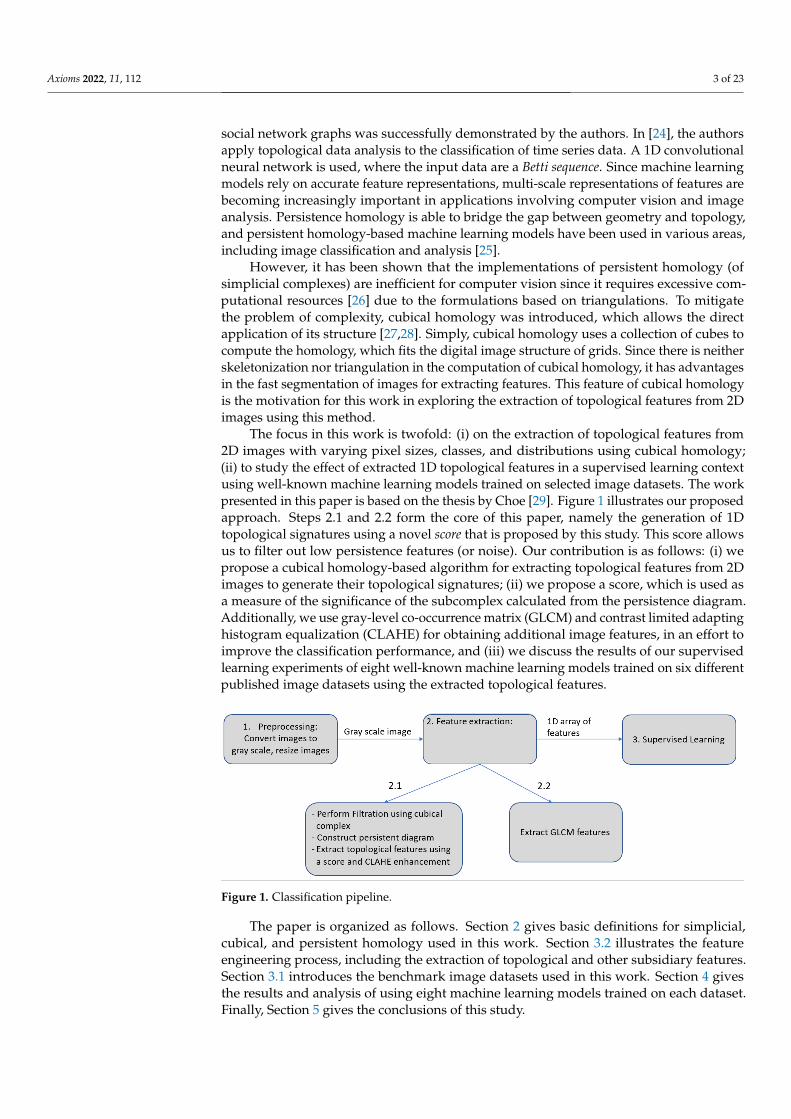
The focus in this work is twofold: (i) on the extraction of topological features from2D images with varying pixel sizes, classes, and distributions using cubical homology;(ii) to study the effect of extracted 1D topological features in a supervised learning contextusing well-known machine learning models trained on selected image datasets. The workpresented in this paper is based on the thesis by Choe [29]. Figure 1 illustrates our proposedapproach. Steps 2.1 and 2.2 form the core of this paper, namely the generation of 1Dtopological signatures using a novel score that is proposed by this study. This score allowsus to filter out low persistence features (or noise). Our contribution is as follows: (i) wepropose a cubical homology-based algorithm for extracting topological features from 2Dimages to generate their topological signatures; (ii) we propose a score, which is used asa measure of the significance of the subcomplex calculated from the persistence diagram.Additionally, we use gray-level co-occurrence matrix (GLCM) and contrast limited adaptinghistogram equalization (CLAHE) for obtaining additional image features, in an effort toimprove the classification performance, and (iii) we discuss the results of our supervisedlearning experiments of eight well-known machine learning models trained on six differentpublished image datasets using the extracted topological features.

Figure 1. Classification pipeline.

The paper is organized as follows. Section 2 gives basic definitions for simplicial,cubical, and persistent homology used in this work. Section 3.2 illustrates the featureengineering process, including the extraction of topological and other subsidiary features.Section 3.1 introduces the benchmark image datasets used in this work. Section 4 givesthe results and analysis of using eight machine learning models trained on each dataset.Finally, Section 5 gives the conclusions of this study.

Axioms 2022, 11, 112 4 of 23

2. Basic Definitions

We recall some basic definitions of the concepts used in this work. A simplicial complexis a space or an object that is built from a union of points, edges, triangles, tetrahedra, andhigher-dimensional polytopes. Homology theory is in the domain of algebraic topologyrelated to the connectivity in multi-dimensional shapes [26].

2.1. Simplicial Homology

Graphs are mathematical structures used to study pairwise relationships betweenobjects and entities.

Definition 1. A graph is a pair of sets, G = (V, E), where V is the set of vertices (or nodes) andE is a set of edges.

Let S be a subset of a group G. Then, the subgroup generated by S, denoted 〈S〉, is thesubgroup of all elements of G that can be expressed as the finite operation of elements in Sand their inverses. For example, the set of all integers, Z, can be expressed by the operationof elements {1} so Z is the subgroup generated by {1}.

Definition 2. A rank of a group G is the size of the smallest subset that generates G.

For instance, since Z is the subgroup generated by {1}, rank(Z)=1.

Definition 3. A simplex complex on a set V is a family of arbitrary cardinality subsets of Vclosed under the subset operation, which means that, if a set S is in the family, all subsets of S arealso in the family. An element of the family is called a simplex or face.

Definition 4. Moreover, p− simplex can be defined to the convex hull of p + 1 affinely indepen-dent points x0, x1, · · · , xp ∈ IRd.

For example, in a graph, 0-simplex is a point, 1-simplex is an edge, 2-simplex is atriangle, 3-simplex is a tetrahedron, and so on (see Figure 2).

0-simplex (vertices) 1-simplex (edges) 2-simplex (triangles) 3-simplex (tets)

Figure 2. Examples of p-simplex for p = 0, 1, 2, 3 in tetrahedron. A 0-simplex is a point, a 1-simplex isan edge with a convex hull of two points, a 2-simplex is a triangle with a convex hull of three distinctpoints, and a 3-simplex is a tetrahedron with a convex hull of four points [30].

Chain, Boundary, and Cycle

To extend simplicial homology to persistent homology, the notion of chain, boundary,and cycle is necessary [31].

Definition 5. A p-chain is a subset of p-simplices in a simplicial complex K. Assume that K is atriangle. Then, a 1-chain is a subset of 1-simplices—in other words, a subset of the three edges.

Definition 6. A boundary, generally denoted ∂, of a p-simplex is the set of (p− 1)-simplices’ faces.

For example, a triangle is a 2-simplex, so the boundary of a triangle is a set of 1-simpliceswhich are the edges. Therefore, the boundary of the triangle is the three edges.

Axioms 2022, 11, 112 5 of 23

Definition 7. A cycle can be defined using the definitions of chain and boundary. A p-cycle c is ap-chain with an empty boundary. More simply, it is a path where the starting point and destinationpoint are the same.

2.2. Cubical Homology

Cubical homology [27] is efficient since it allows the direct use of the cubical structureof the image, whereas simplicial theory requires increasing the complexity of data. Whilethe simplicial homology is built with the triangle and its higher-dimensional structure,such as a tetrahedron, cubical homology consists of cubes. In cubical homology, each cubehas a unit size and the n-cube represents its dimension. For example, 0-cubes are points,1-cubes are lines with unit length, 2-cubes are unit squares, and so on [27,32,33].

Definition 8. Here, 0-cubes can be defined as an interval,

[m] = [m, m], m ∈ Z, (1)

which generate subsets I ∈ R, such that

I = [m, m + 1], m ∈ Z. (2)Therefore, I is called a 1-cube, or elementary interval.

Definition 9. An n-cube can be expressed as a product of elementary intervals as

Q = I1 × I2 × · · · × In ⊆ Rn, (3)

where Q indicates that n-cube Ii(i = 1, 2, · · · , n) is an elementary interval.

A d-dimensional image is a map I : I ⊆ Zd → R.

Definition 10. A pixel can be defined as an element v ∈ I, where d = 2. If d > 2, v is calleda voxel.

Definition 11. Let I(v) be the intensity or grayscale value. Moreover, in the case of binary images,we consider a map B : I ⊆ Zd → {0, 1}.

A voxel is represented by a d-cube and, with all of its faces added, we have

I ′(σ) := minσ face of τ

I(τ). (4)

Let K be the cubical complex built from the image I, and let

Ki := {σ ∈ K|I ′(σ) ≤ i}, (5)

be the i-th sublevel set of K. Then, the set {Ki}i∈Im(I) defines a filtration of the cubicalcomplexes. Thus, the pipeline to filtration from an image with a cubical complex isas follows:

Image→ Cubical complex→ Sublevel sets→ Filtration

Moreover, chain, boundary, and cycle in cubical homology can be defined in the samemanner as in Section 2.1.

2.3. Persistent Homology

In topology, there are subcomplices of complex K and cubes are created (birth) anddestroyed (death) by filtration. Assume that Ki (0 ≤ i ≤, i ∈ Z) is a subcomplex of filteredcomplex K such that

∅ ⊆ K0 ⊆ K1 ⊆ · · · ⊆ Kn = K,

Axioms 2022, 11, 112 6 of 23

and Z ik, Bi

k are its corresponding cycle group and boundary group.

Definition 12. The kth homology group [1] can be defined as

Hk = Zk/Bk. (6)

Definition 13. The p-persistent kth homology group of Ki [1] can be defined as

Hi,pk = Z i

k/Bi+pk ∩ Z i

k. (7)

Definition 14. A persistence is a lifetime of these attributes based on the filtration method used [1].

One can plot the birth and death times of the topological features as a barcode, alsoknown as a persistence barcode, shown in Figure 3. This diagram graphically representsthe topological signature of the data. Illustration of persistence is useful when detecting achange in terms of topology and geometry, which plays a crucial role in supervised machinelearning [34].

115 119115 94

119 119 11994 94 114

115 94115 94115 117

139 100 11499 99 114

117 117 177

(a) (b)

(c)

(d)100 115 130 145

Figure 3. An example of persistent homology for grayscale image. (a) A given image, (b) a matrix ofgray level of given image, (c) the filtered cubical complex of the image, (d) the persistence barcodeaccording to (c).

3. Materials and Methods3.1. Image Datasets

In this section, we give a brief description of the six published image datasets usedin this work. Datasets used for benchmarking were collected from various sources thatinclude Mendeley Data (https://data.mendeley.com/ accessed on 7 January 2022), Tensorflowdataset (https://www.tensorflow.org/datasets accessed on 7 January 2022), and Kagglecompetition (https://www.kaggle.com/competitions accessed on 7 January 2022). Theconcrete crack images dataset [35] contains a total of 40,000 images, where each imageconsists of 227× 227 pixels. These images were collected from the METU campus buildingand consist of two classes: 20,000 images where there are no cracks in the concrete (positive)and 20,000 images of concrete that is cracked (negative). A crack on an outer wall occurswith the passage of time or due to natural aging. It is important to detect these cracks interms of evaluating and predicting the structural deterioration and reliability of buildings.Samples of the two types of images are shown in Figure 4.

The APTOS blindness detection dataset [36] is a set of retina images taken by fundusphotography for detecting and preventing diabetic retinopathy from causing blindness

Axioms 2022, 11, 112 7 of 23

(https://www.kaggle.com/c/aptos2019-blindness-detection/overview accessed on 7 Jan-uary 2022). This dataset has 3662 images and consists of 1805 images diagnosed as non-diabetic (labeled as 0) retinopathy and 1857 images diagnosed as diabetic retinopathy, asshown in Figure 5. Figure 6 shows the distribution of examples in the four classes using aseverity range from 1 to 4 with the following interpretation: 1: Mild, 2: Moderate, 3: Severe,4: Proliferative DR.

(a) Negative crack image (b) Positive crack image

Figure 4. Sample images of the concrete crack dataset.

(a) Non-diabetic retinopathy (b) Diabetic retinopathy

Figure 5. Sample images of APTOS dataset. (a) is a picture of Non-diabetic retionpathy which isordinary case and (b) is a picture of diabetic retinopathy which cas cause blindness.

Figure 6. Data distribution for APTOS 2019 blindness detection dataset. This dataset can be classifiedas non-diabetic and diabetic. Around 50% of images are categorized as non-diabetic retinopathy(label 0) and diabetic retinopathy is subdivided according to the severity range from 1 to 4.

Axioms 2022, 11, 112 8 of 23

The pest classi f ication in mango f arms dataset [37] is a collection of 46,500 images ofmango leaves affected by 15 different types of pests and one normal (unaffected) mangoleaf, as shown in Figure 7. Some of these pests can be detected visually. Figure 8 shows thedata distribution of examples in the 15 classes of pests and one normal class.

(a) normal (b) apoderus javanicus (c) aulacaspis tubercularis (d) ceroplastes rubens

(e) cisaberoptus kenyae (f) dappula tertia (g) dialeuropora decempuncta (h) erosomyia sp

(i) icerya seychellarum (j) ischnaspis longirostris (k) mictis longicornis (l) neomelicharia sparsa

(m) orthaga euadrusalis (n) procontarinia matteiana (o) procontarinia rubus (p) valanga nigricornis

Figure 7. Sample images of pest classification in mango farms.

Axioms 2022, 11, 112 9 of 23

Figure 8. Data distribution for pest classification in mango farms dataset. Labels are assigned inalphabetical order.

The Indian f ruits dataset [38] contains 23,848 images that cover five popular fruits inIndia: apple, orange, mango, pomegranate, and tomato. This dataset includes variationsof each fruit, resulting in 40 classes. This dataset was already separated into training andtesting sets by the original publishers of the dataset, as shown in Figure 9. Note that thisdataset has an imbalanced class distribution.

Figure 9. Data distribution for the Indian fruits dataset. These data are already split by the originalpublishers of the dataset by the ratio of 9 to 1. Labels are assigned in alphabetical order.

Axioms 2022, 11, 112 10 of 23

The colorectal histology dataset [39] contains 5000 histological images of differenttissue types of colorectal cancer. It consists of 8 classes of tissue types with 625 images foreach class, as shown in Figure 10.

Figure 10. Example of colorectal cancer histology. (a) Tumor epithelium, (b) simple stroma, (c) com-plex stroma, (d) immune cell conglomerates, (e) debris and mucus, (f) mucosal glands, (g) adiposetissue, (h) background.

The Fashion MNIST dataset [40] is a collection of 60,000 training images of fashionproducts, as shown in Figure 11. It consists of 28× 28 grayscale images of products from10 classes. Since the dataset contains an equal number of images for each class, there are6000 test images in each class, resulting in a balanced dataset.

Axioms 2022, 11, 112 11 of 23

Figure 11. Example of the Fashion MNIST dataset.

Table 1 gives the dataset characteristics in terms of the various image datasets usedin this work. Moreover, we provide the preprocessing time per image. For example, thefeature extraction time for the concrete dataset was 5 h 12 min.

Table 1. Dataset details with preprocessing times.

Dataset Size Num of Classes Pixel Dimension Balanced Time in Sec/Image

Concrete 1 40,000 2 227 × 227 Yes 0.4713Mangopest 2 46,000 16 from 500 × 333 to 1280 × 853 No 0.5394

Indian fruits 3 23,848 40 100 × 100 No 0.4422Fashion MNIST 4 60,000 10 28 × 28 Yes 0.4297

APTOS 5 3662 5 227 × 227 No 0.5393Colorectal histology 6 5000 8 150 × 150 Yes 0.3218

1 Çaglar Fırat Özgenel, 23 July 2019, https://data.mendeley.com/datasets/5y9wdsg2zt/2; 2 Kusrini Kusrini et al.,accessed on 27 February 2020, https://data.mendeley.com/datasets/94jf97jzc8/1; 3 prabira Kumar sethy, accessedon 12 June 2020, https://data.mendeley.com/datasets/bg3js4z2xt/1; 4 Han Xiao et al., accessed on 28 August2017, https://github.com/zalandoresearch/fashion-mnist; 5 Asia Pacific Tele-Ophthalmology Society, accessedon 27 June 2019, https://www.kaggle.com/c/aptos2019-blindness-detection/overview; 6 Kather, Jakob Nikolaset al., 26 May 2016, https://zenodo.org/record/53169#.XGZemKwzbmG.

3.2. Methods—Feature Engineering

In this section, we describe the feature engineering process. The main purpose of thisprocess is to obtain a 1-dimensional array from each image in the dataset. Each point fromthe persistence diagram plays a significant role in the extraction of the topological features.Moreover, the gray-level co-occurrence matrix (GLCM) supports these topological featuresas additional signatures. Because every image dataset is not identical in size and someimages have very high resolution, resizing every image to 200 × 200 and converting themto grayscale guarantees a relatively constant duration of extraction (approximately 4 s)regardless of its original size.

Axioms 2022, 11, 112 12 of 23

Algorithm 1 gives the method for extracting topological features from a dataset. In thisalgorithm, β0 and β1 are Betti numbers derived from Equation (6), where the dimensionof ith homology is called the ith Betti number of K. β0 gives the number of connectedcomponents and β1 gives the number of holes. Betti numbers represent the count of thenumber of topological features.

Algorithm 1 Extraction of Topological Features.

Input: N ← number of datasetfor i = 1, 2, · · · , N do

img← load ith image from datasetimg← resize img to (200, 200) and convert to grayscalePD0 ← set of points of β0 in persistence diagram of img with cubical complexPD1 ← set of points of β1 in persistence diagram of img with cubical complexPD0 ← sort PD0 in descending order of persistencePD1 ← sort PD1 in descending order of persistencedi ← project each point in PD0 to [0, 1]di ← di + project each point in PD1 to [1, 2]f img← adapt CLAHE filter to imgf PD0 ← set of points of β0 in persistence diagram of f img with cubical complexf PD1 ← set of points of β1 in persistence diagram of f img with cubical complexf PD0 ← sort f PD0 in descending order of persistencef PD1 ← sort f PD1 in descending order of persistencedi ← di + project each point in f PD0 to [0, 1]di ← di + project each point in f PD1 to [1, 2]di ← di + convert img to GLCM with distances (1, 2, 3), directions (0◦, 45◦, 90◦, 135◦),

and properties (energy, homogeneity)Output: D(d1, d2, · · · , dN)

3.3. Projection of Persistence Diagrams

The construction of a persistence diagram is possible once the filtration (using cubicalcomplex) is completed. The dth persistence diagram, Dd, contains all of the d-dimensionaltopological information. These are a series of points with a pair of (birth, death), wherebirth indicates the time at which the topological features were created and the death givesthe time at which these features are destroyed. From here, persistence is defined using thedefinition of birth and death as

pers(birth, death) := death− birth, where (birth, death) ∈ Dd. (8)

Low-persistence features are treated as having low importance, or ‘noise’, whereashigh-persistence features are regarded as true features [1]. However, using persistence asa result of a projection of a topological feature to a 1-dimensional value is not helpful,because it is impossible to distinguish the features which have the same persistence butdifferent values for birth. Therefore, we propose a measure (score) to compensate for thislimitation of persistence, shown in Equation (9).

scored(birth, death) :=

0 if persistence < threshold

d +

(esin ( death

255 ·π2 ) − 1

e− 1

)3

−(

esin ( birth255 ·

π2 ) − 1

e− 1

)3

if persistence ≥ threshold(9)

Since the sinusoidal term is increasing and has the value [0, 1] when the input is [0, π2 ],

the scored has a value range from d to d + 1. Hence, it is easy to distinguish the dimensionand persistence of each feature. Moreover, a higher exponent emphasizes a feature that haslonger persistence and, significantly, ignores a feature that has shorter persistence. Thisin is keeping with ideas underlying homology groups, where longer the persistence, the

Axioms 2022, 11, 112 13 of 23

higher the significance of the homology. Conversely, the homology group that has shortpersistence is considered noise, which degrades the quality of the digital image and, as such,is less significant as a topological feature [10]. By ignoring such noise, using a threshold(as a parameter) allows us to separate useful features from noise. The optimal threshold(value = 10) was determined experimentally by comparing the performance of machinelearning models. In summary, the score takes into account not only the persistence, but alsoother aspects such as the dimension, birth, and death of topological features.

3.4. Contrast Limited Adapting Histogram Equalization (CLAHE)

When pixel values are concentrated in a narrow range, it is hard to perceive featuresvisually. Histogram equalization makes the distribution of pixel values in the imagebalanced, thereby enhancing the image. However, this method often results in degradingthe content of the image and also amplifying the noise. Therefore, it produces undesirableresults. Contrast limited adapting histogram equalization (CLAHE) is a well-knownmethod for compensating for the weakness of histogram equalization by dividing animage into small-sized blocks and performing histogram equalization for each block [41].After completing histogram equalization in all blocks, bilinear interpolation makes theboundary of the tiles (blocks) smooth. In this paper, we used the following hyperparameters:clipLimit=7 and tileGridSize=((8, 8)). An illustration of the CLAHE method on theAPTOS data is given in Figure 12.

(a) (b)

(c) (d)

Figure 12. Comparison of the original image and the CLAHE-filtered image. (a) Original image,(b) persistence diagram of the original image (a), (c) CLAHE-filtered image, (d) persistence diagramof the filtered image (c).

The texture of an image can be described by its statistical properties and this in-formation is useful to classify images [42]. For extracting texture features, we used thewell-known gray-level co-occurrence matrix (GLCM) [43]. GLCM extracts texture infor-

Axioms 2022, 11, 112 14 of 23

mation regarding the structural arrangement of surfaces by using a displacement vectordefined by its radius and orientation. We used three distances (1, 2, 3) and four directions(0◦, 45◦, 90◦, 135◦) to obtain the GLCM features. From each of the co-occurrence matrices,two global statistics were extracted, energy and homogeneity, resulting in 3× 4× 2 = 24texture features for each image.

Table 2 gives a list of extracted features from the APTOS dataset during the filtrationprocess. In total, 144 features were extracted for each dimension ( f dim0 and f dim1) fromthe CLAHE-filtered image in descending order of persistence. Similarly, 100 (dim0 anddim1) topological features for each dimension were extracted. Note that dim0 representsβ0 and dim1 represents β1 Betti numbers, respectively. A total of 24 GLCM features wereextracted from the original gray-level image.

In this paper, feature engineering and learning algorithms were implemented with thefollowing Python libraries: Gudhi [44,45] for calculating persistent homology, PyTorch [46]for modeling and execution of ResNet 1D, and scikit-learn [47] for implementation of othermachine learning algorithms. Moreover, libraries such as NumPy [48] and pandas [49] wereused for computing matrices and analyzing the data structure. All tests were conductedusing a desktop workstation with Intel i7-9700K at 3.6 GHz, 8 CPU cores, 16 GB RAM, andGigabyte GeForce RTX 2080 GPU. The following algorithms were used.

Deep Residual Network, suggested by [50], is an ensemble of VGG-19 [51], plainnetwork, and residual network as a solution to the network depth-accuracy degradationproblem. This is done by a residual learning framework, which is a feedforward networkwith a shortcut. Multi-scale 1D ResNet is used in this work, where multi-scale refers toflexible convolutional kernels rather than flexible strides [52]. The authors use different sizesof kernels so that the network can learn features from original signals with different viewswith multiple scales. The structure of the model is described in Figure 13. The 1D ResNetmodel consists of a number of subblocks of the basic CNN blocks. A basic CNN blockcomputes batch normalization after convolution as follows: y = W⊗ x + b, s = BN(y), andh = ReLU(s), where ⊗ denotes the convolution operator and BN is a batch normalizationoperator. Moreover, stacking two basic CNN blocks forms a subblock of the basic CNNblocks as follows: h1 = Basic(x), h2 = Basic(h1), y = h2 + x, and h = ReLU(y), wherethe Basic operator denotes the basic block described above. Using the above method, itis possible to construct multiple sub-blocks of the CNN with different kernel sizes. Fortraining the network, we used an early stopping option if there was no improvement inthe validation loss after 20 epochs. Using the early stopping option and a learning rate of0.01, the network was trained over 100 epochs, since the average training time was around50 epochs.

For the other machine learning models, the random f orest algorithm with 200 trees,gini as a criterion, and unlimited depth was used. For the K− nearest neighbors (kNN), thefollowing parameters were used: k = 5 and Minkowski as the distance metric. While therandom forest algorithm is an ensemble method based on the concept of bagging, GBM [53]uses the concept of boosting, iteratively training the model by adding new weak modelsconsecutively with the negative gradient from the loss function. Both extreme gradientboosting (XGBoost) [54,55] and lightGBM [56] are advanced models of the gradient boost-ing machines. LightGBM combines two techniques: Gradient-based One-Side Samplingand Exclusive Feature Bundling [57]. Since our dataset is tabular, XGBoost, which is amore efficient implementation of GBM, was used. For the XGBoost implementation, thefollowing training parameters were used: 1000 n_estimators for creating weak learners,learning rate = 0.3 (Eta), and max_depth = 6. For the LightGBM implementation, the follow-ing training parameters were used: 1000 n_estimators for creating weak learners, learningrate = 0.1 (Eta), and num_leaves = 31.

Axioms 2022, 11, 112 15 of 23

Table 2. Results of feature engineering process applied to the APTOS dataset.

img label glcm1 glcm2 · · · glcm24 dim0_0

dim0_1 · · · dim0_

99dim1_

0dim1_

1 · · · dim1_99

fdim0_0

fdim0_1 · · · fdim0_

143fdim1_

0fdim1_

1 · · · fdim1_143

0 2 0.1603 0.1571 · · · 0.4639 1 0.0366 · · · 0 1.2054 1.1815 · · · 0 0.9999 0.2060 · · · 0.0319 1.7698 1.6339 · · · 1.1067...

3661 2 0.1196 0.1160 · · · 0.5387 0.9999 0.0020 · · · 0 1.4787 1.0636 · · · 0 0.9999 0.1295 · · · 0.0042 1.9493 1.3658 · · · 1.10478

Axioms 2022, 11, 112 16 of 23

For all the datasets (except the Indian fruits dataset), 80% of the dataset was used fortraining and 20% was used for testing. The Indian fruits dataset was already separated into90% for training and 10% for testing. This ratio was used in our experiments.

Inp

ut

1×51

2

Con

v L

ayer

(1×

7@6

4)

BN

ReL

U

Max

Poo

lin

g 1×

2

Con

v1-1

1(1

×3@

64

) BN

ReL

UC

onv1

-12

(1×

3@6

4)

BN

ReL

U

Con

v3-1

1(1

×7@

64

) BN

ReL

UC

onv3

-12

(1×

7@6

4)

BN

ReL

U

Con

v2-1

1(1

×5@

64

) BN

ReL

UC

onv2

-12

(1×

5@6

4)

BN

ReL

U

Con

v1-2

1(1

×3@

128

) BN

ReL

UC

onv1

-22

(1×

7@12

8)

BN

ReL

U

Con

v3-2

1(1

×7@

128

) BN

ReL

UC

onv3

-22

(1×

7@12

8)

BN

ReL

U

Con

v2-2

1(1

×5@

128

) BN

ReL

UC

onv2

-22

(1×

5@12

8)

BN

ReL

U

Con

v1-3

1(1

×3@

256

) BN

ReL

UC

onv1

-32

(1×

3@25

6)

BN

ReL

U

Con

v3-3

1(1

×7@

256

) BN

ReL

UC

onv3

-32

(1×

7@25

6)

BN

ReL

U

Con

v2-3

1(1

×5@

256

) BN

ReL

UC

onv2

-32

(1×

5@25

6)

BN

ReL

U

++

+

++

+

++

+

Ave

rage

Poo

lin

g A

vera

ge P

ooli

ng

Ave

rage

Poo

lin

g

Fea

ture

Vec

tor

1 (2

56×

1)

Fea

ture

Vec

tor

2 (2

56×

1)

Fea

ture

Vec

tor

3 (2

56×

1)

Fea

ture

Vec

tor

(76

8×

1)

Con

cate

nat

e

Fu

lly

Con

nec

ted

Net

wor

k

Sof

tmax

Figure 13. Structure of the multi-scale 1D ResNet.

4. Results and Discussion

Table 3 gives the accuracy, weighted F1 score, and run time information for each ofthe datasets. The accuracy score reported with the benchmark datasets is given in the lastcolumn. The best result is indicated in blue. Overall, ResNet 1D outperforms other MLmodels, while different types of gradient boosting machines show fairly good accuracyand weighted F1 scores. In terms of binary classification image datasets, as in the concretedataset, most of the algorithms achieve 0.99 accuracy and F1 score. However, for themulti-class image datasets, the SVM and kNN perform poorly, mainly due to the inherentdifficulty of finding the best parameters. All machine learning models perform significantlyworse than the benchmark results with the Fashion MNIST and APTOS datasets with theextracted topological features. This is because it is hard to obtain good trainable topologicalsignatures from images that have low resolution, even though Fashion MNIST was resized(please see Table 1).

In the case of the APTOS dataset, imbalanced training data were the main cause of thepoor results. For example, Label 0 indicates the absence of diabetic retinopathy and has thehighest number of images (See Figure 6). However, the presence of diabetic retinopathycan be found in four classes, of which Label 2 (severity level 2.0) has the largest number ofcases. As a result, more than half of the examples were classified as Label 2 (see Figure 14c).

Axioms 2022, 11, 112 17 of 23

Table 3. Accuracy and weighted F1 score for each dataset.

ResNet 1D CART GBM LightGBM Random Forest SVM XGBoost kNN Related Works—Benchmark

Accuracy 0.994 0.989 0.991 0.9945 0.993 0.956 0.9935 0.890 0.999 with CNN [35]Concrete Weighted F1 0.994 0.988 0.989 0.994 0.992 0.955 0.993 0.884

Run time 465.87 9.08 252.15 11.25 7.63 214.05 59.15 1.93

Accuracy 0.931 0.764 0.681 0.898 0.869 0.474 0.889 0.666 0.76 with CNN [37]Mangopest Weighted F1 0.931 0.764 0.676 0.898 0.869 0.439 0.889 0.663

Run time 760.94 17.17 5562.09 260.62 13.94 662.45 2041.22 2.33

Accuracy 1.000 0.9608 0.9608 0.9608 0.9608 0.7313 0.9608 0.676 0.999 SVM withIndian fruits Weighted F1 1.000 0.9608 0.9608 0.9608 0.9608 0.7236 0.9608 0.656 deep features [38]

Run time 271.21 4.44 4265.09 82.55 4.13 72.73 451.65 1.18

Accuracy 0.7427 0.567 0.696 0.749 0.693 0.535 0.746 0.397 0.99 with CNN [58]Fashion MNIST Weighted F1 0.7414 0.569 0.694 0.749 0.692 0.529 0.746 0.390

Run time 467.12 8.36 1808.07 89.37 7.66 935.21 1108.20 3.38

Accuracy 0.7326 0.698 0.760 0.787 0.782 0.674 0.775 0.655 0.971 with CNN [59]APTOS Weighted F1 0.667 0.695 0.737 0.771 0.757 0.591 0.764 0.637

Run time 61.81 0.63 86.02 13.16 0.70 3.49 42.34 0.08

Accuracy 0.892 0.75 0.842 0.869 0.855 0.679 0.874 0.759 0.874 with SVM [39]Colorectal histology Weighted F1 0.89 0.727 0.832 0.850 0.834 0.686 0.843 0.743

Run time 86.23 1.18 255.08 12.52 1.10 4.06 44.63 0.14

Accuracy 0.882 ± 0.109 0.789 ± 0.147 0.822 ± 0.121 0.876 ± 0.087 0.856 ± 0.102 0.675 ± 0.154 0.873 ± 0.90 0.674 ± 0.148Weighted F1 0.871 ± 0.125 0.784 ± 0.148 0.815 ± 0.124 0.870 ± 0.091 0.851 ± 0.105 0.654 ± 0.164 0.866 ± 0.092 0.662 ± 0.147

Axioms 2022, 11, 112 18 of 23

0398999%

261%

1261%

0

395699%

1

Truelabel

Predicted label

(a) Concrete

079267%

10%

847%

968%

424%

10%

12411%

00%

303%

81%

171%

111394%

40%

524%

10%

00%

20%

00%

00%

00%

2494%

10%

89375%

292%

1069%

10%

958%

00%

141%

101%

3807%

565%

272%

89273%

796%

30%

514%

10%

202%

71%

4303%

50%

12511%

958%

72462%

30%

17515%

00%

101%

101%

530%

00%

00%

20%

20%

96183%

20%

14512%

192%

292%

618114%

40%

18315%

726%

23519%

71%

53543%

00%

242%

141%

700%

10%

00%

00%

00%

1079%

10%

104184%

101%

867%

8242%

00%

252%

192%

91%

292%

252%

232%

95281%

645%

9192%

0

00%

1

50%

2

71%

3

151%

4

232%

5

71%

6

897%

7

514%

8

100382%

9

Truelabel

Predicted label

(b) Fashion MNIST

034595%

31%

103%

21%

41%

19

13%3144%

2839%

00%

34%

22111%

126%

14878%

11%

74%

349%

511%

3273%

12%

25%

49

14%

0

46%

1

3960%

2

12%

3

1218%

4

Truelabel

Predicted label

(c) APTOS

010290%

22%

33%

00%

44%

22%

00%

00%

100%

10186%

76%

11%

54%

33%

00%

00%

264%

97%

10376%

129%

43%

11%

00%

00%

300%

22%

43%

11394%

00%

11%

00%

00%

411%

1210%

43%

22%

9781%

22%

22%

00%

500%

22%

22%

43%

54%

11390%

00%

00%

600%

00%

00%

00%

32%

00%

12195%

32%

700%

0

00%

1

00%

2

00%

3

00%

4

00%

5

00%

6

1100%

7

Truelabel

Predicted label

(d) Colorectal Histology

Figure 14. Confusion matrices of implementation with ResNet 1D. (a) Concrete, (b) Fashion MNIST,(c) APTOS, (d) Colorectal Histology.

Imbalanced data such as Mangopest and Indian fruits were classified well becausethere were sufficient training examples. In summary, the best classification performanceusing cubical homology with the ResNet 1D classifier was obtained for 2 out of 6 datasetsusing our proposed feature extraction method and score measure. However, these topo-logical signatures were not helpful in the classification of the Fashion MNIST and APTOSimages. For the Indian fruits dataset, the model classifies with an accuracy of 1.00, which is

Axioms 2022, 11, 112 19 of 23

comparable since there is just 0.001 improvement. Similarly, with the concrete dataset, theresult is comparable, with only a slight difference (≤0.005) with the benchmark result.

In Table 4, we give an illustration of the performance of classifiers using featuresderived from cubical homology (TDA), GLCM, and combined TDA-GLCM for two datasets.It is clear from the results that the combined feature set using topological features andGLCM features results in better classifier accuracy.

Confusion matrices for experiments with the 1D ResNet model are given inFigures 14–16. It is noteworthy that, for these datasets, the application of cubical homologyhas led to meaningful results in 4 out of 6 datasets.

062

100%0

0%0

0%0

0%0

0%0

0%0

0%0

0%0

0%0

0%0

0%0

0%0

0%0

0%0

0%0

0%0

0%0

0%0

0%0

0%0

0%0

0%0

0%0

0%0

0%0

0%0

0%0

0%0

0%0

0%0

0%0

0%0

0%0

0%0

0%0

0%0

0%0

0%0

0%0

0%

10

0%61

100%0

0%0

0%0

0%0

0%0

0%0

0%0

0%0

0%0

0%0

0%0

0%0

0%0

0%0

0%0

0%0

0%0

0%0

0%0

0%0

0%0

0%0

0%0

0%0

0%0

0%0

0%0

0%0

0%0

0%0

0%0

0%0

0%0

0%0

0%0

0%0

0%0

0%0

0%

20

0%0

0%57

100%0

0%0

0%0

0%0

0%0

0%0

0%0

0%0

0%0

0%0

0%0

0%0

0%0

0%0

0%0

0%0

0%0

0%0

0%0

0%0

0%0

0%0

0%0

0%0

0%0

0%0

0%0

0%0

0%0

0%0

0%0

0%0

0%0

0%0

0%0

0%0

0%0

0%

30

0%0

0%0

0%66

100%0

0%0

0%0

0%0

0%0

0%0

0%0

0%0

0%0

0%0

0%0

0%0

0%0

0%0

0%0

0%0

0%0

0%0

0%0

0%0

0%0

0%0

0%0

0%0

0%0

0%0

0%0

0%0

0%0

0%0

0%0

0%0

0%0

0%0

0%0

0%0

0%

40

0%0

0%0

0%0

0%64

100%0

0%0

0%0

0%0

0%0

0%0

0%0

0%0

0%0

0%0

0%0

0%0

0%0

0%0

0%0

0%0

0%0

0%0

0%0

0%0

0%0

0%0

0%0

0%0

0%0

0%0

0%0

0%0

0%0

0%0

0%0

0%0

0%0

0%0

0%0

0%

50

0%0

0%0

0%0

0%0

0%53

100%0

0%0

0%0

0%0

0%0

0%0

0%0

0%0

0%0

0%0

0%0

0%0

0%0

0%0

0%0

0%0

0%0

0%0

0%0

0%0

0%0

0%0

0%0

0%0

0%0

0%0

0%0

0%0

0%0

0%0

0%0

0%0

0%0

0%0

0%

60

0%0

0%0

0%0

0%0

0%0

0%53

100%0

0%0

0%0

0%0

0%0

0%0

0%0

0%0

0%0

0%0

0%0

0%0

0%0

0%0

0%0

0%0

0%0

0%0

0%0

0%0

0%0

0%0

0%0

0%0

0%0

0%0

0%0

0%0

0%0

0%0

0%0

0%0

0%0

0%

70

0%0

0%0

0%0

0%0

0%0

0%0

0%116

100%0

0%0

0%0

0%0

0%0

0%0

0%0

0%0

0%0

0%0

0%0

0%0

0%0

0%0

0%0

0%0

0%0

0%0

0%0

0%0

0%0

0%0

0%0

0%0

0%0

0%0

0%0

0%0

0%0

0%0

0%0

0%0

0%

80

0%0

0%0

0%0

0%0

0%0

0%0

0%0

0%63

100%0

0%0

0%0

0%0

0%0

0%0

0%0

0%0

0%0

0%0

0%0

0%0

0%0

0%0

0%0

0%0

0%0

0%0

0%0

0%0

0%0

0%0

0%0

0%0

0%0

0%0

0%0

0%0

0%0

0%0

0%0

0%

90

0%0

0%0

0%0

0%0

0%0

0%0

0%0

0%0

0%55

100%0

0%0

0%0

0%0

0%0

0%0

0%0

0%0

0%0

0%0

0%0

0%0

0%0

0%0

0%0

0%0

0%0

0%0

0%0

0%0

0%0

0%0

0%0

0%0

0%0

0%0

0%0

0%0

0%0

0%0

0%

100

0%0

0%0

0%0

0%0

0%0

0%0

0%0

0%0

0%0

0%75

100%0

0%0

0%0

0%0

0%0

0%0

0%0

0%0

0%0

0%0

0%0

0%0

0%0

0%0

0%0

0%0

0%0

0%0

0%0

0%0

0%0

0%0

0%0

0%0

0%0

0%0

0%0

0%0

0%0

0%

110

0%0

0%0

0%0

0%0

0%0

0%0

0%0

0%0

0%0

0%0

0%59

100%0

0%0

0%0

0%0

0%0

0%0

0%0

0%0

0%0

0%0

0%0

0%0

0%0

0%0

0%0

0%0

0%0

0%0

0%0

0%0

0%0

0%0

0%0

0%0

0%0

0%0

0%0

0%0

0%

120

0%0

0%0

0%0

0%0

0%0

0%0

0%0

0%0

0%0

0%0

0%0

0%63

100%0

0%0

0%0

0%0

0%0

0%0

0%0

0%0

0%0

0%0

0%0

0%0

0%0

0%0

0%0

0%0

0%0

0%0

0%0

0%0

0%0

0%0

0%0

0%0

0%0

0%0

0%0

0%

130

0%0

0%0

0%0

0%0

0%0

0%0

0%0

0%0

0%0

0%0

0%0

0%0

0%64

100%0

0%0

0%0

0%0

0%0

0%0

0%0

0%0

0%0

0%0

0%0

0%0

0%0

0%0

0%0

0%0

0%0

0%0

0%0

0%0

0%0

0%0

0%0

0%0

0%0

0%0

0%

140

0%0

0%0

0%0

0%0

0%0

0%0

0%0

0%0

0%0

0%0

0%0

0%0

0%0

0%100

100%0

0%0

0%0

0%0

0%0

0%0

0%0

0%0

0%0

0%0

0%0

0%0

0%0

0%0

0%0

0%0

0%0

0%0

0%0

0%0

0%0

0%0

0%0

0%0

0%0

0%

150

0%0

0%0

0%0

0%0

0%0

0%0

0%0

0%0

0%0

0%0

0%0

0%0

0%0

0%0

0%90

100%0

0%0

0%0

0%0

0%0

0%0

0%0

0%0

0%0

0%0

0%0

0%0

0%0

0%0

0%0

0%0

0%0

0%0

0%0

0%0

0%0

0%0

0%0

0%0

0%

160

0%0

0%0

0%0

0%0

0%0

0%0

0%0

0%0

0%0

0%0

0%0

0%0

0%0

0%0

0%0

0%96

100%0

0%0

0%0

0%0

0%0

0%0

0%0

0%0

0%0

0%0

0%0

0%0

0%0

0%0

0%0

0%0

0%0

0%0

0%0

0%0

0%0

0%0

0%0

0%

170

0%0

0%0

0%0

0%0

0%0

0%0

0%0

0%0

0%0

0%0

0%0

0%0

0%0

0%0

0%0

0%0

0%66

100%0

0%0

0%0

0%0

0%0

0%0

0%0

0%0

0%0

0%0

0%0

0%0

0%0

0%0

0%0

0%0

0%0

0%0

0%0

0%0

0%0

0%0

0%

180

0%0

0%0

0%0

0%0

0%0

0%0

0%0

0%0

0%0

0%0

0%0

0%0

0%0

0%0

0%0

0%0

0%0

0%72

100%0

0%0

0%0

0%0

0%0

0%0

0%0

0%0

0%0

0%0

0%0

0%0

0%0

0%0

0%0

0%0

0%0

0%0

0%0

0%0

0%0

0%

190

0%0

0%0

0%0

0%0

0%0

0%0

0%0

0%0

0%0

0%0

0%0

0%0

0%0

0%0

0%0

0%0

0%0

0%0

0%69

100%0

0%0

0%0

0%0

0%0

0%0

0%0

0%0

0%0

0%0

0%0

0%0

0%0

0%0

0%0

0%0

0%0

0%0

0%0

0%0

0%

200

0%0

0%0

0%0

0%0

0%0

0%0

0%0

0%0

0%0

0%0

0%0

0%0

0%0

0%0

0%0

0%0

0%0

0%0

0%0

0%88

100%0

0%0

0%0

0%0

0%0

0%0

0%0

0%0

0%0

0%0

0%0

0%0

0%0

0%0

0%0

0%0

0%0

0%0

0%0

0%

210

0%0

0%0

0%0

0%0

0%0

0%0

0%0

0%0

0%0

0%0

0%0

0%0

0%0

0%0

0%0

0%0

0%0

0%0

0%0

0%0

0%58

100%0

0%0

0%0

0%0

0%0

0%0

0%0

0%0

0%0

0%0

0%0

0%0

0%0

0%0

0%0

0%0

0%0

0%0

0%

220

0%0

0%0

0%0

0%0

0%0

0%0

0%0

0%0

0%0

0%0

0%0

0%0

0%0

0%0

0%0

0%0

0%0

0%0

0%0

0%0

0%0

0%58

100%0

0%0

0%0

0%0

0%0

0%0

0%0

0%0

0%0

0%0

0%0

0%0

0%0

0%0

0%0

0%0

0%0

0%

230

0%0

0%0

0%0

0%0

0%0

0%0

0%0

0%0

0%0

0%0

0%0

0%0

0%0

0%0

0%0

0%0

0%0

0%0

0%0

0%0

0%0

0%0

0%37

100%0

0%0

0%0

0%0

0%0

0%0

0%0

0%0

0%0

0%0

0%0

0%0

0%0

0%0

0%0

0%0

0%

240

0%0

0%0

0%0

0%0

0%0

0%0

0%0

0%0

0%0

0%0

0%0

0%0

0%0

0%0

0%0

0%0

0%0

0%0

0%0

0%0

0%0

0%0

0%0

0%52

100%0

0%0

0%0

0%0

0%0

0%0

0%0

0%0

0%0

0%0

0%0

0%0

0%0

0%0

0%0

0%

250

0%0

0%0

0%0

0%0

0%0

0%0

0%0

0%0

0%0

0%0

0%0

0%0

0%0

0%0

0%0

0%0

0%0

0%0

0%0

0%0

0%0

0%0

0%0

0%0

0%51

100%0

0%0

0%0

0%0

0%0

0%0

0%0

0%0

0%0

0%0

0%0

0%0

0%0

0%0

0%

260

0%0

0%0

0%0

0%0

0%0

0%0

0%0

0%0

0%0

0%0

0%0

0%0

0%0

0%0

0%0

0%0

0%0

0%0

0%0

0%0

0%0

0%0

0%0

0%0

0%0

0%52

100%0

0%0

0%0

0%0

0%0

0%0

0%0

0%0

0%0

0%0

0%0

0%0

0%0

0%

270

0%0

0%0

0%0

0%0

0%0

0%0

0%0

0%0

0%0

0%0

0%0

0%0

0%0

0%0

0%0

0%0

0%0

0%0

0%0

0%0

0%0

0%0

0%0

0%0

0%0

0%0

0%53

100%0

0%0

0%0

0%0

0%0

0%0

0%0

0%0

0%0

0%0

0%0

0%0

0%

280

0%0

0%0

0%0

0%0

0%0

0%0

0%0

0%0

0%0

0%0

0%0

0%0

0%0

0%0

0%0

0%0

0%0

0%0

0%0

0%0

0%0

0%0

0%0

0%0

0%0

0%0

0%0

0%43

100%0

0%0

0%0

0%0

0%0

0%0

0%0

0%0

0%0

0%0

0%0

0%

290

0%0

0%0

0%0

0%0

0%0

0%0

0%0

0%0

0%0

0%0

0%0

0%0

0%0

0%0

0%0

0%0

0%0

0%0

0%0

0%0

0%0

0%0

0%0

0%0

0%0

0%0

0%0

0%0

0%40

100%0

0%0

0%0

0%0

0%0

0%0

0%0

0%0

0%0

0%0

0%

300

0%0

0%0

0%0

0%0

0%0

0%0

0%0

0%0

0%0

0%0

0%0

0%0

0%0

0%0

0%0

0%0

0%0

0%0

0%0

0%0

0%0

0%0

0%0

0%0

0%0

0%0

0%0

0%0

0%0

0%44

100%0

0%0

0%0

0%0

0%0

0%0

0%0

0%0

0%0

0%

310

0%0

0%0

0%0

0%0

0%0

0%0

0%0

0%0

0%0

0%0

0%0

0%0

0%0

0%0

0%0

0%0

0%0

0%0

0%0

0%0

0%0

0%0

0%0

0%0

0%0

0%0

0%0

0%0

0%0

0%0

0%44

100%0

0%0

0%0

0%0

0%0

0%0

0%0

0%0

0%

320

0%0

0%0

0%0

0%0

0%0

0%0

0%0

0%0

0%0

0%0

0%0

0%0

0%0

0%0

0%0

0%0

0%0

0%0

0%0

0%0

0%0

0%0

0%0

0%0

0%0

0%0

0%0

0%0

0%0

0%0

0%0

0%49

100%0

0%0

0%0

0%0

0%0

0%0

0%0

0%

330

0%0

0%0

0%0

0%0

0%0

0%0

0%0

0%0

0%0

0%0

0%0

0%0

0%0

0%0

0%0

0%0

0%0

0%0

0%0

0%0

0%0

0%0

0%0

0%0

0%0

0%0

0%0

0%0

0%0

0%0

0%0

0%0

0%45

100%0

0%0

0%0

0%0

0%0

0%0

0%

340

0%0

0%0

0%0

0%0

0%0

0%0

0%0

0%0

0%0

0%0

0%0

0%0

0%0

0%0

0%0

0%0

0%0

0%0

0%0

0%0

0%0

0%0

0%0

0%0

0%0

0%0

0%0

0%0

0%0

0%0

0%0

0%0

0%0

0%67

100%0

0%0

0%0

0%0

0%0

0%

350

0%0

0%0

0%0

0%0

0%0

0%0

0%0

0%0

0%0

0%0

0%0

0%0

0%0

0%0

0%0

0%0

0%0

0%0

0%0

0%0

0%0

0%0

0%0

0%0

0%0

0%0

0%0

0%0

0%0

0%0

0%0

0%0

0%0

0%0

0%44

100%0

0%0

0%0

0%0

0%

360

0%0

0%0

0%0

0%0

0%0

0%0

0%0

0%0

0%0

0%0

0%0

0%0

0%0

0%0

0%0

0%0

0%0

0%0

0%0

0%0

0%0

0%0

0%0

0%0

0%0

0%0

0%0

0%0

0%0

0%0

0%0

0%0

0%0

0%0

0%0

0%33

100%0

0%0

0%0

0%

370

0%0

0%0

0%0

0%0

0%0

0%0

0%0

0%0

0%0

0%0

0%0

0%0

0%0

0%0

0%0

0%0

0%0

0%0

0%0

0%0

0%0

0%0

0%0

0%0

0%0

0%0

0%0

0%0

0%0

0%0

0%0

0%0

0%0

0%0

0%0

0%0

0%67

100%0

0%0

0%

380

0%0

0%0

0%0

0%0

0%0

0%0

0%0

0%0

0%0

0%0

0%0

0%0

0%0

0%0

0%0

0%0

0%0

0%0

0%0

0%0

0%0

0%0

0%0

0%0

0%0

0%0

0%0

0%0

0%0

0%0

0%0

0%0

0%0

0%0

0%0

0%0

0%0

0%43

100%0

0%

390

0%

0

00%

1

00%

2

00%

3

00%

4

00%

5

00%

6

00%

7

00%

8

00%

9

00%

10

00%

11

00%

12

00%

13

00%

14

00%

15

00%

16

00%

17

00%

18

00%

19

00%

20

00%

21

00%

22

00%

23

00%

24

00%

25

00%

26

00%

27

00%

28

00%

29

00%

30

00%

31

00%

32

00%

33

00%

34

00%

35

00%

36

00%

37

00%

38

61100%

39

True

label

Predicted label

Figure 15. Confusion matrix for the Indian fruits dataset with ResNet 1D implementation.

Axioms 2022, 11, 112 20 of 23

019580%

10%

31%

00%

31%

125%

104%

00%

31%

00%

42%

00%

42%

104%

00%

00%

120%

59891%

30%

91%

00%

10%

162%

10%

20%

41%

152%

00%

10%

51%

10%

00%

252%

10%

28185%

31%

00%

72%

155%

00%

31%

10%

124%

10%

21%

10%

00%

00%

300%

40%

00%

96896%

00%

00%

61%

141%

30%

40%

50%

00%

40%

30%

00%

00%

410%

00%

10%

00%

21093%

31%

63%

00%

21%

00%

00%

00%

00%

21%

00%

21%

561%

20%

41%

31%

20%

47188%

112%

00%

41%

51%

132%

00%

41%

71%

10%

00%

620%

40%

131%

20%

30%

121%

102893%

30%

40%

61%

202%

00%

71%

50%

00%

10%

710%

10%

10%

121%

00%

10%

111%

150698%

20%

00%

20%

00%

00%

20%

00%

00%

820%

00%

20%

10%

10%

132%

31%

31%

55795%

00%

00%

10%

20%

10%

00%

10%

900%

62%

41%

31%

00%

00%

82%

72%

00%

35790%

41%

00%

31%

21%

21%

00%

1000%

183%

81%

81%

00%

20%

233%

10%

10%

71%

58388%

10%

61%

41%

10%

00%

1100%

00%

00%

00%

00%

00%

00%

00%

46%

00%

00%

6694%

00%

00%

00%

00%

1251%

20%

51%

51%

10%

30%

101%

20%

10%

41%

61%

00%

63593%

00%

10%

00%

1320%

20%

10%

61%

00%

122%

20%

10%

61%

10%

112%

00%

61%

43589%

31%

10%

1400%

10%

00%

00%

00%

00%

10%

10%

31%

00%

00%

00%

21%

00%

22897%

00%

1500%

0

00%

1

00%

2

00%

3

31%

4

10%

5

00%

6

00%

7

10%

8

00%

9

00%

10

00%

11

00%

12

00%

13

00%

14

51999%

15

Truelabel

Predicted label

Figure 16. Confusion matrix for the Mangopest dataset with ResNet 1D implementation.

Table 4. Comparison of performance of GLCM+TDA, TDA feature-only, and GLCM-only imple-mented by 1D ResNet model on two datasets.

Colorectal Histology Dataset APTOS Dataset

GLCM+TDA 0.892 0.7326TDA 0.7697 0.6739

GLCM 0.694 0.7252

5. Conclusions

The focus of this paper was on feature extraction from 2D image datasets using aspecific topological method (cubical homology) and a novel score measure. These featureswere then used as input to well-known classification algorithms to study the efficacy of theproposed feature extraction process. We proposed a novel scoring method to transformthe 2D input images into a one-dimensional array to vectorize the topological features.In this study, six published datasets were used as benchmarks. ResNet 1D, LightGBM,XGBoost, and five well-known machine learning models were trained on these datasets.Our experiments demonstrated that, in three out of six datasets, our proposed topologicalfeature method is comparable to (or better than) the benchmark results in terms of accuracy.However, with two datasets, the performance of our proposed topological feature methodis poor, due to either low resolution or an imbalanced dataset. We also demonstrate thattopological features combined with GLCM features result in better classification accuracy

Axioms 2022, 11, 112 21 of 23

in two of the datasets. This study reveals that the application of cubical homology to imageclassification shows promise. Since the conversion of input images to 2D data is verytime-consuming, future work will involve (i) seeking more efficient ways to reduce thetime for pre-processing and (ii) experimentation with more varied datasets. The problemof poor accuracy with imbalanced datasets needs further exploration.

Author Contributions: S.C.: Conceptualization, Investigation, Formal Analysis, Supervision, Re-sources, Original Draft. S.R.: Methodology, Validation, Software, Editing. All authors have read andagreed to the publisher version of the manuscript.

Funding: This research was funded by NSERC Discovery Grant#194376 and University of WinnipegMajor Research Grant#14977.

Institutional Review Board Statement: Not applicable.

Informed Consent Statement: Not applicable.

Data Availability Statement: Not applicable.

Conflicts of Interest: The authors declare no conflicts of interest.

References1. Edelsbrunner, H.; Letscher, D.; Zomorodian, A. Topological persistence and simplification. In Proceedings of the 41st Annual

Symposium on Foundations of Computer Science, Redondo Beach, CA, USA, 12–14 November 2000; IEEE Computer SocietyPress: Los Alamitos, CA, USA, 2000; pp. 454–463.

2. Chazal, F.; Michel, B. An Introduction to Topological Data Analysis: Fundamental and Practical aspects for Data Scientists. arXiv2017, arXiv:1710.04019.

3. Zomorodian, A.; Carlsson, G. Computing persistent homology. Discr. Comput. Geom. 2005, 33, 249–274. [CrossRef]4. Carlsson, G. Topology and data. Bull. Am. Math. Soc. 2009, 46, 255–308. [CrossRef]5. Edelsbrunner, H.; Harer, J. Persistent homology. A survey. Contemp. Math. 2008, 453, 257–282.6. Zomorodian, A.F. Computing and Comprehending Topology: Persistence and Hierarchical Morse Complexes. Ph.D. Thesis,

University of Illinois at Urbana-Champaign, Urbana, IL, USA, 2001.7. Aktas, M.E.; Akbas, E.; Fatmaoui, A.E. Persistence Homology of Networks: Methods and Applications. arXiv 2019,

arXiv:math.AT/1907.08708.8. Garin, A.; Tauzin, G. A topological “reading” lesson: Classification of MNIST using TDA. In Proceedings of the 2019 18th

IEEE International Conference On Machine Learning And Applications (ICMLA), Boca Raton, FL, USA, 16–19 December 2019;pp. 1551–1556.

9. Adams, H.; Chepushtanova, S.; Emerson, T.; Hanson, E.; Kirby, M.; Motta, F.; Neville, R.; Peterson, C.; Shipman, P.; Ziegelmeier, L.Persistence Images: A Stable Vector Representation of Persistent Homology. arXiv 2016, arXiv:cs.CG/1507.06217.

10. Kramár, M.; Goullet, A.; Kondic, L.; Mischaikow, K. Persistence of force networks in compressed granular media. Phys. Rev. E2013, 87, 042207. [CrossRef]

11. Nakamura, T.; Hiraoka, Y.; Hirata, A.; Escolar, E.G.; Nishiura, Y. Persistent homology and many-body atomic structure formedium-range order in the glass. Nanotechnology 2015, 26, 304001. [CrossRef]

12. Dunaeva, O.; Edelsbrunner, H.; Lukyanov, A.; Machin, M.; Malkova, D.; Kuvaev, R.; Kashin, S. The classification of endoscopyimages with persistent homology. Pattern Recognit. Lett. 2016, 83, 13–22. [CrossRef]

13. Reininghaus, J.; Huber, S.; Bauer, U.; Kwitt, R. A stable multi-scale kernel for topological machine learning. In Proceedings of theIEEE Conference on Computer Vision and Pattern Recognition, Boston, MA, USA, 7–12 June 2015; pp. 4741–4748.

14. Iijima, T. Basic theory on the normalization of pattern (in case of typical one-dimensional pattern). Bull. Electro-Tech. Lab. 1962,26, 368–388.

15. Bonis, T.; Ovsjanikov, M.; Oudot, S.; Chazal, F. Persistence-based pooling for shape pose recognition. In Proceedings of theInternational Workshop on Computational Topology in Image Context, Marseille, France, 15–17 June 2016; pp. 19–29.

16. Dey, T.; Mandal, S.; Varcho, W. Improved image classification using topological persistence. In Proceedings of the Conference onVision, Modeling and Visualization, Bonn, Germany, 25–27 September 2017; pp. 161–168.

17. Kindelan, R.; Frías, J.; Cerda, M.; Hitschfeld, N. Classification based on Topological Data Analysis. arXiv 2021,arXiv:cs.LG/2102.03709.

18. Carrière, M.; Chazal, F.; Ike, Y.; Lacombe, T.; Royer, M.; Umeda, Y. Perslay: A neural network layer for persistence diagrams andnew graph topological signatures. In Proceedings of the International Conference on Artificial Intelligence and Statistics (PMLR),Online, 26–28 August 2020; pp. 2786–2796.

19. Chung, M.K.; Lee, H.; DiChristofano, A.; Ombao, H.; Solo, V. Exact topological inference of the resting-state brain networks intwins. Netw. Neurosci. 2019, 3, 674–694. [CrossRef]

Axioms 2022, 11, 112 22 of 23

20. Don, A.P.H.; Peters, J.F.; Ramanna, S.; Tozzi, A. Topological View of Flows Inside the BOLD Spontaneous Activity of the HumanBrain. Front. Comput. Neurosci. 2020, 14, 34. [CrossRef]

21. Don, A.P.; Peters, J.F.; Ramanna, S.; Tozzi, A. Quaternionic views of rs-fMRI hierarchical brain activation regions. Discovery ofmultilevel brain activation region intensities in rs-fMRI video frames. Chaos Solitons Fractals 2021, 152, 111351. [CrossRef]

22. Krizhevsky, A.; Sutskever, I.; Hinton, G.E. Imagenet classification with deep convolutional neural networks. Adv. Neural Inf.Process. Syst. 2012, 25, 1097–1105. [CrossRef]

23. Hofer, C.D.; Kwitt, R.; Niethammer, M. Learning Representations of Persistence Barcodes. J. Mach. Learn. Res. 2019, 20, 1–45.24. Umeda, Y. Time series classification via topological data analysis. Inf. Media Technol. 2017, 12, 228–239. [CrossRef]25. Pun, C.S.; Xia, K.; Lee, S.X. Persistent-Homology-Based Machine Learning and its Applications—A Survey. arXiv 2018,

arXiv:math.AT/1811.00252.26. Allili, M.; Mischaikow, K.; Tannenbaum, A. Cubical homology and the topological classification of 2D and 3D imagery. In

Proceedings of the 2001 International Conference on Image Processing (Cat. No. 01CH37205), Thessaloniki, Greece, 7–10 October2001; Volume 2, pp. 173–176.

27. Kot, P. Homology calculation of cubical complexes in Rn. Comput. Methods Sci. Technol. 2006, 12, 115–121. [CrossRef]28. Strömbom, D. Persistent Homology in the Cubical Setting: Theory, Implementations and Applications. Master’s Thesis, Lulea

University of Technology, Lulea, Sweden, 2007.29. Choe, S. Cubical homology-based Image Classification-A Comparative Study. Master’s Thesis, University of Winnipeg, Winnipeg,

MB, Canada, 2021.30. Fisher, M.; Springborn, B.; Schröder, P.; Bobenko, A.I. An algorithm for the construction of intrinsic Delaunay triangulations with

applications to digital geometry processing. Computing 2007, 81, 199–213. [CrossRef]31. Otter, N.; Porter, M.A.; Tillmann, U.; Grindrod, P.; Harrington, H.A. A roadmap for the computation of persistent homology. EPJ

Data Sci. 2017, 6, 1–38. [CrossRef]32. Kaczynski, T.; Mischaikow, K.M.; Mrozek, M. Computational Homology; Springer: Berlin/Heidelberg, Germany, 2004.33. Kalies, W.D.; Mischaikow, K.; Watson, G. Cubical approximation and computation of homology. Banach Cent. Publ. 1999,

47, 115–131. [CrossRef]34. Marchese, A. Data Analysis Methods Using Persistence Diagrams. Ph.D. Thesis, University of Tennessee, Knoxville, TN,

USA, 2017.35. Özgenel, Ç.F.; Sorguç, A.G. Performance comparison of pretrained convolutional neural networks on crack detection in buildings.

In Proceedings of the International Symposium on Automation and Robotics in Construction (ISARC), Berlin, Germany, 20–25July 2018; Volume 35, pp. 1–8.

36. Avilés-Rodríguez, G.J.; Nieto-Hipólito, J.I.; Cosío-León, M.d.l.Á.; Romo-Cárdenas, G.S.; Sánchez-López, J.d.D.; Radilla-Chávez, P.;Vázquez-Briseño, M. Topological Data Analysis for Eye Fundus Image Quality Assessment. Diagnostics 2021, 11, 1322. [CrossRef]

37. Kusrini, K.; Suputa, S.; Setyanto, A.; Agastya, I.M.A.; Priantoro, H.; Chandramouli, K.; Izquierdo, E. Data augmentation forautomated pest classification in Mango farms. Comput. Electron. Agric. 2020, 179, 105842. [CrossRef]

38. Behera, S.K.; Rath, A.K.; Sethy, P.K. Fruit Recognition using Support Vector Machine based on Deep Features. Karbala Int. J. Mod.Sci. 2020, 6, 16. [CrossRef]

39. Kather, J.N.; Weis, C.A.; Bianconi, F.; Melchers, S.M.; Schad, L.R.; Gaiser, T.; Marx, A.; Zöllner, F.G. Multi-class texture analysis incolorectal cancer histology. Sci. Rep. 2016, 6, 27988. [CrossRef]

40. Xiao, H.; Rasul, K.; Vollgraf, R. Fashion-MNIST: A Novel Image Dataset for Benchmarking Machine Learning Algorithms. arXiv2017, arXiv:1708.07747.

41. Pizer, S.M.; Amburn, E.P.; Austin, J.D.; Cromartie, R.; Geselowitz, A.; Greer, T.; ter Haar Romeny, B.; Zimmerman, J.B.; Zuiderveld,K. Adaptive histogram equalization and its variations. Comput. Vision Graph. Image Process. 1987, 39, 355–368. [CrossRef]

42. Gadkari, D. Image Quality Analysis Using GLCM. Master’s Thesis, University of Central Florida, Orlando, FL, USA, 2004.43. Mohanaiah, P.; Sathyanarayana, P.; GuruKumar, L. Image texture feature extraction using GLCM approach. Int. J. Sci. Res. Publ.

2013, 3, 1–5.44. The GUDHI Project. GUDHI User and Reference Manual, 3.4.1 ed.; GUDHI Editorial Board; GUDHI: Nice, France, 2021.45. Dlotko, P. Cubical complex. In GUDHI User and Reference Manual, 3.4.1 ed.; GUDHI Editorial Board; GUDHI: Nice, France, 2021.46. Paszke, A.; Gross, S.; Massa, F.; Lerer, A.; Bradbury, J.; Chanan, G.; Killeen, T.; Lin, Z.; Gimelshein, N.; Antiga, L.; et al. PyTorch:

An Imperative Style, High-Performance Deep Learning Library. In Advances in Neural Information Processing Systems 32; Wallach,H., Larochelle, H., Beygelzimer, A., d'Alché-Buc, F., Fox, E., Garnett, R., Eds.; Curran Associates, Inc.: North Adams, MA, USA,2019; pp. 8024–8035.

47. Pedregosa, F.; Varoquaux, G.; Gramfort, A.; Michel, V.; Thirion, B.; Grisel, O.; Blondel, M.; Prettenhofer, P.; Weiss, R.; Dubourg, V.;et al. Scikit-learn: Machine Learning in Python. J. Mach. Learn. Res. 2011, 12, 2825–2830.

48. Harris, C.R.; Millman, K.J.; van der Walt, S.J.; Gommers, R.; Virtanen, P.; Cournapeau, D.; Wieser, E.; Taylor, J.; Berg, S.; Smith,N.J.; et al. Array programming with NumPy. Nature 2020, 585, 357–362. [CrossRef] [PubMed]

49. McKinney, W. Data structures for statistical computing in python. In Proceedings of the 9th Python in Science Conference, Austin,TX, USA, 28 June–3 July 2010; Volume 445, pp. 51–56.

50. He, K.; Zhang, X.; Ren, S.; Sun, J. Deep residual learning for image recognition. In Proceedings of the IEEE Conference onComputer Vision and Pattern Recognition, Las Vegas, NV, USA, 27–30 June 2016; pp. 770–778.

Axioms 2022, 11, 112 23 of 23

51. Mateen, M.; Wen, J.; Song, S.; Huang, Z. Fundus image classification using VGG-19 architecture with PCA and SVD. Symmetry2019, 11, 1. [CrossRef]

52. Liu, R.; Wang, F.; Yang, B.; Qin, S.J. Multiscale kernel based residual convolutional neural network for motor fault diagnosisunder nonstationary conditions. IEEE Trans. Ind. Inform. 2019, 16, 3797–3806. [CrossRef]

53. Friedman, J.H. Greedy function approximation: A gradient boosting machine. Ann. Stat. 2001, 29, 1189–1232. [CrossRef]54. Chen, T.; He, T.; Benesty, M.; Khotilovich, V.; Tang, Y.; Cho, H. Xgboost: Extreme gradient boosting. R Package Version 0.4-2 2015,

1, 1–4.55. Chen, T.; Guestrin, C. Xgboost: A scalable tree boosting system. In Proceedings of the 22nd ACM SIGKDD International

Conference on Knowledge Discovery and Data Mining, San Francisco, CA, USA, 13–17 August 2016; pp. 785–794.56. Ke, G.; Meng, Q.; Finley, T.; Wang, T.; Chen, W.; Ma, W.; Ye, Q.; Liu, T.Y. Lightgbm: A highly efficient gradient boosting decision

tree. Adv. Neural Inf. Process. Syst. 2017, 30, 3146–3154.57. Patel, V.; Choe, S.; Halabi, T. Predicting Future Malware Attacks on Cloud Systems using Machine Learning. In Proceedings

of the 2020 IEEE 6th International Conference on Big Data Security on Cloud (BigDataSecurity), High Performance and SmartComputing, (HPSC) and Intelligent Data and Security (IDS), Baltimore, MD, USA, 25–27 May 2020; pp. 151–156.

58. Kayed, M.; Anter, A.; Mohamed, H. Classification of garments from fashion MNIST dataset using CNN LeNet-5 architecture. InProceedings of the 2020 International Conference on Innovative Trends in Communication and Computer Engineering (ITCE),Aswan, Egypt, 8–9 February 2020; pp. 238–243.

59. Tymchenko, B.; Marchenko, P.; Spodarets, D. Deep learning approach to diabetic retinopathy detection. arXiv 2020,arXiv:2003.02261.