CloseUp: Statistical Detection ofChromosomal Homology Using Density

Alone–A Comparative Analysis

Steven E. Hampson and Pierre Baldi ∗School of Information and Computer ScienceInstitute for Genomics and Bioinformatics

University of California, IrvineIrvine, CA 92697-3425

(949) 824-5809(949) 824-4056 (FAX)

{hampson,pfbaldi}@ics.uci.edu

Brandon S. GautDepartment of Ecology and Evolutionary Biology

Institute for Genomics and BioinformaticsUniversity of California, Irvine

Irvine, CA 92697-2525bgaut@uci.edu

AbstractOver evolutionary time, various processes including point muta-

tions and insertions, deletions, and inversions of variable sized seg-ments progressively degrade the homology of duplicated chromoso-mal regions making identification of the homologous regions corre-spondingly harder. Existing algorithms that attempt to detect ho-mology are based on density and colinearity (LineUp), and possibly

∗and Department of Biological Chemistry, University of California, Irvine. To whomall correspondence should be addressed.

1

also strand information (ADHoRe). Here we first develop a new algo-rithm for the statistical detection of chromosomal homology, CloseUp,which uses density alone to fully exploit the observation that relax-ing colinearity requirements in general is beneficial for homology de-tection and at the same time optimizes computation time. CloseUphas two components: the generation of candidate homologous regionsfollowed by their statistical evaluation using Monte Carlo methodsand data randomization. We also develop statistical methods to esti-mate false positive and false negative rates at each detection thresholdand assess their tradeoff using ROC (Receiver Operating Character-istic) curves. Using both artificial and real data, we compare AD-HoRe, LineUp, and CloseUp and show that in general CloseUp com-pares favorably to the other algorithms. CloseUp is available throughhttp://www.igb.uci.edu/servers/cgss.html.

Keywords: comparative genomics, genome evolution, chromosomehomology, duplication, gene density, gene colinearity, synteny, syn-teny blocks.

1 Introduction

When a chromosomal segment begins to diverge, whether due to a speciationevent or due to an intra-genomic duplication, the two homologous regions areinitially identical in length and base sequence. Any genes or markers in thehomologous regions are identical in order, spacing and strand. For a recentlyduplicated chromosomal segment, these properties are statistically extreme,and the region is easily identified. However, over evolutionary time, pointmutations, insertions, deletions, and inversions progressively degrade theseproperties toward the statistical background, making precise identification ofthe homologous regions correspondingly difficult [Sankoff and El-Mabrouk,2002; Durand and Sankoff, 2003]. The relative rates of degradation of theseproperties is an open empirical question [Nadeau and Taylor, 1984; Schoen,2000; Wolfe and Li, 2003], so it is not obvious which features, or combi-nation of features, are most useful for detecting highly degraded homology.For example, if insertions and deletions dominate, the order and strand ofshared genes/markers may be more conserved than density. Conversely, ifinversions dominate, density may be more informative. Algorithmic analysisof these properties can vary greatly in complexity, so the choice of featuresand methods of analysis can impact runtime as well as accuracy.

The detection of chromosomal homology is important both for identify-ing synteny between two genomes and for identifying regions of intra-genomicduplication [Kent et al., 2003; Pevzner and Tesler, 2003a]. Two practical al-gorithms for detecting chromosomal homology have been developed recently.The ADHoRe algorithm [Vandepoele et al., 2002] which uses density, orderand strand information and the LineUp algorithm [Hampson et al., 2003]which uses density and order. It is important to note that while ADHoRe

2

and LineUp emphasize order information, neither is completely dependent onit. For example, ADHoRe begins by considering order and strand informationbut can also extend candidate regions based purely on density information.Colinear run generation in LineUp permits a limited amount of local reorder-ing to accommodate uncertainty in marker location or general degradationof order information. The larger the range of reordering permitted, the morerelaxed the definition of colinearity and the greater the reliance on densityover order.

A moderate amount of relaxation is probably always reasonable, butthe reordering approach can be combinatorially expensive for high-densitymarker data, limiting the amount of relaxation possible. Two versions ofLineUp were implemented to address this problem: FullPerm which attemptsto generate all legal colinear permutations, and FastRun which only gener-ates a heuristic subset. FastRun is more efficient in time and space and givesnearly identical homology results, but is still computationally intensive as afunction of the degree of colinear relaxation.

The complexity of ADHoRe and LineUp, both in code and runtime, isdetermined primarily by the use of order information. Consequently, an im-portant question is whether the ability to utilize order information is actuallynecessary for, or even significantly improves, homology detection under rea-sonable application conditions. In theory, the ability to use order informationshould only improve detection, but overly stringent order requirements mightactually exclude homologous but jumbled regions [Sankoff and El-Mabrouk,2002; Sankoff, 2002]. Likewise, it is not entirely clear whether strand infor-mation is essential or useful.

Here we first develop a third algorithm, CloseUp, both to exploit the factthat relaxed colinearity was observed to be generally beneficial for homologydetection and to optimize computational time. CloseUp uses shared geneor marker density alone, without regard to strand or order (see Methods).We then extend the statistical framework developed for LineUp in order toprovide estimates of false positive rates, false negative rates, and ReceiverOperating Characteristic (ROC) curves for detecting chromosomal homology.We compare ADHoRe, LineUp, and CloseUp using both artificial and realdata and show that in general CloseUp compares favorably to the otheralgorithms.

2 Methods

2.1 The CloseUp Algorithm

The CloseUp algorithm can be viewed as a limiting case of the LineUp al-gorithm when its colinearity-relaxing parameters I, D, and O all go to ∞[Hampson et al., 2003]. For completeness and clarity, it is better howeverto provide a self-contained description of CloseUp. Like LineUp, CloseUp

3

has two components: the generation of candidate homologous regions fol-lowed by their statistical evaluation using Monte Carlo methods and datarandomization.

2.1.1 Generation of Candidate Regions

Candidate regions are generated by finding all homologous gene pairs betweentwo chromosomes and attempting to extend each pair into two larger clusters.As seen in the results, CloseUp can compare a chromosome to itself but forthe sake of exposition we will use two distinct chromosomes C1 and C2.The comparison is asymmetric, so the results of comparing C1 to C2 maynot be the same as comparing C2 to C1. CloseUp automatically runs bothcomparisons. Comparison of C1 to C2 is achieved through an outer loop andan inner loop:

Outer Loop: The outer loop cycles through all the genes on C1. For eachgene on C1 it then cycles through all its matches on C2. Gene matchesare precomputed and indexed, so no searching is necessary. The outer looptypically takes linear time in the sense that if N is the typical number ofgenes on a chromosome and k << N is the maximal number of matches anygene on C1 has on C2, then the outer loop requires at most kN basic steps.

Inner Loop: The inner loop progressively extends each gene pair, generatedby the outer loop, into local clusters by using two simple tests of proximityand density, which are explained below, to control the extension process. Inthe inner loop we assume that a gene A on C1 has been matched to a geneA′ on C2. We initialize the corresponding developing clusters as C1 = {A}on C1 and C2 = {A′} on C2. Then:

1. Move to the next gene X to the right of C1. Set C1 = C1 ∪ {X}.2. Find the gene X ′ homologous to X on C2 that is closest to C2 (on its

right or its left). If no gene is found, go to step 1.

3. Test X ′ for proximity to C2. If X ′ is too far, go to step 1.

4. Set C2 = C2 ∪ [X ′], where [X ′] represents X ′ and all the genes betweenC2 and X ′.

5. Test C1 and C2 for density. If dense save C1 and C2 and go to step 1,else stop.

The inner loop saves all possible cluster pairs containing three or more geneseach. The number of steps in the inner loop is commensurate with the sizeof the clusters. Thus if the clusters are bounded in size by l, the complexityof the entire algorithm scales like O(klN), linear in the chromosome length.This scaling is similar to LineUp, except for one important element. As the

4

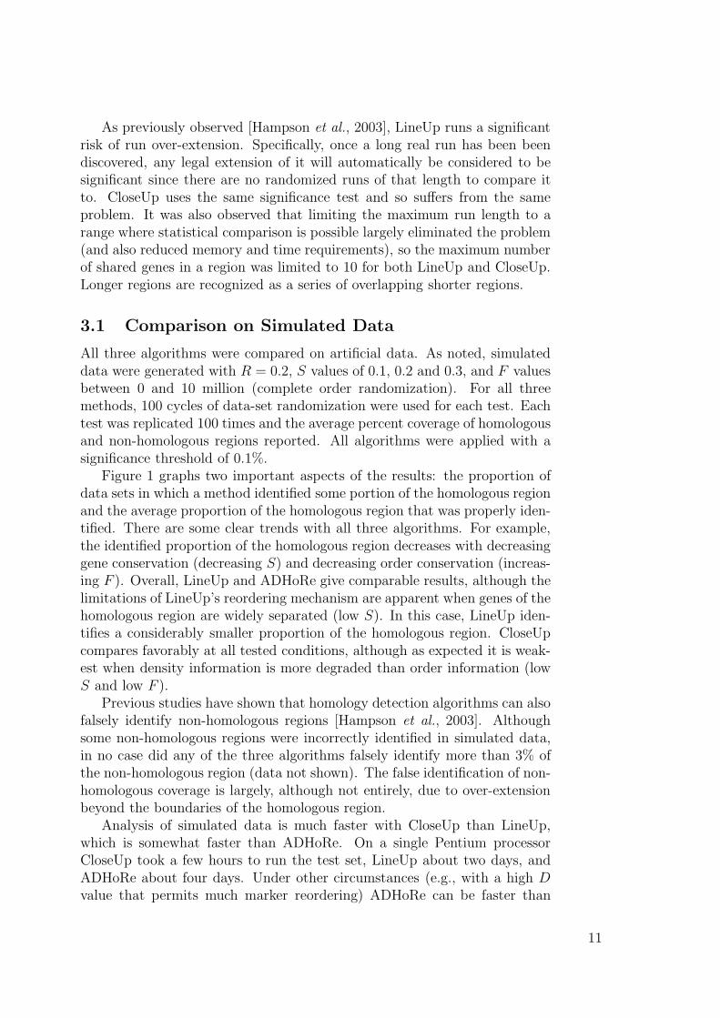
order constraint is relaxed, LineUp can search up to all viable permutationswithin a run, and therefore the inner loop in LineUp can scale like l!, whichrapidly becomes prohibitely slow even for reasonable values of l.

Expanding the region on C1 to the right (step 1) introduces some asym-metry. However, right-to-left, or bidirectional expansion do not greatlychange the results, so for consistency and comparison with LineUp they arenot used in the results presented here. Bidirectional expansion is provided,however, as a runtime option.

Genes with no corresponding matches between C1 and C2 have no impactin LineUp, but have a generally small effect in CloseUp since they effectthe density calculation. An option to retain or exclude unmatched genesis provided, and for consistency and comparison with LineUp the excludeoption is used in the examples presented here.

Test of Proximity: A proximity test is performed by checking whether theabsolute value of the difference in lengths of C1 and C2 is less than 20 timesthe pre-computed average inter-distance between genes in the chromosomes.This test is implicitly based on the idea that, to a first degree of approxima-tion, homologous regions ought to have roughly the same length and numberof genes. For example, consider the situation:

C1: ABTC

C2: ABCxxxxxxxxxxxxxxxxxxxxxxxxxxxxT

This situation might result, for example, from two random transposon (T)insertions. When comparing C1 to C2, if the matching Ts are included in theAB cluster, the resulting C2 region would be grossly over-extended beyondthe region of true homology. LineUp can address this problem by locally re-ordering the genes on C1 to recover the colinear run ABC. CloseUp does notuse the computationally expensive local re-ordering mechanism, and simplyskips any match on C2 that makes the difference in length between the tworegions more than 20 times the average gene distance. This is similar to the“skip” mechanism (I parameter) used in LineUp [Hampson et al., 2003] whichpermits some matching markers to be ignored. Values between 10 and 40gave similar results on a number of real and artificial data sets (see Results),so no further attempt was made to ”tune” this parameter to individual datasets. Further refinement and automatic adjustment of this parameter aretopics of future research.

Test of Density: In algorithms that rely on order information, candidatehomologous regions are terminated when colinear extension is no longer pos-sible. For the identification of cluster pairs in CloseUp, order-based termina-tion is replaced with density-based termination. Here we provide a methodfor identifying relatively high-density cluster pairs based on the expectednumber of shared genes between two random sets of genes. Region extension

5

is terminated if the observed is not significantly greater than the expected;in practice, twice.

To derive an estimate for the expected number of matches between a set ofn genes on C1 and a set of m genes on C2, imagine that the two chromosomescontain a total of T genes subdivided into K classes of non-homologous genes.If the genes are distributed at random, each class occurs on average T/2Ktimes on each chromosome. Thus if we consider a given gene on C1, itsprobability of matching a randomly selected gene on C2 is roughly 1/D. Ifwe take m genes (consecutive or not) on C2, the probability that none ofthem matches the gene on C1 is approximately [1− (1/K)]m ≈ 1−m/D andthe probability of one match or more is m/K. Thus, for n genes on C1, acrude estimate of the number of expected matches is nm/K.

2.1.2 Evaluation of Candidate Regions

Cluster pair detection, and all its variations, provides an initial filter forwhat might be homologous regions. However, the filter is sufficiently broadthat many cluster pairs will occur purely by chance. Consequently it isnecessary to identify the cluster pairs that are least likely to occur by chance.As for LineUp, statistical evaluation is carried using Monte Carlo methodsby randomizing the data many times and ranking cluster pairs highly ifthey have an unusually large number of shared genes in an unusually shortphysical region relative to randomized data. Real homologous regions arethus assumed to be dense.

Two properties are used to evaluate a cluster pair: the number of matchedgenes and their length on the chromosome (e.g, in centimorgans or basepairs). Various measures of length have been tried previously [Gaut, 2001;Hampson et al., 2003], but all gave similar results. We use the SummedSquares (SS) metric here. The SS value of a cluster pair is the sum of thesquared lengths of each cluster.

To test for statistical significance, for each chromosome pair (C1, C2),gene identifiers are permuted on C2 and cluster detection repeated. This isdone a large number of times (generally 1000), and the resulting cluster pairsare binned by the number of matched genes. This provides an estimate ofthe background frequency and distribution of lengths for the cluster pairs ineach bin. For each candidate cluster pair, the number of random cluster pairswith the same gene number but smaller SS value is tallied. This is dividedby the number of cluster pairs in the bin or the number of permutations(generally 1000), whichever is bigger, to compute the significance of the run.We generally use a 1.0% significance threshold, but results can be tunedaccording to the empirical distribution of probability values (see below).

CloseUp is available for download through www.igb.uci.edu/tools.htm.

6

2.2 ROC Curves

Application of CloseUp or other homology identification algorithms [Gaut,2001; Hampson et al., 2003; Vandepoele et al., 2002] can result in thousands ofputatively homologous regions that are tested for significance. Monte-Carlosimulations in CloseUp and LineUp appropriately adjust for multiple tests,but with thousands of tests there can still be an appreciable false positiverate. Here we adapt the methods described in Hung et al. [2002]; Baldi andHatfield [2002] to derive rates of false positives (FP ) and false negatives(FN) at each significance value, as well as the corresponding ROC curves.ROC curves are used in statistics and signal detection to study the tradeoffbetween false positives and false negatives for different detection cutoff values.More precisely, an ROC curve is a plot of the hit rate (or sensitivity) definedby TP/(TP + FN) versus the false alarm rate FP/(FP + TN) at eachpossible threshold, where TN and TP are true negatives and true positives,respectively.

Consider the probability that a pair of runs are homologous by chancealone, computed by the Monte Carlo method above. This probability is verysmall for all the homologous runs. If we look at the distribution histogramover all such probabilities we typically find a curve with a hill close to 0 anda flat uniform region towards 1. Such a distribution can be modeled as amixture of two beta distributions in the form:

P (p) =1∑

i=0

λiβ(p; ri, si) (1)

where β(p; r, s) = Cpr−1(1 − p)s−1 and C = Γ(r + s)/Γ(r)Γ(s). For i = 0,the values r0 = s0 = 1 are used to implement the uniform distribution as aspecial case of Beta distribution. λi represents the prior probability of eachcomponent, i.e. the proportion of pairs of runs that are non-significantlyhomologous (λ0) and significantly homologous (λ1 = 1 − λ0). In general,the mixture model can be fit to the empirical distribution using the EMalgorithm or other iterative optimization methods to determine the valuesof the λ, r, and s parameters. In a typical well-conditioned case, we canuse a shortcut by observing that the level of the empirical distribution closeto p = 1 provides a good estimate of λ0 since the value of the other betacomponent is close to 0 when p = 1. Thus λ1 is found by using λ1 = 1 − λ0

and only the values of r1 and s1 must be found. This can be done in variousways, for example by using the formula for the mean and the covariance ofthe beta distribution. After subtracting the uniform component, the mean ofthe remaining empirical distribution is equal to r/(r + s) while the varianceis equal to rs/(r + s)2(r + s + 1).

For any threshold T , the mixture model allows us to estimate the rateof true positives (TP ), true negatives (TN), false positives (FP ), and falsenegatives (FN). More precisely, we have:

• TP = P (p < T and homologous) = λ1

∫ T0 β(p; r1, s1)dp

7

• TN = P (p > T and non − homologous) = λ0(1 − T )

• FP = P (p < T and non − homologous) = λ0T

• FN = P (p > T and homologous) = λ1

∫ 1T β(p; r1, s1)dp

The posterior probability PPSH(p) of significant homology for a given pcan be computed by

PPSH(p) = P (homology|p) =λ1β(p; r1, s1)∑1i=0 λiβ(p; ri, si)

(2)

Alternatively, one can also use a posterior probability of significant homologyPPSH(< p) for values below a certain threshold p by :

PPSH(< p) = P (homology|p < T ) =λ1

∫ T0 β(p; r1, s1)dp∑1

i=0 λi

∫ T0 β(p; ri, si)dp

(3)

where the integrals can be estimated from the empirical areas.Finally, it is clear that for each threshold T on the significance probabili-

ties p, there is a tradeoff between the rates of true and false positives. A lowconservative threshold leads to few FP but may also reduce the TP rate. Alarge threshold ultimately allows one to recover all the TP but at the cost ofincreasing the FP rate. This fundamental tradeoff is captured by the ROCcurve. In the mixture model above, a simple calculation shows that for agiven threshold T , the false alarm rate

FP

FP + TN= T (4)

andcorresponds to a sensitivity given by

TP

TP + FN=

∫ T

0β(p; r1, s1)dp (5)

2.3 Data

We used both real and simulated data to compare CloseUp, LineUp andADHoRe.

2.3.1 Simulated Data

For the purpose of algorithm testing and comparison, we first use simulateddata. Simulated data presents at least two advantages for assessing algorith-mic performance and accuracy: (1) the difficulty of the problem, in termsof degraded homology, can be adjusted in a controlled fashion; (2) the “cor-rect” answer is known in advance, so that error rates and ROC curves can be

8

determined precisely. Artifical date must be constructed using biologicallyrealistic parameters in order to provide a meaningful point of comparison

Three main parameters were used to generate artificial data: 1) back-ground similarity: what fraction of genes not located in the homologousregion are similar to each other? 2) conserved genes: what fraction of theduplicated genes are still present in homologous regions? 3) conserved order:to what extent is the initial order of the genes retained in the homologousregion? The first parameter–background similarity–will vary depending onthe organism and the type of data (markers in a molecular genetic map vsgenes from a genome sequence). In general, the second and third parameterwill approach the background given sufficient evolutionary time for deletions,rearrangments, and other degradation events to occur.

Artificial data is generated in three steps corresponding to the three pa-rameters above. In general, we have used sequence characteristics from Ara-bidopsis thaliana [Arabidopsis Genome Initiative, 2000] as a guideline forsimulated data.

First, a uniform background is created. This is done by assigning Nunique genes to random locations and random strands on each of two chro-mosomes, C1 and C2. For Arabidopsis, average chromosome length is about25 million bases [Arabidopsis Genome Initiative, 2000], so that value is usedhere, although the actual value used is largely immaterial. For Arabidopsis,N is on the order of 5000, but for simulation efficiency N = 1000 is used here.The N genes are placed randomly along the length of the chromosome. Tocreate a background similarity distribution, each of the 2N genes is consid-ered, and with probability R is replaced with another gene chosen at randomfrom the 2N set. This produces a background distribution of singles (foundonly once on C1 and C2), doubles (found twice on C1 and C2), triples, andso forth, depending on the value of R. Typically we used a value of R = 0.2,which is again similar to A. thaliana [Arabidopsis Genome Initiative, 2000;Vision et al., 2000]. The larger the value of R, the harder the problem for atleast two reasons. First, there is simply a larger background of potential, butrandom homology, and separating signal from noise becomes more difficultas the noise increases. Second, the additional background pairs may breakup the real homology region as in the above transposon example.

Next, a region of homology comprising the middle 20% of each chromo-some is created. For N = 1000, the region contains 200 genes, which can benumbered in any order. A random fraction S of the genes in that region onC2 are replaced with the correspondingly numbered genes from that regionon C1. Strand and location information are also duplicated, so if S = 1 thetwo regions are identical. When S < 1, the number of unpaired genes in thehomologous regions reflects the amount of insertion/deletion that occurredafter duplication. In our simulations, S = 0.1, 0.2 and 0.3, again approxi-mating the A. thaliana genome, for which roughly 28% of genes are retainedin duplicated regions [Blanc et al., 2003; Simillion et al., 2002].

Finally, F randomly chosen neighboring gene pairs are inverted in the

9

homologous region of C2. That is, only small-scale inversions are simu-lated. With increasing F , strand, order and local density are progressivelydegraded. If inversions are performed only within the homologous region,the boundaries remain distinct, but if inversions are permitted over the en-tire chromosome, the homologous and non-homologous regions “diffuse” intoeach other. In that case the actual extent of the homologous region becomessubjective, so for testing purposes we limited the inversions to the bound-aries of the homologous region. Consequently, the density of shared genesover the entire region does not change while the density of shared genes insmaller subregions varies. F was varied between 0 and 10 million, which issufficient to completely randomize gene order in the homologous region. Theupper limit of 10 million inversions was empirically determined, as follows.An array of length X was initialized to A[i] = i. Initially,

∑i |A[i]− i| is zero,

but with successive neighbor inversions, the sum increases to the long-termaverage of X2/3. For X = 200, this value is reached between one and tenmillion inversions.

2.3.2 Marker Data

To briefly compare the performance of CloseUp and LineUp on real data,we also used the Pioneer 1999 Composite map (Pio99) of the maize genome,which is an amalgamation of several maize molecular genetic maps. ThePio99 map contains 2,415 markers that hybridize to more than one loca-tion on the ten chromosomes of the maize genome. Thus, Pio99 data con-stitutes a reasonable data set for indentifying homologous regions betweenchromosomes within the maize genome. Pio99 data were downloaded fromhttp://www.agron.missouri.edu/ , and LineUp results on Pio99 have beenreported previously in Hampson et al. [2003].

3 Results

LineUp, CloseUp and ADHoRe were used primarily with default parametersettings. The reordering parameter, D, for LineUp was set to twice theaverage distance between markers; that is, markers separated by less than Dcould be reordered to achieve colinearity. CloseUp was applied with densityand proximity values of 2 and 20 as previously discussed. Initial ADHoReresults gave relatively poor results, so a number of parameter adjustmentswere attempted (data not shown). All were ineffective except increasingthe ADHoRe.pl “max-dist” value [Vandepoele et al., 2002], which increaseddetection of the homologous region but also increased the proportion of thenon-homologous that was falsely identified as homologous. Consequently, thisvalue was increased from the suggested 20 to 40, which yielded maximumhomologous coverage without producing greater non-homologous coveragethan the other algorithms.

10

As previously observed [Hampson et al., 2003], LineUp runs a significantrisk of run over-extension. Specifically, once a long real run has been beendiscovered, any legal extension of it will automatically be considered to besignificant since there are no randomized runs of that length to compare itto. CloseUp uses the same significance test and so suffers from the sameproblem. It was also observed that limiting the maximum run length to arange where statistical comparison is possible largely eliminated the problem(and also reduced memory and time requirements), so the maximum numberof shared genes in a region was limited to 10 for both LineUp and CloseUp.Longer regions are recognized as a series of overlapping shorter regions.

3.1 Comparison on Simulated Data

All three algorithms were compared on artificial data. As noted, simulateddata were generated with R = 0.2, S values of 0.1, 0.2 and 0.3, and F valuesbetween 0 and 10 million (complete order randomization). For all threemethods, 100 cycles of data-set randomization were used for each test. Eachtest was replicated 100 times and the average percent coverage of homologousand non-homologous regions reported. All algorithms were applied with asignificance threshold of 0.1%.

Figure 1 graphs two important aspects of the results: the proportion ofdata sets in which a method identified some portion of the homologous regionand the average proportion of the homologous region that was properly iden-tified. There are some clear trends with all three algorithms. For example,the identified proportion of the homologous region decreases with decreasinggene conservation (decreasing S) and decreasing order conservation (increas-ing F ). Overall, LineUp and ADHoRe give comparable results, although thelimitations of LineUp’s reordering mechanism are apparent when genes of thehomologous region are widely separated (low S). In this case, LineUp iden-tifies a considerably smaller proportion of the homologous region. CloseUpcompares favorably at all tested conditions, although as expected it is weak-est when density information is more degraded than order information (lowS and low F ).

Previous studies have shown that homology detection algorithms can alsofalsely identify non-homologous regions [Hampson et al., 2003]. Althoughsome non-homologous regions were incorrectly identified in simulated data,in no case did any of the three algorithms falsely identify more than 3% ofthe non-homologous region (data not shown). The false identification of non-homologous coverage is largely, although not entirely, due to over-extensionbeyond the boundaries of the homologous region.

Analysis of simulated data is much faster with CloseUp than LineUp,which is somewhat faster than ADHoRe. On a single Pentium processorCloseUp took a few hours to run the test set, LineUp about two days, andADHoRe about four days. Under other circumstances (e.g., with a high Dvalue that permits much marker reordering) ADHoRe can be faster than

11

0

20

40

60

80

100

0

20

40

60

80

100

0

20

40

60

80

100

101

107

104

103

102

105

106

0

101

107

104

103

102

105

106

0

101

107

104

103

102

105

106

0

S = 0.1

S = 0.2

S = 0.3

Avg

. per

cent

age

of h

omol

ogou

s re

gion

det

ecte

d

Number of Inversions, F

0

20

40

60

80

100

0

20

40

60

80

100

0

20

40

60

80

100

101

107

104

103

102

105

106

0

101

107

104

103

102

105

106

0

101

107

104

103

102

105

106

0

S = 0.2

S = 0.3

S = 0.1

Per

cent

age

of h

omol

ogou

s re

gion

s de

tect

ed

CloseUp

ADHoRe

LineUp

Figure 1: Comparison of CloseUp, LineUp, and ADHoRe on artificial datasets. Conserved gene fraction S values of .1, .2 and .3, and number F ofinversions between 0 and 10 million. Proportion of data sets in which amethod identified some portion of the homologous region and the averageproportion of the homologous region that was properly identified.

LineUp, but CloseUp is always much faster than either. Within reasonableregimes, both CloseUp and LineUp [Hampson et al., 2003] have linear timecomplexity in the number of genes or markers–but it is the constant factorthat can differ significantly.

These results should not be taken as a comprehensive quantitative com-parison of the different approaches. All three algorithms have parametersthat could be optimized for individual test conditions, quite possibly notice-ably improving performance. For example, a fixed significance cutoff of 0.1%was used for both LineUp and CloseUp in all tests. This choice was based onvisual inspection of the number of significant runs/cluster pairs at differentcutoff values, but there is nothing intrinsically special about it. Figure 2shows the number of cluster pairs and their associated probabilities foundby CloseUp for a representative example of artificial data with and withouta homologous region (S = .2, F = 104). Data without a homologous regiondemonstrate a uniform distribution of probabilities, but the artificial datashow a clear peak for probabilities close to 0, presumably representing true

12

homologous cluster pairs. Comparison of these distributions provides insightinto the best signal-to-noise ratio in the data; they appear to differ mostappreciably for cutoff values less than 0.05%.

0.00

0.10

0.20

0.30

0.40

0.00

0.05

0.10

0.15

0.20

0.00

0.05

0.10

0.00 0.100.05

0.00 0.100.05

0.00 0.100.05

Simulated Data (no homology)

Pio99 Data

Simulated Data (homology)

Fre

qu

en

cy

Figure 2: Number of significant cluster pairs in .1% threshold steps from 0 to9.9% for the simulated data with no homology, the Pio99 data set, and thesimulated data with homology. Peak in the distribution for low probabilityvalues corresponds to homologous clusters.

ROC curves allow one to further anlyze this point by formalizing thetradeoff between sensitivity and specificity. In Figure 3, empirical ROCcurves for LineUp and CloseUp are shown for a representative example(S = .2, F = 104), averaged over 1000 tests. To generate these curves,each chromosome was divided into 100 equal-sized regions and the set ofsignificant runs/clusters projected onto it. The significance cutoff was incre-mentally relaxed until near asymptotic coverage was achieved, providing a setof instances that can be analyzed in terms of TP , TN , FP and FN . Withartificial data, TP , TN , FP , and FN values did not have to be estimatedsince the correct P (homologous) and N (non-homologous) sets are known.The resulting curves clearly indicate that CloseUp is uniformly superior toLineUp in this example since, for any threshold or any FP rate, it has ahigher proportion of TP .

ROC curves could be determined for CloseUp and LineUp in this way, butROC curves could not be produced for ADHoRe because adjusting the finalsignificance cutoff in ADHoRe had little effect on results. Presumably this isbecause most of the filtering in ADHoRe is done in various ways during thegeneration phase, so changing the final cutoff in the evaluation phase oftenhas little effect. Tinkering with the filtering steps in the program did notseem suitable or appropriate for external users. Thus ADHoRe results aresummarize by isolated points rather than complete curves. For the particularartificial test for which we have ROC curves, the best Adhore ROC point is(x = 0.0, y = 0.53). Relaxing the cutoff has no effect, while tightening itleads to worse performance (x = 0.0, y = 0.38).

13

0 0.05 0.1 0.15 0.2 0.25 0.3 0.35 0.40.3

0.4

0.5

0.6

0.7

0.8

0.9

1

CloseUpLineUp

Figure 3: ROC curve comparing CloseUp, LineUp, and Adhore on the arti-ficial data set. Each curve is the average of 1000 tests. x = FP/(FP + TN)and y = TP/(TP +FN). Single points o = (0.00, 0.53) and � = (0.00, 0.38)correspond to ADHoRe.

3.2 Comparison on the Pio99 Data Set

Despite their different objective functions, LineUp and CloseUp yield similarresults when applied to the Pio99 data set. ADHoRe could not be applied tothis data set since strand information is not available. The thresholds of thetwo algorithms were adjusted to yield approximately the same number of ho-mologous regions. Unlike artificial data where asymptotic positive coverageis achieved with a threshold of 1%, the results with the Pio99 data are notstable well past 5% (Figure 2), further stressing the importance of statisticalmethods, such as ROC curves.

Visual inspection of the results in Figures 4 (CloseUp) and 5 (LineUp)indicates at least 80% correspondence between the identified regions. If thethresholds are relaxed slightly, well over 90% of the regions in Figures 4 and5 are matched, indicating that any disagreement between the two methods ismore a matter of ordering the positive instances than detecting different sets.This implies that high colinearity and high density are correlated. We takethe correspondence in results both as evidence that the common elementsare real and that density information alone can identify homologous regions.Note however that while there is good agreement between the identified re-

14

0: ...................111................................................. 0: .......222...............................22.....22..................... 0: ...........................................33.......................... 0: ............................................44444444444444444444....... 0: .......................................66666666666..................... 0: ...................77...............77777777777777..................... 0: ..............88888888................................................. 1: ............................000........................................ 1: .......................11.....1........................................ 1: ......................3333333333....................................... 1: ....................55555.............................................. 1: ..........................................66666...6666................. 1: ....99999999999999..................................................... 2: .............000.........0.........00.................................. 2: .............111....................................................... 2: .........................2............................................. 2: .........................333........................................... 2: .............................................................44........ 2: .....................7777777777..777777.......77777......7777777....... 2: .........................888........................................... 2: .........................99999999999................................... 3: ........................000000......................................... 3: ........................1.............................................. 3: ........3.....3333333333333............................................ 3: ......................44444444...........4444444....................... 3: ........................555............................................ 3: .........666............666666..............................6666....... 3: ........................777............................................ 3: ........................8.............................................. 3: .........................99............................................ 4: ....0000000000000000000000............................................. 4: ..................................1111................................. 4: ..................................2.................................... 4: ...................................3.3333333....333...3333............. 4: .................................77777777777........................... 5: .....................................................000000............ 5: ..........222.......................................................... 5: ............5.......................................................... 5: ..........777......................777777777777777777.................. 6: ............1111111111.................11111111111111111111............ 6: .....................3................................................. 6: ...............................................55555................... 7: ...............................00000................................... 7: ..2222............2222222..........2222222.222.222222222............... 7: ................................5555................................... 7: ......................888888888888888.................................. 7: ......................9................................................ 8: .............................0000000000000000000000.....000............ 8: ...........................222........2222............................. 8: ...............................777..................................... 8: .............................8888......................8888............ 9: .................................................000................... 9: ..................................11.................11111111111....... 9: .....................2222222222222..................................... 9: ...77..................................................................

Figure 4: CloseUp results on Pio99 maze marker data set. Each chromosome(C1 = 0-9) aligned against all chromosomes (C2 = 0-9). Maze chromosomes1-10 are numbered 0-9 instead for ease of presentation. For each C1-C2 pair,regions of homology are shown in each row using the number of C1 followedby a representation of the chromosome with the regions of homology markedwith the numeric value of C2. Probability cutoffs for the two algorithmsadjusted to give about the same total number of homologous regions.

15

0: ...................111................................................. 0: .......222..........22...................22.....22..................... 0: ...................................33......33.......................... 0: .............................................444444444444444444........ 0: ................888888................................................. 1: ............................000........................................ 1: ............................111........................................ 1: ......................33333333......................................... 1: ..........................................444.......................... 1: ....................555................................................ 1: ............................................66.....66666............... 1: ....................88888888888........................................ 2: .............000000.000000.........00.........................00....... 2: .........................2............................................. 2: .........................333........................................... 2: .............................................................44........ 2: .........................777........777777......77.......7777777....... 2: .........................888........................................... 2: .........................9...99........................................ 3: ....................000000000000................0...................... 3: ........................11.................111......................... 3: .......3333.......333...333............................................ 3: ......................4444...444444444444444444.4444444......4444444444 3: .........666.......666666666........................................... 3: ........................777............................................ 3: ........................8.............................................. 4: ....0000000000000000000000............................................. 4: ......................111.............................................. 4: ..................................2.................................... 4: ...................................333.333......333...333.............. 4: .....................................7777777........................... 5: ............000......................................000000............ 5: ..........1............................................................ 5: ..........222222222.................................................... 5: .......333333.......................................................... 5: ..........5.5..........................5............................... 5: ..........777..........................77..77..7....................... 6: ..................1111.................11111111111111111111............ 6: .....................3................................................. 7: ..2222.............222222..........222.......22222222222............... 7: ......................3................................................ 7: ........................555........5................................... 7: ..........................666.......................................... 7: ............................7.......................................... 7: .....................................................888............... 7: ......................99............................................... 8: .......................000000....0000.000000000000......000............ 8: .............................111111111................................. 8: ......................................2222............................. 8: ................33..................................................... 8: .........555555555..................................................... 8: ................................77..................................... 8: ...........................888..................88.....88.............. 9: ......................................111111.........1111..11111....... 9: ..........................22222222..................................... 9: ...7...................................................................

Figure 5: LineUp results on Pio99 maze marker data set. Each chromosome(C1 = 0-9) aligned against all chromosomes (C2 = 0-9). Maze chromosomes1-10 are numbered 0-9 instead for ease of presentation. For each C1-C2 pair,regions of homology are shown in each row using the number of C1 followedby a representation of the chromosome with the regions of homology markedwith the numeric value of C2. Probability cutoffs for the two algorithmsadjusted to give about the same total number of homologous regions.

16

gions, the boundaries often differ, again indicating the difficulty of definingthe true extent of regions of highly degraded homology.

It is worth noting that, despite their high statistical significance, someof the best runs and cluster pairs found in the Pio99 data set are probablyspurious. For example, in Figures 4 and 5, note that the same location ofchromosome 3 pairs significantly with many other chromosomes (e.g, chro-mosome 0, 1, 3, 4, 5, 6, 7, 8 and 9), using the 0-9 numbering scheme of thesefigures rather than the usual 1-10 scheme. These results seem to stem fromthe fact that many markers on chromosome 3 map to the same position. Thiscould be biologically real, but more likely reflects a lack of resolution in themap. Similar results can also be found with chromosomes 2 and 5.

Figure 6 shows the empirical ROC curves of the two algorithms, whichwere generated in the same fashion as the curves that were displayed for sim-ulated data (see above), except TP , TN , FP , and FN had to be estimated(see Methods). By this measure CloseUp clearly outperforms LineUp. Notethat the false positive and false negative rates are estimated only relative toeach algorithm without an absolute measure of what the “correct” answeris. Thus, the ROC curves show that CloseUp is better at what it does thanLineUp is at what it does. As a result, these ROC curves do not prove perse that CloseUp is better at detecting homology. However, our results basedon artificial data certainly suggest that this is the case.

0 0.05 0.1 0.15 0.2 0.25 0.3 0.35 0.4 0.45 0.50

0.1

0.2

0.3

0.4

0.5

0.6

0.7

0.8

0.9

1

CloseUpLineUp

Figure 6: ROC curve comparing CloseUp and LineUp on the Pio99 data set.

17

4 Conclusions

We have developed a new algorithm, CloseUp, for the detection of chro-mosomal homology. Although motivated by our previous algorithm–LineUp[Hampson et al., 2003]–CloseUp differs substantially in that it depends ondensity information as opposed to order information. In LineUp the regionon C2 is extended to the right, or on a second separate iteration to the left,as long as colinearity with the region on C1 is maintained. In CloseUp onlya single iteration is made and matching genes on C2 are chosen to be as closeas possible to the developing cluster. The goal is to determine if genes inthe region on C1 are also clustered on C2. As in LineUp, subregions andoverlapping regions are retained for statistical evaluation since portions ofa region may be more significant than the entire region. We have also in-troduced statistical methods based on ROC curves to analyze the tradeoffsbetween true/false positives and negatives and rigorously compare existingalgorithms accordingly.

CloseUp should be regarded as a fast algorithm for detecting putativehomologous clusters or synteny blocks between chromosomes. Other algo-rithms (see, for instance, [Pevzner and Tesler, 2003a,b]) can then be appliedto further study the homology between the blocks and analyze other prop-erties, such as the minimal number of local inversions required to transformone block into the other.

One important qualitative conclusion can be drawn: for both real andartificial data, density information alone can be utilized efficiently and pro-ductively to identify homologous regions. In future work we hope to furtherimprove the accuracy of the CloseUp method without sacrificing its extremesimplicity. Comparison of LineUp and CloseUp on real data should helpidentify strengths and weaknesses of the two approaches, and more realisticartificial test generation should be possible as more biological data and anal-ysis becomes available. While order and strand information is clearly notnecessary for good performance, CloseUp could be extended to include someform of easily computed order information. For example, if the homologousgenes in a cluster on C2 are numbered by their pairing with genes on C1,a simple, global measure of colinearity is possible: the location of gene Nshould to greater than the location of all genes < N and less than all genes> N . The reverse is true when colinearity runs in the opposite direction.Performing this comparison for all gene pairs in the C2 cluster and scalingproduces a global colinear measure between -1 and 1. For reasonable sizedclusters, this measure is reasonably continuous. Not surprisingly, the value ishigh when F is low and close to zero when F is high, and many cluster pairsin the Pio99 results show good colinearity. In general, decreasing density iscorrelated with decreasing colinearity. If useful, this simple measure couldbe included as an additional factor in the evaluation of pairs of clusters.

It appears that order and strand information are degraded prior to den-sity information over evolutionary time [Seoighe et al., 2000; Huynen et al.,

18

2001; Eichler and Sankoff, 2003]. If this is true, strand and order infor-mation, while always potentially useful, are generally unnecessary for de-tecting high-quality homology and largely unobservable for detecting highlydegraded homology. Because of this, the significantly increased code andruntime complexity incurred to deal with those properties may not providesignificantly better results. In addition, too stringent an order requirement isapt to miss regions of highly degraded homology for which density but littleorder information remains. Consequently, rather than defining runs basedon colinearity and then filtering them for density as LineUp does, it may bebetter to initially focus on density and only sparingly (if at all) utilize strandor order information.

Acknowledgments

The work of PB is supported by grants from the NIH, NSF, Sun Microsys-tems, and a Laurel Wilkening Faculty Innovation Award. The work of BGis supported by the NSF. We would like to thank Yimeng Dou for help withthe CloseUp Web site.

References

P. Baldi and G. Wesley Hatfield. Microarrays and gene expression. Fromexperiments to data analysis and modeling. Cambridge University Press,Cambridge, UK, 2002.

G. Blanc, K. Hokamp, and K.H. Wolfe. A recent polyploidy superimposed onolder large-scale duplications in the arabidopsis genome. Genome Research,13:136–144, 2003.

D. Durand and D. Sankoff. Tests for gene clustering. Journal of Computa-tional Biology, 10:453–482, 2003.

E. E. Eichler and D. Sankoff. Structural dynamics of eukaryotic chromosomeevolution. Science, 301:793–797, 2003.

B. S. Gaut. Patterns of chromosomal duplication in maize and their impli-cations for comparative maps of the grasses. Genome Research, 11:55–66,2001.

S. Hampson, A. McLysaght, B. Gaut, and P. Baldi. Lineup: Statisticaldetection of chromosomal homology with applications to plant comparativegenomics. Genome Research, 13(5):999–1010, 2003.

S. Hung, P. Baldi, G. Wesley Hatfield, S. Hung, and P. Baldi. Global gene ex-pression profiling in excherichia coli K12: The effects of leucine-responsive

19

regulatory protein. Journal of Biological Chemistry, 277(43):40309–40323,2002.

M. A. Huynen, B. Snel, and P. Bork. Inversions and the dynamics of eukary-otic gene order. Trends in Genetics, 17:304–306, 2001.

Arabidopsis Genome Initiative. Analysis of the genome sequence of the flow-ering plant Arabidopsis thaliana. Nature, 408:796–815, 2000.

W. J. Kent, R. Baertsch, A. Hinrichs, W. Miller, and D. Haussler. Evo-lution’s cauldron: duplication, deletion, and rearrangement in the mouseand human genomes. Proc Natl Acad Sci USA, 100:11484–11489, 2003.

J. H. Nadeau and B. A. Taylor. Lengths of chromosomal segments conservedsince divergence of mouse and man. Proc. Natl. Acad. Sci., U.S.A, 81:814–818, 1984.

P. Pevzner and G. Tesler. Genome rearrangements in mammalian evolution:lessons from human and mouse genomes. Genome Research, 13:37–45,2003.

P. Pevzner and G. Tesler. Human and mouse genomic sequences reveal exten-sive breakpoint reuse in mammalian evolution. Proc Natl Acad Sci USA,100:7672–7677, 2003.

D. Sankoff and N. El-Mabrouk. Genome rearrangements. In Current Topicsin Computational Biology. MIT Press, New Haven, CT, 2002.

D. Sankoff. Short inversions and conserved gene clusters. Proc. Soc. AppliedComputing (SAC 2002), pages 164–167, 2002.

D. J. Schoen. Comparative genomics, marker density and statistical analysisof chromosome rearrangements. Genetics, 154:943–952, 2000.

C. Seoighe, N. Federspiel, T. Jones, N. Hansen, V. Bivolarovic, R. Surzycki,R. Tamse, C. Komp, L. Huizar, R. W. Davis, S. Scherer, E. Tait, D. J.Shaw, D. Harris, L. Murphy, K. Oliver, K. Taylor, M. A. Rajandream,B. G. Barreell, and K. H. Wolfe. Prevalence of small inversions in yeastgene order evolution. Proc Natl Acad Sci USA, 97:14433–14437, 2000.

C. Simillion, K. Vandepoele, M.C. Van Montagu, M. Zabeau, and Y. Vande Peer. A recent polyploidy superimposed on older large-scale duplicationsin the arabidopsis genome. Proc Natl Acad Sci USA, 99:13627–13632, 2002.

K. Vandepoele, Y. Saeys, C. Simillion, J. Raes, and Y. Van De Peer. Theautomatic detection of homologous regions (ADHoREe) and its applica-tion to microcolinearity between arabidopsis and rice. Genome Research,11:1792–1801, 2002.

20

T. J. Vision, D. G. Brown, and S. D. Tanksley. The origins of genomicduplication in the arabidopsis genome. Science, 290:2114–2117, 2000.

K.H. Wolfe and W-H. Li. Molecular evolution meets the genomics revolution.Nature Gen., 33:255–265, 2003.

21