To the Graduate Council:

I am submitting herewith a dissertation written by Jonathan Nathan Gray entitled “Onthe homology of automorphism groups of free groups.” I have examined the final electroniccopy of this dissertation for form and content and recommend that it be accepted in partialfulfillment of the requirements for the degree of Doctor of Philosophy, with a major inMathematics.

James Conant, Major Professor

We have read this dissertationand recommend its acceptance:

Robert Daverman

Morwen Thistlethwaite

Michael Berry

Accepted for the Council:

Carolyn R. HodgesVice Provost andDean of the Graduate School

(Original signatures are on file with official student records.)

On the homology of automorphism groupsof free groups

A Dissertation

Presented for the

Doctor of Philosophy

Degree

The University of Tennessee, Knoxville

Jonathan Nathan Gray

May 2011

Copyright c© 2011 by Jonathan Nathan Gray.All rights reserved.

ii

Acknowledgments

First and foremost, I must acknowledge my advisor, Dr. James Conant. Throughout mystudies, Dr. Conant has been encouraging and supportive not only in my academic pursuits,but has also been a thoughtful and kind friend. Judging by my captivation and interest inmy research topic, I can only conclude that Dr. Conant may have a supernatural ability todetermine ones passions in mathematics.

Next, I would like to thank various members of the math department that have helped mealong the way. Dr. Thistlethwaite is one of the most charismatic and impassioned instructorsI have had the privilege to learn under; I can best describe his love for mathematics asinfectious and inspiring. Dr. Dobbs taught me much of the algebra that I know. His lectureson category theory and homological algebra have proved their utility in this dissertation.Much credit is also due to Pam Armentrout. She surely wins the award of most helpfulperson in the department.

I would also like to thank my committee members: Dr. Michael Berry, Dr. Robert Dav-erman, and Dr. Morwen Thistlethwaite for devoting their time to reading my dissertationand attending my defense.

iii

Abstract

Following the work of Conant and Vogtmann on determining the homology of the groupof outer automorphisms of a free group, a new nontrivial class in the rational homology ofOuter space is established for the free group of rank eight. The methods started in [8] areheavily exploited and used to create a new graph complex called the space of good chorddiagrams. This complex carries with it significant computational advantages in determiningpossible nontrivial homology classes.

Next, we create a basepointed version of the Lie operad and explore some of it proper-ties. In particular, we prove a Kontsevich-type theorem that relates the Lie homology of aparticular space to the cohomology of the group of automorphisms of the free group.

iv

Contents

1 Introduction 11.1 Overview . . . . . . . . . . . . . . . . . . . . . . . . . . . . . . . . . . . . . 11.2 Organization of the paper . . . . . . . . . . . . . . . . . . . . . . . . . . . . 4

2 Background 52.1 Aut(Fn), Out(Fn), Auter space, and Outer space . . . . . . . . . . . . . . . 52.2 Executive Summary . . . . . . . . . . . . . . . . . . . . . . . . . . . . . . . 102.3 Some notions from category theory . . . . . . . . . . . . . . . . . . . . . . . 102.4 Monoidal categories and operads . . . . . . . . . . . . . . . . . . . . . . . . 122.5 The graph homology of a cyclic operad . . . . . . . . . . . . . . . . . . . . . 162.6 Lie algebra homology . . . . . . . . . . . . . . . . . . . . . . . . . . . . . . . 192.7 The homology of Out(Fn) and Morita’s trace map . . . . . . . . . . . . . . 22

2.7.1 The forested graph complex . . . . . . . . . . . . . . . . . . . . . . . 222.7.2 The graphical trace map . . . . . . . . . . . . . . . . . . . . . . . . . 24

3 The non-vanishing of the homology of Out(F8) 283.1 Chord diagrams . . . . . . . . . . . . . . . . . . . . . . . . . . . . . . . . . . 283.2 Relations of chord diagrams . . . . . . . . . . . . . . . . . . . . . . . . . . . 30

3.2.1 IHX-type relations . . . . . . . . . . . . . . . . . . . . . . . . . . . . 303.2.2 Trace-type relations . . . . . . . . . . . . . . . . . . . . . . . . . . . 313.2.3 The space of good chord diagrams . . . . . . . . . . . . . . . . . . . 33

3.3 H12(Out(F8)) 6= 0 (the case k = 4) . . . . . . . . . . . . . . . . . . . . . . . 373.3.1 Explanation of computer code . . . . . . . . . . . . . . . . . . . . . . 373.3.2 Results, comments, and further directions . . . . . . . . . . . . . . . 41

4 The Graph Homology of Aut(Fn) 444.1 The operad pL . . . . . . . . . . . . . . . . . . . . . . . . . . . . . . . . . . 444.2 The Lie module p1`∞ . . . . . . . . . . . . . . . . . . . . . . . . . . . . . . 454.3 The graph homology of p1L . . . . . . . . . . . . . . . . . . . . . . . . . . . 494.4 An analysis of the sp(2n)-invariants in ∧`n ⊗ p1`n . . . . . . . . . . . . . . 524.5 An analysis of the pointed Lie graph complex . . . . . . . . . . . . . . . . . 594.6 The pointed forested graph complex . . . . . . . . . . . . . . . . . . . . . . 614.7 The main result . . . . . . . . . . . . . . . . . . . . . . . . . . . . . . . . . . 64

Bibliography 68

Appendices 71

v

A Python Code 72A.1 diagram gr.py . . . . . . . . . . . . . . . . . . . . . . . . . . . . . . . . . . . 73A.2 good diagram genr.py . . . . . . . . . . . . . . . . . . . . . . . . . . . . . . 75A.3 reformat and filter.py . . . . . . . . . . . . . . . . . . . . . . . . . . . . . . 77A.4 mc *#.py . . . . . . . . . . . . . . . . . . . . . . . . . . . . . . . . . . . . . 79A.5 str.py . . . . . . . . . . . . . . . . . . . . . . . . . . . . . . . . . . . . . . . 89A.6 good diag enum.py . . . . . . . . . . . . . . . . . . . . . . . . . . . . . . . . 110A.7 bad to good.py . . . . . . . . . . . . . . . . . . . . . . . . . . . . . . . . . . 111A.8 matrix.py . . . . . . . . . . . . . . . . . . . . . . . . . . . . . . . . . . . . . 116A.9 cat rows.py . . . . . . . . . . . . . . . . . . . . . . . . . . . . . . . . . . . . 117

Vita 118

vi

List of Tables

3.1 The size of the spaces Cn and Gn . . . . . . . . . . . . . . . . . . . . . . . . 34

vii

List of Figures

2.1 Ingredients of Outer space in dimension two . . . . . . . . . . . . . . . . . . 62.2 Reduced Outer space with its spine for n = 2 . . . . . . . . . . . . . . . . . 72.3 A cube in the 3-spine corresponding to the graph in the upper left . . . . . 92.4 Creature mating . . . . . . . . . . . . . . . . . . . . . . . . . . . . . . . . . 112.5 Components of an operad . . . . . . . . . . . . . . . . . . . . . . . . . . . . 142.6 Properties of the Lie operad . . . . . . . . . . . . . . . . . . . . . . . . . . . 152.7 Visualizing an element of a cyclic operad . . . . . . . . . . . . . . . . . . . . 162.8 Commutative diagrams for an associative algebra A . . . . . . . . . . . . . 192.9 The trace of a forested graph . . . . . . . . . . . . . . . . . . . . . . . . . . 26

3.1 A chord diagram . . . . . . . . . . . . . . . . . . . . . . . . . . . . . . . . . 283.2 IHX/HX for chord diagrams . . . . . . . . . . . . . . . . . . . . . . . . . . . 293.3 Resolving a forested graph into a linear combination of chord diagrams . . . 303.4 The isolated chord relation . . . . . . . . . . . . . . . . . . . . . . . . . . . 313.5 The double transversal relation . . . . . . . . . . . . . . . . . . . . . . . . . 323.6 The almost double transversal relation . . . . . . . . . . . . . . . . . . . . . 323.7 The parallel chord relation . . . . . . . . . . . . . . . . . . . . . . . . . . . . 333.8 The 6T relation . . . . . . . . . . . . . . . . . . . . . . . . . . . . . . . . . . 353.9 A normal monster and a Morita monster (each with four legs) . . . . . . . . 383.10 Attachment of a two-legged Morita monster . . . . . . . . . . . . . . . . . . 383.11 The boundary of the monstered diagram . . . . . . . . . . . . . . . . . . . . 393.12 One application of IHX to the sum D1 +D2 . . . . . . . . . . . . . . . . . . 403.13 Two applications of IHX yields a sum of chord diagrams . . . . . . . . . . . 413.14 Reduction of a bad diagram via the 6T relation . . . . . . . . . . . . . . . . 423.15 3, 4, and 5-legged Morita monsters . . . . . . . . . . . . . . . . . . . . . . . 42

4.1 The IHX relation in the Aut case . . . . . . . . . . . . . . . . . . . . . . . . 444.2 How an sp(2n)-invariant gives rise to a hairy Lie graph . . . . . . . . . . . . 574.3 IHX and pIHX relators . . . . . . . . . . . . . . . . . . . . . . . . . . . . . . 624.4 A cube in the 3-spine . . . . . . . . . . . . . . . . . . . . . . . . . . . . . . . 654.5 The three codimension-one faces of (δC)|e(g,G,Φ) . . . . . . . . . . . . . . 67

viii

Chapter 1

Introduction

1.1 Overview

There is an intimate interplay between group theory and topology. Through the desireto describe this connection, some of the most beautiful mathematics of the last centurywas born: category theory in Cartan and Eilenberg’s “General Theory of Natural Equiva-lences,” the axiomization of homology by Eilenberg and Steenrod, and homological algebraculminating in Grothendieck’s “Sur quelques points d-algebre homologique” among manyothers. While homology had its beginnings in the work of Poincare, its abstraction cameto fruition during a meeting between Noether and Vietoris. At the time, invariants for aspace were given numerically: Noether suggested they should be given as groups.

One could argue that the most basic group is the free group on n generators; indeed,every finitely generated group is a quotient of a free group. The crux of free groups isthat they are mysterious beasts and they, at times, completely defy our intuition (e.g., Fnhas subgroups of every countable rank when n > 1). Our goal in this paper is to analyzethe homology of two groups related to the free group Fn: its group of automorphismsAut(Fn) and its group of outer automorphisms Out(Fn) = Aut(Fn)/Inn(Fn). In particular,we establish two results. First, in Chapter 3, we establish a new nontrivial class in thecohomology of Out(Fn) by using the methods of Conant and Vogtmann [8]:

Theorem. H12(Out(F8)) 6= 0

Then, in Chapter 4, we give a Kontsevich-type theorem relating the homology of a certaininfinite Lie module with that of the cohomology of Aut(Fn):

Theorem. Hk(`∞; p1`∞)co `∞ ∼= Hk(sp(∞))⊕⊕

n≥2H2n−1−k(Aut(Fn);Q)

There are many avenues by which one can study the free group. One can work froma purely algebraic standpoint, one can work geometrically, or a combination thereof. Onemethod by which we can approach the free group geometrically, is part of a bigger frameworkstarted by Thurston and Gromov. In general, one can create a space where the group ofinterest acts in a nice and predictable manner. In Thurston and Gromov’s case, theyconsidered the mapping class group with its action on Teichmuller space. We will focus onthe groups G = Out(Fn) or Aut(Fn) and the contractible space associated to each on whichG acts with finite stabilizers. It follows that the rational homology of G is the rationalhomology of the space quotiented by the action of G: H•(G;Q) ∼= H•(X/G;Q).

1

The spaces on which Out(Fn) or Aut(Fn) act nicely are called Outer space and Auterspace, respectively. In [9], Culler and Vogtmann created Outer space, translating Thurstonand Gromov’s analysis of marked Riemannian surfaces in Teichmuller space to the markedgraphs of Outer space. Informally, Outer space is a contractible (almost) simplicial complexon which Out(Fn) acts with finite stabilizers. There is a deformation retract of Outer spaceonto its so-called spine Kn. This spine is also contractible, the point-stabilizers in Kn arefinite, and, in addition, the spine can be viewed as a complex of cubes of graphs. Thelatter simplification helps with the computation of the cohomology groups H• because ofits structured and combinatorial definition. Much of the first results in the study of thecohomology of Outer space were achieved in this manner, see [16, 17], [11].

In [21, 22], Kontsevich developed a completely new approach to determining the coho-mology of Out(Fn) by way of graph homology. In particular, Kontsevich showed

Theorem. (Kontsevich) PHk(`∞) ∼= Hk(sp(∞))⊕⊕

n≥2H2n−2−k(Out(Fn))

by relating the Lie homology of the infinite-dimensional Lie algebra `∞ to that of thecohomology of Out(Fn). The middle-man in this equivalence is a graph complex called theLie graph complex; its graph homology also calculates the Lie homology of `∞.

The Lie algebra `∞ in the theorem can be viewed as the vector space arising from agenerating set of symplectospiders. We can picture a symplectospider as an object withtwo or more legs, an abdomen which consists of a binary tree, and at the end of each legis a “shoe” which is an element of a symplectic vector space. There is a mating operationwhich gives rise to a Lie bracket and in turn makes this space of symplectospiders into aLie algebra.

Loosely speaking, from a collection of spiders we can form a graph by gluing their feettogether in a reasonable manner. The space spanned by graphs which consist of a particularnumber of spiders-body components defines a chain group and it is this chain group whichserved as Kontsevich’s graph homology middle-man.

The Lie homology of the Lie algebra `∞ carries a Hopf algebra structure and so theprefix P seen in the statement refers to primitives in the homology. These primitives in theHopf algebra H•(`∞) correspond to the “spider-graphs” which are connected (as in consistof a single component). If we dig deeper into the graph complex and consider the polygonalsubcomplex (connected graphs where all the spiders-components have two legs), then itcan be shown that the graph homology of this subcomplex coincides with the homologyof the Lie algebra sp(∞). The resulting quotient of the graph complex by the polygonalsubcomplex calculates the rational cohomology of Out(Fn) via a second middle-man, theforested graph complex. See [11], [25], or [7, 8] for a thorough treatment of this topic.

Drawing from properties of the mapping class groups and the work of Kontsevich, Morita[31] defined a trace map that he conjectures gives rise to nontrivial cohomology classes:

Conjecture. (Morita) H4k−4(Out(F2k);Q) 6= 0.

Answers in the affirmative (for some values of k) have been reached for this conjectureby Hatcher and Vogtmann [17], Ohashi [32], and Conant and Vogtmann [8].

Kontsevich’s Lie algebra `∞ was originally viewed as a space of derivations on a freeLie algebra which kill a special element ω. It was this definition of `∞ that Morita used tocreate his trace map. It was later shown in [8] that Morita’s trace has a purely combinatorialinterpretation and gives rise to a cocycle in the forested graph complex. In the case of theforested graph complex, Morita’s trace is called the graphical trace map τ.

2

Since the graphical trace τ is a cocycle, we may consider the subspace ∂(ker τ) of theforested graph complex and the quotient of [a graded piece in] the complex by this sub-space. This has the instant advantage that our problem of showing the nonvanishing of thecohomology groups has changed instead to attempting to overdetermine the quotient spacevia relations in ∂(ker τ) and hence show the kernel coincides with the generating set. Thisis the approach by which Conant and Vogtmann in [8] established the nontriviality of thefirst two Morita cocycles and consequently answered Morita’s conjecture in two cases.

We comment that a student of Morita, R. Ohashi has determined the nontriviality of thecohomology spaces in a different manner. In [32], Ohashi performs a computer calculationwhich shows that in the cases of k = 1, 2, and 3 the cohomology is singly generated –whether the generator for each case corresponds to a Morita cocycle was not determined inthe paper. Together with the work of Conant and Vogtmann in [8], it can be said that thesingle generator for the first two cases does correspond to the Morita cocycle. Whether theMorita cocycle is the sole generator for cohomology is an intriguing question, as well.

Although it has not been mentioned, Auter space shares many of the same propertiesof Outer space (e.g., existence of a spine, an associated cubical complex, and most im-portantly, it can be treated homologically in the same manner as Outer space), but alsocarries the additional structure of being basepointed. The stability range of Aut(Fn) isbetter understood than that of Out(Fn). In particular, Hatcher and Vogtmann [17] showedHk−1(Aut(Fn)) ∼= Hk−1(Aut(Fn+1)) for n ≥ 5k/4. Furthermore, it was shown in [18] thatHk(Aut(Fn)) ∼= Hk(Out(Fn)) for n ≥ 2k + 2. In the thesis of Gerlits [11], the first knowninstance (k = 7, n = 5) where the homology of Out(Fn) and Aut(Fn) differ was determinedvia a computation and thus gives a lower bound for the stability range. It is also worth not-ing that in the range k ≤ 7, (and any value of n) the only known case where Hk(Aut(Fn))is nonzero is n = k = 4 and, in light of the work of Gerlits, the nonvanishing homologyclass in H4(Aut(F4)) carries over to H4(Out(F4)).

If we go back to our discussion of Outer space and now allow for the addition of a singledistinguished basepoint; the result, suitably extended, is Auter space as given in [17]. In[7], Conant and Vogtmann generalized Kontsevich’s result to the case of a cyclic operad.In an effort to carry the results from the Out case over to the Aut case, troubles arise.While one can give a multiple-basepointed structure to the Lie operad to make it into acyclic operad, it is not the case that the resulting space of symplectospiders is graded inthe way we desire: the mating of two basepointed symplectospiders will result in multiplebasepoints while the Aut situation allows for one. The consequence of this is that we nolonger get a Lie algebra of symplectospiders, but now get a Lie module of symplectospiders.Similar compromises must be made through the resulting construction. For instance, wehave a Hopf module structure on the homology of the basepointed symplectospiders andgraph complex of basepointed graphs. In Chapter 4 we will show that, despite the weakenedalgebraic structures that arise from a basepoint, there remains a Kontsevich-type relation

Theorem. Hk(`∞; p1`∞)co `∞ ∼= Hk(sp(∞))⊕⊕

n≥2H2n−1−k(Aut(Fn);Q)

where the superscript on the lefthand side consists of the `∞-coinvariants in the comoduleHk(`∞; p1`∞).

3

1.2 Organization of the paper

Let us outline what is to follow in the coming pages. In Chapter 2, we provide much of thedetails regarding our above discussion. We begin by completely defining Outer space andAuter space and elaborate on the hinted-at spine with its cubical complex structure. After,we recall some notions from category theory in preparation to define an operad. Once anoperad is defined, we make rigorous our description of a “symplectospider” and “spider-graph.” We then give a treatment of Lie algebra homology with coefficients, a crucialgeneralization that will be needed in Chapter 4. Finally, we define the forested graphcomplex and completely detail Morita’s trace map and its translation into the language offorest graphs.

In Chapter 3 we utilize our foundation set up in Chapter 2 regarding a programme bywhich to determine the nonvanishing of the Morita cocycle. First, we exhibit a generatingset known to Conant and Vogtmann in [8] called the space of chord diagrams. Using arelation resulting from Morita’s trace map, we reduce the dimension of the space of chorddiagrams so as to be more computationally tractable. At the end of the chapter, we describethe algorithm and programs used to confirm Morita’s conjecture for the case k = 4.

Lastly, in Chapter 4 we expand on the Kontsevich-type isomorphism for Aut(Fn). Abasepointed version of the Lie operad will be defined. Using this operad, we will givea suitable notion of a basepointed spider and a basepointed Lie graph and show theirconnection to the cohomology of Aut(Fn).

4

Chapter 2

Background

In this section we provide the necessary background to understand the questions in thisdissertation. Due to the scope of the material, complete explanations are not always pro-vided and where brevity is chosen the reader is referred to a resource for a more detailedexposition.

2.1 Aut(Fn), Out(Fn), Auter space, and Outer space

For a positive integer n, let Fn denote the free group on n generators. The group ofautomorphisms of Fn, its [normal] subgroup of inner automorphisms, and the resultingquotient of the latter two will be denoted by Aut(Fn), Inn(Fn), and Out(Fn), respectively.

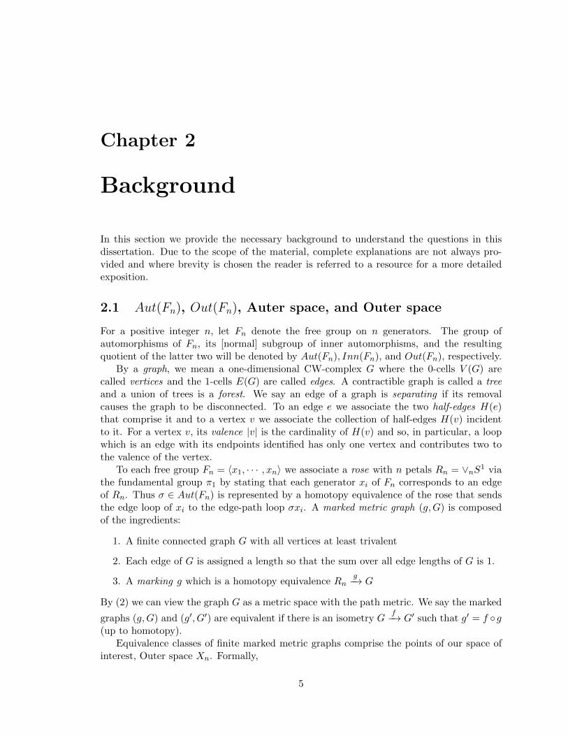
By a graph, we mean a one-dimensional CW-complex G where the 0-cells V (G) arecalled vertices and the 1-cells E(G) are called edges. A contractible graph is called a treeand a union of trees is a forest. We say an edge of a graph is separating if its removalcauses the graph to be disconnected. To an edge e we associate the two half-edges H(e)that comprise it and to a vertex v we associate the collection of half-edges H(v) incidentto it. For a vertex v, its valence |v| is the cardinality of H(v) and so, in particular, a loopwhich is an edge with its endpoints identified has only one vertex and contributes two tothe valence of the vertex.

To each free group Fn = 〈x1, · · · , xn〉 we associate a rose with n petals Rn = ∨nS1 viathe fundamental group π1 by stating that each generator xi of Fn corresponds to an edgeof Rn. Thus σ ∈ Aut(Fn) is represented by a homotopy equivalence of the rose that sendsthe edge loop of xi to the edge-path loop σxi. A marked metric graph (g,G) is composedof the ingredients:

1. A finite connected graph G with all vertices at least trivalent

2. Each edge of G is assigned a length so that the sum over all edge lengths of G is 1.

3. A marking g which is a homotopy equivalence Rng−→ G

By (2) we can view the graph G as a metric space with the path metric. We say the marked

graphs (g,G) and (g′, G′) are equivalent if there is an isometry Gf−→ G′ such that g′ = f ◦g

(up to homotopy).Equivalence classes of finite marked metric graphs comprise the points of our space of

interest, Outer space Xn. Formally,

5

Definition 2.1.1. The space Xn called Outer space is the collection of marked metricgraphs (g,G) which are finite and connected with π1G ∼= Fn. The group Out(Fn) acts(on the right) on Outer space by changing the marking, i.e., for σ ∈ Out(Fn) we take a

representative Rnρ−→ Rn for σ and define (g,G)σ = (g ◦ ρ,G).

Note that in the marked graph (g,G) we can vary the length of any edge of G as long aswe keep the sum of all of the edges equal to one. Moreover, if the graph G has a subforest,we can collapse the subforest to a obtain new graph which is still homotopy equivalent toRn. Thus we can decompose Outer space into a disjoint union of open simplices where agraph G with e edges corresponds to an open simplex of dimension e− 1 in Xn. It is clearthat if G has no subforest, then there are no edges to collapse and so these graphs form thebottom dimension.

If we collapse all separating edges of marked graphs uniformly, the result equivariantlydeformation retracts onto a subspace of Xn called reduced Outer space, denoted Yn. Wedefine the spine Kn of Outer space to be the geometric realization of the posets of the opensimplices of Yn. One can further retract Outer space onto its spine and this has the distinctadvantages that (1) Kn is a simplicial complex (Xn fails this as it is missing 0-cells, etc.),(2) the spine is contractible, and (3) the quotient of Xn by Out(Fn) is compact with finitepoint stabilizers. More to the point (see VII.2, exercise 2 of [5]),

Theorem 2.1.2. H•(Out(Fn);Q) ∼= H•(Xn/Out(Fn);Q)

Let us consider the simplest case, F2. In Figure 2.1, we have depicted the three rank-two

(a) G1 (b) G2 (c) G3

(d) A snippet of Outer space

Figure 2.1: Ingredients of Outer space in dimension two

6

Figure 2.2: Reduced Outer space with its spine for n = 2

graphs (up to graph isomorphism). Note that the first graph G1 has three edges and socorresponds to a 2-simplex. If we collapse any of the edges of G1, the result is the 2-rose,G2. As G2 has two edges, it corresponds to a 1-simplex which “decorates” a face of the 2-simplex of G1. As there are no subforests of G2 to collapse, there are no 0-simplices. It canbe shown that this (almost) simplicial structure is the ideal triangulation of the hyperbolicplane. Let us now see how G3 fits into this picture. Since G3 has three edges of which onlyone can be collapsed, it is represented by a 2-simplex with two edges missing. We visualizethese additional faces as fins protruding from the hyperbolic plane. In this case, Y2 (Figure2.2) is the ideal triangulation without the fins and the spine is the 2-3 tree with verticesgiven by graphs of the form of G1 (the trivalent vertices) and G2 (the bivalent vertices).

Let us modify the construction of Outer space. If we now require our graphs to bebasepointed by some distinguished vertex ∗ and correspondingly basepoint the n-rose, thena marking of such a graph is a marking in the familiar sense with the extra condition thatthe marking preserves basepoints. We remark that the basepoint does not necessarily haveto occur at one of the original vertices of the graph and hence may sit on an edge and have

7

valence 2. Furthermore, the equivalence relation on marked graphs now is required to be arelation where the isometry is basepoint-preserving. Similarly, there is a space An on whichAut(Fn) acts with finite point stabilizers, see [14], [16], or [17].

Let us focus on the space An. Following the construction of Outer space (while makingthe necessary adjustments so as to include the basepoint), we deformation retract onto thesubspace of graphs without a separating edge. This space An is known as Auter space andis invariant under the action of Aut(Fn), see [14]. Thus a point of Auter space An is anequivalence class of basepointed marked graphs (g,G, ∗) without any separating edges.

As described, An is not a simplicial complex (being a union of simplices, it is missingsome faces as in the Out case). We describe the spine SAn of Auter space. A vertex of SAnis an open simplex of An and a pair (G,Φ1 ⊂ · · · ⊂ Φk+1) determines a k-simplex of SAnwhere G is a basepointed marked graph and the subforests of G are partially ordered byinclusion. Similar to the Out case, Aut(Fn) acts with finite point stabilizers on the simplyconnected SAn and so we can compute the rational homology of the group Aut(Fn) byconsidering instead the space Qn = SAn/Aut(Fn).

It will be useful to describe SAn as a cubical complex. Let (g,G,Φ, ∗) denote a markedgraph together with a k-edged subforest Φ of G and basepoint ∗. We may order the k edgesof Φ in k! ways and so this gives rise to k! simplices in the spine SAn. We call the union ofthese simplices a cube and denote the cube by brackets rather than parentheses: [g,G,Φ, ∗].

There are two operations δC , δR which we can place on an edge e ∈ Φ which we will write(δC)|e and (δR)|e. The operation δC contracts an edge e of the forest and the operation δRremoves an edge e from the forest, i.e., given an edge e, (δC)|e[g,G,Φ, ∗] = [g/e,G/e,Φ/e, ∗]and (δR)|e[g,G,Φ, ∗] = [g,G,Φ− e, ∗]. In the cubical complex, the codimension-one faces of[g,G,Φ, ∗] correspond to either (δC)|e[g,G,Φ, ∗] or (δR)|e[g,G,Φ, ∗], see Figure 2.3 or 4.4.

Due to the existence of a distinguished basepoint, we may filter Auter space by degree.The degree of a basepointed graph (G, ∗) is given by deg(G, ∗) =

∑v(|v| − 2) where |v|

denotes the valence of the vertex v and the sum is over all the vertices aside from thebasepoint. Our graphs do not include univalent vertices (thus for any vertex v, |v| ≥ 2) andso the summand given can be interpreted as all of the “surplus” valency at the vertex (or asHatcher- and Vogtmann [16] call it, the “multiplicity”). It is shown in [16] by an argumentinvolving edge-collapses and the Euler characteristic that the degree of a basepointed graphof rank n can be equivalently calculated as 2n− |∗|.

Let us describe the filtration from degree that takes place on the spine and its interpre-tation in the cubical complex. We let SAn,k be spanned by graphs of SAn with degree atmost k and we let Qn,k be the quotient SAn,k by Aut(Fn). It is a result of Hatcher andVogtmann [16] that SAn,k is (k− 1)-connected and we have Hi(Qn,k;Q) ∼= Hi(Aut(Fn);Q)for k > i. By the properties of degree, we note from [17] that the maximal cubes of SAn,kcorrespond to basepointed graphs [G,Φ, ∗] such that

1. Φ is a maximal tree with k edges,

2. deg(G, ∗) = k, and

3. All the vertices of G (aside from ∗) are trivalent.

8

:

Figure 2.3: A cube in the 3-spine corresponding to the graph in the upper left

9

2.2 Executive Summary

The reader may be wondering how our discussion of Outer space and Auter space mayrelate to the theory of Lie algebras and graph homology. As an aid, we provide a map ofthe landscape.

We begin by considering the “creatures” A1 and A2 pictured in Figure 2.4(a) and theoperation ◦ on A1 and A2 illustrated in Figure 2.4(b). We think of these creatures as“spiders” with labeled legs. The ◦ operation can be roughly seen as an identification of apair of legs and subsequent merging of the circular structures. By taking wedges of thesecreatures and adding some additional structure, one can form a Lie algebra of creatures andtreat it homologically in the sense of Chevalley and Eilenberg.

Now, imagine starting out with a graph and superimposing a creature upon each vertex(where the valence of the vertex coincides with the number of legs on the creature) tocreate a “creature-graph.” If we define a differential on such a graph as the sum over alledge-collapses and subsequently “mate” the creatures inhabiting the vertex endpoints of theedge collapse, it turns out that the homology of the corresponding chain complex (roughly)coincides with the homology of the Lie algebra homology of the creatures.

We wish to formalize the process and make precise the claims made above in the contextthat the spider carries some kind of structure. Amazingly, when we impose a “Lie” struc-ture on the spiders, either of the above homologies captures the cohomology of the groupOut(Fn). More can be said if we impose “Commutative” or “Associative” structure, butthese cases will not be discussed herein. See [11], [25], or [7] for these other flavors.

To achieve our goal, we review some basic concepts from algebra. The reader is invitedto keep this example in mind as a template for the process. We follow [7] for much of thefollowing material involving operads, graph homology, and the homology of the Lie algebraof a cyclic operad. The absence of a reference should not be interpreted as a claim tooriginality on the author’s part.

2.3 Some notions from category theory

In preparation to define an operad, we review some basic definitions from category theory.Additional recommended texts are [23] [30], and [3].

By a category C, we shall mean a class of objects together with a set of morphisms (orarrows) C(A,B) for every pair of objects A,B. These morphisms are required to form amonoid under composition. If an arrow f of C has a left and right inverse g, then we callf an isomorphism. A morphism of categories is a functor, i.e., a functor F is a map ofcategories that preserves the order of composition and maps the unit map of an object of acategory to its corresponding image under F.

Many of the objects we consider in mathematics are categorical in nature. The collec-tion of sets Set with arrows given by set maps forms a category. In particular, the categoryFinSet of finite sets with arrows given by bijections [permutations] is a category. Some al-gebraic categories include the category of groups, rings, (left) R-modules, and vector spacesover a field k denoted, respectively, Gp,Ring,R Mod, and k-Vect. On the topological side,we have the category of topological spaces, pointed topological spaces, smooth manifolds,and Lie groups denoted, respectively, Top,Top∗,SMan and LieGp. The morphisms ineach of the given categories should be clear from the context.

10

A1

1

2

3

4

5

6

7

A2

1

2

3

4

(a) The creatures A1 and A2

A1

1

2

3

4

5

6

7

A2

1

2

3

4

º 34 =

A1

1

2

3

5

6

7

A2

1

2

4

= A

1

2

3

4

56

7

8

9

(b) Mating along the legs 4 of A1 and 3 ofA2

A1

1

2

3

4

5

6

7

A2

1

2

3

4

º 34 =

A1

1

2

3

5

6

7

A2

1

2

4

= A

1

2

3

4

56

7

8

9

(c) The result of mating

Figure 2.4: Creature mating

One of first functors we are introduced to as a student is the first homotopy groupπ1: Top∗ −−→ Gp and later we learn of a sequence of functors called the (co-)homology

functors H(•)• . Algebraic examples include the Abelianization of a group and the turning of

an associative algebra into a Lie algebra via the commutator bracket. An important functorwhich plays a critical role in [21, 22] and [7] is the invariants functor V → V g associated toa Lie algebra g with an action on V .

Definition 2.3.1. Given two functors CF,G−−→ D, a natural transformation η from F to G

is an assignment of every object C in C, a morphism FCηC−−→ GC in D such that for every

morphism Cf−→ C ′ in C, we have a commutative diagram as below.

FCηC- GC

FC ′

Ff?

ηC′- GC ′

Gf?

The concept of a natural transformation makes precise our notion of “a morphism offunctors.” A familiar case of naturality arises in the Mayer-Vietoris sequence for homology

11

which relates the homology of a space to certain subspaces of the space. If we assumeX = int(A) ∪ int(B), then there is an exact sequence called the Mayer-Vietoris sequence

· · · → Hn(A ∩B)→ Hn(A)⊕Hn(B)→ Hn(X)→ Hn−1(A ∩B)→ · · · .

To say that the Mayer-Vietoris sequence is natural is to say that if we have another spaceX ′ that decomposes into the interior of its subspace A′ and B′ and if f is a continuous mapX → X ′ that carries A into A′ and B into B′, then we have a commutative diagram withexact rows

· · · −→ Hn(A ∩B) −→ Hn(A)⊕Hn(B) −→Hn(X)−→ Hn−1(A ∩B) −→ · · ·

· · · −→Hn(A′ ∩B′)

f∗?

−→Hn(A′)⊕Hn(B′)

f∗?

−→Hn(X ′)

f∗?

−→Hn−1(A′ ∩B′)

f∗?

−→ · · ·

2.4 Monoidal categories and operads

Recall that a monoidal structure on a set is an associative binary relation with a distin-guished identity element 1. We wish to mimic this construction in the context of a category:

Definition 2.4.1. A monoidal category (C,⊗) is a category C with a functor C×C⊗−→ C,

a natural isomorphism (called the associator)

−⊗ (−⊗−)α−,−,−−−−−→ (−⊗−)⊗−,

and an identity object I with natural isomorphisms I⊗C lC−→ C and C⊗ I rC−→ C such thatthe diagrams below commute.

(A⊗B)⊗ (C ⊗D)

A⊗ (B ⊗ (C ⊗D))

α-

((A⊗B)⊗ C)⊗D

α

-

A⊗ ((B ⊗ C)⊗D)

1A⊗α?

α- (A⊗ (B ⊗ C))⊗D

α⊗1D6

A⊗ (I ⊗B)α- (A⊗ I)⊗B

A⊗B

1A⊗lB?� = - A⊗B

rA⊗1B?

It is a standard exercise in a beginning graduate algebra class to verify the isomorphismR ⊗R M ∼= M ⊗R R ∼= M for a module over a commutative ring R. Unbeknownst to usat the time, we were verifying that the ring R acts as a unit in RMod under the tensorproduct! Furthermore, the familiar associativity of ⊗R is the pentagonal diagram above. Inparticular, if we specialize our ring R, we may assert that the category of k-vector spacesand the category of Abelian groups are monoidal. A less obvious example arises if weconsider the category of pointed topological spaces Top∗ under the smash product. In thiscase, the unit is realized as S0.

Definition 2.4.2. A species is a functor FinSet −→ k-Vect. The category of species willbe denoted Sp and the morphisms are the natural transformations between the functors

12

and given a species q, the image of the set I will be denoted q[I] and is called the space ofq-structures on I.

Note that the objects of Sp are functors and so it makes sense to say the arrows ofSp are natural transformations. There is a monoidal structure which can be placed on thecategory of species; it is given by the ◦ operation illustrated in Figure 2.4(b) and is realizedas a type of formal substitution.

Let us algebraically describe the monoidal structure given by ◦ as in Appendix B of [1].Let p[I] denote the set of all partitions of the finite set I and given a partition π of p[I],we write B ∈ π to mean a block in the partition π. Then, given two species q and q′, wedefine the substitution product ◦ by

(q ◦ q′)[I] =⊕π∈p[I]

(q[π]⊗⊗B∈π

q′[B]) (2.1)

The reader likely noticed the obtuse notation p[I] to denote the collection of all partitionson I. The collection p[I] here refers to the species of partitions: given a finite set I, thefunctor p associates to it all partitions of I.

This ◦ operation can be viewed as a kind of substitution by the following description.Fix a finite set I and a partition π of I. Each summand in 2.1 consists of two components;the second component

⊗B∈π q′[B] can be thought of as the parameters determined by the

species q′ and the first component can be viewed as a post-processor or placeholder for theoutput of q′

As a concrete example, let us consider the extreme case where our partition π0 of I isinto singletons. Then each block B in the partition π0 consists of a single element whichis fed to q′. The “output” q′[ {x} ] is then associated to the partition coordinate of π0 inthe image of q[π0]. For another example in the case of the Lie species, see Example 2.4.7below.

The above construction extends to an arbitrary category and the choice of k-Vect is forour intent. A left Σn-module structure can be given to the q-structure q[{1, 2, 3, · · · , n}] =q[n] as follows: every permutation σ ∈ Σn induces an automorphism q[n](σ) of q[n] whichpermutes the set [n].

There are several approaches to developing operads, two of which are given below.The original motivation for operads was to study iterated loop spaces in J.P. May’s “TheGeometry of Iterated Loop Spaces,” but it has been noted [26] that the study of operadsdates back to 1898 in Whitehead’s “A Treatise on Universal Algebra.” In any event:

Definition 2.4.3. An operad is a monoid O in the monoidal category (Sp, ◦,u) where theunit is given by u[X] = k if |X| = 1 and ∅ otherwise and the operation ◦ is the formalsubstitution described above. [We note that the unit of the operad may also be denoted1O.]

Another approach, in the context of real vector spaces, is given in [7]; the reader iswarned that we shall use them interchangeably.

Definition 2.4.4. A collection O of real vector spaces O[m]m≥1, is an operad if there is anassociative composition

O[m]⊗O[i1]⊗ · · · ⊗ O[im]γ−−−−→ O[i1 + · · · im]

(o, o1, o2, · · · , om) 7−−→ (((o ◦1 o1) ◦l1+1 o2) ◦l1+l2+1 o3) · · · )

13

1

2

3

o

(a) A generic operad ele-ment

1

2

3

o

1

2

3

o’

4

=o”

1

2

3

4

5

6

(b) Plugging o into o′

1

2

3

o

1

2

3

o’

4

=o”

1

2

3

4

5

6

(c) The result

1U

(d) The unit operad

Figure 2.5: Components of an operad

where li is the arity of oi, together with a right Σm-action on O[m], and a unit 1O ∈ O[1].

Additionally, there is an axiom of equivariance. We refer the reader to [26] for a de-scription and proof of the equivalence of these two formulations of an operad.

Example 2.4.5 (The Unit Operad, U). We define the unit species u by u[X] = {X} if|X| = 2 and ∅ otherwise. The operad U is the defined as U [X] = {X} if X is a singletonand ∅ otherwise. Pictorially,

Example 2.4.6 (The Associative Operad, A). Let T be a planar rooted tree with n edgesemanating from one internal vertex. The image A[n] is spanned by such trees and the cyclicordering given by the planar embedding is equivalent to a cyclic ordering of the edges of thetree. See Figure 2.5(a). The ◦ operation of two such elements is performed by identifyingthe root of the first tree with an edge of the second tree, collapsing the resulting edge andinserting the edges from the first tree into the second while preserving the original ordering.This is illustrated in Figure 2.5(c) if one assumes the operads pictured are embedded in theplane.

Example 2.4.7 (The Lie Operad, L). A bracket sequence on the set X = {x1, · · · , xk}is a parenthesization of the elements of X such that each element is used once and onlyonce. An example of a bracket sequence on {a, b, c, d, e} is [[[c, a], e], [b, d]]. As a note ofinterest, the total number of such bracket sequences on a set of size n + 1 is given by the

14

n-th Catalan number

Cn =1

n+ 1

(2n

n

).

We define the Lie species Lie[n] to be the span of all bracket sequences on n elements subjectto the familiar antisymmetry and Jacobi relations of a Lie algebra. The substitution rulefor the elements s1 and s2 is given by inserting in place the bracket sequence s1 into thedesired element in the bracket sequence of s2, e.g. [b, c] ◦b [[a, b], c] = [[a, [b, c]], c].

To bring this into a more tractable form, we note that we can identify a bracket sequenceas a rooted planar binary tree modulo the antisymmetry (Figure 2.6(b)) and IHX (Figure2.6(c)) relations. The substitution operation for the Lie operad is given in Figure 2.6(d).

We now explain how the monoidal structure on the category of species gives rise to anoperadic composition Lie◦Lie

γ−−→ Lie. Given a finite set I, a partition π on I, and bracketsequences on π and a block B of π, we can determine a bracket sequence on I by substitutingthe bracket sequence for each block B in place into the partition bracket sequence associated

[[[c,a],e],[b,d]]

c a

eb d

(a) The correspondence between a bracket sequence and a planar binary tree

a b ab

= -... ...

(b) The antisymmetry relation

= 0-... ... ...

+

ab c a

bc a b

c

(c) The IHX relation

=

1

2

3

4

1

23

1

2

3

4

5

6

(d) Substitution in the Lie operad

Figure 2.6: Properties of the Lie operad

15

to π. We visualize this by forming a rooted tree where the leaves correspond to the blocksin the partition and for every block, we determine a bracket sequence. This block-bracket-sequence in turn defines a rooted tree of which we graft its root onto the corresponding leaffor the block on the partition tree.

Definition 2.4.8. A cyclic operad O is an operad such that the Σn action on O extendsto a Σn+1 action such that the axioms for O still hold.

o

Figure 2.7: Visualizing an element of a cyclic operad

One way to think of a cyclic operad is to erase the distinction of the output and allowany input to serve as an output. We accomplish this by labeling the output by 0 and thinkof Σn+1 as being the group of bijections on the set {0, 1, · · · , n}. Rather than illustratingan operad as a “directed” object, we visualize in a more symmetric manner as in Figure2.7.

The Lie operad is an example of a cyclic operad. Later, we shall define a pointed versionof the Lie operad and show that it is also a cyclic operad. Using this, we will be able toanalyze the homology of Auter space.

2.5 The graph homology of a cyclic operad

Recall from the introductory example that we wish to formalize the concept of attaching a“creature” to the vertices of a graph and subsequently define a homology on the resultinggraph complex generated by these graphs. Of import in this process and the sequel is thenotion of an oriented graph:

Definition 2.5.1. An orientation on the graph G is a choice of a unit vector in

detRV (G)⊗⊗

e∈E(G)

detRH(e)

where detRB corresponds to the top-dimensional wedge of the finite dimensional real vectorspace with basis B, E(G) = set of edges of G, V (G) = vertices of G, H(e) = the two halfedges that compose the edge e, and H(v) = the collection of half edges incident to thevertex v.

Note, if dimRB = n, then detRB = ∧nRB is one-dimensional and hence it makes senseto speak of a choice of a “positive” or “negative” orientation. For a connected graph,there are equivalent formulations of orientation; we refer the reader to [7] for a proof of theequivalences and record the result here for reference.

Lemma 2.5.2. The following formulations of orientation for a connected graph X areequivalent, up to canonical isomorphism:

16

1. detH1(X;R)⊗ detRE(X)

2. detRV (X)⊗⊗

e∈E(X)

detRH(e)

3.⊗

v∈V (X)

detRH(v)⊗ det⊕

|H(v)|even

Rv

To make sense of identifying a vertex of a graph with a “creature” we set the groundworkfor defining an O-spider

Definition 2.5.3. Fix an n-star S with n ≥ 2 edges emanating from a central vertex. Thena labeling of S is a bijection between {0, 1, · · · , n− 1} and E(S), the edges of S.

As discussed in the previous section, the symmetric group Σn acts on the finite set [n]attached to p-structure p[n] and hence when p gives rise to a cyclic operad O, there is acoherent extension of the action to a Σn+1 action on O. Similarly, we have an action of Σn

on the labelings of an n-star. Recall that the space of coinvariants corresponding to theaction of a group G on the space X, denoted XG, is the space X/ 〈x− gx〉 .

Definition 2.5.4. Let O be a cyclic operad and let L be the set of labelings of the n-starfor n ≥ 2. The space of O-spiders with n legs is the space

OS[n] =

(⊕LO[n− 1]

)Σn

where the Σn action is given by σ(oL) = (σo)σL.

From the space of O-spiders with n legs, we form the full space of O-spiders OS =⊕n≥2OS[n]. Since O is a cyclic operad, there is a composition law defined on O and this

gives rise to a mating law on OS. We illustrate the mating law via an example with theLie operad:

Example 2.5.5. Consider the two Lie spiders S (left spider) and S′ (right spider) in Figure2.6(d). We wish to mate S and S′ along the legs l of S and l′ of S. To do so, choose arepresentative SΣ and SΣ

′ of S and S′ where the labeling of the leg l of S is the outputof underlying operad element oS of S and the labeling of the leg l′ is the first input of theunderlying operad element oT of T. Via the substitution law in L, plug the leg l of oS intothe leg l′ of oT , collapse the adjoined legs to form a new edge in the tree, and subsequentlyrelabel the legs so that the leg ordering is coherent with the original leg ordering.

Definition 2.5.6. Let G be an oriented graph with all vertices at least bivalent and letO be a cyclic operad. The n-valent vertex v of G is said to be decorated by the spiderS ∈ OS[n] if there is a fixed bijection between H(v) and the legs of S. The graph G is saidto be an O-graph if all the vertices of G are O-decorated. If the graph G is O-decorated,then we shall denote this by OG. When there is not danger of confusion, we shall suppressthe O prefix.

Later, we shall give another formulation of an O-graph that allows the vertices of Gto be decorated by two operad spiders of differing type. This formulation will be used toextend the methods for determining the homology of Out(Fn) to that of Aut(Fn).

17

Definition 2.5.7. The k-th chain group OGk of O-graphs is the real vector space spannedby O-graphs with k vertices subject to the relations

1. (Orientation) (OG, or) = −(OG,−or)

2. (Vertex Linearity) If a vertex v of OG is decorated by the spider S = a1S1 + a2S2

where a1, a2 ∈ R and S1, S2 ∈ OS[k], then OG = a1OGS1 + a2OGS2 where OGSidenotes the decoration of the vertex v of OG by the spider Si.

Let G be an oriented graph and let OG be its decoration by O-spiders. Define OGe tobe the O-graph formed by mating the underlying spiders decorating the vertex endpoints vand w of e along their legs that form e. In the event that e is a loop, define OGe = 0. Weorient Ge by choosing an orientation representative of G such that v is first and w is secondin the vertex ordering and e is oriented from v to w; the orientation of Ge is then inheritedfrom its parent G and the new vertex formed by mating the spiders decorating v and w isfirst in the vertex ordering.

With these conventions, this action has degree −1 and we subsequently define

OGk∂E−−→ OGk−1 (2.2)

OG 7−−→∑

e∈E(G)

OGe.

As we formed the total space of O-spiders via a grading on the number of spider legs,we form the space of O-graphs

OG =⊕k≥1

OGk.

Proposition 2.5.8. ∂2E = 0. In particular, the pair (OG, ∂E) is a chain complex.

Proof. Let e1, e2 be edges of G with vertex endpoints v1, v2 and w1, w2, respectively. With-out loss of generality (the result would differ by a global sign), choose the orientation of Gso that in the vertex ordering we have v1 before v2, w1 before w2, and v2 before w2. Then(Ge1)e2 = (Ge2)e1 except that the orientation differs since when we collapse e2 first, we pickup a sign from the fact that v2 precedes w2 in the vertex ordering.

As shown, the pair (OG, ∂E) is a chain complex and so we define the O-graph homologyof the cyclic operad O to be the homology of OG with respect to ∂E . We also define thereduced chain groups OGk to be OGk quotiented by the subspace of graphs with some vertexdecorated by 1O. The following proposition is noted in [7] and we provide a proof now.

Proposition 2.5.9. The spaces OG and OG are Hopf algebras.

Proof. Recall that a Hopf algebra is a bialgebra with an antipode map. We define an algebrastructure by disjoint union with the unit being the empty graph, denoted 1. A coalgebrastructure is defined so that the connected graphs are the primitives and the comultiplicationis extended linearly over disjoint union with the counit dual to the empty graph. We showthat these structures are compatible. Note ∆(1) = 1 ⊗ 1 and if G,G′ are connected, then

18

(using the sumless Sweedler notation)

(∆µ)(G⊗G′) = ∆(G) t∆(G′)

= (G(1) ⊗ 1 + 1⊗G(2)) t (G′(1) ⊗ 1 + 1⊗G′(2))

= G(1) tG′(1) ⊗ 1 +G(1) ⊗G′(2) +G′(1) ⊗G(2) + 1⊗G(2) tG′(2)

= (µ⊗ µ)(G(1) ⊗G′(1) ⊗ 1⊗ 1 +G(1) ⊗ 1⊗ 1⊗G′(2)

+G′(1) ⊗ 1⊗ 1⊗G(2) + 1⊗ 1⊗G(2) ⊗G′(2)

= (µ⊗ µ)(I ⊗ T ⊗ I)(G(1) ⊗ 1⊗G′(1) ⊗ 1 +G(1) ⊗ 1⊗ 1⊗G′(2)

+G′(1) ⊗ 1⊗G(2) ⊗ 1 + 1⊗ 1⊗G(2) ⊗G′(2)

= (µ⊗ µ)(I ⊗ T ⊗ I)(∆⊗∆)(G⊗G′).

That is, ∆µ = (µ⊗µ)(I⊗T ⊗I)(∆⊗∆) by linear extension and so ∆ and µ are compatible.The remaining conditions ε(1) = 1 and εµ(G ⊗ G′) = µ(ε(G) ⊗ ε(G′)) follow from thedefinitions of the counit and multiplication map. Finally, the antipode of a graph reversesthe orientation.

Since ∆ is defined so that the connected graphs are primitive, the subspace of primitivesPOG is generated by connected graphs and similarly for OG. Furthermore, the spaces POGand POG are chain complexes with respect to ∂E .

2.6 Lie algebra homology

Let R be a commutative unital ring. An algebra over R is an R-module A with a bilinear

binary operation A⊗A [−,−]−−−→ A. If there is a unit map Ru−→ A and the diagrams in Figure

2.8 are commutative (that is, A is a monoid), then A is called an associative algebra. Notethat all algebras will not be assumed to be associative.

Definition 2.6.1. Let k be a field of characteristic 6= 2. Then a k-algebra g is a Lie algebraif the bilinear operation of g satisfies

1. (Antisymmetry) [x, y] = −[y, x] for all x, y in g,

2. (Jacobi identity) [x, [y, z]] + [y, [z, x]] + [z, [x, y]] = 0 for all x, y, z in g.

Given a Lie algebra g, one can construct its universal enveloping algebra U(g) by quo-tienting the tensor algebra of g by the ideal generated by a⊗ b− b⊗a− [a, b]. The quotientis a unital associative algebra and using standard methods we can form objects such asU(g)-modules. This is the route we take when defining the homology of a Lie algebra with

A⊗A⊗A 1A⊗[−,−]- A⊗A

A⊗A

[−,−]⊗1A?

[−,−] - A

[−,−]

?

(a) Associativity of of the bracket

A⊗A

R⊗A � -

u⊗1A

-

A

[−,−]

?� - A⊗R

1A⊗u

�

(b) Compatibility of the unit

Figure 2.8: Commutative diagrams for an associative algebra A

19

coefficients in a U(g)-module. The complete derivation of Lie algebra homology comes froman analysis of a cocomplex which is suitably dualized to form the Koszul complex whichcalculates our desired homology. Ultimately, it is an exercise in homological algebra andproofs are omitted; the reader is referred to the excellent book [20] for a detailed expositionand derivation.

Definition 2.6.2. Let g be a Lie algebra and let V be a U(g)-module. The homology of gwith coefficients in V , denotedH∗(g;V ), is the homology of the chain complexXn = ∧ng⊗Vwhere the boundary operator is given by

∂(X1 ∧ · · · ∧Xn ⊗ v) =

n∑i=1

(−1)iX1 ∧ · · · ∧ Xi ∧ · · · ∧Xn ⊗Xiv

+∑r<s

(−1)r+s[Xr, Xs] ∧X1 ∧ · · · ∧ Xr ∧ · · · ∧ Xs ∧ · · · ∧Xn ⊗ v.

We note that in the case of trivial coefficients the definition given reduces to one givenin [7].

Example 2.6.3. We calculate the homology groups with trivial R coefficients of g =gl(2,R). Since R acts trivially on g, the first summation in the boundary definition vanishesand we are left with

∂(X1 ∧ · · · ∧Xn) =n∑i<j

(−1)i+j [Xi, Xj ] ∧X1 ∧ · · · ∧ Xi ∧ · · · ∧ Xj ∧ · · · ∧Xn.

Note that g is generated by X1 =

(1 00 −1

), X2 =

(0 10 0

), X3 =

(0 01 0

), and X4 =(

1 00 1

). Computing the brackets [Xi, Xj ] = XiXj −XjXi, we get

[X1, X2] = 2X2

[X1, X3] = −2X3

[X2, X3] = X1,

and all other brackets are zero. If we work our way down the complex

0 −→ ∧4g −→ ∧3g −→ ∧2g −→ ∧g −→ R −→ 0

we see that the only nontrivial images of elements from the chain groups are

∂(X1X2X4) = 2X2X4

∂(X1X3X4) = −2X3X4

∂(X2X3X4) = X1X4

∂(X1X2) = 2X2

∂(X1X3) = 2X3

∂(X2X3) = X1

20

and so when we compute the homology, we get

H1(g;R) = R {X1, X2, X3, X4} /R {X1, X2, X3}∼= R

H2(g;R) = R {X1X4, X2X4, X3X4} /R {X2X4, X3X4, X1X4}∼= 0

H3(g;R) = R {X1X2X3} /R {0}∼= R

H4(g;R) = R {X1X2X3X4} /R {0}∼= R.

In the previous section, we discussed how to associate a graph homology to a cyclicoperad. We now associate a Lie algebra homology to a cyclic operad. The idea is to attachan element from a symplectic vector space to the legs of an O-spider to get what is called asymplectospider; the space generated by these special spiders then forms a Lie algebra andwe can discuss its (Lie algebra) homology.

Definition 2.6.4. A (real) symplectic vector space is a vector space R2n with basis Bn ={p1, · · · , pn, q1, · · · , qn} and a bilinear form ω(·, ·) that satisfies

1. ω(pi, qj) = −ω(qj , pi) = δij

2. ω(pi, pj) = ω(qi, qj) = 0.

Definition 2.6.5. Let (Vn, ω) be a real symplectic vector space. Then the space of sym-plectospiders is defined to be

LOn =⊕m≥2

(OS[m]⊗ V ⊗mn

)Σm

where the action of Σm is simultaneous. We write the element S of LOn as [S⊗v1⊗· · ·⊗vm]where S is an O-spider.

As indicated, the space LOn forms a Lie algebra with the bracket defined as follows.Given symplectospiders S = [S ⊗ v1 ⊗ · · · ⊗ vm] and S′ = [S′ ⊗ v′1 ⊗ · · · ⊗ v′m], we performthe symplectic mating (S, λ)!(S′, λ′) along the legs λ of S and λ′ of S′ and then attach thecoefficient ω(vλ, vλ′) where v∗ is the element of Vn associated to the leg ∗ of S. The bracketof these spiders is then defined to be the sum of all possible matings of the spiders:

[S,S′] =∑

λ∈S,λ′∈S′(S, λ)!(S′, λ′).

We note that this bracket is of the Lie type as it satisfies the Jacobi identity and is anti-symmetric by the properties of the symplectic form.

Recall that the symplectic Lie algebra sp(2n) is the collection of 2n × 2n matrices X

such that XJ = −JXT where J =

(0 I−I 0

). Let LO0

n denote the subspace of LOn

spanned by symplectospiders decorated by 1O. Then it can be shown that LO0n∼= sp(2n).

We note LO0n acts on LOn via the bracket and, in light of the previous isomorphism,

21

sp(2n) acts on LOn. Moreover, the natural inclusion of Vn → Vn+1 extends to an inclusionLOn → LOn+1 compatible with the inclusion sp(2n)→ sp(2n+ 2). Thus we can define theinfinite dimensional symplectic Lie algebra as a direct limit LO∞ = lim

−→LOn. Note that the

natural inclusion LOn → LOn+1 mentioned above induces a chain map ∧LOn → ∧LOn+1

and so we have Hk(LO∞;R) = lim−→

Hk(LOn;R).

We are now able to state a theorem of Kontsevich that connects the graph and Liealgebra homologies associated to certain cyclic operads:

Theorem 2.6.6. (Kontsevich) Let O be the Associate, Commutative, or Lie operad. Thenthere is a Hopf algebra isomorphism between H∗(LO∞;R) and H∗(OG). In particular, wehave PH∗(LO∞;R) ∼= H∗(POG).

The proof of this result requires [among other things] one to analyze the sp(2n)-invariantsof ∧LOn and particular subspaces of OG. A thorough, detailed exposition that holds forall cyclic operads can be found in [7].

2.7 The homology of Out(Fn) and Morita’s trace map

The question is now how does this seemingly disconnected background connect to the co-homology of Out(Fn)? This is answered by a theorem of Kontsevich [21, 22]:

Theorem 2.7.1. (Kontsevich)

PHk(`∞) ∼= Hk(sp(2∞))⊕⊕n≥2

H2n−2−k(Out(Fn))

One can deduce this theorem from Theorem 2.6.6 by decomposing the space POG intothe space of graphs with only bivalent vertices (polygons) and the space of graphs with atleast one ≥ 3-valent vertex. The space of polygons has the same Lie homology as sp(∞)whereas the complement space can be shown to compute the cohomology of Out(Fn) byan intermediate connection which is explained in the following subsection (2.7.1) on theforested graph complex.

The main idea behind the proof is to relate the primitives in the homology of the infiniteLie algebra `∞ = LL∞ to the graphs of PLG. So, indeed, there is a relation between thehomology of the Lie operad and Out(Fn). A natural question to then ask is

Question 2.7.2. Is there an operad O such that its homology captures the cohomology ofAut(Fn)?

It will be shown in Chapter 4 that there is such an operad, the pointed Lie operad.

2.7.1 The forested graph complex

A combinatorial interpretation of the spine Kn of Outer space gives rise to the forestedgraph complex [7]:

Definition 2.7.3. Let G be a finite graph with trivalent vertices and let Φ be a subgraphof G that is acyclic and contains all of the vertices of G. A forested graph is a pair (G,Φ)with an orientation given by ordering the edges of Φ modulo even permutations. We call Φ

22

a subforest of G and when Φ is the largest subforest of G, we say Φ is the maximal subforestof G.

We make two observations based on this definition. First, it is possible that Φ may bea disconnected graph and so the terminology of subforest is appropriate as the subforestmay be a disconnected collection of trees. Second, the reader will recall that an orientationof a graph is given by an ordering of the vertices and a choice of a direction on each of theedges of the graph, i.e. a choice of a unit vector in

detRV (G)⊗⊗

e∈E(G)

detRH(e).

Following [7], we show that an orientation of the forested graph G is equivalent to anordering of the edges of the forest.

Lemma 2.7.4. Let (G,Φ) be a forested graph. Then an orientation of G is equivalent toan ordering of the forest (up to even permutation).

Proof. Consider the graph G formed from G by collapsing each subforest of Φ to a point tocreate a vertex of G. For each vertex v of G, we consider the ε-neighborhood of the pullbackof v under the collapsing action and denote this by Tv. Note that each Tv is necessarily abinary tree and the interior of each Tv consists of one of the connected components of Φ.We write Φ = ∪vΦv where Φv is a connected component of Φ.

An orientation of G is a choice of a unit vector in

detRV (G)⊗⊗

e∈E(G)

detRH(e)

and for the binary tree T•, ⊗v∈V (G)

detRE(Tv).

Thus an orientation of (G, {Ti}) is a choice of a unit vector in

detRV (G)⊗⊗

e∈E(G)

detRH(e)⊗⊗

v∈V (G)

detRE(Tv).

Observe that if Φv has k edges, there are k + 3 leaves on Tv and hence H(v) has k + 3elements and so there are 2k+ 3 edges of Tv. It follows that E(Φv) and H(v) have oppositeparity.

If we apply the partition lemma (Lemma 2 of [7]) to E(Tv) with respect to the subsetsH(v) and E(Φv) and recall the fundamental isomorphism V ⊗ V ∗ ∼= R (for dim V = 1), weget the canonical isomorphism

detRE(Φv) ∼= detRH(v)⊗ detRE(Tv).

Simplifying the expression for orientation with Lemma 2.5.2 and applying the canonical

23

isomorphism recently given we note

detRV (G)⊗⊗

e∈E(G)

detRH(e)⊗⊗

v∈V (G)

detRE(Tv)

∼=⊗

v∈V (G)

detRH(v)⊗ det⊕

|H(v)|even

Rv ⊗ detRE(Tv)

∼= detRE(Φv)⊗⊗

v∈V (G)

det⊕

|H(v)|even

Rv

∼= detRE(Φv)⊗⊗

v∈V (G)

det⊕

|E(Φv)|odd

Rv

∼= det⊕e∈Φ

Re.

We define the vector space fGn to be the space spanned by forested graphs with |E(Φ)| =n, modulo the IHX relation. The boundary of (G,Φ) is given by

∂(G,Φ) =∑e

(G,Φ ∪ {e})

where the sum is over all edges of G−Φ such that Φ∪{e} is a forest. We set fG = ⊕fGn. We

specialize fGn further by defining fGn to be fGn modulo the forested graphs that possessa separating edge, that is, an edge which its removal results in a disconnected graph.

2.7.2 The graphical trace map

Recall that a generator of ∧`n is a wedge of symplectospiders. A pairing π on a wedge is apairing of the legs of the spiders into disjoint two-element subsets. Note that the pairing πinduces a pairing of the two elements of the symplectic vector space Vn decorating the legsgiven by π. If we now state that the individual leg pairings are identified at their “feet,”the resulting object is a trivalent graph, denoted Gπ. Since each [basis] symplectospider isbuilt from a Lie operad element, there is a planar trivalent tree associated to each spiderand we consider the subgraph of Gπ consisting of the union of the interior of the spiders.This union is designated as our subforest, Φπ which carries the orientation from the planarembedding of the tree decorating the operad element. As there is a natural order (up toeven permutation) of the elements in the wedge of spiders, there is a natural induced orderon the vertices of Gπ and hence on the subforest Φπ. The result of this pairing is theforested graph (Gπ,Φπ).

Given a pairing π on a wedge of symplectospiders, there is an associated weight ω(π)formed by taking the product over all paired elements’ corresponding weights under the

symplectic form ω. Consider the map ∧`nψn−−→ fG defined by

X1 ∧ · · · ∧Xk 7→∑π

ω(π)(Gπ,Φπ).

24

It was shown in [7] that ψn is a chain map and, in the limit, an isomorphism on homology:

H∗(∧`∞)H∗ψ∞−−−−→ H∗(fG)

.We define a functional on fG called the graphical trace map: fG4k−4

τ4k−4−−−→ Q. If (G,Φ)is a forested graph with 4k − 4 edges with G of rank 2k, then τ4k−4(G,Φ) = 0 unless thefollowing hold:

1. Φ is the disjoint union of two linear trees Φ1 and Φ2,2. Both Φ1 and Φ2 have 2k − 2 edges each,3. There are non-forested edges connected the ends of Φ1 and Φ2, and4. The vertices of Φ1 and Φ2 and remaining non-forested edges of G form a bipartite

graph.

In this event, we reorder the edges of Φ1 and Φ2 so the edges of each subforest are inorder and precede the ordering of the edges of Φ2. Collapse each of the forests and thenon-forested edge joining the endpoints of each of the forests. This collapse can be viewedas a planar embedding of a 2-vertex graph with 2k − 1 edges. We now adjust the quotientgraph by reordering the edges coming into each vertex (via an action by some permutationσ) so as to coincide with the initial planar embedding of our forested graph. In this case,define τ4k−4(G,Φ) = sign(σ).

We illustrate the process by considering the forested graph (G,Φ) in Figure 2.9(a). Tosee that G is indeed a candidate for nonzero trace, note Φ is the disjoint union of two lineartrees of length 4 = 2 ∗ 3− 2 edges, π1(G) has rank 6 = 2 ∗ 3, each of the subforests has anonforested edge joining its endpoints, and the remaining edges form a bipartite graph onthe vertices of G. As Φ is not coherently ordered, we reorder it via a left Σ8-action withthe element (2 8 7 3 4). Note sign(2 8 7 3 4) = (−1)4 = 1 and so the sign of G remains thesame (Figure 2.9(b)). We collapse each subforest and its “cap” to get a planar embeddingof a graph with 5 = 2 ∗ 3− 1 edges between two vertices and an orientation at each vertexgiven by the forest ordering (Figure 2.9(c)). Finally, we “comb” the edges of our graph togive the standard planar embedding of this graph; this is achieved by permuting (relativeto the bottom vertex), the first and second, the second and third, the fourth and fifth, andthe third and fourth edges (Figure 2.9(d)). Since this required an even number of moves,the sign of the graph remains the same and the resulting trace of G is τ8(G,Φ) = 1.

Question 2.7.5. For which values of k is H4k−4(Out(F2k)) nonzero?

Positive results have been reached in the cases k = 1, k = 2 [Vogtmann], k = 3 [CV,Ohashi]; it is conjectured that it is nonzero for all k. A new case (k = 4) will be shown tohold in Chapter 3.

Theorem 2.7.6. (Conant-Vogtmann) Let fG(r) denote the subcomplex of fG spanned byconnected forested graphs of rank r. Then Hk(fG(r)) ∼= H2r−2−k(Out(Fr);Q).

It should be further noted that the above theorem specializes to the subcomplex fG(r)

of forested graphs without separating edges so that Hk(fG(r)

) ∼= H2r−2−k(Out(Fr));Q.If we wish to show the cohomology group H4k−4(Out(F2k)) is nonzero, we must first

exhibit a non-vanishing generator for Hk(fG(2r)

). As it turns out, the trace map fits thebill.

25

Lemma 2.7.7. τ4k−4 is a cocycle: τ4k−4(∂(G,Φ)) = 0.

Proof. Let (G,Φ) be a forested graph of rank 2k. It suffices to consider the following twocases as all others will have zero trace:

1. Φ = Φ1 ∪ Φ2 where Φ1 has 2k − 2 edges and Φ2 has 2k − 3 edges

2. Φ = Φ1 ∪ Φ2 ∪ Φ3 where Φ1 has 2k − 2 edges and Φ2 together with Φ3 has 2k − 3edges.

The boundary of a type 1 graph has terms that either force Φ to have a trivalent vertex,join the endpoints of Φ1 and Φ2, or increases the linear length of Φ1 or Φ2 by one. The firsttwo cases vanish under the trace and if the length of Φ1 is increased by one, then each ofthe subforests are not of length 2k−2 and hence the term is traceless. We are thus left withthe case that the boundary splits Φ into two components of length 2k− 2 with nonforestededges joining the vertices of the subforests. Note that the trace of the resulting boundarywill have two canceling terms in this case since the added edge can either “precede” or“follow” the subforest Φ2 and the trace of each respective term will differ in sign.

As in the type 1 case, the remaining pair of terms of concern after the boundary isapplied are the two that the edge addition joins the endpoints of Φ2 and Φ3. The sum ofthese two terms will vanish upon application of the trace because the number of edges inΦ2 and Φ3 necessarily have opposite parity.

Let us show directly that H0(Out(F2)) ∼= Q. The space fG0 is generated by the graphG1 shown in Figure 2.1(a) and if we designate any edge of G1 as forested, then the resulting

[forested] graph G generates fG1. If we apply an IHX relation to the forested edge of G,the result is a sum of three graphs, two of which are isomorphic to G and the third which

1 4 7 3

2 68 5

(a) Forested graph

1 4 7 3

2 68 5

1 2 3 4

8 67 5

=

(2 8 7 3 4)

+

(b) Reordering of the forest

1 2 3 4

8 67 5

collapse

(c) Collapsing cycles

comb+

(d) Combing the graph

Figure 2.9: The trace of a forested graph

26

possesses a separating edge (and is equivalent to the graph in Figure 2.1(c)), hence is zero

(recall fGi is defined to be fGi modulo graphs with separating edges). Thus 2G = 0 and

we have fG1 = 0. It now follows that H0(fG0) ∼= Q and so H0(Out(F2)) ∼= Q.In the case k = 2, there are 5 trivalent graphs of rank 4 without separating edges (see

Figure 2.4 of [11] for the explicit generators). Any maximal tree in one of these graphswill have 5 = 2 ∗ 4 − 3 edges (of the 9 total edges) and so there are approximately 630possible forested graphs. It is evident that the case of k = 2 is already reaching the limitsof hand-calculation. The determination of a cycle on which the trace does not vanish isnot entirely obvious and examination of the k = 3 case is even more ghastly. Thus weconsider the quotient CG2k = fG4k−3/∂(ker τ4k−4). The problem of finding a nonvanishingcycle under the trace has now been transformed into finding a sufficient number of relationson the forested graph complex so as to kill the space CG2k. To see that we can procuresuch a cycle if CG2k vanishes, note that if γ is a graph with nonzero trace, then CG2k = 0gives fG4k−3 = ∂(ker τ4k−4) and so ∂(γ) ∈ ∂(ker τ4k−4). Thus the boundary of γ can berealized as the boundary of a traceless element γ′. If we let G = γ − γ′, then τ4k−4(G) =τ4k−4(γ − γ′) = τ4k−4(γ) 6= 0 hence the cycle G does not vanish under the trace.

27

Chapter 3

The non-vanishing of the homologyof Out(F8)

Recall that elements of the top-dimensional chain group for Out(Fr) can be realized as con-nected trivalent graphs without separating edges with an ordered maximal forest. Conant,Gerlits, Hatcher, Ohashi, and Vogtmann [8], [11], [17],[32] have calculated the cohomologyH i(Out(Fr)) of this complex with success for i ≤ 6 and all r. To make the calculationsmore tractable, we discuss a reduction of our generating set of forested graphs to the set ofchord diagrams which we subsequently reduce to the set of good chord diagrams. From hereon, we will assume all forested graphs are without separating edges and hence specializeto the reduced case; there is no loss of generality in this case as each complex equivalentlycalculates the cohomology of Out(Fr).

3.1 Chord diagrams

In [8], Conant and Vogtmann utilized a generating set for the reduced forested graph com-plex that simplified calculations greatly:

Definition 3.1.1. A chord diagram is a forested graph such that the forest is linear andthere is a non-forested edge (called a transversal) of the graph connecting the endpoints ofthe linear forest. The remaining edges of the graph are called chords.

It is important to note that a chord diagram still carries the orientation associated tothe ordering of the linear forest.

Recall that the IHX relation in the Lie operad (Figure 2.6(c)) is the signed sum of thethree blowups of a 4-valent vertex is zero. This relation carries over to the forested graph

1 2 3 4 5 6 7

Figure 3.1: A chord diagram

28

+ + = 0

(a) IHX for chord diagrams

+=

(b) Shorthand for HX

Figure 3.2: IHX/HX for chord diagrams

complex and hence to chord diagrams as an unsigned sum, see Figure 3.2(a). To see howan I − H + X relator in the Lie operad turns into an I + H + X relator in the space offorested graphs, one must analyze the proof given for Theorem 2.7.6 in [7].

Define a filtration on the spine Kr of Outer space by the number of vertices in a markedgraph together with the subcomplex spanned by the previous stage of the filtration (theinitial filtratio is given by all trivalent connected marked graphs of rank r). Note thatthe action of Out(Fr) preserves the filtration and therefore induces a filtration on thequotient of Kr by the Out(Fr) action. It can then be shown that the spectral sequenceassociated to the quotient filtration collapses to a cochain complex which calculates thehomology of the forested graph complex. Recall that a coboundary operator associatedto the cubical complex is the operator δ that expands an edge in a marked graph. Bytaking the coboundary of a particular cube face in Kr and then passing to the quotientwith Out(Fr), the result is a sum of three terms which corresponds to an I +H +X relatorin im(δ). Noting that the kernel of δ coincides with [the dual of] the space of marked graphsmodulo the antisymmetry relation together with the canonical isomorphisms of the latterspaces with their duals, the isomorphism follows.

Using the IHX relation (in fG), we can show that the subspace C of chord diagramsgenerates the space of forested graphs.

Lemma 3.1.2. The space of forested graphs is generated by chord diagrams.

Proof. Suppose (G,Φ) is a forested graph. If the forest Φ is linear (i.e., all vertices of Φ arebivalent), then we are done since an edge (there can be two) joining the endpoints of Φ willform the transversal and the remaining edges will necessarily intersect segments of Φ.

Suppose that Φ is nonlinear and let e = (v, v′) be an edge of G−Φ. Since Φ is a maximaltree, any two vertices are part of the forest and hence there exists a shortest path p in Φjoining v and v′ (the dashed edges in Figures 3.3(b-d)). Note that Φ is not linear and sothere must be a trivalent edge of Φ along p, otherwise Φ would be linear (the arrowed edgesin Figures 3.3(b,c)). If we apply an IHX relation to the first edge that protrudes from p(that is not a part of p), the result is a sum of two diagrams where the length of p hasincreased by one (as in Figure 3.3(d)) and p still joins v and v′. Again, travel along p insearch of trivalent vertices in Φ. If no such vertex exists, we are done. Otherwise, proceedas before by lengthening p one edge at a time until p encompasses Φ, i.e., Φ is linear.

29

e

e'

(a) Graph to resolve

e

(b) Choice of e

e'

(c) Choice of e′

e

(d) The X term from reducing the indicated edgein (b)

Figure 3.3: Resolving a forested graph into a linear combination of chord diagrams

3.2 Relations of chord diagrams

In §2.7, we discussed a method to trivialize the space fG4k−3/∂(ker τ4k−4) by generatingrelations that result from taking the boundary of elements in the kernel of the trace τ4k−4.We explore this concept further by describing a series of relations on the space of chorddiagrams that result from the trace map and the IHX relation.

3.2.1 IHX-type relations

We start with relations that only require the IHX relation. The first relation allows one tochoose any particular chord in a chord diagram and subsequently produce a sum of diagramswhere this chosen chord is the transversal. The proof is very similar to the preceding lemmathat shows the space of forested graphs is generated by chord diagrams.

Lemma 3.2.1. (Transversal Permutation) Let C be a chord in the diagram D. Then Dcan be written as a sum of chord diagrams Di where C is now the transversal of each Di.

Proof. Let D be a chord diagram with a specified chord C as given in the statement.Assuming C is not a transversal, reposition the diagram so that pieces of the forest protrudefrom the endpoints of C. Apply an IHX relation to the forest edge incident to an endpointof C to create two a sum of two diagrams where the sprouting edge has been reduced byone and the C now spans one more edge. Repeat this process until there are no remainingsprouting edges in the sum.

It turns out that diagrams that possess chords of an extreme type vanish, i.e., diagramswith a chord that encompass all of the forest or a single edge of the forest. The latter typeare called isolated chords, see Figure 3.4(a).

30

= 0(a) Isolated chord relation

= - -=

= - -=

= 02

= 0

⇒

⇒

⇒

(b) An application of IHX

= - -=

= - -=

= 02

= 0

⇒

⇒

⇒

(c) Untwisting the chord from (b)

Figure 3.4: The isolated chord relation

Lemma 3.2.2. (Isolated Chord Relation) If a chord joins the endpoints of a single edge inthe forest, then the diagram is zero.

Proof. Apply an IHX relation to the single forested edge spanned by the isolated chordto get a sum (of the negation) of two terms; one of which is the original diagram andthe other is a diagram with a separating edge, see Figures 3.4(b,c). Recall that diagramswith a separating edge vanish and so that diagram is zero. We are then left with twoidentical diagrams [which coincide with our original diagram] whose sum is zero. Since thecharacteristic of Q is not two, we determine that the chord diagram is zero.

3.2.2 Trace-type relations

We now turn our attention to diagrams that require more than an application of the IHXrelation and we consider the boundary of traceless diagrams.

Recall from §2.7.2 that one can create a relation by considering the boundary of tracelessdiagrams (i.e., elements in ker τ4k−4). For the benefit of the reader, we record the definitionof the cocycle τ4k−4 in the manner in which it will be utilized

Definition 3.2.3. Suppose (G,Φ) is a forested graph with 4k− 4 edges with G of rank 2k,then τ4k−4(G,Φ) = 0 provided at least one of the following conditions does not hold:

1. Φ is the disjoint union of two linear trees Φ1 and Φ2,2. Both Φ1 and Φ2 have 2k − 2 edges each,3. There are non-forested edges connected the ends of Φ1 and Φ2, and4. The vertices of Φ1 and Φ2 and remaining non-forested edges of G form a bipartite

graph.

Lemma 3.2.4. (Double Transversal Relation) If a chord diagram has two transversals, thenthe diagram is zero.

Proof. Let D be a diagram with a chord that spans the entire forest, but remove the forestdesignation from the last edge in the forest, i.e., the diagram is of codimension 1.

Note that this diagram is traceless because the forest is not the disjoint union of twosubforests as it is linear, see Figure 3.5(b). The boundary of the graph in Figure 3.5(b) isa sum of three terms shown in Figure 3.5(c).

31

= 0...

(a) Two transversals

∂0

+ + = 0

2 + = 0

= 0

τ = 0

⇒

⇒

⇒

...

... ... ...

... ...

...

(b) The boundary of a traceless dia-gram vanishes

∂0

+ + = 0

2 + = 0

= 0

τ = 0

⇒

⇒

⇒

...

... ... ...

... ...

...

(c) The boundary of the diagram from (b)

∂0

+ + = 0

2 + = 0

= 0

τ = 0

⇒

⇒

⇒

...

... ... ...

... ...

...(d) Straightening the forests from (c)

Figure 3.5: The double transversal relation

Inspection of the last two terms in the sum reveals the presence of a chord that “com-plements” the newly forested edge. This edge is of length one and so it creates an isolatedchord. As a result, these two diagrams are zero in the sum and the result follows.

With this relation, we can now say the transversal with impunity. The two extremechord types have been shown to cause the vanishing of their corresponding diagram. Onemay hope that a diagram which possesses a chord that either spans two edges of the forestor all but one edge of the forest will vanish, as well. While it is unknown if a two-spanningchord in a diagram causes it to vanish, it can be shown that a diagram that has “almosttwo” traversals does vanish. We comment that, strictly speaking, this is not a trace-typerelation but rather is of the IHX-type.

Lemma 3.2.5. (Almost Double Transversal Relation) If a chord spans all but one edge ofthe forest, then the diagram is zero.

Proof. Let D be a diagram with a chord C that spans all but one edge of the forest. Applyan IHX relation to the one edge of the forest that is not spanned by the chord C. Notethat the X term returns the original diagram and the I term is the same as the X termonce the transversal is realized. The result is then a sum of three terms where the I and Xterms coincide and the H term vanishes by the double transversal relation.

= 0...

(a) Almost two transversals

= - -

2 = 0

= 0

...... ...

...

...

IHX

⇒

⇒

(b) An application of IHX

Figure 3.6: The almost double transversal relation

32

We now discuss a relation that involves multiple chords and yields multiple terms in arelation. A pair of chords is said to be parallel if they both start and terminate at adjacentvertices and do not cross one another.

Lemma 3.2.6. (Parallel Chord Relation) Suppose a diagram has a pair of parallel chords.Then the sum of the original diagram and the diagram where one pair of the endpoints areinterchanged is zero.

Proof. Note that an attached bigon (of codimension one) is traceless and the resulting sumof three terms from the boundary of the diagram vanishes. Two of the terms in the sumhave an isolated chord and hence vanish, see Figure 3.7(c). If we apply IHX relations tothe two sprouted forested edges, then we get a sum of four terms equal to zero. As twopairs coincide, we get the sum of a diagram with parallel chords and one with permutedendpoints is zero.

3.2.3 The space of good chord diagrams

Note that a chord diagram of rank n+ 1 necessarily has 2n vertices and n chords (recall wedisregard the transversal in the counting of chords). Thus there are exactly

pn = (2n)!/2nn!

= (2n− 1)!!

= 1 · 3 · 5 · · · (2n− 1)

possible pairings of the vertices and hence pn diagrams with n chords. Examination of theformula for pn makes it immediately clear that the size of these spaces grows at an alarmingrate as exhibited in the second column of Table 3.1. It would be quite nice if we could

= 0...

(a) Parallel chord relation

= 0...

∂0

τ = 0

⇒ = 0++

⇒(IHX)

+ + = 00 0(IC)

⇒(IHX)

(b) The traceless diagram is a boundary

= 0...

∂0

τ = 0

= 0++

⇒(IHX)

+ + = 00 0(IC)

⇒(IHX)

(c) Manipulation of (b)

Figure 3.7: The parallel chord relation

33

further reduce our generating set for fGn as the next unknown case of n = 7 has more than105 diagrams. A possible guess for a generating subspace would be diagrams where thechord endpoints lie on opposite sides of the diagram’s midpoint, to wit:

Definition 3.2.7. A chord diagram is good if each chord crosses the midpoint of the forest.The subspace of good chord diagrams will be denoted Gn. If a diagram has a chord whichdoes not cross the midpoint, the diagram is called bad.

Note that if it is in fact the case that the space Gn generates Cn, then the reduction insize of the spaces is staggering since the size each of the spaces Gn is n!. To see this notethat if we attach only the “starting vertex” of any chord to the first n vertices of our forestΦ, then there are precisely n! permutations (i.e., ways of attaching the terminus of eachedge) of the chord “ending vertex.”

Table 3.1: The size of the spaces Cn and Gn

n |Cn| |Gn|1 1 12 3 23 15 64 105 245 945 1206 10395 7207 135135 50408 2027025 403209 ≈ 3× 107 36288010 ≈ 6× 108 3628800

A pair of chords C1 = (a, b) and C2 = (c, d) are adjacent if c = b+ 1 and a < b < c < d.As an example, the chords that intersect the forest edge labelled “4” in Figure 3.1 areadjacent (or Figure 3.8(a)). The following relation allows us to take a pair of adjacentchords and expand them into a sum of diagrams where all of the chords either remain thesame in length or increase in length.

Proposition 3.2.8. (6T Relation) The sum of the six ways of permuting the endpoints ofa pair of adjacent chords is zero.

Proof. If one joins three non-forested edges to an exterior vertex which is regarded as thepart of the forest, the result is a traceless diagram (Figure 3.8(c)). The boundary of thisdiagram is a sum of three terms which correspond to the three non-forested edges we startedout with (Figure 3.8(d)). If we apply an IHX relation to the sprouting forested edge in eachboundary component we get a sum of 3! = 6 terms that vanish and which correspond to thepermutations of the chord endpoints (Figure 3.8(e)). Recall that the addition of an edge tothe forest via the boundary map causes the forest labeling of the new edge to occur last inthe order. A shuffling of the forest labels gives the signs as indicated in Figure 3.8(f)

Corollary 3.2.9. (Maximally Adjacent Chords) Suppose C1 = (1, k) and C2 = (k + 1, 2n)are chords in the n-chorded diagram D. Then D = −D′ where D′ is the chord diagram withC1 and C2 replaced by (1, k + 1) and (k, 2n), respectively.

34

. . . . . .. . . . . .

a b c d

(a) Adjacent chords

+ + = 0...... ... ... ... ...

(b) The six permutations of the chord endpoints

⇒

⇒

i j k

n-1n-1

n-1

i j k i j k i j k

i j kn-1 n-1 n-1i ij jk k

i j k i ij jk k

∂0

τ = 0

++

(-1)i

(-1)j

(-1)k

+ +

++

= 0

= 0

= 0

... ...

... ... ... ... ... ...

... ... ... ... ... ...

... ... ... ... ... ...

⇒(IHX)

(c) The traceless diagram of con-sideration

⇒

⇒

i j k

n-1n-1

n-1

i j k i j k i j k

i j kn-1 n-1 n-1i ij jk k

i j k i ij jk k

∂0

τ = 0

++

(-1)i

(-1)j

(-1)k

+ +

++

= 0

= 0

= 0

... ...

... ... ... ... ... ...

... ... ... ... ... ...

... ... ... ... ... ...

⇒(IHX)

(d) The boundary of the diagram from (c) ⇒

⇒

i j k

n-1n-1

n-1

i j k i j k i j k

i j kn-1 n-1 n-1i ij jk k

i j k i ij jk k

∂0

τ = 0

++

(-1)i

(-1)j

(-1)k

+ +

++

= 0

= 0

= 0

... ...

... ... ... ... ... ...

... ... ... ... ... ...

... ... ... ... ... ...

⇒(IHX)

(e) Three applications of the IHX relation

⇒

⇒

i j k

n-1n-1

n-1

i j k i j k i j k

i j kn-1 n-1 n-1i ij jk k

i j k i ij jk k

∂0

τ = 0

++

(-1)i

(-1)j

(-1)k

+ +

++

= 0

= 0

= 0

... ...

... ... ... ... ... ...

... ... ... ... ... ...

... ... ... ... ... ...

⇒(IHX)

(f) Reordering the forest

Figure 3.8: The 6T relation

Proof. Apply the 6T relation to the adjacent chords C1 and C2 to get a sum of five negativelysigned chord diagrams. Four of these diagrams contain either a second transversal or almosttwo transversals and are hence zero. The remaining two diagrams are precisely D and D′

as described in the statement.

It turns out that our aspiration that the space of good diagrams generates the space ofchord diagrams is true.

Lemma 3.2.10. The space of chord diagrams is generated by good chord diagrams. Thusthe space of forested graphs is generated by good chord diagrams.

Proof. Let D be a chord diagram. If all of the chords of D are good, we are done. Supposethen that D has a bad chord C. It suffices to show that any bad diagram can first bereduced to a diagram where the bad chord C is adjacent to another bad chord with theadjacency occurring at the midpoint of the forest.

To see that this is sufficient, consider the case where C falls next to the forest midpointand is adjacent to another bad chord. Then an application of the 6T relation to this pairyields five diagrams in which this pair now passes the midpoint of the forest.

Suppose now that the bad chord C is adjacent to a good chord. A 6T relation appliedto the pair will push C at least one edge closer to the midpoint. In the event that a chordincident to the midpoint started out good but turned bad after the 6T application, note

35

that it remains adjacent to the midpoint and so upon further application of the 6T relationto our diagram it will eventually be adjacent to the newly bad chord and hence falls underthe first scenario. If a chord incident to the midpoint is bad, then it is now good and wehave increased the number of good chord by two. In either case, the process terminates toyield a linear combination of diagrams which all have chord passing the forest midpoint.

Let us verify Question 2.7.5 for k = 1, 2, 3 using Lemma 3.2.10. As a matter of con-venience, we may represent a chord diagram (with n chords) as an ordered list of vertexendpoint labels. The diagram corresponding to the list +[1 4 2 6 3 7 5 8] is given in Figure3.1.

In §2.7.2 we determined H0(Out(F2)) was nontrivial by a direct computation. For thesake of completeness, let us verify this fact with the new tools at hand. The space of gooddiagrams in dimension one is 1-dimensional and is generated by the theta graph. Dependingon how one interprets the graph, it either has an isolated chord or two transversals. In anyevent, the graph generates ∂(ker τ4k−4) and so we have

Theorem 3.2.11. H0(Out(F2)) 6= 0.

The cases k = 2, 3 require a bit more work:

Theorem 3.2.12. (Vogtmann) H4(Out(F4)) 6= 0

Proof. In rank four, there are 3! = 6 possible good chord diagrams:

[1 4 2 5 3 6] [1 4 2 6 3 5]D1 D2

[1 5 2 4 3 6] [1 5 2 6 3 4]D3 D4

[1 6 2 4 3 5] [1 6 2 5 3 4]D5 D6

By observation, we note D2, D3, and D4 have almost two transversals while D5 and D6

possess double transversals hence are all zero. Therefore the only remaining diagram is D1.The chords (1,4) and (2,5) form the “crossed” part of a parallel chord relation and so

D1 = −[1 5 2 4 3 6]

= −D3

= 0.

Theorem 3.2.13. (Conant, Vogtmann, Ohashi) H8(Out(F6)) 6= 0

Proof. There are a total of 120 good diagrams in G5. Once we account of double transver-sals and almost two transversals which instantiate at the first forest vertex (note that thelatter are mutually exclusive), 72 diagrams remain and if we now allow for our almost twotransversals chord to terminate at the end of the forest, we have 54 diagrams left. After anapplication of the isolated chord relation, the space is reduced to 46 diagrams (24−3 ·6+2).

36

Lastly, we apply the parallel chords relation to reduce the space down to six diagrams, fourof which are equal due to an orientation reversing automorphism. The four remaining di-agrams are [1 8 2 6 3 10 4 7 5 9], [1 7 2 9 3 6 4 8 5 10], [1 8 2 6 3 9 4 7 5 10], and [17 2 9 3 6 4 10 5 8]. This remaining four-dimensional space is not as easy to trivialize byhand and requires a computer search for relations. The author has independently shownthe nontriviality of this cohomology group via an independent calculation.

3.3 H12(Out(F8)) 6= 0 (the case k = 4)

3.3.1 Explanation of computer code

To determine H∗(fG;Q), Python code was written to generate the spaces of chord diagramsCn. After, relations are created via a generator which attaches graphs onto chord diagramsso as to create a traceless [forested] graph of codimension one. We have coined the termmonster to describe the special attaching graphs which create these relations.

The monstered graphs are then passed to a program that resolves forested graphs intochord diagrams via the IHX relation. Finally, these chord diagrams are fed to a programthat resolves a diagram into a linear combination of good chord diagrams.

Below is a list of the utilized code and a brief description of its purpose. The code (alongwith a more thorough explanation of the syntax, etc.) can be found in the appendix.

1. diagram_gr.py

Generates all chord diagrams with n chords from the space of diagrams withn− 1 chords. Takes as the base space the file fg_2 with contents 1 2.

2. good_diagram_genr.py

All good diagrams from the file fg_$ are filtered out by testing if each chord“straddles” the midpoint. The result is saved as g$.

3. reformat_and_filter.py

For the space of good chord diagrams, it suffices to give a diagram by its endpointsalone. This has the computational advantage that the memory allocation isessentially halved. Because of this, the diagrams are reformatted so as to begiven by their endpoints.

4. mc_∗#.py where ∗ ∈ {r, n} and # is a positive integer

In the calculations, two types of monster (see Figure 3.9) were utilized: Moritaand normal. In each case, # indicates the number of legs present on the monster,e.g. 3-legged normal monsters give rise to the 6T relation. A topological sortwas performed for each monster type: we insert the legs of the monster intothe linear forest subject to some order relations on the attachment vertices; thiswas done to eliminate duplication. For instance, in the case of attaching a 4-legged normal monster, permuting the two adjacent attaching legs give rise toa duplicate relation. Therefore if the vertices we are attaching to are labelleda, b, c, and d we would impose the conditions a < b and a < c < d.

37

Figure 3.9: A normal monster and a Morita monster (each with four legs)

Once all the possible monsters of a particular type have been instantiated (i.e.we have fixed ∗ and #), for each case the unused vertices of the linear forest(called lvnu) are collected and passed to a function which creates a bijectionbetween lvnu and the set {1, 2, · · · ,#lvnu} via the dict type. All possiblechord diagrams are created with the set {1, 2, · · · ,#lvnu} and then translatedback into the initial labeling via the dictionary.

After the possible monstered diagrams are enumerated, each diagram is operatedupon by the boundary operator ∂E to get a zero-sum of diagrams in the topdimension. The result is saved as the pickled python file mo*#_$ where * and# are as above and $ is a counter used to enumerate all possible monstereddiagrams of type (*, #).

An additional feature of this program is that all relations involving isolated, long,and parallel chords among chord diagrams with N chords are created and storedto the files ic_N, lc_N, and pc_N. This is accomplished by reading in a dictionaryof good chords and doing the requisite test for each relation.

Example 3.3.1. We illustrate the algorithm from the previous program by at-taching a two-legged Morita monster to a diagram which will have five chordsafter the boundary operator is applied and hence the result gives rise to a rela-tion in C5. We start with eight vertices in the linear forest and choose all twoelement subsets of the eight vertices such that the first chosen vertex precedesthe second (this is the topological sort). For the sake of argument, let our firstvertex be 3 and the second 6. Then lvnu= {1, 2, 4, 5, 7, 8} and we identify thelatter with {1, 2, 3, 4, 5, 6} of which there are (2 · 6)!/266! = 10395 possible chorddiagrams on the set. Once such pairing is {(1, 4), (2, 6), (3, 5)} which under ourdictionary is the pairing {(1, 5), (2, 8), (4, 7)}.For the sake of computational ease, the forested edges that are part of the lin-ear forest are not listed in the data. Hence the data passed to the boundaryoperator routine would consist of the list of forested edges ft and non-forested

Figure 3.10: Attachment of a two-legged Morita monster

38

edges nft in the diagram. In the case of our example, ft = {(9, 10)}, nft

= {(1, 5), (2, 8), (3, 9), (4, 7), (6, 10), (9, 10)}, and the list of edges that will beforested after applying ∂E are {(3, 9), (6, 10)} .It should be noted that the calculations that have been made in this exampleand the following examples are correct up to a sign since most steps require areordering of the forest, an application of the IHX relation, etc. and hence incura sign change for the orientation. The interested reader is invited to peruse theheavily-commented code of each program to understand the sign conventions andhow they are applied.

5. str.py

Given a diagram with a piece of the forest “growing” from the linear forest, werepeatedly apply the IHX relation to reduce the diagram to a sum of chord dia-grams as in Lemma 3.1.3. Thus when the result of the monster-creator programmc_*#.py of item 4 is fed into this program, we get a linear combination of chorddiagrams and hence a relation of chord diagrams. We comment that the programname str is for sprouting tree reducer for the visual feature that the tree sproutsfrom the forest and is afterwards reduced via the IHX relation.

It is clear by the definition of the IHX relation that a diagram with a piece ofthe nonlinear forest of length m will reduce to a linear combination of at most2m diagrams.

The result of processing a monster of type * with # legs is stored to

~/mo*#relns/mo*#_reln_$

where

– * is the monster type

– # is the number of monster legs

– $ is the relation number for that particular kind of monster

Example 3.3.2. We carry on with our previous example and reduce our relationof ∂E-operated diagrams to a linear combination of chord diagrams. After theapplication of ∂E , we have a sum of two diagrams D1 = [ft1, nft] and D2 =[ft2, nft] where ft1 = {(3, 9), (9, 10)} and ft2 = {(6, 10), (9, 10)}.The diagram Di is fed into a routine which determines the “leftmost” operableforest edge and an IHX relation is applied to the edge to get a sum of twodiagrams where the number of forested edges not part of the linear forest isreduced by one. In the case of D1, the first operated edge would be (3, 9) and a

+

Figure 3.11: The boundary of the monstered diagram

39

single application of the IHX relation yields the sum of diagrams D1,H + D1,X

illustrated in the second row of Figure 3.12.

The second and final IHX application yields four diagrams D1,HH + D1,HX +D1,XH +D1,XX . The final relation after reducing D1 and D2 is shown in Figure3.13.

6. good_diag_enum.py

From the space of chord diagrams with N chords, the good chord diagrams are ex-tracted, enumerated (according to a lexicographic ordering of the vertex list), andsaved to the text file genumN in the format ‘diagram|#’, e.g. ‘[5, 4, 6]|3’.The pipe symbol appears merely as a forced partitioning character for the pythonstring preprocessor .split().

7. bad_to_good.py

Since the space of chord diagrams is generated by the space of good chord dia-grams (Lemma 3.2.10), we take each linear combination of diagrams determinedfrom str.py and make it into a new linear combination of good diagrams. Thisis accomplished by defining a class called Diagram which carries the stubs .g,.orien, .c, and the subroutine .get_chords(). When the first term from arelation in the input file is read into .g, the coefficient is placed in the stub.orien, and then the subroutine processes the chord diagram to test if there isa chord which is bad. If there is a bad chord, the result is stored to the stub .c.Otherwise, the subroutine returns zero and the program knows that the diagramis then good.

At runtime, the enumerated list generated by good_diag_enum.py is loaded andtranslated into the dict type so that the final linear combination of good chorddiagrams can be converted into a row vector.

+

+

++

=

Figure 3.12: One application of IHX to the sum D1 +D2

40

+

++

= +

+

+

+

+

+

+

Figure 3.13: Two applications of IHX yields a sum of chord diagrams

In an effort to reduce computational intensity, after each application for the 6Trelation, the resulting linear combination of diagrams is tested for isolated chordsand long chords.

After the relation mo*#_reln_$ from str.py has been fully processed, it is storedas a row vector in the plain text file ~/mo*#rows/r_$.

Example 3.3.3. We reduce the diagram in the (1, 2) array position, relative tothe equality, in Figure 3.13. Note that the first bad pair is (2, 4), (5, 9). A 6Trelation applied to the chosen chords yields a sum of five chord diagrams thatare all good (Figure 3.14).

8. cat_rows.py

Processing the immense number of relations gives an equally large amount rowsfor our “relation matrix.” To combine the rows generated by bad_to_good.py,a call to the UNIX command cat is utilized; the resulting matrix is stored asrows$ where $ is the number of chords.

3.3.2 Results, comments, and further directions

Upon generating a (hopefully) sufficient number of relations, the matrix generated in 8 isloaded into Octave and the routine rank is called to determine if our matrix is of full rank. Inthe event it is not, we process more relations by generating more monsters. As an indicatorof the amount of data used to determine the k = 4 case, the matrix used had more than

41

+

=

+

++

Figure 3.14: Reduction of a bad diagram via the 6T relation

40 millions entries and the [compressed] file size is over 100MB. The files used to determinethat dim ∂(ker τ8) = 5040 can be found at http://www.math.utk.edu/gray/code/ .

Theorem 3.3.4. H12(Out(F8)) 6= 0

Proof. Using Octave, one can show that the subspace spanned isolated chord relations, par-allel chord relations, and (almost) double transversal relations is not sufficient to trivializethe quotient. If we also allow for trace-type relations induced from three, four, and five-legged Morita monsters (see Figure 3.15), then we note that these relations do trivializethe quotient. That is, taking the relations generated by the Morita monsters along withthe before-mentioned relations, one finds that the spanned subspace is of dimension 5040.Hence the Morita class is nontrivial and we may conclude the result.

We comment that the code used to determine the nontriviality of the cohomology ofOut can be applied to that of Aut in some cases if one does not utilize the almost doubletransversal relation [note that in the proof, the IHX relation is applied to the rightmostedge and the result causes the basepoint to now fall onto the chord hanging beneath thelast diagram in Figure 3.6(b)].

The entirety of the code written was developed on the author’s personal computer andthen transferred to departmental servers for execution. The native version of Python on

Figure 3.15: 3, 4, and 5-legged Morita monsters

42

the departmental servers was a version behind the original scripting (2.6 → 2.5) and sospeed and efficiency reductions were noticed. A portion of this was alleviated thanks to thegenerosity of M. Thistlethwaite; he allowed the author use of a personal workstation whichallowed [immense] parallel computation.

The code as presented was optimized via bottlenecking utilities, but additional optimiza-tions can be made. The most fruitful change to the code would be to create a “top-down”database of the bad chord diagrams which consists of its expansion as good chord diagrams.Using this database, it would be possible to explicitly describe the cocycle generator ofH12(Out(F8)) 6= 0 which was nontractable due to computing constraints. Another avenueof improvement is to rewrite portions of the code in the hybrid Python-C language Cython;preliminary tests showed speed improvements of up to 10x.

43

Chapter 4

The Graph Homology of Aut(Fn)

4.1 The operad pLRecall the Lie operad is the cyclic operad where L[n] is generated by all Lie bracket sequenceson [n] = {1, 2, · · · , n}, or equivalently the space generated by all (rooted) binary planar treeswith n numbered leaves modulo the relations AS and IHX. We wish to define a basepointedversion of L.

Given an element L from the Lie operad, we place distinguished basepoints on the tree.To mimic the IHX relation of L, we impose the relation Aut-IHX illustrated in Figure 4.1(a).

It is useful to think of the basepoints on an operad element as sitting on the ends of“hairs” protruding from the basepoints of the binary tree. With this identification, we notethat the Aut-IHX relation coincides with the IHX relation discussed earlier. To explain theidentification, consider Figure 4.1(b).

+ + = 0

(a) The Aut-IHX relation

+ + = 0

*

*

a a

b b

*

a

b

(b) A hairy IHX relation

Figure 4.1: The IHX relation in the Aut case

44

With the hairs grown with the coherent orientation shown (the opposite coherent ori-entation of the grown edges differs by a global sign), we note this translates to the linearcombination of bracket sequences

[[a, ∗], b] + [∗, [a, b]] + [a, [b, ∗]] = 0. (4.1)

If we consider the standard IHX relation from L, we have

0 = [[a, b], ∗]− [a, [b, ∗]] + [b, [a, ∗]]= −[[a, ∗], b]− [∗, [a, b]]− [a, [b, ∗]]= [[a, ∗], b] + [∗, [a, b]] + [a, [b, ∗]]

which is precisely equation 4.1. Thus the Aut-IHX relation of hairy trees can be interpretedas the standard IHX relation in L.

Proposition 4.1.1. The species derived from adding distinguished basepoints to the ele-ments of L modulo the Aut-IHX, AS, and IHX relations forms a cyclic operad denotedpL.

Proof. We show pL is a monoid in the category of species and hence is an operad. Definean operation on pointed species elements by the standard mating of their underlying Liespecies structure, i.e. mate the spiders along a chosen leg pair and if the legs to be matedhave l and m basepoints (respectively), then the edge formed from mating now has l + mbasepoints. The identity of this monoid is the same as that of L. Note that a Σn+1 actionon the underlying Lie operad structure extends to a Σn+1 action on the pointed counterpartand so pL is cyclic. In particular, if the basepoints are identified with hairs growing fromthe basepoint, the Aut-IHX relation becomes the standard IHX relation of L and hence theAut-IHX subspace is preserved by the Σn+1 action.

4.2 The Lie module p1`∞

In specializing our definitions from Chapter 2 to the operad pL, we note that the base-point/hair identification does not induce a labeling of the hair per the Σn-invariant con-struction. That is, we do not label the hair corresponding to the basepoint, nor do we“attach” an element from our symplectic vector space to the hair in the case of the sym-plectospider construction.

We define the space of basepointed spiders with n legs to be pLS[n] =

(⊕LO[n− 1]

)Σn

and we define the total space of basepointed spiders to be pLS =⊕

n≥1 pLS[n]. The Liealgebra of basepointed symplectospiders is defined as in Definition 2.6.5 and will be denotedp`∞.

We write pk`∞ to denote the subspace of p`∞ with symplectospiders possessing k base-points. Care must be exercised for while p`∞ is a Lie algebra (since pL is a cyclic operad),it is not the case that our object of interest p1`∞ is a Lie algebra. This is easy to seebecause mating preserves the number of basepoints: the mating (that is, the bracket) oftwo single-haired spiders would result in a two-haired spider which is not contained in p1`∞.All is not lost, however, as is indicated in the following lemma.

45

Lemma 4.2.1. The space p1`∞ is a Lie `∞-module.

Proof. In order for the vector space p1`∞ to be a Lie `∞-module, we must show that thereis a map

`∞ ⊗ p1`∞·−→ p1`∞

S⊗ pS 7→ S · pS

that satisfies

[S1,S2] · pS = S1 · (S2 · pS)− S2 · (S1 · pS). (4.2)

Let S ·pS be defined by [S, pS] where the bracket [−,−] is inherited from p`∞. It is clearthat [−,−] is bilinear. Let pS ∈ p1`∞ and S1, S2 ∈ `∞, then by the Jacobi identity we have

[pS, [S1,S2]] + [S1, [S2, pS]] + [S2, [pS,S1]] = 0.

A few applications of the antisymmetry property gives

−[[S1,S2], pS] + [S1, [S2, pS]]− [S2, [S1, pS]] = 0

and then we note[S1, S2] · pS− S1 · (S2 · pS) + S2 · (S1 · pS) = 0

is equation 4.2. Therefore p1`∞ is a Lie `∞-module.

Remark 4.2.2. The action of p1`∞ on `∞ is very natural in light of Kontsevich’s definitionof `∞. Given a symplectic vector space (Vn, ω) with basis B = {p1, · · · pn, q1, · · · , qn} (seeDefinition 2.6.4), we let L2n be the free Lie algebra generated by Vn. Recall that a derivation

is a map L2nD−−→ L2n that respects the bracket of the Lie algebra:

D[x, y] = [Dx, y] + [x,Dy].

As such, the collection of derivations forms a Lie algebra with bracket [D,D′] = D ◦D′ −D′◦D denoted Der(L2n). Given an element x of L2n, we note that we can define the adjointadx by adx(v) = [x, v] where v ∈ L2n. Defined in this way, the adjoint is a derivation. Ifwe then consider the elements of Der(L2n) which kill the special element

∑i[pi, qi], then

this is Kontsevich’s Lie algebra `n. With the basepoint-hair identification, the space p1`∞is isomorphic to the free Lie algebra on L2n. Since `∞ is a Lie algebra of derivations,the standard action with the adjoint representation is adXv = [X, v] where X ∈ `∞ andv ∈ L2n

∼= p1`∞. Note that this action of `∞ on p1`∞ in the world of free Lie algebras isthe translation of the action presented in Lemma 4.2.1 to the world of Lie modules.

To define the Lie algebra homology of `∞ with coefficients in p1`∞ we must establishthat p1`∞ is a representation of `∞, that is, we must establish that p1`∞ is an `∞-module.This is precisely what we showed in the preceding lemma and so we define the homology ofthe “Lie algebra” of singly basepointed spiders as H•(`∞; p1`∞).

Recall from [7] that H•(`∞) was shown to have the structure of a Hopf algebra. Werecall the definition of a Hopf module from §4.1 of [34].

46

Definition 4.2.3. Let H be a Hopf algebra over the field k with multiplication µ andcomultiplication ∆. Then the k-module M is called a Hopf module over H if

1. M is a left H-module with module action h ·m for m ∈M and h ∈ H.

2. M is a left H-comodule with comodule action Mρ−→ H⊗M given by m 7→ m(0)⊗m(1)

for m(0) ∈ H and m(1) ∈M . (Note we are using the sumless Sweedler notation.)

3. The following compatibility relation holds

ρ(h ·m) = h(1) ·m(0) ⊗ h(2)m(1),

or equivalently the following diagram commutes (the map H ⊗ H τ−→ H ⊗ H is thetwist map defined by x⊗ y 7→ y ⊗ x).

M

H ⊗M

·-

H ⊗M

ρ

-

H ⊗H ⊗H ⊗M

∆⊗ ρ?

id⊗ τ ⊗ id- H ⊗H ⊗H ⊗M

µ⊗ ·6

We adjust these operations for the context of the Koszul complex and the result is

Lemma 4.2.4. The space H•(`∞; p1`∞) is a Hopf module over the Hopf algebra H•(`∞).

Proof. We completely describe the product µ and coproduct ∆ from [7]. In the Lie algebra`∞, the symplectospiders are decorated with elements from the symplectic basis B∞. Wedefine the two maps on B∞

B∞E−→ B∞

pi 7−→ p2i

qi 7−→ q2i

B∞O−→ B∞

pi 7−→ p2i−1

qi 7−→ q2i−1

The product on H•(`∞) is then given by S ⊗ S′ 7→ E(S) ∧ O(S′) where S and S′ arewedges of spiders. We give the caveat that this product is associative only up to invariants,but this is fine as it was shown in [7] that the complex of invariants carries the homologyof the full complex.

To define the coproduct, we consider unordered partitions of spiders. Given a wedge ofspiders S1 ∧ · · · ∧ Sk, we define SI to be the wedge Si1 ∧ · · · ∧ Si|I| where i1 < · · · < i|I| and

I ⊂ {1, . . . , k} = [k]. Given an unordered partition I ∪ J = [k], we write S1 ∧ · · · ∧ Sk?=

ε(I, J)SI ∧ SJ where ε(I, J) is the sign required to make this an equality. Given thesedefinitions, the coproduct ∆ is given by

S1 ∧ · · · ∧ Sk 7→∑

[k]=I∪J

ε(I, J)SI ⊗ SJ .

We are now in a position to define a module and comodule action for ∧`∞ on ∧`∞⊗p1`∞;they are completely analogous to the multiplication and comultiplication in `∞.

47

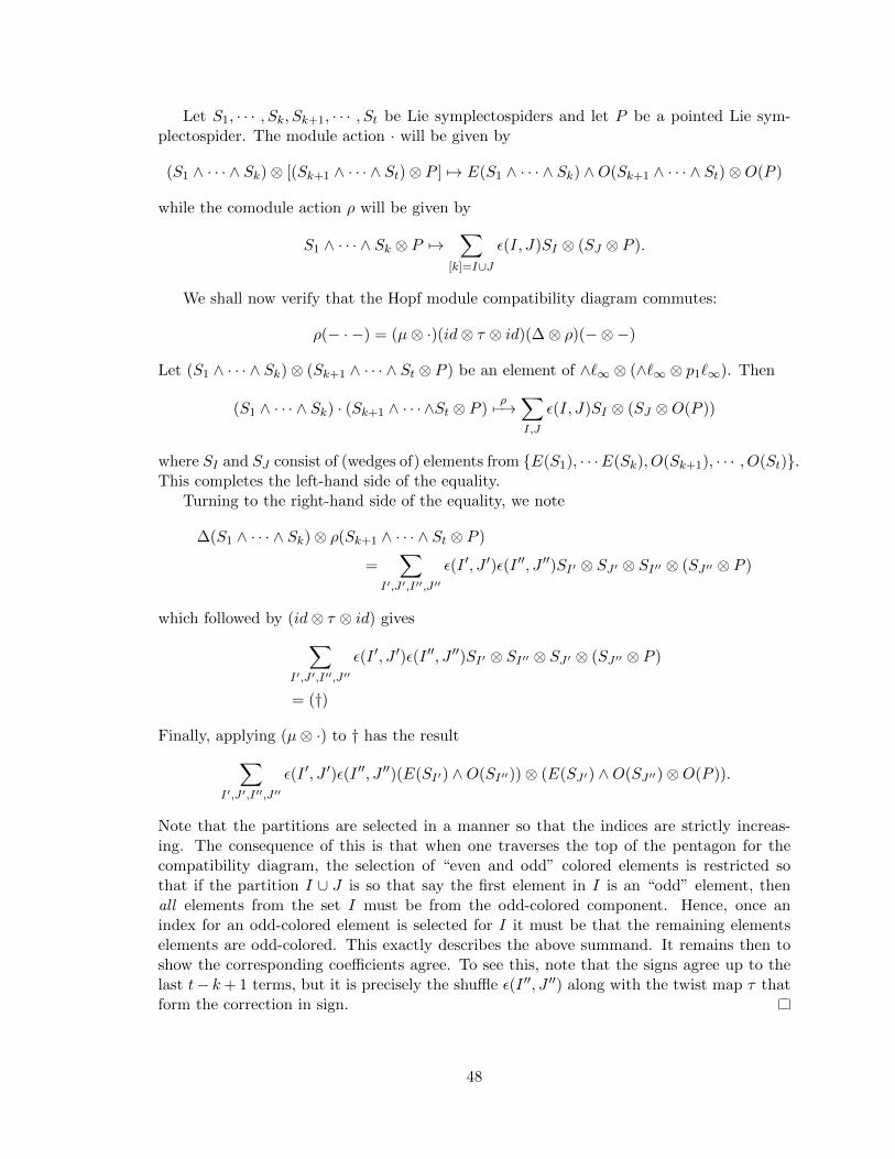
Let S1, · · · , Sk, Sk+1, · · · , St be Lie symplectospiders and let P be a pointed Lie sym-plectospider. The module action · will be given by

(S1 ∧ · · · ∧ Sk)⊗ [(Sk+1 ∧ · · · ∧ St)⊗ P ] 7→ E(S1 ∧ · · · ∧ Sk) ∧O(Sk+1 ∧ · · · ∧ St)⊗O(P )

while the comodule action ρ will be given by

S1 ∧ · · · ∧ Sk ⊗ P 7→∑

[k]=I∪J

ε(I, J)SI ⊗ (SJ ⊗ P ).

We shall now verify that the Hopf module compatibility diagram commutes:

ρ(− · −) = (µ⊗ ·)(id⊗ τ ⊗ id)(∆⊗ ρ)(−⊗−)

Let (S1 ∧ · · · ∧ Sk)⊗ (Sk+1 ∧ · · · ∧ St ⊗ P ) be an element of ∧`∞ ⊗ (∧`∞ ⊗ p1`∞). Then

(S1 ∧ · · · ∧ Sk) · (Sk+1 ∧ · · · ∧St ⊗ P )ρ7−→∑I,J

ε(I, J)SI ⊗ (SJ ⊗O(P ))

where SI and SJ consist of (wedges of) elements from {E(S1), · · ·E(Sk), O(Sk+1), · · · , O(St)}.This completes the left-hand side of the equality.

Turning to the right-hand side of the equality, we note

∆(S1 ∧ · · · ∧ Sk)⊗ ρ(Sk+1 ∧ · · · ∧ St ⊗ P )

=∑

I′,J ′,I′′,J ′′

ε(I ′, J ′)ε(I ′′, J ′′)SI′ ⊗ SJ ′ ⊗ SI′′ ⊗ (SJ ′′ ⊗ P )

which followed by (id⊗ τ ⊗ id) gives∑I′,J ′,I′′,J ′′

ε(I ′, J ′)ε(I ′′, J ′′)SI′ ⊗ SI′′ ⊗ SJ ′ ⊗ (SJ ′′ ⊗ P )

= (†)

Finally, applying (µ⊗ ·) to † has the result∑I′,J ′,I′′,J ′′

ε(I ′, J ′)ε(I ′′, J ′′)(E(SI′) ∧O(SI′′))⊗ (E(SJ ′) ∧O(SJ ′′)⊗O(P )).

Note that the partitions are selected in a manner so that the indices are strictly increas-ing. The consequence of this is that when one traverses the top of the pentagon for thecompatibility diagram, the selection of “even and odd” colored elements is restricted sothat if the partition I ∪ J is so that say the first element in I is an “odd” element, thenall elements from the set I must be from the odd-colored component. Hence, once anindex for an odd-colored element is selected for I it must be that the remaining elementselements are odd-colored. This exactly describes the above summand. It remains then toshow the corresponding coefficients agree. To see this, note that the signs agree up to thelast t− k+ 1 terms, but it is precisely the shuffle ε(I ′′, J ′′) along with the twist map τ thatform the correction in sign.

48

4.3 The graph homology of p1LFrom the space of basepointed spiders, we wish to create a graph complex as in Proposition2.5.8.

Definition 4.3.1. LetG be an oriented graph with all vertices at least bivalent. If we denotethe vertices of G by v1, · · · , vm and the respective valence of each vertex by d1, · · · , dm, thena basepointed graph is an identification of each vertex vi with a spider from pLS[di − 1].

Since pL is a cyclic operad, pLG is a pL-graph complex and so we retain the same con-ventions as in Chapter 2 regarding the calculation of graph homology. As we are interestedin the homology of Aut(Fn), we focus on the situation when our basepointed graphs havea single hair and henceforth when we write “basepointed graph” it will be understood thatthe graph contains a single basepoint.

Denote the subspace of pLG consisting of graphs which possess a single basepoint byp1LG. This means the degree k part of p1LG consists of a single vertex decorated by a pointedspider along with k − 1 vertices decorated by non-pointed spiders. With this definition ofp1LG, it is a subcomplex:

Proposition 4.3.2. The subspace p1LG is a subcomplex of pLG.

Proof. We must show ∂E has degree −1, carries single basepointed graphs to single base-pointed graphs, and ∂2

E = 0 on this subspace.Let P be a pointed Lie graph in p1LGk, that is, there are k vertices on the underlying

oriented graph of P and exactly one of the k vertices is decorated with a pointed Liespider with a single basepoint. Then ∂E(P ) is the sum over all edge collapses of P andconsequent mating of the spiders decorating the edge vertex endpoints, i.e. ∂E(P ) is alinear combination of decorated graphs with k − 1 vertices. Note that the mating of a Liespider with a singly pointed Lie spider results in a singly pointed Lie spider and so, inparticular, the edge collapse will not result in a graph with more than one basepoint norzero basepoints (unless the collapses causes a loop in the quotient graph). The fact that im∂E ⊂ ker ∂E follows as in the proof of Proposition 2.5.8.

We recall that if O is a cyclic operad, then OG has a Hopf algebra structure as detailed inProposition 2.5.9: the product of two graphs is given by their disjoint union and a coalgebrastructure is defined so that the connected graphs are the primitives. Since p1LG is not acyclic operad, we are led to the question: What kind of structure does the space p1LGcarry? Following in the trend for the space of pointed Lie symplectospiders we assert

Proposition 4.3.3. The space p1LG is a Hopf module over the Hopf algebra LG.

Proof. To establish the result, we must define a module action, a comodule action, and thenverify a compatibility relation.

Define an LG-module action LG ⊗ p1LG·−→ p1LG as in the LG case by disjoint union.

That is, if G is a Lie graph and P is a pointed Lie graph, then G · P = G t P where t isthe disjoint union.

We define p1LGρ−→ LG ⊗ p1LG in the spirit of the operation ∆ of the Hopf algebra

LG where ∆ is defined so that the connected graphs are the primitive elements. If P is aconnected, basepointed Lie graph and 1 denotes the empty graph, then P

ρ7−→ 1 ⊗ P andextend linearly over the product.

49

Let us verify the compatibility condition. Let G be a Lie graph and let P be a pointedLie graph. Tracing along the top of the pentagon of the diagram in Definition 4.2.3,

ρ(G · P ) = ρ(G t P )

= 1⊗ (G t P ) +G⊗ P. (4.3)

On the other hand, going down the leftmost vertical map of the pentagon gives

(∆⊗ ρ)(G⊗ P ) = ∆(G)⊗ ρ(P )

= (G⊗ 1 + 1⊗G)⊗ (1⊗ P )

= G⊗ 1⊗ 1⊗ P + 1⊗G⊗ 1⊗ P= (†)

and then traversing the bottom yields

(id⊗ τ ⊗ id)(†) = G⊗ 1⊗ 1⊗ P + 1⊗ 1⊗G⊗ P= (††)

Finally, we go up the rightmost map of the pentagon to note

(µ⊗ ·)(††) = (G t 1)⊗ (1 t P ) + (1 t 1)⊗ (G t P )

= G⊗ P + 1⊗ (G t P ) (4.4)

Note that equations 4.3 and 4.4 coincide; our compatibility condition is verified and thereforep1LG is a Hopf module over the Hopf algebra LG.

Lemma 4.3.4. The map

∧`∞ ⊗ p1`∞ψn−−→ p1LG

is a chain map, that is, the following diagram is commutative.

∧`∞ ⊗ p1`∞ψn- p1LG

∧`∞ ⊗ p1`∞

∂n?

ψn- p1LG

∂E?

Proof. Let S = S1∧· · ·∧Sn⊗P ∈ ∧`∞⊗p1`∞. We show ∂Eψn(X) = ψn∂n(X) (recall ∂E isthe graph-complex boundary map and ∂n is the boundary map for Lie algebra homology).Consider the left hand side:

∂Eψn(X) = ∂E∑π

w(π)(S1 ∧ · · · ∧ Sn ⊗ P )π

=∑e

∑π

w(π)(S1 ∧ · · · ∧ Sn ⊗ P )πe

where the latter sum is over all edges in the graph (S1 ∧ · · · ∧ Sn ⊗ P )π with π a pairing ofthe half edges of the spider legs. We partition this sum into two classes: edges which have

50

a half-edge which is a leg of P and edges which do not.

· · · =∑e∈P

∑π

w(π)(S1 ∧ · · · ∧ Sn ⊗ P )πe

+∑e6∈P

∑π

w(π)(S1 ∧ · · · ∧ Sn ⊗ P )πe .

It was shown in [7] that the the second summand corresponds to∑i<j

(−1)i+j [Si, Sj ] ∧ S1 · · · ∧ Si ∧ · · · ∧ Sj ∧ · · · ∧ Sn ⊗ P

under the image of ψn and so it remains to show the correspondence between∑e∈P

∑π

w(π)(S1 ∧ · · · ∧ Sn ⊗ P )πe (4.5)

and

ψn

n∑i=1

(−1)iS1 ∧ · · · ∧ Si ∧ · · · ∧ Sn ⊗ [Si, P ]. (4.6)

If we expand (4.6) using the definition of the bracket and then apply the map ψn wehave

ψn

n∑i=1

∑α∈Si,β∈P

(−1)iS1 ∧ · · · ∧ Si ∧ · · · ∧ Sn ⊗ (Si, α)!(P, β)

=n∑i=1

∑α∈Si,β∈P

∑π

(−1)iw(π)(S1 ∧ · · · ∧ Si ∧ · · · ∧ Sn ⊗ (Si, α)!(P, β))π. (4.7)

We manipulate (4.5) to bring it into the form of (4.7). Note that the legs (half-edges) αand β comprise an edge of the graph (S1 ∧ · · · ∧ Sn ⊗ P )π if (α, β) ∈ π. Moreover, we mayassume α and β are legs from distinct spiders for if they are not, the graph vanishes under∂E (recall that ∂E is defined so that it vanishes on loops). With this in mind, we recast(4.5) in the following form (with the understanding all the edges e in the inner summandare necessarily incident to P ):∑

π

∑e∈(S1∧···∧Sn⊗P )π

w(π)(S1 ∧ · · · ∧ Sn ⊗ P )πe

=∑π

∑(α,β)∈π

w(π)(S1 ∧ · · · ∧ Sn ⊗ P )πα∪β

=∑π

n∑i=1

∑α∈Si,β∈P,(α,β)∈π

w(π)(S1 ∧ · · · ∧ Sn ⊗ P )πα∪β. (4.8)

We must now translate the pairing π into a spider mating. To accomplish this, we definea new pairing π which is the paring on the legs other than α and β induced by π, i.e.,

51

π = π − (α, β). Working with the summand in (4.6):

w(π)(S1 ∧ · · · ∧ Si ∧ · · · ∧ Sn ⊗ P )πα∪β

= w(π)ω(vα, vβ)(−1)i(S1 ∧ · · · ∧ Si ∧ · · · ∧ Sn ⊗ (Si, α)!(P, β))π.

Note w(π) = w(π)ω(vα, vβ) and so if we change the order of summation and substitute inour new summand into (4.8) we get

· · · =n∑i=1

∑α∈Si,β∈P

∑π

w(π)(−1)i(S1 ∧ · · · ∧ Si ∧ · · · ∧ Sn ⊗ (Si, α)!(P, β))π,

as desired.

4.4 An analysis of the sp(2n)-invariants in ∧`n ⊗ p1`n

Recall in Chapter 2, we defined a Lie symplectospider as an element of

`n =⊕m≥2

(LS[m]⊗ V ⊗mn

)Σm

=⊕m≥2

`mn .

Using the fact p1`n is a `n-module, we form the chain groups ∧`n ⊗ p1`n of the Chevalley-Eilenberg complex and then decompose the chain groups into a direct sum of terms p`k,m ofwedges of k− 1 Lie symplectospiders tensored with one singly-pointed Lie symplectospiderwhich altogether have m legs in total (note we are suppressing the subscript of 1 on p`k,min the interest of keeping the notation manageable). That is,

∧`n ⊗ p1`n =⊕k,m

p`k,m

=⊕k,m

m1 + · · · +mk = m

`m1n ∧ · · · ∧ `mk−1

n ⊗ p1`mkn .

Note that the sp(2n)-action on p1`n and `n is via the mating of two-legged spiders with eithera pointed or unpointed spider. We say more regarding the sp(2n)-invariants of ∧`n ⊗ p1`n:first, (∧`n ⊗ p1`n)sp(2n) forms a subcomplex of ∧`n ⊗ p1`n. Indeed, we have

Lemma 4.4.1. The boundary map of the Chevalley-Eilenberg complex is an sp(2n)-modulemorphism.

Proof. Recall that the boundary map

∧r`n ⊗ p1`n∂−−→ ∧r−1`n ⊗ p1`n

52

is given by

S1 ∧ · · · ∧ Sr ⊗ P 7→r∑i=1

(−1)iS1 ∧ · · · ∧ Si ∧ · · · ∧ Sr ⊗ (Si · P )

+∑i<j

(−1)i+j [Si, Sj ] ∧ S1 ∧ · · · ∧ Si ∧ · · · ∧ Sj ∧ · · · ∧ Sr ⊗ P.

Consider the element S1 ∧ · · · ∧ Sr ⊗ P of ∧r`n ⊗ p1`n and the element ξ of sp(2n); weshow ∂(ξ · (S1 ∧ · · · ∧ Sr ⊗ P )) = ξ · ∂(S1 ∧ · · · ∧ Sr ⊗ P ) for the linearity is clear by thedefinition of ∂. Note that we can expand the left hand side as

∂(ξ · (S1 ∧ · · · ∧ Sr ⊗ P ))

= ∂

(S1 ∧ · · · ∧ Sr ⊗ (ξ · P ) +

r∑i=1

S1 ∧ · · · ∧ (ξ · Si) ∧ · · · ∧ Sr ⊗ P

)= ∂ (S1 ∧ · · · ∧ Sr ⊗ (ξ · P ))

+r∑i=1

∂ (S1 ∧ · · · ∧ (ξ · Si) ∧ · · · ∧ Sr ⊗ P )

=r∑i=1

(−1)iS1 ∧ · · · ∧ Si ∧ · · · ∧ Sr ⊗ (Si · (ξ · P ))

+∑i<j

(−1)i+j [Si, Sj ] ∧ S1 ∧ · · · ∧ Si ∧ · · · ∧ Sj ∧ · · · ∧ Sr ⊗ (ξ · P )

+r∑

α=1

(r∑i=1

(−1)iS1 ∧ · · · ∧ Si ∧ · · · ∧ (ξ · Sα) ∧ · · · ∧ Sr ⊗ (Si · P )

)

+r∑

α=1

∑i<j

(−1)i+j [Si, Sj ] ∧ S1 ∧ · · · ∧ Si ∧ · · · ∧ (ξ · Sα) ∧ · · · ∧ Sj ∧ · · · ∧ Sr ⊗ P

and the right hand side (the details follow similarly) as

ξ · ∂(S1 ∧ · · · ∧ Sr ⊗ P )

=r∑i=1

(−1)iS1 ∧ · · · ∧ Si ∧ · · · ∧ Sr ⊗ (ξ · (Si · P ))

+∑i<j

(−1)i+j [Si, Sj ] ∧ S1 ∧ · · · ∧ Si ∧ · · · ∧ Sj ∧ · · · ∧ Sr ⊗ (ξ · P )

+r∑i=1

(r−1∑α=1

(−1)iS1 ∧ · · · ∧ Si ∧ · · · ∧ (ξ · Sα) ∧ · · · ∧ Sr ⊗ (Si · P )

)

+∑i<j

(r−2∑α=1

(−1)i+j [Si, Sj ] ∧ S1 ∧ · · · ∧ Si ∧ · · · ∧ (ξ · Sα) ∧ · · · ∧ Sj ∧ · · · ∧ Sr ⊗ P

).

Subtracting like quantities, we reduce the lemma to verifying

53

r∑i=1

(−1)iS1 ∧ · · · ∧ Si ∧ · · · ∧ Sr ⊗ (Si · (ξ · P ))

+r∑

α=1

(r∑i=1

(−1)iS1 ∧ · · · ∧ Si ∧ · · · ∧ (ξ · Sα) ∧ · · · ∧ Sr ⊗ (Si · P )

)

+r∑

α=1

∑i<j

(−1)i+j [Si, Sj ] ∧ S1 ∧ · · · ∧ Si ∧ · · · ∧ (ξ · Sα) ∧ · · · ∧ Sj ∧ · · · ∧ Sr ⊗ P

=

r∑i=1

(−1)iS1 ∧ · · · ∧ Si ∧ · · · ∧ Sr ⊗ (ξ · (Si · P ))

+r∑i=1

(r−1∑α=1

(−1)iS1 ∧ · · · ∧ Si ∧ · · · ∧ (ξ · Sα) ∧ · · · ∧ Sr ⊗ (Si · P )

)

+∑i<j

(r−2∑α=1

(−1)i+j [Si, Sj ] ∧ S1 ∧ · · · ∧ Si ∧ · · · ∧ (ξ · Sα) ∧ · · · ∧ Sj ∧ · · · ∧ Sr ⊗ P

).

The latter equality is seen to hold by an appeal to the algebraic structure of our objects.Since p1`∞ is a Lie module over `∞, it must be the case that [S1, S2] · P = S1 · (S2 · P ) −S2 · (S1 ·P ). If we decompose our sums in a “diagonal” (the pulled term), “lower diagonal”(precede the pulled term), and “upper diagonal” (follow the pulled term) manner in thetopmost part of the equality, these terms coincide with the unexpanded (in reference to themodule action) terms of the bottom portion of the equality. We also comment that thislemma follows directly from the fact that the boundary operator commutes with the adjointaction.

Since the boundary operator is an sp(2n)-module morphism, we may conclude that(∧`n ⊗ p1`n)sp(2n) is a subcomplex of ∧`n ⊗ p1`n. Given the decomposition of ∧`n ⊗ p1`ninto the subspaces of k spiders with a total of m legs

⊕k,m p`k,m, we form the spaces

Zk,m = ker ∂n ∩ p`k,mBk,m = im ∂n ∩ p`k,m

Hk,m(`n; p1`n) = Zk,m/Bk,m

so that the Lie homology Hk(`n; p1`n) can be expressed as⊕m

Hk,m(`n; p1`n).

The map ψn of Lemma 4.3.4 provides us with a way to produce a pointed Lie graphfrom a collection of spiders. The reverse map is given as ϕn in [7]; we extend the definitionhere to the pointed case:

Definition 4.4.2. Let P be a basepointed Lie graph with underlying oriented graph X.For each edge of P, break the edge in half so as to get a disjoint union of spiders. Now,to turn this into an element of ∧`n ⊗ p1`n we wedge the spiders in the order given by theorientation (recall an orientation gives a vertex ordering and a direction associated to eachedge) and assign two elements of Bn and a sign to each edge as follows: Let e be an edge

54

of P which consists of the two half-edges e0 and e1 (in order from the orientation of thehalf-edges). Place v ∈ {pi, qi} on the half-edge e0 and v′ ∈ {pi, qi} − {v} on the half-edgee1. If the half-edge e0 is labeled with pi (hence e1 carries qi), then the edge has a positivesign associated to it. If the initial half-edge e0 is labeled with qi, then we associate a minussign to the edge. An assignment of an element of Bn to each half-edge and along with asign for each edge following the previous description is called a state of P . We define thesign σ(s) of the state s to be the product of the signs from the edges given by the state s.As defined, a state s gives rise to an element Ps of ∧`n ⊗ p1`n. Now, we define the mapp1LG

ϕn−−→ ∧`n ⊗ p1`n by

P 7→∑s

σ(s)Ps.

Now, by the work of the previous lemma and the second part of Proposition 8 of [7], wehave that the inclusion of the sp(2n)-invariants of ∧`n ⊗ p1`n into ∧`n ⊗ p1`n induces anisomorphism on homology.

Since the tree decorating the interior of the spider is invariant under this action, thesp(2n) action only affects the tensor power of V ⊗m in `mn and p1`

mn . It thus suffices to

identify the sp(2n)-invariants of V ⊗m. In [10], it is shown that the invariants can be givenby chord diagrams. The details of this identification are given by

Proposition 4.4.3. The image of the map ϕn coincides with the invariants in ∧`n⊗ p1`n,that is, imϕn = (∧`n ⊗ p1`n)sp(2n).

Proof. The idea behind this proof will be to supplement the determination of invariants of∧`n from [7] for our purposes. We recreate much of the proof here for the benefit of thereader.

Let T`nτ−→ ∧`n be the standard quotient map from the tensor algebra to the alternating

algebra and define a map ι by S1 ∧ · · · ∧ Sk 7→ 1k!

∑σ∈Σk

(−1)|σ|Sσ(1) ⊗ · · · ⊗ Sσ(k). Thesemaps fit into a sequence

∧`nι−→ T`n

τ−→ ∧`n

of sp(2n)-module morphisms. Furthermore, we have τι = id and so it follows τ is a epimor-phism of sp(2n)-modules.

Recall that `n is defined as the sum of the Σm-coinvariants in LS[m]⊗ V ⊗mn , that is

`n =⊕m≥2

(LS[m]⊗ V ⊗mn )Σm .

Let n =⊕

m≥2(LS[m]⊗ V ⊗mn ); we again pass to the quotient T n γ−→ T`n and note that ifwe let ι be induced by the map

(LS[m]⊗ V ⊗mn )Σm −−→ LS[m]⊗ V ⊗mn

S 7−−→ 1

m!

∑σ∈Σm

σ · S

we get a similar sequence as before

T`nι−→ T n γ−−→ T`n

55

The maps compose to the identity and are sp(2n)-module morphisms. Hence γ is an epi-morphism of sp(2n)-modules.

Putting this together, we have a new sequence of sp(2n)-module epimorphisms

T n γ−−→ T`nτ−→ ∧`n.

Note that p1`nid−→ p1`n is an sp(2n)-module epimorphism and since the tensor of epi-

morphisms is an epimorphism, we have that τ ⊗ id is an epimorphism. Similar to the nconstruction above, we form p1

n =

⊕m≥2(p1LS[m] ⊗ V ⊗mn ) and observe we again get an

sp(2n)-module epimorphism p1n

η−→ p1`n. This fits nicely together in

T n ⊗ p1n

γ⊗η−−−→ T`n ⊗ p1`nτ⊗id−−−−→ ∧`n ⊗ p1`n,

which we note (τ ⊗ id) ◦ (γ⊗ η) = (τ ◦γ)⊗ (id ◦ η) implies the composite is an epimorphismsince each term is an epimorphism. It now suffices to identify the invariants in T n ⊗ p1

n.

To compute the invariants in T n ⊗ p1n we decompose T n ⊗ p1

n as

T n ⊗ p1n =

⊕k≥2,m≥1

pk,mwith

pk,m =⊕

m1+···+mk=m

(LS[m1]⊗ V ⊗m1n )⊗ · · · ⊗ (LS[mk−1]⊗ V ⊗mk−1

n )⊗ (pLS[mk]⊗ V ⊗mkn ).

Recall that the sp(2n)-action is via a two-legged symplectospider mating and that thismating does not affect the underlying spider structure but does change the symplecticlabeling of the spider. To be precise, the sp(2n)-action on LS[mi]⊗ V ⊗mi is only effectiveon the V ⊗mi term (the same is true for the pointed case). With this, we then are led to

(pk,m)sp(2n)

=⊕

m1+···+mk=m

(V ⊗m1n ⊗· · ·⊗V ⊗mkn )sp(2n)⊗(LS[m1]⊗· · ·⊗LS[mk−1]⊗pLS[mk]).

The determination of the sp(2n)-invariants in V ⊗m1n ⊗ · · · ⊗ V ⊗mkn is a result that goes

back Weyl. We will describe the process as given in [10]. First, we write V ⊗m1n ⊗· · ·⊗V ⊗mkn =

V ⊗m. It turns out that a base for the invariants in V ⊗m is given by oriented chord diagramson m vertices. An oriented chord diagram is a pairing of the m vertices into ordered pairsvi → vj (that is, directed edges) where we consider vi to be the “tail” and vj to be the“head” of the directed edge.

Now, to every pairing vi → vj we define a bijection {vi, vj} ↔ {pk, qk} where theelements {p1, · · · , pn, q1, · · · , qn} form a basis for the symplectic vector space Vn. We imposethe condition that if the element qk is identified with vi while pk is identified with vj , thenthis directed edge carries a minus sign. That is, if a directed edge is given by (head)→ (tail),then (head)↔ pk and (tail)↔ qk causes the edge to carry a “+” sign whereas (head)↔ qkand (tail)↔ pk causes the edge to carry a “−” sign.

Define a state to be an established bijection between every directed edge and {pk, qk}in our chord diagram together with an associated sign given by the product of the signsattached to the directed edges. Then the invariant is the sum over all possible states of the

56

symplectic basis elements representing the vertices for V ⊗m.We have established the invariants in T n⊗ p1

n, but we need to identify the invariants

in ∧`n ⊗ p1`n. Earlier in the proof we concluded that

T n ⊗ p1n

γ⊗η−−−→ T`n ⊗ p1`nτ⊗id−−−−→ ∧`n ⊗ p1`n,

is a sequence of sp(2n)-module epimorphisms. Thus the maps restrict to the sequence ofepimorphisms

(T n ⊗ p1n)sp(2n) γ⊗η−−−→ (T`n ⊗ p1`n)sp(2n) τ⊗id−−−−→ (∧`n ⊗ p1`n)sp(2n).

Let ξ ⊗ S1 ⊗ · · · ⊗ Sk−1 ⊗ P be an element in (V ⊗m1n ⊗ · · · ⊗ V ⊗mkn )sp(2n) ⊗ (LS[m1]⊗ · · · ⊗

LS[mk−1]⊗ pLS[mk]) where ξ is an sp(2n)-invariant in V ⊗m1n ⊗ · · · ⊗ V ⊗mkn . The image of

this element under the map (τ⊗id)◦(γ⊗η) can be identified with the image of a pointed Liegraph G as follows. The sp(2n)-invariant ξ is identified with its chord diagram counterpartand when we map ξ⊗S1⊗· · ·⊗Sk−1⊗P to ∧`n⊗p1`n, the result is attaching the symplecticelements dictated by the pairing of ξ to the legs of the spiders S1, · · · , Sk−1, P . Further, thediagram invariant ξ gives the exact way to attach the spider legs to give rise to a pointedLie graph. Note that each possible state of the oriented chord diagram ξ gives rise to astate of the resulting graph. If we sum over all possible states ξ, this corresponds to a sumover all states of a graph, i.e., it is precisely the image of ϕn.

We illustrate the process of creating a pointed Lie graph from an sp(2n)-invariant forV ⊗10 = (V ⊗2)⊗1 ⊗ (V ⊗4)⊗2. The way to interpret the individual tensor powers is (V ⊗i)⊗j

means there are j vertices in a particular Lie graph which contain a planar binary tree withi leaves. A possible pairing could be given by

q5

p5

p4

q1

q7

q2

q4

p1

p7

p2

*

(a) Three symplectospiders

*

(b) Gluing spider legs together based onchord diagram invariant gives a hairy Liegraph

Figure 4.2: How an sp(2n)-invariant gives rise to a hairy Lie graph

57

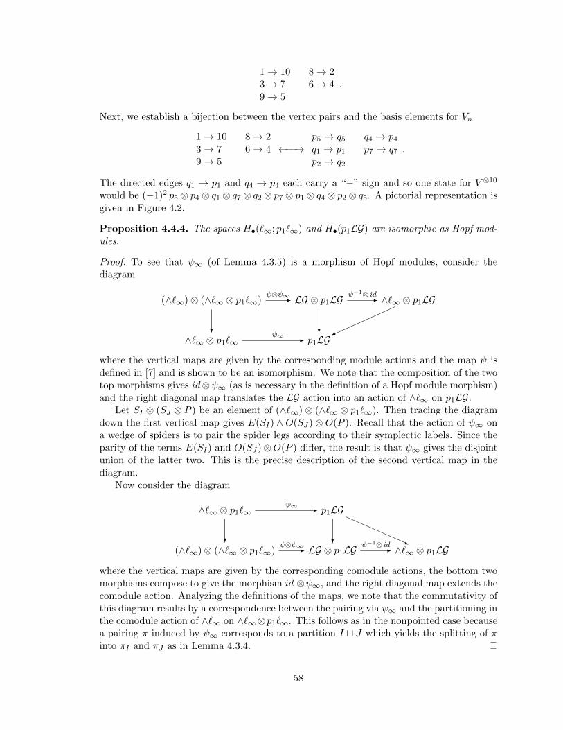
1→ 10 8→ 23→ 7 6→ 49→ 5

.

Next, we establish a bijection between the vertex pairs and the basis elements for Vn

1→ 10 8→ 23→ 7 6→ 49→ 5

←−−→p5 → q5 q4 → p4

q1 → p1 p7 → q7

p2 → q2

.

The directed edges q1 → p1 and q4 → p4 each carry a “−” sign and so one state for V ⊗10

would be (−1)2 p5 ⊗ p4 ⊗ q1 ⊗ q7 ⊗ q2 ⊗ p7 ⊗ p1 ⊗ q4 ⊗ p2 ⊗ q5. A pictorial representation isgiven in Figure 4.2.

Proposition 4.4.4. The spaces H•(`∞; p1`∞) and H•(p1LG) are isomorphic as Hopf mod-ules.

Proof. To see that ψ∞ (of Lemma 4.3.5) is a morphism of Hopf modules, consider thediagram

(∧`∞)⊗ (∧`∞ ⊗ p1`∞)ψ⊗ψ∞- LG ⊗ p1LG

ψ−1⊗ id- ∧`∞ ⊗ p1LG

∧`∞ ⊗ p1`∞?

ψ∞ - p1LG? �

where the vertical maps are given by the corresponding module actions and the map ψ isdefined in [7] and is shown to be an isomorphism. We note that the composition of the twotop morphisms gives id⊗ψ∞ (as is necessary in the definition of a Hopf module morphism)and the right diagonal map translates the LG action into an action of ∧`∞ on p1LG.

Let SI ⊗ (SJ ⊗ P ) be an element of (∧`∞)⊗ (∧`∞ ⊗ p1`∞). Then tracing the diagramdown the first vertical map gives E(SI) ∧ O(SJ)⊗ O(P ). Recall that the action of ψ∞ ona wedge of spiders is to pair the spider legs according to their symplectic labels. Since theparity of the terms E(SI) and O(SJ)⊗O(P ) differ, the result is that ψ∞ gives the disjointunion of the latter two. This is the precise description of the second vertical map in thediagram.

Now consider the diagram

∧`∞ ⊗ p1`∞ψ∞ - p1LG

(∧`∞)⊗ (∧`∞ ⊗ p1`∞)?

ψ⊗ψ∞- LG ⊗ p1LG?

ψ−1⊗ id- ∧`∞ ⊗ p1LG-

where the vertical maps are given by the corresponding comodule actions, the bottom twomorphisms compose to give the morphism id ⊗ψ∞, and the right diagonal map extends thecomodule action. Analyzing the definitions of the maps, we note that the commutativity ofthis diagram results by a correspondence between the pairing via ψ∞ and the partitioning inthe comodule action of ∧`∞ on ∧`∞⊗p1`∞. This follows as in the nonpointed case becausea pairing π induced by ψ∞ corresponds to a partition I t J which yields the splitting of πinto πI and πJ as in Lemma 4.3.4.

58

4.5 An analysis of the pointed Lie graph complex

In order to draw the conclusions we desire, we must get to the connected graphs ofH•(p1LG).Recall that the coaction is defined so that the connected graphs are those such that P 7→1 ⊗ P. In the theory of A-comodules, this subspace has a special name, the coinvariants,and it is indicated by a superscript co A. If we denote the subspace generated by connectedgraphs by H•(P (p1LG)), then, noting ψ∞ is an isomorphism, we let H•(`∞; p1`∞)co `∞ bethe corresponding subspace of H•(`∞; p1`∞).

The subspace of connected pointed Lie graphs splits as P ⊕ P (p1LG)/P where

• P is spanned by graphs with only bivalent vertices (polygons)

• P (p1LG)/P is spanned by graphs with at least one (≥ 3)-valent vertex

Recall that the space of two-legged symplectospiders is isomorphic to sp(2n). If wedecorate the vertices of a graph with these two-legged spiders, we note the correspondencein the graph setting:

Lemma 4.5.1. H•(P) ∼= H•(sp(2∞))

Proof. We will consider the spaces Pj of P =⊕Pj based upon the congruence of j modulo

4 as particular symmetries will be able to be exploited. Let us set up some notation: thespace Pj is spanned by at most the j oriented polygons p1

j , · · · , pjj where pij represents a

polygon with j sides and a distinguished basepoint on the ith vertex.Suppose j ≡ 0 mod 4. If we rotate pij by 2π/j and suitably relabel so that the orientation

of exp(2πi/j)pij is coherent with that of pi+1j , we note that pij = −pi+1

j . Hence Pj is generated

by p1j . Now, rotate p1

j about the axis through the basepoint that bisects the polygon. Thisreverses the orientation and so Pj = 0 for j ≡ 0 mod 4.

If j ≡ 1 mod 4, then pij = 0 for all i. To see this, rotate pij about the axis passingthrough the basepoint on vertex i and the edge “opposite” it on the polygon. This actionreverses the orientation since there is an odd number of sides to reverse and an even numberof vertex pairs to interchange. Therefore pij = 0.

For j ≡ 2 mod 4, we can use the argument presented for the previous scenario exceptnow, there is an even number of edge orientation swaps and odd number of vertex pairswaps. Finally, when j ≡ 3 mod 4, we pick up the generator p1

j . Rotation by 2π/j preserves

the orientation, and so the polygons p1j , · · · , p

jj are all congruent: p1

j = p2j = · · · = pjj .

We then have the chain complex

· · · → 0→ Q{p1

4j−1

}→ 0→ · · ·

It follows that P only has nontrivial homology only if j ≡ 3 mod 4 and in this case it isseen to be cyclic and coincides with the homology of sp(2∞), as was to be shown.

The previous lemma details graphs in which all vertices are bivalent. We now analyzethe effect of sp(2n)-colored vertices in a general pointed Lie graph. To begin, we consider aspecial type of graph and then create a chain complex with boundary operator given by thestandard graph complex boundary ∂ = ∂E . For k ≥ 0, let V 0

k denote the (linear) graph withk internal vertices and hence k − 1 internal edges. Now, take V 0

k and add a distinguishedbasepoint to the ith vertex; denote this new graph by V i

k . The space Vk is then generatedby V 1

k , · · ·V kk . We claim

59

Lemma 4.5.2. The graph homology of Vk vanishes except at k = 0 when it is R.

Proof. It is clear by the definitions of V• and ∂ that H0(V•) = R. Note that for k odd, wehave ∂(V i

k ) vanishes for i odd and ∂(V ik ) = V i

k−1 − Vi+1k−1 for i even. For k even, ∂(V i

k ) and

∂(V i+1k ) have image V i

k−1 where i is odd. Direct computation now yields the result.

Hence, aside from dimension 0, the addition of a bivalent vertex to a pointed Lie graphcontributes nothing to homology. Recall that the space P (p1LG) is spanned by connectedgraphs with no bivalent vertices and P (p1LG)/P is spanned by connected graphs with atleast one (≥ 3)-valent vertex. In the interest of relating P (p1LG) and P (p1LG)/P, letus filter P (p1LG)/P by the number of non-bivalent vertices (call this filter Fg). DefineE0g,b to be the span of graphs with g (≥ 3)-valent vertices and b bivalent (i.e., identity-

colored) vertices. We take the vertical boundary maps E0g,b

∂y−→ E0g,b−1 as the standard

graph complex boundary maps except the edge contractions only occur at edges incidentto a bivalent vertex. Defined as such, we claim that

Lemma 4.5.3. The spaces H•(P (p1LG)) and H•(P (p1LG)/P) are isomorphic.

Proof. Note that the definition of E0g,b given corresponds to filtering the space P (p1LG)/P

by the number of non-bivalent vertices and so the spectral sequence attached to E0g,b is the

quotient complex Fg(P (p1LG)/P)g+b/Fg−1(P (p1LG)/P)g+b. Let us analyze the verticalcomplexes E0

g,•.Define an equivalence relation on connected graphs with at least one (≥ 3)-valent vertex

by G ∼ G′ if G and G′ are isomorphic after the removal of all bivalent identity-coloredvertices. Observe that E0

g,0 consists of graphs with no bivalent vertices and can therefore

be identified with one of our complexes of interest, P (p1LG).We decompose the vertical complex as E0

g,• =⊕

GEg(G) where the index G runs overisomorphism classes of graphs G from E0

g,•, that is a graph G of E0g,• serves as a repre-

sentative for its equivalence class in E0g,• = P (p1LG). Given a representative G, let G

be the graph G except it possesses only trivial automorphisms. Since Eg(G) is free, we

have Eg(G)/Aut(G) = Eg(G) by (I.4.2) of [5]. Moreover, since we are working with real

coefficients, we have Hb(Eg(G)) ∼= Hb(Eg(G)), provided one of the spaces is trivial.

We decompose further: Eg(G) =⊕Eg(G;S1, · · · , Sg) where the indexing is over a

basis for p1LS/R {1LS}. The latter decomposition follows from the fact ∂y is restrictedto the bivalent vertices and so essentially, only the non-1LS colored vertices can con-tribute to homology. Hence, when b > 0 (that is, there exist bivalent vertices), we haveEg(G;S1, · · · , Sg) ∼=

⊗e∈E(G)

E• where the tensor argument E• is acyclic except in dimen-

sion 0 by Lemma 4.5.2. If we appeal to the Kunneth formula, we note⊗

e∈E(G)E• is acyclic

except in dimension 0, as well. Hence, Hb(E•(G)) = 0 when b > 0 and the only contributionto homology occurs on the g-axis (when b = 0).

Now that we have determined that the homology is concentrated along the g-axis, notethat our sequence collapses at the E1 page. We further note that the boundary operatorfor the E1 page coincides with the boundary operator for the point Lie graph complex, ∂Eand the result follows.

So far in this section we have established

(Lemma 4.5.2) H•(P (p1LG)) ∼= H•(P (p1LG)/P) and

60

(Lemma 4.5.3) H•(P) ∼= H•(sp(2∞)).

Recalling that our space of interest P (p1LG) decomposes into P and P (p1LG)/P, we con-clude

Proposition 4.5.4. H•(P (p1LG)) ∼= H•(sp(2∞)⊕H•(P (p1LG)).

4.6 The pointed forested graph complex

In §2.7.1 we defined the forested graph complex fGk and set the foundation for establishinga natural isomorphism between it and the connected Lie graphs without bivalent vertices,PLGk.

Definition 4.6.1. Let G be a finite connected trivalent graph together with a basepoint∗ and an oriented subforest Φ which contains all of the vertices of G. We will call thisobject (G,Φ, ∗) a pointed forested graph. Denote the space spanned by pointed forestedgraphs whose subforest contains r edges (or trees) quotiented by the relation (G,−Φ, ∗) =

−(G,Φ, ∗) by pfGr.

We impose another relation on pointed forested graphs which will correspond to theIHX/Aut-IHX relations from the pointed Lie operad. To start, we define the subspace of

basic IHX relators on pfGr.Consider the graph in Figure 4.3(a). There are three ways to grow the four-valent vertex

v into a new edge of the forest and create an element of pfG4. These three ways are: growit “vertically,” grow it “horizontally,” and grow it “horizontally” with a twist, see Figures4.3(b), 4.3(d), and 4.3(f), respectively. The sum of these three terms will be known as abasic IHX relator and the space spanned by these relators will be denoted IHXr.

We now define the subspace of pointed IHX relators, pIHXr. In Figure 4.3(a), considerthe vertex w where we have continued our convention of growing the basepoint out fromthe graph on a “hair.” As such, the three blow-ups of this “four”-valent vertex follow insuit with the previous paragraph as shown in Figures 4.3(c), 4.3(e), and 4.3(g).

Define pfGr to be pfGr modulo the subspaces IHXr and pIHXr. The boundary mapon the unpointed forested graph complex fGr was given in 2.7.1 as the sum over all waysof adding an edge to the subforest so that the addition of an edge e to Φ remains acyclic.With this identification, fGr becomes a chain complex which is naturally isomorphic (as avector space) to PLGr, see [7]. Along these lines, we claim:

Proposition 4.6.2. There is a natural vector space isomorphism between the pointed forestedgraph complex pfGr and the space Pp1LGr of connected pointed Lie graphs without bivalentvertices.

Proof. We define a morphism pfGrϕ−→ Pp1LGr as follows:

1. Take a pointed forested graph (G,Φ) in pfGr.2. For every connected component of Φ, take an ε neighborhood of the component that

does not intersect any other neighborhood of a component.

3. Collapse each of these neighborhoods to create a vertex in the quotient graph G.For each vertex v of G we associate to it the component Tv which existed before thecollapse. Note that we “lose” the basepoint in the quotient graph, but it is retainedin the tree associated to a collapsed vertex in G.

61

*

v

w(a) A basepointed graph. The solid edges indicatecomponents of the subforest

*

w

(b) Vertical growth “I” of the vertex v

*

(c) Component one of pIHX for the vertex w

*

w

(d) Horizontal growth “H” of the vertex v

*

(e) Component two of pIHX for the vertex w

*

w

(f) Horizontal growth with a twist “X” of thevertex v

*

(g) Component three of pIHX for the vertex w

Figure 4.3: IHX and pIHX relators

62

We comment that the coherency of orientation between these objects follows as in Propo-sition 21 of [7] (or see Lemma 2.7.4) once we grow out our basepoint to the tip of a hair.The orientation of a pointed forested graph is then given by a number of the edges of Φ.Note that the choice of orientation is canonical.

Each Tv is a binary tree and we can identify the leaves of Tv with the half edges incidentto v. We also identify the interior edges of each Tv with their forest preimage, Φv, so that Φcan be expressed as the union over the vertices v ∈ V (G) of Φv. It follows that the imageof a pointed forested graph under ϕ can be expressed as (G, {Tv}).

Let us verify that the IHX and pIHX relators factor through the quotient. If we let

pfGrτ−→ fGr be the quotient map, then we wish verify there exists a map ϕ such that the

diagram below commutes.

pfGrτ - pfGr

p1LGr

ϕ

?

ϕ-

By the universal mapping property of the quotient, it then suffices to show that IHXr

and pIHXr are contained in the kernel of ϕ. That IHXr is contained in kerϕ was shownin [7]; we consider the pointed IHX subspace. Suppose (GI ,ΦI) + (GH ,ΦH) + (GX ,ΦX)is a pointed IHX relator. The image of this relator under ϕ is the linear combination±(GI , {Tv}I)± (GH , {Tv}H)± (GX , {Tv}X). In order for this sum to vanish, it must be thecase that the signs are (+,−,+) so that the pIHX relator maps to the Aut-IHX relation ofp1LGr. Using our convenient trick of turning the basepoint resulting from our distinguishedbasepoint into a (original valence + 1) vertex with the basepoint on the tip of a hair, wenote that indeed this pIHX relator can be viewed as an IHX relator and hence correspondsto the IHX relation in the graph complex. Reidentifying our hair as a hairy IHX relation asin Figure 4.1(b), we conclude that the pIHX relator maps into the Aut-IHX subspace and so(GI ,ΦI) + (GH ,ΦH) + (GX ,ΦX) 7−→ (GI , {Tv}I)− (GH , {Tv}H) + (GX , {Tv}X) = 0. Thus

the subspaces IHXr and pIHXr are in the kernel of ϕ and there exists a map pfGrϕ−−→ p1LGr

such that the diagram above commutes.It now remains to show ϕ is a bijection. We do so by constructing an inverse to ϕ.

Given a pointed Lie graph, we decompose it as an oriented graph together with a vertex-spider association (G, {Sv}). If we take the tree which comprises the interior of each spideras being a component of the forest, then we have Φ is the union of the interiors of theSv. Since the choice of orientation of the vertices and edges is canonical, this completelydetermines the edge numbering in the resulting forested graph.

The boundary operator on the pointed Lie graph complex is defined as the sum of allpossible edge collapses between the spider-decorated vertices. Upon collapsing an edge ofa graph, we note that the two half-edges (spider legs) adjacent to the edge collapse areidentified at their endpoints so as to create a new edge on the interior of the mating spiders.If we instead view this edge collapse as the addition of an edge between the vertices (withsubsequent edge numbering falling after all previous numberings), we note that there is aninduced boundary map on pfG from the boundary map on pLG. As such, we now speak

63

of the pointed forested graph complex where the boundary operator is defined as describedabove.

4.7 The main result

An analysis of the pointed forested graph complex is the last step in identifying the coho-mology of Auter space with H•(`∞; p1`∞). In particular, we prove

Theorem 4.7.1. Hk(pfGr) ∼= H2r−1−k(Aut(Fr))

so that together with Propositions 4.4.4 and 4.5.4 we have the Kontsevich-type isomorphism

Theorem 4.7.2. Hk(`∞; p1`∞)co `∞ ∼= Hk(sp(2∞))⊕⊕r≥2

H2r−1−k(Aut(Fr))

We summarize the process by which we will determine Theorem 4.7.1. First, we define afiltration on SAr and analyze the cohomology spectral sequence associated to the filtration.This spectral sequence collapses to a cochain complex which calculates the cohomology ofAut(Fr). Finally, analysis of this cochain complex will allow us to relate it to the pointedforested graph complex.

Filter the spine SAr by the number of vertices in a marked graph so that F0SAr consistsof all trivalent (aside from the basepoint) graphs with 2r − 1 vertices. In general, we letFpSAr be generated by graphs with 2r − p− 1 vertices along with Fp−1SAr. The filtrationis independent of the marking and so when we quotient by the Aut action, we preservethe filtration and so we have F0Qr ⊂ F1Qr ⊂ · · · ⊂ F2r−2Qr = Qr. With trivial R-coefficients, the spectral sequence attached to this filtration has first page E1 given byHp+q(FpQr, Fp−1Qr) and the spectral sequence converges to H∗(Aut(Fr)).

Note that if all of the terms on the E1 page vanish except for those along the p-axis,then the spectral sequence collapses to the cochain complex

0→ H0(F0Qr)→ H1(F1Qr, F0Qr)→ · · · → H2r−2(F2r−2Qr, F2r−3Qr)→ 0

which calculates the cohomology of Aut(Fr). Let us accept this fact for now and use it toverify

Theorem. Hk(pfGr) ∼= H2r−1−k(Aut(Fr))

Proof. For convenience, let Q(r)p denote FpQr. We analyze the complex

0→ H0(Q(r)0 )→ H1(Q

(r)1 , Q

(r)1 )→ · · · → H2r−2(Q

(r)2r−2, Q

(r)2r−3)→ 0.

Note that at the pth node, we have

Hp(Q(r)p , Q

(r)p−1) =

ker(Cp(Q(r)p , Q

(r)p−1)

δ−→ Cp+1(Q(r)p , Q

(r)p−1))

im(Cp−1(Q(r)p , Q

(r)p−1)

δ−→ Cp(Q(r)p , Q

(r)p−1))

.

Note that the Aut(Fn)-stabilizer of a cube (g,G,Φ) in the spine consists of the basepoint-preserving graph automorphisms of G that fix the forest. We say a basepoint-preservinggraph automorphism is odd if it induces an odd permutation on the edges of the forest;

64

otherwise we say it is even. When we quotient a cube by its stabilizer, the result is eithera cone on a rational homology ball (if there is an odd automorphism) or a cone on arational homology sphere (if all automorphisms are even) by Corollary 3.2 of [17] so that

Hp(Q(r)p , Q

(r)p−1) = Cp(Q

(r)p , Q

(r)p−1)/im(Cp−1(Q

(r)p , Q

(r)p−1)

δ−→ Cp(Q(r)p , Q

(r)p−1)).

We claim

1. Cp(Q(r)p , Q

(r)p−1) is the dual of the span of all basepointed graphs whose non-basepoint

vertices are trivalent along with a p-edged forest modulo the relation AS given as(G,−Φ) = −(G,Φ) and that

2. the image of δ is spanned by the dual of the IHX and pIHX relators.

To see that the result follows from the establishment of these two claims, note that thespace spanned in either case can be identified with its dual and so we have the result

Hp(Q(r)p , Q

(r)p−1) = R {(G,Φ, ∗)} /(pIHX, IHX,AS)

which one can observe is precisely the vector space pfG2r−1−p. Recall that the lattice points

on the E1 page are given by Hp+q(Q(r)p , Q

(r)p−1) and so, in particular, the coboundary map

on this page has bidegree (1, 0). The E1 page vanishes off the p-axis and so the coboundarymap along this remaining cochain complex is the sum over adding an edge e to the forestΦ of the cube [G,Φ] in all possible ways so that Φ∪ e is a forest. This exactly describes the

boundary map on the forested graph complex. That is, the cochain complex H•(Q(r)p , Q

(r)p−1)

is isomorphic to the chain complex pfG2r−1−p.Now that we see how the theorem follows from the two claims, let us verify them; we start

with the first. Note that the dimension of the simplex corresponding to an element of Q(r)p−1

Figure 4.4: A cube in the 3-spine

65

has dimension p − 1 and Cp(Q(r)p , Q

(r)p−1) and may be identified with Cp(Q

(r)p ). Recall that

Q(r)• is defined by a quotient: in the Aut action on a cube (g,G,Φ), the diagonal between

[G/Φ, ∅] and [G, ∅] is fixed. We then note there is a one-to-one correspondence between

the cubes of Q(r)p and the graphs that are basepointed trivalent (aside from the basepoint)

with a forest Φ with p edges. The antisymmetry property follows by the combinatorialconstruction of the spine and the forest ordering. We have identified the cochain groupswith the dual of the vector space spanned by basepointed trivalent graphs (excluding thebasepoint) with a subforest modulo an antisymmetry relation.

We consider the image of the coboundary map. To see that the image coincides withIHX-type relators, we start at the level of the spine filtration and then pass to the quotientfiltration. Suppose we remove the forest designation of an edge e ∈ Φ from the cube (g,G,Φ)in FpSAr, that is, we consider (δR)|e(g,G,Φ). The image (δR)|e(g,G,Φ) is codimensionone to the face (g,G,Φ). In addition, there is a codimension one face (δC)|e(g,G,Φ) of(g,G,Φ) for every face of the form (δR)|e(g,G,Φ) and this face is directly opposite it inthe cube. Succinctly stated, there is a bijective correspondence between the codimensionone faces resulting from contracting or removing an edge in the cube (g,G,Φ). See Figures

2.3 and 4.4 for a pictorial idea of the correspondence. By definition, Cp−1(Q(r)p , Q

(r)p−1)

consists of maps of dimension p − 1 cubes in Q(r)p that are zero on Q

(r)p−1. By the bijective

correspondence of the codimension one faces and the definition of the relative cochaingroups, we may form a basis which consists of indicator functions on the dimension p − 1cubes of the form (δC)|e(g,G,Φ). Consider the vertex resulting from the collapse of theedge e in (δC)|e(g,G,Φ). There are precisely three codimension one faces which share thiscollapsed cube as a common face, see Figure 4.5. Erasing the marking by taking intoaccount the Aut action, we see that these three blow-ups correspond to the three terms ofan IHX relator in pfG. Application of the coboundary map from the cochain complex to thecontracted cube then gives δ((δC)|e(G,Φ)) = (G,Φ) + (G′,Φ′) + (G′′,Φ′′). Furthermore, ifthe basepoint is at a 3-valent vertex of the forest, we can grow out the hair for the basepointand proceed as above so as to get the dual of an pIHX relator in the image of δ. Hence theimage of δ is generated by the indicator functions on the IHX and pIHX relators.

Following [7], we say a complex is k-spherical if it is of dimension k and is homotopyequivalent to a wedge of k-spheres.

Lemma 4.7.3. On the E1 page, we have Hp+q(Q(r)p , Q

(r)p−1) is zero off the p-axis.

Proof. Since Aut acts with finite stabilizers and preserves the filtration, the homology of

Q(r)p /Q

(r)p−1 coincides with the homology of FpSAr/Fp−1SAr (modulo the Aut action). It

therefore suffices to consider the pair (FpSAr, Fp−1SAr).We want to characterize those elements in FpSAr − Fp−1SAr. Given (G,Φ, ∗), grow

out the basepoint ∗ to the end of a hair. If we consider the sum∑

v(|v| − 3) (excludethe univalent vertex at the tip of the hair), then the result is p if (G,Φ) is an element ofFpSAr − Fp−1SAr.

Suppose we have a basepointed graph where the basepoint sprouts off from a trivalentvertex, that is, prior to the hair growth, the vertex was bivalent. In this case, we mayproceed exactly as in Proposition 22 of [7] by shrinking back down our hair so as to return

66

Figure 4.5: The three codimension-one faces of (δC)|e(g,G,Φ)

the graph back to its locally bivalent state. This is because upon consideration of the blow-up complex, we need only consider vertices of valence larger than 3 and this case is handledby the proposition. Now, suppose our graph has a basepoint sprouting off from a vertex withvalence k ≥ 4 (so that the vertex was at least trivalent prior to the hair growing). The blow-up complex for such a vertex is (k− 4)-spherical by Proposition 4.1 of [4]. A combinatorialinterpretation of this is as follows: Prior to the hair growth, the blow-up complex of an atleast trivalent vertex which coincides with the basepoint consists all blow-ups of the vertexin the non-basepoint sense and then a “distribution” of the basepoint to expand the blow-up further. When we grow the basepoint to the tip of a hair and consider the blow-ups ofthis (original valence + 1) vertex, we will distribute the hair across the blow-ups – this isprecisely the same as the previous scenario. Now, further appeal to the cited result gives usthat the quotient FpSAr/Fp−1SAr is p-spherical (the link of a basepointed marked graph(g,G, ∗) is (p − 1)-spherical in the (p − 1)st level of the filtration and there are no edgesbetween the elements of FpSAr − Fp−1SAr). Since we are working with coefficients over

the field R and FpSAr/Fp−1SAr is p-spherical, the cohomology group Hp+q(Q(r)p , Q

(r)p−1) is

nonzero only when q = 0, that is along the p-axis.

67

Bibliography

68

[1] M. Aguiar and S. Mahajan. Monoidal Functors, Species and Hopf Algebras.

[2] F. Bergeron, G. Labelle, and P. Leroux. Combinatorial Species and Tree-like Structures.Encyclopedia of Mathematics and its Applications.

[3] F. Borceux. Handbook of Categorical Algebra 1. Encyclopedia of Mathematics and itsApplications. Cambridge University Press, New York, 1994.

[4] M. Bridson and K. Vogtmann. The symmetries of outer space. Duke Math J,106(2):391–409, 2001.

[5] K. Brown. Cohomology of Groups, volume 87. Springer-Verlag, 1982.

[6] J. Conant and K. Vogtmann. Infinitesimal operations on graphs and graph homology.

[7] J. Conant and K. Vogtmann. On a theorem of Kontsevich. Algebraic & GeometricTopology, 3:1167–1224, 2003.

[8] J. Conant and K. Vogtmann. Morita classes in the homology of automorphism groupsof free groups. Geometry & Topology, 8:1471–1499, December 2004.

[9] M. Culler and K. Vogtmann. Moduli of graphs and automorphisms of free groups.Invent. Math., 84:91–119, 1986.

[10] W. Fulton and J. Harris. Representation Theory: A First Course. Readings in Math-ematics. Springer-Verlag, New York, 1991.

[11] F. Gerlits. Invariants in Chain Complexes of Graphs. PhD thesis, Cornell, 2002.

[12] E. Getzler and M. Kapranov. Cyclic operads and cyclic homology. Conf. Proc. LectureNotes Geom. Topology, IV, pages 167–201, 1995.

[13] A. Hagberg, D. Schult, and P. Swart. Exploring network structure, dynamics, and func-tion using networkx. Proceedings of the 7th Python in Science Conference (SciPy2008),pages 11–15, Aug. 2008.

[14] A. Hatcher. Homological stability for automorphism groups of free groups. Comment.Math. Helv., 70(1):39–62, 1995.

[15] A. Hatcher. Algebraic Topology. Cambridge University Press, New York, seventhedition, 2006.

[16] A. Hatcher and K. Vogtmann. Cerf theory for graphs. J. London Math Soc., 58:633–655, 1998.

69

[17] A. Hatcher and K. Vogtmann. Rational homology of Aut(Fn). Math Research Letters,(5):759–780, 1998.

[18] A. Hatcher, K. Vogtmann, and N. Wahl. Erratum to: Homology stability for outerautomorphisms groups of free groups. Alg. & Geom. Top, 6:573–579, 2006.

[19] A. Joyal. Une theorie combinatoire des series formelles. Adv. in Math., 42:1–82, 1981.

[20] A. Knapp. Lie Groups, Lie Algebras, and Cohomology, volume 34 of MathematicalNotes. Princeton University Press, Princeton, New Jersey, 1988.

[21] M. Kontsevich. Formal (non)commutative symplectic geometry. In Gelfand Mathe-matical Seminars (1990-1992), pages 173–187. Birkhauser, 1993.

[22] M. Kontsevich. Feynmann diagrams and low-dimensional topology. In Progr. Math.,volume II of First European Congress of Mathematics (Paris, 1992), pages 97–121.Birkhauser, 1994.

[23] S. M. Lane. Category Theory for the Working Mathematician. Springer-Verlag, 1971.

[24] T. Leinster. Higher Operads, Higher Categories, volume 298 of London MathmaticalSociety Lecture Note Series. Cambridge University Press, 2004.

[25] S. Mahajan. Symplectic operad geometry and graph homology, Nov. 2002.

[26] M. Markl, S. Shnider, and J. Stasheff. Operads in Algebra, Topology and Physics,volume 96 of Mathematical Surveys and Monographs. AMS, Providence, RI, 2002.

[27] J. May. The Geometry of Iterated Loop Spaces, volume 271 of Lecture Notes in Math-ematics. Springer-Verlag, New York, 1972.

[28] J. McCleary. A User’s Guide to Spectral Sequences. Cambridge University Press,second edition, 2001.

[29] J. Milnor and J. Moore. On the structure of Hopf algebras. The Annals of Mathematics,81(2):211–264, March 1965.

[30] B. Mitchell. Theory of Categories, volume 17. Academic Press, 1965.

[31] S. Morita. Structure of the mapping class groups of surfaces: a survey and a prospect.Geom. Topol. Monogr., (2):349–406, 1999.

[32] R. Ohashi. The rational homology group of Out(Fn) for n ≤ 6. Experiment. Math,17(2):167–179, 2008.

[33] J.-P. Serre. Lie algebras and Lie groups. Benjamin, 1965.

[34] M. Sweedler. Hopf Algebras. W. A. Benjamin Inc., New York, 1969.

[35] D. Thurston. Integral expressions for the Vassiliev knot invariants.

[36] K. Vogtmann. Automorphisms of free groups and outer space.

[37] C. Weibel. An Introduction to Homological Algebra, volume 38 of Cambridge Studiesin Advanced Mathematics. Cambridge University Press, 1994.

[38] A. Whitehead. A Treatise on Universal Algebra. Cambridge University Press, 1898.

70

Appendices

71

Appendix A

Python Code

72

A.1 diagram gr.py

#!/ usr / b in /env python# encoding : u t f−8’ ’ ’Created by Jonathan Gray .Copyright ( c ) Jonathan Gray . A l l r i g h t s r e s e rved .’ ’ ’

import sysimport osimport glob

# Chord Diagram Generator# len ( graph )=num chords in p a r t i c u l a r case

def cd genr ( num chords ) :n ame o f f i l e=” f g ”+s t r ( num chords )f=open ( name o f f i l e , ’w ’ )

for i in xrange (2 ,2∗ num chords+1 ,1) :fn2=” f g ”+s t r ( num chords−1)f i l e 2=open ( fn2 , ’ r ’ )

for row in f i l e 2 :graph=row . s p l i t ( )index=0

for entry in graph :graph [ index ]= in t ( entry )index=index+1

for j in range (0 , l en ( graph ) ,2 ) :i f graph [ j ]> i −2:

graph [ j ]=graph [ j ]+2else :

graph [ j ]=graph [ j ]+1i f graph [ j+1]> i −2:

graph [ j+1]=graph [ j +1]+2else :

graph [ j+1]=graph [ j +1]+1

graph . i n s e r t (0 , i )graph . i n s e r t ( 0 , 1 )

for entry in graph :f . wr i t e ( ”%s ” % entry )

f . wr i t e ( ”\n” )

f . c l o s e ( )

#######################

t op ca s e=4

print ”The spaces fg 2 , . . . , f g {0} w i l l be wr i t t ed to d i sk .\n” . format (top ca s e )

73

contents=glob . g lob ( ’ f g ∗ ’ ) #pu l l s a l l f i l e s p r e f i x e d wi th f g from working d i r

i f ’ f g 1 ’ not in contents :print ”\ nFi l e f g 1 i s miss ing . . . Creat ing f g 1 f o r you . . . \ n”

f=open ( ” f g 1 ” , ’w ’ )f . wr i t e ( ”1 2” )f . c l o s e ( )

for index in xrange (2 , t op ca s e+1) :i f ( ” f g ”+s t r ( index ) ) not in contents :

print ”Writing f g {0} . . . ” . format ( index )diagrams = cd genr ( index )

else :print ” F i l e f g {0} a l r eady e x i s t s . Jumping to next case . . . ” . format ( index )

74

A.2 good diagram genr.py

#!/ usr / b in /env python# encoding : u t f−8’ ’ ’Created by Jonathan Gray .Copyright ( c ) Jonathan Gray . A l l r i g h t s r e s e r v e d .’ ’ ’

import sysimport osimport glob

def t e s tgood ( graph , case ) :want=range (1 , case +1)

v e r t s =[ ]for i in xrange (0 , l en ( graph ) ,2 ) :

v e r t s . append ( graph [ i ] )i f v e r t s == want :

return Trueelse :

return False

# Good Chord Diagram Generatordef cd genr ( num chords ) :

n a m e o f f i l e=”g”+s t r ( num chords )f=open ( n a m e o f f i l e , ’w ’ )

for i in xrange (2 ,2∗ num chords +1 ,1) :fn2=”g”+s t r ( num chords−1)f i l e 2=open ( fn2 , ’ r ’ )

for row in f i l e 2 :graph=eva l ( row )

for j in range (0 , l en ( graph ) ,2 ) : #i f graph [ j ]> i −2:

graph [ j ]=graph [ j ]+2else :

graph [ j ]=graph [ j ]+1i f graph [ j +1]> i −2:

graph [ j +1]=graph [ j +1]+2else :

graph [ j +1]=graph [ j +1]+1

graph . i n s e r t (0 , i )graph . i n s e r t ( 0 , 1 )

i f t e s tgood ( graph , num chords ) == True :f . wr i t e ( ”{0}\n” . format ( graph ) )

f . c l o s e ( )

75

#######################

t op ca s e=8

print ”The spaces g2 , . . . , g{0} w i l l be wr i t t ed to d i sk .\n” . format (top ca s e )

contents=glob . g lob ( ’ g∗ ’ ) #p u l l s a l l f i l e s p r e f i x e d wi th g from workingd i r

i f ’ g1 ’ not in contents :print ”\ nFi l e g1 i s miss ing . . . Creat ing g1 f o r you . . . \ n”

f=open ( ”g1” , ’w ’ )f . wr i t e ( ” [ 1 , 2 ] ” )f . c l o s e ( )

for index in xrange (2 , t op ca s e +1) :i f ( ”g”+s t r ( index ) ) not in contents :

print ” Writing g{0} . . . ” . format ( index )diagrams = cd genr ( index )

else :print ” F i l e g{0} a l ready e x i s t s . Jumping to next case . . . ” . format (

index )

76

A.3 reformat and filter.py

#!/ usr / b in /env python’ ’ ’Created by Jonathan Gray .Copyright ( c ) Jonathan Gray . A l l r i g h t s r e s e r v e d .

Reads in good chord diagrams , re formats the l i s t to endpo in t s only ,k i l l s diagrams with i s o l a t e d or long chords , and keeps one in a p a i ro f p a r a l l e l chords [ the l o n g e r one ] .

’ ’ ’import sysimport osimport glob

class Graph :” c l a s s to d e f i n e a graph ob j e c t with s i gn from IHX and f o r e s t

r e l a b e l l i n g ”def i n i t ( s e l f , graph , c o e f f ) :

s e l f . graph=graphs e l f . c o e f f=c o e f f

def r e f o r m a t a n d f i l t e r c o r e ( num chords ) :o l d f i l e=”g”+s t r ( num chords )n e w f i l e=” endpointg ”+s t r ( num chords )

f o l d=open ( o l d f i l e , ’ r ’ )f new=open ( n e w f i l e , ’w ’ )

for row in f o l d :graph=eva l ( row )index=0

for entry in graph :graph [ index ]= i n t ( entry )index=index+1

graph=reformat ( graph )graph=Graph ( graph , 1 )graph=quot i en t out ( graph , num chords )

i f graph . c o e f f != 0 :f new . wr i t e ( ” {0}|{1}\n” . format ( graph . graph , graph . c o e f f ) )

f new . c l o s e ( )f o l d . c l o s e ( )

def re format ( graph ) :endpoints =[ ]

for i in xrange (1 , l en ( graph ) ,2 ) :endpoints . append ( graph [ i ] )

77

return endpoints

def quot i en t out ( g , case ) :g=i s o l a t e d c h o r d ( g , case )g=long chord ( g , case )

i f g . c o e f f != 0 :g=p a r a l l e l c h o r d s ( g , case )g=p a r a l l e l c h o r d s ( g , case )

return g

def i s o l a t e d c h o r d ( g , case ) :i f g . graph [−1] == case +1:

g . c o e f f =0return g

else :return g

def l ong chord ( g , case ) :v0=g . graph [ 0 ]v1=g . graph [ 1 ]

i f ( v0 == 2∗ case ) or ( v0 == 2∗ case −1) or ( v1 == 2∗ case ) :g . c o e f f =0return g

else :return g

def p a r a l l e l c h o r d s ( g , case ) :for i in xrange ( case −1) :

l e f t=g . graph [ i ]r i g h t=g . graph [ i +1]

i f l e f t ==(r i g h t +1) :g . graph [ i ]= r i g h tg . graph [ i +1]= l e f tg . c o e f f =−1∗g . c o e f fbreak

return g

#######################case=8r e f o r m a t a n d f i l t e r c o r e ( case )

78

A.4 mc *#.py

#!/ usr / b in /env python’ ’ ’Created by Jonathan Gray .

n shoot s mons ter ( ) d e s c r i b e s the a t t a c h i n g o f a monster Mto the l i n e a r t r e e L where t h e r e are n edges from M a t t a c h i n g to L .E. g . , in fG 2 , a r e l a t i o n i s generated v i a the 3−shoots−monster wherea l e n g t h one f o r e s t edge i s a t t a c h e d at the midpoint o f a l i n e segmentand two n o n f o r e s t edges are a t t a c h e d sym metr i ca l l y a t the endpo in t s o fthe l i n e segment : f t =[[ a1 , a2 ] , [ a2 , a3 ] , [ a2 , 1 ] ] , n f t =[[ a1 , 1 ] , [ a3 , 1 ] ]

Throughout ,

Graph =[[ f t ] , [ n f t ] ]f t = f o r e s t e d edges o f Graph g iven as a l i s tn f t = n o n f o r e s t e d edges o f Graph g iven a sa l i s t

’ ’ ’

#from good diag enum import make dic t#from math import f a c t o r i a limport p i c k l e#import time#import numpy . l i n a l g as n la#import numpy#import s c i p y#import pp#import i t e r t o o l s#import c o l l e c t i o n simport copy

class MonsteredGraph :’ ’ ’c l a s s to d e f i n e a graph o f ( top dim−1) and l i s t o f edges t h a t can be

addedv i a the bdy map d ( d=add edge type bdy map from bicomplex )The . bdy s t u b h o l d s the r e s u l t o f adding the f o r e s t e d edge v i a d ands u b s e q u e n t l y enumerating a l l p o s s i b l e diagrams with t h a t monster .

. graph=base graph wi th monster a t t a c h e d g iven as [ [ f t ] , [ n f t ] ]

. edges=edges o f monster t h a t can be added to submaximal t r e e ( l i s t o ft u p l e s )

. components=each o f the terms from t a k i n g bdy map o f monstered graph

. lvnu=the v e r t i c e s which can be u t i l i z e d to c r e a t e chords

n o n f o r e s t e d edge i s i n i t i a l l y s t o r e d in n f tthe edge i s then remove v i a the d e l s ta tements in the

create components method

79

The . crea te monstered d iagrams method has a s p e c i a l par s in g in theevent

t h a t the passed ( non−f o r e s t ) chord l i s t f o r appending i s empty .’ ’ ’def i n i t ( s e l f , f t , nft , v i ab l e edge s , components , lvnu , chords , monsters )

:s e l f . f t=f ts e l f . n f t=n f ts e l f . edges=v i a b l e e d g e ss e l f . components=componentss e l f . lvnu=lvnus e l f . chords=chordss e l f . monsters=monsters

def create components ( s e l f ) :for edge in s e l f . edges :

i=i n t ( edge [ 0 ] [ 1 : ] )m=6 # 2∗num chords − 2n=2 # number o f edges in f o r e s t o f monster

s i gn =(−1)∗∗(n∗( i +1)+m−i )

new graph ft=s e l f . f t [ : ]new graph nft=s e l f . n f t [ : ]

ind=new graph nft . index ( edge [ 0 ] )

del new graph nft [ ind +1]del new graph nft [ ind ]

new graph ft . extend ( l i s t ( edge ) )new graph=[ new graph ft , new graph nft , s i gn ]

s e l f . components . append ( new graph )

def c r e a t e c h o r d c o n f i g u r a t i o n s ( s e l f ) :b i j e c t i o n ={}i=1

for v in s e l f . lvnu :b i j e c t i o n [ i ]=vi=i+1

c h o r d l i s t =[ ]dimn=len ( s e l f . lvnu ) /2

i f dimn !=0:f=open ( ” . / in c lude / f g ”+s t r ( dimn ) )

for l i n e in f :l i n e=l i n e . s p l i t ( ’ ’ )i f l i n e [−1]== ’ \n ’ :

80

l i n e=l i n e [ : −1 ]l i n e=s e l f . remap ( l i n e , b i j e c t i o n )s e l f . chords . append ( l i n e )

f . c l o s e ( )

i f dimn==0:pass

def remap ( s e l f , chords , b i j e c t i o n ) :new chords =[0]∗ l en ( chords )i=0

for entry in chords :new chords [ i ]=”a”+s t r ( b i j e c t i o n [ i n t ( entry ) ] )i=i+1

return new chords

def create monstered d iagrams ( s e l f ) :i f s e l f . chords ==[] :

monster component =[ ]

for comp in s e l f . components :new ft=comp [ 0 ]new nft=comp [ 1 ] [ : ]monster component . append ( [ new ft , new nft , comp [ 2 ] ] )

s e l f . monsters . append ( monster component )

else :for c in s e l f . chords :

monster component =[ ]

for comp in s e l f . components :new ft=comp [ 0 ]new nft=comp [ 1 ] [ : ]new nft . extend ( c )monster component . append ( [ new ft , new nft , comp [ 2 ] ] )

s e l f . monsters . append ( monster component )

# yes , cheesy d e f i n i t i o n .def f a c t o r i a l (n ) :

i f n==1:return 1

i f n==2:return 2

i f n==3:return 6

i f n==4:return 24

i f n==5:

81

return 120i f n==6:

return 720i f n==7:

return 5040

def i c r ( my dict , good diags , num chords , s l o t s ) :new rows =[ ]

for graph in good d iags :i f graph [−1] == ( num chords+1) :

new row =[0]∗ s l o t snew row [ my dict [ s t r ( graph ) ] ]=1new rows . append ( new row )

f i l e i c r=” i c ”+s t r ( num chords )f 1=open ( f i l e i c r , ’w ’ )

for r e l n in new rows :for entry in r e l n :

f 1 . wr i t e ( ”{0} ” . format ( entry ) )f 1 . wr i t e ( ”\n” )

f1 . c l o s e ( )

def l c r ( my dict , good diags , num chords , s l o t s ) :new rows =[ ]

for graph in good d iags :v0=graph [ 0 ]v1=graph [ 1 ]

i f ( v0 == 2∗num chords ) or ( v0 == 2∗num chords−1) or ( v1 == 2∗num chords ) :

new row =[0]∗ s l o t snew row [ my dict [ s t r ( graph ) ] ]=1new rows . append ( new row )

f i l e l c r=” l c ”+s t r ( num chords )f 2=open ( f i l e l c r , ’w ’ )

for r e l n in new rows :for entry in r e l n :

f 2 . wr i t e ( ”{0} ” . format ( entry ) )f 2 . wr i t e ( ”\n” )

f2 . c l o s e ( )

def pcr ( my dict , good diags , num chords , s l o t s ) :new rows =[ ]

for graph in good d iags :new row=para par se ( graph , my dict , good diags , num chords , s l o t s )i f new row != False :

new rows . append ( new row )

82

f i l e p c r=” pc ”+s t r ( num chords )f 3=open ( f i l e p c r , ’w ’ )

for r e l n in new rows :for entry in r e l n :

f 3 . wr i t e ( ”{0} ” . format ( entry ) )f 3 . wr i t e ( ”\n” )

f3 . c l o s e ( )

def g e t d i a g s ( num chords ) :f=open ( ” endpointg ”+s t r ( num chords ) )good d iags =[ ]

for l i n e in f :l i n e=l i n e . s p l i t ( ’ | ’ )good d iags . append ( eva l ( l i n e [ 0 ] ) )

return good d iags

def para par se ( graph , my dict , good diags , num chords , s l o t s ) :for i in xrange ( num chords−1) :

l e f t=graph [ i ]r i g h t=graph [ i +1]

i f l e f t ==(r ight −1) :other graph=make other ( graph , l e f t , r i ght , i )new row =[0]∗ s l o t snew row [ my dict [ s t r ( graph ) ] ]=1new row [ my dict [ s t r ( other graph ) ] ]=1return new row

return False

def make other ( graph , l e f t , r i ght , i ) :o ther graph =[ ]

for v in graph :other graph . append ( v )

other graph [ i ]= r i g h tother graph [ i +1]= l e f t

return other graph

def f l a t t e n ( array ) :i=0

while i<l en ( array ) :while i s i n s t a n c e ( array [ i ] , l i s t ) :

i f not array [ i ] :array . pop ( i )

83

i −= 1break

else :array [ i : i +1] = array [ i ]

i += 1

return array

def two shoots mor i ta monster ( num chords , s l o t s ) :# r e q u i r e s two chords / four v e r t i c e s# range f o r lvnu i s because o f assumption two ” top ” v e r t i c e s in# f o r e s t carry the l a b e l s 2n−1 and 2n where n=num chords

monsters =[ ]

for a in range (1 ,2∗ num chords−2) :for b in range ( a+1 ,2∗num chords−1) :

lvnu=range (1 ,2∗ num chords−1)lvnu . remove ( a )lvnu . remove (b)monsters . append ( [[ ”a”+s t r ( a ) ,2∗ num chords −1] ,[ ”a”+s t r (b) ,2∗ num chords ] ,lvnu ] )

a l l m o n s t e r s =[ ]

v0=2∗num chords−1v1=2∗num chordsf t =[v0 , v1 ]

for monster in monsters :n f t=f l a t t e n ( monster [ : −1 ] )n f t . extend ( [ v0 , v1 ] )ve=monster [ : −1 ]MonsterInstance=MonsteredGraph ( f t , nft , ve , [ ] , monster [ − 1 ] , [ ] , [ ] )MonsterInstance . create components ( )MonsterInstance . c r e a t e c h o r d c o n f i g u r a t i o n s ( )MonsterInstance . c reate monstered d iagrams ( )a l l m o n s t e r s . append ( MonsterInstance )

return a l l m o n s t e r s

def th r e e shoo t s mons t e r ( num chords , s l o t s ) :

# r e q u i r e s two chords / four v e r t i c e s

monsters = [ 0 ]∗ ( ( ( num chords−1) ∗ (4∗ ( num chords−1)∗∗2−1) ) /3)

# t h r e e f o r l o o p s : each p i c k s a v e r t e x use one l e s s v e r t e x f o r ”f o r e s t v e r t ”

# e q u i v a l e n t to genera te a l l t u p l e s (a , b , c ) s . t . a < b < c

84

# t h e r e are n(4nˆ2−1)/3 such t u p l e s

i=0

for v0 in range (1 ,2∗ num chords−2) :for v1 in range ( v0+1 ,2∗num chords−1) :

for v2 in range ( v1+1 ,2∗num chords ) :lvnu=range (1 ,2∗ num chords )lvnu . remove ( v0 )lvnu . remove ( v1 )lvnu . remove ( v2 )monsters [ i ]=[[ ”a”+s t r ( v0 ) ,2∗ num chords ] ,[ ”a”+s t r ( v1 ) ,2∗ num chords ] ,[ ”a”+s t r ( v2 ) ,2∗ num chords ] ,lvnu ]i=i+1

a l l m o n s t e r s =[ ] #a l l c l a s s i n s t a n c e s o f the monstersf t =[ ]

for monster in monsters :n f t=f l a t t e n ( monster [ : −1 ] )ve=monster [ : −1 ]MonsterInstance=MonsteredGraph ( f t , nft , ve , [ ] , monster [ − 1 ] , [ ] , [ ] )MonsterInstance . create components ( )MonsterInstance . c r e a t e c h o r d c o n f i g u r a t i o n s ( )MonsterInstance . c reate monstered d iagrams ( )a l l m o n s t e r s . append ( MonsterInstance )

return a l l m o n s t e r s

def th r e e shoo t s mor i t a mons t e r ( num chords , s l o t s ) :# r e q u i r e s t h r e e chords / s i x v e r t i c e s# range f o r lvnu i s because o f assumption two ” top ” v e r t i c e s in f o r e s t# carry the l a b e l s 2n−1 and 2n where n=num chords

monsters =[ ]choose=range (1 ,2∗ num chords−2)for a in choose :

for b in choose :for c in choose :

i f ( a<c ) and ( a!=b) and ( a!=c ) and (b!=c ) :lvnu=range (1 ,2∗ num chords−1)lvnu . remove ( a )lvnu . remove (b)lvnu . remove ( c )monsters . append ( [[ ”a”+s t r ( a ) ,2∗ num chords −2] ,[ ”a”+s t r (b) ,2∗ num chords −1] ,[ ”a”+s t r ( c ) ,2∗ num chords ] ,lvnu ] )

85

a l l m o n s t e r s =[ ]

v0=2∗num chords−2v1=2∗num chords−1v2=2∗num chordsf t =[v0 , v1 , v1 , v2 ]

for monster in monsters :n f t=f l a t t e n ( monster [ : −1 ] )n f t . extend ( [ v0 , v2 ] )ve=monster [ : −1 ]MonsterInstance=MonsteredGraph ( f t , nft , ve , [ ] , monster [ − 1 ] , [ ] , [ ] )MonsterInstance . create components ( )MonsterInstance . c r e a t e c h o r d c o n f i g u r a t i o n s ( )MonsterInstance . c reate monstered d iagrams ( )a l l m o n s t e r s . append ( MonsterInstance )

return a l l m o n s t e r s

def f ou r shoo t s mons t e r ( num chords , s l o t s ) :# r e q u i r e s t h r e e chords / s i x v e r t i c e s# method = genera te a l l t u p l e s ( [ 2 n ] , [ 2 n ] , [ 2 n ] , [ 2 n ] ) s u b j e c t to the# t o p o l o g i c a l s o r t d e t a i l e d in the i f s ta tement# range f o r lvnu i s because o f assumption two ” top ” v e r t i c e s in f o r e s t# carry the l a b e l s 2n−1 and 2n where n=num chords

monsters =[ ]choose=range (1 ,2∗ num chords−1)

for a in choose :for b in choose :

for c in choose :for d in choose :

i f ( a<c<d) and ( a<b) and ( a!=b) and (b!=c ) and ( c !=d) and (b!=d) :

lvnu=range (1 ,2∗ num chords−1)lvnu . remove ( a )lvnu . remove (b)lvnu . remove ( c )lvnu . remove (d)monsters . append ( [[ ”a”+s t r ( a ) ,2∗ num chords −1] ,[ ”a”+s t r (b) ,2∗ num chords −1] ,[ ”a”+s t r ( c ) ,2∗ num chords ] ,[ ”a”+s t r (d) ,2∗ num chords ] ,lvnu ] )

a l l m o n s t e r s =[ ]v0=2∗num chords−1v1=2∗num chordsf t =[v0 , v1 ]

for monster in monsters :

86

n f t=f l a t t e n ( monster [ : −1 ] )ve=monster [ : −1 ]MonsterInstance=MonsteredGraph ( f t , nft , ve , [ ] , monster [ − 1 ] , [ ] , [ ] )MonsterInstance . create components ( )MonsterInstance . c r e a t e c h o r d c o n f i g u r a t i o n s ( )MonsterInstance . c reate monstered d iagrams ( )a l l m o n s t e r s . append ( MonsterInstance )

return a l l m o n s t e r s

def f ou r shoo t s mor i t a mons t e r ( num chords , s l o t s ) :# r e q u i r e s 4 chords / e i g h t v e r t i c e s# range f o r lvnu i s because o f assumption two ” top ” v e r t i c e s in f o r e s t# carry the l a b e l s 2n−1 and 2n where n=num chords

monsters =[ ]choose=range (1 ,2∗ num chords−3)for a in choose :

for b in choose :for c in choose :

for d in choose :i f ( a<d) and ( a!=b) and ( a!=c ) and (b!=c ) and (b!=d) and ( c !=d

) :lvnu=range (1 ,2∗ num chords−3)lvnu . remove ( a )lvnu . remove (b)lvnu . remove ( c )lvnu . remove (d)monsters . append ( [[ ”a”+s t r ( a ) ,2∗ num chords −3] ,[ ”a”+s t r (b) ,2∗ num chords −2] ,[ ”a”+s t r ( c ) ,2∗ num chords −1] ,[ ”a”+s t r (d) ,2∗ num chords ] ,lvnu ] )

a l l m o n s t e r s =[ ]

v0=2∗num chords−3v1=2∗num chords−2v2=2∗num chords−1v3=2∗num chordsf t =[v0 , v1 , v1 , v2 , v2 , v3 ]

for monster in monsters :n f t=f l a t t e n ( monster [ : −1 ] )n f t . extend ( [ v0 , v3 ] )ve=monster [ : −1 ]MonsterInstance=MonsteredGraph ( f t , nft , ve , [ ] , monster [ − 1 ] , [ ] , [ ] )MonsterInstance . create components ( )MonsterInstance . c r e a t e c h o r d c o n f i g u r a t i o n s ( )MonsterInstance . c reate monstered d iagrams ( )a l l m o n s t e r s . append ( MonsterInstance )

87

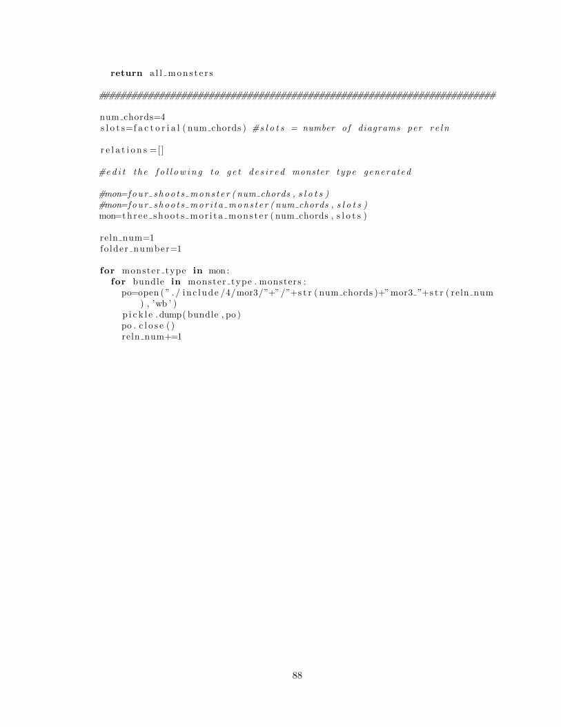
return a l l m o n s t e r s

########################################################################

num chords=4s l o t s=f a c t o r i a l ( num chords ) #s l o t s = number o f diagrams per r e l n

r e l a t i o n s =[ ]

#e d i t the f o l l o w i n g to g e t d e s i r e d monster type generated

#mon=f o u r s h o o t s m o n s t e r ( num chords , s l o t s )#mon=f o u r s h o o t s m o r i t a m o n s t e r ( num chords , s l o t s )mon=three shoo t s mor i t a mons t e r ( num chords , s l o t s )

reln num=1fo lder number=1

for monster type in mon :for bundle in monster type . monsters :

po=open ( ” . / in c lude /4/mor3/”+”/”+s t r ( num chords )+”mor3 ”+s t r ( reln num) , ’wb ’ )

p i c k l e . dump( bundle , po )po . c l o s e ( )reln num+=1

88

A.5 str.py

#!/ usr / b in /env python# encoding : u t f−8

’ ’ ’Created by Jonathan Gray .Copyright ( c ) Jonathan Gray . A l l r i g h t s r e s e r v e d .

Usage :V e r t i c e s o f l i n e a r f o r e s t must be entered as ” s t r i n g s ” w h i l e v e r t i c e s

o f s p r o u t i n gt r e e are a l l g i ven as numbers . Further , the assumption i s made t h a t

the ord er i ngo f the f o r e s t proceeds l i n e a r l y from l e f t to r i g h t . As in , the edge

b e f o r e thet r e e i s n−1, the f i r s t edge in the t r e e i s n , and the edge a f t e r the

t r e e i s n+kwhere k−1 i s the number o f ( f o r e s t e d ) edges in the t r e e .

The v e r t i c e s o f the sprouted t r e e are numbered c o n s e c u t i v e l y from l e f tto r i g h t

The c l a s s Graph has t h r e e s t u b s :graph . g = networkx i n s t a n c e o f the graph s t r u c t u r e , complete wi th

f o r e s t l a b e l l i n ggraph . or ien = a \pm 1 corresponding to or ien determined in the end by

foo

CAUTION:when b r e a k i n g down sprouts , the i n s t a n c e o f an i s o l a t e d chord on a

s p r o u t i n g t r e ei s not permi t t ed . Does not remove g e n e r a l i t y e i t h e r , f o r such diagrams

are a u t o m a t i c a l l y zero .’ ’ ’

import p i c k l efrom copy import ∗from networkx import ∗import sys#import p r o f i l e#import time#import networkx as nx#import m a t p l o t l i b . p y p l o t as p l t#import Tkinter

class Graph :” c l a s s to d e f i n e a graph ob j e c t with s i gn from IHX and f o r e s t

r e l a b e l l i n g ”def i n i t ( s e l f , graph , p m one ) :

89

s e l f . g=graphs e l f . o r i e n=p m one

def a r e t h e r e i s o l a t e d l o n g ( graph , case ) :print graph

for i in range (0 ,2∗ case , 2 ) :v0=graph [ i ]v1=graph [ i +1]

i f abs ( v0−v1 )==1 or abs ( v0−v1 )==(2∗case −1) or abs ( v0−v1 )==(2∗case −2):

return True

return False

def f i l t e r s m a l l c h o r d s ( t o f i l t e r , case ) :for graph in t o f i l t e r :

for edge in graph . g :v0=edge [ 0 ]v1=edge [ 1 ]

i f abs ( v0−v1 )<=2:return [ ]

return t o f i l t e r

def a r e t h e r e i s o l a t e d l o n g t u p l e ( graph , case ) :for edge in graph :

v0=edge [ 0 ]v1=edge [ 1 ]

i f abs ( v0−v1 )==1 or abs ( v0−v1 )==(2∗case −1) or abs ( v0−v1 )==(2∗case −2):

return True

return False

def f i x n b r e d g e f o r o r i e n t a t i o n ( nbr edge ) :# r e t u r n s edge so t h a t# ( s tr1 , s t r 2 ) i s s . t . s t r1<s t r 2# ( s t r , i n t ) i s re turned i f one i s i n t and the o t her s t r# ( int1 , i n t 2 ) i s s . t . i n t 1 < i n t 2

v0=nbr edge [ 0 ]v1=nbr edge [ 1 ]e f=nbr edge [ 2 ]tv0=type ( v0 )tv1=type ( v1 )

i f ( tv0 i s s t r ) and ( tv1 i s s t r ) :v0n=i n t ( v0 [ 1 : ] )v1n=i n t ( v1 [ 1 : ] )

90

i f v0n<v1n :return ( v0 , v1 , e f )

i f v0n>v1n :return ( v1 , v0 , e f )

i f ( tv0 i s s t r ) and ( tv1 i s i n t ) :return ( v0 , v1 , e f )

i f ( tv0 i s i n t ) and ( tv1 i s s t r ) :return ( v1 , v0 , e f )

i f ( tv0 i s i n t ) and ( tv1 i s i n t ) :i f v0<v1 :

return ( v0 , v1 , e f )i f v0>v1 :

return ( v1 , v0 , e f )

def r eo rde r nbr1 nbr2 ( nbr1 , nbr2 ) :#We assume f o r e s t edge w i l l a lways be nbr2 i f one i s f o r e s t and the

o t her not .

i f nbr1 [2]== ’ y ’ and nbr2 [2]== ’n ’ :return nbr2 , nbr1

i f nbr1 [2]== ’n ’ and nbr2 [2]== ’ y ’ :return nbr1 , nbr2

else :return nbr1 , nbr2

def f i x o r i e n t a t i o n ( graph , vert , vep ) :’ ’ ’The s i g n i s dependent on the p o s i t i o n o f the t r e e r e l a t i v e to the

placement o f the newf o r e s t edge . I f the t r e e i s p lac ed a f t e r the new f o r e s t edge in the

l i n e a r f o r e s t , thenthe o r i e n t a t i o n remains the same . I f the t r e e i s p l a c e b e f o r e the new

l i n e a r f o r e s t edge ,then one needs to count the number o f f o r e s t edges in the t r e e (

e x c l u d i n g the edge j u s toperated upon ) and determine how many t r a n s p o s i t i n are r e q u i r e d to

reorder the t r e e in amanner c o n s i s t e n t wi th the r e s t o f the graph . In the case o f a two

sprout wi th non−f o r e s tedge to the r i g h t the H−term r e q u i r e s an o r i e n t a t i o n f i x because the

”2” w i l l f a l l a f t e rthe s p r o u t i n g t r e e . I t r e q u i r e s the t r a n s p o s i t i o n (2 3) to reorder

the graph and so H w i l lcarry a n e g a t i v e s i g n . The X−term caused the ”2” to precede the t r e e

and hence no r e o r d e r i n gi s necessary .

91

The a lgor i thm then becomes : f i n d f i r s t o p e r a b l e edge from ” l e f t tor i g h t ” and then count the

number o f f o r e s t e d edges in s p r o u t i n g t r e e −−above the o p e r a b l e edge−−. Then determine which

o f the H/X terms w i l l cause the new l i n e a r f o r e s t e d edge to precedethe s p r o u t i n g t r e e . The

H/X term with the edge t h a t succeeds the t r e e w i l l carry the s i g n(−1)∗∗(# f o r e s t e d edges in t r e e above o p e r a b l e edge ) .

’ ’ ’

G=graph . g

nbr s o f v ep =[ ]

for nbr in G[ vep ] : #want ( s t r , i n t )i f type ( nbr ) i s s t r :

nb r s o f v ep . append ( ( nbr , vep ,G[ nbr ] [ vep ] [ 0 ] [ ’ f o r e s t ’ ] ) )i f type ( nbr ) i s i n t :

nb r s o f v ep . append ( ( vep , nbr ,G[ nbr ] [ vep ] [ 0 ] [ ’ f o r e s t ’ ] ) )

nb r s o f v ep . remove ( ( vert , vep , ’ y ’ ) )

# g e t a l l f o r e s t e d edges :

f o r e s t e d e d g e s =[( e [ 0 ] , e [ 1 ] ) for e in G. edges ( data=True ) i f e [ 2 ] [ ’f o r e s t ’ ]== ’ y ’ ]

# remove o p e r a b l e edge :try :

f o r e s t e d e d g e s . remove ( ( vert , vep ) )except :

f o r e s t e d e d g e s . remove ( ( vep , ve r t ) )

#c r e a t e new graph from the f o r e s t e d edges :component graph=MultiGraph ( )

component graph . add edges from ( f o r e s t e d e d g e s )

components=connected component subgraphs ( component graph )

# p i c k component which connected to o p e r a b l e edge :re levant component =[ ]

for component in components :for edge in component . edges ( ) :

i f vep in edge :re levant component . extend ( component . edges ( ) )break

try :nbr1=nbr s o f v ep [ 0 ]nbr2=nbr s o f v ep [ 1 ]

except :

92

return graph . or ien , graph . o r i e n

e n d p o i n t s o f n b r s e d g e s =[nbr1 [ 1 ] , nbr2 [ 1 ] ]

i f nbr1 [2]== ’ y ’ and nbr2 [2]== ’ y ’ :problem edges =[ so r t ed ( [ edge [ 0 ] , edge [ 1 ] ] ) for edge in

re levant component i f vep in edge ]

LR graph=MultiGraph ( )LR graph . add edges from ( re levant component )

LR graph . remove edge ( problem edges [ 0 ] [ 0 ] , problem edges [ 0 ] [ 1 ] )LR graph . remove edge ( problem edges [ 1 ] [ 0 ] , problem edges [ 1 ] [ 1 ] )

LR graph . add edge ( ’ l ’ , min ( e n d p o i n t s o f n b r s e d g e s ) )LR graph . add edge ( ’ r ’ ,max( e n d p o i n t s o f n b r s e d g e s ) )

LR components=connected component subgraphs ( LR graph )

for component in LR components :for edge in component . edges ( ) :

i f ’ l ’ in edge :L length=len ( component ) /2

i f ’ r ’ in edge :R length=len ( component ) /2

pm one h=graph . o r i en ∗(−1) ∗∗( L length )pm one x=graph . o r i en ∗(−1) ∗∗( R length+L length )

return pm one h , pm one x

i f nbr1 [2]== ’ y ’ and nbr2 [2]== ’n ’ :’ ’ ’f i g u r e out i f non−f o r e s t edge a t t a c h e s to l i n−f o r e s t , or s p r o u t i n g

t r e e .i f to l i n−f o r e s t , then determine on which s i d e o f v e r t i t appears .’ ’ ’

i f type ( nbr2 [ 0 ] ) == i n t and type ( nbr2 [ 1 ] ) == i n t : #hence , connectsto s p r o u t i n g t r e e

pm one gh=graph . o r i e npm one gx=graph . o r i en ∗(−1)∗∗ l en ( re levant component )

return pm one gh , pm one gx

i f type ( nbr2 [ 0 ] ) == s t r and type ( nbr2 [ 1 ] ) == i n t : #hence , connectsto l i n f o r e s t

nbr2 num=i n t ( nbr2 [ 0 ] [ 1 : ] )vert num=i n t ( ve r t [ 1 : ] )

i f nbr2 num<vert num :pm one gh=graph . o r i e n

93

pm one gx=graph . o r i en ∗(−1)∗∗ l en ( re levant component )

return pm one gh , pm one gx

i f nbr2 num>vert num :pm one gh=graph . o r i e n ∗(−1)∗∗ l en ( re levant component )pm one gx=graph . o r i en

return pm one gh , pm one gx

i f type ( nbr2 [ 0 ] ) == i n t and type ( nbr2 [ 1 ] ) == s t r : #hence , connectsto l i n f o r e s t

# ERROR, order on edges not r e s p e c t e d somehow# Cannot reach t h i s casenbr2 num=i n t ( nbr2 [ 0 ] [ 1 : ] )vert num=i n t ( ve r t [ 1 : ] )

i f nbr1 [2]== ’n ’ and nbr2 [2]== ’ y ’ :’ ’ ’f i g u r e out i f non−f o r e s t edge a t t a c h e s to l i n−f o r e s t , or s p r o u t i n g

t r e e .i f to l i n−f o r e s t , then determine on which s i d e o f v e r t i t appears .’ ’ ’

i f type ( nbr1 [ 0 ] ) == i n t and type ( nbr1 [ 1 ] ) == i n t : #hence , connectsto s p r o u t i n g t r e e

pm one gx=graph . o r i enpm one gh=graph . o r i e n ∗(−1)∗∗ l en ( re levant component )

return pm one gh , pm one gx

i f type ( nbr1 [ 0 ] ) == s t r and type ( nbr1 [ 1 ] ) == i n t : #hence , nbr1connects to l i n f o r e s t

nbr1 num=i n t ( nbr1 [ 0 ] [ 1 : ] )vert num=i n t ( ve r t [ 1 : ] )

i f nbr1 num<vert num :pm one gh=graph . o r i e npm one gx=graph . o r i en ∗(−1)∗∗ l en ( re levant component )

return pm one gh , pm one gx

i f nbr1 num>vert num :pm one gh=graph . o r i e n ∗(−1)∗∗ l en ( re levant component )pm one gx=graph . o r i en

return pm one gh , pm one gx

i f type ( nbr1 [ 0 ] ) == i n t and type ( nbr1 [ 1 ] ) == s t r :print ”PROBLEM! , about l i n e 211 ”

94

#w i l l never h i t t h i s casereturn 1 ,1

i f nbr1 [2]== ’n ’ and nbr2 [2]== ’n ’ :

return graph . or ien , graph . o r i e n

def l i s t s t o n e t w o r k x g r a p h ( f t , n f t ) :e f l =[ ]e n f l =[ ]

#c r e a t e t u p l e s f o r edges

for i in xrange (0 , l en ( f t ) , 2 ) :e f l . append ( ( f t [ i ] , f t [ i +1]) )

for i in xrange (0 , l en ( n f t ) , 2 ) :e n f l . append ( ( n f t [ i ] , n f t [ i +1]) )

g0=MultiGraph ( )g0 . add edges from ( e f l , f o r e s t=”y” )g0 . add edges from ( en f l , f o r e s t=”n” )

return g0

def pickedge (G) :# r e t u r n s edge to opera te upon wi th vep be ing o f type i n t# F i r s t loop g e t s a l l edges t h a t are o p e r a b l e and f o r c e s e n t r i e s in# l i s t o f o p e r a b l e edges to be [ s t r , in t , s t r , in t , . . . ]# numbers . append () in f o r loop j u s t grabs numbers from s t r v e r t i c e s# so the l e f t m o s t v e r t e x may be p ick ed v i a min ( ) .

graph=G

o p e r a b l e v e r t s =[ ]numbers =[ ]

for e in graph . edges ( data=True ) :e 2 f o r=e [ 2 ] [ ’ f o r e s t ’ ]== ’ y ’

i f e 2 f o r and type ( e [ 0 ] ) i s s t r and type ( e [ 1 ] ) i s i n t :o p e r a b l e v e r t s . extend ( [ e [ 0 ] , e [ 1 ] ] )numbers . append ( i n t ( e [ 0 ] [ 1 : ] ) )

i f e 2 f o r and type ( e [ 1 ] ) i s s t r and type ( e [ 0 ] ) i s i n t :o p e r a b l e v e r t s . extend ( [ e [ 1 ] , e [ 0 ] ] )numbers . append ( i n t ( e [ 1 ] [ 1 : ] ) )

l e f t m o s t o p e r a b l e v e r t=”a”+s t r ( min ( numbers ) )i n d e x v e r t c n n t d t o l e f t m o s t o p v e r t=o p e r a b l e v e r t s . index (

l e f t m o s t o p e r a b l e v e r t )

ve r t=l e f t m o s t o p e r a b l e v e r t

95

vep=o p e r a b l e v e r t s [ i n d e x v e r t c n n t d t o l e f t m o s t o p v e r t +1]

return vert , vep

def getnbrs (G, vert , vep ) :nbrs =[ ]

for nbr in G. ne ighbors ( vep ) :nbrs . append ( nbr )

bad nbrs =[ ver tex for ver tex in nbrs i f type ( ver tex )==s t r ]

try :bad nbrs . remove ( ve r t )

except :pass

good nbrs =[ ver tex for ver tex in nbrs i f type ( ver tex ) != s t r ]

return nbrs , bad nbrs , good nbrs

def ihx ( graph ) :G=graph . g

vert , vep=pickedge (G)

###### Get nbrs###

nbrs =[ ]

for nbr in G. ne ighbors ( vep ) :nbrs . append ( nbr )

bad nbrs =[ ver tex for ver tex in nbrs i f type ( ver tex )==s t r ]

try :bad nbrs . remove ( ve r t )

except :pass

good nbrs =[ ver tex for ver tex in nbrs i f type ( ver tex ) != s t r ]

###### Procress edge###

vert number=i n t ( ve r t [ 1 : ] )

i f l en ( good nbrs )==0: # means ver t , vep i s a s i n g l e sprout <=> bad nbrshas l e n g t h 2

96

gh , gx=l e n z e r o (G, vert , vep , bad nbrs , good nbrs , vert number )

i f l en ( good nbrs )==1:gh , gx=len one (G, vert , vep , bad nbrs , good nbrs , vert number )

i f l en ( good nbrs )==2:gh , gx=len two (G, vert , vep , bad nbrs , good nbrs , vert number )

gh or ien , gx o r i en=f i x o r i e n t a t i o n ( graph , vert , vep )

ghc=Graph ( gh , gh o r i en ) #ghc := gh c l a s sgxc=Graph ( gx , gx o r i en )

ghc . o r i en=ghc . o r i en ∗(−1) # app ly s i g n from I = −H − Xgxc . o r i en=gxc . o r i en ∗(−1)

ghc . g=r e n u m b e r t r e e v e r t i c e s g h ( ghc . g )gxc . g=r e n u m b e r t r e e v e r t i c e s g x ( gxc . g )

return ghc , gxc

def comp( v1 , v2 ) :#Manual comparison o f v e r t e x −− v i a a proper order r e l a t i o n# python compares s t r i n g s l e x i o g r a p h i c a l l y , bad b/c then a11 < a2 ! ! !

i f ( type ( v1 )==s t r ) and ( type ( v2 ) )==s t r :v1 number=i n t ( v1 [ 1 : ] )v2 number=i n t ( v2 [ 1 : ] )

i f v1 number < v2 number :return True

i f v2 number < v1 number :return False

else :return ( v1<v2 )

def get new edges (G, vert number , ve r t ) :v a l i d e d g e s =[ ]edges to remove =[ ]

for edge in G. edges ( data=True ) :i f comp( vert , edge [ 0 ] ) and comp( vert , edge [ 1 ] ) :

e0n=i n t ( edge [ 0 ] [ 1 : ] ) #e0n=v e r t 0 numbere1n=i n t ( edge [ 1 ] [ 1 : ] ) #e1n=v e r t 1 number

v a l i d e d g e s . append ( [ ’ a ’+s t r ( e0n+1) , ’ a ’+s t r ( e1n+1) , edge [ 2 ] [ ’ f o r e s t ’] ] )

edges to remove . append ( [ edge [ 0 ] , edge [ 1 ] ] )

e l i f comp( vert , edge [ 0 ] ) and comp( edge [ 1 ] , ve r t ) :e0n=i n t ( edge [ 0 ] [ 1 : ] )

97

v a l i d e d g e s . append ( [ ’ a ’+s t r ( e0n+1) , edge [ 1 ] , edge [ 2 ] [ ’ f o r e s t ’ ] ] )edges to remove . append ( [ edge [ 0 ] , edge [ 1 ] ] )

e l i f comp( edge [ 0 ] , ve r t ) and comp( vert , edge [ 1 ] ) :e1n=i n t ( edge [ 1 ] [ 1 : ] )

v a l i d e d g e s . append ( [ ’ a ’+s t r ( e1n+1) , edge [ 0 ] , edge [ 2 ] [ ’ f o r e s t ’ ] ] )edges to remove . append ( [ edge [ 0 ] , edge [ 1 ] ] )

e l i f comp( edge [ 0 ] , ve r t ) and comp( edge [ 1 ] , ve r t ) :pass

return va l i d edge s , edges to remove

def l e n z e r o (G, vert , vep , bad nbrs , good nbrs , vert number ) :# both edges h i t the l i n e a r f o r e s t

gh=deepcopy (G)gx=deepcopy (G)

bad nbrs=sor t ed ( bad nbrs , comp)

n0=bad nbrs [ 0 ]n1=bad nbrs [ 1 ]

n0 number=i n t ( n0 [ 1 : ] )n0plusone=’ a ’+s t r ( n0 number+1)

n1 number=i n t ( n1 [ 1 : ] )n1plusone=’ a ’+s t r ( n1 number+1)

ve r tp lu sone=’ a ’+s t r ( vert number+1)

gh . remove edge ( vert , vep )gx . remove edge ( vert , vep )

gh . remove edge ( vep , n0 )gh . remove edge ( vep , n1 )

gx . remove edge ( vep , n0 )gx . remove edge ( vep , n1 )

new edges , edges to remove=get new edges ( gh , vert number , ve r t )

gh . remove edges from ( edges to remove )gx . remove edges from ( edges to remove )

for e in new edges :gh . add edge ( e [ 0 ] , e [ 1 ] , f o r e s t=e [ 2 ] )gx . add edge ( e [ 0 ] , e [ 1 ] , f o r e s t=e [ 2 ] )

n0vert=comp( n0 , ve r t )vertn1=comp( vert , n1 )

98

i f n0vert and vertn1 :gha=(n0 , ve r t )ghb=(vertp lusone , n1plusone )gxa=(n0 , ve r tp lu sone )gxb=(vert , n1plusone )

i f comp( n1 , ve r t ) and comp( ver t , n0 ) :gha=(n1 , ve r t )ghb=(vertp lusone , n0plusone )gxa=(n1 , ve r tp lu sone )gxb=(vert , n0plusone )

i f comp( ver t , n0 ) and comp( n0 , n1 ) :gha=(vert , n1plusone )ghb=(vertp lusone , n0plusone )gxa=(vert , n0plusone )gxb=(vertp lusone , n1plusone )

i f vertn1 and comp( n1 , n0 ) :gha=(vert , n0plusone )ghb=(vertp lusone , n1plusone )gxa=(vert , n1plusone )gxb=(vertp lusone , n0plusone )

i f comp( n0 , n1 ) and comp( n1 , ve r t ) :gha=(n0 , ve r tp lu sone )ghb=(n1 , ve r t )gxa=(n0 , ve r t )gxb=(n1 , ve r tp lu sone )

i f comp( n1 , n0 ) and n0vert :gha=(n1 , ve r tp lu sone )ghb=(n0 , ve r t )gxa=(n1 , ve r t )gxb=(n0 , ve r tp lu sone )

gh . add edge (∗ gha , f o r e s t=’n ’ )gh . add edge (∗ghb , f o r e s t=’n ’ )gx . add edge (∗ gxa , f o r e s t=’n ’ )gx . add edge (∗gxb , f o r e s t=’n ’ )

return gh , gx

def l en one (G, vert , vep , bad nbrs , good nbrs , vert number ) :gh=deepcopy (G)gx=deepcopy (G)nbrs =[ ]

i f bad nbrs ! = [ ] :bad nbr number=i n t ( bad nbrs [ 0 ] [ 1 : ] )

for nbr in G. ne ighbors ( vep ) :

99

nbrs . append ( nbr )

nbrs . remove ( ve r t )

gh . remove edge ( vert , vep )gx . remove edge ( vert , vep )

i f gh . number of edges ( vep , nbrs [ 0 ] ) !=2:i f bad nbr number>vert number :

f g=gh [ vep ] [ good nbrs [ 0 ] ] [ 0 ] [ ’ f o r e s t ’ ]fb=gh [ vep ] [ bad nbrs [ 0 ] ] [ 0 ] [ ’ f o r e s t ’ ]

gh . remove edge ( vep , nbrs [ 0 ] )gh . remove edge ( vep , nbrs [ 1 ] )

new edges , edges to remove=get new edges ( gh , vert number , ve r t )

gh . remove edges from ( edges to remove )

for e in new edges :gh . add edge ( e [ 0 ] , e [ 1 ] , f o r e s t=e [ 2 ] )

gha=(vert , good nbrs [ 0 ] )ghb=( ’ a ’+s t r ( vert number+1) , ’ a ’+s t r ( bad nbr number+1) )gh . add edge (∗ gha , f o r e s t=fg )gh . add edge (∗ghb , f o r e s t=fb )

i f bad nbr number<vert number :########f g=gh [ vep ] [ good nbrs [ 0 ] ] [ 0 ] [ ’ f o r e s t ’ ]fb=gh [ vep ] [ bad nbrs [ 0 ] ] [ 0 ] [ ’ f o r e s t ’ ]

gh . remove edge ( vep , nbrs [ 0 ] )gh . remove edge ( vep , nbrs [ 1 ] )

new edges , edges to remove=get new edges ( gh , vert number , ve r t )

gh . remove edges from ( edges to remove )

for e in new edges :gh . add edge ( e [ 0 ] , e [ 1 ] , f o r e s t=e [ 2 ] )

gha=(bad nbrs [ 0 ] , v e r t )ghb=( ’ a ’+s t r ( vert number+1) , good nbrs [ 0 ] )gh . add edge (∗ gha , f o r e s t=fb )gh . add edge (∗ghb , f o r e s t=fg )

i f gh . number of edges ( vep , nbrs [ 0 ] ) ==2:gh . remove edge ( vep , nbrs [ 0 ] )

new edges , edges to remove=get new edges ( gh , vert number , ve r t )

gh . remove edges from ( edges to remove )

100

for e in new edges :gh . add edge ( e [ 0 ] , e [ 1 ] , f o r e s t=e [ 2 ] )

gha=(vert , nbrs [ 0 ] )ghb=( ’ a ’+s t r ( vert number+1) , nbrs [ 0 ] )

gh . add edge (∗ gha , f o r e s t=’n ’ )gh . add edge (∗ghb , f o r e s t=’ y ’ )

i f gx . number of edges ( vep , nbrs [ 0 ] ) !=2:i f i n t ( bad nbrs [ 0 ] [ 1 : ] )>vert number :

f g=gx [ vep ] [ good nbrs [ 0 ] ] [ 0 ] [ ’ f o r e s t ’ ]fb=gx [ vep ] [ bad nbrs [ 0 ] ] [ 0 ] [ ’ f o r e s t ’ ]

gx . remove edge ( vep , nbrs [ 0 ] )gx . remove edge ( vep , nbrs [ 1 ] )

new edges , edges to remove=get new edges ( gx , vert number , ve r t )

gx . remove edges from ( edges to remove )

for e in new edges :gx . add edge ( e [ 0 ] , e [ 1 ] , f o r e s t=e [ 2 ] )

gxa=(vert , ’ a ’+s t r ( bad nbr number+1) )gxb=( ’ a ’+s t r ( vert number+1) , good nbrs [ 0 ] )gx . add edge (∗ gxa , f o r e s t=fb )gx . add edge (∗gxb , f o r e s t=fg )

i f i n t ( bad nbrs [ 0 ] [ 1 : ] )<vert number :f g=gx [ vep ] [ good nbrs [ 0 ] ] [ 0 ] [ ’ f o r e s t ’ ]fb=gx [ vep ] [ bad nbrs [ 0 ] ] [ 0 ] [ ’ f o r e s t ’ ]

gx . remove edge ( vep , nbrs [ 0 ] )gx . remove edge ( vep , nbrs [ 1 ] )

new edges , edges to remove=get new edges ( gx , vert number , ve r t )

gx . remove edges from ( edges to remove )

for e in new edges :gx . add edge ( e [ 0 ] , e [ 1 ] , f o r e s t=e [ 2 ] )

gxa=(bad nbrs [ 0 ] , ’ a ’+s t r ( vert number+1) )gxb=(vert , good nbrs [ 0 ] )gx . add edge (∗ gxa , f o r e s t=fb )gx . add edge (∗gxb , f o r e s t=fg )

i f gx . number of edges ( vep , nbrs [ 0 ] ) ==2:gx . remove edge ( vep , nbrs [ 0 ] )

new edges , edges to remove=get new edges ( gx , vert number , ve r t )

101

gx . remove edges from ( edges to remove )

for e in new edges :gx . add edge ( e [ 0 ] , e [ 1 ] , f o r e s t=e [ 2 ] )

gxa=(vert , nbrs [ 0 ] )gxb=( ’ a ’+s t r ( vert number+1) , nbrs [ 0 ] )gx . add edge (∗ gxa , f o r e s t=’ y ’ )gx . add edge (∗gxb , f o r e s t=’n ’ )

return gh , gx

def l en two (G, vert , vep , bad nbrs , good nbrs , vert number ) :#note t h e r e i s ambigui ty between H and X i f vep has a f o r e s t e d and non

−f o r e s t e d adj edge# to see t h i s , c o n s i d e r the i s o l a t e d chord on a s t r a i g h t t h r e e sprou t .

depending on# what s i d e you put the bubb le , H and X can d i f f e r ( r e f s h e e t #8)

gh=deepcopy (G)gx=deepcopy (G)nbrs =[ ]

i f bad nbrs ! = [ ] :bad nbr number=i n t ( bad nbrs [ 0 ] [ 1 : ] )

for nbr in G. ne ighbors ( vep ) :nbrs . append ( nbr )

nbrs . remove ( ve r t )

n0=min ( nbrs )n1=max( nbrs )

v e p n 0 f o r e s t=gh [ vep ] [ n0 ] [ 0 ] [ ’ f o r e s t ’ ]v e p n 1 f o r e s t=gh [ vep ] [ n1 ] [ 0 ] [ ’ f o r e s t ’ ]

#f i x n0 so t h a t i t i s a lways the ep o f the f o r e s t edge i f in the caseo f a f t / n f t p a i r f o r

# the case when both endpo in t s l i e n s p r o u t i n g t r e e ( see r e f #8)

i f v e p n 0 f o r e s t == ’ y ’ and v e p n 1 f o r e s t==’n ’ :pass

i f v e p n 0 f o r e s t == ’n ’ and v e p n 1 f o r e s t==’ y ’ :n0 , n1=n1 , n0vep n0 f o r e s t , v e p n 1 f o r e s t=vep n1 f o r e s t , v e p n 0 f o r e s t

ve r tp lu sone=’ a ’+s t r ( vert number+1)

gh . remove edge ( vert , vep )

102

gx . remove edge ( vert , vep )

new edges , edges to remove=get new edges ( gh , vert number , ve r t )

gh . remove edges from ( edges to remove )gx . remove edges from ( edges to remove )

for e in new edges :gh . add edge ( e [ 0 ] , e [ 1 ] , f o r e s t=e [ 2 ] )gx . add edge ( e [ 0 ] , e [ 1 ] , f o r e s t=e [ 2 ] )

gh . remove edge ( vep , n0 )gh . remove edge ( vep , n1 )gx . remove edge ( vep , n0 )gx . remove edge ( vep , n1 )

gh . add edge ( vert , n0 , f o r e s t=v e p n 0 f o r e s t )gh . add edge ( vertp lusone , n1 , f o r e s t=v e p n 1 f o r e s t )gx . add edge ( vert , n1 , f o r e s t=v e p n 1 f o r e s t )gx . add edge ( vertp lusone , n0 , f o r e s t=v e p n 0 f o r e s t )

return gh , gx

def r e n u m b e r t r e e v e r t i c e s g h ( gh ) :# grab a l l v e r t i c e s in s p r o u t i n g t r e e ( s )# r e b u i l d graph from v e r t i c e s and count the number o f components# ( i . e . , g e t number o f s p r o u t i n g t r e e s )# I f a v e r t e x i s o f type i n t ( i . e . , not par t o f l i n e a r f o r e s t ) ,# then add to s p e c i a l l i s t . Sort l i s t and g e t i t s l e n g t h .# Set up a b i j e c t i o n between e lements o f l i s t and the s e t {1 , . . . ,

l e n ( l i s t )}

ve r t t o change =[ ]o ld graph =[ ]

for edge in gh . edges ( data=True ) :o ld graph . append ( [ edge [ 0 ] , edge [ 1 ] , edge [ 2 ] [ ’ f o r e s t ’ ] ] )

i f type ( edge [ 0 ] ) i s i n t and edge [ 0 ] not in ve r t t o change :v e r t t o change . append ( edge [ 0 ] )

i f type ( edge [ 1 ] ) i s i n t and edge [ 1 ] not in ve r t t o change :v e r t t o change . append ( edge [ 1 ] )

l v t c=len ( ve r t t o change )new verts=range (1 , l v t c +1)

p a i r s =[(x , y ) for x , y in z ip ( ver t to change , new verts ) ]p a i r s d i c t ={}

for pa i r in p a i r s :p a i r s d i c t [ pa i r [ 0 ] ] = pa i r [ 1 ]

for edge in o ld graph :

103

i f edge [ 0 ] in ve r t t o change :edge [0 ]= p a i r s d i c t [ edge [ 0 ] ]

i f edge [ 1 ] in ve r t t o change :edge [1 ]= p a i r s d i c t [ edge [ 1 ] ]

new graph=MultiGraph ( ) #Bui ld graph f o r sprou t comp edge count

for e in o ld graph :new graph . add edge ( e [ 0 ] , e [ 1 ] , f o r e s t=e [ 2 ] )

return new graph

def r e n u m b e r t r e e v e r t i c e s g x ( gx ) :v e r t t o change =[ ]o ld graph =[ ]

for edge in gx . edges ( data=True ) :o ld graph . append ( [ edge [ 0 ] , edge [ 1 ] , edge [ 2 ] [ ’ f o r e s t ’ ] ] )

i f type ( edge [ 0 ] ) i s i n t and edge [ 0 ] not in ve r t t o change :v e r t t o change . append ( edge [ 0 ] )

i f type ( edge [ 1 ] ) i s i n t and edge [ 1 ] not in ve r t t o change :v e r t t o change . append ( edge [ 1 ] )

l v t c=len ( ve r t t o change )new verts=range (1 , l v t c +1)

p a i r s =[(x , y ) for x , y in z ip ( ver t to change , new verts ) ]p a i r s d i c t ={}

for pa i r in p a i r s :p a i r s d i c t [ pa i r [ 0 ] ] = pa i r [ 1 ]

for edge in o ld graph :i f edge [ 0 ] in ve r t t o change :

edge [0 ]= p a i r s d i c t [ edge [ 0 ] ]

i f edge [ 1 ] in ve r t t o change :edge [1 ]= p a i r s d i c t [ edge [ 1 ] ]

new graph=MultiGraph ( ) #Bui ld graph f o r sprou t comp edgecount

for e in o ld graph :new graph . add edge ( e [ 0 ] , e [ 1 ] , f o r e s t=e [ 2 ] )

return new graph

def f o r e s t l e f t (G) :y counter=0G=G. g

104

for edge in G. e d g e s i t e r ( data=True ) :i f edge [ 2 ] [ ’ f o r e s t ’ ]== ’ y ’ :

return True

i f y counter==0:return False

def p r o c e s s e n d r e s u l t ( g r a p h l i s t ) :#f u n c t i o n to t ake f i n a l graphs and then make them ” d i s p l a y ” c o r r e c t l yg almost done =[ ]g proper =[ ]

for entry in g r a p h l i s t :new g =[ ]

for edge in entry . g . edges ( ) :v1new=i n t ( edge [ 0 ] [ 1 : ] ) +1 #s t r i p the number o f f v e r t e x and add

o f f s e t o f 1v2new=i n t ( edge [ 1 ] [ 1 : ] ) +1new g . append ( min ( v1new , v2new ) )new g . append (max( v1new , v2new ) )

entry . g=new gg almost done . append ( entry )

u s e d v e r t s=g almost done [ 0 ] . g [ : ]u s e d v e r t s=sor t ed ( u s e d v e r t s )good va l s=range (1 , l en ( u s e d v e r t s ) +1)

b i j ={}i=0

for entry in u s e d v e r t s :b i j [ entry ]= good va l s [ i ]i=i+1

for graph in g almost done :e d i t=graph . gnew g =[ ]

for ver t in e d i t :new g . append ( b i j [ ve r t ] )

graph . g=new g

for graph in g almost done :new graph =[ ]

for i in range (0 ,2∗ case , 2 ) :new graph . append ( ( graph . g [ i ] , graph . g [ i +1]) )

graph . g=new graph

105

g proper =[ ]

for graph in g almost done :i f a r e t h e r e i s o l a t e d l o n g t u p l e ( graph . g , case ) i s False :

g proper . append ( graph )

for graph in g proper :graph . g=sor t ed ( graph . g )

return g proper

def end so r t ( diag ) :# s o r t s diagram so the edges are ” i n c r e a s i n g ”case=len ( diag ) /2

for i in xrange (0 , l en ( diag ) −2 ,2) :i f diag [ i ]>diag [ i +2] :

s0=diag [ i ]s1=diag [ i +1]s2=diag [ i +2]s3=diag [ i +3]diag [ i ]= s2diag [ i +1]=s3diag [ i +2]=s0diag [ i +3]=s1

return diag

def program core ( f t , nft , s i gn ) :g0=l i s t s t o n e t w o r k x g r a p h ( f t , n f t )

g done =[ ]g l e f t =[ ]g f i n a l =[ ]

gdapp=g done . append

gc=Graph ( g0 , s i gn )

for entry in ihx ( gc ) :f o r e s t l e f t r e s u l t=f o r e s t l e f t ( entry )

i f f o r e s t l e f t r e s u l t i s True :g l e f t . append ( entry )

else :gdapp ( entry )

# w h i l e loop to p roc es s s p r o u t s# terminates when t h e r e are no s p r o u t s l e f t

while g l e f t ! = [ ] :

106

out =[ ]

for entry in g l e f t :for output in ihx ( entry ) :

out . append ( output )

g l e f t =[ ]

for entry in out :f o r e s t l e f t r e s u l t=f o r e s t l e f t ( entry )

i f f o r e s t l e f t r e s u l t i s True :g l e f t . append ( entry )

else :gdapp ( entry )

g f i n a l=p r o c e s s e n d r e s u l t ( g done )return g f i n a l

def f i x f t n f t ( f t , n f t ) :s t r v e r t s =[ ]print ” . ”num chords= ( l en ( f t )+len ( n f t )−2)/2good range=range (1 , num chords )

for e in n f t :i f type ( e ) i s s t r :

s t r v e r t s . append ( i n t ( e [ 1 : ] ) )

for e in f t :i f type ( e ) i s s t r :

s t r v e r t s . append ( i n t ( e [ 1 : ] ) )

return f t , n f t

######################################################################################### T e s t G r a p h s ##############################################################################################################################################################

#f t =[”a1 ” ,1 ] # s i n g l e sprout in middle#n f t =[”a0 ” ,1 ,” a2 ” ,1 ]

#f t =[”a1 ” ,1 ,1 , 2 ] # two−sprout wi th non−f o r e s t go ing to r i g h to f sprou t

#n f t =[”a0 ” ,2 ,” a2 ” ,1 ,” a3 ” ,2 ]

#f t =[”a2 ” ,1 ,1 , 2 ] # two−sprout wi th non−f o r e s t go ing to l e f to f sprou t

#n f t =[”a0 ” ,2 ,” a1 ” ,1 ,” a3 ” ,2 ]

#f t =[”a1 ” ,1 ,1 , 2 ,1 ,3 ] # Y−sprout in c e n t e r

107

#n f t =[”a0 ” ,2 ,2 ,3 , ’ a2 ’ , 3 ]

#f t =[”a3 ” ,1 ,1 , 2 ,1 ,3 ] # s i g n r e f s h e e t #5#n f t =[”a0 ” ,2 ,” a1 ” ,2 ,” a2 ” ,3 ,” a4 ” ,3 ]

#f t =[”a1 ” ,1 ,1 ,2 ,1 ,3 ,” a4 ” ,4 ] # Y−sprout , spare edge to r i g h t −− tot e s t or ien

#n f t =[”a0 ” ,2 ,2 ,3 , ’ a2 ’ ,3 ,” a3 ” ,4 ,” a5 ” ,4 ]

#f t =[”a1 ” ,1 ,1 , 2 ,1 ,3 ] # r e f s h e e t #6#n f t =[”a0 ” ,2 ,” a2 ” ,2 ,” a3 ” ,3 ,” a4 ” ,3 ]

#f t =[”a2 ” ,1 ,1 , 2 ,1 ,3 ] # r e f s h e e t #7#n f t =[”a0 ” ,2 ,” a1 ” ,2 ,” a3 ” ,3 ,” a4 ” ,3 ]

#f t =[”a1 ” ,1 ,1 ,2 ,2 ,3 ,2 ,4 , 4 , 5 ] # r e f #8#n f t =[”a0 ” ,3 ,1 ,4 ,3 ,5 ,” a2 ” ,5 ]

#f t =[”a1 ” ,1 ,1 ,2 ,2 , 3 ,3 ,4 ] #b i s e c t e d b u b b l e on s i d e o f two−sprout#n f t =[”a0 ” ,4 ,1 ,3 ,” a2 ” ,2 ,” a3 ” ,4 ]

########################################################################################################################################################################################################################################################################

num chords=4global casecase =4

num=i n t ( sys . argv [ 1 ] )

i f num ==1:for i in range (1 ,9999) :

i f i %1000==0: #command c o n s o l e t r i c k to check p r o g r e s sprint i

try :pr=open ( ” . / in c lude /4/mor3/7mor3 ”+s t r ( i ) , ” rb” )

except :print ”End o f a l l f i l e s . . . ”break

d iags=p i c k l e . load ( pr )pr . c l o s e ( )p r e w r i t e =[ ]t o w r i t e =[1 ]

for term in d iags :f t=term [ 0 ]n f t=term [ 1 ]

108

s i gn=term [ 2 ]f i n a l r e s u l t=program core ( f t , nft , s i gn )p r e w r i t e . extend ( f i n a l r e s u l t )

#t o w r i t e=f i l t e r s m a l l c h o r d s ( p r e w r i t e , case )t o w r i t e=p r e w r i t e

i f t o w r i t e != [ ] :pw=open ( ” . / in c lude /4/ mor3re lns / mor3 re ln ”+s t r ( i ) , ”wb” )p i c k l e . dump( to wr i t e ,pw)pw . c l o s e ( )

i f num !=1:for i in range ( (num−1)∗10000 ,num∗10000−1) :

i f i %1000==0:print i

try :pr=open ( ” . / in c lude /4/mor3/7mor3 ”+s t r ( i ) , ” rb” )

except :print ”End o f a l l f i l e s . . . ( second i f ) ”break

d iags=p i c k l e . load ( pr )pr . c l o s e ( )p r e w r i t e =[ ]t o w r i t e =[1 ]

for term in d iags :f t=term [ 0 ]n f t=term [ 1 ]s i gn=term [ 2 ]f i n a l r e s u l t=program core ( f t , nft , s i gn )p r e w r i t e . extend ( f i n a l r e s u l t )

#t o w r i t e=f i l t e r s m a l l c h o r d s ( p r e w r i t e , case )t o w r i t e=p r e w r i t e

i f t o w r i t e != [ ] :pw=open ( ” . / in c lude /4/ mor3re lns / mor3 re ln ”+s t r ( i ) , ”wb” )p i c k l e . dump( to wr i t e ,pw)pw . c l o s e ( )

109

A.6 good diag enum.py

#!/ usr / b in /env python’ ’ ’Created by Jonathan Gray .Copyright ( c ) Jonathan Gray . A l l r i g h t s r e s e r v e d .’ ’ ’

import p i c k l e

def make dict ( num chords ) :f=”genum”+s t r ( num chords )g enum=open ( f , ’ r ’ )g raph d i c t ={}

for graph in g enum :graph=graph . s p l i t ( ’ | ’ )g raph d i c t [ graph [ 0 ] ] = i n t ( graph [ 1 ] )

g enum . c l o s e ( )

return g raph d i c t

def main ( ) :pass

i f name == ’ ma in ’ :main ( )

my dict= make dict (6 )

po=open ( ” g6d i c t ” , ’wb ’ )p i c k l e . dump( my dict , po )po . c l o s e ( )

110

A.7 bad to good.py

#!/ usr / b in /env python# encoding : u t f−8

’ ’ ’Created by Jonathan Gray .Copyright ( c ) Jonathan Gray . A l l r i g h t s r e s e r v e d .

Takes a diagram and r e w r i t e s i t as a sum of good chord diagrams and thenreduces the l i n e a r combination t h a t r e s u l t s .

term1 = i m p l i c i t l y o r i g i n a l diagramterm2 = c r o s s inner edgesterm3 = i n i t v e r t o f second chord i s p u l l e d to l e f t o f i n i t v e r t o f

f i r s t chordterm4 = permute the two o p e r a t i n g v e r t s from term3term5 = term v e r t o f f i r s t chord i s p u l l e d to r i g h t o f term v e r t o f

second chordterm6 = permute two o p e r a t i n g v e r t s from term5

’ ’ ’

from c o l l e c t i o n s import dequeimport p i c k l eimport sysimport osimport glob

class Graph :” c l a s s to d e f i n e a graph ob j e c t with s i gn from IHX and f o r e s t

r e l a b e l l i n g ”def i n i t ( s e l f , graph , p m one ) :

s e l f . g=graphs e l f . o r i e n=p m one

class Diagram :def i n i t ( s e l f , g , or i en , chords ) :

s e l f . g=gs e l f . o r i e n=or i ens e l f . c=s e l f . g e t cho rds ( )

def ge t cho rds ( s e l f ) :case=len ( s e l f . g )for c1 in s e l f . g :

for c2 in s e l f . g :i f ( c2 [0]== c1 [1 ]+1) and ( c2 [1]> case ) :

return c1 , c2 #means diagram i s badreturn 0 #means diagram i s good

def s i x t (D) :edges=D. goutput=deque ( )

111

outappend=output . append

c1=D. c [ 0 ]c2=D. c [ 1 ]

a=c1 [ 0 ]b=c1 [ 1 ]b1=c2 [ 0 ]c=c2 [ 1 ]

##### c r e a t e termsD2=[ ]D3=[ ]D4=[ ]D5=[ ]D6=[ ]

D2ae=D2 . appendD3ae=D3 . appendD4ae=D4 . appendD5ae=D5 . appendD6ae=D6 . append

for edge in edges :e0=edge [ 0 ]e1=edge [ 1 ]i f ( edge != c1 ) and ( edge !=c2 ) :

D2ae ( edge )

# i . e . , i n i t i a l v e r t e x o f edge i s between a and bv0 bw ab=(a <= e0 <= b)v1 bw ab=(a <= e1 <= b)

# i . e . , i n i t i a l v e r t e x o f edge i s between a and cv0 bw ac=(b <= e0 <= c )v1 bw ac=(b <= e1 <= c )

i f v0 bw ab and v1 bw ab :D3ae ( ( e0+1, e1+1) )D4ae ( ( e0+1, e1+1) )

i f v0 bw ab and not v1 bw ab :D3ae ( ( e0+1, e1 ) )D4ae ( ( e0+1, e1 ) )

i f not v0 bw ab and v1 bw ab :D3ae ( ( e0 , e1+1) )D4ae ( ( e0 , e1+1) )

i f not v0 bw ab and not v1 bw ab :D3ae ( edge )D4ae ( edge )

112

i f v0 bw ac and v1 bw ac :D5ae ( ( e0−1,e1−1) )D6ae ( ( e0−1,e1−1) )

i f v0 bw ac and not v1 bw ac :D5ae ( ( e0−1, e1 ) )D6ae ( ( e0−1, e1 ) )

i f not v0 bw ac and v1 bw ac :D5ae ( ( e0 , e1−1) )D6ae ( ( e0 , e1−1) )

i f not v0 bw ac and not v1 bw ac :D5ae ( edge )D6ae ( edge )

D2ae ( ( c1 [ 0 ] , b1 ) )D2ae ( ( b , c2 [ 1 ] ) )

D3ae ( ( a , c ) )D3ae ( ( a+1,b1 ) )

D4ae ( ( a+1,c ) )D4ae ( ( a , b1 ) )

D5ae ( ( a , c ) )D5ae ( ( b , c−1) )

D6ae ( ( a , c−1) )D6ae ( ( b , c ) )

i f a r e t h e r e i s o l a t e d l o n g (D2) i s False :outappend ( Diagram (D2 ,D. o r i en ∗(−1) ∗∗ (0) ∗−1 ,0) )

i f a r e t h e r e i s o l a t e d l o n g (D3) i s False :outappend ( Diagram (D3 ,D. o r i en ∗(−1) ∗∗( a+b) ∗−1 ,0) )

i f a r e t h e r e i s o l a t e d l o n g (D4) i s False :outappend ( Diagram (D4 ,D. o r i en ∗(−1) ∗∗( a+b) ∗−1 ,0) )

i f a r e t h e r e i s o l a t e d l o n g (D5) i s False :outappend ( Diagram (D5 ,D. o r i en ∗(−1) ∗∗( c+b+1)∗−1 ,0) )

i f a r e t h e r e i s o l a t e d l o n g (D6) i s False :outappend ( Diagram (D6 ,D. o r i en ∗(−1) ∗∗( c+b+1)∗−1 ,0) )

return output

def g e t d i c t ( num chords ) :p i c k l e f i l e=” . / in c lude /g”+s t r ( num chords )+” d i c t ”po=open ( p i c k l e f i l e , ’ rb ’ )mydict=p i c k l e . load ( po )

113

po . c l o s e ( )return mydict

def a r e t h e r e i s o l a t e d l o n g ( graph ) :for edge in graph :

v0=edge [ 0 ]v1=edge [ 1 ]i f abs ( v0−v1 )==1 or abs ( v0−v1 )==(2∗case −1) or abs ( v0−v1 )==(2∗case −2)

:return True

return False

def program core (D) :badarray =[ ]goodarray=deque ( )

for entry in s i x t (D) :r e s u l t=entry . ci f r e s u l t == 0 :

goodarray . append ( entry )else :

badarray . append ( entry )

while ( badarray ! = [ ] ) :out =[ ]tempbad =[ ]outapp=out . appendfor entry in badarray :

for output in s i x t ( entry ) :r e s u l t=output . ci f r e s u l t == 0 :

goodarray . append ( output )else :

tempbad . append ( output )badarray=tempbad

return goodarray

def f i l e p r o c e s s ( case , f i l e number ) :

# # = rank case# ∗ = r [ morita ] or n [ normal ]# fn1 =./ i n c l u d e /#/mo∗#r e l n s /mo∗# r e l n# fn2 =./ i n c l u d e /#/mo∗#rows/ r

f o=open ( ” fn1 ”+f i l e number , ’ rb ’ )fw=open ( ” fn2 ”+f i l e number , ’wb ’ )

r e l n s=p i c k l e . load ( fo )

f o . c l o s e ( )

114

my dict=g e t d i c t ( case )

goodarray =[ ]

for r e l n in r e l n s :d iag=Diagram ( r e l n . g , r e l n . or ien , 0 )i f diag . c !=0:

goodarray=(program core ( diag ) )i f diag . c==0:

goodarray . append ( diag )

row =[0 ]∗ (6∗5∗4∗3∗2)

#geplwor = graph endpoint l a b e l s wi th o r i e n t a t i o n

for entry in goodarray :geplwor =[ ]entry . g=sor t ed ( entry . g )for edge in entry . g :

geplwor . append ( edge [ 1 ] )geplwor . append ( entry . o r i e n )row [ my dict [ s t r ( geplwor [ 0 : −1 ] ) ] ]= row [ my dict [ s t r ( geplwor [ 0 : −1 ] ) ] ]+

geplwor [−1]

for element in row :fw . wr i t e ( ”%s ” % element )

fw . wr i t e ( ”\n” )fw . c l o s e ( )print ”end −−>” , f i l e number

global casecase=6

f i l e=open ( ’ . / i n c lude / f g ’+s t r ( case ) , r )

for l i n e in f i l e :l i n e=l i n e . s p l i t ( )print l i n e

115

A.8 matrix.py

#!/ usr / b in /env python# encoding : u t f−8”””Created by Jonathan Gray .Copyright ( c ) Jonathan Gray . A l l r i g h t s r e s e r v e d .”””

import sysimport osimport cP i ck l e

mat=[ ]

o ld=open ( ”mon4rows” , ’ r ’ )

mat=[ ]

for row in o ld :mat . append ( row )

o ld . c l o s e ( )new=open ( ” . / in c lude /7/ mon4rows spl i t / rows 1 ” , ’w ’ )

for i in xrange (1 ,17496+1) :i f i %500==0:

new . c l o s e ( )fn=s t r ( i /500+1)new=open ( ” . / in c lude /7/ mon4rows spl i t / rows ”+fn , ’w ’ )

new . wr i t e ( ”%s ” % mat [ i −1])

new . c l o s e ( )

116

A.9 cat rows.py

#!/ usr / b in /env python# encoding : u t f−8”””Created by Jonathan Gray .Copyright ( c ) Jonathan Gray . A l l r i g h t s r e s e r v e d .”””

import sysimport osimport glob

def main ( ) :pass

i f name == ’ ma in ’ :main ( )

# grab a l i s t o f a l l f i l e s in d i r e c t o r yf i l e s t o p r o c e s s=glob . g lob ( ’ . / i n c lude /7/mor4rows/∗ ’ )

#c r e a t e f i l e to put rows in and then c o n t a t e n a t e rowsos . system ( ” touch s3 ” )

cat=”/ bin / cat ”for entry in f i l e s t o p r o c e s s :

cmd=cat+” ”+entry+” >> ”+”mor4s3”os . system (cmd)

117

Vita

Jonathan Nathan Gray was born in Stuart, Florida. He spent his early years in southFlorida and moved to the state of Tennessee in the summer of 1993. After graduatingfrom high school in 2001, he started his undergraduate work in mathematics and physics atFlorida State University and graduated in 2004. During fall 2004 to spring 2005, Jonathantaught high school mathematics and then left his position to begin doctoral studies at theUniversity of Tennessee, Knoxville. He graduated in May 2011.

118