Thermal tracer testing in a sedimentary aquifer: field experiment (Lauswiesen, Germany) and...

Thermal tracer testing in a sedimentary aquifer: field experiment

(Lauswiesen, Germany) and numerical simulation

Valentin Wagner & Tao Li & Peter Bayer &

Carsten Leven & Peter Dietrich & Philipp Blum

Abstract An active and short-duration thermal tracer test(TTT) was conducted in a shallow sedimentary aquifer atthe Lauswiesen test site, near Tübingen, Germany. Byinjecting 16 m3 of warm water at 22°C, a thermal anomalywas created, which propagated along the local groundwa-ter flow direction. This was comprehensively monitored infive observation wells at a few meters distance. Thepurpose of this well-controlled experiment was to deter-mine the practicability of such a TTT and its suitability toexamine hydraulic characteristics of heterogeneous aqui-fers. The results showed that the thermal peak arrivaltimes in the observation wells were consistent withprevious observations from alternative field testing suchas direct-push injection logging (DPIL). Combined anal-ysis of depth-dependent temperatures and peak arrivaltimes, and comparison with a numerical heat transport

model, offers valuable insights into the natural flow fieldand spatial distribution of hydraulic conductivities. Thestudy was able to identify vertical flow focusing andbypassing, which are attributed to preferential flow pathscommon in such sedimentary sand and gravel aquifers.These findings are fundamental for further development ofexperimental designs of active and short-duration TTTsand provide a basis for a more quantitative analysis ofadvective and conductive transport processes.

Keywords Tracer tests . Heat transport . Direct-pushinjection logging (DPIL) . Germany . Thermal conditions

Introduction

For decades, heat has been considered as a groundwatertracer. However, despite the positive experience fromseveral field tests and a range of different applications, it isstill not routinely used in this context in hydrogeology.Anderson (2005) and Saar (2011) have presented com-prehensive reviews of heat as a tracer. Recently, interesthas been growing, particularly in using natural tempera-ture variability to characterize aquifer/surface-water inter-actions (Doussan et al. 1994; Conant 2004; Schmidt et al.2006; Keery et al. 2007; Constantz 2008; Vogt et al. 2010;Molina-Giraldo et al. 2011b), to reveal climate-changeeffects (e.g. Taniguchi et al. 1999; Brouyère et al. 2004),for localization of preferential flow paths or fractures (e.g.Leaf et al. 2012; Pehme et al. 2013), and to trace backdirect anthropogenic influences (e.g. Ferguson and Wood-bury 2007; Engelhardt et al. 2013; Menberg et al. 2013).Further studies concentrated on temperature-depth profilesto estimate vertical heat flux, vertical groundwater fluxand thermal aquifers properties (e.g. Taniguchi et al. 2003;Lowry et al. 2007; Kollet et al. 2009).

Natural temperature variability has especially been infocus when pronounced andmeasurable over long periods oftime, for example, as vertical temperature profiles in astreambed, or as observed in seasonal or diurnal temperaturefluctuations of groundwater. Such long-term time series canserve as important information to more reliably simulateprocesses in aquifers on different scales. For example, Bravoet al. (2002) applied groundwater temperatures to constrainparameter estimation in a groundwater flow model of a

Received: 11 February 2013 /Accepted: 17 September 2013Published online: 16 November 2013

* Springer-Verlag Berlin Heidelberg 2013

Published in the theme issue “Hydrogeology of Shallow ThermalSystems”

V. Wagner ()) : P. BlumKarlsruhe Institute of Technology (KIT),Institute for Applied Geosciences (AGW), Kaiserstr. 12,76131, Karlsruhe, Germanye-mail: [email protected].: +49-721-608-45065Fax: +49-721-606-279

T. LiInstitute for Geology,Leibniz University Hannover, Callinstr. 30, 30167,Hannover, Germany

P. BayerETH Zurich, Geological Institute,Sonneggstr. 5, 8092, Zurich, Switzerland

C. Leven : P. DietrichCenter for Applied Geoscience (ZAG),University of Tübingen,Sigwartstr. 10, 72076, Tübingen, Germany

P. DietrichDepartment of Monitoring and ExplorationTechnologies (MET), UFZ,Helmholtz Centre for Environmental Research,Permoserstr. 15, 04318, Leipzig, Germany

Hydrogeology Journal (2014) 22: 175–187DOI 10.1007/s10040-013-1059-z

wetland system. Rath et al. (2006) and Jardani and Revil(2009) used synthetic test cases to demonstrate the usabilityof temperature measurements for numerical groundwatermodel inversion.

Significant and abrupt change of temperature inaquifers is not common in nature. In contrast, artificiallygenerated cold or hot temperature anomalies, which canbe caused by geothermal energy utilization, often exhibitsuch a pronounced and abrupt change. Several injection-storage experiments have been performed in the past,mainly deployed to examine the performance of aquiferthermal storage systems (ATES, e.g. Sauty et al. 1982b;Molz et al. 1983; Xue et al. 1990; Palmer et al. 1992;Kocabas 2005; Wu et al. 2008). Such experiments arecommonly conducted with large volume injections of hotwater (thousands of m3) and with monitoring of aquifertemperature changes over a relatively long duration(months to years). The main objectives of such field testsare the assessment of hot-water storage capacity and/orrecovery efficiencies in the target aquifer and modelvalidation to simulate ATES (e.g. Ziagos and Blackwell1986; Xue et al. 1990; Molson et al. 1992).

Sauty et al. (1982a, b) conducted a series of aquiferstorage experiments with single and doublet-well config-urations and injection volume of 245–1,680 m3 at theBonnaud site in France. The temperature measurementswere used to calibrate two numerical models. Palmer et al.(1992) performed a heat injection experiment at theBorden site in Canada, to investigate the feasibility ofstoring thermal energy in shallow unconfined aquifersnear the water table. In a companion study, Molson et al.(1992) successfully validated a three-dimensional (3D)density-dependent numerical flow and transport modelusing the Borden field data. They demonstrated thatprocesses of heat convection, dispersion, diffusion, retar-dation, buoyancy and boundary heat loss can be repre-sented by their model. They also emphasized theimportance of the vertical surface-heat loss mechanismwhen long-term thermal storage is concerned near thewater table. Shook (1999, 2001) suggested predictingtemperature signals from conservative tracer breakthroughcurves (BTC) through variable transformation, for exam-ple, by applying thermal retardation factors. This wasdemonstrated for homogeneous test cases and for hetero-geneous conditions when thermal conduction and disper-sion can be neglected as second-order effects.

When using heat as a tracer, there is another type ofapplication, called ‘thermal tracer test’ (TTT) or activeTTT (e.g. Leaf et al. 2012). The utilization of TTT ismainly for aquifer characterization, in which warm (orcold) water is injected as a tracer into the aquifer and thentemperature changes are measured in the injection welland/or in nearby observation wells. These tests aredifferent from the aforementioned studies for thermalstorage in injection volume and experimental scale, aswell as duration (normally only for a few days in TTT,Table 1). Keys and Brown (1978) presented a field studyof TTT in the High Plains of Texas, USA. They conductedthree artificial recharge experiments with various injection

water volumes and rates. The recharged water wassupplied from a lake, where the water temperaturefluctuated between 13 and 23°C, and provided thermalpulses recorded in the groundwater temperature logs. Byevaluating the thermal pulses they identified contrasts inthe horizontal groundwater velocity of the studied area.Macfarlane et al. (2002) reported an injection/pumpingexperiment in west-central Kansas, USA. They injectedabout 360 m3 of heated water (73°C) at one well and thenpumped from the other well at about 13 m distance. Adistributed optical-fiber temperature-sensing device (DTS)was used for monitoring the temperature changes undertransient conditions, and vertical temperature profiles wererecorded from the production well. This study estimated agroundwater velocity from the temperature profiles, whichwas comparable to that derived from previous pumpingtests. DTS was also applied in recent related work by Leafet al. (2012), who examined a porous fractured sandstoneaquifer using open-well thermal dilution tests in two wellsnear Madison, Wisconsin, USA. Their tests only providedinformation on the borehole flow regimes and not on thespatial heterogeneity of the aquifer. They demonstratedthat DTS measurements are a suitable alternative tostandard heat pulse methods or spinner flow meters. Readet al. (2013) presented a TTT in a fractured aquifer at thePloemeur site in Brittany, France (Table 1). Theydetermined a pronounced retardation of the BTC in amonitoring well compared to the one of a solute tracer.Read et al. (2013) explained this observation by thestronger fracture-matrix interaction of the thermal tracer.

Vandenbohede et al. (2008a, b) reported their experi-ence from two single-well push-pull tests, which theyconducted in a deep aquifer in the Belgian coastal plain.The tests were designed to evaluate the performance of aplanned ATES, but the data were further interpreted tostudy the differences between solute and heat transport inVandenbohede et al. (2008a). The temperature of theinjected water for both tests was about 11.5°C, andslightly colder compared to the ambient aquifer tempera-ture of 15.8°C. The tests, including injection, rest andextraction phase were performed in periods of 9–22 days,with rates of a few m3 per hour. A numerical model wasadopted to simulate the field tests (Vandenbohede et al.2008a). After comparing the simulated results on solute(chloride) and heat transport, they concluded that for apush-pull test, the most sensitive parameter in solutetransport is solute longitudinal dispersivity and in heattransport it is thermal diffusivity. Ma et al. (2012) applieda numerical model of a complex aquifer–river system todiscuss the role of variable density and viscosity assump-tions on heat transport modeling (Table 1). They observedthat up to a maximum temperature difference of 15°C inthe model domain, the assumption of constant fluiddensity and viscosity appears to have only minor effecton the simulated temperature distribution (Ma and Zheng2010). They also state that this is valid for any heattransport model and for various field conditions. All studieson TTTsuccessfully demonstrated that aquifer structures and/or properties can be evaluated from monitoring groundwater

176

Hydrogeology Journal (2014) 22: 175–187 DOI 10.1007/s10040-013-1059-z

temperatures. However, active TTT is still not a standardmethod for aquifer testing.

The current study examines viability and usability of theTTT for characterization of a shallow heterogeneous aquiferat the Lauswiesen test site close to Tübingen, Germany. Anactive, small-scale and short-term TTT was performed withwarm water injection in the well-known unconfined porousaquifer (Table 1), and the resulting temperature anomaly wasmonitored in five downgradient observation wells. For theinterpretation, well- and depth-specific temperature timeseries are evaluated with emphasis on maximum observedtemperature changes and peak arrival times. A numericalflow and heat transport model is set up to simulate theexperiment and identify effects from aquifer heterogeneity.The intention is to determine to what extent spatial hydraulicheterogeneity and density effects influence the thermal tracerpropagation. This is complemented by comparison to thefindings from an alternative field investigation, the direct-push injection logging (DPIL), at the same site (Lessoff et al.2010).

Thermal tracer test set up at Lauswiesen site

Study siteThe Lauswiesen test site is located near the city ofTübingen in southwest Germany (Fig. 1), where numerousinvestigations have previously been performed to studyaquifer properties (e.g. Rein et al. 2004; Riva et al. 2006;Lessoff et al. 2010; Händel and Dietrich 2012). The testsite is part of a heterogeneous alluvial aquifer locatedclose to the Neckar River. The injection well is around60 m away from the river. The aquifer consists of looselypacked Quaternary sandy gravel, overlain by Quaternarysilty clay and clayey gravel. As observed in previousstudies by Bou Ghannam (2006) and Schneidewind(2008), the aquifer can be divided into two major zones.The first zone reaches down to 6 m below land surface(bls) and consists of sand and gravel, with a small portionof fines. Based on these studies, it can be assumed that thefirst layer is relatively more homogeneous than the secondlayer, which ranges from 6 to 10 m bls. According to soil-sample analyses from Sack-Kühner (1996), the portion offines increases in the lower part of the aquifer below 7 mbls. This lower part of the aquifer appears to be moreheterogeneous with some lower-permeability zones andpronounced local anisotropies. The Lauswiesen aquifer isunderlain by Triassic marl and clay stones (MiddleKeuper), which form a natural aquitard. The water tableat the site is about 4 m below surface, but can vary severaldecimeters due to the proximity of the Neckar River. Thehydraulic gradient of Lauswiesen is estimated to bearound 0.2–0.3%. The hydraulic conductivity of theaquifer was measured in several field campaigns using avariety of techniques, yielding average values in the rangeof K=2–3×10−3 m s−1 (Sack-Kühner 1996; Lessoff et al.2010). Using a multilevel multi-tracer field experiment,Riva et al. (2006) determined an average effective porosityof 9.8% for the test site. Thus, the average and naturalT

able

1Overview

ofactiv

e,shortterm

(<12

days)thermal

tracer

testsrepo

rted

intheliterature

Location

Aqu

ifer

type

Injected

volume(m

3)

Injection

rate

(m3h−

1)

Tem

perature

difference

(K)

Injection

time(h)

Duration

(days)

Observatio

nwells

Rem

arks

Reference

Stewartsite,

Texas,USA

Uncon

solid

ated

porous

aquifer

32,832

3,28

3−2

.3to

+7.7

240

105

Natural

gradient

test;variable

injectiontemperature

KeysandBrown

(197

8)Bon

naud

site,

France

Confinedpo

rous

aquifer

245-1,68

02.9-7.5

≈+18

to25

72-480

8-18

411

Seven

experiments:sing

le-,

doub

let-,cyclic-typ

eSauty

etal.(198

2b)

Kansas,USA

Porou

sfractured

sand

ston

eaquifer

359.6

2.5

+55

173

7.2

1Forcedgradient

test,on

eprod

uctio

nandon

eob

servationwell

Macfarlaneet

al.

(200

2)

Coastal

plane,

Belgium

Deepfine

sand

confi

nedpo

rous

aquifer

188

3.9

−4.3

48.15

9.2

–Onlyshortterm

push

and

pulltest

Vandenb

ohede

etal.(200

9)

Hanford

site,

USA

Uncon

finedand

unconsolidated

porous

aquifer

156

16.3

−7.8

9.75

11.8

28Parallelsolute

andthermal

tracer

test

Maet

al.(201

2)

Wisconsin,U

SA

Porou

sfractured

sand

ston

eaquifer

Not

specified

0.6-0.8

+2to

72.6-3

0.2-0.3

–Three

open-w

ellthermal

dilutio

ntests;wells

intersectseveralaquifers

Leafet

al.(201

2)

Ploem

eursite,

France

Fractured

aquifer

32.1

2.1

≈+35

110.67

1Forcedgradient

test,on

eprod

uctio

nandon

eob

servationwell

Readet

al.(201

3)

Lausw

iesensite,

Germany

Uncon

finedshallow

porous

aquifer

162.0

+11

8.0

45

Natural

gradient

test

Thisstud

y

177


groundwater flow velocity towards the Neckar River isaround 5.5 m day−1 at the site.

Thermal tracer testThe main groundwater flow axis through the chosenexperimental area was determined from groundwatercontour maps based on water-level measurements doneover a 2-month period in existing monitoring wells, beforethe installation of the observation wells. The configurationof the wells for the TTT at the Lauswiesen site is outlinedin Fig. 1. Thermal tracer injection was performed in afully penetrating well, B2 (Table 2). For the tracermonitoring, five fully penetrating observation wellsOW1–OW5, 1″ (2.5 cm) diameter, were installed alongthe pre-determined main groundwater flow axis withvarious spacing (Table 2). The reason of using smalldiameter observation wells for TTT was to minimize theeffect of free convection within the well column, so thatthe measured fluid temperature in the observation wellscould more accurately represent the temperature in thesurrounding solid/fluid matrix (Leaf et al. 2012).

For the preparation of the thermal tracer, approximately16 m3 of groundwater were pumped out from the aquiferand then stored in a basin. As the experiment wasconducted in summer time, during a warm weather period,the extracted water could be heated in the sun to about22°C. Groundwater temperatures in the aquifer werecontinually monitored before the injection in everyinstalled observation well and recorded, showing anaverage initial temperature T0 of 11.02±0.30°C. Temper-ature measurements were acquired using chains of PT-100thermistors (Platinum Thermometer, resolution 0.01°C).For each temperature chain, ten PT-100 sensors wereattached with a spacing of 0.5 m to a transmission cablewhich was connected to a data reading unit (Fig. 2). Twotemperature sensors (OW4; 7.2 m bls and OW5; 8.2 mbls) were damaged during the installation and therefore,both sensors were omitted for the experiment. Duringoperation, measurements from each sensor were

transmitted to a reading device at the land surface andrecorded manually. The induced head changes from theinjection were manually recorded in irregular time steps.The constant injection resulted in 3 cm of increase inhydraulic head at the injection well during the wholeinjection period.

During the injection period, the heated water wasintroduced as a thermal tracer from two injection units inB2 at 6 and 9 m bls, both with constant rates of2×1 m3 h−1 using two Grundfos MP1 pumps. Temperaturechanges were then monitored simultaneously in allobservation wells and in the injection well B2. At theearly phase of the experiment, measurements were takenmore frequently (every 30 min). The injection ended after8 h (0.33 days), while the temperature monitoring wascontinued until the end of experiment, which wasterminated after about 100 h (4.2 days) after the start ofinjection.

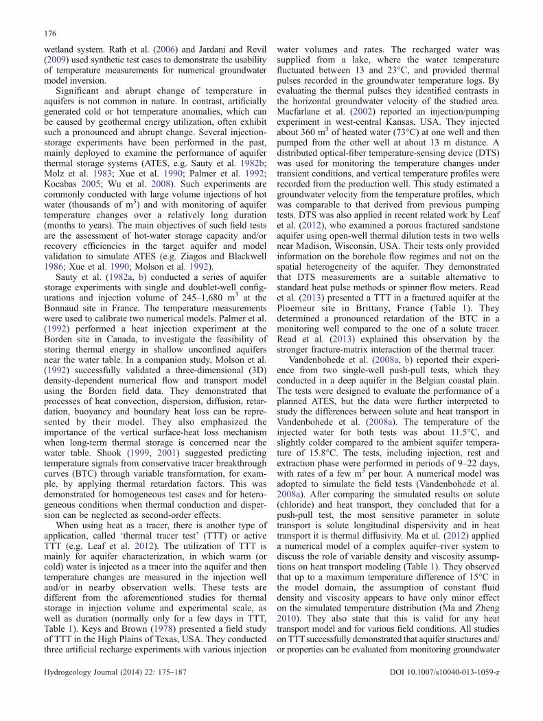
Direct-push injection loggingLessoff et al. (2010) applied the direct-push injectionlogging (DPIL; Dietrich et al. 2008) and direct-push slugtest (DPST; Butler et al. 2002) for characterizing thespatial structure of hydraulic conductivity (K) at theLauswiesen site test. They could demonstrate that the258 measurements of relative conductivity (Kr) usingDPIL are compatible with results from other moreconventional methods performed at the site. All recordedDPIL–profiles (Fig. 3) are within a radius of 15 m aroundthe injection well of the TTT. One DPIL–profile wasdirectly obtained at the injection well and two profiles atthe observation wells OW4 and OW5, which were alsoused for the TTT. The profiles are highlighted in Fig. 3and will be compared to the TTT results of this study. Allmeasured Kr values indicate that there is a significantdifference in the hydraulic conductivities of the upper andlower part of the aquifer. A more detailed inspection of theprofiles from B2, OW4 and OW5 reveals that thetransition between the upper and the lower part of the

Groundwater flow direction

Well

B2

OW1

OW2

OW4

OW3

OW5

0 1 2 3 4 5 6 7 8

1

0

-1

X - location (m)

Y -

loca

tion

(m)

Poland

CzechRepublic

Netherlands

France

Austria

Switzerland

Belgium

Luxembourg

Denmark

River Neckar

River Rhine

Lauswiesen test site

a)

b)Germany

Fig. 1 a Location of the Lauswiesen test site, close to Tübingen, SW Germany. b Plan view of setup of the thermal tracer test. Well B2(x=0, y=0) was used as injection well and OW1–OW5 served as observation wells during the test

178


aquifer is not at constant depth. Lessoff et al. (2010)deduced from the DPIL-profiles, that the upper part of theaquifer is more conductive and more homogenous than thelower part. Moreover, all three profiles show local maximaof Kr at certain depths (e.g. OW4 at a depth of 6.4 m bls,OW5 at a depth of 7.4 m bls).

Numerical modelBased on the existing knowledge of the Lauswiesen site, it isassumed that the subsurface can be represented by a layeredunconfined aquifer with an underlying aquitard. A numericalmodel was set up using FEFLOW (Diersch 2009) tosimulate the TTT with the injection of warm water in theaquifer and the transport of the heated groundwater throughthe sedimentary strata. Analogous to the TTT at theLauswiesen site, the model contains five observation wells(Fig. 4). These are positioned in the center of the modeldomain, where the TTT is simulated. The total size of thenumerical model is 130 m×26 m×15 m (width × height ×depth), which is considered large enough to minimizeboundary effects at the injection and observation wells.The total area is discretized with 30,656 triangle prismatic

elements with an increasing resolution of the numericalmesh towards the well transect. The distance between thenumerical nodes decreases from the model boundary to thewell transect by a factor of 40.

The simulated stratified aquifer is separated in an upperand a lower part as suggested by the results of Lessoff etal. (2010). In the upper part of the aquifer, a free watertable is simulated to account for a potential mound of thewater table due to injection of water. This groundwatermound may affect the flow field, especially close to theinjection well. Unsaturated-zone flow is calculated byapplying the Richards equation, and the model allows forheat exchange between aquifer and unsaturated zone.

Fixed hydraulic heads are assigned at the inflow andoutflow boundary of the model, and no flow at theremaining boundaries. The fixed heads are set to ensure ahorizontal hydraulic gradient of 0.003 along the welltransect and a depth below land surface of the water tableof 4.0 m bls at B2 as measured before the TTT. On theupstream model boundary, a hydraulic head of 3.9 m bls isassigned and on the opposing site a value of 4.3 m bls.The temperatures of the inflowing groundwater and at thesurface are similarly controlled by Dirichlet boundaryconditions. The temperature of the inflowing groundwaterand at all aquifer model edges is set to 11.0°C. This valuewas obtained from groundwater measurements before theTTT started. At the top of the model, the temperature is setfixed at 18.1°C, gradually declining to the groundwatertemperature at the lateral unsaturated boundaries. Thisvalue was derived from linear extrapolation of temperaturevalues obtained before the tracer injection in the section ofthe unsaturated zone (from the water table to 2.2 m bls).

The injection well, B2, is represented by a well moduleintegrated in FEFLOW, which assigns a given extraction orinjection rate to all nodes of the well. To realistically reproducethe conditions of the heated water injection, a combination of atemperature and the described well boundary condition isapplied. For the injection phase (0–8 h), water is injected in theaquifer at a constant rate along the well screen. The

Table 2 Information on the wells used for the thermal tracer test atthe Lauswiesen site

Well Distance fromthe injectionwell B2 (m)

Screenlength (m)

Inner welldiameter(mm)

Material

B2 0.0 Fully screened 150 PVCa

OW1 1.5 6 (from bottom) 25 HDPEb





a Polyvinylchlorideb High-density polyethylene

B2 OW2 OW3 OW4 OW5OW1

Lower aquifer

Water table


0 1.5 2.5 3.75 5.0 7.5 10.0

5

10

PT-100sensor

Well screen

0

6

7

8

9

Dep

th b

elow

sur

face

(m

)

Distance from injection well (m)

Aquitard

Upper aquifer

Injectionpump

Fig. 2 Vertical cross-section along the well axis (x) showing positions of wells (B2, OW1–OW5), water table, aquifer and aquitard

179


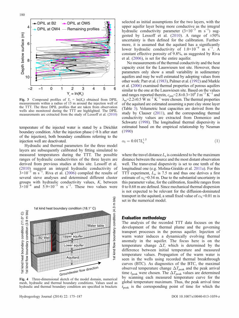
temperature of the injected water is stated by a Dirichletboundary condition. After the injection phase (>8 h after startof the injection), both boundary conditions referring to theinjection well are deactivated.

Hydraulic and thermal parameters for the three modellayers are subsequently calibrated by fitting simulated tomeasured temperatures during the TTT. The possibleranges of hydraulic conductivities of the three layers arederived from previous studies at this site. Lessoff et al.(2010) suggest an integral hydraulic conductivity of3×10−3 m s−1. Riva et al. (2006) compiled the results ofseveral sieve analyses and determined different clustergroups with hydraulic conductivity values, K, between3×10−4 and 5.9×10−3 m s−1. These two values were

selected as initial assumptions for the two layers, with theupper aquifer layer being more conductive as the integralhydraulic conductivity parameter (3×10−3 m s−1) sug-gested by Lessoff et al. (2010). A range of ±50%uncertainty is then defined for the calibration. Further-more, it is assumed that the aquitard has a significantlylower hydraulic conductivity of 1.0×10−9 m s−1. Aconstant effective porosity of 9.8%, as suggested by Rivaet al. (2006), is set for the entire aquifer.

Nomeasurements of the thermal conductivity and the heatcapacity exist for the Lauswiesen test site. However, theseparameters only show a small variability in sedimentaryaquifers and may be well estimated by adopting values fromother work: Parr et al. (1983), Palmer et al. (1992) andMarkleet al. (2006) examined thermal properties of porous aquiferssimilar to the one at the Lauswiesen site. Based on the valuesand ranges reported therein, cpm=2.8±0.3×10

6 J m−3 K−1 andλm=2.2±0.5 Wm−1 K−1 were chosen. The thermal propertiesof the aquitard are estimated assuming a pure clay stone layer(Table 3). Volumetric heat capacities are derived from thestudy by Clauser (2011), and the corresponding thermalconductivity values are extracted from Domenico andSchwartz (1998). The longitudinal thermal dispersivity isestimated based on the empirical relationship by Neuman(1990)

αl ¼ 0:017L1:5s ð1Þ

where the travel distance Ls is considered to be the maximumdistance between the source and the most distant observationwell. The transversal dispersivity is set to one tenth of thelongitudinal one (e.g. Molina-Giraldo et al. 2011a). For thisTTT experiment, Ls, is 7.5 m and thus one derives a firstestimate of αL=0.34 m. Due to the substantial uncertainty inthis parameter value, for the calibration, feasible ranges from0 to 0.68 m are defined. Since mechanical thermal dispersionis not expected to be relevant for the diffusion-dominatedtransport in the aquitard, a small fixed value of αL=0.01 m isset in the numerical model.

Evaluation methodologyThe analysis of the recorded TTT data focuses on thedevelopment of the thermal plume and the governingtransport processes in the porous aquifer. Injection ofwarm water induces a dynamically evolving thermalanomaly in the aquifer. The focus here is on thetemperature change ΔT, which is determined by thedifference between initial temperature and measuredtemperature values. Propagation of the warm water isseen in the wells using recorded thermal breakthroughcurves (BTC). As diagnostics of the BTC, the maximalobserved temperature change ΔTpeak and the peak arrivaltime tpeak were chosen. The ΔTpeak values are determinedby scanning each measured temperature curve for theglobal temperature maximum. Thus, the peak arrival timetpeak is the corresponding point of time for which the

−2 −1 0 1 2 3 4 5 6

Dep

th b

elow

sur

face

(m

)

Yr = ln(Kr)

10

8

6

4DPIL at B2

DPIL at OW4 Remaining profiles

DPIL at OW5

Fig. 3 Compound profiles of Yr = ln(Kr) obtained from DPILmeasurements within a radius of 15 m around the injection well ofthe TTT. The three DPIL profiles that are taken from observationwells also monitored during the TTT are highlighted. The DPILmeasurements are extracted from the study of Lessoff et al. (2010)

1st kind heat boundary condition (18.1° C)

1st k

ind

heat

bou

ndar

y co

nditi

on (

11.0

° C

)1s

t kin

d flo

w b

ound

ary

cond

ition

(3.

9 m

bls

)

Aquitard

Lower aquifer

Upper aquiferB2 Well

1st k

ind

flow

bou

ndar

y co

nditi

on (

4.3

m b

ls)

Water table


Fig. 4 Three-dimensional sketch of the model domain, numericalmesh, hydraulic and thermal boundary conditions. Values used ashydraulic and thermal boundary condition are specified in brackets

180


temperature maximum is detected. According to Bellinand Rubin (2004), evaluation of tpeak has several advan-tages for examining tracer BTCs. It is not so muchinterfered by infrequent sampling, and the lack of early orlate parts of the signal or measurements below thedetection level is not as problematic as it is for theanalysis of moments of the BTC. These interferences,which could hamper BTC interpretation, are also seen ascritical for the TTT at the Lauswiesen site.

The influence of different transport processes can bequantified by dimensionless numbers. To analyze the ratiobetween advection and thermal conduction, the macro-scopic Peclet number is defined as (e.g. Ma et al. 2012)

Pe ¼ cpwvDl

λmð2Þ

where cpw is the volumetric heat capacity of water(cpw=4.2×10

6 J m−3 K−1), vD the Darcy velocity and lthe characteristic length, which is a length specifyingchanges in the temperature (e.g. here total length of theobservation well transect with 7.5 m).

The importance of considering density effects can beevaluated by calculating the ratio between the verticalbuoyancy force and the horizontal friction force fromregional groundwater flow. Oostrom et al. (1992) defineda stability number G as

G ¼KΔρρ0vD

¼ Δρiρ0

ð3Þ

where i is the hydraulic gradient, ρ0 is the referencedensity of the thermally undisturbed aquifer and Δρ is theinduced density difference. Oostrom et al. (1992) exper-imentally determined a critical value of Gc=0.3, where thetransition from a stable to an unstable plume sets in.

Results and discussion

During the TTT, the vertical temperature profiles wererecorded for 4 days in the injection well B2 and in the five

downgradient observations wells (OW1–5). The mea-surements are shown in Fig. 5 as thermoisoplethgraphs, which visualize the time-dependent evolutionof the temperatures in the Lauswiesen aquifer cross-sections. In the same manner, the results of thenumerical simulation are presented in Fig. 6. In thefollowing, first the calibration of the numerical modelis presented and then the temperature development atthe injection well is discussed and the effects ofhydraulic heterogeneity and induced density differencesare examined. Next, the heat transport in the downgradient observation wells is discussed in more detail.Finally, the findings of the TTT are compared to thosefrom previous DPIL measurements.

Calibration of the numerical modelFor the calibration, the mean, minimal and maximalvalues of the uncertain flow and transport parametersof the two aquifer layers K, λm, cpm, and αL wereconsidered. Preliminary testing revealed that simulatedresults are least sensitive to the thermal properties andstrongly controlled by the hydraulic conductivity.Consequently, thermal properties and dispersivity,which are not expected to substantially vary in theaquifer, were assumed to be the same for both aquiferlayers. The hydraulic conductivities were individuallycalibrated for each layer. Thus, 34 = 81 valuecombinations were tested, and the best fit betweensimulated and measured groundwater temperatures atinjection and observation wells during the TTT waschosen for further analysis (Table 3).

For the thermal transport parameters of the aquifer, αL=0.68 m, cpm=2.5×10

6 J m−3 K−1, and λm=2.7 W m−1 K−1

were derived. The obtained hydraulic conductivity of themore conductive upper aquifer layer is 8.9×10−3 m s−1

and the value of the lower one is 4.5×10−4 m s−1. Themodel with this parameter set results in a root meansquared error (RMSE), between all simulated andmeasured BTCs, of 0.65°C. This misfit highlights thatthe numerical model may capture the main thermaltransport processes in the aquifer, but is not capableof fully reproducing the observed temperature evolution,which is comprehensively discussed in the followingsections.

Table 3 Hydraulic and thermal parameter ranges applied for the numerical simulation. Values in italic are used to generate the numericalresults that are further analyzed

Hydraulic conductivityK (m s−1)

Volumetric heat capacitycpm (J m−3 K−1)

Thermal conductivityλm (W m−1 K−1)

Longitudinaldispersivity αl (m)

Lower part Upper part

Aquifer (and gravel) Min 1.5×10−4 3.0×10−3 2.5×106 1.7 0.01Median 3.0×10−4 5.9×10−3 2.8×106 2.2 0.34Max 4.5×10−4 8.9×10−3 3.1×106 2.7 0.68

Aquitard (clay stone) Min 1.0×10−9 2.3×106 1.1 0.01Median 1.0×10−9 2.3×106 1.1 0.01Max 1.0×10−9 2.3×106 1.1 0.01

181


Temperature evolution at injection wellFirst, the temperature evolution at the injection wellB2 is inspected. The temperature changes measured are

illustrated in Fig. 5a. Small vertical variability indi-cates that a homogenized line-source with a tempera-ture of 22.4±0.5°C (ΔT=11.4 K) was created below

b) OW1

Time (day)

Dep

th b

elow

sur

face

(m

)

0 0.5 1 1.5 2 2.5 3 3.5 4

9

8

7

6

5

c) OW2

Time (day)

Dep

th b

elow

sur

face

(m

)

0 0.5 1 1.5 2 2.5 3 3.5 4

9

8

7

6

5

d) OW3

Time (day)

Dep

th b

elow

sur

face

(m

)

0 0.5 1 1.5 2 2.5 3 3.5 4

9

8

7

6

5

f) OW5

Time (day)

Dep

th b

elow

sur

face

(m

)

0 0.5 1 1.5 2 2.5 3 3.5 4

9

8

7

6

5

e) OW4

Time (day)

Dep

th b

elow

sur

face

(m

)

0 0.5 1 1.5 2 2.5 3 3.5 4

9

8

7

6

5

Δ Temperature (K)

a) B2

Time (day)

Dep

th b

elow

sur

face

(m

)

0 0.5 1 1.5 2 2.5 3 3.5 4

9

8

7

6

5

0 1 2 3 4 5 6 7 8Peak arrival time (day)

Fig. 5 Measured depth-related temperature development over the entire experimental period. The temperature change is calculated basedon the initial temperature at the start of the experiment. Additionally, temperature peak arrival times for every measurement location areemphasized: a injection well B2; b–f observation wells OW1–5. For interpolation, the MATLAB®-function contourc is used

182


the water table during the injection experiment(t<0.33 day). Proper mixing of the injected thermaltracer and the groundwater in and around the well was

achieved, and after the warm water injection, only aslight vertical variability in the temperature is ob-served. Even if this variability is only marginal, it can

b) OW1

Time (day)

Dep

th b

elow

sur

face

(m

)

0 0.5 1 1.5 2 2.5 3 3.5 4

9

8

7

6

5

c) OW2

Time (day)

Dep

th b

elow

sur

face

(m

)

0 0.5 1 1.5 2 2.5 3 3.5 4

9

8

7

6

5

d) OW3

Time (day)

Dep

th b

elow

sur

face

(m

)

0 0.5 1 1.5 2 2.5 3 3.5 4

9

8

7

6

5

f) OW5

Time (day)

Dep

th b

elow

sur

face

(m

)

0 0.5 1 1.5 2 2.5 3 3.5 4

9

8

7

6

5

e) OW4

Time (day)

Dep

th b

elow

sur

face

(m

)

0 0.5 1 1.5 2 2.5 3 3.5 4

9

8

7

6

5

Δ Temperature (K)

a) B2

Time (day)

Dep

th b

elow

sur

face

(m

)

0 0.5 1 1.5 2 2.5 3 3.5 4

9

8

7

6

5

0 1 2 3 4 5 6 7 8Peak arrival time (day)

Fig. 6 Simulated depth related temperature development over the entire experimental period using the numerical heat-transport model.The temperature change is calculated based on the initial temperature at the start of the experiment. Additionally, temperature peakarrival times for every measurement location are emphasized: a injection well B2; b–f observation wells OW1–5. For interpolation,the MATLAB®-function contourc is used

183


be seen that long-term cooling is most pronounced atthe bottom, and highest temperatures appear in thelower section at about 7.2 m bls. This pattern of thetemperature signal could be interpreted as a firstindication of non-uniform horizontal groundwatermovement with lower advective flow velocity in thelower part of the aquifer. Minor long-term cooling atthe bottom may be attributed to slight vertical heatloss due to conduction into the aquitard beneath.

The numerical simulation for B2 shows a very similardevelopment of the temperature in the injection well(Fig. 6a). However, a closer look reveals that after theinjection, the thermal anomaly is more persistent. Apossible explanation for this observation is that theassumption of a thermal equilibrium between solid andfluid phase in the numerical model, is not instantaneous inthe vicinity of the injection well. Hence, less heat is storedin the subsurface than expected, based on the simulation,particularly during the fast injection of the warm water. Asa consequence, cooling rates observed in the experimentexceed those in the thermally equilibrated simulations(Fig. 6a). After 1 day, increased temperatures are stillapparent in the model, especially at the central and lowerprofiles. There is a temperature maximum in the injectionwell at a depth of around 7.2–7.7 m bls (Fig. 6a).Apparently, as observed in the field and in the model,the aquitard (and lower aquifer layer) temporally storesand slowly releases thermal energy at the injection well.

Density effects vs. hydraulic heterogeneityDue to layering of the aquifer, advective forces in themore permeable layer dictate and focus thermal break-through in the upper part of the aquifer, which isconfirmed by applying the values used for the calibratednumerical model to calculate the layer-specific Pecletnumbers, Pe (Table 3, Eq. 2). For the upper part of theaquifer, Pe=420 and for the lower part, Pe=21; therefore,heat transport in both parts of the aquifer is dominated byadvection, but it is more pronounced in the upper part. Incomparison, for the aquitard, Pe is only 9×10−5, indicatingconduction dominated conditions in the aquitard.

The next observation well in the regional groundwaterflow direction, OW1, positioned just 1.5 m downgradientof the injection well, reveals that the moving warm wateronly leaves a trace in the upper layer of the aquifer with apeak value of ΔTpeak=6.6 K (Fig. 5b). In comparison,with the numerical model (Fig. 6b), significant tempera-ture changes are only detected in the uppermost part of theaquifer. At first sight, this observation may be a sign ofdensity effects. However, following previous studies by,for example, Hecht-Méndez et al. (2010), Ma and Zheng(2010), Ma et al. (2012) and Leaf et al. (2012), sucheffects are expected to be negligible given the smalltemperature range and the short duration of the performedTTT experiment. Hence, a more plausible reason could behydraulic heterogeneities within the upper layer withhighest advection on top of the profile.

Further insight provides the stability criterion, Gc,according to Oostrom et al. (1992). Based on a ground-water density of 999.6 kg m−3 for 11°C, and anundisturbed hydraulic gradient of i=0.003, a maximumpossible density change of 0.9 kg m−3 would beacceptable to avoid buoyancy effects (G≤Gc=0.3). Duringthe TTT at the Lauswiesen site, the maximal densitychange by temperature increase from 11 to 17°C is Δρ=0.9 kg m−3. Consequently, the resulting value of G=0.3indicates that density effects could not be completely ruledout (Eq. 3). However, temporary warm water infiltrationyields transient conditions with a head build up at theinjection well, and thus during injection, the localhydraulic gradient is increased at the injection well B2(i>0.003). As a result, the maximum ΔT can be expectedto be higher than the limit of ΔT=6 K obtained from acalculated density difference based on Eq. 3 forundisturbed flow conditions. Furthermore, flow fieldchanges are most pronounced very close to the injectionwell and, even under well-controlled experiments, inducedsmall-scale lateral and vertical flow components may besignificant. Since hydraulic heads have not been contin-uously monitored during the experiment, clear quantitativeevidence from the field cannot be provided.

Downgradient propagation of the thermal plumeThe focus of the thermal plume in the uppermost part ofthe well is also observed in the more downgradientobservation wells. Accordingly, the numerical modeloverestimates the vertical extension of the plume through-out the experiment. These observations may be influencedby measurement inaccuracies. The experiment is possiblyprone to technical artifacts, like intra borehole convection,which is not considered in the numerical simulation either.Slight vertical warm water flow in the wells could havesmeared the plume. Therefore, caution is given wheninterpreting the measured temperature trends at the wells.In further analysis, the peak arrival time is favored as apotentially more robust criterion. The values of tpeak aremarked as red crosses in Figs. 5 and 6 for each sensorposition.

The lower aquifer has a lower hydraulic conductivity,assuming that differences in pronounced tpeak are mainlycontrolled by different horizontal advective flow veloci-ties. Thermal effects are minimal in the lower part of theaquifer (6–10 m bls). As a consequence of the smallsignal-to-noise ratio, the tpeak in the lower part the aquifercannot be well determined, which is in line with thesimulated results. The model predicts (Fig. 6) here thatduring the TTT, no thermal peak passes OW2–5, becauseobtained tpeak values are at the end of the experiment.

Under ideal conditions, the result of a TTTwould showlater tpeak values for the more downgradient wells with adecrease of ΔTpeak. Advection would move the peaks inthe upper layer in the flow direction from OW1 to OW5,and diffusion and mechanical dispersion would lead to alongitudinal thermal plume spreading and transversal heatloss. This ideal transport behavior can be seen in the

184


numerical simulation (Fig. 6). There is a gradual declineof the numerically obtained peak temperatures withincreasing distance of observation well from injectionwell. For example, the temperature differences at a depth4.7 m bls are ΔT=8.5 K (OW1) to 6.6 K (OW2), 4.9 K(OW3), 3.8 K (OW4), and 2.5 K (OW5).

The measured temperature values follow a similartrend as those simulated by the model, but with somedeviations. As expected, temperature differences are leastpronounced at the most distant observation well OW5(Fig. 5f). Measured and simulated tpeak agree well in theclosest OW1. However, there is no gradual decline in thewells closer to the injection well. Peak temperatures ontop of the screened section (4.7 m bls) change from ΔT=6.6 K (OW1) to 6.8 K (OW2), 4.0 K (OW3), 4.7 K(OW4), and 3.3 K (OW5). Furthermore, peak arrival timesrecorded at the upper sensor do not increase with distance.

The evolution of the thermal plume measured duringthe TTT and values of tpeak provide crucial hints thatsubstantial spatial heterogeneity are present in the aquifer,which is insufficiently reproduced in the model by twohorizontal and laterally persistent layers. Small-scale,vertical heterogeneity has already been identified as apotential reason that the plume is detected only in theuppermost well screens. In the upper part of the aquifer, atOW2 and OW3, tpeak trends would compare better bysimple shifting along the vertical axis. This shift could bean indication that the boundary between the upper and thelower aquifer part is declined or displaced relative to theassumptions in the model. The inconsistencies in tpeakbetween model and field of OW4 and OW5 are a sign oflateral heterogeneities in the direction of the well transect,as well as perpendicular. The thermal plume appearslocally deviated from the suspected centerline, potentiallywith meandering. Thus, the measured temperatures mayoriginate from the fringe of the thermal plume. Thisconclusion is supported by the measured tpeak values atOW4 and OW5, which are smaller than those at OW3,

meaning that the thermal peak arrives at OW4 and OW5before it passes OW3.

Comparison to DPILFinally, tpeak values are compared to the DPIL profiles(Figs. 3 and 7). The overall patterns are comparable, andboth field experiments are obviously consistent withhigher relative hydraulic conductivities and smaller tpeakvalues in the upper part of the aquifer. The 6 m blsboundary between both aquifer parts in the DPIL-profileof B2 is well reproduced by the model. The DPIL-profilesof OW4 and OW5 indicate that this boundary could be ata more shallow depth, which corresponds to the interpre-tation from trends in the tpeak values. Due to thesubstantial influence of noise on the small values shownon logarithmic scale, the DPIL-based characterization ofthe lower section is as unsatisfactory as from the TTT.Further insights in the heat transport characteristics of thestudied aquifer would mandate an even denser measure-ment network and a longer duration of TTT observation toassure the monitoring of the passage of the thermal peak.

Conclusions

The main objective of the TTT at the Lauswiesen site wasto improve understanding of the results from the experi-ment and, with the obtained experience, identify implica-tions for future TTT designs. By numerical simulation ofthe TTT, the governing transport processes could beidentified, and high-conductivity regions at the top of theaquifer could also be confirmed. The heterogeneoushydraulic properties of the studied shallow aquifer, whichis generally well known and has already served as ahydrogeological test case for decades, have substantialeffects on the heat transport behavior. It is shown thatmacrodispersion and flow-focusing occurred, and that

B2 OW1 OW2 OW3 OW4 OW5

Measured

Simulated

0 1 2 3 4

9

8

7

6

5

Peak arrival time (day)

Dep

th b

elow

sur

face

(m

)

b)

0 1 2 3 4

9

8

7

6

5

Peak arrival time (day)

Dep

th b

elow

sur

face

(m

)

a)

Fig. 7 Comparison of the peak arrival times (tpeak) measured and simulated for the TTT experiment. a B2, OW1 and OW2; b OW3–5.Dashed lines indicate uncertain sections, influenced by measurement inaccuracies or data noise (ΔTpeak<0.3 K)

185


complex flow patterns result in thermal breakthroughcurves (shown as thermoisopleth graphs) that are substan-tially distinct from what would be expected under idealconditions in a layered aquifer. Accordingly, the capabilityof the presented model to simulate the measured propa-gation of the thermal plume is limited. For morecomprehensive flow and transport simulations, however,the data collected during this experiment are insufficient.A main obstacle is that the induced transient hydraulichead change at injection well and in the observation wellswere not continuously monitored during the experiment.Hence, piezometers have to be added to the experimentaldesign, especially, when the injected water volume pertime is significant in comparison to the anticipated naturalgroundwater flow.

Considering that lateral and even vertical flow andtransport components may be significant in such highlyheterogeneous systems, it is also recommended to usea more distributed and space-filling arrangement ofobservation wells (e.g. several observation well tran-sects) than the linear one chosen in the performedTTT. Such wells, which also reveal the thermalevolution aside from the expected dominant flowdirection, show valuable insights in the 3D character-istics of the transport mechanisms. Furthermore, par-ticularly in the case of long-duration experiments,sensors are needed that monitor potential verticalconductive heat losses such as into the underlyingaquitard and the unsaturated zone above.

Ideally, the TTT is complemented by additionalfield experiments such as near surface geophysics (e.g.Slater 2007) or hydraulic tomography (e.g. Brauchleret al. 2013), which are able to identify the mainstructural build-up of the aquifer. For example, at theLauswiesen site, DPIL field tests have been performedbefore the TTT. It is demonstrated that the monitoredthermal transport along the local hydraulic gradient isconsistent with the findings from the DPIL campaign.In addition, as reported by Ma et al. (2012), injectionof both thermal and dye tracers is an appealingcombination, which should be considered for futureactive and short-term TTT. Thus, coupled parameterestimation for determining both thermal and solutetransport parameters would be possible (Rau et al.2012), which would better constrain the inversionproblem than by separate interpretation of individualtracer tests. Although heat appears to be a favorabletracer for studying aquifer properties, care has to betaken to interpret the acquired data. Hence, morestudies on active and short-term TTT are required toestablish such tests as a standard hydrogeologicalinvestigation technique.

Acknowledgements This research was supported by the SwissNational Science Foundation (SNSF) under grant number200021L 144288, and the German Research Foundation(DFG), under grant number BL 1015/4-1. We are also gratefulto Uwe Schneidewind and Wolfgang Kürner for their supportduring the field campaign and two anonymous reviewers fortheir fruitful comments.

References

Anderson MP (2005) Heat as a ground water tracer. Ground Water43(6):951–968

Bellin A, Rubin Y (2004) On the use of peak concentration arrivaltimes for the inference of hydrogeological parameters. WaterResour Res 40(7):1–13

Bou Ghannam O (2006) Determination of the hydraulic conductiv-ity using direct-push methods. MScThesis, University ofTübingen, Germany

Brauchler R, Hu R, Hu L, Jiménez S, Bayer P, Dietrich P, Ptak T(2013) Rapid field application of hydraulic tomography forresolving aquifer heterogeneity in unconsolidated sediments.Water Resour Res 49(4):2013–2024

Bravo HR, Jiang F, Hunt RJ (2002) Using groundwater temperaturedata to constrain parameter estimation in a groundwater flowmodel of a wetland system. Water Resour Res 38(8):1–14

Brouyère S, Carabin G, Dassargues A (2004) Climate changeimpacts on groundwater resources: modelled deficits in a chalkyaquifer, Geer basin, Belgium. Hydrogeol J 12(2):123–134

Butler JJ, Healey JM, McCall GW, Garnett EJ, Loheide SP (2002)Hydraulic tests with direct-push equipment. Ground Water40(1):25–36

Clauser C (2011) Thermal storage and transport properties of rocks,I: heat capacity and latent heat. In: Gupta H (ed) Encyclopediaof solid earth geophysics. Springer, Netherlands, pp 1423–1431

Conant B (2004) Delineating and quantifying ground waterdischarge zones using streambed temperatures. Ground Water42(2):243–257

Constantz J (2008) Heat as a tracer to determine streambed waterexchanges. Water Resour Res 44(4):1–20

Diersch H-JG (2009) FEFLOW reference manual. WASY GmbH,Berlin

Dietrich P, Butler JJ, Faiß K (2008) A rapid method for hydraulicprofiling in unconsolidated formations. Ground Water46(2):323–328

Domenico PA, Schwartz FW (1998) Physical and chemicalhydrogeology, 2nd edn. Wiley, Chichester, UK

Doussan C, Toma A, Paris B, Poitevin G, Ledoux E, Detay M(1994) Coupled use of thermal and hydraulic head data tocharacterize river-groundwater exchanges. J Hydrol 153(1–4):215–229

Engelhardt I, Prommer H, Moore C, Schulz M, Schüth C, TernesTA (2013) Suitability of temperature, hydraulic heads, andacesulfame to quantify wastewater-related fluxes in thehyporheic and riparian zone. Water Resour Res 49:1–15

Ferguson G, Woodbury AD (2007) Urban heat island in thesubsurface. Geophys Res Lett 34(23):1–4

Händel F, Dietrich P (2012) Relevance of deterministic structuresfor modeling of transport: the Lauswiesen case study. GroundWater 50(6):935–942

Hecht-Méndez J, Molina-Giraldo N, Blum P, Bayer P (2010)Evaluating MT3DMS for heat transport simulation of closedgeothermal systems. Ground Water 48(5):741–756

Jardani A, Revil A (2009) Stochastic joint inversion of temperatureand self-potential data. Geophys J Int 179(1):640–654

Keery J, Binley A, Crook N, Smith JWN (2007) Temporal andspatial variability of groundwater–surface water fluxes: devel-opment and application of an analytical method using temper-ature time series. J Hydrol 336(1–2):1–16

Keys WS, Brown RF (1978) The Use of temperature logs to tracethe movement of injected water. Ground Water 16(1):32–48

Kocabas I (2005) Geothermal reservoir characterization via thermalinjection backflow and interwell tracer testing. Geothermics34(1):27–46

Kollet SJ, Cvijanovic I, Schüttemeyer D, Maxwell RM, Moene AF,Bayer P (2009) The influence of rain sensible heat andsubsurface energy transport on the energy balance at the landsurface. Vadose Zone J 8(4):846–857

Leaf AT, Hart DJ, Bahr JM (2012) Active thermal tracer tests forimproved hydrostratigraphic characterization. Ground Water50(5):726–735

186


Lessoff SC, Schneidewind U, Leven C, Blum P, Dietrich P, DaganG (2010) Spatial characterization of the hydraulic conductivityusing direct-push injection logging. Water Resour Res46(12):1–9

Lowry CS, Walker JF, Hunt RJ, Anderson MP (2007) Identifyingspatial variability of groundwater discharge in a wetland streamusing a distributed temperature sensor. Water Resour Res43(10):1–9

Ma R, Zheng C (2010) Effects of density and viscosity inmodeling heat as a groundwater tracer. Ground Water48(3):380–389

Ma R, Zheng C, Zachara JM, Tonkin M (2012) Utility ofbromide and heat tracers for aquifer characterization affectedby highly transient flow conditions. Water Resour Res48(8):1–18

Macfarlane A, Förster A, Merriam D, Schrötter J, Healey J (2002)Monitoring artificially stimulated fluid movement in theCretaceous Dakota aquifer, western Kansas. Hydrogeol J10(6):662–673

Markle JM, Schincariol RA, Sass JH, Molson JW (2006)Characterizing the two-dimensional thermal conductivity distri-bution in a sand and gravel aquifer. Soil Sci Soc Am J70(4):1281–1294

Menberg K, Bayer P, Zosseder K, Rumohr S, Blum P (2013)Subsurface urban heat islands in German cities. Sci TotalEnviron 442:123–133

Molina-Giraldo N, Bayer P, Blum P (2011a) Evaluating theinfluence of thermal dispersion on temperature plumes fromgeothermal systems using analytical solutions. Int J Therm Sci50(7):1223–1231

Molina-Giraldo N, Bayer P, Blum P, Cirpka OA (2011b) Propaga-tion of seasonal temperature signals into an aquifer upon bankinfiltration. Ground Water 49(4):491–502

Molson JW, Frind EO, Palmer CD (1992) Thermal energy storagein an unconfined aquifer: 2. model development, validation, andapplication. Water Resour Res 28(10):2857–2867

Molz FJ, Melville JG, Parr AD, King DA, Hopf MT (1983) Aquiferthermal energy storage: a well doublet experiment at increasedtemperatures. Water Resour Res 19(1):149–160

Neuman SP (1990) Universal scaling of hydraulic conductivitiesand dispersivities in geologic media. Water Resour Res26(8):1749–1758

Oostrom M, Hayworth JS, Dane JH, Güven O (1992) Behavior ofdense aqueous phase leachate plumes in homogeneous porousmedia. Water Resour Res 28(8):2123–2134

Palmer CD, Blowes DW, Frind EO, Molson JW (1992) Thermalenergy storage in an unconfined aquifer: 1. field injectionexperiment. Water Resour Res 28(10):2845–2856

Parr AD, Molz FJ, Melville JG (1983) Field determination of aquiferthermal energy storage parameters. Ground Water 21(1):22–35

Pehme P, Parker BL, Cherry JA, Molson JW, Greenhouse JP (2013)Enhanced detection of hydraulically active fractures by temper-ature profiling in lined heated bedrock boreholes. J Hydrol484:1–15

Rath V, Wolf A, Bücker HM (2006) Joint three-dimensionalinversion of coupled groundwater flow and heat transfer basedon automatic differentiation: sensitivity calculation, verification,and synthetic examples. Geophys J Int 167(1):453–466

Rau GC, Andersen MS, Acworth RI (2012) Experimental investi-gation of the thermal dispersivity term and its significance in theheat transport equation for flow in sediments. Water Resour Res48(3):1–21

Read T, Bour O, Bense V, Le Borgne T, Goderniaux P, KlepikovaMV, Hochreutener R, Lavenant N, Boschero V (2013) Charac-terizing groundwater flow and heat transport in fractured rockusing fiber-optic distributed temperature sensing. Geophys ResLett 40(10):2055–2059

Rein A, Hoffmann R, Dietrich P (2004) Influence of natural time-dependent variations of electrical conductivity on DC resistivitymeasurements. J Hydrol 285(1–4):215–232

Riva M, Guadagnini L, Guadagnini A, Ptak T, Martac E (2006)Probabilistic study of well capture zones distribution at theLauswiesen field site. J Contam Hydrol 88(1–2):92–118

Saar M (2011) Review: geothermal heat as a tracer of large-scalegroundwater flow and as a means to determine permeabilityfields. Hydrogeol J 19(1):31–52

Sack-Kühner B (1996) Establishing the natural test site“Lauswiesen Tübingen”. Diploma Thesis, University ofTübingen, Germany

Sauty JP, Gringarten AC, Fabris H, Thiery D, Menjoz A, Landel PA(1982a) Sensible energy storage in aquifers: 2. field experimentsand comparison with theoretical results. Water Resour Res18(2):253–265

Sauty JP, Gringarten AC, Menjoz, Landel PA (1982b) Sensibleenergy storage in aquifers: 1. theoretical study. Water ResourRes 18(2):245–252

Schmidt C, Bayer-Raich M, Schirmer M (2006) Characterization ofspatial heterogeneity of groundwater-stream water interactionsusing multiple depth streambed temperature measurements atthe reach scale. Hydrol Earth Syst Sci 10(6):849–859

Schneidewind U (2008) Determination of the hydraulic conductivityusing Direct-Push Injection Logger. MSc Thesis, University ofTübingen, Germany

Shook GM (1999) Prediction of thermal breakthrough from tracertests. Paper presented at the 24th Workshop on GeothermalReservoir Engineering, Stanford, CA, January 1999

Shook GM (2001) Predicting thermal breakthrough in heteroge-neous media from tracer tests. Geothermics 30(6):573–589

Slater L (2007) Near surface electrical characterization of hydraulicconductivity: from petrophysical properties to aquifergeometries—a review. Surv Geophys 28(2–3):169–197

Taniguchi M, Shimada J, Tanaka T, Kayane I, Sakura Y, Shimano Y,Dapaah-Siakwan S, Kawashima S (1999) Disturbances oftemperature-depth profiles due to surface climate change andsubsurface water flow: 1. an effect of linear increase in surfacetemperature caused by global warming and urbanization in theTokyo Metropolitan Area, Japan. Water Resour Res35(5):1507–1517

Taniguchi M, Turner JV, Smith AJ (2003) Evaluations of ground-water discharge rates from subsurface temperature in CockburnSound, Western Australia. Biogeochemistry 66(1–2):111–124

Vandenbohede A, Louwyck A, Lebbe L (2008a) Identification andreliability of microbial aerobic respiration and denitrificationkinetics using a single-well push–pull field test. J ContamHydrol 95(1–2):42–56

Vandenbohede A, Van Houtte E, Lebbe LUC (2008b) Study of thefeasibility of an aquifer storage and recovery system in a deepaquifer in Belgium. Hydrol Sci J 53(4):844–856

Vandenbohede A, Louwyck A, Lebbe L (2009) Conservative soluteversus heat transport in porous media during push-pull tests.Transport Porous Media 76(2):265–287

Vogt T, Schneider P, Hahn-Woernle L, Cirpka OA (2010)Estimation of seepage rates in a losing stream by means offiber-optic high-resolution vertical temperature profiling. JHydrol 380(1–2):154–164

Wu X, Pope GA, Shook GM, Srinivasan S (2008) Prediction ofenthalpy production from fractured geothermal reservoirs usingpartitioning tracers. Int J Heat Mass Transf 51(5–6):1453–1466

Xue Y, Xie C, Li Q (1990) Aquifer thermal energy storage: anumerical simulation of field experiments in China. WaterResour Res 26(10):2365–2375

Ziagos JP, Blackwell DD (1986) A model for the transienttemperature effects of horizontal fluid flow in geothermalsystems. J Volcanol Geotherm Res 27(3–4):371–397

187


Thermal tracer testing in a sedimentary aquifer: field experiment (Lauswiesen, Germany) and...

Documents

Transcript of Thermal tracer testing in a sedimentary aquifer: field experiment (Lauswiesen, Germany) and...