Journal of Applied Geophysics 70 (2010) 268–276

Contents lists available at ScienceDirect

Journal of Applied Geophysics

j ourna l homepage: www.e lsev ie r.com/ locate / jappgeo

High-resolution Electrical Resistivity Tomography monitoring of a tracer test in aconfined aquifer

P.B. Wilkinson ⁎, P.I. Meldrum, O. Kuras, J.E. Chambers, S.J. Holyoake, R.D. OgilvyBritish Geological Survey, Kingsley Dunham Centre, Keyworth, Nottingham NG12 5GG, United Kingdom

⁎ Corresponding author. Tel.: +44 115 936 3086; faxE-mail address: pbw@bgs.ac.uk (P.B. Wilkinson).

0926-9851/$ – see front matter © 2009 Natural Envirodoi:10.1016/j.jappgeo.2009.08.001

a b s t r a c t

a r t i c l e i n f o

Article history:Received 29 January 2009Accepted 12 August 2009

Keywords:Electrical Resistivity TomographyTimelapse3D4DEnvironmental monitoringTracerNatural attenuation

A permanent geoelectrical subsurface imaging system has been installed at a contaminated land site tomonitor changes in groundwater quality after the completion of a remediation programme. Since theresistivities of earth materials are sensitive to the presence of contaminants and their break-down products,4-dimensional resistivity imaging can act as a surrogate monitoring technology for tracking and visualisingchanges in contaminant concentrations at much higher spatial and temporal resolution than manualintrusive investigations. The test site, a municipal car park built on a former gasworks, had been polluted by arange of polycyclic aromatic hydrocarbons and dissolved phase contaminants. It was designated statutorycontaminated land under Part IIA of the UK Environmental Protection Act due to the risk of polluting anunderlying minor aquifer. Resistivity monitoring zones were established on the boundaries of the site byinstalling vertical electrode arrays in purpose-drilled boreholes. After a year of monitoring data had beencollected, a tracer test was performed to investigate groundwater flow velocity and to demonstrate rapidvolumetric monitoring of natural attenuation processes. A saline tracer was injected into the confinedaquifer, and its motion and evolution were visualised directly in high-resolution tomographic images in nearreal-time. Breakthrough curves were calculated from independent resistivity measurements, and theestimated seepage velocities from the monitoring images and the breakthrough curves were found to be ingood agreement with each other and with estimates based on the piezometric gradient and assumedmaterial parameters.

© 2009 Natural Environment Research Council (NERC). Published by Elsevier B.V. All rights reserved.

1. Introduction

The use of Electrical Resistivity Tomography (ERT) to study near-surface hydrogeological characteristics and processes over a range ofspatial and temporal scales has been an area of active research formore than a decade. As resistivity depends on properties such assaturation, solute concentration and temperature, time-lapse ERT canbe used to monitor natural and anthropogenic processes that causechanges in these properties, such as infiltration (Daily et al., 1992;Looms et al., 2008), saline intrusion (Slater and Sandberg, 2000;Ogilvy et al., 2007, 2008), leachate recirculation (Guerin et al., 2004),and contaminated land remediation (Daily and Ramirez, 1995;LaBrecque et al., 1996; Slater and Binley, 2003; Halihan et al., 2005,Wilkinson et al., 2008).

Time-lapse ERT provides dynamic volumetric information whilebeing either non-invasive (when using surface electrodes) orminimally invasive (with borehole electrodes). Therefore this methodis well suited to monitoring tracer tests as part of hydrogeological siteinvestigations. It typically gives much higher spatial resolution than

: +44 115 936 3261.

nment Research Council (NERC). Pu

geochemical sampling via monitoring boreholes and is thereforebetter able to capture the complex evolution of a tracer plume. This isparticularly advantageous when monitoring natural flow, or forcedflow in heterogeneous and/or anisotropic formations (Kemna et al.,2002; Sandberg et al., 2002; Vanderborght et al., 2005; Cassiani et al.,2006). Typically, surface ERT canmonitormore extensive regions thancross-borehole ERT, but because its resolution decreases markedlywith depth it tends to be used only for shallow hydrogeologicalsystems (Cassiani et al., 2006; Nimmer et al., 2007). The mostcommon approach is to monitor crosshole resistivity data and use 2Dinversion algorithms to generate images in the borehole planes (e.g.Daily and Ramirez; 1995; LaBrecque et al., 1996; Slater et al., 1997;Sandberg et al., 2002; Kemna et al., 2002; Deiana et al., 2007; Loomset al., 2008). 2D inversion is rapid, permitting monitoring ontimescales of tens of minutes to a few hours, but provides informationonly in the plane between the boreholes and is prone to artefactscaused by off-plane 3D features (Nimmer et al., 2008). By contrast 3Dinversion produces volumetric images, fully reconstructing the 3Dnature of the tracer plume, albeit with decreasing resolution at greaterdistances from the boreholes. This method has been used to monitortracer tests on timescales of several hours to a few days, typicallyusing fewer than 10 boreholes, each with some 10–20 electrodes(Daily and Ramirez, 2000; Binley et al., 2002; Singha and Gorelick,

blished by Elsevier B.V. All rights reserved.

269P.B. Wilkinson et al. / Journal of Applied Geophysics 70 (2010) 268–276

2005; Oldenborger et al., 2007a; Kuras et al., 2009). In many cases,quantitative estimates can be made of seepage velocities (Sandberget al., 2002), spatial moments (Binley et al., 2002; Singha and Gorelick,2005; Looms et al., 2008), hydraulic conductivity (Binley et al., 2002),and tracer mass and concentration (Singha and Gorelick, 2006;Oldenborger et al., 2007a).

In this paper, we present the results of a high spatial and temporalresolution 3D time-lapse monitoring study of a saline tracer test. Theelectrode network comprised 14 boreholes, each with 16 electrodes,covering an area of ~40 m2. Tomographic images were obtained every4 h from a remotely-controlled automated geoelectrical monitoringsystem. The test was undertaken at a former gasworks site that hadrecently undergone remediation, which had been monitored for overa year using a combination of geoelectrical imaging and conventionalgroundwater sampling to validate its success. The aim of the tracertest was to determine the direction and speed of the groundwaterflow and to demonstrate the ability to monitor natural attenuationprocesses such as dilution and dispersion in near real-time usingautomated ERT.

2. Context

The CLARET (Contaminated Land: Assessment of Remediation byElectrical Tomography) project was undertaken by a public/privateconsortium comprising a research institution, two companies, and alocal government authority. The aim of the project was to developautomated 4D geoelectrical imaging as a minimally invasive tool tomonitor contaminated land and validate remediation processes. Fig. 1illustrates the general monitoring concept. Electrodes are installed ata site where a receptor (e.g. a controlled water body) is at risk ofcontamination. Monitoring of the geoelectrical properties of the sitetakes place either automatically in near real-time, or on-demand, withdata being transmitted via one of several possible communicationchannels to the office for automated processing and inversion. Thisprocess generates volumetric time-lapse images of the resistivity ofthe subsurface, which is dependent on the geology, the groundwaterchemistry, and the presence of bulk contaminants and their break-down products (Shevnin et al., 2006). Since the geology is static,monitoring changes in the resistivity images over time highlights

Fig. 1. Schematic diagram of the CLARET concept.

temporal variations in contamination or groundwater quality associ-ated with remediation. A key advantage of this approach is that thevolumetric images can provide information to help interpolatebetween point samples and give extra assurance that contaminationhas not been missed.

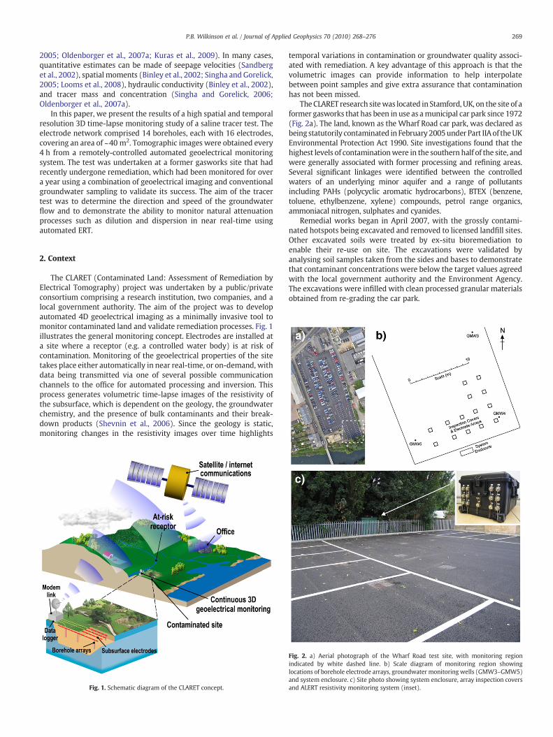
The CLARET research sitewas located in Stamford, UK, on the site of aformer gasworks that has been in use as amunicipal car park since 1972(Fig. 2a). The land, known as the Wharf Road car park, was declared asbeing statutorily contaminated in February2005under Part IIAof theUKEnvironmental Protection Act 1990. Site investigations found that thehighest levels of contaminationwere in the southern half of the site, andwere generally associated with former processing and refining areas.Several significant linkages were identified between the controlledwaters of an underlying minor aquifer and a range of pollutantsincluding PAHs (polycyclic aromatic hydrocarbons), BTEX (benzene,toluene, ethylbenzene, xylene) compounds, petrol range organics,ammoniacal nitrogen, sulphates and cyanides.

Remedial works began in April 2007, with the grossly contami-nated hotspots being excavated and removed to licensed landfill sites.Other excavated soils were treated by ex-situ bioremediation toenable their re-use on site. The excavations were validated byanalysing soil samples taken from the sides and bases to demonstratethat contaminant concentrations were below the target values agreedwith the local government authority and the Environment Agency.The excavations were infilled with clean processed granular materialsobtained from re-grading the car park.

Fig. 2. a) Aerial photograph of the Wharf Road test site, with monitoring regionindicated by white dashed line. b) Scale diagram of monitoring region showinglocations of borehole electrode arrays, groundwater monitoring wells (GMW3–GMW5)and system enclosure. c) Site photo showing system enclosure, array inspection coversand ALERT resistivity monitoring system (inset).

270 P.B. Wilkinson et al. / Journal of Applied Geophysics 70 (2010) 268–276

3. Electrode network and ALERT system

The electrode network was installed after the excavations hadbeen infilled and before the car park surface was reinstated. Thenetwork was arranged to cover the south-eastern corner of theboundaries with the River Welland to the south and privately ownedland to the east (Fig. 2a and b). Each of the 14 vertical electrode arrayswas installed during a 3-day period in a purpose-drilled borehole andeach can be accessed via an inspection cover. The arrays each had 16electrodes spaced at 0.5 m depth intervals, and were connected viapurpose-built subsurface conduits to a system enclosure just beyondthe southern boundary of the site. The installation was undertaken inaccordance with Environment Agency and Construction (Design andManagement) 2007 regulations. The installed system and electrodenetwork had little visual impact on the site (Fig. 2c), and no impact onits use as a car park.

Before installation, the noise characteristics were measured of fourprototype arrays comprising stainless steel, naval brass, phosphorbronze or lead electrodes. Each array was placed in an existinggroundwater monitoring borehole on the site and a set of dipole-dipole measurements were made with reciprocals. It was found thatthe phosphor bronze electrodes exhibited the lowest levels ofreciprocal error. The electrodes for the permanent arrays weretherefore constructed from 5 mm diameter phosphor bronze rods,eachwith an exposed length of 4 cm (Fig. 3a). Each arraywas installedin a 100 mm diameter hole drilled using the sonic percussion drillingmethod. The electrode array was located inside the drill stem andpushed to depth. A plastic lost-point at the end of the drill stem wasthen released to leave the array in position and allow the stem to bewithdrawn over the installed array. Each array was mounted onto theoutside of eight 1 m bentonite sleeve sections (Fig. 3b). Afterinstallation, swelling of the bentonite sleeves caused the borehole toclose, ensuring good electrical contact with the surrounding forma-tion while simultaneously preventing the creation of new pollution

Fig. 3. a) Phosphor bronze electrodes used in the borehole arrays. b) Installation ofelectrodes on bentonite collars before insertion into borehole.

pathways. A single Pb/PbCl2 non-polarising electrode was alsoinstalled at the top of each of the arrays to monitor self-potential.

The resistivity distribution of the subsurface in the vicinity of theelectrode network was monitored on a regular and frequent basisduring the project by a British Geological Survey (BGS) proprietarygeoelectrical imaging system. This system, known as ALERT (Auto-mated time-Lapse Electrical Resistivity Tomography), enables nearreal-time autonomous in-situ monitoring of electrical resistivity,induced polarisation and self-potential data. It uses wireless telemetry(e.g.: GSM/3G, internet, GPRS, or satellite) to communicate with adatabase management system at the office, which controls thestorage, inversion and delivery of the data and resulting tomographicimages. Once installed, no manual intervention is required; data istransmitted automatically according to a pre-programmed scheduleand specific survey parameters, both of which may be modifiedremotely as conditions change. The ALERT instrument is a single unit,contained in a sealed environmental casing (Fig. 2c inset). Connectionof external sensors to the instrument is made via high specificationwater-proof connectorsmounted on the side of the case. The system ispowered by 12 or 24 V batteries, with mains, solar or wind turbinecharging options. It supports 10-channel simultaneous potentialdifference measurements, and open-ended expansion of the numberof attached electrodes (in multiples of 32). Specifically, at the test site238 of a total 288 available electrode addresses were in use (224resistivity electrodes and 14 self-potential electrodes). The batterieswere charged by mains power, and communications were providedvia a 3G wireless cellular router.

4. Data acquisition

To monitor subsurface changes associated with the site remedi-ation, resistivity data were collected between pairs of adjacentboreholes (“panels”) as shown in Fig. 4a. The measurement schemecomprised many sets of four-electrode measurements, in which thecurrent flow and potential measurements are crosshole. In general,these provide better signal-to-noise characteristics and greater imageresolution than configurations with in-hole current flow and potentialmeasurements (Bing and Greenhalgh, 2000; Wilkinson et al., 2006,2008). To provide sufficient image resolution in crosshole ERT, it isimportant that the aspect ratio of the panel (borehole spacing/depth)is <0.75 (LaBrecque et al., 1996). In our case, each panel had an aspectratio <0.5.

Since the system is capable of multichannel data acquisition, manypotential measurements were made for each pair of currentelectrodes. The measurement sets were classified into two types:forward and reciprocal. For the forward measurements, a pair ofcurrent electrodes was selected with a vertical offset of s electrodespacings (solid lines in Fig. 4a). The first potential difference wasmeasured on the electrodes immediately above the current bipole,followed by successive alternating pairs going up the boreholes(dotted lines in Fig. 4a). To cover the whole panel, this geometry wasrepeated to the top of the boreholes. After this, equivalent reciprocalmeasurements were made with the current and potential bipolesinterchanged (so that the potential differences are now measuredbeneath the current electrodes). The purpose of making reciprocalmeasurements is that, in the absence of systematic and random error,equivalent forward and reciprocal electrode configurations shouldyield the same resistivity value (Parasnis, 1988; Zhou and Dahlin,2003). Any difference between the two gives a reliable indicator of theerror in the measurement.

To cover the monitoring region, the single panel measurementscheme was repeated on each of the 31 panels shown by dashed linesin Fig. 4b. During the post-remediation monitoring phase of theproject, forward and reciprocal data were measured on each panel forvertical offsets of s=0, ±3, ±6, ±9, ±12. For the rapid monitoringrequired during the tracer test, only s=0 was used. Reciprocal data

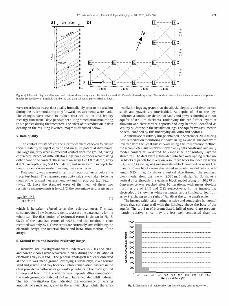
Fig. 4. a) Schematic diagram of forward and reciprocal resistivity data collection for a vertical offset of s electrode spacings. The solid and dotted lines indicate current and potentialbipoles respectively. b) Borehole numbering and data collection panels (dashed lines).

Fig. 5. Distribution of reciprocal errors immediately prior to tracer test.

271P.B. Wilkinson et al. / Journal of Applied Geophysics 70 (2010) 268–276

were recorded to assess data quality immediately prior to the test, butduring the tracer monitoring only forwardmeasurements were made.The changes were made to reduce data acquisition and batteryrecharge time from 2 days per data set during remediationmonitoringto 4 h per set during the tracer test. The effect of this reduction in datadensity on the resulting inverted images is discussed below.

5. Data quality

The contact resistances of the electrodes were checked to ensuretheir suitability to inject current and measure potential differences.The large majority were in excellent contact with the ground, havingcontact resistances of 200–300 Ωm. Only four electrodes weremakingeither poor or no contact. These were on array 1 at 1.0 m depth, array4 at 3.5 m depth, array 5 at 1.5 m depth, and array 8 at 1.5 m depth. Nomeasurements were made involving these electrodes.

Data quality was assessed in terms of reciprocal error before thetracer test began. Themeasured resistivity value ρwas taken to be themean of the forward measurement (ρf) and its reciprocal (ρr), i.e. ρ=(ρf -ρr) /2. Since the standard error of the mean of these tworesistivity measurements is |ρf -ρr| /2, the percentage error is given by

100jρf−ρr jðρf + ρrÞ

; ð1Þ

which is hereafter referred to as the reciprocal error. This wascalculated for all s=0measurements to assess the data quality for thewhole set. The distribution of reciprocal errors is shown in Fig. 5.98.7% of the data had errors of <0.3%, and the maximum errorrecordedwas only 2.7%. These errors are extremely low, validating theelectrode design, the material choice and installation method of thearrays.

6. Ground truth and baseline resistivity image

Intrusive site investigations were undertaken in 2003 and 2006,and borehole cores were recovered in 2007 during the installation ofelectrode arrays 5, 8 and 9. The general lithological sequence observedat the site was made ground, overlying alluvial clays, river terracesand and gravels, and clay bedrock. Before remediation, fissures in theclays provided a pathway for gasworks pollutants in the made groundto seep and leach into the river terrace deposits. After remediation,the made ground consisted of 2–3 m of bioremediated infill material.The site investigation logs indicated the occurrence of varyingamounts of sands and gravel in the alluvial clays, while the array

installation logs suggested that the alluvial deposits and river terracesands and gravels are interbedded. At depths of ~5 m, the logsindicated a continuous deposit of sands and gravels, forming a minoraquifer of 0.5–1 m thickness. Underlying this are further layers ofalluvium and river terrace deposits and clay bedrock, identified asWhitby Mudstone in the installation logs. The aquifer was assumed tobe semi-confined by this underlying alluvium and bedrock.

A subsurface resistivity image obtained in September 2008 duringpost-remediation monitoring is shown in Fig. 6a and b. The data wereinverted with the Res3DInv software using a finite difference method,the incomplete Gauss–Newton solver, an L1 data constraint, and an L2model constraint weighted to emphasize horizontally layeredstructures. The data were subdivided into two overlapping rectangu-lar blocks of panels for inversion, a southern block bounded by arrays3, 4, 8 and 14 (see Fig. 4b) and an eastern block bounded by arrays 1, 4,5 and 9. These blocks were discretised into cubic model cells of sidelength 0.25 m. Fig. 6a shows a vertical slice through the southernblock model along the line y=2.375 m. Similarly, Fig. 6b shows avertical slice through the eastern block model along x=10.375 m.Convergence was reached after 10 iterations, with mean absolutemisfit errors of 3.1% and 2.8% respectively. In the images, theelectrodes are shown as white rectangles, and a lithological log fromarray 8 is shown to the right of Fig. 6b at the same depth scale.

The images exhibit alternating resistive and conductive horizontallayers that correlate well with the lithology above the base of theaquifer. The top 3 m of bioremediated, infilled ground are predom-inantly resistive, since they are less well compacted than the

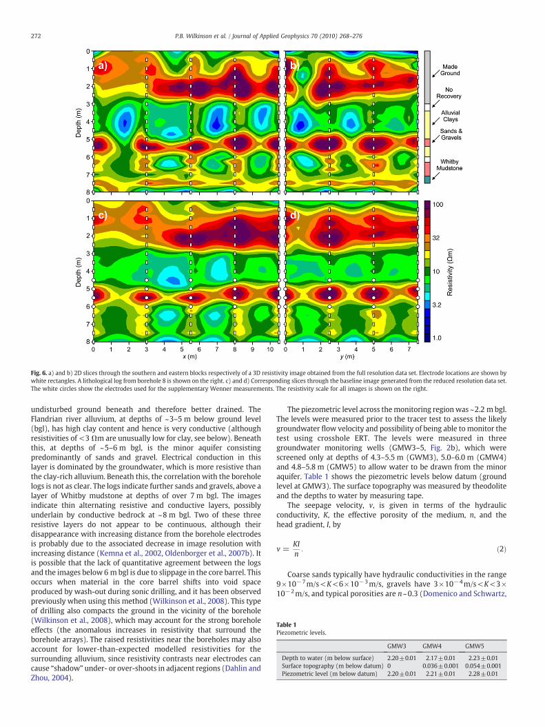
Fig. 6. a) and b) 2D slices through the southern and eastern blocks respectively of a 3D resistivity image obtained from the full resolution data set. Electrode locations are shown bywhite rectangles. A lithological log from borehole 8 is shown on the right. c) and d) Corresponding slices through the baseline image generated from the reduced resolution data set.The white circles show the electrodes used for the supplementary Wenner measurements. The resistivity scale for all images is shown on the right.

Table 1Piezometric levels.

GMW3 GMW4 GMW5

Depth to water (m below surface) 2.20±0.01 2.17±0.01 2.23±0.01Surface topography (m below datum) 0 0.036±0.001 0.054±0.001Piezometric level (m below datum) 2.20±0.01 2.21±0.01 2.28±0.01

272 P.B. Wilkinson et al. / Journal of Applied Geophysics 70 (2010) 268–276

undisturbed ground beneath and therefore better drained. TheFlandrian river alluvium, at depths of ~3–5 m below ground level(bgl), has high clay content and hence is very conductive (althoughresistivities of <3 Ωm are unusually low for clay, see below). Beneaththis, at depths of ~5–6 m bgl, is the minor aquifer consistingpredominantly of sands and gravel. Electrical conduction in thislayer is dominated by the groundwater, which is more resistive thanthe clay-rich alluvium. Beneath this, the correlation with the boreholelogs is not as clear. The logs indicate further sands and gravels, above alayer of Whitby mudstone at depths of over 7 m bgl. The imagesindicate thin alternating resistive and conductive layers, possiblyunderlain by conductive bedrock at ~8 m bgl. Two of these threeresistive layers do not appear to be continuous, although theirdisappearance with increasing distance from the borehole electrodesis probably due to the associated decrease in image resolution withincreasing distance (Kemna et al., 2002, Oldenborger et al., 2007b). Itis possible that the lack of quantitative agreement between the logsand the images below 6 m bgl is due to slippage in the core barrel. Thisoccurs when material in the core barrel shifts into void spaceproduced by wash-out during sonic drilling, and it has been observedpreviously when using this method (Wilkinson et al., 2008). This typeof drilling also compacts the ground in the vicinity of the borehole(Wilkinson et al., 2008), which may account for the strong boreholeeffects (the anomalous increases in resistivity that surround theborehole arrays). The raised resistivities near the boreholes may alsoaccount for lower-than-expected modelled resistivities for thesurrounding alluvium, since resistivity contrasts near electrodes cancause “shadow” under- or over-shoots in adjacent regions (Dahlin andZhou, 2004).

The piezometric level across themonitoring regionwas ~2.2 m bgl.The levels were measured prior to the tracer test to assess the likelygroundwater flow velocity and possibility of being able to monitor thetest using crosshole ERT. The levels were measured in threegroundwater monitoring wells (GMW3–5, Fig. 2b), which werescreened only at depths of 4.3–5.5 m (GWM3), 5.0–6.0 m (GMW4)and 4.8–5.8 m (GMW5) to allow water to be drawn from the minoraquifer. Table 1 shows the piezometric levels below datum (groundlevel at GMW3). The surface topography was measured by theodoliteand the depths to water by measuring tape.

The seepage velocity, v, is given in terms of the hydraulicconductivity, K, the effective porosity of the medium, n, and thehead gradient, I, by

v =KIn: ð2Þ

Coarse sands typically have hydraulic conductivities in the range9×10−7m/s<K<6×10−3m/s, gravels have 3×10−4m/s<K<3×10−2m/s, and typical porosities are n~0.3 (Domenico and Schwartz,

273P.B. Wilkinson et al. / Journal of Applied Geophysics 70 (2010) 268–276

1998). For the sand and gravel minor aquifer, it is reasonable to takethe lower bound for gravel ofK=3×10−4m/s,which overlapswith therange for sand, to obtain an estimated seepage velocity of v~0.5 m/daybetween GMW4 and GMW5 (a distance of 14.0 m approximately inthe −x direction). By comparison the estimated velocity betweenGMW3 and GMW4, approximately in the −y direction, is negligible(~0.04 m/day).

When monitoring dynamic processes using geoelectrical imagingthere is an implicit assumption that the data are collected simulta-neously. This assumption is reasonable if the characteristic timescalesof the processes being monitored are significantly longer than thetime required to collect the data. But if the processes are more rapid,so that significant changes can occur during data collection, then theresulting image can exhibit blurring and poor convergence with themeasured data. The piezometric levels suggested that a tracer injectedinto the aquifer via GMW4 should flow almost directly towardsGMW5, i.e. roughly antiparallel to the x-axis. Since the seepagevelocity in this direction would be ~0.5 m/day, the tracer wouldadvance by ~2 model cells/day. To avoid temporal blurring a shortermonitoring period was required than was used in the post-remediation monitoring (τ=2 days). To reduce the period, onlyoffsets of s=0 were used and reciprocal measurements were notmade, giving a total of 4,689 apparent resistivity data for each imageand reducing the measurement time to 1.7 h. During this time, thetracer would have been expected to move by <0.15 model cells,significantly reducing any time-lapse blurring.

Fig. 7. Wenner apparent resistivity breakthrough curves as a function of time t after injecfeatures affect three of the breakthrough curves (indicated by small vertical arrows).

The total monitoring period was τ=4 h, which allowed time forthe batteries to recharge and data to be inverted (the southern andeastern blocks took 25 and 18 min to invert respectively on a 2.4 GHzdual core processor). The effects of reducing the data density can beseen in Fig. 6c and d, which show the baseline resistivity model for thetracer test that was obtained in October 2008, 18 h prior to injection.The inversions converged after 7 iterations with mean absolute misfiterrors of 1.9% for the both the southern and eastern blocks. There is areduction in contrast in the baseline image in comparison with Fig. 6aand b, and the lack of non-zero vertical offsets appears to havereduced the lateral resolution. However, the layered structure of theimage is still evident, and most of the lateral structure can still bediscerned, suggesting that it should be possible to track the lateralposition of the tracer front.

7. Tracer test and discussion

A strong saline tracer (1000 l, at a concentration of 40 g/l) wasreleased into the aquifer via GMW4 to investigate the local groundwaterflow velocity and to demonstrate rapid ERT monitoring of naturalattenuation processes. A high concentration was used to give a goodresistivity contrast. Density driven flowwas assumed to be insignificantdue to the underlying aquiclude. This investigation was beyond theoriginal scope of the project, so there were no resources for repeatedgroundwater monitoring on the timescales required by the expectedspeed of the tracer, and no loggerwas available that could be installed in

tion. The resistivity minima are indicated by large diagonal arrows. Small anomalous

Table 2Breakthrough curve tracer speeds.

Distance from GMW4(m)

Apparent resistivity minimum(days)

Speed(m/day)

3.24 5.5 0.595.55 17.5 0.327.95 18 0.4411.34 25.5 0.44

274 P.B. Wilkinson et al. / Journal of Applied Geophysics 70 (2010) 268–276

the groundwater monitoring wells. Instead, an extra set of resistivitydatawas taken during each 4-hour period. These comprised unit spacedWenner apparent resistivity measurements taken on each individualelectrode array. These were centred vertically on the aquifer and usedthe electrodes shown as white circles in Fig. 6c and d. Since these datawere not used in the inversion, they could be used to plot independentbreakthrough curves, the resistivity of which would decrease/increaseas the local salinity of the aquifer increased/decreased (although thedependence would not be directly proportional, since the sensitivitydistribution of the Wenner distribution extends beyond its upper andlower electrodes).

An environmental risk assessment was carried out to obtainpermission to undertake the test from the Environment Agency andthe local government authority. This indicated that the tracer shouldbe injected at a moderate rate to minimise the risk of mobilisingresidual contamination by flushing. Therefore the tracer was releasedat a steady rate of ~4 l/min, taking just over 4 h to release 1000 l intothe aquifer. Resistivity data were collected continuously from the timeof the initial release. The Wenner apparent resistivity breakthroughcurves are shown in Fig. 7. The curves are shown at distances in the x

Fig. 8. Horizontal (above) and vertical (below) slices through the southern blocks of the 3normalised to the baseline image in Fig. 6c. Light blue crosses indicate the locations of the

direction of 0, 2.5, 5, 7.5 and 10.5 m (arrays 4, 5, 6, 7, and 14respectively). The curve for array 2 (5 m separation in the y direction)is also shown. For arrays 5, 6 and 14, there are small anomalousfeatures in the breakthrough curves at t~24 days after injection(indicated by small vertical arrows in Fig. 7). The source of these is notknown, although they occur more strongly in other breakthroughcurves that were not used (e.g. for array 8, the resistivity increase dueto this feature has the same magnitude as the decrease due to thesaline front and takes several days to decay, obscuring the resistivityminimum). Assuming the arrival time is shown by the arrowedresistivity minima, the mean tracer velocity is v=0.45±0.06 m/day(see Table 2), which is in good agreement with the value estimatedfrom the piezometric levels.

The spatial distribution of the saline tracer can be seen clearly inthe results of the ERT monitoring, which are shown in Fig. 8. Inversemodels were generated from the monitoring data every four hoursalthough, for the sake of conciseness, only representative images aredisplayed. While not obvious from this limited number of images, it isworth stressing that the evolution of the conductive region is smoothand continuous at the four-hour timescale. Each image shown in Fig. 8was generated from the data set taken between 18:00 and 20:00 h onthe indicated day. For day 0, this was 2 h after the end of the tracerrelease. Due to the low levels of noise, the inversions were performedwithout time-lapse constraints and directly on separate data sets,rather than on differences between subsequent sets. In thesecircumstances, use of the background image as a starting model isnot necessary (Miller et al., 2008). The mean absolute misfit errors forthe models are all in the range 1.8%–1.9%. The images are displayednormalised to the baseline model shown in Fig. 6c, since this reducesthe strong borehole effects that are clearly visible in the baseline

D resistivity monitoring images at time t days after injection. The resistivity is shownmodel cells used to estimate tracer breakthrough times from the resistivity images.

Table 3Model resistivity tracer speeds.

Distance from GMW4 (m) Model resistivity minimum (days) Speed (m/day)

3.37 5 0.675.64 16 0.358.09 19 0.4311.20 23 0.49

275P.B. Wilkinson et al. / Journal of Applied Geophysics 70 (2010) 268–276

model (Slater et al., 2000; Descloitres et al., 2008). Due to thenormalisation, regions that have become more conductive are shownas resistivity ratios <1. Only the southern block is displayed, sincealong the eastern block the tracer migration is observed to stop aty=3.5 m. The upper (horizontal) slices are at a depth of 5.375 mbgl, the lower (vertical) slices are at y=1.375 m.

The ERT images show the appearance and evolution of aconductive region between depths of ~5–6 m bgl. The extent andintensity of this conductive region can be seen to vary considerably onthe scale of several days. Only small changes in resistivity occurred atthese depths over timescales of several months during post-remediation monitoring. Hence, it is reasonable to assume that anyincreases in conductivity are caused by increases in salinity due to thepresence of the tracer. Therefore the changes in the images allow thedistribution and density of the tracer to be visualised directly in 4D.They indicate that the tracer is predominantly localised in a horizontalaquifer that is reasonably uniform and approximately 1 m thickthroughout the model space. The absence of conductivity increasesabove 5 m bgl implies that there is little upward migration of thetracer through fissures in the clay, and that the aquifer is reasonablywell confined. There is some evidence that at t=0 a fraction of thetracer escaped from the injection borehole, suggesting that either thebase or the sides of GMW4 are not perfectly sealed. By contrast, thereappear to be no losses from the electrode array boreholes, which givesconfidence that no pollution pathways were created during the arrayinstallations.

The changes in the extent of the conductive region suggest that themajority of the tracer was carried along the piezometric gradient inthe −x direction. The tracer speed can be estimated from the modelsby finding the time of minimum resistivity at the points marked bylight blue crosses in Fig. 8. The resistivities were calculated as theaverage of all model cells immediately adjacent to each cross. Usingthis method the mean tracer speed was found to be v=0.49±0.07 m/day (see Table 3), in good agreement with the estimatederived from theWenner breakthrough curves. There is also evidencethat there may be some tracer movement along the y axis. Initiallymotion in this direction seems to have been dominated by dispersion.But comparison of the horizontal slices in Fig. 8d, e and f suggests thatthe tracer has since begun to move towards −y, indicating a smallseepage velocity component in this direction.

In addition to the large resistivity decreases observed in theaquifer layer, there are localised increases in resistivity of much lowermagnitude in the made ground at depths of ~1–2 m. Similar changesin the made ground resistivity were observed during post-remedia-tion monitoring, and were found to be strongly anticorrelated withthe average air temperature over the previous 7 days. A tentativeexplanation for this effect is that increases in pore water resistivity inthe made ground are caused by decreases in the received solarradiation, since the black tarmac surface above the made ground has alow albedo (Thompson, 1998).

8. Conclusions

The CLARET project has provided useful experience for thegeoelectrical monitoring of contaminated land and remediationprocesses. It has shown that an electrode network can be installedin parallel with remedial works and in accordance with site and

environmental regulations. The installation method was demonstrat-ed to produce good electrical contact with the ground and excellentdata quality. The ERT images generated from the data were generallyin good agreement with the site lithology derived from core logging,providing useful complementary information where there wasinconsistency in the recovered depths to interfaces.

The capabilities of geoelectrical monitoring were demonstrated bya saline tracer test. Using measurement sequences designed for rapiddata acquisition, the volumetric images permitted the evolution of thetracer to be visualised directly throughout the entire monitoringvolume in near real-time. Apparent resistivity breakthrough curveswere measured independently of the imaging data on each electrodearray. Quantitative estimates of seepage velocity derived from theimages and the breakthrough curves were found to be in goodagreement, and also agreed with estimates based on measuredpiezometric gradients and assumed hydrogeological parameters.

The tracer test has demonstrated that contaminants affecting theelectrical resistivity of the subsurface can be tracked andmonitored atfield-scale in near real-time, on timescales of hours upwards. Byenabling the direct observation of dispersion and dilution processes,this test has shown that geoelectrical monitoring of remediation isdirectly applicable to sites where remediation is being undertaken bymonitored natural attenuation. However, there is no reason why theconcept should not be equally applicable to most other in-situ reme-diation techniques operating on similar timescales. In combinationwith calibration from intrusive sampling and resistivity-concentrationrelations that can be corrected for variable image resolution (Singhaand Gorelick, 2006), time-lapse ERT has the potential to provide directquantitative volumetric imaging of remediation processes.

Acknowledgements

This paper is published with the permission of the ExecutiveDirector of the British Geological Survey (NERC). The research wasfunded by a grant from the Technology Strategy Board (www.innovateuk.org; project TP/5/CON/6/I/H0048B) and contributionsfrom a consortium partnership comprising VHE Construction Plc,Interkonsult Ltd and South Kesteven District Council. We are gratefulto Dr R.A. White of BGS for undertaking the environmental riskassessment for the tracer test. We also thank the editor Prof. AlanGreen and two anonymous reviewers for their helpful comments onour original manuscript.

References

Bing, Z., Greenhalgh, S.A., 2000. Cross-hole resistivity tomography using differentelectrode configurations. Geophysical Prospecting 48, 887–912.

Binley, A., Cassiani, G., Middleton, R., Winship, P., 2002. Vadose zone flow modelparameterisation using cross-borehole radar and resistivity imaging. Journal ofHydrology 267, 147–159.

Cassiani, G., Bruno, V., Villa, A., Fusi, N., Binley, A.M., 2006. A saline trace test monitoredvia time-lapse surface electrical resistivity tomography. Journal of AppliedGeophysics 59, 244–259.

Dahlin, T., Zhou, B., 2004. A numerical comparison of 2D resistivity imaging with 10electrode arrays. Geophysical Prospecting 52, 379–398.

Daily, W., Ramirez, A., 1995. Electrical resistance tomography during in-situtrichloroethylene remediation at the Savannah River Site. Journal of AppliedGeophysics 33, 239–249.

Daily, W., Ramirez, A., 2000. Electrical imaging of engineered hydraulic barriers.Geophysics 65, 83–94.

Daily, W., Ramirez, A., Labrecque, D., Nitao, J., 1992. Electrical-resistivity tomography ofvadose water-movement. Water Resources Research 28, 1429–1442.

Deiana, R., Cassiani, G., Kemna, A., Villa, A., Bruno, V., Bagliani, A., 2007. An experimentof non-invasive characterization of the vadose zone via water injection and cross-hole time-lapse geophysical monitoring. Near Surface Geophysics 5, 183–194.

Descloitres, M., Ribolzi, O., Le Troquer, Y., Thiébaux, J.P., 2008. Study of water tensiondifferences in heterogeneous sandy soils using surface ERT. Journal of AppliedGeophysics 64, 83–98.

Domenico, P.A., Schwartz, F.W., 1998. Physical and Chemical Hydrogeology. 506 pp.Guerin, R., Munoz, M.L., Aran, C., Laperrelle, C., Hidra, M., Drouart, E., Grellier, S., 2004.

Leachate recirculation: moisture content assessment by means of a geophysicaltechnique. Waste Management 24, 785–794.

276 P.B. Wilkinson et al. / Journal of Applied Geophysics 70 (2010) 268–276

Halihan, T., Paxton, S., Graham, I., Fenstemakerb, T., Rileya, M., 2005. Post- remediationevaluationof a LNAPL siteusingelectrical resistivity imaging. Journal of EnvironmentalMonitoring 7, 283–287.

Kemna, A., Vanderborght, J., Kulessa, B., Vereecken, H., 2002. Imaging and characterisa-tion of subsurface solute transport using electrical resistivity tomography (ERT)and equivalent transport models. Journal of Hydrology 267, 125–146.

Kuras, O., Pritchard, J., Meldrum, P.I., Chambers, J.E., Wilkinson, P.B., Ogilvy, R.D.,Wealthall, G.P., 2009. Monitoring hydraulic processes with Automated time-LapseElectrical Resistivity Tomography (ALERT). Comptes Rendus Geosciences - SpecialIssue on Hydrogeophysics 341, 868–885.

LaBrecque, D.J., Ramirez, A.I., Daily, W.D., Binley, A.M., Schima, S.A., 1996. ERTmonitoring of environmental remediation processes. Measurement Science andTechnology 7, 375–383.

Looms, M.C., Jensen, K.H., Binley, A., Nielsen, L., 2008. Monitoring unsaturated flow andtransport using cross-borehole geophysical methods. Vadose Zone Journal 7,227–237.

Miller, C.R., Routh, P.S., Brosten, T.R., McNamare, J.P., 2008. Application of time-lapseERT imaging to watershed characterization. Geophysics 73, G7–G17.

Nimmer, R.E., Osiensky, J.L., Binley, A.M., Sprenke, K.F., Williams, B.C., 2007. Electricalresistivity imaging of conductive plume dilution in fractured rock. HydrogeologyJournal 5, 877–890.

Nimmer, R.E., Osiensky, J.L., Binley, A.M.,Williams, B.C., 2008. Three-dimensional effectscausing artifacts in two-dimensional, cross-borehole, electrical imaging. Journal ofHydrology 359, 59–70.

Ogilvy, R.D., Kuras, O., Meldrum, P.I., Wilkinson, P.B., Gisbert, J., Jorreto, S., Pulido-Bosch,A., Kemna, A., Nguyen, F., Tsourlos, P., 2007. Automated monitoring of coastalaquifers with electrical resistivity tomography. In: Pulido Bosch, A., López-Geta, J.A.,Ramos González, G. (Eds.), Coastal Aquifers: Challenges and Solutions. InstitutoGeológico y Minero de España, Madrid, pp. 333–342.

Ogilvy, R.D., Meldrum, P.I., Kuras, O., Wilkinson, P.B., Chambers, J.E., 2008. Advances inGeoelectric Imaging Technologies for theMeasurement andMonitoring of ComplexEarth Systems and Processes. Invited keynote paper in Proceedings 33rdInternational Geological Congress, Oslo, Norway, 10–14 August 2008.

Oldenborger, G.A., Knoll, M.D., Routh, P.S., LaBrecque, D.J., 2007a. Time-lapse ERTmonitoring of an injection/withdrawal experiment in a shallow unconfinedaquifer. Geophysics 72, F177–F187.

Oldenborger, G.A., Partha, S.R., Knoll, M.D., 2007b. Model reliability for 3D electricalresistivity tomography: application of the volume of investigation index to a time-lapse monitoring experiment. Geophysics 72, F167–F175.

Parasnis, D.S., 1988. Reciprocity theorems in geoelectric and geoelectromagnetic work.Geoexploration 25, 177–198.

Sandberg, S.K., Slater, L.D., Versteeg, R., 2002. An integrated geophysical investigation ofthe hydrogeology of an anisotropic unconfined aquifer. Journal of Hydrology 267,227–243.

Shevnin, V., Delgado Rodríguez, O., Mousatov, A., Flores Hernández, D., ZegarraMartínez, H., Ryjov, A., 2006. Estimation of soil petrophysical parameters fromresistivity data: application to oil-contaminated site characterization. GeofísicaInternacional 45, 179–193.

Singha, K., Gorelick, S.M., 2005. Saline tracer visualized with three-dimensionalelectrical resistivity tomography: field-scale spatial moment analysis. WaterResources Research 41, W05023.

Singha, K., Gorelick, S.M., 2006. Hydrogeophysical tracking of three-dimensional tracermigration: the concept and application of apparent petrophysical relations. WaterResources Research 42, W06422.

Slater, L., Binley, A., 2003. Evaluation of permeable reactive barrier (PRB) integrity usingelectrical imaging methods. Geophysics 68, 911–921.

Slater, L., Sandberg, S., 2000. Resistivity and induced polarization monitoring ofsalttransport under natural hydraulic gradients. Geophysics 65, 408–420.

Slater, L.D., Binley, A., Brown, D., 1997. Electrical imaging of fractures using ground-water salinity change. Ground Water 35, 436–442.

Slater, L., Binley, A.M., Daily, W., Johnson, R., 2000. Cross-hole electrical imaging of acontrolled saline tracer injection. Journal of Applied Geophysics 44, 85–102.

Thompson, R.D., 1998. Atmospheric Processes and Systems. Routledge. 194 pp.Vanderborght, J., Kemna, A., Hardelauf, H., Vereecken, H., 2005. Potential of electrical

resistivity tomography to infer aquifer transport characteristics from tracer studies:a synthetic case study. Water Resources Research 41, W06013.

Wilkinson, P.B., Chambers, J.E., Meldrum, P.I., Ogilvy, R.D., Caunt, S., 2006. Optimizationof array configurations and panel combinations for the detection and imaging ofabandoned mineshafts using 3D cross-hole electrical resistivity tomography.Journal of Environmental and Engineering Geophysics 11, 213–221.

Wilkinson, P.B., Chambers, J.E., Lelliot, M., Wealthall, G.P., Ogilvy, R.D., 2008. Extremesensitivity of crosshole electrical resistivity tomography measurements togeometric errors. Geophysical Journal International 173, 49–62.

Zhou, B., Dahlin, T., 2003. Properties and effects of measurement errors on 2D resistivityimaging. Near Surface Geophysics 1, 105–117.