The vibrational modes of spheroidal cavities in elastic solids

Scholars' Mine Scholars' Mine

Doctoral Dissertations Student Theses and Dissertations

1971

The vibrational modes of spheroidal cavities in elastic solids The vibrational modes of spheroidal cavities in elastic solids

David Stewart

Follow this and additional works at: https://scholarsmine.mst.edu/doctoral_dissertations

Part of the Geophysics and Seismology Commons

Department: Geosciences and Geological and Petroleum Engineering Department: Geosciences and Geological and Petroleum Engineering

Recommended Citation Recommended Citation Stewart, David, "The vibrational modes of spheroidal cavities in elastic solids" (1971). Doctoral Dissertations. 2310. https://scholarsmine.mst.edu/doctoral_dissertations/2310

This thesis is brought to you by Scholars' Mine, a service of the Missouri S&T Library and Learning Resources. This work is protected by U. S. Copyright Law. Unauthorized use including reproduction for redistribution requires the permission of the copyright holder. For more information, please contact [email protected].

https://library.mst.edu/

https://library.mst.edu/

https://scholarsmine.mst.edu/

https://scholarsmine.mst.edu/doctoral_dissertations

https://scholarsmine.mst.edu/student-tds

https://scholarsmine.mst.edu/doctoral_dissertations?utm_source=scholarsmine.mst.edu%2Fdoctoral_dissertations%2F2310&utm_medium=PDF&utm_campaign=PDFCoverPages

http://network.bepress.com/hgg/discipline/158?utm_source=scholarsmine.mst.edu%2Fdoctoral_dissertations%2F2310&utm_medium=PDF&utm_campaign=PDFCoverPages

https://scholarsmine.mst.edu/doctoral_dissertations/2310?utm_source=scholarsmine.mst.edu%2Fdoctoral_dissertations%2F2310&utm_medium=PDF&utm_campaign=PDFCoverPages

mailto:[email protected]

THE VIBRATIONAL MODES OF SPHEROIDAL CAVITIES

IN ELASTIC SOLIDS

by

DAVID MACK STEWART , 1937-

A DISSERTATION

P~esented to the Faculty of the G~aduate School of the

UNIVERSITY OF MISSOURI - ROLLA

In Pa~tial Fulfillment of the Requirements for the Degree

DOCTOR OF PHILOSOPHY

in

GEOPHYSICS

1971

Advisor

ABSTRACT

A general analysis of all possible cavity shapes is glven with a

discussion of the mathematical difficulties involved for the various

ll

cases. Special emphasis is given to cavity shapes describable in terms

of the coordinate surfaces of coordinate systems separating the scalar

wave equation. 112 such shapes are identified and discussed. Free

boundary condition equations for spheres and spheroids are derived ln

complete generality in terms of potentials. The difference ln the

vibrations of a solid and those of a cavity of the same shape is dis-

cussed and made clear. The impossibility of deriving a frequency

equation for uniform radial vibrations of spherical cavities as a

function of cavity size, alone, is proven. frequency equations are

derived for the standing waves between a plane free surface and

radially vibrating cavities of spherical and spheroidal shapes. The

frequency spectrum, for this mode of vibration, is shown to be a

function of cavity size, shape, depth, and orientation.

are given for further research in cavity resonance.

Suggestions

lll

ACKNOWLEDGEMENTS

My most genuine appreciation goes to Dr. Richard D. Rechtien, my

graduate advisor, for his inspiration, patience, understanding, and help,

material, moral and academic, over the past four years. His advice and

guidance over tt1e years have proven lo be consistently good. It was a

stroke of considerable good fortune to have had such an advisor. Very

special appreciation must also go to a fellow student and PhD candidate,

Jerry Davis, without whom this dissertation would have been considerably

less. Our countless hours of thought and discussion together on academic

subjects constitutes one of the principal and most valuable elements of

my graduate education. And finally, a very large share of the credit for

this dissertation must be given to my children and to my wife, Lee, who

constitute the chief source of happiness in my life and whose pleasant

an<l upli~ling company create an ideal environment from which to study

and produce a work such as this.

TABLE OF CONTENTS

ABSTRACT . . . . .

ACKNOWLEDGEMENTS

LIST OF FIGURES

LIST OF TABLES

NOMENCLATURE

INTRODUCTION . . . . . . . . . .

CHAPTER I

AN ANALYSIS OF POSSIBLE CAVITY SHAPES .

Quadric Cavity Shapes

Cavity Shapes Not Corresponding to Quadric Surfaces

Literature Review

CHAPTER II

fREE VIBRATIONS OF SPHERICAL AND SPHEROIDAL CAVITIES

iv

Page

ll

Lll

Vlll

lX

X

1

5

6

29

30

33

l'ree Boundary Conditions and How to Obtain Frequency Lquatiom; 34

General Equations for Spheroids

(Free Boundary Condition Equations for Spheroids)

General Equations for Spheres

(free Boundary Condition Equations for Spheres)

The Difference ln the Solid Problem and the Cavity Problem

Matching Mode.s to l'requencies

The Double-Aught-Radial (DAR) Mode

37

38

39

41

42

44

48

v

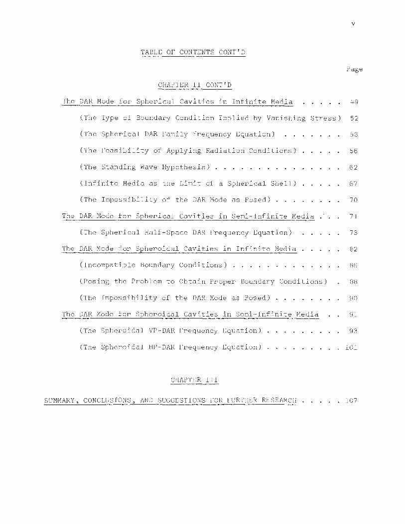
TABLE OF CONTENTS CONT'D

Page

CHAPTER II CONT'D

The DAR Mode for Spherical Cavities in Infinite Media 49

(The Type of Boundary Condition Implied by Vanishing Stress) 52

(The Spherical DAR Family Frequency Equation) 53

(The Feasibility of Applying Radiation Conditions) 56

(The Standing Wave Hypothesis) . . 62

(Infinite Media as the Limit of a Spherical Shell) 67

(The Impossibility of the DAR Mode as Posed) . . 70

The DAR Mode for Spherical Cavities in Semi-Infinite Media 71

(The Spherical Half-Space DAR Frequency Equation) 73

The DAR Mode for Spheroidal Cavities in Infinite Media 82

(Incompatible Boundary Conditions) . 86

(Posing the Problem to Obtain Proper Boundary Conditions) 88

(The Impossibility of the DAR Mode as Posed) . . 90

The DAR Mode for Spheroidal Cavities in Semi-Infinite Media 91

(The Spheroidal VP-DAR Frequency Equation)

(The Spheroidal HP-DAR Frequency Equation)

CHAPTER III

SUMMA.K.Y, CONCLUSIONS, AND SUGGESTIONS FOR FURTHER RESEARCH .

93

101

. 107


APPENDICES

A. NOTATION

B. SPHERICAL COORDINATES

l. Definitions 2. Base Vectors 3. Metric Tensors 4. Scale Factors 5. Representation of Absolute Vectors 6. Vector Operators .. 7. Christoffel Symbols

C. THE DISPLACEMENT VECTOR IN SPHERICAL COORDINATES

1. Displacement in Terms of Potentials 2. Physical, Covariant, and Contravariant Components 3. Ordinary Partial Derivatives of Displacements 4. Covariant Partial Derivatives of Displacements

D. INFINITESMAL STRAIN IN SPHERICAL COORDINATES

1. Covariant Components of Strain 2. Physical Components of Strain

E. STRESS ON THE SURFACE OF A SPHERE

1. Stress ln Terms of Strain 2. Stress ln Terms of Displacement 3. Stress ln Terms of Potentials

f. THE SCALAR WAVE EQUATION IN SPHERICAL COORDINATES

vi

Page

111

112

115

116 118 121

. 123 125 126 128

130

131 133 135 137

139

140 142

143

144 146 147

148

1. The Separated Solution in Spherical Coordinates 149 2. Spherical Bessel functions . . . . . . . . . 151 3. Derivatives of Associated Legendre Functions 154 4. Sine-Cosine Expressions for Spherical Bessel runctions 155

G. SPHEROIDAL COORDINATES 159

1. Definitions 160 2. Relations Between Spherical and Spheroidal Coordinates 166 3. Base Vectors . Hi7 4. Metric Tensors 110 5. Scale Factors 171 6. Representation of Absolute Vectors 172 7. Vector Operators 173 8. Christoffel Symbols 176


APPENDICES CONT'D

H. THE DISPLACEMENT VECTOR IN SPHEROIDAL COORDINATES ..

1. Displacement in Terms of Potentials ...... . 2. Physical, Covariant, and Contravariant Components 3. Ordinary Partial Derivatives of Displacements . 4. Covariant Partial Derivatives of Displacements

I. INFINITESMAL STRAIN IN SPHEROIDAL COORDINATES

1. Covariant Components of Strain 2. Physical Components of Strain .

J. STRESS ON THE SURFACE OF A SPHEROID

1. Stress ln Terms of Strain ... 2. Stress in Terms of Displacement 3. Stress ln Terms of Potentials .

K. THE SCALAR WAVE EQUATION IN SPHEROIDAL COORDINATES

1. The Separated Solution in Spheroidal Coordinates 2. Spheroidal Wave Functions

L. HELMHOLTZ'S THEOREM

M. GENERATING CURVES AND DESCRIPTIVE TERMINOLOGY FOR QUADRIC CAVITIES

BIBLIOGRAPHY

VITA

Vll

Page

177

178 180 182 184

186

187 188

189

190 191 192

194

195 197

202

205

222

229

viii

LIST OF FIGURES

Figures Page

I. COORDINATE GEOMETRY FOR A SPHERICAL CAVITY IN A HALF-SPACE . 72

lX

LIST OF TABLES

Tables Page

I. COORDINATE SURFACES OF QUADRIC SYSTEMS 7

II. QUADRIC SURFACES OF QUADRIC COORDINATE SYSTEMS 9

III. CLASSIFICATION OF QUADRIC SYSTEMS BY NUMBER OF COORDINATE PARAMETERS 12

IV. QUADRIC CAVITY SHAPES 16

V. CLASSES OF QUADRIC CAVITY SHAPES 20

VI. QUADRIC CAVITY SHAPES RANKED BY COMPLEXITY FACTORS 23

VII. FIELD DATA ON TWO CYLINDRICAL CAVITIES IN BASALT . 80

A' A I

a

a, a'

a ( h j mQ) n

(X

B' B I

b

D, b I

b , b (h 1 oo > n n

X

NOMENCLATURE

Arbitrary constants (see Equations (15, 58 & 82)).

Eigenvalues encountered when the scalar wave equation

is separated in spheroidal coordinates (see

Appendix K2).

An abbreviation for the expression, ~~ 2 + 1 (see

Appendix Gl).

The real and imaginary parts of A (see Equation (40)).

Expansion coefficients encountered with spheroidal

radial wave functions of the first kind (see

Appendix K2).

The point on the free plane surface, z = z 0 , directly

above the apex of a spherical cavity (see l'igure I).

The velocity of a plane longitudinal elastic wave

defined by a 2 = (\+2u)/p (see Appendix Fl or Kl); or

the semi-major axis of an ellipse or spheroid defined

by a 2 = c 2 + 8 2 (see Appendix Gl).

Arbitrary constants (see Equations (15, 58 & 82)).

An abbreviation for the expression, ~1 - n 2

Appendix Gl).

(see

The real and imaginary parts of B (see Equation (40)).

Expansion coefficients encountered with spheroidal

radial wave functions of the second kind (see Appendix

K2).

The velocity of a plane shear elastic wave defined by

S2 = u/p (see Appendix Fl or Kl); or the semi-minor

aXlS of an ellipse or spheroid defined by S2 = a 2 - c 2

(see Appendix Gl).

c

c.,c.(90

) l ]_

c

X

D c

D m

D s

DAR

v

Xl

NOMENCLATURE CONT'D

The number of coordinates required by a quadric cavity

shape: C = 1, 2, or 3 (see Table IV).

The ith value for kr 0 ln a spectrum of such values

(see Equation (64)).

The focal distance of an ellipse, ellipsoid, spheroid,

hyperbola, or hyperboloid defined either by

c 2 = a 2 - s2 or c 2 = y 2 + 6 2 ; and the coordinate

parameter ot spheroidal coordinates (see Appendix Gl).

A constant of index, k, defining a coordinate

surface (see Table I).

The scalar wave equation propagation constant which

can take on either the value, a or B (see Appendix

l'l or Kl).

The diameter oi a spherical cavity (see l:quation ( 61+)).

A calculated diameter for a cylinder (see Table VII).

A measured diameter (see Table VII).

A calculated diameter for a spherical cavity irom

Equation (53) ( c~ee Table Vl I).

"Double-Aught-Radjal"

Expdnsion coefficients encountered with sphero_iddJ

angular wave ±unctions oi the first kind (see

Appendix K2).

The vector dii fer'ential operator, del (see Appendix B6).

The semiconjugate axl_s of a hyperboloid dciined by 0 ~ ?

c~"-= c'- y· (see Appendix Cl).

k 6 m

E(n)

e

k£m e

k£m E

f. l

f l

NOMENCLATURE CONT'D

The Kronecker delta (see Appendix El).

A separated n-solution to the scalar wave equation

(see Appendix Kl).

Xll

An abbreviation for the expression, ~~ 2 + n2 (see

Appendix Gl); or the base of the natural logarithm,

e = 2.71828 (see Appendix Fl or Kl).

A unit base vector in the direction of the positive

k-coordinate (see Appendix B2 or G3).

Covariant and physical components of the infinitesmal

strain tensor (see Appendix (Dl or Il).

The permutation symbol (see Appendix B6).

The eccentricity of a spheroid defined by E = c/a

(see Appendix Gl).

The contravariant epsilon symbol (see Appendix B6).

The ith value of frequency ln a spetrum oi frequencies


The fundamental frequency (see Equation (65)).

A function of R0 , the outer radius of a spherical

shell (see Equation (48)).

The scalar displacement potential (see Appendices Cl,

Hl, and L).

A time independent scalar displacement potential

(see Equations (10)).

km gkm' g

y

H n

HP

xiii

NOMENCLATURE CONT'D

The equatorial angle coordinate in circular cylinder,

spherical, parabolic, prolate spheroidal, and oblate

spheroidal coordinate systems (see Table I and

Appendices Bl and ca).

A vertical half plane with the z-axis as the edge

(see Appendix Gl)

Covariant and contravariant curvilinear base vectors

(see Appendices R2 and G3).

The metric tensor (see Appendix B3).

Covariant and contravariant components of the metric

tensor (see Appendix B3 or G4).

The ratio of seismic velocities, a/8 (see Equation

(19)); or the semitransverse axis at a hyperboloid

defined by y 2 = c 2 - 6 2 (see Appendix Gl).

Series coefficients in the HP-DAR frequency equation

(see Equations (109-114)).

''Horizontal Pole"

The splwt'oidc~l wave number defined lJy h = ck whl'PC'

cis LhL' local length oi the ::_;phcl'oid dllU k i:; tlw

ordinary wave number (see Appendix Kl).

Covariant c1nd contravdr_iant ~;cale i actor:; (:A~lc

Appendix B4 or r;~).

sl'herical l'lcmk(;l lunctions ol the ith kind clTlci order

n (::oee Appvndix 1'2).

:;p!Hcroidal llankel functions of the i th kind and

order zero-zero (see Appendix K2).

n

I

i

l' j ' k

J' JCU

J 1 (kr) n+-

2

k

NOMENCLATURE CONT'D

A curvilinear coordinate of the conical, elliptic

cylinder, paraboloidal, prolate spheroidal, oblate

spheroidal, and ellipsoidal coordinate systems.

xiv

In the last three systems it is the x 2 coordinate

representing an ellipsoidal polar angle (see Table I

and Appendix Gl).

Dilatation (see Appendix El).

An index; or /-1

Rectangular base vectors.

Any spheroidal radial wave function (see Appendix K2).

A Bessel function of odd half-integer order and

parameter, k (see Appendix F2).

A spherical Bessel function of order, n (see Appendices

F2 and F4).

The spheroidal radial wave function of the first kind

of order m£ and parameter, h (see Appendix K2).

The spheroidal radial wave function of the first

kind of order zero-zero (see Equation (82)).

An index; or the ordinary wave number defined by

k = w/x (see Appendix Fl or Kl).

The Christoffel symbol of the second kind (see

Appendices B7 and GB).

The length of a vibrating string.

The ratio of cavity depth to cavity radius for spheri

cal cavities (see Equation (63)).

£ m

£, m, n

M

M, N

m

]J

n

w

p

p

NOMENCLATURE CONT'D

A measured value of £ 0 (see Table VII).

Separation constants of the scalar wave equation

(see Appendices Fl and Kl).

Lame's elastic constant associated with compres

sional stresses, vanishing identically for fluids.

A real constant (see Equation (44)).

Solutions of the vector Helmholtz equation (see

Appendices Cl and Hl).

An index; or an abbreviation for meters (see

Table VII).

Lame's elastic constant associated with both

compressional and shear stresses, but is the only

one associated with shear and is thus called the

shear modulus.

A summation index (see Equations

or just an index.

(95 & 108));

A solution of the scalar Helmholtz equation (see

Appendices Cl and Hl).

Angular frequency and separation constant between

time and space for the scalar wave equation (see

Appendix Fl or Kl).

XV

The number of coordinate parameters required by a

quadric cavity shape: P = 0, 1, or 2 (see Table IV).

The position vector (see Appendices Bl and Gl).

The associated Legendre function of the first kind

and order m, n (see Appendices Fl, F3, and K2).

If

R(r)

r

r m

p

s, S(n)

S, S(r,O,cjJ,t)

or S(E;,n,¢,t)

co I

n=O,l

XVl

NOMENCLATURE CONT'D

Pi = 3.14159

The outer radius of a spherical shell (see Equation

( 46)).

A separated r-solution to the scalar wave equation

(see Appendix Fl).

The x 1 or radial curvilinear coordinate of the

spherical and conical coordinate systems (see

Table I and Appendix Bl).

The boundary of a spherical cavity.

A measured radius (see Table VII).

Distances from the foci of a spheroid to its

boundary (see Appendix Gl).

Mass density; or the x 1 curvilinear coordinate

of the circular cylinder coordinate system (see

Table I and Appendix Gl).

Any spheroidal angular wave function (sec Appendix K2).

A separated solution of the scalar wave equation ln

spherical or spheroidal coordinates (see Appendices

F 1 and Kl).

The spheroidal angular wave function of the first

kind of order m£ and parameter, h (see Appendix K?).

Summation, where the prime indicates only over even

integers or odd integers depending upon whether n

begins at zero or one (see Appendix K2).

T

(TCP)

T( t)

t

t(km)

0 (G)

G

u

u

NOMENCLATURE CONT'D

The vector displacement potential (see Appendices

Cl, Hl, and L) .

Physical components of ~ (see Appendices C & H).

xvii

The total number of coordinate values and parameter

values required by a quadric cavity shape (see Table

IV).

The complexity factor of a quadric cavity shape (see

Table VI).

A separated t-solution of the scalar wave equation

(see Appendix Fl or Kl).

Time.

The stress vector across the kth coordinate surface

or across a plane at the point of tangency to the

kth coordinate surface (see Appendices El and Jl).

A physical component of the stress tensor and the

mth component of t(k) (see Appendices El and Jl).

A constant related to A (h) (see Appendix K2). m£

A separated G-solution to the scalar wave equation

(see Appendix Fl).

The spherical polar angle coordinate (see Table I

and Appendix Bl).

The displacement vector (see Appendices Cl and Ill).

The x 1 curvilinear coordinate of the parabolic

cylinder, parabolic, and paraboloidal coordinate

systems (see Table I).

v

v n

VP

v

X(t)

X

X, y, Z

l X

E,o

XVlll

NOMENCLATURE CONT'D

Covariant, contravariant, and physical components

of displacement, U (see Appendices B5, C2, C6 and H2).

The total number of coordinate values required by a

quadric cavity shape (see Table IV).

Expansion coefficients in the VP-DAR frequency

equation (see Equations (96-101)).

"Vertical Pole"

The x 2 curvilinear coordinate of parabolic cyJinder,

parabolic, and paraboloidal coordinate ::.;ysterns (:~ee

Table I).

A separated [,-solution of the scalar wave equation

(see Appendix Kl).

A free horizontal plane surface in a rotated rectan

gular system and center depth for a spheroidal

cavity whose polar axis is of horizontal orientation


The real part of kr0

(see Equatjon (30)).

Rectangular coordinates ln explicit notation.

General curvilinear coordinates ln index notation,

i = 1, 2, or 3 (see Appendix A).

A curvilinear coordinate of the conical, elliptic

cylinder, prolate spheroidal, oblate ::;phcroidal, and

ellipsoidal systems. In the last four it is the x 1

or radial coordinate (see Table l and Appendix Gl).

The boundary of a spheroidal cavity.

Y l(kr) n+-

2

y

y ' y (z) n n

z

l z

z m

NOMENCLATURE CONT'D

A Neumann (or Weber) function of odd half-integer

order and parameter, k (see Appendix f2).

The imaginary part of kr 0 (see Equation (30)).

A spherical neumann function of order, n (see

Appendices F2 and l:'4).

The spheroidal radial wave function of the second

kind of order zero-zero (see Equation (82)).

The vertical rectangular coordinate; a dummy

argument for j and y (see Appendix Fl+); or n n

the complex form for kr0 (see Lquation (30)).

A free horizontal surface and center depth for a

spherical or spheroidal cavity (see Figure I).

Rectangular coordinates in index notation (see

Appendix A).

A measured depth (see Table VII).

The eccentricity of a hyperboloid defined by G

(see Appendix Gl); or a solution to the scalar

Helmholtz equation (see Appendices Cl and Hl); or

the x 3 ellipsoidal coordinate (see Table I).

XlX

c/ Y

INTRODUCTION

Detecting and delineating subterranean cavities lS an unsolved

problem of geophysics. The need for such a geophysical technique

exists among a large variety of concerns. For example, engineers

choosing sites for dams, highways, bridges, or large buildings need

to know if the area under consideration is underlain by zones of

weakness such as cavities or sinks. Water pollution investigators

could use such a method to trace pollution spreading through old,

abandoned mines or natural cave systems. Agen~ies concerned with

groundwater flow and recharge need to be able to locate solution

channels in karst regions, lava tubes ln basaltic regions, and

buried river beds and gorges under till in glaciated regions. The

soluble mineral mining industry, salt in particular, is interested

in an effective way to measure the exact slze and location of their

huge solution cavities created by the removal of minerals hundreds

of feet beneath the surface by means of wells. The National Aero-

nautics and Space Administration has been interested in a simple

method of locating near surface cavities on extraterrestrial bodies

that could serve as living quarters for astronauts or as possible

sources of trozen water. The Atomic Energy Commission needs to

delineate the size, shape, and inclination of their large underground

cavities created by experimental nuclear blasts. The Department ot

Defense needs a simple, effective way to locate enemy tunnels. l~as,

1

2

oil, and water companies might use such a method to find and map

buried caverns for purposes of the storage of their products. Arch eo-

logists are searching for underground chamber tombs in Egypt and for

caves in the Middle East that might contain more historical treasures

such as the Dead Sea Scrolls. Volcanologists need a method to locate

and define the magma chambers beneath an active volcano. And although

it hardly needs mentioning, if such a method were developed that was

simple and inexpensive enough, speleologists and spelunkers would

certainly find it a boon.

The history of attempts to devise a workable geophysic;J.l technique

capable of detecting and delineating underground cavities from the

surface is less than ten years old in the literature. The stclte of

the art is barely in its infancy. Many approaches have been tried.

All have failed to a greater or lesser exter1t. None has been systema

tically studied, developed, and refined for the explicit application

to cavities. None, to date, satisfy all the desirable requirements,

namely, that the method be inexpensive, efficient, and aLJe, not onJy

to detect the presence of a subsurface cavity, but to determine,

accurately, its size, shape, depth, orientcltion, and whether it be

filled with air, water, mud, or something else. The seismic method

was tried by Love (1967), Watkins, Godson & Watson (1967), Ferland

(1969), Cook (1964 & 1965), and Godson & Watkins (1968). J:.:lectrical

resistivity was applied by Love (1967) and Haberjam (1969). Sonar was

used by Meyers (1963), gravity by Colley (1963), and microwaves by

Kennedy (1968).

The most promising results were those of Watkins, Godson and

Watson (two articles). They first predicted and then proved by actual

field measurements over caverns 1n basalt, nuclear bomb cavities 1n

alluvium, and sink holes in carbonates that cavities will vibrate

3

freely for as long as four seconds after the initial seismic disturbance

(caused by dynamite in their case) has died away. Capitalizing upon

cavity resonance, they were able to show that near surface cavities

could be located accurately and easily by a seismic technique. By

measuring the basic resonant frequencies they hoped to also determine

the cavity's size. In this, however, they were not successful. The

reason was because of the lack of theoretical literature on the

vibrational modes of cavities. The best they could find was a single

article by Biot (1952) on certain modes of an infinitely long cylin-

drical cavity in an infinite medium. Assuming that the cavities they

measured in the field might be approximated by a very long cylinder

and that the basic mode of their cavities might be similar to a mode

analyzed by Biot, they used a frequency equation from Lc.c .. article.

But it was only able to predict the actual cavity diameter to within

a factor of three.

Therefore, it lS the purpose of this dissertation to provide a

betler theoretical mode] relating resonant frequency to cavity si7,c;.

'l'hE-: rE:dson for chooc;ing spheroidal and spherical cavity shapes 1s

purtly geologic and partly mathematical. l~eologi cally the range oi

shapes irom very prolate spheroids (which are almost like tinite

cylinders) to ver'y oblate ~;pht~roids (which are almost disks) affords

a lot of flexibility in approximating real cavity shapes. Mathemati-

cally the sphere cmd tlw spheroid are among the simpler shapes to

clrldlyze. l t is hoprccd that the theory of cavity resonance as developed

4

here will be useful ln the interpretation of real seismograms over real

cavities.

Of course, this theoretical dissertation is only a first step in

the total solution to the problem of cavity detection and delineation.

Many questions remain unanswered. Additional theoretical work of this

type will be required before cavity resonance can be fully understood.

There is also a need for research in the field to determine the best

energy sources, the best geophone types and arrays, and the optimum

data processing techniques. The goal is to develope an efficient and

inexpensive seismic technique that unambiguously reveals cavity

presence, depth, size, shape, orientation, and type from surface

measurements. It is a very ambitious goal.

model, and field studies will be required.

Years of theoretical,

But the idea of seismic

resonance seems to be sound and could well lead to the total achievement

of the goal.

5

CHAPTER I

AN ANALYSIS OF POSSIBLE CAVITY SHAPES

The vibrational modes and frequencies of cavities are determined

by expressing boundary conditions in terms of solutions to the equations

of motion. There are two basic mathematical approaches. One is to

assume the equations of motion in differential form and seek separable

solutions in coordinate systems whose coordinate surfaces can describe

cavity shapes of interest. The other way is to assume the equations of

motion in integral form and formulate general integral solutions

applicable to cavities of arbitrary shape. At first, it would seem

that the second way would be the best, since a single formulation

would suffice for cavities of all shapes, however arbitrary. The

catch lies in the fact that formulation in general terms still leaves

a lot of labor to be done when particular cases must be considered.

Sooner or later one must get down to particular cases. In a micro-

scopic sense, real cavities are all different and all quite irregular,

except 1n a few man-made cases. But the fundamental modes of vibrat-

ing cavities will probably not depend on the microscopic details,

but will more likely be a function of their gross, over-aJl shape and

SlZe. Consideration of cavities with their minor irregularities

smoothed out naturally leads to consideration of the ideal shapes

deiined hy spheres, ellipsoids, cylinders, cones, and other quadric

surfaces. When dealing with these shapes, the first mathematical

approach, ;.:;eparation of variable~>, is usually simpler. Furthermore,

a~; ~;haJl be demonstrated in the next section, the variety and number

of cavity sl1apes to which separation of variables can be appJied is

so great that, essentially, it can be applied to all shapes of any

conceivable physical interest.

QUADRIC CAVITY SHAPES

6

The assumed differential equation of motion shall be the elastic

wave equation, solutions to which are always obtainable from the scalar

and vector wave equations as shown ln Appendix L. Hence, simple cavity

shapes are sought whose boundaries coincide with coordinate surfaces

of a coordinate system in which the scalar and vector wave equations

separate. Only eleven systems exist separating the scalar wave

equation, and of these, only eight are known, at the present time, to

separate the vector wave equation. All eleven systems consist of

triply orthogonal sets of coaxial quadric surfaces. Because ten of

them are actually degenerate cases of the ellipsoidal system, they

are sometimes collectively called ''ellipsoidal coordinates.'' They are

also called "quadric coordinate systems." These eleven systems include

all of the common curvilinear systems except the bispherical and

toroidal systems (Laplace's equation partially separates in these,

but not the wave equation).

The eleven scalar wave equation separable systems are tabulated

ln Table I along with their coordinate surfaces (for discussion of these

systems see Morse & Feshbach (1953), pp. 511-515, 657-664; Stratton

(1941); and Arfken (1966)). The coordinate corresponding to each

coordinate surface is given in Table I both in explicit and index

notation (see Appendix A). Hence, by referring to an explicit coordi-

nate, or index, in a particular system, a specific coordinate surface

can be identified from Table I. For example, the designation, r-surface

7

TABLE~ l

COORDINATE SURl'/\CES OF r:JUADJUC SYSTEMS

SYSTD1 CUURDIN/\TJ::S CUOJWIN/\TJ:: S UT~J 'ACI: ~;

I. RECTANGULAF zl = X = C] A Plc1ne z2 = y = c7 A Plane z3 = z = c3 A Plane

II. CIRCULAR CYLINDER xl = iJ = C] A Circular Cylinder x2 = cjJ = c2 A HaJf Plane x3 = z = c3 A Plane

III. ELLIPTIC CYLINDER xl = = c l An Elliptic Cylimler x2 = = c2 A Leg of a Hypedlolic CyLincJer x3 = z = c3 A Plane

IV. PARABOLIC CYLINDER xl = u = C] A Pardbolic Cylinder X/' = v = c;; 1\ Ll'Og of d PdrdboJic r:y 1 i ndPr

3 = z = C:J A Plane X

v. SPHERICAL xl = r = C] A Sphere x2 = 0 = c2 /l, Circular Nappe x3 = ¢ = c3 A Half Plane

VI. CONICAL xl = r = C] A So here X/ = r; c2 An Elliptic Ilappe x3 = T) = c3 Half of an Elliptic lJc1ype

VII. PARABOLIC xl = u = C] A Circular Paraboloid X/' = v = c2 A Circular Pare1boloid x3 = cjJ = c3 A Half Plane

VIII. PROLATE SPHEROIDAL xl = r; = C] A Prolate Spheroid x2 - n = c2 /l, Bre1nch of J Doul•le r:irc'.llar -

H'/T:'E:rL•oloid x3 = ¢ = C] A Half Plane

IX. OBLATE SPHEROIDAL xl = [, = C] An Oblate Spheroid X

2 = n = C2 Half of a Single Ci rce!lar

') Hyperboloid

x~ = ¢ = C] A Half Ple1ne

X. PARABOLOIDAL xl = u = C] An Elliptic Paraboloid / An ~~11 i 1:t i c 1\:irai•oloi cJ X' = v = c~ .-'

x3 = n = c3 A Branch of a Hyperbolic Paraboloid

IX. ELLIPSOIDAL xl = E, = cl An Ellipsoid ')

Half of Single Elliptic x~ = n = c2 a Hyperboloid

x3 = L; = c3 A Branch of a Double Elliptic Hyperboloid

8

or 1-surface, of spherical coordinates, lS seen to be a sphere. In

order to provide accurate descriptive names for the coordinate surfaces

while, at the same time, avoiding unnecessary length, surfaces of

revolution are referred to as "circular" when appropriate, and ln the

case of hyperboloid~3, those of one sheet are termed !!single" and those

of two sheets are termed "double.n The term, 11half,Tr is applied to

plane surfaces which are, in this case, all vertical with the z-axis

as the edge. The term, Trleg," lS applied to parabolas and hyperbolas

to indicate the portion of the curve entirely to one side of the

axis or axes. For any questions regarding the terminology of this

chapter, refer to the glossary in Appendix M.

Inspection of Table I reveals that of the thirty-three coordinate

surfaces, there are only eighteen different quadric surfaces which

can be grouped into seven general classes. These eighteen surfaces

are tabulated in Table II according to class, along with the

coordinate system(s) in which found. The only quadric surfaces found

in more than one system are planes and spheres.

unique to the system in which they occur.

All others are

Six of the eleven coordinate systems of Table I are seen to

possess coordinate surfaces involving c1n (3llipse. These elliptic

or ellipsoidal surfJces are defined, as are all coordinate surfaces,

by holding one coordinate constant while allowing the other two to

take on all values of their ranges. Thus, it appears that an elliptic

or ellipsoidal surface can be completely specified by a single parameter.

The general equation for an ellipse in the xy-plane requires five

parameters. How, then, can an elliptic or ellipsoidal surface be

entirely specified by only one?

TABLE II

QUADRIC SURFACES OF QUADRIC COORDINATE SYSTEMS

SURFACES

1. Planes

2. Cylinders

Circular Elliptic Hyperbolic ParaLo.lic

3. Spheroids

Spheres Prolate Spheroids Oblate Spheroids

4. Cones

Circular Elliptic

5. Hyperboloids

Single Circular Double Circular Single Elliptic Double Elliptic

6. Paraboloids

Circular Elljptic Hyperbolic

7. Ellipsoids

SYSTEMS IN WHICH FOUND

All quadric systems except Conical, Paraboloidal, and Ellipsoidal

Circular Cylinder Elliptic Cylinder Elliptic Cylinder r~ratojic Cylinder

Spherical and Conical Prolate Spheroidal Oblate Spheroidal

Spherical Conical

Oblate Spheroidal Prolate Spheroidal Ellipsoidal Ellipsoidal

Parabolic Paraboloidal Paraboloidal

Ellipsoidal

9

The answer to this question lies in the fact that of the five

parameters defining an elliose, its ellipticity, the degree to which

it deviates from a circle, is determined from only one. Of the other

four parameters, two determine the location, one its orientation,

and one its size. In the six quadric systems involving ellipses, the

locations and orientations are fixed, either with respect to carte

Slan axes or with respect to families of curvilinear coordinate

curves, thus eliminating three of the five parameters. Of the other

two, the focal distance, which determines size, is left as a coordi-

nate parameter and is fixed for particular cases. The fifth para-

meter, the eccentricity, which determines ellipticity, is specified

by the coordinate. Thus, any single coordinate system involving

ellipses fixes everything except ellipticity. Hence, by assigning

a constant value to the elliptic coordinate, an entire elliptic or

elliosoidal surface can be defined by a single parameter, the other

four having been prescribed.

This brings out an interesting difference between the six

coordinate systems involving ellipses and the five that do not.

Because of the existence of a coordinate parameter(s), c, which may

take on any non-negative value, these six coordinate systems are not

really single systems at all. They are actually families of systems.

For example, the prolate spheroidal system consists of confocal,

coaxial prolate spheroids and double circular hyperboloids of focal

distance, c, and half planes (see Appendix Gl). According to the

limiting processes given in Appendix G2, when c = 0, the prolate

spheroid becomes a sphere and the hyperboloid becomes a circular

10

cone. hlhen c ~ =, the prolate spheroid becomes a circular cylinder

and the hyperboloids become planes. Hence, prolate spheroidal

coordinates are actually a family of coordinate systems representing

a continuous transformation between the spherical and the circular

cylinder systems.

11

The five systems not possessing a coordinate parameter, and thus,

not involvinp, ellipses, are each a single system, not a family. Of

the six systems with ellipses, some involve, not just one, but two

independent parameters. This suggests a way to classify the eleven

quadric coordinate systems. Some, such as the rectangular system, will

:be "no-parameter" systems, each representing a single, unique

coordinate system. Some, such as the prolate and oblate spheroidal

systems, will be "one-parameter" systems, each representing a nonde-

numerable family of systems. Still others, such as the ellipsoidal

system, will be "two-parameter" systems, each representing a doubly

nonclenumerable family of systems. Such a classification of the quadric

systems is given in Table III. A comment should be made regarding

conical, paraboloidal, and ellipsoidal coordinates which are tabulated

in Table r T I as onE~, two, and two-parameter ~;ystems respectively. In

c;omP texts conical coordinates are defined in terms of two coordinate

parameters while paraboloiclaJ and ellipsoidal coordinates are defined

in terms of three. In the conical case, only one parameter is inde-

pendc~nt while in each of the other two systems, only two parameters are

independent. lienee, conical coordinates are a one-parameter system, not

a iwo, whi lc paraholoi dal dncl c ll ip:c"oidal coordinates are two parame tPr

systems, not three. No quadric system requires three independent

parameters. In all cases, the coordinate parameters are related to

12

focal distances, usually of ellipses and hyperbolas, but occassionally

of parabolas.

TABLE III

CLASSIFICATION Of QUADRIC SYSTEMS

BY NUMBER OF COORDINATE PARAMETERS

NO-PARAMETER SYSTEMS

Rectangular Circular Cylinder Parabolic Cylinder Spherical Parabolic

ONE-PARAMETER SYSTEMS

Elliptic Cylinder Prolate Spheroidal Oblate Spheroidal Conical

TWO- P ARAME TE R SYSTEMS

Paraboloidal Ellipsoidal

There are literally countless cavity shapes that can be obtained

from the eighteen quadric surfaces of Table II via the eleven coordinate

systems of Table I. Such shapes will be called "quadric cavity shapes"

or, simply, 11 quadri c cavities. tt Table IV is a tabulation of a represen-

tative number of the possibilities and contains, in all, 112 quadric

cavity shapes or families of shapes. In order to make a tabulation such

as Table IV, names had to be given to the shapes. This necessitated the

creation of a set of definitions and new terminology. Appendix M con-

tains a set of six figures defining thirty-nine closed, plane generating

curves which can be extended cylindrically, projected hyperbolically and

parabolically, or revolved circularly and elliptically to form quadric

cavity shapes. Appendix M also contains a glossary of over sixty terms

and expressions from which the names of the cavity shapes of Table IV

are derived. Hence, for questions on the terminology of this chapter,

see Appendix M.

13

Table IV represents an uncountable infinity of quadric cavity

shapes. There are 113 entries. However, only 112 of them are unique

inasmuch as the sphere occurs twice--once under spherical coordinates

and once under conical. Of the 112 unique entries, only two are

actually single, specific shapes, the sphere (31 or 39) and the

circular cylinder (3).* Due to coordinate parameters and/or the

involvement of more than one coordinate or coordinate value, 110

of the entries of Table IV are actually nondenumerable families of

shapes. As a simple example, consider the multitude of shapes

represented by the family of rectangular parallelepipeds (2).* There

can be flat ones, long ones, and cubical ones. Similarly, an elliptic

nappe (40)* can be tall, short, flattened, round, low-sloped, or steep.

And in the more exotic cases, such as the family of partial circular

prolate elliperbolic rectangular toroids (70)*, a single family can

represent an even greater range of shapes. Consideration of the tre-

mendous variety of shapes implied by Table IV, restriction of one's

attention to quadric cavity shapes is not much of a restriction at all.

Table IV contains a great deal of information in abbreviated form.

It is arranged in eleven parts, one for each coordinate system that

separates the scalar wave equation. Beneath each of the coordinate

titles, possible cavity shapes are listed by name (see Appendix M).

The parenthesis immediately after each cavity name contains one or

more coordinates with exponents. The coordinates indicate which

ones are required to generate the shape. The exponents indicate the

•': The numbers in parentheses after these cavity names refer to entry numbers in Table IV.

number of values of the coordinate that are required to define the

shape. The coordinate surfaces implied by the coordinates in the

parentheses can be identified from Table I. For example, ·the

parenthesis, (p 2 ,z2 ), following the circular rectangular toroid (5)

indicates that this cavity shape is fashioned from two p-surfaces

and two z-surfaces. It is seen from Table I that these are a pair

14

of concentric circular cylinders and a pair of parallel planes. Thus,

from the information given in the parenthesis, (p 2 ,z 2 ), it can be

deduced that a circular rectangular toroid is a donut of rectangular

cross-section. Hence, the nature of a particular shape listed in

Table IV can be inferred from two places:

(2) the parenthesis.

(1) the cavity name; and

TabJe IV also contains four columns of figures headed by the

symbols, C, V, P and T. C is the number of coordinates, one, two or

three, that are required to define the shape. V is the sum of the

exponents in the parenthesis and represents the number of values that

must be assigned to coordinates to define the cavity shape. }'or

example, a rectangular cylinder (1) and a finite circular cylinder (4)

both require two coordinates ( C= 2), but the rectangular cy J ind("r

requires tour coordinate values (V=4) while the finite circular

cylinder requires only three (V=3). In some coordinate systems, par-

ticularly those involving parabolas or hyperbolas, the value of V for

a particular shape depends on the way the coordinates are defined or

chosen. In such cases, where V could vary according ·Lo arbitrary

definitions or choices, the lowest possible value of V is given since

this is the way one would choose to work any problem involving these

15

shapes. The third column of figures in Table IV, headed by P, gives

the number of coordin3te parameters to be specified to obr~in a parti-

cular member of the family of cavity shapes of that name. Only the

one and two-parameter coordinate systems of Table Ill generate cavity

shapes requiring non-zero values of P. The last column of Table IV,

headed by T, is the sum of the figures in columns two and three,

(T=V+P), and gives the total number of values of coordinates and

parameters necessary to define a specific cavity shape and size.

Even though Table IV is very extensive, it is neither unique nor

exhaustive. A little familiarity with the coordinate systems, plus

a little imagination, will show that many possible quadric cavity

shapes are not listed. Table IV is intended to serve two purposes:

(1) to provide a representative sample of possible quadric cavity

shapes; and (2) to demonstrate the tremendous variety of cavity shapes

available to the eleven scalar wave equation separable coordinate

systems. Since Table IV lists, among its 112 different entries, thirty

choices of cylinders, nine kinds of cones, thirty-four types of Loroids,

and fifty-two different shapes of circular or elliptic revolutior1, it

should be more than sufficient to satisfy both purposes.

Some of the shapes are difficult to visualize. After familiariz-

1ng oneself with the coordinate systems, the generating curves and the

terminology defined ln Appendix M, it helps to use a piece of

modeling clay.

Inspection of Table IV reveals several general classifications

into which the cavity shapes can be grouped. Some are fi nitr~ while

others are cylinders of unbounded extent. Some are conical while

TABLE IV


COORDINATES AND CAVITY SHAPES

I. RECTANGULAR COORDINATES (x,y,z)

1. Rectangular Cylinder (x 2 ,y2) 2. Rectangular Parallelepiped (x2,y 2 ,z2)

II. CIRCULAR CYLINDER COORDINATES (p,~,z)

3. Circular Cylinder (p 1 )

4. Finite Circular Cylinder (p 1 ,z 2 ) 5. Circular Rectangular Toroid (p 2 ,z 2 ) 6. Partial Circular Cylinder (pl,¢2) 7. Partial Finite Circular Cylinder (pl,¢ 2 ,z 2 ) 8. Partial Circular Rectangular Toroid (p 2 ,¢ 2 ,z 2 )

III. ELLIPTIC CYLINDER COORDINATES (~,~,z)

16

C V P T

2 l+ 0 4 3 6 0 6

1 1 0 1 2 3 0 3 2 4 0 4 2 3 0 3 3 :, 0 5 3 6 0 6

9. Elliptic Cylinder (~ 1 ) l 1 l? 10. Minaxial Elliplic Trapezoidal Cylinder (~ 2 ,~ 7 ) 2 4 l 5 ll. Majaxial Elliptic Trapezoidal Cylinder (~ 2 ,~ 7 ) 2 4 l 5 12. Hyperbolic Rectangular Cylinder (~ 1 ,~ 4 ) 2 5 6 13. Hyperbolic Trapezoidal Cylinder ([, 1 ,~Lt) 2 5 1 6 14. Biconvex Elliperbolic Cylinder (~ 1 ,~ 2 ) 2 3 1 4 15. ~oncavo-convex Elliperbolic Cylinder (~ 1 ,~ 2 ) 2 3 1 4 16. Elliperbolic Rectangular Cylinder (~ 2 ,n 2 ) 2 4 1 5 17. Finite Elliptic Cylinder (~ 1 ,z 2 ) 2 3 1 4 18. Finite Minaxial Elliptic Trapezoidal Cylinder (( 2 ,~ 2 ,z 2 ) 3 6 l 7 19. Finite Majaxial Elliptic Trapezoidal Cylinder (C, 2 ,~ 2 ,z 2 ) 3 6 1 7 20. Finite Hyperbolic Rectangular Cylinder (~ 1 ,~ 4 ,z 2 ) 3 7 l 8 21. Finite Hyperbolic Trapezoidal Cylinder• (r, 1 ,~ 4 ,z 2 ) 3 7 1 8 22. finite Biconvex Ellipcrbolic Cylinder (r, 1 ,~ 7 ,z 2 ) 3 51 6 23. l'ini te Concavo-convcx J:.:lJ iperbolic Cy linJer ( r, 1 , ~ 2 , z 2 ) 3 5 1 6 211. Finite I:lliperbolic Rectangular Cylinder (t; 2 ,n 2 ,z 2 ) 3 516

IV. PAFZABOLIC CYLINDER COORDINATES (u,v,z)

25. Parabolic Eectangular Cylinder (u 2 ,v 2 ) 26. Parabolic Trapezoid2l Cylinder (u 2 ,v 2 ) 27. Biparabolic Cylinder (u 1 ,v2) 28. finite Parabolic Rectangular Cylinder (u 2 ,v 2 ,z 2 )

29. Finite Parabolic Trapezoidal Cylinder (u 2 ,v 2 ,z 2 ) 30. Finite Blparabolic Cylinder (ul,v2 ,z 2 )

? 4 0 4 2 4 0 4 2 3 0 3 3 6 0 6 3 6 0 6 3 5 0 5

TABLE IV CONT'D



V. SPHERICAL COORDINATES (r,8,~)

31. Sphere ( r 1 ) 32. Circular Spheralbased Nappe (r 1 ,o 1 ) 33. Circular Sectorial Toroid (r 1 ,o 2 ) 34. Circular Trapezoidal Toroid (r 2 ,o 2 ) 35. Partial Sphere (r 1 ,~ 2 ) 36. Partial Circular Spheralbased Nappe (r 1 ,e 1 ,~ 2 ) 37. Partial Circular Sectorial Toroid (r 1 ,o 2 ,~ 2 ) 38. Partial Circular Trapezoidal Toroid (r 2 ,e 2 ,~ 2 )

VI. CONICAL COORDINATES (r,~,~)

39. 40. Ltl.

42. 43.

44.

45. 46. 47. 48.

Sphere (r 1 ) Elliptic Spheralbased Nappe (r 1 ,~ 1 ) Circulo-elliptic Sectorial Toroid (r 1 ,~ 2 ) Circulo-elliptic Trapezoidal Toroid (r 2 ,~ 2 ) Minaxial Bielliptic Trapezoidal Spheralbased Na~pe

(r ,t;2,fl2)

Majaxial Bielliptic Trapezoidal Spheralbased Nappe (r 1 ,r,·?,n 7 )

Biconcave Bielliptic Spheralbased Nappe (r 1 ,t; 2 ,n 2 ) Biconvex Bielliptic Spheralbased Nappe (r 1 ,( 1 ,n 2 ) Concavo-convex Bielliptic Spheralbased Nappe (r 1 ,~ 1 ,~ 2 ) Bielliptic Rectangular Spheralbased Nappe (r 1 ,t; 2 ,~ 2 )

VII. PARABOLIC COORDINATES (u,v,~)

49. :,o. 5l. 52. 53. 54.

Circular Parabolic Rectangular Toroid (u 2 ,v 2 ) Circular Parabolic Trapezoidal Cup (u 2 ,v 1 ) Circular Biparaboloid (u 1 ,v 1 ) Partial Circular Parabolic Rectangular Toroid (u 2 ,v 2 ,~ 2 ) Partial Circular Parabolic Trapezoidal Cup (u 2 ,v 1 ,~ 2 ) Partial Circular Biparaboloid (u 1 ,v 1 ,~ 2 )

VIII. PROLATE SPHEROIDAL COORDINATES ((,~,~)

17

C V P T

1 1 0 1 2 2 0 2 2 3 0 3 2 4 0 4 2 3 0 3 3 4 0 4 3 5 0 5 3 6 0 6

1 1 0 1 2 2 1 3 2 3 1 4 2 it 1 5

3 5 1 6

3 5 1 6 3 5 1 6 3 4 1 5 3 4 1 5 3 5 1 6

2 lj 0 1+

2 3 0 3 2 2 0 2 3 6 0 6 3 5 0 5 3 4 0 4

55. Prolate Spheroid ( [, 1 ) l 1 1 2 56. Circular Minaxial Elliptic Trapezoidal Toroid (~ 2 ,rJ 2 ) 2 4 l 5 57. Circular Majaxial Elliptic Trapezoidal Cup (( 7 ,n 1 ) 2 3 l 4 58. Circular Hyperbolic Rectangular Bicup (r, 1 ,n 2 ) 2 3 1 4 59. Circular Hyperbolic Trapezoidal Cup ( E; 1 , ~ 2 ) 2 3 1 lJ

60. Circular Biconvex Elliperboloid (~ 1 ,n 1 ) 2 2 1 3 61. Circular Concavo-convex .Llliperboloid ( ~ 1 , ~ 1 ) 2 2 1 3 62. Circular Prolate Elliperbolic Rectangular Toroid (~ 2 ,~2) 2 4 1 5

18

TABLE IV CONT'D


COORDINATES AND CAVITY SHAPES C V P T

VIII. PROLATE SPHEROIDAL COORDINATES (~,n,¢) CONT'D

63. Partial Prolate Spheroid (~1,¢2) 2 3 l 4 64. Partial Circular Minaxial Elliptic Trapezoidal Toroid

(~2,Tl2,¢2) 3 6 l 7 65. Partial Circular Majaxial Elliptic Trapezoidal Cup

(~2,Tll ,¢2) 3 5 l 6 66. Partial Circular Hyperbolic Rectangular Bicup Ct;1 ,n2,¢2) 3 5 l 6 67. Partial Circular Hyperbolic Trapezoidal Cup (~1,Tl2,cp2) 3 5 l 6 68. Partial Circular Biconvex Elliperboloid (~1,n1,¢2) 3 4 l 5 69. Partial Circular Concavo-convex Elliperboloid (t;1,Tl1,cjJ2) 3 1 t 1 5 70. Partial Circular Prolate Elliperbolic Rectangular Toroid

(t;2,Tl2,cp2) 3 6 l 7

IX. OBLATE SPHEROIDAL COORDINATES (t;,n,¢)

71. Oblate Spheroid ( ~ 1 ) l l l 2 72. Circular Minaxial Elliptic Trapezoidal Spool (t;2,nl) 2 3 l 4 73. Circular Majaxial Elliptic Trapezoidal Toroid (t;,2,r/) 2 4 l 5 '/4. Circular Hyperbolic Rectangular Spool (E;l,n1) 2 2 l 3 75. Circular Hyperbolic Trapezoidal Toroid (t;,1,n2) 2 3 l 1+

76. Circular Biconvex Elliperbolic Toroid (t;1,n1) 2 2 l 3 77. Circular Oblate Ellliperbolic Rectangular Toroid (t;2,n2) 2 4 l 5 78. Partial Oblate Spheroid (t;1,¢2) 2 3 l 1+

79. Partial Circular !vlinaxial Elliptic Trapezoidal S~ool (t; ,rl1,¢7) 3 5 l 6

80. Partial Circular Majaxial Elliptic Trapezoidal Toroid ( E, 2 , r1 7 , cjl ) ) 3 6 l 7

81. Pc~.rtial Circular Hyperbolic Rectangular Spool ( r,l ,Ill,(/\)) 3 4 l 5 82. Partial Circular Hyperbolic Trapezoidal Toroid(£. 1 ,n 2 ,¢ 2 ) 3 ,-

:J l 6 83. Partial Circular Biconvex Ellliperbolic Toroid ( t; 1 , n 1 , cp 2 ) 3 4 1 5 84. P2rtial Circular Oblate Elliperbolic Rectangular Toroid

(i;,7,Tl2,r~2) 3 6 l 7

X. PARABOLOIDAL COORDINATES (u,v,n)

8'-J. Elliptic Bi_focal Parabolic XectangulJr Toroid (u2,v2) 2 l} l ,-J

86. Elliptic Bifocal Parabolic Trapezoidal Cup (ul,v2) 2 3 l I+

8'7. Elliptic Bifocal Biparaboloid (u1,v1) 7 2 l :"1

88. Hyperbolically Sliced Elliptic Trifocal Parabolic Rectangular Toroidal Segment (u2,v7 ,n2) 3 6 2 8

89. Hyperbolically Notched Elliptic Trifocal Parabolic Trapezoidal Cup (u1,v2,n2) 3 5 2 7

90. Hyperbolically Grooved Elliptic Bifocal Biparaboloid (ul ,v1 ,n4) 3 6 2 8

91. Elliptic Bifocal Biparabolic Lunoid (u1,v1,r:4) 3 6 2 8

TABLE IV CONT'D



XI. ELLIPSOIDAL COORDINATES (~,n,~)

92. 93. 94. 95. 96. 97. 98.

99.

100.

101. 102. 103. 104.

Ellipsoid (~ 1 ) Elliptic Minaxial Elliptic Trapezoidal Toroid (~ 7 ,n 7 ) Elliptic Majaxial Elliptic Trapezoidal Cup (~ 2 ,n 1 ) Elliptic Hyperbolic Rectangular Bicup (~ 1 ,n 2 ) Elliptic Hyperbolic Trapezoidal Cu~ (~ 1 ,n 2 ) Elliptic Biconvex Elliperboloid (~ ,n 1 )

Elliptic Prolate Elliperbolic Rectangular Toroid (i;:2,n7)

Elliptic Bifocal Minaxial Elliptic Trapezoidal Spool (t;7,z:,1)

Elliptic Bifocal Majaxial Elliptic Trapezoidal Toroid (E,2,r,2)

Elliptic Elliptic Elliptic Elliptic

Bifocal Hyperbolic Rectangular Spool (~ 1 ,( 1 ) Bifocal Hyperbolic Trapezoidal Toroid (1;: 1 ,r, 2 )

Bifocal Biconvex Ell iperbolic Toroid ( ~ 1 , r, 1 )

Bifocal OhJate Elliperbolic Rectangular Toroid (t, 7 ,C 2 )

Bihyperbo1oid (n 1 ,r,2) Bihyperbolic Rhomboidal Toroid (n 2 ,z:, 2 ) Bihyperbo1ic Lunoidal Cup (n1,c 4 )

19

C V P T

l J 2 3 2 1+ 2 6 2 3 2 5 2 3 2 5 2 3 2 5 2 2 2 4

2 4 2 6

2 3 2 5

2 6 2 2 2 1+ 2 3 2 5 2 2 2 L+

2 4 2 6 2 3 2 5 2 4 2 6 2 5 2 7

.l 0 ~ .. " 106. 107. 108. 109. 110. 111. 112. 113.

BihyperboJic Rectangular Cup (~ 1 ,n 1 ,z:, 2 ) 3 4 2 6 Bihyperbolic Trapezoidal Cup (~ 1 ,n 1 ,z:, 2 ) 3 4 2 6 Bihyperbo1ic E1liperbo1ic Rectangular Toroid( ~ 2 , n 1 , r, 1 ) 3 1+ 2 6 Innerbased Bihyperbolic Triangular Toroid (~ 1 ,n 1 ,G 1 ) Outerbased Bihyperbolic Triangular Toroid (~ 1 ,n 1 ,( 1 )

3 3 2 5

Bihyperbolic Trapeziumic Toroid ([ 1 ,n 1 ,( 2 ) 3 3 ') 5 3 1+ 2 6

others are toroidal. And some are shapes of circular revolution while

others are shapes of elliptic revolution. Table V lists nine of these

possible classifications. They are not mutually exclusive. Most

entries of Table IV fit at least two of these classes.

At least theoretically, all of the 112 quadric cavity shapes of

Table IV can be mathematically analyzed to determine their modes of

vibration. None is really simple. But some are more difficult than

20

TABLE V

CLASSES OF QUADRIC CAVITY SHAPES

CLASS

FINITE

UNBOUNDED

CYLINDRICAL

CONICAL

TOROIDAL

CUP SHAPED

REVOLVED CIRCULARLY

REVOLVED ELLIPTICALLY

PARTIAL

NUMBER OF MEMBERS

IN TABLE IV

98

14

30

9

34

16

25

27

25

TABLE IV ENTRY NUMBERS

2, 4, 5, 7, 8, J7-21f, 28-113

J, 3, 6, 9-16, 25-27

1-30

32, 36, L+O, L+J-IJ-8

5, 8, 33, 34, 37, 38, 41, 42, 49, 52, 56, 62, 64, 70, 73, 75-77, 80, 82-85, 93, 98, 100, 102-104, 106, 110-113

50, 53, 57-59, 65-67, 86, 89, 94-96, 10?-109

3-5, 31-34, 39, 49-51, 55-62, 71-77

9, 17, 40, 55, 71, 85-87, 92-104, 108-113

6-8, 35-38, 52-54, 63-70, 78-84

others, while some would be well nigh unto impossible. If one desired

to choose a cavity shape from Table IV for mathematical analy~is, it

would be helpful if the relative mathematical difficulty were known in

advance. Such foreknowledge would certainly be a deciding factor in

the choice. Untortunate1y, the reJative mathematical difficulty of a

particular shape cannot be truly known unless one has worked aJl cases.

And even then, it would still be a matter of opinion. Hence, no abso-

lute measure of relative mathematical difficulty can ever exist.

Even so, the measure of relative mathematical difficulty is

determined by certain definite things that can be known in advance.

For one, it depends on the number of coordinates required to describe

the shape. This is given in Table IV by the value of C. For another,

it depends on the nature of the coordinate system: the metric tensor,

the Christoffel symbols, the transcendental functions encountered upon

separation of the scalar wave equation, and the manner in which the

vector wave equation separates. The measure of the complexity of the

coordinate system lS given, more or less, by the number of coordinate

21

parameters. This ls given in Table IV by the value of P. Still another

factor upon which mathematical difficulty depends is the total number of

values of coordinates and parameters required to describe the shape.

This is given in Table IV by the value of T.

The foregoing discussion suggests a quantitative scheme whereby all

112 cavity shapes of Table IV can be ranked in a manner that may be a

good measure of relative mathematical difficulty. Consider the ordered

triplet, (T,C,P), where T, C, and P have been defined previously and

are tabulated in Table IV. There is a relation between the relative

mathematical difficulty of a cavity shape and its associated triplet,

(T,C,P). Therefore, let (T,C,P) be called the "complexity factor" and

let it be taken as a measure, in some sense, of the relative mathemati-

cal difficulty of a cavity shape.

C can take on the values, l, 2, and 3. P can take on the values,

0, l, and 2. And for the 113 entries of Table IV, T can take on the

values l, 2, , 8. Therefore, the most complex shape, in the sense

discussed above, would be one whose complexity factor was (832), where

22

since 1', C, and Pare all one-digit numbers, the commas ln the ordered

triplet can be omitted. Inspection of Table IV shows that only three

shapes have been identified with a complexity factor of (832), all oi

which are within the paraboloidal system. Thus, on the basis of com-

plexity factors, one might seek to avoid paraboloidal coordinates.

Other things being considered, this conclusion is probably well justi-

fied. On the basis of complexity factors, the most elementary shapes

would be those with the triplet, (110). Only two such shapes are

given ln Table IV. They are the sphere and the circular cylinder.

Thus, thinking in terms of complexity factors, it becomes clear why,

of the 112 different entries of Table IV, only the sphere and the

circular cylinder represent single, unique shapes, the other 110 being

families. This follows from the realization that families of shapes

are always generated when C;il and/or P;iO and/or T;iC.

Table VI is a ranking of quadric cavity shapes by complexity

factors. The ranking scheme is based upon consideration of the values

ofT, C, and P, in that order. In other words, the triplet, (TCP),

lS simply considered as a three digit number according to which the

112 quadric cavity shapes of Table IV are ranked from 110 to 832.

If cavity shapes with the same complexity factor are delegated to the

same r'ank, the 112 shapes of Table IV fall into tHenty-f ive ranks.

Hence, Table VI contains twenty-five ranks.

It should be emphasized that Table VI lS not neccc~sar i ly a

ranking of quadric cavity shapes according to relative mathematical

difficulty. Because of its subjective nature, such a ranking would

be impossible even if one had worked out the vibrational modes of

RANK

1 1

2 2 2

3 3

4

5 5 5 5 5 5

6 6 6 6 6 6

7 7 7 7 7 7

8 8 8 8

8 8

8

TABLE VI


RANKED BY COMPLEXITY FACTORS

SHAPE NAME

Circular Cylinder Sphere

Elliptic Cylinder Prolate Spheroid Oblate Spheroid

Circular Spheralbased Nappe Circular Biparaboloid

Ellipsoid

Finite Circular Cylinder Partial Circular Cylinder Biparabolic Cylinder Circular Sectorial Toroid Partial Sphere Circular Parabolic Trapezoidal Cup

Elliptic Spheralbased Nappe Circular Biconvex Elliperboloid Circular Concavo-convex Elliperboloid Circular Hyperbolic Rectangular Spool Circular Biconvex Elliperbolic Toroid Elliptic Bifocal Biparaboloid

Rectangular Cylinder Circular Rectangular Toroid Parabolic Rectangular Cylinder Parabolic Trapezoidal Cylinder Circular Trapezoidal Toroid Circular Parabolic Rectangular Toroid

Biconvex Elliperbolic Cylinder Concavo-convex Elliperbolic Cylinder Finite l:lliptic Cylinder Circulo-elliptic Sectorial Toroid Cj_ rcular' Majaxial Elliptic Trapezoidal Cup Circular Hyperbolic Rectangular Bicup Circular Hyperbolic Trapezoidal Cup

23

COMPLEXITY TABLE IV FACTOR ENTRY (TCP) NUMBER

(110) 3 (110) 31 & 39

(211) 9 (211) 55 (211) 71

(220) 32 (220) 51

(312) 92

(320) l+ (320) 6 (320) 27 (320) 33 (320) 35 (320) 50

( 321) 40 ( 3?1) 60 (321) 61 ( 321) 74 ( 321) 76 (321) 87

(420) 1 ( 420) 5 (420) 25 (420) 26 (420) 34 (420) 1+9

(421) 11+ (421) 15 (tl2l) 17 ( lf21) 41 ( 1+21) 57 (421) 58 (421) 59

RANK

8 8 8 8 8

9 9 9

10 10

11 l1 11 11 11 11 11 11 11

12 12 12 12

12 12

13 13 13 13

14 14

TABLE VI CONT'D

QUADRIC CAVITY SHAPCS


24

COMPLEXITY TAbL.G IV SHAPE NAME

Partial Prolate Spheroid Circular Minaxial Elliptic Trapezoidal Spool Circular Hyperbolic Trapezoidal Toroid Partial Oblate Spheroid Elliptic Bifocal Parabolic Trapezoidal Cup

Elliptic Biconvex Elliperboloid Elliptic Bifocal Hyperbolic Rectangular Spool Elliptic Bifocal Biconvex Elliperbolic Toroid

Partial Circular Spheralbased Nappe Partial Circular Biparaboloid

Minaxial Elliptic Trapezoidal Cylinder Majaxial Elliptic Trapezoidal Cylinder Elliperbolic Rectangular Cylinder Circulo-elliptic Trapezoidal Toroid Circular Minaxial Elliptic Trapezoidal Toroid Circular Prolate Elliperbolic Rectangular Toroid Circular Majaxial Elliptic Trapezoidal Toroid Circular Oblate Elliperbolic Rectangular Toroid Elliptic Bifocal Parabolic Rectangular Toroid

Elliptic Majaxial Elliptic Trapezoidal Cup Elliptic Hyperbolic Rectangular Bicup Elliptic Hyperbolic Trapezoidal Cup Elliptic Bifocal Minaxial Elliptic Trapezoidal

Spool Elliptic Bifocal Hyperbolic Trapezoidal Toroid Bihyperboloid

Partial Finite Circular Cylinder Finite Biparabolic Cylinder Partial Circular Sectorial Toroid Partial Circular Parabolic Trapezoidal Cup

Biconvex Bielliptlc Spheralbased Nappe Concavo-convex Bielliptic Spheralbased Nappe

I'ACTOR ENTRY (TCP) NUMB.GR

(421) (4'21) ( 421) ( 421) (I+ 21)

( 4 22) ( 1+2?)

(422)

( L+ 3 0 )

( L+ 3 0 )

( ~21) ( 521) ( 521) ( 521) (~21)

( 521) ( 521) ( 521) (521)

(522) (522) (522)

(522) (522) (522)

(530) (530) (530) ( ~) 3 0 )

( 531)

( 531)

63 72 75 78 86

en lOJ 103

36

10 11 Hi 1+2

56 62 73 77 85

94 95 <J6

99 102 lOS

7 30 37 53

46

47

RANK

14 14 14 14

15 15

16 16

17 17 17

1'/

17

18 18 18 18 18 18

19 19 19 19

19

19 19 19

19

TABLE VI CONT'D



25

COMPLEXITY TABLE IV SHAPE NAME FACTOR ENTRY

( TCP) NUMBER

Partial Circular Biconvex Elliperboloid Partial Circular Concavo-convex Elliperboloid Partial Circular Hyperbolic Rectangular Spool Partial Circular Biconvex Elliperbolic Toroid

Innerbased Bihyperbolic Triangular Toroid Outerbased Bihyperbolic Triangular Toroid

Hyperbolic Rectangular Cylinder Hyperbolic Trapezoidal Cylinder

Elliptic Minaxial Elliptic Trapezoidal Toroid Elliptic Prolate Elliperbolic Rectangular Toroid Elliptic Bifocal Majaxial Elliptic Trapezoidal

Toroid

( 5 31) ( 531) (531) (531)

(532) (532)

(621) (621)

(622) (622)

(622) Elliptic Bifocal Oblate Elliperbolic Rectangular

Toroid (622) Bihyperbolic Rhomboidal Toroid (622)

Rectangular Parallelepiped Partial Circular Rectangular Toroid Finite Parabolic Rectangular Cylinder Finite Parabolic Trapezoidal Cylinder Partial Circular Trapezoidal Toroid Partial Circular Parabolic Rectangular Toroid

Finite Biconvex Elliperbolic Cylinder Finite Concavo-convex Elliperbolic Cylinder Finite Elliperbolic Rectangular Cylinder Minaxial Bielliptic Trapezoidal Spheralbased

Nappe Majaxial Bielliptic Trapezoidal Spheralbased

Nappe Biconcave Bielliptic Spheralbased Nappe Bielliptic Rectangular Spheralbased Nappe Partial Circular Majaxial Elliptic Trapezoidal

Cup Partial Circular llyperbolic Rectangular Bicup

(630) (630) ( 6 30) (630) (630) (630)

(631) ( 631) ( 631)

(631)

(631) ( 631) (631)

(631) ( 631)

68 69 81 83

111 112

12 13

93 98

100

101+ 106

2 8

28 2 ~j 38 5/'

22 23 24

43

44 45 48

65 66

TABLE VI CONT'D



26

COMPLEXITY TABLE IV RANK SHAPE NAME

19 Partial Circular Hyperbolic Trapezoidal Cup 19 Partial Circular Minaxial Elliptic Trapezoidal

Spool 19 Partial Circular Hyperbolic Trapezoidal Toroid

20 20 20 20

21

22 22 22

22

Bihyperbolic Rectangular Cup Bihyperbolic Trapezoidal Cup Bihyperbolic Elliperbolic Rectangular Toroid Bihyperbolic Trapeziurnic Toroid

Bihyperbolic Lunoidal Cup

Finite Minaxial Elliptic Trapezoidal Cylinder Finite Majaxial Elliptic Trapezoidal Cylinder Partial Circular Minaxial Elliptic Trapezoidal

Toroid Partial Circular Prolate Elliperbolic

FACTOR (TCP)

( 631)

(631) ( 631)

(632) (632) (632) (632)

(722)

(731) (731)

( 731)

22 Rectangular Toroid (731)

Partial Circular Majaxial Elliptic Trapezoidal Toroid ( 731)

22 Partial Circular Oblate Elliperbolic

23

25

25

25

Rectangular Toroid (731)

Hyperbolically Notched Elliptic Trifocal Parabolic Trapezoidal Cup

Finite Hyperbolic Rectangular Cylinder Finite Hyperbolic Trapezoidal Cylinder

Hyperbolically Sliced Elliptic Trifocal Parabolic Rectangular Toroidal Segment

Hyperbolically Grooved Elliptic Bifocal BiparaLoloid

Elliptic Bifocal Biparabolic Lunoid

(732)

(831) (831)

(832)

(832) (832)

ENTRY NUMBER

67

79 82

108 109 110 113

107

18 19

70

80

84

20 21

88

<JO 91

27

all possible quadric cavities. However, to the extent that complexity

factors do reflect mathematical difficulty, Table VI can provide useful

guidance to one desiring to choose a quadric cavity shape for analysis.

But the Table must be used with discretion. For example, the ellipsoid

has the triplet, (312), and is of rank five while the rectangular

parallelepiped has the triplet, (630), and lS of rank eighteen. Now

it lS entirely possible that the ellipsoid lS actually easier to analyze

than the parallelepiped as would be implied by Table VI. But on the

other hand, the transcendental functions encountered with the paralle

lepiped are sines and cosines and exponentials while the ellipsoid

brings one into contact with the formidable prospects of Lame's

ellipsoidal wave functions, the theory of which, to date, is only

partially understood. Furthermore, no tables of these ellipsoidal

functions exist anywhere. This points out one factor, involving mathe-

matical difficulty, not included in the complexity factor, (TCP). The

triplet, (TCP), does not take into account the current state of the

developement and understanding of the transcendental functions

encountered with the separation of the scalar wave equation in the

particular coordinate system under consideration. To a certain extent

it cloes, inasmuch as the fewer the coordinate parameters the more

likelihood that the associated transcendental functions have been

studied in detail and tabulated for numerical work. Thus, the value

of P, which is included in the triplet, (TCP), is some measure of the

current state of the art with regard to associated functions. But ln

ranking by complexity factors, consideration of T and C lS given

before consideration of P. Therefore, when using Table VI, this

28

should be taken into account. Details of the transcendental functions

associated with rectangular, circular cylinder, elliptic cylinder,

parabolic cylinder, spherical, and parabolic coordinates are fair'ly

well understood at this time and can be found in many publications

(see, for example, Abramowitz & Stegun (1965); Bath (1968); Lebedev

(1965); Hildebrand (1962); Magnus, Oberhettinger, & Soni (1966);

Morse & Feshbach (1953); Rainville (1960); or Stratton (1941)). For

the functions associated with prolate and oblate spheroidal coordinates,

a great deal of work remains to be done. But some good references do

exist, though incomplete (see Abramowitz & Stegun (1965); Flammer (1957);

and Stratton, et al (1956)). For the functions arising from conical,

paraboloidal, or ellipsoidal coordinates, next to nothing has been done.

for one about to choose a cavity shape for analysis, this must be

considered along with the implications of Table VI.

Inspection of Tables V and VI shows that of the ninety-eight

finite cavity shapes listed in Table IV, the choices of this disser

tation were the three "simplesttr cases, namely, spherical, prolate

spheroidal, and oblate spheroidal cavities. Since the spheroidal

shapes are actually families, the choice of these three covers a

great range of shapes. Prolate spheroids are elongated spheres.

Oblate spheroids are flattened spheres. A very prolate spheroid

is like a long cylindrical rod with rounded ends. A very oblate

spheroid is like a flat disk with rounded edges. Exactly midway

between the two spheroids is the sphere. Hence, solving the problem

for these three shapes solves the problem for cavity shapes of a wide,

continuous range from very long to very flat to perfectly spherical.

29

This completes the analysis of quadric cavity shapes. It has been

amply demonstrated that scalar wave equation separable coordinate sys

tems offer a great deal of variety in the cavity shapes to which they

can be applied. The possibilities may never be exhausted.

CAVITY SHAPI:S NOT CORRESPONDING TO QUADRIC SURfACES

Cavity shapes whose boundaries do not correspond to coordinate

surfaces of quadric coordinate systems cannot usually exploit the

simplifying features of the separated wave equation excq;t ln very

special cases. One such case is the axially symmetric villration:~ of

shapes of circular revolution. Table V lists surfaces oi circular

revolution which are also quadric cavity shapes. Bu l wha l ls referred

to here are more general shapes of circular revolution. lienee, next

to the simple quadric cavity shapes, the next simplest cases would be

the axially symmetric vibrations of general surfaces of circular revo-

luti on. Solutions for other vibrational modes of these shapes are

generally more difficult to obtain and in general would not be c1ble

to employ the elegant features of the wave equation separable systems.

When a cavity shape is neither a quadric nor a surface oi circu

lar revolution, the partial differential equation approach _iS usually

abandoned. Recourse can be made through integral equations where the

cavity shape is incorporated into the problem by an integral over the

cavity boundary. The problem is formulated in terms of a general

coordinate system consisting of one coordinate everywhere normal to

the cavity boundary and two coordinates everywhel~e tangent. ny express-

lng stress, strain, displacement, and the displacement potentials in

30

terms of these coordinates and by combining these with the boundary

conditions and the integral equations of motion, the frequency equation

can be derived. Such a formulation would be quite general and would

hold for cavities of completely arbitrary shape, even ones with corners

and cusps. It would be an interesting problem. But it would probably

be less useful than the chosen shapes of this dissertation, spheres and

spheroids. Sooner or later one always has to get down to consideration

of specific cases. To apply a general formulation to a particular case

can often be a task of greater difficulty than that of deriving the

general formulation itself. For practical reasons, application of

general formulations is usually restricted to simple geometries, the

simplest of which are usually quadrics. Considering the myriad

possibilities of the direct attack on quadric cavity shapes offered

by the use of quadric coordinate systems, it may be some time before

the integral equation approach can offer any practical advantages.

LITERATURE REVIEW

The literature on the mathematical theory of cavity vibrations is

very scant. Only two articles were found specifically on the vibrations

of cavities. One was by Blot (1952) on the vibrations of a fluid-

filled cylindrical borehole. The other was by Duvall & Acthison (1950)

on the forced radial vibrations of a spherical void.

articles was of any assistance in this dissertation.

Neither of these

Howew;r, a few

other works related to cavity vibrations, but not explicitly about

cavities, were found useful.

31

For works on the vibrations of spherical, spheroidal, and axially

symmetric solids and shells, see Jaerisch (1880 & 1889), Love (19L+1+),

Lamb (1881 & 1882), Abraham (1899), Nemergut & Brand (1965), Dimaggio &

Rand (1966), and Rand & Dimaggio (1967). The works of Jaerisch, Lamb,

and Love were found to be the most helpful in this dissertation. The

1882 work of Lamb on the vibrations of a solid sphere is a classic in

its comprehensive treatment of the problem.

For works concerning the scattering of elastic waves by spheres

and spheroids, see Herzfeld (1930), Spence & Granger (1951), Logan

(1965), Ying & Truell (1956), Einspruch, Witterholt, & Truell (1960),

Einspruch & Truell (1960), and Pao & Mow (1963). The best technical

articles were those of Einspruch or Truell. An excellent review of the

literature on spheres is given by Logan.

For articles on the scattering of elastic waves by cavities of

arbitrary shape, see Gel'chinskii (1957), Friendman & Shaw (1962),

Jones (1963), Banaugh & Goldsmith (1963 & 1963), Banaugh (1962 & 1964),

Gassaway (1964), Shaw (1967), and Sharma (1967). The most complete

and clearly written works are those of Banaugh. The article of

Cassaway lS good for the interpretation of the scattered field over

a cavity as actually measured by a string of geophones.

f'or articles on the radiation of seismic energy from cylindrical,

spherical, and spheroidal sources, see Sezewa (1926 & 1926) and Case

& Colewell (1967). These are all good articles.

For an excellent and detailed study of the static loading of

spheroidal cavities, see Smith, et al (1964).

32

For an extensive work on the dynamic response of solid spheres to

various types of loads using Fourier transforms, as well as an excellent

review of Lhe literature on spheres, see Gray & Eringen (1955).

And for a relatively easy to follow account of the general

approach to solving free vibrations problems, as well as an elegant

treatment of the vector wave equation in cylindrical coordinates, see

Armenakas, Gazis, & Herrmann (1969).

33

CJU,FTER II

FREE VIB~AYIONS OF SPHERICAL AND SPHEROIDAL CAVITIES

The motivation for this dissertation is to provide a theoretical

basis for interpreting seismograms taken over seismically excited cavi

ties, particularly those filled with air, since these can be approxi-

mated by the mathematical model of a void. At the outset of this inves-

tigation it was hoped that frequency equations could be derived solely

ln terms of the cavity dimensions and the physical properties of the

medium. Thus, in order to avoid introducing extraneous coordinates into

the frequency equations not related to the cavity itself, the f-irst

attempt was to derive frequency equations for cavities ln media con-

taining no other boundaries--that is, infinite media. As shall be shown

in this chapter, no unique frequency equations exist in an infinite

medium for the case of uniform radial vibrations (the so called "DAR"

mode) of spherical and spheroidal cavities. Since the field work of

Watkins, Godson, & Watson (1967) and Godson & Watkins (1968) indicates

that real cavities in real media vibrate ln a radial mode of the DAR

type, it lS of practical importance that this mode be understood. By

reconsidering the mode in a semi-infinite medium, unique frequency

equations are derivable for the standing wave between the apex of the

cavity and the free horizontal surface above. Unfortunately, these

frequency equations imply that the resonant frequencies measured by

Watkins, Godson, and Watson were functions, not only of cavity size, but

of cavity depth, cavity shape, and cavity orientation. Thus, cavity

size cannot be uniquely determined by measurements of the fundamental

frequency. However, although it shall not be discussed in this disser-

tation, seismograms taken over cavities would probably contain infor-

mation, 1n addition to resonant frequencies, that would reveal the

other parameters, such as depth, so that even though the trequency

equations derived here contain several unknowns, they may still l1P

found useful in determining cavity size.

34

The plan of this chapter begins with a general discussion of the

equations obtained from the so called "free" boundary condition ior an

elastic medium and how such a condition can be transformed into fre-

quency equations. Next follows a presentation of the free boundary

condition equations for spheres and spheroids. Next follows a

discussion of the difference between the vibrational analysis oi a

cavity and the analysis of a solid of the same shape. lJext 1 ::; a

discussion of the problem of identifying and matching modes and

frequencies for three dimensional systems such as spheres and

spheroids. Following this is a discussion of the DAR mode. The idea

of the DAR mode lS then applied to spherical cavities 1n infinite

media and shown to be meaningless 1n such circumstances. The rest

of the chapter is concerned with the developement of the theory 01

DAR vibrations for spherical and spheroidal cavities in sen:i-infinite

media.

FREE BOUNDARY CONDITIONS AND HOW TO OBTAIN E'REQUENCY E:TJAliC·NS

When a boundary of an elastic medium is 1n contact with a void,

the appropriate boundary condition is the so called "free" noundary

condition. The free boundary condition consists of the vanishing o:t

the stress vector acting across the surface of the boundary. Thus,

if t(k) is the stress vector acting across the k boundary surface, tne

35

free boundary condition is given by the following vector equation to

be evaluated on the boundary:

( 1 )

where the e are m unit base vectors and the t(km) are physical components

of the stress tensor with t(kl) acting normal to the k surface, t(k 2 )

and t(kJ) acting tangential ta the k surface (see Appendices B3, E & J).

Thus, the vector free boundary condition is equivalent to three simul-

taneous scalar conditions:

= 0 t = 0 (k2) t(k3) = 0 ( 2 )

If the k boundary sur•fac0 possesses certain finiten2ss properties,

Equations (2) may be transformed into frequency equations by the

following five steps:

(1) By Hooke's r,aw, expr2SS stress lD terms of strain (see

Appendices El & Jl).

(2) By the definition of infinitesmal strain, express strain 1n

terms of displacement (see Appendices D, E2, I & .12).

(3) By Helmholtz's Theorem, express displacement ln terms of

potentials (see Appendices Cl, Hl, & L).

(4) By solutions to the scalar wave equation, express the poten

tials in terms of transcendental functions (see Appendices

Fl & Kl).

(5) By the appropriate identities, recurrence relations, and manl-

pulations, put Equations (2) into a form where angular depen-

dencies can be eliminated.

36

The frequency equations so derived would be perfectly general for

the boundary shape under consideration and would contain mathematical

descriptions of all possible free modes. Steps one, two, and three,

when applied to spherical and spheroidal boundaries, are very tedious,

but are at least straightforward (see Appendices C, D, E, H, I, & J).

Step four could be as laborious as the first three together, but is

also fairly straightforward (see Appendices F & K). Step five is not

straightforward at all and for spherical and spheroidal cavities might

well amount to a dissertation in itself. Lamb (1882) performed the

equivalent of these steps for a spherical solid and may well have spent

several years before finding the right sequence of operations. His pap-

er, though difficult to follow because of the complexity of the problem

and because of the use of archaic mathematical symbology, is a classic.

Since the motivation for this dissertation is a practical one, the

most general frequency equations for freely vibrating cavities are not

derived to completion. However, for spherical and spheroidal cavities,

steps one, two, and three have been performed thus offering a substantial

head start to anyone desiring to continue the calculations to completion.

The resulting free boundary condition equations in terms of potentials

are given in the next sections. These equations, along with the

spherical and spheroidal equations for displacements given ln Appendices

C & H, provide the necessary basis for solving other types of cavity

vibrations problems as well as the free vibration problem dealt with

here. Some of these other types of problems include the cavity contain-

ing an incompressible fluid where tangential stresses vanish and volume

stays constant, the cavity containing a compressible fluid where

normal stresses and displacements are continuous while tangential

37

stresses vanish, the cavity containing a solid rigid substance where

all components of displacement vanish, and the cavity containing a solid

elastic substance where all components of stress and displacement must

be continuous across the boundary.

The principal concern of this dissertation is with the mode most

likely to be of geophysical interest as indicated by the field work of

Watkins, Godson, and Watson. This is the so called ndouble-aught-

radial" mode (abbreviated as the DAR mode) in which displacements ot

the spherical or spheroidal cavity are all normal to the cavity wall

and in which the two integer separation constants (m & n for spheres;

m & £ for spheroids) are both set equal to zero so that all the radial

displacements about the cavity wall are ln phase.

GENERAL EQUATIONS FOR SPHEROIDS

Spheroidal cavities are best described by spheroidal coordinates,

(~,n,¢), which are defined in Appendix G. The three general spheroidal

free boundary condition Equations (3, 4, & 5) are given on the next page.

They are in terms of the scalar and vector displacement potentials, ~,

and \jl, defined and discussed in Appendices Cl & IU. Partie-d differen

tiation is designated by commas and indices as discussed in Appendix A.

Where double signs occur, the upper is for prolate spheroids, the lower

for oblate. In order to simplify the appearance of the equations,

the following abbreviations are used:

For questions concerning the notation used here or any other place 1n

this chapter, see the Nomenclature section, page x, or Appendices A,

B, or G as appropriate.

38

FREE BOUNDARY CONDITION EQUATIONS FOR SPHEROIDS

THE t(~~) EQUATION:

wb 2 )~ - 2na2b 2 (Ae 2 + wb 7 )~ .~ ,n

2wa2be 3 ~(n) + 2w~be 3 ~(n),~ 'cp ~ '+'

( 3 )

THE t(~n) EQUATION:

+ 2b 3,/,(~) - 2cbe3,/,(~) a e '+' ,¢~ s '~-' ,¢ ( 4)

THE t( ) EQUATION: -- ~cp

0 = ?a 2be 5¢ - 2~be 5 ¢,~ .~¢ 'I'

- a3b3e4~(~) + na3b3e2~(~) [ + ~a3b3e2~(~) - 3(nabs~(~) (5) ,nt:- ,, ,n

where A and w are Lame's elastic constants and where the equations are

to be evaluated at~ = [, 0 , the cavity boundary. The computational

details leading to the above equations are given in Appendices H thru J.

39

Thus, inspection of Equations (3, 4, & 5) shows that before the

differentiations are performed the vector Equation (1) contains thirty-

five terms for the spheroidal case. It should be noted here that

Equations (3, 4, & 5) apply not only to spheroidal voids in elastic

solids but to spheroidal solids in voids as well. The difference ln

the two problems (to be discussed later) lies in the choice of

transcendental functions used to express the displacement potentials.

(k) Excluding arbitrary constants, ¢and the three w can be

expressed in terms of transcendental functions, as discussed ln

Appendices Hl and Kl, ln terms of products of the form,

iwt . sin e [Je n/ye n](h,~) (m¢)S n(h,n)

mN mN cos mN

where the time, t, lS ln terms of the complex exponential function, the

radial spheroidal coordinate, ~' lS ln terms of spheroidal radial wave

functions, the equatorial angle coordinQte, ¢, is in terms of circular

functions, and the polar angle spheroidal coordinate, n, is in terms

of spheroidal angular wave functions, and where w, m, and £ are

separation constants, and h is the spheroidal wave number defined by

h = ck, where c is the focal distance of the spheroid and k is the

ordinary wave number defined by kx = w, where X is the wave equation

propagation constant and w is the angular frequency of the motion.

CENERAL EQUATIONS FOR SPHERES

Prolate spheroids are elongated spheres. Oblate spheroids are

flattened spheres. Thus, the sphere is a special case of a spheroid,

being a shape exactly midway between the prolate and the oblate cases.

40

Theoretically, equations for the spherical case can always be obtained

from the equations for the spheroidal case by taking the limit as a

spheroid becomes a sphere as discussed in Appendix G2. But the manner

1n which the limits are to be taken is not always clear. Therefore, to

be on the safe side, the spherical case must be worked out indepen-

dently. When dealing with spherical cavities, it is best to use spheri-

cal coordinates, (r,G,¢), which are defined in Appendix B. The three

free boundary condition equations for spheres are given on the next

page in terms of potentials, ~and ~,which are defined and discussed

1n Appendix Cl.

Inspection of Equations (6, 7, & 8) shows that before the differ

entiations are performed the vector Equation (1) contains thirty terms

for the spherical case which is five terms less than the spheroidal

case. It should be noted here that these equations apply not only to

spherical voids in elastic solids but to spherical solids in voids as

well. The difference in the two problems (to be discussed later)

lies in the choice of transcendental functions used to express the

displacement potentials.

The computational details leading to Equations (6, 7, and 8)

are given in Appendices C thru E. ror questions concerning the nota

tion used here or any other place 1n this dissertation, see the

Nomenclature section, page x, or Appendices A, B, or G, as

appropriate.

FREE BOUNDARY CONDITION EQUATIONS FOR SPHERES

THE t( ) EQUATION: -- rr

+ .\sin8cos8<P 8

' 2 . 0 (8) 2 . 8,1,(8) - wrsln 1jJ + wsln ~ ,~

,r¢ '+'

THE t(r 8 ) EQUATION:

· 0 '1' ( r) 2 · 8 ,1, ( r) + rsln ~ - sln '+' ,r¢ ,¢

• (E-l) (G) - sln8~ + cosOljJ

'G¢ '¢

') 2 ( ¢) - r"sin-GljJ

. 2 C¢) . C¢) c~) + sln OljJ + sln8cos01jJ - cos281jJ '+' ,rr

THE t ( ) EQUATION: -- r¢

0 = 2rsinO<P ~ - 2sinO<P ~ ,r'+' ''+'

'0 0 '8

0 (r) . 0 (r) - rsin'OljJ

0 + 2sln£01jJ

,r ,0

7 · 2 (G) + r sln 0 ~J ,rr

+ sinElt/J(¢) ,El¢ +

- ~/ 0) 'q, ¢

( ¢ ) cosOljJ

,¢

2 . 2o,j,CG) - Sln '+'

where the equations are to be evaluated at r = r 0 , the cavity

boundary, and where ), and w are Lame 1 s elastic constants.

41

( 6)

( 7)

( 8)

42

E 1 d . b. (k) xc u lng ar ltrary constants, ¢ and the three ~ can be

expressed in terms of transcendental functions, as discussed ln

Appendices Cl ~ fl, ln terms of products of the form,

iwt . sin m e [] /y ](kr) (m¢)P (cos8)

n n cos n

where the time, t, and the equatorial angle, ¢, are in terms of the

same functions as the spheroidal case, but where the radial coordinate,

r, is in terms of spherical Bessel or Neumann functions and the polar

angle coordinate, 8, is in terms of associated Legendre functions, and

where !D, m, and n are separation constants, and k is the ordinary wave

number defined in terms of the angular frequency of the motion, w,

and the propagation constant of the scalar wave equation, x, as

discussed in Appendix Fl.

THE DIFI~RENCE IN THE SOLID PROBLEM AND THE CAVITY PROBLEM

As remarked in the previous two sections, Equations (3-8) for the

free boundary condition at the surface of a sphere or a spheroid apply

equally well to solids in voids and voids ln solids. In the five steps

leading to frequency equations from the free boundary conditions, the

first three are the same for both problems. The two problems diverge

at step four when it becomes necessary to express the displacement

potentials, ¢and~. in terms of appropriate solutions to the scalar

wave equation. Step five removes the dependence of the frequency

equations on angles. (for the sphere, this step eliminates 8 and¢;

lor the spheroid, this step eliminates n and ¢.) Thus, tl1e frequency

equations, in their final transcendental form, depend upon transcendental

43

solutions of a second order ordinary differential equation which is ln

~ for spheroids and in r for spheres. Each of these differential

equations must, of necessity, have two independent solutions. Hence,

the most general choice for the transcendental functions to express

~ and ~ would be the sum of two functions each multiplied by an

arbitrary constant. ~ and ~ represent three independent scalar

quantities (see Appendix L) to be expressed in terms of two functions

apiece resulting in a sum total of six arbitrary constants to cope

with. The vector boundary conditions (1) provide only three condi-

tions. Thus, there are twice as many constants as there are boundary

conditions. Hence, other conditions must be found and imposed to

avoid frequency equations containing arbitrary constants.

It is at this point that the difference in the solid and the

cavity becomes apparent. For the solid the condition of finiteness

at the origin can be imposed. For the sphere this eliminates

spherical Bessel functions of the second kind, y (kr), (usually n

called spherical Neumann functions), which have a singularity at the

origin (see Appendix F). For the spheroid this eliminates the

spheroidal radial wave functions of the second kind, yem 2 Ch,~),

which also have a singularity at the origin (see Appendix K). This

finiteness condition, which can be applied to solids, eliminates

three of the six arbitrary constants thus resulting in the necessary

equality between the number of boundary conditions and constants to

be determined.

For the cavity problem, finiteness at the origin is of no consi-

deration since there is nothing there. Other conditions, if they

44

exist, must be applied. Possibilities are radiation conditions,

displacement or stress conditions at infinity, or standing wave condi

tions throughout the medium. As shall be shown for the DAR mode in

an infinite medium, none of these are sufficient to reduce the number

of arbitrary constants to match the number of available boundary condi-

tions. In fact, as will be shown, the DAR mode for cavities in an

infinite medium does not exist. The DAR mode for spherical and spher-

oidal cavities does have meaning when the cavities are in an infinite

half-space, however.

MATCHING MODES TO FREQUENCIES

The notion of a normal mode and an associated frequency is simple

when the problem consists of a single degree of freedom like the parti

cles of the classical vibrating string. But when three dimensions are

considered, the notion of unique mode-frequency pairs is no longer

simple or even always valid. In fact, in some three dimensional

systems a single frequency equation can correspond to several different

modes of vibration.

Before continuing this discussion, however, several terms need

to be defined as they shall be applied in this dissertation to the

vibrations of spheroidal and spherical cavities. The term, mode,

shall be defined as follows: When the two independent integer

separation constants, m and £ (or n), as well as the three independent

components of displacement, have been specified such that a frequency

equation can be derived, the set of specified constants and displace-

ments shall be said to define a mode, The frequency equation for

a given mode will, in general, be transcendental and will possess

a countable infinity of solutions for frequency and associated wave

length. The vibrations corresponding to a single solution shall be

said to be a normal mode. Thus, each mode consists of an infinite

number of normal modes, each with its own frequency. The normal

mode corresponding to the lowest positive root of the frequency

equation shall be called the fundamental. Higher values shall be

said to correspond to the harmonics, the first harmonic correspond

ing to the second normal mode.

In order to more clearly understand the definitions of the

previous paragraph, consider the analogous situation posed by the

45

most general vibrations of a string. Strictly speaking, each particle

of the string possesses three linear degrees of freedom (rotational

degrees being neglected). Thus, the string could vibrate in the

xy-plane, in the xz-plane, or along the axis of the string. In this

sense, it could be said that the string can vibrate in three basic

linear modes. The three modes might be termed as the xy-transverse

mode, the xz-transverse mode, and the longitudinal mode, respectively.

The xy-transverse mode, which lS the classical vibrating string pro

blem, is found to have frequency equations of the type, sin(kL 0 ) = 0

and cos(kL0

) = 0, where L0 is the length of the string. Thus, the

family of normal modes for the xy-transverse mode of the vibrating

string has one member for each value of the wave length, 2n/k.

As was mentioned in the definition of the term, mode, both

integer separation constants and all three displacements must be

considered to define a mode. The separation constants, m and £

46

(or n), occur as indices and argument multipliers of the transcendental

solutions to the scalar wave equation. Their values merely divide the

spheroid or sphere into nodes and antinodes of the vibrational motion,

according to the properties of spheroidal or spherical harmonics (see

Appendices Fl & Kl). For each pair of values for these constants

corresponding to some division of the spheroid or sphere into zones,

sectors, or tesserae, there exists three possible modes--one for each

component of displacement. Conversely, for each choice of displacement

(say radial) there exists an infinity of possible modes--one for each

pair of values of m and £ (or n). Therefore, to completely define a

mode, the integer separation constants and the displacements must

all be taken into consideration.

In the case of the sphere, multiplicity of the frequencies can

exist. That is, several modes can have the same frequency equation.

~his multiplicity is due to the fact that spherical Bessel functions,

upon which spherical frequency equations ultimately depend, are inde-

pendent of the constant, m. Thus, even though the value of m makes

a great deal of difference in how the sphere is divided up into nodes

and antinodes, the frequency equation lS not a function of m. There-

fore, any frequency equation derived for a particular value of n lS

applicable to all the var1ous modes associated with the various choices

available for m, where m s n. Thus, m is uniquely restricted only for

n = 0 (the DAR mode). In all other cases, particular frequency equa-

tions correspond to more than one distribution of displacements about

the spherical cavity. (Morse & Feshbach (1953), p. 1469, comments on

this multiplicity. Also see the general frequency equations for solid

47

spheres and cylindrical shells derived by Lamb (1882) and by Armenakas,

Gazis, & Herrmann (1969) and note the abscence of the constant, m.)

Fortunately, this multiplicity does not exist for spheroidal cavities

since the spheroidal radial wave functions involve both of the

integer constants, m and £.

Thus, the task of matching modes to frequencies lS not at all

straightforward. There are at least two approaches: (1) Carry out

steps four and five with the general free boundary condition

Equations (3-8). The result would be a general frequency equation,

or set of equations, containing mathematical descriptions of all the

possible vibrational modes with their associated frequencies. With

the general equations at one's disposal, one could then study any

particular mode desired. (2) The other approach consists of speci-

fying a mode of interest before performing steps four and five in

general. Then these steps are applied to simplified, particular

versions of Equations (3-8) to derive special frequency equations

applicable only to the mode prespecified. It is apparent from the

material contained in Appendices B through L that the general treat

ment would probably be much too great a task for a dissertation.

Since the most important mode for geophysical purposes seems to be

the DAR mode, the latter approach was taken.

Tl1e technique of guessing a mode and deriving the frequency

equation cannot be accomplished by arbitrary choices of di~placements

and separation constants. This is because of the vector nature of

the boundary conditions. The choice must be made ln such a manner as

to eliminate two of the three scalar conditions or in such a way that

when more than one equation remains, they are compatible--that is,

their combined solution implies a unique frequency equation. When

choices of displacement, etc., are not made properly, incompatible

pairs or triplets of equations result giving ambiguous frequency

spectrums. When this occurs, it is probably a case of having

chosen an impossible mode.

In discussing the vibrational modes of spheres and spheroids,

it is useful to employ the following terminology due to Love (1944):

When the displacement is a function of ~ (orr) only, the mode shall

48

be termed "radial.n When the displacement is a function of n (or 8)

only, the mode shall be termed nspheroidal.n And when the displacement

is a function of¢ only, the mode shall be termed nrotary.n

THE DOUBLE-AUGHT-RADIAL (DAR) MODE

It is apparent from the foregoing discussion that for each of

the general mode types, radial, spheroidal, or rotary, there exists

an infinite number of orders for each. That is, for any one of these

three basic vibrational types, the cavity could vibrate as a whole,

in halves, in thirds, etc. Furthermore, it could vibrate zonally,

sectorally, or tesserally according to the spheroidal (or spherical)

harmonic specified.

It is thought, from a geophysical point of view based on actual

field measurements, that an explosive source of se1sm1c energy

creating a nearly pure compressional wave would excite, as the basic

mode, a type of vibrational motion wherein the cavity would behave as

a whole, alternately contracting and expanding (see Watkins, Godson,

& Watson (1967), and Godson & Watkins (1968)). Mathematically, this

calls for the zero-zero ordered spheroidal (or spherical) harmonic.

This shall be called the "double-aught-radial" mode and shall be

abbreviated as the DAR mode. It is only one of an unlimited number

of possible radial modes but is the most fundamental of them all.

In terms of equations, this mode implies the following for the

displacement vector, U, and the separation constants, m, £, and n:

u = 'Vcfl

U = U(~,t) or U(r,t)

m = £ = n = 0

The DAR mode can be described as that mode for which there is no

nor¢ dependence for spheroids, or no 0 or¢ dependence for spheres,

so that the cavity behaves as a whole.

THE DAR MODE FOR SPHERICAL CAVITIES IN INFINITE MEDIA

49

In this section the DAR mode is considered for spherical cavities

ln infinite media. The choice of an infinite medium was made ln the

hope of finding a frequency equation that was purely a function of

the radius of the cavity and the physical properties of the medium.

As shall be shown, this cannot be done.

The reason for working the spherical problem first lS because

it is considerably simpler than the spheroidal case and because many

of the results derived here for the sphere apply equally well to the

spheroid. Also, becoming familiar with the spherical case first will

make it easier to follow the spheroidal case presented later and to

see how the spherical case follows directly from the spheroidal

problem as a special case. In fact, throughout the developement of

the spheroidal problem, the spherical equations shall be used as a

check upon the validity of the spheroidal equations.

The DAR mode for spherical cavities is equivalent to the

assumption of spherical symmetry with respect to displacements,

that is, displacements of the cavity wall are the same amplitude

and phase for all values of 8 and ¢.

equations:

U = V<P

U = U(r,t)

u = u = 0 G ¢

cp = cJl(r,t)

u = cp r ,r

m = n = 0

r = u g

r

This implies the following

where U 1s the displacement vector, cJl is the scalar displacement

( 9 )

50

r potential, g is the contravariant base vector in the radial direction,

er 1s the unit base vector in the radial direction, the Uk are

covariant components of displacement, U(r) lS the radial physical

component of displacement, and m and n are separation constants of

the scalar wave equation in spherical coordinates (see Appendices

B, C, & F)

In addition to Equations (9) the following equations are also

assumed to hold true:

u r

= <P = <Po e ,r ,r

k = w/a

iwt

(10)

where w is the angular frequency, a is the longitudinal wave propa-

gation constant, k is the wave number, ;\ and 1J are Lame's elastic

constants, and p is the mass density (see Appendices C S }'). The

third equation of (10) is the assumed equation of motion, the scalar

wave equation. When the first of Equations (10) is inserted into

the scalar wave equation, the result is the fourth of Equations (10)

which is the time independent wave equation or the scalar Helmholtz

equation.

Application of ~quations (9 S 10) to the general spherical

free boundary condition Equations (6, 7, !:, 8), with the aid of

expressions found in Appendices E2 and E3, completely eliminates

Equations (7 ~ 8), inctsmuch as t(rO) and t(r¢) vanish identically for

the DAR mode. Eq1ation (6) lS reduced to the following to be

evaluated at r = r·0

, the spherical cavity boundary:

(ll)

51

52

iwt where the time function, e has been factored out. Thus, ln the

spherical case, spherical symmetry (independence from angles, 0 and¢)

with respect to displacement, IT, insures spherical symmetry with

respect to stress. As shall be seen later, this is not so for the

spheroidal case.

THE TYPE OF BOUNDARY CONDITION IMPLIED BY VANISHING STRESS

A natural question at this point lS as follows: What sort of

boundary condition does Equation (11) represent and is it of the right

type to insure uniqueness of solutions to the problem at hand? The

answer to this is as follows. Consider the ~ 0 term of Equation (11). ,rr

It differs from the spherically symmetric quantity, V 2 ~0 , only by the

factor, -(2/r)~ 0 • ,r

That is,

But, v 2 ~ 0 = -k 2 ~ 0 from the scalar Helmholtz equation. Therefore,

which, when inserted into Equation (11), results ln the following:

(12)

(13)

(14)

which, were it not for the factor, r, multiplying ~ 0 , would be homo-

geneous Dirichlet-Neumann boundary conditions. Dirichlet-Neumann

boundary conditions are sufficient to insure unique solutions to

elliptic equations such as the scalar Helmholtz equation provided

that they are available ln the right number to match the number of

arbitrary constants to be determined. Unfortunately, for the

problem at hand there are twice as many arbitrary constants as there

are boundary conditions. (For a discussion of boundary conditions,

see Morse & Feshbach (1953), pp. 676-706).

THE SPHERICAL DAR FAMILY FREQUENCY EQUATION

In terms of radially symmetric solutions of the scalar Helmholtz

equation in spherical coordinates, ¢ 0 takes the following form:

53

(15)

where j 0 and y 0 are the zero order spherical Bessel and Neumann func

tions respectively defined and discussed in Appendix F, k is the

ordinary wave number just defined, and where A and B are arbitrary

constants which may be real or complex. Since the spherically symmetric

scalar Helmholtz equation is an ordinary second order differential

equation, and since j 0 and Yo represent two linearly independent

solutions, Equation (15) is the most general form for 90 •

A serious problem can be anticipated at this point. Equdtion (15)

contains two arbitrary constants while Equation (14) represents the

one and only boundary condition. Unless an additional condition can

be found to establish a value for one of the constants or d relation

between them, the frequency equation resulting from combination of

Equations (14 & 15) will contain the constants, A and B, and thus be

non-unique. However, before searching for such an additional condition,

let us derive an equation containing A and B as parameters which shall

represent the family of all possible candidates for the frequency

equation for the spherical DAR mode in infinite media. Then, if

54

a suitable relationship can be found for A and B, a unique frequency

equation for the DAR mode in infinite media will automatically fall out

of the family equation.

Inserting the transcendental solution (15) into the boundary

condition (14) and writing j 0 and Yo for j 0 (kr) and y 0 (kr) respectively,

the following is obtained where primes denote ordinary differentiation

with respect to r:

I I

k 2 (~+20)r[Aj 0 + By0 ] + 4~[Aj 0 + By0 ] = 0 (16)

where the equation is to be evaluated at r = r 0 , the cavity boundary.

(As will be shown later, Equation (16) can be derived directly from

Equation (93) for a spheroid by taking the spherical limit as described

ln Appendix G2.) It may be noted here that the boundary condition

ln the form of Equation (11) could have been used but Equation (14)

lS preferred because it avoids the operation of taking two derivatives

of ¢0

• The end result is the same for both.

Evaluating the derivatives of (16) by the formulas given ln

Appendix F2 results in the following:

(17)

where the equation has been evaluated at r = r 0 •

Application of the recurrence relation given ln Appendix F4

transforms (17) into the following:

(18)

55

Finally, application of the sine-cosine expressions for j and y · n n

given ln Appendix F4 reduces Equation (18) to the following tractable

form:

= By 2 k 2r~ - 4(Akr 0 + B)

Ay 2 k 2r6 + 4(Bkr 0 - A)

where y is the ratio of seismic velocities, y = a/S, where s2 = w/o

(19)

and a 2 = (~+2w)/p. Equation (19) lS not a frequency equation because

of the presence of the parameters, A and B. What Equation (19)

actually represents is the family of all possible candidates for the

frequency equation for the spherical DAR mode in an infinite elastic

medium. Thus, it shall be referred to as the spherical DAR family

frequency equation. If other considerations can provide a condition

on A and/or B such that the family of Equations (19) reduces to a

single member, this shall be the frequency equation for the DAR mode

for a spherical cavity in an infinite medium.

Let us now consider the possibility of establishing such a

condition for A and/or B where it will be remembered from Equation (15)

that A is the coefficient of j 0 and B ls the coefficient of Yo· If

the sphere l1ad been a solid vibrating ln a void, B would be zero by

the physical requirement that displacements remaln finite everywhere,

including the origin where Yo has a singularity. Inserting the value,

B = 0, into (19) results in the following equation:

(20)

56

which, when compared to Equation (41), p. 285, of Love (1944),

Equation (20) is seen to be the DAR frequency equation for freely

vibrating solid spheres. Thus, Equation (19) is valid at least to the

extent of reducing to the solid sphere equation upon introduction of

the appropriate value of B. For a cavity, the medium and the motion

are all restricted to the region, r > O, where y 0 lS bounded. Hence,

for the cavity, Yo cannot be neglected on the same grounds as can be

done for the solid. It is at this point that the cavity problem and

the solid problem depart company.

Since boundedness at r = 0 cannot be applied, what other

possibilities exist? In some problems, a requirement that the function

vanish at infinity can be of use. But in the case of j 0 and y 0 , they

both vanish at infinity. In fact, j andy vanish at infinity for all n n

values of n. So this sort of condition is of no use either.

THE FEASIBILITY OF APPLYING RADIATION CONDITIONS

Another possibility is some sort of radiation condition. Radia-

tion has to do with the direction in which a wave propagates in time.

It has nothing to do with amplitudes or boundness. Mathematically,

even though j0

and Yo both represent waves of zero amplitude at

infinity, this does not rule out the possibility of their representing

waves starting from infinity with zero amplitude and arriving at the

cavity with finite, non-zero amplitude. In fact, when multiplied by

any sinusoidal time function j 0 and Yo each represent such a wave--

an incoming wave from infinity. They simultaneously represent an

outgoing wave as well. The zero amplitude at infinity simply reflects

57

the consequence of a finite amount of energy being spread uniformly

over a sphere of infinite radius. The energy is still there. But

it becomes vanishingly indetectable when spread so t1,in.

In some problems, physical considerations require that one or

the other type of wave (usually the ones irradiating from infinity)

be neglected. Such a condition is not properly referred to as a

boundary condition at infinity since values of the involved functions

or their derivatives are not specified by such a condition. What is

specified lS that certain forms of the solutions of the differential

equations be prohibited. Such conditions are properly referred to

as radiation conditions. Let us investigate the possibility of

making use of a radiation condition for the problem at hand.

j0

and y0

can be written in terms of exponentials as follows:

ikr -ikr e - e

i2kr (21)

ikr -ikr Yo ( kr) =

e + e 2kr

Recalling that <1>0

= Aj 0 + Ry 0 and that the complete solution of the

scalar wave equation is given by ¢(r,t) = iwt

e '1' 0 , the following lS

obtained:

4>(r,t) = ~[(iA-B)ei(wt-kr) _ (iA+B)ei(wt+kr)J 2kr

( 2 2)

(23)

where it is seen thdt if B = iA or A= -iB, ~(r,t) will be a function

of (wt+kr) which corresponds to incoming waves. If B = -iA or

A = iB, ~(r,t) will be a function of (wt-kr) which corresponds to

outgoing waves. Thus, if one wished to impose a radiation condition

58

condition eliminating either the incoming or the outgoing wave, it

would suffice to set A = ±iB and/or B = ±iA according to which wave

was to be eliminated. Let us investigate the effect of these possibi-

lities upon the DAR family frequency Equation (19).

When B = iA or when A = -iB, only incoming waves remain and ¢ 0

takes one of the two forms below, respectively:

- Ah(l) 0

(24)

(25)

1- h(l) ( 4 ) 1- • H k 1 ~ . i. h I. W11ere 0 and h0

are sp.1er1cal an e ~unct1ons o · t e · 1rst and

fourth kinds (see Appendix F2). Setting B = iA or A = -iB into

Equation (19) results in the same equation for both cases which 1s

as follows:

tan(kr 0 ) = i (26)

which is the resulting "frequency" equation for the case of only

incoming waves.

When B = -iA or when A = iB, only outgoing waves remain and ¢ 0

takes one of the two forms below, respectively:

= Ah( 2 ) 0

( 2 7 )

= Bh( 3 ) 0

(28)

h h ( 2 ) d h( 3 ) 1- • l H k 1 funct1"ons o'' t"1e c::ccond and w ere 0

an 0

are sp.1er1ca an e ~ • -

third kinds (see Appendix l'2). Setting B = -iA or A = iB into

Equation (19) results in the same equation for both cases which 1s

59

as L ollows:

tan(kr0

) = -l (29)

which is the resulting 11frequency" equation for the case of only

outgoing waves.

Let us now investigate the possible solutions to Equations (26

& 29). Let kr 0 = z = x + iy where z is a complex number with real

part, x, and imaginary part, y. Consider the following form for

the two Equations (26 & 29):

tan(z) = sin(2x) + isinh(2y) cosh(2y) - cos(2y) = +" --l

Since ±i is pure imaginary, the real part of tan(z) must vanish.

implies two things:

sin(2x) = 0

cosh(2y) - cos(2x) -f. 0

TT The first of Equations (31) is satisfied if x = n~, n = 0, ~ 1

-· ...L ' +2,

(30)

This

C :n)

As shall now be shown, y -f. O, so that the second of Equations (31) lS

also satisfied. Thus, kr0

can have non-zero real parts.

Now let us investigate the imaginary part of kr0 . It lS clear by

inspection of (30) that the imaginary part of kr0 cannot be zero. In

fact, the imaginary part of kr0 must be such that the imaginary part of

tan(kr0

) reduces to ±1. Consider Equations (26 & 29) in the following

exponential form:

lZ -iz tan ( z) = - i e. - e = ±i

lZ -iz (32)

e + e

60

Equation (32) implies the following for incoming waves:

e-y[cos(x) + isin(x)] = 0 (33)

and implies the following for outgoing waves:

ey[cos(x) - isin(x)] = 0 (34)

Regardless of what x might be, the only way Equations (33 & 34) can be

satisfied is for y = ±oo, respectively. Hence, kr 0 not only has a non-

zero imaginary part, it has an infinite imaginary part.

Thus, the solutions for Equations (26 & 29) corresponding to the

cases of only incoming and only outgoing waves are as tallows:

= n::_ + 2

lOO n = 0, 1, 2, .

where +ioo is for the incoming wave case and -l 00 is for the outgoing

wave case.

( 3 s)

Equation (35) has an interesting physical interpretation. Since

r0

ls always real, the imaginary part of kr0 must be due to k. When

k has a non-zero imaginary part, it can be shown that this corresponds

to damped wave motion where the damping coefficient is proportional

to the negative of the imaginary part of k. For the incoming wave case,

y = +oo which implies that the damping coefficient is negatively

infinite. A negatively infinite damping coefficient means unbounded

amplitudes at the cavity. This result is reasonable inasmuch as if

there are only incoming waves, this corresponds to energy propagating

toward the cavity with no reflections so that energy would accumulate

to unbounded proportions. For the outgoing wave case, y = -=which

implies that the damping coefficient lS positively infinite. A

positively infinite damping coefficient means zero motion everywhere.

This result lS reasonable too inasmuch as if there are only outgoing

waves, this corresponds to energy irradiating from the cavity so that

the cavity boundary acts like a source of energy. But the free

vibrations problem assumes at the outset that there are no sources

of energy anywhere, except sources of zero energy. This is implied

by assuming the homogeneous wave equation. Hence, Slnce the outgoing

wave situation corresponds to a zero energy source at the cavity

boundary, it is not surprising that the result is zero motion.

61

The purpose of the foregoing discussion was to investigate the

feasibility of employing radiation conditions to evaluate the constants

A and B in the DAR family frequency Equation (19). The conclusion is

that for the problem at hand, radiation conditions are of no use slnce

they have been proven to be incompatible with the whole idea of fre~

vibrations.

been proven:

Stated in the form of a theorem, the following has just

Free vibrations do not exist for a spherical cavity

in an infinite medium when only incoming or only outgoing waves

are allowed.

At this point it lS beginning to look like the wl1ole idea of

free vibrations for a cavity in an unbounded medium might be invalid.

So far, the spherical DAR family frequency Equation (19) remains a

family. Boundary conditions at infinity, boundary conditions at the

origin, radiation conditions at the cavity boundary, and radiation

conditions at infinity have all failed to reduce the family Equation (lY)

to J single unique member with real, positive solutions fork.

62

THE STANDING WAVE HYPOTHESIS

Under what conditions, then, can free vibrations exist for a cavity

ln an infinite medium? The answer to this lies ln understanding the

nature of free vibrations. The free vibrations of, say, a solid sphere

are nothing more than standing wave phenomena--the superposition of

two oppositely traveling waves of equal amplitude, equal frequency,

equal phase velocity, and of similar particle trajectories~ the

allowable wave lengths being restricted to aliquots of the diameter.

If only one kind of wave is present, traveling eitl1er left or right,

no standing waves result and there are no free vibrations. If the

two waves are not of the same amplitude, the nodes will oscillate

harmonically instead of being fixed ln space. If the frequencies

are not equal, there may or may not be any nodes at all and ever1 if

there are, the resultant standing wave is of a different form than

either of its component parts. If the phase velocity of one wave

is different from the other, the nodes will move unidirectionally at

some velocity depending on the difference in the two phase velocities.

And if the particle motion is not of the same type and direction for

both waves (i.e. both longitudinal or both similarly polarized trans

verse), no standing waves result at all.

Hence, free vibrations are seen to be a standing wave phenomena

predicated upon a certain hypothesis consisting of the following

five assumptions:

(1) A pair of oppositely traveling waves,

(2) whose phase velocities are of equal magnetude,

(3) whose particle trajectories are similar,

63

(4) whose frequencies are equal,

(S) and whose amplitudes are of equal magnitude.

The standing wave hypothesis in the form of the above five assumptions

has many implications for the problem of this dissertation. Realiza-

tion of the necessity of the first one makes it no longer surprising

that solutions for the DAR mode corresponding to only outgoing or only

incoming waves result in no free vibrations. In fact, the prevlous

discussion of radiation conditions was nothing more than a verification

of the necessity of assumption (1) ln the standing wave hypothesis.

For the solid sphere vibrating freely in a void in the DAR mode, the

standing waves are within and around the sphere. Where are the standing

waves for the DAR mode for a cavity (assuming that it could exist)?

They must be in the medium from r = r 0 to infinity. Therel-ore, it ls

not the cavity that resonates. It is the medium. Thus, fo~ the DAR

mode to exist there must be a countable set of nodes and antinodes from

r0

to infinity in the form of concentric spheres, the first antinode

being on the cavity wall.

The second and third assumptions imply that both waves satisfy

the same type of wave equation. This is assured for the DAR mode

since both waves satisfy the longitudinal wave equation with propa

gation constant, a.

The fourth assumption lS satisfied if a unique frequency

equation can be found with an associated spectrum of discrete values

for the wave number, k.

The fifth assumption, that of equal magnitude of amplitude, may

be of use in establishing a relation between A and B that will

64

reduce the spherical DAR family frequency Equation (19) to a single

unique member with real, non-zero roots. Let us see.

first, let us rephrase the problem in the light of the foregoing

statements relating the free vibrations problem to the standing wave

hypothesis. Let us pose the following situation: Let there exist

a pair of waves, incoming and outgoing, of equal amplitudes, fre-

quencies, etc., such that standing waves exist ln the infinite

medium from the cavity boundary, r = r 0 , to infinity with nodes and

antinodes existing in the form of concentric spheres with an anti-

node falling on the cavity wall. Now, let us see if the family

Equation (19) will reduce to a single, unique, meaningful member

when the problem is posed ln the above form and when the equal

amplitude condition is taken into account.

From Equation (23) the incoming and outgoing parts of ~(r,t)

are as follows:

<J:>(in) (iA+B) i(wt+kr)

= e 2kr

¢(out) (iA-B) i(wt-kr) = e

2kr

Since the standing wave hypothesis lS a physical consideration,

the equal amplitude condition must be applied to the real parts of

the displacement, U . r

Recalling from Equations (10) that U r

the following is obtained:

(in) 1

[A-iB][kr+i] i(wt+kr)

u = e r 2kr 2

Ur(out) 1

[A+iB][kr-i] i(wt-kr)

= e 2kr;J

= cp r' ,

(36)

( ::17)

(38)

( 3 9)

65

Now, let A and B be complex constants defined by real and imaginary

parts, (a,a') and (b,b' ), where A = a+ ia' and B = b + ib', and

expand Equations (38 G 39) to find the real parts of U (in) and r

U (out) which are given below: r

ReU (in) = r

ReU (out) = r

[(b-a') + kr(a+b' )] cos(wt+kr)

1 [(b'+a) + kr(a'-b)] sin(wt+kr)

[(b+a') + kr(a-b' )] cos(wt-kr)

1 [(b'-a) + kr(a'+b)] sin(wt-kr)

Equating the magnitude of ReU (in) to the magnitude of ReU (out) r r

results in the following simple relation between a, a', b, and b',

which must be satisfied in order to have standing waves:

a' b' = a b

which, when inserted into the definition of B or A establishes a

relation between B and A as follows:

B = b + ib' b

= - (a + ia' ) a

which requires that B be a real multiple of A. Letting b/a = M,

the solution for ~0 becomes as follows:

(40)

(41)

(42)

(43)

( Lf 4)

where since a and b are arbitrary real numbers, M can take on any real

value as well as ±=, and where A can take on any complex value. (It may

66

be noted that Equation (42) could have been obtained in a much eas1er

fashion by simply equating the moduli of the coefficients in Equations

(36 & 37), that is, setting /iA+B/ = /iA-B/. But this approach is

of ambiguous physical meaning.)

Inserting the value, B = MA, into the spherical DAR family

frequency Equation (19) results in the following:

tan(kr0 ) = My 2 k 2r; - 4(kr0 +M)

y 2k 2r; + 4(Mkr 0 -l)

where it is seen that the form of Equation (19) remains intact the

only change being that before it varied with an arbitrary complex

(45)

constant, A/B, whereas now it varies with an arbitrary real constant,

M. (As a check on (45) note that M = 0, which corresponds to B = 0,

results in the necessary spherical solid Equation (20).)

Therefore, application of the standing wave hypothesis has

failed. Equation (45) is still a family of equations, not a frequency

equation.

Conceivably, the situation might be such that only certain values

ol the real parameter, M, allow solutions to (45) that represent real,

positive, discrete frequency spectrums. But an investigation of this

line of thought shows that many (if not all) permissible values for M

give rise to real, positive, discrete frequency spectrums where, 1n

general, different spectrums result from different values of M.

The natural tendency at this point is to suspect that the whole

idea is indeterminate, that is, unique, discrete frequency spectra

do not exist for spherical cavities vibrating in the DAR mode in

infinite media. Although it is easy to visualize the possibility of

67

standing waves ln the infinite media with an antinode on the cavity

wall and whereas it may be hard to believe that such a situation could

not exist, the question lS not so much whether it can exist, but

whether it can exist uniquely as a function of cavity size. Perhaps

all frequencies and all wave lengths are permissible. Let us try an

altogether different attack on the infinite medium problem and resolve

the question once and for all.

INFINITE MEDIA AS THE LIMIT OF A SPHERICAL SHELL

Let us find the frequency equation for a spherical shell in vacuo

and take the limit as the outer radius goes to infinity. If a unlque

result is obtained, this should be the frequency equation for a

spherical cavity in an infinite medium.

For the shell, there are two boundary conditions of the same

form as Equation (14)--one at r = r 0 , the cavity boundary, and one at

r = R0

, the outer boundary of the shell. This provides two conditions

of the Dirichlet-Neumann type by which the two constants, A and B,

can be determined. Thus, the problem is well posed at the outset.

Inserting the solution, Aj 0 + By 0 , into the boundary cor1ditlon

Equation (14) and evaluating at r 0 and R0 yields the following pair

of homogeneous equations:

(46)

where y is the ratio of seismic velocities, a/B.

for the ratio, -B/A, yields the following:

Solving Equations (46)

68

which is the DAR frequency equation for a spherical sl1ell in vacuo

of 1nner radius, r 0 , and outer radius, ~0 • (See Love (1944), p. 287)

Now, if the quotient on the far r1ght can be made to approach

a definite limit that is independent of R0 , when R0 ~ oo the result

will be the frequency equation for a spherical cavity 1n an infinite

medium vibrating in the DAR mode. Let the right side of (47) be

denoted by f(R 0 ). It can be seen by inspection that the limit of

f(R0

) as R0

-+ oo is of the form, oo/oo. However, L'Hospital's Rule

is of no help because no matter how many differentiations are made,

the result is still of the form, =/oo. Another approach must be

attempted. Dividing the numerator and denominator of f(R0 ) by R~

results in the following:

=

In this form, taking the limit as R0 ~ =reduces the problem to

consideration of a simpler case since the terms, 4/R~ and 4k/R0 ,

can he neglected for large values of R0 • Consider the following:

lim f(R ) R ~co 0

0

=

(48)

(49)

There at least two possibilities for the limit (49). If R0 approaches

any value of the type, (2n+l)n/2k, tan(kR0

)-+ oo and will dominate f(R0

).

69

Any other value of R0 will leave tan(kR0 ) finite and R0 will dominate

In the first case, '"'"en tan(kR0 ) dominates, the limit ol i(R0 )

behaves like (4-y 2k 2R~)/4kR0 which approaches infinity. In the second

case, when R0 dominates, the limit of f(R 0 ) behaves like -tan(kR0

)

which approaches no limit of any kind Slnce the tangent is a periodic

function taking on all real values from plus infinity to minus infinity

within each period.

exist.

Therefore, the limit of f(R0 ) as R0 ~ w does not

The non-uniqueness of the right hand side of Equation (47) as

the outer radius becomes unbounded and the fact that as infinity is

approached, every value on the real line is attained an unlimited

number of times (once for each period of the tangent) implies that

there is a non-denumerable infinity of frequency equations in r 0 that

could arise by taking such a limit. So long as R0 is finite,

Equation (47) represents a unique frequency equation with a discrete

spectrum of frequencies. The effect of allowing R0

to approach

infinity results in a dense spectrum, that is, all frequencies (or

wave lengths) from zero to infinity are permissible.

Thus, the limit of the spherical shell arrives at precisely the

same result as the vibrating string when one of its ends is allowed

to extend to infinity. Consider a string between the points, x = 0

and x = L0

• The wave lengths of the various harmonics are given by

the expression, 2L0/n, where n is the index of the harmonic, n = 1

being the fundamental, n = 2 the next higher, and so on.

the fundamental wave length approaches infinity. But since n, the

mode index, can also approach infinity, the limit of the expression,

70

21 0 /n, becomes indeterminate and can actually take on all real, positive

values. Thus, as 1n the case of the spherical shell, the result is a

dense spectrum of wave lengths, that is, all wave lengths satisfy the

boundary conditions. For the vibrating string, the conclusion is that

a semi-infinite string does not have free vibrations.

concluded for the 11 semi-infinite" spherical shell.

The same can be

THE IMPOSSIBILITY OF THE DAR MODE AS POSED

The foregoing discussion of the spherical shell is tantamount to

a proof of the following theorem: The DAR mode for a spherical cavity

in an infinite medium does not exist.

NOTE: Nothing is meant to be implied here with regard to any

other mode of vibration for a spherical cavity in an infinite medium.

It is likely that modes with angular dependence do exist for spherical

cavities in infinite media since these would allow for Rayleigh type

waves whose propagation directions are around the surface of the

cavity rather than into or out of the medium as is the case for the

DAR vibrations. Biot's article on the vibrations of a cylindrical

void cavity in an infinite medium seems to indicate the existence of

Rayleigh modes for the cylinder.

them to exist for the sphere.

Hence, it is reasonable to expect

The crux of the indetermination of the DAR mode posed for a

spherical cavity in infinite media lies 1n the fact that two of the

three stress components vanish identically leaving only ~condition

by which to determine two arbitrary constants. This sort of indeter-

mination would not occur for many other types of displacement. Vibra-

tional modes should exist for spherical cavities in infinite media

for any displacement distribution about the cavity that leaves more

than one stress equation to be used as a boundary condition, provided

that the resulting conditions are compatible with elliptic partial

differential equations (i.e., not of the Cauchy type) and provided

that the problem is not over determined (i.e., too many conditions

for the number of arbitrary constants).

THE DAR MODE FOR SPHERICAL CAVITIES IN SEMI-INFINITE MEDIA

After the foregoing results, it might seem advisable to abandon

the DAR mode altogether. But the field results of Watkins, Godson,

and Watson indicate a practical need to understand it. Their field

data indicate that it exists. The difficulties of the previous

sections are all due to having ill-posed the problem. Introduction

of another boundary will provide another boundary condition which

will bring the total to just the right number to account for the

constants, A and B. Since all cavities in the real world would be

measured from some datum surface above the cavity, the most appro-

priate model would be the cavity in a half-space. As can be expected,

tl1is does not yield a frequency equation depending only on cavity

size. Depth is also a factor. Had the attempt to derive a frequency

71

equation for the infinite medium case been successful, the result would

have been an equation in r 0 alone. Considering that the attempt failed,

it is doubtful that a DAR frequency equation exists independent of other

boundaries outside of the cavity. In any case, as shall now be seen,

the half-space problem yields unique and useful results whereby both

radius and depth can be determined by surface measurements.

72

Consider a spherical cavity in a semi-infinite medium as shown in

Figure I below where the origin of coordinates is at the center of the

sphere so that the boundary of the cavity lS at r = p0

and the free

plane surface of the half-space lS at z = z0

•

Free Surface

l z

Spherical Cavity

y

X

FIGURE I

COORDINATE GEOMETRY FOR A SPHERICAL CAVITY IN A HALF-SPACE

It has been shown that no standing waves, and hence no free vibra-

tions, can exist for DAR motion of a spherical cavity in an infinite

medium. What, then, are the possibilities for standing waves for a

DAR vibrating cavity ln a half-space? Standing longitudinal waves can

exist along any line ln the medium between any palr of points on the

two free surfaces, r 0 and z 0 , such that longitudinal waves approaching

each point along the connecting line are totally reflected as longitu-

dinal waves back along the same line.

73

Consideration of Figure I shows only one pair of such points.

These are the points, z = z 0 and r = r 0 along the ray, 0 = 0. For any

other 8, longitudinal waves beginning at the cavity surface, r = r0

,

arrive at the free horizontal surface, z = z 0 , at angles of incidence

such that not only is no wave reflected back along its line of approach,

the wave that is reflected is, in general, split into two parts: a

longitudinal part traveling at velocity, a, and a vertical transverse

part traveling at velocity, B. Therefore, the only standing wave for

a DAR vibrating spherical cavity lD a half-space, is the one between the

apex of the cavity and the point 1n the free surface directly above.

Let us now derive the frequency equation for this standing wave.

THE SPHERICAL HALF-SPACE DAR FREQUENCY EQUATION

There are two vector boundary conditions--the vanishing of the

stress vector across each of the two free surfaces. This involves the

vectors, t(r) and t(z)' which are defined 1n terms of strss tensor

components, t(km)' and unit base vectors, em' as follows:

= t e + t e + t e ( zz ) z ( zx) x ( zy) y

(51)

where t(r) and t(z) must vanish at r = r 0 and z = z 0 , respectively.

problem at this point is to find a common solution to the scalar wave

The

equation for the scalar potentials to represent the two t(k)"

separated spherical solutions, j (kr) andy (kr), to be used?

Are the

Are the n n

separated rectangular solutions, sin(kz) and cos(kz), to be used? Or

are both to be used somehow? Without a common solution, we are stuck

with the unsolvable problem of four arbitrary constants (two for each

solution in each coordinate system) and only two boundary conditions

(see Equations (55-58)). To resolve this difficulty, consider the

following.

The vector, t(r)' lS a valid expression for the stress acting

across any spherical surface centered at r = 0 throughout the entire

semi-infinite medium. It represents a stress vector at all points of

the medium referenced to spherical surfaces about r = 0.

The vector, t(z)' is a valid expression for the stress acting

across any z-plane throughout the entire semi-infinite medium. It

represents a stress vector at all points of the medium referenced to

plane horizontal surfaces.

for any point along the z-axis, the z-plane and the sphere about

r = 0 passing through the point are tangent to each other. for these

74

points of tangency, t(r) and t(z) can be set equal to one another since

at these points they both represent the traction at a point referenced

to an infinitesmal plane area of the same orientation. Now, e = i, X

e = j and e = k, which are the usual rectangular base vectors. y , z l~om

Appendix B2, the spherical unit base vectors can also be expressed ln

terms of the rectangular ones. For 8 = 0, they are as follows:

A

e = k r

A

eo = cos¢ l + sin¢ j (52)

A

e¢ = - sin¢ i + cos¢ J

75

Thus, in terms of rectangular base vectors, t(r) for 8 = 0 ls as

follows:

( s 3)

For the DAR mode, along the line G = 0, U = U = U = U = 0 8 ¢ r,8 r,¢

so that t(r 8 ) = t(r¢) ~ 0, so that t(r) = t(rr)k. Since t(r) = t(z)

along 8 = 0, the implication is that t(zx) ~ t(zy) 0, and that

U = U = U = U = 0 which implies the following: x y z,x z,y

t ( rr ) = t ( z z ) (0 = 0) (51+)

In spherical coordinates, under all the restrictions of the previous

paragraph, t(rr) lS as follows when expressed in terms ot (~~ 0 :

2( ) ( ) ~" (r) t ( rr ) = - k A+ 2 fJ ¢ o r - r '±' o 'r

while t( ) takes the following form when expressed lil terms of zz

where the ¢0

(r) of (55) ls of the form,

while the ¢0

(z) of (Sb) lS o± the form,

¢0

(z) = A'sin(kz) + D'cos(kz)

where A i A' and BiB'.

( ss)

(')b)

(57)

(58)

76

Thus, there are two possibilities. One is to use stress ln the

form (55) with solutions (57). The other one lS to use stress in the

form (56) with solutions (58). The frequency equations obtained are

different for each possibility. But this is not surprising because

the two possibilities actually represent two entirely different situa-

tions. The first case, Equations (55 & 57), is appropriate for a

medium containing incoming and outgoing longitudinal spherical waves

symmetric about r = 0. The second case, Equations (56 & 58), is

appropriate for a medium containing upward traveling and downward

traveling longitudinal plane waves with wave fronts parallel to z = z 0 •

Only in the first case does the spherical cavity vibrate radially ln

the DAR mode.

Making use of the implications of the previous paragraph, the

problem reduces to applying solutions for ¢ 0 of the type, Aj 0 + By0 , to

be inserted into two boundary conditions of the type,

(53)

where (59) is to be evaluated once for r = r 0 and once for r = Z 0 •

Performing the necessary operations results in the following

pair of homogeneous equations:

( 60)

where y = a/8, the ratio of seismic velocities. Solving (60) for the

ratio, B/A, yields the following:

77

(4-y 2k 2r;)tan(kr0 ) - 4kr 0

4kr0tan(kr0 ) + (4-y2k2r;)

= (4-y 2k 2z;)tan(kz0 )- 4kz 0

4kz0tan(kz

0) + (4-y2k2z~)

( 61)

which is identical to the spherical shell DAR frequency equation (47)

except that R0 has been replaced by z 0 •

Thus, it is seen that k, and therefore the frequency, w, is a

function of both depth and cavity size. In fact, since Equation (61)

is of the form, f(r 0 ) = f(z 0 ), where the function, f, is the same for

both r 0 and z 0 , it is seen that z 0 has just as much effect on frequency

Crossmultiplying the denominators of (61) and putting everything

to one side of the equal sign, with a little rearranging of terms,

results in the following:

(62)

Applying the trigonometric identity for the tangent of the

difference of two angles and rearranging terms yields the following:

(63)

which is the frequency equation for the standing wave between the apex

of a spherical cavity of radius, r 0 , and the point directly above on the

free plane surface at Z 0 • Equation (63) shall be called the Spherical

Half-Space DAR Frequency Equation.

78

Setting the ratio, z0 /r 0 , equal to a quantity, £0

, where since

Inserting z 0 /r0 = £0 into Equation (62) yields another

form for the Spher·ical Half-Space DAR Frequency Equation:

( 6 3 )

So that if £0 lS specified, k will be purely a function of r 0 , or con-

versely, r 0 will be purely a function of k. For each permissible value

of £ 0 , a spectrum of values for kr0

can be calculated as a set of numbers

of index, i, which may be denoted as C.(£ 0 ). l

The value, i = 1, is the

fundamental corresponding to a standing wave of length, 2nr 0 /C1

. The

value, i = 2, is the first harmonic corresponding to a standing wave of

length, 2nr0

/C2

, and so on. If f. denotes the frequency in cps corresl

ponding to the ith value of C.(£ 0 ), simple relations between the cavity l

diameter, D0 , and the ith frequency can be derived in the following form:

a Do = C. ( £o) f

l TT • l

i = 1, 2, 3, . (64)

where a is the longitudinal propagation constant. In terms of the fundJ-

mental frequency, £1

, Equation (64) becomes as follows:

( 6 ~ )

Equation (65) is a family of equations with parameter, (; )..;0.

For any given value of £0

, Equation (65) 1s fixed and corresponds

to all spherical cavities of all diameters with the particular given

value of £0

• This result offers an explanation for a certain puzzling

aspect of the field results of Watkins, Godson, & Watson (1967) which

rendered a false impression that a unique relationship between cavity

size and resonant frequency might exist independent of depth. They

measured f 1 for two basalt tunnels whose actual Slze and shape they

were able to measure directly. Then, they compared their measured

diameter, D , to a calculated diameter, D , obtained from an equation m c

of the form, ( 65), based on the analysis cf a certain Rayleigh mode

ln the vibrations of an infinite void circular cylindrical cavity

as derived by Biot (1952). Even though the calculuted diameter, D c

was in error, it was consistently in error inasmuch as the ratio,

D /D was nearly equal to three for both cases. c m

ThiG was surprising

inasmuch as the sizes, depths, and physical parameters of the two

79

cavities were quite different. The tendency was to think that resonant

frequency and cavity diameter were uniquely related by some equation,

such as Biot's, that was independent of depth, the error factor ot 3X

being due to the departure of the true cavity shape from the ideal

cylindrical shape considered by Biot. The pertinent data on the two

cavities is given in Table VII. The names, Pisgah and Kana-iJ., refer

to the names of the lava flows in which the cavities are located and

shall be used to identify them. The given values of z 0 and r 0 are based

on mean values for the cavity cross-section directly beneath the

geophone traverse used to determine the value of f1

. The cross-section

of Kana-a is fairly circular in the region under consideration while

that of Pisgah is elliptic, the major axis being horizontal. Table VI l,

as such, ls not given ln the work of Watkins, Godson & Watson (1967),

but the information of Table VII ls taken entirely from their work.

TABLE VII

FIELD DATA ON TWO CYLINDRICAL C/\.VITil:S IN "jA~,ALT

Location

r m

D m

z m

a

£ m

D c

D s

PISGAH

Near Barstow, Calif.

5 m

10 m

7. 5 m

15 cps

1100 mps

1.5

28 m

41 m

The quantities of Table VII are as follows:

KANA-A

Near flagstaff, Ariz.

l. ?5 m

2.5 rn

2.0 rn

31! cps

800 mps

1.6

8 rn

11 rn

r , J , z , £1

, a, m m rn

and £mare the measured counterparts of r 0 , D0 , z 0 , 1 1 , a, and £0 ,

respectively, for the Pisgah and Kana-a tunnels, Dc is a calculated

diameter based on Biot's cylinder equation, and Ds is a calculutcd

80

diameter based on the Spherical Half-Space DAR frequency Equation (62)

for y 2 = 3, (Poisson's condition). The units are metric. As can

be seen, the data on the two cavities is quite different. They are ol

different sizes, different elastic parameters, different depths, and

different fundamental frequencies. One thing they shar'e in common,

however. The ratio of depth, z 0 , to radius, r 0 ~ given by the quantity,

£ , in Table VII, is virtually the same for both cavities. m

If , as is

81

implied by Equations (63 & 65), all spherical cavities with the same

value of £0 have the same frequency equation ln kr 0 , the consistent

error of Blot's equation, which was of the same form as L4u0tion (65),

is explained. The implication is that use of Blot's equation would

result in the error factor of three times too much for all cylindrical

cavities whose value of £0 is nearly the same as that for Pisgah and

Kana-a, namely, £0

~ 1.55. Had they measured other cavities with

different values of £0

, it should have become apparent that resonant

frequency, f1

, for the DAR mode, is not uniquely related to cavity

size independently of depth. Thus, the consistent error of Biot's

equation when compared to their actual measurements was a coincidence

of having accidentally chosen two seemingly different cavities that

had the same value for £0 •

The last values of Table VII are calculated diameters from the

spherical equations of this dissertation to see if cavities that

are approximately cylindrical might fit a relationship derived for

the spherical case. The correlation is very poor. In fact, Biot's

equation produces closer results. The consistency is still there,

howcover. But instead of three times too much, the spherical fre4uency

equation yields diameters that are about four times too mucl1 for the

vc1Jue of £ 0 involved.

Actually, this is not necessarily a disappointing result. The

implication may be that frequency is sensitive to cavity shape. This

wou1d be a very desirable result and would greatly enhance the technique

of seismic resonance as a cavity delineator.

82

If, as lS implied by the frequency Equation (63), the frequency

spectrum for the standing wave between the surface and the cavity lS a

function of depth and cavity size, frequency measurements, alone, would

not suffice to determine size (or depth). There are too many unknowns.

It is possible that one of these unknowns can be determined from other

surface measurable quantities. If this can be done, Equation (63) could

then be used to calculate the other unknown. The actual practical

value of Equation (63) remains to be seen until such a time that some

field or model experiments can be made.

The principal benefit from the foregoing analysis consists Jn the

conclusion that the surface measurable resonance phenomena associated

with a buried cavity is actually a standing wave directly uver the

cavity. This makes the technique an excellent cavity locator. It

implies that the geophone spread will not see the cavity unless it lS

directly over it. This would be a disadvantage if one were prospecting

for cavities. But if one merely desires to check the possible existence

of cavities beneath a specific area of interest, seismic resonance

should give definite and precise answers. This was already indicated by

the field work of Watkins, Godson and Watson. Now it is indicated un

the basis of theory as well.

THE DAR MODE FOR SPHEROIDAL CAVITIES IN INFINITE MEDIA

By analogy to the spherical case, the DAR mode for spheroidal

cavities would be equivalent to tl1e assumption of spheroidal symmetry

witl1 respect to displacements, that is, the displacement vector on

the cavity boundary would have unly the radial component, U~, which

would be a function of the radial coordinate, ~' alone, being indepen-

dent of n and ¢. This would imply the following:

83

u = V<P

u = U(Ct) = U~g ~ = ucu e[,

u = u¢ = 0 n

(56) ¢ = ¢([,,t)

u = <P [, ,[,

m = £ = 0

which are exactly the same as Equations (9) for the sphere with [,, n,

and £substituted for r, 8, and n respectively (see Appendices G, H, &

K).

However, there are some differences ln the implications of the two

sets of equations--(9) and (66). In the spherical case, the radial

displacements about the cavity were not only in phase, but were ot equal

amplitude all around. In the spheroidal case, the radial displacements

about the cavity, while in phase, are not of equal amplitude. This is

seen by comparison of the spherical and spheroidal radial base vectors

(see Appendices B2 and G3). r

g and g are both of unit magnitude while r

the magnitudes of g[, and g[, depend on the polar angle coordinate, n.

for the prolate case, the maximum displacement occurs for n = 0, that Js,

around the sides in the equatorial plane. For the oblate case, the

maximum displacement occurs at the poles. Both results are a consequence

of the tendency of the spheroid to become spherical when expanded.

By further analogy to the spherical case, the following equations

would also be assumed to hold true:

84

(67)

k = w/a

which are exactly the same as Equations (10) for the sphere with ~

substituted for r and where the spheroidal definition for V2 is used

instead of the spherical one (see Appendices H & K).

Application of Equations (66 & 67) to the general spheroidal

free boundary condition Equations (3, 4, & 5), with the aid of

expressions found in Appendices J2 and J3, eliminates Equation (5)

completely, inasmuch as t(~¢) vanishes identically for the DAR mode,

and reduces Equations (3 & 4) to Equations (68 & 69) respectively:

(68)

(69)

Appendix Gl, where upper signs are for prolate spheroids, lower for

oblate, and where the equations are to be evaluated at~= ~ 0 , the

cavity boundary.

The free stress Equations (68 & 69) are seen to differ from the

spherical case, Equation (11), in two ways. First, they are seen to

contain the angle coordinate, n. And second, there are two equations

instead of one. Hence, assumption of spheroidal symmetry with respect

to displacement was not sufficient to cause spheroidal symmetry with

respect to stress as was analogously the case for the sphere.

85

The fact that two equations remain could be good inasmuch as the

difficulties of the DAR mode problem for spherical cavities in infinite

media were due to an insufficient number of boundary conditions. There

was only one condition when two were required. Equations (68 & 69)

represent two conditions which is exactly the right number. But as shall

be seen ln the next section, even though the number is right, the

problem lS intractable because their type is wrong.

But first, as a necessary, though not sufficient, check upon the

validity of Equations (68 & 69) the limit should be taken as a spheroid

approaches a sphere to see if they reduce to the spherical counterpart,

Equation (11). According to Appendix G2, a spheroid becomes a sphere

when the focal distance, c, vanishes and the coordinate, ~, goes to

infinity such that the product, c~, remains finite and greater than

zero. Under these conditions on the limiting process, the product,

c~, which had been the length of the semi-major axis, 11, in the prolate

case, and the length of the semi-minor axis, B, in the oblate case,

becomes the radius, r, in the spherical case. In symnolic terminology,

the spherical limit of a spheroid is taken when ( ' oo and c • 0 such

that c( + r, ca., r, ce ·'> r, n • cosO, and h .,. sinO. The spherical

limit transforms the terms of Equations (68 & 69) as follows:

86

cE, -~ r

1 * r)l 0 ,rr

'\"" 1 o 'o

c ClE, r r)l

o,r (70)

which causes Equation (69) to vanish identically and causes Equation (68)

to become the following:

(71)

which, upon dividing out the extra radius factor, r, is exactly the

spherical Equation (11). Thus, the spheroidal DAR free boundary condi-

tion in the form of Equations (68 & 69) is seen to be compatible with

the spherical DAR free boundary condition (11).

INCOMPATIBLE BOUNDARY CONDITIONS

In the spherical case, the DAR mode implied a single boundary

condition which, except for an extra multiplicative factor, r, was of

the Dirichlet-Neumann type. Dirichlet-Neumann boundary conditions are

compatible with elliptic partial differential equations such as the

scalar Helmholtz equation of our problem. The intractability of the

spherical DAR problem in infinite media was due to an insufficient

number of conditions. Equations (68 & 69) for the spheroidal DAR

problem provide the right number of conditions, but as shall now be

shown, they are of the wrong type to insure unique solutions for

elliptic equations.

87

Equation (69), which consists of one term, implies that ~0 = 0. ,t;

Combining this with Equation (68) implies that ¢0

= 0 also. Since, ,t;t;

in the spheroidally symmetric case, a 2 ¢ 0 ,t;t; = c 2 e~'J 7 ;·0

- 2(¢ 0 ,t; (see

Appendix G7), and since the scalar Helmholtz equation implies that

V2¢ 0 = -k 2¢ 0 , Equations (68 & 69) reduce to the following pair of

boundary conditions:

¢ 0 = 0 (72)

which are recognized as being homogeneous Cauchy conditions. But such

conditions are known to be incompatible with elliptic partial differ-

ential equations. In fact, Cauchy conditions are incompatible with

closed boundaries (see Morse & Feshbach (1953), pp. 676-706).

As a verification of the incompatibility of the Cauchy conditions

(72 & 73), consider the spherical limit (see Appendix G2) of the

frequency equation derived from them. If they were valid, the spheri-

cal limit so applied would produce Equation (19)--the spherical DAR

family frequency equation. Applying the conditions (72 & 73) to the

spheroidal solution, Equation (82), taking the determinant of the

coefficients of the constants, A and B, taking the spherical limit,

and then applying the formulas of Appendices F2 and F4 results in

the following:

(74)

which is certainly not the same as Equation (19) as it would have been

had conditions (72 & 73) been valid. Furthermore, since the bracketed

term containing the sinusoids is identically equal to unity for all

values of the argument, kr0 , Equation (74) can be satisfied only for

co

' a solution of no useful physical interpretation.

POSING THE PROBLEM TO OBTAIN PROPER BOUNDARY CONDITIONS

Boundary conditions of the proper type, that is, Dirichlet or

Neumann conditions, can be obtained in at least two ways. One is to

make approximations corresponding to special eccentricities of the

spheroidal cavity. Another is to attach an additional condition on

stress. Neither of these approaches yields useful results.

The occurence of Cauchy conditions can be overcome for three

special cases of spheroidal cavities:

(1) The Very Prolate Case (£; + l)

(2) The Very Oblate Case (£; ~ 0)

(3) The Nearly Spherical Case (£; >> l)

In the first case, Equation (69) vanishes and Equation (68) reduces to

<P0

,t; = 0, a Neumann Condition, which is of the right type but of

insufficient number. In the second case, Equation (69) also vanishes

but l:::quation (68) becomes ¢ 0 ,(£; = 0, which, by the scalar Helmholtz

equation, is seen to be a Dirichlet condition, which, again, is of the

88

right type but of insufficient number. In the third case, Equation (69)

again vanishes while Equation (68) reduces to the sum of its first two

terms which, except for certain factors containing r;, would be homo

geneous Dirichlet-Neumann conditions, where again, the type ls right

but the number is wrong. furthermore, an analysis of the respective

domains of validity for these approximations shows them to be so

89

restricted as to be useless. In the first case, ~ can differ from

unity by so little, the resultant prolate spheroid is so extended it

amounts to little more than a mere line segment between the foci at ±c.

In the second case,~ can differ from zero by so little, the resultant

oblate spheroid is so flattened it amounts to little more than a plane

circular area of radius, c. And in the third case, ~must be so large,

the resultant spheroid is virtually indistinguishable from a sphere.

Therefore, this approach is not only intractable because of too few

boundary conditions, its domain of application is useless.

There exists another possibility that reduces Equations (68 & 69)

to the proper boundary condition type. The assumption of spheroidal

symmetry with respect to displacement was made by Equations (66). If

stress is also assumed spheroidally symmetric, that is, no dependence

on angles, Equation (69) vanishes identically and Equation (68) becomes

as follows:

+ = 0 (75)

Checking (75) by the spherical limit, making use of the relations (70),

and dividing by r, produces the following:

+ = 0 (76)

which is identical to the spherical Equation (11). Therefore, ( 75)

satisfies the necessary spherical limit condition. Furthermore, by

use of the definition for ~ 2 given in Appendix G7, in combination with

the scalar Helmholtz equation, Equation (75) can be recognized to be

a boundary condition of the Dirichlet-Neumann type, except for certain

multiplicative factors containing ~-

90

Hence, by attaching an additional condition on stress, the

Cauchy condition difficulty has been overcome. Furthermore, Equation

(75) is valid for spheroids of all eccentricities. There is only one

difficulty with Equation (75): It represents only one boundary

condition when two are required.

THE IMPOSSIBILITY OF THE DAR MODE AS POSED

It appears that conditions (68 & 69) are inadequate to yield

solutions for the DAR problem ln infinite media. Taken at face value,

they represent the wrong type of conditions. And as could be deduced

from the fact they are both homogeneous equations, no special

considerations of the type discussed in the previous section could ever

reduce Equations (68 & 69) to any more than one Dirichlet, one Neumann,

or one Dirichlet-Neumann condition, so that there appears no way to

reduce conditions (68 & 69) to the right type while maintaining the

right number.

Of all the possibilities discussed, the only one with any hope

of offering a useful solution for the problem of a DAR mode for

spheroidal cavities in infinite media lS the last one where stress

is assumed to be spheroidally symmetric. This assumption poses

serious questions as to the physical excitability of the mode. But

even without physical considerations, there are unsurmountable

mathematical difficulties. There is only one boundary condition.

If another condition could be found, the problem would be tractable.

But since the search for such an additional condition failed for the

spherical case, there is no reason to believe such a condition can

91

be found for the spheroidal case. In fact, a sufficient consideration

ls to apply the principle brought to light in the section on the limit

of a spherical shell where it was shown that when the outer radius goes

to infinity, the free boundary conditions are satisfied by a dense

spectrum of wave numbers, k. According to Sommerfeld (1949), this

would happen regardless of shell shape.

Therefore, as was concluded for the spherical cavity 1n an infinite

medium, the following can be stated: The DAR mode for a spheroidal

cavity in an infinite medium does not exist. As was remarked in the

spherical case, this statement implies nothing about other possible

modes of vibration. It is likely that modes with angular dependence

can exist for spheroidal cavities in infinite media since Biot's

article on the free vibrations of a cylindrical cavity in an infinite

medium seems to prove the existence of Rayleigh modes for the cylinder.

Hence, it is reasonable to expect them to exist for the spheroid.

THE DAR MODE FOR SPHEROIDAL CAVITIES IN SEMI-INFINITE MEDIA

Introduction of another boundary into the spheroidal problem would

~3eem to overspecify the case since there are already two boundary con-

ditions. But as was seen in the spherical case, the only possible

standing wave is between an apex of the cavity and a point on the

surface directly above. This implies specific values for the angle

coordinate, n. Hence, if there exist values for n such that one of

the Equations (68 or 69) vanishes and such that the remaining equation

represents a boundary condition of suitable type, introduction of a

plane free surface could lead to unique and useful solutions.

92

Inspection of Equations (68 & 69) reveals only three possible

values of n that cause one equation to vanish: n = 0 and n = ±J. Since

n = ±1 corresponds to the poles of the spheroid, these two values actu-

ally represent the same orientation of the spheroid with respect to the

free surface, namely, with the polar axis vertical and perpendicular to

the horizontal free surface. Therefore, only n = 1 need be considered.

The value, n = 0, corresponds to an orientation turned 90° from that

corresponding to n = 1. In this case, the equatorial plane of the

spheroid is perpendicular to the free surface, the polar axis being

horizontal and thus parallel to the free surface.

When n = 1, b2 = 1 - n2 = 0, so that Equation (69) vanishes identi-

cally and Equation (68) becomes as follows:

= 0 (77)

which is identical to Equation (75) which has already been shown to

satisfy the necessary spherical limit.

When n = 0, Equation (69) vanishes identically because of the n

factor. In this case, b 2 = 1 and e 2 = ~ 2 so that Equation (68)

becomes as follows:

= 0 (78)

which differs from (77) by the term, (2w/~)¢0 ,~, so that the standing

wave between the surface and the apex of the cavity is sensitive to

cavity orientation as well as shape. In order to satisfy the spherical

limit, the extra term of (78) must vanish. Multiplying and dividing

the term,+ (2w/~)~0 ,~, by c 2 and remembering that the spherical limit

93

lS taken by letting c 4 0 and ~ 4 =such that c~ ~ r, the following

result is obtained:

lim = E; )-<xo C 2 = 0

c-:.-0 (79)

Hence, Equations (77 & 78) both satisfy the spherical limit.

Neither (68) nor (69) vanish for any other value of ~. Consequent-

ly, for all other values the problem is intractable, not only because

Cauchy conditions prevail, but for the half-space problem, their number

is too great. The intractability of the half-space DAR problem for most

values of ~ is due to the fact that ray paths for spheroidal wave fronts

are hyperbolas. The standing wave situation posed here requires

straight ray paths. The values, 0 and ±1, represent degenerate hyperbo-

loids which define the only straight ray paths in a spheroidal wave.

The cavity orientation corresponding to n = 1 shall be called the

vertical pole (VP) case with an associated VP-DAR mode. The orientation

corresponding to ~ = 0 shall be called the horizontal pole (HP) case

with an associated HP-DAR mode.

THE SPHEROIDAL VP-DAR FREQUENCY EQUATION

For n = 1, the free surface is at z = z 0 , where the condition,

z0

> cE;0

, must be imposed in order to avoid intersection of the free

surface with the spheroidal cavity (see the two figures of Appendix Gl).

Using the definition for the Laplacian given in Appendix G7 and

setting ~ = 1 gives the following:

( 80)

where a 2 = ~2 + 1. Making use of the scalar Helmnoltz equation,

v2 ¢0

= -k2¢0

, and inserting (80) into (77) yields the following

94

equation to be satisfied for the VP-DAR mode:

+ = 0 (81)

where h = ck, the spheroidal wave number. It can be seen by inspection,

that the spherical limit of (81) results in the spherical counterpart,

Equation (14), so that the necessary spherical condition is satisfied.

In terms of radially symmetric solutions of the scalar Helmholtz

equation in spheroidal coordinates, ¢0 takes the following form:

(82)

where je00 and ye00 are the zero--zc~o ordered spheroidal radial wave

functions of the first and second kinds, respectively, defined and

discussed in Appendix K, and where A and B are arbitrary complex con-

stants. Since the spheroidally symmetric scalar Helmholtz equation is

an ordinary second order differential equation, and slnce je00 and

ye 00 represent two linearly independent solutions, Equation (82) is

the most general possible form for ¢ 0 (~).

By the same arguments presented for the sphere (see Equations

(50-58) and the associated discussion) the VP-DAR frequency equation

shall be determined from solutions of the form (82) by means of two

equations of the form (81)--one evaluated at~ = ~ 0 , the cavity

boundary, and one evaluated at ( = z 0 /c, the free surface, where both

Are ior the value, Tl = 1.

Inserting (82) into (81) results in the following, where Je00 and

ye00

have been written for je 00 (h,~) and ye 00 (h,~) respectively, and

and where primes indicate ordinary differentiation with respect to~:

95

I I

h 2 (A+2w)(~ 2 + l)[Aje 00 + Bye 00 ] + 4w~[Aje 00 + Bye 00 ] = 0 ( 83)

limit_ it can be seen that Equation (83) reduces to the spherical

Equation (59) as required.

I

je00 and ye00 can be obtained from the serles expressions for

je00 and ye00 given in Appendix K2 by differentiating term by term.

This would be as follows:

I

jeoo(h,~) = 00

= n=o

I

a (h/oo)j (hU n n

= 00

I: n=o

I

b (h/oo)y (hU n n

where j and y are spherical Bessel and Neumann functions as discussed n n

~n Appendix F2, the a and b a~0 expansion coefficients as discussed n n

ln Appendix K2, the primed summation, r , denotes summation only over n=o

the even integers beginning with zero, and the primed functions denote

ordinary differentiation with respect to S·

Letting a and b stand for a (h/oo) and b (h/oo) and letting j n n n n n

andy stand for j (h~) andy (h~), Equation (83) may be written as n n n

follows:

I

A r a [h 2 (/,+2w)(~ 2 :;: l)j + n=o n n

4wF:j J n

(84)

+ = 0

where (84) actually represents two boundary condition equations: One

for the cavity,~= r:0

, and one for the free surface, F: = z 0 /c.

96

Forming the two equations from (84) and solving for the ratio,

-BIA, results in the following, where all terms have been divided by w:

CD

a [y2h2(t;2 -L: + 1). + n=o n o Jn 00

b [y2h2(t;2 -2: + l)y + n=o n o n

00

2: n=o

= CD

2: n=o

I

LJ- f~ 0

j J n I

4E:oY J n

a [y2k2(z2 n o

b [y2k2(z2 n o

- c2) j +

-c2)y +

+ n

+ n

I

4(z 0 lc)y ] n

where the left-hand side is to be evaluated at t; = E;0

and the right-

(85)

hand side at t; = z 0 lc and where y = aiS, the ratio of selsmlc veloci-

ties.

Equation ( 85) contains four unwieldy parts, eacl1 one an ini ini te

series. They are all of the same form, their main differences being

in whether they involve the functions, j or y , of arguments, h~ 0 or n n

Since j and y obey the same recurrence relations and differen-n n

tiation formulas, it suffices to deal with just one of the four series

of (85) adapting the results to fit the other three as appropriate.

Consider the nth term of the numerator of the left-l1and side of

tquation (85) given below:

(86)

which can be made to apply to the numerator of the right-hand side

of (85) by substituting k 2 for h 2 , (z~ + c 2 ) for Ct;~ + l) and Z 0 1c

for t;0

in the proper places.

By combination of the differentiation formulas of Appendix F2

with the recurrence relation of Appendix F4, the following is obtained

I

for j (ht;): n

97

I

j (he:) = n Un 1) ( 2n+ 1) j n-?

(87)

+ h2t;

(2n-1)(2n+3) jn

I

(n+l)h 7 i:, ( ?n+ 1) ( 2n+ 3 ~ j n+ 2

where (87) ~an stand for j (ht;) evaluated at ~ = z 0 /c by replacing n

h 2 t; by hkz 0 and by putting kz 0 as the argument of the various J . n

The expression (87) transforms (86) into the following sum of three

parts:

a n

l+nh2t;~

(2n-1)(2n+l) jn-2

+ a n

a n

+ (2n-1)(2n+3)

4(n+l)h 2 i:,~ (2n+l)(2n+3) Jn+2

which can stand for the numerator of the right-hand side of (85) by

substituting k for h, kz0 for h/'; 0 , and (z~ ~ c 2 ) for (t;~ ~ 1) in the

proper places.

(88)

Now consider the zeroth term of ( 88) ':':i ven below ln a rearranged

form:

a h 2 r 2 0 o·o

+ (89) 3

where the motivation for singling out the zeroth term is to derive the

VP-DAR frequency equation in such a form that the spherical part can be

recognized apart from the spheroidal part.

Since every operation to this point is equally valid for y as n'

well as j , the bracketed quantity of (89) could just as well contain n

98

y 0

and y 2

. Consider the two quantities (90 & 91) glven below:

(3y 2 - 4)j - 4j 0 2

( 90 )

( 91)

Applying the sine-cosine expressions of Appendix F4 yields expressions

(92 & 93) for (90 & 91) respectively:

(92)

(93)

which will be used later after one more operation lS performed on (88)

for n ' 0.

Expression (88) is the nth term for the series of the numerator oi

the left-hand side of (85). Excluding then= 0 term, which will be

treated separately by the above expressions, the series of terms (88)

can all be expressed ln terms of j . This is accomplished by manipulatn

ing the dummy index, n, so that for n > 2 - ' the terms (88) represent the

following sum of three series, one beginning at n 0, one at n = 2,

and one at n = 4:

= 4(n+2)h 2 ~~ n~O an+2 (2n+5)(2n+3) jn

+ CD

L: a n=2 n

+ (2n+3)(2n-l)

(94)

= 4(n-l)h 2 ~.? L: n=4 an-2 (2n-1)(2n-3) Jn

99

Combining the foregoing relations (89, 92, 93, & 94) and adapting

them to the four series of Equation (85) yields the Spheroidal VP-DAR

trequency Equation (95), which applied to the standing wave between a

free horizontal surface, z = z0 , and the apex of an oblate or prolate

spheroidal cavity of eccentricity, 1/~0 , focal distance, c, and center

depth, z 0 , with its polar axis in vertical orientation:

IV (a,h)j (h~ 0 ) n n n

IV (b,h)y (h~ 0 ) n n n

(95)

00

+ 2: V (a, k) j ( k Z 0 ) n n n

= + IV (b,k)y (kz0 )

n n n

where the summations are from zero ln even integers, only, and wr1ere the

V are functions of y, c, ~ 0 or z 0 , h or k, and a orb as follows, n n n

where v and v2 have special definitions, the general definition for - 0

V being applicable only for n ~ 4: n

v0

Ca,h) h 3~0

[8~~a 2 = 15a0 cos(h~ 0 )

k 3 z [sz;a 2 v

0Ca,k)

()

= 15a0

cos (kz 0 )

+

+

h 3 ~0 [ 16~~a4 + v

2Ca,h) = 63a 0cos(h~ 0 )

k 3 z (

v2

Ca,k) 0 ll6z~a 4 + = 63a

0cos (kz 0 )

15y 2 a 0 J

15c 2 y 2 a ] 0

[63y 2 (t;~ -

1) 2 l + + 1n 0 Ja2 ,

[63y 2 (z; + c2) + 12z~Ja2 J

(96)

(97)

(98)

(9'J)

100

V (a,h) h3~ [(2n-1)(2n+3)y 2 (~~ ~ 1) + 4~~

= 0 a n a0 cos(h~ 0 ) (2n-l)(2n+3) n

(loo)

+ 4(n+2)t;; 4(n-l)~;

(2n+5)(2n+3) a a l n+2 ( 2n-l )( 2n-3) n-2. !

k 3 z (2n-1)(2n+3)y 2 (z~ ~ c 2 ) + 4z 2 V (a ,k) 0 = 0 a

n aocos(kzo) (2n-1)(2n+3) n

(lol)

+ 4(n+2)z~ 4 C n-Uz;

an-21 (2n+5)(2n+3) a n+2 (2n-1)(2n-3)

where the V (b,h) and V (b,k) can be formed from the V (a,h) and V (a k) n n n n '

by replacing the a by the b . n n

Assuming that the b will bel1ave like the a , all the V vanish n n n

1n the spherical limit so that Equation (95) ~ecomes its spherical

equivalent, Equation (61), as required.

Equation (95) is of very limited immediate practical value

because, as discussed in Appendix K2, no tables exist for the coeffi-

cients , b • n

Tables exist for the a but are limited to values of h n

between 0.1 and 8.0 (see Stratton, et al (1956)). Even so, at least

one useful conclusion can be drawn from (95) even if it isn't presently

~mcnable to numerical evaluation. Since it contains focal length, c,

as well as reciprocal eccentricity, ~ 0 , the implication is that ire-

quency equations for the standing waves between a DAR vibrating cavity

and a free surface give rise to frequency spectra that reflect, not

only cavity size anu depth, but cavity shape as well. The principal

contribution of Equation (95) to the understanding of seismic reso-

nance and cavities will have to wait until a later date when tables oi

b are ~vailable. n

~01

THE SPHEROIDAL HP-DAR FREQUENCY EQUATION

For n = 0, the free plane surface must be a function of x and/or y

in order to represent an orientation of the spheroidal cavity such that

its polar axis is parallel to the free surface. Since spheroids are

bodies of circular revolution, there is no loss of generality if the

plane, x = x 0 , is chosen, where the condition, x 0 > c~~~ + 1, must

be imposed to avoid intersection of the free plane surface with the

spheroidal cavity (see the two figures of Appendix Gl). Even though

x-planes are vertical by the usual orientation of a cartesian system,

the plane, x = x0

, shall be referred to in this section as a horizontal

plane.

Using the definition for the Laplacian given 1n Appendix G~ and

setting n = 0 gives the following:

= c2~2v2¢0 - 2~¢0 ' (102) '"'

Making use of the scalar Helmholtz equation, v2¢ 0 = -k 2 ~ 0 , and inserting

(102) into (78) yields the following equation to be satisfied Ly the

HP-DAR mode:

= 0 (~03)

which is of the same form as Equation (81) for the VP-DAR mode inasmuch

as there 1 s a ¢0

term and a ¢ 0 ,~ term, the difference being in the

coefficients of these two terms. This similarity shall be put to 0~e

so that much of the work employed for the vertical pole (VP) orientation

case can be made to serve for the horizontal pole (HP) case.

102

By the same arguments presented for the sphere (see Equations (50-

58) and the associated discussion) the HP-DAR frequency equation shall

be determined from solutions of the form (82) by means of two equations

of the form (103)--one evaluated at~= ~ 0 , the cavity boundary, and

one evaluated at ~ = (1/c);lx;! c 2 , the free plane surface directly

above the cavity, where both equations are for the value, ~ = 0.

Capitalizing upon the similarities between Equations (81 & 103),

an equation of the form (85) can be written down immediately for the

HP-DAR mode:

(X)

L: n=o

(X)

(104) L:

n=o

3 I (X)

a [hky 2 (x 2 c2)2j 2(2x~ -

c/) j ] L: + + + n=o n o n Tl

= co 3 - I

I b [hky 2 (x 2 + c/)2y + 2(2x; + c;; )y J n=o n o n n

where the left-hand side is to be evaluated at ~ = ~ 0 and the right

hand side at[,= (1/c)/x~ + c 2 , and where upper signs dre for pPoldte

spheroidal cavities, lower for oblate.

Similarly, an expression of the form (88) can be written down

at once for the HP-DAR mode:

a n

2nh 2 t; 0 Cn~ + 1) (2n-1)(2n+l) Jn-2

+ a n

(2n-1)(2n+3)y 2 h 2 [,~ + 2h 2 [, 0 (2[,~ + 1) (2n-1)(2n+3) Jn

2(n+l)h2 [, 0 (2[,; + 1)

(2n+l)(2n+3)

(lOS)

which can apply to

substituting hk(x~

the numerator of the right-hand side of (104) by 3

+ c 2 )2 for h 2 r, 3 and k 2 (2x 2 + c 2 ) for h 2 (2r2 + 1) _ o o s 0 •

Now consider the zeroth term (105) given below in a rearranged

form:

103

(106)

where the bracketed term of (106) is seen to be the same as the bracketed

term of (89) so that expressions (90-93) derived for the vertical pole

(VP) case can also be used for the horizontal pole (HP) case.

Only one step remains before deriving the HP-DAR frequency equation.

This is to put all three terms of (105) in termf of j by manipulating n

indices to obtain an expression analogous to (94) for the (VP) case.

Performing these manipulations results in the following three series,

one beginning at n = 0, one at n = 2, and one at n = 4:

oo 2(n+2)h 2 t, 0 (2(~ + 1) n~O an+2 (2n+5)(2n+3) jn

+ 00

Z a n=2 n

(2n-1)(2n+3)y 2 h 2 r,~ + 2h 2 r, 0 (2r,~ + l) (2n-l)(2n+3) jn

oo 2(n-l)h 2 r, 0 (2r,~ + 1) n~4 an-2 (2n-1)(2n-3) Jn

(107)

which can be applied to the numerator of the right-hand side of (104)

by the proper substitutions.

Combining the foregoing relations (106 & 107) with the aid of

expressions (90-93) and with the proper adaptations to each uf the lour

series of E:quation (104) results ln the Spheroidal HP-DAR Frequency

E:quation (108) which applies to the standing wave between a

free pldne horizontal surrace, x = x 0 , and the apex of a spheroidal

cavity of eccentricity, 1/~ 0 , focal distance, c, and center depth, x0

,

with its pol.L axis in horizontal orj entation:

I H (a,h)j (ht;0

) n n n

(108)

=

where upper signs are for prolate spheroidal cavities, lower for oblate,

where the summations are from zero ln even integers, only, and where the

H are functions of y, c, £;0

or x 0 , h or k, and a orb as follows, n n n

where H0

and H2

have special definitions, the general definition for

H being applicable only for n 2: 4: n

H0

Ca,h) h3t;o

[2(2t;; = 15a cos(ht; ) 0 0

k 3 /x~±c 2

-+ l)a

2

-H

0(a,k) = 15a

0cos[k/x;±c2 ]

[2(2x; +

+

c 2 )a 2

63a 0 cos[k/x~±c 2 ] [

2 - c 2 )a 8 ( 2x 0 + 4

loa0

]

+ 10c 2 a ] 0

+ [63y2(x~! c2) + 6(2x~ + c 2 )Ja2

+ 42c 2a0l

(109)

(110)

( 111)

(112)

h 3 ~ 0 [(2n-1)(2n+3)y 2 ~ 02 + 2(2~ 02 + 1) H (a,h) =

n a 0 cos(h~0 ) (2n-1)(2n+3) a n

+

H (a ,k) = n

2(n+2)(2~~ + 1) (2n+5)(2n+3) an+2

2(n-1)(2~~ + 1) / (2n-1)(2n-3) an-2)

[(2n-1)(2n+3)y 2 (x; ± c 2 ) + 2(2x~ + c2)

(2n-1)(2n+3)

105

(113)

a n

+ 2(n+2)(2x~ + c 2 )

(2n+5)(2n+3) an+2 2 ( n-1 )( 2x~ + c 2)

( 2n-l) (2n-3) (114)

where the H (b,h) and H (b,k) can be formed from the H (a,h) and H (a,k) n n n n

by replacing a by b . n n

Assuming that the b will behave like the a , in the spherical n n

limit all the H vanish, h~ 0 becomes kr 0 , and c 4 0, so that Equation n

(108) becomes its spherical equivalent, Equation (61), as required.

Equation (108), like (95), is of very limited immediate practical

value because, as discussed in Appendix K2, no tables exist for the

coefficients, b . Nevertheless, several useful conclusions can be n

drawn from (108), even if it isn't presently amenable to numerical

evaluation. Since it contains focal length, c, as well as reciprocal

eccentricity, ~ 0 , the implication is that frequency equations for the

standing waves between a cavity and a free surface give rise to

frequency spectra that reflect, not only cavity slze and depth, but

cavity shape as well. furthermore, since the VP Equation (95) lS

different than the HP Equation (108), resonant frequency is seen to be

sensitive to cavity orientation. Among other differences between (95)

and (108), one of the most obvious is the more explicit presence of the

106

focal length, c, especially in the arguments of tl1e trigonometric

functions. This may imply that resonant frequency is more sensitive

to focal length, and therefore, to cavity shape, when the polar axis

lS parallel to the free surface (the HP case) than when the polar

axis is normal to the free surface (the VP case).

Although these implications are of interest, the principal

contribution of Equations (95 & 108) to the understanding of seismic

resonance and cavities will have to wait until a later date when tJbles

of the coefficients, b , are available. n

CHAPTER III

SUMMARY, CONCLUSIONS, AND SUGGESTIONS FOR FURTHER RESEARCH

With regard to the problem of seismic resonance applied to the

detection and delineation of subsurface cavities, the following six

items have been accomplished by this dissertation:

1. A completely general analysis of all possible cavity shapes

amenable to mathematical treatment is given 1n Chapter I with

special emphasis on cavity shapes describable in terms of the

coordinate surfaces of the eleven coordinate systems separating

the scalar wave equation.

2. The free boundary condition equations have been derived 1n

complete generality in terms of potentials for spheres anci

spheroids by Equations (3-8).

3. The difference in the solid problem and the cavity problem 1s

made clear in Chapter II.

4. The impossibility of deriving frequency equations for DAH

vibrations as functions of cavity size alone is proven for

c:3pherical cavities in Chapter II.

5. The frequency equation for the DAH mode for the standing

wave between the surface and a spherical cavity was derived and

shown to be a function of cavity radius and cavity Jepth Ly

I:quation (63).

107

lOB

6. Frequency equations were derived for the standing wave between

the apex of a spheroidal cavity and the surface for four cases:

(a) Prolate spheroidal cavities:

(i) Vertical polar axis (Equation (95))

(ii) Horizontal polar axis (Equation (108))

(b) Oblate spheroidal cavities:

(i) Vertical polar axis (Equation (95))

(ii) Horizontal polar axis (Equation (108))

Several useful conclusions can be drawn from this dissertation ti1at

have implications for the actual application of seismic resonance to the

detection and delineation of real cavities, assuming that the DAR mode

is the fundamental mode of vibration. For one, it is now apparent that

resonant frequency is a function of at least four things:

1. Cavity SlZe

2. Cavity depth

3. Cavity shape

4. Cavity orientation

Thus, a measured value of the fundamental frequency, 11

, is quite

insufficient to determine cavity size as was thought possible at the

time of the work of Watkins, Godson, and Watson (1967). However, the

indications of the spheroidal frequency equations (95 & 108) are that

cavity size, depth, shape, and orientation are all uniquely determined

when the whole spectrum of frequencies is taken into account. Hence,

whcnf:ver the appropriate rnathernati cal tables become availcilJJ e so L i1at

Equations (95 & 108) can be treated numerically, it might be possible

109

to determine the relationship between spectrum and these four pat>ameters.

Then, if a large portion of the spectrum can be measured in the field

for real cavities, it might become possible to interpret the spectrum to

obtain whatever details are desired.

Another useful conclusion to be drawn from this dissertation lS the

indication that the resonance phenomena measured in the field in the

vicinity of a cavity lS actually a standing wave between the cavity and

the surface and that this standing wave lS very narrowly restricted to

the region directly above the cavity. This bears out the actual findings

of Watkins, Godson, and Watson 1n the field. Thus, seismic resonance is

seen to be an excellent cavity locator in theory as well as in the field.

The possibilities for future theoretical research suggested by this

dissertation are myriad. Some of them are as follows:

1. Derive the general frequency equations for void spherical and

spheroidal cavities in semi-infinite media.

2. Solve the surface wave problem associated with cavity resonance.

3. Investigate the possibility of cavity vibrations other than

the DAR mode that might exist lil infinite media and thus be

independent of depth and orientation.

LJ. Compute the b for the spheroidal wave functions of the second n

kind and then do some numerical analysis of the spheroidal DAR

frequency equations.

5. Do some numerical work with the spherical DAR half-space

frequency equation.

110

6. Try the integral equation approach to solve for the vibrations

associated with cavities of arbitrary shape.

7. Work out the theory of vibrations associated with cavities

filled with compressible and incompressible fluids or filled with

a solid material of different elastic properties.

There are many other theoretical possibilities. But at this time,

the most appropriate line of research would be in the field to see just

what cavities really do when stimulated by seismic energy. To date, no

one has ever made any direct measurements inside of a cavity to determine

exactly how it vibrates. Among other benefits, the findings of such a

field study would be of great value in indicating the mo~t fruitful lines

of theoretical research to be pursued next.

lll

APPENDICES

112

APPENDIX A

NOTATION

The notation used throughout this dissertation is consistent with

Eringen (1962 or 1967). Use of Latin miniscules for coordinates and

indices implies Eulerian coordinates. Majuscules imply Lagrangian

coordinates. For purposes of this dissertation, deformations of the

elastic medium are assumed to be so small that the difference between

Eulerian and Lagrangian coordinates vanishes. Therefore, only minis-

cules are used. For a discussion of this see Eringen (1962), p. 209,

or Sokolnikoff (1956), p. 64. Index notation is used in general formu-

lations where the equations are applicable to more than one coordinate

system or to all coordinates of a particular system. Explicit notation

.1 " .o used when making actual calculations 1n a particular system because

it is less cumbersome.

Right-handed rectangular coordinates are represented in index

notation by zi, where i = 1,2,3. The index notation for rectangular

coordinates is related to the explicit notation as follows:

Right-handed, orthogonal curvilinear coordinates are reoresented

1n index notation by x1

, where i = 1,2,3. In general, the index notation

for curvilinear coordinates lS related to the explicit notation such

that if the first coordinate is rotated toward the second, the third

1s ir1 the direction of an advancing right-handed screw. The choice of

which coordinate is to be designated as the first is arbitrary. How-

ever, certain conventions reign. For examole, Jn spherical coordinates

113

the usual designation lS as follows: The

usual designation for prolate or oblate spheroidal coordinates is as

follows:

Covariant tensor components shall be designated by subscripts.

Contravariant tensor components shall be designated by superscripts.

Physical tensor components shall be designated by parentheses about the

superscripts or subscripts. Scalars shall have neither subscripts nor

subscripts since they are tensors of order zero. Scripts may be

expressed in either index or explicit notation. Tensor components may

be purely contravariant, purely covariant, mixed, or physical.

Ordinary partial differentiation shall be designated by a comma

followed by a subscript indicating the differentiating variable

according to the following examples:

u = k,m

<P ,ro

Covariant partial differentiation shall be designated by a seml-

colon followed by a subscript indicating the differentiating variable

according to the following definition:

= uk ,m

wher>e the bracketed quantity is the Christoffel symbol of the second

kind defined and discussed in Aopendix 87.

Symmetric ordinary partial differentiation shall be designated

by parentheses according to the following definition:

114

Antisymmetric ordin<Jry partial differention shall be designated by

brackets according to the following definition:

u = -ku - u J [k,m] 2 k,m m,k

Symmetric and antisymmetric covariant partial differentiation shall

be similarly designated by parentheses and brackets with semicolons in

pl<Jce of the commas.

Summation from one to three shall be designated by diagonally

repeated indices according to the following examples:

Akm gm = Akl

gl + Ak2 g2 + Ak3

g3

m Aklg

1 Ak2g

2 Ak3g

3 Akmg = + +

m 1 2 3 Ak gm = Ak gl + Ak g2 + 1\ 0" D3

etc.

Underscores beneath the indices suspend the summation convention. Hence,

A gm does not imply a summation even though there is a diagonally km

repeated index.

APPENDIX B

SPHERICAL COORDINATES

115

116

APPENDIX Bl

DEFINITIONS

The index notation, i X (i=l,2,3), 1n spherical coordinates is

related to the explicit notation as follows: x 1=r, x2=o, and x3=¢.

The ranges of the variables are as follows: O<r<oo, O<G<n, dnd

0<¢<2n. The units of the coordinates are length, radians, and radians,

respectively.

Graphically, rectangular and spherical coordinates are related

according to the figure given below:

z

P(x,y,z)

Or

P(r,O,¢)

/~-------.,--------y

' I '-.j

X

Algebraically, rectangular and spherical coordinates are related

by the equations given below:

INDEX NOTATION EXPLICIT NOTATION

zl = x 1sinx2cosx 3 X = rsinOcoscp

z2 = x 1slnx2sinx 3 y = rsin'isincp

z3 = x 1cosx 7 z = rcosO

The inverse algebraic relations between rectangular and spherical

coordinates are given below:


xl = /czl )2 + (z2)2 + ( z 3) 2 r = /x2 + y2 + z2

2 -l/Cz 1 ) 2 + (z2)2 -l/x2 + y2 X = tan 8 = tan

z3 z

x3 tan -1 z 2 -1 y

= -- cp = tan --zl X

The coordinate surfaces of spherical coordinates are as follows,

where the c. are constants: l

r = Spheres concentric about the origin

G = Cones with vertices at the origin

cp = c Verticle half-planes with z-axls as the edge 3

The position vector, P(x,y,z) = xi + yj + zk, can be given in

spherical coordinates either in terms of rectangular base vectors,

Ci,],k), or in terms of spherical contravariant, covariant, or unit

base vectors, k (g , gk, or ek' respectively, where k=l,2,3):

P(r,O,cp) = rsinOcoscp i + rsinOsincp 3 + rcosO f

or P( r, G , cp )

117

where in index notation gr is the g 1 base vector, gr the g 1 base vector,

and er the e1

base vector. In the particular case of spherical coordinates

the G and cp (1 and 2) base vectors are not needed to express the position

vector. Base vectors are defined and discussed in Appendix B2.

118

APPENDIX B2

BASE VECTORS

Base vectors in curvilinear coordinates can be defined in three

ways--covariant, contravariant, and unit. All serve a purpose. Unit

base vectors are always unitless, but covariant and contravariant base

vectors may have units and the units may be different for different

members of a single triplet 1n a given coordinate system. Only in

rectangular coordinates are all three types unitless and identical. In

all cases, if a base vector is designated by a subscript or superscript,

k, its direction 1s in the direction of the positive increasing kth

coordinate.

Covariant base vectors are designated by subscrivted g's,

They are defined by the following equation:

= p k ,

where P is the position vector defined in Appendix Bl and where use

of a comma to represent ordinary partial differentiation lS discussed

1n Appendix A.

Contravariant base vectors are designated by superscripted g's,

k (g , k=l,2,3). They are defined 1n terms of covariant base vectors

by the following equation:

k km g = g gm

where gkm is a component of the contravariant metric tensor defined 1n

Appendix B3 and where the diagonally repeated index, m, implies a

summation as discussed in Appendix A.

Unit base vectors are designated by subscripted e's,

(ek, k=l,2,3). They are defined either in terms of covariant base

vectors and contravariant scale factors or in terms of contravariant

base vectors and covariant scale factors according to the folJowing

equation:

k = g h- = k

k g-h

k

k where h and hk are the contravariant and covariant scale factors

defined ln Appendix B4 and where the underscored diagonally repeated

indices, k, imply suspension of the summation convention as discussed

ln Appendix A.

The three kinds of base vectors are tabulated on the next page

ror the special case of spherical coordinates. Both numeric i~ and

explicit coordinate indices are listed for the base vectors.

It is interesting to note the assortment of units attached to

the base vectors in spherical coordinates. They are as follows:

gr (unitless) g0

(length) gcp(length)

gr(unitless) (l -1

g ( lengt:h ) ~~ -1

g (length )

e (unitless) eo(unitless) ecp(unitless) r

This disparity of units among the base vectors is exactly compen-

119

sated for by a reciprocal disparity of the units attached to the vector

components associated with each base vector.

In the tabulation on the next page the quantities, (l,J ,k),

are the unit rectangular base vectors.

120

COVARIANT BASE VECTORS IN SPHERICAL COORDINATES:

g1 = gr = sinOcos¢ i + sin8sin¢ j + cosO k

A

g2 = gfl = rcosGcos¢ l + rcos8sin¢ j - rsinO k

g3 = g¢ = - rsinOsin¢ l + rsinOcos¢ j

CONTRAVARIANT BASE VECTORS IN SPHERICAL COORDINATES:

g1 = gr = sinOcos¢ f + sinOsin¢ j + cosO k

2 8 1 A

.!cosO sin¢ 1 . A

g = g = -cos8cos¢ i + j -SlnO y r r r

3 g¢ .1:csc8sin¢ <' 1 g = = l + -cscOcos¢ ] r r

UNIT BASE VECTORS IN SPHERICAL COORDINATES:

A A

e1 = e = sinO cos¢ ]_

r + sinO sin¢ j + cosO k

A

e2 = ei:J = cose COSib l + cos8sin¢ j - sinO k

e3 = e¢ = - sin¢ l + cos¢ j

121

APPENDIX B3

METRIC TENSORS

The covariant metric tensor shall be represented by the symbol,

Components of [gkm] shall be represented by the symbol, gkm"

[gkm] is a second order tensor of dimension three--that is, there are

two independent indices which can take on integer values 1, 2, and 3.

gkm are defined in terms of covariant base vectors by the following

equation:

where the dot implies ordinary vector dot multiplication. Application

of the above definition gives the following for the components of the

covariant metric tensor ln sph2rical coordinates:

gll = grr = 1

g22 = gee = r2

g33 = g¢¢ = r 2sin 7 8

gkm = 0 for k;im

The contravariant metric tensor shall be represented by the symbol,

km [g J. [

. km.1

km Components of g _ shall be represented by the symbol, g

gkm are defined ln terms of contravariant base vectors by the tollowing

equation:

km k m g = g ·g

where the dot implies ordinary vector dot multiplication. Application

122

of the above definition gives the following for the components of the

contravariant metric tensor ln spherical coordinates:

g ll rr 1 = g =

g22 80 1 = g = r2

g 3 3 gcpcp 1 = = r 2sin2 8

km 0 for kfm g =

The covariant and contravariant metric tensors are related by

the following equation:

k£ g g£m =

where 8k lS the Kronecker delta. m

APPENDIX B4

SCALE FACTORS

Since curvilinear base vectors and vector components may have

units not necessarily of length, scale factors, fashioned from the

metric tensors, are required to transform such quantities to their

so called 11 physical 11 counterparts. For orthogonal curvilinear

coordinates, scale factors always come in triplets--one for each

coordinate. They may be defined covariantly or contravariantly.

One is the reciprocal of the other.

Covariant scale factors shall be represented by subscripted

h's, (hk, k=l,2,3). They are defined in terms of the covariant

metric tensor by the following equation:

Application of the above definition gives the following for the

covariant scale factors in spherical coordinates:

h r

= 1

123

Contravariant scale factors shall be represented by superscripted

h's, k (h , k=l,2,3). They are defined in terms of the contravariant

metric tensor by the following equation:

k lkk h = / g::..:..::...-

Application of the above definition gives the following for the

covariant scale factors ln spherical coordinates:

hl = hr = 1

h2 he 1 = = r

h3 h<P 1 = = rsinEJ

APPENDIX BS

REPRESENTATION OF ABSOLUTE VECTORS

Absolute vectors may be represented in three equivalent ways:

1) covariantly, 2) contravariantly, or 3) physic~lly. Taken as a

whole, the vector is identical in all three representations, but

the components and the base vectors will be different. If A is

an absolute vector, then its three representations are as follows:

A k = A(k)ek = kg

where subscripted quantities are covariant, superscripted quantities

125

are contravariant, and indices in parentheses imply physical qu,mti tie:.:;

(see Appendix A and Appendix B2).

The three kinds of vector components associated with the three

kinds of base vectors are related by the scale factors as follows:

= A h~ k

In spherical coordinates the three kinds of vector components ure

related as follows:

A(r) = Ar = A r

A(A) = rA0 = l_A

r G

A(¢) rsin8A¢ 1

A = = rsinCJn¢

126

APPENDIX B6

VECTOR OPERATORS

Vector operators in general curvilinear coordinates are defined

most simply in terms of covariant and contravariant base vectors and

ln terms of covariant partial differentiation designated by a semi-colon

as discussed ln Appendix A. In these notations, the gradient and

laplacian of an absolute scalar, ¢, and the divergence and curl of an

absolute vector, A, are as follows, where diagonally repeated indices

imply summations as discussed in Appendix A:

grad <P IJcjJ <P k = = kg

' lap cjJ = v2¢ = gkm(¢ )

,m ;k

div A = V·A = Ak ;k

curl A = IJxA = EkQ,mA m;Qgk

where k2m

is the contravariant epsilon symbol by E glven

k2m d t[ km] k2m E = e g e

k2m where e is the familiar permutation symbol defined by

1 for even permutations of kkm

k£m e = -1 for odd permutations of k£m

0 for all other permutations of kCm

When dealing with particular cases it is sometimes more convenient

to use the vector operators defined in terms of unit base vectors, physi-

cal vector components, scale factors, and ordinary partial differentiation.

These definitions are given on the next page. The special case of s er1-

cal coordinates is also given on the next page.

127

VECTOR OPERATORS IN CURVILINEAR COORDINATES IN TERMS OF SCALE FACTORS:

grad Q = v<P

lap <P = v2<P = hlh2h3[(hlh2h3<P,l),l + (h2h3hl<P,2),2 + (h3hlh2<P,3),3J

divA= V•A = h 1h 2h 3 ([h h A(l)J + [h h A(2

)J + [h h A(3

)] J l 2 3 ,1 3 1 ,2 1 2 ,3

curl A= vxA = h 2h3

[[h3

A(3

)J,2

- [h2

A(2

)J,3]e1

+ h 3h 1 [[h A(l)] - [h A(3

)J Je 1 ,3 3 ,1 2

VECTOR OPERATORS IN SPHERICAL COORDINATES:

grad ¢ = V<P =

lap cp

1 1 <P e + -¢ e + . ¢ e ,r r r ,G 8 rslnO ,¢ ¢

<P ,rr

+ ~<P + 2 , 8 G

r

__ l __ <j) + ~c;> ,¢¢ r ,r

cotO ,, + --'V ') 8

r"~ '

div A = v•A = A(r) ,r

+ ~A(G) r ,8

+ 1 A ( ¢) + ~A ( r) rsin8 ,¢ r

cotfJA(O) + --

r

curl A= vxA = r~A(¢) + cotGA(¢) r , 0 r

_l_A(8) le rsinO ,¢} r

+ [-1-A(r) _1:A(¢)- A(c,h) le rsinB ,¢ r ,rj 8

[(G) lA(El)- 1:A(r) le

+ A + -, ol m , r r r , 'j ,' ~

APPENDIX B7

CHRISTOFfEL SYMBOLS

Christoffel symbols of the second kind are introduced to reduce

the amount of work involved in differentiating vectors whose base

vectors are functions of the coordinates. They are defined as

follows:

Cl 2 zn Clxm

ClxkClx£ Clzn

For any given coordinate system, the number and form of these

symbols is fixed. Access to a table of such symbols reduces differ-

entiation of curvilinear base vectors to the following simple

multiplication and summation:

Christoffel symbols contain three independent indices each of which

may take on three integer values. Thus, in general, there would be

33 = 27 symbols for each curvilinear system. However, the symbols

are symmetric in the two lower indices. This reduces the number to

128

18. For orthogonal systems, symbols with all three indices different

vanish. This further reduces the number to 15. In particular cases,

the number of independent, non-zero symbols may be even less. For

example, in rectangular coordinates they all vanish, in cylindrical

coordinates there are only three, and in spherical coordinates there

are only six.

129

The Christoffel symbols of the second kind ln spherical coor-

dinates are as follows:

r ;el = [ 212) = -r

' )

[ ;¢ J = [~3] = -rsin2 o

[:¢) = r 3231 = -sin8cos8

' ,'

[:o J [ ~2 J 1

= = r

[:¢] [ 133 J

1 = =

l'

[ :¢ J = [ 2

33 J = cotO

where all of the other symbols vanish.

130

APPENDIX C

THE DISPLACEMENT VECTOR IN SPHERICAL COORDINAT~S

131

APPENDIX Cl

DISPLACEMENTS IN TERMS OF POTENTIALS

The wave equation for the displacement vector, U, ln a continuous,

homogeneous, isotropic, elastic medium is of a difficult vector form

called the elastic wave equation (see Appendix L). To avoid direct

confrontation with this untenable equation, U will be expressed as the

gradient of a scalar potential, ¢, and the curl of a vector potential,

~. by invoking the following relations known as Helmholtz's Theorem:

u = '17¢ + vx~ '17·~ = 0

where V lS to be cast into spherical coordinates (see Appendix B6),

where ~ = ~(k)e = ~(r)e + ~(B)e + ~(¢)e , and where ¢and ~satisfy k r 0 ¢

the following equations:

which are known as the scalar and vector wave equations, respectively.

In order to reduce consideration of the vector wave equation to consi-

deration of the scalar wave equation, ~ will be defined as follows:

wl1ere

and

M = Vx(rve ) r

N = ~l]xl}x(rr:e ) k " r

where k is the wave number, 1u is the angular frequency, er is a unit

spherical base vector, where M and N are solutions of the vector

Helmholtz equation, and where, most significantly, v and ~ are scalar

functions of r, G, and¢, which, with the time factor, iwt

e are

solutions of the scalar wave equation in spherical coordinates (see

Morse & Feshbach (1953), pp. 1762-1767; and Stratton (1941), pp. 392-

399, 414-420).

Hence, by the foregoing relations, all components of the dis

placement vector, IT, can be entirely obtained from solutions of a

single equation: the scalar wave equation.

132

APPENDIX C2

PHYSICAL, COVARIANT, AND CONTRAVARIANT COMPONENTS

PHYSICAL COMPONENTS Of DISPLACEMENT IN SPHERICAL COORDINATES:

u(r) = <P + l + lljJ(¢) cote~;(¢) ljJ(O)

,r r ,8 r -- ~sin' ,¢

u(o) ~<P l (r) ~ljJ(¢) ljJ(¢) = + --l/J - -r ,8 rsinO ,cjl r ,r

COVARIANT COMPONENTS OF DISPLACEMENT IN SPHERICAL COORDINATES:

u <P ~ljJ(¢) cotO,(A) ~ (U) = + + --lj! --. -4)

r ,r r 8 r Y'Sln0 ,¢

uo <P l (r) I ( cjJ ) rt/;(cjl) = + --4; - ~) -

,o sine ,¢ ,r

<P . GljJ(O) . 8ljJ(fl) · c!4(r) u¢ = + rs1n + s1n - s1n ;

,¢ ,r ,()

CONTRAVARIANT COMPONENTS OF DISPLACEMENT IN SPHERICAL COORDINATES:

r + _1,1;(¢) cotO (¢) l (n) u = <P ~ + -- tjJ - --. -. 1/1 , r r , 0 r rs .1ml , ¢

1 ,(e) --.-UJ rs1nn ,r +

1,(¢) -v r ,r

1 ( ---ij) --'---\j; ( r ) 0

r 7 sinG ,•,·

133

It is interesting to note the var1ous units associated with

each of the various displacement components. They are as follows:

PHYSICAL CASE:

COVARIANT CASE: u r

CONTRAVARIANT CASE: Ur

uo

u¢

length

length

length

length

area

area

length

uni tle~c:s

unitless

The above assortment of units is, of course, peculiar to 3pherlcdl

coordinates. Given another coordinate system, one would find a

different set of units.

134

135

APPENDIX C3

ORDINARY PARTIAL DERIVATIVES OF DISPLACEMENTS

DERIVATIVES OF COVARIANT r-DISPLACEMENTS:

u = ¢ + ~wC¢) r,r ,rr r ,er

1 I ( e ) 1 ,/, ( 8 ) rsinG\jJ ,¢r + '~" ,!,

r 2 sinG '"

u r,¢

11(¢) cote (¢)

= ¢ ,r¢ + ;\jJ ,0¢ + -r- 1~ ,¢

DERIVATIVES OF COVARIANT 8-DISPLACEMENTS:

lJ = ¢ + ___}::._.__ lf) ( p ) rl/J ( cp)

0 'r ,Or s1nO· ,cpl' ,rl'

UG 0 = ¢ + _1_1j!(r) cosO 1j!(r)

,00 sine ,¢0 sin 2 El '

u _l_WI(r) l/!(cp) = ¢ + - -

o,cp 'ocp sinG ,¢¢ ,cp

DUU Vi\TIVES Of' C:OVi\IUANT <jl-Dr~;PLACEMENTS:

1 1j! ( ¢)

rsin 2 0

1 ( 0) rsin01j! ,¢¢

- 2w/¢) ,I'

- rl/!(cp) ,cp ,rG

w ( cjJ ) I'!

,r¢

. ( 0 ) . ( () ) . ( r) 2s1nOW1 s1n041 u <)l + rs1nOl/! + -

¢,r ,¢r ,l'r ,r

. ( 8) ( 0) . ( 0) u = c)l + rs1nOlj! + rcos0~1 + s 1n0~1

cp,o ,¢0 ,ro ,r

. ( r) slnO\j!

. ( () ) -

~ 'tjJ(b) rs1nO ,G¢

cotO ,,,CO) + . 'I' rs1nO , <jJ

-1)!(¢)

,0

,Or

( 0) + cosO~'

'0 (r)

- cos ;J~J ,, ,08 ' "

• () l/! ( () ) . Ol/!(r) lJ = <[l + rs1nOtl1 + sln s1n ,0¢

cp ' cp ,¢¢ ,rep ,¢

lJG

The units associated with these derivatives are given below:

u (unitless) u (length) r,r G,r

u (length) ¢,r

u (length) UG 8 (area) r,O

' u¢,o (area)

u r,¢

(length) ue,¢ (area) u¢,¢ (a:rea)

where the above assortment of units is peculiar to spherical

coordinates.

APPENDIX C4

COVARIANT PARTIAL DERIVATIVES OF DISPLACEMENTS

Covariant partial differentiation is denoted by a semi-colon

and an index as discussed in Appendix A. It is defined as follows:

u = u k;m k,m

where the bracketed quantity is the Christoffel symbol of the second

kind discussed in Appendix B7 and where the diagonally repeated £

implies a summation as discussed in Appendix A. The covariant

derivatives of the covariant components of displacement in spherical

coordinates are as follows:

COVARIANT r-DISPLACEMENT:

u = u r;r r,r

= u r,O

~u r 0

1 u = u - -u r;¢ r,¢ r cp

COVARIANT 0-DISPLACEMENT:

(J = [) lu () ; t' O,r r ()

u(1;D = u + rU o,u r

UO;¢ uo,cp - cotOlJcp

COVARIANT (f'- DISPLACEMENT :

u = ucp l.:u <1) ; 1~ ,r r ¢

uq). o = U¢ (1 cotGUcr ' '

u c/l;c/l

= u + rsin?ou ¢,¢

+ sinOcosGU0 r

137

where the covariant derivatives are given ln terms of ordinary

partial derivatives which can be found in Appendix C3 and in terms

of covariant components of displacement which can be found in

Appendix C2. The units of the covariant partial derivatives are

the same as those of the ordinary partial derivatives.

138

139

APPENDIX D

INFINITESMAL STRAIN IN SPHERICAL COORDINATES

140

APPENDIX Dl

COVARIANT COMPONENTS OF STRAIN

The covariant components of the infinitesmal strain tensor are

defined in terms of symmetric covariant partial derivatives of the

components of displacement. Symmetric covariant partial differentia-

tion is denoted by a parenthesis about the indices and is defined

as follows:

The covariant components of the infinitesmal strain tensor are

defined as follows:

e = U km (k ;m)

They are given below in spherical coordinates ln terms of ordinary

,,.,,ct i_al derivatives and symmetric ordinary partial derivatives:

e = u rr r,r

e88 = 0 e,o + rU r

e¢¢ = u¢,¢ + rsin 7eu + sin8cos8U0 r

e = e = u lu rO Or (r,O) r 0

encp = e¢0 = uco,¢) cotOU¢

The units associated w5th the covariant components of strain are

tho~e ot the derivatives of displacements. Hence, covariant strain

components are not necessarily unitless as physical strain components

must he. In this special case, spherical coordinates, the units are

as follows:

e (unitless) eer (length) ecpr (length) rr

erG (length) eoe (area) e¢8 (area)

er¢ (length) e8cp (area) ecpcp (area)

141

APPENDIX D2

PHYSICAL COMPONENTS OF STRAIN

(k) e (m) = right physical components of strain

(m) e(k) = left physical components of strain

For symmetric tensors referred to orthogonal curvilinear coordi-

nates, right and left physical components are identical and can be

denoted simply by e(km)· In terms of covariant components they are

defined as follows:

k m = h-h -e

km

where the hk are the scale factors defined in Appendix B4. In terms

of ordinary partial derivatives and symmetric ordinary partial deriva-

tives, the pl1ysical components of the infinitesmal strain tensor in

spherical coordinates are given below:

e = u (rr) r,r

e(OO) = l:__u + lu 7 0 '0 r r

r·

1 u lu cotO J e(¢¢) = + + --l

r 2sin 20 ¢,¢ r r 7 8 r

e ( rf)) = e(Or) lu r (r,O)

_l_u r2 e

1 u cosO U e(8¢) = e(¢0) = 7 . 8 (0,¢) r 7sin 7 G <P r ·s.ln

= e(r¢) = _l_u 1 u e(¢r) rsinO (¢,r) 2 'P r sinO

where all physical components of strain are unitless.

142

143

APPENDIX E

STRESS ON THE SURI'ACE OF A SPHERL

APPENDIX El

STRESS IN TERf1S OF STRAIN

In terms of Hooke's Law, stress lS given in terms of strain by

the following equation:

t (k) (m)

(k) + 2we (m)

(k) where t (m) lS a right physical component of stress,~ and ware

Lame's (k)

constants, I is the cubical dilatation given by I= e (k)'

k and o 1s the Kronecker delta. For symmetric tensors referred to

m

orthogonal coordinates right and left physical components are

identical. Hence, components of the stress tensor may be written,

t(km)' instead of the more cumbersome notation used J.n the above

equation. In spherical coordinates the expressions for stress in

terms of strain are as follows:

t = (~+2w)e(rr) + ~[e(OG) + e(¢¢)] (rr)

t( 88) = 0+2p)e(OO) + A[e(¢¢) + e ( rr) ~]

t(¢¢) = 0+2p )e ( cpcp) + A[ e (rr) + e(GG)J

where the units of t(km) are the units of Lame's constants, namely,

force per unit area.

This dissertation lS only concerned with the stress vector acru:;:;

a plane tangent to the cavity wall which lS spherical 1n this case.

144

The stress vector, t(r)' which acts across the surface of a spherical

cavity is given be the equation below:

where the ek are the unit base vectors given 1n Appendix B2. Hence,

of the six independent stress tensor components, only the three with

an r-subscript are required for this dissertation.

145

146

APPENDIX E2

STRESS IN TERMS OF DISPLACEMENT

Stress is given ln terms of strain ln Appendix El and in terms of

displacement potentials in Appendix E3. But when one wishes to specify

a particular vibrational mode by specifying a particular type of

displacement, he needs to refer to expressions of stress ln terms of

displacement before writing stress in terms of potentials. These

expressions are given below where uk and derivatives of uk can be

found in Appendix C. Only the three components of interest in this

dissertation are given:

t ( rr) = 0+2JJ )U r,r

+ ~[u8 0 + ---1--u + 2rU + cotGU8 ]

r 2 ' . 2 8 q) '¢ r Sln

t - JJ [rU + rU,~,,r- 2U,~,] ( r,~, ) - <P '+' '+' '+' r 2sin8 r,

t (rr)

= ( ;\+2JJ )¢ ,rr

= _.1::_ [2r<P 8 r2 ,r

APPENDIX E3

STRESS IN TERMS OF POTENTIALS

,\ l + -2 [ ¢ 8 G + -- ¢ + 2r ¢

r ' sin 2 8 ,¢¢ ,r + cot8¢ ]

,0

+ 2)J [lj!(8) r 2 sin8 ,¢

2¢ 0 '

2,r ( ¢) r ~J

,rr

lj!(8) ,¢G

_1_ (G) J sinAl)! ,¢¢

. d (k) . d . d. where the potent1als, ~an ljJ , are d1scusse 1n Appen 1x Cl. We

note that ( k)

1n terms of '~' and l/J the stress vector on the tangent plane

of a sphere, t(r)' has thirty terms. This is peculiar to spherical

coordinates, of course.

147

148

APPENDIX F

THE SCALAR WAVE EQUATION IN SPHERICAL COORDINATES

149

APPENDIX F1

THE SEPARATED SOLUTION IN SPHERICAL COORDINATES

By casting the scalar wave equation into spherical coordinates and

assuming a solution, S(r,8,¢,t), of the type,

S(r,8,¢,t) = R(r)0(8)<P(¢)T(t)

the equation separates into four ordinary differential equations. Three

separation constants are required. If they are chosen properly, physi-

cally meaningful solutions are obtained. For details of this see

Stratton (1941), Morse & Feshbach (1953), Sokolnikoff (1956), and

Bath (1968). The particular solutions of physical interest in this

dissertation are as follows:

[ Jn (kr) = Spherical Bessel Function R(r) =

yn (kr) = Spherical Neumann Function

0(0) = Pm(cos8) =Associated Legendre Function (lst kind) n

<P(¢)

T(t)

= sin(m¢) cos

iwt = e

where m, n, and ware the separation constants and k = w/x where X 1s

the propagation constant of the scalar wave equation. For plane longi-

tudinal waves, x = a = 1><+2!J/p, and for plane shear waves, X = 6 = lu!c,

where ,\ and lJ are LamL''s constants and p 1s mass density.

l t is in tere~~ ting to note that only the time and radiJl funct i un:~

involve the anr;ular freyuency, w. This is surprising inasmuch ac> the

modes of vibration of a sphere are determined by the manner in which

150

the sphericul harmonics, 0(8)<!>(¢) = sin m

(mcp)P (cos8), divide the sphere cos n

into nodes and antinodes which are, in turn, determined by n and m.

n lS tied to frequency through the spherical Bessel and Neumann functions.

But m is in no way coupled to frequency. Frequency is independent of m.

This means that for a given frequency associated with a given n, all of

the different modes associated with the possible values of m for that

n have the same frequency. See Morse & Feshbach (1953), p. 1469, on

this point.

Excluding arbitrary constants S(r,G,¢,t) takes on the following

form:

S(r,8,¢,t) iwt . sin m

= e [J /y ](kr) (mcp)P (cosG) n n cos n

where

and where the quantity, [j /y ], implies a choice of either the n n

Bessel function, the Neumann function, or both.

The separation constants, m and n, take on only non-negative

integer values while w (or k) can take on -.ill real values continuously

from -"' to +=. Since the scalar wave equation is linear, solutions

may be fashioned by summing over m and/or n and/or integrating over

111 (or k). The separated solutions in each variable each form a corn-

plete set of orthogonal functions.

151

APPENDIX F2

SPHERICAL BESSEL FUNCTIONS

Spherical Bessel functions of the first kind are defined ln terms

of ordinary Bessel functions as follows:

j ( kr) = r;-2

k J 1 ( kr) n / ?k"r n+-

2

where J l(kr) is the ordinary Bessel function of odd half-integer n+-2

order and parameter, k.

The first two derivatives are needed ln this dissertation. They

are as follows:

djn k [ . = 2n+l n]n-1 dr

d/'jn k 2 [n(n-1) = 2n+l (2n-l)

dr 2

where j = j ( kr). n n

(n+l)jn+l]

1 - 2n 2 (2n+3) (n+l)(n+2) jn+2j Jn-2 + (2n-1)(2n+3) Jn +

(2n+3)

The separation constant, n, can take on all integer values, posi-

tive, negative, and 2ero. However, for n< 0 the resulting functions are

usually referred to as spherical Neumann (or Weber) functions or as

spherical Bessel functions of the second kind. In this dissertation

they shall be referred to as spherical Neumann functions, denoted by

y , and defined in terms of j as follows: n n

yn = (-l)n+l . J-(n+l)

152

Spherical Neumann functions can also be defined 1n terms of

ordinary Neumann functions as follows:

y (kr) n

=&Y l(kr) r n+2

where Y l(kr) is the ordinary Neumann function of odd half-integer n+2

order and parameter, k.

The differentiation formulas given above for jn apply equally

well for y . n

j and y are two linearly independent solutions to the second n n

order spherical Bessel differential equation. Hence, all other solu-

tions can be fashioned by linear combinations ot j and y . n n

Some of

the other solutions of particular interest are the so called spherical

Hankel functions. They are important when it is desirable to discuss

purely incoming or purely outgoing waves. This is not possible with

j or y alone since they each imply both kinds of waves when taken n n

separately. Spherical Hankel functions of the first, second, third,

and fourth kinds may be defined as follows:

where j_ = r-T.

h(2) j iy n n n

h(3) = yn + ij n n

( 1+) ij h = yn -

n n

iwt When the time factor, e lS affixed, h(l) and !!( 4 )

n n

both imply

h .l ~ (2) w l e 11 n

incoming waves slnce they reduce to functions of Cwt+kr)

and h(3

) both imply outgoing waves Slnce they reduce to n

f - · f ( k ) ~ h · f i wt · f -· d · -unctlons o wt- r . W11en t e tlme actor, e , lS a f lxe to J n

or y alone, the result lS a function of (wt-kr) plus a function of n

(wt+kr). Hence, jn and yn alone imply both incoming and outgoing

waves. Thus, one of the principal values of the Hankel functions

lies in their ability to express one kind of wave at a time.

153

APPENDIX F3

DERIVATIVES OF ASSOCIATED LEGENDRE FUNCTIONS

Associated Legendre functions are related to Legendre polynomials

by the following equation:

dmPn(cos8)

m d(cos8)

where P (cos8) lS a Legendre polynomial of degree, n, in cosO. n

The first two derivatives of the associated Legendre function are

as follows:

1[ m-1 = 2 (n-m+l)(n+m) Pn

1 [ m-2 = ~ (n-m+l)(n+m)(n-m+2)(n+m-l) Pn +

+

Where Pm Pm( 8) = cos . n n

The separa-tion constants, m and n, can take on all integer values,

positive, negative, and zero, except that for negative values the

associated Legendre function vanishes identically. Also, the values of

mare restricted to be less than or equal to those of n. Hence, for

practical purposes 0 ~ n and 0 n.

APPENDIX F4

SINE-COSINE EXPRESSIONS FOR SPHERICAL BESSEL FUNCTIONS

One of the elegant properties of spherical Bessel functions,

j (z), and spherical Neumann functions, y (z), is the fact that they n n

can be expressed exactly as a sum of a sine and a cosine whose

coefficients are polynomials in the argument, z. (In the spherical

cctse, z = kr, and in the spheroidal case, z = hE;.) Use of this

property often leads to great simplifications in equations containing

spherical Bessel or Neumann functions. These expressions can also

be useful in programming spheroidal wave functions, jc n and ye . , mx. mY.

which are defined in terms of series of j andy (see Appendix K2). n n

Programming j and y to obtain numerical values might be prohibi-n n

tively difficult were it not for these sine-cosine expressions.

j (z) andy (z) are defined in terms of sines and cosines by n n

the following generating formulas (sometimes called Rayleigh's

formulas):

By employing these formulas for n = 0 & 1, all higher orders can be

calculated from the following recurrence relation:

which lS

j ( z) n

_z_(j (z) 2n+l, n-1

I + j l(z)[

Il+ ,

also valid for y . n

These formulas, along with many others,

155

156

are given in Morse & Feshbach (1953), pp. 1573-1576, in Stratton (1941),

pp. 404-406, and in Abramowitz & Stegun (1965), pp. 437-456. Analogous

formulas for Bessel and Neumann functions of odd half-integer order are

given in Lebedev (1965), pp. 111-112, Hildebrand (1962), pp. 77, 153-154,

Magnus, Oberhettinger, & Soni (1966), pp. 72-74, and in McLachlan (1955),

pp. 192-193. None of these references tabulate the sine-cosine expres-

Slons for jn and yn beyond n = 3. Therefore, these expressions have

been calculated, via the above formulas, for j n

and have been tabulated on the next two pages.

and y up to n = 11 n

As can be seen from the expressions for larger n, the utility of

these forms for j and y may vanish beyond a certain point inasmuch n n

as the coefficients of the powers of z become quite large. Since all

of the digits are significant, the accuracy of these expressions for

large n might suffer in a computer slnce computers all have a limit

to the number of significant digits they can handle.

In any case, it will take a clever programmer to obtain good

accuracy for the spheroidal wave functions, jem£ and yem£' expanded

in series of jn and yn because for larger values of the spheroidal

WdVe numher, h, SlX or seven place accuracy in j emQ, or yern£ will

proJ,ably require accurate numerical values of jn and yn tor n = 2C

oc perhaps even higlwr orders.

SINE-COSINE

j_1(z)

jo(z)

j1(z)

j2(z)

j 3 ( z)

j4(z)

j5(z)

j6(z)

:i 7 ( z)

157

EXPRESSIONS FOR SPHERICAL BESSEL FUNCTIONS:

=

=

=

=

=

=

=

=

=

1 -yo(z) cosz = z

1 sinz y_1(z) =

z

1 [ . zcosz) - SlTIZ -z2

_l_[ ( 3-z2 )sinz - 3zcoszJ z3

_l_[ ( 15-6z 2 )sinz - ( 15-z;; )zcosz) z4

~[(105-45z 2 +z 4 )sinz - (105-10z 2 )zcoszJ z5 ,

2~[(945-420z 2 +15z 4 )sinz - (945-105z 2+z 4 )zcoszJ

_l_[(10,395-1+,725z 2 +210z 4 -z 6 )sinz- (10,395-1,260z 2 +21z11

)zcoszl

27 1

_l_f(135,135-62,370z 2 +3,1~0z 4 -28z6)sinz zs

- ( 135,135-17, 325z 2+37 8z1' -z6) zcoszJ

= - 1-[c 34 ,Lr59 ,425-16,216, 200z;;+945, CJ4Sz11

-13 ,860zc+45zP )sinz zlO 1

- (34,459,425-4,729,725z 2+135,135z 4 -990z 6+z 8 )zcoszj

= - 1- r c 6 54 , 7 2 9 , o 7 5 _ 31 o , 13 LJ- , 8 2 5 z 2 + 18 , 918 , 9 o o z 1'

z] d -315,31Sz 6+1,48Sz 8-z 10 )sinz

- (654, 729,075-91,891,800z 2 +2,827 ,835z11

-25,7SOz 6 +55~ 8 )zco~zl

158

SINE-COSINE EXPRESSIONS FOR SPHERICAL NEUMANN FUNCTIONS

yo(z) =

y1(z) =

y2(z) =

y 3 ( z) =

y4(z) =

y5(z) =

y6(z) =

y7(z) =

1 . = - SlDZ = z

1 cosz

z

__!:__[cos z z2

= -j-1(z)

+ zsinz]

J:_[(3-z 2 )cosz + z3

3zsinz J

~[(15-6z 2 )cosz + z4

(15-z? )zsinzJ

~[(lo5-45z2+z 4 )cosz + (105-10z 2 )zsinz J z5 ,

__!:__[( 945-420z 2+ 15z 1+ )cos z + ( 945-10z 7 +z 4 ) zsinz l

26 ;

_!:_r ( 10,395-4,725 z 2 +210z 4 -z G) COS Z + ( 10,395-1, 2f)()z) +21/: 1') ZS i TlZ l

z7 .

J:_J ( 13~), 135-62,3 70z 2 + 3, 1:JOz1+ -2 8zf) )cos z

z8 •. ' + (135,135-J7,325z?+378z 4 -zh)zsinz/

J:_JC2,027,027-945,945z2+51,975z 4 -630z 6+z 8 )cosz

z 9 ' 2 I .. 'C I + C 2 , o 2 7 , o 2 7 - 2 7 o , 2 7 o z + 6 , 9 3 o z ' - 3 o z t· h s i n z 1

- 1 - ( ( 3 4 , lj. 5 9 , 4 2 5 - 16 , L 16 , 2 0 () Z) + 9 4 5 , CJ 1+ 5 ZIt - 13 , 8 6 0 Z f) + 4 5 Z O ) C 0 ::_; Z

z l 0 ~ ' '' · I r [1 ) • I

+ ( 34 459 425-4 729 725z~+135 l35z 1-990z 0 +Z' ZSlTlZ ~ ' , , '

- 1-( cs54, 729 ,o'l5-31o ,134 ,s25z 2+18 ,'Jl8 ,9ooz'~ z l l '

-315,315z 5+1,485zq-z 10 )cosz

') , . I" + (654,729,075-91,891,800z~+2,827,835z ·

APPENDIX G

SPHEROIDAL COORDINATES

159

The index notation, l X

APPENDIX Gl

DEFINITIONS

(i=l,2,3), in spheroidal coordinates is

related to the explicit notation as follows:

In the prolate case the ranges are as follows:

160

The oblate case is the same except 0~~<=, The ~ and n coordinates are

unitless while ¢is measured in radians.

For both spheroidal systems the coordinate parameter, c, is the

focal length of the coordinate surface ellipsoids and hyperboloids. In

terms of the semi-major axis, a, the semi-minor axis, B, and the eccen-

tricity, E, of the ellipsoids, c 2 = a 2 -~ 2 = a 2 E2 . In terms of the semi-

transverse axis, y, the semi-conjugate axis, o, and the eccentricity, G,

Whenever a single equation is written pertaining simultaneously to

both prolate and oblate systems with double signs, (+or+), the upper

sign shall be for prolate and the lower for oblate.

To simplify the appearance of spheroidal equations, the so called

"abe" notation shall be used defined by the following abbreviations:

a = /r: 2 + 1

In the graphical and algebraic descriptions of spheroidal coordi-

nates the following auxilliary coordinates are used in addition to the

rectangular coordinates, (x,y,z):

p = the cyJindrical radial coordinate, where p 2 =x 2 +y 2

d . t l 7t 2 o- 2+ 2 0 = the spherical polar angle coor lna e, w1ere z an -x y

161

PROLATE SPHEROIDAL COORDINATES: The projections of the coordinate

surfaces of prolate spheroidal coordinates onto the two half-planes,

¢=¢ 0 and ¢=¢ 0 +n, are given in the figure below:

-a

THE PROLATE SPHEROIDAL RADIAL COORDINATE (~):

~ = l E

= a c

where l~~~m and E is the eccentricity

1 is ~ orolate spheroid with the equation,

~ = 1 1s the line segment along the z-axis between z=•c

THE PROLATE SPHEROIDAL POLAR ANGLE COORDINATE (n):

c where lnl~l and~ is the eccentricity n = r;

l = l =

lql=lnol "- l _l_S a two-sheet, circular hyperboloid with the equation,

2 z2 c2 p

- -- = l- fl

0 2 no 2

(l=00

=cos -1

with asymptotic cone, no

T1 = ±l lS the part of the z-axis along lzl c

n = o 1s the xy-plane

162

OBLATE SPHEROIDAL COORDINATES: The projections of the coordinate

surfJces of oblate spheroidal coordinates onto the two half-planes,

¢=¢ 0 and ¢=¢ 0 +n, are given 1n the figure below:

z

Tl!E OBLATE SPHEROIDAL RADIAL COORDINATE ([,):

r_, = = s = 2c [ c

r -- ( '· 0 is an obldte spheroid with the equation, \->()

p2 z2 c2 + =

(: 2+1 c-'0 E,o 2

F: = 0 is i'l circular area ln the xy-plane bounded bv x7+y?=c7

TilE OBLATE SEJHEROIDAL POLAR ANc;LE COORDINATE ( ll):

f] --r. c

where lnj<l and G is the eccentricity

Jnl=lnol ~ J is a one-sheet, circular hyperboloid with the equation,

n = + J

n = o

z2 0? c2 =

l-n 0 2

llo :?

. -1 with asymptotic cone, 0=0 0 =Sln 11 0

1s the z-axis

lS the xy-plane excluding the circle, x 2+y 2 =c2

163

The spheroidal equatorial angle coordinate, ¢, is the same for both

prolate and oblate cases and is the very same coordinate, ¢, found in

spherical and circular cylinder coordinates. As in the other two systems,

¢ is measured from the x-axis in the xy-plane, counterclockwise looking

down upon the plane.

Algebraically, rectangular and spheroidal coordinates are related

by the equations given below where the upper signs are for prolate and

the lower for oblate spheroidal coordinates:


zl = c/(xl )2 + 1/1 - (x2 ) 2cosx 3 X = cj[/ + 1/1 - r? cos¢

z2 = c/(xl )2 + 1/1 - (x2 ) 2 sinx 3 y = cjr,2 + 1/1 - n 2sin¢

z3 = cx 1x 2 z = c[,n

Spheroidal coordinates can also be expressed in terms of circular cylin

der coordinates. These are given below in explicit notation:

z = ci',n

where p, ¢, and z are the familiar cylindrical coordinates.

164

The inverse algebraic relations between rectangular and spheroidal

coordinates are given below in exolicit notation:

INVERSE RELATIONS FOR PROLATE CASE

-1 y ¢ = tan -

X

INVERSE RELATIONS FOR OBLATE CASE

+

-1 y cp = tan -

X

The coordinate surfaces of spheroidal coordinates are as follows

where the c. are constants: l

COORDINATE SURFACES FOR PROLATE CASE

{C = cl Prolate spheroids with major axis ulong the '>

n = c2 Double circular hyperboloids with foci along

¢ = c3 Vertical half-planes with z-axis as the edge

COORDINATE SURFACES FOR OBLATE CASE

z-axis

the z-axis

[, = cl Oblate spheroids with mlnor axis along the z-axis

165

'

Tl = c2 Single circular hyperboloids with focal circle ln xy-plane

¢ = c3 Vertical half-planes with z-axis as the edge

The position vector, P(x,y,z) = Xl + yj + zk, in spheroidal

coordinates can be given ln terms of rectangular base vectors, (i,J ,k),

unit spheroidal base vectors, (e ,e ), covariant spheroidal base vectors, t: n

(g ,g ), or contravariant spheroidal base vectors, (g[,,gn). These r, Tl

four equivalent representations of p are given below in abe notation:

rc t: , n , ¢ ) = cab cos¢ l + cab sin¢ j + ct;n k

= ci:;ae er, + cnbe e Tl

= r,a2 g[, + nb 7 g n

c2t:e2 r,

c 2ne 2 Tl = g + g

wher'e a, b' and e are clefined earlier in this appendix and where

upper signs are for prolate spheroidal cavities, lower for oblate.

166

APPENDIX G2

RELATIONS BETWEEN SPHERICAL AND SPHEROIDAL COORDINATES

When the focal distance, or the eccentricity, of a spheroid goes

to zero it becomes a sphere. Consequently, when the spheroidal coor-

dinate parameter, c, goes to zero while the radial coordinate,~, goes

to infinity such that the product, c~, remains finite, both prolate

and oblate spheroidal coordinates reduce to the familiar spherical

system, (r,8,¢). Mathematically stated for rand G~

lim c-*0 c~ = r ~+co

and lim c-~o ll = cosO ~+co

while the spheroidal equatorial angle,¢, lS already the same as the

spherical equatorial angle, ¢.

In terms of tl1e equations relating rectangular and spheroidal

coordinates given in Appendix Gl, ln the limit as c70 and ~-kn, we

have the following:

c/r,2 -X = + 1/1 - ll 2cos¢ + rsinOcos(p

c/r,'~ - 1/1 r]7sin¢ rsi n:l sin¢ y = + - ~

z = c~fl + rcosO

Likewise, all other spheroidal quantities also reduce to the

spherical ones, although the manner in which the limits are to be taken

is not always as clear and straightforward as that shown above.

167

APPENDIX G3

BASE VECTORS

Curvilinear base vectors are defined and discussed in general in

Appendix B2. In the spheroidal case, they are given below in the abe

notation discussed in Appendix Gl. They are given in explicit notation

on the next two pages. The quantities, Cf,~,f), are the rectangular

unit base vectors:

COVARIANT BASE VECTORS IN SPHEROIDAL COORDINATES (abe NOTATION):

ct;b cos¢ gl = gt: = l

a + cE;b

sin¢ a

j + Cll k

Clla Clla sin¢ A

g2 = gll = cos¢ l J + ct; k b b

g3 = g¢ = cab sin¢ l + cab coscp J

CONTRAVARIANT BASE VECTORS IN SPHEROIDAL COORDINATES (abe NOTATION):

1 E; E;ab E,ab . ¢ j na 2

k g = g = cos¢ l + -- Sln + ce 2 ce 2 ce~'

2 n nab nab . ¢ A t:b2 A

g = p: = cosqJ l -- Sln j + -"- k

ce 7 ce~' cc 2

:l </J 1 cos¢ j g = r, = sintj) l + cab cab

UNIT BASE VECTORS IN SPHEROIDAL COORDINATES (abe NOTATION):

= e, = E;b cos¢ l + e 1 <o e

+

= e = Tl

fla sin,P J c

A

sin¢ 1 + cos¢ J

na A

-k e

+ rb A

' k e

COVARIANT BASE VECTORS IN SPHEROIDAL COORDINATES:

/1 - n2 /1 - ll2 A

g1 = gt; = c£; coscp l + c£; sin¢ j + CT) k

jt;2 -

/£;2 -

+ 1 + 1

/£;2 -

/£;2 -+ 1 + 1

g2 = gll = - Cll coscp l - CT) sin¢ j + c[,

/1 - ll2 /1 - q2

cjt;2 -

1/1 ll2 c/c2 -

1/1 ll2 g3 = gcp = + - sincp i + + -

CONTRAVARIANT BASE VECTORS IN SPHEROIDAL COORDINATES:

1 g

2 g

!'; = g

ll = g

3 cp g = g

=

n 1[,2

= c

=

coscp l

+ 1/1 n~ "

coscf, i ( (-' - r: ;, ) +

/( 2 + 1/1 - r/

T' -----------------c

+

168

A

k

' coscp j

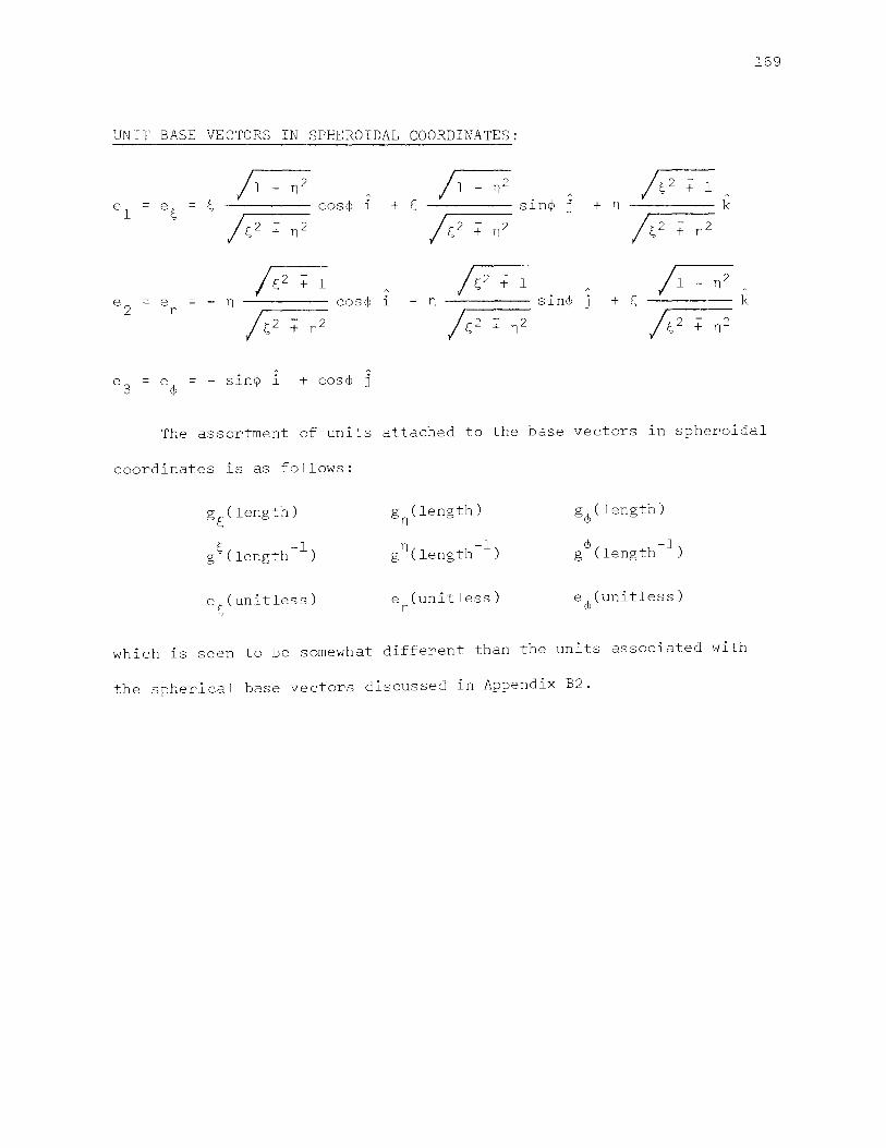
169

UNIT BASE VECTORS IN SPHEROIDAL COORDINATES:

/1 T]2 /1 n2 jr,2 -+ l

s A A

el = es = cos¢ l + s sin¢ j + Tl l<:

jr,2 + n2 /s2 - T)2 jr,2 - n2 + +

/s2 + l Jr,2 + l /1 - n2 A

e2 = e = - n cos¢ i - n sin¢ j + ~ k n

1~2 jr,2 /s2 - n2 + n2

- n2 + +

e3 = ecjl = - sin¢ l + cos¢ j

The assortment of units attached to the base vectors ln spheroidal

coordinates is as follows:

g~ (length) g (length) n

gcjl(length)

s -1 g (length ) n -1

g (length ) cjJ -1

g (length )

e E, (unit less) e (unitless) ecjl(unitless) n

which is seen to be somewhat different than the units associated with

the spherical base vectors discussed in Appendix B2.

170

APPENDIX G4

METRIC TENSORS

Metric tensors in curvilinear coordinates are discussed in general

in Appendix B3. Thev are given below for the spheroidal case in both

explicit notation and abe notation as discussed in Appendix Gl:

COVARIANT METRIC TENSOR IN SPHEROIDAL COORDINATES:

= c2(~2 -+ n2)

(~2 -+ l)

= c2(~2 -+ n2)

(l - ll2)

(cab) 2

CONTRAVARIANT METRIC TENSOR IN SPHEROIDAL COORDINATES:

CE:2 -

1) (a l2 Ll F,E, + g = g = c2 = 1-

( r, 2 - ll2) \ce, +

22 llll 2(1 - n2) r E-l 2 g = g = c

(~2 - n2) ,ce 1 +

33 g = g ¢¢ = -----=1;.___ __ _

c 2 (( 2 -+ 1)(1 - n 2 )

km where in both cases, g =g =0 for k;im. km

( ' 2

= I c~h J \ . )

In the limit as c~o and ~'00 we have the following:

which are the components of the covariant metric tensor ln spherical

coordinates. Similar transformatjons hold for the contravariant metric

tensor as well,

171

APPENDIX GS

SCALE FACTORS

Scale factors in curvilinear coordinates are discussed in general

ln Appendix B4. They are given below for the spheroidal case in both

explicit notation and abe notation as discussed in Appendix Gl:

COVARIANT SCALE FACTORS IN SPHEROIDAL COORDINATES:

/r,2 - n2 +

hE; ce

hl = = c = IE;2

a -+ 1

/r,2 - n2 +

h ce

h2 = = c = n /1- b

n2

c/r,2 - 1/1 n2 cab h3 = h<P = + - =

CONTRAVARIANT SCALE FACTORS IN SPHEROIDAL COORDINATES:

jr2 -+ 1

hl hf, a = = = -

c /-ce - n2 +

/1 - n2 h2 hn b

= = = c (:2:;:: n2

ce

h3 h<P 1 1 = = =

cj 2 1/1 cab - n2 + -f,

APPENDIX G6

REPRESENTATION OF ABSOLUTE VECTORS

Representation of absolute vectors in curvilinear coordinates lS

discussed ln general in Appendix B5. The relations between the

covariant, contravariant, and physical components of an absolute

vector, A, are given below for the spheroidal case in both explicit

notation and abe notation as discussed in Appendix Gl:

EXPLICIT NOTATION:

abe NOTATION:

A ( [,) ce A~ = a

A(n) ce All = b

A(¢) = cab Acp

a A = -ce

b A = ce

1 = cab

n

Acp

I 1 - ll2

c/t:2 + ll2

A ll

172

173

APPENDIX G7

VECTOR OPERATORS

Vector operators in curvilinear coordinates are discussed in

general in Appendix B6. In the spheroidal case, the gradient and

laplacian of an absolute scalar, ¢, and the divergence and curl of an

absolute vector, A, are given below ln the abe notation discussed ln

Appendix Gl. These operators are also given in explicit notation on

the next two pages. Where douhle signs appear, the upper lS for

prolate, the lower for oblate:

VECTOR OPERATORS IN SPHEROIDAL COORDINATES (abe NOTATION):

grad ¢ = 'V¢ =

lap cjl = v2c]l =

div A = V•A =

curl A = VxA

a b 1 ¢

,[,e[, + ¢ e + --cab <jJ e

ce

[ ar - c]l ce , E;F,

+

a A ( [,) + ce 'Eo

ce ,n n

rb r ,, ce ¢ , n fl

~A(n) ce ,n

+

_n_A(¢) cbe

+ [-1_ A co cab ,¢

,¢ ¢

+ r 1 r , cab cJl ,¢¢

1 A(¢) + -- ,¢ cab

t;(e? + a2)

cae 3

+ 2[,

c?e 2

Acu -

(1) -

'c

n(e? ±

che 3

+ [ cae A ( fl ) 'F, + ~: 3 A ( n ) nb A( U _ b + --

-where + 1 '

2n

c2e2

b2)

1> ,n

A(n)

VECTOR OPERATORS IN SPHEROIDAL COORDINATES:

grad cp = \lcjJ =

lap ¢ (t;2 :;: 1)

jr,2 -+ 1

div A = \l•A = cjr,2 -

ll2 +

¢ + ,[,[,

Acu r+ ' '

(l - n2)

c2(t;2 :;: ll2)

+

/1 r?

c/r-2 -r)2 +

c)! e ,11 r)

+

rj, , llll

A(n)

'r I

+

l 'I lj

____ __.:_1:__ ____ ,, c; ' , cjJ t

+ 1

1

'r I

( ~ ) f\

' ~ , j

175

VECTOR OPERATORS IN SPHEROIDAL COORDINATES cont'd:

curl A = VxA =

+

I 2 -r, + 1 -----A (rj;) e

, r, 1l

+

/1 - ll2 /1 - ll2 Acu

+ A (S) - e<P

3 ,jr2 ,n - n/)2

-ll? c( r,? + + c

l76

APPENDIX GS

CHRISTOFFEL SYMBOLS

Christoffel symbols of the second kind are discussed in general ln

Appendix B7. Of the possible fifteen non-vanishing, independent symbols

for any given system, there are only ten for the spheroidal system. They

are given below in both explicit notation and the abe notation discussed

1n Appendix Gl. Where double signs occur, the upper is for prolate, the

lower for oblate:

=

=

=

=

=

=

=

=

=

[ n~]

~~;J

[ :¢)

[ ¢~]

[in~)

[n~]

= +

= +

= +

=

=

= +

= +

= +

= +

=

(~2 + l)(~2 + n2)

n(l - n 2 )

(1 - n2)(~2 + n2)

[,([,2 + l)

(1 - n2)(t:2 + n2)

[,([, 2 + 1)(1 - n2 )

(t;2 + n2)

nCt: 2 + 1)(1 - n 2 )

cr2 + n2)

n = +

= +

= +

n =

=

=

=

=

=

=

-+

+

+

+

nb 2

a2e2

na 2

b2e2

t:a2

b2e2

t;a2b2

e2

177

APPENDIX H

THE DISPLACEMENT VECTOR IN SPHEROIDAL COORDINATES

178

APPENDIX Hl

DISPLACEMENT IN TERMS OF POTENTIALS

The wave equation for the displacement vector, U, ln a continuous,

homogeneous, isotropic, elastic medium, is of a difficult vector form

called the elastic wave equation (see Appendix L). To avoid direct

confrontation with this untenable equation, U, will be expressed as

the gradient of a scalar potential, ¢, and the curl of a vector poten-

tial, ~, by invoking the following relations known as Helmholtz's

Theorem:

U = v¢ + vx~ v·~ = 0

where vis to be cast into spheroidal coordinates (see Appendix G7),

,r, C n) + '~' e

n + ,,,C ¢) and where cJ> and 'l'

'~' e ¢'

satisfy the following equations:

¢ = ex 2 V 2 <P 'tt

~ = -B 2 vxvx-;p 'tt

which are the scalar and vector wave equations respectively. In order

to reduce consideration of the vector wave equation to consideration

of the simpler scalar wave equilt.ion, ~ will be defined as follows:

[M N]e iwt

~ = +

wrwre M = VvxP

J. -and N = -vxvcxP k ,

where k is tl1e wave number, (JJ lS the angular frequency, P = P( E;, r1 ,¢)

is the position vector given in Appendix Gl, where M and N are

solutions to the vector Helmholtz equation, and where, most

179

cantly, v and Care scalar functions of~.~, and¢, which, with the

• f- iwt . f h . t1me :actor, e , are solutlons o t e scalar wave equatlon ln

spheroidal coordinates (see Flammer (1957), Chapter 9).

Hence, by the foregoing relations, all components of the dis-

placement vector, U, are obtained entirely from solutions of a single

Pquation: the scalar wave equation.

180

APPENDIX H2

PHYSICAL, COVARIANT, AND CONTRAVARIANT COMPONENTS

The components of the displacement vector, U, will be expre:;sed

in terms of displacement potentials, <1> and \f', as discussed in /;ppendlcc.c;

Hl and L. The physical, covariant, and contravariant components of

displacement ln spheroidal coordinates are given on the next page.

the spheroidal case, the units of u(k) are all length, those of {\

all area, and the uk are all unitless. As seen in Appendix C2 thi;;

is somewhat different than the units associated with the various

displacement components in soherical coordinates.

In this and all subsequent appendices, as wel1 as most of the

body of the dissertation, use of the abe notation shall be u~ed

almost exclusively where a, b, and e are defined as fo1lows:

a = jr; 2 + 1

where it is seen that e 2 = a 2 + b 2 and where upper signs app1y to

In

are

prolate spheroids, lower to oblate. The tremendou:; space :;av inr:~ dnd

simplifying effect of this notation is immediate1y anparent by

referring to Appendices G3, G6, and C7 where equation:~ are ;_~j-;nr; Jn

both the explicit and the abe notations.

181

PHYSICAL COMPONENTS OF DISPLACEMENT IN SPHEROIDAL COORDINATES:

uc U = ~<P + .E_ 1)!(¢) - _n_ 1)!(¢) __ 1_ l)!(n) ce , E;, ce ,n cbe cab , cp

u(n) = .E_q, ~ lj!(cp) _E;,_ lj!(cp) + 1 (E;,) ce ,n ce , E;, cae cab 1jJ ,cp

u(¢) = _1_ <P + ~ l)!(n) + ~ l)!(n) .E_ lj!(E;,) + .:JE_ 1jJ ( E,)

cab , cp ce ,E;, ce 3 ce ,n

ce 3

COVARIANT COMPONENTS OF DISPLACEMENT IN SPHEROIDAL COORDINATES:

UE;, = <I>,E;, + E._ 1)!(¢) ~ 1)!(¢) _e_lj!(n) a , n ab a 2b ,cp

u = ¢ ~ 1)!(¢) _L 1)!(¢) + _e_lj!(E;,) n ,n b 'E;, ab

ab 2 ,cp

ucp = <P + a 2b lj!(n) +

E;,a 2b lj!(n) ab 2 1jJ (E;,) ±

nab 2 lj!(E;,) ,cp e ,E;, e3 e ,n e3

CONTRAVARIANT COMPONENTS OF DISPLACEMENT IN SPHEROIDAL COORDINATES:

UE;, = a2 ~ 1)!(¢) na 1)!(¢) _1_ l)!(n) --¢ +

,cp c2e2 ,E;, 2 2 , n c 2be 2 c 2be c e

un b2 ¢ ~ 1)!(¢) E;,b 1)!(¢) + _1_ lj!(E;,) =

c2e2 ,n c2e2 ,E;, c 2ae 2 c 2ae ,cp

u¢ 1 _1_ l)!(n) E;, l)!(n) - _1_ lj!(E;,) n 1jJ ( E;,) = <P + + ±

c2a2b2 ,cp c 2be

,E;, c 2be 3 c 2ae

,n c 2ae 3

182

APPENDIX fl3

ORDINARY PARTIAL DERIVATIVES OF DISPLACEMENTS

DERIVATIVES OF COVARIANT ~-DISPLACEMENTS:

u = c)l + b weer) ~b weer) l weer) + h lj;(cp) r,,~ '~~ a ,n~ a3 ,n ab ,E, a 3b

__ e_ lj;(n) E,Ce2 ± b2) , ( n ) + ijJ

a 2b ,cp~ a 4be ,cp

u = c)l +E..u/cfJ) ~ lj;(cp) - _1_ lj;(cp) E:,n ,E,n a , Tlfl ab , n ab 3

_e_ ~~ ( n)

' cp Tl

__ n_ ~~ ( n) ,cp

a 2b b 3e

u = c)l + !:?._ (~(cp) - __!l_ lj;(cp) __ e_ ~/n) ,¢¢ [,,¢ 'r; cp a ,n¢ ab , cp a 2b

DERIVATIVES OF COVARIANT n-DISPLACEMENTS:

.9_ lj;(¢) na lj;(¢) E: ,(¢) - ~ ~~(¢) u = cp ab ~~ n,n ,nn b , ~n b3 ' [, 'n ab 3

e cu n(e 7 + a;') ( t: ) + -- tjJ + 4)

,<I, ') 'cf 'l db 11 e db'

d Cr) 2[, (,jl) l til ( ¢) l) = if) - tjJ ab ~~ r ±

n,( 'nr, b ,U ' ,, a 3b

e ~/ [,) - !C V' ( r, ) 'o

+ -- + ,¢> ab 2 ,¢!:, a 3e

a ~) ( cp ) E, tjJ ( ¢) e ~(F;) () = <fl - - + --) ,¢¢

n , 'P 'n<p b 'f, 4) db ,¢ ab 2

183

rn::rnVATIVCS Of C:OVARIANT ¢-DISPLACEMENTS:

lJ, <jl a 7h VI ( ll ) E:a 2b wCll) ab 2

1cu r]ab 2 ~) ( E: ) = + + - -- lJ +

\~ ''~ , 'P ¢ e ,E:¢ e3 ,¢ e ,ll¢ e3 ,¢

ll cfl ,r, <t' a 2b tJ;(n) 2E;b well) +

b(ll2a2 + 2t;2b2) 1jJ ( rl) = + + ,dlE: e ,E:E: e ,£; es

ab 2 leo t;b 4 ~J ( E; ) llab 2 wU,) £:llb 2 (2a 2 + b2) wco - -- l,J + ± +

e 'n ~ ae 3 ,n e3 ,[, ae 5

[l cjl ab 2 1jJ ([,) 2na ~/U a(t;2b2 - 2n 2a 2 ) wcu = + -- ±

cjJ ,r1 ,;Jlll e ,nn e ,ll es

a 2b ~~ ( n) na 4 1 ( n) t;a 2b w(ll) t;na 2 (a 2 -

2b 2 ) VJ ( n) + + -- --w +

e ,E:n be 3 ,£;: e3 ,n be 5

The uni_ts associated with these derivatives are the same as those

,l.';~;o,,i,lt('cl with the Uk themselves--namely, area. In the spherical case

d i ~;cuc;:;cd in /\ppnndix C3 some of the U had units of length, some area, k,m

c1nd one had no units at all.

184

APPENDIX H4

COVARIANT PARTIAL DERIVATIVES OF DISPLACEMENTS

Covar>iant par>tial differ>entiation is definGd in Appendix C4 ln

ter>ms of ordinary par>tial derivatives and Christoffel symbols of the

second kind. For the spheroidal case, they are given below wher>e the

ordinar>y partial derivatives, uk,m' can be found in Apoendix H2 and the

covariant components of U, Uk, can be found in Appendix Hl. The

Chr>istoffel symbols are wr>itten ln the abe form but can be found ln

explicit form ln Appendix G8:

COVARIANT E;-DISPLACEMENT:

~ ur, + nb 2 u u = u ± --

[,;[, ( '[, a2e2 a 2e 2 n

fl c

u u + ur, 'o u = -

t,;n E,,n -e2 e2 n

u = u - _f_ u<P [,;¢ [,,¢ a2

COVARIANT n-DISPLACEMENT:

(a2 ur,

na 2 u u = u + - --

n;n n,n b2e2 b 7e 2 Tl

u u ± n

u, - ~ u = n;t: n,E: e2 '? e2 n

lJ u + ll u, = n;¢ n,<P b/ cp

!i •,

I 185

c:nv 1\ PLANT 'I'- JJ r SF LA CEMENT:

u u c;a2b2 ut:

na 2b 2 u = + {b ;¢ c/l , q\ e2 e2 ll

lJ = u¢,r - s_u ip ; r: a2 ¢

lJ .J>; n

u <P,n + _!l_u

b2 ¢

186

APPENDIX I

INFINITESMAL STRAIN IN SPHEROIDAL COORDINAT[S

APPENDIX Il

COVARIANT COMPONENTS Of STRAIN

The covariant components of the infinitesmal strain tensor in

curvilinear coordinates are discussed in general in Appendix Dl. ln

the spheroidal case, they are given below in terms of Uk and U k,m

which can be found ln Appendices H2 and H3, and where U lS the (k,m)

symmetric ordinary partial derivative discussed in Appendix A:

eE,[, = UE;,[, ± [_E__l2 [ E;U E: llU J ae) J 7l

e = u + [baer cc:uc: llU ] llll ll,ll ll

e¢¢ = u¢,¢ + [ ab r [t;U - llU ] e E;, n

e = u + [~J2[7lUE, + E;U J F,n C (, n) - 7l

u + 7l u¢ e = ll¢ (ll,¢) b2

e¢(, = u - _L u¢ (¢,0 a2

where a = /-./ 1, + l ' b = 11 - 112 , and e =

187

ThE' units oJ ek in ~~phero.idal m

coordinates are all area. As can

· 1 h · · t the case for so. heri cal coordinates. bl; :;ccn in 1\ppendlx H, t lS lS no

188

APPENDIX I2

PHYSICAL COMPONENTS OF STRAIN

The physical components of the infinitesmal strain tensor in

curvilinear coordinates are discussed in general in Appendix D2. In

the spheroidal case, they are given below in terms of Uk and U k,m

which can be found in Appendices H2 and H3, and where U is the (k ,m)

symmetric ordinary partial derivative discussed in Appendix A:

e = [ aJ 2u + ( c,;o ce ~,E.

e(nn) = [ :eJ 2

un, n • [-"'--rr,u, - nu J ce 2 n

r 1 r r ...!_r [ [.U [. - nU J e(¢¢) = -- u +

cab ¢,¢ lee n

ab ab [nUE. [.U ]

e(E.n) = u + + c2e2 (E.,n) c2e4 n

1 u + n u¢ e(n¢) =

c 2ae C n '¢) c 2ab 2e

_l_u [. u¢ e(¢0 = -

2b ( ¢ '[.) c 2a 2be c e

where a = /c-2 -L, + 1 ' and e =

All physical components of strain are unitless regardless of the

coordinate system.

189

APPENDIX J

STRESS ON THE SURFACE Of' A SPHEROID

190

APPENDIX Jl

STRESS IN TERMS OF STRAIN

Hooke's Law ln curvilinear coordinates is discussed in general

1 n 1\ppend ix El. In the spheroidal case, the nine components of the

stress tensor are given below in terms of the physical components of

strain which can be found in Appendix I2:

t([,[,) = CA+2p)e([,E;) + 71[e( ) + e(¢¢)] nn

t Cnn)

= C\+2JJ)e(nn) + :\[e(¢¢) + e([,t:)]

t(¢¢) = C\+2v)e(q,¢) + :\[e(E;[,) + e(nn)]

t(r"n) = t

( nU = 2)Je([,n)

t ( r: ¢ ) = t ( q 11 ) = 2 JJ e ( n ¢ )

wlrerc: .\ cmd J! are Lame 1 s constants.

Only the stress vector on the plane tangent to a ::;pheroid is

ll<'Ccied in thi:c; clis:,ertat-Lon. This vector, t(r,)' 1s given by the equation,

1-Jhi'Y'(' the ek are the unit base vectors given ln Appendix G3. Hence, of

th•' nine stre,;s tensor components, only the three with an r, -subscript are

required, namely:

191

APPENDIX ,J2

STRESS IN TERMS OF DISPLACEMENT

Spheroidal stress is given in terms of strain in Appendix Jl and

Jn terms of notentials ln Appendix J3. But in order to specify a

particular vibrational mode by specifying a particular type of displace-

m(~nt, it is necessary to refer to express ions of stress in terms of

displacement before writing stress in terms of potentials. These

expressions are given below in terms of uk and uk,m which can be

found in Appendices H2 and H3. Only the three stress components of

interest in this dissertation are given:

WCJ.b pab lJ

2wnab t = u + ±

(E;,n) c2e2 [, 'Tl c2e2 n,E, c2e4

fJ _f_J_ u 2pt; t(r,¢) = u, ¢ + -

c 2be L, ' c 2be ¢,/'; c 2a 2be

wiH' l'l' d = jr2 + 1 and

wiJ<'l'l' ,\ and p are Lame's constants.

ur; -

u¢

e =

u ¢,¢

2wf:ab

c2e4 u

n

and

The units of the physical components of stress, t(km), are the

unit:~ ol lw!me's constants, n3mE~ly, force per unjt area.

192

APPENDIX J3

STRESS IN TERMS OF POTENTIALS

The physical components of stress on the tangent plane of a

spheroid are given on this and the next page in terms of displacement

potentials in a form where the components of displacements and their

derivatives are still recognizable. This results in longer equations

than if like terms were regrouped and lumped together. But regrouping

at this point would reduce the utility of the equations:

(A+ 2JJ )a2

["' t - '¥

(~~) - 2 2 '~~ c e

:\b2 [ + --¢ -2 2 ,nn c e

2'(Ae 2 ± "b2

)[• ~ \j!(¢) ~ \j!(¢) e .,<nl ] + + ---

2 4 '~ a , n ab a 2 b ,¢

c e

2n(Ae 2 ± "b2 )[¢ ~ \j!(¢) - _L ~/¢) + _e_ .,<u 1 2 4 'n b '~ ab ab 2 ,¢,

c e

+ 2)Jnabr¢ + £ ~J(¢) 2 4 ,1:, a ,n

c e l

P fr a 2 b lJ!(n) t(E,¢) = ---;;- ( ,¢[, + --

e c ;e,

-

2 !';, I ( ¢) ab lJ!

2EJ) + -- lf)

,[,[, e

ab 2 --

1 I ( q1) --ljl

<lh 3

e --- ljJ(q)

'¢ rt

1 ,(¢) ~ ± -- li-'

'c, a 3b

e co + -- ljl

ab 2 'jl~

e ---

b

( :1) b(q/a;; + ,_ +

' ' - es

+ (b4

v· ( r )

+ 41 ( [, ) e , 'l 1:,

ae 1 -

+

e ---, ~· ~;

( ~) (') e

1 'lJ

r] ---

(j-. ''

f? (r) + l}l

a\: '\1·

(f) :j '

' i'

2t;?b 2 ) ( Tl ) \jJ

., ( f ) r: (jf-'.

J., -, ('

,:,

r](-;

+ CL) 1 (~)~

~ 1)!(¢) ab ,n

_1_ ljJ(¢)

ab 3

193

+ 2)J nab r<jl + .e_ ljJ ( ¢) - _!l_ ljJ ( ¢) - _e_ ljJ ( n) l c 2e 4 l 'E;, a 'n ab a 2 b ' ¢

+ E;,nb2(2a2 + b2) lj!(E;,)l

ae 5

195

APPENDIX Kl

THE SEPARATED SOLUTION IN SPHEROIDAL COORDINATES

By casting the scalar wave equation into spheroidal coordinates

and assuming a solution, sc~.~.¢,t), of the type,

S(~,~,¢,t) = X(~)E(~)¢(¢)T(t)

the equation separates into four ordinary differential equations. Three

separation constants are required. If they are chosen properly, physi-

cally meaningful solutions are obtained. for details of this, see

Morse & feshbach (1953), Stratton, et al (1956), Flammer (1957), and

Magnus, Oberhettinger & Soni (1966). The particular solutions of

interest in this dissertation are as follows:

xcu =

E(~) =

c!>(¢) =

T ( t ) =

jem£(h,C) = Spheroidal Radial Wave function (lst kind)

yem£(h,~) = Spheroidal Radial Wave function (2nd kind)

sm£(h,~) = Spheroidal Angular Wave Function (lst kind)

sin(m¢) cos

iwt e

where m, 9,, and ul are the separation constants and h = kc where c is

the spheroidal coordinate parameter (a focal distance), and k is the

ordinary wave number defined by k = w/x where X is the propagation

constant of the scalar wave equation. ~or plane longitudinal waves,

X = ex = /,\+2JJ/p, and for plane shear waves, x = B = /iJ/p, where ,\ and t;

are Lame's elastic constants and p is mass density.

196

It is interesting to note that both the radial and angular

wave functions depend explicitly upon the frequency, w, throu~h the

spheroidal wave number, h. In Appendix Fl it is seen that in spherical

coordinates both of the angle functions are independent of frequency.

For the spherical case the only space function that depends on

frequency is the radial function. It should be noted that the function,

~·(¢), is the same for both spherical and spheroidal coordinates. This

is not surprising inasmuch as the coordinate, ¢, is geometrically the

same for both systems. But whereas in the spherical case there was no

coupling of ¢(¢) to frequency at all, in the spheroidal case the function,

<l1 ( ¢), is indirectly coupled to frequency through the separation constant,

m, which is an index of both the spheroidal wave functions which both

Jepeml explicitly upon frequency.

Excluding arbitrary constants, S([,,n,¢,t) takes the following

J OY'Ill:

S([,,n,¢,t) iwt . sin ( ) = e [Je /ye

0](h,[,) (m¢)S n h,n m£ m~ cos m~

where

diHl whc'r'c~ the' quun LiLy, I j c' /ye J, implies cl choice oi either the - ·- rn x, m Q

~;pilvr•uiddL r·ddtdL WdVf' function oi the fir'st kind, of the second kind,

en' d lineae combination of both.

The separdtion constants, m and£, take on only non-negative

i 11 l e g e r· v a lues . The term, sin(m¢)S n(h,n), may be referred to as d cos mx ..

,-;pheroidal harmonic. It eli vi des the surface of a spheroid in to <cones

dnr.l sectors much like spherical harmonics divide the surface of a

c;phere (see Hobson (1955)).

197

APPENDIX K2

SPHEROIDAL WAVE FUNCTIONS

The analytic properties of spheroidal wave functions are discussed

at length in Stratton, et al (1956), Flammer (1957), and Abramowitz &

Stegun (1965). There are eight linearly independent prolate and oblate

radial and angular spheroidal wave functions. They could be considered

as eight separate functions satisfying four different second order

ordinary differential equations--two independent solutions per equation.

But by cleverly defining the ranges of the variables, [,and n, and the

spheroidal wave number, h, to include complex as well as real values,

all eight functions can be reduced to a pair of functions satisfying

a single second order differential equation, Lu t: over different ransec-,

of the variable. However, for numerical work, it lo-; really not

convenient to reduce the pr·oblern to a single pair of functions. Il is

better to consider the four pairs of functions as being of two classe~,

radial and angular, satisfying the following two ordinary differenti<::l

equaticns:

~r ( [ 2 - 1) dJ l df" ' dt;

' r,2 -

+

where J = ,J ( £,) and lS one of the four spheroidal radial wave tunctionc;

and where S = S(n) and is one of the four spheroidal angular wave

functions. h and m are constants defined in Appendix Kl and A = A (h) 1:1>.

198

lS an eigenvalue, or separation constant, defined in terms of m, £,

and h by the following equation:

Am n ( h ) = Q, ( £+ 1 ) + h 2 ( 2.Q, ( £+ 1 ) - 2m2 - 1 ( ) ] ~ \ (2£-1)(2£+3) + tmQ h

where the constants, tm2(h), are tabulated ln and explained ln Stratton,

et al (1956).

Thus, the literature refers to spheroidal radial wave functions

of the first and second kinds and spheroidal angular wave functions of

the first and second kinds which can stand for either the prolate or

the oblate case depending upon the ranges taken by the variables, (

and n, and the parameter, h. The four functions of the first kind are

denoted as follows:

jem£(h,~) = Prolate Spheroidal Radial Wave function l~C~~

S (h,n) = Prolate Spheroidal Angular Wave Function -l~nsl m£

J·e (ih -i~) = Oblate Spheroidal Radial Wave Function Os~<a m£ '

Sm£(ih,n) = Oblate Spheroidal Angular Wave Function -l:..n:..l

and 2 = m, m+l, m+2,

Tables of the functions, jem£ and Sm£' per se, do not exist any-

! t th t tl.me 'l'he be~t available tables concernlng these w 1ere a . e pres en -. ~

functions are tables of coefficients needed to expand them in terms of

other more elementary functions for which explicit tabulations do

exist. The most convenient expansions are in terms of spherical

Ressel functions, j , and associated Legendre functions, Pm ~ which n n

are discussed in Appendix F. In fact, the Bessel and Legendre func-

199

tions may be considered as special cases of spheroidal wave functions

Slnce in the limit as a spheroid becomes a sphere (see Appendix ·~:;)

je becomes j and S n becomes Pm. m£ n m!C n Hence, expansions of the SJ.-ll,ero.icJal

wave functions in terms of the spherical functions converge more

rapidly than if they were expanded in terms of any other set of

orthogonal functions.

The expansions for the spheroidal wave functions of the first

kind used in this dissertation are those of Stratton, et al (1956),

and are given below. The expansion coefficients, a and d , arc n n

tabulated by Stratton, et al, for a sufficient number of terms tu

insure six or seven place accuracy. ror the range of the parameter,

h, coverecJ, namely, O.l<h<B.O, this degree of accuracy is achlevecJ ny

twelve terms or less. In general, the larger the value of h, (i.e.

the greater the ellipticity of the spheroid), the more terms are

required to achieve a given degree of accuracy. For very small val~e.,

of h, seven places are achieved in three terms or less.

PROLATE SPHEROIDAL RADIAL WAVE rUNCTION or TllE rii\ST J<lND

je (h,t_:) = m£

m

fr,2 - 112 L ) r2 n ' 0 )

a Chlmx> j Ch:) n n+m

PROLATE SPHEROIDAL ANGULAR WAVE rUNCTION OF THE riRST KIND

( ) = )'? d Chlm£> Pm (n) Sm£ h,n n n n+m

OBLATE SPHEROIDAL RADIAL WAVE FUNCTION OF THE FIRST KIND

je 9 Cih,-i~) m,

m

= r~2 + 112 r'a (ihlm£) , ~2 J n n

j (h~) n+m

OBI,ATE SPHEROIDAL ANGULAR WAVE FUNCTION OF THE FIRST KIND

where the j are spherical Bessel functions, the Pm are associated n n

Legendre functions of the first kind, a and d are the expansion n n

coefficients, and where the primed summation sign, L', implies sum-

mation over only odd integers when m+£ is odd and over only even

integers when m+£ is even.

for the spheroidal wave functions of the second kind, no tables

or expansions have been developed of any kind. It would seem that

the appropriate expressions would be to expand the spheroidal radial

wave functions of the second kind ln terms of the spherical Bessel

200

functions of the second kind, the so called spherical Neumann functions

denoted by y . n

Likewise, it would seem that the appropriate expres-

sions for spl1eroidal angular wave functions of the second kind would

be expansions in terms of the associated Legendre functions of the

second kind, Qm. n

But the form and coefficients of such expansions, if

they exist, remain unpublished at the present time.

A need for spheroidal radial wave functions of the second ki11d

arises in this dissertation in the discussion of the DAR vibrational

mode for spheroidal cavities. Only the zero-zero order is re4uired.

201

Hence, for purposes of this dissertation let there be a spheroidal

radial wave function of the second kind denoted by whose yem£

expansion for m = £ = 0 is of the following form:

where the y are spherical Neumann functions as discussed in Appendix r n

and the b are expansion coefficients whose values, at the present n

time, remain unknown.

In the discussion of incoming and outgoing waves, it is useful to

form Hankel type spheroidal wave functions. Hence, the following four

functions are defined and referred to in this dissertation as spheroidal

Hankel functions of the first, second, third, and fourth kinds:

( 1) jeoo iyeoo heoo = +

h ( 2) eoo = jeoo iyeoo

( 3) ijeoo heoo = yeoo +

( 4) ijeoo heoo = yeoo

ic11t When the time factor, e 1s affixed, the spheroidal Hankel functions

oi tl1c first and fourth kinds correspond to incoming waves since they

reduce to functions of (wt+h~) wl1ile those of the second and third kinds

correspond to outgoing waves since they reduce to functions ot (wt-h~).

The functions, je00

and ye00

, alone, each imply both kinds of- waves

since when the time factor, illlt

e 1s affixed, the result reduces to

a function of Cwt+h~) plus a function of (wt-h~).

202

APPENDIX L

HELMHOLTZ'S THEOREM

A basic equation of motion for a continuous, homogeneous, isotropic,

elastic medium is the so called elastic wave equation given below:

(a)

where U lS the displacement vector of a particle in the medium, a lS the

velocity of a plane longitudinal wave, and B is the velocity of a plane

transverse wave.

Equation (a) can be solved by several approaches. One way is to

specify an integral or differential form for U which expresses it ln

terms of quantities that are solutions of the much simpler scalar wave

equation. One of these differential forms for U is obtained by invoking

Helmholtz's Theorem, sometimes called Poisson's Corollary. The theorem

allows a vector field, such as U, to be given as the gradient of a

scalar, ¢, plus the curl of a divergenceless vector, ~. The theorem is

stated by the following equations:

U = V¢ + Vx~ , V·~ = 0 (b)

where, in this case, ¢is called the scalar displacement potential and

~ is called the vector displacement potential.

The necessary and sufficient conditions for Helmholtz's Theorem are

not known. Sufficient conditions are discussed by Arfken (1966), PP· 58-

63; Love (1944), pp. 46-48; Pendse (1948), pp. 866-867; Jefimenko (1966),

pp. 42-43; and Morse & Feshbach (1953), pp. 52-54, 142-144. The most

complete account is that of Arfken. These conditions are concerned

with the differentiability and boundedness of the vector field and with

203

the manner in which it must vanish at infinity. Whatever the conditions

required by the theorem, they shall be assumed to be met by the

displacement vector of this dissertation. The theorem is applied ln

Appendices Cl and Hl and is basic to the whole dissertation.

Applying Helmholtz's Theorem, equations (b), to the elastic wave

equation (a) glves the following:

(c)

where some terms have been rearranged and where the orders of differen-

tiation for time and space have been reversed.

Equation (c), and therefore equation (a), lS satisfied if the

following equations are satisfied:

(d)

(e)

Equation (d) is the desired scalar wave equation. Equation (e) is

the vector wave equation (equation (e) is sometimes called the

solenoidal vector wave equation, the term, "vector wave equation",

being reserved for an equation like (e) but with the extra term,

See Flammer (1957), p. 69).

Helmholtz's Theorem is sufficient to reduce the elastic wave

equatjon (a) to the simDler equatjons (d f, e) for all coordinate

c;ystem'~. However, the vector wave equation (e) is still a forr:1idable

prospect. In rectangular coordinates, Helmholtz's Theorem, alone,

is sufficient to further reduce the vector wave equation to three

( k) scalar wave equations, one for each component, ~ , of the vector

potential,~. Hence, in rectangular coordinates the elastic wave

204

equat :ion (a) LS reduced, by Helmholtz's Theorem alone, to the four

:;calar wave equations given below:

k=x,y,z

But th :is hn.poens ~:mly in rectangular coordinates. In the other ten

coordinate systems separating the scalar wave equation, Helmholtz's

Theorem does not reduce the vector wave equation to the scalar one.

One aporoach to solving the vector wave equation (e) is to

define ~ in such a manner that it be obtained from quantities that

are solutions of the scalar wave equation. The manner in which ~

must be defined is different for each coordinate system. When a

:>uitallle definition for ~ has been discovered for some particular

coordinate :c;yc;tem, it is said that this system !!separates 11 not only

the :c;calar wave equation but the vector wave equation as well. To

date, of the eleven systems that separate the scalar wave equation,

only eight are known to separate the vector wave equation. They

are as follows: rectangular, circular cylinder, elliptic cylinder,

parabolic cylincler, spherical, conical, prolate spheroidal, and

oh I ate :3pheroidal. The first six are discussed in Morse & Feshbach

( J (1~):3), Chapter 13; Stratton (l 941), pp. 349-354, 392-399, 414-420;

c1nd t;wing, LTarcietsky f, Press (1957), pp. 7-10. The two spheroidal

ccJ:;c:" are discus::~ed by J'lamnwr ( 1957), Chapter 9.

lienee, it only rer:1ains to discover the proper definitions for

'!' l n parabol :i c, paraboloidal, and ellipsoidal coordinates in order for

all eleven scalar wave equation separable systems to be said to be

vector wave equation separable.

APPENDIX M

GENERATING CURVES AND DESCRIPTIVE TERMINOLOGY

FOR QUADRIC CAVITIES

205

Countless cavity shapes can be generated by intersections of the

coordinate surfaces of the eleven scalar wave equation separable

coordinate systems (see Chapter I of this dissertation). In order to

tabulate and discuss a representative number of them, they had to be

named. Table IV of Chapter I lists 112 shapes and families of shapes.

Thus arose the need for 112 different, unambiguous names which, if

possible, were to be mneumonic, descriptive, and brief. In most cases

brevity was impossible without ambiguity. Fewer than ten of tt1e

shapes had established names. In order to avoid complete confusion,

a logical scheme had to be devised to label the 112 shapes. The

scheme was as follows:

projected onto planes.

The intersecting coordinate surfaces were

The resulting closed curves capable of

generating cavities were named. The names of the 112 quadric cavity

shapes were then derived from their generating curves. In order to

keep the names unambiguous, descriptive, and yet as brief as possible,

many words had to be coined and many existing words l1ad to be defined

1n a special sense. The principal part of this appendix consists of

~ix figures identifying thirty-nine generating curves and a glossary

containing over sixty terms.

In order to see how the quadric cavity names were derived from

the generating curves, consider the following example. Figure (d) o~

t11 is appendix shows pairs of confocal ellipses and hyperbolas, a

situation which can occur in five coordinate systems: elliptic

206

cylinder, prolate spheroidal, oblate spheroidal, ellipsoidal, and

paraboloidal. Consider curve number II, the so called "majaxial ellip-

tic trapezoid," so named because it is symmetric with respect to the

major axis of the ellipse, and four-sided, having two opposite sides

made up of "parallel" ellipses and two opposite sides made up of rrnon-

narallel" legs of a branch of a hyperbola. In elliptic cylinder

coordinates this generates a "majaxial elliptic trapezoidal cylinder."

1n nrolate spheroidal coordinates this generates a "circular majaxial

elliptic trapezoidal cup.n In oblate spheroidal coordinates this

generates a "circular maj axial elliptic trapezoidal toroid." And in

ellipsoidal coordinates this generates an "elliptic majaxial elliptic

trapezoidal cup." The majaxial elliptic trapezoid is also involved

in four of the quadric cavity shapes generated in paraboloidal

coordinates (see Chapter I, Table IV, entries 88-91), but these cavity

c3hares are nameci for their parabolic traces given in Figure (c). Thus,

the shape of a quadric cavity can be deduced from its name by reference

to figures (a-f) and the terms of the glossary.

The various closed curves of Figures (a-f) are identified by

Roman numerals in the enclosed areas. When a curve of interest en-

cl oc;e.s more than one numbered area, it is identified by a sum of

till" appropriate !~oman numerals.

Tlw ,S',lossarv contain:c; only words coined for this dissertation,

vJorcb usecl in a special or unusual sense in this dissertation, or

words not ordinarily found ln any but an unabridged dictjonary. Deriv-

ativcs are not listed either. for example, since biparabola is defined

in the glossary, it is assumed that the meanings of the derivatives,

biparabolic and biparaboloid, are self-evident from the context. In

order to remove any ambiguity arising from the figures (a-f), the

curves defined there by illustration are also defined in the glossary

by verbal description.

A little reflection upon quadric coordinate systems and the

figures (a-f) is sufficient to see that all possible generating

curves have not been identified. for example, no six-sided curves

are mentioned even though they exist for some of the systems and

would benerate quadric cavity shapes not given among the 112 of

Table IV in Chapter I. Furthermore, even the possibilities of the

thirty-nine given curves of figures (a-f) are not exhausted by the

112 entries of Table IV. for example, only seven quadric cavity

shapes are given under the paraboloidal coordinate system even though

Figure (c) shows generating curves that could define more than

seven shapes. lienee, Figures (a-f) and Table IV are only representa

tive samples of the myriad possibilities of quadric cavity shapes

and generating curves that can be obtained from the eleven scalar

wave equation separable coordinate systems. They do not constitute

a comprehensive survey.

figures (a-f) are found 1n the next five pages. The glossary

follows immediately after the figures.

207

FIGURE (a)

GENERATING CURVES FOR QUADRIC CAVITIES

APPROPRIATE SYSTEMS

Spherical Circular Cylinder Conical

FROM RAYS AND CIRCLES

CURVE NAMES

I Sector II Circular Trapezoid

FIGURE (b)


APPROPRIATE SYSTEMS

Parabolic Cylinder Parabolic

FROM COAXIAL CONFOCAL PARABOLAS

CURVE NAMES

I or V Parabolic Rectangle II, IV, or II+I Parabolic Trapezoid III or III+II Biparabola

208

209

FIGURE (c)


FROM COAXIAL, NON-CONFOCAL PARABOLAS

APPROPRIATE SYSTEM

Paraboloidal: This is the only system with coaxial parabolas that are not confocal. There are three families of parabolas with three corresponding foci along the vertical axis. 1~e top and bottom foci define families of elliptic paraboloids. The middle focus defines a family of hyperbolic paraboloids. The pair of foci on the horizontal axis is for the families of elLLpses dnd hyperbolas generated in the horizontal plane.

CURVE NAMES

I or III Bifocal Parabolic Rectangle II Trifocal Parabolic Rectangle IV, V, or VII Bifocal Parabolic

Tra;::,e;,:oid VI Trifocal Parabolic Trapezoid VIII or VIII+VII+VI Bifocal

Biparabola

FIGURE (d)


FROM CONFOCAL ELLIPSES AND HYPERBOLAS

APPROPRIATE SYSTEMS

Elliptic Cylinder Prolate Spheroidal Oblate Spheroidal Paraboloidal Ellipsoidal

CURVE NAMES

I Minaxial Elliptic Trapezoid II Majaxial Elliptic Trapezoid III Hyoerbolic Rectangle IV Hyperbolic Trapezoid V Biconvex Elliperbola V+IV+III Concavo-convex Elliperbola VI Elliperbolic Rectangle

210

211

FIGURE (e)


FROM MONOCONFOCAL ELLIPSES

APPROPRIATE SYSTEM

Conical: This is the only system involving ellipses without involving hyperbolas. Ordinarily, monoconfocal ellipses would not intersect orthogonally. But in the conical system, they are not projected upon a plane, but upon the surface of a sphere.

CURVE NAMES

I Minaxial Bielliptic Trapezoid II or IV Majaxial Bielliptic Trapezoid III Biconcave Biellipse V Biconvex Biellipse V+IV+III Concavo-convex Piellipse VI Bielliptic Rectangle

212

FIGURE (f)


FROM ELLIPSES AND TWO FAMILIES OF HYPERBOLAS

APPROPRIATE SYSTEM

Ellipsoidal: This is the only system with two families of hyperbolas. There are two pairs of foci. The inner foci define a family of double elliptic hyperboloids. The outer foci define a family of single elliptic hyperboloids. The outer foci also define one crosssection of the family of ellipsoids.

CURVE NAMES

I Bifocal Minaxial Elliptic Trapezoid II+VII+XII Bifocal Majaxial Elliptic

Trapezoid III Bifocal Hyperbolic Rectangle IV Bifocal Hyperbolic Trapezoid V+VI+X Bifocal Biconvex Elliperbola V+VI+X+IV+III Bifocal Concavo-convex

Elliperbola IX+XI Bifocal Elliperbolic Rectangle X Bihyperbola X+IV+III Bihyperbolic Rectangle X+IV Bihyperbolic Trapezoid VII+IX+XI Bihyperbolic Elliperbolic

Rectang lP

VII, VIII, or IX Innerbased Bihyperbolic Triangle

XI Outerbased Bihyperbolic Triangle VIII+XI Bihyperbolic Rhomboid VIII+IX+XI Bihyperbolic Trapezium XIII+IV+IX Bihyperbolic Lune

213

GLOSSARY OF TERMS

USED ~J DESCRIBE QUADRIC CAVITIES

BIELLIPSE: A closed, plane curve formed by intersecting coaxial,

monoconfocal ellipses, which is symmetric with respect to the

major axis, and which contains opposing vertices of two ellipses.

Biellipses may be two-sided or four-sided (see Figure (e)).

BIELLIPTIC RECTANGLE: A closed, plane, four-sided curve formed by

intersecting pairs of coaxial, monoconfocal ellipses and which

contains no part of a vertex or axis (see Figure (e)).

BIELLIPTIC TRAPEZOID: A closed, plane, four-sided curve formed by

intersecting pairs of coaxial, monoconfocal ellipses and which

is symmetric with respect to either a major or minor axis (see

Figure (e)).

BICONCAVE BIELLIPSE: A four-sided biellipse that is symmetric witl1

respect to both major and minor axes (see Figure (e)).

BICONVEX BIELLIPSE: A two-sided biellipse circumscribing the common

focus (see Figure (e)).

BICONVEX ELLIPERBOLA: An elliperbola that does not circumscribe the

center of the ellipse (see Figure (d)).

BICUP: A three-dimensional shape that is concave, or cupped, on

opposite sides is called a bicup.

BIFOCAL: Requiring two independent foci.

214

BIHYPERBOLA: A closed, plane, concavo-convex curve formed from

branches of two coaxial non-confocal hyperbolas, which is symmetric

with respect to the transverse axis, contains two vertices, and

circumscribes one focus (see Figure (f)).

BIHYPERBOLIC ELLIPERBOLIC RECTANGLE: A closed, plane, for-sided,

bifocal curve formed by two ellipses and a hyperbola of common

foci and another hyperbola of a different focus (see Figure (f)).

BIHYPERBOLIC LUNE: A closed, plane, concavo-convex, bifocal curve

found from two confocal branches of a hyperbola and the inter

section of a third hyperbolic branch of a longer focal length.

The curve is similar to a crescent and lS therefore termed

a lune (see Figure (f)).

BTI!YPEFI30LIC RECTANGLE: A closed, plane, four-sided, bifocal curve

formed by two opposite non-confocal hyperbolic branches and an

intersecting ellipse, confocal with one of the hyperbolas. It

is symmetric with respect to the major axis of the ellipse,

circumscribes the center of the ellipse, and is the bifocal

equivalent of a hyperbolic rectangle (see Figures (f & d)).

B [JIYPI:l~BOLIC T\I!OMBDI II: A cJosed, plane, four-sided, bifocal curve

formed by two non-confocal pairs of intersecting hyperbolic

branches, containing no part of a vertex or axis (See Figure (f)).

BIHYPERBOLIC TRAPEZIUM: A closed, plane, four-sided, bifocal curve

formed r>y two confocal hyperbolic branches and an intersecting

confocal ellipse and hyperbola, non-confocal with the other two

hyperbolic branches (see Figure (f)).

215

BIHYPERBOLJC TRAPEZOID: A closed, plane, four-sided, bifocal curve

formed by two non-confocal hyperbolic branches and an intersect-

ing ellipse, confocal with one of the hyperbolas. It is symme-

tric with respect to the major axls of the ellipse, does not

circumscribe the center of the ellipse, and is the bifocal

equivalent of a hyperbolic trapezoid (see Figures (f & d)).

BIHYPERBOLIC TRIANGLE: A closed, plane three sided bifocal curve

resembling a triangle with two sides of non-confocal hyperbolas

and the third of an intersecting ellipse, confocal with one,

but not both of the hyperbolas (see Figure (f)).

BIPARABOLA: A closed, plane biconvex curve formed from a pair of

coaxial, oppositely facing parabolas and lS symmetric with

respect to the axls (see Figure (b)).

CARTESIAN: The rectangular coordinate axes and planes are sometimes

referred to as cartesian.

CIRCULAR: A curve revolved about an axis generates a circular shape,

that lS cross-sections normal to the axls are circular. A curve

may also be revolved elliptically. Elliotic and Revolution.

CIRCULAR TRAPEZOID: A closed, plane four-sided curve formed by a

pair of concentric circles and two radii (see figure (a)).

CIRCULO-ELLIPTIC: A toroid whose outer extent is circular while its

inner hole is elliptic is called circulo-elliptic.

COMPLEXITY FACTOR: An ordered triplet of one-digit numbers repre

sented by a three digit number in parenthesis, ( TCP), where T

is the total number of values of coordinates and pardmeters

required to specify a cavity shape, C is the number of coordi

nates, and P is the number of coordinate parameters.

CONCAVO-CONVEX BIELLIPSE: A two-sided biellipse not circumscribing

the common focus (see Figure (e)).

CONCAVO-CONVEX ELLIPERBOLA: An elliperbola that circumscribes the

center of the ellipse (see Figure (d)).

CUP: A three-dimensional shape that is convex on one ~ide and

concave on the other, that is, shaped like a cup.

CYLINDER: Unless otherwise specified, a cylinder lS understood to

extend indefinitely in both directions along its axis.

CYLINDRICAL: Both, cylinders and finite cylinders, are referred to

as cylindrical cavity shapes.

DOUBLE: Hyperboloids of two sheets are called double.

ELLIPERBOLA: A plane, closed two-sided curve rormed by an ell iD::c

on one side and a hynerbola on the other Hhere the t·cJo in~·:r

secting curves are confocal and coaxial (see Figure (d)).

216

ELLIPERBOLIC RECTANGLE: A closed, plane, four-sided curve formed :\·

two pairs of confocal, coaxial hyperbolas and ellipses and w~:~~

contains no part of a vertex or axis (see figure (d)).

217

ELLIPTIC: A curve revolved about a pair of parallel axes generates an

elliptic shape, that is, cross-sections normal to the axes are

elliptic. Thus, a curve may be revolved circularly or elliDtical

ly. See Circular and Revolution.

ELLIPTIC TRAPEZOID: A closed, plane, four-sided curve formed by

intersecting confocal, coaxial hyperbolas and ellipses that ls

symmetric with respect to a major or minor axis (see figure (d)).

FINITE: The term, finite, is meant to imply a cylindrical segment with

plane, parallel ends normal to the wall of the cylinder.

FOUR-SIDED: A closed curve formed by pieces of four intersecting

curves lS said to be four-sided.

HALF: A half-plane, in all cases under consideration here, i :~ a

plane surface extending from the vertical z-axis. A half single

hyperboloid, in all cases under consider at ion l:ere, is that

portion of the surface completely to one side of the cartesian

plane normal to its axis (or axes) of revolution.

HYPERBOLIC RECTANGLE: A closed, plane, four-sided curve formed by

the intersection of an ellipse with both branches of a confocal

hyperbola and is centro-symmetric with respect to the ellipse

(see Figure (d)).

HYPERBOLIC TRAPEZOID: A closed, plane, four-sided curve formed by

the intersection of an ellipse with one branch of each of two

confocal hyperbolas and does not circumscribe the center of

the ellipse (see Figure (d)).

INNERBASED BlHYPERBOLIC TRIANGLE: A bihypcrbolic t rianglc wlJO:~c

elliptic side is toward the interior of the cllip:.ov ic.; lc'rirJcJ

innerbased (see figure (i)).

LEG: A leg of a hyperbola, ln al.l cases under conc;iderdtion lHc>rc,

218

the portion of a hyperbola lying completely J.n d single quadl'dnl.

Thus, hyperbolas have two branches cmd four legs. A lcL, ul , r

parabola, in all cases under consideration here, ic.; the ~;ort; u11

of a parabola completely to one side of a carte'-'lan axic.;.

parabolas have two legs.

l'rJtJ:..--.,,

LUNOID: A crescent, or horse shoe shaped, three dimE'Il:;.iondl :.;l!di'''·

MAJAXIAL: Symmetric with respect to the major' axic~.

MINAXIAL: Symmetric with respect to the mlnor ~x1s.

MONOCONfOCAL: I:llipses that share only one locus arc c.;dlJ lu ; "

monoconfocal.

focal ellipses are also coaxial.

NAPPE: A cone has two purts separated hy the vertex.

one of the parts. In Table IV Chapter I, nal'pe~; df'rc> ndmeci ''·

follows: The first term, or group of t.erTTl:o, re:cr: tu 1!;·

section normal to the axls of the cone.

can be identified from the generating curves of ~-it.~ures (a G '').

The next to the last term refers to the nature of the base c-f

the nappe.

OBLATE: Oblate actually means flattened. But hcrf? it L a'l..; 'L

indicate revolution about the minor axls of dn e J l ~ ~!:.:·,, ' _,- dL

to the oblate spheroid (see entries 77, 811 and lO'l of 'i'dt;L; ...:.. ', '

Chapter I).

2l9

ClPJ'OSITE: The term, onposite or opposing, is applied to vertices

oointing 1n opposite directions. The vertices may be of

hy!1Prholas, ellipses, or oarabolas.

rliJ'!'J:''Bfi.:;I:Il l3lllYPEPJ30LIC TRIANGLE: A bihyperbolic triangle whose

cllintic side is toward the exterior of the ellipse (see

I'. , 1.r:urc (f) ) .

i'/\l<ABrlLJC T\ECTANGLE: A closed, plane four-sided curve formed by

two opoosing pairs of coaxial parabolic legs (see Figure (b)).

PARABOLIC TRAPEZOID: A closed, plane four-sided curve formed by

three intersecting coaxial parabolas, two facing one way

and one the other. It contains two vertices and is symmetric

with re:-ooect to the axis (see Figure (b)).

fn choosing names like rectangle, trapezoid, and

rlJOmho i d, to describe clm;ed curves not made of straight lines,

the idea of "parallel" was extended to apply to members of a

coaxial, confocal family--that is, for example, the members

of a family of confocal, coaxial parabolas are considered as

j,,, i rw. 11 f1.!Yd llc I" in til i ~:: ~;ensc',

I' /\KI' 1/\L: 'J'lw t i vc coorJ i n.Ji:c' :3y:c;tems possessing an equatorial angle,

<)', rrrc'd:;ur·,•d in the xy-pLane cJ.hout the z-axis all generate shapes

nf cir,~uLclr revolution. \-Vhen the revolution lS Jess than 2TT,

This amounts to a pie-slice being

r<'moved i rom tllP circular shape when viewed from above along the

z-cJxi:;. Two vc1lue:~ of 4' are requ·ircd to define the number of

dPp,rec:~_; in tht: p.i.e-::.;li ce. In terms of figure (a), the pie-slice

i~; either a sector, or a circular traDezoid.

PROLATE: Prolate actually means elongated. But here it lS also

used to indicate revolution about the major axls of an ellipse

by analogy to the prolate spheroid (see entries 62,70 and 98

of Table IV, Chapter I).

QUADRIC CAVITY: A cavity shape whose boundaries are completely

defined by coordinate surfaces of a quadric coordinate system,

that is, one of the eleven scalar wave equation separable

systems, is called a quadric cavity.

QUADRIC CAVITY SHAPE: See quadric cavity.

REVOLUTION: Shapes may be such that all cross-sections normal to

some axis are circular or elliptic. Such shapes are said to be

circularly or elliptically revolved, or they may be said to be

shapes of circular or elliptic revolution.

SINGLE: Hyperboloids of one sheet are called single.

SPHERALBASED: A cone or nappe whose base is determined by the

intersection of a sphere centered at the vertex lS said to he

spheralhased.

SPOOL: A shape of revolution that is bigger' at thEo <~nds, that JS,

shaped like a spool or pulley, is called a spool.

THREE-SIDED: A closed curve formed by pieces of three intersecting

curves is said to be three-sided.

TRIFOCAL: Requiring three independent foci.

220

221

TOROID: A doubly-connected shape of revolution, that is, torus-like

but not necessarily of circular cross-section like a donut. In

Table IV of Chapter I, toroids are named as follows: The first

term, elliptic, circular, or circulo-elliptic, refers to the

manner of revolution. The remaining terms specify the generating

curve that is the cross-section of the toroid.

Tlt/0-SIDE!l: A closed curve formed by pieces of two intersecting

curves is said to be two-sided.

UNBOUNDED: All quadric cCJ.vity shapes must be bounded in some

dimension in order to qualify to be a cavity. But the cylinders

extend linearly to infinity in two directions. Thus, quadric

cavity shapes that are cylinders are referred to as being

unbounded. Cylindrical segments taken from unbounded cylinders

I'Y pLme truncations are called finite cylinders.

VUZTEX: When applied to hyperbolas and parabolas, the term, vertex,

LS unambiguous. When applied to ellipses, the term, vertex,

lS intended to refer to the acute end, the end through which the

1n,1j or dX is passc;s.

222

BIBLIOGRAPHY

1. Abraham, M. (1899). Uber einige, bei Schwingungsproblemen auftretende Differentialgleichungen, Math. Ann., val. 52, pp. 81-112

2. Abramowitz, M. & I.A. Stegun (1965). Handbook of Mathematical Functions, Dover, New York

223

3. Arfken, G. (1966). Mathematical Methods for Physicists, Academic Press, New York

4. Armenakas, A.E., D.C. Gazis, & G. Herrmann (1969). Free Vibrations of Circular Cylindrical Shells, Pergamon, New York

5. Banaugh, R.P. (1962). Scattering of Elastic and Acoustic Waves by Surfaces of Arbitrary Shape, PhD Dissertation, U. of Calif. at Berkley

6. Banaugh, R.P. & W. Goldsmith (1963). Diffraction of Steady Acoustic Waves by Surfaces of Arbitrary Shape, ,Jour. Acou~; L.

Soc. Am., val. 35, no. 10, pp. 1590-1601

7. Banaugh, R.P. & W. Goldsmith (1963). Diffraction of Steady Elastic Waves by Surfaces of Arbitrary Sr1ape, ,Jour. Appl. Mech., val. 30, trans. ASME, ser. E, val. 85, pp. 589-5g7

8. Banaugh, R.P. (1964). Application of Integral Representation:~ of Displacement Potentials in Elasto-Dynami cs, Bull. Se i:;. Soc. Am., val. 54, no. 4, pp. 1073-1086

9 Bath, M. (1968). Mathematical Aspects of Seismology, Americdn Elsevier, New York

10.

11.

Biot, M.A. (1952). Propagation of Elastic Waves ln a Cylindrical Bore Containing a Fluid, Jour. Appl. Phys., vol. 23, no. c1,

pp. 997-1005

Bowman, F. ( 19 58) . Introduction to Bessel Functions, Dover, New York

12. Brekhovskikh, L.M. (1960). Waves ln Layered Media, Academic Press, New York

13. Cagnaird, L. (1962). Reflection and Refraction of Progresoive Seismic Waves, trans. by E.A. Flinn & C.H. Dix, McGraw-Hill, New York

14. C K M c J F" C 1 11 (1967) Elastic Waves Radiated ~ase, . . "' . . o we . by Cl

Small Source, Geophys., val. 32, no. l, pp. 52-59

15. Colley, G.C. (1963). The Detection of Caves by Gravity t1easurer.,ent:;, Geophys. Pros., val. 11, no. 1, pp. 1-9

224

16. Cook, J.C. (1964). Progress in Mapping Underground Cavities With Seismic Shear Waves, Trans. Soc. Min. Engnrs., pp. 26-37

17. Cook, ,J.C. (1965). Seismic Mapping of Underground Cavities U:..;ing Reflection Amplitudes, Geophys., val. 30, no. Lt, PlJ· 527-:.,:JB

18. DiMaggio, F. & R. Rand (1966). Axisymmetric Vibrations of Proldtlc Spheroidal Shells, Jour. Acoust. Soc. Am., vol. 40, no. l, pp. 179-186

19. Duvall, W. & T.C. Acthison (1950). Vibrations Associated witt a Spherical Cavity in an Elastic Medium, U.S. Dept. of Interjor,

Bur. Mines, Report no. 4692, 9 pages

20. Einspruch, N.G. & R. Truell (1960). Scattering of a Plane Longitudinal Wave by a Spherical Fluid Obstacle 1n an Clastic Medium, Jour. Acoust. Soc. Am., val. 32, no. 2, pp. 214-220

21. Einspruch, N.G., E.J. Witterholt, & R. Truell (lcl60). ;~cattoring

of a Plane Transverse Wave by a Spherical Obstacle in diJ

Elastic Medium, Jour. Appl. Phys., vol. 31, pp. 80G-8J8

22. Eringen, A.C. (1962). Nonlinear Theory of Continuous i-1edid, McGraw-Hill, New York

23. Eringen, A.C. (1967). t1echanics of Continua, Wiley, New Y•_:TL:

24. EHing, W.M., W.S. Jardetzl<y, & f'. Press (1957). Elastic 'tlaves in Layered Media, McGraw-Hill, New York

25. Ferland, J.A. (1969). Seismic Mapping of Cavities and Voids, paper presented to Highway Geology Symposium, Urbana, Illinois, 10 pages

2G. Flammer, C. (1957). Spheroidal Wave Functions, Stanford, California

27. Friedman, M.B. & R. Shaw (1962). Diffraction of Pulses by Cylindrical Obstacles of Arbitrary Cross Section, Jour. Appl. Mech., val. 29, no. 6, pp. 40-46

28. Gassaway, G.S. (1964). Method Using Ellipses to Interpret Seismic Reflection Data, Geophys, vol. 29, no. G, PP· 926-?34

29. Gel'chinsl<ii, B.I. (1957). Reflection and Refraction of an Elastic Wave of Arbitrary Form in the Case of a Curved Interface, Soviet Phys.-Doklady, val. 3, no. l, pp. 18G-1ES

30. Godson, R.H. & J.S. Watkins (1968). Seismic Resonance Investigation of a Near Surface Cavity in Anchor Reservoir, WyominK, Bull. Assn. Eng. Geol., val. 5, no. 1, pp. 27-36

31. Grant, F.S. & G.F. West (1965). Interpretation Theory ln Applied Geophysics, McGraw-Bill, New York

32. Gray, R.M. & A.C. Eringen (1955). Dynamic and Impact Loading, Contract # Nonr - 1100(02), Lafayette, Indiana

The J::last ic Sptwre lJndcr Tech. Fpt. no. 8, Naval Re;;,•,Jr'CIJ Div. of Eng. Sci., Purdue U.,

22S

33. Habberjam, G.M. (1969). The Location of Spherical Cavitic:c; U:,inl~ Tripotential Resistivity Techniques, Geophys. , vol. 3LI, no. ~~,

pp. 780-784

34. Herzfeld, K.F. (1930). The Scattering of Sound Waves by Small Elastic Spheres, Phil. t1ag., vol. 9, ser. 7, pp. ~/l+l-7~1

35. Hildebrand, F.B. (1962). Advanced Calculus for Application:~, Prentice-Hall, Englewood Cliffs, New Jersey

36. Hildebrand, F.B. (1965). Methods of Applied MathcrnatLc:~, Prentice-Hall, Englewood Cliffs, New ,J er:;ey

37. Hobson, E.W. (1955). The Theory of Spherical .:md J:llip:joicldl Harmonics, Chelsea, New York

38. Hubbert, M. K. (1937). Theory of Scale I1odels as AppJ ie;cJ to the Study of Geologic Structures, Bull. Geo. Soc. Au., vol. q;:., ----~----------~~--------------PP· 1 1+59-1520

39. Hughes, W.F. & E.W. Gaylord (1964). Basic Equations of [n~in~~ring Science, Schaum, New York

40. Jaerisch, P. (1880). Uber die Elastischen Schwingungen <'LTH~r Isotropen Kugel, Jour. f. Reine und AngewandV_: :·ia U1., s 1•i l'

vol. 88, pp. 131-145

41. Jaerisch, P. 0889). Allgemeine Integration der LlJ::.;ticitaLgleichungen fur die Schwingungen und Das C:leichgcw ich t Isotroper Rotationskorper, Jour. f. Reine und An;sewc1wltt.: Math., Cre~1e, vol. 104, pp. 177-210

42. ,Jefimenko, O.D. (1966). Electricity and ~lagnetism, Applt'tonCentury-Crofts, New York

1+3. ,Jones, D.S. (1963). High Frequency Refraction and vif:-ract~on i~, General Media, Phil. Trans., vol. 255, A. 1058, ~'!_:.'· 3I;~<Jf:J'7

44. Kennedy, J.M. (1968). A Hicrowave Radiometric StuJy '~l r '" ·'

Karst Topography, Geo1. Soc. Am. Bull., vol.. 7CJ, r,o.'

pp. 735-71+2

45. Kessler, D.W. & W.H. Sligh (1927). Commercial Linestones Used for United States, U.S. Nat'l Bur.

Physical Properties of the Building Cone:; t_ruct ion in tLc Stand. Tech. Pc1p. no. :JI+q

46. Lamb, H. (1881). On the Oscillations of a Viscous Spheroid, Proc. Lon. Math. Soc., ser. 1, val. 13, nox. 183-184, pp. 51-66

47. Lamb, H. (1882). On the Vibrations of an Elastic Sphere, Proc. Lon. Math. Soc., ser. 1, val. 13, pp. 189-212

48. Lamb, H. (1904). On the Propagation of Tremors Over the Surface of an Elastic Solid, Phil. Trans. Roy. Soc. Lon., ser. A, val. 203, pp. 1-42

49. Lapwood, E.R. (1949). The Disturbance Due to a Line Source in c1

Semi-infinite Elastic Medium, Phil. Trans. Roy. Soc. Lon., Ser. A., val. 242, pp. 63-100

50. Lebedev, N.N. (1965). Special Functions and Their Application,;, trans. by R.A. Silverman, Prentice-Hall, ~nglewood Cliif~, New Jersey

226

51. Lebedev, N.N., I.P. Skalskaya, & Y.S. Uflyand Cl'J65). Problem:~ oi Mathematical Physics, trans. by R.A. Silverman, Prentice-liaJJ, Englewood Cliffs, New Jersey

52. Logan, N.A. (1965). Survey of Some Early Studies on the Scatter·ir1l; of Plane Waves by a Sphere, Proc. IEEE, val. 53, pp. 773-78~

53. Love, A.E.H. (1944). A Treatise on the Mathematical Theory o£ Elasticity, fourth ed., Dover, New York

51+. Love, C.L. (1967). A Geophysical Study of a Highway Problc:n in Limestone Terrain, Engnr. Geol. Bull., val. 4, no. 1, PP· 50-62

55. Magnus, W., f. Oberhettinger, & R.P. Soni (1966). I'ormuL1s an:l Theorems for the Special Functions of Mathematical Physics, third ed., Springer-Verlag, New York

56. McLachlan, N.W. (1948). Bessel Functions for Engineers, Oxford, London

57. Meyers, A.J. (1963). Sonar Measurements of Brine Cavity Sha~es, paper presented to the Symposium on Salt, North Uhio ~eol. Soc., Cleveland, Ohio, pp. 546-554

8 M P M c ]J f hb h ( 19 53) Methods of Theoretical Pl:y~; i c,;, 5 • orse, .. '-' 1. es ac · 2 vols., McGraw-Hill, New York

59.

60.

Nakano, H. (1925). On Rayleigh Waves, Japan Jour. Astron. & Geophys., vol. 2, pp. 233-326

Nemergut, P.J. & R.S. Brand (1965). Axisymmetric Vibrations of Prolate Spheroidal Shells, Jour. Acoust. Soc. Am., vol. 38, no. 2, pp. 262-265

227

61. O'Hara, G.J. & P.F. Cunniff (1963). Elements of Normal Mode Theory, U.S. Naval Research Lab. Rept. no. 6002, Washington, D.C.

62. Pao, Y. & C.C. Mow (1963). Scattering of Plane Compressional Waves by a Spherical Obstacle, Jour. Appl. Phys., vol. 34, no. 3, pp. 493-499

63. Pendse, C.G. (1948). On the Analysis of a Small Arbitrary Disturbance in a Homogeneous Isotropic Elastic Solid, Phil. Mag., vol. 39, pp. 862-867

6 1+. Rainville, E.D. (1960). Special Functions, Macmillan, New York

65. Rand, R. & F. DiMaggio (1967). Vibrations of Fluid-Filled Spherical and Spheroidal Shells, Jour. Acoust. Soc. Am. vol. 42, no. 6, pp. 1278-1286

6(). Sansone, G. (1959). Orthogonal Functions, trans. by A.H. Diamond, Interscience, New York

61. Sczawa, K. (1926). Dilatational and Distortional Waves Generated From a Cylindrical or a Spherical Origin, Bull. Earthquake Inst. Japan, pp. 13-20

68. Sezawa, K. (1926). Propagation of Elastic Waves From an Elliptic or a Spheroidal Origin, Bull. Earthquake lnst. Japan, pp. 29-48

59. Sharma, D. L. ( 1967). Scattering of Steady Elastic Waves by Surfaces of Arbitrary Shape, Bull. Seis. Soc. Am., vol. 57, no. 1+, pp. 795-812

'10. Shdw, R. P. ( 1967). Diffraction of Acoustical Pulses by Obstacles of Arbitrary Shape with a Robin Boundary Condition, Jour. Acoust. Soc. Am., vol. 41, no. 4, pp. 855-859

71. Shaw, R. P. ( J 967). Scattering of Elastic Waves by Rigid Obstacles of Arbitrary Shape, Naval Research Contract no. Nonr-4449(00), Report no. 24, AD-657,854

7/. Smith, r.L., D.C. Card, W.H. ,Jurney, & T.I. Shoups (1964). reasibility of Constructing Large Underground Cavities, U.S. Army Waterways Experiment Sta., Corps of Engnrs., Tech. Report no. 3-648, vol. 11, 147 pages

'·<'

73. Sokolnikoff, I.S. (1956). Mathematical Theory of Elasticity, second ed., McGraw-Hill, New York

228

74. Sommerfeld, A. (1949). Partial Differential Equations J.n Physic:~, Vol. 6 of Lectures on Theoretical Physic~;, trans. by l.:.';. Straus, Academic Press, New York

75. Spence, R.D. & S. Granger (1951). The Scattering of Sound l'rom a Prolate Spheroid, Jour. Acoust. Soc. Am., val. 23, no. 5, pp. 701-706

76. Spiegel, M.R. (1959). Theory and Problems of Vector Analysis, Schaum, New York

77. Stratton, J.A. (1941). Electromagnetic Theory, iirst ed., second prtg., McGraw-Hill, New York

78. Stratton, J.A., P.M. Morse, L.J. Chu, ,J.D.C. Little,[, f'.,l. CorJJ,Jtu (1956). Spheroidal Wave Functions, Wiley, New York

79. Watkins, J .S., R.H. Godson, & K. Watson (1967). Sei~c;rnic !J'---'t'---'cti.urJ of Near Surface Cavities, U.S. Geological Survey Pro£. Pdpcr no. 599-A, 12 pages

80. Watson, G.N. (1945). A Treatise on the Theory of Bessel Funcliom;, second ed., second prtg., MacMillan, New York

81. Wuerker, F..G. (1956). Annotated Tables of Strcn~th dnd I:la:~tic Properties of Rocks, AH1E, Petroleum Branch

82. Ying, C.F. & R. Truell (1956). Scattering of a Plane Longitudinal Wave by a Spherical Obstacle in an Isotropically Elastic Solid, Jour. Appl. Phys., val. 27, no. 9, pp. 1086-1097

VITA

David Mack Stewart was born September 20, JCJ:3'!, at ~;L. Loui:;,

Missouri. Primary and secondary education Un·ougl1 the f;levl'n u, 1·,r·c1J,:

were obtained in the public schools of Crystal City, Hicc0souri. iii

school was completed at the senior high at Jefferson City, ~issouri,

in !1ay 1955. From the fall of 1955 until spring oi lCJ58 he attended

Central Methodist College majoring in English and philosophy.

1958 to 1962 he was employed as a photographer for Self-Realization

Fellowship in Los Angeles, California. In 196/ he enterf;d Centra.l

Missouri State at Warrensburg where he studied a generdl libcrcJJ

ar'ts course including social sciences, biological sciences, pl1y:~ic",

and mathematics. In 1963 he transferred to the University oi I•Jis:;o'H'i

at Rolla. In August of 1965 he received a B.S. in Physics there.

The next two years were spent as a hydraulic engineer and groundwaler

hydrologist for the U.S. Geological Survey in Southern California.

In September of 1967 he accepted an NDEA Fellowship for graduate

study toward a PhD rn Geophysics. In May of 1969 he l'eceivcd the

M.S. in Geophysics at the University of Missouri at Rolla. In

September 1970 he received another NDEA Fellowshtp. He holds mem-

berships in the following honary societies: Phi Kappa Phi, Tau

Beta Pi, Kappa Mu Epsilon, Sigma Pi Sigma, and Sigma ~~amma Epsilon.

He is also a member of the Society of Exploration ~eophysicistc;. He

is married and has three children.

The vibrational modes of spheroidal cavities in elastic solids

Documents

Transcript of The vibrational modes of spheroidal cavities in elastic solids