Journal of Chemical Engineering of Japan, Vol. 42, Supplement 1, pp. s130–s136, 2009 Research PaperJournal of Chemical Engineering of Japan, Vol. 42, Supplement 1, pp. s130–s136, 2009 Research PaperJournal of Chemical Engineering of Japan, Vol. 42, Supplement 1, pp. s130–s136, 2009 Research Paper

DEM Simulation of Gas–Solids Circulating Fluidized Beds

Vaishali SURYAWANSHI and Shantanu ROYDepartment of Chemical Engineering, Indian Institute of Technology-Delhi, Hauz Khas, New Delhi 110016, India

Keywords: Cluster, DEM Simulation, Granular Temperature, Downer, Riser

Gas–solids circulating fluidized beds involve multiscale interactions and hence it is a challenge to model flowin such a system with detail at a particle level. In present work, flow in co-current upflow mode (riser) aswell as co-current downflow mode (downer) is simulated using distinct element method (DEM). Simulationswere performed for number of operating conditions. Detailed post processing results of the fluctuational kineticenergy (granular temperature) are presented.

Introduction

Gas–solids circulating fluidized beds (CFB) are be-ing used from several decades in various chemical indus-tries, in applications varying from fluid catalytic cracking(FCC) (Avidan and Shinnar, 1990), pulverized coal com-bustion and synthesis of important chemical intermedi-ates like maleic anhydride (Contractor, 1999). In addi-tion to conventionally used CFB riser reactor (cocurrentupflow of gas and solids against gravity, CFBR), a rel-atively novel gas solid contactor ‘CFB downer’ (cocur-rent downflow of gas and solids under gravity, CFBD)is also being investigated in recent times. Claimed ad-vantages of the CFBD (as against CFBR), include short(optimal) contact time for highly selective reactions, uni-form gas–solids contacting, and narrow residence timedistribution leading to lower backmixing of solids. Never-theless, design and scale-up of circulating fluidized bedsstill remains a challenging task due to the underlyingcomplex hydrodynamics and till date a comprehensiverecipe for a priori scale-up is not available. The mainreason for this shortcoming is our limited understand-ing of the “local” particle–particle and particle–gas inter-actions, and our inability to “predict” the flow patternsin a reliable manner. In the last few decades, “Euler–Euler” simulations of CFB risers and downers have pro-vided significant insights into their flow fields, but theyare plagued by uncertainties around the choice of appro-priate “closures” for the various force fields. In recenttimes, “Euler–Lagrange” approach has been popular fordispersed flows in which the time-history of each dis-persed entity (solid particle in this case) is tracked. Whilestill a “model”, because no arbitrary “fluid” assumptionsare made about the solids phase, the predictions of this

Received on December 30, 2008; accepted on May 28, 2009.Correspondence concerning this article should be addressed toV. Suryawanshi (E-mail address: roys@chemical.iitd.ac.in).Presented at ISCRE 20 in Kyoto, September, 2008.

simulation are claimed to be more in line with the truepicture in gas–solids flows.

Research groups from the Netherlands (Kuipers etal., 1993; Hoomans et al., 1996) and Japan (Tsuji etal. 1993) pioneered the investigations of gas–solids dis-persed flow using ‘Euler–Lagrange’ methods from 1990s.Simulation results indicated that gas solid dispersed flowinvolves dynamic formation of metastable structures alsocalled as ‘clusters’. Helland et al. (2002) found that clus-ter formation is mainly due to inelastic inter-particle col-lisions and is strongly dependent on the value of restitu-tion coefficient. Zhang et al. (2008) simulated gas–solidsdispersed flow in both riser and downer. In this study, itwas found that riser involves more cluster formation ascompared to that of downer. The broad findings from pre-vious Euler–Lagrange simulations of gas solid dispersedflows may be summarized as follows:

• Gas phase turbulence can be neglected in the Euler–Lagrange modeling of gas–solids dispersed flows;

• Gas–solids dispersed flows are characterized withdynamic evolution and disintegration of metastablestructures;

• Characteristics of metastable structures is signifi-cantly affected by the ‘inelastic collisions’ amongparticles;

• Non–linear nature of gas–solids drag is also one ofthe reasons for the formation of metastable struc-tures.

Thus, most of the previous Euler–Lagrange model-ing studies have focused on the formation of metastablestructure formation in gas–solids dispersed flows whichclearly can’t be investigated using Euler–Euler mod-els. However Euler–Euler model can be used to modelgas–solids flows at larger scales which are subject tothe ad hoc adjustment of closure relationships whereas

s130 Copyright c⃝ 2009 The Society of Chemical Engineers, Japan

Euler–Lagrange models are computationally expensiveand can’t be used at larger scales. This dichotomy perhapscan be best exploited if the computationally expensive butarguably accurate Euler–Lagrange simulation can be usedto generate closures for the force fields in Euler–Eulermodels.

It is prudent to note here how particle–particle in-teractions are accounted for in conventional Euler–Eulermodels. Generally this is done by invoking the ‘Ki-netic Theory of Granular Flow (KTGF)’ (Chapman andCowling, 1990) wherein an ensemble statistics of par-ticle phase fluctuations is represented through the ef-fective “granular temperature (2s)”. Other solid phaseproperties such as solid phase pressure, solid stresses,etc. are expressed in terms of the granular temperature.The granular temperature 2s may be thought of a mea-sure of the kinetic energy of fluctuations of the granularphase, much as thermodynamic temperature representsthe translational kinetic energy of gas molecules. In thepresent contribution, we have used granular temperatureas a metric of solids phase fluctuations and offered it as apossible bridge with Euler–Euler models.

1. Modeling

In case of Euler–Lagrange approach, no arbitrary as-sumptions are made and time history of each particle istracked by solving Newton’s equation of motion. How-ever, the number of particles that can be taken into ac-count in this technique is limited. Therefore, it is not yetpossible to simulate even a pilot scale unit (for instance,downer of length 9.1 and diameter 0.1 m will have atleast 2.3 × 109 particles of 67 µm diameter, at merely0.5% solids fraction) (Zhang et al., 1999) using modernday computational power. However such modeling evendone at the small finite volume of an Eulerian simulationcan play an important role in building closure relation-ships for particle–particle interactions, in large scale E–Emodel.

In literature, various approaches are available forLagrangian tracking of particles viz. direct simulationMonte Carlo (DSMC) (Bird, 1976), hard sphere approach(Hoomans et al., 1996), soft sphere approach (Cundalland Strack, 1979) and others. In the current work, the softsphere approach (also called as ‘distinct element method(DEM)’) is employed to track the particles which allowsslight overlap between colliding particles and evaluatescontact forces from this overlap.1.1 Soft sphere approach formulation (solids phase)

In soft sphere approach, the motion of particle is de-scribed by:

ddt

(mvi ) = Fc,a + Fvdw,a + Fdrag,a − Va∇ P +mag (1)

I∂2θ

∂t2 = T (2)

Here θ denotes angular displacement. The particle veloc-ities are updated using the accelerations from Eqs. (1) and

Spring

Dashpot

Friction slider

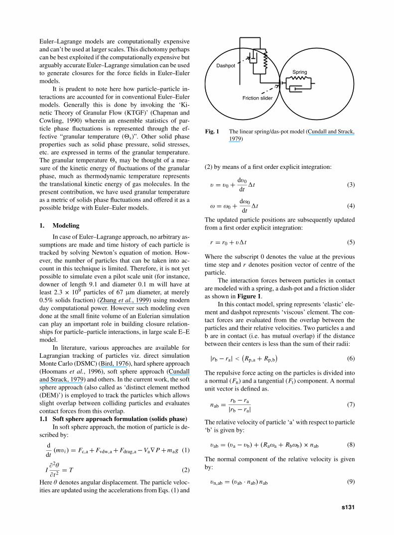
Fig. 1 The linear spring/das-pot model (Cundall and Strack,1979)

(2) by means of a first order explicit integration:

v = v0 + dv0

dt1t (3)

ω = ω0 + dω0

dt1t (4)

The updated particle positions are subsequently updatedfrom a first order explicit integration:

r = r0 + v1t (5)

Where the subscript 0 denotes the value at the previoustime step and r denotes position vector of centre of theparticle.

The interaction forces between particles in contactare modeled with a spring, a dash-pot and a friction slideras shown in Figure 1.

In this contact model, spring represents ‘elastic’ ele-ment and dashpot represents ‘viscous’ element. The con-tact forces are evaluated from the overlap between theparticles and their relative velocities. Two particles a andb are in contact (i.e. has mutual overlap) if the distancebetween their centers is less than the sum of their radii:

|rb − ra| <(Rp,a + Rp,b

)(6)

The repulsive force acting on the particles is divided intoa normal (Fn) and a tangential (Ft) component. A normalunit vector is defined as.

nab = rb − ra

|rb − ra| (7)

The relative velocity of particle ‘a’ with respect to particle‘b’ is given by:

vab = (va − vb) + (Raωa + Rbωb) × nab (8)

The normal component of the relative velocity is givenby:

vn,ab = (vab · nab) nab (9)

s131

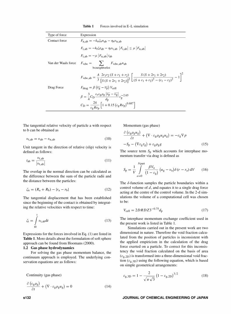
Table 1 Forces involved in E–L simulation

Type of force Expression

Contact force Fn,ab = −knξnnab − ηnvn,ab

Ft,ab = −ktξttab − ηtvt,ab∣∣Ft,ab

∣∣ ≤ µ∣∣Fn,ab

∣∣Ft,ab = −µ

∣∣Fn,ab∣∣ tab

Van der Waals force Fvdw =∑

b∈neighborlist

Fvdw,abnab

Fvdw,ab = A3

2r1r2 (S + r1 + r2)[S (S + 2r1 + 2r2)

]2

[S (S + 2r1 + 2r2)

(S + r1 + r2)2 − (r1 − r2)2 − 1]2

Drag Force Fdrag = β(vg − vp

)Vcell

β = 34

CDεsεgρg

∣∣vp − vg∣∣

dpε−2.65

g

CD = 24εg Rep

[1 + 0.15

(εg Rep

)0.687]

The tangential relative velocity of particle a with respectto b can be obtained as

vt,ab = vab − vn,ab (10)

Unit tangent in the direction of relative (slip) velocity isdefined as follows:

tab = vt,ab∣∣vt,ab∣∣ (11)

The overlap in the normal direction can be calculated asthe difference between the sum of the particle radii andthe distance between the particles:

ξn = (Ra + Rb) − |ra − rb| (12)

The tangential displacement that has been establishedsince the beginning of the contact is obtained by integrat-ing the relative velocities with respect to time:

ξt =t∫

t0

vt,abdt (13)

Expressions for the forces involved in Eq. (1) are listed inTable 1. More details about the formulation of soft sphereapproach can be found from Hoomans (2000).1.2 Gas phase hydrodynamics

For solving the gas phase momentum balance, thecontinuum approach is employed. The underlying con-servation equations are as follows:

Continuity (gas phase)

∂(εgρg

)∂t

+ (∇ · εgρgug) = 0 (14)

Momentum (gas phase)

∂(εgρgug

)∂t

+ (∇ · εgρgugug) = −εg∇ p

−Sp − (∇εgτg) + εgρgg (15)

The source term Sp which accounts for interphase mo-mentum transfer via drag is defined as

Sp = 1V

Npart∫a=0

βVa(1 − εg

) (ug − va

)δ (r − ra) dV (16)

The δ-function samples the particle boundaries within acontrol volume of d , and equates it to a single drag forceacting at the centre of the control volume. In the 2-d sim-ulations the volume of a computational cell was chosento be:

Vcell = 2DRDZ3−0.75dp (17)

The interphase momentum exchange coefficient used inthe present work is listed in Table 1.

Simulations carried out in the present work are twodimensional in nature. Therefore the void fraction calcu-lated from the position of particles is inconsistent withthe applied empiricism in the calculation of the dragforce exerted on a particle. To correct for this inconsis-tency the void fraction calculated on the basis of area(εg,2D) is transformed into a three-dimensional void frac-tion (εg,3D) using the following equation, which is basedon simple geometrical arrangements:

εg,3D = 1 − 2√π

√3

(1 − εg,2D

)3/2 (18)

s132 JOURNAL OF CHEMICAL ENGINEERING OF JAPAN

Table 2 Parameters used in E–L simulation

Particle diameter (dp) 60 µmParticle density (ρp) 2500 kg/m3

Gas density (ρg) 1.2 kg/m3

Number of particles (Np) 6000Gas viscosity (µg) 1.8 × 10−5 kg/msRestitution coefficient (e) 0.90Coefficient of friction (µ) 0.15Normal spring stiffness (kn) 7 N/mBed size (W × H ) 0.0045 m × 0.05 mTime step (1t) 1 × 10−5s

2. Numerical Simulation

A finite difference technique, employing a staggeredgrid to ensure numerical stability, is used to solve the gasphase conservation Eqs. (14) and (15). This implies thatthe scalar variables (P and εg) are defined at the cell cen-tre and that the velocity components are defined at the cellfaces. For the incorporation of the boundary conditions aflag matrix is used which allows boundary conditions tobe specified for each single cell. More details about thenumerical solution can be found out from Kuipers et al.(1993).2.1 Input parameters

Euler–Lagrange simulations were carried for num-ber of operating conditions with number of particles vary-ing from 6000 to 24000 for both riser (gas–solids cocur-rent upflow) as well as downer (gas–solids cocurrentdownflow) configuration. In order to study the effect ofvarious parameters on the behavior of the system first abase case simulation is established for riser and then theconcerned parameters are varied subsequently. Base casefor downer was established by changing the flow direc-tion.

The numerical parameters (Hoomans, 2000) used inthe base case simulation of riser are summarized in Ta-ble 2. In order to ensure the equal normal and tangen-tial contact times the tangential spring coefficient is takento be 2/7 times that of normal spring coefficient. Cor-responding damping coefficient can be readily obtainedfrom the spring coefficient and the mass of involved par-ticles (Hoomans, 2000). No slip condition is used for gasphase whereas particles are allowed for frontal collisionsat wall.2.2 Initialization of the simulation

In case of up flow system (riser), initially a packedbed of given number of particles in the solution domain isconfigured. It is subjected to inlet gas velocity sufficientlyhigher than minimum fluidization velocity for 0.5 s, andthen inlet gas velocity is increased linearly with time tillt = 1.0 s (or t = 2.0 s) to the desired value and kept con-stant. This procedure ensures the smooth fluidization ofsolids at higher inlet gas velocity in case of riser. In case

of downflow system the solids are subjected to the de-sired velocity from t = 0.0 s. Whenever a particle leavesthe domain exit, it is allowed to re-enter into the systemwith the same slip velocity. This slip velocity is the abso-lute difference between the particle velocity and the gasvelocity in the cell from which particle is exiting the sys-tem.2.3 Calculation of granular temperature

In order to calculate the averaged granular tempera-ture, a coarsened grid (let us say ‘post-processing grid’)is used such that each coarsened cell contains around 35particles. Granular temperature in each cell is calculatedas

2k,x =∑(

Ci,x − Cs,k,x)2

Npart,k

2k,y =∑(

Ci,y − Cs,k,y)2

Npart,k(19)

Thus obtained granular temperature is time-averagedover the flow domain as

⟨⟨2i ⟩⟩ = 1tmax − tmin

tmax∫tmin

Ncell∑k

εs,k2k,i

Ncell∑k

εs,k

dt (20)

⟨⟨2⟩⟩ = 2 ⟨⟨2x ⟩⟩ + ⟨⟨2y

⟩⟩3

(21)

In Eq. (19) indicates ensemble averaged velocity in thecorresponding cell. Grid independence (Coarser as wellas finer grid is used) is also checked for the granular tem-perature calculations. Unlike the DEM simulations, in or-der to calculate porosity required in granular temperaturecalculation the centre of particles in the correspondingcells is considered. Calculation of granular temperatureis started from t = 2.0 s so that it is not affected by thestart-up effects. DEM simulation for given case is contin-ued till the variation in time averaged granular tempera-ture with time is small enough.

3. Results and Discussion

Figures 2 and 3 show typical snapshot of DEMsimulation for upflow and downflow mode respectively.Figure 4 shows typical contour of granular temperaturefor riser as well as downer. Jiradilok et al. (2006) ob-tained granular temperature of the order of 0.1–10 m2/s2

for riser via Euler–Euler simulations. Similarly we ob-tained granular temperature of the order of 0.01 m2/s2

(case R.3 and R.4) for riser with relatively smaller di-mensions.Tables 3 and 4 summarize the DEM simula-tions carried out under various operating conditions forupflow and downlow mode respectively. Base case sim-ulation in upflow mode (Case R.1) with realistic colli-sion parameters indicates that, ‘equipartition of energy’assumption in KTGF may not be a good approximation.

VOL. 42 Supplement 1 2009 s133

(a) (b)

Fig. 2 Snapshot of DEM simulation at t = 5 s showing position of particles in the flow domain for Case (a) R.1 and (b) R.4

(a) (b)

Fig. 3 Snapshot of DEM simulation at t = 5 s showing position of particles in the flow domain for case (a) D.1 and (b) D.4

Θ[m2/s2](a) (b)

Fig. 4 Contour plot of time averaged granular temperaturefor (a) case R.1 (b) case D.1

If the particle–particle collisions would have been ideal(i.e. Case R.7, Case D.7) then ‘equipartition of energy’assumption would have been more appropriate. Granulartemperature for downflow mode of operation seems to behigher as compared to that of upflow mode of operation.This is to be expected since in downflow mode solids flowwill be assisted by gravity.

An attempt was made to see the effect of flow vari-ables such as inlet gas velocity and solids fraction ongranular temperature. It was observed that, under investi-gated operating conditions increase in both solids veloc-ity and solids fraction results into increase in averagedgranular temperature of the flow. This was observed forboth upflow mode as well as downflow mode of opera-tion. However, increase in solids fraction (case R.4 andD.4) hardly affects distribution of granular temperaturein each direction whereas for high velocity flows (caseR.3 and D.3) the distribution is much better.

As compared to Geldart group A particles (ρp =2500 kg/m3, dp = 60 µm), Geldart group B particles(case R.8 and D.8) showed higher granular temperatureunder dilute flow conditions whereas lower granular tem-perature under denser flow conditions. In all the inves-tigated operating conditions, Geldart group B particles

s134 JOURNAL OF CHEMICAL ENGINEERING OF JAPAN

Table 3 Summary of DEM simulations for upflow mode

Case No. ρp dp e µ εs,2D Ug,in tstop ⟨⟨2x ⟩⟩ ⟨⟨2y⟩⟩ ⟨⟨2⟩⟩[kg/m3] [µm] [m/s] [s] [m2/s2] [m2/s2] [m2/s2]

R.1 2500 60 0.9 0.15 0.075 1.2 16 0.00092 0.0027 0.0015R.2 2500 60 0.9 0.15 0.075 1.2 10 0.0012 0.0027 0.0017R.3 2500 60 0.9 0.15 0.075 3.4 16 0.0082 0.0226 0.013R.4 2500 60 0.9 0.15 0.15 1.2 12 0.016 0.019 0.017R.5 900 60 0.9 0.15 0.075 1.2 17 0.00045 0.0051 0.002R.6 2500 60 1 0 0.075 1.2 12 0.005 0.007 0.006R.7 2500 60 0.8 0.15 0.075 1.2 10 0.00088 0.0032 0.0016R.8 2500 150 0.9 0.15 0.075 1.2 18 0.0039 0.0068 0.0048

Table 4 Summary of DEM simulations for downflow mode

Case No. ρp dp e µ εs,2D Ug,in tstop ⟨⟨2x ⟩⟩ ⟨⟨2y⟩⟩ ⟨⟨2⟩⟩[kg/m3] [µm] [m/s] [s] [m2/s2] [m2/s2] [m2/s2]

D.1 2500 60 0.9 0.15 0.075 1.2 13 0.00127 0.0035 0.002D.2 2500 60 0.9 0.15 0.075 1.2 23 0.0019 0.0039 0.0026D.3 2500 60 0.9 0.15 0.075 3.4 13 0.011 0.02 0.014D.4 2500 60 0.9 0.15 0.15 1.2 12 0.063 0.108 0.077D.5 900 60 0.9 0.15 0.075 1.2 15 0.00024 0.0019 0.0008D.6 2500 60 1 0 0.075 1.2 12 0.0073 0.012 0.0088D.7 2500 60 0.8 0.15 0.075 1.2 10 0.001 0.004 0.002D.8 2500 150 0.9 0.15 0.075 1.2 18 0.0066 0.0092 0.0075

showed ‘better equipartition of energy’ than that of Gel-dart group A particles. This certainly indicates that parti-cle size as well as solids fraction involved have strong ef-fect on the underlying solids–solids interaction and needsfurther investigation. Another point to be noted is aboutflow behavior of ‘FCC like’ particles. Risers find signif-icant application in the area of ‘Fluid Catalytic Cracking(FCC)’ so one of the simulations was done with parti-cles resembling to ‘typical FCC’ particles (i.e. case R.5and D.5). In this case deviations from ‘equipartition ofenergy’ assumptions were found.

Conclusions

DEM simulations were carried out for gas solids dis-persed flow in both upward as well as downward flowmode. Simulations were extended to variety of operatingconditions.

For ideal–ideal collisions, flow was found to bemore uniform which is in agreement with the previousstudies in the literature. DEM simulations indicated that,distribution of ‘granular temperature’ in all the directionsis not uniform. Thus, ‘equipartition of energy’ assump-tion in kinetic theory of granular flow needs further atten-tion. In future, an attempt will be made to rigorously val-idate the DEM simulations using advanced experimentaltechniques.

The eventual goal is to formulate the better clo-sures for particle–particle interactions which will be sub-sequently used in Euler–Euler simulations of pilot plantscale riser/downer.

AcknowledgmentsThe software for the discrete particle model (DPM) originated

from the group Fundamentals of Chemical Reaction Engineering atthe University of Twente, The Netherlands. Specifically, Prof. J. A. M.Kuipers and Dr. N. G. Deen are gratefully acknowledged for sharinga version of their code with us. Dr. N. G. Deen is acknowledged fordiscussions and clarifications regarding the code.

NomenclatureCD = single particle drag coefficient [—]D = diameter of the column [m]DR, DZ = width, height of computational cell [m]dp = particle diameter [m]e = restitution coefficient [—]F = force [N]I = moment of inertia of the particle [kg m2]k = spring constant [N/m]m = mass of the particle [kg]N = total number [—]P = pressure [N/m2]R = radius [m]Re = Reynolds number [—]S = distance between two neighboring particles [m]T = torque acting on the particle [N m]t = time [sec]ug = superficial gas velocity [m/s]Va = volume [m3]v = velocity [m/s]

βs,f = interphase momentum exchange factor [kg/m3s]ε = volume fraction [—]2 = granular temperature [m2/s2]θ = angular displacement [rad]µ = coefficient of friction [—]ρ = density [kg/m3]τ = shear stress [N/m2]

VOL. 42 Supplement 1 2009 s135

<Subscript>a = particle, ag = gas phasen = normals = solids phaset = tangential

Literature CitedAvidan, A. A. and R. Shinnar; “Development of Catalytic Cracking

Technology. A Lesson in Chemical Reactor Design,” Ind. Eng.Chem. Res., 29, 931–942 (1990)

Bird, G. A.; Molecular Gas Dynamics and Direct Simulation of GasFlows, Oxford University Press, Oxford, U.K. (1976)

Chapman S. and T. G. Cowling; The Mathematical Theory of Non–Uniform Gases, 3rd ed., Cambridge University Press, Cambridge,U.K. (1990)

Contractor, R. M.; “Dupont’s CFB Technology for Maleic Anhydride,”Chem. Eng. Sci., 54, 5627–5632 (1999)

Cundall, P. A. and O. D. L. Strack; “A Discrete Numerical Model forGranular Assemblies,” Geotechnique, 29, 47–65 (1979)

Helland, E., R. Occelli and L. Tadrist; “Computational Study of Fluc-tuating Motions and Cluster Structures in Gas–Particle Flows,” Int.J. Multiphase Flow, 28, 199–223 (2002)

Hoomans, B. P. B.; Granular Dynamics of Gas–Solid Two Phase Flow,Ph.D. Thesis, University of Twente, the Netherlands (2000)

Hoomans, B. P. B., J. A. M. Kuipers, W. J. Briels and W. P. M. vanSwaaij; “Discrete Particle Simulation of Bubble and Slug Forma-tion in a Two-Dimensional Gas Fluidized Bed: A Hard Sphere Ap-proach,” Chem. Eng. Sci., 51, 99–118 (1996)

Jiradilok, V., D. Gidaspow, S. Damronglerd, W. J. Koves andR. Mostofi; “Kinetic Theory Based CFD Simulation of TurbulentFluidization of FCC Particles in a Riser,” Chem. Eng. Sci., 61,5544–5559 (2006)

Kuipers, J. A. M., K. J. van Duin, F. P. H. van Beckum and W. P. M. vanSwaaij; “Computer Simulation of the Hydrodynamics of a Two-Dimensional Gas-Fluidized Bed,” Comput. Chem. Eng., 17, 839–858 (1993)

Tsuji, Y., T. Kawaguchi and T. Tanaka; “Discrete Particle Simulationof Two-Dimensional Fluidized Bed,” Powder Technol., 77, 79–87(1993)

Zhang, H., J. X. Zhu and M. Bergougnou; “Hydrodynamics in Down-flow Fluidized Beds 1: Solids Concentration Profiles and PressureGradient Distributions,” Chem. Eng. Sci., 54, 5461–5470 (1999)

Zhang, M. H., K. W. Chu, F. Wei and A. B. Yu; “A CFD–DEM Studyof the Cluster Behavior in Riser and Downer Reactors,” PowderTechnol., 184, 151–165 (2008)

s136