SULFUR COATING OF UREA IN SHALLOW SPOUTED BEDS ...
244
SULFUR COATING OF UREA IN SHALLOW SPOUTED BEDS by MICHAEL MYUNG-SOO CHOI B.Sc., University of Alberta, 1986 A DISSERTATION SUBMITTED IN PARTIAL FULFILLMENT OF THE REQUIREMENTS FOR THE DEGREE OF DOCTOR OF PHILOSOPHY IN THE FACULTY OF GRADUATE STUDIES DEPARTMENT OF CHEMICAL ENGINEERING We accept this thesis as conforming to the required standard THE UNIVERSITY OF BRITISH COLUMBIA APRIL, 1993 © Michael M.S. Choi, 1993
-
Upload
khangminh22 -
Category
Documents
-
view
3 -
download
0
Transcript of SULFUR COATING OF UREA IN SHALLOW SPOUTED BEDS ...
SULFUR COATING OF UREA IN SHALLOW SPOUTED BEDS
by
MICHAEL MYUNG-SOO CHOI
B.Sc., University of Alberta, 1986
A DISSERTATION SUBMITTED IN PARTIAL FULFILLMENT OF
THE REQUIREMENTS FOR THE DEGREE OF
DOCTOR OF PHILOSOPHY
IN
THE FACULTY OF GRADUATE STUDIES
DEPARTMENT OF CHEMICAL ENGINEERING
We accept this thesis as conforming
to the required standard
THE UNIVERSITY OF BRITISH COLUMBIA
APRIL, 1993
© Michael M.S. Choi, 1993
In presenting this thesis in partial fulfilment of the requirements for an advanced
degree at the University of British Columbia, I agree that the Library shall make it
freely available for reference and study. I further agree that permission for extensive
copying of this thesis for scholarly purposes may be granted by the head of my
department or by his or her representatives. It is understood that copying or
publication of this thesis for financial gain shall not be allowed without my written
permission.
(Signat
CIA^c 0.1 C •rkcji^vt.)
The University of British ColumbiaVancouver, Canada
Date^zo ^1993
Department of
DE-6 (2/88)
Abstract
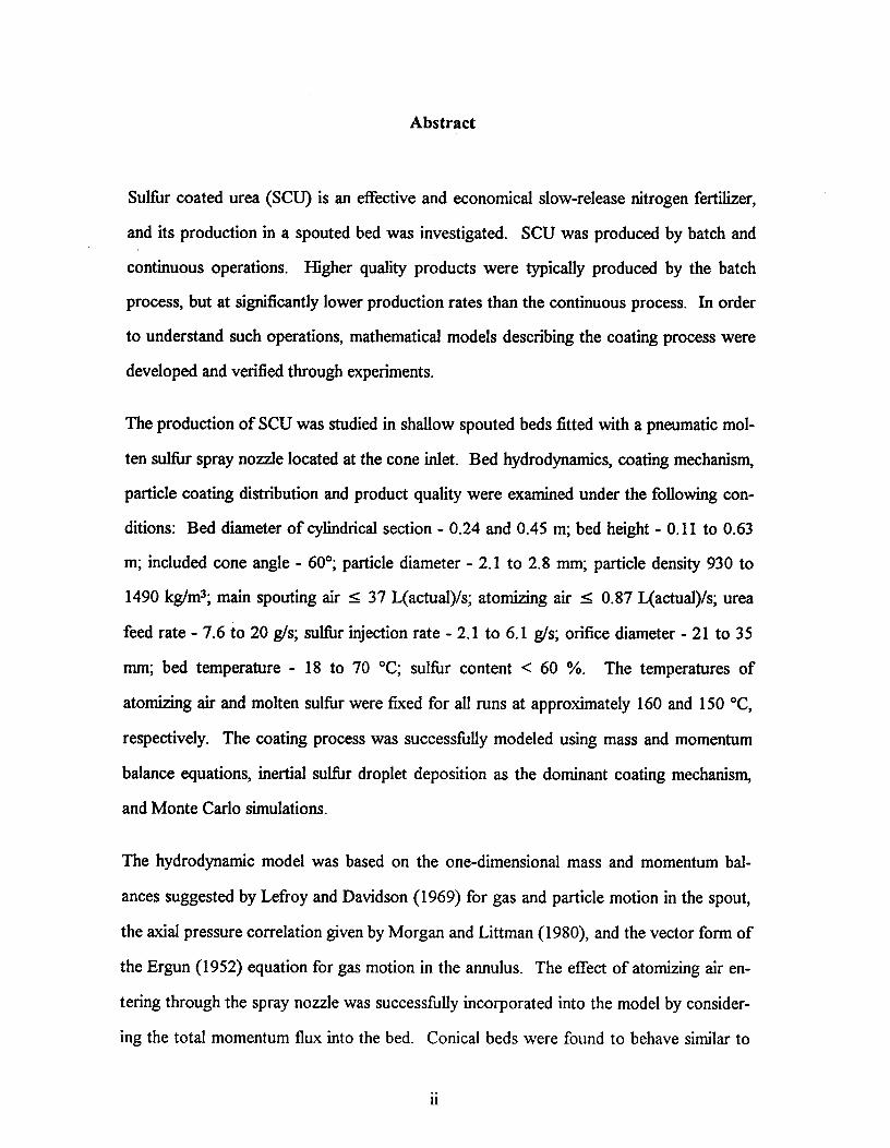
Sulfur coated urea (SCU) is an effective and economical slow-release nitrogen fertilizer,
and its production in a spouted bed was investigated. SCU was produced by batch and
continuous operations. Higher quality products were typically produced by the batch
process, but at significantly lower production rates than the continuous process. In order
to understand such operations, mathematical models describing the coating process were
developed and verified through experiments.
The production of SCU was studied in shallow spouted beds fitted with a pneumatic mol-
ten sulfur spray nozzle located at the cone inlet. Bed hydrodynamics, coating mechanism,
particle coating distribution and product quality were examined under the following con-
ditions: Bed diameter of cylindrical section - 0.24 and 0.45 m; bed height - 0.11 to 0.63
m; included cone angle - 60'; particle diameter - 2.1 to 2.8 mm; particle density 930 to
1490 kg/m3; main spouting air 37 L(actual)/s; atomizing air S 0.87 L(actual)/s; urea
feed rate - 7.6 to 20 g/s; sulfur injection rate - 2.1 to 6.1 g/s; orifice diameter - 21 to 35
mm; bed temperature - 18 to 70 °C; sulfur content < 60 %. The temperatures of
atomizing air and molten sulfur were fixed for all runs at approximately 160 and 150 °C,
respectively. The coating process was successfully modeled using mass and momentum
balance equations, inertial sulfur droplet deposition as the dominant coating mechanism,
and Monte Carlo simulations.
The hydrodynamic model was based on the one-dimensional mass and momentum bal-
ances suggested by Lefroy and Davidson (1969) for gas and particle motion in the spout,
the axial pressure correlation given by Morgan and Littman (1980), and the vector form of
the Ergun (1952) equation for gas motion in the annulus. The effect of atomizing air en-
tering through the spray nozzle was successfully incorporated into the model by consider-
ing the total momentum flux into the bed. Conical beds were found to behave similar to
ii
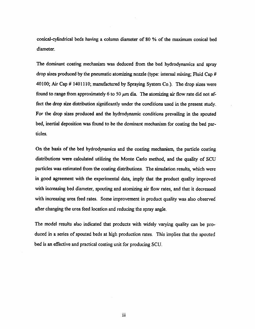
conical-cylindrical beds having a column diameter of 80 % of the maximum conical bed
diameter.
The dominant coating mechanism was deduced from the bed hydrodynamics and spray
drop sizes produced by the pneumatic atomizing nozzle (type: internal mixing; Fluid Cap #
40100; Air Cap # 1401110; manufactured by Spraying System Co.). The drop sizes were
found to range from approximately 6 to 50 Am dia. The atomizing air flow rate did not af-
fect the drop size distribution significantly under the conditions used in the present study.
For the drop sizes produced and the hydrodynamic conditions prevailing in the spouted
bed, inertial deposition was found to be the dominant mechanism for coating the bed par-
ticles.
On the basis of the bed hydrodynamics and the coating mechanism, the particle coating
distributions were calculated utilizing the Monte Carlo method, and the quality of SCU
particles was estimated from the coating distributions. The simulation results, which were
in good agreement with the experimental data, imply that the product quality improved
with increasing bed diameter, spouting and atomizing air flow rates, and that it decreased
with increasing urea feed rates. Some improvement in product quality was also observed
after changing the urea feed location and reducing the spray angle.
The model results also indicated that products with widely varying quality can be pro-
duced in a series of spouted beds at high production rates. This implies that the spouted
bed is an effective and practical coating unit for producing SCU.
iii
Table of Contents
Abstract^
Table of Contents^ iv
List of Tables^ ix
List of Plates^
List of Figures^ xi
Acknowledgment^ xv
Dedications ^ xvi
Chapter 1. Introduction^ 1
1.1. The UBC Spouted Bed Process^ 2
1.2. Objectives of Present Study^ 51.2.1. Bed Hydrodynamics^ 6
1.2.2. Coating Mechanisms^ 61.2.3. Overall Coating Performance^ 6
1.2.4. Benefits of the Study^ 7
Chapter 2. Literature Review^ 8
2.1. UBC Process^ 8
2.1.1. Product Quality^ 9
2.1.2. Effect of Bed Temperature on Product Quality^ 9
2.1.3. Effect of Sulfur Injection Rate on Product Quality^ 11
2.1.4. Effect of Atomizing Air on Product Quality^ 11
2.1.5. Effect of Bed Depth on Product Quality^ 12
2.1.6. Effect of Spouting Air Flow Rate on Product Quality^ 13
2.1.7. Effect of Chemical Additives on Product Quality^ .13
2.2. Models of Spouted Bed Coating Process^ 13
2.3. Models and Correlations for Spouted Bed Hydrodynamics^ 16
2.3.1. Minimum Spouting Velocity^ 16
iv
2.3.2. Solids Circulation and Bed Hydrodynamics^ 172.3.3. Spout Diameter^ 182.3.4. Pressure Profile in Annulus^ 19
2.4. Coating Mechanism^ 20
2.5. Monte Carlo Method^ 21
Chapter 3. Experimental Materials, Apparatus and Procedures^ 23
3.1. Experimental Materials^ 233.1.1. Urea^ 273.1.2. Sulfur^ 283.1.3. Particles Used in Hydrodynamics Study^ 29
3.2. Main Coating Apparatus^ 303.2.1. Spouted Bed^ 323.2.2. Sulfur Supply System^ 34
3.2.2.1. Sulfur Melter^ 343.2.2.2. Sulfur Filter^ 353.2.2.3. Sulfur Rotameter^ 353.2.2.4. Sulfur Line^ 363.2.2.5. Nitrogen Supply^ 37
3.2.3. Nozzle Assembly^ 373.2.4. Urea Feeding Device^ 373.2.5. Product Withdrawal Device^ 393.2.6. Product Collector^ 393.2.7. Dust Collector^ 393.2.8. Air, Steam, and Water Supplies^ 40
3.3. Apparatus for Hydrodynamics Study^ 40
3.4. Apparatus for Spray Study^ 413.4.1. Spray Box^ 423.4.2. Spray Sampler^ 43
3.5. Coating Procedures^ 443.5.1. Start Up^ 44
v

3.5.2. Coating^ 453.5.3. Shut Down and Clean-up^ 46
3.6. Procedures for Hydrodynamics Study^ 463.6.1. Minimum Spouting Velocity, U„,,^ 463.6.2. Voidage of Loosely Packed Bed, ern,-^ 47
3.6.3. Mean Particle Diameter, dp, and Sphericity, (I),^ 473.6.4. Diameter of Inlet Orifice, di^ 473.6.5. Static Pressure in Annulus^ 483.6.6. Air Velocity in the Spout, us^ 483.6.7. Radial Velocity Profile at the Base of the Bed^ 49
3.7. Procedures for Spray Studies^ 493.7.1. Operating Limits of Spray Nozzle^ 493.7.2. Spray Drop Size Measurements^ 50
3.8. Product Quality Analysis^ 503.8.1. Sulfur Content^ 503.8.2. Particle Sulfur Content^ 513.8.3. Seven Day Dissolution Test^ 52
Chapter 4. Mathematical Models^ 53
4.1. Simple Models^ 534.1.1. Model I: Residence Time Model^ 534.1.2. Model II: Simple Spray Zone Model^ 564.1.3. Model III: Variable Concentration Spray Zone Model^ 61
4.2. Model IV: Rigorous Model^ 624.2.1. Calculation of Models for Solids Circulation Rate and Bed
Hydrodynamics^ 634.2.2. Determination of Coating Mechanism and Concentration
Profile^ 664.2.3. Calculation of Coating Distribution Using the Monte Carlo
Method^ 684.2.3.1. Limitation of Analytical Model^ 684.2.3.2. Monte Carlo Procedure for Model III^ 69
vi
4.2.3.3. Monte Carlo Procedure for Model IV^ 704.2.3.3.1. Continuous Operation^ 704.2.3.3.2. Batch Operation^ 72
Chapter 5. Results and Discussions^ 74
5.1. Bed Hydrodynamics^ 745.1.1. Minimum Spouting Velocity, U ^ 755.1.2. Pressure Profile in Annulus^ 855.1.3. Velocity Profile in Annulus^ 895.1.4. Velocity Profile in Spout^ 895.1.5. Solids Movement^ 94
5.2. Spray Studies^ 945.2.1. Operating Limits^ 945.2.2. Spray Drop Size Distribution and Average Drop Size^ 965.2.3. Coating Mechanism and Sulfur Spray Concentration^ 102
5.3. Coating Distribution and Product Quality^ 1055.3.1. Coating Distribution^ 1075.3.2. Product Quality^ 1105.3.3. Effect of Operating and Model Variables on Coating Distri-
bution^ 1125.3.3.1. Effect of Operating Time^ 1125.3.3.2. Effect of Sample Size^ 115
5.3.3.2.1. Numerical Sampling^ 1155.3.3.2.2. Manual Sampling^ 116
5.3.3.3. Effect of Spray Angle^ 1185.3.3.4. Effect of Feed Location^ 1205.3.3.5. Effect of Beds-in-Series^ 1215.3.3.6. Effect of Model Variables, xe and x,^ 123
5.3.4. Sensitivity Analysis Using Model IV^ 125
5.4. Commercial Implications^ 130
Chapter 6. Conclusions and Recommendations^ 131
6.1. Conclusions^ 131
vii
6.1.1. Bed Hydrodynamics^ 1316.1.2. Spray Studies^ 1326.1.3. Coating Distribution and Product Quality^ 132
6.2. Recommendations for Further Work^ 133
Nomenclature^ 134
References^ 141
Appendix I: Supporting Derivations and Methodology^ 149I-1. Determination of Shutter Area^ 1501-2. Model II Derivation for Forced Urea Feed^ 1521-3. Calculation Method for Vector Ergun Equation^ 1541-4. Sulfur Sampling Devices^ 1561-5. Batch Coating Model^ 1611-6. Minimum Spouting Velocity Predictions by Wan-Fyong et al. Equation ^ 163
Appendix II: Experimental Data and Calculated Results^ 164
Appendix HI: Computer Program Listings^ 179
Appendix IV: Calibration Results^ 218
viii

List of Tables
Table^ page
1.1 Major agronomic benefits associated with SCU usage (Tisdale et al., 1985) ^ 1
2.1 Range of operating conditions used in previous studies on the UBC process ^ 9
3.1 Selected physical properties of urea (Perry et al., 1984) ^ 27
3.2 Selected chemical and physical properties of sulfur (Stauffer Chemical Co.) ^ 28
3.3 Properties of common sulfur allotropes (Donahue and Meyer, 1965; Dale andLudwig, 1965) ^ 28
3.4 Physical properties of bed particles^ 30
3.5 Types and capacities of Brooks rotameters used in this work ^ 36
4.1 Assumptions used in simple models^ 58
4.2 Selected infinite series definitions ^ 59
5.1 Operating ranges applicable to this work^ 75
5.2 Operating conditions under which the air velocities in the spout and the pres-sure profiles in the annulus were determined^ 76
5.3 Axial pressure profile near the spout-annulus interface ^ 77
5.4 Air velocity profile in the spout^ 78
5.5 Fitted constants for the Wu et al. (1987) equation ^ 80
5.6 Operating ranges of the spray studies ^ 95
5.7 Results of drop size studies at various operating conditions^ 100
5.8 Sauter mean diameters relative to the operating limits ^ 101
5.9 Mechanical collection efficiency (using correlations suggested by Clift et al.,1981) at selected operating conditions in the spout^ 102
5.10 Operating range applicable to coating distribution and product quality studies ^ 106
5.11 Operating conditions investigated for the coating study^ 106
5.12 Errors associated with sample sizes based on the Model II and III results ^ 116
ix
List of Tables Continued
Table^ page
5.13 Effect of feed location (using Model II with; = 0.5, X, = 0.25) ^ 121
5.14 Range of model variables examined for sensitivity analysis ^ 127
5.15 Results of sensitivity analysis using Model IV (X, =0.25, T = 60 °C) ^ 128
I-1 Direct sulfur sampling ^ 158
1-2 Hot tip: packed bed S = SO2 converter ^ 158
1-3 Hot tip: plate S = SO2 converter ^ 159
1-4 Hot tip: laser beam S = SO2 converter ^ 159
I-5 Hot tip: three tube hot wire S = SO 2 converter ^ 160
I-6 Hot tip: two tube hot wire S = SO2 converter ^ 160
II-1 Ivfmimum spouting velocity data ^ 165
II-2 Spray drop size distribution ^ 174
LE-3 Measured sulfur content of individual particles for selected continuous runs ^ 176
II-4 Predicted sulfur content of individual particles for selected continuous runs ^ 177
II-5 Measured sulfur content of individual particles for batch runs shown inFigures 4.3 and 5.25 ^ 178
IV-1 Calibration equations for flowmeters and refractometer ^ 219
List of Plates
Plate^ page
3.1 Urea ^ 24
3.2 Sulfur coated urea produced by batch process^ 24
3.3 Sulfur coated urea produced by continuous process ^ 25
3.4 Polyformaldehyde ^ 25
3.5 Polyethylene ^ 26
3.6 Polystyrene ^ 26
x
List of Figures
Figure^ page
1.1 Schematic diagram of UBC spouted bed coating unit for producing sulfurcoated urea (heavy arrows indicate direction of solids flow) ^ 3
1.2 Sulfur content of CIL and UBC products (Tsai, 1986) ^ 5
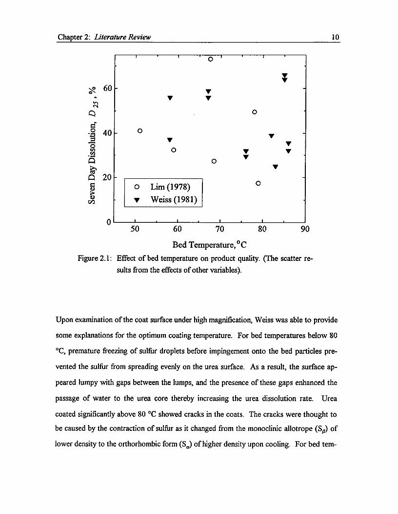
2.1 Effect of bed temperature on product quality. (The scatter results from the ef-fects of other variables) ^ 10
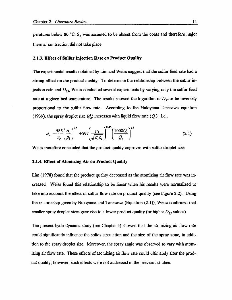
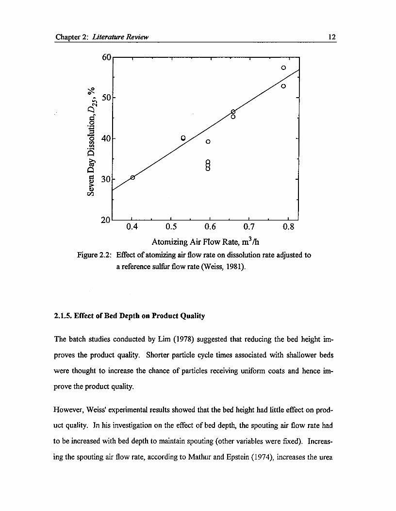
2.2 Effect of atomizing air flow rate on dissolution rate normalized for the sulfurflow rate (Weiss, 1981) ^ 12
3.1 Viscosity of sulfur at low temperature range (Freeport Sulfur Co., 1954) ^ 29
3.2 Simplified flowsheet of UBC spouted bed facility ^ 31
3.3 Sectional view of spouted bed column ^ 32
3.4 Shutter assembly (dimensions are given in mm) designed by Mathur, Meisenand Link (1978) ^ 33
3.5 Sectional view of 18.9 L sulfur reservoir^ 34
3.6 Sectional view of "slip-on" sulfur line connector ^ 36
3.7 Sectional view of nozzle, perforated plate and steam chamber (all dimensionsin mm; designed by Meisen, Lee and Le, 1986) ^ 38
3.8 Modifications to the top of the spouted bed (i.e., see Figure 3.3) for hydrody-namics study ^ 41
3.9 Schematic diagram of static pressure probe^ 42
3.10 Schematic diagram of S-type pitot tube (1/8" tubes and 3/8" tube are held inplace with silver solder)^ 42
3.11 Spray box assembly ^ 43
3.12 Simplified drawing of the rotating sulfur droplet sampler^ 44
3.13 Sectional view of atomizing nozzle and inlet air assembly (not drawn to scale)^48
4.1 Model I — perfectly mixed vessel ^ 54
xi

List of Figures Continued
Figure^ page
4.2 Prediction of Model I using different numbers of continuously stirred tanks inseries ^ 55
4.3 Prediction of Model I^ 57
4.4 System described by Model II ^ 58
4.5 Sectional view of the lower spout ^ 66
4.6 Concentration balance on coating material in the spout ^ 67
5.1 Comparison between experimental and predicted U., values ^ 79
5.2 Radial velocity profile 10 mm above the shutter in an empty bed (Q, = 27.9L/s, di = 24.7 nun and T = 65°C) ^ 80
5.3 Effect of atomizing air on minimum spouting velocity (minimum spouting ve-locity is based only on the main spouting air flow rate; D = 0.45 m, H =0.31 m, d= 35 mm)^ 82
5.4 Momentum flow of air into the spouted bed (dashed and solid lines represent0.24 m and 0.45 m dia. beds, respectively) ^ 82
5.5 Effect of bed height on minimum spouting velocity, Ums. (Cone-cylinder junc-tions are denoted by dashed lines; solid lines represent indicated relation-ships fitted to experimental data) ^ 83
5.6 Comparison between experimental data and predictions from correlation basedon the optimum diameter D'^ 83
5.7 Pressure profile in the annulus (conical bed, Run H22)^ 86
5.8 Axial pressure profile in the annulus near the spout-annulus interface (conical-cylindrical bed, Run H1)^ 86
5.9 Axial pressure profile in the annulus (conical bed, Run H22, column diameterused in calculation) ^ 87
5.10 Axial pressure profile in the annulus (conical bed, Run H22, D' used in calcu-lation) ^ 87
5.11 Axial pressure profile in the annulus (H = 0.53, Run H17)^ 88
xii
List of Figures Continued
Figure^ page5.12 Comparison between measured and predicted pressure profile in the annulus ^ 88
5.13 Effect of atomizing air on axial air velocity profile in the spout (Q, is fixed atapproximately 32 Lls in all runs) ^ 90
5.14 Air velocities in the spout determined experimentally and from Model IVhydrodynamics (Run H1) ^ 91
5.15 Air velocities in the spout determined experimentally and from Model IVhydrodynamics and Equation (5.5) (Run H22)^ 91
5.16 Operating limits for atomization of sulfur ^ 96
5.17 Number distribution and predictions using log-normal equation (Run Sla) ^ 97
5.18 Log-normal representation of drop size distribution (Run Sla)^ 98
5.19 Nukiyama-Tanasawa representation of drop size distribution (Run Sla) ^ 98
5.20 Predictions of Sauter mean diameter ^ 101
5.21 Sulfur concentration profile for various spray angles ^ 104
5.22 Sulfur concentration profile for various coating runs (4) = 20°) ^ 104
5.23 Comparison between measured and predicted coating distributions for RunC17^ 108
5.24 Comparison between measured and predicted coating distributions for RunC38^ 108
5.25 Coating distributions of batch products ^ 109
5.26 Relationship between 7-day dissolution and sulfur content for batch products ^ 111
5.27 Comparison between measured and predicted product quality ^ 112
5.28 Effect of operating period on coating distribution^ 114
5.29 Effect of sample size on coating distribution (Models II and III)^ 117
5.30 Effect of sample size on coating distribution (Model IV) ^ 117
5.31 Effect of sample size (manual sampling) ^ 118
5.32 Effect of spray angle on coating distribution (results from Model IV) ^ 119
List of Figures Continued
Figure^ page
5.33 Effect of the spray concentration on coating distribution (results were ob-tained from Model III using Equation (4.19)) ^ 119
5.34 Effect of feed location^ 122
5.35 Product coating distributions for beds-in-series (from Model IV) ^ 122
5.36 Sensitivity analysis of; on coating distribution using Model II (x c = 0.6) ^ 124
5.37 Sensitivity analysis ofx, on coating distribution using Model II (x e = 0.2) ^ 124
5.38 Model predictions of product quality^ 126
5.39 Effect of a large x, on coating distribution ()cc = 0.05) ^ 129
I-1 Shape of 1/5th of the shutter ^ 150
I-2 Shape of a section of fully open shutter with the same base length (t) shown inFigure I-1 ^ 151
I-3 Simplified flow sheet of a forced feed system ^ 152
I-4 Minimum spouting velocity predictions using Wan-Fyong et al. (1969)equation^ 163
IV-1 Calibration curve for the lower capacity spouting air rotameter^ 220
IV-2 Calibration curve for the higher capacity spouting air rotameter^ 221
IV-3 Calibration curve for the atomizing air rotameter^ 222
IV-4 Calibration curve for the sulfur rotameter ^ 223
IV-5 Calibration curve for the urea feeder^ 224
IV-6 Predictions using the calibrated value of Co for the static-pitot tube ^ 225
IV-7 Predictions using the calibrated value of Co for the S-type pitot tube ^ 226
IV-8 Calibration curve for the Abbey refractometer ^ 227
xiv

Acknowledgement
I wish to express my sincere gratitude to Dr. A. Meisen for his helpful suggestions and
guidance which played a crucial role in the completion of this study.
I wish to thank my committee members for their willing assistance and suggestion — espe-
cially Dr. I. Gartshore for his assistance with designs of fluid velocity measurement de-
vices.
I also wish to extend my sincere appreciation to the following individuals and departments
for their assistance:
• Mr. Van Quan Le and Mr. Victor Lee for their assistance with the operation of the
spouted bed coating unit,
• The Workshop, Stores, faculty and staff of Chemical Engineering for their assistance,
• The Department of Metals and Materials Engineering for their assistance with the use
of image analyzer.
Finally, I wish to thank my family for their continued encouragement, patience and under-
standing. I am especially grateful to my father for encouraging me to pursue a higher de-
gree and for understanding my inability to fulfill my role as a son during the course of this
project. I am also indebted to my wife for single-handedly taking care of our daughter on
top of working to make ends meet.
xv

Delicate a oat icalten,
met eaie Ado,
cued meet dcuellave Alelee94...
Chapter 1.Introduction
Sulfur coated urea (SCU) has been proven as an effective and economical slow release ni-
trogen fertilizer. SCU is produced by applying a light coating of water resistant sulfur on
urea granules. In soil, the sulfur is slowly degraded by microorganisms and the urea is
thereby exposed. For this reason SCU is classified as a slow release nitrogen (SRN) fertil-
izer. Previous studies (Davis, 1973; Waddington and Duich, 1976; Allen et al., 1971)
showed that SCU is at least as effective as other SRN fertilizers or repeated applications
of uncoated nitrogen fertilizers. Moreover, SCU is the least expensive SRN fertilizer cur-
rently on the market, and has the highest nitrogen content. Other agronomic benefits of
using SCU are summarized in Table 1.1.
The major disadvantages of SCU, are that the sulfur increases the soil acidity and lowers
the nitrogen content of the fertilizer. Although lime application can mitigate the acidifying
effect and greater fertilizer dosage can make up the necessary nitrogen requirement, both
remedies add to the total cost. Therefore, it is important to reduce the sulfur content of
SCU without significantly lowering the quality of SCU as a slow release nitrogen fertilizer.
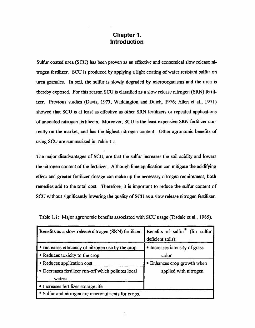
Table 1.1: Major agronomic benefits associated with SCU usage (Tisdale et al., 1985).
Benefits as a slow-release nitrogen (SRN) fertilizer: Benefits of sulfur* (for sulfurdeficient soils):
• Increases efficiency of nitrogen use by the crop • Increases intensity of grasscolor• Reduces toxicity to the crop
• Reduces application cost • Enhances crop growth whenapplied with nitrogen• Decreases fertilizer run-off which pollutes local
waters• Increases fertilizer storage life* Sulfur and nitrogen are macronutrients for crops.
1

Chapter 1: Introduction^ 2
In order to produce high quality SCU an understanding of the production process is im-
portant. Two processes have been studied for manufacturing SCU: the Tennessee Valley
Authority (TVA) rotary drum process and the UBC spouted bed process. The TVA proc-
ess and its development were summarized by Tsai (1986) and will not be repeated here.
The UBC process is the objective of this study and its description and developments are
summarized in the following section.
1.1. The UBC Spouted Bed Process
Development of the spouted bed sulfur coating process started in 1975 by Meisen and
Mathur. The equipment consisted mainly of a cylindrical vessel with a conical base filled
with urea granules as shown in Figure 1.1. Air injected at the base of the apparatus forms
a jet (spout) carrying particles entrained from the dense surrounding region (annulus).
The particles are carried upwards until they reach the top of the bed (fountain) whence
they fall back into the annulus. A cyclic pattern of particle movement is thereby estab-
lished.
Coating is accomplished by spraying molten sulfur into the bottom of the bed coaxially
with the spouting air. Each time a urea granule passes through the spray zone, it acquires
a layer of sulfur which solidifies (if the bed is properly operated) by the time the particle
reaches the top of the bed. Repeated passages through the spray zone build up the coat
and reduce coat imperfections.
The SCU quality, expressed in terms of the 7-day dissolution (D25) 1 value, was found to
depend principally on bed temperature and sulfur flow rate. Initial experiments and disso-
lution tests demonstrated poor reproducibility. Operational problems including nozzle
1 D25 denotes the percentage of urea which dissolves when 50 g of sample containing 25 wt% sulfur areplaced in 250 mL of water at 37.8°C for 7 days.
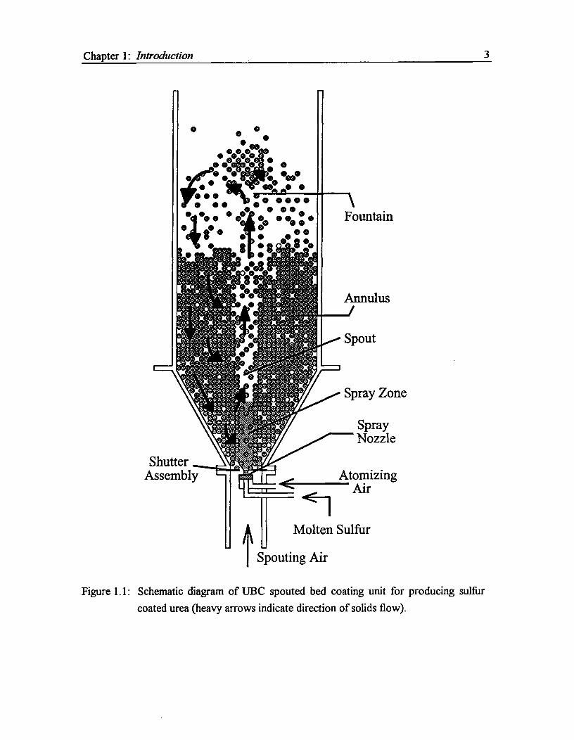
Chapter 1: Introduction^ 3
Figure 1.1: Schematic diagram of UBC spouted bed coating unit for producing sulfurcoated urea (heavy arrows indicate direction of solids flow).
Chapter 1: Introduction^ 4
plugging and sulfur handling difficulties led to further studies by Meisen and co-workers
(Zee, 1977 and Lim, 1978).
Successful batch-wise coating was achieved by Weiss and Meisen (1981, 1983). The
product quality (D25) was comparable to that of the CIL product made by the TVA proc-
ess, and was found to depend on the sulfur droplet size, the spray distribution and the na-
ture of the urea surface.
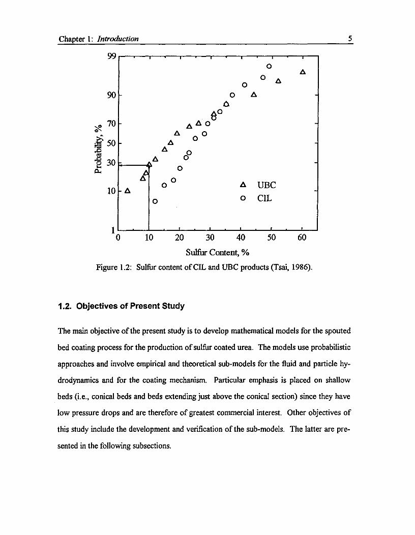
Some operational aspects of the continuous spouted bed process were examined by
Meisen and Tsai (1986). In their initial study, they found the product from the UBC proc-
ess gave higher D25 values (i.e., had lower quality) than those of the CIL product. They
suspected that the higher D25 values of the UBC product resulted from a significant frac-
tion of uncoated particles in the product. This is supported by Figure 1.2 which is a plot
of the percentage of particles which contain less than a certain sulfur content (denoted by
Probability %) as a function of sulfur content. The cumulative percentage is shown on a
"probability scale". The latter implies that the plot would be a straight line if the sulfur
content is normally distributed around the mean value. Figure 1.2 shows that 27% of the
particles contained less than 10 % sulfur while only 5 % of the particles from the CIL
product contained less than 10 % sulfur. Meisen and Tsai suspected that these uncoated
particles resulted from fresh urea particles bypassing the spray zone and leaving the
spouted bed prematurely. By changing the feed location and operating variables such as
the bed height and the flow rate of the spouting air, a product comparable to the CIL
product in terms of D 25 values was obtained.
Many experiments are generally required to determine the effects of operating variables
on the product quality. Since the cost of the experiments is high, an alternative method is
sought. One way to reduce the number of experiments is to develop a mathematical
model describing the coating process.
0A
0 A0
0 A
60A A 0
A 0A 0
AA
4 ooo
46A 00 A UBCA
0 0 CIL
Chapter 1: Introduction^ 5
99
90
70
k 50
0 30
10
10^10^20^30^40
^50^
60
Sulfur Content, %
Figure 1.2: Sulfur content of CIL and UBC products (Tsai, 1986).
1.2. Objectives of Present Study
The main objective of the present study is to develop mathematical models for the spouted
bed coating process for the production of sulfur coated urea. The models use probabilistic
approaches and involve empirical and theoretical sub-models for the fluid and particle hy-
drodynamics and for the coating mechanism. Particular emphasis is placed on shallow
beds (i.e., conical beds and beds extending just above the conical section) since they have
low pressure drops and are therefore of greatest commercial interest. Other objectives of
this study include the development and verification of the sub-models. The latter are pre-
sented in the following subsections.
Chapter 1: Introduction^ 6
1.2.1. Bed Hydrodynamics
Although many hydrodynamic models have been reported for conventional spouted beds,
the hydrodynamics of spouted beds configured for coating has not been addressed in the
literature. In particular, the special geometry at the air inlet, atomizing air and coating
agent make the coater behave differently from conventional beds. The objectives of the
hydrodynamic study are to:
• determine the effects of atomizing air and bed geometry on the air velocities in the
bed, including the minimum spouting velocity;
• develop mathematical models (or modify existing models) to describe the bed hydro-
dynamics in a spouted bed coater;
• verify the models by experimentally examining the fluid velocities in the spout and the
pressure distribution in the annulus.
1.2.2. Coating Mechanisms
The coating mechanism governs the rate at which the sulfur droplets deposit onto urea
particles and, ultimately, the spray concentration profile in the bed. The objectives of this
part of the study are to determine the coating mechanism by experimentally analyzing the
spray droplet size distribution.
1.2.3. Overall Coating Performance
An important objective of this work is the verification of the model predictions on the
coating performance of the bed. Once the model is developed, the following verifications
are conducted:
• the coating distribution of particles is determined for selected experiments;
• the coating distribution is correlated with the product quality expressed in terms of D25
values.
Chapter 1: Introduction^ 7
1.2.4. Benefits of the Study
Use of a mathematical model may be an inexpensive and fast alternative to conducting ex-
periments to determine the optimum operating conditions. The model may also be useful
in designing commercial plants because the product quality information is readily predict-
able for any size and number of beds the plant may require. The commercial implications
based on model predictions are presented in Chapter 5.
A better understanding of the following areas is also achieved as a result of this study:
• the effectiveness of coating models of various complexities is identified;
• the bed hydrodynamics of a spouted bed configured for coating are elucidated;
• the sulfur atomization and urea-sulfur contact mechanisms are characterized.
It should be noted that the physical bonding of sulfur on urea, the related effect of tem-
perature and the influence of chemical additives are not examined in this work. The effect
of bed temperature on product quality is investigated only through its impact on bed hy-
drodynamics.
Chapter 2.Literature Review
2.1. UBC Process
Although the spouted bed coating process has been studied in the past (Singiser et al.,
1966; Umaki and Mathur, 1976), the effects of individual operating variables on product
quality were not investigated until Meisen and Mathur commenced their research in 1975.
The results obtained by Meisen and co-workers since 1975 are reviewed in this section.
The batch-wise2 production of sulfur coated urea was studied by Meisen and co-workers
— Mathur (1978), Zee (1977), Lim (1978), and Weiss (1981, 1983), and the continuous 3
production was studied by Meisen and Tsai (1986). Most of the earlier work was devoted
to improving the operational aspects of the process. (Detailed description of equipment
modifications are provided by Weiss (1981) and by Tsai (1986)). With an improved
coating facility, Lim was able to quantitatively explain the effects of the principal operating
variables on the product quality for the batch process. Weiss followed up with more
equipment modifications and more extensive studies of the batch process. Tsai extended
the investigation to continuous operation. The operating conditions studied are summa-
rized in Table 2.1.
The principal operating variables that were found to affect the product quality were bed
temperature (Tb), sulfur injection rate (W), atomizing air flow rate (Q a), bed depth (II),
2 The "batch process" refers to a process where a batch of urea is placed in the spouted bed, coated anddischarged.
3 The "continuous process" refers to the process where urea is continously fed to the the bed and coatedproduct (SCU) is continuously discharged from the bed.
8
Chapter 2: Literature Review^ 9
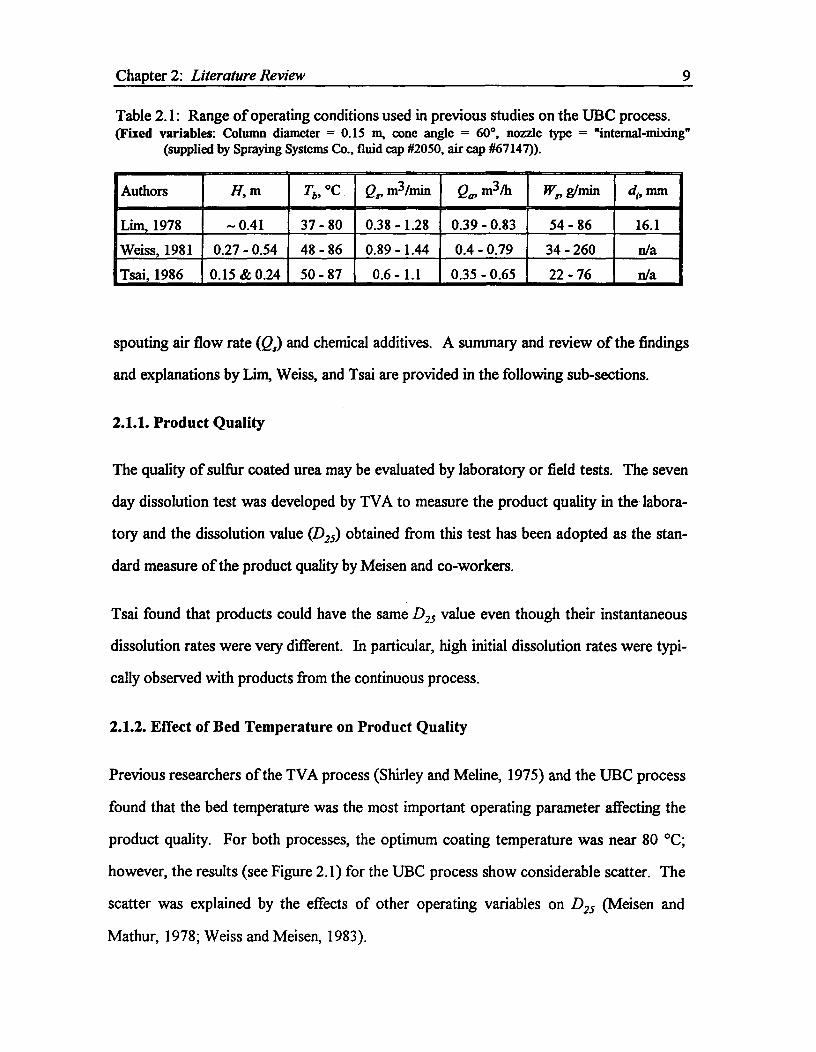
Table 2.1: Range of operating conditions used in previous studies on the UBC process.(Fixed variables: Column diameter = 0.15 m, cone angle = 60°, nozzle type = "internal-mixing"
(supplied by Spraying Systems Co., fluid cap #2050, air cap #67147)).
Authors H,m Tb,°C Q,,m3 /min Q., m3 /h Ws, emin d;, mm
Lim, 1978 — 0.41 37 - 80 0.38 - 1.28 0.39 - 0.83 54 - 86 16.1
Weiss, 1981 0.27 - 0.54 48 - 86 0.89 - 1.44 0.4 - 0.79 34 - 260 n/a
Tsai, 1986 0.15 & 0.24 50 - 87 0.6 - 1.1 0.35 - 0.65 22 - 76 n/a
spouting air flow rate (Q,) and chemical additives. A summary and review of the findings
and explanations by Lim, Weiss, and Tsai are provided in the following sub-sections.
2.1.1. Product Quality
The quality of sulfur coated urea may be evaluated by laboratory or field tests. The seven
day dissolution test was developed by TVA to measure the product quality in the labora-
tory and the dissolution value (D25) obtained from this test has been adopted as the stan-
dard measure of the product quality by Meisen and co-workers.
Tsai found that products could have the same D25 value even though their instantaneous
dissolution rates were very different. In particular, high initial dissolution rates were typi-
cally observed with products from the continuous process.
2.1.2. Effect of Bed Temperature on Product Quality
Previous researchers of the TVA process (Shirley and Meline, 1975) and the UBC process
found that the bed temperature was the most important operating parameter affecting the
product quality. For both processes, the optimum coating temperature was near 80 °C;
however, the results (see Figure 2.1) for the UBC process show considerable scatter. The
scatter was explained by the effects of other operating variables on D25 (Meisen and
Mathur, 1978; Weiss and Meisen, 1983).
0
V
0
0
VV•
V •o Lim (1978)• Weiss (1981)
0
•0
0
Chapter 2: Literature Review^ 10
60
-.8 400
A 20
050^60^70^80
^90
Bed Temperature, °CFigure 2.1: Effect of bed temperature on product quality. (The scatter re-
sults from the effects of other variables).
Upon examination of the coat surface under high magnification, Weiss was able to provide
some explanations for the optimum coating temperature. For bed temperatures below 80
°C, premature freezing of sulfur droplets before impingement onto the bed particles pre-
vented the sulfur from spreading evenly on the urea surface. As a result, the surface ap-
peared lumpy with gaps between the lumps, and the presence of these gaps enhanced the
passage of water to the urea core thereby increasing the urea dissolution rate. Urea
coated significantly above 80 °C showed cracks in the coats. The cracks were thought to
be caused by the contraction of sulfur as it changed from the monoclinic allotrope (S o) of
lower density to the orthorhombic form (S o) of higher density upon cooling. For bed tem-
Chapter 2: Literature Review^ 11
peratures below 80 °C, So was assumed to be absent from the coats and therefore major
thermal contraction did not take place.
2.1.3. Effect of Sulfur Injection Rate on Product Quality
The experimental results obtained by Lim and Weiss suggest that the sulfur feed rate had a
strong effect on the product quality. To determine the relationship between the sulfur in-
jection rate and D25, Weiss conducted several experiments by varying only the sulfur feed
rate at a given bed temperature. The results showed the logarithm of D25 to be inversely
proportional to the sulfur flow rate. According to the Nukiyama-Tanasawa equation
(1939), the spray droplet size (d,) increases with liquid flow rate (Q,): i.e.,
0.45
d =585 ( a 0.5
+597 J1^1000a )I.5
,^( , 1ur Pi^ TIPz)̂ Qa
(2.1)
Weiss therefore concluded that the product quality improves with sulfur droplet size.
2.1.4. Effect of Atomizing Air on Product Quality
Lim (1978) found that the product quality decreased as the atomizing air flow rate was in-
creased. Weiss found this relationship to be linear when his results were normalized to
take into account the effect of sulfur flow rate on product quality (see Figure 2.2). Using
the relationship given by Nukiyama and Tanasawa (Equation (2.1)), Weiss confirmed that
smaller spray droplet sizes gave rise to a lower product quality (or higher D25 values).
The present hydrodynamic study (see Chapter 5) showed that the atomizing air flow rate
could significantly influence the solids circulation and the size of the spray zone, in addi-
tion to the spary droplet size. Moreover, the spray angle was observed to vary with atom-
izing air flow rate. These effects of atomizing air flow rate could ultimately alter the prod-
uct quality; however, such effects were not addressed in the previous studies.
Chapter 2: Literature Review^ 12
60
20^0.4^0.5^0.6^0.7
^0.8
Atomizing Air Flow Rate, m3 /hFigure 2.2: Effect of atomizing air flow rate on dissolution rate adjusted to
a reference sulfur flow rate (Weiss, 1981).
2.1.5. Effect of Bed Depth on Product Quality
The batch studies conducted by Lim (1978) suggested that reducing the bed height im-
proves the product quality. Shorter particle cycle times associated with shallower beds
were thought to increase the chance of particles receiving uniform coats and hence im-
prove the product quality.
However, Weiss' experimental results showed that the bed height had little effect on prod-
uct quality. In his investigation on the effect of bed depth, the spouting air flow rate had
to be increased with bed depth to maintain spouting (other variables were fixed). Increas-
ing the spouting air flow rate, according to Mathur and Epstein (1974), increases the urea
Chapter 2: Literature Review^ 13
circulation rate and consequently lowers the sulfur deposition on the urea particles per
pass. owever, Weiss found that the changes resulting from the variation in bed depth and
spouting air flow rate did not alter the product quality significantly.
Tsai found the bed depth to have a more pronounced influence on the product quality in
the continuous process. In oder to explain his results, Tsai introduced the concept of the
"spray zone". The spray zone was assumed to cover the lower portion of the spout and
consequently the particles that enter the spout above the spray zone did not receive any
additional coating. As the bed height increases, more particles by-pass the spray zone, re-
sulting in more inadequately coated particles and a lower product quality.
The concept of the "spray zone" is explored in the development of the mathematical mod-
els in Chapter 4.
2.1.6. Effect of Spouting Air Flow Rate on Product Quality
Lim (1978) found that the spouting air flow rate had little effect on the product quality in
the batch coating process. Weiss and Tsai did not investigate the effect of the spouting air
flow rate.
2.1.7. Effect of Chemical Additives on Product Quality
Silicone (Dow Corning 200) was found to improve the product quality according to Weiss
(1981). Other chemical additives including CO 2, NH3, N2 and liquid dicyclopentadiene re-
sulted in no major improvements in product quality in the study conducted by Lim (1978).
2.2. Models of Spouted Bed Coating Process
Basically three approaches for modeling spray coating in spouted beds have been reported
in the past.

Chapter 2: Literature Review^ 14
The earliest paper was published by Umaki and Mathur in 1976. The model of a continu-
ous granulation process was based on mass and number balances which took into account
particle growth by solute deposition, particle breakage and dust formation due to particle
abrasion and undeposited spray droplets. The model correlated the experimental particle
growth rate data reasonably well. Unfortunately, as pointed out by Mann (1978), the as-
sumptions of constant bed weight, and constant ratio of the formation rate of fresh nuclei
to the number of particles in the bed implied that the particle growth resulted in a reduc-
tion of the formation of fresh nuclei, which would ultimately lead to just one or two large
particles in the bed. This model was also limited to predicting the mean bed particle size.
The particle size distribution, which is an important feature of slow release fertilizers,
could not be predicted.
In 1983, Mann developed a model which predicted the coating distribution of the solids
produced in a spout-fluid bed equipped with a draft tube and operating in batch mode.
Mann believed that the coating distribution is mainly affected by the number distribution of
passages through the spray zone and the distribution of the coating mass deposited on the
particles per passage. Based on the findings of Cox (1967) and Mann (1974, 1975, 1979
and 1981) that the latter two distributions asymptotically approached normal distributions
with time, Mann developed a 5-parameter model. The parameters were operating time,
mean and variance of cycle time, and mean and variance of coating amount per cycle.
Mann suggested 90 short experimental runs to relate the latter four variables to bed di-
ameter, annulus width, height of draft tube from the base, atomizer type, air flow rate, and
coating solution flow rate.
For a coating process in which the coat itself does not significantly add to the size of the
bed particles and for a fixed bed geometry, this approach appears to be valid. However, if
the coating material significantly increases the size of the bed particles, short experiments
may not give proper indication of the effect of the latter four variables. The increase in the
Chapter 2: Literature Review^ 15
particle size results in particles receiving more coating material per cycle; this adds to the
bed height which may, in turn, decrease the cycle time of the bed particles. Moreover, as
the model is modified for continuous operation, additional operating variables may need to
be considered. In such cases, the number of experiments required to determine the rela-
tionship between the operating variables and the model variables will increase significantly.
Such an increase in the number of experiments may render this approach ineffective for
practical purposes.
In 1984, Berruti et al. developed a mathematical model for predicting the size distribution
of solids formed in a continuous spouted bed coating process. They assumed perfect par-
ticle mixing, constant feed composition (i.e., feed rates of coating material and bed parti-
cles), no particle segregation at the product discharge, constant hold up and negligible par-
ticle breakage and fines formation. On the basis of a particle population balance, which
was developed by Randolph and Larson (1971) for describing a crystallization process, the
model predicted the size distribution of the bed particles under transient conditions. Prior
knowledge of the feed rate, mean feed particle size and growth rate were required to de-
termine the product size distribution. The authors kept the growth rate and the mean feed
particle size constant while altering the feed rate. Their results showed that the size distri-
bution of the product particles approached a log-normal distribution.
Two assumptions, namely perfect particle mixing and a well-dispersed homogeneous gas
phase containing the coating agent, seem, however, unrealistic for the spouted bed proc-
esses.
None of the three aforementioned models considered, in detail, the coating mechanisms
and particle circulation patterns inside the spouted bed. Umaki and Mathur (1976), and
Berruti et al. (1984) treated the bed as a perfectly stirred vessel and assumed that particles
in all regions of the bed received the same amount of coating. Mann (1983) assumed a
Chapter 2: Literature Review^ 16
spray zone, but his model variables were empirical. These variables could not explain the
particle circulation in the bed and the coating mechanism.
2.3. Models and Correlations for Spouted Bed Hydrodynamics
Since only a few hydrodynamic models and correlations for shallow spouted beds are
available in the literature, those that are widely used for standard spouted beds are also
considered here. It should be noted that detailed and critical review of most hydrody-
namic models and correlations considered here can be found elsewhere (Mathur and Ep-
stein, 1974; Epstein and Grace, 1984; Krzywanski, 1992).
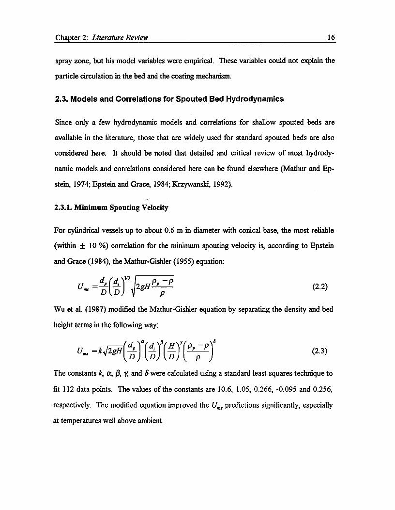
2.3.1. Minimum Spouting Velocity
For cylindrical vessels up to about 0.6 m in diameter with conical base, the most reliable
(within ± 10 %) correlation for the minimum spouting velocity is, according to Epstein
and Grace (1984), the Mathur-Gishler (1955) equation:
d (d.13^p — pU^2gH PD D
Wu et al. (1987) modified the Mathur-Gishler equation by separating the density and bed
height terms in the following way:
8Ums =k1 2.11H-d IK(11)7(PP —P)
D DD p (2.3)
The constants k, a, /3, y, and 3 were calculated using a standard least squares technique to
fit 112 data points. The values of the constants are 10.6, 1.05, 0.266, -0.095 and 0.256,
respectively. The modified equation improved the Um, predictions significantly, especially
at temperatures well above ambient.
(2.2)

Chapter 2: Literature Review^ 17
2.3.2. Solids Circulation and Bed Hydrodynamics
Basically three approaches for predicting the particle circulation rates have been reported
in the literature. Two approaches, according to Morgan et al. (1985), involve using one-
dimensional particle force, and mass and momentum balances in the spout. A more recent
and rigorous approach is based on the theory of plasticity for the solids motion in the an-
nulus (Krzywanski et al., 1992; Amirshahidi, 1984; Khoe, 1980). The former two ap-
proaches also predict fluid velocity and voidage profiles in the spout, while the latter ap-
proach does not. However, Krzywanski et al. (1992) combined the theory of plasticity
with the vector Ergun (1952) equation in the annulus and the two-phase momentum equa-
tions in the spout to solve for the bed hydrodynamics.
The most recent force balance model developed by Lim and Mathur (1978) had problems
with the stiffness of the model equations at the bed inlet, although its predictions using ex-
perimental values away from the inlet as the initial conditions were reasonable. Khoe
(1980) and Amirshahidi (1984) determined the solids flow in the annulus based on the the-
ory of plasticity. The model developed by Khoe was strongly dependent on experimental
results — the magnitudes and locations of sources and sinks were found experimentally.
Amirshahidi encountered difficulties in the computation of the stress field in the conical
region which is required to calculate the velocity field of solids. The theory of plasticity
was applied to solve solids flow in the annulus; the solids flow in the rest of the bed would
require additional equations. The Krzywanski et al. model required basic information such
as wall and internal friction angles as well as the fluid velocity profile at the fluid inlet,
which are not easily calculated nor readily available.
Although the model developed by Krzywanski et al. is the most comprehensive model
available, applying it to the current study requires extraordinary computational resources.
Furthermore, the model must be corrected for the unusual geometry at the bed inlet due to
Chapter 2: Literature Review^ 18
the presence of the nozzle in the coating unit (see Chapter 5). Accounting for the nozzle
is a complex task because the flow rates of atomizing air and spouting air, the location and
type of the spray nozzle all affect the boundary conditions of the model. Moreover, the
bed hydrodynamics were found to be very sensitive to the friction angles which probably
vary with the amount of sulfur on the particles.
The mass and momentum balances model, on the other hand, is much simpler, and yet, it
was generally found to provide good approximations of solids circulation and bed hydro-
dynamics with little or no modification (Lefroy and Davidson, 1969; Morgan et al., 1985;
Stocker, 1987). This model, however, required accurate estimates of spout diameter (D),
pressure distribution in the spout (P,), particle-fluid interaction (I3 p) and air flow into the
annulus (U,). The correlations for the first two of these variables are reviewed in the next
two sections.
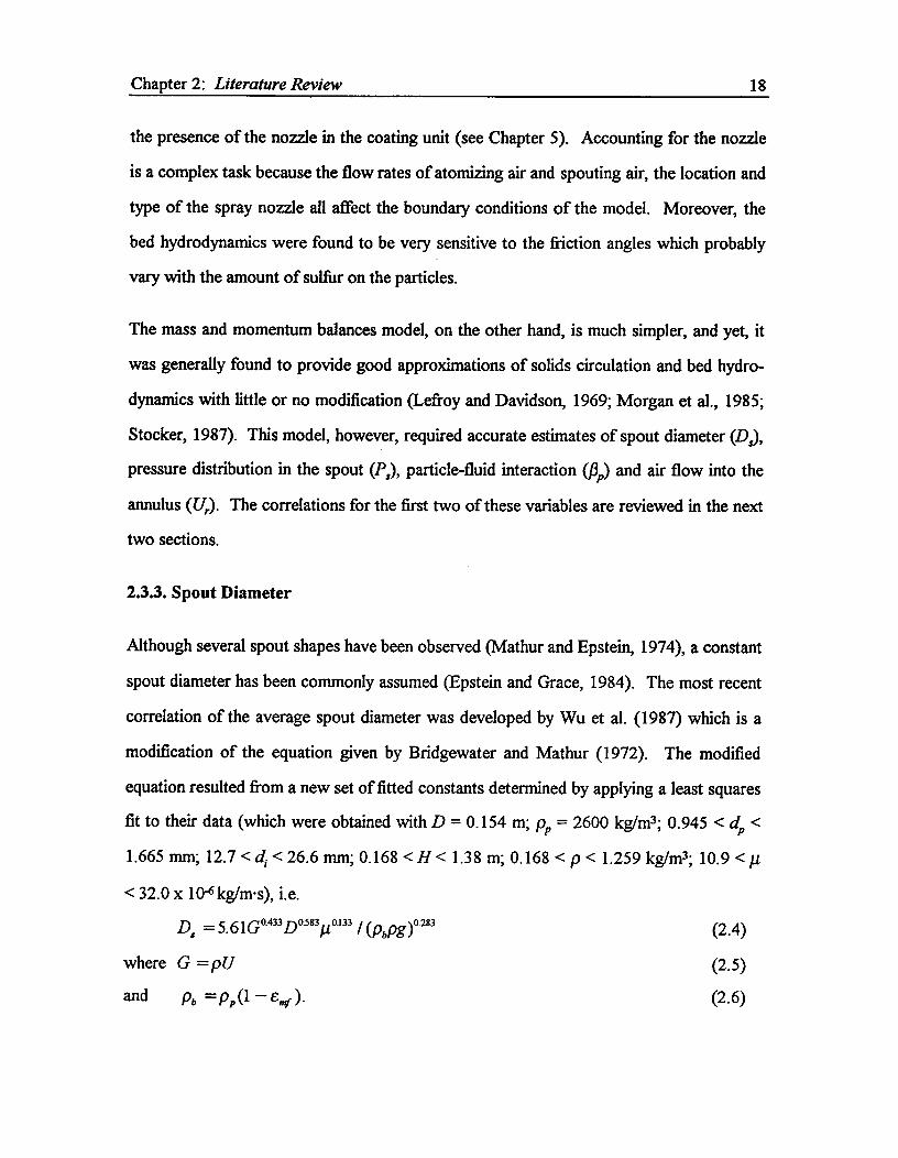
2.3.3. Spout Diameter
Although several spout shapes have been observed (Mathur and Epstein, 1974), a constant
spout diameter has been commonly assumed (Epstein and Grace, 1984). The most recent
correlation of the average spout diameter was developed by Wu et al. (1987) which is a
modification of the equation given by Bridgewater and Mathur (1972). The modified
equation resulted from a new set of fitted constants determined by applying a least squares
fit to their data (which were obtained with D = 0.154 m; pp = 2600 kg/m3; 0.945 < dp <
1.665 mm; 12.7 < d1 < 26.6 mm; 0.168 < H < 1.38 m; 0.168 < p < 1.259 kg/m3; 10.9< µ
< 32.0 x 10⁻⁶ kg/m. s), i.e.
D, =5.61G°433D038340133 / (pbpa 283 (2.4)
where G =pU (2.5)
and^pb = p p (1 — emf ).^ (2.6)

Chapter 2: Literature Review^ 19
This equation was found to give better predictions of their data at elevated temperatures
than the McNab (1972) equation.
2.3.4. Pressure Profile in Annulus
Several pressure distribution correlations have been reported in the literature. Lefroy and
Davidson (1969) used an empirical correlation based on the pressure measurements at the
spout-annulus interface. The only model with a strong theoretical basis was developed by
Epstein and Levine (1978); it was derived from the Ergun equation (1952) and the
Mamuro and Hattori flow correlation (1968), and is given by
.1). ^ r[2(ap — 0[1.5(h 2 —x2 ) —(h3 —x 3 )— AP
ir
f h(2 a p —1)
+0.25(h4 — x4 )] + 3[3(h3 — x3 ) — 4.5(h4 —x4 )+ 3(h5 —x5 ) — (h6 — x6 ) + 0.143(h 7 —x7 )]]
(2.7)
where a = 2 + 129/1(1
— Erni-) (2.8)P pdpU„,f
h = H/H„,,^ (2.9)
and x = z/1/..^ (2.10)
This equation describes the pressure distribution in the annulus but, since there is a rela-
tively small pressure drop between the spout and annulus (Rovero et al., 1985), it can also
be used to estimate the pressure distribution in the spout.
Morgan and Littman (1980) developed the following general pressure drop correlation
based on experimental pressure measurements reported in the literature:A Pms / tiPmf =1 — Y^ (2.11)
where
Y2 +[2(X — 0.2) —1.8 + (3.24 / ap)]Y + [(X —2)(X — 0.2) —(3.24X/ 9)] =0,(2.12)

Chapter 2: Literature Review 20
(2.13)X =11[(HID)+1],
U„,f Uiand^cps = 7.18(
(pp
p —p)gdi
0,(503, —7.570! + 4.094), — 0.516) — —di +1.07 (2.14)D
Fluid flow models for the annulus can also be modified to predict the pressure distribution
with the aid of expressions such as the Ergun (1952) equation. Mamuro and Hattori
(1968) derived a fluid flow model for the annulus using Darcy's law and Rovero et al.
(1983) modified the Mamuro-Hattori equation for beds having a conical base by substitut-
ingA. =n (D2 _ Ds2 )i 4 =4 , for z >H,^ (2.15)
and A. =R [(2ztan(0/ 2)+4)2 —g]/ 4 , forz .Ho^(2.16)
into Qa^Qa ^BUal.,^(2.17)dz dz2
where B =18I1,,F.44,2 /H,3„^ (2.18)
and Qa =Aatla^(2.19)
The boundary conditions are:
Q.= Q.0 at z = 0^ (2.20)
Qa =Ualf. Aa at z =H„,.^ (2.21)
2.4. Coating Mechanism
Four mechanical collection processes 4 have been reported in the literature (Cliff et al.,
1981; Lunde and Lapple, 1957): diffusional deposition, inertial deposition, direct intercep-
tion and gravitational settling. These processes are often aided by electrophoretic, ther-
mophoretic and diffusiophoretic effects (Meisen et al., 1971). However, only the inertial
deposition mechanism is considered because it was inferred that it was the dominating
4 collection process, in this study, corresponds to the mechanisms by which the atomized sulfur dropletsdeposit onto the bed particles.

Chapter 2: Literature Review^ 21
mechanism under the experimental conditions prevailing in this study. Thus, the review in
this section covers more recent inertial deposition correlations reported in the literature.
According to Clift et al. (1981), the correlation given by Thambimuthu (1980) is the most
reliable equation for predicting the inertial impaction efficiency of a single spherical collec-
tor:
rl =(St / (St +0.062e)) 3 , for 0.002 < St < 0.02^ (2.22)
where St =(u — v)dg.2 pc I 18pd p^(2.23)
The range of Stokes numbers (St), however, is rather small and is not generally applicable
to the conditions of this study.
Earlier work by Behie et al. (1972) led to equations which are valid for a wider range of
Stokes numbers:
n =0, for St 50.083^ (2.24)
rl = 0.0036 — 0.2323St + 2.422St2 — 2.033S:, for 0.083 < St 50.6^(2.25)
(s, +0.5)2, for St >0.6^ (2.26)
These equations for the single particle collection efficiency were obtained based on the as-
sumption that the aerosols were rigid and spherical.
2.5. Monte Carlo Method
The term "Monte Carlo" was introduced by von Neumann and Ulam during World War II,
as a code word for the secret work at Los Alamos; it was suggested by the gambling casi-
nos at the city of Monte Carlo in Monaco (Rubinstein, 1981). The Monte Carlo method
has been often confused with "stochastic simulation", and Ripley (1987) suggested that the
term "Monte Carlo method" should have the more specialized meaning of "doing some-
thing clever and stochastic with simulation". Rubinstein (1981) defines stochastic simula-
tion as statistical sampling experiments with a model over time which involves the use of a
Chapter 2: Literature Review^ 22
random number; Monte Carlo simulation as a technique using random or pseudorandom
numbers for solving model equations. The latter definition is used to describe the model
developed in this work.
Although this type of simulation is often viewed as a "method of last resort" to be em-
ployed when everything else has failed, recent advances in simulation methodologies,
availability of software, and technical developments have made Monte Carlo simulation
one of the most widely used and accepted tools in system analysis and operations research
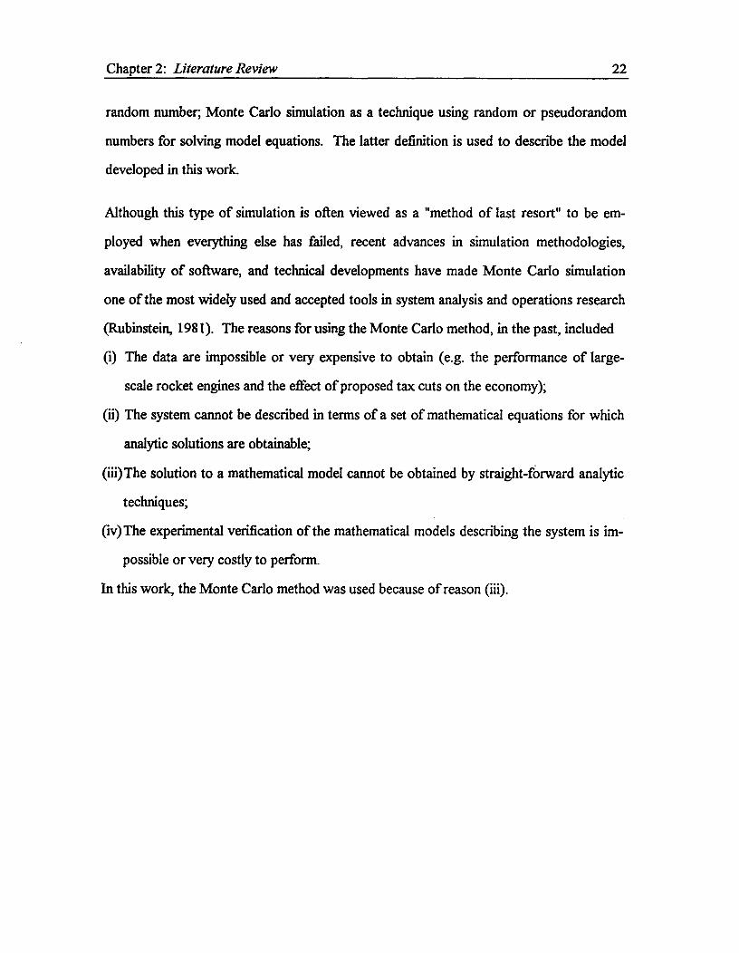
(Rubinstein, 1981). The reasons for using the Monte Carlo method, in the past, included
(i) The data are impossible or very expensive to obtain (e.g. the performance of large-
scale rocket engines and the effect of proposed tax cuts on the economy);
(ii) The system cannot be described in terms of a set of mathematical equations for which
analytic solutions are obtainable;
(iii)The solution to a mathematical model cannot be obtained by straight-fOrward analytic
techniques;
(iv)The experimental verification of the mathematical models describing the system is im-
possible or very costly to perform.
In this work, the Monte Carlo method was used because of reason (iii).
Chapter 3.
Experimental Materials, Apparatus and Procedures
The coating apparatus developed by Meisen et al. (1986) was used for all experiments
conducted in this study. Minor modifications to the spouted beds were necessary for the
study of bed hydrodynamics and a spray box was built to determine size distribution of the
spray droplets. The experimental procedures used for the coating studies were similar to
those described by previous workers (Weiss, 1981 and Tsai, 1986). Since the apparatus
used in this work was largely the same as that used by previous workers, more emphasis is
placed, in this chapter, on describing the modifications to the equipment.
3.1. Experimental Materials
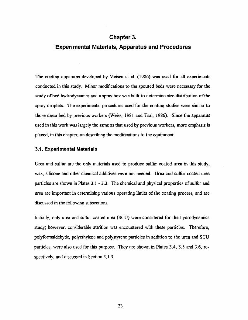
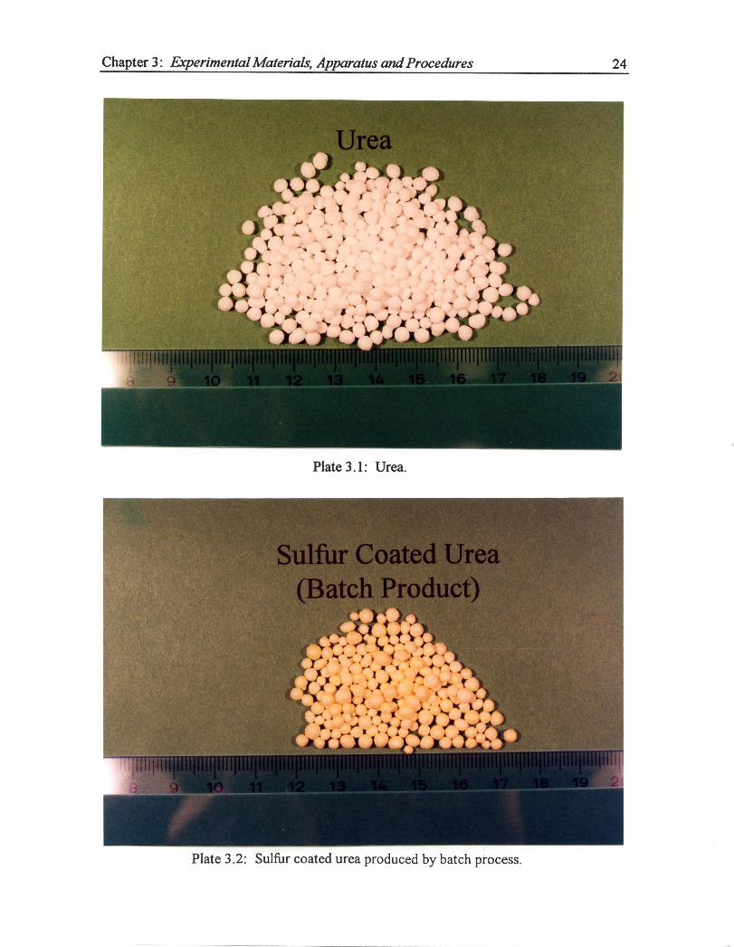
Urea and sulfur are the only materials used to produce sulfur coated urea in this study;
wax, silicone and other chemical additives were not needed. Urea and sulfur coated urea
particles are shown in Plates 3.1 - 3.3. The chemical and physical properties of sulfur and
urea are important in determining various operating limits of the coating process, and are
discussed in the following subsections.
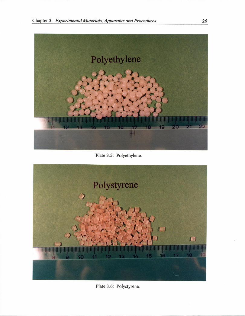
Initially, only urea and sulfur coated urea (SCU) were considered for the hydrodynamics
study; however, considerable attrition was encountered with these particles. Therefore,
polyformaldehyde, polyethylene and polystyrene particles in addition to the urea and SCU
particles, were also used for this purpose. They are shown in Plates 3.4, 3.5 and 3.6, re-
spectively, and discussed in Section 3.1.3.
23
11111111111^1111111 1
Chapter 3: Experimental Materials, Apparatus and Procedures^ 24
Plate 3.1: Urea.
Plate 3.2: Sulfur coated urea produced by batch process.

Chapter 3: Experimental Materials, Apparatus and Procedures^ 25
711111 1 111111 1 111111 1 111111 11 1AO 10 11 24034111k, 14 15^16^17^182y64 19 2C
Plate 3.3: Sulfur coated urea produced by continuous process.
Plate 3.4: Polyformaldehyde.
Chapter 3: Experimental Materials, Apparatus and Procedures^ 26
111111ifilpillIT11111111111119 20 21 2:
Plate 3.5: Polyethylene.
Plate 3.6: Polystyrene.

Chapter 3: Experimental Materials, Apparatus and Procedures^ 27
3.1.1. Urea
Urea was supplied by Sherritt-Gordon Ltd. and produced by the NSM fluidized bed
granulation process. Selected properties of urea are listed in Table 3.1.
The operating bed temperature was kept above 60 °C. Heavy attrition was observed at
room temperatures, i.e., dust build up on the Plexiglas column was observed almost im-
mediately after spouting started. The attrition rate gradually decreased with increasing
temperature; however, no data were collected to determine the effect of temperature on
the attrition rate. The lower operating limit of 60°C was adopted based on visual inspec-
tion of dust build up on the column walls.
Other factors that appeared to influence the attrition rate were spouting air flow rate,
spouting air orifice diameter, and bed diameter. Higher spouting air flow rates, small ori-
fices, and smaller bed diameter increased the attrition rate.
Table 3.1: Selected physical properties of urea.
Melting point (Perry et al., 1984)^ 133°CSphericity^ 1.0Particle density (Perry et al., 1984)^ 1335 kg/m3
Size distribution (Sherritt-Gordon Ltd.)
Mesh (CDN)+ 6
- 6+ 7-7+ 8- 8+10
-10+16- 16
Aperture Size (mm)3.362.832.382.01.19
Wt. fraction (%)2.8
24.533.530.19.1
trace
mean size =[E.x. / d^2.16

Chapter 3: Experimental Materials, Apparatus and Procedures^28
3.1.2. Sulfur
PETROSUL International Ltd. provided sulfur for this work. The sulfur purity exceeded
99.5 wt % due to the presence of only minor traces of ash and carbon (total of 0.10 % on
average).
Selected properties of solid and liquid sulfur are given in Tables 3.2 and 3.3, and Figure
Table 3.2: Selected chemical and physical properties of sulfur (Stauffer Chemical Co.).
Physical state (@ 21°C, 1 atm) SolidBulk density, kg/m3 1200 - 1394 Lumps, 560 - 960 PowderBoiling point 444°CMelting point 119°C (approximate)Odor NoneFlash point 188°C, COCAuto ignition temperature (dust in air) 190°CVapor pressure @ 20°C < 0.0001 nun HgExplosive limits (dust in air) between 35 and 1400 g/m3
Table 3.3: Properties of common sulfur allotropes (Donahue and Meyer, 1965; Daleand Ludwig, 1965).
Property Sa^I^So
Common name Orthorhombic sulfur Monoclinic sulfurRecommended name Orthorhombic (a) sulfur Monoclinic 03) sulfurMolecular formula S1,8 S4RCrystalline form Orthorhombic MonoclinicUnit cell 16 molecules of S > (S 8) 6 molecules of S x (S8)
Stability region < 95.5°C 95.5°C to 119°CColor Opaque yellow at 24°C Between yellow and orangeDensity, kg/m3 2070 1960Shore B-2 hardness 90 1.96Tensile strength, kPa 330 410
Chapter 3: Experimental Materials, Apparatus and Procedures^ 29
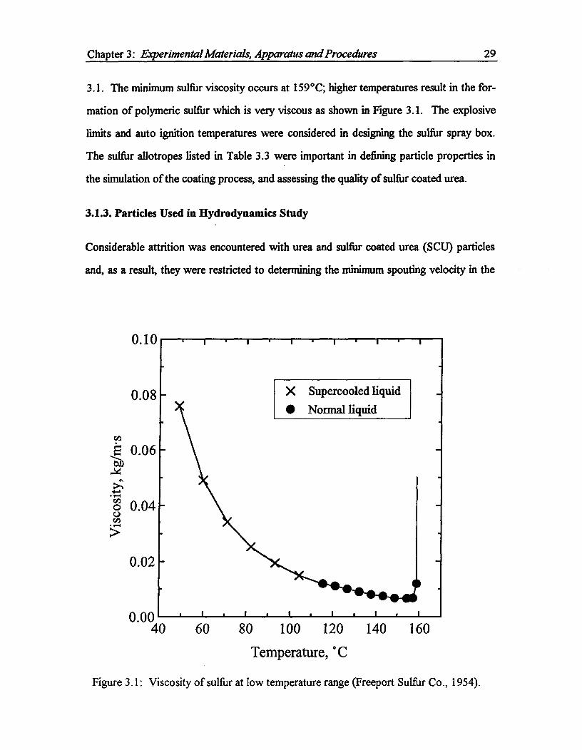
3.1. The minimum sulfur viscosity occurs at 159°C; higher temperatures result in the for-
mation of polymeric sulfur which is very viscous as shown in Figure 3.1. The explosive
limits and auto ignition temperatures were considered in designing the sulfur spray box.
The sulfur allotropes listed in Table 3.3 were important in defining particle properties in
the simulation of the coating process, and assessing the quality of sulfur coated urea.
3.1.3. Particles Used in Hydrodynamics Study
Considerable attrition was encountered with urea and sulfur coated urea (SCU) particles
and, as a result, they were restricted to determining the minimum spouting velocity in the
60^80^100^120^140^160Temperature, °C
Figure 3.1: Viscosity of sulfur at low temperature range (Freeport Sulfur Co., 1954).
Chapter 3: Experimental Materials, Apparatus and Procedures^30
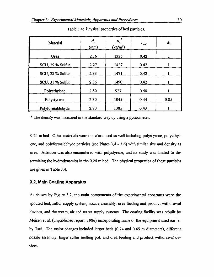
Table 3.4: Physical properties of bed particles.
Material d„(mm)
*Pi,kg/m3)
Erni' Os
Urea 2.16 1335 0.42 1
SCU, 19 % Sulfur 2.27 1427 0.42 1
SCU, 28 % Sulfur 2.33 1471 0.42 1
SCU, 31 % Sulfur 2.36 1490 0.42 1
Polyethylene 2.80 927 0.40 1
Polystyrene 2.30 1045 0.44 0.85
Polyformaldehyde 2.70 1385 0.43 1
* The density was measured in the standard way by using a pycnometer.
0.24 m bed. Other materials were therefore used as well including polystyrene, polyethyl-
ene, and polyformaldehyde particles (see Plates 3.4 - 3.6) with similar size and density as
urea. Attrition was also encountered with polystyrene, and its study was limited to de-
termining the hydrodynamics in the 0.24 m bed. The physical properties of these particles
are given in Table 3.4.
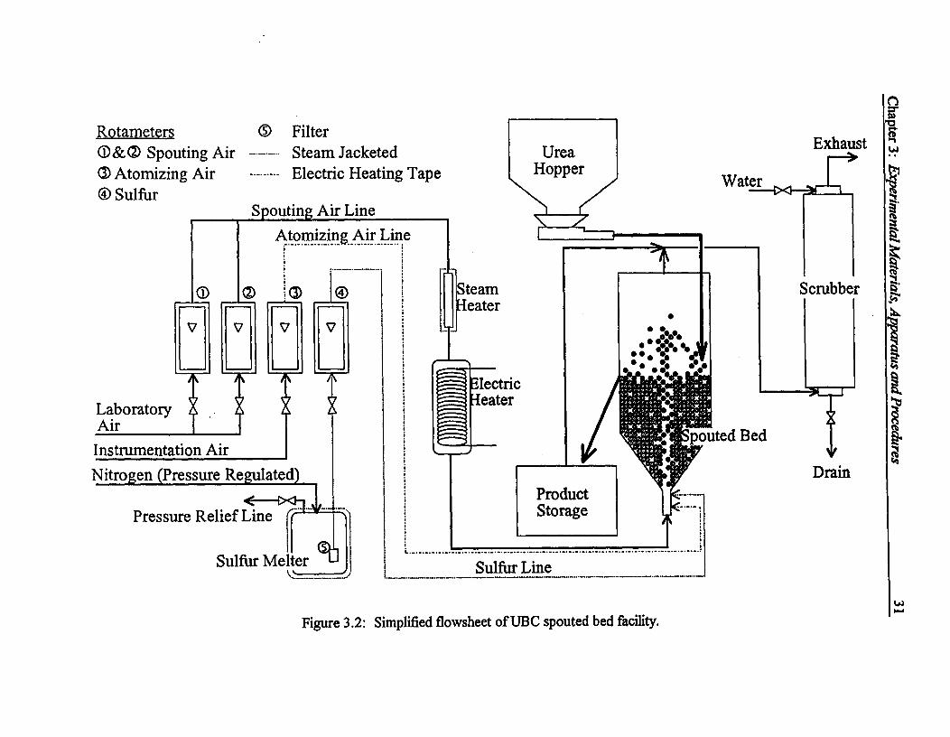
3.2. Main Coating Apparatus
As shown by Figure 3.2, the main components of the experimental apparatus were the
spouted bed, sulfur supply system, nozzle assembly, urea feeding and product withdrawal
devices, and the steam, air and water supply systems. The coating facility was rebuilt by
Meisen et al. (unpublished report, 1986) incorporating some of the equipment used earlier
by Tsai. The major changes included larger beds (0.24 and 0.45 m diameters), different
nozzle assembly, larger sulfur melting pot, and urea feeding and product withdrawal de-
vices.
Exhaust
Water
0 FilterSteam JacketedElectric Heating Tape
Rotameters 0 & 0 Spouting Air0 Atomizing Air® Sulfur
Spouting Air LineAtomizing Air Line
i ;.^;
V
SteamHeater
V
A
LaboratoryAirInstrumentation AirNitro en Pressure Re • ulated
Pressure Relief Line
Sulfur Melter
Electric^ Heater
L._Sulfur Line
Figure 3.2: Simplified flowsheet of UBC spouted bed facility.
Scrubber
DrainProductStorage
UreaHopper
Chapter 3: Experimental Materials, Apparatus and Procedures^ 32
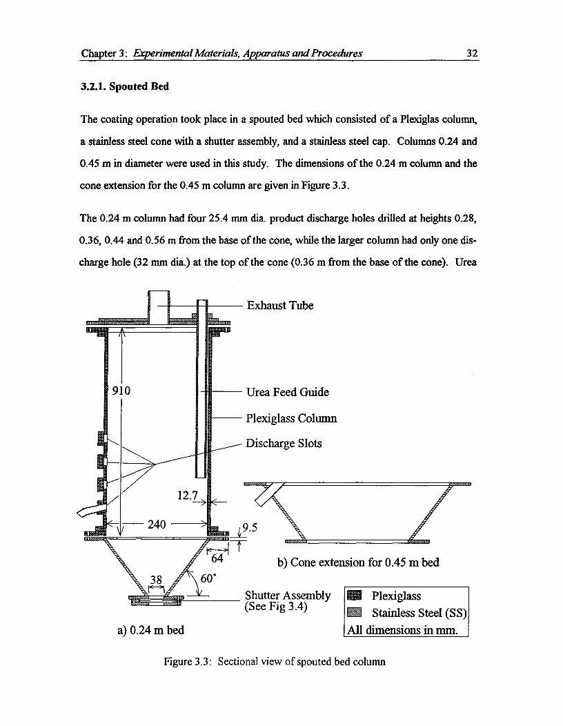
3.2.1. Spouted Bed
The coating operation took place in a spouted bed which consisted of a Plexiglas column,
a stainless steel cone with a shutter assembly, and a stainless steel cap. Columns 0.24 and
0.45 m in diameter were used in this study. The dimensions of the 0.24 m column and the
cone extension for the 0.45 m column are given in Figure 3.3.
The 0.24 m column had four 25.4 mm dia. product discharge holes drilled at heights 0.28,
0.36, 0.44 and 0.56 m from the base of the cone, while the larger column had only one dis-
charge hole (32 mm dia.) at the top of the cone (0.36 m from the base of the cone). Urea
Figure 3.3: Sectional view of spouted bed column

Chapter 3: Experimental Materials, Apparatus and Procedures^ 33
was fed through a Plexiglas tube opposite the product discharge locations and just above
the bed. The Plexiglas column could operate continuously at temperatures up to 110°C.
The shutter mechanism controlled the size of the orifice opening at the base of the bed.
As shown in Figure 3.4, the shutter consisted of five S-shaped, overlapping stainless steel
leaves arranged in a circle. The range of opening was 3.2 to 38 mm dia. Since the shutter
152.4 4)
A-A
I VP114
101.6 4)39.7 40
'Closed Position'Figure 3.4: Shutter assembly (dimensions are given in mm) designed by Mathur, Meisen
and Lim (1978).
Chapter 3: Experimental Materials, Apparatus and Procedures^34
shape changed from a circular to an irregular shape as the shutter was closed, calculating
its open area required a special procedure which is given in Appendix I.
3.2.2. Sulfur Supply System
Only minor modifications were made to the system designed by Meisen et al. (1986). The
sulfur and atomizing air lines to the upper plate had to be reinforced to allow a "slip-on"
type of sulfur line connector (see Section 3.2.2.4). This type of connector was necessary
for a completely steam traced sulfur line. Major components of the sulfur supply system
were the sulfur melter, filter, rotameter, flow control valve, sulfur line and nitrogen supply.
3.2.2.1. Sulfur Melter
The sulfur melter used in this study was originally designed as the sulfur reservoir con-
nected to a steam jacketed sulfur melter. Unfortunately, the steam supply was insufficient
to maintain the reservoir and the melter at the desired temperature. In this work, only the
sulfur reservoir was used because of its large capacity (18.9 L). A schematic diagram of
the reservoir is shown in Figure 3.5.
The reservoir was a modified Bink 83-5404 pressure tank (0.3 m dia. OD and 0.48 m
high), insulated with fiberglass. Holes were drilled through the cap to facilitate sulfur
feeding, molten sulfur withdraw', and pressurizing. The solid sulfur fed into the reservoir
was melted by contact with a stainles steel steam coil (9.5 mm dia. tube wound to 0.178 m
dia. nine times). A full sulfur charge of 30 kg melted in approximately six hours. A pres-
sure relief valve was also added on top of the reservoir to prevent excessive pressure
build-up.

Pressurized Nitrogen
Cap for Sulfur Feed
Steam
Condensate
Chapter 3: Experimental Materials, Apparatus and Procedures^ 35
Figure 3.5: Sectional view of 18.9 L sulfur reservoir.
3.2.2.2. Sulfur Filter
The stainless steel 316 in-line cartridge filter (Rigimesh, manufactured by Pall Canada
Ltd.) was located at the mouth of the molten sulfur outlet. The screen size of the filter
was 149 gm (screen size #100).
3.2.2.3. Sulfur Rotameter
A standard rotameter tube (Brooks, Model R-6M-25-A) inside a steam heated brass block
was used as the sulfur rotameter (designed by Weiss and Meisen, 1983). Two stainless
steel pieces on the top and bottom of the brass casing were used to hold the rotameter
tube in place and Viton 0-rings were used to seal the ends. Two polycarbonate windows
with heat resistant gaskets were placed in front and back of the brass block to allow a
clear view of the rotameter tube. A set of glass and stainless steel floats was used. The

Chapter 3: Experimental Materials, Apparatus and Procedures^ 36
specifications of all rotameters are given in Table 3.5, and their calibration curves are pre-
sented in Appendix IV.
3.2.2.4. Sulfur Line
The main sulfur line was a 6.4 mm dia. 316 SS tube enclosed by 13 mm dia. O.D. 1.TE
tubing overbraided with 304 SS and insulated with fiberglass. Complete steam tracing
was not possible at the points where the line joined the melter, rotameter and base of the
bed and frequent plugging was observed at the connection to the base of the bed. A fully
steam traced connection required a "slip-on" connector as shown in Figure 3.6. This con-
nector was enclosed in a 19 mm O.D. SS tube for the passage of steam. No sulfur plug-
Table 3.5: Types and capacities of Brooks rotameters used in this work.
Stream Maximum Capacity Rotameter
Atomizing air 0.44 L/s Tube: R-7M-25-1Float: Glass
Spouting air 23.9 Us Tube: R-12M-25-4Float: 12-RS-221
42.3 L/s Tube: R-12M-127-3Float: 12-RS-221
Sulfur 1.7 g/s Tube: R-6M-25-1Float: glass and stainless steel
Grooves for 0-rings
Sulfur line (6.35 mm SS tube)^Line connector (9.53 mm SS tube)
\ Viton 0-ring
Figure 3.6: Sectional view of "slip-on" sulfur line connector.
Chapter 3: Experimental Materials, Apparatus and Procedures^37
ging of the sulfur lines was experienced with this modification.
3.2.2.5. Nitrogen Supply
Industrial grade pressurized nitrogen (typically up to 20 psi) was used to force sulfur out
of the melter. The sulfur flow rate was controlled by the N2 pressure using the regulator
on the gas cylinder. The rotameter valve was also used to control the flow rate of the sul-
fur.
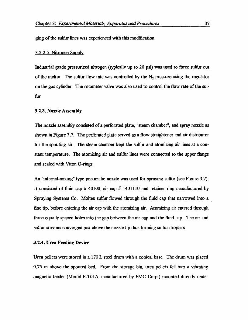
3.2.3. Nozzle Assembly
The nozzle assembly consisted of a perforated plate, "steam chamber", and spray nozzle as
shown in Figure 3.7. The perforated plate served as a flow straightener and air distributor
for the spouting air. The steam chamber kept the sulfur and atomizing air lines at a con-
stant temperature. The atomizing air and sulfur lines were connected to the upper flange
and sealed with Viton 0-rings.
An "internal-mixing" type pneumatic nozzle was used for spraying sulfur (see Figure 3.7).
It consisted of fluid cap # 40100, air cap # 1401110 and retainer ring manufactured by
Spraying Systems Co. Molten sulfur flowed through the fluid cap that narrowed into a
fine tip, before entering the air cap with the atomizing air. Atomizing air entered through
three equally spaced holes into the gap between the air cap and the fluid cap. The air and
sulfur streams converged just above the nozzle tip thus forming sulfur droplets.
3.2.4. Urea Feeding Device
Urea pellets were stored in a 170 L steel drum with a conical base. The drum was placed
0.75 m above the spouted bed. From the storage bin, urea pellets fell into a vibrating
magnetic feeder (Model F-TO1A, manufactured by FMC Corp.) mounted directly under
Air Cap
Retainer Ring
Fluid Cap
6.35 mm OD SS tube
I
Top Plate
Perforated Plate*t
Middle Cylinder(60.3 high)
Steam Chamber
^ Sulfur^ Steam
AtomizinAir
CondensateBottom Plate
00Figure 3.7: Sectional view of nozzle, perforated plate and steam chamber (all dimensions in mm; designed by Meisen et al., 1986).
Chapter 3: Experimental Materials, Apparatus and Procedures^39
neath the bin. The urea feed rate was controlled with an electric controller (Model CSCR
1B, FMC Corp.). The urea was introduced into the bed through a 25 nun ID Plexiglas
tube just above the annulus near the wall and opposite the product withdrawal port. Urea
could not be fed below the surface of the annulus due to slow moving bed particles near
the wall.
3.2.5. Product Withdrawal Device
The product discharged through a column slot and a 25.4 mm ID Plexiglas tube. The tube
was connected to a PVC flexible plastic hose which directed the SCU into the product
storage bin. The discharge mechanism depended on the gravity and air flow into the stor-
age bin from the bed resulting from the pressure difference between the two.
3.2.6. Product Collector
The product leaving the spouted bed was collected in a large wooden box (1.21 x 0.85 x
0.64 m high). The box was air sealed with silicone and gaskets to contain any dust. Three
holes were drilled through the top board: a 19 mm dia. hole for the incoming product, a 54
mm dia. hole for air exhaust, and a 0.3 m dia. hole for cleaning the box. The 0.3 m hole
was covered with a 13 mm thick Plexiglas lid held in place by attaching the cover to a 0.05
x 0.33 m Plexiglas board inside the box. A 25 mm dia. hole was also drilled through the
bottom board to empty the box.
3.2.7. Dust Collector
Urea and sulfur fines elutriated from the top of the spouted bed passed through a flexible
exhaust hose into a water scrubber (see Figure 3.2). The treated air was then vented di-
rectly into the laboratory exhaust system. A nylon mosquito mesh (approximately 1 mm
mesh size) was placed on top of the bed in the exhaust air line to prevent the bed particles
from leaving the bed.
Chapter 3: Experimental Materials, Apparatus and Procedures^ 40
3.2.8. Air, Steam, and Water Supplies
All air lines were connected to the laboratory compressed air supply (maximum pressure
of 510 kPa). Instrument air (maximum pressure of 650 kPa) was used for sulfur atomiza-
tion to provide cleaner air. Rotameters were used for all flow measurements. The type
and capacities of the rotameters are given in Table 3.5.
The spouting air was heated by a steam heater and a 3 kW electric heater. The atomizing
air was heated by a flexible electric heating tape (Type silicone rubber, 312 Watts; manu-
factured by Thermolyne Corp.) wrapped around the air line. The electric heater was con-
trolled by a proportional-integral controller supplied by Omega Engineering Inc. (Model
No. 49J, range of 0 to 200°C). The temperatures were monitored with iron-constantan
thermocouples.
Steam was generated by a 30 kW, three phase, "Electro-Steam" boiler (Type F-10; manu-
factured by Fulton Ltd.) capable of steam flows up to 48 kg/h at 720 kPa. The operating
pressure was set at 650 kPa for all runs in this study. The pressure downstream from the
boiler typically fell into the range of 580 to 620 kPa. All steam traps discharged into a
common atmospheric header that drained into the main sewer system.
Cold tap water was used in the water scrubber.
3.3. Apparatus for Hydrodynamics Study
The modifications to the spouted beds for the hydrodynamics study included replacing the
stainless steel caps with 1/2" (13 mm) plywood caps. The new caps were slotted to allow
a sampling tube to enter from the top of the bed, and the tube could be positioned at any
radial position. The modified cap is shown in Figure 3.8.
Chapter 3: Experimental Materials, Apparatus and Procedures^41
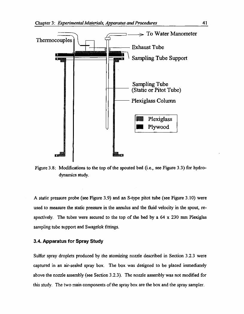
Figure 3.8: Modifications to the top of the spouted bed (i.e., see Figure 3.3) for hydro-dynamics study.
A static pressure probe (see Figure 3.9) and an S-type pitot tube (see Figure 3.10) were
used to measure the static pressure in the annulus and the fluid velocity in the spout, re-
spectively. The tubes were secured to the top of the bed by a 64 x 230 mm Plexiglas
sampling tube support and Swagelok fittings.
3.4. Apparatus for Spray Study
Sulfur spray droplets produced by the atomizing nozzle described in Section 3.2.3 were
captured in an air-sealed spray box. The box was designed to be placed immediately
above the nozzle assembly (see Section 3.2.3). The nozzle assembly was not modified for
this study. The two main components of the spray box are the box and the spray sampler.
1000 mm
To water manometer
—1 mm hole drilled through1/4" SS tube
20 mm
Tubes sealed withsilver solder
3/8" SS Tube
400 mm
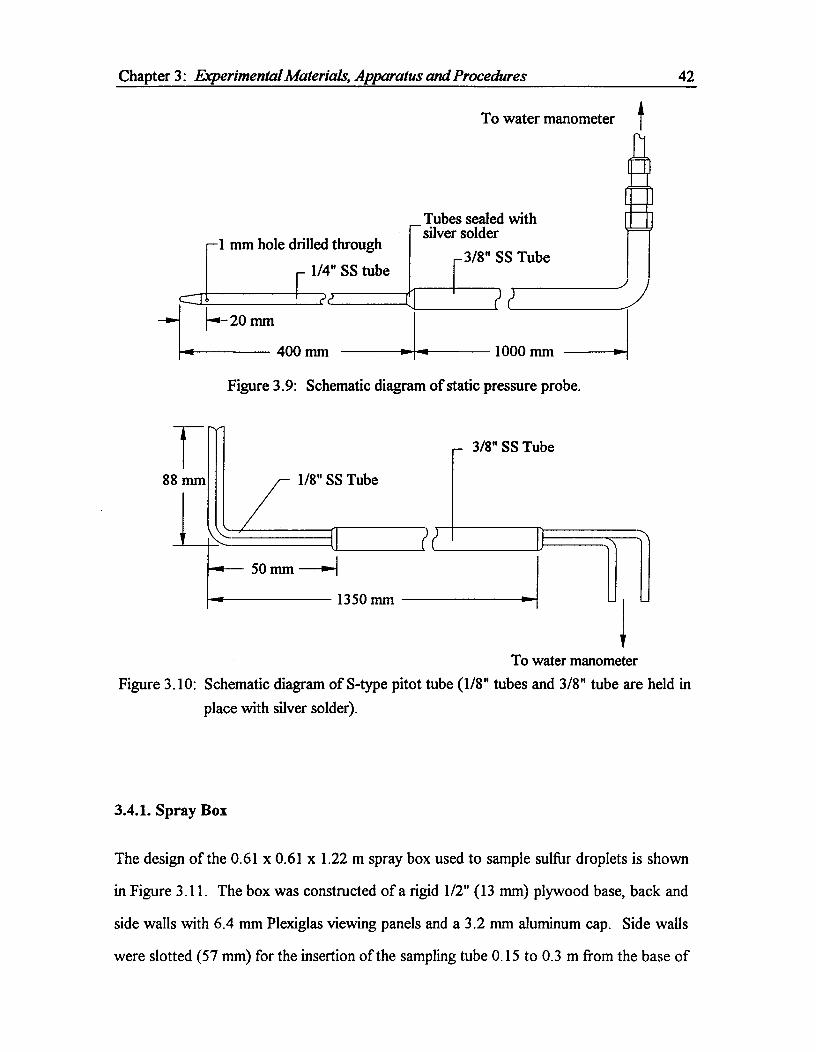
Chapter 3: Experimental Materials, Apparatus and Procedures^42
Figure 3.9: Schematic diagram of static pressure probe.
— 3/8" SS Tube
88 nun^1/8" SS Tube
^ 50 nun —0-1
1350 mm
To water manometerFigure 3.10: Schematic diagram of S-type pitot tube (1/8" tubes and 3/8" tube are held in
place with silver solder).
3.4.1. Spray Box
The design of the 0.61 x 0.61 x 1.22 m spray box used to sample sulfur droplets is shown
in Figure 3.11. The box was constructed of a rigid 1/2" (13 mm) plywood base, back and
side walls with 6.4 mm Plexiglas viewing panels and a 3.2 mm aluminum cap. Side walls
were slotted (57 mm) for the insertion of the sampling tube 0.15 to 0.3 m from the base of
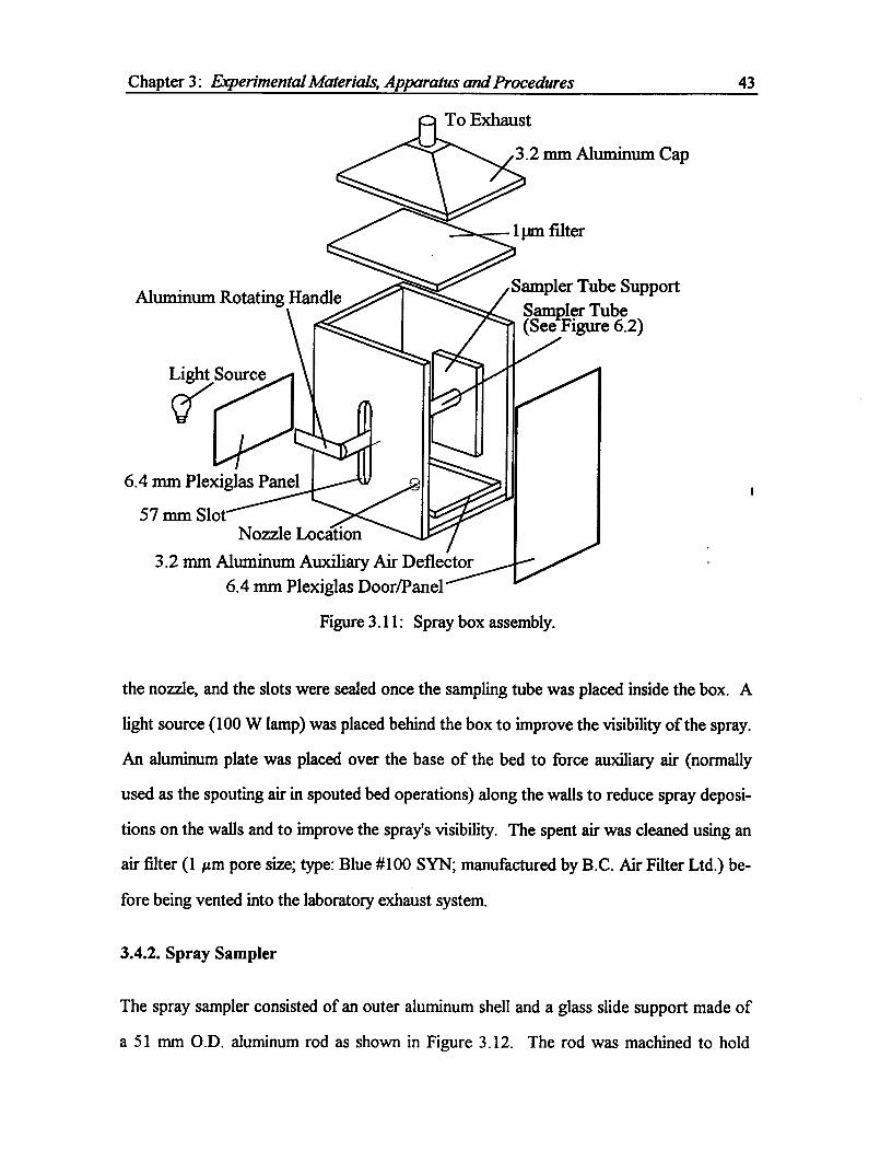
Chapter 3: Experimental Materials, Apparatus and Procedures^43
Figure 3.11: Spray box assembly.
the nozzle, and the slots were sealed once the sampling tube was placed inside the box. A
light source (100 W lamp) was placed behind the box to improve the visibility of the spray.
An aluminum plate was placed over the base of the bed to force auxiliary air (normally
used as the spouting air in spouted bed operations) along the walls to reduce spray deposi-
tions on the walls and to improve the spray's visibility. The spent air was cleaned using an
air filter (1 Am pore size; type: Blue #100 SYN; manufactured by B.C. Air Filter Ltd.) be-
fore being vented into the laboratory exhaust system.
3.4.2. Spray Sampler
The spray sampler consisted of an outer aluminum shell and a glass slide support made of
a 51 mm O.D. aluminum rod as shown in Figure 3.12. The rod was machined to hold
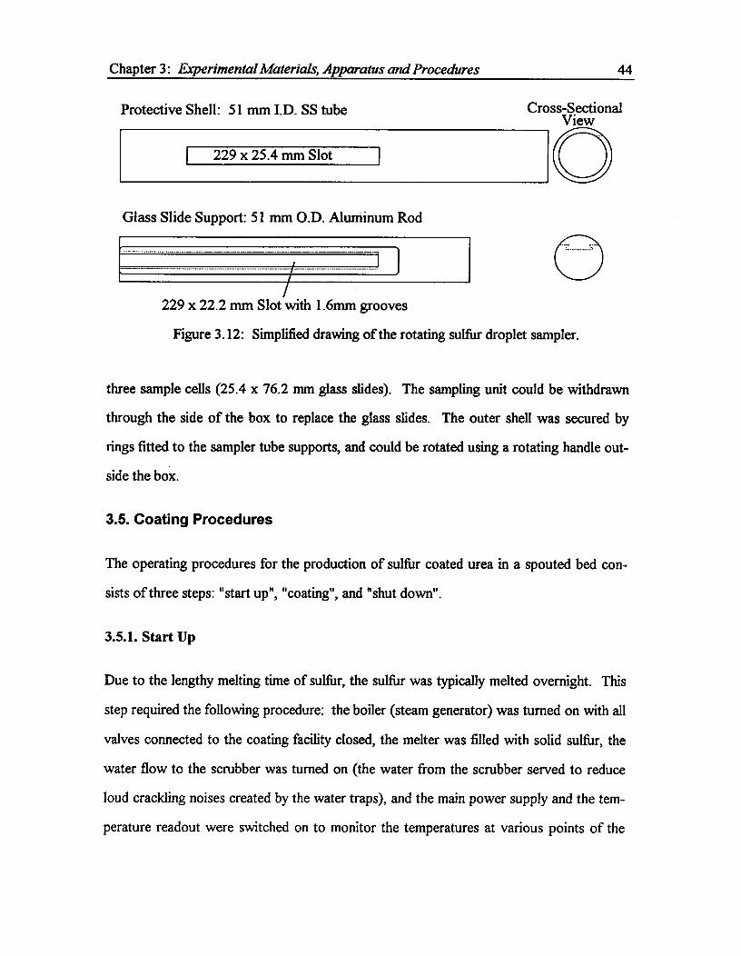
Chapter 3: Experimental Materials, Apparatus and Procedures^ 44
Protective Shell: 51 mm I.D. SS tube Cross-SectionalView
229 x 25.4 mm Slot
Glass Slide Support: 51 mm O.D. Aluminum Rod
229 x 22.2 mm Slot with 1.6mm grooves
Figure 3.12: Simplified drawing of the rotating sulfur droplet sampler.
three sample cells (25.4 x 76.2 mm glass slides). The sampling unit could be withdrawn
through the side of the box to replace the glass slides. The outer shell was secured by
rings fitted to the sampler tube supports, and could be rotated using a rotating handle out-
side the box.
3.5. Coating Procedures
The operating procedures for the production of sulfur coated urea in a spouted bed con-
sists of three steps: "start up", "coating", and "shut down".
3.5.1. Start Up
Due to the lengthy melting time of sulfur, the sulfur was typically melted overnight. This
step required the following procedure: the boiler (steam generator) was turned on with all
valves connected to the coating facility closed, the melter was filled with solid sulfur, the
water flow to the scrubber was turned on (the water from the scrubber served to reduce
loud crackling noises created by the water traps), and the main power supply and the tem-
perature readout were switched on to monitor the temperatures at various points of the
Chapter 3: Experimental Materials, Apparatus and Procedures^45
equipment. Once the pressure in the boiler reached 80 psig (650 kPa), the steam was in-
troduced to the melter by opening the appropriate valves.
In the meantime, the urea hopper was filled and the spray nozzle was placed in position.
The nozzle was checked to ensure there were no plugs.
3.5.2. Coating
The coating operation required the following steps: (i) the spouted bed was placed in the
"coating" position with the shutter open; (ii) atomizing air, spouting air, and their respec-
tive heaters were turned on; (Hi) the urea feeder was turned on after the air temperatures
reached 80 and 160 °C for the spouting and atomizing air, respectively; (iv) the bed was
left spouting with the withdrawal outlet open until steady state temperatures were ob-
served; (v) the nitrogen supply (set at approximately 5 psig) was opened to the sulfur
melter, and the valve attached to the rotameter was opened (an electric heating gun was
frequently used to unblock the valve); (vi) the nitrogen pressure regulator and the rotame-
ter valve were adjusted to set the sulfur flow rate to the desired values; (vii) steady state
(indicated by a constant bed temperature and fountain height) was usually reached after
ten minutes of coating for a given set of operating conditions, and product samples were
collected; (viii) when the experiment was complete, the nitrogen supply valve and the urea
feeder were turned off; (ix) the pressure was relieved from the melter by opening the pres-
sure relief valve and the sulfur flow valve was shut off after the sulfur had flowed back
into the melter; (x) the air heaters were turned off the atomizing air was reduced to mini-
mum, and the shutter and the spouting air valve were closed simultaneously, (xi) the
spouted bed was detached from its base, and the bed particles were unloaded.
The operating bed temperature (Tb) was taken as the steady state bed temperature after
the sulfur was injected into the bed. This temperature was typically 5 to 10°C higher than
the temperature before the sulfur injection.
Chapter 3: Experimental Materials, Apparatus and Procedures^46
To take a sample of the product, the flexible hose in the product withdrawal line was dis-
connected from the product storage bin and attached to a small container. A sudden surge
of particles resulted from the pressure difference between the bed and atmosphere, and ap-
proximately a minute was allowed for the bed to return to steady state conditions before
the products were sampled. The sampling time was also recorded to determine the pro-
duction rate.
All samples at different operating conditions were collected by repeating the above proce-
dure for consistency, i.e. the bed was emptied before starting a new run.
3.5.3. Shut Down and Clean-up
The procedure for shutting down was as follows: the spray nozzle was removed, in-
spected for plugging, and soaked in 50 % NaOH solution, all sources of steam, power,
water and air were turned off and the column was cleaned.
3.6. Procedures for Hydrodynamics Study
3.6.1. Minimum Spouting Velocity, U„..
The minimum spouting velocity was found by spouting the particles and then gradually re-
ducing the air flow rate until spouting ceased. U,,,, was calculated from the total volumet-
ric air flow rate, Q,,,, just before cessation of spouting, i.e.,
U„. = / IrD2 (3.1)
where D denotes the diameter of the cylindrical portion of the bed. It should be noted that
the total air flow rate (Q) is the sum of the spouting (Q,) and atomizing (Q.) air flow
rates. The errors in the measurements, calculated from the rotameter scale readings and
from repeat measurements, were typically less than +5 %.
Chapter 3: Experimental Materials, Apparatus and Procedures^ 47
3.6.2. Voidage of Loosely Packed Bed, e,„f
The voidage (e„,j) was determined by quickly inverting and re-inverting a glass cylinder
(0.1 m dia. by 0.6 m high) filled approximately one-third with particles. The voidage was
calculated from the following equation:
vb
/pp^(3.2)
3.6.3. Mean Particle Diameter, dp, and Sphericity, C
The mean diameter was found by sieving the particles using #5 to #14 Tyler mesh screens
and the equation
d p =11 Ex; I d p,^ (3.3)
where xi denotes the mass fraction of particles with diameter do.
With the exception of polystyrene, all particles were nearly spherical (see Plates 3.1 - 3.5).
The sphericity of the elliptical-cylindrical polystyrene particles (see Plate 3.6) was deter-
mined by measuring the principal dimensions 2.2 x 3.1 x 3.3 mm) of a representative
sample containing over 80 particles. Other particles were assumed to be perfect spheres,
i.e., 0, = 1.
3.6.4. Diameter of Inlet Orifice, di
The orifice is partly obstructed by the presence of the atomizing air nozzle (see Figure
3.13). The effective orifice diameter (d) is therefore calculated from
dz do2 _ da2^ (3.4)
and^do2 = 4A0 / r^ (3.5)
where Ao, do, and da denote the area of the orifice opening, the area equivalent diameter of
the orifice opening and the diameter of atomizing air nozzle, respectively.
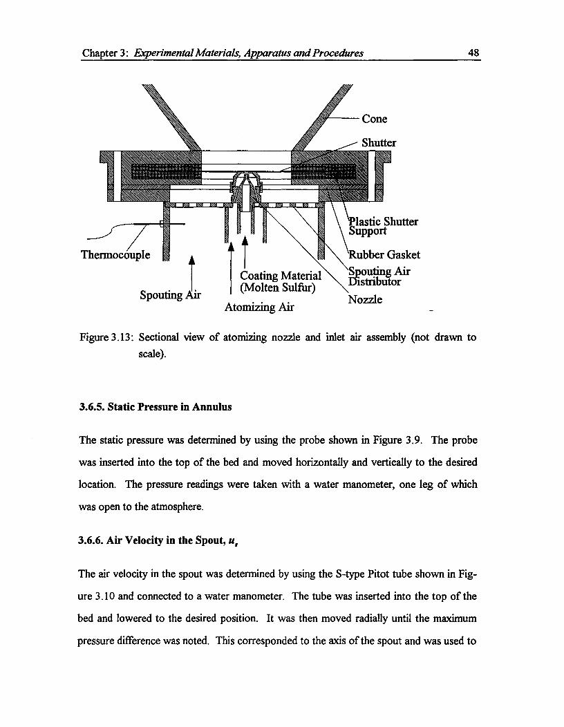
Chapter 3: Experimental Materials, Apparatus and Procedures^ 48
Figure 3.13: Sectional view of atomizing nozzle and inlet air assembly (not drawn toscale).
3.6.5. Static Pressure in Annulus
The static pressure was determined by using the probe shown in Figure 3.9. The probe
was inserted into the top of the bed and moved horizontally and vertically to the desired
location. The pressure readings were taken with a water manometer, one leg of which
was open to the atmosphere.
3.6.6. Air Velocity in the Spout, u,
The air velocity in the spout was determined by using the S-type Pitot tube shown in Fig-
ure 3.10 and connected to a water manometer. The tube was inserted into the top of the
bed and lowered to the desired position. It was then moved radially until the maximum
pressure difference was noted. This corresponded to the axis of the spout and was used to

Chapter 3: Experimental Materials, Apparatus and Procedures^49
calculate u,. (Therefore, the measured us corresponds to the maximum velocity in the
spout.)
The tube was calibrated against an ASME (1971) standard static pitot tube to 40 m/s in a
wind tunnel (0.30 x 0.41 m by 3.7 m long). The standard pitot tube coefficient (Co) was
then determined from the following equation:
u = Co V2AP 1 p (3.6)
The calibration curve is shown in Appendix IV.
3.6.7. Radial Velocity Profile at the Base of the Bed
In the absence of the bed particles, the radial air velocity distribution 10 mm above the
shutter was measured with a static pitot tube connected to a water manometer. The tube
consisted of a 1/16" (1.6 mm) stainless steel inner tube and a 1/8" (3.2 mm) stainless steel
outer tube. The calibration curve and coefficient (Co) for the static pitot tube are provided
in Appendix IV.
3.7. Procedures for Spray Studies
3.7.1. Operating Limits of Spray Nozzle
The operating envelope of the spray nozzle used in this work was investigated by deter-
mining the upper and lower limits of the atomization velocity. The lower limit or the
minimum atomization velocity (u,„a) was determined by gradually reducing the atomizing
air flow rate from a fully atomized state until no atomization was observed. The velocity
was calculated from the superficial air flow rate referenced to the nozzle orifice (day). The
upper limit or the minimum pulsating velocity (ump) was determined by gradually increas-
ing the atomizing air flow rate until inconsistent atomization (indicated by flickering of the
spray) was observed.

Chapter 3: Experimental Materials, Apparatus and Procedures^ 50
3.7.2. Spray Drop Size Measurements
All samples of sulfur droplets were collected 0.2 m above the nozzle. At this distance, the
sprays were fully developed and the spray density was low enough for easy sampling. The
sampling time and the slot size on the protective tube were also varied to obtain low spray
density (effects of sample time and the slot size are discussed in Chapter 5).
The procedure for collecting the spray samples was as follows: (i) the glass slides were
placed on the slide holder (see Figure 3.12); (ii) the holder was placed in the spray box;
(iii) the spray was turned on at desired sulfur and atomizing air flow rates; (iv) the outer
shell was rotated using the rotating handle to expose the glass slides to the spray; (v) the
glass slides were removed and the procedure was repeated for a new operating condition.
The sulfur drops on the glass slides were analyzed under a microscope attached to a LI-
ETZ TAS Image Analyzer available in the Department of Metals and Materials Engineer-
ing at UBC. At least ten frames of size 750 by 750 Am were analyzed to obtain approxi-
mately 100 droplets for each run. Depending on the operating condition, most drop sam-
ples contained more than 100 drops in ten frames. Non-spherical particles were not in-
cluded in the analysis.
3.8. Product Quality Analysis
3.8.1. Sulfur Content
The total sulfur deposited on the urea particles was determined by two methods. One
method involved mass balance calculations based on the urea and sulfur feed rates; negli-
gible loss of sulfur and urea fines was assumed. The other method was more direct and is
referred to as the crush test. In the latter method, either the sulfur or urea could be ana-
lyzed to determine the sulfur content. The former was used in this work to obtain the
mean sulfur content of the product.
Chapter 3: Experimental Materials, Apparatus and Procedures^ 51
The procedure for the crush test was as follows: a weighted sample (approximately 20 g)
of sulfur coated urea was ground in a crucible with 10 mL of water to obtain a fine slurry
(the exposed urea readily dissolved). The slurry was washed into a filter (1gm pores) with
excess water. The filtered sulfur was left over night to dry and the dried sulfur was
weighed the following day. The results could be reproduced to approximately ± 1 % for
batch products, and ± 3 % for continuous products.
3.8.2. Particle Sulfur Content
Up to one hundred individual SCU particles, randomly selected, were analyzed to deter-
mine the sulfur content distribution for each product. The analysis of sulfur (as described
in Section 3.8.1) was difficult due to the relatively small mass of sulfur on each particle.
Consequently, the urea content was analyzed to determine the sulfur content of each parti-
cle. Each particle was weighed, placed in a 0.5 mL vial and crushed (using a paper clip) in
0.5 mL of distilled water. The solution was capped and left overnight to ensure the com-
plete dissolution of urea. The refractive index of the solution was measured with an Abbe
refractometer (Model JB7150, Bausch and Lomb Optical Co.). The urea concentration
was determined from the refractometer calibration curve (see Appendix IV). The urea
content in the solution could be calculated once its concentration was known. The sulfur
content was determined by the difference between the urea and the total particle weights.
The error due to the particle weight measurement (typically 5 to 30 mg) was as large as ±
20 % while the error due to the urea content measurement using the refractometer was
even higher (up to ± 25 %) for 5 mg particle. However, the errors for particles bigger
than 5 mg were typically less than ± 10 and 12 %, respectively.

Chapter 3: Experimental Materials, Apparatus and Procedures^ 52
3.8.3. Seven Day Dissolution Test
The standard seven day test developed by TVA was used, i.e. 50 g of sulfur coated urea
and 250 mL of distilled water were placed in a capped jar for seven days at 37.8°C in an
incubator. The solution was carefully poured out and stirred. A sample of the solution
was analyzed under the refractometer for the urea concentration as mentioned in the previ-
ous section (Section 3.8.2). The seven day dissolution rate (UD„,) was determined as
weight of urea dissolved UDm^ X 100%^ (3.7)weight of urea in sample
The results could be reproduced to approximately ± 2 % for batch products, and to less
than ± 5 % for continuous products.
Chapter 4.Mathematical Models
Mathematical models describing the spouted bed coating process for the production of
sulfur coated urea (SCU) are developed in this chapter. The first section deals with simple
models based on assumptions used for previously published coating models (see Section
2.2). The simple models are then improved by progressively relaxing various assumptions
to determine how they limit these models. Subsequent sections deal with the development
of a "rigorous" model and programming strategy.
4.1. Simple Models
The objectives of developing simple models are to test some of the assumptions used in
the previously mentioned models in the literature, to determine the limitations of the mod-
els, and to establish the need to develop a more comprehensive model. The simple models
can provide quick estimates of the coating performances of a spouted bed, which may be
useful in preliminary plant design.
4.1.1. Model I: Residence Time Model
In developing the first model, two principal assumptions are made: perfect mixing of the
bed particles and uniform sulfur spray concentration throughout the bed. In addition, neg-
ligible coating (sulfur spray) is assumed lost. A schematic diagram of Model I is shown in
Figure 4.1. The tracer tests conducted by previous investigators (Becker and Sallans,
1961; Kugo et al., 1965; Barton et al., 1968) on spouted beds indicated that the residence
time distribution of the bed particles approximated that of a perfectly mixed vessel. The
residence time distribution, F{t}, for bed particles leaving a perfectly mixed vessel is given
by:
RI) =1 —^ (4.1)
53

Urea Feed
X = 0
tExhaust Air
SCU
Xs
Chapter 4: Mathematical Models^ 54
Sulfur Spray
Figure 4.1: Model I — perfectly mixed system.
F{t} may be regarded as the probability that a particle entering the bed at time zero leaves
after time 5 t.
In Model I, the amount of coating (or sulfur), m, on a particle leaving the bed is assumed
to be directly proportional to its residence time in the bed, i.e.,
a t^ (4.2)
This assumption is consistent with assuming that a uniform spray concentration exists
throughout the bed. It is convenient to express the particle coat distribution in terms of
the sulfur content of the particle (X) rather than m, i.e.,
X, —
m, (4.3)+ mi,
where mu denotes the mass of urea in a coated particle. Assuming mu is the same for all
particles, Equations (4.2) and (4.3) may be combined to give
t = X, 1 —X,X, I —X,
Equation (4.1) may now be rewritten in terms of X, as well:
(4.4)
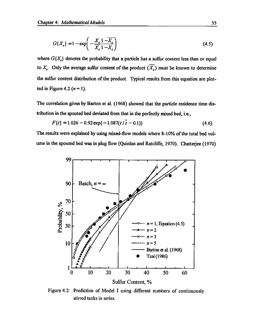
- Batch, n=
••
///XA X• X• X•
Chapter 4: Mathematical Models^ 55
G{X,} =1— expi X, 1 —XsX, 1 —X,
(4.5)
where G{Xs} denotes the probability that a particle has a sulfur content less than or equal
to X,. Only the average sulfur content of the product (X,) must be known to determine
the sulfur content distribution of the product. Typical results from this equation are plot-
ted in Figure 4.2 (n = 1).
The correlation given by Barton et al. (1968) showed that the particle residence time dis-
tribution in the spouted bed deviated from that in the perfectly mixed bed, i.e.,
F{t} =1.026 — 0.92 exp(-1.087(t /t — 0.1))^ (4.6)
The results were explained by using mixed-flow models where 8-10% of the total bed vol-
ume in the spouted bed was in plug flow (Quinlan and Ratcliffe, 1970). Chatterjee (1970)
99
90
70
50
0 30a.,
10
10^
10^
20^30^40^
50^
60
Sulfur Content, %Figure 4.2: Prediction of Model I using different numbers of continuously
stirred tanks in series.
Chapter 4: Mathematical Models^ 56
interpreted the residence time distributions in terms of two continuously stirred tanks
(CST). The results based on these models are also shown in Figure 4.2. The results of
CST's in series were calculated from the following expression (Ira 1977):
F to .1 _ e_noti 4. nt + 1 nt 2 + + 1 nt 11-1 (4.7)t 2! t (n —1)! i
Note that, to obtain Figure 4.2, t / t in all cases was replaced with the relationship given by
Equation (4.4). Batch results for a coating time I are also given in Figure 4.2 for com-
parison.
Tsai's coating distribution data are shown in Figure 4.2 and are fairly well represented in
the mid-range of sulfur concentrations by Equation (4.5), except that most of the experi-
mental data are slightly under predicted. In the same range, some improvement was ob-
served with the model given by Barton et al. (1968). Models based on several CST's de-
viate further from the experimental data.
The presence of significant fractions of uncoated urea particles produced in the continuous
process and the particle sulfur content distribution found in the batch product (see Figure
4.3) cannot be predicted by Model I. This leads to the conclusion that the assumption of a
uniform spray concentration in the bed is not valid for spouted bed coaters.
4.1.2. Model II: Simple Spray Zone Model
The aforementioned deficiencies of Model I suggest the presence of a limited spray zone
which some particles do not enter before leaving the spouted bed. In order to incorporate
such a spray zone, Model II was created on the premise that the bed could be divided into
three regions: spout, annulus and fountain. The spray zone is located in the lower region
of the spout, and the amount of coat a particle receives per pass through the spray zone is
fixed, i.e., the same amount of coat is applied on all particles regardless of the positions at
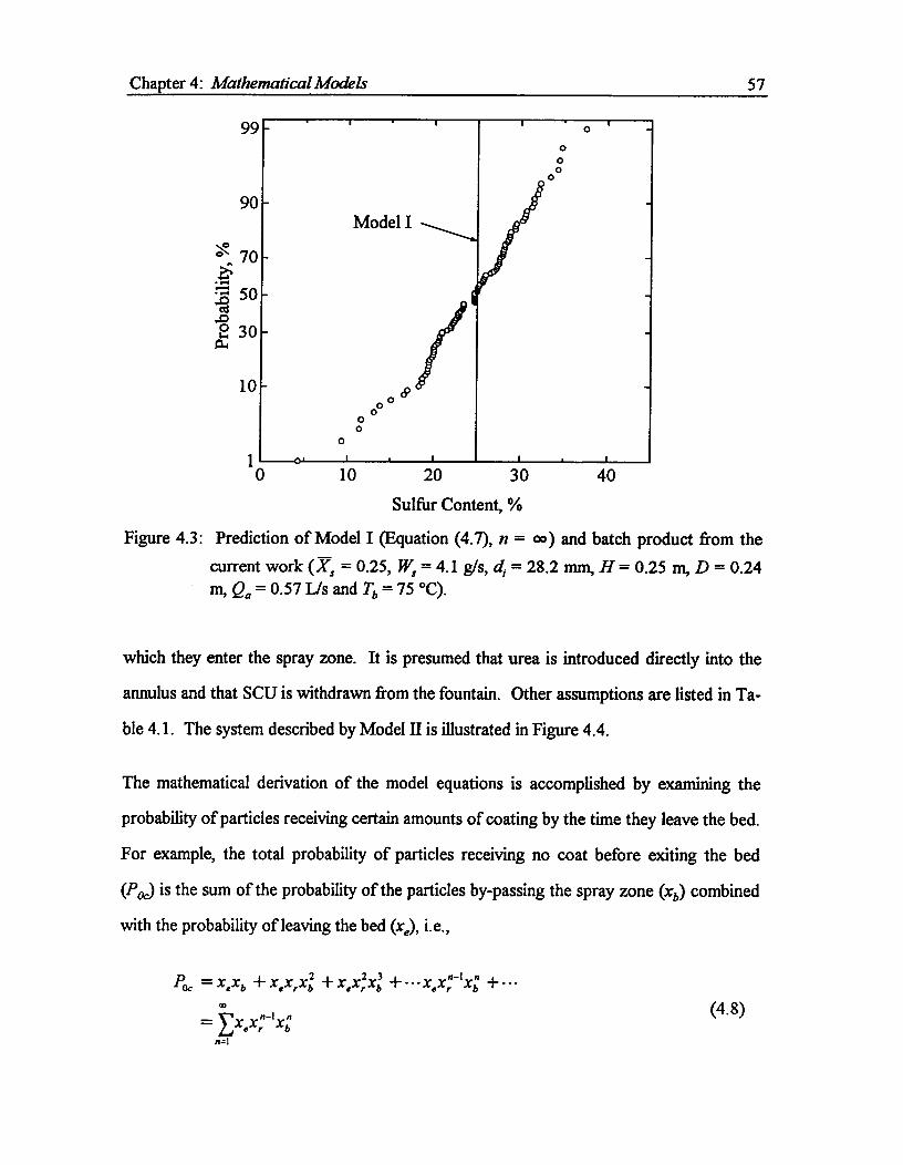
099
° 0 8
00
oo
90Model I
00
0
lo^10^20^30
Sulfur Content, %
0'^
40
70
..cTs 50
2 30
10
Chapter 4: Mathematical Models^ 57
Figure 4.3: Prediction of Model I (Equation (4.7), n = co) and batch product from thecurrent work (r, = 0.25, = 4.1 g/s, di = 28.2 mm, H= 0.25 m, D = 0.24
Qa = 0.57 Lis and Tb= 75 °C).
which they enter the spray zone. It is presumed that urea is introduced directly into the
annulus and that SCU is withdrawn from the fountain. Other assumptions are listed in Ta-
ble 4.1. The system described by Model II is illustrated in Figure 4.4.
The mathematical derivation of the model equations is accomplished by examining the
probability of particles receiving certain amounts of coating by the time they leave the bed.
For example, the total probability of particles receiving no coat before exiting the bed
(Poc) is the sum of the probability of the particles by-passing the spray zone (xb) combined
with the probability of leaving the bed (x,), i.e.,
P„ = xexb + x ex ,x1,2 + x gx,2 + xex,7-1x: +
= Exex,n—ixb^ (4.8)
rr=1

Urea FeedAnnulus
xe
By-passi►g
I zoneSpray zone'1E11.^ ..........,..
b). Simplified Spouted Beda). Spouted Bed
SCU Productxr
Chapter 4: Mathematical Models^ 58
Table 4.1: Assumptions used in simple models.
Perfect mixing Spray zone
Spout Annulus Fountain LocationSulfur drop-let concen-
trationModel I Yes Yes Yes All UniformModel II No No Yes Lower spout FixedModel III No No Yes Lower spout Variable
Figure 4.4: System described by Model II.
where xr = 1 - xe denotes the probability of a particle not exiting from the bed when it
leaves the fountain. The terms on the right hand side of Equation (4.8) represent the
probabilities of particles not receiving any coat after one to an infinite number of cycles.
Inspection of the infinite series formulas given in Table 4.2 reveals that Equation (4.8) re-
duces to:
Poc = xexb / (1 — xrxb )
Similarly, the probability of particles receiving one or more coats (PA,) is given by
Pic^1
=()x xc^2
+i)x xr xc x +()x x`xcbx` + --- + n()xs xn-ixcbxn-1 + --1 e^1^eb^
31^er^1
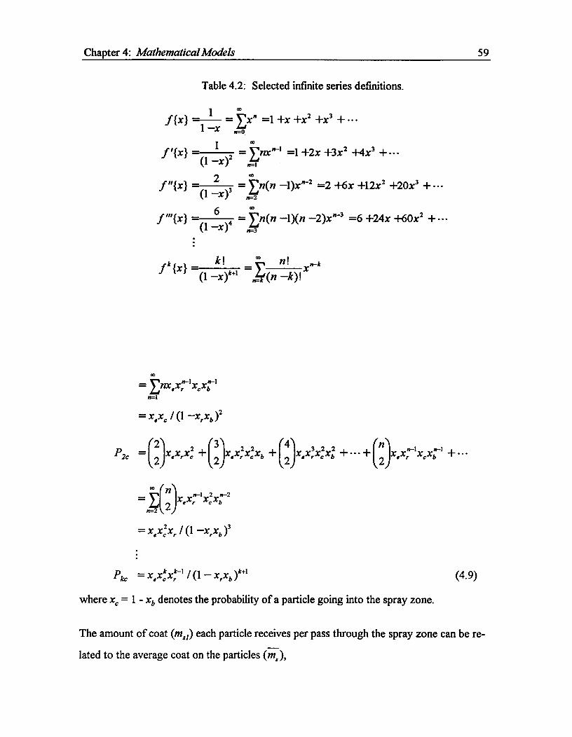
Chapter 4: Mathematical Models^ 59
Table 4.2: Selected infinite series definitions.
f "{x} — 2 — n(n —1)x" =2 +6x +12x 2 +20x3 +—x)3 yz
f "'{x} — 6 = n(n —1Xn —2)x" =6 +24x +60x 2 + --(1 —x)4 rr=3
fk{x} ^k! - r^(1 —x)"^k (n —k)!
= Enx,x,.'"XcXbP"r.
= XeX, / (1 —X,;)2
2 2 ()= ).X Xr cX + 3 XeXr2 Xc
2Xb (4),X.X:XXA2+...+ Nn-1XX7-1X^2 •^2 2^-^2
x xn4 x24-2^2)^c
n=2
Xe4Xr (1 —XrXi, )3
Pk, = XeXcirXrk-1 I (1 — XrXb )k+1^(4.9)
where x, = 1 - xb denotes the probability of a particle going into the spray zone.
f {x} — 1 — Fxn =1 +x +x2 +x3 + - - -1 —x tr=0
f '{x} — 1 = nx'" =1 +2x +3x 2 +4x3 + -(1n=1
Plc
The amount of coat (mfg) each particle receives per pass through the spray zone can be re-
lated to the average coat on the particles (ins),
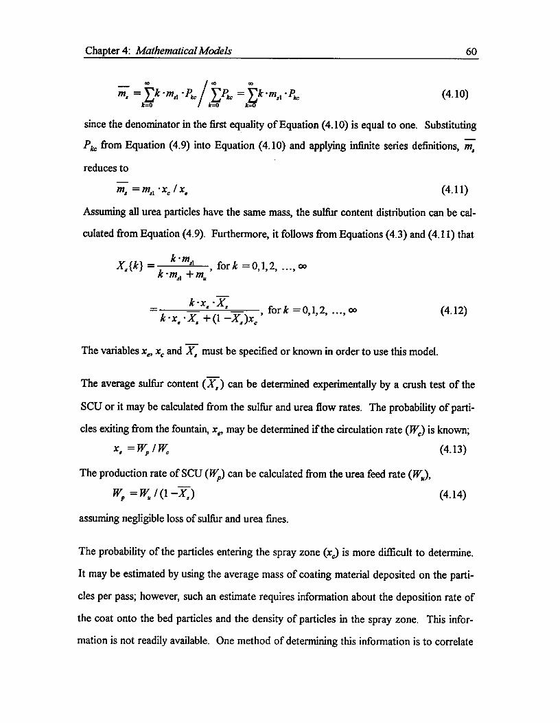
Chapter 4: Mathematical Models^ 60
m, = Ek .m„ • Pk,VP =k^
I co
Lnd kc^ao
' Pkc^(4.10)=0
since the denominator in the first equality of Equation (4.10) is equal to one. Substituting
Pi c, from Equation (4.9) into Equation (4.10) and applying infinite series definitions, in,
reduces to
m, = m„ - xe / x,^ (4.11)
Assuming all urea particles have the same mass, the sulfur content distribution can be cal-
culated from Equation (4.9). Furthermore, it follows from Equations (4.3) and (4.11) that
, for k =0,1,2, ..., a,^X, {k} —^k -mid + m.
k -x • X
^
—^— " ^for k = 0,1,2, ..., 03k•x,• X, + (1 —Xs )x,'
(4.12)
The variables xe, x, and X, must be specified or known in order to use this model.
The average sulfur content (X, ) can be determined experimentally by a crush test of the
SCU or it may be calculated from the sulfur and urea flow rates. The probability of parti-
cles exiting from the fountain, x, may be determined if the circulation rate (We) is known;x, = Wp 1 we^(4.13)
The production rate of SCU (Wp) can be calculated from the urea feed rate (We),Wp =Wa I (1 —Xs )^ (4.14)
assuming negligible loss of sulfur and urea fines.
The probability of the particles entering the spray zone (x e) is more difficult to determine.
It may be estimated by using the average mass of coating material deposited on the parti-
cles per pass; however, such an estimate requires information about the deposition rate of
the coat onto the bed particles and the density of particles in the spray zone. This infor-
mation is not readily available. One method of determining this information is to correlate

Chapter 4: Mathematical Models^ 61
; and ; to the operating variables. The value of; may be determined by optimizing x, to
fit experimental coat distribution data.
This model can also be modified for operations where the urea feed is forced into the
spray zone by moving the feed location near the wall of the column. (Tsai (1986) claimed
that such a change in feed location improved SCU quality.) The assumptions used in this
model are that all urea feed particles pass through the spray zone, and that the volume of
the particles does not change significantly as a result of coating. (See Appendix I for the
details of the derivation.) The resulting model equations are
k k-1Pk, ^
X,X, X r-1, for k = 1, 2, ..., co
(1 —xbxr )k
and Xs {k} — y^k • x, X,+(xbx. + xcX1-
-X,)
for k =1, 2, ...,
(4.15)
(4.16)
The assumption that all particles receive equal amounts of coat as they pass through the
spray zone is questionable since the spray concentration decreases with height. Particles
which enter the spray zone further away from the nozzle will be exposed to a lower sulfur
droplet concentration and spend less time in the spray zone. Such particles receive less
coating material than the particles that enter the spray zone closer to the nozzle. In the
following section, a model which addresses such a spray zone is developed.
4.1.3. Model Variable Concentration Spray Zone Model
The purpose of developing Model III is to see the effects of varying the sulfur concentra-
tion in the spray zone on sulfur content distribution. The sulfur droplet concentration (C)
in the spray zone is assumed to vary with the distance from the nozzle, i.e.,
oc (zc —z)°^ (4.17)

Chapter 4: Mathematical Models^ 62
where zc. = height of the spray zone, z = distance from the nozzle, and a = index. The
amount of coat a particle receives is assumed to be directly proportional to the sulfur
droplet concentration in the spout, i.e.,
Mal °C Cc (4.18)
Therefore, it follows that
m„ = kc (z,. —z)°^ (4.19)
The probability of a particle entering at any location in the spray zone is the same; there-
fore, the probability density (4'{z}) may be expressed as
(13{z} = kp^(4.20)
Since foz` cl)(z)dz = x„ then kp = xjz,. The average amount of coat a particle receives
(m„ ) is given by
msl^/ z
fo ms14) {z}dz/ fo {z}dz^ (4.21)
which, after solving for kc and substituting into Equation (4.19), gives
m„ = (a +1)m„ (z, — iz:^ (4.22)
All other assumptions are the same as for Model II.
Due to the complexity of deriving an analytical expression for Model III, the Monte Carlo
method was applied to find the coating distribution. See Section 4.2.3 for more details.
4.2. Model IV: Rigorous Model
The ultimate goal of the present study is to model the sulfur coating of urea in a spouted
bed by developing sub-models for particle circulation and coating mechanism, and then,
based on the histories of single particles, determine the coating distribution. This model
should require only the operating and design specifications as inputs and should not de-
pend on other information to determine the coating distribution.

Chapter 4: Mathematical Models^ 63
The approach taken to develop the mathematical model for predicting the concentrations
of the sulfur droplets in the gas phase (i.e. spray zone) in the spouted bed is similar to that
taken by Meisen and Mathur (1974) for a spouted bed aerosol collector. The bed is di-
vided into three regions as shown in Figure 1.1. Each region is considered separate and
distinct from each other although interactions exist along the boundaries. The hydrody-
namics and coating in the fountain are expected to be unimportant and, therefore, they are
not considered further in this work.
Several key assumptions are required for Model N. The particles in the fountain are as-
sumed to be perfectly mixed, while those in the spout and annulus are assumed to be in
plug flow. In addition, particle segregation due to changing size and density is assumed to
be absent. The change in sulfur properties resulting from solidification and allotropic
transformations is neglected as far as their effect on bed hydrodynamics, bed temperature
and particle circulation is concerned. Consequently the effects such as the influence of bed
temperature on the quality of coating (Tsai, 1986; Weiss, 1981) cannot be determined
from Model N.
The Model IV equations and methods used to calculate the bed hydrodynamics, sulfur
droplet concentration and coating distribution are outlined in the following sections. The
computer program listings for Model IV are given in Appendix In.
4.2.1. Calculation of Solids Circulation Rate and Bed Hydrodynamics
The hydrodynamics model used in this work is based on the one-dimensional gas and sol-
ids mass and momentum balances for the spout developed by Lefroy and Davidson (1969)
and the vector form of the Ergun (1952) equation for gas flow in the annulus. The spout
diameter is assumed constant and estimated using Equation (2.4). The pressure distribu-
tion at the spout-annulus interface (equal to the radially averaged pressure in the spout) is
determined by Equation (2.11) and
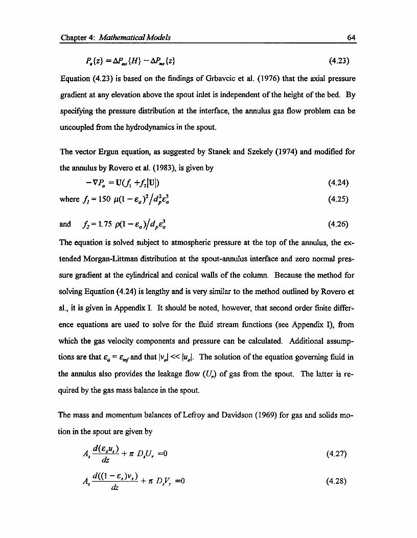
Chapter 4: Mathematical Models 64
(4.23)Pa {z} = tiP„„{H} — AP„„{z}
Equation (4.23) is based on the findings of Grbavcic et al. (1976) that the axial pressure
gradient at any elevation above the spout inlet is independent of the height of the bed. By
specifying the pressure distribution at the interface, the annulus gas flow problem can be
uncoupled from the hydrodynamics in the spout.
The vector Ergun equation, as suggested by Stanek and Szekely (1974) and modified for
the annulus by Rovero et al. (1983), is given by
— VP. = U(fi +f2 IUI)^ (4.24)
where = 150^_ ea )2/dp2e3.^ (4.25)
^
and f2 = 1.75 p(1 — ea )/dpe3,^ (4.26)
The equation is solved subject to atmospheric pressure at the top of the annulus, the ex-
tended Morgan-Littman distribution at the spout-annulus interface and zero normal pres-
sure gradient at the cylindrical and conical walls of the column. Because the method for
solving Equation (4.24) is lengthy and is very similar to the method outlined by Rovero et
al., it is given in Appendix I. It should be noted, however, that second order finite differ-
ence equations are used to solve for the fluid stream functions (see Appendix I), from
which the gas velocity components and pressure can be calculated. Additional assump-
tions are that E. = Erni-and that Ival << kJ. The solution of the equation governing fluid in
the annulus also provides the leakage flow (Ur) of gas from the spout. The latter is re-
quired by the gas mass balance in the spout.
The mass and momentum balances of Lefroy and Davidson (1969) for gas and solids mo-
tion in the spout are given by
d( sus )^Dsur .0 (4.27)dz
A,^dzdal — es )vs )^Dsv; =0 (4.28)

Chapter 4: Mathematical Models^ 65
p Assd(esus2)^A^--L(1P^(u, v i)lus vsks^dz^Pdz
(4.29)
p pAs dal — es)v)^(1 —es )A,^+ 13 p (us — v s)lus v slAsdz^dz^ (4.30)
— (1 — es )(pp — p)Aig
Equations (4.27) and (4.28) represent the gas and solids mass balances while Equations
(4.29) and (4.30) are the gas and solids momentum balances, respectively. The terms on
the right hand sides of the momentum equations account for the normal stress, drag be-
tween the two phases and, in case of solids, the gravity force. The particle-fluid interac-
tion parameter (pp) is approximated by the Richardson and Zaki (1954) equation as ap-
plied by Lefroy and Davidson (1969):
/31, =0.33(1 — es )pidpes1.78^(4.31)
The initial conditions for Equations (4.27), (4.29) and (4.30) are:
Es = 1, us = u0, and vs = 0 at z = 0.^ (4.32)
This set of equations is solved numerically using UBC ODEPACK (Moore, 1989) running
under the UBC MTSG (Runnals, 1987) main frame operating system. Once es, u, and vs
have been obtained, the particle entrainment flux (V,.) at the spout-annulus interface can be
calculated from Equation (4.28).
Finally, the radially averaged particle velocity in the annulus can be determined by equat-
ing the solids up-flow in the spout with the solids down-flow in the annulus at any height
(z), i.e.,
v a =v sA,(1— e s )I Aa (1 — Ea )^ (4.33)
As well as radial uniformity, Equation (4.33) assumes that there is no particle segregation
in the annulus and negligible mass change due to coating in the spout.
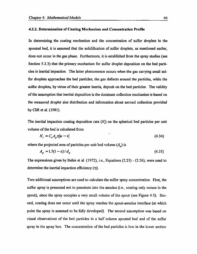
Chapter 4: Mathematical Models^ 66
4.2.2. Determination of Coating Mechanism and Concentration Profile
In determining the coating mechanism and the concentration of sulfur droplets in the
spouted bed, it is assumed that the solidification of sulfur droplets, as mentioned earlier,
does not occur in the gas phase. Furthermore, it is established from the spray studies (see
Section 5.2.3) that the primary mechanism for sulfur droplet deposition on the bed parti-
cles is inertial impaction. The latter phenomenon occurs when the gas carrying small sul-
fur droplets approaches the bed particles; the gas deflects around the particles, while the
sulfur droplets, by virtue of their greater inertia, deposit on the bed particles. The validity
of the assumption that inertial deposition is the dominant collection mechanism is based on
the measured droplet size distribution and information about aerosol collection provided
by Clift et al. (1981).
The inertial impaction coating deposition rate (N) on the spherical bed particles per unit
volume of the bed is calculated from
N = C,Apnlu — vl^ (4.34)
where the projected area of particles per unit bed volume (A p) isAp =1.5(1 — e) I d p^(4.35)
The expressions given by Behie et al. (1972), i.e., Equations (2.23) - (2.26), were used to
determine the inertial impaction efficiency (n).
Two additional assumptions are used to calculate the sulfur spray concentration. First, the
sulfur spray is presumed not to penetrate into the annulus (i.e., coating only occurs in the
spout), since the spray occupies a very small volume of the spout (see Figure 4.5). Sec-
ond, coating does not occur until the spray reaches the spout-annulus interface (at which
point the spray is assumed to be fully developed). The second assumption was based on
visual observations of the bed particles in a half column spouted bed and of the sulfur
spray in the spray box. The concentration of the bed particles is low in the lower section

Fully developedSprayhids
Developing Spray
dzd(C,u,e„As ) _ nv, ior z Hfd, (4.36)
Chapter 4: Mathematical Models^ 67
Figure 4.5: Sectional view of the lower spout.
of the spout and the particles are located primarily near the wall of the spout. The spray
only occupies a small area just above the nozzle.
With these assumptions, a mass balance for coating material in the spout gives (see Figure
4.6):
d(Csu,e,A,) + NA 0, for z hfdsdz
(4.37)
The initial condition is
Cs = Cso at z =0^ (4.38)
Note that Equation (4.38) assumes that the sulfur droplet concentration below z hfas can
be smeared out radially, in order that a one-dimensional approximation may be applied.
Equations (4.36) and (4.37) are solved simultaneously with Equations (4.27) to (4.30)
using UBC ODEPACK. The spray angle of 20° (provided by the manufacturer of the
spray nozzle for spraying water into still air) is used in the calculations to determine hfds.
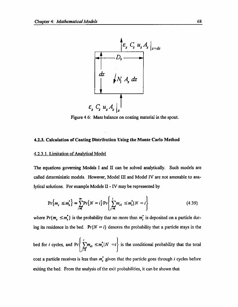
Chapter 4: Mathematical Models^ 68
z+dz
AC As cfr
Es CSuSA lztFigure 4.6: Mass balance on coating material in the spout.
4.2.3. Calculation of Coating Distribution Using the Monte Carlo Method
4.2.3.1. Limitation of Analytical Model
The equations governing Models I and II can be solved analytically. Such models are
called deterministic models. However, Model III and Model IV are not amenable to ana-
lytical solutions. For example Models II - IV may be represented by
Prfm, m:1 = EPr{N = i} Pr Ems, 5 m: I N = i^ (4.39)i4^ 4
where Pr{ms 5 ms, } is the probability that no more than m: is deposited on a particle dur-
ing its residence in the bed. Pr{N = i} denotes the probability that a particle stays in the
{ bed for i cycles, and Pr Ems, /.//:IN =i is the conditional probability that the totalJ 4
coat a particle receives is less than m: given that the particle goes through i cycles before
exiting the bed. From the analysis of the exit probabilities, it can be shown that

Chapter 4: Mathematical Models^ 69
Pr{N = i} =^ (4.40)
Mann (1983) showed that the remainder of the term in Equation (4.39) can be reduced to
{ i
Pr Ems, m*, IN = i =Pr`' fin„ .ini,,IN = ili
(4.41)
where Pr`' {mil »Is, IN = i} denotes the ith order convolution of Pr{m .,1 5 ins, IN = i}.
Simple analytical expressions can be obtained if an exact solution of the convolution in
Equation (4.41) exists and if an infinite series representation exists for Equation (4.39). If
both conditions are satisfied, Equation (4.39) can be reduced to a simple analytical expres-
sion. The equation can usually be solved numerically if the conditions are not satisfied.
However, the derivations of analytical expressions or numerical solutions can be difficult
for complicated models such as Models III and IV, and are susceptible to errors from
dealing with large arrays of coating probabilities or from numerical procedures. More-
over, both processes must be repeated if model specifications change (e.g., change in feed
location for Model II). The errors associated with these methods can be avoided, and the
repeat derivations are unnecessary if the Monte Carlo method is used.
4.2.3.2. Monte Carlo Procedure for Model III
The path of a particle and the sulfur deposited on the particle are simulated from given
values of xe, x, and a, and random parameters Nit/ and NR2. As each particle enters the
bed, its path through the spout is determined by NR/, from which msi can be calculated
msl = 0, for NR 1 > x, (4.42)
msl = (a +1)ms1 (z / z:, for NR l x (4.43)
where z = I, 0 <NRI <1 and z, is the distance indicating the upper limit of the spray
zone. Once the particle leaves the spout and enters the fountain, its path from the fountain
is determined by NR2, i.e.,
Chapter 4: Mathematical Models^ 70
if N, < x„ the particle leaves the bed (4.44)
if N x., the particle stays in the bed (4.45)
where 0 < NR2 <1. If the particle stays in the bed, the procedure is repeated. If the par-
ticle leaves the bed, another particle is introduced until a sufficient number of particles is
simulated to determine the coating distribution. The value of m ai is determined from the
following definition of the mean sulfur weight in the product (WO:
— coating on the particles in units of mg,m, (4.46)
number of particles sampled
and the sulfur content is found by applying Equation (4.3). The random numbers NI?' and
NR2 are generated using the UBC RANDOM (Nicol, 1986) package available in UBC
MTSG (Runnals, 1987). A pseudo-random number generator was used, i.e. the same
'seed' value produces the same sequence of random number.
4.2.3.3. Monte Carlo Procedure for Model IV
The Monte Carlo method (see Section 2.5) was used to determine the distribution of sul-
fur on the particles leaving the spouted bed. The sulfur deposit on a particle is determined
by following the path of the particle in the bed and calculating the amount of coating ma-
terial the particle receives until it leaves the bed. The procedure is then repeated for an-
other feed particle until a sufficient number of particles has been considered to give a good
representation of the coating distribution. The detailed procedure for determining the coat
on an individual particle during its residence in a spouted bed is given in the following sub-
sections:
4.2.3.3.1. Continuous Operation
1. When a feed particle enters the unit or a cycling particle returns via the fountain to the
top of the bed, its radial position at the top of the annulus is randomly assigned. The feed
urea particle, as it enters the bed, is assumed to land within (ADf=) 0.03 m of the column

Chapter 4: Mathematical Models^ 71
wall at the surface of the annulus. This assumption is based on the observations that ma-
jority of particles fall within 0.03 m of the column. The radial position of the feed particle
on the annulus surface is assigned using a random number generated by the UBC RAN-
DOM (Nicol, 1986) package available in the MTSG (Runnals, 1987) main frame operating
system at UBC. The generated number (NR) falls between 0 and 1, and it is used to assign
the radial position (D,) of the particle according to
Dr2NR D̂2
where Df =D — ADf
(4.47)
(4.48)
ADf denotes twice the width (adjacent to the bed wall) of the bed surface area occupied by
the feed and D denotes the column diameter. Similarly, the radial position of the returning
particle (via the fountain) on the annulus is calculated from
NR - 2^2̂ , for Dr Df(Df — Los ) + (1 — xf XD2
NR -(1-
2 xf X.1^D+(D, -D
(Df - D2),) + (1— x f XD2 —D#) ' for Dr <Df
where xf —^2 Wu / Pu v a (D — D f X1 — ea )7r 141H
(4.49)
(4.50)
(4.51)
The denominator in Equations (4.49) and (4.50) represents the total area occupied by the
recycling particles, and xf represents the fraction of area the feed particles occupy in the
area defined by r (D2 — D,-)/ 4.
2. The particle is followed around the bed, i.e. entry into the annulus, transport in the an-
nulus, entry into the spout, transport in the spout, entry into the fountain, transport in the
fountain, entry into the discharge tube or re-entry into the annulus. As the particle spends

Chapter 4: Mathematical Models^ 72
significantly more time in the annulus than the spout or fountain, the total cycle time (tc) is
estimated using the residence time of the particle in the annulus:
to = L"dz 1 v. (z)^ (4.52)
can be determined by equating the particle flow rate at the surface of the annulus be-
tween D and Dr to that in the spout at z,, i.e.,
v.(1 — ea XD.2 — D)111 = v.(1 —^ (4.53)
1— e, Ds2where v = vs 1 ea D2 D2 H
(4.54)
The total residence time (tr) in the bed can be found from the sum of the cycle times
Ntr 1= Et,^ (4.55)
4
where N denotes the total number of cycles a particular particle makes before leaving the
bed. The coating amount per cycle (m,i) can be calculated from
=rAspCi lu, — va in/ vs dz, forz, >hf,^ (4.56)
M i =fH As C lu —v 17.11 v dz, forz, —<hfdss.^hfib ps s^s^.1 (4.57)
where Ap* is the projected area of a single urea particle and hfd, is the height at which the
spray becomes fully developed and, hence, coating occurs beyond this point (see Figure
4.6). The spray angle (0) was assumed to be 20° and hfd, is calculated from
hfds = Di tan(0 / 2)/ 2^ (4.58)
Since coating is assumed not to occur in the annulus and fountain, ms, in Equations (4.56)
and (4.57) represent the total amount of sulfur deposited on the particle in one cycle.
3. The position of the particle is reassigned on the annulus surface. If the particle lands in
the exit stream, the simulation ends for this particular particle and begins for another.
Otherwise, the next cycle begins as before.
Chapter 4: Mathematical Models^ 73
The sulfur content (X44) of the ith particle leaving the bed is given by
X sp,i =ENj4Ms1 (E14Ms1 + Mu) (4.59)
where mu is the mass of urea in a single bed particle. Because the average sulfur contentof simulated particles (X,p) does not always agree with the sulfur content calculated from
the sulfur and urea feed rates (X.,), especially when a small number of particles are simu-
lated, Xva is normalized as follows:)(aim = X,pj X, / X,^ (4.60)
In total, 1000 particles were typically simulated to determine the coating distribution for
each set of operating condition. The values of X, and X,, typically differed by 2 % before
normalizing according to Equation (4.60). The effect of the sample size is discussed in
Chapter 5.
4.2.3.3.2. Batch Operation
The simulation procedure for the batch coating operation is the same as that for the con-
tinuous operation except that the start and the termination of the particle simulation are
different. The simulation of batch coating terminates when the particle's residence time is
equal to the total coating time of the batch product. The cycle and residence times are
calculated from Equations (4.52) and (4.55). The detailed derivation of the batch model is
given in Appendix I.

Chapter 5.Results and Discussions
The results of the studies conducted on the bed hydrodynamics and sulfur spray are dis-
cussed in the first two sections of this chapter. The third section deals with the coating
experiments including the coating distribution and product quality. The commercial impli-
cations of the present work are then discussed.
5.1. Bed Hydrodynamics
The minimum spouting velocity, pressure in the annulus, and fluid velocity in the spout
were measured in the absence of sulfur injection. The validity of expressions presented in
Chapter 2 were compared with the experimental data obtained from the present coating
unit. Modifications were made in the expressions to improve their predictive ability where
necessary and possible. The modifications resulted from the presence of the pneumatic at-
omizing nozzle in the spouting air inlet, the presence of atomizing air, and operating with
shallow conical beds.
The ranges of variables examined in this study are summarized in Table 5.1. A total of
327 runs were performed to determine the minimum spouting velocity and the spout ve-
locity and annulus pressure profiles were measured in 32 runs. The operating conditions
of the experiments performed to determine the pressure profiles and spout velocities are
given in Table 5.2. Pressure and velocity data are given in Tables 5.3 and 5.4, respec-
tively. The minimum spouting velocity data are provided in Appendix II.
74

Chapter 5: Results and Discussions^ 75
Table 5.1: Operating ranges applicable to this work.
Parameter Operating Range Parameter Operating Range
H 0.11 - 0.63 m Q. 0- 0.87 L/s
D 0.24 and 0.45 m T 18 - 70 °C
d,
Q.,
21 - 35 inm
0 - 37 Ifs
p 1 - 1.2 kg/m3
5.1.1. Minimum Spouting Velocity, U„„
Besides providing the lower limit of operation, the minimum spouting velocity (U.) in-
formation may be used to study the effects on bed hydrodynamics of atomizing air, pres-
ence of the nozzle, and operating with shallow conical beds.
Figure 5.1 provides comparison between the measured U. and the values calculated by
the standard equations due to Mathur and Gishler (1955) and Wu et al. (1987) (given by
Equations (2.2) and (2.3), respectively). The values of the constants in Equation (2.3) are
repeated in Table 5.5.
As shown by Figure 5.1, poor agreement was obtained between the experimental meas-
urements and the aforementioned standard equations. The discrepancy was thought to re-
sult from determining the experimental U., values based on the total air flow rate (i.e., the
sum of Q. and Q5) without due regard to the momentum of the main and atomizing air
streams. The atomizing air, which enters at high velocity (up to 131 m/s) in the centre of
the spout, should enhance the effectiveness of the main spouting air stream (typical ve-
locities: 22 to 78 m/s) and therefore reduce the minimum spouting velocity. This is con-
firmed by the radial velocity profile measured at the bottom of the cone (just above the
shutter) in the absence of bed particles (see Figure 5.2).
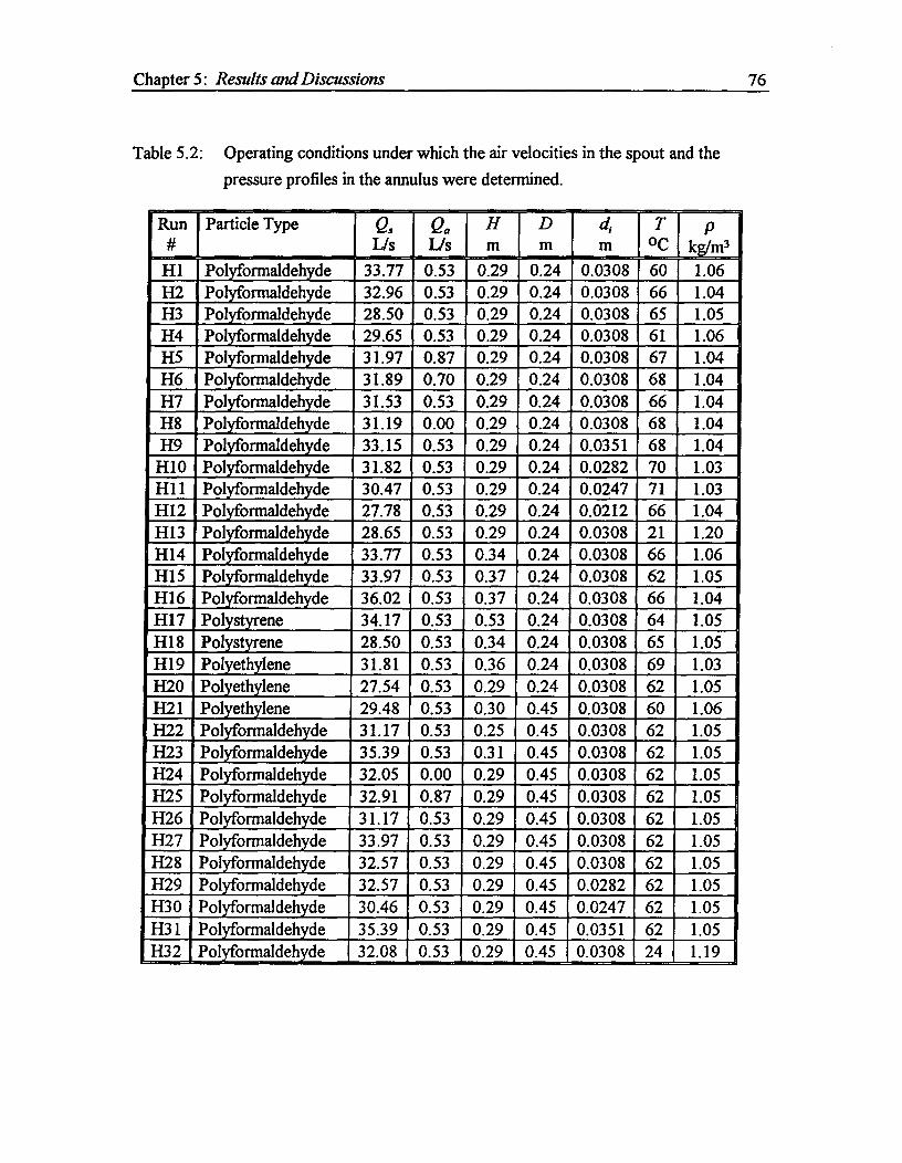
Chapter 5: Results and Discussions^ 76
Table 5.2: Operating conditions under which the air velocities in the spout and thepressure profiles in the annulus were determined.
Run#
Particle Type Q,Us
a,Us
HIm
Dm
dem
T °C
pkg/m3
HI Polyformaldehyde 33.77 0.53 0.29 0.24 0.0308 60 1.06H2 Polyformaldehyde 32.96 0.53 0.29 0.24 0.0308 66 1.04H3 Polyformaldehyde 28.50 0.53 0.29 0.24 0.0308 65 1.05H4 Polyformaldehyde 29.65 0.53 0.29 0.24 0.0308 61 1.06H5 Polyformaldehyde 31.97 0.87 0.29 0.24 0.0308 67 1.04H6 Polyformaldehyde 31.89 0.70 0.29 0.24 0.0308 68 1.04H7 Polyformaldehyde 31.53 0.53 0.29 0.24 0.0308 66 1.04H8 Polyformaldehyde 31.19 0.00 0.29 0.24 0.0308 68 1.04H9 Polyformaldehyde 33.15 0.53 0.29 0.24 0.0351 68 1.04
H10 Polyformaldehyde 31.82 0.53 0.29 0.24 0.0282 70 1.03HI1 Polyformaldehyde 30.47 0.53 0.29 0.24 0.0247 71 1.03H12 Polyformaldehyde 27.78 0.53 0.29 0.24 0.0212 66 1.04H13 Polyformaldehyde 28.65 0.53 0.29 0.24 0.0308 21 1.20H14 Polyformaldehyde 33.77 0.53 0.34 0.24 0.0308 66 1.06H15 Polyformaldehyde 33.97 0.53 0.37 0.24 0.0308 62 1.05H16 Polyformaldehyde 36.02 0.53 0.37 0.24 0.0308 66 1.04H17 Polystyrene 34.17 0.53 0.53 0.24 0.0308 64 1.05H18 Polystyrene 28.50 0.53 0.34 0.24 0.0308 65 1.05H19 Polyethylene 31.81 0.53 0.36 0.24 0.0308 69 1.03H2O Polyethylene 27.54 0.53 0.29 0.24 0.0308 62 1.05H21 Polyethylene 29.48 0.53 0.30 0.45 0.0308 60 1.06H22 Polyformaldehyde 31.17 0.53 0.25 0.45 0.0308 62 1.05H23 Polyformaldehyde 35.39 0.53 0.31 0.45 0.0308 62 1.05H24 Polyformaldehyde 32.05 0.00 0.29 0.45 0.0308 62 1.05H25 Polyformaldehyde 32.91 0.87 0.29 0.45 0.0308 62 1.05H26 Polyformaldehyde 31.17 0.53 0.29 0.45 0.0308 62 1.05H27 Polyformaldehyde 33.97 0.53 0.29 0.45 0.0308 62 1.05H28 Polyformaldehyde 32.57 0.53 0.29 0.45 0.0308 62 1.05H29 Polyformaldehyde 32.57 0.53 0.29 0.45 0.0282 62 1.05H30 Polyformaldehyde 30.46 0.53 0.29 0.45 0.0247 62 1.05H31 Polyformaldehyde 35.39 0.53 0.29 0.45 0.0351 62 1.05H32 Polyformaldehyde 32.08 0.53 0.29 0.45 0.0308 24 1.19

Table 5.3: Axial pressure profile near the spout-annulus interface. (R - Run number as shown in Table 5.2; z - height from the base ofthe bed, mm; pressures are expressed in mm water).
a) Small Bed (D = 0.24 m)Run\z 15 35 55 75 95 115 135 155 175 195 215 235 255^275 295 315 335^355 385 435 485^535
HI 96 92 86 82 78 68 56 48 40 29 22 14 5 0 - -H2 86 88 83 78 76 66 57 46 36 32 22 16 8 4 - - -H3 - 98 92 87 79 73 58 48 39 32 26 18 9 6 - - -H4 97 98 91 84 78 70 61 50 42 31 20 12 6 2 - - - .H5 94 96 92 85 80 70 62 49 40 32 25 17 8 2 - - - -H6 91 92 90 81 76 65 56 46 36 30 21 15 7 0 • - - - - -^.H7 89 93 87 82 75 68 60 49 38 28 25 17 6 1 - - - - -H8 97 100 94 89 82 70 65 56 47 39 28 22 13 6 - - - - -^-H9 91 105 94 88 83 73 62 51 41 31 23 14 7 0
H10 - 86 81 79 75 68 61 51 43 36 28 19 10 4H11 - 76 76 71 67 64 60 50 40 32 28 21 10 5H12 - 67 75 71 72 63 59 51 47 40 32 22 8 0 - - - -H13 - 82 80 75 68 63 59 49 39 29 19 10 2 0 - - - -H14 102 114 111 108 100 92 86 72 62 54 44 34 28 20 12 1 2H15 - - - 107 103 90 85 81 67 62 52 - 35 21 1 - - -H16 63 105 104 99 96 83 73 70 - 65 - 55 - 38 22 - 1 - - -^-H17 154 148 149 140 134 128 128 127 - 119 - 99 - - 86 - 78 52 36 21^1I-118 67 62 59 - 55 49 47 - 37 - 27 - 20 - 7 - 0 - - -H19 99 95 87 83 82 74 70 64 - 49 - 35 25 - 19 - 2 - - -H2O 76 73 66 60 59 52 46 35 26 25 - 12 2 - - - - - . -
b) Large Bed (D = 0.45 m)Run\z 20 40 60 80 100 120 140 160 180 200 220 240 260 270 280 3001121 60 60 56 53 48 44 34 23 - 11 0 -H22 74 72 67 62 55 49 - 34 - 18 1 - -H23 91 96 86 80 73 - 63 - 49 - 33 25 - 0H24 80 80 .76 70 64 51 - 35 17 01.125 80 77 74 69 62 - 50 - 34 19 - 0 -H26 81 81 76 70 64 51 - 35 - 18 0H27 80 80 76 72 64 51 35 18 - 01128 81 85 76 74 63 - 53 36 - 22 - - 2 -H29 76 73 70 65 63 49 - 36 - 19 - 0 -H30 49 60 60 58 56 47 34 18 - 0 -H31 97 92 84 80 74 56 40 22 1 -H32 81 81 76 69 59 - 48 - 32 - 12 0 -
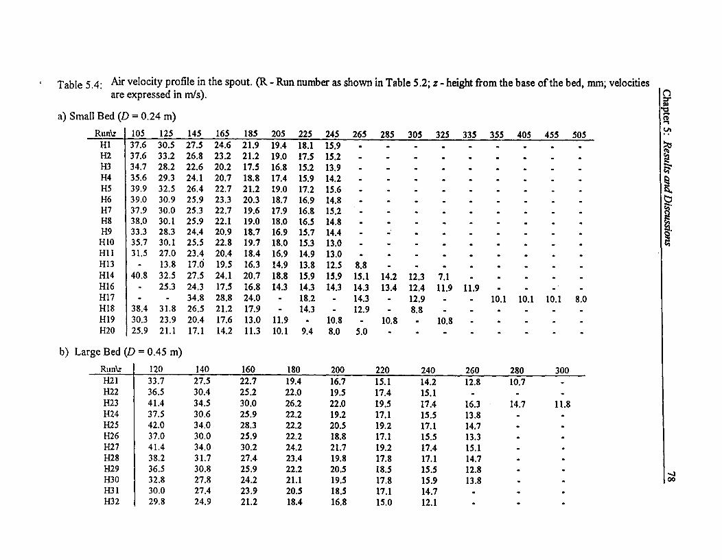
Table 5.4: Air velocity profile in the spout. (R - Run number as shown in Table 5.2; z - height from the base of the bed, mm; velocitiesare expressed in m/s).
a) Small Bed (DRun\z
= 0.24 m)105^125 145 165 185 205 225 245 265 285 305 325 335 355 405 455 505
HIH2H3H4H5H6H7H8H9
H 10H11H13H14H16H17H18H19H2O
37.637.634.735.639.939.037.938.033.335.731.5
40.8
38.430.325.9
30.533.228.229.332.530.930.030.128.330.127.013.832.525.3
31.823.921.1
27.526.822.624.126.425.925.325.924.425.523.417.027.524.334.826.520.417.1
24.623.220.220.722.723.322.722.120.922.820.419.524.117.528.821.217.614.2
21.921.217.518.821.220.319.619.018.719.718.416.320.716.824.017.913.011.3
19.419.016.817.419.018.717.918.016.918.016.914.918.814.3
11.910.1
18.117.515.215.917.216.916.816.515.715.314.913.815.914.318.214.3
9.4
15.915.213.914.215.614.815.214.814.413.013.012.515.914.3
10.88.0
8.815.114.314.312.9
5.0
14.213.4
10.8
12.312.412.98.8
7.111.9
10.8
1•■
11.9101
-
10.1 10.1 10.1
1E1
8.0
b) Large Bed (DRun':
= 0.45 m)120 140 160 180 200 220 240 260 280 300
H21H22H23H24H25H26H27H28H29H30H31H32
33.736.541.437.542.037.041.438.236.532.830.029.8
27.530.434.530.634.030.034.031.730.827.827.424.9
22.725.230.025.928.325.930.227.425.924.223.921.2
19.422.026.222.222.222.224.223.422.221.120.518.4
16.719.522.019.220.518.821.719.820.519.518.516.8
15.117.419.517.119.217.119.217.818.517.817.115.0
14.215.117.415.517.115.517.417.115.515.914.712.1
12.8-
16.313.814.713.315.114.712.813.8
-
-
10.7
14.7 11.8.1•
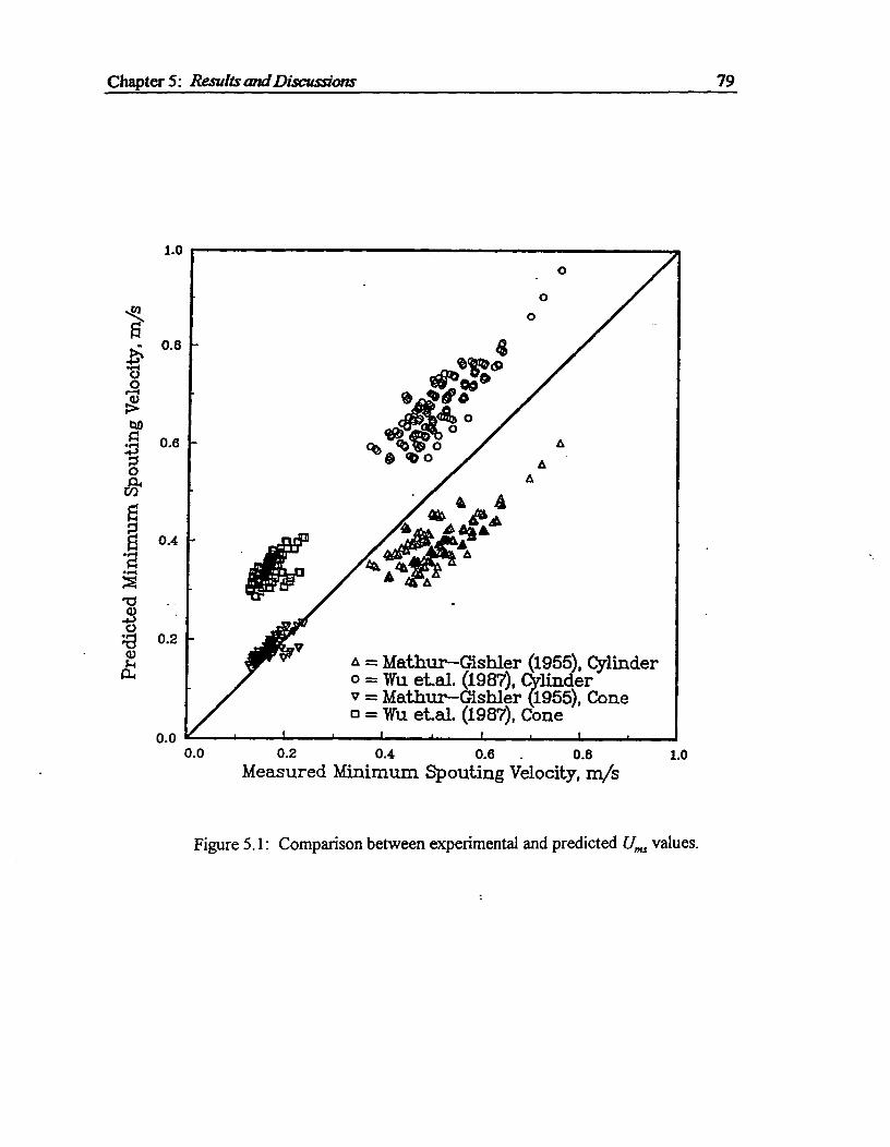
A = Mathur—Gishler (1955), Cylindero = Wu etal. (1987),Cylinderv = Mathur—Gishler (1955), Coneo . Wu et.al. (1987), Cone
t^.^1^.^,
Chapter 5: Results and Discussions^ 79
0.0^0.2^0.4^0.8^.^0.8^
1.0Measured Minimum Spouting Velocity, m/s
Figure 5.1: Comparison between experimental and predicted Ums values.
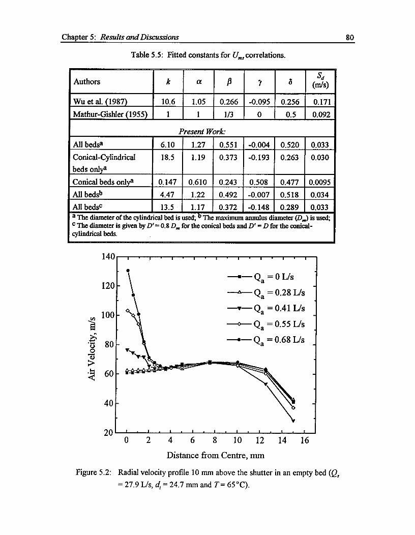
Q a = 0 L/s
Qa = 0.28 L/s
—v— Q a = 0.41 L/s
—0— Q a = 0.55 L/s
Qa = 0.68 L/s -
Chapter 5: Results and Discussions^ 80
Table 5.5: Fitted constants for (1„,1 correlations.
Authors k a 13 7 6Sd
(m/s)
Wu et al. (1987) 10.6 1.05 0.266 -0.095 0.256 0.171Mathur-Gishler (1955) 1 1 1/3 0 0.5 0.092
Present Work:All bedsa 6.10 1.27 0.551 -0.004 0.520 0.033Conical-Cylindricalbeds onlya
18.5 1.19 0.373 -0.193 0.263 0.030
Conical beds onlya 0.147 0.610 0.243 0.508 0.477 0.0095All bedsb 4.47 1.22 0.492 -0.007 0.518 0.034All bedsc 13.5 1.17 0.372 -0.148 0.289 0.033a The diameter of the cylindrical bed is used; b The maximum annulus diameter (D.) is used;c The diameter is given by D' = 0.8 D,„ for the conical beds and D' = D for the conical-cylindrical beds.
0^2^4^6^8^10^12^14^16Distance from Centre, mm
Figure 5.2: Radial velocity profile 10 mm above the shutter in an empty bed (Q.,= 27.9 L/s, cl,= 24.7 mm and T = 65°C).
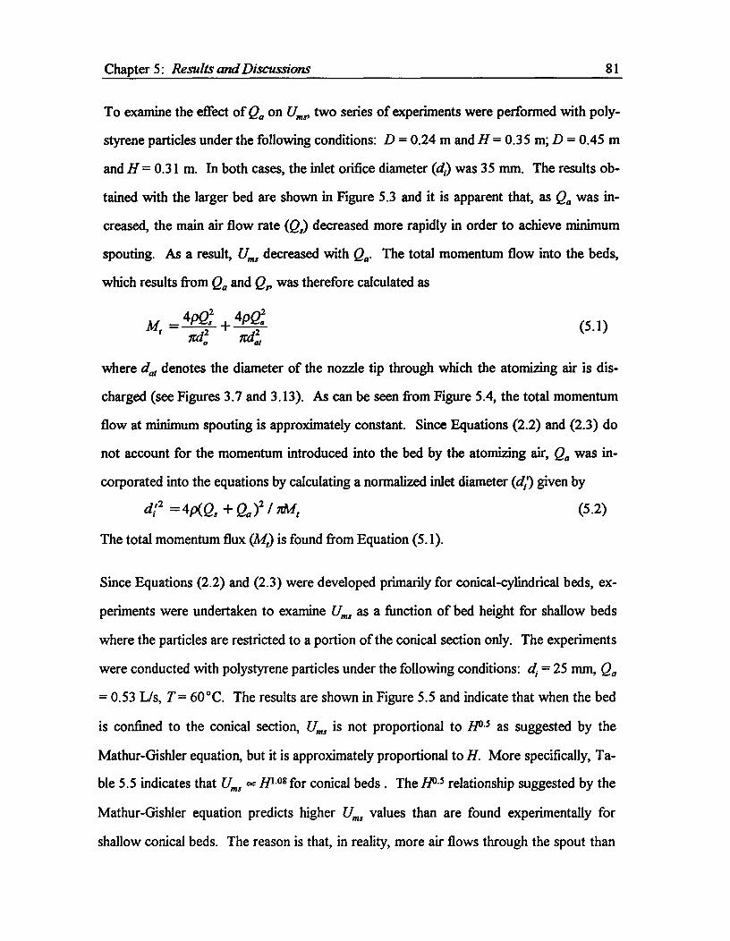
Chapter 5: Results and Discussions^ 81
To examine the effect of Q,, on U two series of experiments were performed with poly-
styrene particles under the following conditions: D = 0.24 m and H = 0.35 m; D = 0.45 m
and H = 0.31 m. In both cases, the inlet orifice diameter (d) was 35 mm. The results ob-
tained with the larger bed are shown in Figure 5.3 and it is apparent that, as Q. Was in-
creased, the main air flow rate (Q,) decreased more rapidly in order to achieve minimum
spouting. As a result, u,,,, decreased with Q.. The total momentum flow into the beds,
which results from Q. and Qs, was therefore calculated as
M — +4pQ2 4pQ2
74,^irdL(5.1)
where dal denotes the diameter of the nozzle tip through which the atomizing air is dis-
charged (see Figures 3.7 and 3.13). As can be seen from Figure 5.4, the total momentum
flow at minimum spouting is approximately constant. Since Equations (2.2) and (2.3) do
not account for the momentum introduced into the bed by the atomizing air, Q. was in-
corporated into the equations by calculating a normalized inlet diameter (d;) given by
= 4P(Qs Q0)2^ (5.2)
The total momentum flux (Mt) is found from Equation (5.1).
Since Equations (2.2) and (2.3) were developed primarily for conical-cylindrical beds, ex-
periments were undertaken to examine U., as a function of bed height for shallow beds
where the particles are restricted to a portion of the conical section only. The experiments
were conducted with polystyrene particles under the following conditions: d, = 25 mm, Qa
= 0.53 L/s, T = 60°C. The results are shown in Figure 5.5 and indicate that when the bed
is confined to the conical section, Ums is not proportional to I] as suggested by the
Mathur-Gishler equation, but it is approximately proportional to H. More specifically, Ta-
ble 5.5 indicates that U., oc HIM for conical beds . The 110 . 5 relationship suggested by the
Mathur-Gishler equation predicts higher U,,,, values than are found experimentally for
shallow conical beds. The reason is that, in reality, more air flows through the spout than

0.61
tz.tO
029
O
A A AA
A
A
A
A
0.65
Chapter 5: Results chid Discussions^820.63
0.0^02^OA^0.6^0.8Atomizing Air Flow Rate, LA
Figure 5.3: Effect of atomizing air on minimum spouting velocity (minimum spoutingvelocity is based only on the main spouting air flow rate; D = 0.45 rn, H =0.31 rn, di 35 mm).
0.9
LO
•
fir 0.8
D. .......^.. G .. ^-0....^ ..
^
...^.
Momentum Flow Due to Atomizing Air0= Momentum Flow Due to Spouting AirCl= Ibtal Momentum Flow
0.30
„NA
0.00.0 0.2^OA^0.6^0.8
Atomizing Air Flow Rate, LA1.0
Figure 5.4: Momentum flow of air into the spouted bed (dashed and solid lines representthe 0.24 m and 0.45 m dia. beds, respectively).
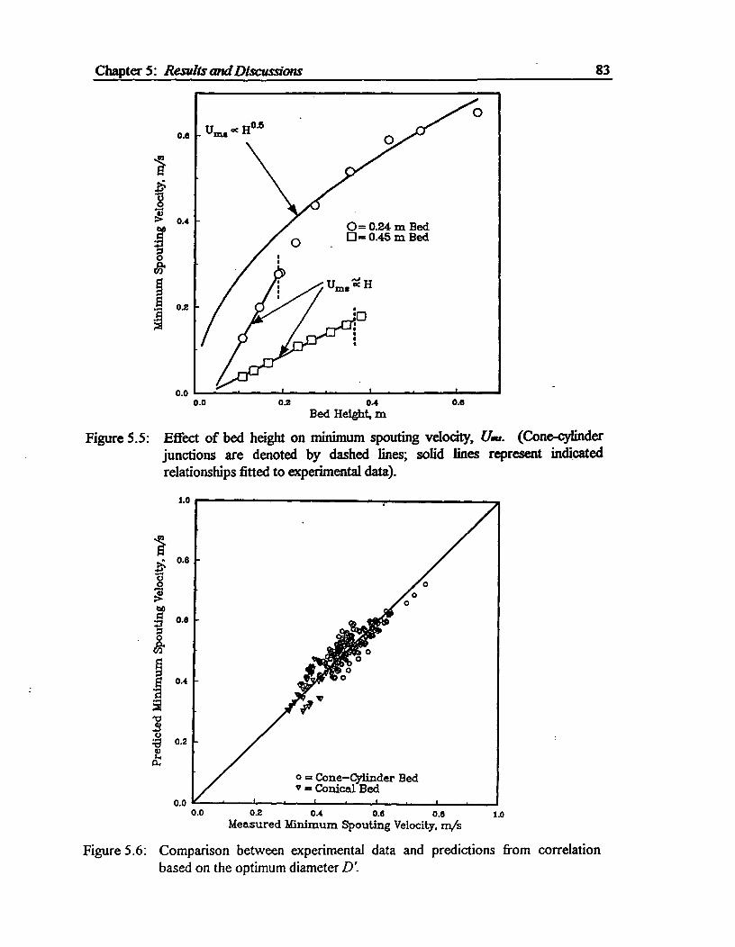
0.60.0^0.2^0.4Bed Height, m
0.6
0.0
Chapter 5: Results and Discussions^ 83
Figure 5.5: Effect of bed height on minimum spouting velocity, Um. (Cone-cylinderjunctions are denoted by dashed lines; solid lines represent indicatedrelationships fitted to experimental data).
1.0
a
U.S8ao
0.6
0.4
0.2Of.
0.00.0^02^0.4^0.6^0.6
Measured Minimum Spouting Velocity, m/s
Figure 5.6: Comparison between experimental data and predictions from correlationbased on the optimum diameter D'.
1.0

Chapter 5: Results and Discussions^ 84
implied by this equation because the inlet air is unable to spread into the annulus as effec-
tively since the annulus is smaller and the wall is closer to the centre of the bed.
Since the constants obtained for the Wu et al. equation are different in the case of conical
and conical-cylindrical beds, an attempt was made to unify the results by using the maxi-
mum bed diameter (Dm) covered by the particles. When the bed particles extend into the
cylindrical region of the spouted bed, this diameter corresponds to the cylinder diameter.
The coefficients resulting from the least squares fit are presented in Table 5.5.
Upon observing the solids movement in the conical beds, D. was suspected to be an inap-
propriate variable representing Urns. The bed particles near the wall on the surface of the
annulus were observed to move significantly slower than the particles near the centre of
the bed. These differences in particle velocities were much more pronounced in conical
beds than in conical-cylindrical beds. Consequently, the conical beds were suspected to
behave as conical-cylindrical beds with D < D..
To determine the "effective" bed diameter (D) representing U,„, for shallow, conical beds
the following relationship was considered:
D' = c D,,,^ (5.3)
The proportionality constant (c) was determined by obtaining the best fit between the ex-
perimental and predicted results. The optimum value of c was found to be 0.8 and the
corresponding coefficients in the Wu et al. equation are also given in Table 5.5. As shown
by Figures 5.1 and 5.6, the agreement between predicted and experimental results is im-
proved. The optimal, modified Wu et al. equation thus becomes:
d )117 ( ,f.372 ( ) -0(^
op _ 0m =13.5 /2-1 -^—
di^H •148^0.289Ul
^D'^D'^D'^0(5.4)
It is interesting to note that Equation (5.4) implies that Ums oc IP352 for deep beds. The
corresponding exponents of H for the equations of Wu et al. (1987) and Mathur and
Chapter 5: Results and Discussions^ 85
Gishler (1955) are 0.4 and 0.5, respectively. This result also supports the contention made
by Wu et al. that the H and p terms should not be combined as suggested by Mathur and
Gishler. For shallow conical beds where D' cc H, Equation (5.4) reduces to Q„,, (= 7t/4
-U',„,(D)2) cc H'196, i.e., the relationship is virtually linear. This agrees well with the ex-
perimental data shown in Figure 5.5 (note that Ums is based on the column diameter in this
figure; hence, Q,,, U„,^). The conical bed data also could be well represented by the
Wan-Fyong et al. (1969) equation, corrected for atomizing air (see Appendix I).
5.1.2. Axial Pressure Profile in Annulus
The axial pressure profiles near the spout-annulus interface are given in Table 5.3. The
temperature, atomizing air and spouting air flow rates did not have a significant effect on
the pressure profiles. Furthermore, the variations in the radial pressure profiles were small
for conical-cylindrical and conical beds (see, for example, Figure 5.7).
The axial pressure profiles for two beds are shown in Figures 5.8 and 5.9 together with
predictions based on the equations provided by Epstein-Levine (1980), Rovero et al.
(1983) (which is the Epstein-Levine equation modified for beds with a conical base), and
Morgan and Littman (1980). Limo Uh Udf,„ and H,„ in these equations were calculated
from the correlations given by Grace (1982), Clift et al. (1978), Epstein et al. (1978) and
McNab and Bridgwater (1977), respectively. The first two expressions under-predicted
the axial pressure profile whereas the Morgan-Littman equation gave fairly good agree-
ment in the case of conical-cylindrical beds (see Figure 5.8). By contrast, all three equa-
tions performed poorly for conical beds as shown by Figure 5.9. However, when the
equations are modified by using D' (see Equation (5.3)), the agreement is significantly im-
proved, especially in the case of the Morgan-Littman equation (see Figure 5.10).
Further examination of the Morgan-Littman correlation showed that for the deeper bed
(0.53 m) and changes in d,, the agreement was not as good. In general, the correlation

^ Near the Spout (Measured)O Radially Averaged (Measured)
Morgan-Littman (1980)^ Epstein-Levine (1978)--- Modified Epstein-Levine (Rovero et al., 1983)
8
^.... .. ......^0^. ^..
• .
Chapter 5: Results and Discussions^ 86
1.2
0.9
Height, m0 = 0270 = 0.22A ER 0.18+ = 0.14x = 0.10• = 0.08v = 0.06• = 0.04x = 0.02
^ VO 0
x X
+ +^x
A AA
O 0^0
rig^ n
0.3
0.0
0
m
0.00^
0.03^
0.08^0.09^
0.12Radius, m
Figure 5.7: Pressure profile in the annulus (conical bed, Run H22).
1.2
0.9
0.6
0.3
0.00.0^0.1^0.2^ 0.4
Height, mFigure 5.8: Axial pressure profile in the annulus near the spout-annulus interface
(conical-cylindrical bed, Run HI).
0.3

^ Near the Spout (Measured)O Radially Averaged (Measured)
Morgan—Littman (1980)^ Epstein—Levine (1978)---- Modified Epstein—Levine (Rovero et al.. 1983)
".."%-.....,„
...„.,,
......
r^. ... ' .Th""7,-.---•
..,,,
1.2
0.9
;Io
cl 0.6EV.,13t
0.3
0.0
^ Near the Spout (Measured)O Radially Averaged (Measured)
Morgan—Littman (1980)^ Epstein—Levine (1978)--- Modified Epstein—Levine (Rovero et aL, 1983)
•
■•
N.
1.1Am
•\
Chapter 5: Results and Discussions^ 87
0.0^
0.1^
0.2^
0.3^
0.4
Height, m
Figure 5.9: Axial pressure profile in the annulus (conical bed, Run H22, columndiameter used in calculation).
12
0.9
vi000
40 0.8
0.3
0.00.0^
0.1^
0.2^
0.3^
0.4
Height. m
Figure 5.10: Axial pressure profile in the annulus (conical bed, Run H22, D' used incalculation).

1.5
0.0' 0.1^0.2^0.3Height, xn
0.4 0.5
^ Near the Spout (Measured)0 Radially Averaged (Measured)
— Morgan—Littman (1980)^ Epstein—Levine (1978)
La
1.2
• ...............
0.6
0.9
0.0
0.9
Chapter 5: Results and Discussions^ 88
Figure 5.11: Axial pressure profile in the annulus (H = 0.53, Run H17).
0.00^
0.03^
0.06^0.09^0.12^0.15^0 18Radius, m
Figure 5.12: Comparison between measured and predicted pressure profile in the annulus.
Chapter 5: Results and Discussions^ 89
over-estimated the pressure drop in the 0.53 m bed (see Figure 5.11), and under-estimated
the effect of di. In an attempt to improve the predictions, the optimal constants in Equa-
tion (2.14) for the 0.24 m bed data were determined by a least squares technique. Al-
though the optimal constants improved the agreement for deeper beds, the predictions for
the shallower beds were somewhat impaired.
5.1.3. Velocity Profile in Annulus
The radial pressure variation in the annulus was found to be small (see Figure 5.7). How-
ever, even small pressure gradients can lead to significant changes in the air flow rate in
the annulus. If no radial variation of pressure is assumed and the Morgan-Littman correla-
tion is used, significant errors in the air flow rate result. This result is due to the larger
flow area away from the centre of the bed. For this reason, the vector Ergun (1952) equa-
tion is solved to determine the fluid flow in the annulus.
The solution of the vector Ergun equation for Run H22 is shown in Figure 5.12 and the
method of solution is given in Appendix I. The model predictions, in general, were in
good agreement with the measured values. Moreover, significant improvement to the
spout velocity predictions was observed when the fluid flow in the annulus is calculated
using the vector Ergun equation rather than the one-dimensional equation.
5.1.4. Axial Velocity Profile in Spout
The measured spout velocity profiles are given in Table 5.4. The effect of atomizing air
flow on us is significant and is particularly noticeable in the lower section of the bed as
shown by Figure 5.13. The total spouting air flow exhibits a similar effect on U. Changes
in bed height did not greatly influence the velocity profile in the spout.
The spout velocities predicted by the mass and momentum balance equations (Lefroy and
Davidson, 1969) introduced in Chapter 4 represented the measured velocities well (e.g.,
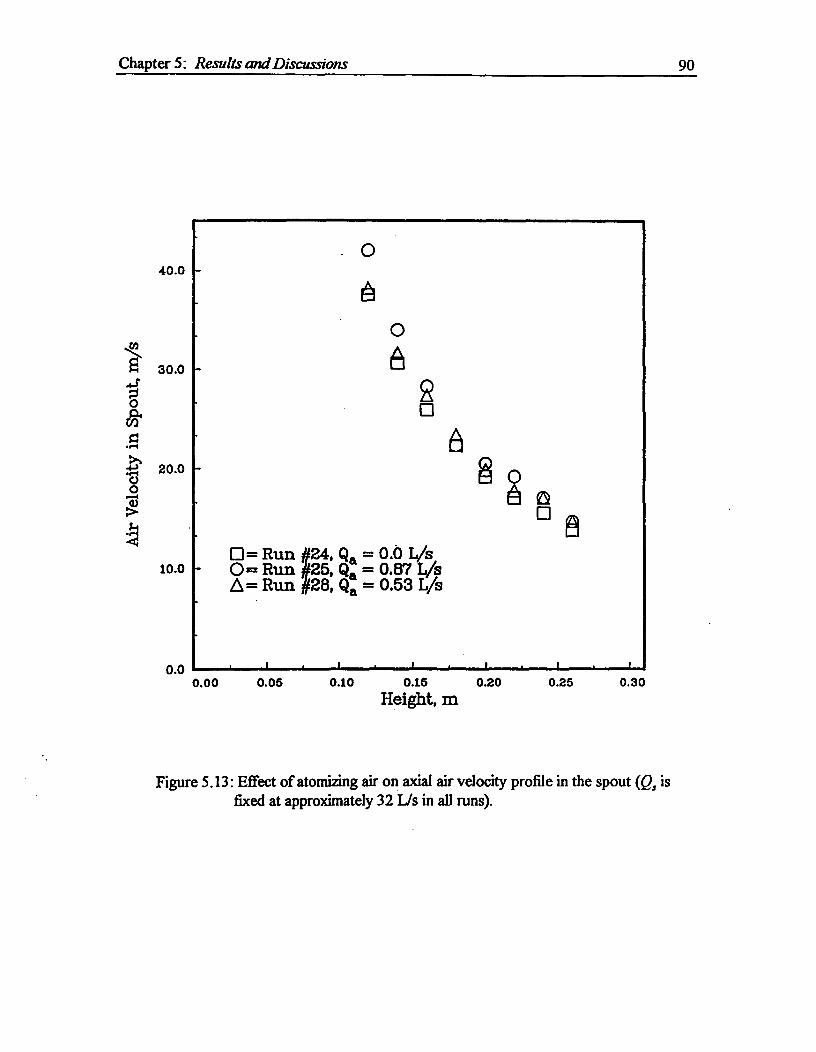
0
0
20
0= Run 24, Qa = 0.0 L/s- 0= Run 25, Qa = 0.87 LA
A= Run 28, Qa = 0.53 L/s
40.0
10.0
0.00.00^0.05^0.10^0.15^0.20
Height, m0.25 0.30
Chapter 5: Results and Discussions^ 90
Figure 5.13: Effect of atomizing air on axial air velocity profile in the spout (Q, isfixed at approximately 32 Us in all runs).
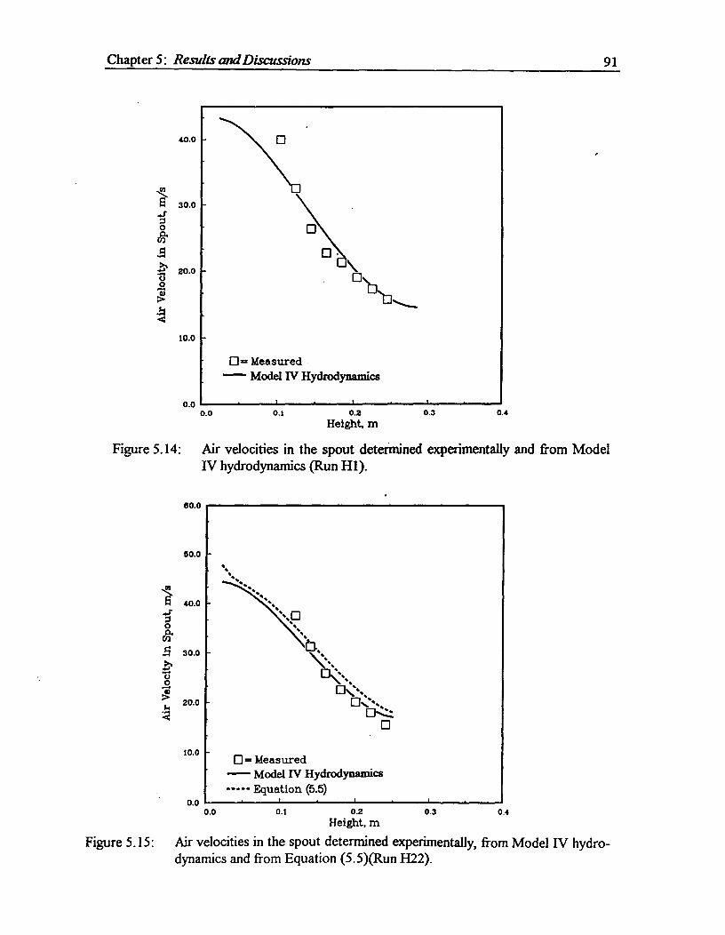
Chapter 5: Results and Discussions^ 91
40.0
0<t30.0
...rO
48 20.00
71;
10.0
0.00.0^0.1^
0.2^0.3
^0.4
Height, m
Figure 5.14: Air velocities in the spout determined experimentally and from ModelIV hydrodynamics (Run H1).
80.0
50.0
40.0
4..r0
90.0
0
20.0
10.0
0.0
^= Measured— Model IV Hydrodynamics^ Equation (5.5)
Figure 5.15:
0.0^0.1^0.2^
0.3^
0.4Height, m
Air velocities in the spout determined experimentally, from Model IV hydro-dynamics and from Equation (5.5)(Run H22).
Chapter 5: Results and Discussions^ 92
see Figures 5.14 and 5.15) if the aforementioned modified equations were used. The cor-
relations and assumptions used in the mass and momentum balance equations included:
• The spout diameter is constant and is given by the Wu et al. correlation (1987);
• The pressure profile is given by the Morgan-Littman (1980) equation modified for
conical beds and effective bed diameter D;
• The air flow rate in the annulus is given by the vector Ergun (1952) equation;
• The fluid-particle interaction term proposed by Richardson and Zaki (1954) is valid;
• The spouting air flow rate is calculated from the total momentum flux into the bed
rather than the total flow rate,
• The air density is based on the initial spouting air temperature rather than the average
bed temperature.
A sensitivity analysis for these variables showed that the strongest factor influencing the
agreement between the velocity predictions and measurements was the correlation used to
predict the pressure profile; good agreement with the velocity measurements was observed
when the difference between the predicted and measured pressures was small.
Figures 5.14 and 5.15 show more pronounced deviations between the measured and pre-
dicted velocities near the base of the bed. Regardless of the presence of the atomizing air,
the measured velocity was expected to be higher than the predicted (i.e., average) velocity
since the measurements were based on the highest pressure difference indicated by the pi-
tot tube (which corresponds to the highest velocity). The large discrepancy near the inlet
may be the result of a large radial velocity gradient in the spout (Krzywanski, 1992; Abra-
movich, 1963).
Moreover, the velocity profiles shown in Figures 5.2 and 5.13 suggest considerable influ-
ence of the atomizing air on the radial velocity profiles, especially near the base of the bed.
In an attempt to model the atomizing air velocity, the following equations were developed,
Chapter 5: Results and Discussions^ 93
based on the assumptions that no mixing between the atomizing jet and spouting air oc-
curred and that the solids voidage remained the same as the average voidage in the spout:
d(etuasAadz =0^
(5.5)
where A., =irD1 / 4^
(5.6)
and^dD as I dz =kik. a lAluasi -flud)^
(5.7)
Equation (5.7) is given in Abramovich (1963). Das represents the spread of the jet bound-
ary layer and ke represents the fully developed jet angle in still air. Using the spray angle
(k8) value of 20°, Equation (5.5) was solved together with Equations (4.27) to (4.30).
The results are presented in Figure 5.15 and show that the atomizing air velocity changes
rapidly to a value slightly higher than the spouting air velocity a short distance away from
the base of the bed. Above this height, the atomizing air velocity changes at the same rate
as the spouting air velocity. This result is most likely due to the assumption that no mix-
ing occurs across the jet boundary layer. In reality, mixing across the atomizing air jet
boundary should occur (Rushton and Oldshue, 1953; Abramovich, 1963) especially with
the entrainment of solids into the spout, and consequently, the boundary should quickly
disappear. To model the atomizing air velocity in the spout appropriately, a means of es-
timating the mixing length should be devised; however, this task was beyond the scope of
this thesis and is pursued no further.
Other explanations for the discrepancy in the measured and predicted velocities near the
base of the bed include the constant spout diameter assumption and the inability to predict
the pressure peak by the Morgan-Littman correlation. Most spout shapes quickly diverge
to a constant spout diameter (Lim, 1978); therefore, the gas velocities in the lower spout
region will be higher than if a constant spout diameter is assumed. In most of the pressure
measurements (see Table 5.3), a pressure peak occurred near the base of the bed and none
of the correlations given in the literature predicts such behavior. It is very likely that the
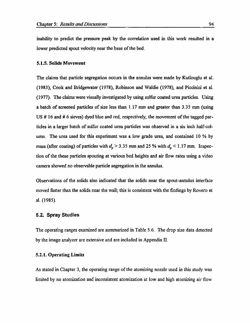
Chapter 5: Results and Discussions^ 94
inability to predict the pressure peak by the correlation used in this work resulted in a
lower predicted spout velocity near the base of the bed.
5.1.5. Solids Movement
The claims that particle segregation occurs in the annulus were made by Kutlouglu et al.
(1983), Cook and Bridgewater (1978), Robinson and Waldie (1978), and Piccinini et al.
(1977). The claims were visually investigated by using sulfur coated urea particles. Using
a batch of screened particles of size less than 1.17 mm and greater than 3.35 mm (using
US # 16 and # 6 sieves) dyed blue and red, respectively, the movement of the tagged par-
ticles in a larger batch of sulfur coated urea particles was observed in a six inch half-col-
umn. The urea used for this experiment was a low grade urea, and contained 10 % by
mass (after coating) of particles with dp > 3.35 mm and 25 % with dp < 1.17 mm. Inspec-
tion of the these particles spouting at various bed heights and air flow rates using a video
camera showed no observable particle segregation in the annulus.
Observations of the solids also indicated that the solids near the spout-annulus interface
moved faster than the solids near the wall; this is consistent with the findings by Rovero et
al. (1985).
5.2. Spray Studies
The operating ranges examined are summarized in Table 5.6. The drop size data detected
by the image analyzer are extensive and are included in Appendix II.
5.2.1. Operating Limits
As stated in Chapter 3, the operating range of the atomizing nozzle used in this study was
limited by no atomization and inconsistent atomization at low and high atomizing air flow
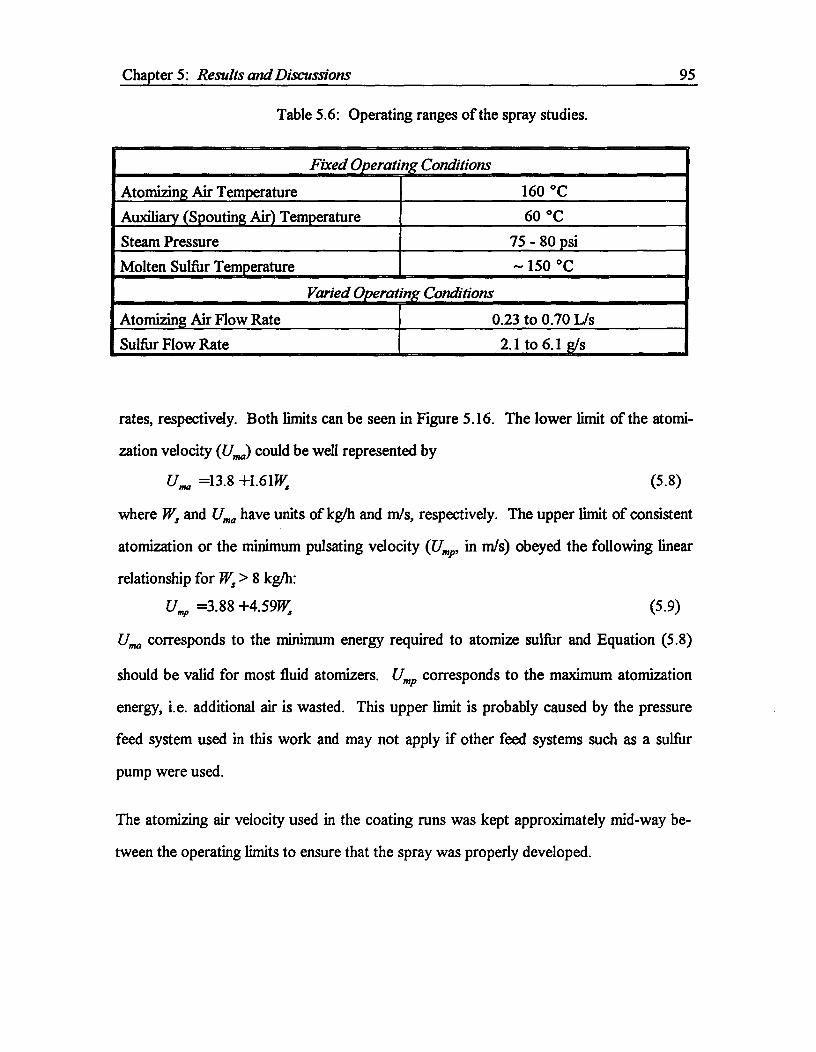
Chapter 5: Results and Discussions^ 95
Table 5.6: Operating ranges of the spray studies.
Fixed Operating Conditions
Atomizing Air Temperature 160 °CAuxiliary (Spouting Air) Temperature 60 °CSteam Pressure 75 - 80 psiMolten Sulfur Temperature — 150 °C
Varied Operating ConditionsAtomizing Air Flow Rate 0.23 to 0.70 L/sSulfur Flow Rate 2.1 to 6.1 g/s
rates, respectively. Both limits can be seen in Figure 5.16. The lower limit of the atomi-
zation velocity (U.) could be well represented by
U. =13.8 +1.61W,^ (5.8)
where Ws and U. have units of kg/h and m/s, respectively. The upper limit of consistent
atomization or the minimum pulsating velocity (U„,p, in m/s) obeyed the following linear
relationship for Ws > 8 kg/h:
U„,,, =3.88 +4.59W,^ (5.9)
U corresponds to the minimum energy required to atomize sulfur and Equation (5.8)
should be valid for most fluid atomizers. Ump corresponds to the maximum atomization
energy, i.e. additional air is wasted. This upper limit is probably caused by the pressure
feed system used in this work and may not apply if other feed systems such as a sulfur
pump were used.
The atomizing air velocity used in the coating runs was kept approximately mid-way be-
tween the operating limits to ensure that the spray was properly developed.
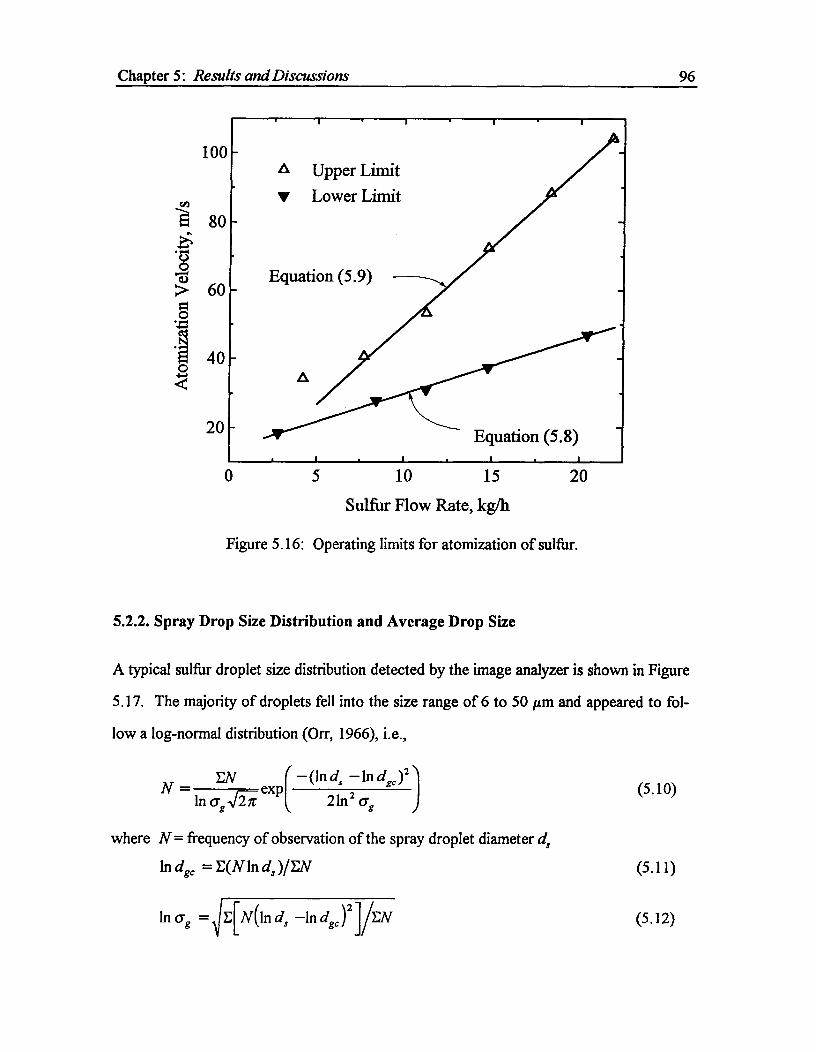
0 5^10^15Sulfur Flow Rate, kg/h
20
Chapter 5: Results and Discussions
100
96
20
N — EN ^(— (ln d s —lnd gc )2 )In ag -Ji exP^21n2 crg
(5.10)
Figure 5.16: Operating limits for atomization of sulfur.
5.2.2. Spray Drop Size Distribution and Average Drop Size
A typical sulfur droplet size distribution detected by the image analyzer is shown in Figure
5.17. The majority of droplets fell into the size range of 6 to 50 Am and appeared to fol-
low a log-normal distribution (On, 1966), i.e.,
where N= frequency of observation of the spray droplet diameter d,
ln dg, = E(Nln ds WEN^ (5.11)
\ 2In ag = 1,1E[N(ln ds —ln dgc ) YEW^ (5.12)

Chapter 5: Results and Discussions
60
50
20
40
30
10
0
97
0^20^40^60^80^
100Spray Drop Size, m
Figure 5.17: Experimental drop size distribution and predictions using log-normal equation (Run S la).
A log-normal plot is shown in Figure 5.18. The Nukiyama-Tanasawa distribution (Lewis
et al., 1948) gave a good representation of the larger drop sizes (see Figure 5.19), but
failed for the range 6 to 50 Am where the ,highest frequencies of drops were recorded.
The Nukiyama-Tanasawa equation is given by
In ^d2
— lnk1 - k2",Ad (5.13)
where Ads denotes the diameter range of the N droplets. The log-normal distribution was
therefore used to represent the drop size data, and the mean drop size and the deviation
were calculated from Equations (5.11) to (5.12), respectively.
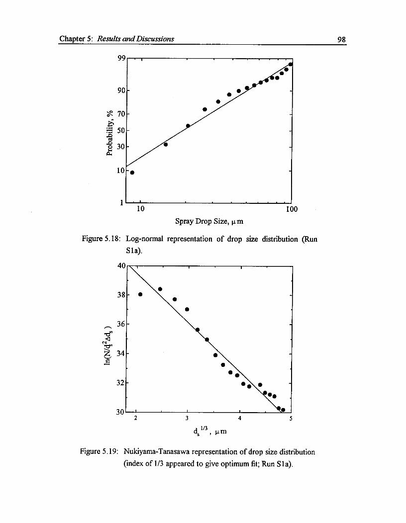
Chapter 5: Results and Discussions^ 98
10 100Spray Drop Size, i.tm
Figure 5.18: Log-normal representation of drop size distribution (RunSla).
Figure 5.19: Nukiyama-Tanasawa representation of drop size distribution(index of 1/3 appeared to give optimum fit; Run Sla).
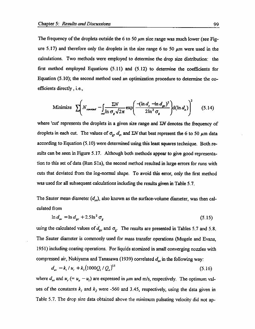
Chapter 5: Results and Discussions^ 99
The frequency of the droplets outside the 6 to 50 Am size range was much lower (see Fig-
ure 5.17) and therefore only the droplets in the size range 6 to 50 gm were used in the
calculations. Two methods were employed to determine the drop size distribution: the
first method employed Equations (5.11) and (5.12) to determine the coefficients for
Equation (5.10); the second method used an optimization procedure to determine the co-
efficients directly , i.e.,
Minimize E N.„,„ted
2r EN^-(ln d, —ln c/102
6g1/2 exP^21n2 a^)4111d8)(5.14)
where 'cut' represents the droplets in a given size range and EtV denotes the frequency of
droplets in each cut. The values of ag, and EN that best represent the 6 to 50 gm data
according to Equation (5.10) were determined using this least squares technique. Both re-
sults can be seen in Figure 5.17. Although both methods appear to give good representa-
tion to this set of data (Run S la), the second method resulted in large errors for runs with
cuts that deviated from the log-normal shape. To avoid this error, only the first method
was used for all subsequent calculations including the results given in Table 5.7.
The Sauter mean diameter (d,), also known as the surface-volume diameter, was then cal-
culated from
Inds, =In dgc + 2.51n 2 ag (5.15)
using the calculated values of dgc and ag. The results are presented in Tables 5.7 and 5.8.
The Sauter diameter is commonly used for mass transfer operations (Mugele and Evans,
1951) including coating operations. For liquids atomized in small converging nozzles with
compressed air, Nukiyama and Tanasawa (1939) correlated d, in the following way:
dn, = k, I u, + k2 (1000a / 0 13^(5.16)
where d, and u, (= u„ — ui ) are expressed in gm and m/s, respectively. The optimum val-
ues of the constants k and k2 were -560 and 3.45, respectively, using the data given in
Table 5.7. The drop size data obtained above the minimum pulsating velocity did not ap-
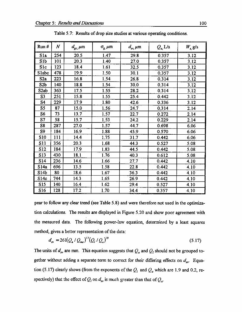
Chapter 5: Results cmd Discussions^ 100
Table 5.7: Results of drop size studies at various operating conditions.
Run # N dga, µm 6& µmp. 41m Qa, Lis Ws g/s
Sla 254 20.5 1.47 29.8 0.357 3.12S lb 101 20.3 1.40 27.0 0.357 3.12S lc 123 18.4 1.61 32.5 0.357 3.12
Slabc 478 19.9 1.50 30.1 0.357 3.12S2a 223 16.8 1.54 26.8 0.314 3.12S2b 140 18.8 1.54 30.0 0.314 3.12S2ab 363 17.5 1.55 28.2 0.314 3.12S3 251 15.8 1.55 25.4 0.442 3.12S4 229 17.9 1.80 42.6 0.336 3.12S5 87 15.0 1.56 24.7 0.314 2.14S6 73 13.7 1.57 22.7 0.272 2.14S7 58 15.7 1.53 24.2 0.229 2.14S8 287 27.0 1.57 44.7 0.698 6.06S9 184 16.9 1.88 45.9 0.570 6.06
S10 111 14.4 1.75 31.7 0.442 6.06Sli 356 20.3 1.68 44.3 0.527 5.08S12 184 17.9 1.83 44.5 0.442 5.08S13 430 18.1 1.76 40.3 0.612 5.08S14 236 14.6 1.66 27.7 0.442 4.10
S14a 696 13.5 1.58 22.8 0.442 4.10S14b 80 18.6 1.67 36.3 0.442 4.10S14c 744 14.3 1.65 26.9 0.442 4.10S15 140 16.4 1.62 29.4 0.527 4.10S16 128 17.2 1.70 34.4 0.357 4.10
pear to follow any clear trend (see Table 5.8) and were therefore not used in the optimiza-
tion calculations. The results are displayed in Figure 5.20 and show poor agreement with
the measured data. The following power-law equation, determined by a least squares
method, gives a better representation of the data:
=261(a, /Q.) ,7(a /09
(5.17)
The units of d,„ are mm. This equation suggests that Qa and Q1 should not be grouped to-
gether without adding a separate term to correct for their differing effects on d„. Equa-
tion (5.17) clearly shows (from the exponents of the Q1 and Qa which are 1.9 and 0.2, re-
spectively) that the effect of Q l on d5 is much greater than that of Qa .

50
45
N
0 35
4:: 25
20
20^25^30^35^40 5045
Chapter 5: Results and Discussions^ 101
Table 5.8: Sauter mean diameters relative to the operating limits.
Near middle ofoperating limits
Near pulsatingpoint
Above pulsat-ing point
Ws, g/s
Q„, Us 0.229 0.272 0.315 2.14d,„, pm 24.7 22.7 24.7CI, Us 0.315 0.357 0.442 3.12cinn Am 30.0 29.8 25.4Q, Us 0.360 0.442 0.527 4.10c/3„, Am 34.4 27.7 29.4Q, Us 0.442 0.527 0.612 5.08d„, Am 44.5 44.3 40.3Q,Us 0.442 0.57 -- 6.06d„, Am 45.9 44.7 --
Measured Drop Size, p, m
Figure 5.20: Predictions of Sauter mean diameter.
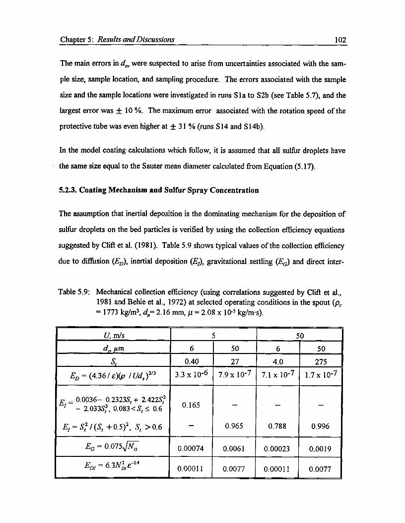
Chapter 5: Results and Discussions^ 102
The main errors in d, were suspected to arise from uncertainties associated with the sam-
ple size, sample location, and sampling procedure. The errors associated with the sample
size and the sample locations were investigated in runs S la to S2b (see Table 5.7), and the
largest error was + 10 %. The maximum error associated with the rotation speed of the
protective tube was even higher at + 31 % (runs S 14 and S 14b).
In the model coating calculations which follow, it is assumed that all sulfur droplets have
the same size equal to the Sauter mean diameter calculated from Equation (5.17).
5.2.3. Coating Mechanism and Sulfur Spray Concentration
The assumption that inertial deposition is the dominating mechanism for the deposition of
sulfur droplets on the bed particles is verified by using the collection efficiency equations
suggested by Clift et al. (1981). Table 5.9 shows typical values of the collection efficiency
due to diffusion (ED), inertial deposition (E), gravitational settling (EG) and direct inter-
Table 5.9: Mechanical collection efficiency (using correlations suggested by Clift et al.,1981 and Behie et al., 1972) at selected operating conditions in the spout (pc
= 1773 kg/m3, cln= 2.16 mm, = 2.08 x 10⁻⁵ kg/m•s).
U, m/s 5 50clx, Am 6 50 6 50
St 0.40 27 4.0 275
ED = (4.36/ e)(p /Ws )" 3.3 x 10⁻⁶ 7.9 x 10⁻⁷ 7.1 x 10⁻⁷ 1.7 x 10⁻⁷
_ 0.0036— 0.2323St + 2.422St2El —
— 2.0334, 0.083< St^0.6
Ei = SS / (St +0.5)2 , St >0.6
0.165
—
—
0.965
—
0.788
—
0.996
0.00074 0.0061 0.00023 0.0019EG = 0.075[NG
EDI = 6.3NijI E-2 4 0.00011 0.0077 0.00011 0.0077

Chapter 5: Results and Discussions^ 103
ception (ED/) at selected operating conditions. The values of the air velocity (U) and the
droplet size (d1) given in Table 5.9 are close to the operating conditions in the spout. The
results clearly indicate that inertial deposition is the dominating collection mechanism
under the present coating conditions.
The collection efficiency alone, however, is not sufficient to calculate the sulfur droplet
deposition rate onto bed particles; information on the spray distribution above the nozzle
is required also. Consequently, experiments were attempted to determine the spray distri-
bution; however, a suitable device for detecting the sulfur concentration in the bed could
not be developed. A sampler without a heated tip could not deal with the molten sulfur
spray, which plugged up the tip of the sampler. Consequently, efforts were made to heat
the tip electrically (to oxidize the sulfur) with NiCr wires wrapped around the tip. Unfor-
tunately, the wires only lasted a few seconds in the bed because they could not withstand
collisions with the fast moving bed particles and the presence of urea dust which left car-
bon residue on wires. Internal heating of the tip was not possible due to space limitations
of the sampler (i.e., the sampler had to be small enough to be placed in the spout without
significantly upsetting the upstream flow). The details of the samplers which were tested
in this work are provided in Appendix I.
Since the spray distribution could not be measured directly, the assumptions concerning
the spray angle (see Chapter 4) and the height (hfds) at which the sulfur droplets start to
deposit onto the bed particles could not be verified. However, the angle and height could
be deduced from the particle coating distribution, which is the topic of the next section.
The predicted sulfur concentration profiles for various spray angles for Run C 17 are
shown in Figure 5.21; corresponding values for various coating runs using a spray angle of
20° are shown in Figure 5.22. The operating conditions for the runs shown in Figures
5.21 and 5.22 are given in Table 5.11. Decreasing spout velocity causes the initial in-
crease in the sulfur concentration until z = hfch. Note that in Figure 5.21, the spray angle
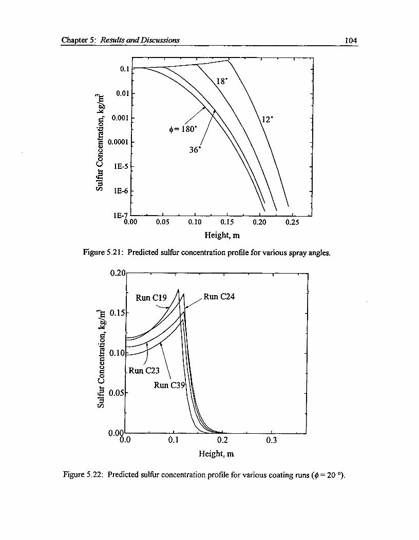
Chapter 5: Results and Discussions^ 104
0. 1
0.01
e 0.0010•4g- 0.0001c.)O
C.)^1E-5
1E-6
1E-70.00^
0.05^0.10^0.15^0.20^0.25Height, m
Figure 5.21: Predicted sulfur concentration profile for various spray angles.
Figure 5.22: Predicted sulfur concentration profile for various coating runs Op = 20 °).
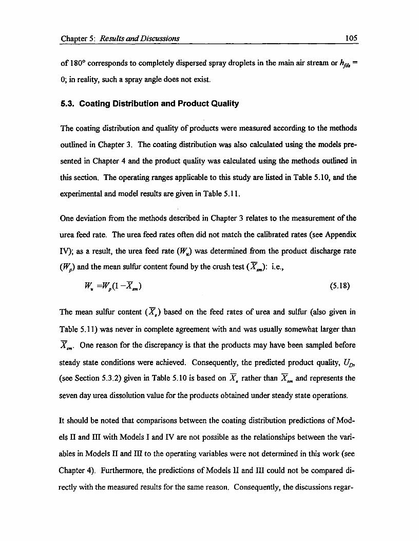
Chapter 5: Results and Discussions^ 105
of 180° corresponds to completely dispersed spray droplets in the main air stream or hid, =
0; in reality, such a spray angle does not exist.
5.3. Coating Distribution and Product Quality
The coating distribution and quality of products were measured according to the methods
outlined in Chapter 3. The coating distribution was also calculated using the models pre-
sented in Chapter 4 and the product quality was calculated using the methods outlined in
this section. The operating ranges applicable to this study are listed in Table 5.10, and the
experimental and model results are given in Table 5.11.
One deviation from the methods described in Chapter 3 relates to the measurement of the
urea feed rate. The urea feed rates often did not match the calibrated rates (see Appendix
IV); as a result, the urea feed rate (W.) was determined from the product discharge rate
(W ) and the mean sulfur content found by the crush test (X ): i.e.,
wi, =Typ o -,Y (5.18)
The mean sulfur content (X,) based on the feed rates of urea and sulfur (also given in
Table 5.11) was never in complete agreement with and was usually somewhat larger than
Xs„,. One reason for the discrepancy is that the products may have been sampled before
steady state conditions were achieved. Consequently, the predicted product quality, UD,
(see Section 5.3.2) given in Table 5.10 is based on X, rather than X and represents the
seven day urea dissolution value for the products obtained under steady state operations.
It should be noted that comparisons between the coating distribution predictions of Mod-
els II and HI with Models I and IV are not possible as the relationships between the vari-
ables in Models II and III to the operating variables were not determined in this work (see
Chapter 4). Furthermore, the predictions of Models II and III could not be compared di-
rectly with the measured results for the same reason. Consequently, the discussions regar-

Chapter 5: Results and Discussions^ 106
Table 5.10: Operating range applicable to coating distribution and product quality studies.
Operating Variable Operating RangeSpouting air flow rate, Q, 20.1 - 29.2 L/sAtomizing air flow rate, Q, 0.23 - 0.78 L/sBed Height, H 0.28 - 0.36 mBed Diameter, D 0.24 and 0.45 mSpouting air orifice diameter, cl, 24.7 - 35.1 mmUrea feed rate, W„ 7.6 - 19.9 g/sSulfur injection rate, K. 3.12 - 6.06 g/sBed Temperature, T h 57 - 64 °C
Table 5.11: Operating conditions investigated for the coating study.
Run#
D.(mm)
Qs
mss)Qa
(Us)
Ws
(g/s)W.
Ws)Ti,
(°C)D
(m)H
(m)X.%
up.%
-x-,%
U D%
C17 24.7 21.1 0.44 4.1 8.6 57 0.24 0.28 25.9 50.7 32.3 42.2C19 24.7 21.1 0A4 4.1 5.65 57 0.24 0.28 32.6 37.5 42.1 32.8C20 24.7 21.1 0.44 4.1 14.6 57 0.24 0.28 23.0 64.2 21.9 59.4C21 24.7 21.1 0.44 4.1 19.9 57 0.24 0.28 17.1 69.2 17.1 70.0C22 24.7 22.8 0.23 5.08 10.1 63 0.24 0.28 30.0 52.3 33.3 41.9C23 24.7 24.5 0.44 5.08 8.75 64 0.24 0.28 32.7 44.1 36.8 38.5C24 24.7 22.8 0.57 5.08 10.1 64 0.24 0.28 28.0 40.6 33.4 41.6C25 24.7 20.1 0.44 4.1 9.91 64 0.24 0.28 26.1 48.2 29.3 46.8C26 24.7 22.8 0.44 4.1 9.73 64 0.24 0.28 23.1 46.3 29.7 46.6C29 28.2 24.5 0.44 4.1 9.92 64 0.24 0.28 22.5 51.0 29.3 47.7C30 35.1 29.2 0.44 4.1 10.5 64 0.24 0.28 21.8 74.6 28.2 n/sC31 24.7 21.1 0.23 3.12 9.43 60 0.24 0.28 21.1 64.7 24.9 54.0C33 24.7 21.1 0.53 6.06 11.3 60 0.24 0.28 24.5 38.0 34.9 39.2C38 24.7 22.8 0.44 4.1 11.7 60 0.24 0.36 23.2 51.5 25.9 52.3C39 24.7 27.6 0.44 4.1 7.6 64 0.45 0.355 17.6 49.9 35.1 n/sC40 24.7 27.6 0.78 6.06 11.1 64 0.45 _0.355, 15.3, 72.4 35.3 n/s

Chapter 5: Results and Discussions^ 107
ding Models II and III results are mostly confined to a sensitivity analysis of the model
variables.
5.3.1. Coating Distribution
Forty sulfur coated urea particles were randomly sampled and the sulfur content of the in-
dividual particles were determined using the particle crush test described in Chapter 3.
The sulfur content (Xspj ) was then normalized according to
(X sp,i)new Xap,iXsp I —Ism^ (5.19)
where Ysi, is the average sulfur content of the 40 particles sampled. The results can be
seen in Figures 5.23 and 5.24 for Runs C17 and C38, respectively; the results for other se-
lected runs are provided in Appendix II.
As shown by Figure 5.24, Model IV with the spray angle (0) of 20° and Model I appear to
give good predictions of the measured sulfur content distributions. Both models, how-
ever, under-predicted the amount of the inadequately coated particles (i.e., Xs < 10 %).
This result was expected for Model I as discussed already in Chapter 4. In case of Model
IV, the size of the actual spray zone was suspected to be lower than that predicted, which
meant that the actual spray angle was larger or that coating occurred below the assumed
hfds. It is unlikely that the spray angle is larger than the angle provided by the manufac-
turer (0 = 20°) as the angle should decrease in the presence of spouting air (see Equation
(5.5)). Therefore, hfd, was suspected to be incorrect.
Consequently, the effect of hfd, was investigated by examining the coating distribution of
batch products. The batch products were used because the effects of the feed location and
exit probability are absent, and the influence of hos can be isolated. Figure 5.25 shows the
coating distributions for the batch products coated for 210 and 480 s under the following
conditions: TV., 3.5 g/s, H 0.3 m, D = 0.24 m, T --tr, 60 °C and di = 28.2 mm.

Chapter 5: Results and Discussions^ 108
20^40^
60Sulfur Content, %
Figure 5.23: Comparison between measured and predicted coating distributions for RunC17.
99
4::
0 6020^40Sulfur Content, %
Figure 5.24: Comparison between measured and predicted coating distributions for RunC38.

99
90
70
k 50cts2 30
gi;
10Operating time = 210 sOperating time = 480 s
Model IV,(hfds)new=a5(11fds).= 20° ""
Chapter 5: Results and Discussions^ 109
10^20^30^
40^
50
Sulfur Content, %
Figure 5.25: Coating distributions of batch products.
Again, the model under-predicted the amount of inadequately coated particles but, when
(hfds)new = ° •50fd4-20° was used, the predictions improved considerably. The physical ex-
planation for this result (assuming the spray angle is fixed at 20°) is that the bed particles
start to be coated at a height which is approximately half of the distance at which the spray
reaches the spout-annulus interface. Significant improvements were also noted for the
continuous data in both Figure 5.24 when these new hfdi values were used in the calcula-
tions.
The discrepancy between the measured and predicted distributions may be attributed to
uncertainties in the measurements of the sulfur flow rate, urea feed rate, and individual
particle sulfur content. The error in the sulfur flow rate is typically ± 1 scale reading on
the sulfur rotameter which amounts to less than ± 5 % error in the flow rate. The error in

Chapter 5: Results and Discussions^ 110
the urea feed rate using Equation (5.18) is less than ± 9 %. The largest error contributing
to the coating distribution is probably the sulfur content measurements of individual parti-
cles (see Chapter 3); the error was as large as + 25 % in determining the urea content of
individual particles. The errors in the measurements of X,A, and Upm amounted to less
than 3 %.
The discrepancies between the measured and predicted distributions shown in Figures 5.23
to 5.25 fall within the maximum measurement errors; however, consistently lower values
of r compared to ri in Table 5.11 suggest that other errors may be involved. Other
errors were suspected to result from the small sample sizes used to measure the coating
distribution and from sampling beds operating under unsteady state conditions. These
matters are further investigated in Section 5.3.3.
5.3.2. Product Quality
The measured and predicted values of the product quality (expressed in terms of the seven
day dissolution test) are given in Table 5.11. In determining the predicted values, the
quality of an individual particle was assumed to be the same as that of batch products
having the same sulfur content.
The quality of the batch product was measured and correlated using a hyperbolic function
which was found to give a good representation of the data: i.e.,
Up i = [tanh( ci —Xs" )4' 1]^ (5.20)' 2 Xsp,i ( c2 )
where Up; and Xsp., represent the seven day urea dissolution rate and sulfur content, re-
spectively. Twenty-three batch runs were conducted to find the optimum values of cl and
c2 which were 0.198 and 0.715, respectively, using a non-linear least squares optimization
method. The results are plotted as Figure 5.26. All runs were conducted under the fol-
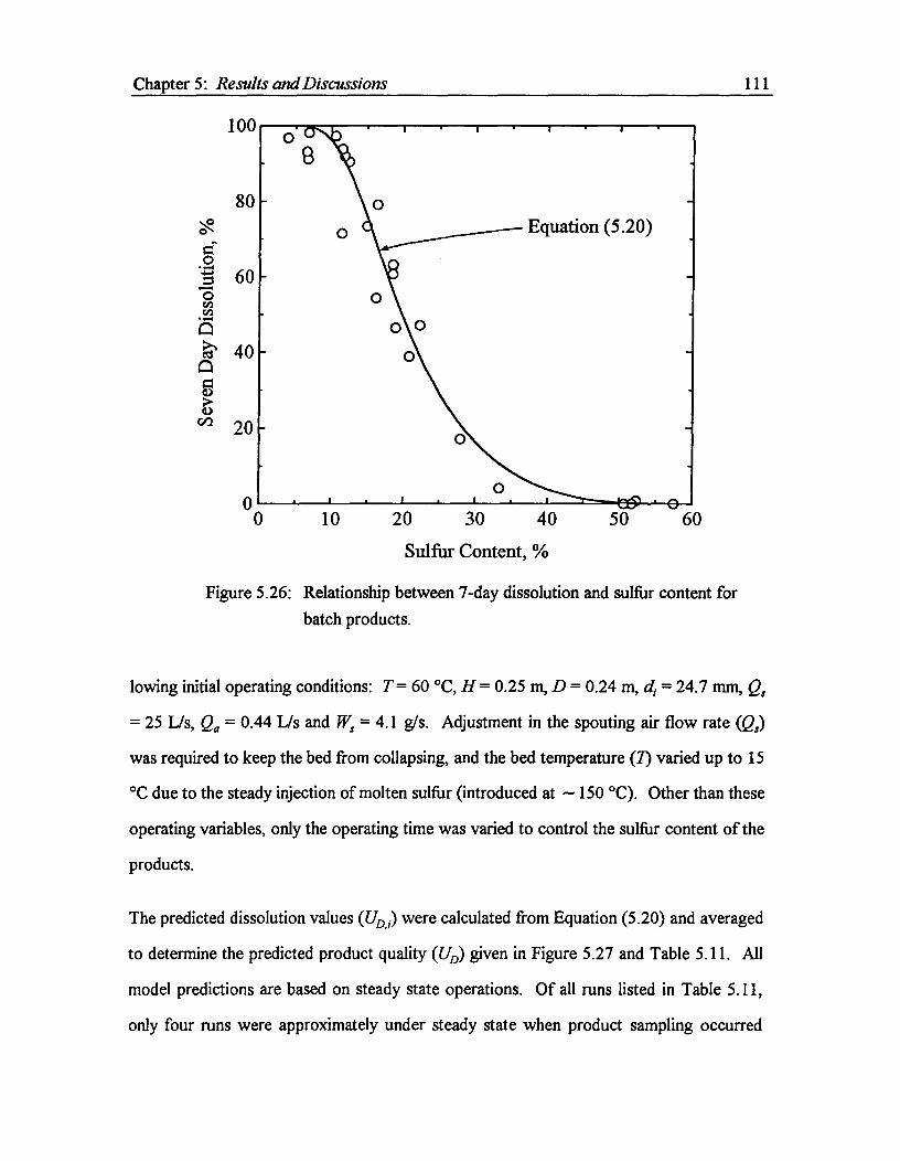
Equation (5.20)
0 60
. 010^20^30^40
Sulfur Content, %50
0 0
0
100
80
060
40
a)
20
Chapter 5: Results and Discussions^ 111
Figure 5.26: Relationship between 7-day dissolution and sulfur content forbatch products.
lowing initial operating conditions: T = 60 °C, H = 0.25 m, D = 0.24 m, d, = 24.7 mm, Q,
= 25 L/s, Qa = 0.44 Us and W, = 4.1 g/s. Adjustment in the spouting air flow rate (Q,)
was required to keep the bed from collapsing, and the bed temperature (7) varied up to 15
°C due to the steady injection of molten sulfur (introduced at — 150 °C). Other than these
operating variables, only the operating time was varied to control the sulfur content of the
products.
The predicted dissolution values (Up ) were calculated from Equation (5.20) and averaged
to determine the predicted product quality (UD) given in Figure 5.27 and Table 5.11. All
model predictions are based on steady state operations. Of all runs listed in Table 5.11,
only four runs were approximately under steady state when product sampling occurred
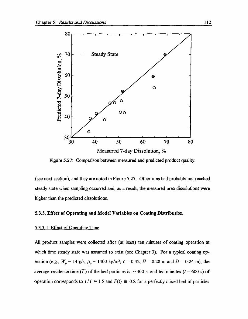
Chapter 5: Results and Discussions^ 112
80
.:, 70
cg"
6cncn0
AcIS'" 50d.r-"CS(1)4.4C.)
"0P. 40a•
3030^40^50^60^70
^80
Measured 7-day Dissolution, %
Figure 5.27: Comparison between measured and predicted product quality.
(see next section), and they are noted in Figure 5.27. Other runs had probably not reached
steady state when sampling occurred and, as a result, the measured urea dissolutions were
higher than the predicted dissolutions.
5.3.3. Effect of Operating and Model Variables on Coating Distribution
5.3.3.1. Effect of Operating Time
All product samples were collected after (at least) ten minutes of coating operation at
which time steady state was assumed to exist (see Chapter 3). For a typical coating op-
eration (e.g., Wp = 14 g/s, pp = 1400 kg/m3, e = 0.42, H = 0.28 m and D = 0.24 m), the
average residence time (I) of the bed particles is — 400 s, and ten minutes (t = 600 s) of
operation corresponds to t / i = 1.5 and F(t) .-- 0.8 for a perfectly mixed bed of particles
Chapter 5: Results and Discussions^ 113
(see Equation (4.1)). (F(t) = 1 indicates the true steady state condition, and occurs when t
-> 00.) For most coating runs, the average coating time was approximately 20 minutes
which corresponds to t I t = 3 and F(t) z- 0.95.
The large values of F(t) indicate that most of the runs were close to steady state condi-
tions; however, the coating distribution and sulfur content results indicated that some runs
might not have reached steady state at the time of sampling. Consequently, an experiment
was conducted to investigate this effect. The effect of the operating time was investigated
in a deep bed (0.36 m) with a very low urea feed rate (approximately 4 g/s) to accentuate
the effect. The average residence time of the particles under this condition was —20 min-
utes. The results can be seen in Figure 5.28. As indicated by the changing shapes of the
coating distribution curve, steady state was not achieved after ten minutes (t II = 0.5) of
coating operation. Even after operating for two hours (tI t = 6 and F(t) = 0.998; i.e.,
very close to steady state for a perfectly mixed bed), the sulfur content of the heavily
coated fraction was still changing. Similar trends were also found in Tsai's (1986) investi-
gation with a 0.15 m bed after three hours of continuous operation.
An explanation for this result is that the spouted bed does not behave as a perfectly mixed
bed. The spouted bed may be seen as a partly well-mixed and partly plug-flow vessel in
which the bed particles spend most of their time in the plug flow zone (annulus). Conse-
quently, the spouted bed approaches steady state more slowly than does a perfectly mixed
vessel.
The steady state condition is also indicated by the values of sulfur content. The measured
sulfur content values (X.) for the three samples collected are given in Figure 5.28 and the
sulfur content based on the feed rates of urea and sulfur (X .,) was 42.3 %. When steady
state is achieved, X. should approach X, . (The fact that the X values for the one and
two hour runs are slightly higher than the X, value is probably due to uncertainty in pro-
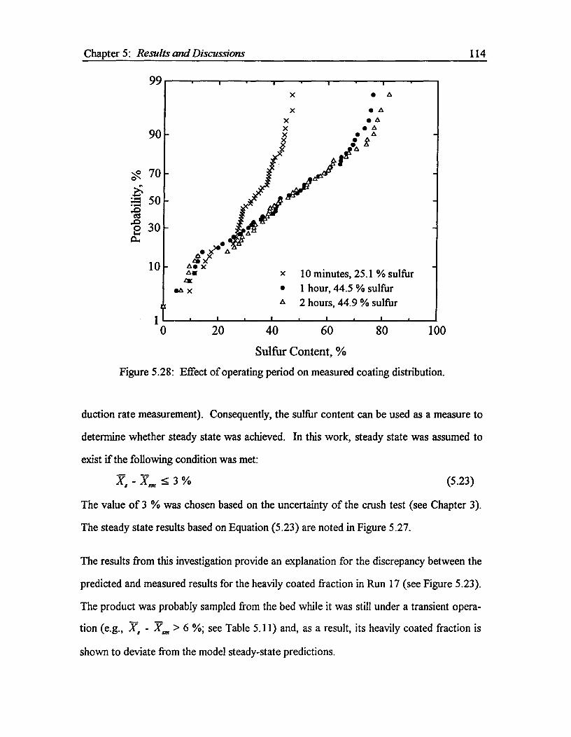
99
90
70
10 minutes, 25.1 % sulfur1 hour, 44.5 % sulfur2 hours, 44.9 % sulfur
10
1
Chapter 5: Results and Discussions^ 114
0^20^40^60^
80^
100
Sulfur Content, %Figure 5.28: Effect of operating period on measured coating distribution.
duction rate measurement). Consequently, the sulfur content can be used as a measure to
determine whether steady state was achieved. In this work, steady state was assumed to
exist if the following condition was met:
,Y, - 1^3 %^ (5.23)
The value of 3 % was chosen based on the uncertainty of the crush test (see Chapter 3).
The steady state results based on Equation (5.23) are noted in Figure 5.27.
The results from this investigation provide an explanation for the discrepancy between the
predicted and measured results for the heavily coated fraction in Run 17 (see Figure 5.23).
The product was probably sampled from the bed while it was still under a transient opera-
tion (e.g., 1, - kr > 6 %; see Table 5.11) and, as a result, its heavily coated fraction is
shown to deviate from the model steady-state predictions.

Chapter 5: Results and Discussions.^ 115
5.3.3.2. Effect of Sample Size
Ideally, the sample size should be as large as possible to obtain a small sampling error;
however, the sample size is limited by the resources available for the analysis. The sample
sizes used to determine the coating distributions in this work were limited to 1000 and 40
particles for numerical (Monte Carlo) and manual sampling, respectively. These sizes
were chosen on the basis of the costs associated with computer time and the time required
to analyze the coated urea products.
5.3.3.2.1. Numerical Sampling
The errors associated with sample sizes and the effect of sample size on coating distribu-
tion were investigated for the various mathematical models. The errors associated with
the sample sizes were determined by comparing the results of Models II and III. Models
II and III were chosen for this purpose because both models should yield identical results
when a = 0 for Model III (see Equation (4.19)), but the methods of solution are different
— i.e., the Model II solutions are exact whereas those of Model III are based on the nu-
merically approximate Monte Carlo method. The differences between the model predic-
tions of the average coating amount were calculated from
n^ 2a =Ai E[Onsil/4
where (midi represents the Model III results given by Equation (4.22), (m, 1 )„, represents
the Model II results given by Equation (4.11), and nsi,„ represents the number of simula-
tions performed. The results are summarized in Table 5.12 and include three simulations
per sample size. For each simulation, a different seed or initialization was used to gener-
ate random numbers. Note that the mil values are directly related to the average sulfur
content (Y,,„) values of the sampled particles; therefore, the a values apply to ,Y,„, as
well. The results are also plotted in Figure 5.29. The step-wise nature of the curves in
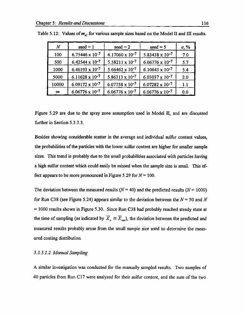
Chapter 5: Results and Discussions^ 116
Table 5.12: Values ofm,/ for various sample sizes based on the Model II and III results.
N seed = 1 seed = 2 seed = 5 a, %100 6.75446 x 10⁻⁷ 6.17060 x 10⁻⁷ 5.83438 x 10⁻⁷ 7.0500 6.42544 x 10⁻⁷ 5.58211 x 10⁻⁷ 6.06776 x 10⁻⁷ 5.71000 6.46193 x 10⁻⁷ 5.66462 x 10 -7 6.10643 x 10⁻⁷ 5.45000 6.11628 x 10⁻⁷ 5.86313 x 10 -7 6.03037 x 10⁻⁷ 2.010000 6.09172 x 10⁻⁷ 6.07758 x 10⁻⁷ 6.07282 x 10⁻⁷ 1.1
co 6.06776 x 10⁻⁷ 6.06776 x 10⁻⁷ 6.06776 x 10⁻⁷ 0.0
Figure 5.29 are due to the spray zone assumption used in Model II, and are discussed
further in Section 5.3.3.3.
Besides showing considerable scatter in the average and individual sulfur content values,
the probabilities of the particles with the lower sulfur content are higher for smaller sample
sizes. This trend is probably due to the small probabilities associated with particles having
a high sulfur content which could easily be missed when the sample size is small. This ef-
fect appears to be more pronounced in Figure 5.29 for N =100 .
The deviation between the measured results (N = 40) and the predicted results (N = 1000)
for Run C38 (see Figure 5.24) appears similar to the deviation between the N = 50 and N
= 1000 results shown in Figure 5.30. Since Run C38 had probably reached steady state at
the time of sampling (as indicated by .k, -=L' Tim ), the deviation between the predicted and
measured results probably arose from the small sample size used to determine the meas-
ured coating distribution.
5.3.3.2.2. Manual Sampling
A similar investigation was conducted for the manually sampled results. Two samples of
40 particles from Run C17 were analyzed for their sulfur content, and the sum of the two
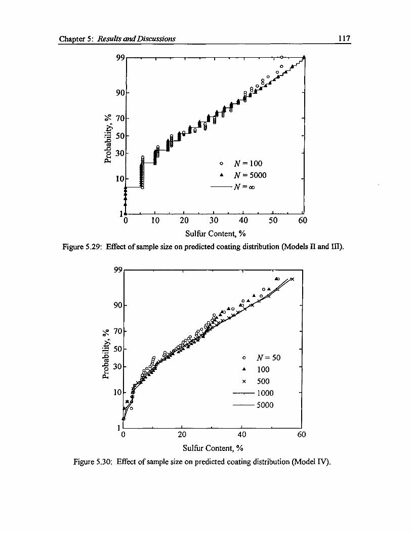
O N = 100• N = 5000^N — co1
Chapter 5: Results and Discussions^ 117
70 -.-..4'= 50 -es0-0 30 -1..,A4
1 0 -^a^•••
a^1 0^
1I0 . 20^ 0'0 ' 3^. 4:030^ 5'0 . 60Sulfur Content, %
Figure 5.29: Effect of sample size on predicted coating distribution (Models II and III).
0^20^40^
60
Sulfur Content, %Figure 5.30: Effect of sample size on predicted coating distribution (Model IV).
99
90 -
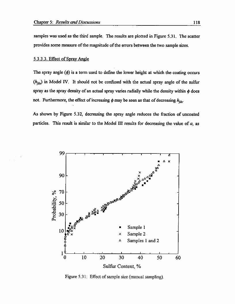
Chapter 5: Results and Discussions^ 118
samples was used as the third sample. The results are plotted in Figure 5.31. The scatter
provides some measure of the magnitude of the errors between the two sample sizes.
5.3.3.3. Effect of Spray Angle
The spray angle (0) is a term used to define the lower height at which the coating occurs
(hfd3) in Model IV. It should not be confused with the actual spray angle of the sulfur
spray as the spray density of an actual spray varies radially while the density within 0 does
not. Furthermore, the effect of increasing (/) may be seen as that of decreasing hfds .
As shown by Figure 5.32, decreasing the spray angle reduces the fraction of uncoated
particles. This result is similar to the Model III results for decreasing the value of a, as
99
I^•^I^•^I^I^•^I^A
90 -X
x Ax ALA'x AA ■
■ A XA
MIA
■
70 -.6:=1 50 -
O 30 -0 •
iA10 - x2es(1 xa.a
I^I
10^20^30^40^50^60Sulfur Content, %
Figure 5.31: Effect of sample size (manual sampling).
1°0
•
X
A
1
Sample 1Sample 2Samples 1 and 2

10 12°
20 6040
99
90
70• r-1r-4 50..0cis0
▪
30a4
_Spray angle = 180°
36°
^-18°
99
90 -
• 70-^a = 8• 50 _a = 4..0cis00 30 -0.%-
10 t. a = 0
a — 1
Chapter 5: Results and Discussions^ 119
Sulfur Content, %Figure 5.32: Effect of spray angle on coating distribution (results from Model IV).
20^40^60Sulfur Content, %
Figure 5.33: Effect of the spray concentration on coating distribution (results wereobtained from Model III using Equation (4.19)).
1 •^0
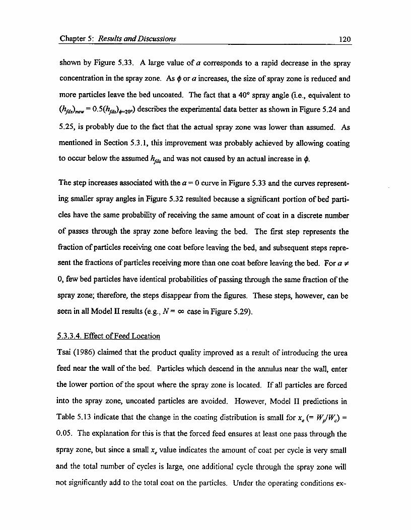
Chapter 5: Results and Discussions^ 120
shown by Figure 5.33. A large value of a corresponds to a rapid decrease in the spray
concentration in the spray zone. As 4, or a increases, the size of spray zone is reduced and
more particles leave the bed uncoated. The fact that a 40° spray angle (i.e., equivalent to
OfdAtew = 0.5(hfde)4,=20.) describes the experimental data better as shown in Figure 5.24 and
5.25, is probably due to the fact that the actual spray zone was lower than assumed. As
mentioned in Section 5.3.1, this improvement was probably achieved by allowing coating
to occur below the assumed hfds and was not caused by an actual increase in q.
The step increases associated with the a = 0 curve in Figure 5.33 and the curves represent-
ing smaller spray angles in Figure 5.32 resulted because a significant portion of bed parti-
cles have the same probability of receiving the same amount of coat in a discrete number
of passes through the spray zone before leaving the bed. The first step represents the
fraction of particles receiving one coat before leaving the bed, and subsequent steps repre-
sent the fractions of particles receiving more than one coat before leaving the bed. For a 0
0, few bed particles have identical probabilities of passing through the same fraction of the
spray zone; therefore, the steps disappear from the figures. These steps, however, can be
seen in all Model II results (e.g., N= 03 case in Figure 5.29).
5.3.3.4. Effect of Feed Location
Tsai (1986) claimed that the product quality improved as a result of introducing the urea
feed near the wall of the bed. Particles which descend in the annulus near the wall, enter
the lower portion of the spout where the spray zone is located. If all particles are forced
into the spray zone, uncoated particles are avoided. However, Model II predictions in
Table 5.13 indicate that the change in the coating distribution is small for x e (= Wp/We) =
0.05. The explanation for this is that the forced feed ensures at least one pass through the
spray zone, but since a small xe value indicates the amount of coat per cycle is very small
and the total number of cycles is large, one additional cycle through the spray zone will
not significantly add to the total coat on the particles. Under the operating conditions ex-
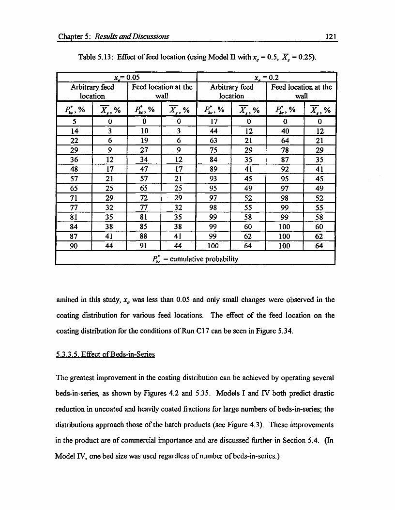
Chapter 5: Results and Discussions^ 121
Table 5.13: Effect of feed location (using Model II with xc = 0.5, Xs = 0.25).
x,= 0.05 x, = 0.2Arbitrary feed
locationFeed location at the
wallArbitrary feed
locationFeed location at the
wall
Pk:, % Pkc,% Pk,% Pk:,%X,, % X,,% X„,% X,,%5 0 0 0 17 0 0 014 3 10 3 44 12 40 1222 6 19 6 63 21 64 2129 9 27 9 75 29 78 2936 12 34 12 84 35 87 3548 17 47 17 89 41 92 4157 21 57 21 93 45 95 4565 25 65 25 95 49 97 4971 29 72 29 97 52 98 5277 32 77 32 98 55 99 5581 35 81 35 99 58 99 5884 38 85 38 99 60 100 6087 41 88 41 99 62 100 6290 44 91 44 100 64 100 64
Pk: = cumulative probability
amined in this study, xe was less than 0.05 and only small changes were observed in the
coating distribution for various feed locations. The effect of the feed location on the
coating distribution for the conditions of Run C17 can be seen in Figure 5.34.
5.3.3.5. Effect of Beds-in-Series
The greatest improvement in the coating distribution can be achieved by operating several
beds-in-series, as shown by Figures 4.2 and 5.35. Models I and IV both predict drastic
reduction in uncoated and heavily coated fractions for large numbers of beds-in-series; the
distributions approach those of the batch products (see Figure 4.3). These improvements
in the product are of commercial importance and are discussed further in Section 5.4. (In
Model IV, one bed size was used regardless of number of beds-in-series.)
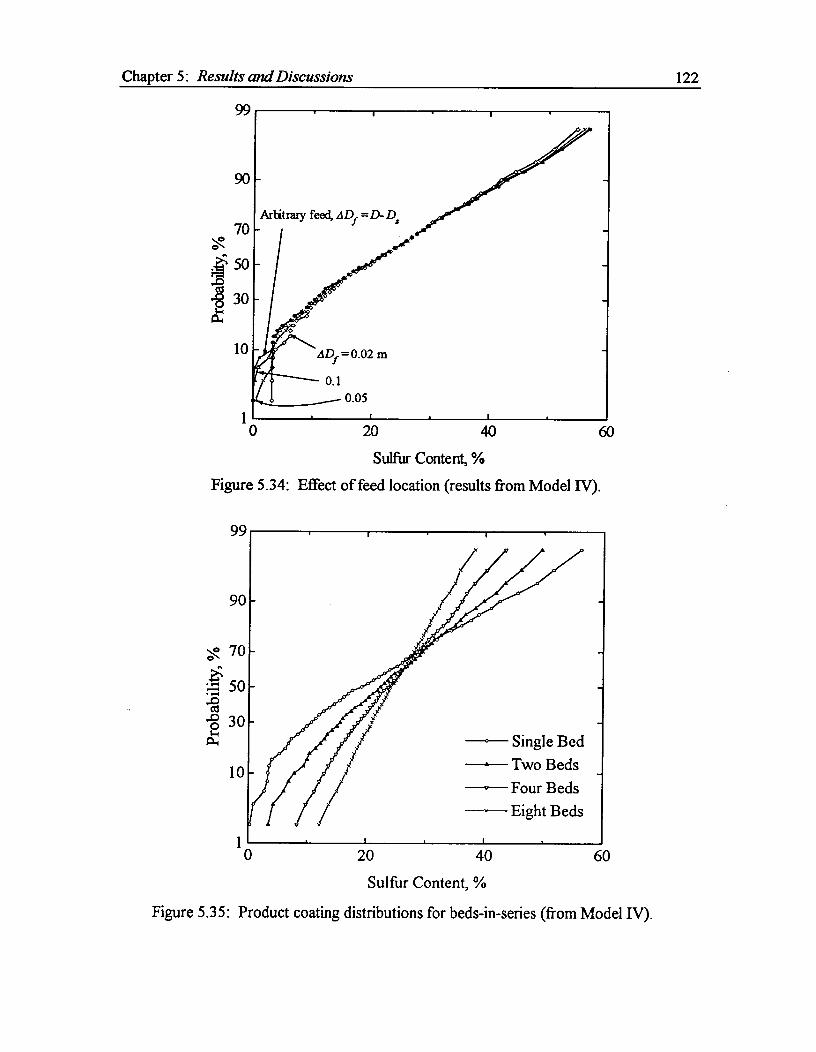
Arbitrary feed, L1Df =D- D,
4/Df =0.02 m
0.10.05
- Single Bed- Two Beds
Four BedsEight Beds
6020^40Sulfur Content, %
Figure 5.35: Product coating distributions for beds-in-series (from Model IV).
99
90
1 ^0
,.. 70
.2.-' 50
..8ct-°0 302a.,
10
Chapter 5: Results and Discussions^ 122
99
70.."'
ti 50i 30a.,
10
20^40^60Sulfur Content, %
Figure 5.34: Effect of feed location (results from Model IV).
Chapter 5: Results and Discussions^ 123
5.3.3.6. Effect of Model Variables, xe and ;
The variables xe and xe in Models II and DI characterize two main factors influencing the
coating distribution. Their relationships to the operating variables were not determined in
this work as a large number of experiments are required (see Chapter 4); however, the ef-
fect of operating variables on these model variables can be explained qualitatively. The
size of the spray zone is characterized by x e, and increasing xe is equivalent to increasing
the spray zone or reducing the by-pass zone. The number of times the particles pass
through the spray zone is characterized by xe (= WiWe), and increasing xe is equivalent to
increasing the particle discharge rate, decreasing the circulation rate, or both.
The operating variables that affect xe are Q„ Qa, FV, and O. Q, determines the impaction
velocity of the droplets onto the bed particles and influences both ri and Ni in Equations
(2.26) and (4.34). Qa and W, determine the droplet size and influence ri in Equation
(2.26). influences the spray zone directly. The value of xe increases with Qa and de-
creases with Q, Ws and 0.
The operating variables that affect xe are Wr, and We. Wp is directly affected by W. and We
is influenced by Q„ H, D and di. We increases with Qs, H, D and di. The value of xe in-
creases with Wp and decreases with We .
The effects of x, and xe on coating distribution are shown in Figures 5.36 and 5.37. The
results presented in Figure 5.36 indicate that for xe = 0.05 and ; = 0.6, over 30 % of par-
ticles receive three coats or less. Three coats on a particle are likely not enough to com-
pletely cover the particle. To increase the number of coats on the particles, x e must be de-
creased and xe increased (see Figure 5.37).
The variables xe and .; can be varied to simulate various types of beds. These variables
are also useful in predicting the presence of uncoated urea particles in the product stream.

0.05
0.1
= 0.3
0.7
0.9
Chapter 5: Results and Discussions
99
90
124
Of
70
• 50
O 30
10x =
•
0.30.1
0.9
^ 0.7
0.05
10^20^30^40^50^60Sulfur Content, %
Figure 5.36: Sensitivity analysis ofxe on coating distribution using Model II ()cc = 0.6).
99
90
• 70
50
O 30
1 0
1-0^ '^'10^20^30^40^50^60
Sulfur Content, %Figure 5.37: Sensitivity analysis of xe on coating distribution using Model II (x e = 0.2).
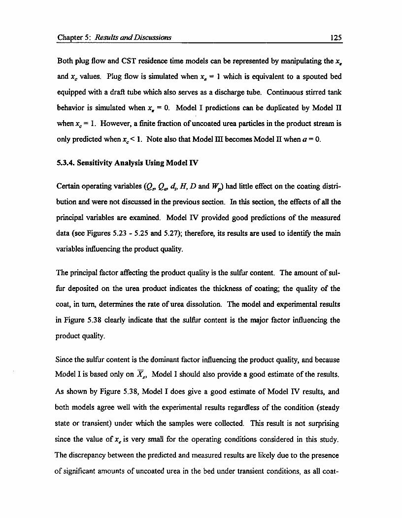
Chapter 5: Results and Discussions^ 125
Both plug flow and CST residence time models can be represented by manipulating the xe
and xe, values. Plug flow is simulated when ; = 1 which is equivalent to a spouted bed
equipped with a draft tube which also serves as a discharge tube. Continuous stirred tank
behavior is simulated when xe = O. Model I predictions can be duplicated by Model II
when xe = 1. However, a finite fraction of uncoated urea particles in the product stream is
only predicted when xe < 1. Note also that Model III becomes Model II when a = O.
5.3.4. Sensitivity Analysis Using Model IV
Certain operating variables (Qs, Q„, di, H, D and Wp) had little effect on the coating distri-
bution and were not discussed in the previous section. In this section, the effects of all the
principal variables are examined. Model IV provided good predictions of the measured
data (see Figures 5.23 - 5.25 and 5.27); therefore, its results are used to identify the main
variables influencing the product quality.
The principal factor affecting the product quality is the sulfur content. The amount of sul-
fur deposited on the urea product indicates the thickness of coating; the quality of the
coat, in turn, determines the rate of urea dissolution. The model and experimental results
in Figure 5.38 clearly indicate that the sulfur content is the major factor influencing the
product quality.
Since the sulfur content is the dominant factor influencing the product quality, and because
Model I is based only on AC, Model I should also provide a good estimate of the results.
As shown by Figure 5.38, Model I does give a good estimate of Model IV results, and
both models agree well with the experimental results regardless of the condition (steady
state or transient) under which the samples were collected. This result is not surprising
since the value of xe is very small for the operating conditions considered in this study.
The discrepancy between the predicted and measured results are likely due to the presence
of significant amounts of uncoated urea in the bed under transient conditions, as all coat-
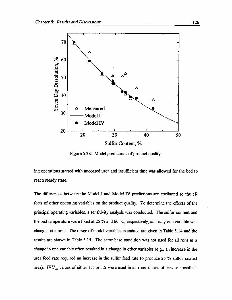
70
30
20
Chapter 5: Results and Discussions^ 126
20^30^40^
50
Sulfur Content, %
Figure 5.38: Model predictions of product quality.
ing operations started with uncoated urea and insufficient time was allowed for the bed to
reach steady state.
The differences between the Model I and Model IV predictions are attributed to the ef-
fects of other operating variables on the product quality. To determine the effects of the
principal operating variables, a sensitivity analysis was conducted. The sulfur content and
the bed temperature were fixed at 25 % and 60 °C, respectively, and only one variable was
changed at a time. The range of model variables examined are given in Table 5.14 and the
results are shown in Table 5.15. The same base condition was not used for all runs as a
change in one variable often resulted in a change in other variables (e.g., an increase in the
urea feed rate required an increase in the sulfur feed rate to produce 25 % sulfur coated
urea). U/Urns values of either 1.1 or 1.2 were used in all runs, unless otherwise specified.
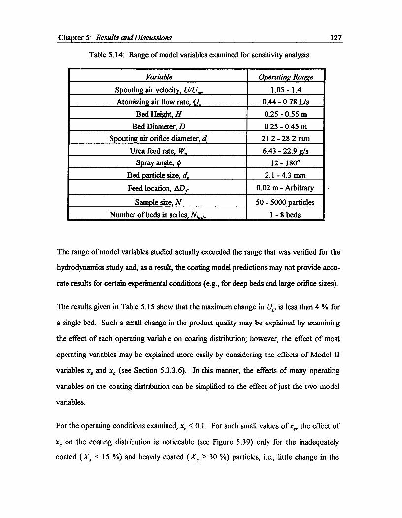
Chapter 5: Results and Discussions^ 127
Table 5.14: Range of model variables examined for sensitivity analysis.
Variable Operating RangeSpouting air velocity, U/U,„, 1.05 - 1.4Atomizing air flow rate, Qa 0.44 - 0.78 Lis
Bed Height, H 0.25 - 0.55 mBed Diameter, D 0.25 - 0.45 m
Spouting air orifice diameter, d, 21.2 - 28.2 mmUrea feed rate, W, 6.43 - 22.9 g/s
Spray angle, 0 12 - 180°Bed particle size, di, 2.1 - 4.3 mmFeed location, ADf 0.02 m - Arbitrary
Sample size, N 50 - 5000 particlesNumber of beds in series, Nhp,i, 1 - 8 beds
The range of model variables studied actually exceeded the range that was verified for the
hydrodynamics study and, as a result, the coating model predictions may not provide accu-
rate results for certain experimental conditions (e.g., for deep beds and large orifice sizes).
The results given in Table 5.15 show that the maximum change in Up is less than 4 % for
a single bed. Such a small change in the product quality may be explained by examining
the effect of each operating variable on coating distribution; however, the effect of most
operating variables may be explained more easily by considering the effects of Model II
variables xe and ; (see Section 5.3.3.6). In this manner, the effects of many operating
variables on the coating distribution can be simplified to the effect of just the two model
variables.
For the operating conditions examined, x e < 0.1. For such small values of xe, the effect of
xe on the coating distribution is noticeable (see Figure 5.39) only for the inadequately
coated as < 15 %) and heavily coated (X1 > 30 %) particles, i.e., little change in the

Chapter 5: Results and Discussions^ 128
Table 5.15: Results of sensitivity analysis using Model IV (iY, =0.25, T = 60 °C).
Bed Diameter Atomizing Air Urea Feed Rate Orifice DiameterD, m Up, % Q„, Lis UD , ° W„, gis Un, % di, mm UD,%
0.25 54.2 0.44 52.5 6.43 53.9 21.2 53.40.35 53.6 0.61 52.2 12.3 54.2 24.7 54.20.45 53.3 0.78 52.0 22.9 54.3 28.2 53.9
Bed Height Spouting Air Bed Particle Id. I^Spray Angle^IH, m Up, % U/Uni, Up, % dn, nun UD , % 0 UD, %
0.25 53.9 1.05 54.7 2.1 54.5 180° 56.00.35 53.9 1.1 54.2 3.2 54.4 36° 52.90.45 54.2 1.2 54.4 4.3 54.6 18° 52.50.55 54.2 1.4 53.7 12° 52.7
Feed Locationh,Df, m 0.02 0.05 0.1 0.15 D - D ,
1D,% 53.4 53.9 54.2 54.3 54.3
Sample SizeN 50 100 500 1000 5000
UD , % 58.4 53.3 54.9 54.0 54.2
Beds in Series^ iNh„d„ 1 2 4 8
UD , % 54.0 46.4 40.8 35.9Model I Prediction: UD = 54.2 %^ 1
range 15 % < 17, < 30 % is observed for x e = 0.05, even though the x, value is quite dif-
ferent. This change in the coating distribution does not change the product quality signifi-
cantly because the product quality is determined primarily by the fraction of particles hav-
ing 15 % < X, < 30 % (see Figure 5.26 or Equation 5.20).
The most significant improvement in product quality occurs when urea is coated in a series
of beds. This result is consistent with the above explanation that the fraction in the range
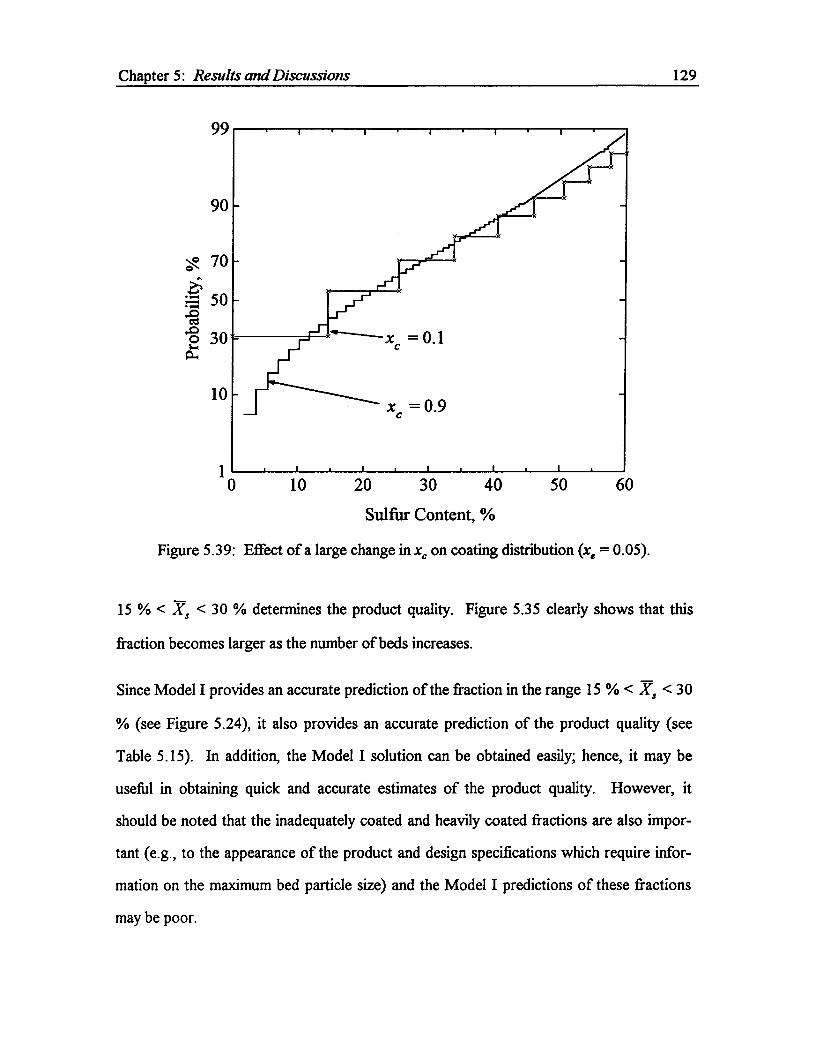
Chapter 5: Results and Discussions^ 129
99
90
e 70
50ozs0 30
10
10^20^30^40^
50^
60Sulfur Content, %
Figure 5.39: Effect of a large change in ; on coating distribution (x e = 0.05).
15 % < ,Y, < 30 % determines the product quality. Figure 5.35 clearly shows that this
fraction becomes larger as the number of beds increases.
Since Model I provides an accurate prediction of the fraction in the range 15 % < X3 < 30
% (see Figure 5.24), it also provides an accurate prediction of the product quality (see
Table 5.15). In addition, the Model I solution can be obtained easily; hence, it may be
useful in obtaining quick and accurate estimates of the product quality. However, it
should be noted that the inadequately coated and heavily coated fractions are also impor-
tant (e.g., to the appearance of the product and design specifications which require infor-
mation on the maximum bed particle size) and the Model I predictions of these fractions
may be poor.
Chapter 5: Results and Discussions^ 130
The effect of sample size can also be seen in Table 5.15. The purpose of including these
values was to check the error associated with the sample size. The results in terms of the
deviations from the value obtained for 5000 particles are similar to those of the standard
deviations calculated for the coating distribution (see Table 5.12).
5.4. Commercial Implications
The findings of this study are applicable to the design of commercial coating plants.
Model I provides a quick estimate of the product quality suitable for preliminary plant de-
signs, while Model IV may be used for more detailed studies. Models II and III can aid
with conceptualizing spouted bed coating processes.
Commercial plants will normally have considerably higher capacities than the current ap-
paratus. Higher capacities may be obtained in two ways: increasing the bed size and in-
creasing the number of beds in parallel. The latter option should be considered only if the
former option does not provide the desired capacity, because an increase in the number of
beds can pose operational difficulties. These include controlling the distributions of air
and liquid sulfur to different beds. Larger beds, on the other hand, may increase the pro-
duction rate without sacrificing the product quality (presuming the hydrodynamics and xe
stay constant).
It is unlikely that the product quality can be controlled by varying the production rate
alone. As discussed already, the product quality is determined primarily by the number of
beds in series. The product quality increases with the number of beds-in-series, but be-
cause operational difficulties also increase, the minimum number of beds that meets the
design quality specification should be used. Note that the increase in the product quality is
large when the number of beds increases from one to two beds, but the increase in the
product quality becomes smaller for each additional bed.

Chapter 6.
Conclusions and Recommendations
6.1. Conclusions
The spouted bed coating process for the batch-wise and continuous production of sulfur
coated urea has been successfully modeled using mass and momentum balance equations
and inertial sulfur droplet deposition as the dominating coating mechanism.
Specific conclusions that may be drawn from the results given in Chapter 5 are listed in the
following sub-sections.
6.1.1. Bed Hydrodynamics
• The minimum spouting velocity (U„, ^) varies linearly with the bed height in conical
beds.
• U., varies proportionally with the total momentum due to atomizing air and spouting
air flow into the bed.
• U„,,, axial pressure profile in the annulus and air velocity in the spout in conical beds
are similar to the corresponding quantities in conical-cylindrical beds with the column
diameter equal to 80 % of the maximum diameter of conical beds.
• U., for shallow beds could be well represented by the correlation given by Equation
(5.4).
• The Morgan-Littman (1980) correlation provides accurate axial pressure profiles in
the annulus for shallow spouted beds if the diameter modification for conical beds is
used.
131
Chapter 6: Conclusions and Recommendations^ 132
• The mass and momentum balances suggested by Lefroy and Davidson (1969) give ac-
curate predictions of air velocity in the spout, provided that the vector form of the Er-
gun (1952) equation for gas flow in the annulus and the modifications listed above are
used.
6.1.2. Spray Studies
• Consistent sulfur atomization by the nozzle used in this work occurs in the range de-
fined by Equations (5.8) and (5.9).
• The size of the sulfur droplets typically ranged from 6 to 50 Am dia. and is well repre-
sented by a log-normal distribution.
• The average droplet size is affected primarily by the sulfur feed rate, and is well repre-
sented by the power-law correlation given by Equation (5.17).
• The dominant mechanism by which the sulfur droplets deposit onto the bed particles is
inertial impaction.
6.1.3. Coating Distribution and Product Quality
• The spray angle, urea feed location and the number of beds-in-series significantly af-
fect the amount of lightly coated and heavily coated particles in the sulfur coated urea
product.
• The product quality is primarily affected by the average sulfur content of the product
and the number of beds-in-series. Spray angle, feed location, atomizing and spouting
air flow rates, urea and sulfur feed rates, and bed diameter also affect the product
quality, but to a much lesser extent.
• The Monte Carlo method provides good representation of coating distribution if a suf-
ficient number of particles are simulated.
• The spouted bed coating unit is capable of producing sulfur coated urea of widely
varying quality at a high production rate.
Chapter 6: Conclusions and Recommendations.^ 133
6.2. Recommendations for Further Work
Certain difficulties and assumptions in modeling the coating process resulted from the limi-
tations of the one-dimensional models used in this work. A significant number of assump-
tions could be reduced if a fully two-dimensional (axi-symmetric) model is developed. For
example, hfd, would not have to be assumed because the particle concentration and the
spray distribution in the spout could be determined in a two-dimensional model. Some
experimental work may be necessary to develop a model of the radial spray density in the
spray region. The model should also be a three-phase model as the effects of sulfur spray
on the bed hydrodynamics cannot be properly determined with the two-phase model de-
veloped in this work. The two-dimensional, two-phase model developed by Krzywanski
(1992) would be a good starting point for such a model.
Before commercialization of the spouted bed process, a pilot plant consisting of several
beds-in-series should be evaluated. Amongst the foreseeable problems are control of the
distribution of air and sulfur to different beds, transportation of large particles from bed to
bed, and separation of large particles from the product. These problems cannot be ad-
dressed until a pilot plant is actually available. A continuous sulfur supply system should
also be incorporated into the pilot plant to study the effects of operating time.
The hydrodynamics of larger diameter beds should also be examined because many corre-
lations used in this work may not apply to larger beds (Lim and Grace, 1987).
Finally, the sulfur droplet distribution in the spouted bed could not be directly measured
using the devices examined in this work. A further study on such a device could be valu-
able and it would advance aerosol detection in complex environments. The devices stud-
ied here could be a good starting point for such an effort.

Nomenclature
Aas^Local spray area, m2
A°^Area of shutter opening, m2
A^Projected area of spout particles per unit volume of spout, m -1
A *^Projected area (cross-sectional area) of a particle, m 2
As^Spout cross-sectional area, m2
a^Exponent in Equation (4.17), dimensionless
C^Concentration of sulfur droplets in the gas phase, kg/m3
Cc^Spray concentration defined for Model III, kg/m 3
Co^Pitot tube coefficient, dimensionless
c^Fitted coefficient ofD in Equation (5.3)
Diffusion Coefficient, m2/s
D^Column diameter, m
D{z}^Local bed diameter, m
D'^"Effective" bed diameter (D' = 0.8 D. in conical section and D' = D inconical-cylindrical section), m
D25^Seven day urea dissolution for products with 25 % sulfur content,fractional
Da„^Local diameter of the spray, m
Df D - ADfi m
Location of feed particle on the surface of the bed during its first cycle, m
D.^Maximum annulus diameter for the conical bed, m
Dr^Location of bed particles on the surface of the bed, m
Di^Spout diameter, m
da^Diameter of atomizing air nozzle cap at top, m
134
Nomenclature^ 135
Diameter of nozzle orifice, m
do^Diameter of aerosol particle, m
dgo^Geometric counted mean of droplet size, m
Orifice diameter based on the flow area of Q„ m
Corrected orifice diameter in Equation (5.2), m
do^Shutter diameter based on the flow area, m
dp^Average diameter of bed particle, m
dp;^Mean diameter of adjacent Tyler screen apertures, m
d,^Diameter of sulfur spray droplets, m
dam,^Sauter mean (surface-volume) diameter, m
F{t}^Distribution function of residence time, dimensionless
11,12^Coefficients of Ergun equation, kg/m3s and kg/m4
ED, 41,^Collection efficiency due to diffusion, direct interception, gravitation andEG, EI^inertial impaction, dimensionless
G pU
G{X,}^Exit sulfur content distribution, dimensionless
g^Acceleration due to gravity, m/s2
H^Loosely packed static bed height, m
Height of cone base, m
H„,^Maximum spoutable bed depth, m
h^H/H,„
hid,^Height at which the spray coating begins, m
k^Coefficient in Equation (2.3); number of passes through the spray zone
ko^Proportionality constant in Equation (4.19)
kp^Probability constant in Equation (4.20), m -1
k 8^Angle of fully developed spray jet, °
M.^Momentum flow of spouting and atomizing air into the bed, kg•m/s2
Nomenclature^ 136
mp^Total weight of the bed particles, kg
mf^Weight of sulfur in sulfur coated urea, kg
mj^Mean weight of sulfur in sulfur coated urea, kg
m,* Conditional weight of sulfur deposited on urea, kg
Ms1^Amount of sulfur deposited on a bed particle per pass through the sprayzone, kg
Mean weight of sulfur picked up per pass through spray zone, kg
Weight of urea in sulfur coated urea, kg
ni„^Mean weight of urea in sulfur coated urea, kg
N Sample size, particles; number of cycles, cycles
Na *^Deposition rate of sulfur droplets in the annulus between streamlines, kg/s
NDI^Interception parameter, dimensionless
NG^Gravitational settling parameter, dimensionless
Deposition rate of sulfur droplets on spout particles per unit volume ofspout, kg/s•m3
NR^Numerically generated random number between 0 and 1
n^Number of beds in series in Equation (4.7)
n^Direction normal to streamlines, m
P Pressure, Pa
Pf^Pressure in fluidized bed, Pa
P a{z}^Pressure at z, Pa
Pr{z}^Probability of particle entering at z into the spray zone, fractional
Pk,^Probability of particle entering the spray zone k times, fractional
Qa^Volumetric atomizing air flow rate, m 3/s
Ql^Flow rate of spray liquid, m3/s
Qma^Atomizing air flow rate at minimum atomization, m 3/s
Qms^Volumetric flow rate at minimum spouting, m3/s

Nomenclature^ 137
Q,^Volumetric spouting air flow rate, m3/s
Q,^Total volumetric flow rate = Q.+ Qs, m3/ss
r^Radial distance from the centre of the bed, m
S Distance along the stream line, m
Sd^Standard deviation of Unis predictions, m/s
,S;^Stoke's number, dimensionless
T, Tb^Bed temperature, °C
t^Time, s
I^Mean residence time of solids, s
t,^Cycle time, s
tr^Residence time, s
U Superficial air velocity, m/s
U Vector form of air velocity, m/s
UD^Predicted seven day urea dissolution rate, fractional
Um,^Measured seven day urea dissolution rate, fractional
Um,^Minimum spouting velocity based on column diameter (D), m/ss
Ilims^Minimum spouting velocity based on D, m/s
Ur^Volumetric rate of air cross-flow per unit area of spout-annulus interface,m/s
Ur^Terminal settling velocity, m/s
u Interstitial air velocity, m/s
ur^Relative velocity between gas and liquid at the orifice, m/s
Vb^Total bed volume, m3
Vr^Entrainment rate of bed particles into the spout per unit area of spout-annulus interface, m/s
^ Local bed particle velocity, m/s
FIC^Circulation rate of bed particles, kg/s

Nomenclature^ 138
TVp^Production rate, kg/s
Sulfur injection rate, kg/s
Wu^Urea feed rate, kg/s
X^Defined in Equation (2.13), dimensionless
Sulfur content, dimensionless
Xa^Mean sulfur content of sulfur coated urea based on urea and sulfur feedrates, fractional
Mean sulfur content of sulfur coated urea based on a crush test, fractional
X ^sulfur content of simulated (SCU) particles, fractional
Xsp,i^Sulfur content of individual particle, fractional
z/H„,
xb^Probability of particle by-passing the spray zone, fractional
Probability of particle entering the spray zone, fractional
xe^Probability of particle exitting the bed after each cycle, fractional
xf^Fraction of area occupied by the urea feed in the area defined by ADf,„
fractional
1 - xe, fractional
Y^Defined in Equation (2.11)
z^Axial destance from base of the bed, m
Length of spray zone from base of the bed, m
Location of particle's entry into the spout for urea feed particles, m
Greek Letters
ap^Defined in Equation (2.8)
a,fi,E,y^Exponent in Equation (2.3)
Pp^Particle-fluid interaction term, dimensionless

Nomenclature^ 139
4^Difference
4Df^Twice the width of annulus covered by feed adjacent to the wall of thespouted bed at the top of the bed, m
E^Voidage, fractional
(1){z}^Probability density, m-1
(fi^Spray angle, °
C^Particle shape factor or sphericity, fractional
11^Collection efficiency, fractional
4)^Defined in equation (2.14), dimensionless
II^Fluid viscosity, kg-m/s
Az^Viscosity of liquid spray, kg-m/s
0^Included spouted bed cone angle, °
P Fluid density, kg/m3
Pa^Atomizing air density, kg/m3
Pb^Bulk density of loose-packed solids, kg/m 3
Pe^Aerosol density, kg/m3
Pi^Density of liquid spray, kg/m3
pp^Particle density, kg/m3
Pa^Density urea particles, kg/m3
I^Sum
a^Standard deviation (Table 5.12), fractional
ag^Log-standard geometric deviation, m
az^Surface tension of liquid spray, dyn/cm
^ Stream function, dimensionless
^ Directional gradient
Nomenclature^ 140
Subscripts
o^Condition at z = 0
per cycle
a^Annulus; atomizing air
as^Atomizing air in spout
Condition at z = H
Pertaining to an individual particle or 'cut'
Liquid spray
ma^At minimum atomization
mf^At minimum fluidization
mp^At minimum pulsation
ms^At minimum spouting
Bed particle
Spout; sulfur
Urea

References
Abramovich, G.N., The Theory of Turbulent Jets, M.I.T Press, Cambridge, 1963.
Allen, S.E., "Sulfur-coated urea: cover controls nitrogen release", Trees and Turf Mag.,June 1980, p54.
Allen, S.E., Terman, G.L. and Hunt, C.M., "Soluable and slow-release nitrogen fertilizereffects on grass forage as influenced by rate and placement", J. Agric. Sci. Can.,v77, p397, 1971.
American Society of Mechanical Engineers, Fluid Meters: Their Theory and Application,(6th edition; Edited by H.S. Bean), The American Society of Mechanical Engi-neers, New York, 1971.
Amirshahidi, M.S., Ph.D. Thesis, Lehigh Univ., 1984.
Balasubramanian, M., Meisen, A. and Mathur, K.B., "Spouted bed collection of solidaerosols in the presence of electrical effects", CJChE, v 56, p297, 1978.
Barton, R.K., Rigby, G.R. and Ratcliffe, J.S., "Fluid-solids contacting in spouted beds",Mech. Chem. Eng. Trans., v4, p105, 1968.
Becker, H.A. and Sallans, H.R., "On the continuous, moisture diffusion controlled dryingof solid particles in a well mixed, isothermal bed", Chem. Eng. Sci., v13, p97,1961.
Behie, S.W., Beekmans, J.M., Knetting, P. and Bulani, W., "Aerosol particle collection ina vertical pneumatic transport line", CJChE, v50, p241, 1972.
Behie, S.W. and Beekmans, J.M., "On the efficiency of a venturi scrubber", CJChE, v51,p430, 1973.
Berruti, R., Rovero, G. and Piccinini, N., "A coating process in a spouted bed: a mathe-matical model", Ing. Chim. Ital., v20, No. 7-8, p51, 1984.
Bitron, M.D., "Atomization of liquids by supersonic air jets", Ind Eng. Chem., v47, p23,1955.
Blouin, G.M., Rindt, D.W. and Moore, O.E., "Sulfur-coated fertilizers for controlled re-lease: Pilot plant production", J. Agr. Food Chem., v19, p801, 1971.
141

References^ 142
Bowen, I.G. and Davis, G.P., "Particle size distribution and the estimation of Sauter meandiameter", Shell Technical Report No. ICT/28, October, 1951.
Box, G.E., Hunter, W.G. and Hunter, J.S., Statistics for Experimenters, Wiley and Sons,New York, 1978.
Bridgewater, J. and Mathur, K.B., "Prediction of spout diameter in a spouted bed — Atheoretical model", Powder Tech., v6, p183, 1972.
Brown, G.W., Modern Mathematics For Engineers, 1956 (Edited by Beckenback, E.F.),chapter 12, McGraw-1K New York, 1956.
Chaterjee, A., "Effect of particle diameter and apparent particle density on internal solidcirculation rate in air-spouted beds", Inch Eng. Chem. PDD., v9, p531, 1970.
Cliff, R., Ghadiri, M. and Thambimuthu, K.V., "Filtration of gases in fluidised beds", Pro-gress and Filtration and Separation, v2, (Edited by Wakeman, R.J.), Elsevier, Am-sterdam, p75, 1981.
Cliff, R., Grace, J.R. and Weber, M.E., Bubbles, Drops and Particles, Academic Press,New York, 1978.
Conroy, E.H. and Jonstone, H.F., "Combustion of sulfur in a venturi spray burner", InchEng. Chem., v41, p 2741, 1949.
Cook, H.H. and Bridgewater, J., "Segregation in spouted beds", CJChE, v56, p636, 1978.
Cox, D.R., Renewal Theory, Methuen and Co. Ltd., London, pp91-101, 1967.
Dale, J.M. and Ludwig, A.C., Mechanical Properties of Sulfur Allotropes, Mat. Res. andStand., 1965.
Davies, C.N., Aerosol Science, Academic Press, London, 1966.
Davis, L.H., "Two grass field trials with sulfur coated urea to examine its potential as aslow release nitrogen fertilizer in the UK", J Sci. Food Agr., v24, p63, 1973.
Day, J.Y., Morgan, M.H., III and Littman, H., "Measurements of Spout Voidage Distribu-tions, Particle Velocities and Particle Circulation Rates in Spouted Beds of CoarseParticles - II. Experimental Verification", Chem. Eng. Sci., v42, no.6, p1461,1987.
Donahue, J. and Meyer, B., "The naming of sulphur allotropes", Elemental Sulphur(Edited by Meyer, B.), John Wiley and Sons, New York, 1965.
References^ 143
Epstein, N. and Grace, J.R., Handbook of Powder Science and Technology, 1984 (Editedby Otten, L. and Fayed, M.E.), chapter 11, Van Nostrand Reinhold, New York,1984.
Epstein, N. and Levine, S., "Non-Darcy Flow and Pressure Distrubution in a SpoutedBed", in Fluidization, Proc. 2nd Engng. Found. Conf., Cambridge, 1978 (Edited byDavidson, J.F. and Keairns D.L.), p98, Cambridge University Press, 1978.
Epstein, N., Lim, C.J. and Mathur, K.B., "Data and models for flow distribution andpressure drop in spouted beds", CJChE, v56, p436, 1978.
Ergun, S., "Flow through packed columns", Chem. Eng. Prog., v48, p89, 1952.
Freeport Sulphur Company (Edited by Tuner, W.N.), The Sulphur Data Book, McGraw-Hill, New York, 1954.
Gerald, C.F. and Wheatley, P.O., Applied Numerical Analysis, Addison-Wesley, Reading,1984.
Gnyp, A.W., St. Pierre, C.C., Smith, D.S., Mozzon, D. and Steiner, J., "S-type pitot tubecoefficients: An experimental investigation of the effect of pitot tube-samplingprobe configurations on the magnitude of the S-type pitot tube coefficients forcommercially available source sampling probes", (written for Ontario Ministry ofthe Environment), University of Wmsor, 1975.
Grace, J.R., "Contacting modes and behaviour classification of gas-solid and other two-phase suspensions", CJChE, v64, p353, 1986.
Grace, J.R., "Fluidized bed hydrodynamics", Chapter 8.1 in Handbook of MultiphaseSystems, ed. G. Hetsroni, Hemisphere, Washington, 1982.
Grace, J.R. and Mathur, K.B., "Height and structure of the fountain region above spoutedbeds", CJChE, v56, p533, 1978.
Harnett, D.L., Statistical Methods, 3rd ed., Addison-Wesley, Reading, 1982.
Hidy, G.M., Aerosols: An Industrial and Environmental Science, Academic Press, Or-lando, 1984.
Hill, Jr., C.G., Chemical Engineering Kinetics and Reactor Design, Wiley and Sons, NewYork, 1977.
Jackson, R., "The mechanics of fluidized beds", Trans. Instn. Chem. Engrs., v41, p13,1968.

References^ 144
Khoe, D.F., Ph.D. Dissertation, Delft Univ., 1980.
Kim, K.Y. and Marshall, Jr., W.R., "Drop size distributions from pneumatic atomizers,AlChE , v17, p575, 1971.
Krzywanski, R., Ph. D. Dissertation, U.B.C., 1992.
Krzywanski, R., Epstein, N and Bowen, B., "Multi-dimensional model of a spouted bed",CJChE, v70, p858, 1992.
Kugo, M., Watanabe, N., Uemaki, 0. and Shibata, T., Bul. Hokkaido Univ. Sapporo Jap.,v39, p95, 1965.
Kutluoglu, E., Grace, J.R., Murchie, K.W. and Cavanagh, P.H., "Particle segregation inspouted beds", CJChE, v61, p308, 1983.
Lefroy, G.A. and Davidson, J.F., "The mechanics of spouted beds", Trans. Inst. Chem.Engrs., v47, pT120, 1969.
Lewis, H.C., Edwards, D.G., Goglia, M.J., Rise, R.I. and Smith, L.W., "Atomization ofliquids in high velocity gas streams", Ind Eng. Chem., v40, p67, 1948.
Lim, C.J., Ph.D. Dissertation, U.B.C., 1975.
Lim, C.J. and Grace, J.R., "Spouted bed hydrodynamics in a 0.91 m diameter vessel",CJChE, v65, p366, 1987.
Lim, C.J. and Mathur, K.B., Fluidization, "Modeling of particle movement in spoutedbeds", Fluidization, Proc. 2nd Engng. Found. Conf., Cambridge, 1978 (Edited byDavidson, J.F. and Keairns D.L.), Cambridge University Press, p104, 1978.
Lim, J., B.A. Sc. Thesis, U.B.C., 1978.
Littman, H., Morgan, M.H., Narayanan, P.V., Kim, S.J., Dan, J. and Lazarek, G.M., "Anaxisymmetric model of flow in the annulus of a spouted bed of coarse particles.Model, experimental verification and residence time distribution", CJChE, v63,p188, 1985.
Littman, H., Narayanan, P.V., Tomlins, A.H. and Friedman, M.L., "A complete theoreticalmodel for a first order isothermal catalytic reaction in a spouted bed", AIChESymp. Ser. No. 205, v77, p174, 1981.
Littman, H., Morgan, M.H., Vukovic, D.V., Zdanski, F.K. and Grbavcic, Z.B., "A theoryfor predicting the maximum spoutable height in a spouted bed", CJChE, v55,p497, 1977.
References^ 145
Lunde, K.E. and Lapple, C.E., "A critique on the state of the art of dust and mist collec-tion", Chem. Eng. Prog., v53, No. 8, p385, 1957.
Mamuro, T. and Hattori, H., "Flow pattern of fluid in spouted beds", J. Chem. Eng. Ja-pan, vl, p1, 1968.
Mann, U., Correspondence, Ind Eng. Chem. Proc. Des. Dev., v17, p103, 1978.
Mann, U., "Analysis of spouted bed coating and granulation. 1. Batch operation", IndEng. Chem. Proc. Des. Dev., v22, p288, 1983.
Mann, U. and Crosby, E.J., "Cycle time distribution measurements in spouted beds",CJChE, v53, p579, 1975.
Mann, U., Rubinovitch, M. and Crosby, E.J., "Characterization and analysis of continuousrecycle systems: Part I. Single unit", AIChEJ., v25, No. 5, p873, 1979.
Mann, U. and Rubinovitch, M., "Characterization and analysis of continuous recycle sys-tems: Part H. Cascade", AIChEJ., v27, No. 5, p829, 1981.
Mann, U., Crosby, E.J. and Rubinovitch, M., "Number of cycles distribution in circulatingsystems", Chem. Eng. Sci., v29, p761, 1974.
Mann, U. and Crosby, E.J., "Cycle time distribution measurements in spouted beds",CJChE, v53, p579, 1975.
Mathur, K.B. and Epstein, N., Spouted Beds, Academic Press, New York, 1974.
Mathur, K.B. and Lim, C.J., "Vapour phase chemical reaction in spouted beds: a theoreti-cal model", Chem. Eng. ScL, v29, p789, 1974.
Mathur, K.B. and Gishler, P.E., "A technique for contacting gases with coarse solid parti-cles", AIChEJ., vl, p157, 1955.
McNab, G.S., "Prediction of spout diameter", Brit. Chem. Eng. and Proc. Tech., v17,p532, 1972.
McNab, G.S. and Bridgwater, J., "Spouted beds — estimation of spouting pressure dropand the particle size for deepest bed", Proc. European Congress on Particle Tech-nology, Nuremberg, 1977.
Meisen, A., Lee, V. and Le, V., unpublished report, 1986.
Meisen, A., Bobkowicz, A.J., Cooke, N.E. and Farkas, E.J., "The separation of micron-size particles from air by diffusiophoresis", CJChE, v49, p449, 1971.

References^ 146
Meisen, A. and Mathur, K.B., "The spouted bed aerosol collector: a novel device forseparating small particles from gases", Multi-Phase Flow Systems Symp., Inst.Chem. Eng. Ser. No. 38, paper K3, 1974.
Meisen, A. and Mathur, K.B., "Production of sulphur-coated urea by the spouted bedprocess", Paper presented at the 2nd International Conference on Fertilizers. Pro-ceeding of the British Sulfur Corporation - Part I, December 3-6, pXIV-2, 1978.
Moore, C., UBC ODEPACK: A Systematized Collection of ODE Solvers, University ofBritish Columbia Computing Centre, 1989.
Morgan, M.H., III and Littman, H., "General Relationships for the Minimum SpoutingPressure Drop Ratio and the Spout-annular Interfacial Condition in a SpoutedBed.", Fluidization, Proc. 3rd Engng. Found. Conf., Henniker (Edited by Grace,J.R. and Matsen, J.M.), Plenum Press, New York, p287, 1980.
Morgan, M.H., III, Day, J.Y. and Littman, H., "Spout voidage distribution, stability andparticle circulation rates in spouted beds of coarse particles - I. theory", Chem.Eng. Sci., v40, No. 8, p1367, 1985.
Mugele, R.A. and Evans, H.D., "Droplet size distribution in sprays", Ind Eng. Chem.,v43, p1318, 1951.
Murphy, C.H., Handbook of Particle Sampling and Analysis Methods, Verlag Chemie In-ternational, Deerfield Beach, Fl., 1984.
Nicol, T., UBC RANDOM: Random Number Generators, University of British ColumbiaComputing Centre, 1986.
Nukiyama, S. and Tanasawa, Y., "An experiment on the atomization of liquid", Trans.Soc. Mech. Engrs. (Japan), v5, p 1, 1939.
Orr, C., Jr. Particulate Technology, MacMillan, New York, 1966.
Perry, R.H., Green, D.W. and Maloney, J.0., Perry's Chemical Engineering Handbook,6th ed., McGraw-Hill, New York, 1984.
Piccinini, N., Bernhard, A., Campagna, P. and Vallana, F., "Segregation phenomena inspouted beds", CJChE, v55, p122, 1977.
Piccinini, N., Grace, J.R. and Mathur, K.B., "Vapour phase chemical reaction in spoutedbeds: a theoretical model", Chem. Eng. Sci., v34, p1257, 1979.
References^ 147
Quinlan, M.J. and Ratcliffe, J.S., "Consequential effects of air drying wheat — spoutedbed design and operation", Mech. and Chem. Eng. Trans., Australia, p19, May
Randolg1D. and Larson, M.P., Theory of Particular Processes, Academic Press, NewYork, 1971.
Richardson, J.F. and Zaki, W.N., "Sedimentation and fluidization", Trans Inst. Chem.Eng., v32, p35, 1954.
Ripley, B., Stochastic Simulation, John Wiley & Sons, New York, 1987.
Robinson, T. and Waldie, B., "Dependency of growth on granule size in a spouted bedgranulator", CJChE, v56, p632, 1978.
Romankov, P.G. and Rashkovskaya, N.B., "Drying in a Suspended State" 2nd ed., in Rus-sian. Chem. Publ. House, Leningrad Branch, 1968.
Rovero, G., Piccinini, W., Grace, J.R., Epstein, N. and Brereton, C.M.H., "Gas flow dis-tribution in conical-base spouted beds", Chem. Eng. Sci., v38, No. 4, p557, 1983.
Rovero, G., Piccinini, N. and Lupo, A., "Solids velocities in full and half-sectional spoutedbeds", Entropie, No. 124, p43, 1985.
Rubinstein, R.Y., Simulation and the Monte Carlo Method, John Wiley & Sons, NewYork, 1981.
Runnals, A., An Introduction to MTS, University of British Columbia Computing Centre,1987.
Rushton, J.H. and Oldshue, J.Y., lvfixing — present theory and practice", Chem. Eng.Prog., v49, No. 4, p161, 1953.
Sauter, J., "Determining the efficiency of atomization by its fineness and uniformity",NACA Tech. Memo., p396, 1927.
Shirley, A.R. Jr., and Meline, R.S., New Uses of Sulfur, Advances in Chemistry Series,v140, AChS, Washington, D.C., 1975.
Singiser, R.E., Heiser, A.L. and Prillig, E.B., "Air-suspension tablet coating", Chem. Eng.Prog., v 62, no. 6, p107, 1966.
Stanek, V., Szekely, "Three dimensional flow of fluids through nonumiform packed beds",AIChE J., v20, p974, 1974.
Stauffer Chemical Co., Bulletin.
References^ 148
Stocker, R.K., Ph.D. Dissertation, Univ. of Calgary, 1987.
Thambimuthu, Ph. D. Dissertation, University of Cambridge, 1980.
Thorley, B., Shaunby, J.B., Mathur, K.B. and Osberg, G.L., "An analysis of air and solidflow in spouted wheat bed", CJChE, v37, p184, 1959.
Tisdale, S.L., Nelson, W.L. and Beaton, J.D., Soil Fertility and Fertilizers (4th ed.),Macmillan, New York, 1985.
Tsai, S.E., M.A.Sc. Thesis, Dept. of Chemical Engineering, U.B.C., 1986.
Uemaki, 0. and Mathur, K.B., "Granulation of ammonium sulfate fertilizer in a spoutedbed", Ind Eng. Chem. Proc. Des. Dev., v15, p504, 1976.
Vaessen, W., UBC NLP: Non-linear Function Optimization, University of British Colum-bia Computing Centre, 1984,
Waddington, D.V. and Duich, J.M., "Two grass field trials with sulfur coated urea to ex-amine its potential as a slow release nitrogen fertilizer in the UK", Agron. J., v68,p812, 1976.
Wan-Fyong, F., Romankov, P.G. and Rashkovskaya, N.B., "Research on thehydrodynamics of the spouting bed", Zh. Prild. Khim., v42, p609, 1969.
Weiss, P.J., M.A.Sc. Thesis, Dept. of Chemical Engineering, U.B.C., 1981.
Weiss, P.J. and Meisen, A., "Laboratory studies on sulphur-coating urea by the spoutedbed process", CJChE, v61, p440, 1983.
Wu, S.W.M., Lim, C.J. and Epstein, N., "Hydrodynamics of spouted beds at elevatedtemperatures", Chem. Eng. Comm., v62, p251, 1987.
Zee, C.J., B.A.Sc. Thesis, U.B.C., 1977.
Appendix I:
Supporting Derivations and Methodology
In this section, selected experimental and numerical methods used to determine various
model and operating variables are provided. All symbols used in this section are consis-
tent with the symbols used in the main body of this thesis, unless specified otherwise. The
following is a list of supporting materials given in this section
I-1. Determination of Shutter Area
1-2. Model II Derivation for Forced Urea Feed
1-3. Calculation Method for Vector Ergun Eqaution
1-4. Sulfur Sampling Devices
1-5. Batch Coating Model
1-6. Minimum Spouting Velocity Predictions by Wan-Fyong et al. Equation
149
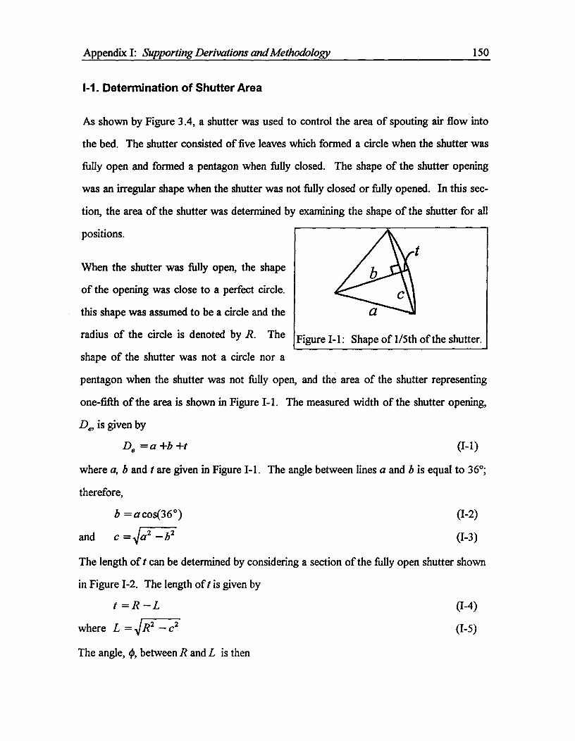
Appendix I: Supporting Derivations and Methodology^ 150
I-1. Determination of Shutter Area
As shown by Figure 3.4, a shutter was used to control the area of spouting air flow into
the bed. The shutter consisted of five leaves which formed a circle when the shutter was
fully open and formed a pentagon when fully closed. The shape of the shutter opening
was an irregular shape when the shutter was not fully closed or fully opened. In this sec-
tion, the area of the shutter was determined by examining the shape of the shutter for all
positions.
When the shutter was fully open, the shape
of the opening was close to a perfect circle.
this shape was assumed to be a circle and the
radius of the circle is denoted by R. The
shape of the shutter was not a circle nor a
pentagon when the shutter was not fully open, and the area of the shutter representing
one-fifth of the area is shown in Figure I-1. The measured width of the shutter opening,
De, is given by
De = a +b +t
where a, b and t are given in Figure I-1. The angle between lines a and b is equal to 36°;
therefore,
b = a cos(36°)
and c = 11c:2 — b2
The length of t can be determined by considering a section of the fully open shutter shown
in Figure 1-2. The length of t is given by
t = R — L^ (I-4)
where L = /R2 — c2^(I-5)
The angle, 4), between R and L is then
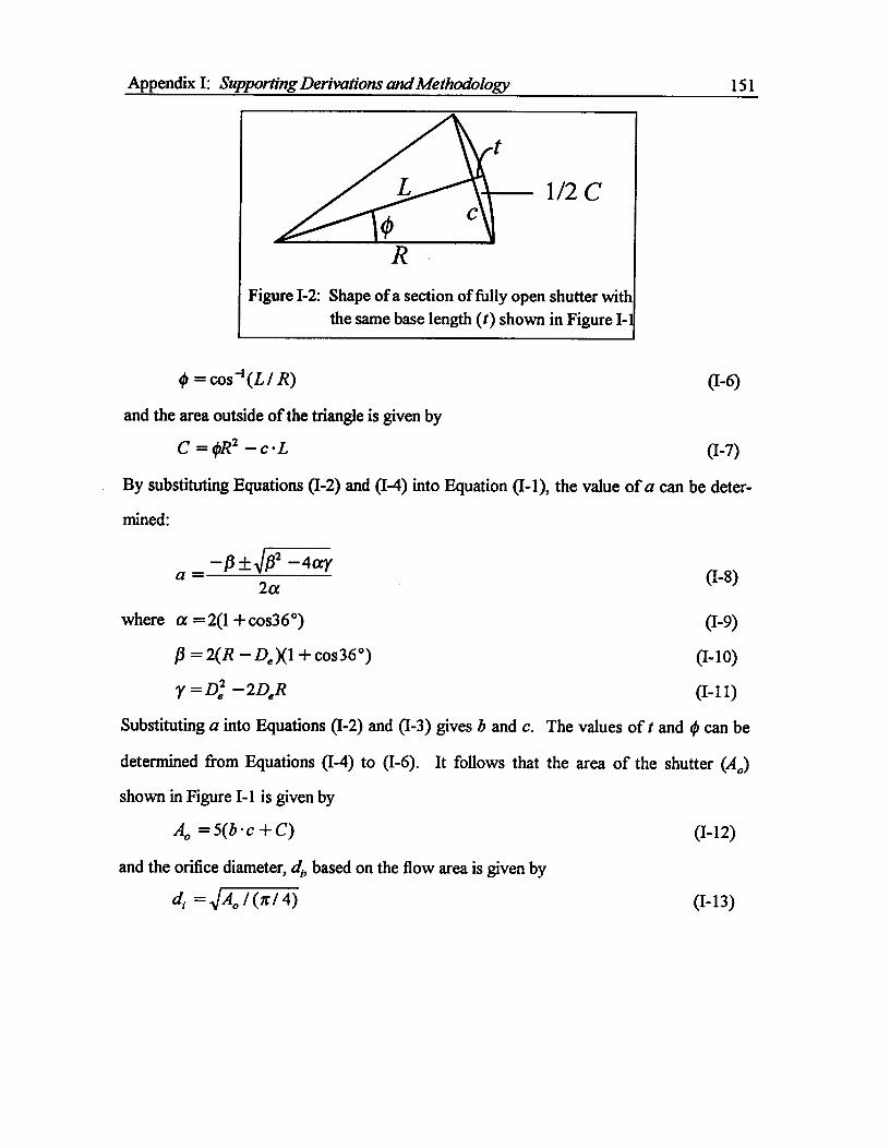
Appendix I: Supporting Derivations and Methodology^ 151
Figure 1-2: Shape of a section of fully open shutter withthe same base length (t) shown in Figure 1-1
ip = cos 4 (L / R)^ (1-6)
and the area outside of the triangle is given by
C = tpR2 — c - L^
(1-7)
By substituting Equations (1-2) and (1-4) into Equation (I-1), the value of a can be deter-
mined:
— f3 ± 3I 132 — 4ay(1-8)—a
2a
where a =2(1 + cos36°)(I-9)
/3 =2(R —4)(1 + cos36°) (I-10)
y = D6 —2DeR (1- 11)
Substituting a into Equations (I-2) and (I-3) gives b and c. The values oft and 0 can be
determined from Equations (I-4) to (I-6). It follows that the area of the shutter (A0)
shown in Figure I-1 is given by
Ao = 5(b - c + C)^ (1-12)
and the orifice diameter, do based on the flow area is given by
di = 1124o 1(xl 4)^ (1-13)
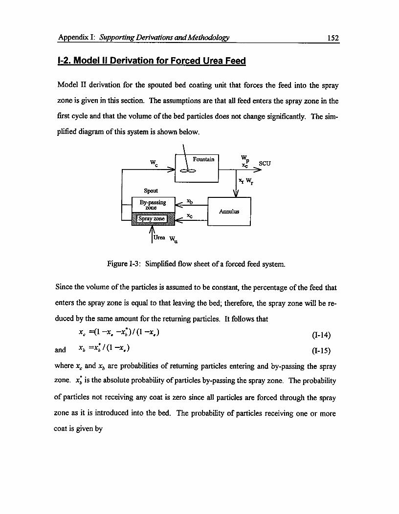
wxep
scu
xi- wr
By-passingIIzone
Spray zone\\ ' MIAnnulus
Appendix I: Supporting Derivations and Methodology^ 152
1-2. Model II Derivation for Forced Urea Feed
Model II derivation for the spouted bed coating unit that forces the feed into the spray
zone is given in this section. The assumptions are that all feed enters the spray zone in the
first cycle and that the volume of the bed particles does not change significantly. The sim-
plified diagram of this system is shown below.
rea wu
Figure 1-3: Simplified flow sheet of a forced feed system.
Since the volume of the particles is assumed to be constant, the percentage of the feed that
enters the spray zone is equal to that leaving the bed; therefore, the spray zone will be re-
duced by the same amount for the returning particles. It follows thatx„ 1 —x, —4)41 x,)^ (1-14)
and^xb =x sb / (1 —x,)^ (I-15)
where x, and xb are probabilities of returning particles entering and by-passing the spray
izone. xb is the absolute probability of particles by-passing the spray zone. The probability
of particles not receiving any coat is zero since all particles are forced through the spray
zone as it is introduced into the bed. The probability of particles receiving one or more
coat is given by
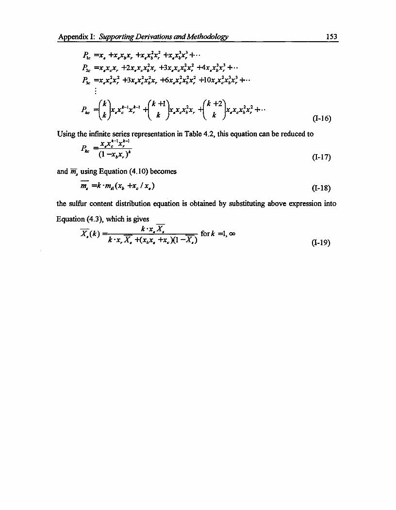
Appendix I: Supporting Derivations and Methodology^ 153
=x. +xexbx, -Exexb2x,2^+ • •P2c =XeXcXr +2;;X:Xr +3X.XcX:X,2 +4;x:x: + • •p3c =xexe2xr2 +3xexc2xb2xr +15xexc2x452xr2 +10xexe2x63xr3 +••
(1-16)
Using the infinite series representation in Table 4.2, this equation can be reduced tok-1 k-1P — x. x„
ke (1 —xbx,)k^ (I-17)
and Fir, using Equation (4.10) becomes
Ins =k • ynd (xb +x, I x.)^ (1-18)
the sulfur content distribution equation is obtained by substituting above expression into
Equation (4.3), which is gives
X „(k) —^kx.X^fork =1, 03k -x, X, +(xbx. +x,)(1—X,)
1x x"x"f,c^•^k^ec_rik +1 X Xc XA2Xr k +2 X X Xh2X2 4•••
(1-19)
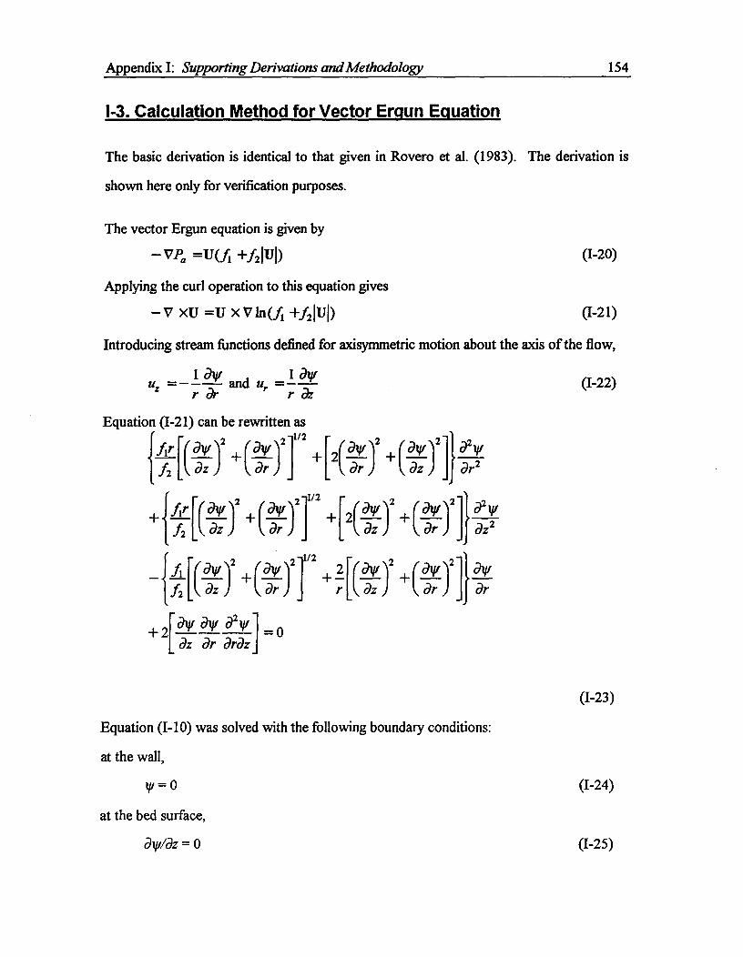
Appendix I: Supporting Derivations and Methodology^ 154
1-3. Calculation Method for Vector Erqun Equation
The basic derivation is identical to that given in Rovero et al. (1983). The derivation is
shown here only for verification purposes.
The vector Ergun equation is given by
— VPa =WI +f2IUI)
Applying the curl operation to this equation gives
— V XU =IT X V ln(ji ±f2111)
(1-20)
(1-21)
Introducing stream functions defined for axisymmetric motion about the axis of the flow,
1 thy ,^1 ay,
^
u =– — and u ..----^ (I-22)Z^r ar^r r az
Equation (I-21) can be rewritten as1/2fff.2 .11)2 + ( (Z-)2] +[2(':..f 4- (a-1121 'dr':
+ { .- -jr2-[(a-1,37r )2 + (Z212 +[2(aJa--) 2 + (a-2-12 ]} '2:
— { -//21( 431a)2 + (Z2 1/2 + [If + ( d142 11 :+2 alY (31Y (321 — 0
az ar ardz
(1-23)
Equation (I-10) was solved with the following boundary conditions:
at the wall,
w = 00
at the bed surface,
atiildz = 0
(1-24)
(I-25)
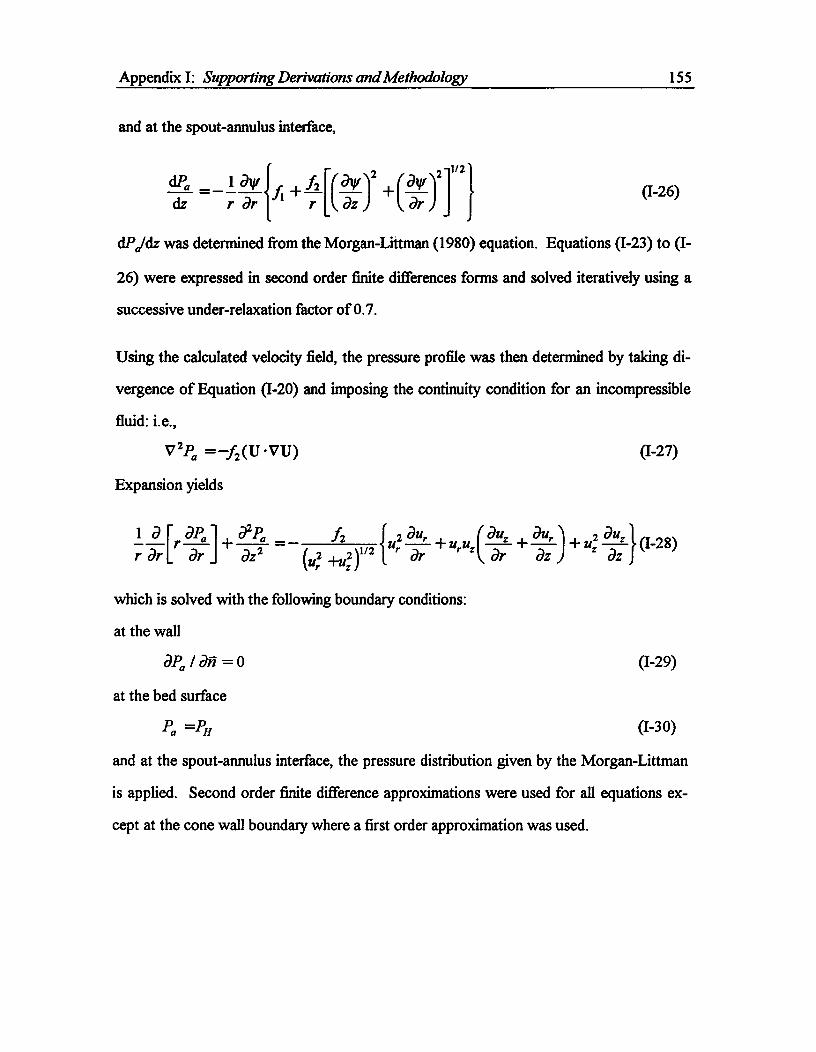
Appendix I: Supporting Derivations and Methodology^ 155
and at the spout-annulus interface,
dPa ._lavf + r, ) 2^)21/21
dz^r^r az )^dr(1-26)
dPjdz was determined from the Morgan-Littman (1980) equation. Equations (1-23) to (I-
26) were expressed in second order finite differences forms and solved iteratively using a
successive under-relaxation factor of 0.7.
Using the calculated velocity field, the pressure profile was then determined by taking di-
vergence of Equation (1-20) and imposing the continuity condition for an incompressible
fluid: i.e.,
V 2P,„ =—f2(U.VU) (1-27)
Expansion yields
[r ]+^— ^A ^2 our1/2 {11^+uruarr dr^dr^C922^(11,2 +Uz2
duz our
dr az2 aU
+ U 41-28)
which is solved with the following boundary conditions:
at the wall
dP,, I an = 0^ (1-29)
at the bed surface
Pa =PH^ (1-30)
and at the spout-annulus interface, the pressure distribution given by the Morgan-Littman
is applied. Second order finite difference approximations were used for all equations ex-
cept at the cone wall boundary where a first order approximation was used.

Appendix I: Supporting Derivations and Methodology^ 156
1-4, Sulfur Sampling Devices
Various sulfur sampling devices were tested for use in the spouted bed and none were
found to be satisfactory. In this section, the problems associated with the devices consid-
ered for measuring the sulfur concentration in the spouted bed are summarized to aid
those wishing to continue this work. Brief descriptions of each device as well as
measurement procedures and problems associated with each device are provided in Tables
I-1 to 1-6.
All devices considered here include a tip with 1 mm opening. The direct sampling of sul-
fur (without heating the sampling tube) was not possible as molten sulfur smothered the
tip of the sampler and immediately plugged the tip. Heated samplers were therefore con-
sidered. Series of tests were conducted with the packed bed heating element; however,
electrical contact between the iron particles could not be established when the iron
particles were in a loose state. Sintering of iron particles resulted in a very low electrical
resistance across the packed bed and partial sintering resulted in a very fragile bed. Plate
design and laser beam methods were also considered, but they were regarded difficult to
construct and costly.
Finally, the quartz tube designs using NiCr wires to heat the tip were built and tested. The
3/8" three-tube was found too large to place in the spout. A smaller 1/4" two-tube was
found to be a satisfactory size for sampling in the spout. However, this design also failed.
The problems inherent to this design were that the quartz tube eventually broke as the
tube was moved around the bed (i.e., slight force against this tube broke the tube), the
exposed NiCr wires could not withstand the presence of urea dust and the impact of SCU
particles, and wire sizes that can be used were limited.
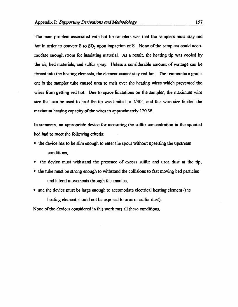
Appendix I: Supporting Derivations and Methodology^ 157
The main problem associated with hot tip samplers was that the samplers must stay red
hot in order to convert S to SO2 upon impaction of S. None of the samplers could acco-
modate enough room for insulating material. As a result, the heating tip was cooled by
the air, bed materials, and sulfur spray. Unless a considerable amount of wattage can be
forced into the heating elements, the element cannot stay red hot. The temperature gradi-
ent in the sampler tube caused urea to melt over the heating wires which prevented the
wires from getting red hot. Due to space limitations on the sampler, the maximum wire
size that can be used to heat the tip was limited to 1/30", and this wire size limited the
maximum heating capacity of the wires to approximately 120 W.
In summary, an appropriate device for measuring the sulfur concentration in the spouted
bed had to meet the following criteria:
• the device has to be slim enough to enter the spout without upsetting the upstream
conditions,
• the device must withstand the presence of excess sulfur and urea dust at the tip,
• the tube must be strong enough to withstand the collisions to fast moving bed particles
and lateral movements through the annulus,
• and the device must be large enough to accomodate electrical heating element (the
heating element should not be exposed to urea or sulfur dust).
None of the devices considered in this work met all these conditions.
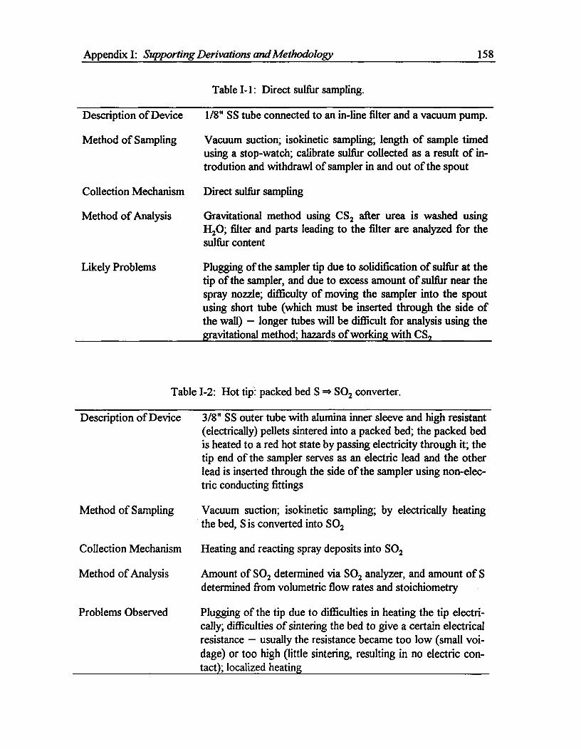
Appendix I: Supporting Derivations and Methodology^ 158
Table I-1: Direct sulfur sampling.
Description of Device
Method of Sampling
Collection Mechanism
Method of Analysis
Likely Problems
1/8" SS tube connected to an in-line filter and a vacuum pump.
Vacuum suction; isokinetic sampling; length of sample timedusing a stop-watch; calibrate sulfur collected as a result of in-trodution and withdrawl of sampler in and out of the spout
Direct sulfur sampling
Gravitational method using CS2 after urea is washed usingH2O; filter and parts leading to the filter are analyzed for thesulfur content
Plugging of the sampler tip due to solidification of sulfur at thetip of the sampler, and due to excess amount of sulfur near thespray nozzle; difficulty of moving the sampler into the spoutusing short tube (which must be inserted through the side ofthe wall) — longer tubes will be difficult for analysis using thegravitational method; hazards of working with CS,
Table 1-2: Hot tip: packed bed S = SO 2 converter.
Description of Device
Method of Sampling
Problems Observed
3/8" SS outer tube with alumina inner sleeve and high resistant(electrically) pellets sintered into a packed bed; the packed bedis heated to a red hot state by passing electricity through it; thetip end of the sampler serves as an electric lead and the otherlead is inserted through the side of the sampler using non-elec-tric conducting fittings
Vacuum suction; isokinetic sampling; by electrically heatingthe bed, S is converted into SO 2
Heating and reacting spray deposits into SO 2
Amount of SO 2 determined via SO2 analyzer, and amount of Sdetermined from volumetric flow rates and stoichiometry
Plugging of the tip due to difficulties in heating the tip electri-cally; difficulties of sintering the bed to give a certain electricalresistance — usually the resistance became too low (small voi-dage) or too high (little sintering, resulting in no electric con-tact); localized heating
Collection Mechanism
Method of Analysis
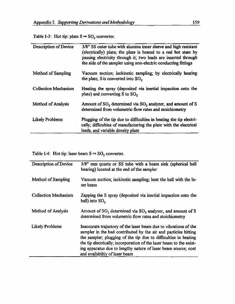
Appendix I: Supporting Derivations and Methodology^ 159
Table 1-3: Hot tip: plate S SO2 converter.
Description of Device
Method of Sampling
Collection Mechanism
Method of Analysis
Likely Problems
3/8" SS outer tube with alumina inner sleeve and high resistant(electrically) plate; the plate is heated to a red hot state bypassing electricity through it; two leads are inserted throughthe side of the sampler using non-electric conducting fittings
Vacuum suction; isokinetic sampling; by electrically heatingthe plate, S is converted into SO2
Heating the spray (deposited via inertial impaction onto theplate) and converting S to SO2
Amount of SO2 determined via SO2 analyzer, and amount of Sdetermined from volumetric flow rates and stoichiometry
Plugging of the tip due to difficulties in heating the tip electri-cally; difficulties of manufacturing the plate with the electricalleads, and variable density plate
Table 1-4: Hot tip: laser beam S SO2 converter.
Description of Device
Method of Sampling
Collection Mechanism
Method of Analysis
Likely Problems
3/8" mm quartz or SS tube with a beam sink (spherical ballbearing) located at the end of the sampler
Vacuum suction; isokinetic sampling; heat the ball with the la-ser beam
Zapping the S spray (deposited via inertial impaction onto theball) into SO2
Amount of SO 2 determined via SO2 analyzer, and amount of Sdetermined from volumetric flow rates and stoichiometry
Inaccurate trajectory of the laser beam due to vibrations of thesampler in the bed contributed by the air and particles hittingthe sampler; plugging of the tip due to difficulties in heatingthe tip electrically; incorporation of the laser beam to the exist-ing apparatus due to lengthy nature of laser beam source; costand availabiltiy of laser beam
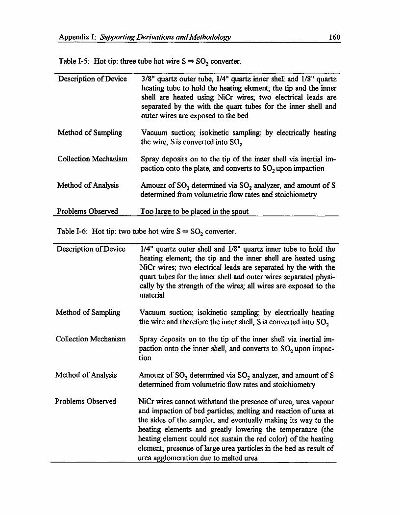
Appendix I: Supporting Derivations and Methodology^ 160
Table 1-5: Hot tip: three tube hot wire S SO2 converter.
Description of Device
Method of Sampling
Collection Mechanism
Method of Analysis
Problems Observed
3/8" quartz outer tube, 1/4" quartz inner shell and 1/8" quartzheating tube to hold the heating element; the tip and the innershell are heated using NiCr wires; two electrical leads areseparated by the with the quart tubes for the inner shell andouter wires are exposed to the bed
Vacuum suction; isokinetic sampling; by electrically heatingthe wire, S is converted into SO2
Spray deposits on to the tip of the inner shell via inertial im-paction onto the plate, and converts to SO2 upon impaction
Amount of SO2 determined via SO 2 analyzer, and amount of Sdetermined from volumetric flow rates and stoichiometry
Too large to be placed in the spout
Table 1-6: Hot tip: two tube hot wire S SO 2 converter.
Description of Device
Method of Sampling
Collection Mechanism
Method of Analysis
Problems Observed
1/4" quartz outer shell and 1/8" quartz inner tube to hold theheating element; the tip and the inner shell are heated usingNiCr wires; two electrical leads are separated by the with thequart tubes for the inner shell and outer wires separated physi-cally by the strength of the wires; all wires are exposed to thematerial
Vacuum suction; isokinetic sampling; by electrically heatingthe wire and therefore the inner shell, S is converted into SO2
Spray deposits on to the tip of the inner shell via inertial im-paction onto the inner shell, and converts to SO 2 upon impac-tion
Amount of SO2 determined via SO2 analyzer, and amount of Sdetermined from volumetric flow rates and stoichiometry
NiCr wires cannot withstand the presence of urea, urea vapourand impaction of bed particles; melting and reaction of urea atthe sides of the sampler, and eventually making its way to theheating elements and greatly lowering the temperature (theheating element could not sustain the red color) of the heatingelement; presence of large urea particles in the bed as result ofurea agglomeration due to melted urea
Appendix I: Supporting Derivations and Methodology^ 161
1-5. Batch Coating Model
Model N may be manipulated to predict coating distributions of batch products. In the
continuous coating operation, the simulation of a particle in the bed begins as the particle
enters the bed and the simulation ends as the particle leaves the bed. The probability asso-
ciated with the urea feed location determines the path of the particle during its first cycle
through the bed, and the probability associated with the returning particles from the foun-
tain determines the subsequent paths. The exit probability of the particle in the fountain
determines the termination of the simulation for each particle. In the batch operation, all
particles have the same residence time in the bed, and hence, the probabilities associated
with the feed location and with the particles exiting no longer apply. Instead, the total
residence time of the particle indicates the termination of the simulation. The coating
amount a particle receives in each cycle can be calculated in the same way as a particle in
the continuous operation; therefore, the only additional information required to determine
the coating distribution for the batch product is the cycle time.
The cycle time for the particle is calculated from Equation (4.52) and the total residence
time from Equation (4.55). The simulation ends when the total cycle time is equal to the
total operating time.
A correction to the above equation is necessary for the first cycle. In the first cycle or at
the start of a coating operation, bed particles could be located anywhere in the bed. To
determine the location of each particle, the Monte Carlo method is applied. First, the ver-
tical position of the particle in the annulus is determined using a random number (NR):
NR •=(Vcco — Ash,)/ K, for conical section
NR =(ic +^— k )A — Ash,)I V01 , for cylindrical section
where Vtc0 = bed volume in the conical section; function of hi
A s = area of the spout
(I-31)
(1-32)

Appendix I: Supporting Derivations and Methodology^ 162
Kat = total bed volume
Va = total bed volume in conical section
A = bed surface area in the cylindrical section
hc = cone height
The radial position (Di) at hi is determined using another random number,
NR = (Le --.1)1(D 2 {hi )^ (1-33)
where D{z) = bed diameter at hi
Ds = spout diameter
The location where the particle enters the spout (h,) can be calculated from the following
particle mass balance which assumes no radial velocity gradient in the annulus:
va (1 —ea )Aa lh, = v ,(1 —e s )24,1z,^(1-34)
where va = particle velocity in the annulus at hi
Aa = annulus area at hi
ea, es = voidages in the annulus and the spout, respectively
= particle velocity in the spout at ;
The value of ; can be determined from a root finding method. The values va and Aa are
given by
va = (1 —63)v,A,Ihi(1 —Ea )Aa i h,^(1-35)
and Aa = Ii(Db + 2hi tan30°), for conical section^ (1-36)
Aa =i D 2 , for cylindrical section^ (1-37)
where Db = bed diameter at the base of the bed
D = bed diameter of the cylindrical section of the bed
The cycle time can then be calculated from Equation (4.52) with hi and ; as the limits.
For subsequent cycles, the cycle time can be calculated using the same equation with the
limits of H and ;.
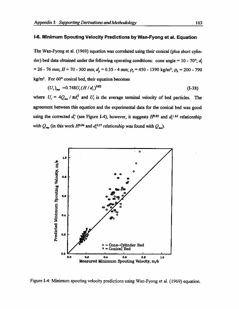
Appendix I: Supporting Derivations and Methodology^ 163
1-6. Minimum Spouting Velocity Predictions by Wan-Fyong et al. Equation
The Wan-Fyong et al. (1969) equation was correlated using their conical (plus short cylin-
der) bed data obtained under the following operating conditions: cone angle = 10 - 70°;
= 26 - 76 mm; H= 70 - 300 mm; dp = 0.35 - 4 mm; ps = 450 - 1390 kg/m3; pb = 200 - 790
kg/m3 . For 60° conical bed, their equation becomes
(U,)„,, =0.748U, (H I di )°82^(I-38)
where Ui = 4Q„,, / irdiF and U, is the average terminal velocity of bed particles. The
agreement between this equation and the experimental data for the conical bed was good
using the corrected di (see Figure 1-4); however, it suggests H3•82 and dills relationship
with Q,, (in this work H3 .96 and d,°37 relationship was found with a„).
1.0
a
O
-
0.8
O
•
0.8
61'
E
• 0.4
02
0.00.0^02^OA^0.6^0.8^to
Measured Minimum Spouting Velocity. m/s
Figure 1-4: Minimum spouting velocity predictions using Wan-Fyong et al. (1969) equation.
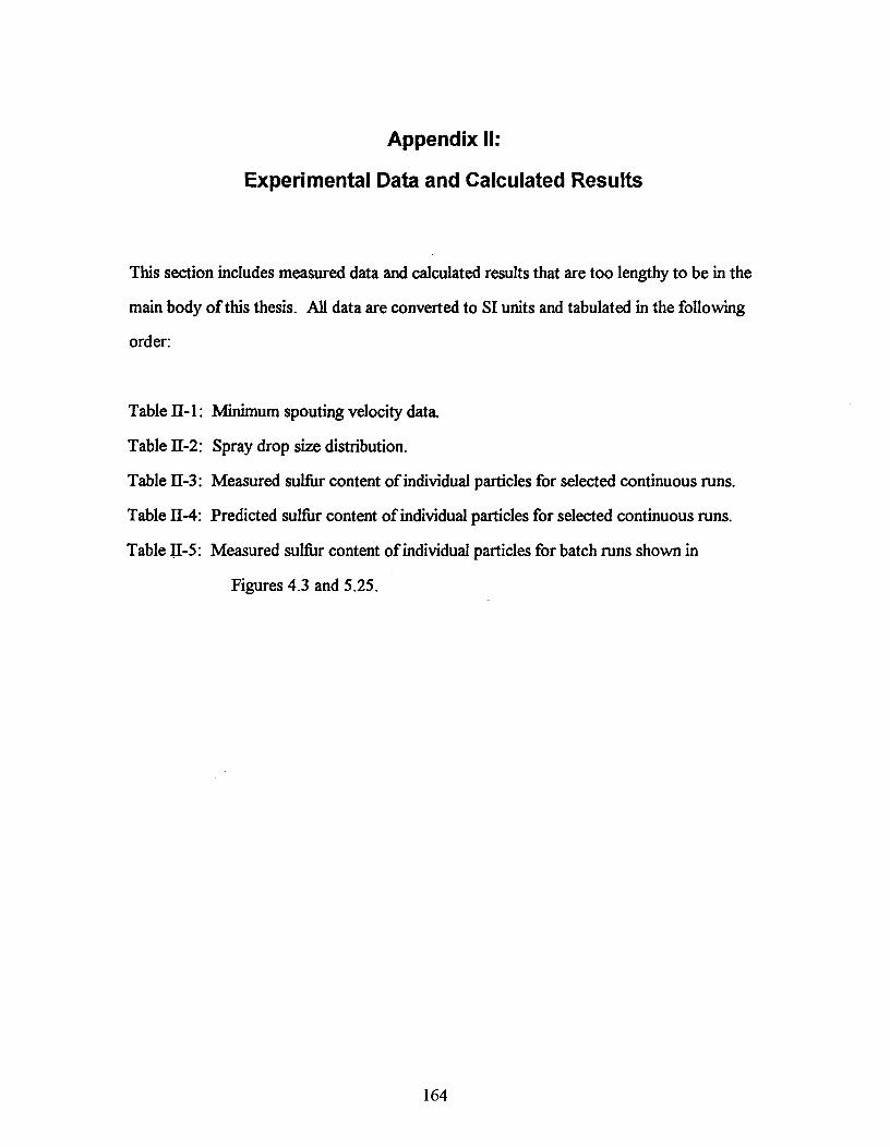
Appendix II:
Experimental Data and Calculated Results
This section includes measured data and calculated results that are too lengthy to be in the
main body of this thesis. All data are converted to SI units and tabulated in the following
order:
Table II-1: Minimum spouting velocity data.
Table II-2: Spray drop size distribution.
Table II-3: Measured sulfur content of individual particles for selected continuous runs.
Table II-4: Predicted sulfur content of individual particles for selected continuous runs.
Table II-5: Measured sulfur content of individual particles for batch runs shown in
Figures 4.3 and 5.25.
164

Appendix II: Experimental Data and Calculated Results^ 165
Table II-1: Minimum spouting velocity data.
dp, mm pp, kg/m3 di, mm Qa,L^I s Qs, Us H, m D, m T, °C
2.33 1471 25.1 0.000 20.8 0.255 0.24 182.33 1471 25.1 0.447 20.5 0.255 0.24 182.33 1471 25.1 0.878 20.1 0.255 0.24 182.33 1471 29.9 0.000 22.5 0.255 0.24 182.33 1471 29.9 0.447 22.1 0.255 0.24 182.33 1471 29.9 0.878 21.6 0.255 0.24 182.33 1471 29.9 0.447 21.3 0.255 0.24 552.33 1471 29.9 0.878 20.3 0.255 0.24 552.33 1471 29.9 0.000 22.0 0.255 0.24 552.33 1471 25.1 0.447 19.7 0.255 0.24 582.33 1471 25.1 0.878 18.9 0.255 0.24 582.33 1471 25.1 0.000 20.2 0.255 0.24 582.33 1471 29.9 0.447 21.3 0.255 0.24 712.33 1471 29.9 0.878 20.3 0.255 0.24 712.33 1471 29.9 0.000 21.6 0.255 0.24 712.33 1471 29.9 0.447 24.7 0.360 0.24 552.33 1471 29.9 0.878 24.1 0.360 0.24 552.33 1471 29.9 0.000 25.2 0.360 0.24 552.33 1471 25.1 0.447 22.9 0.360 0.24 552.33 1471 25.1 0.878 22.1 0.360 0.24 552.33 1471 25.1 0.000 23.2 0.360 0.24 552.36 1490 29.9 0.447 21.7 0.255 0.24 622.36 1490 29.9 0.878 20.6 0.255 0.24 622.36 1490 29.9 0.000 22.3 0.255 0.24 622.36 1490 25.1 0.447 20.3 0.255 0.24 622.36 1490 25.1 0.878 19.5 0.255 0.24 622.36 1490 25.1 0.000 20.8 0.255 0.24 622.27 1427 29.9 0.447 20.9 0.260 0.24 612.27 1427 29.9 0.878 19.9 0.260 0.24 612.27 1427 29.9 0.000 21.2 0.260 0.24 612.27 1427 25.1 0.447 19.1 0.260 0.24 612.27 1427 25.1 0.878 18.3 0.260 0.24 612.27 1427 25.1 0.000 19.4 0.260 0.24 612.16 1335 29.9 0.000 20.1 0.270 0.24 202.16 1335 29.9 0.447 19.5 0.270 0.24 202.16 1335 29.9 0.878 18.7 0.270 0.24 202.16 1335 25.1 0.000 18.6 0.270 0.24 202.16 1335 25.1 0.447 18.3 0.270 0.24 202.16 1335 25.1 0.878 17.7 0.270 0.24 20

Appendix II: Experimental Data and Calculated Results^ 166
Table 111- 1 continued.
dp, mm pp, kg/m3 di, mm Qa, L s Qs, L/s H, m D, m T, °C2.16 1335 29.9 0.000 23.9 0.405 0.24 202.16 1335 29.9 0.447 23.6 0.405 0.24 202.16 1335 29.9 0.878 23.3 0.405 0.24 202.16 1335 25.1 0.000 22.0 0.405 0.24 202.16 1335 25.1 0.447 21.6 0.405 0.24 202.16 1335 25.1 0.878 21.2 0.405 0.24 202.16 1335 29.9 0.000 18.7 0.270 0.24 602.16 1335 29.9 0.447 18.3 0.270 0.24 602.16 1335 29.9 0.878 17.6 0.270 ,^0.24 602.16 1335 25.1 0.000 17.5 0.270 0.24 602.16 1335 25.1 0.447 16.8 0.270 0.24 602.16 1335 25.1 0.878 16.0 0.270 0.24 602.16 1335 29.9 0.000 22.6 0.405 0.24 602.16 1335 29.9 0.447 22.3 0.405 0.24 602.16 1335 29.9 0.878 21.6 0.405 0.24 602.16 1335 25.1 0.000 20.2 0.405 0.24 602.16 1335 25.1 0.447 19.8 0.405 0.24 602.16 1335 25.1 0.878 19.2 0.405 0.24 602.8 927 24.7 0.000 24.2 0.297 0.45 242.8 927 28.2 0.000 25.1 0.297 0.45 242.8 927 30.8 0.000 25.3 0.297 0.45 242.8 927 35.1 0.000 26.9 0.297 0.45 242.8 927 24.7 0.528 23.7 0.297 0.45 242.8 927 28.2 0.528 24.5 0.297 0.45 242.8 927 30.8 0.528 25.0 0.297 0.45 242.8 927 35.1 0.528 26.5 0.297 0.45 242.8 927 24.7 0.868 23.4 0.297 0.45 242.8 927 28.2 0.868 24.0 0.297 0.45 242.8 927 30.8 0.868 24.3 0.297 0.45 242.8 927 35.1 0.868 26.0 0.297 0.45 242.8 927 21.2 0.000 20.2 0.249 0.45 242.8 927 24.7 0.000 21.3 0.249 0.45 242.8 927 28.2 0.000 22.1 0.249 0.45 242.8 927 30.8 0.000 22.7 0.249 0.45 242.8 927 35.1 0.000 24.0 0.249 0.45 242.8 927 21.2 0.528 19.6 0.249 0.45 242.8 927 24.7 0.528 20.8 0.249 0.45 242.8 927 28.2 0.528 21.8 0.249 0.45 242.8 927 30.8 0.528 22.1 0.249 0.45 24
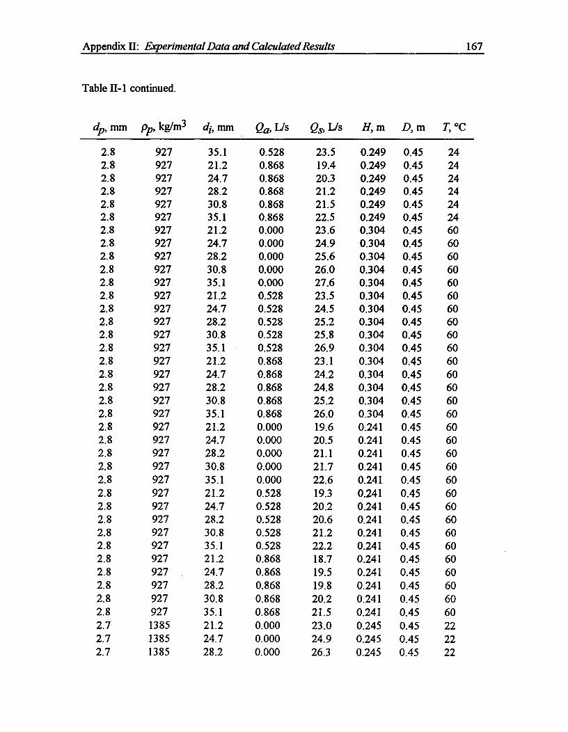
Appendix II: Experimental Data and Calculated Results^ 167
Table II-1 continued.
dp, nun pp, kem3 di, trim Qa,L s Qs,L s H, m D, m T, °C
2.8 927 35.1 0.528 23.5 0.249 0.45 242.8 927 21.2 0.868 19.4 0.249 0.45 242.8 927 24.7 0.868 20.3 0.249 0.45 242.8 927 28.2 0.868 21.2 0.249 0.45 242.8 927 30.8 0.868 21.5 0.249 0.45 242.8 927 35.1 0.868 22.5 0.249 0.45 242.8 927 21.2 0.000 23.6 0.304 0.45 602.8 927 24.7 0.000 24.9 0.304 0.45 602.8 927 28.2 0.000 25.6 0.304 0.45 602.8 927 30.8 0.000 26.0 0.304 0.45 602.8 927 35.1 0.000 27.6 0.304 0.45 602.8 927 21.2 0.528 23.5 0.304 0.45 602.8 927 24.7 0.528 24.5 0.304 0.45 602.8 927 28.2 0.528 25.2 0.304 0.45 602.8 927 30.8 0.528 25.8 0.304 0.45 602.8 927 35.1 0.528 26.9 0.304 0.45 602.8 927 21.2 0.868 23.1 0.304 0.45 602.8 927 24.7 0.868 24.2 0.304 0.45 602.8 927 28.2 0.868 24.8 0.304 0.45 602.8 927 30.8 0.868 25.2 0.304 0.45 602.8 927 35.1 0.868 26.0 0.304 0.45 602.8 927 21.2 0.000 19.6 0.241 0.45 602.8 927 24.7 0.000 20.5 0.241 0.45 602.8 927 28.2 0.000 21.1 0.241 0.45 602.8 927 30.8 0.000 21.7 0.241 0.45 602.8 927 35.1 0.000 22.6 0.241 0.45 602.8 927 21.2 0.528 19.3 0.241 0.45 602.8 927 24.7 0.528 20.2 0.241 0.45 602.8 927 28.2 0.528 20.6 0.241 0.45 602.8 927 30.8 0.528 21.2 0.241 0.45 602.8 927 35.1 0.528 22.2 0.241 0.45 602.8 927 21.2 0.868 18.7 0.241 0.45 602.8 927 24.7 0.868 19.5 0.241 0.45 602.8 927 28.2 0.868 19.8 0.241 0.45 602.8 927 30.8 0.868 20.2 0.241 0.45 602.8 927 35.1 0.868 21.5 0.241 0.45 602.7 1385 21.2 0.000 23.0 0.245 0.45 222.7 1385 24.7 0.000 24.9 0.245 0.45 222.7 1385 28.2 0.000 26.3 0.245 0.45 22

Appendix II: Experimental Data and Calculated Results^ 168
Table II-1 continued.
dp, mm pp, kg/m3 di, mm Qa, L/s Qs, Lis H, m D, m T, °C2.7 1385 30.8 0.000 26.6 0.245 0.45 222.7 1385 35.1 0.000 28.1 0.245 0.45 222.7 1385 21.2 0.528 22.7 0.245 0.45 222.7 1385 24.7 0.528 24.4 0.245 0.45 222.7 1385 28.2 0.528 25.8 0.245 0.45 222.7 1385 30.8 0.528 26.3 0.245 0.45 222.7 1385 35.1 0.528 27.8 0.245 0.45 222.7 1385 21.2 0.868 22.2 0.245 0.45 222.7 1385 24.7 0.868 23.8 0.245 0.45 222.7 1385 28.2 0.868 24.9 0.245 0.45 222.7 1385 30.8 0.868 25.5 0.245 0.45 222.7 1385 35.1 0.868 26.6 0.245 0.45 222.7 1385 21.2 0.000 27.7 0.289 0.45 222.7 1385 24.7 0.000 28.6 0.289 0.45 222.7 1385 28.2 0.000 29.5 0.289 0.45 222.7 1385 30.8 0.000 30.2 0.289 0.45 222.7 1385 35.1 0.000 31.6 0.289 0.45 222.7 1385 21.2 0.528 27.4 0.289 0.45 222.7 1385 24.7 0.528 28.3 0.289 0.45 222.7 1385 28.2 0.528 29.1 0.289 0.45 222.7 1385 30.8 0.528 29.8 0.289 0.45 222.7 1385 35.1 0.528 31.2 0.289 0.45 222.7 1385 21.2 0.868 27.0 0.289 0.45 222.7 1385 24.7 0.868 28.0 0.289 0.45 222.7 1385 28.2 0.868 28.7 0.289 0.45 222.7 1385 30.8 0.868 29.3 0.289 0.45 222.7 1385 35.1 0.868 30.8 0.289 0.45 222.7 1385 21.2 0.000 24.2 0.243 0.45 652.7 1385 24.7 0.000 25.4 0.243 0.45 652.7 1385 28.2 0.000 26.0 0.243 0.45 652.7 1385 30.8 0.000 26.3 0.243 0.45 652.7 1385 35.1 0.000 28.5 0.243 0.45 652.7 1385 21.2 0.528 23.8 0.243 0.45 652.7 1385 24.7 0.528 24.8 0.243 0.45 652.7 1385 28.2 0.528 25.7 0.243 0.45 652.7 1385 30.8 0.528 26.0 0.243 0.45 652.7 1385 35.1 0.528 27.9 0.243 0.45 652.7 1385 21.2 0.868 23.2 0.243 0.45 652.7 1385 24.7 0.868 24.2 0.243 0.45 65
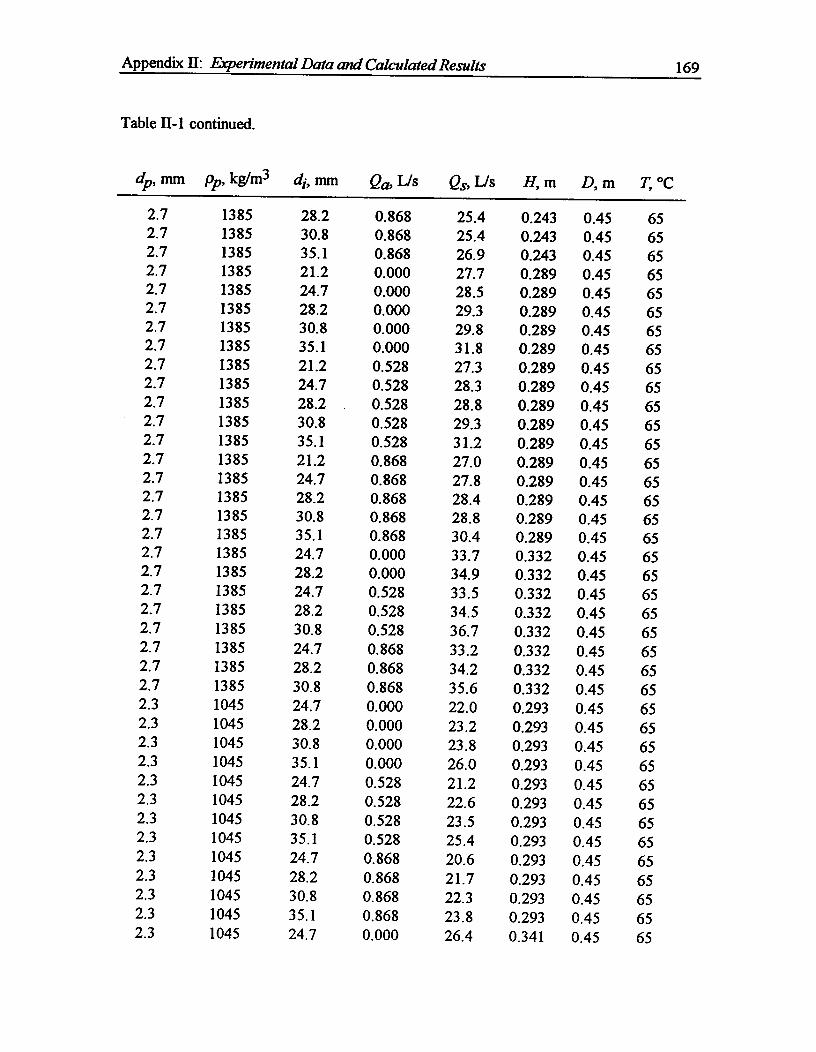
Appendix II: Experimental Data and Calculated Results^ 169
Table II- 1 continued.
dp, mm pp, kg/m3 di, nun Qa, U Qs, Us H, m D, m T, °C
2.7 1385 28.2 0.868 25.4 0.243 0.45 652.7 1385 30.8 0.868 25.4 0.243 0.45 652.7 1385 35.1 0.868 26.9 0.243 0.45 652.7 1385 21.2 0.000 27.7 0.289 0.45 652.7 1385 24.7 0.000 28.5 0.289 0.45 652.7 1385 28.2 0.000 29.3 0.289 0.45 652.7 1385 30.8 0.000 29.8 0.289 0.45 652.7 1385 35.1 0.000 31.8 0.289 0.45 652.7 1385 21.2 0.528 27.3 0.289 0.45 652.7 1385 24.7 0.528 28.3 0.289 0.45 652.7 1385 28.2 0.528 28.8 0.289 0.45 652.7 1385 30.8 0.528 29.3 0.289 0.45 652.7 1385 35.1 0.528 31.2 0.289 0.45 652.7 1385 21.2 0.868 27.0 0.289 0.45 652.7 1385 24.7 0.868 27.8 0.289 0.45 652.7 1385 28.2 0.868 28.4 0.289 0.45 652.7 1385 30.8 0.868 28.8 0.289 0.45 652.7 1385 35.1 0.868 30.4 0.289 0.45 652.7 1385 24.7 0.000 33.7 0.332 0.45 652.7 1385 28.2 0.000 34.9 0.332 0.45 652.7 1385 24.7 0.528 33.5 0.332 0.45 652.7 1385 28.2 0.528 34.5 0.332 0.45 652.7 1385 30.8 0.528 36.7 0.332 0.45 652.7 1385 24.7 0.868 33.2 0.332 0.45 652.7 1385 28.2 0.868 34.2 0.332 0.45 652.7 1385 30.8 0.868 35.6 0.332 0.45 652.3 1045 24.7 0.000 22.0 0.293 0.45 652.3 1045 28.2 0.000 23.2 0.293 0.45 652.3 1045 30.8 0.000 23.8 0.293 0.45 652.3 1045 35.1 0.000 26.0 0.293 0.45 652.3 1045 24.7 0.528 21.2 0.293 0.45 652.3 1045 28.2 0.528 22.6 0.293 0.45 652.3 1045 30.8 0.528 23.5 0.293 0.45 652.3 1045 35.1 0.528 25.4 0.293 0.45 652.3 1045 24.7 0.868 20.6 0.293 0.45 652.3 1045 28.2 0.868 21.7 0.293 0.45 652.3 1045 30.8 0.868 22.3 0.293 0.45 652.3 1045 35.1 0.868 23.8 0.293 0.45 652.3 1045 24.7 0.000 26.4 0.341 0.45 65
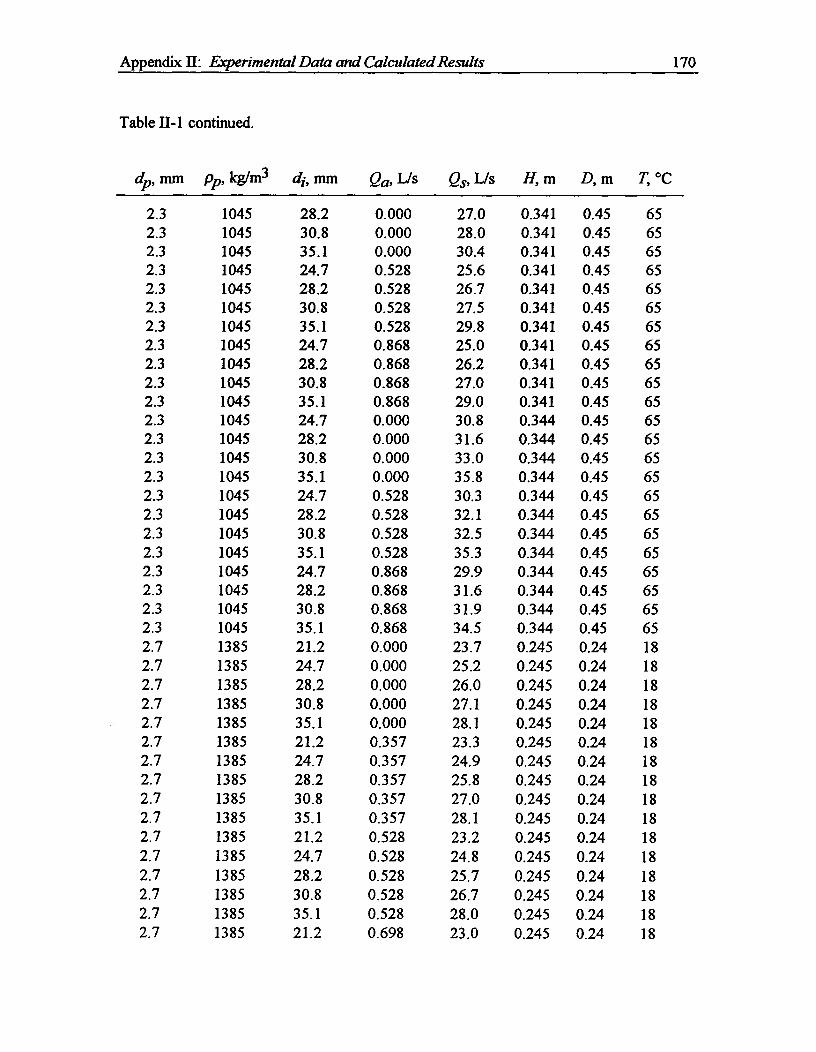
Appendix II: Experimental Data and Calculated Results^ 170
Table II-1 continued.
dp, mm pp, kg/m3 dl, mm Qa, Qs, Us H, m D, m T, °C
2.3 1045 28.2 0.000 27.0 0.341 0.45 652.3 1045 30.8 0.000 28.0 0.341 0.45 652.3 1045 35.1 0.000 30.4 0.341 0.45 652.3 1045 24.7 0.528 25.6 0.341 0.45 652.3 1045 28.2 0.528 26.7 0.341 0.45 652.3 1045 30.8 0.528 27.5 0.341 0.45 652.3 1045 35.1 0.528 29.8 0.341 0.45 652.3 1045 24.7 0.868 25.0 0.341 0.45 652.3 1045 28.2 0.868 26.2 0.341 0.45 652.3 1045 30.8 0.868 27.0 0.341 0.45 652.3 1045 35.1 0.868 29.0 0.341 0.45 652.3 1045 24.7 0.000 30.8 0.344 0.45 652.3 1045 28.2 0.000 31.6 0.344 0.45 652.3 1045 30.8 0.000 33.0 0.344 0.45 652.3 1045 35.1 0.000 35.8 0.344 0.45 652.3 1045 24.7 0.528 30.3 0.344 0.45 652.3 1045 28.2 0.528 32.1 0.344 0.45 652.3 1045 30.8 0.528 32.5 0.344 0.45 652.3 1045 35.1 0.528 35.3 0.344 0.45 652.3 1045 24.7 0.868 29.9 0.344 0.45 652.3 1045 28.2 0.868 31.6 0.344 0.45 652.3 1045 30.8 0.868 31.9 0.344 0.45 652.3 1045 35.1 0.868 34.5 0.344 0.45 652.7 1385 21.2 0.000 23.7 0.245 0.24 182.7 1385 24.7 0.000 25.2 0.245 0.24 182.7 1385 28.2 0.000 26.0 0.245 0.24 182.7 1385 30.8 0.000 27.1 0.245 0.24 182.7 1385 35.1 0.000 28.1 0.245 0.24 182.7 1385 21.2 0.357 23.3 0.245 0.24 182.7 1385 24.7 0.357 24.9 0.245 0.24 182.7 1385 28.2 0.357 25.8 0.245 0.24 182.7 1385 30.8 0.357 27.0 0.245 0.24 182.7 1385 35.1 0.357 28.1 0.245 0.24 182.7 1385 21.2 0.528 23.2 0.245 0.24 182.7 1385 24.7 0.528 24.8 0.245 0.24 182.7 1385 28.2 0.528 25.7 0.245 0.24 182.7 1385 30.8 0.528 26.7 0.245 0.24 182.7 1385 35.1 0.528 28.0 0.245 0.24 182.7 1385 21.2 0.698 23.0 0.245 0.24 18
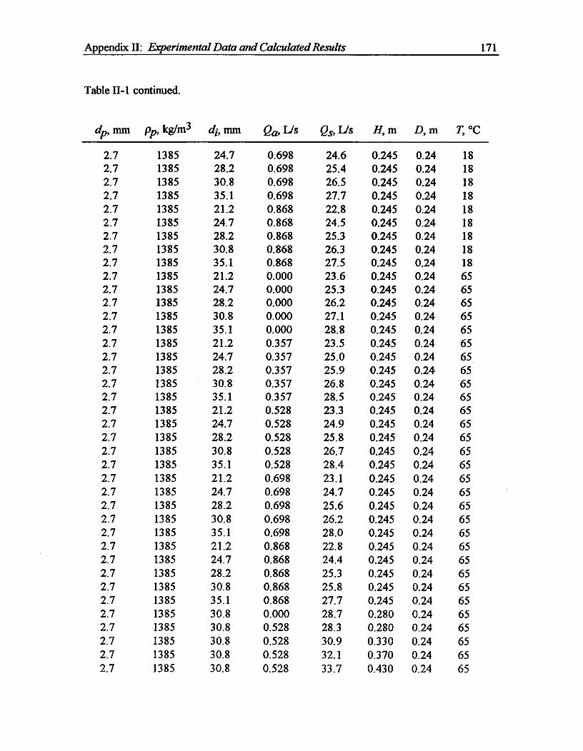
Appendix II: Experimental Data and Calculated Results^ 171
Table 11- 1 continued.
dp, mm pp, kg/m3 di, mm Qa, Us Qs, Us H, m D, m T, °C
2.7 1385 24.7 0.698 24.6 0.245 0.24 182.7 1385 28.2 0.698 25.4 0.245 0.24 182.7 1385 30.8 0.698 26.5 0.245 0.24 182.7 1385 35.1 0.698 27.7 0.245 0.24 182.7 1385 21.2 0.868 22.8 0.245 0.24 182.7 1385 24.7 0.868 24.5 0.245 0.24 182.7 1385 28.2 0.868 25.3 0.245 0.24 182.7 1385 30.8 0.868 26.3 0.245 0.24 182.7 1385 35.1 0.868 27.5 0.245 0.24 182.7 1385 21.2 0.000 23.6 0.245 0.24 652.7 1385 24.7 0.000 25.3 0.245 0.24 652.7 1385 28.2 0.000 26.2 0.245 0.24 652.7 1385 30.8 0.000 27.1 0.245 0.24 652.7 1385 35.1 0.000 28.8 0.245 0.24 652.7 1385 21.2 0.357 23.5 0.245 0.24 652.7 1385 24.7 0.357 25.0 0.245 0.24 652.7 1385 28.2 0.357 25.9 0.245 0.24 652.7 1385 30.8 0.357 26.8 0.245 0.24 652.7 1385 35.1 0.357 28.5 0.245 0.24 652.7 1385 21.2 0.528 23.3 0.245 0.24 652.7 1385 24.7 0.528 24.9 0.245 0.24 652.7 1385 28.2 0.528 25.8 0.245 0.24 652.7 1385 30.8 0.528 26.7 0.245 0.24 652.7 1385 35.1 0.528 28.4 0.245 0.24 652.7 1385 21.2 0.698 23.1 0.245 0.24 652.7 1385 24.7 0.698 24.7 0.245 0.24 652.7 1385 28.2 0.698 25.6 0.245 0.24 652.7 1385 30.8 0.698 26.2 0.245 0.24 652.7 1385 35.1 0.698 28.0 0.245 0.24 652.7 1385 21.2 0.868 22.8 0.245 0.24 652.7 1385 24.7 0.868 24.4 0.245 0.24 652.7 1385 28.2 0.868 25.3 0.245 0.24 652.7 1385 30.8 0.868 25.8 0.245 0.24 652.7 1385 35.1 0.868 27.7 0.245 0.24 652.7 1385 30.8 0.000 28.7 0.280 0.24 652.7 1385 30.8 0.528 28.3 0.280 0.24 652.7 1385 30.8 0.528 30.9 0.330 0.24 652.7 1385 30.8 0.528 32.1 0.370 0.24 652.7 1385 30.8 0.528 33.7 0.430 0.24 65
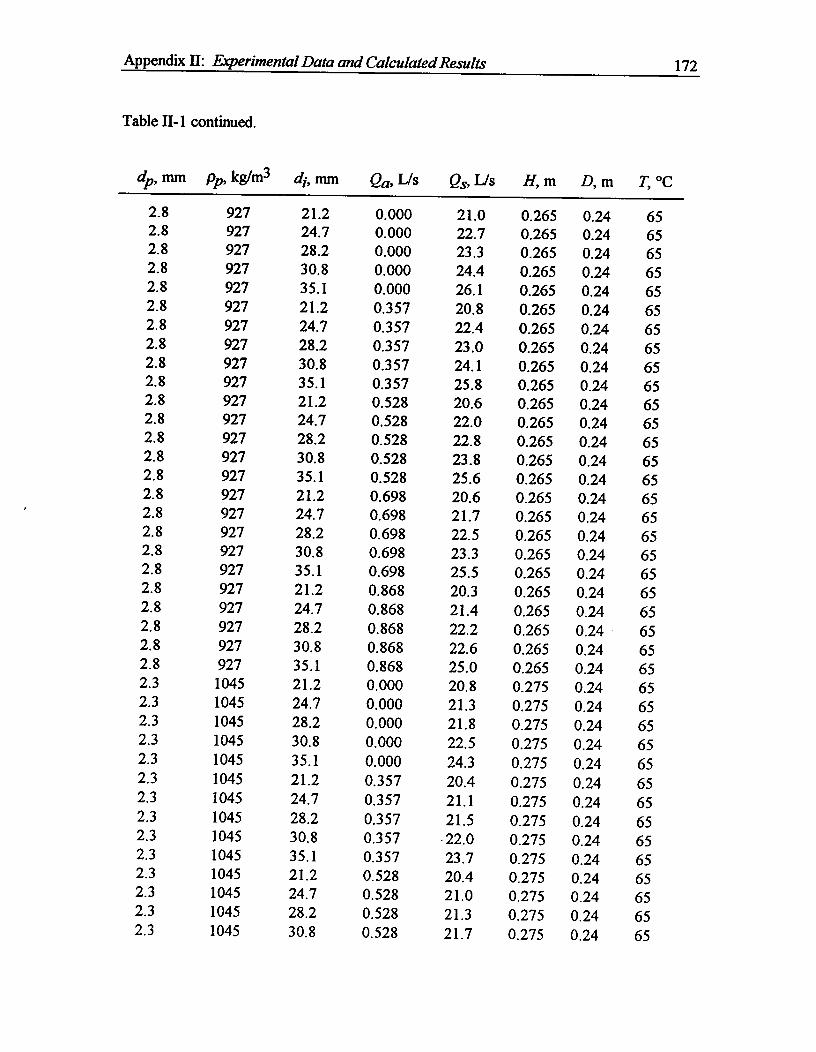
Appendix II: Experimental Data and Calculated Results^ 172
Table 1T- 1 continued.
c/p, mm pp, kg/m3 di, mm Qa,L Is Qs,L s H, m D, m T, °C
2.8 927 21.2 0.000 21.0 0.265 0.24 652.8 927 24.7 0.000 22.7 0.265 0.24 652.8 927 28.2 0.000 23.3 0.265 0.24 652.8 927 30.8 0.000 24.4 0.265 0.24 652.8 927 35.1 0.000 26.1 0.265 0.24 652.8 927 21.2 0.357 20.8 0.265 0.24 652.8 927 24.7 0.357 22.4 0.265 0.24 652.8 927 28.2 0.357 23.0 0.265 0.24 652.8 927 30.8 0.357 24.1 0.265 0.24 652.8 927 35.1 0.357 25.8 0.265 0.24 652.8 927 21.2 0.528 20.6 0.265 0.24 652.8 927 24.7 0.528 22.0 0.265 0.24 652.8 927 28.2 0.528 22.8 0.265 0.24 652.8 927 30.8 0.528 23.8 0.265 0.24 652.8 927 35.1 0.528 25.6 0.265 0.24 652.8 927 21.2 0.698 20.6 0.265 0.24 652.8 927 24.7 0.698 21.7 0.265 0.24 652.8 927 28.2 0.698 22.5 0.265 0.24 652.8 927 30.8 0.698 23.3 0.265 0.24 652.8 927 35.1 0.698 25.5 0.265 0.24 652.8 927 21.2 0.868 20.3 0.265 0.24 652.8 927 24.7 0.868 21.4 0.265 0.24 652.8 927 28.2 0.868 22.2 0.265 0.24 652.8 927 30.8 0.868 22.6 0.265 0.24 652.8 927 35.1 0.868 25.0 0.265 0.24 652.3 1045 21.2 0.000 20.8 0.275 0.24 652.3 1045 24.7 0.000 21.3 0.275 0.24 652.3 1045 28.2 0.000 21.8 0.275 0.24 652.3 1045 30.8 0.000 22.5 0.275 0.24 652.3 1045 35.1 0.000 24.3 0.275 0.24 652.3 1045 21.2 0.357 20.4 0.275 0.24 652.3 1045 24.7 0.357 21.1 0.275 0.24 652.3 1045 28.2 0.357 21.5 0.275 0.24 652.3 1045 30.8 0.357 . 22.0 0.275 0.24 652.3 1045 35.1 0.357 23.7 0.275 0.24 652.3 1045 21.2 0.528 20.4 0.275 0.24 652.3 1045 24.7 0.528 21.0 0.275 0.24 652.3 1045 28.2 0.528 21.3 0.275 0.24 652.3 1045 30.8 0.528 21.7 0.275 0.24 65
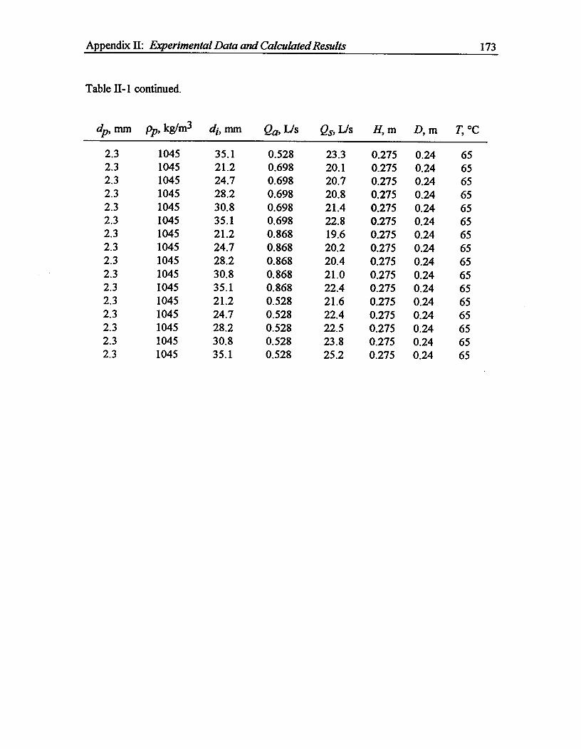
Appendix II: Experimental Data and Calculated Results^ 173
Table II-1 continued.
dp, mm pp, kg/m3 di, mm Qa, Us Qs, Us H, m D, m T, °C
2.3 1045 35.1 0.528 23.3 0.275 0.24 652.3 1045 21.2 0.698 20.1 0.275 0.24 652.3 1045 24.7 0.698 20.7 0.275 0.24 652.3 1045 28.2 0.698 20.8 0.275 0.24 652.3 1045 30.8 0.698 21.4 0.275 0.24 652.3 1045 35.1 0.698 22.8 0.275 0.24 652.3 1045 21.2 0.868 19.6 0.275 0.24 652.3 1045 24.7 0.868 20.2 0.275 0.24 652.3 1045 28.2 0.868 20.4 0.275 0.24 652.3 1045 30.8 0.868 21.0 0.275 0.24 652.3 1045 35.1 0.868 22.4 0.275 0.24 652.3 1045 21.2 0.528 21.6 0.275 0.24 652.3 1045 24.7 0.528 22.4 0.275 0.24 652.3 1045 28.2 0.528 22.5 0.275 0.24 652.3 1045 30.8 0.528 23.8 0.275 0.24 652.3 1045 35.1 0.528 25.2 0.275 0.24 65
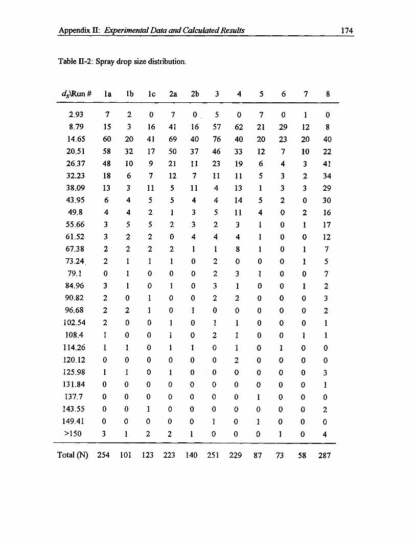
Appendix II: Experimental Data and Calculated Results^ 174
Table II-2: Spray drop size distribution.
ds\Run # la lb lc 2a 2b 3 4 5 6 7 8
2.93 7 2 0 7 0 5 0 7 0 1 08.79 15 3 16 41 16 57 62 21 29 12 814.65 60 20 41 69 40 76 40 20 23 20 4020.51 58 32 17 50 37 46 33 12 7 10 2226.37 48 10 9 21 11 23 19 6 4 3 4132.23 18 6 7 12 7 11 11 5 3 2 3438.09 13 3 11 5 11 4 13 1 3 3 2943.95 6 4 5 5 4 4 14 5 2 0 3049.8 4 4 2 1 3 5 11 4 0 2 16
55.66 3 5 5 2 3 2 3 1 0 1 1761.52 3 2 2 0 4 4 4 1 0 0 1267.38 2 2 2 2 1 1 8 1 0 1 773.24 . 2 1 1 1 0 2 0 0 0 1 579.1 0 1 0 0 0 2 3 1 0 0 7
84.96 3 1 0 1 0 3 1 0 0 1 290.82 2 0 1 0 0 2 2 0 0 0 396.68 2 2 1 0 1 0 0 0 0 0 2102.54 2 0 0 1 0 1 1 0 0 0 1108.4 1 0 0 1 0 2 1 0 0 1 1
114.26 1 1 0 1 1 0 1 0 1 0 0120.12 0 0 0 0 0 0 2 0 0 0 0125.98 1 1 0 1 0 0 0 0 0 0 3131.84 0 0 0 0 0 0 0 0 0 0 1137.7 0 0 0 0 0 0 0 1 0 0 0
143.55 0 0 1 0 0 0 0 0 0 0 2149.41 0 0 0 0 0 1 0 1 0 0 0>150 3 1 2 2 1 0 0 0 1 0 4
Total (N) 254 101 123 223 140 251 229 87^73^58 287
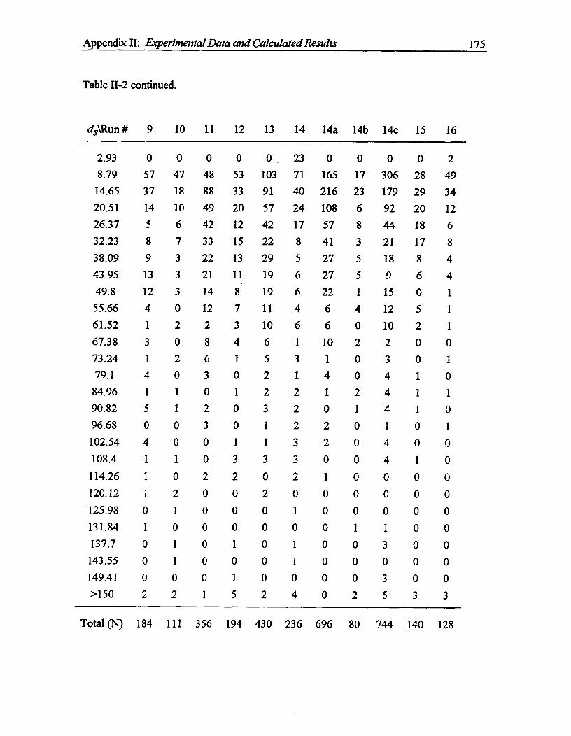
Appendix II: Experimental Data and Calculated Results^ 175
Table II-2 continued.
ds\Run # 9 10 11 12 13 14 14a 14b 14c 15 16
2.93 0 0 0 0 0 23 0 0 0 0 28.79 57 47 48 53 103 71 165 17 306 28 4914.65 37 18 88 33 91 40 216 23 179 29 3420.51 14 10 49 20 57 24 108 6 92 20 1226.37 5 6 42 12 42 17 57 8 44 18 632.23 8 7 33 15 22 8 41 3 21 17 838.09 9 3 22 13 29 5 27 5 18 8 443.95 13 3 21 11 19 6 27 5 9 6 449.8 12 3 14 8 19 6 22 1 15 0 155.66 4 0 12 7 11 4 6 4 12 5 161.52 1 2 2 3 10 6 6 0 10 2 167.38 3 0 8 4 6 1 10 2 2 0 073.24 1 2 6 1 5 3 1 0 3 0 179.1 4 0 3 0 2 1 4 0 4 1 0
84.96 1 1 0 1 2 2 1 2 4 1 190.82 5 1 2 0 3 2 0 1 4 1 096.68 0 0 3 0 1 2 2 0 1 0 1102.54 4 0 0 1 1 3 2 0 4 0 0108.4 1 1 0 3 3 3 0 0 4 1 0
114.26 1 0 2 2 0 2 1 0 0 0 0120.12 1 2 0 0 2 0 0 0 0 0 0125.98 0 1 0 0 0 1 0 0 0 0 0131.84 1 0 0 0 0 0 0 1 1 0 0137.7 0 1 0 1 0 1 0 0 3 0 0143.55 0 1 0 0 0 1 0 0 0 0 0149.41 0 0 0 1 0 0 0 0 3 0 0>150 2 2 1 5 2 4 0 2 5 3 3
Total (N) 184 111 356 194 430 236 696 80 744 140 128
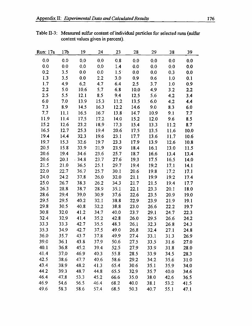
Appendix II: Experimental Data and Calculated Results^ 176
Table II-3:
Run: 17a
Measured sulfur content of individual particles for selected runs (sulfurcontent values given in percent).
17b^19^24^23^28^29^38^39
0.0 0.0 0.0 0.0 0.8 0.0 0.0 0.0 0.00.0 0.0 0.0 0.0 1.4 0.0 0.0 0.0 0.00.2 3.5 0.0 0.0 1.5 0.0 0.0 0.3 0.01.3 3.5 0.0 2.2 3.0 0.9 0.6 1.0 0.11.7 4.9 6.2 4.7 6.4 2.5 3.7 1.0 0.92.2 5.0 10.6 5.7 6.8 10.0 4.9 3.2 2.22.5 5.5 12.1 8.5 9.4 12.5 5.6 4.2 3.46.0 7.0 13.9 15.3 11.2 13.5 6.0 4.2 4.47.3 8.9 14.5 16.3 12.2 14.6 9.0 8.3 6.07.7 11.1 16.5 16.7 13.8 14.7 10.9 9.1 7.711.9 11.4 17.5 17.2 14.0 15.2 12.0 9.6 8.515.2 12.6 23.2 18.9 17.3 15.4 13.3 11.2 8.716.5 12.7 25.3 19.4 20.6 17.5 13.5 11.6 10.019.4 14.4 32.3 19.6 23.1 17.7 13.6 11.7 10.619.7 15.3 32.6 19.7 23.3 17.9 13.9 12.6 10.820.5 15.8 33.9 21.9 23.9 18.4 16.1 13.0 11.520.6 19.4 34.6 23.6 25.7 18.7 16.6 13.4 13.420.6 20.1 • 34.8 23.7 27.6 19.3 17.5 16.5 14.021.5 21.0 36.5 25.1 29.7 19.4 19.2 17.1 14.122.0 22.7 36.7 25.7 30.1 20.6 19.8 17.2 17.124.0 24.2 37.8 26.0 32.0 21.1 19.9 19.2 17.425.0 26.7 38.3 26.2 34.3 21.7 21.5 19.4 17.726.3 28.8 38.7 28.9 35.1 22.1 23.3 20.1 18.028.6 29.4 39.0 30.9 37.6 22.6 23.5 20.9 19.029.5 29.5 40.2 32.1 38.8 22.9 23.9 21.9 19.129.8 30.5 40.8 32.2 38.8 23.0 26.6 22.2 19.730.8 32.0 41.2 34.7 40.0 23.7 29.1 24.7 22.332.4 32.9 41.4 35.2 42.8 26.0 29.5 26.6 24.233.3 33.3 42.7 35.5 48.3 26.1 32.3 26.8 24.335.3 34.9 42.7 37.5 49.0 26.8 32.4 27.1 24.836.0 35.7 43.7 37.8 49.9 27.4 33.1 31.3 26.939.0 36.1 43.8 37.9 50.6 27.5 33.5 31.6 27.040.1 36.8 45.2 39.4 52.5 27.9 33.9 31.8 28.041.4 37.0 46.9 40.3 55.8 28.5 33.9 34.5 28.342.5 38.6 47.7 40.6 58.6 29.2 34.2 35.6 31.043.4 38.9 48.2 41.3 65.4 30.6 35.1 35.9 34.044.2 39.3 48.7 44.8 65.5 32.9 35.7 40.0 34.646.4 47.8 53.3 45.2 66.6 35.0 38.0 42.6 36.546.9 54.6 56.5 46.4 68.2 40.0 38.1 53.2 41.549.6 58.3 58.6 57.4 68.5 50.3 40.7 55.1 47.1
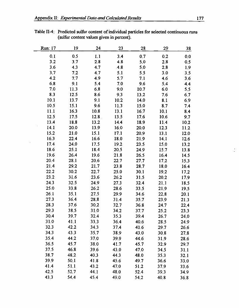
Appendix Experimental Data and Calculated Results 177
Table 11-4: Predicted sulfur content of individual particles for selected continuous runs(sulfur content values given in percent).
Run: 17 19 24 23 28 29 380.1 0.5 1.1 3.4 0.7 0.2 0.03.2 3.7 2.8 4.8 5.0 2.8 0.53.6 4.3 4.7 4.8 5.0 2.8 1.93.7 7.2 4.7 5.1 5.5 3.0 3.54.2 7.7 4.9 5.7 7.1 4.6 3.66.8 9.1 5.4 7.0 9.6 5.4 4.47.0 11.3 6.8 9.0 10.7 6.0 5.58.3 12.5 8.6 9.3 13.2 7.6 6.7
10.1 13.7 9.1 10.2 14.0 8.1 6.910.5 15.1 9.6 11.3 15.0 8.7 7.411.1 16.3 10.8 13.1 16.7 10.1 8.412.5 17.5 12.8 13.5 17.6 10.6 9.713.4 18.8 13.2 14.4 18.9 11.4 10.214.1 20.0 13.9 16.0 20.0 12.3 11.215.2 21.0 15.1 17.1 20.9 13.1 12.016.3 22.4 16.6 18.0 21.9 14.1 12.617.4 24.0 17.5 19.2 23.5 15.0 13.218.6 25.1 18.4 20.5 24.9 15.7 13.819.6 26.4 19.6 21.8 26.5 16.4 14.520.4 28.1 20.6 22.7 27.7 17.2 15.321.4 29.2 21.7 23.8 28.7 18.0 16.422.2 30.2 22.7 25.0 30.1 19.2 17.223.2 31.6 23.6 26.2 31.5 20.2 17.924.3 32.5 24.9 27.3 32.4 21.1 18.525.0 33.8 26.2 28.6 33.5 21.9 19.526.1 35.1 27.5 29.9 34.6 22.8 20.127.3 36.4 28.8 31.4 35.7 23.9 21.328.3 37.6 30.2 32.7 36.8 24.7 22.429.3 38.5 31.0 34.2 37.7 25.2 23.330.4 39.7 32.4 35.3 39.4 26.7 24.031.0 41.1 33.3 36.4 40.6 28.5 24.932.3 42.2 34.3 37.4 41.6 29.7 26.634.3 43.3 35.7 38.9 43.0 30.8 27.835.4 44.2 37.0 39.9 44.6 31.9 28.636.5 45.7 38.0 41.7 45.7 32.9 29.737.5 46.8 39.6 43.0 47.0 34.5 31.138.7 48.2 40.3 44.3 48.0 35.3 32.139.9 50.1 41.8 45.6 49.7 36.6 33.041.4 51.1 43.2 47.0 51.2 37.9 33.642.5 52.7 44.1 48.0 52.4 39.3 34.943.3 54.4 45.4 49.0 54.2 40.8 36.8
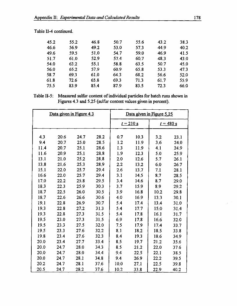
Appendix II: Experimental Data and Calculated Results^ 178
Table II-4 continued.
45.2 55.2 46.8 50.7 55.6 43.2 38.346.6 56.9 49.2 53.0 57.3 44.9 40.249.6 59.5 51.0 54.7 59.0 46.9 41.551.7 61.0 52.9 57.4 60.7 48.3 43.054.0 63.2 55.1 58.8 63.5 50.7 45.056.0 65.2 57.9 60.9 65.8 53.3 47.358.7 69.3 61.0 64.3 68.2 56.6 52.061.8 72.6 65.8 69.3 71.3 61.7 55.975.5 83.9 85.4 87.9 83.5 72.3 66.0
Table II-5: Measured sulfur content of individual particles for batch runs shown inFigures 4.3 and 5.25 (sulfur content values given in percent).
Data given in Figure 4.3 Data given in Figure 5.25
t = 210 s t = 480 s
4.3 20.6 24.7 28.2 0.7 10.3 3.2 23.19.4 20.7 25.0 28.5 1.2 11.9 3.6 24.011.4 20.7 25.1 28.6 1.3 11.9 4.1 24.911.6 20.9 25.1 28.8 1.9 12.3 5.0 25.913.1 21.0 25.2 28.8 2.0 12.6 5.7 26.113.8 21.6 25.3 28.9 2.2 13.2 6.0 26.715.1 22.0 25.7 29.4 2.6 13.7 7.1 28.116.6 22.0 25.7 29.4 3.1 14.5 8.7 28.517.0 22.2 25.8 29.5 3.4 14.6 8.7 29.018.3 22.3 25.9 30.3 3.7 15.9 8.9 29.218.7 22.5 26.0 30.5 3.9 16.8 10.2 29.818.7 22.6 26.6 30.6 4.0 16.9 13.3 30.119.1 22.8 26.9 30.7 5.4 17.4 13.4 31.019.3 22.8 27.2 31.3 5.4 17.7 15.0 31.419.3 22.8 27.3 31.5 5.4 17.8 16.1 31.719.5 23.0 27.3 31.5 6.9 17.8 16.6 32.019.5 23.3 27.5 32.0 7.5 17.9 17.4 33.719.5 23.3 27.6 32.2 8.1 18.2 18.5 33.819.8 23.4 27.6 32.3 8.4 19.3 18.6 34.920.0 23.4 27.7 33.4 8.5 19.7 21.2 35.620.0 24.7 28.0 34.3 8.5 21.2 22.0 37.620.0 24.7 28.0 34.4 9.4 22.5 22.1 38.520.0 24.7 28.1 34.8 9.4 26.9 22.2 39.520.2 24.7 28.1 37.6 10.0 27.1 22.5 39.820.5 24.7 28.2 37.6 10.2 33.8 22.9 40.2

Appendix III:
Computer Program Listings
The source code listings (written in FORTRAN) and a description of the main computer pro-
gram used to determine the coating distribution and product quality are given in this section.
The numerical procedure, solution methods and definitions of selected variables in the COM-
MON statements used in the program are described first. The computer program represents
Model IV and includes hydrodynamics, spray distribution and Monte Carlo models.
The procedure for solving Model IV including the solution methods for solving the mass and
momentum equations in the spout and the fluid flow in the annulus are given below:
Numerical Procedure
Read in the experimental data, convert equipment units to metric units using calibration
equations, and determine properties of air using equations of state.
Calculate bed parameters such as U„,fi U„,„ vt and Ds;
Determine the axial pressure distribution (Pa{z}) using Equations (2.11) and (4.23), and
calculate the values of SPLINE parameters (cubic interpolation parameters);
Solve for the steam function (p) using Equation (1-23), velocities (ua{z,r}) using
Equation (1-22) and pressures (Pa{z,r}) in the annulus using Equation (1-28); determine
the fluid flow rate across the spout-annulus interface and calculate the values of SPLINE
parameters for the exchange flux Ur;
Solve Equations (4.27), (4.29), (4.30), (4.36) and (4.37) to determine es, v, us and C,
and determine the corresponding values of SPLINE parameters;
Calculate ins, at various positions on the surface of the bed (Dr) and the values of
SPLINE parameters;
179
Appendix HI Computer Program Listings^ 180
(vii) Determine the particle sulfur content distribution with the Monte Carlo methods out-
lined in Section 4.2.3.3.
In all steps, the calculated information is stored as SPLINE parameters which provide this in-
formation whenever it is required through a simple calculation.
Solution Methods for Steps (iv) and (v)
In step (iv), the vector Ergun (1952) equation was written in terms of the stream function
(i.e., Equation (I-23)) which was then expressed in second order finite differences forms and
solved using an successive under-relaxation factor of 0.7. The grid size was set in such a way
that nodes were located on the conical wall. Twenty-one grids (between D and D,) were used
in the radial direction, and the number of grids in the axial direction was calculated from the
number of grids in the radial direction, cone angle, H and D. In most cases, the number of
grids in the axial direction exceeded that in the radial direction. The convergence criterion of
of 10-9 for the maximum change in the stream function value from iteration to iteration was
used. (Decreasing this value to 10 -10 did not significantly improve the results, but the number
of iterations required to meet the criterion nearly doubled). For most runs, convergence was
reached in under 5000 iterations using an under-relaxation factor of 0.7. No attempt was
made to find the optimum relaxation factor; however, the rate of convergence appeared to be
slower with smaller values, and larger values resulted in no convergence.
The same method was applied for solving the pressure profile in the annulus (i.e., Equation (I-
28)), except that linear or first order approximations were used to predict the normal pressure
derivative (Equation (I-29)) at the conical wall.
In step (v), the set of non-linear, coupled ordinary differential equations were solved using
LSODE (in UBC ODEPACK, Moore, 1989) which utilizes the Gear method (Gerald and
Wheatley, 1984). The solution could be obtained in most cases provided the equations were
rewritten (and solved) in terms of u, use, and v,2(1 -e3). Absolute and relative tolerance values
of 10-12 and 10 -5 , respectively, were used.
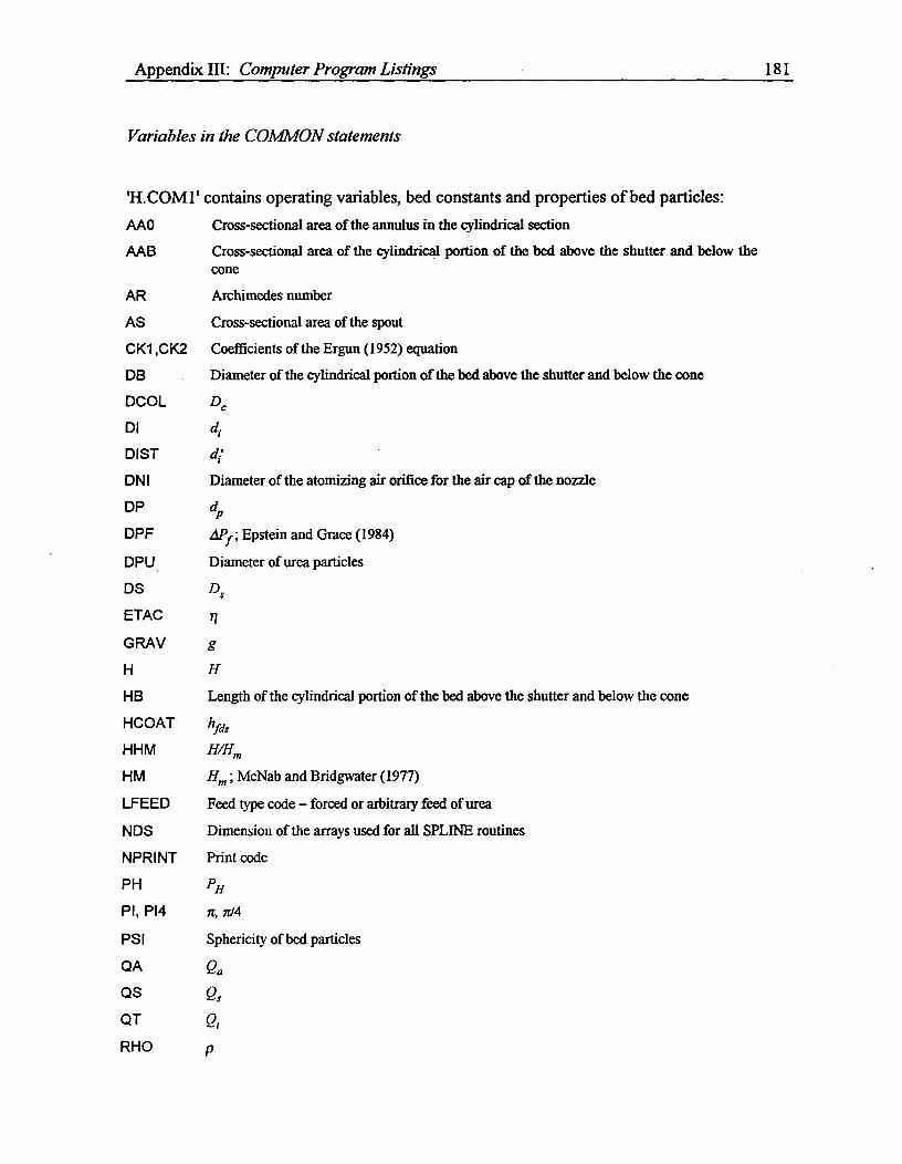
Appendix III: Computer Program Listings^ 181
Variables in the COMMON statements
'H.COM1' contains operating variables, bed constants and properties of bed particles:AA0^Cross-sectional area of the annulus in the cylindrical section
AAB^Cross-sectional area of the cylindrical portion of the bed above the shutter and below thecone
AR^Archimedes number
AS^Cross-sectional area of the spout
CK1,CK2 Coefficients of the Ergun (1952) equation
DB^Diameter of the cylindrical portion of the bed above the shutter and below the cone
DCOL^Dc
DI
DIST^di'
DNI^Diameter of the atomizing air orifice for the air cap of the nozzle
DP
DPF^APf • Epstein and Grace (1984)
DPU^Diameter of urea particles
DS^Ds
ETAC^71GRAV
H^H
HB^Length of the cylindrical portion of the bed above the shutter and below the cone
HCOAT brasHHM^H/Hm
HM^Hin; McNab and Bridgwater (1977)
LFEED^Feed type code — forced or arbitrary feed of urea
NDS^Dimension of the arrays used for all SPLINE routines
NPRINT^Print code
PH^PHPI, PI4^rt, 7r/4
PSI^Sphericity of bed particles
QA^Qa
QS^Q,
QT^QrRHO
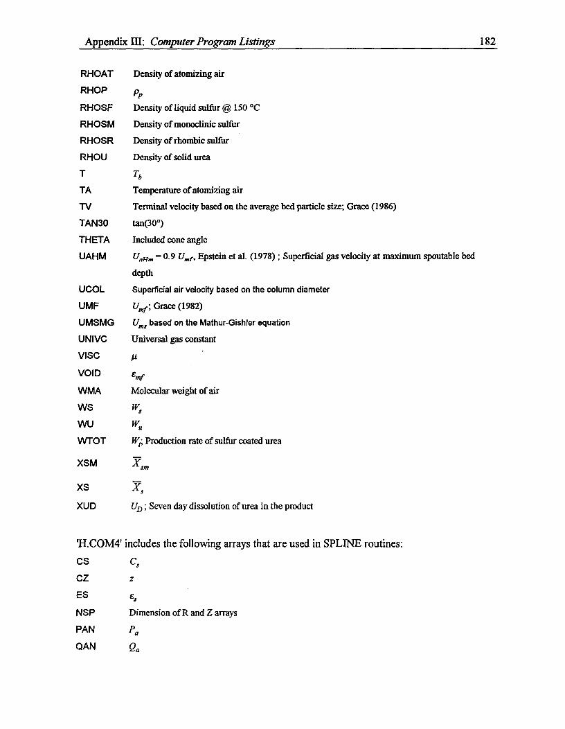
Appendix In: Computer Program Listings^ 182
RHOAT^Density of atomizing air
RHOP^Pp
RHOSF^Density of liquid sulfur @ 150 °C
RHOSM^Density of monoclinic sulfur
RHOSR^Density of rhombic sulfur
RHOU^Density of solid urea
T^Tb
TA^Temperature of atomizing air
TV^Terminal velocity based on the average bed particle size; Grace (1986)
TAN30^tan(30°)
THETA^Included cone angle
UAHM^C I aim = 0.9 Umr, Epstein et al. (1978) ; Superficial gas velocity at maximum spoutable bed
depth
UCOL^Superficial air velocity based on the column diameter
UMF^Um •i. ' Grace (1982)
UMSMG^Um, based on the Mathur-Gishler equation
UNIVC^Universal gas constant
VISC^it
VOID^emf
WMA^Molecular weight of air
WS^Ws
1NU^Wu
WTOT^WI; Production rate of sulfur coated urea
XSM Xsm
XS^AC
XUD^UD; Seven day dissolution of urea in the product
'H.COM4' includes the following arrays that are used in SPLINE routines:CS^CsCZ^z
ES^es
NSP^Dimension of R and Z arrays
PAN^Pa
QAN^Qa

Appendix HI: Computer Program Listings^ 183
R^Radial distance from the centre of the bed
SMT^Amount of sulfur on a bed particle calculated by the Monte Carlo method
VS^vs
Z^Vertical distance from the base of the bed
ZMT^Vertical distance corresponding to SMT
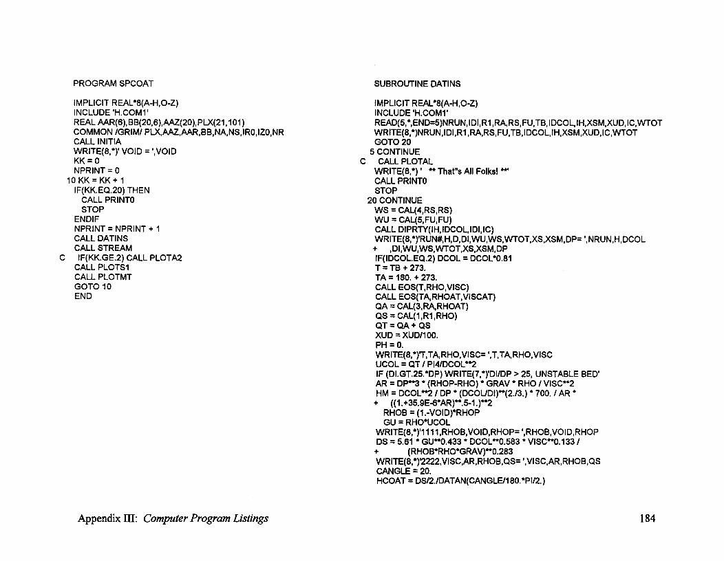
SUBROUTINE DATINS
IMPLICIT REAL*8(A-H 2O-Z)INCLUDE 'H.COM1'READ(5,",END=5)NRUN,IDI,R1,RA,RS,FU,TB,IDCOL,IH,XSM,XUD,IC,VVTOTWRITE(8,1NRUN,IDI,R1,RA,RS,FU,TB,IDCOL,IH,XSM,XUD,IC,WTOTGOTO 20
5 CONTINUEC CALL PLOTAL
WRITE(8,*) ' **Than All Folks! **'CALL PRINTOSTOP
20 CONTINUEWS = CAL(4,RS,RS)WU = CAL(5,FU,FU)CALL DIPRTY(IH,IDCOL,IDI,IC)WRITE(8,")'RUN#,H,D,DI,WU,WS,VVTOT,XS,XSM,DP= ',NRUN,H,DCOL+ ,DI,WU,WS,VVTOT,XS,XSM,DPIF(IDCOL.EQ.2) DCOL = DCOL*0.81T = TB + 273.TA = 180. + 273.CALL EOS(T,RHO,VISC)CALL E0S(TA,RHOAT,VISCAT)QA = CAL(3,RA,RHOAT)QS = CAL(1,R1,RHO)QT = QA + QSXUD = XUD/100.PH = 0.WRITE(8,1T,TA,RHO,VISC= ',T,TA,RHO,VISCUCOL = QT / P14/DCOL**2IF (DI.GT.25.*DP) WRITE(7,1DI/DP > 25, UNSTABLE BED'AR = DP**3 * (RHOP-RHO) * GRAV" RHO / VISC**2HM = DCOL**2 / DP * (DCOL/D1)**(213.)* 700. / AR *+ ((1.+35.9E-6*AR)**.5-1.)**2
RHOB = (1.-VOID)*RHOPGU = RHO*UCOL
WRITE(8,11111,RHOB,VOID,RHOP= ',RHOB,VOID,RHOPDS = 5.61 * GU**0.433 * DCOL**0.583 * VISC**0.133 /• (RHOB*RHO*GRAV)**0.283WRITE(8,1 12222,VISC,AR,RHOB,QS= ',VISC,AR,RHOB,QSCANGLE = 20.HCOAT = DS/2./DATAN(CANGLE/180.*PI/2.)
PROGRAM SPCOAT
IMPLICIT REAL*8(A-H 2 O-Z)INCLUDE 'H.COM1'REAL AAR(6),BB(20,6),AAZ(20),PLX(21,101)COMMON /GRIM/ PLX,AAZ,AAR,BB,NA,NS,IRO,IZO,NRCALL INITIAWRITE(8,1 1 VOID = ',VOIDKK = 0NPRINT = 0
10 KK = KK + 1IF(KK.EQ.20) THEN
CALL PRINTOSTOP
ENDIFNPRINT = NPRINT + 1CALL DATINSCALL STREAM
C IF(KK.GE.2) CALL PLOTA2CALL PLOTS1CALL PLOTMTGOTO 10END
Appendix III: Computer Program Listings^ 184
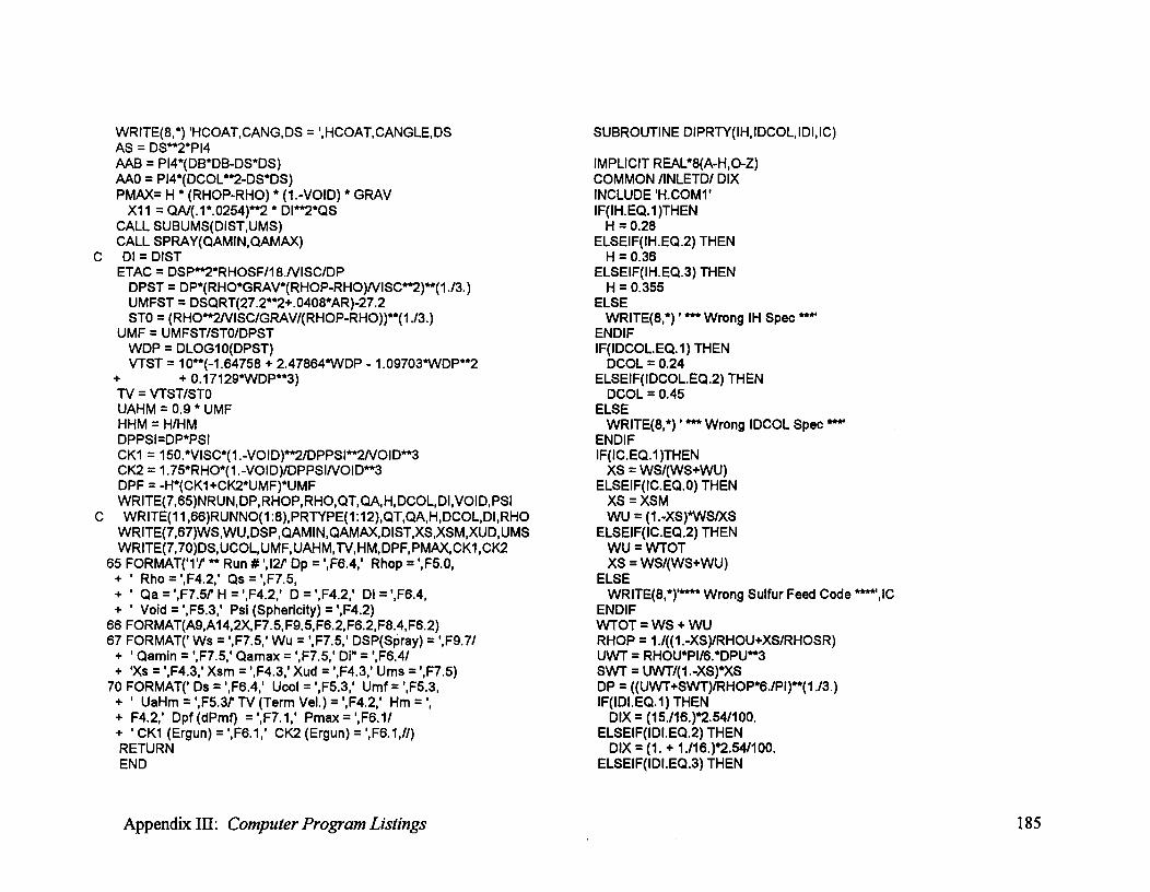
WRITE(8,*) 'HCOAT,CANG,DS = ',HCOAT,CANGLE, DSAS = DS**2*PI4AAB = PI4*(DB*DB-DS*DS)AA0 = PI4*(DCOL**2-DS*DS)PMAX= H * (RHOP-RHO) * (1.-VOID) * GRAV
X11 = QA/(.1*.0254)**2 * DI**2*QSCALL SUBUMS(DIST,UMS)CALL SPRAY(QAMIN,QAMAX)
C DI = DISTETAC = DSP**2*RHOSF/18.NISC/DP
DPST = DPIRHO*GRAVIRHOP-RHO)NISC**2)**(113.)UMFST = DSQRT(27.2**2+.0408*AR)-27.2STO = (RHO**2NISC/GRAVARHOP-RHO))**(1./3.)
UMF = UMFST/STO/DPSTWDP = DLOG10(DPST)VTST = 10**(-1.64758 + 2.47864*WDP - 1.09703*WDP**2
+ 0.17129*WDP**3)TV = VTST/STOUAHM = 0.9 * UMFHHM = H/HMDPPSI=DP*PSICK1 = 150.*VISC*(1.-VOID)**2/DPPSI**2NOID**3CK2 = 1.75*RHO*(1.-VOID)/DPPSINOID**3DPF = -H*(CK1+CK2*UMF)*UMFWRITE(7,65)NRUN,DP,RHOP,RHO,QT,QA,H,DCOL,DI,VOID,PSI
C WRITE(11,66)RUNNO(1:8),PRTYPE(1:12),QT,QA,H,DCOL,DI,RHOWRITE(7,67)WS,WU,DSP,QAMIN,QAMAX,DIST,XS,XSM,XUD,UMSWRITE(7,70)DS,UCOL,UMF,UAHM,TV,HM,DPF,PMAX,CK1,CK2
65 FORMAT(I't ** Run # ',I2/' Dp = ',F6.4, 1 Rhop = ',F5.0,+ ' Rho = ',F4.2,' Qs = ',F7.5,+ ' Qa = ',F7.5/' H = ',F4.2,' D = ',F4.2,' Di = ',F6.4,+ ' Void = ',F5.3,' Psi (Sphericity) = ',F4.2)
66 FORMAT(A9,A14,2X, F7.5, F9.5,F6.2,F6.2,F8.4,F6.2)67 FORMAT(' Ws = ',F7.5,' Wu = ',F7.5,' DSP(Spray) = ',F9.7/
+ Qamin = ',F7.5,' Qamax = ',F7.5,' Di" = ',F6.4/+ 'Xs = ',F4.3,' Xsm = ',F4.3,' Xud = ',F4.3,' Urns = ',F7.5)
70 FORMAT(' Ds = ',F6.4,' Ucol = ',F5.3,' Umf = ',F5.3,+ ' UaHm = ',F5.3P TV (Term Vel.) = ',F4.2,' Hm = ',
+ F4.2,' Dpf (dPmf) = ',F7.1,' Pmax = ',F6.1/+ ' CK1 (Ergun) = ',F6.1,' CK2 (Ergun) = ',F6.1,//)RETURNEND
Appendix III: Computer Program Listings
SUBROUTINE DIPRTY(IH,IDCOL,IDI,IC)
IMPLICIT REAL*8(A-H 2 O-Z)COMMON /INLETD/ DIXINCLUDE 'H.COM1'IF(IH.EQ.1)THEN
H = 0.28ELSEIF(1H.EQ.2) THEN
H = 0.36ELSEIF(IH.EQ.3) THEN
H = 0.355ELSE
WRITE(8,1 ' ***Wrong IH Spec *** 1
ENDIFIF(IDCOL.EQ.1) THEN
DCOL = 0.24ELSEIF(IDCOL.EQ.2) THEN
DCOL = 0.45ELSE
WRITE(8,1 ' Wrong IDCOL Spec "'*"'ENDIFIF(IC.EQ.1)THEN
XS = WS/(WS+WU)ELSEIF(IC.EQ.0) THEN
XS = XSMWU = (1.-XS)*WS/XS
ELSEIF(IC.EQ.2) THENWU = WTOTXS = WS/(WS+WU)
ELSEWRITE(8,1 1**** Wrong Sulfur Feed Code ****',IC
ENDIFWTOT = WS + WURHOP = 1./((1.-XS)/RHOU+XS/RHOSR)UWT = RHOU*PI/6.*DPU**3SWT = UWT/(1.-XS)*XSDP = ((UWT+SWT)/RHOP*6./PI)**(1./3.)IF(IDI.EQ.1) THEN
DIX = (15./16.)"2.54/100.ELSEIF(IDI.EQ.2) THEN
DIX = (1. + 1./16.)*2.54/100.ELSEIF(IDI.EQ.3) THEN
185

DIX = (1. + 3./16.)*2.54/100.ELSEIF(IDI.EQ.4) THEN
DIX = (1. + 9./32. )*2.54/100.ELSEIF(IDI.EQ.5) THEN
DIX = (1. + 7116.)*2.54/100.ELSE
WRITE(8,*)'***** Wrong DI Spec *****'STOP
ENDIFDI = CAL(8,DIX,DIX)END
SUBROUTINE SUBUMS(DIPR,UMS)
IMPLICIT REAL*8(A-H 2 O-Z)EXTERNAL FUMSINCLUDE 'H.COM1'DIMENSION WORK(80)X = DINF = 1SCALE = 1.D10EPSL = 1.0-10IC = 1MI = 500LOG =6CALL DPOWEL(FM,X,NF,SCALE,EPSL,IC,MI,LOG,WORK,IE,FUMS,*32)GOTO 33
32 CONTINUEWRITE(7,*)'error in POWEL, IE = ',IE
33 CONTINUEDIPR = XGH = DSQRT(2.*GRAV*H)UMS =13.50*(DP/DCOL)**1.165 *(DIPR/DCOL)**0.3715
+ *(DCOUH)**0.1475*((RHOP-RHO)/RHO)**0.2894*GHWRITE(8,*)'values Of FM,X are',FM,XEND
Appendix III: Computer Program Listings^ 186

DOUBLE PRECISION FUNCTION FUMS(X,ND)
IMPLICIT REAL*8(A-H 2 O-Z)INCLUDE 'H.COM1'VA = QA/PI4/DAT**2Al = PI4*D1**2GH = DSQRT(2.*GRAV*H)XX = XIF(X.LE.0.) THEN
FUMS = -X*10000.+1000.RETURN
ENDIFUMS =13.50*(DP/DCOL)**1.165 *(XX/DCOL)**0.3715+ *(DCOUH)**0.1475*((RHOP-RHO)/RHO)"0.2894*GHQMS = UMS*PI4*DCOL**2QTX = QMS+QAVTX = QTX/XX**2/P14QMS2 = QTX*VTX*A1-(WS*VA+RHOAT*QA*VA)*Al/RHOIF(QMS2.LE.0.) QMS2 = -QMS2*1000.QMS1 = DSQRT(QMS2)FUMS = ((QMS-QMS1)*1000.)**2RETURNEND
SUBROUTINE SPRAY(QAMIN,QAMAX)
IMPLICIT REAL*8(A-H 2 O-Z)INCLUDE 'H.COM1'UAMIN = 13.7893 + 1.6086*WS*3600.UAMAX = 3.881397 + 4.592215*WS*3600.QAMIN = UAMIN*DAT**2*PI4QAMAX = UAMAX*DAT**2*PI4DSP = 0.261012*(QA/QAMIN)**1.7015*(WS/RHOSF/QA)**1.8759RETURNEND
Appendix III: Computer Program Listings^ 187

US(I) = Y(2)ES(I) = Y(1)N(2)
. CS(I) = Y(4)PRINT(1,NPRINT,I) = Y(4)
200 CONTINUEPRINT(1,NPRINT,1) = CS(1)WSL = CS(N)*US(N)*ES(N)*ASWCIRC = VS(N)*(1.-ES(N))*AS*RHOPWPROD = WU/(1.-XS)WRITE(7,203)WSL,WSUVVS*100,WCIRC,WPROD
203 FORMAT(/' Sulfur Lost = ',G12.4,' KG/S = ',G12.4, 1 %7- 'Part Circ Rate = ',G12.4,' KG/S, Prod Rate = ',G12.4)CALL MYSPLN(CZ,CS,CQ,CR,CT,N,NDS)CALL MYSPLN(CZ,VS,VQ,VR,VT,N,NDS)CALL MYSPLN(CZ,ES,EQ,ER,ET,N,NDS)CALL MYSPLN(CZ,US,UQ,UR,UT,N,NDS)
WRITE(8,1 1 HSPOUT OK'RETURNEND
SUBROUTINE HSPOUT
IMPLICIT REAL*8(A-H 2 O-Z)EXTERNAL FUNCINCLUDE 'H.COM1'INCLUDE 'H.COM4'DIMENSION Y(4), RTOL(4), ATOL(4),RWORK(80),IWORK(25), IPAK(100)DATA RTOU4*1.D-5/ATOU4*1.D-12/ITOL,ITASK,ISTATE, 'OPT/1,1,1,0/DATA LRW,LIW,MF/80,25,22/MUA/4/
* Solve the Lefroy Davidson EquationsU0 = QT/P14/DI**2VS(1) = O.US(1) = UOES(1)= 1.CS(1) = WS/PI4/DS**2/U0!STATE = 1WRITE(7,102)HB,1.0,U0,0.,CS(1)
102 FORMAT(//4X,'H',10X,'VOID.',7X,'AIR V.',6X,'PART. V.',3X,- 'SULF. C'//5G12.4)
103 FORMAT(7G12.4)X1 = CZ(1)N = NSP
C DCOL = 0.445Y(1) = U0Y(2) = U0Y(3) = 0.D0Y(4) = CS(1)DO 200 I=2,N
X2 = CZ(I)CALL LSODE(FUNC,MUA,Y,X1,X2,ITOL,RTOL,ATOL,ITASK,ISTATE,
1^lOPT,RWORK,LRW,IWORK,LIW,JAC,MF)IF(ISTATE.NE.2) WRITE(8,*)'******* !STATE = ',ISTATEV8 = O.DOVOIDMI = 1.- Y(1)/Y(2)IF(Y(3).GT.0.)V8 = DSQRT(Y(3)/(1.D0-VOIDM1))I F(I/2*2. EQ.I)WRITE(7,103)X2,Y(1)N(2),Y(2),V8,Y(4)IF(X2.GT.H)THEN
WRITE(8,17>H, Z = ',X2GOTO 200
ENDIFVS(I) = V8
Appendix III: Computer Program Listings^ 188

SUBROUTINE FUNC(M,X,Y,Z)
* This subroutine provides RHS of the differential equations.* Parameters are* Z = array containing RHS values of differential equations.• X = independent variabLE, Z/H* Y = array containing dependent variables• M = number of differential equations
IMPLICIT REAL*8(A-H 2 O-Z)REAL*8 Z(M),Y(M)INCLUDE 'H.COM1'E = Y(1)/Y(2)
C WRITE(8,1) X,Y(1),Y(2),Y(3),EC 1 FORMAT('X, U*E, U, V2*E, E = ',5G11.4)
EM = 1.-EVS = 0.IF(EM.GT.0)THEN
VS2 = Y(3)/EMVS = O.IF(VS2.GT.0.)VS = DSQRT(Y(3)/EM)
ENDIFIF(E.LE.0.)E = 0.000001DUV = Y(2) - VSUV = DABS(DUV)*DUVB = FSI(E,1)BB = B*UVDPZ = QAINT(X,10)DQZ = QAINT(X,8)Z(1) = -DQZ/ASZ(2) = -DPZ/Y(2)/RHO - BB/RHO/Y(1) - Z(1)/EZ(3) = BB/RHOP - DPZ/RHOP*EM - EM*(RHOP-RHO)*GRAV/RHOPIF(X.GE.HCOAT) THEN
Z(4) = - (1.5*EM*ETA(DABS(DUV))*DABS(DUV)/DP+Z(1))*+^Y(4)N(1)
C^Z(4) = - (4./DS*DQZ+1.5*EM*ETA(DABS(DUV))*DABS(DUV)/DP+Z(1))*C +^Y(4)/Y(1)
ELSEZ(4) = -Z(1)*Y(4)N(1)
ENDIFRETURNEND
DOUBLE PRECISION FUNCTION ETA(X)
* Calculates impaction efficiency
IMPLICIT REAL*8(A-H 2 O-Z)INCLUDE 'H.COM1'SS = ETAC*XIF(SSIE.0.083D0)THEN
ETA = O.DOELSEIF(SS.GT.0.600)THEN
ETA = SS*SSASS+0.5D0)**2ELSE
ETA = 0.036-0.2323*SS+2.422*SS*SS-2.033*SS**3ENDIFEND
Appendix HI: Computer Program Listings^ 189

DOUBLE PRECISION FUNCTION FSI(X,I)
* FLUID-SOLID interaction term estimation.** 1. RICHARDSON-ZAKI EQUATION* 2. ERGUN'S EQUATION* 3. MODIFIED (BY 4) R-Z EQUATION* 4. MORGAN & LITTMAN CORRELATION
IMPLICIT REAL*8(A-H 2 O-Z)INCLUDE 'H.COM1'IF(I.EQ.1)THEN
FSI = 0.33*(1.-X)*RHO/DP/X**1.78ELSEIF(I.EQ.2)THEN
FSI = 1.75*(1.-X)*RHO/DPELSEIF(I. EQ.3)THEN
FSI = 0.109*(1.-X)*RHO/DP/X**1.64ELSEIF(I.EQ.4)THEN
FSI = RHO/DP/X*(78.44-633.94*X + 2124.52*X*X - 3772.5*X**3+^+ 3741.3*X**4 - 1964.27*X"5 + 426.45*X**6)ELSE
WRITE(7,1 1ERROR IN FSI CODE'ENDIFRETURNEND
DOUBLE PRECISION FUNCTION CAREA(X)
* This function finds the area of the annulus (cone-base).
IMPLICIT REAL*8(A-H 2 O-Z)INCLUDE 'H.COM1'IF(X.LT.HB)THEN
CAREA = AABELSE
D = DB + 2.*(X-HB)*TAN30IF(D.LT.DCOL) THEN
CAREA = PI4*(D*D-DS*DS)ELSE
CAREA = MOENDIF
ENDIFRETURNEND
Appendix III: Computer Program Listings^ 190
DOUBLE PRECISION FUNCTION QAINT(X,ICODE)
IMPLICIT REAL*8(A-H 2 O-Z)INCLUDE 'H.COM1'INCLUDE 'H.COM4'IF(ICODE.LT.3)THEN
I = INTT(X,DMT,NSP,DX)ELSEIF(ICODE.GE.11) THEN
I = INTT(X,Z,NZ,DX)ELSE
I = INTT(X,CZ,NSP,DX)ENDIFIF(ICODE.EQ.1)THEN
QAINT = ZMT(I)+ZMTQ(I)*DX+ZMTR(I)*DX*DX+ZMTS(1)*DX**3ELSEIF(ICODE.EQ.2)THEN
QAINT = SMT(I)+SMTQ(I)*DX+SMTR(I)*DX*DX+SMTS(I)*DX**3ELSEIF(ICODE.EQ.3)THEN
C^QAINT = PA(I)+PQ(I)*DX+PR(I)*DX**2+PS(1)*DX**3QAINT = CS(I)+CQ(I)*DX+CR(I)*DX**2+CT(I)*DX**3
ELSEIF(ICODE.EQ.4)THENQAINT = US(I)+UQ(I)*DX+UR(I)*DX**2+UT(I)*DX**3
ELSEIF(ICODE.EQ.5)THENQAINT = VS(I)+VQ(I)*DX+VR(I)*DX*DX+VT(I)*DX**3
ELSEIF(ICODE.EQ.6)THENQAINT = ES(I)+EQ(I)*DX+ER(I)*DX**2+ET(I)*DX**3
ELSEIF(ICODE.EQ.7)THENQAINT = QAN(I)+QANQ(I)*DX+QANR(I)*DX**2+QANS(I)*DX**3
ELSEIF(ICODE.EQ.8)THENQAINT = DQAN(1)+DQANQ(1)*DX+DOANR(1)*DX**2+DQANS(1)*DX**3
ELSEIF(ICODE.EQ.9)THENQAINT = PAN(I)+PANQ(I)*DX+PANR(I)*DX**2+PANS(I)*DX**3
ELSEIF(ICODE.EQ.10)THENQAINT = DPAN(I)+DPANQ(I)*DX+DPANR(I)*DX**2+DPANS(I)*DX**3
ELSEIF(ICODE.EQ.11)THENQAINT = QZA(I)+QZAQ(I)*DX+QZAR(I)*DX**2+QZAS(I)*DX**3
ELSEIF(ICODE.EQ.12)THENQAINT = RAD(I)+RADQ(I)*DX+RADR(I)*DX**2+RADS(I)*DX**3
ELSEWRITE(7,1 1 ERROR IN CODE IN QAINT, ICODE =',1CODE
ENDIFRETURNEND
FUNCTION INTT(X,Y,N,DX)
Determines the interval at which X belongs. Used with Spline* calculations.
IMPLICIT REAL*8(A-H 2 O-Z)REAL*8 Y(N)INTT = 1J = N-1
30 K = (1NTT+J)/2IF(X.LT.Y(K))J=KIF(X.GE.Y(K))INTT=K1F(J.NE.INTT+1)GOTO 30DX = X - Y(INTT)RETURNEND
Appendix III: Computer Program Listings^ 191

SUBROUTINE PLOTA2
IMPLICIT REAL*8(A-H 2 O-Z)DIMENSION IPAK(800)REAL AX(30),P(30),PAV(30)INCLUDE 'H.COM1'CALL DSPDEV('PLOT')CALL NOBRDRCALL AREA2D(6.0,6.0)CALL PHYSOR(1.,2.)CALL THKCRV(0.03)CALL XREVTKCALL YREVTKCALL COMPLXCALL YAXANG(0.)CALL XNAME('Height, m$',100)CALL YNAME('Pressure in Annulus, kPa$',100)CALL YTICKS(3)CALL XTICKS(2)
C CALL HEADIN('Pressure Profile in Annulus$',-100,-3,1)CALL GRAF(0,.1,.4,0,.3,1.3)CALL SCLPIC(2.)CALL FRAMEPMORH = PMOR(H)/1000.AX(1) = O.P(1) = PMORH - PMOR(0.D0)/1000.DO 30 I = 2,21
ZZZ = H*(I-1)/20.AX(I) = ZZZP(I) = PMORH - PMOR(ZZZ)/1000.
30 CONTINUECALL CURVE(AX,P,21,0)CALL ENDGR(0)CALL ENDPL(0)END
DOUBLE PRECISION FUNCTION PMOR(X)
IMPLICIT REAL*8(A-H 2 O-Z)INCLUDE 'H.COM1'AC = RHO*UMF*TV/(RHOP-RHO)/GRAV/DIIF(PSI.NE.1.)AC=AC*PS1*(5.*PS1**3-7.57*PS1**2+4.09*PS1-.516)PHIA = 7.18*(AC-DI/DCOL) + 1.07IF(AC.GT.0.07)WRITE(8,1 1 P-MOR NOT VALID, AC>.07 = ',ACXX1 = 1 ./(X/DCOL+1 . )XQT = .1BB1 = 2.*(XX1-2.*XQT)-2.*(1.-XQT)+4.*(1.-XQT)**2/PHIACC1 = (XX1-2.)*(XX1-2.*XQT) - 4.*(1 .-XQT)**2*XX1/PH IAY1 = -BB1/2. + DSQRT(BB1**2-4.*CC1)/2.
C Y2 = -BB1/2. - DSQRT(BB1**2-4.*CC1)/2.DPFO = -DPF*X/HPMOR = (1.-Y1)*DPF0RETURNEND
Appendix III: Computer Program Listings^ 192
CALL XNAME('Height, m$',100)CALL YNAME('Concentration in Spout, kg/m3$',100)CALL YTICKS(3)CALL XTICKS(2)CALL GRAF(0,.1,.36,0,.05,.15)CALL FRAMECALL SCLPIC(2.)DO 23 I = 1,20
XXX = START + DX*IAX(I) = XXXV(I) = QAINT(XXX,3)
23 CONTINUECALL CURVE(AX,V,20,0)CALL ENDGR(0)CALL ENDPL(0)END
SUBROUTINE PLOTSI
IMPLICIT REAL*8(A-H 2 O-Z)DIMENSION IPAK(500)REAL AX(20),V(20),VAJ(20),AX2(2)INCLUDE 'H.COM1'CALL DSPDEV('PLOT')CALL NOBRDRCALL AREA2D(6.0,6.0)CALL PHYSOR(1.,2.)CALL THKCRV(0.03)CALL XREVTKCALL YREVTKCALL COMPLXCALL YAXANG(0.)CALL XNAME('Height, m$',100)CALL YNAME('Air Velocity In Spout, m/s$',100)CALL YTICKS(3)CALL XTICKS(2)CALL GRAF(0,.1,.36,0.,10.,50.)CALL FRAMECALL SCLPIC(2.)CALL HSPOUTDX = (H-HB)/20.START = HBDO 20 I = 1,20
XXX = START + DX*IAX(I) = XXXV(I) = QAINT(XXX,4)
20 CONTINUECALL CURVE(AX,V,20,0)CALL ENDGR(0)CALL ENDPL(0)CALL DSPDEV('PLOT')CALL NOBRDRCALL AREA2D(6.0,6.0)CALL PHYSOR(1.,2.)CALL THKCRV(0.03)CALL XREVTKCALL YREVTKCALL COMPLXCALL YAXANG(0.)
Appendix III: Computer Program Listings^ 193
SUBROUTINE STREAM^ NZS = 3ELSE
* This pgm determines the stream functions in the annulus using^ IRO = IRO +1* the boundary condition^ RWO = DELR +RS* str = 0 © wall^ 2 IF(RWO.GT.RB) THEN• d(str)/dz = 0 © annulus surface^ Z(1) = (RW0-RB)*TAN30 + HB• P = function given by Morgan © spout-annulus interface^ IF(Z(1).GT.DELR) THEN
4^Z(1) = Z(1)- DELZIMPLICIT REAL*8(A-H 2 O-Z)^ IZO = IZO + 1INCLUDE 'H.COM1'^ IF(Z(1).GT.DELZ) GOTO 4INCLUDE 'H.COM4'^ ENDIFDIMENSION STR(101,101),VEL(5,101,101),DPMOR(101)^ NZS = IZO + 1DIMENSION RW(1 01 ),PMORG(1 01),PERG(1 01,101 )^ WRITE(8,1'HERE DS<DB, IRO = ',IROREAL X1,X2,Y1,Y2,RSIZ,ZSIZ,XSTEP,YSTEP^ GOTO 6REAL AAR(6),BB(20,6),AAZ(20),PLX(21,101)^ ENDIFCOMMON /GRIM/ PLX,AAZ,AAR,BB,NA,NS,IRO,IZO,NR^ RWO = RWO + DELRCOMMON WORK(50000)^ IRO = IRO + 1COMMON /FSTRSB/ F1,F2,RX,DELR,DELRZ2,ILIN^ GOTO 2DATA NRM,EPS,MAXIT/51,1.D-9,7000/^ ENDIFILIN = 1^ 6 CONTINUENRM = 20^ IROM = IRO - 1ALPHA = 0.7^ IROMM = IROM - 1ALPHAM=1.-ALPHA^ IZOM = IZO - 1ALP2 = ALPHA^ IZOP = IZO + 1ALP2M = 1. - ALP2^ DELRZ = DELR*DELZF1 = CK1^ DELRZ2 = (DELR/DELZ)**2F2 = CK2^ NZP = 1RS = DS/2.^ 8 ZO = Z(1) + DELZ*NZPRB = DB/2.^ NZP = NZP + 1RO = DCOU2.^ IF(ZO.LT.H) GOTO 8IF(DCOL.GT.0.24) RO = R0/0.81^ NZ = NZP -1NR = NRM + 1^ NZM = NZ -1NRP = NR + 1^ NZMM = NZ - 2NRMM = NR - 2^ WRITE(8,1' N,NR,NZ,ALPHA,DELR,Z1= ',NRM,NR,NZ,ALPHA,DELR,Z(1)DELR = (R0-RS)/NRM^ WRITE(8,*)' DS,DB,F1,F2,H,DCOL= ',DS,DB,F1,F2,H,DCOLDELR2 = DELR"2^ PMORH = PMOR(H)DELZ = DELR/TAN30^ PMORG(1) = PMORH - PMOR(Z(1))R(1) = RS^ RW(1) = RB+(Z(1)-HB)*TAN30IZO = 1^ DO 10 I=2,NZIRO = 1^ Z(I) = Z(I-1) + DELZIF(RS.GE .RB)THEN^ RW(I) = RB+(Z(I)-HB)*TAN30
Z(1) = (RS-RB)/TAN30 + HB^ IF(Z(I).LT.HB) RW(I) = RB
Appendix III: Computer Program Listings^ 194

IF(RW(I).GT.R0) RW(I) = ROPMORG(I) = PMORH-PMOR(Z(I))
10 CONTINUEDPMOR(1) = (4.*PMORG(2)-PMORG(3)-3.*PMORG(1))/2./DELRDPMOR(NZ) = (PMORG(NZ-2)-4.*PMORG(NZM)+3.*PMORG(NZ))/2./DELRDO 15 I = 2,NZM
DPMOR(I) = (PMORG(I+1)-PMORG(I-1))/2./DELR15 CONTINUE17 FORMAT('I,PMORG,DPMOR =',15G12.5)
C DO 18 I = 1,NZC^WRITE(8,17)1,PMORG(1),DPMOR(1)C 18 CONTINUEC STOP
DO 20 J = 2,NRIF(J.LT.IRO)R(J) = R(J-1) + DELRIF(J.GE.IRO)R(J) = RW(IZO+J-IRO)
C WRITE(8,1 1R(J),RW,NR = R(J),RW(J),(R(J)-RS)/DELR20 CONTINUE
DELZS = H - Z(NZ)ZDIVS = DELZS/DELZWRITE(8,1'DELZS,DELZ,DELR = DELZS,DELZ,DELRZDIVSP = 1. + ZDIVSZDIVSM = 1. - 1./ZDIVSDNM = 2.*(1.+DELRZ2)DNMS = 2.*(1.+DELRZ2/ZDIVS)El = (1.+DELR/2.)/DNME2 = (1.-DELR/2.)/DNME3 = DELRZ2/DNME4 = E1*DNM/DNMSE5 = E2*DNM/DNMSE6 = 2.*DELRZ2/ZDIVSP/DNMSIF(IRO.GT.1) THEN
DELZB = Z(1)ZDIVB = DELZB/DELZZDIVBP = 1. + ZDIVBIF(IRO.EQ.2)THEN
DELRB = RB - RSELSE
DELRB = RB - IROM * DELR - RSENDIFRDIVB = DELRB/DELRRDIVBP = 1. + RDIVB
RDIVBM =1. -1./RDIVBENDIFII = IZOJJ = IRODO 50 I = 1,NZP
DO 40 J = 1, NRPSTR(I,J) = 0.PERG(I,J) = PMORG(1)IF(R(J).LT.RW(I))STR(I,J) = (RW(I)-R(J))*Z(I)*1.D-3IF(II.EQ.I.AND.JJ.EQ.J)THEN
II = II + 1JJ = JJ + 1STR(I,J) = 0.
ENDIFDO 30 K = 1, 5
VEL(K,I,J) = 1.30 CONTINUE40 CONTINUE
STR(I,NR)=0.50 CONTINUE
55 CONTINUEDO 1000 ITER=1,MAXITDIFMAX=0.RX = RS
*
* If the spout diameter is larger than the cone neck
IF(IRO.EQ.1)THENDR1 = -STR(2,NRP)/2./DELRDRIM = -STR(1,NRP)/DELRDZ1 = STR(3,1)/2./DELZDZR = (VEL(1,3,1)-DR1M)/2./DELZCALL FSTR(DZ1,DR1,DZR,C1,C2,C3,C4,C5,C6)CO = DPMOR(2)*RS/(Fl+F2/RS*DSQRT(DZ1**2+DR1**2))C7 = 2.*C1 - C5STRNEW = ALPHAM*STR(2,1)+ALPHA*(C5*STR(2,2) +
+^C7*STR(2,NRP)+C2*DELRZ2*+^(STR(3,1)+STR(1,1))+C4*DELR2)/2./C6
DIFMAX = DMAX1(DIFMAX,DABS(STRNEW-STR(2,1)))STR(2,NRP) = - C0*2.*DELRVEL(1,2,1) = DR1
Appendix DI Computer Program Listings^ 195

ELSEIF(IRO.EQ.2) THENDR1 = -STR(1,NRP)/2./DELRBDZ1 = STR(2,1)/2./DELZBDZR = (STR(2,NRP)/2./DELR-DR1 +DR1/ZDIVB)/2./DELZCALL FSTR(DZ1,DR1,DZR,C1,C2,C3,C4,C5,C6)CO = DPMOR(1)*RS/(F1+F2/RS*DSQRT(DZ1**2+DR1**2))STRNEW = ALP HAM*STR(1 ,1 )+ALPHA*((C1-C3*DELRB/2. )*
• STR(1,NRP)+2.*C2/ZDIVBP*DELRZ2*RD1VB**2*STR(2,1)• + C4*DELRB**2)/2./(C1+C2/ZD1VB*DELRZ2*RDIVB**2)
DIFMAX = DMAX1(DIFMAX,DABS(STRNEW-STR(2,1)))STR(2,NRP) = - CO*2.*DELRBVEL(1,1,1)= DR1VEL(2,1,1) = DZ1STR(1,1) = STRNEWIF(IZO.GT.2) THEN
DO 60 I = 2,IZOMIP = 1 + 1IM = I - 1DR1 = -STR(I,NRP)/2./DELRBDZ1 = (STR(IP,1)-STR(IM,1))/2./DELZDZR = (STR(IP,NRP)-STR(IM,NRP))/4./DELRB/DELZCALL FSTR(DZ1,DR1,DZR,C1,C2,C3,C4,C5,C6)CO = DPMOR(I)*RS/(F1+F2/RS*DSQRT(DZ1**2+DR1**2))STRNEW = ALP HAM*STR( I, 1 )+ALPHATC1-C3*DELRB/2. )*
• STR(I,NRP)+C2*DELRZ2*RDIVB**2*(STR(IP,1)+STR(IM,1))• + C4*DELRB**2)/2./(C1+C2*DELRZ2*RDIVB**2)
DIFMAX = DMAX1(DIFMAX,DABS(STRNEW-STR(1,1)))STR(I,NRP) = - C0*2.*DELRVEL(1,I,1)= DR1VEL(2,I,1) = DZ1STR(I,1) = STRNEW
60 CONTINUEENDIF1 = IZO
VEL(2,2,1) = DZ1STR(2,1) = STRNEWDZ1 = STR(2,1)/DELZCO = DPMOR(1)*RS/(F1+F2/RS*DSQRT(DZ1**2+DR1M**2))STR(2,NRP) = - CO*DELR*
* If the spout diameter is less than the cone neck
Appendix III: Computer Program Listings
IP = 1 + 11M = 1 - 1DR1 = -STR(I,NRP)/2./DELRDZ1 = (STR(IP, 1 )-STR(IM,1 ))/2./DELZDZR = (VEL(1,IP,1)-VEL(1,1M,1))/2./DELZCALL FSTR(DZ1,DR1,DZR,C1,C2,C3,C4,C5,C6)CO = DPMOR(I)*RS/(F1+F2/RS*DSQRT(DZ1"2+DR1**2))C7 = 2.*C1 - C5STRNEW = ALPHAM*STR(1,1)+ALPHA*(C5*STR(1,2) +
+ C7*STR(I,NRP)+C2*DELRZ2*+ (STR(IP,1)+STR(IM,1))+C4*DELR2)/2./C6
DIFMAX = DMAX1(DIFMAX,DABS(STRNEW-STR(1,1)))STR(I,NRP) = - C0*2.*DELRVEL(1,I,1) = DR1VEL(2,I,1) = DZ1STR(I,1) = STRNEW
ELSE** If the second r node exist, calculate str at 1 = 1*
DR1 = (STR(1,2)-STR(1,NRP))/2./DELRDZ1 = (STR(2,1)-STR(1,1)+STR(1,1)/ZDIVBy2./DELZDZR = (VEL(1,2,1)-DR1+DR1/ZDIVB)/2./DELZCALL FSTR(DZ1,DR1,DZR,C1,C2,C3,C4,C5,C6)CO = DPMOR(1)*RS/(F1+F2/RS*DSQRT(DZ1**2+DR1**2))C7 = 2.*C1 - C5STRNEW = ALPHAM*STR(1,1)+ALPHA*(C5*STR(1,2) +
• C7*STR(1,NRP)+2.*C2*DELRZ2/ZDIVPB*• STR(2,1)+C4*DELR2y2Ac1+C2*DELRZ2/ZDIVB)
DIFMAX = DMAX1(DIFMAX,DABS(STRNEW-STR(1,1)))STR(1,NRP) = STR(1,2) - C0*2.*DELRVEL(1,1,1) = DR1VEL(2,1,1) = DZ1STR(1,1) = STRNEWIF(IROM.LE.2) GOTO 80DO 70 J = 2,IROMM
JP=J+1JM=J-1DR1 = (STR(1,JP)-STR(1,JM))/2./DELRDZ1 = (STR(2,J)-STR(1,J)+STR(1,J)/ZDIVB)/2./DELZDZR = (VEL(1,2,J)-DR1+DR1/ZDIVB)/2./DELZRX = R(J)
196
CALL FSTR(DZ1,DR1,DZR,C1,C2,C3,C4,C5,C6)C7 = 2.*C1 - C5STRNEW = ALPHAM*STR(1,J)+ALPHA*(C5*STR(1,JP) +
• C7*STR(1,JM)+2.*C2*DELRZ2/ZDIVBP*• STR(2,J)+C4*DELR2y2./(C1+C2*DELRZ2/ZDIVB)
DIFMAX = DMM1(DIFMAX,DABS(STRNEW-STR(1,J)))VEL(1,1,J) = DR1VEL(2,1,J) = DZ1STR(1,J) = STRNEW
70 CONTINUE80 CONTINUE
DR1 = (RDIVBM*STR(1,IROM)-STR(1,IROMM))/2./DELRDZ1 = (STR(2,IROM)-STR(1,IROM)+STR(1,IROM)/ZDIVB)/2./DELZDZR = (VEL(1,2,IROM)-DR1+DR1/ZDIVB)/2./DELZRX = R(IROM)CALL FSTR(DZ1,DR1,DZR,C1,C2,C3,C4,C5,C6)STRNEW = ALPHAM*STR(1,IROM)+ALPHA*((2.*C1/ZDIVBP+C3*DELRB/2.)
+ *STR(1,IROMM)+2.*C2*DELRZ2/ZDIVBP*+ STR(2,IROM)+C4*DELR2y2./(C1/RDIVB+C2*DELRZ2/ZDIVB+ -RDIVBM*C3*DELRB/4.)
DIFMAX = DMAX1(DIFMAX,DABS(STRNEW-STR(1,IROM)))VEL(1,1,IROM) = DR1VEL(2,1,IROM) = DZ1STR(1,IROM) = STRNEW
* If the second r node exist, calculate str at 1 > I > IZO*
IF(IZO.EQ.2) GOTO 120DO 110 1= 2,IZOM
IP = I + 1IM = I - 1DR1 = (STR(1,2)-STR(I,NRP)y2./DELRDZ1 = (STR(IP,1)-STR(IM,1))/2./DELZDZR=(STR(IP,2)-STR(IP,NRP)-STR(IM,2)+STR(IM,NRP))/4./DELRZRX = RSCALL FSTR(DZ1,DR1,DZR,C1,C2,C3,C4,C5,C6)CO = DPMOR(I)*RS/(F1+F2/RS*DSQRT(DZ1**2+DR1**2))C7 = 2.*C1 - C5STRNEW = ALPHAM*STR(1,1)+ALPHA*(C5*STR(1,2) +
• C7*STR(I,NRP)+C2*DELRZ2*• (STR(IP,1)+STR(IM,1))+C4*DELR2)/2./(C1+C2*DELRZ2)
DIFMAX = DMAX1(DIFMAX,DABS(STRNEW-STR(I,1)))
STR(I,NRP) = STR(I,2) - CO*2.*DELRVEL(1,I,1) = DR1VEL(2,I,1) = DZ1STR(I,1) = STRNEWIF(IROM.LE.2) GOTO 100DO 90 J = 2,IROMM
JP=J+ 1JM=J- 1DR1 = (STR(I,JP)-STR(I,JM))/2./DELRDZ1 = (STR(IP,J)-STR(IM,J))/2./DELZ
DZRNSTR(IP,JP)-STR(IP,JM)-STR(IM,JP)+STR(IM,JM)y4./DELRZRX = R(J)CALL FSTR(DZ1,DR1,DZR,C1,C2,C3,C4,C5,C6)C7 = 2.*C1 - C5STRNEW = ALPHAM*STR(I,J)+ALPHA*(C5*STR(I,JP) +C7*STR(I,JM)+C2*DELRZ2*(STR(IP,J)+STR(1M,J))+C4*DELR2)/2./(C1+C2*DELRZ2)
DIFMAX = DMAX1(DIFMM,DABS(STRNEW-STR(I,J)))VEL(1,I,J) = DR1VEL(2,I,J) = DZ1STROM = STRNEW
CONTINUECONTINUE
DR1 = (RDIVBM*STR(I,IROM)-STR(I,IROMM))/2./DELRDZ1 = (STR(IP,IROM)-STR(IM,IROM))/2./DELZDZR = (VEL(1,1P,IROM)-VEL(1,IM,IROM))/2./DELRZRX = R(IROM)CALL FSTR(DZ1,DR1,DZR,C1,C2,C3,C4,C5,C6)C7 = 2.*C1 - C5STRNEW = ALPHAM*STR(1,IROM)+ALPHA*((2.*C1/RDIVBP+
C8*DELRB/2.)*STR(1,IROMM) + C2*DELRZ2*(STR(IP,IROM)+STR(IM,IROM))+C4*DELR2)/2./(C1/RDIVB+C2*DELRZ2-RDIVBM*C3*DELRB/4.)
DIFMAX = DMAX1(DIFMAX,DABS(STRNEW-STR(I,IROM)))VEL(1,I,IROM) = DR1VEL(2,I,IROM) = DZ1STR(I,IROM) = STRNEWCONTINUECONTINUE
DR1 = (STR(1Z0,2)-STR(IZO,NRP))/2./DELRDZ1 = (STR(IZ0P,1)-STR(IZ0M,1))/2./DELZDZR = (VEL(1,1ZOP,1)-VEL(1, IZOM,1))/2./DELZ
90100
110120
Appendix III: Computer Program Listings^ 197

RX = RSCALL FSTR(DZI,DRI,DZR,C1,C2,C3,C4,C5,C6)CO = DPMOR(IZO)*RS/(F1+F2/RS*DSQRT(DZ1**2+DR1**2))C7 = 2.*C1 - C5STRNEW = ALPHAM*STR(1Z0,1)+ALPHA*(C5*STR(IZ0,2) +
• C7*STR(IZO,NRP)+C2*DELRZ2*+ (STR(IZOP,1 )+STR(IZOM,1))+C4*DELR2)/2./(C1+C2*DELRZ2)
DIFMAX = DMAX1(DIFMAX,DABS(STRNEW-STR(IZ0,1)))STR(IZO,NRP) = STR(IZ0,2) - CO*2.*DELRVEL(1,IZ0,1) = DR1VEL(2,120,1) = DZ1STR(IZ0,1) = STRNEWIF(IROM.LE.2) GOTO 135DO 130 J = 2,IROMM
JP = J + 1JM = J - 1DR1 = (STR(IZO,JP)-STR(IZO,JM))/2./DELRDZ1 = (STR(IZOP,J)-STR(IZOM,J))/2./DELZDZR = (VEL(1, IZOP,1)-VEL(1,1ZOM,1))/2./DELZRX = R(J)CALL FSTR(DZ1,DR1,DZR,C1,C2,C3,C4,C5,C6)C7 = 2.*C1 - C5STRNEW = ALPHAM*STR(IZO,J)+ALPHA*(C5*STR(IZO,JP) +
• C7*STR(IZO,JM)+C2*DELRZ2*• (STR(IZOP,J)+STR(IZOM,J))+C4*DELR2)/2./(C1+C2*DELRZ2)
DIFMAX = DMAX1(DIFMAX,DABS(STRNEW-STR(IZO,J)))VEL(1,IZO,J) = DR1VEL(2,IZO,J) = DZ1STR(IZO,J) = STRNEW
130 CONTINUE135 CONTINUE
DR1 = -STR(IZO,IROMM)/2./DELRDZ1 = (STR(IZOP,IROM)-STR(IZOM,IROM))/2./DELZDZR = (VEL(1,IZOP,IROM)-VEL(1,IZOM,IROM))/2./DELZRX = R(IROM)CALL FSTR(DZ1,DR1,DZR,C1,C2,C3,C4,C5,C6)C7 = 2.*C1 - C5STRNEW = ALPHAM*STR(IZO,IROM)+ALPHA*(C5*STR(IZO,IRO) +
+ C7*STR(IZO,IROMM)+C2*DELRZ2*+ (STR(IZOP,IROM)+STR(IZOM,IRO))+C4*DELR2)+ /2./(C1+C2*DELRZ2)
DIFMAX = DMAX1(DIFMAX,DABS(STRNEW-STR(IZO,IROM)))
VEL(1,1Z0,1ROM) = DR1VEL(2,1Z0,1ROM) = DZ1STR(IZO,IROM) = STRNEW
ENDIFDO 140 I = NZS,NZM
IP = I + 1IM = I - 1DZ1 = (STR(IP, 1)-STR(IM,1))/2./DELZDR1 = (STR(I,2)-STR(I,NRP))/2./DELRDZR = (STR(IP,2)-STR(IM,2)-STR(IP,NRP)+STR(IM,NRP))/4./DELRZRX = RSCALL FSTR(DZ1,DR1,DZR,C1,C2,C3,C4,C5,C6)CO = DPMOR(I)*RS/(F1+F2/RS*DSQRT(DZ1**2+DR1**2))C7 = 2.*C1-05STRNEW = ALPHAM*STR(I,1)+ALPHA*(C5*STR(1,2) + C7*STR(I,NRP)
• + C2*DELRZ2*(STR(IP,1)+STR(IM,1))+C4*DELR2y2./C6DIFMAX = DMAX1(DIFMAX,DABS(STRNEW-STR(I,1)))VEL(1,I,1) = DR1VEL(2,I,1) = DZ1STR(1,1) = STRNEWSTR(I,NRP) = STR(I,2) - C0*2.*DELRDO 137 J = 2,NRM
JP=J+ 1JM=J-1IF(RW(I).LT.RO.AND.R(JP).EQ.RW(I)) THEN
DZ1 = STROP,Jy2./DELZDR1 = -STR(I,JM)/2./DELRDZR = (STR(I,J)-STR(IP,JM))/4./DELRZRX = R(J)CALL FSTR(DZ1,DR1,DZR,C1,C2,C3,C4,C5,C6)C7 = 2*C1 - C5STRNEW = ALPHAM*STR(I,J)+ALPHA*(C5*STR(I,JP) +
• C7*STR(I,JM)• + C2*DELRZ2*(STR(IP,J)+STR(IM,J))+C4*DELR2)/2./C6
DIFMAX = DMAX1(DIFMAX,DABS(STRNEW-STR(I,J)))VEL(1,I,J) = DR1VEL(2,I,J) = DZ1STR(I,J) = STRNEWGOTO 140
ENDIFDZ1 = (STR(IP,J)-STR(IM,J)y2./DELZDR1 = (STR(I,JP)-STR(I,JM)y2./DELR
Appendix HI: Computer Program Listings^ 198
DZR = (STR(IP,JP)-STR(IM,JP)-STR(IP,JM)+ +STR(1M,JM))/4./DELRZ
RX = R(J)CALL FSTR(DZ1,DR1,DZR,C1,C2,C3,C4,C5,C6)C7 = 2.*C1 - C5STRNEW = ALPHAM*STR(I,J)+ALPHA*(C5*STR(I,JP) +
+ C7*STR( I,JM)+C2*DELRZ2*+ (STR(IP,J)+STR(IM,J))+C4*DELR2)/2./C6
DIFMAX = DMAX1(DIFMAX,DABS(STRNEW-STR(1,J)))VEL(1,I,J) = DR1VEL(2, I,J) = DZ1STR(I,J) = STRNEW
137 CONTINUE140 CONTINUE
DZ1 = (STR(NZ,1)-STR(NZM,1))/2./DELZDR1 = (STR(NZ,2)-STR(NZ,NRP))/2./DELRDRIP = (STR(NZ,2)-STR(NZP,NRP))/2./DELRDZR = (DRIP-VEL(1,NZM,1))/2./DELZRX = RSCALL FSTR(DZ1,DR1,DZR, C1,C2,C3,C4,C5, C6)CO = DPMOR(NZ)*RS/(F1+F2/RS*DSQRT(DZ1**2+DR1**2))C7 = 2.*C1 - C5STRNEW = ALPHAM*STR(NZ,1)+ALPHA*(C5*STR(NZ,2) +
+ C7*STR(NZ,NRP)+2.*C2*DELRZ2/ZDIVSP*+ STR(NZM,1)+C4*DELR2)/2./(C1+C2*DELRZ2/ZDIVSP)DIFMAX = DMAX1(D1FMAX,DABS(STRNEW-STR(NZ,1)))STR(NZ,NRP) = STR(NZ,2) - C0*2.*DELRCO = -PMORG(NZ)/DELZS*RS/(F1+F2/RS*DSORT(DZ1**2+DR1**2))STR(NZP,NRP) = STR(NZ,2) - C0*2.*DELRVEL(1,NZ,1) = DR1VEL(2,NZ,1) = DZ1STR(NZ,1) = STRNEWSTR(NZP,1) = STR(NZ,1)DO 150 J = 2,NRM
JP = J+1JM = J-1DZ1 = (STR(NZ,J)-STR(NZM,J))/2./DELZDR1 = (STR(NZ,JP)-STR(NZ,JM))/2./DELRDZR = (DR1-VEL(1,NZM,J))/2./DELZIF(RW(I).LT.RO.AND.R(JP).EQ.RW(I))
+ DZR=(STR(NZ,J)-STR(NZ,JM))/4./DELRZRX = R(J)
CALL FSTR(DZ1,DR1,DZR,C1,C2,C3,C4,C5,C6)C7 = 2.*C1 -05STRNEW = ALPHAM*STR(NZ,J)+ALPHA*(C5*STR(NZ,JP) +
+ C7*STR(NZ,JM)+2.*C2*DELRZ2/ZDIVSP*+ STR(NZM,J)+C4*DELR2)/2./(C1+C2*DELRZ2/ZDIVSP)
DIFMAX = DMAX1(DIFMAX,DABS(STRNEW-STR(NZ,J)))VEL(1,NZ,J) = DR1VEL(2,NZ,J) = DZ1STR(NZ,J) = STRNEWSTR(NZP,J) = STR(NZ,J)IF(RW(NZ).LT.RO.AND.R(JP).EQ.RW(NZ))GOTO 160
150 CONTINUE160 CONTINUE
C 1F(ITER/100*100.EQ. ITER)WRITE(8,170)ITER,STR(NZ,1),STR(NZ,5)C + ,STR(NZ,10),STR(NZ,15),STR(NZ,NR),DIFMAX
170 FORMAT(I5,6G12.3)IF (DIFMAX.LT.EPS)GOTO 2000
1000 CONTINUEWRITE(6,1 1 Convergence Failure - DIFMAX = ',DIFMAX
2000 IF(ILIN.EQ.0)THENILIN = 1GOTO 55
ENDIFII = IZOJJ = IRODO 410 I = 1,NZ
IPP=I+ 2IP=I+ 1IM = 1- 1IMM = I - 2PERG(I,1) = PMORG(I)VEL(3, 1,1) = VEL(2,I,1)/RsVEL(4,I,1) = -VEL(1,I,1)/RSIF(IRO.EQ.1.AND.I.EQ.1) THEN
VEL(3,I,1) =FDIF(1,STR(1,1),STR(2,1),STR(3,1),DELZ)/RSVEL(4,I,1) = STR(I,NRP)/DELR/RSGOTO 410
ENDIFIF(IRO.EQ.2.AND.I.LT.IZO)GOTO 410DO 400 J = 2,NRM
JMM = J - 2JM = J - 1
Appendix III: Computer Program Listings^ 199

IF(JMM.EQ.0) JMM = NRP^ UAR = VEL(3,I,J)IF(IRO.EQ.1.AND.J.EQ.2.AND.I.EQ.J) THEN^ UZ = VEL(4,I,J)
VEL(3,I,J) = FDIF(1,STR(I,J),STR(IP,J),STR(IPP,J),DELZ)^IF(UAR+UZ.LE.0.)WRITE(8,12ERO AT*',I,J,NZ
^
/R(J)^ JP=J+ 1VEL(4,I,J) =-FDIF(3,STR(I,J),STR(1,1),STR(I,NRP),DELR)^IF(I.EQ.NZ) THEN
^
/R(J)^ DURR = FDIF(2,VEL(3,I,JP),VEL(3,I,JM),XX,DELR)II = II + 2^ DUZR = FDIF(2,VEL(4,I,JP),VEL(4,I,JM),XX,DELR)JJ = JJ + 2^ DURZ = (ZDIVSM*VEL(3,I,J)-VEL(3,IM,J))/2./DELZGOTO 410^ DUZZ = (VEL(4,I,J)-VEL(4,IM,J))/2./DELZ
ELSEIF(II.EQ.I.AND.JJ.EQ.J) THEN^ VEL(5,1,J)=F2*(UAR**2*DURR+UAR*UZIDUZR+DURZ)VEL(3,I,J) =FDIF(1,STR(I,J),STR(IP,J),STR(IPP,J),DELZ)^
•^
+UZ**2*DUZZ)/ DSQRT(UAR**2+UZ**2)
^
/R(J)^ ELSEIF(IRO.EQ.1.AND.J.EQ.2.AND.I.EQ.J) THENVEL(4,1,J)=-FDIF(3,STR(I,J),STR(I,JM),STR(I,JMM),DELR)^DURR = (VEL(3,I,J)-VEL(3,I,JM))/DELR
^
/R(J)^ DURZ = FDIF(1,VEL(3,I,J),VEL(3,IP,J),VEL(3,IPP,J),DELZ)II = II + 1^ DUZR = (VEL(4,I,J)-VEL(4,I,JM))/DELRJJ = JJ + 1^ DUZZ = FDIF(1,VEL(4,I,J),VEL(4,IP,J),VEL(4,IPP,J),DELZ)GOTO 410^ VEL(5,1,J)=F2*(UAR**2*DURR+UAR*UZIDUZR+DURZ)
ELSE^
•^
+UZ**2*DUZZ)/ DSQRT(UAR**2+UZ**2)VEL(3,I,J) = VEL(2,I,J)/R(J)^ 11=11+2VEL(4,I,J) = -VEL(1,I,J)/R(J)^ JJ = JJ + 2IF(I.LT.II.AND.J+1.EQ.JJ) GOTO 410^ GOTO 430
ENDIF^ ELSEIF(II.EQ.I.AND.JJ.EQ.J) THEN
^
400 CONTINUE^ DURR = FDIF(3,VEL(3,I,J),VEL(3,I,JM),VEL(3,I,JMM),DELR)VEL(3,I,NR) = O.^ DURZ = FDIF(1,VEL(3,I,J),VEL(3,IP,J),VEL(3,IPP,J),DELZ)VEL(4,I,NR) = -FDIF(3,STR(I,NR),STR(I,NRM),STR(1,NRMM),DELR)^DUZR = FDIF(3,VEL(4,I,J),VEL(4,I,JM),VEL(4,I,JMM),DELR)
+^/R(NR)^ DUZZ = FDIF(1,VEL(4,I,J),VEL(4,IP,J),VEL(4,IPP,J),DELZ)
^
410 CONTINUE^ IF(J.EQ.2.AND.IRO.EQ.2) THENII = IZO^ DURR = (VEL(3,I,J)-VEL(3,I,JM))/DELRJJ = IRO^ DUZR = (VEL(4,I,J)-VEL(4,I,JM))/DELRMJUN = 0^ ENDIFWRITE(8,*)%1Z,NR = ',NZ,NR^ VEL(5,I,J)=F2*(UAR**2*DURR+UAR*UZ*(DUZR+DURZ)DO 430 I = 1,NZ^
•^
+UZ**2*DUZZ)/ DSQRT(UAR**2+UZ**2)IPP = I + 2^ 11=11+1IP = I + 1^ JJ=JJ+ 1IM = I - 1^ GOTO 430IMM = I - 2^ ELSEIF(I.EQ.1.AND.IRO.EQ.1) GOTO 430^ DURR = FDIF(2,VEL(3,I,JP),VEL(3,I,JM),XX,DELR)IF(I.LT.IZO.AND.IRO.EQ.2) GOTO 430^ DURZ = FDIF(2,VEL(3,1P,J),VEL(3,IM,J),XX,DELZ)DO 420 J = 2,NRM^ DUZR = FDIF(2,VEL(4,I,JP),VEL(4,I,JM),XX,DELR)
JMM = J -2^ DUZZ = FDIF(2,VEL(4,IP,J),VEL(4,IM,J),XX,DELZ)JM = J - 1^ VEL(5,1,J)=F2*(UAR**2*DURR+UAR*UZIDUZR+DURZ)IF(JMM.EQ.0) JMM = NRP^
•^
+UZ**2*DUZZy DSQRT(UAR**2+UZ**2)
Appendix III: Computer Program Listings^ 200
IF(I.LT.II.AND.J+1.EQ.JJ) GOTO 430ENDIF
420 CONTINUEUAR = VEL(3,I,NR)UZ = VEL(4,I,NR)
IF(UAR+UZ.LE.0.)WRITE(8,1'ZERO AT ',I,NRIF(MJUN. EQ.0)THEN
DURR = FDIF(3,VEL(3,I,NR),VEL(3,I,NRM),VEL(3,I,NRMM),DELR)DURZ = FDIF(1,VEL(3,I,NR),VEL(3,IP,NR),VEL(3,IPP,NR),DELZ)DUZR = FDIF(3,VEL(4,I,NR),VEL(4,I,NRM),VEL(4,I,NRMM),DELR)DUZZ = FDIF(1,VEL(4,I,NR),VEL(4,IP,NR),VEL(4,IPP,NR),DELZ)VEL(5,I,NR)=F2*(UAR**2*DURR+UAR*UZ*(DUZR+DURZ)
• +UZ**2*DUZZ)/ DSQRT(UAR**2+UZ**2)MJUN = 1
ELSEIF(I.EQ.NZ) THENDURR = FDIF(3,VEL(3,I,NR),VEL(3,I,NRM),VEL(3,I,NRMM),DELR)DURZ FDIF(3,VEL(3,I,NR),VEL(3,IM,NR),VEL(3,IMM,NR),DELZ)DUZR = FDIF(3,VEL(4,I,NR),VEL(4,I,NRM),VEL(4,I,NRMM),DELR)DUZZ = FDIF(3,VEL(4,I,NR),VEL(4,IM,NR),VEL(4,IMM,NR),DELZ)VEL(5,I,NR)=F2*(UAR**2*DURR+UAR*UZ*(DUZR+DURZ)
• +UZ**2*DUZZ)/ DSQRT(UAR**2+UZ**2)ELSE
DURR = FDIF(3,VEL(3,I,NR),VEL(3,I,NRM),VEL(3,I,NRMM),DELR)DURZ = FDIF(1,VEL(3,IP,NR),VEL(3,IM,NR),XX,DELZ)DUZR = FDIF(3,VEL(4,I,NR),VEL(4,I,NRM),VEL(4,I,NRMM),DELR)DUZZ = FDIF(1,VEL(4, IP,NR),VEL(4,1M,NR),XX,DELZ)VEL(5,I,NR)=F2*(UAR**2*DURR+UAR*UZ*(DUZR+DURZ)
• +UZ"2*DUZZ)/ DSQRT(UAR**2+UZ**2)ENDIF
430 CONTINUEEPSP = EPS*PERG(1,1)WRITE(8,*)'EPS, EPSP = ',EPS,EPSPANG = 1./6.RDIVC = 2.*DCOS(ANG)**2 - 1.ZDIVC = 2.*DCOS(ANG)*DSIN(ANG)*TAN30DO 7000 ITER = 1,MAXITII = IZOJJ = IRODIFMAX=0.DO 450 I = 1,NZ
IP = 1 + 1IM = I - 1
IF(I.EQ.1.AND.IRO.EQ.1) GOTO 450IF(I.LT.IZO.AND.IRO.EQ.2) GOTO 450DO 440 J = 2,NR
JM=J-1JP=J+1IF(I.EQ.NZ) THEN
E4 = (1.+DELR/2./R(J))/DNMSE5 = (1.-DELR/2./R(J))/DNMSPERNEW=PERG(I,J)*ALP2M+ALP2*(E4*PERG(I,JP) +
• E5*PERG(I,JM)+E6*PERG(IM,J)+VEL(5,1,J)*DELR2/DNMS)DIFMAX = DMAX1(DIFMAX,DABS(PERNEW-PERG(I,J)))PERG(I,J) = PERNEWIF(II.EQ.I.AND.JJ.EQ.J) PERG(I,JP) = 0.
ELSEEl = (1.+DELR/2./R(J))/DNME2 = (1.-DELR/2./R(J))/DNMPERNEW=PERG(I,J)*ALP2M+ALP2*(El*PERG(I,JP) +
• E2*PERG(I,JM)+E3*(PERG(IM,J)+PERG(IP,J))• +VEL(5,I,J)*DELR2/DNM)
DIFMAX = DMAX1(DIFMAX,DABS(PERNEVV-PERG(I,J)))PERG(I,J) = PERNEW
ENDIFIF(IRO.EQ.I.AND.J.EQ.2.AND.I.EQ.J) THEN
P2 = PERG(I,JM)P1 = PERG(IM,JM)PERG(IM,J) = P1 + (P2-P1)*ZDIVC11=11+2JJ = JJ + 2GOTO 450
ELSEIF(II.EQ.I.AND.JJ.EQ.J) THENIF(J.GT.2) THEN
JMM = J - 2P1 = PERG(IM,JM) + (PERG(IM,JMM)-PERG(IM,JM))*RDIVCP2 = PERG(I,JM) + (PERG(I,JMM)-PERG(I,JM))*RDIVCPERG(IM,J) = P1 + (P2-P1)*ZDIVC
ELSEP2 = PERG(I,JM)P1 = PERG(IM,JM)PERG(IM,J) = P1 + (P2-P1)*ZDIVC
ENDIFIF(J.EQ.NR) PERG(I,NRP) = PERG(I,NRM)11=11+1
Appendix III: Computer Program Listings^ 201

JJ = JJ + 1^ WRITE(8,*)'DDX = ',DDXGOTO 450^ DO 490 I = 2,NSPM
ELSEIF(I.LT.II.AND.JP.EQ.JJ)THEN^ CZ(I) = CZ(I-1) + DDXPERG(I,JP) = PERG(I,J)^ PAN(I) = PMORH - PMOR(CZ(I))GOTO 450^ QAN(I) = QAINT(CZ(I),11)
ENDIF^ 490 CONTINUE440 CONTINUE^ CZ(NSP) = H
PERG(I,NRP) = PERG(I,NRM)^ PAN(NSP) = O.450 CONTINUE^ QAN(NSP) = QZA(NZ)
C IF( ITER/10*10.EQ. ITER)WRITE(8,170)ITER ,PERG(NZ,1),PERG(NZ,5)^DPAN(1) = (4.*PAN(2)-PAN(3)-3.*PAN(1))/2./DELRC + ,PERG(NZ,10),PERG(NZ,15),PERG(NZ,NR),DIFMM^ DPAN(NSP) = (PAN(NSP-2)-4.*PAN(NSPM)+3.*PAN(NSP))/2./DELR
IF (DIFMAX.LT.EPSP)GOTO 8000^ DQAN(1) = (4.*QAN(2)-QAN(3)-3.*QAN(1))/2./DELR7000 CONTINUE^ DQAN(NSP) = (QAN(NSP-2)-4.*QAN(NSPM)+3.*QAN(NSP))/2./DELR
WRITE(6,*)' CONVERGENCE FAILURE II - DIFMAX = ',DIFMAX^DO 520 I = 2,NSPM8000 CONTINUE^ DPAN(I) = (PAN(I+1)-PAN(1-1))/2./DELR
DQAN(I) = (QAN(I+1)-QAN(I-1))/2./DELRNSP = NZP^ 520 CONTINUENSPM = NSP - 1^ CALL MYSPLN(CZ,QAN,QANQ,QANR,QANS,NSP,NDS)DDX = (H-Z(1))/(NSP-1.)^ CALL MYSPLN(CZ,DQAN,DQANQ,DQANR,DQANS,NSP,NDS)JJ = IRO^ CALL MYSPLN(CZ,PAN,PANQ,PANR,PANS,NSP,NDS)DO 510 I= 1, NZ^ CALL MYSPLN(CZ,DPAN,DPANQ,DPANR,DPANS,NSP,NDS)
IP = I + 1^ DO 6040 I = 1,NZIF(I.EQ.1.AND.IRO.EQ.1) THEN^ DO 6030 J=1,NR
QZA(I) = O.^ PLX(J,I) = PERG(I,J)JJ = 2^ 6030 CONTINUEGOTO 510^ 6040 CONTINUE
ELSEIF(I.LT.IZO.AND.IRO.EQ.2) THEN^ RETURNQZA(I) = PI*VEL(4,I,J)*(RS+RB)/2.*(RB-RS)^ 1111 WRITE(8,5000)((STR(I,J),J=1,NR,2),I=1,NZ)GOTO 510^ C WRITE(8,5000)((PERG(I,J),J=1,NR,2),1=1,NZ)
ENDIF^ C WRITE(8,5000)((VEL(1,I,J),J=1,NR,2),I=1,NZ)QZA(I) = O.^ C WRITE(8,5000)((VEL(2,I,J),J=1,NR,2),I=1,NZ)DO 500 J = 1, JJ - 1^ C WRITE(8,5000)((VEL(3,I,J),J=1,NR,2),I=1,NZ)JP = J + 1^ C WRITE(8,5000)((VEL(4,I,J),J=1,NR,2),I=1,NZ)QZA(1)=QZA(1)+P1*(VEL(4,1,J)*R(J)+VEL(4,1,JP)*R(JP))/2.*DELR^C WRITE(8,5000)((VEL(5,I,J),J=1,NR,2),I=1,NZ)
500 CONTINUEJJ = JJ + 1^ RSIZ = 3.0IF(JJ.GT.NR ) JJ = NR^ ZSIZ = (Z(NZ)-Z(1))*2.5/(R0-RS) + 0.5
510 CONTINUE^ X1= 0.02CALL MYSPLN(Z,QZA,QZAQ,QZAR,QZAS,NZ,NDS)^ XSTEP = 0.02CZ(1) = Z(1)^ X2= R(NR)PAN(1) = PMORG(1)^ Y1= DNINT(100.*zom00.QAN(1) = O.^ YSTEP = 0.04
Appendix III: Computer Program Listings^ 202

Y2= Z(NZ)IF(RO.GT.0.121) THEN
RSIZ = 3.5ZSIZ = (Z(NZ)-Z(1))*3.0/(R0-RS) + 0.5XSTEP = 0.04
ENDIF5000 FORMAT(11G12.3)
CALL DSPDEV('PLOT')CALL AREA2D(RSIZ,ZSIZ)CALL COMPLXCALL XNAME('Radius, m',1)CALL YNAME('Height, m',1)CALL GRAF(X1,XSTEP,X2,Y1,YSTEP,Y2)CALL FRAMECALL BCOMON(50000)DO 5020 I = 1,NZ
DO 5010 J=1,NRPLX(J,I) = STR(I,J)*1.E5
5010 CONTINUE5020 CONTINUE
CALL CONMAK(PLX,NR,NZ,'SCALE')CALL CONLIN (0,'SOLID','LABEL',2,5)CALL CONLIN (1,'DASH','NOLABELS',1,3)CALL CONANG(90.)CALL RASPLN(0.25)CALL CONTUR(2,'LABELS','DRAW')CALL ENDPL(0)CALL DONEPLCALL DSPDEV('PLOT')CALL AREA2D(RSIZ,ZSIZ)CALL COMPLXCALL XNAME('Radius, m',1)CALL YNAME('Height, m',1)CALL GRAF(X1,XSTEP,X2,Y1,YSTEP,Y2)CALL FRAMECALL BCOMON(50000)DO 5040 I = 1,NZ
DO 5030 J=1,NRPLX(J,I) = PERG(I,J)
5030 CONTINUE5040 CONTINUE
CALL CONMAK(PLX,NR,NZ,'SCALE')
CALL CONLIN (0,'SOLID','LABEL',2,5)CALL CONLIN (1,'DASH','NOLABELS',1,3)CALL CONANG(90.)CALL RASPLN(0.25)CALL CONTUR(2,'LABELS','DRAW')CALL ENDPL(0)CALL DONEPLEND
Appendix III: Computer Program Listings^ 203
SUBROUTINE FSTR(DZ1,DR1,DZR,C1,C2,C3,C4,C5,C6)^
DOUBLE PRECISION FUNCTION FDIF(K,X,Y,Z,DEL)
IMPLICIT REAL*8(A-H 2 O-Z)COMMON /FSTRSB/ Fl,F2,RX,DELR,DELRZ2,1LINIF(ILIN.EQ.1)THEN
A2STR = DZ1**2 + DR1**2IF(A2STR.LE.0.)WRITE(8,1 1 YEP, A2STR = ',A2STRAISTR = DSQRT(A2STR)C1 = F1*RX/F2*A1STR + A2STR + DR1**2C2 = C1 - DR1**2 + DZ1**2C3 = -(Fl/F2+2./RX*A1STR)*A1STRC4 = 2.*DZR*DR1*DZ1C5 = C1+C3*DELR/2.C6 = C1+C2*DELRZ2RETURN
ENDIFC1 = 10.C2 = 10.C3 = 1.C4 = 1.C5 = C1+C3*DELR/2.C6 = C1+C2*DELRZ2END
* K: 1 = FORWARD 2 = CENTRAL 3 = BACKWARD
IMPLICIT REAL*8(A-H 2 O-Z)IF(K.EQ.1) THEN
FDIF = (-3.*X+4.*Y-Z)/2./DELELSEIF(K.EQ.2) THEN
FDIF = (X - Y)/2./DELELSEIF(K.EQ.3) THEN
FDIF = (3.*X - 4.*Y + Z)/2./DELELSE
WRITE(8,1 1 Error in FDIF code, code = ',KENDIFEND
Appendix III: Computer Program Listings^ 204

SUBROUTINE PLOTMT
IMPLICIT REAL*8(A-H 2 O-Z)EXTERNAL SSINCLUDE 'H.COM1'INCLUDE 'H.COM4'DIMENSION STOT(10000)REAL XP1(10000),PR1(10000),XP2(100)N = NSPVAH = VS(N)*(1.-ES(N))/((DCOUDS)"2-1.)/(1.-VOID)DMT(N) = DCOLZMT(N) = CZ(1)DMT(1) = DSZMT(1) = HDO 10 1 = 2,N-1
J = I - 1ZMT(N-J) = CZ(I)XXX = DCOL**2-DS**2*VS(I)NAH*(1 .-ES(I))/( 1 .-VO I D)IF(XXX.LE.0)WRITE(8,1 1XXX,CZ(1),VS(1),VAH,ES(I)',
+ XXX,CZ(I),VS(I),VAH,ES(I)DMT(N-J) = DSIF(XXX.GT.0.) DMT(N-J) = DSQRT(XXX)IF(DMT(N-J).LE.DS) DMT(N-J) = DS+0.001*
• (H-ZMT(N-J))/H10 CONTINUE
WRITE(8,17MT NOT OK'CALL MYSPLN(DMT,ZMT,ZMTQ,ZMTR,ZMTS,N,NDS)WRITE(8,17MT OK'SMT(1) = O.DO 20 I = 2, N
SMT(I) = O.IF(ZMT(I-1).GT.HCOAT) CALL NC4AD(SS,ZMT(I),ZMT(I-1),
+ 0.5D-1,SMT(I),NFC)SMT(I) = SMT(I-1) + SMT(I)
C^WRITE(7,*)I, DMT(I), ZMT(I), SMT(I)20 CONTINUE
C WRITE(7,*)1, DMT(1), ZMT(1), SMT(1)C CALL MYSPLN(DMT,SMT,SMTQ,SMTR,SMTS,N,NDS)C* Randomly choose particle landing position and start the* simulation
UWT = PI/6.*DPU**3*RHOU
DOUBLE PRECISION FUNCTION QAERG(X)
IMPLICIT REAL*8(A-H 2 O-Z)INCLUDE 'H.COM1'QAERG = Pl*QAINT(X,11)*QAINT(X,12)END
Appendix III: Computer Program Listings^ 205
SURE = WS*UWT/WUVEXIT = WU/(1.-XS)/RHOPVTOT = VS(N)*(1.-ES(N))*P14*DS**2VCIRC = VTOT - VEXITPEXIT = VEXITNTOTPTOT = VTOTNCIRCWRITE(7,8)SURE,VCIRC,VEXIT,PEXIT,PTOT
8 FORMAT(' SURE,VCIRC,VEXIT,PEXIT,PTOT = ',5G12.5)MMM = 1000LFEED = 1C1 = DS**2CALL DSPDEV('PLOT')CALL ATRANSCALL NOBRDRCALL COMPLXCALL AREA2D(5.5,5.)CALL XNAME('Sulfur Content$',100)CALL YNAME('Cumulative Probability$',100)CALL XREVTKCALL YREVTK
C CALL HEADIN('Sulfur Content Distribution$',-100,3,1)CALL YAXANG(0.)CALL GRAF(0.,0.1,.8,0.0,.20,1.)CALL THKCRV(3)CALL SCLPIC(2.)
47 CONTINUEIF(LFEED.EQ.1) THEN
DFEED = DCOL-0.06CBI = DFEED**2CC = DCOL**2 - CB1C2 = CBI - C1C3 = DCOL**2 - C1XFEED = WU/RHOUNTOT*C3/CCIF (XFEED.GT.1.) THEN
WRITE (8,1 'XFEED too large, inc. feed area, XF=',XFEEDSTOP
ENDIFCA = C2 + (1.-XFEED)*CCCB = CA/(1.-XFEED)CB2 = -C2/(1.-XFEED)XFM = C2/(C2+(1.-XFEED)*CC)WRITE(8,113) C1,C2,C3,CA,CB,CB1,CB2,DFEED,XFEED,XFM
113 FORMAT('C1,C2,C3,CA,CB, CB1,CB2,DFEED,XFEED,XFM = '/+ 5G12.5/5G12.5)ELSEIF(LFEED.EQ.0) THEN
C = DCOL**2 - C1ELSE
WRITE(8,*) ' Wrong Feed Code, LFEED = ',LFEEDSTOP
ENDIFWRITE(7,1 1XFM, XFEED, DFEED =', XFM,XFEED, DFEEDXRAND = RAND(831.)DO 390 11 = 1,MMM
XRAND = FRAND(1.0)XRAND = XRAND*PTOTIF(LFEED.EQ.1) THEN
DMTI = DSQRT(CBI+XRAND*CC)ELSE
DMTI = DSQRT(C1+XRAND*C)ENDIFII = INTT(DMTI,DMT,NSP,DX)STOT(11)=SMTOINSMT(11+1)-SMT(11))*DMDMT(11+1)-DMT(11))
C^STOT(I1) = QAINT(DMTI,2)C^WRITE(8,71)XRAND,DMTI,STOT(I1)C^IF(STOT(I1).LT.0.) STOT(I1) = 0.391 XRAND = FRAND(1.0)
XRAND = XRAND* PTOTIF(XRAND.GT.1.0)GOTO 390IF(LFEED.EQ.0) THEN
DMTI = DSQRT(C1+XRAND*C)ELSE
IF(XRAND.LE.XFM) THENDMTI = DSQRT(C1+XRAND*CA)
ELSEDMTI = DSQRT(CB1+CB2+XRAND*CB)
ENDIFENDIFII = INTT(DMTI,DMT,NSP,DX)SMTI = SMT(II) + (SMT(11+1)-SMT(11))*DX/(DMT(11+1)-DMT(11))
C^SMTI = QAINT(DMTI,2)C^WRITE(8,71)XRAND,DMTI,STOT(I1)C 71 FORMAT('XRAND,DMTI,STOT = ',3G12.5)C^IF(SMTI.LT.0.) SMTI = 0.
STOT(I1) = STOT(I1) + SMTI
Appendix III: Computer Program Listings^ 206
CALL CURVE(XP1,PR1,40,-1)C CALL MARKER(5)C CALL CURVE(XP2,PR1,40,-1)
51 CONTINUECALL FRAMECALL ENDGR(0)CALL ENDPL(0)
C REWIND (4)555 CONTINUE
CALL DSPDEV('PLOT')CALL NOBRDRCALL COMPLXCALL AREA2D(5.5,5.)CALL XNAME('Height, m$',100)CALL YNAME('Coating Amount per Cycle, kg$',100)CALL XREVTKCALL YREVTK
C CALL HEADIN('Density of Coating amount/c$',-100,3,1)CALL YAXANG(0.)IF(HCOAT.LE.0.)CALL GRAF(0.,0.05,0.3,0.0,.25E-4,1.E-4)IF(HCOAT.GT.0.)CALL GRAF(0.,0.05,0.3,0.0,.2E-6,.1E-5)CALL THKCRV(3)DO 567 I = 1,N
XP1(I) = ZMT(I)PR1(I) = SMT(I)PRINT(2,NPRINT,I) = SMT(I)
567 CONTINUECALL CURVE(XP1,PR1,N,0)CALL FRAMECALL ENDGR(0)CALL ENDPL(0)RETURNEND
GOTO 391390 CONTINUE
SUM1 = O.SUMUD = O.
C WRITE(7,*)'1, STOT, XP1 UWT = ',UWTDO 557 11 = 1, MMM
SUM1 = SUM1 +STOT(I1)XP1(I1) = STOT(11)/(STOT(I1)+UVVT)
C^WRITE(7,*)I1, STOT(I1),XP1(I1)557 CONTINUE
SAVG = SUM1/(SUM1+UVVT*MMM)SUM2 = O.DO 395 1= 1,MMM
SUM2 = SUM2 + (SAVG-XP1(I))**2XP1(1) = STOT(1)/(STOT(1)+UVVT)*XS/SAVGTANHC = (0.19823-XP1(I))/XP1(1)/(0.715183-XP1(1))PARTUD = (DTANH(TANHC)+1. )/2.IF(XP1(1).GT.0.715183) PARTUD = O.SUMUD = SUMUD + PARTUD
395 CONTINUEUDC = SUMUD/MMMXUDC = UDC*(1.-XS)STD = (SUM2/(MMM-1))**.5CALL CUMP(MMM,XPI,PRI,UWT)DO 397 I= 1,50
PRINT(3,NPRINT,I) = XP1(I*20)397 CONTINUE
WRITE(7,*)'S AVERAGE = ',SAVG,' ST.DEV. = ',STDWRITE(7,*)'UWT =' , UWT,' UREA DIS = ',UDC,' XUDC = ',XUDCCALL CURVE(XP1,PR1,MMM,O)CALL DASH
C IF (LFEED.EQ.1) GOTO 48IF (LFEED.EQ.1) GOTO 51LFEED = 1GOTO 47
48 CONTINUEDO 49 JJ = 1,40
PR1(JJ) = JJ/40.READ(4,*)SC1XP1(JJ) = SC1/100.
C^XP2(JJ) = SC2/100.49 CONTINUE
Appendix HI: Computer Program Listings^ 207
SUBROUTINE PROBTR(A,B,IC)^
SUBROUTINE CUMP(M,X1,Y1,WTU)
* Initialization routine for probability plot for *disspla^ * Sorts and calculates cumulative Ws for plotting
ENTRY TRANS(A,B, IC)^
REAL*8 WTUCALL YPRTRN(A,B,IC)^
REAL X1(10000),Y1(10000)RETURN^
DO 10 I=1,M-1END^
DO 10 J=1,M-IIF(X1(J).GT.X1(J+1))THEN
SAVE = X1(J+1)X1(J+1) = X1(J)X1(J) = SAVE
ENDIF10 CONTINUE
DO 20 l=1,MY1(I) = FLOAT(I)/FLOAT(M)
C^WRITE(8,*)'PR, SC = ',Y1(I),X1(1)C^X1(I) = X1(1)/(X1(I)+WTU)
20 CONTINUERETURNEND
Appendix III: Computer Program Listings^ 208
SUBROUTINE PRINTO
IMPLICIT REAL*8(A-H 2 O-Z)INCLUDE 'H.COM1'INCLUDE 'H.COM4'DO 10 I = 1,3
IF(I.EQ.3) THENNPRO = 50
ELSENPRO = NSP
ENDIFDO 20 J = 1,NPRO
IF(I.EQ.3)WRITE(11,100)J,(PRINT(I,K,J),K=1,NPRINT)IF(I.EQ.2)WRITE(11,100)ZMT(J),(PRINT(I,K,J),K=1,NPRINT)IF(I.EQ.1)WRITE(11,100)CZ(J),(PRINT(I,K,J),K=1,NPRINT)
20 CONTINUE10 CONTINUE100 FORMAT(2X,50G12.4)
STOPEND
DOUBLE PRECISION FUNCTION SS(X)
* Finds the amount of sulfur a particle picks up in the spout
IMPLICIT REAL*8(A-H 2 O-Z)INCLUDE 'H.COM1'1 = INTT(X,C2,11,DX)V = QAINT(X,5)E = QAINT(X,6)U = QAINT(X,4)C = QAINT(X,3)IF(V.LE.O.DO.OR.X.LT.HCOAT)THEN
SS = O.RETURN
ENDIFSS = PI4*C*ETA(DABS(U-V))*DABS(U-V)*DP**2NRETURNEND
Appendix III: Computer Program Listings^ 209
SUBROUTINE INITIA^
VOID = 0.42PSI = 1.
* This subroutine assigns the following constants to be used* in the spouted bed hydrodynamics and coating calculations:^* Voidage calculations.* PI = pi^PI4 = pi/4^ C^H = 0.25 + 0.017" THETA = half cone angle^ C^XS = 0.31" WMA = molecular weight of air^ C^WB = 6.02273* RHOSM = density of monoclinic sulfur^ C^V = CAL(9,H,H)" RHOSR = " " rhombic sulfur^ C^VP = WB*((1.-XS)/RHOU+XS/RHOSR)* RHOU = " " urea^ C VOID = (V-VP)N* DPU = averaged diameter of urea^ RETURN* GRAV = gravitational constant^ END* UNIVC = universal constant* DCOL = column diameter* HB = the distance from the shuttle to the bottom of the cone* DB = the diameter of cone base* TAN30 = tangent of 30 degrees* VOID = loose packed voidage of the bed.* NDS = dimension size for the arrays in SPLINE* DAT = nozzle opening for air* AAT = area of flow through the nozzle cap
IMPLICIT REAL*8(A-H 2 O-Z)INCLUDE 'H.COM1'NDS = 101PI = DACOS(-1.D0)PI4 = PI/4.THETA = PI/6.TAN30 = DTAN(THETA)WMA = 29.0RHOSF = 1780.RHOSM = 1960.RHOSR = 2007.RHOU = 1335.DPU = 0.00216GRAV = 9.8UNIVC = .08206DNI = 0.0029DAT = 0.002921MT = PI4*DAT**2HB = .01DB = .04
Appendix III: Computer Program Listings^ 210

DOUBLE PRECISION FUNCTION CAL(I,X,T)
* This subroutine provides calibration correlations for* I = 1: Spouting air rotameter 1 (the larger of the two)* 2:^"^"^" 2 (the smaller " " " )• 3: Atomizing air rotameter• 4: Sulfur rotameter• 5: Urea Feeder• 6: S-type pitot tube• 7: Smaller pitot tube• 8: Effective shutter diameter at the spouting air inlet• 9: Bed volume* Parameters are* I = Type of equipment as given above• X: for I = 1 to 4, X = float position (4 - lower ball)
"5, X = feeder setting"6 to/7, X = water manometer height difference
in meters"8, X = diameter of shutter inlet, metres"9, X = bed height, metres
• T = density of air where the measurement was taken• - dummy value of T may be given for they are not used
* Units of CAL:* for I = 1 to 3: cubic meters/s
4 to 5: kg/s6 to 7: m/s
8: m9: cubic metres
IMPLICIT REAL*8(A-H 2 O-Z)IF(I.EQ.2)THEN
IF(X.LE.O.DO)THENCAL = 0.D0RETURN
ENDIFQ = 0.0194 + 0.0058196*X - 1.12D-5*X*X
+ 2.9982D-8*X**3CAL = Q/T/60.RETURN
ELSEIF(I.EQ.1)THENIF(X.LE.0.D0)THEN
SUBROUTINE E0S(XT,DENSTY,VISCOT)
* This subroutine calculates density and viscosity of air.* Parameters are:* T = Temperature in Kelvin as INPUT• D = Will contain density data in Kg/Cubic Metres AS OUTPUT• V = "^" viscosity " " Pa/s or kg.m/s AS "
IMPLICIT REAL*8(A-H 2 O-Z)INCLUDE 'H.COM1'
* Density calculated from the ideal gas law.DENSTY = 1.*WMA/UNIVC/XT
Viscosity calculated from the correlation by Neufeld (1972) given in* The Properties of Gases and Liquids (1977).
TSTAR = XT/78.6OMEGA = 1.16145TTSTAR**0.14874 + 0.52487*EXP(-0.7732*TSTAR)
+ 2.16178*EXP(-2.43787*TSTAR)VISCOT = 10.43676*XT**.5/0MEGA*1.E-7RETURNEND
Appendix III: Computer Program Listings^ 211
CAL = 0.D0RETURN
ENDIFQ = 0.10089 + 0.0147172*X + 1.55D-5*X*X
+ 8.3131D-8*X**3CAL = Q/T/60.RETURN
ELSEIF(I.EQ.3)THENIF(X.LE.O.DO)THEN
CAL = 0.00RETURN
ENDIFC^Q = (32.3 - 636.12/(X-41.2))/1000.160.C^CAL = Q*1.2fT
CAL = (0.811+0.2085*X)/60./T/1000.RETURN
ELSEIF(I.EQ.4)THENIF(X.LE.O.DO)THEN
CAL = 0.00RETURN
ENDIFCAL = (0.0117605*X - 0.047784)/60.RETURN
ELSEIF(I.EQ.5)THENCAL = (.749 - 1.485*X + .452*X*X)/60.RETURN
ELSEIF(I.EQ.6)THENCAL = 0.827*DSQRT(2*9.8*998.*X/T)RETURN
ELSEIF(I.EQ.7)THENCAL = 1.06*DSQRT(2*9.8*998.*X/T)RETURN
ELSEIF(I.EQ.8)THENR = 23./32.*.0254IF(X.GT.R*2.)THEN
PRINT*,' *** DI BIGGER THAN POSSIBLE *** 'STOP
ENDIFPI = DACOS(-1.D0)Al = 1.+DCOS(PI/5.)A2 = 1.-DCOS(PI/5.)**2A = A2+A1**2
B = -2.*A1*(X-R)C = (X-R)**2-R*RXL1 = (-B + DSQRT(B*8-4.*A*C))/2./AXL2 = XL1*DCOS(PI/5.)XL3 = DSQRT(XL1**2-XL2**2)XL4 = DSQRT(R*R-XL3**2)
C^XL5 = R - XL4A3 = 5.*XL2*XL3 + 5.*(DASIN(XL3/R)*R*R -
+^XL3*XL4)CAL = DSQRT(4./PI*(A3-.8107318D-4))CAL = DSQRT(4./PI*(A3-1.*0.8107318D-4))RETURN
ELSEIF(I.EQ.9)THENC^PI4 = DACOS(-1.D0)/4.C^ANG = 30.C^DB = 0.04C^HB = 0.01C^AB = PI4 *DB*DBC^VB = HB*ABC^PHI = ANG/180.*PI4*4.C^HN = DB/2./DTAN(PHI)C^VN = HN*AB/3.C^D= 0.24C^A = PI4*D*DC^HC = D/2./DTAN(PHI)C^VC = A*HC/3.C^VP = VC - VNC^HT = HC-HN+HBC^VT = VP+VB
HT = 0.18320509VT = 0.313230165320-2A = 0.4523893780696D-1VA = A*(X-HT)CAL = VA + VTRETURN
ENDIFPRINT *,'"* UNKNOWN CODE IN CALIBRATION SUB. ***.STOPEND
Appendix III: Computer Program Listings^ 212
ENDIFADEL = INT((ADEL*FACT+5.)/5.)*5/FACTAl = INT(AS/ADEL)*ADELIF(A1.LT.0.)A1 = Al-ADELA3 = ADEL*L+AlIF(A3.LT.AM )A3=A3+ADELBDEL = (BM - Bs)/LFACT=1.IF(BDELLT.10.)THEN
I = 13000 FACT = 10**I
IF(BDEL*FACT.LT.10)THENI = I + 1GOTO 3000
ENDIFELSEIF(BDELGE.100)THEN
I =14000 FACT = 1 ./1 0.**1
IF(BDEL*FACT.GT.100)THENI = I + 1GOTO 4000
ENDIFENDIFBDEL = INT((BDEL*FACT+5.)/5.)*5/FACTB1 = INT(BS/BDEL)*BDELIF(Bl.LT.0.)Bl = Bl-BDELB3 = BDEL*L+B1IF(B3.LT.BM)B3=B3+BDELC(1) = AlC(2) = ADELC(3) = A3C(6) = B1C(7) = BDELC(8) = B3C(4) = ASC(5) = AMC(9) = BSC(10)= BMRETURNEND
SUBROUTINE PTIN(L,N,A,B,C)
* This subroutine finds the minimum and maximum values of arrays* A and B as well as determine the axis scales of plots.* Parameters are* L = no. of divisions in axis'* N = no. of data in A and B* A,B = array of x and y data respectively* C = array containing the output values* 1,6 = minimum x- and y-axis values respectively* 2,7 = length of " " " " scales^"* 3,8 = maximum " " " " values^II
* 4,9 = minimum value in A and B* 5,10 = maximum " " " " "
REAL A(N),B(N),C(10)AM = A(N)BM = B(N)AS =A(1)BS = B(1)DO 10 I=1,N
IF(AM.LT.A(I) )AM=A(1)IF(BMIT.B(1))BM=B(1)IF(BS.GT.B(1))BS=B(1)IF(AS.GT.A(I))AS=A(I)
10 CONTINUEADEL = (AM - AS)/LFACT=1.IF(ADEL. LT.1 0.)THEN
1 = 11000 FACT = 10.**I
IF(ADEL*FACT. LT.1 0)THENI = I + 1GOTO 1000
ENDIFELSE1F(ADELGE.100)THEN
I = -12000 FACT = 10.**I
IF(ADEL*FACT.GT.100)THENI = I - 1GOTO 2000
ENDIF
Appendix III: Computer Program Listings^ 213

IF(N(10).LE.1)GOTO 200NP = 0DO 20 I=2,N(10)
NP = N(1-1) + NPDO 30 J=1,N(1)
X(J) = A(J+NP)• Y(J) = B(J+NP)
30 CONTINUECALL MARKER(MARK+I)CALL CURVE(X,Y,N(1),M(1))
20 CONTINUE200 CALL ENDGR(0)
CALL ENDPL(0)RETURNEND
SUBROUTINE MYPLO(L,M,N,A,B,XN,YN,T,C)
* This subroutine plots data given in A and B. Multi plots in* one graph are possible per call. Parameters are• L = total number of data to be plotted* M = array containing the specifications of number & type of data• to be plotted, ie. 0=no symbols,just a line, 1=every point• connected by a line, -1=every point not connected by a line• N = array containing the number of data in the respective plots• A,B = x and y data
XN,YN,T = titles of x- and y-axis and plot• C = array containing the scales of the axis' usually determined
from PTIN subroutine
REAL A(L),B(L),C(10),X(200),Y(200)DIMENSION M(10), N(10)CHARACTER*50 XN,YN,TCALL DSPDEV('PLOT)CALL NOBRDRCALL AREA2D(6.0,6.0)CALL PHYSOR(1.,2.)CALL THKCRV(0.03)CALL XREVTKCALL YREVTKCALL BLSYMCALL YAXANG(0.)CALL XNAME(XN,100)CALL YNAME(YN,100)CALL YTICKS(2)CALL XTICKS(2)CALL COMPLXCALL HEADIN(T,100,-3,1)CALL GRAF(C(1),C(2),C(3),C(6),C(7),C(8))
C CALL GRAF(C(6),C(7),C(8),C(1),C(2),C(3))CALL FRAMEMARK = 14DO 10 J=1,N(1)
X(J) = A(J)Y(J) = B(J)
10 CONTINUECALL MARKER(2)CALL CURVE(X,Y,N(1),M(1))
Appendix III: Computer Program Listings^ 214
SUBROUTINE MYSPLN(X,Y,Q,R,S,N,NDS)^ KI=K10+1TAB(KM)=(TAB(KM+1)-TAB(KM))/(X(KI+J-1)-X(K1))
Interpolation using cubic splines with fitted end points.^ TAB(I)=(TAB(1+1)-TAB(1)y(X(I+J-1)-X(1))20 CONTINUE
Input: X Array of independent x-values^ A4=TAB(1)Y Array of dependent y-values^ B4=TAB(M)N Number of data points
* Calculate H(I)Output: Q,R,S Coefficients of cubic spline equations^ DO 50 I=1,NM
50 H(I)=X(I+1)-X(I)IMPLICIT REAL*8(A-H 2 O-Z)REAL*8 Y(N),X(N),H(200),A(200),B(200),C(200),D(200),TAB(200)^* Coefficients of tridiagonal equationsREAL*8 Q(NDS),R(NDS),S(NDS)^ A(1) = 0.D0
B(1)=-H(1)* Write an error message if N < 2*M.^ C(1)=H(1)
M=4^ D(1 )=3. D0*H(1 )*H(1 )*A4IF(N.LT.M)THEN^ DO 60 I=2,NM
PR1NT*,'ORDER OF DIFFERENCES GREATER THAN NO OF DATA'^IP=I+1STOP^ IM=1-1
ELSEIF(N.LT.2*M)THEN^ A(I)=H(IM)PRINT*,'NO OF END PTS TO BE FITTED EXCEED NO OF DATA PTS.'^B(I)=2.D0*(H(IM)+H(I))STOP^ C(1)=H(1)
ENDIF^ 60 D(1)=3.D0*((Y(IP)-Y(1))/H(1)-(Y(1)-Y(IM))/H(IM))A(N)=H(NM)
* Find coefficients A4 and B4 using divided difference method.^ B(N)=-H(NM)* The method considered here only makes use of m end points on^C(N) = O.DO
either end.^ D(N)=-3.D0*H(NM)*H(NM)*B4NM=N-1MP=M+1^ * Call Thomas algorithm to solve tridiagonal setMM=M-1^ CALL TDMA(A,B,C,D,R,N)KIO=N-M11=1^ * Determine Q(I) and S(I)DO 10 I=1,NM^ DO 70 I=1,NM
IF(I.LE.MM.OR.I.GT.KIO)THEN^ IP=I+1TAB(II)=(Y(I+1)-Y(I))/(X(I+1)-X(I))^ Q(1)=(Y(IP)-Y(1))/H(1)-H(1)*(2.*R(1)+R(IP))/3.11=11+1^ 70 S(I)=(R(IP)-R(I)Y(3.*H(I))
ENDIF^ RETURN10 CONTINUE^ END
10=1I-MDO 20 J=3,M
DO 20 I=1,MP-JKM=10+I
Appendix III: Computer Program Listings^ 215
SUBROUTINE NC4AD(F,A,B,EPS,SUM,N)
" This subroutine utilies the Newton-Cotes four panel method* to integrate the function F between the limits A and B with an* accuracy of EPS. The integrated area is return as SUM and the* total number of function evaluation is returned as N.
IMPLICIT REAL*8(A-H 2 O-Z)DIMENSION H(20),TOL(20),SR(20),XR(20),F1(20),F2(20),F3(20)DIMENSION F5(20),F6(20),F7(20),F8(20),F9(20),F4(20)
* Initialization: set convergence tolerance slightly lower than* the calculated value.
IMAX=20N=5SUM=0. D0X1=AH(1)=(B-A)/4.D0TOL(1)=63.DO*EPS
* Calculate the step sizes and the tolerances at each level* up to 20 levels.
DO 101=2,IMAXIM=1-1H(I)=H(IM)/2.D0TOL(1)=TOL(IM)/2.D0
10 CONTINUEHIM=H(IMAX)/2.D0XR(1)=BF1(1)=F(A)F3(1)=F(A+H(1))F5(1)=F(A+2.D0*H(1))F7(1)=F(B-H(1))F9(1)=F(B)
* Calculate the total area in level 1.S=H(1)/22.5D0*(7.D0*(F1(1)+F9(1))+32.D0*(F3(1)+F7(1))
+12.D0*F5(1))1=1
20 N=N+4F2(1)=F(X1+H(1)/2.D0)F4(1)=F(X1+1.5D0*H(1))
SUBROUTINE TDMA(A,B,C,D,X,N)
* Thomas algorithm
IMPLICIT REAL*8(A-H 2 O-Z)DIMENSION A(N),B(N),C(N),D(N),X(N),P(201),Q(201)NM=N-1P(1)=-C(1)/B(1)Q(1)=D(1)/B(1)DO 10 I=2,NIM=1-1DEN=A(1)"P(IM)+B(1)P(I)=-C(I)/DEN
10 Q(1)=(D(1)-A(1)*Q(IM))/DENX(N)=Q(N)DO 20 II=1,NMI=N-11
20 X(I)=P(I)*X(I+1)+Q(I)RETURNEND
Appendix III: Computer Program Listings^ 216
F6(I)=F(X1+2.5D0*H(I))^ GOTO 20F8(I)=F(X1+3.5D0*H(I))^ 70 FORMAT(1X,Warning - Integration Fails Beyond X = ',G12.5)SL=H(1)/45.D0*(7.D0*(F1(1)+F5(1))+32.D0*(F2(1)+F4(1))^ END
1^+12.D0*F3(1))SR(1)=H(1)/45.D0*(7.D0*(F5(1)+F9(1))+32.D0*(F6(1)+F8(1))
1^+12.00*F7(1))
" If tolerance not met, divide the LHS area in two and redo* the calculations at 20.
IF(DABS(SL+SR(I)-S).GT.TOL(I))THENIM=11=1+1IF(I.GT.IMAX)THEN
WRITE(8,70)X1RETURN
ENDIFS=SLF1(I)=F1(IM)F3(1)=F2(1M)F5(I)=F3(IM)F7(I)=F4(IM)F9(1)=F5(IM)XR(1)=X1+4.D0*H(1)
* If the convergence criteria is satisfied, then add the area* and restart the calculations with the next section.
ELSESUM=SUM+SL+SR(1)X1=X1+4.D0*H(I)DO 40 J=1,I
IF(DABS(X1-XR(J)).LT.HIM) GOTO 5040 CONTINUE50 I=J
1F(I.EQ.1)RETURNIM=1-1S=SR(IM)F1(I)=F5(IM)F3(I)=F6(IM)F5(I)=F7(IM)F7(I)=F8(IM)F9(I)=F9(IM)
ENDIF
Appendix III: Computer Program Listings^ 217

Appendix IV:
Calibration Results
In this section calibration results are provided for air, sulfur and urea flowmeters, and pitot
tubes used in this work (and described in Chapter 3). The rotameters for the spouting air
were calibrated against standard ASME orifice meter using 1/2" and 1 1/4" orifice sizes.
The rotameter for the atomizing air was calibrated against Stainless Steel Wet Test Meter
(manufactured by Fisher Scientific; capacity: 680 L/h; Model Type 63115). Sulfur and
urea flowmeters were calibrated from direct measurements of the flow rates using a stop-
watch and weight balance. Pitot tubes were calibrated against a standard ASME pitot
tube in a 0.30 x 0.41 by 3.7 m long wind tunnel attached to an Axial Flow Fan (size 15;
type B-VANE; manufactured by Canadian Blower & Forge Co. Ltd.).
The calibration results are shown in Figures IV-1 to IV-8. The solid lines in the figures
represent the calibration equations as they were used in all calculations in this work. The
calibration equations were derived using either linear or non-linear regressions using UBC
NLP (Vaessen, 1984) available under the UBC MTSG (Runnals, 1989) main frame oper-
ating system, and are listed in Table IV-1.
218

Appendix IV: Calibration Results^ 219
Table IV-1: Calibration equations for flowmeters and refractometer.
Figure Flowmeter Calibration Equation
1 Spouting air rotameter 1 Q,(—kg ) = 0.0194 + 0.00482RR —1.12 X10 -3 + 3.00 X10 -84
min
Qs(---) =0.0101 + 0.0147RR —1.55 x10 -5 R; +8.31 X10 44min
Qo (I, / min) = 0.811 + 0.209RR
Ws (kg / min) = 0.0118RR — 0.0478
Qs (kg / min) = 0.749 —1.49RR + 0.4524
Co (Equation (5.6)) = 1.06
Co (Equation (5.6)) = 0.827
C.(g / mL) =7.20A(Rj ) —63.5A(R/ )2 +3240,44)3
where A(RI ) = RI —1.3345; 1.3345 = RI for distilled water
2 Spouting air rotameter 2
3 Atomizing air rotameter
4 Sulfur rotameter
5 Urea feeder
6 1/16" pitot tube
7 S-type pitot tube
8 Refractometer
RR = Rotameter reading or urea feeder setting; RI = Refractive index reading.
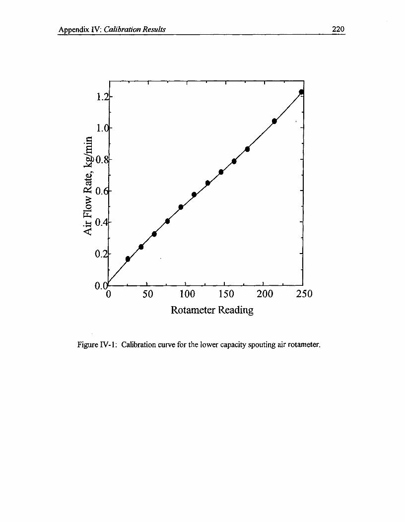
Appendix N: Calibration Results^ 220
0.0-̂ •0 50^100^150^200^250
Rotameter Reading
Figure N-1: Calibration curve for the lower capacity spouting air rotameter.
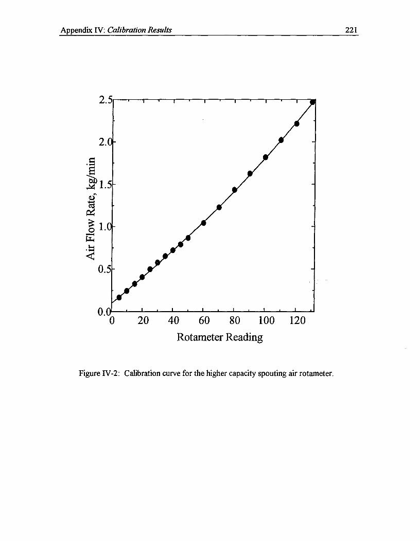
Appendix IV: Calibration Results^ 221
2.5
2.0
.5
_41.5. a )-
17esf: 40 Lo-
...,.0.5
^
0.0^
^
0^20^40^60^80^100 120Rotameter Reading
Figure IV-2: Calibration curve for the higher capacity spouting air rotameter.
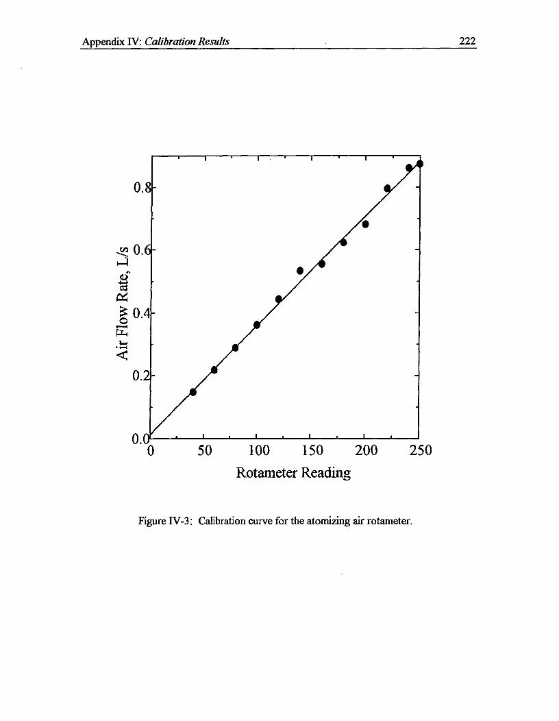
Appendix IV: Calibration Results^ 222
0.8-
0. 0- '̂0 50^100^150^200^250
Rotameter Reading
Figure IV-3: Calibration curve for the atomizing air rotameter.
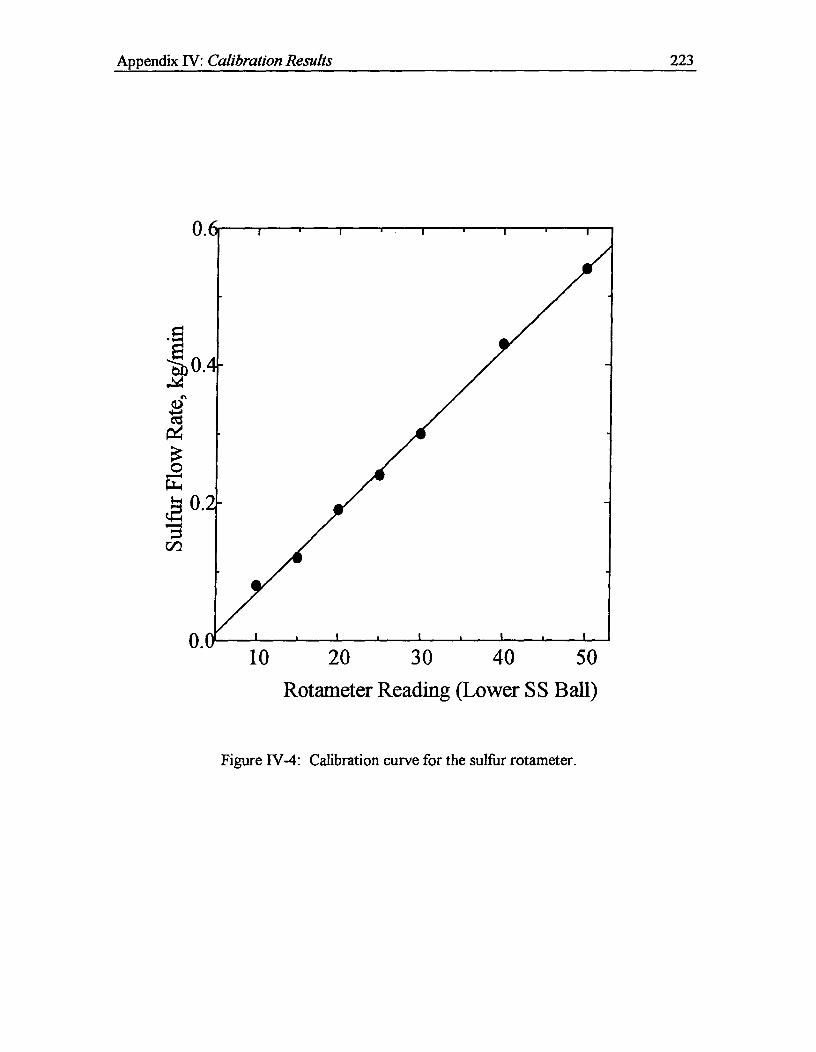
Appendix N: Calibration Results^ 223
0.6^
^
0.0^10^20^30^40^50
Rotameter Reading (Lower SS Ball)
Figure IV-4: Calibration curve for the sulfur rotameter.
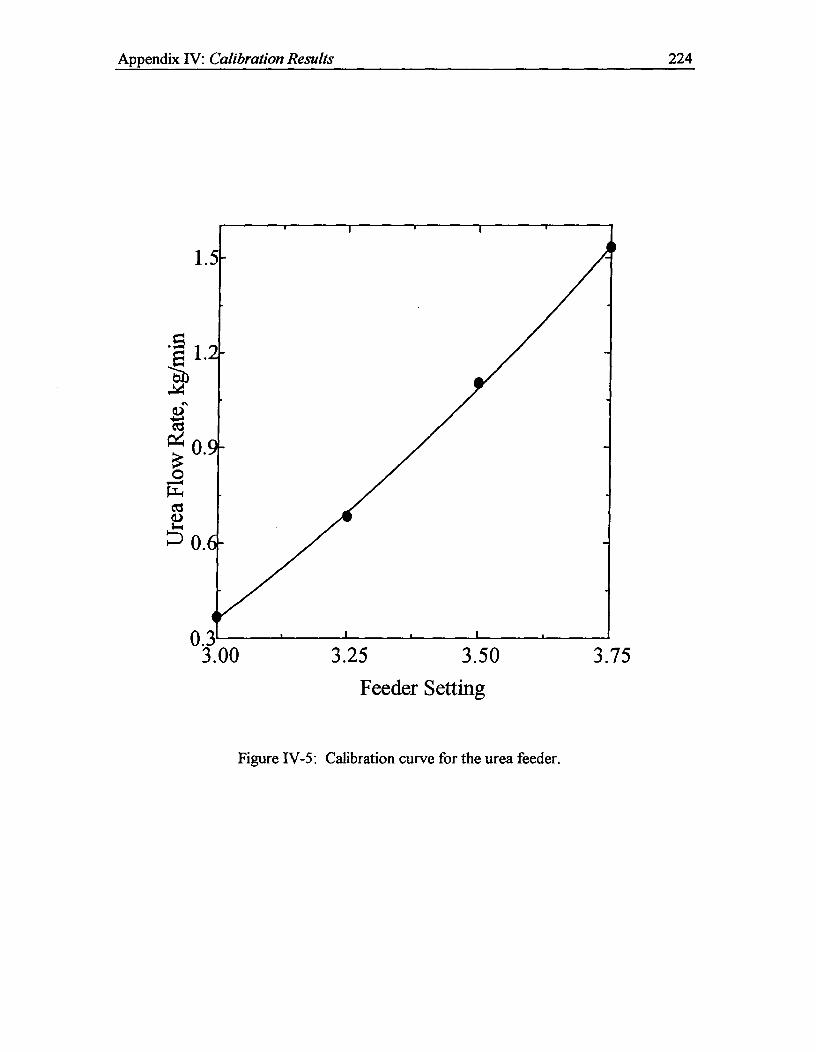
Appendix IV: Calibration Results^ 224
1.5-
0.3^3.00
I^ I
3.25^3.50Feeder Setting
3.75
Figure IV-5: Calibration curve for the urea feeder.
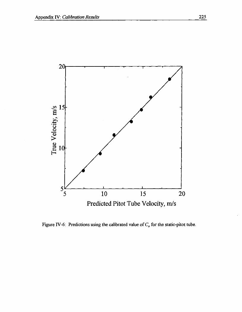
Appendix IV: Calibration Results^ 225
5^10^15^20Predicted Pitot Tube Velocity, m/s
Figure IV-6: Predictions using the calibrated value of C o for the static-pitot tube.
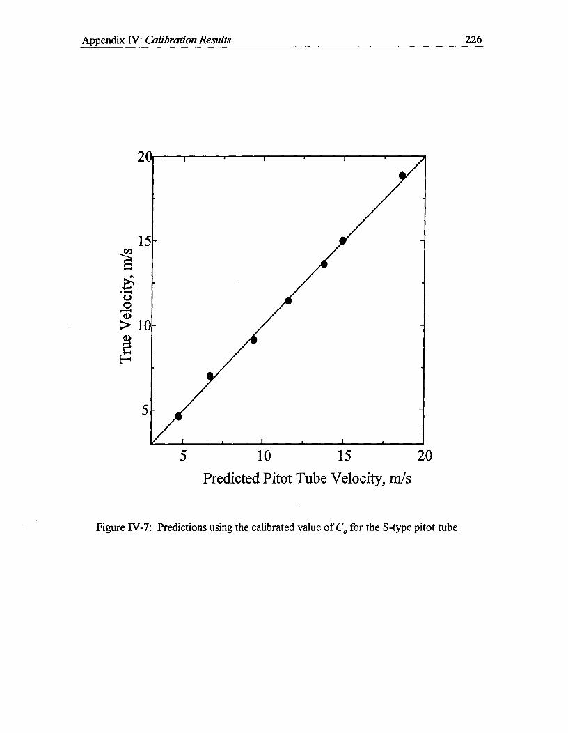
Appendix IV: Calibration Results^ 226
5^10^15^20Predicted Pitot Tube Velocity, m/s
Figure IV-7: Predictions using the calibrated value of Co for the S-type pitot tube.
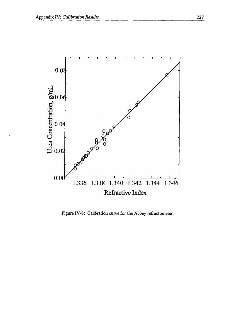
0.0C •^'^•^I^I
1.336 1.338 1.340 1.342 1.344 1.346
0.0E
Appendix IV: Calibration Results^ 227
Refractive Index
Figure IV-8: Calibration curve for the Abbey refractometer.