Plantwide Control and Simulation of Sulfur-Iodine ...

Department of Chemical Engineering

Faculty of Engineering and Science

Plantwide Control and Simulation of Sulfur-Iodine Thermochemical

Cycle Process for Hydrogen Production

Noraini Mohd

This thesis is presented for the Degree of

Doctor of Philosophy

of

Curtin University

July 2018

iii

Acknowledgements

All praises to Almighty Allah Who had given me the strength, endurance and patience in

completing this Doctoral Philosophy (PhD) dissertation. Without His will, this dissertation

will never be completed. I would like to express my warmest appreciation to my supervisor,

Associate Professor Dr. Jobrun Nandong, for his continuous support, motivation and

guidance as well as his constructive comments and suggestions throughout my PhD

adventure. I can’t thank him enough for all he had done, which sparked my curiosity,

excitement and determination in completing this PhD adventure.

I would like to extend my appreciations to my thesis committee, Associate Prof. Dr.

Chua Han Bing, Associate Prof. Dr. Zhuquan Zang and Dr. Ujjal K. Ghosh for their

insightful comments and encouragement throughout my PhD research. I would like to

thank the Higher Degrees by Research (HDR) team of Curtin Malaysia Graduate School

represented by Prof. Marcus Lee and Prof. Clem Kuek, and the Faculty of Engineering and

Science, represented by Prof. Lau Hieng Ho, for their valuable supports. The list of my

acknowledgement goes to all the lecturers and staffs involved in both faculties.

I acknowledge the financial supports given by Curtin University, Curtin Malaysia

Research Institution (CMRI) and Ministry of Higher Education (MOHE).

I would like to express my sincere appreciation to my process control teammates,

especially to Dr. Seer Qiu Han, Dr. Saw Shuey Zi, Dr. Tiong Ching Ching, and my CMRI

colleagues Khizar Abid, Wan Nur Firdaus, Kok Ka Yee, Evelyn Chiong, Tan Kei Xian,

Chan Bun Seng, Ignatius, Timothy, Angie, Luke and to all HDR members for their warm

friendship, continuous support, ideas sharing, useful advices and for all the fun we have

had. To my dearest Solehah’s, Muslimat’s, Masturat’s and friends in Miri, Sarawak, thank

you for always making me feel like being with my family with their care, kindness, helps

and moral support during my study.

iv

Last but not least, I dedicate my heartiest gratitude to my adored parents Mr. Noh Mat

and Mrs. Nor Azizah Awang, my parent in laws, Mr. Khaleb Mohamad and Mrs. Zainab

Mohamad, also to my siblings Jeffry, Nurul Naziral, Mohamad Aiman Amsyar and my

sibling in laws for their prayers and encouragements. The most special gratitude goes to

my beloved husband, Mohamad Izuan Khaleb for his understanding, encouragement,

endless love, prayers and supports for me. Not forgotten to my beloved son, Muhammad

Naufal Khalis Mohamad Izuan, who is the most precious motivation throughout this

journey. Finally, I would like to thanks to those who have indirectly contributed to this

research, their kindness means a lot to me. I dedicate this thesis to all of you.

Noraini Mohd, July 2018.

v

Abstract

Driven by the urgency to address the growing threats of energy security and global

warming issues, extensive researches across multi-disciplinary fields have been conducted

to develop novel technologies for the alternative fuel production. Amongst several

alternative fuels, hydrogen has been identified as one of the most promising energy vectors

as well as the potential to serve as key technologies for future sustainable energy systems

in the stationary power, transportation, industrial and residential sectors. Despite its

tremendous potential as a fuel, presently, hydrogen only accounts for 2% of the global

primary energy usage where over 90% of this hydrogen is generated from fossil fuels.

Therefore, the current production of hydrogen is still considered unsustainable because it

depends on non-renewable sources, e.g., coal and natural gas. It is important to note that,

the actual impact of hydrogen fuel on the environment depends on the technological option

and raw materials used to produce the fuel. Ideally, hydrogen should be produced from

water in order for its production to be sustainable. One option to realize this idea is through

the Sulfur-Iodine Thermochemical Cycle (SITC) process. Although a number of studies

related to the SITC process have been conducted, very little of these studies have addressed

the design, optimization and control aspects of the process. As such it remains to be

answered whether the SITC process is viable or not at an industrial scale in terms of the

economic and controllability grounds. The goal of this PhD study is to address this

important gap, and more specifically to focus on the controllability of the entire SITC plant.

This plantwide control study has now become possible because of the availability of data

on the chemical reactions taking place in the process. Before the plantwide control and

simulation study can be performed, the dynamic model of a pre-defined SITC flowsheet is

first established via mass and energy balances. MATLAB (R2014) programs are developed

in order to enable simulation of the process model, which includes a number of

unconventional reaction schemes and configurations, some of which prohibits the

simulation to be conducted using the Aspen Plus software (version 8.6). The SITC

vi

flowsheet is divided into three major sections: Bunsen Section, H2SO4 Decomposition

Section and HI Decomposition Section. As far as the proposed SITC flowsheet is

concerned, there are four major challenges in the SITC plant operation and control. First,

the HIx (HI-I2-H2O mixture) solution from the Bunsen Section must be controlled well

above an azeotropic composition; otherwise, the proposed separation scheme using a flash

tank will not work. Second, the H2SO4 decomposition section must be supplied with a high-

temperature heating medium to keep the reactor temperature in the range of 800oC to

1000oC. Third, the HI decomposition section which is of a high endothermic reaction must

be maintained at a temperature in the range of 450oC to 500oC. This heat is supplied via a

direct heat integration scheme between the H2SO4 and HI decomposition sections. The

fourth process control challenge of the SITC plant arises from the multiple mass and energy

recycles used in the system, which can potentially lead to a “snowball” effect.

In order to address the aforementioned operational challenges, a plantwide control

(PWC) strategy is carefully designed using the Self-Optimizing Control (SOC) structure

approach, in combination with the Principal Component Analysis (PCA) and Response

Surface Methodology (RSM) techniques. In the plantwide control strategy, both

decentralized Proportional Integral Derivative (PID) control and multivariable Model

Predictive Control (MPC) schemes are adopted. One of the important results from the

plantwide control simulation shows that a nonlinear MPC is recommended to be used for

controlling the HI decomposition section. One reason for this is that a decentralized PID

control scheme is unable to prevent the violation of input constraints in the reactor. It is

worth highlighting that, the proposed plantwide control strategy can effectively handle all

of the above-mentioned challenges, which results in the achievement of 68.6% thermal

efficiency at a maximum hydrogen production of 2,400 kg/hr. This is the highest thermal

efficiency ever reported so far for the SITC plant. Furthermore, a few new contributions

are made in the present work where one of them is the development of the modified PWC

methodology incorporating SOC structure, PCA and RSM techniques. Another

vii

contribution of the work is a novel Loop Gain Controllability (LGC) index. The LGC index

can be used to determine an operating condition having favourable controllability property.

Keywords: Hydrogen; Sulfur-Iodine Thermochemical Cycle; Plantwide Control;

Modelling; Controllability

viii

List of Publications and Presentations

Publications

1) Noraini Mohd and Jobrun Nandong. “Multi-Scale Control of Bunsen Section in

Iodine-Sulphur Thermochemical Cycle Process for Hydrogen Production”.

Chemical Product and Process Modelling. 2016. (accepted).

2) Noraini Mohd and Jobrun Nandong. “Routh-Hurwitz tuning method for

stable/unstable time-delay MIMO processes.” Int. Conf. on Process Engineering &

Advanced Materials (ICPEAM 2018), Kuala Lumpur, Malaysia, 13-15 Aug. 2018.

(accepted).

3) Noraini Mohd, Jobrun Nandong and Ujjal K. Ghosh. “Plantwide Design and

Control of Sulfur-Iodine Thermochemical Cycle Plant.” Submitted to a journal

(under review).

4) Noraini Mohd and Jobrun Nandong. “Self-Optimizing Control Structure of Sulfur-

Iodine Thermochemical Cycle Plant for Hydrogen Production.” Submitted to a

journal (under review).

5) Noraini Mohd, Jobrun Nandong and Syamsul Rizal Abd Shukor. “Simulation

Studies of Sulphur-Iodine Thermochemical Cycle Process for Renewable

Hydrogen Generation: A Review”. (to be submitted to a journal).

6) Noraini Mohd and Jobrun Nandong. “Dynamic Controllability Analysis Method

for Decentralized PID Controller: Application to Patented H2SO4 Decomposition

Reactor”. (to be submitted to a journal).

ix

Presentations

1) Symposium of Malaysian Chemical Engineers (SOMChE) 2016, Miri, Sarawak,

Malaysia. Presentation title: “Multi-Scale Control of Bunsen Section in Iodine-

Sulphur Thermochemical Cycle Process for Hydrogen Production”.

2) North Borneo Research Colloquium (NBRC) 2016, Curtin University Malaysia,

Malaysia. Presentation title: “Simulation Study on Bunsen Section in Hydrogen

Production via Sulfur-Iodine Thermochemical Cycle Process”.

3) Symposium of Malaysian Chemical Engineers (SOMChE) 2017, Kuala Lumpur,

Malaysia. Presentation title: “Dynamic Modelling and Controllability Analysis of

Intensified Reactor: High Temperature Sulphuric Acid Decomposition in a

Hydrogen Production via Thermochemical Cycle process”.

4) One Curtin Postgraduate Conference (OCPC) 2017, Curtin University Malaysia,

Malaysia. Presentation title: “Rigorous Dynamic Modelling of Flash Tank for

Sulphuric Acid and Water Separation in a Sustainable Alternative Fuel Production

Cycle”.

5) 5th Postgraduate Borneo Research Colloquium, 2017, University Malaysia

Sarawak, UNIMAS, Kuching, Sarawak, Malaysia. Presentation title: “Modelling

of High Temperature SO3 Decomposer in Section II of Thermochemical Cycle

Process for Hydrogen Production”.

6) One Curtin Postgraduate Conference (OCPC) 2018, Curtin University Malaysia,

Malaysia. Presentation title: “Dynamic Simulation and Control of Sulfuric Acid

Decomposition in Integrated Boiler-Superheater-Decomposer Reactor”.

x

Table of Contents

Chapter Page

Acknowledgements iii

Abstract v

List of Publications and Presentations viii

Table of Contents x

List of Tables xviii

List of Figures xxiii

List of Abbreviations xxix

1 Introduction 1

1.1 Overview 1

1.2 Problem Statements 4

1.3 Research Objectives 6

1.4 Novelty, Contributions and Significance 6

1.5 Thesis Structure 8

2 Recent Progress and Future Breakthrough of SITC Process 11

2.1 Background 11

xi

2.2 Production of Hydrogen from Water via Thermal Energy Method 12

2.3 Sulfur-Iodine Thermochemical Cycle (SITC) Process 13

2.3.1 Bunsen Section (Section I) 17

2.3.2 Sulfuric Acid Section (Section II) 17

2.3.3 Hydrogen Iodide Section (Section III) 18

2.3.4 Energy Sources to Power the Industrial Scale SITC Process 18

2.3.5 SITC Pilot-Scale Research Projects 21

2.4 Process Modelling and Controller Development of Thermochemical Cycle

Processes 29

2.4.1 Process Controller Development 29

2.4.2 Process Controller Application 34

2.4.3 Process Modelling Development 43

2.4.4 Controllability Analysis Methods 53

2.5 Plantwide Control Structure 58

2.6 Research Challenges in SITC Process 59

2.7 Summary 61

3 Methodology: From Process Modelling to PWC Structure Development 63

3.1 Overview 63

xii

3.2 Overall Process Methodology 65

3.2.1 Preliminary Work 65

3.2.2 Modelling 65

3.2.3 Plant Scale-up 67

3.2.4 Process Controller Design and Development (by Section) 68

3.2.5 Plantwide Model 70

3.2.6 Plantwide Control Structure Development 72

3.2.7 Process Controller Performance Evaluation 74

3.3 Loop Gain Controllability (LGC) Index 74

3.3.1 Fundamental of LGC 74

3.3.2 Derivation of LGC Index 76

3.3.3 Illustrative Examples – Evaluation of Dynamics via LGC Index 81

3.4 Plantwide Control Approach 92

3.5 Optimal-Practical Plantwide (OPPWIDE) Optimization 93

3.6 Multi-scale Control Scheme 96

3.7 Model Predictive Control 97

3.7.1 MPC tuning 101

3.8 Summary 101

xiii

4 Bunsen Section: Dynamic Modelling and Controllability Analysis 103

4.1 Fundamental of Bunsen Section 103

4.1.1 Reaction Mechanism 104

4.2 Bunsen Reactor 105

4.2.1 Modeling of Bunsen Reactor 105

4.3 Bunsen Reactor Scale-Up Procedure 118

4.4 Liquid-Liquid Separator 122

4.4.1 Mass Balance 123

4.5 Novel Procedure for Control System Design 125

4.6 Loop Gain Controllability Analysis 127

4.7 Process Controller Design for Bunsen Section 131

4.7.1 NMPC Design for Bunsen reactor 131

4.7.2 MSC-PID Design for Liquid-liquid separator 134

4.8 Performance Evaluation of NMPC in Bunsen Reactor 135

4.8.1 NMPC Performance on Bunsen reactor 135

4.8.2 MSC-PID Performance 139

4.9 Summary 141

xiv

5 Sulfuric Acid Section (Section II): Dynamic Modelling and Controllability Analysis

143

5.1 Fundamental of Sulphuric Acid Section 143

5.1.1 Reaction Mechanisms 144

5.2 Dynamic Modelling and Simulation 145

5.2.1 Sulfuric Acid Flash Tank (SA-FT) 145

5.2.2 Sulfuric Acid Decomposition in SA-IBSD Reactor 154

5.3 Loop Gain Controllability Analysis of SA-IBSD Reactor 170

5.4 Process Controller Design of SA-IBSD Reactor 172

5.5 Controller Performance of SA-IBSD Reactor 173

5.6 Summary 175

6 Hydrogen Iodide Section: Dynamic Modelling and Controllability Analysis 177

6.1 Fundamental of Hydrogen Iodide Section 177

6.1.1 Reaction Mechanisms 178

6.2 Hydrogen Iodide Flash Tank (HI-FT) 178

6.3 Hydrogen Iodide Decomposition (HI-DE) Reactor 181

6.3.1 Dynamic Modelling of HI-DE Reactor 181

6.3.2 Scale-up Procedure of HI-DE Reactor 184

xv

6.4 Loop Gain Controllability Analysis of HI-DE Reactor 186

6.5 Process Controller Design of HI-DE Reactor 189

6.6 Controller Performance of HI-DE Reactor 190

6.7 Summary 194

7 Industrial SITC Plant Flowsheet 196

7.1 Chemical Reactions in SITC Plant 196

7.1.1 Section I 198

7.1.2 Section II 199

7.1.3 Section III 201

7.2 Plantwide SITC Flowsheet 203

7.3 SITC Process Optimization and Sensitivity Analysis 206

7.3.1 Process Optimization via Response Surface Methodology (RSM) 206

7.3.2 Input-Output Sensitivity via Principle Component Analysis (PCA) 209

7.4 Economic Analysis 215

7.4.1 Plant Investment, Specification and Targets 215

7.4.2 Capital Cost Estimation 215

7.4.3 Equipment Cost Summary for the Whole Plant 216

7.4.4 Fixed Capital Investment 216

xvi

7.5 Summary 220

8 Plantwide Control of Industrial SITC Plant 222

8.1 PWC Objectives 222

8.2 PWC Preliminary Steps 224

8.2.1 Significance of Preliminary Steps 224

8.2.2 Step by Step Procedure 225

8.3 PWC Structure Development 230

8.3.1 Skogestad Top-down Analysis 230

8.3.2 Skogestad Bottom-up Design 238

8.4 PWC Performance Assessment 247

8.5 Summary 248

9 Conclusion and Recommendations 249

9.1 Conclusions 249

9.1.1 Development of Industrial Scale of SITC Plant Flowsheet 249

9.1.2 Process Optimization and Controllability Analysis of SITC Process 250

9.1.3 PWC Structure Development of the SITC Process 251

9.1.4 New Contributions 251

9.2 Recommendations 253

xvii

References 254

Appendix A 274

Appendix B 277

xviii

List of Tables

Table 2.1: Advantages and challenges of SITC process (Perret, 2011a) .......................... 14

Table 2.2: Potential input and output variables of SITC process ..................................... 16

Table 2.3: Outdoor research facilities and demonstration plants on solar thermochemical

processes (Yadav and Banerjee, 2016b) ........................................................................... 20

Table 2.4: Overview of the research and development of the SITC process in JAEA ..... 24

Table 2.5: The current and future phase research on SITC process by INET .................. 28

Table 2.6: Controllers developed and applied in various parts of thermochemical cycle

processes for hydrogen production. .................................................................................. 31

Table 2.7: Summary of the process controller application on CSTR, L-L separator, flash

tank and tubular reactor of various processes ................................................................... 40

Table 2.8: Type of models developed for various thermochemical cycle processes ........ 45

Table 2.9: Application of Aspen Plus and HYSIS in various thermochemical processes

modelling and simulation .................................................................................................. 50

Table 2.10: Function and feature comparison between RGA, NI and LGC ..................... 57

Table 3.1. Baseline conditions for the Distillation Column (DC) .................................... 81

Table 3.2. Baseline conditions for the Interacting Tanks (IT) .......................................... 81

Table 3.3. Transfer Functions for the DC and IT processes. ............................................ 82

xix

Table 3.4: Distillation Column Model 1: feature comparison among RGA, NI and LGC.

........................................................................................................................................... 84


........................................................................................................................................... 85

Table 3.6: Interacting Tanks Model 3: Features comparison between RGA, NI and LGC

........................................................................................................................................... 89

Table 3.7: Interacting Tanks, Model 4: Features comparison between RGA, NI and LGC

........................................................................................................................................... 90

Table 4.1: Kinetic parameters for the Bunsen reactor (Zhu et al., 2013) ....................... 110

Table 4.2: Design parameters for the Bunsen reactor ..................................................... 110

Table 4.3: Physical constants for the Bunsen reactor (Don and Perry, 1984) ............... 110

Table 4.4: Bunsen Reactor Validation Parameters and Results ...................................... 111

Table 4.5: Factors, levels and actual values for Bunsen reactor optimization ................ 114

Table 4.6: Optimum values of parameters for Bunsen reactor ....................................... 118

Table 4.7: Bunsen reactor laboratory scale and plant scale parameters ......................... 121

Table 4.8: Parameters of LLS dynamic model ............................................................... 124

Table 4.9: Controllability analysis based on 2x2 MIMO model of Bunsen reactor ....... 130

Table 4.10: Transfer function models for the Bunsen reactor at nominal conditions. .... 131

Table 4.11: NARX model nonlinearity estimator object best fit value .......................... 133

Table 4.12: SSE values for CV1 and CV2 of Bunsen reactor for various MPC tuning . 134

xx

Table 4.13: Nominal value of LLS levels ....................................................................... 135

Table 5.1: Sulfuric acid flash tank output from the Aspen Plus simulation. .................. 149

Table 5.2: NRTL parameters for Sulfuric Acid/ Water separation in SA-FT. ............... 150

Table 5.3: Flash tank dynamic modelling results vs. literature ...................................... 154

Table 5.4: Parameters of the patented integrated reactor for sulfuric acid decomposition

proposed by Moore et.al, 2011. ...................................................................................... 156

Table 5.5: Values of model parameters used in the simulation of the Evaporator Zone 160

Table 5.6: Values of parameters used in the simulation of the Superheater Zone.......... 162

Table 5.7: Values of parameters used in the simulation of the decomposition zone ...... 166

Table 5.8: SA-IBSD reactor laboratory scale and plant scale parameters ...................... 169

Table 5.9: SA-IBSD transfer function models and its input-output pairing ................... 170

Table 5.10: Controllability analysis for SA-IBSD reactor .............................................. 171

Table 5.11: Nominal values and the constraints of the SA-IBSD reactor output variables.

......................................................................................................................................... 172

Table 6.1: Stream table of HI-FT simulation in Aspen Plus........................................... 180

Table 6.2: Non-randomness and dimensionless interaction parameter for hydrogen

iodide/hydroiodic acid separation in HI-FT from Aspen Plus simulation. ..................... 180

Table 6.3: Parameters involved in the simulation of HI-DE reactor .............................. 183

Table 6.4: Parameters of HI-DE reactor models for laboratory scale and plant scale

production. ...................................................................................................................... 186

xxi

Table 6.5: HI-DE transfer function models and its input-output pairing ........................ 187

Table 6.6: Controllability analysis for HI-DE reactor .................................................... 188

Table 6.7: Nominal values and the constraints of the HI-DE reactor output variables. . 189

Table 7.1: The equipment design material, size, production capacity and design operating

condition of industrial scale SITC plant ......................................................................... 204

Table 7.2: The responses (output) and factors (input) in the SITC process optimization

......................................................................................................................................... 207

Table 7.3: Desired process optimization criteria of the SITC plant using RSM in Design

Expert software ............................................................................................................... 209

Table 7.4: Optimum values obtained for SITC plant variables based on RSM optimization

......................................................................................................................................... 209

Table 7.5: Sensitivity analysis of input-output variables coefficient table of SITC plant via

RSM analysis: Checked box present significant effect (p<0.05) .................................... 212

Table 7.6: Sensitivity analysis of input-output variables coefficient table of SITC plant via

PCA analysis: Checked box represent significant effect ................................................ 213

Table 7.7: Input-output sensitivity analysis via PCA method ........................................ 214

Table 7.8: List of main equipment of SITC plant .......................................................... 219

Table 8.1: Variables specification of SITC ..................................................................... 223

Table 8.2: Optimized steady-state flowrate of SITC plant ............................................. 226

Table 8.3: Total energy required in the Bunsen reactor .................................................. 227

xxii

Table 8.4: Total energy required for SA-IBSD reactor .................................................. 227

Table 8.5: Total energy required for HI Decomposer..................................................... 228

Table 8.6: Scale up volume of SITC equipment ............................................................. 229

Table 8.7: Cost of products, feedstock and utilities ........................................................ 231

Table 8.8: CDOF and ODOF of SITC plant ................................................................... 233

Table 8.9: Controlled variables, manipulated variables and controller type of SITC plant

......................................................................................................................................... 234

Table 8.10: Potential inputs and their PCA coefficient values in relation to oxygen and

hydrogen flowrates.......................................................................................................... 237

Table 8.11: The optimization performance of two SITC models. .................................. 246

xxiii

List of Figures

Figure 1-1: Flowchart of overall thesis structure .............................................................. 10

Figure 2-1 : SITC process flow diagram, Section I, Section II, and Section III (Sakaba et

al., 2006) ........................................................................................................................... 15

Figure 3-1: Flowchart of overall research methodology................................................... 64

Figure 3-2: Flowchart of overall modelling methodologies ............................................. 66

Figure 3-3: Flowchart of overall methodology for dynamic controllability analysis. ...... 69

Figure 3-4: Flowchart of overall PWC structure development ......................................... 73

Figure 3-5: Loop gain (dashed square area) of a general control loop structure .............. 75

Figure 3-6: Upper and lower limits concept behind the LGC approach ........................... 76

Figure 3-7: Overall methodology of LGC index determination and closed-loop simulation.

........................................................................................................................................... 80

Figure 3-8: LGC analysis of distillation column for step up and step down models: a) Model

1, 1st order, b) Model 1, 5th order, c) Model 2, 1st order, d) Model 2, 5th order. ............... 86

Figure 3-9: LGC analysis of interacting tanks for step up and step down models: a) Model

3, 1st order, b) Model 3, 5th order, c) Model 4, 1st order, d) Model 4, 5th order ................ 91

Figure 3-10: LGC analysis of interacting tanks Model 3, Loop 1 (y1) and Loop 2 (y2) for

direct and indirect pairings................................................................................................ 92

Figure 3-11: Control hierarchy of a chemical plant (Skogestad, 2000a) .......................... 93

xxiv

Figure 3-12: Multi-scale control scheme: (a) three-loop, (b) reduced two-loop, and (c)

equivalent single-loop block diagrams (Nandong, 2014). ................................................ 98

Figure 3-13: A simplified block diagram of the typical MPC .......................................... 99

Figure 4-1: Bunsen reactor (jacket CSTR) ..................................................................... 105

Figure 4-2: Bunsen Reactor Validation Plots: Simulation of Current Work (solid line) vs.

Zhu et al. (2013) (dot marker). (a) Temperature 336K, (b) Temperature 345K, (c)

Temperature 358K. ......................................................................................................... 113

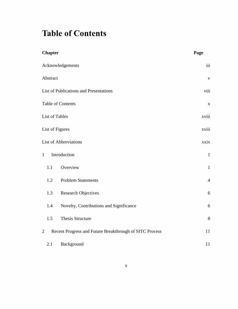
Figure 4-3: Overlay plot for 𝐻𝐼 and 𝐻2𝑆𝑂4 flow rates under optimum condition of the

main input ranges ............................................................................................................ 116

Figure 4-4: 3D Plot of optimum 𝐻𝐼 molar flow rate and operating condition: 1.8 mol . 117

Figure 4-5: 3D Plot of optimum 𝐻2𝑆𝑂4 molar flow rate and operating condition: 0.9 mol

......................................................................................................................................... 117

Figure 4-6: An example illustration block diagram of SITC plant scale-up. .................. 119

Figure 4-7: Flowchart of scaling up steps for Bunsen reactor ........................................ 120

Figure 4-8: Scaling-up schematic diagram for Bunsen reactor: (a) the laboratory scale

Bunsen reactor, (b) the plant scale Bunsen reactor. ........................................................ 121

Figure 4-9: Liquid-liquid separator: (a) schematic diagram, and (b) internal view ........ 123

Figure 4-10: Flowchart of novel procedure for designing control system...................... 127

Figure 4-11: NARX model identification for 𝑢1𝑎𝑛𝑑 𝑦1................................................ 132

Figure 4-12: NARX model identification for 𝑢2 𝑎𝑛𝑑 𝑦2 ............................................... 132

xxv

Figure 4-13: Response of NMPC for setpoint changes in CV1, sulfuric acid flowrate.. 136

Figure 4-14: Response of iodine molar feed flow (MV1) under the setpoint changes in

CV1. ................................................................................................................................ 136

Figure 4-15: Response of NMPC for setpoint changes in CV2, Bunsen reactor temperature.

......................................................................................................................................... 137

Figure 4-16: Response of sulfur dioxide volumetric flow rate (MV2) under the setpoint

changes in CV2. .............................................................................................................. 137

Figure 4-17: Response of NMPC for disturbance rejection test for CV1 ....................... 138

Figure 4-18: Response of NMPC for disturbance rejection test for CV2 ....................... 138

Figure 4-19: Response of MSC-PID and IMC-PID for setpoint tracking in CV, heavy phase

level of LLS. ................................................................................................................... 139

Figure 4-20: Response of MSC-PID and IMC-PID for setpoint changes in CV, heavy phase

level of LLS. ................................................................................................................... 140

Figure 4-21: Response of MSC-PID for disturbance rejection test for CV. ................... 141

Figure 4-22: Response of IMC-PID for disturbance rejection test for CV. .................... 141

Figure 5-1: The schematic diagram of SA-FT (Watkins, 1967) ..................................... 145

Figure 5-2: Output profiles, (a) Flash tank level, (b) Sulfuric acid liquid fraction (bottom

outlet), (c) Sulfuric acid vapor fraction (upper outlet) .................................................... 153

Figure 5-3: Schematic diagram of the modified SA-IBSD reactor (Moore et.al, 2011) 155

Figure 5-4: Zoom in diagram for the reaction zone in the SA-IBSD reactor cell. ......... 164

xxvi

Figure 5-5: Validation plot of temperature profile of SA-IBSD reactor: Simulation (solid

line) vs. Literature (Moore et.al, 2011) (dotted) ............................................................. 167

Figure 5-6: Scaling-up illustrative diagram for SA-IBSD reactor: a) the laboratory scale

SA-IBSD reactor cell, b) the plant scale multi-cell SAIBSD reactor. ............................ 168

Figure 5-7: Response of MSC-PID and IMC-PID for setpoint changes in CV1, temperature

of SA-IBSD reactor......................................................................................................... 173

Figure 5-8: Response of MSC-PID and IMC-PID for setpoint changes in CV2, product

flowrate of SA-IBSD reactor. ......................................................................................... 174

Figure 5-9: Response of MSC-PID and IMC-PID for setpoint changes in MV2, external

jacket flowrate of SA-IBSD reactor. ............................................................................... 174

Figure 5-10: Response of MSC-PID for disturbance rejection test for SA-IBSD

temperature, CV1. ........................................................................................................... 175

Figure 6-1: Schematic diagram of hydrogen iodide flash tank (HI-FT) ......................... 179

Figure 6-2: HI-FT simulation diagram in Aspen Plus. ................................................... 179

Figure 6-3: Schematic diagram of HI-DE reactor........................................................... 181

Figure 6-4: Scaling-up schematic diagram for HI-DE reactor: a) the laboratory scale HI-

DE reactor, b) the plant scale multi-tubes HI-DE reactor. .............................................. 185

Figure 6-5: Response of Robust-PID controller for setpoint changes in CV2, temperature

of HI-DE reactor. ............................................................................................................ 190

Figure 6-6: MV2 response of Robust-PID controller for setpoint changes in CV2, feed

jacket temperature of HI-DE reactor. .............................................................................. 190

xxvii

Figure 6-7: Response of SS-MPC and NARX-MPC for setpoint changes in CV2, HI-DE

reactor temperature. ........................................................................................................ 192

Figure 6-8: Response of SS-MPC and NARX-MPC for setpoint changes in CV1, hydrogen

flowrate. .......................................................................................................................... 192

Figure 6-9: Response changes of SS-MPC and NARX-MPC for setpoint changes in MV2,

feed jacket temperature. .................................................................................................. 193

Figure 6-10: Disturbance rejection test of NARX-MPC for 10% increase in the feed

temperature. .................................................................................................................... 194

Figure 7-1: Bunsen Section (Section I) flowsheet .......................................................... 199

Figure 7-2: H2SO4 Section (Section II) flowsheet .......................................................... 201

Figure 7-3: HI Section (Section III) flowsheet. .............................................................. 202

Figure 7-4: A complete industrial scale SITC plant flowsheet. ...................................... 205

Figure 7-5: 3D Plots of (a) optimum molar hydrogen flow rate (b) optimum oxygen flow

rate................................................................................................................................... 208

Figure 7-6: 3D Plots of (a) optimum HI-DE temperature (b) optimum SA-IBSD jacket

temperature. .................................................................................................................... 208

Figure 7-7: Principal component plots of PCA analysis ................................................. 211

Figure 7-8: 2D Pareto plot of PCA analysis ................................................................... 211

Figure 8-1: Steady-state input and output mass flow of SITC plant............................... 225

Figure 8-2: Industrial scale SITC plant with control loops............................................. 235

xxviii

Figure 8-3: Control hierarchy of a chemical plant (Skogestad, 2000a) .......................... 238

Figure 8-4: CV profile: Robustness test of NMPC for -30% load change in the TPM on

hydrogen flowrate. .......................................................................................................... 239

Figure 8-5: MV profile: Robustness test of NMPC for -30% load change in the TPM. 240

Figure 8-6: CV1 profile: Performance of NMPC for setpoint change on ratio of hydrogen

iodide mixture, 𝐻𝐼𝑥/(𝐻𝐼 + 𝐻2𝑂) .................................................................................. 241

Figure 8-7: CV2 profile: Performance of NMPC for setpoint change on hydrogen flowrate,

𝑚𝐻2 ................................................................................................................................ 241

Figure 8-8: MV profile: Performance of NMPC for setpoint change on the feed 𝐼2/𝐻2𝑂

molar ratio. ...................................................................................................................... 242

Figure 8-9: Flowchart of OPPWIDE optimization approach ......................................... 243

Figure 8-10: Skogestad SOC plot ................................................................................... 244

Figure 8-11: PCA Pareto plot ......................................................................................... 245

xxix

List of Abbreviations

FFNN Feed forward neural network

GMC Generic Model Control

LGC Loop Gain Controllability index

ISE Integrated Squared Error

LMPC Linear MPC

LP Linear programming

MIMO Multi input multi output

MPC Model Predictive Control

MSE Means Squared Error

MAE Means Absolute Error

MSC Multi Scale Control

NARX Nonlinear autoregressive model with exogenous input

NLP Nonlinear programming

NMPC Nonlinear Model Predictive Control

NN-MPC Neural Network model based on Model Predictive Control

ODEs Ordinary Differential Equations

OPPWIDE Optimal-Practical Plantwide optimization

PID Proportional Integral Derivative controller

QP Quadratic programming

SISO Single input single output

SS-MPC State space model based on Model Predictive Control

SSE Sum Squared Error

SITC Sulfur-Iodine Thermochemical Cycle

1 Introduction

Sulfur-Iodine Thermochemical Cycle (SITC) process has emerged as a promising

alternative technology to produce environmental friendly hydrogen fuel. Its strong

potential is currently being studied at the lab-scales and pilot plant scales. To date, the

SITC plant is not yet available anywhere at the industrial scale. This chapter provides a

brief research background and problem identification, which is to be addressed in this

research project. This introduction presents descriptions on the research motivation and

objectives, as well as the novelty, contribution and significance of the proposed study,

followed by brief research procedures and finally, the thesis structure.

1.1 Overview

Hydrogen has been recognized as an environmentally friendly alternative to other fuels in

both transportation and non-transportation usages. Recent publications have advocated the

potential of hydrogen fuel usage as an effective mitigation method to decrease the rate of

anthropogenic greenhouse gas emissions, which have been identified responsible for

increasing global warming issue (Cipriani et al., 2014; Gupta and Pant, 2008a; Moriarty

and Honnery, 2009; Satyapal and Thomas, 2008). Over the last few decades, considerable

research efforts have been dedicated to addressing renewable hydrogen production

technologies, hence realizing the Hydrogen Economy (Kasahara et al., 2017). In this

regard, the production of hydrogen fuel should be based on a renewable sources, non-fossil,

and one that produces clean environmentally benign by-products; see (Almogren and

Veziroglu, 2004; Duigou et al., 2007; Levene et al., 2007). Based on these criteria,

hydrogen production is considered a clean, environment-friendly energy carrier if it is

produced from water via thermal route using a renewable energy source (Nowotny and

Veziroglu, 2011). So far, water represents the main feedstock for clean hydrogen

production via the thermal route, which has recently established itself as a strong potential

candidate to realizing the Hydrogen Economy (Funk, 2001; Schultz, 2003).

2

Some of the ways to produce hydrogen from water via the thermal route includes the

electrolysis method, thermochemical water splitting method and hybrid cycle method.

Unlike the conventional electrolysis, which needs electrical energy to split water

molecules, the thermochemical cycle can split water molecules into hydrogen and oxygen

directly using thermal energy (Huang and T-Raissi, 2005). Since the thermal energy can

be obtained from solar or waste heat from a high temperature nuclear reactor, the

thermochemical cycle has a potential to significantly reduce the cost of hydrogen

production from water. There are more than 350 thermochemical cycles, which have been

identified and evaluated in 2011 by the DOE-EERE Fuel Cell Technologies Program,

Sandia National Laboratories, under a project called Solar Thermochemical Cycles for

Hydrogen production (STCH) (Perret, 2011a). An extensive report by Perret (2011b)

summarizes that the Sulfur-Iodine Thermochemical Cycle (SITC) has demonstrated the

most promising performance in terms of experimental and technical feasibility, efficiency

and stability when compared to other types of thermochemical cycles.

Even though the use of ‘renewable’ hydrogen as a substitute for the non-renewable

fossil fuels appears to be an attractive way to address global warming and energy security

issues, none of the currently available hydrogen production technologies are anywhere near

to a point of economic viability (Abbasi and Abbasi, 2011). Consequently, it has been

envisioned that the development of optimized plant designs and engineering methods that

are able to improve overall system efficiency, reduce system complexity, increase

controllable properties, and lower the capital cost are imperative for the systems-level

improvements of a hydrogen production plant. So far, most mainstream works related to

the SITC process have focused on experimental studies with some heavy attention to

chemical reaction behaviours (Xu et al., 2017a). Presently, only a limited study on

modelling of hydrogen production via the SITC process has been reported, partly due to

the complex nature of this process, particularly when it is desired to be operated at a

commercial-scale. Furthermore, existing research on the modelling has been done rather

3

disparately, confined to certain sections or equipment of the thermochemical cycle process,

i.e., not on the entire plantwide process.

At the plantwide level, various mechanisms and process interactions are expected to

come into play in determining the process dynamics and performance of the SITC process.

One important factor in determining the efficiency of the SITC plant is the formation of

different immiscible phases which can occur in the Bunsen Section (Guo et al., 2012). At

the heart of SITC operation is the Bunsen Section, in which the reaction yield must be high

enough to achieve compositions well above that of azeotropic compositions. Meeting this

objective is crucial as to enable smooth operations of the subsequent sulfuric acid and

hydrogen iodide decomposition sections. Other challenges can also arise from the high

temperature requirement in the Sulfuric Acid Decomposition Section and the high thermal

energy demand in the Hydrogen Iodide Decomposition Section (Wang et al., 2014a).

Furthermore, the presence of more than a few serial reactions, together with the mass and

heat recycle streams in the SITC plant are expected to pose some challenges to controlling

the plant. All of the above-mentioned challenges contribute to inherent complexity in the

plantwide SITC dynamics, hence to its plantwide design and control.

Due to the presence of multiple constraints in the SITC process, the conventional PID-

based control system alone may not be able to provide sufficient performance in controlling

the whole plant. Furthermore, the plant nonlinearity may impose a big challenge to the

control system design, e.g., dynamic nonlinearity in the separation columns or equipment

operated under critical conditions, loads of recycle lines, non-stationary behaviour in some

of the sub-systems, and time delays of the sensors (Rodriguez-Toral et al., 2000). Despite

the expected complex dynamics of SITC plant, the application of conventional PID

controllers is still desirable because the control system can be applied without that much

need on knowledge of advanced process modelling and control technique. However, for a

certain part/s where complex dynamics and process constraints arise, it is may be necessary

to apply some advanced control techniques to control this part of the plant. Thus, a practical

4

plantwide control system for the SITC plant are expected to be of a mix of PID and

advanced controllers, e.g., nonlinear model predictive control (NMPC).

As a holistic methodology to improve performance, a plantwide control strategy has

until now remained underutilized to address some of the difficulties encountered in a

thermochemical process design. In the present study, one of the focal idea is to build a

systematic procedure of plantwide control strategy, which takes into account multiscale

information from across multiscale layers of units in the plant. In other words, data and

dynamic behaviours of each equipment in every section are combined into an integrated

model, which should offer enhanced predictions and interpretations of the system emergent

properties – thus, to preserve system level properties such as robustness and flexibility. It

is worth highlighting that process control and optimization along with the plant design are

preferably addressed systematically within a plantwide framework. This then should allow

simultaneous considerations of the economic and controllability analysis of the SITC plant.

Overall, by applying the plantwide control strategies, the integration of advanced and

conventional ways can be formulated into a practical solution for the complex and new

SITC process.

1.2 Problem Statements

The motivation for this study is driven by two important research gaps in the existing

studies related to the SITC process:

a) There has been no study on the plantwide control (PWC) structure development of

the entire SITC plant.

b) There has been study on the design, simulation and optimization of an industrial

scale SITC plant.

In view of the aforementioned research gaps, the present study aims to answer the

following questions:

5

a) Is the industrial scale SITC process viable on the controllability and economic

grounds?

b) Which section/s in the SITC plant will impose the most difficult challenge/s to

operation and control?

c) Will the heat integration between Sulfuric Acid Decomposition and Hydrogen

Iodide Decomposition Sections be feasible?

d) What is the workable plantwide control structure of the industrial SITC plant?

Relating to the first motivating factor, the control structure problem is the central issue

to be resolved in modern process control which is an integral part of a plant design. An

integrated plant design and plantwide control study of the SITC process has so far, received

very little attention from research community. Besides, there has been no report of the

complete industrial scale SITC process. Bear in mind that, an integrated system design is

essential to address the key operational problems in all of the three sections in the SITC

process. The primary goal of the plantwide control structure analysis is to achieve both

economically feasible and dynamically controllable flow sheet design. This integrated

study so far, has not been performed on the SITC process. Hence in this research work, the

goal is to develop a design that can achieve an optimal compromise between steady-state

economic and dynamic controllability performance criteria for the entire SITC plant.

As for the second motivation factor, existing research on the modelling, optimization

and controllability of an industrial scale SITC process, remains very limited. In particular,

the controllability study for the SITC process is currently not available in the open

literature. In short, a rigorous system engineering study (robustness, flexibility and optimal

operation) of the industrial scale SITC process has not yet been done. It is believed that,

the system engineering study is a crucial step toward the commercialization of the SITC

process for hydrogen production.

6

1.3 Research Objectives

The overall goal of the research project is to study an industrial scale SITC plant design to

meet a production rate of at least 1,000 kg of hydrogen per hour. To attain the

aforementioned goal, the following specific objectives are pursued:

1) To develop a flowsheet of an industrial scale SITC plant. Based on the designed

flowsheet, a plantwide model of the SITC system will be established and utilized

in objective (ii) and (iii) of this study.

2) To optimize the plantwide SITC process using the constructed model (objective (i))

aiming to achieve an optimal trade-off between steady-state economic and dynamic

controllability performance criteria. Aspen Plus software will be used for

conducting steady-state simulation and to generate data for steady-state

optimization. The controllability performance evaluations will be conducted using

the plantwide SITC model implemented in MATLAB environment.

3) To design plantwide control strategy (hybrid of PID controller and NMPC) for the

SITC process. To address the high nonlinear characteristic in certain parts of the

plant, the NMPC scheme will be used to control the parts involved. Conventional

PID controllers designed based on the Multi-Scale Control (MSC) scheme will be

used to control other parts which demonstrates mild dynamic nonlinearity or

behaviours.

1.4 Novelty, Contributions and Significance

The novelty of the proposed research project lies in the adoption of thorough system

engineering approach to hydrogen production via the SITC process, which attempts to

address steady-state and dynamic operability performance issues. As far as the

thermochemical cycle process is concerned, such an integrative research approach has not

7

yet been reported in the open literature. The main contributions of this work can be

summarized as follows.

From the novelty perspectives:

1) New idea of combining MSC-PID and NMPC schemes in an integrated plantwide

control (PWC) structure.

2) Application of system engineering approach incorporating controllability,

robustness, flexibility and optimal operations of the thermochemical cycle process.

3) A unified methodology taking into accounts both steady-state performance and

dynamic controllability criteria in the plantwide optimization.

From the scientific contributions perspectives:

1) A new controllability index is developed to help analyze the controllability property

of the SITC process.

2) Some new insights into the design and operating condition influences on the SITC

system-level properties, which answer the aforementioned research questions.

3) Novel procedure to develop a hybrid MSC-PID and advanced NMPC strategy for

effective plantwide control of a complete process plant.

The significance of the proposed study can be viewed as follows:

1) Provide some new insights into the operation and control of SITC process at an

industrial scale, which should serve as an essential reference in the thermochemical

cycle research topic.

2) Provide some new research directions in the development of thermochemical cycle

technology as an intensified approach to high-performance, economic and

environmentally friendly of hydrogen production.

3) This project contributes to the Malaysian National Key Area (NKA): Oil, Gas &

Energy, and Education sectors. The improvement in this process has the potential

8

in opening a new opportunity for the energy industry in Malaysia, i.e., to venture

into a new technology to producing environmentally friendly as well as

economically feasible alternative fuel for utility in the transportation sector.

It is worth highlighting that, to date, the plantwide modelling and control research remains

an open problem that has become increasingly important in recent years. The reason for

this arises from the need of process industries to meet tighter environmental regulations

and product qualities. It has been recognized that the linkage of plant layout information

(plantwide model) with the advancement in process control is a key to effectively using

improved standards for achieving specified process performances. For some new

underdeveloped processes, such as the SITC, a novel approach is required to addressing

the design and control problems in the process.

1.5 Thesis Structure

This thesis is arranged into nine chapters. In all chapters, a relatively short background on

the main subject of the chapter is presented in the introduction section.

Chapter 2 includes the background review of the SITC process scheme. The chapter

illustrates the main concern on the control issues in the whole process plant, along with a

discussion of research, modelling, control and plant design opportunities. Finally, a general

framework is suggested for the case study.

Chapter 3 presents the methodology. This chapter provides all the basic and preliminaries

to the subsequent chapters. It is then followed by the step-by-step procedures of the

proposed methodology up to the controller performance evaluation procedure.

Chapter 4 presents the process description, modelling, controllability analysis, process

controller design and the result evaluation of the Bunsen Section in the SITC plant.

9


controller design and the result evaluation of the Sulfuric Acid Section in the SITC plant.


controller design and result evaluation of the Hydrogen Iodide Section in the SITC plant.

Chapter 7 presents the complete flowsheet development of the industrial scale SITC plant.

Chapter 8 details the plantwide control structure development of the SITC plant.

Chapter 9 provides main conclusions. Figure 1-1 shows the overall thesis structure.

10

Chapter 1Introduction

Chapter 2Literature

Review

Chapter 3Methodology

Chapter 4Bunsen Section

Chapter 5Sulfuric Acid

Section

Chapter 6Hydrogen Iodide

Section

Chapter 7Industrial Scale

SITC Plant

Chapter 8PWC Structure of SITC Plant

Chapter 9Conclusion and

Recommendations

Key Problems

Dynamic Modelling, Controllability,Process Controller and PWC Development

Scale-up and Process

OptimizationInformation





Controllability Analysis

and Process Controller Evaluation





Complete SITC Plant

Figure 1-1: Flowchart of overall thesis structure

11

2 Recent Progress and Future Breakthrough

of SITC Process

Modelling and process control, which accounts for major portions in the development of

process models, controllers and optimization techniques have been increasingly

implemented to improve product quality and productivity, and at the same time, to optimize

the safety and economic performances of a given chemical plant. Efficient modelling and

process control are crucial for complex processes that exhibit nonlinear behaviour, involve

variable constraints, time delays and unstable reaction. The main objective of this chapter

is to explore and review the existing research studies reported in literature, which are

related to the modelling and process control development of the hydrogen production via

Sulfur-Iodine Thermochemical Cycle (SITC) process. Additionally, the chapter

summarizes the latest findings and makes some recommendations on promising research

directions at the end of the chapter. The suggested framework in this chapter serves as a

roadmap to the plantwide control structure development and simulation of SITC process

in the subsequent stage of this thesis.

2.1 Background

Hydrogen is a superior energy carrier and its efficiency is comparable to electricity, which

can be used with almost zero emission at the point of use (Gupta and Pant, 2008b). It has

been technically established that hydrogen can be utilized for transportation, heating,

power generation, and could replace current fossil fuel in their present use. Moreover,

hydrogen can be produced from both renewable and non-renewable sources.

There are four different conventional ways of producing hydrogen: (i) from natural gas

through steam reforming, (ii) from processing oil (catalytic cracking), (iii) from coal

gasification and, (iv) from electrolysis using different energy mixes. The first to third

12

methods use fossil fuels as their raw materials (Vitart et al., 2006). Steam-methane

reforming pathway represents the current leading technology for producing hydrogen in

large quantities, which essentially extracts hydrogen from methane. However, this reaction

causes a side production of carbon dioxide and carbon monoxide, which are greenhouse

gases that contribute to global warming phenomenon. For each tonne of hydrogen produced

from hydrocarbons, approximately 2.5 tonnes of carbon is released as carbon dioxide (𝐶𝑂2)

(Gupta and Pant, 2008b). Meanwhile, in the cases of hydrogen being produced from coal,

approximately 5 tonnes of 𝐶𝑂2 is emitted per tonne of hydrogen produced to the

atmosphere (Gupta and Pant, 2008b). These two pathways undeniably contribute to high

greenhouse gas emissions and are a large fraction of air pollutions.

As today’s world face an urgency to combat global warming, developing renewable fuel

technologies are becoming more important, a factor that motivates the development of

alternative methods of hydrogen production from renewable sources. Many recent

publications presented the potential of hydrogen as transportation fuel (Gupta and Pant,

2008a; Moriarty and Honnery, 2009; Satyapal and Thomas, 2008) and mostly are focusing

on the production of hydrogen from renewable energy (Duigou et al., 2007; Levene et al.,

2007). In this respect, hydrogen is a clean, renewable energy carrier if it is produced from

water using thermal energy by utilizing renewable energy source.

2.2 Production of Hydrogen from Water via Thermal Energy

Method

A well-known method for generating renewable hydrogen is via thermal method using

water as the feedstock. The water molecule is a natural and abundant source of hydrogen.

It presents as a high volume resource from seawater and fresh water, especially in tropical

regions like Malaysia. However, high capacities of thermal energy are required to split its

molecule. There are a few ways to produce hydrogen from water using thermal energy,

which are:

13

1. Electrolysis

2. Thermochemical water splitting

3. Hybrid cycles

Electrolysis is an established hydrogen production via thermal energy method

consuming water as the feedstock. At present, electrolysis is widely used as the renewable

hydrogen energy production (Gupta and Pant, 2008b). Besides electrolysis, SITC process

was found to be promising for large-scale hydrogen production (Y. Guo et al., 2014; Paul

et al., 2003a; Smitkova et al., 2011a; Zhang et al., 2010a). Unlike the conventional

electrolysis, SITC process can convert thermal energy directly into chemical energy by

forming hydrogen and oxygen (Huang and T-Raissi, 2005). The potential of SITC process

is supported by abundance of quality publications and researches from a number of well-

known research institutions in United States (General Atomic), Italy (ENEA), Japan

(JAEA), China (INET), Korea (KAIST), and many other institutions that are currently

working toward commercialisation of the SITC process.

2.3 Sulfur-Iodine Thermochemical Cycle (SITC) Process

A few factors presented by Zhang et al., (2010b) brought up the possibilities for

commercialisation of the SITC process. Firstly, the SITC process is a purely thermal

process, so the industrial scale is estimated to be very economic. Secondly, SITC process

is proven to have high thermal efficiency, which is 50% at average; henceforth, this is good

indication for the large-scale hydrogen production. Thirdly, SITC process is an all-fluid

process, which makes it easier to be scaled up and consequently, realising continuous

operation. There are a few challenges in the SITC process as listed in Table 2-1, including

the cost of raw material, the energy source and the highly corrosive chemical reaction. The

challenges, however, may be overcome with continuous research and development efforts.

14

Table 2.1: Advantages and challenges of SITC process (Perret, 2011a)

Advantages Challenges

Sulfur and water are cheap and abundant Iodine is scarce and expensive

Liquid/ gas stream; continuous flow

process; separations are relatively easy

Corrosive chemicals

Thermal heat well-matched to advanced

power tower

Non-ideal solutions prevent theoretical

prediction of equilibrium states

Thermal storage concept is simple Heat exchanger for solid particle thermal

medium not demonstrated

In the thermochemical cycle process, there are three main reactions involved: Section I

involves the Bunsen reaction in producing hydrogen iodide (𝐻𝐼) and sulfuric acid (𝐻2𝑆𝑂4).

In Section II, the 𝐻2𝑆𝑂4 decomposition occurs to produce sulfur dioxide (𝑆𝑂2) and 𝑂2, and

in Section III, the 𝐻𝐼 is decomposed to generate hydrogen. Equations (2.1) to (2.3) show

the general chemical reactions involved (Kubo et al., 2004):

Section I, Bunsen reaction: Exothermic Reaction, ∆H = -165 kJ/mol

HISOHOHSOI 22 42222 (2.1)

Section II, Sulfuric acid decomposition: Endothermic Reaction, ∆H = +371 kJ/mol

OHOSOSOH 222422

1 (2.2)

Section III, Hydrogen iodide decomposition: Endothermic Reaction, ∆H = +173 kJ/mol

222 IHHI (2.3)

Figure 2-1 shows an overview depicting the interconnections of the three sections in

the SITC process. In this figure, the water decomposition is carried out via chemical

reactions using intermediary elements: sulfur and iodine that are recycled from Section II

and Section III, respectively. In order to study the operation of a process, it is important to

15

investigate which parameters are involved in the process operation. The inlet

parameters/variables and outlet of each section are listed as in Table 2.2. At least more than

ten input and output variables, respectively, are involved in the SITC process. Each

variable plays a significant role in determining the dynamic controllability of the SITC

plant and needs to be optimized accordingly to meet the desired plant objective.

Section II: H2SO4

decomposition

Section II:

H2SO4

distillation

Section III: HI

decomposition

Section III:

HI

distillation

Section I: Bunsen reaction

SO

2 +

H2O

I 2 +

H2O

Fee

d:

H2O

Pro

du

ct

O2 H2

Lig

ht

ph

ase

Hea

vy

ph

ase

Heat Heat

Pro

du

ct

Figure 2-1 : SITC process flow diagram, Section I, Section II, and Section III (Sakaba et

al., 2006)

16

Table 2.2: Potential input and output variables of SITC process

Section Input Output

I-Bunsen 1. Feed iodine flow rate

2. Feed sulfur dioxide flow rate

3. Feed water and iodine

mixture

flow rate

4. Feed sulfur dioxide gas

flow rate

5. Feed temperature

6. Feed cooling water

temperature

7. Feed cooling water flow rate

1. Sulfuric acid flow rate

2. Hydrogen iodide flow rate

3. Trace of iodide concentration

4. Water flow rate

5. Trace of sulfur dioxide

concentration

6. Outlet temperature

7. Outlet cooling water temperature

II-H2SO4 1. Feed sulfuric acid

flow rate

2. Feed sulfuric acid

concentration

3. Feed temperature

4. Feed heating element

temperature

5. Feed heating element flow

rate

1. Oxygen flow rate


3. Sulfuric acid conversion

4. Sulfur dioxide flow rate

5. Sulfur trioxide flow rate

III-HI 1. Feed hydrogen iodide

concentration

2. Feed flow rate of hydrogen

iodide

3. Feed temperature

4. Feed heating element

temperature

5. Feed heating element flow

rate

1. Hydrogen flow rate


3. Hydrogen yield

4. Water/iodine flow rate

17

2.3.1 Bunsen Section (Section I)

The Bunsen Section consists of the mixing-reacting process. In this section, the objectives

are to produce the desired product and to do the separation of the products. The reaction

process is carried out by a continuous-stirred tank reactor (CSTR) for the liquid phase

reaction (Zhang et al., 2014), while a liquid-liquid (L-L) separator is used for product

separation. The Bunsen reactor is initially operated at selected steady-state conditions and

assumed to be perfectly mixed. Consequently, there is no time dependence or position

dependence of the temperature, concentration or reaction rate inside the reactor. This

means every variable is the same at every point inside the Bunsen reactor. Thus, the

concentration is identical everywhere in the reaction vessel; concentrations or temperatures

are the same as the exit point as they are elsewhere in the tank. A mixture of excess iodine

and water is initially fed into the Bunsen reactor and mixed with sulfur dioxide. The

products formed are 𝐻2𝑆𝑂4 and 𝐻𝐼. The 𝐻2𝑆𝑂4 solution in the lighter phase is diluted with

water, while the 𝐻𝐼𝑥 solution is in the heavier phase. These solutions are then sent to an L-

L separator to be separated into two different liquid mixtures.

2.3.2 Sulfuric Acid Section (Section II)

From the L-L separator in the Bunsen Section, the aqueous light phase 𝐻2𝑆𝑂4 solution is

pumped into a separator in Section II, where water is separated from the solution and

recycled back to the Bunsen Section. From the separator, the enriched 𝐻2𝑆𝑂4 is sent to an

evaporator, where the acid is decomposed into 𝑆𝑂3 and water. 𝑆𝑂3 is further heated up in

a decomposer to separate the 𝑆𝑂2 and it is recycled back into the Bunsen Section. In

general, this section usually consists of three main equipment: a separator, an 𝐻2𝑆𝑂4

concentrator/evaporator and an 𝑆𝑂3 decomposer. Section II is where the highest

temperature reaction occurs in the SITC plant, where the decomposition process of SO3

into SO2 requires a supercritical temperature.

18

2.3.3 Hydrogen Iodide Section (Section III)

From the Bunsen Section, the heavy phase, which is the 𝐻𝐼𝑥 solution, is sent to a separator

in the Section III prior to entering the 𝐻𝐼 decomposer. In Section III, water will be distilled

from 𝐻𝐼 solution and the remaining 𝐻𝐼 will be decomposed into hydrogen and iodine. The

iodine will be recycled back into Section I. The main issue of Section III is the selection of

a few choices of comparable methods. Without carefully analyzing the right chemical

reaction and equipment, Section III is prone to deal with an azeotropic 𝐻𝐼 solution. Hence,

the method chosen to deal with the 𝐻𝐼 solution is very crucial from the beginning of SITC

process design.

2.3.4 Energy Sources to Power the Industrial Scale SITC Process

The easiest way to produce hydrogen in the SITC process is to heat the reactants with an

adequate temperature so that the change of Gibbs energy is less than or equal to zero

(Yadav and Banerjee, 2016a). Two energy sources that are available and currently being

developed to power the SITC process are the nuclear and solar energy. Nuclear energy is

the preferred heat source for the SITC introduced by GA in 1980’s (O’Keefe et al., 1982).

Solar energy was proposed later but has now become the focus as it is safer and more

practical in certain aspects when compared to nuclear energy (Schultz, 2003). In this

section, the potential of hydropower as the heat supply for the SITC process will be

presented.

2.3.4.1 Nuclear Power Plant

Nuclear energy is currently utilized to produce electricity worldwide (Adamantiades and

Kessides, 2009; Fino, 2014; Lattin and Utgikar, 2009; World Nuclear Association, n.d.).

A number of countries have benefited from the co-generation and heat production using

nuclear reactors. In 2016, more than 9 GW of new nuclear capacity was commissioned

19

around the world; this was the largest annual increase in the last 25 years (World Nuclear

Association, n.d.).

The main process of the reactor core in a nuclear power plant is to convert nuclear energy

into heat. A nuclear power plant, when coupled with a high temperature reactor, is capable

of producing very high-pressure steam. It is reported that the SITC process, if combined

with a nuclear energy source could achieve a thermal cycle efficiency of 52% (Schultz,

2003). At present, the main SITC research institutions in the East Asia region are following

in the steps of the GA by designing and utilizing nuclear power plant facilities to supply

heat for the SITC process (Cho et al., 2009; Kasahara et al., 2017; Wang et al., 2014a).

2.3.4.2 Solar Power Plant

Even though the SITC process was predominantly developed for hydrogen production with

nuclear energy as the heat source, it can also be powered by solar energy (solar plant) as

the required temperature for the cycle can be fulfilled by both sources. Solar hydrogen,

which is considered an ultimate solution to energy and environmental problems, has

received very intense research efforts globally (Bennur and Dhere, 2008; Liberatore et al.,

2012; Perret, 2011b; Prosini et al., 2009; Ratlamwala and Dincer, 2014; Yadav and

Banerjee, 2016b). A solar plant has the potential to produce hydrogen from water at a much

larger scale in the near future. Some centers, worldwide, that are working on the solar

thermochemical cycle are listed in Table 2.3. The solar plant capacity can be expanded

solely by increasing the number of plant units which can be achieved by setting up solar

plant units in areas where solar energy and water supply are readily available (Baykara,

2004). The only drawback of solar energy is that it is either too costly, or it faces a

deficiency of high energy efficiency for the commercialisation of the SITC plants (Bennur

and Dhere, 2008; Liberatore et al., 2012; Perret, 2011b).

20

Table 2.3: Outdoor research facilities and demonstration plants on solar thermochemical

processes (Yadav and Banerjee, 2016b)

No Centre (region) Facility

1 CSIRO (Australia) 25kW(dish), 500kW, 1200kW(solar towers) solar

methane reforming plants

2 University of Miyazak

(Japan)

100kW beam down concentrator

3 IU and KIER (South

Korea)

5kW dish concentrator, 45kW solar furnace

4 CAS (China) 10kW multi-dish concentrator

5 Masdar Institute (UAE) 100kW beam down facility

6 NREL (USA) 10kW solar furnace

7 IER-UNAM (Mexico) 30kW solar furnace

8 PSA (Spain) 5kW vertical axis solar furnace, 40kW and 60kW

solar furnace, 7MW and 2.7MW solar towers

9 PROMES-CNRS

(France)

1MW solar furnace

10 PSI (Switzerland) 40kW solar furnace

11 UCB, SuF (USA) 1MW solar biomass gasification plant

12 SNL (USA) 16kW solar furnace

13 DLR (Germany) 25kW solar furnace

14 Academy of Sciences

(Uzbekistan)

1MW solar furnace

2.3.4.3 Hydro Power Plant

The potential of hydro technology is dependent on three factors: resource accessibility,

minimum cost and technology enhancement. Some authorities proposed the use of hydro

21

power as the energy source of renewable ‘carbon-free’ hydrogen (Abbasi and Abbasi,

2011). The advantage of hydro power plant is that it has a very high ramp-up rate, which

makes it particularly useful in peak load and emergency situations. Nevertheless, the SITC

technology stands a good chance to be integrated with mega hydro power stations, where

the high-temperature thermal energy required can be supplied via a high-temperature solar

concentrator technology built at the dam site. The open space of the hydro lakes can be

used as a cost-effective solar field to generate the high-temperature thermal energy

supplied to Section II in the SITC plant. Water required in Section I of the SITC plant can

be provided directly from the stream leaving the dam. Nevertheless, the efficiency of the

SITC process combined with hydro power has yet to be achieved at this point of time.

2.3.5 SITC Pilot-Scale Research Projects

This section seeks to give an overview on important SITC pilot-scale projects and their

progress. Japan, South Korea and China, through their specialised institutions, are now

leading research and development of the SITC technology. In the past three decades, these

countries have been working on the SITC projects on a laboratory scale and until today,

they have achieved continuous production in a bench scale with the average hydrogen

production rate of 10 NL/hr to 60 NL/hr. Now, these countries are moving forward to the

next project, which is the scaling-up of the SITC process to industrial scale (Kasahara et

al., 2017; Ping et al., 2016a).

2.3.5.1 Japan Atomic Energy Agency (JAEA) (formerly known as Japan Atomic Energy

Research Institute)

2.3.5.1.1 Institution background

The JAEA has been doing research on the atomic since June 1956 (“Japan Atomic Energy

Agency (JAEA),” 2017), while research and development of the SITC process started in

the early 1990’s. Since then, the JAEA has arranged researches of SITC in a systematic

22

manner. The construction and operation of a test apparatus of an entire cycle has been the

absolute objective of each procedure. When the operation of the test apparatus succeeded,

research and development progressed to the next step for a larger scale test. In February

2010, a center called the High-Temperature Gas-Cooled Reactor (HTGR) Hydrogen and

Heat Application Research Centre, located at the JAEA Oarai site was set up for hydrogen

production. It hosted a High-Temperature Engineering Test Reactor (HTTR), which is the

largest size with a capacity of 30 MWth, and is the highest temperature (950℃) reactor

currently operating in the world (Sakaba et al., 2012). Due to its advantage over other

water-splitting hydrogen production processes using heat from the HTGR, the SITC

process has been selected by the JAEA as an important research priority for future energy

technology (Sato et al., 2011).

2.3.5.1.2 Description and current facilities

At JAEA, Bunsen reaction experiments for Section I was carried out to investigate the

effect of 𝑆𝑂2 pressure and temperature on 𝐻𝐼 concentration in the 𝐻𝐼𝑥 phase. The Bunsen

reaction condition was in the range of 323-363 K and 0.01–0.599 MPa. In the case of high

𝑆𝑂2 pressure and high temperature, 𝐻𝐼 molar ratio ([𝐻𝐼]/([𝐻𝐼] + [𝐻2𝑂])) was higher. The

highest molar ratio was 18.4 ± 0.8 mol% (Kubo et al., 2012). The vapour liquid equilibrium

(VLE) data of 𝐻𝐼 − 𝐻2𝑂 and 𝐻𝐼 − 𝐻2𝑂 − 𝐼2 mixtures were measured (Hodotsuka et al.,

2008). In Section II, the JAEA fabricated a 𝐻2𝑆𝑂4 decomposer bayonet reactor for 𝐻2𝑆𝑂4

vapourisation and 𝑆𝑂3 decomposition. The reactor was composed of silicon carbide (𝑆𝑖𝐶),

ceramic tubes and one 𝑆𝑖𝐶 thermocouple sheath tube on the nest (Kasahara et al., 2017).

Sealing was made of gold, and tie rods and springs were used for the connection to a

pressure vessel to absorb thermal expansion. The thermal stress of the heat exchanger was

analyzed, where maximum stress (126 MPa) was about half of the average tensile strength

of SiC material (249 MPa) (Kubo et al., 2012). For Section III, a combination of electro-

electrodialysis (EED) and conventional distillation was selected by the JAEA from several

23

proposed separation methods. The distilled 𝐻𝐼 vapour was decomposed thermally with a

heat of 450–500℃ in the 𝐻𝐼 decomposition part.

An overview of the research and development activities on the SITC process in the

JAEA is presented in Table 2.4. The research started on a small scale and was powered by

electric heat supply. The first step was the laboratory-scale test, which was carried out until

1998 (Kubo et al., 2012). The JAEA then started a bench scale facility of the SITC research

in 1998, which achieved a continuous closed loop operation in 2004. In 2007, one of a

constructed pilot plant had successfully operated for a week with a capacity of 30 Nm3/hr

of hydrogen. In 2014, the JAEA planned to produce approximately 1,000 Nm3/hr of

hydrogen via an HTTR-IS industrial scale project. The HTTR-IS plant would be driven by

the sensible heat of high-pressure helium gas, whose highest temperature reached 900℃

(Terada et al., 2007). Based on the current test facility of the industrial materials

constructed by the JAEA, a 150 L/hr hydrogen production was successfully achieved. The

test, with the objective of seeking for components and stability, has demonstrated a stable

production rate of oxygen and hydrogen by the 𝐻2𝑆𝑂4 decomposer and 𝐻𝐼 decomposer

(Kasahara et al., 2017).

24

Table 2.4: Overview of the research and development of the SITC process in JAEA

Research and

Development

Stage

Lab stage

middle of

1980s to 1997

(Sakaba et al.,

2007)

Bench stage

1998 to 2005

(Sakaba et al.,

2007)

Pilot stage

2007 to 2016

(Kasahara et

al., 2017)

HTTR-IS

stage 2016 to

now

(planned)

Hydrogen

production

(Nm3/hr)

±0.001 ±0.05 ±0.1 ±1000

Heat supply Electric Electric Helium heated

electrically

Helium heated

by HTTR

Material Glass Glass Industrial

materials

Industrial

materials

Process

pressure

Atmospheric Atmospheric High pressure High pressure

2.3.5.2 SITC research institutes in South Korea


More than one institute in South Korea are currently focused on the SITC research and

development. The Korea Institute of Energy Research (KIER), the Korea Atomic Energy

Research Institute (KAERI), the Korea Advanced Institute of Science and Technology

(KAIST), and the Korea Electric Power Research Institute (KEPRI) have been

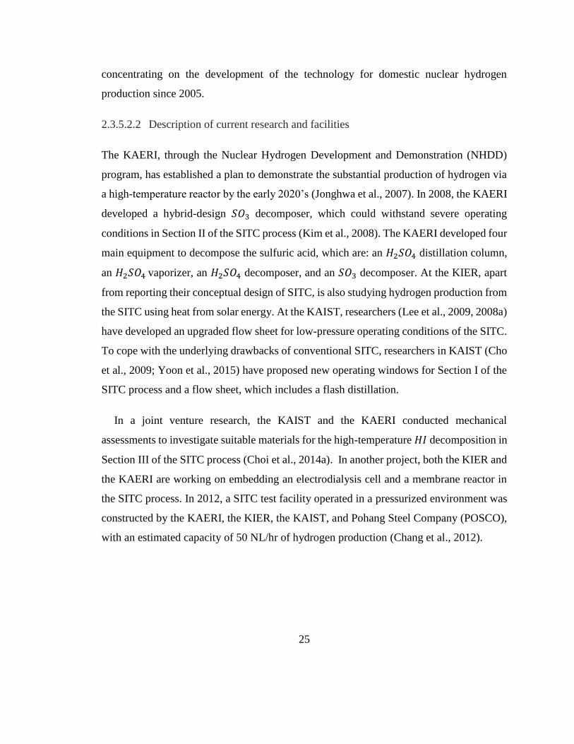
25

concentrating on the development of the technology for domestic nuclear hydrogen

production since 2005.

2.3.5.2.2 Description of current research and facilities

The KAERI, through the Nuclear Hydrogen Development and Demonstration (NHDD)

program, has established a plan to demonstrate the substantial production of hydrogen via

a high-temperature reactor by the early 2020’s (Jonghwa et al., 2007). In 2008, the KAERI

developed a hybrid-design 𝑆𝑂3 decomposer, which could withstand severe operating

conditions in Section II of the SITC process (Kim et al., 2008). The KAERI developed four

main equipment to decompose the sulfuric acid, which are: an 𝐻2𝑆𝑂4 distillation column,

an 𝐻2𝑆𝑂4 vaporizer, an 𝐻2𝑆𝑂4 decomposer, and an 𝑆𝑂3 decomposer. At the KIER, apart

from reporting their conceptual design of SITC, is also studying hydrogen production from

the SITC using heat from solar energy. At the KAIST, researchers (Lee et al., 2009, 2008a)

have developed an upgraded flow sheet for low-pressure operating conditions of the SITC.

To cope with the underlying drawbacks of conventional SITC, researchers in KAIST (Cho

et al., 2009; Yoon et al., 2015) have proposed new operating windows for Section I of the

SITC process and a flow sheet, which includes a flash distillation.

In a joint venture research, the KAIST and the KAERI conducted mechanical

assessments to investigate suitable materials for the high-temperature 𝐻𝐼 decomposition in

Section III of the SITC process (Choi et al., 2014a). In another project, both the KIER and

the KAERI are working on embedding an electrodialysis cell and a membrane reactor in

the SITC process. In 2012, a SITC test facility operated in a pressurized environment was

constructed by the KAERI, the KIER, the KAIST, and Pohang Steel Company (POSCO),

with an estimated capacity of 50 NL/hr of hydrogen production (Chang et al., 2012).

26

2.3.5.3 Institute of Nuclear and New Energy Technology (INET)


From the 1970s, high-temperature gas-cooled reactor (HTGR) technology experienced

advanced expansion in China. The Institute of Nuclear and New Energy Technology

(INET) of Tsinghua University China is a body that has been initiated to carry out

fundamental studies on nuclear hydrogen production since 2005. Prior to the venture in

hydrogen production, the INET began with a nuclear reactor design. In 2000, the INET had

successfully produced a 10 MW test reactor (HTR-10) with spherical fuel elements. In

2003, the reactor achieved its full power operation, in which a number of safety-related

experiments were conducted on the HTR-10. A commercial demonstration plant project

set up by the INET, namely, HTR-PM (Pebble Module) has led to the interest of the central

government of China in nuclear hydrogen production research, which finally gave its

approval to support the project (Ping et al., 2016b).

2.3.5.3.2 Description of current research and facilities

Unlike other institutions, the INET studied the separation characteristic of the Section I

products in terms of phase equilibrium. The Bunsen reactor in Section I was studied under

simulated closed-cycle conditions; the reaction between 𝐼2/𝐻𝐼/𝐻2𝑂 solution and 𝑆𝑂2 (Guo

et al., 2012; Lan et al., 2013). For Section II, the 𝑃𝑡/𝑆𝑖𝐶 catalyst was chosen for the 𝐻2𝑆𝑂4

decomposition process. An electro-electrodialysis (EED) process was chosen for Section

III to decompose the 𝐻𝐼 solution over pseudo-azeotropic conditions. The INET carried out

several series of research on Section III, focusing on the catalyst selection for the 𝐻𝐼

decomposer. It is hard for 𝐻𝐼 to decompose without catalysts, even at 500℃. In the last

three decades, INET’s research on 𝐻𝐼 decomposition catalyst was conducted with Pt-based

catalyst. The 𝑃𝑡/𝐶𝑁𝑇 catalyst was found to have the highest performance, which revealed

that the dispersion and particle size of 𝑃𝑡 on the supports played a significant role in the

catalyst activity. The active carbon was selected to support 𝑃𝑡 to catalyse the 𝐻𝐼

27

decomposition in the IS-10, which reached a conversion of up to 20% with 10 L/h of

hydrogen production (Wang et al., 2012).

For bench scale, the INET chose a new catalyst, the platinum-based iridium active

carbon (Pt-Ir/ C), which produced 60 NL/hr of hydrogen. Further study on the catalyst by

INET may be retrieved in the work of Wang et al., (2014b, 2012), Xu et al., (2017b) and

Zhang et al., (2010a). The INET research center had essential facilities for the process

studies of nuclear hydrogen. The HTR-10 constructed in the INET provided a proper

nuclear reactor facility for upcoming research and development of nuclear-powered

hydrogen production technology. A proof-of-concept facility (IS-10) (Zhang et al., 2010a)

and an integrated lab-scale facility (IS-100) were constructed in consequence. From 2010

to 2014, supported by the National S&T Major project of the Ministry of Science and

Technology, the INET carried out studies on the key technology of hydrogen production

from HTGR. The bench-scale facility IS-100 with a hydrogen production rate 100 NL/hr

was designed and built. Demonstration of continuous production of 60 NL/hr was achieved

by the end of 2014 (Xu et al., 2017b). Table 2.5 presents a summary of the current and

future phase research plans on the SITC process by the INET.

28

Table 2.5: The current and future phase research on SITC process by INET

Phase 1 2 3 4 5

Year 2006 to 2010 2011 to 2015 2016 to 2020 2021 to 2025 Beyond 2030

Research

focus

Fundamental study

and process

verification of

nuclear hydrogen

process

Integrated

laboratory-

scale test

Develops the key

technologies of

pilot scale

demonstration

Coupling the SITC

technology with the

nuclear reactor, nuclear

hydrogen production

safety and the pilot-scale

test.

Aims at the

commercialization of

nuclear hydrogen

production in China

29

2.4 Process Modelling and Controller Development of

Thermochemical Cycle Processes

Safety is of paramount importance in the SITC plant. In the discussion of previous section,

JAEA, KAIST and INET have shown a significant effort in the research and development

of a stable and safe SITC process. In this respect, the control system components play an

important role to ensure safety as well as a consistent operation of the overall SITC plant.

Thus, the impact of control system components failure on the consistency of the hydrogen

production plant must be studied (Sato et al., 2011). A good control system should be able

to cope with complex dynamics such as inverse response, dead time, process uncertainties,

and strong nonlinearities as well as to deal with changing operational conditions in the

presence of unmeasured disturbances. In this section, discussion of the four sub-sections

will be presented, they are: 1) Process controller development, 2) Process modelling

development, 3) Process controller application, 4) Controllability analysis method.

2.4.1 Process Controller Development

Currently, the Proportional-Integral-Derivative (PID) controllers are most widely used to

control industrial processes. Various PID controller tuning methods were developed in the

past few decades. A few researchers have also studied the use of PID controllers in various

thermochemical processes. A multiple input-single output (MISO) Proportional-Integral

(PI) controller was developed by Sack et.al, (2012, 2015) (Säck et al., 2012), in which it

was reported that the hydrogen iodide decomposition reactor unit in Section III SITC was

prone to overheating due to the presence of constraints. It was reported that the control

scheme to control the heat source generation of the plant developed by Sato et al. (2011)

(Sato et al., 2011) was able to compensate for the disturbances, but its validation remains

to be seen in further work. Al Dabbagh et al. (2010) (Al-Dabbagh and Lu, 2010) developed

a different control scheme using a network control system and found that the scheme was

capable of capturing the system behaviour and interaction in the controlled system.

30

However, verification and validation studies of the system to ensure the credibility of the

method have yet to be conducted. Table 2.6 lists the recent controller schemes developed

for the thermochemical cycle processes.

It is important to note that the presence of multiple constraints in the SITC process

makes the PID-based controller less effective in controlling the whole plant. Furthermore,

plant nonlinearity often imposes a big challenge to the control system design, e.g., the

presence of nonlinearity in the separation columns or equipment operating under critical

conditions, loads of recycle lines, non-stationary behaviour in the systems, and time delay

of the sensors (Rodriguez-Toral et al., 2000). In general, the cost of modelling and the fact

that feedback control might be designed without much need for models has motivated the

use of PID control locally, but it will not be effective when applied to the entire plantwide

system. In addition, model-free methods, which often lack detailed information on a given

process, might lead to a low-performance controller (Ashoori et al., 2009).

As mentioned earlier, it is very difficult to achieve an effective control system design

for the SITC process reactors due to the presence of constraints and nonlinearities. Due to

these difficulties, the study of advanced control strategy, particularly on a model-based

controller to control these systems has generated a growing attention in recent years

(Ashoori et al., 2009; Costa et al., 2002). Among the well-known model-based control

strategies are the Internal Model Control (IMC), the Generic Model Control (GMC) and

the Model Predictive Control (MPC) (Ashoori et al., 2009; Deshpande et al., 2009; Garcia

et al., 1989; Henson, 2003; Zhu et al., 2000).

31

Table 2.6: Controllers developed and applied in various parts of thermochemical cycle

processes for hydrogen production.

No Authors Process Controller Controlled

Variable

Manipulated

Variable

1 Sack et al.

(2015) (Säck

et al., 2012)

and (2012)

Thermochemi

cal water

splitting cycle

using metal

oxides

(Simulation)

PI Controller Temperature Solar input

power, fluid

temperature

of the

preheating gas

2 Sato et al.

(2011) (Sato

et al., 2011)

Thermochemi

cal cycle

process

integrated with

VHTR

(Simulation)

Conventional

feedback

controller

Inlet turbine

temperature,

turbine speed

Bypass flow,

coolant feed

flow rate

3 Al Dabbagh

et al.

(2010) (Al-

Dabbagh and

Lu, 2010)

Thermochemi

cal Copper-

Chlorine (Cu-

Cl) Cycle

(Simulation)

Network

Control

System

(NCS)

Hydrogen

production

rate and

hydrogen

level

in the storage

tank

Feed flow of

HCl gas, Cu

particles and

cooling water

32

2.4.1.1 Nonlinear Model Predictive Controller (NMPC)

MPC refers to a class of control algorithms, in which a dynamic process model is used to

predict and optimize process performance. An important advantage of this type of

controller is its ability to cope with input and output constraints, time delay, non-minimum

phase behaviour and multivariable systems (Temengfl et al., 1995). The majority of

chemical processes (e.g. reactors, distillation columns) are multivariable in nature, where

cross-coupling effects are strong and cannot be neglected in the control design.

An extensive review on linear and nonlinear MPCs was reported by Morari and Lee

(1999). Despite the fact that most real processes are approximately linear within only a

limited operating window, linear MPC approaches with linear models embedded are used

in the majority of applications (Morari and Lee, 1999), with the feedback mechanism of

the MPC compensating for prediction errors due to a structural mismatch between the

model and the process. In addition, a linear model controller is acceptable when the process

operates at a single set-point and the primary use of the controller is for the rejection of

disturbances. However, many processes do not operate at a single set-point, rather, in

different conditions depending on market requirements.

When linear models are not sufficiently accurate because of process nonlinearities, the

process can be controlled with nonlinear model predictive controllers (NMPC). In recent

years, a nonlinear MPC (NMPC) has been used in several industrial processes

(Ramaswamy et al., 2005). The NMPC possesses its own specialty in coping with

important issues in the chemical process. It is a versatile controller, where it copes

satisfactorily with a few critical fermentation issues such as nonlinearity behaviour, time

delay, inverse response, multivariable system, constraint, and optimization (future

prediction based on calculations), which could not cope through a conventional controller

that has no models. The NMPC uses a nonlinear model and current plant measurements to

calculate future moves in the independent variables (e.g. feed flow rate, inlet

concentration). The nonlinear model used may be in the form of an empirical data fit or a

33

high fidelity model based on fundamentals such as mass, species and energy balances. The

NMPC is well suited for high performance control of constrained multivariable processes

such as the SITC process because the explicit pairing of input and output variables is not

required and the constraints can be integrated directly into the related open loop optimal

control formulation.

2.4.1.2 Multi-scale Controller (MSC)

Even though several more advanced controller techniques than the PID control have been

developed over the last few decades, it is interesting to note that the PID is still the most

frequently used control technique in the chemical process due to historical factors and

implementation facilities. For this reason, developing and embedding a control technology

that is more practical for the industry is crucial. For instance, part of the control strategies

for the plant can be built based on the latest control PID-based approach, i.e., the multi-

scale control (MSC) scheme, developed recently by Nandong and Zang (2013) (Nandong

and Zhuquan, 2013). The MSC scheme has shown reliable performance in various

processes, including multivariable processes (Nandong, 2015).

The details of the multi-scale control scheme can be found in (Nandong and Zang,

2013a). It was shown that the multi-scale control scheme could be used to synthesise

practical PID controller augmented with a filter. It is interesting to note that the multi-scale

control scheme can provide significant performance and robustness improvement over the

conventional PID control for processes with long dead time and inverse-response

behaviour. The basic idea of the multi-scale control scheme is to decompose a given plant

into a sum of basic factors with distinct response speeds-multi-scale modes. A set of sub-

controllers is designed based on the basic modes, which are then combined in such a way

to enhance co-operation among these different modes-vital to good performance and

robustness.

34

2.4.2 Process Controller Application

There is scarce information on the controller application applied on the SITC plant or its

equipment. Hence, this section will serve as a reference analysis on the process controller

applications on the other processes equipment that is similar to the equipment in the SITC

plant. There are four types of major equipment in the SITC plant, which are continuous

stirred-tank reactor (CSTR), liquid-liquid (L-L) separator, flash tanks, and tubular reactor

or decomposers.

2.4.2.1 Continuous Stirred Tank Reactor (CSTR)

CSTR is widely used in chemical industry. The demand of global economy and increase in

competition are forcing chemical processes to operate under multiple constraints. To

address this requirement, research has been carried out by Pan et al. (2007) through the

application of Lazy Learning-Based Online Identification and Adaptive PID Control on a

CSTR system. The simulation was carried out in an AAS simulator to control the output

concentration by manipulating the cooling jacket temperature. A two-layer PID according

to GMV criteria has been proposed. The results show that the control system drives the

controlled variable to its desired setpoint with better accuracy as compared with tuning

scheme based on RHW and conventional PID method.

Seki and Naka (2008) had designed a controller scheme for CSTR with one recycle

line. They applied a self-optimising control structure and selected an MPC for the

supervisory layer. A PI controller is developed for the regulatory layer to control the reactor

level. Both MPC and PI show good performances in controlling the nominated layer. This

work can be a good reference on the PWC application on CSTR.

Prakash and Srinivan (2009) designed a nonlinear PID and an NMPC scheme to control

output concentration of a stand-alone CSTR. The nonlinear process or system is

represented as a family of local linear state-space model. The proposed PID and NMPC are

35

designed based on the local linear models. The controller performance is compared with

Analytical Model-Based LMPC and NMPC. The proposed nonlinear PID has shown good

set-point tracking, disturbance rejection capability at nominal and shifted operating points,

and is comparable to the performance of Analytical Model-Based NMPC.

Zhao et al. (2015) had designed a terminal sliding mode controller for CSTR. By using

sliding mode principles, a finite time stability observer to measure the unmeasurable states

was designed. Compared to the existing terminal sliding controller, the proposed controller

shows stronger robustness to external disturbance and can eliminate the error in setpoint

tracking.

In 2016, Mohd and Aziz had designed the NMPC controller to control an integrated

CSTR system. NARX-Based NMPC was designed to control the CSTR. In comparison to

LMPC (using state-space model) and conventional PID controller, the NMPC has

outperformed the other controllers in setpoint tracking, disturbance rejections and

robustness tests. It can be seen that the accuracy of the model has an important role on the

control of the controller action performance.

Deepa and Baraniligesan (2017) had developed a Neural Network-Based NMPC. A

deep learning neural network MPC was designed and the performance of CSTR was

analyzed. A hybrid article swarm optimization-gravitational search is employed to tune the

weight of the neural network model. The result revealed that the controller is able to

achieve minimal ISE in comparison to other types of Neural Network-Based MPC.

2.4.2.2 Liquid-liquid (L-L) separator

Designing separation equipment for two immiscible liquids is important in SITC plant. The

challenge is in the fluctuations of the feed stream that inhibit the system to achieve the

desired product level. Chonwattana et al. (2018) carried out an experimental work on the

dynamic modelling and control of a liquid-liquid separator, or also known as a decanter.

36

The decanter is a bench-scale palm oil/water separator. They proposed a feedback

controller to control the interface level of the liquid by manipulating the feed flow rate.

The proposed controller performance was compared with the LQR and PI controllers. The

experimental results showed that integrating the real-time estimation of the unmeasured

disturbance into the control strategy (proposed controller) shows obvious controller

improvement as compared to the LQR and PI controller. The proposed technique proved

that the real-time dynamic behaviour of the decanter plays a significant role in determining

good controller performance.

2.4.2.3 Flash tank

Rangaiah et al. (2002) in a study of the controller design for industrial four-stage evaporator

system addressed the importance of dynamic model onto controller design. Since systems

with moderate to strongly nonlinear dynamics are often encountered in the separation

processes, there is a need for nonlinear model-based controller to achieve a desired system

controller performance. In their study, Rangaiah et al. (2002) had designed an NMPC to

control an MIMO system of an integrated flash tank. A stable control is obtained initially

but steady-state offset was observed. A simple parameter adaptation technique is proposed

and successfully applied to offset-free control. The result showed that NMPC is better than

the PID-type controller. However, both controllers are comparable since they can be tuned

to achieve the desired setpoints.

Zhang et al. (2018) carried out a study on integrating feedback control and safety

systems. Their work focuses on two case studies, including one flash tank to elucidate the

dynamic interaction between feedback control and safety system. In the flash tank case,

they regulated temperature, level and pressure by applying a PID-type controller. Using a

large-scale dynamic model simulator, they demonstrate that modifying the PID-type

controllers (in this case, a PI) lead to improved close-loop performance compared to fixing

the controller parameters regardless the actions of the safety system.

37

2.4.2.4 Tubular reactor/ decomposer

A tubular flow reactor is a vessel through which flow is continuous. The flow is usually at

steady state, and configured so that conversion of the chemicals and other dependent

variables are functions of position within the reactor rather than of time. Tubular flow

reactors are mainly used in chemical industry and wastewater discharged units. Control of

output variables is very challenging because due to the presence of high time delay in these

types of reactors. Vural et al. (2015) presented an application of pH control to a tubular

flow reactor. A comparison of a conventional PID controller, self-tuning PID and a PID

system using fuzzy model is carried out. The excellent performance of fuzzy-based PID

controller is verified as compared to the conventional PID. However, when compared to

the self-tuning PID, the conventional PID shows better performance. It is worth

highlighting that controlling pH via PID controller is an established method in industry.

The question is, can PID control the other output variables of tubular reactor such as

temperature?

Arefi et al. (2008) presented a Neural Wiener Based MPC to control a tubular reactor

temperature. The performances of Neural Wiener Based MPC (NWMPC), LMPC and PID

controllers are compared. The setpoint tracking behaviour system with NMPC shows good

tracking speed and low overshoot for all operating points. Since the process has strong

nonlinearity and wide range of operating points, it makes the PID and LMPC techniques

unsuitable and hence, demanding a more complex identification and controller design

procedure such as NMPC.

Another study by Puebla et al. (2013) presented a spatiotemporal pattern control by

manipulating the fluid velocity of tubular reactor. The controller is implemented via

numerical simulations in three benchmark tubular reactors. The proposed robust feedback

controller embedded in a state estimator showed adequate performance in regulating the

output and tracking the spatiotemporal pattern at a desired position. However, the concept

of suppression of the complex dynamics through control at a single position does not seem

38

feasible to many systems. Table 2.7 presents the summary of the process controller

application on CSTR, L-L separator, flash tank, and tubular reactor of various processes

discussed above.

From these controller application reviews, it can be seen that the first principle

mathematical model is the most popular model chosen. Even though theoretically rigorous

models are more realistic and would probably lead to better results, the excessive

complexity of the first principle model hinders the determination of the optimal result. This

issue was asserted earlier by Willis (2000) and Willis et al. (1991), who reported that the

development of the white box model (first principle model) is complicated and costly due

to deficient understanding of the actual processes. In addition, these models may be too

difficult to be practical because computational loads or assumptions involved will degrade

the model accuracy in real-time applications (Pearson, 1995).

The black-box (empirical model) and the grey-box models (hybrid model) possess their

own specialty. They are able to simplify the calculation burden of the white-box model by

replacing some equations using empirical relationships, yet still fulfilling excellent

performance requirement. For the nonlinear black-box model, researchers have mainly

focused on NARX models and the Neural Network model. However, due to the generic

structure of Neural Network, this model usually requires the estimation of a large number

of parameters. Problems related to computational procedures are necessary to achieve good

results, including the definition of the Neural Network dimension, the choice of nonlinear

activation functions and the search for the optimum weight set, are still drawbacks to a

wider use of Neural Network (Dote and Ovaska, 2001; Haykin, 1999).

On the other hand, the implementation of the NARX model is easier, where the model

parameters can be verified using the information matrix, the covariance matrices or able to

evaluate the model prediction error using a given final prediction error criterion. Another

preferable property of the NARX model based MPC algorithm is the availability of tuning

parameters that enables the adjustment of the control law and as a consequence, allows for

39

adjustments in controller behaviour (Mjalli and Al-asheh, 2005). In addition, it provides a

great presentation for real process analysis, modelling and prediction due to its strength in

accommodating the dynamic, complex and nonlinear nature of the actual process

application (Harris and Yu, 2007; Mu et al., 2005). Therefore, it can be seen that the NARX

model based MPC is an excellent option to represent a nonlinear or an unstable process.

40

Table 2.7: Summary of the process controller application on CSTR, L-L separator, flash tank and tubular reactor of various

processes

No Year Author/s Process Controller Manipulated and Controlled

variables (MVs and CVs)

Research category

CSTR

1 2007

Pan et al., 2007 (Pan et al.,

2007)

Lazy-Learning

identification according

to general minimum

variance (GMV)

criterion based PID

controller.

MV: Cooling jacket temperature

CV: Output concentration

Simulation of a stand-

alone CSTR in AAS

simulator system.

2 2008

Seki and Naka, 2008 (Seki

and Naka, 2008)

PI controller and linear

MPC (applied in a self-

optimizing control

structure)

MVs: Reactor feed flow, reflux

ratio

CVs: Reactor holdup, reactor

temperature

Simulation of an

integrated CSTR.

3 2009

Prakash and Srinivasan,

2009 (Prakash and

Srinivasan, 2009)

Nonlinear PID,

nonlinear MPC and

linear MPC

MV: Coolant flowrate

CV: Output concentration


alone CSTR

4 2015

Zhao et al., 2015 (Zhao et

al., 2015)

Terminal sliding mode

controllers (TSMC)

MV: Coolant flowrate Simulation of a stand-

alone CSTR

41

CV: Output concentration, reactor

temperature

5 2016 Mohd and Aziz, 2016

(Mohd and Aziz, 2016)

Multi input multi output

NARX-MPC, linear

MPC and PID controller

MVs: Feed flowrate, Cooling water

flowrate

CVs: Product concentration,

Reactor temperature.

Simulation of an

integrated CSTR.

6 2017

Shakeri et al., 2017

(Shakeri et al., 2017)

Focker-Plank observer

based MPC

MV: Coolant flowrate


temperature (via a probability

density function (PDF) relation)


alone CSTR

7 2017

Deepa and Baranilingesan,

2017 (Deepa and

Baranilingesan, 2017)

Deep learning neural

network MPC

(DLNNMPC) and PID

controller

MV: Feed temperature


temperature


alone CSTR

L-L Separator

8 2018

Chonwattana et al, 2018

(Chonwattana et al., 2018)

LQR, PI and a proposed

model-based controllers

MVs: Water flow rate, oil flow rate

CVs: Interface level, total height in

the separator

Experimental and


alone separator.

Flash Tank

42

9 2002

Rangaiah et al, 2002

(Rangaiah et al., 2002)

Nonlinear MPC

(NMPC) and PI

controllers

MVs: Feed flow rate, feed

temperature, feed density

CVs: Tank level, outlet flow rate,

outlet density

Simulation of

integrated flash tanks.

10 2018

Z. Zhang et al, 2018

(Zhang et al., 2018)

PI controller MVs: Cooling water flow rate,

outlet flow rate

CVs: Tank level, tank temperature


alone flash tanks.

Tubular reactor/ decomposer

11 2008

Arefi et. al, 2008 (Arefi et

al., 2008)

PID, LMPC and NMPC MV: Coolant flow rate

CV: Reactor temperature


alone reactor

12 2013

Puebla et.al, 2013 (Puebla

et al., 2013)

Robust Feedback

Controller

MV: Fluid velocity

CV: Spatiotemporal pattern


alone reactor

13 2015

Vural et al, 2015 (Vural et

al., 2015)

PID MV: Feed base flowrate

CV: pH

Experimental and


alone reactor

43

2.4.3 Process Modelling Development

Referring to the SITC challenges as mentioned earlier, the development of a precise and

consistent model taking into account the critical immiscible-phase regions that will

probably occur is essential in the SITC process. Also, the intricacy to deal with electrolytic

behaviour, liquid-liquid immiscibility, and optimum temperature can be overcome with a

well-founded process modelling. It is undeniably that the natural progression from a scratch

idea to steady-state simulator to decisions on PWC is centered upon the modelling (Downs,

2012). Process modelling is well known as an invaluable tool for process cycle analysis;

for flowsheet development, designing controller, performing cycle improvements, and

minimizing costly experimental procedures as mentioned above. Thus, model-based

control should be used when the modelling effort gives enough payback in terms of

simplicity and improved performance, especially to increase the production efficiency, and

this will usually be at the higher layers in the plantwide control hierarchy.

Previous control studies on thermochemical cycle process have focused on the cycle

efficiency improvements, more specifically, the studies of static characteristics (Goldstein

et al., 2005; Kasahara et al., 2007; Lee et al., 2008a; Paul et al., 2003a). Very little attempts

have been made to investigate the process dynamics and modelling of the entire SITC plant.

Recently, Singh and co-workers (Singh et al., 2012) worked on the two nonlinear models

comparison without optimizer in the real-time of fault propagation analysis for the dynamic

of the Cu-Cl thermochemical cycle. Their results have shown that the accuracy of the

NARX model is better than the Genetic Programming (GP) in the prediction of the selected

process variable behaviour and identifying the variable’s interrelationship pattern. Yoon et

al. (2008) also developed a nonlinear model without an optimizer by improving a

Neumann’s model for the SITC. The improved nonlinear model gave a result with less

performance deviation as compared to the other models.

44

Meanwhile, Revankar et al. (2010) and Sato et al. (2011) had carried out an

investigation on the dynamics of heat cogeneration systems for the thermochemical cycle

process as well as investigating a control scheme that enables continuous operation of the

reactors against unusual events. The simulation results demonstrated that the efficacy and

technical feasibility of their proposed control scheme for continuous operation of the

reactor and power conversion unit against load change events in the plant. All these

phenomena are independent and must be considered in an integrated process design if it is

to produce meaningful results. Table 2.8 summarizes the types of models developed for

the various thermochemical processes.

45

Table 2.8: Type of models developed for various thermochemical cycle processes

No

Authors Type of Model Model Input / Output and model source Optimizer

1 Hossam et

al.

(2014)

NARX and Genetic

Programming (GP)

Nonlinear SISO*

Valve Opening Percentage/Reactor Pressure.

EXPERIMENTAL

NIL

2 Thanh et al.

(2014)

Langmuir–

Hinshelwood

Linear MISO**

I2 feed flow rate, current flow (co and counter) of heating

medium/HI conversion.

EXPERIMENTAL

NIL

3 Sack et al.

(2012)

State-space Linear MIMO***

Solar input power, fluid temperature of the gas preheating /

Temperature, H2 Concentration.

EXPERIMENTAL

NIL

4 Singh et al.

(2012)

State- space Linear SISO

Steam flow rate/ Temperature.

SIMULATION AND EXPERIMENTAL

NIL

5 Ahmad et al.

(2010)

Dynamic Flow graph

Methodology (DFM)

Linear MIMO

4 flow rate/temperature HCl and Cu.

SIMULATION

NIL

6 Yoon et al.

(2008)

Neumann-NRTL

Thermochemical

model vs. KAIST

model (improved

Neumann’s)

Nonlinear MIMO

Temperature and HI concentration /Total pressure, hydrogen

production.

SIMULATION

YES

46

2.4.3.1 Dynamic Modelling of Separation Process

In the dynamic modelling of separation processes, to calculate the phase equilibria, there

are two available methods: (1) Based on activity coefficient, and (2) Using fugacity

coefficient. Before computers became readily available, the fugacity coefficient method is

the preferred one, until the last six decades when the activity coefficient method took over

the cumbersome calculations via computing technology. The activity coefficient can be

estimated from a few models such as Pitzer, Van Laar, NRTL, UNIQUAC, Margules, and

Wilson models. The NRTL and UNIQUAC models have been widely used for almost thirty

years, superseding the equations of Margules, van Laar, and Wilson models (Prausnitz and

Tavares, 2004).

Besides the need for choosing the right phase equilibrium estimation model, the

properties of pure components and mixtures must also be estimated appropriately for a

reliable simulation work. In fact, selecting the proper method for determining properties is

one of the most important steps that will affect the simulation output. As a result, it is vital

to carefully consider appropriate techniques to estimate different properties used in the

separation model. Due to the scarcity of thermodynamic data, a lot of effort has been made

to determine these properties from a known molecular structure. There are three

mainstream techniques (but are not limited to) available to estimate thermodynamic

properties, which are UNIFAC, Equation of State (EOS) and Langmuir.

Recently, a simulation has been carried out by Chao et al. (2017) by employing the

UNIFAC method for modelling an ionic liquid process to estimate the thermodynamic

properties involved at a room temperature and atmospheric pressure. Based on their

findings, it was demonstrated that the UNIFAC model is adequate to estimate the

thermodynamic properties at low temperature and pressure conditions. Note that for a

process under supercritical conditions, the EOS approach is more frequently used. Among

the popular EOS-based methods, especially for the hydrocarbon and gas processing

47

systems, are the Peng-Robinson (PR) and Soave-Redlich-Kwong (SRK). A new approach

exploiting the PR method was presented by Deilamani and Assar (2015), which is based

on a black oil separation process. It was verified that for the particular crude oil separation,

the PR is efficient in identifying the gas phases as well as for two- or three-phase flash

calculations. Although the EOS (PR) has been widely used, there are a few drawbacks

under certain cases; it is unable to define the standard states for the high temperature and

pressure conditions. Due to this limitation, a number of studies based on the mixture of

different EOS methods have been carried out. For an example, Costa et al. (2009)

performed a study of polyethylene separation case; they showed that the mix EOS of SRK-

van der Waals (VDW) is good enough for estimating the thermodynamic of polyethylene

in industrial separators. However, it is not as accurate as the single EOS method, which

was also proposed in the aforementioned work. It is worth highlighting that the dynamic

modelling is the best model presentation of any separation equipment, including flash tank.

In the SITC plant, flash tanks play a significant role to separate both sulfuric and

Hydroiodic acids from their mixtures. To estimate the phase equilibria and thermodynamic

properties of a flash tank, a pre-simulation in the Aspen Plus software shall be carried out.

Once the phase equilibria and desired thermodynamic properties are obtained, the dynamic

modelling of the flash tank can be performed via the MATLAB simulation. The reason for

performing such modelling in MATLAB is to enable the use of many tools available in this

software for optimization, nonlinear analysis and control studies–in Aspen, such studies

can be limited.

2.4.3.2 Commercial Product Used for Process Modelling

The systematic method of the SITC process development via simulation consists of the

modelling of the principal reactor, cooling systems, heating equipment, and separators. In

evaluating the credibility of any proposed flowsheet, a few types of simulation tools were

used by researchers. For instance, PROSIM software was used by Neumann (1987) to study

48

the activity coefficient of HI decomposition system in Section III SITC process (Cho et al.,

2009). INET used OLI software to analyze the SITC electrolyte system and designed

equipment model (Guo et al., 2011). Chart FX, Spread 7.0, and ActiveX control software

programs were also used by INET conjointly. Nagarajan et al. (2008,2014) (Nagarajan et

al., 2009) utilized the FLUENT and CFD software to model the H2SO4 decomposer in

Section II SITC process. The JAEA utilized the dynamic simulation codes in RELAP5

software to model the HTTR-IS system (Sakaba et al., 2012). On top of it all, Aspen Plus

and Aspen HYSIS are mostly used in the modelling and simulation of the SITC process

(Doizi et al., 2007; Gabbar et al., 2014; Zhang et al., 2010b).

Embedding Aspen Plus and Aspen HYSIS in the modelling, design and simulation of

the SITC process has now become a worldwide trend among researchers (Park et al., 2013;

Schultz, 2003; Smitkova et al., 2011b). Gabbar et al. (2014) (Gabbar et al., 2014) proposed

a hazard identification and risk assessment method based on the Fault Semantic network.

In this work, they extracted data of the Cu-Cl thermochemical cycle (CuCl-TC) from

Aspen HYSIS and carried out variable interaction analysis for the CuCl-TC process using

the proposed method. Conjoining Aspen HYSIS and the FSN, researchers have

successfully achieved reasonable detection and prediction of the process variables

interaction. Park et al. (2013) (Park et al., 2013) had developed a best-fit electrolyte

dynamic model for Section II SITC process via Aspen Plus simulation. The chosen model

is the electrolyte NRTL combined with an ideal gas EOS for the phase fugacity coefficient.

The conversions and heat transfers in the designed decomposer sections were found to have

acceptable agreement with the experimental data. This work is useful as the foundation for

further simulation on the sulfuric acid decomposition section at high pressure and

temperature. Smitkova et al. (2011) (Smitkova et al., 2011b) compared the Westinghouse

and the SITC methods. They carried out a life cycle analysis (LCA) via Aspen Plus

simulation. The LCA results confirm that the SITC process is an attractive method for

hydrogen production due to its low environmental impact. If solar energy is utilized as the

heat source, any harmful environment impact will further decrease. The researchers found

49

a major problem to be addressed in the SITC process, which is recycling iodine. Shin et al.

(2012) (Shin et al., 2012) embedded an electrodialysis cell (EDC) and a membrane reactor

(MR) model in a preliminary SITC flowsheet simulation via the Aspen Plus. The EDC and

MR models were designed for the HI decomposition section (Section III). The researchers

calculated the thermal energy and electric energy required per unit of equipment for the

entire SITC process via the simulation method. It was found that the overall thermal

efficiency of hydrogen production of up to 39.4% could be expected if both EDC and MR

are implanted in the process. In INET, Aspen Plus software combined with the OLI

thermodynamics database was used to simulate Section III. Some parameters in the Aspen

Plus databank were reviewed based on available data and models in the OLI databank to

solve the HI decomposition problems and the reliability of the simulation was verified with

published data (Guo et al., 2011).

A summary of simulation research carried out via Aspen Plus and Aspen HYSIS for

various thermochemical cycle processes is shown in Table 2.9.

50

Table 2.9: Application of Aspen Plus and HYSIS in various thermochemical processes modelling and simulation

No Authors Simulation detail Software Simulation

section (if

SITC)

1 Rosen, 1996 (Rosen, 1996) Comparing few hydrogen production processes; Steam methane

reforming (SMR), Thermochemical Cycle (TC) and integrated

processes via exergy analysis simulation.

Aspen Plus

2 Rosen and Scott, 1998

(Rosen, 1998)

Comparing few hydrogen production processes; SMR, TC (ispra-

mark 10) and integrated process via efficiency assessments

simulation

Aspen Plus

3 Paul and Brown, 2003

(Paul et al., 2003a)

Thermodynamic study of SITC process using simulation Aspen Plus Section I, II

and III

4 Schultz et.al, 2003

(Schultz, 2003)

Design a GA SITC process (experiment verification is needed) and

compare solar and nuclear energy source for the SITC

Aspen Plus Section III

5 Huang and Raissi, 2005

(Huang and T-Raissi,

2005)

Simulation for Section II SITC process. Resulted in a simpler, more

stable, and yield higher conversion efficiencies.

Aspen

HYSIS

Section II

51

6 Yoon et.al, 2008 (Yoon et

al., 2008)

Thermodynamic study of SITC process using by simulation Aspen Plus Section III

7 Andress et .al, 2009

(Andress et al., 2009)

Simulation using Aspen algorithm for the conceptualization, reaction

cluster synthesis, process integration and performance evaluation for

the Fe-Cl TC. Achieved efficiency 35% to 49%.

Aspen Plus

8 Cho et.al, 2009 (Cho et al.,

2009)

Simulation of SITC process using ELECNRTL for evaluation of state

and activity model. Design a model for EED coupled for HI section

(applied Redlich-kwong EOS properties and Henry constant for

partial pressure)


9 Anantharaman et.al, 2010

(Ananthraman et al., 2010)

Model gasification of CO2 and H2 purification and compression, for

the Integrated Gasification Combined Cycle (IGCC) process.

Aspen

HYSIS

10 Zhang et.al, 2010 (Zhang

et al., 2010b) Simulation for a HI decomposition model referring to experimental

work of IS-10 by INET. Produced hydrogen at a rate 10 NL/hr.,

(catalyst used = Platinum on activated carbon and copper chromite)


11 Guo et.al, 2014 (H. Guo et

al., 2014) Simulated SITC process as reported by Brown (2003) Aspen Plus Section III

52

12 Perret,2011 (Perret, 2011a) Compared few conceptual design; SITC, Hybrid Sulfur, Photolytic

Sulfur, Zinc Oxide, Cadmium Oxide, Sodium Manganese, Hybrid

Copper Chloride).

Aspen Plus Section II

and III

13 Smitkova et.al, 2011

(Smitkova et al., 2011b)

Compared Westinghouse and SITC method. Carried out a life cycle

analysis (LCA). Found a major problem with recycling iodine in

SITC process.

Aspen Plus Section I, II

and III

14 Shin et.al, 2012 (Shin et al.,

2012)

Simulated a membrane reactor od the HI decomposition section Aspen Plus Section I, II

and III

15 Park et.al, 2013 (Park et al.,

2013)

Develop best-fit electrolyte dynamic model and compare with

experimental work Aspen Plus Section II

16 Gabbar et.al, 2014 (Gabbar

et al., 2014)

Extract data from Aspen Hysys and carried out variable interaction

analysis for CuCl-TC process.

Aspen

HYSIS

53

2.4.4 Controllability Analysis Methods

Most industrial process control applications involve a set of output (controlled) and

manipulating variables. These processes with multiple inputs and outputs often lead to

complicated transfer function models (Seborg et al., 2004). For complex units such as

the separation column, the input-output variables are often interrelated, which poses a

challenging problem to control engineers (Seferlis and Georgiadis, 2004). In two-input

two-output (TITO) process, two input variables may affect one controlled variable or

two controlled variables may be affected by one manipulated variable. This is known

as the process interaction or coupling, which plays a critical role in the process

controller design. As the interaction gets severe, it becomes more difficult to control

the given process. Conventionally, controllability index is utilized to determine input-

output interaction as well as controller pairing, where it is an essential step prior to the

process controller development.

The currently available controllability analysis methodologies range from pure

mathematical programming techniques (e.g. Heath, Kookos, & Perkins, 2000; Wang &

McAvoy, 2001) to heuristic-based methods (e.g. Luyben, Tyreus, & Luyben, 1999)

(Kookos and Perkins, 2002). There are three categories of controllability methods: (1)

Steady-state, (2) Linear dynamic, and (3) Nonlinear dynamic model-based (Karami et

al., 2015).

Relative Gain Array (RGA) by Bristol (1966) is the most widely steady-state type

controllability analysis method used over the past fifty years. Although there are other

more advanced controllability methods, the RGA is still used as an initial screening tool

to avoid impractical pairings based on some criteria such as reliability and robustness

(Rangaiah and Kariwala, 2012). The steady-state RGA analysis is based on the open-

loop gains of the given process. It provides a relatively simple way to evaluate the

severity of process interaction and its impact on controller pairings. For a decentralized

control based on the RGA analysis, one should pair the manipulated variable, uj with

the controlled variable, yi such that λij is positive and close to 1. Based on the RGA, the

best pairings should meet two rules: i) The pairings along the diagonal shall have the

RGA matrix close to unity at frequencies around the closed-loop bandwidth, and ii) The

54

steady-state RGA elements are positive (avoid negative elements, if possible). Note that

several variants of the Bristol's RGA have been developed, e.g. dynamic RGA, RNGA,

et cetera. Rigorous analysis and discussion on the process controllability was presented

by Shen et al., (2010). The authors laid down some rules in the pairings of manipulated

and controlled variables for a decentralized control system as follows:

1) All paired RGA elements are positive.

2) Niederlinski Index (NI) is positive.

3) All paired relative normalized gain array (RNGA) elements are closest to 1.

4) Large RNGA elements are avoided.

Since the controllability analysis involves the RNGA, RGA and NI criteria, the result

should give a more thorough understanding of the issue affecting the decentralized

control design. Here, the RNGA is used to measure the loop interactions whilst the

RGA and NI are used to rule out closed-loop unstable pairings. Just like the RGA, the

NI can also be used alone to analyze controller pairings for multi-loop SISO controllers,

but this only gives partial understanding on the controllability. As RGA does not use

information about the process dynamics, it can sometimes lead to incorrect pairings.

A number of methods have been proposed to overcome this restriction of RGA,

which uses RGA-type mapping. Unlike RGA, the resulting matrix for some of such

recently proposed methods has no associated physical interpretation. An obvious reason

for the success of the RGA-type mapping is that repeated application of this mapping

can identify diagonally dominant elements of a matrix, provided such elements exist.

On the other hand, methods such as µ-interaction measure and those based on

controllability and observability analysis are theoretically more sound; their use has

however, been limited (Moaveni and Kariwala, 2012).

2.4.4.1 Research Gap in Controllability Analysis

An interesting quote made by Downs (2012), “A theoretically correct but persistently

time-consuming approaches will depreciate their implementation by the process

control design community” (Downs, 2012). Inspired by this quote, it is understood that

any controllability analysis methods should be simple but efficient.

55

When we come across an unstable model or a nonlinear model, it is common to

jump straight forward onto a model-based controller. Similarly, for a stable or linear

model it is always decided to use a PID controller. In regard to this issues, a few

questions aroused,

1) To what extent does an unstable or a nonlinear model is unable to be control by

a PID controller?

2) Is there a way to know the possibility whether an unstable or a nonlinear type

of model is controllable by a PID controller?

3) Is it true that a stable or linear model is surely controllable by a PID controller?

4) How reliable is the RGA index interpretation in articulating the level of a model

controllability?

Essential in a controllability analysis is that the adopted method should, in theory:

a) Enable the determination of the input-output pairings in the presence of process

interaction, and

b) Estimate the maximum achievable controller performance.

However, none of the aforementioned controllability indices can simultaneously meet

these two criteria, i.e., determination of controller pairings and estimation of the

maximum achievable controller performance. Many of the existing controllability

analysis methods address the controller pairings based solely on the steady-state

process gains.

The past thirty years have seen rapid advances in the process controller

development that utilizes process dynamic behaviour and to a certain extent, this has

led to a more efficient process operation; see (Alberto et al., 2010; Chin et al., 2010;

Froisy, 2006; Mohd and Aziz, 2016; Shafiee et al., 2008). The advancement in the

process controller design has spurred a renewed interest to improve the controllability

analysis method based on the dynamic behaviour of the process model. Compared to

the steady-state controllability analysis method, the dynamic model-based method can

give significantly improved performance.

56

In order to fulfill the aforementioned gap, a controllability analysis index has been

developed recently. The Loop Gain Controllability (LGC) is a controllability index that

utilizes the loop gain information of a control loop, seeking for the upper and lower

limit of the process controller. An advantage of the proposed LGC index is that it is not

only straightforward, but can utilize both steady-state and dynamic information from

the given process. The index estimates the impacts of process interaction, dead time

and time constants on the maximum achievable controller performance. Hence, it not

only assesses the pairings, but also estimates the controller performance achievable

from a given pairing. Both the stability and performance margins of the single-input

single-output (SISO) controller can be inferred from the LGC index. LGC can

efficiently evaluate the performance of a control scheme without performing controller

design and closed-loop simulation. Table 2.10 lists the function-feature comparison

between the LGC index and the RGA and NI indices. Noticeably, the LGC can provide

a more comprehensive controllability analysis than the RGA and NI-LGC capable of

determining the best pairing as well as estimating controller performance limit.

57

Table 2.10: Function and feature comparison between RGA, NI and LGC

Controllability

Indices

Function-

feature

Objective Interpretation

Relative Gain

Array (RGA)

(Bristol, 1966)

Based on 𝜆𝑖𝑖

derived from

process gains.

Steady-state

approach’

To determine

input-output

pairings based

on the

diagonal

matrix.

If 𝜆𝑖𝑖 = 1, the

corresponding input-output

pairing has no control effect

on the output. If 0 < 𝜆𝑖𝑖 <

1, closed loop interaction is

more severe the smaller the

value. Interaction is most

severe at 𝜆 = 0.5. For 𝜆𝑖𝑖 >

1, the interaction becomes

severe as the value

increases, so more difficult

to control. Pairing on

negative 𝜆 should be

avoided.

Niederlinski Index

(Niederlinski,

1971)(Niederlinski,

1971)

Ratio of a

determinant of

the process

gain matrix to

the product of

the diagonal

elements.

Steady-state

approach

To determine

if multi-loop

SISO

controllers

with integral

action can

control the

system.

The negative value means

that the closed-loop system

is unstable under PI control

with positive loop gain and

integral action.

Loop Gain

Controllability

(LGC) (present

work)

Function of

𝑘, 𝜏, 𝜃 and 𝜆𝑖𝑖.

Dynamic

approach

Use to

estimate

controller

performance

of multi-loop

SISO

controllers.

The positive value indicates

the selected pairing is

controllable by PID

controller. While negative

value means that the loop is

uncontrollable. The larger

the value means the higher

the achievable controller

performance. If two

systems have comparable

LGC values, then the

performance will also be

comparable.

58

2.5 Plantwide Control Structure

Since the SITC process has many measurements and control loops, the strategy of

Plantwide Control (PWC) is proposed in this work. The PWC design has attracted a lot

of research interest in the process control community over the last four decades, since

the pioneering work by Buckley (1964). In definition, the PWC refers to a control

philosophy of the overall plant emphasizing on the structural decisions. The PWC

calculates optimal values for the set of selected manipulated variables in order to

maximize a plantwide profitability objective function instead of just maintaining a set

of controlled outputs at the predefined setpoint. The PWC considers the entire aspects

such as feed changes and interaction between processes affecting the safety and optimal

operation of the entire plant (Rangaiah and Kariwala, 2012). The structural decision

comprises the selection or placement of manipulators and measurements along with the

classification and breakdown of the total problem into smaller sub-problems (the

control configuration) (Larsson and Skogestad, 2000).

Luyben and Tyreus (1997) presented nine steps of the PWC design. Steps 1 and 2

establish the objectives of the control system and the available degrees of freedom. Step

3 ensures that any production of heat (entropy) within the process is properly dissipated.

Steps 4 and 5 are to satisfy the business objectives concerning production rate, product

quality and safety. Step 6 involves total mass balance control, whereas in Step 7, it

ensures that non-conserved chemical components are accounted for. In Step 8, complete

the control systems for individual unit operations. Finally, Step 9 uses the remaining

degrees of freedom for optimization and improves dynamic controllability. It should be

highlighted that most of these steps required experience-based knowledge. Hence, in

this work, these nine steps will be used as the general guideline for PWC structure

design.

Larrson and Skogestad (2000) introduced a new PWC method, which is a hybrid

between process- and mathematically-oriented approaches. The PWC method inspired

by the Luybens procedure is known as Skogestad Self-Optimizing Control (SOC). SOC

is a stepwise PWC procedure of seven-step and divided into a top-down part and a

bottom-up part.

59

2.6 Research Challenges in SITC Process

In the last few decades, the exploration of the SITC process has grown rapidly. This is

evident by the increasing number of research that has been published. Nevertheless,

there is scarce information on the rigorous dynamic modelling and process controller

development of the entire SITC process or research on the complete SITC process

flowsheet particularly on an industrial scale. This includes overall mass and energy

balances and presenting the focal operating conditions such as temperature, pressure

and composition in the process, equipment design, process controllability analysis, and

cost (capital and operating) estimates. It is indisputable that the actual implementation

of the SITC process is much more complex than the simple presentation of its chemical

reactions. The entire SITC process is closely attached with many recycle streams.

Therefore, the reliability of a designed flowsheet is difficult to evaluate by means of

experimentation tools.

At this point, a requirement to build an effective design, modelling and process

control system by dint of a simulation tool to evaluate the reliability of the designed

flowsheet is important. A number of tools can be used for 𝐻𝐼 and 𝐻2𝑆𝑂4

decomposition; however, there are no available tool to simulate the entire cycle (Ping

et al., 2016a). There are a few major constraints to be addressed in the modelling and

process control development of the SITC process:

a) The chemical species includes strong acids (𝐻𝐼 and 𝐻2𝑆𝑂4) that are immiscible

(Paul et al., 2003b). During the operation, the ratio of 𝐻𝐼 and 𝐻2𝑆𝑂4 in the

reactor involved must be kept above a threshold value for optimum separation.

The ratio of these two species is very sensitive to changes in the operating

conditions induced by disturbances. Also, it is important to feed iodine and

sulfur to the reactor at an optimum composition ratio. An analysis of

thermodynamics by Baykara (2004) (Baykara, 2004) suggests that at 1 bar and

2500 K, only 2.69% of water is decomposed into hydrogen and this will increase

to 25% at a lower pressure of 0.05 bar. Hence, the optimum operating pressure

and temperature must be studied.

60

b) Two main elements for the simulation of the Section I are the prediction of the

phase states and the calculation of the phase compositions (Guo et al., 2012). In

the Bunsen Reactor, the 𝐻𝐼, 𝐼2, 𝐻2𝑂, and 𝐻2𝑆𝑂4 co-exist. The evaluation of the

phase states has to be portrayed with an appropriate modelling method. There

are three possible states in the Bunsen Reactor: homogeneous phase, two-liquid

phase, and two-liquid phase with 𝐼2 precipitation. All states are possible to be

simulated by a simulation software. For instance, if the two-phase state is

selected, then the accurate calculation of the solution composition is essential.

For a control system design, it is essential to control the feed of 𝑆𝑂2 pressure as

well as the 𝐻2𝑂 feed flow rate in order to produce optimum amounts of 𝐻𝐼 and

𝐻2𝑆𝑂4(Mohd and Nandong, 2017).

c) Section II has units that operate at very high temperatures (around 800℃ or

more) that go beyond the critical temperature of water (374℃), which is the

𝐻2𝑆𝑂4 decomposer (Kim et al., 2008; Nagarajan et al., 2014). Since the

𝐻2𝑆𝑂4 decomposer runs endothermic reaction, the temperature and energy

supplied to the system must be sufficient. As a rule of thumb, a higher

temperature tends to favors greater efficiency. However, the energy (heat) must

be controlled below 1140℃ to prevent a dangerous process runaway reaction

from occurring. If the temperature can be decreased to some extent, but at the

same time keeping the operational efficiency at the same level, or even higher,

then a great deal of many resources can be saved with better safety conditions.

Interestingly, that is a challenge to be addressed in order to design Section II

effectively and to make sure that a high conversion is achievable by the designed

𝐻2𝑆𝑂4 decomposer. The next constraint is the type and efficiency of the

available energy source, which requires an in-depth study on the

thermodynamic properties of the heat supply that include the heat capacity of

the design material. The efficiency of the sulfuric acid and water separation

system prior to entering the 𝐻2𝑆𝑂4 decomposer should also be realistic. Since

the SITC process occurs in a cycle, failure to remove water will affect the cycle

efficiency, hence reducing the hydrogen production (Lee et al., 2009).

61

d) Section III often encounters the complex nonlinear behaviour of the 𝐻𝐼 − 𝐼2 −

𝐻2𝑂 system, which includes various liquid phases, azeotropes and possible

solid precipitation. From the thermodynamic point of view, the current

understanding of Section III has so far remained limited compared to Sections

I and II. The binary (𝐻𝐼 − 𝐻2𝑂) and ternary (𝐻𝐼 − 𝐼2 − 𝐻2𝑂) mixtures in the

𝐻𝐼 section are strongly non-ideal solutions and partially immiscible systems,

which are difficult to model and predict their thermodynamic behaviours. In

addition, the presence of an azeotrope in the binary mixture 𝐻𝐼 − 𝐻2𝑂 prevents

a high concentration of 𝐻𝐼, which causes the incomplete and slow

decomposition of 𝐻𝐼 into 𝐻2 and 𝐼2, and leads to a very large energy demand

due to the substantial calorific capacity of the HI mixture containing large

amounts of iodine and water.

All of the constraints above must be overcome for the SITC to move forward to the

commercialization stage. In this work, fundamental and empirical models will be

developed to describe the dynamic behaviour of the thermochemical cycle process.

Aspen Plus simulation will be utilized to extract the required data and parameters that

are not available in the literature. An integrated MSC and NMPC scheme will be

designed in MATLAB environment and implemented to control the SITC process. A

new controllability analysis method will be implemented prior to process controller

design. All controllers developed in this work will be implemented in the PWC strategy

and the proposed approach will be evaluated based on its efficiency, economic and

operability, while demonstrating the benefits of using the proposed PWC strategy.

2.7 Summary

In this chapter, the background of SITC process has been reviewed and summarized as

follows:

a) SITC process has received a remarkable attention worldwide due to its high

potential as a renewable hydrogen production in a large scale.

62

b) The availability of renewable energy sources such as from a nuclear, solar and

hydro power would increase the potential of SITC process toward its

commercialization.

c) SITC process to date has received little research attention in the area of

modelling and process controller design. Thus, this lack of study opens a new

opportunity for fresh new ideas and innovative researches in this area.

d) The dynamic modelling, process controller design and PWC structure

development present a bright prospective to optimize the energy usage of SITC

plant, and achieve trade-off between economic and dynamic plant

controllability; therefore, producing an optimal STIC plant.

63

3 Methodology: From Process Modelling to

PWC Structure Development

In Chapter 2 it has been substantiated that the dynamic modelling, process controller

design and PWC structure development have a bright prospective in the development

of SITC plant. In regard to that, Chapter 3 will provide several further basics and

preliminaries, including methodology for the process modelling, controller design for

subsequent works in this research. This chapter is laid down as follows - starting with

SITC flowsheet design, process modelling and finally the PWC structure design. The

details and summaries of the Loop Gain Controllability index and its related analysis,

the PWC structure optimization procedure and its control approach, as well as the

Multi-Scale Control and Model Predictive Control schemes are also presented.

3.1 Overview

Controlling the Bunsen Section, Sulfuric Acid Section and Hydrogen Iodide Section

are crucial in SITC process. In the past, many researchers only focused on the study of

the process behaviour rather than study on the process control development of the SITC

process. Until now, there is no research has been carried out to study which section

impose the most difficult challenges to operation and control. Moreover, no work has

been reported to improve the controllability of the given SITC process. Therefore,

dynamic modelling of the entire plant of the SITC process will be develop prior to the

controllability analysis and process controller design. The process controller

development will be assembled in a systematic PWC structure. One of the task in this

work is to embark the SITC plant scale-up procedure since there is none industry scale

of SITC plant available. The SITC process will be scale-up from laboratory scale to an

industrial plant scale prior to PWC structure development.

The overall process methodology in this work consisted of preliminary work,

modelling and simulation study, plant scale-up, process controller design and

development, plantwide model, plantwide optimization, plantwide control structure

64

design, and finally the performance evaluation. The detail of each methodology are

presented as follows. An overall summary of process methodology is presented by a

flowchart in Figure 3-1.

Preliminary Study

Flowsheet Design

System Modelling

System Scaling Up

Plantwide Control Design

Evaluation and Diagnostic

Meet Specifications?

Yes

Stop

Start

No

No

Figure 3-1: Flowchart of overall research methodology

65

3.2 Overall Process Methodology

3.2.1 Preliminary Work

Literature related to the SITC process including the process behaviour and control

strategies will be collected, and the most suitable theoretical process models will be

selected and adapted to the current research work. A practical flowsheet design will be

chosen for Section I, Section II and Section III of the SITC process. The main

information sources such as published literature, manufacturers, and researchers

working actively in the SITC process area will be consulted in order to obtain relevant

information and data.

3.2.2 Modelling

In this work, mathematical and empirical models will be developed to describe the

process behaviour of SITC process using Aspen Plus and MATLAB. The model is

developed based on the fundamental mass and energy balances. The process data from

Aspen Plus simulation will be extracted to synthesize the control system for SITC

process using MATLAB. Furthermore, an empirical model will be developed based on

the data generated from mathematical model run in Aspen Plus which is to be embedded

into the process control scheme, i.e., to be used in the model-based control strategy.

Simulation studies will be carried out both in the Aspen Plus and MATLAB

environments for the SITC process system. The flowsheet design of the system will

take into account the recycled parts of the process. The result of simulation studies will

be compared with available experimental results, and the model will be validated using

data from the literature. Figure 3-2 summarized the overall modelling methodologies

for each unit in the SITC plant. It should be noted that, the tremendous impact that

simulation has had on the chemical process industry is due to the following benefits:

1) Economic desirability. It is usually cheaper to use simulation techniques

incorporating fundamental laboratory data into the mathematical model than it

is to build numerous different-sized pilot plants.

66

2) It is a convenient way to investigate the effects of the system parameters and

process disturbances upon operating.

3) Simulations are the reasonable way of extrapolating performance, but only for

scaling up processes (e.g.: lab scale process to plant scale process).

4) It provides a better understanding of the important process behaviour and

mechanisms.

Data Collection

Identify Property Model and Constitutive Equations

Apply Mass-Energy Balances (for each unit)

Write Matlab Program (for each unit model)

Perform Open-Loop Simulation (for each unit)

Start

Validate Selected Unit Model

Combine all Unit Models/Programs (Plantwide Model)

Perform Open-Loop Simulation (Plantwide Model)

Stop

Figure 3-2: Flowchart of overall modelling methodologies

67

3.2.3 Plant Scale-up

In this work the SITC plant scale-up procedure will be carried out since there is none

industry scale of SITC plant available. The scale-up will be done by unit based. Scale-

up chemical processes are well-known to be complicated area of chemical engineering,

and can be costly when it goes wrong. It is an art of designing using limited data. In

this work, specific types of challenges have been address include the following physical

and chemical elements of a scale-up of process technology:

1) Reaction kinetics: SITC system involve a number of reaction kinetic

parameters. In system with good reaction kinetics, molecules from each element

mix efficiently and quickly together, reaching a state of equilibrium for the

solution. Unsuitable changes in physical and chemical factors can prevent the

molecules of the mixture from mixing and colliding correctly. This can create

bad reaction kinetics without proper system design. For SITC, the reaction

kinetic parameters are assumed to be similar between laboratory scale and plant

scale.

2) Chemical equilibrium: a reaction is not productive until chemical equilibrium

is reached, which does not occur immediately. It is observed that as increased

quantities of chemicals are mixed, the time for SITC reactions to reach

equilibrium increases at a nonlinear rate.

3) Material properties: incorrectly selected materials can influence the reaction,

erode over time, or make the system unnecessarily expensive. The material of

construction for SITC plant are collected from reliable literature studies.

4) Thermodynamics: heat loss and gain can play a major role in chemical reactions.

Controlling reaction temperature is important to a successful plant scale up.

Most of control loop in the SITC will be focusing on the temperature control.

5) Equipment selection and design: the ratio of surface area to mixture volume

determines how quickly heat can be discharged from the system. If the tank is

the incorrect size, it will be difficult to control the chemical reaction, which will

begin escalating quickly. In addition, a correct size will inhibit the snowball

effect to the plant. Practical methods from the established procedures will be

68

used for equipment selection and size scale-up. The detail scale-up information

will be presented in Chapter 4, 5 and 6.

3.2.4 Process Controller Design and Development (by Section)

The MSC and the NMPC algorithm will be formulated for controlling the SITC plant.

The constraints imposed by the nonlinear model will be identified while the input and

output variables information gathered from the previous stage will be considered during

the controller development stage. Prior to the process controller design, a dynamic

controllability analysis is proposed. The analysis is based on Loop Gain Controllability

(LGC) index, a type of dynamic controllability analysis to analyze the extent of PID

controller performance on the particular pairing and operating condition. The details of

LGC will be presented in Section 3.3. The flowchart of overall dynamic controllability

methodology is presented in Figure 3-3.

69

Specify Controllability Properties

Select Controllability Indexes

Select Input-Output Pairings

Design of Experiments

Input-Output Linearization as of DOE

Start

Apply Controllability Indexes

Tabulate Results

Stop

Figure 3-3: Flowchart of overall methodology for dynamic controllability analysis.

3.2.4.1 Input Signal Selection for NMPC

Particularly for the development of NMPC, the selection of the input excitation

sequence is very important especially in the empirical modeling development stage.

The modeling must use the initial data that have comprehensive process input-output

information over the entire nonlinear operating range. Pseudo-Random Binary Signal

(PRBS) sequence is often used as inputs to a system in order to produce representative

sets of data to be analyzed (Arefi et al., 2008). It is one of the input excitation which is

traditionally and successfully used in a linear identification. However, it is not a good

choice for a nonlinear system since it only applies two input magnitudes and does not

excite the process over a broad enough range of inputs (Hong et al., n.d.). In this work,

70

the multi-level input sequence was used because it was implemented successfully in a

nonlinear identification (Proll and Karim, 1994)

The steps of multi-level input development are explained below. The multi-level

input sequences were generated in the range [0, 0.5] of random values as follows (Hong

et al., n.d.):

a) Type 1: If the value is higher than 0.5, the multi-level sequence applied is

uniform distribution form upper and lower bounds. The maximum magnitudes

used in the uniform distribution are 2% to 3% of the steady states for 𝑢1 and 𝑢2.

For example, let the steady state value for 𝑢1 is 42 m3/h while 𝑢2 is 52 m3/h.

b) Type 2: If the value is in the range [0.25, 0.5], the Type 1 multi-level procedure

is repeated except that maximum magnitudes are assigned to 10% of the steady

states.

c) Type 3: If the value is within [0, 0.25], Type 1 multi-level procedure is repeated

except that the bounds for 𝑢1 and 𝑢2 are [37, 47] and [47, 57], respectively.

d) Type 4: If the value is lower than 0, the Type 1 multi-level procedure is repeated

with [34, 50] and [42, 62] as the bounds for 𝑢1 and 𝑢2, respectively.

The initial data was generated by exciting the first principle model to the multi-level

input sequences.

3.2.5 Plantwide Model

The plantwide modelling is the development of dynamic model for the entire plant. In

this work, the plantwide model is the combination of the dynamic model of Section I,

Section II and Section III in the SITC plant. The final part of plantwide modeling is the

process model optimization.

3.2.5.1 Process Model Optimization

In this work Response Surface Methodology (RSM) is selected as the process

optimization methodology. RSM is a type of sensitivity study method is advantageous

in minimising the number of trials and predicting interactions between the variables of

71

interest, which in turn improves the operational performance of the process. It is widely

used in processing several factors where it is necessary to study the interaction effects

of the factors on a response. It serves as a good tool to determine potential MV and CV.

In RSM, an analysis of process variables is designed in such a way where there are two

or more factors, each with possible distinguished values or ‘levels’, and whose

experimental or simulation responses take on all possible combinations of these factors.

The RSM analysis is carried out via Design Expert (v9) software. Besides RSM, PCA

method will be also incorporate to analyze the input-output of the SITC plant. The detail

on PCA method is available in the literature (Nandong and Samyudia, 2009). The

proposed sensitivity study and analysis procedure via RSM and PCA are summarized

in a systematic procedure as follows:

1) Step 1 – Generation of operating regimes. Select a nominal (0) operating level,

and for each nominal level apply step input changes to produce a set data for

lower (-1) and higher level (+1). The magnitude of perturbed input selection of

the levels is based on the variable’s constraint in the process.

2) Step 2 – Data generation. Compute the responses of the quality variables

corresponding to each level.

3) Step 3a – RSM Analysis. Gather and combine all the generated data on the

process parameters, input-output variables and the computed response variables

in Step 2. Analysis of Variance, ANOVA and optimum operating conditions are

determined. Based on ANOVA result, the significant factors are selected as

potential MVs while the significant response are selected as potential CVs.

4) Step 3b- PCA analysis. Gather and combine all the generated data on the

process parameters, input-output variables and the computed response variables

in Step 2. The principle components (2D and 3D) as well as the Pareto will be

plotted. Based on these plots, the significant factors are selected as potential

MVs while the significant response are selected as potential CVs

72

3.2.6 Plantwide Control Structure Development

The overall summary of the PWC structure development is shows in Figure 3-4. The

PWC structure will be design in a systematic procedure as follows:

1) Identification of control objectives and constraints.

2) Input-output identification. Input-output identification is generally part of

modelling and simulation procedure. Process model optimization and

sensitivity study method are used to identify the potential input as manipulated

variable (MV) and the output as controlled variable (CV); see Section 3.2.5.

3) Selection of control structure; decentralized or centralized or mixed of both.

a. Decomposition into major plant sections.

b. Selection of control laws and synthesis methods, e.g., IMC-PID, MSC-

PID, NMPC, etc.

c. Evaluation of each section or unit via simulation study.

4) Assembling PWC structure. The control strategies of each sections (i.e., in step

3) are assemble to develop a complete PWC structure. The Skogestad Self-

Optimizing Control (SOC) is chosen as the PWC structure methodology. The

details of PWC structure will be presented in Section 3.4.

5) Plantwide optimization. The developed PWC structure is optimized (steady-

states and dynamics). The details of the plantwide optimization formulation will

be presented in Section 3.5.

6) Pre-evaluation of the PWC structure.

7) Enhancement of the PWC structure.

8) Evaluation of the refined control strategy.

9) Stop after meeting all control objectives and constraints.

73

Define Control Objectives and Constraints

Identify Input-Output Variables

Select Manipulated-Controlled Variables

Optimization (Steady-State and Dynamics)

Select Control Architecture (Decentralized/Centralized)

Start

Combine Section Control Strategies (Initial PWC)

Pre-Evaluation of PWC Strategy

Enhance PWC Strategy

Evaluation of Enhanced PWC Strategies

Stop

Figure 3-4: Flowchart of overall PWC structure development

74

3.2.7 Process Controller Performance Evaluation

The built controller’s configurations of each section in the SITC plant will be evaluated

via simulation for performance and robustness. The performance criteria for controller

will be assessed via Integrated Absolute Error (IAE) while for the model, Mean Squared

Error (MSE) will be used. They are defined as:

dtteIAE 0 )( (3.1)

where 𝑒 is the differences between the output profile and the desired profile.

nt

fyMSE

nti ii

12)(

(3.2)

where 𝑦 is the desired profile, 𝑓 is the output profile and 𝑛𝑡 is the number of samples.

The economic and the thermal efficiency assessment of the SITC plant will be

performed.

3.3 Loop Gain Controllability (LGC) Index

3.3.1 Fundamental of LGC

Loop Gain Controllability analysis is proposed to seek the extent of controllability of

any model regardless the model type, by giving an index value. Figure 3-5 shows the

standard single-loop feedback control structure consisting of a controller and process

model (including actuator and sensor). In Figure 3-5, the dashed area represents the

proposed LGC calculation for the given loop. The idea of LGC is to utilize both the

controller and process model data collectively in defining the controllability index. In

the present study, the LGC is derived for a two-input two-output (TITO) model.

75

KL,i

ControllerProcess

Model

Measured output

Measured

errorReference

Trajectory

-

+

Process

input

Process

output

Figure 3-5: Loop gain (dashed square area) of a general control loop structure

Essentially, the LGC index is directly related to the minimum upper limit (�̅�𝑖,𝑚𝑖𝑛) and

maximum lower limit (𝐾𝑖,𝑚𝑎𝑥) on the loop gain for a given ith-loop, i.e., 𝐾𝐿,𝑖 = 𝐾𝑐,𝑖𝑘𝑖𝑖

where 𝐾𝑐,𝑖 and 𝑘𝑒𝑓𝑓,𝑖𝑖 denote the control gain and effective open-loop process gain

respectively. For closed-loop stability, the loop gain must be placed in the range of

min,,max, iiLi KKK (3.3)

Figure 3-6 illustrates the main idea behind the LGC index. For a process under PID

control, there exist several upper and lower limits on the loop gain (Seer and Nandong,

2017a) the closed-loop system is stable between these two limits. The distance between

these two limits represents the LGC index. For a TITO process with two loops, the LGC

calculation attempts to first find the minimum upper limit, �̅�𝑖,𝑚𝑖𝑛 and the maximum

lower limit, 𝐾𝑖,𝑚𝑎𝑥. The LGC index, δ is given by:

0, maxmaxmin KforKK (3.4)

else,

0, maxmin KforK (3.5)

76

Upper Limits

Ǩi,min

Ḵi,max

Lower limits

δ

Figure 3-6: Upper and lower limits concept behind the LGC approach

Note that, the larger the value of 𝛿, the larger is the robustness margin as well as the

maximum achievable performance. For a first order plus dead time (FOPDT) model,

the LGC function is a function of process gain 𝑘, dead time 𝜃 and time constant 𝜏, i.e.:

,,kf (3.6)

The following section presents the derivation of LGC index for a TITO process.

3.3.2 Derivation of LGC Index

Consider a 2𝑥2 (TITO) process given as follows

)()(

)()(

2221

1211

sgsg

sgsgP(s) (3.7)

where the transfer function 𝑔𝑖𝑗 for 𝑖 = 1, 2 and 𝑗 = 1, 2 takes the form of

1

)exp()(

s

sksg

ij

ijij

ij

(3.8)

In (3.8), 𝑘𝑖𝑗 , 𝜏𝑖𝑗 and 𝜃𝑖𝑗 denote the process gain, time constant and deadtime

respectively. Note that, the transfer function matrix (3.7) can be written in the

decoupled form as follows

77

)(0

0)(

2

1

sg

sgeff

eff

P(s) (3.9)

where the decoupled effective open-loop transfer function (EOTF) is given by

)(

)()()()(

sg

sgsgsgsg

jj

jiij

ii

eff

i (3.10)

Upon simplification, the EOTF can be written as follows

11

exp(1

1

)exp()(

ss

ss

kk

kk

s

sksg

jiij

Ijj

jjii

jiij

ii

ii

ii

eff

ii

(3.11)

where 𝜃𝐼𝑖= 𝜃𝑖𝑗 + 𝜃𝑗𝑖 − 𝜃𝑗𝑗.

Consider the loop 1, we can express (3.11) in term of the diagonal RGA element 𝜆11

11

exp(1

1

)exp()(

2112

22

1

11

11111

1

ss

ss

s

sksg

Ieff

(3.12)

Here, 𝜓1 is defined as

11

11

2211

21121

1

kk

kk (3.13)

The RGA matrix corresponding to (3.13) assuming direct pairings is

1111

1111

1

1

(3.14)

where

78

22

211211

1111

k

kkk

k

(3.15)

Based on the EOTF, the closed-loop set-point transfer function for the loop 1 is

)()(1

)()()(

1

1

1

1

1 sgsg

sgsgsH

eff

c

eff

c

R

(3.16)

By approximating the dead time term using first-order Padé formula and assuming P-

only controller is used, the closed-loop characteristic equation for (3.12) becomes

0

111

11

11

111

12112

22

1

1111

11 1

1

11

sss

ss

ss

s

s

sK

I

I

I

IL

(3.17)

where 𝛼𝑖𝑖 = 0.5𝜃𝑖𝑖 and the loop gain is 𝐾𝐿1= 𝑘𝑐1

𝑘11.

Equation (3.17) can be simplified into a polynomial form as proposed by (Seer and

Nandong, 2017a):

0011

2

22

3

333

4

44

5

55

6

6

112

11

hKshKfshKf

shKfshKfshKfsf

LLL

LLL (3.18)

From (3.18), we may write general equations as in (3.19) and (3.20)

6,2,111112 kforaaf Ikkk (3.19)

5,1,0211121111 kforbbbbh kkkkIk (3.20)

The parameters in (3.18) - (3.20) are presented in the Appendix A. By adapting the PID

stability theorem in (Seer and Nandong, 2017a), a set of upper and lower limits on the

loop gain can be obtained. As the PID stability theorem is based on Routh-Hurwitz

stability criteria, both the necessary and sufficient conditions will yield upper and lower

79

limits on the loop gain. Considering all of these limits, the value of LGC index 𝛿1 is

then calculated as in (3.4) or (3.5).

In the present study, the LGC index is based on the P-only controller. Following a

similar procedure, we can also derive the LGC index based on the PI or full PID

controller but this will lead to a higher order characteristic polynomial (seventh-order

for PI and eighth-order for PID). For the derivation of limits on loop gain based on the

PID controller applied to a fourth-order nonminimum-phase system, refer to (Seer and

Nandong, 2017b). Note that, a limitation of the LGC index derived in this work is that

the total dead time 𝜃𝐼𝑖> 0 . The LGC calculation is not valid when 𝜃𝐼𝑖

< 0. When 𝜃𝐼𝑖>

0, the following interpretations can be made of the δ value:

a) The positive δ value indicates the selected pairing is controllable. While 𝛿 ≤ 0

means that the loop is uncontrollable (unstable closed loop).

b) Larger δ value means a higher maximum achievable control performance of the

given pairing.

c) If two systems have comparable values of LGC, then the controllability

performance of the systems should also be comparable even though the systems

have different orders, e.g., one first-order and another fourth-order.

The LGC index can also be derived based on the FOPDT model (3.8) for purely single-

loop case. By approximating the dead time term using first-order Padé formula, it can

be readily shown that the LGC index based on 𝑔𝑖𝑖 is given by

ii

iiii

ii

5.0

5.0 (3.21)

Figure 3-7 depicted the overall methodology to determine LGC of a system as well as

the step to apply the LGC testing in a closed-loop simulation.

80

Step 1:

Model linearization

(2 by 2). Save as

‘LinModelPlant1’.

Step 2:

Extract transfer functions from

model and save as: ‘G11’,

‘G12’, ‘G21’, ‘G22’. Where ‘Gxx’

is a function of (k, τ, θ).

Step 3:

Save all transfer functions in a

specified form (see Appendix B)

with a filename ‘TFModelPlant1'.

LGC INDEX

DETERMINATION

Step 4:

With ‘TFModelPlant1' file open, now open

‘calculcoeffa’ file (see Appendix B). In Command

Window type: ‘[K1d,K1r,T1d,T1r,Dt1d,Dt1r] =

TFModelPlant1]’.

Step 5:

With ‘TFModelPlant1' file open, now open ‘LGCcalc’

file (see Appendix B). In Command Window type:

‘[Kulmin,Kllmax,L11,LGCs,Klb1,Klb2,Klc,Kld] =

LGCcalc(K1d,T1d,Dt1d)’.

The smallest value

among Klb1, Klb2,

Klc, or Kld is selected

as the LGC index.

Step 11:

Repeat Step 1 to 10 for

another plant or equipment

model structure.

Step 9:

In Simulink, draw a close

loop diagram for EOTF model

with PID controller designed

in Step 8.

Step 7:

Write EOTF transfer

function (see Chapter 3).

CLOSE-LOOP

SIMULATION

Step 8:

Design a PI or PID controller

for the EOTF model.

Suggestion: use ‘PID tuner

app’.

Step 10:

Close loop simulation.

Evaluate IAE.

Step 12:

Compare the models

performance; LGC and

IAE. Model with highest

LGC shall has lowest IAE.

Start

End

Are LGC and IAE

results parallel?No

Yes

Dynamic Model of a plant

or equipment. File name:

‘DynaModelPlant1’.

Figure 3-7: Overall methodology of LGC index determination and closed-loop

simulation.

81

3.3.3 Illustrative Examples – Evaluation of Dynamics via LGC Index

This section demonstrates the applications of the LGC analysis to two familiar

processes, namely a binary distillation column (benzene-toluene separation) and

interacting liquid tanks. Both of the TITO processes are simulated in the Control

Station's Loop-Pro Trainer software. The baseline of both systems are presented in

Tables 3.1 and 3.2. The transfer functions are obtained using ±10% single-direction

step tests and presented in Table 3.3. Both of the processes are nonlinear so the transfer

functions obtained vary with direction of the step tests. Each linearized system is

evaluated based on the LGC (𝛿) index as well as RGA and NI indices for benchmarking

purposes. Based on linearized systems, the controllability indices are obtained as in the

Tables 3.4, 3.5, 3.6 and 3.7. By using a multi-loop PI controller, simulation study is

carried out in MATLAB environment. The PI controller performances are evaluated

against sequential step changes of 1 unit each in the setpoint of 𝑦1 and 𝑦2.

Table 3.1. Baseline conditions for the Distillation Column (DC)

Parameters Value

Reflux R (%) = u1 50

Steam S (%) = u2 47

Feed flow (kg/min) 596

Top purity Xd (%) = y1 94.5

Bottom purity Xb (%) = y2 2.6%

Table 3.2. Baseline conditions for the Interacting Tanks (IT)

Parameters Value

Feed flow 1 (m3/min) = u1 61.5

Feed flow 2 (m3/min) = u2 61.5

Disturbance 1 (m3/min) 1.0

Liquid Level 1 (m) = y1 3.46

Liquid Level 2 (m) = y2 3.26

82

Table 3.3. Transfer Functions for the DC and IT processes.

Model 𝒈𝟏𝟏 𝒈𝟏𝟐 𝒈𝟐𝟏 𝒈𝟐𝟐

Distillation

Column - step

up (DCSU):

Model 1

0.415𝑒−22.4𝑠

41.9𝑠 + 1

−0.919𝑒−24.8𝑠

43.2𝑠 + 1

1.049𝑒−44.6𝑠

63.2𝑠 + 1

−0.161𝑒−7.6𝑠

28.7𝑠 + 1

Interaction

Tanks - step up

(ITSU): Model

3

0.0755𝑒−5.91𝑠

16.4𝑠 + 1

0.042𝑒−6.75𝑠

15𝑠 + 1

0.0361𝑒−6.77𝑠

17.1𝑠 + 1

0.0767𝑒−7.57𝑠

16.1𝑠 + 1

Distillation

Column - step

down (DCSD):

Model 2

1.056𝑒−32.6𝑠

36.2𝑠 + 1

−0.333𝑒−18.7𝑠

40.7𝑠 + 1

0.146𝑒−21.7𝑠

21.7𝑠 + 1

−0.984𝑒−31.7𝑠

60.9𝑠 + 1

Interaction

Tanks - step

down (ITSD):

Model 4

0.0673𝑒−6.11𝑠

13.7𝑠 + 1

0.0404𝑒−5.95𝑠

14.2𝑠 + 1

0.034𝑒−6.84𝑠

14.9𝑠 + 1

0.0697𝑒−6.81𝑠

14.6𝑠 + 1

3.3.3.1 Distillation Column

Distillation column is a nonlinear process. Advanced model-based process controller is

always a preferable choice to control the distillation column due to its high nonlinearity

behaviour (Pearson, 2003). In this section, the objective is to seek the controllability of

the distillation column. Table 3.4 and 3.5 show the LGC values for Model 1 and 2 of

distillation column. The LGC of Model 1 (1st order DC11SU) is 4.741 while DC22SU is

83

8.553. Comparison of both LGC values for loop 1 and 2 using Model 1 (1st order DC11SU

and DC22SU) results revealed that,

a) The preferable pairing is DC22SU since it has the highest LGC value.

b) The LGC indices are not in parallel with RGA which is -0.0746 and NI which

is 0.1386 where both indices suggested indirect pairing.

c) For Model 1, 5th order, the results of LGC are smaller than the 1st order. The

LGC for Model 1, 5th order DC11SU is 2.8463 is smaller than DC22SU which is

2.9769. The smaller the value of LGC at 5th order model indicates that the

interaction is high and it is quite challenging to be controlled by a PID

controller. However, it is still controllable since the LGC is positive.

The profiles of both Model 1 and 2 are shown in Figure 3-8. For both Model 1 and 2,

the best performance of controller can be obtained by DC22. It is shown that for certain

case, instead of suggesting for indirect pairing, one may still use direct pairing by

changing the diagonal position (from G11 to using G22) to see whether it is controllable.

The question is, if both are controllable which one will produce higher controller

performance if controlled by a PID controller?

a) The answer is given by the LGC value, where for a SISO controller, it is

revealed that DC22SU should have a higher achievable controller performance.

Meanwhile, with regard to the TITO system, the choice of DC22SD shall produce

a higher achievable controller performance.

b) In conclusion based on the LGC index, the distillation column is controllable

by a conventional PID controller.

84


Control

Loop

1st Order Model 5th Order (EOTF) Model

LGC PI controller IAE LGC PI controller IAE RGA NI

DC11SU

Loop 1 4.74

𝐾𝑐1 = 2.262

𝜏𝐼1 = 42 98.1

Direct

pairing:

2.846

𝐾𝑐1 = 0.161

𝜏𝐼1 = 94 298.5 Direct

pairing:

-0.0746

Direct

pairing:

0.1386 DC22SU

Loop 2 8.55

𝐾𝑐2 = −11.87

𝜏𝐼2 = 29 33.6

Direct

pairing:

2.977

𝐾𝑐2 = 0.294

𝜏𝐼2 = 64 225.2

85


Control

Loop


LGC PI controller IAE LGC PI controller IAE RGA NI

DC11SD

Loop 1 3.22

𝐾𝑐1 = 0.538

𝜏𝐼1 = 37 140.6

Direct

pairing:

3.111

𝐾𝑐1 = 0.899

𝜏𝐼1 = 46 145.4 Direct

pairing:

1.049

Direct

pairing:

0.0936 DC22SD

Loop 2 4.84

𝐾𝑐2 = −1.202

𝜏𝐼2 = 69 129.6

Direct

pairing:

4.719

𝐾𝑐2 = −1.293

𝜏𝐼2 = 76 138.6

86

Figure 3-8: LGC analysis of distillation column for step up and step down models: a)

Model 1, 1st order, b) Model 1, 5th order, c) Model 2, 1st order, d) Model 2, 5th order.

3.3.3.2 Interacting Tanks

Model 3 and 4 represent the interacting tanks (IT) systems. The IT system consists of

four interconnected tanks. Table 3.6 and 3.7 shows the LGC values for Model 3 and

Model 4 respectively. Comparison of both LGC values for loop 1 and 2 using Model 1

(1st order IT11SU and IT22SU) results revealed that,

(a) (b)

(c) (d)

87

a) For the case where the interaction is ignored, notice that the LGC for the loop 1

(IT11SU) is larger than that for the loop 2 (IT22SU) indicating that the loop 1 should

exhibit higher achievable performance. This is shown by the loop 1 has IAE

value smaller than that of the loop 2.

b) For the case where the interaction is considered (i.e., based on the EOTF), the

loop 1 also exhibits larger LGC value than that of the loop 2 suggesting that

even when interaction is considered, the loop 1 shall have higher achievable

performance than the loop 2. In fact, this confirmed by the IAE for the loop 1 is

smaller than for the loop 2.

c) For comparison between two systems with different orders, consider the loop 2.

Notice that the LGC value based on the FOPDT (without interaction) and fifth-

order EOTF (with coupling), the former has larger LGC than the latter, hence

indicating that the coupling effect has reduced the achievable control

performance. Again this result is confirmed by the IAE value of the system

without coupling (based on G11) is smaller than that of the system with coupling

(based on EOTF- 5th Order).

d) The LGC index for Model 3 (1st Order) is in parallel with RGA which is 1.3547

and NI which is 0.5237 where all indices suggested direct pairing.

e) For the Model 3, 5th order, the results of both LGC showing high values. The

LGC for IT11SU is 4.9674 which is higher than IT22SU which is 4.0170. The

higher the value of LGC indicates that the interaction is low and it is easier to

be controlled by a PID controller. The profiles of both Model 3 and 4 are shown

in Figure 3-9. For both Model 1 and 2 either for SISO or TITO controller, the

best performance of controller can be obtained by IT11SU.

An additional LGC calculation was carried out for the Model 3 if the IT system uses

the indirect pairing. As shown in Table 3.6, the indirect pairing of Model 3 Loop 1

produced 5.3921 which is slightly higher than direct pairing which is high LGC index,

5.1067. Denoted that if the LGC is comparable than the control performance is

estimated to be comparable. Meanwhile the indirect pairing of Model 3 Loop 2, the

LGC is 5.9012 which is higher that the direct pairing LGC of 4.017. The higher LGC

value of the indirect pairing is indicating a higher control loop performance. Next, both

88

loops were test with process controller performance and the result are plotted. Figure

3-10 shown the result of both direct and indirect pairing of loop 1 and loop 2 of Model

3 IT system. From the plot in Figure 3-10 it is proven that the indirect pairing of IT

system Model 3 Loop 2, produced a better controller performance as compared to the

direct pairing.

89

Table 3.6: Interacting Tanks Model 3: Features comparison between RGA, NI and LGC

Control

Loop


LGC PI

controller

IAE LGC PI controller IAE RGA NI

IT11SU

Loop 1

6.550

𝐾𝑐1 = 19.7

𝜏𝐼1 = 16

24.8

Direct pairing:

5.1067

Indirect pairing:

5.3921

Direct pairing:

𝐾𝑐11 = 37.62, 𝜏𝐼11= 28

Indirect pairing:

𝐾𝑐21 = −10.13, 𝜏𝐼21= 16

Direct pairing:

26.2

Indirect pairing:

25.9 Direct pairing:

1.3547

Direct pairing:

0.5237 IT22SU

Loop 2

5.254

𝐾𝑐2 = 18.8

𝜏𝐼2 = 14

25.7

Direct pairing:

4.017

Indirect pairing:

5.9012

Direct pairing:

𝐾𝑐22 = 21.73, 𝜏𝐼22= 18

Direct pairing:

𝐾𝑐12 = −13.22, 𝜏𝐼12= 18

Direct pairing:

34.19

Direct pairing:

28.7

90

Table 3.7: Interacting Tanks, Model 4: Features comparison between RGA, NI and LGC

Control

Loop


LGC PI

controller

IAE LGC PI controller IAE RGA NI

IT11SD

Loop 1

5.484

𝐾𝑐1

= 19.50

𝜏𝐼1 = 15 26.6

Direct pairing:

3.586

Indirect pairing:

4.4054

Direct pairing:

𝐾𝑐11 = 28.12, 𝜏𝐼11= 24

Indirect pairing:

𝐾𝑐21 = −10.95, 𝜏𝐼21= 13

Direct pairing:

35.3

Direct pairing:

27.1 Direct pairing:

1.4141

Direct pairing:

0.5857 IT22SD

Loop 2

5.288

𝐾𝑐2

= 14.81

𝜏𝐼2 = 14 30.61

Direct pairing:

3.893

Indirect pairing:

5.9012

Direct pairing:

𝐾𝑐22 = 19.95, 𝜏𝐼22= 19

Indirect pairing:

𝐾𝑐12 = −12.22, 𝜏𝐼12= 14

Direct pairing:

38.2

Indirect pairing:

30.6

91

Figure 3-9: LGC analysis of interacting tanks for step up and step down models: a)

Model 3, 1st order, b) Model 3, 5th order, c) Model 4, 1st order, d) Model 4, 5th order

(a) (b)

(c) (d)

92

Figure 3-10: LGC analysis of interacting tanks Model 3, Loop 1 (y1) and Loop 2 (y2)

for direct and indirect pairings.

Up to this section, the LGC has been introduced and its application has been validated.

In the next chapter the LGC will be applied onto each sections in SITC plant and the

entire plant eventually.

3.4 Plantwide Control Approach

The control system of a plant usually divided into several layers. Typically, layers

consisted of scheduling (weeks), site-wide optimization (day), local optimization

(hour), supervisory (minutes) and regulatory control (seconds). The Skogestad SOC

method (Skogestad, 2012) consists of the following steps:

Top-down part (focus on steady-state optimal operation)

1) Step S1. Define operational objectives (economic cost function and constraints)

2) Step S2. Identify steady-state degrees of freedom and determine the optimal

steady-state operation conditions, including active constraints.

(a) (b)

93

3) Step S3. Identify candidate measurements and select primary controlled

variables.

4) Step S4. Select the location of throughput manipulator (TPM).

Bottom-up part (focus on the control layer structures).

1) Step S5. Select the structure of regulatory (stabilizing) control layer.

2) Step S6. Select the structure of the supervisory control layer.

3) Step S7. Select structure of (or assess need for) optimization layer. The

OPPWIDE optimization is proposed for optimization layer.

3.5 Optimal-Practical Plantwide (OPPWIDE) Optimization

The multilayer control system structure is typically used in the advanced process

control. The layer comprised of the basic control layer which is responsible for safe

operation of the process, the supervisory control layer and the set-point optimization

layer. The standard multilayer system structure applied in this work is depicted in

Figure 3-11.

Figure 3-11: Control hierarchy of a chemical plant (Skogestad, 2000a)

94

The basic control layer is the lowest layer of the process. The second layer which

is the supervisory control layer calculates on-line setpoint for the basic control layer.

The third layer which is the optimization layer calculates on-line economically optimal

set-points for the supervisory control layer in such a way that the production profit is

maximized and constraints are satisfied (Ławrynczuk, 2010).

In this work, the OPPWIDE optimization will be embedded into the third layer of

the plantwide control system. Following are the steps used to construct the OPPWIDE

optimization formulation. These steps will be applied onto the developed PWC

structure of SITC plant.

1) Step 1: Specify desired performance measures. For the selected flowsheet, the

optimization objective is measured as follows,

21 , (3.22)

where

𝜑1 = 𝑜𝑝𝑡𝑖𝑚𝑎𝑙𝑖𝑡𝑦 𝑝𝑒𝑟𝑓𝑜𝑟𝑚𝑎𝑛𝑐𝑒 𝑚𝑒𝑎𝑠𝑢𝑟𝑒

𝜑2 = 𝑝𝑟𝑎𝑐𝑡𝑖𝑐𝑎𝑙𝑖𝑡𝑦 𝑝𝑒𝑟𝑓𝑜𝑟𝑚𝑎𝑛𝑐𝑒 𝑚𝑒𝑎𝑠𝑢𝑟𝑒

In this work the optimality performance is defined as the optimum profit, 𝑃

achievable by controlling the primary variable.

sproduct value-(energy) utilities cost+feed cost=-JP (3.23)

In brief, the optimality performance shall directly proportional to the primary

controlled variable of the plant (e.g. 𝜑1 ≡ �̇�𝐻2). Where �̇�𝐻2

is mass flowrate

of hydrogen. The primary controlled variable will only be established in the

later chapter of the thesis. Meanwhile, the practicality performance 𝜑2 will be

represented by the LGC index. These criteria are used to measure the overall

performances of the SITC plant.

95

2) Step 2: Selection of decision variables, 𝑈1. From the given process flowsheet

and model, select the decision variables which consist of operating or/and

design parameters. The selection is made based on the final structure of the

developed plant flowsheet. Assuming that 𝑈1 ∈ 𝑢𝑟 is a row vector with a total

𝑟 number of operating and design parameters.

],[ 211 ruuuU (3.24)

3) Step 3: Determination of constraints. All constraints imposed on the selected

decision variables as well as other (outputs) constraints must be identified and

their values specified. It is assumed that the decision variables are bounded as

follows

max,11min,1 UUU (3.25)

where 𝑈1,𝑚𝑖𝑛 and 𝑈1,𝑚𝑎𝑥 denote the lower and upper constraint limits on 𝑈1

respectively.

4) Step 4: Selection of baseline condition. The baseline or nominal condition

represents the nominal values of operating and design parameters selected in

Step 2. The baseline condition can be selected based on prior knowledge

obtained from previous study or literature reports. Alternatively, if one has a

dynamic process model corresponding to the desired flowsheet, numerical or

simulation study can be first conducted in order to determine a viable baseline

condition.

5) Step 5: Magnitude of input perturbations. Select the magnitude of perturbation

of each decision variable. The magnitude of perturbation should not be so large

or so small. A 10% to 20% of perturbation is advised (Mohd and Aziz, 2016)

but must not violate the constraints imposed on that particular variable.

6) Step 6: Formation of dataset, 𝑋. Based on Step 5 and 6 and by using the

developed process model, a series of simulation runs is conducted. For each

simulation run, calculate the values of optimality and practicality performance

measures as specified in Step 1.

96

3.6 Multi-scale Control Scheme

The basic control layer in the PWC structure which is also known as regulatory layer is

responsible for safe operation of the process. Contrasting to the other layers, this layer

has direct access to input variable of the process. PID controllers are usually used in

this layer (Ławrynczuk, 2010). In this work MSC will be chosen to assist the lowest

layer if it is not controllable by conventional PID controller. The controllability analysis

of each loop or equipment will be done by determining LGC index.

Figure 3-12 shows the three types of MSC loops. As refer to Nandong & Zang,

(2013b), the principle of the proposed MSC scheme is basically to utilize all dynamics

information (represented as modes) of a plant with the purpose of improving

cooperation among these different plant modes. To attain decent cooperation among

the different plant modes, it is essential to assemble the sub-controllers based on the

cascade configuration. Each controller can be deduced as being designed to control a

specific plant mode where the slower mode commands the faster mode. By enhancing

good cooperation among the different plant modes, a significant performance

improvement can be made over that of the standard single-loop feedback control

scheme. For the standard single-loop feedback control scheme where only a single

controller is used, good cooperation among the different plant modes might not be

achievable, and subsequently, this could result in rather poor closed-loop

performance/robustness.

The overall multi-scale controller, Kmsc, can be expressed as,

)()()( 21 sGsGsKK omsc (3.26)

Where, G1(s) and G2(s) are from the plant model transfer function called the augmented

overall transfer function,

)()()()( 21 sPsGsGsPC (3.27)

97

Where the inner-layer closed loop transfer function in equation (3.26) can be expressed

as,

)()()(1

)(

)(

)()(

112

1

1sWsKsG

sK

sC

sUsG

o (3.28)

)()(1

)(

)(

)()(

22

2

1

2sWsK

sK

sC

sUsG

(3.29)

And the predictors are given by,

)(

)(

)(

)(

2

1

2

1

sP

sP

sW

sW (3.30)

3.7 Model Predictive Control

In the optimizing layer, a model based control will be embedded. Model Predictive

Control (MPC) is often used for the supervisory control in this layer (Ławrynczuk,

2010). The MPC technique started its development in the 1970s because conventional

single loop controllers (e.g. PID) were unable to satisfy the increasingly stringent

performance requirements. MPC is formulated as the repeated solution of a (finite)

horizon open loop optimal control problem subject to plant dynamics and inputs and

state constraints. To incorporate feedback, the optimal open loop control is

implemented only at the next sampling time instant (Allgower et.al, 2004). A simplified

block diagram of the typical MPC is shown in Figure 3-13.

98

Figure 3-12: Multi-scale control scheme: (a) three-loop, (b) reduced two-loop, and (c)

equivalent single-loop block diagrams (Nandong, 2014).

99

Figure 3-13: A simplified block diagram of the typical MPC

There are three common elements in the MPC system and their functions as explained

below:

1) Target selection: Determines the best feasible, steady-state operating point for

controlled outputs and manipulated inputs based on steady-state gains of the

model. It can be implemented on the basis of minimising deviations from the

desired steady-state or as the result of an economic-based steady-state

optimization.

2) Controller: Determines optimal, feasible future inputs over a moving horizon

to minimize predicted future controlled errors of controlled outputs from the

targets determined by the target selection. Tuning parameters (e.g. weights) are

used to establish the dynamic objectives.

3) Estimator: Updates the model predictions to account for unmeasured

disturbances and model errors. It includes a deterministic part that models the

effect of the controller manipulated variables on the process outputs, and a

Target

selection

Estimator

Plant Controller

Constraints

Steady state

objectives

Dynamic

objectives

ysk.usk

yk

dk

y’k, u’k

100

stochastic part that models the effect of unmeasured disturbances on the process

outputs. The simplest form for the disturbance estimator, corresponding to an

integrating disturbance model driven by white noise, is the original MPC output

correction where the current offset between the measurement and the model

prediction is used to bias future model predictions.

A number of researchers have advocated an improved form of MPC which is a

nonlinear control scheme as to overcome the process nonlinearity issues; one of such

scheme is the Nonlinear MPC (NMPC) which has become a popular topic in recent

years and has successfully been used in several industrial processes. The NMPC tool

can be used for rapid prototyping and evaluation of an algorithm for any industrial

process, hence making it a convenient means to broaden the acceptance of this

technique in the industrial community (Nagy and Agachi, 1997; Nagy et al., 2007). The

general NMPC formulation can be expressed as a nonlinear programming problem as

follows:

1

01 ))(())(())(())(( Mj

TTPj jkuRjkujkeQjkeJ (3.31)

subject to

),( uyFy pre (3.32)

maxmin )( ujkuu 𝑓𝑜𝑟 𝑗 = 0,1, … ,𝑀 − 1 (3.33)

)1()( Mkuju 𝑓𝑜𝑟 𝑗 > 𝑘 + 𝑀 − 1 (3.34)

with

,)()( )( jkpreref yjkyjke 𝑗 = 1,2, …𝑃 (3.35)

)1()()( jkujkujku 𝑗 = 0,1, …𝑀 − 1 (3.36)

where, 𝑦𝑟𝑒𝑓(𝑘 + 𝑗) is the vector of the setpoint, and 𝑦𝑝𝑟𝑒(𝑘+𝑗) signify the predicted

controlled variable given by the model. P is the prediction horizon, M is the control

101

horizon, and Q and R are weighting matrices which are all adjustable parameters in

MPC.

3.7.1 MPC tuning

Tuning an MPC is accomplished based on offline simulation and the actual

performance of the online controller. The offline simulation done in this work is used

to verify steady state behaviour (ensuring optimal operation for various constraint

scenarios) and to determine, via trial and error, initial tuning values for the controlled

variable and the manipulated variable weights. The objective functions of the MPC

online optimization used are:

))(),((min0|,| tUtYJ

itpmUttU (3.37)

Pk

Mk ksetpoktpmUttU tkturuYtktYw

k1 1

2

int|,| |)|(min0 (3.38)

Where Y is the desired product, U is the input. P and M are the process output prediction

and the manipulated process input horizons, respectively with P ≥ M and they are

adjustable as well as and the weighting matrices Q and R. U[t+k|t]k=0,…,P

is the future

process input values. In general, a longer control horizon will make the controller more

aggressive. Meanwhile, the weighting matrix, R, allows the input variables to be

weighted according to their relative importance. In R, the diagonal elements rii are

referred to as move suppression factors. They provide convenient tuning parameters

because increasing the value of rii tends to make the MPC controller more conservative

by reducing the magnitudes of the input moves (Seborg et al. 2004).

3.8 Summary

A conceptual framework of an overall PWC structure for the SITC plant has been

proposed and summarized as follows:

102

a) The PWC structure is modified by incorporating the RSM and PCA concepts to

include input-output sensitivity studies. The modification relates the sensitivity

analysis and process optimization of the SITC plant.

b) Prior to sensitivity analysis, dynamic modelling of each major sections in the

SITC plant is completed and subsequently scaled-up. Scaling-up is carried out

by unit based, and all sections will be finally assembled to form an industrial

scale SITC plant. Practical methods from the established procedures will be

used for equipment selection and dimensional scale-up. If the scale up result is

incorrect, it will be difficult to control the chemical reactions involved, and can

lead to failure to meet the minimum target production rate. In addition, a correct

size will avoid the snowball effect from occurring in the plant. The detail scale-

up information will be presented in Chapters 4, 5 and 6.

c) Controllers including MSC-PID and NMPC will be designed to control each

sections in the plant.

d) The final step of PWC structure development is the plantwide optimization. A

PWC optimization formulation, namely OPPWIDE optimization is proposed.

The OPPWIDE is a function of optimality and practicality, which will be

calculated based on the steady-state economic (optimality) and LGC index

(practicality) indexes.

103

4 Bunsen Section: Dynamic Modelling and


This chapter covers fundamental modelling of the Bunsen Section (Section I),

controllability analysis and evaluation of control strategies for the Bunsen Section.

Prior to scaling up, the developed model was first validated using the data from a

laboratory scale Bunsen reactor reported in the literature. The effects of input variables

on output variables were analyzed and the process operating conditions were optimized.

The controllability analysis for the Bunsen reactor was carried out via the LGC index

to identify the operating condition that gives the most favorable dynamics. The dynamic

modelling of the Liquid-liquid separator, which was part of the Bunsen Section was

also presented. Some control strategies were proposed and evaluated for both Bunsen

reactor and Liquid-liquid separator units. At the end of this chapter, a summary on the

Bunsen Section is presented.

4.1 Fundamental of Bunsen Section

In the Bunsen Section, there are two main processes involved: Bunsen reaction and

liquid-liquid separation of heavy, hydrogen iodide/iodine, 𝐻𝐼/𝐼2 solution from the

aqueous sulfuric acid, 𝐻2𝑆𝑂4 light solution. In the Bunsen reactor, 𝐻2𝑂 reacts with

iodine, I2 and sulfur dioxide 𝑆𝑂2 to produce two immiscible liquid-aqueous phases: one

phase mainly contains sulfuric acid and the other phase containing hydrogen iodide.

Note that, the Bunsen Section is the most important part of the SITC process. The

products quality from this section will influence the selection of equipment or process

in the next section, and consequently can greatly affect the plant cost.

In view of various studies, there are three important criteria which must be fulfilled

by the Bunsen reactor. These criteria are as follows:

104

a) The operating window for the reactor temperature should be between 330 K and

350 K. This range is the optimal temperature window proposed by (Lee et al.,

2008b).

b) The feed molar ratio of 𝐼2/𝐻2𝑂 should be between 0.333 and 0.538. If the

𝐼2/𝐻2𝑂 molar ratio is outside of this range, the Bunsen reactor’s heavy phase

product will prone to be azeotropic.

c) The molar ratio of 𝐻𝐼/(𝐻𝐼 + 𝐻2𝑂) should be kept in the range of 0.16 to 0.25

to ensure the solution composition is above the azeotropic condition. It is

essential to produce an over-azeotropic solution composition to reduce the

complexity of the separation process in Section II and III.

4.1.1 Reaction Mechanism

In this study, the main chemical reaction equation is taken to be the optimal Bunsen

reaction as proposed by Lee et al. (Lee et al., 2008a). This is an exothermic reaction

with ∆𝐻 = −165 𝑘𝐽/𝑚𝑜𝑙 and can be presented as follows

OHIHIOHSOHSOIOH 22242222 6425513 (4.1)

Meanwhile, the predominant reaction steps are taken from Zhu et al. (2013) as follows:

322 III

k

(4.2)

HISOOHISOk

422 2

22221

(4.3)

HISOOHISOk

432 2

42323

(4.4)

Where 𝑘1 is the first step reaction rate coefficient, 𝑘2 is the second step reaction rate

coefficient which is solely represented the reaction kinetic on iodine, and 𝑘3 is the third

step reaction rate coefficient. All steps have different value of reaction kinetics.

Two main elements for the simulation of the Section I are the prediction of the phase

states and the calculation of the phase compositions (Guo et al., 2012). In the Bunsen

reactor, the 𝐻𝐼, 𝐼2, 𝐻2𝑂 and 𝐻2𝑆𝑂4 co-exist. The evaluation of the phase states has to

105

be portrayed with an appropriate modelling method. There are three possible states in

the Bunsen reactor: homogeneous phase, two-liquid phase, and two liquid phase with

I2 precipitation. All states are possible to be simulated by a simulation software. For

instance, if the two-phase state is selected, then the accurate calculation of the solution

composition is essential.

4.2 Bunsen Reactor

4.2.1 Modeling of Bunsen Reactor

According to literature reports, a continuous stirred tank reactor (CSTR) is often chosen

for the laboratory scale experimental study of Bunsen reaction (Yoon et al., 2015). The

schematic of CSTR used for conducting Bunsen reaction is shown in Figure 4-1.

Input:

Sulfur Dioxide, SO2

Outputs:

Sulfuric Acid, H2SO4

Hydrogen Iodide, HI

Water, H2O

Iodine, I2

Cooling

water in

Cooling

water out

Inputs:

Water, H2O

Iodine, I2

Figure 4-1: Bunsen reactor (jacket CSTR)

In order to model the CSTR shown in Figure 4-1, several state variables are required

which include 𝐻𝐼 and 𝐻2𝑆𝑂4 molar flow rates, in addition to a number of kinetics

parameters. In the experimental study, the reactor is initially started in a semi-batch

mode. A certain amount of 𝐼2 and 𝐻2𝑂 are initially fed into the semi-batch reactor while

𝑆𝑂2 gas is continuously fed into the reactor at a specified flow rate from a storage tank.

106

After a certain period, all reactants feed flowrate are switched to a continuous mode

when the state variables reach steady state responses. In the continuous mode, the

products are taken out continuously from the reactor.

The following assumptions are made in the modelling of Bunsen reactor (Figure 4-1).

A.4.2.1: Complete mixing inside the reactor and jacket compartments, i.e., jacketed

CSTR.

A.4.2.2: Constant liquid volume in the jacket compartment.

A.4.2.3: Kinetic information taken from Zhu et al., 2013.

A.4.2.4: Constant physical properties.

A.4.2.5: Reactor is in an adiabatic condition.

A.4.2.6: Iodine is fully dissolved in the solution.

A.4.2.7: The products form two immiscible liquids.

A.4.2.8: The reaction only takes place in the aqueous phase in which the iodine

molecules and bisulphate anions come into contact.

4.2.1.1 Mass and Energy Balance

The kinetics and design parameters of the semi-batch mode can be retrieved from the

experimental work of Zhu et al. (2013). The predominant reaction steps (Zhu et al.,

2013) as represented by equations (4.5) – (4.8) are modified to develop mass balance

of Bunsen reactor,

IISOI

Icckcck

dt

dc

222

2

21 (4.5)

IISOISOI

I cckcckcckdt

dc

22322 231 32 (4.6)

107

0232

3

32

SOIII

Icckcck

dt

dc (4.7)

2322

24

31 SOISOI

SOcckcck

dt

dc

(4.8)

where 𝑐𝐼2 is the 𝐼2 concentration, 𝑐𝐼− is the 𝐼− concentration, 𝑐𝐼3− is the 𝐼3

− concentration,

𝑐𝑆𝑂42− is the 𝑆𝑂4

2− concentration, and 𝑐𝑆𝑂2 is the 𝑆𝑂2 concentration.

The developed species mol balances (mol/min) in the Bunsen reactor are represented

by equations (4.9) – (4.21):

VRFFdt

dnIIoI

I

222

2 (4.9)

VRFFdt

dnHIHIHIo

HI (4.10)

VRFFdt

dnSOSOoSO

SO

222

2 (4.11)

VRFFdt

dnSOHsoHsoH

SOH

424242

42 (4.12)

VRFFdt

dnOHOHOoH

OH

222

2 (4.13)

Where 𝑛𝐼2 is the mol of 𝐼2 ,𝑛𝐻𝐼 is the mol of 𝐻𝐼, 𝑛𝑆𝑂2 is the mol of 𝑆𝑂2 , 𝑛𝐻2𝑆𝑂4

is the

mol of 𝐻2𝑆𝑂4 and 𝑛𝐻2𝑂 is the mol of water. 𝐹𝑥 is the molar flowrate of component x,

𝑅𝑥 is the reaction rate of component x, where 𝑥 = 𝐼2, 𝐻𝐼, 𝑆𝑂2, 𝐻2𝑆𝑂4 𝑜𝑟 𝐻2𝑂.

Note that, the reaction rates based on the predominant steps are given as follows

2211 SOI CCkr (4.14)

II CCkr

222 (4.15)

108

23 rr (4.16)

While the species reaction rates are as follows

212rrRI (4.17)

321 32 rrrRHI (4.18)

12rRso (4.19)

3142rrR SOH (4.20)

31142

rrR OH (4.21)

The energy balances are given by equations (4.22) – (4.23):

p

fan jr

pgg

opggSO

C

QHnR

CV

TTCv

dt

dTo

)(2 (4.22)

j

j

jjspjjQ

V

TTv

dt

dT

(4.23)

where 𝑇 is the reactor temperature, 𝑣𝑆𝑂2 is the volumetric flowrate of 𝑆𝑂2, 𝜌𝑔 is the

density of 𝑆𝑂2 gas, 𝐶𝑝𝑔 is the heat capacity of 𝑆𝑂2 gas, 𝑇𝑜 is the feed temperature, 𝑉 is

the reaction volume, ∑𝑅 (𝑛) is the total reaction rates of iodine, hydrogen iodide, sulfur

dioxide, sulfuric acid and water, 𝐻𝑟 is the heat of reaction, 𝑄𝑗 is the jacket heat, 𝜌 is the

density of solution, 𝐶𝑝 is the heat capacity of solution in the Bunsen reactor, 𝑇𝑗 is the

jacket temperature, 𝑣𝑗 is the volumetric flowrate of cooling water, 𝑇𝑗𝑠𝑝 is the desired

jacket temperature, and 𝑉𝑗 is the jacket volume. The heat transfer rate from the reactor

to the jacket compartment is as follows

109

jp

jrr

jVC

TTAUQ

(4.24)

where 𝑈𝑟 is the overall heat coeffient, and 𝐴𝑟 is the reaction area.

By applying the total mass balance on the reactor side, the holdup liquid level (HL) in

a stand-alone Bunsen reactor is expressed as follows

OH

OHrOHOoH

c

HLRAFF

dt

dHL

2

222/)(

(4.25)

For an integrated Bunsen reactor in the SITC plant, the reactor level is given as

4321 mmmmdt

dHLA ar

(4.26)

where �̇�1, �̇�2, �̇�3 and �̇�4 denote the mass flow rates of fresh feed of aqueous iodine,

recycle 𝑆𝑂2 stream from the Section II, liquid reactor effluent containing HI and vapour

reactor effluent respectively.

The average liquid density is calculated using the formula given by

n

iiia x

1

)( (4.27)

where 𝑥𝑖 and 𝜌𝑖 denote the mass fraction and liquid density of i-component

respectively.

Note that, the gaseous recycle stream of 𝑆𝑂2 also contains 𝑂2 and some other minor

impurities. This gaseous stream is directly bubbled (from the bottom of reactor) through

the liquid in the reactor. The 𝑆𝑂2 component is dissolved in the liquid forming sulfuric

acid while the insoluble 𝑂2 gas leaves the Bunsen reactor to be store in a storage tank.

For the purpose of simulation study, the mass and energy balances are solved using

numerical differentiation formulas (NDFs), ode15s in MATLAB environment. The

110

kinetic, design and physical parameter values and their units used for simulation are

given in the Tables 4.1, 4.2 and 4.3.

Table 4.1: Kinetic parameters for the Bunsen reactor (Zhu et al., 2013)

Parameter Value or expression

Frequency factor, 𝐴1 2.622

𝐿

𝑚𝑜𝑙.𝑚𝑖𝑛

Frequency factor, 𝐴2 43.9044

𝐿

𝑚𝑜𝑙.𝑚𝑖𝑛

Activation Energy, 𝐸𝑎1 9212

𝐿. 𝑘𝑝𝑎

𝑚𝑜𝑙. 𝐾

Activation Energy, 𝐸𝑎2 23513

𝐿. 𝑘𝑝𝑎

𝑚𝑜𝑙. 𝐾

Overall heat coefficient, 𝑈𝑟 90

𝐽

𝑚𝑖𝑛.𝑚2. 𝐾

Table 4.2: Design parameters for the Bunsen reactor

Parameter Value or expression

Area of reaction, 𝐴𝑟 0.03 𝑚2

Reactor Volume, 𝑉 0.5 𝐿

Cooling Jacket Volume, 𝑉𝑗 0.35𝑉 𝐿

Enthalpy change, ∆𝐻𝑅 𝐸𝑎1 − 𝐸𝑎2

Table 4.3: Physical constants for the Bunsen reactor (Don and Perry, 1984)

Constant Value

Gas constant, 𝑅 8.314

𝐿. 𝑘𝑝𝑎

𝑚𝑜𝑙. 𝐾

Density of liquid, 𝜌 1000 𝑔

𝐿

Density of gas, 𝜌𝑔 2.619 𝑔

𝐿

Specific heat capacity, 𝐶𝑝 4.184𝑒3

𝐽

𝑔. 𝐾

Molecular weight of Water 18 𝑔

𝑚𝑜𝑙

Molecular weight of Iodine 253.8 𝑔

𝑚𝑜𝑙

Molecular weight of Sulphur Dioxide 64.1 𝑔

𝑚𝑜𝑙

111

4.2.1.2 Model Validation

A laboratory scale of Bunsen reactor is assumed and simulated based on the dynamic

model and properties as presented in the previous Section 4.2.1. The simulation is

performed until the process reaches an equilibrium. Then the simulated result is then

compared with the data that obtained from the literature (Zhu et al., 2013). Table 4.4

displays the simulation parameters and the comparison between the model predictions

and experimental data at three different operating temperatures: 336K, 345K and 358K.

Note that, 𝛼𝑆𝑂2 denotes the total conversion of 𝑆𝑂2 gas.

Table 4.4: Bunsen Reactor Validation Parameters and Results

Set of operating conditions 𝜶𝑺𝑶𝟐

No T (K) Feed 𝑺𝑶𝟐

(L/min)

Feed Ratio (𝑰𝟐/

𝑯𝟐𝑶)

Time

(min)

Zhu et al.

(2013)

Current

work (2016)

1 336 0.086 0.9/4.2 10 0.07 0.07

20 0.10 0.18

30 0.40 0.31

50 0.60 0.60

80 1.00 0.92

100 1.00 1.00

2 345 0.086 0.9/4.2 10 0.05 0.08

20 0.10 0.20

30 0.30 0.34

50 0.80 0.66

80 1.00 0.95

100 1.00 1.00

3 358 0.086 0.9/4.2 5 0.03 0.03

30 0.45 0.40

40 0.80 0.60

50 0.90 0.77

60 0.97 0.88

90 1.00 1.00

112

Figure 4-2 (a), (b), and (c), shows the validation plots. With the average of mean

squared error (MSE) equals to 0.12 and mean absolute error (MAE) equals to 0.03, it

can be concluded that the developed model prediction is comparable with the

experimental data from the literature. Therefore, the model can be used to conduct

further studies, such as for process optimization and control.

(a)

(b)

0

0.5

1

1.5

0 50 100 150

Alp

ha

Time (min)

Bunsen Reactor Validation Profile (T

= 336K)

0

0.5

1

1.5

0 50 100 150

Alp

ha

Time (min)

Bunsen Reactor Validation Profile (T =

345K)

113

(c)

Figure 4-2: Bunsen Reactor Validation Plots: Simulation of Current Work (solid line)

vs. Zhu et al. (2013) (dot marker). (a) Temperature 336K, (b) Temperature 345K, (c)

Temperature 358K.

4.2.1.3 Sensitivity Analysis and Process Optimization of Bunsen Reactor

After validation of the model, sensitivity analysis and process optimization are carried

out using the model. This analysis is particularly useful in the early stage of data

processing for Bunsen reactor. In this analysis, more than two factors are considered:

originally, there are eight factors to be investigated to assess the effects on the desired

products in terms of the molar flow rates of 𝐻𝐼 and 𝐻2𝑆𝑂4. By using the RSM method

(see Section 3.2.5), a contoured, 3D surface, and cube plots corresponding to the

obtained functions at each optimum value can be analyzed, hence to explore the

function in the factor (input) space. Also, an individual response (output) may be

graphed to show the optimum point. The following steps are the simplified steps

adopted in order to identify the main inputs on a certain response. Further details on the

RSM methodology can be retrieved from Section 3.2.5.1.

1) Step 1: Generate an RSM equation for each output or response.

2) Step 2: Plot 3D diagram for each response against certain inputs.

3) Step 3: Analyze the plots.

0

0.5

1

1.5

0 20 40 60 80 100A

lpha

Time (min)

Bunsen Reactor Validation Profile (T =

358K)

114

Table 4.5 lists the nominal values of eight input variables used in the RSM analysis.

The magnitude of input perturbation is chosen to be 30%. Note that, the Level -1 (-0.3)

shows the values of the eight input variables after decreasing them by 30% from their

nominal values. Level +1 (+0.3) denotes the values of the eight input variables after

increasing them by 30% from their nominal values.

Table 4.5: Factors, levels and actual values for Bunsen reactor optimization

Factor Variable Level -1

(-0.3)

Nominal

values (0)

Level +1

(+0.3)

A 𝑆𝑂2 gas pressure, P (kPa) 140 200 260

B 𝑆𝑂2 volumetric feed flow rate, υSO2o

(L/min)

0.0602 0.086 0.1118

C Iodine initial mol, 𝑛𝐼2 (mol) 0.63 0.9 1.17

D Water initial mol, 𝑛𝐻2𝑂 (mol) 2.94 4.2 5.46

E Feed reactor temperature, 𝑇𝑜 (K) 324 345 367

F Feed jacket temperature, 𝑇𝑗𝑜 (K) 292 300 308

G Cooling water volumetric feed flow

rate, 𝑣𝑗𝑜 (L/min)

0.00252 3.60e-03 0.00468

H Water volumetric feed flow rate, 𝑣𝑜

(L/min)

0.00007 1.00e-04 0.00013

The first column of the experimental matrix is used to show the factor coding. The

second column shows the variable based on the names of the factors or a combination

of them which are taken at their high level (+1) during an experimental run. The third

column holds the first factor levels in coded form -1. The forth column has the coded

levels of the nominal and the last column to the right contains the high level with +1.

Please note that, the number of simulation (computer experimental) runs is

determined via the Design of Experiment (DOE) based on the Box–Behnken

experimental design method. The simulation runs are conducted in order to obtain

enough data which shall systematically help evaluate the effects of operational

parameters on the responses, which are the 𝐻𝐼 and 𝐻2𝑆𝑂4 molar flow rates.

115

In total, there are eight factors as reported in literature which have effects on the 𝐻𝐼

and 𝐻2𝑆𝑂4 molar flow rates: these include feed gas pressure, feed iodine molar flow

rates, feed temperature, and total water feed flow rate to the reactor and cooling water

flow rate to the jacket. These are independent variables which affect the kinetic of

reactions and selectivity of the process, hence influencing the quantity and quality of

products. The data generated from the computer experiments is then analyzed using

statistical method in the Design Expert Software.

From the statistical data analysis, i.e., the ANOVA suggests that a quadratic order

statistical model is sufficient to represent the effects of the aforementioned eight factors

on the 𝐻𝐼 and 𝐻2𝑆𝑂4 molar flow rates. The adjusted R-square for the model is 0.99,

thus indicating it is significant. There are four factors that cause the significant effects

(p-value < 0.0001) on all responses, which are: (1) feed sulfur dioxide gas pressure, (2)

feed iodine molar flow rate, (3) feed temperature, and (4) feed volumetric water flow

rate.

Figure 4-3 shows the range of optimum condition (yellow region) of the two most

significant factors in the Bunsen reactor. This range is obtained by setting the desired

product molar flow rates to the maximum. Noted that, the statistical model is applicable

over a wide region to produce the optimum value of both desired products. This wide

region of optimal operation provides a good criterion for controller development.

The precise point of optimal values of 𝑃𝑆𝑂2 and 𝑣𝐻2𝑂 for the 𝐻𝐼 and 𝐻2𝑆𝑂4 are

depicted in Figures 4-4 and 4-5 (3D plots) respectively. As can be seen in Figures 4-4

and 4-5, the upper plane representing the optimum surface is fairly flat. Significantly,

the flat plane means that the optimum values of 𝐻𝐼 and 𝐻2𝑆𝑂4 flow rates (1.8 and 0.9

mol/min) are quite insensitive to the values of the manipulated variables, (𝑃𝑆𝑂2 and

𝑣𝐻2𝑂); thus, the input constraint implementation is usually easy (Skogestad, 2000b). In

other words, there is no economic loss (e.g., on the HI production) occurred by

adjusting the manipulated inputs (feed sulfur dioxide gas pressure and feed water flow

rate), from the constant optimal values of both manipulated variables. On the contrary,

the sharper the optimum surface as the manipulated inputs change, the bigger the

economic loss will be when the inputs are adjusted (i.e., control purpose).

116

Figure 4-3: Overlay plot for 𝐻𝐼 and 𝐻2𝑆𝑂4 flow rates under optimum condition of the

main input ranges

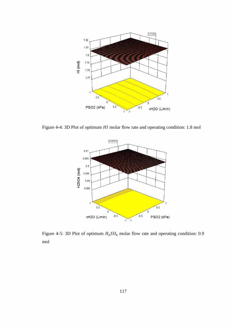
117

Figure 4-4: 3D Plot of optimum 𝐻𝐼 molar flow rate and operating condition: 1.8 mol

Figure 4-5: 3D Plot of optimum 𝐻2𝑆𝑂4 molar flow rate and operating condition: 0.9

mol

118

Table 4.6: Optimum values of parameters for Bunsen reactor

Coded

Factor

Variable Value

A 𝑆𝑂2 gas pressure, P (kPa) 223

B 𝑆𝑂2 volumetric feed flow rate, υSO2o (L/min) 0.1

C Iodine initial mol, 𝑛𝐼2 (mol) 0.9

D Water initial mol, 𝑛𝐻2𝑂 (mol) 5.2

E Feed reactor temperature, 𝑇𝑜 (K) 345

F Feed jacket temperature, 𝑇𝑗𝑜 (K) 300.8

G Cooling water volumetric feed flow rate, 𝑣𝑗𝑜

(L/min)

3.79e-3

H Water volumetric feed flow rate, 𝑣𝑜 (L/min) 1.00e-04

4.3 Bunsen Reactor Scale-Up Procedure

The scaling-up procedure for the Bunsen reactor is carried out based on the objective

to achieve more than 1,000 kg/hr of 𝐻2 production. The scale-up calculation is done

by backward calculation of the overall SITC chemical reaction equation as follows.

IIISectionIISectionISection

OHIHIOHSOHSOIOH 22242222 6425513 (4.28)

Figure 4-6 illustrates an example block diagram of SITC plant scale-up. A summary

flow chart indicating the steps involved in the scaling up procedure is presented in

Figure 4-7. Figure 4-8 depicts the idea of Bunsen reactor scaling up. By assuming 99%

conversion in each Section II and Section III, the estimated total production rate of

𝐻2𝑆𝑂4 and 𝐻𝐼 mixture required is 9,500 𝑘𝑔

ℎ𝑟 . This production rate shall be

accomplished by setting the feed flow rates of water, iodine and sulfur dioxide

119

accordingly. Once the estimated feedstock amount is calculated, the size of the reactor

including the area and height can be optimized based on the desired feed and production

rates. The kinetic parameters used for both laboratory scale and plant scale are

unchanged. Table 4.7 listed the kinetics, operating and design parameters of Bunsen

reactor used in both laboratory scale and plant scale simulation studies.

Section I

Section II

Section III

500 kmol/hr

7000 kmol/hr

3000 kmol/hr

FSO2,in

FSO2

FH2O,in

FI2,in

FI2

FH2O

FH2O

FO2

250 kmol/hr

FH2

500 kmol/hr

Figure 4-6: An example illustration block diagram of SITC plant scale-up.

120

Estimate the desired total plant

production rate (assume 99%

conversion)

Calculate the feed flow rates of water,

iodine and sulfur dioxide according to

the desired production rate

Achieve desired

production?

Start

End

Optimized the size of the Bunsen

reactor (area, height) and its operating

conditions

Simulate the Bunsen reactor based on

the new calculated feed flow rates and

reactor size

Determine the size of the Bunsen

reactor (area, height)

YES

NO

Figure 4-7: Flowchart of scaling up steps for Bunsen reactor

121

(b)

Input:

Sulfur Dioxide, SO2

Outputs:


Hydrogen Iodide, HI

Water, H2O

Iodine, I2

Cooling

water in

Cooling

water out

Inputs:

Water, H2O

Iodine, I2

(a)

Figure 4-8: Scaling-up schematic diagram for Bunsen reactor: (a) the laboratory scale

Bunsen reactor, (b) the plant scale Bunsen reactor.

Table 4.7: Bunsen reactor laboratory scale and plant scale parameters

Bunsen reactor Parameter Laboratory

Scale

Plant Scale

Cross section area, 𝐴𝑟𝑥 3.3𝑒−3 𝑚2 20 𝑚2

Maximum height, 𝐻𝑇 0.15 𝑚 25 𝑚

Volumetric feed flow rate of water, 𝑣𝑜 2.4𝑒−4

𝑚3

ℎ𝑟 0.102

𝑚3

ℎ𝑟

Molar feed flow rate of iodine, 𝑛𝐼2 0.9 𝑚𝑜𝑙/𝑚𝑖𝑛 1425 𝑘𝑚𝑜𝑙/ℎ𝑟

Volumetric feed flow rate of sulphur dioxide

(gas), 𝑣𝑆𝑂2 9.6𝑒−4

𝑚3

ℎ𝑟 0.48

𝑚3

ℎ𝑟

Volumetric feed flow rate of cooling water, 𝑣𝑗𝑜 2.28𝑒−4

𝑚3

ℎ𝑟 1.466

𝑚3

ℎ𝑟

Iodine to water molar ratio 0.36 0.37

Temperature, 𝑇 345 𝐾 338 𝐾

122

4.4 Liquid-Liquid Separator

Liquid-liquid separator (LLS) is the second important equipment in the Bunsen Section.

It is used to separate the two immiscible phases, which are the sulfuric acid and

hydrogen iodide solutions. Figure 4-8 shows the schematic design of LLS used in the

study.

There is one input line and two output lines. The input line consisting sulfuric acid

and hydrogen iodide mixtures. The first output line consisted of light phase liquid which

is sulfuric acid and water mixture. The second output line consisted of heavy phase

liquid which is hydrogen iodide, water and iodine mixture. The LLS is designed for a

plant-scale size.

For the LLS model simplification, assumptions have been made where few are

referred to Chonwattana et al, (2018):

A.4.4.1: Both liquid solutions fed to the separator are immiscible and dispersed

uniformly in the LLS separation chamber.

A.4.4.2: Densities of both liquid solutions are constant.

A.4.4.3: There is an adequate different between the two liquid densities for a phase

separation.

A.4.4.4: The separator has a sufficient retention time to allow the immiscible mixtures

to separate into two layers.

A.4.4.5: The emulsion layer between the two liquids formed in the separator is not

considered in the developed model.

A.4.4.6: The heavy phase liquid solutions are always below the specified v-notch

height. The v-notch angle is 60o.

A.4.4.7: The process is always in a continuous mode.

123

Heavy phase output:

Hydrogen iodide mix, Hix

Water, H2O

Iodine, I2

Input:

Sufuric acid and hydrogen

iodide mix

Light phase output:


Water, H2O

H2

H1 H

3HV

-no

tch

Heavy phase output:

Hydrogen iodide mix, Hix

Water, H2O

Iodine, I2

Input:

Sufuric acid and hydrogen

iodide mix

Light phase output:


Water, H2O

(a) (b)

Light phase

Light phaseHeavy phase

Figure 4-9: Liquid-liquid separator: (a) schematic diagram, and (b) internal view

4.4.1 Mass Balance

The proposed LLS dynamic model is developed by mean of mass balance for each

phase to account for the levels of liquid phases. The objective of LLS modelling is to

capture the light and heavy phase dynamics of liquid levels in the separation chamber,

and the liquid level in the collecting (light phase) chamber. For the heavy phase liquid

in the separation chamber, mass balance on the phase leads to

sH

HinAVin

A

mmx

dt

dH

11

(4.29)

where 𝐻1 is the level of heavy phase solution, 𝑥𝑖𝑛 is the feed fraction of the heavy phase

solution, 𝜌𝐴𝑉 is the density of the mixture, �̇�𝑖𝑛 is the feed flow rate mixture, 𝜌𝐻 is the

density of heavy phase solution and 𝐴𝑠 is the surface area of the separating chamber

LLS. Mass balance on the light phase liquid in the separation compartment yields

sL

vLinAVin

A

Qmx

dt

dH

)1(2 (4.30)

where 𝐻2 is the level of light phase solution, 𝜌𝐿 is the density of light phase solution

and 𝑄𝑣 is the flow rate at the v-notch of the LLS.

124

Meanwhile, the light phase liquid level in the collecting chamber of the LLS gives

c

v

A

mQ

dt

dH 23

(4.31)

where 𝐻3 is the level of light phase solution in the collecting chamber, �̇�2 is the outlet

flow rate from collecting camber and 𝐴𝑐 is the surface area of collecting chamber LLS.

Note that, parameters appear in the equations (4.29) – (4.31) above are expressed as

follows:

21111 75.0 HkvHkvm (4.32)

322 Hkvm (4.33)

0

,))(2

28.4(

,0

5.2

v

dvcvv

Q

else

khCmQ

hfor

(4.34)

Where h is the height of light phase level in the separating chamber. If ℎ > 0, the

height is above the bottom of V-notch. If the level is below the V-notch, there will be

no flow. On the other hand, it is essential to make sure that the heavy phase liquid level

is always below the bottom of V-notch; otherwise, HI solution will go to the collecting

chamber. The parameters of LLS dynamic model are listed in the Table 4.8. The

parameters are based on the industrial scale.

Table 4.8: Parameters of LLS dynamic model

Parameters Value or expression

Heavy phase density, 𝜌𝐻 1300

𝑘𝑔

𝑚3

125

Light phase density, 𝜌𝐿 1100

𝑘𝑔

𝑚3

Average density, 𝜌𝐴𝑉 𝜌𝐻𝑥𝑖𝑛 + (1 − 𝑥𝑖𝑛)𝜌𝐿

Area of separator, 𝐴𝑠 20 𝑚2

Area of collecting chamber, 𝐴𝑐 0.2𝐴𝑠 𝑚2

Valve coefficient 1, 𝑘𝑣1 0.4

Valve coefficient 2, 𝑘𝑣2 1

Total liquid height, 𝐻𝑡 𝐻1 + 𝐻2

V-notch height, 𝐻𝑣−𝑛𝑜𝑡𝑐ℎ 13 𝑚

Height above the V-notch bottom, ℎ 𝐻𝑡 − 𝐻𝑣−𝑛𝑜𝑡𝑐ℎ

Total height of LLS, 𝐻𝐻𝑇 25 𝑚

4.5 Novel Procedure for Control System Design

In order to design a control system or strategy for the Bunsen reactor unit, the following

procedure is applied:

Step 1: Determine control objectives. The explicit objectives of controlling the

Bunsen reactor are to maintain the X and Y variables at constant optimal setpoint. The

reasons of implicit objectives of controlling X and Y variables are maintained (i.e, keep

𝐻𝐼𝑥 solution above azeotropic composition, etc).

Step 2: Determine potential manipulated variables. PCA and RSM analyses are

adopted in order to determine which inputs are strongly correlated with the controlled

variables X and Y. RSM analysis is used to determine which inputs that cause minimum

economic loss (i.e., flat) when the inputs are used as manipulated variables.

Step 3: Determine favorable operating conditions and pairings. To determine a

favorable operating conditions, the fundamental model is linearized at different

operating points. A few sets of linearized models (2x2 transfer function matrices) are

obtained, which are then analyzed for the controllability properties by using LGC and

RGA indices.

126

Step 4: Select and design controller algorithms. Based on the LGC index, a suitable

controller algorithm is chosen, e.g., either standard PID controller or MPC; the latter

will be used if the LGC value is very small, which implies difficult to control the system

using the standard decentralized PID control.

Step 5: Evaluate control strategy. The control strategy designed in Step 4 is evaluated

for its servo and regulatory control performances. If the performances are not

satisfactory, a new control strategy will be designed or a different controller law will

be adopted.

The strength or advantage of the procedure is that it allows the simultaneous

determination of suitable operating condition and controller pairing. In some existing

methods, the operating condition is often pre-defined, or selected in ad-hoc manner.

Avoiding an operating condition that gives poor controllability is just as important as

selecting proper controller pairings in a decentralized control scheme. Poor

controllability of the given operating condition will unavoidable lead to poor control

performance regardless of the type of control law being used.

Another advantage of the proposed procedure is its ability to avoid an engineer from

selecting unsuitable manipulated variables which can cause serious economic loss due

to the adjustments of the inputs. This ability arises from the incorporation of PCA and

RSM techniques in Step 2. Figure 4-10 presented the above step in a flowchart form.

Step 1 to 3 will be presented in detail in Section 4.6. Step 4 will be presented in detail

in Section 4.7 and Step 5 will be presented in detail in Section 4.8.

127

Step 1: Determine control objectives

Step 2: Determine potential

manipulated variables.

Tools: RSM and PCA.

Start

End

Step 4: Select and design controller

algorithms

Step 3: Determine favourable operating

condition and pairing.

Tools: LGC and RGA.

Step 5: Evaluate control strategies

Figure 4-10: Flowchart of novel procedure for designing control system

4.6 Loop Gain Controllability Analysis

In this section, the LGC analysis will be carried out for the Bunsen reactor. Since

Bunsen reactor is a multivariable process, controlling the reactor will require more than

one control loops. Here, the LGC analysis can be used to determine:

128

a) Dynamically favorable operating conditions which give good controllability

performance, i.e., to find the operating conditions, at which the reactor is easy

to control even by using a simple PID control system.

b) The best sets of manipulated inputs and controlled outputs which can lead to the

highest achievable control performance.

Based on the sensitivity analysis via RSM method, there are four potential manipulated

input variables have been identified for the Bunsen reactor: (1) cooling jacket flow rate,

(2) feed molar flow rate of iodine, (3) feed temperature, and (4) sulfur dioxide feed flow

rate or pressure. Table 4.9 lists down the potential manipulated inputs (MVs) and

controlled outputs or variables (CVs) for the Bunsen reactor. The LGC analysis results

are also presented corresponding to the different sets of MVs and CVs. In this case the

feed temperature is not chosen as the manipulated variable since it cannot be adjusted

rapidly – its application as manipulated variable will be hampered by long time-delay,

which is not desirable for closed-loop stability. Thus, in practice the feed temperature

acts as one of the potential disturbance variables (DVs). Controlling the reactor holdup

level is crucial as this directly leads to inventory control of the reactor to avoid potential

unsafe conditions. If the reactor holdup level drops to a very low value, then this can

cause cavitation of the pump installed beneath the reactor. On the contrary, if the reactor

holdup level is not controlled, this can lead to a possible overflow of the reactor. To

control the reactor holdup level, either the feed flow or outlet flow from the reactor can

manipulated. In the present study, it is preferable to manipulate the outlet flow rate as

to control the reactor holdup level. Alternatively, the reactor holdup level can be

controlled indirectly by controlling the production rate. From the PCA analysis, it is

found that the production rate and holdup level are positively correlated, which implies

that if one of these variables are controlled, then this would indirectly control another

variable.

In the Table 4.9, it is shown that the LGC value for the 2 × 2 MIMO Model 1 (set

1 of MV-CV) is higher than that of the Model 2. Note that, for Model 2 the LGC value

is negative which implies very poor controllability property based on the sets of MV-

CV selected.

129

Even though the RGA values between the Model 1 and Model 2 are comparable,

hence indicating equally favorable input-output pairings, the negative LGC value of the

Model 2 implies that it is not controllable. Therefore, the pairing as in the Model 1 is

choose for the controller design of the Bunsen reactor.

Recall that, a positive LGC value but lower than unity suggests that the system is

difficult to control using the conventional decentralized PID control. In this case the

LGC value for Model 1 is less than one, which implies it is hard to control with PID-

based controller. For this reason, the application of an advanced model based controller

will be preferable, e.g., Nonlinear MPC.

Table 4.10 shows the transfer function models for Bunsen reactor which are derived

via linearization of the fundamental model at some nominal operating conditions.

Notice that the diagonal transfer functions for the Model 2 exhibit very large time-

delays compared to that of the Model 1. Thus, the reason for the negative LGC value

of the Model 2 (difficult to control) is due to the long time-delays. For a given system,

as the time-delays become larger, the maximum achievable control performance

becomes smaller.

130

Table 4.9: Controllability analysis based on 2x2 MIMO model of Bunsen reactor

Model

BR

Sensitivity analyzes 𝜽𝒆𝒐𝒕𝒇 LGC RGA

Manipulated Input Controlled Output

Model 1 Outlet Flowrate Reactor Level 10.62 0.9077 [1.0151 −0.0151

−0.0151 1.0151]

Jacket Flowrate Reactor Temperature

Feed Flowrate Iodine, 𝐼2 (MV1) Product Flowrate (CV1)

Reactor Temperature

Feed Flowrate Sulphur Dioxide, 𝑆𝑂2 (MV2) Product Flowrate

Reactor Temperature (CV2)

Feed temperature Reactor Level

Reactor Temperature

Model 2 Outlet Flowrate Reactor Level 35.11 -0.9841

[0.9815 0.01850.0185 0.9815

]

Jacket Flowrate (MV1) Reactor Temperature (CV1)

Feed Flowrate Iodine, 𝐼2 (MV2) Product Flowrate (CV2)

Reactor Temperature

Feed Flowrate Sulphur Dioxide, 𝑆𝑂2 Product Flowrate

Reactor Temperature

Feed temperature Reactor Level

Reactor Temperature

131

Table 4.10: Transfer function models for the Bunsen reactor at nominal conditions.

No Bunsen reactor Model Input-Output Pairing

1

𝑀𝑜𝑑𝑒𝑙 1 =

[

1.0469𝑒−0.8503𝑠

20.32𝑠 + 1

0.031𝑒−0.3978𝑠

0.4105𝑠 − 1−0.0047𝑒−10.637𝑠

51.14𝑠 + 1

−3.87 × 10−5𝑒−0.4104𝑠

0.4105𝑠 − 1 ]

Feed Flowrate Iodine,

𝐼2 (MV1)

Feed Flowrate Sulfur

Dioxide, 𝑆𝑂2 (MV2)

Product Flowrate (CV1)

Reactor Temperature

(CV2)

2

𝑀𝑜𝑑𝑒𝑙 2 =

[ 7.7084 × 10−4𝑒−30.68𝑠

154.29𝑠 + 1

381.25𝑒−2.31𝑠

59.66𝑠 + 10.00146𝑒−63.52𝑠

62.4𝑠 + 1

−13.574𝑒−30.72𝑠

154.11𝑠 + 1 ]

Jacket Flowrate (MV1)

Feed Flowrate Sulphur

Dioxide, 𝑆𝑂2 (MV2)

Reactor Temperature

(CV1)

Product Flowrate

(CV2)

4.7 Process Controller Design for Bunsen Section

4.7.1 NMPC Design for Bunsen reactor

Based on the LGC analysis result (small index value less than 1) as well as the presence

of unstable poles in the Model 1, it is can be anticipated that the Bunsen reactor is

difficult to be control by using PID-based controllers. In view of this problem in this

work a nonlinear MPC (NMPC) is chosen for controlling the Bunsen reactor. A NARX

model is embedded into the MPC to form the NMPC. The significant of NARX model

can be retrieved from (Mohd and Aziz, 2016).

For the NMPC scheme, the manipulated variables (MVs) used are iodine molar feed

flow (MV1) and sulfur dioxide feed flow (MV2) while the controlled variables (CVs)

are sulfuric acid flowrate (CV1) and reactor temperature (CV2).

132

4.7.1.1 Identification of NARX empirical model

A set of input-output data of Bunsen reactor corresponding to the Model 1 (from

previous section) consisting of 16,455 samples is generated from the first principle

Bunsen reactor model. The type of simulation input used is the multi-level input signal

(see details in Section 3.2.4) to mimic the input of a real plant input. The generated data

is then used for the development of NARX model using the System Identification

Toolbox in MATLAB via, ‘nlarx’ nonlinear function. The NARX model order and

delay; [𝑛𝑎, 𝑛𝑏, 𝑛𝑘]; [3,2,3] are used. Figure 4-11 and 4-12 show the plotted NARX

models for both input-output pairings. Table 4.11 tabulated the result from these

figures. It is demonstrated that the nonlinearity estimator object ‘sigmoidnet’ and

‘wavenet’ shown the best fit NARX model for Bunsen reactor.

Figure 4-11: NARX model identification for 𝑢1𝑎𝑛𝑑 𝑦1

Figure 4-12: NARX model identification for 𝑢2 𝑎𝑛𝑑 𝑦2

133

Table 4.11: NARX model nonlinearity estimator object best fit value

Nonlinearity estimator

object

Best fit value

Pairing 1 Pairing 2

Wavenet 54.45 80.89

Wavenet (high order) 54.45 80.89

Wavenet (custom order) 56.24 70.10

Treepartition 59.53 -95.36

Sigmoidnet 61.12 69.56

4.7.1.2 NMPC development

The NMPC is first tuned via an offline simulation. The objective functions of the

NMPC given as follow,

))(),((min0]|[],...|[ tNtSAJ ItpmNttN iII (4.35)

))(),((min2022

]|[],...|[ tvtTJ SOtpmvttv iSOSO (4.36)

M

k k

P

k setpoktpmNttN tkturSAtktSAwkII 1

2

1

2

int]|[],...|[ ]|[)]|[(min0

(4.37)

Mk k

Pk setpoktpmvttv tkturTtktTw

kSOSO 12

12

int]|[],...|[ ]|[)]|[(min022

(4.38)

where 𝑺𝑨 is the product flowrate and 𝑻 is the temperature. 𝑷 is process output

prediction, 𝑴 is manipulated input horizons and 𝑸 and 𝑹 are the weighting matrices.

𝑵𝑰[𝒕 + 𝒌|𝒕]𝒌=𝟎…𝑷 and 𝒗𝑺𝑶𝟐[𝒕 + 𝒌|𝒕]𝒌=𝟎…𝑷 are the set of future process input values.

The output prediction shall be more or equal than the manipulated input horizons,

𝑷 ≥ 𝑴 where they are adjustable. In this work, the tuning test begins with 𝑴 = 𝟏 and

𝑷 = 𝟏𝟓. The weighting matrix 𝑹 is a diagonal form as 𝒓𝒌 = 𝒅𝒊𝒂𝒈(𝒂, 𝒃, 𝒄, … ) while

𝒘𝒌 = 𝟐 × 𝟐 matrix. The tuning Set 2 with 𝑴 = 𝟏 and 𝑷 = 𝟐𝟎 produced the best

performance. Table 4.12 listed the SSE values of various MPC tuning.

134

Table 4.12: SSE values for CV1 and CV2 of Bunsen reactor for various MPC tuning

Weighting matrices Set Control

horizon,

M

Prediction

horizon, P

SSE for

CV1

SSE for

CV2 𝒘𝒌 𝒓𝒌

𝟐 × 𝟐

matrix

(input)

[𝟐 𝟎𝟎 𝟐

] 1 1 15 14.5330 31.4951

2 1 20 14.1726 31.0756

3 2 15 14.1827 30.7564

4 2 20 14.5787 30.4951

5 3 15 14.5273 31.0756

6 3 20 14.5330 31.0610

4.7.2 MSC-PID Design for Liquid-liquid separator

The details of the multi-scale control (MSC) scheme can be found in (Nandong and

Zang, 2013a). The MSC scheme can be used to synthesize practical PID controller

augmented with a filter. i.e., MSC-PID controller. It is interesting to note that, the MSC

scheme can provide significant performance and robustness improvements for some

processes with long dead time and inverse-response behaviors. The basic idea of the

MSC scheme is to decompose a given plant into a sum of basic factors with distinct

speeds of responses – multi-scale modes. A set of sub-controllers is designed based on

the basic modes, which are then combined in such a way to enhance cooperation among

these different modes. For the LLS unit, the MSC scheme will be used to design the

required PID controllers for controlling liquid levels in the unit.

For the LLS effective operation, it is crucial to keep the level of each heavy phase

and light phase liquid in the collection chamber at constant setpoint so that the

separation process can be performed efficiently. Two SISO PID controllers are

designed to achieve this purpose. The nominal conditions of the LLS at which the

controllers are designed are shown in Table 4.13. The transfer function of a linearized

LLS model (heavy phase) is as follows

135

sss

essGLLS

002153.01326.0

353.90008062.006864.023

62

(4.39)

Based on the transfer function of LLS, an MSC-PID controllers is obtained using

the MSC scheme. The inner-loop P-only controller is first designed, and then the PI

controller. The overall MSC-PID controllers are given as follows.

1137.0

73.462476

1137.0

0189.012467

s

s

s

sGMSC

(4.40)

Note that the MSC-PID controller above is compared with an IMC-PID controller. The

IMC-PID controller setting (using MATLAB Control System Design) is given as

follows.

s

esGIMC

)35.11(96100083832.0 (4.41)

Table 4.13: Nominal value of LLS levels

Variables Nominal value

Heavy phase level, 𝐿𝐻𝐿𝑆 (m) 5.997

Light phase level, 𝐿𝐿𝐿𝑆 (m) 8.523

Collecting chamber level, 𝐿𝐿𝐶𝐿𝑆 (m) 2.244

4.8 Performance Evaluation of NMPC in Bunsen Reactor

4.8.1 NMPC Performance on Bunsen reactor

4.8.1.1 Setpoint tracking

Figures 4-13, 4-14, 4-15 and 4-16 show the results for the setpoint tracking of sulphuric

acid flow rate (CV1), i.e., the primary controlled variable. The setpoint for the CV1 is

changed from a nominal steady-state, 1,360 kg/hr to 1,385 kg/hr at 750th hour (in

simulation unit), then from 1,385 kg/hr to 1,335 kg/hr at the 1200th hour, and finally set

back to original point value for the rest of simulation. Meanwhile, the setpoint of

temperature (CV2) is changed from a nominal steady-state, 338 K to 341 K at 750th

136

hour, then from 341 K to 335 K at the 1200th hour, and finally set back to the original

nominal steady state value for the rest of simulation. For both CV1 and CV2, the NMPC

is able to drive the controlled outputs to their desired setpoint smoothly with a fast

response without any delay while the MVs are still within the desired boundaries. There

is a small offset for CV1. However, the offset is less than 1.5 kg/hr which is

insignificant to the overall flowrate of the plant.

Figure 4-13: Response of NMPC for setpoint changes in CV1, sulfuric acid flowrate.

Figure 4-14: Response of iodine molar feed flow (MV1) under the setpoint changes in

CV1.

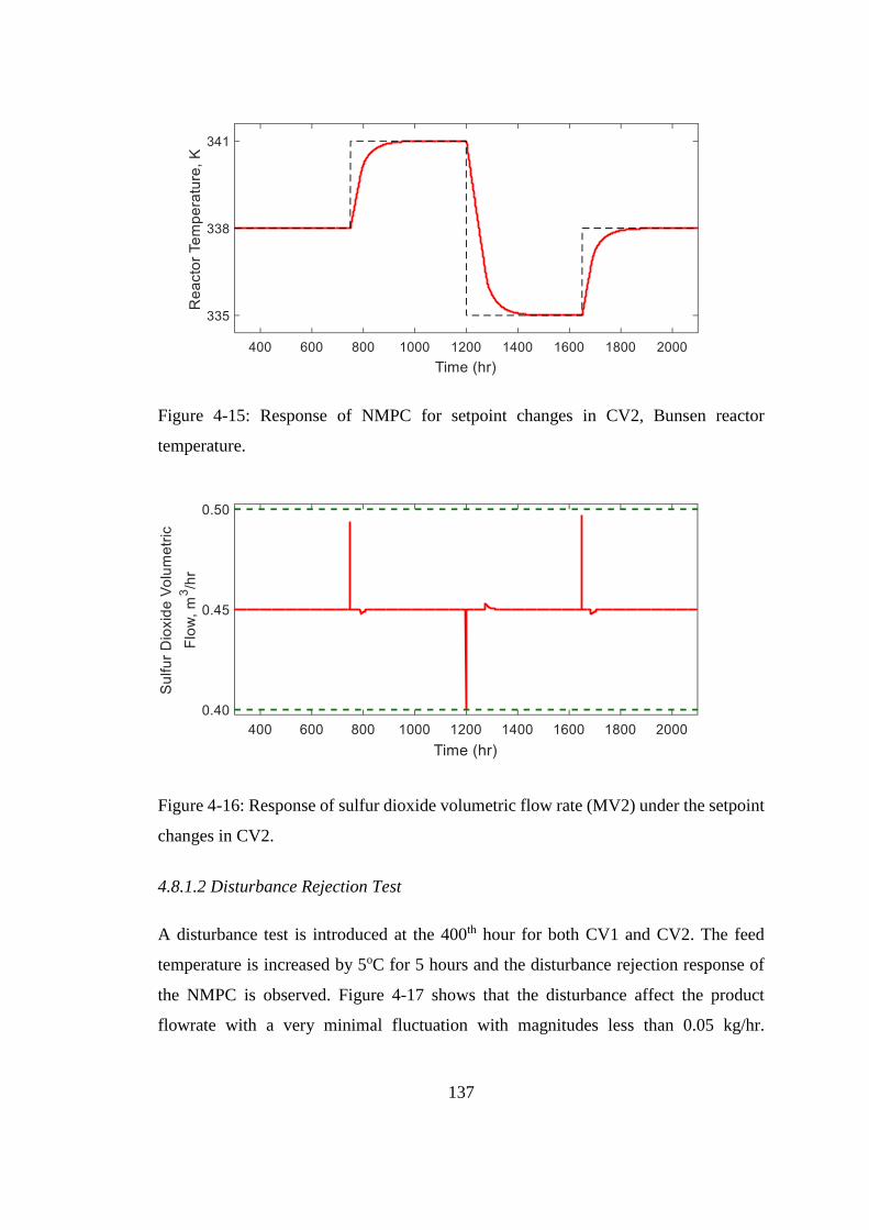
137

Figure 4-15: Response of NMPC for setpoint changes in CV2, Bunsen reactor

temperature.

Figure 4-16: Response of sulfur dioxide volumetric flow rate (MV2) under the setpoint

changes in CV2.

4.8.1.2 Disturbance Rejection Test

A disturbance test is introduced at the 400th hour for both CV1 and CV2. The feed

temperature is increased by 5oC for 5 hours and the disturbance rejection response of

the NMPC is observed. Figure 4-17 shows that the disturbance affect the product

flowrate with a very minimal fluctuation with magnitudes less than 0.05 kg/hr.

138

Meanwhile, Figure 4-18 shows that the NMPC is able to completely reject the

disturbance after about 150 hours. Even though the rejection time is long; the reactor

temperature is still kept within the optimal temperature window, i.e., 330 𝐾 ≤ 𝑇 ≤

350 𝐾.

Figure 4-17: Response of NMPC for disturbance rejection test for CV1

Figure 4-18: Response of NMPC for disturbance rejection test for CV2

139

Based on the setpoint tracking and disturbance rejection test, it is shown that the NMPC

is able to fulfill all three keys criteria for Bunsen reactor:

a) The resulting feed molar ratio of 𝐼2/𝐻2𝑂 is between 0.356 and 0.377, i.e., within

the optimal operating range.

b) The resulting molar ratio of 𝐻𝐼/(𝐻𝐼 + 𝐻2𝑂) lies between 0.16 and 0.25, i.e., at

0.23 where this will ensure the solution remains over azeotropic condition.

As a conclusion, the NMPC can provide satisfactory closed-loop performances for the

Bunsen reactor, under both servo and regulatory control objectives.

4.8.2 MSC-PID Performance

4.8.2.1 Setpoint tracking

Figure 4-19 shows the results for the setpoint tracking of heavy phase level in the LLS

separating chamber. The nominal setpoint is set at 5.6 m. It is shows that MSC-PID

drives the heavy phase liquid level to the setpoint faster that IMC-PID which could not

settle to the desired setpoint. The IAE for MSC-PID is very small which is only 0.0468

showing an efficient controller performance as compared to the IMC-PID with IAE of

121.4.

Figure 4-19: Response of MSC-PID and IMC-PID for setpoint tracking in CV, heavy

phase level of LLS.

140

The setpoint tracking is continued with another setpoint change test. The CV changes

from nominal steady state, to 7 m at 25th hour, 7 m to 3 m at the 50th hour and then set

back to the steady state value for the rest of hours. Figure 4-20 reveals that the MSC-

PID is able to drive the process output to its desired setpoint with a fast response with

little delay, while the IMC-PID is not able to track the given setpoint changes.

Figure 4-20: Response of MSC-PID and IMC-PID for setpoint changes in CV, heavy

phase level of LLS.

4.8.2.2 Disturbance rejection test

A disturbance test is introduced at the 80th hour. The feed flowrate which is the

upstream flow from the Bunsen reactor is increased by 20% for 1 hour and the

disturbance rejection time of both controllers are observed. Figure 4-21 shows response

of the MSC-PID controller, notice that the disturbance has only little effect on the heavy

phase liquid level. On the contrary, Figure 4-22 shows that the IMC-PID is not able to

reject the disturbance and which indicates instability behaviour of the controller. For

both setpoint tracking and disturbance rejection tests, the MSC-PID show satisfactory

performances as compared to the IMC-PID.

141

Figure 4-21: Response of MSC-PID for disturbance rejection test for CV.

Figure 4-22: Response of IMC-PID for disturbance rejection test for CV.

4.9 Summary

To the best of our knowledge, to date, there has been no report on the detailed

fundamental models and scale-up for the Bunsen reactor and L-L separator units of the

SITC plant. The sensitivity analysis for Bunsen reactor reveals that the kinetics of

Bunsen reaction in the CSTR:

142

a) Has little dependence on temperature changes within the specified optimal

range.

b) Slightly sensitive to the changes in both feed flow rate of 𝑆𝑂2 gas and its partial

pressure.

c) Changes in iodine and water molar feed flow rates have the most significant

influences on the total output variables; sulfuric acid and hydrogen iodide

flowrate.

It has been demonstrated that, the scaling up of the L-L separator presented a number

of challenges, and must be addressed when selecting the area and height of weir. After

the scaling up procedure, the controllability analyses were carried out via LGC index.

Since the value of LGC based on the Model 1 is less than unity, this means that the

system is very difficult to control using the standard decentralized PID control. Thus,

for the Bunsen reactor, a NMPC is chosen. In view of the satisfactory servo and

regulatory performances demonstrated by the NMPC, it can be concluded that the

application of NARX model in the controller is adequate enough to capture the main

nonlinear dynamics of the Bunsen reactor. Meanwhile, for the LLS, two PID controllers

are developed and compared, which are designed based on the MSC-PID and IMC-PID

approaches. Based on the setpoint tracking and disturbance rejection tests, it has been

shown that the MSC-PID outperforms the IMC-PID controllers.

143

5 Sulfuric Acid Section (Section II):

Dynamic Modelling and Controllability

Analysis

This chapter covers aspects from fundamental to process controller performance

evaluation of the Sulfuric Acid Section. Prior to plant scale-up, a preliminary simulation

of a laboratory scale Sulfuric Acid Integrated Boiler Superheater Decomposer (SA-

IBSD) reactor using kinetic parameters available in literature was carried out and

validated. The effects of input variables on output variables were analyzed and the

process operating conditions were then optimized. Meanwhile, the controllability

analysis for the reactor was carried out based on the LGC method and the most

controllable model (operating condition) is selected. The dynamic modelling of a flash

tank for concentrating sulfuric acid solution was also presented. Suitable controller

strategies were selected and designed for the SA-IBSD reactor, and their performances

were evaluated. At the end of this chapter, a summary on the Sulfuric Acid Section is

highlighted.

5.1 Fundamental of Sulphuric Acid Section

In the Sulfuric Acid Section there are two main processes :(1) sulfuric acid flashing,

and (2) sulfuric acid decomposition processes. A sulfuric acid flash tank (SA-FT) is

used to first concentrate the sulfuric acid solution from the Bunsen Section. It follows

that the concentrated acid is then sent to an integrated reactor, i.e., Sulfuric Acid

Integrated Boiler Superheater Decomposer (SA-IBSD) reactor to decompose the

sulfuric acid.

The sulfuric acid mixture from the Bunsen Section is fed to the SA-FT to be

concentrated to a desired concentration, which is more than 90% acid concentration.

From the sulfuric acid solution, water vapor is eliminated as much as possible before

the sulfuric acid is fed to the SA-IBSD reactor. In the SA-IBSD reactor, the sulfuric

144

acid is decomposed into sulfur dioxide and oxygen. Sulfur dioxide is recycled to

Bunsen reactor while oxygen is collected as a byproduct.

5.1.1 Reaction Mechanisms

The overall chemical reaction of Sulfuric Acid Section is given as follows,

)(5)( 242 lOHlSOH ⇌ )(2

1)(6)( 222 gOgOHgSO (5.1)

The chemical reactions taking place in the SA-IBSD reactor are as follows,

Reaction 1: Evaporation

42 )(lSOH ⇌ )()( 23 gOHgSO ∆H1 = +300 kJ/mol (5.2)

Reaction 2: Decomposition

)(3 gSO ⇌ )(2

1)( 22 gOgSO ∆H2 = +274 kJ/mol (5.3)

Note that, the decomposition reaction is carried out in the presence of catalyst.

The SA-IBSD unit operates at a very high temperatures that goes beyond the critical

temperature of water (374℃) (Kim et al., 2008; Nagarajan et al., 2014). Since the SA-

IBSD reactor is an endothermic reaction, the reaction temperature and the thermal

energy supplied to the system must be sufficient. As a rule of thumb, a higher

temperature tends to favor greater efficiency. Please note that, however, it is desired to

control the reaction temperature below 1140℃ to prevent a potentially dangerous

process runaway reaction and catalyst deactivation.

145

5.2 Dynamic Modelling and Simulation

5.2.1 Sulfuric Acid Flash Tank (SA-FT)

D

Vapor phase

Maximum Level

H2SO4

solution

T: 337 K

P: 201 kPa

hL

hV

Liquid phase

hF

H2O

H2SO4

T: 502 K

P: 101 kPa

H2SO4

H2O

T: 502 K

P: 101 kPa

Figure 5-1: The schematic diagram of SA-FT (Watkins, 1967)

In this section, a dynamic model of the flash tank to concentrate sulfuric acid is

presented. Figure 5-1 shows the schematic diagram of SA-FT, which is modified from

the Watkins’s separator and accumulator design (Watkins, 1967). The height or length

of the SA-FT is given as follows

VFL HHHL (5.4)

From Figure 5-1, 𝐻𝐿 is the liquid level, 𝐻𝐹 is the flooding level which is the distance

between liquid level and feed nozzle, 𝐻𝑉 is the vapor level, and 𝐷 is diameter.

The essential rule of the flash tank design is that to specify the length-to-diameter

(L/D) ratio, which shall lie between 3 and 5. This is based on the fact that, as the

diameter decreases, the shell thickness decreases and vessel length increases. In

addition to that, at some point between the L/D ratios of 3 and 5, a minimum vessel

146

weight can be found, and this will result in the minimum capital cost of the unit (Rao,

2012).

The sulfuric acid/water binary separation is a crucial unit operation in a SITC

process for hydrogen production. In the dynamic modelling of the SA-FT unit, it is

decided to estimate the activity coefficients for the binary mixture using the NRTL

model whereas the thermodynamic properties are estimated via the EOS type, i.e.

specifically the Peng-Robinson (PR) method. To estimate the phase equilibria and

thermodynamic properties, a pre-simulation is first carried out in the Aspen Plus

software. Once the phase equilibria and the desired thermodynamic properties are

obtained, the dynamic modelling of the SA-FT can be performed via the MATLAB

simulation. One of the reasons for conducting this modelling in MATLAB is to enable

the use of many tools available in this software, e.g., for optimization, nonlinear

analysis and control studies; in Aspen such studies are quite limited. The results of the

SA-FT simulation are then compared with the available literature data.

From the liquid-liquid separation (LLS) unit in the Bunsen Section, the aqueous

𝐻2𝑆𝑂4 solution is fed into the SA-FT. The sulfuric acid stream is pre-heated and

flashed in the SA-FT unit to remove water as much as possible. It is important to note

that, the relative volatility of the components to be separated should be much larger

than 1 for the single flash operation to be able to achieve the required separation. Since

water has a lower volatility than the sulfuric acid, so the evaporation of water is much

higher than the acid. Hence, the water is separated from the solution (as the light vapour

phase) and it is recycled back to the Bunsen Section. The sulfuric acid is accumulated

in the liquid phase during the flash process. Since the SITC plant involves a closed

cycle, failing to remove most water from the acid stream prior to entering the SA-IBSD

147

reactor will affect the cycle efficiency, which in turn shall reduce the hydrogen

production (Lee et al., 2009).

The proposed SA-FT dynamic model (mass and energy balances) and design

procedure are summarized as follows:

Step SA-FT.1: Calculate the bubble point and the vapour pressure for the water/sulfuric

acid mixture.

Step SA-FT.2: Find the steady-state value for each variable based on the derived

differential equations. The steady-state is important to see the capability of the

developed dynamic model to achieve stable output.

Step SA-FT.3: Simulate the SA-FT model in, i) stand-alone mode and ii) integrated

mode. The model is simulated in the MATLAB Simulink environment.

5.2.1.1 Mass and Energy Balances

The following steps are applied in the modeling and simulation of SA-FT:

Step SA-FT.1 Bubble point and vapour pressure calculation

The following algorithm is applied to find the bubble-point.

Step SA-FT.1.1: Guess the flash tank temperature, e.g., 𝑇 = 𝑇1.

The liquid mass fractions are first estimated in addition to flash tank pressure. From

this estimation, the bubble-point calculation is then continued as follows. Note that, the

summation of mass fractions in either liquid or vapour phase must be unity, so that:

11

11

m

i

s

iii

m

ii Px

Py (5.5)

where 𝑦𝑖 denote the the vapor fraction, 𝑥𝑖 is the liquid fraction, 𝛾𝑖 is the liquid activity

coefficient and 𝑃𝑖𝑠 is the vapour pressure of i-th component.

148

From the equation (5.5), the mass fractions in liquid and vapour are related via the

Vapour-Liquid Equilibrium relation:

P

P

x

y s

ii

i

i (5.6)

Step SA-FT.1.2: Calculate the vapour pressure via Eqn. (5.7).

Vapour pressure 𝑃𝑖𝑠 of the i-th component is calculated using the Antoine’s equation

TC

BAP

i

ii

si

10log (5.7)

Step SA-FT.1.3: Calculate the activity coefficients via Eqn. (5.8) to (5.9)

The activity coefficients of two liquid mixtures can be calculated using the Non-

Random Two-Liquid (NRTL) model (Prausnitz and Tavares, 2004) given by:

2

1212

1212

2

2121

2121

2

2lnGxx

G

Gxx

Gxi

(5.8)

2

2121

2121

2

1212

1212

2

12lnGxx

G

Gxx

Gx

(5.9)

The Gibbs energy equation is given as follows

121212ln G (5.10)

212121ln G (5.11)

The non-randomness parameter 𝛼𝑖𝑗 and the dimensionless interaction parameter 𝜏𝑖𝑗 are

extracted from the Aspen Plus simulation as described in the following section.

149

5.2.1.1.1 Aspen Plus Simulation

Table 5.1 lists the products of the flash tank according to the Aspen Plus simulation.

From Table 5.1 it can be seen that 99% of water is evaporated while more than 80% of

sulfuric acid is recovered from the aqueous solution. Note that, the output is

comparable to the literature (Lee et al., 2009) hence the design of flash tank model in

the Aspen Plus environment is acceptable. The next step is to extract the data of Vapour-

Liquid Equilibrium (VLE) from the Properties Data in Aspen Plus. For each component

in a binary mixture, one can easily plot a VLE diagram.

Table 5.1: Sulfuric acid flash tank output from the Aspen Plus simulation.

Flow rate (mol/s) Current Work Reference (Lee et

al., 2009)

Vapour

Water, 𝐻2𝑂 11.18 10.69

Sulfuric Acid, 𝐻2𝑆𝑂4 0.45 0.83

Liquid

Water, 𝐻2𝑂 0.12 0.61


From the simulation in Aspen Plus, the non-randomness parameter, 𝛼𝑖𝑗 and the

dimensionless interaction parameter 𝜏𝑖𝑗 are extracted and tabulated in Table 5.2. Once

𝛼𝑖𝑗 and 𝜏𝑖𝑗 are determined, then the Equations (5.10) and (5.11) can be solved

completely in MATLAB to obtain the activity coefficients required for simulation of

the SA-FT unit.

Step SA-FT.1.4: Calculate the summation in Eqn. (5.5).

If the summation in equation (5.5) is unity, then the bubble point is determined,

otherwise, go to Step SA-FT.1.1 and repeat the previous procedure until the specified

error tolerant is achieved.

Step SA-FT.2 Find the steady state based on differential equations

150

The differential equation for the holdup liquid level is determined by the amount of

feed, evaporation and liquid product flow rate:

Levaf

L

L FFFAdt

dH

1 (5.12)

Where the 𝐻𝐿 is the liquid level in the flash tank, 𝜌𝐿 is the liquid density, 𝐴 is the surface

area of the flash tank, 𝐹𝑓 is the feed flowrate to the flash tank, 𝐹𝑒𝑣𝑎 is the flowrate of

the evaporated vapor at the upper part of flash tank and 𝐹𝐿 is the liquid flowrate at the

bottom of flash tank.

Table 5.2: NRTL parameters for Sulfuric Acid/ Water separation in SA-FT.

Parameters (subscript: 1- H2O, 2- H2SO4) Value

Non-randomness parameter, 12 272.6


Dimensionless interaction parameter, 12 0.3


The mass balance, 𝑀𝑇 of the flash tank is expressed as the sum of feed flow minus the

exit flows.

VLfT FFF

dt

dM (5.13)

The mass fraction of liquid phase, 𝑥𝑖 for each component is expressed in the form of

iievaiif

LL

i xyFxzFAHdt

dx

1 (5.14)

Where 𝑧𝑖 is the total fraction of liquid and vapor.

Meanwhile, the mass fraction in the vapour phase is expressed in terms of the liquid

phase changes and the relative volatility written as follows

151

dt

dx

P

P

dt

dy iiii

* (5.15)

The energy balance representing the temperature change, is calculated according to

s

pApLLpApVVpAfpff

TpA Q

MWt

TCCFTCCFTCTCF

MC

MWt

dt

dT

(5.16)

where 𝑀𝑊𝑡 is the average molar mass, 𝐶𝑝𝐴 is the average heat capacity, 𝐶𝑝𝑓 is the feed

heat capacity, 𝑇𝑓 is the feed temperature, 𝐶𝑝𝑉 is the vapor heat capacity, 𝐶𝑝𝐿 is the liquid

heat capacity, 𝜆 is the sensible heat, and 𝑄𝑠 is the amount of heat supplied to flash tank.

The evolution of pressure, 𝑃 with time is described as a function of temperature changes

dt

dT

MW

y

dt

MW

yd

TRdt

dPni

i

i

ni

i

i

v (5.17)

Here, we assume that the vapour density 𝜌𝑣 is taken from the previous time step 𝑡 − 1.

Its value is recalculated after each time step as follows

ni

i

itv

MW

tytRT

tP

))1(

)(1(

)1()1( (5.18)

For the exit liquid flow rate, it is assumed that the flow rate is given by a square root of

liquid height in the tank,

LLL HkF (5.19)

where 𝑘𝐿 denotes the valve coefficient. Note that, the exit flow rate of vapour is

assumed to be linearly proportional to the pressure in the flash tank, i.e.:

152

PkF vV (5.20)

where 𝑘𝑣 denotes the coefficient of valve attached to the vapour line. Since 𝑋𝑉 + 𝑋𝐿 =

1, we can express the average specific heat capacity in terms of

pVLpLLpA CXCXC 1 (5.21)

Note that, 𝐹𝑒𝑣𝑎 denotes the rate of evaporation due to the excess heat 𝑄𝑒𝑥 defined by

heatsensible

fpffSex TTCFQQ (5.22)

Significantly, the excess heat represents a balance of heat from steam, which is not used

to heat up the cold feed; a portion to heat up the feed is called sensible heat. So, the rate

of evaporation is given by the excess heat is as follows

MWQF ex

eva (5.23)

where 𝑄𝑆 and 𝜆 denote the heat supplied by steam and the latent heat of evaporation,

respectively. The heat supply is

TTAUQ SwtS (5.24)

Step SA-FT.3 Simulation in the Simulink

The developed first principal model in the previous steps is simulated in the MATLAB

environment. For analysis, the output profiles; tank level, outlet liquid sulfuric acid

fraction and outlet vapor sulfuric acid fraction, of the system are then plotted. Figure

5-2(a) shows the liquid level of the SA-FT unit. The output profiles are plotted based

on a start-up simulation. The liquid level which is set at an initial value reaches a steady

state value which shows that the dynamic model met the desired constraint level, hence

preventing the occurrence of flooding in the flash tank.

153

Figure 5-2: Output profiles, (a) Flash tank level, (b) Sulfuric acid liquid fraction (bottom

outlet), (c) Sulfuric acid vapor fraction (upper outlet)

The desired output variables are presented in Table 5.3. Table 5.3 provided the output

vapor and liquid fraction of the sulfuric acid as well as the pressure and temperature of

the designed flash tank, in comparison to the experimental data from the literature (Lee

et al., 2009). The output fraction profiles are also plotted and presented in Figure 5-2(b)

and 5-2(c). As compared to the output data from the literature, the output sulfuric acid

liquid fraction in this work is 15.7% higher where the amount of water effectively

removed is 99% as compared to only 93% in the literature. While the outlet vapor

fraction of the sulfuric acid is efficiently reduced to 85% as compared to the literature.

Based on the result it is revealed that the developed flash tank model is reasonable and

realistic for further simulation in the SITC plant.

(a) (b) (c)

154

Table 5.3: Flash tank dynamic modelling results vs. literature

Variables Current Work Literature (Lee et al.,

2009)

Pressure <10 bar

Temperature >100oC

L/D Ratio 3-5 NA

Bubble point (99% water

evaporation)

a. 177 oC

(VLE diagram)

b. 110-206 oC (Step

SA-FT.1)

NA

Feed Fraction (dimensionless)

Water, 𝐻2𝑂 0.83

Sulfuric Acid, 𝐻2𝑆𝑂4 0.17

Outlet Vapor Fraction (dimensionless)

Water, 𝐻2𝑂 0.99 0.93


Outlet Liquid Fraction (dimensionless)

Water, 𝐻2𝑂 0.19 0.30


5.2.2 Sulfuric Acid Decomposition in SA-IBSD Reactor

Conventionally, Section II should consist of at least three major equipment; a flash tank,

𝐻2𝑆𝑂4 concentrator/ evaporator, and 𝑆𝑂3 decomposer. Usually, after the SA-FT unit

the relatively flashed acid is first heated in a boiler unit, then followed by further heating

in a superheater unit before finally decomposition in a catalytic fixed bed reactor unit.

In this study, instead of using three separate units for the sulfuric acid evaporation,

super heating and decomposition processes, an integrated boiler, superheater and

decomposer (SA-IBSD) reactor is developed in this work. Please note that the required

energy is obtained from an external high temperature reactor, e.g., nuclear reactor.

155

Feed

H2SO4

T: 613 K

P: 10000 kPa

SO2

O2

H2SO4

T: 1123 K

P: 10000 kPa

Length, L

Diameter, D

Cata

lyst

EJ Zone

IJ

Zone

RX

Zone

Fin

Decomposer,

LD

Superheater,

LS

Boiler/

Evaporator,

LB

Figure 5-3: Schematic diagram of the modified SA-IBSD reactor (Moore et.al, 2011)

Bear in mind that, Section II involves the highest temperature in the SITC plant (up to

1000oC). Such a high temperature operation poses a number of significant challenges

that have led to several studies on the behaviour of the Section II, e.g., catalyst stability

and overheating reactor (Rashkeev et al., 2009; Kim et al., 2013; Park et al., 2013;

Noguchi et al., 2014).

The SA-IBSD apparatus was patented by Moore et.al, (2011). The reactor is

constructed of ceramics and other corrosion resistant materials to decompose the 𝐻2𝑆𝑂4

into 𝑆𝑂2, 𝑂2 and 𝐻2𝑂. The integrated reactor is designed with one part of it is packed

with catalyst and the inner part with a fin to increase the recuperation efficiency of

thermal energy. Figure 5-3 shows the schematic diagram of the modified version of a

single cell SA-IBSD reactor. In a large scale operation, a number of cells are arranged

in a single shell. The configuration resembles a shell and tube heat exchanger type

reactor. Here, each tube is replaced with a reactor cell shown in Figure 5-3. In this

study, a modification is made to enable scaling up of the SA-IBSD reactor, i.e., for an

156

industrial-scale production. The properties used in the patented SA-IBSD reactor

(single cell) are described in Table 5.4.

Table 5.4: Parameters of the patented integrated reactor for sulfuric acid decomposition

proposed by Moore et.al, 2011.

Parameter Value

Length, LT or HT 4 ft. to 5ft, or 14 ft.

Ratio of length to

diameter, L/D

10 to 100

Length of Decomposer,

LD

1/3 LT

Length of Superheater,

LS

1/3 LT

Length of Boiler, LB 1/3 LT

Sources of heat Either nuclear, solar, electrical, and/or chemical

combustion

Active catalyst Either platinum, iron oxide, rhodium and metal oxides

(chosen in this work is in form of pellets (Choi et al.,

2014b))

Design material Either ceramics, silicon carbide, silicon carbide alloys,

alumina, quartz or glass

Operating pressure Up to 100 bar or 10,000 kPa

Operating temperature With Catalyst: 750 to 900 oC

Without Catalyst: more than 1000 oC

Boiler temperature 340 oC

Superheater temperature >700 oC

Decomposer

temperature

700 to 900 oC or >1000 oC

Feed temperature, To <100 oC

Feed H2SO4

concentration, CSAo

20% to 100%

Maximum conversion of

H2SO4

36%

157

In the proposed dynamic modelling, the SA-IBSD is divided into five zones which are:

a) Evaporator Zone

b) Superheater Zone

c) Decomposer Zone or Reaction (RX) Zone

d) Internal Jacket (IJ) Zone (acting as a central baffle to increase recuperation

efficiency)

e) External Jacket (EJ) Zone

5.2.2.1 Model Assumptions

The assumptions made in the modelling and simulation of the SA-IBSD reactor are

listed as follows; some are adopted from (Nagarajan et al., 2009):

A.5.2.1: The SA-IBSD is designed as a long catalytic packed bed reactor and

considered having pseudo-homogenous reaction zone.

A.5.2.2: The mass of the catalyst is uniformly distributed throughout the packed bed

(Reaction Zone) where the chemical reaction only occurs in the catalyst phase.

A.5.2.3: The flow is assumed to be in gas phase outside the catalyst pellets.

A.5.2.4: The pressure is assumed constant in all zones.

A.5.2.5: Well mixing in both IJ and EJ Zones, so the temperature is uniform in these

two zones.

A.5.2.6: Well mixing in Evaporator, Superheater and Decomposer Zones.

158

5.2.2.2 Mass and Energy Balance

5.2.2.2.1 Evaporator Zone

This is the zone where the sulfuric acid from the Bunsen Section of the SITC plant

enters the SA-IBSD reactor. In this zone, the sulfuric acid is first heated up to its boiling

temperature before it is subsequently decomposed into 𝑆𝑂3 and 𝐻2𝑂 as depicted in

(5.25) - (5.26). The power law is used to represent the rate law. The reaction type

follows reversible elementary second order kinetics:

)(42 lSOH ⟶ afaaf CkrgOHgSO ),()( 23 (5.25)

)()( 23 gOHgSO ⟶ araar CkrlSOH ),(42 (5.26)

where 𝐻2𝑆𝑂4, 𝑆𝑂3 and 𝐻2𝑂 are denote as components a, b and c respectively.

The net rate of reaction is given by

arafa rrr (5.27)

Eq

cb

afaaK

CCCkr (5.28)

a

cb

EqC

CCK (5.29)

where 𝑟𝑎 is the total reaction rate, 𝑟𝑎𝑓 is the forward reaction rate, 𝑟𝑎𝑟 is the reverse

reaction rate. 𝐾𝐸𝑞 is the equilibrium constant, 𝐶𝑖 is the concentration of component-i.

The general species mass balances considering input and output concentration

(kmol/m3.hr) is given by (5.30) - (5.32).

Ea

g

a

g

a

T

a

E VrCC

Mdt

dCV

Eo

o

Ei

i

(5.30)

159

Ea

g

b

g

b

T

b

E VrCC

Mdt

dCV

Eo

o

Ei

i

(5.31)

Ea

g

c

g

c

T

c

E VrCC

Mdt

dCV

Eo

o

Ei

i

(5.32)

Meanwhile, the energy balances (kJ/hr) on the reactor and jacket sides are given as in

(5.33) and (5.34) respectively.

IJEa

g

o

g

i

aTEpgE

QVHrHH

CMdt

dT

WM

CV

EoEi

EEo

1

(5.33)

DfinIJ

IJoutE

o

IJinE

i

IJIJ

IJpIJoutIJQQ

HHCM

dt

dT

WM

CVIJ

(5.34)

where

EIJrrIJ TTUAQDD

(5.35)

Notations: 𝑉𝐸 is the volume of Evaporator Zone, 𝑀𝑇̇ is the total feed flowrate, 𝜌𝑔𝐸𝑖 is

the density of the inlet mixture, 𝜌𝑔𝐸𝑜 is the density of the outlet mixture, ∆𝐻1 is the

reaction enthalpy, 𝑄𝐼𝐽 is the heat transfer from IJ Zone, 𝑄𝐷𝑓𝑖𝑛 is the heat transfer from

fin, 𝐴𝑟𝐷 is the heat transfer cros section area, 𝑈𝑟𝐷 is the iverall heat transfer coefficient,

𝑇𝐼𝐽 is the temperature of the IJ zone, 𝑇𝐸 is the temperature of the Evaporator Zone and

𝑀𝑊̅̅ ̅̅ ̅̅ is the average molecular weight. The subscript 𝑖 and 𝑜 denote the input and output

respectively.

Table 5.5 shows the parameters and constants used in the simulation for the Evaporator

Zone.

160

Table 5.5: Values of model parameters used in the simulation of the Evaporator Zone

Evaporator - Parameters or Constants Value References

Volume of evaporation section, 𝑉𝐸 𝐻𝐸 × 𝐴𝐸 𝑚3

Heat capacity of feed mixture, 𝐶𝑝𝐸 159 𝑘𝐽/𝑘𝑚𝑜𝑙. 𝐾 ASPEN PLUS

Simulation

Height of evaporation section, 𝐻𝐸 1

3𝐻𝑇

(Moore et al., 2011)

Average Molecular weight, 𝑀𝑊 51 𝑘𝑔/𝑘𝑚𝑜𝑙 ASPEN PLUS

Simulation

Diameter of tank, 𝐷𝐸 0.57 𝑚

Total height of SA-IBSD, 𝐻𝑇 4 𝑚

Area of tank, 𝐴𝐸 0.25𝜋𝐷𝐸2 𝑚2

Wall area for heat transfer, 𝐴𝑟𝐸 0.13 𝐴𝐸

Arrhenius Constant, 𝐴𝑅𝐻𝐸 3.275𝑒3 (Choi et al., 2014b)

Activation energy, 𝐸𝑎𝐸 62.798 𝑘𝐽/𝑚𝑜𝑙 (Choi et al., 2014b)

Enthalpy, 𝐻𝑅𝐸 5882 𝑘𝐽/𝑚𝑜𝑙 ASPEN PLUS

Simulation

5.2.2.2.2 Superheater zone

In the superheater region, the vapour is superheated to more than 700℃ before is

subsequently sent to the third region, i.e., the decomposer zone. The energy balances

for the superheater are given as follows:

EJEJEJ

v

hotEJEJEJEJpEJ

EJ

EJT TFFC

qTFTFC

dt

dT

RT

VPoi

EJ

ooiiEJ

(5.36)

SSS

sv

coolSSSSpS

S

ST TFFC

qTFTFC

dt

dT

RT

VPoi

ooiiS

(5.37)

161

coolhot

w

wcoolwhot

w

S

SpwThTh

dt

dT

A

VC

(5.38)

where,

EJ

EJ

EJhot

hot TMW

Ahq (5.39)

S

S

Scool

cool TMW

Ahq (5.40)

where 𝐶𝑃𝐸𝐽 is the heat capacity of the EJ Zone, 𝑃𝑇 is the total pressure of the reactor,

𝑇𝐸𝐽 is the EJ Zone temperature, 𝑉𝐸𝐽 is the volume of EJ Zone, 𝐹𝐸𝐽 is the flowrate in the

EJ Zone, 𝑉𝑆 is the volume of Superheater Zone, 𝑇𝑆 is the temperature of Superheater

Zone, 𝐶𝑃𝑆 is the heat capacity of the mixture in Superheater Zone, 𝑇𝑤 is the wall

temperature, 𝑞𝑐𝑜𝑜𝑙 is the heat transfer from Superheater Zone to EJ Zone, 𝑞ℎ𝑜𝑡 is the

heat transfer from EJ Zone to Superheater Zone, 𝐴𝐸𝐽 is the heat transfer area of EJ Zone,

𝐴𝑆 is the heat transfer area of Superheater Zone, 𝑀𝑊𝐸𝐽 is the molar mass of EJ Zone,

𝑀𝑊𝑆 is the molar mass of Superheater Zone, ∆𝑇𝑆 and ∆𝑇𝐸𝐽 are the log mean temperature

different.

162

Table 5.6: Values of parameters used in the simulation of the Superheater Zone

Parameters or Constants Value

Feed molar flowrate of mixture, 𝐹2𝑜 (𝑀𝑇̇ )/𝑀𝑊2𝑜

Molar flowrate of mixture, 𝐹2 (𝑀𝑇̇ )/𝑀𝑊2

Feed molar flowrate of EJ, 𝐹𝐸𝐽𝑜 (𝑀𝑇𝐸𝐽𝑜̇ )/𝑀𝑊𝐸𝐽𝑜

Molar flowrate of EJ, 𝐹𝐸𝐽 (𝑀𝑇𝐸𝐽̇ )/𝑀𝑊𝐸𝐽

Density at the wall, 𝜌𝑤 (𝑀𝑊2/𝑇𝑤)(𝑃/𝑅) 𝑘𝑔/ℎ𝑟

Molar heat capacity of feed mixture, 𝐶𝑝2 3.7 𝑘𝐽/𝑘𝑔. 𝐾

Molar heat capacity of feed mixture, 𝐶𝑝𝐸𝐽 2.47 𝑘𝐽/𝑘𝑔. 𝐾

Gas molar heat capacity of feed mixture, 𝐶𝑣2 𝐶𝑝2 – (𝑅/𝑀𝑊2)

Steam molar heat capacity of feed mixture, 𝐶𝑣𝐸𝐽 𝐶𝑝𝐸𝐽 – (𝑅/𝑀𝑊𝐸𝐽)

Hot side heat transfer coefficient, ℎℎ𝑜𝑡 1200 𝑘𝐽/ℎ𝑟.𝑚2. 𝐾

Cool side heat transfer coefficient, ℎ𝑐𝑜𝑜𝑙 1200 𝑘𝐽/ℎ𝑟.𝑚2. 𝐾

5.2.2.2.3 Decomposer Zone

The decomposition zone is the upper part of the SA-IBSD reactor which is packed with

catalyst pellets. In this zone, the sulfur trioxide is decomposed catalytically into SO2

and O2 molecules. This region required the highest temperature in the whole reactor.

For simplicity the power law is used to derive the rate law of the decomposition

reaction. Here, it is considered that the reaction type follows a reversible elementary

first order kinetics as proposed by Choi et al., (2014b).

)(3 gSO ⇌ )(2

1)( 22 gOgSO (5.41)

The net chemical rate law is as follows. Notation 𝑏, 𝑑 and 𝑒 denote 𝑆𝑂3, 𝑆𝑂2 and 𝑂2

components respectively:

edb rrr 2 (5.42)

1PAkr catDADb (5.43)

163

where by using Dalton’s Law, the partial pressure is given by

T

Tn

nPP 1

1 (5.44)

Here 𝐴𝑐𝑎𝑡𝐷 is the surface area of catalyst is, 𝑛1is the mol of species 1 and 𝑛𝑇 is the total

moles of all species.

The species mass balances considering the input and output concentrations

(kmol/m3.hr) are given by the following equations.

catb

g

b

g

bb

D WrCC

Mdt

dCV

Do

o

Di

i

(5.45)

catb

g

d

g

dd

D WrCC

Mdt

dCV

Do

o

Di

i

(5.46)

catb

g

e

g

ee

D WrCC

Mdt

dCV

Do

o

Di

i 5.0

(5.47)

where the volume of gas and total volume are

RXD VV (5.48)

RXTD nVV (5.49)

Notations: 𝐶 is concentration, �̇� is the mass flowrate to the Decomposer Zone, 𝜌𝑔𝐷 is

the density of Decomposer Zone mixture, 𝑊𝑐𝑎𝑡 is the weight of catalyst, 휀 is the voidage

factor, and 𝑉𝑅𝑋 is the volume of the reaction zone.

The volumetric flowrate 𝑣, m3/hr is given by

Mv

(5.50)

164

Meanwhile, the average density, �̅� is derived from the ideal gas equation:

DTDT RTnVP (5.51)

MW

MnT

(5.52)

DDT RTMW

MVP

(5.53)

R

P

T

MW

V

M T

DD

(5.54)

Note that, the average molecular weight, 𝑀𝑊̅̅ ̅̅ ̅̅ is calculated as follows:

3

1i i

i

in

ny (5.55)

iii

i i

MWCc

MW

3

131

1 (5.56)

Finally, the energy balances (kJ/hr) are given as follows

Figure 5-4: Zoom in diagram for the reaction zone in the SA-IBSD reactor cell.

Figure 5-4 displays the zoom in diagram of the Reaction (RX) Zone; the heat flows

from the EJ Zone into the RX Zone, which subsequently flows into IJ Zone. In term of

the defined variables, the energy balances involved can be written as follows.

165

For the energy balance in the reaction zone (catalyst region), the differential equation

is expressed as

DEJDcatb

gD

bDp

gD

bDp

TDpgDD

QQHWrCTCCTC

Mdt

dT

WM

CV

o

o

i

iioo

(5.57)

For the internal jacket zone, i.e., IJ Zone:

DfinD

IJo

IJp

IJ

IJp

bIJ

IJpIJIJoIJQQ

TCTCCM

dt

dT

WM

CVoo

i

ii

(5.58)

where

IJIJIJ VM (5.59)

mLmk

hmL

mLmk

hmL

MQDfin

sinhcosh

coshsinh

(5.60)

The parameters M and m are calculated using the following equations

Dcf TkAhPM (5.61)

c

f

kA

hPm (5.62)

where h and k, are the heat transfer coefficients, Pf is the perimeter of the fin cross-

section, and Ac is the cross section area of fin.

For the external jacket zone, i.e., EJ zone:

EJ

EJo

EJpS

EJ

EJpS

bEJ

EJ

EJ

pEJEJoEJQ

TCTCCM

dt

dT

WM

CVo

i

i

(5.63)

166

where

)( DEJEJEJEJ TTUAQ (5.64)

EJEJEJ VM (5.65)

Table 5.7: Values of parameters used in the simulation of the decomposition zone

Parameters or Constants Value Reference

Feed volumetric flowrate, ⱱD 0.025 m3/hr Aspen Plus Simulation

Gas constant, R 8.314×10-3

m3.kPa/K.mol

Molar heat capacity of feed

mixture, CpD

93 kJ/kmol.K Aspen Plus Simulation

Height of decomposition

section, HD

1

3𝐻𝑇 Aspen Plus Simulation +

Flash Tank Design and

Rules

Diameter of tank, DD 0.57 m (Moore et al., 2011)

Area of tank, AD 0.25πDD2 m2 (Moore et al., 2011)

Overall heat transfer

coefficient, 𝑈𝑟𝐷

1.8 ×107

kJ/hr.m2.K

Arrhenius Constant, ARHD 4.54×109 m3/m.hr (Kim et al., 2013)

Activation energy, 𝐸𝑎𝐷 141400 kJ/kmol (Kim et al., 2013)

Enthalpy, 𝐻𝑟𝐷 273760 kJ/kmol Aspen Plus Simulation

Bed porosity, 휀𝑏𝑒𝑑 0.8 (Str??hle et al., 2014)

Area of a catalyst, Fe2O3,

𝐴𝑐𝑎𝑡𝐷

1.17 m2/g (Kim et al., 2013)

Diameter of a catalyst pellet,

𝐷𝑐𝑎𝑡

0.006 m (Kim et al., 2013)

Bulk density of catalyst,

𝜌𝑏𝑢𝑙𝑘_𝑐𝑎𝑡

2320 kg/m3 (Kim et al., 2013)

Mass of Catalyst, Fe2O3, Wcat 2800 g (Kim et al., 2013)

167

5.2.2.3 Validation of the SA-IBSD Reactor Model

Note that, the model of the SA-IBSD reactor developed previously is based on a single

cell. The model is validated using available literature data (Moore et al., 2011). Figure

5-5 shows the result of the model validation. As can be seen in Figure 5-5, the

temperature profiles given by the simulation and literature are comparable. Comparison

between the simulated and experimental data yields a small value of Mean Squared

Error (MSE) of 0.25, which demonstrates that the developed model is reliable to be

used for further research, e.g. for optimization and control purposes.

Figure 5-5: Validation plot of temperature profile of SA-IBSD reactor: Simulation

(solid line) vs. Literature (Moore et.al, 2011) (dotted)

5.2.2.4 SA-IBSD Scale-up Procedure

The scaling-up process for the SA-IBSD reactor is carried out based on the objective to

achieve more than 1000 kg/hr of 𝐻2 production. Figure 5-6 depicted the idea of SA-

IBSD reactor scaling up process. Given the product flow rate from the Bunsen Section,

the size of Section II equipment is adjusted accordingly.

0

200

400

600

800

1000

1200

1400

0 5 10 15 20 25 30

Tem

per

ature

of

SA

-IB

SD

(K

)

Height of SA-IBSD (in)

Temperature Profile of SA-IBSD: Simulation vs Literature

168

H2SO4

H2SO4

SO2

O2

EJ Zone

Decomposer

Zone

Boiler/

Evaporator

Zone

Catalyst

Superheater

Zone

(a)

(b)Heating

Element Inlet

Outlet

Figure 5-6: Scaling-up illustrative diagram for SA-IBSD reactor: a) the laboratory scale

SA-IBSD reactor cell, b) the plant scale multi-cell SAIBSD reactor.

The hydrogen production amount shall be accomplished by setting the feed flow rate

and operating conditions accordingly. Once the estimated feedstock amount to achieve

the target production rate is calculated, the dimension of the reactor including the area

and height are optimized based on the desired feed and production rates. The kinetic

parameters used for both laboratory scale and plant scale are kept the same, except for

the amount of catalysts. The height is scaled based on the L/D ratio proposed by Moore,

et.al (2011). The total cross section area is calculated based on the area of the total tubes

in the SA-IBSD reactor. The number of tubes is calculated based on trial-and-error

simulation. The chosen number of tubes is the one that can produce the desired

minimum production rate. The catalyst weight is scale based on the total catalyst of 150

169

tubes or cells in the SA-IBSD. The calculation of catalyst weight is done using the

following equations

4

2

tube

tubetube

DLV (5.66)

bedtubetubecatT VNW (5.67)

catbed (5.68)

where 𝑉𝑡𝑢𝑏𝑒 is the volume of tube (SA-IBSD Decomposition Zone), m3, 𝐿𝑡𝑢𝑏𝑒 is the

tube length, m, 𝐷𝑡𝑢𝑏𝑒 is the tube diameter, 𝑊𝑐𝑎𝑡𝑇 is the total catalyst weight, kg, 𝜌𝑏𝑒𝑑

is the density of catalyst bed, kg/m3, and 𝜌𝑐𝑎𝑡 is the density of catalyst, kg/m3. Table

5.8 listed the parameters of SA-IBSD reactor both for the laboratory scale and plant

scale units.

Table 5.8: SA-IBSD reactor laboratory scale and plant scale parameters

SA-IBSD reactor Parameters Laboratory Scale Plant Scale

Number of tube or cell 1 150

External Jacket diameter, 𝐷𝐸𝐽 0.0397 𝑚 2.07 𝑚

Tube diameter, 𝐷𝐷 0.0381 𝑚 0.0381 𝑚

Total reaction cross section area, 𝐴𝑟𝑥 1.14𝑒−3 𝑚2 0.17 𝑚2

Maximum height, 𝐻𝑇 4 𝑚 20.7 𝑚

Feed flow rate of sulphuric acid 8.04𝑒−4

𝑚3

ℎ𝑟 1400

𝑘𝑔

ℎ𝑟

Total mass of catalyst, Fe2O3, 𝑊𝑐𝑎𝑡𝑇 2.8 𝑘𝑔 ±1857 𝑘𝑔

Overall sulfuric acid conversion 0.39 0.41

External jacket temperature, 𝑇𝐸𝐽 1203 𝐾 1203 𝐾

Reactor temperature, 𝑇 1123 𝐾 1073 𝐾

Reactor pressure, 𝑃 1000 𝑘𝑃𝑎 10000 𝑘𝑃𝑎

170

5.3 Loop Gain Controllability Analysis of SA-IBSD Reactor

Based on the sensitivity study, there are three significant inputs and two significant

outputs in the SA-IBSD reactor. The LGC is used as a tool to find the favorable dynamic

controllability property for TITO model of SA-IBSD reactor. Prior to LGC analysis,

the SA-IBSD simulation is carried out in MATLAB Simulink. Ode15s solver is chosen

since the SA-IBSD reactor dynamics exhibit that of a stiff ODE system. A few SA-

IBSD transfer function models (linearized) are presented in Table 5.9. The pairings are

shortlisted based on a sensitivity study analysis. The best model is indicating by the

highest LGC value as well as RGA index which in this case is Model 1 as presented in

Table 5.10. The controller setting for SA-IBSD is then designed based on the Model 1.

The question is, what is the suitable controller to design for SA-IBSD reactor? To

answer this question, on may refer to the LGC index where in this case LGC index less

than 1. This value indicating the model is hardly controllable by a conventional PID-

based controller.

Table 5.9: SA-IBSD transfer function models and its input-output pairing

No SA-IBSD reactor Model Input-Output

pairing

1 𝑀𝑜𝑑𝑒𝑙 1

=

[ 0.002𝑒−5.18×10−5𝑠

1.002𝑠 + 1

−0.3572𝑒−5.18×10−5𝑠

0.6159𝑠 + 1

0.001𝑒−3.27×10−5𝑠

6.71𝑒−5𝑠 + 1

−0.2694𝑒−3.27×10−5𝑠

0.8506𝑠 + 1 ]

Feed Flowrate (MV1)

Feed Jacket

Temperature (MV2)

Product Flowrate

(CV1)

Reactor Temperature

(CV2)


=

[ 0.0018𝑒−5.18×10−5𝑠

𝑠 + 1

−0.442𝑒−5.18×10−5𝑠

1.328𝑠 + 1

0.001𝑒−3.27×10−5𝑠

𝑠 + 1

−0.55𝑒−3.27×10−5𝑠

𝑠 + 1 ]

Feed Flowrate (MV1)

Feed Temperature

(MV2)

Product Flowrate

(CV1)

Reactor Temperature

(CV2)

171

Table 5.10: Controllability analysis for SA-IBSD reactor

Model

SAIBSD

Sensitivity Study Analysis 𝜽𝒆𝒐𝒕𝒇 LGC RGA

Significant

Input

Significant

Output

Model 1 Feed

Flowrate

(MV1)

Product

Flowrate

(CV1)

5.18e-5 0.3684 [2.3253 −1.3253

−1.3253 2.3253]

Reactor

Temperature

Feed

External

Jacket

Flowrate

(MV2)

Product

Flowrate

Reactor

Temperature

(CV2)

Feed

temperature

Product

Flowrate

Reactor

Temperature

Model 2 Feed

Flowrate

(MV1)

Product

Flowrate

(CV1)

5.18e-5 0.3643 [47.82 −46.82

−46.82 47.82]

Reactor

Temperature

Feed

External

Jacket

Flowrate

Product

Flowrate

Reactor

Temperature

Feed

temperature

(MV2)

Product

Flowrate

Reactor

Temperature

(CV2)

172

5.4 Process Controller Design of SA-IBSD Reactor

The control objectives of the SA-IBSD reactor are:

a) To achieve a desired production flowrate.

b) To keep the temperature as minimum as possible without violating the

constraints (minimum temperature limit of the SA-IBSD reactor at 1073 K).

A SISO controller will be developed for the SA-IBSD reactor. The SISO type controller

is chosen because it is shown by the sensitivity study (see Chapter 7) that the jacket

feed flow rate has a direct impact on both oxygen production rate and the reactor

temperature. Hence, by controlling one CV; reactor temperature is sufficient which can

indirectly affect the other CV. For the SA-IBSD, a PID-based controller is designed

which of an MSC-PID type, i.e., PID designed using multi-scale control (MSC) scheme.

The chosen MV is the external jacket flow rate and the CV is the reactor temperature.

Table 11 listed the nominal values and the constraints of the output variables.

Table 5.11: Nominal values and the constraints of the SA-IBSD reactor output

variables.

Variables Nominal value Constraints

Reactor temperature, 𝑇𝑆𝐴−𝐼𝐵𝑆𝐷

(K)

1123 Min: 1073 , Max: 1140

Oxygen flowrate, 𝑚𝑂2 (kg/hr) 450 Min: 350

The details of the multi-scale control scheme can be found in (Nandong and Zang,

2013a). The basic idea of the multi-scale control scheme is to decompose a given plant

into a sum of basic factors with distinct speeds of responses – multi-scale modes. A set

of sub-controllers is designed based on the basic modes, which are then combined in

such a way to enhance cooperation among these different modes.

The MSC-PID control is designed using the multi-scale control scheme: the inner-

loop is based on a P-only controller and outer-loop based on a PI controller. The MSC-

PID controllers are given as follows.

173

054.7

82.21561.18

1137.0

33.11561.18

s

s

s

sGMSC

(5.69)

The MSC-PID controller is compared with an IMC-PID controller. The IMC-PID

controller setting is given as follows

s

eseeGIMC

)35.11(7.2185.4

610 (5.70)

5.5 Controller Performance of SA-IBSD Reactor

The setpoint tracking is carried out via a setpoint change test. The reactor temperature

(CV1) is changed from the nominal steady state value, 1073 K to 1083 K at 200th hour,

1083 K to 1063 K at the 400th hour and then set back to the steady state value for the

rest of hours. Figures 5-7 and 5-8 demonstrate that the MSC-PID is able to drive the

temperature output to its desired setpoint with a fast response and little delay. On the

other hand, the IMC-PID controller is not even able to track the given setpoint changes.

Figure 5-9 shows that the MSC-PID does not violate the MV constraints.

Figure 5-7: Response of MSC-PID and IMC-PID for setpoint changes in CV1,

temperature of SA-IBSD reactor.

174

Figure 5-8: Response of MSC-PID and IMC-PID for setpoint changes in CV2, product

flowrate of SA-IBSD reactor.

Figure 5-9: Response of MSC-PID and IMC-PID for setpoint changes in MV2, external

jacket flowrate of SA-IBSD reactor.

A disturbance is introduced at 100th hour. The feed temperature from the upstream flow

of SA-FT is disturbed by ±5oC for 1 hour and the disturbance rejection times of both

CVs by one controller are observed. Figure 5-10 shows that with the MSC-PID

controller, the disturbance on the reactor temperature is successfully rejected after about

20 hours.

175

Figure 5-10: Response of MSC-PID for disturbance rejection test for SA-IBSD

temperature, CV1.

MSC-PID is developed based on a careful selection and derivation of fast and slow

mode of the transfer function model. Hence MSC-PID is able to capture the behaviour

of the process better than the conventional PID.

5.6 Summary

Dynamic modelling and design of the SA-FT and SA-IBSD reactor units in the Section

II of the SITC plant have been presented in this chapter. The summary is as follows,

a) To meet the minimum cost design criteria, the flash tank is successfully

designed using the developed fundamental model with a length over diameter

(L/D) ratio within the recommended range, i.e., between 3 and 5.

b) Data on the kinetic and physical-chemical properties for the model development

have been obtained from Aspen Plus package and some literature reports.

c) Based on the dynamic simulation, the output liquid fraction of sulfuric acid

obtained was 15.7% higher than the value reported in literature. Overall, the

comparisons between the simulation and experimental data showed that the

proposed model can satisfactorily predict the separation characteristics of the

system under the designed temperature and pressure. The results demonstrated

that the selected NRTL model and PR thermodynamic data are appropriate for

176

the sulfuric acid/water separation simulation. The accuracy of the model was

confirmed via a careful comparison between the simulation results and

experimental data collected from the open literature. Significantly, this flash

tank model can be used for the flash tank design, optimization and control

studies in the other chemical plant.

d) A Sulfuric Acid Integrated Boiler Superheater and Decomposer (SA-IBSD)

reactor has been designed based on a patented reactor design, and the model has

been successfully validated.

e) The simulated dynamic model exhibited stable outputs of oxygen flowrate and

reactor temperature. The SA-IBSD was then scaled-up to a plant-scale size

consisting of 150 tubes, with an overall conversion of 41%.

f) The LGC analysis has been carried out for the selected input-output pairings of

SA-IBSD reactor. Model 1 of SA-IBSD reactor was chosen to represent the SA-

IBSD reactor temperature and was then used for the PID controller design via

the multi scale control scheme (i.e., MSC-PID). Unlike the internal model

control (IMC-PID) controller, the MSC-PID controller can successfully drive

the SA-IBSD reactor temperature to its desired setpoints in addition to showing

good performance on the disturbance rejection tests.

177

6 Hydrogen Iodide Section: Dynamic

Modelling and Controllability Analysis

This chapter covers the fundamentals of Hydrogen Iodide Section including process

controller performance evaluation. Prior to plant scale-up, a preliminary simulation of

a laboratory scale Hydrogen Iodide Decomposition (HI-DE) was carried out. The

controllability analysis for the reactor was carried out using the LGC method, and the

most controllable model (or pairings and operating conditions) was selected. The

dynamic modelling of a flash tank for hydrogen iodide vaporization was also presented.

Suitable process controllers were designed for the HI-DE reactor and their performance

were evaluated. At the end of this chapter, a summary on the Hydrogen Iodide Section

is highlighted.

6.1 Fundamental of Hydrogen Iodide Section

In this section there are two main processes involved: hydrogen iodide concentration

and decomposition processes. Two units used in these processes are a flash tank to

concentrate the hydrogen iodide (i.e., HI-FT unit) and a decomposition reactor to

decompose the concentrated hydrogen iodide into hydrogen and iodine. Based on the

literature (Chapter 2), the tubular reactor is the best type of reactor to decompose

hydrogen iodide into hydrogen and iodine. To maximize the production of hydrogen a

Hydrogen Iodide Decomposer (HI-DE) reactor is designed.

The hydroiodic acid solution coming from the Bunsen Section will first enter the

HI-FT unit. Hydrogen iodide is vaporized while water including the unreacted iodine

is sent out as the bottom output of the flash tank. The vaporized hydrogen iodide is then

fed to the HI-DE reactor. In the HI-DE reactor, the hydrogen iodide is decomposed into

iodine and hydrogen over catalyst; HI-DE reactor is of multi-tubular configuration

where catalyst pellets are packed inside the tubes. The iodine is recycled back to Section

I of the SITC plant whereas the product hydrogen is sent to a storage tank.

178

6.1.1 Reaction Mechanisms

The overall chemical reaction of Hydrogen Iodide Section is given as follows,

)(6)(4)(2 22 lOHlIlHI ⇌ )(6)(5)( 222 lOHlIgH (6.1)

The reaction is an endothermic reversible reaction. Suitable decomposition

temperatures range from 350 to 550 oC. Note that this section often demonstrates

complex nonlinear behaviour because the 𝐻𝐼𝑥 (𝐻𝐼 − 𝐼2 − 𝐻2𝑂) system includes

multiple liquid phases, with the possibility of forming azeotropes and solid

precipitation. The binary 𝐻𝐼 − 𝐻2𝑂 mixture is known to be a strongly non-ideal

solution which partially immiscible with other phases in the system, and for these

reasons are very difficult to model and predict their thermodynamic behaviour. By

introducing the optimum feed molar ratio (between 0.333 and 0.538) to the Bunsen

reactor in the Section I, the presence of an azeotrope in the binary 𝐻𝐼 − 𝐻2𝑂 can be

eliminated as well as avoiding the occurrence of solid precipitation (Lee et al., 2008b).

Therefore, a binary separation via a flash tank is sufficient for this section. The design

of this flash tank is described in the next section.

6.2 Hydrogen Iodide Flash Tank (HI-FT)

The section presents the design of a flash tank for the vaporization of hydrogen iodide

from hydroiodic acid solution. Figure 6-1 shows the schematic diagram of the hydrogen

iodide flash tank (HI-FT) unit. The methodology adopted in the dynamic modelling of

HI-FT unit is similar to the one used in the dynamic modelling of SA-FT unit (in

Chapter 5). Note that, the activity coefficients and non-randomness parameters of the

hydrogen iodide solution are different due to the different characteristic of chemical

species involved. Since the information of these parameters is scarce in the literature, a

simulation in Aspen Plus is first carried out to estimate their values. Figure 6-2 shows

the simulation diagram of a plant scale HI-FT in the Aspen Plus software. Table 6.1 is

a stream table printed out from the Aspen Plus simulation after the HI-FT simulation.

Table 6.1 lists all information for the HI-FT process including the vapor and liquid

flowrates as well as the required energy balance parameters.

179

D

Vapor phase

Maximum Level

Feed Nozzle

hL

hV

Liquid phase

hF

HI

HI

I2

H2O

Figure 6-1: Schematic diagram of hydrogen iodide flash tank (HI-FT)

An extension of Table 6.1 may be generated to determine the activity coefficient

and the non-randomness parameters. Table 6.2 shows the activity coefficients and the

NRTL parameters generated from the Aspen Plus simulation. These values will be used

in the complete dynamic modelling and simulation of the HI-FT in the MATLAB

Simulink environment.

Figure 6-2: HI-FT simulation diagram in Aspen Plus.

B1

300

50

0.51

1

354

50

1.00

2

354

50

0.00

3

180

Table 6.1: Stream table of HI-FT simulation in Aspen Plus

Heat and Material Balance Table

Stream ID 1 2 3

From B1 B1

To B1

Phase MIXED VAPOR LIQUID

Sub-stream:

MIXED

Mole Flow kmol/hr

Hydrogen

Iodide

7.39 2.81 4.58

Water 25.85 1.55 24.30

Iodine 18.46 1.11 17.35

Total flow kmol/hr 51.70 5.47 46.23

Total flow kg/hr 6096.28 668.26 5428.02

Total flow l/min 370.75 83.53 49.97

Temperature C 300 354.33 354.33

Pressure bar 50 50 50

Vapor fraction 0.51 1.00 0.00

Liquid fraction 0.49 0.00 1.00

Solid fraction 0.00 0.00 0.00

Enthalpy cal/mol -24513.51 -8026.73 -27157.20

Entropy cal/mol.K 2.96 13.72 0.09

Density g/m3 0.27 0.13 1.81

Average MW 117.92 122.24 117.41

Liq Vol (60F) 32.81 4.08 28.73

Table 6.2: Non-randomness and dimensionless interaction parameter for hydrogen

iodide/hydroiodic acid separation in HI-FT from Aspen Plus simulation.

Parameters (subscript: 1- HI, 2- HIx) Value





181

6.3 Hydrogen Iodide Decomposition (HI-DE) Reactor

The hydrogen iodide decomposition (HI-DE) reactor is used to break down hydrogen

iodide into iodine and hydrogen molecules. The design of HI-DE reactor is modified

from the decomposer zone of the SA-IBSD reactor (see Chapter 5), previously

constructed of ceramics and other corrosion resistant materials. The HI-DE reactor

designed is a catalytic multi-tubular type, with catalyst pellets packed inside the tubes

while heating fluid outside the tubes. Figure 6-3 shows the schematic diagram of the

HI-DE reactor.

Feed

HI

H2

I2Heating

Element in

Heating

Element out

Figure 6-3: Schematic diagram of HI-DE reactor

6.3.1 Dynamic Modelling of HI-DE Reactor

6.3.1.1 Model Assumption

The assumptions made for the HI-DE reactor simulation are as follows:

A.6.3.1: The HI-DE reactor is designed as a long catalytic packed bed tubular reactor

and considered as pseudo-homogenous in the reaction zone.

182

A.6.3.2: The mass of the catalyst is uniformly distributed throughout the packed bed

where the chemical reaction only occurs in the catalyst (solid) phase.

A.6.3.3: The flow is assumed to be in gas phase.

A.6.3.4: The pressure is assumed constant in all zones.

A.6.3.5: The reactor is assumed as a plug flow type reactor in both reaction zone and

external jacket zone

Remark: The modelling is based on fundamental mass and energy balances using

lumped parameter approach for reasons of simplicity. Normally a multi-tubular reactor

is to be divided into a few zones of equal volumes, where each zone is assumed to be

completely-mixed, hence ordinary differential equations are applicable to each zone.

For the small reactor, only a single zone is applied. For the large reactor a few zones

are often adopted.

6.3.1.2 Mass and Energy Balances

The hydrogen iodide vapor from the HI-FT unit enters the HI-DE reactor at temperature

and pressure of about 300 oC and 10 bars respectively. Before sending hydrogen to the

hydrogen storage tank, the outlet from the HI-DE reactor is first sent to an iodine

absorber facility. The absorbed iodine is recycled back to Section I of SITC plant.

The power law is used to describe the rate law. The reaction type is assumed to

follow a first order as follows

)(2 gHI ⇌ )()( 22 gIgH , PAkr catfAa (6.2)

where,

HI=Component a

𝐻2 = 𝐶𝑜𝑚𝑝𝑜𝑛𝑒𝑛𝑡 𝑏

𝐼2 = 𝐶𝑜𝑚𝑝𝑜𝑛𝑒𝑛𝑡 𝑐

183

Table 6.3 provides the values of parameters and constants used in the simulation of HI-

DE reactor.

Table 6.3: Parameters involved in the simulation of HI-DE reactor

Parameters or Constants Value Reference

Diameter of tank, DHID 2.5 cm (Choi et al., 2014b).

Total height of HI Decomposer, HTHID 45 cm (Choi et al., 2014b).

Area of tank, AHID 0.25π DE2 m2

Volumetric flow rate, v 0.1 mL/min (Choi et al., 2014b).

Bed porosity, 휀 0.8

Area of a Catalyst, Ni/Al Catalyst

(supported on porous alumina) , Acat

107.1 m2/g (Choi et al., 2014b).

Mass of a Catalyst, Ni/Al Catalyst

(supported on porous alumina), Wcat

2200 g (Choi et al., 2014b).

Heat capacity of feed mixture, CpHID 159 kJ/kmol.K Aspen Plus simulation

(Table 6.1)

Average Molecular weight. MW 117.9 kg/kmol Aspen Plus simulation

(Table 6.1)

Enthalpy, HrHID 5882 kJ/mol Aspen Plus simulation

(Table 6.1)

The general mass balance in terms of input and output concentrations (kmol/m3.hr) is

as follows

cata

goutHID

a

ginHID

ao

T

a

HID WrCC

Mdt

dCV 2

(6.3)

cata

goutHID

b

ginHID

bo

T

b

HID WrCC

Mdt

dCV

(6.4)

184

cata

goutHID

c

ginHID

co

T

c

HID WrCC

Mdt

dCV

(6.5)

Based on the energy balance (kJ/hr) the following equation is obtained

EJcatHIDa

goutHID

ap

ginHID

aopo

T

pogoutHIDHIDQWHr

TCCCTCM

dt

dT

WM

CV

(6.6)

Where

)( TThAQ EJrEJrEJEJ (6.7)

Notations: 𝑟𝑎 is the total reaction rate, 𝐶𝑖 is the concentration of component-i, 𝑉𝐻𝐼𝐷 is

the volume of reaction zone HI-DE, 𝐶𝑝 is the specific heat capacity, 𝑀𝑇̇ is the total feed

flowrate, 𝜌𝑔𝑖𝑛𝐻𝐼𝐷 is the density of the inlet mixture, 𝜌𝑔𝑜𝑢𝑡𝐻𝐼𝐷 is the density of the outlet

mixture, ∆𝐻𝐻𝐼𝐷 is the reaction enthalpy, 𝑄𝐸𝐽 is the heat transfer from external jacket,

𝐴𝑟𝐸𝐽 is the heat transfer cross section area, 𝑊𝑐𝑎𝑡 is the catalyst weight, ℎ𝑟𝐸𝐽 is the heat

transfer coefficient, 𝑇𝐸𝐽 is the temperature of the external jacket, 휀 is the voidage factor,

𝑇 is the temperature of the HI-DE and 𝑀𝑊̅̅ ̅̅ ̅̅ is the average molecular weight. The

subscript 𝑜 denote the input.

6.3.2 Scale-up Procedure of HI-DE Reactor

The scaling-up procedure for the HI-DE reactor is carried out based on the objective to

achieve a minimum of 1000 kg/hr of 𝐻2 production. Figure 6-4 depicts the scaling-up

procedure of HI-DE reactor. Given the product flow rate from the Bunsen Section, the

size of Section III unit is adjusted accordingly.

185

Feed

HI

H2

I2

Feed

HI

H2

I2Heating

Element in

Heating

Element outlet

(a)

(b)

Figure 6-4: Scaling-up schematic diagram for HI-DE reactor: a) the laboratory scale

HI-DE reactor, b) the plant scale multi-tubes HI-DE reactor.

This minimum 1,000 kg/hr H2 production rate shall be accomplished by adjusting the

feed flow rate and operating conditions accordingly via trial-and-error simulation. Once

the estimated feedstock amount is calculated, the operating conditions can be optimized

based on the desired feed and production rates. The optimization is done via graphical

optimization of following the RSM methodology (Chapter 3). The kinetic parameters

used for both laboratory scale and plant scale are the same, except for the amount of

catalysts. The height is scaled based on the L/D ratio proposed by Moore, et.al (2011).

The total cross section area is calculated based on the area of the total tubes in the HI-

DE reactor. The number of tubes is calculated based on a trial-and-error simulation.

The chosen number of tubes is the one that can produce the desired minimum

production rate of hydrogen. Table 6.4 lists the values of parameters of HI-DE reactor

model, both for laboratory scale and plant scale.

186

Table 6.4: Parameters of HI-DE reactor models for laboratory scale and plant scale

production.

HI-DE reactor Parameters Laboratory

Scale

Plant Scale

Number of tube 1 100

External Jacket diameter, 𝐷𝐸𝐽 0.0397 𝑚 2.07 𝑚

Tube diameter, 𝐷𝐷 0.025 𝑚 0.0381 𝑚

Maximum length, 𝐿 4 𝑚 10.7 𝑚

Feed flow rate, 𝐹𝑜𝐻𝐼 6 × 10−6

𝑚3

ℎ𝑟 645.5

𝑘𝑔

ℎ𝑟

Voidage factor, 휀 0.8 0.8

Mass of Ni/Al Catalyst, 𝑊𝑐𝑎𝑡 10 𝑘𝑔 2264 𝑘𝑔

Hydrogen iodide conversion 0.40 0.68

Feed external jacket temperature, 𝑇𝐸𝐽𝑜 1053 𝐾 1053 𝐾

Outlet reactor temperature, 𝑇 750 𝐾 760 𝐾

Pressure, 𝑃 100 𝑘𝑃𝑎 1000 𝑘𝑃𝑎

6.4 Loop Gain Controllability Analysis of HI-DE Reactor

The HI-DE simulation is carried out using ode15s solver in MATLAB since reactor

model is considered a stiff system. For the purpose of controller design, the reactor

model is linearized at two pre-defined operating conditions; the corresponding transfer

function models are presented in Table 6.5. The pairings are shortlisted based on a

sensitivity study analysis; RSM analysis. Overall, there are three inputs and two outputs

of HI-DE reactor. The inputs are feed flowrate, feed jacket temperature and feed

temperature. Meanwhile, the outputs are product flowrate (hydrogen) and reactor

temperature. Considering the feed temperature as a disturbance variable, thus the

remaining two inputs are left as the potential manipulated variables. Based on the RSM

analysis, all of the three inputs have significant influences on both reactor outputs. The

best model (pairings) is indicated by the highest LGC value as well as RGA index close

to unity, which in this case is the Model 1 as presented in Table 6.6. Based on the

187

transfer functions, it is demonstrated that Model 1 has unstable poles. Unstable poles

usually will lead to a challenging dynamic behaviour and difficult to control. However,

the LGC index of 7.6475 revealed that it is possible for an unstable model to be

controllable by a PID controller despite its unstable pole characteristic.

Table 6.5: HI-DE transfer function models and its input-output pairing

No HI-DE reactor Model Input-Output pairing


=

[ 1.0850 × 10−4𝑒−0.473𝑠

1.4726𝑠 + 1

0.3424𝑒−0.507𝑠

1.4726𝑠 + 10.0455𝑒−0.473𝑠

4.02 × 10−4𝑠 − 1

−4.8399𝑒−0.507𝑠

4.021 × 10−4𝑠 − 1]

Feed Flowrate (MV1)

Feed Jacket Temperature

(MV2)


Reactor Temperature

(CV2)


=

[

0.3424𝑒−0.5072𝑠

1.4726𝑠 + 1

0.385𝑒−1.5565𝑠

1.4726𝑠 + 1−4.8404𝑒−0.507𝑠

4.021 × 10−4𝑠 − 1

−10.1809𝑒−1.5565𝑠

4.02 × 10−4𝑠 − 1 ]

Feed Flowrate (MV2)

Feed Temperature

(MV1)

Reactor Temperature

(CV2)


188

Table 6.6: Controllability analysis for HI-DE reactor

Model

HI-DE

Sensitivity study analysis 𝛉𝐞𝐨𝐭𝐟 LGC RGA

Input Output

Model 1 Feed Flowrate (MV1) Product Flowrate (CV1) 0.4730 7.6475 [0.9674 0.03260.0326 0.9674

]

Reactor Temperature

Feed Jacket Temperature (MV2)

Product Flowrate


Feed temperature Product Flowrate

Reactor Temperature

Model 2 Feed Flowrate

(MV2)

Product Flowrate 0.507 0.8996 [2.1485 −1.1485

−1.1485 2.1485]


Feed Jacket Temperature

Product Flowrate

Reactor Temperature

Feed temperature (MV1) Product Flowrate (CV1)

Reactor Temperature

189

6.5 Process Controller Design of HI-DE Reactor

The control objectives of the HI-DE reactor are:

a) To achieve desired production flowrate.

b) To keep the temperature as minimum as possible but not violating the

constraints.

A SISO controller will be developed for the HI-DE reactor. The SISO type controller

is chosen because it is shown in the Table 6.6 that, the feed flow rate (as the manipulated

variable) has direct effects on both product (hydrogen) flowrate and the reactor

temperature. Hence, controlling one loop is sufficient because the controller can

directly affect the other controller variable (CV). Based on the LGC index in Table 6.6,

Model 1 shows a higher controllability performance than that of Model 2. The chosen

manipulated flowrate (MV) is feed flow rate and the CV is the reactor temperature.

According to the value of LGC (7.6475), it is estimated that a PID controller can

produce a high performance in controlling the HI-DE reactor. The Robust-PI controller

setting from MATLAB Control Design toolbox is as follows

sG PIDROBUST

1001362.90 (6.8)

Table 6.7 gives the nominal values and the constraints of the output variables.

Table 6.7: Nominal values and the constraints of the HI-DE reactor output variables.

Variables Nominal value Constraints

Reactor temperature, 𝑇𝐻𝐼𝐷𝐸

(K)

750 Input:

Min: 1033 , Max: 1083

Hydrogen flowrate, 𝑚𝐻2

(kg/hr)

1138 Output:

Min: 1000

190

6.6 Controller Performance of HI-DE Reactor

The setpoint tracking is carried out via a sequential setpoint change tests. The reactor

temperature (CV2) changes from its nominal steady state which is 750 K to 800 K at

450th hour, followed by 800 K to 700 K at the 700th hour and then finally set back to

the original state value for the rest of simulation hours.

Figure 6-5: Response of Robust-PID controller for setpoint changes in CV2,

temperature of HI-DE reactor.

Figure 6-6: MV2 response of Robust-PID controller for setpoint changes in CV2, feed

jacket temperature of HI-DE reactor.

191

Figure 6-5 shows that the Robust-PID is able to drive the process outputs to their desired

setpoint with a fast response. However, Figure 6-6 revealed that the Robust-PID

controller violates both upper and lower constraint of the feed jacket temperature. The

feed jacket temperature cannot exceed the upper constraint as well as cannot be lower

than the lower constraint since it can adversely affect the conversion and operation.

Due to the input constraint violation, it can be concluded that the Robust-PID is not

practical to control the HI-DE reactor with the given input constraints. Alternatively, a

MIMO MPC is designed to control the HI-DE reactor instead. Two types of MPC is

developed; NARX based MPC and state-space (SS) based MPC. The NARX-MPC

represents a nonlinear controller while the SS-MPC represents a standard linear MPC.

The MPC design steps can be retrieved from Chapter 4. A similar setpoint tracking test

is carried as that for the previous Robust-PID controller to evaluate the two different

MPC controller performances.

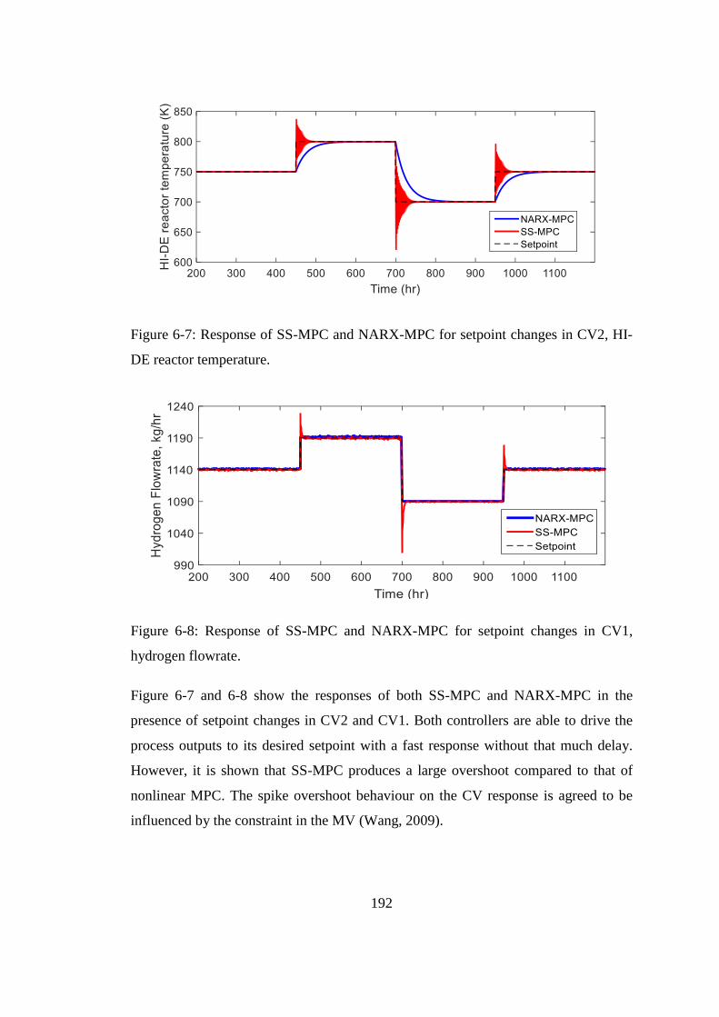
192

Figure 6-7: Response of SS-MPC and NARX-MPC for setpoint changes in CV2, HI-

DE reactor temperature.

Figure 6-8: Response of SS-MPC and NARX-MPC for setpoint changes in CV1,

hydrogen flowrate.

Figure 6-7 and 6-8 show the responses of both SS-MPC and NARX-MPC in the

presence of setpoint changes in CV2 and CV1. Both controllers are able to drive the

process outputs to its desired setpoint with a fast response without that much delay.

However, it is shown that SS-MPC produces a large overshoot compared to that of

nonlinear MPC. The spike overshoot behaviour on the CV response is agreed to be

influenced by the constraint in the MV (Wang, 2009).

193

Figure 6-9: Response changes of SS-MPC and NARX-MPC for setpoint changes in

MV2, feed jacket temperature.

Figure 6-9 explain the reason for the large overshoots produced by SS-MPC. It seems

that SS-MPC is not able to drive the MV between the constraints limit, hence violating

the upper constraint. On the other hand, the NARX-MPC can successfully keep the MV

within n the allocated constraints, i.e., 1033 K to 1083 K.

Another test is carried out to see the performance of NARX-MPC. A disturbance is

introduced at 800th hour of simulation time. The disturbance variable which is the feed

temperature increases by 10%. Figure 6-10 shows that NARX-MPC can successfully

reject the disturbance after less than 100 hours of simulation time. As a conclusion,

NARX-MPC is a suitable to controller to control the HI-DE reactor. Nevertheless, the

NARX model can be further improved hence improving the overall NARX-MPC

performance in estimating the dynamic behavior of the real process as well as able to

reject the disturbance efficiently. Otherwise, a cascade or feedforward controller may

be introduced to compare their performance in controlling the HI-DE reactor.

194

Figure 6-10: Disturbance rejection test of NARX-MPC for 10% increase in the feed

temperature.

6.7 Summary

To the best of our knowledge, so far, there has been no report on the detailed

fundamental models and scale-up for the HI-FT unit and HI-DE reactor of this section.

The summary of this chapter is as follows,

a) The sensitivity analysis for HI-DE reactor revealed that there are three

significant inputs and two outputs of HI-DE reactor. The inputs are feed

flowrate, feed jacket temperature and feed temperature. Meanwhile, the outputs

are product concentration and reactor temperature. Based on the RSM analysis,

all of the three inputs have significant effects on both outputs.

b) Two possible sets of manipulated variables-controlled variables were identified

and the LGC analysis was conducted to determine which one has the most

favorable controllability property.

c) The LGC value of Model 1 (feed flowrate (MV1), feed jacket temperature

(MV2), product flowrate (CV1), reactor temperature (CV2)) is 7.6475.

d) The LGC value of Model 2 (feed flowrate (MV2), feed temperature (MV1),

reactor temperature (CV2), product flowrate (CV1)) is 0.8996.

e) Input-output pairing of Model 1 was chosen for the controller design of the HI-

DE reactor. Since the value of LGC based on the Model 1 is large, a good PID

controller performance for HI-DE reactor is anticipated. It was proven that the

195

PID controller can indeed successfully track the desired setpoint. However, the

PID leads to possible violation of the feed jacket temperature constraints.

f) As an alternative control system to PID, two MPC schemes have been

developed, NARX-MPC and SS-MPC to control the HI-DE reactor.

g) Based on the performance evaluation, it was shown that the NARX-MPC

outperforms the SS-MPC in both setpoint tracking and constraint handling. It

can be concluded that the application of NARX model is adequate enough to

capture the main nonlinear dynamics of the HI-DE reactor.

196

7 Industrial SITC Plant Flowsheet

Based on the developed flowsheet of all the SITC sections reported in the previous

Chapters 4, 5 and 6, a complete SITC plant flowsheet was developed in this chapter.

All sections were assembled to form a complete industrial scale SITC plant.

Additionally, this chapter presents summaries on chemical reactions in the SITC

process, updated flowsheet for each section as well as for the entire SITC plant, process

optimization of the entire SITC plant and the plant capital cost analysis.

7.1 Chemical Reactions in SITC Plant

There are three main chemical reactions taking place in the SITC process. These

reactions are distinctively categorized into three sections, i.e., each section represents

one main reaction. The sections involved are described as follows.

1) Section I (Bunsen Section)

This is also known as the Bunsen Reaction Section, which is exothermic and

reversible in nature with the enthalpy of reaction, ∆𝐻1 = −165 𝑘𝐽/𝑚𝑜𝑙. Note

that, this section is very important as a first step to producing the desired

intermediate product, Hydrogen Iodide (𝐻𝐼). The general reaction scheme can

be represented by

)(2)()( 222 lOHgSOlI ⇌ )(2)(42 lHIlSOH (7.1)

The reactants participating in this reaction are iodine (𝐼2), sulfur dioxide (𝑆𝑂2)

and water (𝐻2𝑂). One of the key challenges in this section is to produce

sufficiently high yield of 𝐻𝐼 as to avoid complex azeotropic mixture of 𝐻𝐼𝑥

(i.e., 𝐻𝐼 − 𝐼2 − 𝐻2𝑂 mixture), which can lead to a very difficult and high cost

of separation process prior to feeding the 𝐻𝐼 intermediate to the 𝐻𝐼

decomposition section (Section III).

2) Section II

197

The purpose of this section is to decompose sulfuric acid (𝐻2𝑆𝑂4) produced in

the Section I into gaseous 𝑆𝑂2, 𝑂2 and 𝐻2𝑂. This decomposition reaction is

endothermic and reversible in nature with the enthalpy of reaction, ∆𝐻2 =

371 𝑘𝐽/𝑚𝑜𝑙. The general reaction scheme can be expressed as follows

)(42 lSOH ⇌ )()(5.0)( 222 gOHgOgSO (7.2)

Note that, the product of the decomposition, i.e., 𝑆𝑂2 is recycled back to the

Section I. The major challenge in this section is to provide sufficient amount of

high-temperature thermal energy in the range of 800 − 1000𝑜𝐶. Note that, a

catalyst is required for the sulfuric acid decomposition reaction to occur. More

details can be found in Chapter 5.

3) Section III

In this section, the decomposition reaction takes place where the intermediate

product 𝐻𝐼 molecules are broken into 𝐻2 and 𝐼2 molecules in a catalytic multi-

tubular reactor. This reaction is strongly endothermic with the enthalpy of

reaction, ∆𝐻3 = 173 𝑘𝐽/𝑚𝑜𝑙. It is also a reversible reaction.

)(2 lHI ⇌ )()( 22 gIgH (7.3)

A major issue in this section is related to the difficulty to purify 𝐻𝐼 solution

(coming from the Bunsen Section) before it is being fed into the decomposing

reactor. In this work, this issue is resolved by feeding an optimized amount of

𝐼2/𝐻2𝑂 to the Bunsen reactor so that the produced 𝐻𝐼𝑥 solution is well above

the azeotropic 𝐻𝐼𝑥 composition. Therefore, the produced 𝐻𝐼𝑥 solution can be

concentrated in a flash tank. On the contrary, if the 𝐻𝐼𝑥 solution is closed to its

azeotropic composition ([𝐻𝐼/(𝐻𝐼 + 𝐻2𝑂)] < 0.16) (Lee et al., 2008a), then a

more complicated separation scheme is needed, e.g., using a reactive

distillation.

198

7.1.1 Section I

7.1.1.1 Process Flowsheet Description

The flowsheet of Section I is shown in Figure 7.1. Notice that, the gaseous 𝑆𝑂2 is fed

into the Bunsen reactor from the bottom, so that the gas will bubble through the liquid

iodine-water mixture. Note that, iodine and water mixture enters from the top at 393 K

in a liquid form. Since the reaction is exothermic, it is required to maintain the Bunsen

reactor temperature using an external cooling jacket. Two immiscible layers consisting

of hydrogen iodide and sulfuric acid solutions may be formed in the reactor under

insufficient mixing. The formation of separate layers can be prevented by applying

adequate mixing inside the reactor. Please note that, for the purpose of modelling

(Chapter 4), it has been assumed that there is no formation of separate layers in the

reactor, i.e., homogeneous mixing. An excess of iodine to water molar ratio is

introduced between 0.33 to 0.54 (minimum and maximum limits) to maintain an over-

azeotropic (Lee et al., 2009) mixture of 𝐻𝐼𝑥. The two layers consisting of a heavy phase

(𝐻𝐼 in 𝐼2) and a light phase (aqueous 𝐻2𝑆𝑂4) are then formed in the liquid-liquid (L-L)

separator. The 𝐻𝐼 mixture is sent to Section III while the aqueous 𝐻2𝑆𝑂4 is sent to

Section II in the SITC plant. In the Bunsen reactor, the 𝑆𝑂2 is selected as a limiting

reactant and it is assumed to undergo complete conversion under the optimal reactor

condition.

Once a plant cycle is completed, the fresh feed (𝐼2 and 𝐻2𝑂) to the Bunsen reactor

is mixed with the two recycle streams from the Section II and Section III. The recycle

line from Section II consists of a mixture of water, sulfur dioxide, oxygen, and the

unconverted sulfuric acid. Oxygen is vented out as gas from the Bunsen reactor and

stored in a storage tank. Meanwhile, the recycle line from Section III consists of a

mixture of water, iodine and the unconverted hydrogen iodide. Before being mixed with

the fresh feed and fed to the Bunsen reactor, both recycle lines are first cooled down to

the desired feed temperature of the Bunsen reactor. The materials used for Bunsen

reactor and L-L separator are assumed to be titanium and nickel alloys trade which have

demonstrated high resistance to sulfuric acid.

199

BUNSEN REACTOR

O2 STORAGE

Recycle stream from

Section III

Recycle stream from

Section II

MIXER 1FRESH FEED

H2O & I2

FRESH FEED

SO2

To Section II

H2SO4

H2O

Cooling water in

Cooling water out

L-L SEPARATOR

To Section III

HI

H2O

I2

Figure 7-1: Bunsen Section (Section I) flowsheet

7.1.2 Section II


The light phase mixture leaving the L-L separator of the Bunsen Section is subsequently

sent to Section II; first the stream is fed to a flash tank (SA-FT) to concentrate the acid.

The mixture is heated up in the flash tank to remove substantial amount of water and to

attain a desired sulfuric acid concentration. The design operating pressure in the flash

tank is set to be 101 kPa as this is a favorable value, for which the corresponding cost

of the equipment is acceptable. In addition, this condition leads to minimising the

difficulty in designing and controlling the unit. Please note that the desired sulfuric acid

final concentration value is based on the optimized value from sensitivity study via

RSM analysis. Bear in mind that, a concentration exceeding 90% (wt) will lead to

impractically high energy consumption. The water evaporated from the SA-FT unit is

recycled back to the Section I while the concentrated acid is fed to the SA-IBSD reactor.

The materials used for the SA-FT unit are assumed to be titanium and nickel alloys

which have been demonstrated to be highly resistance to sulfuric acid.

200

In some articles by researchers from General Atomic and Aachen University, it was

proposed that the sulfuric acid is to be decomposed in extractive and reactive distillation

columns respectively (Vitart et al., 2006). Unfortunately, this option is very energy

intensive and involves high capital cost as the equipment must be able to cope under

high temperature in the range of 800-1000℃. Generally, the sulfuric acid

decomposition happens via three stages, which in a more conventional flowsheet, the

stages involves a boiler or evaporator, a superheater and a catalytic decomposer. In the

boiler stage, the sulfuric acid is heated up to remove any remaining water. In the

superheater stage, the concentrated sulfuric acid is further heated up to a desired feed

temperature prior to feeding the gas to the decomposer stage. In the decomposer stage,

the gaseous sulfuric acid is catalytically decomposed into oxygen and sulfur dioxide.

Thus, for this conventional flowsheet, three units are required to carry out the sulfuric

acid decomposition. It is interesting to note that these three units can be replaced by a

single reactor, i.e., bayonet reactor (Moore et al., 2011; Nagarajan et al., 2014).

In this work, an integrated reactor which is called Sulfuric Acid-Integrated Boiler

Superheater Decomposer (SA-IBSD) reactor is designed for the sulfuric acid

decomposition. In the SA-IBSD reactor, three stages are integrated into one equipment

where integrating evaporator with the decomposer has been proven able to reduce

energy demand (Liberatore et al., 2012).

The boiler or evaporator zone in the SA-IBSD reactor functions to purify the

sulfuric acid from impurities, which include traces of hydrogen iodide as well as excess

water at a temperature of more than 400 ℃. In the SA-IBSD reactor, the evaporated

product from the evaporator zone which consists of water and sulfur trioxide, are then

sent into the catalytic decomposer zone. After the superheater zone and evaporator

zone, the gas is passed over a catalyst bed under high pressure in the range of 1,000-

10,000 kPa and temperature no more than 1,123 K. In this reactive zone, the sulfur

trioxide is decomposed into oxygen and sulfur dioxide.

The schematic diagram of this Section II is shown in Figure 7.2. As can be seen

from the diagram, the effluent of SA-IBSD reactor consists of water, oxygen, sulfur

dioxide, and unconverted sulfuric acid. The SA-IBSD output is then sent to the Section

201

I as a recycle stream. To utilize the extra heating energy from the SA-IBSD reactor, the

outlet stream (heating fluid) from the SA-IBSD external jacket is sent to Section III, as

a source of thermal energy in the HI decomposition reactor, which involves highly

endothermic reaction but requiring a lower reaction temperature. The materials of

construction for the SA-IBSD are either ceramic or silicon carbide (Moore et al., 2011),

which have demonstrated highly resistance to sulfuric acid under high pressure and

temperature conditions.

H2SO4 FLASH TANK

H2SO4

Recycle stream to Section I

H2O

SA-IBSD

REACTOR

From Section I

H2SO4

H2O

Heating

element out

Heating

element inRecycle stream to Section I

H2O

SO2

O2

H2SO4

Figure 7-2: H2SO4 Section (Section II) flowsheet

7.1.3 Section III


Figure 7.3 shows the main units involved in the HI decomposition section. By

introducing excess iodine and water in the Bunsen section, the potential azeotropic issue

of 𝐻𝐼 − 𝐼2 − 𝐻2𝑂 (𝐻𝐼𝑥) solution can be avoided, hence eliminating the need for using

a complicated separation system, e.g., electrodialysis and reactive distillation.

However, the large excess of iodine and water from the Bunsen reaction still contributes

to substantial energy demand in the 𝐻𝐼 separation system, i.e., in the flash tank.

Consequently, an effective design of 𝐻𝐼 section is very crucial to reduce the energy

consumption and the unit capital cost.

202

In the 𝐻𝐼 section, the heavy liquid phase (𝐻𝐼 mainly in 𝐼2) from the Bunsen section

is sent to the flash tank (HI-FT) to evaporate hydrogen iodide from the HIx mixture.

The evaporated hydrogen iodide is then sent to the decomposer (HI-DE), in which 𝐻𝐼

is decomposed into hydrogen and iodine over catalyst pallets. In the HI-DE reactor, the

hydrogen iodide decomposition occurs over a catalyst, at pressure of about 1,000 kPa

and temperature range of 723 K to 770 K. Since the HI-DE reactor involves a highly

endothermic reaction, the required heating source is supplied by the exit heating

medium from the SA-IBSD reactor. The HI-DE reactor effluent is then sent to an

absorber to remove iodine from the stream before sending the purified hydrogen to a

storage tank. Meanwhile, the bottom mixture containing mainly hydrogen iodide, water

and iodine are also treated in the absorber, before the treated stream is recycled back to

Section I.

HI FLASH TANK

I2 ABSORBER

HI

HI

H2O

I2

H2 STORAGE

H2

HI

H2O

I2

MIXER 3

From Section I

HI

H2O

I2

HI DECOMPOSER

Recycle stream to Section I

Heating

element in

Heating

element out

Figure 7-3: HI Section (Section III) flowsheet.

203

7.2 Plantwide SITC Flowsheet

A major issue in the application of plantwide control (PWC) design is related to the

availability of a reliable plantwide model (Downs and Skogestad, 2009). Generally, for

most plant design, modifying a steady-state model into a dynamic model is already an

enormous effort. Extending an elementary dynamic model by taking into account the

details and components needed to describe the plantwide dynamics is another time

consuming task. Our approach in this work is that for each unit or equipment, a

fundamental dynamic model is first developed. The dynamic models are based on

laboratory scale unit. It should be noted that, industrial scale dynamic models of most

of the units involved are not available in the open literature where most data in the

literature are derived under laboratory scale studies. Once the laboratory scale dynamic

model is successfully initialized, converged and validated (in MATLAB environment),

then the unit is scaled up to industrial size. After scaling up, the model is ready to be

connected with the next equipment/section model. For the subsequent section,

equipment or unit based simulation is repeated to compare the unit model prediction

with its corresponding laboratory scale data. For the CSTR, flash tank and

decomposers, preliminary Aspen Plus simulations are first carried out to obtain basic

information relating to the energy balance parameters, and physical/chemical properties

as well as for some validation purposes. Once these basic data are obtained, our goal is

to perform the plantwide simulation and control entirely in the MATLAB environment.

The reason for choosing MATLAB because it offers a broad range of engineering tools,

which enable rigorous analysis of the system.

In this work, the data and procedure reported by Liberatore et.al (2012) are used as

the guideline for the overall plant scale-up. The heat transfer surface of the external

jacket in both SA-IBSD reactor (Section II) and HI decomposer (Section III) are based

on the heat transfer coefficient deduced from the flow rate and configuration i.e.:

number of tubes in the shell (see Chapter 5 and 6). As for the evaporator zone in the

SA-IBSD reactor, the heat transfer coefficient is estimated based on the necessary heat

load. For the flash tanks, the maximum diameters should be chosen such that it

204

corresponds to 60% of the flooding rate. The summary of design material (Kasahara et

al., 2017) and sizes of all units involved are tabulated in Table 7.1.

Figure 7.4 shows the complete flowsheet diagram of the proposed industrial scale

SITC plant. This plant consists of six primary units which have been designed based on

their first principle models. That is include two external heaters, two storage tanks, an

iodine absorber, a hold up tank and 21 streamlines including two recycle lines. There

is heat integration between Section II (SA-IBSD reactor) and Section III (HI-DE

reactor) in red line.

Table 7.1: The equipment design material, size, production capacity and design

operating condition of industrial scale SITC plant

Equipment Maximum

volume

(m3)

Material of

construction (MoC)

Production

capacity

(kg/hr)

Design

operating

condition

Section I

Bunsen

reactor

300 Titanium and nickel

alloy trade

10,000 P: 101 kPa

T: 350 K

L-L separator 500 Titanium and nickel

alloy trade

10,000 P: 101 kPa

T: 350 K

Section II

Flash tank 1,500 Titanium and nickel

alloy trade

3,000 P: 101 kPa

T: 550 K

SA-IBSD

reactor

400 Ceramic or silicon

carbide

1,000 P: 10,000 kPa

T: 1,400 K

Section III

Flash tank 1,500 Titanium and nickel

alloy trade

6,000 P: 201 kPa

T: 350 K

HI-DE reactor 200 Ceramic or silicon

carbide

2,500 P: 1,000 kPa

T: 900 K

205

BUNSEN REACTOR

T: 338 K

P: 101 kPa

H2SO4 FLASH TANK

T: 502 K

P: 101 kPa

HI FLASH TANK

T: 627 K

P: 201 kPa

I2 ABSORBER

COOLER

HEATER 2

O2 STORAGE

21

6

H2SO4

H2O

13

HI

H2O

I2

15

HI

H2O

I2

10

H2O

SO3

SO2

O2

H2SO4

MIXER 2

11

5

O2

HOLD UP TANK

H2 STORAGE

20

H2

MIXER 1

2

12

1

MAKE UP

FEED

H2O & I2

3

MAKE UP FEED

SO2

4

H2SO4

HI

H2O

I2

8

H2SO4

9

H2O

19

HI

H2O

I2

COOLING WATER

IN

COOLING WATER

OUT

MIXER 3

18

SA-IBSD

REACTOR

T: 1073 K

P: 10,000 kPa

14

HEATER 1

7

16

HI

HI DECOMPOSER

T: 760 K

P: 1000 kPa

17

HI

H2

I2

L-L SEPARATOR

HEAT

FLOW OUT/IN

HEAT

FLOW OUT

Figure 7-4: A complete industrial scale SITC plant flowsheet.

206

7.3 SITC Process Optimization and Sensitivity Analysis

7.3.1 Process Optimization via Response Surface Methodology (RSM)

Process optimization is carried out using Design Expert Software. There are 13 factors

and 14 responses that are studied. The factors and responses are listed in the Table 7.2.

These are considered independent variables which determine the kinetic of reactions

and selectivity of the process, hence influencing the quantity and quality of products.

The optimization is based on Box-Behnken method and consist of 210 simulations

(computer experimental) runs. The desired optimum steady-state criterion is generated

based on the hydrogen flowrate, feed molar iodine, and feed jacket flowrate of the SA-

IBSD reactor and jacket temperature of the SA-IBSD reactor. The data generated from

the computer experiments is then analyzed using statistical method. Figure 7-5 and 7-6

show the 3D plots generated from RSM analysis. The 3D plots revealed the optimum

value of hydrogen flowrate, oxygen flowrate, HI-DE temperature and SA-IBSD jacket

temperature.

From the overall data analysis, the ANOVA suggests that a quadratic order

statistical model is sufficient to represent the effects of the aforementioned 13 factors

on all 14 responses. The adjusted R-square for the model is 0.99, thus indicating it is

significant. There are nine factors that cause the significant effects (p-value < 0.05) on

all responses, the results which are given in Table 7.4. For reasons of simplicity, all

responses are coded as R1 to R14. Based on the post sensitivity analysis, a coefficient

table is presented in Table 7.5. The significant input variable affecting output variables

(p<0.05) is represented by a check mark. From Table 7.5 it can be observed that the

main products; hydrogen and by product; oxygen are affected by:

a) 𝐼2/𝐻2𝑂 feed molar ratio

b) Valve opening of LLS

c) Valve opening of SA-FT

d) External jacket flowrate of SA-IBSD reactor

e) Valve opening of HI-FT. The valves opening are controlling the tank level.

207

Table 7.2: The responses (output) and factors (input) in the SITC process optimization

Code Responses

R1 LBR represented level of Bunsen reactor (BR)

R2 TBR presented the temperature of BR

R3 LHLS represented the level of heavy phase liquid in L-L separator (LLS)

R4 LLLS represented the level of light phase liquid in LLS

R5 LLCLS represented the level of light phase liquid in collecting chamber of LLS

R6 LSAFT represented the level in the sulfuric acid section flash tank

R7 TSAFT represented the temperature of sulfuric acid section flash tank

R8 LHIFT represented the level in the hydrogen iodide section flash tank

R9 THIFT represented the temperature of hydrogen iodide section flash tank

R10 mO2 represented the oxygen flowrate

R11 TJSAIBSD represented the temperature of external jacket SA-IBSD reactor

R12 TSAIBSD represented the temperature of SA-IBSD reactor

R13 mH2 represented the hydrogen flowrate

R14 THIDE represented the hydrogen iodide decomposer (HI-DE)

Factors

A ToBR represented the feed temperature of BR

B NoBR represented the iodine molar feed

C FoBR represented the feed flowrate of BR

D FSO2BR represents the sulfur dioxide feed flowrate to BR

E FJoBR represented the feed jacket flowrate of BR

F V1LLS represented the valve opening of LLS

G V1SAFT represented the valve opening of SA-FT

H TsSAFT represented the steam temperature of SA-FT

J FJSAIBSD represented jacket flowrate of SA-IBSD

K V1HIFT represented the valve opening of HI-FT

L TsHIFT represented the steam temperature of HI-FT

M FJHIDE represented jacket flowrate of HI-DE

N Vrec represented the valve opening of recycle stream

208

Figure 7-5: 3D Plots of (a) optimum molar hydrogen flow rate (b) optimum oxygen

flow rate.

Figure 7-6: 3D Plots of (a) optimum HI-DE temperature (b) optimum SA-IBSD jacket

temperature.

(a) (b)

(a) (b)

209

Table 7.3: Desired process optimization criteria of the SITC plant using RSM in Design

Expert software

No Input or output variables Desired criteria

1 Hydrogen production, kg/hr Maximum (2,400 kg/hr)

2 Feed Molar of Iodine, kmol/hr Between the optimal range

(0.33 to 0.54)

3 Feed Jacket Flowrate of SA-IBSD Reactor, m3/hr Minimum (4,500)

4 Jacket Temperature of SA-IBSD reactor, K Minimum (1,203)

Table 7.4: Optimum values obtained for SITC plant variables based on RSM

optimization

No Variables Optimum values

1 Feed Bunsen Reactor Temperature, K 338.8

2 Feed Molar of Iodine, kmol/hr 1,409.3

3 Feed Flowrate of Water, m3/hr 0.12

4 Feed Jacket Flowrate of Bunsen Reactor, m3/hr 1.47

5 Feed Sulfur Dioxide Flowrate, m3/hr 0.48

6 Feed Steam Temperature to Flash Tank Section

II, K

529.3

7 Feed Jacket Flowrate of SA-IBSD Reactor, m3/hr 9,499.2

8 Feed Steam Temperature to Flash Tank Section

III, K

527.3

9 Feed Jacket Flowrate of HI-DE Reactor, m3/hr 768.9

7.3.2 Input-Output Sensitivity via Principle Component Analysis

(PCA)

Principal Component Analysis (PCA) analysis method is utilized as part of the method

to optimize the SITC plant. Here, the PCA analyzes the extents of the effect of input on

output variables. The advantage of PCA is that it enables one to quickly determine the

dominant input variables which critically affect the plant performance and main output

210

variables (possibly to be controlled). Figure 7.7 shows a principal component plot while

Figure 7.8 shows a Pareto plot from the PCA analysis for SITC plant. Based on the

result in RSM and PCA Pareto plot, Table 7.5 and 7.6 are generated. Table 7.5 presents

the significant input variables which can critically affects the output variables as

represented by a check mark. From Table 7.6 it can be observed that the main products,

which are hydrogen and by product, oxygen are affected by:

a) Feed BR temperature,

b) 𝐼2/𝐻2𝑂 feed molar ratio,

c) Valve opening of SA-FT,

d) Steam temperature of SA-FT,

e) Eternal jacket flowrate of SA-IBSD reactor,

f) Valve opening of HI-FT and

g) external jacket flowrate of HI-DE.

The additional important factors identified via the PCA in addition to that the RSM

analysis are the feed temperatures of BR and SA-FT. As a result, both analysis are

mutually complementing each others. One may deduce the significant output variables

to be controlled as tabulated in Table 7.7. The results on significant controlled variables

will be utilize in Chapter 8; PWC structure development.

211

Figure 7-7: Principal component plots of PCA analysis

Figure 7-8: 2D Pareto plot of PCA analysis

212

Table 7.5: Sensitivity analysis of input-output variables coefficient table of SITC plant via RSM analysis: Checked box present significant

effect (p<0.05)

Variables:

Input (top) and

Output

A:

𝑻𝒐𝑩𝑹

B:

𝑵𝒐𝑩𝑹

C:

𝑭𝒐𝑩𝑹

D:

𝑭𝑱𝒐𝑩𝑹

E:

𝑭𝑺𝑶𝟐𝒐𝑩𝑹

F:

𝑽𝟏𝑳𝑳𝑺

G:

𝑽𝟏𝑺𝑨𝑭𝑻

H:

𝑻𝒔𝑺𝑨𝑭𝑻

J:

𝑭𝑱𝑺𝑨𝑰𝑩𝑺𝑫

K:

𝑽𝟏𝑯𝑰𝑭𝑻

L:

𝑻𝒔𝑯𝑰𝑭𝑻

M:

𝑭𝑱𝑯𝑰𝑫𝑬

N:

𝑽𝑹𝑬𝑪

R1: 𝑳𝑩𝑹 √ √

R2: 𝑻𝑩𝑹 √ √ √ √ √

R3: 𝑳𝑯𝑳𝑺 √ √

R4: 𝑳𝑳𝑳𝑺 √ √

R5: 𝑳𝑳𝑪𝑳𝑺 √ √ √ √

R6: 𝑳𝑺𝑨𝑭𝑻 √ √ √ √

R7: 𝑻𝑺𝑨𝑭𝑻 √ √ √

R8: 𝑳𝑭𝑻𝑯𝑰 √ √ √

R9: 𝑻𝑭𝑻𝑯𝑰 √ √

R10: 𝒎𝑶𝟐 √ √ √ √ √

R11: 𝑻𝑱𝑺𝑨𝑰𝑩𝑺𝑫 √ √ √ √

R12: 𝑻𝑺𝑨𝑰𝑩𝑺𝑫 √ √ √ √

R13: 𝒎𝑯𝟐 √ √

R14: 𝑻𝑯𝑰𝑫𝑬 √

Total 4/14 13/14 - - 1/14 8/14 6/14 3/14 2/14 3/14 - 1/14 2/14

Rank (pre-

estimated)

4 1 10 2 3 6 7 5 9 8

213

Table 7.6: Sensitivity analysis of input-output variables coefficient table of SITC plant via PCA analysis: Checked box represent significant

effect

Variables:

Input (top) and

Output

A:

𝑻𝒐𝑩𝑹

B:

𝑵𝒐𝑩𝑹

C:

𝑭𝒐𝑩𝑹

D:

𝑭𝑱𝒐𝑩𝑹

E:

𝑭𝑺𝑶𝟐𝒐𝑩𝑹

F:

𝑽𝟏𝑳𝑳𝑺

G:

𝑽𝟏𝑭𝑻𝑺𝑨

H:

𝑻𝒔𝑭𝑻𝑺𝑨

J:

𝑭𝑱𝑺𝑨𝑰𝑩𝑺𝑫

K:

𝑽𝟏𝑭𝑻𝑯𝑰

L:

𝑻𝒔𝑭𝑻𝑯𝑰

M:

𝑭𝑱𝑯𝑰𝑫𝑬

N:

𝑽𝑹𝑬𝑪

R1: 𝑳𝑩𝑹 √ √ √ √ √

R2: 𝑻𝑩𝑹 √ √ √

R3: 𝑳𝑯𝑳𝑺 √ √ √

R4: 𝑳𝑳𝑳𝑺 √ √

R5: 𝑳𝑳𝑪𝑳𝑺

R6: 𝑳𝑭𝑻𝑺𝑨 √ √ √

R7: 𝑻𝑭𝑻𝑺𝑨 √ √ √

R8: 𝑳𝑭𝑻𝑯𝑰

R9: 𝑻𝑭𝑻𝑯𝑰

R10: 𝒎𝑶𝟐 √ √

R11: 𝑻𝑱𝑺𝑨𝑰𝑩𝑺𝑫 √ √

R12: 𝑻𝑺𝑨𝑰𝑩𝑺𝑫 √ √

R13: 𝒎𝑯𝟐 √ √ √ √ √

R14: 𝑻𝑯𝑰𝑫𝑬 √ √ √ √ √

Total 4/14 3/14 - - 4/14 4/14 4/14 3/14 3/14 3/14 - 3/14 4/14

Rank (pre-

estimated)

4/2 1/8 10/4 2/3 3/1 6/6 7/7 5/9 9/10 8/5

214

Table 7.7: Input-output sensitivity analysis via PCA method

Output Variables

Components (Input and Output Variables)

Same quadrant Orthogonal quadrant

R1: 𝐿𝐵𝑅 R14, R13 R9, H, J, R5, B, R8, K, M

R2: 𝑇𝐵𝑅 G, R7, R6, R3, A R12, R10, R4, F, E, R11, N

R3: 𝐿𝐻𝐿𝑆 G, R7, R6, R2, A R12, R10, R4, F, E, R11, N

R4: 𝐿𝐿𝐿𝑆 R12, R10, F, E, R11, N R7, G, R6, R3, A, R2

R5: 𝐿𝐿𝐶𝐿𝑆 R9, H, J, B, R8, K, M R1, R14

R6: 𝐿𝑆𝐴𝐹𝑇 G, R7, R2, R3, A R12, R10, R4, F, E, R11, N

R7: 𝑇𝑆𝐴𝐹𝑇 G, R6, R2, R3, A R12, R10, R4, F, E, R11, N

R8: 𝐿𝐻𝐼𝐹𝑇 R9, H, J, R5, B, K, M R1, R14

R9: 𝑇𝐻𝐼𝐹𝑇 R8, H, J, R5, B, K, M R1, R14

R10: 𝑚𝑂2 R12, R4, F, E, R11, N R7, G, R6, R3, A, R2

R11: 𝑇𝐽𝑆𝐴𝐼𝐵𝑆𝐷 R12, R10, R4, F, E, N R7, G, R6, R3, A, R2

R12: 𝑇𝑆𝐴𝐼𝐵𝑆𝐷 R11, R10, R4, F, E, N R7, G, R6, R3, A, R2

R13: 𝑚𝐻2 R1, R14 R9, H, J, R5, B, R8, K, M

R14: 𝑇𝐻𝐼𝐷𝐸 R1, R13 R9, H, J, R5, B, R8, K, M

215

7.4 Economic Analysis

In this section, the economic analysis of the proposed industrial SITC plant is carried out.

In the following section, the costing of entire plants is presented including both capital and

operating costs.

7.4.1 Plant Investment, Specification and Targets

This work presents the costing details of the hydrogen production plant assuming a total

capacity of 1000 kg/hr of hydrogen, hence a total 24 metric tons/day for a plant operating

24 hr/day for 300 days in a year. Thus, the annual production of hydrogen is 7,200,000

tons. The fresh feedstock consists of fresh make-up water and iodine and fresh sulfur

dioxide. It is assumed that the plant lifetime is 20 years. Note that, the plant is modelled

using Aspen Plus® (steady-state assessment) and MATLAB® software (for dynamics

simulation).

7.4.2 Capital Cost Estimation

The costs of equipment and other expenses related to capital investment play a crucial role

in a plant design. The capital costs of a newfangled plant comprise primarily of the Fixed

Capital Investment (FCI), the land cost and the working capital costs. The FCI consists of

the equipment purchase costs; which we will refer to as the Bare Module Cost (BMC), and

all the necessary supplementary costs required to construct the plant. These additional costs

are associated to the BMC. BMC is the sum of the direct and indirect cost of the purchase

price. Direct cost includes material cost, labor cost, and equipment price while indirect cost

includes freight, insurance, taxes, construction, overhead and contractor engineering

expenses. The BMC is defined as:

216

BMPBM FCC (7.4)

where CBM = Bare module equipment cost: direct and indirect cost for each unit

CP = Purchase cost for the base condition: equipment made of the most common material,

usually carbon steel and operating at near ambient pressures

FBM = Bare module cost factor

7.4.3 Equipment Cost Summary for the Whole Plant

The purchase costs of this work are based on the basis of Chemical Engineering Plant Cost

Index (CEPCI) 2016 which is 558 (Chemical Engineering, 2016). Pre-design capital cost

estimates are usually gathered from old price data. Thus, because of inflation, correction

indices are needed to adjust old data to the current values. The total BMC, CTBM is equal

to $ 62,832,000.

7.4.4 Fixed Capital Investment

A detail of process design is crucial to capital cost estimation. An optimal process design

with complete mass balance, energy balance, equipment sizing, materials of construction

and process control configurations plus piping, instrumentation and electrical equipment

are used to estimate the capital cost. Following this method of estimation, the bare module

cost of all equipment is obtained from the correlation method which has been presented in

the Table 7.12, in the previous sub-section. Meanwhile, the equation for the total capital

investment by the Guthrie method (Guthrie, 1969) is given as below:

W CTPITCI CCC (7.5)

217

W CilituiesoffsitefacbuildingsiteTBMTCI CCCCCC )(18.1 (7.6)

where,

𝐶𝑇𝐶𝐼 = Total capital investment cost, $

𝐶𝑇𝑃𝐼 = Total permanent investment cost, $

𝐶𝑊𝐶 = Working capital, $

𝐶𝑇𝐵𝑀 = Total bare module cost, $ (Section 7.4.3)

Step 1: Estimation of site development cost, 𝑪𝒔𝒊𝒕𝒆

For grass-roots plant, we assume the site development cost is 10% of 𝐶𝑇𝐵𝑀

𝐶𝑠𝑖𝑡𝑒 = 0.10𝐶𝑇𝐵𝑀

𝐶𝑠𝑖𝑡𝑒 = 0.10 𝑥 $62,832,000

𝐶𝑠𝑖𝑡𝑒 = $ 6,283,200

Step 2: Estimation of building cost, 𝐶𝑏𝑢𝑙𝑑𝑖𝑛𝑔

For grassroots plant, the building cost can be estimated as 20% of 𝐶𝑇𝐵𝑀 which including

process building and non-process building

𝐶𝑏𝑢𝑙𝑑𝑖𝑛𝑔 = 0.20𝐶𝑇𝐵𝑀

𝐶𝑏𝑢𝑙𝑑𝑖𝑛𝑔 = 0.20 𝑥 $62,832,000

𝐶𝑏𝑢𝑙𝑑𝑖𝑛𝑔 = $ 12,566,400

Step 3: Estimation of offsite facilities cost, 𝑪𝒐𝒇𝒇𝒔𝒊𝒕𝒆𝒇𝒂𝒄𝒊𝒍𝒊𝒕𝒊𝒆𝒔

218

𝐶𝑜𝑓𝑓𝑠𝑖𝑡𝑒𝑓𝑎𝑐𝑖𝑙𝑖𝑡𝑖𝑒𝑠 = 𝐶𝑢𝑡𝑖𝑙𝑖𝑡𝑖𝑒𝑠 + 0.05𝐶𝑇𝐵𝑀

𝐶𝑜𝑓𝑓𝑠𝑖𝑡𝑒𝑓𝑎𝑐𝑖𝑙𝑖𝑡𝑖𝑒𝑠 = $ 11,700,000 + 0.05𝐶𝑇𝐵𝑀

219

Table 7.8: List of main equipment of SITC plant

Equipment Tag Equipment Name Purchase Cost ($) Bare Module Factor

(FBM)

Bare Module Cost ($)

R-101 Section I Bunsen

Reactor

25,800 1.50 38,800

S-102 Section I L-L Separator 20,600 6.17 127,000

H-201 Section II Heat

Exchanger

4,750 1.81 92,000

F-202 Section II Flash Tank 27,100 7.97 216,000

E-203

D-204

Section II SA-IBSD

reactor (Evaporator +

Decomposer)

27,100 7.97 216,000

27,100 9.74 264,000

H-301 Section III Heat

Exchanger

4,750 19.37 92,000

F-302 Section III Flash Tank 27,100 7.97 216,000

D-303 Section III Decomposer 27,100 7.97 216,000

A-304 Section III Absorber 17,000 8.06 137,000

Bare Module Cost CBM 1,350,800

Total Bare Module Cost

CTBM

1,350,800 (558) / (12) =

62,832,000

220

𝐶𝑜𝑓𝑓𝑠𝑖𝑡𝑒𝑓𝑎𝑐𝑖𝑙𝑖𝑡𝑖𝑒𝑠 = $ 14,841,600

Step 4: Estimation of total permanent investment cost, 𝑪𝑻𝑷𝑰

Total permanent investment,

𝐶𝑇𝑃𝐼 = 1.18 (𝐶𝑇𝐵𝑀 + 𝐶𝑠𝑖𝑡𝑒 + 𝐶𝑏𝑢𝑙𝑑𝑖𝑛𝑔 + 𝐶𝑜𝑓𝑓𝑠𝑖𝑡𝑒𝑓𝑎𝑐𝑖𝑙𝑖𝑡𝑖𝑒𝑠) = $ 96, 523,200

Step 5: Estimation of working capital cost, 𝑪𝑾𝑪

𝐶𝑊𝐶 = 0.176𝐶𝑇𝑃𝐼 = $ 16,988,083

Step 6: Estimation of total capital investment, 𝑪𝑻𝑪𝑰

𝐶𝑇𝐶𝐼 = $ 113,511,283

From this section, the total capital investment 𝐶𝑇𝐶𝐼 has been estimated to be $

113,511,283.

7.5 Summary

In this chapter, a complete SITC plant flowsheet has been developed based on

combining the unit based flowsheets presented in Chapters 4 to 6. Based on the

sensitivity analyses via RSM and PCA, it has been identified that the main product

hydrogen and by product oxygen are strongly affected by the following input variables:

a) Feed BR temperature,

b) 𝐼2/𝐻2𝑂 feed molar ratio,

c) Valve opening of SA-FT,

d) Steam temperature of SA-FT,

e) External jacket flowrate of SA-IBSD reactor,

f) Valve opening of HI-FT and external jacket flowrate of HI-DE.

Detailed ecpnomic analysis showed that the cost to build a SITC plant with the nominal

production capacity of 1,000 kg/hr is US$ 113.5 million. This calculation has been done

by assuming certain prices on materials of construction for certain units, which have to

221

operate under high temperature and pressure conditions, and corrosive nature of the

sulfuric acid, e.g., the SA-IBSD reactor for the sulfuric acid decomposition.

222

8 Plantwide Control of Industrial SITC

Plant

Plantwide Control (PWC) deals with the synthesis and development of a complete

control system of a given plant. This complete control system often involves multiple

layers in a control hierarchy: at the basic level is called a regulatory layer while the

layer above it is called the supervisory layer. In this chapter, both regulatory and

supervisory layers were described and developed for the SITC plant. Note that, the

PWC study of the SITC process has never been reported before. To address this

uncharted territory, a set of preliminary steps was proposed prior to the PWC structure

design. The Skogestad’s Self-Optimizing Control structure was then adopted in the

PWC design of the plant. This chapter describes the PWC objectives, PWC preliminary

steps and PWC structure of the SITC plant.

8.1 PWC Objectives

PWC problem can be divided into two major elements: (1) control structure selection,

and (2) controller design. It has been well recognized that the first element has a far

reaching impact on the plantwide control performance compared to the second element.

In the control structure selection, the key questions to be answered are: (1) which

outputs to be controlled, (2) which variables to be manipulated, and (3) what are the

connections between the sets of controlled and manipulated variables?

The PWC structure design starts with defining the process control objectives. In this

work, there are three process control objectives to be fulfilled for the SITC plant:

a) To achieve a production rate of minimum 1 tons/hr of hydrogen under specified

operating conditions. The amount of hydrogen production rate chosen is

comparable with that of the currently operational electrolysis industrial scale

plant (Zeng and Zhang, 2010) and the JAEA industrial scale thermochemical

cycle (Kasahara et al., 2017).

223

b) To keep molar feed flow 𝐼2/𝐻2𝑂 into the Bunsen Section at an optimum ratio.

Lee et, al (2008) proposed an optimum operating window for 𝐼2/𝐻2𝑂 molar

feed flow ratio in the Section I to be between 0.333 and 0.538. The significance

of maintaining the optimum 𝐼2/𝐻2𝑂 ratio is to produce a 𝐻𝐼𝑥 liquid solution

that is well above its azeotropic composition in order to:

i. Allows for spontaneous liquid-liquid (𝐻𝐼 in 𝐼2 and aqueous

𝐻2𝑆𝑂4) phase separation in the L-L Separator,

ii. Eliminates the need to concentrating the 𝐻𝐼 gas (via an energy

intensive electro electrodialysis (EED) or Reactive Distillation

Column).

c) To retain the SA-IBSD temperature as minimum as possible for plant safety and

to reduce high-temperature energy utilization but subject to attaining minimum

SA-IBSD reactor conversion of 36%. The SITC process becomes a less

favorable renewable energy production method if it consumes an excessively

high amount of high-temperature thermal energy. Keep in mind that, the

aforementioned temperature corresponds to the reaction zone temperature

inside the SA-IBSD reactor – this is the hottest zone in the reactor.

In summary, the major constraints in the SITC plant operation are the production

specification, SA-IBSD (reactive zone) temperature and molar feed ratio of 𝐼2/𝐻2𝑂.

The values of these constraints are displayed in Table 8.1.

Table 8.1: Variables specification of SITC

Variables Constraint Specification

Hydrogen flowrate, �̇�𝐻2 (kg/hr) ≥ 1000

Temperature SA-IBSD reactor, 𝑇𝑆𝐴−𝐼𝐵𝑆𝐷 (K) ≤ 1200

Ratio of feed molar flowrate 𝐼2/𝐻2𝑂, 𝑅𝑛𝐼2/𝐻2𝑂 0.33 𝑡𝑜 0.54

224

In this work, the Self-Optimizing Control (SOC) procedure proposed by Skogestad is

applied to design a PWC structure of the SITC plant. SOC procedure consists of two

sections (Skogestad, 2012, 2004, 2000b):

1) Top-down analysis, including specifications of operational objectives and

degrees of freedom (see Chapter 3). This analysis mostly focuses on the

economics and steady-state evaluations of the given plant.

2) Bottom-up design of the control system, which starting with the design of

stabilizing control layer. This analysis is focuses on the dynamic performance

of the plant.

The Principal Component Analysis (PCA) analysis method (Nandong et al., 2010) is

utilized as part of the top down analysis and bottom up design. It is to identify the input-

output variables that have the self-optimizing property. The decision of SITC plant

structure may be retrieved from previous Chapter 4 to 7. In the next sections, the details

of PWC design for the SITC plant are discussed.

8.2 PWC Preliminary Steps

8.2.1 Significance of Preliminary Steps

The SOC approach provides a rigorous step by step procedure to design a PWC

structure for an existing plant. For a plant that is not yet designed at the industrial stage,

it is important to conduct some PWC preliminary steps to determine the essential

information before applying any PWC structure procedure. PWC preliminary steps

identify steady-state mass balance, analysis of total energy, analysis of utilities, scaling-

up the SITC plant production rate, scaling-up each unit and testing via dynamic

simulations. These analyzes are essential to ensure the integrity of the plant design and

operation prior to the PWC structure development. The PWC preliminary procedure is

proposed as follows.

225

8.2.2 Step by Step Procedure

8.2.2.1 Pre-Step 1: Identifying steady-state mass balance

The steady-state mass balance is important to identify the total inflow and outflow of

the entire plant regardless it’s dynamic. Figure 8-1 shows the plant input and output

signals at steady-state condition. In this figure, the solid lines indicate the external

inputs and outputs while the dotted lines indicate the recycle streams in the plant.

H2

H2O

SITC

PlantI2

SO2

O2

SO2

I2

H2O

Utilities

Figure 8-1: Steady-state input and output mass flow of SITC plant.

Based on Figure 8-1, the steady-state mass balance equation is

22222222 SOIOHOHSOIOH FFFFFFFF (8.1)

where 𝐹 represents flowrate.

Table 8.2 displays the details of inflow and outflow shown in Figure 8-1. In this step,

it is desired to optimize both the inflow and outflow of each unit in the SITC plant.

Process optimization is carried out via RSM analysis to attain the optimum values for

the inflow and outflow, as well as the other operating conditions. The details of process

optimization of the entire SITC plant are presented in Chapter 7.

226

Table 8.2: Optimized steady-state flowrate of SITC plant

Component Flowrate (kg/hr)

Input

Water 139,860

Iodine 720,900

Sulfur Dioxide 30,400

Output

Hydrogen ≥1,000

Oxygen ≥450

Recycle

Water 138,461

Iodine 716,661

Sulfur Dioxide 30,096

Conversion

Section I 0.99

Section II 0.40

Section III 0.99

8.2.2.2 Pre-Step 2: Analysis of total energy

It is desired through this step to analyze the total energy requirement by the SITC plant,

𝐻𝑇 necessary to meet the conversion criteria as in the Table 8.2. Table 8.3 shows the

energy required in the Bunsen reactor. The energy to be absorbed by the cooling jacket

of Bunsen reactor is calculated as follows

Section I (Exothermic): )( 21111 ccpEcEE TTCFH (8.2)

where 𝐹𝑐𝐸1 and 𝐶𝑝𝐸1 are the cooling water flow rate and its specific heat capacity, while

𝑇𝑐1 and 𝑇𝑐2 are its inlet and outlet temperatures.

227

Table 8.3: Total energy required in the Bunsen reactor

Bunsen Reactor Value

Energy to be absorbed by jacket, 𝑄𝐵𝑅 or 𝐻𝐸1 2.4191 kJ

Operating temperature, 𝑇𝐵𝑅 60 oC -120 oC

Exit temperature, 𝑇𝐵𝑅𝑒𝑥𝑖𝑡 60 oC -120 oC

Based on the calculation as in Equation (8.2) the energy to be absorbed by jacket at the

reactor temperature between 60 ℃ -120 ℃ is 2.4191 kJ.

Table 8.4 lists the energy required by the SA-IBSD reactor. The energy required by the

SA-IBSD reactor is represented as follows

Section II (Endothermic): energyThermalH E 2 (8.3)

In Equation 8.3, the term ‘thermal energy’ is used since the heating medium is not

finalized either nuclear or solar energy.

Table 8.4: Total energy required for SA-IBSD reactor

SA-IBSD Reactor Value

Energy required, 𝑄𝑆𝐴−𝐼𝐵𝑆𝐷 or 𝐻𝐸2 5.1×106 kJ

Operating temperature, 𝑇𝑆𝐴−𝐼𝐵𝑆𝐷 800 oC - 950 oC

Exit temperature, 𝑇𝑆𝐴−𝐼𝐵𝑆𝐷𝑒𝑥𝑖𝑡 800 oC - 950 oC

Energy released at exit temperature,

𝑄𝐻𝐸2𝑆𝐴−𝐼𝐵𝑆𝐷= 𝐹𝑝𝐸2𝐶𝑝𝐸2(𝑇𝑆𝐴−𝐼𝐵𝑆𝐷𝑒𝑥𝑖𝑡

− 𝑇𝑆𝐴−𝐼𝐵𝑆𝐷)

2.9×109 kJ

where 𝐹𝑝𝐸2 and 𝐶𝑝𝐸2 are the heating medium flow rate and its specific heat capacity.

For SA-IBSD reactor, a specified amount of energy is supplied until the desired

product conversion is achieve. The energy required by SA-IBSD from external thermal

energy 5.1× 106 𝑘𝐽.

228

Table 8.5 lists the energy required for 𝐻𝐼 Decomposer. The calculation of energy

required is important to ensure that the energy integration between 𝐻𝐼 decomposer and

SA-IBSD reactor is feasible. The heat integration is feasible only if there is much more

energy remains after it is utilized by the 𝐻𝐼 decomposer. The required energy by the

𝐻𝐼 decomposer calculation is as follows.

Section III (Endothermic): )( 3333 EpsEsEE CFH (8.4)

where 𝐹𝑠𝐸3 the heating element flow rate (from the SA-IBSD reactor), 𝐶𝑝𝑠𝐸3 is its heat

capacity and 𝜆𝐸3 is the sensible heat.

Table 8.5: Total energy required for HI Decomposer

HI Decomposer Value

Energy required, 𝑄𝐻𝐼−𝐷𝐸 or 𝐻𝐸3 9.5×104 kJ

Operating temperature, 𝑇𝐻𝐼−𝐷𝐸 450 oC -500 oC

Exit temperature, 𝑇𝐻𝐼_𝐷𝐸𝑒𝑥𝑖𝑡 450 oC -500 oC

Balance energy remains,

𝑄𝐻𝐼−𝐷𝐸𝑎𝑑𝑑= 𝑄𝐻𝐼−𝐷𝐸 − 𝑄𝐻𝐸2𝑆𝐴−𝐼𝐵𝑆𝐷

-2.9×109 kJ

From calculation in Equation (8.4) it is known that the energy required to decompose

hydrogen iodide is 9.5 × 104 𝑘𝐽. The energy is supplied by the exhaust thermal energy

from SA-IBSD reactor in Section II.

The total energy required by the SITC plant is given as

kJHHHH EEETE

6

321 10011.5 (8.5)

Based on the analysis, it is proven that the heat integration between Section II and III

is feasible. Total energy releases by Section II is 2.9 × 109 𝑘𝐽. This amount is as double

as the required amount of energy needed in the Section III which is only 9.5 × 104 𝑘𝐽.

For Section I, there is no additional energy required since it is an exothermic reaction.

229

8.2.2.3 Pre-Step 3: Analysis on utilities

Based on the calculated energy requirement, 𝐻𝑇𝐸 in the previous step, the required

utilities energy, 𝐸𝑇 can be estimated as follows:

kWhEH TTE 1403

8.2.2.4 Pre-Step 4: Scale-up of SITC plant production

Prior to applying the scale-up procedure (see Chapter 3), each equipment is first

designed individually based on laboratory scale. The scaling-up of each sections were

presented in Chapter 4,5 and 6. Compilation of all unit models according to pre-defined

flowsheet (unit-based approach) has been covered in Chapter 7. Once the design of all

laboratory scale units is completed, they will be assembled and then the entire process

flowsheet based on laboratory scale is developed and simulated. In this work, the target

production rate is more than 1 tons/hr of hydrogen.

8.2.2.5 Pre-Step 5: Scale-up equipment unit

After deciding the desired production rate, the unit scale-up is carried out. The

procedure is presented in Chapter 3 while the results can be retrieved from to Chapter

4 to 6. The scale-up dimension of main units are listed in Table 8.6.

Table 8.6: Scale up volume of SITC equipment

Equipment Maximum Volume

Bunsen Reactor volume 300 m3

Liquid-Liquid Separator volume 500 m3

Sulfuric Acid Flash Tank volume 1500 m3

SA-IBSD Reactor volume 400 m3

Hydrogen Iodide Flash Tank volume 1500 m3

HI Decomposer volume 200 m3

230

8.2.2.6 Pre-Step 6: Dynamic model and MATLAB program simulation

Note that, the dynamic model of each unit is developed individually by mean of

fundamental modelling approach (refer Chapter 4 to 6 for details). These dynamic

models are translated into m-files and s-functions in MATLAB environment. After the

dynamic model of each equipment is successfully converged and validated, then the

individually dynamic models are assembled into a main file to form a complete process

flowsheet based on the laboratory scale unit. The laboratory-scale dynamic model is

then modified further, mainly on the sizing, feed flowrates and heat duties in order to

form a dynamic model of the plant-scale equipment. The plantwide model is simulated

via the MATLAB Simulink.

8.3 PWC Structure Development

8.3.1 Skogestad Top-down Analysis

8.3.1.1 Step 1: Cost Function and Constraints

Typically, one of the primary objectives of PWC is to achieve the pre-defined scalar

cost function 𝐽 that should be minimized. A typical cost function is represented as

follows.

sproduct value-(energy) utilities cost+feed cost=J

J can be written in the following form

DpVpFpPpJP DVoFp o (8.6)

where 𝑃(𝑈𝑆$/𝑘𝑔) is the profit, 𝑝𝑝(𝑈𝑆$/𝑘𝑔) is the product price, 𝑝𝐹𝑜(𝑈𝑆$/𝑘𝑔) the

feedstock price, 𝑝𝑉(𝑈𝑆$/𝑘𝑔) is the energy cost, and 𝑝𝐷(𝑈𝑆$/𝑘𝑔) is the recycle cost.

The fixed costs and capital costs are not included because based on the hourly timescale

basis, they usually has no effect on both costs (Skogestad, 2012). The prices ($/kg)

involved are listed in Table 8.7. The cost of utilities is often time varying and subjected

to the location and proximity of their sources. For example, a company may purchase

231

the utilities or build their own utility plants; the cost will be different for different

options. Meanwhile, cooling water it is often withdrawn from a nearby river and filtered

or treated before use. The feedstock water however must be purified so as to avoid

undesired impurities that may disrupt chemical reaction or causing damages to reactor.

The utilities considered (see Table 8.7) are electricity, process and cooling water and

by product credit (in this case is oxygen). The recycle cost usually can be neglected if

it does not involve a gas-phase system with compression (Larsson et al., 2003).

Table 8.7: Cost of products, feedstock and utilities

Item Price

Products

Hydrogen, H2

Oxygen, O2

Total 5.26 ($/kg)

Feedstock

Water, H2O

Sulfur dioxide, SO2

Iodine, I2

Total 0.38 ($/kg)

Utilities

Total 0.11 (Liberatore et al., 2012)

($/kWh)

Based on the equation (8.6) and information in Tables 8.2 and 8.7, with assumption that

at least 99% of feedstock; water, sulfur dioxide and iodine, are recycled with minimum

hydrogen production rate, the steady-state cost function −𝐽 which is equal to gross

profit, 𝑃, is as follows

hrUSJP /$4400)1403)(11.0()3900)(38.0()1140)(26.5(

232

The minimum gross profit, 𝑃 estimated is US$ 34,800,000 per annum. This value is

including an estimates thermal energy; solar energy, (Liberatore et al., 2012) price for

Section II.

8.3.1.2 Step 2: Control Degree of Freedom (CDOF) analysis

The next step in PWC structure design is the determination of control degree of freedom

(CDOF), which is a step ahead after carrying out the degree of freedom (DOF) analysis.

The purpose of CDOF is essentially to find out the number of input variables that can

be manipulated. In many cases, the CDOF (𝑁𝑚) is equal to the number of manipulated

variables (Murthy Konda and Rangaiah, 2012). One of the techniques for analyzing the

CDOF is the flowsheet-oriented method by (Murthy Konda et al., 2006). This technique

is briefly explained as follows:

unitstheall

redundantgrestraininstreamsm NNNN1

)( (8.7)

𝑁𝑟𝑒𝑑𝑢𝑛𝑑𝑎𝑛𝑡 and 𝑁𝑟𝑒𝑠𝑡𝑟𝑎𝑖𝑛𝑖𝑛𝑔 are applicable in a reference table developed by Konda and

Rangaiah (Murthy Konda and Rangaiah, 2012). Once the 𝑁𝑚 is obtained, another

analysis is carried out, which is the optimization of the degrees of freedom (ODOF),

𝑁𝑠𝑠. The ODOF is the degrees of freedom that has impact on the specified cost function,

𝐽 (𝑈𝑆$/ℎ𝑟) and is given by,

)( oyommSS NNNN (8.8)

Here, 𝑁0𝑚 is the number of manipulated (input) variables which ideally shall have no

steady-state effect on the cost function. On the contrary, 𝑁0𝑦 is the number of output

variables that need to be controlled but ideally shall have no steady-state impact on the

plant cost. Table 8.8 displays the CDOF of the SITC plant. There are at most 19 CDOF

and 14 ODOF identified for the SITC plant.

233

Table 8.8: CDOF and ODOF of SITC plant

DOF of SITC

Plant

𝑵𝒎 𝑵𝟎𝒎 𝑵𝟎𝒚 𝑵𝒔𝒔

Section

Section I 7 0 3 4

Section II 7 0 1 6

Section III 5 0 1 4

Total 19 0 5 14

Full plant

All 3 Sections 19 0 5 14

Following the identification 14 CDOF, the next task is to list the output variables based

on the 𝑁𝑠𝑠 values. The selected controlled variables are listed in Table 8.9. The

complete control structure of industrial scale SITC plant is shown in Figure 8-2.

234

Table 8.9: Controlled variables, manipulated variables and controller type of SITC plant

No Controlled Variable Manipulated Variable Controller

type

Section I

1 Bunsen reactor temperature Feed flow rate of cooling

water

NMPC

2 Bunsen reactor conversion Feed flow rate SO2 NMPC

3 Bunsen reactor level Total feed flow rate PID

4 Heavy phase level in L-L

separator

Outlet heavy phase flow of

L-L separator

MSC

5 Light phase level in

separating chamber of L-L

separator

Inlet flowrate MSC

Section II

6 H2SO4 flash tank

temperature

Feed flow rate of heating

element 1

PID

7 H2SO4 flash tank level Feed flow rate to flash tank PID

8 SA-IBSD reactor

temperature

Feed flow rate of external

jacket

MSC

Section III

9 HI flash tank temperature Feed flow rate of heating

element 2

PID

10 HI flash tank level Feed flow rate to flash tank PID

11 HI decomposer temperature Feed flow rate of heating

element

NMPC

12 Hydrogen production rate Feed flow rate I2/H2O NMPC

235

BUNSEN REACTOR

H2SO4 FLASH TANK

HI FLASH TANK I2 ABSORBER

HEATER 2

O2 STORAGE

HI

H2O

I2

H2SO4

H2O

HI

H2O

I2

HI

HI

H2O

I2

H2O

MIXER 2

O2

HOLD UP TANK

H2 STORAGE

H2

MIXER 1

FRESH

FEED

H2O & I2

FRESH FEED

SO2

H2SO4

HI

H2O

I2

COOLING WATER

IN COOLING WATER

OUT

MIXER 3

SA-IBSD

REACTOR

HEATER 1

HI

DECOMPOSER

L-L SEPARATOR

HEAT

FLOW OUT

LC

TC

TC

TC

LC

LC

TC

TC

TC

LCFC

NMPC

H2SO4

HI

H2O

I2

Figure 8-2: Industrial scale SITC plant with control loops

236

8.3.1.3 Step 3: Identify Primary Controlled Variables

The yields of main product (hydrogen) and by product (oxygen) are affected by the BR

holdup liquid level, BR temperature, LLS separator holdup liquid levels, SA-FT holdup

liquid level, SA-FT temperature, external jacket temperature of SA-IBSD, temperature of

SA-IBSD and temperature of HI-DE. In conclusion, all of these output variables are

significant and, therefore, they should output to be controlled.

8.3.1.4 Step 4: Select the Location of Throughput Manipulator (TPM)

The position of TPM is an important as it links the top-down and bottom-up parts of SOC

procedure (Skogestad, 2012). In this section, the TPM is selected based on the PCA

analysis (see Chapter 7, Table 7.4 and 7.5). The analysis reveal that the feed 𝐼2/𝐻2𝑂 molar

ratio is the most significant input affecting the SITC plant production. Therefore, the first

TPM will be chosen is feed 𝐼2/𝐻2𝑂 molar ratio. Table 8.10 shortlisted the potential inputs

based on the PCA. Recall the process optimization described in Chapter 7 Section 7.3; by

the optimization one can deduce the significant input variables having effects on the

oxygen and hydrogen production rates. It follows that, both 𝑇𝑜𝐵𝑅 and 𝐹𝑆𝑂2𝑜𝐵𝑅 from Bunsen

reactor are identified as the potential inputs for the TPM. Additional, there is another

significant input from the SA-IBSD reactor which is the external jacket flowrate, 𝐹𝐽𝑆𝐴𝐼𝐵𝑆𝐷.

However, the 𝐹𝐽𝑆𝐴𝐼𝐵𝑆𝐷 is a utilities flow rate, hence it is not suitable as a manipulated

input. Based on Skogestad (2012), the objective of TPM is to determine the amount of

mass flow through the plant which can be usually expressed as a feed rate or product rate.

Based on the PCA results, the significant mass flow affecting the hydrogen production is

the iodine and water feeds to the Bunsen reactor. As it is desired that the reactor operating

conditions (i.e.: temperature) be fixed by optimization, the best alternative choice is to

select the sulphur dioxide feed flowrate as the second TPM of SITC plant. Please note that,

it is quite common to have more than one TPMs for a given plant. Since both the feed

𝐼2/𝐻2𝑂 molar ratio, 𝑁𝐼2/𝐻2𝑂 and feed sulfur dioxide flowrate, 𝐹𝑆𝑂2𝑜𝐵𝑅 are introduced to

Bunsen reactor, one may reduce these two TPMs into one TPM by specifying optimal feed

237

ratio of both TPMs; ratio of feed 𝐼2/𝐻2𝑂 to sulfur dioxide flowrate or choosing only one

TPM; either feed 𝐼2/𝐻2𝑂 or sulfur dioxide flowrate. The later approached is adopted in

this study. The coefficient value of PCA relate to how strong is the correlation between the

input and a given output. Larger magnitude implies stronger correlation. The opposite

quadrant of PCA plot implies a strong correlation.

Table 8.10: Potential inputs and their PCA coefficient values in relation to oxygen and

hydrogen flowrates.

Output Potential Input PCA Coefficient

Oxygen Flowrate A: 𝑇𝑜𝐵𝑅 0.0013

E: 𝐹𝑆𝑂2𝑜𝐵𝑅 0.00076

J: 𝐹𝐽𝑆𝐴𝐼𝐵𝑆𝐷 -0.00038

Hydrogen Flowrate A: 𝑇𝑜𝐵𝑅 -0.03

E: 𝐹𝑆𝑂2𝑜𝐵𝑅 -0.00275

J: 𝐹𝐽𝑆𝐴𝐼𝐵𝑆𝐷 -0.0189

238

8.3.2 Skogestad Bottom-up Design

Figure 8-3: Control hierarchy of a chemical plant (Skogestad, 2000a)

Figure 8-3 depicts the typical control hierarchy in a modern chemical plant. The hierarchy

consists of supervisory and regulatory layers. This control hierarchical structure can be

developed based on the SOC bottom-up design as follows.

8.3.2.1 Step 5: Select the Structure of Regulatory Control Layer

The objective of regulatory control layer is to ‘stabilize’ the given plant, which can be

achieved by controlling flow rates, liquid levels, pressures and temperatures. For the SITC

plant, this regulatory control objective can be achieved by controlling the Bunsen reactor

level, L-L separator level and flash tank levels. The constraints on regulatory control layer

are often imposed by the higher level supervisory control layer.

239

8.3.2.2 Step 6: Select the Structure of the Supervisory Control Layer

The objective of supervisory control layer is to control the main production in the SITC

plant. The supervisory control layer is directly linked to the economic performance of the

plant. In this case, the oxygen and hydrogen production rates as well as all reactor

temperatures are selected to be under the supervisory control layer. In Chapter 4, 5 and 6,

NARX-MPC (NMPC) is designed for controlling the oxygen and hydrogen flowrate. To

test the robustness of the NMPC in the supervisory layer, a load change is introduced for

at 300th hour for a period of 100 hours to the TPM at the Bunsen reactor. Figure 8-4 shows

that the controller took a while to reject the disturbance but still able to drive the hydrogen

flowrate to its desired setpoint. Even under the influence of disturbance, the controller still

able to maintain the hydrogen flowrate as per objective of the PWC structure where it is

desired to maintain the hydrogen production rate more than 1,000 kg/hr. Figure 8-5 shows

the MV profile corresponding to the robustness test. It is shown that the controller does not

violate the constraints. These results prove that the NMPC controller is robust towards load

change. A robust controller verifies that the selection of TPM is the right decision to obtain

a self-optimize control structure.

Figure 8-4: CV profile: Robustness test of NMPC for -30% load change in the TPM on

hydrogen flowrate.

240

Figure 8-5: MV profile: Robustness test of NMPC for -30% load change in the TPM.

Another test is carried out which is setpoints change test. The setpoints change test

objective is also to test the robustness of the NMPC in controlling both hydrogen iodide

mixture, 𝐻𝐼𝑥 and hydrogen flowrate, 𝑚𝐻2. Figures 8-6 and 8-7 demonstrate that the NMPC

is able to drive the ratio of hydrogen iodide mixture, 𝐻𝐼𝑥/(𝐻𝐼 + 𝐻2𝑂) and hydrogen

flowrate, 𝑚𝐻2 to their desired setpoints respectively, with a fast response and no delay. The

spikes in the controlled variable (CV) profiles are due to the NMPC constraint implemented

to the manipulated variable (MV). The spike phenomenon is common in the MPC which

has been discussed in Liuping (2009). Figure 8-8 shows the MV profiles with upper and

lower limit. It is shown that the MV which is feed 𝐼2/𝐻2𝑂 molar ratio is not violating the

specified constraint; 0.32 to 0.54.

241

Figure 8-6: CV1 profile: Performance of NMPC for setpoint change on ratio of hydrogen

iodide mixture, 𝐻𝐼𝑥/(𝐻𝐼 + 𝐻2𝑂)

Figure 8-7: CV2 profile: Performance of NMPC for setpoint change on hydrogen flowrate,

𝑚𝐻2

242

Figure 8-8: MV profile: Performance of NMPC for setpoint change on the feed 𝐼2/𝐻2𝑂

molar ratio.

8.3.2.3 Step 7: Select the Structure of Optimization Layer

In the industry, the trade-off between optimality and practicality presents a difficult

assessment to make (Downs, 2012). In this work, the optimality is defined as achieving the

optimum production rate by setting the optimum input (operating parameters). Oppositely,

the practicality is another feature that covers a wide range of definitions where one of them

may be represented by controllability feature. Since there is a no work on the optimality

and practicality assessments of the SITC industrial plant in the literature, this study

proposed an optimization function to achieve the trade-off for both features namely

Optimal-Practical Plant Wide (OPPWIDE) optimization.

The OPPWIDE optimization function, 𝐽𝑂𝑃𝑃𝑊𝐼𝐷𝐸 is to achieve a trade-off between

optimum steady-state economic (represents optimality) and dynamic controllability

(represents practicality) of the SITC plant. Figure 8-9 presents the flowchart of OPPWIDE

optimization approach. The optimality feature identifies the optimum values of the

operating and design parameters. The objective is to seek the effect of each variable onto

the plant operation to achieve optimum production profit. Meanwhile, the practicality

243

feature is based on the controllability index; a higher LGC value represents a more

controllable plant.

Trade-off

Practicality

· A controllable plant

· Ability to achieve a good

controller performance

Optimality

· Optimum production rate

· Optimum profit

Optimality function is

represent via Steady-

state Economic Analysis

Practicality function is

represent via

LGC Index

OPPWIDE Optimization

Figure 8-9: Flowchart of OPPWIDE optimization approach

8.3.2.3.1 Twin Plot SOC Method

Twin Plot SOC method is a tool applied in the OPPWIDE optimization procedure. The

objective of Twin Plot SOC method is to obtain self-optimize cost function, JSOC, of a

particular plant. There are two plots involved in this method, (1) Skogestad’s SOC plot, (2)

PCA Pareto plot. Figure 8-10 shows a Skogestad SOC plot. This plot illustrates loss

imposed by changing the setpoint; CV. It is desired that the cost function is kept at an

optimal value if a disturbance is introduced. This idea is known as ‘self-optimizing’

control. In Figure 8-10, the one with smaller amount of loss is a preferable choice of cost

function. In this case it is clear that JB has a smaller amount of loss as compare to JA. The

next step is to find the manipulated variable (MV) to obtain a self-optimize cost function

as JB. The selection of MV will be based on the second plot; PCA Pareto plot.

244

J

CV

JA

JB

Amount of loss

Figure 8-10: Skogestad SOC plot

Figure 8-11 illustrates a PCA Pareto plot. A PCA Pareto plot consists of four quadrants,

i.e., quadrant A, quadrant B, quadrant C and quadrant D. Quadrant A and D are opposite,

as well as quadrant B and C. There are two criteria of a variables correlation, (1) variables

in the same quadrant (2) variables in the opposite quadrant, e.g., variables in quadrant B

are correlated to variables in quadrant C. As can be seen from Figure 8-11, quadrant B has

three variables which are controlled variable 1 (CV1), controlled variable 2 (CV2), and a

cost function, J. Based on this plot, one may deduce that the variables J, CV1 and CV2

(quadrant B) are highly correlated to variables MV1 and MV2 (quadrant C) since they are

in the opposite quadrant. The length of each variable represents a coefficient value. A

longer variable represents higher coefficient value. Hence it has a greater influence onto

the variables in the opposite quadrant and its own quadrant. In this case, CV1 has a greater

effect on the process as compare to CV2. Therefore, CV1 is chosen as the primary control

variable. In order to control CV1, a manipulated variable (MV) will be selected from the

quadrant C. MV2 has a smaller PCA coefficient than MV1 (see Figure 8-11; MV2 is shorter

than MV1) indicating that MV2 has a smaller correlation to CV1 as compare to MV1.

245

Hence, MV2 is a preferable manipulated variable for CV1. As a result, a self-optimize cost

function is obtained where JB is a function of CV1 and MV2.

PC2

PC1

MV1MV2

CV1

CV2J

A B

C D

Figure 8-11: PCA Pareto plot

In this work, the manipulated variables and controlled variables for LGC index are selected

based on Twin Plot SOC method. This method will help to reduce the number of variables

to be included in the PWC structure, hence saving a lot of time (due to reduced complexity)

and simulation effort. The application of Twin Plot SOC method and LGC index is the

reason why the OPPWIDE optimization is a unique and efficient way to perform a PWC

optimization. Table 8.11 shows the optimization results of two SITC models. Model 1 is

optimized based on the PWC structure. Model 2 is optimized based on solely sensitivity

study analysis. For Model 1, the LGC index is 0.1096. This indicates that the Model 1 is

controllable. The smaller the value of LGC (less than unity) means the harder to control

the system using the conventional PID controller. While the profit corresponding to Model

1 is $ 8070 per hour, demonstrated that Model 1 is a profitable model scheme. The profit

246

(economic) of Model 2 is comparable to that of Model 1. However, for Model 2, the LGC

is negative. This implies that the system based on Model 2 is not controllable. Therefore,

it is made to known that a profitable plant is not an assurance that it is a controllable plant.

By applying the proposed optimization method, one is able to seek for a profitable yet

controllable plant scheme. It this case it is proven that the control structure developed based

on PWC structure satisfies both optimality (economic) and practicality (controllability)

performance criteria.

Table 8.11: The optimization performance of two SITC models.

SITC model Controllability

performance

(LGC) (𝝍𝟏)

Economic

performance

($/hr H2) (𝝍𝟐)

Model 1

MV1: Feed molar ratio

I2/H2O

MV2: Feed flowrate

sulfur dioxide

CV1: Hydrogen

flowrate

CV2: Temperature HI-

DE reactor

0.1096 8070

Model 2

MV1: Feed molar ratio

I2/H2O

MV2: Feed flowrate

sulfur dioxide

CV1: Hydrogen

flowrate

CV2: Temperature HI-

DE reactor

-1.009 8019

247

8.4 PWC Performance Assessment

In 2012, Liberatore et al. (2012) carried out an economic and energy analyzes for a solar

energy based industrial scale SITC plant. The SITC plant by Liberatore et al. (2012) was

designed for a production capacity of 100 metric ton/day of hydrogen, which achieved 34%

thermal efficiency with the hydrogen production cost of 10.25 $/kg.

By applying the SOC PWC structure on the presently developed SITC plant, the

thermal efficiency that can be achieved at the maximum production rate of hydrogen (2400

kg/hr H2) is calculated as follows:

686.0/7.416

/8.2852

2/2400

HmolkJ

molkJ

H

H

hrHkgheat

HHV

while at a minimum production rate (1140 kg/hr H2) is,

329.0/6.869

/8.2852

2/1140

HmolkJ

molkJ

H

H

hrHkgheat

HHV

Note that, HHHV denotes the higher heating value of H2 and

Hheat the heat required to produce the desired hydrogen production rate (calculated based

on preliminary PWC steps).

As shown by the above calculations, the achievable thermal efficiency for the proposed

SITC plant lies between 32.9% and 68.6%. It should be noted that, by applying process

optimization and efficient controller design, the plant thermal efficiency can be increased

beyond the currently reported values in the literature. The gross profit is estimated to be

US$ 34,800,000 per annum with the hydrogen production cost of 4.19 $/kg. The production

cost has assumed that the external heating energy for Section II is similar to the value in

Liberatore et.al (2012). As compared to the work of Liberatore et.al (2012), it is shown that

the application of the PWC is able to reduce the production cost of hydrogen via the SITC

248

process. This result is parallel to the main property of SOC, where the configuration of the

supervisory layer and regulatory layer shall decrease the losses due to reactor operations

(manipulated variables) (Seki and Naka, 2008).

8.5 Summary

The summary of Chapter 8 is as follows,

a) There is a number of PWC development methods available in the literature but very

little work has been reported on the PWC preliminary steps. The application of

PWC preliminary steps prior to applying an established PWC structure

development enables us to check for a practical PWC structure for the SITC plant

that has not yet existed at the industrial scale.

b) This work proposed a Twin Plot SOC method embedded into a new PWC

optimization method (OPPWIDE) to access self-optimizing cost function.

c) Simulation result showed that the performance of the SITC plant under the

developed SOC structure is better in terms of controllability and economic than that

of the unit-based PWC structure (Chapter 7). It is worth highlighting that, under the

given SOC structure, the SITC plant can attain a maximum production capacity of

2,400 kg/hr of hydrogen with a thermal efficiency reaching up to 69%. Presently,

the highest thermal efficiency of a SITC plant reported in the literature is 34%

(Liberatore et.al. 2012). At the minimum production rate of about 1,000 kg/hr of

hydrogen, the gross profit was estimated to be US$ 34.8 million per annum with

the hydrogen production cost of 4.18 $/kg.

249

9 Conclusion and Recommendations

9.1 Conclusions

In this PhD study, several open questions pertaining to the SITC have been addressed:

a) Which section/s in the SITC plant that impose the most difficult challenges (i.e.,

bottleneck) to the operation and control of the plant?

b) Will the heat integration between sulfuric acid decomposition and hydrogen iodide

decomposition sections be technically feasible?

c) How to efficiently analyze the controllability of the SITC plant?

d) What is the workable PWC structure of the industrial SITC plant?

The answers to the above mentioned questions are summarized in the following sections.

9.1.1 Development of Industrial Scale of SITC Plant Flowsheet

In this work, the dynamic models of all the major units in the SITC sections have been

developed based on the fundamental approach as presented in Chapters 4, 5 and 6. These

unit models have been combined to represent a complete SITC plant. Based on the

extensive simulation (unit-based and plantwide), it has been revealed that the Section I

(Bunsen reactor) imposes the most difficult challenges (bottlenecks) to the operation and

control of the plant. One of the challenges is to ensure that the 𝐻𝐼𝑥 solution is always well

above the azeotropic compositions. Otherwise, the failure to do so will cause the plant

operation to fail, i.e., the flash tank will not be able to achieve required separation between

𝐻𝐼 and water. Since it has been shown via the LGC analysis that the Bunsen reactor cannot

be effectively controlled using the traditional PID control system, i.e., due to the critical

constraints and nonlinearity, a nonlinear MPC has been used instead. This nonlinear MPC

has demonstrated capability to providing effective control of this reactor, hence making the

plant operation smooth and reliable (shown by plantwide simulation, Chapter 8).

250

Pertaining to the second question above, a steady-state analysis conducted in Chapter

8 has shown that it is possible to apply a simple heat integration between Section II and III.

In other words, the heating medium leaving the SA-IBSD reactor (Section II) possesses

more than enough thermal energy than what is required by the hydrogen iodide reactor

(Section III). It should be noted that, this simple heat integration has substantially reduced

the total amount of high-temperature thermal energy input, hence increasing the thermal

efficiency up to 69% when the plant is running at its maximum capacity of 2,400 kg/hr (or

58 ton/day) of hydrogen. Even when the plant is running at its minimum (baseline)

production capacity of 1,000 kg/hr (24 ton/day) of hydrogen, the gross profit attainable is

equivalent to US$ 37.8 million per annum; at this minimum production capacity, the

thermal efficiency is 33%. Note that, the total investment cost to building the SITC plant

that is capable of producing maximum 58 ton/day of hydrogen was estimated to be US$114

million. It is important to point out that, the plant performance is guaranteed under the

implemented Self-Optimizing Control (SOC) structure, which ensures minimum loss of

the economic (profit) in the face of disturbances. As a result, the proposed SITC flowsheet

has successfully demonstrated a stable and economical operation.

9.1.2 Process Optimization and Controllability Analysis of SITC Process

In order to answer the third question above, process optimization and controllability

analyses have been conducted on all sections and the entire SITC plant. Results from the

process optimization suggest that the main product (hydrogen) and by product (oxygen)

are affected mostly by the variables from the Bunsen Section. By using the LGC index, we

have managed to identify the most suitable control configuration and type for each SITC

section. In addition to assessing the controllability of each section, the LGC index has also

been used to assess the controllability of the overall SITC plant – it has been shown that

the SOC implementation can give better controllability performance than that of the unit-

based control structure/strategy.

251

9.1.3 PWC Structure Development of the SITC Process

Finally, to answer the fourth question above, plantwide control (PWC) design based on the

SOC structure approach has been performed. The governing concept of SOC structure is

to find suitable sets of manipulated and controlled variables, which lead to minimum loss

of cost function (i.e., in the present study, gross profit) in the face of disturbances and

setpoint changes. Before applying the SOC structure method, a PWC preliminary

procedure has been proposed. After the execution of PWC preliminary procedure, the next

task was to identify the control structure which gives a minimum economic loss. Note that,

in the original Skogestad’s SOC structure method, the optimization technique was

proposed to obtain the suitable structure. However, the method on how to find a cost

function with a minimum loss is still an open ended question. To facilitate the finding of

the suitable structure, this work proposed a Twin Plot SOC method embedded into a new

PWC optimization method (OPPWIDE) to access the self-optimizing cost function. Thus,

a modified SOC structure method (Chapter 8).

By using this modified SOC structure method, it is quite easy to identify the suitable

sets of manipulated and controlled variables which possess the self-optimizing

characteristic. Indeed, based on the performance evaluation, it has been shown that the

SITC plant developed based on the proposed SOC structure can produce better

performance in terms of controllability and economic as compared to the unit-based

structure. Most importantly, the developed SITC industrial plant based on the PWC

structure has demonstrated a high thermal efficiency up to 69%. To the best of our

knowledge, this thermal efficiency is higher than the presently highest value reported in

the literature, i.e., 34%.

9.1.4 New Contributions

Some new contributions made in this PhD work can be summarized as follows:

252

a) A novel controllability analysis called the Loop Gain Controllability (LGC) index.

The LGC index can be used to assess the controller pairings which possess the

highest performance margin. This index can be used together with the traditional

RGA analysis.

b) A complete industrial scale SITC plant design with PWC control strategy. Both

economics and controllability factors have been taken into consideration in the

flowsheet design.

c) A plantwide dynamics model of the SITC plant. Most analysis reported in the

literature only relies on the steady-state model, i.e., applicable to steady-state

economic analysis only. The developed SITC plantwide model (in MATLAB)

allows for rigorous dynamics simulation, thus enabling the evaluation of a given

control strategy. MATLAB environment has been chosen since some of the reactor

configurations and kinetics used in the model cannot be run on some commercial

software, e.g., Aspen Plus.

d) Modified Self-Optimizing Control Structure method. The modification enables

easy identification of the suitable sets of manipulated and controlled variables via

the RSM and PCA.

e) Optimal-Practical Plantwide optimization (OPPWIDE) methodology. This work

proposed a Twin Plot SOC method embedded into a new PWC optimization

method (OPPWIDE) to access the self-optimize cost function (Chapter 8). The

application of Twin Plot SOC method and LGC index made the OPPWIDE

optimization as an exceptional and efficient way to perform PWC optimization.

From this study, we can conclude that the implementation of an industrial scale of SITC

plant capable of producing minimum 24 tons/day to maximum 58 ton/day of hydrogen is

viable, on the grounds of economics and controllability (optimality and practicality).

However, it should be noted that this evaluation is based on some limited assumptions due

to the presently lack of data on the materials of constructions for some units in the plant.

Thus, for an example, we have assumed that the materials of construction for the SA-IBSD

253

reactor is available and can stand the high pressure, temperature and corrosive conditions

in this reactor. Recommendations for future study presented in the next section.

9.2 Recommendations

The following are some recommendations for possible future research to expand the

current study.

a) Multi-scale dynamic modelling. The study of the process behavior of each

equipment in the SITC could be expanded to the multi scale dynamic modelling.

For example, an extensive study on the modelling and design of SA-IBSD and HI-

DE reactors would be able to give deeper understanding on the SITC process. This

will improve the control development process because they might give great impact

whether the process is exhibiting problematic dynamics among its variables that

imposes severe limitations on the control system performance.

b) Explore the plantwide control study based on different flowsheets. Beside the

proposed flowsheet in this work, there are a few other flowsheets for the SITC

plant. A number of current available flowsheets use reactive distillation or electro-

dialysis for acid purification. The modified SOC structure method can be used for

these different flowsheets.

c) Expanding the economic assessment of SITC plant. In this work, the type of

external thermal energy source is not finalized due to a few limitations. The

economic assessment can be expanded further by integrating the external thermal

energy to the plant. The developed industrial SITC plant on this work can be

integrated to either a nuclear, solar or hydroelectric power plant and the economic

assessment can be carried out.

254

References

Abbasi, T., Abbasi, S. a., 2011. “Renewable” hydrogen: Prospects and challenges. Renew.

Sustain. Energy Rev. 15, 3034–3040. doi:10.1016/j.rser.2011.02.026

Adamantiades, A., Kessides, I., 2009. Nuclear power for sustainable development: Current

status and future prospects. Energy Policy 37, 5149–5166.

doi:10.1016/j.enpol.2009.07.052

Al-Dabbagh, A.W., Lu, L., 2010. Dynamic flowgraph modeling of process and control

systems of a nuclear-based hydrogen production plant. Int. J. Hydrogen Energy 35,

9569–9580. doi:10.1016/j.ijhydene.2010.06.059

Alberto, L., Suárez, P., Georgieva, P., Feyo, S., Azevedo, D., 2010. Chemical Engineering

Research and Design Nonlinear MPC for fed-batch multiple stages sugar

crystallization 9, 753–767. doi:10.1016/j.cherd.2010.10.010

Almogren, S., Veziroglu, T.N., 2004. Solar-hydrogen energy system for Saudi Arabia. Int.

J. Hydrogen Energy 29, 1181–1190. doi:10.1016/j.ijhydene.2003.11.010

Ananthraman, R., Bolland, O., Gundersen, T., 2010. Energy Integration of an IGCC Plant

for Combined Hydrogen and Electricity Production — Methodology and Tools

Integration. Taylor and Francis Group.

Andress, R.J., Huang, X., Bequette, B.W., Martin, L.L., 2009. A systematic methodology

for the evaluation of alternative thermochemical cycles for hydrogen production. Int.


Arefi, M.M., Montazeri, A., Poshtan, J., Jahed-Motlagh, M.R., 2008. Wiener-neural

identification and predictive control of a more realistic plug-flow tubular reactor.

Chem. Eng. J. 138, 274–282. doi:10.1016/j.cej.2007.05.044

255

Ashoori, A., Moshiri, B., Khaki-sedigh, A., Reza, M., 2009. Optimal control of a nonlinear

fed-batch fermentation process using model predictive approach. J. Process Control

19, 1162–1173. doi:10.1016/j.jprocont.2009.03.006

Baykara, S.Z., 2004. Hydrogen production by direct solar thermal decomposition of water,

possibilities for improvement of process efficiency. Int. J. Hydrogen Energy 29,

1451–1458. doi:10.1016/j.ijhydene.2004.02.014

Bennur, R., Dhere, N., 2008. Use of Solar Energy to Produce Hydrogen, in: Hydrogen

Fuel. CRC Press, pp. 227–282. doi:doi:10.1201/9781420045772.ch7

Chang, J., Shin, Y., Lee, K., Kim, Y., Youn, C., 2012. Development of a dynamic

simulation code for the sulfur-iodine process coupled to a very high-temperature gas-

cooled nuclear reactor. Simulation 89, 139–155. doi:10.1177/0037549712464716

Chin, W., Song, H., Lee, J.H., Ramkrishna, D., 2010. Control Engineering Practice Hybrid

cybernetic model-based simulation of continuous production of lignocellulosic

ethanol : Rejecting abruptly changing feed conditions. Control Eng. Pract. 18, 177–

189. doi:10.1016/j.conengprac.2009.09.002

Cho, W.C., Park, C.S., Kang, K.S., Kim, C.H., Bae, K.K., 2009. Conceptual design of

sulfur-iodine hydrogen production cycle of Korea Institute of Energy Research. Nucl.

Eng. Des. 239, 501–507. doi:10.1016/j.nucengdes.2008.11.017

Choi, J.Y., Kim, Y.S., Sah, I., No, H.C., Jang, C., 2014a. Corrosion resistances of alloys in

high temperature hydrogen iodide gas environment for sulfur-iodine thermochemical

cycle. Int. J. Hydrogen Energy 39, 14557–14564. doi:10.1016/j.ijhydene.2014.07.082

Choi, J.Y., No, H.C., Kim, Y.S., 2014b. Stability of nickel catalyst supported by

mesoporous alumina for hydrogen iodide decomposition and hybrid decomposer

development in sulfur-iodine hydrogen production cycle. Int. J. Hydrogen Energy 39,

3606–3616. doi:10.1016/j.ijhydene.2013.12.153

256

Choi, J.Y., NO, H.C., Kim, Y.S., 2014c. Stability of nickel catalyst supported by

mesoporous alumina for hydrogen iodide decomposition and hybrid decomposer

development in sulfur–iodine hydrogen production cycle. Int. J. Hydrogen Energy 39,

3606–3616. doi:10.1016/j.ijhydene.2013.12.153

Chonwattana, W., Panjapornpon, C., Tawai, A., Dechakupt, T., 2018. Model-based

estimation and control of interface level in a two-phase vertical decanter: A case study

of palm-oil/water system. Comput. Chem. Eng. 108, 372–381.

doi:10.1016/j.compchemeng.2017.10.022

Cipriani, G., Di Dio, V., Genduso, F., La Cascia, D., Liga, R., Miceli, R., Ricco Galluzzo,

G., 2014. Perspective on hydrogen energy carrier and its automotive applications. Int.


Costa, A.C., Meleiro, L.A.C., Filho, R.M., 2002. Non-linear predicti v e control of an

extracti v e alcoholic fermentation process 38, 743–750.

Deepa, S.N., Baranilingesan, I., 2017. Optimized deep learning neural network predictive

controller for continuous stirred tank reactor. Comput. Electr. Eng. 0, 1–16.

doi:10.1016/j.compeleceng.2017.07.004

Deshpande, A.P., Patwardhan, S.C., Narasimhan, S.S., 2009. Intelligent state estimation

for fault tolerant nonlinear predictive control. J. Process Control 19, 187–204.

doi:10.1016/j.jprocont.2008.04.006

Doizi, D., Dauvois, V., Roujou, J.L., Delanne, V., Fauvet, P., Larousse, B., Hercher, O.,

Carles, P., Moulin, C., Hartmann, J.M., 2007. Total and partial pressure measurements

for the sulphur-iodine thermochemical cycle. Int. J. Hydrogen Energy 32, 1183–1191.

doi:10.1016/j.ijhydene.2006.11.039

Don, W.G., Perry, R.H., 1984. Perry’s Chemical Engineers Handbook. McGraw-Hill, New

York.

257

Dote, Y., Ovaska, S.., 2001. Industrial applications of soft computing: a review, in: IEEE.

pp. 1243–1265.

Downs, J.J., 2012. Industrial Perspective on Plantwide Control, in: Rangaiah, G.P.,

Kariwala, V. (Eds.), Plantwide Control: Recent Developments and Applications. John

Wiley and Sons Ltd, pp. 11–17.

Downs, J.J., Skogestad, S., 2009. An industrial and academic perspective on plantwide

control. IFAC Proc. Vol. 7, 117–128. doi:10.1016/j.arcontrol.2011.03.006

Duigou, A. Le, Borgard, J.M., Larousse, B., Doizi, D., Allen, R., Ewan, B.C., H. Priestman,

G., Elder, R., Devonshire, R., Ramos, V., Cerri, G., Salvini, C., Giovannelli, A., De

Maria, G., Corgnale, C., Brutti, S., Roeb, M., Noglik, A., Rietbrock, P.M., Mohr, S.,

de Oliveira, L., Monnerie, N., Schmitz, M., Sattler, C., Martinez, A.O., de Lorenzo

Manzano, D., Cedillo Rojas, J., Dechelotte, S., Baudouin, O., 2007. HYTHEC: An

EC funded search for a long term massive hydrogen production route using solar and

nuclear technologies. Int. J. Hydrogen Energy 32, 1516–1529.

doi:10.1016/j.ijhydene.2006.10.047

Fino, D., 2014. Advances in Hydrogen Production, Storage and Distribution, Advances in

Hydrogen Production, Storage and Distribution. Elsevier.

doi:10.1533/9780857097736.1.85

Froisy, J.B., 2006. Model predictive control — Building a bridge between theory and

practice 30, 1426–1435. doi:10.1016/j.compchemeng.2006.05.044

Funk, J.E., 2001. Thermochemical hydrogen production: Past and present. Int. J. Hydrogen

Energy 26, 185–190. doi:10.1016/S0360-3199(00)00062-8

Gabbar, H. a., Hussain, S., Hosseini, A.H., 2014. Simulation-based fault propagation

analysis-Application on hydrogen production plant. Process Saf. Environ. Prot. 92,

723–731. doi:10.1016/j.psep.2013.12.006

258

Garcia, C.E., Prett, D.M., Morari, M., 1989. Model predictive control: Theory and practice-

a survey,. Automatica 335–348.

Goldstein, S., Borgard, J.M., Vitart, X., 2005. Upper bound and best estimate of the

efficiency of the iodine sulphur cycle. Int. J. Hydrogen Energy 30, 619–626.

doi:10.1016/j.ijhydene.2004.06.005

Guo, H., Kasahara, S., Onuki, K., Zhang, P., Xu, J., 2011. Simulation study on the

distillation of hyper-pseudoazeotropic HI-I 2-H2O mixture. Ind. Eng. Chem. Res. 50,

11644–11656. doi:10.1021/ie200448m

Guo, H., Zhang, P., Chen, S., Wang, L., Xu, J., 2014. Review of Simulation Methods of

the Distillation Column and Thermodynamic Models in the Hi Decomposition Section

of the Iodine-Sulfur Process. Chem. Eng. Commun. 201, 751–789.

doi:10.1080/00986445.2013.790814

Guo, H., Zhang, P., Lan, S., Chen, S., Wang, L., Xu, J., 2012. Study on the phase separation

characteristics of HI–I2–H2SO4–H2O mixture at 20°C. Fluid Phase Equilib. 324, 33–

40. doi:10.1016/j.fluid.2012.03.019

Guo, Y., Wang, S., Huelsman, C.M., Savage, P.E., 2014. Kinetic model for reactions of

indole under supercritical water gasification conditions. Chem. Eng. J. 241, 327–335.

doi:10.1016/j.cej.2013.11.012

Guthrie K.M. Capital Cost Estimating. Chem. Eng., 76(6), pp. 114-142 (1969).

Gupta, R., Pant, K.K., 2008a. Hydrogen Storage in Metal Hydrides, in: Hydrogen Fuel.

CRC Press, pp. 381–407. doi:doi:10.1201/9781420045772.ch11

Gupta, R., Pant, K.K., 2008b. Fundamentals and Use of Hydrogen as a Fuel, in: Hydrogen

Fuel. CRC Press, pp. 2–32. doi:doi:10.1201/9781420045772.ch1

Harris, T.., Yu, W., 2007. Controller assessment for a class of nonlinear system. J. Process

259

Control 17, 607–619.

Haykin, S., 1999. Neural Networks: A Comprehensive Foundation, Second. ed. Prentice-

Hall International, Englewood Cliffs.

Henson, M.A., 2003. Dynamic modeling and control of yeast cell populations in

continuous biochemical reactors 27, 1185–1199. doi:10.1016/S0098-1354(03)00046-

2

Hodotsuka, M., Yang, X., Okuda, H., Onuki, K., 2008. Vapor−Liquid Equilibria for the HI

+ H 2 O System and the HI + H 2 O + I 2 System. J. Chem. Eng. Data 53, 1683–1687.

doi:10.1021/je700544w

Hong, T., Zhang, J., Morris, A.J., Martin, E.B., Karim, M.N., n.d. Neural Based Predictive

Control of a Multivariable Microalgae Fermentation 345–350.

Huang, C., T-Raissi, A., 2005. Analysis of sulfur-iodine thermochemical cycle for solar

hydrogen production. Part I: Decomposition of sulfuric acid. Sol. Energy 78, 632–

646. doi:10.1016/j.solener.2004.01.007

Japan Atomic Energy Agency (JAEA) [WWW Document], 2017. URL

https://www.jaea.go.jp/04/o-arai/nhc/en/_top/top.htm (accessed 11.14.17).

Jonghwa, C.;, Yong-Wan, K.;, KI-Young, L.;, Lee, Y.-W., Won Jae, L., Jae-Man, N., Min-

Hwan, K., Hong-Sik, L., Young-Joon, S., KI-Kwang, B., Jung, K.-D., 2007. A Study

of Nuclear Hydrogen Production Demonstration Plant. Nucl. Eng. Technol. 39, 111–

122.

Karami, G., Amidpour, M., Sheibani, B.H., Salehi, G.R., 2015. Distillation column

controllability analysis through heat pump integration. Chem. Eng. Process. Process

Intensif. 97, 23–37. doi:10.1016/j.cep.2015.08.005

Kasahara, S., Iwatsuki, J., Takegami, H., Tanaka, N., Noguchi, H., Kamiji, Y., Onuki, K.,

260

Kubo, S., 2017. Current R&D status of thermochemical water splitting iodine-sulfur

process in Japan Atomic Energy Agency. Int. J. Hydrogen Energy 42, 13477–13485.

doi:10.1016/j.ijhydene.2017.02.163

Kasahara, S., Kubo, S., Hino, R., Onuki, K., Nomura, M., Nakao, S.I., 2007. Flowsheet

study of the thermochemical water-splitting iodine-sulfur process for effective

hydrogen production. Int. J. Hydrogen Energy 32, 489–496.

doi:10.1016/j.ijhydene.2006.05.005

Kim, C.S., Hong, S.D., Kim, Y.W., Kim, J.H., Jae Lee, W., Chang, J., 2008. Thermal

design of a laboratory-scale SO3 decomposer for nuclear hydrogen production. Int. J.

Hydrogen Energy 33, 3688–3699. doi:10.1016/j.ijhydene.2008.04.049

Kim, Y.S., No, H.C., Choi, J.Y., Yoon, H.J., 2013. Stability and kinetics of powder-type

and pellet-type iron (III) oxide catalysts for sulfuric acid decomposition in practical

Iodine-Sulfur cycle. Int. J. Hydrogen Energy 38, 3537–3544.

doi:10.1016/j.ijhydene.2013.01.039

Kookos, I.K., Perkins, J.D., 2002. Regulatory control structure selection of linear systems.

Comput. Chem. Eng. 26, 875–887. doi:10.1016/S0098-1354(02)00013-3

Kubo, S., Nakajima, H., Kasahara, S., Higashi, S., Masaki, T., Abe, H., Onuki, K., 2004.

A demonstration study on a closed-cycle hydrogen production by the thermochemical

water-splitting iodine - Sulfur process. Nucl. Eng. Des. 233, 347–354.

doi:10.1016/j.nucengdes.2004.08.025

Kubo, S., Tanaka, N., Iwatsuki, J., Kasahara, S., Imai, Y., Noguchi, H., Onuki, K., 2012.

R&D status on thermochemical IS process for hydrogen production at JAEA. Energy

Procedia 29, 308–317. doi:10.1016/j.egypro.2012.09.037

Lan, S.R., Guo, H.F., Zhang, P., Chen, S.Z., Wang, L.J., Xu, J.M., 2013. Phase separation

characteristics of HI-I-2-H2SO4-H2O mixture at elevated temperatures. Fluid Phase

261

Equilib. 342, 1–7. doi:DOI 10.1016/j.fluid.2012.12.015

Larsson, T., Govatsmark, M.S., Skogestad, S., Yu, C.C., 2003. Control structure selection

for reactor, separator, and recycle processes. Ind. Eng. Chem. Res. 42, 1225–1234.

doi:10.1021/ie0200860

Larsson, T., Skogestad, S., 2000. Plantwide control - a review and a new design procedure.

Model. Identif. Control 21, 209–240. doi:10.4173/mic.2000.4.2

Lattin, W.C., Utgikar, V.P., 2009. Global warming potential of the sulfur-iodine process

using life cycle assessment methodology. Int. J. Hydrogen Energy 34, 737–744.

doi:10.1016/j.ijhydene.2008.10.059

Lee, B.J., Cheon NO, H., Joon Yoon, H., Jun Kim, S., Soo Kim, E., 2008a. An optimal

operating window for the Bunsen process in the I-S thermochemical cycle. Int. J.


Lee, B.J., Cheon NO, H., Joon Yoon, H., Jun Kim, S., Soo Kim, E., 2008b. An optimal

operating window for the Bunsen process in the I-S thermochemical cycle. Int. J.


Lee, B.J., No, H.C., Yoon, H.J., Jin, H.G., Kim, Y.S., Lee, J.I., 2009. Development of a

flowsheet for iodine-sulfur thermo-chemical cycle based on optimized Bunsen

reaction. Int. J. Hydrogen Energy 34, 2133–2143. doi:10.1016/j.ijhydene.2009.01.006

Levene, J.I., Mann, M.K., Margolis, R.M., Milbrandt, A., 2007. An analysis of hydrogen

production from renewable electricity sources. Sol. Energy 81, 773–780.

doi:10.1016/j.solener.2006.10.005

Liberatore, R., Lanchi, M., Giaconia, A., Tarquini, P., 2012. Energy and economic

assessment of an industrial plant for the hydrogen production by water-splitting

through the sulfur-iodine thermochemical cycle powered by concentrated solar

energy. Int. J. Hydrogen Energy 37, 9550–9565. doi:10.1016/j.ijhydene.2012.03.088

262

Mjalli, B.F.S., Al-asheh, S., 2005. Neural-Networks-Based Feedback Linearization versus

Model Predictive Control of Continuous Alcoholic Fermentation Process 1191–1200.

doi:10.1002/ceat.200500166

Moaveni, B., Kariwala, V., 2012. Input-Output Pairing Selection for Design of

Decentralized Controller, in: Plantwide Control: Recent Developments and

Applications. John Wiley and Sons Ltd, pp. 73–96.

Mohd, N., Aziz, N., 2016. Performance and robustness evaluation of Nonlinear

Autoregressive with Exogenous input Model Predictive Control in controlling

industrial fermentation process. J. Clean. Prod. 136, 42–50.

doi:10.1016/j.jclepro.2016.06.191

Mohd, N., Nandong, J., 2017. Multi-scale Control of Bunsen Section in Iodine-Sulphur

Thermochemical Cycle Process. Chem. Prod. Process Model. doi:10.1515/cppm-

2017-0036

Moore, R., Pickard, P.S., Pharma Jr, E.J., Vernon, M.E., Gelbard, F., Lenard, R.X., 2011.

United States Patent: Integrated Boiler, Superheater and Decomposer for Sulfuric

Acid Decomposition 2, 19–35. doi:10.1145/634067.634234.

Moriarty, P., Honnery, D., 2009. Hydrogen’s role in an uncertain energy future. Int. J.


Mu, J., Rees, D., Liu, G.., 2005. Advanced controller design for aircraft gas turbine

engines. Control Eng. Pract. 13, 1001–1015.

Murthy Konda, N.V.S.., Rangaiah, G.P., 2012. Control Degrees of Freedom Analysis for

Plantwide Control of Industrial Process, in: Rangaiah, G.P., Kariwala, V. (Eds.),

Plantwide Control: Recents Development and Applications. John Wiley and Sons Ltd,

pp. 22–42.

Murthy Konda, N.V.S.N., Rangaiah, G.P., Krishnaswamy, P.R., 2006. A simple and

263

effective procedure for control degrees of freedom. Chem. Eng. Sci. 61, 1184–1194.

doi:10.1016/j.ces.2005.08.026

Nagarajan, V., Chen, Y., Hung, T.-C., Wang, Q., Ponyavin, V., 2014. Numerical modeling

of bayonet-type heat exchanger and decomposer for the decomposition of sulfuric

acid to sulfur dioxide. Heat Transf. Eng. 35, 589–599.

doi:10.1080/01457632.2013.837644

Nagarajan, V., Ponyavin, V., Chen, Y., Vernon, M.E., Pickard, P., Hechanova, A.E., 2009.

CFD modeling and experimental validation of sulfur trioxide decomposition in

bayonet type heat exchanger and chemical decomposer for different packed bed

designs. Int. J. Hydrogen Energy 34, 2543–2557. doi:10.1016/j.ijhydene.2008.10.094

Nagy, Z., Agachi, S., 1997. Model predictive control of a PVC batch reactor 21, 571–591.

Nagy, Z.K., Mahn, B., Allgo, F., 2007. Evaluation study of an efficient output feedback

nonlinear model predictive control for temperature tracking in an industrial batch

reactor $ 15, 839–850. doi:10.1016/j.conengprac.2006.05.004

Nandong, J., 2015. Heuristic-based multi-scale control procedure of simultaneous multi-

loop PID tuning for multivariable processes. J. Process Control 35, 101–112.

doi:10.1016/j.jprocont.2015.08.015

Nandong, J., 2014. A Multi-scale Control Approach for PID Controller Tuning based on

Complex Models.

Nandong, J., Samyudia, Y., 2009. PCA-BASED METHOD OF IDENTIFICATION OF

DOMINANT 1–10.

Nandong, J., Yudi, S., Moses O, T., 2010. Novel PCA-Based Technique for Identification

of Dominant Variables for Partial Control. Chem. Prod. Process Model. 5.

Nandong, J., Zang, Z., 2013a. High-performance multi-scale control scheme for stable,

264

integrating and unstable time-delay processes. J. Process Control 23, 1333–1343.

doi:10.1016/j.jprocont.2013.08.007

Nandong, J., Zang, Z., 2013b. Novel Multiscale Control Scheme for Nonminimum-Phase

Processes.

Nandong, J., Zhuquan, Z., 2013. Multi-scale control: Improved technique to overcome

time-delay limitation. Ind. Electron. Appl. (ICIEA), 2013 8th IEEE Conf. on, 19-21

June 2013.

Niederlinski, a., 1971. A heuristic approach to the design of linear multivariable interacting

control systems. Automatica 7, 691–701. doi:10.1016/0005-1098(71)90007-0

Noguchi, H., Terada, A., Onuki, K., Hino, R., 2014. Boiling heat transfer characteristics of

a sulfuric-acid flow in thermochemical iodine–sulfur cycle. Chem. Eng. Res. Des. 92,

1659–1663. doi:10.1016/j.cherd.2013.12.014

Nowotny, J., Veziroglu, T.N., 2011. Impact of hydrogen on the environment. Int. J.


O’Keefe, D., Allen, C., Besenbruch, G., Brown, L., Norman, J., Sharp, R., McCorkle, K.,

1982. Preliminary results from bench-scale testing of a sulfur-iodine thermochemical

water-splitting cycle. Int. J. Hydrogen Energy 7, 381–392. doi:10.1016/0360-

3199(82)90048-9

Pan, T., Li, S., Cai, W.J., 2007. Lazy learning-based online identification and adaptive PID

control: A case study for CSTR process. Ind. Eng. Chem. Res. 46, 472–480.

doi:10.1021/ie0608713

Park, J., Cho, J.H., Jung, H., Jung, K.D., Kumar, S., Moon, I., 2013. Simulation and

experimental study on the sulfuric acid decomposition process of SI cycle for


doi:10.1016/j.ijhydene.2013.03.027

265

Paul, M.M., Brown, L.C., Technology, A., Park, T.C., 2003a. Thermodynamics of the

Sulfur-Iodine Cycle for Thermochemical Hydrogen Production. Outlook.

Paul, M.M., Brown, L.C., Technology, A., Park, T.C., 2003b. Thermodynamics of the

Sulfur-Iodine Cycle for Thermochemical Hydrogen Production.

Pearson, R.K., 2003. Selecting nonlinear model structures for computer control 13, 1–26.

Pearson, R.K., 1995. Nonlinear input / output modelling 5, 197–211.

Perret, R., 2011a. Solar Thermochemical Hydrogen Production Research ( STCH )

Thermochemical Cycle Selection and Investment Priority. Sandia Rep. 1–117.

Perret, R., 2011b. Solar Thermochemical Hydrogen Production Research ( STCH )

Thermochemical Cycle Selection and Investment Priority.

Ping, Z., Laijun, W., Songzhe, C., Jingming, X., 2016a. Progress of nuclear hydrogen

production through the iodine-sulfur process in China. Renew. Sustain. Energy Rev.

1–11. doi:10.1016/j.rser.2017.05.275

Ping, Z., Laijun, W., Songzhe, C., Jingming, X., 2016b. Progress of nuclear hydrogen

production through the iodine-sulfur process in China. Renew. Sustain. Energy Rev.

1–11. doi:10.1016/j.rser.2017.05.275

Prakash, J., Srinivasan, K., 2009. Design of nonlinear PID controller and nonlinear model

predictive controller for a continuous stirred tank reactor. ISA Trans. 48, 273–282.

doi:10.1016/j.isatra.2009.02.001

Prausnitz, J.M., Tavares, F.W., 2004. Thermodynamics of Fluid-Phase Equilibria for

Standard Chemical Engineering Operations. AIChE J. 50, 739–761.

doi:10.1002/aic.10069

Proll, T., Karim, M.N., 1994. Nonlinear control of bioreactor model using exact and U0

266

linerization. Int. J. Control 60, 499–519.

Prosini, P.P., Cento, C., Giaconia, A., Caputo, G., Sau, S., 2009. A modified sulphur-iodine

cycle for efficient solar hydrogen production. Int. J. Hydrogen Energy 34, 1218–1225.

doi:10.1016/j.ijhydene.2008.11.011

Puebla, H., Hernandez-Martinez, E., Hernandez-Suarez, R., Ramirez-Muñoz, J., Alvarez-

Ramirez, J., 2013. A simple feedback control approach for output modulation of

spatiotemporal patterns in a class of tubular reactors. Ind. Eng. Chem. Res. 52, 17517–

17528. doi:10.1021/ie4013562

Rangaiah, G.P., Kariwala, V., 2012. Plantwide Control Recents Developments and

Applications, First. ed. John Wiley and Sons Ltd, United Kingdom.

Rangaiah, G.P., Saha, P., Tadé, M.O., 2002. Nonlinear model predictive control of an

industrial four-stage evaporator system via simulation. Chem. Eng. J. 87, 285–299.

doi:10.1016/S1385-8947(01)00240-6

Rao, K.R., 2012. Companion Guide to the ASME Boiler and Pressure Vessel Code,

Volume 2, 4th ed. ASME, United States.

Rashkeev, S.N., Ginosar, D.M., Petkovic, L.M., Farrell, H.H., 2009. Catalytic activity of

supported metal particles for sulfuric acid decomposition reaction. Catal. Today 139,

291–298. doi:10.1016/j.cattod.2008.03.029

Ratlamwala, T.A.H., Dincer, I., 2014. Comparative energy and exergy analyses of two

solar-based integrated hydrogen production systems. Int. J. Hydrogen Energy.

doi:10.1016/j.ijhydene.2014.10.123

Rodriguez-Toral, M.A., Morton, W., Mitchell, D.R., 2000. Using new packages for

modelling, equation oriented simulation and optimization of a cogeneration plant.

Comput. Chem. Eng. 24, 2667–2685. doi:10.1016/S0098-1354(00)00620-7

267

Rosen, M., 1998. Comparative efficiency assessments for a range of hydrogen production

processes. Int. J. Hydrogen Energy 23, 653–659. doi:10.1016/S0360-3199(97)00080-

3

Rosen, M. a., 1996. Thermodynamic comparison of hydrogen production processes. Int. J.

Hydrogen Energy 21, 349–365. doi:10.1016/0360-3199(95)00090-9

Säck, J.P., Roeb, M., Sattler, C., Pitz-Paal, R., Heinzel, a., 2012. Development of a system

model for a hydrogen production process on a solar tower. Sol. Energy 86, 99–111.

doi:10.1016/j.solener.2011.09.010

Sakaba, N., Kasahara, S., Ohashi, H., Sato, H., Kubo, S., Terada, a., Nishihara, T., Onuki,

K., Kunitomi, K., 2006. Hydrogen production by thermochemical water-splitting IS

process utilizing heat from high-temperature reactor HTTR. Whec 16 1–11.

Sakaba, N., Kasahara, S., Onuki, K., Kunitomi, K., 2007. Conceptual design of hydrogen

production system with thermochemical water-splitting iodine-sulphur process

utilizing heat from the high-temperature gas-cooled reactor HTTR. Int. J. Hydrogen

Energy 32, 4160–4169. doi:10.1016/j.ijhydene.2007.06.005

Sakaba, N., Sato, H., Ohashi, H., Nishihara, T., Kunitomi, K., 2012. Development Scenario

of the Iodine-Sulphur Hydrogen Production Process to be Coupled with VHTR

System as a Conventional Chemical Plant Development Scenario of the Iodine-

Sulphur Hydrogen Production Process to be C. J. Nucl. Sci. Technol. 45, No 9, 962–

969.

Sato, H., Kubo, S., Yan, X.L., Tachibana, Y., Kato, Y., 2011. Control strategies for

transients of hydrogen production plant in VHTR cogeneration systems. Prog. Nucl.

Energy 53, 1009–1016. doi:10.1016/j.pnucene.2011.04.013

Satyapal, S., Thomas, G., 2008. Targets for Onboard Hydrogen Storage Systems, in:

Hydrogen Fuel. CRC Press, pp. 327–340. doi:doi:10.1201/9781420045772.ch9

268

Schultz, K., 2003. Thermochemical Production of Hydrogen from Solar and Nuclear

Energy Presentation to the Stanford Global Climate and Energy Project.

Seborg, D.E., Edgar, T.F., Mellichamp, D.A., 2004. Process Dynamics and Control,

Second. ed. John Wiley & Sons, Inc, United States.

Seer, Q.H., Nandong, J., 2017a. Stabilization and PID tuning algorithms for second-order

unstable processes with time-delays. ISA Trans. 67, 233–245.

Seer, Q.H., Nandong, J., 2017b. Stabilising PID tuning for a class of fourth-order

integrating nonminimum-phase systems. Int. J. Control 1–17.

Seferlis, P., Georgiadis, M.C., 2004. The Integration of Process Design and Control.

Amsterdam Elsevier.

Seki, H., Naka, Y., 2008. Optimizing control of CSTR/distillation column processes with

one material recycle. Ind. Eng. Chem. Res. 47, 8741–8753. doi:10.1021/ie800183a

Shafiee, G., Arefi, M.M., Jahed-Motlagh, M.R., Jalali, A.A., 2008. Nonlinear predictive

control of a polymerization reactor based on piecewise linear Wiener model. Chem.

Eng. J. 143, 282–292. doi:10.1016/j.cej.2008.05.013

Shakeri, E., Latif-Shabgahi, G., Abharian, A.E., 2017. Design of an intelligent stochastic

model predictive controller for a continuous stirred tank reactor through a Fokker-

Planck observer. Trans. Inst. Meas. Control 014233121771258.

doi:10.1177/0142331217712583

Shen, Y., Cai, W., Li, S., 2010. Multivariable Process Control: Decentralized, Decoupling,

or Sparse? 761–771.

Shin, Y., Lee, K., Kim, Y., Chang, J., Cho, W., Bae, K., 2012. A sulfur-iodine flowsheet

using precipitation, electrodialysis, and membrane separation to produce hydrogen.

Int. J. Hydrogen Energy 37, 16604–16614. doi:10.1016/j.ijhydene.2012.02.082

269

Singh, a., Al-Raqom, F., Klausner, J., Petrasch, J., Sato, H., Kubo, S., Yan, X.L.,

Tachibana, Y., Kato, Y., Säck, J.P., Roeb, M., Sattler, C., Pitz-Paal, R., Heinzel, a.,

Nguyen, T.D.B., Gho, Y.K., Cho, W.C., Kang, K.S., Jeong, S.U., Kim, C.H., Park,

C.S., Bae, K.K., Giraldi, M.R., François, J.L., Castro-Uriegas, D., Gabbar, H. a.,

Hussain, S., Hosseini, A.H., Al-Dabbagh, A.W., Lu, L., Revankar, S.T., Nguyen,

T.D.B., Gho, Y.K., Cho, W.C., Kang, K.S., Jeong, S.U., Kim, C.H., Park, C.S., Bae,

K.K., Giraldi, M.R., François, J.L., Castro-Uriegas, D., Gabbar, H. a., Hussain, S.,

Hosseini, A.H., Fruehauf, P.S., Chien, I.L., Lauritsen, M.D., Al-Dabbagh, A.W., Lu,

L., 2012. Development of a system model for a hydrogen production process on a

solar tower. Int. J. Hydrogen Energy 37, 99–111. doi:10.1016/j.solener.2011.09.010

Skogestad, S., 2012. Economic Plantwide Control, in: Rangaiah, G.P., Kariwala, V. (Eds.),

Plantwide Control: Recent Developments and Applications. John Wiley and Sons Ltd,

pp. 230–251.

Skogestad, S., 2004. Control structure design for complete chemical plants. Comput.

Chem. Eng. 28, 219–234. doi:10.1016/j.compchemeng.2003.08.002

Skogestad, S., 2000a. Self-optimizing control: the missing link between steady-state

optimization and control. Comput. Chem. Eng. 24, 569–575. doi:10.1016/S0098-

1354(00)00405-1

Skogestad, S., 2000b. Plantwide control: The search for the self-optimizing control

structure. J. Process Control 10, 487–507. doi:10.1016/S0959-1524(00)00023-8

Smitkova, M., Janíček, F., Riccardi, J., 2011a. Life cycle analysis of processes for


doi:10.1016/j.ijhydene.2011.01.177

Smitkova, M., Janíček, F., Riccardi, J., 2011b. Life cycle analysis of processes for


doi:10.1016/j.ijhydene.2011.01.177

270

Str??hle, S., Haselbacher, A., Jovanovic, Z.R., Steinfeld, A., 2014. Transient discrete-

granule packed-bed reactor model for thermochemical energy storage. Chem. Eng.

Sci. 117, 465–478. doi:10.1016/j.ces.2014.07.009

Temengfl, K.O., Schnelle, P.D., Mcavoy, T.J., 1995. Model predictive control of an

industrial packed bed reactor using neural networks. J. Process Control. 5, 19–27.

Terada, A., Iwatsuki, J., Ishikura, S., Noguchi, H., Kubo, S., Okuda, H., Kasahara, S.,

Tanaka, N., Ota, H., Onuki, K., Hino, R., 2007. Development of hydrogen production

technology by thermochemical water splitting IS process pilot test plan. J. Nucl. Sci.

Technol. 44, 477–482. doi:10.1080/18811248.2007.9711311

Vitart, X., Le Duigou, a., Carles, P., 2006. Hydrogen production using the sulfur-iodine

cycle coupled to a VHTR: An overview. Energy Convers. Manag. 47, 2740–2747.

doi:10.1016/j.enconman.2006.02.010

Vural, I.H., Altinten, A., Hapoʇlu, H., Erdoʇan, S., Alpbaz, M., 2015. Application of pH

control to a tubular flow reactor. Chinese J. Chem. Eng. 23, 154–161.

doi:10.1016/j.cjche.2014.10.002

Wang, L., 2009. Model Predictive Control System Design and Implementation Using

MATLAB, 1st ed. Springer-Verlag, London.

Wang, L., Li, D., Zhang, P., Chen, S., Xu, J., 2012. The HI catalytic decomposition for the

lab-scale H2 producing apparatus of the iodine-sulfur thermochemical cycle. Int. J.


Wang, L., Zhang, P., Chen, S., Xu, J., 2014a. Overview of the development of catalysts for

HI decomposition in the iodine–sulfur thermochemical cycle at INET. Nucl. Eng. Des.

271, 60–63. doi:10.1016/j.nucengdes.2013.11.010

Wang, L., Zhang, P., Chen, S., Xu, J., 2014b. Overview of the development of catalysts for

HI decomposition in the iodine–sulfur thermochemical cycle at INET. Nucl. Eng. Des.

271

271, 60–63. doi:10.1016/j.nucengdes.2013.11.010

Willis, M., 2000. Review of methods for non-linear control. Lorien.Ncl.Ac.Uk.

World Nuclear Association, n.d. World Nuclear Association [WWW Document]. URL

www.world-nuclear.org (accessed 11.25.17).

Xu, L., Wang, L., Zhang, P., Hu, S., Li, D., Chen, S., 2017a. INET’s catalysts study for HI

decomposition in the thermochemical water-splitting iodine???sulfur process for


doi:10.1016/j.ijhydene.2016.08.042

Yadav, D., Banerjee, R., 2016a. A review of solar thermochemical processes. Renew.


Yadav, D., Banerjee, R., 2016b. A review of solar thermochemical processes. Renew.


Yoon, H.J., Kim, S.J., Cheon No, H., Lee, B.J., Kim, E.S., 2008. A thermo-physical model

for hydrogen-iodide vapor-liquid equilibrium and decomposition behavior in the

iodine-sulfur thermo-chemical water splitting cycle. Int. J. Hydrogen Energy 33,

5469–5476. doi:10.1016/j.ijhydene.2008.05.107

Yoon, H.J., No, H.C., Lee, J., Choi, J.Y., Pyon, C.U., 2015. Experimental validation of an

optimal operating window in the Bunsen reaction section of the iodine–sulfur cycle.

Int. J. Hydrogen Energy 1–9. doi:10.1016/j.ijhydene.2015.05.104

Zeng, K., Zhang, D., 2010. Recent progress in alkaline water electrolysis for hydrogen

production and applications. Prog. Energy Combust. Sci. 36, 307–326.

doi:10.1016/j.pecs.2009.11.002

Zhang, P., Chen, S.Z., Wang, L.J., Yao, T.Y., Xu, J.M., 2010a. Study on a lab-scale

hydrogen production by closed cycle thermo-chemical iodine-sulfur process. Int. J.

272


Zhang, P., Chen, S.Z., Wang, L.J., Yao, T.Y., Xu, J.M., Yoon, H.J., No, H.C., Lee, J.I.,

Choi, J.Y., Pyon, C.U., Cheon No, H., Kim, Y.Y.S., Jin, H.G., Lee, J.I., Lee, B.J.,

Wang, Z.L., Naterer, G.F., Gabriel, K.S., Gravelsins, R., Daggupati, V.N., Shin, Y.,

Chang, J., Lee, T., Lee, K., Kim, Y.Y.S., Murphy IV, J.E., O’Connell, J.P., Leybros,

J., Gilardi, T., Saturnin, a., Mansilla, C., Carles, P., Lee, B.J., Cheon No, H., Joon

Yoon, H., Jun Kim, S., Soo Kim, E., Kubo, S., Tanaka, N., Iwatsuki, J., Kasahara, S.,

Imai, Y., Noguchi, H., Onuki, K., Giaconia, A., Caputo, G., Sau, S., Prosini, P.P.,

Pozio, A., De Francesco, M., Tarquini, P., Nardi, L., Ceroli, a., Diamanti, M.,

Barbarossa, V., Tarquini, P., Sau, S., Cerri, G., Salvini, C., Corgnale, C., Giovannelli,

A., De Lorenzo Manzano, D., Martinez, A.O., Le Duigou, A., Borgard, J.M.,

Mansilla, C., Cementizi, M., 2010b. Study on a lab-scale hydrogen production by

closed cycle thermo-chemical iodine-sulfur process. Int. J. Hydrogen Energy 35,

7939–7948. doi:10.1016/j.ijhydene.2008.11.009

Zhang, Y., Peng, P., Ying, Z., Zhu, Q., Zhou, J., Wang, Z., Liu, J., Cen, K., 2014.

Experimental investigation on multiphase bunsen reaction in the thermochemical

sulfur-iodine cycle. Ind. Eng. Chem. Res. 53, 3021–3028. doi:10.1021/ie4038856

Zhang, Z., Wu, Z., Durand, H., Albalawi, F., Christofides, P.D., 2018. On integration of

feedback control and safety systems: Analyzing two chemical process applications.

Chem. Eng. Res. Des. 132, 616–626. doi:10.1016/j.cherd.2018.02.009

Zhao, D., Zhu, Q., Dubbeldam, J., 2015. Terminal sliding mode control for continuous

stirred tank reactor. Chem. Eng. Res. Des. 94, 266–274.

doi:10.1016/j.cherd.2014.08.005

Zhu, G., Henson, M.A., Ogunnaike, B.A., 2000. A hybrid model predictive control strategy

for nonlinear plant-wide control 10, 449–458.

Zhu, Q., Zhang, Y., Ying, Z., Wang, S., Wang, Z., Zhou, J., Cen, K., 2013. Kinetic and

273

thermodynamic studies of the Bunsen reaction in the sulfur-iodine thermochemical

process. Int. J. Hydrogen Energy 38, 8617–8624. doi:10.1016/j.ijhydene.2013.04.110

Every reasonable effort has been made to acknowledge the owners of copyright materials.

I would be pleased to hear from any copyright owner who has been omitted or incorrectly

acknowledge.

274

Appendix A

Equation (3.18) can be simplified into a polynomial form

0011

2

22

3

333

4

44

5

55

6

6

11

211

hKshKf

shKfshKfshKfshKfsf

LL

LLLL

Given that,

11146 Iaf

141135 Jaaf

131124 Iaaf

121113 Iaaf

11112 Iaf

11 If

General equation

6,,2,111112 kforaaf Ikkk

241145 1bbh I

2411423134 1bbbbh iI

23113221123 1bbbbh I

22112211112 1bbbbh I

21111201101 1bbbbh I

275

10 1 h

General equation

5,,1.0211121111 kforbbbbh kkkkIk

The parameters in definition are

01 a

10 a

11121121 Ia

11 1111211221122 IIa

2112111121123 11 IIa

11121124 Ia

0)1(2)1(1 bb

12010 bb

21121111 1 Ib

21122112111112 11 IIb

21121121121113 11 IIb

21121114 1 Ib

111221121 Ib

11 11112211221122 IIb

276

22111111221123 11 IIb

111221124 Ib

The condition for P-controller,

4,3,2,1,0

inf

)( 111

kforfif

K

f

aaK

k

klower

k

kkkupper

4,3,2,1,0

inf

)( 111

kforfif

K

f

aaK

k

klower

k

kkkupper

The condition for PI-controller,

6,5,4,3,2,1,0

inf

11112

kforfif

K

f

aaK

k

klower

k

Ikk

kupper

6,5,4,3,2,1,0

inf

11112

kforfif

K

f

aaK

k

klower

k

Ikk

kupper

Finally, the limit or stability region can be calculate

)min(min kupperKK

)max(max klowerKK

By providing three desired inputs; process gains, time constants and time delays, one may

calculate the limits (�̅�𝑚𝑖𝑛 and 𝐾𝑚𝑎𝑥) via an m-file in the MATLAB software.

277

Appendix B

Figure 3.7, ‘calculcoeffa’ file

function [A,B,C,L11,LGCs] = calculcoeffa(K,T,D) %Characteristic polynomial % Af(s) + Kl*(Bf(s) - Cf(s)) = 0 % Kl = Kc*K1/L11; Loop gain % This function to calculate coefficient ai, i = 1, 2, ...,5 % where Af(s) = A(n)*s^n + ... + A(2)*s^2 + A(1)*s + 1; % Process gain k11 = K(1,1); k12 = K(1,2); k21 = K(2,1); k22 = K(2,2); % Time constant t11 = T(1,1); t12 = T(1,2); t21 = T(2,1); t22 = T(2,2); % Deadtime d11 = D(1,1); d12 = D(1,2); d21 = D(2,1); d22 = D(2,2); % RGA L11 = k11/(k11 - (k12*k21/k22)); % SISO upper limit LGCs = (t11 + 0.5*d11)/(0.5*d11); % SISO upper limit % Assume pade approx exp(-D*s) = (1 - alp*s)/(1 + alp*s); alp = 0.5*D alp1 = d11/2; alpI = (d12 + d21 - d22)/2; % a1 = alp1 + alpI + t12 + t21; a2 = alp1*alpI + t12*t21 + (alp1+alpI)*(t12+t21); a3 = alp1*alpI*(t12+t21) +t12*t21*(alp1+alpI); a4 = t12*t21*alp1*alpI; % A = [t11 + a1; a1*t11 + a2; a2*t11 + a3; a3*t11 + a4; a4*t11]; % % Calculate coefficient bi, i = 1, 2, ...4 % Bf(s) = B(n)*s^b + B(1)*s + 1; b1 = alpI - alp1 + t12 + t21; b2 = t12*t21 - alp1*alpI + (alpI-alp1)*(t12 + t21); b3 = (alpI-alp1)*t12*t21 - alp1*alpI*(t12 + t21); b4 = -alp1*alpI*t12*t21;

278

B = L11*[b1;b2;b3;b4]; % % Calculate coefficient ci, i = 1, 2, ..., 4 % Cf(s) = C(n)*s^n + ... C(1)*s + 1; c1 = alp1 - alpI + t11 + t22; c2 = t11*t22 - alp1*alpI + (alp1-alpI)*(t11+t22); c3 = (alp1-alpI)*t11*t22 - alp1*alpI*(t11+t22); c4 = alp1*alpI*t11*t22; C = (L11-1)*[c1;c2;c3;c4]; % end %

279

Figure 3.7, ‘LGCcalc’ file

function [Kulmin,Kllmax,L11,LGCs,Klb1,Klb2,Klc,Kld] = LGCcalc(K,T,D) % % This function is to calculate the upper and lower limits % Characteristic polynomial is given by % Af(s) + Kl*(Bf(s) - Cf(s)) = 0; % Calculate coefficients in Af, Bf, and Cf % Express characteristic polynomial as (for power up to 5) % (f5 + Kl*h5)*s^5 + ... (f1 + Kl*h1)*s + (f0 + Kl*h0) = 0 % where fi = A(i) and h(i) = B(i) - C(i); f0 = 1 and h0 = 1 % ---------------------------------------------------------- [A,B,C,L11,LGCs] = calculcoeffa(K,T,D); % f = A; h = [B - C]; % length of h; n = length(h); for i = 1:n if h(i) < 0 Kul(i) = f(i)/abs(h(i)); Kll(i) = -inf; else Kll(i) = -f(i)/h(i); Kul(i) = inf; end end % Note that the coeffcient of s^0 alaways lead to lower limit Kll = -1; % % Determine maximum lower limit Kllmax = max([-1,Kll]); % Determine minimum upper limit Kulmin = min(Kul); % End of function % Klb1 = fzero(@costb1,0.1*Kulmin); Klb2 = fzero(@costb2,0.1*Kulmin); Klc = fzero(@costc,0.1*Kulmin); Kld = fzero(@costd,0.1*Kulmin); % function Jb1 = costb1(Klb1) Jb1 = ( (f(4)+Klb1*h(4))*(f(3)+Klb1*h(3)) - ... (f(5)*(f(2)+Klb1*h(2))) )/(f(4)+Klb1*h(4)); end function Jb2 = costb2(Klb2) Jb2 = ( (f(4)+Klb2*h(4))*(f(1)+Klb2*h(1)) - f(5)

)/(f(4)+Klb1*h(4)); end function Jc = costc(Klc) coefb1 = ( (f(4)+Klc*h(4))*(f(3)+Klc*h(3)) - ... (f(5)*(f(2)+Klc*h(2))) )/(f(4)+Klc*h(4));

280

coefb2 = ( (f(4)+Klc*h(4))*(f(1)+Klc*h(1)) - f(5)

)/(f(4)+Klc*h(4)); Jc = coefb1*(f(2)+Klc*h(2)) - coefb2*(f(4)+Klc*h(4)); end function Jd = costd(Kld) coefb1 = ( (f(4)+Kld*h(4))*(f(3)+Kld*h(3)) - ... (f(5)*(f(2)+Kld*h(2))) )/(f(4)+Kld*h(4)); coefb2 = ( (f(4)+Kld*h(4))*(f(1)+Kld*h(1)) - f(5)

)/(f(4)+Kld*h(4)); coefc1 = (coefb1*(f(2)+Kld*h(2)) -

coefb2*(f(4)+Kld*h(4)))/coefb1; Jd = coefc1*coefb2 - coefb1; end % end %

Plantwide Control and Simulation of Sulfur-Iodine ...

Documents

Transcript of Plantwide Control and Simulation of Sulfur-Iodine ...