I – STRESS STRAIN DEFORMATION OF SOLIDS – SMEA1305
165
1 SCHOOL OF MECHANICAL ENGINEERING DEPARTMENT OF MECHANICAL ENGINEERING UNIT – I – STRESS STRAIN DEFORMATION OF SOLIDS – SMEA1305
-
Upload
khangminh22 -
Category
Documents
-
view
1 -
download
0
Transcript of I – STRESS STRAIN DEFORMATION OF SOLIDS – SMEA1305

1
SCHOOL OF MECHANICAL ENGINEERING
DEPARTMENT OF MECHANICAL ENGINEERING
UNIT – I – STRESS STRAIN DEFORMATION OF SOLIDS – SMEA1305

2
Mechanics of solids (SMEA1305) 2019 – Regulations
(B.E MECHANICAL ENGG / MECHATRONICS)
UNIT 1: STRESS STRAIN DEFORMATION OF SOLIDS
Rigid and Deformable bodies – Strength, Stiffness and Stability – Stresses; Tensile,
Compressive and Shear – Deformation of simple and compound bars under axial load –
Thermal stresses and strains. Elastic constants – Relation between Elastic constans-
Strain energy and unit strain energy – Strain energy in uniaxial loads.
INTRODUCTION The theory of strength of Materials was developed over several centuries by a judicious
combination of mathematical analysis, scientific observations and experimental results.
Ancient structures had been constructed based on thumb rules developed through experience
and intuition of their builders.
A structure designed to carry loads comprises various members such as beams, columns and
slabs. It is essential to know the load carrying capacity of various members of structure in
order to determine their dimensions for the minimum rigidity and stability of isolated
structural members such as beams and columns.
The theory of strength of materials is presented in this book in a systematic way to enable
students understand the basic principles and prepare themselves to the tasks of designing
large structures and systems subsequently. It should be appreciated that even awe inspiring
structures such as bridges, high rise towers tunnels and space crafts, rely on these principle of
their analysis and design
HISTORICAL REVIEW
Though ancient civilizations could boast of several magnificent structures, very little
information is available on the analytical and design principles adopted by their builders.
Most of the developments can be traced to the civilizations of Asia, Egypt, Greece and Rome.
Greek philosophers Aristotle (384-322 BC) and Archimedes (287 – 212) who formulated
significant fundamental principles of statics. Though Romans were generally excellent
builders, they apparently had little knowledge about stress analysis. The strength of materials
were formulated by Leonardo da Vinci (AD 1452 – 1549, Italy) arguably the greatest
scientist and artist of all times. It was much later in the sixteenth century that Galileo Galilei
( AD 1564 – 1642, Italy) commenced his studies on the strength of materials and behavior of
structures. Robe Hooke (1635 – 1703) made one of the most significant observations in 1678
that materials displayed a certain relation between the stress applied and the strain induced.
Mariotte (1620 – 1684), Jacob Bernoulli (1667 – 1748), Daniel Bernoulli (1700 – 1782),
Euler (1707 – 1783), Lagrange (1736 – 1813), Parent (1666 – 1748), Columb (1736 – 1806)
and Navier (1785 – 1836), among several others made the most significant contributions.
3
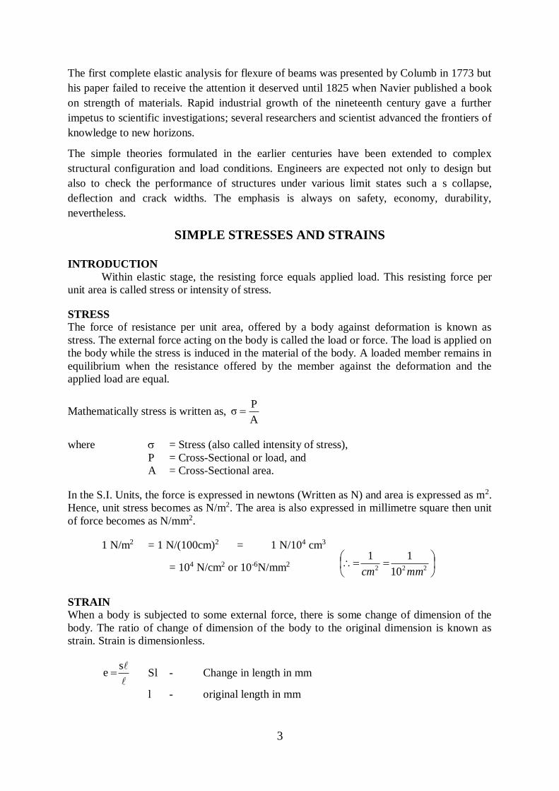
The first complete elastic analysis for flexure of beams was presented by Columb in 1773 but
his paper failed to receive the attention it deserved until 1825 when Navier published a book
on strength of materials. Rapid industrial growth of the nineteenth century gave a further
impetus to scientific investigations; several researchers and scientist advanced the frontiers of
knowledge to new horizons.
The simple theories formulated in the earlier centuries have been extended to complex
structural configuration and load conditions. Engineers are expected not only to design but
also to check the performance of structures under various limit states such a s collapse,
deflection and crack widths. The emphasis is always on safety, economy, durability,
nevertheless.
SIMPLE STRESSES AND STRAINS
INTRODUCTION
Within elastic stage, the resisting force equals applied load. This resisting force per
unit area is called stress or intensity of stress.
STRESS The force of resistance per unit area, offered by a body against deformation is known as
stress. The external force acting on the body is called the load or force. The load is applied on
the body while the stress is induced in the material of the body. A loaded member remains in
equilibrium when the resistance offered by the member against the deformation and the
applied load are equal.
Mathematically stress is written as, A
Pσ
where = Stress (also called intensity of stress),
P = Cross-Sectional or load, and
A = Cross-Sectional area.
In the S.I. Units, the force is expressed in newtons (Written as N) and area is expressed as m2.
Hence, unit stress becomes as N/m2. The area is also expressed in millimetre square then unit
of force becomes as N/mm2.
1 N/m2 = 1 N/(100cm)2 = 1 N/104 cm3
= 104 N/cm2 or 10-6N/mm2
222 10
11
mmcm
STRAIN
When a body is subjected to some external force, there is some change of dimension of the
body. The ratio of change of dimension of the body to the original dimension is known as
strain. Strain is dimensionless.
se Sl - Change in length in mm
l - original length in mm

4
Strain may be:-
1. Tensile strain, 2. Compressive strain
2. Volumetric strain, and 4. Shear strain
If there is some increase in length of a body due to external force, then the ratio of increase of
length to the original length of body is known as tensile strain. But if there is some decrease
in length of the body, then the ratio of decrease of the length of the body to the original length
is known as compressive strain. The ratio of change of volume of the body to the original
volume is known as volumetric strain. The strain produced by shear stress is known as shear
strain.
TYPES OF STRESSES
The stress may be normal stress or a shear stress.
Normal stress is the stress which acts in a direction perpendicular to the areas. It is
represented by (sigma). The normal stress is further divided into tensile stress and
compressive stress.
Tensile Stress. The stress induced in a body, when subjected to two equal and opposite pulls
as shown in Fig.1.1 () as a result of which there is an increase in length, is known as tensile
stress. The ratio of increase in length to the original length is known as tensile strain. The
tensile stress acts normal to the area and it pulls on the area.
Let P = Full (or force) acting on the body.
A = Cross-sectional area of the body.
L = Original length of the body
dL = Increase in length due to pull P acting on the body
= Stress induced in the body, and
e = Strain (i.e., tensile strain)
Fig. 1.1 Stress distributions during Tension
Fig.1.1 () shown a bar subjected to a tensile force P as its ends. Consider -, which divides
the bar into two parts. The part left to the section -, will be in equilibrium if P = resisting
force (R). This is shown in Fig.1.1 (b). Similarly the part right to the sections -, will be in
equilibrium if P = Resisting force as shown in Fig.1.1 (c). This relating force per unit area is
known as stress or intensity of stress.

5
A
(P) Load Tensile
area sectional-Cross
(R) forceReistingσTensile (P= R)
or A
P ... (1.1)
And tensile strain is given by,
L
dL
LengthOriginal
lengthinIncreasee ... (1.2)
Compressive Stress
The stress induced in a body, when subjected to two equal and opposite pushes as shown in
Fig.1.2. () as a result of which there is a decrease in length of the body, is shown as
compressive stress. And the ratio of decrease in length to the original length is known as
compressive strain. The compressive stress acts normal to the area and it pushes on the area.
Let an axial push P is acting on a body is cross-sectional area A. Due to external push P, let
the original length L of the body decrease by dL.
Fig. 1.2 Stress distributions during compression
The compressive stress is given by,
A
P
(A) Area
(P)Push
(A) Area
(R) forceReistingσ
And compressive strain is given by,
L
dL
length Original
lengthin Decreasee
1.4.2 Shear stress. The stress induced in a body, when subjected to two equal and opposite
forces which are acting tangentially across the resisting section as shown in Fig.1.3 as a result

6
of which the body tends to shear off across the section, is known as shear stress. The
corresponding strain is known as shear strain. The shear stress is the stress which acts
tangential to the area. It is represented by .
Fig. 1.4 Lap Joint in Shear
As the bottom face of the block is fixed, the face ABCD will be distorted to ABC, D
through an angle as a result of force P as shown in Fig.1.4 (d).
And shear strain () is given by
ADDistance
ntdisplacemelTransversa
or AD
h
dlDD1
...(1.4)
ELASTICITY AND ELASTIC LIMIT
When an external force acts on a body tends to undergo some deformation. If the external
force is removed and the body comes back to its origin shape and size (which means the
deformation disappears completely), the body), the body is known as elastic body. The
property by virtue of which certain materials return back to their original position after the
removal of the external force, is called elasticity.
The body will regain its previous shape and size only when the deformation caused by the
external force, is within a certain limit. Thus there is a limiting value of force upto and within
which, the deformation completely disappears on the removal of the force. The value of stress
corresponding to this limiting force is known as the elastic limit of the material.
If the external force is so large that the stress exceeds the elastic limit, the material loses to
some extent its property of elasticity. If now the force is removed, the material will not return
to the origin shape and size and there will be residual deformation in the material.
HOOKES LAW AND ELASTIC MODULII
Hooke's Law states that when a material is loaded within elastic limit, the stress is
proportional to the strain produced by the stress. This means the ratio of the stress to the
corresponding strain is a constant within the elastic limit. This constant is known as Module
of Elasticity or Modulus of Rigidity or Elastic Modulii.
7
MODULUS OF ELASTICITY (OR YOUNG'S MODULUS)
The ratio of tensile or compressive stress to the corresponding strain is a constant. This ratio
is known as Young's Modulus or Modulus of Elasticity and is denoted by E.
StraineCompressiv
StresseCompressivor
StrainTensile
StressTensileE
or e
E
... (1.5)
Modulus of Rigidity or Shear Modulus. The ratio of shear stress to the corresponding shear
strain within the elastic limit, is known as Modulus or Rigidity or Shear Modulus. This is
denoted by C or G or N.
C (or G or N) φ
x
StrainShear
StressShear ... (1.6)
Let us define factor of safety also.
FACTOR OF SAFETY
It is defined as the ratio of ultimate tensile stress to the working (or permissible) stress.
Mathematically it is written as
Factor of Safety = Stress Pemissible
StressUltimate ... (1.7)
CONSTITUTIVE RELATION BETWEEN STRESS AND STRAIN
For One Dimensional Stress System. The relationship between stress and strain for
unidirectional stress (i.e., for normal stress in one direction only) is given by Hooke's law,
which states that when a material is loaded within its elastic limit, the normal stress
developed is proportional to the strain produced. This means that the ratio of the normal
stress to the corresponding strain is a constant within the elastic limit. This constant is
represented by E and is known as modulus of elasticity or Young's modulus of elasticity.
Constant Strain ingCorrespond
StressNormal or E
e
where = Normal stress, e = strain and E = Young's Modulus
or E
σe ... [1.7 (A)]
The above equation gives the stress and strain relation for the normal stress in one direction.
For Two Dimensional Stress System. Before knowing the relationship between stress and
strain for two-dimensional stress system, we shall have to define longitudinal strain, lateral
strain, and Poisson's ratio.

8
Longitudinal Strain. When a body is subjected to an axial tensile load, there is an increase
in the length of the body. But at the same time there is a decrease in other dimensions of the
body at right angles to the line of action of the applied. Thus the body is having axial
deformation and also deformation at right angles to the line of action of the applied load (i.e.,
lateral deformation).
The ratio of axial deformation to the original length of the body is known as longitudinal (or
linear) strain. The longitudinal strain is also defined as the deformation of the body per unit
length in the direction of the applied load.
Let L = Length of the body,
P = Tensile force acting on the body.
L = Increase in the length of the body in the direction of P.
Then, longitudinal strain = L
L
Lateral strain. The strain at right angles to the direction of applied load is known as lateral
strain. Let a rectangular bar of length L, breadth b and depth is subjected to an axial tensile
load P as shown in Fig.1.6. The length of the bar will increase while the breadth and depth
will decrease.
Let L = Length of the body,
b = Decrease in breadth, and
d = Decrease in depth.
Then longitudinal strain = L
L ... [1.7 (B)]
and lateral strain = b
bor
d
d ... [1.7 (C)]
Note:(i) If longitudinal strain is tensile, the lateral strains will be compressive.
(ii) If longitudinal strain is compressive then lateral strains will be tensile.
(iii) Hence every longitudinal strain in the direction of load is accompanied by lateral strains
of the opposite kind in all directions perpendicular to the load.
Poisson's Ratio. The ratio is lateral strain to the longitudinal strain is a constant for a given
material, when the material is stressed within the elastic limit. This ratio is called Poisson's
ratio and it is generally denoted by . Hence mathematically.
Poisson's ratio, = strainalLongitudin
strainLateral ... [1.7 (D)]
or Lateral strain = x Longitudinal strain
As lateral strain is opposite in sign to longitudinal strain, t\hence algebraically, lateral
strain is written as
9
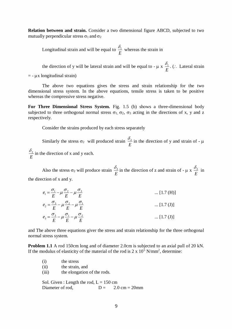
Relation between and strain. Consider a two dimensional figure ABCD, subjected to two
mutually perpendicular stress 1 and 2
Longitudinal strain and will be equal to E
1 whereas the strain in
the direction of y will be lateral strain and will be equal to - x E
1 . ( Lateral strain
= - x longitudinal strain)
The above two equations gives the stress and strain relationship for the two
dimensional stress system. In the above equations, tensile stress is taken to be positive
whereas the compressive stress negative.
For Three Dimensional Stress System. Fig. 1.5 (b) shows a three-dimensional body
subjected to three orthogonal normal stress 1, 2, 3 acting in the directions of x, y and z
respectively.
Consider the strains produced by each stress separately
Similarly the stress 2 will produced strain E
2 in the direction of y and strain of -
E
2 in the direction of x and y each.
Also the stress 2 will produce strain E
3 in the direction of z and strain of - x E
3 in
the direction of x and y.
EEE
e 3211
... [1.7 (H)]
EEE
e 1232
... [1.7 (J)]
EEE
e 2133
... [1.7 (J)]
and The above three equations giver the stress and strain relationship for the three orthogonal
normal stress system.
Problem 1.1 A rod 150cm long and of diameter 2.0cm is subjected to an axial pull of 20 kN.
If the modulus of elasticity of the material of the rod is 2 x 10⁵ N/mm2, determine:
(i) the stress
(ii) the strain, and
(iii) the elongation of the rods.
Sol. Given : Length the rod, L = 150 cm
Diameter of rod, D = 2.0 cm = 20mm

10
Area, A = 22 m100π(20)
4
πm
Axial pull, P = 20 kN = 20,000N
Modulus of elasticity E = 2.0 x 10⁵ N/mm2
(i) The stress () is given equation (1.1) as
= 100
2000
A
P - 63.662 N/mm2, Ans.
(ii) Using equation (1.5) the strain is obtained as
e
E
Strain, e = E
E
= 610x2
63.662= 0.000318. Ans.
(iii) Elongation is obtained by using equation (1.2) as
L
dLe
Elongation, dL = e x L
= 0.000318 x 150 = 0.0477cm. Ans
Problem 1.2. Find the minimum diameter of a steel wire, which is used to raise load of
4000 N if the stress in the rod is not to exceed 95MN/m2.
Sol. Given : Load, P = 4000N
Stress, = 95MN/m2 = 95 x 106 N/m2 ( M=Mega=106)
= 95N/mm2 ( 106 N/m2 = 1N/mm2)
Let D = Diameter of wire in mm
Area, A = 2
4D
Now Stress = A
P
Area
Load
95 = 2
2
4x4000
D4
π
4000
D or D2 =
95 x π
4x4000= 53.61
D = 7.32mm Ans.
Problem 1.3. A tensile test was conducted on a mild steel bar. The following data was
obtained from the test:
(i) Diameter of the steel bar = 3cm
(ii) Gauge length of the bar = 20cm
(iii) Load at elastic limit = 250 kN
(iv) Extension at a load of 150 kN = 0.21mm
(v) Maximum load = 380 kN
(vi) Total extension = 60mm
(vii) Diameter of the rod at the failure = 2.25cm

11
Determine : (a) the Young's Modulus, (b) the stress elastic limit
(c) the percentage elongation, and (d) the percentage decrease in area.
Sol. Area of rod, A = 2cm2(3)
4
π2D4
π
= 7.06835 cm2 = 7.0685 x 10⁻⁴ m2
2
2
100
1mcm
(a) To find Young's modulus, first calculate the value of stress and strain within elastic limit.
The load at elastic limit it given but the extension corresponding to the load of elastic limit is
not given. But a load 150 kN (which is within elastic limit) and corresponding extension of
0.21mm are given. Hence these values are used for stress and strain within elastic limit
2N/m4-10 x 7.0685
1000 x 150
Area
LoadStress
( 1 kN = 1000 N)
= 21220.9 x 104 N/m2
length) Guage(or Length Original
Extension)(or length inIncreaseStrain and
00105.010mm x 20
0.21mm
Young's Modolus
2N/m410 x 202095230.00105
421220.9x10x
Strain
StressE
= 202.095 x 10⁹ N/m2 ( 109 = Giga = G)
= 202.095 x GN/m2 Ans.
(b) The stress at the elastic limit is given by
47.0685x10
250x1000
Area
limit elasticat Load Stress
= 35368 x 104 N/m2
= 353.68 x 10⁶ N/m2 ( 106 = Mega = M)
= 353.68 MN/m2. Ans.
(c) The percentage decrease is obtained as,
percentage elongation

12
100x length) guage(or length Original
lengthin Increase Total
Ans. 30%100x 10mm x 20
60mm
(d) The percentage decrease in area is obtained as
percentage decrease in area.
100x area Original
failure) at the Area - area (Original
= 100 x
3 x 4
π
2.25 x 4
π3 x
4
π
2
22
= Ans. 43.75%100 x 9
5.0625)-(9 100 x
3
2.2532
2 2
ANALYSISZS OF BARS OF VARYING SECTIONS
A bar of different lengths and of different diameters (and hence of different cross-sectional
areas) is shown in Fig.1.4 (). Let this bar is subjected to an axial load P.
Fig. 1.5 Bar with varied cross sections and Axial load
Though each section is subjected to the same axial load P, yet the stresses, strains and change
in length will be different. The total change in length will be obtained by adding the changes
in length of individual section
Let P = Axial load acting on the bar,
L1 = Length of section 1,
A1 = Cross-Sectional area of section 1,
L2, A2 = Length and cross-sectional areas of section 2,
L3, A3 = Length and cross-sectional areas of section 3, and
E = Young's modulus for the bar.
Problem 1.4. An axial pull of 35000 N is acting on a bar consisting of three lengths as shown
in Fig.1.6 (b). If the Young's modulus = 2.1 x 10⁵ N/mm2, determine.
(i) Stresses in each section and
(ii) total extension of the bar

13
Fig. 1.6 Bar with varied cross sections and Axial load as 35000N
Sol. Given:
Axial pull, P = 35000 N
Length of section 1, L1 = 20cm = 220mm
Dia. of Section 1, D1 = 2cm = 20mm
Area of Section 1, A1 = 22 mm 100 )(20
4
π
Length of section 2, L2 = 25cm = 250mm
Dia. of Section 2, D2 = 3cm = 30mm
Area of Section 2, A2 = 22 mm 225 )(30
4
π
Length of section 3, L3 = 22cm = 220mm
Dia. of Section 3, D3 = 5cm = 50mm
Area of Section 2, A3 = 22 mm 625 )(50
4
π
Young's Modulus, E = 2.1 x 10⁵ N/mm2
(i) Stress in each section
Stress in section 1, 1 = 1Section of Area
load Axial
= 100π
35000
A
P
1
= 111.408N/mm2. Ans.
Stress in section 2, = x π225
35000
A
P
2
= 49.516N/mm2. Ans.
Stress in section 3, = x π625
35000
A
P
3
= 17.825 N/mm2. Ans.
(ii) Total extension of the bar
Using equation (1.8), we get

14
Total Extension =
3A
3L
2A
2L
1A
1L
E
P
= 510 x 2.1
35000
x π625
230
x π225
250
100π
200
= 510 x 2.1
35000(6.366 + 3.536 + 1.120) = 0.183mm Ans.
Problem 1.5. A member formed by connecting a steel bar to aluminium for bar is shown in
Fig.1.7. Assuming that the bars are presented from buckling, sideways, calculate the
magnitude of force P that will causes the total length of the member to decrease 0.25mm. The
values of elastic modulus for steel and aluminium are 2.1 x 10⁶ N/mm2 and 7 x 10⁴ N/mm2
respectively.
Sol. Given
Length of Steel bar, L1 = 30c m = 300mm
Area of Steel bar, A1 = 5 x 5 = 25m2 = 250mm2
Elastic modulus for steel bar, E1 = 2.1 x 10⁵ N/mm2
Length of Aluminium bar, L2 = 38cm = 380mm
Area of Aluminium bar A2 = 10 x 10 = 100cm2 = 1000mm2
Elastic modulus for aluminium bar E2 = 7 x 10⁴ N/mm2
Total Decrease in length, dL = 0.25mm
Let P = Required force
As both the bars are made of different materials, hence total change in the lengths of the bar
is given by equation (1.9)
dL = P 22
2
11
1
AE
L
AE
L
or
0.25 = P
1000 x 10 x 7
380
2500 x 10 x 2.1
30045
= P (5.714 x 10⁻⁷ + 5.428 x 10⁻⁷) = P x 11.142 x 10⁻⁷
P = 11.142
10 x 0.25
10 x 11.142
0.25 7
7- = 2.2437 x 105 = 224.37 kN. Ans.
Principle of Superposition. When a number of Loads are acting on a body, the resulting
strain, according to principle of superposition, will be the algebraic sum of strains caused by
individual loads.
While, using this principle for an elastic body which is subjected to a number of direct forces
(tensile or compressive) at different sections along the length of the body, first the free body
diagram of individual section is drawn. Then the deformation of the each section is obtained.

15
The total deformation of the body will be then equal to the algebraic sum of deformation of
the individual sections.
Problem 1.6 A brass bar, having cross-sectional area of 1000 mm2 , is subjected to axial
forces as shown in Fig.
Fig. 1.7 Bar with same cross section and Axial loads
Find the total elongation of the bar, Take E = 1.05 x 10⁵ N/mm2
Sol. Given:
Area A = 1000mm2
Value of E = 1.05 x 10⁵ N/mm2
Let d = Total elongation of the bar
The force of 80 kN acting at B is split up into three forces of 50 kN, 20 kN and 10 kN. Then
the part AB of the bar will be subjected to a tensile load of 50 kN, part BC is subjected to a
compressive load of 20 kN and part BD is subjected to a compressive load of 10 kN as shown
in Fig.
Part AB. This part is subjected to a tensile load of 50kN. Hence there will be increase in
length of this part.,
Increase in the length of AB
= 1
1 x AE
PL = 600x
10 x 1.05 x 1000
1000 x 5005
(P1=50,000 N,L1 = 600mm)
= 0.2857
Part BC. This part is subjected to a compressive load of 20kN or 20,000 N. Hence there will
be decrease in length of this part.
Decrease in the length of BC
= 2
2 Lx AE
P= 1000x
10 x 1.05 x 1000
20,0005
(L2=1m = 1000mm)
= 0.1904
Part BD. The part is subjected to a compressive load of 10kN or 10,000 N. Hence there will
be decrease in length of this part.
Decrease in the length of BC
= 3
3 Lx AE
P= 2200x
10 x 1.05 x 1000
10,0005
(L2=1.2 + 1.22m or 2200m)
= 0.2095
Total elongation of bar = 0.2857 – 0.1904 – 0.2095)
(Taking +ve sign for increase in length and –ve sign for
decrease in length

16
=- 0.1142mm. Ans.
Negative sign shows, that there will be decrease in length of the bar.
Problem 1.7. A Member ABCD is subjected to point loads P1, P2, P and P4 as shown in Fig.
Fig. 1.8 Bar with varied cross section and Axial loads
Calculate the force P2 necessary for equilibrium, if P1 = 45 kN, P3 = 450 kN and P4 = 130 kN.
Determine the total elongation of the member, assuming the modulus of elasticity to be 2.1 x
105 N/mm2.
Set Given:
Part AB : Area. A1 = 625 mm2 and
Length L1 = 120cm = 1200mm
Part BC : Area A2 = 2500 mm2 and
Length L2 = 60cm = 600mm
Part CD : Area A3 = 12.0mm2 and
Length L3 = 90cm = 900mm
Value of E = 2.1 x 10⁵ N/mm2
Value of P2 necessary for equilibrium
Resolving the force on the rod along its (i.e., equating the forces acting towards right to those
acting towards left) we get
P1 + P3 = P2 + P4
But P1 = 45kN
P3 = 450 kN and P4 = 130kN
45 + 450 = P2 = 130 or P2 = 495 – 130 =, 365 kN
The force of 365 kN acting at B is split into two forces of 45 kN and 320 kN (i.e., 365 – 45 =
320 kN)
The force of 450 kN acting at C is split into two forces of 320 kN and 130 kN (i.e., 450 – 320
= 130 kN) as shown Fig.
It is clear that part AB is subjected to a tensile load of 45kN, part BC is subjected to a
compressive load of 320 kN and par CD is subjected to a tensile load 130 kN.
Hence for part AB, there will be increase in length; for part BC there will be decrease in
length and for past CD there will be increase in length.
17
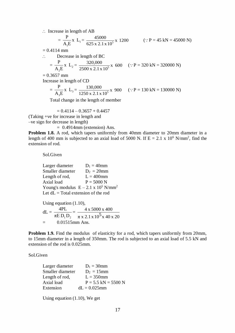
Increase in length of AB
= 1
1
Lx EA
P= 1200x
10 x 2.1 x 625
450005
(P = 45 kN = 45000 N)
= 0.4114 mm
Decrease in length of BC
= 2
2
Lx EA
P= 600x
10 x 2.1 x 2500
320,0005
(P = 320 kN = 320000 N)
= 0.3657 mm
Increase in length of CD
= 3
3
Lx EA
P= 900x
10 x 2.1 x 1250
130,0005
(P = 130 kN = 130000 N)
Total change in the length of member
= 0.4114 – 0.3657 + 0.4457
(Taking +ve for increase in length and
–ve sign for decrease in length)
= 0.4914mm (extension) Ans.
Problem 1.8. A rod, which tapers uniformly from 40mm diameter to 20mm diameter in a
length of 400 mm is subjected to an axial load of 5000 N. If E = 2.1 x 10⁶ N/mm2, find the
extension of rod.
Sol.Given
Larger diameter D1 = 40mm
Smaller diameter D2 = 20mm
Length of rod, L = 400mm
Axial load P = 5000 N
Young's modulus E – 2.1 x 10⁵ N/mm2
Let dL = Total extension of the rod
Using equation (1.10),
dL = 2 1 DD πE
4PL=
20 x 40x 510 x 2.1 x π
400 x 5000 x 4
= 0.01515mm Ans.
Problem 1.9. Find the modulus of elasticity for a rod, which tapers uniformly from 20mm,
to 15mm diameter in a length of 350mm. The rod is subjected to an axial load of 5.5 kN and
extension of the rod is 0.025mm.
Sol.Given
Larger diameter D1 = 30mm
Smaller diameter D2 = 15mm
Length of rod, L = 350mm
Axial load P = 5.5 kN = 5500 N
Extension dL = 0.025mm
Using equation (1.10), We get
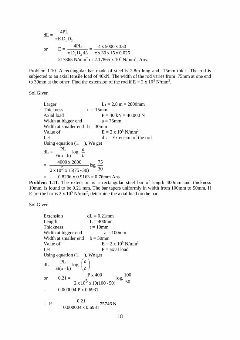
18
dL = 2 1 DD πE
4PL
or E = LdDD π
4PL
2 1
= 0.025 x 15 x 30 x π
350 x 5000 x 4
= 217865 N/mm2 or 2.17865 x 10⁵ N/mm2. Ans.
Problem 1.10. A rectangular bar made of steel is 2.8m long and 15mm thick. The rod is
subjected to an axial tensile load of 40kN. The width of the rod varies from 75mm at one end
to 30mm at the other. Find the extension of the rod if E = 2 x 10⁵ N/mm2.
Sol.Given
Larger L1 = 2.8 m = 2800mm
Thickness t = 15mm
Axial load P = 40 kN = 40,000 N
Width at bigger end a = 75mm
Width at smaller end b = 30mm
Value of E = 2 x 10⁵ N/mm2
Let dL = Extension of the rod
Using equation (1. ), We get
dL = b)-Et(a
PLlog,
b
a
= 30
75log,
30)-15(75 x 510 x 2
2800 x 4000
= 0.8296 x 0.9163 = 0.76mm Ans.
Problem 1.11. The extension is a rectangular steel bar of length 400mm and thickness
10mm, is found to be 0.21 mm. The bar tapers uniformly in width from 100mm to 50mm. If
E for the bar is 2 x 10⁵ N/mm2, determine the axial load on the bar.
Sol.Given
Extension dL = 0.21mm
Length L = 400mm
Thickness t = 10mm
Width at bigger end a = 100mm
Width at smaller end b = 50mm
Value of E = 2 x 10⁵ N/mm2
Let P = axial load
Using equation (1. ), We get
dL = b)-Et(a
PLlog,
b
a
or 0.21 = 50
100log,
50)-10(100 x 510 x 2
400 x P
= 0.000004 P x 0.6931
P = N 757460.6931 x 0.000004
0.21

19
= 75.746 kN Ans.
ANALYSIS OF BARS OF COMPOSITE SECTIONS
A bar, made up two or more bars of equal lengths but of different materials rigidly fixed with
each other and behaving as one unit for extension or compressive when subjected to an axial
tensile or compressive loads, is called a composite bar. For the composite bar the following
two points are important:
1. The extension or compression in each bar is equal. Hence determination per
unit length i.e. strain in each bar is equal.
2. The total external load on the composite bar is equal to the sum of the loads
carried by each different material.
Problem 1.12. A steel rod of 3cm diameter is enclosed centrally in a hollow copper tube of
external diameter of 4cm. The composite bar is ten subjected to an axial pull of 45000 N. If
the length of each bar is equal to 15cm, determine.
(i) The stresses in the rod and tube, and
(ii) Load carried by each bar
Take E for steel = 2.1 x 10⁵ N/mm2 and for copper = 1.1 x 10⁵ N/mm2
Fig. 1.9 Composite bar
Sol Given:
Dia of steel rod = 3cm = 30mm
Area of steel rod,
Ae = 4
(30)2 = 706.86mm2
External dia. of copper tube
= 5cm = 50mm
Internal dia. of copper tube
= 4cm = 40mm
Area of copper tube,

20
Ae = 4
(502-402)mm2 = 706.86mm2
Axial pull on composite bar, P = 45000 N
Length of each bar L = 15cm
Young's modulus for steel, ES = 2.1 x 10⁵ N/mm2
Young's modulus for copper Ec = 1.1 x 10⁵ N/mm2
(i) The stress in the rod and tube
Let S = Stress in steel
PS = Load carried by steel rod
c = Stress in copper, and
Pc = Load carried by copper tube.
Now strain in steel = Strain in copper
Strain
E
σ
or c
c
S
S
E
σ
E
σ
S = 106 x 11
10 x 2.1σ x
E
E 6
c
c
S x c =- 1.900 c
Now Stress = Area
Load, Load = Stress x Area
Load on steel + load on copper = Total load
S x AS + c x Ac = P P) Load Total(
or 1.909 c x 706.86 + 706.86 = 45000
or c (1.909 x 706.86 + 706.86) = 45000
or 2056.25 c = 45000
Ans21.88N/mm2056.25
45000σ 2
c
Substituting the value of c in equation (i), we get
c = 1.909 x 21.88 N/mm2
= 41.77 N/mm2. Ans
(ii) Load carried by each bar
As Load = Stress x Area
Load carried by steel rod
Ps = S x AS
= 41.77 x 706.86 = 29525.5 N. Ans
Load Carried by copper tube,
Pc = 45000 – 29525.5
= 15474.5 N. Ans
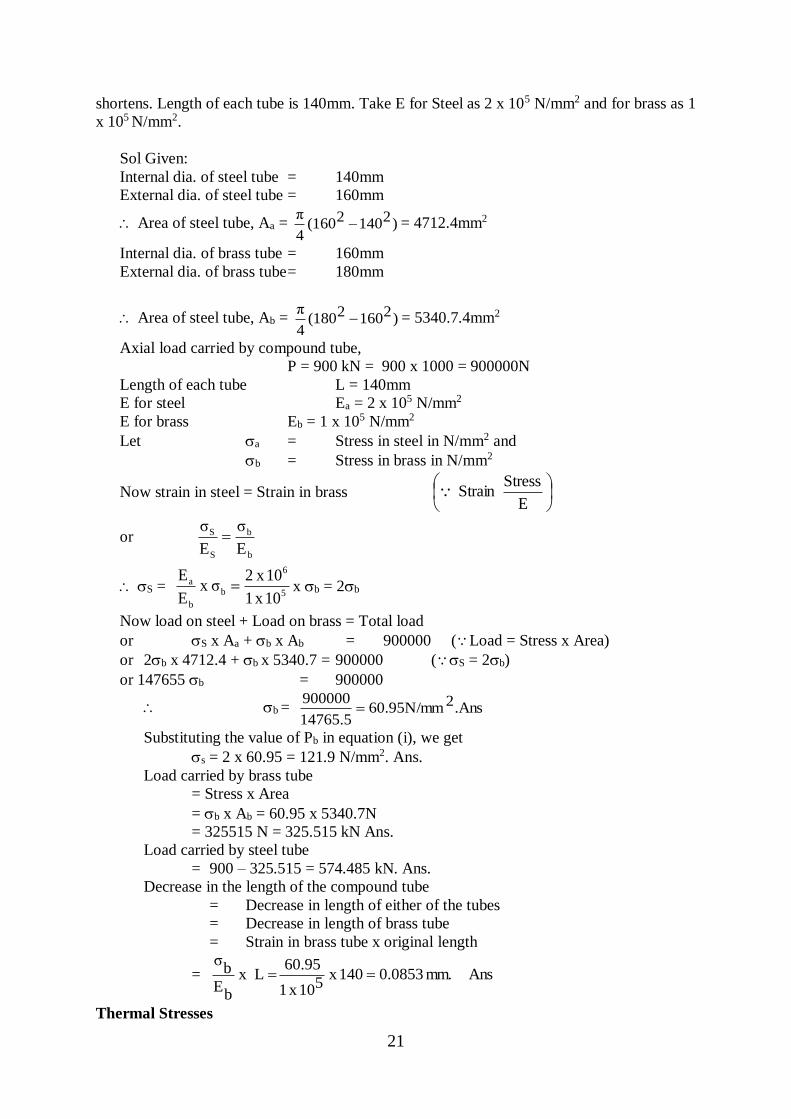
Problem 1.13. A compound tube consists of a steel tube 140mm internal diameter and
160mm external diameter and an out brass tube 160mm internal diameter and 180mm
external diameter. The two tubes are of the same length. The compound tube carries an axial
load of 900 kN. Find the stresses and the load carried by each tube and the amount if
21
shortens. Length of each tube is 140mm. Take E for Steel as 2 x 10⁵ N/mm2 and for brass as 1
x 105 N/mm2.
Sol Given:
Internal dia. of steel tube = 140mm
External dia. of steel tube = 160mm
Area of steel tube, Aa = )21402(1604
π = 4712.4mm2
Internal dia. of brass tube = 160mm
External dia. of brass tube = 180mm
Area of steel tube, Ab = )21602(1804
π = 5340.7.4mm2
Axial load carried by compound tube,
P = 900 kN = 900 x 1000 = 900000N
Length of each tube L = 140mm
E for steel Ea = 2 x 10⁵ N/mm2
E for brass Eb = 1 x 10⁵ N/mm2
Let a = Stress in steel in N/mm2 and
b = Stress in brass in N/mm2
Now strain in steel = Strain in brass
E
StressStrain
or b
b
S
S
E
σ
E
σ
S = 5
6
b
b
a
10 x 1
10 x 2σ x
E
E x b = 2b
Now load on steel + Load on brass = Total load
or S x Aa + b x Ab = 900000 (Load = Stress x Area)
or 2b x 4712.4 + b x 5340.7 = 900000 (S = 2b)
or 147655 b = 900000
b = .Ans260.95N/mm14765.5
900000
Substituting the value of Pb in equation (i), we get
s = 2 x 60.95 = 121.9 N/mm2. Ans.
Load carried by brass tube
= Stress x Area
= b x Ab = 60.95 x 5340.7N
= 325515 N = 325.515 kN Ans.
Load carried by steel tube
= 900 – 325.515 = 574.485 kN. Ans.
Decrease in the length of the compound tube
= Decrease in length of either of the tubes
= Decrease in length of brass tube
= Strain in brass tube x original length
= Ans mm. 0.0853140 x 510 x 1
60.95L x
bE
bσ
Thermal Stresses

22
A solid structure is changes in original shape due to change in temperature its might expand
or contract.
Fig. 1.10 Thermal expansion and contraction
Definition: A temperature change results in a change in length or thermal strain. There is no
stress associated with the thermal strain unless the elongation is restrained by the supports.
Raise at temperature ∝ materials is expands (elongate)
Decreases at temperature ∝ materials is contract (shorten)
AE
PLLT PT
Thermal strain e = .T and thermal stress p= .T.E
coef.expansion thermal T=Rise or fall of temperature E= young’s modulus
Solved problem
Problem: 1A steel rod of 50m long and 3cm diameter is connected to two grips and the rod is
maintained at a temperature of 95oC. Find out the force exerted by the rod after it has been
cooled to 30oC, if (a) the ends do not yield, and (b). The ends yield by .12cm. Take E = 2.1 x
105 N/mm2; α = 12 x 10-6/ oC.

23
Diameter length T1 T2 T=T1-T2 E α
3cm 5m 95 30 65 2.00E+05 1.20E-05
30 5000
mm m ˚C ˚C ˚C N/mm^2 /˚C
To find I)when the ends do not yield
ii)when the ends yield.12cm
Required formula
stress Area pi 4 d^2
α.T.E (∏/4) d^2 3.14 4 900
stressXArea
stress
(α.T.L-δ)/L
X E
stressXArea
1.2 δ
α.T.E (∏/4) d^2
1.56E+02 706.5 1.10E+05 N
(Ans)
α.T.L δ L E α.T.L-δ α.T.L-δ/L (α.T.L-δ/L)XE
3.90E+00 1.2 50 2.00E+05 2.70E+00 5.40E-04 1.08E+02
7.63E+04 N
(Ans)
The ends yield by
0.12cm
stressXArea
Given Data
Sloution
The rod not yield
The ends yield by
0.12cm
The rod not yield
stressXArea
Problem: 2 A copper rods of 10cm diameter and 1.5m long is connected to two grips and
the rod is maintained at a temperature of 125oC. Find out the force exerted by the rod after it
has been cooled to 45oC, if (a) the ends do not yield, and (b). The ends yield by 1.7mm.Take
E = 120Gpa; α = 1.7 x 10⁻⁶/ oC.

24
Diameter length T1 T2 T=T1-T2 E α
10cm 1.5m 125 45 80 1.20E+05 1.70E-05
100 1500
mm m ˚C ˚C ˚C N/mm^2 /˚C
To find I)when the ends do not yield
ii)when the ends yield.12cm
Required formula
stress Area pi 4 d^2
α.T.E (∏/4) d^2 3.14 4 10000
stressXArea
stress
(α.T.L-δ)/L
X E
stressXArea
1.5 δ
α.T.E (∏/4) d^2
1.63E+02 7850 1.28E+06 N
(Ans)
α.T.L δ L E α.T.L-δ α.T.L-δ/L (α.T.L-δ/L)XE
2.04E+00 1.5 50 1.20E+05 5.40E-01 3.60E-04 4.32E+01
3.39E+05 N
(Ans)
The ends yield by
0.12cm
stressXArea
Given Data
Sloution
The rod not yield
The ends yield by
0.15cm
The rod not yield
stressXArea
Thermal stress in composite bar In certain application it is necessary to use a combination of elements or bars made from
different materials, each material performing a different function. Temperature remains the
same for all the materials but strain rate is different due to thermal expansion of materials.
The blow figure shows the thermal expansion on composite bar.
Fig. 1.11 Thermal expansion on Composite bar
The Expression for thermal stress is Load on the brass = load on the steel
From the stress equation
=
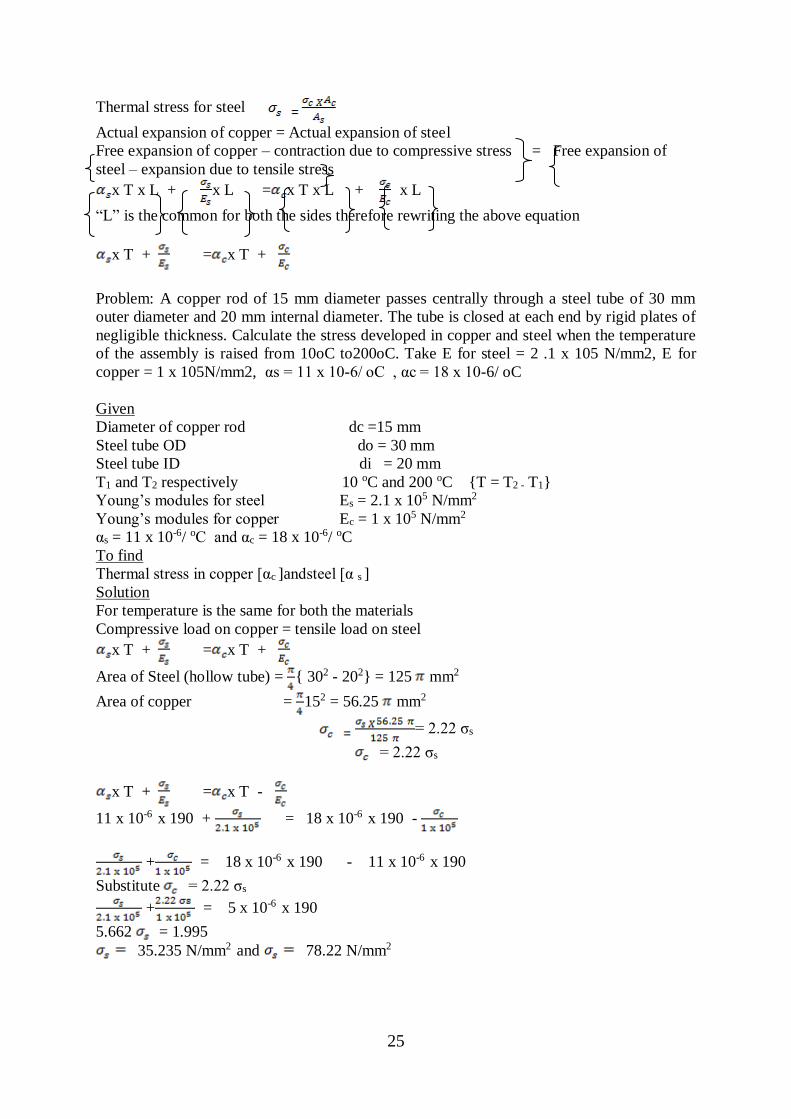
Thermal stress for copper
25
Thermal stress for steel
Actual expansion of copper = Actual expansion of steel
Free expansion of copper – contraction due to compressive stress = Free expansion of
steel – expansion due to tensile stress
x T x L + x L = x T x L + x L
“L” is the common for both the sides therefore rewriting the above equation
x T + = x T +
Problem: A copper rod of 15 mm diameter passes centrally through a steel tube of 30 mm
outer diameter and 20 mm internal diameter. The tube is closed at each end by rigid plates of
negligible thickness. Calculate the stress developed in copper and steel when the temperature
of the assembly is raised from 10oC to200oC. Take E for steel = 2 .1 x 105 N/mm2, E for
copper = 1 x 10⁵N/mm2, αs = 11 x 10-6/ oC , αc = 18 x 10-6/ oC
Given
Diameter of copper rod dc =15 mm
Steel tube OD do = 30 mm
Steel tube ID di = 20 mm
T1 and T2 respectively 10 oC and 200 oC {T = T2 - T1}
Young’s modules for steel Es = 2.1 x 10⁵ N/mm2
Young’s modules for copper Ec = 1 x 10⁵ N/mm2
αs = 11 x 10-6/ oC and αc = 18 x 10-6/ oC
To find
Thermal stress in copper [αc ]andsteel [α s ]
Solution
For temperature is the same for both the materials
Compressive load on copper = tensile load on steel
x T + = x T +
Area of Steel (hollow tube) = { 302 - 202} = 125 mm2
Area of copper = 152 = 56.25 mm2
= 2.22 σs
= 2.22 σs
x T + = x T -
11 x 10-6 x 190 + = 18 x 10-6 x 190 -
+ = 18 x 10-6 x 190 - 11 x 10-6 x 190
Substitute = 2.22 σs
+ = 5 x 10-6 x 190
5.662 = 1.995
35.235 N/mm2 and 78.22 N/mm2

26
Elastic constants
When the structural stressed by axial load it’s under goes the deformation and it’s comes
back to original shape or structural stressed by within the elastic limit then there is the
changes in length along x-direction, y-direction and z - direction.
Types of elastic constant related to isotropic materials
1.Elasticity Modulus (E)0r Young’s Modulus
2. Poisson’s Ratio ( )
3. Shear Modulus (G)
4. Bulk Modulus (K)
Elasticity Modulus or Young’s Modulus(E)
= E
Fig. Before applied load and after applied
load
2. Poisson’s Ratio (μ)
(μ) (or)
=
Lateral strain (et)
= (or)
Fig. 1.12 Load applied on rod Fig. 1.13 linear change and lateral change
Longitudinal strain (el) =
Shear Modulus (G)
Shear modulus G =
G =
Fig. Shear stress
Volumetric Strain
=
Fig. 1.14 Shear force applied situation
The volumetric strain is defined as materials tends to change in volume at three direction by
external load within the elastic limit

27
Volume of uniform rectangular section = L X b X d
Here b=d
X = lateral strain
Rewriting the above equation
Volumetric strain of rectangular structural subjected to three forces which are mutually
perpendicular
Similarly for and
{ }
{ } - {
{ } - }
Volumetric strain of cylindrical rod
Bulk modulus [K]
Fig. 1.15 Change in volume

28
Relation between young’s modulus and bulk modulus
Volume = L x L x L
V = L3 =3 L2 x
=3 L2 x
=3 L2 x
=
=
E From this equation
Relationship between modulus of elasticity and modulus of rigidity {E and G}
Easy to identify with the four elastic constant are calculated by single module as shown in
fig.
Relation between modulus of elasticity (E) and bulk modulus (K):
29
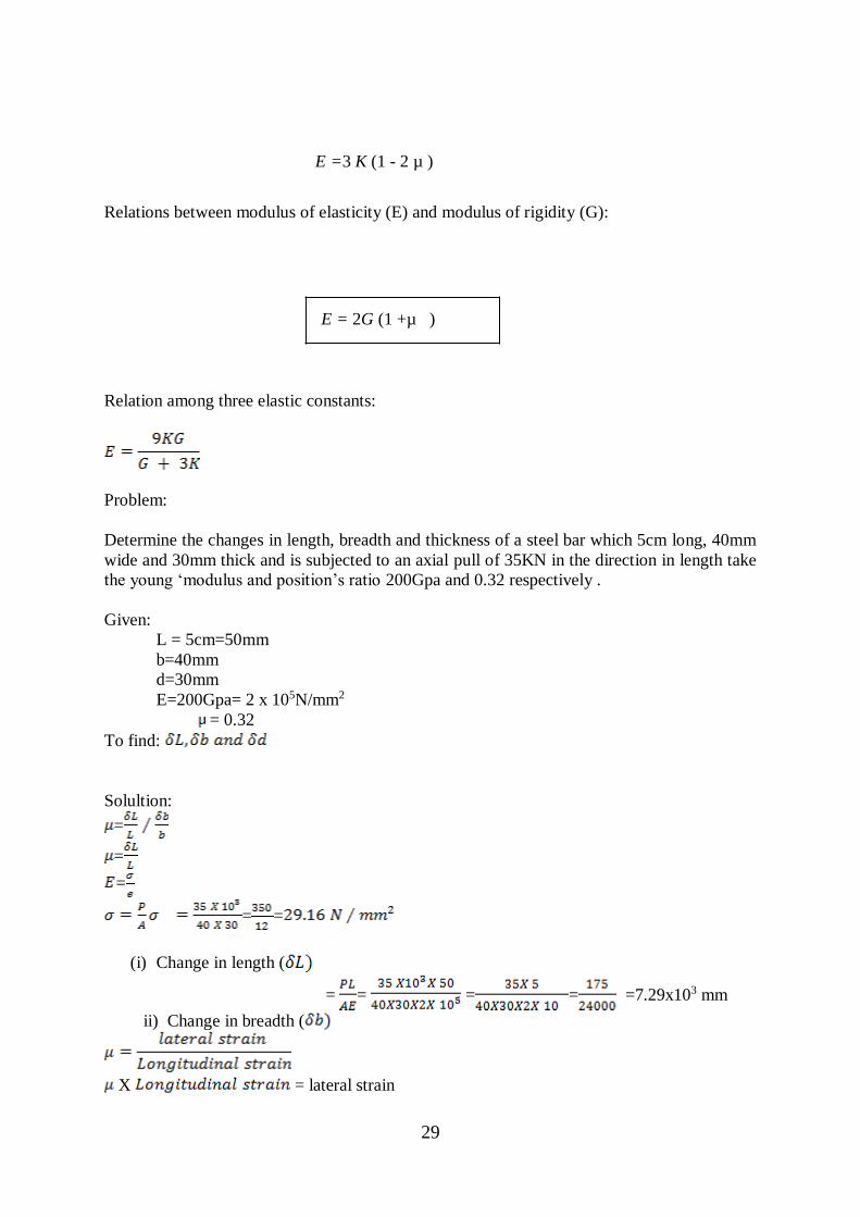
E =3 K (1 - 2 µ ) Relations between modulus of elasticity (E) and modulus of rigidity (G):
E = 2G (1 +µ ) Relation among three elastic constants:
Problem:
Determine the changes in length, breadth and thickness of a steel bar which 5cm long, 40mm
wide and 30mm thick and is subjected to an axial pull of 35KN in the direction in length take
the young ‘modulus and position’s ratio 200Gpa and 0.32 respectively .
Given:
L = 5cm=50mm
b=40mm
d=30mm
E=200Gpa= 2 x 10⁵N/mm2
= 0.32
To find:
Solultion:
=
=
=
= =
(i) Change in length (
= = = = =7.29x103 mm
ii) Change in breadth (
X = lateral strain

30
X =
= X X b = 0.32 x 40 x = 1.866 x 10 -3 mm
ii) Change in diameter (
X =
= X X d=0.32 x x 40 =1.39 X10 -3 mm
Problem:
Calculate the modulus of rigidity and bulk modulus of cylindrical bar of diameter of 25mm
and of length 1.6m. if the longitudinal strain in a bar during a tensile test is four times the
lateral strain find the change in volume when the bar subjected to hydrostatic pressure of 100
the young’s modulus of cylindrical bar E is 100 GPa
Given:
D=25 mm
L=1.6m=1600 mm
Longitudinal strain = 4 X lateral strain
E=100Gpa=1 x 10⁵N/mm2
To find:
(i) Modulus of Rigidity (ii) Bulk modulus (iii) Change in volume
(i) Modulus of Rigidity[G]
E= 2G (1+µ) ---------- Relationship between E, G & µ
Longitudinal strain = 4 X lateral strain
E= 2G (1+µ) =2G (1+ ) =2G (1+0.25)
E=2G (1+0.25)
G = = = 4 x 10 4 N/mm2
(ii) Bulk modulus [K]
E = 3K [1-2 µ]
= K x 3[ 1-0.5]
1 x 105 = 1.5 x K
= K
K = .666 X N/mm2
(iii)Change in volume [dV]
= = =1.5 X 10 -3
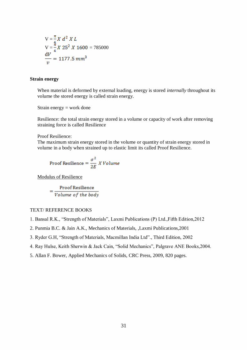
31
V =
V = = 785000
Strain energy
When material is deformed by external loading, energy is stored internally throughout its
volume the stored energy is called strain energy.
Strain energy = work done
Resilience: the total strain energy stored in a volume or capacity of work after removing
straining force is called Resilience
Proof Resilience:
The maximum strain energy stored in the volume or quantity of strain energy stored in
volume in a body when strained up to elastic limit its called Proof Resilience.
Modulus of Resilience
TEXT/ REFERENCE BOOKS
1. Bansal R.K., “Strength of Materials”, Laxmi Publications (P) Ltd.,Fifth Edition,2012
2. Punmia B.C. & Jain A.K., Mechanics of Materials, ,Laxmi Publications,2001
3. Ryder G.H, “Strength of Materials, Macmillan India Ltd”., Third Edition, 2002
4. Ray Hulse, Keith Sherwin & Jack Cain, “Solid Mechanics”, Palgrave ANE Books,2004.
5. Allan F. Bower, Applied Mechanics of Solids, CRC Press, 2009, 820 pages.

1
SCHOOL OF MECHANICAL ENGINEERING
DEPARTMENT OF MECHANICAL ENGINEERING
UNIT – II– ANALYSIS OF STRESSES IN TWO DIMENSIONS – SMEA1305
2
MECHANICS OF SOLIDS (SMEA1305)
UNIT 2: ANALYSIS OF STRESSES IN TWO DIMENSIONS
Principal planes and stresses – Mohr’s circle for biaxial stresses – Maximum shear
stress - simple problems- Stresses on inclined plane
Biaxial state of stresses – Thin cylindrical and spherical shells – Deformation in thin
cylindrical and spherical shells – Efficiency of joint- Effect of Internal Pressure
Introduction: Principal planes and stresses
The planes, which have no shear stress, are known as principal planes. Hence principal planes
are the planes of zero shear stress. These planes carry only normal stresses. The normal
stresses, acting on a principal plane, are known as principal stresses.
Methods for determining principal planes and stresses
Analytical method
Graphical method
Analytical method on oblique section
The following are the two cases considered
1. A member subjected to a direct stress in one plane
2. A member subjected to like direct stresses in two mutually perpendicular directions.
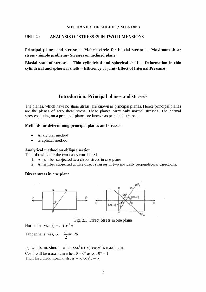
Direct stress in one plane
Fig. 2.1 Direct Stress in one plane
Normal stress, 2cosn
Tangential stress,
2sin2
t
n will be maximum, when 2cos (or) cos is maximum.
Cos θ will be maximum when θ = 0° as cos 0° = 1
Therefore, max. normal stress = σ cos2θ = σ

3
t will be max, when sin 2θ is maximum.
Sin2θ be max. when sin2θ = 1 or 2θ = 90° (or) 270°
θ = 45° (or) 135°
Max. value of shear stress =
2sin2
= 2
Fig. 2.2 Position of planes
Member subjected to direct stresses in two mutually perpendicular directions
Fig. 2.3 Member subjected to Direct stress in two perpendicular directions
2cos22
Stress,Normal 2121
n
2sin2
)(Stress,Tangential 21 t
22Stress,ResultanttnR
n
t
tanObliquity,

4
Problem
A small block is 4 cm long, 3 cm high and 0.5 cm thick. It is subjected to uniformly
distributed tensile forces of resultants 1200 N and 500 N as shown in Fig. below. Compute
the normal and shear stresses developed along the diagonal AB.
Given
Length = 4 cm, Height = 3 cm and Width = 0.5 cm
Force along x-axis = 1200 N Force along y-axis = 500 N
Area of cross-section normal to x-axis = 3 x 0.5 = 1.5 cm2
Area of cross-section normal to y-axis = 4 x 0.5 = 2 cm2
2x
1 N/cm800F
axis,- xalong Stress xA
2y
2 N/cm250F
axis,-y along Stress yA
33.13
4θtan
06.53)33.1(tanθ 1
Fig. 2.4 Cube at loading condition
2cos22
Stress,Normal 2121
n
)06.532cos(2
250800
2
250800
2N/cm65.448
2sin2
)(Stress,Tangential 21 t
)06.532sin(2
250800
2N/cm18.264
Members subjected to direct stresses in two mutually perpendicular directions accompanied
by simple shear stress

5
Fig. 2.5 Principal Planes Identification diagram
2sin2cos22
Stress,Normal 2121
n
2cos2sin2
)(Stress,Tangential 21
t
)(
22tan
21
Fig. 2.6 Loaded Cube
6
2
2
2121
22 stress principalMajor
2
2
2121
22 stress principalMinor
22
21 42
1 stressShear Max.
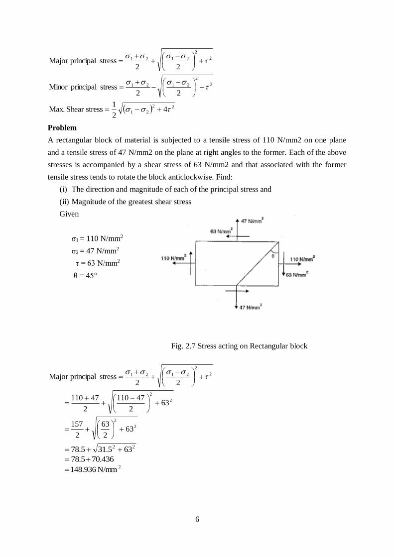
Problem
A rectangular block of material is subjected to a tensile stress of 110 N/mm2 on one plane
and a tensile stress of 47 N/mm2 on the plane at right angles to the former. Each of the above
stresses is accompanied by a shear stress of 63 N/mm2 and that associated with the former
tensile stress tends to rotate the block anticlockwise. Find:
(i) The direction and magnitude of each of the principal stress and
(ii) Magnitude of the greatest shear stress
Given
σ1 = 110 N/mm2
σ2 = 47 N/mm2
τ = 63 N/mm2
θ = 45°
Fig. 2.7 Stress acting on Rectangular block
2
2
2121
22 stress principalMajor
2
2
632
47110
2
47110
2
2
632
63
2
157
22 635.315.78
436.705.78
2N/mm936.148

7
2
2
2121
22 stress principalMinor
2
2
632
47110
2
47110
436.705.78
2N/mm064.8
)(
2θ2tan
21
)2(tanθ2 1
3431θ
Magnitude of the greatest shear stress
22
21maxt 42
1 )(
2263447100
2
1
2
maxt N/mm436.70 )(
Mohr’s circle method
It is a graphical method of finding normal, tangential and resultant stresses or an oblique
plane. It is drawn for following cases
1.
A body subjected to two mutually perpendicular principal stresses of unequal
intensities
2.
A body subjected to two mutually perpendicular stresses which are unequal and
unlike (one is tension and other is compression)
3.
A body subjected to two mutually perpendicular tensile stresses accompanied by a
simple shear stress.
Case 1: A body subjected to two mutually perpendicular principal stresses of unequal
intensities
Let σ1= Major tensile stress
σ2 = Minor tensile stress
θ = Angle made by the oblique plane with the axis of minor tensile stress
Mohr’s Circle procedure

8
Take any point A and draw a horizontal line through A. Take AB = σ1 and AC = σ2
towards right from A to some suitable scale. With BC as diameter draw a circle. Let O is the
centre of circle. Now through O, draw a line OE marking an angle 2θ with OB. From E,
draw ED perpendicular on AB. Join AE. Then the normal and tangential stresses on the
oblique plane are given by AD and ED respectively. The resultant stress on the oblique plane
is given by AE.
Fig. 2.8 Mohr’s Circle
From Figure, we have
Length AD = Normal stress on oblique plane; Length ED = Tangential stress on oblique
plane; Length AE = Resultant stress on oblique plane; Angle φ = obliquity
Case 2: Mohr’s circle when a body is subjected to two mutually perpendicular principal
stresses which are unequal and unlike (one is tensile and other is compressive)
Fig. 2.9 Mohr Circle Position
Take any point A and draw a horizontal line through A on both sides of A as shown in Fig.
Take AB = σ1(+) towards right of A and AC = σ2(-) towards left of A to some suitable scale.
Bisect BC at O. With O as centre and radius equal to CO or OB, draw a circle. Through O

9
draw a line OE making an angle 2θ with OB. From E, draw ED perpendicular to AB. Join AE
and CE. Then normal and shear stress on the oblique plane are given by AD and ED. Length
AE represents the resultant stress on the oblique plane.
Case 3: Mohr’s circle when a body subjected to two mutually perpendicular tensile
stresses accompanied by a simple shear stress.
Fig. 2.10 Mohr Circle
Take any point A and draw a horizontal line through A. Take AB = σ1and AC = σ2
towards right of A to some suitable scale. Draw perpendiculars at B and C and cut off BF and
CG equal to shear stress to the same scale. Bisect BC at O. Now with O as centre and radius
equal to OG or OF draw a circle. Through O, draw a line OE making an angle of 2θ with OF
as shown in Fig. From E, draw ED perpendicular to CB. Join AE. Then length AE represents
the resultant stress on the oblique plane. And lengths AD and ED represents the normal stress
and tangential stress respectively.
Problems
1.
A point in a strained material is subjected to stresses shown in Fig. Using Mohr’s circle
method, determine the normal and tangential stress across the oblique plane.
Fig. 2.11 Rectangular bar Stress state
Given:

10
Fig. 2.12 Mohr Circle Diagram
σ1 = 65 N/mm2
σ2 = 35 N/mm2
τ = 25 N/mm2
θ = 45°
Let 1 cm = 10 N/mm2
cm5.610
651
cm5.310
352
cm5.210
25
By measurements, Length AD = 7.5 cm and
Length ED = 1.5 cm
Normal stress (σn) = Length AD x Scale = 7.5 x 10 = 75 N/mm2
Tangential stress (σt) = Length ED x Scale = 1.5 x 10 = 15 N/mm2
2. An elemental cube is subjected to tensile stresses of 30 N/mm2 and 10 N/mm2 acting on
two mutually perpendicular planes and a shear stress of 10 N/mm2 on these planes. Draw the
Mohr’s circle of stresses and hence or otherwise determine the magnitudes and directions of
principal stresses and also the greatest shear stress.
Given:
Fig. 2.13 Mohr Circle diagram
σ1 = 30 N/mm2
11
σ2 = 10 N/mm2
τ = 10 N/mm2
Let 1 cm = 2 N/mm2
cm152
301
cm52
102
cm52
10
By measurements,
Length AM = 17.1 cm; Length AL = 2.93 cm; Length OH = Radius of Mohr’s circle
= 7.05 cm; 452)( orFOB
Major Principal stress = Length AM x Scale = 17.1 x 2 = 34.2 N/mm2
Minor principal stress = Length AL x Scale = 2.93 x 2 = 5.86 N/mm2
5.222
45
The second principal plane is given by θ+90°
= 22.5 + 90
= 112.5°
Greatest shear stress = Length OH x Scale
= 7.05 x 20 = 14.1 N/mm2
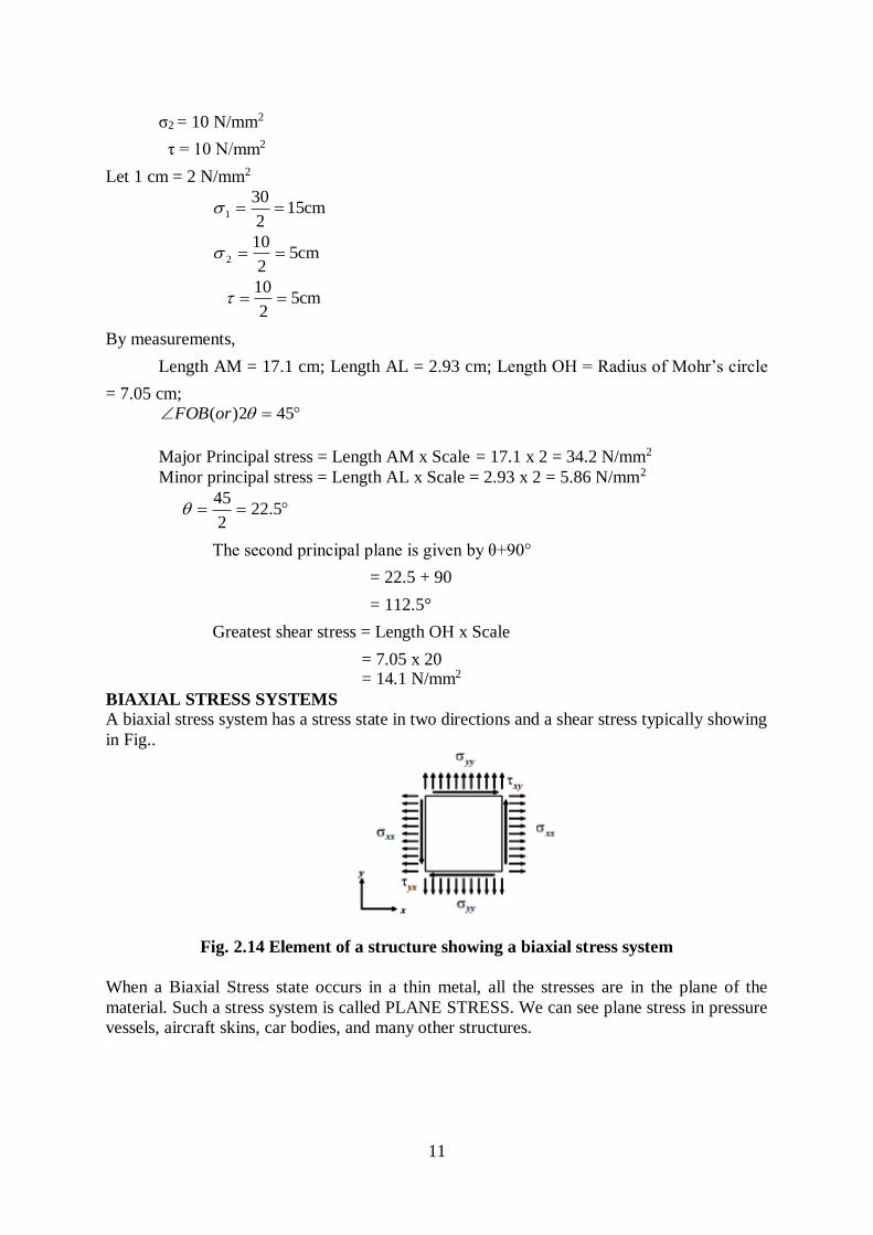
BIAXIAL STRESS SYSTEMS
A biaxial stress system has a stress state in two directions and a shear stress typically showing
in Fig..
Fig. 2.14 Element of a structure showing a biaxial stress system
When a Biaxial Stress state occurs in a thin metal, all the stresses are in the plane of the
material. Such a stress system is called PLANE STRESS. We can see plane stress in pressure
vessels, aircraft skins, car bodies, and many other structures.
12
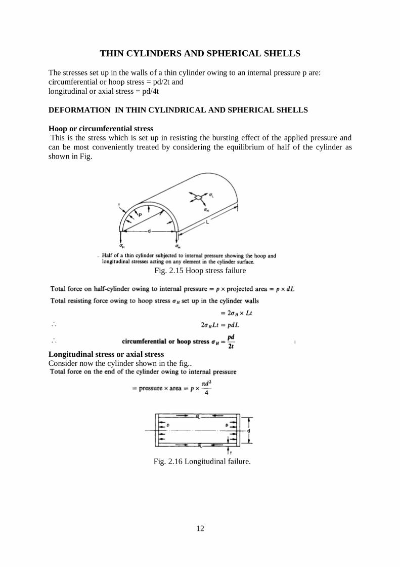
THIN CYLINDERS AND SPHERICAL SHELLS
The stresses set up in the walls of a thin cylinder owing to an internal pressure p are:
circumferential or hoop stress = pd/2t and
longitudinal or axial stress = pd/4t
DEFORMATION IN THIN CYLINDRICAL AND SPHERICAL SHELLS
Hoop or circumferential stress
This is the stress which is set up in resisting the bursting effect of the applied pressure and
can be most conveniently treated by considering the equilibrium of half of the cylinder as
shown in Fig.
Fig. 2.15 Hoop stress failure
Longitudinal stress or axial stress
Consider now the cylinder shown in the fig..
Fig. 2.16 Longitudinal failure.

13
Problem 1
A thin cylindrical pipe of diameter 1.5 mm and thickness 1.5 cm is subjected to an internal
fluid pressure of 1.2 N/mm2. Determine:
i)Longitudinal stress developed in the pipe and
ii)Circumferential stress developed in the pipe.
Solution:
Given:
Dia of pipe d=1.5 m
Thickness, t=1.5 cm = 1.5x10⁻²m
Internal fluid pressure, p=1.2 N/mm2
i) The longitudinal stress is given by
σ =pd/2t
= (1.2x1.5)/(4x1.5x10-2)
=30 N/mm2
ii) The circumferential stress is given by
σ =pd/4t
=(1.2x1.5) / (2x1.5x10-2)
=60 N/mm2
Problem 2
A cylinder of internal diameter 2.5 m and of thickness 5cm contains a gas.If the tensile stress
in the material is not to exceed 80 N/mm2, determine the internal pressure of the gas.
Solution:
Given:
Internal dia of cylinder d=2.5 cm
Thickness of cylinder t= 5cm=5x10⁻²m
Maximum permissible stress =80 N/mm2
As maximum permissible stress is given, hence this should be equal to circumferential stress
σ
σ =80 N/mm2
σ =pd/2t
P=(2t x σ)/d

14
=(2x5x10-2x80) / 2.5
=3.2 N/mm2
Efficiency of a joint
The cylindrical shells are having two types of joints namely longitudinal joint and
circumferential joint.
Let ɳ l = efficiency of a longitudinal joint and
ɳ c = efficiency of a circumferential joint……
the circumferential stress(σ1) is given by,
σ1 = (p x d) / (2t x ɳ l) and
longitudinal stress(σ2) is given by.,
σ2 = (p x d) / (4t x ɳ c)
In longitudinal joint, the circumferential stress is developed whereas in circumferential joint
the longitudinal stress is developed.
Problem 3:
A boiler is subjected to an internal steam pressure of 2 N/mm2, the thickness of a boiler plate
is 2cm and permissible tensile stress is 120 N/mm2 , find out the maximum diameter when
efficiency of longitudinal joint is 90% and that of circumferential joint is 40%.
Solution:
Given
Internal steam pressure, p = 2 N/mm2
Thickness of boiler plate, t =2cm
Permissible tensile stress = 120 N/mm2
In case of a joint, the permissible stress may be circumferential stress or longitudinal
stress.
efficiency of longitudinal joint = ɳ l = 90% = 0.90
efficiency of circumferential joint = ɳ c = 40% = 0.40
max. diameter for circumferential stress is given by,
σ1 = (p x d) /(2t x ɳ l)
where σ1 = given Permissible tensile stress = 120 N/mm2
120 = (2 x d) / (2x 0.90 x2)
d= (120x2x0.9x2) / 2
= 216 cm.
Max.diameter for longitudinal stress is given by,
σ2 = (p x d) / (4t x ɳ c)
where σ2 = given Permissible tensile stress = 120 N/mm2

15
120 = (2 x d) / (4x 0.40 x2)
d= (120x4x0.4x2) / 2
d=192 cm.
the longitudinal or circumferential stresses included in the material are directly
proportional to the diameter (d), and hence stress induced will be less if the value of d
is less. Hence minimum value of d is taken…..so, max.diameter = 192 cm
Effect of internal pressure on the dimensions of a thin cylindrical shell
Then, circumferential strain,
e1 = (σ1 / E) – ( µ σ2 /E)
= (1- µ/2)
and longitudinal strain,
e2 = (σ2 / E) – ( µ σ1 / E)
= (1/2 - µ)
Change in diameter, δd/d = (1- µ/2)

16
Change in length, δL/L = (1/2 - µ)
Change in volume, δV/V = (2e1+ e2)
=V(2 δd/d + δL/L)
Problem 4:
Calculate change in diameter, change in length and change in volume of a thin cylindrical
shell 100cm diameter, 1cm thickness and 5m long when subjected to internal pressure of
3N/mm2, take the value of E = 2 x 10⁵ N/mm2 and poisson’s ratio µ = 0.3
Solution:
Given: diameter of shell, d=100cm
Thickness of shell, t= 1cm
Length of shell, L= 5m= 500cm
Internal pressure, p = 3N/mm2
Young’s modulus, E= 2 x 10⁵ N/mm2
And Poisson’s ratio µ = 0.3
(iii) change in volume δV/V is given by,

17
Thin spherical shells
The figure shows a thin spherical shell of internal diameter d and thickness t and subjected to
internal fluid pressure p , the fluid inside the shell has a tendency to split the shell into two
hemispheres along x-x axis.
Fig. 2.17 Spherical shell
Circumferential or hoop stress(σ1) is given by,
σ1 = pd/4t
circumferential stress when the joint efficiency is given by,
σ1 = pd/4t. ɳ
Problem 5
A vessel in the shape of a spherical shell of 1.20m internal diameter and 12mm shell
thickness is subjected to pressure of 1.6 N/mm2, determine the stress induced in the material
of the vessel.
Solution
Given.
Internal diameter , d = 1.2m = 1200mm
Shell thickness, t = 12mm and
Fluid pressure, p = 1.6 N/mm2
The stress induced in the material of the spherical shell is given by,
σ1 = pd/4t
= (1.6 x 1200) / (4x12)
= 40 N/mm2
Problem 6
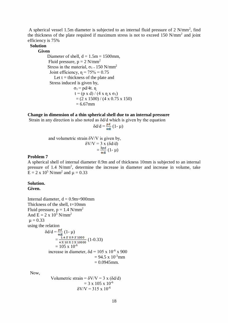
18
A spherical vessel 1.5m diameter is subjected to an internal fluid pressure of 2 N/mm2, find
the thickness of the plate required if maximum stress is not to exceed 150 N/mm2 and joint
efficiency is 75%
Solution
Given
Diameter of shell, d = 1.5m = 1500mm,
Fluid pressure, p = 2 N/mm2
Stress in the material, σ1 = 150 N/mm2
Joint efficiency, ɳ = 75% = 0.75
Let t = thickness of the plate and
Stress induced is given by,
σ1 = pd/4t. ɳ
t = (p x d) / (4 x ɳ x σ1)
= (2 x 1500) / (4 x 0.75 x 150)
= 6.67mm
Change in dimension of a thin spherical shell due to an internal pressure
Strain in any direction is also noted as δd/d which is given by the equation
δd/d = (1- µ)
and volumetric strain δV/V is given by,
δV/V = 3 x (δd/d)
= (1- µ)
Problem 7
A spherical shell of internal diameter 0.9m and of thickness 10mm is subjected to an internal
pressure of 1.4 N/mm2, determine the increase in diameter and increase in volume, take
E = 2 x 10⁵ N/mm2 and µ = 0.33
Solution.
Given.
Internal diameter, d = 0.9m=900mm
Thickness of the shell, t=10mm
Fluid pressure, p = 1.4 N/mm2
And E = 2 x 10⁵ N/mm2
µ = 0.33
using the relation
δd/d = (1- µ)
= (1-0.33)
= 105 x 10-6
increase in diameter, δd = 105 x 10-6 x 900
= 94.5 x 10⁻³mm
= 0.0945mm.
Now,
Volumetric strain = δV/V = 3 x (δd/d)
= 3 x 105 x 10-6
δV/V = 315 x 10-6
19
increase in volume , δV = 315 x 10-6 x V
= 315 x 10-6 x ( π/6 d3)
= 315 x 10-6x (π/6 x 9003)
= 12028.5 mm3
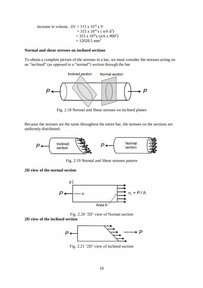
Normal and shear stresses on inclined sections
To obtain a complete picture of the stresses in a bar, we must consider the stresses acting on
an “inclined” (as opposed to a “normal”) section through the bar.
Fig. 2.18 Normal and Shear stresses on inclined planes
Because the stresses are the same throughout the entire bar, the stresses on the sections are
uniformly distributed.
Fig. 2.19 Normal and Shear stresses pattern
2D view of the normal section
Fig. 2.20 ‘2D’ view of Normal section
2D view of the inclined section
Fig. 2.21 ‘2D’ view of inclined section

20
REFERENCE BOOKS
1. Bansal R.K., “Strength of Materials”, Laxmi Publications (P) Ltd.,Fifth Edition,2012
2. Punmia B.C. & Jain A.K., Mechanics of Materials, ,Laxmi Publications,2001
3. Ryder G.H, “Strength of Materials, Macmillan India Ltd”., Third Edition, 2002
4. Ray Hulse, Keith Sherwin & Jack Cain, “Solid Mechanics”, Palgrave ANE Books,2004.
5. Allan F. Bower, Applied Mechanics of Solids, CRC Press, 2009, 820 pages.

1
SCHOOL OF MECHANICAL ENGINEERING
DEPARTMENT OF MECHANICAL ENGINEERING
UNIT – III – BEAMS - LOADS AND STRESSES – SMEA1305
2
MECHANICS OF SOLIDS (SMEA1305)
UNIT 3: BEAMS - LOADS AND STRESSES
Types of beams - Supports and Loads – Shear force and Bending Moment in beams –
Cantilever, Simply supported and Overhanging beams – SFD and BMD for inclined
loads and couples
Stresses in beams – Theory of simple bending – Stress variation along the length and in
the beam section – Effect of shape of beam section on stress induced.
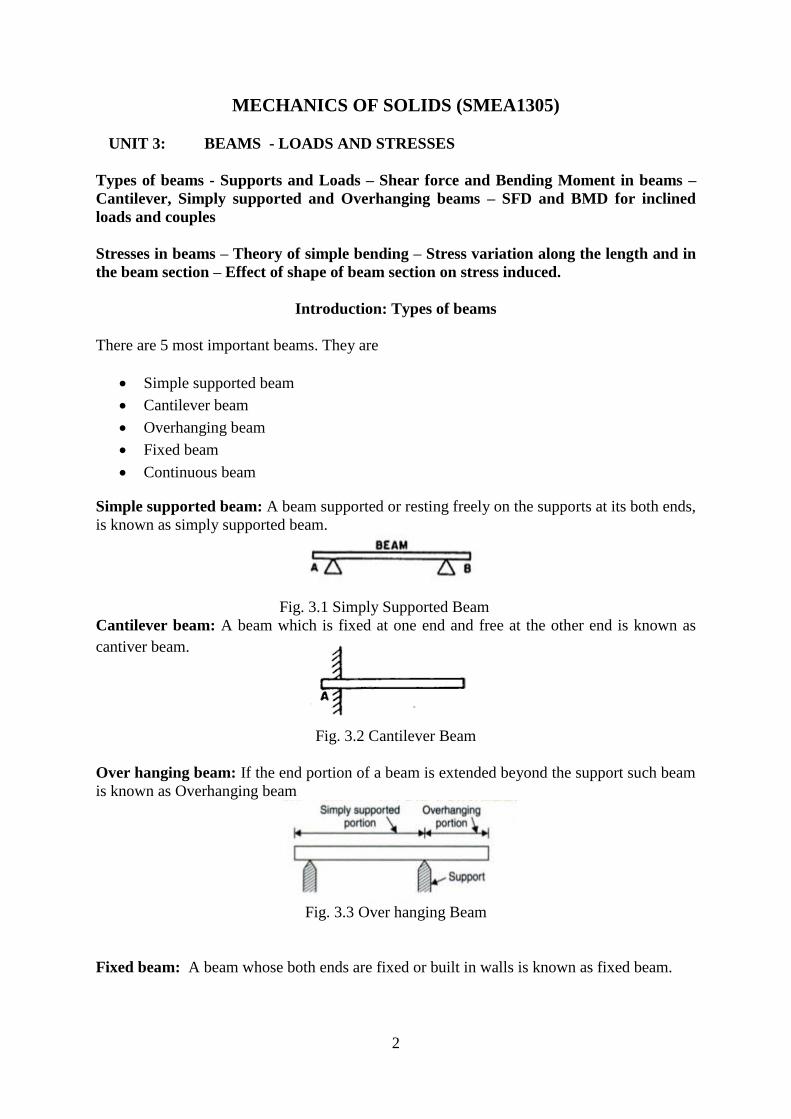
Introduction: Types of beams
There are 5 most important beams. They are
Simple supported beam
Cantilever beam
Overhanging beam
Fixed beam
Continuous beam
Simple supported beam: A beam supported or resting freely on the supports at its both ends,
is known as simply supported beam.
Fig. 3.1 Simply Supported Beam
Cantilever beam: A beam which is fixed at one end and free at the other end is known as
cantiver beam.
Fig. 3.2 Cantilever Beam
Over hanging beam: If the end portion of a beam is extended beyond the support such beam
is known as Overhanging beam
Fig. 3.3 Over hanging Beam
Fixed beam: A beam whose both ends are fixed or built in walls is known as fixed beam.
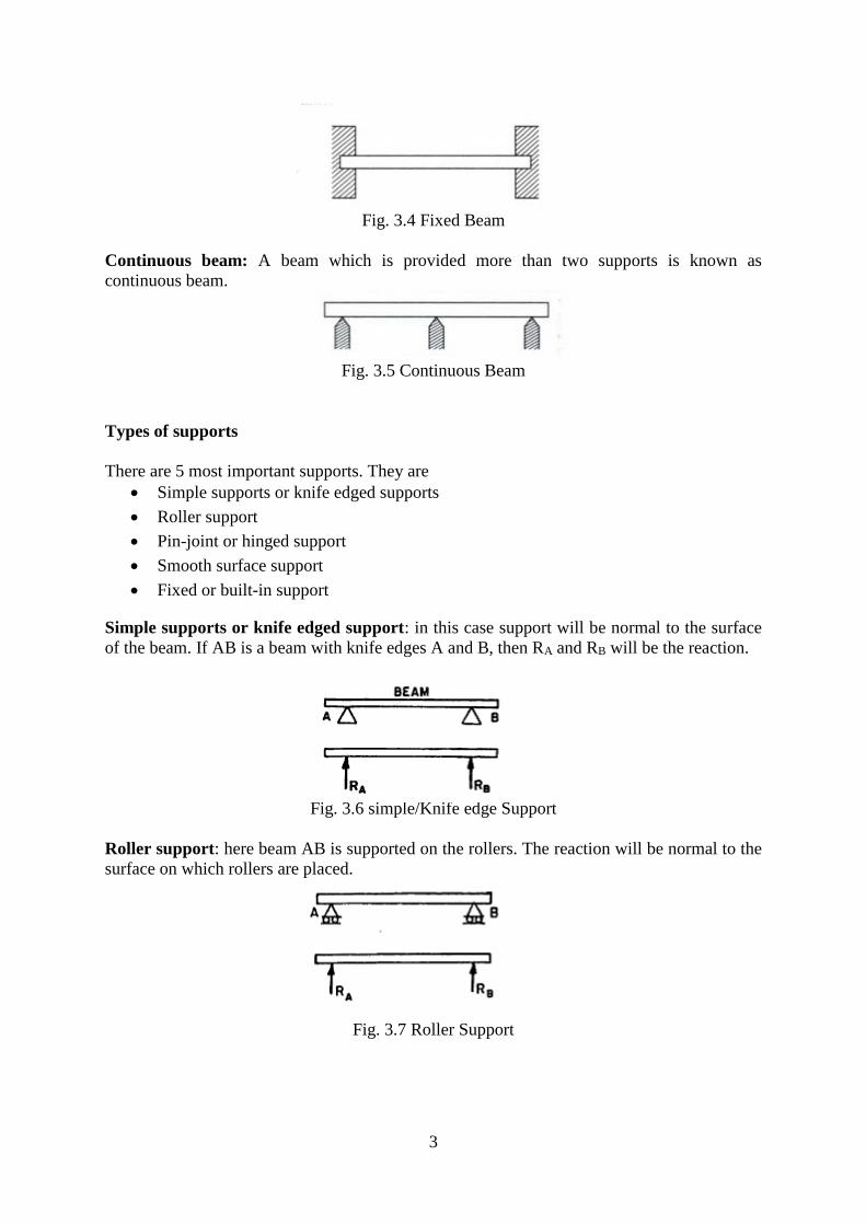
3
Fig. 3.4 Fixed Beam
Continuous beam: A beam which is provided more than two supports is known as
continuous beam.
Fig. 3.5 Continuous Beam
Types of supports
There are 5 most important supports. They are
Simple supports or knife edged supports
Roller support
Pin-joint or hinged support
Smooth surface support
Fixed or built-in support
Simple supports or knife edged support: in this case support will be normal to the surface
of the beam. If AB is a beam with knife edges A and B, then RA and RB will be the reaction.
Fig. 3.6 simple/Knife edge Support
Roller support: here beam AB is supported on the rollers. The reaction will be normal to the
surface on which rollers are placed.
Fig. 3.7 Roller Support

4
Pin joint (or hinged) support: here the beam AB is hinged at point A. the reaction at the
hinged end may be either vertical or inclined depending upon the type of loading. If load is
vertical, then the reaction will also be vertical. But if the load is inclined, then the reaction at
the hinged end will also be inclined.
Fig. 3.8 Hinged Support
Fixed or built-in support: in this type of support the beam should be fixed. The reaction will
be inclined. Also the fixed support will provide a couple.
Types of loading
There are 3 most important type of loading:
Concentrated or point load
Uniformly distributed load
Uniformly varying load
Concentrated or point load: A concentrated load is one which is considered to act at a
point.
Fig. 3.9Concentrated or point load
Uniformly distributed load: A uniformly distributed load is one which is spread over a
beam in such a manner that rate of loading is uniform along the length.
Fig. 3.10 Uniformly distributed load

5
Uniformly varying load: A uniformly varying load is one which is spread over a beam in
such a manner that rate of loading varies from point to point along the beam.
Fig. 3.11 Uniformly varying load
CONCEPT AND SIGNIFICANCE OF SHEAR FORCE AND BENDING MOMENT
SIGN CONVENTIONS FOR SHEAR FORCE AND BENDING MOMENT
(i) Shear force: Fig. 1 shows a simply supported beam AB. carrying a load of 1000 N at
its middle point. The reactions at the supports will be equal to 500 N. Hence RA= RB= 500
N.
Now imagine the beam to be divided into two portions by the section X-X. The resultant of
the load and reaction to the left of X-X is 500 N vertically upwards. And the resultant of the
load and reaction to the right of X-X is (1000↓ -500 ↑= 500↓N) 500 N downwards. The
resultant force acting on any one of the parts normal to the axis of the beam is called the
shear force at the section X-X is 500N.
The shear force at a section will be considered positive when the resultant of the forces to
the left to the section is upwards, or to the right of the section is downwards. Similarly the
shear force at a the section will be considered negative if the resultant of the forces to the left
of the section is downward, or to the right of the section is upwards. Here the resultant force
to the left of the section is upwards and hence the shear force will be positive.
Fig. 3.12 Shear force and Bending Moment Sign Convention
(ii) Bending moment. The bending moment at a section is considered positive if the bending
moment at that section is such that it tends to bend the beam to a curvature having
concavity at the top as shown in Fig. 2. Similarly the bending moment at a section is
considered negative if the bending moment at that section is such that it tends to bend the
beam to a curvature haling convexity at the top. The positive B.M. is often called
sagging moment and negative B.M. as hogging Moment.
6
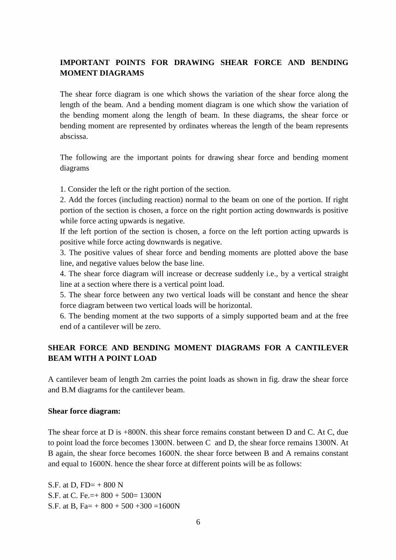
IMPORTANT POINTS FOR DRAWING SHEAR FORCE AND BENDING
MOMENT DIAGRAMS
The shear force diagram is one which shows the variation of the shear force along the
length of the beam. And a bending moment diagram is one which show the variation of
the bending moment along the length of beam. In these diagrams, the shear force or
bending moment are represented by ordinates whereas the length of the beam represents
abscissa.
The following are the important points for drawing shear force and bending moment
diagrams
1. Consider the left or the right portion of the section.
2. Add the forces (including reaction) normal to the beam on one of the portion. If right
portion of the section is chosen, a force on the right portion acting downwards is positive
while force acting upwards is negative.
If the left portion of the section is chosen, a force on the left portion acting upwards is
positive while force acting downwards is negative.
3. The positive values of shear force and bending moments are plotted above the base
line, and negative values below the base line.
4. The shear force diagram will increase or decrease suddenly i.e., by a vertical straight
line at a section where there is a vertical point load.
5. The shear force between any two vertical loads will be constant and hence the shear
force diagram between two vertical loads will be horizontal.
6. The bending moment at the two supports of a simply supported beam and at the free
end of a cantilever will be zero.
SHEAR FORCE AND BENDING MOMENT DIAGRAMS FOR A CANTILEVER
BEAM WITH A POINT LOAD
A cantilever beam of length 2m carries the point loads as shown in fig. draw the shear force
and B.M diagrams for the cantilever beam.
Shear force diagram:
The shear force at D is +800N. this shear force remains constant between D and C. At C, due
to point load the force becomes 1300N. between C and D, the shear force remains 1300N. At
B again, the shear force becomes 1600N. the shear force between B and A remains constant
and equal to 1600N. hence the shear force at different points will be as follows:
S.F. at D, FD= + 800 N
S.F. at C. Fe.=+ 800 + 500= 1300N
S.F. at B, Fa= + 800 + 500 +300 =1600N

7
S.F. at A, FA = + 1600 N.
The shear force, diagram is shown in Fig. which is drawn as: Draw a horizontal line AD as
base line. On the base line mark the points B and C below the point loads. Take the ordinate
DE = 800 N in the upward direction. Draw a line EF parallel to AD. The point F is vertically
above C. Take vertical line FG is 500 N. Through G, draw a horizontal line GH in which
point H is vertically above B. Draw vertical line HI = 300 N. From I, draw a horizontal line
IJ. The point J is vertically above A. This completes the shear force diagram.
Bending Moment Diagram
The bending moment at D is zero:
Fig. 3.13 SF & BM Diagram
(i) The bending moment at any section between C and Data distance: and D is given by,
Mx = - 800 X x which follows a straight line law.
At C, the value of x = 0.8 m. B.M. at C, = - 800 X 0.8 = - 640 Nm.
(ii) The B.M. at any section between B and C at a distance x from D is given by (At C, x
= 0.8 and at B, x = 0.8 + 0.7 = 1.5 m. Hence here varies from 0.8 to 1.5).
Mx = - 800x - 500(x- 0.8)
Bending moment between B and C also varies by a straight line law.
B.M. at B is obtained by substituting x = 1.5 m in equation (i).
MB = -800 X 1.5 - 500 (1.5 - 0.8)
= 1200 – 350 = 1550 Nm.
(iii) The B.M. at any section between A and B at a distance x from D is given by

8
(At B, x = 1.5 and at A, x = 2.0 m. Hence here x varies from 1.5m to 2.0 m
Mx = - 800x - 500 (x - 0.8) – 300 (x- 1.5)
Bending moment between A and B varies by a straight line law.
B.M. at A is obtained by substituting x = 2.0 m in equation (ii),
MA = - 800 X 2 - 500 (2 - 0.8) - 300 (2 - 1.5)
= - 800 X 2 - 500 X 1.2 - 300 X 0.5
= - 1600 - 600 - 160 = - 2350 Nm. Hence the bending moments at different points
will be as given below : MD = 0 Mc = - 640 Nm MB= - 1550 Nm, M A= - 2350 Nm
SHEAR FORCE AND BENDING MOMENT DIAGRAMS FOR A CANTILEVER
BEAM WITH A UNIFORMLY DISTRIBUTED LOAD
A cantilever beam of length 2m carries a uniformly distributed load of 2kN/m length over the
whole length and a point load of 3kN at the free end. draw the shear force and B.M diagrams
for the cantilever beam.
Fig. 3.14 SF & BM Diagram
Shear Force diagram
The shear force at B = 3 kN
Consider any section at a distance x from the free end B. The shear force at the section is
given by.
Fx = 3.0 + w.x ( +ve sign is due to downward force on right portion of the section)
= 3.0 + 2 X x
The above equation shows that shear force follows a straight line law.
At B, x = 0 hence FB = 3.0 kN
At A. x = 2 m hence FA = 3 + 2 x 2 = 7 kN.

9
The shear force diagram is shown in Fig. 6.18 (b), in which FB = BC = 3 kN and FA = AD =
7 kN. The points C and D are joined by a straight line.
Bending Moment Diagram
The bending moment at any section at a distance x from the free end B is given by.
Mx = - ( 3x + wx . x/2)
= - ( 3x + 2x2/2)
= - (3x + x2)
( The bending moment will be negative as for the right portion of the section. the moment of
loads at x is clockwise)
Equation (i) shows that the B. M. varies according to the parabolic law. From equation (i) we
have At B. x = 0 hence MB = -(3x0 + 02) = 0
At A, x = 2 m hence MA = - ( 3 x 2 + 22) = - 10 kN/m
Now the bending moment diagram is drawn In this diagram.
AA' = 10 kNm and points A' and B are joined by a parabolic curve.
SHEAR FORCE AND BENDING MOMENT DIAGRAMS FOR A CANTILEVER
CARRYING A GRADUALLY VARYING LOAD
A cantilever of length 4 m carries a gradually varying load, zero at the free end to 2 Kn/m. at
the fixed end. Draw the S.F. and B.M. diagrams for the cantilever.
Fig. 3.15 SF & BM Diagram
Shear Force Diagram

10
The shear force is zero at B.
The shear force at C will be equal to the area of load diagram ABC.
Shear force at C = (4 x 2) / 2 = 4 kN
The shear force between A and B varies according to parabolic law.
Bending Moment Diagram
The B.M. at B is zero.
The bending moment at A is equal to MA = – w. l2 / 6 = - 2 x 42 / 6 = - 5.33 kNm.
The B.M. between A and B varies according to cubic law.
SHEAR FORCE AND BENDING MOMENT DIAGRAMS FOR A SIMPLY
SUPPORTED BEAM WITH POINT LOAD
A simply supported beam of length 6 m, carries point load of 3 kN and 6 kN at distances of 2
m and 4 m from the left end. Draw the shear force and bending moment diagrams for the
beam.
Sol.
First calculate the reactions RA and RB.
Taking moments of the force about A, we get
RB X 6 = 3 X 2 + 6 X 4 = 30
RB = 30/ 6 = 5 kN
RA = Total load on beam - RB = (3 + 6) – 5 = 4 kN
Fig. 3.16 SF & BM Diagram
Shear Force Diagram
Shear force at A, FA= + RA= + 4 kN
Shear force between A and C is constant and equal to + 4 kN
Shear force at C, Fc = + 4 - 3.0 = + 1 kN
11
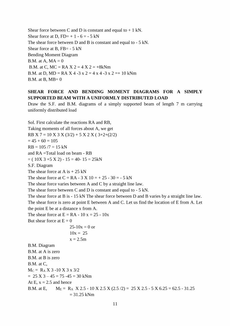
Shear force between C and D is constant and equal to + 1 kN.
Shear force at D, FD= + 1 - 6 = - 5 kN
The shear force between D and B is constant and equal to - 5 kN.
Shear force at B, FB= - 5 kN
Bending Moment Diagram
B.M. at A, MA = 0
B.M. at C, MC = RA X 2 = 4 X 2 = +8kNm
B.M. at D, MD = RA X 4 -3 x 2 = 4 x 4 -3 x 2 =+ 10 kNm
B.M. at B, MB= 0
SHEAR FORCE AND BENDING MOMENT DIAGRAMS FOR A SIMPLY
SUPPORTED BEAM WITH A UNIFORMLY DISTRIBUTED LOAD
Draw the S.F. and B.M. diagrams of a simply supported beam of length 7 m carrying
uniformly distributed load
Sol. First calculate the reactions RA and RB,
Taking moments of all forces about A, we get
RB X 7 = 10 X 3 X (3/2) + 5 X 2 X ( 3+2+(2/2)
= 45 + 60 = 105
RB = 105 /7 = 15 kN
and RA =Total load on beam - RB
= ( 10X 3 +5 X 2) - 15 = 40- 15 = 25kN
S.F. Diagram
The shear force at A is + 25 kN
The shear force at C = RA - 3 X 10 = + 25 - 30 = - 5 kN
The shear force varies between A and C by a straight line law.
The shear force between C and D is constant and equal to - 5 kN.
The shear force at B is - 15 kN The shear force between D and B varies by a straight line law.
The shear force is zero at point E between A and C. Let us find the location of E from A. Let
the point E be at a distance x from A.
The shear force at E = RA - 10 x = 25 - 10x
But shear force at E = 0
25-10x = 0 or
10x = 25
x = 2.5m
B.M. Diagram
B.M. at A is zero
B.M. at B is zero
B.M. at C,
MC = RA X 3 -10 X 3 x 3/2
= 25 X 3 – 45 = 75 -45 = 30 kNm
At E, x = 2.5 and hence
B.M. at E, ME = RA X 2.5 - 10 X 2.5 X (2.5 /2) = 25 X 2.5 - 5 X 6.25 = 62.5 - 31.25
= 31.25 kNm

12
B.M. at D. MD= 25(3 + 2) - 10 X 3 X ((3/2) + 2) = 125 - 105 = 20 kNm
The B.M. between AC and between BD varies according to parabolic law. But B.M. between
C and D varies according to straight line law.
Fig. 3.17 SF & BM Diagram
SHEAR FORCE AND BENDING MOMENT DIAGRAMS FOR OVER HANGING
BEAM
A beam of length 12 m is simply supported at two supports which are 8m apart, with an
overhang of 2 m on each side as shown in Fig. The beam carries a concentrated load of 1000
N at each end. Draw S.F. and B.M. diagrams.
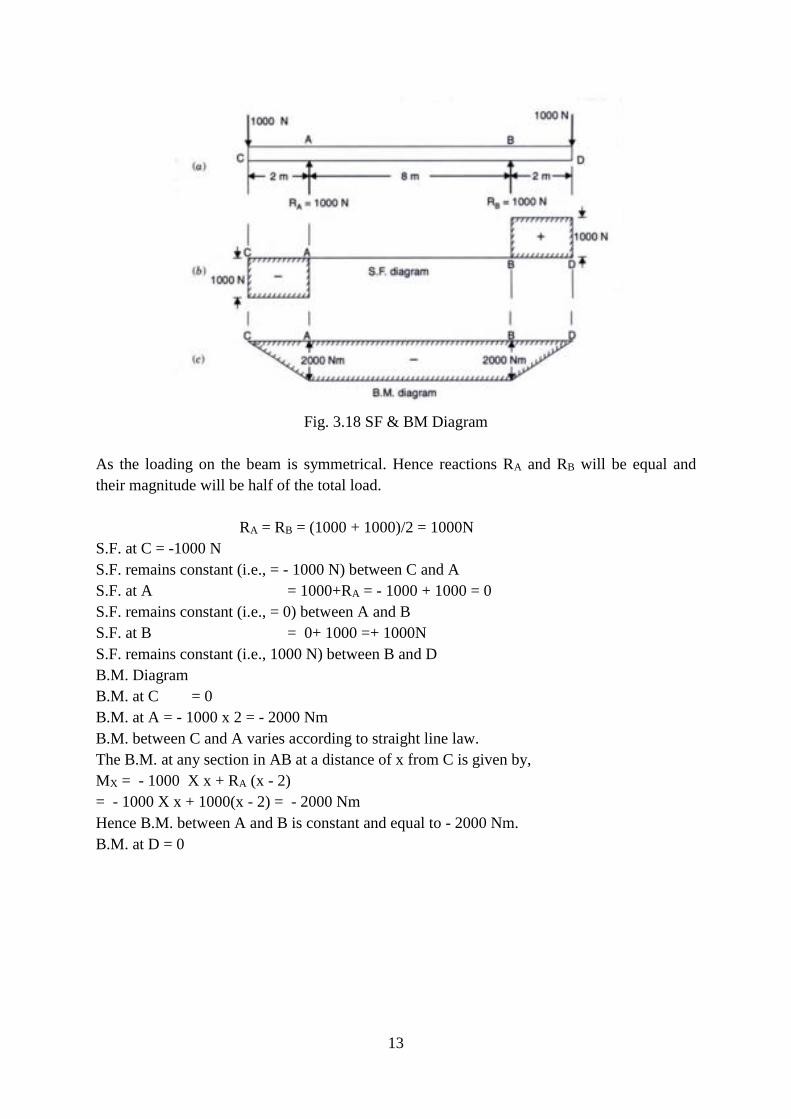
13
Fig. 3.18 SF & BM Diagram
As the loading on the beam is symmetrical. Hence reactions RA and RB will be equal and
their magnitude will be half of the total load.
RA = RB = (1000 + 1000)/2 = 1000N
S.F. at C = -1000 N
S.F. remains constant (i.e., = - 1000 N) between C and A
S.F. at A = 1000+RA = - 1000 + 1000 = 0
S.F. remains constant (i.e., = 0) between A and B
S.F. at B = 0+ 1000 =+ 1000N
S.F. remains constant (i.e., 1000 N) between B and D
B.M. Diagram
B.M. at C = 0
B.M. at A = - 1000 x 2 = - 2000 Nm
B.M. between C and A varies according to straight line law.
The B.M. at any section in AB at a distance of x from C is given by,
MX = - 1000 X x + RA (x - 2)
= - 1000 X x + 1000(x - 2) = - 2000 Nm
Hence B.M. between A and B is constant and equal to - 2000 Nm.
B.M. at D = 0

14
STRESSES IN BEAMS
When some external load acts on a beam, the shear force and bending moments are set up at
all sections of the beam. Due to the shear force and bending moment, the beam undergoes
certain deformation. The material of the beam will offer resistance or stresses against these
deformations. These stresses with certain assumptions can be calculated. The stresses
introduced by bending moment are known as bending stresses.
If a length of a beam is subjected to a constant bending moment and no shear force (i.e., zero
shear force), then the stresses will be set up in that length of the beam due to B.M. only and
that length of the beam is said to be in pure bending or simple bending. The stresses set up in
that length of beam are known as bending stresses.
Fig. 3.19 SF & BM Diagram
A beam simply supported at A and B and overhanging by same length at each support is
shown in Fig. 7.1. A point load W is applied at each end of the overhanging portion. The S.F.
and B.M. for the beam are drawn as shown in Fig. 7.1 (b) and Fig. 7.1 (c) respectively. From
these diagrams, it is clear that there is no shear force between A and B but the B.M. between
A and B is constant. This means that between A and B, the beam is subjected to a constant
bending moment only. This condition of the beam between A and B is known as pure
bending or simple bending.
THEORY OF SIMPLE BENDING
THEORY OF SIMPLE BENDING WITH ASSUMPTIONS MADE
Before discussing the theory of simple bending, let us see the assumptions made in the theory
of simple bending. The following are the important assumptions:
1. The material of the beam is homogeneous* and isotropic**.
2. The value of Young's modulus of elasticity is the same in tension and compression.

15
3. The transverse sections which were plane before bending, remain plane after bending
4. The beam is initially straight and all longitudinal filaments bend into circular arcs with a
common centre of curvature.
5. The radius of curvature is large compared with the dimensions of the cross-section. 6. Each
layer of the beam is free to expand or contract, independently of the layer, above or below it.
A beam subjected to simple bending. Consider a small length fit of this part of beam.
Consider two sections AB and CD which are normal to the axis of the beam N - N. Due to the
action of the bending moment, the part of length &x will be deformed as shown in Fig.(b).
From this figure, it is clear that all the layers of the beam, which were originally of the same
length, do not remain of the same length any more. The top layer such as AC has deformed to
the shape NC. This layer has been shortened in its length. The bottom layer BD has deformed
to the shape B'D'. This layer has been elongated. From the Fig. 7.2 (b), it is clear that some of
the layers have been shortened while some of them are elongated. At a level between the top
and bottom of the beam, there will be a layer which is neither shortened nor elongated. This
layer is known as neutral layer or neutral surface. This layer in Fig.(b) is shown by N' — N'
and in Fig.(a) by N — N. The line of intersection of the neutral layer on a cross-section of a
beam is known as neutral axis (written as N.A.).
Fig. 3.20 Before and after Bending of Beam
The layers above N — N (or N' — N') have been shortened and those below, have been
elongated. Due to the decrease in lengths of the layers above N— N, these layers will be
subjected to compressive stresses. Due to the increase in the lengths of layers below N — N,
these layers will be subjected to tensile stresses. We also see that the top layer has been
shortened maximum. As we proceed towards the layer N— N, the decrease in length of the
layers decreases. At the layer N— N, there is no change in length. This means the
compressive stress will be maximum at the top layer. Similarly the increase in length will be
maximum at the bottom layer. As we proceed from bottom layer towards the layer N — N,
the increase in length of layers decreases. Hence the amount by which a layer increases or
decreases in length, depends upon the position of the layer with respect to N - N. This theory
of bending is known as theory of simple bending.
Simple Bending Theory OR Theory of Flexure for Initially Straight Beams
(The normal stress due to bending are called flexure stresses)

16
Preamble:
When a beam having an arbitrary cross section is subjected to a transverse loads the beam
will bend. In addition to bending the other effects such as twisting and buckling may occur,
and to investigate a problem that includes all the combined effects of bending, twisting and
buckling could become a complicated one. Thus we are interested to investigate the bending
effects alone, in order to do so; we have to put certain constraints on the geometry of the
beam and the manner of loading.
Assumptions: The constraints put on the geometry would form the assumptions:
1. Beam is initially straight, and has a constant cross-section.
2. Beam is made of homogeneous material and the beam has a longitudinal plane of
symmetry. 3. Resultant of the applied loads lies in the plane of symmetry.
4. The geometry of the overall member is such that bending not buckling is the primary cause
of failure.
5. Elastic limit is nowhere exceeded and ‘E' is same in tension and compression.
6. Plane cross - sections remains plane before and after bending.
Fig. 3.21 Before and after Bending to an arc
Let us consider a beam initially unstressed as shown in fig 1(a). Now the beam is subjected to
a constant bending moment (i.e. „Zero Shearing Force') along its length as would be obtained
by applying equal couples at each end. The beam will bend to the radius R as shown in Fig
1(b)
As a result of this bending, the top fibers of the beam will be subjected to tension and the
bottom to compression it is reasonable to suppose, therefore, that somewhere between the
two there are points at which the stress is zero. The locus of all such points is known as
neutral axis. The radius of curvature R is then measured to this axis. For symmetrical
sections the N. A. is the axis of symmetry but whatever the section N. A. will always pass
through the centre of the area or centroid.
The above restrictions have been taken so as to eliminate the possibility of 'twisting' of
the beam.

17
Concept of pure bending: Loading restrictions:
As we are aware of the fact internal reactions developed on any cross-section of a beam may
consists of a resultant normal force, a resultant shear force and a resultant couple. In order to
ensure that the bending effects alone are investigated, we shall put a constraint on the loading
such that the resultant normal and the resultant shear forces are zero on any cross-section
perpendicular to the longitudinal axis of the member,
That means F = 0
Since or M = constant.
Thus, the zero shear force means that the bending moment is constant or the bending is same
at every cross-section of the beam. Such a situation may be visualized or envisaged when the
beam
Fig.3.22 Plane of Bending
When a member is loaded in such a fashion it is said to be in pure bending. The
examples of pure bending have been indicated in EX 1and EX 2 as shown below:
Fig. 3.23 Pure bending State for SSB

18
Fig. 3.24 Pure bending State for Cantilever
When a beam is subjected to pure bending are loaded by the couples at the ends, certain
cross-section gets deformed and we shall have to make out the conclusion that,
1. Plane sections originally perpendicular to longitudinal axis of the beam remain plane and
perpendicular to the longitudinal axis even after bending , i.e. the cross-section A'E', B'F' (
refer Fig 1(a) ) do not get warped or curved.
2. In the deformed section, the planes of this cross-section have a common intersection i.e.
any time originally parallel to the longitudinal axis of the beam becomes an arc of circle.
Fig. 3.25 Position of Neutral Surface/Axis
We know that when a beam is under bending the fibers at the top will be lengthened while at
the bottom will be shortened provided the bending moment M acts at the ends. In between
these there are some fibers which remain unchanged in length that is they are not strained,
that is they do not carry any stress. The plane containing such fibers is called neutral
surface.The line of intersection between the neutral surface and the transverse exploratory
section is called the neutral axis Neutral axis (N A).
.
Bending Stresses in Beams or Derivation of Elastic Flexural formula :
In order to compute the value of bending stresses developed in a loaded beam, let us consider
the two cross-sections of a beam HE and GF , originally parallel as shown in fig 1(a).when
the beam is to bend it is assumed that these sections remain parallel i.e. H'E' and G'F' , the
final position of the sections, are still straight lines, they then subtend some angle q.
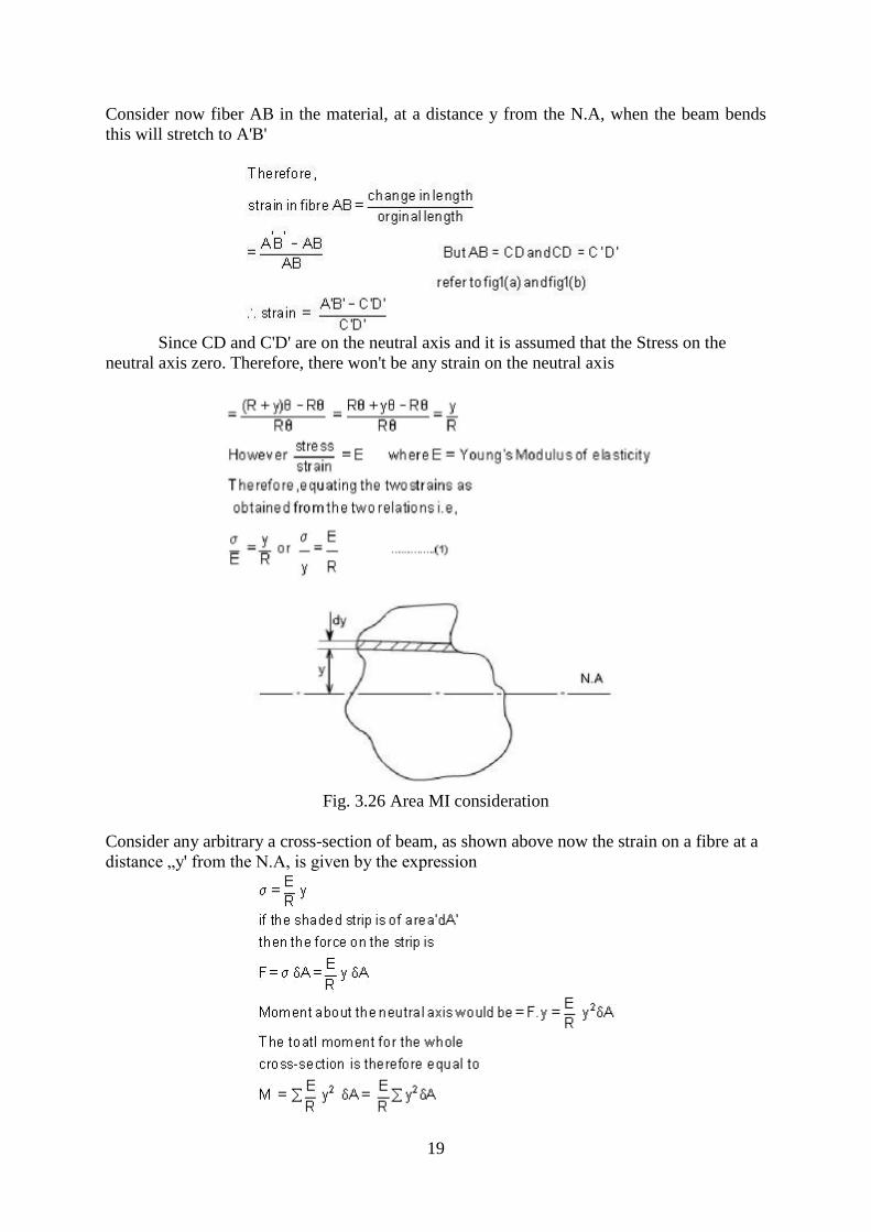
19
Consider now fiber AB in the material, at a distance y from the N.A, when the beam bends
this will stretch to A'B'
Since CD and C'D' are on the neutral axis and it is assumed that the Stress on the
neutral axis zero. Therefore, there won't be any strain on the neutral axis
Fig. 3.26 Area MI consideration
Consider any arbitrary a cross-section of beam, as shown above now the strain on a fibre at a
distance „y' from the N.A, is given by the expression

20
Now the term is the property of the material and is called as a second moment of area of the
cross-section and is denoted by a symbol I.
Therefore
This equation is known as the Bending Theory Equation.
The above proof has involved the assumption of pure bending without any shear force being
present. Therefore this termed as the pure bending equation. This equation gives distribution
of stresses which are normal to cross-section i.e. in x-direction.
Section Modulus:
From simple bending theory equation, the maximum stress obtained in any cross-section is
given as
For any given allowable stress the maximum moment which can be accepted by a particular
shape of cross-section is therefore
For ready comparison of the strength of various beam cross-section this relationship is
sometimes written in the form
Is termed as section modulus
STRESSES IN BEAMS
In previous chapter concern was with shear forces and bending moment in beams. Focus in
this chapter is on the stresses and strains associated with those shear forces and bending
moments.
Loads on a beam will cause it to bend or flex.
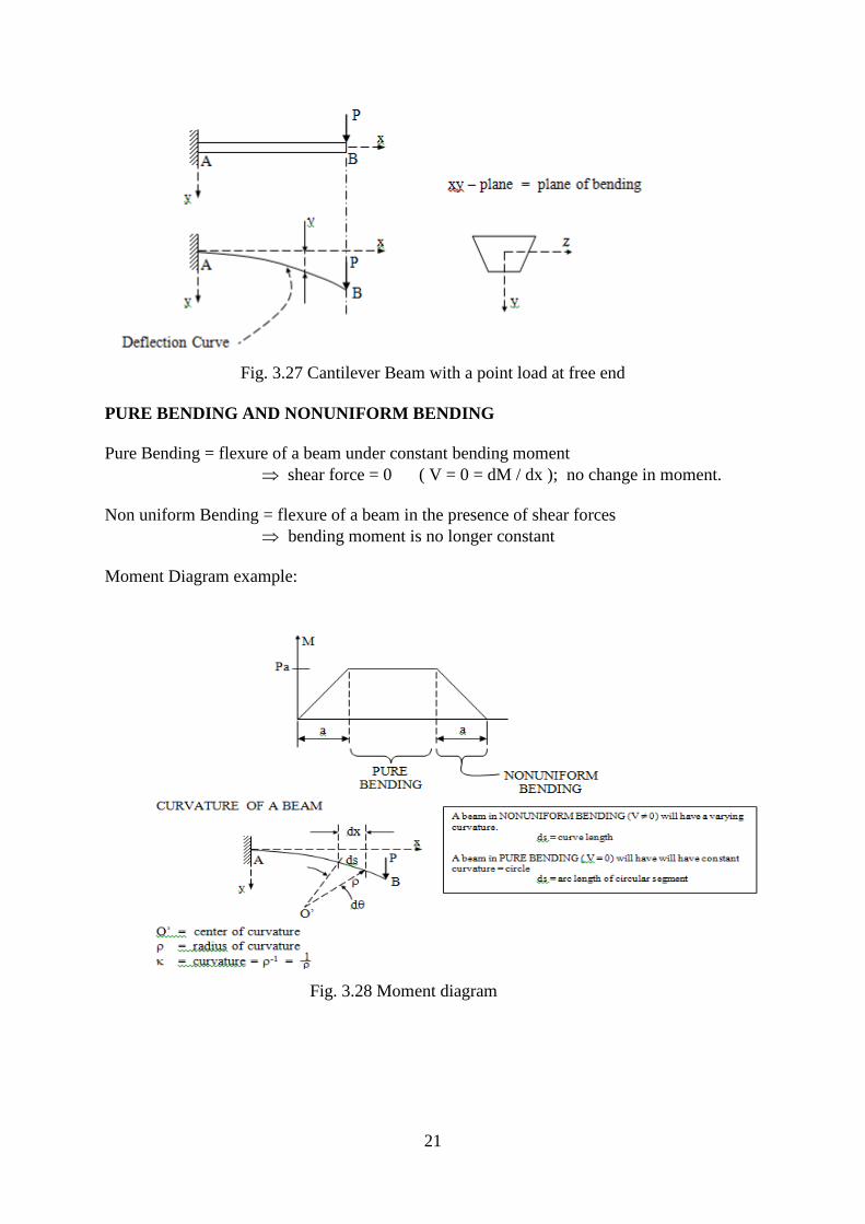
21
Fig. 3.27 Cantilever Beam with a point load at free end
PURE BENDING AND NONUNIFORM BENDING
Pure Bending = flexure of a beam under constant bending moment
shear force = 0 ( V = 0 = dM / dx ); no change in moment.
Non uniform Bending = flexure of a beam in the presence of shear forces
bending moment is no longer constant
Moment Diagram example:
Fig. 3.28 Moment diagram

22
d = ds
For small deflections: ds dx
dx
d
1 (1)
Fig. 3.29 Sign Convention
Somewhere between the top and bottom of the beam is a place where the fibers are neither in
tension or compression.
Neutral axis of the cross section
Fig. 3.30 Neutral Axis and Neutral Layer
dashed line = neutral surface of the beam
when bent: a b lengthens
c d shortens causes normal strains, x

23
The normal strain is: yy
x
___________________ ( 2 )
Where, y = distance from neutral axis
From Eqn ( 2 ):
- y = + εx (elongation)
for +
+ y = - εx (shortening)
Transverse Strains: yxz
Where = Poisson’s Ratio
NORMAL STRESSES IN BEAMS
If material is elastic with linear stress-strain diagram, THEN:
= E (Hooke’s Law)
x = Ex = - Ey ____________ ( 3 )
Where x is longitudinal axis of beam and is the normal stresses in this direction acting on
the cross section. These stresses varies linearly with the distance y from the neutral surface.
Fig. 3.31 Stress Distribution Diagram
0dAyEdAx
0dAy ( 4 )
Eqn ( 4 ) is the 1st Moment of the Area of the cross section w.r.t. z-axis and it is zero
varies
linearly
with y
x
+ y
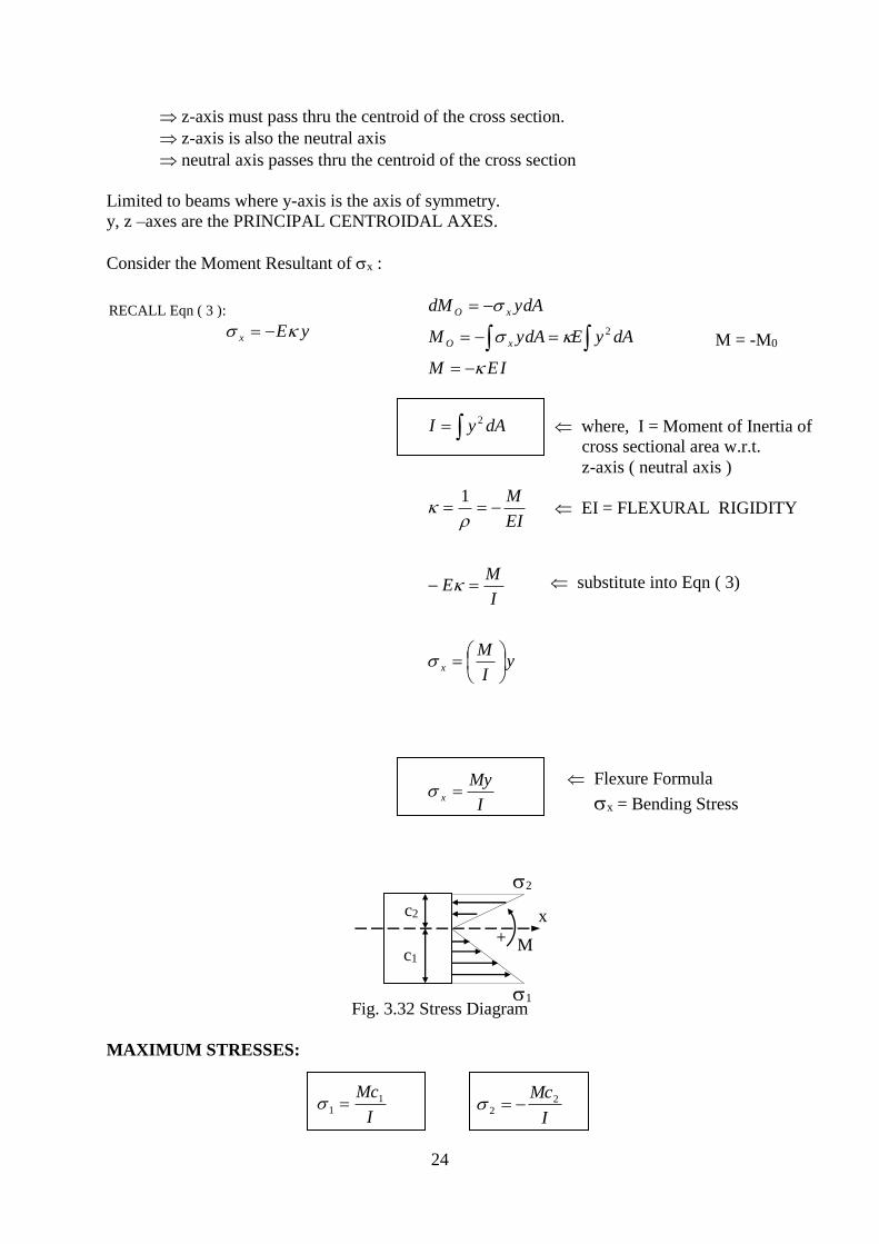
24
z-axis must pass thru the centroid of the cross section.
z-axis is also the neutral axis
neutral axis passes thru the centroid of the cross section
Limited to beams where y-axis is the axis of symmetry.
y, z –axes are the PRINCIPAL CENTROIDAL AXES.
Consider the Moment Resultant of x :
dAyI
IEM
dAyEdAyM
dAydM
xO
xO
2
2
yI
M
I
ME
EI
M
x
1
I
Myx
Fig. 3.32 Stress Diagram
MAXIMUM STRESSES:
I
Mc11
I
Mc22
where, I = Moment of Inertia of
cross sectional area w.r.t.
z-axis ( neutral axis )
EI = FLEXURAL RIGIDITY
Flexure Formula
x = Bending Stress
x
M
c2
c1 +
2
1
RECALL Eqn ( 3 ):
yEx
M = -M0
substitute into Eqn ( 3)
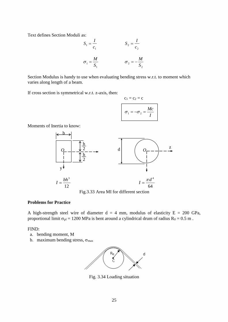
25
Text defines Section Moduli as:
1
1c
IS
2
2c
IS
1
1S
M
2
2S
M
Section Modulus is handy to use when evaluating bending stress w.r.t. to moment which
varies along length of a beam.
If cross section is symmetrical w.r.t. z-axis, then:
c1 = c2 = c
I
Mc 21
Moments of Inertia to know:
12
3bhI
64
4dI
Fig.3.33 Area MI for different section
Problems for Practice
A high-strength steel wire of diameter d = 4 mm, modulus of elasticity E = 200 GPa,
proportional limit pl = 1200 MPa is bent around a cylindrical drum of radius R0 = 0.5 m .
FIND:
a. bending moment, M
b. maximum bending stress, max
Fig. 3.34 Loading situation
y
b
h 2
h 2
O z
O d
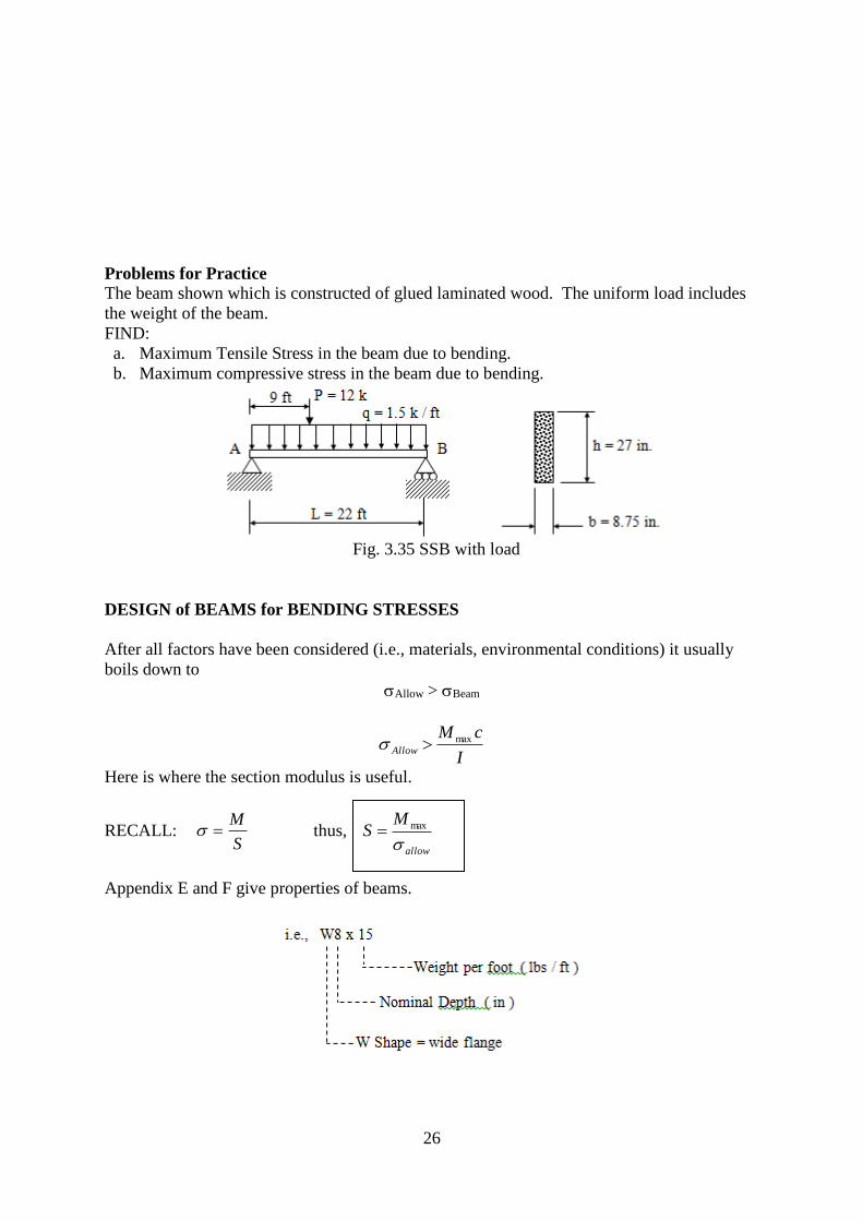
26
Problems for Practice
The beam shown which is constructed of glued laminated wood. The uniform load includes
the weight of the beam.
FIND:
a. Maximum Tensile Stress in the beam due to bending.
b. Maximum compressive stress in the beam due to bending.
Fig. 3.35 SSB with load
DESIGN of BEAMS for BENDING STRESSES
After all factors have been considered (i.e., materials, environmental conditions) it usually
boils down to
Allow > Beam
I
cMAllow
max
Here is where the section modulus is useful.
RECALL: S
M thus,
allow
MS
max
Appendix E and F give properties of beams.

27
Fig. 3.36 I Section considerations
Wood Beams - 2 x 4 really is: 1.5” x 3.5” net dimensions (should always use net
dims.)
For W Shapes; S ≈ 0.35 Ah
You want as much material as possible, as far from the neutral axis as possible because this is
where the greatest stress is occurring.
However, you have to be careful because if the web is too thin, it could fail by:
1.) being overstressed in shear
2.) buckling
TEXT/ REFERENCE BOOKS
1. Bansal R.K., “Strength of Materials”, Laxmi Publications (P) Ltd.,Fifth Edition,2012
2. Punmia B.C. & Jain A.K., Mechanics of Materials, ,Laxmi Publications,2001
3. Ryder G.H, “Strength of Materials, Macmillan India Ltd”., Third Edition, 2002
4. Ray Hulse, Keith Sherwin & Jack Cain, “Solid Mechanics”, Palgrave ANE Books,2004.
5. Allan F. Bower, Applied Mechanics of Solids, CRC Press, 2009, 820 pages.

SCHOOL OF MECHANICAL ENGINEERING
DEPARTMENT OF MECHANICAL ENGINEERING
UNIT – IV – TORSION – SMEA1305
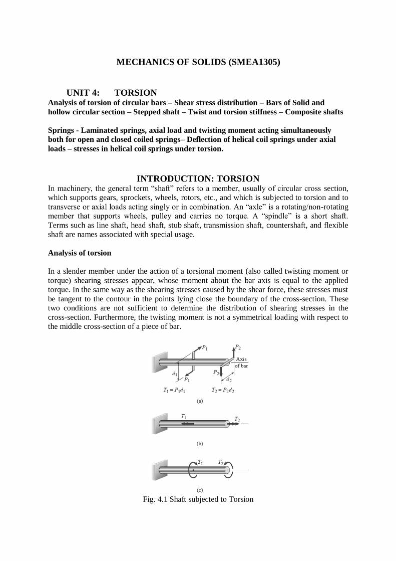
MECHANICS OF SOLIDS (SMEA1305)
UNIT 4: TORSION
Analysis of torsion of circular bars – Shear stress distribution – Bars of Solid and
hollow circular section – Stepped shaft – Twist and torsion stiffness – Composite shafts
Springs - Laminated springs, axial load and twisting moment acting simultaneously
both for open and closed coiled springs– Deflection of helical coil springs under axial
loads – stresses in helical coil springs under torsion.
INTRODUCTION: TORSION In machinery, the general term “shaft” refers to a member, usually of circular cross section,
which supports gears, sprockets, wheels, rotors, etc., and which is subjected to torsion and to
transverse or axial loads acting singly or in combination. An “axle” is a rotating/non-rotating
member that supports wheels, pulley and carries no torque. A “spindle” is a short shaft.
Terms such as line shaft, head shaft, stub shaft, transmission shaft, countershaft, and flexible
shaft are names associated with special usage.
Analysis of torsion
In a slender member under the action of a torsional moment (also called twisting moment or
torque) shearing stresses appear, whose moment about the bar axis is equal to the applied
torque. In the same way as the shearing stresses caused by the shear force, these stresses must
be tangent to the contour in the points lying close the boundary of the cross-section. These
two conditions are not sufficient to determine the distribution of shearing stresses in the
cross-section. Furthermore, the twisting moment is not a symmetrical loading with respect to
the middle cross-section of a piece of bar.
Fig. 4.1 Shaft subjected to Torsion

An idealized case of torsional loading is a straight bar supported at one end and loaded by
two pairs of equal and opposite forces. The first pair consists of the forces P1 acting near the
midpoint of the bar and the second pair consists of the forces P2 acting at the end. Each pair
of forces forms a couple that tends to twist the bar about its longitudinal axis. As we know
from statics, the moment of a couple is equal to the product of one of the forces and the
perpendicular distance between the lines of action of the forces; thus, the first couple has a
moment T1 = P1d1 and the second has a moment T2 = P2d2.
Torsion refers to the twisting of a straight bar when it is loaded by moments (or torques) that
tends to produce rotation about the longitudinal axis of the bar. For instance, when you turn a
screwdriver, your hand applies a torque T to the handle and twists the shank of the
screwdriver. Other examples of bars in torsion are drive shafts in automobiles, axles,
propeller shafts, steering rods, and drill bits.
The moment of a couple may be represented by a vector in the form of a double-headed
arrow. The arrow is perpendicular to the plane containing the couple, and therefore in this
case both arrows are parallel to the axis of the bar. The direction (or sense) of the moment is
indicated by the right-hand rule for moment vectors—namely, using your right hand, let your
fingers curl in the direction of the moment, and then your thumb will point in the direction of
the vector. An alternative representation of a moment is curved arrow acting in the direction
of rotation. The choice depends upon convenience and personal preference. Moments that
produce twisting of a bar, such as the moments T1 and T2, are called torques or twisting
moments. Cylindrical members that are subjected to torques and transmit power through
rotation are called shafts; for instance, the drive shaft of an automobile or the propeller shaft
of a ship. Most shafts have circular cross sections, either solid or tubular. In this chapter we
begin by developing formulas for the deformations and stresses in circular bars subjected to
torsion. We then analyze the state of stress known as pure shear and obtain the relationship
between the moduli of elasticity E and G in tension and shear, respectively. Next, we analyze
rotating shafts and determine the power they transmit. Finally, we cover several additional
topics related to torsion, namely, statically indeterminate members, strain energy, thin-walled
tubes of noncircular cross section, and stress concentrations.
Torsional deformations of a circular bar
A prismatic bar with a circular cross-section has a symmetrical geometry with respect to any
plane passing through the bar axis. If, in addition, the material also has symmetrical
rheological properties with respect to these planes, which happens if the material is isotropic
or monotropic with the monotropy direction parallel to the bar axis, the bar is totally
symmetric with respect to the bar axis, i.e., it is axisymmetric. As a consequence of this type
of symmetry, all the points of a cross-section lying on a circumference with the centre in the
bar axis, are in the same conditions with respect to the centre of the cross-section. If we
consider a vector applied at the centre of the cross-section, representing the torque acting on
the bar, all the points of that circumference are also in the same conditions with respect to
that vector. As a consequence, all the points will undergo the same displacement in relation to
the bar axis, i.e., the radial, circumferential and longitudinal components of the displacement
will be the same in all points of the circumference. This means that the circumference will
remain on a plane perpendicular to the bar axis and that its centre will remain on that axis.
The shear strains in a circular bar in torsion, we are ready to determine the directions and
magnitudes of the corresponding shear stresses. The directions of the stresses can be
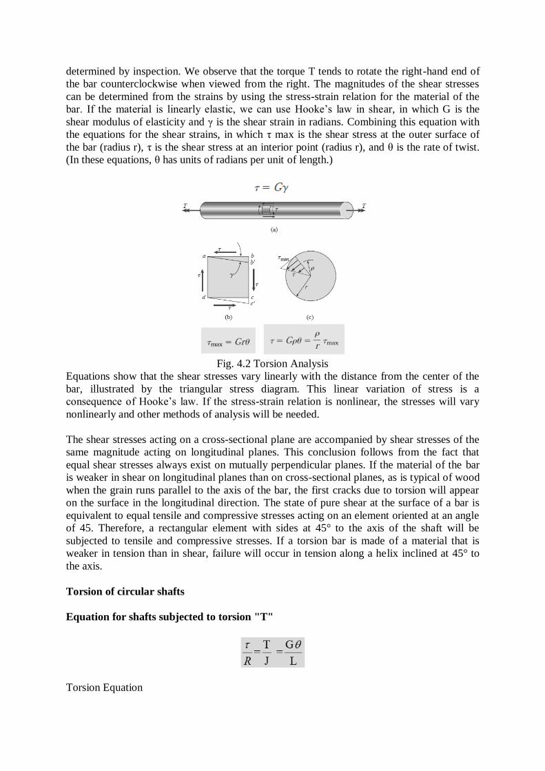
determined by inspection. We observe that the torque T tends to rotate the right-hand end of
the bar counterclockwise when viewed from the right. The magnitudes of the shear stresses
can be determined from the strains by using the stress-strain relation for the material of the
bar. If the material is linearly elastic, we can use Hooke’s law in shear, in which G is the
shear modulus of elasticity and γ is the shear strain in radians. Combining this equation with
the equations for the shear strains, in which τ max is the shear stress at the outer surface of
the bar (radius r), τ is the shear stress at an interior point (radius r), and θ is the rate of twist.
(In these equations, θ has units of radians per unit of length.)
Fig. 4.2 Torsion Analysis
Equations show that the shear stresses vary linearly with the distance from the center of the
bar, illustrated by the triangular stress diagram. This linear variation of stress is a
consequence of Hooke’s law. If the stress-strain relation is nonlinear, the stresses will vary
nonlinearly and other methods of analysis will be needed.
The shear stresses acting on a cross-sectional plane are accompanied by shear stresses of the
same magnitude acting on longitudinal planes. This conclusion follows from the fact that
equal shear stresses always exist on mutually perpendicular planes. If the material of the bar
is weaker in shear on longitudinal planes than on cross-sectional planes, as is typical of wood
when the grain runs parallel to the axis of the bar, the first cracks due to torsion will appear
on the surface in the longitudinal direction. The state of pure shear at the surface of a bar is
equivalent to equal tensile and compressive stresses acting on an element oriented at an angle
of 45. Therefore, a rectangular element with sides at 45° to the axis of the shaft will be
subjected to tensile and compressive stresses. If a torsion bar is made of a material that is
weaker in tension than in shear, failure will occur in tension along a helix inclined at 45° to
the axis.
Torsion of circular shafts
Equation for shafts subjected to torsion "T"
Torsion Equation
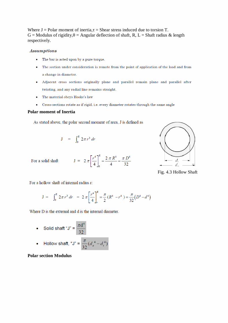
Where J = Polar moment of inertia,τ = Shear stress induced due to torsion T.
G = Modulus of rigidity,θ = Angular deflection of shaft, R, L = Shaft radius & length
respectively.
Polar moment of Inertia
Fig. 4.3 Hollow Shaft
Polar section Modulus

Polar Moment of Inertia and Section Modulus.
The polar moment of inertia, J, of a cross-section with respect to a polar axis, that is, an axis
at right angles to the plane of the cross-section, is defined as the moment of inertia of the
cross-section with respect to the point of intersection of the axis and the plane. The polar
moment of inertia may be found by taking the sum of the moments of inertia about two
perpendicular axes lying in the plane of the cross-section and passing through this point.
Thus, for example, the polar moment of inertia of a circular or a square area with respect to a
polar axis through the center of gravity is equal to two times the moment of inertia with
respect to an axis lying in the plane of the cross-section and passing through the center of
gravity. The polar moment of inertia with respect to a polar axis through the center of gravity
is required for problems involving the torsional strength of shafts since this axis is usually the
axis about which twisting of the shaft takes place.
The polar section modulus
(also called section modulus of torsion), Zp, for circular sections may be found by dividing
the polar moment of inertia, J, by the distance c from the center of gravity to the most remote
fiber. This method may be used to find the approximate value of the polar section modulus of
sections that are nearly round. For other than circular cross-sections, however, the polar
section modulus does not equal the polar moment of inertia divided by the distance c.
Power Transmission
Safe diameter of a shaft (d)

In Twisting
Problems on Solid and hollow circular section
1. What torque, applied to a hollow circular shaft of 25 cm outside diameter and 17.5 cm
inside
diameter will produce a maximum shearing stress of 75 MN/m2 in the material.
2. A ship's propeller shaft has external and internal diameters of 25 cm and 15 cm. What
power can be
transmitted at 1 10 rev/minute with a maximum shearing stress of 75 MN/m2, and what
will then
be the twist in degrees of a 10 m length of the shaft? G = 80 GN/m2

3. A solid circular shaft of 25 cm diameter is to be replaced by a hollow shaft, the ratio of the
external to internal diameters being 2 to 1. Find the size of the hollow shaft if the maximum
shearing stress is to be the same as for the solid shaft. What percentage economy in mass will
this change effect?

4. A ship's propeller shaft transmits 7.5 x 10⁶ W at 240 rev/min. The shaft has an internal
diameter of 15 cm. Calculate the minimum permissible external diameter if the shearing
stress in the shaft is to be limited to 150 MN/m2.
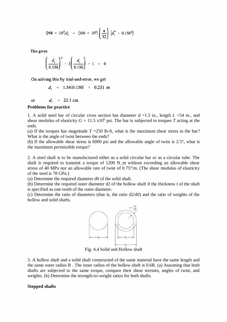
Problems for practice
1. A solid steel bar of circular cross section has diameter d =1.5 in., length L =54 in., and
shear modulus of elasticity G = 11.5 x10⁶ psi. The bar is subjected to torques T acting at the
ends.
(a) If the torques has magnitude T =250 lb-ft, what is the maximum shear stress in the bar?
What is the angle of twist between the ends?
(b) If the allowable shear stress is 6000 psi and the allowable angle of twist is 2.5°, what is
the maximum permissible torque?
2. A steel shaft is to be manufactured either as a solid circular bar or as a circular tube. The
shaft is required to transmit a torque of 1200 N_m without exceeding an allowable shear
stress of 40 MPa nor an allowable rate of twist of 0.75°/m. (The shear modulus of elasticity
of the steel is 78 GPa.)
(a) Determine the required diameter d0 of the solid shaft.
(b) Determine the required outer diameter d2 of the hollow shaft if the thickness t of the shaft
is specified as one-tenth of the outer diameter.
(c) Determine the ratio of diameters (that is, the ratio d2/d0) and the ratio of weights of the
hollow and solid shafts.
Fig. 4.4 Solid and Hollow shaft
3. A hollow shaft and a solid shaft constructed of the same material have the same length and
the same outer radius R . The inner radius of the hollow shaft is 0.6R. (a) Assuming that both
shafts are subjected to the same torque, compare their shear stresses, angles of twist, and
weights. (b) Determine the strength-to-weight ratios for both shafts.
Stepped shafts

When a shaft is made of different lengths and of different diameters, it is termed as shaft as
varying cross section. For such a shaft, the torque induced in its individual sections should be
calculated first. The strength of the shaft is the minimum of all these torques.
Problems
A stepped shaft has the appearance as shown in figure. The region AB is aluminum, having G
= 28 GPa, and the region BC is steel, having G = 84 GPa. The aluminum portion is of solid
circular cross section 45 mm in diameter, and the steel region is circular with 60-mm outside
diameter and 30-mm inside diameter. Determine the maximum shearing stress in each
material as well as the angle of twist at B where a torsional load of 4000 N - m is applied.
Ends A and C are rigidly clamped.
SOLUTION: The free-body diagram of the system is shown. The applied load of 4000 N-m
as well as the unknown end reactive torques are as indicated. The only equation of static
equilibrium is
Fig. 4.5 Stepped shaft subjected to Torque
Since there are two unknowns TL and TR, another equation (based upon deformations) is
required. This is set up by realizing that the angular rotation at B is the same if we determine
it at the right end of AB or the left end of BC. We thus have
Problems for practice
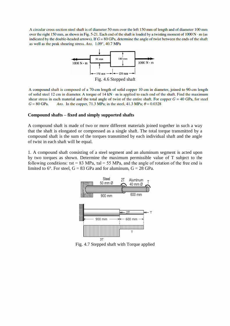
Fig. 4.6 Stepped shaft
Compound shafts – fixed and simply supported shafts
A compound shaft is made of two or more different materials joined together in such a way
that the shaft is elongated or compressed as a single shaft. The total torque transmitted by a
compound shaft is the sum of the torques transmitted by each individual shaft and the angle
of twist in each shaft will be equal.
1. A compound shaft consisting of a steel segment and an aluminum segment is acted upon
by two torques as shown. Determine the maximum permissible value of T subject to the
following conditions: τst = 83 MPa, τal = 55 MPa, and the angle of rotation of the free end is
limited to 6°. For steel, G = 83 GPa and for aluminum, G = 28 GPa.
Fig. 4.7 Stepped shaft with Torque applied

2. The compound shaft shown is attached to rigid supports. For the bronze segment AB, the
diameter is 75 mm, τ ≤ 60 MPa, and G = 35 GPa. For the steel segment BC, the diameter is
50 mm, τ ≤ 80 MPa, and G = 83 GPa. If a = 2 m and b = 1.5 m, compute the maximum torque
T that can be applied.
Fig. 4.8 Stepped shaft with Torque
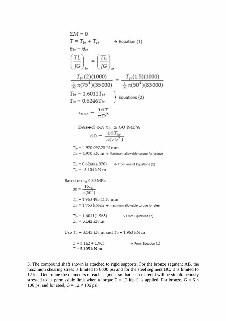
3. The compound shaft shown is attached to rigid supports. For the bronze segment AB, the
maximum shearing stress is limited to 8000 psi and for the steel segment BC, it is limited to
12 ksi. Determine the diameters of each segment so that each material will be simultaneously
stressed to its permissible limit when a torque T = 12 kip·ft is applied. For bronze, G = 6 ×
106 psi and for steel, G = 12 × 106 psi.

Fig. 4.9 Shaft with Torque applied
Fig. 4.10 Stepped shaft

4. A shaft composed of segments AC, CD, and DB is fastened to rigid supports and loaded as
shown. For bronze, G = 35 GPa; aluminum, G = 28 GPa, and for steel, G = 83 GPa.
Determine the maximum shearing stress developed in each segment.
Fig. 4.11 Stress developed in each segment with respect to TA
Fig. 4.12 Stress developed in each segment

5. A hollow bronze shaft of 3 in. outer diameter and 2 in. inner diameter is slipped over a
solid steel shaft 2 in. in diameter and of the same length as the hollow shaft. The two shafts
are then fastened rigidly together at their ends. For bronze, G = 6 × 10⁶ psi, and for steel, G =
12 × 106 psi. What torque can be applied to the composite shaft without exceeding a shearing
stress of 8000 psi in the bronze or 12 ksi in the steel?
Fig. 4.13 Composite shaft
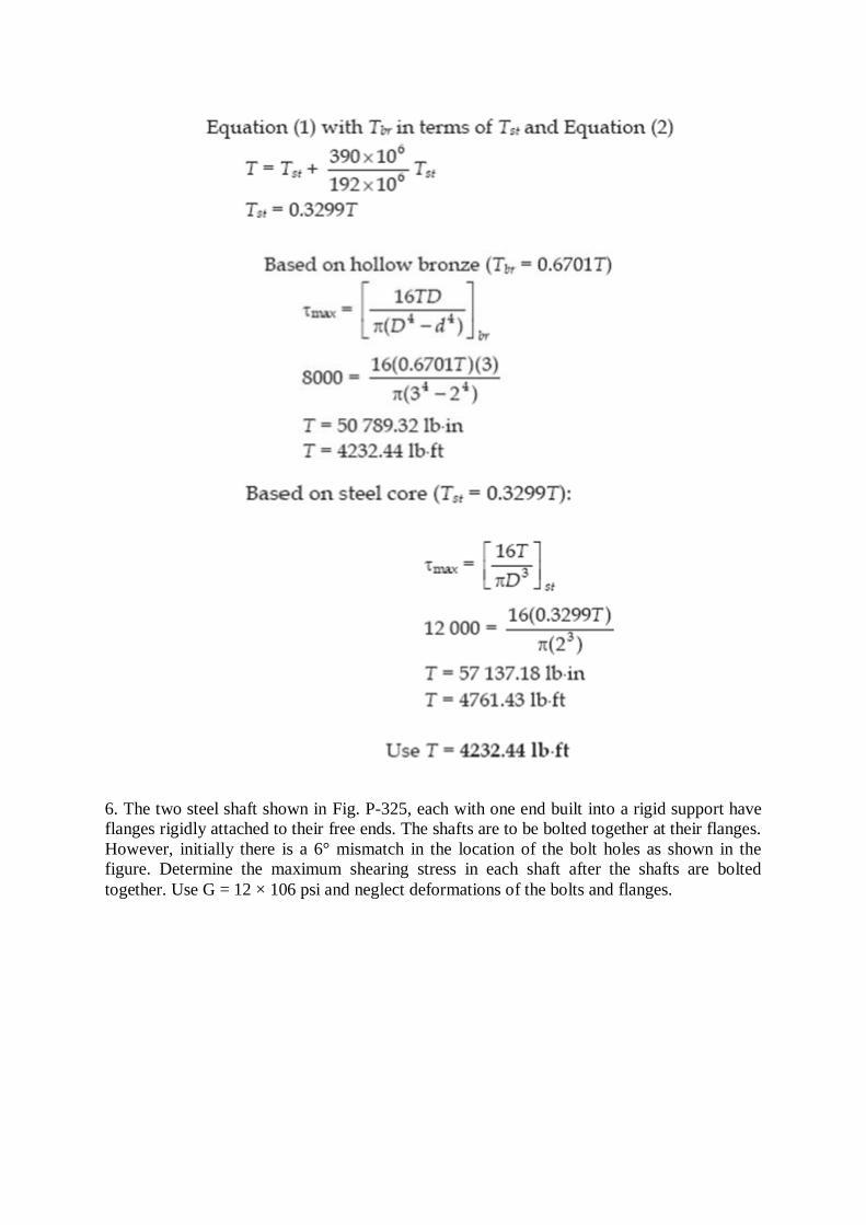
6. The two steel shaft shown in Fig. P-325, each with one end built into a rigid support have
flanges rigidly attached to their free ends. The shafts are to be bolted together at their flanges.
However, initially there is a 6° mismatch in the location of the bolt holes as shown in the
figure. Determine the maximum shearing stress in each shaft after the shafts are bolted
together. Use G = 12 × 106 psi and neglect deformations of the bolts and flanges.


Closed Coiled helical springs subjected to axial loads:
Definition: A spring may be defined as an elastic member whose primary function is to
deflect or distort under the action of applied load; it recovers its original shape when load is
released. Also Springs are energy absorbing units whose function is to store energy and to
restore it slowly or rapidly depending on the particular application.
Important types of springs are:
There are various types of springs such as
(i) helical spring: They are made of wire coiled into a helical form, the load being applied
along the axis of the helix. In these type of springs the major stresses is Torsional shear stress
due to twisting. They are both used in tension and compression.
Fig.4.14 Helical Spring
(ii) Spiral springs: They are made of flat strip of metal wound in the form of spiral and
loaded in torsion.
In this the major stresses are tensile and compression due to bending.
(iii) Leaf springs: They are composed of flat bars of varying lengths clamped together so as
to obtain greater efficiency. Leaf springs may be full elliptic, semi elliptic or cantilever types,
In these type of springs the major stresses which come into picture are tensile & compressive.
Uses of springs:
(a) To apply forces and to control motions as in brakes and clutches.
(b) To measure forces as in spring balance.
(c) To store energy as in clock springs.
(d) To reduce the effect of shock or impact loading as in carriage springs.
(e) To change the vibrating characteristics of a member as inflexible mounting of motors.
Derivation of the Formula :
In order to derive a necessary formula which governs the behaviour of springs, consider a
closed coiled spring subjected to an axial load W.

Fig.4.15 Helical Spring major notation
Let
W = axial load
D = mean coil diameter
d = diameter of spring wire
n = number of active coils
C = spring index = D / d For circular wires
l = length of spring wire
G = modulus of rigidity
x = deflection of spring
q = Angle of twist
when the spring is being subjected to an axial load to the wire of the spring gets be twisted
like a shaft.
If q is the total angle of twist along the wire and x is the deflection of spring under the action
of load W along the axis of the coil, so that
x = D / 2 . q
again l = p D n [ consider ,one half turn of a close coiled helical spring ]
Fig.4.16 Helical Spring wire
Assumptions: (1) The Bending & shear effects may be neglected
(2) For the purpose of derivation of formula, the helix angle is considered to be so small that
it may be neglected.
Any one coil of a spring will be assumed to lie in a plane which is nearly perpendicular to the
axis of the spring. This requires that adjoining coils be close together. With this limitation, a
section taken perpendicular to the axis the spring rod becomes nearly vertical. Hence to

maintain equilibrium of a segment of the spring, only a shearing force V = F and Torque T =
F. r are required at any X – section. In the analysis of springs it is customary to assume that
the shearing stresses caused by the direct shear force is
uniformly distributed and is negligible
so applying the torsion formula. Using the torsion formula i.e
SPRING DEFLECTION
Spring striffness: The stiffness is defined as the load per unit deflection therefore
Shear stress
WAHL'S FACTOR :
In order to take into account the effect of direct shear and change in coil curvature a stress
factor is defined, which is known as Wahl's factor
K = Wahl' s factor and is defined as

Where C = spring index
= D/d
if we take into account the Wahl's factor than the formula for the shear stress becomes
Strain Energy : The strain energy is defined as the energy which is stored within a material
when the work has been done on the material.
In the case of a spring the strain energy would be due to bending and the strain energy due to
bending is given by the expansion
Worked examples:
1. A close coiled helical spring is to carry a load of 5000N with a deflection of 50 mm and a
maximum shearing stress of 400 N/mm2 if the number of active turns or active coils is
8.Estimate the following:
(i) wire diameter
(ii) mean coil diameter
(iii) weight of the spring.
Assume G = 83,000 N/mm2 ; r = 7700 kg/m3
solution :
(i) for wire diametre if W is the axial load, then
Further, deflection is given as

Therefore,
D = .0314 x (13.317)3mm
=74.15mm
D = 74.15 mm
2. Determine the maximum shearing stress and elongation in a helical steel spring composed
of 20 turns of 20-mm-diameter wire on a mean radius of 90 mm when the spring is
supporting a load of 1.5 kN. G = 83 GPa.
3. Determine the maximum shearing stress and elongation in a bronze helical spring
composed of 20 turns of 1.0-in.-diameter wire on a mean radius of 4 in. when the spring is
supporting a load of 500 lb. G = 6 × 10⁶ psi.
4. A helical spring is fabricated by wrapping wire ¾ in. in diameter around a forming
cylinder 8 in. in diameter. Compute the number of turns required to permit an elongation of 4
in. without exceeding a shearing stress of 18 ksi. G = 12 × 106 psi.
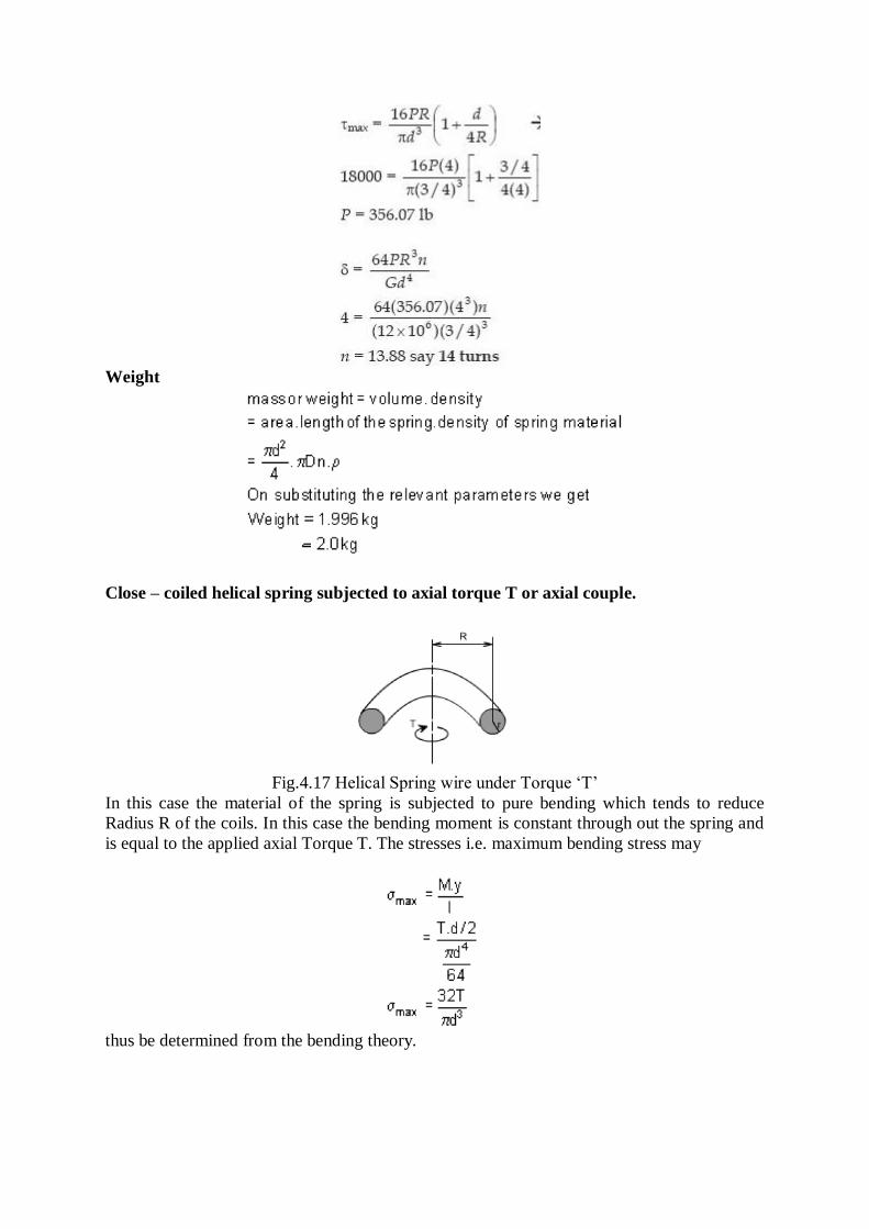
Weight
Close – coiled helical spring subjected to axial torque T or axial couple.
Fig.4.17 Helical Spring wire under Torque ‘T’
In this case the material of the spring is subjected to pure bending which tends to reduce
Radius R of the coils. In this case the bending moment is constant through out the spring and
is equal to the applied axial Torque T. The stresses i.e. maximum bending stress may
thus be determined from the bending theory.

Springs in Series: If two springs of different stiffness are joined endon and carry a common
load W, they are said to be connected in series and the combined stiffness and deflection are
given by the following equation
.
Fig.4.18 Springs in Series
Springs in parallel: If the two spring are joined in such a way that they have a common
deflection ‘x' ; then they are said to be connected in parallel. In this care the load carried is
shared between the two springs and total load W = W1 + W2
Fig.4.19 Springs in Parallel
1. Two steel springs arranged in series as shown supports a load P. The upper spring has 12
turns of 25-mm-diameter wire on a mean radius of 100 mm. The lower spring consists of 10
turns of 20-mmdiameter wire on a mean radius of 75 mm. If the maximum shearing stress in
either spring must not exceed 200 MPa, compute the maximum value of P and the total
elongation of the assembly. G = 83 GPa. Compute the equivalent spring constant by dividing
the load by the total elongation.

Fig.4.20 Helical Spring in Series
Design of helical coil springs – stresses in helical coil springs under torsion loads
Worked problems

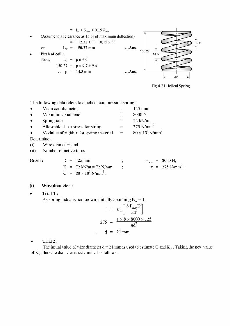
Fig.4.21 Helical Spring


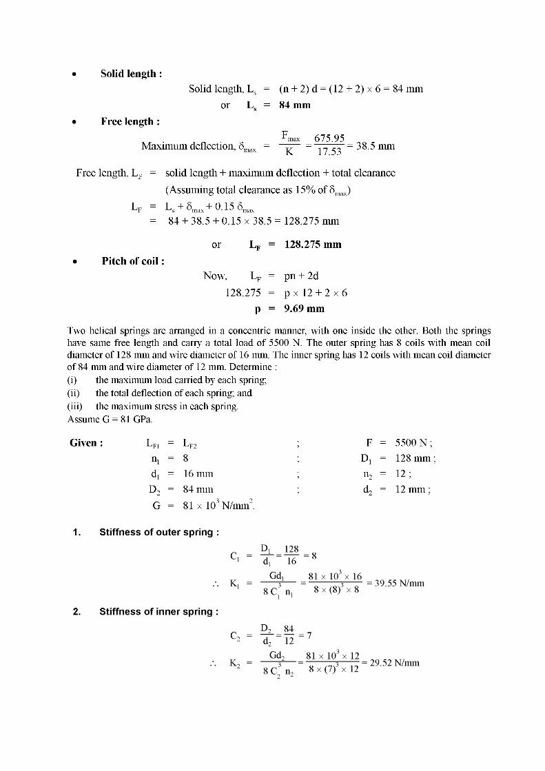
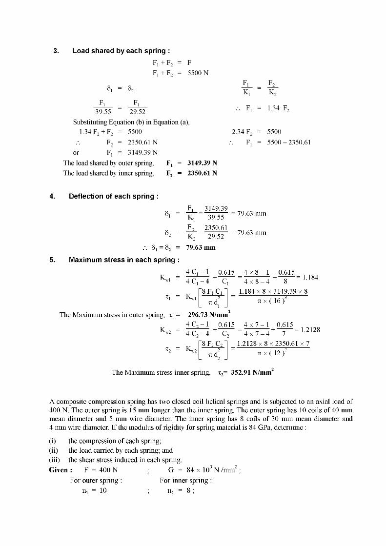

Fig.4.22 Helical Spring in parallel
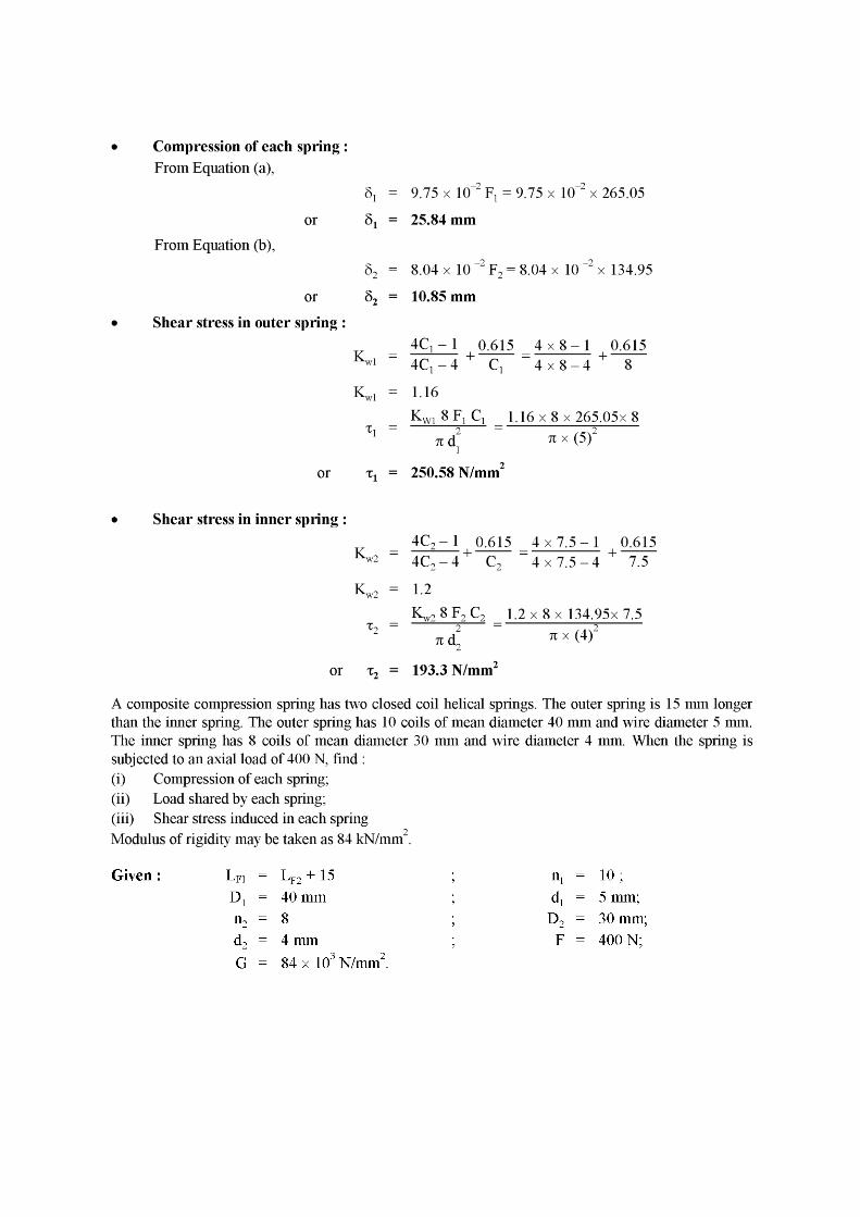
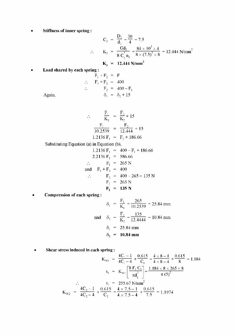

TEXT/ REFERENCE BOOKS
1. Bansal R.K., “Strength of Materials”, Laxmi Publications (P) Ltd.,Fifth Edition,2012
2. Punmia B.C. & Jain A.K., Mechanics of Materials, ,Laxmi Publications,2001
3. Ryder G.H, “Strength of Materials, Macmillan India Ltd”., Third Edition, 2002
4. Ray Hulse, Keith Sherwin & Jack Cain, “Solid Mechanics”, Palgrave ANE Books,2004.
5. Allan F. Bower, Applied Mechanics of Solids, CRC Press, 2009, 820 pages.
SCHOOL OF MECHANICAL ENGINEERING
DEPARTMENT OF MECHANICAL ENGINEERING
UNIT – V – BEAM DEFLECTION – SMEA1305

MECHANICS OF SOLIDS (SMEA1305)
UNIT 5: BEAM DEFLECTION
UNIT 5: BEAM DEFLECTION Columns –
End conditions – Equivalent length of a column – Euler equation – Slenderness ratio –
Rankine Gordon formula for columns
Elastic curve of Neutral axis of the beam under normal loads – Evaluation of beam
deflection and slope: Double integration method, Macaulay Method, and Moment-area
Method
Introduction: Elastic Stability of Columns
Structural members which carry compressive loads may be divided into two broad categories
depending on their relative lengths and cross-sectional dimensions. The analysis and design
of compression members can differ significantly from that of members loaded in tension or in
torsion. If you were to take a long rod or pole, such as a meter stick, and apply gradually
increasing compressive forces at each end, nothing would happen at first, but then the stick
would bend (buckle), and finally bend so much as to fracture. Try it. The other extreme
would occur if you were to saw off, say, a 5-mm length of the meter stick and perform the
same experiment on the short piece. You would then observe that the failure exhibits itself as
a mashing of the specimen, that is, a simple compressive failure. For these reasons it is
convenient to classify compression members according to their length and according to
whether the loading is central or eccentric. The term column is applied to all such members
except those in which failure would be by simple or pure compression.
General comments
The critical load of a column is proportional to the flexural rigidity EI and inversely
proportional to the square of the length. Of particular interest is the fact that the strength of
the material itself, as represented by a quantity such as the proportional limit or the The
flexural rigidity can be increased by using a “stiffer” material (that is, a material with larger
modulus of elasticity E) or by distributing the material in such a way as to increase the
moment of inertia I of the cross section, just as a beam can be made stiffer by increasing the
moment of inertia. The moment of inertia is increased by distributing the material farther
from the centroid of the cross section. Hence, a hollow tubular member is generally more
economical for use as a column than a solid member having the same cross-sectional area.
Reducing the wall thickness of a tubular member and increasing its lateral dimensions (while
keeping the cross-sectional area constant) also increases the critical load because the moment
of inertia is increased. This process has a practical limit, however, because eventually the
wall itself will become unstable. When that happens, localized buckling occurs in the form of
small corrugations or wrinkles in the walls of the column. Thus, we must distinguish between
overall buckling of a column, which is discussed in this chapter, and local buckling of its
parts. yield stress, does not appear in the equation for the critical load. Therefore, increasing a
strength property does not raise the critical load of a slender column. It can only be raised by
increasing the flexural rigidity, reducing the length, or providing additional lateral support.
we assumed that the xy plane was a plane of symmetry of the column and that buckling took
place in that plane. The latter assumption will be met if the column has lateral supports
perpendicular to the plane of the figure, so that the column is constrained to buckle in the xy
plane. If the column is supported only at its ends and is free to buckle in any direction, then
bending will occur about the principal centroidal axis having the smaller moment of inertia. If
the cross section is square or circular, all centroidal axes have the same moment of inertia and
buckling may occur in any longitudinal plane.
Limitations
In addition to the requirement of small deflections, the Euler buckling theory used in this
section is valid only if the column is perfectly straight before the load is applied, the column
and its supports have no imperfections, and the column is made of a linearly elastic material
that follows Hooke’s law.
Columns:
Short, thick members are generally termed columns and these usually fail by crushing when
the yield stress of the material in compression is exceeded. Columns can be categorized then
as:
Long columns with central loading
Intermediate-length columns with central loading
Columns with eccentric loading
Struts or short columns with eccentric loading
Struts:
Long, slender columns are generally termed as struts; they fail by buckling some time before
the yield stress in compression is reached. The buckling occurs owing to one the following
reasons. A short bar loaded in pure compression by a force P acting along the centroidal axis
will shorten in accordance with Hooke’s law, until the stress reaches the elastic limit of the
material. At this point, permanent set is introduced and usefulness as a machine member may
be at an end. If the force P is increased still more, the material either becomes “barrel-like” or
fractures. When there is eccentricity in the loading, the elastic limit is encountered at smaller
loads.
(a) The strut may not be perfectly straight initially.
(b) The load may not be applied exactly along the axis of the Strut.
(c) One part of the material may yield in compression more readily than others owing to some
lack of uniformity in the material properties throughout the strut.
In all the problems considered so far we have assumed that the deformation to be both
progressive with increasing load and simple in form i.e. we assumed that a member in simple
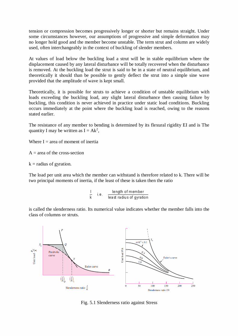
tension or compression becomes progressively longer or shorter but remains straight. Under
some circumstances however, our assumptions of progressive and simple deformation may
no longer hold good and the member become unstable. The term strut and column are widely
used, often interchangeably in the context of buckling of slender members.
At values of load below the buckling load a strut will be in stable equilibrium where the
displacement caused by any lateral disturbance will be totally recovered when the disturbance
is removed. At the buckling load the strut is said to be in a state of neutral equilibrium, and
theoretically it should than be possible to gently deflect the strut into a simple sine wave
provided that the amplitude of wave is kept small.
Theoretically, it is possible for struts to achieve a condition of unstable equilibrium with
loads exceeding the buckling load, any slight lateral disturbance then causing failure by
buckling, this condition is never achieved in practice under static load conditions. Buckling
occurs immediately at the point where the buckling load is reached, owing to the reasons
stated earlier.
The resistance of any member to bending is determined by its flexural rigidity EI and is The
quantity I may be written as I = Ak2,
Where I = area of moment of inertia
A = area of the cross-section
k = radius of gyration.
The load per unit area which the member can withstand is therefore related to k. There will be
two principal moments of inertia, if the least of these is taken then the ratio
is called the slenderness ratio. Its numerical value indicates whether the member falls into the
class of columns or struts.
Fig. 5.1 Slenderness ratio against Stress

Euler's Theory: The struts which fail by buckling can be analyzed by Euler's theory. In the
following sections, different cases of the struts have been analyzed.
Case A: Strut with pinned ends:
Consider an axially loaded strut, shown below, and is subjected to an axial load ‘P' this load
‘P' produces a deflection ‘y' at a distance ‘x' from one end.
Assume that the ends are either pin jointed or rounded so that there is no moment at either
end.
Fig. 5.2 Strut with Pinned Ends
Assumption:
The strut is assumed to be initially straight, the end load being applied axially through
centroid.
Fig. 5.3 Strut with Pinned Ends sign convention
In this equation ‘M' is not a function ‘x'. Therefore this equation can not be integrated directly
as has been done in the case of deflection of beams by integration method.

Though this equation is in ‘y' but we can't say at this stage where the deflection would be
maximum or minimum.
So the above differential equation can be arranged in the following form
Let us define a operator
D = d/dx
(D2 + n2) y =0 where n2 = P/EI
This is a second order differential equation which has a solution of the form consisting of
complimentary function and particular integral but for the time being we are interested in the
complementary solution only[in this P.I = 0; since the R.H.S of Diff. equation = 0]
Thus y = A cos (nx) + B sin (nx)
Where A and B are some constants.
In order to evaluate the constants A and B let us apply the boundary conditions,
(i) at x = 0; y = 0
(ii) at x = L ; y = 0
Applying the first boundary condition yields A = 0 and applying the second boundary
condition gives

From the above relationship the least value of P which will cause the strut to buckle, and it is
called the “ Euler Crippling Load ” Pe from which w obtain.
The interpretation of the above analysis is that for all the values of the load P, other than
those which make sin nL = 0; the strut will remain perfectly straight since
y = B sin nL = 0
For the particular value of
Then we say that the strut is in a state of neutral equilibrium, and theoretically any deflection
which it suffers will be maintained. This is subjected to the limitation that ‘L' remains
sensibly constant and in practice slight increase in load at the critical value will cause the
deflection to increase appreciably until the material fails by yielding.
Further it should be noted that the deflection is not proportional to load, and this applies to all
strut problems; like wise it will be found that the maximum stress is not proportional to load.
The solution chosen of nL = p is just one particular solution; the solutions nL= 2p, 3p, 5p etc
are equally valid mathematically and they do, infact, produce values of ‘Pe' which are equally
valid for modes of buckling of strut different from that of a simple bow. Theoretically
therefore, there are an infinite number of values of Pe , each corresponding with a different
mode of buckling.
The value selected above is so called the fundamental mode value and is the lowest critical
load producing the single bow buckling condition.
The solution nL = 2p produces buckling in two half – waves, 3p in three half-waves etc.

Fig. 5.4 Member subjected with different modes
If load is applied sufficiently quickly to the strut, then it is possible to pass through the
fundamental mode and to achieve at least one of the other modes which are theoretically
possible. In practical loading situations, however, this is rarely achieved since the high stress
associated with the first critical condition generally ensures immediate collapse.
struts and columns with other end conditions: Let us consider the struts and columns
having different end conditions
Case b: One end fixed and the other free:
Fig. 5.5 One End fixed and other is free End condition
writing down the value of bending moment at the point C

Hence in operator form, the differential equation reduces to ( D2 + n2 ) y = n2a
The solution of the above equation would consist of complementary solution and particular
solution, therefore
ygen = A cos(nx) + sin(nx) + P. I
where
P.I = the P.I is a particular value of y which satisfies the differential equation
Hence yP.I = a
Therefore the complete solution becomes
Y = A cos(nx) + B sin(nx) + a
Now imposing the boundary conditions to evaluate the constants A and B
(i) at x = 0; y = 0
This yields A = -a
(ii) at x = 0; dy/dx = 0
This yields B = 0
Hence
y = -a cos(nx) + a
Futher, at x = L; y = a
Therefore a = - a cos(nx) + a or 0 = cos(nL)
Now the fundamental mode of buckling in this case would be

Case 3
Strut with fixed ends:
Fig. 5.6 Both Ends in fixed End condition
Due to the fixed end supports bending moment would also appears at the supports, since this
is the property of the support.
Bending Moment at point C = M – P.y

Case 4
One end fixed, the other pinned
Fig. 5.7 One end Fixed and oer pinned End conditions
In order to maintain the pin-joint on the horizontal axis of the unloaded strut, it is necessary
in this case to introduce a vertical load F at the pin. The moment of F about the built in end
then balances the fixing moment.
With the origin at the built in end, the B,M at C is given as

Also when x = L ; y = 0
Therefore
nL Cos nL = Sin nL or tan nL = nL
The lowest value of nL ( neglecting zero) which satisfies this condition and which therefore
produces the fundamental buckling condition is nL = 4.49radian
Equivalent Strut Length:
Having derived the results for the buckling load of a strut with pinned ends the Euler loads
for other end conditions may all be written in the same form.

Where L is the equivalent length of the strut and can be related to the actual length of the
strut depending on the end conditions.
The equivalent length is found to be the length of a simple bow(half sine wave) in each of the
strut deflection curves shown. The buckling load for each end condition shown is then readily
obtained. The use of equivalent length is not restricted to the Euler's theory and it will be
used in other derivations later.
The critical load for columns with other end conditions can be expressed in terms of the
critical load for a hinged column, which is taken as a fundamental case.
For case(c) see the figure, the column or strut has inflection points at quarter points of its
unsupported length. Since the bending moment is zero at a point of inflection, the freebody
diagram would indicates that the middle half of the fixed ended is equivalent to a hinged
column having an effective length Le = L / 2.
The four different cases which we have considered so far are:
(a) Both ends pinned (c) One end fixed, other free
(b) Both ends fixed (d) One end fixed and other pinned
Fig. 5.8 Different End conditions loading
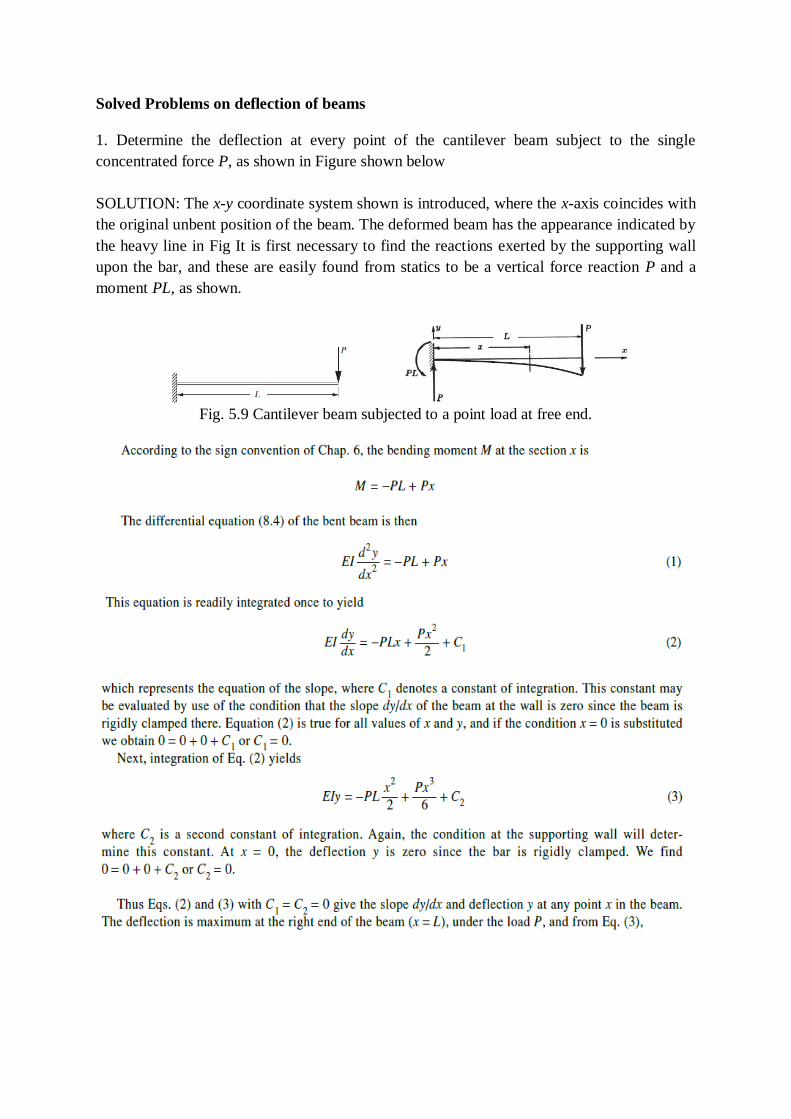
Solved Problems on deflection of beams
1. Determine the deflection at every point of the cantilever beam subject to the single
concentrated force P, as shown in Figure shown below
SOLUTION: The x-y coordinate system shown is introduced, where the x-axis coincides with
the original unbent position of the beam. The deformed beam has the appearance indicated by
the heavy line in Fig It is first necessary to find the reactions exerted by the supporting wall
upon the bar, and these are easily found from statics to be a vertical force reaction P and a
moment PL, as shown.
Fig. 5.9 Cantilever beam subjected to a point load at free end.

2. The cantilever beam AB is of uniform cross section and carries a load P at its free end A).
Determine the equation of the elastic curve and the deflection and slope at A.
Fig. 5.10 Cantilever beam subjected to a point load and reactions

3. The simply supported prismatic beam AB carries a uniformly distributed load w per unit
length. Determine the equation of the elastic curve and the maximum deflection of the beam.
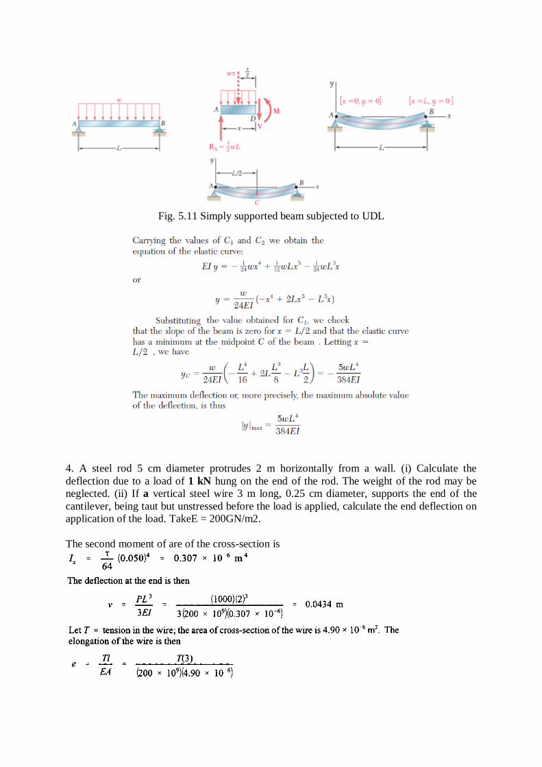
Fig. 5.11 Simply supported beam subjected to UDL
4. A steel rod 5 cm diameter protrudes 2 m horizontally from a wall. (i) Calculate the
deflection due to a load of 1 kN hung on the end of the rod. The weight of the rod may be
neglected. (ii) If a vertical steel wire 3 m long, 0.25 cm diameter, supports the end of the
cantilever, being taut but unstressed before the load is applied, calculate the end deflection on
application of the load. TakeE = 200GN/m2.
The second moment of are of the cross-section is
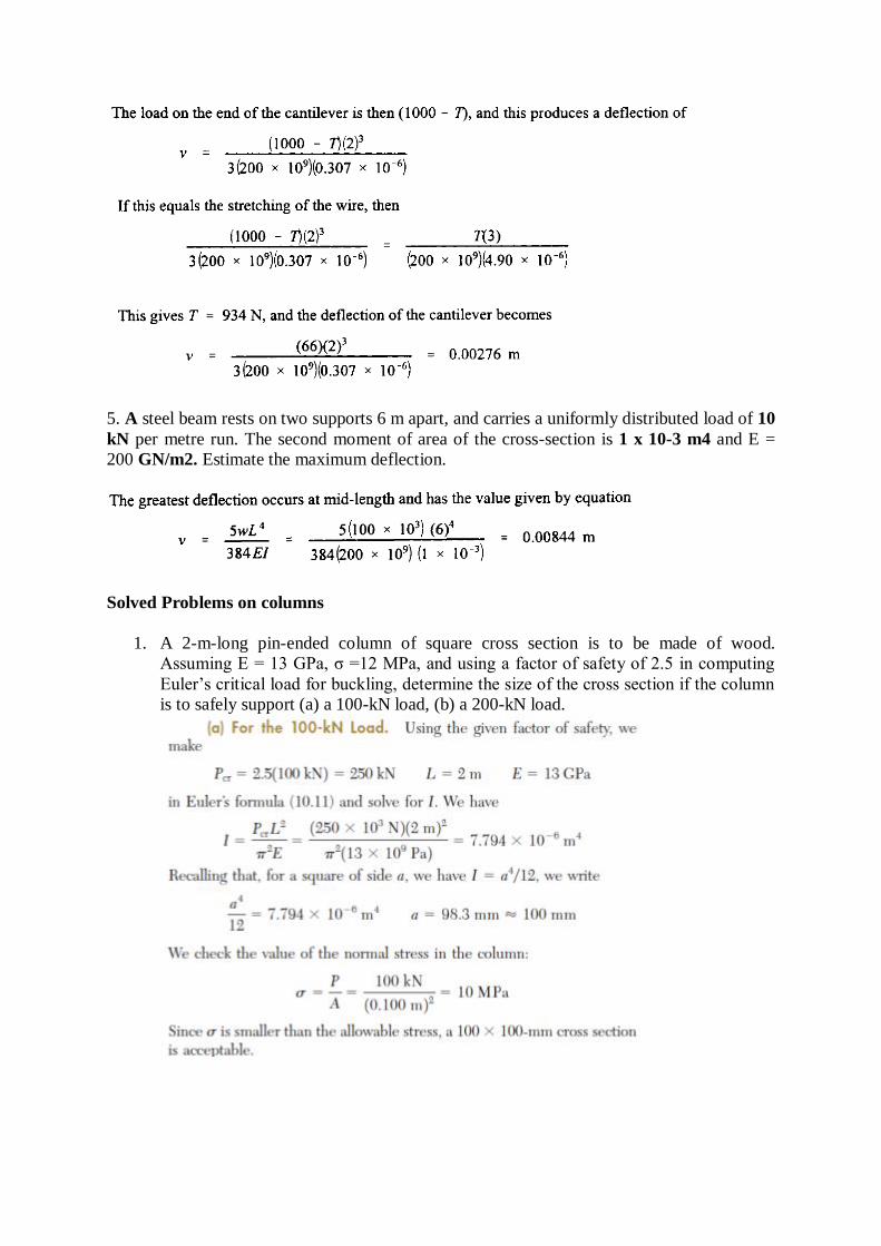
5. A steel beam rests on two supports 6 m apart, and carries a uniformly distributed load of 10
kN per metre run. The second moment of area of the cross-section is 1 x 10⁻³ m4 and E =
200 GN/m2. Estimate the maximum deflection.
Solved Problems on columns
1. A 2-m-long pin-ended column of square cross section is to be made of wood.
Assuming E = 13 GPa, σ =12 MPa, and using a factor of safety of 2.5 in computing
Euler’s critical load for buckling, determine the size of the cross section if the column
is to safely support (a) a 100-kN load, (b) a 200-kN load.
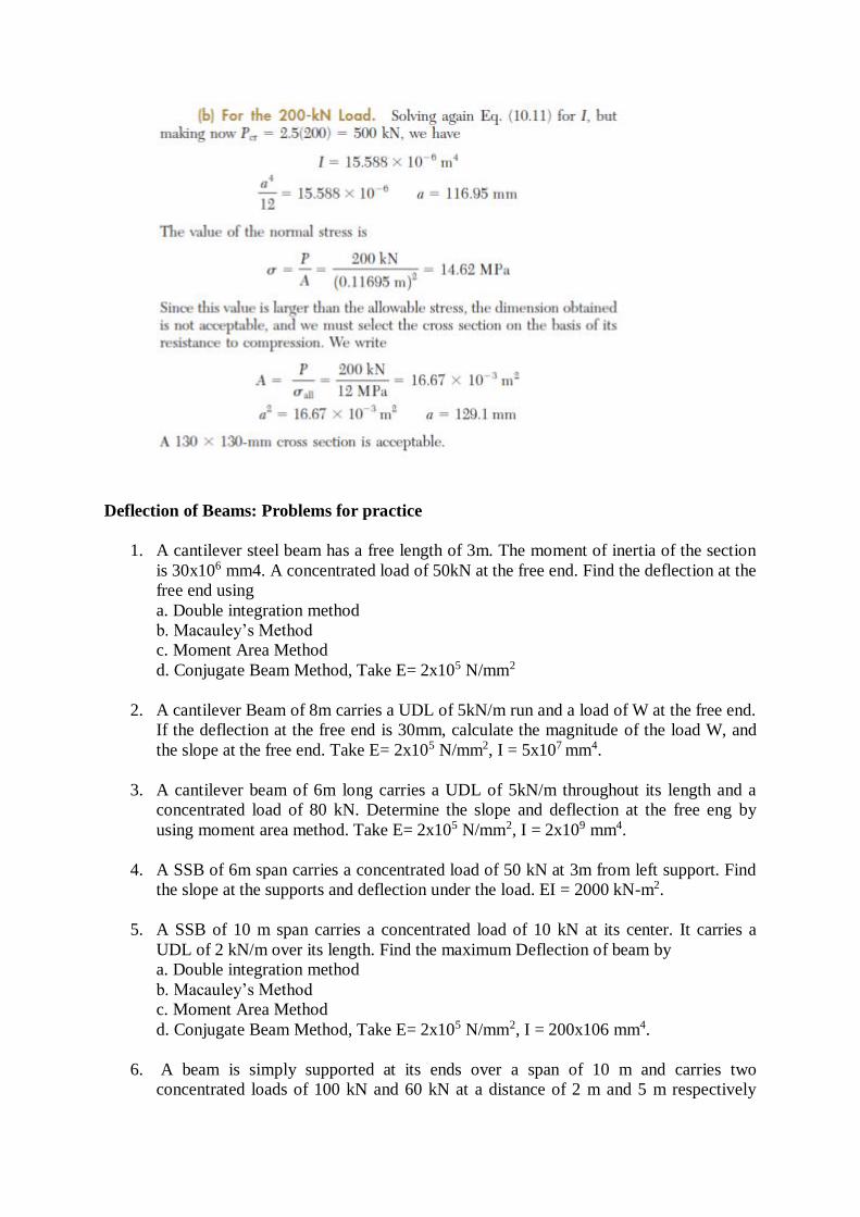
Deflection of Beams: Problems for practice
1. A cantilever steel beam has a free length of 3m. The moment of inertia of the section
is 30x106 mm4. A concentrated load of 50kN at the free end. Find the deflection at the
free end using
a. Double integration method
b. Macauley’s Method
c. Moment Area Method
d. Conjugate Beam Method, Take E= 2x10⁵ N/mm2
2. A cantilever Beam of 8m carries a UDL of 5kN/m run and a load of W at the free end.
If the deflection at the free end is 30mm, calculate the magnitude of the load W, and
the slope at the free end. Take E= 2x10⁵ N/mm2, I = 5x107 mm4.
3. A cantilever beam of 6m long carries a UDL of 5kN/m throughout its length and a
concentrated load of 80 kN. Determine the slope and deflection at the free eng by
using moment area method. Take E= 2x10⁵ N/mm2, I = 2x109 mm4.
4. A SSB of 6m span carries a concentrated load of 50 kN at 3m from left support. Find
the slope at the supports and deflection under the load. EI = 2000 kN-m2.
5. A SSB of 10 m span carries a concentrated load of 10 kN at its center. It carries a
UDL of 2 kN/m over its length. Find the maximum Deflection of beam by
a. Double integration method
b. Macauley’s Method
c. Moment Area Method
d. Conjugate Beam Method, Take E= 2x10⁵ N/mm2, I = 200x106 mm4.
6. A beam is simply supported at its ends over a span of 10 m and carries two
concentrated loads of 100 kN and 60 kN at a distance of 2 m and 5 m respectively

from the left support. Calculate (i) slope at the left support (ii) slope and deflection
under the 100 kN load. Assume EI = 36 × 104 kN-m2.
7. (i) State Moment-Area Mohr’s theorem.
(ii) A simply supported beam AB uniform section, 4 m span is subjected to a
clockwise moment of 10 kNm applied at the right hinge B. Derive the equation to the
deflected shape of the beam. Locate the point of maximum deflection and find the
maximum deflection.
Columns: Problems for practice
1. Find the Euler critical load for a hollow cylindrical cast iron column 150mm external
diameter, 20 mm wall thickness if it is 6 m long with hinged at both ends. Assume
Young’s modulus of cast iron as 80 kN/mm2. Compare this load with that given by
Rankine formula. Using Rankine constants α = 1/1600 and 567 N/mm2.
2. A column of solid circular section, 12 cm diameter, 3.6 m long is hinged at both ends.
Rankine’s constant is 1 / 1600, σc = 54 KN/cm2. Find the buckling load. ii) If another
column of the same length, end conditions and rankine constant but of 12 cm X 12 cm
square cross-section, and different material, has the same buckling load, find the value
of σc of its material.
3. Determine the section of a hollow C.I. cylindrical column 5 m long with ends firmly
built in. The column has to carry an axial compressive load of 588.6 KN. The internal
diameter of the column is 0.75 times the external diameter. Use Rankine’s constants.
a = 1 / 1600, σc = 57.58 KN/cm2 and F.O.S = 6.
4. Find the euler critical load for a hollow cylindrical cast iron column 150mm external
diameter, 20mm wall thick ness if it is 6m long with hinged at both ends. Assume
young’s modulus of cast iron as 80 KN/mm2.compare this load with that given by
rankine constants. a=1/1600 and 567N/mm2.
5. A 1.2m long column has a cross section of 45mm diameter one of the ends of the
column is fixed in direction and position and other end is free. Taking factor of safety
as 3, calculate the safe load using. I. Rankine’s formula, take yield stress=560N/mm2
and a=1/1600 for pinned ends. II. Euler’s formula Young’s modulus for cast iron =
1.2X10⁵ N/mm2.
6. The external and internal diameters of a hollow cast iron column are 50mm and
40mm respectively. If the length of this column is 3m and both of its ends are fixed,
determine the crippling load using Euler formula taking E=100Gpa. Also determine
the rankine load for the column assuming fc=550Mpa and α=1/1600.
7. An I section joists 400mmx200mmx20mm and 6m long is used as a strut with both
ends fixed. What is Euler’s crippling load for the column? Take E=200Gpa.

Deflection of Beams
In all practical engineering applications, when we use the different components, normally we
have to operate them within the certain limits i.e. the constraints are placed on the
performance and behavior of the components. For instance we say that the particular
component is supposed to operate within this value of stress and the deflection of the
component should not exceed beyond a particular value. In some problems the maximum
stress however, may not be a strict or severe condition but there may be the deflection which
is the more rigid condition under operation. It is obvious therefore to study the methods by
which we can predict the deflection of members under lateral loads or transverse loads, since
it is this form of loading which will generally produce the greatest deflection of beams.
Assumptions: The following assumptions are undertaken in order to derive a differential
equation of elastic curve for the loaded beam
1. Stress is proportional to strain i.e. hooks law applies. Thus, the equation is valid only for
beams that are not stressed beyond the elastic limit.
2. The curvature is always small.
3. Any deflection resulting from the shear deformation of the material or shear stresses is
neglected.
It can be shown that the deflections due to shear deformations are usually small and hence
can be ignored.
Equation of the Elastic curve
We first recall from elementary calculus that the curvature of a plane curve at a point Q(x,y)
of the curve can be expressed as
where dy/dx and d2y/dx2 are the first and second derivatives of the function y(x) represented
by that curve. But, in the case of the elastic curve of a beam, the slope dy/dx is very small,
and its square is negligible compared to unity. We write, therefore,
It should be noted that, in this chapter, y represents a vertical displacement, while it was used
in previous chapters to represent the distance of a given point in a transverse section from the
neutral axis of that section.
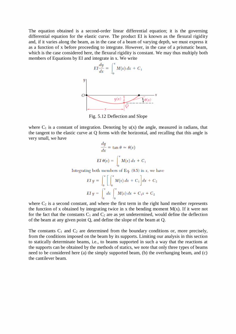
The equation obtained is a second-order linear differential equation; it is the governing
differential equation for the elastic curve. The product EI is known as the flexural rigidity
and, if it varies along the beam, as in the case of a beam of varying depth, we must express it
as a function of x before proceeding to integrate. However, in the case of a prismatic beam,
which is the case considered here, the flexural rigidity is constant. We may thus multiply both
members of Equations by EI and integrate in x. We write
Fig. 5.12 Deflection and Slope
where C1 is a constant of integration. Denoting by u(x) the angle, measured in radians, that
the tangent to the elastic curve at Q forms with the horizontal, and recalling that this angle is
very small, we have
where C2 is a second constant, and where the first term in the right hand member represents
the function of x obtained by integrating twice in x the bending moment M(x). If it were not
for the fact that the constants C1 and C2 are as yet undetermined, would define the deflection
of the beam at any given point Q, and define the slope of the beam at Q.
The constants C1 and C2 are determined from the boundary conditions or, more precisely,
from the conditions imposed on the beam by its supports. Limiting our analysis in this section
to statically determinate beams, i.e., to beams supported in such a way that the reactions at
the supports can be obtained by the methods of statics, we note that only three types of beams
need to be considered here (a) the simply supported beam, (b) the overhanging beam, and (c)
the cantilever beam.
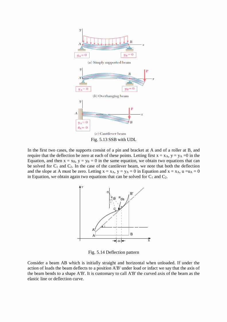
Fig. 5.13 SSB with UDL
In the first two cases, the supports consist of a pin and bracket at A and of a roller at B, and
require that the deflection be zero at each of these points. Letting first x = xA, y = yA =0 in the
Equation, and then x = xB, y = yB = 0 in the same equation, we obtain two equations that can
be solved for C1 and C2. In the case of the cantilever beam, we note that both the deflection
and the slope at A must be zero. Letting x = xA, y = yA = 0 in Equation and x = xA, u =uA = 0
in Equation, we obtain again two equations that can be solved for C1 and C2.
Fig. 5.14 Deflection pattern
Consider a beam AB which is initially straight and horizontal when unloaded. If under the
action of loads the beam deflects to a position A'B' under load or infact we say that the axis of
the beam bends to a shape A'B'. It is customary to call A'B' the curved axis of the beam as the
elastic line or deflection curve.

In the case of a beam bent by transverse loads acting in a plane of symmetry, the bending
moment M varies along the length of the beam and we represent the variation of bending
moment in B.M diagram. Futher, it is assumed that the simple bending theory equation holds
good.
If we look at the elastic line or the deflection curve, this is obvious that the curvature at every
point is different; hence the slope is different at different points. To express the deflected
shape of the beam in rectangular co-ordinates let us take two axes x and y, x-axis coincide
with the original straight axis of the beam and the y – axis shows the deflection.
Futher,let us consider an element ds of the deflected beam. At the ends of this element let us
construct the normal which intersect at point O denoting the angle between these two normal
be di But for the deflected shape of the beam the slope i at any point C is defined,
This is the differential equation of the elastic line for a beam subjected to bending in the
plane of symmetry. Its solution y = f(x) defines the shape of the elastic line or the deflection
curve as it is frequently called.
Relationship between shear force, bending moment and deflection: The relationship
among shear force, bending moment and deflection of the beam may be obtained as
differentiating the equation as derived

Therefore, the above expression represents the shear force whereas rate of intensity of
loading can also be found out by differentiating the expression for shear force
Methods for finding the deflection: The deflection of the loaded beam can be obtained
various methods. The one of the method for finding the deflection of the beam is the direct
integration method, i.e. the method using the differential equation which we have derived.
Direct integration method: The governing differential equation is defined as
Where A and B are constants of integration to be evaluated from the known conditions of
slope and deflections for the particular value of x.
Illustrative examples: let us consider few illustrative examples to have a familiarity with the
direct integration method
Case 1: Cantilever Beam with Concentrated Load at the end:- A cantilever beam is subjected
to a concentrated load W at the free end, it is required to determine the deflection of the beam
Fig. 5.15 Cantilever Beam with Concentrated Load at the free end
In order to solve this problem, consider any X-section X-X located at a distance x from the
left end or the reference, and write down the expressions for the shear force and the bending
moment
The constants A and B are required to be found out by utilizing the boundary conditions as
defined below
i.e at x= L ; y= 0 -------------------- (1)
at x = L ; dy/dx = 0 -------------------- (2)
Utilizing the second condition, the value of constant A is obtained as

Case 2: A Cantilever with Uniformly distributed Loads:- In this case the cantilever beam is
subjected to U.d.l with rate of intensity varying w / length. The same procedure can also be
adopted in this case
Fig. 5.16 Cantilever Beam with UDL

Boundary conditions relevant to the problem are as follows:
1. At x = L; y = 0
2. At x= L; dy/dx = 0
The second boundary conditions yields
Case 3: Simply Supported beam with uniformly distributed Loads:- In this case a simply
supported beam is subjected to a uniformly distributed load whose rate of intensity varies as
w / length.
Fig. 5.17 SSB with UDL
In order to write down the expression for bending moment consider any cross-section at
distance of x metre from left end support.
Fig. 5.18 SSB with UDL a section at X-X
Boundary conditions which are relevant in this case are that the deflection at each support
must be zero.
i.e. at x = 0; y = 0 : at x = l; y = 0
let us apply these two boundary conditions on equation (1) because the boundary conditions
are on y, This yields B = 0.
In this case the maximum deflection will occur at the centre of the beam where x = L/2 [ i.e.
at the position where the load is being applied ].So if we substitute the value of x = L/2
Conclusions
(i) The value of the slope at the position where the deflection is maximum would be zero.
(ii) The value of maximum deflection would be at the centre i.e. at x = L/2.

The final equation which is governs the deflection of the loaded beam in this case is
By successive differentiation one can find the relations for slope, bending moment, shear
force and rate of loading.
Deflection (y)
Slope (dy/dx)
Fig. 5.19 SSB with UDL Deflection and
Slope
Bending Moment
So the bending moment diagram would be
Fig. 5.20 SSB with UDL SF & BM
Shear Force
Shear force is obtained by
taking third derivative.

Rate of intensity of loading
Case 4: The direct integration method may become more involved if the expression for entire
beam is not valid for the entire beam.Let us consider a deflection of a simply supported beam
which is subjected to a concentrated load W acting at a distance 'a' from the left end.
Fig.5.21 SSB with a point load acting elsewhere in the beam
Let R1 & R2 be the reactions then,
Fig.5.22 SSB with a point load reaction marked diagram
These two equations can be integrated in the usual way to find ‘y' but this will result in four
constants of integration two for each equation. To evaluate the four constants of integration,
four independent boundary conditions will be needed since the deflection of each support
must be zero, hence the boundary conditions (a) and (b) can be realized.

Further, since the deflection curve is smooth, the deflection equations for the same slope and
deflection at the point of application of load i.e. at x = a. Therefore four conditions required
to evaluate these constants may be defined as follows:
(a) at x = 0; y = 0 in the portion AB i.e. 0 ≤ x ≤ a
(b) at x = l; y = 0 in the portion BC i.e. a ≤ x ≤ l
(c) at x = a; dy/dx, the slope is same for both portion
(d) at x = a; y, the deflection is same for both portion
By symmetry, the reaction R1 is obtained as
Using condition (c) in equation (3) and (4) shows that these constants should be equal, hence
letting K1 = K2 = K , Hence
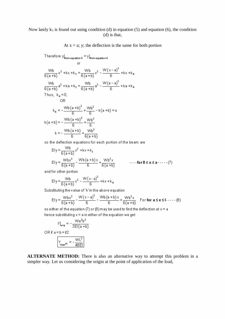
Now lastly k3 is found out using condition (d) in equation (5) and equation (6), the condition
(d) is that,
At x = a; y; the deflection is the same for both portion
ALTERNATE METHOD: There is also an alternative way to attempt this problem in a
simpler way. Let us considering the origin at the point of application of the load,

Fig.5.23 SSB with a Mid-point load
Boundary conditions relevant for this case are as follows
(i) at x = 0; dy/dx= 0
hence, A = 0
(ii) at x = l/2; y = 0 (because now l / 2 is on the left end or right end support since we have
taken the origin at the centre)
Hence the integration method may be bit cumbersome in some of the case. Another limitation
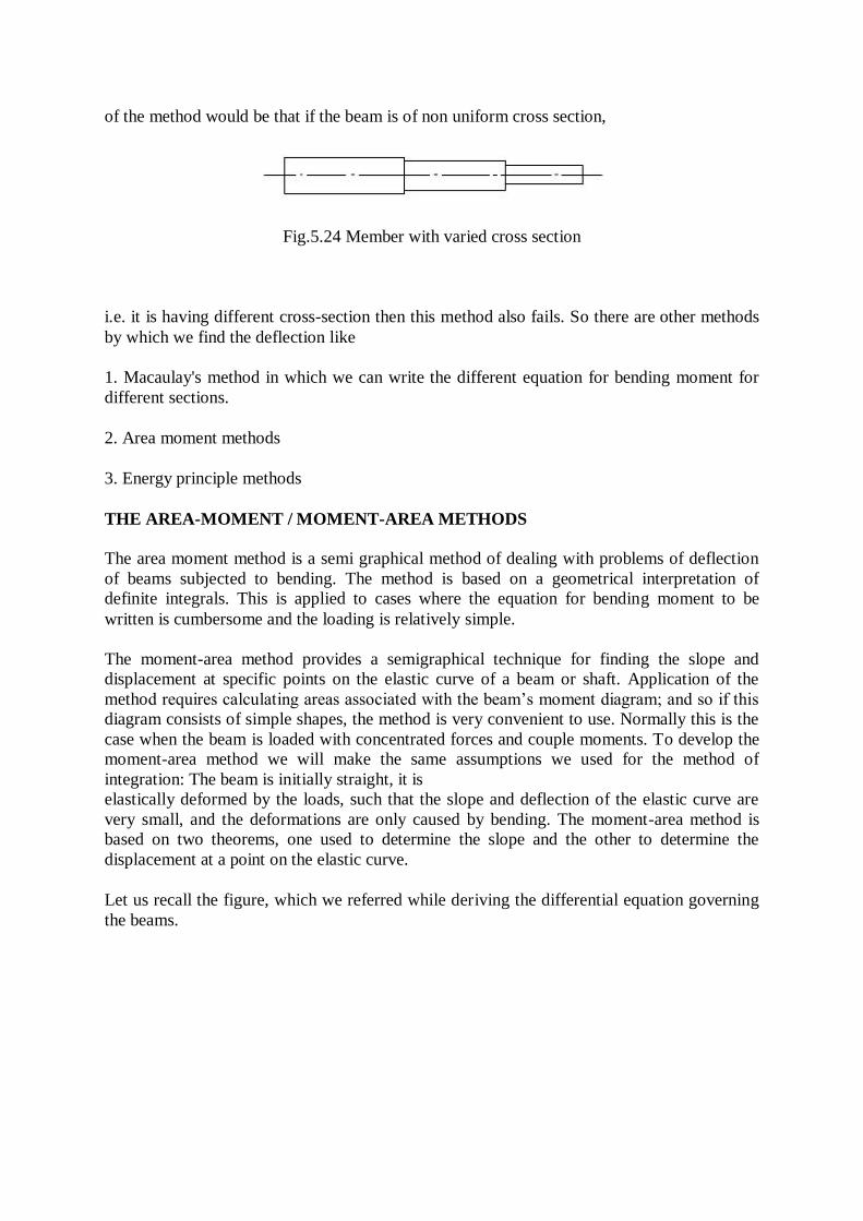
of the method would be that if the beam is of non uniform cross section,
Fig.5.24 Member with varied cross section
i.e. it is having different cross-section then this method also fails. So there are other methods
by which we find the deflection like
1. Macaulay's method in which we can write the different equation for bending moment for
different sections.
2. Area moment methods
3. Energy principle methods
THE AREA-MOMENT / MOMENT-AREA METHODS
The area moment method is a semi graphical method of dealing with problems of deflection
of beams subjected to bending. The method is based on a geometrical interpretation of
definite integrals. This is applied to cases where the equation for bending moment to be
written is cumbersome and the loading is relatively simple.
The moment-area method provides a semigraphical technique for finding the slope and
displacement at specific points on the elastic curve of a beam or shaft. Application of the
method requires calculating areas associated with the beam’s moment diagram; and so if this
diagram consists of simple shapes, the method is very convenient to use. Normally this is the
case when the beam is loaded with concentrated forces and couple moments. To develop the
moment-area method we will make the same assumptions we used for the method of
integration: The beam is initially straight, it is
elastically deformed by the loads, such that the slope and deflection of the elastic curve are
very small, and the deformations are only caused by bending. The moment-area method is
based on two theorems, one used to determine the slope and the other to determine the
displacement at a point on the elastic curve.
Let us recall the figure, which we referred while deriving the differential equation governing
the beams.
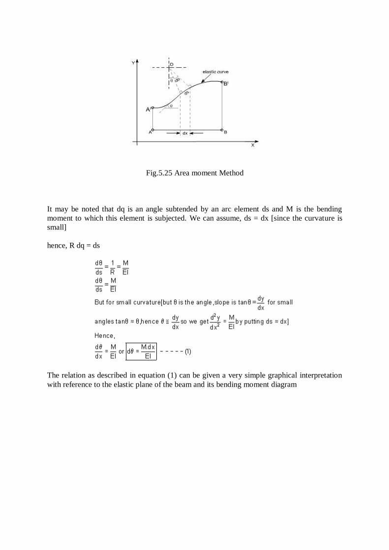
Fig.5.25 Area moment Method
It may be noted that dq is an angle subtended by an arc element ds and M is the bending
moment to which this element is subjected. We can assume, ds = dx [since the curvature is
small]
hence, R dq = ds
The relation as described in equation (1) can be given a very simple graphical interpretation
with reference to the elastic plane of the beam and its bending moment diagram

Fig.5.26 Area moment Method
Refer to the figure shown above consider AB to be any portion of the elastic line of the
loaded beam and A1B1is its corresponding bending moment diagram.
Let AO = Tangent drawn at A
BO = Tangent drawn at B
Tangents at A and B intersects at the point O.
Futher, AA ' is the deflection of A away from the tangent at B while the vertical distance B'B
is the deflection of point B away from the tangent at A. All these quantities are futher
understood to be very small.
Let ds ≈ dx be any element of the elastic line at a distance x from B and an angle between at
its tangents be dq. Then, as derived earlier
This relationship may be interpreted as that this angle is nothing but the area M.dx of the
shaded bending moment diagram divided by EI.
From the above relationship the total angle q between the tangents A and B may be
determined as
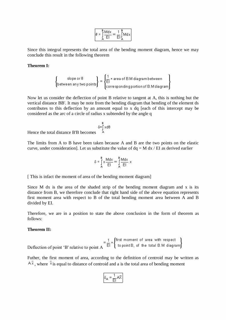
Since this integral represents the total area of the bending moment diagram, hence we may
conclude this result in the following theorem
Theorem I:
Now let us consider the deflection of point B relative to tangent at A, this is nothing but the
vertical distance BB'. It may be note from the bending diagram that bending of the element ds
contributes to this deflection by an amount equal to x dq [each of this intercept may be
considered as the arc of a circle of radius x subtended by the angle q
Hence the total distance B'B becomes
The limits from A to B have been taken because A and B are the two points on the elastic
curve, under consideration]. Let us substitute the value of dq = M dx / EI as derived earlier
[ This is infact the moment of area of the bending moment diagram]
Since M dx is the area of the shaded strip of the bending moment diagram and x is its
distance from B, we therefore conclude that right hand side of the above equation represents
first moment area with respect to B of the total bending moment area between A and B
divided by EI.
Therefore, we are in a position to state the above conclusion in the form of theorem as
follows:
Theorem II:
Deflection of point ‘B' relative to point A
Futher, the first moment of area, according to the definition of centroid may be written as
, where is equal to distance of centroid and a is the total area of bending moment
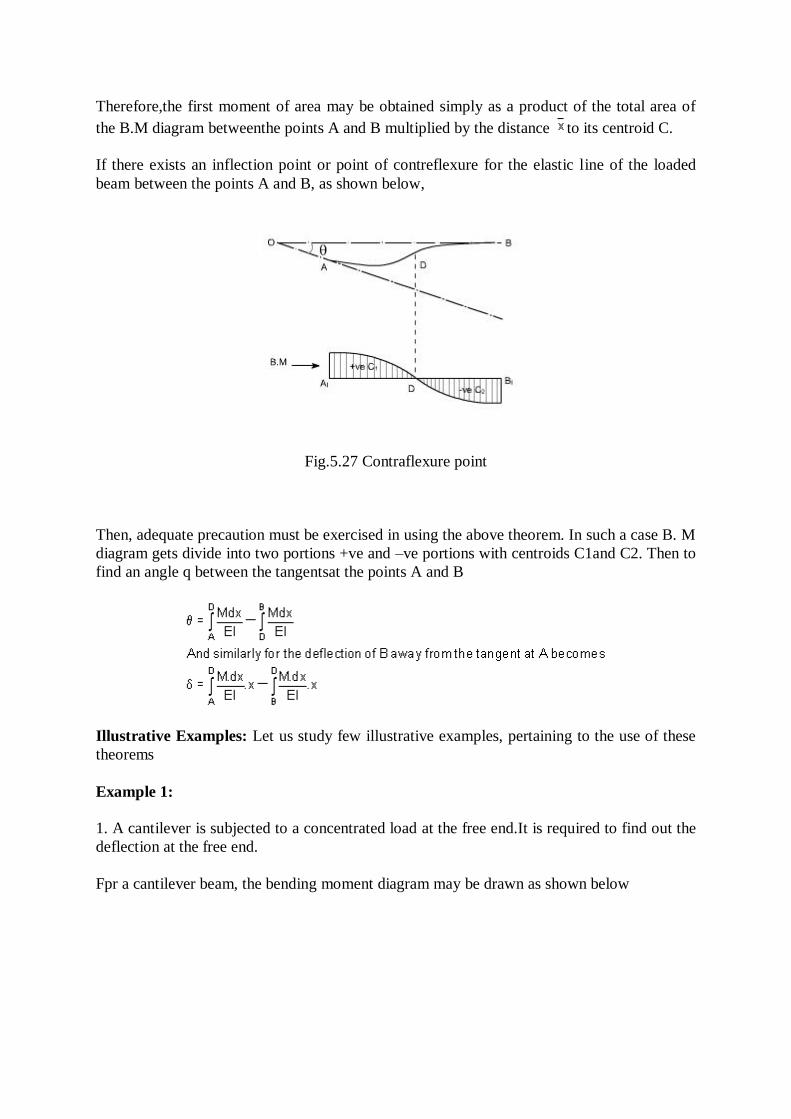
Therefore,the first moment of area may be obtained simply as a product of the total area of
the B.M diagram betweenthe points A and B multiplied by the distance to its centroid C.
If there exists an inflection point or point of contreflexure for the elastic line of the loaded
beam between the points A and B, as shown below,
Fig.5.27 Contraflexure point
Then, adequate precaution must be exercised in using the above theorem. In such a case B. M
diagram gets divide into two portions +ve and –ve portions with centroids C1and C2. Then to
find an angle q between the tangentsat the points A and B
Illustrative Examples: Let us study few illustrative examples, pertaining to the use of these
theorems
Example 1:
1. A cantilever is subjected to a concentrated load at the free end.It is required to find out the
deflection at the free end.
Fpr a cantilever beam, the bending moment diagram may be drawn as shown below

Fig.5.28 Cantilever point load at free end BM diagram
Let us workout this problem from the zero slope condition and apply the first area - moment
theorem
The deflection at A (relative to B) may be obtained by applying the second area - moment
theorem
NOTE: In this case the point B is at zero slope.
Example 2: Simply supported beam is subjected to a concentrated load at the mid span
determine the value of deflection.
A simply supported beam is subjected to a concentrated load W at point C. The bending
moment diagram is drawn below the loaded beam.

Fig.5.29 SSB and Mid-point Load - BM diagram
Again working relative to the zero slope at the centre C.
Example 3: A simply supported beam is subjected to a uniformly distributed load, with a
intensity of loading W / length. It is required to determine the deflection.
The bending moment diagram is drawn, below the loaded beam, the value of maximum B.M
is equal to Wl2 / 8

Fig.5.30 SSB with UDL – SF & BM diagram
So by area moment method,
Macaulay's Methods
If the loading conditions change along the span of beam, there is corresponding change in
moment equation. This requires that a separate moment equation be written between each
change of load point and that two integrations be made for each such moment equation.
Evaluation of the constants introduced each integration can become very involved.
Fortunately, these complications can be avoided by writing single moment equation in such a
way that it becomes continuous for entire length of the beam in spite of the discontinuity of
loading.
Note : In Macaulay's method some author's take the help of unit function approximation (i.e.

Laplace transform) in order to illustrate this method, however both are essentially the same.
For example consider the beam shown in fig below:
Let us write the general moment equation using the definition M = ( ∑ M )L, Which means
that we consider the effects of loads lying on the left of an exploratory section. The moment
equations for the portions AB,BC and CD are written as follows
Fig.5.31 SSB with different load intensities
It may be observed that the equation for MCD will also be valid for both MAB and MBC
provided that the terms ( x - 2 ) and ( x - 3 )2are neglected for values of x less than 2 m and 3
m, respectively. In other words, the terms ( x - 2 ) and ( x - 3 )2 are nonexistent for values of
x for which the terms in parentheses are negative.
Fig.5.32 SSB with different loads
As an clear indication of these restrictions,one may use a nomenclature in which the usual
form of parentheses is replaced by pointed brackets, namely, ‹ ›. With this change in

nomenclature, we obtain a single moment equation
Which is valid for the entire beam if we postulate that the terms between the pointed brackets
do not exists for negative values; otherwise the term is to be treated like any ordinary
expression.
As an another example, consider the beam as shown in the fig below. Here the distributed
load extends only over the segment BC. We can create continuity, however, by assuming that
the distributed load extends beyond C and adding an equal upward-distributed load to cancel
its effect beyond C, as shown in the adjacent fig below. The general moment equation,
written for the last segment DE in the new nomenclature may be written as:
Fig.5.33 SSB with different loads
It may be noted that in this equation effect of load 600 N won't appear since it is just at the
last end of the beam so if we assume the exploratary just at section at just the point of
application of 600 N than x = 0 or else we will here take the X - section beyond 600 N which
is invalid.
Procedure to solve the problems
(i). After writing down the moment equation which is valid for all values of ‘x' i.e. containing
pointed brackets, integrate the moment equation like an ordinary equation.
(ii). While applying the B.C's keep in mind the necessary changes to be made regarding the
pointed brackets.
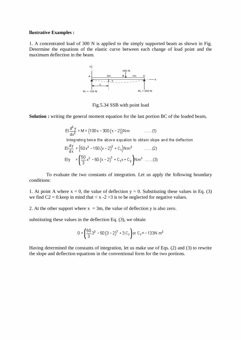
llustrative Examples :
1. A concentrated load of 300 N is applied to the simply supported beam as shown in Fig.
Determine the equations of the elastic curve between each change of load point and the
maximum deflection in the beam.
Fig.5.34 SSB with point load
Solution : writing the general moment equation for the last portion BC of the loaded beam,
To evaluate the two constants of integration. Let us apply the following boundary
conditions:
1. At point A where x = 0, the value of deflection y = 0. Substituting these values in Eq. (3)
we find C2 = 0.keep in mind that < x -2 >3 is to be neglected for negative values.
2. At the other support where x = 3m, the value of deflection y is also zero.
substituting these values in the deflection Eq. (3), we obtain
Having determined the constants of integration, let us make use of Eqs. (2) and (3) to rewrite
the slope and deflection equations in the conventional form for the two portions.
Continuing the solution, we assume that the maximum deflection will occur in the segment
AB. Its location may be found by differentiating Eq. (5) with respect to x and setting the
derivative to be equal to zero, or, what amounts to the same thing, setting the slope equation
(4) equal to zero and solving for the point of zero slope.
We obtain
50 x2– 133 = 0 or x = 1.63 m (It may be kept in mind that if the solution of the equation does
not yield a value < 2 m then we have to try the other equations which are valid for segment
BC)
Since this value of x is valid for segment AB, our assumption that the maximum deflection
occurs in this region is correct. Hence, to determine the maximum deflection, we substitute x
= 1.63 m in Eq (5), which yields
The negative value obtained indicates that the deflection y is downward from the x axis.quite
usually only the magnitude of the deflection, without regard to sign, is desired; this is denoted
by d, the use of y may be reserved to indicate a directed value of deflection.
if E = 30 Gpa and I = 1.9 x 106 mm4 = 1.9 x 10 -6 m4 , Eq. (h) becomes
Example 2:
It is required to determine the value of EIy at the position midway between the supports and
at the overhanging end for the beam shown in figure below.
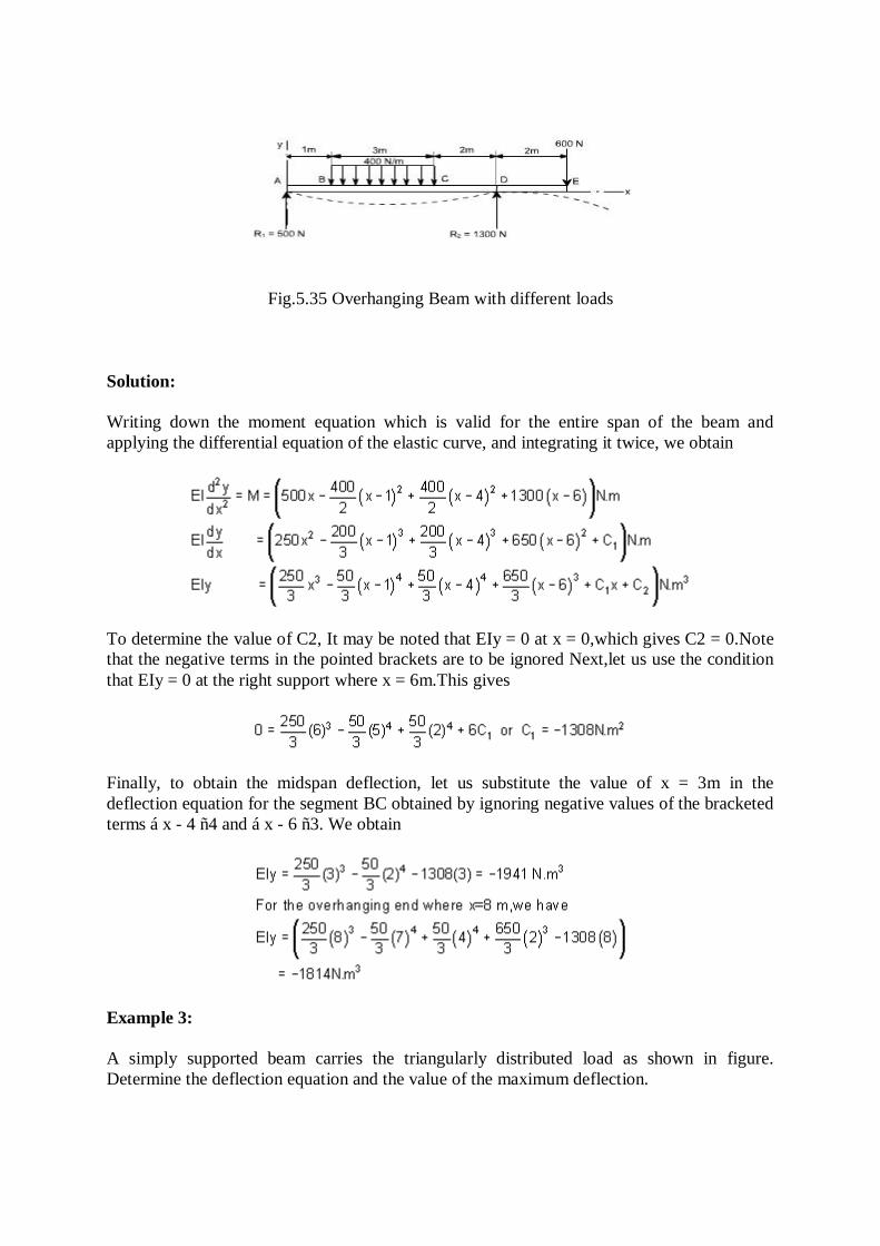
Fig.5.35 Overhanging Beam with different loads
Solution:
Writing down the moment equation which is valid for the entire span of the beam and
applying the differential equation of the elastic curve, and integrating it twice, we obtain
To determine the value of C2, It may be noted that EIy = 0 at x = 0,which gives C2 = 0.Note
that the negative terms in the pointed brackets are to be ignored Next,let us use the condition
that EIy = 0 at the right support where x = 6m.This gives
Finally, to obtain the midspan deflection, let us substitute the value of x = 3m in the
deflection equation for the segment BC obtained by ignoring negative values of the bracketed
terms á x - 4 ñ4 and á x - 6 ñ3. We obtain
Example 3:
A simply supported beam carries the triangularly distributed load as shown in figure.
Determine the deflection equation and the value of the maximum deflection.

Fig.5.36 SSB with Triangular load
Solution:
Due to symmetry, the reactionsis one half the total load of 1/2w0L, or R1 = R2 =
1/4w0L.Due to the advantage of symmetry to the deflection curve from A to B is the mirror
image of that from C to B. The condition of zero deflection at A and of zero slope at B do not
require the use of a general moment equation. Only the moment equation for segment AB is
needed, and this may be easily written with the aid of figure(b).
Taking into account the differential equation of the elastic curve for the segment AB and
integrating twice, one can obtain
In order to evaluate the constants of integration,let us apply the B.C'swe note that at the
support A, y = 0 at x = 0.Hence from equation (3), we get C2 = 0. Also,because of symmetry,
the slope dy/dx = 0 at midspan where x = L/2.Substituting these conditions in equation (2) we
get
Hence the deflection equation from A to B (and also from C to B because of symmetry)
becomes
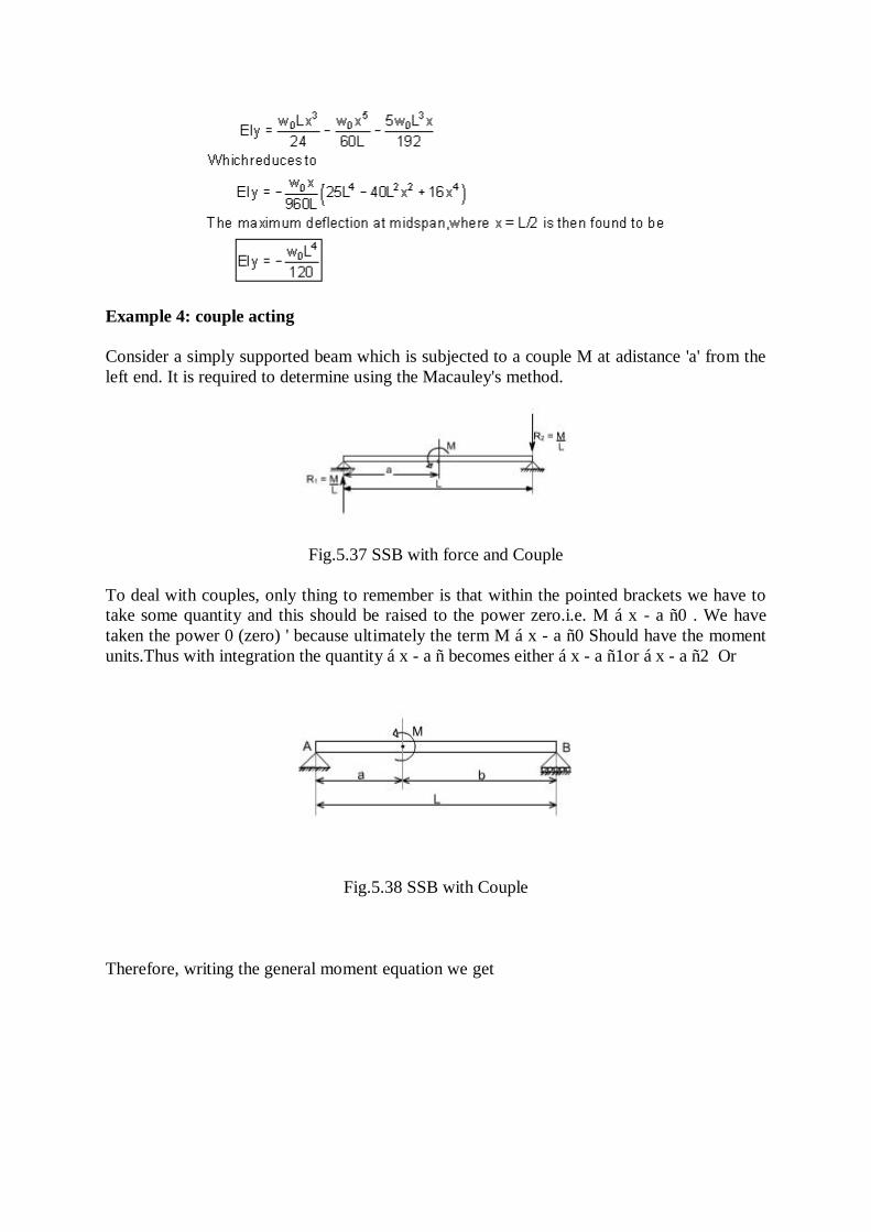
Example 4: couple acting
Consider a simply supported beam which is subjected to a couple M at adistance 'a' from the
left end. It is required to determine using the Macauley's method.
Fig.5.37 SSB with force and Couple
To deal with couples, only thing to remember is that within the pointed brackets we have to
take some quantity and this should be raised to the power zero.i.e. M á x - a ñ0 . We have
taken the power 0 (zero) ' because ultimately the term M á x - a ñ0 Should have the moment
units.Thus with integration the quantity á x - a ñ becomes either á x - a ñ1or á x - a ñ2 Or
Fig.5.38 SSB with Couple
Therefore, writing the general moment equation we get

Example 5:
A simply supported beam is subjected to U.d.l in combination with couple M. It is required to
determine the deflection.
Fig.5.39 Overhanging beam with different loads
This problem may be attemped in the some way. The general moment equation my be written
as
Integrate twice to get the deflection of the loaded beam.
TEXT/ REFERENCE BOOKS
1. Bansal R.K., “Strength of Materials”, Laxmi Publications (P) Ltd.,Fifth Edition,2012
2. Punmia B.C. & Jain A.K., Mechanics of Materials, ,Laxmi Publications,2001
3. Ryder G.H, “Strength of Materials, Macmillan India Ltd”., Third Edition, 2002
4. Ray Hulse, Keith Sherwin & Jack Cain, “Solid Mechanics”, Palgrave ANE Books,2004.
5. Allan F. Bower, Applied Mechanics of Solids, CRC Press, 2009, 820 pages.