Small solids in an inviscid fluid
77
Small solids in an inviscid fluid Nicolas Seguin Laboratoire J.-L. Lions, UPMC Paris 6, France September 4, 2009 In coll. with B. Andreianov, F. Lagouti` ere and T. Takahashi Nicolas Seguin (LJLL, UMPC) Small solids in an inviscid fluid September 4, 2009 1 / 37
Transcript of Small solids in an inviscid fluid

Small solids in an inviscid fluid
Nicolas Seguin
Laboratoire J.-L. Lions, UPMC Paris 6, France
September 4, 2009
In coll. with B. Andreianov, F. Lagoutiere and T. Takahashi
Nicolas Seguin (LJLL, UMPC) Small solids in an inviscid fluid September 4, 2009 1 / 37
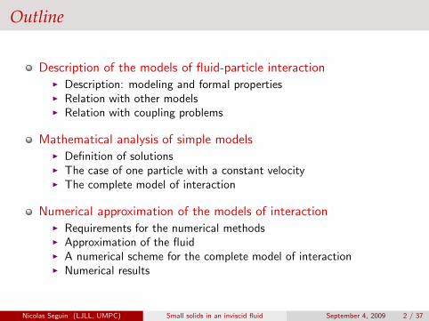
Outline
Description of the models of fluid-particle interaction◮ Description: modeling and formal properties◮ Relation with other models◮ Relation with coupling problems
Mathematical analysis of simple models◮ Definition of solutions◮ The case of one particle with a constant velocity◮ The complete model of interaction
Numerical approximation of the models of interaction◮ Requirements for the numerical methods◮ Approximation of the fluid◮ A numerical scheme for the complete model of interaction◮ Numerical results
Nicolas Seguin (LJLL, UMPC) Small solids in an inviscid fluid September 4, 2009 2 / 37

Motivations
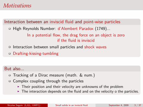
Interaction between an inviscid fluid and point-wise particles
High Reynolds Number: d’Alembert Paradox (1749)...
In a potential flow, the drag force on an object is zeroif the fluid is inviscid
Interaction between small particles and shock waves
Drafting-kissing-tumbling
But also...
Tracking of a Dirac measure (math. & num.)
Complex coupling through the particles◮ Their position and their velocity are unknowns of the problem◮ The interaction depends on the fluid and on the velocity o the particles.
Nicolas Seguin (LJLL, UMPC) Small solids in an inviscid fluid September 4, 2009 3 / 37
Motivations
Interaction between an inviscid fluid and point-wise particles
High Reynolds Number: d’Alembert Paradox (1749)...
In a potential flow, the drag force on an object is zeroif the fluid is inviscid
Interaction between small particles and shock waves
Drafting-kissing-tumbling
But also...
Tracking of a Dirac measure (math. & num.)
Complex coupling through the particles◮ Their position and their velocity are unknowns of the problem◮ The interaction depends on the fluid and on the velocity o the particles.
Nicolas Seguin (LJLL, UMPC) Small solids in an inviscid fluid September 4, 2009 3 / 37

An inviscid model of fluid-particle interaction
Euler equations for the fluid (ρ: density, u ∈ Rd: velocity, p: pressure)
N point-wise particles (hk(t): position, mk: mass, λk: drag coefficient)
Classical Euler equations everywhere except on the particles (x 6= hk)
Point-wise particles: Dirac measures δ0(x − hk)
Particles governed by the 2nd Newton law:Acceleration = Drag force (function of (u − h′
k))
Conservation of the total momentum
d
dt
(
∫
Rdρu dx +
N
∑k=1
mkh′k
)
= 0
Nicolas Seguin (LJLL, UMPC) Small solids in an inviscid fluid September 4, 2009 4 / 37

An inviscid model of fluid-particle interaction
Euler equations for the fluid (ρ: density, u ∈ Rd: velocity, p: pressure)
N point-wise particles (hk(t): position, mk: mass, λk: drag coefficient)
For t > 0 and x ∈ Rd
∂tρ + ∇ · (ρu) = 0∂t(ρu +∇ · (ρu ⊗ u + p(ρ)I) = −∑
k
Fk δ0(x − hk(t))
For t > 0 and k = 1, ..., N
mk h′′k (t) = Fk
Coupling by the drag force: Fk = λkρD(
u − h′k
)
where D(v) = v or v|v|.
Nicolas Seguin (LJLL, UMPC) Small solids in an inviscid fluid September 4, 2009 4 / 37

A simple model of interaction
Euler equations replaced by the 1D Burgers equation + one particle
[Lagoutiere, Seguin, Takahashi]
∂tu + ∂x(u2/2) = λ D(h′(t) − u) δ0(x − h(t))
m h′′(t) = −λ D(h′(t) − u(t, h(t)))
u(t, x): velocity of the fluid
h(t): position of the particle
λ: drag coefficient (> 0)
D(v) = v or v|v| (“laminar” or “turbulent” case)
Fluid-particle coupling by the drag force term◮ Burgers equation + singular source term◮ ODE of relaxation (h′ → u)
Nicolas Seguin (LJLL, UMPC) Small solids in an inviscid fluid September 4, 2009 5 / 37

A simple model of interaction
Euler equations replaced by the 1D Burgers equation + one particle
[Lagoutiere, Seguin, Takahashi]
∂tu + ∂x(u2/2) = λ D(h′(t) − u) δ0(x − h(t))
m h′′(t) = −λ D(h′(t) − u(t, h(t)))
Formal properties (also available with Euler equations)
Conservation of the total momentum:d
dt
(
∫
R
u dx + m h′)
= 0
Equation for the total kinetic energy:1
2
d
dt
(
∫
R
u2 dx + m(h′)2
)
(t) ≤ 0
Nicolas Seguin (LJLL, UMPC) Small solids in an inviscid fluid September 4, 2009 5 / 37

Comparison with other models
Burgers equation coupled with one point-wise particle
∂tu + ∂x(u2/2) = λ D(h′(t) − u) δ0(x − h(t))
m h′′(t) = −λ D(h′(t) − u(t, h(t)))
Vlasov model - Baranger, Desvillettes, Goudon, Carillo, Domelevo...
Introduce f (t, x, v): density of particles (with velocity v)
∂tu + ∂x(u2/2) =λ
m
∫
R
(v − u) f dv
∂t f + v ∂x f +λ
m∂v((u − v) f ) = 0
One formally recovers the previous model, setting
f (t, x, v) = m δ0(x − h(t)) δ0(v − V(t)).
Nicolas Seguin (LJLL, UMPC) Small solids in an inviscid fluid September 4, 2009 6 / 37
Comparison with other models
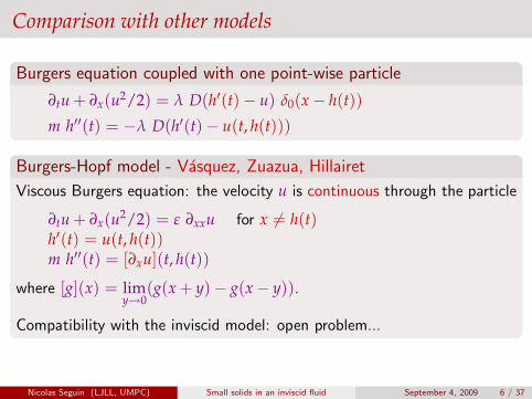
Burgers equation coupled with one point-wise particle
∂tu + ∂x(u2/2) = λ D(h′(t) − u) δ0(x − h(t))
m h′′(t) = −λ D(h′(t) − u(t, h(t)))
Burgers-Hopf model - Vasquez, Zuazua, Hillairet
Viscous Burgers equation: the velocity u is continuous through the particle
∂tu + ∂x(u2/2) = ε ∂xxu for x 6= h(t)h′(t) = u(t, h(t))m h′′(t) = [∂xu](t, h(t))
where [g](x) = limy→0
(g(x + y) − g(x − y)).
Compatibility with the inviscid model: open problem...
Nicolas Seguin (LJLL, UMPC) Small solids in an inviscid fluid September 4, 2009 6 / 37
Comparison with other models
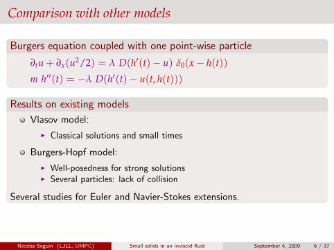
Burgers equation coupled with one point-wise particle
∂tu + ∂x(u2/2) = λ D(h′(t) − u) δ0(x − h(t))
m h′′(t) = −λ D(h′(t) − u(t, h(t)))
Results on existing models
Vlasov model:
◮ Classical solutions and small times
Burgers-Hopf model:
◮ Well-posedness for strong solutions◮ Several particles: lack of collision
Several studies for Euler and Navier-Stokes extensions.
Nicolas Seguin (LJLL, UMPC) Small solids in an inviscid fluid September 4, 2009 6 / 37
Definition of solutions
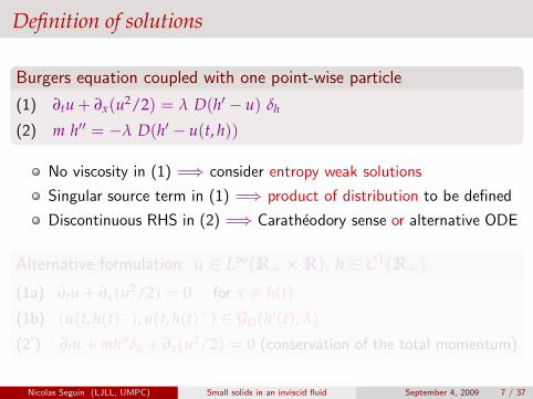
Burgers equation coupled with one point-wise particle
(1) ∂tu + ∂x(u2/2) = λ D(h′ − u) δh
(2) m h′′ = −λ D(h′ − u(t, h))
No viscosity in (1) =⇒ consider entropy weak solutions
Singular source term in (1) =⇒ product of distribution to be defined
Discontinuous RHS in (2) =⇒ Caratheodory sense or alternative ODE
Alternative formulation: u ∈ L∞(R+ × R), h ∈ C1(R+)
(1a) ∂tu + ∂x(u2/2) = 0 for x 6= h(t)
(1b) (u(t, h(t)−), u(t, h(t)+) ∈ GD(h′(t), λ)
(2’) ∂tu + mh′′δh + ∂x(u2/2) = 0 (conservation of the total momentum)
Nicolas Seguin (LJLL, UMPC) Small solids in an inviscid fluid September 4, 2009 7 / 37

Definition of solutions
Burgers equation coupled with one point-wise particle
(1) ∂tu + ∂x(u2/2) = λ D(h′ − u) δh
(2) m h′′ = −λ D(h′ − u(t, h))
No viscosity in (1) =⇒ consider entropy weak solutions
Singular source term in (1) =⇒ product of distribution to be defined
Discontinuous RHS in (2) =⇒ Caratheodory sense or alternative ODE
Alternative formulation: u ∈ L∞(R+ × R), h ∈ C1(R+)
(1a) ∂tu + ∂x(u2/2) = 0 for x 6= h(t)
(1b) (u(t, h(t)−), u(t, h(t)+) ∈ GD(h′(t), λ)
(2’) ∂tu + mh′′δh + ∂x(u2/2) = 0 (conservation of the total momentum)
Nicolas Seguin (LJLL, UMPC) Small solids in an inviscid fluid September 4, 2009 7 / 37
Alternative formulation
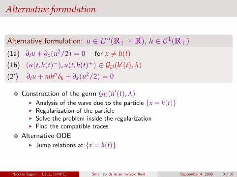
Alternative formulation: u ∈ L∞(R+ × R), h ∈ C1(R+)
(1a) ∂tu + ∂x(u2/2) = 0 for x 6= h(t)
(1b) (u(t, h(t)−), u(t, h(t)+) ∈ GD(h′(t), λ)
(2’) ∂tu + mh′′δh + ∂x(u2/2) = 0
Construction of the germ GD(h′(t), λ)◮ Analysis of the wave due to the particle {x = h(t)}◮ Regularization of the particle◮ Solve the problem inside the regularization◮ Find the compatible traces
Alternative ODE◮ Jump relations at {x = h(t)}
Nicolas Seguin (LJLL, UMPC) Small solids in an inviscid fluid September 4, 2009 8 / 37

Wave due to the particle – Quasilinear form of the PDE
Equivalent form: δ0(x) = ∂xH(x), H Heaviside function
∂tu + ∂x(u2/2) − λ D(h′ − u) ∂xw = 0
∂tw + h′(t) ∂xw = 0
w(0, x) = H(x − h(0)) =⇒ w(t, x) = H(x − h(t))
Quasilinear formulation:
∂t
(
uw
)
+
(
u −λD(h′ − u)0 h′
)
∂x
(
uw
)
= 0
Hyperbolic system (diagonalisable in R even if u = h′ since D(0) = 0).
Wave associated with u: genuinely non linear fieldWave associated with h′: linearly degenerate field
What happen when u = h′ ?
Nicolas Seguin (LJLL, UMPC) Small solids in an inviscid fluid September 4, 2009 9 / 37
Construction of the germ GD(h′, λ) – Regularisation
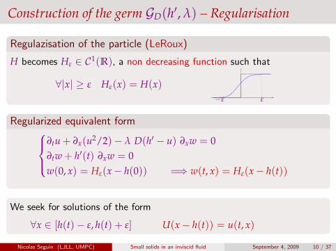
Regulazisation of the particle (LeRoux)
H becomes Hε ∈ C1(R), a non decreasing function such that
∀|x| ≥ ε Hε(x) = H(x)
−ε ε
Regularized equivalent form
∂tu + ∂x(u2/2) − λ D(h′ − u) ∂xw = 0
∂tw + h′(t) ∂xw = 0
w(0, x) = Hε(x − h(0)) =⇒ w(t, x) = Hε(x − h(t))
We seek for solutions of the form
∀x ∈ [h(t) − ε, h(t) + ε] U(x − h(t)) = u(t, x)
Nicolas Seguin (LJLL, UMPC) Small solids in an inviscid fluid September 4, 2009 10 / 37

Construction of the germ GD(h′, λ) – Change of frame
The equations “inside” the regularized particle
∂tu + ∂x(u2/2) − λ D(h′ − u) ∂xw = 0
w(t, x) = Hε(x − h(t))
U(x − h(t)) = u(t, x)
gives for ξ = x − h(t) ∈ [−ε, ε],
−h′(t)U′(ξ) + (U2/2)′(ξ) − λD(h′(t) − U(ξ))H′ε(ξ) = 0 (⋆)
in the weak entropy sense:
Smooth parts: solve (⋆) in the classical sense
Shock wave at ξ0: (U(ξ−0 ) + U(ξ+0 ))/2 = h′(t) and U(ξ−0 ) > U(ξ+
0 )
Search all the pairs U(−ε) and U(+ε) which can be connected
Nicolas Seguin (LJLL, UMPC) Small solids in an inviscid fluid September 4, 2009 11 / 37

Germ GD(h′, λ) for a linear drag force D(v) = v
In the case of a linear drag force: D(v) = vSmooth solutions (t is fixed):
(U2/2 − h′(t)U)′(ξ) − λD(h′(t) − U(ξ))H′ε(ξ) = 0
⇐⇒ (U(ξ) − h′(t))(
U′(ξ) + λH′ε(ξ)
)
= 0
⇐⇒
{
Either U(ξ) = h′(t)
Or U(ξ) + λHε(ξ) = Cst
Shock wave:{
(U(ξ−0 ) + U(ξ+0 ))/2 = h′(t)
U(ξ−0 ) > h′(t) > U(ξ+0 )
Search all the pairs U(−ε) and U(+ε) which can be connectedThe germ GD(h′, λ) is the set of all these pairs
Nicolas Seguin (LJLL, UMPC) Small solids in an inviscid fluid September 4, 2009 12 / 37

Germ GD(h′, λ) for a linear drag force D(v) = v
Smooth solutions:{
Either U(ξ) = h′(t)
Or U(ξ) + λHε(ξ) = Cst
Shock wave:{
(U(ξ−0 ) + U(ξ+0 ))/2 = h′(t)
U(ξ−0 ) > h′(t) > U(ξ+0 )
Hε
U
0 1
U(−ε)
U(ε) = U(−ε)− λ
h′(t)
Nicolas Seguin (LJLL, UMPC) Small solids in an inviscid fluid September 4, 2009 13 / 37
Germ GD(h′, λ) for a linear drag force D(v) = v
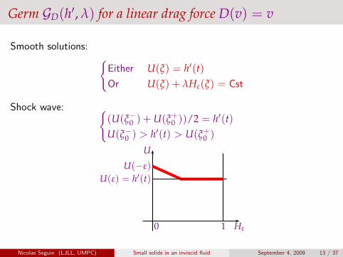
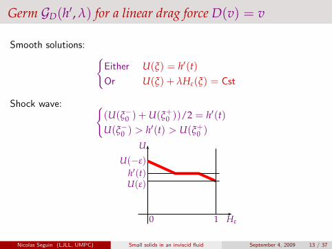
Smooth solutions:{
Either U(ξ) = h′(t)
Or U(ξ) + λHε(ξ) = Cst
Shock wave:{
(U(ξ−0 ) + U(ξ+0 ))/2 = h′(t)
U(ξ−0 ) > h′(t) > U(ξ+0 )
Hε
U
0 1
U(−ε)
U(ε) = h′(t)
Nicolas Seguin (LJLL, UMPC) Small solids in an inviscid fluid September 4, 2009 13 / 37
Germ GD(h′, λ) for a linear drag force D(v) = v
Smooth solutions:{
Either U(ξ) = h′(t)
Or U(ξ) + λHε(ξ) = Cst
Shock wave:{
(U(ξ−0 ) + U(ξ+0 ))/2 = h′(t)
U(ξ−0 ) > h′(t) > U(ξ+0 )
Hε
U
0 1
U(−ε)
h′(t)U(ε)
Nicolas Seguin (LJLL, UMPC) Small solids in an inviscid fluid September 4, 2009 13 / 37

Germ GD(h′, λ) for a linear drag force D(v) = v
Smooth solutions:{
Either U(ξ) = h′(t)
Or U(ξ) + λHε(ξ) = Cst
Shock wave:{
(U(ξ−0 ) + U(ξ+0 ))/2 = h′(t)
U(ξ−0 ) > h′(t) > U(ξ+0 )
Hε
U
0 1
U(−ε)
h′(t)
U(−ε)− λ∋ U(ε)
Nicolas Seguin (LJLL, UMPC) Small solids in an inviscid fluid September 4, 2009 13 / 37

Germ GD(h′, λ) for a linear drag force D(v) = v
Smooth solutions:{
Either U(ξ) = h′(t)
Or U(ξ) + λHε(ξ) = Cst
Shock wave:{
(U(ξ−0 ) + U(ξ+0 ))/2 = h′(t)
U(ξ−0 ) > h′(t) > U(ξ+0 )
Hε
U
0 1
U(−ε)
h′(t)
U(ε)
Nicolas Seguin (LJLL, UMPC) Small solids in an inviscid fluid September 4, 2009 13 / 37

Germ GD(h′, λ) for a linear drag force D(v) = v
Smooth solutions:{
Either U(ξ) = h′(t)
Or U(ξ) + λHε(ξ) = Cst
Shock wave:{
(U(ξ−0 ) + U(ξ+0 ))/2 = h′(t)
U(ξ−0 ) > h′(t) > U(ξ+0 )
Hε
U
0
U(−ε)
h′(t)
∋ U(ε)
Nicolas Seguin (LJLL, UMPC) Small solids in an inviscid fluid September 4, 2009 13 / 37

Germ GD(h′, λ) according the drag force
Germ GD(h′, λ): set of all pairs (u−, u+) ∈ R2 such that
(U2/2 − h′(t)U)′(ξ) − λD(h′(t) − U(ξ))H′ε(ξ) = 0
U(−ε) = u− and U(+ε) = u+
(h′, h′)
u−
u+
(h′, h′)
u−
u+
h′ + λ
h′ − λ
{u+ = u−e−λ + h′}
{u+ = u−e+λ + h′} {u+ = −u−e+λ + h′}
{u+ = −u−e−λ + h′}
D(v) = v D(v) = v|v|
Nicolas Seguin (LJLL, UMPC) Small solids in an inviscid fluid September 4, 2009 14 / 37
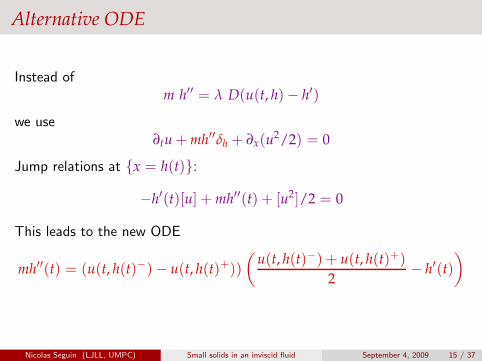
Alternative ODE
Instead ofm h′′ = λ D(u(t, h)− h′)
we use∂tu + mh′′δh + ∂x(u2/2) = 0
Jump relations at {x = h(t)}:
−h′(t)[u] + mh′′(t) + [u2]/2 = 0
This leads to the new ODE
mh′′(t) = (u(t, h(t)−) − u(t, h(t)+))
(
u(t, h(t)−) + u(t, h(t)+)
2− h′(t)
)
Nicolas Seguin (LJLL, UMPC) Small solids in an inviscid fluid September 4, 2009 15 / 37
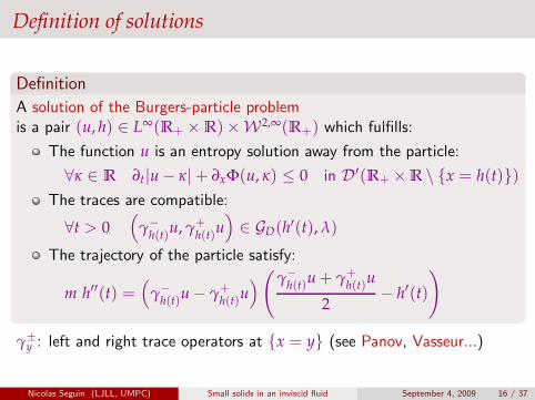
Definition of solutions
Definition
A solution of the Burgers-particle problemis a pair (u, h) ∈ L∞(R+ × R)×W2,∞(R+) which fulfills:
The function u is an entropy solution away from the particle:
∀κ ∈ R ∂t|u − κ|+ ∂xΦ(u, κ) ≤ 0 in D′(R+ × R \ {x = h(t)})
The traces are compatible:
∀t > 0(
γ−h(t)
u, γ+h(t)
u)
∈ GD(h′(t), λ)
The trajectory of the particle satisfy:
m h′′(t) =(
γ−h(t)
u − γ+h(t)
u)
(
γ−h(t)
u + γ+h(t)
u
2− h′(t)
)
γ±y : left and right trace operators at {x = y} (see Panov, Vasseur...)
Nicolas Seguin (LJLL, UMPC) Small solids in an inviscid fluid September 4, 2009 16 / 37

The case of one particle with a zero velocity
The case (h ≡ 0)
[P0]
{
∂tu + ∂x(u2/2) + λD(u) δ0 = 0
u|t=0 = u0
See also Isaacson-Temple, LeRoux, Dielh, Gosse, Vasseur,Burger-Garcıa-Karlsen-Towers...
Definition
A function u ∈ L∞(R+ × R) is an entropy solution of [P0] if
∀κ ∈ R ∂t|u − κ|+ ∂xΦ(u, κ) ≤ 0 in D′(R+ × R \ {x = 0})
∀t > 0(
γ−0 u(t), γ+
0 u(t))
∈ GD(0, λ)
Nicolas Seguin (LJLL, UMPC) Small solids in an inviscid fluid September 4, 2009 17 / 37

The Riemann problem
Theorem (with D(v) = v or v|v|)
The Riemann problem
∂tu + ∂x(u2/2) + λD(u) δ0 = 0
u(0, x) =
{
uL if x < 0
uR if x > 0
admits one and only one self-similar entropy solution for all (uL, uR) ∈ R.
Construct the set U−(uL) = {W(0−; uL, u), u ∈ R}Construct the set U+(uR) = {W(0+; u, uR), u ∈ R}Existence and uniqueness of (u−, u+) ∈ R
2 such thatu− ∈ U−(uL), u+ ∈ U+(uR) and (u−, u+) ∈ GD(0, λ).
N.B. Uniqueness fails if λ < 0 !
Nicolas Seguin (LJLL, UMPC) Small solids in an inviscid fluid September 4, 2009 18 / 37
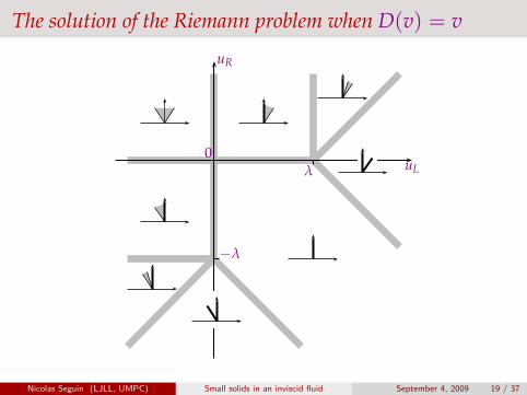
The solution of the Riemann problem when D(v) = v
0
−λ
λ uL
uR
Nicolas Seguin (LJLL, UMPC) Small solids in an inviscid fluid September 4, 2009 19 / 37
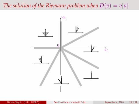
The solution of the Riemann problem when D(v) = v|v|
0uL
uR
Nicolas Seguin (LJLL, UMPC) Small solids in an inviscid fluid September 4, 2009 20 / 37

The Cauchy problem for a particle with a zero velocity
Alternative definition: Adapted Kruzhkov entropies
Let c be defined by c(x) =
{
cL if x < 0,
cR if x > 0..
A function u ∈ L∞(R+ × R) is an entropy solution of [P0] iff
∂t|u − c|+ ∂xΦ(u, c) ≤ 0 in D′(R+ × R \ {x = 0})
for all (cL, cR) ∈ GD(0, λ).
Baiti-Jenssen, Audusse-Perthame, Adimurthi-Mishra-Veerappa Gowda,Burger-Karlsen-Towers, Andreianov-Karlsen-Risebro...
If u|t=0(x) = c(x), then c is a stationary entropy solution of [P0],for all (cL, cR) ∈ GD(0, λ).
An entropy solution is “dissipative” w.r.t. any stationary solution.
Nicolas Seguin (LJLL, UMPC) Small solids in an inviscid fluid September 4, 2009 21 / 37

The Cauchy problem for a particle with a zero velocity
Proposition (dissipative germ)
For all (cL, cR) ∈ GD(0, λ) and (dL, dR) ∈ GD(0, λ), we have
Φ(cR, dR) − Φ(cL, dL) ≤ 0.
This property enables to compare two solutions, in the spirit of Kruzhkov’suniqueness proof.
Theorem
Let the drag force be D(v) = v or v|v|.The Cauchy problem [P0] admits one and only one entropy solution in L∞.
The existence will follow, using the convergence of numericcal schemes.
N.B. Also available for h′(t) = V, V ∈ R.
Nicolas Seguin (LJLL, UMPC) Small solids in an inviscid fluid September 4, 2009 22 / 37

The full model
Theorem (D(v) = v)
The Riemann problem for the Burgers-particle model
∂tu + ∂x(u2/2) = λ (h′(t) − u) δ0(x − h(t))
m h′′(t) =(
γ−h(t)
u − γ+h(t)
u) (
(γ−h(t)
u + γ+h(t)
u)/2 − h′(t))
u|t=0 =
{
uL if x < 0
uR if x > 0
h(0) = 0, h′(0) = V
admits at least one solution for all uL, uR, V ∈ R.
Proof by construction (solutions are not self-similar).
When t → +∞ or λ → +∞, the solution tends to a solution of theclassical Burgers equation and h′(t) to a predictable constant.
Nicolas Seguin (LJLL, UMPC) Small solids in an inviscid fluid September 4, 2009 23 / 37

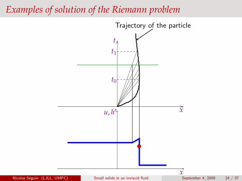
Examples of solution of the Riemann problem
x
t
t0
t1
Trajectory of the particle
x
u, h′
Nicolas Seguin (LJLL, UMPC) Small solids in an inviscid fluid September 4, 2009 24 / 37

Examples of solution of the Riemann problem
x
t
t0
t1
Trajectory of the particle
x
u, h′
Nicolas Seguin (LJLL, UMPC) Small solids in an inviscid fluid September 4, 2009 24 / 37

Examples of solution of the Riemann problem
x
t
t0
t1
Trajectory of the particle
x
u, h′
Nicolas Seguin (LJLL, UMPC) Small solids in an inviscid fluid September 4, 2009 24 / 37
Examples of solution of the Riemann problem
x
t
t0
t1
Trajectory of the particle
x
u, h′
Nicolas Seguin (LJLL, UMPC) Small solids in an inviscid fluid September 4, 2009 24 / 37

Examples of solution of the Riemann problem
x
t
t0
t1
Trajectory of the particle
x
u, h′
Nicolas Seguin (LJLL, UMPC) Small solids in an inviscid fluid September 4, 2009 24 / 37

Examples of solution of the Riemann problem
x
t
t0
t1
Trajectory of the particle
x
u, h′
Nicolas Seguin (LJLL, UMPC) Small solids in an inviscid fluid September 4, 2009 24 / 37

Examples of solution of the Riemann problem
x
t
Trajectory of the particle
Shock waves
Nicolas Seguin (LJLL, UMPC) Small solids in an inviscid fluid September 4, 2009 25 / 37

Well-posedness of the Burgers-particle model
Riemann problem
The solution is not self-similar
Existence by construction
Uniqueness... Probably equivalent to study the Cauchy problem
Cauchy problem: still open
Existence via the methods devoted to hyperbolic systems?
Uniqueness by comparison, continuity...
Nicolas Seguin (LJLL, UMPC) Small solids in an inviscid fluid September 4, 2009 26 / 37
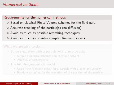
Numerical methods
Requirements for the numerical methods
Based on classical Finite Volume schemes for the fluid part
Accurate tracking of the particle(s) (no diffusion)
Avoid as much as possible remeshing techniques
Avoid as much as possible complex Riemann solvers
What we are able to do...
Burgers equation with a particle with a zero velocity◮ Simple numerical schemes (no Riemann solver)◮ Analysis of convergence
The full Burgers-particle model◮ Use of the Riemann solver for a particle with a constant velocity◮ Random sampling for the evolution of the position of the particle
Nicolas Seguin (LJLL, UMPC) Small solids in an inviscid fluid September 4, 2009 27 / 37
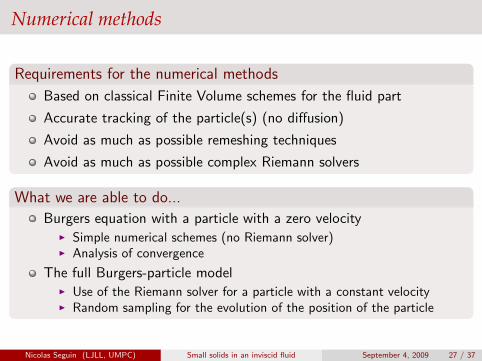
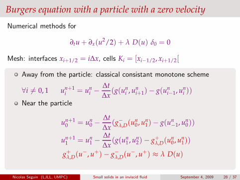
Burgers equation with a particle with a zero velocity
Numerical methods for
∂tu + ∂x(u2/2) + λ D(u) δ0 = 0
Mesh: interfaces xi+1/2 = i∆x, cells Ki = [xi−1/2, xi+1/2[
Away from the particle: classical consistant monotone scheme
∀i 6= 0, 1 un+1i = un
i −∆t
∆x(g(un
i , uni+1) − g(un
i−1, uni ))
Near the particle
un+10 = un
0 −∆t
∆x(g−λ,D(un
0 , un1) − g(un
−1, un0))
un+11 = un
1 −∆t
∆x(g(un
1 , un2) − g+
λ,D(un0 , un
1))
g+λ,D(u−, u+) − g−λ,D(u−, u+) ≈ λ D(u)
Nicolas Seguin (LJLL, UMPC) Small solids in an inviscid fluid September 4, 2009 28 / 37
Burgers equation with a particle with a zero velocity
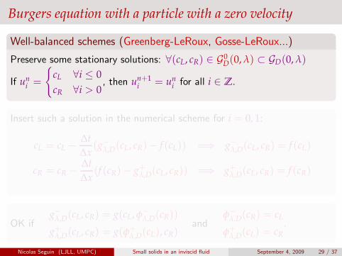
Well-balanced schemes (Greenberg-LeRoux, Gosse-LeRoux...)
Preserve some stationary solutions: ∀(cL, cR) ∈ G0D(0, λ) ⊂ GD(0, λ)
If uni =
{
cL ∀i ≤ 0
cR ∀i > 0, then un+1
i = uni for all i ∈ Z.
Insert such a solution in the numerical scheme for i = 0, 1:
cL = cL −∆t
∆x(g−λ,D(cL, cR) − f (cL)) =⇒ g−λ,D(cL, cR) = f (cL)
cR = cR −∆t
∆x(f (cR) − g+
λ,D(cL, cR)) =⇒ g+λ,D(cL, cR) = f (cR)
OK ifg−λ,D(cL, cR) = g(cL, φ−
λ,D(cR))
g+λ,D(cL, cR) = g(φ+
λ,D(cL), cR)and
φ−λ,D(cR) = cL
φ+λ,D(cL) = cR
.
Nicolas Seguin (LJLL, UMPC) Small solids in an inviscid fluid September 4, 2009 29 / 37

Burgers equation with a particle with a zero velocity
Well-balanced schemes (Greenberg-LeRoux, Gosse-LeRoux...)
Preserve some stationary solutions: ∀(cL, cR) ∈ G0D(0, λ) ⊂ GD(0, λ)
If uni =
{
cL ∀i ≤ 0
cR ∀i > 0, then un+1
i = uni for all i ∈ Z.
Insert such a solution in the numerical scheme for i = 0, 1:
cL = cL −∆t
∆x(g−λ,D(cL, cR) − f (cL)) =⇒ g−λ,D(cL, cR) = f (cL)
cR = cR −∆t
∆x(f (cR) − g+
λ,D(cL, cR)) =⇒ g+λ,D(cL, cR) = f (cR)
OK ifg−λ,D(cL, cR) = g(cL, φ−
λ,D(cR))
g+λ,D(cL, cR) = g(φ+
λ,D(cL), cR)and
φ−λ,D(cR) = cL
φ+λ,D(cL) = cR
.
Nicolas Seguin (LJLL, UMPC) Small solids in an inviscid fluid September 4, 2009 29 / 37
Burgers equation with a particle with a zero velocity
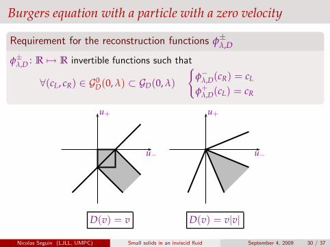
Requirement for the reconstruction functions φ±λ,D
φ±λ,D : R 7→ R invertible functions such that
∀(cL, cR) ∈ G0D(0, λ) ⊂ GD(0, λ)
{
φ−λ,D(cR) = cL
φ+λ,D(cL) = cR
u−
u+
u−
u+
D(v) = v D(v) = v|v|
Nicolas Seguin (LJLL, UMPC) Small solids in an inviscid fluid September 4, 2009 30 / 37

Burgers equation with a particle with a zero velocity
Requirement for the reconstruction functions φ±λ,D
φ±λ,D : R 7→ R invertible functions such that
∀(cL, cR) ∈ G0D(0, λ) ⊂ GD(0, λ)
{
φ−λ,D(cR) = cL
φ+λ,D(cL) = cR
u−
u+
u−
u+
G0D(0, λ)
D(v) = v D(v) = v|v|
Nicolas Seguin (LJLL, UMPC) Small solids in an inviscid fluid September 4, 2009 30 / 37
Burgers equation with a particle with a zero velocity
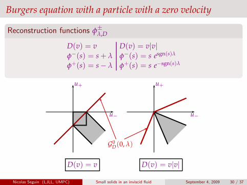
Reconstruction functions φ±λ,D
D(v) = v D(v) = v|v|
φ−(s) = s + λ φ−(s) = s esgn(s)λ
φ+(s) = s − λ φ+(s) = s e−sgn(s)λ
u−
u+
u−
u+
G0D(0, λ)
D(v) = v D(v) = v|v|
Nicolas Seguin (LJLL, UMPC) Small solids in an inviscid fluid September 4, 2009 30 / 37
Burgers equation with a particle with a zero velocity
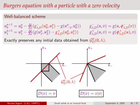
Well-balanced scheme
un+10 = un
0 −∆t∆x(g−λ,D(un
0 , un1) − g(un
−1, un0)) g−λ,D(u, v) = g(u, φ−
λ,D(v))
un+11 = un
1 −∆t∆x(g(un
1 , un2)− g+
λ,D(un0, un
1)) g+λ,D(u, v) = g(φ+
λ,D(u), v)
Exactly preserves any initial data obtained from G0D(0, λ).
u−
u+
u−
u+
G0D(0, λ)
D(v) = v D(v) = v|v|
Nicolas Seguin (LJLL, UMPC) Small solids in an inviscid fluid September 4, 2009 30 / 37

Burgers equation with a particle with a zero velocity
Analysis of the well-balanced scheme
Let u∆ be the piecewise constant function obtained from (uni )i,n
Under a classical CFL condition:
u∆ is uniformly bounded in L∞(R+ × R)
u∆ is uniformly bounded in BVloc([0, T] × (R \ {0})) [BGKT 08]
u∆ satisfies discrete (adapted) entropy inequalities
u∆ converges in L1loc(R+ × R) to the entropy weak solution
Corollary. Existence of the entropy weak solution.
Analysis of ∂tu + ∂x(u2/2) + λ D(u) δ0(x − Vt) = 0
Existence and uniqueness of the entropy weak solution
Convergence of well-balanced schemes (in the frame of the particle)
Nicolas Seguin (LJLL, UMPC) Small solids in an inviscid fluid September 4, 2009 31 / 37

The full Burgers-particle model
The numerical method
The mesh is fixed
The particle is always located at an interface (random sampling)
The fluid equation is solved using the Riemann problem for the caseof a particle with a constant velocity
The trajectory of the particle is computed by the explicit Euler method
Nicolas Seguin (LJLL, UMPC) Small solids in an inviscid fluid September 4, 2009 32 / 37

The full Burgers-particle model
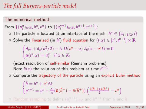
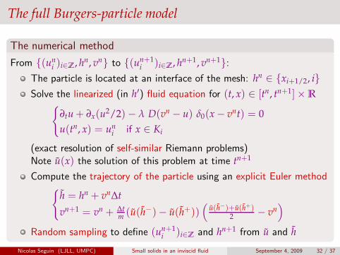
The numerical method
From {(uni )i∈Z, hn, vn} to {(un+1
i )i∈Z, hn+1, vn+1}:
The particle is located at an interface of the mesh: hn ∈ {xi+1/2, i}
Solve the linearized (in h′) fluid equation for (t, x) ∈ [tn, tn+1]× R
{
∂tu + ∂x(u2/2) − λ D(vn − u) δ0(x − vnt) = 0
u(tn, x) = uni if x ∈ Ki
(exact resolution of self-similar Riemann problems)Note u(x) the solution of this problem at time tn+1
Compute the trajectory of the particle using an explicit Euler method{
h = hn + vn∆t
vn+1 = vn + ∆tm (u(h−)− u(h+))
(
u(h−)+u(h+)2 − vn
)
Random sampling to define (un+1i )i∈Z and hn+1 from u and h
Nicolas Seguin (LJLL, UMPC) Small solids in an inviscid fluid September 4, 2009 32 / 37

The full Burgers-particle model
The numerical method
From {(uni )i∈Z, hn, vn} to {(un+1
i )i∈Z, hn+1, vn+1}:
The particle is located at an interface of the mesh: hn ∈ {xi+1/2, i}
Solve the linearized (in h′) fluid equation for (t, x) ∈ [tn, tn+1]× R
{
∂tu + ∂x(u2/2) − λ D(vn − u) δ0(x − vnt) = 0
u(tn, x) = uni if x ∈ Ki
(exact resolution of self-similar Riemann problems)Note u(x) the solution of this problem at time tn+1
Compute the trajectory of the particle using an explicit Euler method{
h = hn + vn∆t
vn+1 = vn + ∆tm (u(h−)− u(h+))
(
u(h−)+u(h+)2 − vn
)
Random sampling to define (un+1i )i∈Z and hn+1 from u and h
Nicolas Seguin (LJLL, UMPC) Small solids in an inviscid fluid September 4, 2009 32 / 37

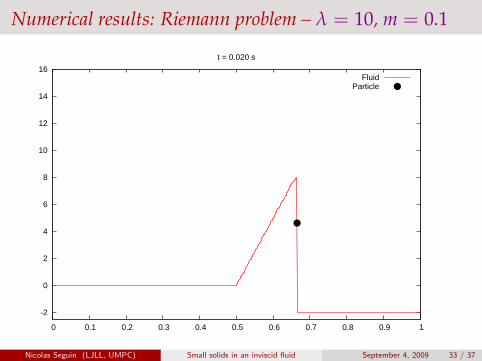
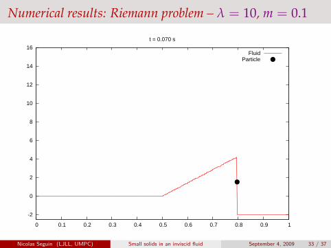
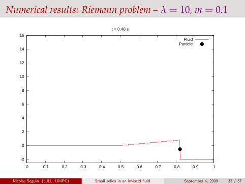
Numerical results: Riemann problem – λ = 10, m = 0.1
-2
0
2
4
6
8
10
12
14
16
0 0.1 0.2 0.3 0.4 0.5 0.6 0.7 0.8 0.9 1
t = 0.000 s
FluidParticle
Nicolas Seguin (LJLL, UMPC) Small solids in an inviscid fluid September 4, 2009 33 / 37

Numerical results: Riemann problem – λ = 10, m = 0.1
-2
0
2
4
6
8
10
12
14
16
0 0.1 0.2 0.3 0.4 0.5 0.6 0.7 0.8 0.9 1
t = 0.003 s
FluidParticle
Nicolas Seguin (LJLL, UMPC) Small solids in an inviscid fluid September 4, 2009 33 / 37

Numerical results: Riemann problem – λ = 10, m = 0.1
-2
0
2
4
6
8
10
12
14
16
0 0.1 0.2 0.3 0.4 0.5 0.6 0.7 0.8 0.9 1
t = 0.007 s
FluidParticle
Nicolas Seguin (LJLL, UMPC) Small solids in an inviscid fluid September 4, 2009 33 / 37

Numerical results: Riemann problem – λ = 10, m = 0.1
-2
0
2
4
6
8
10
12
14
16
0 0.1 0.2 0.3 0.4 0.5 0.6 0.7 0.8 0.9 1
t = 0.013 s
FluidParticle
Nicolas Seguin (LJLL, UMPC) Small solids in an inviscid fluid September 4, 2009 33 / 37
Numerical results: Riemann problem – λ = 10, m = 0.1
-2
0
2
4
6
8
10
12
14
16
0 0.1 0.2 0.3 0.4 0.5 0.6 0.7 0.8 0.9 1
t = 0.020 s
FluidParticle
Nicolas Seguin (LJLL, UMPC) Small solids in an inviscid fluid September 4, 2009 33 / 37

Numerical results: Riemann problem – λ = 10, m = 0.1
-2
0
2
4
6
8
10
12
14
16
0 0.1 0.2 0.3 0.4 0.5 0.6 0.7 0.8 0.9 1
t = 0.040 s
FluidParticle
Nicolas Seguin (LJLL, UMPC) Small solids in an inviscid fluid September 4, 2009 33 / 37
Numerical results: Riemann problem – λ = 10, m = 0.1
-2
0
2
4
6
8
10
12
14
16
0 0.1 0.2 0.3 0.4 0.5 0.6 0.7 0.8 0.9 1
t = 0.070 s
FluidParticle
Nicolas Seguin (LJLL, UMPC) Small solids in an inviscid fluid September 4, 2009 33 / 37

Numerical results: Riemann problem – λ = 10, m = 0.1
-2
0
2
4
6
8
10
12
14
16
0 0.1 0.2 0.3 0.4 0.5 0.6 0.7 0.8 0.9 1
t = 0.20 s
FluidParticle
Nicolas Seguin (LJLL, UMPC) Small solids in an inviscid fluid September 4, 2009 33 / 37
Numerical results: Riemann problem – λ = 10, m = 0.1
-2
0
2
4
6
8
10
12
14
16
0 0.1 0.2 0.3 0.4 0.5 0.6 0.7 0.8 0.9 1
t = 0.40 s
FluidParticle
Nicolas Seguin (LJLL, UMPC) Small solids in an inviscid fluid September 4, 2009 33 / 37
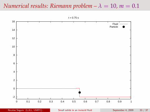
Numerical results: Riemann problem – λ = 10, m = 0.1
-2
0
2
4
6
8
10
12
14
16
0 0.1 0.2 0.3 0.4 0.5 0.6 0.7 0.8 0.9 1
t = 0.75 s
FluidParticle
Nicolas Seguin (LJLL, UMPC) Small solids in an inviscid fluid September 4, 2009 33 / 37

Numerical results: Riemann problem – λ = 10, m = 0.1
-2
0
2
4
6
8
10
12
14
16
0 0.1 0.2 0.3 0.4 0.5 0.6 0.7 0.8 0.9 1
t = 1.20 s
FluidParticle
Nicolas Seguin (LJLL, UMPC) Small solids in an inviscid fluid September 4, 2009 33 / 37
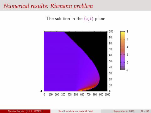
Numerical results: Riemann problem
The solution in the (x, t) plane
0 100 200 300 400 500 600 700 800 900 1000 0
10
20
30
40
50
60
70
80
90
100
-2 0 2 4 6 8
-2
0
2
4
6
8
Nicolas Seguin (LJLL, UMPC) Small solids in an inviscid fluid September 4, 2009 34 / 37
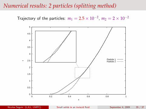
Numerical results: 2 particles (splitting method)
Trajectory of the particles: m1 = 2.5 × 10⁻², m2 = 2 × 10⁻²
0
0.5
1
1.5
2
2.5
3
3.5
4
4.5
5
0 0.2 0.4 0.6 0.8 1
t
x
Particle 1Particle 2
Nicolas Seguin (LJLL, UMPC) Small solids in an inviscid fluid September 4, 2009 35 / 37

Numerical results: 2 particles (splitting method)
Trajectory of the particles: m1 = 2 × 10⁻², m2 = 2 × 10⁻²
0
0.5
1
1.5
2
2.5
3
3.5
4
4.5
5
0 0.2 0.4 0.6 0.8 1
t
x
Particle 1Particle 2
Nicolas Seguin (LJLL, UMPC) Small solids in an inviscid fluid September 4, 2009 35 / 37

Numerical results: 2 particles (splitting method)
Trajectory of the particles: m1 = 1.5 × 10⁻², m2 = 2 × 10⁻²
0
0.5
1
1.5
2
2.5
3
3.5
4
4.5
5
0 0.2 0.4 0.6 0.8 1
t
x
Particle 1Particle 2
Nicolas Seguin (LJLL, UMPC) Small solids in an inviscid fluid September 4, 2009 35 / 37

Conclusion
Done...
Models for the coupling of an inviscid fluid with point-wise particles
Main difficulties well understood◮ Influence of the particle on the fluid◮ Evolution of the particle
Several numerical strategies◮ Particle with a constant velocity: simple numerical schemes◮ Burgers-particle model: use the linearized Riemann solver (w.r.t. h′)◮ Extension to several particles
Deep connections with interfacial coupling, with a free boundary◮ Compatibility of the traces of the solution◮ Echange of informations between both sides (well-balanced schemes)
Nicolas Seguin (LJLL, UMPC) Small solids in an inviscid fluid September 4, 2009 36 / 37
Conclusion
To do...
Complete the analysis of the Burgers-particle model◮ Well-posedness of the Cauchy problem◮ Extension to several particles
Find numerical methods without Riemann solver◮ Use the numerical schemes for a particle with a constant velocity◮ Analysis of convergence
Extension to 1D-Euler equations for the fluid
Extension to the multidimensional case
Adapt these works to the interfacial coupling
Nicolas Seguin (LJLL, UMPC) Small solids in an inviscid fluid September 4, 2009 37 / 37