Flow regime transition pointers in three-phase fluidized beds inferred from a solid tracer...

Chemical Engineering and Processing 45 (2006) 350–358

Flow regime transition pointers in three-phase fluidized bedsinferred from a solid tracer trajectory

Marıa Sol Fraguıoa, Miryan C. Cassanelloa,∗, Faıcal Larachib, Jamal Chaoukic

a PINMATE, Dep. de Industrias, FCEyN, Universidad de Buenos Aires, Int. Guiraldes 2620, Buenos Aires C1428BGA, Argentinab Dep. of Chemical Engineering and CERPIC, Universite Laval, Ste-Foy, Que., Canada G1K7P4

c Dep. of Chemical Engineering, Ecole Polytechnique de Montreal, P.O. Box 6079, Montreal, Que., Canada H3C 3A7

Received 21 March 2005; received in revised form 6 October 2005; accepted 7 October 2005Available online 21 November 2005

Abstract

Trajectories of solid radioactive tracers freely moving in a 3D gas–liquid–solid fluidized bed are analyzed from a data mining approach andusing tools of symbolic dynamics. The trajectories are obtained by the radioactive particle tracking (RPT) technique, employing solids of differentdensities (glass beads and hydrophilized PVC particles), tap water as the fluidizing media and filtered air as the gas phase. Different gas velocitiesa gime pointers.H ans of datas l sequenceE©

K

1

ogathrep

gpflabh

cencegimeter-itiesslug-eter.imetendcome

d onpro-to

ea-haseries,suredor to

lid inthe

0d

re examined to span the homogeneous and the heterogeneous flow regimes. The aim is to define parameters that can act as flow reence, particular features of the particle motion are examined in detail to relate them to the underlying flow regime. In addition, by meymbolization, it is found that the recurrence of specific patterns of the tracer trajectories leads to higher frequencies of certain symbos.stimated frequencies are strongly influenced by the flow regime and may allow for regime identification.2005 Elsevier B.V. All rights reserved.

eywords: Flow regime transition; Three-phase fluidization; Radioactive particle tracking

. Introduction

Flow transitions in gas–liquid–solid fluidized beds dependn many different variables, liquid and gas velocities, liquid andas physical properties, solid features, gas distributor designnd geometric characteristics of the bed. It is well known that

he flow regime largely affects these reactors’ performance;ence, methodologies that allow objective identification of flowegime transitions are always desirable. Moreover, the knowl-dge regarding the flow regimes and their transition in three-hase systems is still far from satisfactory[1].

Many different flow regimes have been identified inas–liquid–solid fluidized beds, i.e., discrete bubble flow, dis-ersed bubble flow, coalesced bubble flow, slug flow, churnow, bridging flow and annular flow. However, the main interestlways resides in identifying the transition between the disperseubble flow and the coalesced bubble flow, commonly termedomogeneous and heterogeneous flow regimes, respectively. In

∗ Corresponding author. Tel.: +54 11 4576 3383; fax: +54 11 4576 3366.

the homogeneous bubble flow regime, no bubble coalesoccurs; the bubbles are uniform and of small size. This repredominates at high liquid velocities and at low and inmediate gas velocities. For low and moderate liquid velocand high gas velocities, either the churn-turbulent or theging flow regime occurs, depending on the column diamIn columns of large diameter, the churn-turbulent flow regalways occurs at high gas velocities. In this regime, bubblesto coalesce and both bubble size and bubble rise velocity belarge and show a wide distribution[1–3].

Many studies of flow regime transitions have been basevisual observations. Although visual observation clearlyvides information on the flow patterns, it is often difficultidentify the flow regime transition without quantitative msurements, due to the relatively opaque nature of multipflow [3]. Therefore, several characteristic variables time seanalyzed according to different theories, have been meain three-phase systems either to identify a flow transitiondiagnose the underlying flow regime[3–8].

The gas and the liquid phases impose the motion of the sothe fluidized bed. Hence, a flow transition will be reflected in

E-mail address: [email protected] (M.C. Cassanello). solid motion inside the bed[7,8]. In this work, solid trajectories

255-2701/$ – see front matter © 2005 Elsevier B.V. All rights reserved.oi:10.1016/j.cep.2005.10.001

M.S. Fraguıo et al. / Chemical Engineering and Processing 45 (2006) 350–358 351

obtained by the radioactive particle tracking (RPT) techniqueare analyzed. RPT is able to provide extensive time series of theactual path of a particle totally similar to the other particles inthe bed, sampling non-invasively in 3D the whole volume thatcontains the three-phase system[9]. A data-mining approachand tools of the theory of symbolic dynamics[10] are appliedto define and calculate parameters that characterize the motionof the solid tracer. Their ability as flow regime pointers is thenexamined.

2. Experimental

The actual displacements of solid radioactive tracers, withproperties similar to those of the fluidized particles are analyzed.They have been obtained with a radioactive particle tracking(RPT) technique in a 0.1 m internal diameter acrylic column. TheRPT facility was provided with an array of eight NaI(Tl) scintil-lation detectors to capture the gamma rays issued by the tracer.The counts recorded depended on the tracer location, the attenua-tion of the media and dead time of the detectors used. The spatialcoordinates of the tracer were reconstructed by inverse algo-rithms. For details on the experimental procedure, the readers arereferred to Chapter 11 of the book Non-invasive Monitoring ofMultiphase Flows[9]. Extended time series of tracers’ positionswere determined with a sample period of 30 ms for about 6 h.

mm:ρ me so part ere0 iffere ther

ater.E itieso lass

F RPT,a ;(

beads. Gas superficial velocities were varied within the range0 <uG < 0.11 m/s. Experiments in the homogeneous and in theheterogeneous flow regimes are examined. The change in flowregime when using the glass beads, as identified by visual inspec-tion, corresponded fairly well with those predicted by Nacef[11] for a static mixer distributor; i.e.,uG = 0.038 m/s. For thelight particles, onset of heterogeneous flow regime appearedarounduG = 0.02 m/s, as judged from visual inspection. Withzero gas velocity (liquid fluidization) particulate flow regimewas observed for the light particles and segregate flow regimefor the glass beads.

3. Results and discussion

Solids trajectories are markedly dependent on the gas veloc-ity at a given liquid flow rate, as can be observed inFig. 1, where

Fig. 2. Possible pointers for the homogeneous and the heterogeneous flowregimes, inferred from fast ascending axial displacements found in the solidtrajectory time series: (a) number of tracer fast ascending paths per minute,ξ, and mean time lag between fast ascensions,τ; (b) projected wake-area ofinfluence inferred from fast ascensions. Experiments with glass beads of 3 mm;dashed line predicted by Nacef[11] and from visual observations.

Solids employed were 3 mm glass beads (GB3= 2500 kg/m3) and hydrophilized PVC particles of 5.5 mquivalent diameter (PVC5.5 mm:ρ = 1300 kg/m3). The masf solids used was 4 kg for glass beads and 0.8 kg for PVC

icles; corresponding bed heights at rest (no liquid flow) w.35 and 0.2 m, respectively. Expanded bed heights were dnt for the different operating conditions and varied withinange 0.45–0.65 m.

The fluid system used was filtered air and tap wxperiments were performed at liquid superficial velocf 0.058 m/s for PVC particles and 0.065 m/s for the g

ig. 1. Time series of the GB3 mm tracer axial coordinate, evaluated bytuL = 0.065 m/s and different gas velocities: (a)uG = 0 m/s; (b)uG = 0.032 m/sc) uG = 0.069 m/s; (d)uG = 0.110 m/s.

-

-

352 M.S. Fraguıo et al. / Chemical Engineering and Processing 45 (2006) 350–358

the axial coordinate of the radioactive glass tracer has been rep-resented against time for a 2-min period. For zero gas velocity, asegregated flow regime prevails in the column for a three-phasefluidized bed of GB3 mm. The tracer remains around a givenlocation for prolonged periods of time, moving only occasion-ally to a different region of the reactor. When a gas flow rate isimposed, the tracer moves continuously throughout the wholebed, alternating between the bottom and the top of the three-phase emulsion.

For the PVC particles, the tracer expands all the availablespace even for liquid fluidization. However, inception of gasstrongly modifies its motion as for the GB3 mm.

3.1. Data mining of solid trajectories

As the gas velocity is increased, sharper and persistentascending paths are apparent in the axial displacement of thetracers (Fig. 1b–d). It has been argued that these fast ascensionsmay be caused by an entrapment of the tracer in the wake ofrelatively large bubbles. Moreover, some information on largebubbles has been inferred from these fast ascending paths[12].The number of continuous sharp ascending motions that end inthe upper half of the three-phase emulsion is clearly larger asthe energy imposed by the gas velocity increases. This is prob-ably related to an increase in large bubbles’ frequency as thegas velocity is increased. The influence of the gas velocity onta witG isa anst oro

Consequently, the mean time lag among fast ascending paths,τ, is also abruptly modified (reduced) after the flow transitionhas occurred, and remains around 1 s for the experiments carriedout in the heterogeneous regime (Fig. 2a). Naturally this timeinterval should stabilize around a physically possible value, itcannot keep on decreasing since there is a residence time of thetracer in the ascending path, which must be surpassed.

Another indicator that can be evaluated from the fast ascend-ing paths is the projected wake area of influence, AW, calculatedas the area of the ellipses that contain thex–y projections of thetracer while being trapped in the rapid ascensions. A thoroughdiscussion of the meaning and the way these projected ellipsesare calculated can be found in[12,13]. The sizes of the ellipsesare related to the swinging motion of the particle while goingupwards, and are generally larger when the tracer is capturedby bigger bubbles. The percentage of the column section thatcontains 99% of all the ellipses is indicated inFig. 2b. Thepercentage increases as the gas velocity is increased. Again,there is a physical limit for the projected area, the columnsection, which indicates that this value will also stabilize forlarger gas velocities and a clear break is apparent after the flowtransition.

It is also interesting to observe the evolution of the tracertrajectories that start at definite locations in the column, so asto analyze if there is a spatial influence on the pattern of thetracer motion after a flow transition.Figs. 3 and 4show projec-t yc eousa ctionso y 1 s,h at dis-t , the

F ossin .H

he number of fast ascending displacements per minute,ξ (i.e.,scensions likely caused by large bubbles), for experimentsB3 mm, is illustrated inFig. 2a. A marked break in the trendpparent after the gas velocity that leads to a flow regime tr

ion is exceeded and suggests thatξ could constitute an indicatf the flow regime, related to the large bubbles’ frequency.

ig. 3. Time evolution of the tracer trajectories (1 s) computed after cromogeneous flow regime, solid: GB3 mm,uL = 0.065 m/s,uG = 0.032 m/s.

h

i-

ions of the tracer displacements on ther–z andx–y planes. Theorrespond to experiments with GB3 mm in the homogennd the heterogeneous flow regimes, respectively. Projef the instantaneous tracer positions, during approximatelave been represented after crossing the column center

inct heights. It is clear that, in the homogeneous flow regime

g the column center at different axial positions. Radial–axial andx–y projections


Fig. 4. Time evolution of the tracer trajectories (1 s) computed after crossing the column center at different axial positions. Radial–axial andx–y projections.Heterogeneous flow regime, solid: GB3 mm,uL =0.065 m/s,uG =0.110 m/s.

particle does not depart too far from its radial location, exceptclose to the boundaries, where it is obliged to approach the col-umn wall. On the contrary, for experiments in the heterogeneousflow regime, the high energy exerted by the gas is soon trans-mitted to the solid and permits its prompt motion towards thewall, in spite of the other particles interaction. This is a transientbehavior, which differs from the averaged solid radial velocitythat is approximately nil[12]. It can clearly provide means toidentify the underlying flow regime.

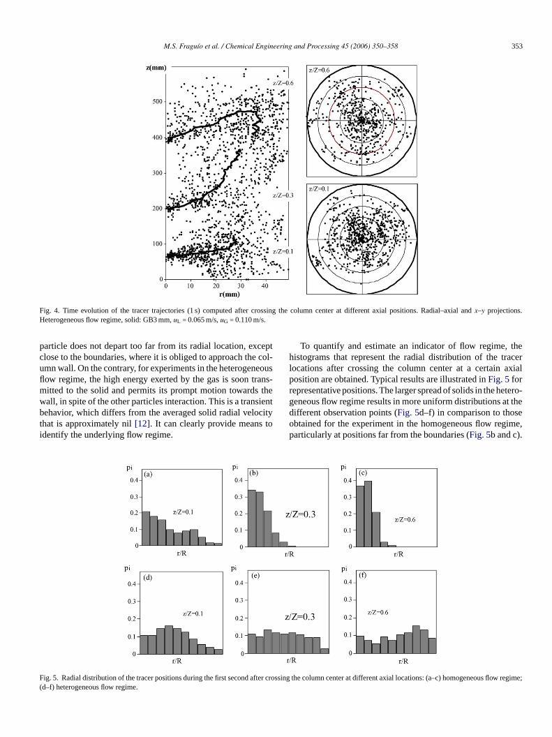
To quantify and estimate an indicator of flow regime, thehistograms that represent the radial distribution of the tracerlocations after crossing the column center at a certain axialposition are obtained. Typical results are illustrated inFig. 5forrepresentative positions. The larger spread of solids in the hetero-geneous flow regime results in more uniform distributions at thedifferent observation points (Fig. 5d–f) in comparison to thoseobtained for the experiment in the homogeneous flow regime,particularly at positions far from the boundaries (Fig. 5b and c).

F er cro ;(

ig. 5. Radial distribution of the tracer positions during the first second aftd–f) heterogeneous flow regime.

ssing the column center at different axial locations: (a–c) homogeneous flow regime


Fig. 6. Shannon entropy,H, calculated from the radial distribution of tracerpositions during the first second after crossing the column center at differ-ent axial locations. Experiments with glass beads of 3 mm. Gas velocities: (�)uG = 0.032 m/s; (�) uG = 0.069 m/s; (�) uG = 0.110 m/s.

In order to get a unique parameter to diagnose the underlyingflow regime, the Shannon entropy was calculated according to

H =N∑

i=1

pi log2(pi) (1)

whereN represents the number of radial partitions;pi is thefrequency of particle occurrences in that partition and represents

Fig. 7. Influence of the flow regime on the axial variability of the Shannonentropy,H, calculated from the radial distribution of tracer positions duringthe first second after crossing the column center at different axial locations.Experiments with glass beads of 3 mm; dashed line predicted by Nacef[11] andfrom visual observations: (�) σ; (�) HMax/HMin ; (�)

∑(H/HMax).

the conditional probability that the tracer is located at that radialposition, provided it was at the column center in some instantduring the previous second, for the axial position considered.The axial variation of the values ofH, calculated with Eq.(1), isillustrated inFig. 6, for experiments with GB3 mm at differentgas velocities.

Fe

ig. 8. Static symbolization: histograms of symbol sequences determined fxperiments. Experiments with glass beads of 3 mm at different gas velocitiesuG

rom tracer axial displacements in the 3D-three-phase fluidized bed duringthe 6 h: (a)= 0 m/s; (b)uG = 0.032 m/s; (c)uG = 0.069 m/s; (d)uG = 0.110 m/s.


The axial variation of the entropy is larger in the homo-geneous flow regime. This variability can be reflected in thestandard deviation among the estimated values and also by com-paring the maximum to the minimum values obtained, or the sumof H at different axial locations, normalized with the maximumvalue. For the experiments with GB3 mm, these three numbershave been represented versus the gas velocity inFig. 7, to high-light the influence of the flow regime on them. For the lighterparticles, variations are also apparent and follow similar trendsbut the differences are less abrupt, probably due to the lowersolid holdup, which reduces the effect of solid interactions.

3.2. Symbolic analysis of solid trajectories

The symbolic analysis of experimental data has beenemployed in the last decade to classify different dynamic statesand to monitor fluidization[9,14,15]. Briefly, the time series isconverted into a time series of symbols following certain crite-ria, and the symbol sequences are analyzed[9,16]. Two simpleapproaches are presented here, either by defining the symbolsfrom a static or a dynamic methodology.

3.2.1. Static symbolizationTo generate the series of symbol sequences, the time series

of tracer axial positions are converted into a series of symbols

according to the tracer location in the bed. The bed is dividedaxially in four regions. Groups of four axial positions of thetracer, separated 0.12 s each, are inspected successively. Theregion of the bed that contains the particle is assigned a number 1,while the others get a 0. Hence, 24 symbol sequences are defined(0000, 0001, 0010, 0011, 0100, 0101, 0110, 0111, 1000, 1001,1010, 1011, 1100, 1101, 1110, 1111) and their relative frequencydepends on the intensity of the tracer axial motion. Actually,symbol sequence 0000 is forbidden since the particle is alwaysin a certain location in the bed.Fig. 8 shows the histograms ofsymbols sequence occurrences for experiments with GB3 mmat different gas velocities. The symbol indexes used in the figureare the decimal representation of the binary numbers given bythe symbol sequences.

Some characteristics are evident, like the marked preemi-nence of the symbol sequence 1000 (index 8) in the liquid solidsegregated experiment. Only two other symbols sequences areobserved: 0100 (index 4), which correspond to the particle inthe region immediately below the one where it stays most ofthe time, and 1100 (index 12), a combination of the other two.After introducing gas, the situation is completely modified. Thefrequency of bin #8 decreases progressively as the gas velocityis increased, being almost negligible for the highest gas velocity.

Comparing only the experiments with circulating gas, it isobserved that the number of symbol sequences found is larger as

Fu

ig. 9. Grouped histograms of symbol sequences determined from tracer axia

G = 0 m/s; (b)uG = 0.032 m/s; (c)uG = 0.069 m/s; (d)uG = 0.110 m/s.
l displacements. Experiments with glass beads of 3 mm at different gas velocities: (a)


Table 1Entropies calculated from the symbol sequence histograms and frequency ofsymbol A for the examined experiments

Solid uG (m/s) H (bits/s) pi(A)

GB3 mm 0 0.77 0.930.032 2.87 0.530.069 3.14 0.200.110 3.11 0.15

PVC5.5 mm 0 2.46 0.760.010 2.78 0.620.025 2.82 0.54

the gas velocity is increased. For the experiment in the homoge-neous flow regime, the symbol sequences that correspond to theparticle in a unique region (#1, 2, 4 and 8) are more frequent thanfor the experiments in the heterogeneous flow regime. In addi-tion, those that correspond to the particle in two non-successiveregions are negligible or nil (#5, 7, 9–11, 13–15). To remarkthese differences and to get a flow regime indicator, new symbolgroups have been defined considering symbols sequences thatpoint to the presence of the tracer in one or more successive andnon-successive regions. Groups have been classified accordingto: symbol A (only one region: #1, 2, 4, 8); symbol B (onlytwo successive regions: #3, 6, 12); symbol C (three successiveregions or two non-successive regions: #5, 7, 9, 10, 14) and sym-bol D (three non-successive regions or four successive regions:#11, 13, 15). The corresponding histograms are presented inFig. 9. It is clear that the symbol which may act as a flow regimeindicator is symbol A (particle located in only one region).

The frequencies of symbol A and the Shannon entropy, calcu-lated from the histograms shown inFig. 8, are detailed inTable 1for all the examined experiments.

Apart from the large differences found between liquid–solidand three-phase fluidization, there is a clear increasing trend inthe entropy and a decreasing trend of the frequency of symbolA as the gas velocity is increased. These trends apparently leveloff in the heterogeneous flow regime, suggesting that they mayconstitute indicators of the underlying flow regime.

3to

e in thea ngesip igna ents.T -r wered tracer(

••••

Fig. 10. Dynamic symbolization: histograms of symbol sequences determinedfrom tracer axial displacements in the 3D-three-phase fluidized bed during the 6 hexperiments. Experiments with glass beads of 3 mm at different gas velocities:(a) uG = 0 m/s; (b)uG = 0.032 m/s; (c)uG = 0.069 m/s; (d)uG = 0.110 m/s.

After the time series of tracer axial coordinates is convertedto a time series of symbols, symbol sequences given by all thepossible binary combinations of the four defined symbols arecomputed. In this way, 42 = 16 symbol sequences are generated.The histograms calculated from the 6 h experiments are illus-trated inFig. 10. Actually, it is not necessary to compute thehistograms from the 6 h time series, invariant frequencies arealready obtained from time series of more than 20 min.

Several forbidden symbol sequences are found: AD, BA,BD, CB, DB, DC, leaving only 10 indexes for comparison.The influence of the gas flow rate is particularly reflected inthe binary combinations BB and DD, which readily increasewith gas velocity. These symbol sequences point to longer per-sistent excursions of the tracer as the gas velocity is increased,so they quantify a feature which is actually observed in the timeseries (seeFig. 1). In addition, symbol sequences AC and CA,which correspond to a jittery behavior of the time series with

.2.2. Dynamic symbolizationThe dynamic symbolization is generally appropriate

mphasize certain temporal patterns, which are apparentnalyzed time series. It is the preferred strategy when cha

n time are more important than absolute measurements[10]. Aarticular way of dynamic symbolization is to directly asssymbol to a particular trend of successive measurem

his approach was used by Cazelles[17] to compute tempoal patterns in animal population time series. Four symbolsefined considering three successive axial positions of thezi−1, zi, zi+1) according to the following rule:

zi ≤ zi−1 ≤ zi+1 andzi < zi+1 ≤ zi−1 ⇒ a trough, symbol Azi−1 < zi < zi+1 ⇒ an increasing trend, symbol Bzi−1 < zi+1 ≤ zi andzi+1 < zi−1 ≤ zi ⇒ a peak, symbol Czi+1 < zi < zi−1 ⇒ a decreasing trend, symbol D


Fig. 11. Influence of the flow regime on theχ2 statistics calculated by com-paring histograms in experiments with gas to the histograms obtained for theliquid–solid experiment at the same liquid velocity. Dashed lines predicted byNacef[11] and from visual observations.

successive maxima and minima, decrease their frequency forlarger gas velocities.

A statistics that can be computed to quantify differencesamong histograms is the chi-square statistics,χ2, defined as

χ2 =∑

i(pi − qi)2∑i(pi + qi)

(2)

wherepi are the frequencies of a test time series andqi thefrequencies for a reference one. Taking as references the hitograms obtained for the liquid–solid experiments (uG = 0), theχ2 statistics was computed for all the experiments with similarsolid inventory. The influence of the gas velocity on the calcu-lated parameter is shown inFig. 11for both the heavy and lightparticles. Theχ2 statistics stays close to zero for experiments inthe homogeneous flow regime and sharply increases in the heerogeneous flow regime, indicating that it may be a classificationindex.

4. Conclusion

Different parameters extracted from the analysis of the trajectories of a solid tracer freely moving in a three-phase fluidizedbed, have been postulated as flow regime indices. They havbeen obtained from a data-mining approach and by a symbolia ak int hado aluei of al bustn r.

A

omU andf 1).

Appendix A. Nomenclature

AW area that contains 99% of all thex–y projections of thetracer while being rapidly trapped in the ascension

H Shannon entropy defined in Eq.(1) (bits/s)N number of radial partitionspi, qi frequencies in the histogramsu superficial velocity (m/s)

Greek lettersξ number of fast ascending paths of the tracer per minute

(min−1)ρ density (kg/m3)σ standard deviation of the computed Shannon entropies

(bits/s)τ time lag between fast ascending paths (s)χ2 chi-square statistics, defined in Eq.(2), dimensionless

SubscriptsG gasL liquidMin minimumMax maximum

R

ubble

ts ofspen-

ationci. 52

sys-meth-

em-

am-865–

arti-222–

en-phase

of

[ s of

[ tsstitut

[ f theE J.

[ from, in:

nalysis of the experimental data. They clearly show a breheir trend with gas velocity after a change in flow regimeccurred, and some of them tend to level off to a constant v

n the heterogeneous flow regime. However, examinationarger body of data would be desirable to establish the roess of each magnitude suggested as a flow regime pointe

cknowledgments

Authors from Argentina acknowledge financial support frniversidad de Buenos Aires and CONICET (Argentina)

rom the International Atomic Energy Agency (RC12458/R

s-

t-

-

ec

-

eferences

[1] P.C. Mena, M.C. Ruzicka, F.A. Rocha, J.A. Teixeira, J. Drahos, Effect ofsolids on homogeneous–heterogeneous flow regime transition in bcolumns, Chem. Eng. Sci. 60 (2005) 6013–6026.

[2] L.S. Fan, G.Q. Yang, D.J. Lee, K. Tsuchiya, X. Luo, Some aspechigh-pressure phenomena of bubbles in liquids and liquid–solid susions, Chem. Eng. Sci. 54 (1999) 4681–4709.

[3] J.P. Zhang, J.R. Grace, N. Epstein, K.S. Lim, Flow regime identificin gas–liquid flow and three-phase fluidized beds, Chem. Eng. S(1997) 3979–3992.

[4] L.A. Briens, N. Ellis, Hydrodynamics of three-phase fluidized bedtems examined by statistical, fractal, chaos and wavelet analysisods, Chem. Eng. Sci. 60 (2005) 6094–6106.

[5] L.A. Briens, C.L. Briens, Cycle detection and characterization in chical engineering, AIChE J. 48 (2002) 970–980.

[6] R. Kikuchi, A. Tsutsumi, K. Yoshida, Fractal aspect of hydrodynics in a three-phase fluidized bed, Chem. Eng. Sci. 51 (1996) 22870.

[7] W. Luewisuthichat, A. Tsutsumi, K. Yoshida, Fractal analysis of pcle trajectories in three-phase systems, Trans. IChemE 73 (1995)227.

[8] M. Cassanello, F. Larachi, M.N. Marie, C. Guy, J. Chaouki, Experimtal characterization of the solid phase chaotic dynamics in three-fluidization, Ind. Eng. Chem. Res. 34 (1995) 2971–2980.

[9] J. Chaouki, F. Larachi, M.P. Dudukovic, Non-invasive MonitoringMultiphase Flows, Elsevier, Amsterdam, 1997.

10] C.S. Daw, C.E.A. Finney, E.R. Tracy, A review of symbolic analysiexperimental data, Rev. Sci. Instrum. 74 (2003) 915–932.

11] S. Nacef, Hydrodynamique des lits fluidises gaz-liquide-solide. Effedu distributeur et de la nature du liquide, Ph.D. Dissertation, InNational Polytechnique de Lorraine, Nancy, France, 1991.

12] F. Larachi, M.C. Cassanello, J. Chaouki, C. Guy, Flow structure osolids in a three-dimensional gas–liquid–solid fluidized bed, AICh42 (1996) 2439–2452.

13] M. Cassanello, F. Larachi, J. Chaouki, Dynamical features extractedthe solids circulation trajectories in gas–liquid–solid fluidized bed


Proceedings of Tracer 3, Conference on Tracers and Tracing Methods,Ciechocinek, Poland, 2004, pp. 68–73.

[14] C.E.A. Finney, K. Nguyen, C.S. Daw, J.S. Halow, Symbol-sequencestatistics for monitoring fluidization, in: Proceedings of the 1998 Inter-national Mechanical Engineering Congress & Exposition (ASME), Ana-heim, CA, USA, 1998, pp. 405–411.

[15] J. Godelle, C. Letellier, Symbolic sequence statistical analysis for freeliquid jets, Phys. Rev. E 62 (2000) 7973–7981.

[16] H. Kantz, T. Schreiber, Nonlinear Time Series Analysis, CambridgeUniversity Press, Cambridge, 1997.

[17] B. Cazelles, Symbolic dynamics for identifying similarity betweenrhythms of ecological time series, Ecol. Lett. 7 (2004) 755–763.

Flow regime transition pointers in three-phase fluidized beds inferred from a solid tracer...

Documents

Transcript of Flow regime transition pointers in three-phase fluidized beds inferred from a solid tracer...