The structure and dynamics of multilayer networks

S. Boccalettia,b,∗, G. Bianconic, R. Criadod,e, C.I. del Geniof,g,h, J. Gómez-Gardeñesi, M. Romanced,e, I.Sendiña-Nadalj,e, Z. Wangk,l, M. Zaninm,n

aCNR- Institute of Complex Systems, Via Madonna del Piano, 10, 50019 Sesto Fiorentino, Florence, ItalybThe Italian Embassy in Israel, 25 Hamered st., 68125 Tel Aviv, Israel

cSchool of Mathematical Sciences, Queen Mary University of London, London, United KingdomdDepartamento de Matemática Aplicada, Universidad Rey Juan Carlos, 28933 Móstoles, Madrid, Spain

eCenter for Biomedical Technology, Universidad Politécnica de Madrid, 28223 Pozuelo de Alarcón, Madrid, SpainfWarwick Mathematics Institute, University of Warwick, Gibbet Hill Road, Coventry CV4 7AL, United KingdomgCentre for Complexity Science, University of Warwick, Gibbet Hill Road, Coventry CV4 7AL, United Kingdom

hWarwick Infectious Disease Epidemiology Research (WIDER) Centre,University of Warwick, Gibbet Hill Road, Coventry CV4 7AL, United Kingdom

iInstitute for Biocomputation and Physics of Complex Systems, University of Zaragoza, Zaragoza, SpainjComplex Systems Group, Universidad Rey Juan Carlos, 28933 Móstoles, Madrid, Spain

kDepartment of Physics, Hong Kong Baptist University, Kowloon Tong, Hong Kong SRA, ChinalCenter for Nonlinear Studies, Beijing-Hong Kong-Singapore Joint Center for Nonlinear and

Complex Systems (Hong Kong) and Institute of Computational and Theoretical Studies,Hong Kong Baptist University, Kowloon Tong, Hong Kong SRA, China

mInnaxis Foundation & Research Institute, José Ortega y Gasset 20, 28006 Madrid, SpainnFaculdade de Ciências e Tecnologia, Departamento de Engenharia Electrotécnica,

Universidade Nova de Lisboa, 2829-516 Caparica, Portugal

Abstract

In the past years, network theory has successfully characterized the interaction among the constituents of avariety of complex systems, ranging from biological to technological, and social systems. However, up untilrecently, attention was almost exclusively given to networks in which all components were treated on equiv-alent footing, while neglecting all the extra information about the temporal- or context-related propertiesof the interactions under study. Only in the last years, taking advantage of the enhanced resolution in realdata sets, network scientists have directed their interest to the multiplex character of real-world systems,and explicitly considered the time-varying and multilayer nature of networks. We offer here a comprehen-sive review on both structural and dynamical organization of graphs made of diverse relationships (layers)between its constituents, and cover several relevant issues, from a full redefinition of the basic structuralmeasures, to understanding how the multilayer nature of the network affects processes and dynamics.

Keywords:2010 MSC: 00-01, 99-00

Contents

1 Introduction 41.1 The multilayer network approach to nature . . . . . . . . . . . . . . . . . . . . . . . . . . . . 41.2 Outline of the report . . . . . . . . . . . . . . . . . . . . . . . . . . . . . . . . . . . . . . . . . 6

∗Corresponding authorEmail address: stefano.boccaletti@gmail.com (S. Boccaletti)

Preprint submitted to Physics Reports July 16, 2014

arX

iv:1

407.

0742

v2 [

phys

ics.

soc-

ph]

13

Jul 2

014

2 The structure of multilayer networks 72.1 Definitions and notations . . . . . . . . . . . . . . . . . . . . . . . . . . . . . . . . . . . . . . 7

2.1.1 The formal basic definitions . . . . . . . . . . . . . . . . . . . . . . . . . . . . . . . . . 72.1.2 A small (and less formal) handbook . . . . . . . . . . . . . . . . . . . . . . . . . . . . 10

2.2 Characterizing the structure of multilayer networks . . . . . . . . . . . . . . . . . . . . . . . . 132.2.1 Centrality and ranking of nodes . . . . . . . . . . . . . . . . . . . . . . . . . . . . . . . 132.2.2 Clustering . . . . . . . . . . . . . . . . . . . . . . . . . . . . . . . . . . . . . . . . . . . 152.2.3 Metric structures: Shortest paths and distances . . . . . . . . . . . . . . . . . . . . . . 182.2.4 Matrices and spectral properties . . . . . . . . . . . . . . . . . . . . . . . . . . . . . . 202.2.5 Mesoscales: Motifs and modular structures . . . . . . . . . . . . . . . . . . . . . . . . 21

2.3 Matrices and tensor representation: Spectral properties . . . . . . . . . . . . . . . . . . . . . 222.4 Correlations in multiplex networks . . . . . . . . . . . . . . . . . . . . . . . . . . . . . . . . . 26

2.4.1 Degree correlations in multiplex networks . . . . . . . . . . . . . . . . . . . . . . . . . 262.4.2 Overlap and multidegree . . . . . . . . . . . . . . . . . . . . . . . . . . . . . . . . . . . 282.4.3 Multistrength and inverse multiparticipation ratio in weighted multiplex networks . . 302.4.4 The activities of the nodes and the pairwise multiplexity . . . . . . . . . . . . . . . . . 32

3 Generative models 343.1 Multiplex networks models . . . . . . . . . . . . . . . . . . . . . . . . . . . . . . . . . . . . . 34

3.1.1 Growing multiplex networks models . . . . . . . . . . . . . . . . . . . . . . . . . . . . 343.1.2 Simple static models . . . . . . . . . . . . . . . . . . . . . . . . . . . . . . . . . . . . . 373.1.3 Ensembles of multiplex networks . . . . . . . . . . . . . . . . . . . . . . . . . . . . . . 38

3.2 Ensembles of networks of networks . . . . . . . . . . . . . . . . . . . . . . . . . . . . . . . . . 423.2.1 Case I: Networks of networks with fixed supernetwork and links allowed only between

replica nodes . . . . . . . . . . . . . . . . . . . . . . . . . . . . . . . . . . . . . . . . . 433.2.2 Case II: Networks of networks with given superdegree distribution . . . . . . . . . . . 443.2.3 Case III: Networks of networks with fixed supernetwork and random permutations of

the labels of the nodes . . . . . . . . . . . . . . . . . . . . . . . . . . . . . . . . . . . . 453.2.4 Case IV: Networks of networks with multiple interconnections . . . . . . . . . . . . . . 46

4 Resilience and percolation 464.1 The fragility of multilayer interdependent networks . . . . . . . . . . . . . . . . . . . . . . . . 474.2 Percolation in interdependent networks . . . . . . . . . . . . . . . . . . . . . . . . . . . . . . . 49

4.2.1 The mutually connected giant component of a multilayer network . . . . . . . . . . . . 494.3 Interdependent multiplex networks . . . . . . . . . . . . . . . . . . . . . . . . . . . . . . . . . 51

4.3.1 Case of a multiplex formed by M Poisson networks with the same average degree . . . 524.3.2 Case of a duplex network formed by two Poisson networks with different average degree 534.3.3 Multiplex networks formed by layers of scale-free networks . . . . . . . . . . . . . . . . 534.3.4 Cascading failures . . . . . . . . . . . . . . . . . . . . . . . . . . . . . . . . . . . . . . 544.3.5 Partial interdependence . . . . . . . . . . . . . . . . . . . . . . . . . . . . . . . . . . . 574.3.6 Percolation in multiplex networks with multiple support-dependence relations . . . . . 59

4.4 Interdependent networks of networks . . . . . . . . . . . . . . . . . . . . . . . . . . . . . . . . 604.4.1 Case I: Networks of networks with fixed supernetwork and interdependent links allowed

only between replica nodes . . . . . . . . . . . . . . . . . . . . . . . . . . . . . . . . . 604.4.2 Case II: Networks of networks with given superdegree of the layers . . . . . . . . . . . 624.4.3 Case III: Networks of networks with fixed supernetwork and random permutation of

the labels of the nodes . . . . . . . . . . . . . . . . . . . . . . . . . . . . . . . . . . . . 644.5 Effects of correlations and embedding space on percolation properties of multilayer networks . 65

4.5.1 Percolation in networks with overlap of the links . . . . . . . . . . . . . . . . . . . . . 654.5.2 Percolation in networks with degree correlations . . . . . . . . . . . . . . . . . . . . . 654.5.3 Percolation in spatial multiplex networks . . . . . . . . . . . . . . . . . . . . . . . . . 66

4.6 Other percolation problems . . . . . . . . . . . . . . . . . . . . . . . . . . . . . . . . . . . . . 67

2

4.6.1 Classical percolation . . . . . . . . . . . . . . . . . . . . . . . . . . . . . . . . . . . . . 674.6.2 Percolation of antagonistic networks . . . . . . . . . . . . . . . . . . . . . . . . . . . . 674.6.3 K-core percolation . . . . . . . . . . . . . . . . . . . . . . . . . . . . . . . . . . . . . . 684.6.4 Viability in multiplex networks and weak percolation . . . . . . . . . . . . . . . . . . . 68

4.7 Cascades on multilayer networks . . . . . . . . . . . . . . . . . . . . . . . . . . . . . . . . . . 69

5 Spreading processes and games 705.1 Diffusion on multilayer networks . . . . . . . . . . . . . . . . . . . . . . . . . . . . . . . . . . 70

5.1.1 Linear Diffusion . . . . . . . . . . . . . . . . . . . . . . . . . . . . . . . . . . . . . . . 715.1.2 Random walks . . . . . . . . . . . . . . . . . . . . . . . . . . . . . . . . . . . . . . . . 735.1.3 Diffusion-based centrality measures . . . . . . . . . . . . . . . . . . . . . . . . . . . . . 765.1.4 Routing and congestion phenomena . . . . . . . . . . . . . . . . . . . . . . . . . . . . 76

5.2 Spreading processes . . . . . . . . . . . . . . . . . . . . . . . . . . . . . . . . . . . . . . . . . 785.2.1 Disease spreading on single-layer networks . . . . . . . . . . . . . . . . . . . . . . . . . 785.2.2 Disease spreading on interconnected networks . . . . . . . . . . . . . . . . . . . . . . . 805.2.3 Disease spreading on multiplex networks . . . . . . . . . . . . . . . . . . . . . . . . . . 845.2.4 Voluntary prevention measures . . . . . . . . . . . . . . . . . . . . . . . . . . . . . . . 885.2.5 Opinion formation dynamics . . . . . . . . . . . . . . . . . . . . . . . . . . . . . . . . 90

5.3 Evolutionary games on multilayer networks . . . . . . . . . . . . . . . . . . . . . . . . . . . . 935.3.1 Pairwise interaction games . . . . . . . . . . . . . . . . . . . . . . . . . . . . . . . . . 945.3.2 The public goods game . . . . . . . . . . . . . . . . . . . . . . . . . . . . . . . . . . . 985.3.3 Partial overlap and spatial coevolution . . . . . . . . . . . . . . . . . . . . . . . . . . . 99

6 Synchronization 1016.1 Synchronization in multilayer networks with alternating layers . . . . . . . . . . . . . . . . . . 102

6.1.1 The Master Stability Function for time dependent networks . . . . . . . . . . . . . . . 1026.1.2 Commutative layers . . . . . . . . . . . . . . . . . . . . . . . . . . . . . . . . . . . . . 1036.1.3 Enhancing synchronization via evolution through commutative layers . . . . . . . . . 1056.1.4 Non-commutative layers . . . . . . . . . . . . . . . . . . . . . . . . . . . . . . . . . . . 1086.1.5 Building a solution for a generic layer switching . . . . . . . . . . . . . . . . . . . . . . 110

6.2 Synchronization in multilayer networks with coexisting layers . . . . . . . . . . . . . . . . . . 1176.2.1 Hypernetworks . . . . . . . . . . . . . . . . . . . . . . . . . . . . . . . . . . . . . . . . 1176.2.2 Interconnected/interdependent networks and networks of networks . . . . . . . . . . . 1186.2.3 Multiplex, multiplex with time delay and master-slave configurations . . . . . . . . . . 1186.2.4 Bipartite and multilayer networks . . . . . . . . . . . . . . . . . . . . . . . . . . . . . 1196.2.5 Synchronization and the problem of targeting . . . . . . . . . . . . . . . . . . . . . . . 120

7 Applications 1237.1 Social . . . . . . . . . . . . . . . . . . . . . . . . . . . . . . . . . . . . . . . . . . . . . . . . . 123

7.1.1 Multilayer social networks: an old concept . . . . . . . . . . . . . . . . . . . . . . . . . 1237.1.2 Online communities . . . . . . . . . . . . . . . . . . . . . . . . . . . . . . . . . . . . . 1247.1.3 Internet . . . . . . . . . . . . . . . . . . . . . . . . . . . . . . . . . . . . . . . . . . . . 1287.1.4 Citation networks . . . . . . . . . . . . . . . . . . . . . . . . . . . . . . . . . . . . . . 1287.1.5 Other social interactions . . . . . . . . . . . . . . . . . . . . . . . . . . . . . . . . . . . 128

7.2 Technical systems . . . . . . . . . . . . . . . . . . . . . . . . . . . . . . . . . . . . . . . . . . . 1297.2.1 Interdependent systems . . . . . . . . . . . . . . . . . . . . . . . . . . . . . . . . . . . 1297.2.2 Transportation systems . . . . . . . . . . . . . . . . . . . . . . . . . . . . . . . . . . . 1307.2.3 Other technical systems . . . . . . . . . . . . . . . . . . . . . . . . . . . . . . . . . . . 131

7.3 Economy . . . . . . . . . . . . . . . . . . . . . . . . . . . . . . . . . . . . . . . . . . . . . . . 1317.3.1 Trade networks . . . . . . . . . . . . . . . . . . . . . . . . . . . . . . . . . . . . . . . . 1317.3.2 Interbank market . . . . . . . . . . . . . . . . . . . . . . . . . . . . . . . . . . . . . . . 1337.3.3 Organizational networks . . . . . . . . . . . . . . . . . . . . . . . . . . . . . . . . . . . 134

3

7.4 Other applications . . . . . . . . . . . . . . . . . . . . . . . . . . . . . . . . . . . . . . . . . . 1357.4.1 Biomedicine . . . . . . . . . . . . . . . . . . . . . . . . . . . . . . . . . . . . . . . . . . 1357.4.2 Climate . . . . . . . . . . . . . . . . . . . . . . . . . . . . . . . . . . . . . . . . . . . . 1367.4.3 Ecology . . . . . . . . . . . . . . . . . . . . . . . . . . . . . . . . . . . . . . . . . . . . 1377.4.4 Psychology . . . . . . . . . . . . . . . . . . . . . . . . . . . . . . . . . . . . . . . . . . 137

8 Conclusions and open questions 138

Acknowledgements 141

Note added in proof 141

References 142

1. Introduction

1.1. The multilayer network approach to natureIf we just turn our eyes to the immense majority of phenomena that occur around us (from those

influencing our social relationships, to those transforming the overall environment where we live, to eventhose affecting our own biological functioning), we realize immediately that they are nothing but the result ofthe emergent dynamical organization of systems that, on their turn, involve a multitude of basic constituents(or entities) interacting with each other via somehow complicated patterns.

One of the major effort of modern physics is then providing proper and suitable representations of thesesystems, where constituents are considered as nodes (or units) of a network, and interactions are modeled bylinks of that same network. Indeed, having such a representation in one hand and the arsenal of mathematicaltools for extracting information in the other (as inherited by several gifted centuries of thoughts, conceptsand activities in applied mathematics and statistical mechanics) is the only suitable way through which wecan even dare to understand the observed phenomena, identify the rules and mechanisms that are lyingbehind them, and possibly control and manipulate them conveniently.

The last fifteen years have seen the birth of a movement in science, nowadays very well known underthe name of complex networks theory. It involved the interdisciplinary effort of some of our best scientistsin the aim of exploiting the current availability of big data in order to extract the ultimate and optimalrepresentation of the underlying complex systems and mechanisms. The main goals were i) the extraction ofunifying principles that could encompass and describe (under some generic and universal rules) the structuralaccommodation that is being detected ubiquitously, and ii) the modeling of the resulting emergent dynamicsto explain what we actually see and experience from the observation of such systems.

It would look like even pleonastic to report here on each and every original work that was carried outin specific contexts under study (a reader, indeed, will find, along this review, all the relevant literaturethat was produced so far on this subject, properly addressed and organized in the different sections of thereport). At this initial stage, instead, and together with the pioneering articles [1–4] and classical books[5–8] on complex networks, we address the interested reader to some other reports [9–13] that were publishedrecently on this same Journal, which we believe may constitute very good guides to find orientation into theimmensely vast literature on the subject. In particular, Ref. [9] is a complete compendium of the ideas andconcepts involved in both structural and dynamical properties of complex networks, whereas Refs. [12, 13]have the merit of accompanying and orienting the reader through the relevant literature discussing modularnetworks [12], and space-embedded networks [13]. Finally, Refs. [10, 11] constitute important accounts onthe state of the art for what concerns the study of synchronous organization of networking systems [11], andprocesses like evolutionary games on networks [10].

The traditional complex network approach to nature has mostly been concentrated to the case in whicheach system’s constituent (or elementary unit) is charted into a network node, and each unit-unit interactionis represented as being a (in general real) number quantifying the weight of the corresponding graph’sconnection (or link). However, it is easy to realize that treating all the network’s links on such an equivalent

4

footing is too big a constraint, and may occasionally result in not fully capturing the details present insome real-life problems, leading even to incorrect descriptions of some phenomena that are taking place onreal-world networks.

The following three examples are representative, in our opinion, of the major limitation of that approach.The first example is borrowed from sociology. Social networks analysis is one of the most used paradigms

in behavioral sciences, as well as in economics, marketing, and industrial engineering [14], but some questionsrelated to the real structure of social networks have been not properly understood. A social network canbe described as a set of people (or groups of people) with some pattern of contacts or interactions betweenthem [14, 15]. At a first glance, it seems natural to assume that all the connections or social relationshipsbetween the members of the network take place at the same level. But the real situation is far different. Theactual relationships amongst the members of a social network take place (mostly) inside of different groups(levels or layers), and therefore they cannot be properly modeled if only the natural local-scale point of viewused in classic complex network models is taken into account. Let us for a moment think to the problem ofspreading of information, or rumors, on top of a social network like Facebook. There, all users can be seen asnodes of a graph, and all the friendships that users create may be considered as the network’s links. However,friendships in Facebook may result from relationships of very different origins: two Facebook’s users mayshare a friendship because they are colleagues in their daily occupations, or because they are fans of thesame football team, or because they occasionally met during their vacation time in some resort, or for anyother possible social reason. Now, suppose that a given user gets aware of a given information and wants tospread it to its Facebook’s neighborhood of friends. It is evident that the user will first select that subgroupof friends that he/she believes might be potentially interested to the specific content of the information, andonly after will proceed with spreading it to that subgroup. As a consequence, representing Facebook as aunique network of acquaintances (and simulating there a classical diffusion model) would result in drawingincorrect conclusions and predictions of the real dynamics of the system. Rather, the correct way to proceedis instead to chart each social group into a different layer of interactions, and operating the spreading processseparately on each layer. As we will see in Section 5, such a multilayer approach leads actually to a seriesof dramatic and important consequences.

A second paradigmatic example of intrinsically multirelational (or multiplex) systems is the situationthat one has to tackle when trying to describe transportation networks, as for instance the Air Transporta-tion Network (ATN) [16] or subway networks [17, 18]. In particular, the traditional study of ATN is byrepresenting it as a single-layer network, where nodes represent airports, while links stand for direct flightsbetween two airports. On the other hand, it is clear that a more accurate mapping is considering that eachcommercial airline corresponds instead to a different layer, containing all the connections operated by thesame company. Indeed, let us suppose for a moment that one wants to make predictions on the propagationof the delays in the flight scheduling through the system, or the effects of such a dynamics on the movementof passengers [19]. In particular, Ref. [16] considered the problem of passenger rescheduling when a fractionof the ATN links, i.e. of flights, is randomly removed. It is well known that each commercial airline incursin a rather high cost whenever a passenger needs to be rescheduled on a flight of another company, andtherefore it tries first to reschedule the passenger by the use of the rest of its own network. As we will seein full details in Section 7, the proper framework where predictions about such dynamical processes can bemade suitably is, in fact, considering the ATN as a fully multilayer structure.

Moving on to biology, the third example is the effort of scientists in trying to rank the importance of aspecific component in a biological system. For instance, the Caenorhabditis elegans or C. elegans is a smallnematode, and it is actually the first ever organism for which the entire genome was sequenced. Recently,biologists were even able to get a full mapping of the C. elegans’ neural network, which actually consists of281 neurons and around two thousands of connections. On their turn, neurons can be connected either by achemical link, or by an ionic channel, and the two types of connections have completely different dynamics.As a consequence, the only proper way to describe such a network is a multiplex graph with 281 nodesand two layers, one for the chemical synaptic links and a separate one for the gap junctions’ interactions.The most important consequence is that each neuron can play a very different role in the two layers, and aproper ranking should be then able to distinguish those cases in which a node of high centrality in a layeris just marginally central in the other.

5

These three examples, along with the many others that the reader will be presented with throughout therest of this report, well explain why the last years of research in network science have been characterizedby more and more attempts to generalize the traditional network theory by developing (and validating) anovel framework for the study of multilayer networks, i.e. graphs where constituents of a system are thenodes, and several different layers of connections have to be taken into account to accurately describe thenetwork’s unit-unit interactions, and/or the overall system’s parallel functioning.

Multilayer networks explicitly incorporate multiple channels of connectivity and constitute the naturalenvironment to describe systems interconnected through different categories of connections: each channel(relationship, activity, category) is represented by a layer and the same node or entity may have differentkinds of interactions (different set of neighbors in each layer). For instance, in social networks, one canconsider several types of different actors’ relationships: friendship, vicinity, kinship, membership of thesame cultural society, partnership or coworker-ship, etc.

Such a change of paradigm, that was termed in disparate ways (multiplex networks, networks of net-works, interdependent networks, hypergraphs, and many others), led already to a series of very relevant andunexpected results, and we firmly believe that: i) it actually constitutes the new frontier in many areas ofscience, and ii) it will rapidly expand and attract more and more attention in the years to come, stimulatinga new movement of interdisciplinary research.

Therefore, in our intentions, the present report would like to constitute a survey and a summary of thecurrent state of the art, together with a weighted and meditated outlook to the still open questions to beaddressed in the future.

1.2. Outline of the reportTogether with this introductory Preamble, the Report is organized along other 8 sections.In the next section, we start by offering the overall mathematical definitions that will accompany the

rest of our discussion. Section 2 contains several parts that are necessarily rather formal, in order to prop-erly introduce the quantities (and their mathematical properties and representation) that characterize thestructure of multilayer networks. The reader will find there the attempt of defining an overall mathematicalframework encompassing the different situations and systems that will be later extensively treated. If moreinterested instead in the modeling or physical applications of multilayer networks, the reader is advised,however, to take Section 2 as a vocabulary that will help and guide him/her in the rest of the paper.

Section 3 summarizes the various (growing and not growing) models that have been introduced so far forgenerating artificial multilayer networks with specific structural features. In particular, we extensively reviewthe available literature for the two classes of models considered so far: that of growing multiplex networks (inwhich the number of nodes grows in time and fundamental rules are imposed to govern the dynamics of thenetwork structure), and that of multiplex network ensembles (which are ultimately ensembles of networkssatisfying a certain set of structural constraints).

Section 4 discusses the concepts, ideas, and available results related to multilayer networks’ robustnessand resilience, together with the process of percolation on multilayer networks, which indeed has attracteda huge attention in recent years. In particular, Section 4 will manifest the important differences, as far asthese processes are concerned, between the traditional approach of single-layer networks, and the case wherethe structure of the network has a multilayer nature.

In Section 5, we summarize the state of current understanding of spreading processes taking place ontop of a multilayer structure, and discuss explicitly linear diffusion, random walks, routing and congestionphenomena and spreading of information and disease. The section includes also a complete account onevolutionary games taking place on a multilayer network.

Section 6 is devoted to synchronization, and we there describe the cases of both alternating and coexistinglayers. In the former, the different layers correspond to different connectivity configurations that alternateto define a time-dependent structure of coupling amongst a given set of dynamical units. In the latter, thedifferent layers are simultaneously responsible for the coupling of the network’s units, with explicit additionallayer-layer interactions taken into account.

Section 7 is a large review of applications, especially those that were studied in social sciences, technology,economy, climatology, ecology and biomedicine.

6

Finally, Section 8 presents our conclusive remarks and perspective ideas.

2. The structure of multilayer networks

Complexity science is the study of systems with many interdependent components, which, in turn, mayinteract through many different channels. Such systems – and the self-organization and emergent phenomenathey manifest – lie at the heart of many challenges of global importance for the future of the WorldwideKnowledge Society. The development of this science is providing radical new ways of understanding manydifferent mechanisms and processes from physical, social, engineering, information and biological sciences.Most complex systems include multiple subsystems and layers of connectivity, and they are often open, value-laden, directed, multilevel, multicomponent, reconfigurable systems of systems, and placed within unstableand changing environments. They evolve, adapt and transform through internal and external dynamicinteractions affecting the subsystems and components at both local and global scale. They are the source ofvery difficult scientific challenges for observing, understanding, reconstructing and predicting their multiscaleand multicomponent dynamics. The issues posed by the multiscale modeling of both natural and artificialcomplex systems call for a generalization of the “traditional” network theory, by developing a solid foundationand the consequent new associated tools to study multilayer and multicomponent systems in a comprehensivefashion. A lot of work has been done during the last years to understand the structure and dynamics of thesekind of systems [20–24]. Related notions, such as networks of networks [25, 26], multidimensional networks[20], multilevel networks, multiplex networks, interacting networks, interdependent networks, and manyothers have been introduced, and even different mathematical approaches, based on tensor representation[21, 22] or otherwise [23, 24], have been proposed. It is the purpose of this section to survey and discussa general framework for multilayer networks and review some attempts to extend the notions and modelsfrom single layer to multilayer networks. As we will see, this framework includes the great majority of thedifferent approaches addressed so far in the literature.

2.1. Definitions and notations2.1.1. The formal basic definitions

A multilayer network is a pairM = (G, C) where G = Gα; α ∈ 1, · · · ,M is a family of (directed orundirected, weighted or unweighted) graphs Gα = (Xα, Eα) (called layers ofM) and

C = Eαβ ⊆ Xα ×Xβ ; α, β ∈ 1, · · · ,M, α 6= β (1)

is the set of interconnections between nodes of different layers Gα and Gβ with α 6= β. The elements of Care called crossed layers, and the elements of each Eα are called intralayer connections of M in contrastwith the elements of each Eαβ (α 6= β) that are called interlayer connections.

In the remainder, we will use Greek subscripts and superscripts to denote the layer index. The set ofnodes of the layer Gα will be denoted by Xα = xα1 , · · · , xαNα and the adjacency matrix of each layer Gαwill be denoted by A[α] = (aαij) ∈ RNα×Nα , where

aαij =

1 if (xαi , x

αj ) ∈ Eα,

0 otherwise, (2)

for 1 ≤ i, j ≤ Nα and 1 ≤ α ≤ M . The interlayer adjacency matrix corresponding to Eαβ is the matrixA[α,β] = (aαβij ) ∈ RNα×Nβ given by:

aαβij =

1 if (xαi , x

βj ) ∈ Eαβ ,

0 otherwise.(3)

The projection network ofM is the graph proj(M) = (XM, EM) where

XM =

M⋃α=1

Xα, EM =

(M⋃α=1

Eα

)⋃ M⋃α,β=1α6=β

Eαβ

. (4)

7

We will denote the adjacency matrix of proj(M) = (XM, EM) by AM.This mathematical model is well suited to describe phenomena in social systems, as well as many other

complex systems. An example is the dissemination of culture in social networks in the Axelrod Model [27],since each social group can be understood as a layer within amultilayer network. By using this representationwe simultaneously take into account:

(i) the links inside the different groups,

(ii) the nature of the links and the relationships between elements that (possibly) belong to different layers,

(iii) the specific nodes belonging to each layer involved.

A multiplex network [28] is a special type of multilayer network in which X1 = X2 = · · · = XM = Xand the only possible type of interlayer connections are those in which a given node is only connected to itscounterpart nodes in the rest of layers, i.e., Eαβ = (x, x); x ∈ X for every α, β ∈ 1, · · · ,M, α 6= β. Inother words, multiplex networks consist of a fixed set of nodes connected by different types of links. Theparadigm of multiplex networks is social systems, since these systems can be seen as a superposition ofa multitude of complex social networks, where nodes represent individuals and links capture a variety ofdifferent social relations.

A given multiplex network M, can be associated to several (monolayer) networks providing valuableinformation about it. A specific example is the projection network proj(M) = (XM, EM). Its adjacencymatrix AM has elements

aij =

1 if aαij = 1 for some 1 ≤ α ≤M0 otherwise. (5)

A first approach to the concept of multiplex networks could suggest that these new objects are actually(monolayer) networks with some (modular) structure in the mesoscale. It is clear that if we take a multiplexM, we can associate to it a (monolayer) network M = (X, E), where X is the disjoint union of all the nodesof G1, · · · , GM , i.e.

X =⊔

1≤α≤M

Xα = xα; x ∈ Xα (6)

and E is given by

(M⋃α=1

(xαi , x

αj

);(xαi , x

αj

)∈ Eα

)⋃ M⋃α,β=1α 6=β

(xαi , x

βi

); xi ∈ X

. (7)

Note that M is a (monolayer) graph with N ×M nodes whose adjacency matrix, called supra-adjacencymatrix ofM, can be written as a block matrix

A =

A1 IN · · · ININ A2 · · · IN...

.... . .

...IN IN · · · AM

∈ RNM×NM , (8)

where IN is the N -dimensional identity matrix.The procedure of assigning a matrix to a multilayer network is often called flattening, unfolding or

matricization. It is important to remark that the behaviors ofM and M are related but different, since asingle node ofM corresponds to different nodes in M. Therefore, the properties and behavior of a multiplexM can be understood as a type of non-linear quotient of the properties of the corresponding (monolayer)network M.

It is important to remark that the concept of multilayer network extends that of other mathematicalobjects, such as:

8

Figure 1: (Color online). Schematic illustration of the mapping of a temporal network into a multilayer network. (Left side)At each time t = 1, 2, 3, a different graph characterizes the structure of interactions between the system’s constituents. (Rightside) The corresponding multilayer network representation where each time instant is mapped into a different layer.

1. Multiplex networks. As we stated before, a multiplex network [28]M, with M layers is a set of layersGα; α ∈ 1, · · · ,M, where each layer is a (directed or undirected, weighted or unweighted) graphGα = (Xα, Eα), with Xα = x1, · · · , xN. As all layers have the same nodes, this can be thoughtof as a multilayer network by taking X1 = · · · = XM = X and Eαβ = (x, x); x ∈ X for every1 ≤ α 6= β ≤M .

2. Temporal networks [29]. A temporal network (G(t))Tt=1 can be represented as a multilayer networkwith a set of layers G1, · · · , GT where Gt = G(t), Eαβ = ∅ if β 6= α+ 1, while

Eα,α+1 = (x, x); x ∈ Xα ∩Xα+1 (9)

(see the schematic illustration of Fig. 1). Notice that here t is an integer, and not a continuousparameter as it will be used later on in Sec. 6.1.1.

3. Interacting or interconnected networks [24]. If we consider a family of networks G1, · · · , GL thatinteract, they can be modeled as a multilayer network of layers G1, · · · , GL and whose crossed layersEαβ correspond to the interactions between network Gα and Gβ (see Fig. 2).

4. Multidimensional networks [20, 30–33]. Formally, an edge-labeled multigraph (multidimensional net-work) [30] is a triple G = (V,E,D) where V is a set of nodes, D is a set of labels representing thedimensions, and E is a set of labeled edges, i.e. it is a set of triples E = (u, v, d); u, v ∈ V, d ∈ D.It is assumed that given a pair of nodes u, v ∈ V and a label d ∈ D, there may exist only one edge(u, v, d). Moreover, if the model considered is a directed graph, the edges (u, v, d) and (v, u, d) aredistinct. Thus, given |D| = m, each pair of nodes in G can be connected by at most m possible edges.When needed, it is possible to consider weights, so that the edges are no longer triplets, but quadruplets(u, v, d, w), where w is a real number representing the weight of the relation between nodes u, v ∈ Vand labeled with d ∈ D. A multidimensional network G = (V,E,D) can be modeled as a multiplexnetwork (and therefore, as a multilayer network) by mapping each label to a layer. Specifically, G canbe associated to a multilayer network of layers G1, · · · , G|D| where for every α ∈ D, Gα = (Xα, Eα),Xα = V ,

Eα = (u, v) ∈ V × V ; (u, v, d) ∈ E and d = α (10)

and Eαβ = (x, x); x ∈ V for every 1 ≤ α 6= β ≤ |D|.5. Interdependent (or layered) networks [25, 34, 35]. An interdependent (or layered) network is a collection

of different networks, the layers, whose nodes are interdependent to each other. In practice, nodes fromone layer of the network depend on control nodes in a different layer. In this kind of representation,

9

Figure 2: (Color online). Schematic illustration of the rather straightforward mapping of interacting networks into multilayernetworks. Each different colored network on the left side corresponds to a different blue layer on the right side.

the dependencies are additional edges connecting the different layers. This structure, in between thenetwork layers, is often called mesostructure. A preliminary study about interdependent networks waspresented in Ref. [34] (there called layered networks). Similarly to the previous case of multidimensionalnetworks, we can consider an interdependent (or layered) network as a multilayer network by identifyingeach network with a layer.

6. Multilevel networks [36]. The formal definition of a multilevel network is the following. Let G = (X,E)be a network. A multilevel network is a triple M = (X,E,S), where S = S1, . . . , Sp is a family ofsubgraphs Sj = (Xj , Ej), j = 1, . . . , p of G such that

X =

p⋃j=1

Xj , E =

p⋃j=1

Ej . (11)

The network G is the projection network of M and each subgraph Sj ∈ S is called a slice of themultilevel network M. Obviously, every multilevel network M = (X,E,S) can be understood as amultilayer network with layers S1, . . . , Sp and crossed layers Eαβ = (x, x); x ∈ Xα∩Xβ for every1 ≤ α 6= β ≤ p. It is straightforward to check that every multiplex network is a multilevel network, anda multilevel network M = (X,E,S) is a multiplex network if and only if Xα = Xβ for all 1 ≤ α, β ≤ p.

7. Hypernetworks (or hypergraphs) [17, 37–43]. A hypergraph is a pair H = (X,H) where X is a non-empty set of nodes and H = H1, . . . ,Hp is a family of non-empty subsets of X, each of them calleda hyperlink of H. Now, if G = (X,E) is a graph, a hyperstructure S = (X,E,H) is a triple formedby the vertex set X, the edge set E, and the hyper-edge set H. If H = (X,H) is a hypernetwork(or hypergraph), then it can be modeled as a multilayer network, such that for every hyperlink h =(x1, · · · , xk) ∈ H we define a layer Gh which is a complete graph of nodes x1, · · · , xk, and the crossedlayers are Eαβ = (x, x); x ∈ Xα ∩Xβ (see Fig. 3).

2.1.2. A small (and less formal) handbookA large amount of studies has shown how representing the elements of a complex system and their

interactions with nodes and links can help us to provide insights into the system’s structure, dynamics, andfunction. However, except for a number of complex systems, the simple abstraction of their organizationinto a single layer of nodes and links is not sufficient. As we have discussed in the previous section, severalextensions of complex networks to multistructure or multirelational networks have been developed in recentyears [16, 20–22, 24, 25, 28, 35, 44–60]. In the following, we briefly describe the characteristics of the mainones.

10

Figure 3: (Color online). Schematic illustration of the transformation of a hypergraph into a multilayer network. The set of rednodes on the left side defines three hyperlinks (H1, H2, and H3), each of which is mapped to a layer consisting of a completegraph of its nodes.

Amongst the mathematical models that consider non-local structures are the hypergraphs (or hypernet-works) [37] and the hyperstructures [17]. However, these models are not able to combine the local scale withthe global and the mesoscale structures of the system. For instance, if one wants to model how a rumorspreads within a social network, it is necessary to have in mind not only that different groups are linkedthrough some of their members, but also that two people who know the same person do not necessarilyknow each other. In fact, these two people may very well belong to entirely different groups or levels. If onetries to model this situation with hypernetworks, then one only takes into account the social groups, and notthe actual relationships between their members. In contrast, if one uses the hyperstructure model, then onecannot determine to which social group each contact between two nodes belongs. The key-point that makeshypernetworks and hyperstructures not the best mathematical model for systems with mesoscale structuresis that they are both node-based models, while many real systems combine a node-based point of view witha link-based perspective.

Following on with the social network example, when one considers a relationship between two membersof a social group, one has to take into account not only the social groups that hold the members, but alsothe social groups that hold the relationship itself. In other words, if there is a relationship between twopeople that share two distinct social groups, such as a work and a sporting environment, one has to specifyif the relationship arises in the work place, or if it has a sport nature. A similar situation characterizes alsopublic transport systems, where a link between two stations belonging to several transport lines can occuras a part of different lines.

Nevertheless, the use of hypergraph analysis is far from being inadequate. In Ref. [61], the Authors inves-tigate the theory of random tripartite hypergraphs with given degree distributions, providing an extensionof the configuration model for traditional complex networks, and a theoretical framework in which analyticalproperties of these random graphs are investigated. In particular, the conditions that allow the emergenceof giant components in tripartite hypergraphs are analyzed, along with classical percolation events in thesestructures. Moreover, in Ref. [62] a collection of useful metrics on tripartite hypergraphs is provided, makingthis model very robust for basic analysis.

Another mathematical model capturing multiple different relations that act at the same time is that ofmultidimensional networks [14, 20, 30–33, 63–67]. In a multidimensional network, a pair of entities may belinked by different kinds of links. For example, two people may be linked because they are acquaintances,friends, relatives or because they communicate to each other by phone, email, or other means. Each possibletype of relation between two entities is considered as a particular dimension of the network. In the case of amultidimensional network model, a network is a labeled multigraph, that is, a graph where both nodes andedges are labeled and where there can exist two or more edges between two nodes. Obviously, it is possible

11

to consider edge-only labeled multigraphs as particular models of multidimensional networks.When edge-labeled multigraphs are used to model a multidimensional network, the set of nodes represents

the set of entities or actors in the networks, the edges represent the interactions and relations between them,and the edge labels describe the nature of the relations, i.e. the dimensions of the network. Given the strongcorrelation between labels and dimensions, often the two terms are used interchangeably. In this model, anode u belongs to (or appears in) a given dimension d if u has at least one edge labeled with d. So, given anode u ∈ V , nu is the number of dimensions in which u appears, i.e.

nu = |d ∈ D; there is v ∈ V s.t. (u, v, d) ∈ E| . (12)

Similarly, given a pair of nodes u, v ∈ V , nuv is the number of dimensions which label the edges between uand v, i.e. nuv = |d ∈ D; (u, v, d) ∈ E|. A multidimensional network can be considered as a multilayernetwork by making every label equivalent to a layer.

Other alternative models focus on the study of networks with multiple kinds of interactions in thebroadest as possible sense. For example, interdependent networks were used to study the interdependenceof several real world infrastructure networks in Refs. [25] and [35], where the Authors also explore severalproperties of these structures such as cascading failures and percolation. Related to this concept, in Ref. [35]the Authors report the presence of a critical threshold in percolation processes, creating an analogy betweeninterdependent networks and ideal gases. The main advantage of interdependent networks is their abilityof mapping a node in one relation with many different nodes in another relation. Thus, the mesostructurecan connect a single node in a network N1 to several different nodes in a network N2. This is not possiblein other models where there is no explicitly defined mesostructure, and therefore a node is a single, notdivisible entity.

Multilevel networks [36] lie in between the multidimensional and the interdependent networks, as theyextend both the classic complex network model and the hypergraph model [37]. Multilevel networks arecompletely equivalent (isomorphic) to multidimensional networks by considering a dimension d in conjunctionwith the equivalent slice Sd. The set D corresponding to dimension d is the collection of edges labeled withthe label d, i.e. D = (u, v, x); x = d, while Sd is the collection of nodes and edges of relation d, i.e. allthe u and v that are present in at least one edge labeled with d. In order to perform more advanced studiessuch as the shortest path detection, in Ref. [36] Authors introduced also a mesostructure called auxiliarygraph. Every vertex of the multilevel network M is represented by a vertex in the auxiliary graph and,if a vertex in M belongs to two or more slice graphs in M, then it is duplicated as many times as thenumber of slice graphs it belongs to. Every edge of E is an edge in the auxiliary graph and there is onemore (weighted) edge for each vertex duplication between the duplicated vertex and the original one. Thisoperation breaks the isomorphism with multidimensional networks and brings this representation very closeto a layered network [30]. However, these two models are not completely equivalent, since in the multilevelnetwork the one-to-one correspondence of nodes in different slices is strict, while this condition does not holdfor layered networks. In Ref. [36], the Authors also define some extensions of classical network measuresfor multilevel networks, such as the slice clustering coefficient and the efficiency, as well as a collection ofnetwork random generators for multilevel structures.

In Ref. [68] the Authors introduce the concept of multiplex networks by extending the popular modularityfunction for community detection, and by adapting its implicit null model to fit a layered network. Themain idea is to represent each layer with a slice. Each slice has an adjacency matrix describing connectionsbetween nodes belonging to the previously considered slice. This concept also includes a mesostructure,called interslice couplings which connects a node of a specific slice Sα to its copy in another slice Sβ .The mathematical formulation of multiplex networks has been recently developed through many works[23, 28, 45, 47–57, 59, 60]. For instance, in Ref. [23] a comprehensive formalism to deal with multiplex systemsis proposed, and a number of metrics to characterize multiplex systems with respect to node degree, edgeoverlap, node participation to different layers, clustering coefficient, reachability and eigenvector centralityis provided.

Other recent extensions include multivariate networks [69], multinetworks [70, 71], multislice networks[68, 72–74], multitype networks [75–77], multilayer networks [21, 22, 78, 79], interacting networks [24, 80, 81],

12

and networks of networks [46], most of which can be considered particular cases of the definition of multilayernetworks given in Sec. 2.1.1. Finally, it is important to remark that the terminology referring to networkswith multiple different relations has not yet reached a consensus. In fact, different scientists from variousfields still use similar terminologies to refer to different models, or distinct names for the same model. It isthus clear that the introduction of a sharp mathematical model that fits these new structures is crucial toproperly analyze the dynamics that takes place in these complex systems which even nowadays are far frombeing completely understood.

The notation proposed in Sec. 2.1.1 is just one of the possible ways of dealing with multilayer networks,and indeed there have been other recent attempts to define alternative frameworks. In particular, the tensorformalism proposed in Refs. [21] and [22], which we will extensively review in Sec. 2.3, seems promising,since it allows the synthetic and compact expression of multiplex metrics. Nevertheless, we believe thatthe notation we propose here is somehow more immediate to understand and easier to use for the study ofreal-world systems.

In the following, we describe the extension to the context of multilayer networks of the parameters thatare traditionally used to characterize the structural properties of a monolayer graph.

2.2. Characterizing the structure of multilayer networks2.2.1. Centrality and ranking of nodes

The problem of identifying the nodes that play a central structural role is one of the main topics in thetraditional analysis of complex networks. In monolayer networks, there are many well-known parameters thatmeasure the structural relevance of each node, including the node degree, the closeness, the betweenness,eigenvector-like centralities and PageRank centrality. In the following, we discuss the extension of thesemeasures to multilayer networks.

One of the main centrality measures is the degree of each node: the more links a node has, the morerelevant it is. The degree of a node i ∈ X of a multiplex networkM = (G, C) is the vector [20, 23]

ki = (k[1]i , · · · , k

[M ]i ), (13)

where k[α]i is the degree of the node i in the layer α, i.e. k[α]

i =∑j a

[α]ij . This vector-type node degree is the

natural extension of the established definition of the node degree in a monolayer network.One of the main goals of any centrality measure is ranking the nodes to produce an ordered list of the

vertices according to their relevance in the structure. However, since the node degree in a multiplex networkis a vector, there is not a clear ordering in RM that could produce such a ranking. In fact, one can definemany complete orders in RM , and therefore we should clarify which of these are relevant. Once one hascomputed the vector-type degree of the nodes, one can aggregate this information and define the overlappingdegree [23] of the node i ∈ X, as

oi =

M∑α=1

k[α]i , (14)

i.e. oi = ‖ki‖1. In fact, many other aggregation measures f(ki) could be alternatively used to compute thedegree centrality, such as a convex combination of k[1]

i , · · · , k[M ]i , or any norm of ki.

Other centrality measures, such as closeness and betweenness centrality, are based on the metric structureof the network. These measures can be easily extended to multilayer networks, once the metric and geodesicstructure are defined. In Sec. 2.2.3, the reader will find a complete discussion of the metric structures inmultilayer networks, which allow straightforward extensions of this kind of centrality measures.

A different approach to measure centrality employs the spectral properties of the adjacency matrix.In particular, the eigenvector centrality considers not only the number of links of each node but also thequality of such connections [82]. There are several different ways to extend this idea to multilayer networks,as discussed in Ref. [28], or in Ref. [83] where eigenvector centrality is used to optimize the outcome ofinteracting competing networks. In the former reference, several definitions of eigenvector-like centralitymeasures for multiplex networks are presented, along with studies of their existence and uniqueness.

13

The simplest way to calculate eigenvector-like centralities in multiplex networks is to consider the eigen-vector centrality cα = (c

[α]1 , · · · , c[α]

N ) in each layer 1 ≤ α ≤ M separately. With this approach, for everynode i ∈ X the eigenvector centrality ci is another vector

ci = (c[1]i , · · · , c

[M ]i ) ∈ RM , (15)

where each coordinate is the centrality in the corresponding layer. Once all the eigenvector centralities havebeen computed, the independent layer eigenvector-like centrality [28] ofM is the matrix

C =(

cT1 cT2 . . . cTM)∈ RN×M . (16)

Notice that C is column stochastic, since all components of cα are semipositive definite and ‖cα‖1 = 1 forevery 1 ≤ α ≤ M , and the centrality ci of each node i ∈ X is the ith row of C. As for the degree-typeindicators, a numeric centrality measure of each node can be obtained by using an aggregation measuref(ci) such as the sum, the maximum, or the `p-norm. The main limitation of this parameter is that it doesnot fully consider the multilevel interactions between layers and its influence in the centrality of each node.

If one now bears in mind that the centrality of a node must be proportional to the centrality of itsneighbors (that are distributed among all the layers), and if one considers that all the layers have the sameimportance, one has that

∀xαi , xαj ∈ Xα, c(xαi ) ∝ c(xαj ) if (xαj → xαi ) ∈ Gα, α ∈ 1, . . . ,M, (17)

so the uniform eigenvector-like centrality is defined [28] as the positive and normalized eigenvector c (if itexists) of the matrix A given by

A =

M∑α=1

(A[α])T, (18)

where (A[α])T is the transpose of the adjacency matrix of layer α. This situation happens, for instance,in social networks, where different people may have different relationships with other people, while one isgenerically interested to measure the centrality of the network of acquaintances.

A more complex approach is to consider different degrees of importance (or influence) in different layersof the network, and to include this information in the definition of a matrix that defines the mutual influencebetween the layers. Thus, to calculate the importance of a node within a specific layer, one must take intoaccount also all the other layers, as some of them may be highly relevant for the calculation. Consider, forinstance, the case of a boss living in the same block of flats as one of his employees: the relationship betweenthe two fellows within the condominium layer formed by all the neighbors has a totally different nature fromthat occurring inside the office layer, but the role of the boss (i.e. his centrality) in this case can be evenbigger than if he was the only person from the office living in that block of flats. In other words, one needsto consider the situation where the influence amongst layers is heterogeneous.

To this purpose, one can introduce an influence matrix W = (wαβ) ∈ RM×M , defined as a non-negativematrix W ≥ 0 such that wαβ measures the influence on the layer Gα given by the layer Gβ . Once G andW = (wαβ) have been fixed, the local heterogeneous eigenvector-like centrality of G on each layer Gα isdefined [28] as a positive and normalized eigenvector c?α ∈ RN (if it exists) of the matrix

A?α =

M∑β=1

wαβ(A[β])T. (19)

So, the local heterogeneous eigenvector-like centrality matrix can be defined as

C? =(

c?1 c?2 . . . c?M)∈ RN×M . (20)

A similar approach was introduced in Ref. [23], but using a matrix

A?α =

M∑β=1

bβ(A[β])T, (21)

14

where bβ ≥ 0 and∑β bβ = 1.

Another important issue is that, in general, the centrality of a node xαi within a specific layer α maydepend not only on the neighbors that are linked to xαi within that layer, but also on all other neighbors ofxαi that belong to the other layers. Consider the case of scientific citations in different areas of knowledge.For example, there could be two scientists working in different subject areas (a chemist and a physicist)with one of them awarded the Nobel Prize: the importance of the other scientist will increase even thoughthe Nobel prize laureate had few citations within the area of the other researcher. This argument leadsto the introduction of another concept of centrality [28]. Given a multiplex network M and an influencematrix W = (wαβ), the global heterogeneous eigenvector-like centrality of M is defined as a positive andnormalized eigenvector c⊗ ∈ RNM (if it exists) of the matrix

A⊗ =

w11(A[1])T w12(A[2])T · · · w1M (A[M ])T

w21(A[1])T w22(A[2])T · · · w2M (A[M ])T

......

. . ....

wL1(A[1])T wL2(A[2])T · · · wMM (A[M ])T

∈ R(NM)×(NM). (22)

Note that A⊗ is the Khatri-Rao product of the matrices

W =

w11 · · · w1M

.... . .

...wM1 · · · wMM

and(

(A[1])T (A[2])T · · · (A[M ])T). (23)

In analogy with what done before, one can introduce the notation

c⊗ =

c⊗1c⊗2...

c⊗M

, (24)

where c⊗1 , · · · , c⊗M ∈ RN . Then, the global heterogeneous eigenvector-like centrality matrix ofM is defined

as the matrix given byC⊗ =

(c⊗1 c⊗2 . . . c⊗M

)∈ RN×M . (25)

Note that, in general C⊗ is neither column stochastic nor row stochastic, but the sum of all the entries ofC⊗ is 1.

Other spectral centrality measures include parameters based on the stationary distribution of randomwalkers with additional random jumps, such as the PageRank centrality [84]. The extension of these measuresand the analysis of random walkers in multiplex networks will be discussed in Sec. 5.

2.2.2. ClusteringThe graph clustering coefficient introduced by Watts and Strogatz in Ref. [85] can be extended to

multilayer networks in many ways. This coefficient quantifies the tendency of nodes to form triangles,following the popular saying “the friend of your friend is my friend”.

Recall that given a network G = (X,E) the clustering coefficient of a given node i is defined as

cG(i) =# of links between the neighbors of i

largest possible # of links between the neighbors of i. (26)

If we think of three people i, j and k with mutual relations between i and j as well as between i and k,the clustering coefficient of i represents the likelihood that j and k are also related to each other. Theglobal clustering coefficient of G is further defined as the average of the clustering coefficients of all nodes.Obviously, the local clustering coefficient is a measure of transitivity [86], and it can be interpreted as thedensity of the local node’s neighborhood.

15

Notice that the global clustering coefficient is sometimes defined differently, with an expression thatrelates it directly to the global features of a network. This alternative definition is not equivalent to theprevious one, and it is commonly used in the social sciences [87]. Its expression, sometimes called networktransitivity [14], is

T =# of triangles in the network# of triads in the network

. (27)

In order to extend the concept of clustering to the context of multilayer networks, it is necessary toconsider not only the intralayer links, but also the interlayer links. In Ref. [36], the Authors establish somerelations between the clustering coefficient of a multilevel network, the clustering coefficient of its layersand the clustering coefficient of its projection network. This generalization is obtained straightforwardly byidentifying each slice Sq of a multilevel networkM with a layer Gα of the corresponding multiplex networkM = (G, C). Before giving a definition of the clustering coefficient of a node i ∈ X within a multilevelnetworkM, we need to introduce some notation.

For every node i ∈ X let N (i) be the set of all neighbors of i in the projection network proj(M). Forevery α ∈ 1, · · · ,M let Nα(i) = N (i) ∩Xα and Sα(i) be the subgraph of the layer Gα induced by Nα(i),i.e. Sα(i) = (Nα(i), Eα(i)), where

Eα(i) =

(k, j) ∈ Eα; k, j ∈ Nα(i). (28)

Similarly, we will define S(i) as the subgraph of the projection network proj(M) induced by N (i). Inaddition, the complete graph generated by Nα(i) will be denoted by KNα(i), and the number of links inKNα(i) by |Eα(i)|. With this notation we can define the clustering coefficient of a given node i inM as

CM(i) =

2

M∑α=1

|Eα(i)|

M∑α=1

|Nα(i)|(|Nα(i)| − 1)

. (29)

Then, the clustering coefficient ofM can be defined as the average of all CM(i).Once again, the clustering coefficient may be defined in several different ways. For instance, we may

consider the average of the clustering coefficients of each layer Gα. However, it is natural to opt for adefinition that considers the possibility that a given node i has two neighbors k and j with (i, k) ∈ Eα,(i, j) ∈ Eβ with α 6= β, and (j, k) ∈ Eγ with γ 6= α, β. This is a situation occurring in social networks:one person i may know j from the aerobic class and k from a reading club, while j and k know each otherfrom the supermarket. Averaging the clustering coefficients of the layers does not help in describing suchsituations, and an approach based on the projection network seems more relevant, as evidenced by thefollowing example: consider the multiplex network M with layers G1, G2, G3 and X = x1, x2, x3, x4(Fig. 4); it is easy to check that cproj(M)(xi) = 1 for all xi ∈ X but cGα(xi) = 0 for all xi and α. In orderto establish a relation between the clustering coefficients of the nodes in the multiplex network, CM(i), andthe clustering coefficients of the nodes in the projected network, cproj(M)(i), we can use the same argumentsemployed in Ref. [36] for multilevel networks. Define θ(i) as the number of layers in which i has less thantwo neighbors. Then,

1

M − θ(i)cproj(M)(i) ≤ CM(i) ≤ cproj(M)(i). (30)

Note that Eq. (30) shows that the range of CM(i) increases with θ(i).While the previous example (Fig. 4) shows the implicit limitations in defining the clustering coefficient

of nodes in a multiplex from that of individual layers, still it makes sense to provide an alternative “layers”definition. Similarly to the previous case, let N ∗α(i) = j ∈ X ; j is a neighbor of i in Gα and Sα(i) =(N ∗α(i), Eα(i)), where Eα(i) = (k, j) ∈ Eα ; k, j ∈ N ∗α(i). Note that Sα(i) is the subgraph of the layer Gα

16

j

Figure 4: (Color online). An example of the difference between clustering coefficients. The local clustering coefficient of allnodes is 0 in each single layer, but 1 in the projection network.

induced by N ∗α(i). Then, the layer clustering coefficient of node i is defined as

ClyM(i) =

2

M∑α=1

|Eα(i)|

M∑α=1

|N ∗α(i)|(|N ∗α(i)| − 1)

. (31)

Notice that Sα(i) is a subgraph of Sα(i). Accordingly, N ∗α(i) ⊆ Nα(i) and so the largest possible numberof links between neighbors of i in layer α cannot exceed the corresponding largest possible number of linksbetween neighbors of i in Nα(i). Also, we have the relation

|N (i)|(|N (i)| − 1)

2≤ 1

2

M∑α=1

|N ∗α(i)|(|N ∗α(i)| − 1) +∑k<j

|N ∗k (i)||N ∗j (i)|, (32)

where the last sum has(M2

)terms. We can further assume that the nodes can be rearranged so that

|N ∗α(i)| ≤ |N ∗α+1(i)| for all 1 ≤ α ≤ M . Thus, using the method described in Ref. [36], we can obtaina relation between the clustering coefficient in the projected network cproj(M)(i) and the layer clusteringcoefficient Cly

M(i):

ClyM(i) ≤M · cproj(G)(i)

[1 + (M − 1)

(4 +

θ(i)

M − θ(i)

)]. (33)

Another possible definition of the layer clustering coefficient of a node i is the average over the clusteringcoefficients cGα(i) of the slices

Clyproj(M)(i) =

1

M

M∑α=1

cGα . (34)

The following relationship between both clustering coefficients holds [36]:

M · min1≤α≤M

|N ∗α(i)|(|N ∗α(i)| − 1)

2Clyproj(M)(i) ≤ Cly

proj(M)(i) ≤M · max1≤α≤M

|N ∗α(i)|(|N ∗α(i)| − 1)

2Clyproj(M)(i).

(35)Further generalizations of the notion of clustering coefficient to multilayer networks have been proposed

in Refs. [23] and [47]. In Ref. [23], the Authors point out the necessity of extending the notion of triangle

17

to take into account the richness added by the presence of more than one layer. They define a 2-triangle asa triangle formed by an edge belonging to one layer and two edges belonging to a second layer. Similarly,a 3-triangle is a triangle which is composed by three edges all lying in different layers. In order to quantifythe added value provided by the multiplex structure in terms of clustering, they consider two parameters ofclustering interdependence, I1 and I2. I1 (I2) is the ratio between the number of triangles in the multiplexwhich can be obtained only as 2-triangles (3-triangles), and the number of triangles in the aggregated system.Then, I = I1 + I2 is the total fraction of triangles of the aggregated network which cannot be found entirelyin one of the layers. They also define a 1-triad centered at node i, for instance j − i− k, as a triad in whichboth edge (j − i) and edge (i − k) are on the same layer. Similarly, a 2-triad is a triad whose two linksbelong to two different layers of the systems. This way, they establish two further definitions of clusteringcoefficient for multiplex networks. For each node i the clustering coefficient Ci1 is the ratio between thenumber of 2-triangles with a vertex in i and the number of 1-triads centered in i. A second clusteringcoefficient Ci2 is defined as the ratio between the number of 3-triangles with node i as a vertex, and thenumber of 2-triads centered in i. As the Authors point out, while Ci1 is a suitable definition for multiplexeswith M ≥ 2, Ci2 can only be defined for systems composed of at least three layers, and both coefficientsare poorly correlated, so it is necessary to use both clustering coefficients in order to properly quantify theabundance of triangles in multilayer networks. Averaging over all the nodes of the system, they obtain thenetwork clustering coefficients C1 and C2.

In Ref. [23] the Authors also generalize the definition of transitivity. They propose two measures oftransitivity: T1 as the ratio between the number of 2-triangles and the number of 1-triads, and T2 as the ratiobetween the number of 3-triangles and the number of 2-triads. As it is stressed by the Authors, clusteringinterdependencies I1 and I2, average multiplex clustering coefficients C1 and C2, and multiplex transitivitiesT1 and T2 are all global network variables which give a different perspective on the multilayer patterns ofclustering and triadic closure with respect to the clustering coefficient and the transitivity computed foreach layer of the network.

In Ref. [47], the Authors derive measurements of transitivity for multiplex networks by developing sev-eral multiplex generalizations of the clustering coefficient, and provide a comparison between some differentformulations of multiplex clustering coefficients. For instance, Authors point out that the balance betweenintralayer versus interlayer clustering is different in social versus transportation networks, reflecting the factthat transitivity emerges from different mechanisms in these cases. Such differences are rooted in the newdegrees of freedom that arise from interlayer connections, and are invisible to calculations of clustering coef-ficients on single-layer networks obtained via aggregation. Generalizing clustering coefficients for multiplexnetworks thus makes it possible to explore such phenomena and to gain deeper insights into different typesof transitivity in networks. Further multiplex clustering coefficients are defined in Refs. [64, 88, 89].

2.2.3. Metric structures: Shortest paths and distancesThe metric structure of a complex network is related to the topological distance between nodes, written

in terms of walks and paths in the graph. So, in order to extend the classical metric concepts to the contextof multilayer networks, it is necessary to establish first the notions of path, walk and length. In order tointroduce all these concepts, we will follow a similar scheme to that used in Ref. [90]. Given a multilayernetworkM = (G, C), we consider the set

E(M) = E1, · · · , EM⋃C. (36)

A walk (of length q − 1) inM is a non-empty alternating sequence

xα11 , `1, x

α22 , `2, · · · , `q−1, x

αqq , (37)

of nodes and edges with α1, α2, · · · , αq ∈ 1, · · · ,M, such that for all r < q there exists an E ∈ E(M) with

`r =(xαrr , x

αr+1

r+1

)∈ E . (38)

If the edges `1, `2, `q−1 are weighted, the length of the walk can be defined as the sum of the inverse ofthe corresponding weights. If xα1

1 = xαqq , the walk is said to be closed.

18

A path ω = xα11 , xα2

2 , · · · , xαqq , between two nodes xα11 and x

αqq in M is a walk through the nodes

of M in which each node is visited only once. A cycle is a closed path starting and ending at the samenode. If it is possible to find a path between any pair of its nodes, a multilayer networkM is referred to asconnected; otherwise it is called disconnected. However, different types of reachability may be considered[20, 23] depending, for example, on whether we are considering only the edges included in some layers.

The length of a path is the number of edges of that path. Of course, in a multilayer network there are atleast two types of edges, namely intralayer and interlayer edges. Thus, this definition changes depending onwhether we consider interlayer and intralayer edges to be equivalent. Other metric definitions may be easilygeneralized from monolayer to multilayer networks. So, a geodesic between two nodes u and v inM is oneof the shortest path that connects u and v. The distance duv between u and v is the length of any geodesicbetween u and v. The maximum distance D(M) between any two vertices in M is called the diameter ofM. By nuv we will denote the number of different geodesics that join u and v. If x is a node and ` is a link,then nuv(x) and nuv(`) will denote the number of geodesics that join the nodes u and v passing through xand ` respectively.

A multilayer network N = (G′, C′) is a subnetwork ofM = (G, C) if for every γ, δ with γ 6= δ, there existα, β with α 6= β such that X ′γ ⊆ Xα, E′γ ⊆ Eα and E′γδ ⊆ Eαβ . A connected component ofM is a maximalconnected subnetwork ofM. Two paths connecting the same pair of vertices in a multilayer network are saidto be vertex-independent if they share no vertices other than the starting and ending ones. A k-componentis a maximal subset of the vertices such that every vertex in the subset is connected to every other by kindependent paths. For the special cases k = 2, k = 3, the k-components are called bi-components andthree-components of the multilayer network. For any given network, the k-components are nested: everythree-component is a subset of a bi-component, and so forth.

The characteristic path length is defined as

L(M) =1

N(N − 1)

∑u,v∈XMu6=v

duv, (39)

where |XM| = N , and is also a way of measuring the performance of a graph.The concept of efficiency, introduced by Latora and Marchiori in Ref. [91] may also be extended to

multilayer networks in a similar way to the one used in Ref. [36]. With the same notation, the efficiency ofa multilayer networkM is defined as

E(M) =1

N(N − 1)

∑u,v∈XMu 6=v

1

duv. (40)

It is quite natural to try to establish comparisons between the efficiency E(M) of a multilayer networkM, the efficiency E(proj(M)) of its projection and the efficiencies of the different layers E(Gα). In Ref. [36]there are some analytical results that establish some relationships between these parameters.

If we consider interlayer and intralayer edges not to be equivalent, we can give alternative definitions ofthe metric quantities. LetM = (G, C) be a multilayer network, and

ω = xα11 , `1, x

α22 , `2, · · · , `q, x

αq+1

q+1 , (41)

be a path inM. The length of ω can be defined as the non-negative value

`(ω) = q + β

q∑j=2

∆(j), (42)

where∆(j) =

1 if `j ∈ C, (i.e. if `j is a crossed layer)0 otherwise, (43)

19

and β is an arbitrarily chosen non-negative parameter.In this case, the distance inM between two nodes i and j is the minimal length among all possible paths

in from i to j.Notice that for β = 0, the previous definition reduces to the natural metric in the projection network

proj(M), while positive values of β correspond to metrics that take into account also the interplay betweenthe different layers.

One can generalize the definition of path length even further by replacing the jumping weight β with anM ×M non-negative matrix Θ = (β(Gλ, Gµ)), to account for different distances between layers. Thus, thelength of a path ω becomes

˜(ω) = q +

q∑j=2

∆(j), (44)

where∆(j) =

β(Gσ(j−1), Gσ(j)) if Gσ(j) 6= Gσ(j−1),0 otherwise. (45)

The jumping weights can be further extended to include a dependence not only on the two layers involvedin the layer jump, but also on the node from which the jump starts.

For a multiplex network, it is also important to quantify the participation of single nodes to the structureof each layer in terms of node reachability [23]. Reachability is an important feature in networked systems.In single-layer networks it depends on the existence and length of shortest paths connecting pairs of nodes.In multilevel systems, shortest paths may significantly differ between different layers, as well as betweeneach layer and the aggregated topological networks. To address this, the so-called node interdependence wasintroduced in Refs. [57] and [92]. The interdependence λi of a node i is defined as:

λi =∑j 6=i

ψijσij

, (46)

where σij is the total number of shortest paths between node i and node j on the multiplex network, andψij is the number of shortest paths between node i and node j which make use of links in two or morelayers. Therefore, the node interdependence is equal to 1 when all shortest paths make use of edges layingon at least two layers, and equal to 0 when all shortest paths use only one layer of the system. Averagingλi over all nodes, we obtain the network interdependence.

The interdependence is a genuine multiplex measure that provides information in terms of reachability.It is slightly anti-correlated to measures of degree such as the overlapping degree. In fact, a node with highoverlapping degree has a higher number of links that can be the first step in a path toward other nodes;as such, it is likely to have a low λi. Conversely, a node with low overlapping degree is likely to have ahigh value of λi, since its shortest paths are constrained to a smaller set of edges and layers as first step.This measure is validated in Ref. [23] on the data set of Indonesian terrorists, where information among 78individuals are recorded with respect to mutual trust, common operations, exchanged communications andbusiness relationships.

2.2.4. Matrices and spectral propertiesIt is well known that the spectral properties of the adjacency and Laplacian matrices of a network provide

insights into its structure and dynamics [9, 93, 94]. A similar situation is possible for multilayer networks,if proper matrix representations are introduced.

Given a multilayer network M, several adjacency matrices can give information about its structure:amongst others, the most used are the adjacency matrix A[α] of each layer Gα, the adjacency matrix AMof the projection network proj(M) and the supra-adjacency matrix AM. The spectrum of the supra-adjacency matrix is directly related to several dynamical processes that take place on a multilayer network.Using some results from interlacing of eigenvalues of quotients of matrices [93–95], in Ref. [79] it was proven

20

that if λ1 ≤ · · · ≤ λN is the spectrum of the supra-adjacency matrix AM of an undirected multilayer networkand µ1 ≤ · · · ≤ µnα is the spectrum of the adjacency matrix A[α] of layer Gα, then for every 1 ≤ k ≤ nα

λk ≤ µk ≤ λk+N−nα . (47)

A similar situation occurs for the Laplacian matrix of a multiplex network. The Laplacian matrixLM = L (also called supra-Laplacian matrix) of a multiplexM is defined as the MN ×MN matrix of theform:

L =

D1L

1 0 . . . 00 D2L

2 . . . 0...

.... . .

...0 0 . . . DMLM

+

∑β D1βI −D12I . . . −D1MI

−D21I∑β D2βI . . . −D2MI

......

. . ....

−DM1I −DM2I . . .∑β DMβI

. (48)

In the equation above, I is the N × N identity matrix and Lα is the usual N × N Laplacian matrix ofthe network layer α whose elements are Lαij = sαi δij − wαij where sαi is the strength of node i in layer α,sαi =

∑j w

αij . We will see in Sec. 5 that the diffusion dynamics on a multiplex network is strongly related

to the spectral properties of L. In Ref. [79], the Authors prove that if λ1 ≤ · · · ≤ λN is the spectrum ofthe Laplacian matrix L of an undirected multilayer network and µ1 ≤ · · · ≤ µnα is the spectrum of theLaplacian matrix Lα of layer Gα, then for every 1 ≤ k ≤ nα

µk ≤ λk+N−nα . (49)

Similar results can be found using perturbative analysis [59, 96].In addition to the spectra of the adjacency and Laplacian matrices, other types of spectral properties

have been studied for multiplex network, such as the irreducibility [97]. Several problems in network theoryinvolve the analysis not only of the eigenvalues, but also of the eigenvectors of a matrix [9]. This analysistypically includes the study of the existence and uniqueness of a positive and normalized eigenvector (Perronvector), whose existence is guaranteed if the corresponding matrix is irreducible (by using the classic Perron-Frobenius theorem). As for the spectral properties, it is possible to relate the irreducibility of such a matrixwith the irreducibility in each layer and on the projection network. In Refs. [28, 97] it was shown that ifwij > 0 and the adjacency matrix AM of the projection network proj(M) is irreducible, then the matrixA⊗ defining the global heterogeneous eigenvector-like centrality is irreducible. A similar situation occurswhen we consider random walkers in multiplex networks [98]. In this case, the uniqueness of a stationarystate of the Markov process is guaranteed by the irreducibility of a matrix of the form

B =

P11 P12 · · · P1M

P21 P22 · · · P2M

......

. . ....

PM1 PM2 · · · PMM

∈ R(NM)×(NM), (50)

where Pαβ = Wαβ A[β] + vαβI, Wαβ ∈ RN×N , vαβ ∈ RN , and Wαβ A[β] is the Hadamard productof matrices Wαβ and A[β] (see Ref. [97]). It can be proven that, under some hypotheses, if the adjacencymatrix AM of the projection network proj(M) is irreducible, then B is irreducible and hence the randomwalkers proposed in Ref. [98] have a unique stationary state.

2.2.5. Mesoscales: Motifs and modular structuresAn essential method of network analysis is the detection of mesoscopic structures known as communities

(or cohesive groups). These communities are disjoint groups (sets) of nodes which are more densely connectedto each other than they are to the rest of the network [12, 99, 100]. Modularity is a scalar that can becalculated for any partition of a network into disjoint sets of nodes. Effectively, modularity is a qualityfunction that counts intracommunity edges compared to what one would expect at random. Thus, one triesto determine a partition that maximizes modularity to identify communities within a network.

21

Figure 5: Schematic illustration of the monoplex network discussed in Sec. 2.3 and whose adjacency matrix is given in Table 1.

In Ref. [21], there is a definition of modularity for multilayer networks in which the Authors introducea tensor that encodes the random connections defining the null model. Ref. [68] provides a framework forthe study of community structure in a very general setting, covering networks that evolve over time, havemultiple types of links (multiplexity), and have multiple scales. The Authors generalize the determinationof community structure via quality functions to multislice networks that are defined by coupling multipleadjacency matrices.

As described above, communities are mesoscale structures mainly defined at a global level. One may askwhether more local mesoscales, i.e. those defined slightly above the single node level, can also be extended tomultilayer networks. Without doubts, the most important of them are motifs, i.e. small sub-graphs recurringwithin a network with a frequency higher than expected in random graphs [101]. Their importance residesin the fact that they can be understood as basic building blocks, each associated with specific functionswithin the global system [102].

Little attention so far has been devoted to understanding the meaning of motifs in multilayer networks.An important exception is presented in Ref. [63] in the framework of the analysis of the Pardus socialnetwork, an on-line community that comprises 300.000 players interacting in a virtual universe. When linksare grouped in two layers, corresponding to positively and negatively connoted interactions, some resultingstructures, which can be seen as multilayered motifs, appear with a frequency much higher (e.g. triplets ofusers sharing positive relations) or lower (e.g. two enemy users that both have a positive relation with athird) than expected in random networks.

2.3. Matrices and tensor representation: Spectral propertiesThere have been some attempts in the literature for modeling multilayer networks properly by using the

concept of tensors [21, 22, 47]. Before describing these results, we recall some basic tensor analysis concepts.There are two main ways to think about tensors:

(1) tensors as multilinear maps;

(2) tensors as elements of a tensor product of two or more vector spaces.

The former is more applied. The latter is more abstract but more powerful. The tensor product of two realvector spaces V and L, denoted by V ⊗ L, consists of finite linear combinations of v ⊗ w, where v ∈ V andw ∈ L.

The dual vector space of a real vector space V is the vector space of linear functions f : V −→ R, indicatedby V∗. Denoting by Hom(V∗,L) the set of linear functions from V∗ to L, there is a natural isomorphismbetween the linear spaces V ⊗ L and Hom(V∗,L). Moreover, if V is a finite dimensional vector space, thenthere exists a natural isomorphism (depending on the bases considered) between the linear spaces V andV∗. In fact, if V is finite-dimensional, the relationship between V and V∗ reflects in an abstract way therelation between the (1 ×N) row-vectors and the (N × 1) column-vectors of a (N ×N) matrix. However,if V and L are finite-dimensional, then we can identify the linear spaces V ⊗ L with Hom(V,L). Thus, atensor σ ∈ V ⊗ L can be understood as a linear function σ : V −→ L, and therefore, once two bases of thecorresponding vector spaces have been fixed, a tensor may be identified with a specific matrix.

22

Figure 6: (Color online). Schematic illustration of a two-layer multiplex network obtained by duplicating the network of Fig. 5,and connecting each node with its counterpart in the other layer.

Now, let us consider a multiplex networkM made of M layers Gα; 1 ≤ α ≤M, Gα = (Xα, Eα), withX1 = · · · = XM = x1, · · · , xN = X, in order to describe it as a tensor product

M = 〈X〉 ⊗ 〈`1, · · · , `M〉 , (51)

where `i represents the layer Gi.Linear combinations of a family of vectors are obtained by multiplying a finite number among them by

nonzero scalars (usually real numbers) and adding up the results. The span of a family of vectors is the setof all their linear combinations. In the following, we will denote the span of a family of vectors v1, · · · , vmby

span(v1, · · · , vm) = 〈v1, · · · , vm〉 . (52)

Given the sets x1, · · · , xN and `1, · · · , `M, we consider the formal vector spaces on R of all their linearcombinations as follows:

V = 〈x1, · · · , xN〉 , (53)

L = 〈`1, · · · , `M〉 . (54)

It is straightforward to check that x1, · · · , xN and `1, · · · , `M are basis of V and L respectively, andtherefore

xi ⊗ `α; 1 ≤ i ≤ N, 1 ≤ α ≤M (55)

is a basis of V ⊗ L. So, we may give xi ⊗ `α the intuitive meaning of “being in the node i and in the layer`α”.

Now, if we consider a monolayer network G = (X,E) of N nodes, with V = 〈x1, · · · , xN〉, we canidentify G with the linear transformation σ : V −→ V such that the matrix associated to σ with respect tothe basis X = x1, · · · , xN is the adjacency matrix of G.

Thus, if the adjacency matrix of G is A, we can find the set of nodes accessible from any node i in onestep by multiplying A on the left by the ith canonical basis row-vector. For example, the adjacency matrixof the graph in Fig. 5 is 0 1 1

0 0 11 0 0

. (56)

x1 x2 x3

x1 0 1 1x2 0 0 1x3 1 0 0

Table 1: The adjacency matrix of the monoplex in Fig. 5

23

Figure 7: (Color online). Schematic illustration of a generic two-layer network with interlayer connections.

From node 1, we can access in one step nodes 2 and 3, since

(1 0 0

) 0 1 10 0 11 0 0

=

011

. (57)

In the same way, a multilayer networkM of N nodes and with layers `1, · · · , `M can be identified witha linear transformation σ : V ⊗ L −→ V ⊗ L where XM = x1, · · · , xN,

V = 〈x1, · · · , xN〉 , (58)

L = 〈`1, · · · , `M〉 . (59)

It is easy to check that M is completely determined by the matrix associated to σ with respect to thebasis

xi ⊗ `α; 1 ≤ i ≤ N, 1 ≤ α ≤M, (60)

As an example, consider the monolayer network G = (X,E), with X = x1, x2, x3, whose adjacencymatrix A is given in Table 1.

Now consider the multiplex networkM with layers `1, `2, and nodes XM = x1, x2, x3, obtained byduplicating the previous monoplex network in both layers, and connecting each node with its counterpartin the other layer (Fig. 6). The adjacency matrix ofM is given in Table 2.

Of course, the specific matrix representing a tensor depends on the way we order the elements of thebasis chosen.

xi ⊗ `α; i ∈ 1, · · · , N, α ∈ 1, · · · ,M, (61)

x1 x2 x3

x1 ⊗ `1 x1 ⊗ `2 x2 ⊗ `1 x2 ⊗ `2 x3 ⊗ `1 x3 ⊗ `2x1

x1 ⊗ `1 0 1 1 0 1 0x1 ⊗ `2 1 0 0 1 0 1

x2x2 ⊗ `1 0 0 0 1 1 0x2 ⊗ `2 0 0 1 0 0 1

x3x3 ⊗ `1 1 0 0 0 0 1x3 ⊗ `2 0 1 0 0 1 0

Table 2: Adjacency matrix of the duplex obtained by duplicating the network of Fig. 5, and connecting each node with itscounterpart in the other layer.

24

`1 `2x1 ⊗ `1 x2 ⊗ `1 x3 ⊗ `1 x1 ⊗ `2 x2 ⊗ `2 x3 ⊗ `2

`1

x1 ⊗ `1 0 1 1 1 0 0x2 ⊗ `1 0 0 1 0 1 0x3 ⊗ `1 1 0 0 0 0 1

`2

x1 ⊗ `2 1 0 0 0 1 1x2 ⊗ `2 0 1 0 0 0 1x3 ⊗ `2 0 0 1 1 0 0

Table 3: The supra-adjacency matrix (see text for definition) corresponding to the duplex network in Fig. 6.

However, if A and B are two different matrices assigned to the same tensor, there exists a permutation matrixP such that B = P ·A · P−1, and thus both matrices have the same spectral properties (see Sec. 2.2.4).

If in the previous example we swap the order of layers and nodes, we get a different adjacency matrix,called supra-adjacency matrix ofM (Table 3), which can be written in the usual form

A =

(A1 I3I3 A2

)∈ R6×6, (62)

where Ai is the adjacency matrix of layer `i. Note that, unlike the case of multiplex networks, the blocksin the supra-adjacency matrix of a general multilayer networks are not necessarily square matrices. It isworth mentioning the dual roles between layers and nodes that may be observed by comparing Table 2 andTable 3.

An example of a generic 2-layer network, can be seen in Fig. 7, where we can pass in one step from nodex1⊗ `1 to node x2⊗ `2, and from node x3⊗ `1 to node x1⊗ `2. Its adjacency matrix is listed in Table 4. It isimportant to stress that while the adjacency matrix of a multilayer network with M layers and N nodes hasN2M2 entries, the adjacency matrix of a multiplex network with the same layers and nodes is completelydetermined by only N2M +M2 elements. In fact, a multiplex network ofM layers is completely determinedby the M adjacency matrices corresponding to the layers and its influence matrix W = (wαβ) ∈ RM×M , i.e.the non-negative matrix W ≥ 0 such that wαβ is the influence of the layer Gα on the layer Gβ .

Multilayer networks, multidimensional networks, hypergraphs, and some other objects can be representedwith tensors, which represent a convenient formalism to implement different models [103]. Specifically,tensor-decomposition methods [103, 104] and multiway data analysis [105] have been used to study vari-ous types of networks. These kind of methods are based on representing multilayer networks as adjacencyhigher-order tensors and then applying generalizations of methods such as Singular Value Decomposition(SVD) [106], and the combination of CANDECOMP (canonical decomposition) by Carroll and Chang [107]and PARAFAC (parallel factors) by Harshman [108] leading to CANDECOMP/PARAFAC (CP). Thesemethods have been used to extract communities [104], to rank nodes [109, 110] and to perform data min-ing [103, 111, 112].

x1 x2 x3

x1 ⊗ `1 x1 ⊗ `2 x2 ⊗ `1 x2 ⊗ `2 x3 ⊗ `1 x3 ⊗ `2x1

x1 ⊗ `1 0 1 1 1 1 0x1 ⊗ `2 1 0 0 1 0 1

x2x2 ⊗ `1 0 0 0 1 1 0x2 ⊗ `2 0 0 1 0 0 1

x3x3 ⊗ `1 1 1 0 0 0 1x3 ⊗ `2 0 1 0 0 1 0

Table 4: The adjacency matrix of the two-layer network with interlayer connections sketched in Fig. 7.

25

2.4. Correlations in multiplex networksMultiplex networks encode significantly more information than their single layers taken in isolation, since

they include correlations between the role of the nodes in different layers and between statistical propertiesof the single layers. Discovering the statistically significant correlations in multilayer networks is likely to beone of the major goals of network science for the next years. Here we outline the major types of correlationsexplored so far. We distinguish between:

• Interlayer degree correlationsGenerally speaking these correlations are able to indicate if the hubs in one layer are also the hubs, orthey are typically low degree nodes, in the other layer.

• Overlap and multidegreeThe node connectivity patterns can be correlated in two or more layers and these correlations can becaptured by the overlap of the links. For example, we usually have a large fraction of friends withwhich we communicate through multiple means of communications, such as phone, email and instantmessaging. This implies that the mobile phone social network has a significant overlap with the oneof email communication or the one of instant messaging. The overlap of the links can be quantifiedby the global or local overlap between two layers, or by the multidegrees of the nodes that determinethe specific overlapping pattern.

• Multistrengths and inverse multiparticipation ratio of weighted multiplexThe weights of the links in the different layers can be correlated with other structural properties of themultiplex. For example, we tend to cite collaborators differently from other scientists. These types ofcorrelations between structural properties of the multiplex and the weights distribution are capturedby the multistrengths and inverse multiparticipation ratio.

• Node pairwise multiplexityWhen the nodes are not all active in all layers two nodes can have correlated activity patterns. Forexample they can be active on the same, or on different layers. These correlations are captured by theNode Pairwise Multiplexity.

• Layer pairwise multiplexityWhen the nodes are not all active in all layers, two layers can have correlated activity patterns. Forexample they can contain the same active nodes, or different active nodes. These correlations arecaptured by the Layer Pairwise Multiplexity.

2.4.1. Degree correlations in multiplex networksEvery node i = 1, 2, . . . , N of a multiplex has a degree k[α]

i in each layer α = 1, 2, . . . ,M . The degreesof the same node in different layers can be correlated. For example, a node that is a hub in the scientificcollaboration network is likely to be a hub also in the citation network between scientists. Therefore, thedegree in the collaboration network is positively correlated with that of the citation network. Negativecorrelations also exist, when the hubs of one layer are not the hubs of another layer. The methods toevaluate the degree correlations between a layer α and a layer β are the following:

• Full characterization of the matrix P (kα, kβ).One can construct the matrix

P (kα, kβ) =N(kα, kβ)

N, (63)

where N(kα, kβ) is the number of nodes that have degree kα in layer α and degree kβ in layer β. Fromthis matrix, the full pattern of correlations can be determined.

26

• Average degree in layer α conditioned on the degree of the node in layer βA more coarse-grained measure of correlation is kα(kβ), i.e. the average degree of a node in layer αconditioned to the degree of the same node in layer β:

kα(kβ) =∑kα

kαP (kα|kβ) =

∑kα k

αP (kα, kβ)∑kα P (kα, kβ)

. (64)

If this function does not depend on kβ , the degrees in the two layers are uncorrelated. If this functionis increasing (decreasing) in kβ , the degrees of the nodes in the two layers are positively (negatively)correlated.

• Pearson, Spearman and Kendall correlations coefficientsEven more coarse-grained correlation measures are the Pearson, the Spearman and the Kendall’scorrelations coefficients.The Pearson correlation coefficient rαβ is given by

rαβ =

⟨k

[α]i k

[β]i

⟩−⟨k

[α]i

⟩⟨k

[β]i

⟩,

σασβ(65)

where σα =

√⟨k

[α]i k

[α]i

⟩−⟨k

[α]i

⟩2

. The Pearson correlation coefficient can be dominated by the

correlations of the high degree nodes if the degree distributions are broad.

The Spearman correlation coefficient ραβ between the degree sequences k[α]i and k

[β]i in the two

layers α and β is given by

ραβ =

⟨xαi x

βi

⟩− 〈xαi 〉

⟨xβi

⟩σ(xα)σ(xβi )

, (66)

where xαi is the rank of the degree k[α]i in the sequence k[α]

i and xβi is the rank of the degree

k[β]i in the sequence k[β]

i . Moreover, σ(xαi ) =√〈(xαi )2〉 − 〈xαi 〉

2 and σ(xβi ) =

√⟨(xβi )2

⟩−⟨xβi

⟩2

.

The Spearman coefficient has the problem that the ranks of the degrees in each degree sequence arenot uniquely defined because degree sequences must always have some degeneracy. Therefore, theSpearman correlation coefficient is not a uniquely defined number.

The Kendall’s τ correlation coefficient between the degree sequences k[α]i and k[β]

i is a measurethat takes into account the sequence of ranks xαi and x

βi . A pair of nodes i and j is concordant

if their ranks have the same order in the two sequences, i.e. (xαi − xαj )(xβi − xβj ) > 0, and discordant

otherwise. The Kendall’s τ is defined in terms of the number nc of concordant pairs and the numbernd of discordant pairs and is given by

τ =nc − nd√

(n0 − n1)(n0 − n2). (67)

In the equation above, n0 = 1/2N(N − 1) and the terms n1 and n2 account for the degeneracy of theranks and are given by

n1 =1

2

∑n

un(un − 1),

n2 =1

2

∑n

vn(vn − 1), (68)

where un is the number of nodes in the nth tied group of the degree sequence k[α]i , and vn is the

number of nodes in the nth tied group of the degree sequence k[β]i .

27

+

MP

UC

MN

Figure 8: (Color online). Schematic illustration of three kinds of correlated multiplex networks, maximally-positive (MP),uncorrelated (UC), and maximally-negative (MN). Each layer of the networks has different types of links, indicated by solidand dashed links, respectively. Reprinted figure with permission from Ref. [48]. c© 2014 by the American Physical Society.

The level of degree correlations in the multiplex networks can be tuned by reassigning new labels to thenodes of the multiplexes [48]. Let us for simplicity consider a duplex where we have two degree sequencesk[1]i and k

[2]i as proposed in Ref. [48]. The label of the nodes in layer 1 and layer 2 can be reassigned

in order to generate the desired correlations between the two degree sequences. Assume we have ranked thedegree sequences in the two layers. If the labels of the nodes in both sequences are given according to theincreasing rank of the degree in each layer, then the sequences are maximally-positive correlated (MP), i.e.the nodes of equal rank in the two sequences are replica nodes of the multiplex. Conversely, if the labelof a node in one layer is given according to the increasing rank of the degree in the same layer, and thelabel of a node in the other layer is given according to the decreasing rank of the degree in the same layer,the two degree sequences are maximally-negative correlated (MN). In Fig. 8, an example is given for theconstruction of maximally-positive (MP) correlations and maximally-negative (MN) correlations from twogiven degree sequence in two layers of a multiplex network.

2.4.2. Overlap and multidegreeA large variety of data sets, including the multiplex airport network, on-line social games, collaboration

and citation networks [63, 78, 113], display a significant overlap of the links. This means that the numberof links present at the same time in two different layers is not negligible with respect to the total number oflinks in the two layers.

The total overlap Oαβ between two layers α and β [49, 63] is defined as the total number of links thatare in common between layer α and layer β:

Oαβ =∑i<j

aαijaβij , (69)

where α 6= β.It is sometimes useful also to define the local overlap oαβi between two layers α and β [49], defined as the

28

total number of neighbors of node i that are neighbors in both layer α and layer β:

oαβi =

N∑j=1

aαijaβij . (70)

The total and local overlap in multilayer networks can be very significant. Take for example the online socialgame studied in Ref. [63]. In this data set the friendship and the communication layers have a significantoverlap, similarly to the communication and trade layers. Even the two “negative” layers of enmity andattack have significant overlap of the links. As a second example of multiplex network with significantoverlap, consider the APS data set of citations and collaboration networks [113]. The two layers in this dataset display significant overlap because two co-authors are also usually citing each other in their papers.

One way to characterize the link overlap is by introducing the concept of multilinks [49, 113]. A multilinkfully determines all the links present between any given two nodes i and j in the multiplex. Consider forexample the multiplex with M = 2 layers, i.e. the duplex shown in Fig. 9. Nodes 1 and 2 are connectedby one link in the first layer and one link in the second. Thus, we say that the nodes are connected by amultilink (1, 1). Similarly, nodes 2 and 3 are connected by one link in the first layer and no link in layer 2.Therefore, they are connected by a multilink (1, 0). In general, for a multiplex of M layers we can definemultilinks, and multidegrees in the following way. Let us consider the vector ~m = (m1,m2, . . . ,mα, . . .mM )in which every element mα can take only two values mα = 0, 1. We define a multilink ~m as the set oflinks connecting a given pair of nodes in the different layers of the multiplex: mα = 1 if and only if they areconnected in layer α. We can therefore introduce the multiadjacency matrices A~m with elements A~m

ij equalto 1 if there is a multilink ~m between node i and node j, and zero otherwise:

A~mij =

M∏α=1

[aαijmα + (1− aαij)(1−mα)

]. (71)

Thus, multiadjacency matrices satisfy the condition∑~m

A~mij = 1, (72)

for every fixed pair of nodes (i, j). Multiadjacency matrices are a way to describe the same informationencoded in the M adjacency matrices of each layer, and while they do not encode more information, theycan be useful tools to characterize partial overlap and correlations. Finally, we define the multidegree ~m ofa node i, k ~mi as the total number of multilinks ~m incident to node i, i.e.

k ~mi =

N∑j=1

A~mij . (73)

For a duplex the non trivial multidegrees, i.e. the multidegrees ~m 6= ~0, have the explicit expression in termsof the adjacency matrix a1 of layer 1 and a2 of layer 2 given by

k(1,0)i =

N∑j=1

a1ij(1− a2

ij),

k(0,1)i =

N∑j=1

(1− a1ij)a

2ij ,

k(1,1)i =

N∑j=1

a1ija

2ij . (74)

29

Figure 9: (Color online). Example of all possible multilinks in a multiplex network with M = 2 layers and N = 5 nodes. Nodesi and j are linked by one multilink ~m = (mα,mα′ ). Reprinted figure from Ref. [113].

Considering the example of a social duplex, formed by the same set of agents interacting by mobile phone inlayer 1 and by email in layer 2, k(1,0)

i indicates the number of acquaintances of node i that only communicatewith it via mobile phone, k(0,1)

i indicates the number of acquaintances of node i that only communicate withit via email, and k(1,1)

i indicates the number of acquaintances of node i that communicate with it via bothmobile phone and email.

When the number of layers is very large, it is difficult to keep track of all the different types of multilinks.In this case one can consider the multiplicity of the overlap νij between node i and node j indicating thetotal number of layers in which the two nodes are connected, i.e.

νij =

M∑α=1

aαij =

M∑α=1

mαij , (75)

where the nodes i and j are linked by a multilink ~m = ~mij .

2.4.3. Multistrength and inverse multiparticipation ratio in weighted multiplex networksIn weighted multiplex networks the weights might be correlated with the multiplex network structure in

a non trivial way. To study weighted multiplex networks, two new measures, the multistrengths and theinverse multiparticipation ratio have been introduced in Ref. [113]. For layer α associated to multilinks ~m,such that mα > 0, we define the multistrength s~mi,α and the inverse multiparticipation ratio Y ~m

i,α of node i,as

s~mi,α =

N∑j=1

aαijA~mij , (76)

Y ~mi,α =

N∑j=1

(aαijA

~mij∑

r aαirA

~mir

)2

, (77)

30

100

101

102

103

s(m1,m2)

(1,1) in(1,1) out(1,0) in(1,0) out

PREcollaborations

(1,1)(0,1)

PREcitations in

(1,1)(0,1)

PREcitations out

10-1100101102103

k(m

1,m2)

10-2

10-1

100

Y(m

1,m2)

(1,1) in(1,1) out(1,0) in(1,0) out

100101102103

k(m

1, m

2)

(1,1)(0,1)

100101102103

k(m

1,m2)

(1,1)(0,1)

Figure 10: (Color online). Properties of multilinks in the weighted collaboration (layer 1)/citation (layer 2) multiplex net-work based on the PRE publications analyzed in Ref. [113]. In the case of the collaboration network, the distributionsof multistrengths versus multidegrees always have the same exponent, but the average weight of multilinks (1, 1) is largerthan the average weight of multilinks (1, 0). Moreover, the exponents λ(1,0),col,in, λ(1,0),col,out are larger than exponentsλ(1,1),col,in, λ(1,1),col,out. In the case of the citation layer, both the incoming multistrengths and the outgoing multistrengthshave a functional behavior that varies depending on the type of multilink. Conversely, the average inverse multiparticipationratio in the citation layer does not show any significant change of behavior when compared across different multilinks. Reprintedfigure from Ref. [113].

respectively. The multistrength s~mi,α measures the total weights of the links incident to node i in layer α thatform a multilink of type ~m. For example, in a social multiplex network where each layer is either mobilephone communication (layer 1) or email communication (layer 2), s(1,0)

i,1 is the total strength of phone callsof node i with people that do not communicate with it by email, s(0,1)

i,2 is the total strength of email contactsof node i with people that do not communicate with it via mobile phone, s(1,1)

i,1 is the total strength ofphone calls of node i with people that also communicate with it via email, and s(1,1)

i,2 is the total strengthof email communication of node i with people that also communicate with it via mobile phone. The inversemultiparticipation ratio Y ~m

i,α is a measure of the inhomogeneity of the weights of the nodes that are incidentto node i in layer α and at the same time are part of a multilink ~m. Since for every layer α and node i thenon trivial multistrengths must involve multilinks ~m with mα = 1, the number of non trivial multistrengthss~mi,α is given by 2M−1. Therefore, for each node, the number of multistrengths that can be defined in amultiplex network ofM layers isM2M−1. Similarly to what happens for single layers [114–116], the averagemultistrength of nodes with a given multidegree, i.e. s~m,α(k ~m) =

⟨s~m,αi δ(k ~mi , k

~m)⟩, and the average inverse

multiparticipation ratio of nodes with a given multidegree, Y ~m,α(k ~m) =⟨Y ~m,αi δ(k ~mi , k

~m)⟩, are expected to

31

Figure 11: (Color online). Distributions P (Bi) of the node-activity Bi for (a) the six continental airline multiplex networksand for (b) APS and IMDb. Note that these distributions are broad and can be fitted by power-law exponents between 1.5and 3.0 indicating that the typical number of layers in which a node is active is subject to unbound fluctuations. Reprintedfigure from Ref. [117]. Courtesy of V. Latora.

scale as

s~m,α(k ~m) ∝ (k ~m)β~m,α

Y ~m,α(k ~m) ∝ 1

(k ~m)λ~m,α, (78)

with exponents β~m,α ≥ 1 and λ~m,α ≤ 1. In Ref. [113] the weighted multilink properties of multiplex networksbetween scientist collaborating (in layer 1) and citing each other (in layer 2) have been analyzed startingfrom the APS data set. In this case the citation network is also directed, and the Authors find that theexponents λ and β depend on the type of multilink, i.e. they are significantly different for links withoutoverlap and for links with overlap. It is clear from this analysis that many weighted multiplex networkshave a distribution of the weights that depends on the non-trivial correlations existing in their structure. InFig. 10, the multistrength and inverse multiparticipation ratio for the collaboration and citation networksof PRE Authors are shown.

2.4.4. The activities of the nodes and the pairwise multiplexityFrom the M adjacency matrices aα of each layer α = 1, 2 . . .M of the network it is possible to construct

an N ×M activity matrix b of elements bi,α indicating if node i is present in layer α. This matrix can beseen as an adjacency matrix between nodes and layers indicating which node is active in each layer of themultiplex. For a undirected multiplex network, node i is active in layer α if it has a positive degree in layerα, i.e. k[α]

i > 0. Therefore we have

bi,α = 1− δ0,k

[α]i

= 1− δ0,∑Nj=1 a

αij, (79)

where δx,y indicates the Kronecker delta. For a directed multiplex network, node i is inactive in layer α ifboth its in-degree and its out-degree in layer α are zero. Therefore we can define the matrix elements bi,αas

bi,α = 1− δ0,∑Nj=1 a

αijδ0,∑Nj=1 a

αji. (80)

The activity Bi of a node i has been defined in Ref. [117] and is given by the number of layers in which nodei is active:

Bi =

M∑α=1

bi,α. (81)

32

Figure 12: The network between 20 European airline companies in which each link is weighted with their layer pairwisemultiplexity. This method can reveal non trivial correlations between the activities of the nodes in the different layers.Reprinted figure from Ref. [117]. Courtesy of V. Latora.

The layer activity Nα has been defined in Ref. [117] and is given by the number of nodes active in layer α:

Nα =

N∑i=1

bi,α. (82)

By analyzing a large set of multiplex networks, including a multiplex formed by a very large number oflayers, Nicosia and Latora in Ref. [117] have shown that the activity distribution P (Bi) is typically broadand can be fitted by a power-law P (Bi) ' B−δi with δ ∈ [1.5, 3.0]. This implies that for some multiplexnetworks the bipartite network between nodes and layers described by the activity adjacency matrix can beeither dense (δ ≤ 2) or sparse (δ > 2) but the typical number of layers in which a node is active is alwayssubject to unbound fluctuations (see Fig. 11). Moreover, in Ref. [117] a broad distribution P (Nα) of layeractivities has been reported.

In Ref. [117] the Authors studied the layer pairwise multiplexity Qαβ measuring the correlation betweenthe layers. The layer pairwise multiplexity is defined as

Qαβ =1

N

N∑i=1

bi,αbi,β , (83)

and quantifies the fraction of nodes that are active in layer α as well as in layer β. Similarly, one can usethe node pairwise multiplexity Qij , measuring the correlation of activities between two nodes. The nodepairwise multiplexity, introduced in Ref. [36], is defined as

Qij =1

M

M∑α=1

bi,αbi,β , (84)

and quantifies the fraction of layers in which both node i and node j are active.In Fig. 12 the network of European airline companies is plotted, where the links between two different

companies is weighted with the layer pairwise multiplexity. This method can reveal non trivial correlationsbetween the activities of the nodes in different layers.

33

3. Generative models

In the last fifteen years large attention has been devoted to unveil the basic mechanisms for the generationof monolayer networks with specific structural properties. The discussion of all generative models for single-layer networks is beyond the scope of this report, and we refer the interested reader to the existing reviews[2–4, 9, 118] and to more recent works [119, 120] on the subject. Here we mention only that the modelsintroduced so far in the Literature can be cast in two major categories:

• the growing networks models, including the mechanism of preferential attachment introduced in theBarabási-Albert (BA) model to explain the emergence of power-law distributions, and

• the static models, describing networks ensembles with given structural properties. Examples of suchstructural properties are: the degree sequence (the configuration model), the expected degree sequence(the exponential random graph, or the hidden-variable model), the degree sequence and the blockstructure or the expected degree sequence and the block structure. These network ensembles can beconsidered as a generalization of the random graphs to more complex network topologies.

Similarly, most of the generative models for multilayer networks can be divided also into two classes:

• growing multilayer networks models, in which the number of the nodes grows, and there is a generalizedpreferential attachment rule [55, 57, 121–123]. These models explain multilayer network evolutionstarting from simple, and fundamental rules for their dynamics.

• multilayer network ensembles, which are ensembles of networks with N nodes in each layer satisfying acertain set of structural constraints [49, 69, 113, 124]. These ensembles are able to generate multilayernetworks with fully controlled set of degree-degree correlations and of overlap.

In the case of multilayer networks the modeling framework is still in its infancy. Yet, different ways toconstruct multiplex networks with different topological features have been proposed, and summarizing themain results and concepts coming from these works is the object of the present section.

3.1. Multiplex networks models3.1.1. Growing multiplex networks models

Growing multiplex networks’ models start from the consideration that many real networks are the resultof a growing process, such as, for instance, the case of the airport network formed by airline connections ofdifferent airline companies [78, 117], or that of the social network between scientists collaborating with eachother and citing each other [113]. Similarly to what happens for single-layer networks, the way the linksof the new nodes are attached to the existing nodes is not random, therefore it is important to explore theconsequences on the resulting topology of assuming different attachment kernels.

In two recent papers [55, 57], a similar growing multiplex model has been proposed. There, the networkhas a dynamics dictated by growth, and generalized preferential attachment. Starting at time t = 0 from aduplex network with n0 nodes (with a replica in each of the two layers) connected by m0 > m links in eachlayer, the model proceeds as follows:

• Growth: At each time t ≥ 1 a node with a replica node in each of the two layers is added to themultiplex. Each newly added replica node is connected to the other nodes of the same layer by mlinks.

• Generalized preferential attachment: The new link in layers α = 1, 2 is attached to node i withprobability Πα

i proportional to a linear combination of the degree k[1]i of node i in layer 1 and k[2]

i ofnode i in layer 2, i.e.,

Π[1]i ∝ c1,1k

[1]i + c1,2k

[2]i ,

Π[2]i ∝ c2,1k

[1]i + c2,2k

[2]i , (85)

where cα,β ∈ [0, 1] with c1,1 + c1,2 = c2,1 + c2,2 = 1.

34

In the case in which c1,1 = c2,2 = 1 the model reduces to two apparently decoupled BA models. Nevertheless,in the multiplex network two replica nodes have the same age, therefore this characteristic of the model isresponsible for generating degree-degree correlations in the layers of the duplex. The model for c1,1 = c2,2 = 1has been solved by the use of the master equation approach [57] giving the joined degree distribution P (k, q)of having a node with degree k[1] = k in layer 1 and degree k[2] = q in layer 2,

P (k, q) =2Γ(2 + 2m)Γ(k)Γ(q)Γ(k + q − 2m+ 1)

Γ(m)Γ(m)Γ(k + q + 3)Γ(k −m+ 1)Γ(q −m+ 1). (86)

The average degree k(q) defined in Sec. 2.4.1 in one layer conditioned to the degree in the other layer [57]is given by

k(q) =∑k[1]

k[1]P (k[1]|k[2] = q) =m(q + 2)

1 +m. (87)

Therefore, the two layer have positive degree correlations.In this case, the degree distribution in each layer P (k) is given by the degree distribution of the BA

network model. In Ref. [57] it has been shown by mean-field calculations and simulations (see Fig. 13) thatalso for other values of the parameters cα,β the average degree k(q) in one layer conditioned to the degreeof the other layer remains linear, because older nodes of the multiplex are more connected than youngernodes in both layers. Moreover, in Ref. [55] it has been shown that for c1,1 < 1 and c2,2 < 1 the degreecorrelations in the two layers become more significant. In fact, the Pearson correlation coefficient r defined inSec. 2.4.1 between the degrees in the two layers has been characterized for the model with c1,1 = c2,2 = 1− εand c1,2 = c2,1 = ε, finding in the limit t→∞

r =〈(k − 〈k〉)(q − 〈q〉)〉

σkσq=

12 for ε = 01 for ε > 0,

(88)

where k = k[1] indicates the degree in layer 1 and q = k[2] indicates the degree in layer two. Finally, bothRefs. [57] and [55] explore some variations of this model. In Ref. [57] the case of a semilinear attachmentkernel (giving rise to networks with different degree distributions) and that of time delay of the arrival ofone replica node in one layer have been discussed. In Ref. [55] an initial attractiveness has been added to thegeneralized preferential attachment, giving rise to two layers formed by scale-free networks with a tunablevalue of the power-law exponent γ > 2.

A similar growing multiplex model has been also proposed by Magnani and Rossi in Ref. [122, 123]. Intheir model, the multiplex layers grow by the addition of new links and new nodes that do not arrive in thedifferent layers at the same time. Also in their case, the way the new links are attached to the rest of thenetwork follows the preferential attachment rule. The model displays layers that have either uncorrelatedor positively correlated degree features.

In Ref. [121] it has been shown that growing multiplex networks models can also generate negative degreecorrelations between the layers. In particular, the attachment kernel used in Ref. [121] is a non-linear kernel.The model includes growth and non-linear preferential attachment depending on the degree of the same nodein the different layers. For a duplex, the model is described by the following algorithm. Starting at timet = 0 from a duplex network with n0 nodes (with a replica in each of the two layers) connected by m0 > mlinks in each layer, the model proceed as follows.

• Growth: At each time t ≥ 1, a node with a replica node in each of the two layers is added to themultiplex. Each newly added replica node is connected to the other nodes of the same layer by mlinks.

• Generalized non-linear preferential attachment: The new links are attached to node i with probabilityΠ

[1]i in layer 1 and with probability Π

[2]i in layer 2 with

Π[1]i ∝ k

[α]i q

[β]i ,

Π[2]i ∝ q

[α]i k

[β]i (89)

35

10-6

10-4

10-2

100

~k-3.0

0

100

200

300

k ~ m(k+2)/(m+1)

10 100 1000

10-6

10-4

10-2

100

~ k-3.0

0 100 200 3000

100

200

300

k ~ k

b)a)

k

P(k)k(k)

k

Figure 13: (Color online). Panels (a)-(b): Degree distribution P (k) in each layer (left), and the interlayer degree-degreecorrelations k(k) (right) for the case c1,1 = 1, c1,2 = 0, c2,1 = 0, c2,2 = 1 (top) and the case c1,1 = 0, c1,2 = 1, c2,1 = 1, c2,2 = 0(bottom) attachment kernels (red circles are for the first layer, yellow squares for the second layer). Reprinted figure withpermission from Ref. [57]. c© 2013 by the American Physical Society.

where ki is the degree of node i in layer 1, and qi is the degree of node i in layer 2. Notice that hereα and β are two parameters of the model taking real values.

This model displays a very interesting physics, generating multiplex networks with different types of degreedistributions, degree-degree correlations, and with a condensation of the links for some parameter values.In Ref. [121], the phase diagram of the model (see Fig. 14) has been completely characterized. The numberof distinct degree classes |k| shown in panel (a) of Fig. 14 allows to define a region of parameter spacecorresponding to homogeneous degree distributions (region Ia), and another region corresponding to hetero-geneous degree distributions (region Ib). The inverse partition ratio Y −1

2 of the degree distribution in a givenlayer shown in panel (b) of Fig. 14 provides evidence of a condensation occurring for α+β > 1 when β ≥ 0,or for α > 1 when β < 0, in agreement with the theoretical derivations discussed in Ref. [121]. Finally, theKendall τ correlation coefficient between the degrees of corresponding replica nodes shows that the modelcan display at the same time positive and negative degree-degree correlations in the two layers. Panel (d)of Fig. 14 shows the Kendall correlation coefficient τ(t) between the degree of corresponding replica nodes,calculated only over the nodes arrived at time t′ < t. This last panel shows that for every β < 0 the oldernodes have always negatively correlated degrees in the two different layers. Therefore, in the region in whichτ > 0 and β < 0 shown in panel (c) of Fig. 14, only the recently added nodes in the multiplex have positivelycorrelated degrees, due to the stochastic nature in the model.

Other growing multiplex network models have been proposed [36, 117], where the multiplex network

36

Figure 14: (Color online). Phase diagrams of the non-linear multiplex network growing model. By means of a color code, thefollowing quantities are plotted (see Ref. [121] for the definition of the plotted measures): (a) the number of distinct degreeclasses |k|, (b) the participation ratio Y −1

2 , and (c) the Kendall’s τ correlation coefficient. The solid black lines in panel (a) and(b) separate the non-condensed (region I) from the condensed phase (region II, small |k|, small Y −1

2 ). In region I we can haveeither homogeneous (region Ia) or heterogeneous degree distributions (region Ib). The solid black line in panel (c) separatesthe two regions corresponding to positive (region +, τ > 0) or negative interlayer degree correlations (region −, τ < 0). Thevalue of τ for the whole multiplex is negative only in region −b. In panel (d) the plot of τ(t), which is the Kendall’s restrictedto the nodes arrived up to time t is shown. The dashed black line corresponds to τ = 0 and is reported for visual reference.For β < 0 the interlayer correlations for older nodes are disassortative (τ(t) < 0 for small t), even if the value computed on allthe nodes might be positive due to the prevalence of young nodes. Reprinted figure from Ref. [121].

grows by the addition of an entire new layer at each time step. In Ref. [36], two nodes i and j in the newlayer are linked with a probability pij that depends on the quantity there called node multiplexity Qij . Inparticular, pij can be either positively correlated with Qij , or negatively correlated to it. In the first casetwo nodes that are active at the same time in many layers are more likely to be connected in the new layer,in the second case two nodes that are active at the same time in many layers have small probability tobe connected in the new layer. In Ref. [117], instead, every node i of the new layer will be active with aprobability Pi proportional to the activity of the node Bi, i.e.,

Pi ∝ A+Bi(t), (90)

where A is a parameter of the model. This model enforces a sort of “preferential attachment” of the newlayers to nodes of high activity Bi, and a power-law distribution P (Bi) of the activities of the nodes.

3.1.2. Simple static modelsThe simplest way to obtain a static generative model for multiplex networks is to generalize the existing

methods for single-layer ones. Fixing the degree sequence in each layer, one can use a configuration modelto obtain a particular realization of the given set of connectivities. Of course, the full structural informationin a multiplex includes also the connections between layers. In Refs. [48] and [125], the Authors have madethe choice to add interlayer links arbitrarily. A different approach is to keep using a configuration model,but to specify the edges between the layers by means of a joint-degree distribution [56, 126, 127]. Note that,while the terms “joint-degree sequence”, “joint-degree matrix” and “joint-degree distribution” are normallyused in literature to indicate quantities related to the degrees of the nodes at the end of the links in a simplenetwork, here they explicitly refer, instead, to multilayer connections [128].

A similar method is to specify the degree sequences together with a probability matrix whose element(i, j) is the fraction of interlayer links between layers i and j. The actual link placement is still achieved viauniform random choice [129–133]. A generalization of this approach has been proposed in Ref. [134]. There,the Authors impose the degree correlations within and between layers by means of a set of matrices thatspecify the fraction of edges between nodes of given degrees in given layers.

Further models of multilayer networks can be created by defining classes of nodes that share similarstructural characteristics. While the definitions of such classes are somewhat arbitrary, these models findapplication in the detection of higher-level features in real-world networks, mostly related to communitystructure [135–138].

37

The choice of any network model for a particular study results in the imposition of constraints of somesort. Each network model corresponds to a network ensemble, i.e., to the set of networks that satisfy theconstraints implicitly imposed by the model. Thus, it is important to study the properties of networkensembles, which we discuss in the following from a statistical physics perspective.

3.1.3. Ensembles of multiplex networksNetwork ensembles and their entropy. A given set of constraints can give rise to a microcanonical networkensemble, satisfying the hard constraints, or to a canonical network ensemble in which the constraints aresatisfied in average over the ensemble. The canonical network ensembles have been widely studied in thesociological literature under the name of exponential random graphs or p? models [139–142], and recentlystudied by physicists [143–147]. The most popular examples of microcanonical network ensembles are theG(N,L) ensemble and the configuration model. The distinction between the canonical and microcanonicalensembles allows to draw a well defined parallelism [146] between such network ensembles and the classicalensembles in statistical mechanics where one considers system configurations compatible either with a fixedvalue of the energy (microcanonical ensembles) or with a fixed average of the energy determined by thethermal bath (canonical ensembles). For example, the G(N,L) random graphs formed by networks of Nnodes and L links is an example of a microcanonical network ensemble, while the G(N, p) ensemble (whereeach pair of links is connected with probability p) is an example of canonical network ensemble since thenumber of links can fluctuate but has a fixed average given by 〈L〉 = pN(N − 1)/2. Despite this similarity,an ensemble that enforces an extensive number of hard constraints on its networks (such as the degreesequence) is not equivalent in the thermodynamic limit to the conjugated network ensemble enforcing thesame constraints in average (such as the sequence of expected degrees). For instance, the ensemble of regularnetworks with degrees ki = c ∀i = 1, 2, . . . , N is clearly not equivalent to the Poisson network in which everynode has the same expected degree ki = c. The non-equivalence of microcanonical and canonical networkensembles with an extensive number of constraints needs also to be taken into account when characterizingdynamical processes on networks, because it can have relevant effects on their critical behavior.

The entropy of network ensembles is given by the logarithm of the number of typical networks in theensemble, and it quantifies the complexity of the ensemble. In particular we have that the smaller is theentropy of the ensemble, the smaller is the number of networks satisfying the corresponding constraints,implying that these networks are more optimized. Both the network ensembles and their entropy can beused on several inference problems to extract information from a given network [147, 148].

Multiplex network ensembles. The statistical mechanics of randomized network ensembles (exponential ran-dom graphs) has been extended to describe multiplex ensembles [49, 69, 113, 124, 149], and applied toanalyze different multiplex data sets [113, 150, 151]. Consider a multiplex formed by N labeled nodesi = 1, 2, . . . , N and M layers. We can represent the multiplex as described for example in Ref. [68]. To thisend, we indicate by ~G = (G1, G2, . . . , GM ) the set of all the networks Gα at layer α = 1, 2, . . . ,M formingthe multiplex. Each of these networks has an adjacency matrix with matrix elements aαij = 1 if there isa link between node i and node j in layer α = 1, 2, . . . ,M , and zero otherwise. A multiplex ensemble isspecified when the probability P (~G) for each possible multiplex is given. In a multiplex ensemble, if theprobability of a multiplex is given by P (~G), the entropy of the multiplex S is defined as

S = −∑~G

P (~G) logP (~G). (91)

and measures the logarithm of the typical number of multiplexes in the ensemble. One can distinguish be-tween microcanonical and canonical multiplex network ensembles, and between uncorrelated and correlatedmultiplex network ensembles [49].

Uncorrelated multiplex networks ensembles. The uncorrelated multiplex ensembles are ensembles of networksin which the links in different layers are not correlated. Note that the degree in the different layers can

38

nevertheless be eventually correlated, as described below. The probability P (~G) of an uncorrelated multiplexensemble is given by

P (~G) =

M∏α=1

Pα(Gα), (92)

where Pα(Gα) is the probability of network Gα on layer α. In this case, the entropy of the multiplexensemble is the sum of the entropies of the network in the single layers, i.e.,

S =

M∑α=1

Sα = −M∑α=1

Pα(Gα) logPα(Gα). (93)

In a uncorrelated multiplex network, the links in two different layers α and α′ 6= α are uncorrelated. In fact,from Eq. (92) it immediately follows that

〈aαijaα′

ij 〉 = 〈aαij〉〈aα′

ij 〉 (94)

for every choice of pair of nodes i, j.Examples of uncorrelated multiplex ensembles are multiplex layers with given degree sequence, or given

degree sequence and community structure, directed networks with given in-out degree, weighted networkswith given degree and strength of the links, etc.

A pivotal role is played by the ensemble in which we fix either the expected or the exact degree sequence.These degree sequences can be eventually correlated. Let us consider here a simple case of a duplex M = 2in which we either fix i) the expected degree sequence (canonical multiplex network ensemble) or ii) theexact degree sequence (microcanonical multiplex network ensemble).

• i) Fixed expected degree sequenceIn the first case, when we fix the expected degree sequence kαi , the probability of the multiplexPC(~G) is given by

PC(~G) =

M∏α=1

∏i<j

[pαija

αij + (1− pαij)(1− aαij)

](95)

where pαij is the probability of the link (i, j) in layer α and can be expressed in terms of the Lagrangianmultipliers λαi as

pαij =e−(λαi +λαj )

1 + e−(λαi +λαj ). (96)

The Lagrangian multipliers λαi are fixed by the NM conditions

kαi =∑j 6=i

pαij , (97)

where kαi is the expected degree of node i in layer α. This last expression, in the case in which thereis a structural cutoff kαi <

√〈kα〉N , has a very simple solution given by

pαij =kαi k

αj

〈kα〉N. (98)

Note that here 〈 〉 indicates average over the nodes. This is an example of canonical multiplex networks.The entropy of this multiplex ensemble is called Shannon entropy and is given by

S = −∑~G

PC(~G) lnPC(~G)

= −M∑α=1

∑i<j

[pαij log pαij + (1− pαij) log(1− pαij)]. (99)

39

These ensembles can display degree correlations in the different layers, but they are uncorrelated en-sembles in the sense that they satisfy Eq. (92) and Eqs. (94).

The multiplex networks in this ensemble can be generated by putting a link between node i and nodej with probability pαij given by Eq. (96) or, in presence of the structural cutoff, by Eq. (98).

• ii) Fixed degree sequenceHere we also consider the microcanonical multiplex network ensembles in which we fix the exact degreesequence kαi in every layer. In this case the probability of a multiplex network is given by

PM (~G) =1

Z

M∏α=1

∏i<j

δ

kαi ,∑j

aαij

, (100)

where Z is a normalization constant. We call the entropy of this ensemble Gibbs entropy NΣ todistinguish it from the Shannon entropy S of the canonical ensembles. We have

NΣ =∑~G

PM (~G) lnPM (~G),

= S −NΩ. (101)

where S is the Shannon entropy of the conjugated canonical model given by Eq. (99) calculatedassuming that the expected degree of each node i is given exactly by its degree ki, and where Ω isgiven by

NΩ = −M∑α=1

N∑i=1

log πkαi (kαi ) (102)

where πy(x) = 1x!y

x exp[−y] is the Poisson distribution with average y calculated at x. Therefore,the Gibbs entropy NΣ is lower than S, and the microcanonical ensemble is not equivalent in thethermodynamic limit to the conjugated canonical ensemble. The multiplex networks in this ensemblecan be generated by generating the different networks in the different layers with the configurationmodel without allowing for multiple edges and tadpoles in the networks.

These types of networks are the most simple examples of multiplex, and many dynamical processes have beenfirst studied on these ensembles, by analyzing also the effect of correlation between the degrees in differentlayers. In Ref. [49] it has been shown that if a uncorrelated multiplex network ensemble is formed by sparsenetworks (e.g. Poisson networks, exponential networks with finite average degree, scale-free networks withpower-law exponent γ > 2), the expected overlap of the links between any two layers of the multiplex isnegligible. Therefore, these ensembles cannot be used to describe multiplex networks where the overlap ofthe links is significant.

Correlated multiplex networks ensembles. The correlated multiplex ensembles are ensembles of networksin which the links in different layers are correlated. In particular, in the correlated multiplex networkensembles, Eq. (92) does not hold, i.e.

P (~G) 6=M∏α=1

Pα(Gα). (103)

In this correlated ensembles, the entropy S cannot be expressed as the sum of the entropies Sα, i.e.

S 6=∑α

Sα = −M∑α=1

Pα(Gα) logPα(Gα). (104)

40

Furthermore, one has that it exists at least a pair of layers α and α′ and a pair of nodes i and j for which

〈aαijaα′

ij 〉 6= 〈aαij〉〈aα′

ij 〉. (105)

Examples of correlated multiplex ensembles are multiplex layers with given multidegree sequence, di-rected networks with given directed multidegree sequence, weighted networks with given multidegree andmultistrength of the links, etc. [49, 113].

In particular, correlated multiplex networks can display a significant overlap of the links. Let us considerhere a simple case of a duplexM = 2 in which we either fix (i) the expected multidegree sequence (canonicalmultiplex network ensemble) or (ii) the exact multidegree sequence (microcanonical multiplex networkensemble).

• (i) Fixed expected multidegree sequenceThe probability PC(~G) of a multiplex network ~G in which we fix the expected multidegree sequencek ~mi is given by

PC(~G) =∏i<j

∑~m

[p~mijA

~mij

](106)

where p~mij is the probability of the multilink ~m = (m1,m2, . . . ,mα) between node i and node j, and A~m

is the multiadjacency matrix with elements A~mij =

∏Mα=1

[aαijmα + (1− aαij)(1−mα)

]. For a sparse

network, the probabilities p~mij of a multilink ~m 6= ~0 can be expressed in terms of the Lagrangianmultipliers λ~mi as

p~mij =e−(λ~mi +λ~mj )∑~m e−(λ~mi +λ~mj )

, (107)

while p~0ij is fixed by the normalization condition∑

~m p~mij = 1. The Lagrangian multipliers λ~mi are fixed

by the conditions

k ~mi =∑j 6=i

p~mij , (108)

where k ~mi is the expected multidegree ~m 6= ~0 of node i. This last expression, in the case in which thereis a structural cutoff on the multidegree k ~mi <

√〈k ~m〉N has a very simple solution given by

p~mij =k ~mi k

~mj

〈k ~m〉N, (109)

for every multilink ~m 6= ~0. This is an example of canonical multiplex networks. The entropy of thismultiplex ensemble is called again Shannon entropy and is given by

S = −∑~G

PC(~G) lnPC(~G)

= −∑~m

∑i<j

[p~mij log p~mij ]. (110)

In order to construct a correlated multiplex ensemble with given multidegree sequence it is sufficientto follow the following scheme.

– Calculate the probability p~mij to have a multilink ~m between node i and j using Eq. (107) ordirectly Eq. (109) in the presence of a structural cutoff on the multidegrees.

41

– For every pair of node i and j, draw a multilink ~m with probability p~mij and consequently put alink in every layer α where mα = 1, and put no link in every layer α where mα = 0.

• (ii) Fixed multidegree sequenceThe conjugated multiplex network ensemble of the previous example is the ensemble in which we fixthe exact multidegree sequence kαi in every layer. In this case the probability of a multiplex networkis given by

PM (~G) =1

Z

∏~m

∏i<j

δ

k ~mi ,∑j

a~mij

, (111)

with Z being a normalization constant. We call again the entropy of this ensemble Gibbs entropy NΣto distinguish it from the Shannon entropy S of the canonical ensemble. We have

NΣ =∑~G

PM (~G) lnPM (~G),

= S −NΩ. (112)

where S is the Shannon entropy of Eq. (99) calculated assuming that the expected multidegrees of anode are given by the exact multidegree of the nodes in the microcanonical ensemble, and where Ω isgiven by

NΩ = −∑

~m|∑Mα=1mα>0

N∑i=1

log πk~mi (k ~mi ). (113)

Spatial multiplex network ensembles. When the multiplex networks are embedded in a real or in a hiddenspace (as in the case of the airport multiplex network in Ref. [78]), the overlap of the links can emergenaturally from the correlations induced by the distance in the embedding space. Intuitively, if in everylayer links are more likely between nodes that are closer in the embedding space, then one can observenon-negligible overlap of the links because two nodes that are close in the embedding space are more likelyto be connected to each other in every layer of the multiplex. We have that, if the probability P (~G|~ri) ofa network ~G with N nodes on positions ~ri is given by

P (~G|~ri) =

M∏α=1

Pα(Gα|~ri), (114)

where P (Gα|~ri) is the probability of a network in layer α, then we can observe a significant overlap of thelinks [149].

3.2. Ensembles of networks of networksIn this case, there are multiple degrees of freedom that may characterize these complex structures, and

therefore several types of networks of networks can be considered:

• Networks of networks with fixed supernetwork, i.e., networks of networks where if a layer α is connectedwith layer β, every node (i, α) is connected to its replica node (i, β) in layer β [152, 153].

• Networks of networks with given superdegree distribution, where every node (i, α) is connected to q = qαreplica nodes (i, β) of randomly chosen layers β [154].

• Networks of networks with fixed supernetwork and random permutations of the labels of the nodes, i.e.network of networks where if a layer α is connected with layer β, any node (i, α) is connected to asingle node (j, β), where j is taken from a random permutation πα,β of the indices i [26, 155, 156].

42

1

2

3

1

1

1

2

2

2

3

3

3

α=1

α=2

α=3

α=4

Figure 15: (Color online). Schematic view of a typical network of networks with given supernetwork. Interdependencies(interlinks between nodes from different levels) are shown by the black dashed lines. Intralinks between nodes within layersare shown as solid red lines. Reprinted figure from Ref. [152].

• Networks of networks with multiple interconnections, where every node (i, α) has kα,βi connections withnodes in layer β [80].

In order to distinguish the links between nodes of the same layers and the links between nodes of differentlayers, we will call the latter interlinks.

3.2.1. Case I: Networks of networks with fixed supernetwork and links allowed only between replica nodesIn this subsection we will consider a network of networks in which if network α is connected with

network β, each node (i, α) of network α is connected to the node (i, β) of network β (see Fig. 15). Thesupra-adjacency matrix of the network of networks has elements aiα,jβ = 1 if there is a link between node(i, α) and node (j, β), and zero otherwise. In these specific networks, aiα,jβ = 0 if both i 6= j and α 6= β. Thenetwork of networks is characterized by an adjacency matrix Aαβ , such that for every node i = 1, 2, . . . , N ,Aαβ = aiα,iβ . The adjacency matrix Aαβ is the adjacency matrix of the supernetwork, G, of the networkof networks. We can consider ensemble of networks where the interlinks between different layers are fixedby the adjacency matrix Aαβ , but the network in a given layer is random. In particular, we can choose acanonical ensemble of networks of networks in which each layer is a uncorrelated network and each nodehas a given expected degree kαi in each layer α. In this case, the probability P (a) of the supra-adjacencymatrix a is given by

P (a) =

M∏α=1

N∏i=1

δ(aiα,iβ , Aαβ)∏β 6=α

∏j 6=i

δ(aiα,jβ , 0)

× (115)

×M∏α=1

∏i<j

[(kαi k

αj

〈kα〉N

)aiα,jα +

(1−

kαi kαj

〈kα〉N

)(1− aiα,jα)

]. (116)

43

q3=1

q1=1

q2=2

q4=3

1

2

3

1

1

1

2

2

2

3

3

3

α=1

α=2

α=3

α=4

Figure 16: (Color online). Schematic representation of a network of networks with given superdegree distribution. Each layer αhas assigned given superdegree qα but each node (i, α) can be linked to any qα replica nodes. Reprinted figure from Ref. [154].

An alternative is to consider an ensemble of networks of networks in which the network in each layer is builtusing the configuration model, i.e. each node has given degree kαi in layer α. In this case, the probability ofthe supra-adjacency matrix a is

P (a) =1

Z

M∏α=1

N∏i=1

δ(aiα,iβ , Aαβ)∏β 6=α

∏j 6=i

δ(aiα,jβ , 0)

M∏α=1

N∏i=1

δ(kαi ,

N∑j=1

aiα,jα). (117)

3.2.2. Case II: Networks of networks with given superdegree distributionIn this case, each node (i, α) can be linked only to its replica nodes (i, β), but there is no fixed supernet-

work between the layers. Nevertheless, we assume that each layer α has a given superdegree qα, i.e. in thesenetworks of networks every node (i, α) is linked to q = qα replica nodes (i, β) of randomly chosen layers β[154] (see Fig. 16).

Moreover, each network (layer) α is generated randomly according to a canonical or a microcanonicalnetwork ensemble. If fact, we can consider a microcanonical version of this model in which the degreesequence in each layer kαi is fixed, or a canonical version of this model in which the expected degreesequence kαi is fixed. Therefore, for the canonical network of networks ensemble, every network of networks

44

with a supra-adjacency matrix a has a probability P (a) given by

P (a) =1

Z

M∏α=1

N∏i=1

δqα,∑

β 6=α

aiα,iβ

[( kαi kαj

〈kα〉N

)aiα,jα +

(1−

kαi kαj

〈kα〉N

)(1− aiα,jα)

] ∏β 6=α

∏j 6=i

δ (aiα,jβ , 0)

.

(118)

Alternatively, one can consider the microcanonical network of networks ensemble in which every network ofnetworks with a supra-adjacency matrix a has a probability P (a) given by

P (a) =1

Z

M∏α=1

N∏i=1

δkαi ,∑

j 6=i

aiα,jα

δ

qα,∑β 6=α

aiα,iβ

M∏α=1

N∏i=1

∏β 6=α

∏j 6=i

δ (aiα,jβ , 0) . (119)

3.2.3. Case III: Networks of networks with fixed supernetwork and random permutations of the labels of thenodes

We here consider networks of networks in which if network α is connected with network β, each node(i, α) of network α is connected to a single node (j, β) of network β randomly chosen between the nodes oflayer β (see Fig. 17). The one to one mapping between the nodes is performed by defining a permutation πα,βof the indices i such that j = πα,β(i) if and only if node (i, α) is linked to node (j, β). In order to definea undirected network of networks, we need to impose that the permutation πβ,α is the inverse permutationof πα,β , enforcing that if j = πα,β(i) then i = πβ,α(j). The network of networks supra-adjacency matrix haselements aiα,jβ = 1 if there is a link between node (i, α) and node (j, β), i.e. if and only if j = πα,β(i), andzero otherwise. In these specific networks, for β 6= α, aiα,jβ = 0 if j 6= πα,β(i). The network of networks ischaracterized by an adjacency matrix Aαβ , such that for every node i = 1, 2, . . . , N , Aαβ = aiα,πα,β(i)β isthe adjacency matrix of the supernetwork.The present case differs substantially from case I. For instance, consider the case of a supernetwork forminga loop of size M between the different layers. In case I, starting from each node (i, α) and following onlyinterlinks between different layers, we can reach only M other nodes, while in case III (as each permutationπα,β(i) is random) the number of different nodes that can be reached following interlinks can be significantlyhigher than M (see Fig. 17). If the supernetwork is a fully connected network of M nodes, case I describesa multiplex with all the replica nodes in the different layers connected to each other, while case III does notreduce to the multiplex case.

One can consider an ensemble of networks where the interlinks between different layers are fixed bythe adjacency matrix Aαβ and the permutations πα,β(i), but the network in a given layer is random. Inparticular, we can choose a canonical ensemble of networks of networks in which each layer is a uncorrelatednetwork, and each node has a given expected degree kαi in each layer α. In this case, the probability P (a)of the supra-adjacency matrix a is given by

P (a) =

M∏α=1

N∏i=1

δ(aiα,πα,β(i)β , Aαβ)∏β 6=α

∏j 6=πα,β(i)

δ(aiα,jβ , 0)

× (120)

×M∏α=1

∏i<j

[(kαi k

αj

〈kα〉N

)aiα,jα +

(1−

kαi kαj

〈kα〉N

)(1− aiα,jα)

]. (121)

An alternative is to consider an ensemble of networks of networks in which the network in each layer is builtusing the configuration model, i.e. each node has given degree kαi in layer α. In this case, the probability ofthe supra-adjacency matrix a is

P (a) =1

Z

M∏α=1

N∏i=1

δ(aiα,πα,β(i)β , Aαβ)∏β 6=α

∏j 6=πα,β(i)

δ(aiα,jβ , 0)

M∏α=1

N∏i=1

δ(kαi ,

N∑j=1

aiα,jα). (122)

45

1

1

1

2

2

2

3

3

3

α=1

α=2

α=3

Figure 17: (Color online). Schematic representation of a network of networks with fixed supernetwork and random permutationsof the labels of the nodes (case III). The supernetwork can be arbitrary but in the drawing we show a specific realization inwhich the supernetwork is a loop formed by M = 3 layers.

3.2.4. Case IV: Networks of networks with multiple interconnectionsThe last example assumes that the nodes of a layer can be linked to any other node in other layers, and

that also multiple interlinks between one node and the node of other layers are allowed. This model hasbeen used, for instance, in Ref. [80]. The model considers every node (i, α) as having kαβi connections withnodes in layer β = 1, 2, . . . ,M , and therefore it requires a number MN of parameters (the degrees kα,βi )which is much larger than the number of parameters needed for the other models proposed before, as longas M 1. The typical structure of a network of networks in this ensemble is shown in Fig. 18. Once again,one can have a microcanonical version of this model (in which the degree sequences kαβi are fixed), or acanonical version (in which the expected degree sequences kαβi are fixed). For the canonical ensemble thesupra-adjacency matrix a has a probability P (a) given by

P (a) =

M∏α=1

∏β≤α

N∏i=1

∏j<i

[(kαβi kβ,αj〈kαβ〉N

)aiα,jβ +

(1−

kαβi kβ,αj〈kαβ〉N

)(1− aiα,jβ)

], (123)

while for the microcanonical ensemble the probability P (a) is

P (a) =1

Z

M∏α=1

M∏β=1

N∏i=1

δkαβi ,

∑j 6=i

aiα,jβ

. (124)

4. Resilience and percolation

The present section is devoted to review the rather huge literature regarding two very relevant, andsomehow correlated, processes: resilience of the multilayer networks’ structure under random failures (and/orcascades of failures), and percolation.

Resilience is the ability of a network to maintain its main topological structure under the action of somekind of damages. It is well known that single-layer heterogeneous networks, such as scale-free (SF) networks,are particularly resilient to random damages, whereas they generally are extremely fragile to attacks targeting

46

i

α=1

α=2

α=3

α=4

ki1,4=3

ki1,3=4

ki1,2=2

ki1,1=3

Figure 18: (Color online). Schematic representation of a network of networks with multiple interconnections. Each node (i, α)

has kαβi links with nodes in layer β.

the nodes with higher degrees. This is, actually, one important motivation that the scientific community hasgiven to the observed SF degree distribution: both technological (e.g. the Internet) and biological networks(e.g. the protein-protein interaction and other biological networks in the cell) display a SF nature becausethey must be robust against random failures [157–163]. In a multilayer scenario, nevertheless, conclusionsand predictions are far different, and indeed the available literature allows one to conclude that, if a networkis interdependent with other networks, its robustness properties can be strongly affected.

On the other side, percolation (from the Latin percolare, whose meaning is “to filter” or “to tricklethrough”) refers, in classical physics, to the movement and filtering of fluids through porous materials.Within the last fifteen years, the main formalism and predictions of percolation theory have been appliedalso to complex networks, for the study of the emergence (and robustness) of a giant connected componentin the graph having a size of the order of the size of the entire network. In this framework, statisticalphysics concepts (such as scaling theory and phase transitions) have been used to characterize networkpercolation properties, and study percolation thresholds. Along this section we will extensively discuss howthe traditional percolation theory has been recently generalized to the context of multilayer networks.

4.1. The fragility of multilayer interdependent networksIt is a matter of fact that in many multilayer networks some nodes of a layer are interdependent on

nodes in other layers. A node is interdependent on another node in another layer if it needs the other nodeto function in order to function itself properly. Examples of interdependent networks are found in com-plex infrastructures, which are increasingly interconnected, in economy where networks of banks, insurancecompanies, and firms interact with each other, in transportation networks, where railway networks, airlinenetworks and other transportation networks are interdependent, or in biology where the cell is alive only ifall its biological networks are functioning at the same time.

When two or more networks are interdependent, a fraction of node failures in one layer can trigger acascade of failures that propagate in the multilayer network (as it was the case, for instance of the 2003

47

a11

a12

a13

a11

a12

a13

a31

a32

a33

a34

b21

b22

b23

b24

b21

b22

b23

b24

Attack

Stage 1 Stage 2 Stage 3A B

a b c d

Figure 19: Schematic description on how to find the mutually connected component in a multilayer interdependent network(duplex) considering the cascading failures propagating from one layer to the other one as described in Sec. 4.2. The set ofactive nodes that remains at the end of the cascade is the mutually connected component. Reprinted figure from Ref. [25].Courtesy of S. Havlin.

blackout in Italy [25]), and this is indicative of an increasing fragility of these structures with respectto the single-layer cases [25, 164]. Therefore, new aspects of the robustness of networks emerge wheninterdependencies are taken into account. Moreover, the impact of the topology of the interdependentnetworks on their robustness properties is also unexpected: in fact, in absence of correlations, interdependentSF networks are more fragile than Poisson networks when a constant average degree is kept [25]. Whenwe consider multiplex networks or networks of networks with given supernetwork and links allowed onlybetween replica nodes as described in Sec. 3.2.1, the system responds globally to the damage inflicted in asingle layer. At any given time, either all the layers have a percolating cluster, or none of them has one [152].When instead one considers a network of networks with given superdegree sequence as described in Sec. 3.2.2, layers with different number of interdependencies respond differently to the inflicted damage. In this lattercase, the layers with higher number of interdependencies, i.e. with higher superdegree qα, are more fragilethan those with smaller superdegree [154]. Indeed, in these layers the percolation cluster disappears for afraction of initial damaged nodes 1− p smaller than the one that is necessary to disrupt layers with smallernumber of interdependencies. Finally, if we consider a network of networks with fixed supernetwork andrandom permutations of the label of the nodes, as described in Sec. 3.2.3 one has to distinguish betweenthe case in which the supernetwork is a tree, and that in which the supernetwork contains loops [26, 156].If the supernetwork is a tree, all the layers start to percolate when the fraction of initially damaged nodesis less than 1 − pc, i.e. either all the layers percolate or none of them does [153]. In the case in which thesupernetwork contains loops and the supernetwork is a random network with given superdegree distribution,the layers α with higher superdegree qα are more fragile than those with smaller superdegree. In this casethe mutually connected component is described by the same equations derived for the network of networksdescribed in Sec. 3.2.2 [154].

The increased fragility of interdependent networks opens new important scientific questions. A majorone is the design of optimal strategies to mitigate the dramatic effect of interdependencies and allow forcorrelated topologies with increased resilience under random damage. This might have consequence for theinfrastructure design of the new generation, for reducing risk in financial networks, and for assessing therobustness of the biological networks in the cell. Notice that, while for random interdependent networkspercolation is clearly sharpened by the presence of interdependencies, the question weather interdependenciesalways sharpen the percolation transition has been matter of debate [165–167].

48

4.2. Percolation in interdependent networksAfter the pioneering and seminal work of Ref. [25], it became clear that, in presence of interdependencies,

the robustness of multilayer networks can be evaluated by calculating the size of their mutually connectedgiant component (MCGC) when a random damage affects a fraction 1− p of the nodes in the system. TheMCGC of a multilayer network is the largest component that remains after the random damage propagatesback and forth in the different layers.

In Fig. 19, it is shown how to construct the MCGC for the case of a multiplex formed by two layers(layer A and layer B) where the replica nodes are interdependent. Assume that a group of nodes in layer Ais damaged, all the nodes in the giant component of layer A are active while the nodes that are not in thegiant component are not active. Then consider the layer B. All the nodes of layer B that are interdependentwith nodes that are not active in layer A, are damaged. Next, set as active all the nodes that remain inthe giant component of layer B, and set as not active all the nodes that are not in the giant component.By repeating the algorithm alternating the analysis of layer A and layer B, it is possible to characterize anavalanche of failure events that propagates from one layer to the other one, until the avalanche does notpropagate any more. The set of active nodes that remains at the end of the iteration is the MCGC. Betweenany two nodes in this mutually connected component there are at least two paths, one in one layer A andone in layer B, that connect the two nodes and that pass only through nodes that belong to the mutuallyconnected component. In this case, the MCGC is also called the viable cluster of the network[168].

The size of the MCGC of a multilayer network emerges discontinuously at a critical value p = pc, at leastin the case of random networks in which there is no overlap of the links in the different layers and every nodeis interdependent at least on another node in another layer. This is in contrast with the theory of percolationin single-layer networks, where the giant component emerges continuously at a second order phase transition.Moreover, if one approaches the value p = pc, the interdependent networks are affected by cascading failuresthat propagate throughout the structure. Other works have extended the original formalism to network ofnetworks [26, 153, 156], network with partial interdependencies [35] with multiple dependencies links [169]and exploring the effect of targeted attack [170]. Subsequent studies on the subject have been carried outby Son et al. [171]. The Authors call this algorithm an “ epidemic spreading” process, but the algorithmcan be more suitably termed as the “message passing algorithm” for this generalized percolation problem[172–174]. Here we will try to present all this material in a pedagogical way, starting from a generalizationof the algorithm of Ref. [171] that can be used both for multiplex and for networks of networks.

4.2.1. The mutually connected giant component of a multilayer networkIn this subsection, we will consider a special type of a multilayer network formed by M layers α =

1, 2, . . . ,M , each one formed by interactions between N nodes i = 1, 2, . . . , N . Every node will be indicatedby the pair (i, α), which denotes the label i of the nodes in the specific layer α. We furthermore call allthe nodes (i, α) characterized by the same label i but belonging to different layers α the “replica nodes”.Every node (i, α) can be connected to nodes (j, α) within the same layer with “connectivity links”, or withits “replica nodes” (i, β) in other layers with “interdependency links”. In Ref. [169], it is further allowed toone node in layer α to be interdependent to more than one node in a given layer β, but here (if not explicitlyotherwise stated) we make the simplifying assumption that every node in layer α can be interdependentat most to a node in layer β, i.e. on its “replica node”. This framework allows to treat at the same time,multiplex networks and networks of networks as described in Sec. 3.2.1 and Sec. 3.2.2. We define the networkof networks with a supra-adjacency matrix of elements aiα,jβ = 1 if there is a link between node (i, α) andnode (j, β) and zero otherwise. Therefore, here we will treat multilayer networks in which aiα,jβ = 0 if bothi 6= j and α 6= β.

The MCGC is defined in Ref. [171] as the set of nodes (i, α) that satisfy the following recursive set ofequations:

a) at least one neighbor (j, α) of node (i, α) in layer α is in the MCGC;b) all the interdependent nodes (i, β) of node (i, α) are in the mutually connected giant component.

For a given multilayer network which is locally tree-like, it is easy to construct a “message passing” algorithm[172–174] that allows us to determine if node (i, α) is in the mutually connected component. This approach

49

has been proposed in Ref. [171] and further investigated in Ref. [175]. We denote by σiα→jα = 1, 0 themessage within a layer, from node (i, α) to node (j, α), σiα→jα = 1 indicating that node (i, α) is in themutually connected component when we consider the cavity graph constructed by removing the link (i, j) inlayer α. Furthermore, let us denote by S′iα→iβ = 0, 1 the message between the “replicas” (i, α) and (i, β) ofnode i in layers α and β. S′iα→iβ = 1 indicates that the node (i, α) is in the mutually connected componentwhen we consider the cavity graph by removing the link between node (i, α) and node (i, β). In addition, weindicate with siα = 0 a node that is removed as an effect of the damage inflicted to the network, otherwisesiα = 1.

If the node (i, α) is not damaged, i.e. siα = 1, the message σiα→jα will be equal to one if all the messagescoming to node (i, α) from the interdependent nodes (i, β) are equal to one, and if at least one messageσ`α→iα coming from a node (`, α) neighbor of node (i, α) in layer α and different from node (j, α), is equalto one. If the node (i, α) is instead damaged, the message σiα→jα will be equal to zero.

If the node (i, α) is not damaged, i.e. siα = 1, the message S′iα→iβ will be equal to one if all the messagescoming to node (i, α) from the interdependent nodes (i, γ) different from (i, β) are equal to one, and if atleast one message σ`α→iα coming from a node (`, α) neighbor of node (i, α) in layer α, is equal to one. Ifthe node (i, α) is instead damaged, the message S′iα→iβ will be equal to zero.

Therefore, the message passing equations are of the following form:

σiα→jα = siα∏

β∈Ni(α)

S′iβ→iα

1−∏

`∈Nα(i)\j

(1− σ`α→iα)

,S′iα→iβ = siα

∏γ∈N (α)\β

S′iγ→iα

1−∏

`∈Nα(i)

(1− σ`α→iα)

, (125)

where Nα(i) indicates the set of nodes (`, α) which are neighbors of node i in layer α, and Ni(α) indicatesthe layers β of the nodes (i, β) interdependent on the node (i, α).

Finally, Siα = 1 (Siα = 0) indicates that the node (i, α) is (is not) in the mutually connected component,namely

Siα = siα∏

β∈Ni(α)

S′iβ→iα

1−∏

`∈Nα(i)

(1− σ`α→iα)

. (126)

In other words, a node (i, α) is in the mutually connected component if it is not damaged (i.e. siα = 1), ifall the messages S′iβ→iα coming from the interdependent nodes are equal to one, and if at least one messagecoming from a neighbor node (`, α) in layer α is equal to one. In Ref. [152], it has been shown that thesemessage passing equations can be solved explicitly for every network of networks of this type including bothcases described in Sec. 3.2.1 and Sec. 3.2.2 giving, for the messages σiα→jα within each layer

σiα→jα = siα

1−∏

`∈Nα(i)\j

(1− σ`α→iα)

∏β∈Ci(α)\α

siβ1−

∏`∈Nβ(i)

(1− σ`β→iβ)

, (127)

where Ci(α) is the set of layers β such that the “replica nodes” (i, β) are connected to the the node (i, α) bypaths going through the interdependency links. Finally, the Eqs. (126) for Siα can be written exclusively asfunctions of the messages σiα→jα as

Siα = siα∏

β∈Ci(α)

siβ1−

∏`∈Nβ(i)

(1− σ`β→iβ)

. (128)

For the network of networks described in Sec. 3.2.3 or Sec. 3.2.4 a similar calculation can be carried outshowing that in networks of networks of any type, the mutually connected component can be defined as thefollowing: A node (i, α) is in the mutually connected giant component if and only if:

50

a) it has at least one neighbor node (j, α) in layer α that belongs to the mutually connected component;b) all the nodes (`, β) that can be reached from node (i, α) by interdependent links have at least one neighbor

node that belongs to the mutually connected component.

4.3. Interdependent multiplex networksA multiplex network can be considered as a network of networks of the type described in Sec. 3.2.1,

in which each layer is connected with all the other layers (the supernetwork formed by the layer is a fullyconnected network) and each node is connected only to its replica nodes in the other layers. Let us considera multiplex network in which every layer α has a degree distribution Pα(k) and in which every node (i, α)is interdependent on every one of its replica nodes. In order to evaluate the expected size of the mutuallyconnected component, we average the messages over this ensemble of the network of networks. We indicatewith σα the average message within a layer 〈σiα→jα〉 = σα.

The equations for the average messages σα are given in terms of the parameter p and the generatingfunctions Gα0 (z) and Gα1 (z) defined as

Gα0 =∑k

Pα(k)zk

Gα1 =∑k

kPα(k)

〈k〉αzk−1, (129)

where 〈k〉α indicates the average degree in layer α, i.e. 〈k〉α =∑k kPα(k). We assume here that the damage

of the nodes in the different layers is correlated, and that therefore a node (i, α) is damaged with probabilityp together with all its replica nodes. We have

P (si,a) =

M∏i=1

[p

M∏α=1

δ(1, si,α) + (1− p)M∏α=1

δ(0, si,α)

], (130)

where δ(x, y) indicates the Kronecker delta. This assumption is needed if we interpret the set of differentreplica nodes (i, α) in a multiplex like a single node having different types of interactions. Therefore, usingEq. (127), in Ref. [171] it was found that

σα = p

∏β 6=α

[1−Gβ0 (1− σβ)

] [1−Gα1 (1− σα)] . (131)

Moreover, using Eq. (128), the probability for Sα = 〈Siα〉 = S that a randomly chosen node belongs tothe mutually connected component is

S = p

M∏β=1

[1−Gβ0 (1− σβ)

]. (132)

Equivalent equations have been previously found in Refs. [25, 153] using an alternative derivation. Inparticular, if all layers β have the same topology, then the average messages within different layers β are allequal σβ = σ, and are given by

σ = p [1−G0(1− σ)]M−1

[1−G1(1− σ)]. (133)

Furthermore, the probability S = 〈Siα〉 that a node in a given layer is in the mutually connected componentis given by

S = p [1−G0(1− σ)]M. (134)

In Ref. [170] the case of targeted attack toward high or low degree nodes have been considered. It has beenfound in this context that in contrast with the single-layer network scenario, SF interdependent networksare difficult to defend using the strategy of protecting high degree nodes.

51

0 1. 2. 3.0.5

0

0.5

x

gyx

1. 2. 3.

x

y 2.6

y 2.455

y 2.2y=2.2

y=2.455

y=2.6

Figure 20: (Color online). The function gcp=y(x = Sc) = x− y(1− e−x)2 plotted for different values of y = cp. The solutionof the equation gcp(Sc) = 0 determines the fraction S of nodes in the mutually connected component of a duplex formed bytwo Poisson networks with average degree c, when a fraction 1− p of nodes has been damaged. As cp < 2.45541 . . ., only thetrivial solution S = 0 exists, while at cp = 2.45541 . . . a non trivial solution S > 0 emerges discontinuously.

4.3.1. Case of a multiplex formed by M Poisson networks with the same average degreeIn the case of a multiplex formed by M Poisson networks with the same average degree 〈k〉α = c, we

have that the equation for the order parameter becomes

σ = S = p(1− e−cS

)M. (135)

For every finite M ≥ 2 it is possible to show that the MCGC emerges discontinuously at p = pc(M). Theequation for the order parameter σ can be written as

gy=cp(Sc = x) = x− y(1− e−x

)M= 0. (136)

The equation gy(x) = 0 has always a solution σ = 0, but at y = cp = yc another solution appearsdiscontinuously when the function gy(x) is tangential to the x axis at the point x = xc, y = yc. Therefore,in order to find the critical values x = xc and y = yc, we can impose the set of equations

gy(x) = 0

dgy(x)

dx= 0. (137)

In Fig. 20 we plot the function gy(x) for M = 2, showing that at y = yc = 2.45541 . . . the equation gy(x)develops a non trivial solution at Sc = xc = 1.25643 . . ..

In Fig. 21 we plot the order parameter S as a function of y = cp, for the case of a duplex, i.e. M = 2. Itis clear that the order parameter has a discontinuity at y = yc = 2.45541 . . .. Moreover, it can be shown thatthe order parameter has a singularity for y → y+

c . In fact, it has been shown [35, 168] that the transition isa discontinuous hybrid transition characterized by a square-root singularity at the phase transition, in otherwords the order parameter, close to the transition, scales as

S − Sc ∝ (cp− yc)1/2, (138)

for cp− yc = ε and 0 < ε 1.

52

0 1 2 3 4 50

1

2

3

4

cp

Sc

Figure 21: The quantity Sc as a function of the product cp, where S is the fraction of nodes in the mutually connectedcomponent of a duplex network formed by two Poisson networks with average degree c, and 1 − p is the fraction of nodesinitially damaged in the multiplex network.

4.3.2. Case of a duplex network formed by two Poisson networks with different average degreeIn Ref. [171], the case of a duplex network formed by two Poisson networks (network A and network

B) with different degree distribution (with average degree respectively 〈k〉A = zA and 〈k〉B = zB) hasbeen studied. The equations determining the emergence of the MCGC reduce to a single equation forS = σA = σB given by

S = p(1− e−zAS)(1− e−zBS). (139)

Therefore, the phase diagram only depends on the parameters (pzA, pzB). Also in this case, the emergenceof the mutually connected component is described by a discontinuous hybrid transition, at the points of thephase diagram satisfying simultaneously the following set of equations

h(S) = S − p(1− e−zAS)(1− e−zBS) = 0

h′(S) = 0. (140)

The phase diagram of the model is shown in Fig. (22) for p = 1.

4.3.3. Multiplex networks formed by layers of scale-free networksIn the case of single-layer networks, SF networks (with power-law degree distribution P (k) = Ck−γ and

γ ∈ (2, 3]) are known to be much more robust to random failures than networks with a finite second moment〈k2〉, e.g. of Poisson networks [157–159]. Indeed, for SF networks of size N , the giant component emergesif the fraction of nodes that are not initially damaged p > pc with pc → 0 as N → ∞. Therefore, thesenetworks continue to have the giant component also if most of the nodes are initially damaged. A finitepercolation threshold in these networks is a finite size effect, i.e. the percolation threshold disappears inthe limit N → ∞. The situation is completely different for multiplex networks formed by interdependentSF networks [25]. The percolation threshold p = pc for the mutually connected component is finite also formultiplex networks formed by layers of SF networks [25]. In the case in which the layers of the multiplexhave the same power-law degree distribution p(k) = Ck−γ , the mutually connected component emergesdiscontinuously for p = pc as a hybrid phase transition with a square root singularity [25, 168]. In thesenetworks, pc is not vanishing but remains finite as in the case of a multiplex in which the layers are formedby Poisson networks [25, 168]. In Fig. 23 we show the size of the mutually connected component for two SFnetworks with the same power-law exponent γ. As γ → 2, and keeping the minimal degree constant, thediscontinuity of S becomes smaller and smaller but is not vanishing as long as γ > 2. In Ref. [25] it wasshown that actually another major difference exists between SF single-layer and multiplex networks. In fact,

53

Figure 22: Phase diagram (for p = 1) of a multiplex formed by two Poisson networks (network A and network B) with averagedegrees 〈k〉A = zA and 〈k〉B = zB respectively. Reprinted figure from Ref. [171]. c© IOP Publishing Ltd and Sissa Medialabsrl. Reproduced by permission of IOP Publishing. All rights reserved.

if we consider a multiplex formed by two SF networks with the same degree distribution, and compare theirpercolation threshold pc keeping the average degree 〈k〉 constant, changing only the power-law exponent weobtain that the percolation threshold p = pc(γ) increases as γ is decreased. This implies that multiplexformed by broader SF are more fragile than multiplex with a steeper degree distribution (see Fig. 24). Thissurprising result shows that the robustness of multiplex networks has very new and unexpected features.

4.3.4. Cascading failuresIn the case of a multiplex network, one can follow the propagation of the failures back and forth from

one network to the others [25, 155, 176]. In the specific case of a duplex, it is possible to characterize howthe failure in one network propagates in the other layer in the following way. We start form the layer Aand we consider the equations determining the size S(0)

A of the giant component when the random damageto a fraction 1 − p of the nodes has been inflicted to the network. In particular, S(0)

A will depend on theaverage message σ(0)

A indicating what is the probability that a node at an end of a link in layer A is in thegiant component of the same layer. Then, we consider layer B, where we assume that all the nodes whosereplica nodes in layer A are not in the giant component of layer A are damaged. Therefore, we considerall the nodes in layer B that remain in the giant component of layer B after this damage propagating fromlayer A has been inflicted. The probability that the nodes are not damaged is p[1−G0(1−σ(0)

A )] and, usingthis probability one can calculate the probability σ(1)

B that a random link in layer B reaches a node in thegiant component of layer B and the probability S

(1)B that a random node in layer B is in the remaining

giant component of layer B. Iterating this process back and forth from one layer to the other, it is possibleto describe the propagation of cascading events in the interconnected network. At the end of this iterativeprocedure, the remaining nodes are the nodes in the mutually connected component. We will call σ(n)

A andσ

(n)B the probability that, in following a link either in layer A or in layer B, one reaches a node in the giant

component of layer A or in the giant component of layer B at the nth step of this cascading process. Similarly,we will call by S(n)

A and S(n)B the probability that a node in layer A or in layer B is in the giant component

of layer A or of layer B. The propagation of failures from one network to the other can be described by the

54

Figure 23: (Color online). Fraction of nodes S in the MCGC as a function of p for two symmetric power-law distributednetworks with, from right to left, power-law exponent γ = 2.8, 2.5, and γ = 2.1 and same minimal degree. The height of thejump becomes very small as the power-law exponent γ approaches 2, but is not zero, as seen in the inset, which show S vs. pon a logarithmic vertical scale for γ = 2.1. Reprinted figure with permission from Ref. [168]. c© 2012 by the American PhysicalSociety.

following equations for the probabilities σ(n)A , σ(n)

B

σ(0)A = p[1−GA1 (1− σ(0)

A )]

σ(1)B = p[1−GA0 (1− σ(0)

A )][1−GB1 (1− σ(1)B )]

. . .

σ(2m+2)A = p[1−GB0 (1− σ(2m+1)

B )][1−GA1 (1− σ(2m+2)A )]

σ(2m+3)B = p[1−GA0 (1− σ(2m+2)

A )][1−GB1 (1− σ(2m+3)B )], (141)

and by the following equations for the probabilities S(n)A , S(n)

B

S(0)A = p[1−GA0 (1− σ(0)

A )]

S(1)B = p[1−GA0 (1− σ(0)

A )][1−GB0 (1− σ(1)B )]

. . .

S(2m+2)A = p[1−GB0 (1− σ(2m+1)

B )][1−GA0 (1− σ(2m+2)A )]

S(2m+3)B = p[1−GA0 (1− σ(2m+2)

A )][1−GB0 (1− σ(2m+3)B )]. (142)

See Refs. [155, 176] for the general equations describing the cascades of failures in multiplex networks witha generic value of M . Eventually, these cascading events stop when the damage does not propagate furtherin the duplex network. Close to the phase transition p ' pc, the cascades become systemic events andpropagate until the mutually connected component completely disappears. This phenomenon reveals thatthe interdependent networks can be much more fragile than single-layer networks and are prone to abruptcascading failures.

In Ref. [25] the size of the network after n steps of propagation of the failures from one network to theother was first studied and characterized. In particular, pn indicates the fraction of non-damaged nodes in

55

Figure 24: (Color online). Simulation results for the fraction of nodes p∞ = S in the mutually connected component as afunction of p for SF networks with power-law exponent λ = 3, 2.7, 2.3, an ER network and a Random Regular (RR) network,all with an average degree 〈k〉 = 4. The simulation results are performed at finite number of nodes N , and therefore are notclearly discontinuous due to finite size effects. Nevertheless, it can be seen already that pc is higher for broader distributions.Reprinted figure from Ref. [25]. Courtesy of S. Havlin.

the network after n steps. In other words

pn =

S

(n)A for n = 2m, m = 1, 2, . . .

S(n)B for n = 2m+ 1, m = 1, 2, . . . .

(143)

In Fig. 25 the subsequent values of pn are plotted for different realizations of a duplex Poisson networkwith p = 2.45/〈k〉 < pc. The solid red line indicates the theoretical predictions valid in the limit N → ∞.These predictions are very good for small n, but for large values of n the simulations start to show finite sizefluctuations. In particular, the simulations result either in a multiplex network with a non zero mutuallyconnected giant component or in a multiplex network without it, while the deterministic theory predictsthat in the N →∞ the mutually giant component disappears in the network. In Ref. [25] an analysis of thefinite size effects was first performed, yielding the following scenario for the average number of steps 〈n〉 ofa cascade of failures as a function of p and N :

• Case p < pc The average number of steps 〈n〉 of the cascade of failures can be approximated by

〈n〉 ∼ 1√pc − p

. (144)

• Case p = pc The probability P (n) that a critical avalanche of failures has n steps scales like

P (n) = Ce−α n

N1/4

N1/4, (145)

56

Figure 25: (Color online). The fraction of nodes pn in the mutually connected component remaining after n steps of thepropagation of the damage back and forth between the two layers of a duplex network. In this case, the duplex has two layerswith Poisson degree distribution and the same average 〈k〉. Moreover, p is set at the value p = 2.455/〈k〉 < pc, and the totalnumber of nodes N is given by N = 12800. The red circles indicate the theoretical predictions valid in the limit N → ∞.Reprinted figure from Ref. [25]. Courtesy of S. Havlin.

where C > 0 and α > 0 are constants, independently on the number of nodes N in the multiplex.Therefore, the average number of steps of a critical avalanche of failures 〈n〉 is diverging with themultiplex size N as

〈n〉 ∼ N1/4. (146)

• Case p > pc The average number of steps 〈n〉 of the cascade of failures can be approximated by

〈n〉 ∼ lnN√p− pc

. (147)

4.3.5. Partial interdependenceIf the networks are only partially interdependent, the transition becomes continuous[35, 171]. Different

versions of this model have been proposed modulating the degree distribution, and the correlations betweenthe layers [177–180]. Here we show how a passage between a discontinuous and a continuous transition canoccur in the simplest setting of a multiplex, and in particular in a duplex, formed by ER networks. Let usconsider a multiplex of M layers where each node (i, α) is interdependent on each of its replica nodes (i, β)with probability r. In this case, the message passing Eqs. (127) still remain valid, where Ci(α) defines allthe set of layers β for which the node (i, α) is interdependent on its replica node (i, β). We assume thatevery layer α has degree distribution Pα(k), and that every node (i, α) is interdependent on every one ofits replica nodes. We will describe the emergence of the mutually connected component by averaging themessages over links in each layer. We indicate with σα the average message within a layer 〈σiα→jα〉 = σα.Similarly to the case of a fully interdependent multiplex, we will assume that the damage of the nodes inthe different layers is correlated and that, therefore, we have P (siα) given by Eq. (130) that we rewrite

57

here for convenience, i.e.

P (si,a =

M∏i=1

[p

M∏α=1

δ(1, si,α) + (1− p)M∏α=1

δ(0, si,α)

]. (148)

The equations for the average messages within a layer are given in terms of the parameter p and thegenerating functions Gα0 (z) and Gα1 (z) defined in Eq. (129). Using Eq. (127) we find

σα = p

∏β 6=α

[1− rGβ0 (1− σβ)

] [1−Gα1 (1− σα)] . (149)

Moreover, using Eq. (128) we can derive the probability for Sα = 〈Siα〉 = S that a randomly chosen nodebelongs to the mutually connected component

S = p

∏β 6=α

[1− rGβ0 (1− σβ)

] [1−Gα0 (1− σα)] . (150)

In particular, if all layers β have the same topology, then the average messages within different layers areall equal σβ = σ, and are given by

σ = p [1− rG0(1− σ)]M−1

[1−G1(1− σ)]. (151)

Furthermore, the probability S = 〈Siα〉 that a node in a given layer is in the mutually connected componentis given by

S = p[1− rG0(1− σ)]M−1 [1−G0(1− σ)] . (152)

For r = 0 the nodes of each layer have no interdependencies with the nodes of the other layers, thereforeeach layer will percolate independently, and the percolation transition will be a second order continuousphase transition. On the contrary, when r = 1 we have complete interdependency of each node of a givenlayer on all its replica nodes in the other M − 1 layers, and the transition will be a discontinuous hybridtransition. Figure 26 reports simulations results of these two limits, in duplex networks of different degreedistributions. In particular, there is a tricritical point (r = rc, p = pc) for which the transition changes itsnature, from discontinuous (for r > rc) to continuous (for r < rc).

Let consider a duplex network formed by two Poisson networks with the same average degree 〈k〉 = c.The order parameter σ = S is the solution of the equation

S = p(1− re−cS

) (1− e−cS

). (153)

The points of the hybrid phase transition can be found by imposing

h(S) = S − p(1− re−cS

) (1− e−cS

)= 0,

dh(S)

dS= 0,

(154)

and by looking for a non trivial solution S > 0. This solution can be found for any r > rc characterizingthe level of partial interdependence of the tricritical point of the model. For r < rc, the emergence of themutually connected component is dictated by a second order phase transition at a critical value of p thatcan be obtained by imposing the conditions h(0) = 0, h′(0) = 0. The tricritical point separates these tworegimes, and results [171] from imposing h(0) = 0, h′(0) = 0, and h′′(0) = 0. This system of equations yieldsthe parameters of the tricritical point:

rc =1

3,

cpc =3

2. (155)

58

β

Figure 26: (Color online). Simulation results for the fraction of nodes β∞ = S in the MCGC of a duplex formed by N = 50, 000nodes, as a function of p. For strong coupling (high value of r) between the networks, there is a discontinuity in β∞ (Poissonnetworks-circle-, and SF networks-up rectangle). For weak coupling (low value of r) between the networks, the change in β∞is described by a continuous transition (Poisson networks-square, and SF networks-right rectangle). Reprinted figure withpermission from Ref. [35]. c© 2010 by the American Physical Society.

The avalanches of failures in the partially interdependent networks have been characterized in Refs. [35, 177–179], where the Authors observe a different scenario depending on the nature of the phase transition in thenetwork. In particular, it has been observed, that if the system is close to the hybrid discontinuous phasetransition, the avalanches of failures are very long. In fact, the order parameter pn decays very slowly withthe number of steps n of the propagation of the damage back and forth in the two layers, and finally decaysto a zero value. On the contrary, the critical avalanches of failures close to the second order phase transitionare characterized by an order parameter pn that decays very rapidly with the number of steps n of thepropagation of the damage.

4.3.6. Percolation in multiplex networks with multiple support-dependence relationsIn Ref. [169], the case of a duplex is considered in which each node (i, α) can be at the same time

connected to several nodes (j, β) in layer β 6= α and can have multiple connections within the same layer α.It is assumed that a node (i, α) is in the mutually connected component if the following two conditions aremet:

a) there is at least one neighbor (j, α) of node (i, α) in layer α that is in the mutually connected component;b) for every layer β 6= α, there is at least one node (j, β) connected to node (i, α) which is in the mutually

connected component.

Assuming that the layers are two (layer A and layer B) and that the degrees kαβi are drawn from a Poissondegree distribution Pαβ(kαβ) with 〈kA,A〉 = a, 〈kBB〉 = b, 〈kAB〉 = a and 〈kBA〉 = b, it has been shownin Ref. [169] that the equations determining the probability σA (σB) that a node in layer A (B) is in themutually connected component are given by

σA = pA[1− e−aσB

] [1− e−aσA

],

σB = pB[1− e−bσA

] [1− e−bσB

], (156)

59

where 1 − pA (1 − pB) is the initial fraction of damaged node in layer A (B). For these networks, thepercolation is hybrid and discontinuous, but in the limit a, b→∞ it becomes continuous.

4.4. Interdependent networks of networksFollowing Refs. [26, 152–156], we will consider three major types of networks of networks.

• Case I:Networks of networks with fixed supernetwork and interdependent links allowed only betweenreplica nodes, where every node (i, α) of layer α is interdependent on its replica node (i, β) in the sameset of layers β [152]. This ensemble of network of networks has been described in Sec. 3.2.1.

• Case II: Networks of networks with fixed supradegree distribution, where every node (i, α) is interde-pendent on q = qα replica nodes (i, β) of randomly chosen layers β [154]. This ensemble has beendescribed in Sec. 3.2.2.

• Case III: Networks of networks with fixed supernetwork and random permutation of the labels of thenodes, where every node (i, α) is interdependent on a node (πα,β(i), β) if layer α is interdependent onlayer β, where πα,β is a random permutation of the labels i of the nodes [26, 153, 155, 156].

4.4.1. Case I: Networks of networks with fixed supernetwork and interdependent links allowed only betweenreplica nodes

In this subsection, we will consider networks of networks in which, if network α is interdependent withnetwork β, each node (i, α) of network α is interdependent on node (i, β) of network β, and vice versa.This ensemble has been introduced in Sec. 3.2.1, and it has been graphically represented in Fig. 15. Thecorresponding supra-adjacency matrix has elements aiα,jβ = 1 if there is a link between node (i, α) andnode (j, β), and zero otherwise. In these specific networks, aiα,jβ = 0 if both i 6= j and α 6= β. The graphof interdependencies is characterized by an adjacency matrix Aαβ such that, for every i, Aαβ = aiα,iβ . Thematrix Aαβ is the adjacency matrix of the supernetwork G.

In Ref. [152] it has been shown that for this type of networks of networks, where each node can beinterdependent only on its replica nodes in the other layers, the supernetwork can be a tree or can containloops, and in both cases, as long as the supernetwork is connected, the size of the mutually connectedcomponent is determined by the same equations determining the MCGC in a multiplex network formed bythe same layers. This result is strongly dependent on the type of considered networks of networks. Forexample, for networks of networks of case III the presence of loops in the supernetwork change significantlythe mutually connected component [26, 153, 155, 156].

In Ref. [152] it has been shown that the problem of a wide range of networks of networks can be actuallyreduced to the well studied problem of multiplex networks. The main technical results of Ref. [152] hasbeen to show that the messages σiα→jα within each layer are given by Eq. (127), that we rewrite here forconvenience

σiα→jα = siα

1−∏

`∈Nα(i)\j

(1− σ`α→iα)

∏β∈Ci(α)\α

siβ1−

∏`∈Nβ(i)

(1− σ`β→iβ)

, (157)

where Ci(α) is the set of layers β such that the “replica nodes” (i, β) are connected to the node (i, α) bypaths going through the interdependency links, and where Nα(i) = ` indicates that set of label ` of nodes(`, α) that are neighbors of node (i, α) in layer α. Ref. [152] considered the case in which the supernetworkis given (fixed by its adjacency matrix Aαβ), and where each layer α is generated independently from aconfiguration model with a degree distribution Pα(k). The supernetwork is, therefore, not random, whilethe layers are infinite uncorrelated random networks. It is assumed that each layer α has a degree sequencekαi , and that the degrees of the replica nodes in the different layers are uncorrelated. Furthermore, it isassumed that the nodes (i, α) are removed from layers with probability 1 − pα (i.e. they are instigators ofcascading failures). Consequently, the probability P (siα) is given by

P (siα) =

M∏α=1

N∏i=1

psiαα (1− pα)1−siα . (158)

60

In order to evaluate the expected size of the mutually connected component, the messages are averagedover this ensemble. If σα indicates the average message within a layer 〈σiα→jα〉 = σα, the equations for theaverage messages within a layer are given in terms of the parameters pβ = 〈siβ〉 and the generating functionsGβ0 (z) and Gβ1 (z) are defined as

Gβ0 =∑k

Pβ(k)zk,

Gβ1 =∑k

kPβ(k)

〈k〉βzk−1. (159)

Without loss of generality, we can consider a connected supernetwork G formed by M layers. In fact, if thesupernetwork is not connected, we can consider each connected component of the supernetwork separately.Using Eq. (157), the expression for σα is given by

σα = pα∏

β∈G\α

pβ [1−Gβ0 (1−σβ)]

[1−Gα1 (1−σα)]. (160)

Moreover, using Eq. (128), the probability Sα = 〈Siα〉 that a randomly chosen node in layer α belongs tothe mutually connected component is given by

Sα =∏β∈G

pβ [1−Gβ0 (1− σβ)]

. (161)

Thus, as long as the supernetwork is connected, the resulting mutual component is determined by the sameequations governing the case of a mutually connected component between the same layers, where the onlydifference between Eq. (160) and Eq. (131) and between Eq. (161) and Eq. (132) depends on the differentchoice of the probability P (siα) for the initial damage inflicted in the network. In the case in which alllayers β have the same topology and equal probabilities pβ = p, the average messages within different layersare all equal σβ = σ, and are given by

σ = pM [1−G0(1− σ)]M−1

[1−G1(1− σ)]. (162)

Furthermore, the probability S = 〈Siα〉 that a node in a given layer is in the mutually connected componentis given by

S = p[1−G0(1− σ)]M . (163)

Therefore, the size of the mutually connected component always depends on the number of layers M in theconnected supernetwork.

When we include partial interdependence between the nodes, by introducing the probability r that anode is interdependent on a linked node in another layer, the Eqs. (160)-(161) become respectively

σα = pα∏

β∈G\α

pβ [1− rGβ0 (1−σβ)]

[1−Gα1 (1−σα)], (164)

andSα =

∏β∈G\α

pβ [1− rGβ0 (1− σβ)]

[1−Gα0 (1−σα)]. (165)

From these results, four main conclusions can be drawn:a) the transition is hybrid and discontinuous as soon as M ≥ 2,b) the critical value pc always depends on the number of layers M ,c) when the mutually connected component emerges at p = pc, every layer of the network of networks

contains a finite fraction of nodes that is in the mutually connected component, i.e. in each layer thepercolation cluster emerges at the same time at p = pc,

d) if we include a partial interdependence of the nodes, the transition changes from discontinuous to con-tinuous at a tricritical point, but also in this case either all layers percolate, or any of them does.

61

4.4.2. Case II: Networks of networks with given superdegree of the layersNetworks of networks can have a structure more random than the one considered in the above subsection.

In Ref. [154], the attention has been addressed to the case in which every node of a network (layer) α isconnected with qα > 0 randomly chosen replicas in some other networks, and it is interdependent of thesenodes with probability r. Each network (layer) α is generated from a configuration model with the samedegree distribution Pα(k) = P (k), and each node (i, α) is connected to qα other “replica” nodes (i, β) chosenuniformly at random. We further assume that the degree sequence in each layer is kαi and that the degreesof the replicas of node i are uncorrelated. This is the ensemble described in Sec. 3.2.2, and graphicallyrepresented in Fig. 16. Every network of networks in this ensemble has a supra-adjacency matrix a withprobability P (a) given by

P (a) =

M∏α=1

N∏i=1

δkαi ,∑

j 6=i

aiα,jα

δ

qα,∑β 6=α

aiα,iβ

M∏α=1

N∏i=1

∏β 6=α

∏j 6=i

δ (aiα,jβ , 0) . (166)

The initially inflicted random damage is defined by the variables siα. In particular, if siα = 0, the node(i, α) is initially damaged, otherwise siα = 1. The following probability P (siα) is considered:

P (siα) =M∏α=1

N∏i=1

psiα(1− p)1−siα . (167)

In order to quantify the expected size of the mutually connected component in this ensemble, Ref. [154] con-siders the average of the messages over this ensemble. The message passage equations for this problem aregiven by Eqs. (127). Let us first consider the case r = 1, where all the links between the different layers indi-cate an interdependency between the two linked replica nodes. The equations for the average message withina layer are given in terms of the parameter p = 〈siα〉, and the generating functions Gk0(z), Gk1(z), Gq0(z), Gq1(z)are given by

Gk0(z) =∑k

P (k)zk, Gk1(z) =∑k

kP (k)

〈k〉zk−1,

Gq0(z) =∑q

P (q)zq, Gq1(z) =∑q

qP (q)

〈q〉zq−1. (168)

In particular, if σq indicates the average messages within a layer α of degree qα = q, we obtain

σq = p∑s

P (s|q)

∑q′

q′P (q′)

〈q〉p[1−G0(1− σq′)]

s−1

[1−G1(1− σq)], (169)

where P (s|q) indicates the probability that a node i in layer α with qα = q is in a connected componentC(i, α) of the local supernetwork of cardinality (number of nodes) |C(i, α)| = s.

Similarly, the probability that a node i in a layer α with superdegree qα = q is in the mutually connectedcomponent Sq = 〈Siα〉 is given by

Sq = p∑s

P (s|q)

∑q′

q′P (q′)

〈q〉p[1−G0(1− σq′)]

s−1

[1−G0(1− σq)]. (170)

In Ref. [154] it has been shown that Eqs. (169) and Eqs. (170) can be expressed in the following simplified

62

0 0.2 0.4 0.6 0.8 10

0.2

0.4

0.6

p

Σ

Γ=2.8

0 0.2 0.4 0.6 0.8 10

1

2

3

p

ma

x

2.8

0 0.2 0.4 0.6 0.8 10

1

2

3

p

qm

ax

Γ=2.8

Figure 27: Plots of the order parameter Σ (left panel) and of the maximal superdegree of percolating layers qmax (right panel)vs. p for a configuration model with a Poisson P (k) distribution with average 〈k〉 = c = 20 and a SF P (q) distribution withγ = 2.8, and with minimal degree m = 1 and maximal superdegree Q = 103. Reprinted figure from Ref. [154].

way:

σq = p(Σ)q[1−Gk1(1− σq)],

Sq = p(Σ)q[1−Gk0(1− σq)],

Σ =

∑q′

q′P (q′)

〈q〉p[1−Gk0(1− σq′)]

∑q′

q′P (q′)

〈q〉(Σ)q

′−1. (171)

Therefore, in this ensemble the parameter Σ determines both σq and Sq for any value of the superdegree q.For this reason, Σ can be considered the order parameter.

From the study of these equations, the following scenario can be drawn in the limit M →∞:

a) if the degrees qα are heterogeneous, the percolation transitions are multiple, each one corresponding tothe emergence of a percolation cluster in each layer with a different value of q;

b) each of these transitions is hybrid and discontinuous, andc) the layers with higher number of interdependencies are more fragile than those with a smaller number of

interdependencies.

The increased fragility of those layers with higher superdegree is in sharp contrast with what happens inthe percolation of single layers, in which nodes of high degree are the more robust. In Fig. 27, the orderparameter Σ is shown for a power-law distribution P (q) ∼ q−γ , with γ = 2.8 and a Poisson distributionP (k) with average 〈k〉 = c = 20. The multiple discontinuous phase transitions are apparent. Moreover, thedegree qmax corresponding to the degree of interdependencies of the percolating layers with maximal valueof qα is shown. Each transition, characterized by a discontinuity of the order parameter Σ, corresponds tothe activation of the layers with increasing superdegree qα. Figure 28 shows that the size of the percolationcluster σq in the layers with q number of interdependencies have multiple discontinuities in correspondencewith the discontinuities of the order parameter Σ. Moreover, it is shown that the percolating cluster of layerswith higher superdegree q is disrupted before the percolating cluster of layers with smaller superdegree.

63

0 0.2 0.4 0.6 0.8 10

0.1

0.2

0.3

0.4

0.5

p

σq

q=3

q=2

q=1

Figure 28: (Color online). Plot of σq = Sq (fraction of nodes in a layer of superdegree q, belonging to the mutual component)vs. p for different values q = 1, 2, 3 in the configuration model of the network of networks having a Poisson P (k) distributionwith average 〈k〉 = c = 20 and a SF P (q) distribution with γ = 2.8, minimal degree m = 1 and maximal superdegree Q = 103.For each value of q = 1, 2, 3, σq emerges discontinuously, with a jump, which becomes smaller and smaller with increasing q.The emergence of σ2 is accompanied by a discontinuity of σ1(p). The emergence of σ3 is accompanied by discontinuities ofσ1(p) and σ2(p). Reprinted figure from Ref. [154].

For r < 1, Eqs. (171) are modified as follows:

σq = p(rΣ + 1− r)q[1−Gk1(1− σq)],

Sq = p(rΣ + 1− r)q[1−Gk0(1− σq)],

Σ =

∑q′

q′P (q′)

〈q〉p[1−Gk0(1− σq′)]

∑q′

q′P (q′)

〈q〉(rΣ + 1− r)q

′−1. (172)

We note here that, in the case in which the local supernetwork is regular, i.e. P (q) = δ(q,m), and eachlayer is formed by a Poisson network with 〈k〉 = c, one finds Σ[rΣ + 1− r] = σm = σ satisfying the followingequation

σ = p

[1

2

(1− r +

√(1− r)2 + 4rσ

)]m(1− e−cσ). (173)

The emergence of the mutually connected component in the configuration model of a network of networkswith r < 1 can always display multiple percolation transitions corresponding to the activation of layers inincreasing value of qα. Nevertheless, these transitions can be either continuous or discontinuous, dependingon the value of r.

4.4.3. Case III: Networks of networks with fixed supernetwork and random permutation of the labels of thenodes

Here we consider the robustness of networks of networks described in Sec. 3.2.3 where every node (i, α)is interdependent on a node (πα,β(i), β) if layer α is interdependent on layer β, and πα,β is a randompermutation of the labels i of the nodes.

In Refs. [26, 153, 155, 156] this structure for the network of networks is implicitly assumed and theydemonstrate that the structure of the supernetwork matters. In fact, if the supernetwork G is a tree, thenthe size of its mutual component is determined by the same equations that determine the size of the MCGC

64

in a network of networks of case I. On the other hand, it was found that, for a supernetwork with loops, thisis not any more true [26, 155, 156]. In particular, in Refs. [26, 155, 156] the size of the MCGC for a networkof networks was explicitly derived for the case of a regular random supernetwork. The size of the mutuallyconnected component when each layer is a Poisson network of average degree c and the supernetwork isregular (i.e. the superdegree q of each layer has distribution P (q) = δ(q,m)) is given by

σ = p

[1

2

(1− r +

√(1− r)2 + 4rσ

)]m(1− e−cσ), (174)

where here partial interdependency of the links is taken into account and r indicates the probability that anode is interdependent on a linked node in another layer [26, 156]. We observe here that the Eq. (174) isequivalent to Eq. (173) derived for networks of networks belonging to case II. This result can be generalized.In fact if the supernetwork is a random network with given superdegree distribution the mutually connectedcomponent of a network of network of case III follows the same equations determining the MCGC in thenetwork of network of case II. Therefore the following general scenario holds for networks of networks incase III:

• If the supernetwork is a tree, the MCGC is determined by the same equations determining the MCGCin a network of networks of case I. Therefore, in this case either all the layers are percolating or nonedoes.

• If the supernetwork is a random network with given superdegree distribution, the MCGC is determinedby the same equations determining the MCGC in a network of networks of case II. Therefore, in thiscase, there are multiple phase transitions and layers with higher superdegree are more fragile thanlayers with smaller superdegree.

4.5. Effects of correlations and embedding space on percolation properties of multilayer networksThe correlations on multiplex networks have important consequences on their percolation properties.

Here we will consider the effects of overlap of the links, degree correlations, and those of the embeddingspace.

4.5.1. Percolation in networks with overlap of the linksThe overlap of the links can change significantly the properties of the percolation transition. In fact, in the

limit in which we have a multiplex ofM totally overlapping layers, the mutually connected giant componentof the multiplex is identical to the giant component of a single layer, and the percolation transition is of thesecond order.

For these reasons, it would be natural to expect that, when the overlap between the layers is over athreshold value, the emergence of the mutually connected component is continuous, while when the overlapis below such a critical value, the emergence of the mutually connected component is described by a hybridtransition.

This problem was tackled by several groups [48, 51, 181, 182], finding different results. In Ref. [51], theAuthors have studied the phase diagram corresponding to the message passing algorithm finding a tricriticalpoint for a non vanishing value of the overlap of the links. In [181] the mutually connected component hasbeen studied with different analytical techniques. In this latter case, the Authors do not find any tricriticalpoint, and the percolation transition remains discontinuous for any finite fraction of links without overlap.

4.5.2. Percolation in networks with degree correlationsThe presence of degree correlations in multiplex networks can modify drastically the percolation threshold

pc [183, 184]. The general equations for the percolation transition in correlated multiplex have been firstderived in Ref. [168], while Refs. [48, 183, 184] considered the case of single-layer networks with the helpof the message passing algorithm of Ref. [175]. Ref. [183] considered multiplex networks in which thereplica nodes have the same degree. Refs. [184, 185] studied the robustness of the interdependent world-wide airport network and the world-wide port network with positive degree correlations and clustering.

65

Figure 29: (Color online). The mutually connected component for a duplex of Poisson networks with different level of degreecorrelations. The symbol MP indicates maximally-positive degree correlations, the symbol MN indicates maximally-negativedegree correlations, the symbol UC indicates no degree correlations. Reprinted figure with permission from Ref. [48]. c© 2014by the American Physical Society.

Finally, in Ref. [48] different types of correlation between the degree of the nodes in the different layershave been considered. The Authors investigated the maximal changes induced by the degree correlationsfor duplex with the same degree sequences, but either uncorrelated by the degree or maximally-positivecorrelated or maximally-negative correlated. For maximally-positive correlated multiplex networks, thepercolation threshold pc is smaller than that for the maximally-negative correlated case. The networks withuncorrelated degrees in the different layers have a percolation threshold pc that is in between the previoustwo. In Fig. 29 the dependence of the fraction of nodes in the MCGC of correlated Poisson networks isshown as a function of the average degree of the nodes. In Ref. [48], the role of targeted attack of multiplexnetworks is also investigated and discussed.

Other papers have investigated the effect of the degree correlations within a layer on the percolationproperties of the network, and in particular assortativity [185], or the effect of clustering [186]. Finally, inRef. [187], the effect of degree correlations has been studied on a duplex network with partial interdependence.

4.5.3. Percolation in spatial multiplex networksMany networks are not only interdependent, but also embedded in a physical space. For instance,

infrastructures are mostly spatial and therefore it is essential to investigate the role of space in deter-mining their robustness. Ref. [165] has shown that when the multiplex networks are embedded in realspace, the interdependencies do not always sharpen the percolation transition. The topic is the subjectof debate in the literature [166, 167]. Moreover, the nature of the percolation transition can dependon the typical distance in space of the interdependent nodes. In fact, by modulating the typical dis-tance from two interdependent nodes, the transition can change from discontinuous (for large typical dis-tances), to continuous (for typical distances lower than a threshold value) [188]. This model has beenextended in several directions [189–191]. For example, in Ref. [189] partial interdependence was consideredand the Authors found that, in contrast to unembedded networks, for any fraction of dependency links thesystem collapses in an abrupt transition.Reference [190] tackled the problem of a network that recovers after each cascade. Furthermore, Ref. [191]studied the case of localized attack percolation in spatial networks.

66

4.6. Other percolation problems4.6.1. Classical percolation

The percolation of multilayer networks can also be studied in the absence of interdependencies. Thisis the case in which all the connections, either those between nodes in the same layer and those betweennodes in different layers, have the same role and all the links are “dependency links”. In particular, one canconsider the giant component as a function of the fraction of damaged nodes in the multilayer structure. Inthe context of multilayer transportation systems, involving different means of communication such as buses,undergrounds, trains, etc., one station will be in the giant component if by following at least a path usingany number of transportation systems, it is possible to reach a finite fraction of other stations. In this case,a node of the structure belongs to the giant component of the multiplex if at least one of its links connectsthe node to the giant component. This problem has been studied in Ref. [80], considering the model ofnetworks of networks described in Sec. 3.2.4, and graphically shown in Fig. 18. Previously similar problemshave been already addressed in the context of networks with different mixing patterns [192], or epidemicspreading [75, 77]. As in the interdependent network case, the percolation threshold depends on the differenttypes of degree correlations between the layers. Ref. [48] investigated and discussed also the role of targetedattacks of multiplex networks. Finally, in Ref. [193] the percolation transition has been characterized for anetwork in which each layer is a subgraph of some underlying network.

4.6.2. Percolation of antagonistic networksIn Ref. [194], the Authors considered the case in which there is antagonism between the different layers of

a multiplex. In particular, they studied the case of a duplex, and they assumed that the function or activityof a node is incompatible with the function or activity of the replica node in the other layer. The nodesin layer α are indicated in the following by (i, α), while the nodes in layer β are indicated by (i, β), withi = 1, 2, . . . , N . The two nodes (i, α) and (i, β) are replica nodes with an antagonistic interaction. In orderto determine if a node (i, α) is in the percolation cluster of the α, or if a node (i, β) is in the percolationcluster of the layer β, the following algorithm has been proposed.

A node (i, α) is part of the percolation cluster in layer α if the following recursive set of conditions issatisfied:

a) at least one neighbor (j, α) of node (i, α) in layer α is in the percolation cluster of layer α;b) none of the nodes (j, β), neighbors of the replica node (i, β), are in the percolation cluster of layer β.

Similarly, a node (i, β) is part of the percolation cluster in layer β if the following recursive set of conditionsis satisfied:

a) at least one neighbor (j, β) of node (i, β) in layer β is in the percolation cluster of layer β;b) none of the nodes (j, α), neighbors of the replica node (i, α), are in the percolation cluster of layer α.

For a given multilayer network which is locally tree-like it is possible to construct a “message passing”algorithm that determines if node (i, α) belongs to the percolation cluster of layer α.

We denote by σiα→jα = 1, 0 the message within a layer, from node (i, α) to node (j, α). σiα→jα = 1indicates that node (i, α) is in the percolation cluster of layer α when we consider the cavity graph byremoving the link (i, j) in network α. In addition, we indicate with siα = 0 a node that is removed from thenetwork as an effect of the damage inflicted to the network, otherwise siα = 1.

The message passing equations take the following form:

σiα→jα = siα

1−∏

`∈Nα(i)\j

(1− σ`α→iα)

∏`∈Nβ(i)

(1− σ`β→iβ),

σiβ→jβ = siβ

1−∏

`∈Nβ(i)\j

(1− σ`β→iβ)

∏`∈Nα(i)

(1− σ`α→iα).

(175)

67

Siα = 1 (Siα = 0) indicates that the node (i, α) is (is not) in the percolation cluster of layer α. The variablesSiα can be expressed in terms of the messages, i.e.

Siα = siα

1−∏

`∈Nα(i)

(1− σ`α→iα)

∏`∈Nβ(i)

(1− σ`β→iβ),

Siβ = siβ

1−∏

`∈Nβ(i)

(1− σ`β→iβ)

∏`∈Nα(i)

(1− σ`α→iα).

(176)

If we consider a duplex formed by two random networks with degree distribution PA(k) and PB(k) respec-tively, we can average the messages in each layer getting the equations for σA = 〈σiα→jα〉 and σB = 〈σiβ→jβ〉,that read as

σA = p[1−GA1 (1− σA)]GB0 (1− σB)

σB = p[1−GB1 (1− σB)]GA0 (1− σA). (177)

The probabilities SA, (or SB) that a random node in layer A (or layer B) is in the percolation cluster oflayer A (or layer B) are given by

SA = p[1−GA0 (1− σA)]GB0 (1− σB)

SB = p[1−GB0 (1− σB)]GA0 (1− σA). (178)

This novel percolation problem has surprising features [194]. For example, for a duplex network formedby two Poisson networks with average degree respectively 〈k〉A = zA and 〈k〉B = zB , the phase diagramis shown in Fig. 30, and displays a bistability of the solutions for some parameter values. In region I, forzA < 1 and zB < 1 none of the two Poisson networks are percolating. In Region II-A only network Acontains a percolation cluster. Symmetrically, in region II-B only network B contains a percolation cluster.Nevertheless, in region III, the solution of the model is bistable, and depending on the initial condition ofthe message passing algorithm, either network A or network B is percolating. Therefore, this percolationproblem can display an hysteresis loop, as shown in Ref. [194].

4.6.3. K-core percolationIn Ref. [195], the k-core of multiplex networks was defined as the set of nodes between which there are

at least kα ≤ 2 paths connecting them in each layer α = 1, 2, . . . ,M . It has been shown that the k-coreon a duplex emerges always discontinuously and for every degree distribution as a function of the fraction1− p of removed nodes, following a hybrid transition, with the only exception of the trivial (1, 1)-core. Thecharacterization of the k-core composition of a multiplex networks is a significantly richer problem than thecharacterization of the k-core structure of single-layer networks. Moreover, it has been shown that multiplexnetworks are also less robust than their counterpart single-layer ones, if one considers the destruction of thek-cores induced by random removal of the nodes.

4.6.4. Viability in multiplex networks and weak percolationDifferent models have been recently proposed that generalize the concept of percolation to interdependent

networks. Ref. [196] assumed that each layer has a certain number of resource nodes. Each node of themultiplex will then belong to the viable cluster of the resource network, if it is connected by at least onepath to a resource node in each layer. The model displays discontinuity, bistability, and hysteresis in thefraction of viable nodes with respect to the density of networks and the fraction of resource nodes. Themodel can be used in the context of infrastructures, to show that the recovery from damage can also beextremely slow and difficult, due to hysteresis. In Ref. [197] the weak bootstrap percolation and the weakpruning percolation have been proposed. The weak bootstrap percolation describes the recovery of multiplex

68

0 0.5 1 1.5 2 2.5 3 3.5 4 4.5 5ZA

00.5

11.5

22.5

33.5

44.5

5Z B

IIIII-B

II-AI

Figure 30: Phase diagram of the percolation of two antagonistic Poisson networks with average degree 〈k〉A = zA and 〈k〉B = zBfor p = 1. In region I none of the two networks is percolating. In Region II-A network A is percolating but not network B.Symmetrically, in region II-B network B is percolating but not network A. In region III there are two bistable solutions to thepercolation problem and, depending on the initial conditions, either network A or network B is percolating. Reprinted figurewith permission from Ref. [194]. c©IOP Publishing Ltd and Sissa Medialab srl. Reproduced by permission of IOP Publishing.All rights reserved.

networks, while the weak pruning percolation describes the deactivation/damage propagating processes ina multiplex structure. While bootstrap percolation and pruning percolation on single-layers are equivalent,Ref. [197] shows that they do differ in the multiplex case. When layers are formed by Poisson networks, theweak bootstrap percolation includes both continuous and discontinuous transitions, while the weak pruningpercolation has only a continuous transition when defined on a duplex, and a discontinuous hybrid transitionwhen defined on a multiplex with 3 or more layers.

4.7. Cascades on multilayer networksIn multilayer networks, cascades can be caused not only by interdependent percolation but also by other

processes including cascades of loads [81, 198] described, for instance, by the Bak-Tang-Wiesenfeld sandpilemodel [199], by the threshold cascade model [50] proposed by Watts in Ref. [200], or by novel cascadeprocesses [201]. In Ref. [81] cascades of loads have been proposed to study the robustness of multilayerinfrastructures and power-grids. In that work, it has been shown that moderately increasing the interlayerconnectivity can reduce the size of the largest cascade in each layer, and it is therefore advantageous.Nevertheless, it has been shown that too much interconnections can become detrimental for the stabilityof the multilayer system because it allows single layers to inflict lager cascades to neighbor layers, andfurthermore new interconnections increase the capacity and the total possible load, eventually generatinglarger cascades.

In Ref. [198] the role of multiplexity in the sandpile dynamics was further explored, showing that theavalanche size distribution is not affected by the multiplexity of the network. However, the detailed dynamicsis affected by the multiplexity. For example, high-degree nodes in multiplex networks fail more often thanin single-layer networks. In Ref. [50] cascades of adoption of a behavior, such as ideas or financial strategies,or movement to join, are studied with the Watts model [200]. It is shown that multiplexity can actually

69

increase the network vulnerability to global cascades. This has relevance for advertising strategies that canbecome more effective with an increasing multiplexity, or for banks that might become more vulnerablewith every new layer in the multiplex. In Ref. [201] a novel cascade model, inspired by the Watts thresholdmodel, has been considered in which some nodes adopt a behavior once enough neighbors in all the layershave also adopted it, and some other nodes adopt the behavior only if enough neighbors in some layers do.This model can either inhibit or facilitate the cascade of events. Moreover, the model in some region ofthe phase space, allows for abrupt emergence of cascading events, revealing some novel mechanisms for theonset of avalanches that can be useful to characterize civil movements, or product adoption.

5. Spreading processes and games

As in the case of single-layer networks, the characterization of multilayer networks has to be completedwith the knowledge about how the structural features of these networks affect their functioning. Theubiquity of multilayer networks in natural, social and technological systems demands to revisit most ofthe dynamical settings that were previously successfully addressed. This is the goal of this section. Themost relevant processes that have been studied include stochastic processes such as random walks, epidemicspreading and evolutionary game dynamics. In addition, each layer can sustain different coevolving processes,that are influencing each other. Thus, the multilayer formalism allows to study the important scenario inwhich different dynamical processes interplay, such as the competition between different virus strains in apopulation.

The section is structured as follows. The first part is devoted to diffusion processes starting from thesimple cases of linear diffusion and random walks. As a generalization of these processes, we also addressthe onset of congestion in communication systems. In this latter framework, the diffusion in the networktakes into account the limited capacity of the nodes for sending and storing incoming packets. There, theinterest lies on uncovering how the multiple routes between network layers affects the onset of jamming inthe system.

The second part of the section focuses on spreading processes. In this case, the main goal is to revisit themethods developed for epidemic spreading on complex networks and generalize them to the framework ofmultilayer. As usual in this context, the main concern is the prediction of the outbreak threshold. However,other measures such as the effect of potential control measures, the coevolution of the disease spreading,and the transmission of information about its impact can be addressed by coupling the dynamical processesin each of the network layers. In addition to disease spreading, another type of contact process, i.e. opiniondynamics, will be reviewed. In this setting, the goal is identifying the conditions for reaching agreement orconsensus that, in the context of multilayer networks, can be extended to a problem for the coevolution ofdifferent opinions in a system of agents.

Finally, the third part is concerned with the emergence of cooperative traits, and their survival under theframework of natural selection. This topic is quite challenging since defective behaviors are seen to providemore benefits at an individual level, leading to the extinction of cooperation. In the last decade, spatialevolutionary games have been extensively investigated showing that cooperation is promoted thanks to thepossibility of forming compact cooperative clusters. This mechanism coined network reciprocity turned outto be enhanced in single heterogeneous networks. One interesting question naturally arises: could networkreciprocity be further enhanced? Many different ways of coupling the evolutionary dynamics in each networklayer have been proposed, and we will here systematically review the main achievements in this direction.

5.1. Diffusion on multilayer networksOne of the most general issues on networks is the study of transport processes across network topolo-

gies [202, 203]. These studies, indeed, are good proxies for many real dynamics involving navigation andflows of many kinds, data in computer networks, resources in technological ones or goods and humans intransportation systems. The variety of such processes ranges from simple diffusive dynamics and randomwalks [204–208] to sophisticated protocols aimed at routing information [209–212]. These efforts allowed tocharacterize many central features of networks that cannot be captured from intrinsically local propertiesof nodes, and to design optimal navigation schemes suited to real network architectures.

70

5.1.1. Linear DiffusionThe study of transport processes in multilayer networks has allowed to add an intrinsic ingredient of

real transportation and communication systems, which is the possibility of driving flows by using multiplechannels, or modes. The first attempt to address this issue was done by Gómez et al. in Ref. [45], in whichsimple linear diffusion is generalized to the case of multiplex networks. The time-continuous equations forthe linear diffusion in a multiplex composed of M networked layers (each of them having one representationof each of the N nodes) are:

dxαidt

= Dα

N∑j=1

wαij(xαj − xαi ) +

M∑β=1

Dαβ(xβi − xαi ) , (179)

where xαi (t) (i = 1, . . . , N and α = 1, . . . ,M) denotes the state of node i in layer α. The diffusion coefficientsare, in general, different for each of the intralayer diffusive processes (Dα with α = 1, . . . ,M) and for eachof the interlayer diffusion dynamics (Dαβ with α, β = 1, . . . ,M). In this way, the first term in the right-hand side of Eq. (179) accounts for the intralayer diffusion, while the second one represents those interlayerprocesses. Being a multiplex, the latter ones take place between the replicas of a given node in each of thelayers.

The above dynamical equations can be casted in the usual form by defining the Laplacian L (usuallycalled supra-Laplacian) of the multiplex as an MN ×MN matrix of the form:

L =

D1L

1 0 . . . 00 D2L

2 . . . 0...

.... . .

...0 0 . . . DMLM

+

∑β 6=1D1βI −D12I . . . −D1MI

−D21I∑β 6=2D2βI . . . −D2MI

......

. . ....

−DM1I −DM2I . . .∑β 6=M DMβI

, (180)

where I is the N ×N identity matrix and Lα is the usual N ×N Laplacian matrix of the network layer αwhose elements are Lαij = sαi δij − wαij , and sαi is here the strength of the representation of node i in layerα, sαi =

∑j w

αij . With this definition of L, the diffusion equation (179) can be formulated as x = Lx.

For the sake of simplicity, one considers that the intralayer diffusion coefficients are set to Dα = 1 ∀α(without any loss of generality, as each coefficient Dα can be absorbed by the terms of the correspondingLaplacians Lα) and that the interlayer coefficients are equal to Dαβ = Dx ∀ α, β. The simplified Laplacianthus reads:

L =

L1 0 . . . 00 L2 . . . 0...

.... . .

...0 0 . . . LM

+Dx ·

(M − 1)I −I . . . −I−I (M − 1)I . . . −I...

.... . .

...−I −I . . . (M − 1)I

. (181)

The above formulation allows to study the role of the interlayer coupling Dx in the diffusion propertiesof the multiplex, and relating them with those of the set of isolated network layers (Dx = 0). In fact,given the symmetry of the Laplacian (181), the solution of the linear system can be expressed in terms ofthe eigenvectors and eigenvalues of L whose time evolution reads φi(t) = φi(0)e−λit. Thus, the diffusiontime-scale, i.e. the time τ that the multiplex needs to relax to the stationary solution, is given by the inverseof the smallest non-zero eigenvalue of L that, for a connected multiplex, is the second eigenvalue (from thesmallest λ1 = 0, to the largest one), that is τ = 1/λ2.

In Ref. [45] the Authors focused on the case of two layers, M = 2, and through perturbation limit theywere able to relate the value of λ2 for the weak (Dx 1) and strong (Dx 1) interlayer coupling limits. InRef. [59], Solé et al. extended the perturbative analysis to the full spectrum of L, λ1 = 0, λ2, . . . , λM ·N,and for an arbitrary number M of layers. The main results of Ref. [59] concerning the smallest non-trivialeigenvalues of L are the following:

• For Dx 1 the set of the M − 1 smallest non-trivial eigenvalues of L increases linearly with Dx.

71

λ 2

10-2

10-1

100

101

102

Dx10-2

10-1

100

101

102

λ2 of L1λ2 of L2λ2 of (L1+L2) / 2λ = 2 D

x

λ2 of Supra-Laplacian

(c)

λ 2

10-2

10-1

100

101

102

(a)

λ2 of L1λ2 of L2λ2 of (L1+L2) / 2λ = 2 D

x

λ2 of Supra-Laplacian

10-2

10-1

100

101

102

(b)

λ2 of L1λ2 of L2λ2 of (L1+L2) / 2λ = 2 D

x

λ2 of Supra-Laplacian

10-2

10-1

100

101

10210

-2

10-1

100

101

102

(d)

λ2 of L1λ2 of L2λ2 of (L1+L2) / 2λ = 2 D

x

λ2 of Supra-Laplacian

DxFigure 31: (Color online). Evolution of λ2(Dx) for multiplexes composed of two layers and N = 103. The layers are of theform: (a) scale-free (SF) with P (k) ∼ k−2.5 and Erdős-Rényi network with average degree 〈k〉 = 8, (b) same SF network asin (a) and a Watts-Strogatz small-world network with 〈k〉 = 8 and replacement probability of 0.3, (c) same SF network as in(a) and another SF network with P (k) ∼ k−3 and (d) same SF network as in (a) and the same SF network plus 400 additionallinks randomly placed. It is clear that in the first three examples superdiffusion shows up for large values of Dx, whereas forthe multiplex in (d) this is not the case. Reprinted figure with permission from Ref. [45]. c© 2013 by the American PhysicalSociety.

• For Dx 1 the set of the N − 1 smallest non-trivial eigenvalues of L are approximately the N − 1non-zero eigenvalues of a Laplacian corresponding to a simple network of N nodes resulting fromtaking the average of the layers composing the multiplex, so that the weights of each link in this latternetwork read as wavij =

∑α w

αij/M .

The main result of Refs. [45, 59] appears evident when looking at the strong coupling regime, Dx 1.While for Dx 1 the time scale associated to diffusion goes as τ ∝ (M · Dx)−1, the case Dx 1 showsthat the multiplex is always faster than the slowest one of the composing layers. Moreover, althoughnot guaranteed, superdiffusion (i.e. the fact that the multiplex relaxes faster than any of its composinglayers) is also possible. In Fig. 31 we show the evolution of λ2(Dx) for four multiplexes (with and withoutsuperdiffusion) composed of two layers.

From the evolution of λ2(Dx) shown in Fig. 31 it is clear that the diffusive properties (as described by τ)of the multiplex do not evolve homogeneously with the interlayer coupling, and there is a value (Dx)c (thatdepends on the composition of the multiplex) in which the linear increase of λ2(Dx) changes abruptly. Thisphenomenon is explained by Radicchi and Arenas in Ref. [96] as a structural transition from a decoupledregime (in which layers behave as independent) to a systemic regime (in which layers are indistinguishable).This change is also explained in terms of the eigenvector v2 associated to the smallest non-zero eigenvalue

72

0.5

1.0

1.5

2.0

λ 2

-0.5

0.0

0.5<v A|vB>

10-1

100

101

102

Dx

-5

0

5

<v A|1>,<v B|1>

-0.1 0.0 0.1 -0.1 0.0 0.1

b

c

d

a e

characteristic valuation characteristic valuation

Figure 32: (Color online). Evolution of λ2 and its associated eigenvector, v2, as a function of Dx for a multiplex composed oftwo Erdős-Rényi networks of N = 50 nodes and average degree k = 5. In this example, the critical point is (Dx)c = 0.602(1).a) Values of the components in v2 (characteristic valuations) for the nodes in the two layers for Dx = 0.602 (just before theonset of the transition). b) λ2 as a function of Dx (black line). The discontinuity of the first derivative of λ2 is very clear.

The transition between the two known different regimes (2 · Dx, blue dashed line, andλ2

(LA+LB

)2

, red dash-dotted line) isevident. c) Projection of vB

2 into vA2 as function of Dx. d) Projection of the unit vector into vA

2 and vB2 as functions of

Dx. These two projections indicate the sum of all components of vA2 and vB

2 respectively. e) Values of the components in v2

(characteristic valuations) for the nodes in the two layers for Dx = 0.603 (just after the onset of the transition). Reprintedfigure from Ref. [96]. Courtesy of A. Arenas.

of the Laplacian of the multiplex, λ2, since it provides useful information about the modular structure ofa network, as it is the key ingredient of the spectral partitioning method developed by Fiedler [213–215].In Ref. [96], the Authors focused on multiplexes composed of 2 layers A and B and recovered, by solvinga minimization problem, the same result as in Ref. [45] for the behavior of λ2 for small and large valuesof Dx. Then, they analyzed the evolution with Dx of the components of the vector v2 focusing on thedifference between its first N components (those corresponding to the first layer A), vA

2 , and the remainingN (those corresponding to the second layer B), vB

2 . They observed, as in Ref. [45], that for Dx ≤ (Dx)cthe components of v2 are of the form vA

2 = −vB2 (see panel a) of Fig. 32), each one of them having all the

N entries identical. On the other hand, when Dx 1, the components of each subvector have the samesign (see panel e) of Fig. 32). Thus, in this limit, the partition of the multiplex into two layers is no longerpossible. Furthermore, they found an upper bound for the value (Dx)c as:

(Dx)c ≤1

4λ2(LA + LB) , (182)

where LA and LB are the Laplacian matrices of layers A and B, respectively. The structural phase transitionshowing the exact value of (Dx)c is apparent in panel c) of Fig. 32 when measuring the evolution of theprojection of vB

2 into vA2 as function of Dx.

5.1.2. Random walksAlthough linear diffusion provides already a deep understanding of the differences between the behavior

of single and multilayer networks, the connection with diffusion phenomena on real systems is not so straight-forward due to the discrete nature of flows in real communication and transport systems. In Ref. [98] DeDomenico et al. generalized random walks in monolayer graphs to the case of multiplex networks. Figure 33

73

Figure 33: (Color online). Path (sequence of arrows) of a random walker navigating a multiplex network composed of N = 7nodes and M = 3 layers. In this example, the walker is neither allowed to switch between layer 1 and layer 3 in one time stepnor to change node and layer simultaneously. Reprinted figure from Ref. [98]. Courtesy of A. Arenas.

is an illustration of a path of a random walker (RW) exploring a multiplex network composed of N = 7nodes and M = 3 layers, in which intralayer and interlayer transitions are shown.

In Ref. [98] a general form for the evolution of the occupation probabilities of a RW in a multiplex of Mlayers and N nodes is written as

pi,α(t+ 1) = Πααii pi,α(t) +

M∑β=1β 6=α

Πβαii pi,β(t) +

N∑j=1j 6=i

Πααji pj,α(t) +

M∑β=1β 6=α

N∑j=1j 6=i

Πβαji pj,β(t). (183)

where pi,α(t) is the probability of finding the walker at time t in the representation of node i in layer α. Thetransition probabilities are encoded in Π so that Παα

ii is the probability that the walker does not move, Παβii

is the probability that a walker changes from layer α to β staying in the same node i, Πααij is the probability

that the walker hops from node i to j within the same layer α, and Παβij is the probability that the walker

changes from node i to node j, and also from layer α to β (this last movement being not actually representedin Fig. 33).

By setting the values of each transition probability, the Authors of Ref. [98] studied different kindsof RWs. As in the case of single-layer networks, the mathematical formulation of RWs makes use of theadjacency matrix, A, of the multiplex (also called supra-adjacency matrix) in order to write the expressionsfor the transition probabilities between nodes and layers. The matrix is of the form

A =

W1 D12I . . . D1MID21I W2 . . . D2MI...

. . ....

DM1I DM2I . . . WM

, (184)

where Wα is the adjacency matrix of layer α with elements wαij. Then, the generalization of the classical

74

RW to a multiplex is obtained by setting

Πααii = (1− q) , (185)

Παβii = q

Dαβ

sαi + Sαi, (186)

Παβii = q

wαijsαi + Sαi

, (187)

Παβii = 0 . (188)

In the above expressions Sαi =∑β=1MDαβ is the strength of the interlayer coupling of the representation

of node i in layer α, and q is the hopping rate such that 1 − q accounts for the possibility of the randomwalker to wait in a given vertex and in a certain layer. In fact, considering the typical assumption in classicalRWs, one can set q = 1 so that Παα

ii = 0 (i.e. the walkers never remain in the same position) and, followingagain the simplification done for linear diffusion, one can further assume that Dαβ = Dx ∀α, β.

With the help of these assumptions, one can study the diffusion properties of RWs. In Ref. [98], thecoverage of the walks (measuring the number of nodes visited at least once in a given time window τ) isstudied in detail for multiplexes composed of two layers. The main result is that for large enough valuesof Dx, the time to cover the multiplex is smaller than the whole required to explore each one of the layersseparately.

Another important measure (when dealing with RWs) is the concept of communicability [216, 217], thatquantifies the number of possible paths communicating two given nodes of a network. In the same frameworkof classical RWs in multiplex, communicability has also been extended in Ref. [218] to account for the allthe walks between any pair of nodes in a multiplex. Indeed, considering the supra-adjacency matrix ofEq. (184), the number of walks of length L between the representation of a node i in layer α and therepresentation of node j in layer β is given by different entries of the Lth power of the supra-adjacencymatrix, AL. Considering the definition of communicability in single-layer networks, one is interested inassigning more importance to shorter walks than to long ones. In this way, one defines the communicabilitymatrix G as

G = I +A+A2

2!+ · · · =

∞∑L=0

AL

L!= exp(A) . (189)

One can further express the communicability matrix as

G = exp(A) =

G1 G12 . . . G1M

G21 G2 . . . G2M

.... . .

...GM1 GM2 . . . GM

, (190)

where Gα is a N × N matrix containing the communicability between the representations of every pairof nodes within layer α of the multiplex. It is important to note that Gα 6= exp(Wα), since Gα takesinto account those paths that, while connecting the representations of two nodes within the same layer, caninclude hops to any other layer different from α due to the coupling Dx. Obviously, if Dx = 0, then one has

G =

exp(W1) 0 . . . 0

0 exp(W2) . . . 0...

. . ....

0 0 . . . exp(WM)

. (191)

This means that communicability naturally accounts for the fact that, in a multiplex, information betweenthe representation of two nodes within the same layer flows actually in parallel at the different layers.

75

5.1.3. Diffusion-based centrality measuresAnother relevant aspect of diffusive processes is the evaluation of the importance that the nodes of

a network have on its global organization. To this aim, RWs have intensively been used to assess theimportance of nodes based on their occupation number, i.e. the probability of finding a walker in each of thenodes in the steady state of the dynamics. In Ref. [98], the Authors study the set of occupation numbers inthe steady state of the dynamics, p∗i,α, for the general family of walks described in Eq. (183), including theclassical one, by assigning different values for the transition probabilities included in Π. In Ref. [125], theAuthors focused on the generalization of the classical RWs (with q = 1). Since the occupation probabilitiesin a multiplex refer to each representation of a given node i on a given layer α, p∗i,α, in order to evaluate thecentrality of a given node i one must aggregate the occupation numbers for each of its representations in allthe layers

p∗i =

M∑α=1

p∗i,α , (192)

so that p∗i accounts for the probability of finding the walker in node i, regardless of the layer.One of the most successful applications of RWs to derive centrality measures is the well-known PageRank

centrality method [84, 219], which is at the core of the most widely-used search engine of the World-Wide-Web, Google. PageRank is based on a diffusion process that mimics the navigation through webpages asthe motion of a random walker following hyperlink pathways. Whereas these link-by-link hops are followedmost of the times, there is a small probability r that at a given time step the walker performs a long distancehop to an arbitrary node of the system. In this case, the transitions encoded in Π should be reformulatedin the following way Π = rΠ + (1 − r)H , with r ∈ [0, 1], where (1 − r) is the probability of performing along distance hop and the elements of H are defined as Hαβ

ij = 1/(MN).In Ref. [54], Halu et al. proposed a different version of the PageRank dynamics that is not as general as

the above in the sense that there is a privileged layer that influence the remaining layers of the multiplex. Inthe case of a 2-layer multiplex, the nodes in the first one are characterized by means of the usual PageRankon single-layer networks, whereas the transitions between adjacent nodes of the second layer are biased bythe centrality of their counterparts in the first layer.

Finally, in Ref. [125] the Authors use the formalism provided by RWs in a multiplex to compute othercentrality measures not directly computed from the occupation numbers of the nodes, but with the number ofpaths that cross them. Examples are betweenness and closeness centralities, which in principle are designedto account for shortest paths, but that can be extended to RW paths.

5.1.4. Routing and congestion phenomenaThe processes described in this section are proxies of real diffusion dynamics in transportation and

information interconnected networks. In fact, most of the data and human flows in such systems are farfrom random, and most of the times they follow paths that minimize a distance or certain other costfunctions. This is the case of shortest-path diffusion through which the agents (such as data packets orhumans) go from an origin node to a destination one following the path that minimizes the number ofnodes visited along their trip (in the case of unweighted networks), or the sum of the inverse of the weightsassociated to each link contained in it (for weighted ones). In this context, the problem of congestion ariseswhen the so-called capacity of nodes is limited, i.e. the number of packets that a node can send to itsneighbors per unit time is bounded. However, in a time step, it may occur that a node receives more packetsthan its capacity. When this event happens for a macroscopic part of the system, congestion shows up.

The usual set up for studying congestion is a situation in which a number of packets, pN , is injected inthe network per unit time, being the origin and destination nodes of these packets randomly assigned, and pthe probability of an information packet is created. Packets are delivered from the origin to their destination(where they disappear) by hopping between adjacent nodes. As congestion results in the unbalance betweenthe number of packets introduced in the network and that of delivered ones, the following order parameter

76

Figure 34: (Color online). Evolution of the the average Gene coefficient 〈G〉 of the distribution of paths across the edges (leftpanel) and the average distance 〈d〉 between nodes (right panel) as functions of the average value of the interlayer coupling 〈λ〉in the model introduced in Ref. [92]. The different curves correspond to different organization of the origin-destination matrixTij . This organization is initially centralized (one node is the unique destination of all the packets) and then randomized withsome probability p. Reported data correspond to: p = 0 (purple dots), 0.2 (blue squares), 0.4 (green diamonds), 0.6 (orangetriangles), and 0.8 (red inverted triangles). Reprinted figure with permission from Ref. [92]. c© 2012 by the American PhysicalSociety.

[220, 221]

ρ = limt→∞

A(t+ T )−A(t)

pNT(193)

is used to monitor the transition to congestion. In the latter equation, A(t) is the number of packets thatthe network is handling at some time t, and thus ρ measures the normalized (0 ≥ ρ ≥ 1) increase of packetsper unit time. Many works in single-layer networks (see for instance Refs. [203, 211, 220–223]) have studiedthe transition from the free-flow regime (ρ = 0) to the congested one (ρ > 0) at some critical load of thenetwork pc. Many different ways of delivering the packets on top of a variety of network topologies havebeen introduced in order to delay the onset of congestion.

Recently, several works have addressed the problem of congestion [92, 224–226] on top of interconnectednetworks. In Ref. [92], Morris and Barthélemy analyzed an interconnected system formed by two layerswhich partially resembles a multiplex. In fact, the second layer is composed of a subset of nodes of thefirst one so that each node in the second layer is directly connected with its representation in the firstnetwork. Origin and destinations can be only chosen in the first (large) layer so that, given that the agentstravel following the shortest path, when networks are uncoupled the agents do not make use of the secondplatform. However, coupling enters into play when the diffusion of agents between adjacent nodes is fasterin the second of the layers. In this case, agents may find short paths between their origin and destinationmaking use of the second layer. To account for this coupling, the Authors measure the coupling betweenlayers as

λ =∑i 6=j

Tijσcoupledij

σij, (194)

where Tij is the fraction of agents traveling from node i to node j (of the first layer) whereas σij and σcoupledij

are, respectively, the number of shortest paths between the former two nodes i and j, and those paths thatcontain edges from both network layers. Obviously λ ∈ [0, 1], being λ small (large) in the weakly (strongly)coupled regime. In fact, as λ increases, the average distance between two nodes in the first layer decreasesas an effect of the use of the second layer. However, this effect comes together with the accumulation of the

77

used paths on a very small subset of edges which can lead to a saturation of the system due to congestion.This latter effect is shown by measuring the Gene coefficient G ∈ [0, 1] that accounts for the distribution ofpaths across the edges, so that small (large) values of G correspond to a spread (concentrated) distributionof the flows across the edges (see Fig. 34). The Authors show that it is possible to obtain an optimal couplingλ? that balances the aforementioned effect, so to obtain an optimal communication multiplex.

The congestion diagram ρ(p) has been studied for usual routing protocols implemented on top of in-terconnected networks in Refs. [224–226]. As described above, congestion can be directly connected to thelimited capacity of nodes and links for handling the flows. In these latter works, the Authors considerinterconnected networks in which some pairs of nodes of different networks are linked, thus providing thecommunication between the two networks and the mix of their flows. The main conclusion [224, 226] is thatthe more is the interconnection between networks, the better is the performance of the system in terms ofthe critical value pc from which the system gets congested. Moreover, in Ref. [226] the Authors show thatwhen nodes of similar degrees from different networks are linked, the critical value pc raises considerably,pointing out that the connection of the hubs of the different networks helps to alleviate the saturation ofboth networks.

5.2. Spreading processesAmong the possible dynamical scenarios of relevance, the analysis of the spreading of diseases and

the design of contention policies have capitalized most of the literature in the field of network science[4, 8, 9, 227–229]. This interest has been rooted in the successful extension of the classical compartmentalmodels used in mathematical epidemiology [230–233] beyond the mean-field equations, so to incorporatenetworked architectures that capture realistic interaction patterns. From the physical point of view, thestudy of epidemic models on top of networks has allowed to extend a paradigm of non-equilibrium phasetransitions beyond lattice models [234]. In addition, the study of the spreading of infectious diseases on topof networks gives also insight on other dynamical processes of interest, such as the information and rumorspreading in social networks. Thus, the recent interest on multilayer networks has provided a natural way toextend and improve our understanding of the basics of spreading dynamics in real-world complex systems.

Let us first briefly review two typical compartmental models: the Susceptible-Infected-Susceptible (SIS)and the Susceptible-Infected-Recovered (SIR) models. In both cases susceptible individuals can be infectedwhen they are in contact with an already infected agent. In this case, and considering the time discreteversion of SIS and SIR dynamics, there is some probability β that the individual takes the infection. Onceinfected, agents recover with some probability µ per unit time. The difference between SIS and SIR modelsis the following: in the SIS model recovered individuals become susceptible of contracting the disease, i.e.there is no acquired immunity after suffering the infection (this setting suits with most of the typical sexuallytransmitted diseases). At the opposite, in the SIR case, recovered individuals are immune to the disease,and they cannot be infected again. From the dynamical point of view, SIS and SIR models differ in theirstationary regime: while for the SIR model the dynamics dies out once there is no infected individual in thepopulation (so that only susceptible and recovered agents coexist), for the SIS model sustained epidemicactivity may persist over time as a consequence of the reinfections of recovered agents.

In any case, the key question is whether the spread of the disease causes an epidemic scenario in which amacroscopic part of the population is affected. The typical control parameter in both SIR and SIS modelsis the ratio between the infection and recovery probabilities, β/µ, while the order parameter that quantifiesthe impact of the disease depends on the type of dynamics used. In the case of the SIR model, the impactof the disease is given by the number of recovered individuals in the final state of the dynamics. For the SISmodel, instead, the order parameter is the number of infected agents in the sustained endemic state, thatallows to track a non-equilibrium transition between the healthy and the epidemic phases.

5.2.1. Disease spreading on single-layer networksWe start by briefly summarizing the basic equations that capture a disease spreading process on top of a

single-layer network. To this aim, we will focus on the SIS model, although other compartmental dynamics

78

such as the SIR model can be casted under the same framework, and we will review the microscopic formalismdeveloped in Ref. [235].

As usual, we consider a network of N nodes that, in the most general case, is weighted. We representthe connections between the nodes by the entries wij of a N ×N weighted adjacency matrix W. Underthe SIS framework, at each time step, an infected node makes a number λ of trials to transmit the diseaseto its neighbors with probability β per unit time. Since this process has no memory, the probability pi(t)that node i is infected at time t follows a Markovian dynamics defined as

pi(t+ 1) = (1− qi(t))(1− pi(t)) + (1− µ)pi(t) , (195)

where qi(t) is the probability that node i is not being infected by any neighbor at time t,

qi(t) =

N∏j=1

(1− βrjipj(t)) , (196)

and rij are the elements of a N × N matrix R representing the probability that node i is in contact withnode j, that is

rij = 1−(

1− wijsi

)λ. (197)

The first term on the right hand side of Eq. (195) is the probability that node i is susceptible (1−pi(t)) andis infected (1 − qi(t)) by at least one of its neighbors, whereas the second one is the probability that nodei is infected at time t and does not recover. The form of matrix R in Eq. (197) allows to capture differentkinds of interactions under the same mathematical formulation. For instance, the case λ = 1 (one contactbetween i and j per unit time) corresponds to a Contact Process (CP), so that rij = wij/si, being si thetotal strength of node i. Another general situation is that corresponding to λ→∞, which yields rij = aij ,leading to a Reactive Process (RP), regardless of whether the network is weighted or not. The latter limitis what is typically adopted for the SIS dynamics.

The phase diagram of the SIS model is then obtained by searching for the stationary solution p∗i ofEq. (195), that results in the following equation

p∗i = (1− q∗i ) + (1− µ)p∗i q∗i , (198)

and computing the usual order parameter of the SIS model as

ρ =1

N

N∑i=1

p∗i . (199)

Equation (198) has always the trivial solution pi = 0, ∀i = 1, . . . , N (corresponding to ρ = 0). However,other solutions corresponding to ρ > 0 are possible, and they represent the existence of an epidemic state.The relevant question is thus what is the critical value of the control parameter β/µ for which ρ > 0 is asolution of the SIS dynamics.

The calculation of this critical point is performed by considering that, when the value β/µ is close to thecritical one the probabilities pi ≈ εi (0 < εi 1). The substitution in Eq. (196) and Eq. (198) yields

qi ≈ 1− βN∑j=1

rjiεj , (200)

0 =

N∑j=1

(rji −

µ

βδji

)εj , (201)

where δij = 1 for i = j, and δij = 0 otherwise. The system of Eqs. (201) shows that a non-trivial solutionis possible when µ/β is an eigenvalue of the matrix R. Thus, the problem of finding the epidemic threshold

79

(the minimum value of β/µ giving rise to an epidemic) is tantamount to computing the spectra of thecontact matrix R. In particular, since we are interested in finding the smallest as possible value of β/µ, weare interested in the largest eigenvalue, Λ = max(λ1, λ2, . . . , λN ), of the matrix R. For a given value of µ,the critical value for the probability of infection, βc, that represents the onset of the epidemic phase, is

βc =µ

Λ(R). (202)

It is worth analyzing the two limiting cases of CP and RP. In the first case, one obtains the trivial resultthat the only non-zero solution corresponds to βc = µ, because the matrix R is a transition matrix whosemaximum eigenvalue is always Λ = 1. For the RP corresponding to the SIS spreading process, instead,the largest eigenvalue must be calculated [236]. We observe here that the determination of the epidemicthreshold for single-layer networks is a subject of active debate [228, 229]. Indeed, there is one potentialproblem in the derivation of Eq. (202) coming from the fact that the maximal eigenvector of the matrix rijmight be localized on an infinitesimal fraction of nodes in the network. In this case, the order parameterwould be non vanishing only on an infinitesimal fraction of the network and, therefore, it is not possibleto speak of a true phase transition at βc determined by Eq. (202). Finally, for annealed networks whichrewire their connections on the same time scale of the dynamical process and keep their degree sequenceconstant, one can approximate rij as rij = 〈aij〉 =

kikj〈k〉 . This matrix has maximal eigenvalue Λ′ = 〈k2〉/〈k〉,

recovering for these networks [237, 238] the classical result reported in Ref. [239].The above result was originally obtained by means of the so-called heterogeneous mean-field (HMF)

approximation developed in Refs. [239–241]. The HMF assumes that the contact matrix rij can be approx-imated as rij = 〈aij〉, and considers that all nodes having the same degree behave equally which, in termsof the microscopic formulation, means that pi(t) = pj(t) whenever ki = kj . Under this assumption, valid ifthe network is dynamically rewiring its connections keeping the degree distribution fixed, one ends up witha system of equations for each degree class k present in the network.

By assuming ρk(t) to be the probability that a node of degree k is infected and assuming rij = 〈aij〉 =kikj〈k〉 , the HMF equations read

ρk(t+ 1) = ρk(t)− µρk(t) + kβ(1− ρk(t))∑k′

P (k′|k)ρk′(t) , (203)

where P (k′|k) is the conditional probability that, given a node of degree k, this is connected with anotherone with degree k′. The stationary solution, ρ∗k, of the above set of equations gives the value of theorder parameter ρ = N

∑k P (k)ρ∗k. In analogy with the microscopic formulation, one is interested in the

non-trivial solutions (yielding ρ > 0) of

µρ∗k = kβ(1− ρ∗k)∑k′

P (k′|k)ρ∗k′ . (204)

In Refs. [239–241] it is shown that the above equation has non-trivial solutions when β/µ > 〈k〉/〈k2〉 (inagreement with the result obtained via the microscopic formulation). It is important to note that this resultpoints to the fact that for degree-heterogeneous networks (such as SF networks) the epidemic threshold canbe extremely small, since the second moment of the degree distribution P (k) becomes very large. On itsturn, the evidence of an almost absent epidemic threshold in real systems defied the classical results onepidemiology, and demanded for a change in the usual contention policies applied in systems in which anhomogeneous structure was assumed.

5.2.2. Disease spreading on interconnected networksIn this context, two main kinds of multilayer networks have capitalized the attention in the recent years:

interconnected, and multiplex graphs. As far as disease spreading dynamics is concerned, both substrateshave their own relevance, and the generalization of compartmental models such as the SIS and SIR to these

80

substrates has stimulated a great interest. The case of interconnected networks considers the spreading of adisease in several network layers, each node of each network representing a different agent. One example isthe case of sexually transmitted diseases. Just think of three networks of sexual contacts: one composed ofagents sharing heterosexual relationships, and two other graphs of homosexual (gay and lesbian) contacts.These three networks are connected through edges in which one (or both) of the connected nodes is abisexual agent. Obviously, the values of the parameters describing the spreading dynamics, such as theinfection rates, depend in principle on the nature of the link through which the contagion is produced. Inthis setting, the key question is to relate the epidemic onset of the whole system with those correspondingto the isolated networks.

Different works have addressed the above issue in both the SIS [53, 242–244] and SIR [76, 245] frameworks.For the SIS case, different approaches point out to a same central result: An epidemic may appear in theinterconnected system even for infection rates for which a disease would be unable to propagate in eachisolated network. This result is obtained both via the HMF approximation [242], and via the analysis of themicroscopic equations and the spectral properties of the associated connectivity matrix [53, 243, 244].

As pointed above, the SIS dynamics considers different parameters depending on the nature of thecontacts and the agents. Focusing on the case of two populations A and B, βaa (βbb) is the infectious ratebetween individuals belonging to the same network A (B) whereas βab (βba) is the infectious rate from anode in network A (B) to another one in B (A). The recovery rates are also fixed to µa (µb) for individualsin population A (B). In this way, one can write the microscopic equations based on the adjacency matrix ofthe whole interconnected system, which in the case of two coupled networks read as

A = A + C =

[A1 00 A2

]+

[0 C12

C21 0

](205)

where submatrices A1 (A2) define the connections between nodes of network A (B), while C12 (C21)define, on their turn, the connections from nodes of network A (B) to those in B (A). In Ref. [53], the exactmicroscopic equations for generic SIS dynamics are written, extending Eq. (195), which in the case of theusual Reactive scenario (and for two populations) yields

~p(t+ 1) = (~1− ~p(t)) ∗ (~1− ~q(t)) + (~1− ~µ) ∗ ~p(t) . (206)

Note that ~µ is a vector whose components can take values µa and µb depending on the network in which thecorresponding agent is placed. In addition, the expression for the probability that a node i is not infectedby any neighbor (in network A or B), qi(t), reads as

qi(t) =∏j

(1−Rijpj(t)) , (207)

where the reaction matrix R of the system incorporates the infection rates into the adjacency matrix of theinterconnected networks:

R =

[βaaA1 βabC12

βbaC21 βbbA2

]. (208)

As in the case of single-layer networks, the spectral properties of this reaction matrix yield the criticalbehavior of the system, i.e. the epidemic onset of the interconnected system. As a consequence, one canstudy different combinations of the transmission parameters to assess the conditions for the emergence ofan epidemic as in Ref. [243].

A useful insight about the behavior of the epidemic onset is achieved by treating equally the propagationproperties of the disease within each layer (βaa = βbb = β and µa = µb = µ), and by symmetrizingthe propagation between them βab = βba = δ. Consequently, one can derive interesting results basedon perturbation theory [53] and spectral graph theory [243, 244]. For instance, the works reported inRefs. [53, 244] show that the epidemic threshold βc is given by the largest eigenvalue of a matrix defined asA = A + δ

βC, so that

βc =µ

Λ(A). (209)

81

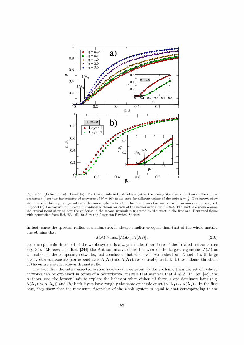
0 0.2 0.4 0.6 0.8 1 β/µ

0

0.2

0.4

0.6

0.8

1

ρ

η = 0.25 η = 0.5 η = 1.0 η = 2.0 η = 3.0

0 0.1 0.2 0.3 0.4 0.5 β/µ

0

0.2

0.4

0.6

ρ

η = 0.0

1/Λ1

1/Λ2

0 0.2 0.4 0.6 0.8 1 β/µ

0

0.2

0.4

0.6

0.8

1

ρ1,ρ

2

Layer 1

Layer 2

0 0.1 0.2 β/µ

0

0.2

0.4

ρ1,ρ

2

1/Λ2

1/Λ1

η =2.0 b)

a)

Figure 35: (Color online). Panel (a): Fraction of infected individuals (ρ) at the steady state as a function of the controlparameter β

µfor two interconnected networks of N = 104 nodes each for different values of the ratio η = δ

β. The arrows show

the inverse of the largest eigenvalues of the two coupled networks. The inset shows the case when the networks are uncoupled.In panel (b) the fraction of infected individuals is shown for each of the networks and for η = 2.0. The inset is a zoom aroundthe critical point showing how the epidemic in the second network is triggered by the onset in the first one. Reprinted figurewith permission from Ref. [53]. c© 2013 by the American Physical Society.

In fact, since the spectral radius of a submatrix is always smaller or equal than that of the whole matrix,one obtains that

Λ(A) ≥ max [Λ(A1),Λ(A2)] , (210)

i.e. the epidemic threshold of the whole system is always smaller than those of the isolated networks (seeFig. 35). Moreover, in Ref. [244] the Authors analyzed the behavior of the largest eigenvalue Λ(A) asa function of the composing networks, and concluded that whenever two nodes from A and B with largeeigenvector components (corresponding to Λ(A1) and Λ(A2), respectively) are linked, the epidemic thresholdof the entire system reduces dramatically.

The fact that the interconnected system is always more prone to the epidemic than the set of isolatednetworks can be explained in terms of a perturbative analysis that assumes that δ β. In Ref. [53], theAuthors used the former limit to explore the behavior when either (i) there is one dominant layer (e.g.Λ(A1) Λ(A2)) and (ii) both layers have roughly the same epidemic onset (Λ(A1) ∼ Λ(A2)). In the firstcase, they show that the maximum eigenvalue of the whole system is equal to that corresponding to the

82

dominant layer Λ(A) = Λ(A1), whereas the nontrivial stationary solution at βc yields

4~v =

(~p∗1δβΛ~p

∗1

), (211)

where ~p∗1 is the stationary solution in the dominant network at its epidemic onset. It is clear that the onsetof an epidemic in the dominant layer automatically induces the spreading in the other one.

The second limit (Λ(A1) ∼ Λ(A2)) reveals the strong synergetic effect of the coupling between layers.If isolated, the networks would have a roughly simultaneous epidemic onset located at their correspondingβc. However, the interconnection of layers makes a correction of the maximum eigenvalue as

Λ(A) = max[Λ(A1),Λ(A2)] +δ

β

~p∗1C12~p∗2 + ~p∗2C21~p

∗1

(~p∗1)T ~p∗1 + (~p∗2)T ~p∗2(212)

thus pointing out that the critical point of the system is smaller than any of the isolated layers, and that thecorrection to its value depends on the product of eigenvector centralities between connected nodes belongingto different networks, as pointed out in Ref. [244].

The HMF approximation, although being a coarse-grained picture, also recovers the above result. Inthis case, one can easily generalize Eq. (203) to the case of interconnected graphs. Once again, in the caseof two interconnected graphs A and B, the HMF equations in their time-continuous version read [242],

dρAkadt

= −µAρAka + βaa(1− ρAka)kaa∑k′a

ρAk′aPAA(k′a|ka) + βba(1− ρAka)kab

∑k′b

ρBk′bPAB(k′b|ka) , (213)

for the evolution of the fraction of infected individuals in network A having kaa neighbors in network Aand kab neighbors in network B [the evolution for ρBkb is analogous to Eq. (213)]. Here the degree classes ineach network, say A, is characterized by a vector degree ka ≡ (kaa, kab), and the conditional probabilitiesused in Eq. (213) make use of this vectorial classification of nodes. As in the case of the HMF equations insingle-layer networks, in order to derive the epidemic onset, one is interested in the limit where the densitiesof infected individuals are small, and therefore one works with the linear equation

d~ρ

dt= −~ρ+ C~ρ, (214)

where ~ρ ≡ (ρAka , ρBkb

), and

C =

βaakaaPAA(k′a|ka) βbakabPAB(k′b|ka)

βabkbaPBA(k′a|kb) βbbkbbPBB(k′b|kb)

. (215)

Obviously, whenever the maximum eigenvalue of matrix C satisfies Λ(C) < 1, any initial fraction of infectedindividuals decays to the trivial solution ~ρ = ~0. As a result, the critical epidemic point is defined byΛ(C) = 1. The analysis of this condition in uncorrelated networks was carried out in Ref. [242], yieldingthat Λ(C) ≥ max[Λ(A),Λ(B),Λ(AB)], being λ(A) and Λ(B) the maximum eigenvalues of the isolatednetworks, and Λ(AB) the one corresponding to that of the bipartite network obtained by considering onlythe links between nodes belonging to different networks. Once again, the HMF approximation allows toconclude that the coupled system can sustain an epidemic even when the isolated networks would be free ofdisease.

For the SIR model the treatment is quite similar [76, 245]. However, in Ref. [245], based on the analogybetween bond percolation and the SIR model, the Authors unveiled one important difference with respectto the case of the SIS dynamics. Whereas for strongly coupled networks the value of the epidemic onset ofthe whole system is smaller than that of the isolated networks (as in the SIS model), when the coupling isweak (i.e. the internetwork links are much less than those connecting individuals within the same network),the system can sustain an epidemic state in one network while not affecting the remaining ones. Thesemixed states point out that for the SIR dynamics there is a critical internetwork coupling, below which thenetwork behaves quite similarly to a set of unconnected networks.

83

5.2.3. Disease spreading on multiplex networksAs pointed out many times already, multiplex networks are, from the structural point of view, just

particular cases of multilayer networks in which each node is represented in each of the layers (so thatthe layers have the same number N of nodes). In addition, each layer is connected to another one via Nconnections resulting from the links that each node establishes with its representations in the remaininglayers. Given that the results shown for the disease spreading on top of an interconnected network arerooted in the spectral properties of its contact matrix, the case of a single disease spreading on top of amultiplex network can be analyzed in the same way by considering that the (MN ×MN) adjacency matrixis of the particular form

A = A + C =

A1 0 · · · · · · 00 A2 0 · · · 0· · · · · · · · · · · · · · ·0 · · · · · · · · · AM

+

0 I · · · · · · II 0 I · · · I· · · · · · · · · · · · · · ·I · · · · · · I 0

. (216)

However, a multiplex automatically sets the constraint that when a node gets infected by the disease in onelayer, and therefore it becomes a spreader of the disease in any of the other layers. This ingredient can onlybe approached (in the interdependent framework) by setting βab = βba = 1 and βaa, βbb, µa, µb 1, whichis a far different case with respect to the weakly coupled regime usually studied in interdependent networks.

In fact, in Ref. [246] the Authors analyzed the SIS model in a multiplex in a similar way to Ref. [53], i.e.by writing the microscopic dynamics. In this case, the expression for the probability that a node i is notinfected by any neighbor (in network A or B), qi(t), reads

qi(t) =

M∏α=1

N∏j=1

(1− βα(Aα)ij · pj(t)) , (217)

where Aα is the adjacency matrix in layer α. Note that, at variance with Eq. (207), the vector containing theprobability that any node is infected, ~p, has N components since now the state of a node must be the same inany of the layers composing the multiplex. One can note that the only difference with an epidemic spreadingon the projected network (the network resulting from the sum of the layers) is that the transmission ratesβα are different for each of the layers. The analysis of the microscopic dynamics relates the epidemic onsetwith the maximum eigenvalue of the matrix, defined as

Rij = 1−M∏α=1

(1− βα(Aα)ij) . (218)

Again, it is shown that the epidemic onset is always smaller than those of the isolated networks.The SIR model in multiplex networks has been analyzed in Refs. [247, 248]. In Ref. [247], the Authors

made use of a two-layers network in which a SIR disease switches layer at the expense of a cost. They derivedthe epidemic threshold, obtaining a similar result to that of SIR dynamics in interconnected networks [245]when the coupling between networks is strong: the epidemic threshold cannot be larger than those of theisolated networks. Obviously, multiplexity incorporates naturally the constraint that the network layers arefar from the weak coupling regime in which mixed states appeared. In this work, the Authors derived aninteresting result concerning the behavior of βc in a multiplex composed of two ER graphs as a function ofthe difference, δλ, between the intralayer and interlayer transmission rates and the difference, δz, betweenthe average degree of both layers. It was shown (see Fig. 36) that the multiplex epidemic threshold βc growswith δλ (when the intralayer transmission rate increases with respect to the interlayer one), for low valuesof δz. However, this trend is reversed when δz grows enough, so that βc decreases with δλ.

In Ref. [248], the SIR dynamics is addressed on top of a multiplex containing one physical layer and asecond one in which only a subset of the nodes in the first layer takes part. Importantly, the size of thissubset is tunable so that they are able to derive the conditions for the spreading of the disease as a functionof the size of the second layer.

84

"25" u 2:1:3

0 0.2 0.4 0.6 0.8 1δλ

0

0.2

0.4

0.6

0.8

1

δz

0.3

0.4

0.5

0.6

0.7

0.8

Figure 36: (Color online). The contour plot shows the epidemic threshold βc as a function of δz and δλ for a two layer multiplexcomposed of two ER networks. The dashed line (black) is a boundary of ∂βc/∂δλ > 0 for all δλ, and the green (blue) lineindicates the lowest (highest) value of βc at a given δz. βc shows non-monotonic dependence on δλ. Reprinted figure fromRef. [247]. Courtesy of B. Min.

Competing epidemics. The particular setting of multiplex networks provides the best suited structural back-bone for the study of the dynamical interplay between different dynamical processes taking place within thesame set of nodes. In this way, multiplexity offers the possibility of incorporating different network layersfor each dynamical process at work. This possibility leads to approach a well studied problem in single-layernetworks: the competition between the spreading of two different diseases. In Ref. [249], Newman proposeda model in which two consecutive SIR diseases spread within a single-layer network. For the first diseaseat work, the critical properties and the diffusion of the infections remain the same, as usual. However, thesecond disease finds it more difficult to spread since those agents recovered from the first of the diseases gainimmunity also to the second one. The main result is that, even for SF networks, the epidemic threshold forthe coexistence of both diseases is larger than zero. Subsequently, other works extended the framework tothe case of simultaneous spreading of diseases [250], or to the SIS model [251].

The further extension of those works to multiplex networks is natural, and adds the possibility of exploringthe effects of having two different transmission networks for each one of the diseases, and thus incorporatingthe fact that different diseases may have different transmission channels. Funk and Jansen were the firstto address this issue in Ref. [126] by considering, as in Ref. [249], that the disease spreads in a consecutiveway. To this end, they considered a multiplex composed of two networks and a SIR model so that the firstspreading takes place in one of the networks leaving a set of recovered nodes. These nodes are also set asrecovered in the second layer (as if they were fully immunized) prior to the second spreading that takes placein this second layer. The main result is that a positive correlation between the degrees of the nodes in bothlayers enhances the immunization of the network to the second spreading (increasing the effective epidemicthreshold for the coexistence of two epidemics). This approach has been generalized in Ref. [127] to thescenario of two SIR diseases whose spreading takes place simultaneously in the two layers of the multiplex,

85

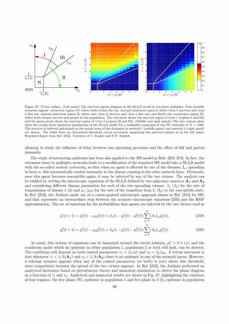
N

III

II

I

(0,0)

c

c

1

1

Figure 37: (Color online). (Left panel) The survival regions diagram in the SI1I2S model in two-layer multiplex. Four possiblescenarios appear: extinction region (N) where both viruses die-out, mutual extinction region I, where virus 1 survives and virus2 dies out, mutual extinction region II, where only virus 2 survives and virus 1 dies out, and finally the coexistence region III,where both viruses survive and persist in the population. The red arrow shows the survival region of virus 1 (regions I and III)and the green arrow shows the survival region of virus 2 (regions II and III). (Middle and right panels) The two contour plotsshow the results from numerical simulations of the SI1I2S model for a multiplex composed of two SF networks of N = 1000.The fraction of infected individuals in the steady state of the dynamics in network 1 (middle panel) and network 2 (right panel)are shown. The white lines are theoretical threshold curves accurately separating the survival regions as in the left panel.Reprinted figure from Ref. [252]. Courtesy of C. Scoglio and F.D. Sahneh.

allowing to study the influence of delay between two spreading processes and the effect of full and partialimmunity.

The study of interacting epidemics has been also applied to the SIS model in Refs. [252–254]. In fact, theextension there to multiplex networks leads to a modification of the standard SIS model into a SI1I2S modelwith the so-called mutual exclusivity, so that when an agent is affected by one of the diseases, Iα, spreadingin layer α, this automatically confers immunity to the disease running in the other network layer. Obviously,once this agent becomes susceptible again, it may be infected by any of the two viruses. The analysis canbe tackled by writing the microscopic equations of the SI1I2S defined by two adjacency matrices A1 and A2

and considering different disease parameters for each of the two spreading viruses: β1 (β2) for the rate oftransmission of disease 1 (2) and µ1 (µ2) for the rate of the transition from I1 (I2) to the susceptible state.In Ref. [252], the Authors made use of a coarse-grained microscopic approach shown in Ref. [255] for SIS,and that represents an intermediate step between the accurate microscopic equations [235] and the HMFapproximation. The set of equations for the probabilities that agents are infected by the two viruses read as

p1i (t+ 1) = p1

i (t)− µ1p1i (t) + β1(1− p1

i (t)− p2i (t))

N∑j=1

(A1)ijp1j (t), (219)

p2i (t+ 1) = p2

i (t)− µ2p2i (t) + β2(1− p1

i (t)− p2i (t))

N∑j=1

(A2)ijp2j (t). (220)

As usual, this system of equations can be linearized around the trivial solution, pαi = 0 ∀ i,α, and theconditions under which an epidemic in either population 1, population 2 or both will hold, can be derived.The conditions will depend on both control parameters τ1 = β1/µ1 and τ2 = β2/µ2. A trivial statement isthat whenever τ1 < 1/Λ(A1) and τ2 < 1/Λ(A2) there is no epidemic in any of the network layers. However,a relevant scenario appears when any of the control parameters (or both) is (are) above this threshold,since competition between the spread of the two viruses appears. In Ref. [252], the Authors performed ananalytical derivation based on perturbation theory and numerical simulations to derive the phase diagramas a function of τ1 and τ2. Analytical and numerical results are shown in Fig. 37, highlighting the existenceof four regimes: the free phase (N), epidemic in population 1 and free phase in 2 (I), epidemic in population

86

Figure 38: (Color online). Dependence of the onset of the epidemics βc as a function of λ for different values of the recoveryrates δ and µ for a two-layer multiplex composed of: (i) a SF network of N = 1000 and exponent 2.5 in the physical layer, whereSIS dynamics takes place, and (ii) the same SF network of the physical layer plus 400 extra random links (non-overlappingwith previous) in the virtual layer, where Aware-Unaware dynamics works. The shaded rectangle shows the free phase (inwhich all individuals are Unaware and Healthy) when the layers are uncoupled. The boundaries are defined by the bound ofthe structural characteristics of each layer: 1/Λ(A1) and 1/Λ(A2). Reprinted figure with permission from Ref. [256]. c© 2013by the American Physical Society.

2 and free phase in 1 (II), and finally the coexistence of both epidemic states in layers 1 and 2 (III).Interestingly, from the diagrams, it is clear that when the infection rate is large enough in one population,say 1, it hinders the epidemic onset in 2, even when τ2 > 1/Λ(A2). A further relevant result of Ref. [252] isthat whenever the two network layers are identical, the coexistence region disappears.

Interaction between social dynamics and epidemic spreading. As mentioned above, the multiplex structureallows to couple different dynamical processes involving the same set of agents being, in principle, differentthe structural backbone on top of which each process operates. In this way, disease spreading has beenrecently coupled to social dynamics [256], in order to take into account how the social awareness about thespreading of a disease can influence the impact of the latter. To this aim, the Authors coupled the SISspreading taking place on a physical network with another compartmental stochastic model in which thestate of the agents can be of two kinds: Aware (A) and Unaware (U). The first dynamics is completelycharacterized by the usual two parameters: the transmission, β, and recovery, µ, rates. The second dynamicstakes place on the second layer (a kind of virtual network in which information about the epidemic flows)and the transition between states A and U is analogous to that in the SIS model: the direct contact of anA agent with another one in U produces two A agents with probability λ, whereas an aware individual canbecome unaware with probability δ. The coupling between the two dynamical models is done by reducingthe transmission rates from infected individuals to aware and susceptible ones by a factor γ (γ = 0 meansthat aware individuals become fully immunized). In addition, the state unaware-infected is not admittedand, in a time discrete-version, it becomes aware-infected with probability 1 (if not recovered).

As in Ref. [252], when isolated, the two dynamical processes display a critical point at some values ofthe respective control parameters, β/µ and λ/δ. In particular: βc = µ/Λ(A1) and λc = δ/Λ(A2), whereA1 and A2 are the adjacency matrices of the first layer where SIS and Aware-Unaware dynamics take place

87

respectively. Once again, the coexistence of these processes changes the onset of the epidemic state. Inparticular, when the infection rate of the SIS dynamics is large enough, the infected agents trigger themechanism of awareness in the virtual layer, thus lowering the incidence of the disease and increasing theepidemic onset. This result is shown in Fig. 38 for several values of µ and δ. Interestingly, as the ratio δ/µdecreases, the value of the epidemic onset is more influenced by the Aware-Unaware dynamics.

Impact of interlayer topological properties. Except for the influence of dynamical processes located in otherlayers, the network properties between different layers also play a significant role in the diffusion of disease.The first viewpoint comes from the investigation of coupling density, which tries to reproduce the empiricalfact that not all the nodes are present on each layer of social networks. In Ref. [257], a fraction q of nodes areshared by two layers enabling to form partially overlapped networks. Since there exists the same disease inboth layers, the equal transmission probability is assumed, whereas the spreading of infection starts from onerandom node. The main aim becomes here to explore the effect of the overlapping fraction q on the diseasepropagation with reference to the SIR dynamics model. Based on the theoretical analysis and simulations,the Authors found that the epidemic threshold of multiplex networks depends on both topology and thecoupling density. In the limit of q → 1, the epidemic threshold is minimum, and both layers have the identicalratio of recovered nodes at any transmission probability. This is because nearly each node belongs to twolayers at the same time. However, with q decreasing, the epidemic threshold monotonously enhances, so as toreach the maximal value (at q → 0) dominated by the isolated threshold of the layer with larger propagationability. This point means that, even though there exists negligible differences between the system composedof two isolated networks and the system connected by just a few interlayer connections, these links canmake the epidemic threshold of the isolated network with lower spreading ability discontinuously change thethreshold of the other layer. This finding is shedding light into the non-medical intervention for the controlof the disease propagation.

Of particular interest is distinguishing how the disease spreads if the nodes are coupled by a certainrule from the case of simple overlapping. In a recent investigation [258], a two-route transmitted diseaseemploying SIR model is introduced into the multiplex framework, where two transmission routes take placeon each layer, respectively. Moreover, the Authors defined two new measures to evaluate the influence ofinterlayer links. The first is the degree-degree correlation (DDC) between layers: positive (negative) valuesindicate that high (low) degree nodes are inclined to have more (less) connections within another layer. Theother quantity is the average similarity of neighbors (ASN) from different layers of nodes, which measureshow many joint neighbors one node possesses in both layers. The Authors found that, even if both layersare below their respective thresholds, the disease can still propagate across the multiplex system. If thevalue of DDC is larger, a lower disease threshold and a smaller outbreak size are supported. The epidemicthreshold and disease size keep both robust against the change of ASN.

5.2.4. Voluntary prevention measuresExcept for the outstanding achievements of the prediction of the outbreak threshold, another task of

utmost urgency, during the study of epidemiology, is searching for the effective policy or strategy to controlthe epidemic spreading, and to warrant public health [259, 260]. This point seems particularly remarkablewith worldwide pandemics of severe acute respiratory syndrome (SARS), bird flu and new H1N1 flu [261–263]. A great number of immunization scenarios, such as targeted immunization [264], ring immunization[265], and acquaintance immunization [266], have been proposed, but the majority of them, based on thepremise of compulsory requirements, completely neglects the individuals’ willingness and desires, whichinstead follow many social factors including religious beliefs, the human rights and social total expensesas well [267–270]. In this sense, voluntary prevention measures, incorporating both studies of infectiousdisease and spontaneous human behavior traits, become popular programs [271, 272], namely, the so-called“disease-behavior feedback dynamics study”.

Voluntary vaccination on single-layer networks. Among several existing control measures, vaccination at-tracts the hugest attention from theoretical and experimental perspectives [273–276]. During the seasons ofdisease spreading, the high risk of infection usually stimulates individual vaccination enthusiasm, while high

88

0.01 0.02 0.03 0.04 0.05 0.06 0.07 0.08 0.09 0.10

10

20

30

40

50

60

70

Transmission probability

Attack/A

doption R

ate

(%

)

Influenza−only Attack Rate

Coupled Diffusion Attack Rate

Coupled−Diffusion Adoption Rate

Figure 39: Attack or adoption rate vs. the transmission probability in disease-only diffusion processes and coupled diffusionprocesses, where influenza is selected as the potential disease. Here, the adoption rate denotes the percentage of nodes adoptingprevention behavior. Reprinted figure from Ref. [282]. c© 2012 with permission from Elsevier.

expenses or side effects of a vaccine may lead to the opposite case. Thus, individuals face a dilemma: tovaccinate or not, both of which ways can be managed as two basic strategies with respective cost functions.To resolve this dilemma, game theory has been integrated into individual decision-making processes, wherenodes hold the prevention strategy according to risk and expenses in the epidemic campaign [277]. In arecent research [278], where nodes are only allowed to make rational selection (i.e. taking vaccination only ifits expense is low), the Authors found that disease outbreak can be more effectively inhibited on SF networksthan on random networks. Compared with early theoretical predictions of disease thresholds [239], this in-teresting outcome indicates that voluntary vaccination can effectively control the spreading of diseases inreal-world networks. Similarly, when the imitation dynamics with noise replaces the deterministic rule in thedisease-behavior study, multiple effects spontaneously arise: for perfect vaccine, vaccination behavior of SFnetworks beats that of random networks, while imperfect vaccine enables the promotion of vaccination anderadication of disease to act better on homogeneous connectivity patterns [279]. In Ref. [280] it is found thatthe spatial population structure shows a “double-edged sword” effect, which fosters vaccine uptake at thelow cost of vaccination, but causes vaccination to plummet when the cost goes beyond a certain threshold.More specifically, if a small fraction of individuals consistently holds vaccinating in flu-like diseases, thesecommitted vaccinators can efficiently avoid the clustering of susceptible individuals and stimulate otherimitators to take vaccination, thus contributing to the promotion of vaccine uptake [281].

Voluntary prevention behavior on multilayer networks. Although both infection diseases and preventionmeasures diffuse simultaneously through networks and interact with each other, few existing studies havecoupled them together. Recently, the research of disease-behavior interactions on top of multilayer structureshas also received attention. In the first conceptual work [282], two diffusion processes are implemented inthe multiplex viewpoint, where two networks, which are fully or partially coupled via the interlayer links,involve the same individuals yet different intralayer connections. Under such a framework, one network isregarded as the infection network to transmit diseases, and the remaining communication network channelsindividual influence concerning preventive behavior. Moreover, at variance from the aforementioned casewhere vaccination is the principal measure on single networks, other prevention behaviors, such as wearing

89

facemasks, washing hands frequently, taking pharmaceutical drugs, and avoiding contact with sick people,are considered as the main strategies, which seem particularly reasonable before attaining effective vaccine[283].

Based on the online surveys, the threshold model is selected, whereas only once the proportion of adoptersamong intralayer neighbors of communication networks reaches the perceived threshold of adoption pressure(or the proportion of infected individuals exceeds the perceived risk of infection on the infection network),the node can adopt the preventive behavior. Surprisingly, the Authors found that, as compared to the widelyused disease-only model, the coupled diffusion model leads to a lower frequency of infection. Figure 39 showsthat, as preventive behavior protects a certain people from being infected, the threshold and peak of diseaseoutbreak are effectively suppressed in the new embedded scenario. Furthermore, the sensitivity analysisidentifies that the structure of infection network has dramatic influence on both epidemic and adoptionpercentages, while the variant of communication network produces less effects.

After such a seminal research, the role of multiplex networks in the coupled disease-behavior system hasbeen further investigated. Recently, a triple diffusion process, comprising disease transmission, informa-tion flow regarding disease and preventive behaviors against disease, was integrated into multilayer socialnetworks [284]. Among the interaction of the three diffusion dynamics, the negative and positive feedbackloops are formed. Here it is worth mentioning that, as compared with Ref.[256] involving the informationdiffusion as well, the effect of prevention behavior is of particular evidence. Under the help of agent-basedmethod, this new conceptual framework can reasonably replicate the observed trends of influenza infectionand online query frequency in the empirical population.

Finally, a similar scenario was proposed in Ref. [285], where the social and biological dynamics processesare embedded into a multiplex viewpoint. Under such a disease-behavior system, biological contagion spreadson one layer, while the main control measure, vaccination, is carried out in the social network. At variancewith the case of an isolated network, the Authors suggested that the resulting coupling can bring positiveor negative impact on the vaccination coverage during a vaccine scare, i.e. accelerating or decelerating theelimination of disease, which can get support from the empirical examples. Due to the variety of factorson the social layer, the epidemic trajectories and the uptake of control measures can also change to a largeextent. Moreover, inspired by these findings, the Authors suggested that the coupled disease-behavior model,which gets empirical validation, can be used as a predictive tool to explore the optimal strategies for publichealth.

5.2.5. Opinion formation dynamicsUnderstanding the emergence of a macroscopically ordered state is one of the based questions in natural

and social sciences. To elucidate this issue, dozens of experimental and theoretical frameworks have beenproposed from viewpoints of statistical physics, economics and sociology [227, 286–289]. Opinion formationdynamics, as one simple and paradigmatic dynamical process, has attracted particular attention. Up to now,various spin-like setups have been put forward to study the evolution of opinion dynamics, which includethe Sznajd model [290], majority rule model [291, 292], bounded confidence model [288, 293], and votermodel [294, 295], to name but a few. Among the existing scenarios, the voter model is attracting the mostremarkable attention [286, 296], and therefore it is also the main candidate in this subsection.

The basic definition of the voter model is rather simple: each agent (voter) is endowed with a binaryvariable s = ±1. At each time step, an agent i is chosen along with one of its neighbors j and si = sj ,i.e., the agent adopts the opinion of the neighbor. In this sense, the transition rate of individual opinion isproportional to the fraction of neighboring nodes in the opposite state. The dynamical process is repeateduntil the states with all sites equal (consensus) are absorbing. In spite of being extremely simple, the votermodel produces rich dynamical behaviors [295, 297], especially from the angles of spatial interaction. Inone-dimensional lattices, the dynamics is exactly the same as the zero-temperature Glauber dynamics [298].Turning to two-dimensional lattices, the growth of domains can makes the interfaces quite rough, at oddswith usual coarsening systems [299]. Moreover, a series of extended versions, such as the vacillating votermodel [300], nonlinear voter model [301], heterogeneous voter model [302], and constrained voter model [303]have also been suggested. In the following we will present more details on the voter model.

90

Figure 40: (Color online). Snapshots of the evolution of opinion dynamics with three typical freezing periods H. From left toright, the values of H are 0, 15 and 4000. In each panel, the vertical axis corresponds to the elapsed time, while the yellowand blue areas on the horizontal lines represent the opinion clusters. The total time spent to reach a global consensus, i.e. theconsensus time 〈T 〉, under the scenario of intermediate value (H = 15) is far less than two other cases. The size of networks isN = 500, q = 0.01 is the switching ratio during the freezing period. Reprinted figure from Ref. [313].

Voter model on single-layer networks. As it is well-known, the property of spatial topology usually has anontrivial influence on the dynamical models. In this sense, the ordering dynamics of voter model shouldnot be exceptional. If employing one complete graph, the mean consensus time 〈T 〉 can be easily obtainedby using the Fokker-Planck equation [304]. The consideration of a heterogeneous connectivity can make themean consensus time 〈T 〉 to become closely related with the structural network details. On SF networkswith exponent γ, direct voter model makes 〈T 〉 to scale as the size N of the network for γ > 3 and sublinearlyfor γ ≤ 3 [296, 305, 306]. Non trivial relationships between 〈T 〉 and N are also found in other versions ofthe voter model as in Ref. [307]. For small-world networks, the plateau formed by active interfaces hindersthe diffusion of opinions, so that the consensus eventually relies on the linear system size [308, 309]. Alongthis research line, Zschaler et al. recently examined the effect of directed networks on the order-disordertransition [310]. The impact of other spatial mechanisms, such as social influence and heterogeneous beliefs,are also of particular evidence [311, 312].

At variance with the aforementioned processes on static networks or in a Markovian memoryless fashion,coevolution voter model has also been duly studied. We first focus on non-Markovian patterns. In recentresearches [314, 315], Stark et al. explored the effect of a memory-dependent transition rate, which isdetermined by the persistence time of individual current opinion. The longer a voter keeps its opinion, theless probable is that it switches the status in the long run. The Authors found that the process towardsreaching a macroscopic consensus was accelerated by slowing down the microscopic dynamics. Looking atanother recent report [313], where individual ability q of opinion switching is weakened during a freezingperiod H, the Authors revealed that an intermediate freezing period can lead to the fastest consensus, i.e.to the smallest 〈T 〉. The essence of this accelerated consensus is attributed to the biased random walk ofthe interface between adjacent opinion clusters (as shown in Fig. 40). Moreover, it is worth checking how

91

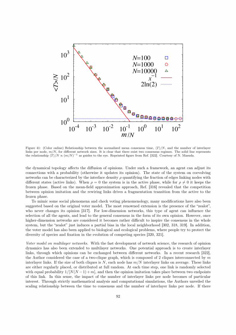
m

Figure 41: (Color online) Relationship between the normalized mean consensus time, 〈T 〉/N , and the number of interlayerlinks per node, m/N , for different network sizes. It is clear that there exist two consensus regimes. The solid line representsthe relationship 〈T 〉/N ∝ (m/N)−1 as guides to the eye. Reprinted figure from Ref. [322]. Courtesy of N. Masuda.

the dynamical topology affects the diffusion of opinions. Under such a framework, an agent can adjust itsconnections with a probability (otherwise it updates its opinion). The state of the system on coevolvingnetworks can be characterized by the interface density ρ quantifying the fraction of edges linking nodes withdifferent states (active links). When ρ = 0 the system is in the active phase, while for ρ 6= 0 it keeps thefrozen phase. Based on the mean-field approximation approach, Ref. [316] revealed that the competitionbetween opinion imitation and the rewiring links drives a fragmentation transition from the active to thefrozen phase.

To mimic some social phenomena and check voting phenomenology, many modifications have also beensuggested based on the original voter model. The most renowned extension is the presence of the “zealot”,who never changes its opinion [317]. For low-dimension networks, this type of agent can influence theselection of all the agents, and lead to the general consensus in the form of its own opinion. However, oncehigher-dimension networks are considered it becomes rather difficult to inspire the consensus in the wholesystem, but the “zealot” just induces a partial bias in the local neighborhood [302, 318, 319]. In addition,the voter model has also been applied to biological and ecological problems, where people try to protect thediversity of species and fixation in the evolution of competing species [320, 321].

Voter model on multilayer networks. With the fast development of network science, the research of opiniondynamics has also been extended to multilayer networks. One potential approach is to create interlayerlinks, through which opinions can be exchanged between different networks. In a recent research [322],the Author considered the case of a two-clique graph, which is composed of 2 cliques interconnected by minterlayer links. If the size of both cliques is N , each node has m/N interlayer links on average. These linksare either regularly placed, or distributed at full random. At each time step, one link is randomly selectedwith equal probability 1/[N(N − 1) +m], and then the opinion imitation takes place between two endpointsof this link. In this sense, the impact of the number of interlayer links per node becomes of particularinterest. Through strictly mathematical analysis and computational simulations, the Authors unveiled thescaling relationship between the time to consensus and the number of interlayer links per node. If there

92

exist many interlayer links per node, the mean consensus time is 〈T 〉 = O(N), i.e. the system reaches thefast consensus regime, which agrees with the expectation of a complete graph [307]. However, once thenumber of interlayer links per node is much smaller than unity, the mean consensus time is 〈T 〉 = O(N2),i.e. the system attains the slow consensus regime. The crossover between these two regimes takes places atapproximately one interlayer link per node, as shown in Fig. 41. Thus, these results suggest that the sparseinterlayer connections between two networks extremely decelerate the ordering state for the voter modeldynamics.

In Ref. [323], a coevolution voter model is incorporated into a multilayer framework, where a fractionq of nodes has the interlayer links across two networks. On each layer l (l = 1, 2), individual opinion andintralayer link are allowed to evolve in accordance with their own topological temporal scales. Node i selectsone random neighbor j in the same layer. If both have different opinions, node i copies the state of j withprobability pl, otherwise (with probability 1 − pl) it severs the connection with j and draws a new linkto one randomly chosen node in the same layer possessing a state identical to itself. The case p1 = p2

preserves the symmetric multilayer setup, namely, the time scales are the same in both layers. At variance,for p1 6= p2, an asymmetric multilayer case takes place, namely, different topological time scales characterizethe two layers. In the symmetric case, the Authors found that interlayer connectivity plays a critical role indetermining the state transition of systems. Once again, the absorbing fragmentation transition appears at acertain threshold value of pl. Moving to the asymmetric case, the Authors unveiled an anomalous shatteredfragmentation transition, where the layer dynamics splits into many isolated components possessing differentopinions, namely an explosive growth of the number of disconnected components. Moreover, Ref. [323] alsoidentified the critical degree of interlayer connectivity to stop the fragmentation of one layer by coupling itto another layer that has no fragments.

Finally, it is interesting to consider the application of opinion dynamics in the multiplex perspective. Ina recent research [324] a simple model of opinion formation dynamics is proposed to describe the partiescompeting for votes within a political election. At variance with previous setups of voter model [286, 296],each opinion or party is modeled here as one social network where the contagion dynamics takes place. Everyagent, at the election day, can choose either to be active in only one of the two networks (vote for one party)or to be inactive, namely, not to vote on both networks. Based on the simulated annealing algorithm, theAuthors showed a rich phase diagram. In a wide region of the phase diagram, the competition between thetwo parties allows for the emergence of pluralism, namely two antagonistic parties gather a finite share ofthe total votes. The densely connected network usually wins the election campaign, regardless of the initialdistribution. Nevertheless, small perturbations could break the existing equilibrium, and a small minorityof committed agents can alter the election outcome, which is consistent with recent claims [325].

5.3. Evolutionary games on multilayer networksThe study of evolutionary games on top of single-layer networks has attracted a lot of interest as a

connector between statistical physics, evolutionary dynamics and social sciences [326–328]. This is a veryappealing research topic since the dynamics implemented in the network arises from an evolutionary approach[329]. In addition, the study of evolutionary games on networks has been one of the most studied avenuesto understand the emergence of cooperation in different contexts [330]. The emergence of such a collectivephenomenon, cooperation, is a key issue that arises when studying seemingly diverse evolutionary puzzles,such as the origin of multicellular organisms [331], the altruistic behavior of humans and primates [332], orthe way advanced animal societies, such as ant colonies, work [333, 334], among others.

Previous research on evolutionary games on networks has mainly focused on social dilemmas, in whichagents can take one of two strategies: Cooperation (C) and Defection (D). Among these dilemmas, thePrisoner’s Dilemma game (PDG) represents the most addressed paradigm when studying the emergence ofcooperation [335, 336]. This game is fully described by the following payoff matrix

Π =

(C DC R SD T P

)=

( C DC 1 0D b > 1 1 > ε ≥ 0

), (221)

93

showing that when two cooperators meet, each one obtains a “Reward” (R = 1) whereas the interactionbetween two defectors causes a “Punishment” (P = ε) to both. However, cooperation is hampered by theplayers’ “Temptation” to defect, since defecting against a cooperator yields more payoff than cooperating(T = b > 1), and by the risk arising from cooperating with a defector, as it yields the lowest payoff, usuallycalled “Suckers”, (S = 0) [337]. These payoffs satisfy the ranking T > R > P ≥ S. The social dilemma isthus established, since mutual cooperation yields both an individual and total benefit higher than that ofmutual defection.

The pairwise nature of the game is translated to a population scale by making the agents interacting(playing) with each other, and accumulating the payoff obtained from each interaction. After each roundof the game, the strategies of the agents are updated so that those agents with less payoff are tempted tocopy (replicate) the strategy of those fittest individuals. In unstructured populations, in which players arewell-mixed, evolutionary dynamics leads all the individuals to defection [338, 339]. However, the existence ofa network of interactions, so that each agent can only play with those directly connected to it, the populationcan sometimes promote the emergence of cooperation. This mechanism promoting cooperation was coinedas network reciprocity [340], and it was observed to be substantially enhanced when the network substrateis SF [341, 342].

Very recently [328] the attention of the community has been extended to the n-player (n > 2) gener-alization of the PDG, also called Public Goods Game (PGG) [343]. Under this setting, each cooperatorcontributes a fixed investment v to the public good whereas defectors do not contribute. The total contribu-tion of the n agents is then multiplied by an enhancement factor 1 < r < n and finally the result is equallydistributed between all n members of the group. The payoff of cooperators and defectors in a group with afraction x of cooperators is, respectively

fC(x) = (rx− 1)v , (222)fD(x) = rxv. (223)

Thus, defectors obtain the same benefit of cooperators at zero cost, i.e. they free-ride on the effort ofcooperators. As in the PDG, the evolutionary outcome of the PGG differs if played on a well-mixedpopulation, in which the dynamics ends up in a full defector population, or on a structured one. In particular,Brandt et al. [344, 345] showed that, when games are restricted to local interactions, cooperation is promotedso that full cooperation is observed for values of the enhancement factor r < n. This result was latergeneralized to complex networks [346] and bipartite graphs [347, 348].

5.3.1. Pairwise interaction gamesGames on interconnected networks. The study about emergence of cooperation in the PDG in networkedpopulations has been also extended to the case of multilayer systems. One of the approaches is to considerthat each layer is composed of a different set of agents, so that each of them plays both with those neighborswithin the same network layer and with those placed in the other ones [349, 350]. In Ref. [349] the Authorsconsidered the case of 2 interconnected networks in which each agent plays a different game depending onwhether the neighbor belongs to its same network, or to the other one. In particular, they considered twopossible payoff matrices, one for those interactions between nodes of the same network layer, Πintra, thattakes the same form of Eq. (221), and the following one for interlayer interactions

Πinter =

( C DC 1 0D b > 1 ε < 0

). (224)

Thus, if A1 and A2 are the adjacency matrices of the two networks and C12 = C21 is the matrix containingthe interlayer connections (so that the total adjacency matrix reads as in Eq. (205)), the payoff of a node ibelonging to network layer α is

fαi (t) =

N1∑j=1

(Aα)ij · ~siα(t)TΠintra ~sjα(t) +

N2∑j=1

(C12)ij · ~siα(t)TΠinter ~sjβ(t) , with α 6= β , (225)

94

1 1.5 2 2.5 3b

0

0.2

0.4

0.6

0.8

1

c

00.0010.0020.0050.010.020.04

p

Figure 42: (Color online) Fraction of cooperators c in the population 1 as a function of b, for different values of the fraction p ofinterpopulation contacts. The population 1 (of size N1 = 103) has been coupled to a smaller population 2 (N2 = 102). Whileinitial strategies in population 1 are equally probable (random initial conditions), the population 2 starts from the absorbentstate of fully defection. Other parameters are r = 0, ε = −0.4. Both populations have a random (Erdős-Rényi) network ofcontacts with average degree 〈k〉 = 6. Reprinted figure with permission from Ref. [349]. c©, 2012 by the American PhysicalSociety.

where ~siα is a two-components vector denoting the strategy of the node i in layer α at time t: ~siα reads(1, 0)T for Cooperation and (0, 1)T for Defection.

Thus, nodes gain payoff according to a PDG when playing with neighbors in the same layer, whereas forinterlayer connections the payoff remains the same except for those interactions between two defectors, asthe Punishment becomes negative being the smallest possible payoff in this matrix, i.e. the payoff rankingevolves into T > R > S > P . This latter change turns the PDG into a Snowdrift game (SDG). In thisway, the exploitation that defectors make of cooperators, regardless of the layer where they are located, ishampered by the payoff loss when meeting a defector belonging to the other network layer. The results inRef. [349] reveal that, both for well-mixed layers and networked ones, it is possible to find polarized statesin which cooperation dominates in one of the layers whereas defection does in the other. Figure 42 showsthe fraction of cooperators, c, as a function of the Temptation b. When there are no connections betweennetwork layers (p = 0), so that the two populations play a PDG, the diagram follows the usual trend insingle-layer networks: cooperation resists for small values of b > 1 and then suddenly decreases so that c = 0for b 1. However, polarized states (here revealed by the plateau at c = 0.5) appear as soon as the twolayers are connected, i.e. even for a small number of interlayer links, thus showing the importance that theinterconnection between layers has on the evolutionary outcome.

In Ref. [350] the Authors addressed a similar interconnected system of 2 networks, but considering thatboth intra and interlayer interactions are governed also by the same Eq. (221), i.e. the payoff matrix ofthe PDG. In this case, the Authors focus on the emergence of cooperation as a function of the density ofinterlayer links and the topology of each layer at work. In general, for low density of interlayer connections,the overall cooperation of the system is enhanced. In this regime, it was found that those agents connectingthe two network layers are more likely to cooperate than those sharing only intralayer links. Furthermore,although in general the interconnection of layers promotes cooperation in the whole system, when lookingat the level of single layers, the effect of interconnection can produce a reduction of cooperation in one ofthe layers that is compensated by the increase in the other one.

95

Figure 43: (Color online). Cooperation diagrams of multinetworks. Average level of cooperation 〈c〉 as a function of thetemptation b to defect for several multinetworks with different number of layers M (the number of layers in indicated in thelegend). In panel A the network layers are ER graphs with 〈k〉 = 3 (sparse graphs) while in panel B we have 〈k〉 = 20. Inboth cases N = 250 nodes. As it can be observed, the resilience of cooperation increases remarkably as the number of layersM grows. Reprinted figure from Ref. [352].

Aside from involving payoff via playing games with nodes of other networks, another potential approachis to allow direct information transmission or exchange between layers. In a recent research [351], wherePDG and SDG are respectively implemented on different layers, a biased imitation is proposed: a node withprobability p can mimic the strategy of intralayer neighbor in the same network, otherwise the internetworkneighbor is chosen as the strategy donor. Under such a framework, the Authors try to explore how thecooperation trait varies as a function of a biased probability p. The biased probability unveils a multipleeffect, which is robust against the change of population structures. A slight decline of the biased probabilitystarting from p = 1 promotes the cooperation behavior in the PDG layer. On the contrary, this decreaseimpairs the evolution of cooperation in the SDG subpopulation. Ref. [351] also verifies that qualitativelyvalid observations can be extended to a much broader parameter space in virtue of the mean-field method.

Games on multiplex networks. A second stream of works addressed the study of evolutionary dynamics inmultilayer networks [352]. In this way, all the M layers have the same number of nodes, say N , since eachnode is the representation of a particular agent, and the only links between layers are those connecting thenodes representing the same agent. The assumption of a multiplex imposes dynamical correlations betweenthe states (or strategies) of the replica nodes. In Ref. [352] this correlation is implemented by consideringthat an agent i can, in principle, take different strategies in each of the layers. For instance, in the PDG anagent i can be a defector in n layers, while it cooperates in the remaining M − n layers. The total payoff ofa node i in layer α at time t reads

fαi (t) =

N∑j=1

Aαij ~siα(t)Π~sj

α(t) , (226)

where the payoff matrix is defined as in Eq. (221). In addition, the total payoff of agent i is the sum of allthe payoffs accumulated by the different representations across the M layers

fi(t) =

M∑α=1

fαi (t). (227)

96

In Ref. [352] the update of the strategy used by an agent i at layer α depends on fi(t) (instead of takinginto account only the payoff accumulated at this layer fαi (t)), thus coupling the evolution of the states ofthe nodes in a given layer with the dynamical states of the rest of the layers. Figure 43 shows that thecorrelation between layers influences the cooperation levels of the system in a way that, by increasing thenumber M of layers, the resilience of cooperation is enhanced at the expense of decreasing the level ofcooperation observed for small values of the temptation b to defect.

Moreover, motivated by the fact that each agent is usually member of different networks in humansocieties, a completely distinct setup is suggested in Ref. [353]. The system is there composed of 2-layer SFnetworks. One network, named interaction layer, is used for the accumulation of payoffs, and the other servesas the updating network for strategies or states. The Authors show that, with all the possible combinations ofdegree mixing, breaking the symmetry through assortative mixing in one layer and/or disassortative mixingin the other as well as preserving the symmetry by means of assortative mixing in both layers, impedes theevolution of cooperation. The essence of this scenario for the cooperation inhibition can be attributed to thecollapse of giant cooperation clusters, especially as compared to the case of single-layer SF networks [353].

Games on interdependent networks. The third realm of the evolutionary game in multilayer networks turnsto that of interdependent networks. It is worth mentioning that this form possesses evident differenceswith the aforegoing situations. As compared to the case of interconnected networks, the direct interactionof game and strategy exchanged between network layers are strictly forbidden. On the other hand, thecorresponding nodes connected via the internetwork links represent different agents, at variance with themultiplex scenario, thus both the accumulation of payoff and strategy updating are just limited to the samenetwork layer. In this sense, the internetwork links are mainly used to create mutual influence betweendifferent networks. Since utility and strategy are prime elements in evolutionary game theory, creatinginterdependence through both factors becomes a natural choice. The framework of interdependent networkgames is then the following: agents of each layer do not engage in any game interaction beyond their ownlayer, but just refer utility or strategy information of other systems during the process of strategy updatingwith their intranetwork neighbors.

A recent research suggests the case of 2 interdependent networks, network α and network β, in which eachnode obtains the payoff by playing the games with its intralayer neighbors [354]. Then the interdependentcorrelation between networks (the node-to-point interdependence) is realized by defining an utility functionas follows:

Uαi (t) = (1− γ) · fαi (t) + γ · fβi′ (t), (228)

where fαi (t), fβi′ (t) represent the payoffs of a given node i in network α and that of corresponding partneri′ from network β, and γ ∈ [0, 1] is the parameter accounting for the coupling strength between layers. Thefunction Uαi (t) is then used for the update of the strategy of agent i at layer α. Such an expression is asymmetric function, i.e. the payoff of the node in network β also accounts for the same part (1 − γ) inits utility. It is worth noting that setting γ = 0 decouples both networks, and the model gets back to thetraditional single-layer network case [326]. With the increment of the coupling correlation, the utility ofone network depends more and more on the other system. In particular, for γ = 1, the utility of one nodebecomes fully determined by the other network, and the updating strategy becomes the process of tossinga coin.

The Authors selected the PDG as the paradigmatic model to explore the effect of the coupling strength.They found that there exists a threshold value γt (γt ' 0.5) in the system, such that, when the couplingstrength γ is smaller than this threshold, the symmetry of cooperation level in both networks is maintained.However, as the value of γ exceeds γt, there is a spontaneous symmetry breaking of the fraction of cooperatorsbetween different networks. Figure 44 shows the typical cross sections of phase diagrams for different couplingdegree γ. In the case of γ = 0.4, where cooperation level is well promoted, one can observe the existenceof three sections: pure cooperators section, mixed strategies section and pure defectors section. If γ is setas 0.9, a novel section emerges: the symmetry breaking section. Moreover, this observation is universallyeffective on different networks and can be qualitatively predicted by the strategy-couple pair approximation

97

Figure 44: (Color online). Cross sections of phase diagrams for γ = 0.4 (left) and γ = 0.9 (middle) on the interdependentsquare lattices (green squares) and small-world networks (red triangles) with a fraction of rewired links equal to 0.05. Thecolored regions correspond to different sections: yellow is pure cooperators section, cyan is mixed strategies section, gray ispure defectors section and purple is symmetry breaking section. The lines in right panel denote the results of strategy-couplepair approximation for γ = 0.9, which is qualitatively similar to the case of the middle panel. The dashed line represents anunstable solution of the analytical approach. Note that different ranges for the horizontal axis are used in the three panels,just for the guide of the eye. Reprinted figure from Ref. [354].

approach, in which an accurate prediction of the phase transition is difficult, due to the fact that long-rangeinteractions are neglected among nodes in the network [326].

5.3.2. The public goods gameThe first work on this game in multilayered networks [355] addressed a simple system composed of

two regular lattices that are coupled in the usual coupling way (each node in a layer has a link with itscorresponding partner in the other one). The PGG is played according to the usual rules, so that in eachof the layers, an individual constitutes a group together with its 4 nearest intralayer neighbors, thus takingpart simultaneously in 5 different PGGs. As described for PDG, the coupling between layers comes froman utility function that couples the payoff obtained by the agent i in layer α, fαi , with that obtained by itspartner i′ in the other layer β, fβi′ . In this case, the coupling takes the form

Ui = γ · fαi + (1− γ) · fβi′ . (229)

Here the utility function, at variance with Ref. [354], is the same for the two layers, and it incorporates a newingredient since there is one dominating layer depending on the value of γ (namely, a biased master-slaveinterdependence fashion): when γ < 0.5 (γ > 0.5) layer α (β) is dominated by layer β (α). As usual, theutility function is used for updating the strategies of the nodes in each layer. The most interesting resultobtained in Ref. [355] is that, when one layer almost dominates the other, cooperation is extraordinarilyfavored in the slave layer. For γ → 0 and γ → 1, the corresponding master layer behaves almost equallyto an isolated square lattice showing more weakness to defection than the slave one, in which the relationbetween the strategy and the utility function is almost random. These results are explained in terms oftime-scale separation for the spread of strategies that favors the development of cooperator clusters in theslave layer.

Many other kinds of interlayer couplings can be introduced in the utility function. In Ref. [356], using atwo-layer topology composed of two identical 2-dimensional lattices, the Authors followed a similar approachto that used in Ref. [354] for the PDG, since each one of the layers has its own utility function, which inits turn depends on what is the state of the other layer. In this case, the utility function for the agent i inlayer α is defined as

Uαi = (1− γ − γ′) · fαi + γ ·

N∑j=1

Aαijfαj

+ γ′ ·

N∑j′=1

Aβi′j′fβj′

, (230)

where the terms multiplied by γ and γ′ account for the average payoff of the neighbors of i in the same layerα and that of those neighbors of the corresponding partner i′ in the other layer β, respectively. The effect of

98

γ

0.0 0.1 0.2 0.3 0.4 0.50.0

0.1

0.2

0.3

0.4

0.5

0.0 0.1 0.2 0.3 0.4 0.50.0

0.1

0.2

0.3

0.4

0.5

0.0 0.1 0.2 0.3 0.4 0.50.0

0.1

0.2

0.3

0.4

0.5

0.0

0.2

0.4

0.6

0.8

1.0

00.00.00.00.00.10.10.10.10.10.10.10.10.10.10.10.20.20.20.20.20.20.20.20.20.30.30.30.30.30.30.30.30.30.30.40.40.40.40.40.40.40.40.40.40.50.50.50.50.50.50.50.50.50.50.60.60.60.60.60.60.60.60.60.60.70.70.70.70.70.70.70.70.70.70.80.80.80.80.80.80.80.80.80.80.90.90.90.90.90.90.90.90.90.91.01.01.01.01.01.0

frac

tion

of c

oope

rato

rs

0.0

0.2

0.4

0.6

0.8

1.0

10 -2 10 -1 10 0 10 1 10 2 10 3 10 4

frac

tio

n o

f ed

ges

time [MCS]

P (D,D)iP (C,C)iP (D,D)eP (C,C)e

0.0 0.1 0.2 0.3 0.4 0.50.0

0.1

0.2

0.3

0.4

0.5

0.0 0.1 0.2 0.3 0.4 0.50.0

0.1

0.2

0.3

0.4

0.5

0.0 0.1 0.2 0.3 0.4 0.5

0.0

0.1

0.2

0.3

0.4

0.5

0.0

0.2

0.4

0.6

0.8

1.0

00.00.00.00.00.10.10.10.10.10.10.10.10.10.10.10.20.20.20.20.20.20.20.20.20.30.30.30.30.30.30.30.30.30.30.40.40.40.40.40.40.40.40.40.40.50.50.50.50.50.50.50.50.50.50.60.60.60.60.60.60.60.60.60.60.70.70.70.70.70.70.70.70.70.70.80.80.80.80.80.80.80.80.80.80.90.90.90.90.90.90.90.90.90.91.01.01.01.01.01.0

frac

tion

of c

oope

rato

rs

’

γ

<c>

Figure 45: (Color online) The contour plots show the stationary fraction of cooperators 〈c〉 as a function of the couplingparameters γ and γ′ entering in Eq. (230) for r = 3.5 in PGG (left panel). Time courses of strategy pairs within and betweennetworks (right panel), where Pi and Pe denote the corresponding pair configuration probabilities within (internal) and between(external) networks, respectively. The parameters are r = 3.5, γ = 0.15 and γ′ = 0.5 in right panel. Reprinted figure fromRef. [356].

the coupling parameters γ and γ′ is the promotion of cooperation although this effect is more pronouncedfor γ than for the interlayer coupling γ′ (see the left panel of Fig. 45). This observation was given the nameof interdependent network reciprocity. The essence of this mechanism requires the simultaneous formationof correlated cooperator clusters on both networks, which can get further support from the synchronizedevolution of strategy pairs between networks, as shown in the right panel of Fig. 45. If synchronization doesnot emerge or if the coordination process is disturbed, interdependent network reciprocity fails, resulting inthe total collapse of cooperation. Moreover, this promoting effect is proven to take place also in systemsinvolving more than 2 layers, as long as the coordination between the networks is not disturbed.

Another way to model the interlayer coupling via the utility function is the probabilistic interconnectionintroduced in Ref. [357], in which two lattices are coupled in an interconnected way. However, two nodes ofboth layers are effectively coupled with probability p, so that not all the possible N pairs of interlayer linksare active. When an interlayer link is active, the utility function of player i in layer α is influenced, so thatapart from the 5 PGG in which it is enrolled within the corresponding layer α, it also participates in thatcentered on its partner i′ in the other layer β. In this way, the Authors showed that there is an optimalinterlayer connection probability p that maximizes the cooperation level.

The information of strategy also plays a crucial role in affecting the trait of other systems. In Ref. [358],the Authors proposed an alternative coupling between two lattices. The coupling is done via the update ruleby which the agents decide their strategies (to cooperate or to defect) for the next round of the game insteadthat via the utility function. The probability that agent i in layer α adopts the strategy of a neighboringnode j in the same layer depends here on the difference between their payoff functions and on the fact thatthe corresponding partner of i in layer β has the same or a different strategy. If the strategies of both thenode i and its partner i′ are the same, the probability of changing is decreased with respect to the usual onewhen the network layers are isolated. This coupling is seen not only to enhance cooperation in both PDGand PGG, but also to sustain the spontaneous emergence of correlated behaviors between the two networks.If the range of information sharing is extended to groups, this promotion effect is even more evident.

5.3.3. Partial overlap and spatial coevolutionWhile the effect of interlayer nodes has been extensively identified, the question of what would be the best

overlapping level for the resolution of social dilemmas remains unclear. To answer this issue, one scenario ofpartial overlapping is suggested in Ref. [359], where two networks possessing the same number N of nodescompose the interdependent system. Before any interaction, a fraction ρ of the nodes of one layer, ρN nodes,which are chosen uniformly at random, are linked to their corresponding partners in the other one, and the

99

residual nodes have no internetwork partners. Due to the existence of interdependence, the utilities of theseoverlapping nodes are not simply payoffs obtained from the interactions with the intralayer neighbors inthe same network, but they rather involve the performance of their partners in the other network. Herethe correlation between the payoffs obtained by a given node i and its partner i′ is done by defining thefollowing utility function:

Uαi (t) = fαi (t) + γ · fβi′ (t), (231)

with γ ∈ [0, 1] determining the strength of coupling between layers. In particular, if the node i has noexternal links, its utility simply equals to its own payoff (Uαi (t) = fαi (t)). The utility function Uαi (t) is thenused for the update of the strategy of agent i at layer α. As in the setup of Ref. [354], the utility functionhas here a symmetric form.

Under such a scenario, cooperation is studied as a function of ρ and γ. The Authors found that anintermediate density of sufficiently strong coupling between networks (more accurately, γ → 1 and ρ ' 0.5)warrants an optimal regime for cooperation to survive. This observation is robust to the variations of thestrategy updating dynamics, the interaction topology, and the governing social dilemma, thus suggesting ahigh degree of universality. Similarly to Ref. [350] it is observed that, within a layer, cooperation tends tofixate preferentially in those nodes that are connected with their counterpart in the other layer.

Furthermore, it is instructive to examine how the cooperative behavior survives on the coevolutionframework, in which the heterogeneity is usually ubiquitous [360, 361]. In a recent research [362], whereno interlayer links exist between two independent structured populations, a utility threshold is designed tomanage the emergence of temporary interlayer links. If the current utility of node i exceeds this threshold,it is rewarded by one interlayer link to the corresponding partner belonging to the other network in the nexttime step; otherwise the external link is not formed. As for the evaluation of utility, Eq. (231) is retained.It is easy to estimate that, as long as the utility of all nodes drops below the threshold, the external linkis terminated, which returns to decoupled single-layer networks. The Authors showed that an intermediatethreshold gives rise to distinguished players that act as strong catalysts of cooperative behavior in bothPDG and PGG. However, there also exist critical utility thresholds beyond which distinguished playersare no longer able to percolate. The interdependence between the two populations then vanishes, and thesurvival of cooperation becomes a hard task. Finally, this demonstration of the spontaneous emergence ofoptimal interdependence by means of a simple coevolutionary rule based on the self-organization of rewardand fitness is proven to be universally effective on different interaction networks.

At variance with the scenario of utility threshold, another setup referring to coevolution between strategyand network structures considers the strategy transmission ability [364]. Initially, each node i of two inde-pendent networks has a low and identical transmission ability wi. If node i succeeds in passing its strategyto one of its intranetwork neighbors, its ability enhances by ∆, wi = wi + ∆; otherwise wi becomes wi −∆.A threshold wth is selected as the criterion of creating an external link: only when the transmission abilitysatisfies wi ≥ wth, player i is allowed to have an interlayer link to its corresponding partner in the othernetwork. If wi drops below the threshold wth, the external link is terminated. The making and breakingof the interlayer links between the two networks thus serves as individual rewarding and punishment, thatreflect the evolutionary success within a network. Here, the utility of a node with (without) interlayer linkis in accordance with Ref. [359], yet using the fixed strength of coupling. In this sense, the question becomeswhat are the optimal conditions for resolving social dilemma.

The Authors showed that, due to coevolutionary rule, the interdependence between networks self-organizes so as to yield optimal conditions for the evolution of cooperation even under extremely adverseconditions. In this case, approximately half of the nodes form an interlayer link, while the other half is deniedthe participation in the activities beyond their host network. Moreover, due to the spontaneous emergenceof a two-class society, with only the upper class being allowed to control and take advantage of the externalinformation, Authors verified that cooperative nodes having the interlayer links are much more competentthan defectors in sustaining compact clusters of followers. Such an asymmetric exploitation confers them astrong evolutionary advantage that may resolve even the toughest of social dilemmas.

100

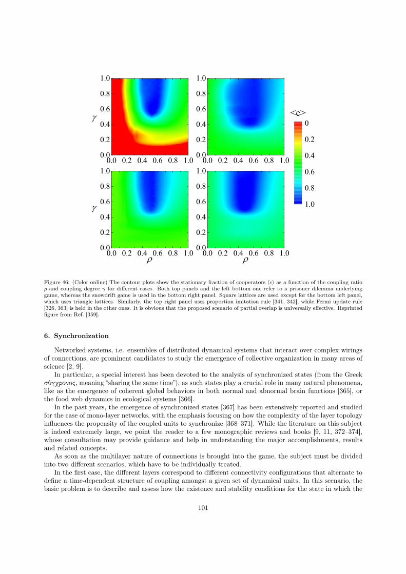
0.0 0.2 0.4 0.6 0.8 1.00.0

0.2

0.4

0.6

0.8

1.0

<c>

0.0 0.2 0.4 0.6 0.8 1.00.0

0.2

0.4

0.6

0.8

1.0

0.0 0.2 0.4 0.6 0.8 1.00.0

0.2

0.4

0.6

0.8

1.0

0.0 0.2 0.4 0.6 0.8 1.00.0

0.2

0.4

0.6

0.8

1.0

0

0.2

0.4

0.6

0.8

1.0

Figure 46: (Color online) The contour plots show the stationary fraction of cooperators 〈c〉 as a function of the coupling ratioρ and coupling degree γ for different cases. Both top panels and the left bottom one refer to a prisoner dilemma underlyinggame, whereas the snowdrift game is used in the bottom right panel. Square lattices are used except for the bottom left panel,which uses triangle lattices. Similarly, the top right panel uses proportion imitation rule [341, 342], while Fermi update rule[326, 363] is held in the other ones. It is obvious that the proposed scenario of partial overlap is universally effective. Reprintedfigure from Ref. [359].

6. Synchronization

Networked systems, i.e. ensembles of distributed dynamical systems that interact over complex wiringsof connections, are prominent candidates to study the emergence of collective organization in many areas ofscience [2, 9].

In particular, a special interest has been devoted to the analysis of synchronized states (from the Greekσύγχρονος, meaning “sharing the same time”), as such states play a crucial role in many natural phenomena,like as the emergence of coherent global behaviors in both normal and abnormal brain functions [365], orthe food web dynamics in ecological systems [366].

In the past years, the emergence of synchronized states [367] has been extensively reported and studiedfor the case of mono-layer networks, with the emphasis focusing on how the complexity of the layer topologyinfluences the propensity of the coupled units to synchronize [368–371]. While the literature on this subjectis indeed extremely large, we point the reader to a few monographic reviews and books [9, 11, 372–374],whose consultation may provide guidance and help in understanding the major accomplishments, resultsand related concepts.

As soon as the multilayer nature of connections is brought into the game, the subject must be dividedinto two different scenarios, which have to be individually treated.

In the first case, the different layers correspond to different connectivity configurations that alternate todefine a time-dependent structure of coupling amongst a given set of dynamical units. In this scenario, thebasic problem is to describe and assess how the existence and stability conditions for the state in which the

101

network’s dynamical units are synchronous are modified with respect to the classic (monolayer) situation,in which the coupling between the networked units is time-independent.

The second case, instead, is the scenario where the different layers are simultaneously responsible for thecoupling of the network’s units, with explicit additional layer-layer interactions to be taken into account. Itis worth stressing that here an inter layer synchronized state is a different and much more general concept,as it does not necessarily require intralayer synchronization. In other words, the dynamical units withineach layer can be out of synchrony, but synchronized with the corresponding units in all other layers.

As a consequence, this section is divided into two main parts, each reporting on one of the two describedscenarios, and is intended to summarize for each case the extension of the main analytical treatments andapproaches that are traditionally used to deal with synchronization of monolayer networked systems.

6.1. Synchronization in multilayer networks with alternating layersWe start with the case in which the network under consideration is composed of a number N of identical

dynamical systems, which interact via a time-dependent structure of connections, each of which correspond-ing, at a given time, to one of the different layers.

Very recent investigations on synchronization of time-varying networks include the treatment of completesynchronization in temporal Boolean networks [375], the analysis of stability of synchronized states inswitching networks in the presence of time delays [376], and the investigation of the effects of temporalnetworking interactions when compared with the corresponding aggregate dynamics where all interactionsare present permanently [377].

We focus here on the situation of an ensemble of identical units where the wiring of connections isswitching between the different layers following a periodic or aperiodic sequence. It is important to remarkthat detailed studies of the latter case actually started much before the relatively recent introduction of theconcept of multilayer networks. In particular, a widely studied case is the limit of the so-called blinkingnetworks [378, 379], where the switching between different configurations happens rapidly, i.e. with acharacteristic time scale much shorter than that of the networked system’s dynamics. Under these conditions,it was found that synchronous motion can be established for sufficiently rapid switching times even in thecase where each visited wiring configuration (each network layer) would prevent synchronization under staticconditions.

Yet, the limit of blinking networks is not a suitable framework for an adequate description of severalnatural phenomena. For instance, modeling processes such as mutations in biological systems [380], oradaptations in social systems or financial market dynamics [381] would demand the very opposite limitof time-varying networks whose structure evolution takes place over characteristic time scales that arecommensurate with, or even secular with respect to, those of the nodes’ dynamics.

Thus, in the following, we will concentrate on the case in which synchronized states appear in dynamicalnetworks, without making any explicit a priori assumption on the time scale of the variation of the couplingwiring.

6.1.1. The Master Stability Function for time dependent networksThe starting point is the generic equation describing the evolution of an ensemble of N identical systems,

networking via a time dependent structure of connections:

xi = f(xi)− σN∑j=1

Gij(t)h[xj ], i = 1, . . . , N . (232)

Here, dots denote temporal derivative, xi ∈ Rm is the m-dimensional vector describing the state of theith network unit, and f(x) : Rm → Rm and h[x] : Rm → Rm are two vectorial functions describing the localdynamics of the nodes and the output from a node to another, respectively.

Furthermore, Gij(t) ∈ R are the time varying elements of an N × N symmetric matrix specifying theevolution, in strength and topology, of the network connections. The matrix G(t) satisfies the definingproperties of a Lagrangian matrix: it has zero row-sums (

∑j Gij(t) = 0 ∀i and ∀t), strictly positive diagonal

terms (Gii(t) > 0 ∀i and ∀t) and strictly non-positive off-diagonal terms (Gij(t) ≤ 0 ∀i 6= j and ∀t).

102

Our goal is to assess the stability of the synchronized solution x1(t) = x2(t) = . . . = xN (t) ≡ xs(t),whose existence is indeed warranted by the zero row-sum property of G(t).

To this purpose, we first notice that G(t) is symmetric, and therefore it is always diagonalizable and, atall times, admits a set λi(t) of real eigenvalues and a set vi(t) of associated orthonormal eigenvectors, suchthat G(t)vi(t) = λi(t)vi(t) and vT

j · vi = δij .The zero row-sum condition and the Gershgorin’s circle theorem [382] further ensure that:

1. the spectrum of eigenvalues is such that λi(t) ≥ 0 ∀i and ∀t;2. the smallest eigenvalue λ1(t) ≡ 0, with associated eigenvector v1(t) = 1√

N1, 1, . . . , 1T, entirely

defines the synchronization manifold (xi(t) = xs(t) ∀i);3. all the other eigenvalues λi(t) (i = 2, . . . , N) have associated eigenvectors vi(t) that form a basis of

the space transverse to the manifold of xs(t) in the m×N -dimensional phase space of Eq. (232).

Notice that all the eigenvalues except the first are strictly positive for connected graphs (λi(t) > 0 fori = 2, . . . , N).

Consider then δxi(t) = xi(t) − xs(t) = (δxi,1(t), . . . , δxi,m(t)), i.e. the deviation of the ith vector statefrom the synchronized state, and construct the N × m column vectors X = (xT

1 ,xT2 , . . . ,x

TN ) and δX =

(δxT1 , . . . , δx

TN ). It is straightforward to show that the linearization of Eq. (232) around the synchronized

solution leads, in linear order of δX, to

δX = [IN ⊗ Jf(xs)− σG(t)⊗ Jh(xs)] δX , (233)

where ⊗ denotes the direct product, and J is the Jacobian operator.The arbitrary state δX, at each time, can be written as a sum of direct products of the eigenvectors of

G(t) and a time-dependent set of row-vectors ηi (t), i.e.

δX =

N∑i=1

vi(t)⊗ ηi(t) ,

with ηi(t) = (ηi,1, . . . , ηi,m). Therefore, applying vTj to the left side of each term in Eq. (233), one finally

obtains

d

dtηj = Kjηj −

N∑i=1

vTj (t) · d

dtvi(t)ηi , (234)

where j = 1, . . . , N and Kj = [Jf(xs)− σλj(t)Jh(xs)].The key point here is noticing that the boxed term in Eqs. (234) is what differentiates them from the

classical equations used to calculate the Master Stability Function (MSF) [370], as it explicitly accountsfor the time variation of the eigenvector basis. In the following, we will first discuss the case where suchan extra term vanishes, and later the general case of constructing a quasi-static evolution among differentnetwork layers, deriving a proper analytical expression for it.

6.1.2. Commutative layersEqs. (234) transform into a set of N variational equations of the form

d

dtηj = Kjηj (235)

if∑Ni=1 vT

j (t) · ddtvi(t)ηi = 0, i.e. if all eigenvectors are constant in time.

This condition can be satisfied in two different ways, namely either the coupling matrix G(t) is constant,as in the case of a monolayer network originally considered in Ref. [370], or the temporal evolution occursthrough commutative layers. The latter case means that starting from an initial wiring G0 ≡ G(t = 0),the coupling matrix G(t) must commute with G0 at all times t (G0G(t) = G(t)G0 ∀t). This was explicitlydiscussed in Ref. [383], where it was shown that:

103

1. an evolution along commutative graphs (i.e., different commutative layers of a multilayer network) canbe constructed by starting from any initial wiring G0, and

2. such an evolution provides a much better condition for the stability of the synchronous state than thatgiven by a monolayer network.

To show this, the first step is constructing explicitly the set of commutative layers through which theevolution takes place. To this purpose, one can notice that any initial symmetric coupling matrix canbe written as G0 = V Λ0V

T, where V = v1, . . . ,vN is an orthogonal matrix whose columns are theeigenvectors of G0, and Λ0 = diag(0, λ2(0), . . . , λN (0)) is the diagonal matrix formed by the eigenvalues ofG0.

At any other time t, a zero row-sum symmetric commuting matrix G(t), defining the layer visited by thestructure evolution at that time, can be constructed as

G(t) = V Λ(t)V T , (236)

where Λ(t) = diag(0, λ2(t), . . . , λN (t)) with λi(t) > 0 ∀i > 1. It is easy to show that G(t) is positivesemidefinite, and since the canonical basis vectors are not collinear with the eigenvector v1 we have Gii >0 ∀i. Thus, Eq. (236) provides a way to generate all possible layers that commute with G(0), are positivesemidefinite with zero row-sum, and dissipatively couple each network unit. Henceforth, we refer to this setof matrices as the dissipative commuting set (DCS) of G(0). It is important to notice that while not allmembers of the DCS are true Lagrangian matrices (it is in fact possible for their off-diagonal componentsto be positive), nevertheless all commuting Lagrangian matrices are contained in the DCS.

In Ref. [383], the Authors proposed a general method to select a set of commutative matrices within theDCS. The method is based on starting from a given layer graph G0, and producing a large set of differentrealizations of the same graph. This allows the estimation of the initial distribution p(λ0) of the non-vanishingeigenvalues of the set. Then, one can directly construct Λ(t) to use in Eq. (236) by randomly drawing a setof eigenvalues either according to p(λ0), or uniformly between λ2(0) and λN (0). The former approach can beimplemented either by using the spectrum of a different realization of G0 (the so-called eigenvalue surrogatemethod [383]), or by extracting directly the eigenvalues from the distribution p(λ0). The latter method,instead, simply corresponds to the random selection of the eigenvalues from a uniform distribution. In eithercase, the random extractions can be performed in an ordered (0 ≤ λ2(t) ≤ . . . ≤ λN (t)) or unordered way,and one only needs to extract N − 1 eigenvalues, since λ1(t) must be always 0.

In addition, Ref. [383] also discusses how the different choices for the construction of commutative layerslead to modifications of the main topological structures. In general, the resulting matrix G(t) is a densematrix that can be associated to a undirected weighted network, whose weight matrix W (t) has elementsWii(t) = 0, and Wij(t) = |Gij(t)| for i 6= j. The main properties that were studied in Ref. [383] are theaverage value of the strength distribution, the average local clustering coefficient, and the average shortestpath length, defined as follows [2, 9, 91, 384].

For weighted networks, the distance between two adjacent nodes i and j is lij = 1Wij

, and the distance

along a path n(1), n(2), . . . , n(m) can be expressed as Ln(1)→n(m) =∑m−1k=1 ln(k)n(k+1). Then, the distance

between two non-adjacent nodes i and j is the length of one of the shortest paths connecting them:

`ij = minallpaths i→j

Li→j .

With these definitions, a network’s average shortest path length is [2, 9, 91, 384]

〈`〉 =2

N(N − 1)

∑i,ji 6=j

`ij .

Similarly, the clustering coefficient of node i can be defined as

ci =2

si(N − 2)

∑j,m

WijWimWjm ,

104

〈s〉 〈C〉 〈`〉Initial condition G0 (scale-free) 9.94 5.5773× 10−4 5.5144Eigenvalue surrogate method 11.6881 8.4730× 10−4 5.2758Choosing from p(λ0) (ordered) 12.7042 9.1235× 10−4 5.2325

Choosing from p(λ0) (unordered) 142.8746 0.0543 3.7144Uniform distribution (ordered) 123.6484 0.0634 0.9570

Uniform distribution (unordered) 521.7568 0.6125 1.1098

Table 5: Statistical properties of the commuting layers. The table reports the average strength 〈s〉, the average local clusteringcoefficient 〈C〉 and the average shortest path length 〈`〉 for the different methods of selecting the set of commuting layers. Inall cases the results are ensemble averages over 100 different realizations of networks of size N = 500. Table reproduced figurewith permission from Ref. [383]. c© 2006 by the American Physical Society.

where si =∑jWij is the strength of node i. The average local clustering coefficient 〈C〉 is then given by

〈C〉 = 1N

∑i ci, while the strength distribution P (s) characterizes the heterogeneity of the network [91, 384].

Table 5 summarizes the behavior of these quantities for the different eigenvalue selection strategiesdescribed above. The initial layer G0 is the Laplacian matrix of a scale-free (SF) network grown using thepreferential attachment algorithm [385], and whose strength distribution follows a power-law P (s) ∼ s−γ .Figure 47 illustrates the strength distributions of the network layers constructed with different methods.It is evident that the eigenvalue surrogate method, as well as the ordered selection of eigenvalues from theinitial distribution p(λ0), do not change the SF character of the strength distribution (thick red and dashedblue lines in panel a). At the same time, they yield values for 〈s〉 =

∑s sP (s), 〈C〉 and 〈`〉 that deviate

only slightly from those of the original graph (see Table 5). This indicates that both methods are convenientstrategies to construct a commuting set of layers through which the evolution of the graph substantiallypreserves all the main topological features of the initial condition. Conversely, choosing the eigenvalues froma uniform distribution, either in an ordered or in a unordered way, produces layers that completely destroythe original SF strength distribution (thick red solid line and dashed blue line in panel b). These correspondto structural configurations for which each measured quantity wildly differs from its value in G0. Finally,the intermediate solution of choosing the eigenvalue spectrum from the initial p(λ0) in a unordered way,while still preserving the power-law tail of the strength distribution (solid black line in panel b), still changessubstantially the topological structure of the underlying network.

6.1.3. Enhancing synchronization via evolution through commutative layersBesides the analysis of changes in the structural properties of the layers belonging to the DCS and gener-

ated via different methods, one also needs to study the consequences of the evolution through commutativelayers on the stability of the synchronization solution.

Because of the commutativity of the layers, Eq. (234) takes the form given by Eq. (235).Replacing σλj(t) by ν in the kernel Kj , the problem of stability of the synchronization manifold becomes

equivalent to studying the m-dimensional parametric variational equation

η = Kνη ,

where Kν = [Jf(xs)− νJh(xs)]. This allows to plot the curve Λmaxvs. ν, where Λmax is the largest of them associated conditional Lyapunov exponents. This curve is classically called the Master Stability Function[370].

For G(t) = constant, the synchronized state is transversely stable if all λi (i = 2, . . . , N), multiplied bythe same coupling strength σ, fall in the range where Λmax(ν) < 0. When G(t) evolves inside the DCS, theeigenvectors are fixed in time, and one can make the hypothesis that at time T = kdt, the modulus of each

105

Figure 47: (Color online). Strength distributions P (s) of the commuting layers. (a) Initial condition G0 (solid black line), G(t)constructed by the eigenvalue surrogate method (thick solid red line), and Λ(t) obtained by randomly choosing the eigenvaluesfrom p(λ0) in an ordered way (dashed blue line). (b) Eigenvalues randomly chosen from p(λ0) in a unordered way (solid blackline), eigenvalues chosen from a uniform distribution in an ordered way (thick solid red line), and in a unordered way (dashedblue line). The details of the statistical ensembles are the same as for Table 5. Reprinted figure with permission from Ref. [383].c© 2006 by the American Physical Society.

eigenmode ηi (i 6= 1) is bounded by the corresponding maximum conditional Lyapunov exponent

|ηi(T )||ηi(0)|

≤k−1∏n=0

exp (Λmax (σλi (ndt)) dt) .

It immediately follows that the transverse stability condition for the synchronization manifold is nowthat ∀i 6= 1

Si = limT→∞

1

T

∫ T

0

Λmax (σλi (t′)) dt′ < 0 . (237)

It is extremely important to notice that condition (237) does not require Λmax (σλi(t)) to be negative atall times.

In fact, one can construct a commutative evolution such that at each time there exists at least oneeigenvalue λi(t) for which Λmax (σλi(t)) > 0, and yet obtain a transversely stable synchronization manifold.

The very relevant conclusion is that a multilayer network where different layers are visited at differenttimes may produce a stable synchronized motion even when the emergence of a synchronous behavior of theunits would be prevented by using any of the layers as a constant wiring configuration. Similar conclusionswere independently reached in Ref. [386] for fast switching times between commutative layers.

A simple example is a periodic evolution between network layers, with period Tp = (N − 1)τ , duringwhich G(t) is given by

G(t) =

N−1∑l=1

Glχ[(l−1)τ,lτ) , (238)

where χ[(l−1)τ,lτ) denotes the characteristic function of the interval [(l − 1) τ, lτ). Here, the matrices Gldefining the layers are constructed, as before, as Gl = V1ΛlV

T1 . Given Λ1 = diag(0, λ2, . . . , λN ), the set of

106

0 1000 2000t

10-10

10-5

100

⟨δ⟩

0 0.5 1τ

102

103

104

Tsync

Figure 48: Time evolution of synchronization error 〈δ〉 for τ = 0.2 (empty circles), 0.3 (filled circles), 0.4 (empty squares),0.5 (filled squares), 0.6 (empty diamonds), 0.7 (filled diamonds), 0.9 (empty up triangles), 1.1 (filled up triangles), and 1.5(empty down triangles). In all cases, the results are ensemble averages over 5 different random initial conditions for a dynamicalnetwork of N = 200 identical chaotic Rössler oscillators. Inset: Synchronization time Tsync vs. switching time τ (open circlesrefer to different initial conditions, solid line is the ensemble average). Reprinted figure with permission from Ref. [383]. c©2006 by the American Physical Society.

the other N − 2 matrices Λl is constructed by subsequently shifting the sequence of the eigenvalues of G1,i.e. Λ2 = diag(0, λ3, λ4, . . . , λN , λ2), Λ3 = diag(0, λ4, λ5, . . . , λ2, λ3), etc.

If, for instance, Λmax (σλ2) > 0, then all the layers will have a direction in the phase space along which thesynchronization manifold is transversely unstable. However, if

∑N−1j=2 Λmax (σλj) < 0, then condition (237)

will be satisfied in all directions transverse to the synchronization manifold, and therefore the synchronizedsolution will be transversely stable.

As an example of such an extreme situation, Fig. 48 shows the results of an evolution of a network wherethe initial layer is a SF graph of N = 200 Rössler chaotic oscillators, each obeying Eq. (232) with

x ≡ (x, y, z), f(x) = (−y − z, x+ 0.165y, 0.2 + z (x− 10)) , h[x] = y .

The evolution of the wiring follows Eq. (238). For σ = 0.03 one finds that∑N−1j=2 Λmax (σλj) ≈ −9.158,

but Λmax (σλj) is positive for the first 80 eigenvalues, i.e., the synchronization manifold would be unstablein at least 80 different transverse directions in each of the layers, if taken as fixed. However, defining thesynchronization error as

〈δ〉(t) =

N∑j=2

|xi − x1|+ |yi − y1|+ |zi − z1|3(N − 1)

,

and the synchronization transient Tsync as the time needed for 〈δ〉(t) to become smaller than 0.1, we seefrom the data of Fig. 48 that the multilayer network is always able to synchronize, with a Tsync that scalesalmost exponentially with τ .

It is important to remark that, while this numerical example is used here just to illustrate the en-hancement of synchronization in multilayer commuting graphs under extreme conditions, the validity ofcondition (237) is general, and by no means limited to periodic evolutions of the connectivity matrices.

A further point that should be stressed is that the multilayer commuting case is substantially differentfrom the fast switching procedure described in Ref. [378]. Indeed, the stability condition does not impose

107

in principle any limitation on the switching time τ , making it possible to enhance the collective functioningof the network even for wirings evolving over secular (yet finite) time scales.

6.1.4. Non-commutative layersSo far, we considered the case of an evolution through commutative layers, clearly demonstrating the

importance of explicitly accounting for a multilayer nature of interactions in networked dynamical systems,and the fact that such multilayer structure can greatly enhance the stability of the synchronization solution.Yet, it is evident that considering commutative layers is too strong an assumption to adequately representthe general case encountered in real world multilayer graphs.

When explicitly dealing with non commutative layers, the boxed term in Eqs. (234) no longer vanishes.Thus, Eqs. (234) do not reduce anymore to a set of variational equations, and one must examine in detail theeffects of this extra term on the coupling of the different directions of stability for the synchronous solution.To do so, there are some issues that need to be properly dealt with.

The first is that the boxed term in Eqs. (234) is explicitly proportional to the time derivatives of theeigenvectors of the network Laplacian, and therefore any evolution involving instantaneous jumps from alayer to another of a multilayer structure would result in a divergence. As a consequence, one must consider aquasi-static evolution that depends on two different time scales: first, the network structure is kept constantfrom time t = 0 to t = t0, period over which it is described by one given layer of the network; then, fromt = t0 to t = t1, a smooth switching process takes place, bringing the network from one layer to another.

Second, the switching process should be carefully constructed. Indeed, one needs to find a smoothevolution that, starting from a generic layer whose Laplacian is L0, leads to another generic layer whoseLaplacian is L1, through a set of intermediate configurations that all maintain the basic conditions forthe existence of the synchronized solution. In practice, this means that the switching process should occurthrough a path of connecting matrices, each displaying the zero-row sum condition, each being diagonalizable,and each sharing the same eigenvector corresponding to the null eigenvalue.

To achieve this, we first consider the matrices A and B, consisting of the eigenvectors of L0 and L1,respectively, and describe how to transform one into the other by means of a proper rotation, and inparticular a proper rotation around a fixed axis. Then, we use this framework to find a transformationbetween L0 and L1.

Eigenvector matrices. Let A and B be two N × N orthogonal matrices. In our case, we know that thevectors of A and B correspond to the eigenvectors of two network Laplacians. We also know that at leastone vector a is common between A and B. This vector a corresponds to the null eigenvalue of the Laplacian,and thus to the synchronization manifold.

We want to find a one-parameter transformation group Gs such that:

• G0A = A;

• GsA contains the vector a for all 0 6 s 6 1;

• G1A = B.

Existence of a solution. To show that it is always possible to find a solution, first notice that, in general,the transformation O from A to B is a rotation, because the vectors of both matrices form orthonormalbases of the same space. To find O, one can simply solve the linear system of N2 equations in N2 variablesOA = B. As we are free of choosing the set of coordinates, we put ourselves in the basis defined by thematrix A. In this basis, A ≡ 1, where 1 is the identity.

Now, without loss of generality, assume that the conserved vector a is the first vector of A, (1, 0, . . . , 0)T.

108

Then, the transformation matrix O will have the form

O =

1 0 0 · · · 00 O22 O23 · · · O2N

0 O32 O33 · · · O3N

......

.... . .

...0 ON2 ON3 · · · ONN

. (239)

Notice that, O is a unitary matrix, and therefore the absolute value of |O| is equal to 1. In general O is anelement of the orthogonal group O (N), which means that it is a proper rotation, if its determinant is 1, ora composition of rotations and reflections, if its determinant is −1. However, as the form of O in Eq. (239)indicates, its determinant equals the determinant of the minor O′ obtained by removing from O the firstrow and the first column. Then, we only need to find a solution to the problem in N − 1 dimensions. Wewill henceforth use primes when referring to objects in N − 1 dimensions.

From these considerations, we have G′0 = 1′ and G′1 = O′. But O′ itself is trivially an orthogonal matrix,belonging to O (N − 1). Thus, our problem is equivalent to determining the possibility of finding a pathbetween the identity and O′.

At this point, we have two cases.Case 1: |O′| = 1. If the determinant of O′ is positive, then O′ belongs to the special orthogonal

group SO (N − 1). In this case, describing a solution is straightforward. In fact, SO (N − 1) is the identitycomponent of the orthogonal group. Moreover, as the orthogonal group is a Lie group, SO (N − 1) is notonly connected, but also path-connected. This means that for every orthogonal (N − 1)× (N − 1) matrix,there is a continuum of orthogonal matrices of the same dimension connecting it to the identity. Each pointalong this path corresponds to an orthogonal matrix that can be embedded in SO (N) by adding a 1 in thetop left corner. Since every embedded matrix along the continuum will keep the vector corresponding tothe synchronization manifold invariant, a parametrization of the path from the identity to O will provide adirect solution to the original problem.

Case 2: |O′| = −1. If the determinant of O′ is negative, then O′ belongs to O (N − 1) \ SO (N − 1).The same considerations as for Case 1 apply. However, while O (N − 1) \ SO (N − 1) is also a connectedtopological space, the identity does not belong to it. This means that there is no path that can connect theidentity to O′, and we cannot solve the problem the same way.

Yet, in our particular case, we do not really care about the labeling of the vectors. In other words,provided that we keep the vector a constant, we can very well swap two vectors in the basis given by thematrix A. This literally just means creating a new matrix C by swapping two rows in A. Of course, thisimposes a swap of the corresponding columns in the transformation matrix O as well. But we also know thatswapping two rows (or columns) in a matrix changes the sign of its determinant. This means that the newmatrix O′ does not belong to O (N − 1) \SO (N − 1), but rather to SO (N − 1). Thus, it is path-connectedto the identity, and all the procedure of Case 1 can be applied. The only consequence of the swap is that theimplicit order of the eigenvalues will be changed. As this order is irrelevant for our purposes, the problemcan always be solved. To illustrate this, consider the following simple example in R3.

Suppose we want to go from the basis on the left in Fig. 49 (the canonical basis of R3) to the one in themiddle. Then, the transformation matrix is

O =

1 0 00 1 00 0 −1

.

The determinant of O is −1, so there is no continuous way to go from the identity to O. However, supposewe relabel the y and z vectors in our original basis, obtaining the basis in the right panel of Fig. 49. Then,the transformation matrix will be

O =

1 0 00 0 10 −1 0

.

109

y

x

z

y

z

x x

z

y

Figure 49: Example of label swapping. Going from the basis on the left to the one in the middle while keeping x constantnecessarily involves a reflection. However, going from the basis on the right to the one in the middle can be accomplished viaa proper rotation.

This time, its determinant is 1. Thus O ∈ SO (3), or, equivalently, O′ ∈ SO (2). This means we can find apath that connects the identity to O. This path can be readily turned into a family of transformations:

Gs =

1 0 00 cos

(−π2 s

)− sin

(−π2 s

)0 sin

(−π2 s

)cos(−π2 s

) .

Note that for every value of the parameter s between 0 and 1, the determinant of Gs equals 1. Also, forany value of s, the vector x remains always constant. However, the main point here is that while O leavesy unchanged and reflects z across the origin, O instead rotates the “new y” onto the position previouslyoccupied by y, and the “new z” onto the position opposite to that previously occupied by z. In other words,the final arrangement of the original transformation is preserved, but this time the transformation is a properrotation. As we are only interested in getting the final result right, and not in the order of the eigenvectors,we can disregard this difference.

6.1.5. Building a solution for a generic layer switchingGiven a specific A and B, cast in the form discussed above, we build an explicit solution by factoring

the transformation O′ into rotations and reflections in mutually orthogonal subspaces. Before describingthe actual procedure, we recall two useful results. Proving these results involves constructions we will usein the solution and provides further insight into our original problem. Thus, we present the proofs in thefollowing.

Existence of invariant subspaces. First, any orthogonal operator X in a normed space over R induces aninvariant subspace. This subspace is either 1-dimensional or 2-dimensional. To see this, given X, define theoperator U that acts on a+ib as U (a+ ib) = Xa+iXb. As U is a unitary operator, its spectrum lies on theunit circle. Then, one can find a non-vanishing eigenvector x with eigenvalue λ. In general, x = xR + ixI ,and λ = eiϑ = λR + iλI . Then, we have two cases.

Case 1: λ is real. In this case, Ux = XxR + iXxI = ±xR ± ixI . Then, XxR = ±xR and XxI = ±xI .As x 6= ~0, at least one between xR and xI cannot vanish. Without loss of generality, let the non vanishingcomponent be xR. Then, all vectors proportional to xR are mapped by X into vectors proportional to xR.Thus, the 1-dimensional subspace of the vectors proportional to xR is invariant under X.

Case 2: λ is complex. In this case, xR and xI are linearly independent. We prove this by contradiction.First note that x ≡ xR − ixI is an eigenvector of U with eigenvalue λ = e−iϑ = λR − iλI , and thatxR = x− ixI = x+ ixI .

Now assume that it were xR = αxI . Then one could write

αUxI = UxR = U (x− ixI) = λx− iUxI ,

110

hence(α+ i)UxI = (α+ i)XxI = λx = λ (αxI + ixI) = (α+ i)λxI ,

from which it would follow thatXxI = λxI . (240)

Similarly, one could write

αUxI = UxR = U (x+ ixI) = λx+ iUxI ,

hence(α− i)UxI = (α− i)XxI = λx = λ (αxI − ixI) = (α− i) λxI ,

from which it would follow thatXxI = λxI . (241)

Thus, Eqs. (240) and (241) would imply that λ = λ. But this directly contradicts the hypothesis thatλ /∈ R.

Having proved that xR and xI are linearly independent, apply U to x:

Ux = XxR + iXxI = λx = λRxR − λIxI + i (λIxR + λRxI) ,

henceXxR = λRxR − λIxI (242)

andXxI = λIxR + λRxI . (243)

The two equations above imply that

X (αxR + βxI) = αλRxR − αλIxI + βλIxR + βλRxI =

(αλR + βλI)xR + (βλR − αλI)xI = γxR + δxI ,

where γ = αλR + βλI and δ = βλR − αλI . This means that any linear combination of xR and xI ismapped by X into a linear combination of the same vectors xR and xI . As we have proved above that theyare linearly independent, this implies that the 2-dimensional subspace determined by the basis xR, xI isinvariant under application of X.

Orthogonality of the eigenvector components. We show now that the components xR and xI of the eigen-vector x used in Case 2 of the previous proof are not only linearly independent, but actually orthogonal. Tosee this, compute the inner product between xR and xI , exploiting the fact that the operator X preservesthe inner product, since it is orthogonal:

〈xR, xI〉 = 〈XxR, XxI〉 = 〈λRxR − λIxI , λIxR + λRxI〉 , (244)

where we have used Eqs. (242) and (243).Then it is

〈xR, xI〉 = λRλI ‖xR‖2 + λ2R 〈xR, xI〉 − λ2

I 〈xI , xR〉 − λRλI ‖xI‖2

=

λRλI

(‖xR‖2 − ‖xI‖2

)+(λ2R − λ2

I

)〈xR, xI〉 ,

hence

〈xR, xI〉 =λRλI

1− λ2R + λ2

I

(‖xR‖2 − ‖xI‖2

)=λRλI2λ2

I

(‖xR‖2 − ‖xI‖2

)=

λR2λI

(‖xR‖2 − ‖xI‖2

),

(245)

111

where we have used λ2R + λ2

I = 1.Similarly, applying the same property of X, and using Eq. (242), the squared norm of xR is

‖xR‖2 = 〈xR, xR〉= 〈λRxR − λIxI , λRxR − λIxI〉

= λ2R ‖xR‖

2 − λRλI 〈xR, xI〉 − λRλI 〈xI , xR〉+ λ2I ‖xI‖

2

= λ2R ‖xR‖

2 − 2λRλI 〈xR, xI〉+ λ2I ‖xI‖

2

= λ2R ‖xR‖

2+(1− λ2

R

)‖xI‖2 − 2λRλI 〈xR, xI〉

= λ2R

(‖xR‖2 − ‖xI‖2

)+ ‖xI‖2 − 2λRλI 〈xR, xI〉 .

Then, it is‖xR‖2 − ‖xI‖2 = λ2

R

(‖xR‖2 − ‖xI‖2

)− 2λRλI 〈xR, xI〉 ,

and, using again λ2R + λ2

I = 1,

‖xR‖2 − ‖xI‖2 = −2λRλI〈xR, xI〉 . (246)

Substituting Eq. (246) into Eq. (245) yields

〈xR, xI〉 = −λ2R

λ2I

〈xR, xI〉 .

Now, we know by hypothesis that λI 6= 0. Then, if λR 6= 0 it must be 〈xR, xI〉 = 0. Alternatively, ifλR = 0, then it is λI = ±1. In this case, from Eq. (244), it follows that

〈xR, xI〉 = 〈∓xI ,±xR〉 = −〈xI , xR〉 ⇒ 〈xR, xI〉 = 0 .

Either way, xR and xI are orthogonal.

The solution. Using the two results just shown, we can describe an algorithmic procedure to find the solutionto our problem. The initial situation is that we have two orthonormal bases A and B of RN . Then, we canbuild a transformation of A into B with the following steps:

1. Express the problem in the basis A. In this basis, the transformation matrix O between A = 1 and Btakes the form given by Eq. (239).

2. Consider the operator O′ obtained from O by removing the first row and the first column. Let d beits dimension.

3. Build the operator U that acts on a+ ib as U (a+ ib) = O′a+ iO′b, where a and b belong to Rd.4. Find an eigenvector x = xR + ixI of U , with eigenvalue λ.5. Normalize xR and xI .6. If λ ∈ R

(a) Pick the non-vanishing component between xR and xI . If both are non-zero, choose one of themrandomly. Without loss of generality, assume this is xR.

(b) Create d − 1 other orthonormal vectors, all orthogonal to xR, and arrange all these vectors sothat xR is the last of them. This set of vectors is an orthonormal basis C of Rd.

(c) Change the basis of the d-dimensional sub-problem to C. In this basis, all the elements in thelast row and in the last column of O′ will be 0, except the last one, which will be ±1.

(d) If d > 1, consider a new operator O′ obtained from the old O′ by removing the last row and thelast column. Let d be its dimension, and restart from step 3. Otherwise stop.

7. If λ /∈ R(a) Create d−2 other orthonormal vectors, all orthogonal to xR and xI , and arrange all these vectors

so that xR and xI are the first two of them. This set of vectors is an orthonormal basis C of Rd.

112

(b) Change the basis of the d-dimensional sub-problem to C. In this basis, all the elements in thefirst two rows and in the first two columns of O′ will be 0, except the first two.

(c) If d > 2, consider a new operator O′ obtained from the old O′ by removing the first two rows andthe first two columns. Let d be its dimension, and restart from step 3. Otherwise stop.

The steps described above effectively solve the problem of finding the basis transformation by divide-and-conquer. At each repetition, 1 or 2 dimensions are eliminated from the problem. All the subsequentchanges of bases do not affect the elements of the transformation matrix determined in the previous steps,because they act on subspaces that are orthogonal to those that have been already eliminated, which includethe top left element in A and B, corresponding to the synchronization manifold. Thus, one can reconstructthe transformation matrix O piece by piece. At the end of the procedure, O has a block-diagonal form

O =

1 0 0 0 0 · · · 0 00 O22 O23 0 0 · · · 0 00 O32 O33 0 0 · · · 0 00 0 0 O44 O45 · · · 0 00 0 0 O54 O55 · · · 0 0...

......

......

. . ....

...0 0 0 0 0 · · · ON−1N−1 ON−1N

0 0 0 0 0 · · · ONN−1 ONN

,

where the blocks correspond to the action of the orthogonal operator on the invariant subspaces. If theinvariant subspace is 1-dimensional, then its block is a single ±1 element. Conversely, if the subspace is2-dimensional, then its block is either a rotation or a reflection. This means that it is either(

cosα − sinαsinα cosα

)or (

±1 00 ∓1

).

At this point, one can proceed as follows. First, permute the basis vectors from the second onwards sothat they correspond, in order, first to all the actual rotation blocks, then to the −1 elements, and finally tothe +1 elements. It’s easy to see that this can always be done. In fact, if we call our change-of-basis matrixT , we can determine the new form of the transformation matrix, ON , via the following logical chain:

OKA = KB ⇒ ONTKA = TKB ⇒ T−1ONTKA = KB ⇒ T−1ONT = O ⇒ ON = TOT−1 ,

where K is the change-of-basis matrix corresponding to the composition of all changes of bases done insteps 6 or 7 above.

As the matrix T that swaps the position of the basis vectors is a permutation matrix, it follows that ONhas exactly the required form

O =

1 0 0 ··· 0 0 0 0 0 ··· 0 00 cosϑ1 − sinϑ1 ··· 0 0 0 0 0 ··· 0 00 sinϑ1 cosϑ1 ··· 0 0 0 0 0 ··· 0 0...

.

.

....

. . . 0 0 0 0 0 ··· 0 00 0 0 0 cosϑk − sinϑk 0 0 0 ··· 0 00 0 0 0 sinϑk cosϑk 0 0 0 ··· 0 00 0 0 0 0 0 −1 0 0 ··· 0 00 0 0 0 0 0 0 −1 0 ··· 0 0...

.

.

....

.

.

....

.

.

....

.

.

..... . .

.

.

....

0 0 0 0 0 0 0 0 0 ··· 1 00 0 0 0 0 0 0 0 0 ··· 0 1

. (247)

Having obtained the form in Eq. (247), there is still the possibility that the determinant of O is −1.However, as we saw, in this case we can approach the problem by relabeling two vectors of the original basis,

113

which induces a swap of the corresponding columns of O. To perform this, first note that, if |O| = −1, thenthe number of −1 elements in O must be odd. Then, there are three possible cases.

Case 1: O′ has at least one +1 element. In this case, permute once more the basis vectors, swappingthose corresponding to the first −1 and the first +1 elements in O′. Then, the first block after the “sin–cos”

blocks is(

1 00 −1

). Now, relabel the two corresponding vectors, as in the R3 example, swapping the relevant

rows in the starting matrix. This makes the block in O′ become(0 1−1 0

)=

(cos(−π2)− sin

(−π2)

sin(−π2)

cos(−π2) ) .

Case 2: O′ has no +1 elements and only one −1 element. In this case, the basis vectors to swapare those corresponding to the first two vectors in the last 3× 3 block of O′. This will become

M =

− sinϑk cosϑk 0cosϑk sinϑk 0

0 0 −1

.

Now, change once more the basis of the problem. In particular, leave all the basis vectors unchanged,but map the last three into the eigenvectors of M . This is easily accomplished, as the matrix of eigenvectorsof M is

V =

0 (− secϑk − tanϑk) sin(π4 −

ϑk2

)(secϑk − tanϑk) sin

(ϑk2 + π

4

)0 1 11 0 0

.

Then, the new form of M is

M ′ = V TMV =

−1 0 00 −1 00 0 1

.

Case 3: O′ has no +1 elements and at least three −1 elements. Similar to the previous case,swap the basis vectors corresponding to the first two after the “sin–cos” blocks. Their 3× 3 block is now

M =

0 −1 0−1 0 00 0 −1

.

Next, do a change of basis as described in Case 2. The eigenvector matrix of M is

V =

0 1√2− 1√

2

0 1√2

1√2

1 0 0

,

so after the basis change the new form of M is once more

M ′ = V TMV =

−1 0 00 −1 00 0 1

.

Whether the determinant of O was +1 to start with, or it was −1 and taken care of as one of the casesabove, there are now either no −1 elements in O, or an even number of them. Then, if there are any, takeevery two subsequent −1 elements and change their diagonal blocks into(

cosπ − sinπsinπ cosπ

).

114

This yields the final general form for the transformation matrix:

O =

1 0 0 ··· 0 0 0 0 0 0 0 ··· 0 00 cosϑ1 − sinϑ1 ··· 0 0 0 0 0 0 0 ··· 0 00 sinϑ1 cosϑ1 ··· 0 0 0 0 0 0 0 ··· 0 0...

.

.

....

. . . 0 0 0 0 0 0 0 ··· 0 00 0 0 0 cosϑk − sinϑk 0 0 0 0 0 ··· 0 00 0 0 0 sinϑk cosϑk 0 0 0 0 0 ··· 0 0

0 0 0 0 0 0 cos(−π2 ) − sin(−π2 ) 0 0 0 ··· 0 0

0 0 0 0 0 0 sin(−π2 ) cos(−π2 ) 0 0 0 ··· 0 0

0 0 0 0 0 0 0 0 cosπ − sinπ 0 ··· 0 00 0 0 0 0 0 0 0 sinπ cosπ 0 ··· 0 0...

.

.

....

.

.

....

.

.

....

.

.

....

.

.

..... . .

.

.

....

0 0 0 0 0 0 0 0 0 0 0 ··· 1 00 0 0 0 0 0 0 0 0 0 0 ··· 0 1

. (248)

Finally, introducing a parameter s ∈ [0, 1], we get the required transformation:

Gs =

1 0 0 ··· 0 0 0 0 0 0 0 ··· 0 00 cos(ϑ1s) − sin(ϑ1s) ··· 0 0 0 0 0 0 0 ··· 0 00 sin(ϑ1s) cos(ϑ1s) ··· 0 0 0 0 0 0 0 ··· 0 0...

.

.

....

. . . 0 0 0 0 0 0 0 ··· 0 00 0 0 0 cos(ϑks) − sin(ϑks) 0 0 0 0 0 ··· 0 00 0 0 0 sin(ϑks) cos(ϑks) 0 0 0 0 0 ··· 0 0

0 0 0 0 0 0 cos(−π2 s) − sin(−π2 s) 0 0 0 ··· 0 0

0 0 0 0 0 0 sin(−π2 s) cos(−π2 s) 0 0 0 ··· 0 0

0 0 0 0 0 0 0 0 cos(πs) − sin(πs) 0 ··· 0 00 0 0 0 0 0 0 0 sin(πs) cos(πs) 0 ··· 0 0...

.

.

....

.

.

....

.

.

....

.

.

....

.

.

..... . .

.

.

....

0 0 0 0 0 0 0 0 0 0 0 ··· 1 00 0 0 0 0 0 0 0 0 0 0 ··· 0 1

. (249)

Notice that when s = 0, Gs = G0 = 1, and when s = 1, Gs = G1 = O. Also, for every value of s, thedeterminant of Gs is always 1, and the first vector is kept constant, which means that Gs always describes aproper rotation around the axis defined by the eigenvector corresponding to the synchronization manifold.Moreover, note that the first vector has always been left untouched by all the possible basis transformations.Thus, as s is varied continuously between 0 and 1, the application of Gs sends A into B smoothly andcontinuously, as we need.

Laplacian transformation. To describe how to obtain a transformation between the two Laplacians L0 andL1, let us first summarize what we have shown.

We started from the matrices A and B, consisting of the eigenvectors of L0 and L1. These two matricesare orthonormal bases of RN . We showed that we can always find a series of basis changes casting theproblem in a reference frame where we can explicitly construct a 1-parameter transformation group Gsthat transforms A into B with continuity via a rotation around an axis determined by the eigenvectorcorresponding to the synchronization manifold.

In formulae, the group Gs is such that G0 = 1 and G1RA = RB, where R is the change-of-basis matrixresulting from the composition of all basis changes done in steps 6 and 7 of the method, the permutation ofthe vectors to obtain O, and the eventual final adjustment in case of negative determinant. To simplify theformalism, in the following we let B0 ≡ A and B1 ≡ B.

Then, since B0 and B1 are matrices of eigenvectors, it is

BT0 L0B0 = D0

BT1 L1B1 = D1 ,

where D0 and D1 are diagonal matrices whose elements are the eigenvalues of L0 and L1.However, as Gs is a group of orthogonal transformation, we can write that

GsRB0 = RBs ∀0 6 s 6 1 ,

where Bs is a basis of RN . Multiplying the equation above by RT on the left, we get

RTGsRB0 = RTRBs = Bs , (250)

115

where we have used the fact that RT = R−1.Now, note that all the basis changes done to build G are between orthonormal bases. Therefore, their

composition R is an isometry, as is any Gs, since they are all proper rigid rotations. Thus, any Bs stilldefines an orthonormal basis of RN .

Then, we can say that the Laplacian for the parameter s is given by the matrix Ls that solves theequation

BTs LsBs = Ds , (251)

where Ds is a diagonal matrix whose elements are the eigenvalues of Ls, and Bs consists of the eigenvectorsof Ls. However, the equation above has two unknowns, namely Ls and Ds.

To solve this last problem we impose a linear evolution of the eigenvalues of the Laplacians. Thus, forall 1 6 i 6 N ,

λ(s)i = (1− s)λ(0)

i + sλ(1)i , (252)

where λ(0)i and λ(1)

i are the ith eigenvalues of L0 and L1, respectively. Then, multiplying Eq. (251) on theright by BT

s , it isBTs LsBsB

Ts = DsB

Ts ,

henceBTs Ls = DsB

Ts .

Multiplying this on the left by Bs, we get

BsBTs Ls = BsDsB

Ts ,

henceLs = BsDsB

Ts .

Substituting Eq. (250) into the equation above, we get

Ls = RTGsRB0Ds

(RTGsRB0

)T= RTGsRB0DsB

T0 R

TGTs R . (253)

In Eq. (253), B0 is known; R and Gs have been explicitly built, so they are known as well; Ds iscompletely determined by Eq. (252). Thus, Eq. (253) defines the Laplacian for any given value of theparameter 0 6 s 6 1. The evolution of the eigenvalues follows a simple linear form, imposed by Eq. (252),and the evolution of the eigenvectors is given by Eq. (250).

As a consistency check, it is straightforward to treat the left-hand side of Eq. (253) as an unknown andsolve it for either s = 0 or s = 1, recovering L0 and L1, respectively. Similarly, it is easy to see that for anys the determinant of Ls is the product of the eigenvalues defined by Eq. (252).

With this result, we can finally describe the evolution via non-commutative layers. We use the settingintroduced in Sec. 6.1.4: at time t = 0, the network starts in a layer whose Laplacian is L0, in which itremains up to time t0; then, it switches to a layer whose Laplacian is L1, completing the switch at time t1.What is needed is to compute the boxed term in Eqs. (234) for all times t.

It is clear that, from t = 0 to t = t0, the term vanishes. To compute its value during the switch, firstnote that the ith eigenvector at time t is the ith column of Bs, where s ≡ t−t0

t1−t0 . But then, using Eq. (250),it is straightforward to see that the kth element of the ith eigenvector is

(vi)k = (Bs)ki =(RTGsRB0

)ki

=

N∑r=1

N∑q=1

N∑x=1

Rrk (Gs)rq Rqx (B0)xi .

Notice that in the equation above the only term that depends on time is (Gs)rq, since R is just achange-of-basis matrix, and B0 is the matrix of eigenvectors of L0 at time t = 0. Therefore, it is

d

dt(vi)k =

N∑r=1

N∑q=1

N∑x=1

RrkRqx (B0)xi1

t1 − t0d

ds(Gs)rq .

116

This allows us to write a final expression for the extra term that accounts for the time variation of theeigenvectors. In a fully explicit form, this is

−N∑i=1

vTj (t) · d

dtvi (t) ηi =

− 1

t1 − t0

N∑i=1

N∑k=1

[N∑r=1

N∑q=1

N∑x=1

Rrk (Gs)rq Rqx (B0)xj

][N∑r=1

N∑q=1

N∑x=1

RrkRqx (B0)xid

ds(Gs)rq

]ηi . (254)

However, for all practical purposes, one does not need to use Eq. (254) directly. In fact, considering thatmost elements of Gs are 0, it is quite simple to compute and store Bs in a symbolic form. Similarly, mostof the terms d

ds (Gs)rq are 0. In fact, they vanish in all the following cases:

• r = 1 or q = 1 (the eigenvector corresponding to the synchronization manifold, and axis of rotation ofthe basis of eigenvectors);

• if the (rq) element is outside the tridiagonal, i.e. if |r − q| > 1;

• if r > 2b+ 1 or q > 2b+ 1, where b is the number of “sin–cos” blocks in Gq.

Also, for all other cases dds (Gs)rq, is proportional to a sine or a cosine. Thus, we can define Gs to be the

matrix whose (rq) element is 1t1−t0

dds (Gs)rq; also, we can define Bs ≡ RTGsRB0. Again, Bs can be easily

computed and stored in a symbolic form. Then, Eq. (254) becomes

−N∑i=1

vTj (t) · d

dtvi (t) ηi = −

N∑i=1

N∑k=1

(Bs)kj

(Bs

)kiηi . (255)

Once more, Eq. (255) can be computed symbolically, and evaluated at any particular time t, when needed.

6.2. Synchronization in multilayer networks with coexisting layersA completely different scenario is that of networking dynamical units with coexisting layers. In this case,

indeed, the different layers determine as a whole the overall coupling structure through which the systemcomponents interact, and which in general cannot be simply represented in terms of a single time-independentcoupling matrix.

The current state of the art on the matter includes only a few direct studies, pointing however to someimportant considerations and results. In the following, we first summarize the available literature followingthe categorization given in Section 2, in the hope to point out promising directions to those researchers who,in the near future, will try to approach such a challenging issue. After that, we concentrate on a specificcase, involving a two-layer network in a master-slave configuration, in view of the relevance of this situationthat extends the very concept of synchronization and provides practical tools to target the dynamics ofcomplex networks toward any desired collective behavior (not necessarily synchronous).

6.2.1. HypernetworksIn this framework, one considers a set of N identical dynamical systems linked through the connections

of M different layers, that is, all the connections that correspond to the same type of coupling form a layer,and the systems are connected by more than one layer.

Refs. [387, 388] focused on the necessary and sufficient conditions for the stability of the synchronoussolution in a hypernetwork. The main conclusion is that, in general, it is not possible to reduce the problemto a simpler monolayer formalism. However, for M = 2, such a reduction is indeed possible in three casesof interest: i) if the two associated Laplacians commute; ii) if one of the two layers is unweighted and fullyconnected; iii) if one of the two networks has an adjacency matrix of the form Aij = aj with i, j = 1, . . . , N .The major result is the definition of a class of networks such that if one of the two coupling layers satisfies

117

condition iii), the reduction can be obtained independently of the structural form of the other network layer.The Authors of Refs. [387, 388] also discuss some generalization of their results to the case of hypernetworksconsisting of more than two layers, and present an example of a network of neurons connected by bothelectrical gap-junctions and chemical synapses.

6.2.2. Interconnected/interdependent networks and networks of networksOther studies dealt with the problem of seeking connection strategies between interconnected networks

(different layers of an overall network) to achieve complete synchronization. In this framework, each of theinterconnected layers is a network made of elements of similar or different nature.

Ref. [389] is a combination of experimental, numerical and analytical studies in the case of only twolayers. The Authors find that connector nodes (those at the ends of interlayer links), play a crucial role forthe setting of the synchronous behavior of the whole system. In particular, the main result is that connectingthe hubs of both networks is the best strategy to achieve complete synchronization.

In Ref. [390] the same problem is investigated in the framework of identical layers. A phase transition inthe network synchronizability is described when the number of interlinks increases. The exact location of thetransition depends exclusively on the algebraic connectivity of the graph models, and it is always observedregardless of the interconnected graphs. Furthermore, by means of computer simulations and analyticalmethods, Ref. [391] investigates the effects of the degree distribution in determining mutual synchronizationof neural networks made of two identical layers. The main claim of Ref. [391] is that a SF topology is moreeffective in inducing synchronization, or in preventing the system from being synchronized, provided thatthe interlayer links involve the nodes with larger degrees.

Refs. [392] and [393] studied synchronization in a complex clustered network (or network of clusters)when two clusters interact via random connections, showing that the interplay between interconnectionsand intraconnections plays a key role in the global synchronizability, as well as in determining differentsynchronization scenarios. For instance, Ref. [392] demonstrated that the network has the strongest syn-chronizability only when the number of inter and intraconnections matches perfectly, whereas any mismatchweakens or even destroys the synchronous state. However, Ref. [393] pointed out that in a modular networkof phase oscillators there exists an optimal balance condition between the number and weight of inter andintralinks that maximizes at the same time the network’s segregation and integration processes.

Furthermore, in networks of interacting populations of phase oscillators, the onset of coherent collectivebehavior was studied in Ref. [394]. A typical biological application of the model is the description ofinteracting populations of fireflies, where each population inhabits a separate tree. The model includesheterogeneity at several levels. Each population consists of a collection of phase oscillators whose naturalfrequencies are drawn at random from a given distribution. To allow for heterogeneity at the population level,each population has its own frequency distribution. In addition, the system is heterogeneous at the couplinglevel, as the model explicitly considers the possibility to specify separately the coupling strengths betweenthe members of different populations. The assumption of a global (yet population-weighted) coupling allowsfor an analytical determination of the critical condition for the onset of a coherent collective behavior.

6.2.3. Multiplex, multiplex with time delay and master-slave configurationsRef. [395] reports on the synchronization properties of interconnected networks of oscillators with a

time delay on the interactions between networks, and analyzes the synchronization scenario as a functionof the coupling and communication lag. In particular, the Authors consider the competition between aninstantaneous intranetwork and a delayed internetwork coupling. The major result is the discovery of anew breathing synchronization regime, with the emergence of two groups in each network synchronized atdifferent frequencies. Each group has a counterpart in the opposite network, one group being in phase andthe other in anti-phase with the counterpart. For strong coupling strengths, however, networks are internallysynchronized, in some cases with a phase shift between them.

In Ref. [396] the reader can find an interesting study on the Master Stability Function for class IIIsystems [9]. The motivation is to investigate how the topologies of the layers influence the synchronizationcriteria and rate for the multiplex network. For that purpose, Ref. [396] considers different topologies, such

118

as random (ER), random regular (RR), small-world (SW) and scale-free (SF), and studies a 2-layered mul-tiplex network formed by interconnecting a layer with ER, SW or SF structure with another layer with anRR structure. This choice of the global topology is motivated by its correspondence to the highest synchro-nizability. The links between the layers have a constant weight c. The inspection of the eigenratio λN/λ2

allows to draw non-trivial and interesting conclusions for the synchronization properties. In particular, itis shown that a SW-RR topology enhances the synchronization, even though individually the SF topologyhas a lower eigenratio and a better synchronizability than the SW topology. In addition, it is shown thatthe ER-RR configuration displays similar synchronization properties to the SW-RR configuration for smallcoupling strengths, whereas at large coupling strengths the ER-RR configuration leads to a synchronizationscenario similar to that occurring for the SF-RR configuration.

In Ref. [397], using Lyapunov stability theory, the Authors predict theoretically that in a master-slaveconfiguration, complete synchronization between master and slave can be achieved if they have identicalconnection topologies. This prediction is verified numerically for a two-layer network of Lorenz systems.Ref. [397] also provides some numerical test for the case in which the master and the slave layers havenon-identical connection topologies. In this case, the behavior of the system is highly non-trivial, withsynchronization and de-synchronization alternately appearing for increasing values of the coupling strength.In this very same context, a fault-tolerant control scheme has been proposed to guarantee synchronizationwhen the coupling connections fail [398].

Other forms of synchronization, such as generalized synchronization, have been explored in networkswith unidirectional coupling in a master-slave configuration [399–403] and with fractional-order dynamics[404].

Finally, in Ref. [405] a relatively simple model is studied, consisting of a pair of bidirectional sub-networkseach with an arbitrary number of identical neurons in a ring structure and two-way couplings between thering sub-networks. Different time delays are introduced in the internal connections within each layer, andin the couplings between the layers. The network exhibits different dynamical phenomena depending onthe parity of the number of neurons in the sub-network. Multiple stability switches of the network equi-librium, synchronous and asynchronous periodic oscillations, and the coexistence of the bifurcated periodicoscillations are shown numerically.

6.2.4. Bipartite and multilayer networksConcurrent synchronization or multisynchronous evolution in networks is a dynamical regime where mul-

tiple groups of fully synchronized elements coexist in distinct, possibly chaotic, dynamics, so that elementsfrom different groups are not necessarily synchronized. This kind of behavior has been studied in relationto robotics and neuroscience, where groups of interacting robots or neurons perform synchronous parallelcoordinated tasks.

In Refs. [406, 407] the issue of multiple synchronized, possibly chaotic, motions occurring in networksof groups has been independently addressed. In the first study, the Authors tackled the stability of aninvariant subspace corresponding to multisynchronicity in unweighted networks. In the second, the stabilityof the multisynchronous evolution in bipartite networks is evaluated by introducing a MSF that decouplesthe effects of the network topology from those of the dynamics on the nodes. The MSF approach seemsto be inadequate to assess the stability of the synchronous evolution when both intragroup (intralayer)and extra-group (interlayer) connections are allowed in the network. The Authors considered examples ofgeneral network topologies, where links are also allowed to fall within each layer, and reported numericalevidence that the presence of diffusive couplings amongst nodes within the same layer can enhance thenetwork synchronizability.

Based on Lyapunov stability theory and linear matrix inequality, the Authors of Ref. [408] studied “inner”(within each network) and “outer” (between two networks) synchronization between two coupled discretetime networks with time delays. They were able to provide sufficient conditions to assess the stability of thesynchronous solution within each network, but once again the method used cannot guarantee the stabilitywhen both intra-group and extra-group connections are allowed.

In Refs. [409–411] the synchronization of one-layer [409], two-layer [410], and three-layer center net-works [411] of coupled maps has been studied, using linear stability analysis. Multicenter layer networks

119

are characterized by the presence in each layer of nodes with special properties, called center nodes. Eachlayer is considered adjacent to the layer immediately preceding it and the one immediately following it; theexceptions are the first layer, which is only adjacent to the second, and the last, which is only adjacent to theprevious one. All center nodes in a layer are not connected among them (except for the first layer in whichthey are globally connected) but to all the center nodes in the adjacent layers. In addition, each center nodein the last layer has n different non-center nodes which are not connected among them. The Authors foundconditions for stable synchronization that depend on the number of center nodes and non-center nodes.

A natural framework for synchronization in multilayer networks is that of transmission of information inneural networks. A debate on the role of synchrony in nervous system signaling is addressed in Ref. [412],where a detailed analysis of the relationship between synchronization and rate encoding has been carried outin models of feed-forward multilayer neuronal networks [412–414]. In Ref. [414], a feed-forward multilayernetwork of Hodgkin-Huxley neurons was constructed (with no intralayer links), where synchronous firingscan develop gradually within the layered network, consistently with experimental findings [412] and withother theoretical work [413].

An analogy between crowd synchrony and multilayer neural network architectures is proposed in Ref. [415].The Authors showed that a two-layer system of many non-identical oscillators (semiconductor lasers) com-municating indirectly via a few mediators (hubs) can synchronize when the number of optically delayedcouplings to the hubs, or the strength of the coupling, is large enough. The synchronization transition isdiscontinuous, but its order depends on the detuning between the hubs. If the detuning is increased, thetransition becomes continuous, with a diverging synchronization time near the critical coupling that doesnot depend on the number of hubs.

6.2.5. Synchronization and the problem of targetingA very important point to stress is that, as long as the nodes are identical dynamical systems represented

by vector states of the kind xli(t), with i = 1, . . . , N indicating the node, and l = 1, . . . ,M the layer, theanalysis of the synchronization properties may be one of two very different endeavors.

The first involves an extension of the usual synchronization concept that we call intralayer synchroniza-tion, and corresponds to analyzing the conditions for which the solution limt→∞ |xli(t) − xlj(t)| = 0 (withi 6= j and ∀l) is stable.

Notice that the stability conditions of such a solution can be simply found by considering an overallmodular-like network of size NM , and applying to usual MSF formalism [9] to study the spectral propertiesof the NM×NM Laplacian matrix, which will have the form ofM diagonal blocks describing the intralayerconnection structures, plus extra blocks describing the inter layer interactions.

The second case is much more general, as it encompasses explicitly the first case as one of its particularinstances. It corresponds to assessing the stability conditions of the solution limt→∞ |xli(t) − xl

′

i (t)| = 0with l 6= l′ and ∀i). Such a solution, which we call the inter layer synchronized solution, does not implynecessarily that the dynamical evolution of nodes be synchronized within each layer.

In particular, when restricting the framework to a two-layer network with unidirectional interactionsfrom a master layer to a slave layer, the importance of the interlayer solution was stressed in connectionwith the problem of targeting the dynamics of a complex network [416], i.e. finding a generic procedure tosteer the dynamics of a network toward a given, desired evolution.

In fact, in Ref. [416], the feasibility of targeting any goal dynamics g(t) compatible with the naturalevolution of the network was proven to be tantamount to demonstrating that two identical layers coupled ina master-slave scheme can identically synchronize [417, 418] when starting from different initial conditions.There, the Authors considered two identical layers, namely a master network (MN) providing the specificg(t) and a slave network (SN). Starting from different initial conditions, both layers produce a turbulentregime, i.e. generic dynamics not showing any particular global or local order. The Authors properlyengineered a unidirectional pinning action from the MN to the SN with the aim of ultimately synchronizingthe dynamics of the two layers.

In the following, we briefly summarize the main results of Ref. [416].The master network considered is composed of N identical, diffusively coupled chaotic units. Calling the

120

vector state of the ith node xMi ∈ Rm, one has:

xMi = f(xMi )− σ1

N∑j=1

Lijh1(xMj ) , (256)

where f(x) : Rm → Rm and h1(x) : Rm → Rm are a local evolution and an vectorial output function,respectively. σ1 is a coupling strength, and Lij are the elements of the corresponding zero row-sum Laplacianmatrix of the interaction network. Notice that, here and in the following, M indicates the master network,and not the number of layers, which is here always 2 (the master and the slave). f and h1 are chosen to makethe network units of class I, with a monotonically increasing trend of the MSF associated to the intralayersynchronous state xM1 = xM2 = · · · = xMN = xsync [9], which is, therefore, always unstable, regardless of thechoice of σ1.

Let now

xSi = f(xSi )− σ1

N∑j=1

Lijh1(xSj ) (257)

be the slave network (SN), obtained as a copy of the MN.As long as both networks remain uncoupled and start from different initial conditions, each one will

sustain a different turbulent state, so that XS(t) ≡ (xS1 (t), . . . ,xSN (t)) 6= XM (t) ≡ (xM1 (t), . . . ,xMN (t)) =g(t), and the SN will never attain the desired goal dynamics.

In Ref. [416], the Authors implemented a pinning strategy to target g(t) consisting of sequentiallyestablishing unidirectional links between nodes in the MN and their copies in the SN. The dynamicalevolution of the SN is therefore described by:

xSi = f(xSi )− σ2χih2(xSi − xMi )− σ1

N∑j=1

Lijh1(xSj ) , (258)

where h2 : Rm → Rm is the coupling function between MN and SN, with the condition that h2(0) = 0, andχi encodes the pinning procedure, i.e. χi = 1 if there is a link from the ith node of the MN to the ith nodeof the SN, and 0 otherwise. Furthermore, σ2 is the parameter ruling the interlayer link strength.

It follows that the equation for the vector describing the difference between the master and the slavelayers’ dynamics δX = XS −XM ≡ (δx1, . . . , δxN ) can be written in terms of its components δxi as

δxi = f(xSi )− f(xMi )− σ1

N∑j=1

Lij [h1(xSj )− h1(xMj )]− σ2χih2(xSi − xMi ) . (259)

A stable fixed point of Eqs. (259) at δX = 0 is a necessary condition for layers (256) and (258) to displaythe interlayer synchronized state XM = XS .

The synchronization error is then defined as limT→∞(1/T )∫ T

0‖δX(t)‖dt.

The linear stability of this solution can be assessed rigorously via the analysis of the linearized systemfor small δX, which reads:

δxi = [Df(xMi )− σ2χiDh2(xMi )]δxi − σ1

N∑j=1

LijDh1(xMj )δxj , (260)

where Df , Dh1, and Dh2 are the Jacobian functions, and XM = g(t) is the MN state to be targeted. Thisequation represents the MSF for the solution corresponding to the identical synchronization between MNand SN. Each of the linear equations (260), solved in parallel to the N nonlinear equations for the MN (256),corresponds to a set of m conditional Lyapunov exponents at each pinning configuration (PC). Therefore,each particular PC for which the largest of all such exponents is negative makes the interlayer synchronousstate XM = XS stable.

121

−0.02

0

0.02

0.04

λm

ax

20 90 1600

200

400

600

sync e

rror

targeting step

SF deg

SF rand

ER deg

ER rand

Figure 50: (Color online). Targetability of different topologies. Targeting scheme for ER and SF networks of N = 500 Rössleroscillators. The top panel shows λmax as a function of the targeting step, for degree ranking and random ranking. The zerolevel is highlighted as a black horizontal line. The bottom panel shows the synchronization error vs. the targeting step. Thelegend contains the symbol codes for the specific topologies considered, as well as for the specific ranking used for the targeting.All results correspond to ensemble averages over 40 different graph realizations, and, for the random ranking case over 40different ranking realizations.

In Ref. [416], the validity of such a targeting procedure was demonstrated for layers of Rössler oscillators,configured with Erdős–Rényi (ER) [419] and Barabási-Albert SF [385] topologies. More precisely, a pair ofidentical master and slave layers were considered, described by the following set of equations:

xMi = −yMi − zMi ,

yMi = xMi + 0.2yMi ,

zMi = 0.2 + zMi(xMi − 7.0

)+ σ1

∑j∈Ni

(zMj − zMi

),

xSi = −ySi − zSi ,

ySi = xSi + 0.2ySi + σ2

∑k∈Tt

(yMk − ySk ) ,

zSi = 0.2 + zSi(xSi − 7.0

)+ σ1

∑j∈Ni

(zSj − zSi

),

where Ni denotes the neighborhood of the node i, and Tt the set of pinning nodes for which a unidirectionalconnection is formed from the master to the slave layers.

The equations above correspond, in the notations of Eqs. (256), (257) and (258), to xM ≡ (xM , yM , zM ),xS ≡ (xS , yS , zS), h1(x) = (0, 0, z), h2(x) = (0, y, 0) and f = [−y − z, x+ 0.2y, 0.2 + z(x− 7.0)].

By fixing σ1 = σ2 = 1, the Authors of Ref. [416] considered both sequences of pinning nodes followingdirectly the degree ranking, or following a random ranking (in which the order of appearance of each node isfully random), in order to compare between both ends of the whole spectrum of possible targeting strategies.

In Fig. 50, the results are shown for the first 200 targeting steps, sufficient in all cases to attain the desiredgoal dynamics g(t). It is easy to see that the maximum Lyapunov exponent λmax, obtained from Eq. (260)and reported in the upper panel of the figure, always crosses the zero line exactly in correspondence of avanishing synchronization error, reported in the lower panel of the figure.

Furthermore, a comparative inspection of Fig. 50 allows to draw two important conclusions: i) for bothSF and ER topologies, the degree ranking leads to a much better targeting, as compared to the randomscheme, and ii) the relative improvement in SF networks is much more evident than in the ER case, indicating

122

that the dynamics of heterogeneous structures, like the ones encountered in real-world networks, are mucheasier to be manipulated and targeted.

7. Applications

If the success of a scientific theory can be assessed by its contributions to the understanding of real-world problems, complex networks can possibly be seen as one of the most prosperous developments in thelast decades, having found applications in a plethora of different contexts [420]. Nevertheless, it is usuallyrecognized that the traditional network representation is an oversimplification of the corresponding system;for instance, social interactions seldom develop on a single channel, and more than one relationship can bindpairs of people. It is thus not surprising that multilayer networks have raised a great expectation, as theyshould be able to better represent the topology and dynamics of real-world systems.

In the following, we present a review of works dealing with the analysis of real multilayer networks. Mostof them were introduced well before the recent development of the mathematical framework reported here,when Erving Goffman first proposed his frame analysis social theory in 1974. Due to this, the reader shouldexpect a large heterogeneity in concepts and solutions.

This section is organized into three main topics: social, technological and economical networks - asynopsis of the main references is provided in Table 6.

Social networks have captured most of the attention, thanks to the data availability maintained by onlinecommunities, and the inherent multilayer structure of social relationships. Yet, relevant problems can also befound in the two latter topics, as for instance the analysis of transportation systems and of trade networks.The end of this section is devoted to other applications, which have hitherto received less attention, butwhose relevance, and the relevance of the corresponding multilayer representations, is expected to grow inthe near future: this includes biomedicine, e.g. the analysis of the brain dynamics taking into accountthe layers of neural organization, climate (global networks created by correlation between climatologicalvariables), ecology and psychology.

7.1. Social7.1.1. Multilayer social networks: an old concept

While the mathematical formulation of multilayer networks is very young, the idea of studying the waysocial interactions develop on multiple layers dates back to the seventies. The first of such approaches wasprobably introduced by Erving Goffman in 1974, along with the theory of frame analysis [465]. According tothis research method, any communication between individuals (or organizations) is constructed (or framed)in order to maximize the probability of being interpreted in a particular manner by the receiver. Suchframing may differ according to the type of relations between the involved individuals, several of thempotentially overlapping in a single communication: thus, the output of multiple framings can be interpretedas a multilayer structure.

After this first attempt, White et al. proposed an extension of the classical work by Nadel and Fortes[466] to perform a quantitative analysis of multilayer social networks [467]. A simple three-layer structure isconsidered, where nodes represent biomedical researchers specialized in the neural control of food and waterintake; the three layers respectively represent the existence of a bidirectional personal tie, an unidirectionalawareness, and the absence of awareness [468]. Notice that this three-layer structure contains informationthat, in modern complex network theory, would be synthesized into a single directed network, as the thirdlayer is the complementary of the second. Using this network as a test bed, they proposed a method fordetecting blocks that are coherent across the different layers: in other words, they had just introduced thefirst community detection algorithm. Along this line of research, Greiger and Pattison in Ref. [469] analyzedthe multilayer social structure reported in Ref. [470], characterized by business and marriage relationshipsbetween important families from Florence in the fifteenth century. Authors showed how a personal hierarchy,comprising information from both layers, can be used to create meaningful partitions of the graph.

Finally, it is worth concluding this short review on the classical social applications by presenting the workproposed in Ref. [471]. Authors argued that an analysis of the health condition in old people, e.g. their

123

Resume of topics and referencesField Topic References

Social

Online communities

Pardus: [63, 421–424]Netflix: [425, 426]Flickr: [66, 88, 427]Facebook: [68, 428–430]Youtube: [431]Other online communities: [54, 89, 432]Merging multiple communities: [122, 123, 433, 434]

Internet [109, 110, 435]

Citation networks DBLP: [31, 33, 436–441]

Other social networks

Scottish Community Alliance: [442]Politics: [68, 443]Terrorism: [23]Bible: [444]Mobile communication: [445]

TechnicalInterdependent systems Power grids: [25, 81, 446]

Space networks: [447]

Transportation systemsMultimodal: [149, 184]Cargo ships: [448]Air transport: [16, 78]

Other technical networks Warfare: [449]

EconomyTrade networks International Trade Network: [70, 71, 450]

Maritime flows: [451]

Interbank market [452]

Organizational networks [453–455]

Other applications

Biomedicine [456–461]

Climate [24, 462]

Ecology [64, 463]

Psychology [464]

Table 6: Resume of the main application topics, and related references.

resilience to external shocks, can be performed only when multiple networks are simultaneously considered,like living arrangements (i.e. ties created by the residence type), family, or organizations like church orvoluntary associations.

7.1.2. Online communitiesInformation and communications technology (ICT) is behind the boost experienced in the last decade

by the online communities. ICT favors users’ interactions through the sharing of multiple contents, fromtastes to photos and videos, and at the same time it fulfills one of the most basic social needs: interpersonalcommunication. On the other hand, all those communication exchanges are stored in a digital support:researchers can thus find plenty of information for analyzing social behaviors, and for representing the widevariety of human interactions under a multilayer framework.

124

Link

overlap

Degree/R

ankcorrelation

C:F T:C E:A C:A E:B A:B C:E T:F F:A T:A C:B T:E F:B F:E T:B0

0.04

0.08

0.12

0.16

0.2Link overlapDegree correlationDegree rank correlation

Figure 51: Link overlap (Jaccard coefficient), degree correlation and rank correlation for all pairs of layers in the Pardus socialgame network. E, enmity; F, friendship; A, attack; T, trade; C, communication; and B, bounty. Pairs of equal connotation(positive-positive and negative-negative) are marked with a gray background. Reprinted figure from Ref.[63]. Courtesy of S.Thurner.

The Pardus social game. One of the most interesting online community data sets has been provided byPardus, an online game in which more than 300.000 players live in a virtual, futuristic universe, exploringand interacting with others, pursuing their personal goals by means of different communication channelsranging from instantaneous one-to-one communications, e.g. e-mail and personal messages, while othersimply a more stable relationship (friendship, cooperation, attacks, and so forth) [472].

Several papers have used this data set to explore whether particular network topological features werepresent. For instance, Ref. [63] extracted a six-layers structure, respectively representing friendship or enmityrelations between pairs of players, private messages exchange, trading activities, the presence of one-to-oneaggressive acts, and placing head money (bounties) on other players. Different characteristics were foundfor each layer: specifically, negatively connoted (i.e. aggressive) actions are characterized by power-lawtopologies, while positive ones exhibit a higher clustering coefficient. Furthermore, different layers interactin a non-trivial way: for instance, there is a strong overlap between communication and friendship networks,but also between communication and aggression, and between communication and friendship - see Fig. 51.Ref. [421] expands further those results, by considering the time evolution of such a multilayer network.The network dynamics follows some well-known processes, like triadic closure and network densification.Furthermore, it seems that the Dunbar conjecture is confirmed [473], as out-degrees are limited at around150 connections. More recently, the effect of the user’s gender was tackled in Ref. [422], demonstrating thatthe structural properties of the layers are different for men and women, especially when the interaction timescale is considered.

The problem of the triadic closure has more recently been addressed in Ref. [423], through the analysis ofa Pardus data set composed of friendship, communication and trading relationships. Specifically, a networkgrowth model is presented, in which links are either added to form a closed triangle with probability r, orfollowing a standard preferential attachment mechanism [385] with probability 1− r. Such a simple modelis yet able to reproduce most of the topological features of the original multilayer network, thus suggestingthat both dynamics compete in the real system.

Finally, Ref. [424] tackles the problem of detecting elite structures in the Pardus network, i.e. subgroupsof individuals that have the ability of influencing the behavior of others. This is accomplished by meansof a modified k-core algorithm. Results indicate that different layer projections can be used to predict howplayers will perform socially, e.g. their leadership or wealth.

125

Netflix. Netflix, Inc. is a US-based company specialized in video rental and online streaming. When usersnavigate in the website, for instance to select the next content they want to watch, an advance recommendersystem [474] analyzes their tastes and suggests a set of videos expected to be to their liking. In 2006, withthe aim of improving this recommendation system and position it above competitor ones, Netflix discloseda large data set, including millions of movie ratings assigned by users [475].

Two works [425, 426] have examined this data set by considering its structure as a multilayer network.Specifically, the initial bipartite network (users can only be connected to movies) is projected into a movie’snetwork, i.e. where nodes represent movies, pairwise connected when a single user rated both of them.Furthermore, information about ratings has been used to organize links in three different layers: positive,negative and mixed ratings. The resulting three layers have different characteristics, which are lost whenthe global projection is considered. For instance, positive and negative networks display a high clusteringcoefficient, indicating that users tend to like (or dislike) groups of similar movies; on the other hand, mixedratings create more heterogeneous structures, characterized by larger but sparser communities.

Flickr. Flickr is a worldly recognized online community, specialized in the hosting and sharing of multimediacontent like photos and videos. In 2013, the popularity of this web service was such that counted morethan 87 million registered users, and 3.5 million new images uploaded daily. Due to the large quantity ofinformation available about interactions between users, it is not a surprise that several studies have leveragedon Flickr to validate network analyzes, both applied (e.g. automatic assignation of tags to photos by meansof community detection algorithms [476]) and theoretical (as validating network growing mechanisms againstreal data [477]).

Recently, three works have focused on the multilayer structure of the Flickr community. While nodesalways represent users, these may be linked through different types of relations. Specifically, Authors identify9 of them, spanning from direct user friendship, to common comments or common tag usage.

First of all, two of them [66, 427] have introduced the concept of multilayer networks in the design ofimproved recommendation systems, i.e. systems able to recommend new friends or relevant contents totarget users. Results indicate that users are more likely to share photos and tags when they are alreadyfriends, or in other words, that the social layer drives the semantic one. Also, there is a strong bidirectionalityin social relations: if a user comments on the photo of another user, the latter reciprocates by commentinga photo of the former person. It is worth noticing that these results, and especially the relationship betweensocial and semantic connections, could not be inferred if all layers were collapsed into a single-layer network.Furthermore, time is here an essential ingredient: data is then represented as multilayer time-varying graphs.

Finally, Ref. [88] focused on the problem of identifying communities of users across the structure. Thisis accomplished by firstly generalizing the concept of local clustering coefficient to multilayer networks (seeSec. 2.2.2) averaging the metric as measured in each layer. Secondly, the communities are detected through agrowing mechanism, in which nodes are assigned to independent communities when their respective clusteringcoefficient is higher than a given threshold.

Facebook. Facebook.com is a social website where people can interact and share tastes and commentsabout their daily activities. What is uncommon about it, is its popularity: in 2013 it was recognized as thesecond most visited website in the world, with 1.230 million registered users, requiring a farm of 50 thousandservers for ensuring its correct operation. As for other online social networks, many works can be found inthe Literature which analyze the topology emerging from user interactions, as for instance Refs. [478–481];and possibly Facebook has attracted even more scientific attention due to the large business possibilitiesprovided by the system.

The analysis of Facebook as a multilayer network has mainly been possible by the work presented inRef. [428]. In that reference, Authors have crossed online interaction information with real-world data for agroup of 1.640 students from a private college in the northeast of the United States. The resulting data setcomprises five different layers: Facebook friendship, picture friendship (i.e. two users sharing photos), androommate, dormmate and groupmate relationships. Furthermore, the data set is longitudinal, as it includesinformation at different time moments between 2006 and 2009; finally, it includes demographic and culturaldetails of each user.

126

Taking advantage of the usefulness of such a valuable data set, several works have leveraged on it toperform different types of analyzes, some of them focusing on its multilayer dimension. Among others, theyinclude the study of different types of multilayer structures [68, 429] up to dynamical processes, like peerinfluence [430].

Youtube. Youtube.com is a website whose purpose is video sharing, i.e. it allows users to upload personalvideos and share them with the community. In February 2014, it was recognized as the third website in theworld in terms of traffic generated.

While few works have focused on the network dimension of the website, Ref. [431] analyzed in a multilayercontext the interactions among Youtube registered users. The resulting network is composed of five layers,each one defining different relations between pairs of users: friendship, co-contacts (i.e. when two usersboth add a third one as a friend), co-subscription (when they follow the same content), co-subscribed (whentwo users are followed by the same people), and when they share favorite videos. The tackled problemis the detection of communities of users, sharing the same tastes and interests. The proposed solution isthe extraction of structural features from each layer of the network, and their integration via PrincipalComponent Analysis [482].

Other online communities. Beside these popular websites, additional (and usually less well-known) onlinecommunities have been studied from the multilayer perspective, representing more specific types of interac-tions. Here below, some of those analyzes are reported.

In the first one, Ref. [432] analyzes a Swiss online social network connecting musicians through friendship,such that subscribers can be classified either as users (followers and fans) or as artists. Three different layersare considered, respectively created by friendship, communication, and music download. Notably, the threenetworks share a similar structure, with a clear presence of homophily and reciprocity.

Ref. [89] studies the social network behind the web portal extradom.pl, specialized in gathering peopleengaged in building their own houses in Poland. Eleven different layers are reconstructed from user inter-actions, including forum groups and topic creation, or message posting. The interest resides in the analysisof the neighborhood of each user, specifically through a multilayered neighborhood. Results indicate that,while people are exposed to many different types of relationships, they tend to focus themselves in just oneor two types.

Finally, Ref. [54] tackles the problem of defining node centrality (see Sec. 2.2.1) by expanding the classicalPageRank algorithm [84], and by using as a test bed the social network of the online community at theUniversity of California, Irvine. Such network comprises two layers: the first one representing direct instantmessaging, the second the bipartite topology created by users and discussion groups. As it may be expected,taking the multiplex nature of the network into account, i.e. using a multiplex PageRank, helps uncoveringthe emergence of rankings of nodes that differ from the rankings obtained from the projected topology.

Merging multiple social networks. After realizing the wealth of social networks populating Internet, and howinformation can straightforwardly be extracted and processed, the reader may wonder about the possibilityof merging online networks, where nodes would represent individuals, and links representing friendship (orother relations) between pairs of them sitting at different layers, each layer codifying a different social site.While this is in principle feasible, the main problem resides in the identification of common users acrosswebsites, as real names are usually concealed, and the same user can appear under different pseudonyms,or nicknames.

One way of tackling this problem is by using information extracted from Friendfeed, a social mediaaggregator. Besides performing regular activities like posting messages, it also allows users to register theiraccounts in other systems, thus allowing the retrieval of the multiple accounts associated to the same userin several social services. Ref. [123] make use of this website to obtain information from Friendfeed, Twitterand YouTube, creating a network of 7.628 nodes to test different multilayer network generation algorithms.The same data set is also the source in Refs. [122, 433] for node centrality studies.

An alternative approach has been proposed by Ref. [434], where two content-driven websites (Pinterestand Last.fm) are scanned for connections toward a generic social network, Facebook. The work aimed at con-

127

firming social bootstrapping as a common technique used by novel websites, that is, the act of recommendingnew social ties depending on the existence of that link in a different network.

7.1.3. InternetIn the previous part of this section, the World Wide Web has been considered as an instrument to put

people in contact, and therefore as an instrument to drive online social networks. Yet, Internet is also theresult of social forces: for instance, the structure created by hyperlinks is partly the result of connectionsbetween real people. Here we present networks created by hyperlinks between web contents as a socialaspect of Internet.

Three papers addressed this problem from a multilayer point of view. Firstly, Refs. [109, 110] considera data set created by the automatic crawling of 4.986 unique URLs, connected between them by 122.196hyperlinks. Each web page is also associated to one or more anchor text terms, i.e. the visible words of anhyperlink. After an initial data filtering, the final network was composed of 787 pages and 533 terms, eachone of them defining a different layer. Upon this network, an algorithm called TOPHITS was developed,aimed at identifying clusters of similar content web pages and at ranking web sites by taking into accountthe multilayer structure of links.

Ref. [435] describes the creation of a university URL-citations network, a network generated by checkingthe number of hyperlinks connecting web pages of couples of universities. While this network has a single-layer nature, complementary information has been added, which creates additional graphs supporting (andpartly explaining) the initial structure. For instance, two universities can be connected when they share thesame primary language, when they are located in the same country, or when they are located within a givenphysical distance. Results indicate that the topological structure is mainly explained by language, USA andUK universities forming a main cluster, while the geographical distance is not relevant.

7.1.4. Citation networksSince the beginning of the complex network theory, citation networks captured a lot of attention, espe-

cially as far as the topology underlying citations between scientific papers was concerned. In this latter case,analysis is motivated, firstly, by the relative simplicity in obtaining the network structure, and secondly, bythe interest in creating new metrics better assessing the importance of manuscripts and journals.

When moving to a multilayer setting, the main source of information comes from the DBLP (formerlyknown as DataBase systems and Logic Programming, and later as Digital Bibliography & Library Project),a computer science bibliography website hosted by Universität Trier, Germany, nowadays listing more than2.3 million references.

Several works have been based on such data set, starting from the seminal paper by Cai et al. aboutcommunity detection [436]. In this network representation, nodes correspond to Authors, pairwise connectedwhen they have published a paper in the same conference; the more than 1.000 conferences recognized byDBLP constitute the multilayer structure of the network. Later works have used the same network to studyspecific characteristics of the system, like for instance node centrality assessment and ranking [33, 437, 438],the discovery of shortest-paths [439], and the identification of coherent subgraphs [440].

On the other hand, the DBLP data set has also been used as a test ground for more general multilayernetwork analysis. For instance, Ref. [441] proposes the use of higher order tensors algebra to multilayer andtime evolving networks, i.e. an offline tensor analysis (OTA) as an extension of the celebrated PrincipalComponent Analysis [483, 484]. Also, Ref. [31] proposes the extension of several well-known metrics, e.g.the degree of a node, as well as new ones, as the case of the dimension relevance of a node in a layer.

7.1.5. Other social interactionsIn addition to online human interactions and citations, other types of multilayer social interactions can be

found in the Literature. Here, we briefly report them, as an example of the variety of goals and approachesthat can be accomplished by means of the multilayer network paradigm.

As a first example, Ref. [442] describes the Scottish Community Alliance, a network composed of localcommunities of people, deriving from the ancient Highlanders communities. Such a system has the structure

128

of a network of networks, as communities are organized in larger groups at a regional level; but it is alsoorganized in different layers, according to their main topics: “Community Energy Scotland”, “CommunityWoodlands Association”, the “Federation of City Farms and Community Gardens” and the “Scottish Leagueof Credit Unions”.

Politics is the focus of Ref. [68] and specifically the network created by call voting: nodes thus representUS senators, and pairs of them are connected if they shared similar voting patterns across one year. Theanalysis of multiple years is thus represented as a multilayer structure. Authors demonstrate the usefulnessof such a representation by performing a community analysis, and showing how the community structure canbe used to infer information about the global political situation. Specifically, 9 communities are identified,which are associated to important historical situations as the Compromise of year 1850, the beginning ofthe American Civil War, or the Great Depression.

Another example can be found in Ref. [23] which analyzes the Noordin Top Terrorist Network, composedof 78 known terrorists active in Indonesia [485]. Each network is defined by the interactions between pairsof individuals, i.e. trust, operational, communication and business relations.

The social network built by Saint Paul along its biblical voyage through the Aegean sea is characterizedin Ref. [444], which considers the two layers corresponding to strong and weak ties. While the former(including close friends and family) was usually considered to be essential for spreading risky ideas (thusincluding recruitment to, and spreading of the new religion), results suggest that Saint Paul mainly achievedhis mission through a large network of weak social links.

Ref. [445] is concerned about the process of social communication using different technologies as phonecalls, or short text messages (SMS). The considered data set has been created from billing informationcorresponding to a large European metropolitan area, from March 26 to May 31, 2012. It contains morethan 63 millions phone-call records, and 20 millions SMS records. The two layers do not perfectly overlap,with a 30% (8%) of users using only phone calls (SMS). Moreover, most of the links, i.e. communicationsbetween two people, exclusively occur by means of phone calls, while the share of people exchanging onlySMS is as low as 21%.

Finally, Ref. [443] analyzed the networking between representatives from 168 leading groups on nationalhealth policy located in Washington DC during year 2003. Three overlapping networks, i.e. layers, areconsidered: communication, coalition overlap and issue overlap.

7.2. Technical systems7.2.1. Interdependent systems

One of the most promising fields of application of the multilayer framework is the study of technicalinterdependent systems, i.e. those sets of systems in which the correct functioning of one of them stronglydepends on the status of the others. In other words, the failure of one element does not only provokethe breakdown of similar elements, but also affects the dynamics of other coupled systems. This leads toan iterative process of cascading failures, as summarized before in Sec. 4, that has a devastating effect onthe network stability. In a natural way, different types of systems can be represented by layers, connectedbetween them by dependency links [25, 177].

Electrical power grids have been one of the first targets of such analysis, due to their high intercon-nectedness with both networks of different nature, like communication networks providing synchronizationbetween different stations [25], and of similar kind, like neighboring power grids [81]. The devastating effectsof such cascading failure dynamics has been firstly studied in Ref. [25]. Specifically, Authors analyzed theelectrical blackout that affected the major part of Italy on 28 September 2003. The shutdown of powerstations directly led to the failure of nodes in the Internet communication network, which in turn causedfurther power station breakdowns.

Two years later, Brummitt et al. in Ref. [81] analyzed the interactions between different power grids,specifically between the three main regions constituting the U.S. network - Western, Eastern, and Texas.Adding some connectivity between the different regions is beneficial, as it suppresses the largest cascade ineach system by providing alternative paths. Yet, higher levels of interconnectivity have a negative impact,both because they open pathways for neighboring networks to inflict large cascades, and because new

129

Figure 52: Example of a space-based network. The two light gray boxes represent two spacecrafts, connected through ahigh-capacity communication system. Each one of them is composed of different modules, e.g. the Telemetry, Tracking andCommand (TTC): when one of them fails, the corresponding spacecraft can rely on the other to backup that function, and tofulfill its mission. Reprinted figure from Ref. [447].

interconnections increase capacity and total possible load, which fuels even larger cascades. In the samespirit, Ref. [446] again considered the interaction between the power grid and the supporting communicationnetwork by focusing on the problem of detecting the most central, i.e. the most vulnerable, node. Authorsfocused on the Maricopa County, the most densely populated county of Arizona, USA. The resulting networkcomprised 70 power plants, 470 transmission lines, and 42.723 fiber links.

Beyond power grids, it is worth noticing the completely different problem tackled in Ref. [447]. There,Authors introduced space-based networks, i.e. a technology that allows the sharing of spacecraft on-orbitresources, such as data storage, processing, and downlink [486] - see Fig. 52. Each spacecraft in the networkcan have different subsystem composition and functionality, and can rely on others to complement (or back-up) its equipment. Thus, in this case, each layer represents a spacecraft, with links connecting different layersrepresenting the possibility of sharing capabilities. Various design insights are derived and discussed, and thecapability to perform trade-space analysis with the proposed approach for various network characteristics isindicated.

7.2.2. Transportation systemsTransportation systems are natural candidates for a multilayer network representation. Firstly because

connections between different nodes, e.g. direct flights or trains, are explicit, that is, their existence ispublished, requiring little effort for the network construction. Secondly, because transportation systemsare usually interconnected, with a multilayer approach thus being the natural choice for intermodalitystudies. This latter aspect, i.e. the multimodal nature of transportation, has been tackled in two recentpapers. In the first one, a two-layer structure has been created by merging the world wide port and airportnetworks [184], with the aim of studying the global robustness against random attacks. While previousstudies have considered the resilience of coupled systems when such a coupling was of a random nature[25, 35], there Authors focused on the level of similarity between layers, given for instance the fact thatwell-connected airports are more connected to central ports. Such a similarity is assessed by means of twometrics, namely, the inter degree-degree correlation and the interclustering coefficient. Simulations executedusing the topology of such a transportation system reveal that, as the networks become more intersimilar,the system becomes significantly more robust to random failure, as one network is able to back-up the other,when needed.

In the second publication [149], a multilayer structure is used to model the Indian air and train trans-portation networks, the nodes of the latter being stations, with pairs of them being connected if within onestop distance. Pairs of nodes belonging to different layers, i.e. airport-station pairs, are connected whenevera direct road access between both of them is present. It is worth noticing that both networks have a verydifferent nature. While the airport network is small (with 78 nodes) and presents a scale-free disassortativestructure, the rail one is much larger (6.769 stations) and has a topology strongly constrained by the geog-raphy, implying a narrow degree distribution and an assortative topology. Yet, such heterogeneity enablesa good performance of the global network in terms of navigability.

As for the analysis of individual transportation networks, a few examples can be found in the Literature,in which a multilayer structure is used to model different aspects of the transportation process. For instance,Ref. [448] analyzed the network created by worldwide cargo ship movements; while the 90% of world trade

130

is carried by sea, it is noteworthy that little attention has been devoted to this transportation mode fromthe field of complex networks. The multilayer structure is given by the three most common classes of cargoships, i.e. container ships, bulk dry carriers and oil tankers, which usually connect different ports andtravel following different patterns. For instance, bulk dry carriers and oil tankers tend to move in a lessregular manner between ports than container ships. The understanding of the specific patterns of movementcreated by each type of ship, instead of analyzing the topological projection of this multilayer network, ismotivated by the problem of invasive species spreading: bulk dry carriers and oil tankers often sail empty,thus exchanging large quantities of ballast water and favoring the spreading process.

Finally, the air transport network [19] has also been studied alone, but taking into account the multilayerstructure created by different airlines. As demonstrated in Ref. [78], the global network is the result of theinteractions between two main types of layers: those created by major airlines on the one side, and thosegenerated by low cost (or low fares) carriers on the other. The former are characterized by a hub-and-spoke topology, with one central hub receiving and dispatching all flights; the latter by a point-to-pointconfiguration, of a more random nature. The topological properties of the global network, as for instanceits low diameter or the high clustering coefficient, only appear when several layers of different nature aremerged together. While an analysis of the topology of connections may be relevant, at least from a theoreticalpoint of view, the study of the dynamics taking place on top of it is of high interest for the air transportcommunity, as it would allow tackling problems like the propagation of delays through the system, or theeffects of such dynamics on the movement of passengers [19]. Ref. [16] tackles the problem of passengerrescheduling when a fraction of the links, i.e. of flights, is randomly removed. A simple dynamical modelis executed using two networks: the single-layer projected network, and the whole multilayer structure. Inthe latter, airlines incur in a cost whenever a passenger needs to change layer, thus effectively reducing theflexibility of the system. Results indicate that the layered structure is associated to a lower resilience ofthe system against such kind of perturbations. In other words, the use of a projection is a simplificationthat results in an over-estimation of the resilience of the air transport network, as it does not take intoaccount the cost of moving between layers - see Fig. 53 for more details. At the intersection between thetopological and dynamical analysis of the air transport network, Ref. [218] focused on the communicability,i.e. the number of possible routes that two nodes can choose to communicate with each other [216]. Byaggregating the communicability corresponding to each departure node, i.e. considering the broadcasting ofinformation to passengers, and by varying the degree of interactions between different layers, it is possibleto create airport rankings that takes into account the multilayer structure or, in other words, quantifies theeffects of the airline structure on the movement of passengers. The most central node thus varies: while theairport of Paris CdG is the most central in Europe when layers are disconnected (main consequence of theextension of the Air France network), this role is passed to London Stansted and Frankfurt when increasingthe coupling.

7.2.3. Other technical systemsAs a final note on technological systems, it is worth noticing Ref. [449], which analyzes the problem

of establishing a reliable communication network between heterogeneous elements, and specifically betweendifferent warfighters in an army. Thanks to the technological progress, each soldier and vehicle in thebattlefield can be connected to others by means of different communication channels, each one havingspecific characteristics: being wireless or not, bandwidth, range, etc. When these different systems areconsidered as heterogeneous layers, the battlefield can be represented by a single multilayer network - seeFig. 54. The challenge is then to ensure a high end-to-end Quality of Service (QoS), i.e. that two units canshare information when needed, making use of different communication channels.

7.3. Economy7.3.1. Trade networks

The International Trade Network (ITN), also known as the World Trade Web (WTW), is defined as thegraph of all import/export relationships between world countries. In recent years, it has been extensivelyanalyzed from the complex network theory point of view, due to its importance: for instance, its topologycan be used to assess the likelihood that economic shocks might be transmitted between countries [487].

131

Figure 53: (Color online). Outcome of the re-scheduling process in the multilayer air transport network, as a function of theprobability of link failure, p, and load tolerance, ftol. Each column displays (from top to bottom): the average fraction ofpassengers that cannot fly, that of those that are re-scheduled in other layers, and that for those re-scheduled within the originallayer. Each column accounts for the possibility of scheduling passengers on paths with length 0 (left), 1 (center), and 2 (right).Reprinted figure from Ref. [16]. With kind permission from Springer Science and Business Media c© 2013.

Traditional network studies have considered the ITN at the aggregate level, in which links represent thepresence of a trade relation, irrespectively of the commodity actually traded. Nevertheless, the introduc-tion of the concept of multilayer network has enabled the unfolding of the aggregate ITN such that eachlayer represents import and export relationships for a given commodity class, according to some standardclassification scheme.

This latter approach has been conducted in Refs. [70, 71], by using a network composed of 162 countries(nodes) and 97 layers, evolving yearly from 1992 to 2003. In the former work, Authors considered differenttopological metrics and how they differ across the layers: among others, node centralities (and thus, countryrankings) and connected components. On the other hand, the latter work focused on the identification ofcommunities, highlighting the fact that commodity-specific communities have a degree of granularity whichis lost in the aggregate analysis. A similar study was performed in Ref. [450], but relying on a differentdata set: the UNCOMTRADE, collected by the United Nations, which includes information for 94 countriesstarting from year 1962.

A different approach to trade analysis has been proposed in Ref. [451] regarding the study of maritimeflows. Extending the large research body devoted to the study of maritime flows by means of standardcomplex networks [448, 488, 489], Ref. [451] presents a model where ports (nodes) are connected through fivedifferent layers, representing the five main categories of commodities exchanged in maritime business: liquid

132

Nation 2

Nation 1

Nation 1 SatComNation 1 UHF Network1Nation 1 VHF NetworkNation 1 UHF Network2Nation 2 UHF Network

Multi nationalDeployed HQ

Land MobileNetwork

6

5

Figure 54: (Color online). Example of an heterogeneous mobile communication network. The battlefield can be seen as a setof resources, e.g. tanks, soldiers, or even satellites, which require to continuously transmit tactical information to the others.Due to the different characteristics and capabilities of each resource, multiple communication networks are deployed (as, forinstance, satellite, UHF or VHF links), making the system a multilayer network. Reprinted figure from Ref. [449]. Courtesy ofP. Lubkowski.

bulk (i.e. crude oil, oil products, chemicals, etc.), solid bulk (like aggregates, cement, or ores), containers,passengers/vehicles and general cargo. Data have been extracted from the Lloyd’s Voyage Records, coveringthe months of October and November 2004. An inspection of this disaggregated network suggests that mostnetworks measures, like centrality or clustering, exhibit strong sensitivity to the type of commodity tradedin a given set of ports. The most diversified ports are on average, the bigger and more dominant they are inthe network, while they also connect over greater physical distances than more specialized ports - see Fig.55.

7.3.2. Interbank marketThe 2008 financial crisis has raised the interest of the scientific community toward the understanding

of the complex system emerging from the interaction between financial institutions and markets [490–492].Most contributions have focused on the interbank market, where nodes represent financial institutions, andlinks credit relations between two counterparties. Networks are usually directed and weighted, such thatdirectionality identifies the borrower and the lender, and the weight of the link represents the loan amount.

Ref. [452] is hitherto the only work analyzing this network from a multilayer point of view. Authorsutilize a unique database of supervisory reports of Italian banks to the Banca d’Italia, including all bilateralexposures of all Italian banks, broken down by maturity and by the secured and unsecured nature of thecontract. Each layer in the network represents a different type of exposure, namely: unsecured overnight,unsecured short-term (less than 12 months), unsecured long-term (more than 12 months), secured short-term and secured long-term. The analysis of these five layers shows a high heterogeneity between them, withthe topology of the overall network largely reflecting the one of the unsecured overnight layer. This layer isespecially important from the policy-making point of view, as it is the focus of monetary policy operationsin several jurisdictions. Notably, such layer is characterized by a high persistence of links over time, suchthat, if two banks are connected at a given time, they will have a high probability of being connected inthe future. This may have important consequences in the stability of the system, in terms of perturbations

133

removing for each port all its links except the largest one. This im- plies the search for hidden hierarchical, tree-like substructur es as well as of the central nodes polarizing such subsystems. Colors and grayscale as well as a visualization algorithm are used to best delimitate the resulting ‘‘nodal regions’’. Two applicati ons are pro- posed: one for the coupled network (simple graph) that retains the number of commod ity types at ports and at links (Fig. 4), and one for the multigrap h that maps the commodity type of the largest flows at ports and at links (Figs. 5a and 5b ). Only ports connecting three or more largest flow links are named in the figures for the sake of clarity.

In the coupled network and in line with previous results, the most dominant ports in their subsystems are also the most diver-

sified nodes that act as hubs in the larger network. Most subordi- nate ports are much more specialized. There are very few exception s to the general rule. Examples include Port Hedland (Australia) and Thunder Bay (Canada) which are dominant in their respective subsystems despite a slightly less diversified profile as bulk ports; the same applies to Milford Haven (United Kingdom )given its very specialized profile (liquid bulk). In addition, those dominan t ports are surrounded by most diversified ports as well in the tree structure, as diversity decreases at the sinks (extremi-ties) of subtrees. This confirms the idea that smaller traffic ports are less diversified and rarely act as hubs in their port system. One important outcome of this analysis is the lack of a specific re- gional logic in the distribution of commodity diversity: each

Fig. 4. Commodity diversity and nodal regions in the coupled network. Source: own realization based on Lloyd’s List data and TULIP software.

84 C. Ducruet / Journal of Transport Geography 30 (2013) 77–88

Figure 55: (Color online). Commodity diversity and nodal regions in the maritime flow network. Nodes represent ports,pairwise connected by links when a commodity is transported between them. Different commodities are considered, thusmaking this graph a multilayer network. In order to represent this heterogeneity, links are colored according to the number ofcommodity types traveling between ports. Furthermore, both nodes and links sizes represent the corresponding traffic share.Reprinted figure from Ref. [451]. c© 2013 with permission from Elsevier.

contagion.

7.3.3. Organizational networksA third active field of research in economy is the study of organizational networks, i.e. the study of

how different organizations interact, by exchanging information, money, or other resources, with the aim ofcollectively produce a good or a service. While traditionally such interactions had a hierarchical structure,in recent years more complex topologies have emerged, in which the power of the decision making processis spread among many participants [493]. Once again, complex networks stand for as the most suitableinstrument for the analysis of the resulting interaction structures [494, 495]. While the importance of the

134

multilayer nature of these networks was recognized almost three decades ago [496, 497], only recently thisproblem has been mathematically tackled.

One of the first works analyzing organizational networks as multilayer structures is Ref. [453]. There,Authors analyzed more than 6.000 Research & Development and more than 6.500 Management & Develop-ment alliances involving 1.000 biotech firms in the United States. The time window considered covers over30 years, in which data were available quarterly, thus enabling the construction of a 120-layers temporalnetwork. The underlying hypothesis is that the actions of a given firm can be better understood if one takesinto account changes in the network structure, like the firm position (centrality). The main result suggeststhat biotech firms act following a process of preferential attachment, i.e. organizations are more likely toform ties with organizations of similar institutional and structural status.

The multiplex paradigm has also been used to study the interactions between organizations using Infor-mation and Communications Technology (ICT) firms for development goals, i.e. the use of ICTs as a tool forempowering less developed countries [454]. Specifically, two nodes can be connected when the correspond-ing organizations collaborate in implementation or knowledge-sharing projects, thus creating a two-layersnetwork. In Ref. [454], the studied data set comprised 323 projects between years 1997 and 2005, 211 ofwhich were implementation projects and 112 knowledge-sharing projects, for a total of 752 organizations.Results indicate that the existence of a link in one layer is influenced by several factors: the presence of thecorresponding link in the other layer, the presence of a common third-party, or the centrality of connectednodes, among others.

Within organizational networks analysis, of special interest has been Corporate Governance, defined asthe study of the interrelations between ownership and control of a firm. Stockholders invest their money ina company whose strategic decisions are taken by the top management: as both of them are embedded ina network (for instance, a single investor may hold shares of multiple companies), the resulting structurecan be seen as a multilayer network composed of two layers, respectively ownership and control. Thus, amultilayer analysis may give a unique perspective on the relevance of management rather than ownershipin the company’s policy. Such an approach has been addressed in Ref. [455], focusing on the shareholdingand board structures in the year 2013 for 273 quoted companies on the Italian Stock Market. The mainclaim is that corporate governance cannot be understood unless ownership and management are takensimultaneously, as the two layers are characterized by a small overlap: while the core of shareholding iscomposed of banks and financial institutions, the most central nodes in the management layer are largeindustrial companies.

7.4. Other applications7.4.1. Biomedicine

The introduction of the complex network methodology in biomedicine caused a kind of a small revolution,as it made possible a real systems medicine: not only studying the elements constituting a living being, butanalyzing how they communicate and interact in a systemic way. Two are the main fields where the networkapproach has been successful. On the one side, the characterization of how the main constituents of the cellare organized: specifically, genes [498, 499], proteins [380, 500] and metabolites [501]. On the other side, andfrom a higher level perspective, one may find all the works in neuroscience that deals with the complexityof the brain as a network, both anatomically [502] and functionally [503].

Up to now, these networks, e.g. the ones created by interactions between genes, proteins and metabolites,have been considered in an independent fashion. Nevertheless, they are clearly not independent: genescontrol the production of proteins, which in turn catalyze metabolic reactions. Malfunctions in cells areseldom due to just one element, being instead the result of multiple interactions at different levels. It hasbeen recently suggested that a multilayer approach, i.e. a representation of the cell composed of differentlayers for each one of these elements, may yield relevant knowledge about the normal dynamics, as well asabout the appearance of pathological conditions [456]. The final aim is called personalized medicine, i.e. amedicine focused on the individual and proactive in nature, which would allow a significant improvement inhealth care by customizing the treatment according to each patient needs [457]. In spite of its importance,such multilayer approach has not yet been achieved.

135

While a full multilayer representation of the cell has not yet been constructed, there are several situationsin which different networks can be combined or analyzed together. For instance, molecule interactionnetworks can be extracted from different organisms, the objective being the identification of modules thathave been preserved across different evolution steps. Following this line of research, in Ref. [458] Authorsfound common modules by means of a spectral clustering algorithm extending the Perron-Frobenius theorem.Among the resulting shared modules, some examples include the Mini Chromosome Maintenance complex,which plays an important role in eukaryotes DNA replication [504], or the V-ATPase, an ancient and highlypreserved enzyme that performs different functions in eukaryotes cells [505]. It has also been proposed themultilayer analysis of the protein-protein interaction network by considering the type of relation connectingpairs of them: physical when they can bind together to form a larger complex, and genetic if one of the twoproteins regulates the other, i.e. by triggering the activation (or repression) of the gene responsible for theproduction of the target protein [459].

Another example of a multilayer approach emerges when a set of data, representing the same molecules,are extracted from different conditions, or are analyzed by different means. These two approaches areexplored in Refs. [460, 461]. Specifically, Ref. [460] works with a multilayer structure composed of 130co-expression networks, in which each layer represents a different experimental condition. The aim was theidentification of recurrent heavy subgraphs, i.e. subsets of densely interconnected nodes that consistentlyappear in the different layers. While this is similar to a community identification task in a single layer, thesimultaneous analysis of multiple layers is expected to enhance signal-noise separation. In Ref. [461], aninitial data set of gene expressions is used to create two different networks: firstly, a standard co-expressionnetwork, where pairs of genes are connected whether a relationship (e.g. statistical correlation) is foundbetween their expression levels; and secondly, an exon co-splicing network, in which nodes represent exonsand the edge weights represent correlations between the inclusion rates of two exons across all samples inthe data set. These two networks are not independent, but indeed form a two-layers system, as each genecontains several exons. Furthermore, transcription and splicing factors are expected to be consistent amongrelated genes, thus giving rise to coupled modules. This last hypothesis has been confirmed by comparingthe obtained modules with data sets of gene functions.

7.4.2. ClimateThe last decade has witnessed an increasing interest toward the application of complex network theory

to climate science. Networks are usually reconstructed such that nodes correspond to spatial grid points ofthe Earth, and links are added between pairs of nodes depending on the degree of statistical interdependencebetween the corresponding pairs of anomaly time series taken from the climate data set. The graph approachthen allows a topological and dynamical analysis of the climate system over many scales, i.e. from localproperties of a single point and its influence on the whole planet, to global network measures associated tostabilization mechanisms [506–508].

Ref. [24] constructs a multilayer network, where each layer represents the Earth’s atmospheric conditionat a given geopotential height; nodes are associated to pairs of coordinates (i.e. latitude and longitude),and pairs of them are connected with a weight defined by the zero-lag linear correlation between the timeseries corresponding to the two nodes. In this way, the multilayer network provides a representation of thegeostrophic wind field as well as large-scale convection processes in the troposphere and the lower strato-sphere. By analyzing its topology, and especially the centrality of nodes (by means of adapted degree,closeness and betweenness centralities), it is possible to extract relevant knowledge about the atmospheredynamics, without considering fields of temperature, moisture content or other relevant climatological vari-ables that are not straightforward to obtain.

A different approach is proposed in Ref. [462], where a two-layer network is constructed to analyze sea-airinteractions. Nodes in the two layers respectively codify positions (pairs of latitudes and longitudes), andlinks are once more weighted according to a zero-lag linear correlation between time series associated toeach node: geopotential heights for points in the air, and surface sea temperature for points in the sea. Byanalyzing this network, it is possible to recover the coupled Asian monsoon and Walker circulations, knownas the Indian and Pacific Ocean (GIP) model.

136

Figure 2: Communities detected by Louvain method: (a) English, (b) Chinese, and (c) Arabic. To labeleach community, we list the symbols with the highest Eigenvector centrality. The complete networks areillustrated in the upper right corners of each figure, with colors corresponding to the communities (colors arenot intended to match across di↵erent networks).

can compare the networks by investigating correlation be-tween strengths and edge weights.

3.2 Correlation between layersOne way to look at the structural similarities between

dream interpretation networks in di↵erent languages is to fo-cus on common nodes (detected by automatic symbol trans-lation) and measure the correlations between properties ofthese nodes. Let’s consider two properties: strength of com-mon nodes and weight of edges connecting pairs of commonnodes. We measure Pearson’s correlation r. For strength thedefinition is straightforward. For edge weight the correlationis defined as follows:

r(A, B) =

X

i,j2SA\SB

(eAij eA)(eB

ij eB)

s X

i,j2SA

(eAij eA)2

s X

i,j2SB

(eBij eB)2

,

where eA is the average weight of edges in network A. Weonly consider edges between nodes common to both net-works. SA is the set of edges among common nodes that arepresent in A.

Table 2 reports on the numbers of common nodes andedges, as well as correlations between layers. The corre-lations are not very strong, but positive and significant inalmost all cases. These results indicate that interconnectednodes have somewhat similar connectivity: symbols tend tobe connected to the same neighbors across languages. Sym-bols also tend to have similar strength: general (specific)symbols in one language tend to be general (specific) in otherlanguages as well. These results hold whether we considerthe backbone or fully connected networks.

3.3 Sentiment analysisSentiment analysis is an important tool for probing tex-

tual data to identify nuanced di↵erences, such as happi-ness. In dreams, emotions and feelings play important rolesin the interpretation of the meaning of symbols. We ana-lyzed the symbol interpretations in each community to studywhether communities can be further grouped into largerclusters based on similar sentiment. We computed a happi-ness score for each symbol using a dataset of happiness scores

in English [20]. This dataset contains happiness scores formore than 10,000 English words, each ranging between 1and 9 (1: least happy, 5: neutral, and 9: most happy). Eachinterpretation text contains a set of words that has a happi-ness score in the dataset. The happiness score for the symbolis averaged across the words in the interpretation text.

We further investigated the sentiment properties of thedream network. Building a sentiment similarity networkamong symbols is infeasible, because we cannot evaluate sta-tistical significance of the similarity between two individualsentiment scores. Therefore, we focused on the relationshipsbetween sentimentally similar communities. The symbolsin each community produce happiness score samples drawnfrom the distribution of sentiment. These samples allow usto compute statistical significance (p-values) of di↵erencesbetween community distributions, using two-sample t-tests.The p-values are then used as similarity measures betweencommunities, and passed to an aggregative hierarchical clus-tering algorithm to join sentimentally similar communities.Fig. 3 reports the similarities between communities and il-lustrates the dream clusters with similar sentiment. A mul-tiple comparison Kruskal-Wallis test [21] of sentiment scoresconfirms that the clusters are highly significant. The resultsare not particularly dependent on the similarity measure;Jensen-Shannon divergence [23] between the distributionsyields similar partitions.

The most central symbols in the sentimentally similarcommunities are illustrated in Table 3. Each communityin the English dream interpretation network deserves in-vestigation. Interpretations of symbols in C1 concern freshstarts and new beginnings; C4 mostly deals with warningsabout upcoming life changes and suggests awareness to sur-rounding events. C7 contains symbols that describe forms ofprotection. These three communities concern change, fore-warning, and protection from the unexpected. Similarly,we analyzed the symbols in communities C2 and C5, whichhave the lowest sentiment scores. These symbols deal withtroubles in life and personal relationships and encounteringhighly stressful situations. The last group of communitieshas the highest sentiment scores. Symbols in communitiesC0 and C3 are associated with strong emotions about spe-cific situations and others. C6 contains symbols dealing withambition for reaching targets or achieving success.

Figure 56: (Color online). Communities in the dream interpretation network: English (left), Chinese (center), and Arabic(right). Symbols with the highest eigenvector centrality are used to label each community. The complete networks areillustrated in the upper right corners of each figure, with colors corresponding to the communities (colors are not intended tomatch across different networks). Reprinted figure from Ref. [464].

7.4.3. EcologyIn this subsection, we concentrate on two paperworks that analyzed, from a multilayer point of view, the

interactions between animals and the structure of an aquifer system, respectively.In the first one, the interaction network of a group of 12 female baboons in the De Hoop Nature Reserve,

South Africa, is considered [64]. Specifically, three different types of interactions were recorded along 10years, by means of human observations: agonistic, spatial and grooming interactions. This remarkable dataset has then been used to build a multilayer structure, in which each layer represents each one of those socialaspects. Beyond the complete, or control, network, two more have been reconstructed, by monitoring thesocial changes resulting from the death of two subjects, specifically a dominant and a low-ranked female.This allowed Authors to compare the topological properties of the three networks, specifically their clusteringcoefficients, and analyze how social ties are modified by the two events. The loss of the dominant femaleresulted in an instability in the dominance hierarchy, which was compensated for by adjustments in thespatial association network. On the other hand, the loss of the low-ranked female had little effect on thesocial network. This suggests that dominance serves to regulate the interactions of all group members.

A completely different application is proposed in Ref. [463], where the aquifer system of the Oragevalcatchment in France is studied. In order to correctly describe the structure of this system, a two-layer networkrepresentation has been reconstructed, where the two layers respectively map the Oligocene and the Eocenegeological layers. After geophysical and drilling investigations, aimed at assessing the general structureof the aquifer system, electrical resistivity tomography was used to reconstruct the connectivity patternsat different spatial resolutions. When combined with temperature and hydraulic head information, thismultilayer structure provides the researcher with valuable information about the stream-aquifer interface.

7.4.4. PsychologyWhile psychology has not traditionally contemplated complex networks as a tool for analyzing human

behavior, it is worth noticing the study proposed in Ref. [464]. In this work, the symbolism of dreams andtheir interpretation, i.e. oneirology [509], is studied by means of networks: nodes represent dream symbols,pairwise connected according to the overlap in their meaning (i.e. the similarity in their correspondinginterpretation documents). A different network is created for each considered culture (English, Chinese andArabic), for then constructing a network of networks by connecting common symbols. Findings suggest thatsentiments connected with a given interpretation can be associated with communities in the network, andthat communities can be themselves clustered into three main categories of positive, negative, and neutraldream symbols - thus revealing a complex multiscale structure - see Fig. 56.

137

8. Conclusions and open questions

After having revisited the main theory and applications of multilayer networks, we feel our duty to drawa few concluding remarks, and pinpoint questions that remain still open to future progresses, at the sametime addressing the reader to some issues and problems that we consider of key relevance, and that webelieve it is more than likely that would attract soon the attention of scientists in the area.

In Section 2 we started with trying to establish a common notation (and some basic definitions) formultilayer networks, this way joining forces that have been spent in the last years to describe the structureof several complex systems. The main inspiration was trying to prove that the different terminologiesreported so far could be, in fact, encompassed within a single framework. However, there is still a lotof work ahead in order to set a proper and comprehensive mathematical formalism, and possibly a longway to go. Among the different open problems to be solved, we highlight the following three: i) the needof setting up other metric concepts that could possibly affect relevant parameters of the systems, such asthe betweenness, the vulnerability and the efficiency amongst others; ii) the need of gathering a betterknowledge and understanding on the mathematical relationships among the values of centrality parameterswhen measured on each single network’s layer and when, instead, measured on the whole multilayer structure;iii) the need of paying effort for extending other quantifications pertinent to the dynamics of single-layernetworks, such as, for instance, those regarding controllability and observability.

In Section 3, we followed up by reviewing the different models that have been proposed for generatingmultilayer networks endowed with the topological structures observed in real world systems. Possibly, thisis the part of state of the art that still lies in its infancy. Definitely, and much more than being confidentof, this issue is of the utmost importance. Retrieving the mechanisms at the basis of what is ubiquitouslyseen in social, technological and biological environments will certainly contribute to uncover the intimatephysical processes that ultimately determine the way networked systems shape their interactions. Multilayerand multiplex networks encode indeed, significant more information in their structure with respect to theirsingle-layers taken in isolation. A direct way to extract information from these structures is to look atcorrelations. For multiplex networks, these can be represented by degree correlations between differentlayers, or overlap of the links, or correlations in the activities of the nodes. For networks of networks, thedegrees of freedom are even more pronounced since the interlinks between the nodes in different layers canbe assigned using a large variety of rules. In our Section 3, we have tried to give an overview of generativemodels using both a growing multilayer network framework, and the framework of an ensemble of networksgenerating unbiased null models. Growing multiplex network models can be used to generate multiplexeswith positive correlation in the degrees of the nodes, when the preferential attachment is linear, or tunable(positive or negative) degree correlation when the preferential attachment is non linear. On the other side,multiplex network ensembles using multilinks can be used to generate multiplex networks with tunable levelsof overlap of the links incident to each node, that cannot be generated using the configuration model in eachlayer of the multiplex.

At variance, in Section 4 we attempted to review what are probably the most studied problems inmultilayer networks, i.e. the issues connected to the overall network’s resilience (or fragility) to externalperturbations, and to percolation. Such processes, indeed, once defined on multilayer networks, display manyrelevant and unexpected properties that cannot be simply reported to the case of a single layer. As soon asinterdependencies between the nodes in different layers are taken into account, one of the most importantquestions is to characterize their robustness properties, i.e. their response to random damage. In systemslike complex infrastructures, we observe that an increased level of interdependencies can be responsible foran increased fragility of the system that might be affected by cascades of failure events. On the other hand,in a network with interdependencies between the nodes of different layers, the percolation transition canbe discontinuous, indicating a discontinuous emergence/disruption of the mutually connected component.At the same time, the response to damage of these networks generates eventually a disrupting avalanche offailures events. The investigation of the effects of multiplexity into the robustness of networks has revealedthat when the networks are uncorrelated and each node has at least one interdependency link, the transitionis always expected to be discontinuous and characterized by avalanches of failures.

The nature (and structural characteristic) of the interlink might also affect the robustness properties

138

of the network. For instance, in the context of networks of networks, if any node is linked to its replicanode and there is a fixed supernetwork, the size of the mutually connected component is independent of thestructure of the supernetwork as long as it is connected, while in the case of nodes randomly linked to othernodes in other layers, the structure of the supernetwork matters.Moreover, if the nodes are only connectedto their replica ones, either all the layers percolate, or none does. In the case in which the nodes in onelayer are linked to random nodes in other layers, one has that layers with higher superdegrees are morefragile than layers with lower superdegrees. Moreover, in the presence of partial interdependence or overlapof the links, the transition can become continuous, and the response to damage less disruptive. This opensthe challenging problem of characterizing the general structural conditions that can enhance resilience androbustness of the entire system. While for infrastructure and man made networks it is plausible to assumethat the design of the system has not taken into account the role of interdependencies and has thereforeresulted in fragile structures, in biological system such as the cell (or the brain) we are more inclined tobelieve that evolution must have driven the system toward a relatively robust configuration, at least findinga tradeoff between robustness and adaptability of the entire system.

In Sec. 5 we have shown that spreading processes in multilayer networks constitute possibly one of thebest suited dynamical frameworks to unveil the effects that the coupling between networks has on theirfunctioning. For instance, linear diffusion being the most simple dynamical setup allows to monitor thetransition between two limiting regimes (one in which the networks behave independently and anothercorresponding to a coordinated functioning) with the transition between these two phases appearing to beabrupt according to the spectrum of the Laplacian. The use of more refined diffusion processes such asrandom walkers allows to go one step further and device tools for ranking the importance of the nodes, andmonitoring it as a function of the coupling between networks. The study of even more realistic diffusionprocesses, such as those mimicking the transport of information packets, on interconnected networks hasbeen also addressed, although more results on this line are certainly to be expected. In this regard, thetransition to congestion in information networks is of key importance.

In addition to the report on diffusion processes, Sec. 5 paid attention to the problem of disease spreadingon multilayer networks, where several related disease dynamics propagate on separated network layers, orboth social information and infection information simultaneously diffuse and affect each other. Comparedwith the case of single-layer networks, this new framework can greatly change the threshold of diseaseoutbreak, which is usually shown in the form of a phase transition between the healthy and epidemicphases. More research regarding this important issue is needed since SIR and SIS models seem to behavedifferently. In particular, SIR dynamics allows system states in which the epidemic regime only occurs inone of the networks (while not affecting the others) whereas for the SIS dynamics the propagation in onenetwork automatically induces the epidemic in all the remaining networks. Besides the prediction of theepidemic threshold, we also emphasized studies that take advantage of the multilayer benchmark to couplethe spreading dynamics with the development of voluntary prevention measures to control and eradicatethe infection risk. Along this research line, there is still room for many proposals considering interconnectednetworks. As it is known, social dynamics, including information propagation and opinion formation, playsa non-trivial role in the risk perception under an epidemic threat. Apart from studying the emergence ofindividual contention measures under disease outbreaks, the same approach seems to be adequate to exploredynamical prevention measures in the Internet, so to control, in a dynamical way, the attack of viruses.

As we have seen in Sec. 5, evolutionary games are another fascinating field of research that can benefitfrom the multilayer framework. At variance with games in single-layer networks, evolutionary games ondifferent network layers can be coupled via either the utility function or the strategy of the nodes. We sum-marized the main influence of these kinds of inter-layer coupling on the maintenance of collective cooperationbehavior both in pair-wise games (such as the Prisoner’s Dilemma) and n-person ones (such as the PublicGoods Game). The reviewed studies clearly point out that the different coupling between networks enrichesthe enhancement of cooperative behaviors provided by spatial reciprocity. In spite of the great achievements,there are still unexplored problems related to evolutionary games that merit further attention. The mostobvious issue is extending to multilayer networks other types of games like the Ultimatum game [510, 511],the Rock-Scissor-Paper game [512], the Naming game [513, 514] and the Collective-risk social dilemma [515].These games usually focus on the emergence of other collective states such as, fairness, species diversity,

139

cyclical dominance, language evolution and prevention of dangerous climate change. Within the novel mul-tilayer framework, one can get a better understanding on the impact that the interaction among differentnetworks plays on the emergence of collective states. For instance, during the campaign of mitigating climatechange, the mutual impact of different local systems is crucial. If the total contribution of these systemsis less than the expected target, it may cause a cascade of reducing investment leading to the tragedy ofthe commons [516]. Experimental research is another unexplored field of evolutionary games on multilayernetworks. Previous experiments on single-layer networks have unveiled that heterogeneous topology doesnot promote cooperation [517], which is inconsistent with theoretical predictions [341]. Naturally, if themultilayer interaction is involved, how cooperation trait varies will become of particular importance.

In section 6 we have given a rather complete overview of the current results about synchronization inmultilayer networked systems. Starting from the simplest case of only two layers, we have first reported onthe enhancement of synchronization when the topological evolution of a network happens through a sequenceof commutative layers. We have then demonstrated how one can in fact obtain a fully general treatment,without the need to impose any constraint on the layers and their mutual relations. Other specific caseswe considered are coexisting layers, hypergraphs, interconnected networks, multiplex networks and bipartitegraphs. Finally, we discussed recent results on the problem of targeting dynamical trajectories of a system.The new approach we described for general network evolution opens several possibilities for research areasin the near future. In particular, it should be noted that by the application of Eq. (252) and Eq. (255) onecan effectively specify the evolution of the Laplacian eigenvalues and eigenvectors during the switch fromone layer to another. Thus, one can impose any kind of transient behavior in the network. This methodcan be exploited to achieve finer control on time-evolving complex networks, with potential applications tomany areas of social impact.

Further, the role of symmetry on the dynamical properties of multilayer networks is currently completelyunexplored. Studies exist describing the importance of topological symmetries for synchronization, but theyall deal with single-layer graphs. The addition of new layers could lead to substantially different results,which need to be investigated. Notice that the two cases of temporal layers and spatial layers are likely toinvolve different mathematics, with potentially different conclusions.

Another very relevant subject of investigation that will certainly attract attention is the study of how amultilayer distribution of links can spontaneously emerge as a consequence of adaptation of the interactionsbetween constituents of a system. In Refs. [518–520] it was indeed shown that, when considering a single-layernetwork of phase oscillators and when the interaction weights are themselves dynamical variables evolvingby means of differential equations explicitly coupled with the state of the network’s nodes, the asymptoticemergence of a synchronous state is associated with a structural self-organization into a modular and scale-free topology. The extension of this formalism to the case of multilayer interactions between oscillators is inprogress, and promises to unveil relevant information on how a multilayer structure of connections emergesspontaneously in connection with the setting of specific collective dynamics.

Finally, in Sec. 7 we have reviewed the current literature on applications of the multilayer formalism andrepresentation to several cases of relevance in social sciences, technological systems and economy. We firmlybelieve that in the future biology and biomedicine will greatly take advantage of a multilayer representation,although these two fields of research have until now lag behind. This is mainly due to the difficulty associatedwith the recording of real data in living organisms, especially with the high resolution needed to discriminatethe physical layers. This is, for instance, the case of the human brain: while the human cortex is composedof six layers, each one processing information in a distinctive way, actual recording technologies (e.g. EEG orMEG) can only detect the activity of the top-most layers. When functional representations (i.e. representingthe activity of the brain in terms of information processing) will be merged with structural ones (e.g. theconnectome, that is, the structure of fibers connecting different parts of the brain), the result will be acomplex multilayer network, describing both how and why information moves. Beyond the brain, it iscommonly accepted that cells are composed of different networks interacting between them: from the RNA,mRNA, up to proteins and metabolites. While these networks have been deeply studied in separated andisolated fashion, many pathological conditions generate from the wrong interaction of the different networks(layers). Adopting the multilayer paradigm will then provide an elegant mathematical way of representingthese cross-interactions, paving the way for a deeper comprehension of the structure and function of cells.

140

Acknowledgements

We would like to acknowledge gratefully all colleagues with whom we maintained (and are currentlymaintaining) interactions and discussions on the topic covered in our report.

In particular, we would like to thank J.A. Almendral, A. Amann, R. Amritkar, K. Anand, R.F.S. An-drade, F.T. Arecchi, A. Arenas, S. Assenza, V. Avalos-Gaytán, A. Ayali, N. Azimi-Tafreshi, A. Baronchelli,M. Barthélemy, K.E. Bassler, E. Ben Jacob, P. Bonifazi, J. Bragard, J.M. Buldú, J. Burguete, M. Campillo,A. Cardillo, T. Carroll, D. Cellai, M. Chavez, M. Courbage, A. Díaz-Guilera, L. Dall’Asta, D. De Martino,A.L. Do, S.N. Dorogovtsev, P. Echenique, E. Estrada, L.M. Floría, J. Flores, S. Fortunato, J. Gao, E.García, S. Gómez, A. García del Amo, J.P. Gleeson, C. Gracia-Lazaro, C. Grebogi, P. Grigolini, B. Guerra,R. Gutiérrez, A. Halu, M. Hassler, S. Havlin, H.G.E. Hentschel, A. Hramov, D-U. Hwang, Q. Jin, H. Kim,A. Koronovski, J. Kurths, V. Latora, S. Lepri, I. Leyva, F. Lillo, R. Livi, Y. Liu, E. Lopez, P. Lubkowski,S. Luccioli, H. Mancini, M. Marsili, N. Masuda, D. Maza, S. Meloni, J.F.F Mendes, R. Meucci, B. Min, G.Mindlin, R.J. Mondragon, Y. Moreno, O. Moskalenko, S. Mukherjee, F. Naranjo, A. Navas, M. Newmann,V. Nicosia, J. García-Ojalvo, C.J. Pérez-Vicente, P. Panzarasa, D. Papo, L.M. Pecora, M. Perc, P. Pin,A. Pikovski, A.N. Pisarchick, A. Politi, J. Poncela, F. del Pozo, I. Procaccia, A.A. Rad, I. Reinares, D.Remondini, C. Reyes-Suárez, M. Rosenblum, R. Roy, S. Ruffo, G. Russo, F.D. Sahneh, A. Sánchez, D. deSantos-Sierra, S.E. Schaeffer, C. Scoglio, J.R. Sevilla Escoboza, K. Showalter, L. Solá, S. Solomon, H. E.Stanley, R. Stoop, S. Strogatz, K. Syamal Dana, E. Strano, A. Szolnoki, S. Thurner, A. Torcini, Z. Toroczkai,V. Tsioutsiou, D. Vilone, L. Wang, C-y. Xia, Y. Zhang, K. Zhao, and J. Zhou.

The uncountable number of stimulating and inspired discussions with them (and their sharing with us ofunpublished results on the subject) are largely responsible for having spurred and encouraged us to providethe present account on this rapidly growing field of research.

At the same time, we also would like to gratefully acknowledge all the discussions we had (in meetings,Conferences, Workshops, and personal visits) with other colleagues who are not mentioned in the above list(and, for that, we really apologize), which equally inspired our efforts, and opened up our minds in a waythat contributed, eventually and substantially, to the realization of the present survey.

This work was partly supported by the Spanish MINECO under projects FIS2011-25167, FIS2012-38949-C03-01, and FIS2012-38266-C02-01; by the European FET project MULTIPLEX “Foundational researchon multilevel complex networks and systems” (Reference Number 317532); by the Comunidad de Aragon(FENOL group); the Brazilian CNPq through the PVE project of the Ciencia Sem Fronteiras. C.D.G.acknowledges support by EINS, Network of Excellence in Internet Science, via the European Commission’sFP7 under Communications Networks, Content and Technologies, grant No. 288021; J.G.G is supported byMINECO through the Ramon y Cajal program. Z.W. acknowledges the National Natural Science Foundationof China (Grant No. 11005047).

Note added in proof

After editing the present Report, we learned about the publication of other recent and important contri-butions which relate to subjects and arguments treated in our Sections. In the following, we provide a listof these additional References that the reader may find useful to consult, together with the number of theSection they refer to.

Section 2:M. De Domenico, and V. Nicosia, ArXiv e-prints (2014) 1405.0425v1; I. Laut, C. Räth, L. Wörner, V.Nosenko, S. K. Zhdanov, J. Schablinski, D. Block, H.M. Thomas, G. E. Morfill, Phys. Rev. E 89 (2014)023104; R. J. Sánchez-García, E. Cozzo, Y. Moreno, Phys. Rev. E 89 (2014) 052815; M. De Domenico,M. A. Porter, A. Arenas, ArXiv e-prints (2014) 1405.0843; C. W. Loe, H. J. Jensen, ArXiv e-prints (2014)1406.2205; A. Solé-Ribalta, M. De Domenico, S. Gómez, A. Arenas, WebSci ’14 Proceedings of the 2014ACM conference on Web science (2014) 149-155.

Section 4:F. Tan, Y. Xia, ArXiv e-prints (2014) 1405.4342; Z. Su, L. Li, H. Peng, J. Kurths, J. Xiao, Y. Yang, Sci.

141

Rep. 4 (2014) 5413; L. Daqing, J. Yinan, K. Rui, S. Havlin, Sci. Rep. 4 (2014) 5381; B. Kotnis, ArXive-prints (2014) 1406.2106.

Section 5:E. Valdano, L. Ferreri, C. Poletto, V. Colizza, ArXiv e-print (2014) 1406.4815; F. Bagnoli, E. Massaro,ArXiv e-prints (2014) 1405.5348; W. Wang, M. Tang, H. Yang, Y. Do, Y. C. Lai, G. W. Lee, Sci. Rep. 4(2014) 57; B. Wang, Z. Pei, L. Wang, ArXiv e-prints (2014) 1405.1573; B. Sun, B. Leonard, P. Ronhovde,Z. Nussinov, ArXiv e-prints (2014) 1406.7282; J. Sanz, Ch.-Y. Xia, S. Meloni, Y. Moreno, ArXiv e-prints(2014) 1402.4523; M. Salehi, R. Sharma, M. Marzolla, D. Montesi, P. Sivari, M. Magnani, ArXiv e-prints(2014) 1405.4329; C. Granell, S. Gomez, A. Arenas, ArXiv e-prints (2014) 1405.4480; A. Chmiel, P. Klimek,S Thurner, ArXiv e-prints (2014) 1405.3801

Section 6:L. M. Pecora, F. Sorrentino, A. M. Hagerstrom, T. E. Murphy, R. Roy, Nat. Comm. 5 (2014) 4079; V.Nicosia, P. S. Skardal, V. Latora, A. Arenas, ArXiv e-prints (2014) 1405.5855v1; M. Asllani, D. M. Busiello,T. Carletti, D. Fanelli, G. Planchon, ArXiv e-prints (2014) 1406.6401.

Section 7:D. Hristova, M. Musolesi, C. Mascolo, Proceedings of the 8th AAAI International Conference on Weblogsand Social Media (ICWSM’14), Ann Arbor, Michigan, USA.

Furthermore, a part of the material quoted in our presentation was taken from the ArXiv public reposi-tory, and we warn the reader that it is very likely that those Manuscripts could have appeared meanwhile onpeer-reviewed Journals. For instance, we ourselves were made aware of publication of some of those sources,that we gladly report here below:

Our Ref. [98] was published as Proc. Nat. Acad. Sci. U.S.A 111 (2014) 8351.Our Ref. [154] was published as Phys. Rev. E 89 (2014) 062814.Our Ref. [226] was published as Phys. Rev. E 89 (6) (2014) 062813.Our Ref. [252] was published as Phys. Rev. E 39 (2014) 062817.Our Ref. [257] was published as PLoS ONE 9 (3) (2014) e92200.Our Ref. [322] was published as Phys. Rev. E 90 (2014) 012802.Our Ref. [323] was published as Phys. Rev. E 89 (6) (2014) 062818.

References

References

[1] S. H. Strogatz, Exploring complex networks, Nature 410 (6825) (2001) 268–276. doi:10.1038/35065725.[2] R. Albert, A.-L. Barabási, Statistical mechanics of complex networks, Rev. Mod. Phys 74 (1) (2002) 47–97. doi:

10.1103/RevModPhys.74.47.[3] S. N. Dorogovtsev, J. F. Mendes, Evolution of networks, Adv. Phys. 51 (4) (2002) 1079–1187. doi:10.1080/

00018730110112519.[4] M. Newman, The structure and function of complex networks, SIAM review 45 (2) (2003) 167–256. doi:10.1137/

S003614450342480.[5] D. Watts, Small Worlds: The Dynamics of Networks Between Order and Randomness, Princeton University Press,

Princeton, NJ, USA, 1999.[6] S. Bornholdt, H. G. Schuster (Eds.), Handbook of Graphs and Networks: From the Genome to the Internet, John Wiley

& Sons, Inc., New York, NY, USA, 2003.[7] S. N. Dorogovtsev, J. F. Mendes, Evolution of networks: From biological nets to the Internet and WWW, Oxford

University Press, Oxford, 2003.[8] R. Pastor-Satorras, A. Vespignani, Evolution and Structure of the Internet: a statistical physics approach, Cambridge

University Press, Cambridge, 2004.[9] S. Boccaletti, V. Latora, Y. Moreno, M. Chavez, D.-U. Hwang, Complex networks : Structure and dynamics, Phys. Rep.

424 (4-5) (2006) 175–308. doi:10.1016/j.physrep.2005.10.009.

142

[10] G. Szabó, G. Fath, Evolutionary games on graphs, Phys. Rep. 446 (4) (2007) 97–216. doi:10.1016/j.physrep.2007.04.004.

[11] A. Arenas, A. Díaz-Guilera, J. Kurths, Y. Moreno, C. Zhou, Synchronization in complex networks, Phys. Rep. 469 (3)(2008) 93–153. doi:10.1016/j.physrep.2008.09.002.

[12] S. Fortunato, Community detection in graphs, Phys. Rep. 486 (2010) 75–174. doi:10.1016/j.physrep.2009.11.002.[13] M. Barthélemy, Spatial networks, Phys. Rep. 499 (1-3) (2011) 1–101. doi:10.1016/j.physrep.2010.11.002.[14] S. Wasserman, K. Faust, Social Networks Analysis, Cambridge University Press, Cambridge, 1994.[15] J. Scott, Social Network Analysis: A Handbook, SAGE Publications, London, 2000.[16] A. Cardillo, M. Zanin, J. Gómez-Gardeñes, M. Romance, A. García del Amo, S. Boccaletti, Modeling the multi-layer

nature of the european air transport network: Resilience and passengers re-scheduling under random failures, Eur. Phys.J. Special Topics 215 (1) (2013) 23–33. doi:10.1140/epjst/e2013-01712-8.

[17] R. Criado, M. Romance, M. Vela-Pérez, Hyperstructures, a new approach to complex systems, IJBC 20 (03) (2010)877–883. doi:10.1142/S0218127410026162.

[18] R. Criado, B. Hernández-Bermejo, M. Romance, Efficiency, vulnerability and cost: An overview with applications tosubway networks worldwide, IJBC 17 (07) (2007) 2289–2301. doi:10.1142/S0218127407018397.

[19] M. Zanin, F. Lillo, Modelling the air transport with complex networks: A short review, Eur. Phys. J. Special Topics 215(2013) 5–21. doi:10.1140/epjst/e2013-01711-9.

[20] M. Berlingerio, M. Coscia, F. Giannotti, A. Monreale, D. Pedreschi, Foundations of multidimensional network analysis,2011 International Conference on Advances in Social Networks Analysis and Mining (2011) 485–489doi:10.1109/ASONAM.2011.103.

[21] M. De Domenico, A. Solé-Ribalta, E. Cozzo, M. Kivelä, Y. Moreno, M. A. Porter, S. Gómez, A. Arenas, Mathematicalformulation of multilayer networks, Phys. Rev. X 3 (2013) 041022. doi:10.1103/PhysRevX.3.041022.

[22] M. Kivelä, A. Arenas, M. Barthélemy, J. P. Gleeson, Y. Moreno, M. A. Porter, Multilayer Networks, ArXiv e-printsarXiv:1309.7233.

[23] F. Battiston, V. Nicosia, V. Latora, Structural measures for multiplex networks, Phys. Rev. E 89 (2014) 032804. doi:10.1103/PhysRevE.89.032804.

[24] J. Donges, H. Schultz, N. Marwan, Y. Zou, J. Kurths, Investigating the topology of interacting networks, Eur. Phys. J.B 84 (4) (2011) 635–651. doi:10.1140/epjb/e2011-10795-8.

[25] S. V. Buldyrev, R. Parshani, G. Paul, H. E. Stanley, S. Havlin, Catastrophic cascade of failures in interdependentnetworks, Nature 464 (7291) (2010) 1025–1028.

[26] J. Gao, S. V. Buldyrev, H. E. Stanley, S. Havlin, Networks formed from interdependent networks, Nat. Phys. 8 (1) (2012)40–48.

[27] R. Axelrod, The dissemination of culture: A model with local convergence and global polarization, J. Confl. Resolut.41 (2) (1997) 203–226.

[28] L. Solá, M. Romance, R. Criado, J. Flores, A. García del Amo, S. Boccaletti, Eigenvector centrality of nodes in multiplexnetworks, Chaos 23 (3) (2013) 033131.

[29] J. P.Holme, Temporal networks, PR 519 (3) (2012) 97–125.[30] M. Coscia, Multidimensional network analysis, Ph.D. thesis, Universitá Degli Studi Di Pisa, Dipartimento di Informatica

(2012).[31] M. Berlingerio, M. Coscia, F. Giannotti, A. Monreale, D. Pedreschi, Multidimensional networks: foundations of structural

analysis., World Wide Web 16 (5-6) (2013) 567–593.[32] M. Berlingerio, F. Pinelli, F. Calabrese, Abacus: frequent pattern mining-based community discovery in multidimensional

networks., Data Min. Knowl. Discov. 27 (3) (2013) 294–320.[33] M. Coscia, G. Rossetti, D. Pennacchioli, D. Ceccarelli, F. Giannotti, "you know because i know": A multidimensional

network approach to human resources problem, in: Proc. of the 2013 IEEE/ACM International Conference on Advancesin Social Networks Analysis and Mining, ASONAM ’13, ACM, New York, NY, USA, 2013, pp. 434–441.

[34] M. Kurant, P. Thiran, Layered complex networks, Phys. Rev. Lett. 96 (2006) 138701.[35] R. Parshani, S. V. Buldyrev, S. Havlin, Interdependent networks: reducing the coupling strength leads to a change from

a first to second order percolation transition, Phys. Rev. Lett. 105 (4) (2010) 048701. doi:10.1103/PhysRevLett.105.048701.

[36] R. Criado, J. Flores, A. García del Amo, J. Gómez-Gardeñes, M. Romance, A mathematical model for networks withstructures in the mesoscale, International Journal of Computer Mathematics 89 (3) (2012) 291–309.

[37] C. Berge, Hypergraphs: Combinatorics of Finite Sets, North-Holland, 1989.[38] D. P., Hypergraphs, in: R. Graham, M. Grötschel, L. Lovász (Eds.), Handbook of Combinatorics, North-Holland, 1995,

pp. 381–432.[39] J. J., Hypernetworks for reconstructing the dynamics of multilevel systems, European Conference on Complex Systems,

Saïd Business School, University of Oxford, Oxford, 2006.[40] E. Estrada, J. Rodríguez-Velázquez, Subgraph centrality and clustering in complex hyper-networks, Physica A 364 (2006)

581–594.[41] E. Konstantinova, V. Skorobogatov, Application of hypergraph theory in chemistry, Discrete Mathematics 235 (2001)

365–383.[42] M. Karonski, T. Luczak, Random hypergraphs, in: D. Miklós, V. T.Sós, T. Szõnyi (Eds.), Combinatorics, Paul Erdös is

Eighty, Vol. 2, Bolyai Society Mathematical Studies, Budapest, 1996, pp. 283–293.[43] J. A. Rodríguez, On the laplacian spectrum and walk-regular hypergraphs, Linear and Multilinear Algebra 51 (2003)

285–297.

143

[44] B. Guerra, J. Poncela, J. Gómez-Gardeñes, V. Latora, Y. Moreno, Dynamical organization towards consensus in theAxelrod model on complex networks, Phys. Rev. E 81 (2010) 056105.

[45] S. Gómez, A. Díaz-Guilera, J. Gómez-Gardeñes, C. J. Pérez-Vicente, Y. Moreno, A. Arenas, Diffusion dynamics onmultiplex networks, Phys. Rev. Lett. 110 (2013) 028701.

[46] G. D’Agostino, A. Scala, Networks of networks: the last frontier of complexity, Understanding Complex Systems, Springer,2014.

[47] E. Cozzo, M. Kivelä, M. De Domenico, A. Solé, A. Arenas, S. Gómez, M. A. Porter, Y. Moreno, Clustering Coefficientsin Multiplex Networks, ArXiv e-printsarXiv:1307.6780.

[48] B. Min, S. D. Yi, K.-M. Lee, K.-I. Goh, Network robustness of multiplex networks with interlayer degree correlations,Phys. Rev. E 89 (2014) 042811. doi:10.1103/PhysRevE.89.042811.

[49] G. Bianconi, Statistical mechanics of multiplex networks: entropy and overlap, Phys. Rev. E 87 (6) (2013) 062806.[50] C. D. Brummitt, K. M. Lee, K. I. Goh, Multiplexity-facilitated cascades in networks, Phys. Rev. E 85 (4 Pt 2) (2012)

045102.[51] D. Cellai, E. Lopez, J. Zhou, J. P. Gleeson, G. Bianconi, Percolation in multiplex networks with overlap, Phys. Rev. E

88 (5) (2013) 052811.[52] E. Cozzo, A. Arenas, Y. Moreno, Stability of Boolean multilevel networks, Phys. Rev. E 86 (3 Pt 2) (2012) 036115.[53] E. Cozzo, R. A. Banos, S. Meloni, Y. Moreno, Contact-based social contagion in multiplex networks, Phys. Rev. E 88 (5)

(2013) 050801. doi:10.1103/PhysRevE.88.050801.[54] A. Halu, R. J. Mondragon, P. Panzarasa, G. Bianconi, Multiplex PageRank, PLoS ONE 8 (10) (2013) e78293.[55] J. Y. Kim, K. I. Goh, Coevolution and correlated multiplexity in multiplex networks, Phys. Rev. Lett. 111 (5) (2013)

058702.[56] K.-M. Lee, J. Y. Kim, W. kuk Cho, K.-I. Goh, I.-M. Kim, Correlated multiplexity and connectivity of multiplex random

networks, New J. Phys. 14 (3) (2012) 033027.[57] V. Nicosia, G. Bianconi, V. Latora, M. Barthélemy, Growing multiplex networks, Phys. Rev. Lett. 111 (2013) 058701.[58] V.Nicosia, R.Criado, M.Romance, G.Russo, V. Latora, Controlling centrality in complex networks, Sci. Rep. 2 (218).[59] A. Solé-Ribalta, M. De Domenico, N. E. Kouvaris, A. Díaz-Guilera, S. Gómez, A. Arenas, Spectral properties of the

laplacian of multiplex networks, Phys. Rev. E 88 (2013) 032807.[60] O. Yağan, V. Gligor, Analysis of complex contagions in random multiplex networks, Phys. Rev. E 86 (2012) 036103.[61] G. Ghoshal, V. Zlatić, G. Caldarelli, M. E. Newman, Random hypergraphs and their applications, Phys. Rev. E 79 (6

Pt 2) (2009) 066118.[62] V. Zlatić, G. Ghoshal, G. Caldarelli, Hypergraph topological quantities for tagged social networks, Phys. Rev. E 80

(2009) 036118.[63] M. Szell, R. Lambiotte, S. Thurner, Multirelational organization of large-scale social networks in an online world, Proc.

Natl. Acad. Sci. U.S.A. 107 (31) (2010) 13636–13641.[64] L. Barrett, S. P. Henzi, D. Lusseau, Taking sociality seriously: the structure of multi-dimensional social networks as a

source of information for individuals, Proc. Natl. Acad. Sci. U.S.A. 367 (1599) (2012) 2108–2118.[65] M. Berlingerio, M. Coscia, F. Giannotti, A. Monreale, D. Pedreschi, The pursuit of hubbiness: Analysis of hubs in large

multidimensional networks, J. Comput. Science 2 (3) (2011) 223–237.[66] P. Kazienko, K. Musial, T. Kajdanowicz, Multidimensional social network in the social recommender system, Systems,

Man and Cybernetics, Part A: Systems and Humans, IEEE Transactions on 41 (4) (2011) 746–759.[67] P. Kazienko, K. Musial, E. Kukla, T. Kajdanowicz, P. Bródka, Multidimensional social network: Model and analysis, in:

P. Jedrzejowicz, N. T. Nguyen, K. Hoang (Eds.), ICCCI 1, Vol. 6922 of Lecture Notes in Computer Science, Springer,2011, pp. 378–387.

[68] P. J. Mucha, T. Richardson, K. Macon, M. A. Porter, J. P. Onnela, Community structure in time-dependent, multiscale,and multiplex networks, Science 328 (5980) (2010) 876–878.

[69] P. Pattison, S. Wasserman, Logit models and logistic regressions for social networks, ii: Multivariate relationships, Br.J. Math. Stat. Psychol. 52 (1999) 169–193.

[70] M. Barigozzi, G. Fagiolo, D. Garlaschelli, Multinetwork of international trade: A commodity-specific analysis, Phys. Rev.E 81 (2010) 046104.

[71] M. Barigozzi, G. Fagiolo, G. Mangioni, Identifying the community structure of the international-trade multi-network,Physica A 390 (11) (2011) 2051 – 2066.

[72] D. S. Bassett, M. A. Porter, N. F. Wymbs, S. T. Grafton, J. M. Carlson, P. J. Mucha, Robust detection of dynamiccommunity structure in networks, Chaos 23 (1) (2013) –.

[73] V. Carchiolo, A. Longheu, M. Malgeri, G. Mangioni, Communities unfolding in multislice networks, in: Complex Net-works, Springer Berlin Heidelberg, 2011, pp. 187–195.

[74] P. J. Mucha, M. A. Porter, Communities in multislice voting networks, Chaos 20 (2010) 041108.[75] A. Allard, P.-A. Noël, L. J. Dubé, B. Pourbohloul, Heterogeneous bond percolation on multitype networks with an

application to epidemic dynamics, Phys. Rev. E 79 (2009) 036113.[76] J. Hindes, S. Singh, C. R. Myers, D. J. Schneider, Epidemic fronts in complex networks with metapopulation structure,

Phys. Rev. E 88 (2013) 012809.[77] A. Vazquez, Spreading dynamics on heterogeneous populations: Multitype network approach, Phys. Rev. E 74 (2006)

066114.[78] A. Cardillo, J. Gómez-Gardeñes, M. Zanin, M. Romance, D. Papo, F. del Pozo, S. Boccaletti, Emergence of network

features from multiplexity, Sci. Rep. 3 (2013) 1344.[79] R. J. Sánchez García, E. Cozzo, Y. Moreno, Dimensionality reduction and spectral properties of multilayer networks,

144

ArXiv e-printsarXiv:1311.1759.[80] E. A. Leicht, R. M. D’Souza, Percolation on interacting networks, ArXiv e-printsarXiv:0907.0894.[81] C. D. Brummitt, R. M. D’Souza, E. A. Leicht, Suppressing cascades of load in interdependent networks, Proc. Natl.

Acad. Sci. U.S.A. 109 (12) (2012) E680–689.[82] P. Bonacich, Power and centrality: A family of measures, Amer. J. Sociol. 92 (5) (1987) 1170–1182.[83] J. Aguirre, D. Papo, J. M. Buldu, Successful strategies for competing networks, Nat. Phys. 9 (4) (2013) 230–234.

doi:10.1038/nphys2556.[84] S. Brin, L. Page, The anatomy of a large-scale hypertextual web search engine, in: Computer networks and ISDN systems,

Elsevier Science Publishers B. V., 1998, pp. 107–117.[85] D. J. Watts, S. H. Strogatz, Collective dynamics of ’small-world’ networks, Nature 393 (6684) (1998) 440–442.[86] R. Luce, A. Perry, A method of matrix analysis of group structure, Psychometrika 14 (2) (1949) 95–116.[87] V. Latora, M. Marchiori, Economic small-world behavior in weighted networks, Eur. Phys. J. B 52 (2003) 249–263.[88] P. Bródka, K. Musial, P. Kazienko, A method for group extraction in complex social networks, in: M. Lytras, P. Ordonez

De Pablos, A. Ziderman, A. Roulstone, H. Maurer, J. Imber (Eds.), Knowledge Management, Information Systems,E-Learning, and Sustainability Research, Vol. 111 of Communications in Computer and Information Science, SpringerBerlin Heidelberg, 2010, pp. 238–247.

[89] P. Bródka, P. Kazienko, K. Musiał, K. Skibicki, Analysis of neighbourhoods in multi-layered dynamic social networks,International Journal of Computational Intelligence Systems 5 (3) (2012) 582–596.

[90] L. da F. Costa, F. Rodrigues, G.Travieso, P. Boas, Characterization of complex networks: A survey of measurements,Advances in Physics 56 (2007) 167–242.

[91] V. Latora, M. Marchiori, Efficient behavior of small-world networks, Phys. Rev. Lett. 87 (19) (2001) 198701. doi:10.1103/PhysRevLett.87.198701.

[92] R. G. Morris, M. Barthélemy, Transport on coupled spatial networks, Phys. Rev. Lett. 109 (12) (2012) 128703. doi:10.1103/PhysRevLett.109.128703.

[93] P. Van Mieghem, Graph Spectra for Complex Networks, Cambridge University Press, Cambridge, 2012.[94] A. Brouwer, W. Haemers, Spectra of graphs, Springer, Amsterdam, 2012.[95] W. Haemers, Interlacing eigenvalues and graphs, Linear Algebra and its applications 226 (1995) 593–616.[96] F. Radicchi, A. Arenas, Abrupt transition in the structural formation of interconnected networks, Nat. Phys. 9 (2013)

717–720.[97] R. Criado, J. Flores, E. Garcia, A. G. del Amo, M. Romance, L. Sola, A perron-frobenius theory for block matrices and

tensor calculus of multiplex networks, Preprint 1 (2014) 1–20.[98] M. De Domenico, A. Solé-Ribalta, S. Gómez, A. Arenas, Random Walks on Multiplex Networks, ArXiv e-printsarXiv:

1306.0519.[99] M. A. Porter, J.-P. Onnela, P. J. Mucha, Communities in networks, Notices of the American Mathematical Society 56

(2009) 1082–1097.[100] M. E. J. Newman, M. Girvan, Finding and evaluating community structure in networks, Phys. Rev. E 69 (2004) 026113.[101] R. Milo, S. Shen-Orr, S. Itzkovitz, N. Kashtan, D. Chklovskii, U. Alon, Network motifs: simple building blocks of complex

networks, Science 298 (5594) (2002) 824–827.[102] S. S. Shen-Orr, R. Milo, S. Mangan, U. Alon, Network motifs in the transcriptional regulation network of escherichia

coli, Nature genetics 31 (1) (2002) 64–68.[103] T. G. Kolda, B. W. Bader, Tensor decompositions and applications, SIAM REVIEW 51 (3) (2009) 455–500.[104] D. M. Dunlavy, T. G. Kolda, , W. P. Kegelmeyer, Multilinear algebra for analyzing data with multiple linkages, in:

J. Kepner, J. Gilbert (Eds.), Graph Algorithms in the Language of Linear Algebra, Fundamentals of Algorithms, SIAM,Philadelphia, 2011, pp. 85–114.

[105] E. Acar, B. Yener, Unsupervised multiway data analysis: A literature survey., IEEE Trans. Knowl. Data Eng. 21 (1)(2009) 6–20.

[106] C. D. Martin, M. A. Porter, The extraordinary svd, Am. Math. Mon. 119 (10) (2012) 838–851.[107] J. Carroll, J.-J. Chang, Analysis of individual differences in multidimensional scaling via an n-way generalization of

"Eckart-Young" decomposition, Psychometrika 35 (3) (1970) 283–319.[108] R. Harshman, Foundations of the parafac procedure: Models and conditions for an “explanatory” multi-modal factor

analysis, UCLA Working Papers in Phonetics 16.[109] T. Kolda, B. Bader, The TOPHITS model for higher-order web link analysis, in: Proc. of Link Analysis, Counterterrorism

and Security 2006, 2006, pp. 1–12.[110] T. G. Kolda, B. W. Bader, J. P. Kenny, Higher-order web link analysis using multilinear algebra, in: ICDM 2005: Proc.

of the 5th IEEE International Conference on Data Mining, 2005, pp. 242–249.[111] T. G. Kolda, J. Sun, Scalable tensor decompositions for multi-aspect data mining, in: Proc. of the 8th IEEE International

Conference on Data Mining (ICDM 2008), 2008, pp. 363–372.[112] E. Acar, D. M. Dunlavy, T. G. Kolda, Link prediction on evolving data using matrix and tensor factorizations, in: Proc. of

the 2009 IEEE International Conference on Data Mining Workshops, ICDMW ’09, IEEE Computer Society, Washington,DC, USA, 2009, pp. 262–269.

[113] G. Menichetti, D. Remondini, P. Panzarasa, R. J. Mondragón, G. Bianconi, Weighted Multiplex Networks, ArXiv e-printsarXiv:1312.6720.

[114] A. Barrat, M. Barthélemy, R. P.-S. A. Vespignani, The architecture of complex weighted networks, PNAS 101 (2004)3747–3752.

[115] M. Barthélemy, B. Gondran, E. Guichard, Spatial structure of the internet traffic, Physica A 319 (2003) 633–642.

145

[116] E. Almaas, B. Kovacs, T. Vicsek, Z. N. Oltvai, A.-L. Barabási, Global organization of metabolic fluxes in the bacteriumescherichia coli., Nature 427 (2004) 839–843.

[117] V. Nicosia, V. Latora, Measuring and modelling correlations in multiplex networks, ArXiv e-printsarXiv:1403.1546v1.[118] S. N. Dorogovtsev, J. F. F. Mendes, Evolution of Networks: From Biological Nets to the Internet and WWW, Oxford

University Press, 2003.[119] C. I. D. Genio, H. Kim, Z. Toroczkai, K. E. Bassler, Efficient and exact sampling of simple graphs with given arbitrary

degree sequence, PLoS ONE 5 (2010) e10012.[120] H. Kim, C. I. D. Genio, K. E. Bassler, Z. Toroczkai, Constructing and sampling directed graphs with given degree

sequences, New J. Phys. 14 (2) (2012) 023012.[121] V. Nicosia, G. Bianconi, V. Latora, M. Barthélemy, Non-linear growth and condensation in multiplex networks, ArXiv

e-printsarXiv:1312.3683.[122] M. Magnani, L. Rossi, The ml-model for multi-layer social networks, in: ASONAM, IEEE Computer Society, 2011, pp.

5–12.[123] M. Magnani, L. Rossi, Formation of multiple networks, in: A. Greenberg, W. Kennedy, N. Bos (Eds.), Social Com-

puting, Behavioral-Cultural Modeling and Prediction, Vol. 7812 of Lecture Notes in Computer Science, Springer BerlinHeidelberg, 2013, pp. 257–264. doi:10.1007/978-3-642-37210-0_28.

[124] P. Wang, G. Robins, P. Pattison, E. Lazega, Exponential random graph models for multilevel networks, Social Networks35 (2013) 96–115.

[125] M. De Domenico, A. Solé-Ribalta, E. Omodei, S. Gómez, A. Arenas, Centrality in Interconnected Multilayer Networks,ArXiv e-printsarXiv:1311.2906.

[126] S. Funk, V. A. A. Jansen, Interacting epidemics on overlay networks, Phys. Rev. E 81 (2010) 036118.[127] V. Marceau, P.-A. Noël, L. Hébert-Dufresne, A. Allard, L. J. Dubé, Modeling the dynamical interaction between epidemics

on overlay networks, Phys. Rev. E 84 (2011) 026105.[128] A. Patrinos, S. Hakimi, Relations between graphs and integer-pair sequences, Discrete Mathematics 15 (4) (1976) 347 –

358.[129] B. Söderberg, General formalism for inhomogeneous random graphs, Phys. Rev. E 66 (2002) 066121.[130] B. Söderberg, Random graphs with hidden color, Phys. Rev. E 68 (2003) 015102.[131] B. Söderberg, Properties of random graphs with hidden color, Phys. Rev. E 68 (2003) 026107.[132] B. Söderberg, Random graph models with hidden color, Acta Phys. Pol. B (2003) 5085.[133] A. Barbour, G. Reinert, The shortest distance in randommulti-type intersection graphs, Random Structures & Algorithms

39 (2) (2011) 179–209.[134] S. Melnik, M. A. Porter, P. J. Mucha, J. P. Gleeson, Dynamics on modular networks with heterogeneous correlations,

Chaos 24 (2) (2014) 023106.[135] P. W. Holland, K. B. Laskey, S. Leinhardt, Stochastic blockmodels: First steps, Social Networks 5 (2) (1983) 109 – 137.[136] S. E. Fienberg, M. M. Meyer, S. S. Wasserman, Statistical analysis of multiple sociometric relations, J. Amer. Statist.

Assoc. 80 (389) (1985) 51–67.[137] Y. J. Wang, G. Y. Wong, Stochastic blockmodels for directed graphs, Journal of the American Statistical Association

82 (397) (1987) 8–19.[138] M. E. J. Newman, E. A. Leicht, Mixture models and exploratory analysis in networks, Proc. Natl. Acad. Sci. U.S.A.

104 (23) (2007) 9564–9569.[139] G. Robins, P. Pattison, Y. Kalish, D. Lusher, An introduction to exponential random graph (p)models for social networks,

Social Networks 29 (2007) 173–191.[140] G. Robins, T. A. B. Snijders, P. Wang, M. Handcock, P. Pattison, Recent developments inexponential random graph (p)

models for social networks, Social Networks 29 (2007) 192–215.[141] O. Frank, D. Strauss, Markov graphs, J. Am. Stat. Assoc. 81 (395) (1986) 832–842.[142] D. Lusher, J. Koskinen, G. Robins, Exponential Random Graph Models for Social Networks, Cambridge University

Press,Cambridge, 2013, 2013.[143] J. Park, M. E. J. Newman, The statistical mechanics of networks, Phys. Rev. E 70 (2004) 066117.[144] G. Bianconi, The entropy of randomized network ensembles, Eurphys. Lett. 81 (2008) 28005.[145] T. Squartini, D. Garlaschelli, Analytical maximum-likelihood method to detect patterns in real networks, New J. Phys.

13 (2011) 083001.[146] K. Anand, G. Bianconi, Entropy measures for networks: toward an information theory of complex topologies, Phys. Rev.

E 80 (2009) 045102.[147] M. M. G. Bianconi, P. Pin, Assessing the relevance of node features for network structure, Proc. Natl. Acad. Sci. U.S.A.

106 (28) (2009) 11433–11438.[148] M. Rosvall, C. T. Bergstrom, An information-theoretic framework for resolving community structure in complex networks,

Proc. Natl. Acad. Sci. U.S.A. 104 (18) (2007) 7327–7331.[149] A. Halu, S. Mukherjee, G. Bianconi, Emergence of overlap in ensembles of spatial multiplexes and statistical mechanics

of spatial interacting network ensembles, Phys. Rev. E 89 (2014) 012806.[150] E. Lazega, P. E. Pattison, Multiplexity, generalized exchange and cooperation in organizations: a case study, Social

Networks 21 (1999) 67–90.[151] M. T. Heaney, Multiplex networks and interest group influence reputation: An exponential random graph model, Social

Networks 36 (2014) 66–81.[152] G. Bianconi, S. N. Dorogovtsev, J. F. F. Mendes, Mutually connected component of network of networks, ArXiv e-

printsarXiv:1402.0215.

146

[153] J. Gao, S. V. Buldyrev, S. Havlin, H. E. Stanley, Robustness of a network of networks, Phys. Rev. Lett. 107 (19) (2011)195701.

[154] G. Bianconi, S. N. Dorogovtsev, Multiple percolation transitions in a configuration model of network of networks, ArXive-printsarXiv:1402.0218.

[155] J. Gao, S. V. Buldyrev, S. Havlin, H. E. Stanley, Robustness of a network formed by n interdependent networks with aone-to-one correspondence of dependent nodes, Phys. Rev. E 85 (6 Pt 2) (2012) 066134.

[156] J. Gao, S. V. Buldyrev, H. E. Stanley, X. Xu, S. Havlin, Percolation of a general network of networks, Phys. Rev. E 88(2013) 062816.

[157] D. S. Callaway, M. E. J. Newman, S. H. Strogatz, D. J. Watts, Network robustness and fragility: Percolation on randomgraphs, Phys. Rev. Lett. 85 (2000) 5468–5471.

[158] R. Cohen, K. Erez, D. ben Avraham, S. Havlin, Resilience of the internet to random breakdowns, Phys. Rev. Lett. 85(2000) 4626–4628.

[159] R. Cohen, K. Erez, D. ben Avraham, S. Havlin, Breakdown of the internet under intentional attack, Phys. Rev. Lett. 86(2001) 3682–3685.

[160] R. Cohen, D. ben Avraham, S. Havlin, Percolation critical exponents in scale-free networks, Phys. Rev. E 66 (2002)036113.

[161] A. Vázquez, Y. Moreno, Resilience to damage of graphs with degree correlations, Phys. Rev. E 67 (2003) 015101.doi:10.1103/PhysRevE.67.015101.

[162] P. Crucitti, V. Latora, M. Marchiori, A. Rapisarda, Efficiency of scale-free networks: error and attack tolerance, PhysicaA 320 (0) (2003) 622 – 642.

[163] P. Crucitti, V. Latora, M. Marchiori, A. Rapisarda, Error and attack tolerance of complex networks, Physica A 340 (1–3)(2004) 388 – 394.

[164] A. Vespignani, Complex networks: The fragility of interdependency, Nature 464 (7291) (2010) 984–985.[165] S.-W. Son, P. Grassberger, M. Paczuski, Percolation transitions are not always sharpened by making networks interde-

pendent, Phys. Rev. Lett. 107 (2011) 195702.[166] Y. Berezin, A. Bashan, S. Havlin, Comment on “percolation transitions are not always sharpened by making networks

interdependent”, Phys. Rev. Lett. 111 (2013) 189601.[167] S.-W. Son, P. Grassberger, M. Paczuski, Son, grassberger, and paczuski reply:, Phys. Rev. Lett. 111 (2013) 189602.[168] G. J. Baxter, S. N. Dorogovtsev, A. V. Goltsev, J. F. F. Mendes, Avalanche collapse of interdependent networks, Phys.

Rev. Lett. 109 (2012) 248701. doi:10.1103/PhysRevLett.109.248701.[169] J. Shao, S. V. Buldyrev, S. Havlin, H. E. Stanley, Cascade of failures in coupled network systems with multiple support-

dependence relations, Phys. Rev. E 83 (2011) 036116.[170] X. Huang, J. Gao, S. V. Buldyrev, S. Havlin, H. E. Stanley, Robustness of interdependent networks under targeted

attack, Phys. Rev. E 83 (2011) 065101.[171] S.-W. Son, G. Bizhani, C. Christensen, P. Grassberger, M. Paczuski, Percolation theory on interdependent networks

based on epidemic spreading, Eurphys. Lett. 97 (1) (2012) 16006.[172] M. Mezard, A. Montanari, Information, Physics and Computation, Oxford University Press, Oxford, 2009.[173] M. Mézard, G. Parisi, The cavity method at zero temperature, J. Stat. Phys. 111 (1-2) (2003) 1–34.[174] A. K. Hartmann, M. Weigt, Phase Transitions in Combinatorial Optimization Problems: Basics, Algorithms and Statis-

tical Mechanics, Wiley-VCH, Weinheim, 2005.[175] S. Watanabe, Y. Kabashima, Cavity-based robustness analysis of interdependent networks: Influences of intranetwork

and internetwork degree-degree correlations, Phys. Rev. E 89 (2014) 012808.[176] O. Yağan, V. Gligor, Analysis of complex contagions in random multiplex networks, Phys. Rev. E 86 (2012) 036103.[177] R. Parshani, S. V. Buldyrev, S. Havlin, Critical effect of dependency groups on the function of networks, Proc. Natl.

Acad. Sci. U.S.A. 108 (3) (2011) 1007–1010.[178] A. Bashan, R. Parshani, S. Havlin, Percolation in networks composed of connectivity and dependency links, Phys. Rev.

E 83 (2011) 051127.[179] Y. Hu, B. Ksherim, R. Cohen, S. Havlin, Percolation in interdependent and interconnected networks: Abrupt change

from second- to first-order transitions, Phys. Rev. E 84 (2011) 066116.[180] D. Zhou, J. Gao, H. E. Stanley, S. Havlin, Percolation of partially interdependent scale-free networks, Phys. Rev. E 87

(2013) 052812.[181] Y. Hu, D. Zhou, R. Zhang, Z. Han, C. Rozenblat, S. Havlin, Percolation of interdependent networks with intersimilarity,

Phys. Rev. E 88 (2013) 052805.[182] M. Li, R.-R. Liu, C.-X. Jia, B.-H. Wang, Critical effects of overlapping of connectivity and dependence links on percolation

of networks, New J. Phys. 15 (9) (2013) 093013.[183] S. V. Buldyrev, N. W. Shere, G. A. Cwilich, Interdependent networks with identical degrees of mutually dependent nodes,

Phys. Rev. E 83 (2011) 016112.[184] R. Parshani, C. Rozenblat, D. Ietri, C. Ducruet, S. Havlin, Inter-similarity between coupled networks, Eurphys. Lett.

92 (6) (2010) 68002.[185] D. Zhou, H. E. Stanley, G. D’Agostino, A. Scala, Assortativity decreases the robustness of interdependent networks,

Phys. Rev. E 86 (2012) 066103.[186] X. Huang, S. Shao, H. Wang, S. V. Buldyrev, H. E. Stanley, S. Havlin, The robustness of interdependent clustered

networks, Eurphys. Lett. 101 (1) (2013) 18002.[187] L. D. Valdez, P. A. Macri, H. E. Stanley, L. A. Braunstein, Triple point in correlated interdependent networks, Phys.

Rev. E 88 (2013) 050803.

147

[188] W. Li, A. Bashan, S. V. Buldyrev, H. E. Stanley, S. Havlin, Cascading failures in interdependent lattice networks: Thecritical role of the length of dependency links, Phys. Rev. Lett. 108 (2012) 228702. doi:10.1103/PhysRevLett.108.228702.

[189] A. Bashan, Y. Berezin, S. V. Buldyrev, S. Havlin, The extreme vulnerability of interdependent spatially embeddednetworks, Nat. Phys. 9 (10) (2013) 667–672.

[190] M. Stippinger, J. Kertész, Enhancing resilience of interdependent networks by healing, ArXiv e-printsarXiv:1312.1993.[191] Y. Berezin, A. Bashan, M. M. Danziger, D. Li, S. Havlin, Spatially localized attacks on interdependent networks: the

existence of a finite critical attack size, ArXiv e-printsarXiv:1310.0996.[192] M. E. J. Newman, Mixing patterns in networks, Phys. Rev. E 67 (2003) 026126.[193] S. Guha, D. Towsley, C. Capar, A. Swami, P. Basu, Layered Percolation, ArXiv e-printsarXiv:1402.7057.[194] K. Zhao, G. Bianconi, Percolation on interacting, antagonistic networks, Journal of Statistical Mechanics: Theory and

Experiment 2013 (05) (2013) P05005.[195] N. Azimi-Tafreshi, J. Gómez-Gardeñes, S. N. Dorogovtsev, k-Core percolation on multiplex networks, ArXiv e-

printsarXiv:1405.1336.[196] B. Min, K.-I. Goh, Multiple resource demands and viability in multiplex networks, Phys. Rev. E 89 (2014) 040802.[197] G. J. Baxter, S. N. Dorogovtsev, J. F. F. Mendes, D. Cellai, Weak percolation on multiplex networks, Phys. Rev. E 89

(2014) 042801.[198] K.-M. Lee, K.-I. Goh, I.-M. Kim, Sandpiles on multiplex networks, J. Korean Phys. Soc. 60 (4) (2012) 641–647.[199] P. Bak, C. Tang, K. Wiesenfeld, Self-organized criticality, Phys. Rev. A 38 (1988) 364–374.[200] D. J. Watts, A simple model of global cascades on random networks, Proc. Natl. Acad. Sci. U.S.A. 99 (9) (2002) 5766–

5771.[201] K.-M. Lee, C. D. Brummitt, K.-I. Goh, Slowed yet explosive global cascades driven by response heterogeneity in multiplex

networks, ArXiv e-printsarXiv:1403.3472.[202] P. Blanchard, D. Volchenkov, Random Walks and Diffusions on Graphs and Databases, Springer, 2011.[203] B. Tadic, G. J. Rodgers, Packet transport on scale-free networks, Advances in Complex Systems (ACS) 05 (04) (2002)

445–456.[204] J. D. Noh, H. Rieger, Random walks on complex networks, Phys. Rev. Lett. 92 (11) (2004) 118701.[205] S.-J. Yang, Exploring complex networks by walking on them, Phys. Rev. E 71 (2005) 016107.[206] L. F. Costa, O. Sporns, L. Antiqueira, M. G. V. Nunes, O. N. Oliveira Jr., Correlations between structure and random

walk dynamics in directed complex networks, Appl. Phys. Lett. 91 (5) (2007) 054107.[207] S. Condamin, O. Bénichou, V. Tejedor, R. Voituriez, J. Klafter, First-passage times in complex scale-invariant media,

Nature 450 (7166) (2007) 77–80.[208] J. Gómez-Gardeñes, V. Latora, Entropy rate of diffusion processes on complex networks, Phys. Rev. E 78 (6 Pt 2) (2008)

065102.[209] S. Valverde, R. V. Solé, Self-organized critical traffic in parallel computer networks, Physica A 312 (3) (2002) 636–648.[210] R. Guimera, A. Díaz-Guilera, F. Vega-Redondo, A. Cabrales, A. Arenas, Optimal network topologies for local search

with congestion, Phys. Rev. Lett. 89 (24) (2002) 248701.[211] P. Echenique, J. Gómez-Gardeñes, Y. Moreno, Dynamics of jamming transitions in complex networks, Eurphys. Lett.

71 (2) (2005) 325.[212] D. De Martino, L. Dall’Asta, G. Bianconi, M. Marsili, Congestion phenomena on complex networks, Phys. Rev. E 79 (1

Pt 2) (2009) 015101.[213] M. Fiedler, Algebraic connectivity of graphs, Czechoslovak Mathematical Journal 23 (2) (1973) 298–305.[214] M. E. J. Newman, Networks: An Introduction, Oxford University Press, New York, 2010.[215] R. Cohen, S. Havlin, Complex Networks: Structure, Robustness and Function, Cambridge University Press, Cambridge,

2010.[216] E. Estrada, N. Hatano, Communicability in complex networks, Phys. Rev. E 77 (2008) 036111.[217] E. Estrada, N. Hatano, M. Benzi, The physics of communicability in complex networks, Physics reports 514 (3) (2012)

89–119.[218] E. Estrada, J. Gómez-Gardeñes, Communicability reveals a transition to coordinated behavior in multiplex networks,

ArXiv e-printsarXiv:1312.3234.[219] M. Marchiori, The quest for correct information on the web: Hyper search engines, Computer Networks and ISDN

Systems 29 (8) (1997) 1225–1235.[220] A. Arenas, A. Díaz-Guilera, R. Guimerá, Communication in Networks with Hierarchical Branching, Phys. Rev. Lett. 86

(2001) 3196.[221] R. Guimerá, A. Díaz-Guilera, F. Vega-Redondo, A. Cabrales, A. Arenas, Optimal Network Topologies for Local Search

with Congestion, Phys. Rev. Lett. 89 (2002) 248701.[222] Z. Toroczkai, K. Bassler, Network dynamics: Jamming is limited in scale-free systems, Nature 428 (2004) 716.[223] P. Echenique, J. Gómez-Gardeñes, Y. Moreno, Improved routing strategies for internet traffic delivery, Phys. Rev. E 70

(2004) 056105.[224] J. Zhou, G. Yan, C.-H. Lai, Efficient routing on multilayered communication networks, Eurphys. Lett. 102 (2) (2013)

28002.[225] Y. Zhuo, Y. Peng, C. Liu, Y. Liu, , K. Long, Traffic dynamics on layered complex networks, Phyica A 391 (2011) 2401.[226] F. Tan, J. Wu, Y. Xia, C. K. Tse, Traffic congestion in interconnected complex networks, ArXiv e-printsarXiv:1401.0412.[227] S. N. Dorogovtsev, A. V. Goltsev, J. F. F. Mendes, Critical phenomena in complex networks, Rev. Mod. Phys 80 (2008)

1275–1335.[228] A. V. Goltsev, S. N. Dorogovtsev, J. G. Oliveira, J. F. F. Mendes, Localization and spreading of diseases in complex

148

networks, Phys. Rev. Lett. 109 (2012) 128702. doi:10.1103/PhysRevLett.109.128702.[229] M. Boguñá, C. Castellano, R. Pastor-Satorras, Nature of the epidemic threshold for the susceptible-infected-susceptible

dynamics in networks, Phys. Rev. Lett. 111 (2013) 068701. doi:10.1103/PhysRevLett.111.068701.[230] R. Anderson, R. May, B. Anderson, Infectious diseases of humans: Dynamics and Control, Oxford University Press,

Oxford, 1992.[231] H. Hethcote, The mathematics of infectious diseases, SIAM Review 42 (2000) 599–653.[232] D. Daley, J. Gani, Epidemic Modelling, Cambridge University Press, Cambridge, 1999.[233] J. Murray, Mathematical Biology, Springer-Verlag, Berlin, 2002.[234] J. Marro, R. Dickman, Nonequilibrium Phase Transition in Lattice Model, Cambridge University Press, Cambridge,

1999.[235] S. Gómez, A. Arenas, J. Borge-Holthoefer, S. Meloni, Y. Moreno, Discrete-time markov chain approach to contact-based

disease spreading in complex networks, Eurphys. Lett. 89 (3) (2010) 38009.[236] F. Chung, L. Lu, V. Vu, Spectra of random graphs with given expected degrees, Proc. Natl. Acad. Sci. U.S.A. 100 (11)

(2003) 6313–6318.[237] B. Guerra, J. Gómez-Gardeñes, Annealed and mean-field formulations of disease dynamics on static and adaptive net-

works, Phys. Rev. E 82 (3 Pt 2) (2010) 035101.[238] S. Gómez, J. Gómez-Gardeñes, Y. Moreno, A. Arenas, Nonperturbative heterogeneous mean-field approach to epidemic

spreading in complex networks, Phys. Rev. E 84 (3 Pt 2) (2011) 036105.[239] R. Pastor-Satorras, A. Vespignani, Epidemic spreading in scale-free networks, Phys. Rev. Lett. 86 (14) (2001) 3200–3203.[240] R. Pastor-Satorras, A. Vespignani, Epidemic dynamics and endemic states in complex networks, Phys. Rev. E 63 (6 Pt

2) (2001) 066117.[241] M. Boguñá, R. Pastor-Satorras, Epidemic spreading in correlated complex networks, Phys. Rev. E 66 (4 Pt 2) (2002)

047104.[242] A. Saumell-Mendiola, M. A. Serrano, M. Boguna, Epidemic spreading on interconnected networks, Phys. Rev. E 86 (2

Pt 2) (2012) 026106.[243] F. Sahneh, C. Scoglio, F. Chowdhury, Effect of coupling on the epidemic threshold in interconnected complex networks:

A spectral analysis, in: American Control Conference (ACC), 2013, 2013, pp. 2307–2312.[244] H. Wang, Q. Li, G. D’Agostino, S. Havlin, H. E. Stanley, P. Van Mieghem, Effect of the interconnected network structure

on the epidemic threshold, Phys. Rev. E 88 (2) (2013) 022801.[245] M. Dickison, S. Havlin, H. E. Stanley, Epidemics on interconnected networks, Phys. Rev. E 85 (6 Pt 2) (2012) 066109.[246] R. Vida, J. Galeano, S. Cuenda, Vulnerability of overlay networks under malware spreading, ArXiv e-printsarXiv:

1310.0741.[247] B. Min, K.-I. Goh, Layer-crossing overhead and information spreading in multiplex social networks, ArXiv e-printsarXiv:

1307.2967.[248] O. Yagan, D. Qian, J. Zhang, D. Cochran, Conjoining speeds up information diffusion in overlaying social-physical

networks, Selected Areas in Communications, IEEE Journal on 31 (6) (2013) 1038–1048.[249] M. E. Newman, Threshold effects for two pathogens spreading on a network, Phys. Rev. Lett. 95 (10) (2005) 108701.[250] B. Karrer, M. E. Newman, Competing epidemics on complex networks, Phys. Rev. E 84 (3 Pt 2) (2011) 036106.[251] Y. Wang, G. Xiao, J. Liu, Dynamics of competing ideas in complex social systems, New J. Phys. 14 (1) (2012) 013015.[252] F. Darabi Sahneh, C. Scoglio, May the Best Meme Win!: New Exploration of Competitive Epidemic Spreading over

Arbitrary Multi-Layer Networks, ArXiv e-printsarXiv:1308.4880.[253] X. Wei, N. Valler, B. A. Prakash, I. Neamtiu, M. Faloutsos, C. Faloutsos, Competing memes propagation on networks:

A case study of composite networks, SIGCOMM Comput. Commun. Rev. 42 (5) (2012) 5–12.[254] X. Wei, N. Valler, B. A. Prakash, I. Neamtiu, M. Faloutsos, C. Faloutsos, Competing memes propagation on networks:

A network science perspective., IEEE Journal on Selected Areas in Communications 31 (6) (2013) 1049–1060.[255] P. V. Mieghem, J. Omic, R. Kooij, Virus spread in networks., IEEE/ACM Trans. Netw. 17 (1) (2009) 1–14.[256] C. Granell, S. Gómez, A. Arenas, Dynamical interplay between awareness and epidemic spreading in multiplex networks,

Phys. Rev. Lett. 111 (12) (2013) 128701. doi:10.1103/PhysRevLett.111.128701.[257] C. Buono, L. G. Alvarez Zuzek, P. A. Macri, L. A. Braunstein, Epidemics in partially overlapped multiplex networks,

ArXiv e-printsarXiv:1310.1939.[258] D. Zhao, L. Li, H. Peng, Q. Luo, Y. Yang, Multiple routes transmitted epidemics on multiplex networks, Physics Letters

A 378 (2014) 770–776. arXiv:1312.6931.[259] C. A. Gilligan, An epidemiological framework for disease management, Advances in botanical research 38 (2002) 1–64.[260] W. H. Organization, Global tuberculosis control: WHO report 2010, World Health Organization, 2010.[261] R. A. Fouchier, T. Kuiken, M. Schutten, G. Van Amerongen, G. J. van Doornum, B. G. van den Hoogen, M. Peiris,

W. Lim, K. Stöhr, A. D. Osterhaus, Aetiology: Koch’s postulates fulfilled for sars virus, Nature 423 (6937) (2003) 240.[262] M. Small, D. M. Walker, C. K. Tse, Scale-free distribution of avian influenza outbreaks, Phys. Rev. Lett. 99 (18) (2007)

188702.[263] C. Fraser, C. A. Donnelly, S. Cauchemez, W. P. Hanage, M. D. Van Kerkhove, T. D. Hollingsworth, J. Griffin, R. F.

Baggaley, H. E. Jenkins, E. J. Lyons, et al., Pandemic potential of a strain of influenza a (h1n1): early findings, science324 (5934) (2009) 1557–1561.

[264] R. Pastor-Satorras, A. Vespignani, Immunization of complex networks, Phys. Rev. E 65 (3) (2002) 036104.[265] J. Müller, B. Schönfisch, M. Kirkilionis, Ring vaccination, Journal of mathematical biology 41 (2) (2000) 143–171.[266] R. Cohen, S. Havlin, D. Ben-Avraham, Efficient immunization strategies for computer networks and populations, Phys.

Rev. Lett. 91 (24) (2003) 247901.

149

[267] V. M. Eguiluz, M. G. Zimmermann, Transmission of information and herd behavior: an application to financial markets,Phys. Rev. Lett. 85 (26) (2000) 5659.

[268] A. Nowak, J. Szamrej, B. Latané, From private attitude to public opinion: A dynamic theory of social impact., Psycho-logical Review 97 (3) (1990) 362.

[269] S. Funk, E. Gilad, C. Watkins, V. A. Jansen, The spread of awareness and its impact on epidemic outbreaks, Proc. Natl.Acad. Sci. U.S.A. 106 (16) (2009) 6872–6877.

[270] P. E. Fine, J. A. Clarkson, Individual versus public priorities in the determination of optimal vaccination policies,American Journal of Epidemiology 124 (6) (1986) 1012–1020.

[271] C. T. Bauch, Imitation dynamics predict vaccinating behaviour, Proc. R. Soc. B 272 (1573) (2005) 1669–1675.[272] C. for Disease Control, Prevention, Preventing seasonal flue., Atlanta: Centers for Disease Control and Prevention, 2008.[273] P.-Y. Geoffard, T. Philipson, Disease eradication: private versus public vaccination, American Economic Review 87 (1)

(1997) 222–230.[274] Y. Ibuka, M. Li, J. Vietri, G. B. Chapman, A. P. Galvani, Free-riding behavior in vaccination decisions: An experimental

study, PloS one 9 (1) (2014) e87164.[275] P. J. Francis, Dynamic epidemiology and the market for vaccinations, Journal of Public Economics 63 (3) (1997) 383–406.[276] C. T. Bauch, A. P. Galvani, D. J. Earn, Group interest versus self-interest in smallpox vaccination policy, Proc. Natl.

Acad. Sci. U.S.A. 100 (18) (2003) 10564–10567.[277] C. T. Bauch, D. J. Earn, Vaccination and the theory of games, Proc. Natl. Acad. Sci. U.S.A. 101 (36) (2004) 13391–13394.[278] H. Zhang, J. Zhang, C. Zhou, M. Small, B. Wang, Hub nodes inhibit the outbreak of epidemic under voluntary vaccination,

New Journal of Physics 12 (2) (2010) 023015.[279] A. Cardillo, C. Reyes-Suárez, F. Naranjo, J. Gómez-Gardeñes, Evolutionary vaccination dilemma in complex networks,

Phys. Rev. E 88 (3) (2013) 032803.[280] F. Fu, D. I. Rosenbloom, L. Wang, M. A. Nowak, Imitation dynamics of vaccination behaviour on social networks, Proc.

R. Soc. B 278 (1702) (2011) 42–49.[281] X.-T. Liu, Z.-X. Wu, L. Zhang, Impact of committed individuals on vaccination behavior, Phys. Rev. E 86 (5) (2012)

051132.[282] L. Mao, Y. Yang, Coupling infectious diseases, human preventive behavior, and networks–a conceptual framework for

epidemic modeling, Social Science & medicine 74 (2) (2012) 167–175.[283] K. Stöhr, M. Esveld, Will vaccines be available for the next influenza pandemic?, Science 306 (5705) (2004) 2195–2196.[284] L. Mao, Modeling triple-diffusions of infectious diseases, information, and preventive behaviors through a metropolitan

social network—an agent-based simulation, Applied Geography 50 (2014) 31–39.[285] C. T. Bauch, A. P. Galvani, Social factors in epidemiology, Science 342 (6154) (2013) 47–49.[286] S. Redner, A guide to first-passage processes, Cambridge University Press, 2001.[287] C. Castellano, S. Fortunato, V. Loreto, Statistical physics of social dynamics, Reviews of modern physics 81 (2) (2009)

591.[288] R. Hegselmann, U. Krause, Opinion dynamics and bounded confidence models, analysis, and simulation, Journal of

Artificial Societies and Social Simulation 5 (3).[289] J. H. Fowler, C. T. Dawes, Two genes predict voter turnout, The Journal of Politics 70 (03) (2008) 579–594.[290] K. Sznajd-Weron, J. Sznajd, Opinion evolution in closed community, International Journal of Modern Physics C 11 (06)

(2000) 1157–1165.[291] P. Krapivsky, S. Redner, Dynamics of majority rule in two-state interacting spin systems, Phys. Rev. Lett. 90 (23) (2003)

238701.[292] Z.-X. Wu, P. Holme, Majority-vote model on hyperbolic lattices, Phys. Rev. E 81 (1) (2010) 011133.[293] B. Kozma, A. Barrat, Consensus formation on adaptive networks, Phys. Rev. E 77 (1) (2008) 016102.[294] R. A. Holley, T. M. Liggett, Ergodic theorems for weakly interacting infinite systems and the voter model, The annals

of probability (1975) 643–663.[295] K. Suchecki, V. M. Eguíluz, M. San Miguel, Voter model dynamics in complex networks: Role of dimensionality, disorder,

and degree distribution, Phys. Rev. E 72 (3) (2005) 036132.[296] V. Sood, S. Redner, Voter model on heterogeneous graphs, Phys. Rev. Lett. 94 (17) (2005) 178701.[297] J. Shao, S. Havlin, H. E. Stanley, Dynamic opinion model and invasion percolation, Phys. Rev. Lett. 103 (1) (2009)

018701.[298] R. J. Glauber, Time-dependent statistics of the ising model, Journal of mathematical physics 4 (2) (2004) 294–307.[299] I. Dornic, H. Chaté, J. Chave, H. Hinrichseh, Critical coarsening without surface tension: The universality class of the

voter model, Phys. Rev. Lett. 87 (4) (2001) 045701–045701.[300] R. Lambiotte, S. Redner, Dynamics of vacillating voters, Journal of Statistical Mechanics: Theory and Experiment

2007 (10) (2007) L10001.[301] J. Molofsky, R. Durrett, J. Dushoff, D. Griffeath, S. Levin, Local frequency dependence and global coexistence, Theoretical

Population Biology 55 (3) (1999) 270–282.[302] N. Masuda, N. Gibert, S. Redner, Heterogeneous voter models, Phys. Rev. E 82 (1) (2010) 010103.[303] F. Vazquez, P. L. Krapivsky, S. Redner, Constrained opinion dynamics: Freezing and slow evolution, Journal of Physics

A: Mathematical and General 36 (3) (2003) L61.[304] F. Slanina, H. Lavicka, Analytical results for the sznajd model of opinion formation, EPJ B 35 (2) (2003) 279–288.[305] C. Castellano, V. Loreto, A. Barrat, F. Cecconi, D. Parisi, Comparison of voter and glauber ordering dynamics on

networks, Phys. Rev. E 71 (6) (2005) 066107.[306] K. Suchecki, V. M. Eguiluz, M. San Miguel, Conservation laws for the voter model in complex networks, Eurphys. Lett.

150

69 (2) (2005) 228.[307] V. Sood, T. Antal, S. Redner, Voter models on heterogeneous networks, Phys. Rev. E 77 (4) (2008) 041121.[308] C. Castellano, D. Vilone, A. Vespignani, Incomplete ordering of the voter model on small-world networks, Eurphys. Lett.

63 (1) (2003) 153.[309] D. Vilone, C. Castellano, Solution of voter model dynamics on annealed small-world networks, Phys. Rev. E 69 (1) (2004)

016109.[310] G. Zschaler, G. A. Böhme, M. Seißinger, C. Huepe, T. Gross, Early fragmentation in the adaptive voter model on directed

networks, Phys. Rev. E 85 (4) (2012) 046107.[311] B. Latane, The psychology of social impact., American psychologist 36 (4) (1981) 343.[312] S. Galam, Heterogeneous beliefs, segregation, and extremism in the making of public opinions, Phys. Rev. E 71 (4) (2005)

046123.[313] Z. Wang, Y. Liu, L. Wang, Y. Zhang, Freezing period strongly impacts the emergence of a global consensus in the voter

model, Scientific reports 4 (2014) 3597.[314] H.-U. Stark, C. J. Tessone, F. Schweitzer, Decelerating microdynamics can accelerate macrodynamics in the voter model,

Phys. Rev. Lett. 101 (1) (2008) 018701.[315] H.-U. Stark, C. J. Tessone, F. Schweitzer, Slower is faster: Fostering consensus formation by heterogeneous inertia,

Advances in Complex Systems 11 (04) (2008) 551–563.[316] F. Vazquez, V. M. Eguíluz, M. San Miguel, Generic absorbing transition in coevolution dynamics, Phys. Rev. Lett.

100 (10) (2008) 108702.[317] M. Mobilia, Does a single zealot affect an infinite group of voters?, Phys. Rev. Lett. 91 (2) (2003) 028701.[318] M. Mobilia, A. Petersen, S. Redner, On the role of zealotry in the voter model, Journal of Statistical Mechanics: Theory

and Experiment 2007 (08) (2007) P08029.[319] M. Mobilia, I. T. Georgiev, Voting and catalytic processes with inhomogeneities, Phys. Rev. E 71 (4) (2005) 046102.[320] T. Antal, S. Redner, V. Sood, Evolutionary dynamics on degree-heterogeneous graphs, Phys. Rev. Lett. 96 (18) (2006)

188104.[321] T. Zillio, I. Volkov, J. R. Banavar, S. P. Hubbell, A. Maritan, Spatial scaling in model plant communities, Phys. Rev.

Lett. 95 (2005) 098101. doi:10.1103/PhysRevLett.95.098101.[322] N. Masuda, Voter model on the two-clique graph, arXiv preprint arXiv:1403.4763.[323] M. Diakonova, M. San Miguel, V. M. Eguiluz, Absorbing and Shattered Fragmentation Transitions in Multilayer Coevo-

lution, ArXiv e-printsarXiv:1403.4534.[324] A. Halu, K. Zhao, A. Baronchelli, G. Bianconi, Connect and win: The role of social networks in political elections,

Eurphys. Lett. 102 (1) (2013) 16002.[325] J. Xie, S. Sreenivasan, G. Korniss, W. Zhang, C. Lim, B. K. Szymanski, Social consensus through the influence of

committed minorities, Phys. Rev. E 84 (1) (2011) 011130.[326] G. Szabó, G. Fáth, Evolutionary games on graphs, Phys. Rep. 446 (4–6) (2007) 97 – 216.[327] C. P. Roca, J. A. Cuesta, A. Sánchez, Evolutionary game theory: Temporal and spatial effects beyond replicator dynamics,

Phys. Life Rev. 6 (4) (2009) 208 – 249.[328] M. Perc, J. Gómez-Gardeñes, A. Szolnoki, L. M. Floría, Y. Moreno, Evolutionary dynamics of group interactions on

structured populations: A review, J. R. Soc. Interface 6 (2013) 20120997.[329] M. Nowak, Evolutionary Dynamics: Exploring the equations of life, Belknap Press of Hardvard University Press, Cam-

bridge, Massachusets, 2006.[330] M. Nowak, Five rules for the evolution of cooperation, Science 8 (5805) (2006) 1560–1563.[331] J. Maynard-Smith, E. Szathmary, The Major Transitions in Evolution, Freeman, Oxford, 1995.[332] P. Kappeler, C. van Schaik (eds.), Cooperation in Primates and Humans: Mechanisms and Evolution, Springer-Verlag,

Berlin-Heidelberg, 2006.[333] E. Wilson, Sociobiology, Belknap Press of Harvard University Press, Cambridge, Massachusets, 2000.[334] J. Henrich, R. Boyd, S. Bowles, C. Camere, E. Fehr, H. G. (eds.), Foundations of Human Sociality: Economic Experiments

and Ethnographic Evidence from Fifteen Small-Scale Societies, Oxford University Press, Oxford, 2004.[335] A. Rapoport, M. Guyer, A taxonomy of 2x2 games, General Systems: Yearbook of the Society for General Systems

Research 11 (1996) 203–214.[336] R. Axelrod, The Evolution of Cooperation, Basic Books, New York, 1984.[337] M. Macy, A. Flache, Learning dynamics in social dilemmas, Proc. Natl. Acad. Sci. U.S.A. 99 (2002) 7229–7236.[338] J. Hofbauer, K. Sigmund, Evolutionary Games and Population Dynamics, Cambridge University Press, Cambridge, 1998.[339] K. Sigmund, The Calculus of Selfishness, Princeton University Press, Princeton, New Yersey, 2010.[340] M. A. Nowak, R. M. May, Evolutionary games and spatial chaos, Nature 359 (6398) (1992) 826–829.[341] F. C. Santos, J. M. Pacheco, Scale-free networks provide a unifying framework for the emergence of cooperation, Phys.

Rev. Lett. 95 (2005) 098104.[342] J. Gómez-Gardeñes, M. Campillo, L. M. Floria, Y. Moreno, Dynamical organization of cooperation in complex topologies,

Phys. Rev. Lett. 98 (10) (2007) 108103.[343] J. Kagel, A. Roth, The Handbook of Experimental Economics, Princeton University Press, Cambridge, Massachusets,

1995.[344] H. Brandt, C. Hauert, K. Sigmund, Punishment and reputation in spatial public goods games, Proc. R. Soc. B 270 (1519)

(2003) 1099–1104.[345] C. Hauert, G. Szabó, Prisoner’s dilemma and public goods games in different geometries: Compulsory versus voluntary

interactions., Complexity 8 (4) (2003) 31–38.

151

[346] F. C. Santos, M. D. Santos, J. M. Pacheco, Social diversity promotes the emergence of cooperation in public goods games,Nature 454 (7201) (2008) 213–216.

[347] J. Gómez-Gardeñes, M. Romance, R. Criado, D. Vilone, A. Sánchez, Evolutionary games defined at the networkmesoscale: The public goods game, Chaos 21 (1) (2011) 016113.

[348] J. Gómez-Gardeñes, D. Vilone, A. Sánchez, Disentangling social and group heterogeneities: Public goods games oncomplex networks, Eurphys. Lett. 95 (6) (2011) 68003.

[349] J. Gómez-Gardeñes, C. Gracia-Lazaro, L. M. Floria, Y. Moreno, Evolutionary dynamics on interdependent populations,Phys. Rev. E 86 (5 Pt 2) (2012) 056113.

[350] L.-L. Jiang, M. Perc, Spreading of cooperative behaviour across interdependent groups, Sci. Rep. 3 (2013) 2483.[351] M. Santos, S. Dorogovtsev, J. Mendes, Biased imitation in coupled evolutionary games in interdependent networks, Sci.

Rep. 4 (2014) 4436.[352] J. Gómez-Gardeñes, I. Reinares, A. Arenas, M. Floria, Evolution of cooperation in multiplex networks, Sci. Rep. 2 (2012)

620.[353] Z. Wang, L. Wang, M. Perc, Degree mixing in multilayer networks impedes the evolution of cooperation, Phys. Rev. E

89 (2014) 052813.[354] Q. Jin, C.-y. Xia, L. Wang, Z. Wang, Spontaneous symmetry breaking in interdependent networked game, Scientific

reports 4 (2014) 4095.[355] Z. Wang, A. Szolnoki, M. Perc, Evolution of public cooperation on interdependent networks: The impact of biased utility

functions, Eurphys. Lett. 97 (4) (2012) 48001.[356] Z. Wang, A. Szolnoki, M. Perc, Interdependent network reciprocity in evolutionary games, Sci. Rep. 3 (2013) 1183.[357] B. Wang, X. Chen, L. Wang, Probabilistic interconnection between interdependent networks promotes cooperation in

the public goods game, Journal of Statistical Mechanics: Theory and Experiment 2012 (11) (2012) P11017.[358] A. Szolnoki, M. Perc, Information sharing promotes prosocial behaviour, New Journal of Physics 15 (5) (2013) 053010.[359] Z. Wang, A. Szolnoki, M. Perc, Optimal interdependence between networks for the evolution of cooperation, Sci. Rep. 3

(2013) 2470.[360] M. Perc, Z. Wang, Heterogeneous aspirations promote cooperation in the prisoner’s dilemma game, PLoS One 5 (12)

(2010) e15117.[361] M. Perc, A. Szolnoki, Coevolutionary games—a mini review, BioSystems 99 (2) (2010) 109–125.[362] Z. Wang, A. Szolnoki, M. Perc, Rewarding evolutionary fitness with links between populations promotes cooperation,

Journal of theoretical biology 349 (2014) 50–56.[363] G. Szabó, C. Tőke, Evolutionary prisoner’s dilemma game on a square lattice, Phys. Rev. E 58 (1998) 69–73. doi:

10.1103/PhysRevE.58.69.[364] Z. Wang, A. Szolnoki, M. Perc, Self-organization towards optimally interdependent networks by means of coevolution,

New Journal of Physics 16 (3) (2014) 033041.[365] F. Varela, J.-P. Lachaux, E. Rodriguez, J. Martinerie, The brainweb: Phase synchronization and large-scale integration,

Nat. Rev. Neurosci. 2 (4) (2001) 229–239.[366] E. L. Berlow, Strong effects of weak interactions in ecological communities, Nature 398 (6725) (1999) 330–334.[367] S. Boccaletti, J. Kurths, G. Osipov, D. Valladares, C. Zhou, The synchronization of chaotic systems, Phys. Rep. 366 (1–2)

(2002) 1 – 101.[368] L. F. Lago-Fernández, R. Huerta, F. Corbacho, J. A. Sigüenza, Fast response and temporal coherent oscillations in

small-world networks, Phys. Rev. Lett. 84 (2000) 2758–2761.[369] T. Nishikawa, A. E. Motter, Y.-C. Lai, F. C. Hoppensteadt, Heterogeneity in oscillator networks: Are smaller worlds

easier to synchronize?, Phys. Rev. Lett. 91 (2003) 014101.[370] L. M. Pecora, T. L. Carroll, Master stability functions for synchronized coupled systems, Phys. Rev. Lett. 80 (1998)

2109–2112.[371] M. Barahona, L. M. Pecora, Synchronization in small-world systems, Phys. Rev. Lett. 89 (2002) 054101.[372] A. E. Motter, C. Zhou, J. Kurths, Enhancing complex-network synchronization, Eurphys. Lett. 69 (3) (2005) 334.[373] D.-U. Hwang, M. Chavez, A. Amann, S. Boccaletti, Synchronization in complex networks with age ordering, Phys. Rev.

Lett. 94 (2005) 138701.[374] M. Chavez, D.-U. Hwang, A. Amann, H. G. E. Hentschel, S. Boccaletti, Synchronization is enhanced in weighted complex

networks, Phys. Rev. Lett. 94 (2005) 218701.[375] F. Li, X. Lu, Complete synchronization of temporal boolean networks, Neural Networks 44 (0) (2013) 72 – 77.[376] J. Yao, H. O. Wang, Z.-H. Guan, W. Xu, Passive stability and synchronization of complex spatio-temporal switching

networks with time delays, Automatica 45 (7) (2009) 1721 – 1728.[377] N. Masuda, K. Klemm, V. M. Eguíluz, Temporal networks: Slowing down diffusion by long lasting interactions, Phys.

Rev. Lett. 111 (2013) 188701.[378] I. V. Belykh, V. N. Belykh, M. Hasler, Blinking model and synchronization in small-world networks with a time-varying

coupling, Physica D: Nonlinear Phenomena 195 (1–2) (2004) 188 – 206.[379] D. Stilwell, E. Bollt, D. Roberson, Sufficient conditions for fast switching synchronization in time-varying network

topologies, SIAM Journal on Applied Dynamical Systems 5 (1) (2006) 140–156.[380] J.-D. J. Han, N. Bertin, T. Hao, D. S. Goldberg, G. F. Berriz, D. Zhang, Lan V.and Dupuy, A. J. M. Walhout, M. E.

Cusick, F. P. Roth, M. Vidal, Evidence for dynamically organized modularity in the yeast protein-protein interactionnetwork, Nature 430 (6995) (2004) 88–93.

[381] P. W. Anderson, K. Arrow, D. Pines, The Economy as an Evolving Complex System, Addison-Wesley Co., RedwoodCity, CA, 1988.

152

[382] S. Geršgorin, Über die abgrenzung der eigenwerte einer matrix, Bulletin de l’Académie des Sciences de l’URSS. Classedes sciences mathématiques et na 6 (1931) 749–754.

[383] S. Boccaletti, D.-U. Hwang, M. Chavez, A. Amann, J. Kurths, L. M. Pecora, Synchronization in dynamical networks:Evolution along commutative graphs, Phys. Rev. E 74 (2006) 016102.

[384] J. D. Noh, H. Rieger, Stability of shortest paths in complex networks with random edge weights, Phys. Rev. E 66 (2002)066127.

[385] A. L. Barabasi, R. Albert, Emergence of scaling in random networks, Science 286 (5439) (1999) 509–512.[386] R. E. Amritkar, C.-K. Hu, Synchronized state of coupled dynamics on time-varying networks, Chaos 16 (1) (2006) 015117.[387] D. Irving, F. Sorrentino, Synchronization of dynamical hypernetworks: Dimensionality reduction through simultaneous

block-diagonalization of matrices, Phys. Rev. E 86 (2012) 056102.[388] F. Sorrentino, Synchronization of hypernetworks of coupled dynamical systems, New J. of Phys. 14 (3) (2012) 033035.[389] J. Aguirre, R. Sevilla-Escoboza, R. Gutiérrez, D. Papo, M. Buldú, J. Synchronization of interconnected networks: The

role of connector nodes, Phys. Rev. Lett. 112 (2014) 248701. doi:10.1103/PhysRevLett.112.248701.[390] J. Martin-Hernandez, H. Wang, P. Van Mieghem, G. D’Agostino, On Synchronization of Interdependent Networks, ArXiv

e-printsarXiv:1304.4731.[391] S.-J. Wang, X.-J. Xu, Z.-X. Wu, Y.-H. Wang, Effects of degree distribution in mutual synchronization of neural networks,

Phys. Rev. E 74 (2006) 041915.[392] L. Huang, K. Park, Y.-C. Lai, L. Yang, K. Yang, Abnormal synchronization in complex clustered networks, Phys. Rev.

Lett. 97 (2006) 164101.[393] A. A. Rad, I. Sendiña Nadal, D. Papo, M. Zanin, J. M. Buldú, F. del Pozo, S. Boccaletti, Topological measure locating

the effective crossover between segregation and integration in a modular network, Phys. Rev. Lett. 108 (2012) 228701.[394] E. Barreto, B. Hunt, E. Ott, P. So, Synchronization in networks of networks: The onset of coherent collective behavior

in systems of interacting populations of heterogeneous oscillators, Phys. Rev. E 77 (2008) 036107.[395] V. H. P. Louzada, N. A. M. Araújo, J. S. Andrade Jr., H. J. Herrmann, Breathing synchronization in interconnected

networks, Sci. Rep. 3.[396] A. Bogojeska, S. Filiposka, I. Mishkovski, L. Kocarev, On opinion formation and synchronization in multiplex networks,

in: Telecommunications Forum (TELFOR), 2013 21st, 2013, pp. 172–175.[397] C. Li, W. Sun, J. Kurths, Synchronization between two coupled complex networks, Phys. Rev. E 76 (2007) 046204.[398] Z. Wang, C. Cai, J. Wang, H. Zhang, Adaptive fault estimation of coupling connections for synchronization of complex

interconnected networks, in: C. Guo, Z.-G. Hou, Z. Zeng (Eds.), Advances in Neural Networks-ISNN 2013, Vol. 7952 ofLecture Notes in Computer Science, Springer, 2013, pp. 455–462.

[399] Y. Shang, M. Chen, J. Kurths, Generalized synchronization of complex networks, Phys. Rev. E 80 (2009) 027201.[400] X. Wu, W. X. Zheng, J. Zhou, Generalized outer synchronization between complex dynamical networks, Chaos 19 (1)

(2009) –.[401] Y. Wu, C. Li, Y. Wu, J. Kurths, Generalized synchronization between two different complex networks, Communications

in Nonlinear Science and Numerical Simulation 17 (1) (2012) 349 – 355.[402] Q. Xu, S. Zhuang, D. Hu, Y. Zeng, J. Xiao, Generalized mutual synchronization between two controlled interdependent

networks, Abstract and Applied Analysis 2014.[403] M. M. Asheghan, J. Miguez, Robust global synchronization of two complex dynamical networks, Chaos 23 (2) (2013)

023108.[404] M. M. Asheghan, J. Miguez, M. T. Hamidi-Beheshti, M. S. Tavazoei, Robust outer synchronization between two complex

networks with fractional order dynamics, Chaos 21 (3) (2011) 033121.[405] X. Mao, Stability switches, bifurcation, and multi-stability of coupled networks with time delays, Appl. Math. Comput.

218 (11) (2012) 6263 – 6274.[406] Q.-C. Pham, J.-J. Slotine, Stable concurrent synchronization in dynamic system networks, Neural networks 20 (1) (2007)

62–77.[407] F. Sorrentino, E. Ott, Network synchronization of groups, Phys. Rev. E 76 (5) (2007) 056114.[408] W. Sun, R. Wang, W. Wang, J. Cao, Analyzing inner and outer synchronization between two coupled discrete-time

networks with time delays, Cognitive Neurodynamics 4 (3) (2010) 225–231.[409] Y.-Q. Gu, C. Shao, X.-C. Fu, Complete synchronization and stability of star-shaped complex networks, Chaos, Solitons

& Fractals 28 (2) (2006) 480 – 488.[410] M. Liu, Y. Shao, X. Fu, Complete synchronization on multi-layer center dynamical networks, Chaos, Solitons & Fractals

41 (5) (2009) 2584 – 2591.[411] Y.-L. Xi, Z.-Y. Wu, X.-C. Fu, Dynamical synchronization and stability of complex networks with multi-layer centers,

Chaos, Solitons & Fractals 40 (2) (2009) 635 – 641.[412] A. D. Reyes, Synchrony-dependent propagation of firing rate in iteratively constructed networks in vitro, Nat Neurosci

6 (6) (2003) 593–599.[413] T. Nowotny, R. Huerta, Explaining synchrony in feed-forward networks: Are mcculloch-pitts neurons good enough?,

Biological Cybernetics 89 (4) (2003) 237–241.[414] M. Yi, L. Yang, Propagation of firing rate by synchronization and coherence of firing pattern in a feed-forward multilayer

neural network, Phys. Rev. E 81 (2010) 061924.[415] E. Cohen, M. Rosenbluh, I. Kanter, Phase transition in crowd synchrony of delay-coupled multilayer laser networks, Opt.

Express 20 (18) (2012) 19683–19689.[416] R. Gutiérrez, I. Sendiña Nadal, M. Zanin, D. Papo, S. Boccaletti, Targeting the dynamics of complex networks, Sci. Rep.

2 (2012) 396.

153

[417] L. M. Pecora, T. L. Carroll, Synchronization in chaotic systems, Phys. Rev. Lett. 64 (1990) 821–824.[418] L. Kocarev, U. Parlitz, Generalized synchronization, predictability, and equivalence of unidirectionally coupled dynamical

systems, Phys. Rev. Lett. 76 (1996) 1816–1819.[419] P. Erdős, A. Rènyi, On random graphs, I, Publicationes Mathematicae (Debrecen) 6 (1959) 290–297.[420] L. d. F. Costa, O. N. Oliveira Jr, G. Travieso, F. A. Rodrigues, P. R. Villas Boas, L. Antiqueira, M. P. Viana, L. E.

Correa Rocha, Analyzing and modeling real-world phenomena with complex networks: a survey of applications, Advancesin Physics 60 (3) (2011) 329–412.

[421] M. Szell, S. Thurner, Measuring social dynamics in a massive multiplayer online game, Social Networks 32 (2010) 313–319.[422] M. Szell, S. Thurner, How women organize social networks different from men, Sci. Rep. 3.[423] P. Klimek, S. Thurner, Triadic closure dynamics drives scaling laws in social multiplex networks, New J. Phys. 15 (6)

(2013) 063008.[424] B. Corominas-Murtra, B. Fuchs, S. Thurner, Detection of the elite structure in a virtual multiplex social system by means

of a generalized $K$-core, ArXiv e-printsarXiv:1309.6740.[425] E.-A. Horvát, K. A. Zweig, One-mode projection of multiplex bipartite graphs., in: ASONAM, IEEE Computer Society,

2012, pp. 599–606.[426] E.-A. Horvát, K. Zweig, A fixed degree sequence model for the one-mode projection of multiplex bipartite graphs, Social

Network Analysis and Mining 3 (4) (2013) 1209–1224.[427] K. Musiał, P. Kazienko, T. Kajdanowicz, Multirelational social networks in multimedia sharing systems, in: Knowledge

Processing and Reasoning for Information Society, Academic Publishing House EXIT, Warsaw, 2008, pp. 275–2982.[428] K. Lewis, J. Kaufman, M. Gonzalez, A. Wimmer, N. Christakis, Tastes, ties, and time: A new social network dataset

using facebook.com., Social Networks 30 (4) (2008) 330–342.[429] A. Hashmi, F. Zaidi, A. Sallaberry, T. Mehmood, Are all social networks structurally similar?, in: Advances in Social

Networks Analysis and Mining (ASONAM), 2012 IEEE/ACM International Conference on, IEEE, 2012, pp. 310–314.[430] K. Lewis, M. Gonzalez, J. Kaufman, Social selection and peer influence in an online social network, Proc. Natl. Acad.

Sci. U.S.A.[431] L. Tang, X. Wang, H. Liu, Community detection via heterogeneous interaction analysis., Data Min. Knowl. Discov. 25 (1)

(2012) 1–33.[432] A. Ansari, O. Koenigsberg, F. Stahl, Modeling multiple relationships in social networks, Journal of Marketing Research

48 (4) (2011) 713–728.[433] M. Magnani, L. Rossi, Multi-Stratum Networks: toward a unified model of on-line identities, ArXiv e-printsarXiv:

1211.0169.[434] C. Zhong, M. Salehi, S. Shah, M. Cobzarenco, N. Sastry, M. Cha, Social Bootstrapping: How Pinterest and Last.fm

Social Communities Benefit by Borrowing Links from Facebook, ArXiv e-printsarXiv:1402.6500.[435] G. A. Barnett, H. W. Park, K. Jiang, C. Tang, I. F. Aguillo, A multi-level network analysis of web-citations among the

world’s universities, Scientometrics 99 (1) (2014) 5–26.[436] Z. Wu, W. Yin, J. Cao, G. Xu, A. Cuzzocrea, Community detection in multi-relational social networks, in: X. Lin,

Y. Manolopoulos, D. Srivastava, G. Huang (Eds.), Web Information Systems Engineering WISE 2013, Vol. 8181 ofLecture Notes in Computer Science, Springer Berlin Heidelberg, 2013, pp. 43–56. doi:10.1007/978-3-642-41154-0_4.

[437] M. K.-P. Ng, X. Li, Y. Ye, Multirank: Co-ranking for objects and relations in multi-relational data, in: Proc. of the 17thACM SIGKDD International Conference on Knowledge Discovery and Data Mining, KDD ’11, ACM, New York, NY,USA, 2011, pp. 1217–1225.

[438] X. Li, M. K. Ng, Y. Ye, Har: Hub, authority and relevance scores in multi-relational data for query search., in: SDM,SIAM / Omnipress, 2012, pp. 141–152.

[439] P. Bródka, P. Stawiak, P. Kazienko, Shortest path discovery in the multi-layered social network., in: ASONAM, IEEEComputer Society, 2011, pp. 497–501.

[440] B. Boden, S. Günnemann, H. Hoffmann, T. Seidl, Rmics: a robust approach for mining coherent subgraphs in edge-labeled multi-layer graphs., in: A. Szalay, T. Budavari, M. Balazinska, A. Meliou, A. Sacan (Eds.), SSDBM, ACM, 2013,p. 23.

[441] J. Sun, D. Tao, C. Faloutsos, Beyond streams and graphs: Dynamic tensor analysis, in: Proc. of the 12th ACM SIGKDDInternational Conference on Knowledge Discovery and Data Mining, KDD ’06, ACM, New York, NY, USA, 2006, pp.374–383.

[442] A. Walker, The fall and rise of the scottish community, Social Sciences Directory 2 (3).[443] M. T. Heaney, Multiplex networks and interest group influence reputation: An exponential random graph model., Social

Networks 36 (2014) 66–81.[444] D. C. Duling, Paul’s aegean network: The strength of strong ties, Biblical Theology Bulletin: Journal of Bible and

Culture 43 (3) (2013) 135–154.[445] M. Zignani, C. Quadri, S. Gaitto, G. P. Rossi, Exploiting all phone media? a multidimensional network analysis of phone

users’ sociality, arXiv preprint arXiv:1401.3126.[446] A. Sen, A. Mazumder, J. Banerjee, A. Das, R. Compton, Identification of K most vulnerable nodes in multi-layered

network using a new model of interdependency, arXiv preprint arXiv:1401.1783.[447] J.-F. Castet, J. H. Saleh, Interdependent multi-layer networks: Modeling and survivability analysis with applications to

space-based networks, PLoS ONE 8 (4) (2013) e60402.[448] P. Kaluza, A. Kölzsch, M. T. Gastner, B. Blasius, The complex network of global cargo ship movements, Journal of the

Royal Society Interface 7 (48) (2010) 1093–1103.[449] M. Hauge, L. Landmark, P. Lubkowski, M. Amanowicz, K. Maslanka, Selected issues of qos provision in heterogenous

154

military networks, International Journal of Electronics and Telecommunications 60 (1) (2014) 7–13.[450] M. C. Mahutga, The persistence of structural inequality? a network analysis of international trade, 1965–2000, Social

Forces 84 (4) (2006) 1863–1889.[451] C. Ducruet, Network diversity and maritime flows, Journal of Transport Geography 30 (2013) 77 – 88.[452] L. Bargigli, G. Di Iasio, L. Infante, F. Lillo, F. Pierobon, The multiplex structure of interbank networks, arXiv preprint

arXiv:1311.4798.[453] T. L. Amburgey, A. Al-Laham, D. Tzabbar, B. Aharonson, The structural evolution of multiplex organizational networks:

Research and commerce in biotechnology, Advances in Strategic Management 25 (2008) 171–209.[454] S. Lee, P. Monge, The coevolution of multiplex communication networks in organizational communities, Journal of

Communication 61 (4) (2011) 758–779.[455] F. Bonacina, M. D’Errico, E. Moretto, S. Stefani, A. Torriero, A multiple network approach to corporate governance,

arXiv preprint arXiv:1401.4387.[456] D. Vandamme, W. Fitzmaurice, B. Kholodenko, W. Kolch, Systems medicine: helping us understand the complexity of

disease, QJM 106 (10) (2013) 891–895.[457] L. Hood, Systems biology and p4 medicine: Past, present, and future, RMMJ 4 (2) (2013) e0012.[458] T. Michoel, B. Nachtergaele, Alignment and integration of complex networks by hypergraph-based spectral clustering,

Phys. Rev. E 86 (2012) 056111.[459] V. Nicosia, V. Latora, Measuring and modelling correlations in multiplex networks, arXiv preprint arXiv:1403.1546.[460] W. Li, C.-C. Liu, T. Z. 0001, H. Li, M. S. Waterman, X. J. Zhou, Integrative analysis of many weighted co-expression

networks using tensor computation., PLoS Computational Biology 7 (6).[461] W. Li, C. Dai, C.-C. Liu, X. J. Zhou, Algorithm to identify frequent coupled modules from two-layered network series:

Application to study transcription and splicing coupling., Journal of Computational Biology 19 (6) (2012) 710–730.[462] A. Feng, Z. Gong, Q. Wang, G. Feng, Three-dimensional air–sea interactions investigated with bilayer networks, Theo-

retical and Applied Climatology 109 (3-4) (2012) 635–643.[463] A. Mouhri, N. Flipo, F. Rejiba, C. de Fouquet, L. Bodet, G. Tallec, V. Durand, A. Jost, P. Ansart, P. Goblet, Designing a

multiscale experimental sampling system for quantifying stream-aquifer water exchanges in a multi-layer aquifer system,Geophysical Research Abstracts 15.

[464] O. Varol, F. Menczer, Connecting dream networks across cultures, in: Proc. of the Companion Publication of the 23rdInternational Conference on World Wide Web Companion, WWW Companion ’14, 2014, pp. 1267–1272.

[465] E. Goffman, Frame analysis: An essay on the organization of experience, Harvard University Press, 1974.[466] S. F. Nadel, M. Fortes, The theory of social structure, Cohen & West, 1957.[467] H. C. White, S. A. Boorman, R. L. Breiger, Stability of shortest paths in complex networks with random edge weights,

Am. J. Sociol. 81 (1976) 730–780.[468] B. C. Griffith, V. L. Maier, A. J. Miller, Describing communication networks through the use of matrix-based measures,

unpublished paper, Graduate School of Library Science, Drexel University.[469] R. L. Breiger, P. E. Pattison, Cumulated social roles: the duality of persons and their algebras, Social Networks 8 (1986)

215–256.[470] J. F. Padgett, C. K. Ansell, Robust action and the rise of the medici, Am. J. Sociol. 98 (1993) 1259–1319.[471] K. Knipscheer, P. Dykstra, J. de Jong Gierveld, T. van Tilburg, Living arrangements and social networks as interlocking

mediating structures, VU University Press, Amsterdam, 1995, Ch. 1, pp. 1–14.[472] E. Castronova, Synthetic Worlds: The Business and Culture of Online Games, University of Chicago Press, 2005.[473] R. I. Dunbar, Coevolution of neocortical size, group size and language in humans, Behavioral and brain sciences 16 (04)

(1993) 681–694.[474] L. Lü, M. Medo, C. H. Yeung, Y.-C. Zhang, Z.-K. Zhang, T. Zhou, Recommender systems, Physics Reports 519 (1)

(2012) 1 – 49.[475] J. Bennett, S. Lanning, The netflix prize, in: Proc. of the KDD Cup Workshop 2007, ACM, New York, 2007, pp. 3–6.[476] K. Shen, L. Wu, Folksonomy as a Complex Network, eprint arXiv:cs/0509072arXiv:cs/0509072.[477] A. Mislove, H. S. Koppula, K. P. Gummadi, P. Druschel, B. Bhattacharjee, Growth of the flickr social network, in: Proc.

of the First Workshop on Online Social Networks, WOSN ’08, ACM, New York, NY, USA, 2008, pp. 25–30.[478] A. Nazir, S. Raza, C.-N. Chuah, Unveiling facebook: A measurement study of social network based applications, in:

Proc. of the 8th ACM SIGCOMM Conference on Internet Measurement, IMC ’08, ACM, New York, NY, USA, 2008, pp.43–56.

[479] B. Viswanath, A. Mislove, M. Cha, K. P. Gummadi, On the evolution of user interaction in facebook, in: Proc. of the2nd ACM workshop on Online social network, ACM, New York, NY, USA, 2009, pp. 37–42.

[480] F. Schneider, A. Feldmann, B. Krishnamurthy, W. Willinger, Understanding online social network usage from a networkperspective, in: Proc. of the 9th ACM SIGCOMM Conference on Internet Measurement Conference, IMC ’09, ACM,New York, NY, USA, 2009, pp. 35–48.

[481] N. P. Nguyen, T. N. Dinh, S. Tokala, M. T. Thai, Overlapping communities in dynamic networks: Their detectionand mobile applications, in: Proc. of the 17th Annual International Conference on Mobile Computing and Networking,MobiCom ’11, ACM, New York, NY, USA, 2011, pp. 85–96.

[482] H. Abdi, L. J. Williams, Principal component analysis, Wiley Interdisciplinary Reviews: Computational Statistics 2 (4)(2010) 433–459.

[483] P. Kroonenberg, J. Leeuw, Principal component analysis of three-mode data by means of alternating least squaresalgorithms, Psychometrika 45 (1) (1980) 69–97.

[484] D. Xu, S. Yan, L. Z. 0001, H. Zhang, Z. Liu, H.-Y. Shum, Concurrent subspaces analysis., in: CVPR (2), IEEE Computer

155

Society, 2005, pp. 203–208.[485] S. F. Everton, The noordin top terrorist network, in: Disrupting Dark Networks, Cambridge University Press, New York,

2012, pp. 385–397.[486] W. D. Ivancic, Architecture and system engineering development study of space-based networks for nasa missions, in:

Proc. IEEE Aerospace Conference, ACM, 2003, pp. 1179–1186.[487] R. Kali, J. Reyes, The architecture of globalization: a network approach to international economic integration, Journal

of International Business Studies 38 (4) (2007) 595–620.[488] R. P. Keller, J. M. Drake, M. B. Drew, D. M. Lodge, Linking environmental conditions and ship movements to estimate

invasive species transport across the global shipping network, Diversity and Distributions 17 (1) (2011) 93–102.[489] C. Ducruet, T. Notteboom, The worldwide maritime network of container shipping: spatial structure and regional

dynamics, Global networks 12 (3) (2012) 395–423.[490] M. Boss, H. Elsinger, M. Summer, S. Thurner 4, Network topology of the interbank market, Quantitative Finance 4 (6)

(2004) 677–684.[491] K. Soramäki, M. L. Bech, J. Arnold, R. J. Glass, W. E. Beyeler, The topology of interbank payment flows, Physica A

379 (1) (2007) 317–333.[492] P. Gai, S. Kapadia, Contagion in financial networks, Proc. R. Soc. A 466 (2120) (2010) 2401–2423.[493] L. M. Camarinha-Matos, H. Afsarmanesh, Collaborative networks: a new scientific discipline, Journal of intelligent

manufacturing 16 (4-5) (2005) 439–452.[494] L. Dooley, D. O’sullivan, Managing within distributed innovation networks, International Journal of Innovation Manage-

ment 11 (03) (2007) 397–416.[495] C. Durugbo, W. Hutabarat, A. Tiwari, J. R. Alcock, Modelling collaboration using complex networks, Information

Sciences 181 (15) (2011) 3143–3161.[496] M. Granovetter, Economic action and social structure: the problem of embeddedness, American journal of sociology

(1985) 481–510.[497] J. Galaskiewicz, W. Bielefeld, Nonprofit organizations in an age of uncertainty: A study of organizational change,

Transaction Publishers, 1998.[498] A.-L. Barabási, Z. N. Oltvai, Network biology: understanding the cell’s functional organization, Nat. Rev. Genet. 5 (2)

(2004) 101–113.[499] A.-L. Barabasi, N. Gulbahce, J. Loscalzo, Network medicine: a network-based approach to human disease, Nat. Rev.

Genet. 12 (1) (2011) 56–68.[500] H. Jeong, S. P. Mason, A. L. Barabási, Z. N. Oltvai, Lethality and centrality in protein networks, Nature 411 (6833)

(2001) 41–42.[501] R. Guimera, L. A. N. Amaral, Functional cartography of complex metabolic networks, Nature 433 (7028) (2005) 895–900.[502] O. Sporns, The human connectome: a complex network, Annals of the New York Academy of Sciences 1224 (1) (2011)

109–125.[503] E. Bullmore, O. Sporns, Complex brain networks: graph theoretical analysis of structural and functional systems, Nat.

Rev. Neurosci. 10 (3) (2009) 186–198.[504] R. J. Fletcher, B. E. Bishop, R. P. Leon, R. A. Sclafani, C. M. Ogata, X. S. Chen, The structure and function of mcm

from archaeal m. thermoautotrophicum, Nat Struct Mol Biol 10 (3) (2003) 160–167.[505] H. Kibak, L. Taiz, T. Starke, P. Bernasconi, J. Gogarten, Evolution of structure and function of v-atpases, J. Bioenerg.

Biomemb. 24 (4) (1992) 415–424.[506] K. Yamasaki, A. Gozolchiani, S. Havlin, Climate networks around the globe are significantly affected by el niño, Phys.

Rev. Lett. 100 (2008) 228501.[507] J. F. Donges, Y. Zou, N. Marwan, J. Kurths, The backbone of the climate network, Eurphys. Lett. 87 (4) (2009) 48007.[508] K. Steinhaeuser, A. Ganguly, N. Chawla, Multivariate and multiscale dependence in the global climate system revealed

through complex networks, Climate Dynamics 39 (3-4) (2012) 889–895.[509] L. H. de Saint-Denys, Dreams and how to guide them, Duckbacks, 1982.[510] W. Güth, R. Schmittberger, B. Schwarze, An experimental analysis of ultimatum bargaining, Journal of economic

behavior & organization 3 (4) (1982) 367–388.[511] G. E. Bolton, R. Zwick, Anonymity versus punishment in ultimatum bargaining, Games and Economic Behavior 10 (1)

(1995) 95–121.[512] M. Peltomäki, M. Alava, Three-and four-state rock-paper-scissors games with diffusion, Phys. Rev. E 78 (3) (2008)

031906.[513] A. Baronchelli, M. Felici, V. Loreto, E. Caglioti, L. Steels, Sharp transition towards shared vocabularies in multi-agent

systems, J. Stat. Mech. Theor. Exp. 06 (2006) P06014. doi:10.1088/1742-5468/2006/06/P06014.[514] A. Baronchelli, L. Dall’Asta, A. Barrat, V. Loreto, Topology-induced coarsening in language games, Phys. Rev. E 73 (1)

(2006) 015102.[515] M. Milinski, R. D. Sommerfeld, H.-J. Krambeck, F. A. Reed, J. Marotzke, The collective-risk social dilemma and the

prevention of simulated dangerous climate change, Proc. Natl. Acad. Sci. U.S.A. 105 (7) (2008) 2291–2294.[516] G. Hardin, The tragedy of the commons, Science 162 (3859) (1968) 1243–1248.[517] C. Gracia-Lázaro, A. Ferrer, G. Ruiz, A. Tarancón, J. A. Cuesta, A. Sánchez, Y. Moreno, Heterogeneous networks do not

promote cooperation when humans play a prisoner’s dilemma, Proc. Natl. Acad. Sci. U.S.A. 109 (32) (2012) 12922–12926.[518] S. Assenza, R. Gutiérrez, J. Gómez-Gardeñes, V. Latora, S. Boccaletti, Emergence of structural patterns out of synchro-

nization in networks with competitive interactions, Sci. Rep. 1. doi:10.1038/srep00099.[519] R. Gutiérrez, A. Amann, S. Assenza, J. Gómez-Gardeñes, V. Latora, S. Boccaletti, Emerging meso- and macroscales

156

from synchronization of adaptive networks, Phys. Rev. Lett. 107 (2011) 234103. doi:10.1103/PhysRevLett.107.234103.[520] V. Avalos-Gaytán, J. A. Almendral, D. Papo, S. E. Schaeffer, S. Boccaletti, Assortative and modular networks are shaped

by adaptive synchronization processes, Phys. Rev. E 86 (2012) 015101. doi:10.1103/PhysRevE.86.015101.

157