Parallel and distributed implementation of a multilayer ...

The University of ToledoThe University of Toledo Digital Repository

Theses and Dissertations

2013

Parallel and distributed implementation of amultilayer perceptron neural network on a wirelesssensor networkZhenning GaoThe University of Toledo

Follow this and additional works at: http://utdr.utoledo.edu/theses-dissertations

This Thesis is brought to you for free and open access by The University of Toledo Digital Repository. It has been accepted for inclusion in Theses andDissertations by an authorized administrator of The University of Toledo Digital Repository. For more information, please see the repository's Aboutpage.

Recommended CitationGao, Zhenning, "Parallel and distributed implementation of a multilayer perceptron neural network on a wireless sensor network"(2013). Theses and Dissertations. Paper 79.

http://utdr.utoledo.edu?utm_source=utdr.utoledo.edu%2Ftheses-dissertations%2F79&utm_medium=PDF&utm_campaign=PDFCoverPages

http://utdr.utoledo.edu/theses-dissertations?utm_source=utdr.utoledo.edu%2Ftheses-dissertations%2F79&utm_medium=PDF&utm_campaign=PDFCoverPages

http://utdr.utoledo.edu/theses-dissertations?utm_source=utdr.utoledo.edu%2Ftheses-dissertations%2F79&utm_medium=PDF&utm_campaign=PDFCoverPages

http://utdr.utoledo.edu/theses-dissertations/79?utm_source=utdr.utoledo.edu%2Ftheses-dissertations%2F79&utm_medium=PDF&utm_campaign=PDFCoverPages

http://utdr.utoledo.edu/about.html

http://utdr.utoledo.edu/about.html

A Thesis

entitled

Parallel and Distributed Implementation of A Multilayer Perceptron Neural Network

on A Wireless Sensor Network

by

Zhenning Gao

Submitted to the Graduate Faculty as partial fulfillment of the requirements for the

Master of Science Degree in Engineering

_________________________________________ Dr. Gursel Serpen, Committee Chair _________________________________________ Dr. Mohsin Jamali, Committee Member _________________________________________ Dr. Ezzatollah Salari, Committee Member _________________________________________

Dr. Patricia R. Komuniecki, Dean College of Graduate Studies

The University of Toledo

December 2013

Copyright 2013, Zhenning Gao

This document is copyrighted material. Under copyright law, no parts of this document may be reproduced without the expressed permission of the author.

iii

An Abstract of

Parallel and Distributed Implementation of A Multilayer Perceptron Neural Network on A Wireless Sensor Network

by

Zhenning Gao

Submitted to the Graduate Faculty as partial fulfillment of the requirements for the

Master of Science Degree in Engineering

The University of Toledo

December 2013

This thesis presents a study on implementing the multilayer perceptron neural network on

the wireless sensor network in a parallel and distributed way. We take advantage of the

topological resemblance between the multilayer perceptron and wireless sensor network.

A single neuron in the multilayer perceptron neural network is implemented on a wireless

sensor node, and the connections between neurons are achieved by the wireless links

between nodes. While the computation of the multilayer perceptron benefits from the

massive parallelism and the fully distribution when the wireless sensor network is serving

as the hardware platform, it is still unknown whether the delay and drop phenomena for

message packets carrying neuron outputs would prohibit the multilayer perceptron from

getting a decent performance.

A simulation-based empirical study is conducted to assess the performance profile of the

multilayer perceptron on a number of different problems. Simulation study is performed

using a simulator which is developed in-house for the unique requirements of the study

iv

proposed herein. The simulator only simulates the major effects of wireless sensor

network operation which influence the running of multilayer perceptron. A model for

delay and drop in wireless sensor network is proposed for creating the simulator. The

setting of the simulation is well defined. Back-Propagation with Momentum learning is

employed as the learning algorithms for the neural network. A formula for the number of

neurons in the hidden layer neuron is chosen by empirical study. The simulation is done

under different network topology and condition of delay and drop for the wireless sensor

network. Seven data sets, namely Iris, Wine, Ionosphere, Dermatology, Handwritten

Numerical, Isolet and Gisette, with the attributes counts up to 5000 and instances counts

up to 7797 are employed to profile the performance.

The simulation results are compared with those from the literature and through the

non-distributed multilayer perceptron. Comparative performance evaluation suggests that

the performance of multilayer perceptron using wireless sensor network as the hardware

platform is comparable with other machine learning algorithms and as good as the

non-distributed multilayer perceptron. The time and message complexity have been

analyzed and it shows the scalability of the proposed method is promising.

v

Acknowledgements

First and foremost, I would like to express my sincere gratitude to my advisor Dr. Gursel

Serpen for the continuous support of my study and research, for his wisdom, motivation,

patience and immense knowledge, for his guidance which helped me in all the time of

research and writing of this thesis. His great enthusiasm for his research works would

inspire me forever.

I would also like to thank my other committee members, Dr. Mohsin Jamali, Dr.

Ezzatollah Salari for their knowledge and support throughout my study.

Many thanks to my fellow labmates: Jiakai Li, Lingqian Liu and Chao Dou for their

assistance for my research work and the enjoyable time we had. Also thank them for the

great research work they did, which motivate me during this thesis work.

At last, I would like to give my special thanks to my family: my parents Xiaomin Gao

and Baofeng Xu, for their continuous support throughout my graduate and undergraduate

study. I know they would always stand by me whenever and wherever. Thanks to my

girlfriend Qi He for her understanding and support. I really cherish her three years of

waiting.

vi

Table of Contents

Abstract ..........................................................................................................................iii

Acknowledgements ......................................................................................................... v

Table of Contents ........................................................................................................... vi

List of Tables .............................................................................................................. x

List of Figures ..............................................................................................................xiii

1 Introduction ......................................................................................................... 1

2 Background ......................................................................................................... 6

2.1 Artificial Neural Networks ........................................................................ 6

2.1.1 Neuron Computational Model ....................................................... 7

2.1.2 Multilayer Perceptron Neural Network ......................................... 8

2.1.3 Learning for ANNS...................................................................... 10

2.2 Parallel and Distributed Processing for ANNs ........................................... 12

2.2.1 Supercomputer-based Systems .................................................... 13

2.2.2 GPU-based Systems ..................................................................... 14

2.2.3 Circuit-based Systems .................................................................. 15

2.2.4 WSN-based Systems .................................................................... 16

2.3 Scalability of MLP-BP ................................................................................ 16

2.4 Wireless Sensor Networks .......................................................................... 19

2.4.1 Single Node (Mote) Architecture................................................. 20

vii

2.4.2 Network Protocols ....................................................................... 22

2.5 WSN Simulators ......................................................................................... 25

2.5.1 Bit Level Simulators .................................................................... 25

2.5.2 Packet Level Simulators .............................................................. 26

2.5.3 Algorithm Level Simulators ........................................................ 27

2.5.4 Proposed Approach of Simulation for WSN-MLP Design.......... 28

3 Probabilistic Modeling of Delay and Drop Phenomena for Packets Carrying

Neuron Outputs in WSNs ................................................................................ 29

3.1 Neuron Outputs and Wireless Communication Delay ................................ 29

3.2 Modeling the Probability Distribution for Packet Drop and Delay Phenomena

............................................................................................................... 31

3.2.1 Literature Survey ......................................................................... 32

3.2.2 Dataset for Building the Drop Model .......................................... 32

3.2.3 Empirical Model as an Equation for Packet Delivery Ratio vs. Node

Count ............................................................................................. 34

3.2.4 The number of transmission hops ................................................ 36

3.3 Neuron Outputs and Wireless Communication Delay ................................ 40

3.3.1 Delay and Delay Variance ........................................................... 40

3.3.2 Delay Generation using Truncated Gaussian distribution ........... 42

3.4 Modeling the Neuron Output Delay (NOD) ............................................... 45

3.4.1 Distance Calculation .................................................................... 45

3.4.2 Model of the Delay for Transmission of Neuron Outputs ........... 47

4 Simulation Study: Preliminaries ....................................................................... 54

viii

4.1 Data Sets ..................................................................................................... 54

4.1.1 Iris Data Set.................................................................................. 55

4.1.2 Wine Data Set .............................................................................. 55

4.1.3 Ionosphere Data Set ..................................................................... 56

4.1.4 Dermatology Data Set .................................................................. 57

4.1.5 Handwritten Numerals Data Set .................................................. 57

4.1.6 Isolet Data Set .............................................................................. 58

4.1.7 Gisette Data Set............................................................................ 58

4.2 Data Preprocessing...................................................................................... 59

4.2.1 Data Normalization ...................................................................... 59

4.2.2 Balance of Classes ....................................................................... 60

4.2.3 Data Set Partitioning for Training and Testing ............................ 64

4.3 MLP Neural Network Parameter Settings .................................................. 66

4.3.1 Training Algorithm ...................................................................... 66

4.3.1.1 Back-Propagation with Adaptive Learning Rate ............ 67

4.3.1.2 Resilient Back-Propagation ............................................ 68

4.3.1.3 Conjugate Gradient Back-Propagation ........................... 69

4.3.1.4 Levenberg-Marquardt Algorithm.................................... 69

4.3.1.5 Back-Propagation with Momentum ................................ 70

4.3.2 Learning Rate, Momentum and Hidden Layer Neuron Count .... 71

5 Simulation Study ............................................................................................... 82

5.1 The Simulator.............................................................................................. 82

5.2 Parameter Value Settings ............................................................................ 84

ix

5.3 Simulation Results ...................................................................................... 85

5.3.1 Iris Dataset ................................................................................... 86

5.3.2 Wine Dataset ................................................................................ 89

5.3.3 Ionosphere Dataset ....................................................................... 92

5.3.4 Dermatology Dataset ................................................................... 95

5.3.5 Numerical Dataset ........................................................................ 99

5.3.6 Isolet Dataset .............................................................................. 102

5.3.7 Gisette Dataset ........................................................................... 106

5.3.8 Summary and Discussion ........................................................... 110

5.4 Performance Comparison with Studies Reported in Literature ......................... 111

5.5 Time and Message Complexity ................................................................ 115

5.5.1 Time Complexity of WSN-MLP ............................................... 115

5.5.2 Message Complexity of WSN-MLP .......................................... 118

5.6 Weights of Neurons in Output Layer ........................................................ 121

6 Conclusions ..................................................................................................... 126

6.1 Research Study Conclusions ..................................................................... 126

6.2 Recommendations for Future Study ......................................................... 128

References ................................................................................................................... 130

A Data from Literature Survey for Drop and Delay ........................................... 148

B Time and Message Complexity ...................................................................... 154

C C++ Code for WSN-MLP Simulator .............................................................. 159

x

List of Tables

3.1 Coefficients �� and �� of the Linear Model for Each Case in Figure 3-1 ..... 36

3.2 Empirical Models of �� in Terms of Parameter �� .............................. 38

4.1 Characteristics of Data Sets ............................................................................... 55

4.2 Sample Patterns for Iris Dataset ......................................................................... 55

4.3 Sample Patterns (in columnar format) for Wine Dataset ................................... 56

4.4 Instance Statistics for Each Class of Dermatology Dataset ............................... 58

4.6 Options for Hidden Neuron Counts for Each Data Set ...................................... 75

5.1 Classification Accuracy Results for Iris Data Set .............................................. 86

5.2 Training Iterations for Iris Data Set ................................................................... 87

5.3 MSE for Iris Data Set ......................................................................................... 87

5.4 Percentage of Neuron Output Delay for Iris Data Set ....................................... 87

5.5 Classification Accuracy for Wine Data Set ....................................................... 90

5.6 Training Iterations for Wine Data Set ................................................................ 90

5.7 MSE for Wine Data Set ..................................................................................... 90

5.8 Percentage of Neuron Output Delay for Wine Data Set .................................... 91

5.9 Classification Accuracy for Ionosphere Data Set .............................................. 93

5.10 Training Iterations for Ionosphere Data Set....................................................... 93

5.11 MSE for Ionosphere Data Set ............................................................................ 93

xi

5.12 Percentage of Neuron Output Delay for Ionosphere Data Set ........................... 94

5.13 Classification Accuracy for Dermatology Data Set ........................................... 96

5.14 Training Iterations for Dermatology Data Set ................................................... 97

5.15 MSE for Dermatology Data Set ......................................................................... 97

5.16 Percentage of Neuron Output Delay for Dermatology Data Set........................ 97

5.17 Classification Accuracy for Numerical Data Set ............................................. 100

5.18 Training Iterations for Numerical Data Set ..................................................... 100

5.19 MSE for Numerical Data Set ........................................................................... 100

5.20 Percentage of Neuron Output Delay for Numerical Data Set .......................... 101

5.21 Classification Accuracy for Isolet Data Set ..................................................... 103

5.22 Training Iterations for Isolet Data Set ............................................................. 103

5.23 MSE for Isolet Data Set ................................................................................... 104

5.24 Percentage of Neuron Output Delay for Isolet Data Set .................................. 104

5.25 Classification Accuracy for Gisette Data Set ................................................... 107

5.26 Training Iterations for Gisette Data Set ........................................................... 107

5.27 MSE for Gisette Data Set ................................................................................. 107

5.28 Percentage of Neuron Output Delay for Gisette Data Set ............................... 108

5.29 Comparison of Classification Accuracy for Iris Data Set ................................ 112

5.30 Comparison of Classification Accuracy for Wine Data Set ............................ 112

5.31 Comparison of Classification Accuracy for Ionosphere Data Set: .................. 113

5.32 Comparison of Classification Accuracy for Dermatology Data Set ................ 113

5.33 Comparison of Classification Accuracy for Numerical Data Set .................... 113

5.34 Comparison of Classification Accuracy for Isolet Data Set ............................ 114

xii

5.35 Comparison of Classification Accuracy for Gisette Data Set .......................... 114

5.36 Simulation Parameter Values Affecting Time Complexity for WSN-MLP .... 117

5.37 Simulation Parameter Values Affecting Message Complexity for WSN-MLP120

5.38 Average Values for Magnitudes of Weights over Different Hop Distances vs.

Neuron Output Delays for Iris Data Set ......................................................... 122


Percentage of Neuron Output Delays for Wine Data Set .............................. 122


Percentage of Neuron Output Delays for Ionosphere Data Set ..................... 123


Percentage of Neuron Output Delays for Dermatology Data Set .................. 123


Percentage of Neuron Output Delays for Numerical Data Set ...................... 124


Percentage of Neuron Output Delays for Isolet Data Set .............................. 124


Percentage of Neuron Output Delays for Gisette Data Set ............................ 125

xiii

List of Figures

2-1 Diagram of a neuron mathematical model ...............................................................7

2-2 Diagram of a three-layer MLP neural network ......................................................10

3-1 Plots for Probability of Drop vs. Node Count for Various Routing Protocols ......35

3-2 Example Illustrating Relationship between �� and �� ............................37

3-3 Histogram of Delay for Survey Data .....................................................................41

3-4 Function for Generating the Truncated Normal Distribution ................................44

3-5 Histogram of Truncated Gaussian Distribution as Generated by MATLAB Code

in Figure 3-4 ...........................................................................................................44

3-6 Basic Flow Chart for the Calculation of NOD.......................................................45

3-7 Deployment for MLP neural network within WSN topology ...............................46

3-8 MATLAB Code for the Calculation of Pairwise Distance between Neurons .......47

3-9 Pseudo-code for Implementation of Delay and Drop (NOD) Model ....................50

3-10 An example for the Implementation of the Delay and Drop Modeling .................52

3-11 MATLAB code for the Delay and Drop (NOD) Model ........................................53

4-1 MATLAB Code for SMOTE Preprocessing Procedure ........................................62

4-2 Original Proportion of Classes for Dermatology Data Set ....................................63

4-3 Proportion of Classes for Dermatology Data Set after Application of SMOTE

Class Balancing Procedure ....................................................................................63

xiv

4-4 Comparison of Incorrectly Classified Instances for Dermatology Data Set for

SMOTE vs. No SMOTE ........................................................................................64

4-5 MATLAB code for Splitting the Data Set into Training and Testing ...................66

4-6 MLP Performance on Iris Data Set for Different Hidden Layer Neurons (a)MSE

(b)Training Iterations .............................................................................................76

4-7 MLP Performance on Wine Data Set for Different Hidden Layer Neurons (a)

MSE (b) Training Iterations ...................................................................................77

4-8 MLP Performance on Ionosphere Data Set for Different Hidden Layer Neurons

(a)MSE (b) Training Iterations ..............................................................................78

4-9 MLP Performance on Dermatology Data Set for Different Hidden Layer Neurons


4-10 MLP Performance on Numeral Data Set for Different Hidden Layer Neurons


4-11 MLP Performance on Isolet Data Set for Different Hidden Layer Neurons (a)

MSE (b) Training Iterations ...................................................................................81

5-1 Classification Accuracy vs. Percentage of NOD for Iris Data Set ........................88

5-2 MSE vs. Percentage of NOD for Iris Data Set.......................................................88

5-3 Training Iterations vs. Percentage of NOD for Iris Data Set .................................89

5-4 Classification Accuracy vs. Percentage of NOD for Wine Data Set .....................91

5-5 MSE vs. Percentage of NOD for Wine Data Set ...................................................92

5-6 Training Iterations vs. Percentage of NOD for Wine Data Set ..............................92

5-7 Classification Accuracy vs. Percentage of NOD for Ionosphere Data Set ............94

5-8 MSE vs. Percentage of NOD for Ionosphere Data Set ..........................................95

xv

5-9 Training Iterations vs. Percentage of NOD for Ionosphere Data Set ....................95

5-10 Classification Accuracy vs. Percentage of NOD for Dermatology Data Set .........98

5-11 MSE vs. Percentage of NOD for Dermatology Data Set .......................................98

5-12 Training Iterations vs. Percentage of NOD for Dermatology Data Set .................99

5-13 Classification Accuracy vs. Percentage of NOD for Numerical Data Set ...........101

5-14 MSE vs. Percentage of NOD for Numerical Data Set .........................................102

5-15 Training Iterations vs. Percentage of NOD for Numerical Data Set ...................102

5-16 Classification Accuracy vs. Percentage of NOD for Isolet Data Set ...................105

5-17 MSE vs. Percentage of NOD for Isolet Data Set .................................................105

5-18 Training Iterations vs. Percentage of NOD for Isolet Data Set ...........................106

5-19 Classification Accuracy vs. Percentage of NOD for Gisette Data Set ................108

5-20 MSE vs. Percentage of NOD for Numerical Data Set .........................................109

5-21 Training Iterations vs. Percentage of NOD for Gisette Data Set .........................109

1

Chapter 1

Introduction

A truly parallel and distributed hardware implementation of artificial neural network

algorithms has been a leading and on-going quest of researchers for decades. Artificial

neural network (ANN) algorithms inherently possess fine-grain parallelism and offer the

potential for fully distributed computation. A scalable hardware computing platform

that can fully takes advantage of such a massive parallelism and distributed computation

attributes of artificial neural networks will be well-poised to compute real-time solutions

of complex and large-scale problems. Solving complex and very large-scale problems

in real time is likely to have radical and ground-breaking impact on the entire spectrum of

scientific, technological, economic and industrial endeavors enabling many solutions that

were simply not feasible, except in specialized circumstances where supercomputing type

platforms could be afforded, due to the computational cost or complexity.

As a recent and constantly evolving technology, wireless sensor networks offer a very

promising option for a truly parallel and distributed processing (PDP) platform for

artificial neural network implementations. There have been fundamental and significant

technological advancements for the wireless sensor networks (WSN) during the past

decade. More and more WSNs are being deployed for a very diverse set of applications.

2

First the micro electromechanical systems (MEMS) and then the Nano technology

facilitated devices to dramatically shrink in size and to be manufactured in mass which

resulted in the cost to reduce at an accelerated pace to an affordable level. It is now

possible to deploy a WSN with 10,000 motes at a cost of $50,000 US while the size of a

mote can be made as small as a US dime. It is therefore not unrealistic to project that

the future will bring even more increases in the mote count and more shrinkage in the

mote size.

A WSN mote can be considered as a basic computer with a built-in microcontroller and a

radio trans-receiver as a wireless communication device as well as a number of sensors as

the application needs dictate. There is sufficient computational power in each mote to

implement the computations associated with neuron dynamics very fast or in real time for

most, if not all, applications. In fact, as time passes and technology brings about further

progress, it is conceivable that a single mote will be able to satisfy the computation

requirements of tens or hundreds of neurons. Consequently, in light of the current

technology, it is possible to prototype a WSN with thousands of motes where each mote

can compute dynamics of one or more neurons in real time. This conjecture leads to a

new parallel and distributed computing platform for neurocomputing.

A WSN and an ANN possess structural resemblance that makes it easy to map an ANN

algorithm to be computed in parallel and distributed fashion using a WSN as a computing

platform. Wireless sensor networks are topologically similar to artificial neural networks.

In fact there is a one-to-one correspondence, in that, a sensor mote can represent and

3

implement computations associated with a neural network neuron or node, while

(typically multi-hop) wireless links among the motes are analogous to the connections

among neurons. Sensors and associated circuitry on motes are not needed for

implementation of artificial neural network computations. Accordingly it is sufficient for

the nodes or motes in the wireless network to possess the microcontroller (or similar) and

wireless communication radio to be able to serve as a PDP hardware platform for ANN

computations. Additionally since this modified version of motes and the associated

wireless sensor network will not need to be deployed in the field, the batteries may be

replaced with the grid or line power and hence eliminating the most significant

disadvantage (e.g., limited power storage or capacity) associated with the operation of

wireless sensor networks.

We are proposing to employ a WSN as computer architecture for fine-grain and

massively parallel and distributed hardware realization of the multi-layer perceptron

(MLP) artificial neural network algorithm with the objective of achieving computations

of solutions for problems of larger-scale and complexity. The technology that has been

emerging for the wireless sensor networks (WSN) will be leveraged to conceptualize,

design and develop the proposed WSN computer architecture for the MLP ANN.

There is notable prior work relevant to the proposed study [20, 21]. Li [20] considered

embedding artificial neural networks in a distributed and parallel mode to infuse

capability for adaptation and intelligence into wireless sensor networks. He studied a

recurrent Hopfield neural network as an optimization algorithm for topology adaptation

4

of the wireless sensor network. Liu [21] considered the wireless sensor networks as

parallel and distributed computers for Neurocomputing and demonstrated successful

training of Kohonen’s self-organizing maps for clustering in a smaller dimension space.

In a way, the work reported in this thesis is a continuation of these earlier efforts by Li

and Liu.

We will define the new parallel and distributed processing (PDP) and computing

architecture and its application for MLP artificial neural network computations. Next,

we will demonstrate mapping an MLP artificial neural network algorithm configured for

a comprehensive set of classification or function approximation problems to the proposed

WSN architecture. We will then present a simulation platform that was developed

in-house for the unique requirements of the study proposed herein. Finally, we will

perform an extensive simulation study to assess the performance profile of and

demonstrate the proposed computing architecture, with respect to scalability and for

solution of larger-scale problems.

The methodology to be employed can be summarized as follows. The underlying

architectural principles and structure of the proposed parallel and distributed computing

platform hardware and software will be formulated and defined. Procedures for

mapping the MLP artificial neural network configured for a larger-scale problem to the

proposed parallel and distributed WSN-based hardware platform will be developed for a

representative and comprehensive set of domain problems. A wireless sensor network

simulator appropriate for large-scale simulations will be custom developed to perform a

5

comprehensive simulation study for validation and performance assessment of the

proposed computational framework.

6

Chapter 2

Background

2.1 Artificial Neural Networks

An artificial neural network (ANN) is a biologically inspired mathematical model of

computation in the neural circuitry of animal brains. ANNs attempt to reproduce some of

the flexibility and power of animal brains. They mimic the real life behavior of neurons

and the electrical messages they produce between input processing by the animal brain

and the final output from the brain. They are known for their ability to model highly

complicated input-output relationships that are difficult for conventional techniques [1].

ANNs are widely used in areas such as classification, prediction, function approximation,

dynamic system controls, associative memory and etc. [2].

The basis of most modern artificial neural networks is the model proposed by McCulloch

and Pitts in 1943 [3]. Their model presented a simple threshold-based logic unit that

would fire either an inhibitory or an excitatory signal based on the input received, and

computations would occur in discrete time intervals. In 1949, Donald Hebb further

reinforced McCulloch-Pitts’s model and proposed a learning mechanism for neurons,

7

which is known as Hebbian learning [4]. In 1986, the back propagation algorithm

originally discovered by Werbos in 1974 was rediscovered [5]. It makes multi-layer

perceptron (MLP) capable of solving nonlinear separation problems. Since then, ANNs

have been widely applied in solving countless real life problems.

2.1.1 Neuron Computational Model

The basic component of an ANN is the neuron whose model is based on the proposal by

McCulloch and Pitts. A neuron is the fundamental computational unit within an ANN.

The computational model of a neuron consists of two components: a summing function

and an activation function. Data is transmitted into a neuron via n inputs, �� , j = 1,2,…,n.

The neuron initially calculates a weighted sum of its inputs, and then the output is

computed according to the activation function. An example for the computational model

of a neuron is shown in Figure 2.1.

Figure 2.1: Diagram of a neuron mathematical model

Output

�� Σ

��

��

��

...

��

�

��

…

Inputs Weights

Summing Function

Activation Function

��

8

The mathematical model of the computation is given by the Equation 2.1 as

� = ��∑ �� × �� − ��, (2.1)

where the summing function simply combines each input multiplied by the respective

weight �� ; the neuron’s threshold is given by θ and can be treated as a weight with a

constant input of -1. The sum is represented by y.... The activation function � acts as a

squashing function for the weighted sum, limiting the permissible amplitude range of the

output signal. Typical activation functions [6] used for continuous or discrete output

values, respectively, are given by

�� = ��! "#$, (2.2)

and

�� = %+1, > 0−1, < 0 , (2.3)

where +>0 in Equation 2.2 is proportional to the neuron gain determining the

steepness of the continuous function �( ) near = 0. Notice that as+ → ∞, the

limit of the continuous function becomes the function defined in Equation 2.3.

2.1.2 Multilayer Perceptron Neural Network

While a single neuron can only perform the basic computation, a collection or network of

neurons can exhibit emergent computational properties. An artificial neural network can

be viewed as a directed graph with neurons as the nodes and weighted connections

between neurons acting as edges. Outputs of neurons become inputs for other neurons.

9

This study is focused on the most common type of ANN, namely the multilayer

perceptron (MLP) neural network.

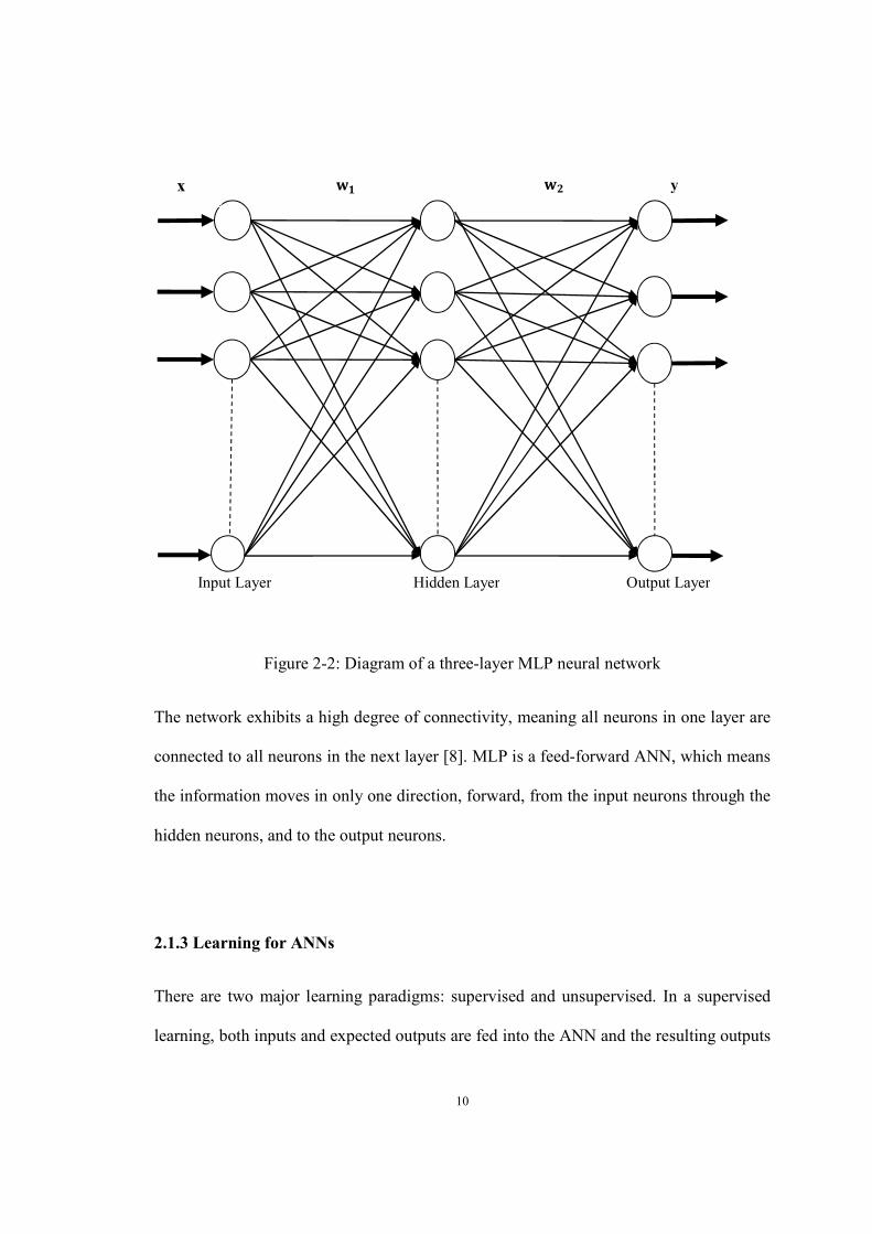
Figure 2.2 shows a typical three-layer MLP. An MLP consist of at least 3 layers, an input

layer, one or more hidden layer(s) and an output layer. The input layer is not considered a

“true” layer because no computation is performed by it. It receives problem-specific

inputs from the outside world. An MLP contains one or more hidden layers, which

receive inputs from preceding layers (input or hidden layers) and their outputs connect to

the next layers (output or hidden layers). Each neuron in a hidden layer employs a

nonlinear activation function that is differentiable [8]. The output layer presents the final

result of the computation performed by the network to the outside world.

10

Figure 2-2: Diagram of a three-layer MLP neural network

The network exhibits a high degree of connectivity, meaning all neurons in one layer are

connected to all neurons in the next layer [8]. MLP is a feed-forward ANN, which means

the information moves in only one direction, forward, from the input neurons through the

hidden neurons, and to the output neurons.

2.1.3 Learning for ANNs

There are two major learning paradigms: supervised and unsupervised. In a supervised

learning, both inputs and expected outputs are fed into the ANN and the resulting outputs

y

Hidden Layer Input Layer Output Layer

./ x .0

11

are then compared to the expected outputs to calculate the error. Using this error a

learning algorithm is then used to compute weight adjustments in order to lower the

network’s total error. After many pattern presentations and weight adjustments, the

network exhibits the learning behavior. That means the output of the ANN should

converge towards the desired output as additional training inputs are provided.

In an unsupervised learning, there is no target output data. The goal of these networks is

not to achieve high accuracy but to apply induction principles to organize data. The

learning behavior exhibits through supplying substantial data so that the network can

observe similarities and therefore use clusters to generalize its input data.

In its most basic form, an MLP neural network utilizes a supervised learning technique

called back-propagation for training the network. The training consists of two phases of

operation: a forward phase and a backward phase. During the forward phase, the

in-network processing or computation takes place, where input data are propagated

forward through the ANN from the input layer to the output layer while the weights

remain unaltered. At the start of the backward phase an error signal vector for output

layer neurons is calculated based on the difference between the desired and the computed

output values. Then the error signal vector is propagated back to the hidden layers. The

error signal vector for hidden layers is next calculated. The weights are updated based on

the error signal and the input value. The back-propagation performs a gradient descent

search in the weight space for the lowest error function value. There are several

12

variations on gradient descent back-propagation error correction. Further information for

these variations of back-propagation is documented in Section 3.1.1 of this thesis

manuscript.

2.2 Parallel and Distributed Processing for ANNs

It is well known that the training of or learning by an artificial neural network can be very

time consuming [9]. Meanwhile, ANNs possess inherent parallel processing capability, as

the neurons in the same layer can compute simultaneously. Therefore, a parallel

computing system is desirable to speed-up the computations needed for training an ANN.

Often, the challenge however is figuring out a mapping the parallel tasks associated with

the neuro-computing aspect with the parallel computing hardware or the processors of the

parallel system [10].

Nordstrom et al. suggested that parallelism for a typical ANN can be achieved in five

different ways [11]:

� Training session parallelism (simultaneously execution of different sessions).

� Training example parallelism (simultaneously learning of different training patterns).

� Layer and forward-backward parallelism (simultaneously processing of each layer).

� Neuron parallelism (simultaneously processing of each neuron in a layer).

13

� Weight parallelism (simultaneously multiplication of each weight with the

corresponding input in a neuron).

They also mentioned that since high degree of connectivity and large data flows are

characteristic features of neural networks, the structure and bandwidth of internal and

external communication in the computer to be used is of great importance.

In general, there are three different ways to implement the parallelism of ANNs:

Supercomputer-based systems, GPU-based systems and VLSI circuit-based systems.

Each of them has been under development for decades and still draws attention from

researchers. Supercomputer-based systems are known for their huge computation power,

which could be used to implement ANNs consisting of up to billions of neurons [15].

GPU-based systems take advantage of the availability through common PC and the

GPU’s highly parallel structure [17]. Circuit-based systems are powered by VLSI

architectures which offer massive parallelism that naturally suits the neural computational

paradigm of arrays of simple elements computed in tandem [19]. Recently, wireless

sensor network (WSN) based systems have been also proposed as parallel and distributed

processing hardware platforms. The similarity between the topologies of wireless sensor

networks and ANNs makes WSN a good candidate for implementing the parallel and

distributed processing of ANNs.

14

2.2.1 Supercomputer-based Systems

Blue Brain Project is a well-known supercomputer-based neural computation system [15].

The project began in 2005. Researchers used an IBM Blue Gene/L supercomputer to

simulate the mammalian brain. By July 2011 a cellular microcircuit of 100 neocortical

columns with a million cells was built. A cellular rat brain is planned for 2014 with 100

microcircuit totaling a hundred million cells [15].

Ananthanarayanan et al. from IBM Almaden Research Center pursued a similar project.

The ANN consisted of 900 million neurons and 6.1 trillion synapses. The supercomputer

they used is a Blue Gene/P with 147,456 CPUs and 144 TB of total memory. Their scale

for the neuron count has reached the level of a cat cortex which is 4.5% of the human

cortex.

2.2.2 GPU-based Systems

A graphics processing unit or GPU is known for its parallel computation power

achieved through highly parallel computing structure. GPU is capable of running up to

thousands of threads per thread block in parallel. Ciresan et al. implemented MLPs on

GPUs to running the MNIST handwritten digits benchmark [17]. Their system consists

of 2 x GTX 480 and 2 x GTX580 GPUs. In their implementation a tread is assigned to

one neuron. The result shows the GPU implementation is more than 60 times faster

than a compiler-optimized CPU version. Cai et al. designed a matrix-based training

15

algorithm of Conditional Restricted Boltzmann Machine (CRBM) and implemented on

GPU directly by using the library CUBLAS [18]. Their results show that the

computation of CRBM is accelerated by almost 70 times by employing their GPU

implementation.

2.2.3 Circuit-based Systems

An example for this realization is the REMAP (Real-time, Embedded, Modular, Adaptive,

Parallel processor) which was designed by Nordstrom et al [12]. The project is aimed at

obtaining a massively parallel computer architecture put together by modules in a way

that allows the architecture to be adjusted to a specific application. The prototype was

built using the FPGA technology. It mainly uses bit-serial processing elements (PEs)

which are organized as a linear processor array. They have implemented different kinds

of ANNs on the REMAP, such as Sparse Distributed Memory (SDM) [13],

self-organizing maps (SOM) [14], multilayer perceptron neural network with

back-propagation (BP) learning, and the Hopfield network [15].

Basu have developed a neuromorphic analog chip that is capable of implementing

massively parallel neural computations [19]. They showed measurements from neurons

with Hopf bifurcation and integrate and fire neurons, excitatory and inhibitory

synapses, passive dendrite cables, excitatory and inhibitory synapses, passive dendrite

cables, coupled spiking neurons, and central pattern generators implemented on the

16

chip. Using floating-gate transistors, the topology of the networks and the parameters

of the individual blocks can both be modified.

2.2.4 WSN-based Systems

WSN-based systems are relatively recent and only have been in existence starting with

the last decade ([20], [21]). Although a really large scale ANN could be trained and

executed on a super computer or a VLSI (GPU would still be unable to train because of

the technology limits), they are still not accessible for the typical user. Thanks to the

recent advances in micro-electro-mechanical systems technology, WSN nodes have

become low cost (some even below $1 US). Each WSN mote has sufficient

computation power to implement one or more neurons. The wireless link between

motes can be treated as the synapses, and weights could be stored in the memory of

motes. Thus, parallelism at the level of neuron processing is possible. Such a system

can be implemented to perform neural network computations in a truly parallel and

distributed manner.

2.3 Scalability of MLP-BP

The scalability of MLP-BP is affected by the complexity of the network topology and

structure, and the cost to train it. The network structure depends on the problem being

solved. For instance, considering the classification problems, the number of attributes

and classes directly translate into the number of neurons in the input layer and output

layer, respectively. The number of neurons in the hidden layer is affected by several

factors, such as the training algorithm and the activation functions used in the neurons,

17

but still is tightly related to the problem being solved. The number of attributes, classes

and patterns of the problem, the category of the problem and the percentage of noise in

the data would all affect the choice of an efficient structure of the MLP-BP network. If

the structure is chosen improperly the network would not achieve a good performance

and even fail to learn. For instance, if the network is too complex (have too many

hidden layer neurons) then it would probably cost too much time to train and won’t be

able to generalize since it would potentially over fit the training data [22].

The training time and the memory cost, which are measures for the time complexity

and space complexity, respectively, are prohibitively high for large-scale problems.

The primary part of the memory cost is the storage of the weights. In a MLP-BP

network each neuron in the hidden layer maintains weights for all the neurons in the

input layer, and each neuron in the output layer maintains weights for all the neurons in

the hidden layer. The weight count for a network would be given by

(1� ×1�) + (1� × �23), (2.4)

where1�, 1� and 4�23 are number of neurons in the input layer, hidden layer and

output layer, respectively.

The topology of an MLP-BP network typically has the most of the neurons in the input

layer, much less number of neurons in the hidden layer, and several neurons in the

output layer. Accordingly, the memory cost is not a primary source of

computational complexity for an MLP-BP network.

18

The projections for the time cost however are dramatically different. During training

the number of iterations to convergence, which will be represented by13 � , depends

on the properties of the specific problem being solved and the topology of the network.

During any given iteration, each pattern of the problem, piϵP for i=1, 2…|P|, is

propagated through the network, so there are |P| pattern presentations. Let’s denote

the number of addition operations, multiplication operations, and function evaluation

operations as78��, 792: and7;2�<, respectively. There are two phases for a single

pattern presentation to a typical MLP-BP. The first phase is the forward propagation.

In this phase, for each hidden layer neuron, computation for neuron output requires

1� × 792: (multiplication of inputs and weights) + (1� × 78��) − 1 (sum of

weighted inputs) + 7;2�< (function evaluation for neuron output) operations. For each

output layer neuron, computation of neuron output requires, 1� × 792:

(multiplication of inputs and weights) + (1� × 78��) + 1(sum of weighted inputs) +

7;2�< (error signal function evaluation) operations.

The second phase is back propagation of the signals. In this phase, for each hidden

layer neuron, computation for weights update requires �23 × 78�� (sum of output

layer errors) + 7;2�< (error signal function evaluation) + 1� × (78�� + 2 × 792:)

(adjustment of weights) operations. For each output layer neuron, computation for

weight update requires 1� × 792: (calculation of output layer errors) + 7;2�<

(error signal function evaluation) + 1� × (78�� + 2 × 792:) (adjustment of

weights) operations.

19

Overall, the total number of operations needed for a pattern presentation is

1� × �1� × (3 × 792: + 2 ×78��) + �23 × 78�� + 2 × 7;2�<�

+�23 × �1� × (4 × 792: + 2 ×78��) + 2 × 7;2�<�, (2.5)

where the significant or dominant term is given by

1� × (5 × 1� + 6 × �23) × 7;�, (2.6)

floating point operations (ofp) assuming that 78��, 792: and7;2�<all take the same

amount of time. From above the total floating point operations it may take to train a

MLP-BP network is on the order of

13 � × |P| × 1� × �5 × 1� + 6 × �23�, (2.7)

which will depend on the number of iterations, the size of the training data set, and the

number of neurons in each of the three layers (assuming a single hidden layer

topology). In the worst case, where the data set size is very large, the training

iterations count is also large, so the time cost can be significant. Therefore the time

complexity is the dominant cost factor for training an MLP-BP neural network.

2.4 Wireless Sensor Networks

Wireless sensor networks (WSN) are a recently emerging technology owing to

advancements in miniaturization of microcontrollers, radio devices and high density

storage and sensors. A WSN consists of spatially distributed motes (nodes with sensors)

that are able to interact with their environment by sensing or controlling physical

parameters. The network size may vary from a few to thousands, and these motes have

to collaborate to fulfill their task as a single mote is incapable of doing so. Motes use

wireless communication to enable their collaboration. WSNs can be used in a variety

20

of applications. Area monitoring is a common application of WSNs, in which case

the WSN is deployed to monitor some phenomenon such as enemy intrusion. WSNs

are also highly relevant for precision agriculture, as the sensors can be used to monitor

the crop and the environment to determine, for instance, the amount of irrigation and

time to harvest. Another application for which WSNs can be used in is smart building

monitoring, where a WSN can monitor the human movement to adjust the facilities in

the building. Structural health monitoring of bridges, highways, overpasses etc.,

another area of application. In transportation, embedded vehicles with a wireless

sensor network to develop ability to sense a wide array of phenomena is of interest.

The potential applications list appears to be very long.

2.4.1 Single Node (Mote) Architecture.

The majority of the applications for the WSNs require the motes to be small, cheap and

energy efficient. A sensor node or mote could be smaller than 1 cm, weight less than

100 g, cheaper than $1 US, and dissipate less than 100μW. The sensor nodes

possess processing and computing resources through utilization of a technologically

low-end microcontroller. A sensor node is capable of performing collecting of sensory

information and communicating with other nodes. A basic sensor node comprises five

main components: controller, memory, sensors, communication device, and power

supply. A brief description of each component follows.

Controller--The core of a mote is the controller which collects data from sensors,

processes the data, controls the transceiver to send and receive data and decides on the

21

actuator’s behavior. The controller has the ability of executing various programs,

ranging from the time-critical signal processing and communication protocols to

application programs. The clock speed of the controller for different kinds of nodes

ranges from less than 1 MHz to 16 MHz and beyond. The clock speed for the most

common nodes, such as Mica 2, T-Mote Sky, TelosB, Iris mote etc., is around 16 MHz.

The performance for the microcontroller on board the TelosB motes is 8 MIPS, Mica

motes is 1 MIPS, and Egs motes is 90 MIPS.

Memory—Memory subsystem of sensor node is used to store intermediate sensor

readings, packets from other nodes and so on. The memory system consists of RAM

and flash/external memory. Currently the size of RAM ranges from 512 bytes to 512

KB, and the size of flash/external memory ranges from 4 KB to 4 MB.

Sensors-- Sensors are the devices which make it possible for the motes to sense its

environment. Typical sensors measure temperature, light, vibration, sound, humidity,

chemical structure or makeups, video, and ultrasound to list a select few among many

other options.

Communication device-- The communication device is a wireless radio and used to

exchange data between individual nodes. A wireless radio device combines a

transmitter and a receiver called transceiver. The frequency of transceiver ranges from

433 MHz to 2.4 GHz given the current technology.

22

Power supply-- The common power supply for sensor nodes is batteries. Batteries

might be for one-time use or rechargeable. In the latter case, energy harvesting

mechanisms can be incorporated into a mote platform to charge batteries or supply

different electronics or sensors onboard.

2.4.2 Network Protocols

A WSN is distinguished from other types of wireless or wired networks by its

characteristics of energy efficiency, data centricity, scalability, distributed processing,

and self-organization. These characteristics lead to protocols that must be custom

developed and designed for WSNs. Energy efficiency is the most significant

characteristic for WSNs, which limits the radio transmission range and requires the

motes to sleep most of the time. Data-centric characteristic implies the network

protocols to be designed with a clear focus on the transactions of data instead of node

identities (id-centric). A WSN may consist of thousands of motes, so the protocols

need to consider its scalability for truly large networks. Distributed sensing and

processing implies that often the data to be sensed is collected by a larger number of

spatially spread sensors and processed in part and progressively by motes concurrently.

Self-organization means once the motes are deployed the network is left unattended,

then the network must adapt in the presence of environmental stimulus, conditions,

changes to topology, destruction or damage to motes or sub-networks, which are

typically unpredictable.

23

Medium Access Control Protocols -- The goal of medium access control (MAC)

protocols is controlling when to send a packet and when to receive a packet. MAC

protocols can be classified roughly into three categories [23]: contention-based

protocols, contention-free (schedule-based) protocols, and hybrid protocols. In

contention-based MAC protocols, sensor nodes that want to communicate with others

compete for access to the medium. IEEE 802.11, PAMAS, S-MAC and T-MAC are

common contention-based protocols. This kind of protocols inherits good scalability

and adaptability, but the idle listening, collision, overhearing, and control-packet

overhead lead to energy inefficiency. Contention-free protocols can be implemented

based on time-division multiple-access (TDMA), frequency-division multiple-access

(FDMA), and code-division multiple-access (CDMA) techniques. TRAMA, FLAMA,

SRSA, R-MAC and SMACS belong to this kind of MAC protocols. The advantage for

this kind of protocols is their energy efficiency, but the disadvantage is their lack of

scalability or adaptability. Hybrid MAC protocols combine the strengths of

contention-based and schedule-based protocols. Examples for this kind of protocols are

Funneling-MAC, HYMAC, AS-MAC and Z-MAC. A switching mechanism is

designed to let a hybrid MAC protocol switch itself between contention-based and

schedule-based protocols, so it can take advantage of each one while offsetting their

disadvantages. However, the disadvantage of this kind of protocols is the relatively

high protocol complexity.

Routing Protocols -- Routing is the act of moving information or data across a

network from a source to a destination. The routing protocols designed for WSNs can

24

be classified as data-centric, hierarchical and location-based [24]. Data centric

protocols are based on query and depend on the naming of desired data, which can

eliminate many redundant transmissions. SPIN, Directed Diffusion, Rumor routing and

CADR are common data-centric routing protocols [111,112,113,114]. Hierarchical

protocols cluster the whole network into several clusters so that the cluster heads can

do some aggregation and reduction of data in order to save energy. LEACH, TEEN

and PEGASIS belong to this kind of routing protocols [115,116,117]. The

location-based routing protocols use the position information to relay the data to the

destination. Examples for location-based protocols are GAF, GEAR and MECN

[118,119,120].

Time Synchronization Protocols -- Time plays an important role in WSNs. The

accuracy of time can influence many applications and protocols assigned to the

network. Because of random phase shifts and drift rates of oscillators, the local time

reading of motes will start to differ without correction. Time synchronization protocols

for WSNs need to guarantee the accuracy while keeping the energy consumption low.

These protocols could be divided into sender-receiver and receiver-receiver protocols.

In the sender-receiver protocols, a receiver synchronizes to the clock of a sender. For

the sender-sender protocols, the receivers synchronize to each other by the

time-stamped packet sent from another mote.

Localization and Positioning Protocols -- Location is necessary for the nodes to

know for many functions: location stamps, coherent signal processing, tracking and

25

locating objects, cluster formation, efficient querying and routing. Equipping every

node with a GPS receiver is not a feasible option because of cost, energy and

deployment limitations. An example of localization protocol is the APIT [121], which

locates a node by deciding whether it is within or outside of a triangle formed by any

three anchors. DV-Hop is another positioning protocol relevant for WSNs [122].

2.5 Wireless Sensor Network Simulators

Recently, there has been growing interest in implementing WSNs for wide variety of

applications and designing protocol-level or application-level algorithms for WSNs.

Since running real experiments is very costly and time consuming, simulation is

essential to study WSNs. New applications and protocols for WSNs are implemented

on simulators to verify the feasibility and to test the performance. Although simulation

models are usually not able to represent the real environments with the desired level of

completeness and accuracy, compared to the cost and time involved in setting up an

entire testbed, simulators are still relatively fast and inexpensive.

Simulators can be classified into three major categories based on the level of

complexity: bit level, packet level and algorithm level. As the complexity goes up, the

time and memory consumption of the simulation grows. It is desirable to select the

level of simulation based on the rigor requirements of the experiment. For instance, a

timing-sensitive MAC protocol would probably need a bit level simulation while an

algorithm level simulation is sufficient to test the prototype developed for an

agriculture management application.

26

2.5.1 Bit Level Simulators

Bit-level simulators model the CPU execution at the level of instructions or even

cycles, they are often regarded as emulators. TOSSIM [25] is a both bit and package

level simulator for detailed simulation of TinyOS based motes. TOSSIM simulates the

entire TinyOS execution by replacing components with simulation implementations. It

uses the same code as is used on real motes. The programming language for it is nesC,

a dialect of C. TOSSIM simulates the nesC code running on actual hardware by

mapping hardware interrupts to discrete events. TOSSIM can handle simulations up to

around a thousand motes. Avrora [26] is another bit-level simulator that is open source

and built using the Java programming language. It has language and operating system

independence. It simulates a network of motes by running the actual microcontroller

programs, and accurate simulations of the devices and the radio communication.

Avrora is capable of running a complete sensor network simulation with high timing

accuracy.

2.5.2 Packet Level Simulators

Packet level simulators implement the data link and physical layers in a typical OSI

network stack. The most widely used simulator is ns-2 [27]. ns-2 is an object-oriented

discrete event network simulator built in C++. ns-2 can simulate both wired and

wireless network. ns-2 possesses great extensibility, and its object-oriented design

allows for straightforward creation and use of new protocols. Due to its popularity and

ease of protocol development, there are many protocols that are available for it.

J-Sim[28] is a simulator that adopts loosely-coupled, component-based programming

27

model, and supports real-time process-driven simulation. OPNET [29] is a commercial

simulator, which provides a simulation environment with powerful standard modules.

OPNET is a good choice to simulate Zigbee based networks.

2.5.3 Algorithm Level Simulators

Algorithm level simulators focus on the logic, data structure and presentation of

algorithms. They do not consider detailed communication models, and they normally

rely on some form of a graph data structure to illustrate the communication between

nodes. Shawn [30] is a simulator implemented in C++ that has its own application

development model or framework based on so called processors. The nodes in Shawn

simulator are containers of processors, which process incoming messages, run

algorithms and emit messages. The motivation of Shawn is as follows: there is no

difference between a complete simulation of the physical environment (or lower-level

networking protocols) and the alternative approach of simply using well-chosen

random distributions on message delay and drop for algorithm design on a higher level,

such as localization algorithms. From their point of view, the common simulators

spend much processing time on producing results that are of no interest at all, thereby

actually hindering productive research on the algorithm. The framework of Shawn

replaces low-level effects with abstract and exchangeable models. Shawn simulates the

effects caused by a phenomenon instead of the phenomenon itself. For example,

instead of simulating a complete MAC layer including the radio propagation model, its

effects (packet drop and delay) are modeled in Shawn. The simulation time of Shawn

28

is significantly reduced compare to other simulators, and the choice of the

implementation model is more flexible.

2.5.4 Proposed Approach of Simulation for WSN-MLP Design

As discussed in Section 2.5, the simulation of MLP-BP network for large problems is

potentially time consuming. Simulation of a WSN is another source of complexity if

not done properly as earlier discussion indicated. MLP-BP algorithm can be

implemented at the application level with respect to the WSN context. Simulation of

WSN can be therefore realized for the effects of events occurring below the application

layer or levels such as physical layer and the wireless protocol layer. Accordingly,

inspired by the design philosophy of Shawn wireless sensor network simulator, we

decided to simulate the WSN for its effects at the application level. In our approach,

only the major effects, namely packet delay and drop, of WSN operation, which have

influence on the execution of ANN are modeled.

29

Chapter 3

Probabilistic Modeling of Delay and Drop Phenomena

for Packets Carrying Neuron Outputs in WSNs

Neuron outputs will need to be communicated to other neurons through wireless

communication channels or over the air for a wireless sensor network (WSN) that is

embedded with an artificial neuron network where each mote houses one or more

neurons. Packets are subject to delay and drop during wireless transmission due to

medium access (such as channel being busy or collision of packets), outgoing or

incoming message processing, multi-hop communications, and routing algorithms among

many other factors in a wireless communications medium. Meaningful simulation of a

wireless sensor network (WSN) computations and communications with an artificial

neural network (ANN) embedded into it requires that such delay and drop be modeled as

accurately as reasonably possible. In response to this requirement, a probabilistic model

for delay and drop has been developed and employed in the simulation study, which will

be presented in this chapter.

30

3.1 Neuron Outputs and Wireless Communication Delay

Consider a multilayer perceptron (MLP) type artificial neural network (NN) with at least

three layers of neurons, namely an input layer, one or more hidden layers, and an output

layer. The input layer is not considered as a “true” layer since no computation is

performed by the neurons in that layer. Neurons in the input layer simply distribute the

components of an input pattern vector to neurons in the hidden layer without any other

processing. Distribution of training patterns can be accomplished by either a multi-hop

routing scheme or by a gateway or clusterhead mote that can reach all the WSN motes

directly. In our simulations, we assumed that there is a gateway mote which can

communicate with each mote in the WSN directly through a single-hop transmission: also

potential delays or drop for the communications originating from the gateway mode were

not considered.

Outputs of neurons in one layer must be communicated to inputs of neurons in the other

layer during training and following the deployment. Since the wireless communication of

such packets that carry neuron output values is accomplished through multi-hop routing,

it is reasonable to assert that the delay due to medium access, packet processing, and the

hop-count among others will be mainly affected by the distance (or the equivalently the

number of hops) between the sending and receiving neurons or motes. Although it may

depend on the actual routing protocol chosen, the distance for the routing path for a

packet can be approximated (or underestimated) by the hop count, which is measurable

through various approximation schemes [1]. As an another factor that plays a significant

31

role in the overall communications and computation process, the likelihood of packet

drop carrying a neuron output increases as the number of hops increases between the

sender-receiver neuron or the corresponding mote pair.

Accordingly, the hop count will be employed as the primary factor affecting the amount

of delay and the likelihood of drop for packets carrying neuron outputs. When delay

occurs and its value varies and, in the worst case, the drop happens, a procedure needs to

be developed to make available past values of the output for the neuron whose output is

delayed.

3.2 Modeling the Probability Distribution for Packet Drop and Delay Phenomena

The probability of packet drop during transmission in WSNs is highly dependent on the

specific implementation of the network and its protocol stack. There are many factors at

play, such as topology of the network, routing and MAC protocols, network traffic load,

etc.

It is not desirable to have the model for the probability distribution for drop or delay

limited to a certain scenario (using certain protocols, set a number of nodes, set a

topology, etc.) since the results of such a study would not be applicable in general terms.

The model to be developed instead should be generalized enough to be applicable for the

widest variety of WSN realizations, implementations and applications possible. One

readily available option to develop or formulate a model for packet delay and drop is to

32

leverage the empirical data reported in the literature, which is the venue pursued in our

study.

3.2.1 Literature survey

We conducted a survey to compile the empirical data of delay and drop reported in the

literature [1-22]. We studied the simulation scenarios and compiled a record of the

simulation settings and results. The simulation settings included routing protocols, MAC

protocols, simulator type, number of motes, field size, radio range and other settings

(traffic, source count, dead node count etc.). The simulation results included delivery

ratio and delay, which were extracted from tables and figures in the surveyed literature.

The detailed data can be found in Appendix A.

3.2.2 Data set for building the drop model

In order to build an empirical model for the drop probability distribution, a literature

survey was performed to collect and compile simulation data for different WSN designs,

with variations in the topology and the protocol stack, and applications. The data used

for building the empirical delay or drop model was compiled from the studies reported in

[1-22]. The packet delivery ratio that was recorded in each study is considered as the

main variable. Denoting the packet delivery ratio as B� :1C �D , the probability of drop

as given byB��, can be calculated through B�� = 1 −B� :1C �D. Specific values

for the packet delivery ratio versus node count for a number of WSN topologies and

33

protocol stack implementations, which were used as the data to build the empirical model

for the probability of drop, are retrieved from the same studies cited herein.

The data points are chosen based on the following specifications:

1) The node count is one of the primary independent variables, which means the

data is collected for different node count values.

2) The density of nodes within the WSN topology will stay “approximately” the

same although the node count may vary. This means that the area of

deployment for the network or the transmission range should change to keep

the node distribution density the same.

3) No other significant factors are considered to affect the probability of drop,

such as the changing network traffic load or the static or time-varying

percentage of dead nodes.

Establishing the above specifications is intended to ensure that packet drop probability is

fundamentally affected by the number of hops only, which is assumed to approximate the

distance between the sender and receiver mote pair. When the density is kept the same,

the hop count from the source to the destination is increased with the number of nodes in

the network: further elaboration on this statement will be presented in the upcoming

sections.

34

3.2.3 Empirical Model as an Equation for Packet Delivery Ratio vs. Node Count

In this section, we investigate the relationship between the probability of drop and node

count using the studies reported in literature [31-52]. The tool we use for handling these

data is the statistical computing and graphics software package called R. After importing

the empirical data into R, we use the “xyplot” function in R to plot the data. The plots for

different routing protocols for the probability of drop versus node count are shown in

Figure 3-1. The routing protocols included QoS Routing [40], Speed [40], GBR [31],

LAR [42], LBAR [42], Opportunistic Flooding [38], AODVjr [42], BVR [34], DD [47],

and EAR [31].

35

Figure 3-1: Plots for Probability of Drop vs. Node Count for Various Routing Protocols

The x-axis is the node count, while the y-axis is the probability of drop. Each individual

plot is specific to a “routing protocol”. Denoting the node count as �� , Figure 3-1

shows that B� :1C �D decreases when the value of �� increases. The relationship

appears to be linear in general. Since these data are due to specific experiments, in order

to generalize, it may not be a good idea to make the model fit the data precisely.

Therefore the linear regression (versus a polynomial which is a more tight fit) for fitting

these data points is a reasonable option. Then the resultant empirical model is given by

36

(EF!EG×�HIJKL)�� , (3.1)

where coefficients �� and �� are real numbers for the linear model. The

probability of drop is then calculated as

B�� = 1 − (EF!EG×�HIJKL)�� , (3.2)

The linear model for each plot shown in Figure 3-1 is obtained through the linear

regression and the coefficients �� and �� calculated for each case is shown in Table 3.1.

In the case for the opportunistic flooding routing protocol, a special scenario arises: it can

guarantee a successful delivery, which means the probability of drop is zero.

Table 3.1: Coefficients �� and �� of the Linear Model for Each Case in Figure 3-1

Routing Protocol ��

EAR 100.82 -0.0107

GBR 94.50 -0.1130

BVR 94.44 -0.0760

QoS 97.00 -0.0980

Speed 97.40 -0.0840

LBAR 95.79 -0.0198

LAR 92.57 -0.0154

AODVjr 90.57 -0.0154

DD 89.60 -0.0440

Opportunistic Flooding 100.00 0.0000

3.2.4 The number of transmission hops

The number of hops will be used as the primary factor affecting the probability of drop,

therefore it is necessary to establish its definition. For a two-dimensional deployment

topology for a WSN, let �� denote the hop count between a source and a destination

37

mote pair. Defining the B�� in terms of �� is of interest. Given that we know

the value for �� , which is the number of motes in the WSN, a relationship between

�� and �� needs to be derived for a given specific deployment topology.

For instance, as shown in Figure 3-2, �� nodes are uniformly randomly distributed

in a square deployment area. Consequently, the number of motes along any edges will be

approximatelyM�� . Assume the sink mote is located at the center, while the source

node is close to one of the corners. Average hops count for any given message, ��,

can be approximated by the length of the diagonal in terms of number of hops divided by

two. Then the relationship of �� and �� is given by�� = 2�� .

Figure 3-2 Example Illustrating Relationship between �� and ��

Source

Sink

M��

motes

38

In the worst case for a source and sink mote pair where the motes are located at the

terminal points of a given diagonal, the relationship between these two variables becomes

�� = �NIOLP

� , while also noting that the minimum hop distance is 1. Consequently,

the hop count values changes as follows: 1≤ �� ≤ M2�� .

The square topology assumed for the above analysis is a reasonable approximation to

many of the deployment realizations. If necessary, other topologies can also be readily

analyzed following a similar approach. In somewhat general terms then, the relationship

between �� and �� can be represented as

�� = R × ��, (3.3)

where τ is the coefficient whose value is positive and will vary based on a number of

WSN-related parameter settings including the shape of the topology and the density of

mote deployment. In the linear regression curves obtained for each routing protocol

earlier, the coefficients �� and �� and the parameter �� values are substituted to

yield the models shown in Table 3.2.

39

Table 3.2 Empirical Models of �� in Terms of Parameter ��

Routing

Protocol

TU T/ Empirical Model

EAR 100.82 -0.0107 B�� = �−0.82 + 0.043 × ��/100

GBR 94.50 -0.1130 B�� = �5.5 + 0.45 × ��/100

BVR 94.44 -0.0760 B�� = �5.6 + 0.076 × ��/100

QoS 97.00 -0.0980 B�� = �3 + 0.049 × ��/100

Speed 97.40 -0.0840 B�� = �2.6 + 0.042 × ��/100

LBAR 95.79 -0.0198 B�� = �4.21 + 0.020 × ��/100

LAR 92.57 -0.0154 B�� = �7.43 + 0.015 × ��/100

AODVjr 90.57 -0.0154 B�� = �9.43 + 0.015 × ��/100

DD 89.60 -0.0440 B�� = �10.4 + 0.088 × ��/100

Opportunistic Flooding

100.00 0.0000 B�� = 0

The calculations ofR are done based on a specific topology implemented in the literature.

As an example, consider the QoS-based routing protocol implementation in the study

reported in [24]. The topology is a unit square and the two sink nodes are placed in the

lower corners of the square deployment area. The nodes in the upper right report to the

sink in the bottom left and the nodes in the upper left report to the sink in the bottom right.

The distance between the source and the sink nodes is approximately the diagonal of the

square area. Accordingly, the coefficient τ has a value of√2.

40

The empirical models in Table 3.2 indicate that the models for GBR and Opportunistic

Flooding routing are exceptions as their performance vary significantly when compared

to the performances of the other cases. The GBR protocol would not be appropriate for a

large network, and the Opportunistic Flooding would incur too much delay to guarantee

the delivery. Therefore, the models for GBR and Opportunistic Flooding are not

considered any further. We consider all the remaining models in Table 3.2 to set a

range for �8and �\ parameters in Equation 3.3. Accordingly, the empirical model for

�� is defined in general terms as

B�� = �� +�� × ��/100 , (3.4)

where the range of values for �� is (-1, 11), and the range of values for �� is (0.013,

0.09). When this model is employed in the simulation study,��and��values are

generated randomly using a uniform distribution in their corresponding ranges.

3.3 Modeling the Delay

3.3.1 Delay and Delay Variance

Delay is an inherent property of WSN operation with respect to wireless communications.

According to a literature survey we did, the length of delay varies from 10 ms to 3000 ms

for different implementations (such as variations in number of nodes, routing protocol,

MAC protocol, packet length, traffic load etc.) [31-52]. Figure 3-3 shows the histogram

for the delay based on the survey data.

41

Figure 3-3 Histogram of Delay for Survey Data

In a real scenario where one or more neurons are embedded into a given mote, the

exchange of neuron outputs among motes will be subject to certain delay that is inherent

in wireless communications. This delay, which will dictate the duration of a waiting

period by a given neuron for its inputs to arrive from other neurons on other motes is not

a fixed value but rather a random variable. The delay-induced wait time will be denoted

as]^813. Note that ]^813 is both application dependent and network dependent: its value

was found to vary from 10 ms to 3000 ms per the literature survey which was presented

in Figure 3-3 indicated. For a specific network the delay between for a pair of motes

from one pair to another varies substantially, and even for the same pair of motes the

delay variance is significant. Additionally, the maximum delay could be much larger than

42

the mean delay [53, 59]. In simulating a neural network embedded across motes of a

wireless sensor network, the ]^813 is set according to the mean delay value and the

specific network topology to make sure that a good number of inputs successfully arrive

for any given neuron to be able to calculate its own output.

Per the surveyed literature, a specific delay distribution is highly dependent on many

factors such as the MAC protocol, traffic, queue capacity, channel quality, back-off time

setting in MAC protocol, etc. [53, 54, 55, 57 and 59]. It is impossible to get a highly

accurate model of delay distribution considering so many factors play a role in affecting

its value. A reasonably good but approximate model however can be formulated by using

the Gaussian distribution which have been used in the literature to model the delay

distribution [54, 55], and has also been shown to be relevant in other literature studies [56,

57, 58]. Empirical evidence suggests that the delay distribution is truncated and

heavy-tailed [57, 59]. Consequently, a truncated Gaussian distribution for modeling the

delay variance is chosen, which is elaborated upon in the next section.

3.3.2 Delay Generation using Truncated Gaussian distribution

The truncated Gaussian distribution is the probability distribution of a normally

distributed random variable whose value is bounded. Suppose X~N(μ, c�) has a

normal distribution and lies within a range of (a, b), then x conditional on a<x<b has a

truncated normal distribution. Its probability density function � is given by

43

�(�; e, c, f, g) =Ghi(j"kh )

lmn"oh pql(r"oh ), (3.6)

where x is the random variable, e represents the mean, c represents the standard

deviation, a represents the minimum value, b represents the maximum value, s(∙) is the

probability density function of the standard normal distribution, and u(∙) is the

cumulative distribution function.

The overall delay for a given neuron output is positive integer valued and quantified to

indicate the number of pattern presentations. This parameter value, namely overall delay,

is computed by summing per hop delays for the total number of hops between the

sending-receiving neuron pair and dividing their sum by the ]^813 parameter value.

Truncated Gaussian distribution is used as the model for the per hop delay parameter. In

other words, the computation employs the following steps:

OverallDelay = �~77�(∑ � �� :8DHNIOLG

3�r��) (3.6)

Where the floor () function get the largest integer not greater than the variable. The

parameter ]^813 is defined in terms of three other parameters which are multiplied to

yield

t�� = ϑ × μ × l��, (3.7)

where ϑ is a coefficient to be set in the simulator, μ is the mean value of the Truncated

Gaussian distribution, and l�� is the max hop count of the topology being considered.

For ease of computation, the mean value of Truncated Gaussian distribution will be

44

normalized to relocate it to the value of 1. Based the empirical studies in the literature [53,

54], other parameters of the Truncated Gaussian distribution are set as a=0.3, b=5, and

σ=0.6. The MATLAB code for generating the truncated Gaussian distribution is

presented in Figure 3-4. A histogram of the truncated Gaussian distribution generated by

the code in Figure 3-4 is shown in Figure 3-5.

Figure 3-4 Function for Generating the Truncated Normal Distribution

Figure 3-5 Histogram of Truncated Gaussian Distribution as Generated by MATLAB

Code in Figure 3-4.

function x = trimnormrnd(mu,sigma,a,b,m,n) A = (a-mu)/sigma; B = (b-mu)/sigma; delta = normcdf(B)-normcdf(A); x = sigma*norminv(delta*rand(m,n)+normcdf(A)) + mu;

45

3.4 Modeling the Neuron Output Delay (NOD)

The Neron output delay is the delay for the output of neuron. It emerges when the packet

contain the output got delayed or drop. For each packet transmission between two motes,

the NOD was modeled by combining the drop and delay values. The basic flow chart for

the model is shown in Figure 3-6. The entire process will be discussed in the following

paragraphs.

Figure 3-6: Basic Flow Chart for the Calculation of NOD

3.4.1 Distance Calculation

Calculate the Distance between

the Pair of Motes

Calculate the Drop Probability

of the Packet

Calculate the Delay of the

Packet

Generate the NOD

46

For each pair of nodes, the distance needs to be calculated as follows. We randomly

deploy the nodes in a 2-D field. The size of the field is determined in relationship to the

number of nodes in the hidden layer and output layer of the multilayer perceptron neural

network. The output-layer nodes are in a smaller square field in the middle of the larger

square field of hidden-layer nodes as shown in Figure 3-7. This deployment arrangement

facilitates the average of distances between node pairs to be minimized, and also keeps

the variance of distance as small as possible.

Figure 3-7 Deployment for MLP neural network within WSN topology

Let �� and �� represent the number of neurons for the hidden layer and the output

layer, respectively. The entire deployment area is determined according to the node count.

Corresponding to the case shown in Section 3.2.4, the length of larger square area is

given byf = M�� + ��. The hidden layer neurons are deployed uniformly randomly in

this square. The output layer neurons are deployed in the inner square and its length

(denoted as b) is given byg = M��. For each neuron, its coordinates are generated

randomly in the corresponding square area. The Euclidian distance between a pair of

Hidden Layer

a Output

Layer

b

47

motes (neurons) with coordinates (�� , ��) and (��, ��) would be �� =

M(�� − ��)� + (�� − ��)�. Since the metric is the number of nodes, this distance

would also correspond roughly to the distance in terms of the number of (transmission)

hops. The MATLAB code that positions each mote-neuron pair in the concentric squares

based on MLP layer association of neurons is shown in Figure 3-8.

Figure 3-8: MATLAB Code for the Calculation of Pairwise Distance between Neurons.

3.4.2 Model of the Delay for Transmission of Neuron Outputs

%Calculate the dimensions of squares lengthHid = sqrt(m+n); %m and n are the node counts in hidden and output layers lengthOut = sqrt(n);

%Randomly assign the coordinates for each neuron-mote pair xHid = lengthHid * rand(1,m);%the x coordinates for hidden layer nodes yHid = lengthHid * rand(1,m); xOut = (lengthHid - lengthOut)/2 + lengthOut * rand(1,n); yOut = (lengthHid - lengthOut)/2 + lengthOut * rand(1,n); %The extremum coordinates of the inner square for the output layer point1 = (lengthHid - lengthOut)/2; point2 = (lengthHid + lengthOut)/2; %Generate hidden layer neuron coordinates outside the output layer square for i = 1:m while(xHid(i)>point1&&xHid(i)<point2&&yHid(i)>point1&&yHid(i)<point2)

xHid(i) = lengthHid * rand(); yHid(i) = lengthHid * rand(); end;

nodeDist = zeros(m,n);%the node distance matrix %Calculate the distance for each pair of neurons for i2 = 1:m for j2 = 1:n nodeDist(i2,j2) = int16(sqrt((xHid(i2)-xOut(j2))^2+(yHid(i2)-

yOut(j2))^2)+0.5); end end

48

Each MLP neuron is embedded into a separate WSN mote. For each pair of motes, the

probability of drop B�� for a packet is calculated based on the hop count between them

using Equation 3.3. The value of ]^813is application specific and set by Equation 3.7. In

our experiments, we change the value of the coefficient ϑ to observe the neural network

performance under different conditions. Then the delay amount for each transmission is

generated using Equation 3.6.

Let the following definitions hold for the delay and drop model under the assumption that

each mote is embedded with a single neuron of an MLP neural network:

�: a uniformly-distributed random number in the range [0,1].

i: index for sending mote;

j: index for receiving mote;

�1 , ��: labels for sending and receiving motes or neurons;

�1�: delay (positive integer-valued) for the packet sent by mote (neuron) �1 to mote

(neuron)��;

�1�: one-dimensional array of integers for communication between motes �1 and

�� , where the array index corresponds to pattern presentation number (or the

sequence number for the number of patterns presented in a single training epoch),

and contents hold the most recent pattern presentation number when the output

49

from mote (neuron) �1 arrives at mote (neuron) �� at the this pattern

presentation;

��: one-dimensional array of integers for neuron j where each element holds the

pattern presentation number in which the most recently generated output from the

corresponding neuron (mote) arrived at mote �� . ��[�] holds the pattern

presentation number for the most recently generated packet among the packets

which arrived at mote �� from mote�1;

��: one-dimensional array of integers where ��[�] holds the value of output for

neuron �� computed at pattern presentation �.

The pseudo-code in Figure 3-9 defines the model of neuron output delay (NOD) between

motes �1 and��. Mote �1 transmits a packet carrying its output value to mote��

after each pattern presentation unless there is delay. At a given pattern presentation

iteration k, the first step is to update the array�1�. Initial decision is to determine if the

packet should be dropped or not. The packet is considered as “not dropped” if the

randomly generated number � is greater than the probability of drop (B��7B). Then the

delay amount �1� is generated by the delay model. The presentation sequence number

for the current pattern k is stored in the array �1� at the position indexed by� + ��; this

means the packet that carries the neuron output value and destined from mote �1 to

mote �� during pattern presentation k would arrive at mote �� during pattern

presentation � + �� . If the random number z is not larger than the probability of

dropB��7B, then the packet is considered as “dropped.” Then �1� won’t be updated which

50

means the packet from mote �1 to mote �� at pattern presentation k won’t arrive at all.

The second step is to update��[�], which holds the pattern presentation sequence number

for the most recently generated packet among the packets which arrived at neuron ��

from �1 (an example is given in the following paragraph). If �1�[�] is larger

than��[�],��[�] value is updated to that of the�1�[�]. This means that there is a packet

that arrived during pattern presentation k which is more recent compared to any other

output which arrived from that same sending neuron. The content of��[��[�]] is used for

the updating neuron’s outputs or weights on mote��.

Figure 3-9: Pseudo-code for Implementation of Delay and Drop (NOD) Model.

An illustrated example demonstrating the use and the realization of the delay and drop

modeling is presented next. Corresponding to Figure 3-10, the example shows the

Step 0: a. Initialize the array�1�[] to 0. b. Initialize ��[�] to 0. At a given pattern presentation k, where k=1,2,3,a

Step 1: If � > B ¡¢£ Generate the �� value using the delay model. Update the array�¤¥[]: �1�[�� + �] = k. Else do nothing.

Step 2: If �1�[�] > ��[�] Update��[�]: ��[�] =�1�[�]. Else do nothing.

51

execution during pattern presentations 17 and 18. The original value of the array �1� and

§�[�] are assumed as shown in Figure 3-10. In the first step of pattern presentation

iteration 17, assume � is larger thanB��7B, and the generated delay amount �1� is 1.

This means the packet generated during this pattern presentation would arrive at the next

pattern presentation, namely during pattern presentation sequence number 18. The

content of �1�[18] is updated to 17. In the second step of pattern presentation 17, the

packet arrived at this pattern presentation is from pattern presentation 15 (the content of

�1�[17] is 15). It is older than the packet that arrived during pattern presentation 16.

Since 15 is less than 16 where the latter is stored in��[�], ��[�] is not updated. The

neuron output value (from�1) stored in��[16] is used for updating the output or weights

of the neuron on mote�� . Next, consider the pattern presentation sequence 18. During

the first step of pattern presentation 18, assume � is larger thanB��, and the delay

amount �1� is determined to be 0. This means the packet arrived on time (it arrived

during the current pattern presentation). The content of �1�[18] is updated to 18 (18

replaces 17). In the second step of pattern presentation 18, the packet that arrived during

this pattern presentation is from pattern presentation 18 (the content of �1�[18] is 18). 18

is greater than the content of ��[i] which is equal to 16, so ��[�] is updated to be 18. The

output value stored in��[18] is used for updating the output or weights of the neuron on

mote��.

52

Figure 3-10: Example for the Implementation of the Delay and Drop Modeling

14 16 15 0 0 0

16 17 19 15

20 18

�1�[]:

��[�]: 16

Step 1: z >B�� ; �1� = 1

14 16 15 17 0 0

16 17 19 15 20 18

�1�[]:

��[�]:::: 16 ��[�]:::: 16

Step 2

14 16 15 17 0 0

16 17 19 15 20 18

�1�[]:

��[�]: 16

Step 1: z > B�� and �1� =0

14 16 15 18 0 0

16 17 19 15 20 18

�1�[]:

��[�]:::: 16 ��[�]:::: 18

Step 2

17th

pattern presentation

18th

pattern presentation

53

The code in MATLAB for implementing the delay and drop (NOD) model is shown in

Figure 3-11. For the memory purpose, the length of array�¤¥ is set to be the potential

maximum delay pattern presentations. The actual index of the array is calculated by the

desired index mod the array length.

Figure 3-11: MATLAB code for the Delay and Drop (NOD) Model

% Generate the NOD for the pair of neurons % c is a variable and holds the sequence number % i and j are indices for neuron identification % Initialize the Sequence Array to zero sequenceArray = zeros(m,n,dmax); % mem is a 2D array to store the sequence number of the most recent output % received by a neuron mem = zeros(m,n); %Update the NOD model in each pattern presentation for each pair of neurons. function r = updateOutput(pDrop,tDelay, i, j, c) a = rand(); %Determine if the packet should be dropped if a > pDrop %Calculate the index of the sequence array outInd = rem(c + tDelay,dmax)+1; %Store the sequence number sequenceArray(i,j,outInd) = c; end mem(i,j)=max(sequenceArray(i,j, (rem(c,dmax)+1)), mem(i,j)); r = c - mem(i,j); end

54

Chapter 4

Simulation Study: Preliminaries

This section describes and defines the conceptualization of the simulation study. It

starts with the data sets employed in the simulation study and details the preprocessing

implemented for utilization on the proposed wireless sensor network and multilayer

perceptron (WSN-MLP) platform. Next, it discusses parameter settings for the

MLP-BP algorithm including the number of hidden layer neurons, the training algorithm

selection rationale, and partitioning of the data set for training and testing and others.

4.1 Data Sets

The simulation study is conceived to assess the scalability of the WSN-MLP design as

the number of attributes, instances, and classes of a problem domain increase. Six data

sets are used for the simulation study. They differ for their number of attributes, number

of classes, number of instances, and the domain. As Equation 2.3 indicates, the effect of

packet drop would be significant only when the nodes count is large enough. Due to this

reason, the attribute count of data sets which are used in the simulation study is up to

5000, which requires the MLP to have hundreds of hidden layer neurons. The

55

characteristics of datasets are presented in the Table 4.1. The data sets are from the UCI

Machine Learning Repository (UCI) [60] and discussed in the following subsections.

Table 4.1: Characteristics of Data Sets

Dataset Attribute

Count

Instance

Count

Class

Count

Class Distribution

Problem

Domain

Iris 4 150 3 1:1:1 Life

Wine 13 175 3 1:1.2:0.8 Physical

Ionosphere 34 351 2 1.3:0.7 Physical

Dermatology 34 358 6 1.9:1:1.2:0.8:0.8:0.3 Life

Handwritten numerals 240 2000 10 1:1:1:….1 Word

Isolet 617 7797 26 1:1:1:….1 Speech

Gisette 5000 7000 2 1:1 Word

4.1.1 Iris Data Set

This is one of the best known data sets in the pattern recognition field. This data set

contains 3 classes of 50 instances each, where each class refers to a type of Iris plant [60].

It contains 4 attributes as sepal length, sepal width, petal length, and petal width. Three

arbitrarily chosen sample patterns, one from each of three classes, are shown for

illustration purposes in Table 4.2.

Table 4.2: Sample Patterns for Iris Dataset

Pattern # Sepal length Sepal Width Petal length Petal Width Class

1 4.9 3.1 1.5 0.1 Setosa

2 6.5 2.8 4.6 1.5 Versicolor

3 7.2 3.6 1.0 2.5 Virginica

56

4.1.2 Wine Data Set

The wine data set is the result of a chemical analysis of wines grown in the same region

in Italy but derived from three different cultivars [60] or classes. The 13 attributes relate

to the quantities of 13 constituents found in each of the tree types of wines. Three classes

(namely Class 1, Class 2, and Class 3) have 58, 71, and 48 instances, respectively. A

sample pattern or instance from each of the three classes is shown in Table 4.3.

Table 4.3: Sample Patterns (in columnar format) for Wine Dataset

Attribute Name Class

1 2 3

Alcohol 13.20 12.33 14.13

Malic Acid 1.78 1.10 4.10

Ash 2.14 2.28 2.74

Alcalinity of Ash 11.20 16.00 24.5

Magnesium 100.00 101.00 96.00

Total Phenols 2.65 2.05 2.05

Flavanoids 2.76 1.09 0.76

Nonflavanoid Phenols 0.26 0.63 0.56

Proanthocyanins 1.28 0.41 1.35

Color Intensity 4.38 3.27 9.20

Hue 1.05 1.25 0.61

OD280/OD315 of Diluted Wines 3.40 1.67 1.60

Proline 1050.00 680.00 560.00

4.1.3 Ionosphere Data Set

57

The ionosphere data set contains radar data collected by a system in Goose Bay, Labrador

[60]. This system consists of a phased array of 16 high-frequency antennas with a total

transmitted power on the order of 6.4 kilowatts. The classes are “good” and “bad” radar

returns. "Good" radar returns are those showing evidence of some type of structure in the

ionosphere. "Bad" returns are those that do not; their signals pass through the

ionosphere. Received signals were processed using an autocorrelation function whose

arguments are the time of a pulse and the pulse number. There were 17 pulse numbers for

the Goose Bay system. Instances in this database are described by 2 attributes per pulse

number, corresponding to the complex values returned by the function resulting from the

complex electromagnetic signal. There are 126 instances for “good” class and 225

instances for “bad” class.

4.1.4 Dermatology Data Set

This data set is for the diagnosis of the family of erythemato-squamous diseases which

pose a serious problem in dermatology [60]. They all share the clinical features of

erythema and scaling, with very little differences. The diseases in this group are psoriasis,

seboreic dermatitis, lichen planus, pityriasis rosea, cronic dermatitis, and pityriasis rubra

pilaris. The instance count for each class is shown in Table 4.4. The attributes in this data

set consist of 12 clinical attributes and 22 histopathological features.

58

Table 4.4: Instance Statistics for Each Class of Dermatology Dataset

Class Instance Count Instance Percentage

Psoriasis 111 31.0%

Seboreic dermatitis 60 16.8%

Lichen planus 71 19.8%

Pityriasis rosea 48 13.4%

Cronic dermatitis 48 13.4%

Pityriasis rubra pilaris 20 5.6%

4.1.5 Handwritten Numerals Data Set

This data set consists of a set of handwritten numerals as used on Dutch utility maps.

They were scanned in 8 bits using 400 dpi. The grey value images were sharpened and

normalized for size resulting in 30 by 48 binary pixels. The 30 by 48 pixels were divided

into 15 by 16 tiles of 2 by 3 pixels. All these tiles were averaged, resulting in 240 features.

For each of the 10 classes, namely represented by single decimal digits ‘0’through ‘9’,

200 instances are available.

4.1.6 Isolet Data Set

The Isolet data set contains 7797 instances of spoken letters. The dataset was recorded

from 150 speakers balanced for gender and representing many different accents and

dialects. Each speaker spoke each of the 26 letters twice (except for a few cases). A

total of 617 features were computed for each utterance. Spectral coefficients account for

59

352 of the features. The features include spectral coefficients; contour features

pre-sonorant features, and post-sonorant features [61].

4.1.7 Gisette Data Set

Gisette is a dataset for the handwritten digit recognition problem domain. The problem is

to separate the highly confusable digits ‘4’ and ‘9’ [60]. The digits have been

size-normalized to a fixed-size image of the dimensions 28×28. Pixels of the original

data were sampled at random in the middle top part where containing the information

necessary to disambiguate 4 from 9. Higher order features were created as products of

these pixels to plunge the problem into a higher dimensional feature space. The data set

contains 13500 instances and 5000 attributes. There are reportedly 2500 probe attributes,

which have no predictive power.

4.2 Data Preprocessing

Preprocessing the data improves the efficiency of neural network training [62, 63].

Classes in data sets are represented in distributed binary format: for instance, class 3 is

represented by the binary sequence “001”. Patterns in the training data set were

randomly selected for presentation to the neural network to improve the performance.

Further preprocessing details are discussed in the following sections.

4.2.1 Data Normalization

60

Normalization is a "scaling down" transformation of the features. Input data

normalization prior to training process is crucial to obtain good results [64]. Within a

feature there is often a large difference between the maximum and minimum values, e.g.

0.01 and 1000. When normalization is performed the value magnitudes are scaled to

appreciably small values. The two common methods are min-max normalization and

z-score normalization [65]. Assuming that for a particular feature x, x’ is the value after

normalization, computation for min-max normalization is shown in Equation 4.1 where

min(x) is the minimum value of x and max(x) is the maximum value:

�′ = ¬q��(¬)��(¬)q��(¬) (4.1)

The z-score normalization is shown in Equation 4.2 where the mean(x) is the mean value

of x and variance(x) represents the variance:

�® = ¬q9 8�(¬)C8�18�< (¬) (4.2)

In our simulation study, we use the min-max normalization for its lower computational

cost. The computational complexity of variance calculation, which is required for the

z-score normalization, is too high for it to be feasible for a wireless sensor network

computing framework. Consequently, attributes or features for every data set are

normalized to the range of [-1, 1] for the simulation study reported herein.

4.2.2 Balance of Classes

It has been observed that class imbalance (that is, significant differences in class prior

probabilities) may result in substantial deterioration of the performance achieved by

existing learning and classification algorithms [65, 66]. In our data sets, as shown in

Table 4.1, the classes for the Dermatology data set are unbalanced. A common way to

61

deal with imbalance is resampling. There are two different ways of resampling the

original data set, either by over-sampling the minority class or under-sampling the

majority class.

The simplest way to over-sampling is to increase the class count by random replication of

the class instances. However this method can increase the likelihood of over fitting, since

it makes exact copies of the minority class instances. The major problem of

under-sampling is that it can discard data potentially important for the classification

process. Chalwa et al. proposed a technique called SMOTE [67]. The SMOTE method

generates new synthetic data along the lines between the minority examples and their

selected nearest neighbors. Each new data point is created as follows:

1. Find the k nearest neighbors of a minority class to the existing minority class

example;

2. Randomly select one of the k nearest neighbors; and

3. Extrapolate between that example and its chosen neighbors to create a new

example.

This method allows the classifier to build larger decision regions and generalize better

[68]. The effect of SMOTE has been presented in a study in the literature [69]. We chose

to use SMOTE to balance the classes in our data set for its desirable characteristics for

training. We implemented the SMOTE pseudo code in MATLAB [70]. The MATLAB

code is shown in Figure 4.1. The proportion of classes for the Dermatology data set

before and after apply SMOTE is shown in Figures 4.2 and 4.3.

62

Figure 4-1 MATLAB Code for SMOTE Preprocessing Procedure

function [final_features, final_mark] = SMOTE(original_features, original_mark,class) %final_features and final_mark are the data set after apply SMOTE. Original_features and original_mark are the %original data set, class is the class to be sampled ind = find(original_mark(:,class) == 1); %locate the class n=2; %times to sample % P = candidate points P = original_features(ind,:); T = P'; % X = Complete Feature Vector X = T; % Finding the 5 positive nearest neighbors of all the positive blobs I = nearestneighbour(T, X, 'NumberOfNeighbours', 4); I = I'; %compute the new instance [r c] = size(I); S = []; th=0.3; for i=1:r for k=2:n j=int8(2+rand()*(c-2)); index = I(i,j); new_P=(1-th).*P(i,:) + th.*P(index,:); S = [S;new_P]; end end %attach the new instances to the data set original_features = [original_features;S]; [r c] = size(S); [r1 c1] = size(original_mark); mark = zeros(r,c1); mark(:,class) = ones(r,1); original_mark = [original_mark;mark]; final_features = original_features; final_mark = original_mark; end

63

Figure 4-2 Original Proportion of Classes for Dermatology Data Set

Figure 4-3 Proportion of Classes for Dermatology Data Set after Application of SMOTE Class Balancing Procedure

Class 1

31.01%

Class 2

16.76%Class 3

19.83%

Class 4

13.41%

Class 5

13.41%

Class 6

5.59%Classes

Class 1

29.37%

Class 2

15.87%Class 3

18.78%

Class 4

12.7 %

Class 5

12.7 %

Class 6

10.58%

Classes

64

To validate the effect of SMOTE algorithm, we performed a comparison of

performances using the Weka MLP classifier by training on the original Dermatology

data set and the modified one. For all simulation cases, the learning rate is set to 0.1;

momentum is set to 0; hidden layer neuron count is set to be the Weka default; and

training time is set to 30. We ran the experiment for 5 times by changing the random

seed each time. The misclassified instance rate (in %) is shown in Figure 4-4. The

results show that the classification performance significantly increased for the

modified data set for which the SMOTE algorithm was applied for addressing the

class imbalance.

Figure 4-4 Comparison of Incorrectly Classified Instances for Dermatology Data Set

for SMOTE vs. No SMOTE.

0%

1%

2%

3%

4%

5%

6%

7%

8%

1 2 3 4 5

Mis

clas

sifi

cati

on R

ate

Trial Number

SMOTE EFFECT

NO SMOTE

SMOTE

65

4.2.3 Data Set Partitioning for Training and Testing

We split the data sets into two subsets as the training and the testing data. The training

data subset is used for training the network, while the testing data subset is used for

testing the performance of the trained network. Two-thirds or roughly 66% of the

instances are selected as the training data, and one-third or 33% as the testing data.

The data sets are split according to the proportions of each class in order to make the

testing results impartial. The MATLAB code for splitting the data sets is shown in

Figure 4-5.

66

Figure 4-5 MATLAB code for Splitting the Data Set into Training and Testing

function [out,numTrain, numTest] = splitData(in,classes)

%randomize the data set in case of it is sorted by some order

[m,n]=size(in);

k = rand(1,m);

[a,b] = sort(k);

in = in(b,:);

classInd = n - classes + 1; %Index to class position in data set

count = zeros(1,classes);

testCount = zeros(1,classes);

for i = 1 : classes

%get the total count and test data count for each class

count(i) = histc(in(:,classInd + i - 1),1);

testCount(i) = ceil (count(i)/4);

%number of test instance is a quarter of total, at least 1

End

%get the training data set and the test data set

temp = in(in(:,classInd)==1,:);

test = temp(1:testCount(1),:);

train = temp(testCount(1)+1:count(1),:);

for i = 2:classes

temp = in(in(:,classInd + i - 1)==1,:);

test = [test;temp(1:testCount(i),:)];

train = [train;temp(testCount(i) + 1: count(i),:)];

end

%number of train instance and test instance

numTest = sum(testCount);

numTrain = m - numTest;

%randomize the train data and test data

k = rand(1,numTest);

[a,b] = sort(k);

test = test(b,:);

k = rand(1,numTrain);

[a,b] = sort(k);

train = train(b,:);

%merge the train data and test data together

out = [train;test];

end

67

4.3 MLP Neural Network Parameter Settings

4.3.1 Training Algorithm

It is a well-established fact in the literature that the basic back-propagation algorithm

can be very slow for training even a simple multilayer perceptron neural network [88,

89]. What is needed is a fast learning algorithm for the MLP, which projects minimal

computational cost, requires minimal centralized coordination if any, realizable

through incremental learning (vs. batch learning), and can be implemented in a

parallel and distributed manner.

4.3.1.1 Back-Propagation with Adaptive Learning Rate

In the standard back-propagation algorithm, the learning rate is held constant

throughout the training. Performance of the algorithm is very sensitive to the proper

setting of the learning rate. If the learning rate is set too high, the algorithm can

oscillate and become unstable. If the learning rate is too small, the algorithm takes too

long to converge. The back-propagation with Adaptive Learning Rate algorithm [71]

was proposed to solve this problem. The main idea is when the error decreases, then

the changes of weights are accepted and the learning rate is increased by a factor. If

the error increases by more than a factor, the changes of weights are canceled and the

learning rate is decreased by a factor.

68

Although this algorithm is simple it calls for a centralized control in the training

procedure. The error for each epoch is compared with the previous epoch error and

the learning rate is modified accordingly. The centralized control makes this

algorithm not suitable for the MLP NN distributed over a WSN, since the training of

the neural network should be distributed and in parallel.

4.3.1.2 Resilient Back-Propagation

This is a local adaptive learning scheme performing supervised batch learning in

feed-forward neural networks [72]. The basic principle of this algorithm is to

eliminate the harmful influence of the size of the partial derivative on the weight

updates. Only the sign of the derivative can determine the direction of the weight

update; the magnitude of the derivative has no effect on the weight update. The size of

the weight change is determined by a separate update value. The update value for

each weight and bias is increased by a factor whenever the derivative of the

performance function with respect to that weight has the same sign for two successive

iterations. The update value is decreased by a factor whenever the derivative with

respect to that weight changes sign from the previous iteration.

This algorithm could be an alternative learning algorithm for the MLP on WSN. In

the further study, this learning algorithm is worth to be implemented. This algorithm

maintains an update-value for each weight. The adaptive update-value evolves during

69

the training process based on its gradient change. However, it must be noted that this

algorithm would consume more memory and computation time compared to

back-propagation with momentum. Therefore, an algorithm with reduced

computational complexity but with equal performance would be preferable.

4.3.1.3 Conjugate Gradient Back-Propagation

Like standard back-propagation, conjugate gradient back-propagation iteratively tries

to get closer to the minimum of the error or performance function. But while standard

back-propagation always proceeds down the gradient of the error function, a

conjugate gradient method will proceed in a direction which is conjugate to the

directions of the previous steps. Thus the minimization performed in one step is not

partially undone by the next. The algorithm is not susceptible to the possible

instabilities and oscillatory behavior associated with the use of a fixed step size as in

the conventional back propagation method. The search direction is periodically reset

to the negative of the gradient. The reset point is determined by certain methods. This

algorithm has many versions [90, 91, 92]. In all cases, this series of algorithms are

applied in batch-learning mode. The WSN context dictates an online or incremental

learning algorithm for error backpropogation. Therefore, conjugate gradient

back-propogation algorithms are not appropriate for the WSN-MLP design.

70

4.3.1.4 Levenberg-Marquardt Algorithm

The Levenberg-Marquardt algorithm [73] blends the standard back-propagation and

the Gauss-Newton algorithms. It inherits the speed advantage of the Gauss-Newton

algorithm and the stability of the standard back-propagation algorithm. This algorithm

doesn’t need to compute the Hessian matrix, instead it approximates it by the Jacobian

matrix that contains the first derivatives of the network errors with respect to weights

and biases.

The Levenberg-Marquardt algorithm is perhaps the fastest back-propagation

algorithm. However the Jocobian matrix has to be stored, and there needs to be a

matrix inversion at each iteration. The computation and memory cost might be large

even for a desktop computer. It is obvious that this algorithm would be impractical on

the distributed computing platform like the WSN.

4.3.1.5 Back-Propagation with Momentum

The rationale for the use of the momentum term [74] is that the steepest descent is

particularly slow when there is a long and narrow valley in the error function surface.

Momentum allows a network to respond not only to the local gradient, but also to

recent trends in the error surface. The momentum term helps average out the

oscillation along the short axis while at the same time adds up contributions along the

long axis [75]. It is well known that such a term greatly improves the speed of

learning. Momentum is added to back propagation learning by making weight

71

changes equal to the sum of a fraction of the last weight change and the new change

suggested by the gradient descent rule. When using the back propagation with

momentum, the i-th update value for a weight �¯ is given by

∆�¯(�) = −±²¯ + ³∆�¯(� − 1) (4.3)

where γ is the learning rate, ³ is the momentum rate, ²¯ is gradient of the error

with respect to the weight vector, and ∆�¯(� − 1) is the former update value for

the�¯. During training of each node, all that is needed is to store the previous local

weight update values. This makes the algorithm very economical to implement for the

MLP on a WSN.

4.3.2 Learning Rate, Momentum and Hidden Layer Neuron Count

The context within which the MLP NN will be deployed is one where the tasks need

to be accomplished autonomously to the extent possible and feasible. Accordingly,

the WSN will need to be provided guidelines, heuristics, rules of thumb, bounds or

formulas to help aid in the process or initializing or setting its parameter values

including the learning rate, momentum and the hidden layer neuron count among

others. The primary focus of study is to demonstrate the feasibility of MLP NN

training in a fully distributed and parallel framework on a WSN. As such, establishing

specific values for the learning rate, momentum and the hidden layer neuron count

that would be applicable for a wide variety of problem domains is of interest.

Therefore, following the lead by Weka Machine Learning workbench, we will explore

72

feasibility of default settings as suggested by the Weka for the parameters mentioned.

We set the learning rate and momentum rate to be 0.3 and 0.8 respectively, same as

the default settings of Weka for the MLP classifier [76]. The only exception to these

settings are that the learning rate is set to be 0.03 for the datasets Isolet and Gisette,

which is based on the fact that Weka default settings did not lead to successful

training results for our in-house simulations.

The hidden layer plays a vital role in the performance of MLP NN: it can directly

affect the learning and convergence processes. Deciding the number of neurons in the

hidden layer is a very important part for setting up an MLP NN [77]. Many

researchers have put their best efforts in finding a well-defined procedure or criterion

to decide this number (of hidden layer neurons) over the past several decades.

Although there has been some progress, it is not possible to state that one can

formulate a number for the hidden layer neuron count readily without a need for

empirical exploration. In the current literature there are empirical formulas [78, 79 ,80

and 81] which suggest good heuristics to determine the number of hidden layer

neurons. There is also evidence [77, 81] that shows that the number of hidden layer

neurons should be determined by training several networks and estimating the

generalization error of each. In the case of implementing the MLP NN on a WSN,

determining the hidden layer neurons by trial-and-error is obviously improper since it

would be too costly or unpredictable. It is desirable however to provide at least certain

73

guidelines to make this search or task easier. Ideally, a formula that sets a range of

values on the hidden layer neuron counts such that the MLP NN delivers good (but

not necessarily superb) performance is the goal.

There are currently some bounds on the hidden layer neuron count which may serve a

reasonably good starting point for the ongoing discussion. As it is well-established,

input layer and output layer neuron counts are the same as the number of attributes

and classes of the data set, respectively. Boger [78] proposed the following formula

for the number of hidden layer neurons

1� = �µ (1� +�23), (4.4)

where 1� denotes the hidden layer neuron count, 1� represents the input layer

neuron count, and �23 is for the output neuron count.

According to the Kolmogorov theorem [79], the number of hidden neurons should be

1� = 2 × 1� + 1 (4.5)

Daqi and Shouyi [80] determined the “best” number of hidden neurons as

1� =M1� ∗ (�23 + 2) (4.6)

The default setting for the number of hidden neurons in Weka [76] is given by

1� = (1� +�23)/2 (4.7)

In order to determine which formula is better for our datasets, we conducted an

exploratory simulation study to compare the performance of MLP generated by each

74

formula on the first six data sets presented in Table 4.1. We didn’t conduct simulation

on the Gisette data set since the time cost is prohibitively high for multiple

simulations on that data set. For further comparison, we also adopted hidden neuron

counts for the same data sets as reported in literature [82-87]. Table 4.4 shows the

hidden neuron counts for each data set. During the experiment each MLP NN instance

is trained with the training data set and evaluated by the test data set. The training

stops when the test (validation) data error begins to increase. The training for each

MLP was repeated for several times with different initial weights. We compared the

mean squared error (MSE) values due to the testing data and the iteration count it took

to train the network. For Numeral and Isolet datasets, we repeated the training for

each MLP instance for 5 times rather than 10 due to the potentially very long traning

times for these two large data sets. Another point of exception is that the MLP NN

generated by the Equation 4.5 for the Isolet dataset would be too large, which would

cost too much time to train. In conjunction with the poor performance of the MLP NN

instance generated through Equation 4.5 for other data sets, it is reasonable to

conclude that hidden layer neuron count through this equation would not be suitable

for the Isolet dataset either.

Results of the simulation study are presented in Figures 4.6 through 4.11. Figure 4-6

shows that, for the Iris data set, performance of MLP NN instances with different

hidden neuron counts is similar to each other. From Figure 4-7, the MLP generated

by Equation 4.5 demonstrated the best performance for the Wine data set, while

75

MLPs due to Equations 4.6 and 4.7 performed the worst. However, the differences in

performances are negligible. In Figure 4-8, the MLPs generated by Equations 4.6 for

the Ionosphere data set perform better than the others. For the Dermatology data set,

the MLP through the Equation 4.6 delivered the best performance as shown in Figure

4-9. As Figure 4-10 shows, for the Numeral data set, the MLP generated by Equation

4.6 projected the best performance which is also much better than the rest. In the case

of the Isolet data set, the MLP generated by Equation 4.6 again delivered the best

performance as detailed in Figure 4-11: not only this performance is better than the

others, but it is also comparable to the performance reported in the literature for the

same dataset.

In general, MLP NN instances generated by Equation 4.6, which prescribes a

consistently smaller number of hidden layer neurons, always delivered a descent

performance while being remarkably good for the large data sets. As a result we chose

to use Equation 4.6 as the formula to determine the number of hidden layer neurons

for the simulation study.

Table 4.3: Options for Hidden Neuron Counts for Each Data Set

Dataset Eq 3.4 Eq 3.5 Eq 3.6 Eq 3.7 Literature Literature

Iris 4 9 4 3 6 [82] 3 [83]

Wine 10 27 8 8 9 [84]

Ionosphere 24 69 11 18 22 [85] 10 [86]

Dermatology 26 69 16 20

Numerals 166 481 53 125

Isolet 428 1235 131 321 156 [68]

76

(a)

(b)

Figure 4-6 MLP Performance on Iris Data Set for Different Hidden Layer Neurons (a)MSE

(b)Training Iterations

0.019

0.0195

0.02

0.0205

0.021

0.0215

0.022

0.0225

0.023

1 2 3 4 5 6 7 8 9 10

Te

stin

g

Me

an

Sq

ua

red

Err

or

(MS

E)

Trial Number

Iris

4

9

42

3

6

34

Number of

Hidden Neurons

0

5

10

15

20

25

30

35

40

1 2 3 4 5 6 7 8 9 10

Tra

inin

g I

tera

tio

ns

Trial Number

Iris

4

9

4 (2)

3

6

3 (2)

Number of

Hidden Neurons

77

(a)

(b)

Figure 4-7 MLP Performance on Wine Data Set for Different Hidden Layer Neurons (a) MSE

(b) Training Iterations

0

0.002

0.004

0.006

0.008

0.01

0.012

1 2 3 4 5 6 7 8 9 10

Te

stin

g

Me

an

Sq

ua

red

Err

or

(MS

E)

Trial Number

Wine

10

27

8

8 (2)

9

Number Of

Hidden Neurons

9.4

9.6

9.8

10

10.2

10.4

10.6

10.8

11

11.2

1 2 3 4 5 6 7 8 9 10

Tra

inin

g I

tera

tio

ns

Trial Number

Wine

10

27

8

8 (2)

9 (2)

Number of

Hidden Neurons

78

(a)

(b)

Figure 4-8 MLP Performance on Ionosphere Data Set for Different Hidden Layer Neurons

(a)MSE (b) Training Iterations

0

0.02

0.04

0.06

0.08

0.1

0.12

0.14

0.16

0.18

1 2 3 4 5 6 7 8 9 10

Te

stin

g

Me

an

Sq

ua

red

Err

or

(MS

E)

Trial Number

Ionosphere

24

69

11

18

22

10

Number of

Hidden Neurons

0

20

40

60

80

100

120

140

160

1 2 3 4 5 6 7 8 9 10

Tra

inin

g I

tera

tio

ns

Trial Number

Ionosphere

24

69

11

18

22

10

Number of

Hidden Neurons

79

(a)

(b)

Figure 4-9 MLP Performance on Dermatology Data Set for Different Hidden Layer Neurons


0

0.005

0.01

0.015

0.02

0.025

1 2 3 4 5 6 7 8 9 10

Te

stin

g

Me

an

Sq

ua

red

Err

or

(MS

E)

Trial Number

Dermatology

26

69

16

20

Number of

Hidden Neurons

0

100

200

300

400

500

600

1 2 3 4 5 6 7 8 9 10

Tra

inin

g I

tera

tio

ns

Trial Number

Dermatology

26

69

16

20

Number of

Hidden Neurons

80

(a)

(b)

Figure 4-10 MLP Performance on Numeral Data Set for Different Hidden Layer Neurons


0

0.02

0.04

0.06

0.08

0.1

0.12

0.14

0.16

0.18

0.2

1 2 3 4 5

Te

stin

g

Me

an

Sq

ua

red

Err

or

(MS

E)

Trial Number

Numeral

166

481

53

125

Number of

Hidden Neurons

0

50

100

150

200

250

300

350

1 2 3 4 5

Tra

inin

g I

tera

tio

ns

Trial Number

Numeral

166

481

53

125

Number of

Hidden Neurons

81

(a)

(b)

Figure 4-11 MLP Performance on Isolet Data Set for Different Hidden Layer Neurons (a) MSE

(b) Training Iterations

0

0.0005

0.001

0.0015

0.002

0.0025

0.003

0.0035

0.004

1 2 3 4 5

Te

stin

g

Me

an

Sq

ua

red

Err

or

(MS

E)

Trial Number

Isolet

428

1235

131

321

156

Number of

Hidden Neurons

0

20

40

60

80

100

120

140

160

1 2 3 4 5

Tra

inin

g I

tera

tio

ns

Trial Number

Isolet

428

1235

131

321

156

Number of

Hidden Neurons

82

Chapter 5

Simulation Study

The simulation study is conceived to profile the performance of the proposed

WSN-MLP design for a set of problem domains or data sets in pattern classification.

Classification rate, message complexity and time complexity measures will be

employed to establish the perimeters of performance. The simulation study will

further explore the comparative performance of the proposed design with those

reported in the literature on the same problem domains or data sets.

5.1 The Simulator

The simulator was custom developed in-house and implemented in C++. It simulates

the delay and drop effects on the transmission of neuron outputs as described in an

earlier chapter, thus provides a highly computationally efficient simulation bypassing

the details not relevant for performance assessment associated with application

development within a wireless sensor network context.

The simulator implements several phases of data access, initialization, delay and drop

instantiation, neural network training, and performance recording. For each dataset,

83

the simulator first needs to execute the data access phase. During data access, the

simulator reads the configuration file and the data set into the memory. The simulator

first reads the configuration file, and then allocates array data structures dynamically

for the data set. Afterwards, the simulator reads the entire data set into the system

memory, parses and stores it into arrays. The dataset is further partitioned into

training and testing data subsets.

During initialization, the simulator allocates and initializes the resources for the MLP

network and the delay and drop models instantiation. For the MLP network, arrays for

neurons and weights are allocated, and then the weight are initialized. For the delay

and drop model generation, the arrays for implementing the models for delay and drop

associated with the packets carrying neuron outputs are allocated and initialized. Next,

the coordinates of WSN motes are initialized.

After the simulator initialization phase, the training of the MLP neural network begins.

Training of the MLP network entails forward propagation, back propagation, and

weights update. After each complete iteration over the entire training dataset the MLP

performance is validated on the testing data. The delay and drop affects transmission

of outputs from the hidden layer neurons in the forward propagation step, and the

error signals generated at the output layer and communicated back to hidden layer

neurons in the backward propagation step. In the end, the monitored data recorded

during simulation is saved in text files. This data includes classification accuracy on

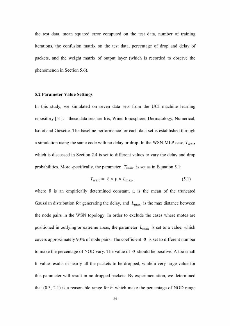
84

the test data, mean squared error computed on the test data, number of training

iterations, the confusion matrix on the test data, percentage of drop and delay of

packets, and the weight matrix of output layer (which is recorded to observe the

phenomenon in Section 5.6).

5.2 Parameter Value Settings

In this study, we simulated on seven data sets from the UCI machine learning

repository [51]: these data sets are Iris, Wine, Ionosphere, Dermatology, Numerical,

Isolet and Giesette. The baseline performance for each data set is established through

a simulation using the same code with no delay or drop. In the WSN-MLP case,·̂ 813

which is discussed in Section 2.4 is set to different values to vary the delay and drop

probabilities. More specifically, the parameter ·̂ 813 is set as in Equation 5.1:

·�� = ϑ × μ × ¸��, (5.1)

where ϑ is an empirically determined constant, μ is the mean of the truncated

Gaussian distribution for generating the delay, and ¸�� is the max distance between

the node pairs in the WSN topology. In order to exclude the cases where motes are

positioned in outlying or extreme areas, the parameter ¸�� is set to a value, which

covers approximately 90% of node pairs. The coefficient ϑ is set to different number

to make the percentage of NOD vary. The value of ϑ should be positive. A too small

ϑ value results in nearly all the packets to be dropped, while a very large value for

this parameter will result in no dropped packets. By experimentation, we determined

that (0.3, 2.1) is a reasonable range forϑ which make the percentage of NOD range

85

from 0.4% to 99%. Consequently, in this study, we equally divided the range of

values for ϑ and therefore set it to 0.3, 0.6, 0.9, 1.2, 1.5, 1.8 and 2.1.

Simulation on each data set is repeated five times with different initial weights. The

only exception is the case of Giesette dataset due to its high computational cost. The

packets carrying neuron outputs and error signals are subject to delay and drop during

the training phase only and not during the testing phase.

5.3 Simulation Results

The simulation study reports classification accuracy, training iteration count, mean

squared error (MSE), and the percentage of NOD (probabilities of delay and drop).

All tables in this subsection, namely Tables 5.1 through 5.28 have the same format: a

specific run is repeated for seven different values of the parameter ϑ and the

corresponding ·�� value is shown in the first column. The topology varies for the

5 runs, therefore, for some datasets ¸�� in the Equation 5.1 is not consistant. This

leads to a range of ·�� value. Furthermore, the same initial weights are employed

for different values of ϑ during a given run. The first seven rows of in these tables

are the results due to simulation of WSN-MLP for different values of the parameterϑ.

The last row in each table is the result of simulation of MLP with no delay or drop.

The figures present the classification accuracy, MSE, and training iteration count

versus different percentage values of NOD.

86

5.3.1 Iris Dataset

Figure 5-1 shows the classification accuracy versus the percentage of NOD of the

WSN-MLP and the MLP on the test data for the Iris dataset. The classification

accuracy of WSN-MLP is close to MLP except for the cases when percentage of

NOD goes above 64.5%. The highest accuracy of 96% is achieved by both the

WSN-MLP and the MLP. Figure 5-2 plots the training iteration under different

percentages of NOD. The training iteration count for the WSN-MLP varies greatly

while the MLP demonstrates very stable and small values for the training iterations

and the mean value for the WSN-MLP is significantly more than that of the MLP. The

training iterations for the WSN-MLP shows no trend when the percentage of NOD

increases towards the upper bound value. Figure 5-2 shows the MSE under different

percentage of NOD. The MSE shows no significant difference for the percentage of

NOD less than 42.5%, while growing very rapidly beyond that value. The WSN-MLP

can hardly learn when the percentage of NOD is larger than 80%.

Table 5.1: Classification Accuracy Results for Iris Data Set

·�� Run #1 Run #2 Run #3 Run #4 Run #5

[39, 58.5] 76.0% 34.0% 66.0% 34.0% 82.0%

[78, 117] 88.0% 34.0% 96.0% 54.0% 74.0%

[117, 175.5] 96.0% 94.0% 94.0% 94.0% 96.0%

[156, 234] 94.0% 96.0% 96.0% 94.0% 96.0%

[195, 292.5] 96.0% 96.0% 96.0% 96.0% 96.0%

[234, 351] 94.0% 96.0% 94.0% 94.0% 96.0%

[273, 409.5] 94.0% 96.0% 94.0% 96.0% 96.0%

0 96.0% 96.0% 96.0% 96.0% 96.0%

87

Table 5.2: Training Iterations for Iris Data Set


[39, 58.5] 71 33 79 83 199

[78, 117] 203 14 134 340 295

[117, 175.5] 114 191 56 98 213

[156, 234] 95 239 12 144 355

[195, 292.5] 370 147 330 385 238

[234, 351] 131 147 223 45 392

[273, 409.5] 85 147 202 406 63

0 31 31 29 30 36

Table 5.3: MSE for Iris Data Set


[39, 58.5] 0.1998 0.2221 0.2188 0.2235 0.2029

[78, 117] 0.0840 0.2221 0.0954 0.1800 0.1328

[117, 175.5] 0.0242 0.0286 0.0958 0.0618 0.0630

[156, 234] 0.0292 0.0228 0.0392 0.0293 0.0290

[195, 292.5] 0.0215 0.0231 0.0219 0.0218 0.0220

[234, 351] 0.0264 0.0233 0.0265 0.0230 0.0233

[273, 409.5] 0.0220 0.0233 0.0275 0.0239 0.0215

0 0.0214 0.0214 0.0213 0.0212 0.0206

Table 5.4: Percentage of Neuron Output Delay for Iris Data Set


[39, 58.5] 82.9% 95.8% 90.9% 97.6% 96.9%

[78, 117] 53.1% 80.5% 64.0% 87.8% 82.7%

[117, 175.5] 38.1% 39.7% 60.1% 47.8% 64.5%

[156, 234] 16.0% 20.3% 36.9% 28.6% 42.5%

[195, 292.5] 8.7% 12.3% 19.5% 17.4% 25.0%

[234, 351] 6.9% 10.0% 10.6% 12.0% 15.5%

[273, 409.5] 6.8% 9.7% 7.0% 10.9% 11.9%

0 0.0% 0.0% 0.0% 0.0% 0.0%

88

Figure 5-1 Classification Accuracy vs. Percentage of NOD for Iris Data Set

Figure 5-2 MSE vs. Percentage of NOD for Iris Data Set

0%

20%

40%

60%

80%

100%

0 0 0

6.9

%

8.7

%

10

.0%

10

.9%

12

.0%

15

.5%

17

.4%

20

.3%

28

.6%

38

.1%

42

.5%

53

.1%

64

.0%

80

.5%

82

.9%

90

.9%

96

.9%

Cla

ssif

ica

tio

n A

ccu

racy

Percentage of NOD

Iris

0

0.05

0.1

0.15

0.2

0.25

0 0 0

6.9

%

8.7

%

10

.0%

10

.9%

11

.9%

15

.5%

17

.4%

20

.3%

28

.6%

38

.1%

42

.5%

53

.1%

64

.0%

80

.5%

82

.9%

90

.9%

96

.9%

MS

E

Percentage of NOD

Iris

89

Figure 5-3 Training Iterations vs. Percentage of NOD for Iris Data Set

5.3.2 Wine Dataset


WSN-MLP and the MLP on the test data for the Wine dataset. The classification

accuracy achieved by the WSN-MLP is similar to that of the MLP when the

corresponding percentage of NOD is below 66.6%. The highest accuracy is 98.3%

and achieved by both the WSN-MLP and the MLP. Figure 5-4 shows the training

iteration count versus percentage of NOD, which appears very similar to that the for

Iris data set. The training iteration count of the WSN-MLP appears unstable and the

mean value is significantly higher than that of the MLP. Figure 5-3 presents the MSE

against the percentage of NOD. From the figure, when the percentage of NOD is less

than 72.3% the MSE value for both designs are comparable while the WSN-MLP

tends to generate more MSE compared to those by the MLP. The MSE for the

WSN-MLP significantly increases at the percentage of NOD value of 72.3% and the

0

100

200

300

400

500

0 0 0

6.9

%

8.7

%

10

.0%

10

.9%

12

.0%

15

.5%

17

.4%

20

.3%

28

.6%

38

.1%

42

.5%

53

.1%

64

.0%

80

.5%

82

.9%

90

.9%

96

.9%

Tra

inin

g I

tera

tio

ns

Percentage of NOD

Iris

90

learning capability becomes very low once the percentage of NOD is more than

78.5%.

Table 5.5: Classification Accuracy for Wine Data Set


58.5 56.7% 70.0% 86.7% 40.0% 71.7%

117 61.7% 83.3% 98.3% 63.3% 98.3%

175.5 98.3% 98.3% 96.7% 98.3% 98.3%

234 98.3% 96.7% 96.7% 98.3% 98.3%

292.5 96.7% 96.7% 98.3% 98.3% 96.7%

351 98.3% 96.7% 96.7% 96.7% 98.3%

409.5 96.7% 98.3% 96.7% 98.3% 98.3%

0 96.7% 96.7% 98.3% 96.7% 98.3%

Table 5.6: Training Iterations for Wine Data Set


58.5 187 398 419 56 398

117 500 132 78 342 287

175.5 334 301 206 229 29

234 197 241 40 172 10

292.5 46 87 226 452 83

351 122 46 134 344 27

409.5 23 209 134 127 172

0 10 11 11 10 11

91

Table 5.7: MSE for Wine Data Set


58.5 0.1729 0.1517 0.1527 0.2181 0.1524

117 0.1381 0.0872 0.0989 0.1856 0.0160

175.5 0.0157 0.0165 0.0161 0.0135 0.0127

234 0.0145 0.0135 0.0151 0.0140 0.0095

292.5 0.0166 0.0176 0.0130 0.0114 0.0160

351 0.0133 0.0120 0.0157 0.0158 0.0096

409.5 0.0131 0.0140 0.0171 0.0126 0.0155

0 0.0111 0.0098 0.0101 0.0093 0.0096

Table 5.8: Percentage of Neuron Output Delay for Wine Data Set


58.5 96.6% 91.2% 94.8% 99.5% 93.1%

117 78.5% 72.3% 74.4% 81.9% 68.0%

175.5 40.9% 66.6% 42.9% 46.0% 65.2%

234 16.4% 46.3% 21.9% 24.8% 42.5%

292.5 5.9% 24.5% 12.7% 13.5% 22.4%

351 3.2% 12.0% 9.9% 10.2% 11.2%

409.5 2.8% 8.4% 9.3% 9.7% 7.1%

0 0.0% 0.0% 0.0% 0.0% 0.0%

Figure 5-4 Classification Accuracy vs. Percentage of NOD for Wine Data Set

0.0%

20.0%

40.0%

60.0%

80.0%

100.0%

0 0 0

3.2

%

7.1

%

9.3

%

9.9

%

11

.2%

12

.7%

16

.4%

22

.4%

24

.8%

42

.5%

46

.0%

65

.2%

68

.0%

74

.4%

81

.9%

93

.1%

96

.6%

Cla

ssif

ica

tio

n A

ccu

racy

Percentage of NOD

Wine

92

Figure 5-5 MSE vs. Percentage of NOD for Wine Data Set

Figure 5-6 Training Iterations vs. Percentage of NOD for Wine Data Set

5.3.3 Ionosphere Dataset


WSN-MLP and the MLP on the test data for the Ionosphere dataset. For

approximately 90% percent of the trials, the classification accuracy achieved by the

WSN-MLP is lower than that of the MLP. The highest accuracy is 94% and achieved

0

0.05

0.1

0.15

0.2

0.25

0 0 0

3.2

%

7.1

%

9.3

%

9.9

%

11

.2%

12

.7%

16

.4%

22

.4%

24

.8%

42

.5%

46

.0%

65

.2%

68

.0%

74

.4%

81

.9%

93

.1%

96

.6%

MS

E

Percentage of NOD

Wine

0

100

200

300

400

500

600

0 0 0

3.2

%

7.1

%

9.3

%

9.9

%

11

.2%

12

.7%

16

.4%

22

.4%

24

.8%

42

.5%

46

.0%

65

.2%

68

.0%

74

.4%

81

.9%

93

.1%

96

.6%

Tra

inin

g I

tera

tio

ns

Percentage of NOD

Wine

93

by the MLP. Figure 5-5 plots the relationship between MSE and the percentage of

NOD. It shows that the WSN-MLP tends to generate more MSE as the percentage of

NOD increases. Figure 5-6 presents the plot of training iteration count against the

percentage of NOD. The training iteration count of the WSN-MLP tends to increase

and fluctuate more as the percentage of NOD exceeds 35.4%.

Table 5.9: Classification Accuracy for Ionosphere Data Set


[39, 58.5] 80.3% 64.1% 76.1% 64.1% 79.5%

[78, 117] 82.1% 80.3% 84.6% 81.2% 83.8%

[117, 175.5] 82.1% 82.9% 88.0% 83.8% 83.8%

[156, 234] 86.3% 87.2% 82.1% 93.2% 83.8%

[195, 292.5] 90.6% 83.8% 91.5% 82.9% 83.8%

[234, 351] 90.6% 88.9% 88.0% 90.6% 87.2%

[273, 409.5] 84.6% 86.3% 90.6% 86.3% 85.5%

0 94.0% 90.6% 90.6% 90.6% 90.6%

Table 5.10: Training Iterations for Ionosphere Data Set

·�� ϑ Run #1 Run #2 Run #3 Run #4 Run #5

[39, 58.5] 0.3 141 48 96 4 143

[78, 117] 0.6 217 344 191 235 133

[117, 175.5] 0.9 14 500 313 167 279

[156, 234] 1.2 46 45 7 69 37

[195, 292.5] 1.5 157 181 96 104 6

[234, 351] 1.8 57 94 169 69 106

[273, 409.5] 2.1 24 70 121 31 106

0 No NOD 45 34 38 41 45

94

Table 5.11: MSE for Ionosphere Data Set


[39, 58.5] 0.1764 0.2273 0.1841 0.2281 0.1735

[78, 117] 0.1491 0.1409 0.1411 0.1467 0.1329

[117, 175.5] 0.1506 0.1551 0.1229 0.1367 0.1451

[156, 234] 0.1100 0.1098 0.1464 0.0674 0.1561

[195, 292.5] 0.0848 0.1346 0.0763 0.1228 0.1419

[234, 351] 0.0728 0.1067 0.0959 0.0848 0.1034

[273, 409.5] 0.1258 0.1036 0.0821 0.1177 0.1154

No NOD 0.0511 0.0754 0.0730 0.0698 0.0753

Table 5.12: Percentage of Neuron Output Delay for Ionosphere Data Set


[39, 58.5] 96.2% 95.3% 93.0% 93.6% 92.9%

[78, 117] 77.7% 78.1% 69.4% 71.9% 70.1%

[117, 175.5] 42.2% 55.8% 38.7% 41.4% 42.8%

[156, 234] 18.3% 35.3% 16.1% 19.3% 22.0%

[195, 292.5] 9.0% 20.5% 6.4% 9.9% 12.9%

[234, 351] 6.2% 11.4% 4.0% 6.7% 9.9%

[273, 409.5] 5.9% 7.5% 3.6% 6.3% 9.6%

0 0.0% 0.0% 0.0% 0.0% 0.0%

Figure 5-7 Classification Accuracy vs. Percentage of NOD for Ionosphere Data Set

0.0%

20.0%

40.0%

60.0%

80.0%

100.0%

0 0 0

4.0

%

6.2

%

6.4

%

7.5

%

9.6

%

9.9

%

12

.9%

18

.3%

20

.5%

35

.4%

41

.4%

42

.8%

69

.4%

71

.9%

78

.1%

93

.0%

95

.3%

Cla

ssif

ica

tio

n A

ccu

racy

Percentage of NOD

Ionosphere

95

Figure 5-8 MSE vs. Percentage of NOD for Ionosphere Data Set

Figure 5-9 Training Iterations vs. Percentage of NOD for Ionosphere Data Set

5.3.4 Dermatology Dataset


WSN-MLP and the MLP on the test data for the Dermatology dataset. For the

percentage of NOD lower than 73%, the classification accuracy of the WSN-MLP is

0

0.05

0.1

0.15

0.2

0.25

0 0 0

4.0

%

6.2

%

6.4

%

7.5

%

9.6

%

9.9

%

12

.9%

18

.3%

20

.5%

35

.3%

41

.4%

42

.8%

69

.4%

71

.9%

78

.1%

93

.0%

95

.3%

MS

E

Percentage of NOD

Ionosphere

0

100

200

300

400

500

600

0 0 0

4.0

%

6.2

%

6.4

%

7.5

%

9.6

%

9.9

%

12

.9%

18

.3%

20

.5%

35

.4%

41

.4%

42

.8%

69

.4%

71

.9%

78

.1%

93

.0%

95

.3%

Tra

inin

g I

tera

tio

ns

Percentage of NOD

Ionosphere

96

similar to those of the MLP. For half of the trials the WSN-MLP scores better in

terms of the classification accuracy when compared to the MLP. The highest accuracy

is 96.9% and achieved by the WSN-MLP. Figure 5-7 depicts the MSE versus

different percentages of NOD. The MSE is close to each other at low percentages of

NOD but suddenly begins to increase at or above 73% of NOD. When the percentage

of NOD is lower than 73%, in 12 trials out of 28, MSE of the WSN-MLP is less than

the MSE of the MLP. The lowest MSE is achieved by the WSN-MLP, which is

0.0120. Performance of WSN-MLP becomes poor when the percent of NOD is over

76.7%. Figure 5-8 indicates that the training iteration count for the dermatology

dataset tends to be fluctuating with a larger spread between extreme values when the

percentage of NOD increases.

Table 5.13: Classification Accuracy for Dermatology Data Set


78 48.0% 75.6% 51.2% 78.7% 74.0%

156 76.4% 91.3% 96.9% 95.3% 89.8%

234 96.1% 96.1% 95.3% 94.5% 95.3%

312 94.5% 94.5% 95.3% 95.3% 96.1%

390 95.3% 96.1% 94.5% 94.5% 94.5%

468 96.1% 94.5% 93.7% 96.1% 95.3%

546 94.5% 94.5% 95.3% 92.9% 93.7%

0 94.5% 94.5% 94.5% 93.7% 95.3%

97

Table 5.14: Training Iterations for Dermatology Data Set


78 500 259 62 138 176

156 38 63 88 312 89

234 500 133 98 45 247

312 89 37 76 74 51

390 120 208 197 48 72

468 20 91 200 20 112

546 73 235 212 111 60

0 22 81 19 34 79

Table 5.15: MSE for Dermatology Data Set


78 0.1035 0.0697 0.1082 0.0644 0.0852

156 0.0643 0.0416 0.0258 0.0120 0.0332

234 0.0137 0.0147 0.0156 0.0208 0.0147

312 0.0159 0.0157 0.0143 0.0154 0.0114

390 0.0165 0.0143 0.0153 0.0167 0.0154

468 0.0132 0.0173 0.0175 0.0127 0.0152

546 0.0164 0.0160 0.0158 0.0202 0.0166

0 0.0150 0.0168 0.0143 0.0169 0.0150

Table 5.16: Percentage of Neuron Output Delay for Dermatology Data Set


78 97.0% 93.9% 96.1% 93.4% 96.7%

156 76.7% 69.8% 73.0% 70.8% 74.5%

234 39.5% 45.2% 37.9% 41.7% 42.9%

312 13.8% 21.3% 17.0% 16.3% 20.8%

390 3.7% 11.4% 8.7% 6.3% 11.2%

468 1.2% 9.5% 7.0% 3.4% 9.0%

546 0.9% 9.3% 6.8% 3.0% 8.6%

0 0.0% 0.0% 0.0% 0.0% 0.0%

98

Figure 5-10 Classification Accuracy vs. Percentage of NOD for Dermatology Data Set

Figure 5-11 MSE vs. Percentage of NOD for Dermatology Data Set

0.0%

20.0%

40.0%

60.0%

80.0%

100.0%

0 0 0

1.2

%

3.5

%

6.3

%

7.0

%

8.7

%

9.3

%

11

.2%

13

.8%

17

.0%

21

.3%

39

.5%

42

.9%

69

.8%

73

.0%

76

.7%

93

.9%

96

.7%

Cla

ssif

ica

tio

n A

ccu

racy

Percentage of NOD

Dermatology

0

0.02

0.04

0.06

0.08

0.1

0.12

0 0 0

1.2

%

3.4

%

6.3

%

7.0

%

8.7

%

9.3

%

11

.2%

13

.8%

17

.0%

21

.3%

39

.5%

42

.9%

69

.8%

73

.0%

76

.7%

93

.9%

96

.7%

MS

E

Percentage of NOD

Dermatology

99

Figure 5-12 Training Iterations vs. Percentage of NOD for Dermatology Data Set

5.3.5 Numerical Dataset


WSN-MLP and the MLP on the test data for the Numerical dataset. The classification

accuracy values achieved by the WSN-MLP and the MLP are compatible when the

percentage of NOD is less than 76.4%. The difference in performance is within

2.5%. The highest accuracy is 97.2% and achieved by the WSN-MLP. Figure 5-9

shows the MSE is generally increasing slightly with the percentage of NOD increases

before it goes higher than 94.2%, then the MSE suddenly goes up. The learning

capability of WSN-MLP appears highly diminished when the percentage of NOD is

higher than 94.2%. In Figure 5-10, the training iteration count of the WSN-MLP

appears to be fluctuating with a relatively large variation and is generally more than

that of the MLP. The training iteration count does not indicate a definitive trend when

the percentage of NOD increases.

0

100

200

300

400

500

600

0 0 0

1.2

%

3.5

%

6.3

%

7.0

%

8.7

%

9.3

%

11

.2%

13

.8%

17

.0%

21

.3%

39

.5%

42

.9%

69

.8%

73

.0%

76

.7%

93

.9%

96

.7%

Tra

inin

g I

tera

tio

ns

Percentage of NOD

Dermatology

100

Table 5.17: Classification Accuracy for Numerical Data Set


117 65.5% 79.1% 75.8% 47.3% 66.6%

234 96.7% 95.2% 96.0% 94.5% 95.7%

351 94.5% 94.6% 95.8% 96.1% 95.2%

468 96.3% 95.5% 96.4% 95.4% 95.7%

585 95.8% 96.1% 96.4% 96.4% 96.3%

702 96.1% 96.3% 96.3% 97.2% 96.1%

819 96.4% 95.5% 96.7% 94.5% 96.6%

0 96.9% 96.6% 96.6% 96.7% 96.6%

Table 5.18: Training Iterations for Numerical Data Set


117 34 35 61 78 194

234 65 212 258 364 87

351 10 11 206 241 51

468 121 65 141 13 46

585 37 82 168 29 71

702 37 13 92 106 65

819 46 235 201 4 471

0 47 52 100 26 40

101

Table 5.19: MSE for Numerical Data Set


117 0.05852 0.04796 0.05469 0.07148 0.04926

234 0.00712 0.00925 0.00729 0.01039 0.00714

351 0.00957 0.00920 0.00899 0.00741 0.00852

468 0.00550 0.00812 0.00714 0.00813 0.00678

585 0.00600 0.00637 0.00644 0.00623 0.00627

702 0.00601 0.00803 0.00644 0.00466 0.00552

819 0.00527 0.00631 0.00690 0.01067 0.00592

0 0.00484 0.00585 0.00540 0.00518 0.00607

Table 5.20: Percentage of Neuron Output Delay for Numerical Data Set


117 96.3% 95.4% 95.5% 97.4% 94.2%

234 69.4% 71.3% 71.0% 76.4% 65.4%

351 36.2% 35.3% 37.2% 38.8% 34.1%

468 9.2% 11.6% 17.2% 17.0% 11.6%

585 1.5% 5.6% 12.0% 9.6% 4.3%

702 0.6% 5.0% 11.7% 9.0% 3.1%

819 0.4% 4.8% 11.2% 8.7% 2.8%

0 0.0% 0.0% 0.0% 0.0% 0.0%

Figure 5-13 Classification Accuracy vs. Percentage of NOD for Numerical Data Set

0.0%

20.0%

40.0%

60.0%

80.0%

100.0%

0 0 0

0.4

%

2.8

%

4.3

%

4.8

%

8.7

%

9.2

%

11

.2%

11

.6%

12

.0%

17

.2%

35

.3%

37

.2%

65

.4%

71

.0%

76

.4%

95

.4%

96

.3%

Cla

ssif

ica

tio

n A

ccu

racy

Percentage of NOD

Numerical

102

Figure 5-14 MSE vs. Percentage of NOD for Numerical Data Set

Figure 5-15 Training Iterations vs. Percentage of NOD for Numerical Data Set

5.3.6 Isolet Dataset


WSN-MLP and the MLP on the test data for the Isolet dataset. The classification

accuracy for the WSN-MLP is very similar to that of the MLP except for those trials

0

0.01

0.02

0.03

0.04

0.05

0.06

0.07

0.08

0 0 0

0.4

%

2.8

%

4.3

%

4.8

%

8.7

%

9.2

%

11

.2%

11

.6%

12

.0%

17

.2%

35

.3%

37

.2%

65

.4%

71

.0%

76

.4%

95

.4%

96

.3%

MS

E

Percentage of NOD

Numerical

0

100

200

300

400

500

0 0 0

0.4

%

2.8

%

4.3

%

4.8

%

8.7

%

9.2

%

11

.2%

11

.6%

12

.0%

17

.2%

35

.3%

37

.2%

65

.4%

71

.0%

76

.4%

95

.4%

96

.3%

Tra

inin

g I

tera

tio

ns

Percentage of NOD

Numerical

103

when percentage of NOD is higher than 94.8%. Otherwise, the difference in

performance is within 1%. The highest accuracy is 96.3% and achieved by the

WSN-MLP. From Figure 5-11, the MSE of the WSN-MLP shows no difference with

the MLP when the percentage of NOD is less than 74.8%. Table 5.22 lists the training

iterations of the WSN-MLP and the MLP for the Isolet data set. When the percentage

of NOD exceeds 94.8% the performance of WSN-MLP suffers dramatically. Figure

5-12 depicts the training iteration count against the percentage of NOD. The training

iterations of the WSN-MLP are significantly higher than those for the MLP and start

fluctuating greatly once the percentage of NOD exceeds 9%.

Table 5.21: Classification Accuracy for Isolet Data Set


175.5 76.2% 59.5% 71.2% 74.8% 61.2%

351 95.1% 95.6% 94.9% 95.2% 95.2%

526.5 95.5% 96.0% 95.4% 96.0% 95.7%

702 95.7% 95.8% 96.0% 95.8% 96.0%

877.5 95.9% 96.2% 95.9% 96.0% 95.8%

1053 96.0% 95.5% 96.0% 96.3% 95.9%

1228.5 96.0% 95.9% 96.0% 96.3% 95.9%

0 95.4% 95.6% 95.8% 95.7% 95.3%

104

Table 5.22: Training Iterations for Isolet Data Set


175.5 233 124 78 79 300

351 300 300 54 89 76

526.5 217 85 43 300 134

702 300 113 177 115 300

877.5 92 201 107 220 204

1053 92 178 81 300 195

1228.5 92 179 107 300 195

0 96 46 67 69 39

Table 5.23: MSE for Isolet Data Set


175.5 0.01407 0.02104 0.01686 0.01682 0.02172

351 0.00350 0.00328 0.00370 0.00338 0.00339

526.5 0.00291 0.00276 0.00324 0.00302 0.00283

702 0.00278 0.00277 0.00276 0.00313 0.00274

877.5 0.00279 0.00268 0.00295 0.00296 0.00280

1053 0.00276 0.00280 0.00280 0.00274 0.00280

1228.5 0.00276 0.00278 0.00293 0.00273 0.00280

0 0.00279 0.00292 0.00286 0.00280 0.00296

Table 5.24: Percentage of Neuron Output Delay for Isolet Data Set


175.5 94.8% 97.1% 96.0% 95.9% 96.3%

351 70.1% 74.7% 73.3% 74.8% 74.0%

526.5 32.9% 35.9% 38.4% 40.9% 36.2%

702 9.0% 11.8% 16.0% 17.5% 13.0%

877.5 2.6% 5.7% 10.1% 12.0% 7.2%

1053 2.1% 5.0% 9.4% 11.5% 6.6%

1228.5 2.1% 5.0% 9.4% 11.5% 6.6%

0 0.0% 0.0% 0.0% 0.0% 0.0%

105

Figure 5-16 Classification Accuracy vs. Percentage of NOD for Isolet Data Set

Figure 5-17 MSE vs. Percentage of NOD for Isolet Data Set

0.0%

20.0%

40.0%

60.0%

80.0%

100.0%

0 0 0

2.1

%

5.0

%

5.7

%

6.6

%

9.0

%

9.4

%

11

.5%

11

.9%

13

.0%

17

.5%

35

.9%

38

.4%

70

.1%

74

.0%

74

.8%

95

.9%

96

.3%

Cla

ssif

ica

tio

n A

ccu

racy

Percentage of NOD

Isolet

0

0.005

0.01

0.015

0.02

0.025

0 0 0

2.1

%

5.0

%

5.7

%

6.6

%

9.0

%

9.4

%

11

.5%

11

.8%

13

.0%

17

.5%

35

.9%

38

.4%

70

.1%

74

.0%

74

.8%

95

.9%

96

.3%

MS

E

Percentage of NOD

Isolet

106

Figure 5-18 Training Iterations vs. Percentage of NOD for Isolet Data Set

5.3.7 Gisette Dataset


WSN-MLP and the MLP on the test data for the Gisette dataset. In general, the

classification accuracy achieved by WSN-MLP is very similar to that of the MLP.

The difference for all the trials is within 1.5%. The highest accuracy is 97.2% and

achieved by the WSN-MLP. Figure 5-13 shows that the training iteration count for

this data set is unstable. From Figure 5-14, the MSE of the WSN-MLP does not

change even when the percentage of NOD becomes very high. For instance, for 97%

NOD, the MSE of 0.034 for the WSN-MLP is very close to the MSE of the MLP

which is 0.0247. It shows that the WSN-MLP is capable of learning this data set even

when the probability of NOD is very large.

0

50

100

150

200

250

300

350

0 0 0

2.1

%

5.0

%

5.7

%

6.6

%

9.0

%

9.4

%

11

.5%

11

.9%

13

.0%

17

.5%

35

.9%

38

.4%

70

.1%

74

.0%

74

.8%

95

.9%

96

.3%

Tra

inin

g I

tera

tio

ns

Percentage of NOD

Isolet

107

Table 5.25: Classification Accuracy for Gisette Data Set

·�� Run #1 Run #2 Run #3

[136.5, 156] 95.6% 95.4% 96.1%

[273, 312] 96.0% 96.0% 95.5%

[409.5, 468] 95.5% 94.2% 96.4%

[546, 624] 97.2% 96.5% 96.6%

[682.5, 780] 96.8% 97.1% 96.3%

[819, 936] 96.7% 95.3% 96.8%

[955.5, 1092] 96.9% 96.2% 96.7%

0 97.0% 96.9% 96.7%

Table 5.26: Training Iterations for Gisette Data Set

·�� Run #1 Run #2 Run #3

[136.5, 156] 39 153 20

[273, 312] 159 112 71

[409.5, 468] 16 89 23

[546, 624] 73 300 172

[682.5, 780] 36 300 65

[819, 936] 54 8 90

[955.5, 1092] 55 227 162

0 145 53 70

Table 5.27: MSE for Gisette Data Set

·�� Run #1 Run #2 Run #3

[136.5, 156] 0.0330 0.0340 0.0401

[273, 312] 0.0251 0.0257 0.0290

[409.5, 468] 0.0334 0.0436 0.0272

[546, 624] 0.0250 0.0293 0.0276

[682.5, 780] 0.0271 0.0256 0.0311

[819, 936] 0.0275 0.0376 0.0274

[955.5, 1092] 0.0250 0.0326 0.0258

0 0.0234 0.0247 0.0261

108

Table 5.28: Percentage of Neuron Output Delay for Gisette Data Set

·�� Run #1 Run #2 Run #3

[136.5, 156] 96.3% 97.0% 96.5%

[273, 312] 76.6% 75.8% 77.7%

[409.5, 468] 48.4% 41.8% 44.9%

[546, 624] 23.0% 13.8% 18.2%

[682.5, 780] 12.1% 3.5% 7.7%

[819, 936] 10.5% 1.5% 6.4%

[955.5, 1092] 10.4% 1.4% 6.4%

0 0.0% 0.0% 0.0%

Figure 5-19 Classification Accuracy vs. Percentage of NOD for Gisette Data Set

0.0%

20.0%

40.0%

60.0%

80.0%

100.0%

0 0 0

1.4

%

1.5

%

3.5

%

6.4

%

6.4

%

7.7

%

10

.4%

10

.5%

12

.1%

13

.8%

18

.2%

23

.0%

41

.8%

44

.9%

48

.4%

75

.8%

76

.6%

77

.7%

96

.3%

96

.5%

97

.0%

Cla

ssif

ica

tio

n A

ccu

racy

Percentage of NOD

Gisette

109

Figure 5-20 MSE vs. Percentage of NOD for Numerical Data Set

Figure 5-21 Training Iterations vs. Percentage of NOD for Gisette Data Set

0

0.01

0.02

0.03

0.04

0.05

0 0 0

1.4

%

1.5

%

3.5

%

6.4

%

6.4

%

7.7

%

10

.4%

10

.5%

12

.1%

13

.8%

18

.2%

23

.0%

41

.8%

44

.9%

48

.4%

75

.8%

76

.6%

77

.7%

96

.3%

96

.5%

97

.0%

MS

E

Percentage of NOD

Gisette

0

50

100

150

200

250

300

350

0 0 0

1.4

%

1.5

%

3.5

%

6.4

%

6.4

%

7.7

%

10

.4%

10

.5%

12

.1%

13

.8%

18

.2%

23

.0%

41

.8%

44

.9%

48

.4%

75

.8%

76

.6%

77

.7%

96

.3%

96

.5%

97

.0%

Tra

inin

g I

tera

tio

ns

Percentage of NOD

Gisette

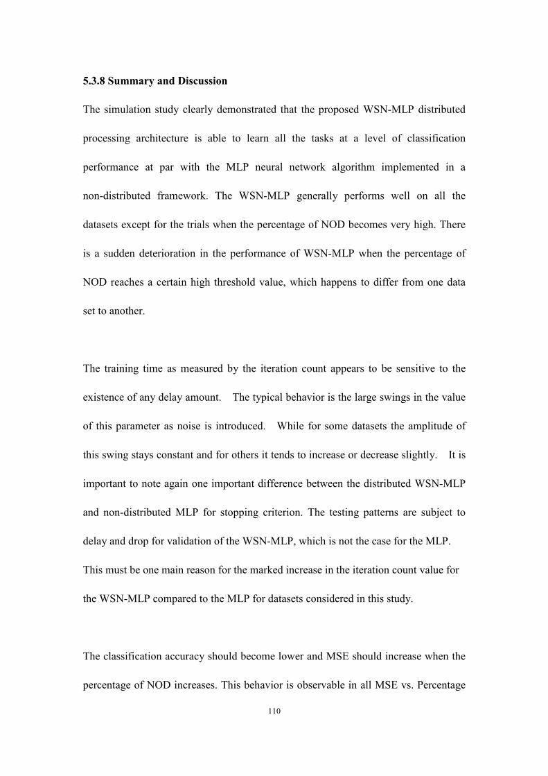
110

5.3.8 Summary and Discussion

The simulation study clearly demonstrated that the proposed WSN-MLP distributed

processing architecture is able to learn all the tasks at a level of classification

performance at par with the MLP neural network algorithm implemented in a

non-distributed framework. The WSN-MLP generally performs well on all the

datasets except for the trials when the percentage of NOD becomes very high. There

is a sudden deterioration in the performance of WSN-MLP when the percentage of

NOD reaches a certain high threshold value, which happens to differ from one data

set to another.

The training time as measured by the iteration count appears to be sensitive to the

existence of any delay amount. The typical behavior is the large swings in the value

of this parameter as noise is introduced. While for some datasets the amplitude of

this swing stays constant and for others it tends to increase or decrease slightly. It is

important to note again one important difference between the distributed WSN-MLP

and non-distributed MLP for stopping criterion. The testing patterns are subject to

delay and drop for validation of the WSN-MLP, which is not the case for the MLP.

This must be one main reason for the marked increase in the iteration count value for

the WSN-MLP compared to the MLP for datasets considered in this study.

The classification accuracy should become lower and MSE should increase when the

percentage of NOD increases. This behavior is observable in all MSE vs. Percentage

111

of NOD charts with one interesting deviation. For most datasets, the MSE stays

within a small range of values for notable increases in the value of delay and drop as

indicated by the NOD parameter: this indicates that the WSN-MLP has tolerance to

noise. Others researchers also confirmed this attribute [109, 110], who reported of

adding a controlled amount of noise during training which appeared to increase the

generalization ability of the MLP. During the simulation study, we found a notable

behavior of the MLP implemented in WSN. The connections between the neurons

which affected by noise tends to be weakened during training. This behavior of MLP

reduces the impact of noise. Section 5.6 shows the detail study of this observation.

5.4 Performance Comparison with Studies Reported in Literature

In this section, the classification accuracy performance of the WSN-MLP on all seven

datasets are compared to the performances of various algorithms as reported in the

machine learning literature on the same datasets [93-108]. The purpose of this

comparison is to evaluate the performance of WSN-MLP within the larger context of

machine learning approaches. In the Tables 5.29 through 5.35, the max and min

performance of WSN-MLP as well as the performance of the non-distributed MLP

(through in-house implementation) are reported for comparison. The minimum values

are chosen for the smallest possible value of the NOD percentage such that the

classification accuracy plot does not exhibit the sudden decrease in Figures 5.1, 5.4,

5.7, 5.10, 5.13, 5.16, and 5.19. The maximum values are the 60% of the values

achived for the cases when the NOD does not exceed the corresponding threshold.

112

These tables show the classification accuracy values ordered in a descending manner

with the value for our simulation results in bold. Results across all the tables show

that the WSN-MLP has a competitive performance with a very diverse and large set

of machine learning classifiers. The maximum performance for the WSN-MLP is

among the upper-middle tier of the entire set of classifier included in these tables. It

is also worth noting that the WSN-MLP performance even surpasses those of the

entire set of machine learning classification algorithms for the Dermatology dataset.

Table 5.29: Comparison of Classification Accuracy for Iris Data Set

Algorithm Full Name/Percentage of NOD Threshold Reference Accuracy

QNN Quantum Neural Network [93] 98.0%

C&S SVM Crammer and Singer Support Vector Machine [94] 97.3%

SVM Support Vector Machine [95] 96.7%

WSN-MLP (max) Percentage of NOD Threshold = 42.5% 96.0%

MLP 96.0%

C4.5 C4.5 Tree [95] 96.0%

NBC Naive Bayes Classifier [95] 94.0%

LBR Logitboost Bayes Classifier [96] 93.2%

WSN-MLP (min) Percentage of NOD Threshold = 64.5% 88.0%

Table 5.30: Comparison of Classification Accuracy for Wine Data Set

Algorithm Full Name/ Percentage of NOD Threshold Reference Accuracy


LBR Logitboost Bayes Classifier [96] 98.7%


MLP 98.3%

Bayesian Network Bayesian Network [96] 98.2%


M-SVM Multiclass Support Vector Machine [97] 96.6%

C4.5 C4.5 Tree [98] 92.8%

M-RLP Multicategory Robust Linear Programming [97] 91.0%

113

Table 5.31: Comparison of Classification Accuracy for Ionosphere Data Set:



MLP 94.0%

Refined GP Refined Genetic Programming Evolved Tree [100] 92.3%

C4.5 C4.5 Tree [100] 91.1%


Bayesian network Bayesian Network [96] 89.5%

FSS Forward Sequential Selection [101] 87.5%


Table 5.32: Comparison of Classification Accuracy for Dermatology Data Set



MLP 95.3%

C4.5+GA C4.5 Tree with Genetic Algorithm [102] 94.5%

VFI5 Voting Feature Intervals [103] 93.2%

FSS Forward Sequential Selection [101] 90.4%

WSN-MLP (min) Percentage of NOD Threshold =74.5% 89.8%

C4.5 C4.5 Tree [101] 86.0%

114

Table 5.33: Comparison of Classification Accuracy for Numerical Data Set


MLP with feature

selection method

MLP with feature selection method [103] 98.5%

MLP 96.6%


KNN K-Nearest Neighbor [103] 95.8%

LVQ Learning Vector Quantization [104] 94.9%


kNN(PCA) K-Nearest Neighbor with Principal component

analysis [105] 80.4%

kNN(LDA) K-Nearest Neighbor with Linear discriminant


Table 5.34: Comparison of Classification Accuracy for Isolet Data Set



kLOGREG Kernelized logistic regression [106] 97.0%


MLP 95.8%


NBC Naive Bayes [107] 84.4%

C4.5 C4.5 Tree [107] 80.2%

kNN(LDA) K-Nearest Neighbor with Principal component


kNN(PCA) K-Nearest Neighbor with Linear discriminant


115

Table 5.35: Comparison of Classification Accuracy for Gisette Data Set


LeNet Convolutional Neural Network [108] 99.2%

MLP (deskewing) Deskewing Multilayer Perceptron [108] 98.4%

MLP 97.0%


MLP Multilayer Perceptron [108] 96.4%

kNN K-Nearest Neighbor [108] 95.0%


Linear Classifier Logitboost Bayes Classifier [108] 88.0%

5.5 Time and Message Complexity

This section presents time and message complexity analysis for the WSN-MLP

architecture. It is important to note that this analysis is subject to a large number of

assumptions in regards to the WSN modeling and simulation as described in the prior

chapters.

5.5.1 Time Complexity of WSN-MLP

Assume that there are |PT| patterns in the training set and |PV| patterns in the

validation or testing set, respectively. Patterns in the training set PT are provided to

the MLP network (with two layers: one hidden and one output) one at a time.

Processing of each pattern is realized in parallel at the level of individual neuron

through distributed (and asynchronous) computation. Processing time by individual

neurons can be incorporated into the cumulative delay, Twait, which is mainly affected

by the delays originating due to MAC and routing protocols related requirements.

116

This delay parameter is a random variable and its value depends on numerous factors

as detailed earlier for its formulation and definition. Number of iterations,13 � ,

needed for convergence to a solution is a random variable also and its value depends

on the initial weight and parameter values, the stopping criterion, the data set

characteristics and its presentation order among other factors.

The time complexity, TC, for a WSN-MLP architecture can be estimated by the

following equation:

TC = 13 � × (|PT| +|PV|) × E{·̂ 813}, (5.2)

where E{} is the expected value operator. ·̂ 813 value is set in the simulation

according to the Equation 5.1. The mean value of truncated Gaussian distributionμ is

relocated to be 1 in the simulation. To get the actual value for time, μ need to be

multiplied by the value of per hop delay. From the literature survey [31-52], the range

of per hop delay is 2 ms to 226 ms and the expected value is 65 ms. The TC for all

the experiments in section 5.2 is shown in the Appendix B. TC calculation utilized

the parameter value set or obtained through the simulation study. For instance, the

mean value for the iteration count was calculated as the average of all values in Table

5.2 for the Iris dataset. Mean values for the other datasets used corresponding tables

for the iteration count parameter. Similarly, mean value for the simulation duration

was calculated by average all the entries in corresponding tables in Appendix B.

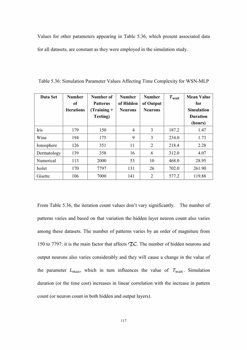
117

Values for other parameters appearing in Table 5.36, which present associated data

for all datasets, are constant as they were employed in the simulation study.

Table 5.36: Simulation Parameter Values Affecting Time Complexity for WSN-MLP

Data Set Number

of

Iterations

Number of

Patterns

(Training +

Testing)

Number

of Hidden

Neurons

Number

of Output

Neurons

¹.º»¼ Mean Value

for

Simulation

Duration

(hours)

Iris 179 150 4 3 187.2 1.47

Wine 194 175 9 3 234.0 1.73

Ionosphere 126 351 11 2 218.4 2.28

Dermatology 139 358 16 6 312.0 4.07

Numerical 113 2000 53 10 468.0 28.95

Isolet 170 7797 131 26 702.0 261.90

Gisette 106 7000 141 2 577.2 119.88

From Table 5.36, the iteration count values don’t vary significantly. The number of

patterns varies and based on that variation the hidden layer neuron count also varies

among these datasets. The number of patterns varies by an order of magniture from

150 to 7797: it is the main factor that affects TC. The number of hidden neurons and

output neurons also varies considerably and they will cause a change in the value of

the parameter ¸98¬, which in turn influences the value of ·�� . Simulation

duration (or the time cost) increases in linear correlation with the increase in pattern

count (or neuron count in both hidden and output layers).

118

5.5.2 Message Complexity of WSN-MLP

Message complexity will be measured by estimating the number of messages sent

which carry neuron output values. More specifically, each original or retransmission

of a given message that carries a neuron output value will be counted as a basic unit

of measurement.

During forward propagation cycle of the MLP training phase, 1� hidden neurons

send their outputs on the average to �23 neurons in the output layer. Each hop

requires retransmission of a given message. The hop distance between hidden neuron

i and output neuron j is denoted byℎ1�. Therefore, the total number of message

transmissions (including retransmissions) for a single training patter during forward

propagation cycle as represented by �;� is given by

��B =∑ ∑ ℎ��74]��

ℎ��1�� (5.3)

This cost is incurred for each training pattern in the training and validation sets,

namely PT and PV. The message complexity, MC, for the entire training episode

will depend on the size of the data set as well as problem properties, which, in

conjunction with other factors such as the initial values of weights and learning

parameters to name a few, will dictate the number of iterations to convergence.

Accordingly, the message complexity for the entire forward propagation phase is

estimated by the following equation:

119

MCFP = 13 �×(|PT| +|PV|)×��B, (5.4)

During the backward propagation phase, �23 output-layer neurons transmit their

outputs through 1� hidden-layer neurons, which result in the same amount of

messages as�;�. Assuming that online or incremental learning is implemented, the

above cost is incurred for each pattern in the training set for the duration of training

which will continue for a number of iterations to convergence. Hence the message

complexity for the backward propagation phase is estimated by

MCBP = 13 �×|PT|×��B, (5.5)

The overall message complexity for the training and validation combined is given by

MC = MCFP + MCBP = 13 �×(2|PT|+|PV|)×∑ ∑ ℎ��74]��

ℎ��1�� , (5.6)

The message complexity measurements for all the simulation experiments in Section

5.2 is presented in Appendix B. Table 5.37 presents the mean value of message

complexity measure for each data set. The message complexity depends on number of

iterations，number of training and testing patterns and the sum of hop distances

between every node pairs.

In Table 5.37, as the number of neurons (which is calculated as a function of pattern

count) in the hidden and output layers increases, the sum of distances (as measured by

the number of hops) between any two neurons (motes) also increases as does the

number of messages (packets). For a hundred-fold increase in the neuron count, the

120

total hop count increases thousand-fold, and the number of messages increases on the

order of thousand-fold as well. Therefore the message complexity results in the

dominant bound for the scalability of the WSN-MLP algorithm compared to the time

and space complexities.

Table 5.37: Parameters Affecting Message Complexity for WSN-MLP

Data Set Number

of

Iterations

Number

of

Training

Patterns

Number

of

Testing

Patterns

Number

of

Hidden

Neurons

Number

of

Output

Neurons

¾¾ ℎ��74]

��

ℎ��

1��

Number of

Packets

Transmitted

Iris 179 100 50 4 3 22 985,671

Wine 194 117 58 9 3 52 2,858,248

Ionosphere 126 234 117 11 2 45 3,260,205

Dermatology 139 239 119 16 6 269 23,755,353

Numerical 113 2000 666 53 10 2128 804,279,201

Isolet 170 5198 2599 131 26 20724 2,549,444,060

Gisette 106 4667 2333 141 2 1446 1,381,217,200

121

5.6 Weights of Neurons in Output Layer

We have noticed that the hop distance associated with a particular weight for the

connection between two neurons has an important effect on the value of that weight

during training. In more specific terms, those weights over multiple hops tend to

smaller magnitudes: the larger the hops distance is, the closer the weight magnitude to

the value of zero. In order to substantiate this observation, we conducted further

simulation work and results are presented in Tables 5.38 through 5.44. Each table

shows average value of the magnitudes of all the weights over a certain hop distance

for a particular percentage of NOD. Each column label in a table corresponds to a

certain hop distance.

Table 5.38: Average Values for Magnitudes of Weights over Different Hop Distances

vs. Neuron Output Delays for Iris Data Set

Hop Count

NOD 1 2 3

96.7% 0.902 0.326 0.552

77.9% 6.325 0.327 0.476

43.4% 6.084 2.002 0.632

18.4% 2.484 2.778 0.827

6.2% 1.853 3.151 2.247

3.1% 1.691 3.365 3.225

2.8% 1.627 3.331 3.318

0% 1.384 4.019 4.232

122


vs. Percentage of Neuron Output Delays for Wine Data Set

Hop Count

NOD 1 2 3

96.7% 1.097 0.278 0.550

77.1% 6.781 0.799 0.870

40.9% 4.932 1.906 0.521

16.5% 3.488 1.992 0.340

5.9% 2.787 1.496 1.247

3.2% 3.226 1.899 2.233

2.8% 3.270 1.990 2.447

0% 2.677 1.416 1.900


vs. Percentage of Neuron Output Delays for Ionosphere Data Set

Hop Count

NOD 1 2 3

97.8% 0.955 0.322 0.385

78.5% 5.168 0.364 0.319

39.0% 5.644 1.098 0.572

14.1% 1.965 1.137 0.598

3.4% 1.647 1.154 1.285

0.9% 3.259 2.677 3.604

0.4% 1.179 0.853 1.447

0% 1.163 0.853 1.451

123


vs. Percentage of Neuron Output Delays for Dermatology Data Set

Hop Count

NOD 1 2 3 4 5

95.8% 3.480 0.727 0.506 0.741 0.301

75.3% 4.140 1.508 0.469 0.425 0.348

39.5% 2.387 2.151 0.546 0.211 0.235

13.8% 1.915 2.081 1.428 0.359 0.178

3.7% 1.449 1.572 1.482 0.872 0.347

1.2% 1.103 1.191 1.128 0.805 0.551

0.9% 1.098 1.180 1.128 0.808 0.606

0% 1.021 1.098 1.068 0.755 0.565


vs. Percentage of Neuron Output Delays for Numerical Data Set:

Hop Count

NOD 1 2 3 4 5 6 7

96.1% 5.880 1.003 0.517 0.389 0.388 0.496 0.445

73.9% 8.923 8.361 2.172 0.660 0.821 0.586 0.629

36.2% 1.423 1.968 1.574 0.559 0.184 0.218 0.191

9.2% 0.746 0.756 0.790 0.749 0.585 0.186 0.161

1.5% 0.869 0.767 0.826 0.793 0.813 0.624 0.306

0.5% 0.725 0.620 0.692 0.665 0.680 0.652 0.635

0.4% 0.714 0.611 0.683 0.657 0.673 0.650 0.670

0% 0.752 0.649 0.724 0.700 0.719 0.708 0.724

124


vs. Percentage of Neuron Output Delays for Isolet Data Set

Hop Count

NOD 1 2 3 4 5 6 7 8 9 10 11

96.6% 3.499 1.657 0.256 0.220 0.140 0.113 0.098 0.100 0.095 0.098 0.098

72.8% 1.483 1.468 1.546 0.687 0.175 0.135 0.155 0.141 0.109 0.096 0.087

34.5% 0.642 1.071 0.939 0.912 0.812 0.364 0.139 0.128 0.176 0.161 0.169

9.7% 0.603 0.765 0.697 0.644 0.625 0.588 0.517 0.307 0.161 0.138 0.136

4.1% 0.570 0.716 0.646 0.610 0.590 0.570 0.533 0.503 0.383 0.246 0.109

3.6% 0.525 0.683 0.619 0.584 0.569 0.548 0.514 0.491 0.422 0.399 0.283

3.5% 0.525 0.683 0.619 0.584 0.569 0.548 0.514 0.491 0.422 0.400 0.309

0% 0.432 0.546 0.514 0.491 0.501 0.508 0.498 0.493 0.459 0.472 0.410


vs. Percentage of Neuron Output Delays for Gisette Data Set:

Hop Count

NOD 1 2 3 4 5 6 7 8 9

95.0% 5.270 0.176 0.168 0.135 0.112 0.099 0.101 0.098 0.086

74.9% 2.754 1.901 0.693 0.172 0.156 0.159 0.159 0.120 0.060

48.4% 1.217 0.624 0.535 0.513 0.133 0.112 0.139 0.141 0.030

23.0% 1.096 0.654 0.622 0.647 0.522 0.237 0.131 0.137 0.107

12.1% 0.895 0.552 0.510 0.484 0.366 0.450 0.370 0.236 0.010

10.5% 0.675 0.573 0.536 0.624 0.474 0.472 0.530 0.317 0.357

10.4% 0.796 0.486 0.456 0.511 0.440 0.404 0.505 0.341 0.127

0% 0.856 0.568 0.699 0.772 0.486 0.683 0.544 0.622 0.053

125

Simulation results in Tables 5.38 through 5.44 show that the weights for the

connection of the long hop distance node pairs tend to become smaller under high

percentage of NOD. For example, in Table 5.43, when the percentage of NOD is 96.6%

the magnitudes of weights for connections of the node pairs whose hop distance are 3

to 11 are significantly lower than the remaining two. When the percentage of NOD is

34.5% the magnitudes of weights for connections of the node pairs whose hop

distance are 6 to 11 are significantly lower than those of the rest. When the percentage

of NOD is 1.5% the magnitudes of weights for connection of the node pairs whose

hop distance is 7 is significantly lower than those of the others. When the percentage

of NOD is 5%, 4% and 0%, the weights for connections are similar to each other.

Under a certain percentage of NOD, the connection of a long hop distance node pairs

is affected by a larger amount of noise compare to a short hop distance node pairs. In

conclusion, the WSN-MLP training process tends to reduce the weights for the

connections depending on the amount of noise they are subjected to.

126

Chapter 6

Conclusions

6.1 Research Study Conclusions

The study reported in this thesis explored the feasibility, cost and scalability of

parallel and distributed neurocomputing on wireless sensor networks (WSN) as the

computational hardware-software platform. More specifically, the parallel and

distributed implementation of a multilayer perceptron neural network on a wireless

sensor network has been evaluated for feasibility, computational complexity and

scalability.

The research study employed a specially-developed simulation environment where

the “effects” of wireless sensor network operation were modeled. The delay and

drop phenomena for message packets carrying neuron outputs in WSNs have been

modeled empirically based on a comprehensive survey of the literature. A

probability distribution function for the delay and drop phenomena was defined and

employed in the simulation to model the effects of wireless communication protocol

stack and the distributed and parallel nature of computations and processing by the

WSN motes.

127

The multilayer perceptron neural network (MLP NN) was trained, and tested in an

entirely distributed and maximally parallel manner for several classification problems

from the machine learning literature. The MLP NN was trained with the

back-propagation with momentum learning and a validation procedure was employed

for the stopping criterion of the training process. An exploratory empirical simulation

study was performed to determine an appropriate value for the hidden layer neuron

count for each problem considered. Seven datasets with highly varied pattern (or

instance) and feature (or attribute) counts were employed for the simulation study.

The performance was evaluated through the measures of classification accuracy, and

total number of training iterations. For each dataset, a series of simulations were

completed for different values of mean values for the random variables delay and

drop. The WSN-MLP platform was able to tolerate the message delay and drop for

relatively significant increases in the values of these parameters and still learn the

classification function for all seven datasets tested. However, there was a gradual

but not dramatic deterioration in the classification accuracy and total training

iterations as the mean value for these parameters increased. Furthermore, there was

a sudden and substantial drop in the classification rate and equivalent jump in the

training iterations count once the amount of delay reached a threshold value, which

was different for each problem domain.

128

For comparative evaluation purposes, a non-distributed or centralized implementation

of the exact same MLP NN algorithm with parameter settings identical to those for

the WSN-MLP distributed versions was accomplished. The simulations show that, for

all datasets, the WSN-MLP was able to learn and perform as good as the MLP

implemented in a non-distributed framework. A performance comparison with other

studies reported in the machine learning literature had also been done. It shows that

the performance of WSN-MLP is comparable to those using numerous other

machine-learning algorithms, which practically included a very comprehensive set of

approaches proposed in the literature. In conclusion, this study demonstrated the using

of MLP on a WSN is feasible and the classification accuracy is competitive with other

prominent machine learning algorithms in that respect.

The analyses of space, time and message complexities have been done. Space

complexity of the proposed WSN-MLP design is constant or minimal due to

distributed storage of required algorithm or process memory space. The analysis of

time complexity shows it changes for different datasets. It is mainly affected by the

number of patterns in a particular dataset as well as the number of neurons in the

hidden and output layers. The message complexity, on the other hand, is primarily

affected by the number of hidden neurons and output neurons, and the total hop

distances in the WSN. The message complexity increases much faster than the time

complexity. Overall, the scalability for the WSN-MLP is promising but bounded

above by the communication cost or the message complexity.

129

6.2 Recommendations for Future Study

Hardware prototyping through actual motes need to be performed to validate the

feasibility of using the MLP on a WSN. The time and message complexity is worth to

be noted. More accurate data need to be acquired to refine the model of delay and

drop phenomena for packets carrying neuron outputs in WSNs. Larger data sets which

required more hidden neurons (up to thousands) should be employed to

comprehensive profile the performance of WSN-MLP. A new stopping criteria need

to be invented for WSN-MLP which is compensate for the noise caused by the drop

and delay of packets in WSN. Batch learning is worth to be tested in the further

simulation. The batch learning updates the weights after presentation of all the

instances, which could minimize the influence of delay for packets carrying the

neuron output. However, the memory cost for batch learning might be a problem for

WSN motes. More effective learning algorithm should be tested on WSN-MLP such

as the Resilient Back-Propagation algorithm, which mentioned in the study. Data

aggregation should be applied in the WSN to reduce the message complexity.

130

References

[1] Kangas LJ, Keller PE, Hashem S, Kouzes RT, Allen PA (1995) Adaptive life

simulator: A novel approach to modeling the cardiovascular system. Proc Am

Control Conf, Evanston, IL pp 796-800.

[2] Jeff Heaton, “Introduction to Neural Networks with Java Second Edition”, Heaton

Research Inc., pp. 46 – 47

[3] Warren S. McCulloch and Walter Pitts. 1943. A logical calculus of the ideas

immanent in nervous activity. In The bulletin of mathematical biophysics James

A. Anderson and Edward Rosenfeld (Eds.). 5: 115-133.

[4] Donald O. Hebb. 1949. The Organization of Behavior: A Neuropsychological

Theory

[5] D. E. Rumelhart, G. E. Hinton, and R. J. Williams. 1986. Learning internal

representations by error propagation. In Parallel distributed processing:

explorations in the microstructure of cognition, vol. 1, David E. Rumelhart,

James L. McClelland, and CORPORATE PDP Research Group (Eds.). MIT

Press, Cambridge, MA, USA 318-362.

[6] Jacek M. Zurada. 1999. Introduction to Artificial Neural Systems (1st ed.). PWS

Pub. Co., Boston, MA, USA.

131

[7] Jain, A.K., Mao, J. (1996, March). Artificial neural networks: a tutorial.

Computer, 29, 31-44.

[8] Haykin, S. (2009). Neural networks and learning machines (3rd ed.). Upper

Saddle River, NJ: Pearson Education

[9] [1] Y.Boniface, F.Alexandre, S.Vialle, “A Bridge between two Paradigms for

Parallelism: Neural Networks and General Purpose MIMD Computers”, in

Proceedings of International Joint Conference on Neural Networks, (IJCNN'99),

Washington, D.C.

[10] I. Foster, “Designing and Building Parallel Programs”, Addison-Wesley

Publishing Company, 1st edition, 1995.

[11] Nordström, T. and B. Svensson (1992). Using and designing massively parallel

computers for artificial neural networks. Journal of Parallel and Distributed

Computing, Vol. 14, No. 3, pp. 260-285.

[12] Bengtsson, L., A. Linde, B. Svensson, M. Taveniku and A. Åhlander, “The

REMAP massively parallel computer platform for neural computations,” in

Third International Conference on Microelectronics for Neural Networks

(MicroNeuro '93), Edinbur gh, Scotland, UK, pp. 47-62, 1993.

[13] Nordström, T., “Sparse distributed memory simulation on REMAP3,” Res. Rep.

TULEA 1991:16, Luleå University of Technology, Sweden, 1991.

[14] Nordström, T., “Designing parallel computers for self-organizing maps,” in

DSA-92, Fourth Swedish Workshop on Computer System Architecture,

Linköping, Sweden, 1992,

132

[15] Svensson, B. and T. Nordström. "Execution of neural network algorithms on an

array of bit-serial processors." In 10th International Conference on Pattern

Recognition, Computer Architectures for Vision and Pattern Recognition, Vol.

II, pp. 501-505, Atlantic City, New Jersey, USA, 1990.

[16] “The BLUE BRAIN PROJECT EPFL”. Internet:

http://jahia-prod.epfl.ch/page-56882-en.html. May. 16, 2013.

[17] D. C. Ciresan, U. Meier, J. Masci, L. M. Gambardella, and J. Schmidhuber,

“High-performance neural networks for visual object classification,” Istituto

Dalle Molle di Studi sull’Intelligenza Artificiale (IDSIA), Tech. Rep. IDSIA-01-

11, 2011.

[18] Xianggao Cai, Guoming Lai, and Xiaola Lin. 2013. Forecasting large scale

conditional volatility and covariance using neural network on GPU. J.

Supercomput. 63, 2 (February 2013), 490-507.

[19] Basu, A.; Ramakrishnan, S.; Petre, C.; Koziol, S.; Brink, S.; Hasler, P.E., "Neural

Dynamics in Reconfigurable Silicon," Biomedical Circuits and Systems, IEEE

Transactions on , vol.4, no.5, pp.311,319, Oct. 2010

[20] Jiakai Li, Gursel Serpen, TOSSIM simulation of wireless sensor network serving

as hardware platform for Hopfield neural net configured for max independent

set, Procedia Computer Science, Volume 6, 2011, Pages 408-412, ISSN

1877-0509

[21] Linqian Liu, A Parallel and Distributed Computing Platform for Neural

Networks Using Wireless Sensor Networks. Thesis, 2012

133

[22] Teoh, E.J.; Tan, K.C.; Xiang, C., "Estimating the Number of Hidden Neurons in

a Feedforward Network Using the Singular Value Decomposition," Neural

Networks, IEEE Transactions on , vol.17, no.6, pp.1623,1629, Nov. 2006

[23] Yi Zhi Zhao, Chunyan Miao, Maode Ma, Jing Bing Zhang, and Cyril Leung.

2012. A survey and projection on medium access control protocols for wireless

sensor networks. ACM Comput. Surv.45, 1, Article 7 (December 2012), 37

pages.

[24] Kemal Akkaya, Mohamed Younis, A survey on routing protocols for wireless

sensor networks, Ad Hoc Networks, Volume 3, Issue 3, May 2005, Pages

325-349, ISSN 1570-8705, 10.1016/j.adhoc.2003.09.010.

[25] B. Titzer, D.K. Lee, J. Palsberg, Avrora: scalable sensor network simulation with

precise timing, in: Proceedings of the Fourth International Symposium on

Information Processing in Sensor Networks (IPSN 2005), UCLA, Los Angeles,

California, USA, April, 2005.

[26] P. Levis, N. Lee, M. Welsh, D.E. Culler, Tossim: accurate and scalable

simulation of entire Tinyos applications, in: Proceedings of ACM Sensys 2003,

Los Angeles, USA, November, 2003.

[27] The Network Simulator - ns-2, http://www.isi.edu/nsnam/ns/, Internet, May 27,

2013.

[28] J-SIM, http://www.physiome.org/jsim/, Internet, May 27, 2013.

[29] OPNET, http://www.opnet.com/, Internet. May 27, 2013.

134

[30] Fekete, S.P.; Kroller, A.; Fischer, S.; Pfisterer, D., "Shawn: The fast, highly

customizable sensor network simulator," Networked Sensing Systems, 2007.

INSS '07. Fourth International Conference on , vol., no., pp.299,299, 6-8 June

2007

[31] Loh, P.K.K.; Pan, Y.; Hsu Jing; "Performance evaluation of efficient and reliable

routing protocols for fixed-power sensor networks," Wireless Communications,

IEEE Transactions on , vol.8, no.5, pp.2328-2335, May 2009

[32] Fan Ye, Gary Zhong, Songwu Lu, and Lixia Zhang. 2005. GRAdient broadcast: a

robust data delivery protocol for large scale sensor networks. Wirel. Netw. 11, 3

(May 2005), 285-298.

[33] Bacco, G.D., T. Melodia and F. Cuomo (2004). A MAC protocol for

delay-bounded applications in wireless sensor networks. In: Proc. Med-Hoc-Net.

pp. 208-220.

[34] L. Alazzawi , A. Elkateeb, Performance evaluation of the WSN routing protocols

scalability, Journal of Computer Systems, Networks, and Communications, 2008,

p.1-9, January 2008

[35] Felemban, E.; Chang-Gun Lee; Ekici, E.; , "MMSPEED: multipath

Multi-SPEED protocol for QoS guarantee of reliability and. Timeliness in

wireless sensor networks," Mobile Computing, IEEE Transactions on , vol.5,

no.6, pp. 738- 754, June 2006

135

[36] BLUM, B., HE, T., SON, S., AND STANKOVIC, J. 2003. IGF: A state-free

robust communication protocol for wireless sensor networks. Tech. rep.

CS-2003-11

[37] Z. Ke, X. Guo, Y. Weng, and Z. Li, "DDGR: A Directed Diffusion Game

Routing Protocol for Wireless Multimedia Sensor Networks", ;in Proc. ICAIC

(2), 2011, pp.700-707.

[38] Zhang, L., Ferrero, R., Sanchez, E. R. and Rebaudengo, M. (2012), Performance

analysis of reliable flooding in duty-cycle wireless sensor networks. Trans

Emerging Tel Tech. doi: 10.1002/ett.2556

[39] Rezayat, P.; Mahdavi, M.; GhasemZadeh, M.; AghaSarram, M.; , "A novel

real-time routing protocol in wireless sensor networks," Current Trends in

Information Technology (CTIT), 2009 International Conference on the , vol.,

no., pp.1-6, 15-16 Dec. 2009

[40] Fonoage, M.; Cardei, M.; Ambrose, A.; "A QoS based routing protocol for

wireless sensor networks," Performance Computing and Communications

Conference (IPCCC), 2010 IEEE 29th International , vol., no., pp.122-129, 9-11

Dec. 2010

[41] S. Ganesh and R. Amutha, “Efficient and Secure Routing Protocol for Wireless

Sensor Networks through Optimal Power Control and Optimal Handoff-Based

Recovery Mechanism,” Journal of Computer Networks and Communications,

vol. 2012, Article ID 971685, 8 pages, 2012

136

[42] X. Li, S.H. Hong, and K. Fang, "Location-Based Self-Adaptive Routing

Algorithm for Wireless Sensor Networks in Home Automation", ;presented at

EURASIP J. Emb. Sys., 2011.

[43] Shu L, Zhang Y, Yang LT, Wang Y, Hauswirth M, Xiong NX: TPGF:

geographic routing in wireless multimedia sensor networks. Telecommun

Syst 2010,44(1–2):79–95.

[44] Shuo Guo, Yu Gu, Bo Jiang, and Tian He. 2009. Opportunistic flooding in

low-duty-cycle wireless sensor networks with unreliable links. In Proceedings of

the 15th annual international conference on Mobile computing and

networking (MobiCom '09). ACM, New York, NY, USA, 133-144.

[45] Pei Huang, Hongyang Chen, Guoliang Xing, and Yongdong Tan. 2009. SGF: A

state-free gradient-based forwarding protocol for wireless sensor networks. ACM

Trans. Sen. Netw. 5, 2, Article 14 (April 2009), 25 pages

[46] Li Zhiyu; Shi Haoshan; , "Design of Gradient and Node Remaining Energy

Constrained Directed Diffusion Routing for WSN," Wireless Communications,

Networking and Mobile Computing, 2007. WiCom 2007. International

Conference on , vol., no., pp.2600-2603, 21-25 Sept. 2007

[47] Chalermek Intanagonwiwat, Ramesh Govindan, Deborah Estrin, John

Heidemann, and Fabio Silva. 2003. Directed diffusion for wireless sensor

networking. IEEE/ACM Trans. Netw. 11, 1 (February 2003), 2-16

[48] Xuedong Liang; Balasingham, I.; Leung, V.C.M.; , "Cooperative

Communications with Relay Selection for QoS Provisioning in Wireless Sensor

137

Networks," Global Telecommunications Conference, 2009. GLOBECOM 2009.

IEEE , vol., no., pp.1-8, Nov. 30 2009-Dec. 4 2009

[49] Xuedong Liang; Min Chen; Yang Xiao; Balasingham, I.; Leung, V.C.M.; , "A

novel cooperative communication protocol for QoS provisioning in wireless

sensor networks," Testbeds and Research Infrastructures for the Development of

Networks & Communities and Workshops, 2009. TridentCom 2009. 5th

International Conference on , vol., no., pp.1-6, 6-8 April 2009

[50] Lanny Sitanayah, Kenneth N. Brown, and Cormac J. Sreenan. 2012.

Fault-Tolerant relay deployment based on length-constrained connectivity and

rerouting centrality in wireless sensor networks. In Proceedings of the 9th

European conference on Wireless Sensor Networks(EWSN'12), Gian Pietro

Picco and Wendi Heinzelman (Eds.). Springer-Verlag, Berlin, Heidelberg,

115-130

[51] Zhengming Bu, Bing Wang, Zhijie Shi. Delay Measurement in Sensor Networks

Using Passive Air Monitoring. UCONN CSE Technical Report

BECAT/CSE-TR-07-07. Oct 2007

[52] Lin Zhang, Manfred Hauswirth, Lei Shu, Zhangbing Zhou, Vinny Reynolds, and

Guangjie Han. 2008. Multi-priority Multi-path Selection for Video Streaming in

Wireless Multimedia Sensor Networks. In Proceedings of the 5th international

conference on Ubiquitous Intelligence and Computing (UIC '08),.

Springer-Verlag, Berlin, Heidelberg, 439-452

138

[53] Yunbo Wang; Vuran, Mehmet C.; Goddard, S., "Cross-Layer Analysis of the

End-to-End Delay Distribution in Wireless Sensor Networks," Networking,

IEEE/ACM Transactionson , vol.20, no.1, pp.305, 318, Feb. 2012.

[54] Jeremy Elson. Lewis Girod. and Deborah Estrin. 2002. Fine-grained network

time synchronization using reference broadcasts. SIGOPS Oper. Syst. Rev. 36,

SI (December 2002), 147-163.

[55] Mei Leng; Yik-Chung Wu, "On Clock Synchronization Algorithms for Wireless

Sensor Networks Under Unknown Delay," Vehicular Technology, IEEE

Transactions on , vol.59, no.1, pp.182,190, Jan. 2010

[56] Mei Leng; Yik-Chung Wu, "On joint synchronization of clock offset and skew

for Wireless Sensor Networks under exponential delay," Circuits and Systems

(ISCAS), Proceedings of 2010 IEEE International Symposium on, vol., no.,

pp.461,464, May 30 2010-June 2 2010

[57] Min Xie; Haenggi, M., "Delay performance of different MAC schemes for

multihop wireless networks," Global Telecommunications Conference, 2005.

GLOBECOM '05. IEEE , vol.6, no., pp.5 pp.,3427, 2-2 Dec. 2005

[58] Jang-Sub Kim, Jaehan Lee, Erchin Serpedin, and Khalid Qaraqe. 2009. A robust

estimation scheme for clock phase offsets in wireless sensor networks in the

presence of non-Gaussian random delays. Signal Process. 89, 6 (June 2009),

1155-1161.

[59] Sakurai, T.; Vu, H.L., "MAC Access Delay of IEEE 802.11 DCF," Wireless

Communications, IEEE Transactions on , vol.6, no.5, pp.1702,1710, May 2007

139

[60] “UCI Machine Learning Repository”. Internet: http://archive.ics.uci.edu/ml/.

March. 22, 2013.

[61] Fanty, M., Cole, R. Spoken letter recognition. Advances in Neural Information

Processing Systems 3. San Mateo, CA: Morgan Kaufmann. 1991.

[62] S. B. Kotsiantis and et al. Data Preprocessing for Supervised Learning.

International Journal of Computer Science, vol.1, No. 2 2006.

[63] Krystyna, Kuźnia; Maciej, Zając. Data pre-processing in the neural network

identification of the modified walls natural frequencies. Computer Methods in

Mechanics. MS12, 9 - 12. May 2011.

[64] Sola, J.; Sevilla, J., "Importance of input data normalization for the application of

neural networks to complex industrial problems," Nuclear Science, IEEE

Transactions on , vol.44, no.3, pp.1464,1468, Jun 1997

[65] Garcia V; Sánchez, J.S; Mollineda R.A; Alejo R; Sotoca J.M, The class

imbalance problem in pattern classification and learning. In proceeding of

TAMIDA 2007, vol.1, Jan 2007

[66] Nathalie Japkowicz; and Shaju Stephen, The class imbalance problem: A

systematic study.Intell. Data anal.6, 5, Oct 2002, 429-449.

[67] Nitesh V. Chawla, Kevin W. Bowyer, Lawrence O. Hall, and W. Philip

Kegelmeyer. 2002. SMOTE: synthetic minority over-sampling technique. J.

Artif. Int. Res. 16, 1 June 2002, 321-357.

140

[68] Huang, De-Shuang; Zhang, Xiao-Ping; Huang, Guang-Bin, Borderline-SMOTE:

A New Over-Sampling Method in Imbalanced Data Sets Learning. Advances in

Intelligent Computing (2005), pp. 878-887

[69] Julia Bondarenko. Oversampling under Statistical Criteria: Example of Daily

Traffic Injuries Number. Contemporary Engineering Sciences, Vol. 2, 2009, no.

6, 249 - 264

[70] Manohar. SMOTE (Synthetic Minority Over-Sampling Technique) code.

Internet:

http://www.mathworks.com/matlabcentral/fileexchange/38830-smote-synthetic-

minority-over-sampling-technique. March 16, 2013.

[71] Martin T. Hagan, Howard B. Demuth and Mark H. Beale, Neural Network

Design, Martin Hagan, 2002, pp. 12-12.

[72] Riedmiller, M.; Braun, H., "A direct adaptive method for faster backpropagation

learning: the RPROP algorithm," Neural Networks, 1993., IEEE International

Conference on , vol., no., pp.586-591 vol.1, 1993

[73] Hagan, M.T.; Menhaj, M.-B., "Training feedforward networks with the

Marquardt algorithm," Neural Networks, IEEE Transactions on , vol.5, no.6,

pp.989-993, Nov 1994

[74] Rumelhart, D.E., Hinton, G.E., & Williams, R.J. (1986). Learning internal

representations by error propagation. In D.E. Rumelhart, & J.L. McClelland

(Eds.), Parallel distributed processing .Vol. 1, pp. 318-362.

141

[75] Yan-jing SUN, Shen ZHANG, Chang-xin MIAO, Jing-meng LI, Improved BP

Neural Network for Transformer Fault Diagnosis, Journal of China University of

Mining and Technology, Volume 17, Issue 1, March 2007, Pages 138-142

[76] Machine Learning Group at the University of Waikato, Weka 3: Data Mining

Software in Java. Internet: http://www.cs.waikato.ac.nz/ml/weka/. March 10,

2013.

[77] Gaurang Panchal; Amit Ganatra; Y P Kosta; Devyani Panchal, “Behaviour

Analysis of Multilayer Perceptrons with Multiple Hidden Neurons and Hidden

Layers” International Journal of Computer Theory and Engineering, Vol. 3, No.

2, April 2011.

[78] Boger, Z., and Guterman, H., "Knowledge extraction from artificial neural

network models," IEEE Systems, Man, and Cybernetics Conference, 1997

[79] Kurkova, V. (1992). Kolmogorov's thorem and multilayer neural networks.

Neural Networks , 5 (3), 501-506.

[80] Daqi, G., & Shouyi, W. (1998). An optimization method for the topological

structures of feed-forward multi-layer neural networks. Pattern Recognition ,

1337-1342.

[81] Steve Lawrence and C. Lee Giles and Ah Chung Tsoi, “What size neural network

gives optimal generalization? convergence properties of backpropagation” April

1996.

[82] Ismail Taha and Joydeep Ghosh. Symbolic Interpretation of Artificial Neural

Networks. IEEE Trans. Knowl. Data Eng, 11. 1999

142

[83] Wl/odzisl/aw Duch and Rafal Adamczak and Geerd H. F Diercksen. Neural

Networks from Similarity Based Perspective. In: New Frontiers in

Computational Intelligence and its Applications. Ed. M. Mohammadian,

IOS.2000, 93-108

[84] Perry Moerland and E. Fiesler and I. “Ubarretxena-Belandia. Incorporating

LCLV Non-Linearities in Optical Multilayer Neural Networks” Preprint of an

article published in Applied Optics. 1996, 26-35

[85] Chun-nan Hsu and Dietrich Schuschel and Ya-ting Yang, “The

ANNIGMA-Wrapper Approach to Neural Nets Feature Selection for Knowledge

Discovery and Data Mining” Institute of Information Science. June 5, 1999

[86] Stavros J. Perantonis and Vassilis Virvilis, Input Feature Extraction for

Multilayered Perceptrons Using Supervised Principal Component

Analysis. Neural Process. Lett. 10, 3, December 1999, 243-252

[87] Thomas G. Dietterich and Ghulum Bakiri, Solving multiclass learning problems

via error-correcting output codes. J. Artif. Int. Res. 2, 1 ,January 1995, 263-286

[88] Hung-Han Chen, Michael T. Manry, Hema Chandrasekaran, A neural network

training algorithm utilizing multiple sets of linear equations, Neurocomputing,

Volume 25, Issues 1–3, April 1999, Pages 55-72

[89] Bello, M.G., "Enhanced training algorithms, and integrated training/architecture

selection for multilayer perceptron networks," Neural Networks, IEEE

Transactions on , vol.3, no.6, pp.864,875, Nov 1992

143

[90] E.M. Johansson, F.U. Dowla, and D.M. Goodman, "Backpropagation

Learning for Multilayer Feed-Forward Neural Networks Using the Conjugate

Gradient Method", ;presented at Int. J. Neural Syst., 1991, pp.291-301.

[91] N. M. Nawi; R. S. Ransing; M. R. Ransing, An Improved Conjugate Gradient

Based Learning Algorithm for Back Propagation Neural Networks, International

Journal of Computational Intelligence; 2008, Vol. 4 Issue 1, p46

[92] Martin Fodslette Møller, A scaled conjugate gradient algorithm for fast

supervised learning, Neural Networks, Volume 6, Issue 4, 1993, Pages 525-533

[93] Bob Ricks and Dan Ventura. Training a Quantum Neural Network. NIPS. 2003

[94] Chih-Wei Hsu; Chih-Jen Lin, "A comparison of methods for multiclass support

vector machines," Neural Networks, IEEE Transactions on , vol.13, no.2,

pp.415,425, Mar 2002

[95] Anthony Quinn, Andrew Stranieri, and John Yearwood. 2007. Classification for

accuracy and insight: a weighted sum approach. In Proceedings of the sixth

Australasian conference on Data mining and analytics - Volume 70 (AusDM

'07), Peter Christen, Paul Kennedy, Jiuyong Li, Inna Kolyshkina, and Graham

Williams (Eds.), Vol. 70. Australian Computer Society, Inc., Darlinghurst,

Australia, Australia, 203-208.

[96] Sotiris B. Kotsiantis and Panayiotis E. Pintelas , “Logitboost of Simple Bayesian

Classifier”, Informatica 2005(Slovenia) vol 29, pages 53

144

[97] Erin J. Bredensteiner and Kristin P. Bennett. 1999. Multicategory Classification

by Support Vector Machines. Comput. Optim. Appl. 12, 1-3 (January 1999),

53-79

[98] Mukund Deshpande and George Karypis. 2002. Using conjunction of attribute

values for classification. In Proceedings of the eleventh international conference

on Information and knowledge management (CIKM '02). ACM, New York, NY,

USA, 356-364.

[99] Hyunsoo Kim and Haesun Park and Hyunsoo Kim and Haesun Park, Data

Reduction in Support Vector Machines by a Kernelized Ionic Interaction Model,

SDM, 2004

[100] Jeroen Eggermont, Joost N. Kok, and Walter A. Kosters. 2004. Genetic

Programming for data classification: partitioning the search space.

In Proceedings of the 2004 ACM symposium on Applied computing (SAC '04).

ACM, New York, NY, USA, 1001-1005.

[101] A. Lofti, J. Garibaldi, and R. John, editors, A multiobjective genetic algorithm

for attribute selection, 4th Int. Conf. on Recent Advances in Soft Computing

(RASC-2002), pages 116-121. Nottingham Trent University, December 2002.

[102] Gisele L. Pappa, Alex Alves Freitas, and Celso A. A. Kaestner. 2002. Attribute

Selection with a Multi-objective Genetic Algorithm. In Proceedings of the 16th

Brazilian Symposium on Artificial Intelligence: Advances in Artificial

Intelligence (SBIA '02), Guilherme Bittencourt and Geber Ramalho (Eds.).

Springer-Verlag, London, UK, UK, 280-290.

145

[103] H. Altay Gfivenir, A Classification Learning Algorithm Robust to Irrelevant

Features, Bilkent University, Department of Computer Engineering and

Information Science

[104] Cordello, L., De Stefano, C., Fontanella, F., & Marrocco, C. (2008). A Feature

Selection Algorithm for handwritten character recognition. ICPR, (pp. 1-4).

[105] Peltonen, J., & Kaski, S. (2005). Discriminative Components of Data. IEEE

Trans. Neural Networks , 68-83.

[106] Roth, V. (2001). Probabilistic Discriminative Kernel Classifiers for Multi-class

Problems. Proc. DAGM Symposium on Pattern Recognition, (pp. 246-253).

[107] Fernando, F., & Isasi, P. (2009). Nearest Prototype Classification of Nosity

Data. Artificial Intelligence Review , 53-66.

[108] Y. LeCun, L. Bottou, Y. Bengio, and P. Haffner. "Gradient-based learning

applied to document recognition." Proceedings of the IEEE, 86(11):2278-2324,

November 1998.

[109] Kam-Chuen Jim; Giles, C.L.; Horne, B.G., "An analysis of noise in recurrent

neural networks: convergence and generalization," Neural Networks, IEEE

Transactions on , vol.7, no.6, pp.1424,1438, Nov 1996

[110] Hayakawa Y, Marumoto A, Sawada Y. Effects of the chaotic noise on the

performance of a neural network model for optimization problems. Phys Rev

E,vol.51,pp.R2693,R2696.1995 Apr;51(4)

[111] Joanna Kulik, Wendy Rabiner, and Hari Balakrishnan. Adaptive Protocols for

Information Disseminationn in Wireless Sensor Networks. In Proceedings of the

146

Fifth Annual International Conference on Mobile Computing and Networks

(MobiCom 1999), Seattle, WA, 1999.

[112] C. Intanagonwiwat, R. Govindan, D. Estrin, J. Heidemann, and F. Silva.

Directed Diffusion for Wireless Sensor Networks. IEEE/ACM Transactions on

Networking, 11(1): 2–16, 2003.

[113] D. Braginsky and D. Estrin. Rumour Routing Algorithm for Sensor Networks.

In Proceedings of the 1st Workshop on Sensor Networks and Applications,

Atlanta, GA, September 2002.

[114] J. Liu, F. Zhao, and D. Petrovic. Information-Directed Routing in Ad Hoc

Sensor Networks. In Proceedings of the 2nd ACM International Workshop on

Wireless Sensor Networks and Applications (WSNA), San Diego, CA,

September 2003.

[115] W. B. Heinzelman, A. P. Chandrakasan, and H. Balakrishnan. An

Application-Specific Protocol Architecture for Wireless Microsensor Networks.

IEEE Transactions on Wireless Networking, 1(4): 660–670, 2002.

[116] Arati Manjeshwar; Agrawal, D.P., "TEEN: a routing protocol for enhanced

efficiency in wireless sensor networks," Parallel and Distributed Processing

Symposium., Proceedings 15th International , vol., no., pp.2009,2015, 23-27

April 2000

[117] S. Lindsey and K. M. Sivalingam. Data Gathering Algorithms in Sensor

Networks Using Energy Metrics. IEEE Transactions on Parallel and Distributed

Systems, 13(9): 924–934, 2002.

147

[118] Y. Xu, J. Heidemann, and D. Estrin. Geography-Informed Energy Conservation

for Ad Hoc Routing. In Proceedings of the 7th Annual International Conference

on Mobile Computing and Networking (Mobi- Com), pages 70–84, Rome, Italy,

July 2001. ACM.

[119] Y. Yu, R. Govindan, and D. Estrin. Geographical and Energy Aware Routing:

A Recursive Data Dissemination Protocol for Wireless Sensor Networks.

Technical Report UCLA/CSD-TR-01-0023, University of California at Los

Angeles, May 2001.

[120] V. Rodoplu and T. H. Meng. Minimum energy mobile wireless networks. IEEE

J. Selected Areas in Communications, 17(8):1333–1344, August 1999

[121] T. He, C. Huang, B. M. Blum, J. A. Stankovic, and T. Abdelzaher. Range-Free

Localization Schemes for Large Scale Sensor Networks. Proceedings of the 9th

Annual International Conference on Mobile Computing and Networking, pages

81–95. ACM Press, 2003.

[122] D. Niculescu and B. Nath. Ad Hoc Positioning System (APS). In Proceedings

of IEEE GlobeCom, San Antonio, AZ, November 2001.

148

Appendix A

Data from Literature Survey for Drop and Delay

Routing Mac Simulator Nodes: Field size, Radio

range

Other: Deliver

ratio(%)

Delay (ms)

EAR[31] GloMoSim 100:

150:

200:

250:

300:

350:

400:

50% source 100

99

98

98

99

97

96

75

130

170

390

350

1100

2300

GBR[31] GloMosim 100:

150:

200:

250:

300:

350

400:

50% source 88

72

72

66

60

56

50

75

140

130

225

225

310

310

GRAB[32] CSMA Parsec 900:

1200:

1600:

150*150, same

f=15% e=15%

Hops 80 e=0.3

140

200

91

97

97

99

97

96

Bellman-Ford*

[33]

DB-MAC For CSMA* 200:

600:

900:

200:

500:

900:

25*25m 8m

5*80m 8m

Sour: 60% 28

35

39

70

180

260

149

BVR[34] prowler 100:

200:

300:

400:

450:

500:

,10 units 86

79

74

63

60

56

400

700

800

850

900

1000

MMSPEED[35] 802.11e EDCF J-Sim 100 200*200m, 40m Flows:20

12

2

70

87

100

600

330

110

IGF[36] IGF GloMoSim 100 150*150m, 40m Traffic:

2:

4:

6

8:

100

100

98

92

100

100

200

2000

DD [37] 802.15.4 INETMANET 50

60

70

120

80

60

DDGR [37] 802.15.4 INETMANET 100

120

120

220

190

60

Opportunistic

flooding[38]

Omnet++ 200

400

600

800

1000

99.8

99.6

99.3

100

99.8

730

1000

1120

1210

1500

PATH[39] B-mac prowler 200 200*200m Delay Deadline 79

90

92

96

97

1000

1200

1400

1600

1800

THVR[39] B-mac Prowler 200 200*200 Delay Deadline 65

86

1000

1200

150

90

93

97

1400

1600

1800

QoS

Routing[40]

JistSwans 100

150

200

250

300

2000*2000m 110m 88

82

76

73

68

91

94

92

93

93

Speed[40] JistSwans 100

150

200

250

300

2000*2000m 110m 89

85

80

77

72

78

78

78

81

82

ESRP[41] DCF Glomosim 100

200

300

400

500

1000*1000m 377m 2000

650

700

1800

1000

LBAR[42] 802.15.4 NS2 16

100

256

150

200

20*20 10m

50*50m

80*80m

50*50m

50*50m

96

93

91

88

87

12

56

61

89

123

LAR[42] 802.15.4 NS2 16

100

256

150

200

20*20 10m

50*50m

80*80m

50*50m

50*50m

93

90

89

87

82

10

37

56

27

86

AODVjr[42] 802.15.4 NS2 16

100

256

150

200

20*20 10m

50*50m

80*80m

50*50m

50*50m

91

88

87

82

71

12ms

33

68

99

244

TPGF[43] NetTopo 800 600*400 100

90

80

70

60

11*20=220

12.5*20=250

15*20=300

17.5*20=350

21*20=420

151

GPSR[43] NetTopo 800 600*400 54*20=1080

60*20=1200

62*20=1240

66*20=1320

70*20=1400

Opportunistic

Flooding[44]

200

400

600

800

1000

800

200*200 – 400*400

Same density

300*300

Depend on size

Delay – delivery

5% duty-cycle

80

85

90

95

96

97

98

99

500

750

950

1000

1100

210

400

490

640

700

760

850

1030

SGF[45] SGF NS2 210 1000*500 Node dead: 5%

15%

30%

50%

75%

100

100

99

95

85

GRE-DD[46] s-mac NS2 50

60

70

80

90

100

670*670 20 50

60

90

120

140

190

DD[47] TDMA NS2 50

100

150

200

250

160*160m 40

Same density

88

85

82

81

79

220

350

450

540

510

QoS-RSCC[48] 802.15.4 Castalia

(OMnet++)

100 200*200m 50m Traffic 0 flow

2

4

6

97

96

94

91

700

720

750

780

152

8

10

87.5

81

830

1000

CRP[48] 802.15.4 Castalia

(OMnet++)

100 200*200m 50m Traffic 0 flow

2

4

6

8

10

96

94

92.5

88

83

73

725

750

780

860

1010

1280

MRL-CC[49] 802.15.4 Castalia

(OMnet++)

200 400*200m 50m Link failure = 0.2

Traffic 10 kbps

25

35

Packet arrival rate

5p/s

86

88

87

94

92

93

1070

1000

930

720

810

1100

MMCC[49] 802.15.4 Castalia

(OMnet++)

200 400*200m 50m Link failure = 0.2

Traffic 10 kbps

25

35

Packet arrival rate

5p/s

85

87

91

91

88

91

1090

1220

1150

740

860

1300

STR(using

GRASP-ABP)

[50]

802.11 NS-2 100 Dead node 10

15

20

25

30

35

93

88

85

83

80

76

90

120

125

130

130

128

153

[51] B-MAC Real Mote Single source

Parallel sources

11(per hop)

17(per hop)

TPGF [52] NetTopo 399 500*500m 48 240ms

260ms

320ms

260ms

240ms

300ms

154

Appendix B

Time and Message Complexity

Time Complexity

The tables of time complexity for each data set are list below. The time

complexity is measured for the simulations in section 5.3. The unit of

time complexity is hours.

Iris Data Set:

ϑ Run #1 Run #2 Run #3 Run #4 Run #5

0.3 0.17 0.05 0.19 0.13 0.32

0.6 0.99 0.05 0.65 1.11 0.96

0.9 0.83 1.40 0.27 0.48 1.04

1.2 0.93 2.33 0.08 0.94 2.31

1.5 4.51 1.79 2.68 3.13 1.93

1.8 1.92 2.15 2.17 0.44 3.82

2.1 1.45 2.51 2.30 4.62 0.72

Wine Data Set:


0.3 0.53 1.13 1.19 0.16 1.13

0.6 2.84 1.71 0.44 1.95 1.63

0.9 2.85 0.75 1.76 1.95 0.16

1.2 2.24 1.83 0.46 1.96 0.08

1.5 0.65 0.82 3.21 6.43 0.79

1.8 2.08 0.52 2.29 5.87 0.31

2.1 0.46 2.77 2.67 2.53 2.28

155

Ionosphere Data Set:


0.3 0.80 0.18 0.55 0.02 0.82

0.6 2.48 2.62 2.18 2.68 1.52

0.9 0.24 5.70 5.36 2.86 4.77

1.2 1.05 0.68 0.16 1.57 0.84

1.5 4.48 3.44 2.74 2.97 0.17

1.8 1.95 2.14 5.78 2.36 3.63

2.1 0.96 1.86 4.83 1.24 4.23

Dermatology Data Set:


0.3 4.10 2.12 0.51 1.13 1.44

0.6 0.62 1.03 1.44 5.11 1.46

0.9 12.29 3.27 2.41 1.11 6.07

1.2 2.92 1.21 2.49 2.42 1.67

1.5 4.91 8.52 8.07 1.97 2.95

1.8 0.98 4.47 9.83 0.98 5.50

2.1 4.19 13.47 12.15 6.36 3.44

Numerical Data Set:


0.3 5.07 29.84 15.41 0.65 1.43

0.6 17.94 17.03 13.78 19.24 8.19

0.9 1.95 2.15 40.17 47.00 9.95

1.2 31.46 16.90 36.66 3.38 11.96

1.5 12.03 26.65 54.60 9.43 23.08

1.8 14.43 5.07 35.88 41.34 25.35

2.1 20.93 106.93 91.46 1.82 214.31

Isolet Data Set:


0.3 88.56 47.13 29.65 30.03 114.03

0.6 228.06 228.06 41.05 67.66 57.78

156

0.9 247.45 96.93 49.03 342.09 152.80

1.2 456.12 171.81 269.11 174.85 456.12

1.5 174.85 382.01 203.36 418.11 387.71

1.8 209.82 405.95 184.73 684.19 444.72

2.1 244.79 476.27 284.70 798.22 518.84

Gisette Data Set:

ϑ Run #1 Run #2 Run #3

0.3 10.35 40.61 5.31

0.6 84.40 59.45 37.69

0.9 12.74 70.87 18.31

1.2 77.50 318.50 182.61

1.5 47.78 398.13 86.26

1.8 86.00 12.74 143.33

2.1 102.19 421.75 300.98

Message Complexity

The tables of message complexity for each data set are list below. The

message complexity is measured for the simulations in section 5.3. The

unit of message complexity is message sent.

Iris Data Set:


0.3 355,000 173,250 454,250 477,250 1,094,500

0.6 1,015,000 73,500 770,500 1,955,000 1,622,500

0.9 712,500 1,146,000 308,000 441,000 1,171,500

1.2 593,750 1,434,000 66,000 648,000 1,952,500

1.5 2,312,500 882,000 1,815,000 1,732,500 1,309,000

1.8 818,750 882,000 1,226,500 202,500 2,156,000

2.1 531,250 882,000 1,111,000 1,827,000 346,500

157

Wine Data Set:


0.3 2,819,960 5,655,580 6,561,540 909,440 5,655,580

0.6 7,540,000 4,277,210 1,221,480 5,554,080 4,078,270

0.9 5,133,580 1,837,440 3,046,740 3,386,910 378,450

1.2 3,027,890 3,354,720 591,600 2,543,880 130,500

1.5 707,020 1,211,040 3,342,540 6,685,080 1,083,150

1.8 1,875,140 640,320 1,981,860 5,087,760 352,350

2.1 353,510 2,909,280 1,981,860 1,878,330 2,244,600

Ionosphere Data Set:


0.3 3,959,280 1,067,040 2,583,360 109,980 3,848,130

0.6 6,093,360 7,647,120 5,139,810 6,461,325 3,579,030

0.9 393,120 11,115,000 8,422,830 4,591,665 7,507,890

1.2 1,291,680 1,000,350 188,370 1,897,155 995,670

1.5 4,408,560 4,023,630 2,583,360 2,859,480 161,460

1.8 1,600,560 2,089,620 4,547,790 1,897,155 2,852,460

2.1 673,920 1,556,100 3,256,110 852,345 2,852,460

Dermatology Data Set:


0.3 87,745,500 41,705,216 10,685,452 23,610,144 29,336,560

0.6 6,668,658 10,144,512 15,166,448 53,379,456 14,834,965

0.9 87,431,000 23,256,646 15,965,278 7,925,400 43,190,914

1.2 15,562,718 6,469,894 12,381,236 13,032,880 8,917,962

1.5 20,983,440 36,371,296 32,093,467 8,453,760 12,590,064

1.8 3,497,240 15,912,442 32,582,200 3,522,400 19,584,544

2.1 12,764,926 41,092,570 34,537,132 19,549,320 10,491,720

Numerical Data Set:


0.3 551,168,280 3,321,365,310 1,651,816,530 73,426,500 149,889,960

0.6 975,143,880 947,927,790 738,787,140 1,086,712,200 429,230,340

158

0.9 74,159,100 78,021,900 1,435,756,140 1,732,662,270 364,115,520

1.2 897,325,110 461,038,500 982,726,290 93,463,110 328,417,920

1.5 274,388,670 581,617,800 1,170,907,920 208,494,630 506,905,920

1.8 274,388,670 92,207,700 641,211,480 762,083,820 464,068,800

2.1 341,131,860 1,666,831,500 1,400,907,690 28,757,880 3,362,713,920

Isolet Data Set:


0.3 1,747,293,91 3,654,966,80 3,763,340,63 4,197,126,73 3,666,332,17

0.6 2,360,334,67 4,270,599,67 1,614,243,37 2,608,108,28 3,333,985,83

0.9 1,793,208,09 1,639,499,97 2,955,681,07 3,869,054,17 1,809,427,06

1.2 2,360,334,67 663,699,738 280,335,874 1,053,640,70 3,666,332,17

1.5 2,957,218,96 3,118,999,81 2,959,984,05 3,696,299,85 3,523,898,02

1.8 2,957,218,96 1,159,499,60 273,881,410 3,869,054,17 1,094,625,72

2.1 2,957,218,96 1,431,432,97 2,959,984,05 3,869,054,17 1,094,625,72

Gisette Data Set:

ϑ Run #1 Run #2 Run #3

0.3 656,583,759 2,588,323,950 338,576,340

0.6 2,676,841,479 1,894,720,800 1,201,946,007

0.9 269,367,696 1,505,626,350 389,362,791

1.2 1,228,990,113 780,177,704 2,911,756,524

1.5 606,077,316 780,177,704 1,100,373,105

1.8 909,115,974 135,337,200 1,523,593,530

2.1 925,951,455 3,840,193,050 2,742,468,354

159

Appendix C

C++ code for WSN-MLP simulator

The whole simulator has eight files. The header file is used to set the dataset and the

main settings of simulation. The mlpnet head and source file contain the main

function and the implementation of MLP neural networl. The nodmodel head and

source file contain the implementation of the model of Delay and Drop Phenomena

for Packets Carrying Neuron Outputs in WSNs. The wiretofile head and source file

provide the overload functions for recording the simulation results. The ran head file

provides the random generator.

The simulator is implemented on Windows platform. However, the code is easy to be

ported to other platform. The only thing need to be changed is the directory structure.

The simulator takes 2 file as input which are data file and configure file. The directory

and name is set in the Header.h file. Each row in the data file corresponds to a pattern.

The elements in front are the inputs, and the last few elements are the expected

outputs. The input and output value could be arbitrary in principle, but it is suggested

to be norminlized between -1 and 1. The data file for Iris dataset is like:

160

The configure file contains the configuration for the MLP and the information for the

dataset. The value, in order, were number of layers, number of neurons in each layer,

sigmoid polarity for the activation function, sigmoid slope coefficient for the

activation function, learning rate, minimum MSE, number of training patterns,

number of testing patterns, dimension of input patterns and dimension of output

patterns. The configure file sample for the Iris data set is:

The simulation pattern (for instance, simulate MLP or WSN-MLP) is set in the

Header.h file. The detailed simulation setting (such as the ϑ value for the·�� and the

stopping criteria) could be changed in the mlpNet.cpp file. By default, the results of the

simulation are stored in the files in a folder named “result” under the simulator folder.

This could be changed in the mlpNet.cpp file.

-0.666667 -0.083333 -0.830508 -1 1 0 0

0.444444 -0.083333 0.389831 0.833333 0 0 1

-0.888889 -0.750000 -0.898305 -0.833333 1 0 0

-0.611111 0.250000 -0.898305 -0.833333 1 0 0

-0.666667 -0.666667 -0.220339 -0.250000 0 1 0

3 4 3 3

0 1 0.3 0.001

100 50 4 3

161

1. Header.h

#ifndef Header_H

#define Header_H

#define DATAFILE "..\\finaldata\\iris.txt" //the directory of data file

#define CONFILE "..\\finaldata\\iris_conf.txt" //the directory of configure file

#define NOD 1 //disable NOD when set to 0

#define E 1 //E is the number of experiment

#define MAXIT 500 //max iteration per training

#define SEED 257 //random seed

#define SHOWWEIGHTS 0 //record the weights if set to 1

#define SHOWCONFUSIONMATRIX 0 //record the confusion matrix if set to 1

#endif

2. mlpNet.h

// This is C-style, class-free implementation of multilayer perceptron network in C++ syntax

// Version: 1.0 Developed by Gursel Serpen as a non-distributed MLP implementation

// Version: 2.0 Revised to include “delay and drop” model for distributed computation simulation

#ifndef MLPNET_H

162

#define MLPNET_H

#include <stdlib.h>

#include <time.h>

#include <math.h>

#include <iostream>

#include <fstream>

#include <windows.h>

#include <string.h>

#include "Header.h"

#include "nodModel.h"

#include "writeToFile.h"

//the N times output memory struct

struct outputMem{

unsigned long memIndex; //the calculated output index

unsigned long currentIndex;//the current output index

double mem[10]; //mem for N times output. Pay attention to this!!!

void initMem() {

currentIndex = 0;

memIndex = 0;

//set all the N times output to be 0 initially

for(int i = 0;i < 10;i++)

163

mem[i] = 0;

}

//update the memory when the neuron got a new output.

inline void updateMem(double output) {

currentIndex++;

mem[currentIndex % 10] = output;

}

//generate the memIndex

inline void calMemIndex(int back) {

memIndex = currentIndex - back;

}

//get the current memIndex

inline void curMemIndex() {

memIndex = currentIndex;

}

inline double memOut() {

return mem[memIndex % 10];

}

};

struct Neuron {

double weightedInput;

double output;

164

double lastOutput;

outputMem outputOld;

outputMem *outputDeltaAndWeight;

outputMem testOutputOld;

double delta;

unsigned int *inputIndex;

unsigned int *testInIndex;

};

struct MLP {

Neuron *neuronArray1D;

unsigned long int netNeuronCount;

};

MLP *MLPnet;

double **weightMatrix; //pointer to a pointer of doubles

double **updateWeightMatrix;

struct WeightMatrixInfo {

unsigned short int rowSize;

unsigned short int colSize;

};

165

WeightMatrixInfo *weightMatrixDimensionArray;

struct Pattern {

double *inputVector;

double *desiredOutputVector;

};

struct PatternSet {

Pattern *trainingPatternSet;

Pattern *testingPatternSet;

unsigned long int numOfTrainPatterns;

unsigned long int numOfTestPatterns;

unsigned short int dimOfInpPatterns;

unsigned short int dimOfOutPatterns;

};

PatternSet *dataSet;

//function declarations

void runExperiments(int);

int trainMLP(double*,double*,double*,double*,long long*);

void updateNeuronInput();

void updateNeuronOutput(unsigned short int);

void accessData();

166

void initWeights();

void initNod();

void initConfusionMatrix();

void releaseNod();

void initParameters();

void propogateSignals(int,long, int);

double computeError(long, bool);

bool computeClassifyError(long, bool);

void updateConfusionMatrix(long);

void computeErrorSignalVectors(int,long);

void adaptOutputLayerWeights();

void adaptHiddenLayerWeights();

bool convergenceCriterionSatisfied(double,int,int,int,int);

void accessTestingData();

void createMLPnetResources();

void processPatterns();

void collectStats();

void releaseDynamicallyAllocatedMemory();

void releaseFinalMemory();

void testingHid(int);

#endif

3. mlpNet.cpp

167

// C++ implementation file for C-style MLP/BP network in WSN

//Dynamic memory allocation for variable number of hidden layers, variable number of nodes in each

//layer, and variable number of weight matrices and elements in each matrix.

#include "mlpNet.h"

using namespace std;

Ran mlpran(SEED);

// declare data variables to exist in the DATA and not STACK stkorage space with file scope and yet

// no external modules can access these variables/data structures

static unsigned short int numberOfLayers = 3; //default value

static unsigned short int *layerwiseNodeCount;

static unsigned short int numberOfWeightMatrices = 2;

static unsigned short int sigmoidPolarity = 0;

static double sigmoidSlope = 1.0;

static double learningRate = 0.1;

static double momentumeValue = 0.8; //set momentume value

static bool trainingModeFlag;

static double minMSEValue = 0.01;

static double tWaitFactor = 0.3; //set twait factor

static int noDrop = 0;

static int randSeed = 0;

int **confusionMatrix;

void main() {

168

DWORD start_time=GetTickCount();

accessData(); //read the datafile

layerwiseNodeCount[1] = (int)(sqrt(layerwiseNodeCount[0] * (layerwiseNodeCount[2] + 2)));

if(NOD) {

for(int i = 0; i < 7; i++)

{

runExperiments(E);

tWaitFactor += 0.3;

}

/*if(SHOWWEIGHTS) {

tWaitFactor = 5;

noDrop = 1;

runExperiments(1);

}*/

}

else

runExperiments(E);

//testingHid(E);

releaseFinalMemory();

DWORD end_time = GetTickCount();

cout<<"The run time is:"<<(end_time-start_time)<<"ms!"<<endl;//输出运行时间

system("pause");

}

void runExperiments(int epoches) {

169

//define the result measurments

int sumOfIteration = 0;

int resultIteration[E];

double classifyError[E];

double resultError[E];

double meanOfIteration[1];

double nodSt[E];

double timeTaken[E];

long long msgSent[E];

//running experiments under different random seeds

for (int j = 0; j < epoches;j++) {

randSeed = (j+1)*SEED;

mlpran = Ran(randSeed);

createMLPnetResources();

resultIteration[j] =

trainMLP(&resultError[j],&classifyError[j],&nodSt[j],&timeTaken[j],&msgSent[j]);

if (SHOWCONFUSIONMATRIX)

saveToFile(confusionMatrix,dataSet->dimOfOutPatterns,".\\result\\confusionMatrix.txt");

sumOfIteration += resultIteration[j];

releaseDynamicallyAllocatedMemory();

std::cout<<"continue"<<std::endl;

}

//meanOfIteration[0] = sumOfIteration/E;

//save the experiments results to corresponding files

170

if (!NOD) {

//saveToFile(meanOfIteration,1,".\\result\\nmeanIteration.txt",layerwiseNodeCount[1]);

saveToFile(resultIteration,E,".\\result\\nIteration.txt",layerwiseNodeCount[1]);

saveToFile(resultError,E,".\\result\\nmse.txt",layerwiseNodeCount[1]);

saveToFile(classifyError,E,".\\result\\nclassify.txt",layerwiseNodeCount[1]);

} else {

//saveToFile(meanOfIteration,1,".\\result\\ymeanIteration.txt",layerwiseNodeCount[1]);

saveToFile(resultIteration,E,".\\result\\yIteration.txt",layerwiseNodeCount[1]);

saveToFile(resultError,E,".\\result\\ymse.txt",layerwiseNodeCount[1]);

saveToFile(classifyError,E,".\\result\\yclassify.txt",layerwiseNodeCount[1]);

saveToFile(nodSt,E,".\\result\\ynodstats.txt",layerwiseNodeCount[1]);

saveToFile(timeTaken,E,".\\result\\ytimeTaken.txt",layerwiseNodeCount[1]);

saveToFile(msgSent,E,".\\result\\ymsgSent.txt");

}

}

void accessData() { //load the data file

DWORD start_time = GetTickCount();

unsigned int numOfTrainingPatterns = 5;

unsigned int numOfTestingPatterns = 3;

unsigned int dimOfInpPatterns = 2;

unsigned int dimOfOutPatterns = 2;

ifstream inputConfigureFile( CONFILE, ios::in );

if ( !inputConfigureFile ) {

171

cerr << "Configure file could not be open\n";

system("pause");

exit (1);

}

inputConfigureFile >> numberOfLayers;

layerwiseNodeCount = new unsigned short int[numberOfLayers];

unsigned short int index = 0;

while (index < numberOfLayers) {

inputConfigureFile >> layerwiseNodeCount[index];

index++;

}

inputConfigureFile >> sigmoidPolarity >> sigmoidSlope >> learningRate >> trainingModeFlag >>

minMSEValue;//default value

inputConfigureFile >> numOfTrainingPatterns >> numOfTestingPatterns >> dimOfInpPatterns >>

dimOfOutPatterns;

//dynamically allocate memory for training/testing pattern set

dataSet = new PatternSet;

dataSet->trainingPatternSet = new Pattern[numOfTrainingPatterns];

dataSet->testingPatternSet = new Pattern[numOfTestingPatterns];

dataSet->numOfTrainPatterns = numOfTrainingPatterns;

dataSet->numOfTestPatterns = numOfTestingPatterns;

dataSet->dimOfInpPatterns = dimOfInpPatterns;

dataSet->dimOfOutPatterns = dimOfOutPatterns;

172

//read the whole data file into memory

char *dataBuffer;

FILE *inputDataFile;

unsigned long dataFileSize;

size_t resultSize;

//open the file

inputDataFile = fopen (DATAFILE, "rb" );

if (inputDataFile == NULL) {

fputs ("File error",stderr);

system("pause");

exit (1);

}

//get the length of the data file

fseek(inputDataFile,0,SEEK_END);

dataFileSize = ftell(inputDataFile);

rewind(inputDataFile);

//allocate memory to store the data

dataBuffer = (char*) malloc(sizeof(char)*dataFileSize);

if (dataBuffer == NULL) {

fputs("MEMORY ERROR",stderr);

exit(2);

}

//copy the data file into buffer

resultSize = fread(dataBuffer,1,dataFileSize,inputDataFile);

if (resultSize != dataFileSize) {

fputs("Reading error",stderr);

173

exit(3);

}

fclose(inputDataFile);

//load values into data structures

unsigned int patternInd = 0;

char *dataPointer = dataBuffer;

char tmpData[20] = "";

int tmpIndex = 0;

while (patternInd < dataSet->numOfTrainPatterns) {

dataSet->trainingPatternSet[patternInd].inputVector = new double[dimOfInpPatterns]; // externally

supplied data

for (unsigned int ind = 0; ind < dimOfInpPatterns;ind++) {

while (true) {

if (*dataPointer == ' '|| *dataPointer == '\t' || *dataPointer == '\n' || *dataPointer == '\r')

{

tmpData[tmpIndex] = '\0';

tmpIndex = 0;

dataPointer++;

if (tmpData[0] != '\0') {

dataSet->trainingPatternSet[patternInd].inputVector[ind] = atof(tmpData); //externally

supplied

//cout<<dataSet->trainingPatternSet[patternInd].inputVector[ind]<<" ";

break;

}

} else {

tmpData[tmpIndex++] = *dataPointer;

174

}

dataPointer++;

}

}

dataSet->trainingPatternSet[patternInd].desiredOutputVector = new double[dimOfOutPatterns];

for (unsigned int ind = 0; ind < dimOfOutPatterns;ind++) {

while (true) {

if (*dataPointer == ' ' || *dataPointer == '\t' || *dataPointer == '\n' || *dataPointer == '\r')

{


tmpIndex=0;

dataPointer++;

if (tmpData[0] != '\0') {

dataSet->trainingPatternSet[patternInd].desiredOutputVector[ind] =atof(tmpData);

//externally supplied

//cout<<dataSet->trainingPatternSet[patternInd].desiredOutputVector[ind]<<" ";

break;

}

} else {

tmpData[tmpIndex++]=*dataPointer;

}

dataPointer++;

}

}

patternInd++;

175

}

patternInd = 0;

while (patternInd < dataSet->numOfTestPatterns) {

dataSet->testingPatternSet[patternInd].inputVector = new double[dimOfInpPatterns]; // externally

supplied data

for (unsigned int ind = 0; ind < dimOfInpPatterns;ind++) {

while (true) {


{


tmpIndex=0;

dataPointer++;

if (*tmpData != '\0') {

dataSet->testingPatternSet[patternInd].inputVector[ind] =atof(tmpData); //externally

supplied

break;

}

} else {


}

dataPointer++;

}

}

dataSet->testingPatternSet[patternInd].desiredOutputVector = new double[dimOfOutPatterns];

176

for (unsigned int ind = 0; ind < dimOfOutPatterns;ind++) {

while (true) {


{


tmpIndex = 0;

dataPointer++;

if(*tmpData!='\0')

{

dataSet->testingPatternSet[patternInd].desiredOutputVector[ind] =atof(tmpData);

//externally supplied

break;

}

} else

{


}

dataPointer++;

}

}

patternInd++;

}

free(dataBuffer);

dataBuffer = NULL;

DWORD end_time = GetTickCount();

177

cout<<"The run time is:"<<(end_time-start_time)<<"ms!"<<endl;

}

int trainMLP(double *MSE, double *classifyErr, double *nodSt,double *time,long long *msg) {

//declare SSE MSE and classify error

double cumulTrainingErr = 0.0;

double cumulTestingErr = 0.0;

double meanSquaredTrainingError = 0.0;

double meanSquaredTestingError = 0.0;

int cumulClassifyErr = 0;

int cumulClassifyTrainingErr = 0;

initWeights();

initParameters();


initConfusionMatrix();

if (NOD)

initNod();

//process training patterns to adjust weights

static long int patternToProcess;

unsigned long int patternInd = 0;

int iterationCount = 0, propogateIteration = 1;

double lastCumulTestingErr = 1;

int flag = 0;

int flagflag = 0;

178

do {

cumulTrainingErr = 0.0;

cumulClassifyErr = 0;

patternInd = 0;

cumulTestingErr = 0.0;

cumulClassifyTrainingErr = 0;

// Training the MLP and get the training errors

while (patternInd < dataSet->numOfTrainPatterns) {

patternToProcess = patternInd;

propogateSignals(iterationCount,patternToProcess, 0); //Propagate the training data through the

network

//Calculate Error signal and adapt weights

if (NOD && propogateIteration > 1) adaptHiddenLayerWeights();//The weight change of hidden neurons

take place at the next iteration when implemented In WSN,

//delta and input used here are from the former

iteration.

computeErrorSignalVectors(iterationCount,patternToProcess);

adaptOutputLayerWeights();

if (!NOD) adaptHiddenLayerWeights();

//Calculate errors

cumulTrainingErr += computeError(patternToProcess, 0);

cumulClassifyTrainingErr += computeClassifyError(patternToProcess,0);

patternInd++;

propogateIteration++;

179

}

// Testing the MLP and get the testing errors

patternInd = 0;


patternToProcess = patternInd;

if(NOD)

//propogateSignals(iterationCount,patternToProcess, 1);//Propagate the testing data through the

network

propogateSignals(iterationCount,patternToProcess, 2);

else

propogateSignals(iterationCount,patternToProcess, 1);

//Calculate errors

cumulTestingErr += computeError(patternToProcess, 1);

cumulClassifyErr += computeClassifyError(patternToProcess, 1);

patternInd++;

}

meanSquaredTrainingError = cumulTrainingErr / (dataSet->numOfTrainPatterns *

dataSet->dimOfOutPatterns);

meanSquaredTestingError = cumulTestingErr / (dataSet->numOfTestPatterns * dataSet->dimOfOutPatterns);

if(cumulTestingErr >= lastCumulTestingErr) {

flag++;

flagflag++;

}

180

else

flag = 0;

lastCumulTestingErr = cumulTestingErr;

iterationCount++;

//cout<<learningRate<<": "<<iterationCount<<" "<<cumulClassifyErr<<" "<<meanSquaredTestingError<<"

"<<cumulClassifyTrainingErr<<" "<<meanSquaredTrainingError<<endl;

} while (convergenceCriterionSatisfied(cumulTestingErr,cumulClassifyErr,iterationCount,flag,flagflag) ==

false);

//cout<<learningRate<<": "<<iterationCount<<" "<<cumulClassifyErr<<" "<<meanSquaredTestingError<<"

"<<cumulClassifyTrainingErr<<" "<<meanSquaredTrainingError<<endl;

if (SHOWWEIGHTS) {

int **nodeDistance = getNodeDistance();

saveToFile(weightMatrix[1],nodeDistance,layerwiseNodeCount[1],weightMatrixDimensionArray[1].colSize*we

ightMatrixDimensionArray[1].rowSize,".\\result\\weightMatrix.txt");

}

patternInd = 0;

cumulTestingErr = 0.0;

cumulClassifyErr = 0;


propogateSignals(iterationCount,patternInd, 1);//Propagate the training data through the network


updateConfusionMatrix(patternInd);

//Calculate errors

cumulTestingErr += computeError(patternInd, 1);

181

cumulClassifyErr += computeClassifyError(patternInd, 1);

patternInd++;

}

meanSquaredTestingError = cumulTestingErr / (dataSet->numOfTestPatterns * dataSet->dimOfOutPatterns);

cout<<learningRate<<": "<<iterationCount<<" "<<cumulClassifyErr<<" "<<meanSquaredTestingError<<endl;

if (NOD) {

*nodSt = stats();

int ddd = numOfMsgs();

*time = iterationCount * (dataSet->numOfTrainPatterns + dataSet->numOfTestPatterns) * twaitValue();

*msg = iterationCount * (dataSet->numOfTrainPatterns * 2 * numOfMsgs() + dataSet->numOfTestPatterns *

numOfMsgs());

} else {

*nodSt = 0;

*time = 0;

*msg = 0;

}

releaseNod();

*MSE = meanSquaredTestingError;

*classifyErr = 1 - (double)cumulClassifyErr / dataSet->numOfTestPatterns;

return iterationCount;

}

void createMLPnetResources() {

//get number of layers, node count in each layer, learning rate, sigmoid slope from a file

//dynamically allocate memory for neurons

182

int totalNeuronCount = 0;

for (unsigned short int index = 0; index < numberOfLayers; index++)

totalNeuronCount += layerwiseNodeCount[index];

MLPnet = new MLP;

MLPnet->neuronArray1D = new Neuron[totalNeuronCount];

unsigned short int globalLinearIndex = layerwiseNodeCount[0];

//The inputIndex denote the input from which iteration the neuron get

if (NOD) {

for(unsigned short int index = 0;index < layerwiseNodeCount[1];index++) {

MLPnet->neuronArray1D[globalLinearIndex].outputOld.initMem();

MLPnet->neuronArray1D[globalLinearIndex].testOutputOld.initMem();

//set the inputIndex array in hidden layer

//the length of each array is equal to the number of neurons in output layer

MLPnet->neuronArray1D[globalLinearIndex].inputIndex = new unsigned int[layerwiseNodeCount[2]];

MLPnet->neuronArray1D[globalLinearIndex].testInIndex = new unsigned int[layerwiseNodeCount[2]];

//init the array to all 0

for (int i = 0; i<layerwiseNodeCount[2];i++) {

MLPnet->neuronArray1D[globalLinearIndex].inputIndex[i] = 0;

MLPnet->neuronArray1D[globalLinearIndex].testInIndex[i] = 0;

}

globalLinearIndex ++;

}

for(unsigned short int index = 0;index < layerwiseNodeCount[2];index++) {

183

MLPnet->neuronArray1D[globalLinearIndex].outputDeltaAndWeight = new

outputMem[layerwiseNodeCount[1]];

for (unsigned short int neuronIndex = 0; neuronIndex < layerwiseNodeCount[1]; neuronIndex++) {

MLPnet->neuronArray1D[globalLinearIndex].outputDeltaAndWeight[neuronIndex].initMem();

}

//set the inputIndex array in output layer

//the length of each array is equal to the number of neurons in hidden layer

MLPnet->neuronArray1D[globalLinearIndex].inputIndex = new unsigned int[layerwiseNodeCount[1]];

MLPnet->neuronArray1D[globalLinearIndex].testInIndex = new unsigned int[layerwiseNodeCount[1]];

//init the array to all 0

for(int i=0; i<layerwiseNodeCount[1];i++) {

MLPnet->neuronArray1D[globalLinearIndex].inputIndex[i] = 0;

MLPnet->neuronArray1D[globalLinearIndex].testInIndex[i] = 0;

}

globalLinearIndex ++;

}

}

MLPnet->netNeuronCount = totalNeuronCount;

//dynamically allocate memory for weight matrices

numberOfWeightMatrices = numberOfLayers - 1;

weightMatrix = new double*[numberOfWeightMatrices];

updateWeightMatrix = new double*[numberOfWeightMatrices];

int index = 0;

unsigned short int rowDimension = 0, colDimension = 0;

184

long int numberOfElementsInWeightMatrix = 0;

//create an array of structs to store row & col dimensions for each weight matrix

weightMatrixDimensionArray = new WeightMatrixInfo[numberOfWeightMatrices];

while (index != numberOfWeightMatrices) {

rowDimension = layerwiseNodeCount[index+1];

colDimension = layerwiseNodeCount[index] + 1; //additional one for the threshold

numberOfElementsInWeightMatrix = rowDimension * colDimension;

weightMatrixDimensionArray[index].rowSize = rowDimension;

weightMatrixDimensionArray[index].colSize = colDimension;

//create weight matrices

weightMatrix[index] = new double[numberOfElementsInWeightMatrix];

updateWeightMatrix[index] = new double[numberOfElementsInWeightMatrix];

//2D weight matrix is represented as a 1D array/vector

index++;

}

if (SHOWCONFUSIONMATRIX) {

confusionMatrix = new int*[dataSet->dimOfOutPatterns];

for(int i = 0; i < dataSet->dimOfOutPatterns; i++)

confusionMatrix[i] = new int[dataSet->dimOfOutPatterns];

}

}

void initWeights() {

185

unsigned short int rowDimension = 0, colDimension = 0;

unsigned long int numberOfElementsInWeightMatrix = 0;

unsigned short int index = 0;

while (index != numberOfWeightMatrices){

rowDimension = layerwiseNodeCount[index+1];

colDimension = layerwiseNodeCount[index] + 1; //+1 for threshold

numberOfElementsInWeightMatrix = rowDimension * colDimension;

weightMatrixDimensionArray[index].rowSize = rowDimension;

weightMatrixDimensionArray[index].colSize = colDimension;

//init weight matrix entries to small values in the range -0.2 to +0.2

for (unsigned long int index2 = 0; index2 < numberOfElementsInWeightMatrix; index2++)

weightMatrix[index][index2] = ((float)mlpran.doub()*0.4 - 0.2);

for (unsigned long int index2 = 0; index2 < numberOfElementsInWeightMatrix; index2++)

updateWeightMatrix[index][index2] = 0;

index++;

}

}

void initConfusionMatrix() {

for(int i = 0; i < dataSet->dimOfOutPatterns; i++)

for(int j= 0; j < dataSet->dimOfOutPatterns; j++)

confusionMatrix[i][j] = 0;

}

186

void initNod() {

nodInit(layerwiseNodeCount[1],layerwiseNodeCount[2],tWaitFactor,noDrop,randSeed);

}

void releaseNod() {

nodRelease();

}

void initParameters() {

}

void releaseDynamicallyAllocatedMemory() {

//free all dynamically allocated memory

delete [] MLPnet;

delete [] weightMatrix;

delete [] weightMatrixDimensionArray;

delete [] confusionMatrix;

}

void releaseFinalMemory() {

delete [] dataSet;

delete [] layerwiseNodeCount;

}

void propogateSignals(int iteration,long patternInd, int opModeFlag) {

187

unsigned short int globalLinearIndex = layerwiseNodeCount[0]; // points to elements of 1D array MLPnet;

starting with the first element of the first hidden layer

unsigned short int cumulNeuronCountPL = 0; //starting with the first element of the first hidden layer

//training mode operation

if (opModeFlag == 0) {

//go over output layer

for (unsigned short int index = 0; index < layerwiseNodeCount[0]; index++) {

MLPnet->neuronArray1D[index].weightedInput =

dataSet->trainingPatternSet[patternInd].inputVector[index];

MLPnet->neuronArray1D[index].lastOutput = MLPnet->neuronArray1D[index].output; //use for the

further execution

MLPnet->neuronArray1D[index].output = MLPnet->neuronArray1D[index].weightedInput;

}

unsigned short int currentLayerIndex = 1;

//go over hidden layer(s)

while (currentLayerIndex < numberOfLayers-1) {

for (unsigned short int neuronIndex = 0; neuronIndex < layerwiseNodeCount[currentLayerIndex];

neuronIndex++) {

// point to neurons in previous layer in linear 1D array MLPnet

unsigned short int linearNeuronIndPL = 0;

//point to elements of 1D weight array

unsigned short int linearWeightIndexForNeuronInPL = 0;

//initialize neuron input to 0.0

MLPnet->neuronArray1D[globalLinearIndex].weightedInput = 0.0;

188

for (unsigned short int neuronIndPL = 0; neuronIndPL < layerwiseNodeCount[currentLayerIndex-1];

neuronIndPL++) {

linearNeuronIndPL = cumulNeuronCountPL + neuronIndPL;

linearWeightIndexForNeuronInPL = neuronIndex * (layerwiseNodeCount[currentLayerIndex-1] + 1)

+ neuronIndPL;

MLPnet->neuronArray1D[globalLinearIndex].weightedInput +=

MLPnet->neuronArray1D[linearNeuronIndPL].output

* weightMatrix[currentLayerIndex - 1][linearWeightIndexForNeuronInPL];

}

MLPnet->neuronArray1D[globalLinearIndex].weightedInput += -1 * weightMatrix[currentLayerIndex -

1][linearWeightIndexForNeuronInPL + 1]; //plus threshold

updateNeuronOutput(globalLinearIndex);

if (NOD)

MLPnet->neuronArray1D[globalLinearIndex].outputOld.updateMem(MLPnet->neuronArray1D[globalLinearIndex].

output);

//point to the next neuron in MLPnet

globalLinearIndex++;

}

cumulNeuronCountPL += layerwiseNodeCount[currentLayerIndex - 1];

currentLayerIndex++;

}

//go over the output layer

// currentLayerIndex = numberOfLayers - 1; cumulNeuronCountPL and globalLinearIndex are inherited from

the while loop above

189


neuronIndex++) {



for (unsigned short int neuronIndPL = 0; neuronIndPL < layerwiseNodeCount[currentLayerIndex - 1];

neuronIndPL++) {

linearWeightIndexForNeuronInPL = neuronIndex * (layerwiseNodeCount[currentLayerIndex-1] + 1) +

neuronIndPL;

if (!NOD)


MLPnet->neuronArray1D[cumulNeuronCountPL + neuronIndPL].output


else {

long int nodIt = iteration * dataSet->numOfTrainPatterns + patternInd; //calculate the total

iterations for the nod use

MLPnet->neuronArray1D[cumulNeuronCountPL +

neuronIndPL].outputOld.calMemIndex(nod1(nodIt,neuronIndPL,neuronIndex));//generate an index to decide which

output it get.

MLPnet->neuronArray1D[globalLinearIndex].inputIndex[neuronIndPL] =

MLPnet->neuronArray1D[cumulNeuronCountPL + neuronIndPL].outputOld.memIndex;


MLPnet->neuronArray1D[cumulNeuronCountPL + neuronIndPL].outputOld.memOut()


}

}

190





}

}

else // opModeFlag = 1 testing mode operation opModeFlag = 2 testing with NOD

{

//go over input layer

for (unsigned short int index = 0; index < layerwiseNodeCount[0]; index++) {

MLPnet->neuronArray1D[index].weightedInput =

dataSet->testingPatternSet[patternInd].inputVector[index];

MLPnet->neuronArray1D[index].output = MLPnet->neuronArray1D[index].weightedInput;

}

//go over hidden layer(s)

unsigned short int currentLayerIndex = 1;

while (currentLayerIndex < numberOfLayers-1) {


neuronIndex++) {





//initialize neuron input to 0.0


191

for (unsigned short int neuronIndPL = 0; neuronIndPL <

layerwiseNodeCount[currentLayerIndex-1]; neuronIndPL++) {

linearNeuronIndPL = cumulNeuronCountPL + neuronIndPL;

linearWeightIndexForNeuronInPL = neuronIndex*(layerwiseNodeCount[currentLayerIndex-1] +

1)+neuronIndPL;


MLPnet->neuronArray1D[linearNeuronIndPL].output


}

MLPnet->neuronArray1D[globalLinearIndex].weightedInput += -1 *

weightMatrix[currentLayerIndex - 1][linearWeightIndexForNeuronInPL + 1]; //plus threshold


if (NOD)

MLPnet->neuronArray1D[globalLinearIndex].testOutputOld.updateMem(MLPnet->neuronArray1D[globalLinearInd

ex].output);

//point to the next neuron in MLPnet


}

cumulNeuronCountPL += layerwiseNodeCount[currentLayerIndex - 1];

currentLayerIndex++;

}

//go over output layer

// currentLayerIndex = numberOfLayers - 1; cumulNeuronCountPL and globalLinearIndex are inherited

from the while loop above

192


neuronIndex++) {



for (unsigned short int neuronIndPL = 0; neuronIndPL < layerwiseNodeCount[currentLayerIndex-1];

neuronIndPL++){

linearWeightIndexForNeuronInPL = neuronIndex*(layerwiseNodeCount[currentLayerIndex-1] +

1)+neuronIndPL;

if (opModeFlag != 2)


MLPnet->neuronArray1D[cumulNeuronCountPL + neuronIndPL].output


else {

long int nodIt = iteration * dataSet->numOfTestPatterns + patternInd; //calculate the total

iterations for the nod use

MLPnet->neuronArray1D[cumulNeuronCountPL +

neuronIndPL].testOutputOld.calMemIndex(nod3(nodIt,neuronIndPL,neuronIndex));//generate an index to decide

which output it get.

MLPnet->neuronArray1D[globalLinearIndex].testInIndex[neuronIndPL] =

MLPnet->neuronArray1D[cumulNeuronCountPL + neuronIndPL].testOutputOld.memIndex;


MLPnet->neuronArray1D[cumulNeuronCountPL + neuronIndPL].testOutputOld.memOut()


}

}

193





}

}

}

inline void updateNeuronOutput(unsigned short int linearIndex) {

double sigmoidOutput = 0.0;

if (sigmoidPolarity == 1) // 0 for unipolar sigmoid and 1 for bipolar sigmoid

sigmoidOutput = (1.0 - exp( -2 * sigmoidSlope * MLPnet->neuronArray1D[linearIndex].weightedInput )) /

(1.0 + exp( -2 * sigmoidSlope * MLPnet->neuronArray1D[linearIndex].weightedInput

));

else

sigmoidOutput = 1.0 / (1.0 + exp(- sigmoidSlope * MLPnet->neuronArray1D[linearIndex].weightedInput));

MLPnet->neuronArray1D[linearIndex].output = sigmoidOutput;

}

inline double computeError(long patternToProcess, bool opModeFlag)

194

{

//determine the linearIndex for the starting output layer node in 1D array MLPnet

unsigned short int linearIndex = 0;

for (unsigned short int index = 0; index < numberOfLayers - 1; index++)

linearIndex += layerwiseNodeCount[index];

//compute the pattern error.

double patternError = 0.0;

unsigned short int dimInd = 0;

while (dimInd < dataSet->dimOfOutPatterns) {

if (opModeFlag == 0)

patternError += (dataSet->trainingPatternSet[patternToProcess].desiredOutputVector[dimInd] -

MLPnet->neuronArray1D[linearIndex].output)*

(dataSet->trainingPatternSet[patternToProcess].desiredOutputVector[dimInd] -

MLPnet->neuronArray1D[linearIndex].output);

else

patternError += (dataSet->testingPatternSet[patternToProcess].desiredOutputVector[dimInd] -

MLPnet->neuronArray1D[linearIndex].output)*

(dataSet->testingPatternSet[patternToProcess].desiredOutputVector[dimInd] -

MLPnet->neuronArray1D[linearIndex].output);

dimInd++;

linearIndex++;

}

return patternError;

195

}

inline bool computeClassifyError(long patternToProcess, bool opModeFlag) {

//determine the linearIndex for the starting output layer node in 1D array MLPnet




//compute the output

unsigned short int dimInd = 0, outputMaxInd = 0, desiredMaxInd = 0;

double max = 0;

while(dimInd < dataSet->dimOfOutPatterns)

{

if(max < MLPnet->neuronArray1D[linearIndex].output)

{

outputMaxInd = dimInd;

max = MLPnet->neuronArray1D[linearIndex].output;

}

if (opModeFlag == 0)

{

if(dataSet->trainingPatternSet[patternToProcess].desiredOutputVector[dimInd] == 1)

desiredMaxInd = dimInd;

}

else

if(dataSet->testingPatternSet[patternToProcess].desiredOutputVector[dimInd] == 1)


196

dimInd++;

linearIndex++;

}

if(outputMaxInd == desiredMaxInd)

return 0;

else

return 1;

}

void updateConfusionMatrix(long patternToProcess) {




//compute the output

unsigned short int dimInd = 0, outputMaxInd = 0, desiredMaxInd = 0;

double max = 0;

while(dimInd < dataSet->dimOfOutPatterns)

{

if(max < MLPnet->neuronArray1D[linearIndex].output)

{

outputMaxInd = dimInd;

max = MLPnet->neuronArray1D[linearIndex].output;

}

if(dataSet->testingPatternSet[patternToProcess].desiredOutputVector[dimInd] == 1)

197


dimInd++;

linearIndex++;

}

confusionMatrix[desiredMaxInd][outputMaxInd]++;

}

void computeErrorSignalVectors(int iteration,long patternToProcess) {

//compute error signal terms of the output layer given the training pattern on hand

//first point to the output neuron in 1D array MLPnet

unsigned long int startingNeuronPtrForOutLayer = 0;

for (unsigned short int layerInd = 0; layerInd < numberOfLayers - 1; layerInd++) {

startingNeuronPtrForOutLayer += layerwiseNodeCount[layerInd];

}

unsigned long int outLayerInd = startingNeuronPtrForOutLayer;

for (unsigned short int dimenInd = 0; dimenInd < layerwiseNodeCount[numberOfLayers - 1]; dimenInd++) {

// this formula is valid for bipolar sigmoidal nonlinearity

if (sigmoidPolarity == 1)

MLPnet->neuronArray1D[outLayerInd].delta = 0.5 *

(dataSet->trainingPatternSet[patternToProcess].desiredOutputVector[dimenInd]

- MLPnet->neuronArray1D[outLayerInd].output) *

(1 - (MLPnet->neuronArray1D[outLayerInd].output *

MLPnet->neuronArray1D[outLayerInd].output) );

198

//if output linearity is unipolar

else

MLPnet->neuronArray1D[outLayerInd].delta =

(dataSet->trainingPatternSet[patternToProcess].desiredOutputVector[dimenInd]

- MLPnet->neuronArray1D[outLayerInd].output) * sigmoidSlope *

(1 - MLPnet->neuronArray1D[outLayerInd].output) *

MLPnet->neuronArray1D[outLayerInd].output ;

outLayerInd++;

}

//compute error signal terms of the hidden layer(s)

/* loop over hidden layers with the last one first

compute deltas using deltas of "next" layer */

unsigned short int hidLayerInd = numberOfLayers - 2;

unsigned short int startingNeuronPtrForCurrentHidLayer,

linearNeuronIndCHL,

linearNeuronIndNL,

linearWeightInd;

unsigned short int currentHidLayerInd = 0;

double cumulSumOfDeltaAndWeights = 0.0,

deltaAndWeight;

while (hidLayerInd > 0) {

//determine the linear index for the starting node in this hidden layer

199

startingNeuronPtrForCurrentHidLayer = 0;

for (unsigned short int layerInd = 0; layerInd < hidLayerInd; layerInd++)

startingNeuronPtrForCurrentHidLayer += layerwiseNodeCount[layerInd];

linearNeuronIndCHL = startingNeuronPtrForCurrentHidLayer;

linearNeuronIndNL = linearNeuronIndCHL + layerwiseNodeCount[hidLayerInd];

for (unsigned short int neuronIndCHL = 0; neuronIndCHL < layerwiseNodeCount[hidLayerInd];

neuronIndCHL++) {

for (unsigned short int neuronIndNL = 0; neuronIndNL < layerwiseNodeCount[hidLayerInd + 1];

neuronIndNL++) {

linearWeightInd = neuronIndNL * (layerwiseNodeCount[hidLayerInd] + 1) + neuronIndCHL;

deltaAndWeight = MLPnet->neuronArray1D[linearNeuronIndNL].delta *

weightMatrix[hidLayerInd][linearWeightInd];

long int nodIt = iteration * dataSet->numOfTrainPatterns + patternToProcess;

if(!NOD)

cumulSumOfDeltaAndWeights += deltaAndWeight;

else {

MLPnet->neuronArray1D[linearNeuronIndNL].outputDeltaAndWeight[neuronIndCHL].updateMem(deltaAndWeight);

MLPnet->neuronArray1D[linearNeuronIndNL].outputDeltaAndWeight[neuronIndCHL].calMemIndex(nod2(nodIt,neu

ronIndCHL,neuronIndNL));

MLPnet->neuronArray1D[linearNeuronIndCHL].inputIndex[neuronIndNL] =

MLPnet->neuronArray1D[linearNeuronIndNL].outputDeltaAndWeight[neuronIndCHL].memIndex;

cumulSumOfDeltaAndWeights +=

MLPnet->neuronArray1D[linearNeuronIndNL].outputDeltaAndWeight[neuronIndCHL].memOut();

200

}

linearNeuronIndNL++;

}

if (sigmoidPolarity == 1)

MLPnet->neuronArray1D[linearNeuronIndCHL].delta = cumulSumOfDeltaAndWeights * 0.5 * (1 -

MLPnet->neuronArray1D[linearNeuronIndCHL].output *

MLPnet->neuronArray1D[linearNeuronIndCHL].output);// +0.1 is fix for flat spot see

http://www.heatonresearch.com/wiki/Flat_Spot

else

MLPnet->neuronArray1D[linearNeuronIndCHL].delta = cumulSumOfDeltaAndWeights * (1 -

MLPnet->neuronArray1D[linearNeuronIndCHL].output) *

sigmoidSlope *

MLPnet->neuronArray1D[linearNeuronIndCHL].output;

linearNeuronIndCHL++;;

linearNeuronIndNL = startingNeuronPtrForCurrentHidLayer + layerwiseNodeCount[hidLayerInd];

cumulSumOfDeltaAndWeights = 0.0;

}

hidLayerInd--;

}

}

inline void adaptOutputLayerWeights() {

unsigned long int linearIndOL = MLPnet->netNeuronCount - layerwiseNodeCount[numberOfLayers - 1];

unsigned long int linearIndFHL = linearIndOL - layerwiseNodeCount[numberOfLayers - 2];//check

201

unsigned short int linearWeightInd = 0;

for (unsigned short int indexOL = 0; indexOL < layerwiseNodeCount[numberOfLayers - 1]; indexOL++) {

for (unsigned short int indexFHL = 0; indexFHL < layerwiseNodeCount[numberOfLayers - 2]; indexFHL++)

{

linearWeightInd = indexOL * (layerwiseNodeCount[numberOfLayers - 2] + 1) + indexFHL;

if(!NOD)

updateWeightMatrix[numberOfLayers - 2][linearWeightInd] = momentumeValue *

updateWeightMatrix[numberOfLayers - 2][linearWeightInd]

+ learningRate *

MLPnet->neuronArray1D[linearIndOL].delta * MLPnet->neuronArray1D[linearIndFHL].output;

else

updateWeightMatrix[numberOfLayers - 2][linearWeightInd] = momentumeValue *

updateWeightMatrix[numberOfLayers - 2][linearWeightInd]

+ learningRate *

MLPnet->neuronArray1D[linearIndOL].delta

* MLPnet->neuronArray1D[linearIndFHL]

.outputOld.mem[MLPnet->neuronArray1D[linearIndOL].inputIndex[indexFHL] % 10];

//check this; pay attention to delta; mem

weightMatrix[numberOfLayers - 2][linearWeightInd] += updateWeightMatrix[numberOfLayers -

2][linearWeightInd];

linearIndFHL++;

}

updateWeightMatrix[numberOfLayers - 2][linearWeightInd + 1] = momentumeValue *

updateWeightMatrix[numberOfLayers - 2][linearWeightInd + 1]

+ learningRate *

MLPnet->neuronArray1D[linearIndOL].delta * -1;

202

weightMatrix[numberOfLayers - 2][linearWeightInd + 1] += updateWeightMatrix[numberOfLayers -

2][linearWeightInd + 1]; //update threshould

linearIndFHL = MLPnet->netNeuronCount - layerwiseNodeCount[numberOfLayers - 1] -

layerwiseNodeCount[numberOfLayers - 2];

linearIndOL++;

}

}

inline void adaptHiddenLayerWeights() {



unsigned short int linearNeuronIndCHL = 0;



unsigned short int ptrFirstNeuronInCHL = 0,

ptrFirstNeuronInPL = 0;

unsigned short int layerIndHL = 1;

//update weights for hidden layer(s)

while (layerIndHL < numberOfLayers-1) {

// point to current hidden layer neuron in linear 1D array MLPnet

ptrFirstNeuronInCHL += layerwiseNodeCount[layerIndHL - 1];

ptrFirstNeuronInPL += ptrFirstNeuronInCHL - layerwiseNodeCount[layerIndHL - 1];

203

linearNeuronIndCHL = ptrFirstNeuronInCHL;

linearNeuronIndPL = ptrFirstNeuronInPL;

// loop over neurons in current hidden layer

for (unsigned short int neuronIndCHL = 0; neuronIndCHL < layerwiseNodeCount[layerIndHL]; neuronIndCHL++)

{

//loop over neurons in previous layer

for (unsigned short int neuronIndPL = 0; neuronIndPL < layerwiseNodeCount[layerIndHL - 1];

neuronIndPL++){

linearWeightIndexForNeuronInPL = neuronIndCHL * (layerwiseNodeCount[layerIndHL - 1] + 1) +

neuronIndPL;

if(!NOD)

updateWeightMatrix[layerIndHL - 1][linearWeightIndexForNeuronInPL] = momentumeValue *

updateWeightMatrix[layerIndHL - 1][linearWeightIndexForNeuronInPL]

+ learningRate *

MLPnet->neuronArray1D[linearNeuronIndCHL].delta * MLPnet->neuronArray1D[linearNeuronIndPL].output;

else

updateWeightMatrix[layerIndHL - 1][linearWeightIndexForNeuronInPL] = momentumeValue *

updateWeightMatrix[layerIndHL - 1][linearWeightIndexForNeuronInPL]

+ learningRate *

MLPnet->neuronArray1D[linearNeuronIndCHL].delta * MLPnet->neuronArray1D[linearNeuronIndPL].lastOutput;

//The weight change of hidden neurons take

place at the next iteration when implemented In WSN

//delta and input are from the former

iteration.

204

weightMatrix[layerIndHL - 1][linearWeightIndexForNeuronInPL] += updateWeightMatrix[layerIndHL -

1][linearWeightIndexForNeuronInPL];

linearNeuronIndPL++;

}

updateWeightMatrix[layerIndHL - 1][linearWeightIndexForNeuronInPL + 1] = momentumeValue *

updateWeightMatrix[layerIndHL - 1][linearWeightIndexForNeuronInPL + 1]

+ learningRate *

MLPnet->neuronArray1D[linearNeuronIndCHL].delta * -1;

weightMatrix[layerIndHL - 1][linearWeightIndexForNeuronInPL + 1] += updateWeightMatrix[layerIndHL

- 1][linearWeightIndexForNeuronInPL + 1];//update threshould

linearNeuronIndPL = ptrFirstNeuronInPL;

linearNeuronIndCHL++;

}

layerIndHL++;

}

}

bool convergenceCriterionSatisfied(double testErr,int classifyErr, int iteration, int flag, int flagflag) {

bool MLPnetConverged = false;

double mse = testErr/(dataSet->numOfTestPatterns * dataSet->dimOfOutPatterns);

if (mse <= -minMSEValue)

{

205

MLPnetConverged = true;

cout<<mse<<endl;

cout<< iteration<<endl;

}

if(classifyErr <= -1)

{


cout<< iteration<<endl;

}

if(iteration >= MAXIT)

{


cout<<classifyErr<<endl;

}

if(flag > 3)

{

/*cout<<iteration<<endl;

cout<<mse<<endl;

cout<<classifyErr<<endl;*/


}

if (flagflag < 0) {

206


}

//cout << mse << endl;

return MLPnetConverged;

}

void testingHid(int epoches) //running experiments of different hidden layer settings

{

for (int i = 0; i < 4; i++)

{

switch(i)

{

case 0:

{

layerwiseNodeCount[1] = (int)((layerwiseNodeCount[0] + layerwiseNodeCount[2]) * 2/3 + 0.5);

break;

}

case 1:

{

layerwiseNodeCount[1] = (int)((2 * layerwiseNodeCount[0]) + 1 + 0.5);

break;

}

case 2:

207

{

layerwiseNodeCount[1] = (int)(sqrt(layerwiseNodeCount[0] * (layerwiseNodeCount[2] + 2)));

break;

}

case 3:

{

layerwiseNodeCount[1] = (int)((layerwiseNodeCount[0] + layerwiseNodeCount[2])/2 +0.5);

break;

}

case 4:

{

layerwiseNodeCount[1] = 22;

break;

}

case 5:

{

layerwiseNodeCount[1] = 10;

break;

}

}

runExperiments(epoches);

}

}

4. nodeModel.h

208

#ifndef NODMODEL_H

#define NODMODEL_H

#include <stdlib.h>

#include <iostream>

#include <random>

#include <math.h>

#include <time.h>

#include "ran.h"

#include "Header.h"

void createNodResource();

int genDistance();

void genDistribution();

int calcDelay(int, double);

void calcDelayArray();

void calcPDrop(int);

int updateOutput(double , int , int , int , int );

int updateTestOutput(double , int , int , int , int );

int updateHidden(double , int , int , int , int );

void nodInit(int,int,double,int,int);

int numOfMsgs();

double twaitValue();

209

int nod1(long,int,int);



double stats();

double nodStats1();

double nodStats2();

int **getNodeDistance();

void nodRelease();

#endif

5. nodModel.cpp

#include "nodModel.h"


int mu = 1, dmax = 10 * mu,maxDistance,sumofDistance;

long long cd1,cd2,cd3,ct1,ct2,ct3,cn1,cn2,cn3;

double sigma = 0.6, dmin = 0.3 * mu, twait;

int hCount,oCount;

double **pDropArray, normDistribution[10000];

int **nodeDistance,*distDistri,**delayArray,***nodMatrix;

long **nodMem1, **nodMem2, **nodMem3, ***outputFlags1,***outputFlags2,***outputFlags3;

Ran myran(1);

void createNodResource() { //allocate resource for the nod model

210

outputFlags1 = new long**[dmax];



for (int i = 0; i < dmax ; i++) {

outputFlags1[i] = new long*[hCount];



for(int j = 0; j < hCount; j++) {

outputFlags1[i][j] = new long[oCount];



}

}

pDropArray = new double*[hCount];

nodMem1 = new long*[hCount];



for(int i = 0; i< hCount; i++) {

pDropArray[i] = new double[oCount];

nodMem1[i] = new long[oCount];



}

for(int i = 0; i < hCount; i++)

for(int j = 0; j < oCount; j++) {

211

nodMem1[i][j] = 0;

nodMem2[i][j] = 0;

nodMem3[i][j] = 0;

}

}

//return the diagonal length

int genDistance() {

double *xCoordinateHid = new double[hCount];

double *yCoordinateHid = new double[hCount];

double *xCoordinateOut = new double[oCount];

double *yCoordinateOut = new double[oCount];

nodeDistance = new int*[hCount]; //the minimum is 1 hop

for (int i = 0; i < hCount; i++) {

nodeDistance[i] = new int[oCount];

}

maxDistance = 1;

sumofDistance = 0;

int nodesCount = hCount * oCount;

double lengthH = sqrt(hCount + oCount);

double lengthO = sqrt(oCount);

double point1 = (lengthH - lengthO) / 2;

double point2 = (lengthH + lengthO) / 2;

for (int i = 0; i<hCount;i++) {

xCoordinateHid[i] = lengthH * myran.doub();

212

yCoordinateHid[i] = lengthH * myran.doub();

while(xCoordinateHid[i]>point1 && xCoordinateHid[i]<point2 && yCoordinateHid[i]>point1 &&

yCoordinateHid[i]<point2) {

xCoordinateHid[i] = lengthH * myran.doub();

yCoordinateHid[i] = lengthH * myran.doub();

}

//std::cout << "HID" << xCoordinateHid[i] << " " << yCoordinateHid[i] << std::endl;

}

for(int i = 0; i<oCount;i++){

xCoordinateOut[i] = point1 + lengthO*myran.doub();

yCoordinateOut[i] = point1 + lengthO*myran.doub();

//std::cout<< "OUT" <<xCoordinateOut[i] << " " << yCoordinateOut[i] << std::endl;

}

for (int rowIndex = 0;rowIndex < hCount;rowIndex++) {

for (int colIndex = 0;colIndex < oCount;colIndex++) {

nodeDistance[rowIndex][colIndex] =

(int)sqrt(pow(xCoordinateHid[rowIndex]-xCoordinateOut[colIndex],2)+pow(yCoordinateHid[rowIndex]-yCoordina

teOut[colIndex],2)) + 1;

if (nodeDistance[rowIndex][colIndex] > maxDistance)

maxDistance = nodeDistance[rowIndex][colIndex];

//sumofDistance += nodeDistance[rowIndex][colIndex];

//std::cout<<rowIndex<<" distance: " <<nodeDistance[rowIndex][colIndex]<<endl;

}

}

distDistri = new int[maxDistance + 1]; //distDistri[1] means the counts for distance 1

213

delayArray = new int*[maxDistance];

for (int i = 0; i < maxDistance; i++)

delayArray[i] = new int[1000];

for (int i = 0; i < maxDistance + 1; i++)

distDistri[i] = 0; //init to 0

//get the distance distribution of the network

for (int rowIndex = 0;rowIndex < hCount;rowIndex++)

for (int colIndex = 0;colIndex < oCount;colIndex++)

distDistri[nodeDistance[rowIndex][colIndex]]++;

/*for (int i = 0;i < maxDistance + 1;i++)

cout<<i<<": "<<(double)distDistri[i]/nodesCount<<endl;*/

int distThre = nodesCount * 0.08 + 1; // threshould of distance count

int distMax = maxDistance; //max distance been considered.

int flag = 0;

while (true) {

flag += distDistri[distMax];

if (flag > distThre) break;

else distMax--;

}

return distMax;

}

void genDistribution() {

std::default_random_engine generator;

std::normal_distribution<double> distribution(mu,sigma);

double number;

214

for (int i = 0; i < 10000; i++) {

number = distribution(generator);

while (number < dmin || number > dmax) {

number = distribution(generator);

}

normDistribution[i] = number;

}

}

int calcDelay(int hops) {

double sumDelay = 0;

int index = 0;

for (int i = 0; i < hops; i++) {

index = (int)(myran.doub()*10000);

sumDelay = sumDelay + normDistribution[index];

}

int sum = (int) (sumDelay / twait);

return sum;

}

void calcDelayArray() {

double sumDelay = 0;

int index = 0;

for(int i = 0; i < maxDistance; i++) {

for(int j = 0; j < 1000; j++) {

sumDelay = 0;

215

for(int k = 0; k < i + 1; k++) {

index = (int)(myran.doub()*10000);

sumDelay = sumDelay + normDistribution[index];

}

delayArray[i][j] = (int) (sumDelay / twait);

}

}

}

void calcPDrop(int noDrop) {

double constantb = myran.doub() * 12 - 1;

double constantm = myran.doub() * 0.077 +0.013;

for (int i = 0; i < hCount; i++) {

for(int j = 0; j < oCount; j++) {

if(noDrop)

pDropArray[i][j] = 0;

else

pDropArray[i][j] = (constantb + constantm*nodeDistance[i][j]*nodeDistance[i][j]) / 100;

}

}

}

int updateOutput(double pDrop, int tDelay, int h, int o, long int cInd) {

double r = myran.doub();

if (r > pDrop) {

216

int outInd = (cInd + tDelay) % dmax;

outputFlags1[outInd][h][o] = cInd;

}

if (outputFlags1[cInd % dmax][h][o] > nodMem1[h][o])

nodMem1[h][o] = outputFlags1[cInd % dmax][h][o];

int nod = cInd - nodMem1[h][o];

if (nod > 0) cn1++;

return nod;

}

int updateHidden(double pDrop, int tDelay, int h, int o, long int cInd) {

if (myran.doub() > pDrop) {



}




if (nod > 0)

cn2++;

return nod;

}

int updateTestOutput(double pDrop, int tDelay, int h, int o, long cInd) {

double r = myran.doub();

if (r > pDrop) {

217



}




if (nod > 0) cn3++;

return nod;

}

void nodInit(int m, int n,double t, int drop, int myranSeed) {

hCount = m;

oCount = n;

int distMax;

createNodResource();

myran = Ran(myranSeed);

distMax = genDistance();

twait = distMax * t * mu;

genDistribution();

calcDelayArray();

calcPDrop(drop);

cn1 = 0;

cn2 = 0;

cn3 = 0;

ct1 = 0;

218

ct2 = 0;

ct3 = 0;

cd1 = 0;

cd2 = 0;

cd3 = 0;

}

int numOfMsgs() {

int sum = 0;

for(int i = 0; i < hCount; i++) {

for(int j = 0; j < oCount; j++)

sum += nodeDistance[i][j];

}

return sum;

}

double twaitValue() {

return twait;

}

int nod1(long c, int i, int j) {

int index = (int)(myran.doub()*1000);

int delay = delayArray[nodeDistance[i][j] - 1][index];

ct1++;

if(ct1 < 0) {

cout<<"overflow"<<ct1<<endl;

cerr << "overflow!!\n";

219

system("pause");

}

if (delay > 0) cd1++;

return updateOutput(pDropArray[i][j],delay,i,j,c);

}




ct2++;


return updateHidden(pDropArray[i][j],delay,i,j,c);

}




ct3++;


return updateTestOutput(pDropArray[i][j],delay,i,j,c);

}

double stats() {

/*//output the details of nod

double min = pDropArray[0][0], max = pDropArray[0][0];

for (int i = 0; i < hCount; i++)

220

for (int j = 0;j < oCount; j++) {

if(min > pDropArray[i][j])

min = pDropArray[i][j];

if(max < pDropArray[i][j])

max = pDropArray[i][j];

}

//cout<< "cn1 is: "<<ct1<<endl;

//cout<< "cn2 is: "<<ct2<<endl;

cout << "The proportion of delay for ouput layer is: " <<(double)cd1/ct1<<endl;

cout << "The proportion of delay for ouput layer is: " <<(double)cd3/ct3<<endl;

//cout << "The proportion of delay for hidden layer is: " <<(double)maxD2/ct2<<endl;

cout << "The max and min drop is: " << max << "---" << min <<endl;

cout << "The propotion of NOD for output layer is: "<<(double)cn1/ct1<<endl;

cout << "The propotion of NOD for output layer is: "<<(double)cn3/ct3<<endl;

//cout << "The propotion of NOD for hidden layer is: "<<(double)cn2/ct2<<endl;*/

return ((double)cn1/ct1 + (double)cn2/ct2)/2;

}

double nodStats1() {

return (double)cn1/ct1;

}

double nodStats2() {

return (double)cn2/ct2;

}

221

int **getNodeDistance() {

return nodeDistance;

}

void nodRelease() {

delete [] outputFlags1;



delete [] pDropArray;

delete [] nodMem1;

delete [] nodMem2;

delete [] nodMem3;

delete [] nodMatrix;

delete [] nodeDistance;

}

6. writTofile.h

#ifndef WRITETOFILE_H

#define WRITETOFILE_H

#include <iostream>

#include <fstream>

#include "Header.h"

222

void saveToFile(int[], int, char*);

void saveToFile(long long[], int, char*);

void saveToFile(double[], int,char*);

void saveToFile(double[], int**, int, int, char*);

void saveToFile(int**,int,char*);

void saveToFile(int[], int,char*,int);

void saveToFile(double[], int,char*,int);

#endif

7. writToFile.cpp

#include "writeToFile.h"


void saveToFile(int result[], int length,char *file) {

ofstream outputResultFile( file, ios::app );

if ( !outputResultFile ) {

cerr << "output file could not be opened\n";

exit (1);

}

outputResultFile<<DATAFILE<<" ";

for(int i = 0; i<length;i++)

{

outputResultFile<<result[i]<<" ";

}

outputResultFile<<"\n";

223

}

void saveToFile(long long result[], int length,char *file) {




exit (1);

}



{


}


}

void saveToFile(double result[], int length,char *file) {




exit (1);

}



{


}

224


}

//Save Weights

void saveToFile(double result[], int **dist, int row, int length,char *file) {




exit (1);

}


int j1 = 0,j2 = 0,maxDist = 0;

double sumWeight[16] = {0};

double meanWeight[16] = {0};

int countWeight[16] = {0};


{

j1 = i % (row + 1);

j2 = i / (row + 1);

/* if (j1 != row)

outputResultFile<<dist[j1][j2]<<" ";

else

outputResultFile<<0<<" ";

outputResultFile<<result[i]<<" "; */

225

if (j1 != row) {

sumWeight[dist[j1][j2] - 1] += abs(result[i]);

countWeight[dist[j1][j2] - 1]++;

if (maxDist < dist[j1][j2])

maxDist = dist[j1][j2];

}

}


for(int i = 0; i < maxDist; i++)

meanWeight[i] = sumWeight[i] / countWeight[i];

saveToFile(meanWeight, maxDist, ".\\result\\weightDistri.txt");

}

void saveToFile(int **result,int length,char *file) {




exit (1);

}

outputResultFile<<DATAFILE<<"\n";

for(int i = 0; i < length; i++) {

for(int j = 0; j < length; j++)

{

outputResultFile<<result[i][j]<<" ";

}


}

226


}

void saveToFile(int result[], int length,char *file,int num) {




exit (1);

}

outputResultFile<<DATAFILE<<" "<<num<<" ";


{


}


}

void saveToFile(double result[], int length,char *file,int num) {




exit (1);

}

outputResultFile<<DATAFILE<<" "<<num<<" ";


{


227

}


}

8. ran.h

#ifndef RAN_H

#define RAN_H

typedef unsigned long long int Ullong;

struct Ran {

Ullong u, v, w;

Ran(Ullong j) : v(4101842887655102017LL), w(1) {

//Constructor. Call with any integer seed (except value of v above).

u = j ^ v; int64();

v = u; int64();

w = v; int64();

}

inline Ullong int64() {

u = u * 2862933555777941757LL + 7046029254386353087LL;

v ^= v >> 17; v ^= v << 31; v ^= v >> 8;

w = 4294957665U*(w & 0xffffffff) + (w >> 32);

Ullong x = u ^ (u << 21); x ^= x >> 35; x ^= x << 4;

return (x + v) ^ w;

}

inline double doub() { return 5.42101086242752217E-20 * int64(); }

inline unsigned int int32() { return (unsigned int)int64(); }

228

};

#endif

Parallel and distributed implementation of a multilayer ...

Documents

Transcript of Parallel and distributed implementation of a multilayer ...