Routing into Two Parallel Links: Game-TheoreticDistributed Algorithms

Eitan Altman†1, Tamer Basar‡2, Tania Jimenez∗†1 and Nahum Shimkin§1

† INRIA B.P. 93, 06902 Sophia Antipolis Cedex, France‡ Coordinated Science Laboratory, University of Illinois, 1308 West Main Street, Urbana, IL

61801-2307, USA∗C.E.S.I.M.O., Universidad de los Andes, Merida, Venezuela

§Electrical Engineering Department, Technion, Haifa 32000, Israel

We study a class of noncooperative networks where N users send traffic

to a destination node over two links with given capacities in such a way

that a Nash equilibrium is achieved. Under a linear cost structure for

the individual users, we obtain several dynamic policy adjustment schemes

for the on-line computation of the Nash equilibrium, and study their local

convergence properties. These policy adjustment schemes require minimum

information on the part of each user regarding the cost/utility functions of

the others.

Key Words: Routing; nonzero-sum games; noncooperative equilibria; greedy algorithms

1. INTRODUCTION

We consider a routing problem in networks, in which two parallel links are sharedbetween a number of players. In the context of telecommunication networks, theplayers could stand for users, who have to decide on what fraction of their trafficto send on each link of the network.

A natural framework within which to analyze this class of problems is that ofnoncooperative game theory, and an appropriate solution concept is that of Nashequilibrium [2]: a routing policy for the users constitutes a Nash equilibrium if nouser can gain by unilaterally deviating from his own policy.

There exists rich literature on the analysis of equilibria in networks, particularlyfor the case of the infinitesimal user; see, e.g., [6, 10] in the context of road traffic.More recently, the issue of competitive routing has been studied, where the network

1Research supported by a Grant from the France-Israel Scientific Cooperation (in ComputerScience and Engineering) between the French Ministry of Research and Technology and the IsraeliMinistry of Science and Technology, on information highways.

2Research supported in part by Grants NSF INT 98-04950, NSF ANI 98-13710, and anARO/EPRI MURI Grant.

1

2 E. ALTMAN, T. BASAR, T. JIMENEZ AND N. SHIMKIN

is shared by several users with each one having a non-negligible amount of flow.Our starting point here is the work reported in [10, 18, 15, 14, 16] on competi-tive routing, which has presented the basic optimality concept in routing withina noncooperative framework, and using the Nash equilibrium solution concept. Inthese cited papers, conditions have been obtained for the existence and unique-ness of a Nash equilibrium. This has enabled, in particular, the design of networkmanagement policies that induce efficient equilibria [15].

Nash equilibrium has an obvious operational meaning if all users employ from thebeginning their equilibrium policies; in that case it is self-enforcing and is optimal,in the sense that no user has any incentive to deviate from it. The main difficultywith this notion of equilibrium from a practical point of view, however, is that inrealistic situations there is no justification for the assumption that the system isinitially in equilibrium, nor for the one that there is coordination among the usersin reaching an equilibrium. Moreover, the users are generally unable to computethe equilibrium individually, since it is a function of the unknown utilities and otherparameters private to each player. Instead, a natural assumption on the behaviorof users is that they are likely to behave in a greedy way: each user would updateoccasionally its own decisions so as to optimize its individual performance, withoutany coordination with other users. Accordingly, a central objective of this paper isto analyze different types of greedy behavior on the part of the users, and to relatethese to the Nash equilibrium.

The need for decentralized distributed individual controls in telecommunicationnetworks has stimulated a substantial amount of research using game theoreticmethods, in both routing and flow control [1, 4, 5, 7, 8, 12, 14, 15, 17, 18, 19, 21].Within the design of flow control, decentralized and distributed greedy protocolshave been analyzed. The study of decentralized greedy routing, however, is new,and heretofore only the special case of two links and two players has been studied[18].

In the next section we introduce the model adopted in the paper for the generalM link case, and establish the existence of a unique Nash equilibrium. In Section 3,we obtain an explicit expression for the equilibrium under a linear cost on rate offlow for M parallel links. In Section 4 we develop and study stability of variousupdate algorithms, for the case of two links. The concluding remarks of the lastsection end the paper.

2. THE MODELConsider M parallel links between two points — source and destination. There

are N users who have to send traffic from the source to the destination. User irequires a total rate of transmission Λi, and Λ :=

∑Ni=1 Λi is the total traffic rate

sent by all users. The users have to decide on how to distribute their traffic overthe M links.

Each link may correspond to a processor, in a context of parallel processors anddistributed computing [13]. The traffic then corresponds to a flow of jobs.

We formulate this problem as a noncooperative network, i.e., a network in whichthe rate at which traffic is sent is determined by selfish users, each having its ownutility (or cost). Letλim:= the rate of traffic that user i sends over link m,

! Please write \titlerunninghead{<(Shortened) Article Title>} in file ! 3

λm:= the total rate of traffic sent over link m, i.e.,∑i λ

im, and

λ−im := λm − λim.As in [15, 18], we assume that the cost per unit of traffic of player i sent over linkm

is a function of λm, which we denote by fm(λm). This cost typically represents theexpected delay, or a function of the expected delay over the link. Thus, the overallcost for user i (per unit time) of sending at a rate λim over link m is λimfm(λm),and the total cost (over all links) for user i is given by:

Ji(λ) :=M∑m=1

λimfm(λm) . (1)

We assume that the link capacities are large enough so that capacity constraintscan be ignored. The collection {λim}m,i =: λ is called a multi-policy, which we sayis feasible if it satisfies the following two conditions:

• (R1) Positivity: λim ≥ 0, ∀i,m.• (R2) Rate constraints:

∑Mm=1 λ

im = Λi, ∀i.

The optimality concept we adopt is that of Nash equilibrium, i.e., we seek a fea-sible multi-policy λ = {λim}m,i such that no player (user) i can benefit by deviatingunilaterally from his policy λi = {λim}m to another feasible multi-policy. In otherwords, for every player i,

J i(λ) = J i(λ1, . . . , λi−1, λi, λi+1, . . . , λM ) = minλi

J i(λ1, . . . , λi−1, λi, λi+1, . . . , λM )

where the minimum is taken over all policies λi that lead to a feasible multi-policy.We recall the following result from [18] for the unconstrained case.

Proposition 2.1. Assume that fm : IR → [0,∞], m = 1, ...,M , are continuousand convex increasing. Then the game has a unique Nash equilibrium.

In [15, 18], a further special case was considered, where the cost functions havethe structure: fm(λm) = 1/(Cm − λm), which corresponds to the expected delayof an M/M/1 queue (i.e., an infinite buffer queue in which arrivals occur accordingto a Poisson process with rate λm, service times have independent exponentialdistribution with parameter 1/Cm, and arrivals and service times are mutuallyindependent). For this special structure, it is possible to compute explicitly thecorresponding Nash equilibrium solution.

In this paper we specialize to the following particular (but different) cost function,which will also allow us to compute and characterize the Nash equilibrium:

fm(λm) = amλm . (2)

In the context of telecommunication systems, this cost would represent the expectedwaiting time of a packet in a light traffic regime. Indeed, under a large variety ofstatistical conditions, the expected waiting time of a packet in link m is proportionalto λm/(Cm − λm). For example, in an M/G/1 queue (i.e., a queue with an infinitebuffer, where arrivals follow a Poisson process with parameter λm, where service

4 E. ALTMAN, T. BASAR, T. JIMENEZ AND N. SHIMKIN

times are independent with general distribution, and where all interarrival andservice times are independent), the expected value of the waiting time Wm is givenby

E[Wm] =β

(2)m

2(1− λmβ(1)m )

λm ,

where β(1)m and β

(2)m are, respectively, the first and second moments of the service

time in the queue. The parameter Cm introduced earlier can then be identifiedwith 1/β(1)

m , since the number of packets that the server can handle per unit timeis on the average 1/β(1)

m . Now, under the light traffic regime, i.e., with λm << Cm,the above expression for EWm can be approximated by amλm, where am = β

(2)m .

A special application for this model arises in road traffic. The setting is appro-priate if a user is viewed as a company that ships goods using many vehicles. Thecompany then has to decide what fraction of its traffic to route on each link.

3. COMPUTATION OF NASH EQUILIBRIUMIn this section we obtain an explicit expression for the Nash equilibrium when fm

is given by (2), and further show that the equilibrium is unique. The main resultis given in the following theorem.

Theorem 3.1. For the N -player M -link game with player costs given by (1),where fm is structured as (2), there exists a unique Nash equilibrium given by

λil =( 1al/

M∑m=1

1am

)Λi, i = 1, ..., N ; l = 1, ...,M. (3)

Proof: In order to avoid using the rate constraints for user i, we can assumethat he has only M − 1 decision variables: (λi1, ..., λ

iM−1); the value of λiM is then

determined from the relationship: λiM = Λi−∑M−1k=1 λik. In terms of these decision

variables, the cost (1) for user i, with fm given by (2), can be rewritten as:

Ji(λ) =M−1∑m=1

λimamλm +

(Λi −

M−1∑k=1

λik

)aMλM . (4)

In the computation of the Nash equilibrium, we first ignore the positivity con-straints (R1), by assuming the existence of a Nash equilibrium solution with strictlypositive flows, and then show that such a solution indeed exists. From the unique-ness result of [18], it then follows that this is indeed the unique equilibrium point.

With the positivity constraint thus ignored, the best response of user i can beobtained by computing the partial derivative of Ji with respect to λil, l = 1, ...,M−1,and setting it equal to zero. (Indeed, the best response of player i corresponds tothe minimum cost for that player for given strategies of the other players. Sincethe cost is convex, this minimum is indeed obtained at the value of {λil}l for whichthe partial derivative of Ji with respect to λil is zero.)

∂Ji(λ)∂λil

= alλl + alλil − aMλM − aMλiM = 0, l = 1, ...,M − 1. (5)

! Please write \titlerunninghead{<(Shortened) Article Title>} in file ! 5

The best response {λil∗}l for player i, for fixed strategies {λjl }l,j , j 6= i, is thus

obtained by solving

al(λ−il + λil∗) + alλ

il

∗ − aM(

Λ−M−1∑k=1

(λ−ik + λik∗))− aM

(Λi −

M−1∑k=1

λik∗)

= 0.

This yields the following expression for the minimizing rate λil∗, l = 1, ...,M − 1:

λil∗

=1

2(al + aM )

−(al + aM )λ−il + aM

Λ−M−1∑k=1k 6=l

(λ−ik + λik∗) + Λi −

M−1∑k=1k 6=l

λik∗

(6)

Since λ∗l = λl is a necessary condition for {λil}l,i to be in equilibrium, we obtain bytaking the sum,

∑Ni=1 λ

il∗ = λ∗l = λl,

λl =1

2(al + aM )

−(al + aM )λl(N − 1) + aM

NΛ−NM−1∑k=1k 6=l

λk + Λ−M−1∑k=1k 6=l

λk

=1

2(al + aM )[− (al + aM )λl(N − 1) + aM (N + 1)(Λ−

M−1∑k=1k 6=l

λk)]

We thus arrive at the following necessary condition:

λl =aM

al + aM(Λ−

M−1∑k=1k 6=l

λk) =aM

al + aM(λM + λl) , (7)

and solving for λl, we have: λl = (aM/al)λM , or equivalently, λl = k/al , forsome constant k. This constant can be obtained from the rate constraint, i.e.,Λ =

∑Ml=1 λl = k

∑Ml=1(1/al), which leads to

λl =

(1al

/M∑l=1

1al

)Λ. (8)

By substituting this into (5) and equating the resulting expression to zero, we obtainλilal = λiMaM . Since

∑Ml=1 λ

il = Λi, this finally leads to

λil =

(1al

/M∑l=1

1al

)Λi. (9)

�

Remark. We observe from the theorem above that the total amount of trafficat equilibrium, given by (8), is not a function of the number of users. In particular,this is also the socially optimal solution, i.e., it is the routing policy obtained whenthere is only one user whose total requirement for transmission rate equals Λ (this

6 E. ALTMAN, T. BASAR, T. JIMENEZ AND N. SHIMKIN

can be seen from our analysis by setting Λj = 0 for all users j 6= i). This impliesthat the Nash equilibrium is efficient (this means that it coincides with the solutionto a global optimization problem in which the cost to be minimized is the sum ofcosts of all users). It is thus also a Pareto optimal solution (a Pareto optimalsolution is a multi-strategy for which there does not exist a dominating one, i.e. wecannot find another multi-strategy that performs at least as good for all players,and strictly better for at least one player. This is a natural concept in the context ofcooperation between users). Thus, even if there were cooperation, the users wouldstill use the same equilibrium policy. �

4. THE TWO-LINK CASE: CONVERGENCE TO EQUILIBRIUMThe equilibrium has the property that once it is reached, the users will continue

to use the same policy, and the system will remain in that equilibrium. A crucialquestion is the dynamics of reaching that equilibrium. Toward addressing thisquestion, we shall make the behavioral assumption that users occasionally updatetheir policies in a greedy way, i.e., they use their best response to the current policyof other users. We study the convergence of such schemes for the two-link case,that is with M = 2.

For each fixed policy of user j, the best response of user i, i 6= j, is computedthrough (6), with M = 2. Since the sum λi1+λi2 = Λi is fixed for each i, it will sufficeto focus on only the best response λi1, of user i, and for convenience we suppress inthe following the subscript m = 1. Let λi(E) be the equilibrium solution for user

i, as given in Theorem 3.1, and introduce λi

:= λi − λi(E), λi∗

:= λi∗ − λi(E).

In terms of this notation, we obtain from (6) and Theorem 3.1:

λi∗

=N∑k=1

(∇A)ikλk, (10)

where ∇A is an N ×N matrix whose entries are given by

(∇A)ik =∂λi

∂λk={−1/2 if i 6= k

0 if i = k.(11)

Remark. The optimal response requires from each user to know only the sumof the flows on each link, and not their individual values — which makes imple-mentation easier. Indeed, it suffices for a user to know the cost that he accrues oneach link and his own flows, to be able to compute the sum of flows of other userson each link. �

Remark. In the algorithms that follow, we do not take into account the flowpositivity constraints in the computation of the optimal responses. Thus, if westart far enough from the equilibrium point, then the computed flows could becomenegative. The following stability results should therefore be interpreted only locally,and the analysis becomes valid once the flows stir away from the boundaries at zero.

! Please write \titlerunninghead{<(Shortened) Article Title>} in file ! 7

4.1. Round-Robin responseWe first consider a round-robin adjustment scheme where the users update their

policies (by using the optimal response (6) or (10)) sequentially, in the order1, 2, . . . , N , 1, 2, . . . , N , etc.

Denote by λi(n) the value of λ

iat the nth iteration for Player i. We note that it

is a function of all λj’s for j 6= i, where for j < i these have already been updated

n times, and for j > i these have only been updated n− 1 times.More precisely, we can express the updates in the form:

λ1(n+ 1) = g1(λ

2(n), λ

3(n)..., λ

N(n)),

λ2(n+ 1) = g2(λ

1(n+ 1), λ

3(n), ..., λ

N(n)),

...

λN

(n+ 1) = gN (λ1(n+ 1), ..., λ

N−1(n+ 1)).

Thus, using (10) we have

λ(n+ 1) = −12

0 1 1 · · · 10 0 1 · · · 10 0 0 · · · 1...

......

. . ....

0 0 0 · · · 0

λ(n)− 12

0 0 0 · · · 01 0 0 · · · 01 1 0 · · · 0...

......

. . ....

1 1 1 · · · 0

λ(n+ 1)

=: −12Aλ(n)− 1

2Bλ(n+ 1). (12)

This provides an implicit recursive updating formula for the deviation of the policiesfrom their equilibrium values at the end of the n + 1st update cycle. Solving forλ(n+ 1) from (12), we have

λ(n+ 1) = −C−1Aλ(n) , (13)

provided that C is invertible, where C := (2I + B), and I denotes the identitymatrix. We now show that this scheme is convergent.

Theorem 4.1. The Round-Robin update algorithm converges to the unique Nashequilibrium given in Theorem 3.1.

Proof: From (13) we see that a necessary and sufficient condition for convergenceof the Round Robin scheme is that all eigenvalues of −C−1A be in the interior ofthe unit disk. The eigenvalues of −C−1A are the zeros z of

det(C−1A+ Iz) = 0 (14)

8 E. ALTMAN, T. BASAR, T. JIMENEZ AND N. SHIMKIN

or equivalently, of detM(z) = 0 where

M(z) := A+ 2Iz + Bz =

2z 1 1 · · · 1

z 2z 1 · · · 1

z z 2z · · · 1...

......

. . ....

z z z · · · 2z

Simplification of this matrix (by multiplying rows by constants and adding rows),yields:

z (1 − 2z) 0 · · · 0 0

0 z (1 − 2z) · · · 0 0

0 0 z · · · 0 0...

......

. . ....

...

0 0 0 · · · z (1 − 2z)

−(1 − 2z) 0 0 · · · 0 −1

=:M′(z)

Details of this simplification, for a generic row i is as follows:(i) For i < N , we have replaced row i by the difference between row i and row

i+ 1 in matrix M(z).(ii) For i = N , we have first multiplied this row by −1/z and then added to it

row 1.It is easy to see that z = 1 is not a solution of detM(z) = 0, but it is a solution

of detM′(z) = 0. On the other hand, z = 0 is a solution of detM(z) = 0, butnot a solution of detM′(z) = 0. The reason for this is that in step (ii) we havemultiplied row N by −1/z, and in doing so we have cancelled a zero at z = 0 fromthe characteristic polynomial of the determinant ofM(z). In this process, this zerowas replaced by a new one at z = 1. For all other rows and for all other valuesof z, the multiplying factor is nonzero, and hence the remaining set of solutions ofdetM′(z) = 0 is the same as the remaining set of solutions of detM(z) = 0.

Thus it remains to show that the zeros of det(M′(z)) = −zN−1 +(1−2z)N (−1)N

are all in the interior of the unit disk.Consider first |z| > 1. Since |1− 2z| > |z|,

|det(M′(z))| ≥ |(1− 2z)N (−1)N | − |zN−1| > |z|N − |z|N−1 = (|z| − 1)|z|N−1 > 0.

It then remains to check the case |z| = 1 with z 6= 1. Toward this end, write z asz = zx + izy where zx and zy are respectively the real and imaginary parts of z.

We have (since zx < 1) |1− 2z| =√

(1− 2zx)2 + 2zy2 =√

5− 4zx > 1 . Hence

|det(M′(z))| ≥ |(1− 2z)N (−1)N | − |zN−1| = |(1− 2z)|N − 1 > 0.

We conclude that all zeros ofM(z) are in the interior of the unit disk, which impliesthat the Round Robin update scheme converges to the unique Nash equilibrium. �

4.2. Pairwise simultaneous adjustmentWe consider in this subsection a Round Robin scheme in which the users update

their policies in pairs, i.e., first players 1 and 2 update, then players 3 and 4 update,

! Please write \titlerunninghead{<(Shortened) Article Title>} in file ! 9

and so on. For this scheme to make sense, we take the number of players to beeven. We call this scheme Round Robin in blocks of two, which also converges asshown below.

Theorem 4.2. The Round Robin in blocks of two converges to the unique Nashequilibrium given in Theorem 3.1.

Proof: With the notation of the previous subsection, we obtain the implicit updaterule as λ(n+ 1) = − 1

2Aλ(n)− 12Bλ(n+ 1) where

A :=

0 1 1 1 · · · 1 1

1 0 1 1 · · · 1 1

0 0 0 1 · · · 1 1

0 0 1 0 · · · 1 1...

......

. . ....

...

0 0 0 0 · · · 0 1

0 0 0 0 · · · 1 0

and B :=

0 0 0 · · · 0 0

0 0 0 · · · 0 0

1 1 0 · · · 0 0

1 1 0 · · · 0 0...

......

. . ....

...

1 1 1 · · · 0 0

.

The explicit update formula is again (13) with the new definitions for A and B.Let again C := (2I + B), with the above definitions of A and B. As before, theeigenvalues of interest are the zeros of det(C−1A + Iz) = 0, which are equivalentto the zeros of det(M(z)) = 0 where

M(z) := A+ 2Iz + Bz =

2z 1 1 1 · · · 1 1

1 2z 1 1 · · · 1 1

z z 2z 1 · · · 1 1

z z 1 2z · · · 1 1...

......

.... . .

......

z z z z · · · 2z 1

z z z z · · · 1 2z

(15)

We can simplify this matrix by replacing row i by the difference between row i androw i+ 1, i = 1, ..., N − 1, and obtain

M′(z) :=

2z − 1 1 − 2z 0 0 · · · 0 0

1 − z z 1 − 2z 0 · · · 0 0

0 0 2z − 1 1 − 2z · · · 0 0

0 0 1 − z z · · · 0 0...

......

.... . .

......

0 0 0 0 · · · 2z − 1 1 − 2z

z z z z · · · 1 2z

The characteristic polynomial Pn(z) of this matrix is given by

(x− 1)n[(x− 1)n−2(x2 + 1) + 2[(x− 1)n−3 + (x− 1)n−4 + · · ·+ (x− 1) + 1]] (16)

where x = 2z, and n = N/2. For λ 6= 1, it can be simplified to:

(2z − 1)n

1− z[1− z(2z − 1)n] (17)

10 E. ALTMAN, T. BASAR, T. JIMENEZ AND N. SHIMKIN

This step is obtained by induction. Indeed, it holds for n = 1, for which we obtainP1(z) = (2z − 1)(2z + 1). Assume that it holds for some n.

Note that the characteristic polynomial for the matrix without the first columnand the last row is (1− x)2n. Pn+1(z) can be written as Pn+1 = (x− 1)[Minor1 +Minor2], where by the induction hypothesis we have:

Minor1 = z(Pn + (1− x)2n), Minor2 = (1− z)Pn + z[(1− x)2n].

Thus,

Pn+1 = (x− 1)[2z(1− x)2n +(x− 1)n

1− z(1− z(x− 1)n)

=(x− 1)n+1

1− z[2z(x− 1)n(1− z) + 1− z(x− 1)n]

=(x− 1)n+1

1− z[(x− 1)n(z − 2z2) + 1] =

(x− 1)n+1

1− z[1− z(x− 1)n+1] .

This establishes by induction the form (17) of the characteristic polynomial Pn(z)for z 6= 1.

Now, we prove that the roots of the polynomial Pn(x) are in the interior of theunit circle:

If |z| > 1, then |x| > 2, so that |x−1| > 1 and |x−1|n > 1. Hence |1−z(x−1)n| >0, which implies that Pn(z) 6= 0.

By a simple verification in (16), z = 1 is not a zero.If |z| = 1, z 6= 1, we have (with the notation of the previous subsection)

|z| =√z2x + z2

y ⇒ |x− 1| =√

5− 4zx > 1⇒ |1− z(x− 1)n| > 0.

This implies that z is not a zero of Pn(z).We thus conclude that all zeros of the characteristic polynomial Pn(x) are in the

interior of the unit disk, and hence the update scheme converges to the unique Nashequilibrium. �

4.3. Random greedy algorithmsConsider now the following Random Polling algorithm. There is a fixed integer

K < N , such that at each update time n, K players are chosen at random toupdate. We shall first show that this algorithm converges to the Nash equilibriumwhen K = 1. Later we shall show that for K > 3 the random polling is unstable.

Theorem 4.3. The Random Polling algorithm with K = 1 converges to the Nashequilibrium with probability 1.

Proof: We shall show that limn→∞ λ(n) = 0 with probability one. Let A(i)denote the matrix that corresponds to the update of player i, i.e., the matrix givenby A(i)(j,j) = 1 and A(i)i,j = −1/2 for all j 6= i, and all other elements are 0. For

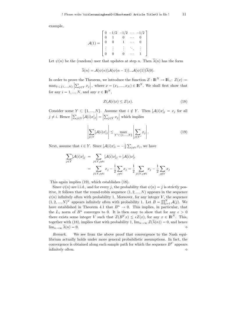
! Please write \titlerunninghead{<(Shortened) Article Title>} in file ! 11

example,

A(1) =

0 −1/2 −1/2 · · · −1/2

0 1 0 · · · 0

0 0 1 · · · 0...

......

. . ....

0 0 0 · · · 1

Let ψ(n) be the (random) user that updates at step n. Then λ(n) has the form

λ(n) = A(ψ(n))A(ψ(n− 1))...A(ψ(1))λ(0).

In order to prove the Theorem, we introduce the function Z : IRN → IR+: Z(x) :=maxY⊂{1,...,N}

∣∣∣∑j∈Y xj

∣∣∣ , where x = (x1, ..., xN ) ∈ IRN . We shall first show that

for any i = 1, ..., N , and any x ∈ IRN ,

Z(A(i)x) ≤ Z(x). (18)

Consider some Y ⊂ {1, ..., N}. Assume that i /∈ Y . Then [A(i)x]j = xj for all

j 6= i. Hence∣∣∣∑j∈Y [A(i)x]j

∣∣∣ =∣∣∣∑j∈Y xj

∣∣∣ which implies

∣∣∣∣∣∣∑j∈Y

[A(i)x]j

∣∣∣∣∣∣ ≤ maxY ′⊂{1,...,N}

∣∣∣∣∣∣∑j∈Y ′

xj

∣∣∣∣∣∣ . (19)

Next, assume that i ∈ Y . Since [A(i)x]i = − 12

∑j 6=i xj , we have∑

j∈Y[A(i)x]j =

∑j∈Y,j 6=i

[A(i)x]j + [A(i)x]i

=∑

j∈Y,j 6=i

xj −12

∑j 6=i

xj =12

∑j∈Y,j 6=i

xj −12

∑j /∈Y

xj

This again implies (19), which establishes (18).Since ψ(n) are i.i.d., and for every j, the probability that ψ(n) = j is strictly pos-

itive, it follows that the round-robin sequence (1, 2, ..., N) appears in the sequenceψ(n) infinitely often with probability 1. Moreover, for any integer V , the sequence(1, 2, ..., N)V appears infinitely often with probability 1. Let B =

∏Nj=1A(j). We

have established in Theorem 4.1 that Bn → 0. This implies, in particular, thatthe L1 norm of Bn converges to 0. It is then easy to show that for any ε > 0there exists some integer V such that Z(BV x) ≤ εZ(x), for any x ∈ IRN . This,together with (18), implies that with probability 1, limn→∞ Z(λ(n)) = 0, and hencelimn→∞ λ(n) = 0. �

Remark. We see from the above proof that convergence to the Nash equi-librium actually holds under more general probabilistic assumptions. In fact, theconvergence is obtained along each sample path for which the sequence BV appearsinfinitely often. �

12 E. ALTMAN, T. BASAR, T. JIMENEZ AND N. SHIMKIN

Next, we show that if we relax the condition K = 1 in the random pollingalgorithm, then this could give rise to instability. To see this, consider a sequenceof i.i.d. random vectors {Xn}, n = 1, 2, ..., where Xn = (X1

1 , . . . , XNn ), with Xi

n

taking the values 0 or 1, with respective probabilities 1 − p and p. (Note that fora fixed n, we allow the different components of Xn to be dependent.) Introducethe Random Greedy algorithm as follows: player i updates at time n if and only ifXin = 1. Consider the symmetric case where p := EXi

n does not depend on i or n.Then it can be shown that if p ≥ 4/(N + 1), the Random Greedy algorithm doesnot converge. Indeed, it follows from (10) that

λi(n+ 1) = −X

in

2

∑k 6=i

λk(n) + (1−Xi

n)λi(n).

Letting Li := Eλi, we obtain Li(n+ 1) = −p2

∑k 6=i L

k(n) + (1− p)Li(n). Further-more letting L(n) :=

∑Ni=1 L

i , we have

L(n+ 1) =[−p

2(N − 1) + (1− p)

]L(n) =

[−p

2(N + 1) + 1

]L(n).

If the term in the square brackets is smaller than or equal to -1, then L(n) does notconverge. This condition is equivalent to p ≥ 4/(N+1). This implies, in particular,that the parallel update algorithm, in which all users update simultaneously (p = 1),does not converge if N > 3. Moreover, the random polling algorithm does notconverge if K > 3. This phenomenon may be related to the well known factthat different conditions for convergence may apply to the Gauss-Seidel and Jacobiiterative schemes; see e.g., [2, 3].

In order to avoid the above instability in the case of parallel update, some re-strictions have to be imposed. This motivates us to introduce in the next section aforgetting factor that smooths the variations due to best responses of players.

4.4. Parallel update with a forgetting factor (relaxation parameter)We have seen above that if N > 3 and all players update simultaneously at

each step (K = N), then there is no convergence to the Nash equilibrium. Theinstability seems to be due to the fact that when all players change their strategiesin the same manner, then this leads to growing oscillations. We consider in thissubsection a possible dampening of these oscillations by allowing only a partialupdate; we consider a natural scenario where a player does not completely changehis strategy from one step to the next, but rather uses a new strategy obtained asa convex combination of the calculated optimal response and the previously usedaction. In other words, the deviation vector λn+1 at the n+ 1th step is given by

λn+1 = (γ∇A+ (1− γ)I)λn,

where ∇A is as defined by (11), I is the identity matrix, and γ > 0 is called theforgetting factor.

Theorem 4.4. Consider the parallel update algorithm with forgetting factor γ.Then the system is stable if and only if 0 < γ < 4/(N + 1).

! Please write \titlerunninghead{<(Shortened) Article Title>} in file ! 13

Proof: We have stability if and only if all eigenvalues of γ∇A + (1 − γ)I are inthe interior of the unit disk, or equivalently, the zeros of the determinant of

Q(z) = γ∇A+ (1− γ − z)I =

1 − γ − z −γ/2 −γ/2 · · · −γ/2−γ/2 1 − γ − z −γ/2 · · · −γ/2−γ/2 −γ/2 1 − γ − z · · · −γ/2

......

.... . .

...

−γ/2 −γ/2 −γ/2 · · · 1 − γ − z

are within the interior of the unit disk. The zeros of Q(z) are the same as thoseof the matrix Q′(z), obtained by replacing row i, i = 2, ..., N , by the differencebetween row i and row i− 1:

Q′(z) =

1 − γ − z −γ/2 −γ/2 · · · −γ/2 −γ/2−w w 0 · · · 0 0

0 −w w · · · 0 0

0 0 −w · · · 0 0...

......

. . ....

0 0 0 · · · −w w

where w = 1− γ

2− z.

The determinant of Q′(z) is easily computed and is given by

det[Q′(z)] =(

1− γ − z − (N − 1)γ2

)(1− γ

2− z)N−1.

Its zeros are (1− γ/2) and (1− (N + 1)γ/2), and this completes the proof. �

5. CONCLUSIONSWe have studied in this paper the problem of static competitive routing, first for

M parallel links and subsequently in more detail for the case of two parallel links,and with linear link holding costs. In the two-link case, we have focused on thestability of the equilibrium, i.e., on the question of whether equilibrium is actuallyreached if players start initially at some other arbitrary point.

Our analysis suggests that under some scenarios where users update their actionsindependently and in a completely greedy way, the unique equilibrium may beunstable. In particular, if all users update simultaneously, oscillations could occurand the routing decisions diverge if the number of players is larger than 3. On theother hand if memory is added and updated actions use a convex combination ofprevious actions and the new greedy best response, then stability can be achieved.

Our approach is related to the so called ”Cournot Adjustment” scheme [9] ineconomics. The round-robin scheme is known as the alternating-move Cournotdynamic; it is closely related to the Gauss-Seidel iteration for the solution of linearequations; see, e.g., [2, 3]. An alternative way of adding memory to the bestresponse would be to compute best responses to the time averaged actions of otherplayers, and not just to their latest strategy. This approach, known as ”fictitiousplay” [9] will be the subject of future study.

We plan to study in the future the stability of equilibria in more complex topolo-gies, in particular for those where it is known that there exists a unique equilibrium.

14 E. ALTMAN, T. BASAR, T. JIMENEZ AND N. SHIMKIN

Furthermore, we intend to consider other cost functions, such as those whose lin-earized versions contain bias terms, and those that are player-dependent.

ACKNOWLEDGMENTThe authors wish to thank Prof. Frank P. Kelly for suggesting the study of the parallel update

with forgetting factor.

REFERENCES

1. E. Altman and T. Basar, “Multi-user rate-based flow control”, IEEE Trans. Communications,46, no. 7, pp. 940–949, July 1998.

2. T. Basar and G. J. Olsder, “Dynamic Noncooperative Game Theory,” SIAM Series in Classicsin Applied Mathematics, Philadelphia, 1999.

3. D. P. Bertsekas and J. Tsitsiklis, “Parallel and Distributed Computation,” Prentice Hall, NJ,1989.

4. A. D. Bovopoulos and A. A. Lazar, “Asynchronous iterative algorithms for optimal load bal-ancing”, Proc. 22nd Annual Conference on Information Sciences and Systems, PrincetonUniv., pp. 1051–1057, March 1988.

5. D. Cansever, “Decentralized algorithms for flow control in networks”, Proc. 25th Conf. Deci-sion and Control, Athens, Greece, pp. 2107–2212, Dec. 1986.

6. S. Dafermos and A. Nagurney, “On some traffic equilibrium theory paradoxes”, TransportationResearch B, 18, pp. 101-110, 1984.

7. C. Douligeris and R. Mazumdar, “A Game-Theoretic Approach to Flow Control in an Inte-grated Environment”, Journal of the Franklin Institute, pp. 383-402, March 1992.

8. A. A. Economides and J. A. Silvester, “Multi-objective routing in integrated services networks:a game theory approach”, Proceedings of INFOCOM, pp. 1220-1225, 1991.

9. D. Fudenberg and D. Levine, Theory of Learning in Games, MIT in press, 1998.

10. A. Haurie and P. Marcotte, “On the relationship between Nash-Cournot and Wardrop Equi-libria”, Networks, Vol. 15, pp. 295-308, 1985.

11. R. A. Horn and C. R. Johnson, Matrix Analysis, Cambridge University Press, 1985 (reprintof 1996).

12. M. T. Hsiao and A. A. Lazar, “Optimal decentralized flow control of Markovian queueingnetworks with multiple controllers”, Performance Evaluation, 13, No. 3, pp. 181-204, 1991.

13. H. Kameda, E. Altman and T. Kozawa, “A case where a paradox like Braess’s occurs inthe Nash equilibrium but does not occur in the Wardrop equilibrium - a situation of loadbalancing in distributed computer systems”, Proc. of the 38th IEEE Conference on Decisionand Control, Phoenix, Arizona, USA, Dec. 1999.

14. H. Kameda, T. Kozawa and J. Li, “Anomalous relations among various performance objectivesin distributed computer systems”, Proc. World Congress on Systems Simulation, pp. 459-465,Sept, 1997.

15. Y. A. Korilis, A. A. Lazar and A. Orda, “Architecting noncooperative networks”, IEEE J. onSelected Areas in Communications, 13, No. 7, sept 1995, pp. 1241-1251.

16. R. J. La and V. Anantharam, “Optimal routing control: game theoretic approach”, Proc. ofthe 36th IEEE Conference on Decision and Control, San Diego, California, pp. 2910–2915,Dec. 1997.

17. R. Mazumdar, L. Mason and C. Douligeris, “Fairness in network optimal flow control: opti-mality of product forms”, IEEE Trans. on Communications, 39, No. 5, pp. 775-782, 1991.

18. A. Orda, R. Rom and N. Shimkin, “Competitive routing in multiuser communication net-works”, IEEE/ACM Transactions on Networking, 1, pp. 614-627, 1993.

19. S. Shenker, “Making greed work in networks: A game-theoretic analysis of switch servicedisciplines”, IEEE/ACM Transactions on Networking, vol. 3, pp. 819-831, December 1995.

20. J.G. Wardrop, Some Theoretical Aspects of Road Traffic Research, Proc. Inst. Civ. Eng. Part2, 1, 325–378, 1952.

21. Z. Zhang and C. Douligeris, ”Convergence of Synchronous and Asynchronous Greedy Algo-rithms in a Multiclass Telecommunications Environment,” IEEE Transactions on Communi-cations, Vol. 40, no. 8, pp. 1277-1281, August 1992.