Autonomous and reliable operation of multilayer optical ...
149
Autonomous and reliable operation of multilayer optical networks Sima Barzegar ADVERTIMENT La consulta d’aquesta tesi queda condicionada a l’acceptació de les següents condicions d'ús: La difusió d’aquesta tesi per mitjà del repositori institucional UPCommons (http://upcommons.upc.edu/tesis) i el repositori cooperatiu TDX ( h t t p : / / w w w . t d x . c a t / ) ha estat autoritzada pels titulars dels drets de propietat intel·lectual únicament per a usos privats emmarcats en activitats d’investigació i docència. No s’autoritza la seva reproducció amb finalitats de lucre ni la seva difusió i posada a disposició des d’un lloc aliè al servei UPCommons o TDX. No s’autoritza la presentació del seu contingut en una finestra o marc aliè a UPCommons (framing). Aquesta reserva de drets afecta tant al resum de presentació de la tesi com als seus continguts. En la utilització o cita de parts de la tesi és obligat indicar el nom de la persona autora. ADVERTENCIA La consulta de esta tesis queda condicionada a la aceptación de las siguientes condiciones de uso: La difusión de esta tesis por medio del repositorio institucional UPCommons (http://upcommons.upc.edu/tesis) y el repositorio cooperativo TDR (http://www.tdx.cat/?locale- attribute=es) ha sido autorizada por los titulares de los derechos de propiedad intelectual únicamente para usos privados enmarcados en actividades de investigación y docencia. No se autoriza su reproducción con finalidades de lucro ni su difusión y puesta a disposición desde un sitio ajeno al servicio UPCommons No se autoriza la presentación de su contenido en una ventana o marco ajeno a UPCommons (framing). Esta reserva de derechos afecta tanto al resumen de presentación de la tesis como a sus contenidos. En la utilización o cita de partes de la tesis es obligado indicar el nombre de la persona autora. WARNING On having consulted this thesis you’re accepting the following use conditions: Spreading this thesis by the institutional repository UPCommons (http://upcommons.upc.edu/tesis) and the cooperative repository TDX (http://www.tdx.cat/?locale- attribute=en) has been authorized by the titular of the intellectual property rights only for private uses placed in investigation and teaching activities. Reproduction with lucrative aims is not authorized neither its spreading nor availability from a site foreign to the UPCommons service. Introducing its content in a window or frame foreign to the UPCommons service is not authorized (framing). These rights affect to the presentation summary of the thesis as well as to its contents. In the using or citation of parts of the thesis it’s obliged to indicate the name of the author.
-
Upload
khangminh22 -
Category
Documents
-
view
0 -
download
0
Transcript of Autonomous and reliable operation of multilayer optical ...

Autonomous and reliable operation of multilayer optical networks
Sima Barzegar
ADVERTIMENT La consulta d’aquesta tesi queda condicionada a l’acceptació de les següents condicions d'ús: La difusió d’aquesta tesi per mitjà del repositori institucional UPCommons (http://upcommons.upc.edu/tesis) i el repositori cooperatiu TDX ( h t t p : / / w w w . t d x . c a t / ) ha estat autoritzada pels titulars dels drets de propietat intel·lectual únicament per a usos privats emmarcats en activitats d’investigació i docència. No s’autoritza la seva reproducció amb finalitats de lucre ni la seva difusió i posada a disposició des d’un lloc aliè al servei UPCommons o TDX. No s’autoritza la presentació del seu contingut en una finestra o marc aliè a UPCommons (framing). Aquesta reserva de drets afecta tant al resum de presentació de la tesi com als seus continguts. En la utilització o cita de parts de la tesi és obligat indicar el nom de la persona autora. ADVERTENCIA La consulta de esta tesis queda condicionada a la aceptación de las siguientes condiciones de uso: La difusión de esta tesis por medio del repositorio institucional UPCommons (http://upcommons.upc.edu/tesis) y el repositorio cooperativo TDR (http://www.tdx.cat/?locale- attribute=es) ha sido autorizada por los titulares de los derechos de propiedad intelectual únicamente para usos privados enmarcados en actividades de investigación y docencia. No se autoriza su reproducción con finalidades de lucro ni su difusión y puesta a disposición desde un sitio ajeno al servicio UPCommons No se autoriza la presentación de su contenido en una ventana o marco ajeno a UPCommons (framing). Esta reserva de derechos afecta tanto al resumen de presentación de la tesis como a sus contenidos. En la utilización o cita de partes de la tesis es obligado indicar el nombre de la persona autora. WARNING On having consulted this thesis you’re accepting the following use conditions: Spreading this thesis by the institutional repository UPCommons (http://upcommons.upc.edu/tesis) and the cooperative repository TDX (http://www.tdx.cat/?locale- attribute=en) has been authorized by the titular of the intellectual property rights only for private uses placed in investigation and teaching activities. Reproduction with lucrative aims is not authorized neither its spreading nor availability from a site foreign to the UPCommons service. Introducing its content in a window or frame foreign to the UPCommons service is not authorized (framing). These rights affect to the presentation summary of the thesis as well as to its contents. In the using or citation of parts of the thesis it’s obliged to indicate the name of the author.

3
Universitat Politècnica de Catalunya
Optical Communications Group
Autonomous and Reliable
Operation of Multilayer Optical
Networks
Sima Barzegar
Advisor:
Dr. Luis Velasco
Co-advisor:
Dr. Marc Ruiz
A thesis presented in partial fulfilment of the requirements for
the degree of
Philosophy Doctor
April 19, 2022

3
© 2022 by Sima Barzegar
All rights reserved. No part of this book may be reproduced, in any form or by any
means, without permission in writing from the author.
Optical Communications Group (GCO)
Universitat Politècnica de Catalunya (UPC)
C/ Jordi Girona, 1-3
Campus Nord, D4-2013
08034 Barcelona, Spain

Acta de calificación de tesis doctoral
Curso académico:
Nombre y apellidos
Programa de doctorado
Unidad estructural responsable del programa
Resolución del Tribunal
Reunido el Tribunal designado a tal efecto, el doctorando / la doctoranda expone el tema de la su tesis
doctoral titulada _______________________________________________________________________
____________________________________________________________________________________.
Acabada la lectura y después de dar respuesta a las cuestiones formuladas por los miembros titulares del
tribunal, éste otorga la calificación:
NO APTO APROBADO NOTABLE SOBRESALIENTE
(Nombre, apellidos y firma)
Presidente/a
(Nombre, apellidos y firma)
Secretario/a
(Nombre, apellidos y firma)
Vocal
(Nombre, apellidos y firma)
Vocal
(Nombre, apellidos y firma)
Vocal
______________________, _______ de __________________ de _______________ El resultado del escrutinio de los votos emitidos por los miembros titulares del tribunal, efectuado por la
Escuela de Doctorado, a instancia de la Comisión de Doctorado de la UPC, otorga la MENCIÓN CUM
LAUDE:
SÍ NO
(Nombre, apellidos y firma)
Presidente de la Comisión Permanente de la Escuela de Doctorado
(Nombre, apellidos y firma)
Secretaria de la Comisión Permanente de la Escuela de Doctorado
Barcelona a _______ de ____________________ de __________


Acknowledgements
First and foremost, I am extremely grateful to my supervisors, Prof. Luis Velasco
and Dr. Marc Ruiz for their invaluable advice, continuous support, and patience
during my PhD study. Their immense knowledge and plentiful experience have
encouraged me in all the time of my academic research and daily life. I would also
like to thank Dr. Filippo Cugini and Dr. Matias Richart for accepting and supporting
me to work within their group in CNIT, Italy and Universidad de la República,
Uruguay; these stays provided me bunch of skills and experiences in my carrier and
in my life.
I would like to thank all the colleagues, Fatemeh, Morteza, Mariano, Masab, Diogo,
Hailey, Shaoxuan and Pol for the cherished time spent together in the GCO lab, and
all my colleagues in Italy and Uruguay whose contribution in my life is
unforgettable.
Finally, I would like to express my gratitude to my parents, my brother, my family
and my friends. Without their tremendous understanding and encouragement in the
past few years, it would be impossible for me to complete my study.

II Autonomous and Reliable Operation of Multilayer Optical Networks
This PhD thesis is dedicated to my dear parents, Khadijeh and Ahmad,
and my dear brother, Salar, who have taught me how to live, be strong and love
unconditionally.

Abstract
This Ph.D. thesis focuses on the reliable autonomous operation of multilayer optical
networks.
The first objective focuses on the reliability of the optical network and proposes
methods for health analysis related to Quality of Transmission (QoT) degradation.
Such degradation is produced by soft-failures in optical devices and fibers in core
and metro segments of the operators’ transport networks. Here, we compare
estimated and measured QoT in the optical transponder by using a QoT tool based
on GNPy. We show that the changes in the values of input parameters of the QoT
model representing optical devices can explain the deviations and degradation in
performance of such devices. We use reverse engineering to estimate the value of
those parameters that explain the observed QoT. We show by simulation a large
anticipation in soft-failure detection, localization and identification of degradation
before affecting the network. Finally, for validating our approach, we experimentally
observe the high accuracy in the estimation of the modeling parameters.
The second objective focuses on multilayer optical networks, where lightpaths are
used to connect packet nodes thus creating virtual links (vLink). Specifically, we
should study how lightpaths can be managed to provide enough capacity to the
packet layer without detrimental effects in their Quality of Service (QoS), like added
delays or packet losses, and at the same time minimize energy consumption. Such
management must be as autonomous as possible to minimize human intervention.
In addition, the relation between the packet and the optical layer should be
considered, as it can bring global optimal solutions. We study the autonomous
operation of optical connections based on digital subcarrier multiplexing (DSCM).
We propose several solutions for the autonomous operation of DSCM systems. In
particular, the combination of two modules running in the optical node and in the

IV Autonomous and Reliable Operation of Multilayer Optical Networks
optical transponder activate and deactivate subcarriers to adapt the capacity of the
optical connection to the upper layer packet traffic. The module running in the
optical node is part of our Intent-based Networking (IBN) solution and implements
prediction to anticipate traffic changes. Our comprehensive study demonstrates the
feasibility of DSCM autonomous operation and shows large cost savings in terms of
energy consumption. In addition, our study provides a guideline to help vendors and
operators to adopt the proposed solutions.
The final objective targets at automating packet layer connections (PkC).
Automating the capacity required by PkCs can bring further cost reduction to
network operators, as it can limit the resources used at the optical layer. However,
such automation requires careful design to avoid any QoS degradation, which would
impact Service Level Agreement (SLA) in the case that the packet flow is related to
some customer connection. We study autonomous packet flow capacity management.
We apply RL techniques and propose a management lifecycle consisting of three
different phases: 1) a self-tuned threshold-based approach for setting up the
connection until enough data is collected, which enables understanding the traffic
characteristics; 2) RL operation based on models pre-trained with generic traffic
profiles; and 3) RL operation based on models trained with the observed traffic. We
show that RL algorithms provide poor performance until they learn optimal policies,
as well as when the traffic characteristics change over time. The proposed lifecycle
provides remarkable performance from the starting of the connection and it shows
the robustness while facing changes in traffic. Finally, we take advantage of our
experience and revisit our proposed solutions for autonomous vLink operation
supported by DSCM systems. The contribution is twofold: 1) and on the one hand,
we propose a solution based on RL, which shows superior performance with respect
to the solution based on prediction; and 2) because vLinks support packet
connections, coordination between the intents of both layers is proposed. In this case,
the actions taken by the individual PkCs are used by the vLink intent. The results
show noticeable performance compared to independent vLink operation.

Resumen
Esta tesis doctoral se centra en la operación autónoma y confiable de redes ópticas
multicapa.
El primer objetivo se centra en la fiabilidad de la red óptica y propone métodos para
el análisis del estado relacionados con la degradación de la calidad de la transmisión
(QoT). Dicha degradación se produce por fallos en dispositivos ópticos y fibras en las
redes de transporte de los operadores que no causan corte de la señal. Aquí,
comparamos el QoT estimado y medido en el transpondedor óptico mediante el uso
de una herramienta de QoT basada en GNPy. Mostramos que los cambios en los
valores de los parámetros de entrada del modelo QoT que representan los
dispositivos ópticos pueden explicar las desviaciones y la degradación en el
rendimiento de dichos dispositivos. Usamos ingeniería inversa para estimar el valor
de aquellos parámetros que explican el QoT observado. Mostramos, mediante
simulación, una gran anticipación en la detección, localización e identificación de
fallos leves antes de afectar la red. Finalmente, validamos nuestro método de forma
experimental y comprobamos la alta precisión en la estimación de los parámetros de
los modelos.
El segundo objetivo se centra en las redes ópticas multicapa, donde se utilizan
conexiones ópticas (lightpaths) para conectar nodos de paquetes creando así enlaces
virtuales (vLink). Específicamente, estudiamos cómo se pueden gestionar los
lightpaths para proporcionar suficiente capacidad a la capa de paquetes sin efectos
perjudiciales en su calidad de servicio (QoS), como retardos adicionales o pérdidas de
paquetes, y al mismo tiempo minimizar el consumo de energía. Dicha gestión debe
ser lo más autónoma posible para minimizar la intervención del operador. Además,
se debe considerar la relación entre las capas de paquetes y óptica, ya que pueden
obtenerse soluciones óptimas globales. Estudiamos el funcionamiento autónomo de
conexiones ópticas basadas en multiplexación de subportadoras digitales (DSCM).

VI Autonomous and Reliable Operation of Multilayer Optical Networks
Proponemos varias soluciones para el funcionamiento autónomo de los sistemas
DSCM. En particular, la combinación de dos módulos que se ejecutan en el nodo
óptico y en el transpondedor óptico activan y desactivan subportadoras para adaptar
la capacidad de la conexión óptica al tráfico de paquetes de la capa superior. El
módulo que se ejecuta en el nodo óptico es parte de nuestra solución de red basada
en intención (IBN) e implementa predicción para anticipar los cambios de tráfico.
Nuestro estudio integral demuestra la viabilidad de la operación autónoma de DSCM
y muestra un gran ahorro de costos en términos de consumo de energía. Además,
nuestro estudio proporciona una guía para ayudar a los proveedores y operadores a
adoptar las soluciones propuestas.
El objetivo final es la automatización de conexiones de capa de paquetes (PkC). La
automatización de la capacidad requerida por las PkC puede generar una mayor
reducción de costes para los operadores de red, ya que puede limitar los recursos
utilizados en la capa óptica. Sin embargo, dicha automatización requiere un diseño
cuidadoso para evitar cualquier degradación de QoS, lo que afectaría acuerdos de
nivel de servicio (SLA) en el caso de que el flujo de paquetes esté relacionado con
alguna conexión del cliente. Estudiamos la gestión autónoma de la capacidad del
flujo de paquetes. Aplicamos técnicas de aprendizaje por refuerzo (RL) y proponemos
un ciclo de vida de gestión que consta de tres fases diferentes: 1) un enfoque basado
en umbrales auto ajustados para configurar la conexión hasta que se recopilen
suficientes datos, lo que permite comprender las características del tráfico; 2)
operación RL basada en modelos pre-entrenados con perfiles de tráfico genéricos; y
3) operación de RL en base a modelos entrenados con el tráfico observado. Mostramos
que los algoritmos de RL ofrecen un desempeño deficiente hasta que aprenden las
políticas óptimas, así como también cuando las características del tráfico cambian
con el tiempo. El ciclo de vida propuesto proporciona un rendimiento notable desde
el inicio de la conexión y muestra la robustez frente a cambios en el tráfico.
Finalmente, aprovechamos nuestra experiencia y revisamos las soluciones
propuestas para la operación autónoma de vLink respaldada por sistemas DSCM.
La contribución es doble: 1) por un lado, propusimos una solución basada en RL, que
muestra un rendimiento superior con respecto a la solución basada en predicción; y
2) debido a que los vLinks admiten conexiones de paquetes, se propone la
coordinación entre las intenciones de ambas capas. En este caso, la intención de
vLink utiliza las acciones realizadas por los PkC individuales. Los resultados
muestran un rendimiento notable en comparación con la operación independiente de
vLink.

Table of Contents
Page
Introduction ............................................................. 1
1.1 Motivation ....................................................................................................... 1
1.2 Goals of the thesis ........................................................................................... 3
1.3 Methodology .................................................................................................... 4
1.4 Thesis outline .................................................................................................. 6
1.5 Contributions and References from the Literature ...................................... 7
Background .............................................................. 8
2.1 Toward Network Automation ......................................................................... 8
Previous Architectures ........................................................................ 8
Software-Defined Networking (SDN) ................................................. 9
Intent-Based Networking .................................................................. 10
2.2 Advanced ML Techniques ............................................................................ 12
Regression for Time Series ................................................................ 12
Reinforcement Learning .................................................................... 13
2.3 Examples of Autonomous Network Operation ............................................ 14
2.4 Digital Subcarrier Multiplexing (DSCM) .................................................... 16
2.5 Generation of Reliable and Accurate Synthetic Data ................................. 17
State-of-the-Art ...................................................... 20

VIII Autonomous and Reliable Operation of Multilayer Optical Networks
3.1 Optical Network Health Analysis ................................................................ 20
Failure Detection and Localization .................................................. 20
Feasible Configuration of Optical Devices and Fibers .................... 22
Severity Estimation ........................................................................... 22
Experimental Validation ................................................................... 23
3.2 Reliable vLink Autonomous Operation ....................................................... 24
3.3 Autonomous Packet Flow Capacity Management ...................................... 25
3.4 Conclusions ................................................................................................... 26
Optical Network Health Analysis ...................... 27
4.1 Introduction................................................................................................... 28
4.2 The MESARTHIM methodology .................................................................. 30
4.3 Surveillance and Localization ...................................................................... 32
SNR-wise Surveillance ...................................................................... 32
Modeling-wise Surveillance .............................................................. 35
Soft-Failure Localization ................................................................... 36
Finding the Most Likely Modeling Configuration ........................... 36
4.4 Soft-Failure Identification and Severity Estimation .................................. 37
Soft-failure Identification .................................................................. 39
Severity Estimation ........................................................................... 41
4.5 Results ........................................................................................................... 42
Experimental assessment ................................................................. 42
Simulation environment .................................................................... 45
Surveillance and Device Configuration Estimation ........................ 46
Soft-Failure Localization ................................................................... 51
Identification and Severity Estimation ............................................ 53
4.6 Concluding Remarks..................................................................................... 58
Towards Autonomous vLink Capacity
Management ........................................................................... 60
5.1 Introduction................................................................................................... 60
5.2 Autonomous Capacity Management ............................................................ 61

Table of Contents IX
5.3 Capacity Management .................................................................................. 64
Transponder Agent ............................................................................ 64
Virtual Link Intent-Based Capacity Management .......................... 66
5.4 Illustrative Results ....................................................................................... 67
Power Model ....................................................................................... 67
Transponder Agent Capacity Management ..................................... 68
Intent-based vlink operation ............................................................. 71
5.5 Concluding Remarks..................................................................................... 72
Autonomous Packet Flow Capacity
Management ........................................................................... 74
6.1 Introduction................................................................................................... 75
6.2 The Flow Capacity Autonomous Operation (CRUX) Problem .................... 76
Flow Capacity Autonomous Operation ............................................. 76
Proposed Architecture ....................................................................... 79
6.3 CRUX Problem Definition and RL Methodology ......................................... 80
Problem Definition and Basic Modeling ........................................... 81
Generic RL-Based Methodology ........................................................ 83
Specific Adaption of RL Approaches ................................................. 85
6.4 Cycles for Robust RL .................................................................................... 86
6.5 Illustrative Results ....................................................................................... 91
Online RL-Based Operation .............................................................. 92
Offline Leaning + Online RL-Based Operation ................................ 97
6.6 Concluding Remarks................................................................................... 100
Revisiting Autonomous vLink Capacity
Operation .............................................................................. 103
7.1 Introduction................................................................................................. 103
7.2 Autonomic vLink Capacity Adaptation ..................................................... 104
7.3 Cooperative Intent Operation .................................................................... 105
7.4 Illustrative Intent-Based Applications ...................................................... 106
Autonomous vLink Capacity Operation ......................................... 106

X Autonomous and Reliable Operation of Multilayer Optical Networks
Cooperative Intent Operation ......................................................... 109
7.5 Concluding Remarks................................................................................... 111
Closing Discussion .............................................. 113
8.1 Main Contributions ..................................................................................... 113
8.2 List of Publications ..................................................................................... 114
Publications in Journals .................................................................. 114
Publications in Conferences ............................................................ 115
8.3 List of Research Projects ............................................................................ 115
European Funded Projects .............................................................. 115
National Funded Projects ................................................................ 116
Pre-doctoral Scholarship ................................................................. 116
8.4 Collaborations ............................................................................................. 116
8.5 Topics for Further Research ....................................................................... 116
List of Acronyms ...................................................................... 118
References ................................................................................. 121

List of Figures
Page
Figure 1-1: Overview of the proposed architecture ..................................................... 5
Figure 1-2: Methodology to be followed in this Ph.D. thesis ....................................... 6
Figure 2-1 Policy-Based Network Management .......................................................... 9
Figure 2-2 Software-Defined Networking and Monitoring and Data Analytics ...... 10
Figure 2-3 Intent-Based Networking ......................................................................... 11
Figure 2-4 Capacity operation of PkCs and vLinks .................................................. 15
Figure 2-5 Example of a DSCM system ..................................................................... 16
Figure 2-6 Examples of digital twins for the packet (a-b) and the optical (c-d) layers.
...................................................................................................................................... 18
Figure 4-1 Overview of the proposed MESARTHIM methodology ........................... 31
Figure 4-2 Three examples of behavior. ..................................................................... 33
Figure 4-3. Example of identification and severity estimation at time t. ................ 39
Figure 4-4 Experimental testbed................................................................................ 43
Figure 4-5 Modeling parameter value vs. bandwidth for A/D WSS OSNR (a) and OA
NF (b) ........................................................................................................................... 44
Figure 4-6 SNR vs. link length ................................................................................... 44
Figure 4-7 Optical network topology considered in this chapter. ............................. 45
Figure 4-8 Number of distinct routes per link and max number of routes for
localization. .................................................................................................................. 46
Figure 4-9 Modeling Config Search ............................................................................ 47

XII Autonomous and Reliable Operation of Multilayer Optical Networks
Figure 4-10 Evolution of monitored SNR and estimation of modeling parameters. 48
Figure 4-11 Evolution of monitored SNR and estimation of modeling parameters. 48
Figure 4-12 Evolution of monitored SNR and estimation of modeling parameters. 49
Figure 4-13 Absolute and relative modeling parameter estimation error. .............. 50
Figure 4-14 NF Gradual Soft-Failure Identification. ................................................ 54
Figure 4-15 P-max Gradual Soft-Failure Identification. .......................................... 55
Figure 4-16 Localization by identifying the Soft-Failure. ......................................... 56
Figure 4-17 Severity Estimation. ............................................................................... 57
Figure 5-1 Vlink workflow overview. ......................................................................... 62
Figure 5-2 Intent-based autonomous vlink operation to allocate capacity for the input
traffic. ........................................................................................................................... 63
Figure 5-3 Optical connection managed by the Transponder Agent. Total and SCs
capacity vs time for two traffic profiles. ..................................................................... 70
Figure 6-1 Flow capacity autonomous operation. RL framework with learner, agent,
and environment. ........................................................................................................ 77
Figure 6-2 Operation lifecycle. (a) Online learning RL operation. (b) Offline training
with online fine tuning RL operation. ........................................................................ 78
Figure 6-3 Extended architecture for flow capacity autonomous operation with
offline learning. ........................................................................................................... 80
Figure 6-4 Delay model example. ............................................................................... 82
Figure 6-5 Capacity allocation definition (a) and evolution (b). ............................... 83
Figure 6-6 General RL workflow. ............................................................................... 84
Figure 6-7 Reward function vs. capacity slack/surplus. ............................................ 85
Figure 6-8. Achieving zero loss operation .................................................................. 92
Figure 6-9. Q-Learning operation. Traffic and allocated capacity for low (a),
moderated (b), and high (c) traffic variance. .............................................................. 93
Figure 6-10 QoS as a function of ρ models trained with a sinusoidal traffic pattern
(a–c) and real traffic (d–f). .......................................................................................... 94
Figure 6-11. Optimal margin multiplier (a) and overprovisioning (b). .................... 95
Figure 6-12 Relative extra overprovisioning. ............................................................ 95
Figure 6-13. Phase I: Self-tuned threshold (a) and traffic variance analysis (b). .... 97
Figure 6-14 Phase II: QoS (a) and ρ (b) evolution. .................................................... 98

List of Figures XIII
Figure 6-15. Overprovisioning reduction. .................................................................. 99
Figure 6-16 Phase III: Traffic variance change scenarios. Gradual increase (a) and
sudden increase (b). ..................................................................................................... 99
Figure 7-1 RL-based Autonomous vLink Operation Architecture. ........................ 105
Figure 7-2 Extended architecture with hierarchical intent cooperation. ............... 106
Figure 7-3 Optical connection managed by the vLink intent. Total capacity vs time
for the High Traffic profile. ....................................................................................... 107
Figure 7-4 Autonomic vLink Capacity Adaptation (a) and obtained delay (b). ..... 108
Figure 7-5 PKC-vLink intent cooperation performance. ......................................... 110
Figure 7-6 Comparative results ................................................................................ 110
Figure 8-1 Example of distributed flow routing based on RL ................................. 117


List of Tables
Page
Table 1-1: Thesis goals .................................................................................................. 4
Table 3-1: Study scenarios .......................................................................................... 24
Table 3-2: State-of-the-art summary .......................................................................... 26
Table 4-1: Notation ...................................................................................................... 32
Table 4-2 Indicator function components ................................................................... 41
Table 4-3 Examples of Soft-Failure Localization ...................................................... 52
Table 4-4 Summary of the MESARTHIM Methodology ........................................... 59
Table 5-1 Configurations, Power, and Sets ................................................................ 69
Table 5-2 Summary of Results for Optical Connection Configuration Managed by the
Transponder Agent ..................................................................................................... 70
Table 5-3 Summary of Results for Optical Connection Configuration Managed by
vlink Intent .................................................................................................................. 71
Table 5-4 Main Lessons Learnt .................................................................................. 73
Table 6-1: Notation ...................................................................................................... 80
Table 6-2: Summary of RL approaches ...................................................................... 86
Table 6-3: Additional overprovisioning when fixing ρ ............................................... 96
Table 6-4: Phase III: Analysis under traffic changes .............................................. 100
Table 6-5: Summary of results for policy-based and RL operation with and without
offline learning .......................................................................................................... 102

XVI Autonomous and Reliable Operation of Multilayer Optical Networks
Table 7-1: Summary of results for Optical Connection Configuration Managed by
vlink Intent based on Q-learning ............................................................................. 107
Table 7-2 vLink Capacity Adaptation Summary ..................................................... 109
Table 7-3 Cooperative IBN summary....................................................................... 111

Chapter 1
Introduction
1.1 Motivation
The massive application of the optical technology [EON16], not only in the core
segment of the operators’ transport networks, but also in the metro and even in the
access segments [Ve13], is a clear consequence of its characteristic high bandwidth,
low latency, and high reliability.
One ingredient of the optical technology is that of the Forward Error Correction
(FEC) techniques [Ty06] that allow to correct errors in the optical transmission. FEC
techniques are applied in the end Optical Transponders (TRX) of optical connections
(lightpath) to guarantee zero post-FEC Bit Error Rate (BER) transmission provided
that pre-FEC BER is below some BER threshold; when such threshold is exceeded,
zero post-FEC error cannot be achieved (FEC limit) and the lightpath will be
consequently torn down.
Although degradation of the Quality of Transmission (QoT) is related to linear and
Non-Linear (NL) optical impairments, other effects like optical fiber and devices
aging have a great impact as well. Aging effects are usually considered by means of
costly system margins [Po17]; examples include the increasing fiber losses due to
splices to repair fiber cuts, degradation of Optical Amplifiers (OA) noise factor, and
detuning of the lasers in the TRXs leading to misalignment with filters in
Wavelength Selective Switches (WSS). If those degradations (soft-failures) are not
corrected (e.g., by retuning, repairing or replacing the related optical device/fiber),
they can degenerate into hard-failures and affect a number of lightpaths supporting
a large amount of network services; therefore, it is of paramount importance not only

2 Autonomous and Reliable Operation of Multilayer Optical Networks
to detect any QoT degradation as soon as possible [APV17], but also to localize the
device/fiber causing the degradation to facilitate maintenance [APV18].
For such detection and localization to be possible, the control plane of the optical
network, which based on the Software-Defined Networking (SDN) concept [Ne17],
needs to be enriched with Monitoring and Data Analytics (MDA) capabilities
[Ve19.1]. Once monitoring data have been collected from the data plane, data
analytics algorithms, e.g., based on Machine Learning (ML) [Ra18.1], can analyze
them either as soon as they are available or periodically to proactively detect the
degradation and anticipate hard-failures before they actually happen; once detected,
recommendations can be issued to the network controller so it can make decisions
about rerouting and/or reconfiguring the network [Ve17], as well as to notify the
management plane for scheduling maintenance.
Further, a considerable effort is being payed towards disaggregating the optical layer
to enrich the offer of available solutions and to enable the deployment of optical
nodes that better fit optical network operators’ needs [Ve18]. Such disaggregation,
however, tends to make network surveillance and maintenance more complex in
general.
From the operation perspective, the optical network is becoming more and more are
complex, since it interacts with many other systems to provide end-to-end services.
With localized and highly engineered operational tools, it is typical of these networks
to take several weeks to months for any changes, upgrades or service deployments
to take effect. However, as the dynamicity of the traffic increases, the need for self-
network operation becomes more evident. In this regard, advances in network
automation [Ra18.1] are receiving considerable attention from the industry as the
complexity of the network increases and the requirements from the services become
more stringent and diverse. Autonomous network operation evolves from SDN and
promises to reduce operational expenditures by implementing closed loops based on
data analytics [Ve19.1], [Bo21]; network automation entails the collection of
performance monitoring data that are analyzed, and the extracted knowledge is used
to make decisions (control loop). Machine Learning (ML), a sub-domain of Artificial
Intelligence (AI), is highly suitable for complex system representation [Ra18.1].
Using ML algorithms for network automation entails analyzing heterogeneous data
collected from monitoring points in network devices.
Among the large number of use cases for autonomous optical network operation,
three major categories covering the entire lifecycle of optical connections are
highlighted in [Ve19.1]. The first category refers to the automation of connectivity
provisioning, when the provisioning process itself requires meeting some
performance, e.g., achieve resource efficiency or minimize connection blocking
[Da15], [Ch19.1]. In addition, monitoring and estimation of QoT is of paramount
importance for both connection provisioning and reconfiguration. A second category
is related to the dynamic network adaptation, which entails monitoring one or more
network entities (e.g., an optical connection) and make decisions to achieve some

Chapter 1 – Introduction 3
target performance. The target is to deal with situations ranging from those that
require scaling or reallocating resources to elastically adjust to demand variations
in volume and direction, to those that require healing and recovery. Examples
include QoT degradation and connection rerouting [Ve18.2], in-operation network
planning [Ve17], dynamic capacity allocation of virtual links supported by one or
more optical connections or even reconfigure a virtual network topology [Mo17],
[Ve18.1]. Finally, as a third category, degradation detection can be used also for
failure localization [Sh19]. Here, the performance to be achieved is related, e.g., to
availability metrics.
However, the drawback is the proliferation of individual control loops, which brings
also complexity to network management. In addition, defining how to achieve
operational goals is very complex. To address some of these issues, Intent-Based
Networking (IBN) [Cl21], [Ve21] allows the definition of operational objectives that
a network entity, e.g., a lightpath or a traffic flow, has to meet without specifying
how to meet them. IBN implements and enforces those objectives, often with the help
of ML. This strategy reduces human intervention and paves the way to the
application of AI/ML techniques.
Another issue is that of data availability, since AI/ML usually require a large dataset
for training purposes, which is difficult to obtain. The lack of data can be
compensated with the use of tools that include analytic models to explain the data
plane, e.g., GNPy [Fi18] for the optical and CURSA-SQ [Ru18] to generate packet
traffic and measure Quality of Service (QoS) related performance. Such tools can run
in sandbox domains [Ru20.1] and used for training AI/ML algorithms (see [ITU20]).
1.2 Goals of the thesis
In light of the above, this Ph.D. thesis focuses on the reliable autonomous operation
of multilayer optical networks. Specifically, the following goals are defined to achieve
this main objective:
G.1 – Optical Network Health Analysis
This first objective focuses on the reliability on the optical network and proposes
methods for health analysis related to QoT degradation. Such degradation is
produced by soft-failures in optical devices and fibers in core and metro segments of
the operators’ transport networks. This goal targets at several aspects related to QoT
degradation, including:
• Detecting and localizing soft-failures that impact on the optical layer.
• Finding the likely configuration of the optical devices and fibers that are the
cause of a soft-failure, while minimizing both the computation requirements
and the time needed for that.

4 Autonomous and Reliable Operation of Multilayer Optical Networks
• Estimating the severity of the soft-failure, defined as the time when some
threshold value will be exceeded. The intention is to evaluate the urgency for
making the proper decision to avoid disruption, including re-tuning, re-
routing, maintenance, etc.
• Comparing estimation results to real test bed measurement for validating the
accuracy of the proposed methods.
G.2 – Reliable vLink Autonomous Operation
This goal focuses on multilayer optical networks, where lightpaths are used to
connect packet nodes thus, creating virtual links (vLink). Specifically, we should
study how lightpaths can be managed to provide enough capacity to the packet layer
without detrimental effects in their QoS, like added delays or packet losses, and at
the same time minimize energy consumption. Such management must be as
autonomous as possible to minimize human intervention. In addition, the relation
between the packet and the optical layer should be considered, as it can bring global
optimal solutions.
G.3 – Autonomous Packet Flow Capacity Management
This final goal targets at automating packet layer connections (PkC). Automating
the capacity required by PkCs can bring further costs reduction to network
operators, as it can limit the resources used at the optical layer. However, such
automation requires careful design to avoid any QoS degradation, which would
impact Service Level Agreement (SLA) in the case that the packet flow is related to
some customer connection.
A summary of the goals of the Ph.D. thesis is presented in Table 1-1.
Table 1-1: Thesis goals
Goals
G.1
Optical Network Health Analysis
G.2
Reliable vLink Autonomous Operation
G.3
Autonomous Packet Flow Capacity Management
1.3 Methodology
This Ph.D. thesis assumes the architecture in Figure 1-1, where the optical layer
consists of a disaggregated set of ROADMs and TRXs, and a set of optical links

Chapter 1 – Introduction 5
interconnecting ROADMs with a number of OAs. On top of the optical layer, a packet
layer is configured, where the packet nodes are connected through the optical layer.
The control plane includes:
i) a Network Controller to program the network devices;
ii) an MDA system [Ve19.1] that collates measurements from the data plane,
analyses the data and issues recommendations to the network controller;
iii) a QoT tool that estimates the SNR of the lightpaths and it is used for connection
provisioning, as well as for diagnosis and failure localization.
Monitoring and Data Analytics (MDA)
Network Controller(SDN)
QoT tool
Data
Multilayer OpticalTransport Network
SNR EstimationRecommendations
TRX OA
ROADM
Measurements
TRX
SNR Estimation
Configuration
Figure 1-1: Overview of the proposed architecture
To carry out the studies needed to meet the goals of this thesis, the methodology in
Figure 1-2 will be followed.
As the starting point of every study, one or more topologies and scenarios will be
conceived. Then, due to the nature of this Ph.D. thesis’ goals, performance data will
be generated, where configuration parameters of the optical devices and fibers or the
packet traffic itself will be varied. Such initial data set will be the input for a data
generator that will produce performance or traffic data that evolved with the time
following some predefined profile.

6 Autonomous and Reliable Operation of Multilayer Optical Networks
Data set generation
Monitoring data generation
Surveillance, Localization and
estimation
Performance evaluation
Experiments
SNR(config params) SNR (t)degradation
Topology and scenario results
QoT Tool
Packet traffic data generation
Capacity Management
results
Figure 1-2: Methodology to be followed in this Ph.D. thesis
The main algorithms developed in this Ph.D. thesis will concentrate on the
surveillance, localization and estimation on the one hand, and on the other, on the
capacity management for autonomous operation. The former algorithms will receive
the evolution of the performance and use an external QoT for estimating the likely
configuration parameters of the optical devices and fibers, whereas the latter, will
receive the packet traffic and compute the capacity of the lightpath or packet flow to
guarantee the committed performance.
Finally, the results obtained in the previous steps will be evaluated through
experiments carried out in a real test bed. Such evaluation will help the
improvement of the algorithms.
The results will be disseminated and considered as the conception of new ideas
requiring further research.
1.4 Thesis outline
The remainder of this Ph.D. thesis is organized as follows.
Chapter 2 provides the needed background on AI/ML methods, SDN and IBN
concepts.
Chapter 3 briefly reviews the state-of-the-art related to the objectives of this Ph.D.
thesis such as optical network health analysis and Autonomous Operation in
multilayer optical networks and highlighting the niches to be covered.
Chapter 4 focuses on goal G.1 and covers optical network health analysis. This
chapter is based on the journal publication [TNSM21].

Chapter 1 – Introduction 7
Chapter 5 relates to goal G.2 and investigates vLink autonomous operation based on
predefined policies and simple ML techniques. This chapter is based on one journal
publication [JSAC21].
Chapter 6 concentrates on goal G.3 and is devoted to the application of apply
Reinforcement Learning (RL) for the autonomous packet flow capacity management.
This chapter is based on the journal publication [SENSORS21].
Chapter 7 aims the complete achievement of goal G.2, where we apply RL for reliable
vLink autonomous operation. In addition, cooperation between PkC and vLink
intents is proposed. This chapter is based on the journal papers [JSAC21] and
[JOCN22].
Finally, Chapter 8 concludes this Ph.D. thesis.
1.5 Contributions and References from the
Literature
For the sake of clarity and readability, references contributing to this Ph.D. thesis
are labelled using the following criteria: [<conference/journal>
<Year(yy)[.autonum]>], e.g., [ECOC20] or [JSAC21]; in case of more than one
contribution with the same label, a sequence number is added.
The rest of the references to papers or books, both auto references not included in
this Ph.D. thesis and other references from literature are labelled with the initials
of the first author’s surname together with its publication year, e.g., [Ve17].

Chapter 2
Background
In this chapter, we introduce the needed background on the IBN paradigm. IBN
targets at defining high-level abstractions, so network operators can define what are
their desired outcomes without specifying how they would be achieved. The latter
can be achieved by leveraging network programmability, monitoring and data
analytics, as well as the key assurance component.
IBN relates to AI/ML techniques and those need large datasets for training purposes.
In this chapter, we cover the AI/ML techniques that we consider for the solutions
proposed in this Ph.D. thesis, as well as some challenges and solutions for the
generation of accurate synthetic data.
2.1 Toward Network Automation
Previous Architectures
Network automation has been long time envisioned. In fact, the Telecommunications
Management Network (TMN), defined by the International Telecommunication
Union in [ITU00], is a hierarchy of management layers (network element, network,
service, and business management), where high-level operational goals propagate
from upper to lower layers.
In the way toward autonomic adaptation to changes, while hiding intrinsic
complexity to operators and users, the Internet Engineering Task Force developed
the concept of Policy-Based Network Management (PBNM) [St04]. PBNM separates
the rules governing the behavior of a system from its functionality. In PBNM, high-

Chapter 2 – Background 9
level management policies are broken down into low-level configurations and control
logic (policy rules) to ensure that the network provides the required services. Policies
can be defined as a set of simple control loops; each policy rule consists of a set of
events and conditions and a corresponding set of actions, where each condition
defines when the policy rule is applicable.
The most extended PBNM architecture consists of four systems (Figure 2-1): i) the
policy management tool allows operators to define and update policies and it
translates and validates policy rules; ii) the policy repository that stores the policies;
iii) a set of policy decision points, which interprets the policies, translates them into
a device-specific representation, and triggers the execution of the related actions
whenever they satisfy the specified conditions; and iv) the policy enforcement points
running on a policy-aware node that executes the policies. The drawback of PBNM
is solving conflicts that might arise within or among policies; conflict resolution
requires some external system or iterations with operators and/or users.
Policy Management Tool
• Policy Editing
• Rule Translation
• Rule Validation
• Conflict Resolution
Policy Decision Point
• Policy Trigger
• Rule Locator
• Device Adapter
• Resource Validation
Policy Enforcement
Points
Policy Repository
Policy Decision Point
Communicate
RuleControl
Loops
Figure 2-1 Policy-Based Network Management
Software-Defined Networking (SDN)
The network management architecture has evolved with the development of the
Software-Defined Networking (SDN) [Ne17] concept. SDN brings programmability
to simplify configuration (it breaks down high-level service abstraction into lower-
level device abstractions), orchestrates operation, and automatically reacts to
changes or events. SDN defines a centralized control plane architecture with global
network vision, which can achieve optimal routing at provisioning time and during
reconfiguration [Ve14]. Placed besides the SDN controller, a Monitoring and Data

10 Autonomous and Reliable Operation of Multilayer Optical Networks
Analytics (MDA) system was proposed in [Gi18] and [Ve19.1] to collect monitoring
data, analyze such data, and make decisions (control loop) (Figure 2-2). Such data
analysis can be based on AI / ML algorithms [Ra18.1], which enable network
automation solutions, aiming at reducing operational costs.
Programmability
(SDN)
Analytics
(MDA)
Orchestrate
and configure
systems
Collect
Measurements
Reports Expected future
conditions and
recommendations
Requests
Network Management System
(NMS)
Figure 2-2 Software-Defined Networking and Monitoring and Data Analytics
The MDA complements the SDN controller, so the network becomes proactive. Being
proactive is of paramount importance, as the analytics system could anticipate
anomalies and degradations (soft-failures) before they cause major problems or
become hard-failures. Upon the detection, the analytics system can issue proper
recommendations to the SDN controller, which can take the most appropriate action.
Additionally, such analysis can be extended to forecasting network conditions that
can be used to improve resource efficiency. In this architecture, control loops can be
defined at various levels, from the device [APV17.2] to the network, depending on
the use case [APV18], [APV17.1], as monitoring is collected and can be analyzed
locally and/or network-wide.
The drawback of this architecture is that the analytics system needs to combine
information about services and the network itself, which, in practice, requires
redesigning that and other control and management systems.
Intent-Based Networking
Another approach for network automation is IBN [Cl21], [Ve21]. In IBN intents are
defined as high-level abstractions that allow network operators to define what are
their desired outcomes, without specifying how they would be achieved.

Chapter 2 – Background 11
In an IBN environment thus, operators provide intents as inputs to guide content-
based systems to implement them without human intervention. Intents allow to
define the goals and outcomes and provide: i) data abstraction to avoid users and
operators to take care of specific device configuration; and ii) functional abstraction
to avoid users and operators being concerned with how to achieve the goals.
IBN complements SDN control and orchestration by allowing a declarative syntax
while abstracting the operational process and focusing on behavior. Service
definition can be based on templates to define resources and relationships for the
service and allow specifying the Intent in terms of policy rules that guide the service
behavior, specifying the applications, analytics and closed control loop events needed
for the elastic management of the service.
Programmability
(SDN)Analytics
Orchestrate
and configure
systems
Collect Context
Assurance
Continuous verification,
insights and visibility,
and corrective actions
Intent:
Business goal
Translation
Capture business
intent, translate to
policies, and check
integrity
What
How
Figure 2-3 Intent-Based Networking
A translation mechanism is needed to convert the intent into a network configuration
to be automatically deployed within the network infrastructure and a set of policies
that the IBN needs to verify that such policies can be executed (Figure 2-3). During
the service lifecycle, the service assurance system makes sure that the network
continues to deliver on that intent based on the specified design, analytics, and
policies and with the help of ML algorithms. Intent-Based ML algorithms find the
right knowledge and data to identify conditions with significant semantic value
(insights) from raw telemetry, without being explicitly programmed. Actionable
insights and rich context together with policy-driven closed loops can take automated
actions whenever the network deviates from the intent. Reporting is intended to
generate descriptive outputs, e.g., statistical summaries, as well as knowledge
transfer of main key performance indicators of the service. Differentiated reports can
12 Autonomous and Reliable Operation of Multilayer Optical Networks
be generated, so applications can reconfigure policies to adjust to service
requirements and the network management can gather knowledge transferred for
different services and processed jointly to improve actions [Ch21], [Ru20.2], [Ta21].
Finally, the IBN architecture can be complemented with sandbox domains, where
model training will be performed with data from a data lake populated from
heterogeneous data and context sources, including network, applications, and other
systems, and augmented with data from simulation [Ve19.2], [Be20].
2.2 Advanced ML Techniques
Many intent-based solutions need from ML techniques as a way to implement
proactive approaches. In this section, we give some background on advanced ML
techniques that are used in the applications that are presented in the next sections.
Note that simpler (but not necessarily less effective) ML techniques for network
automation can be found in [Ra19].
Regression for Time Series
Time series forecasting covers those methodologies that predict future events as a
function of previous observations, as well as some additional features that may or
not depend on time. Traditionally, Autoregressive Integrated Moving Average
(ARIMA) models [ShSt17] have been proposed for time series forecasting, due to
several key characteristics, such as easiness of interpretability and the ability to
provide probability distributions of the predicted events. They assume linearity
between features and need some data pre-processing to remove important
components out of the model (such as trend or heteroscedasticity), which reduces
their applicability for more complex time series events.
Deep learning techniques can be applied to predict complex future events without
considering strongly limiting assumptions. In particular, the use of feed-forward
neural networks (FFNN) [ZhQi05] allows considering complex nonlinear relations
among input features and the predicted future event. Moreover, they facilitate
working with a mix of numerical and categorical inputs, as well as making
predictions for several steps ahead, i.e., multi-step prediction.
In general, FFNNs work better with pre-processed features that summarize the
input information to be considered for prediction, e.g., some statistics and trend of
the last observed events. This can be a limiting factor if features are not well
designed. Another approach is to use raw data, e.g., all data observed in a large past
window. In this regard, convolutional neural networks (CNN) have the inherent
ability to learn and automatically extract features from raw input data [Ag18]. By

Chapter 2 – Background 13
means of hidden convolutional layers, automatic identification and extraction of
relevant features is produced in an unsupervised manner.
Although both FFNN and CNN can be designed and trained to predict time series
events, they were devised for applications that do not depend on time. On the
contrary, Recurrent Neural Networks (RNN) [MaCh01] have been proposed
specifically to deal with time series events, since they can explicitly manage the
ordering among inputs. RNNs implement knowledge persistence, so it can be used
for predictions. However, in general, this memory is short and knowledge vanishes
with time. To improve RNNs, Long Short-Term Memory (LSTM) networks [MaCh01]
were proposed to expand temporal dependence learning. LSTM units consist of a set
of different complex gates, namely input, output, and forget gates and the coefficients
of the network are dynamically managed to keep long term memory. LSTMs provide
accurate prediction of time series with complex temporal correlation, e.g., periodical
sharp changes [GuTh19].
Reinforcement Learning
Reinforcement Learning (RL) considers the paradigm of an intelligent agent that
takes actions in an environment. At every discrete time step t, with a given state s,
the agent selects action a with respect to a policy, and it receives from the
environment a reward r and the new state s’. The objective is to find the optimal
policy that maximizes a cumulative reward function. RL fits perfectly as part of
intent agents, as the related problems can be usually stated in the form of a Markov
decision process and they can be solved RL using dynamic programming techniques.
In addition, in contrast to supervised learning, RL does not need labeled datasets
and it can correct sub-optimal actions through exploration.
The simplest RL is Q-learning [SuBa18], which is a model-free discrete RL method
that uses a Q-table to represent the learned policy, where every pair <s, a> contains
a q value. Being at state s, the action a to be taken is the one with the highest q value
(or it is chosen randomly). Once the action is implemented and the new state s’ and
the gained reward r are received from the environment, the agent updates the
corresponding q value in the Q-table. Q-learning works efficiently for problems
where both states and actions are discrete and finite. However, it usually introduces
overestimation, which leads to suboptimal policies, and the Q-table grows with the
number of states.
Deep Q-learning (DQN) substitutes the Q-table by a FFNN that receives a
continuous representation of the state and returns the expected q value for each
discrete action [SuBa18]. However, the FFNN tends to make learning unstable, so a
replay buffer can be used to retrain the FFNN. Double DQN [Ha16] uses two
different FFNNs (learning and target) to avoid overestimation, which happens when
a non-optimal action is quickly biased (due to noise or exploration) with a high q
value that makes it preferably selected. The learning model is updated using the q

14 Autonomous and Reliable Operation of Multilayer Optical Networks
values retrieved from the target model, which is just a simple copy of the learning
model and it is periodically updated. Finally, D3QN [Wa16] uses two different
estimators to compute the q value of a pair <s, a>: i) the value estimator, an average
q value of any action taken at state s; and ii) the advantage estimator, which is the
specific state-action dependent component. The sum of both components returns
expected q values.
DQN-based methods assume a finite discrete action space. Nonetheless, other
approaches, such as Actor-Critic methods [Fu18], use continuous state and action
spaces. Actor-Critic methods train two different types of models separately: i) actors,
which compute actions based on states, and ii) critics that evaluate the actions taken
by actors, i.e., compute q values. Both actor and critic models can be implemented by
means of FFNNs. Aiming at reducing overestimation, the TD3 method [Fu18]
considers one single actor and two different critic models, where the minimum value
from the two critics is used for learning the optimal policy.
2.3 Examples of Autonomous Network Operation
Autonomous network operation can be reactive (i.e., in response to events) or
proactive (i.e., acting ahead of time). Let us illustrate the difference with an example,
where a packet connection (PkC) is established and conveys a traffic flow with
unknown traffic characteristics. Our target here is to allocate just enough capacity
to ensure the required performance, which would optimize resource utilization.
However, every different PkC supports services with different operational goals in
terms of delay and throughput (e.g., keeping the total delay below a given maximum,
or minimizing the capacity while ensuring zero packet losses, etc.), and so, the
tailored capacity dimensioning is required.
Imagine that a policy-based management based on a fixed threshold (e.g., defined in
terms of the ratio traffic volume over capacity) is set to operate the capacity of a PkC.
Note that such operation can be highly reliable and it is based on a specific rule that
is easily understood by human operators. However, deciding the value of the
threshold requires knowledge of the traffic: i) a high threshold value (e.g., 90%)
would result into poor performance coming from high delay, and it can be worse when
the variability of the traffic is high; and ii) a low threshold value (e.g., 60%) would
result into poor resource utilization. Therefore, some traffic analysis would be
required. Further, since traffic characteristics can change over time, such analysis
need to be continuously performed to change the operating model, when needed.
When PkCs are routed on top of virtual networks, where vLink are supported by the
optical layer, capacity might not be instantly allocated. Let us illustrate this problem
with an example. Figure 2-4a shows two PkCs (DC1-DC4 and DC2-DC3) that are
established on top of a virtual network. Packet nodes are connected through vLinks,
each supported by lightpaths on the optical layer. To minimize overprovisioning,

Chapter 2 – Background 15
such capacity is dynamically adjusted, thus enabling the dynamic vLink capacity
management, e.g., by establishing and releasing parallel lightpaths between the end
packet nodes or activating and deactivating subcarriers in DSCM systems.
Note that modifying the capacity of a PkC entails programming some rules in packet
nodes and new capacity becomes immediately available. In contrast, adding more
capacity to the vLink entails establishing a new lightpath, which requires some time
(e.g., one minute). Therefore, vLink intents must make decisions with enough time
to guarantee capacity availability. Such time depends, among others, of the packet
traffic variation and thus, the value of the configured threshold could result into high
delay and packet loss.
R1 R2
R3
vLink R1-R2
capacity
trafficPkC DC2-DC3
DC1
DC2
DC3
DC4
vLink
(a)
PkC DC1-DC4
traffic(t), cap(t)
Monitoring
Data
State & Reward
compCapacity
Adjustment
Environment
req.
cap(t+1)agent
cap(t+1)
Capacity
Adjustment
Thr-based
capacity
adaption
req. cap(t+1)
(b) Threshold-based Operation
traffic(t), cap(t) cap(t+1)
(c) RL-based Operation
Figure 2-4 Capacity operation of PkCs and vLinks
The inner graph for PkC DC2-DC3 in Figure 2-4a shows the capacity adjustments
performed assuming that the operational goal of the PkC is to minimize the allocated
capacity to reduce connectivity costs, by following as close as possible the input
traffic, while avoiding traffic loss. Figure 2-4b-c present two alternative approaches
to operate the capacity of the PkCs, based on a simple threshold rule or based on an
intelligent ML-based algorithm, in this case, RL. Every connection (PkC or vLink)
intent agent collects the amount of input traffic that is injected to the connection, as
well as some other measurements, like packet loss and delay, and it determines the
capacity of the connection that will be needed to meet the given operational goals for
the next period (e.g., one minute). Such capacity can be used to program some rules

16 Autonomous and Reliable Operation of Multilayer Optical Networks
in the packet nodes not only to increment the capacity but also, e.g., to adjust the
amount of buffer at the input of the connection.
2.4 Digital Subcarrier Multiplexing (DSCM)
DSCM systems, based on advanced digital signal processing (DSP) modules,
represent a key technology to transparently route heterogenous data in an efficient
and cost-effective way [Zh11], [Ra16]. The key-aspect of DSCM with respect to single
wavelength transmission is the usage of one single laser to digitally generate
multiple Nyquist SC, e.g., 4, 8 or more, instead of a single one [Kr17], [Su20].
One of the major advantages of using DSCM in optical transport networks is to keep
high data-rates (e.g., 400 Gb/s) while using lower symbol rates (SR) per SC (e.g., 8 or
11 GBaud). As an example, a 32 GBaud system can be implemented using 4×8
GBaud SCs, multiplexed at near Nyquist sub-carrier spacing. This lowers the
penalties caused by fiber propagation impairment, such as dispersion and nonlinear
Kerr effects [Qi14]. The DSCM is realized at the transmitter (Tx) side and each SC
is individually detected and post-processed at the coherent receivers (Rx); SCs with
different modulation format (MF), SR, and FEC overhead can coexist. Figure 2-5
illustrates a DSCM system with 4 SCs, where each Sc can be independently
modulated using Quadrature Phase-Shift Keying (QPSK) and Quadrature
Amplitude Modulation (QAM). For an introduction to DSCM, we refer the reader to
[Su20] and the guide in [Infinera].
Tx Rx
Subcarriers
QPSK
8QAM
16QAM
1 2 3 4
Figure 2-5 Example of a DSCM system
The flexibility provided by DSCM systems can be used to substantially reduce the
energy consumption; for example, in case the actual amount of traffic that the
lightpath needs to transport is low, the number of SCs that are active can be reduced.
This represents a step further in terms of flexibility with respect to the sliceable-
bandwidth variable transponder proposed in [Sa15], by achieving a higher
granularity and increasing the flexibility thanks to the digital generation of the SCs;
this might be useful, especially for metro applications [Ve13].

Chapter 2 – Background 17
2.5 Generation of Reliable and Accurate Synthetic
Data
How to gather data for training ML algorithms is one of the main challenges that
need to be solved for the deployment of network automation solutions. The objectives
to be achieved include not only the quality of such dataset, which is directly related
to the final accuracy of the prediction for network operation, but also the time needed
for that collection. Note that in many cases, performance-related data heavily
depends on the actual characteristics of the network entity of interest and are only
available when such entity is set-up. For instance, QoT measurements depend on
the actual routing and spectrum allocation of an optical connection; in consequence,
real measurements can only be available after such optical connection is established,
and might change due to the provisioning of neighboring connections. However, ML
algorithms need to be ready to be deployed at connection set-up time and thus,
special techniques are needed to train accurate ML algorithms before data for that
specific network entity is available. Further, the inherent prediction ability of ML
algorithms can be used during the lifetime of the network entity to elastically
allocate resources to the optimality.
Synthetic data generation is one of the solutions that can be implemented for the
identified challenges and can run in a sandbox domain. However, for the generated
data to be reliable and accurate, they must be generated using techniques that
rigorously reproduce the real scenario, thus creating a digital twin. Such a digital
twin can be based on a combination of analytics and simulation models, which need
to be tuned using the characteristics of the real entity, as well as with real
measurements collected before or during operation.
In this context, some open-source projects, like GNPy, are considering the specific
characteristics of the different optical devices that participate in the optical layer,
like Reconfigurable Optical Add / Drop Multiplexers (ROADM), TRXs, and In-Line
OAs, e.g., Erbium Doped Fiber Amplifier (EDFA). The GNPy library is being
developed within the Telecom InfraProject [TIP] for physical layer -aware
networking [Fi18]. The core of GNPy is the QoT estimator calculating the
Generalized Signal to Noise Ratio (GSNR), considering both the ASE noise and NL
Interference (NLI) accumulation; GSNR is the accepted parameter as performance
meter for optical data transport, corresponding to the error vector magnitude (EVM)
[Ch12]. For the NLI evaluation, the current version of GNPy is using the generalized
Gaussian-noise model [Ca18]. In order to derive the GSNR, a series of parameters is
provided as input to the GNPy, together with the network topology, which includes
the characteristics of the ROADMs, fiber types, span length, and EDFAs gain, power,
and Noise Figure (NF). GNPy can be used as a tool to estimate the expected QoT for
a set of lightpaths for several purposes, from off-line and in-operation network

18 Autonomous and Reliable Operation of Multilayer Optical Networks
planning [VeRu17] to performance measurements dataset generation for ML
algorithm training purposes [Ve19.2].
For the packet layer, a digital twin can be based on the CURSA-SQ methodology
[Ru18]. CURSA-SQ’s includes a continuous G/G/1/k queue model with a first-in-first-
out discipline based on the logistic function, which enables solving the model in near-
real time.
To illustrate accurate data generation, Figure 2-6 presents two examples of digital
twins for the packet (Figure 2-6a-b) and the optical layer (Figure 2-6c-d). For the
packet layer, Figure 2-6a presents an example of a network with four nodes
interconnecting four data centers (DC), where DC1-3 exchange data with DC4 (flows
are also represented). Let us assume that traffic is monitored at the input interfaces,
so a number of observation points have been activated. A digital twin is represented
in Figure 2-6b based on the CURSA-SQ methodology. To accurately reproduce the
real scenario, however, parameter tuning for the queues is required. To that end, the
dynamic configuration module is in charge of defining the traffic to be generated and
consumed by every DC, as well as the entities configuration, which evaluates the
accuracy of the estimation by comparing it against the real traffic conditions
measured from the observation points in the network.
M
M
Q1-R3
e2e performance
estimation
S
Simulation
CURSA-SQ
M
MM
M
M
M
Evaluation and
Tuning
Q1-R1
Q1-R2
Network
MonitoringDynamic
Configuration
Queue State
and Traffic
G
G
MR1 R3
R4
R2
DC1
DC2
DC4DC3
G Q1-R4
(a)
(b)
X1
X2
X3TpA TpZ
OA2-3_1OA1-2_1
MM
M Observation Point
(c)
e2e QoT
estimation
Simulation
GNPY
Evaluation
and Tuning
Network
MonitoringDynamic
Configuration
Input and
Output Traffic
OSNR
(d)
M
M
TpA TpZ
X1 X2 X3
OA1-2_1 OA2-3_1M
Figure 2-6 Examples of digital twins for the packet (a-b) and the optical (c-d)
layers.

Chapter 2 – Background 19
In the case of the optical layer, Figure 2-6c reproduces an example of optical
connection established between two locations A and Z; optical transponders in the
remote locations, cross-connects and intermediate amplifiers are represented. As for
the optical layer, a digital twin is represented in Figure 2-6d, based on the GNPy
tool [Fi18] to estimate the expected SNR of the optical connections. In this case, the
dynamic configuration module finds the most likely value of modeling parameters
based on the monitoring data received from the network.

Chapter 3
State-of-the-Art
In this chapter, we present a review of the state-of-the-art of the different goals
defined for this Ph.D. thesis with the twofold objective of ensuring that these goals
have not yet been covered in the literature and for serving as a starting point for this
research work.
3.1 Optical Network Health Analysis
Failure Detection and Localization
Network performance monitoring is a key enabler for failure identification and
localization, which can greatly bring down both, the repair time and operational cost
of optical networks. Many research efforts have been dedicated to develop failure
localization techniques for hard failures, i.e., unexpected events that suddenly
interrupt the established connections. Nonetheless, although some works can be
found in the literature focused on the identification and localization of soft failures,
i.e., events that progressively degrade the QoT, this topic remains rather unexplored.
Owing to the fact that soft failures might eventually evolve to hard failures, it is of
paramount importance not only to detect them a priori before connections disruption,
but also to localize their cause in order to take proper action, e.g., finding a
restoration path. Such monitoring data can be used by data analytics applications,
especially those based on ML [Ra18.1].
Recently, the authors in [APV17] proposed several solutions to monitor the
performance of lightpaths at the transponders side to verify their proper operation,
as well as to detect BER degradations. The authors studied several soft-failure

Chapter 3 – State-of-the-Art 21
causes affecting signal QoT, such as Filter Shift (FS) and Filter Tightening (FT), and
proposed algorithms to detect and identify the most probable failure. Some of these
failures happen in the optical switching intermediate nodes, so monitoring the signal
solely at the egress node (or even ingress) does not allow their localization. Hence,
monitoring techniques to evaluate QoT in-line are required.
As the abovementioned failures noticeably affect the optical spectrum of the
lightpaths, Optical Spectrum Analyzers (OSA) can be used to monitor the spectrum
along the transmission line aiming at detecting and localizing that type of failures.
Practically speaking, the realization of such solutions become possible with the
emergence of a new generation of compact cost-effective OSAs with sub-GHz
resolution in the form of optical components [FINISAR] allowing real-time
monitoring of the optical spectrum of the lightpaths.
Considering the optical spectrum of a lightpath, when a signal is properly configured,
its central frequency should be around the center of the assigned frequency slot to
avoid filtering effects, and it should be symmetrical with respect to its central
frequency. The authors in [APV18], presented several descriptive features to
characterize the optical spectrum of a lightpath. Such features were used to train a
set of ML algorithms to detect and identify failures. The most common filtering
related failures are FS and FT; the optical spectrum becomes asymmetrical in the
case of FS, and its edges get noticeably rounded in the case of FT. These
irregularities allow distinguishing optical spectra suffering from such failures from
the properly configured ones.
Authors in [Sh19] extended the work in [APV18] and studied different feature-based
approaches that use optical spectrum features for classification, as well as the
residual-based approach, in which the received signal is pre-processed using a
theoretically-calculated expected signal. Note that one single filter type was
considered in [APV18] and [Sh19], which limits the deployment of ML approaches in
real operator networks that usually consist of equipment from different vendors. The
most straightforward solution to overcome this limitation is to have different models
being trained upon various types of filters that might be available in the network.
Nonetheless, it makes the training phase very complex and data-hungry. Yet, it will
not be easy to comprehend the sequence of filters a priori and the responses of a
slightly non-identical filters in the network might not be well detected, necessitating
even more combination of models to have an appropriate generic model. The
application of out-of-field model training and in-field adaptation [Ve19.2] leads to a
robust, yet feasible, solution for networks with heterogeneous filtering; just one type
of filter is used for ML training and adaptation of the optical spectrum acquired from
OSA that have passed through several type of different filters is developed.
In fact, to the best of our knowledge, no works in the literature have focused on the
analysis of the QoT degradation produced by soft-failures in the optical devices and
fibers and the estimation of the evolution of the values of its working parameters
that are causing the observed effects in the QoT. Therefore, our work will be focused

22 Autonomous and Reliable Operation of Multilayer Optical Networks
on addressing the latter by implementing techniques to localize soft-failures and
device parameters estimation and study their SNR measurement based on the value
of working parameters.
Feasible Configuration of Optical Devices and Fibers
Several approximate non-linear fiber propagation models have been proposed over
the years. Recent re-consideration and extension of earlier modeling efforts has led
to the formalization of the so-called Gaussian-noise (GN) model. The evidence
collected so far hints at the GN-model as being a relatively simple and, at the same
time, sufficiently reliable tool for performance prediction of uncompensated coherent
systems, characterized by a favorable accuracy versus complexity trade-off. Authors
in [Po14] tried to gather the recent results regarding the GN-model definition,
understanding, relations versus other models, validation, limitations, closed form
solutions, approximations and, in general, its applications and implications in link
analysis and optimization, also within a network environment.
Authors in [Po12] focused on the GN model which describes non-linear propagation
in uncompensated coherent transmission systems. They reviewed similar models
and validation efforts and then the main equations of GN model were presented. The
features of equations and the main characteristics of the NLI noise spectra that the
GN model produces were discussed. To speed up the numerical integration, they
proposed a new formulation in hyperbolic coordinates. Also, for distributed-
amplification scenarios, an extension of GN model was introduced. They studied
about NLI noise accumulation vs distance and band-width and the concept of GN
model for optimization and design of networks and system were discussed.
In conclusion, considering the previous works, it is obvious that the GN model
appears as a useful tool for system and network analysis design and control and is
suitable to focus on to further study in deep to propose methods to use the GN model
as an accurate source.
Severity Estimation
Optical connections support virtual links in MPLS-over-optical multilayer networks
and therefore, errors in the optical layer impact on the quality of the services
deployed on such networks. Monitoring the performance of the physical layer allows
verifying the proper operation of optical connections, as well as detecting BER
degradations and anticipating connection disruption. Authors in [APV17] used
linear extrapolation in three different time instants for max BER anticipation.
Simulation results in this work showed that maximum BER violation was
anticipated several days before the connection was disrupted, which allows planning
a network reconfiguration to be per-formed on low activity hours.

Chapter 3 – State-of-the-Art 23
Authors in [Sh18] used the prediction to anticipate a potential anomaly, when a
signal’s CF shifts and might impacting neighboring signals. They proposed an
algorithm that periodically scans the whole C-band and compares the found signal
against the list of lightpaths received from the network controller. By using this scan
process, three different anomalies can be identified. The detection of any of these
anomalies triggers a notification with critical severity level to the controller.
In compare to previous works’ methods, we can use polynomial extrapolation in our
estimation because it fits a nonlinear model to data and we can make better
prediction in our research.
Experimental Validation
The key-operation to enabling an effective data transport abstraction in open optical
line systems (OLS) is the capability to predict the QoT, that is given by the GSNR,
including both the effects of the ASE noise and the nonlinear interference NLI
accumulation. Among the two impairing effects, the estimation of the ASE noise is
the most challenging task, because of the spectrally resolved working point of the
EDFA depending on the spectral load, given the overall gain. While, the computation
of the NLI is well addressed by mathematical models based on the knowledge of
parameters and spectral load of fiber spans. So, the NLI prediction is mainly
impaired by the uncertainties on insertion losses a spectral tilting. An accurate and
spectrally resolved GSNR estimation enables to optimize the power control and to
reliably and automatically deploy lightpaths with minimum margin, consequently
maximizing the transmission capacity. Authors in [Cu19] addressed the
potentialities of ML methods combined with analytic models for the NLI
computation to improve the accuracy in the QoT estimation. They also analyzed an
experimental data-set showing the main uncertainties and addressing the use of ML
to predict their effect on the QoT estimation.
We can conclude that, although some previous works have proposed algorithms and
different methods for failures detection and localization at the optical layer, many
improvements can still be made, where finding the actual configuration of optical
devices and fibers can be used to improve the performance of the network.
As summarized in Table 3-1, in this Ph.D. thesis we assume that modulation formats
used in the metro segment are 16QAM and QPSK and devices that will be suffering
from soft-failure are the TRX, WSS and Fiber; in the other side modulation format
in the core segment will be limited to just QPSK and devices that will be suffering
from soft-failure are the optical TRX, A/D WSS and Optical Amplifier. This advanced
network performance analysis procedure supported by GNPy tool facilitates
diagnosis and network maintenance.

24 Autonomous and Reliable Operation of Multilayer Optical Networks
Table 3-1: Study scenarios
Metro scenarios Core scenarios
Modulation formats
QPSK and QAM-16 QPSK
Degradations (Soft-failures)
WSS, TRX, and Fiber Optical Amplifier, TRX, and WSS
3.2 Reliable vLink Autonomous Operation
Over 38% of the total power consumption of a coherent optical transponder comes
from subsystems that could be switched off in case a SC can be de-activated [Fl20].
The authors in [Fr17] show power increments of ~28% for an optical transponder
when increasing the order of the QAM over QPSK and about the same ratio when
increasing the symbol rate from 32 to 43 GBaud. Therefore, a proper dynamic
configuration of the SCs in terms of MF and SR to adapt the capacity of the lightpath
to the actual traffic can lead to non-negligible energy savings, since the power
consumption of several subsystems, including those that are always active, depends
on the actual configuration of the SCs.
Some works can be found in the literature exploiting the inherent capability of
Elastic Optical Networks (EON) [EON16] to adapt lightpaths as a function of the
actual traffic, and to create multiple parallel lightpaths to offer a combined capacity
as seen from the virtual link (vlink) perspective in the packet layer (see e.g., [Kl13],
[Pa14]). In this work, we target at extending EON capabilities by adopting dynamic
capacity management of SC-operated lightpaths. To implement such dynamic
configuration of the SCs, both the Tx and the Rx sides must be synchronized to
properly encode and decode the optical signals of every SC. To that end, the SDN
controller can be in charge of configuring each SC of every lightpath by programming
both sides with the specific configuration. However, this would significantly increase
the number of tasks to be performed within the centralized controller (i.e., analyzing
measured traffic, finding optimal SC configuration, and re-tuning Tx and Rx when
needed for every single lightpath) and, because it requires near real-time operation,
it would introduce more complexity in the whole network.
However, a key issue remains to be addressed; i.e., how the lightpath can be
managed to provide enough capacity to the packet layer without detrimental effects,
like added delays or packet losses, and at the same time minimize energy
consumption.

Chapter 3 – State-of-the-Art 25
3.3 Autonomous Packet Flow Capacity
Management
Several works have proposed the application of RL algorithms for autonomous
network operation. In the context of optical networking, the authors in [Ch19.1]
proposed the use of Actor–Critic-based algorithms running in the SDN controller for
dynamic lightpath provisioning. They showed that changes in the traffic profile
impact the obtained performance. The authors of [Ch19.2] extend their work from
[Ch19.1] to multi-domain scenarios where multiple RL agents improve their learning
by transferring knowledge. The authors of [Tr21] studied the application of several
deep RL algorithms (including DQN) and reward functions to increase network
availability in SDN-controlled wide area networks. Finally, the work in [Pa19]
proposed an RL algorithm for autonomous bandwidth allocation in the context of
multilayer optical networks. They proposed a centralized algorithm running in the
SDN controller that supervises the network performance. When the network
performance degrades, the centralized algorithm tunes parameters in the RL
algorithms.
One of the key issues in the previous works is the time needed to learn optimal
policies, as exploration entails low-reward decision making (i.e., far from optimal
operation), as shown in [Ch19.1]. In view of this, the performance of RL methods is
typically evaluated after some training phase, i.e., when reward achieves a
stationary behavior. However, a subject that is poorly or not even considered in the
literature is when RL algorithms need to operate before they are properly trained.
Note that this happens in our case, as the actual characteristics of the traffic flow
are unknown until it is provisioned. Moreover, it is not realistic to assume, in
general, the same conditions during training and operation phases, due to mid/long-
term traffic evolution, which makes it difficult to reproduce highly accurate
operation conditions during training. To solve these issues, the authors of [Ve19.2]
proposed a general learning lifecycle that included both offline training (e.g., in a
sandbox domain [Ru20.1]) and online learning, in the context of supervised ML. The
objective of that work was to accelerate autonomous operation by deploying accurate
models that are firstly trained offline and fine-tuned while in operation, thus
adapting pre-trained models to actual in-field operation conditions.
Although some previous works have proposed algorithms and different methods for
autonomic PkC capacity management, they have not considered realistic network
scenarios where RL approaches can be deployed without a major impact on the
performance of the PkC until the optimal policies are learned.

26 Autonomous and Reliable Operation of Multilayer Optical Networks
3.4 Conclusions
In this chapter, we have reviewed the state-of-the-art of relevant works related to
the goals of this thesis. Table 3-2 summarizes the study.
Table 3-2: State-of-the-art summary
Goals References
G1 - Optical Network Health
Analysis
Failures detection and localization
[Ra18.2], [APV17], [FINISAR], [APV18], [Sh19],
[Ve19.2]
Feasible configuration of optical devices and
fibers
[Po14], [Po12]
Severity Estimation
[APV17], [Sh18]
Experimental Validation
[Cu19]
G2 - Reliable vLink
Autonomous Operation [Fl20], [Fr17], [EON16], [Kl13], [Pa14]
G3 - Autonomous Packet
Flow Capacity Management [Ch19.1], [Ch19.2], [Tr21], [Pa19], [Ve19.2],
[Ru20.1]
In view of this study, although some previous works have presented proposals
related to degradation detection and localization and autonomous operation, the
challenges defined as objectives for this Ph.D. thesis remain still open. In the
following chapters, we present the essence and contributions of this Ph.D. thesis for
the defined objectives.

Chapter 4
Optical Network Health Analysis
In the previous chapters, we have reviewed the state-of-the-art and the background
concepts needed to fully understand this work. In this chapter, we focus on analyzing
the health of the optical network.
The performance of optical devices can degrade because of aging and external causes
like, for example, temperature variations. Such degradation might start with a low
impact on the QoT of the supported lightpaths (soft-failure). However, it can
degenerate into a hard-failure if the device itself is not repaired or replaced, or if an
external cause responsible for the degradation is not properly addressed. In this
chapter, we propose comparing the QoT measured in the transponders with the one
estimated using a QoT tool. Those deviations can be explained by changes in the
value of input parameters of the QoT model representing the optical devices, like
noise figure in optical amplifiers and reduced Optical SNR (OSNR) in the WSS. By
applying reverse engineering, the value of those modeling parameters can be
estimated as a function of the observed QoT of the lightpaths. Experiments reveal
high accuracy estimation of modeling parameters, and results obtained by
simulation show large anticipation of soft-failure detection and localization, as well
as accurate identification of degradations before they have a major impact on the
network.

28 Autonomous and Reliable Operation of Multilayer Optical Networks
4.1 Introduction
The massive application of the optical technology [EON16] in the core, metro, and
access segments [Ve13], is a clear consequence of its high bandwidth, low latency,
and high reliability, which enables the deployment of 5G and beyond. Because of the
growing complexity of optical systems, it is critical to assess the QoT of optical
connections (lightpath). This can be quantified in terms of Signal to Noise Ratio
(SNR) and measured within Optical TRX.
The QoT is related to the linear and nonlinear (NL) optical noise, and it can be
estimated based on a model describing the physics of propagation, e.g., the
generalized Gaussian Noise (GN) model [Ca18]. Additionally, effects such as aging
of optical devices might severely affect the QoT. Aging effects are usually considered
by means of costly system margins [Po17]. Examples include: i) the degradation of
OA, which can be quantified as increased NF; and ii) detuning of the lasers in the
TRXs or frequency drift of the filters in WSSs, which can lead to misalignments. If
those degradations (soft-failures) are not properly handled (e.g., by retuning,
repairing, or replacing the related optical device), they can degenerate into hard-
failures when the SNR reduces, and zero post- FEC error cannot be achieved (FEC
limit); this could affect a large portion of network services. Therefore, it is of
paramount importance not only to detect any QoT degradation, but also to identify
the cause and localize the device causing the degradation.
Further, a considerable effort is being paid towards disaggregating the optical layer
to enrich the offer of available solutions and to enable the deployment of solutions
that better fit optical network operators’ needs [Ve18.2]. Such disaggregation,
however, tends to make network surveillance and maintenance more complex in
general, due to the absence of vendors providing support of vertically integrated
network equipment.
To support failure management, the control plane of the optical network needs to be
enriched with MDA capabilities [Ve19.1], [Gi18]. Once monitoring data,
notifications, and alarms have been collected from the data plane, data analytics
algorithms (e.g., based on ML techniques [Ra18.1]) can analyze them to proactively
detect the degradation, identify and localize the cause, and anticipate hard-failures
before they occur. Once detected, identified, and localized, recommendations can be
issued to the network controller so it can decide about rerouting and/or reconfiguring
the network [Ve17], as well as notifying the management plane for maintenance.
Note that ML-based approaches require training and validation datasets, which
makes their practical application difficult due to key drawbacks, namely: i) limited
data availability; ii) long duration of the training and validation phases until
obtaining robust and reliable ML models (this could be accelerated by using
simulation tools in sandbox domains [FGML19], [Ru20.1]); iii) poor adaptability in

Chapter 4 – Optical Network Health Analysis 29
the event of physical layer changes; and iv) reduced exportability to other scenarios/
conditions different than those used for training.
The topic of failure management in optical networks (including anticipated
detection, identification, and localization) has been extensively explored and several
related works can be found in the literature, in particular using ML techniques (see
the tutorial in [Mu19]). For soft-failure detection and identification, the authors in
[APV17.1] proposed to analyze the evolution of the BER in the transponders and
issue notifications when the BER increases; an algorithm running in the centralized
network manager anticipates degradations and identifies the most probable cause of
failure and its probability. The work in [Sh19] focused on detecting and identifying
filter-related failures by analyzing the spectrum of optical signals at the receiver. An
autoencoder-based solution to detect and identify soft-failures in optical links was
proposed in [Va20], while in [Lu20] the authors proposed a convolutional neural
network running in the TRXs that estimates the probabilities for four types of soft-
failures with good performance for single failure scenarios. The work in [Zh20]
presented a solution for failure prediction that scores the features related to failures
based on their importance. The authors in [Pa18] proposed a classifier to predict the
failure probability of optical links complemented with a heuristic for failure
localization under the single link-failure assumption. Methods for localization of
filter-related failures were proposed in [APV18] by analyzing the optical spectrum
in intermediate locations. Finally, a method based on graph neural networks was
proposed in [Li20] that analyzes the alarms received to identify the root alarm and
localize the failure.
Apart from alarm correlation, several of these works centered on analyzing the QoT
represented by the measured BER, spectrum, etc. for detecting failures, or
correlating alarms for localization. In contrast, the status of optical devices was
analyzed in [Ra18.2] through measures related to device parameters like optical
power, gain, temperature, etc. to proactively detect and localize potential faults and
determining the likely root-cause. This approach to failure detection, derived from
the analysis of devices’ parameters, is key to really identify and localize the failure
itself.
However, it is not always possible to obtain the right value of those devices’
parameters that can be related to the QoT, in particular in disaggregated scenarios.
Note that any QoT model uses a set of input parameters to describe the specific
characteristics of the different optical devices that participate in the optical layer,
like WSSs as building blocks of ROADM, TRXs, and In-Line OAs, e.g., EDFA. The
authors in [Se18], [Bo18] proposed ML methods for finding the right value of such
QoT model’s parameters aiming at improving the QoT estimation. Our approach
applies reverse engineering from the real QoT values—collected periodically from
the TRXs—to derive the evolution of the value of QoT model’s parameters (referred
to as modeling parameters in the rest of the chapter) that explain such QoT

30 Autonomous and Reliable Operation of Multilayer Optical Networks
observations. We believe that, by analyzing such evolution, it is possible to anticipate
more precisely future degradations, and enable failure localization.
This chapter proposes the MESARTHIM methodology that targets at: i) detecting
and localizing the optical device responsible for the soft-failure; ii) identifying the
modeling parameters that explain the observed effects in the QoT; and iii) estimating
the evolution of the value of such parameters to find whether the soft-failure will
degenerate into a hard-failure. This advanced network performance analysis
procedure facilitates diagnosis and network maintenance. Furthermore, because the
relation between monitored SNR and modeling parameters is not linear, the analysis
carried out in the later space (i.e., modeling parameters) can accelerate soft-failure
detection, identification, and localization.
The rest of the chapter is organized as follows. MESARTHIM methodology for soft-
failure detection, identification, and localization, modeling parameter estimation
and severity estimation. Section 4.2 details its building blocks. Network surveillance
and soft-failure localization based on device modeling parameter estimation, which
is a key part of the MESARTHIM methodology. Soft-failure localization and device
working parameters estimation in disaggregated scenarios algorithms based on the
analysis of the SNR and optical device modeling parameters are detailed in Section
6.2. Moreover, this section presents a procedure that combines the analysis of SNR
values with the expected ones, obtained with the open source GNPy QoT tool [Fi18],
to find the most likely value of modeling parameters. Procedures for identification
and severity estimation, once a soft-failure has been detected and localized. Section
6.2 applies time series forecasting techniques to provide answers to critical
questions, such as whether and when an SNR threshold will be violated for a given
soft-failure.
The discussion is supported by the experiments and numerical results presented in
Section 4.5.
4.2 The MESARTHIM methodology
Among the effects degrading the QoT within optical systems, in this chapter, we
consider degradations arising from ROADMs and In-Line OAs, where a ROADM
consists of WSSs and OAs. Both building blocks face aging and non-ideal conditions.
For example, although OAs are considered robust devices, they also suffer time-
varying effects like NF which might increase over time due to the aging of the
amplifier building blocks. The NF is also frequency dependent and, as the allocation
of the spectrum might become time-dependent. Therefore, the NF can be modeled as
a time-frequency variation. The pump lasers of the EDFAs also present degradation,
which can be adjusted thanks to internal control loops, but which still reduces the
EDFA efficiency. For what concerns the WSSs, they might suffer temperature-
dependent variations, which might lead to frequency shift over time; furthermore,

Chapter 4 – Optical Network Health Analysis 31
individual channels can drift as well, and both effects can be highly detrimental in
terms of QoT. In the context of this chapter, we consider gradual time-varying device
degradations on OA and add/drop (A/D) WSSs in the ROADMs. Specifically, we
consider that soft-failures can be explained by one of the following events in the
modeling parameters: a) NF increase; b) maximum optical output power (P-max)
decrease; and c) OSNR degradation caused by frequency drifts of the WSSs due to
temperature fluctuation. Our proposed architecture for soft-failure analysis is based
on that in Figure 1-1, where the QoT tool is based on GNPy.
Monitoring DB
Monitoring and Data Analytics (MDA)
Operational DB
SurveillanceSeverity
Estimation
MESARTHIM Manager(Soft-failure Detection, Localization, and Identification)
Find Modeling Configuration
Soft-failure Identification
MESARTHIM
Device Modeling Config DB
Network Diagnosis DB
OtherMDA
Modules
Localization
1 2 3 4 5
Figure 4-1 Overview of the proposed MESARTHIM methodology
The MDA system stores a replica of the operational databases (DB) that are
synchronized from the network controller. In addition, it collects measurements from
the optical devices with a given periodicity and stores them in a Monitoring DB; in
this chapter, we assume that the MDA collects SNR samples from the TRXs every
15 minutes. These measurements are used by MESARTHIM to: i) estimate those
modeling parameters related to optical devices (resources); ii) analyze the evolution
of the measured SNR and that of the modeling parameters to detect any degradation
as soon as it appears; and iii) determine the severity of the degradation based on the
foreseen impact on the performance of the lightpaths.
Figure 4-1 sketches the MESARTHIM methodology implemented in the MDA
system. Specifically, the following building blocks can be identified: (1) the
Surveillance block that analyzes the SNR measurements and the value of modeling
parameters to detect any meaningful degradation (e.g., by threshold crossing); (2)
the Localization block that localizes the soft-failure; (3) the Find Modeling
Configuration block that finds the most likely value of the modeling parameters of a
given resource, so it results into SNR values of the lightpaths being supported by
such resources similar to those that have been actually measured; (4) the soft-failure
Identification block that, assuming a resource has been localized as the source of the
soft-failure, finds what is the modeling parameter responsible for such failure; and
(5) the Severity Estimation block that estimates whether and when the soft-failure
will degenerate into a hard-failure. In addition, two internal repositories are used: i)
the Device Modeling Config DB with the evolution of the value of modeling

32 Autonomous and Reliable Operation of Multilayer Optical Networks
parameters along time for every resource; and ii) the Network Diagnosis DB that
stores historical data for analysis purposes. The MESARTHIM manager coordinates
those blocks to achieve intelligent QoT analysis, as well as manages the interface
with the QoT tool. The main procedures for the different blocks of MESARTHIM are
detailed next.
4.3 Surveillance and Localization
In this section, we describe two different approaches for the surveillance block,
named SNR-wise that analyzes the evolution of the SNR, and Modeling-wise that
analyzes the evolution of the value of modeling parameters. Resources affected by a
soft-failure procedure are localized. Additionally, the main procedure for the Find
Modeling Configuration block is presented. Table 4-1 introduces the used notation.
We assume that surveillance is carried out periodically, e.g., after at least one new
SNR measurement has been collected for every lightpath in the network. Both
algorithms return the resources with the found likely modeling configuration, each
with a subset of lightpaths, indicating that some soft-failure has been detected.
Table 4-1: Notation
G Graph representing the network topology.
P Set of all lightpaths
P’ Subset of lightpaths (P’⊆P)
R Set of optical devices, index r.
C Set of clusters of lightpaths with found same behavior ({<behavior, P’>})
SR Set of resources suspicious. Each element identifies the resource r and the
lightpaths that it supports (SR = {<r, P’>}).
SF Set of Soft-Failures. (SF = {<r, P’>})
SNR-wise Surveillance
This approach focuses on the analysis of SNR measurements and compares them to
the SNR estimated by the QoT tool for every lightpath, to detect any meaningful
deviation (exceeding a differential threshold). The lightpaths that exceed the
differential threshold are considered degraded and are further analyzed in terms of
the behavior of the measured SNR evolution to find a correlation among them;
behavior is the result of stationarity analysis [Sh05] of the SNR evolution. Non-
stationary patterns (e.g., trend, periodicity), if found, are quantified (e.g., a period
interval in case of seasonality) to compose the behavior. For illustrative purposes,
Figure 4-2 shows three examples of behavior: a) stationary (typical for lightpaths
that do not exceed the differential SNR threshold); b) gradual decay; and c) cyclic. In

Chapter 4 – Optical Network Health Analysis 33
the case of finding groups of lightpaths with similar behavior, common underlying
resources are analyzed to localize the responsible for such degradation. It is worth
highlighting that grouping lightpaths with similar behavior enables localizing
multiple soft-failures. In such a case, the likely configuration parameters are
estimated using the Find Modeling Configuration block with all lightpaths
supported by that resource.
(a) stationary
(b) gradual
(c) cyclic
SN
R
Time
Figure 4-2 Three examples of behavior.
Algorithm 4-1 describes the procedure used to find the behavior of the evolution in
time of a time series data. The algorithm receives an object x, which includes: i) the
time series to be analyzed (e.g., the SNR of a path p); ii) a window size w used for
smoothing purposes; and iii) a threshold thr used to detect a significant non-
stationary behavior.
Algorithm 4-1. Find Behavior Procedure
INPUT: x OUTPUT: hasBehavior
1:
2:
3:
4:
5:
6:
7:
8:
9:
10:
11:
Y ← x.<time series> # snr OR evol
Ỹ ← nonOverlappingMovingAverage(Y, x.w)
if max(Ỹ) - min(Ỹ) < x.thr then return False
if isMonotonic(Ỹ) then
trendline ← computeFittestTrendline(Ỹ)
x.behaviour ← <“gradual”, trendline>
else
period ← findPeriodicity(Ỹ)
if period then x.behaviour ← <“cyclic”, period>
else x.behaviour ← <“other”, ∅>
return True
The data series (Y) is smoothed (Ỹ) by computing a moving average in non-overlapped
windows of size w (lines 1-2 in Algorithm 4-1). Then, the difference between
maximum and minimum in Ỹ is computed and compared with the threshold; if it is
lower than the threshold, no behavior is returned (line 3). Otherwise, the algorithm
carries out an analysis to characterize the type of behavior by clearly distinguishing
between gradual degradation (gradual) and cyclic fluctuation (cyclic), as well as any

34 Autonomous and Reliable Operation of Multilayer Optical Networks
other undefined evolution (e.g., random peaks). Specifically, if Ỹ presents an
incremental or decremental monotonic evolution, the fittest trendline (in terms of
Pearson correlation coefficient) among linear, polynomial, exponential, and
logarithmic trends is computed and returned as a parameter of the identified gradual
degradation (lines 4-6). Otherwise, the periodicity of Ỹ is computed based on the
results of automated periodogram power spectral density analysis [Sh05]. In case
that a significant period is found, cyclic fluctuation with that period is returned (lines
8-9), whereas other behavior is returned if neither gradual nor cyclic behavior is
found (line 10).
Algorithm 4-2 details the pseudocode of the SNR-wise Surveillance algorithm; it
receives as input the network graph G, the list P of lightpaths currently established
in the network, the number T of historical monitoring samples to be considered, and
the current time (current_t).
Algorithm 4-2 SNR-Wise Surveillance Algorithm
INPUT: G, P, T, current_t OUTPUT: SR
1:
2:
3:
4:
5:
6:
7:
8:
9:
10:
11:
12:
13:
14:
15:
16:
17:
18:
P’ ← ∅
for p in P do
if getMonitoringData(p, current_t) < SNR_threshold(p) then
P’ ← P’ ∪ {p}
if P’ = ∅ then return ∅
C = {<behavior, P’>} ← ∅
for each p in P’ do
p.snr ← getMonitoringData(p, T)
hasBehavior ← findBehavior(p)
if hasBehavior then addByBehaviorSimilarity(C, p)
if C = ∅ then return ∅ else SR ← ∅
for each c in C do
R = {<resource, P’>} ← FindCommonResources(G, c.P’)
SR ← SR ∪ R
for each r in R do
r.evol ← ∅
for each t in T do findLikelyModelingConfig (r, t)
return SR
The algorithm first retrieves and examines the last monitoring data available for
every lightpath looking for those with degraded SNR (lines 1-5 in Algorithm 4-2). In
case some SNR degradation is found, SNR-wise Surveillance proceeds with an in-
depth SNR analysis carried out in two steps. During the first step, the set of clusters
C, capturing the behavior observed in the lightpaths, is found (lines 6-10); for this
analysis, the last T monitoring samples are considered. Note that by considering the
evolution of lightpaths’ SNR, spurious measurements in one lightpath can be
detected and ignored. In the case that, at least, one set of lightpaths presents a
similar behavior, e.g., decay or periodicity (as in Figure 4-2), the algorithm continues
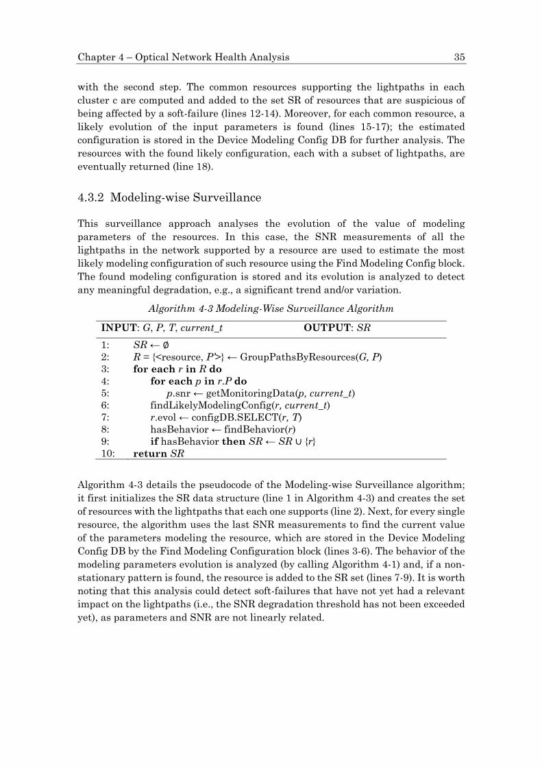
Chapter 4 – Optical Network Health Analysis 35
with the second step. The common resources supporting the lightpaths in each
cluster c are computed and added to the set SR of resources that are suspicious of
being affected by a soft-failure (lines 12-14). Moreover, for each common resource, a
likely evolution of the input parameters is found (lines 15-17); the estimated
configuration is stored in the Device Modeling Config DB for further analysis. The
resources with the found likely configuration, each with a subset of lightpaths, are
eventually returned (line 18).
Modeling-wise Surveillance
This surveillance approach analyses the evolution of the value of modeling
parameters of the resources. In this case, the SNR measurements of all the
lightpaths in the network supported by a resource are used to estimate the most
likely modeling configuration of such resource using the Find Modeling Config block.
The found modeling configuration is stored and its evolution is analyzed to detect
any meaningful degradation, e.g., a significant trend and/or variation.
Algorithm 4-3 Modeling-Wise Surveillance Algorithm
INPUT: G, P, T, current_t OUTPUT: SR
1:
2:
3:
4:
5:
6:
7:
8:
9:
10:
SR ← ∅
R = {<resource, P’>} ← GroupPathsByResources(G, P)
for each r in R do
for each p in r.P do
p.snr ← getMonitoringData(p, current_t)
findLikelyModelingConfig(r, current_t)
r.evol ← configDB.SELECT(r, T)
hasBehavior ← findBehavior(r)
if hasBehavior then SR ← SR ∪ {r}
return SR
Algorithm 4-3 details the pseudocode of the Modeling-wise Surveillance algorithm;
it first initializes the SR data structure (line 1 in Algorithm 4-3) and creates the set
of resources with the lightpaths that each one supports (line 2). Next, for every single
resource, the algorithm uses the last SNR measurements to find the current value
of the parameters modeling the resource, which are stored in the Device Modeling
Config DB by the Find Modeling Configuration block (lines 3-6). The behavior of the
modeling parameters evolution is analyzed (by calling Algorithm 4-1) and, if a non-
stationary pattern is found, the resource is added to the SR set (lines 7-9). It is worth
noting that this analysis could detect soft-failures that have not yet had a relevant
impact on the lightpaths (i.e., the SNR degradation threshold has not been exceeded
yet), as parameters and SNR are not linearly related.

36 Autonomous and Reliable Operation of Multilayer Optical Networks
Soft-Failure Localization
In case that the surveillance phase has identified a set of suspicious resources,
Algorithm 4-4 localizes the soft-failures. The algorithm first removes the suspicious
resources that explain the very same set of lightpaths (lines 1-6 in Algorithm 4-4),
as localization is not yet possible in those cases. Next, the resources that explain the
SNR of complete subsets of lightpaths are localized and classified as independent
soft-failures, iSF (lines 6-10). The rest of the suspicious resources are related to soft-
failures that affect common subsets of lightpaths, so a given lightpath can be affected
by more than one soft-failure.
Algorithm 4-4 Soft-Failure Localization Algorithm
INPUT: SR OUTPUT: iSF, mSF
1:
2:
3:
4:
5:
6:
7:
8:
9:
10:
11:
for each r in SR do
Rr ← ∅
for each r’ in SR | r ≠ r’ do
if r.P = r’.P then Rr ← Rr ∪ {r, r’}
SR ← SR - Rr
iSF ← ∅
for each r in SR do
if r.P ∩ r’.P = ∅ ∀r’ SR | r ≠ r’ then
iSF ← iSF ∪{r}
SR ← SR - {r}
return iSF, SR
Finding the Most Likely Modeling Configuration
The above surveillance approaches use the FindModeling Configuration block, which
estimates the most likely modeling configuration of a given resource r. Given the
ranges of feasible configuration values 𝕍 of r, the configuration estimation problem
consists in finding the most likely values v, by minimizing the error (computed as
mean squared error -MSE) between the measured (S) and the estimated (Ŝ) SNR for
the set of lightpaths being supported by r, P(r), i.e.:
min𝑣∈𝕍
𝑀𝑆𝐸 (𝑆(𝑃(𝑟)), �̂�(𝑃(𝑟)|𝑣)) (4-1)
The SNR estimation Ŝ(·) is obtained by calling the QoT tool and thus, the
optimization problem in (4-1) cannot be solved by traditional methods like Steepest
Descent, which are based on computing the gradient of the function to be minimized.
In view of that, the findLikelyModelingConfig() procedure uses the
modelingConfigSearch() one (Algorithm 4-5) to solve the optimization problem in
(4-1). The algorithm interrogates the QoT tool with different values of the
parameters and the configuration entailing the lowest error with respect to the SNR
values measured is returned. The procedure assumes that: i) the function is convex
in 𝕍, i.e., there is just one minimum that is the global minimum (tests supporting

Chapter 4 – Optical Network Health Analysis 37
this assumption will be carried out); and ii) there is just one of the modeling
parameters of r with a value different than the initially found. The procedure fixes
the value(s) of the parameter(s) and requests the QoT tool to compute, with such
configuration, the SNR values of the lightpaths being supported by r. By computing
the mse(·) function, the procedure determines if such configuration is likely enough
or if more queries to the QoT tool are needed.
As calls to the QoT tool are time consuming, modelingConfigSearch() targets at
minimizing them; instead of using the brute force and request the estimation of the
SNR for the whole range of possible values, the procedure uses the projection of two
points to determine the next value of the parameters to be used for the estimation.
As parameters typically evolve smoothly in time when devices are affected by a soft-
failure, it also stores the last configuration(s) in the Device Modeling Config DB;
every time it is called, it uses such configurations as starting points for the search
aiming at finding the optimal solution fast.
Algorithm 4-5 Modeling Config Search
INPUT: P, r, vmin, vmax OUTPUT: <v, m>
1:
2:
3:
4:
5:
6:
7:
8:
9:
10:
11:
12:
13:
14:
15:
16:
17:
<v, m> ← configDB.getMin(); numIters ← 0
while m > epsilon AND numIters++ < MaxIters do
<vl, ml>, <vr, mr> ← configDB.getNeigbours(v)
va ← intersect(v, m, vl, ml, vmin, vmax)
vb ← intersect(v, m, vr, mr, vmin, vmax)
if va = vl then va ← (v + vl) / 2
if vb = vr then vb ← (v + vr) / 2
ma ← configDB.getConfig(va)
if ma = None then
ma ← MSE(P.SNR, QTool(P, r, va))
configDB.addConfig(<va, ma>)
mb ← configDB.getConfig(vb)
if mb = None then
mb ← MSE(P.SNR, QTool(P, r, vb))
configDB.addConfig(<vb, mb>)
<v, m> ← configDB.getMin()
return <v, m>
4.4 Soft-Failure Identification and Severity
Estimation
Let us now focus on the Soft-Failure Identification and the Severity Estimation
blocks, which are assumed to be executed as soon as degradation is detected and
localized (via SNR and/or device configuration analysis). These blocks make
MESARTHIM able to generate notifications to the network controller containing not

38 Autonomous and Reliable Operation of Multilayer Optical Networks
only the list of degraded lightpaths, but also their expected evolution and the
estimated time for the soft-failure to degrade into a hard-failure.
Let us imagine that the surveillance and localization analysis in Section 4.3 detected
some degradation at time t and therefore, non-empty ISR and/or MSF sets were
found. In addition, let us define state as the combination of the estimated modeling
configuration of the resources that are involved, and the SNR experienced by the
supported lightpaths. With the aim of an accurate diagnosis, it is interesting not only
to analyze the current state but also to predict its future evolution. It is for this very
reason that historical data (within a pre-defined time window) are gathered from
monitoring and device config DBs and stored in the Network Diagnosis DB. The
evolution of each parameter (lightpaths’ SNR and device modeling config
parameters) is analyzed individually using time series forecasting techniques. By
using different techniques with different parametrization, several expected
evolutions can be obtained as a practical way to generate different likely projections
for parameter degradation.
For illustrative purposes, let us analyze an example of the evolution of three
parameters selected from a hypothetical state: the SNR of a given lightpath affected
by an SNR degradation, as well as the NF and P-max parameters modeling an OA
traversed by that lightpath. Figure 4-3 presents three time-evolutions of the OA
modeling parameters and SNR, and their analysis at current time t. At this time,
the failure has been correctly localized in the selected OA; however, the cause of the
degradation (either NF or P-max) is still unclear. This is the reason behind
performing the estimation and evolution analysis for all modeling parameters; such
analysis is carried out following forecasting techniques. Three curves representing
the upper (fu), centered (fc), and lower (fl) projected possible evolutions are depicted
for each parameter. Based on such projections, monitored data are evaluated and an
indicator (φ) is computed and used to discard modeling parameters while identifying
the one that is the most likely to be the real cause of the observed performance
degradation. Hence, the indicator provides large values when the modeling
parameter is far from the expected behavior of an affected parameter. The obtained
indicator is accumulated with the values obtained in the previous computations, and
identification is positive when the parameter with the lowest accumulated indicator
is far from all the rest of the parameters with a significantly higher accumulated
one. This evidence can be easily observed by setting up a threshold allowing the
discrimination of low and high accumulated indicator modeling parameters.
Once the Soft-Failure Identification block has found enough evidence of the modeling
parameter explaining the soft-failure, the Severity Estimation block uses the
centered projection of the evolution of such modeling parameter to estimate the
likely evolution of the SNR for the affected lightpaths (i.e., those being supported by
the localized resource). Analyzing such evolution, it is easy to check whether any
lightpath would exceed a given threshold. For instance, the minimum SNR defined

Chapter 4 – Optical Network Health Analysis 39
by its modulation format and bit rate. The next subsections detail these two
MESARTHIM blocks.
SNR
Severity Estimation
t
NF
Centered NF projection (fc)
Lower NF projection (fl)
Upper NF projection (fu)
P-max
QoT estimation based on centered NF projection
Poor centered projection, upper and centered overlapHigh Indicator
Accurate centered, different upper and lower ones
Low Indicator
δ
Time
Figure 4-3. Example of identification and severity estimation at time t.
Soft-failure Identification
Algorithm 4-6 is used to identify the most likely modeling parameter(s) explaining
the observed performance degradation; it receives as input the resource responsible
for the soft-failure and the number T of historical monitoring samples, and, if
sufficient evidence is found, it returns the modeling parameter identified as a
potential failure.
The algorithm starts by retrieving the modeling parameters v that characterize the
state of the resource, as well as the evolution of each modeling parameter in the last
T measurements (lines 1-2 in Algorithm 4-6). Then, each parameter i in v is
evaluated independently to compute a score indicating how likely is that such
parameter is responsible for the resource failure. Specifically, the time series of the
parameter i is selected and split into two portions: one with the first T-δ data points
(Yfit) used for fitting and a second one (Yeval), with the last δ measurements, used for
evaluation and indicator computation (lines 3-6) (dark grey area in Figure 4-3).
Using the Yfit segment, a set of time-dependent functions F, where the parameter

40 Autonomous and Reliable Operation of Multilayer Optical Networks
value is modeled as a function of time, is obtained by applying Holt-Winters
exponentially-based modeling and polynomial fitting in a wide range of degrees (e.g.,
from 1 to 7) [30] (line 7). The set F contains all functions with similar goodness-of-
fit, i.e., +/- 5% of variation in terms of Pearson correlation coefficient. Moreover,
functions are evaluated in the time interval of Y to verify that trend is always
monotonic; otherwise, the function is discarded. Then, three of those functions are
selected to be the likely projections illustrated in Figure 4-3 (line 8). This selection
contains: i) fl (lower) and fu (upper), with the functions with the lowest and highest
value at the current time, respectively; and ii) fc (centered), with the function with
the smallest number of coefficients providing maximum Pearson correlation
coefficient (+/- 5%), which is assumed to be the most likely parameter evolution.
Algorithm 4-6 Soft Failure Identification
INPUT: r, T OUTPUT: param
1:
2:
3:
4:
5:
6:
7:
8:
9:
10:
11:
12:
13:
14:
15:
v ← getModelingParameters(r)
r.evol ← configDB.SELECT(r, T)
for each i in v do
Y ← getTimeSeries(r.evol, i)
Yfit ← Y[1..T-δ]
Yeval ← Y[T-δ+1..T]
F ← fitTimeDependentFunctions(Yfit, δ)
F*=<fl, fc, fu>←selectLikelyEvolution(F,T)
r.φ[i]← φ(F*,Yeval) (Eq. (4-2))
v* ←selectHighIndicatorParameters(r)
for each i in v* do
r.accumφ[i]+=r.φ[i]
if r.accumφ[i]>thr then v← v\i
if |v| = 1 then return v.getFirst()
return ∅
After obtaining the likely projections, they are compared with the trendline
(computed using the same methodology of fc) in Yeval. This comparison is carried out
using an additive multi-factorial indicator (φ) that combines several Boolean and
continuous variables according to Eq. (4-2), where xi represents a variable and bi the
weighting coefficient for that variable.
𝜑 = ∑ 𝑏𝑖𝑖=1..𝑛
· 𝑥𝑖 (4-2)
Table 4-2 briefly describes the considered variables, sorted in the descendent degree
of importance. Two Boolean functions are used: x1 returns True if there is no evidence
of degradation in the parameter, whereas x4 checks if any of the upper and lower
projections is the same function as the centered one. In addition, two continuous
variables are defined: x2 accounts for the relative Mean Square Error (rMSE) of the
data in the evaluation portion with respect to the centered projection, whereas x3

Chapter 4 – Optical Network Health Analysis 41
returns the minimum rMSE of the data with one of the projections. Note that if
measurements in the evaluation portion follow a trend showing a parameter
degradation similar to the projections (preferably, the centered one), the indicator
remains low; otherwise, the indicator increases indicating that the observed
behavior differs from the expected one and therefore, the likelihood of the parameter
not to be the cause of the failure increases.
Table 4-2 Indicator function components
i Description (xi)
1 [boolean] Projections fl, fc, fu do not show parameter degradation
2 [continuous] rMSE(Yeval, fc)
3 [continuous] min(rMSE(Yeval, fi)) | i = {l,c,u}
4 [boolean] fl = fc OR fu = fc
Once the indicator is computed for all modeling parameters characterizing the state
of the resource, the selection of parameters, whose indicator is significantly higher
than the rest, is conducted (line 10). Thus, considering φmin as the minimum indicator
value of a parameter, the limit φmin+∆φ is defined as the reasonable limit for
parameters with low indicator, being all parameters above φmin+∆φ selected as those
with high indicator. For the resultant set of parameters (if not empty), the
cumulative indicator is updated by adding the current one (lines 11-12). Finally, the
cumulative indicator is compared with an identification threshold thr and, if
exceeded, the parameter is removed from the candidate parameter set (line 13). The
identification is considered positive when just one parameter remains as a candidate
and it is eventually returned (line 14). Otherwise, the algorithm returns no
identification (line 15). It is worth noting that the value of thr needs to be high
enough to clearly identify the parameter without false positives.
Severity Estimation
Once a modeling parameter has been identified as the cause of the observed
degradation, the severity estimation algorithm is executed. This method uses the
projection of the modeling parameters to estimate when some affected lightpath will
cross the FEC limit.
Although the severity estimation could be based on the projected evolution of the
modeling parameters, defining a threshold for each one is not easy as different
lightpaths are impacted differently by its degradation.
Algorithm 4-7 details the pseudocode; it receives as input the resource responsible
for the soft-failure, the list of lightpaths supported by such device, the number T of
historical monitoring samples, and the identified modeling parameter, and it returns

42 Autonomous and Reliable Operation of Multilayer Optical Networks
the estimated time that the soft-failure will cause a major impact on, at least, one of
the lightpaths. The algorithm first retrieves the last T configuration values from the
Device Modeling Config DB, which are used to compute the centered projection fc for
the considered input parameter on a given time window (lines 1-2 in Algorithm 4-7).
The projection fc is used as the input parameter to estimate the SNR for the list of
lightpaths; in case that the estimated QoT for any of the lightpaths falls behind the
minimum SNR, the algorithm returns the estimated time of this event to happen
(lines 3-6); otherwise, it returns a large value that exceeds the considered time
window (line 7).
Algorithm 4-7 Severity Estimation
INPUT: r, P, T, param OUTPUT: estimatedTime
1:
2:
3:
4:
5:
6:
7:
r.evol ← modelingConfigDB.SELECT(r, T)
fc←getCenteredProjection(r.evol[param],timeWindow)
for t in [1, timeWindow] do
SNR ← Ŝ(P | fc(t))
for each p in P do
if SNR[p] < p.minSNR then return t
return INF
4.5 Results
Experimental assessment
Being the basis of the MESARTHIM methodology, the Find Modeling Configuration
has been evaluated experimentally in the testbed depicted in Figure 4-4. Two
commercial coherent transponders (labeled TRX-1 and TRX-2), with optical line
interface at 100G (32-GBd Quadrature Phase-Shift Keying -QPSK), have been
connected using an optical multi-span link. The pair of transponders has been
equipped with a specifically designed driver enabling both the configuration and the
real-time monitoring of the SNR; the generated signal is filtered by a WSS Wave
Shaper device. The optical link consists of 4 spans, each realized by an 80 km single-
mode-fiber spool, for a total distance of 320 km. Five EDFAs have been used to
compensate for the power attenuation; all being the single stage with gain in the
range 15-25 dB. OA1 was configured with a constant 17.5 dB gain to compensate for
the filter insertion losses and the other OAs with a constant gain of 16 dB to
compensate entirely for the fiber losses within the span.
Two different experiments were carried out. In the first, we reproduced the effect of
a filter detuning. We configured the TRXs at 193.9 THz and the WSS with a
bandwidth of 50 GHz, collecting the estimated SNR at TRX-2. Then, we reconfigured
the WSS filter, reducing the bandwidth with steps of 2 GHz, until the operational
status of TRX-2 card was down. GNPy was used as a tool to estimate the expected

Chapter 4 – Optical Network Health Analysis 43
QoT for the lightpath. In order to estimate the QoT, together with the scenario that
includes fiber types and span length, modeling parameters of the WSS, OAs and the
TRXs are provided as input to GNPy; it estimates the QoT using the generalized GN
model [Ca18], which considers both the ASE noise and NLI accumulation.
TRX-1 TRX-2
1 2 3 4 5 AA
Att=5dB
G=17.5dB G=16dB G=16dB G=16dB G=16dB
WSS
Att=10dB
span 1L=80km
span 2L=80km
span 3L=80km
span 4L=80km
0 dBm
Figure 4-4 Experimental testbed
Assuming that the device responsible for the SNR measured in TRX-2 is unknown,
we run the Find Modeling Configuration block of MESARTHIM to estimate the most
likely modeling configuration of the WSS and one of the OAs in the optical link.
Figure 4-5 presents the results obtained when the observed SNR is explained by a
reduction in the OSNR of the A/D WSS (Figure 4-5a) and by an increased value of
the NF in one of the OAs (Figure 4-5b). We observe that changes in both modeling
parameters could explain the evolution of the observed SNR in the lightpath with
minimal error, being the resulting values of the modeling parameters within a
feasible range. Note that with just one lightpath in this experiment, it is not possible
to make any localization, as any of the devices could be responsible for the observed
reduction in the SNR.
In the second experiment, we slightly changed the multi-span link scenario with
respect to that in Figure 4-4, by adding 5 dB attenuators before spans 2-4 emulating
an additional 25 km in each span. Therefore, the gain of OAs 3-5 had to increase to
21 dB to compensate for the increased losses that also affected the NF of our
amplifiers (which is inversely proportional to the configured gain). The experiment
was carried out in three steps, where one span was modified at a time. For each step,
we continuously collected the estimated SNR at TRX-2, detecting the variation of the
transmission metrics during the testbed evolution. Figure 4-6 presents the results
from the Find Modeling Configuration block when the length of the spans 2-4 was
increased to an equivalent of 105 km and consequently, the gain of OAs 3-5. At each
step, the module was able to explain the increment in the SNR of the lightpath by a
reduction in the NF of the related OA. For illustrative purposes, the estimated SNR
of the lightpath that would be obtained by keeping the NF constant is also
represented in Figure 4-6. These two experiments assess the high accuracy of the
Modeling Config Search for estimating the modeling parameters of the devices.

44 Autonomous and Reliable Operation of Multilayer Optical Networks
R² = 0.9868
R² = 0.9884
253035404550
A/D
OSN
R (
dB
)N
F (d
B)
Bandwidth (GHz)
(a)
(b)
25
30
35
40
45
50
0
3
6
9
12
15
Figure 4-5 Modeling parameter value vs. bandwidth for A/D WSS OSNR (a) and
OA NF (b)
SNR
(d
B)
Length of the link (km)
19
20
21
22
23
310 330 350 370 390 410
ExperimentalNF=[3.3,7.57]NF =7.57
Figure 4-6 SNR vs. link length
The next subsections evaluate the MESARTHIM methodology through simulation.

Chapter 4 – Optical Network Health Analysis 45
Simulation environment
For the simulation, we selected a German-like network topology with 17 nodes and
26 bidirectional links (see Figure 4-7). 136 bidirectional lightpaths, representing all
the origin-destination pairs, were established through the shortest route in terms of
hops. Figure 4-8 plots the number of lightpaths that every link in the network is
supporting (which is particularly important for failure localization). For the sake of
simplicity in the analysis of the results, we assume that all signals use the QPSK
modulation format.
Leipzig
Berlin
Düsseldorf
Norden
Ulm
Munich
Nuremberg
Hamburg
Essen
Cologne
Dortmund
Frankfurt
Mannheim
Karlsruhe
Stuttgart
Bremen
Hanover
Figure 4-7 Optical network topology considered in this chapter.
The optical data plane was simulated by a GNPy instance. We generated SNR
measurements for every lightpath by varying every modeling parameter of every
intermediate OAs and A/D WSSs in the ROADMs in the network, independently.
With these measurements, a set of realistic types of failures (use cases) affecting
optical devices were reproduced by forcing the modeling parameters of the selected
devices (NF and P-max in the OAs and OSNR in the WSSs) to vary over time. From
the different variations that might happen, we focus on gradual variations, i.e., those
soft-failures that can eventually degenerate into hard-failures. Among all possible
gradual degradations, we focus on the exponential increase (NF) and logarithmic
decay (P- max and OSNR), since both types of degradations accelerate in time and
hence, it is crucial to anticipate their detection and localization as much as possible.
Finally, variability to the SNR samples was added in the form of random noise.

46 Autonomous and Reliable Operation of Multilayer Optical Networks
0
10
20
30
40# distinct routes
max # routes for perfect localization
# ro
ute
s
Figure 4-8 Number of distinct routes per link and max number of routes for
localization.
The resulting samples were stored in the simulated control plane and fed the module
implementing the MESARTHIM methodology. In the case of the SNR- wise
Surveillance algorithm, the SNR_threshold (line 3 in Algorithm 4-2) was set to the
expected SNR for each given lightpath minus a fixed value that exceeds the random
variations introduced by the monitoring generator.
The next subsections present the obtained results for the different procedures of the
MESARTHIM methodology based on this simulation setup.
Surveillance and Device Configuration Estimation
Let us first illustrate the convergence of the Modeling Config Search algorithm with
an example entailing two sets of lightpaths. We are interested in finding the most
likely modeling config for the OSNR of an A/D WSS and for the NF of an OA (each
supporting one of the sets of lightpaths), given its monitored SNR. Figure 4-9 plots
the MSE as a function of the configuration value, as well as those values explored by
the algorithm for the two optical devices. The inset tables specify the MSE values,
where the configuration that gives the minimum MSE is finally selected. From these
results, as well as from those in the experimental assessment, we conclude that the
algorithm converges in the whole range of the true soft-failure origin, regardless of
the selected QoT parameter.

Chapter 4 – Optical Network Health Analysis 47
0
2
4
6
8
10
12
14
16
18
20
20 22 24 26 28 30 32 34 36 38A/D OSNR (dB)
MSE
0
2
4
6
8
10
12
5 10 15 20
MSE
NF (dB)
(a)
(b)
Figure 4-9 Modeling Config Search
We now focus on the evolution of the SNR over time for the defined use cases. The
graphs in the upper row in Figure 4-10 (P-max gradual), Figure 4-11 (NF-gradual),
and Figure 4-12 (A/D WSS gradual) present such evolution, where, for the sake of
clarity, we plot only one sample of the affected lightpath. Note that only the
lightpaths affected by the failure will experience an evolution in their SNR, whereas
the rest of the lightpaths will show no variation over time other than a random one
plus some uncorrelated spurious measurements introduced by the monitoring
generator. The time in the graphs is normalized, as the time-scales for the considered
soft-failures are different, ranging from days to months or even years. The evolution
of the modeling parameters is shown in the bottom-row graphs, where the actually
programmed value and the interval of values [max, min] estimated by the Find
Configuration block is plotted.

48 Autonomous and Reliable Operation of Multilayer Optical Networks
10
12
14
16
18
20
P-m
ax (
dB
m)
SNR
(d
B)
13
14
15
16
17
18
19
P-max gradual
13
20
0 0.2 0.4 0.6 0.8 1
0.92
15%
0.78
Time
Figure 4-10 Evolution of monitored SNR and estimation of modeling parameters.
13
14
15
16
17
18
19
5
7
9
11
13
15
0 0.2 0.4 0.6 0.8 1
0.86
45%
0.47
NF gradualSNR
(d
B)
NF
(dB
)
Time
Figure 4-11 Evolution of monitored SNR and estimation of modeling parameters.

Chapter 4 – Optical Network Health Analysis 49
15
20
25
30
35
4013
14
15
16
17
18
19
0 0.2 0.4 0.6 0.8 1
EstimationReal Value
0.63
0.86
27%
A/D WSS gradualSNR
(d
B)
A/D
WSS
(d
B)
Time
Figure 4-12 Evolution of monitored SNR and estimation of modeling parameters.
We observe that the range of possible values of the modeling parameters is tighter
when the value of the parameter deviates from its nominal one. In addition, the
range of possible values for the modeling parameters is different for the different
parameters, being the P-max of the OAs the one with the largest range. This might
have a clear impact if the detection of the soft-failure is performed by tracking the
evolution of that parameter. Figure 4-13 complements the previous study by plotting
the maximum and average error in the estimation of the modeling parameters as a
function of the magnitude of the degradation. We observe in Figure 4-13a that both
maximum and average P-max estimation errors are high for low degradation
magnitudes (15.6% and 7.8%, respectively). In contrast, the average error for NF and
A/D WSS (Figure 4-13b.c) are remarkably low and almost constant for the
degradation magnitudes studied. Figure 4-13 also confirms the observation
regarding the error in the estimation of the value of the modeling parameters greatly
reduces with the magnitude of the degradation, which is a very promising result and
it can be exploited for soft-failure localization and identification.
Some conclusions can be drawn from the results obtained so far: 1) the proposed
method for estimating the value of modeling parameters of the devices has shown
remarkable accuracy in the experimental tests, which has been confirmed by
simulation for all failure use cases; 2) in general, the estimation interval is tighter
when the impact of the value of the parameter on the observed SNR is higher; 3) in
the specific case of the maximum power of the OAs, the range of values that result

50 Autonomous and Reliable Operation of Multilayer Optical Networks
in the SNR values observed is large when the observed SNR remains around the
nominal value. However, when SNR degrades with evident trend, the correlation
between P-max and SNR becomes larger.
0.0
0.5
1.0
1.5
2.0
2.5
3.0
3.5
0 1 2 3 4 5 6 7 8 9 10
error_max
error_avg
Ab
solu
te E
rro
r
Degradation (absolute difference with the nominal value)
(c) A/D WSS OSNR
1.4%
0.4%0.3%
0.0
0.5
1.0
1.5
2.0
2.5
3.0
3.5
(b) NF
1.3%0.4%
7.9%
0.0
0.5
1.0
1.5
2.0
2.5
3.0
3.5
(a) P-max15.6%
0.8%
7.8%
Nominal value = 5 dB
Nominal value = 20 dBm
Nominal value = 38 dB
Ab
solu
te E
rro
rA
bso
lute
Err
or
Figure 4-13 Absolute and relative modeling parameter estimation error.
To help developing intuition about the differences that can be expected by analyzing
the SNR of the lightpaths and the value of the modeling parameters of optical
devices, Figure 4-10, Figure 4-11, and Figure 4-12 compare the time to detect a

Chapter 4 – Optical Network Health Analysis 51
degradation by analyzing the measured SNR and the value of the modeling
parameters. For the sake of simplicity, let us assume that degradation detection is
performed by threshold crossing; the threshold was set to 1 dB below the nominal
SNR value for the lightpaths, not below a minimum SNR resulting in a pre-FEC
BER over 4∙10-3 for QPSK signals. The thresholds related to modeling parameters
were defined as a percentage of the variation range given by the nominal value and
the extreme value. Values are selected to reduce detecting false degradations: i) for
P-max it was set to 40% in the interval between the nominal value (20 dBm) and the
extreme value (10 dBm) due to the large range of variation observed; ii) for NF of the
OAs, the percentage was set to 20% in the interval between the nominal (5 dB) and
the extreme value (15 dB); and iii) for the OSNR of the A/D WSSs, the percentage
was set also to 20% in the interval between the nominal (38 dB) and the extreme
value (20 dB).
With these values, the detection of the degradation in the case of the SNR of the
lightpath happened at normalized times 0.92, 0.86, and 0.86 for the P-max, NF, and
A/D WSS OSNR gradual soft-failure use cases, respectively. This contrasts with the
detection at times 0.78, 0.47, and 0.63 when the analysis was in the value of the P-
max, NF, and OSNR of the A/D WSSs, respectively, which results in anticipation
between 15% and 45%. Note that such anticipation is enabled by the different
evolution of modeling parameters and their non-linear impact on the SNR of the
lightpaths.
Soft-Failure Localization
The above discussion considered the time for the detection only. Note that soft-
failure location (Algorithm 4-4 in Section 4.3.2) requires several lightpaths to find
the common resources in the network topology. When the evolution of the monitored
SNR changes suddenly, SNR-wise surveillance (Algorithm 4-2) collects enough
lightpaths to easily localize the failure; however, under a gradual degradation, the
lightpaths exceeding the threshold might be not enough for the localization.
Figure 4-8 includes a study of the maximum number of distinct routes that need to
be considered to unambiguously identify every link as responsible for a soft-failure,
considering that longer lightpaths will be more affected by device degradations. For
the study, we selected all the links in the network, together with an incremental
number of lightpaths selected by their total length, and fed Algorithm 4-4 for the
(multiple) soft-failure localization (i.e., 26 soft-failures were localized with a single
execution of Algorithm 4-4). For the localization, not only the number of lightpaths
is important, but also their routes. We repeated the experiments with the lightpaths
sorted in inverse order, i.e., assuming that shorter lightpaths would exceed the
(relative) threshold first. The results showed that all soft-failures could be perfectly
localized when the resources of the two shortest lightpaths were analyzed.

52 Autonomous and Reliable Operation of Multilayer Optical Networks
With the above in mind, let us now show how the SNR-wise surveillance and
localization evolves over time. Table 4-3 presents the results from two different
failures. The first failure was in an OA in the link Frankfurt-Mannheim (supporting
41 distinct lightpaths), and the second in the A/D WSS in the Dusseldorf ROADM
(supporting 16 distinct lightpaths). For each failure, each row shows the detection
time when the measured SNR of some new lightpaths is below the threshold (bear
in mind that the threshold is relative to the expected SNR for that specific lightpath).
However, the localization of the soft-failure is not successful until just one resource
(assuming that it is responsible for the failure) can be identified. Such identification
happens at normalized times 0.93 and 0.91 for the failures in the OA and the A/D
WSS, respectively. Note that the number of lightpaths needed to localize the soft-
failure, although small, adds some extra time that could be of paramount importance
for the impact on the network.
Table 4-3 Examples of Soft-Failure Localization
Failure in OA in link Frankfurt-Mannheim
Time Degraded paths Common Resources
0.86 1 2 TRXs, 2 A/Ds, 1 Link
0.90 2 2 Links
0.93 4 1 Link (Failure in Frankfurt-Mannheim)
Failure in A/D WSS Dusseldorf
0.86 1 2 TRXs, 2 A/Ds, 1 Link
0.91 2 1 A/D WSS (Failure in Dusseldorf)
In contrast, soft-failure localization under the Modeling-wise approach considers all
the lightpaths supported by such resource, as it analyzes the estimated evolution of
the modeling parameters by resource. In consequence, Algorithm 4-4 under the
Modeling-wise approach can localize the cause of degradations in their very early
stages (between 31% and 49% with respect to the SNR-wise approach).
As a final remark, it should be noted that even though the Modeling-wise approach
considers all the lightpaths supporting a given resource, unambiguous localization
might still not be possible if few lightpaths with distinct routes are established.
Figure 4-8 shows that, for some links in the considered scenario, unambiguous
localization of a soft-failure is only possible when all supported lightpaths are
analyzed. Therefore, in case that not all these paths are established, the localization
procedure (Algorithm 4-4) would be unable to localize the failure. E.g., let us consider
the soft-failure in the link Frankfurt-Mannheim in Table 4-3 and imagine that only
one lightpath is supported by such link. Then, a degradation in that lightpath can
be explained by degradation in more than one resource. This highlights the need for

Chapter 4 – Optical Network Health Analysis 53
additional procedures to be applied for those scenarios which result in ambiguous
localization.
Identification and Severity Estimation
Once the degradation has been localized, let us focus on the identification of the
modeling parameter responsible for such degradation. We assume that the device
explaining the observed degradation is an OA. According to the notation in Section
4.4.1, identification performance is clearly dependent on the configuration of all
coefficients related to indicator φ. Several configurations were tested to find the one
giving the desired importance to every component, ensuring that parameters with a
high indicator are correctly selected, while guaranteeing no false positives. Such
configuration is <b1, b2, b3, b4, ∆φ, thr> = <20, 10, 2, 1, 5, 30>, which will be used
hereafter.
Figure 4-14 shows the obtained results for a gradual degradation caused by NF,
whereas Figure 4-15 shows the results for a gradual degradation caused by P-max.
In both cases, Figure 4-14a and Figure 4-15a plot the evolution of the accumulative
indicator with time, and the decision threshold thr. Both indicators remain clearly
under the threshold until time around 0.32, where enough evidence of the cause of
the degradation is found. Note that the time of such identification represents 32% of
anticipation compared to the earliest time obtained for degradation detection (at
time 0.47) using a threshold on the evolution of the input parameter and 64%
compared to the earliest detection time using a threshold on the evolution of the
SNR. Figure 4-14b-c and Figure 4-15b-c show the computed projections for the two
modeling parameters under study and for both failures; note that such figures are
similar to Figure 4-3. The projections are plotted for a long window (around 0.25 time
units) for clarity purposes, although the value used for fitting and evaluation was δ
=0.03 normalized time units.
In the case that the failure is a consequence of the NF degradation (Figure 4-14b-c),
we observe that the centered projection fc for the NF parameter is highly accurate
and clearly between the upper and lower ones, which results in the minimum
indicator parameter. On the contrary, P-max indicates an evident but less accurate
projection and moreover, fc overlaps with fu, which increases its indicator above 5
units from the one of NF. As a consequence of this, P-max is selected as a parameter
with a high indicator, so its accumulative indicator increased. Conversely, in Figure
4-15b-c the minimum indicator is that of P-max, where there is an evident
degradation for fl. Note that this indicator is much lower than that computed for NF,
where no degradation is observed, thus exceeding by far the indicator limit. In
conclusion, we see how the proposed methodology allows discriminating the actual
failing parameter and perform a fine failure identification.

54 Autonomous and Reliable Operation of Multilayer Optical Networks
0
10
20
30
40
50
60
70
80
90
0 0.2 0.4 0.6
NF
P-max
Acc
um
ula
ted
Ind
icat
or
NF
(dB
)
Time
(a)
(b)
(c)
0.32
0.32
5.5
6.0
6.5
7.0
7.5
8.0
8.5
15
16
17
18
19
0.25 0.35 0.45 0.55 0.65
Pm
ax (
dB
m)
Figure 4-14 NF Gradual Soft-Failure Identification.

Chapter 4 – Optical Network Health Analysis 55
0
10
20
30
40
50
60
70
80
90
0 0.2 0.4 0.6
NF
P-max
Time
(a)
(b)
(c)
NF
(dB
)A
ccu
mu
late
d In
dic
ato
r
5.0
5.5
6.0
6.5
7.0
7.5
8.0
0.32
0.32
15
16
17
18
19
20
0.25 0.35 0.45 0.55 0.65
Pm
ax (
dB
m)
Figure 4-15 P-max Gradual Soft-Failure Identification.
We can take advantage of the identification method to implement an alternative
localization method that can be applied when not enough lightpaths with distinct
routes are established in the network. This allows the unambiguous localization of a
soft-failure, as motivated at the end of Section 4.5.4. In this case, we assume that
only lightpaths between the two end ROADMs of the link Frankfurt-Mannheim are
established and have considered soft-failures in one of the supporting devices (OA,
TRX or A/D WSS), in line with Table 4-3. In this case, we execute Algorithm 4-6

56 Autonomous and Reliable Operation of Multilayer Optical Networks
considering a single virtual resource that abstracts the supporting optical device
types. The algorithm returns the most probable modeling parameter among those of
OA, TRX and A/D WSS, which helps to reduce the number of devices to be analyzed
manually.
0
10
20
30
40
50
60
70
80
90
0 0.2 0.4 0.6
0
10
20
30
40
50
60
70
80
90
Acc
um
ula
ted
Ind
icat
or
0
10
20
30
40
50
60
70
80
90
OA
A/D WSS
TRx
Time
(c) A/D WSS
(b) TRX
(a) OA
0.30
Acc
um
ula
ted
Ind
ica
tor
Acc
um
ula
ted
Ind
icat
or
Figure 4-16 Localization by identifying the Soft-Failure.
Figure 4-16 shows the performance of the identification procedure for soft-failure
localization. Three scenarios are considered for the real cause of the soft-failure: i)
gradual NF degradation in an OA (Figure 4-16a), ii) gradual OSNR degradation in

Chapter 4 – Optical Network Health Analysis 57
an A/D WSS (Figure 4-16b), and iii) gradual OSNR degradation in a TRX (Figure
4-16c). We observe that the accumulated score clearly increases for the two types of
devices that are not the real cause of the failure for all the analyzed scenarios. This
happens at time 0.3 in all the cases.
0
0.2
0.4
0.6
0.8
1
0 0.2 0.4 0.6
49.6%
Esti
mat
ed T
ime
Time from identification
0.3
(c) A/D WSS OSNR
(b) NF
(a) P-max
0
0.2
0.4
0.6
0.8
1
42.8%
0.37
0
0.2
0.4
0.6
0.8
1
62.8%
0.22
Esti
mat
ed T
ime
Esti
mat
ed T
ime
Figure 4-17 Severity Estimation.
Finally, Figure 4-17 presents the obtained results for severity estimation for gradual
degradation of P-max, NF and A/D WSS OSNR as a function of the time. The plots

58 Autonomous and Reliable Operation of Multilayer Optical Networks
show the evolution of the estimated time with the real-time, where the area in grey
color highlights the real-time when the soft-failure degenerates into a hard-failure
±5%. We observe that the estimated time takes a large value when the estimation
does not observe a major impact in the selected timeWindow for any of the affected
lightpaths, and rapidly converges to the real degeneration time. In fact, assuming
that the severity is accurately estimated after two consecutive executions returning
estimated times close enough one to the other, anticipation over 42% to the
degeneration time are obtained, which leave enough time to plan the adequate
maintenance operations.
4.6 Concluding Remarks
QoT estimation is typically carried out during the provisioning phase and in-
operation planning to ensure that computed lightpaths will provide zero post-FEC
errors, assuming some values for the QoT model input parameters related to the
optical devices in the network. In this chapter, QoT estimation was used for the
reverse process, i.e., given the real measured QoT of a set of lightpaths, we were
interested in estimating the value of the modeling parameters of the optical devices.
Because of the non-linear relation between lightpaths QoT and the value of the
modeling parameters, the ability to estimate the value of such parameters opens the
opportunity to analyze its evolution, which can be as a result of, e.g., aging,
temperature variations, etc. The proposed MESARTHIM methodology combines
analysis of the evolution of the monitoring QoT and their transformation into the
estimated modeling parameters space, not only for the degradation detection, but
also for its localization, identification, and severity estimation.
After the experimental assessment of the method for estimating the modeling
parameters of the devices, the MESARTHIM methodology was evaluated through
simulation. The methodology demonstrated remarkable anticipation in failure
detection and localization by analyzing the estimation of the value of the modeling
parameters of the devices. A simple example showed the reason behind such
potentials in the different evolution of the modeling parameters and the lightpaths
SNR. In addition, accurate cause identification based on the analysis of the projected
evolution of the modeling parameters was demonstrated, which enabled the
estimation of the severity in terms of the time when the soft-failure degrades into a
hard-failure. Such severity estimation allows planning maintenance, as it largely
anticipates degradation.
Table 4-4 summarizes the main characteristics with pros and cons of the
MESARTHIM methodology.

Chapter 4 – Optical Network Health Analysis 59
Table 4-4 Summary of the MESARTHIM Methodology
Method Degradation Detection and
Failure Localization
Cause Identification and
Severity Estimation
Analysis in
the
lightpaths’
SNR space
• SNR-wise surveillance finds
common resources in sets of affected
lightpaths by analyzing its SNR.
• Analyzes all lightpaths. For failure
localization, the algorithm needs
that several lightpaths to be
affected.
• No cause can be identified.
• QoT can be estimated based on
the projected evolution of the
SNR.
Analysis in
the
devices’
modeling
parameters
space
• Modeling-wise surveillance analyzes
the value of the modeling
parameters for all network devices.
• The algorithm detects degradations
and localizes their sources very
ahead in time.
• Cause identification based on
the projected evolution of the
modeling parameter of the
device where the failure is
localized.
• Severity estimation difficult to
estimate by analyzing the
evolution of the input
parameters.

Chapter 5
Towards Autonomous vLink
Capacity Management
The massive deployment of 5G and beyond will require high capacity and low latency
connectivity services, so network operators will have either to overprovision capacity
in their transport networks or to upgrade the optical network controllers to make
decisions nearly in real time; both solutions entail high capital and operational
expenditures. A different approach could be to move the decision making toward the
nodes and subsystems, so they can adapt dynamically the capacity to the actual
needs and thus reduce operational costs in terms of energy consumption. To achieve
this, several technological challenges need to be addressed. In this chapter, we focus
on the autonomous operation of DSCM systems, which enable the transmission of
multiple and independent subcarriers (SC). Herein, we present several solutions
enabling the autonomous DSCM operation, including: i) SC quality of transmission
estimation; ii) autonomous SC operation at the transmitter side and blind SC
configuration recognition at the receiver side. We provide useful guidelines for the
application of autonomous SC management supported by the extensive results
presented.
5.1 Introduction
In this chapter, we propose a decentralized approach where the intelligence is
distributed [APV17.2]; the Tx decides autonomously the SC configurations, i.e., the
SC’s MF and SR, and the Rx can detect and recognize such configurations.
Nevertheless, the role of the SDN controller is of paramount importance as it solves

Chapter 5 – Towards Autonomous vLink Capacity Management 61
the routing and spectrum allocation (RSA) [Ve12] for the request, thus providing a
lightpath in the optical network topology that satisfies not only the needed capacity
but also the required QoT for every SC. Note that individual SCs are impaired
differently when they cross WSSs, which are part of ROADM. To this end, software
tools like the open source GNPy [Fe20], can be used but need to be upgraded to
properly consider the filter penalties.
The remainder of the chapter is organized as follows. Section 5.2 introduces the
proposed solution for autonomous SC operation, where an intent, with the
operational objective to allocate enough capacity, is in charge of autonomously
making decisions to configure and activate or deactivate SCs at the Tx side. Section
5.3 focuses on lightpath provisioning and includes an estimation of per-SC QoT,
which is later used to solve the RSA with SC (RSA-SC) configuration problem.
Section 5.3 proposes algorithms to manage the SC at the Tx and Rx sides; the
Transponder Agent at the Tx side is in charge of managing the capacity of the
lightpath by properly configuring the different SCs to minimize energy consumption,
whereas the agent at the Rx side needs to recognize the configuration of each SC.
Section 5.3.2 is devoted to our intent-based solution and the approach is proposed to
anticipate future traffic conditions thus minimizing or totally eliminating
undesirable effects at the packet layer. This solution uses a short-term traffic
forecast. Section 5.3.2 is devoted to our intent-based solution and our approach is
proposed to anticipate future traffic conditions thus minimizing or totally
eliminating undesirable effects at the packet layer. This solution uses a short-term
traffic forecast. The discussion is supported by extensive illustrative results in
Section 5.4, including exhaustive simulations over realistic scenarios. Finally,
Section 5.5 draws the main conclusions of our work.
5.2 Autonomous Capacity Management
As previously stated, we propose the autonomous operation of the vlinks performed
locally at their end nodes and being able to recognize in one end the decisions made
at the remote end. This is particularly important at the optical layer, as the Rx
optical transponder of the lightpath supporting the vlink needs to realize the actual
configuration of the signal that was transmitted. From the packet layer perspective,
it is also desirable to devise solutions that: i) do not introduce delays and traffic
losses; and ii) minimize the changes in the capacity of the vlink to facilitate the
management of such capacity at the packet nodes.
Figure 5-2 presents the key elements in the control and data planes and overviews
the envisioned workflow of vlinks. At the set-up time, the SDN controller receives a
request to create a vlink between two end nodes with a given maximum capacity.
The SDN controller computes the best route of the underlying lightpath and
estimates the QoT. Based on such estimation, the SDN controller determines the

62 Autonomous and Reliable Operation of Multilayer Optical Networks
number of SCs and a configuration map with the set of feasible configurations for
each SC s in terms of pairs <MFs, SRs> that can be used; this would allow the
autonomous SC operation and will support the given maximum capacity (step 1 in
Figure 5-2). Then, the SDN controller establishes the lightpath by allocating the
needed optical spectrum along the path connecting Tx and Rx, and sends the
configuration map to the vlink intent in charge of the autonomous vlink operation
(step 2). The SDN then relies on the vlink intent to manage the capacity of the vlink
as a function of the input traffic (step 3). An illustrative example of such capacity
management is displayed in the inset in Figure 5-2, where the capacity of the vlink
(orange line) increases and decreases to serve the input traffic (blue area). The vlink
intent communicates the desired capacity of the vlink to the Transponder Agent,
which activates or deactivates SCs in the underlying optical signal. Such decision
making is performed within the Tx and consequently, a mechanism is needed for the
Rx to detect and configure SCs’ MF and SR, as well as to detect the absence of a SC
(step 4). Finally, notifications are sent to the SDN controller informing about
changes in the vlink and the optical signal (step 5).
vlink capacity
traffic
Metro Network
TxRx
SDN
Controller
vlink
Lightpath
25
Node
Agent
Node
Agent4
3
QoT
Estimation
1
Figure 5-1 Vlink workflow overview.
Figure 5-2 presents an example of the evolution over time of the input traffic and the
active configuration of the optical signal, as decided by the Tx, to meet the capacity
requirements of the vlink intent. Once the connection is set up by the SDN controller
at time t0, the vlink intent observes the amount of input traffic and makes decisions
consequently. For instance, based on required capacity, the transponder agent
within the Tx configures the first 8 GBaud QPSK SC (SC1) at t0, which entails that
the connection capacity is 25 Gb/s, considering a FEC overhead of 20%. Based on
periodical capacity updates, received from the vlink intent, the Tx increases
connection’s capacity to 50 Gb/s at t1 by activating SC4 with the same configuration
as for SC1. The capacity is increased to 100 Gb/s at time t2 by activating SC2
configured as 11 GBaud 8QAM. If the input traffic would continue increasing, the

Chapter 5 – Towards Autonomous vLink Capacity Management 63
last SC (SC3) would be activated, e.g., with an 11 GBaud 16QAM configuration to
increase capacity up to 170 Gb/s. On the contrary, if the capacity requirements would
decrease (as in t3), one or more SCs could be turned off, thus saving energy.
Note that the decisions made in the SC configuration can limit the maximum
capacity of the vlink. For instance, if all SCs can be configured with QPSK, 8QAM
or 16QAM MFs and 8 or 11 GBaud, the maximum capacity of the vlink would lie in
the range [100-280] Gb/s depending on the selected configuration. Therefore,
assuming that SCs cannot be reconfigured (i.e., to change the configuration of a SC,
the SC needs to be deactivated and then activated again with a different
configuration, which would cause packet losses if the SC is supporting traffic), such
decision-making process need to be intelligently carried out to maximize the
potential capacity of the connection without traffic disruption, while saving as much
energy as possible. For instance, in view of the evolution of the traffic at t1, the vlink
intent could have requested a capacity of 75 Gb/s, so that the Tx would have
configured SC2 as a 11 GBaud 16QAM signal and then, deactivated SC4, thus
resulting in the same performance but with lower total energy and configuration
changes. In addition, note that not all SCs can support all different configurations,
as this depends on the expected SNR at the receiver. For example, a cascade of filters
will affect the “external” SCs more severely than the inner ones, thus limiting the
MF order of the former to just QPSK. This introduces additional complexity in the
decision-making process.
Node
AgentTransponder
Agent
Tx Rx
0
25
50
75
100
time
Inp
ut
Traf
fic
(Gb
/s)
Sub
carr
iers
1 41 1 2 4 1 2
t1 t2 t3t0 t4
vlink
Intent
Transponder
AgentActivate and
deactivate SC
Required
Capacity
Detect and
configure SCs
Actual
Capacity
Input
traffic
Node
Agent
Figure 5-2 Intent-based autonomous vlink operation to allocate capacity for the
input traffic.
The modules that make possible the envisioned autonomous vlink operation are
presented next.

64 Autonomous and Reliable Operation of Multilayer Optical Networks
5.3 Capacity Management
When the lightpath is established, the actual capacity that is provided by the
connection can be managed by activating and configuring each SC independently as
a function of the traffic to be conveyed. In this section, we first present the procedures
for the Tx to select the configuration of the optical connection, including which SCs
are active and their configuration to provide the needed capacity. Then, we propose
a solution to predict the traffic evolution. We assume that the SC definition contains
a SC configuration map with all possible options, from those allowed by the
transponder, that do not exceed the maximum configuration received from the
controller.
Transponder Agent
We propose two different policies for the autonomous management of the optical
connection at the transponder agent:
• the maxSC connection management policy, which allocates the SC with
maximum possible capacity, thus potentially minimizing the changes in the
connection’s configuration;
• the adaptive connection management policy, which allocates the minimum
capacity to satisfy the input traffic needs, targeting at minimizing the excess
of capacity with respect to the actual traffic with the goal of eventually
minimizing the total energy consumption.
Both algorithms return one single SC change in the connection configuration.
Therefore, they must be executed within an outer loop until they cannot perform
more changes (i.e., returning <s=∅, config=∅>).
The pseudocode for maxSC connection management policy is presented in Algorithm
5-1. The algorithm receives as input the state of the connection in terms of the
configuration of the SCs, the map of feasible configurations for each SC, and the
target capacity for the connection. It returns the SC to be activated/deactivated, if
any, and its target configuration. The algorithm computes the difference of capacity
between the current and the requested ones (line 1). In case the capacity of the
connection needs to be increased, the SC providing the largest capacity among those
not yet active is selected (lines 2-3). On the other hand, the capacity of the connection
is reduced by selecting the active SC with the lowest capacity, whose deactivation
leaves enough capacity in the connection (lines 4-6). Finally, the selected SC, if any,
and the target configuration are returned (line 7).
This policy enables minimizing the number of configurations to be supported thus
potentially reducing the cost of the transponders. It selects the SC with the largest
capacity among the non-active ones; this minimizes the number of changes in the

Chapter 5 – Towards Autonomous vLink Capacity Management 65
capacity of the connection, which facilitates its management at the packet layer.
Nonetheless, this policy might lead to large energy consumption due to the
overprovisioning, since the selection of the SC to be activated does not depend on the
actual capacity needs.
Algorithm 5-1 maxSC Capacity Management
Input: conn, configMap, targetCapacity
Output: s, config
1:
2:
3:
4:
5:
6:
7:
diffCap ← targetCapacity - conn.capacity
if diffCap > 0 then
<s, config> ← argmax{s.getMaxConfig(configMap)
∀ s ∈ conn | NOT s.isActive()}
return <s, config>
config ← ∅
s ← argmin{s.capacity ∀ s ∈ conn | s.isActive() AND s.capacity < -diffCap}
return <s, config>
Algorithm 5-2 presents the adaptive connection management policy, which targets
at minimizing the energy consumption by configuring the connection capacity as
close as possible to the actual needs.
Algorithm 5-2 Adaptive Capacity Management
Input: conn, configMap, targetCapacity
Output: s, config
1:
2:
3:
4:
5:
6:
7:
8:
9:
10:
11:
12:
13:
14:
15:
diffCap ← targetCapacity - conn.capacity
if diffCap > 0 then
activeSC ← argmax{sc.upgradability ∀ s ∈ SC |
sc.upgradability = sc.getMaxConfig(configMap) - diffCap}
if activeSC ≠ ∅ then
<s, config> ← findNonActiveSC(conn, configMap,
activeSC.capacity + diffCap)
if s ≠ ∅ then return <s, config >
<s, config> ← findNonActiveSC (conn, configMap, diffCap)
if s ≠ ∅ then return <s, config >
<s, config> ← argmax{s.getMaxConfig(configMap)
∀ s ∈ conn | NOT s.isActive()}
return <s, config >
config ← ∅
s ← argmax{s.capacity ∀ s ∈ conn |
s.isActive() AND c.capacity < -diffCap}
if s = ∅ AND conn.numActiveSCs = 1 then
<s, config> ← findNonActiveSC (conn, configMap, targetCapacity)
return <s, config >
In case that an increment of capacity is requested, the algorithm identifies the active
SC with the largest potential capacity increase (lines 2-3 in Algorithm 5-2), so
another SC can be activated supporting the requested capacity plus the identified

66 Autonomous and Reliable Operation of Multilayer Optical Networks
active SC (lines 4-6). In that case, a consecutive execution of the algorithm will find
that the first SC can be deactivated. If any active SC is identified, a non-active SC
needs to be activated, which is configured to support the requested increment of
capacity (lines 7-8). In case that the increment of capacity cannot be supported by
just one single SC, the non-active SC with the maximum capacity is returned (lines
9-10). In the case of reducing capacity, a target SC is identified, so the total capacity
of the connection still supports the requested one (lines 11-12). If no SC can be
deactivated and there is just one single SC activated, the algorithm tries to activate
one SC so all target capacity can be served (lines 13-14). Again, a consecutive
execution of the algorithm will find that the first SC can be deactivated, so just one
single SC will remain active.
The algorithm for the adaptive connection management policy calls the
findNonActiveSC() function. This identifies the non-active SC providing the
minimum overprovisioning (line 1 in Algorithm 5-3) and among them, the one that
will be closer to its maximum capacity (line 2). The configuration that better fits the
required capacity is returned, except if there is just one single non-active SC, where
the maximum configuration is returned (lines 4-6).
Algorithm 5-3 FindNonACtiveSC() Function
Input: conn, configMap, capacity
Output: s, config
1:
2:
3:
4:
5:
6:
SC={s} ← argmin{s.overProvision ∀ s ∈ conn |
NOT s.isActive() AND s.overProvision =
s.getMinConfig(configMap, capacity) - capacity}
<s, config> ← argmin{s.upgradability ∀ s ∈ SC |
s.upgradability = s.getMaxConfig(configMap) -
s.getMinConfig(configMap, capacity)}
if s ≠ ∅ AND conn.numNonActiveSCs = 1 then
return <s, s.getMaxConfig(configMap)>
return <s, config>
Virtual Link Intent-Based Capacity Management
The capacity management algorithms, introduced in the previous section, require
measuring the input traffic to determine the capacity that needs to be ensured.
However, such monitoring reflects the capacity that was needed at the time the
measurement was performed, so in case that the target capacity exceeded the one of
the optical connections, some traffic might need to be queued waiting for more
capacity to be available; this is at the cost of introducing delay or even traffic losses
in case the queue capacity is exceeded. In addition, this approach is purely reactive,
as if the traffic volume reduces, the capacity of the connection reduces as well, which
can derive into capacity oscillations making difficult for the packet nodes managing
it. Therefore, it is desirable to devise solutions that not only reduce the energy

Chapter 5 – Towards Autonomous vLink Capacity Management 67
consumption by managing the configuration of the SCs, but also predict: i) how to
configure the SCs before the capacity is exhausted to avoid introducing delays and
traffic losses; and ii) how to reduce the changes in the vlink capacity. To this end, we
propose a capacity management to be carried out at the vlink level and keep the
capacity management at the transponders as a back-up in case the prediction fails
and the current capacity is exhausted, so that the measured traffic volume is always
ensured provided that is under the maximum capacity to be guaranteed.
A solution is to use short-term traffic forecasts, instead of the actual measured traffic,
to predict future capacity needs. This short-term prediction can be obtained by
projecting forward the last monitored traffic samples, i.e., interpolating traffic in the
last w measurements and extrapolating for next δ time units [Is02]. Although this
approach can help to anticipate potential capacity exhaustion by allocating capacity
in advance, when the traffic volume decreases, the reduction of capacity can lead to
undesired capacity fluctuations and to increase queuing.
5.4 Illustrative Results
In this section, we first introduce the power model used for comparing the proposed
SC management solutions, and then we study the performance of different SC
configurations and the QoT estimation, with the aim of finding the operational limits
of DSCM for autonomous capacity management. Next, we analyze the performance
of the capacity management performed at the transponder or by the vlink intent.
Power Model
The results in the following subsections present power savings that have been
computed assuming a power model aiming to abstract the actual realization of a
DSCM transponder. The power model is based on the conclusions from [Fl20] and
[Fr17] that can be summarized as follows: i) the power consumption of a transponder
is related to its actual configuration in terms of MF and SR, and ii) the architecture
of a DSCM transponder contains subsystems that are always active independently
of the number and configuration of active SCs (e.g., DAC / ADC), and others that can
be switched off in case a SC is not active.
With the above considerations, the power consumption of a DSCM transponder can
be modeled as Eq. (5-1), where Pbase is the minimum power consumption and β(∙) is a
multiplier that depends on the actual configuration of the SCs. Eq. (5-2) defines β(∙)
as the summation of two components, those coming from always active subsystems
and those from subsystems that are associated to a particular SC and thus, can be
switched off if that SC is not active. The ratio R(∙), defined in Eq. (5-3), computes the
proportion of power from subsystems in each group, and α(∙) computes the
incremental power as a function of the MF and SR configured in a given SC, being 0

68 Autonomous and Reliable Operation of Multilayer Optical Networks
if the SC is not active. Then, from Eq. (5-2), the power consumption of always active
subsystems starts from a minimum one given by the minimum configuration
supported (e.g., <QPSK,8>) and increases depending on the actual configuration,
whereas that of the subsystems associated to a particular SC can be 0 if that
particular SC is not active.
𝑃 = 𝑃𝑏𝑎𝑠𝑒 ∗∑ 𝛽(𝑀𝐹𝑆𝐶 , 𝑆𝑅𝑆𝐶)𝑆𝐶
(5-1)
𝛽(𝑀𝐹𝑆𝐶 , 𝑆𝑅𝑆𝐶) = 𝑅(𝑎𝑙𝑤𝑎𝑦𝑠 𝑜𝑛) ∗ 𝑚𝑎 𝑥(𝛼𝑚𝑖𝑛,𝛼(𝑀𝐹𝑆𝐶 , 𝑆𝑅𝑆𝐶)) + 𝑅(𝑝𝑒𝑟 𝑆𝐶)
∗ 𝛼(𝑀𝐹𝑆𝐶 , 𝑆𝑅𝑆𝐶) (5-2)
𝑅(∙) =𝑃𝑏𝑎𝑠𝑒(∙)
𝑃𝑏𝑎𝑠𝑒 (5-3)
In this chapter, we assume: R(always on) = 62%, and the values of α(∙) in Table 5-1.
This leads to energy savings in the range [56.6%-46.8%] when only one SC is active.
Transponder Agent Capacity Management
From the viewpoint of the pure optical layer, all the configurations studied can be
used, especially for 50 and 62 GHz slot widths. However, transponders not
supporting all such configurations might be more cost effective. With this in mind,
we now focus on the capacity management and study whether reducing the number
of configurations available would be also convenient from the packet layer
perspective. In this subsection, we consider that the transponder agent at the Tx side
adapts the configuration of the optical connection to provide enough capacity for the
input traffic, by running the algorithms in Section 5.3.1.
For this analysis, we define three configuration sets for the transponders (see Table
5-1): i) all: transponders implement all possible configurations; ii) selected:
transponders implement some configurations with the maximum diversity in
capacity and lightpath scenarios; and iii) 16QAM: transponders implement only
16QAM for all SRs. The normalized power consumption and capacity (assuming 20%
FEC overhead) of every configuration are detailed in Table 5-1. Besides the power
related to the SCs, another 15% of the maximum configuration supported by the
transponder for each SC (active or not) needs to be accounted.
Two different policies have been carefully selected to concentrate numerical
evaluation under relevant conditions: i) the maxSC with only the 16QAM
configuration set; and ii) the adaptive connection management with the three
configuration sets. Two traffic profiles lasting for 2.5 days are used to compare the
aforementioned policies, namely High Traffic and Low Traffic. In the High Traffic
profile, the traffic varies from 20 to 240 Gb/s, whereas in the Low Traffic case it is
limited to 60 Gb/s. The traffic profiles have been especially tailored to induce many
configuration changes, as they contain traffic variations around the values of the
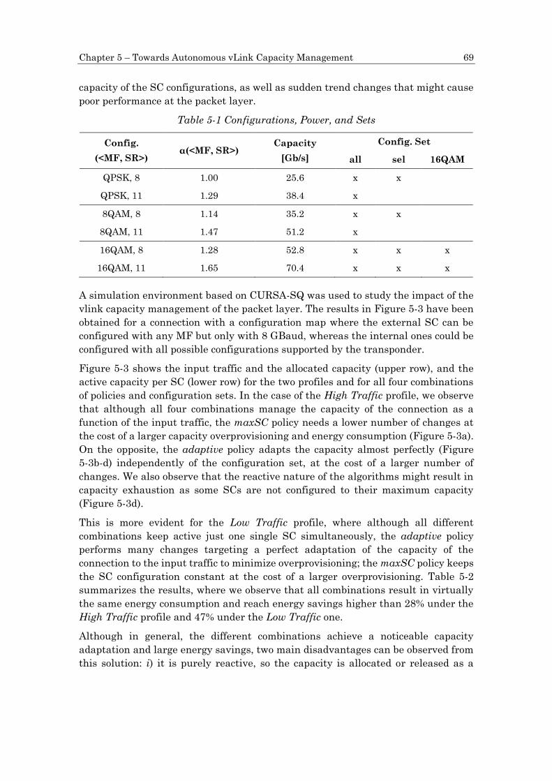
Chapter 5 – Towards Autonomous vLink Capacity Management 69
capacity of the SC configurations, as well as sudden trend changes that might cause
poor performance at the packet layer.
Table 5-1 Configurations, Power, and Sets
Config.
(<MF, SR>) α(<MF, SR>)
Capacity
[Gb/s]
Config. Set
all sel 16QAM
QPSK, 8 1.00 25.6 x x
QPSK, 11 1.29 38.4 x
8QAM, 8 1.14 35.2 x x
8QAM, 11 1.47 51.2 x
16QAM, 8 1.28 52.8 x x x
16QAM, 11 1.65 70.4 x x x
A simulation environment based on CURSA-SQ was used to study the impact of the
vlink capacity management of the packet layer. The results in Figure 5-3 have been
obtained for a connection with a configuration map where the external SC can be
configured with any MF but only with 8 GBaud, whereas the internal ones could be
configured with all possible configurations supported by the transponder.
Figure 5-3 shows the input traffic and the allocated capacity (upper row), and the
active capacity per SC (lower row) for the two profiles and for all four combinations
of policies and configuration sets. In the case of the High Traffic profile, we observe
that although all four combinations manage the capacity of the connection as a
function of the input traffic, the maxSC policy needs a lower number of changes at
the cost of a larger capacity overprovisioning and energy consumption (Figure 5-3a).
On the opposite, the adaptive policy adapts the capacity almost perfectly (Figure
5-3b-d) independently of the configuration set, at the cost of a larger number of
changes. We also observe that the reactive nature of the algorithms might result in
capacity exhaustion as some SCs are not configured to their maximum capacity
(Figure 5-3d).
This is more evident for the Low Traffic profile, where although all different
combinations keep active just one single SC simultaneously, the adaptive policy
performs many changes targeting a perfect adaptation of the capacity of the
connection to the input traffic to minimize overprovisioning; the maxSC policy keeps
the SC configuration constant at the cost of a larger overprovisioning. Table 5-2
summarizes the results, where we observe that all combinations result in virtually
the same energy consumption and reach energy savings higher than 28% under the
High Traffic profile and 47% under the Low Traffic one.
Although in general, the different combinations achieve a noticeable capacity
adaptation and large energy savings, two main disadvantages can be observed from
this solution: i) it is purely reactive, so the capacity is allocated or released as a

70 Autonomous and Reliable Operation of Multilayer Optical Networks
function of the current input traffic, without considering any requirement (e.g., time)
to properly configure the connection, and consequently induces packet loss and
added delay as a result of the time packets spent in the vlink queue; and ii) it does
not consider the traffic evolution, so it produces unnecessary fluctuations in the
configuration of the connections.
Traf
fic
and
Cap
acit
y [G
b/s
]SC
s A
ctiv
e C
apac
ity
[Gb
/s]
(b) Adaptive - All configurations (c) Adaptive - Selected configurations (d) Adaptive – 16QAM configurations(a) MaxSC Capacity configuration
Time [days]
Traf
fic
and
Cap
acit
y [G
b/s
]SC
s A
ctiv
e C
apac
ity
[Gb
/s]
Hig
h T
raff
ic P
rofi
leLo
w T
raff
ic P
rofi
le
0
50
100
150
200
250
0 50 100 150 200 250
input trafficcapacity
0
50
100
150
200
250
0 50 100 150 200 250
0
50
100
150
200
250
0 50 100 150 200 250
0
50
100
150
200
250
0 50 100 150 200 250
0
10
20
30
40
50
60
70
80
0 50 100 150 200 250
SC1 SC2 SC3 SC4
0
10
20
30
40
50
60
70
80
0 50 100 150 200 250
0
10
20
30
40
50
60
70
80
0 50 100 150 200 250
0
10
20
30
40
50
60
70
80
0 50 100 150 200 250
080
0
50
100
150
200
250
0 50 100 150 200 250
input traffic
capacity
0
50
100
150
200
250
0 50 100 150 200 250
0
50
100
150
200
250
0 50 100 150 200 250
0
50
100
150
200
250
0 50 100 150 200 250
0250
0
10
20
30
40
50
60
70
80
0 0.5 1 1.5 2 2.5
SC1 SC2 SC3 SC4
0
10
20
30
40
50
60
70
80
0 0.5 1 1.5 2 2.5
0
10
20
30
40
50
60
70
80
0 0.5 1 1.5 2 2.5
0
10
20
30
40
50
60
70
80
0 0.5 1 1.5 2 2.5
080
Figure 5-3 Optical connection managed by the Transponder Agent. Total and SCs
capacity vs time for two traffic profiles.
Table 5-2 Summary of Results for Optical Connection Configuration Managed by
the Transponder Agent
High Traffic Profile
maxSC adapt-all adapt-sel adapt-16Q
#Changes per day 8.8 51.2 51.2 23.2
Energy savings [%] 28 30 31 32
Packet Loss [MB] 4.8 14.9 11.4 14.9
Queue (max) [MB] 16 16 16 16
Queue (avg) [MB] 0.3 1.4 1.4 1

Chapter 5 – Towards Autonomous vLink Capacity Management 71
Low Traffic Profile
maxSC adapt-all adapt-sel adapt-16Q
#Changes per day 0 68 82.4 44
Energy savings [%] 47 51 53 51
Packet Loss [MB] 0 0 0 0
Queue (max) [MB] 0 9 8 8
Queue (avg) [MB] 0 1.2 1 0.7
Intent-based vlink operation
Let us now consider the architecture depicted in Figure 5-3, where the vlink intent
takes the role of client to manage the capacity of the vlink and the Transponder
Agent serves such capacity by properly managing the configuration of the SCs. In
view of the results obtained in the last subsection, for this study we consider the two
policies with only the 16QAM configuration set for the transponders.
For the predictive solution, we exhaustively explored configurations of δ and w
ranging between 1 and 20 minutes. The obtained results for the configuration with
best performance (6 and 10 min for δ and w, respectively) are presented in Table 5-3.
We observe that no packet loss has been produced and the time in the vlink queue
has been drastically reduced by using a short-term prediction of the evolution of the
traffic. Such queue is produced as a result of the no perfect accuracy of the prediction,
which produces some capacity exhaustion, and thus the capacity of the vlink is
increased automatically by the transponder agent. Besides, we observe a slight
reduction in the number of configuration changes and on the energy savings, that
are now over 26% and 45% for the High and Low Traffic profiles, respectively.
Table 5-3 Summary of Results for Optical Connection Configuration Managed by
vlink Intent
High Traffic Profile Low Traffic Profile
maxSC adapt-16Q maxSC adapt-16Q
#Changes per day 7.2 18.8 1.6 20.8
Energy savings [%] 26 28 45 49
Packet Loss [MB] 0 0 0 0
Queue (max) [MB] 4.5 10.3 0 5
Queue (avg) [MB] 0 0.2 0 0.1
Cap. Exhaust. per day 1 5 0 4

72 Autonomous and Reliable Operation of Multilayer Optical Networks
5.5 Concluding Remarks
The autonomous operation of SCs has been presented in this chapter from a holistic
perspective, with the objective to reduce energy consumption at the optical layer,
motivated by the fact that SCs can be configured independently with the desired MF
and SR. This, together with the possibility to switch off parts of the transponder
directly related to each of the SC and the fact that the power consumption of a
transponder is related to its actual configuration in terms of MF and SR, opened an
opportunity to save energy by activating only those SCs which are needed to support
the upper layer packet traffic.
The need to perform a per-SC QoT estimation was introduced, which considering the
path and the specific SC configuration. Such QoT estimation can be used to define
the SC configuration map that will be used afterwards for the autonomous capacity
management.
The autonomous capacity management problem was faced following an incremental
approach. First, the algorithms in the transponder agent were built with the
objective to provide the required capacity for the lightpath and reduce energy
consumption by activating SCs when their capacity is needed, while not adding
detrimental effect neither for the packet traffic (packet loss and time spent in the
vlink queue) nor for the packet nodes (excessive changes in the capacity of the vlink).
At the Tx side, two policies for capacity management were discussed and the
required algorithms designed. Specifically, the maxSC targeting at minimizing the
changes in the SC configuration and the adaptive focuses on minimizing the energy
consumption by adjusting the capacity of the lightpath to the input traffic as much
as possible.
The capacity management implemented in the transponder agent is purely reactive,
which would impact on the operation and performance of the packet layer. To solve
that, an intent-based solution was proposed to manage the vlink capacity at the
packet layer, where such capacity is actually used. The intent-based solution targets
to ensure the packet layer performance indicators, like packet loss, time in queue,
and configuration changes, while relying on the transponder agent for the SC
configuration management targeting at minimizing energy consumption. A solution
based on short-term prediction was developed.
Table IX summarizes the main lessons learnt in this work, which we believe that
might help telecom operators and system vendors to introduce autonomous SC
management in their networks and portfolios.

Chapter 5 – Towards Autonomous vLink Capacity Management 73
Table 5-4 Main Lessons Learnt
Features Main observations
Set of
supported SC
configurations
Having a large variety of SC configurations might increase
the cost of the transponders unnecessarily, as they do not
show additional energy savings and their use might result
in variations in the capacity of the vlink, which might add
additional complexity at the packet layer.
Capacity
management
at the Tx side
Algorithms that try to tightly adapt the capacity of the vlink
to the current or near future input traffic, did not show large
energy savings. Increments in capacity of one SC configured
to the maximum capacity resulted in effective alternatives,
which also simplifies the algorithms.
Capacity management uniquely at the optical layer, resulted
in poor performance at the packet layer.

Chapter 6
Autonomous Packet Flow
Capacity Management
One of the solutions that might bring cost savings to network operators is the
dynamic capacity management of large packet flows, especially in the context of
packet over optical networks. However, managing packet flows requires meeting
strict performance (e.g., delay, packet loss, and capacity overprovisioning) and
therefore, is of paramount importance to develop solutions that guarantee them.
Machine Learning, particularly Reinforcement Learning, seems to be an enabler for
autonomicity as a result of its inherent capacity to learn from experience. However,
precisely because of that, RL methods might not be able to provide the required
performance when managing the capacity of packet flows, until they learn the
optimal policy. In view of that, we propose a management lifecycle with three phases:
1) a self-tuned threshold-based approach operating just after the packet flow is set
up and until enough data on the traffic characteristics are available; 2) an RL
operation based on models pre-trained with a generic traffic profile; and 3) an RL
operation with models trained for real traffic.
Exhaustive simulation results confirm the poor performance of RL algorithms until
the optimal policy is learnt and when traffic characteristics change over time, which
prevents deploying such methods in operators’ networks. In contrast, the proposed
lifecycle outperforms benchmarking approaches, achieving noticeable performance
from the beginning of operation while showing robustness against traffic changes.

Chapter 6 – Autonomous Packet Flow Capacity Management 75
6.1 Introduction
Control loops can be put into practice based on policies that specify the action to be
taken under some circumstance (policy-based management), e.g., allocate the
capacity of a packet flow so that the ratio traffic volume over capacity is under 80%.
In packet flows, this ratio is related to the average delay that the packets in the flow
will experience because of queuing, and thus to the SLA in the case that the packet
flow is related to some customer connection. Although such policies can be modified,
they are purely reactive. Under high traffic variations, they might entail either poor
QoS (e.g., high delay or even traffic loss) and SLA breaches or poor resource
utilization, which in both cases represent large costs for network operators. Note
that policy-based management does not define the desired performance and thus,
agents implementing those policies are unable to learn the best actions to be taken.
Although many ML techniques could be potentially applied for the autonomous
capacity operation of traffic flows, in this chapter, we rely on RL and consider several
methods of different complexity and analyze their performance, in particular: (i) Q-
learning; (ii) D3QN, and (iii) TD3 (see [Fu18]).
With the deployment of network slicing [Ve18.1] and the support to time-sensitive
applications [Ve20], the flow capacity autonomous operation (hereafter referred to
as CRUX) focuses on answering a major problem that network operators are facing
nowadays: how to allocate the right capacity to every traffic flow, so as to provide the
desired QoS (e.g., by preventing traffic loss and ensuring a given maximum average
delay), while minimizing overprovisioning (i.e., capacity–traffic).
In this chapter, we apply the main lessons learnt from the previous chapter to IBN
agents based on RL. We assume that a packet flow (alternatively, referred as traffic
flow or simply flow) conveying traffic with unknown characteristics is established
and the allocated capacity needs to be set to ensure the required QoS (from the set-
up time), while minimizing resource utilization. To this end, a policy-based
management is used at the set-up time to start operating the capacity of the flow;
meanwhile, traffic measurements are collected to characterize the traffic. Note that
policy-based operation can be highly re-liable, as it is based on specific rules that can
be defined and understood by human operators. However, such an operation usually
obtains poor resource utilization. Therefore, it would be useful to substitute policy-
based operation by an RL model as soon as possible. To that end, pre-trained
generally applicable models for the partly observed traffic characteristics are loaded
and the RL algorithm starts operating. A per-flow algorithm supervises the
performance of the RL algorithm and tunes model parameters to ensure the re-
quired QoS. Once enough traffic measurements are available, offline training is
carried out in a sandbox domain to produce a specific model well-suited for that
particular traffic flow, which then substitutes the generic one. Since the traffic
characteristics can change over time, analysis must be continuously performed to
detect them and change the operating model when needed. By iterating that cycle,

76 Autonomous and Reliable Operation of Multilayer Optical Networks
the proposed RL agent will be able to adapt to traffic changes that would otherwise
degrade performance.
The rest of the chapter is organized as follows. The pros and cons of applying RL to
real network operation is highlighted in Section 6.2, which include poor performance
during the initial set-up and during changes in the traffic flow. The CRUX problem
and the pro-posed approach are as follows: it targets operating a traffic flow and
ensuring the required QoS from set-up time without previous knowledge of the
traffic characteristics. The motivation behind the different phases of operation and
the proposed lifecycle is presented, where pre-trained models and offline–online RL
cycles aim at solving the identified is-sues. The CRUX problem is formally defined
in Section 6.3. Several RL approaches can be used to solve CRUX, and each one
requires different settings of states and actions. A methodological approach is
provided to model the problem with different RL algorithms, and how the QoS
targets are related to parameters in the reward function. Section 6.4 presents the
algorithms that analyze the traffic characteristics, supervise the performance, and
make decisions regarding the model and parameters to be used for operation. The
discussion is supported by the results presented in Section 6.5. Finally, Section 6.6
concludes this chapter.
6.2 The Flow Capacity Autonomous Operation
(CRUX) Problem
Flow Capacity Autonomous Operation
Let us start by analyzing the result of the autonomous capacity operation of a traffic
flow. Similar to the transponder agent defined in Chapter 5, a flow manager might
collect monitoring data from the network and expose some interface, so a flow intent
based on RL can take an action. For illustrative purposes, Figure 6-1 shows a typical
RL framework, where the learning agent is separated into two different blocks, the
learner and the agent.
Let us assume that the monitoring data include the byte count since the last
monitoring sample (amount of traffic) and the actual capacity allocated to the flow.
The actions to be taken are related to the actual capacity allocated to the flow, which
can be increased or decreased as needed with some granularity to meet the required
QoS. For instance, a customer connection can manage the capacity of the flow with
granularity 1 Gb/s by configuring some packet node, whereas in a virtual link
supported by the optical layer, the capacity can be increased/decreased by
establishing or tearing down parallel lightpaths, each with a capacity of 100 s Gb/s.
It seems clear that the time to change the capacity is also different, ranging from
seconds to minutes. The RL algorithm should then decide the capacity to be allocated
to the flow to absorb variation in the traffic from one monitoring sample to the next,

Chapter 6 – Autonomous Packet Flow Capacity Management 77
plus the time to increase the allocated capacity, with the objective to avoid any traffic
loss and ensure some additional QoS metric. Then, the traffic variation becomes a
major feature for a flow, together with the traffic pattern, i.e., the evolution of the
mean traffic with time.
State function Reward function
Action
Reward
State
Models
BufferOnline Learner
ActionModel
Updates
Environment
Agent
Learner
Flow
Monitoring Capacity
Flow Manager
Required CapacityTraffic, Capacity
RL-based Operation
Figure 6-1 Flow capacity autonomous operation. RL framework with learner,
agent, and environment.
This approach can provide excellent performance once the policies that avoid traffic
losses meet the desired QoS, and minimize overprovisioning are learned; however,
online learning of such policies requires time. In addition, there are several issues
that can impact the aforementioned online learning performance, e.g., (1) changes in
traffic variability might produce loss before new policies are learned; (2) smooth
model fine tuning could not be enough to mitigate persistent errors in taking some
specific actions; and (3) online learning tends to forget valuable learning in the long
run, thus reducing the model’s accuracy [SuBa18].
Figure 6-2a represents a possible evolution of the traffic variation (the traffic pattern
is omitted here for simplicity) and the obtained performance—overprovisioning,
traffic loss, and some other QoS metric. The path supporting the flow is established
at time t0 and the desired QoS is specified, so the RL algorithm needs time to learn
the traffic variation (and the traffic pattern); meanwhile (until ta in Figure 6-2a),
poor performance, including traffic loss, can be expected. Once a good model is
obtained, it is expected that an RL algorithm can provide the target performance.
However, a steep change in the variation of the traffic (times t1 to t2) can impact the
performance until the new variation is learned. Nonetheless, it might happen that
the performance does not converge to the desire level even after learning the new
traffic variation.

78 Autonomous and Reliable Operation of Multilayer Optical Networks
timet0 t1
Traffic variation
t2taPath
Set-upQ
oS
Traf
fic
Loss
time
time
Ove
rpro
visi
on
ing
TrafficChange
(a)
On-lineLearning
PathSet-up
Pre-trainedmodel
Off-line-trainedmodel
t0 ta' tb’
Traffic VariationDetection
Off-line-trainedmodel
tc'
Traffic variation
Traffic VariationDetection
time
Qo
STr
affi
c Lo
ss
time
t1 t2
(b)
Phase I
Self-tunedthreshold
TrafficChange
Phase II Phase III Phase II Phase III
On-lineLearning
Ove
rpro
visi
on
ing
time
time
Figure 6-2 Operation lifecycle. (a) Online learning RL operation. (b) Offline
training with online fine tuning RL operation.
It seems clear that the above behavior is unacceptable for network operators, as it
would provide poor performance and might incur penalties due to SLA breaches.
Specifically, it seems of paramount importance to start the operation with already
trained models. To that end, an initial model can be trained offline using a network
simulator in a sandbox domain. Once in operation, the model will be improved by
the online learner. However, there are traffic characteristics, e.g., traffic pattern,
that are observed after a long period of time, e.g., several days. Therefore, some
alternatives are needed to operate the flow during that initial time.

Chapter 6 – Autonomous Packet Flow Capacity Management 79
Our solutions go beyond training offline and propose implementing offline–online
learning cycles to deal with large changes in traffic flow, i.e., to provide guaranteed
performance during the whole lifetime of the traffic flow (Figure 6-2b). Specifically,
(i) a policy-based management implemented as a self-tuned threshold-based
algorithm is in charge of managing the flow capacity during the time immediately
after the path is set up (Phase I: time interval [t0, ta’], where ta’-t0 should be short,
e.g., 1 h). That algorithm tunes a threshold for the flow capacity and accurately
determines the traffic variation. This approach enables dynamic flow capacity
allocation by fixing the right values for the threshold that minimize
overprovisioning. However, avoiding traffic loss and guaranteeing that the required
QoS is met is not a straightforward task, as it depends on the variance in the traffic
flow—defined as the difference between maximum and minimum amount of traffic
during some period. Therefore, during this period, the threshold is set conservatively
to avoid underprovisioning (i.e., traffic exceeds capacity, and some traffic is loss) at
the expense of large overprovisioning. (ii) Once the variation of the traffic has been
determined, a pre-trained generic model can be used for flow operation (Phase II:
time interval [ta’, tb’]). The model is general as it has been pre-trained assuming a
given traffic pattern, e.g., sinusoidal with daily periodicity, but supporting the
measured traffic variation. Once in operation, the pre-trained model starts to fine
tune with the observed samples. (iii) Once enough measurements are available to
determine the characteristics of the flow, including the traffic pattern, a specific
model can be trained in a sandbox domain by using a simulator set to operate at time
tb’ (Phase III). That model should improve the performance or be easier to operate
than the pre-trained one. (iv) Assuming that the traffic pattern does not change, any
change in the traffic variation that cannot be absorbed by the current model can
trigger returning to Phase II for more intensive parameter tuning for the new traffic
variation, while a new specific model is trained and is set to operate at time tc’ (Phase
II-Phase III cycle).
Proposed Architecture
This work extends the basic RL-based flow capacity operation (Figure 6-1) and
proposes a scheme based on (Figure 6-3): (i) analyzing the traffic to obtain
meaningful traffic characteristics; (ii) making decisions regarding the allocated
capacity when no model is in operation (Phase I); (iii) selecting pre-trained models
that fit with the observed traffic characteristics; (iv) training new models in a
sandbox domain (offline learning), where real traffic measurements are used to
generate traffic in a simulation environment and the QoS can be realistically
estimated; a replica of the RL algorithm in operation is used here for training new
models; and (v) once accurate models are obtained, they are used for flow operation
and will be progressively fine-tuned online. As in Figure 6-1, a Flow Manager collects
monitoring data from the forwarding plane and enforces flow capacity.

80 Autonomous and Reliable Operation of Multilayer Optical Networks
Flow
Monitoring Capacity
Traffic Analyzer
Flow Manager
Required Capacity(Phase II and III)
Traffic, Capacity
Analyzer
Reward Analyzer
Reward
Required CapacityTraffic, Capacity
Flow Simulator
Decision Making
Traffic DBTraffic
Generation
QoS Estimation
Metering
Flow Simulation
Set ()
Train new Model (params)
Offline Learning(Sandbox Domain)
RL-based Operation
From SDNController
QoS
Required Capacity(Phase I)
Traffic, Capacity
New Model
RL Framework(Learner, Agent, Environment)
RL Framework(Learner, Agent, Environment)
Figure 6-3 Extended architecture for flow capacity autonomous operation with
offline learning.
The models include some parameters that need to be tuned as a function of the
traffic, to provide the desired performance while meeting the required QoS. Such
parameter tuning can be carried out during offline learning, as well as during online
operation to deal with small traffic changes. Based on the analysis of the traffic and
the reward, the Analyzer block decides when to tune parameters and when to update
the model with an offline learned one (labeled Set() in Figure 6-3) to meet the given
QoS. Note that both parameter tuning and the offline–online cycle can be completed
several times during the operation to improve the learned models, which will also
enable adaptability to changes.
The next section details the RL approaches used to solve the autonomous flow
capacity management problem, CRUX.
6.3 CRUX Problem Definition and RL
Methodology
This section formally defines the CRUX problem, and introduces the main
parameters and variables used hereafter. Next, it introduces the methodology to
solve the problem using RL, and finally defines the different RL approaches under
study. The used notation is summarized in Table 6-1, where parameters and
variables are defined.
Table 6-1: Notation
Capacity and QoS Params for the Flow
zmax Maximum capacity (Gb/s)
dmax Target maximum delay (s)

Chapter 6 – Autonomous Packet Flow Capacity Management 81
l* Optimal load (unleashing dmax) ∊ [0, 100]%
qa QoS Assurance (%)
Traffic and Capacity
xmax(t) Maximum traffic at time t (Gb/s)
xvar(t) Traffic variation at time t (Gb/s)
z(t) Capacity allocated at time t (Gb/s)
o(t) Capacity slack/surplus at time t (Gb/s)
y(t) Overprovisioning margin (Gb/s)
ρ Traffic variance multiplier
b Granularity of capacity allocation (Gb/s)
w(t) Traffic loss margin (Gb/s)
Autonomous Capacity Allocation
a(t) Action time t (b/s)
na Number of discrete actions
s(t) State at time t
ns Number of discrete states
r(t) Reward at time t
k Threshold-based scaling factor
βi Reward function coefficients (≥0)
Problem Definition and Basic Modeling
Let us consider that the autonomous flow capacity management problem is solved
periodically, when a new set of measurements, statistics, and parameters for the
traffic flow x are collected and computed. Along this section and the following, we
adopt the informational representation of time, where t represents a point in time
that refers to the time interval [t - 1, t) [Po11]. Specifically, x(t) represents the traffic
measurements collected in [t - 1, t), and statistics, such as the maximum (xmax(t)) and
variation (xvar(t)), summarize traffic dynamicity during that time interval.
Additionally, decisions made at time t, e.g., the capacity to be allocated (z(t)), consider
data that arrived up to time t.
The main objective of the CRUX problem is to find the optimal (minimum) capacity
z(t) at time t that satisfies a desired QoS. In this work, we assume that that the QoS
is defined by a desirable maximum end-to-end delay dmax; this also entails that
packet loss is not tolerated during flow operation.

82 Autonomous and Reliable Operation of Multilayer Optical Networks
Without loss of generality, we assume that the delay can be modeled as a function of
the traffic volume, the allocated capacity for the flow, the load (ratio traffic/capacity),
and other components such as the transmission delay (load–delay models). Such
load–delay models can be obtained during the commissioning testing phase using,
e.g., active monitoring techniques [Ru20.1]. Once the model is available, a target
load l* unleashing the target maximum delay dmax can be selected. Figure 6-4
illustrates an example of a load–delay model, where dmax has been selected to a value
where queueing delay becomes the predominant delay component, e.g., for l* = 80%.
load (l)
del
ay
dmax
l*0 1
Figure 6-4 Delay model example.
A policy (threshold)-based approach can be used to make decisions from the currently
available monitoring data, as defined in Eq. (6-1), where k is a constant factor that
is related to the traffic dynamicity and variability; k needs to be tuned to guarantee
the required QoS. However, finding the proper value of k is not a straightforward
task: if the value of k is high, QoS is ensured at the cost of high overprovisioning,
whereas if the value of k is low, QoS requirements might be not met. In addition,
decisions are reactive, so altogether, sub-optimal solutions are usually obtained.
𝑧(𝑡) = 𝑘 · 𝑥𝑚𝑎𝑥(𝑡) 𝑙∗⁄ (6-1)
The optimal capacity allocation to the CRUX problem requires knowledge of the
expected traffic to allocate the capacity of the flow at time t - 1 to the value that fits
the expected maximum load for the period [t - 1, t) (proactive decision making):
𝑧∗(𝑡 − 1) = 𝑥𝑚𝑎𝑥(𝑡) 𝑙∗⁄ (6-2)
In the case that the capacity allocation is not optimal, some capacity slack/surplus
(o) will exist, which can be formally computed at time (t) as follows:
𝑜(𝑡) = 𝑧(𝑡 − 1) − 𝑥𝑚𝑎𝑥(𝑡) 𝑙∗⁄ (6-3)
Figure 6-5 sketches an example of a traffic flow x(t) for which some capacity
allocation z(t) is required. In the figure, the optimal capacity z*(t) that should be
allocated at time ti−1 is shown. The different colors provide a visual representation of
the values of o(t). In particular, two different sub-optimal capacity allocations can be
distinguished (see labels in Figure 6-6a): (i) if z(t) > z*(t) (i.e., o(t) > 0), QoS

Chapter 6 – Autonomous Packet Flow Capacity Management 83
requirements are met at the expense of an excess of overprovisioning; (ii) if z(t) <
z*(t) (i.e., o(t) < 0), QoS requirements are violated.
(a)
traf
fic
or
cap
acit
y
time
z*(ti-1)
(loss)
xmax(ti)w(ti)
o(t) < -w(t)
o(t) > 0
o(t) < 0
overprovision
(delay)
underprovision
(b)
t0 t1 t2 t3
z*(t1)
xmax(t2)
xmax(t3)
z*(t2)z*(t0)
xmax(t1)
x (ti)
ti-1 ti
overprovision
time
Figure 6-5 Capacity allocation definition (a) and evolution (b).
The width w(t) of the high delay area is formally defined as a function of the
maximum traffic in Eq. (6-4). Therefore, traffic loss appears if o(t) ≤ -w(t).
𝑤(𝑡) = 𝑥𝑚𝑎𝑥(𝑡) ∗1 − 𝑙∗
𝑙∗ (6-4)
It is worth noting that the quality of a solution taken at time t - 1 can only be
evaluated at time t, which motivates the use of RL to learn the optimal policy that
allocates the minimum value of z(t) to meet the QoS requirements. The details of the
RL-based methodology are presented in next subsections.
Generic RL-Based Methodology
Figure 6-6 illustrates the RL workflow, where the main three elements involved are
represented, namely: (i) the learner in charge of learning the optimal policy; (ii) the
agent in charge of taking actions to adjust the capacity allocated to the flow; (iii) the
environment adaptation module in charge of implementing and evaluating the
actions taken; and (iv) the flow manager, which enforces the capacity and collects
traffic measurements. Three time periods are specified, from t0 to t2; let us assume
that some initial policy model has been set in the agent before operation starts at
time t0, when the agent applies the first action a(t0).

84 Autonomous and Reliable Operation of Multilayer Optical Networks
a(t0) Allocate z(t0)
…
Mon. dataMon. data
Mon. datas(t1), r(t1)
Learn
Allocate z(t1)
a(t1)
…
Mon. dataMon. data
Mon. data
Allocate z(t2)a(t2)
s(t2), r(t2)
Agent Environment Flow MgrLearner
t0
t1
t2
model
model…
Mon. dataMon. data
a(t1)
a(t2)
Figure 6-6 General RL workflow.
For the sake of simplification and to reduce complexity, action a(t) is defined in Eq.
(6-5) as the differential capacity with regard to the current one. Actions are processed
by the environment, which computes the new capacity z(t) to be allocated.
𝑎(𝑡) = 𝑧(𝑡) − 𝑧(𝑡 − 1) (6-5)
The flow manager periodically sends traffic monitoring data to the environment,
which processes them at the end of every time interval to compute state s(ti) and
reward r(ti). Upon receiving the state, the agent finds the action a(ti) to be taken with
the current policy. In addition, the learning process uses state, reward, and action to
improve the model, which is updated in the next time interval. The state function
s(t) is defined in terms of o(t) normalized by a parameter y(t) (Eq. (6-6)), which is
conveniently set up using parameter ρ to absorb the traffic variation observed in the
flow (Eq. (6-7)).
𝑠(𝑡) = 𝑜(𝑡)/𝑦(𝑡) (6-6)
𝑦(𝑡) = 𝜌 ∙ 𝑥𝑣𝑎𝑟(𝑡) (6-7)
As for the reward r(t), the objective is to minimize overprovisioning, without
providing high delay. To ensure that, the higher delay must be obtained by producing
some overprovisioning. To that end, we have defined a piece-wise function with four
different regions in the range of o(t), representing the sub-optimal cases. Such
division allows for individual modes of operation that correspond to an adequate
reward in each case. The reward function r(t) is formally expressed in Eq. (6-8) and
illustrated in Figure 6-7. The first and second components of r(t) penalize traffic loss
and high delay, respectively. Both components are linear functions of o(t), where
coefficients β1 and β2 can be tuned to penalize traffic loss and high delay. The third
component gives the maximum reward, which is slightly shifted to the positive

Chapter 6 – Autonomous Packet Flow Capacity Management 85
values of o(t) to reduce the risk of QoS violation. This segment is concave quadratic
with regard to the relation o(t)/y(t), with the maximum value weighted by coefficient
β3. Finally, overprovisioning above y(t) is linearly penalized by coefficient β4.
𝑟(𝑡) =
{
𝛽1 · (𝑜(𝑡) − 𝑤(𝑡)) + 𝛽2 · 𝑤(𝑡), 𝑜(𝑡) < −𝑤(𝑡)
𝛽2 · 𝑜(𝑡), −𝑤(𝑡) ≤ 𝑜(𝑡) < 0
𝛽3 · (1 −𝑜(𝑡)
𝑦(𝑡)) ·𝑜(𝑡)
𝑦(𝑡), 0 ≤ 𝑜(𝑡) < 𝑦(𝑡)
−𝛽4 · (𝑜(𝑡) − 𝑦(𝑡)), 𝑜(𝑡) ≥ 𝑦(𝑡)
(6-8)
High delayTraffic loss
underprovision
overprovision
-100
-80
-60
-40
-20
0
20
-40 -20 0 20 40Capacity Slack / Surplus (o)-w 0 y
Re
war
d(r
)
Figure 6-7 Reward function vs. capacity slack/surplus.
Specific Adaption of RL Approaches
As introduced in Section 6.2.1, three RL methods are considered to solve the CRUX
problem, namely: (i) Q-learning, (ii) D3QN, and (iii) TD3.
For each method, the main adaptation of the generic problem definition is to
discretize state and action spaces. Q-learning requires discretizing the continuous
state function s(t) in Eq. (6-6) into a number of discrete states (ns). Such discrete
state function s’(t) can be formally expressed as Eq. (6-9). Discrete states 0 and ns - 1
indicate underprovisioning and overprovisioning above margin y(t), respectively,
whereas the rest states ns - 2 are used to evenly discretize the overprovisioning below
margin y(t).
𝑠′(𝑡) = {
0, 𝑠(𝑡) < 0⌈(𝑛𝑠 − 2) · 𝑠(𝑡)⌉, 𝑠(𝑡) ∈ [0,1]
𝑛𝑠 − 1, 𝑠(𝑡) > 1
(6-9)
In addition, Q-learning and all DQN variants require a discrete space of na actions.
Let us define a’(t) as the set of discrete actions, where a discrete action is defined by
an integer number of units of capacity b to update (add or subtract) the current
capacity. The discrete set of actions that depend on both na ∊ 2 * ℕ - 1 (natural odd
number) and b can be formally defined as:

86 Autonomous and Reliable Operation of Multilayer Optical Networks
𝑎′(𝑡) ∈ {𝑏 · 𝑖, 𝑖 ∈ [−𝑛𝑎 − 1
2,𝑛𝑎 − 1
2]}
(6-10)
Table 6-2 summarizes the main characteristics and parameters to be configured for
each method.
Table 6-2: Summary of RL approaches
Approach State Space Action Space Parameters
Q-learning Discrete
Equation (6-9)
Discrete
Equation (6-10) ns, na, b
D3QN Continuous
Equation (6-6)
Discrete
Equation (6-10)
na, b, DNN config, Replay
buffer
TD3 Continuous
Equation (6-6)
Continuous
Equation (6-10)
Actor/critic DNN config
Replay buffer
6.4 Cycles for Robust RL
This section is devoted to the details of the operation lifecycle presented in Figure
6-2b. Let us assume that when a new path for a flow is set up, an instance of every
element in the architecture in Figure 6-3 is instantiated. The characteristics of the
instances depend on the flow requirements, e.g., pre-trained generic models loaded
in the Offline Learning block are those that were trained with similar QoS
requirements (dmax and qa) to those of the current flow. When the operation starts,
no online RL models exist and the maximum capacity for the flow zmax is allocated.
All the algorithms presented next run in the Analyzer block (see Figure 6-3), which
makes decisions and orchestrates the rest of the blocks based on some analysis
results.
Algorithm 6-1: Analyzer Initialization
INPUT: offlineLearn, onlineRL, flowMgr
OUTPUT: -
1:
2:
3:
4:
store(offlineLearn, onlineRL, flowMgr)
initialize DB
params ← [<l*, zmax, k, eps>, // Phase I
<qa, cfl, ∆ρ>, // Phase II
<var_l, var_h, r_l, m>] // Phase III
phase ← PhaseI
Algorithm 6-1 shows the Analyzer initialization that receives the pointers to external
modules that interact with the Analyzer, i.e., offline learner, online RL, and flow

Chapter 6 – Autonomous Packet Flow Capacity Management 87
manager, and stores them (line 1 in Algorithm 6-1), and initializes the main
variables used by the rest of the procedures. In particular, DB contains the needed
traffic-related data for the analysis carried out at every phase (line 2), params is a
vector with the parameters that characterize flow’s requirements and some
configuration and that are used during the different phases (line 3), and phase
records the current phase, which is initialized to Phase I (line 4).
Before describing the algorithms for the different phases, let us present a specific
procedure for traffic variance analysis. Algorithm 6-2 is applied to the set of observed
traffic-related measurements, stored in DB, with the objective of characterizing and
quantifying the fluctuation of the traffic around its observed average. After
retrieving data time series contained in DB, the average pattern on the given traffic
time series X is computed (lines 1–2 in Algorithm 6-2). Note that the result of this
operation produces time series Xavg, with the smoothed average that better fits X.
Without loss of generality, we assume that a combination of regression techniques
including polynomial fitting, spline cubic regression, and sum-of-sin regression is
applied, returning the best result in terms of accuracy and model complexity [Ma21].
The relative residuals are computed (line 3) and the difference between maximum
and minimum of these residuals (var) is considered as the traffic variance
measurement (line 4). This value together with the previous var measurements
stored in DB (time series Y) are used to compute the derivative drv of var in time,
i.e., the first-order difference [Br16] (lines 5). The last value in drv denotes the
current derivative, which is later used for the identification of the traffic variance
(line 6). In addition, a variance score is computed as the maximum absolute
derivative value normalized by the observed variance (line 7). The score approaches
1 if the traffic fluctuates around its maximum range between two consecutive time
measurements. This score will be used later for generic model tuning purposes. The
computed variance results are eventually returned (line 8).
Algorithm 6-2: varianceAnalysis()
INPUT: DB
OUTPUT: V
1:
2:
3:
4:
5:
6:
7:
8:
<X,Y > ← < DB.traffic, DB.var>
Xavg ← computeAveragePattern(X)
Xres ← (X—Xavg) ⨀ X−1
var ← max(Xres)—min(Xres)
Y.append(var)
drv ← computeDerivative(Y)
score ← max(|drv|)/var
return <var = var, curdrv = drv[-1], score = score >
Algorithm 6-3 specifies the main procedure running in the Analyzer block and it is
called periodically every time t. First, new traffic monitoring data are gathered from
the flow manager (line 1 in Algorithm 6-3). Then, the specific procedure for each

88 Autonomous and Reliable Operation of Multilayer Optical Networks
phase is called with the current time and the collected data, and the phase changes
only when the called procedure returns True (lines 2-10); DB is initialized every time
phase changes (line 11).
Algorithm 6-3: Main Analyzer Procedure
INPUT: t
OUTPUT: -
1:
2:
3:
4:
5:
6:
7:
8:
9:
10:
11:
x(t)←flowMgr.getMonitoringData(t)
if phase = PhaseI then
changePhase ← thresholdBased(t, x(t))
if changePhase then phase ← PhaseII
else if phase = PhaseII then
changePhase ← modelSelectionAndTuning(t, x(t))
if changePhase then phase ← PhaseIII
else // phase = PhaseIII
changePhase ← specificModel(t, x(t))
if changePhase then phase ← PhaseII
if changePhase then initialize DB
Algorithm 6-4 defines the operation of the Analyzer block during Phase I. Recall that
during this phase, flow capacity allocation is managed following a threshold-based
procedure, defined by Eq. (6-1). First of all, DB is updated with the new monitoring
data and the variance analysis described in Algorithm 6-2 is executed, storing the
result in variable V (lines 1–2 in Algorithm 6-4). Then, the absolute value of the
current derivative is compared with a small epsilon value (param eps) to decide
whether enough traffic data have been already analyzed to estimate variance with
high accuracy (line 3). If so, a generic pre-trained model f0 for the computed variance
is retrieved from the offline learner and factor ρ0 is scaled with the ratio of scores
between the generic model and the observed traffic (lines 4–5); the scaled factor
increases (decreases) if the computed score is higher (lower) than the score of the
generic model. The rationale behind such factor correction is to achieve a more robust
and conservative operation of the generic model under the actual traffic variance
behavior. Then, the online RL module is updated with new model f0 and scaled factor
ρ1 and Phase I ends (lines 6–7).
In case the current derivative is still high, the threshold-based capacity allocation
procedure continues. Here, factor k in Eq. (6-1) is adapted from its input value as
soon as more traffic data are available and traffic variance is better estimated. With
the estimated variance and target load l*, factor k(t) is computed. Then, k is updated
in two different ways: (i) reducing by half between k and k(t) if k is larger than
needed; or (ii) replaced by k(t) if is k is lower than needed (lines 8–10). The flow
manager is requested to modify the flow capacity to the computed z(t), which is
bounded by the maximum capacity zmax (line 11) and Phase I continues (line 12).

Chapter 6 – Autonomous Packet Flow Capacity Management 89
Algorithm 6-4: thresholdBased() (Phase I)
INPUT: t, x(t)
OUTPUT: changePhase
1:
2:
3:
4:
5:
6:
7:
8:
9:
10:
11:
12:
DB.traffic.append(x(t))
V ←varianceAnalysis(DB)
if |V.curdrv| < eps then
<f0, ρ0, sc0>← offlineLearn.getGenericModel(V.var)
ρ1←ρ0·(sc0 / V.score)
onlineRL.setModel(f0, ρ1)
return True
DB.var.append(V.var)
k(t)←max(1, V.var / (1-l*))
if k(t)>k then k←k(t) else k←k - (k(t)-k)/2
flowMgr.setupCapacity(max(k · max(x)/l*, zmax))
return False
Algorithm 6-5: ModelSelectionAndTuning() (Phase II)
INPUT: t, x(t)
OUTPUT: changePhase
1:
2:
3:
4:
5:
6:
7:
8:
9:
10:
11:
12:
13:
14:
15:
16:
17:
18:
offlrn.updateTrafficDB(x(t))
if offlineLearn.newModelAvailable() then
<f, ρ>← offlineLearn.getModel()
onlineRL.setModel(f, ρ)
return True
xmax(t)=max(x)
z(t-1)← flowMgr.getCurrentCapacity(t)
o(t)←computeSlackSurplus(xmax(t), z(t-1)) // Eq. (6-3)
if o(t)<0 then DB.QA.append(0)
else DB.QA.append(1)
pobs←avg(DB.QA)
pval_l←BinomialTest1(“pobs<qa”)
pval_g←BinomialTest2(“pobs>qa”)
if min(pval_g, pval_l)>cfl then
DB.QA←∅
if pval_l<cfl then onlineRL.tuneParam(‘ρ’, ∆ρ)
else onlineRL.tuneParam(‘ρ’, -∆ρ)
return False
Algorithm 6-5 details the procedure during Phase II. Traffic data collected from the
flow manager are sent to the offline learner block for updating a historical traffic
database used to train RL models offline in the sandbox (line 1 in Algorithm 6-5).
The offline model training procedure runs in parallel in the sandbox domain. When
enough traffic measurements are collected and processed and an accurate and robust

90 Autonomous and Reliable Operation of Multilayer Optical Networks
offline-trained RL model is available, it is sent to the online RL block to be used for
flow capacity operation; this ends Phase II (lines 2–5). Otherwise, Phase II continues,
aiming to identify whether the RL model currently in operation needs some
parameter tuning (in addition to model updates that the RL algorithm performs
during operation). In particular, this procedure aims to supervise the degree of QoS
assurance (as compared with the target value, qa) obtained by the current model and
modifying factor ρ when needed to achieve the target performance. Note that low
overprovisioning is the secondary objective and therefore, QoS assurance analysis
requires computing whether the current capacity violated maximum delay (o(t) < 0)
or not (o(t) ≥ 0). The result is stored in DB (lines 6–10). Next, two different one-
sample proportion binomial hypothesis tests [Ca02] are conducted to detect whether
the observed degree of QoS assurance is significantly below (test 1) or above (test 2)
the target value qa (lines 11–13). In the case that some of the hypotheses can be
confirmed (on the contrary, it is assumed that QoS assurance is in the target), ρ
needs to be tuned. If hypothesis test 1 is confirmed, some extra capacity allocation is
needed, which is achieved by increasing ρ with a given step size ∆ρ. On the contrary,
if hypothesis test 2 is confirmed, allocated capacity can be reduced, so ρ is decreased
by the same step size.
Algorithm 6-6: specificModel() (Phase III)
INPUT: t, x(t)
OUTPUT: changePhase
1:
2:
3:
4:
5:
6:
7:
rw(t) ← onlineRL.getReward(t)
DB.traffic.append(x(t))
DB.reward.append(r(t))
if |DB.traffic|>m then DB.traffic.pop(0)
if |DB.reward|>m then DB.reward.pop(0)
V←varianceAnalysis(DB)
return V.var NOT IN [var_l, var_h] OR rw(t) < rw_l
Finally, Algorithm 6-6 describes the procedure running in the Analyzer during Phase
III. This algorithm analyzes the last m traffic measurements and the reward
obtained by the online RL (lines 1–6 in Algorithm 6-6). The objective of this analysis
is to check whether both the current traffic and reward follow the expected behavior
(line 7). Let us assume that an extended estimation of the working variance with
range [var_l, var_h] is found during the offline training phase—with a minimum and
maximum variance that the RL model can support without losing either robustness
or desired performance. Bear in mind that operating a traffic flow with more
variance than what is supported by the model can lead to poor QoS assurance and
even traffic loss. On the contrary, a traffic flow with less variance can produce large
overprovisioning, which the online RL can hardly decrease with its fine adaption
configuration. In fact, online RL continuously adapts the model to smooth traffic
changes with controlled reward fluctuations, so that a minimum reward (rw_l) can

Chapter 6 – Autonomous Packet Flow Capacity Management 91
be considered as the reasonable limit of a normal RL operation. Therefore, Phase II
is triggered back when traffic variance leaves the working range of the RL model or
the observed reward goes below that limit; otherwise, Phase III continues.
6.5 Illustrative Results
For the ongoing evaluation, a Python-based simulator reproducing the modules
described in Figure 6-3 was implemented. Realistic traffic flow behavior was
accurately emulated using a simulator based on CURSA-SQ [Ru18]. CURSA-SQ
combines statistically based traffic flow generation and continuous G/G/1/k queue
model based on the logistic function; multiple queuing systems can be numerically
analyzed and related statistics, such as traffic magnitude, queuing delay, and packet
loss, be computed. CURSA-SQ was validated with the experimental measurements
in [Ru20.1] and was used to successfully reproduce realistic packet scenarios
[Ve20.2], [Be20]. In the context of this work, CURSA-SQ is used as: (i) a lightweight
network simulator to emulate a flow manager and the forwarding plane; and (ii) a
flow simulator running in the ML sandbox domain for offline RL training purposes.
It is worth highlighting that both CURSA-SQ instances have been independently
configured and managed in order to reproduce the actual separation between the
physical network and the sandbox domain.
Traffic was randomly generated according to different traffic configurations. Each
traffic configuration is the combination of traffic pattern and variance. Two different
daily patterns were considered: a simple sinusoidal pattern for offline training
purposes, and a realistic pattern to emulate the real traffic in the forwarding plane.
In both cases, traffic fluctuates between 5 Gb/s (valley) and 40 Gb/s (peak)
throughout the day. Regarding variance, it is defined as a percentage of the mean,
so the magnitude of traffic oscillations changes in time (heteroscedasticity). For the
sake of a wider analysis, we considered five different variance values: 1%, 3%, 6%,
12%, and 25%.
RL algorithms running in the RL-based operation and offline learning modules have
been implemented in Python3 using libraries such as pytorch. A general epsilon
decay strategy was implemented in all the RL methods for balancing between
exploration and exploitation [SuBa18], with decay factor equal to 0.00125. Moreover,
a discount factor equal to 0.95 was set up. Q-learning was configured with ns = 14
states and na = 3 actions, as well as capacity allocation granularity b = 1 Gb/s. In the
case of D3QN and TD3, every DNN consisted of two hidden layers with 100 neurons
each implementing the Rectified Linear Unit activation function. All DNNs were
trained by means of the Adam replacement optimizer with learning rate equal to
0.001 and maximum replay buffer equal to 1e6 samples.
Finally, the capacity and QoS parameters for the flow under study are maximum
capacity zmax = 100 Gb/s, optimal load l* = 80%, and QoS assurance qa = 99%.

92 Autonomous and Reliable Operation of Multilayer Optical Networks
In the next two subsections, we first focus on comparing the different RL methods
for the scenario where the pure online learning RL-based operation is performed (see
Figure 6-2a). Next, we evaluate the offline leaning + online RL-based operation
(Figure 6-2b), including the three proposed phases.
Online RL-Based Operation
Let us first analyze the reliability of the RL operation under real traffic; we focus
specifically on the traffic loss. For this study, low (1%) and high (25%) variances were
considered. Figure 6-8 plots the traffic loss as a function of time from the path set-
up time. We observe extremely poor performance (high loss) at the beginning of
operation, as it was anticipated in Figure 6-2a. Interestingly, we observe that the
simplest Q-learning method provides the fastest convergence time to achieve zero
loss, although it needs more than one day to achieve zero loss operation when traffic
variance is high. Note that D3QN is the most sensitive to traffic configuration (zero
loss operation time increases three times from low to high variance). TD3 is the
method with the slowest convergence (around 4 days).
1.E+00
1.E+01
1.E+02
1.E+03
1.E+04
1.E+05
1.E+06
1.E+07
1.E+08
1.E+09
1.E+10
1.E+11
0 1 2 3 4 5
Q-Learning Q-Learning
D3QN D3QN
TD3 TD3
Ave
rage
traf
fic
loss
[b/s
]
Time from path set-up [dd]
+0Zero loss
1% variation
25% variation
1 ⨯ 1011
1 ⨯ 1010
1 ⨯ 109
1 ⨯ 108
1 ⨯ 107
1 ⨯ 106
1 ⨯ 105
1 ⨯ 104
1 ⨯ 103
1 ⨯ 102
1 ⨯ 101
Figure 6-8. Achieving zero loss operation
As all the RL methods have achieved zero loss operation, the rest of the results
analyze the performance after 5 days of operation. As an illustrative example of the
RL-based operation, Figure 6-9 shows one day of real traffic x(t) and variance from
low to high, as well as the capacity z(t) allocated using Q-learning; optimal ρ for each
variance is configured. The optimal capacity allocation (o(t) = 0) and the margin for
overprovisioning y(t) are also plotted. We observe that the allocated capacity is close
to the optimal one, absorbing fluctuations with enough margin to meet the target
QoS.

Chapter 6 – Autonomous Packet Flow Capacity Management 93
10
20
30
40
50
60
70
80
90
100
10
20
30
40
50
60
70
80
90
100
Traf
fic
and
Cap
acit
y[G
b/s
]
Time (t) [hh]
y(t)
z(t)
o(t) = 0
x(t)
variance = 25%ρ = 2.0
2400 03 06 09 12 15 18 21
(a)
(c)
10
20
30
40
50
60
70
80
90
100
variance = 1%ρ = 2.8
variance = 6%ρ = 2.9
(b)
Traf
fic
and
Cap
acit
y[G
b/s
]Tr
affi
can
d C
apac
ity
[Gb
/s]
10100
10100
Figure 6-9. Q-Learning operation. Traffic and allocated capacity for low (a),
moderated (b), and high (c) traffic variance.
Let us now analyze the impact of the margin multiplier ρ to achieve the desired QoS.
Figure 6-10 shows the obtained QoS assurance as a function of ρ. For the sake of a
comprehensive study, all traffic configurations for sinusoidal (Figure 6-10a-c) and
real (Figure 6-10d-f) traffic patterns have been analyzed. The minimum ρ value has
been set to 1. The ρ values for which the target QoS of 99% is achieved are
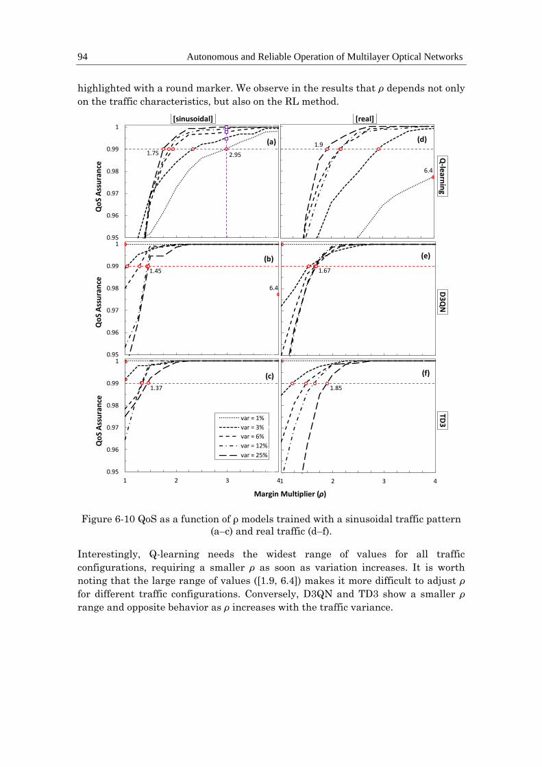
94 Autonomous and Reliable Operation of Multilayer Optical Networks
highlighted with a round marker. We observe in the results that ρ depends not only
on the traffic characteristics, but also on the RL method.
0.95
0.96
0.97
0.98
0.99
1
1 2 3 4
Qo
S A
ssu
ran
ceQ
-learnin
g
(a)
1.75 2.95
0.95
0.96
0.97
0.98
0.99
1
1 2 3 4
D3Q
N
(b)
1.45
0.95
0.96
0.97
0.98
0.99
1
1 2 3 4
var=1%
var=3%
var=6%
var=12%
var=25%
TD3
(c)
[sinusoidal]
1.37
var = 1%
var = 3%
var = 6%
var = 12%
var = 25%
Qo
S A
ssu
ran
ceQ
oS
Ass
ura
nce
0.95
0.96
0.97
0.98
0.99
1
1 2 3 4
(d)1.9
6.4
[real]
0.95
0.96
0.97
0.98
0.99
1
1 2 3 4
Margin Multiplier (ρ)
(e)
6.4
1.67
0.95
0.96
0.97
0.98
0.99
1
1 2 3 4
(f)
1.85
Figure 6-10 QoS as a function of ρ models trained with a sinusoidal traffic pattern
(a–c) and real traffic (d–f).
Interestingly, Q-learning needs the widest range of values for all traffic
configurations, requiring a smaller ρ as soon as variation increases. It is worth
noting that the large range of values ([1.9, 6.4]) makes it more difficult to adjust ρ
for different traffic configurations. Conversely, D3QN and TD3 show a smaller ρ
range and opposite behavior as ρ increases with the traffic variance.

Chapter 6 – Autonomous Packet Flow Capacity Management 95
0
1
2
3
4
5
6
7
0 5 10 15 20 25
0
2
4
6
8
10
12
14
16
18
20
0 5 10 15 20 25
Q-learning [sin] Q-learning [real]D3QN [sin] D3QN [real]TD3 [sin] TD3 [real]
Traffic variation [%]
Op
tim
alM
argi
nM
ult
iplie
r(ρ
)O
verp
rovi
sio
nin
g[T
b/d
ay]
(a)
Real
Sinusoidal
Q-learningD3QNTD3
(b)
Figure 6-11. Optimal margin multiplier (a) and overprovisioning (b).
0%
10%
20%
30%
40%Q-LD3QNTD3
0%
10%
20%
30%
40%
1 3 6 12 25Traffic variation [%]
[real]
[sinusoidal]
Extr
a o
verp
rovi
sio
nin
g [%
]
Q-learningD3QNTD3
Figure 6-12 Relative extra overprovisioning.
The detailed evolution of the optimal ρ with respect to the traffic variation is plotted
in Figure 6-11a, and Figure 6-11b shows the total overprovisioning introduced by
every RL method operating with the optimal ρ. We observe that overprovisioning
increases with traffic variation, with a slightly different trend depending on the
traffic pattern (sinusoidal and real). Moreover, every RL method introduces different
amounts of overprovisioning as shown in Figure 6-12, where the relative

96 Autonomous and Reliable Operation of Multilayer Optical Networks
overprovisioning per RL method with respect to the minimum one for every traffic
configuration is represented. Q-learning is the method that requires larger
overprovisioning in general terms, whereas D3QN and TD3 show better
performance. Interestingly, the differences are proportionally larger when traffic
variation is small.
Let us analyze the effect in terms of extra-overprovisioning when ρ is fixed to a
constant value, high enough to assure reliable QoS performance in online RL
operation under traffics with a wide range of characteristics. The squared purple
markers in Figure 6-10a indicate the QoS that could be achieved under different
traffic characteristics for the largest ρ. Table 6-3 summarizes the relative and
absolute increment of overprovisioning (computed in total Tb per day of operation)
produced with the most conservative ρ configuration for all traffic configurations and
RL methods. When the fixed ρ happens to be the optimal one for the traffic and RL
method, no additional overprovisioning is set up (values in boldface); otherwise,
additional overprovisioning is introduced. Q-learning is the method that adds the
largest extra overprovisioning (exceeding 200% and 30 Tb/day). In any case, it is
worth highlighting that achieving optimal performance in terms of QoS assurance
while achieving efficient capacity allocation requires some method to find the
optimal ρ for the traffic characteristics.
Table 6-3: Additional overprovisioning when fixing ρ
Traffic
Pattern
Traffic
Variance
Q-Learning D3QN TD3
% Tb/day % Tb/Day % Tb/Day
Sinusoidal
1% 0.00% 0 0.88% 0.02 2.49% 0.05
3% 19.18% 0.67 6.04% 0.16 20.67% 0.51
6% 38.71% 1.85 5.21% 0.21 15.38% 0.63
12% 44.15% 3.56 0.00% 0.00 4.01% 0.32
25% 60.40% 8.29 0.00% 0.00 0.00% 0.00
Real
1% 0.00% 0 0.05% 0.00 4.95% 0.11
3% 106.68% 3.94 9.52% 0.28 0.39% 0.01
6% 192.50% 9.52 12.72% 0.60 2.90% 0.14
12% 200.69% 18.37 0.00% 0.00 0.00% 0.00
25% 219.35% 34.46 0.00% 0.00 0.00% 0.00
To conclude this section, we can highlight (i) that the CRUX problem proposed in
Section 6.2 can be tackled using RL; under different traffic characteristics and RL
methods, the target QoS is assured with reduced overprovisioning; (ii) online RL
operation leads to traffic loss at the beginning of flow capacity operation; this fact
prevents us from using RL until online learning has come up with a robust and

Chapter 6 – Autonomous Packet Flow Capacity Management 97
reliable model to guarantee autonomous flow operation; and (iii) the comparison of
the RL methods shows interesting differences among them. While Q-learning learns
fast, it also produces larger overprovisioning. D3QN and TD3 need more time to
ensure zero loss and adjust QoS at the benefit of reducing overprovisioning.
Offline Leaning + Online RL-Based Operation
Let us now focus on evaluating the operational approach detailed in Section 6.4
(Figure 6-2b), which consists of three phases. Before emulating flow operation, we
generated synthetic data for all the traffic variances following the sinusoidal traffic
pattern and used them to pre-train generic models independently for each traffic
configuration and RL method. We ran every offline RL training for 14,400 episodes
to guarantee QoS assurance with minimum overprovisioning.
0,0
0,5
1,0
1,5
2,0
2,5
3,0
3,5
4,0
0
10
20
30
40
50
60
70
80
90
100
0 20 40 60 80
x(t)z(t)k
Traf
fic
and
Cap
acit
y[G
b/s
]
Time since path set-up [mm]
k
var k1% 13% 16% 1.04
12% 1.47
25% 1.81
(a)
0%
5%
10%
15%
20%
25%
30%
10 30 50 70 90 110Time since path set-up [mm]
(b)24.97%
12.56%
6.31%
3.27%
1.72%1%3%
6%
12%
25%
Traf
fic
Var
iati
on
Figure 6-13. Phase I: Self-tuned threshold (a) and traffic variance analysis (b).
Starting with the analysis of Phase I, Figure 6-13a shows an illustrative example of
the evolution of the capacity during the operation of the threshold-based algorithm
(Algorithm 6-4) for the real traffic pattern and variation 12%. Actual traffic x(t),
allocated capacity z(t), and the evolution of the self-tuned k parameter are also

98 Autonomous and Reliable Operation of Multilayer Optical Networks
shown. Note that k quickly evolves from its initial value (k = 4) to reach a capacity
closer to actual traffic. However, as soon as the load exceeds the optimal one l*, k is
increased until reaching a stable value (1.47), which happens after 60 minutes of
operation. The inset table in Figure 6-13a details the values of k after one hour of
operation for all traffic configurations. It is worth noting that the self-tuned
threshold-based algorithm operates with zero traffic loss for all the cases.
Parallel to the threshold-based operation, traffic variance analysis (Algorithm 6-2)
is conducted in order to compute the true variance of the traffic. Figure 6-13b shows
the computed traffic variation as a function of time for all traffic configurations.
Round markers highlight when the derivative of traffic variance reached a small eps
= 0.01 and labels show the final computed variance value. The low error between
computed and true variances is noticeable. Such estimation is achieved within two
hours in all the cases.
After two hours of operation, Phase II (Algorithm 6-5) can start and an RL method
with a generic pre-trained model for the true traffic variance is set to operate. The
tuning of parameter ρ (∆ρ = 0.1) and the resulting QoS are shown in Figure 6-14a
and b, respectively, for traffic variance equal to 12%. To detect whether the measured
QoS is considerably below or above the desired qa value, a significance level cfl =
0.05 was used to be compared against the obtained p-value from the binomial tests.
We observe that ρ decreases up to a magnitude that produces QoS below 99%; just
after that, ρ increases and remains stable from that point on. As shown in Figure
6-14a, the time to converge to the best ρ is 3960, 1440, and 3600 min (2.75, 1, and
2.5 days) for Q-learning, D3QN, and TD3, respectively.
1
1.2
1.4
1.6
1.8
2
0 1000 2000 3000 4000 5000
Q-learningD3QNTD3
98%
99%
100%
0 1000 2000 3000 4000 5000Phase II time [mm]
Qo
Sρ
(b)
(a)1
100% 3960
1440
3600
Figure 6-14 Phase II: QoS (a) and ρ (b) evolution.
The above analysis, however, needs to be complemented with the overprovisioning
to extract meaningful conclusions. Figure 6-15 presents the overprovisioning
obtained by every RL method before and after tuning ρ in Phase II. For reference

Chapter 6 – Autonomous Packet Flow Capacity Management 99
purposes, the overprovisioning introduced by the threshold-based algorithm during
Phase I is also included as a dotted line. The large benefits in terms of
overprovisioning reduction for the RL-based operation with regard to the threshold-
based algorithm are remarkable—up to 45% of capacity allocation reduction and 11
Tb/day of total capacity savings for one single flow. After ρ tuning, D3QN shows the
worst performance, as Q-learning and TD3 achieved significantly lower
overprovisioning (24%, ~3 Tb/day). Figure 6-15 also shows the obtained
overprovisioning when the specific model (trained offline with the collected traffic)
is loaded in Phase III after 10 days of operation. We observe that Q-learning and
TD3 reduce overprovisioning slightly, whereas a larger reduction is achieved with
D3QN; we conclude that the former RL methods are less dependent on an accurate
model of the specific traffic to achieve optimal capacity allocation.
0
5
10
15
20
25
30
Phase II (Before tuning) Phase II (After tuning) Phase III
Q-LearningD3QNTD3
Threshold-based
~45%~11 Tb/day ~24%
~3 Tb/day
Ove
rpro
visi
on
ing
[Tb
/day
]
Phase
Figure 6-15. Overprovisioning reduction.
0
25
50
,0 2,000 4,000 6,000 8,000 10,000
Time [mm]
0
25
50
Tra
ffic
[Gb
/s]
(a)
(b)
0
Figure 6-16 Phase III: Traffic variance change scenarios. Gradual increase (a) and
sudden increase (b).
Finally, let us analyze the performance of Algorithm 6-6 to detect traffic changes
while flow is operated in Phase III; recall that such detection immediately triggers

100 Autonomous and Reliable Operation of Multilayer Optical Networks
Phase II. To this end, we generated four different scenarios, combining two different
types of changes in traffic variance while keeping traffic profile unchanged. We
evaluate gradual and sudden/increase or decrease traffic variance changes. Figure
6-16 illustrates two out of four scenarios: gradual increase (variance gradually
increases from 1% to 25% along 5 days) and sudden increasing (from 1% to 25% in
just one minute); an inverse trend is configured for gradual and sudden decrease
scenarios.
Table 6-4 details the time to detect the traffic change when the variance range was
configured as [var_l, var_h] = [−10%, +10%]; the current traffic variance and
minimum reward rw_l was set to 5% of the minimum observed reward (see
Algorithm 6-6). We observe that the proposed mechanism ensures prompt reaction
under any of the studied changes—immediate detection is achieved when a sudden
change happens, and no more than one hour is required for gradual change detection.
Table 6-4: Phase III: Analysis under traffic changes
Traffic Change
Scenario
Detection
Time (min)
QoS at Detection Time
(%)
Reward Degradation
(Min from Detection)
Q-L D3QN TD3 Q-L D3QN TD3
Gradual increase 45 99.30 100 100 419 595 585
Gradual decrease 650 99.86 99.44 99.72 3,354 2,440 2,233
Step increase 1 99.17 99.86 99.86 332 413 433
Step decrease 1 99.03 99.44 99.44 494 683 212
To evaluate the promptness of detection, Table 6-4 considers the observed QoS at the
detection time, as well as the elapsed time between detection time and the time when
reward begins to degrade (reveals whether the RL module is working properly). Note
that the detection happens when the QoS is still above the target value in all the
cases. This is proof of anticipation of the change detection, which is key to guarantee
robust and reliable RL-based operation.
6.6 Concluding Remarks
The Flow Capacity Autonomous Operation (CRUX) problem has been introduced to
deal with online capacity allocation of traffic flows subject to dynamic traffic changes;
it guarantees precise QoS requirement assurance and minimizes capacity
overprovisioning. RL-based operation was proposed to learn the best policy for the
traffic characteristics and QoS requirements of a given flow. RL allows adaptive and
proactive capacity allocation once the optimal policy is learnt. However, pure RL
operation lacks robustness during online learning (e.g., at the beginning of flow

Chapter 6 – Autonomous Packet Flow Capacity Management 101
operation and in the event of traffic changes) and might result in undesirable traffic
loss. However, this can be avoided using simpler reactive threshold-based capacity
allocation.
In view of the above, an offline + online learning lifecycle was proposed, aiming at
providing guaranteed performance during the entire lifetime of the traffic flow. The
proposed management lifecycle consists of three phases. Firstly, a self-tuned
threshold-based approach was proposed to operate just after the flow is set up and
until enough evidence of the traffic characteristics are available (Phase I). Secondly,
an RL operation based on models with a pre-trained generic traffic profile but
meeting specific traffic variance that was measured during Phase I was executed
(Phase II). Lastly, an RL operation with models trained for the real measured traffic,
while allowing an online RL to adapt to smooth traffic changes (Phase III). In
addition, during Phase III online traffic analysis and RL performance tracking was
conducted to detect sharper traffic changes that might require moving back to Phase
II to keep high reliability.
The proposed lifecycle was implemented under three different RL models, namely,
Q-learning, D3QN, and TD3. While Q-learning allows for simple and easy-to-learn
definition of policies under discrete spaces of states and actions, D3QN and TD3
enable the application of more complex policies based on deep learning models with
continuous state space (D3QN) and continuous action space (TD3).
Numerical evaluation of the proposed offline + online lifecycle under different RL
techniques was carried out, reproducing realistic traffic flows in a simulation
environment. For benchmarking purposes, comparative results against basic
threshold-based operation and online RL operation were also presented. The main
conclusions extracted from the numerical evaluation are summarized in Table 5,
where colors are used to highlight the results. As expected, online RL produces
moderate to high loss (reaching peaks of 1–10 Gb/s) at the beginning of the network
operation. Among the different methods, Q-learning reached the required QoS
operation earlier (up to 6 times faster than TD3) at the expense of moderate to large
overprovisioning (up to 40% larger than TD3). On the other hand, D3QN and TD3
needed more time to converge to the required QoS operation but resulted in
considerably better capacity allocation efficiency.
The analysis of the numerical results of the proposed lifecycle leads to several
conclusions. Firstly, zero traffic loss and QoS assurance is guaranteed from path set-
up regardless of the chosen RL method. Secondly, Phase II allows a very efficient
and robust operation based on pre-trained generic models that were tuned with
specific traffic characteristics. Phase II clearly outperformed threshold-based
operation in terms of capacity utilization since it remarkably reduced
overprovisioning (up to 45%). Thirdly, all the methods reached outstanding capacity
efficiency (more than 50% of capacity reduction with respect to threshold-based
operation) without losing QoS performance in Phase III; Q-learning and TD3
behaved slightly better than D3QN. Finally, the continuous analysis and tracking
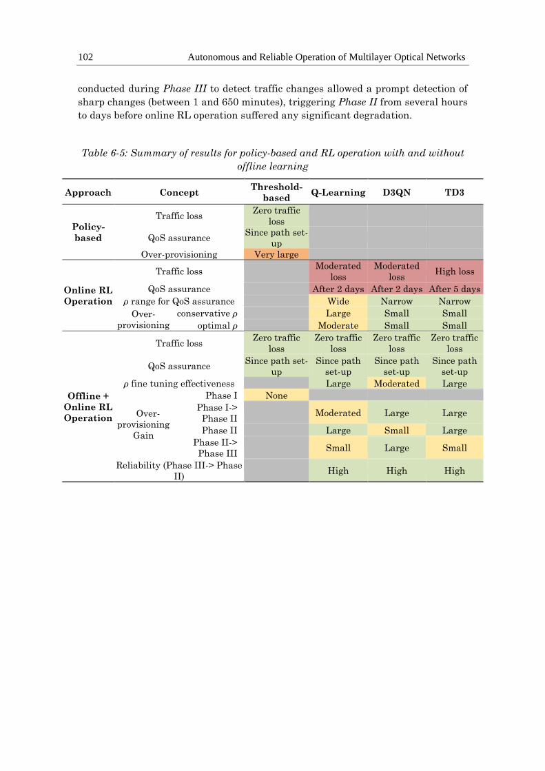
102 Autonomous and Reliable Operation of Multilayer Optical Networks
conducted during Phase III to detect traffic changes allowed a prompt detection of
sharp changes (between 1 and 650 minutes), triggering Phase II from several hours
to days before online RL operation suffered any significant degradation.
Table 6-5: Summary of results for policy-based and RL operation with and without
offline learning
Approach Concept Threshold-
based Q-Learning D3QN TD3
Policy-
based
Traffic loss Zero traffic
loss
QoS assurance Since path set-
up
Over-provisioning Very large
Online RL
Operation
Traffic loss Moderated
loss
Moderated
loss High loss
QoS assurance After 2 days After 2 days After 5 days
ρ range for QoS assurance Wide Narrow Narrow
Over-
provisioning
conservative ρ Large Small Small
optimal ρ Moderate Small Small
Offline +
Online RL
Operation
Traffic loss Zero traffic
loss
Zero traffic
loss
Zero traffic
loss
Zero traffic
loss
QoS assurance Since path set-
up
Since path
set-up
Since path
set-up
Since path
set-up
ρ fine tuning effectiveness Large Moderated Large
Over-
provisioning
Gain
Phase I None
Phase I->
Phase II
Moderated Large Large
Phase II Large Small Large
Phase II->
Phase III
Small Large Small
Reliability (Phase III-> Phase
II)
High High High

Chapter 7
Revisiting Autonomous vLink
Capacity Operation
In this chapter, we revisit the scenario described in Chapter 5 for vLink capacity
management when the vLink was supported by a lightpath based on the DSCM.
Specifically, in view of the results obtained in Chapter 5 for vLink capacity
management, here we propose a RL model for vlink capacity management. We next
go a step beyond and consider intent cooperation, where the intents deployed for the
individual PkCs take actions based on the traffic in the connection (as in Chapter 6)
and cooperate with the vLink intent, which aggregates the capacity of the individual
PkCs to decide the capacity of the vLink.
7.1 Introduction
Recall that in Chapter 5 the vLink intent was based on short-term traffic forecasts
to predict future capacity needs. Although this approach can help to anticipate
potential capacity exhaustion by allocating capacity in advance, when the traffic
volume decreases, the reduction of capacity can lead to undesired capacity
fluctuations and to increase queuing. In this chapter, we propose a vLink intent
based on RL to manage the capacity of the vLink. As demonstrated in Chapter 6, RL
fits well with IBN as it entails learning on how to map situations to actions to
maximize rewards, without specifically programming the learner. In turn, the
algorithm in the transponder, making decisions on the configuration of the SCs, can
be based on policies received from the SDN controller. This approach aims at
managing the capacity of the vLink as a function of the current and predicted traffic

104 Autonomous and Reliable Operation of Multilayer Optical Networks
volume, while avoiding queuing (and traffic losses) and keeping moderated SC
configuration changes by removing oscillating capacity allocation actions.
Recall that the vLink intent targets at making decisions proactively to reach some
performance defined for the vLink. A related concept is that of independent operation
vs coordinated operation. Independent operation occurs when the decisions that are
made on a network entity (in this case the vLink) are based on measurements
collected for the same entity. However, since in a network infrastructure many
entities are sharing the set of common resources, pure independent operation is rare,
as it can lead to overall suboptimal resource utilization and even to result in poor
performance because of the natural competence for resources. Therefore, some kind
of coordination among entities should be devised.
Although PkCs and related vLinks can work independently making decisions based
on the observed input traffic, some coordination might facilitate the overall
operation. For instance, as a result of the capacity required by the PkCs, the capacity
of the vLink needs to be reconfigured. Nonetheless, if the available capacity of the
vLink is exhausted, competition for the available capacity of the vLink would lead to
poor performance for both PkCs. A possible solution to avoid conflicts and
countereffects between intent agents competing for common resources is to consider
cooperation among them to ensure that they can achieve their operational goals.
The rest of the chapter is organized as follows. Section 7.2 extends the intent agent
proposed in Chapter 5 and adapt it, so the intent can be based on RL. In addition,
details of the definition of the reward function for the definition of the RL solutions
are given. In Section 7.3, we propose a cooperative intent operation approach
between PkC and vLink intents. The discussion is supported by the experiments and
numerical results presented in Section 7.4. Finally, Section 7.5 draws the main
conclusions of our work.
7.2 Autonomic vLink Capacity Adaptation
In this section, we extend the intent agent in Figure 5-2 with the architecture in
Figure 7-1; note the similarities with the architecture in Figure 6-1 for flow capacity
autonomous operation. In Figure 7-1, a RL-based vLink intent analyzes monitoring
data, specifically input traffic x(t) and current vLink capacity z(t), that is collected
periodically (e.g., every minute). Based on such analysis, the vLink intent agent
determines the target capacity z’(t+1) that should be allocated for the next period by
using the learned optimal policy. With such capacity, an agent running at the optical
transponder (Tx side) decides the actual capacity z(t+1) to be allocated, which will
depend on the characteristics of the optical layer. The operation can be based on
policies and other parameters received from the SDN controller.

Chapter 7 – Revisiting Autonomous vLink Capacity Operation 105
RL agent
Environment
Actions
a(t)
State s(t),
Reward r(t)
vLink
Intent
Manage SC
configMonitoring
Transponder
Agent
Tx
From SDN
Controller
List of allowed
configurations
vlink traffic
Traffic (x(t))
Capacity (z(t))
Max Capacity,
Granularity,
Period, Policy
x(t), z(t)Target
Capacity
(z’(t+1))
Actual
Capacity
(z(t+1))
Figure 7-1 RL-based Autonomous vLink Operation Architecture.
The goal is to adjust the vLink capacity to guarantee that the vLink load l(t) (defined
as x(t) / z(t)) does not exceed but is close to a given maximum lmax; this will minimize
over-provisioning (defined as z(t)-x(t)) while limiting the average maximum delay for
the traffic. In this scenario, the learning process can be focus on the traffic variation
and its evolution with time, which is key for a tight load adjustment and for avoiding
high delay and traffic loss due to insufficient capacity allocation.
The environment in the intent agent is in charge of computing the state s(t), whereas
s(t) is obtained as a function of both l(t) and lmax. Given s(t), the RL agent selects the
action a(t) with highest total reward with probability 1-ε (exploitation) or randomly
with probability ε (exploration) [SuBa98], where exploration is encouraged during
an initial learning phase and a decay strategy is implemented. Action a(t) consists
in a capacity volume ∆z to be added to or subtracted from the current vLink capacity.
The reward function r(t) is a linear function with three penalty components (ordered
by importance): i) traffic loss (x(t) > z(t)), ii) lmax violation (l(t) > lmax), and iii) over-
provisioning (z(t) - x(t)). Thus, the maximum reward is achieved when neither loss
nor lmax violation is observed, and over-provisioning is minimized.
7.3 Cooperative Intent Operation
Let us imagine now the case where the traffic that the vLink is supporting comes
from a number of PkCs, which capacity is being managed by specific PkC intents. In
this case, the capacity to be ensured in the vLink can be easily computed as the
summation of the capacity required by every PkC. Therefore, in this section, we

106 Autonomous and Reliable Operation of Multilayer Optical Networks
extend the previous stand-alone intent-based vLink capacity adaptation and focus
on evaluating the potential benefits of a hierarchical cooperation with PkC intents.
Figure 7-2 shows the architecture, where PkC intent agents implement a RL-based
method similarly to the previously used for the vLink. The aggregation of the target
capacity requested for every PkC is used as target capacity for the vLink.
vlink
PkC 1
…PkC n
z1' (t+1)
z1'(t+1)
+
Packet Connection Intent 1
z1 (t)
x1 (t)
RL agent
Environment
s(t), r(t) a(t)
zn'(t+1)
Target Capacity
Analysis z’(t+1)
Manage
SC config
z(t+1)
Tx
vLink intent
Packet Connection Intent n
zn' (t+1)
zn (t)
xn (t)
Figure 7-2 Extended architecture with hierarchical intent cooperation.
For PkCs specifically, let us consider different operational goals than those used for
the vLink; every PkC has a different requirement in terms of maximum delay budget
dmax that needs to be guaranteed. This entails changes in the reward function r(t),
where a new component adds a large penalty if the measured delay in the packet
connection exceeds the required dmax. Moreover, no penalty for maximum load
violation is considered.
7.4 Illustrative Intent-Based Applications
In this section, we first present the results obtained assuming a RL-based vlink
intent and then, the results assuming cooperation between the vLink and the PkC
intents.
Autonomous vLink Capacity Operation
A Python-based simulator reproducing the architecture in Figure 7-1 has been
implemented for evaluation purposes. As in Chapter 5, realistic vLink input traffic
was generated using the flow simulator and parameters described in [Ru18]. The
target load lmax was set to 80%.
Q-learning, D3QN, and TD3 RL methods were implemented, adapting state and
action spaces to either discrete or continuous space depending on the method (see

Chapter 7 – Revisiting Autonomous vLink Capacity Operation 107
Chapter 2). The FFNNs for D3QN and TD3 methods were configured with 2 layers
each with 100 neurons implementing ReLU activation function [ZhQi05]. For the
sake of fairness, ∆z was setup to 10 Gb/s in all the methods. In addition, a threshold-
based approach was implemented for benchmarking purposes, which reactively adds
or releases capacity to keep l(t) in the range [0.7-0.8].
Traf
fic
and
Cap
acit
y [G
b/s
]
0
50
100
150
200
250
0 0.5 1 1.5 2 2.5
input trafficcapacity
0
50
100
150
200
250
0 0.5 1 1.5 2 2.5
(a) Q-LEARNING - MaxSC (b) Q-LEARNING - Adaptive - 16QAM
TimeTime
Figure 7-3 Optical connection managed by the vLink intent. Total capacity vs time
for the High Traffic profile.
To facilitate comparison with the results the obtained in Chapter 5, let us first
assume that the RL-based vlink intent was based on Q-learning. The obtained
results are presented in Figure 7-3a-b and Table 5-3 (down). Initial exploration
probability ε was set to 1, reducing every episode by a multiplicative factor of 0.98.
The Q-learning algorithm was configured with a learning rate of 0.05 and a discount
factor of 0.95.
Table 7-1: Summary of results for Optical Connection Configuration Managed by
vlink Intent based on Q-learning
Q-Learning
High Traffic Profile Low Traffic Profile
maxSC adapt-16Q maxSC adapt-16Q
#Changes per day 7.2 5.6 0 1.6
Energy savings [%] 31 26 47 46
Packet Loss [MB] 0 0 0 0
Queue (max) [MB] 0 0 0 0
Queue (avg) [MB] 0 0 0 0
Cap. Exhaust. per day 0 0 0 0

108 Autonomous and Reliable Operation of Multilayer Optical Networks
The results confirm that intent-based vlink capacity management based on RL
results in a good solution for smooth capacity evolution, eliminating completely
packet loss and time in vlink queue, while energy savings are still over 26% and 46%
for the High and Low Traffic profiles, respectively.
Let us now compare the performance of the different RL methods. Figure 7-4 shows
the performance of the threshold-based approach and RL-based methods (note that
latter ones need a sufficiently large number of episodes to guarantee robust and
efficient operation).
0
200
400
600
800
1000
0
200
400
600
800
1000
0 50 100 150 200 250
0
100
200
300
400
0 50 100 150 200 250
0
100
200
300
400
0 50 100 150 200 250
0
100
200
300
400
Traffic or Capacity (Gb/s)
Thre
sho
ld-b
ase
dQ
-Le
arn
ing
D3
QN
Loss ~4 Gb/s0
200
400
600
800
1000Delay (ns)
0
200
400
600
800
1000
Time
TD3
01000
Loss ~4 Gb/s
0400
0400
01000
01000
0
100
200
300
400
0 50 100 150 200 250
x(t)z'(t)z(t)
0400
Time
Figure 7-4 Autonomic vLink Capacity Adaptation (a) and obtained delay (b).
The measured input traffic x(t), target capacity z’(t) in the case of RL-based methods,
and allocated capacity z(t) are plotted for a typical day. We observe that the
threshold-based method with an a priori good configuration produces poor

Chapter 7 – Revisiting Autonomous vLink Capacity Operation 109
performance (traffic loss and high delay) as a result of its reactive nature. In
contrast, all RL-based methods learned policies to avoid losses and they adapt better
to the traffic characteristics. Specifically, D3QN achieves low maximum delay (at
least, half of the other RL methods). However, the main conclusions to be extracted
from delay analysis is that although the reward function explicitly controls the load,
which is closely related to delay performance, a finer delay control (e.g., keeping
delay below a target maximum) requires ad-hoc delay analysis components to be
considered in the reward function. Table 7-2 summarizes the results. In general, RL
methods require higher overprovisioning than the threshold-based approach, but
such overprovisioning is necessary to achieve the target performance. Therefore,
these results validate the usefulness of RL for the proposed vLink operation use case.
Table 7-2 vLink Capacity Adaptation Summary
Method Loss
(Gb/s)
Over-
Provisioning
(Tb/day)
Num SC
Changes
Delay (μs)
min avg max
Thr-based 4.05 19.2 18 45 129 1629
Q-Learning 0 21.6 54 23 95 603
D3QN 0 22.6 34 19 82 267
TD3 0 20.8 70 21 96 512
The drawbacks rely on the need for a larger number of SC changes (activations and
deactivations) compared to the threshold-based approach. E.g., among the RL-based
methods, the lowest overprovisioning is achieved by TD3 at the expense of doubling
the number of SC changes with respect to D3QN, which requires double number of
SC changes than the threshold-based approach. Hence, the selection of the RL
method is not trivial and it might depend on limitations of the hardware, e.g., the
SC activation time.
Finally, it is worth noting that RL-based operation at the vLink level cannot provide
differentiated delay performance for the different PkCs supported by the vLink. On
the contrary, implementing the RL-based operation at the PkC would provide
specific performance to the individual PkC but would require from specific
cooperation between PkC and vLink intent agents.
Cooperative Intent Operation
Let us assume the numerical evaluation scenario detailed in the previous section
where phree PkCs A, B, C with maximum traffic 120, 60, and 60 Gb/s and different
delay budgets generate the same aggregated vLink traffic as in Figure 7-4. We focus
on the TD3 RL method and similarly as for vLink intent operation, we run it until
achieving a robust and accurate operation.

110 Autonomous and Reliable Operation of Multilayer Optical Networks
The accuracy of the proposed cooperative scheme to predict vLink traffic is
illustrated in Figure 7-5a. The vLink traffic is compared against the prediction from
the PkC intents; the models learned by different PkCs intent agents for the short 1-
min scope can be aggregated and used by the vLink for a much longer time scope
with remarkable accuracy. Figure 7-5b shows the delay at the source node for all
PkCs, assuming that PkCs leave through 100/200 Gb/s interfaces. We observe that
RL-based operation at the PkC level allows achieving the targeted differentiated
delay performance. From Figure 7-5, we observe that the requested target capacity
for every PkC is accurate and well-fitted so, the sum of all target capacities to be
considered by the vLink intent agent results into an overall capacity that meets PkCs
needs.
0
200
400
600
800
1000
0 50 100 150 200 250
f1 [measured]f2 [measured]f3 [measured]
De
lay
(ns)
(b)PkC-APkC-BPkC-C
Traf
fic
(Gb
/s)
Time
0
50
100
150
200
250
300
350
400
0 50 100 150 200 250
(a)
Time
x(t)
x’(t+m)
Figure 7-5 PKC-vLink intent cooperation performance.
Figure 7-6 and Table 7-3 compare hierarchical cooperation named hierarchical and
vLink model. Results of the vLink allocated capacity and introduced delay are
presented.
0
100
200
300
400
0 50 100 150 200 250
x(t)
z(t) [vlink]
z(t) [hierarchical]Traf
fic
or
cap
(Gb
/s)
0
200
400
600
800
1000
0 50 100 150 200 250
vlink
hierarchical
Time (min)
De
lay
(ns)
Figure 7-6 Comparative results

Chapter 7 – Revisiting Autonomous vLink Capacity Operation 111
Table 7-3 Cooperative IBN summary
Method
Over-
Provisioning
(Tb/day)
Num SC
Changes
Delay (ns)
min avg max
vLink 20.8 70 21 96 512
Hierarchical 29.8 50 15 54 233
In view of the graphs, the requirements from the PkCs to achieve differentiated delay
performance result in a higher capacity that cannot be successfully learnt by the
vLink intent. Interestingly, when PkC operation is intent-based, the number of SC
changes at the optical layer reduces noticeably. This fact points out the benefits of
hierarchical intent cooperation to simplify multilayer operation. Moreover, the delay
contribution introduced by the vLink is greatly reduced. We can conclude that
hierarchical intent cooperation is the option that provides the best trade-off between
the achievement of the operational goals and resource utilization and management.
7.5 Concluding Remarks
In this final chapter, intent agents based on RL were proposed to adjust the capacity
of a vLink as a function of the input traffic. Next, cooperative intent operation
between pkC and vLinks was proposed, where the capacity required by the vLink
comes directly from the capacity of the supported PkCs. Numerical results were
presented and discussed. The solutions presented extended the ones in Chapter 5 for
vLink autonomous operation.


Chapter 8
Closing Discussion
8.1 Main Contributions
This Ph. D. thesis focuses on applying ML techniques for the autonomous and
reliable operation of multilayer optical networks. The main contributions are
summarized as following:
• First, in Chapter 4, we compared estimated and measured QoT in the optical
transponder by using a QoT tool based on GNPy. We showed that the changes
in the values of input parameters of the QoT model representing optical
devices can explain the deviations and degradation in performance of such
devices. we used reverse engineering to estimate the value of those
parameters tat explain the observed QoT. We showed by simulation a large
anticipation in soft-failure detection, localization and identification of
degradation before effecting the network. Finally, for validating our
approach, we experimentally observed the high accuracy in the estimation of
the modeling parameters.
• In Chapter 5, we studied the autonomous operation of optical connections
based on digital subcarrier multiplexing. We proposed several solutions for
the autonomous operation of DSCM systems. In particular, the combination
of two modules running in the optical node and in the optical transponder
activate and deactivate subcarriers to adapt the capacity of the optical
connection to the upper layer packet traffic. The module running in the
optical node is part of our IBN solution and implements prediction to
anticipate traffic changes. Our comprehensive study demonstrated the

114 Autonomous and Reliable Operation of Multilayer Optical Networks
feasibility of DSCM autonomous operation and showed large cost savings in
terms of energy consumption. In addition, Chapter 5 provides a guideline to
help vendors and operators to adopt the proposed solutions.
• Chapter 6 is devoted to the autonomous packet flow capacity management.
In this chapter we applied RL techniques and proposed a management
lifecycle consisting of three different phases: 1) a self-tuned threshold-based
approach for setting up the connection until enough data is collected, which
enables understanding the traffic characteristics; 2) RL operation based on
models pre-trained with generic traffic profiles; and 3) RL operation based on
models trained with the observed traffic. We showed that RL algorithms
provide poor performance until they learn optimal policies, as well as when
the traffic characteristics change over time. The proposed lifecycle provides
remarkable performance from the starting of the connection and it shows the
robustness while facing changes in traffic.
• In Chapter 7 we took advantage of the experience from Chapter 6 and
revisited the solutions proposed in Chapter 5 for autonomous vLink operation
supported by DSCM systems. The contributions of this chapter are twofold:
1) and the one hand, we proposed a solution based on RL, which showed
superior performance with respect to the solution based on prediction; and 2)
because vLinks support packet connections, coordination between the intents
of both layers was proposed. In this case, the actions taken by the individual
PkCs are used by the vLink intent. The results showed noticeable
performance compared to independent vLink operation.
8.2 List of Publications
Publications in Journals
[JOCN22] L. Velasco, S. Barzegar, F. Tabatabaeimehr, and M. Ruiz, “Intent-Based
Networking for Optical Networks [Invited Tutorial],” IEEE/OSA Journal
of Optical Communications and Networking, vol.14, pp. A11-A22, 2022.
[SENSORS21] S. Barzegar, M. Ruiz, and L. Velasco, “Packet Flow Capacity
Autonomous Operation based on Reinforcement Learning,” MDPI
Sensors, vol. 21, pp. 8306, 2021.
[TNSM21] S. Barzegar, M. Ruiz, A. Sgambelluri, F. Cugini, A. Napoli, and L.
Velasco, “Soft-Failure Detection, Localization, Identification, and
Severity Prediction by Estimating QoT Model Input Parameters,” IEEE
Transactions on Network and Service Management, vol. 18, pp. 2627-
2640, 2021.

Chapter 8 – Closing discussion 115
[JSAC21] L. Velasco, S. Barzegar, D. Sequeira, A. Ferrari, N. Costa, V. Curri, J.
Pedro, A. Napoli, and M. Ruiz, “Autonomous and Energy Efficient
Lightpath Operation based on Digital Subcarrier Multiplexing,” IEEE
Journal on Selected Areas in Communications, vol. 39, pp. 2864-2877,
2021.
Publications in Conferences
[OFC21.1] S. Barzegar, M. Ruiz and L. Velasco, “Reliable and Accurate Autonomous
Flow Operation based on Off-line Trained Reinforcement Learning,” in Proc.
IEEE/OSA Optical Fiber Communication Conference (OFC), 2021.
[OFC21.2] F. Tabatabaeimehr, S. Barzegar, M. Ruiz and L. Velasco, “Combining Long-
Short Term Memory and Reinforcement Learning for Improved Autonomous
Network Operation,” in Proc. IEEE/OSA Optical Fiber Communication
Conference (OFC), 2021.
[ECOC20] S. Barzegar, M. Ruiz and L. Velasco, “Reinforcement Learning -based
Autonomous Multilayer Network Operation,” in Proc. European Conference
on Optical Communication (ECOC), 2020.
[ICTON20] S. Barzegar, Marc Ruiz, and Luis Velasco, “Soft-Failure Localization and
Time-Dependent Degradation Detection for Network Diagnosis,” in Proc.
IEEE International Conference on Transparent Optical Networks (ICTON),
2020.
[OFC20] S. Barzegar, E. Virgillito, M. Ruiz, A. Ferrari, A. Napoli, V. Curri, and L.
Velasco, “Soft-Failure Localization and Device Working Parameters
Estimation in Disaggregated Scenarios,” in Proc. IEEE/OSA Optical Fiber
Communication Conference (OFC), 2020.
[ICTON19] S. Barzegar, M. Ruiz, and L. Velasco, “Adaptation of the residual signal for
filter failure detection in scenarios with multiple filter types,” in Proc. IEEE
International Conference on Transparent Optical Networks (ICTON), 2019.
8.3 List of Research Projects
European Funded Projects
• B5G-OPEN: Beyond 5G - OPtical nEtwork continuum, H2020-ICT-2020-2
(G.A. 101016663).
• METRO-HAUL: METRO High bandwidth, 5G Application-aware optical
network, with edge storage, compute and low Latency, H2020-ICT-2016-2
(G.A. 761727).

116 Autonomous and Reliable Operation of Multilayer Optical Networks
National Funded Projects
• IBON: AI-Powered Intent-Based Packet and Optical Transport Networks
and Edge and Cloud Computing for Beyond 5G, Ref: PID2020-114135RB-I00,
2021-2024.
• TWINS: cogniTive 5G application-aware optical metro netWorks Integrating
moNitoring, data analyticS and optimization, Ref: TEC2017-90097-R, 2018-
2020.
Pre-doctoral Scholarship
• Pre-doctoral scholarship related to ICREA Academia 2015-2020 and 2021-
2025 awards.
8.4 Collaborations
I had the opportunity to collaborate with:
• OPTCOM group at Politecnico di Torino on the estimation of configuration
parameters for QoT (G.1).
• Infinera on the application of Reinforcement Learning to DSCM systems
(G.2).
• Consorzio Nazionale Interuniversitario per le Telecomunicazioni (CNIT) and
Universidad de la República on the application of Reinforcement Learning to
packet networks (G.3).
8.5 Topics for Further Research
First, some of the algorithms and architectures devised in this Ph. D. thesis are being
implemented experimentally in the framework of the B5G-OPEN project.
In addition, we are working on distributed decision-making following the concept of
Multi-Agent Systems (MAS) [MAS]. MAS is a subfield of AI and it can be defined as
a set of individual agents that share knowledge and communicate with each other in
order to solve a problem that is beyond the scope of a single agent. In the scope of
networking, we proposed that agent nodes make autonomous decisions real-time
based on guidelines received from the SDN controller. Such decision-making will be
performed based on its own observed data, as well as on the data and models received
from other nodes. To illustrate this concept, we have first focused on flow routing. As
in Chapter 6, we are assuming packet flows carrying traffic with unknown

Chapter 8 – Closing discussion 117
characteristics entering in a packet node. However, in this work, flows need to be
routed to the destination though several output interfaces, while ensuring some
given QoS, e.g., in terms of end-to-end delay, and optimizing resource utilization.
Figure 8-1 represents an example of flow routing operation in a node in the targeted
multilayer scenario. The packet node agent has received from the SDN controller
three possible routes for a given traffic flow and it has to decide which one or
combination of several are the allow to reach some QoS performance (in this case,
the end-to-end delay), while minimizing some cost function. In this case, we use RL
to implement a service agent for the traffic flow. In such a figure, the traffic of the
flow is routed through two different interfaces (in this case both supported by the
optical layer) among the three available ones for the flow. Here, we assume that the
traffic flow actually consists of multiple sub-flows, which are routed independently
so the packets belonging to each sub-flow follow the same route. In the destination,
the end-to-end delay is measured (e.g., using in-band telemetry) and some statistics
are computed (e.g., maximum and weighted average) and sent to the node agents
participating in the routing of the flow.
Traffic, delay, Percentages
Learning Agent
Environment
RewardState Action
Packet Node Agent
Requiredpercentages
DRL-based Flow Routing
If 1
If 2
If 3
Flowdestination
Traffic
end-to-end delay
0%
20%
80%
Packet Node Agent
delay
Flowsource or
intermediate Packet Layer
Optical Layer
Figure 8-1 Example of distributed flow routing based on RL
Initial results show promising results of the proposed approach

List of Acronyms
PLC
FEC
Packet Layer Connections
Forward Error Correction
TRX Transponders
BER Bit Error Rate
QoT Quality of Transmission
NL Non-Linear
OA Optical Amplifier
WSS Wavelength Selective Switch
MDA Monitoring and Data Analytics
ROADM Reconfigurable Optical Add / Drop Multiplexer
GSNR Generalized Signal to Noise Ratio
ASE Amplified Spontaneous Emission
NLI NL Interference
EDFA Erbium Doped Fiber Amplifier
NF Noise Figure
ML Machine Learning
SNR Signal to Noise Ratio
OSNR Optical Signal to Noise Ratio
FS Filter Shift
FT Filter Tightening

List of Acronyms 119
OSA Optical Spectrum Analyzer
GN Gaussian-noise
OLS optical line system
A/D WSS Add/Drop Wavelength Selective Switch
QAM Quadrature Amplitude Modulation
QPSK Quadrature Phase-Shift Keying
RL Reinforcement Learning
DQN Deep Q-Network
DNN Deep Neural Network
D3QN Dueling Double DQN
TD3 Twin Delayed Deep Deterministic Policy Gradient
SDN Software-Defined Networking
IBN Intent-Based Networking
DB database
rMSE relative Mean Square Error
DSCM Digital Subcarrier Multiplexing
SC subcarriers
DSP Digital Signal Processing
SR Symbol Rates
Tx Transmitter
Rx Receiver
MF Modulation Format
EON Elastic Optical Networks
vLink virtual Link
RSA Routing and Spectrum Allocation
AI Artificial Intelligence
RMSA Routing, Modulation and Slot Assignment
SLA Service Level Agreement
VIO Virtual Infrastructure Orchestrator
MLFO ML Function Orchestrator
TMN Telecommunications Management Network

120 Autonomous and Reliable Operation of Multilayer Optical Networks
PBNM Policy-Based Network Management
UI User Interface
PLD ML Pipeline Deployment
NBI Northbound Interface
WF1 Deployment Workflow
ARIMA Autoregressive Integrated Moving Average
FFNN Feed-forward Neural Networks
CNN Convolutional Neural Networks
RNN Recurrent Neural Networks
LSTM Long Short-Term Memory
DC Data Center
PkC Packet Connection

References
[Ag18] C. Aggarwal, “Neural Networks and Deep Learning: A
Textbook,” Springer, 2018.
[APV17.1]
A. P. Vela et al., “BER Degradation Detection and Failure
Identification in Elastic Optical Networks,” IEEE/OSA J. of
Lightwave Technology, vol. 35, pp. 4595-4604, 2017.
[APV17.2]
A. P. Vela et al., “Distributing Data Analytics for Efficient
Multiple Traffic Anomalies Detection,” Elsevier Computer
Communications, vol. 107, pp. 1-12, 2017.
[APV18]
A. P. Vela et al., “Soft failure localization during commissioning
testing and lightpath operation,” IEEE/OSA J. of Optical Comm
and Networking, vol. 10, pp. A27-A36, 2018.
[Be20]
A. Bernal et al., “Near Real-Time Estimation of End-to-End
Performance in Converged Fixed-Mobile Networks,” Elsevier
Computer Communications, vol. 150, pp. 393-404, 2020.
[Bo18]
M. Bouda et al., “Accurate Prediction of Quality of Transmission
Based on a Dynamically Configurable Optical Impairment
Model,” IEEE/OSA J. of Optical Communications and
Networking, pp. A102-A109, 2018.
[Bo21]
L. Bonati et al., “Intelligence and Learning in O-RAN for Data-
Driven NextG Cellular Networks,” IEEE Communications
Magazine, vol. 59, pp 21-27, 2021.
[Br16] P. Brockwell et al., “Introduction to Time Series and
Forecasting,” Springer: Berlin/Heidelberg, Germany, 2016.

122 Autonomous and Reliable Operation of Multilayer Optical Networks
[Ca02] G. Casella et al., “Statistical Inference,” Duxbury Press: Pacific
Grove, USA, 2002.
[Ca18]
M. Cantono et al., “On the Interplay of Nonlinear Interference
Generation with Stimulated Raman Scattering for QoT
Estimation,” IEEE/OSA Journal of Lightwave Technology (JLT),
vol. 36, pp. 3131-3141, 2018.
[Ch12]
R. Chmogrow et al., “Error Vector Magnitude as a Performance
Measure for Advanced Modulation Formats,” IEEE Photonics
Technology Letters, vol. 24, pp. 61-63, 2012.
[Ch19.1]
X. Chen et al., “DeepRMSA: A deep reinforcement learning
framework for routing, modulation and spectrum assignment in
elastic optical networks,” IEEE/OSA J. Lightwave Technology,
vol. 37, pp. 4155-4163, 2019.
[Ch19.2]
X. Chen et al., “Building Autonomic Elastic Optical Networks
with Deep Reinforcement Learning,” IEEE Commun. Mag., vol.
57, pp. 20–26, 2019.
[Ch21]
X. Chen et al., “A Multi-Task-Learning-based Transfer Deep
Reinforcement Learning Design for Autonomic Optical
Networks,” IEEE J. on Sel. Areas in Communications, vol. 39,
pp. 2878-2889, 2021.
[Cl21] A. Clemm et al., “Intent-Based Networking - Concepts and
Definitions,” IRTF draft work-in-progress, 2021.
[Cu19]
V. Curri et al., “Synergetical Use of Analytical Models and
Machine-Learning for Data Transport Abstraction in Open
Optical Networks,” in Proc. IEEE International Conference on
Transparent Optical Networks (ICTON), 2019
[Da15]
M. Dallaglio et al., “Routing, Spectrum, and Transponder
Assignment (RSTA) in Elastic Optical Networks,” IEEE/OSA J.
of Lightwave Technology, vol. 33, pp. 4648-4658, 2015.
[EON16]
V. López and L. Velasco, Elastic Optical Networks: Architectures,
Technologies, and Control, in Optical Networks book series,
ISBN 978-3-319-30173-0, Springer, 2016.
[Fe20]
A. Ferrari et al., “GNPy: an open source application for physical
layer aware open optical networks,” IEEE/OSA J. of Optical
Communications and Networking, vol. 12, pp. C31-C40, 2020.

References 123
[FGML19]
Focus group on Machine Learning for Future Networks including
5G, “Unified architecture for machine learning in 5G and future
networks,” Technical Specification ITU-T FG-ML5G-ARC5G,
2019.
[Fi18]
M. Filer et al., “Multi-Vendor Experimental Validation of an
Open Source QoT Estimator for Optical Networks,” IEEE/OSA
Journal of Lightwave Technology (JLT), vol. 36, pp. 3073-3082,
2018.
[FINISAR] Flexgrid High Resolution Optical Channel Monitor (OCM) [On-
line] www.finisar.com, accessed June 2018.
[Fl20] C. Fludger, “Performance oriented DSP design for flexible
coherent transmission,” in Proc. OFC, 2020.
[Fr17]
F. Frey et al., “Estimation of Trends for Coherent DSP ASIC
Power Dissipation for different bitrates and transmission
reaches,” in Proc. Photonic Networks, 2017.
[Fu18] S. Fujimoto et al., “Addressing Function Approximation Error in
Actor-Critic Methods,” in Proc. ICML, 2018.
[Gi18]
Ll. Gifre et al., “Autonomic Disaggregated Multilayer
Networking,” IEEE/OSA J. of Optical Communications and
Networking, vol. 10, pp. 482-492, 2018.
[GuTh19]
V. Le Guen and N. Thome, “Shape and Time Distortion Loss for
Training Deep Time Series Forecasting Models,” In Proc.
NeurIPS, 2019.
[Ha16] H. Hasselt et al., “Deep Reinforcement Learning with Double Q-
learning,” in Proc. AAAI Conference on AI, 2016.
[Infinera]
Infinera: “The Ultimate Guide to Nyquist Subcarriers,” [on-line]
https://www.infinera.com/wp-content/uploads/ The-Ultimate-
Guide-to-Nyquist-Subcarriers-0208-WP-RevA-0719.pdf.
[Is02]
S. Ishak et al., “Performance Evaluation of Short-Term Time-
Series Traffic Prediction Model,” J. of Transportation
Engineering, vol. 128, pp. 490-498, 2002.
[ITU00] “Principles for a Telecommunications Management Network,”
ITU-T, Rec. M.3010, 2000.
[ITU20] “Framework for data handling to enable ML in future networks
including IMT-2020,” ITU-T Y.3174, 2020.

124 Autonomous and Reliable Operation of Multilayer Optical Networks
[Kl13]
M. Klinkowski et al., “Elastic Spectrum Allocation for Time-
Varying Traffic in FlexGrid Optical Networks,” IEEE J. on
Selected Areas in Communications, vol. 31, pp. 26-38, 2013.
[Kr17] D. Krause et al., “Design considerations for a digital subcarrier
coherent optical modem,” in Proc. OFC, 2017.
[Li20]
Z. Li et al., “Demonstration of Fault Localization in Optical
Networks Based on Knowledge Graph and Graph Neural
Network,” in Proc. OFC, 2020.
[Lu20]
H. Lun et al., “Soft Failure Identification for Long-haul Optical
Communication Systems Based on One-dimensional
Convolutional Neural Network,” IEEE/OSA J. of Lightwave
Technol., vol. 38, pp. 2992-2999, 2020.
[Ma21]
H. Mahmoud, “Parametric versus Semi and Nonparametric
Regression Models,” International Journal of Statistics and
Probability, vol. 10, pp 90–109, 2021.
[MaCh01]
D. Mandic and J. Chambers, “Recurrent Neural Networks for
Prediction: Learning Algorithms, Architectures and Stability,”
Wiley, 2001.
[Mo17]
F. Morales et al., “Dynamic core VNT adaptability based on
predictive metro-flow traffic models,” IEEE/OSA J. Optical
Comm and Networking, vol. 9, pp. 1202–1211, 2017.
[Mu19]
F. Musumeci et al., “A Tutorial on Machine Learning for Failure
Management in Optical Networks,” IEEE/OSA J. of Lightwave
Technol., vol. 37, pp. 4125-4139, 2019.
[Ne17] P. Neves et al., “Future mode of operations for 5G–The
SELFNET approach enabled by SDN/NFV,” Comput. Stand.
Interfaces 2017, 54, 229–246.
[Pa14]
F. Paolucci et al., “Multipath Restoration and Bitrate Squeezing
in SDN-based Elastic Optical Networks,” Photonic Network
Communications, vol. 28, pp. 45-57, 2014.
[Pa18]
T. Panayiotou et al., “Leveraging Statistical Machine Learning
to Address Failure Localization in Optical Networks,” IEEE/OSA
J. of Optical Communications and Networking, vol. 10, pp. 162-
173, 2018.
[Pa19] T. Panayiotou et al., “A Data-Driven Bandwidth Allocation
Framework with QoS Considerations for EONs,” IEEE/OSA

References 125
Journal of Lightwave Technology (JLT), vol. 37, pp. 1853–1864,
2019.
[Po11] W. Powell, “Approximate Dynamic Programming, 2nd ed,” Wiley:
New Jersey, USA, 2011.
[Po12]
P. Poggiolini, “The GN Model of Non-Linear Propagation in
Uncompensated Coherent Optical Systems,” IEEE/OSA Journal
of Lightwave Technology (JLT), vol. 30, pp. 3857 - 3879, 2012
[Po14]
P. Poggiolini et al., “The GN-Model of Fiber Non-Linear
Propagation and its Applications,” IEEE/OSA Journal of
Lightwave Technology (JLT), vol. 32, pp. 694 - 721, 2014
[Po17]
Y. Pointurier, “Design of Low-Margin Optical Networks,”
IEEE/OSA Journal of Optical Communications and Networking,
vol. 9, pp. A9-A17, 2017.
[Qi14]
M. Qiu et al. “Digital subcarrier multiplexing for fiber
nonlinearity mitigation in coherent optical communication
systems,” OSA Optics Express, vol 22, pp. 18770-18777, 2014.
[Ra16]
T. Rahman et al., “Digital Subcarrier Multiplexed Hybrid QAM
for Data-rate Flexibility and ROADM Filtering Tolerance,” in
Proc. OFC, 2016.
[Ra18.1]
D. Rafique and L. Velasco, “Machine Learning for Optical
Network Automation: Overview, Architecture and Applications,”
IEEE/OSA Journal of Optical Communications and Networking
(JOCN), vol. 10, pp. D126-D143, 2018.
[Ra18.2] D. Rafique et al., “Analytics driven fault discovery and diagnosis
for cognitive root cause analysis,” in Proc. OFC, 2018.
[Ra19]
D. Rafique et al., “Machine Learning for Optical Network
Automation: Overview, Architecture and Applications,”
IEEE/OSA J. of Optical Comm and Networking, vol. 10, pp.
D126-D143, 2018.
[Ru18]
M. Ruiz et al., “CURSA-SQ: A Methodology for Service-Centric
Traffic Flow Analysis,” IEEE/OSA J. of Optical Comm and
Networking, vol. 10, pp. 773-784, 2018.
[Ru20.1]
M. Ruiz et al., “Modeling and Assessing Connectivity Services
Performance in a Sandbox Domain,” IEEE/OSA J. of Lightwave
Technology, vol. 38, pp. 3180-3189, 2020.

126 Autonomous and Reliable Operation of Multilayer Optical Networks
[Ru20.2]
M. Ruiz et al., “Knowledge Management in Optical Networks:
Architecture, Methods and Use Cases [Invited],” IEEE/OSA J. of
Optical Comm and Networking, vol. 12, pp. A70-A81, 2020.
[Sa15]
N. Sambo et al., “Next Generation Sliceable Bandwidth Variable
Transponders,” IEEE Communications Magazine, vol. 53, pp.
163-171, 2015.
[Se18]
E. Seve et al., “Learning Process for Reducing Uncertainties on
Network Parameters and Design Margins,” IEEE/OSA J. of
Optical Communications and Networking, pp. A298-A306, 2018.
[Sh05] R. Shumway et al., “Time Series Analysis and Its Applications”,
Springer Texts in Statistics, 2005.
[Sh18]
B. Shariati et al., “Real-time Optical Spectrum Monitoring in
Filterless Optical Metro Networks,” in IEEE/OSA Optical Fiber
Communication Conference (OFC), 2018.
[Sh19]
B. Shariati et al., “Learning from the Optical Spectrum: Failure
Detection and Identification [Invited],” IEEE/OSA J. of
Lightwave Technology, vol. 37, pp. 433-440, 2019.
[ShSt17] R. Shumway and D. Stoffer, “Time Series Analysis and Its
Applications,” Springer International Publishing, 2017.
[St04] J. Strassner, “Policy-Based Network Management: Solutions for
the Next Generation,” Morgan Kaufmann, 2004.
[Su20]
H. Sun et al., “800G DSP ASIC Design Using Probabilistic
Shaping and Digital Sub-Carrier Multiplexing,” IEEE/OSA J. of
Lightwave Technology, vol. 38, pp. 4744-4756, 2020.
[SuBa18]
R. Sutton and A. Barto., “Reinforcement Learning: An
Introduction, 2nd ed,” MIT Press: Cambridge, MA, USA; p. 1054,
2018.
[SuBa98] R. Sutton and A. Barto, “Reinforcement learning: an
introduction,” MIT Press, 1998.
[Ta21]
F. Tabatabaeimehr et al., “Cooperative Learning for
Disaggregated Delay Modeling in MultiDomain Networks,”
IEEE Transactions on Network and Service Management, vol.
18, pp. 3633-3646, 2021.
[TIP] Telecom Infra Project. [On-line]
https://www.telecominfraproject.com/

References 127
[Tr21]
S. Troia et al., “On Deep Reinforcement Learning for Traffic
Engineering in SD-WAN,” IEEE J. Sel. Areas Commun., vol. 39,
pp. 2198–2212, 2021.
[Ty06]
A. Tychopoulos et al., “FEC in optical communications - A
tutorial overview on the evolution of architectures and the future
prospects of outband and inband FEC for optical
communications,” IEEE Circuits and Devices Magazine, vol. 22,
pp. 79-86, 2006.
[Va20]
S. Varughese et al., “Low Complexity Soft Failure Detection and
Identification in Optical Links using Adaptive Filter
Coefficients,” in Proc. OFC, 2020.
[Ve12]
L. Velasco et al., “Modeling the Routing and Spectrum Allocation
Problem for Flexgrid Optical Networks,” Photonic Network
Comm, vol. 24, pp. 177-186, 2012.
[Ve13]
L. Velasco et al., “Saving CAPEX by Extending Flexgrid-based
Core Optical Networks towards the Edges,” IEEE/OSA Journal
of Optical Communications and Networking (JOCN), vol. 5, pp.
A171-A183, 2013.
[Ve14] L. Velasco et al., “In-Operation Network Planning,” IEEE
Communications Magazine, vol. 52, pp. 52-60, 2014.
[Ve17]
L. Velasco et al., “Designing, Operating and Re-Optimizing
Elastic Optical Networks,” (Invited Tutorial) IEEE/OSA J. of
Lightwave Technology, vol. 35, pp. 513-526, 2017.
[Ve18.1]
L. Velasco et al., “An Architecture to Support Autonomic Slice
Networking [Invited],” IEEE/OSA J. of Lightwave Technology,
vol. 36, pp. 135-141, 2018.
[Ve18.2]
L. Velasco et al., “Building Autonomic Optical Whitebox-based
Networks,” IEEE/OSA J. of Lightwave Technology, vol. 36, pp.
3097-3104, 2018.
[Ve19.1]
L. Velasco et al., “Monitoring and Data Analytics for Optical
Networking: Benefits, Architectures, and Use Cases,” IEEE
Network Magazine, vol. 33, pp. 100-108, 2019.
[Ve19.2]
L. Velasco et al., “A Learning Life-Cycle to Speed-up Autonomic
Optical Transmission and Networking Adoption,” in IEEE/OSA
Journal of Optical Communications and Networking, vol. 11, pp.
226-237, 2019.

128 Autonomous and Reliable Operation of Multilayer Optical Networks
[Ve20]
L. Velasco et al., “Supporting Time-Sensitive and Best-Effort
Traffic on a Common Metro Infrastructure,” IEEE
Communications Letters, vol. 24, pp. 1664-1668, 2020.
[Ve21] L. Velasco et al., “End-to-End Intent-Based Networking,” IEEE
Communications Magazine, vol. 59, pp. 106-112, 2021.
[VeRu17] L. Velasco and M. Ruiz, Provisioning, Recovery and In-operation
Planning in Elastic Optical Networks, Wiley, 2017.
[Wa16] Z. Wang et al., “Dueling Network Architectures for Deep
Reinforcement Learning,” in Proc. ICML, 2016.
[Zh11]
Y. Zhang et al., “Digital subcarrier multiplexing for flexible
spectral allocation in optical transport network,” OSA Optics
Express, vol. 19, pp. 21880-21889, 2011.
[Zh20]
C. Zhang et al., “Interpretable Learning Algorithm Based on
XGBoost for Fault Prediction in Optical Network,” in Proc. OFC,
2020.
[ZhQi05]
P. Zhang and M. Qi, “Neural network forecasting for seasonal
and trend time series,” European J. of Operational Research, vol.
160, pp. 501-514, 2005.