Dynamics of Voter Models on Heterogeneous Networks
68
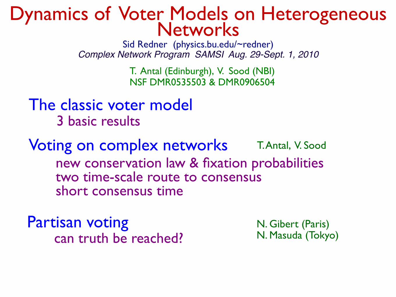
Dynamics of Voter Models on Heterogeneous Networks Sid Redner (physics.bu.edu/~redner) Complex Network Program SAMSI Aug. 29-Sept. 1, 2010 T. Antal (Edinburgh), V. Sood (NBI) NSF DMR0535503 & DMR0906504
-
Upload
khangminh22 -
Category
Documents
-
view
0 -
download
0
Transcript of Dynamics of Voter Models on Heterogeneous Networks

Dynamics of Voter Models on Heterogeneous Networks
Sid Redner (physics.bu.edu/~redner) Complex Network Program SAMSI Aug. 29-Sept. 1, 2010
T. Antal (Edinburgh), V. Sood (NBI)NSF DMR0535503 & DMR0906504
Dynamics of Voter Models on Heterogeneous Networks
Sid Redner (physics.bu.edu/~redner) Complex Network Program SAMSI Aug. 29-Sept. 1, 2010
T. Antal, V. Sood
new conservation law & fixation probabilitiestwo time-scale route to consensus short consensus time
Voting on complex networks
The classic voter model3 basic results
Partisan voting can truth be reached?
N. Gibert (Paris)N. Masuda (Tokyo)
T. Antal (Edinburgh), V. Sood (NBI)NSF DMR0535503 & DMR0906504

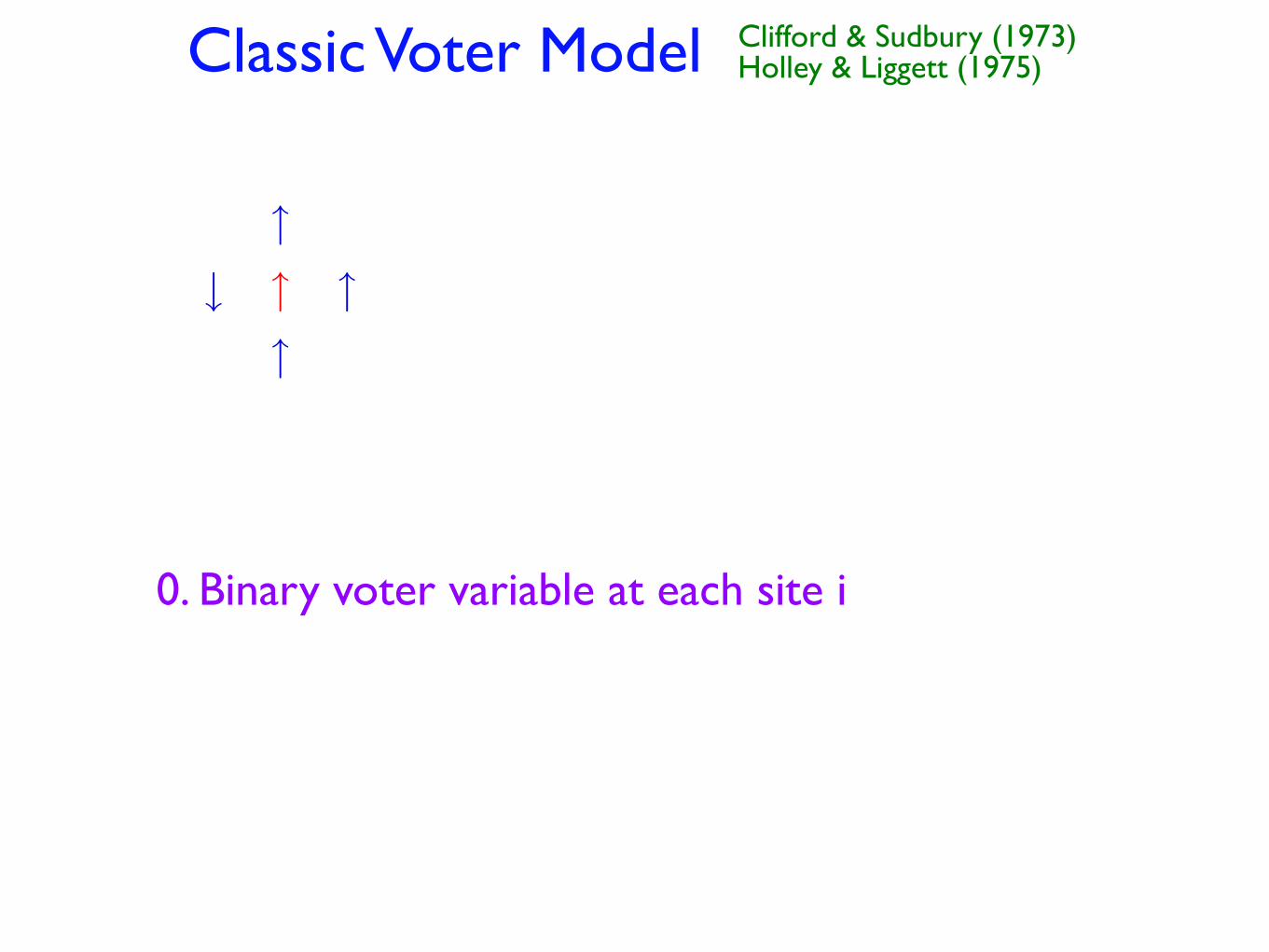
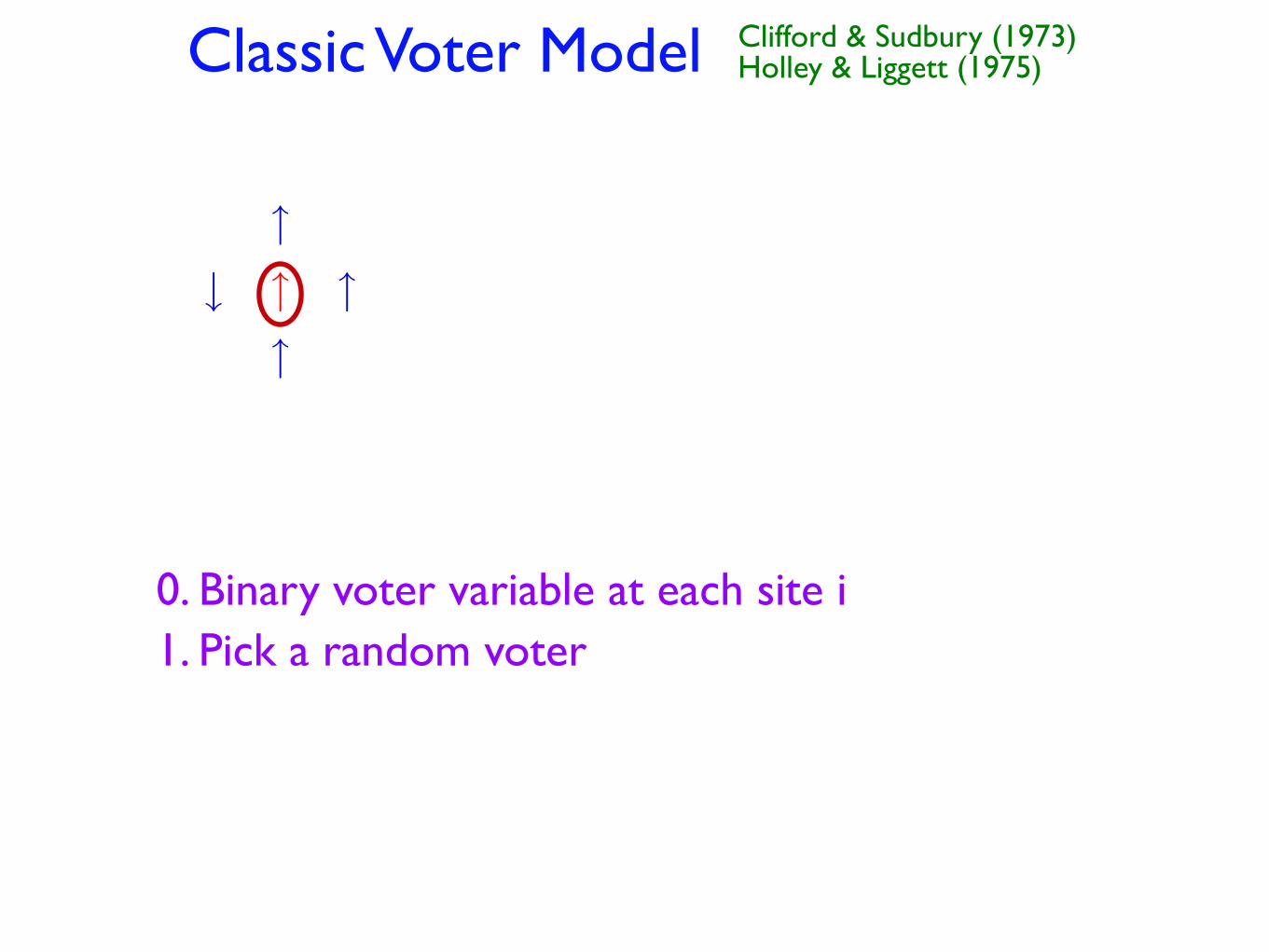
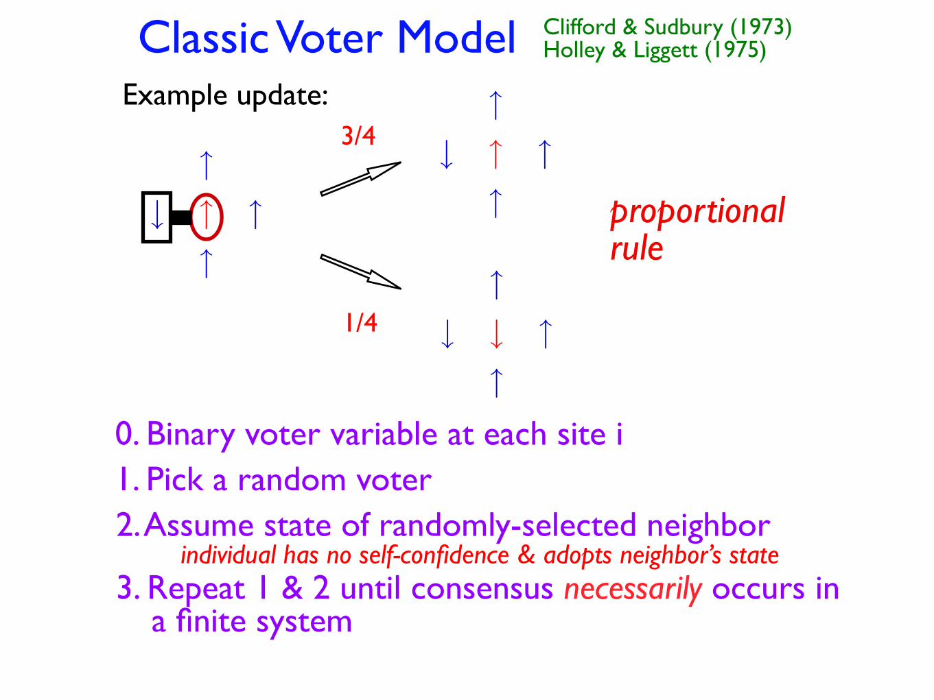
Classic Voter Model Clifford & Sudbury (1973) Holley & Liggett (1975)
Classic Voter Model Clifford & Sudbury (1973) Holley & Liggett (1975)
!
" ! !
!
0. Binary voter variable at each site i
Classic Voter Model Clifford & Sudbury (1973) Holley & Liggett (1975)
!
" ! !
!
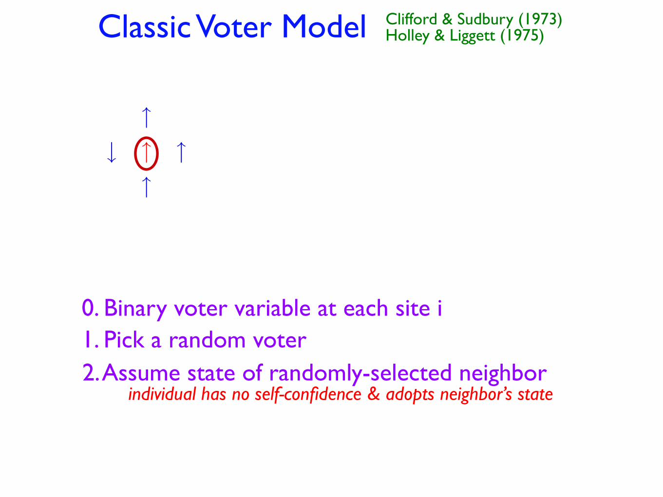
0. Binary voter variable at each site i1. Pick a random voter
Classic Voter Model Clifford & Sudbury (1973) Holley & Liggett (1975)
!
" ! !
!
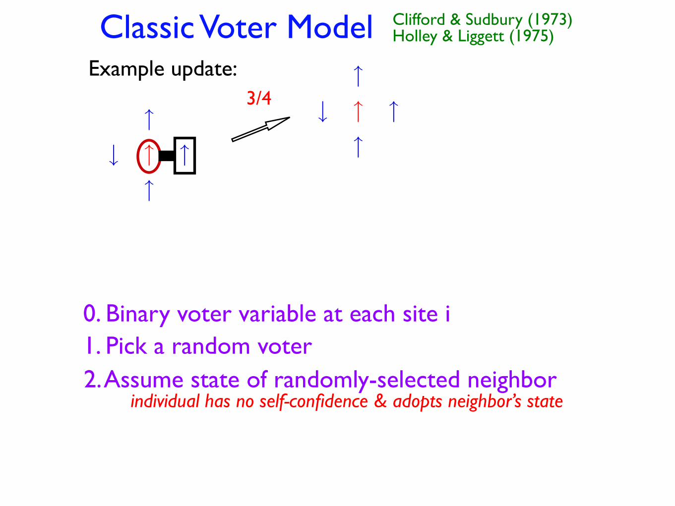
0. Binary voter variable at each site i1. Pick a random voter2. Assume state of randomly-selected neighbor
individual has no self-confidence & adopts neighbor’s state
Classic Voter Model Clifford & Sudbury (1973) Holley & Liggett (1975)
!
" ! !
!
0. Binary voter variable at each site i1. Pick a random voter
!
" ! !
!
3/4
Example update:
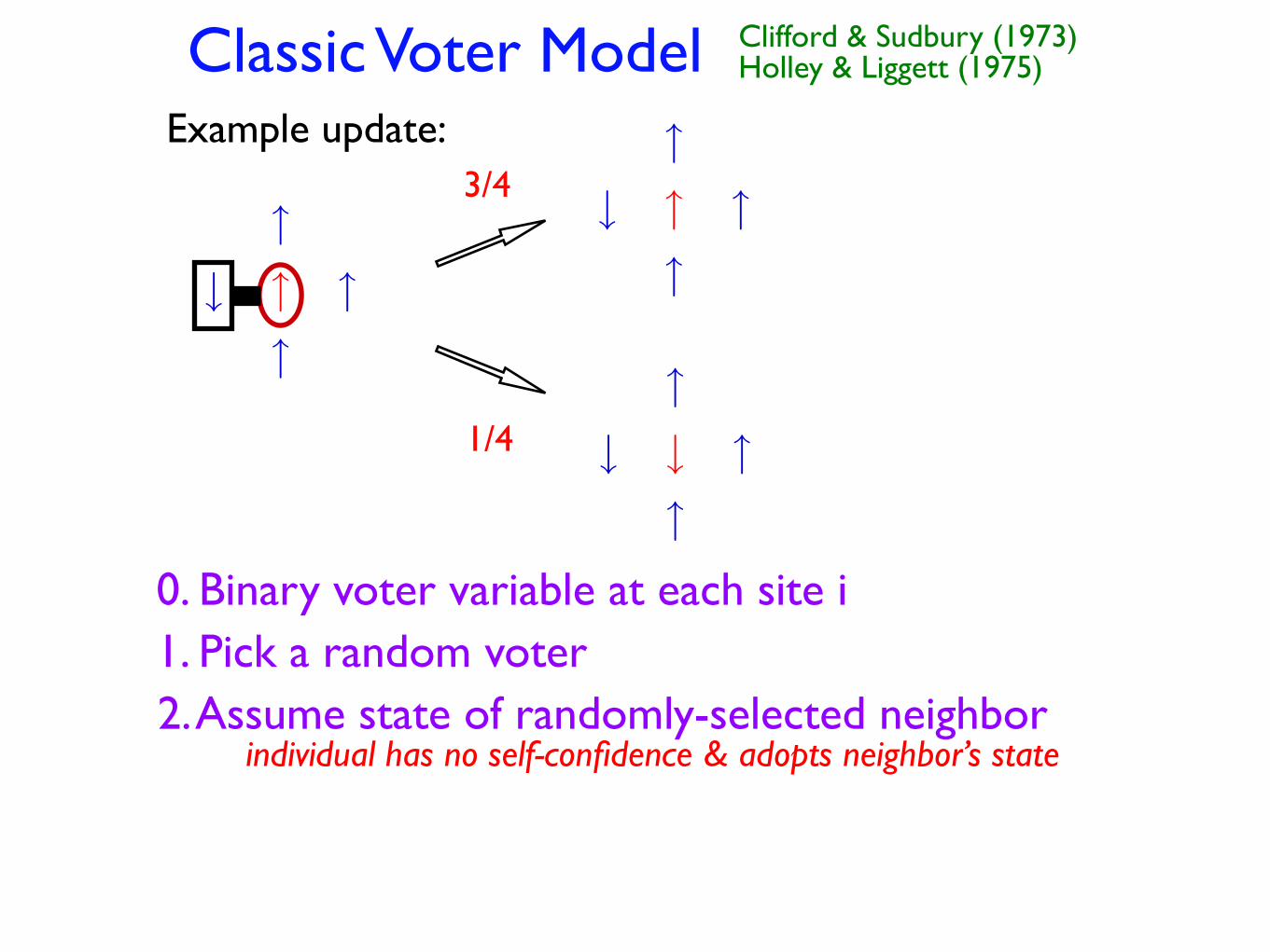
2. Assume state of randomly-selected neighborindividual has no self-confidence & adopts neighbor’s state
2. Assume state of randomly-selected neighborindividual has no self-confidence & adopts neighbor’s state
!
" ! !
!
0. Binary voter variable at each site i1. Pick a random voter
!
" ! !
!
3/4
Example update:
!
" " !
!
1/4
Classic Voter Model Clifford & Sudbury (1973) Holley & Liggett (1975)

2. Assume state of randomly-selected neighborindividual has no self-confidence & adopts neighbor’s state
!
" ! !
!
0. Binary voter variable at each site i1. Pick a random voter
!
" ! !
!
3/4
Example update:
!
" " !
!
1/4
proportional rule
Classic Voter Model Clifford & Sudbury (1973) Holley & Liggett (1975)
2. Assume state of randomly-selected neighborindividual has no self-confidence & adopts neighbor’s state
!
" ! !
!
0. Binary voter variable at each site i
3. Repeat 1 & 2 until consensus necessarily occurs in a finite system
1. Pick a random voter
!
" ! !
!
3/4
Example update:
!
" " !
!
1/4
proportional rule
Classic Voter Model Clifford & Sudbury (1973) Holley & Liggett (1975)
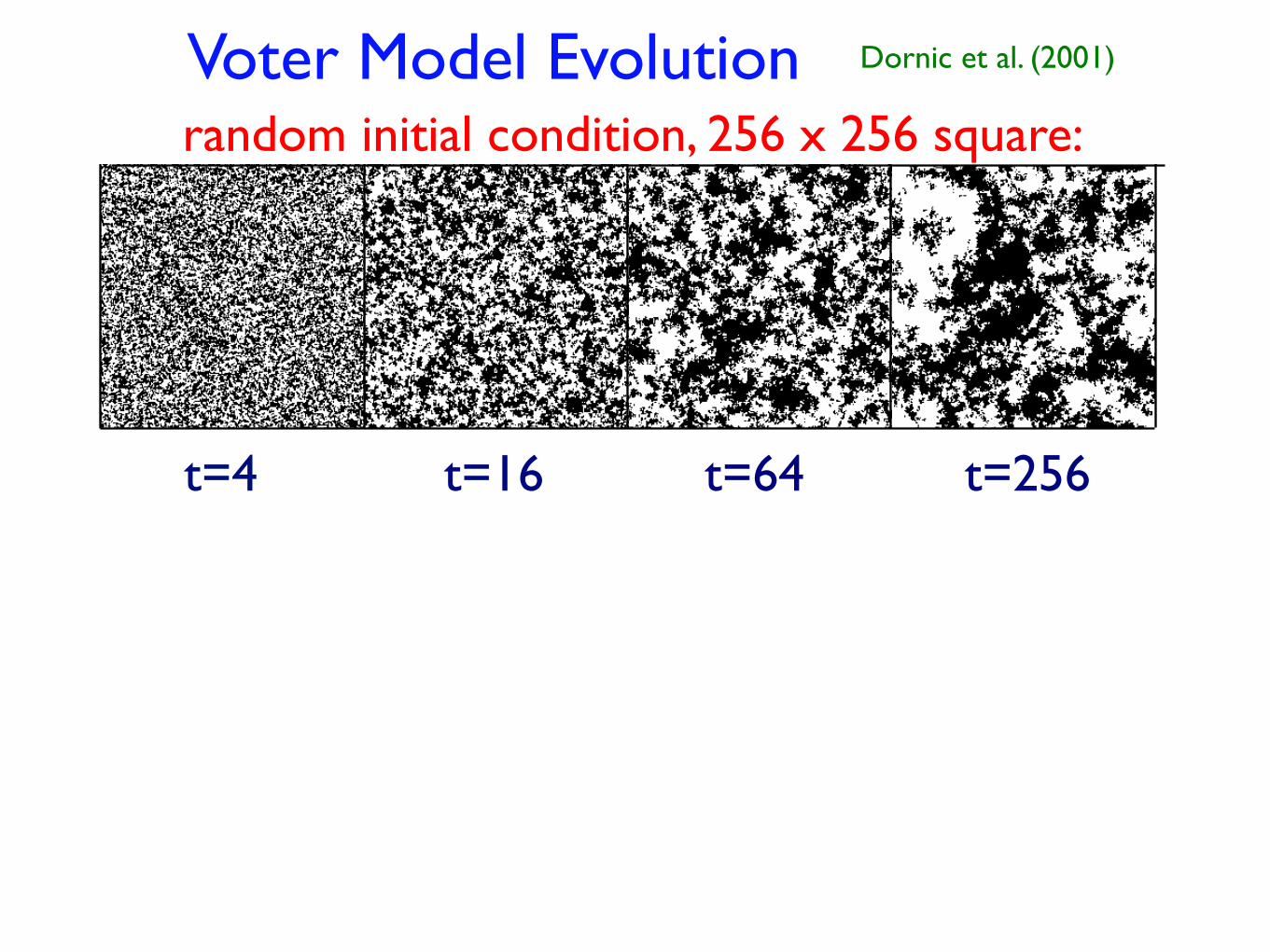
random initial condition, 256 x 256 square: Voter Model Evolution Dornic et al. (2001)
t=4 t=16 t=64 t=256
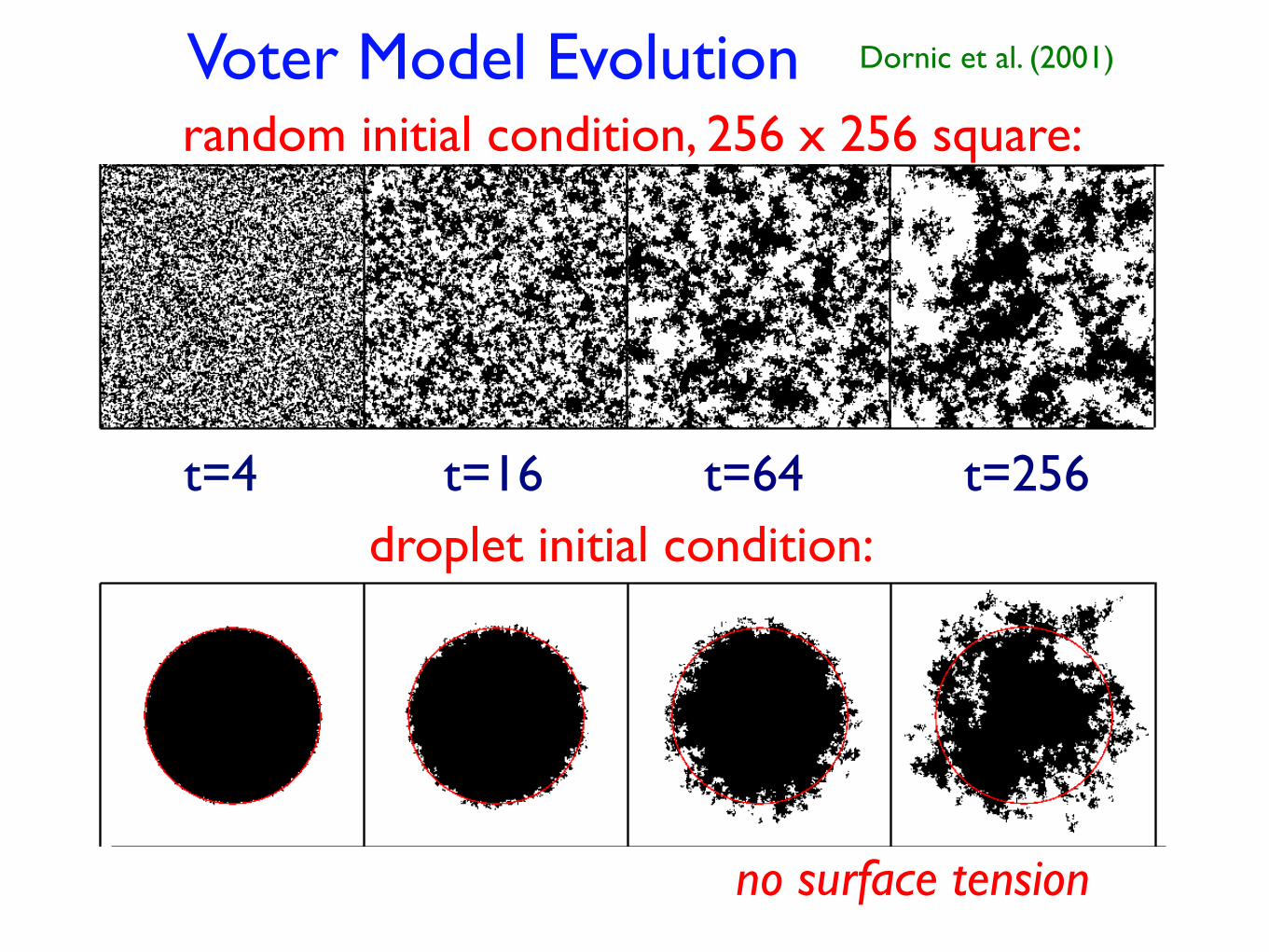
random initial condition, 256 x 256 square: Voter Model Evolution Dornic et al. (2001)
t=4 t=16 t=64 t=256
droplet initial condition:t=4 t=16 t=64 t=256
no surface tension
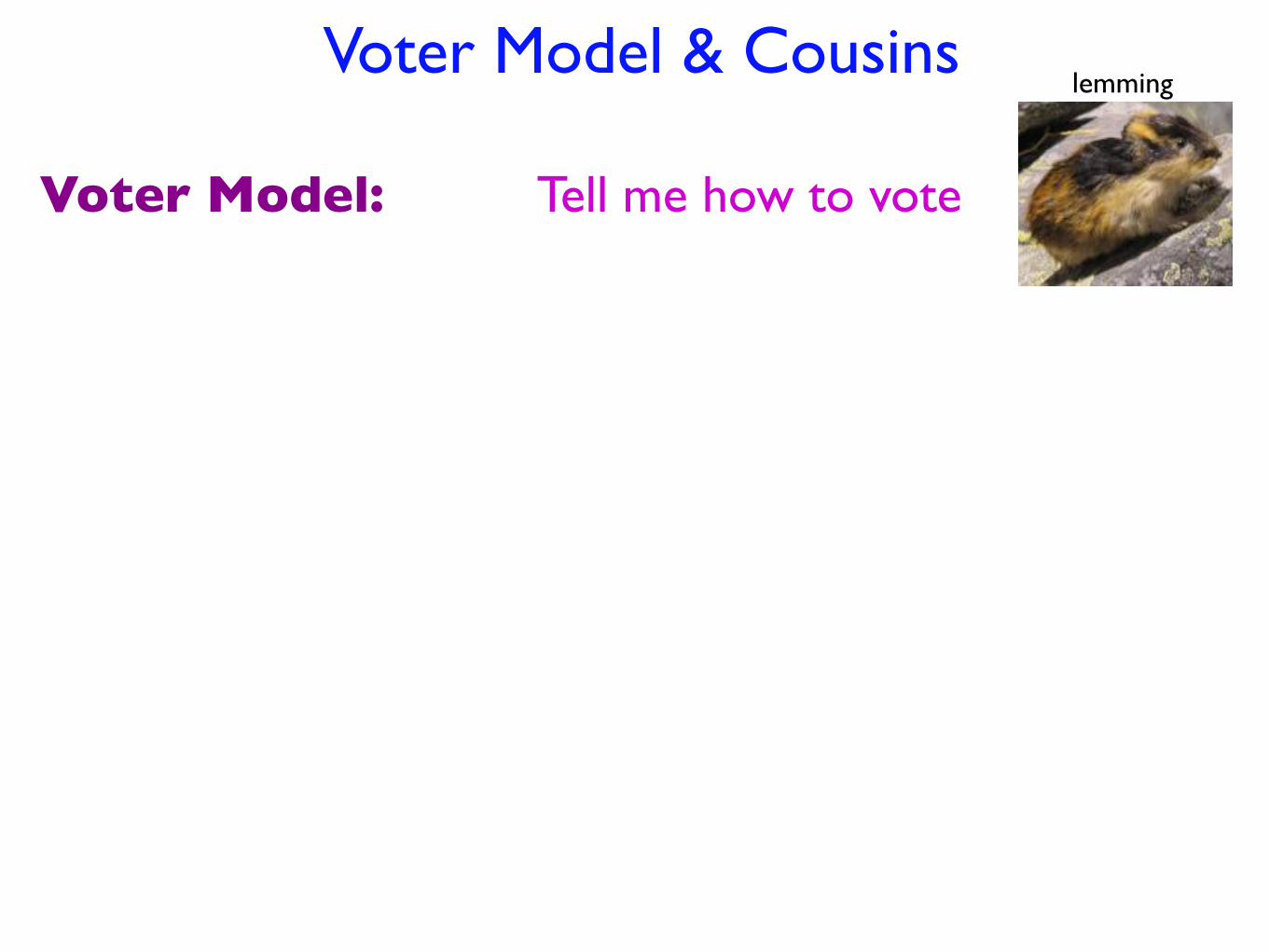
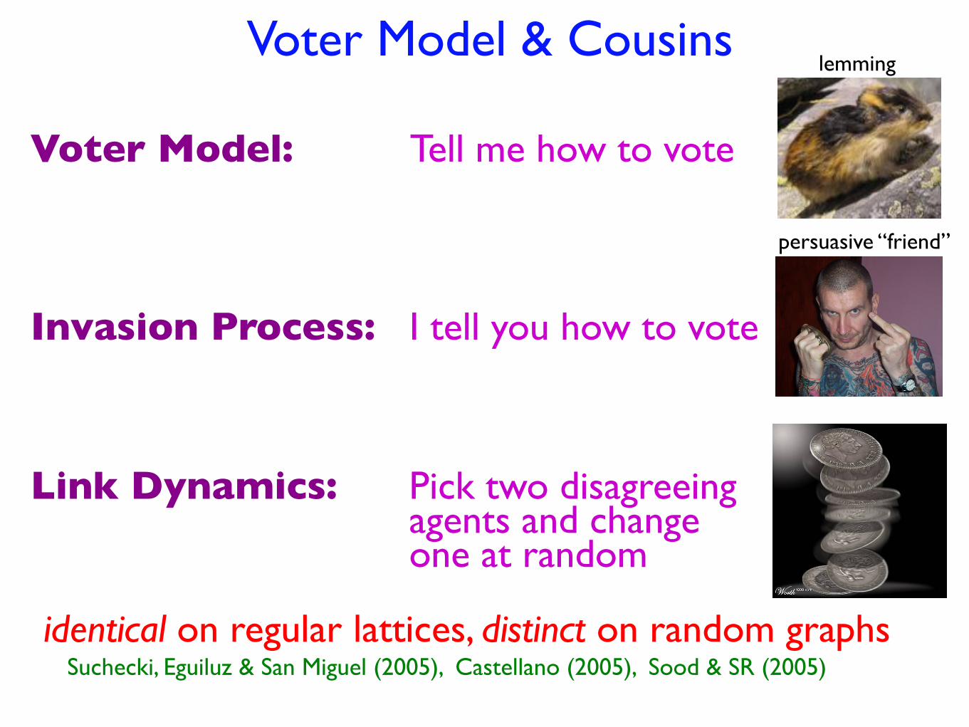
Voter Model & Cousins
Voter Model: Tell me how to vote
lemming

Voter Model & Cousins
Voter Model: Tell me how to vote
lemming
Invasion Process: I tell you how to vote
persuasive “friend”

Voter Model & Cousins
Voter Model: Tell me how to vote
lemming
Link Dynamics: Pick two disagreeing agents and change one at random
Invasion Process: I tell you how to vote
persuasive “friend”
Voter Model & Cousins
identical on regular lattices, distinct on random graphsSuchecki, Eguiluz & San Miguel (2005), Castellano (2005), Sood & SR (2005)
Voter Model: Tell me how to vote
lemming
Link Dynamics: Pick two disagreeing agents and change one at random
Invasion Process: I tell you how to vote
persuasive “friend”
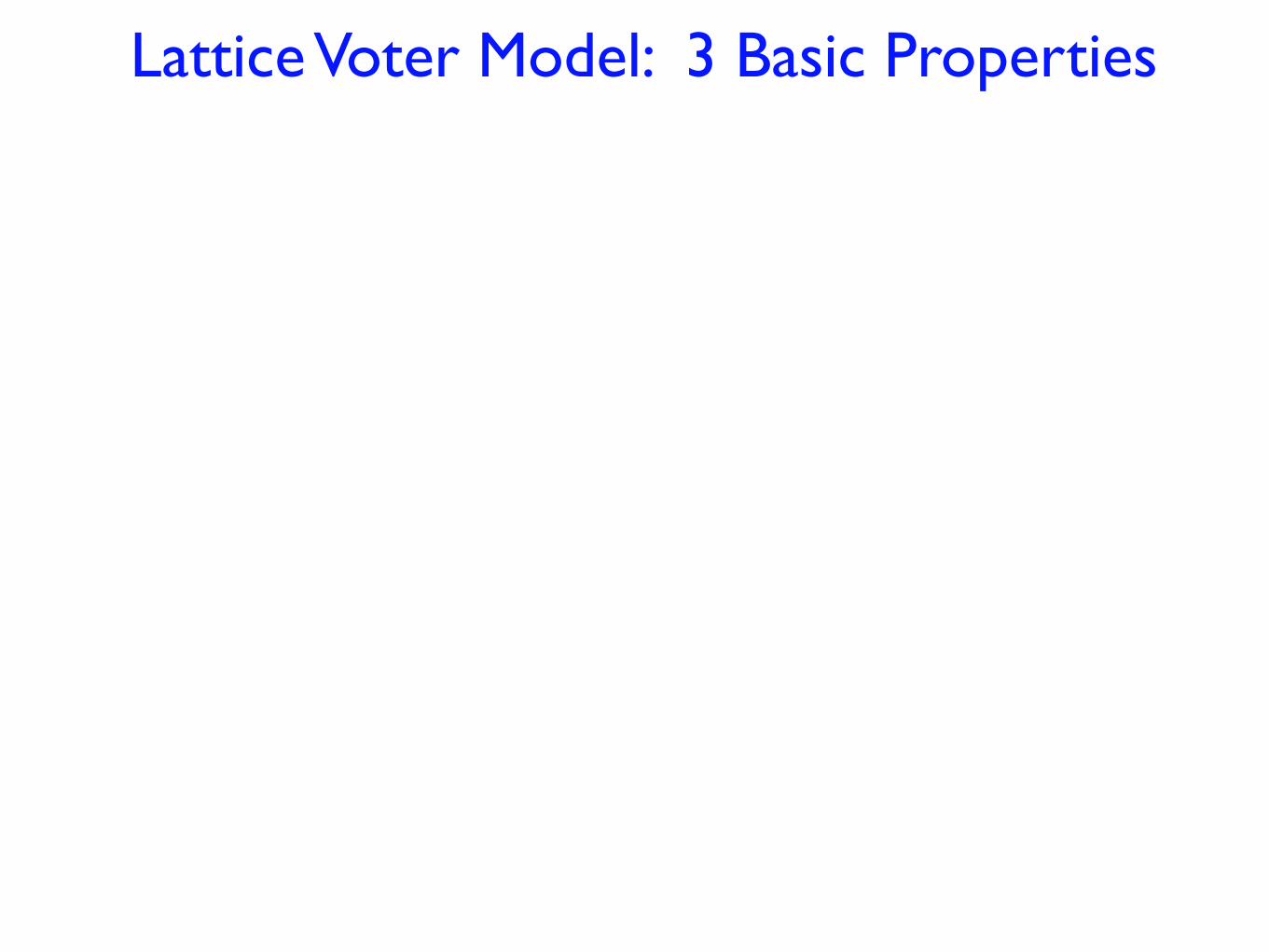
Lattice Voter Model: 3 Basic Properties

Lattice Voter Model: 3 Basic Properties
Evolution of a single active link:
1/2
1/2
average magnetization conserved
1. Final State (Exit) Probability E(!0)

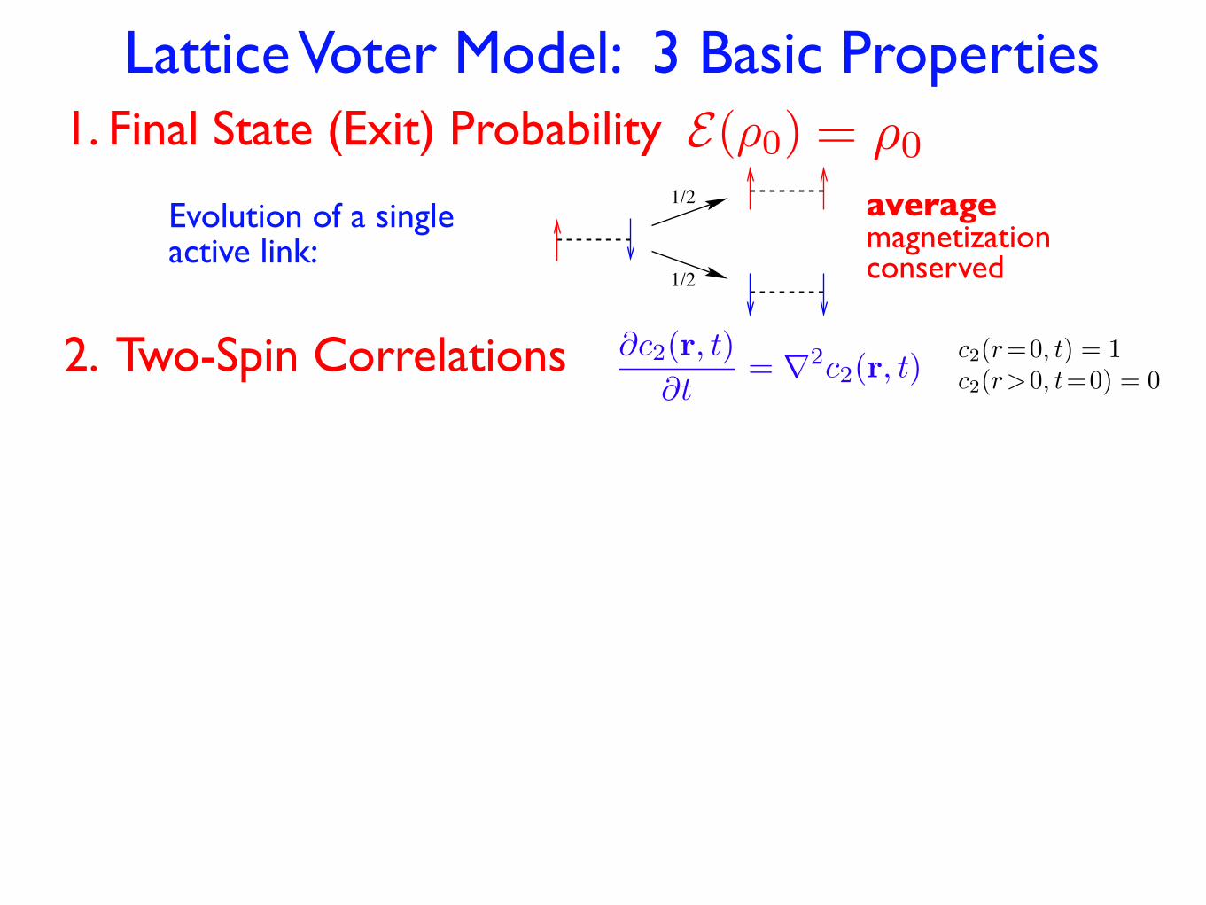
Lattice Voter Model: 3 Basic Properties
Evolution of a single active link:
1/2
1/2
average magnetization conserved
1. Final State (Exit) Probability E(!0) = !0
Lattice Voter Model: 3 Basic Properties
Evolution of a single active link:
1/2
1/2
average magnetization conserved
1. Final State (Exit) Probability E(!0) = !0
2. Two-Spin Correlations !c2(r, t)
!t= !
2c2(r, t)c2(r=0, t) = 1c2(r>0, t=0) = 0

Lattice Voter Model: 3 Basic Properties
Evolution of a single active link:
1/2
1/2
average magnetization conserved
1. Final State (Exit) Probability E(!0) = !0
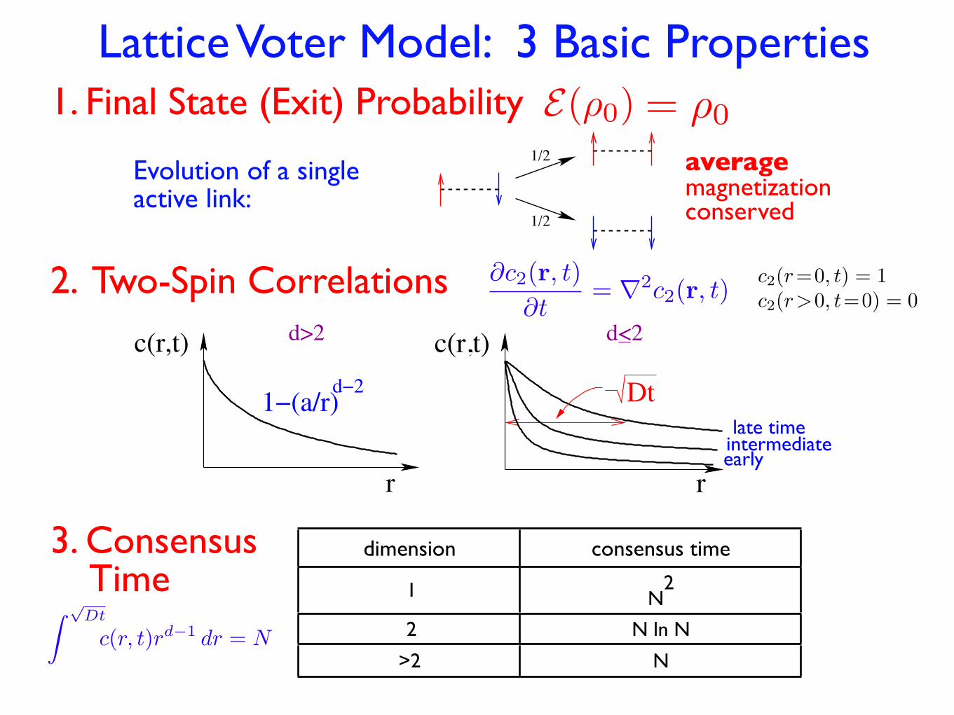
late time
early
d>2c(r,t)
r
1!(a/r)d!2
c(r,t) d<2
Dt
rintermediate
2. Two-Spin Correlations !c2(r, t)
!t= !
2c2(r, t)c2(r=0, t) = 1c2(r>0, t=0) = 0
Lattice Voter Model: 3 Basic Properties
Evolution of a single active link:
1/2
1/2
average magnetization conserved
1. Final State (Exit) Probability E(!0) = !0
late time
early
d>2c(r,t)
r
1!(a/r)d!2
c(r,t) d<2
Dt
rintermediate
2. Two-Spin Correlations !c2(r, t)
!t= !
2c2(r, t)c2(r=0, t) = 1c2(r>0, t=0) = 0
dimension consensus time
1 N2
2 N ln N
>2 N
3. Consensus Time! !
Dt
c(r, t)rd"1 dr = N

Voter Model on Complex Networks
V. Sood & SR, PRL 94, 178701 (2005);
C. Castellano, D. Vilon, A. Vespignani, EPL 63, 153 (2003)
T. Antal, V. Sood, SR, PRE 77, 041121 (2008)K. Suchecki, V. M. Eguiluz, M. San Miguel, EPL 69, 228 (2005)

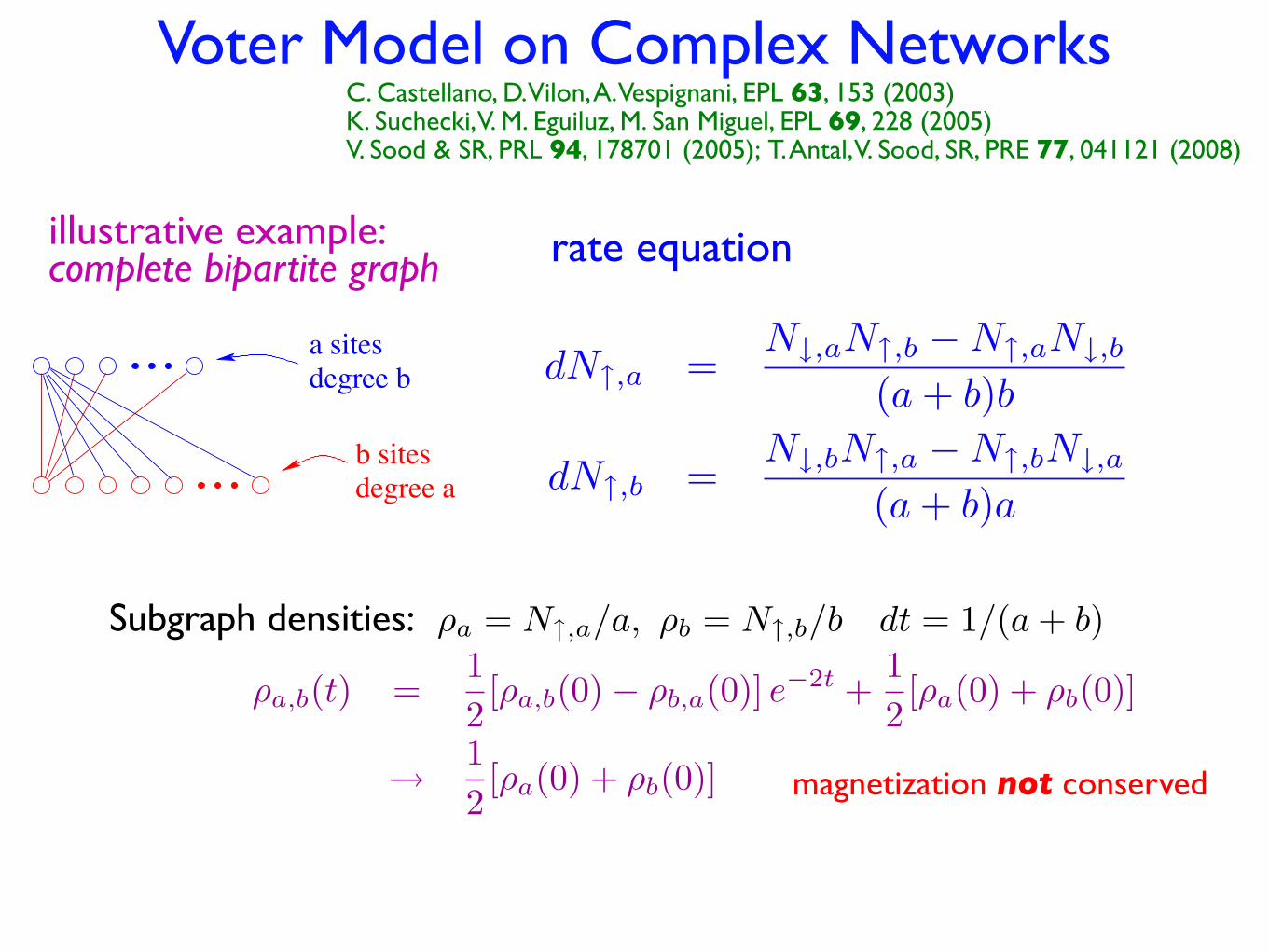
Voter Model on Complex Networks
illustrative example: complete bipartite graph
degree a
a sitesdegree b
b sites
V. Sood & SR, PRL 94, 178701 (2005);
C. Castellano, D. Vilon, A. Vespignani, EPL 63, 153 (2003)
T. Antal, V. Sood, SR, PRE 77, 041121 (2008)K. Suchecki, V. M. Eguiluz, M. San Miguel, EPL 69, 228 (2005)
dN↑,a =N↓,aN↑,b −N↑,aN↓,b
(a + b)b
dN↑,b =N↓,bN↑,a −N↑,bN↓,a
(a + b)a
rate equation
Voter Model on Complex Networks
magnetization not conserved
illustrative example: complete bipartite graph
degree a
a sitesdegree b
b sites
V. Sood & SR, PRL 94, 178701 (2005);
C. Castellano, D. Vilon, A. Vespignani, EPL 63, 153 (2003)
T. Antal, V. Sood, SR, PRE 77, 041121 (2008)K. Suchecki, V. M. Eguiluz, M. San Miguel, EPL 69, 228 (2005)
dN↑,a =N↓,aN↑,b −N↑,aN↓,b
(a + b)b
dN↑,b =N↓,bN↑,a −N↑,bN↓,a
(a + b)a
rate equation
Subgraph densities:
!a,b(t) =1
2[!a,b(0) ! !b,a(0)] e!2t +
1
2[!a(0) + !b(0)]
"
1
2[!a(0) + !b(0)]
ρa = N↑,a/a, ρb = N↑,b/b dt = 1/(a + b)

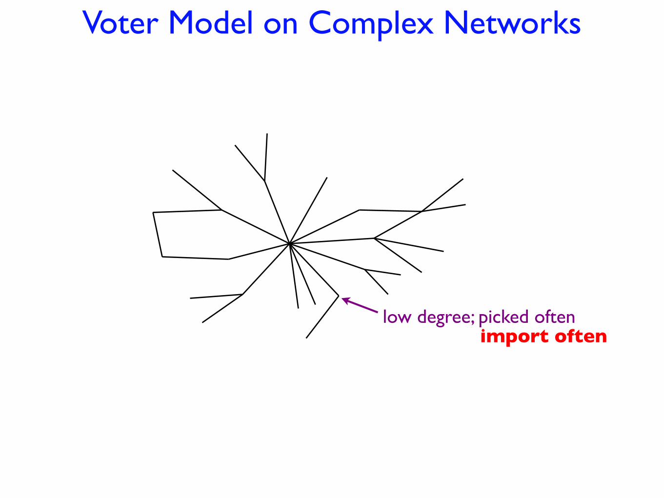
Voter Model on Complex Networks
Voter Model on Complex Networks
low degree; picked often import often
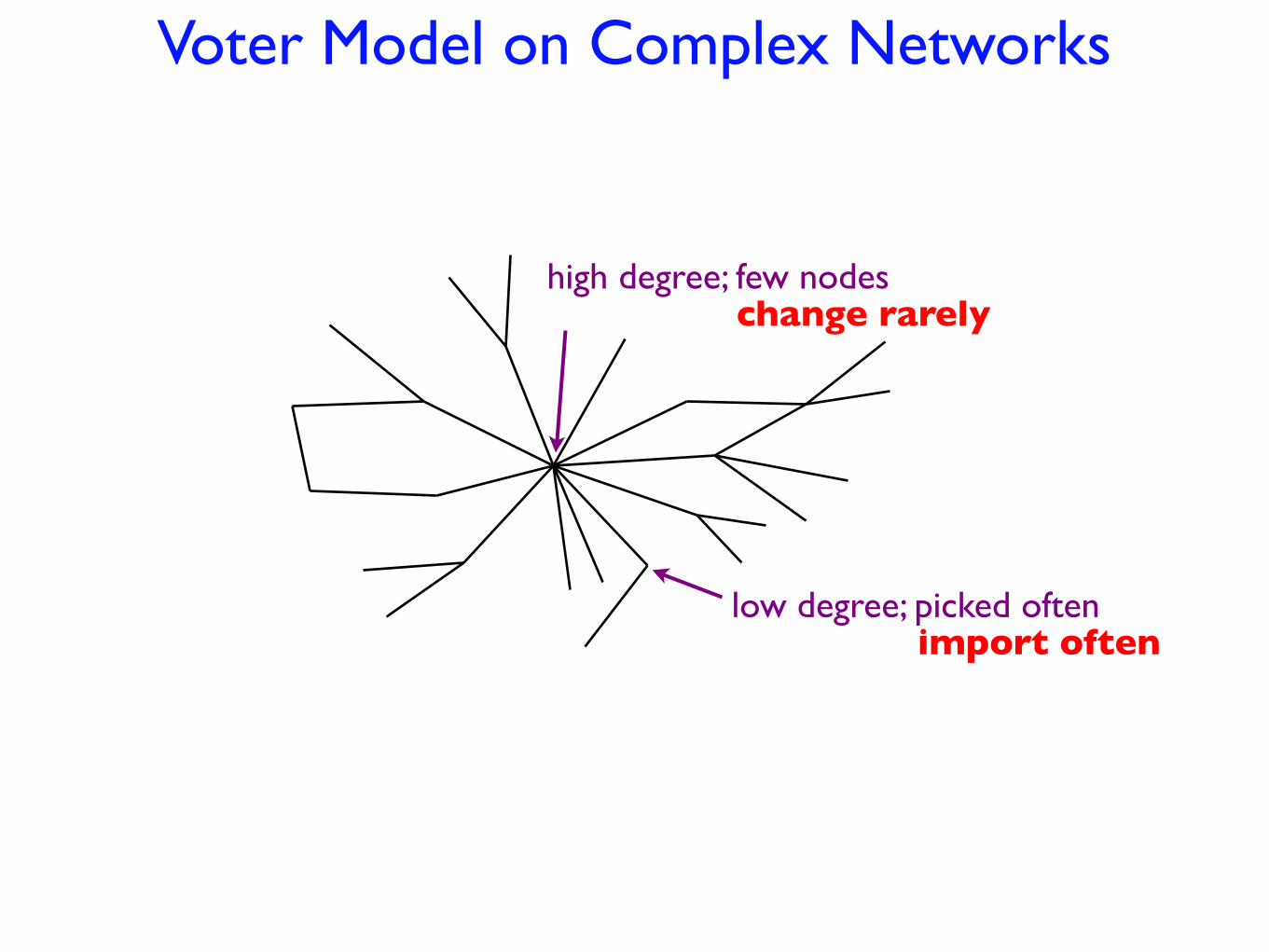
Voter Model on Complex Networks
high degree; few nodes change rarely
low degree; picked often import often

Voter Model on Complex Networks
high degree; few nodes change rarely
low degree; picked often import often
“flow” from high degree to low degree

Invasion Process on Complex NetworksCastellano, AIP Conf Proc 779, 114 (2005)
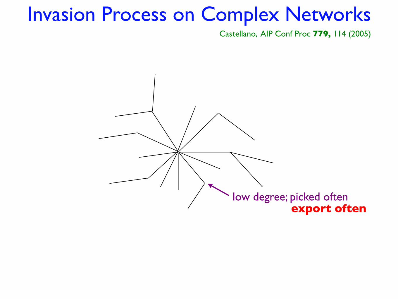
low degree; picked often export often
Invasion Process on Complex NetworksCastellano, AIP Conf Proc 779, 114 (2005)
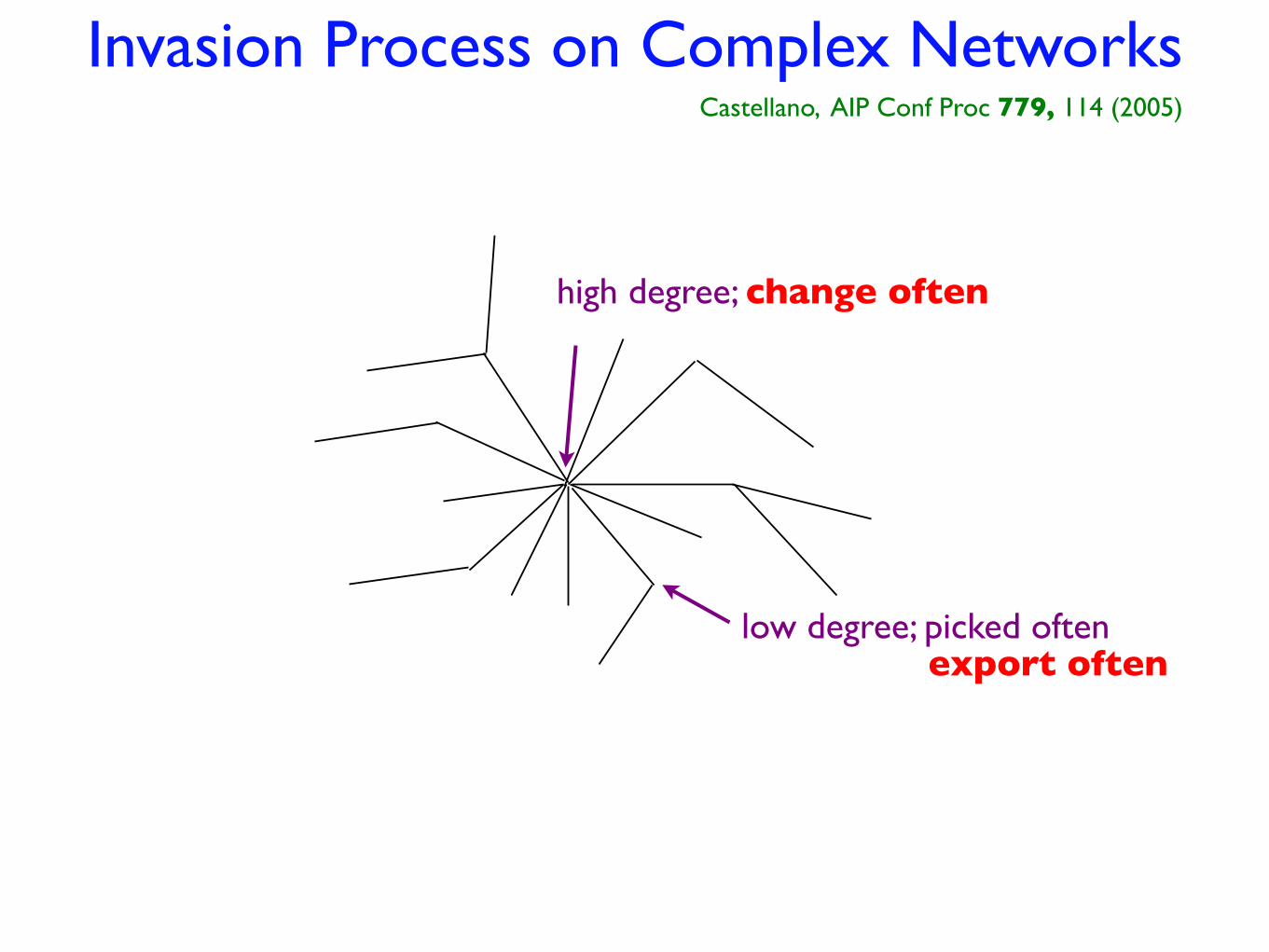
high degree; change often
low degree; picked often export often
Invasion Process on Complex NetworksCastellano, AIP Conf Proc 779, 114 (2005)

high degree; change often
low degree; picked often export often
“flow” from low degree to high degree
Invasion Process on Complex NetworksCastellano, AIP Conf Proc 779, 114 (2005)

η = {1, 1, 0, 0, . . . , 1} system stateηx = system state when voter at x flipsη(x) = state of voter at x
Formal Approach for Conservation Law
flip rate: P[η → ηx] =�
y
Axy
Z [Φ(x, y) + Φ(y, x)]

η = {1, 1, 0, 0, . . . , 1} system stateηx = system state when voter at x flipsη(x) = state of voter at x
Formal Approach for Conservation Law
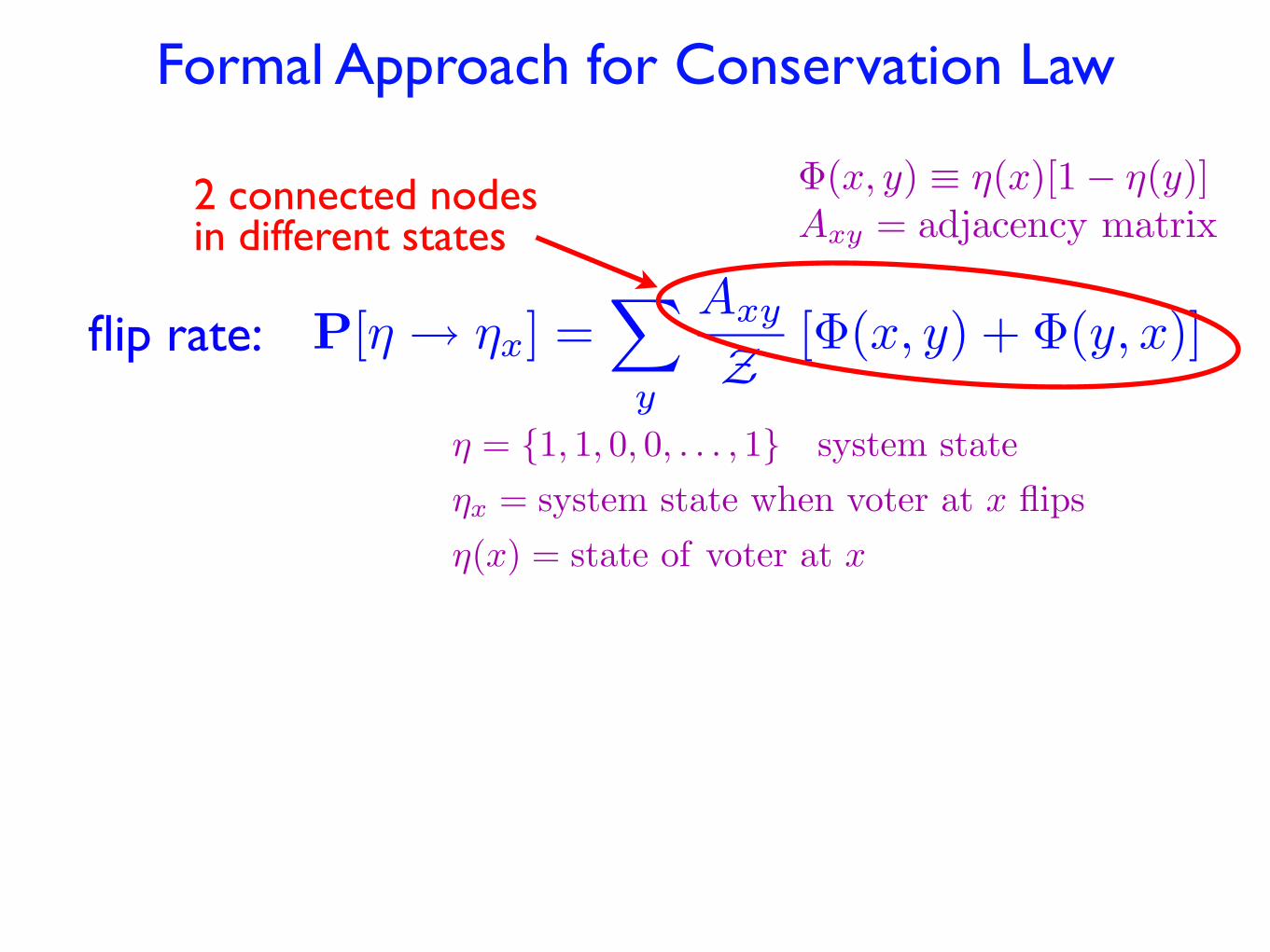
Φ(x, y) ≡ η(x)[1− η(y)]Axy = adjacency matrix
flip rate: P[η → ηx] =�
y
Axy
Z [Φ(x, y) + Φ(y, x)]
η = {1, 1, 0, 0, . . . , 1} system stateηx = system state when voter at x flipsη(x) = state of voter at x
Formal Approach for Conservation Law
Φ(x, y) ≡ η(x)[1− η(y)]Axy = adjacency matrix
flip rate: P[η → ηx] =�
y
Axy
Z [Φ(x, y) + Φ(y, x)]
2 connected nodes in different states

η = {1, 1, 0, 0, . . . , 1} system stateηx = system state when voter at x flipsη(x) = state of voter at x
Formal Approach for Conservation Law
Φ(x, y) ≡ η(x)[1− η(y)]Axy = adjacency matrix
flip rate: P[η → ηx] =�
y
Axy
Z [Φ(x, y) + Φ(y, x)]
choose x, choose neighbor of x with prob.
choose y (neighbor of x), choose of x with prob.
choose link & update x with prob.
Z ≡
Nkx VMNky IPNµ1 LD
(Nkx)−1
(Nky)−1
(Nµ1)−1
2 connected nodes in different states
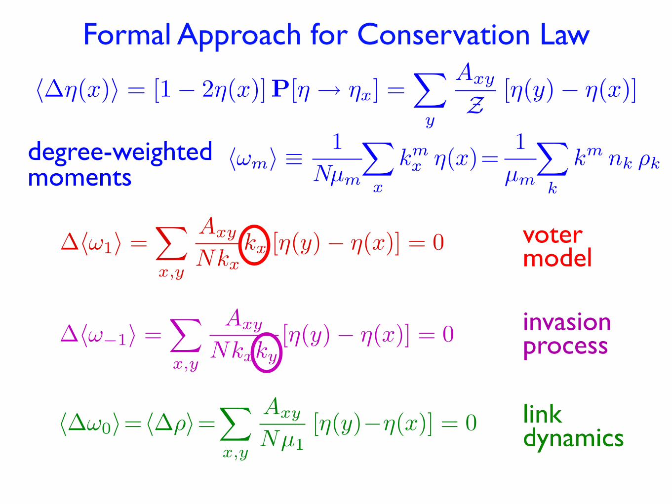
Formal Approach for Conservation Law
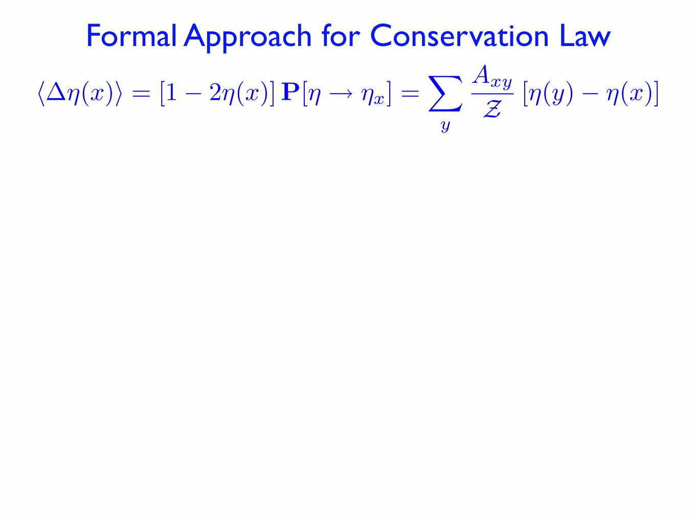
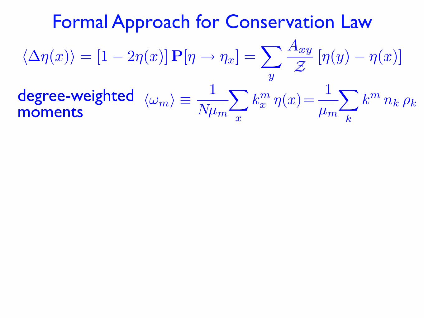
�∆η(x)� = [1− 2η(x)]P[η → ηx] =�
y
Axy
Z [η(y)− η(x)]
Formal Approach for Conservation Law
�∆η(x)� = [1− 2η(x)]P[η → ηx] =�
y
Axy
Z [η(y)− η(x)]
degree-weighted moments
�ωm� ≡ 1Nµm
�
x
kmx η(x)=
1µm
�
k
km nk ρk
Formal Approach for Conservation Law
�∆η(x)� = [1− 2η(x)]P[η → ηx] =�
y
Axy
Z [η(y)− η(x)]
link dynamics
�∆ω0�=�∆ρ�=�
x,y
Axy
Nµ1[η(y)−η(x)] = 0
invasionprocess∆�ω−1� =
�
x,y
Axy
Nkxky[η(y) − η(x)] = 0
∆�ω1� =�
x,y
Axy
Nkxkx [η(y) − η(x)] = 0 voter
model
degree-weighted moments
�ωm� ≡ 1Nµm
�
x
kmx η(x)=
1µm
�
k
km nk ρk
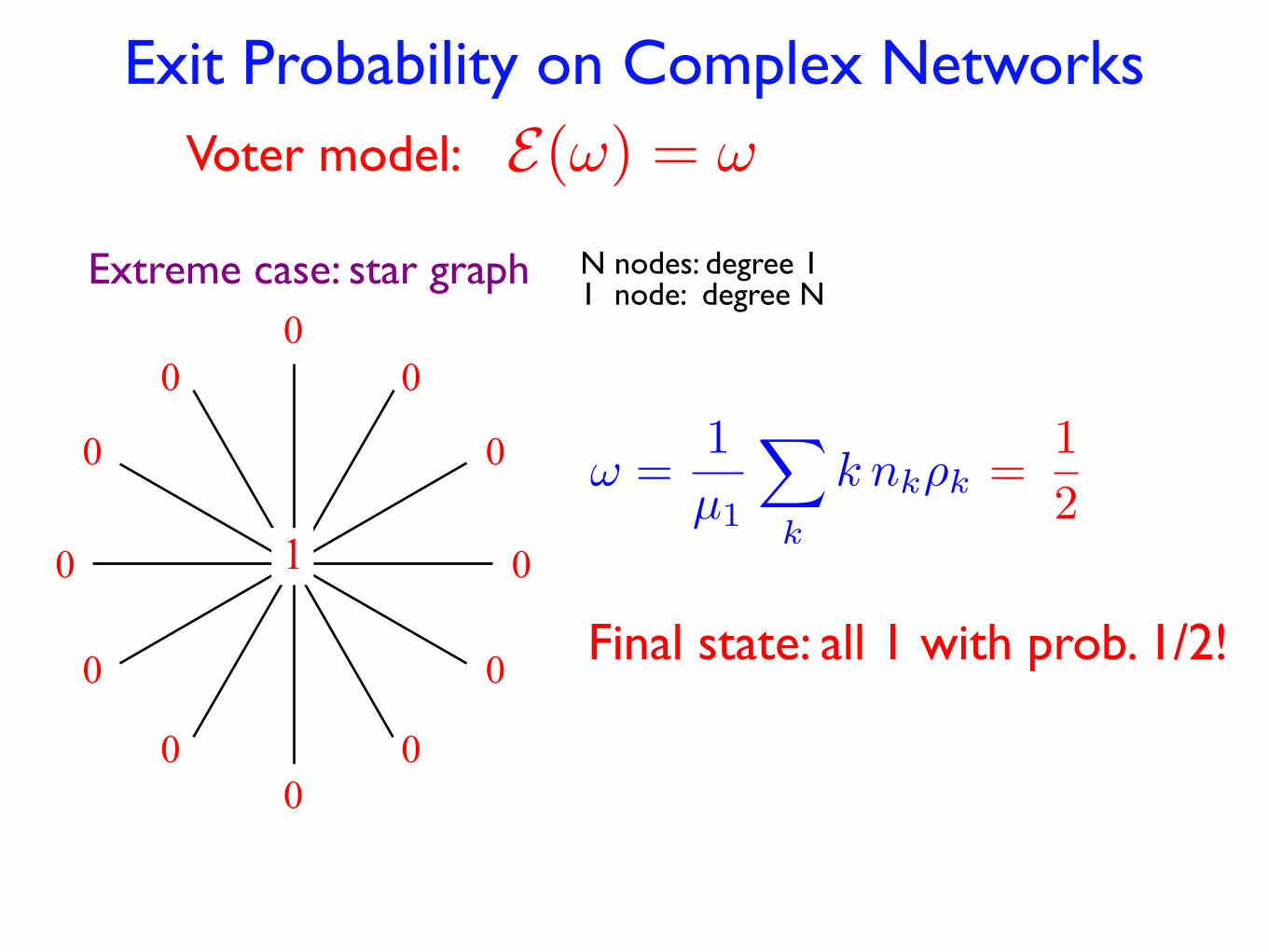
Exit Probability on Complex NetworksE(!) = !Voter model:
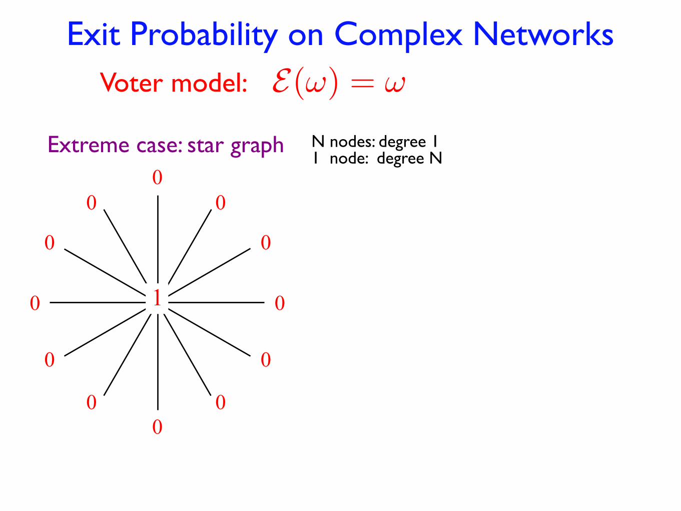
Exit Probability on Complex Networks
Extreme case: star graph0
0
0
0
0
00
0
0
0
0
0
1
N nodes: degree 11 node: degree N
E(!) = !Voter model:
Exit Probability on Complex Networks
Extreme case: star graph0
0
0
0
0
00
0
0
0
0
0
1
N nodes: degree 11 node: degree N
Final state: all 1 with prob. 1/2!
ω =1µ1
�
k
k nkρk =12
E(!) = !Voter model:

Byproduct: Voter Model Fixation ProbabilityWhat is the probability that a single mutant “takes over” a population?
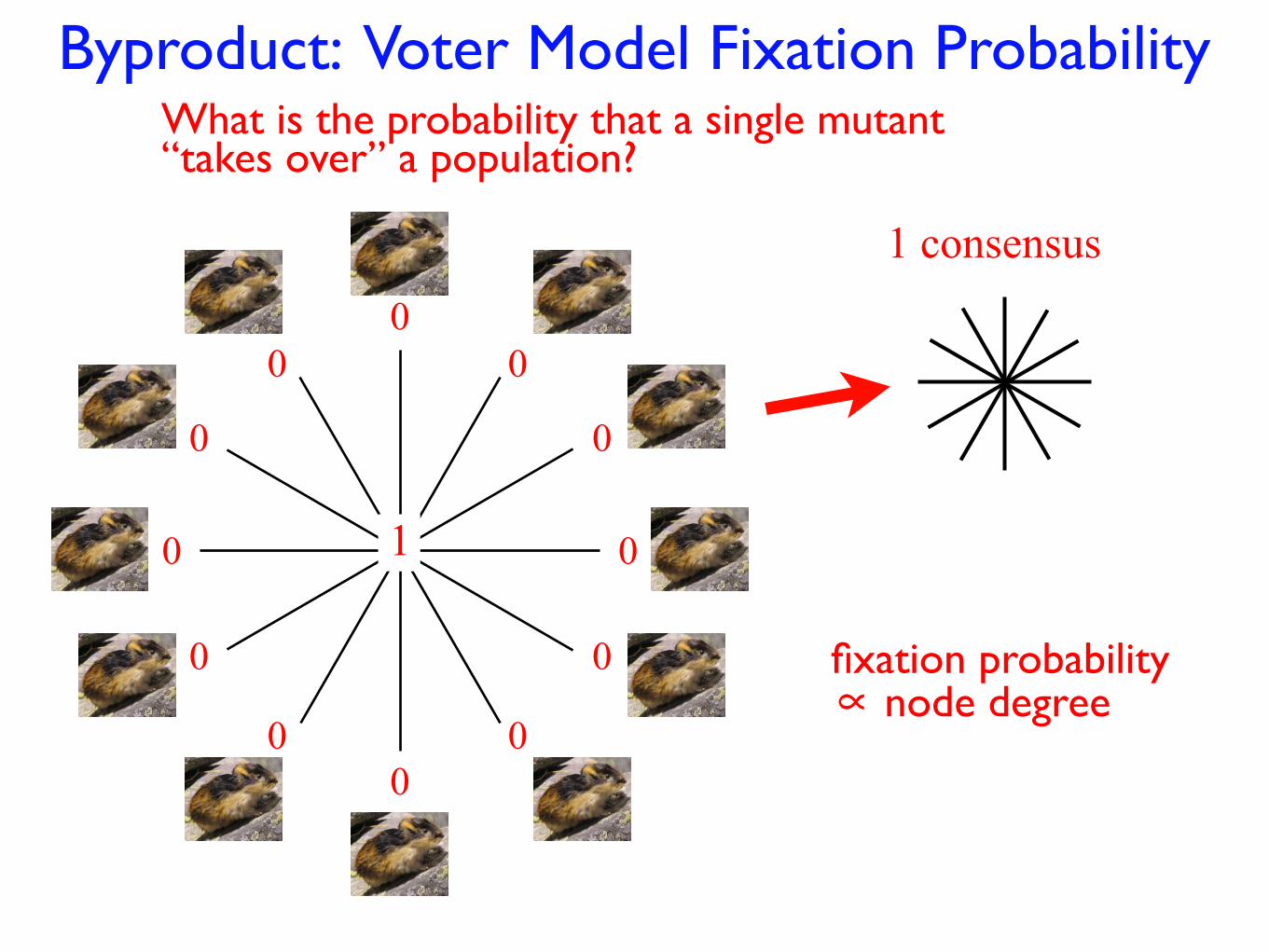
Byproduct: Voter Model Fixation ProbabilityWhat is the probability that a single mutant “takes over” a population?
00
0
0
0
00
0
0
0
0
0
1
1 consensus
fixation probability∝ node degree
00
0
0
0
00
0
0
0
0
0
1
0 consensus
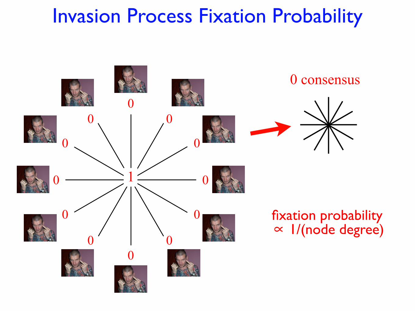
Invasion Process Fixation Probability
fixation probability∝ 1/(node degree)
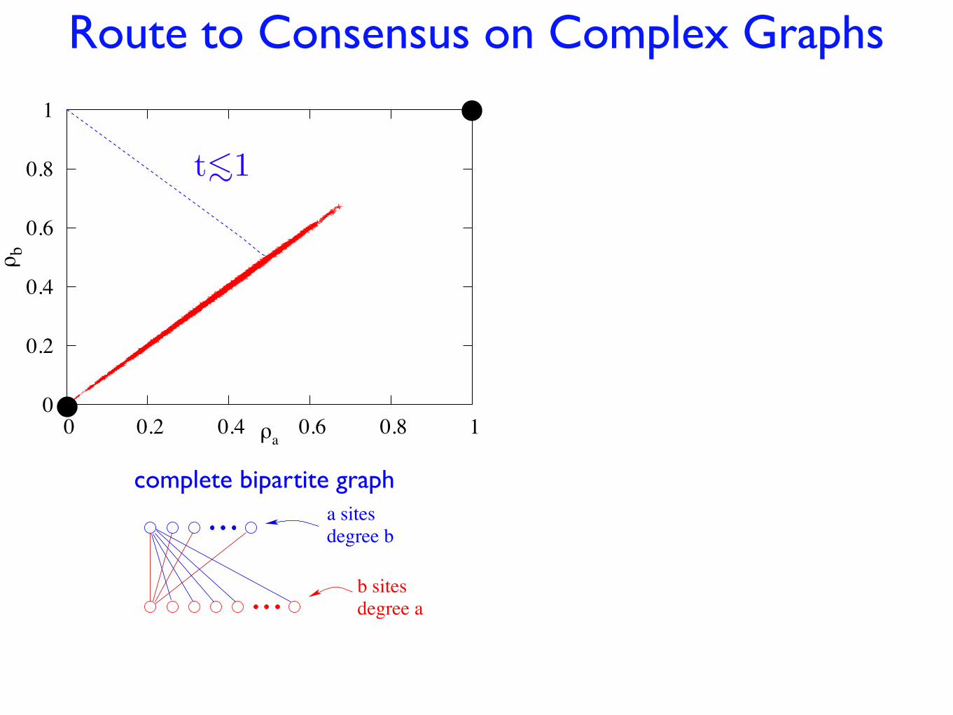
Route to Consensus on Complex Graphs
complete bipartite graph
degree a
a sitesdegree b
b sites
0
0.2
0.4
0.6
0.8
1
0 0.2 0.4 0.6 0.8 1
ρ b
ρa
t<!
1
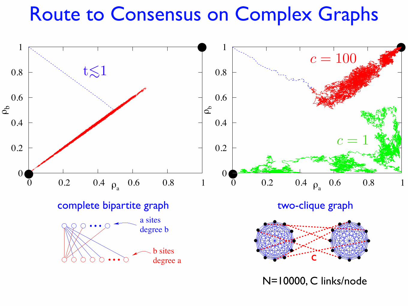
Route to Consensus on Complex Graphs
complete bipartite graph
degree a
a sitesdegree b
b sites
0
0.2
0.4
0.6
0.8
1
0 0.2 0.4 0.6 0.8 1
ρ b
ρa
t<!
1
c = 1
c = 100
0
0.2
0.4
0.6
0.8
1
0 0.2 0.4 0.6 0.8 1
ρ b
ρa
two-clique graph
c
N=10000, C links/node
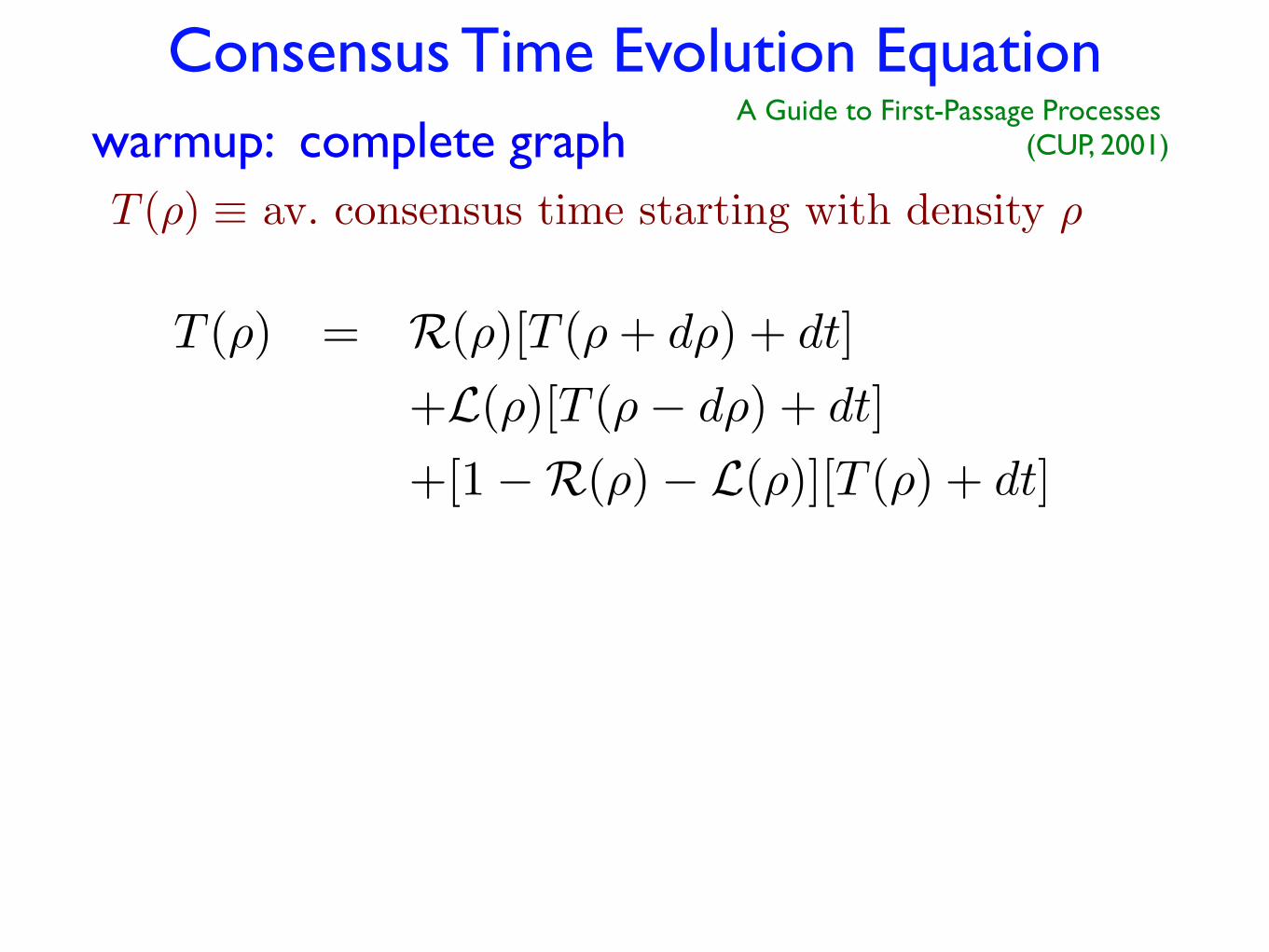
Consensus Time Evolution Equation
T (ρ) = R(ρ)[T (ρ + dρ) + dt]+L(ρ)[T (ρ− dρ) + dt]+[1−R(ρ)− L(ρ)][T (ρ) + dt]
warmup: complete graphT (ρ) ≡ av. consensus time starting with density ρ
A Guide to First-Passage Processes (CUP, 2001)
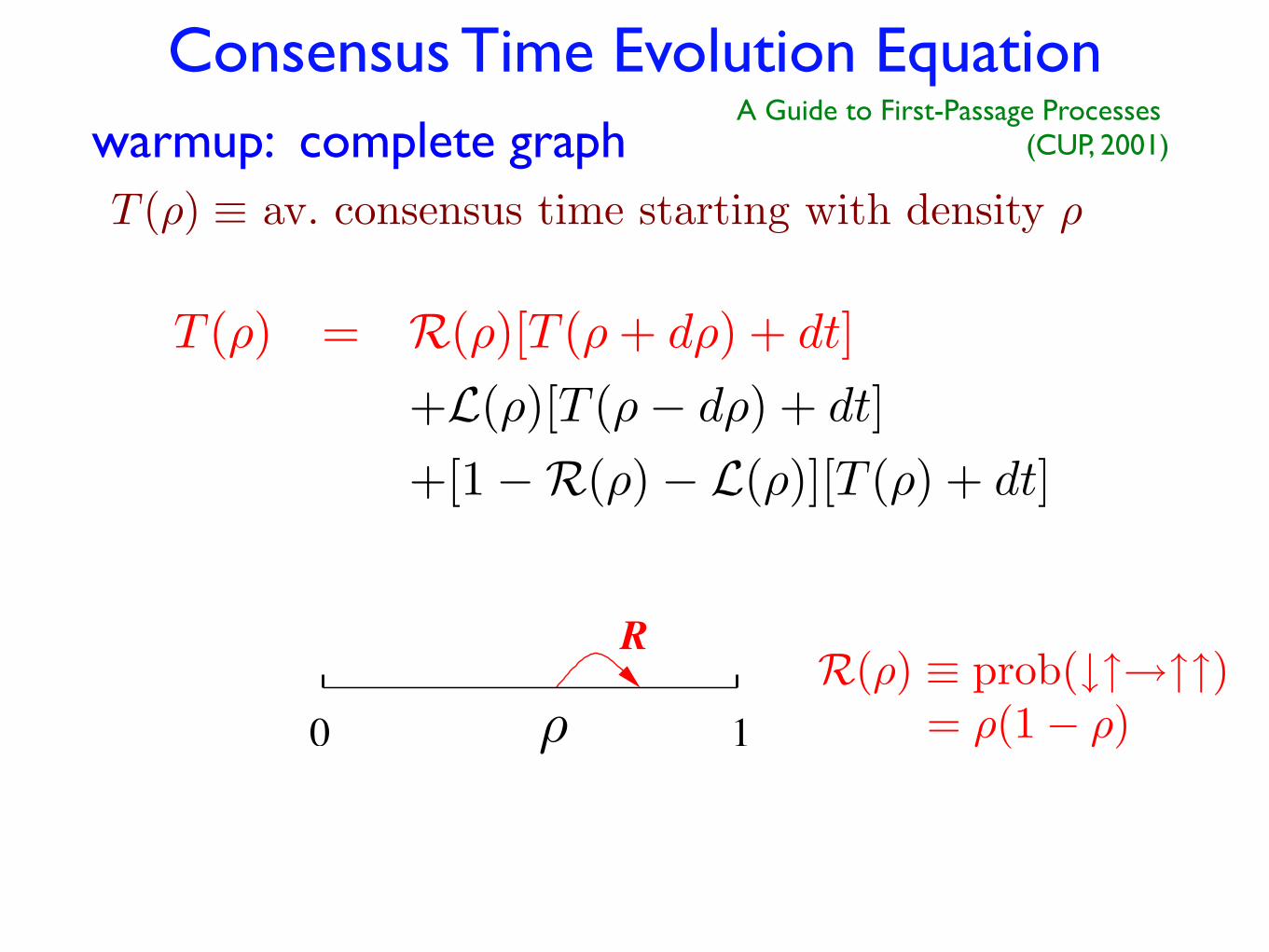
Consensus Time Evolution Equationwarmup: complete graphT (ρ) ≡ av. consensus time starting with density ρ
R(ρ) ≡ prob(↓↑→↑↑)= ρ(1− ρ)ρ
T (ρ) = R(ρ)[T (ρ + dρ) + dt]+L(ρ)[T (ρ− dρ) + dt]+[1−R(ρ)− L(ρ)][T (ρ) + dt]
1
R
ρ0
A Guide to First-Passage Processes (CUP, 2001)
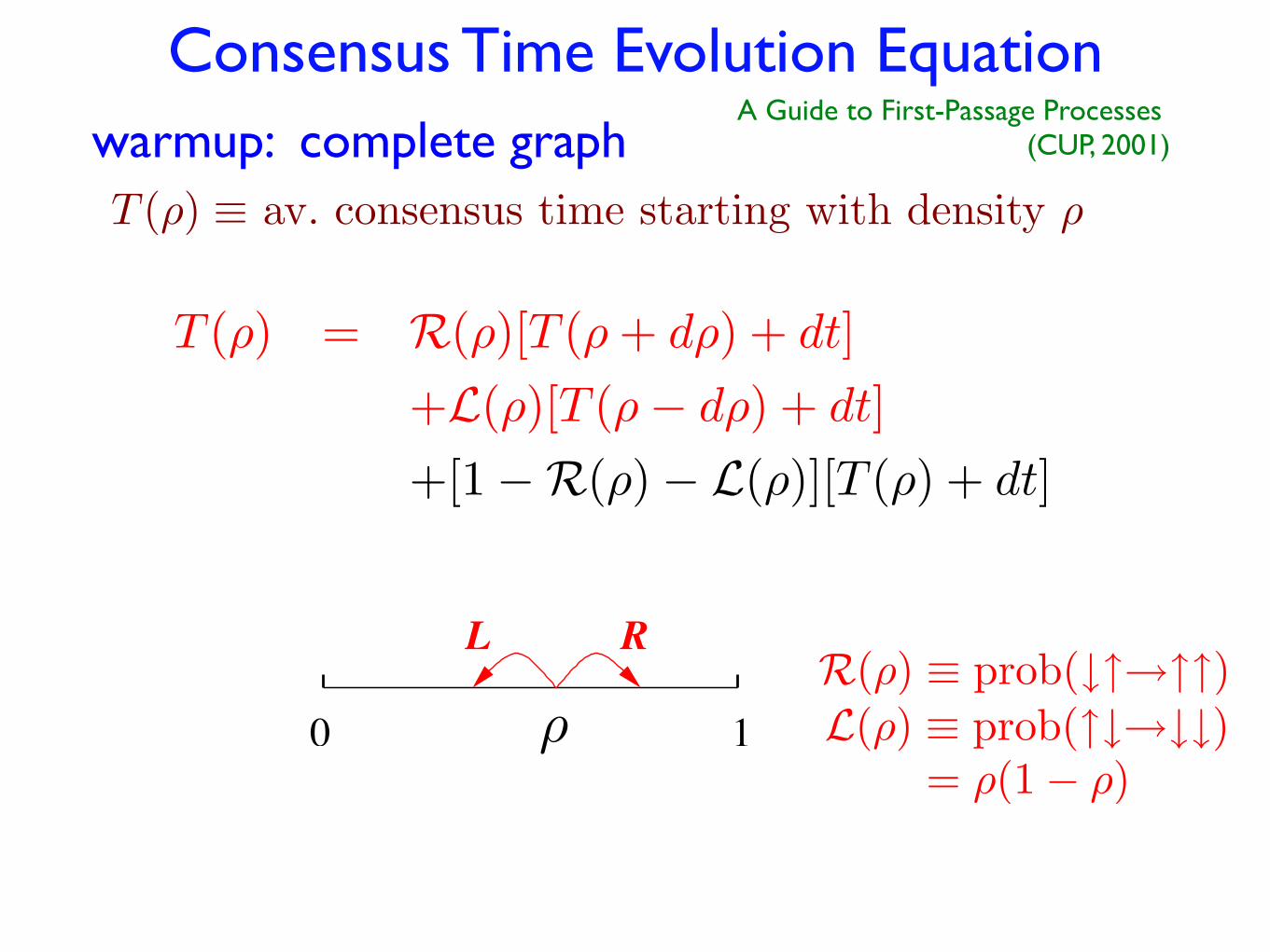
Consensus Time Evolution Equationwarmup: complete graphT (ρ) ≡ av. consensus time starting with density ρ
R(ρ) ≡ prob(↓↑→↑↑)L(ρ) ≡ prob(↑↓→↓↓)
= ρ(1− ρ)ρ
T (ρ) = R(ρ)[T (ρ + dρ) + dt]+L(ρ)[T (ρ− dρ) + dt]+[1−R(ρ)− L(ρ)][T (ρ) + dt]
1
RL
0
A Guide to First-Passage Processes (CUP, 2001)
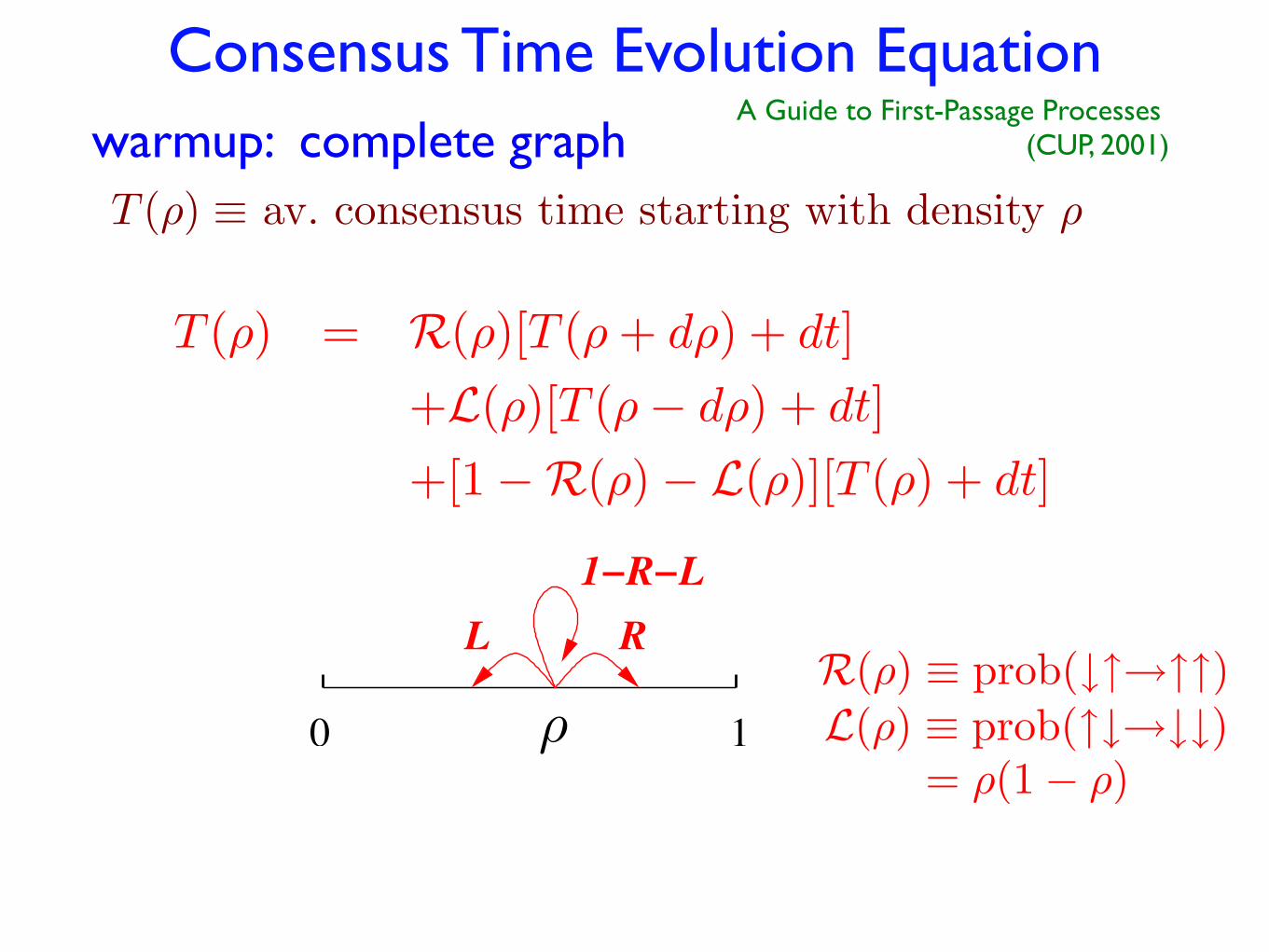
Consensus Time Evolution Equationwarmup: complete graphT (ρ) ≡ av. consensus time starting with density ρ
R(ρ) ≡ prob(↓↑→↑↑)L(ρ) ≡ prob(↑↓→↓↓)
= ρ(1− ρ)ρ
T (ρ) = R(ρ)[T (ρ + dρ) + dt]+L(ρ)[T (ρ− dρ) + dt]+[1−R(ρ)− L(ρ)][T (ρ) + dt]
1
RL1−R−L
0
A Guide to First-Passage Processes (CUP, 2001)

Consensus Time on Complete Graph
continuum limit: T �� = − N
ρ(1− ρ)
T (ρ) = −N [ρ ln ρ + (1− ρ) ln(1− ρ)]
solution:
T (ρ) = R(ρ)[T (ρ + dρ) + dt]+L(ρ)[T (ρ− dρ) + dt]+[1−R(ρ)− L(ρ)][T (ρ) + dt]
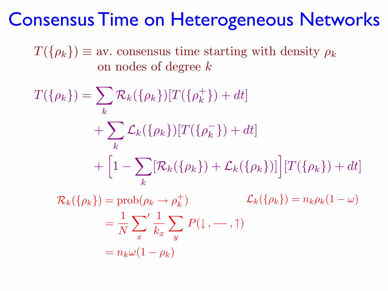
Consensus Time on Heterogeneous Networks
T ({ρk}) ≡ av. consensus time starting with density ρk
on nodes of degree k
T ({ρk}) =�
k
Rk({ρk})[T ({ρ+k }) + dt]
+�
k
Lk({ρk})[T ({ρ−k }) + dt]
+�1−
�
k
[Rk({ρk}) + Lk({ρk})]�[T ({ρk}) + dt]
Lk({ρk}) = nkρk(1− ω)Rk({ρk}) = prob(ρk → ρ+k )
=1N
��
x
1kx
�
y
P (↓ ,−− , ↑)
= nkω(1− ρk)
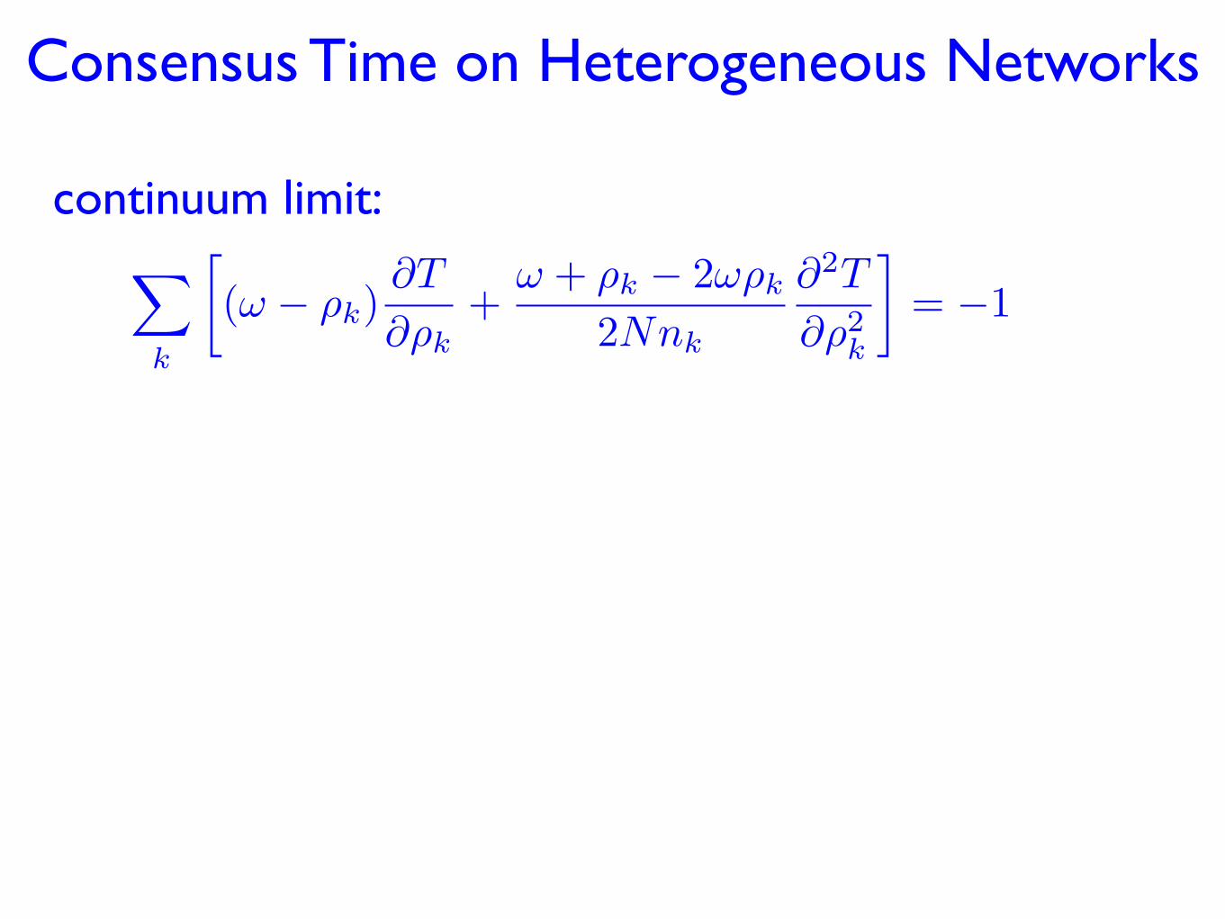
continuum limit:�
k
�(ω − ρk)
∂T
∂ρk+
ω + ρk − 2ωρk
2Nnk
∂2T
∂ρ2k
�= −1
Consensus Time on Heterogeneous Networks

0
0.2
0.4
0.6
0.8
1
0 0.2 0.4 0.6 0.8 1
ρ
ω
ρ6
ρ11
(Molloy-Reed) Configuration Modelnk ! k!2.5, µ1 = 8
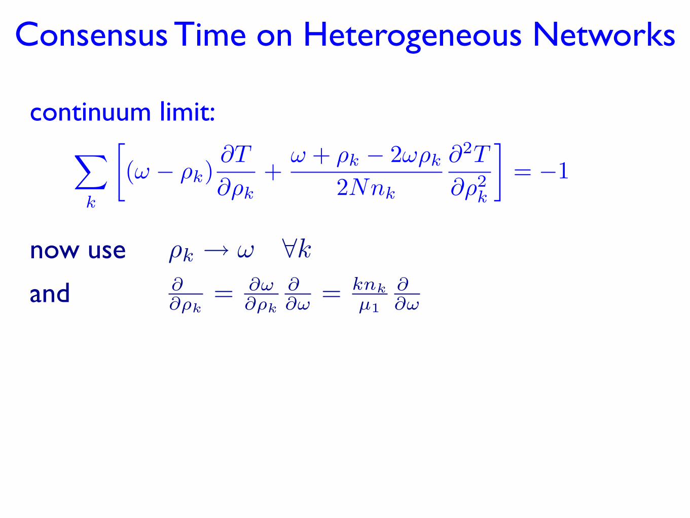
continuum limit:�
k
�(ω − ρk)
∂T
∂ρk+
ω + ρk − 2ωρk
2Nnk
∂2T
∂ρ2k
�= −1
now use ρk → ω ∀k∂∂ρk
= ∂ω∂ρk
∂∂ω = knk
µ1
∂∂ωand
Consensus Time on Heterogeneous Networks
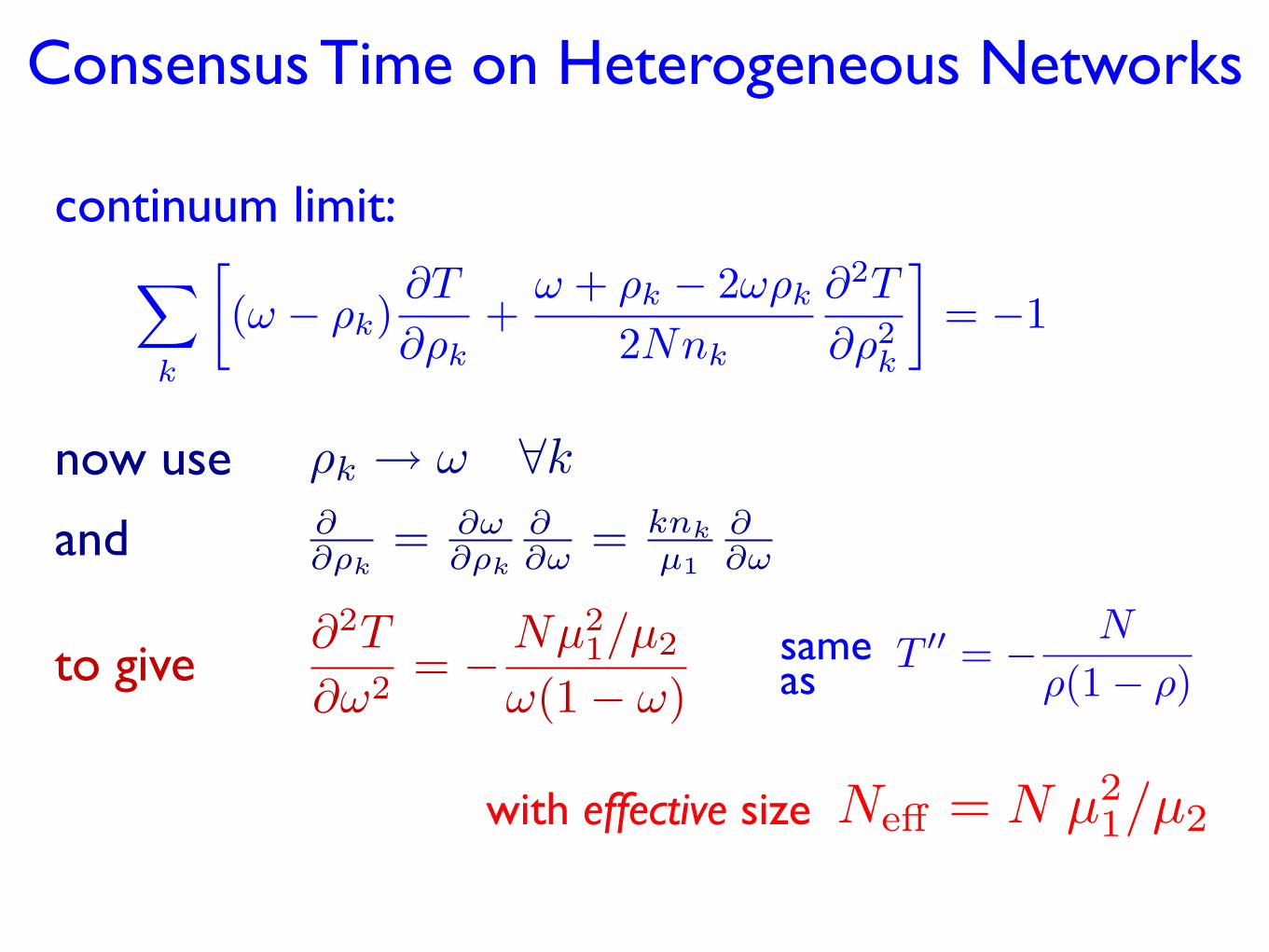
continuum limit:�
k
�(ω − ρk)
∂T
∂ρk+
ω + ρk − 2ωρk
2Nnk
∂2T
∂ρ2k
�= −1
now use ρk → ω ∀k∂∂ρk
= ∂ω∂ρk
∂∂ω = knk
µ1
∂∂ωand
T �� = − N
ρ(1− ρ)same as
Neff = N µ21/µ2with effective size
to give∂2T
∂ω2= − Nµ2
1/µ2
ω(1− ω)
Consensus Time on Heterogeneous Networks

Consensus Time for Power-Law Degreenk ! k
!!Distribution
TN !
!
"
"
"
#
"
"
"
$
N ! > 3,N/ lnN ! = 3,N (2!!4)/(!!1) 2 < ! < 3,(lnN)2 ! = 2,O(1) ! < 2.
Voter model: TN ∼ Neff = Nµ21/µ2

Consensus Time for Power-Law Degreenk ! k
!!Distribution
TN !
!
"
"
"
#
"
"
"
$
N ! > 3,N/ lnN ! = 3,N (2!!4)/(!!1) 2 < ! < 3,(lnN)2 ! = 2,O(1) ! < 2.
Voter model: TN ∼ Neff = Nµ21/µ2
lnvasion process: TN ∼ Neff = Nµ1 µ−1
TN ∼
N ν > 2N lnN ν = 2N3−ν ν < 2

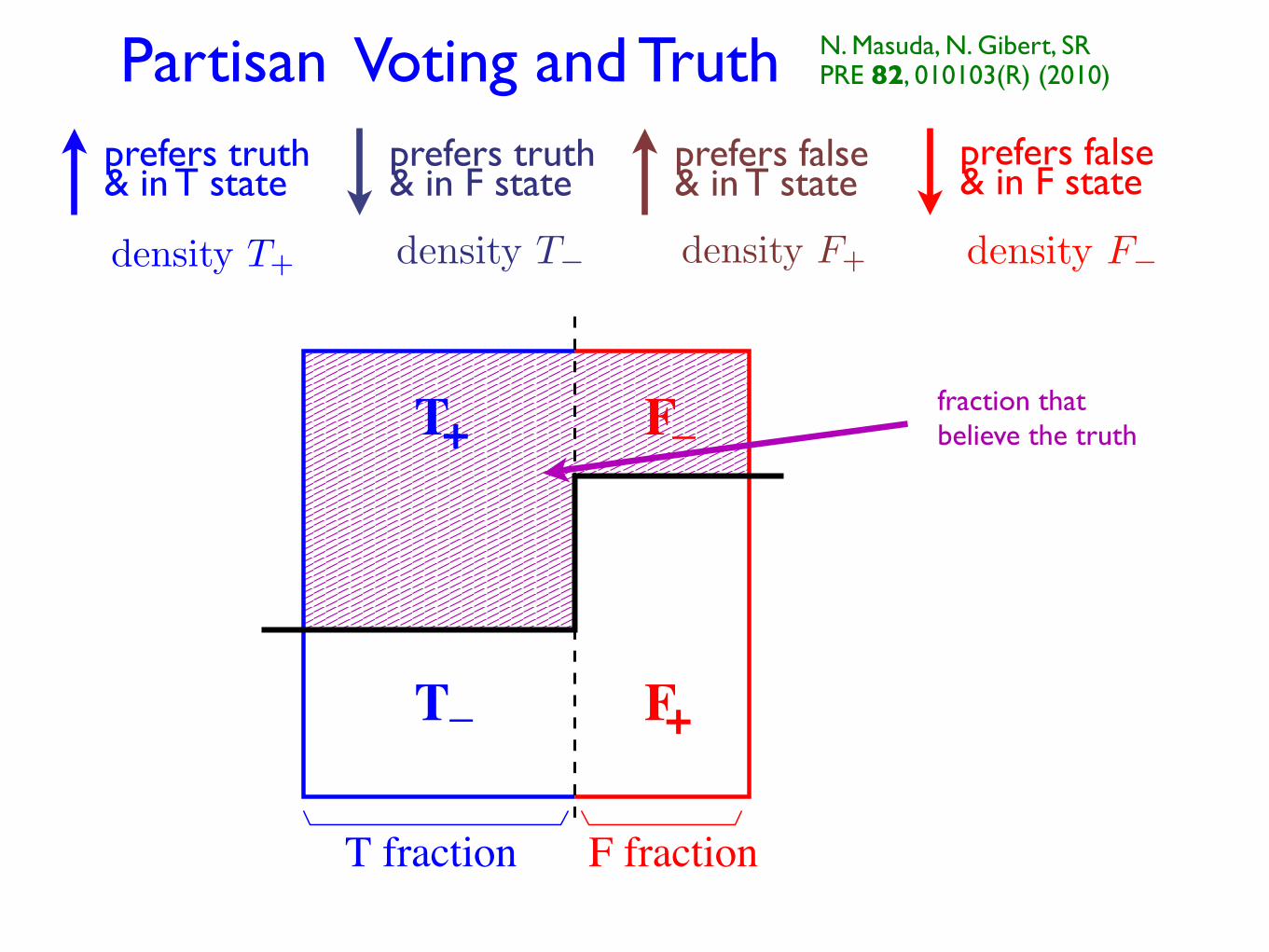
Partisan Voting and Truth N. Masuda, N. Gibert, SRPRE 82, 010103(R) (2010)
prefers truth& in T state
density T+
prefers false& in F state
density F−
prefers false& in T state
density F+
prefers truth& in F state
density T−
Partisan Voting and Truth N. Masuda, N. Gibert, SRPRE 82, 010103(R) (2010)
prefers truth& in T state
density T+
prefers false& in F state
density F−
prefers false& in T state
density F+
prefers truth& in F state
density T−
T
T fraction F fraction
+F_
+T F_ fraction that believe the truth

1. Pick voter, pick neighbor (as in usual voter model);
2a. If initial voter becomes concordant by adopting neighboring state, change occurs with rate 1+ε; 1+ε
2b. If initial voter becomes discordant by adopting neighboring state, change occurs with rate 1-ε. 1-ε
partisan voting update:
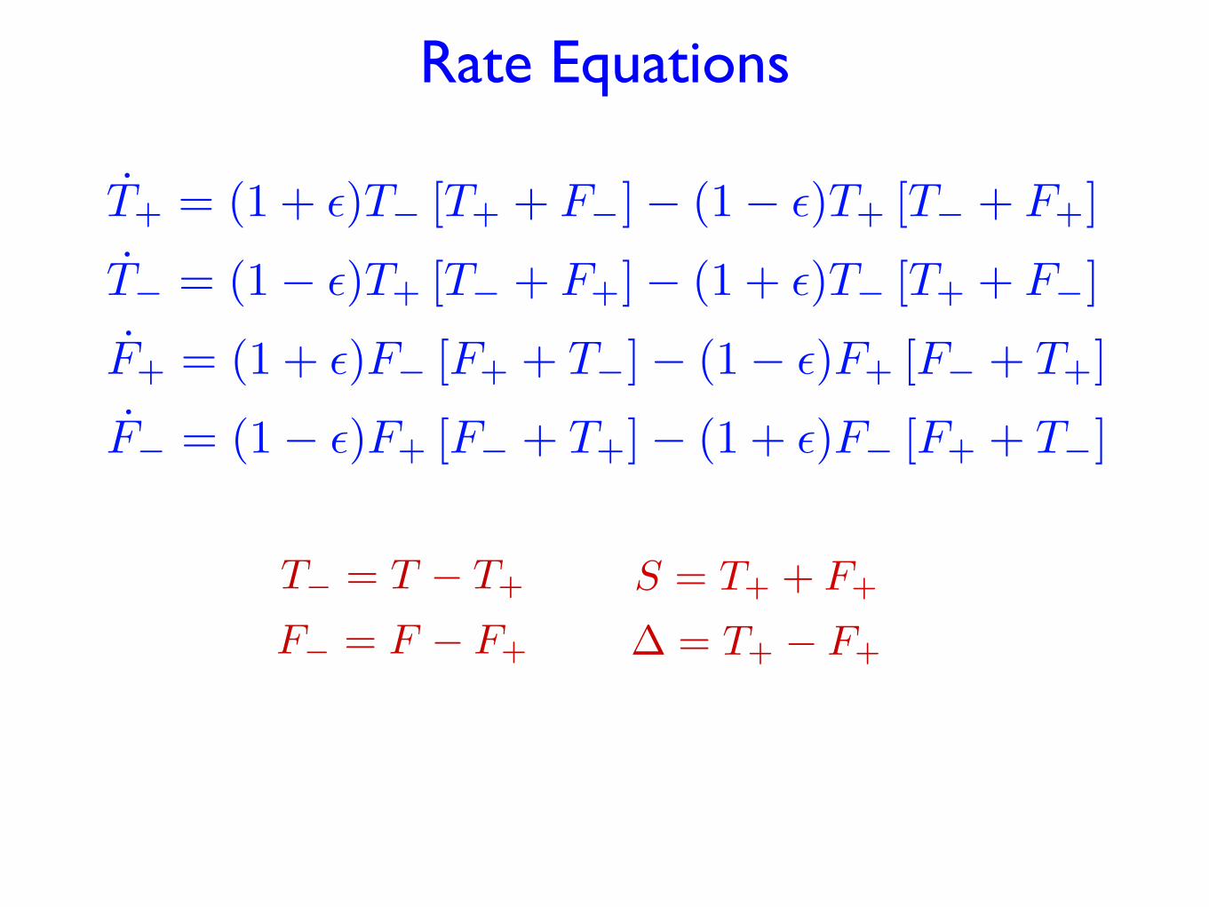
Rate Equations
S = T+ + F+
∆ = T+ − F+
T− = T − T+
F− = F − F+
T+ = (1 + �)T− [T+ + F−]− (1− �)T+ [T− + F+]
T− = (1− �)T+ [T− + F+]− (1 + �)T− [T+ + F−]
F+ = (1 + �)F− [F+ + T−]− (1− �)F+ [F− + T+]
F− = (1− �)F+ [F− + T+]− (1 + �)F− [F+ + T−]
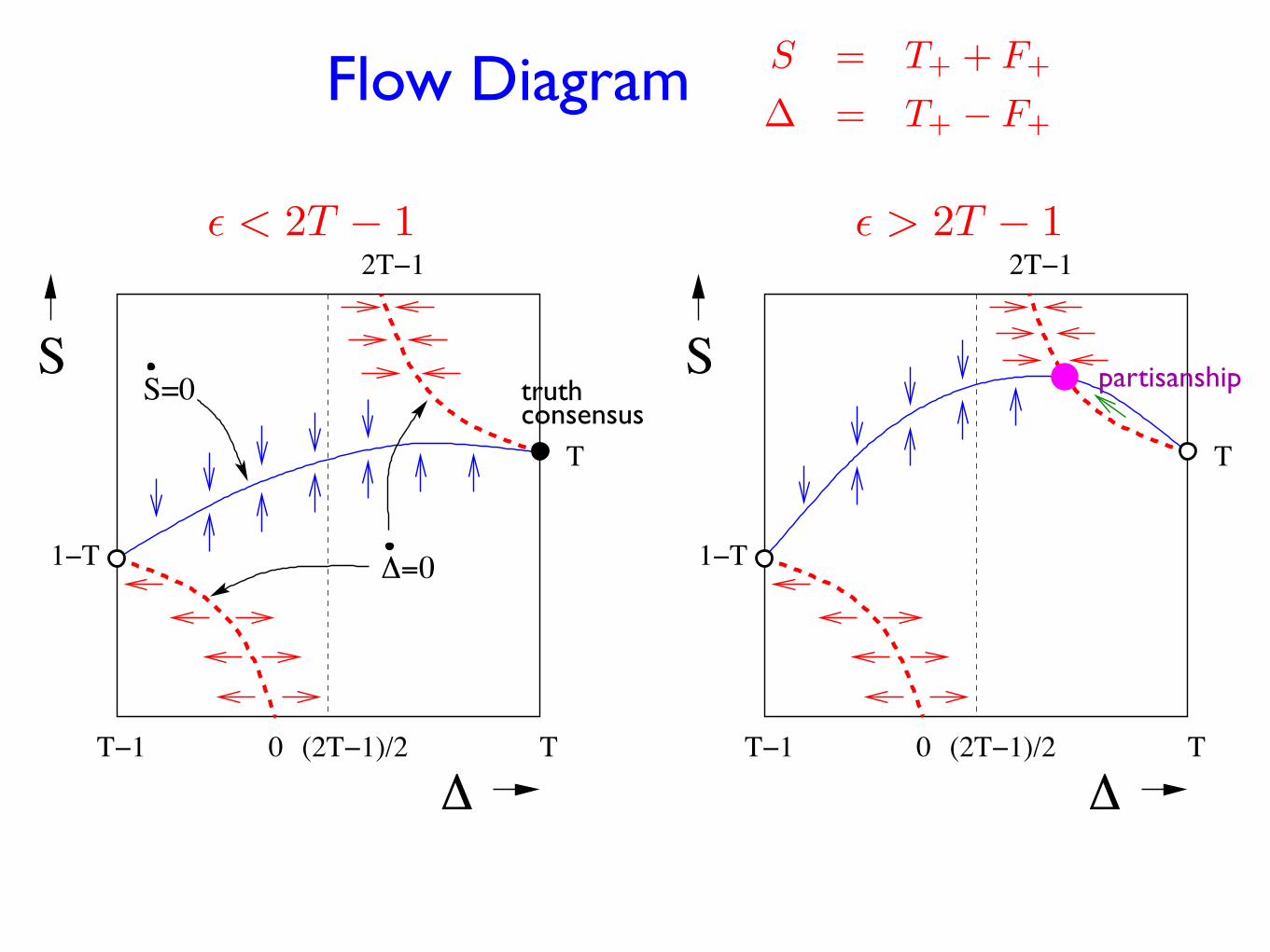
S=0
1−T Δ=0
2T−1
T
S
ΔT−1
T
(2T−1)/20
� < 2T − 1
truth consensus
1−T
T
(2T−1)/20 TT−1
S
Δ
2T−1� > 2T − 1
partisanship
Flow Diagram S = T+ + F+
∆ = T+ − F+
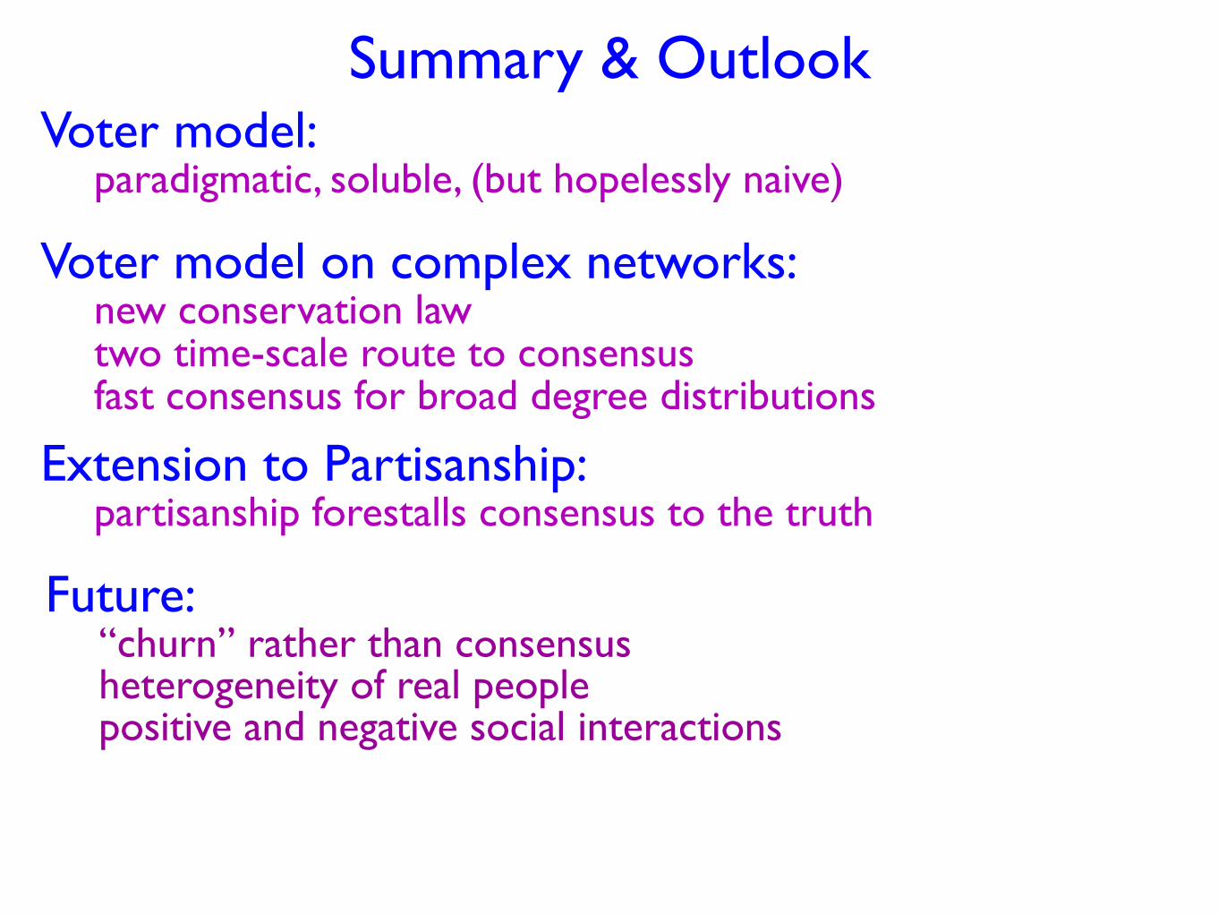
Summary & OutlookVoter model:
paradigmatic, soluble, (but hopelessly naive)
Voter model on complex networks:new conservation lawtwo time-scale route to consensusfast consensus for broad degree distributions
Future: “churn” rather than consensusheterogeneity of real peoplepositive and negative social interactions
Extension to Partisanship:partisanship forestalls consensus to the truth
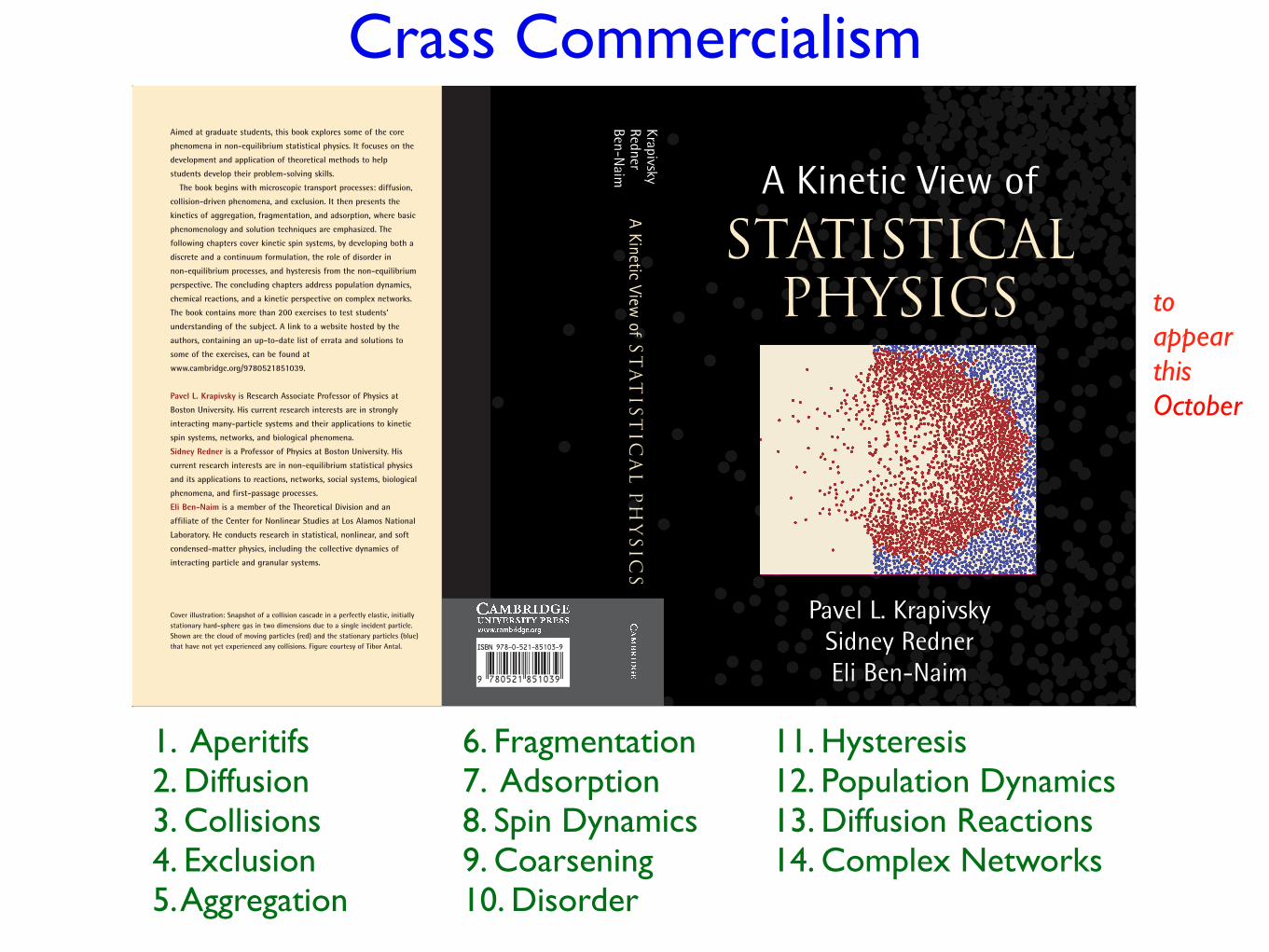
Crass Commercialism
1. Aperitifs2. Diffusion3. Collisions4. Exclusion5. Aggregation
6. Fragmentation7. Adsorption 8. Spin Dynamics9. Coarsening10. Disorder
11. Hysteresis12. Population Dynamics13. Diffusion Reactions14. Complex Networks
to appear this October
TABLE OF CONTENTS
Aimed at graduate students, this book explores some of the core
phenomena in non-equilibrium statistical physics. It focuses on the
development and application of theoretical methods to help
students develop their problem-solving skills.
The book begins with microscopic transport processes: diffusion,
collision-driven phenomena, and exclusion. It then presents the
kinetics of aggregation, fragmentation, and adsorption, where basic
phenomenology and solution techniques are emphasized. The
following chapters cover kinetic spin systems, by developing both a
discrete and a continuum formulation, the role of disorder in
non-equilibrium processes, and hysteresis from the non-equilibrium
perspective. The concluding chapters address population dynamics,
chemical reactions, and a kinetic perspective on complex networks.
The book contains more than 200 exercises to test students'
understanding of the subject. A link to a website hosted by the
authors, containing an up-to-date list of errata and solutions to
some of the exercises, can be found at
www.cambridge.org/9780521851039.
Pavel L. Krapivsky is Research Associate Professor of Physics at
Boston University. His current research interests are in strongly
interacting many-particle systems and their applications to kinetic
spin systems, networks, and biological phenomena.
Sidney Redner is a Professor of Physics at Boston University. His
current research interests are in non-equilibrium statistical physics
and its applications to reactions, networks, social systems, biological
phenomena, and first-passage processes.
Eli Ben-Naim is a member of the Theoretical Division and an
affiliate of the Center for Nonlinear Studies at Los Alamos National
Laboratory. He conducts research in statistical, nonlinear, and soft
condensed-matter physics, including the collective dynamics of
interacting particle and granular systems.
Cover illustration: Snapshot of a collision cascade in a perfectly elastic, initiallystationary hard-sphere gas in two dimensions due to a single incident particle.Shown are the cloud of moving particles (red) and the stationary particles (blue)that have not yet experienced any collisions. Figure courtesy of Tibor Antal.
A Kinetic View of
St
at
ist
ica
lP
hy
sic
sKrapivskyRednerBen-N
aim
Pavel L. Krapivsky Sidney Redner Eli Ben-Naim
A Kinetic View of
Statistical Physics
KRAP
IVSK
Y: S
tatis
tical
Phy
sics
PPC
C M
Y
BL
K