Time Resolved Correlation measurements of temporally

heterogeneous dynamics

Agnes Duri, Hugo Bissig, Veronique Trappe, Luca Cipelletti

To cite this version:

Agnes Duri, Hugo Bissig, Veronique Trappe, Luca Cipelletti. Time Resolved Correlation mea-surements of temporally heterogeneous dynamics. Physical Review E : Statistical, Nonlinear,and Soft Matter Physics, American Physical Society, 2005, 72, pp.051401. <10.1103/Phys-RevE.72.051401>. <hal-00007744>

HAL Id: hal-00007744

https://hal.archives-ouvertes.fr/hal-00007744

Submitted on 1 Aug 2005

HAL is a multi-disciplinary open accessarchive for the deposit and dissemination of sci-entific research documents, whether they are pub-lished or not. The documents may come fromteaching and research institutions in France orabroad, or from public or private research centers.

L’archive ouverte pluridisciplinaire HAL, estdestinee au depot et a la diffusion de documentsscientifiques de niveau recherche, publies ou non,emanant des etablissements d’enseignement et derecherche francais ou etrangers, des laboratoirespublics ou prives.

ccsd

-000

0774

4, v

ersi

on 1

- 1

Aug

200

5Time Resolved Correlation measurements of temporally heterogeneous dynamics

Agnes Duri1, Hugo Bissig2, Veronique Trappe2, and Luca Cipelletti1∗1Laboratoire des Colloıdes, Verres et Nanomateriaux (UMR 5587),

Universite Montpellier 2 and CNRS, 34095 Montpellier Cedex 5, France2Department de Physique, Universite de Fribourg, Chemin du Musee 3, 1700 Fribourg, Suisse

(Dated: August 1, 2005)

Time Resolved Correlation (TRC) is a recently introduced light scattering technique that allows todetect and quantify dynamic heterogeneities. The technique is based on the analysis of the temporalevolution of the speckle pattern generated by the light scattered by a sample, which is quantified bycI(t, τ ), the degree of correlation between speckle images recorded at time t and t+τ . Heterogeneousdynamics results in significant fluctuations of cI(t, τ ) with time t. We describe how to optimizeTRC measurements and how to detect and avoid possible artifacts. The statistical properties of thefluctuations of cI are analyzed by studying their variance, probability distribution function, and timeautocorrelation function. We show that these quantities are affected by a noise contribution due tothe finite number N of detected speckles. We propose and demonstrate a method to correct for thenoise contribution, based on a N → ∞ extrapolation scheme. Examples from both homogeneousand heterogeneous dynamics are provided. Connections with recent numerical and analytical workson heterogeneous glassy dynamics are briefly discussed.

PACS numbers: 82.70.-y, 42.30.Ms, 64.70.Pf, 05.40.-a

I. INTRODUCTION

Soft glassy systems such as concentrated colloidal sus-pensions, emulsions, surfactant phases, gels and foamsexhibit very slow and unusual dynamics, characterized bynon-exponential relaxations of correlation and responsefunctions, which often depend on sample history and maybe heterogeneous both in space and time [1]. These phe-nomena have attracted a great interest, in part due totheir “universal” character. Examples of unifying de-scriptions are the mode coupling theory of the stationaryaverage dynamics of concentrated suspensions of parti-cles with both repulsive or attractive interactions [2, 3, 4]or, at a more qualitative level, the concept of jamming,which rationalizes the fluid-to-solid transition in a widerange of systems and experimental configurations [5].Additionally, soft glassy materials often exhibit intrigu-ing similarities with hard condensed matter glasses, suchas the dependence of the dynamics on sample history(aging phenomena [6, 7], rejuvenation and memory ef-fects [8, 9]) or the presence of dynamical heterogeneity([10, 11, 12]).

Light scattering is a popular means to measure the av-erage dynamics. In a traditional dynamic light scatter-ing experiment, one measures the normalized time auto-correlation function of the scattered intensity: g2(τ) =

I1(t)I1(t + τ)/I1(t)2, where the average · · · is over time,

t, and I1(t) is the intensity collected by a single detector.The intensity autocorrelation function provides quanti-tative information on the dynamics of the sample; theway this information is extracted depends on the exper-imental configuration. In single scattering experiments,

∗Electronic address: lucacip@lcvn.univ-montp2.fr

g2(τ) is related to the intermediate scattering function,

f(τ), via the Siegert relation: f(τ) =

√

β−1(

g2(τ) − 1)

,

where β is the coherence factor that depends on the sizeratio between the speckle —or coherence area— and thedetector [13, 14]. In the opposite limit of strong multiplescattering, the diffusing-wave spectroscopy (DWS) for-malism [15] allows the particle mean square displacement

to be calculated from g2(τ)−1, provided that the dynam-ics be spatially and temporally homogeneous. For glassysystems the average over time required to compute g2(τ)may become in practice unfeasible, either because thedynamics is so slow that prohibitively long experimentswould be required to accumulate a satisfactory statistics,or because the dynamics may be non-stationary, e.g. foraging systems. Various schemes have been introducedto address this issue, most of them based on the idea ofmeasuring g2(τ) for many independent speckles and av-eraging the intensity correlation function not only overtime, but also over distinct speckles. This can be doneeither sequentially –e.g. by slowly rotating the sample soas to illuminate a single detector with different speckles(interleave [16] or echo [17] methods)– or in parallel, e.g.by using the pixels of a charge-coupled device camera(CCD) as independent detectors (multispeckle method[18, 19, 20]).

These techniques drastically reduce the required timeaverage and thus extend the applicability of light scatter-ing to glassy systems. Similarly to traditional light scat-tering measurements, however, they provide informationonly on the average dynamics, not on its fluctuations.However, recent theoretical and simulation works sug-gest that dynamic heterogeneity is a key feature of theslow dynamics in glassy systems. In view of the verylimited number of experiments that directly test this be-havior on soft glasses [10, 11], new experimental tools

2

that access fluctuations of the dynamics are needed. Wehave recently introduced the Time Resolved Correlation(TRC) scheme [21], a method that allows temporallyheterogeneous dynamics to be investigated by scatter-ing techniques. The idea at the heart of TRC is that thetemporal evolution of the speckle pattern generated bythe scattered light will be very different for homogeneousvs. heterogeneous dynamics. For homogeneous dynam-ics, we expect the speckle images to change smoothlyin time. By contrast, for heterogeneous dynamics thespeckle pattern is expected to evolve discontinuously, be-cause the rate of change of the sample configuration willnot be constant but rather fluctuate with time. Exper-imentally, the speckle images are recorded by a CCDcamera and their evolution is quantified by introducingcI(t, τ), the degree of correlation between images takenat time t and t + τ (a rigorous definition will be givenin sec. II). Inspection of the t-dependence of cI at fixedτ allows temporally heterogeneous dynamics to be dis-criminated from homogeneous dynamics. Indeed, in theformer case a large drop (increase) of cI is observed when-ever the dynamics is faster (slower) than average, whilein the latter the degree of correlation is constant. Thismethod is quite general, since it can be applied to anyexperimental configuration where a multi-element detec-tor can be used to record the speckle pattern generatedby a sample illuminated by coherent radiation. Examplesare CCD-based light scattering experiments in the singlescattering regime, both at wide [19] and small angle [20],DWS in the transmission [22] or backscattering [23] ge-ometry, and X-photon Correlation Spectroscopy (XPCS)at small angles [24]. In principle, the technique couldalso be extended to non-electromagnetic radiation, e.g.to acoustic DWS [25].

Experiments on diluted suspensions of colloidal Brow-nian particles have shown that the degree of correlationexhibits some fluctuations even in the absence of dynamicheterogeneity [21]. As it will be shown in detail, thesefluctuations are due to statistical noise stemming fromthe finite number of speckles in the CCD images. Inorder to exploit quantitatively TRC data it is thus nec-essary to separate the contribution to the fluctuations ofcI due to the noise from that due to dynamic heterogene-ity. Although in most cases it is not possible to directlycorrect the TRC time series for the noise, we will showthat it is possible to correct statistical quantities derivedfrom the TRC data and used to quantify the fluctuationsof cI . We focus in particular on three statistical objects:the time variance of cI(t, τ), the probability distributionfunction (PDF) of cI(t, τ) for a fixed τ , and the timeautocorrelation of the cI(t, τ) trace itself.

The variance of cI , σ2cI

(τ), is the lowest moment ofthe data that provides information on the fluctuations.It corresponds to the so-called dynamical susceptibilityχ4 studied in many simulation and theoretical works onglassy systems [26, 27, 28, 29]. In a typical simulation,χ4 is the variance of the intermediate scattering function,or a similar correlation function describing the system’s

change in configuration, which is obtained from severalindependent runs. Similarly, σ2

cIquantifies the fluctua-

tions of the intensity correlation function as the systemevolves through statistically independent configurations.Importantly, σ2

cIallows one to relate temporal dynamic

heterogeneity to spatial correlations of the dynamics. Infact, it can be shown that χ4 is the volume integral ofthe spatial correlation of the local dynamics [30]. There-fore, large values of σ2

cIwill be indicative of long-range

correlations of the dynamics. Intuitively, one can expectthe variance of the fluctuations of the dynamics to scaleas the inverse number of “dynamically independent” re-gions in the scattering volume, and thus to increase asthe spatial range of the correlation of the dynamics in-creases. Recent TRC experiments on a shaving creamfoam support this simple picture [12].

The PDF of the TRC signal is the most complete sta-tistical characterization of the dispersion of the data.Any deviation from a Gaussian shape immediately hintsto heterogeneous dynamics, as suggested by experi-ments on a variety of systems, including colloidal gels[21, 31, 32], concentrated colloidal suspensions [33] andsurfactant phases [34], foams [35], and granular materi-als [36]. Remarkably, the shape of the PDF of cI is oftenstrongly reminiscent of that obtained for similar quanti-ties in theoretical and simulation work on other glassysystems. An example is provided by simulations of spinglasses, where the fluctuations of the correlation func-tion of the spin orientation are distributed according to ageneralized Gumbel PDF [37], a probability distributioncharacterized by an exponential tail strikingly similar tothose reported for cI in refs. [21, 31, 32, 33, 34, 36] orshown in this paper (see figs. 8 and 11). Similar distri-butions are also obtained in a variety of numerical andanalytical investigations of systems with heterogeneousdynamics, both at equilibrium and out-of-equilibrium[28, 38, 39, 40]. Indeed, it has been proposed that theGumbel distribution arises as a universal PDF for vari-ous quantities measured in systems with extended spatialand/or temporal correlations [41]. Clearly, in order tocompare in detail and quantitatively the PDF measuredin TRC experiments to those obtained analytically or bysimulations it is necessary to correct the experimentaldata for the contribution of the measurement noise.

The variance and the PDF of cI describe the disper-sion of the data, but are insensitive to the way the fluc-tuations are distributed in time. By contrast, the timeautocorrelation of the TRC signal, which was introducedin ref. [34] and which we shall term “second correla-tion”, provides information on the temporal organizationof the fluctuations of the dynamics, and sheds light onthe rate and life time of rearrangement events. The sec-ond correlation introduced here is similar to the 4-th or-der intensity correlation function proposed by Lemieuxand Durian [42, 43] and to the multi-time correlationfunctions measured in nuclear magnetic resonance exper-iments probing dynamical heterogeneity near the glasstransition [44]. Moreover, we note that the second cor-

3

relation is the analogous, in the time domain, of the so-called second spectrum originally introduced to investi-gate non-gaussian fluctuations in the dynamics of spinglasses [45].

In this paper, we first describe how to optimize a TRCmeasurement by correcting the CCD data for the darknoise, due to the electronic noise of the CCD, and for theuneven illumination of the detector (sec. II). We thenturn to the temporal fluctuations of cI and analyze sep-arately the contribution of the measurement noise, dueto the finite number of pixels, (sec. III) and that due toheterogeneous dynamics (sec. IV). We illustrate our anal-ysis by showing TRC data obtained mainly from a dilutesuspension of Brownian particles and a shaving creamfoam, two model systems that exhibit homogeneous andheterogeneous dynamics, respectively. We then intro-duce a method for correcting the experimentally mea-sured variance and PDF of cI for the noise contribution.The method consist of an extrapolation scheme based onthe observation that the measurement noise vanishes inthe limit N → ∞ (N being the number of CCD pixelsused to calculate cI), whereas the fluctuations due to dy-namical heterogeneities are independent of N . In sec. Vwe introduce the second correlation and provide a work-ing formula for correcting it for the noise contribution.Possible artifacts that may affect the fluctuations of cI

and lead to spurious contributions to its PDF and to thesecond correlation are discussed in sec. VI, together withmethods to detect or correct them. In the concluding sec-tion, we briefly discuss the connections between TRC andother techniques that measure dynamical heterogeneitiesin soft glassy systems, focussing on the advantages andthe limitations of the various methods.

II. TIME RESOLVED CORRELATION:MEASURING THE TIME-DEPENDENT

DEGREE OF CORRELATION cI(t, τ )

In a TRC experiment [21] a CCD camera is used torecord, at constant rate, the speckle pattern of the lightscattered by the sample [14]. The CCD images are storedon the hard disk of a personal computer (PC) for laterprocessing. The degree of correlation, cI , between specklepatterns at times t and t+ τ is then calculated accordingto

cI(t, τ) =G2(t, τ)

I(t)I(t + τ)− 1 , (1)

where G2(t, τ) = 〈Ip(t)Ip(t + τ)〉p and I(t) = 〈Ip(t)〉p,with Ip(t) the intensity measured at time t by the p-thCCD pixel and 〈· · ·〉p an average over N pixels. Notethat the normalization factor in Eq. (1), I(t)I(t + τ),allows to cancel out exactly any fluctuations due tochanges in the laser power. For stationary dynamics,the intensity correlation function usually measured in alight scattering experiment, g2(τ), may be obtained from

g2(τ) − 1 = cI(t, τ).

In Eq. (1) the intensity value at each pixel is required.In practice, however, the images recorded by the CCD areaffected by a pixel- and time-dependent dark (or elec-tronic) noise, Dp(t), and, possibly, by the non-uniformillumination of the detector, depending on the setup op-tics. To account for these effects, we write the raw signalfor pixel p, Sp, as Sp(t) = Ip(t)bp/〈bp〉p + Dp(t), wherebp is a time-independent, spatially slowly-varying func-tion that accounts for non-uniform illumination and 〈bp〉pis introduced so that the factor multiplying Ip(t) hasunit average. Prior to each measurement, we collect 100dark images by covering the CCD detector with a blackcap. These dark images are used to calculate the time-averaged dark noise Dp. The raw signal is corrected bysubtracting, pixel-by-pixel, the average dark noise. To es-timate bp, we average over time the dark-noise-corrected

CCD signal : bp = Sp(t) − Dp. For experiments whoseduration, Texp, is much longer than the relaxation time of

g2(τ), τ0, this procedure averages out the spatial fluctua-tions associated with the speckles and leads to a smoothfunction bp, since for each pixel the intensity fully fluctu-ates many times and its time average is a good estimatorof the mean intensity at a given location of the CCDdetector. By contrast, when Texp . τ0, bp keeps somememory of the speckled appearance of the instantaneousintensity distribution. In this case, we further smooth bp

by averaging it over a few adjacent pixels. The desiredintensity to be used in Eq. (1) is obtained from

Ip(t) = [Sp(t) − Dp]〈bp〉p/bp. (2)

Note that Ip(t) is still affected by an instanteneous noise

ǫp(t) = Dp(t) − Dp, since only the average dark noisecould be subtracted. By definition, ǫp = 0, while thestandard deviation σǫ of ǫ is typically of the order of1/100 of the saturation level for an 8-bit CCD camera.When all the relevant time scales of the dynamics aremuch longer than the inverse CCD rate, ǫp(t) may beconsiderably reduced by averaging Ip(t) over a few CCDimages before applying Eq. (1). In the following, we willdisregard ǫp(t), unless when explicitly stated.

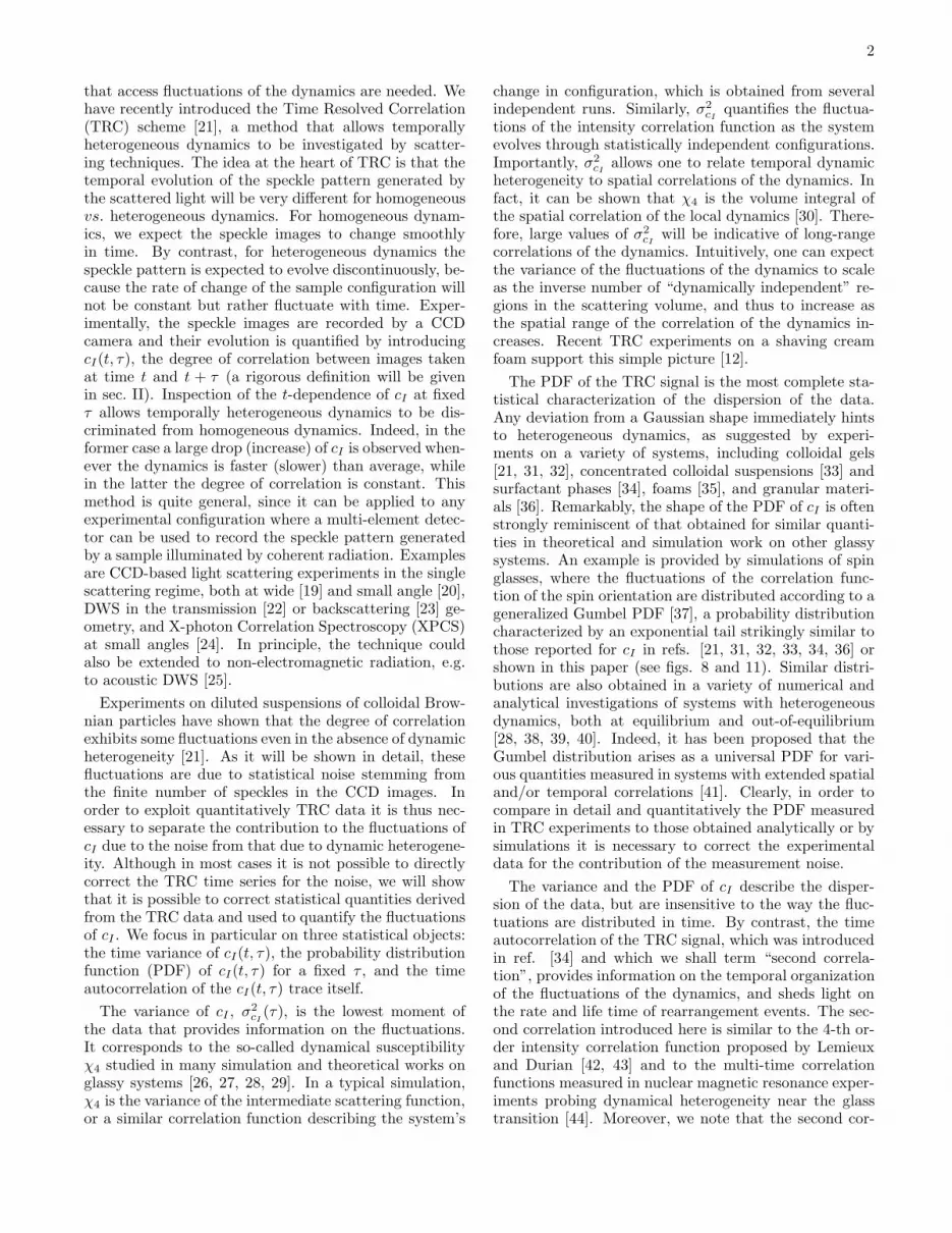
We show in fig. 1 how the different corrections dis-cussed above affect the intensity autocorrelation functionmeasured for a dilute suspension of monodisperse Brow-nian particles. Data are collected in the single scatteringgeometry, at a scattering angle θ = 45 deg. The particlesare polystyrene spheres of radius a = 265 nm, suspendedat a volume fraction φ = 3.7× 10−5 in almost pure glyc-erine cooled at 15 oC in order to make the dynamics slowenough to match the limited acquisition rate of the CCD,which is 2 Hz in this experiment. Both the dark noiseand the non-uniform illumination result in a spurious in-crease of the base line of the autocorrelation function(squares and circles in fig. 1) and lead to a change ofits τ → 0 intercept (see inset). However, the relaxationtime obtained from the small τ behavior of the intensityautocorrelation function is essentially unaffected by thedark noise and the non-uniform illumination. When the

4

0 10 20 30 40 50 6010

-4

10-3

10-2

10-1

1

g2 (

τ) -1

τ (sec)

0 1 20.2

0.4

0.6

FIG. 1: Semi-logarithmic plot of the intensity time autocor-relation function measured for a suspension of monodisperseBrownian particles in the single scattering regime (θ = 45deg). Data are averaged over N = 151800 pixels and overTexp = 10800 sec. Squares: intensity autocorrelation functioncalculated from the CCD raw signal, Sp(t); circles: the samedata after correcting for the dark noise only; triangles: aftercorrecting for both the dark noise and the uneven detectorillumination. The line is a fit to the corrected data by a sin-gle exponential decay, the functional form of g2 − 1 predictedfor monodisperse Brownian particles, yielding a characteristictime τ0 = 5.8 sec. Inset: zoom of the small τ behavior of theintensity autocorrelation function.

CCD signal is corrected according to Eq. (2) (up trian-gles), a single exponential decay is observed, as predictedfor monodisperse Brownian particles. For the correcteddata, the base line is limited only by the dark noise ǫp(t):its value is of the order of 2× 10−4 and is comparable tothat obtained in traditional light scattering setups, whichuse a photomultiplier tube or an avalanche photodiode asa detector.

III. TEMPORAL FLUCTUATIONS OF cI(t, τ ):THE NOISE CONTRIBUTION

When disregarding the fluctuations of ǫp(t), the tem-poral fluctuations of the degree of correlation cI(t, τ) at afixed lag τ have only two independent sources: the statis-tical noise due to the finite number of speckles probed inthe experiment and the intrinsic fluctuations of the sam-ple dynamics. The first contribution is always present:we shall refer to it as to the “measurement noise”, not tobe confused with the dark noise discussed in Sec. II. Thesecond contribution, on the contrary, is present only ifthe dynamics is temporally heterogeneous and thus rep-resents the physically valuable information that we aimto extract from the fluctuations of cI . To highlight thetwo different contributions, we rewrite Eq. (1) as

cI(t, τ) = g2(a1(t), ..., ak(t); τ) − 1 + n(t, τ), (3)

where n(t, τ) is the measurement noise, with n(t, τ) = 0,and g2(a1(t), ..., ak(t); τ) − 1 is the pixel-averaged two-time intensity correlation function that would be mea-sured in the absence of any noise, i.e. if cI was averagedover an infinite number of speckles. a1(t), ..., ak(t) areparameters that fluctuate with time if the dynamics areheterogeneous, but are constant for homogeneous dynam-ics.

To illustrate this point, let us consider as an exampleof homogeneous dynamics the single scattering measure-ment of the dynamics of monodisperse Brownian parti-cles at a scattering vector q. If the temperature is care-fully controlled, the diffusion coefficient D of the particlesdoes not evolve with time and g2(a1(t), ..., ak(t); τ)−1 =a1 exp(−a2τ), with a1 = β and a2 = 2q2D constant [13].In this case, the fluctuations of cI are due only to thenoise n(t, τ). By contrast, the spatially and temporallylocalized bubble rearrangements in a shaving cream foamprovide a simple example of heterogeneous dynamics. Fora foam, the average intensity correlation function mea-sured in a DWS experiment in the transmission geom-etry has a shape very close to that for Brownian par-ticles in single scattering: g2(τ) − 1 = β exp[−(2γτ)µ],with µ ≈ 0.9 and γ = Rr3L2/l∗2 [46] [63]. Here, R isthe average bubble rearrangement rate per unit time andunit volume, r3 is the typical volume that is rearrangedby a single event, L is the sample thickness, and l∗ isthe photon transport mean free path. In contrast withthe Brownian suspension, however, the degree of correla-tion measured for a foam fluctuates not only because ofthe noise, but also because the instantaneous rearrange-ment rate continuously changes due to the intermittentnature of the bubble dynamics [12, 35]. Hence, for thefoam g2(a1(t), ..., ak(t); τ) − 1 = a1 exp[−(a2(t)τ)a3(t)],with a1 = β constant while a2(t) = R(t)r3L2/l∗2 anda3(t) = µ(t) fluctuate with time.

In view of the correction scheme described in secs.IV and V, it is useful to first analyze the contributionto the fluctuations of cI due to the noise. We assumethat the sample dynamics be temporally homogeneousand stationary, as for the dilute suspension of Brown-ian particles discussed above. In this case, the param-eters a1, ..., ak in Eq. (3) are constant and the fluctua-tions of cI are due only to the noise term, n(t, τ). SincecI(t, τ) is averaged over a large number of pixels (typ-ically N & 10000), its temporal fluctuations at a fixedτ are expected to be Gaussian distributed, because ofthe central limit theorem (see Appendix B). Accordingly,only cI and the variance σ2

n(τ) of the noise n(t, τ) areneeded to obtain the full probability distribution of cI :PcI

(cI) = (2πσ2n)−1/2 exp[−(cI − cI)

2/2σ2n]. For homo-

geneous dynamics, σ2n(τ) = σ2

cI(τ) ≡ cI(t, τ)2 − cI(t, τ)

2.

To calculate σ2cI

, we recall that the variance of a quantityy that depends on the m variables x1, ..., xm is given by

σ2y =

m∑

i=1

[

∂y

∂xi

]2

xi=xi

σ2xi

+∑

i6=j

[

∂y

∂xi

∂y

∂xj

]

xi=xixj=xj

σxi,xj,(4)

5

where σ2xi

≡ x2i − xi

2 is the variance of xi and σxi,xj≡

xixj − xi xj is the covariance between xi and xj (i 6= j).The first sum accounts for the sensitivity of y to thefluctuations of the independent variables x1, ..., xm, whilethe second sum accounts for any correlations between thexi’s. If distinct xi’s are uncorrelated, xixj = xi xj fori 6= j and the second sum vanishes.

By applying Eq. (4) to the definition of cI , Eq. (1), wefind

σ2cI

(τ) = 1/I4σ2

G2(τ) + 2G2(τ)

2/I

6σ2

I

+ 2G2(τ)2/I

6σI,J(τ) − 4G2(τ)/I

5σG2,I(τ), (5)

where we have introduced the notation J(t) ≡ I(t+τ). Inwriting Eq. (5), we have used I = J and σG2,I = σG2,J ,because the scattered light was assumed to be stationary.

The physical origin of the fluctuations of I and G2,quantified by σ2

I and σ2G2

, as well as that of the corre-lation between I and J and between I and G2, quan-tified by σI,J and σG2,I , is the finite number of pixelsover which the instantaneous intensity and the inten-sity correlation are averaged. To illustrate this point, letus consider as an example I(t). As the sample evolvesthrough different configurations, the speckle pattern fluc-tuates with a characteristic time τ0. Since the instanta-neous pixel-averaged intensity is calculated for a finiteset of speckles, different speckle patterns yield slightlydifferent values of I(t). The larger the number of thesampled speckles, the closer will I(t) be to the “true”value of the average scattered intensity, whose estimatoris I, and thus the smaller will be σ2

I . Indeed, we showin Appendix A that σ2

I ∼ N−1, as expected from thecentral limit theorem . Moreover, one expects the in-stantaneous pixel-averaged intensity at time t to be cor-related to the same quantity measured at time t + τ , atleast for τ . τ0, because it takes a few τ0 for the specklepattern to be completely renewed. Therefore, the covari-ance term σI,J (τ) will vanish only for τ ≫ τ0. More

precisely, we expect σI,J (τ) to be proportional to G2(τ).In fact, σI,J (τ) is precisely the un-normalized correla-tion function measured by using the whole CCD chip asa single detector, similarly to the case of a traditionallight scattering experiment where the detector collects alarge number of speckles.

Similar arguments may be invoked for σ2G2

(τ) andσG2,I(τ), suggesting that the variance and covariance fac-tors in Eq. (5) scale with N−1 and depend linearly on theaverage correlation function:

σxi,xj(τ) = N−1[Axi,xj

+ Bxi,xjcI(τ)], (6)

where xi and xj stand for any of I, J , and G2, whileAxi,xj

and Bxi,xjare constants whose values are given in

Appendix A. To test the linear dependence of the vari-ance and covariance factors on the time-averaged corre-lation function, we plot parametrically σ2

G2(τ), σI,J(τ),

and σG2,I(τ) as a function of cI(τ), for data obtained inthe single scattering experiment on Brownian particles,

0.0 0.2 0.4 0.6

0.0

2.0x10-4

4.0x10-4

σ2G2

/G2

σG2,I /G

2I

σI,J /I 2

var, covar

cI

FIG. 2: Parametric plot of the normalized variance and co-variance terms in the r.h.s. of Eq. (5), as a function of cI(τ ),for the same experiment as in fig. 1. The lines are linear fitsto the data, suggesting the cI dependence of Eq. (6).

as shown in fig. 2. In all cases the data are very well fittedby straight lines, thus confirming the validity of Eq. (6).

The τ dependence of the variance of the measurementnoise can be obtained by substituting Eq. (6) into Eq. (5).

Using G2(τ) = I2(cI(τ)+1) (see Appendix B), one finds

a third order polynomial dependence of the variance ofn(t, τ) on cI(τ):

σ2n(τ) = σ2

cI(τ) = N−1

3∑

l=0

αlcI(τ)l, (7)

where the coefficients αl can be obtained from I, Axi,xj,

and Bxi,xj. Note that this third-order polynomial de-

pendence is due to the choice of the normalization of cI

(see Eq. (1)). If the denominator was chosen to be I2,

as in traditional light scattering experiments, only thefirst term in the r.h.s. of Eq. (5) would be non-zero andσ2

cI(τ) ∝ σ2

G2, i.e. the fluctuations would increase linearly

with cI(τ). Although the normalization we have chosenleads to a more complicated expression for σ2

n(τ), we re-mind that it suppresses spurious variations of cI due tofluctuations of the incoming beam power and thus shouldbe used in TRC experiments. The inset of fig. 3 showsa semi-logarithmic plot of σcI

(τ) vs. τ for the Brownianparticles, confirming that the noise of cI decreases withτ , as indicated by Eq. (7). In the main plot, the samedata are plotted parametrically as a function of cI(τ). Avery good agreement is found between the experimentaldata and the polynomial form suggested by Eq. (7), asshown by the line.

The N−1 dependence of σ2n(τ) is the key feature that

will be exploited in the correction for the measurementnoise. To test this scaling, we analyze the time seriesof speckle images recorded for the Brownian particle sus-pension, for which σ2

cI= σ2

n, by processing different num-ber of pixels. First, all pixels of each image are processedand cI(t, τ) and its variance σ2

cI(τ) are calculated. Each

image is then divided into two regions of interest (ROI)

6

0.0 0.2 0.4 0.6

0.0

1.0x10-5

2.0x10-5

3.0x10-5

σ cI2

cI

0 20 40 6010

-6

10-5

10-4

τ (sec)σ c

I2

FIG. 3: Main plot: parametric representation of the varianceof cI as a function of cI(τ ) for the same experiment as in figs. 1and 2 (single scattering from a dilute suspension of Brownianparticles). The line is a fit of Eq. (7) to the data. Inset: samedata plotted vs. τ .

of equal size. For each ROI, cI and its variance are calcu-lated and the values of σ2

cI(τ) obtained for the two ROIs

are averaged, yielding the variance of cI when only N/2pixels are processed. This scheme is iterated until thesize of each ROI is reduced to 225 pixels. Figure 4 showsσ2

cI(τ) as a function of the inverse number of processed

pixels, N−1, for three time delays corresponding to 0.09,0.87, and 8.7 times the relaxation time of g2 − 1, respec-tively. In all cases, the data for N−1 < 1.2 × 10−4 arevery well fitted by a straight line that goes through theorigin, as shown in the inset [64]. This confirms that fortemporally homogeneous dynamics σ2

cI∝ N−1, as indi-

cated by Eq. (7). Note that a deviation from this lineartrend is observed at the largest N−1, due to edge effects.In fact, the contribution of each pixel to cI is not com-pletely independent from that of nearby pixels, becausethe intensity of the speckle pattern is spatially correlatedover a distance of a few pixels. Pixels far from the edgesof a ROI have more nearby pixels than those on the edges;accordingly, the statistically independent contribution tocI carried by a bulk pixel is less than that of an edgepixel. When reducing the size of the processed ROI, theweight of edge pixels relative to bulk pixels increases andcorrections to the N−1 scaling become increasingly ap-parent. These corrections are negligible for N & 8000,as seen in fig. 4. We find that a similar N−1 scaling isobtained at all time delays (data not shown). Indeed, theslopes of the straight line fits to σ2

cIvs. N−1 provide an

estimate of the proportionality coefficient∑3

l=0 αlcI(τ)l

that agrees within 1% with the value directly obtainedwhen calculating σ2

cIby processing the maximum number

of available pixels.

For temporally homogeneous dynamics, the statisticsof the variables G2(t, τ) and I(t) in Eq. (1) is Gaussian,

0.0 2.0x10-3

4.0x10-3

0.0

1.0x10-2

2.0x10-2

3.0x10-2

0

τ/τ0 = 8.7

τ/τ0 = 0.87

τ/τ0 = 0.09

N -1

σ cI

2

10-4

5.0x10-4

FIG. 4: For the same experiment on Brownian particles asin the preceding figures: variance of cI as a function of theinverse number of pixels over which cI is averaged. The linesare linear fits to the data for N−1

≤ 1.2×10−4 , demonstratingthat for large N σ2

cI∝ N−1. The inset zooms in the region

near to the origin.

0.48 0.52

1

10

102

cI

PcI (cI )

0.20 0.24

0.00

FIG. 5: Symbols: PDF of cI(t, τ ), PcI(cI), for the same sus-

pension of Brownian particles as for the preceding figures.From left to right, the normalized delay τ/τ0 is 0.09, 0.87,and 8.7. In the three panels the cI axis spans an intervalof equal width (0.04). The lines are Gaussian distributionswhose mean and standard deviations are directly obtainedfrom the cI time series, without any fitting parameter.

because of the central limit theorem. As a consequence,the probability density function (PDF) of cI is also Gaus-sian, as demonstrated in Appendix B. In fig. 5 we showthe PDF of cI for various τ for a Brownian suspensionof particles. The symbols are the experimental data,while the lines are Gaussian PDFs with mean cI(τ) andstandard deviation σcI

(τ) obtained directly from the cI

time series, without any fitting parameters. An excellentagreement between the data and the theoretical shape ofthe distributions is observed at all τ .

7

IV. TEMPORALLY HETEROGENEOUSDYNAMICS: CORRECTIONS FOR THE NOISE

CONTRIBUTION

In temporally heterogeneous dynamics, the fluctua-tions of cI are due both to the noise and to dynamicalheterogeneity. In this section we propose a method forcorrecting the variance and the PDF of cI for the noisecontribution, so as to obtain the statistics of the fluctua-tions due to dynamical heterogeneity. Moreover, we showthat in some instances the full temporal evolution of cI

may be corrected for the noise, thus allowing g2(t, τ)− 1to be determined, not only its variance and PDF.

A. Correction of the variance of cI

In the case of dynamically heterogeneous processes, theparameters a1, ..., ak in the two-time correlation functiong2(a1(t), ..., ak(t); τ)−1, Eq. (3), fluctuate with t. There-fore, an extra term, σg2

, contributes to the variance of cI ,in addition to the noise term analyzed in the precedingsection:

σ2cI

(τ) = N−13

∑

l=0

αlcI(τ)l+ σ2

g2(τ). (8)

In writing the expression above, we have assumed thatno correlation exists between the noise n(t, τ) due to thefinite number of pixels and the fluctuations of a1, ..., ak.Using Eq. (4), σ2

g2may be expressed as

σ2g2

(τ) =k

∑

i=1

[

∂g2

∂ai

]2

ai=ai

σ2ai

+∑

i6=j

[

∂g2

∂ai

∂g2

∂aj

]

ai=aiaj=aj

σai,aj. (9)

An example where σ2g2

assumes a particularly simple formis given by the dynamics of a shaving cream foam, result-ing from intermittent bubble rearrangements, as mea-sured in a DWS experiment. We find that the fluctua-tions in the instantaneous decay rate γ(t) of the correla-tion function are slow compared to γ, so that at any giventime g2−1 is well approximated by a stretched exponen-tial, β exp[−(γ(t)τ)µ(t)]. Small variations of µ(t) accountfor slight changes of the decay rate on a time scale com-parable to γ −1. For example, if the dynamics tend toslow down during the measurement of g2 − 1, the initialdecay of the correlation function will be faster than itsfinal decay. Thus, the shape of g2 will be more stretchedthan the average one (µ < µ). Conversely, µ > µ if thedynamics accelerate during the measurement of g2 − 1.By taking into account the fluctuations of both γ and µ,

Eq. (9) yields, for the foam,

σ2g2

(τ) = (γτ)2β2 exp[

−2(γτ)µ]

×{

(

µ

γσγ

)2

+ [ ln(γτ)σµ]2

}

(10)

with σ2γ = (γ − γ)2 and σ2

µ = (µ − µ)2. Equation (10)extends a similar expression given in ref. [12], where onlythe fluctuations of γ where taken into account. However,here we still neglect possible correlations between γ andµ that could be described by including the second termof the r.h.s. of Eq. (9).

A direct test of Eq. (10) is not possible, since we ex-perimentally only access σ2

cI, not σ2

g2. Therefore, for the

foam as well as for the general case of temporally hetero-geneous dynamics it is desirable to subtract the trivialcontribution of the measurement noise from the experi-mentally measured σ2

cI, in order to obtain the physically

relevant variance σ2g2

. We have tested two different ap-proaches. In the first method, the linear dependence ofσxi,xj

on cI shown in fig. 2 is used to derive formulasfor these quantities that are independent of the instan-taneous dynamics and thus of the homogeneous vs. het-erogeneous nature of the dynamics. These formulas arepresented in Appendix A. Unfortunately, although theyprovide separately fairly good estimates of the variousterms σxi,xj

, when combined using eq. 5 to evaluate σ2n

uncertainties add up leading to errors of the order of30 − 40%, as tested on the data for the single scatteringexperiment on the Brownian particles.

In the following, we describe in detail a second methodthat has proven to be highly effective. The key point isto recognize that, contrary to the noise term, the fluctu-ations of g2(a1, ..., ak; τ) do not depend on the number ofpixels over which cI is averaged. This is because in thefar field geometry of the scattering experiments describedin this work, each CCD pixel collects light scattered bythe whole illuminated sample. Thus, any spatial or tem-poral heterogeneity of the dynamics affects in the sameway the signal measured by each pixel. The differentpixel-number dependence of the noise and the fluctua-tions (first and second term in the r.h.s. of Eq. (8), re-spectively) suggests a way to discriminate between thesetwo contributions. We analyze the speckle images byprocessing different number of pixels, as described for theBrownian suspension in sec. III, and plot σ2

cI(τ) as a func-

tion of N−1, as shown in fig. 6. As indicated by Eq. (8),

the slope of a linear fit to the data yields∑3

l=0 αlcI(τ)l,

while the intercept at N−1 = 0 is σ2g2

(τ), the desired vari-ance of the correlation function due to dynamical hetero-geneity. Thus, the representation of figs. 4 and 6 allowsone to extrapolate σ2

cIto N = ∞, where the measure-

ment noise vanishes. As seen in the inset of fig. 6, forτγ ≪ 1 or τγ ≫ 1 the intercept of the linear fit is veryclose to zero, indicating that at these delays the fluctu-ations of cI are mainly determined by the measurementnoise. By contrast, at intermediate delays the intercept

8

clearly departs from zero, revealing the intermittent na-ture of the dynamics of the foam.

In fig. 7 we plot the τ dependence of σ2cI

measured

for the foam, together with the noise contribution, σ2n =

N−1∑3

l=0 αlcI(τ)l

, and that of the intrinsic fluctua-tions, σ2

g2. The noise contribution is extracted from the

slope of σ2cI

vs. N−1, while the variance of the intrinsic

fluctuations is given by the N−1 → 0 limit of σ2cI

vs. N−1.

At all τ we find σ2cI

= σ2n + σ2

g2within 0.8%, thus con-

firming that our analysis allows to correctly account forthe two contributions to the fluctuations of cI . Note that,while the shape of the time-averaged correlation functiong2 − 1 is almost the same for the foam and the Brownianparticles (a slightly stretched exponential for the formerand a simple exponential decay for the latter), the τ de-pendence of the fluctuations of cI is very different (com-pare the inset of fig. 3 to fig. 7), thus allowing temporallyheterogeneous dynamics to be unambiguously detected.For the foam, correcting σ2

cIfor the noise contribution

is especially important at time delays far from the meanrelaxation time, because the intrinsic fluctuations die offfor τ → 0, when virtually no rearrangement had a chanceto occur, and for τ → ∞, when so many rearrangementevents occurred that the statistical fluctuations of theirnumber are negligible. By contrast, we recall that σ2

n

remains finite at all τ . Once corrected for the noise con-tribution, σ2

g2(τ) is very well described by Eq. (10), as

shown by the line in fig. 7. Interestingly, the fluctuationsare maximal on the time scale of the mean relaxationtime, a general feature found also in the dynamic suscep-tibility χ4 measured in simulations. Intuitively, this canbe explained by recognizing that the correlation functionis most sensitive to a change of the instantaneous relax-ation time for τ ≈ τ0. Finally, note that when comparingthe absolute values of σ2

g2(τ) and χ4 one should keep in

mind that the latter is usually defined as the varianceof the correlation function multiplied by the number Mof particles in the system. Therefore, for homogeneousdynamics χ4 ∼ 1, since the variance of the number fluc-tuations is of order 1/M , while χ4 > 1 for heterogeneousdynamics. In the case of the foam shown in fig. 7, tak-ing M as the number of bubbles in the scattering volumeleads to Mσ2

g2(τ) ∼ 1000, indicating strongly heteroge-

neous dynamics.

B. Correction of the PDF of cI

In the absence of intrinsic dynamical fluctuations,knowledge of the average degree of correlation, cI , andof the noise variance, σ2

n, is sufficient to fully determinethe PDF of cI at fixed lag, because cI is a Gaussianvariable. Heterogeneous dynamical processes, on thecontrary, lead in general to non-Gaussian distributionsof cI(t, τ) [21, 31, 34], whose shape depends on boththe dynamical process and the time delay τ . BecausecI(t, τ) is the sum of two uncorrelated random variables,

0.0 1.0x10-3

2.0x10-3

0.0

1.0x10-3

2.0x10-3

4.0x10-4

1.0x10-4

τγ=6.1

τγ=0.97

τγ=0.06

σ2 cI

N -1

FIG. 6: Variance of cI(t, τ ) for a foam, as a function of theinverse number of pixels over which cI is averaged, for threetime delays τ . The lines are linear fits to the data for N−1 <5.5×10−4. For τγ ≈ 1, the intercept of the fit strongly departsfrom zero, indicating temporarily heterogeneous dynamics asdiscussed in the text. Note that the fit yields a non-zerointercept also at small delay, as shown in the inset that zoomsinto the small σ2

cI, large N region. Data were collected in the

DWS transmission geometry for a duration Texp = 160 sec,242 times longer than the relaxation time of cI , γ−1 = 0.33sec.

10-2

10-1

1 1010

-7

10-6

10-5

10-4

10-3

σ2

τ (sec)

FIG. 7: Variance of cI(t, τ ) for a foam, as a function of τ .Open squares: variance of the raw data (cI); open circles:noise contribution; solid triangles: σ2

g2(τ ), the contribution

due to the fluctuations of the number of rearrangement eventsper unit time. The line is a fit to σ2

g2(τ ) using Eq. (10). Data

were collected in the DWS transmission geometry.

g2(a1(t), ..., ak(t); τ) − 1 and the noise n(t, τ), the PDFof cI is the convolution of the probability distribution ofg2(a1(t), ..., ak(t); τ) − 1 with that of n(t, τ) [47]:

PcI(cI) = Pg2−1(g2 − 1) ⊗ Pn(n), (11)

where Px(x) denotes the PDF of x and (f ⊗ g)(x) =∫

dx′f(x′)g(x − x′) is the convolution product. In orderto recover the physically relevant PDF of g2−1 from themeasured PcI

(cI), one may use standard Fourier trans-form techniques to deconvolute the experimental data,

9

using Pn(n) as the response function [48]: Pg2−1 =F−1[F(PcI

)/F(Pn)], where F and F−1 indicate directand inverse Fourier transform, respectively. Unfortu-nately, this procedure is very sensitive to noise in thedata and leads typically to unstable solutions exhibitingwide oscillations. Instead, we use a technique similar tothe indirect Fourier transformation (IFT) method usedto process static scattering data. Details on the IFTmethod can be found in [49, 50], here we simply describethe main steps of our implementation. We first assumethat the unknown PDF of g2 − 1 at fixed lag τ may bewritten as the linear superposition of a set of suitablefunctions φk:

Pg2−1 =

M∑

k=1

µkφk(g2 − 1). (12)

It is convenient to choose φk(x) = rect(x−xk; 2∆), where

rect(x − xk; 2∆) =

{

1 : |x − xk| ≤ ∆0 : elsewhere

(13)

is a square pulse of width 2∆ centered on xk. 2∆ istaken to be the width of the bins used to calculate thePDF of cI , i.e. the separation between the cI coordinatesof the M experimental PcI

data. Because the convolutionis a linear transformation, Eqs. (11) and (12) yield thefollowing guess for the PDF of cI :

Pguess(cI) =

M∑

k=1

µkrect(cI − cI,k; ∆) ⊗ Pn(cI)

=

M∑

i=k

µkσ2n

√

π

2

[

erf(x+) − erf(x−)]

(14)

with

x± =1√2

σ2n (cI − cI,k ± ∆) . (15)

Here erf(x) = 2π−1/2∫ x

0exp(−u2)du is the error func-

tion [47] and cI,k is the center of the k-th binused to calculate the experimental PDF. In writingthe last line of Eq. (14) we have used Pn(cI) =(2πσ2

n)−1/2 exp[−c2I/2σ2

n] and calculated explicitly theconvolution product. We note that the width of the rectfunctions is typically much smaller than that of the Gaus-sian noise Pn, so that the difference of the erf functionsin square brackets is very close to a Gaussian. We stressthat the only unknowns in Eqs. (14) and (15) are thecoefficients µk, since the variance of the noise σ2

n canbe obtained directly from the experimental cI using theextrapolation scheme described in the preceding subsec-tion.

In principle, the coefficients µk can be determined byfitting Eq. (14) to the experimentally measured PDF ofcI . Once the µk’s are known, the desired PDF of g2 −1 can be obtained by using Eq. (12). In practice, two

issues must be addressed when determining the set ofµk. Firstly, noise in the experimental PcI

can make thefitting procedure unstable. It is therefore convenient tosmooth the experimental PcI

before fitting it by Eq. (14).To this end, PcI

is approximated by a smooth curve, Psm,obtained by fitting the data by a suitable function. Wefind that in most cases

Psm(cI) = Aeν1(cI−c0)+ν2(cI−c0)2−ν3 exp[ν4(cI−c0)] (16)

fits well the whole experimental PDF, although fittingPcI

piecewise may be sometimes necessary. Note that theGumbell PDF corresponds to the case ν1 = ν4 = α > 0,ν2 = 0, and ν3 = 1 [37]. The coefficients µk are thenfound by fitting Pguess(cI) to Psm, rather than directlyto PcI

. Secondly, the PDF of g2 − 1 determined by in-serting the µk’s thus obtained in Eq. (14) often exhibitslarge oscillations. This is because the erf functions inEq. (14) do not form an orthogonal basis, as discussed inref. [50]. This problem can be solved by adding a stabi-lization condition when fitting Psm by Pguess. We followref. [50] and determine the set of µk by minimizing thefollowing expression:

L∑

l=1

[Psm(cI,l) − Pguess(cI,l)]2 + Λ

M−1∑

k=1

(µk+1 − µk)2.(17)

The first term in the above expression corresponds to theusual sum of squared deviations between the fitting func-tion (Pguess) and the data (Psm). The second term assignsa cost to any large variation between successive µk andthus tends to suppress all fast oscillation of Pguess. Therelative weight of the two terms is controlled by the La-grange multiplier Λ, whose optimum value is determinedas described in ref. [50].

The top panel of fig. 8 shows the PDF of cI measuredin the DWS TRC experiment on foam, for τ = 0.02 sec(open circles). The solid line is the smoothed PDF, Psm,obtained by fitting the data to Eq. (16). The dotted lineis the Gaussian PDF of the noise, Pn, whose width is σn

(for display purposes, Pn has been centered on cI , ratherthan on 0). In the bottom panel, the thick line is the PDFcorrected for the noise contribution, Pg2−1. Note thatthe right wing of the corrected PDF drops much moreabruptly than that of the raw data (for comparison, theuncorrected and the smoothed PDF are also plotted inthe bottom panel). The left wing, on the contrary, is al-most unaffected by the correction. This is a consequenceof the nearly exponential behavior of the left wing: in-deed, it can be shown that the convolution of an exponen-tial function with a Gaussian is again exponential, withthe same growth rate. We test how close the raw dataand the corrected PDF are to a Gumbel distribution byfitting the data to the expression of Eq. (16), with ν2 = 0and ν1 = ν3ν4, corresponding to a generalized GumbelPDF [37]. For the raw data, we find ν3 = 1.04, very closeto ν3 = 1, the value for a Gumbel PDF. By contrast, forthe corrected data ν3 = 0.42, showing that the right wing

10

0.240

100

1

10

102

PcI P

sm

Pn

PDF

0.22 0.24

1

10

102

Pg - 1

cI

2

FIG. 8: Top panel: PDF of cI(t, τ ) for a foam, for τ = 0.2 sec(open circles); data were collected in the DWS transmissiongeometry. The continuous line is the smoothed distribution,Psm, obtained from a fit to Eq. (16). The dotted line is theGaussian PDF of the noise. Bottom panel: the correcteddistribution, Pg2−1, (thick line), together with the raw dataand the smoothed PDF (same symbols as in the top panel).Note the much steeper decay of the right wing of the correctedPDF. The inset shows the data around the peak in a linearaxis graph.

of the corrected PDF strongly departs from both a Gum-bel distribution and the “universal” PDF of ref. [41], forwhich ν3 = π/2 ≈ 1.57. A more detailed investigation ofthe shape of the PDF of cI for various delays τ and dif-ferent systems will be presented elsewhere: here we juststress the importance of the noise correction in view ofany quantitative comparison.

C. Direct correction of cI(t, τ ) for τ << τ0

The methods developed in subsecs. IVA and IVB al-low one to calculate the variance and the PDF of g2 − 1,but not to correct directly the time-dependent degree ofcorrelation cI(t, τ). Here we show that such a correctionis possible, i.e. that the noise-free g2(t, τ) − 1 at fixedτ may be retrieved as a function of t, provided that thefollowing assumptions are fullfilled: i) the dynamics ishomogeneous on a time scale comparable to the CCDexposure time; ii) τ << τ0, where τ0 is the average re-laxation time of g2 − 1.

We first observe that cI(t, τ = 0) measures the so-called contrast of the speckle pattern, or coherence factorβ. The latter is determined only by the speckle-to-pixelsize ratio, which is a time-independent quantity, and by

the blurring due to the fluctuations of the speckle duringthe time the CCD chip is exposed [14]. If i) is fulfilled,the amount of blurring is constant over time and hencecI(t, 0) fluctuates only because of the noise [65]. There-fore, n(t, 0) can be directly obtained from the experimen-tally measured cI(t, 0):

n(t, 0) = cI(t, 0) − cI(t, 0) (18)

If in addition also ii) is fulfilled, n(t, τ) ≈ n(t, 0), be-cause the noise evolves on the same time scale as thespeckle pattern, τ0. Indeed, by analyzing TRC datafor Brownian particles, we have shown in ref. [34] thatthe noise is highly correlated for τ << τ0. This sug-gests that cI(t, τ) may be directly corrected according tog2(t, τ) − 1 = cI(t, τ) − n(t, τ) ≈ cI(t, τ) − n(t, 0), withn(t, 0) obtained via Eq. (18). This approximation may befurther refined by taking n(t, τ) ≈ [n(t, 0)+n(t+ τ, 0)]/2rather than n(t, τ) ≈ n(t, 0) and by scaling this estimateof the noise so that its standard deviation matches theactual standard deviation of n(t, τ):

g2(t, τ) − 1 = cI(t, τ) − [n(t, 0) + n(t + τ, 0)]/2

× σn(τ)/σn(0). (19)

Here, the standard deviation of the noise of cI(t, τ),σn(τ), is obtained by applying the extrapolation schemedescribed in subsec. IVA, while n(t, 0) and n(t+τ, 0) aregiven by Eq. (18) and σn(0) is directly calculated fromn(t, 0).

We test Eq. (19) on TRC data taken for the dilute sus-pension of Brownian particles, for which the fluctuationsof cI are due only to the measurement noise: cI(t, τ) =

n(t, τ) + cI(t, τ). The top panel of fig. 9 shows a portionof cI(t, 0) and cI(t, τ1), with τ1 = 0.5 sec << τ0 = 5.8sec. Clearly, the two traces are highly correlated, as ex-pected if n(t, τ1) ≈ n(t, 0). The dotted line is g2(t, τ1)−1calculated according to Eq. (19). Notice that g2(t, τ1)−1is almost constant, as expected for temporally homoge-neous dynamics, thus demonstrating the effectiveness ofthe correction. The bottom panel shows the PDF ofcI(t, τ1) and g2(t, τ1) − 1 calculated over the whole du-ration of the experiment. By correcting cI(t, τ1) for thenoise, its variance is reduced by almost a factor of 100(from 3.0×10−5 to 3.9×10−7). The residual fluctuationsof g2(t, τ1) are most likely due to the noise ǫp(t) discussedin reference to Eq. (2), whose variance we estimate to beof the order of 3.9 × 10−7 [66].

D. Influence of the duration of the experiment

The analysis of the fluctuations of cI presented in sub-secs. IVA and IVB was developed under the assumptionthat the dynamics be stationary, so that data could becollected over a period, Texp, much longer than the aver-age relaxation time of the intensity correlation function,τ0. Dynamical heterogeneity, however, appear to be moreprominent for systems close to jamming or quenched in

11

0 20 40 60

0.48

0.52

τ = 0.5 sec

cI(t,

τ)

t (sec)

τ = 0 sec

0.48 0.50 0.52

10-1

100

101

102

103

σ 2 = 3.0 x10-5

PDF

cI , g

2 - 1

σ 2 = 3.9 x10-7

FIG. 9: Top panel: cI(t, 0) and cI(t, τ1 = 0.5 sec) measuredfor a diluted suspension of Brownian particles, for which therelaxation time of g2 − 1 is τ0 = 5.8. Data are plotted overa short time window to show the strong correlation betweenthe two traces. The dashed blue line is g2(t, τ1) − 1 obtainedby correcting cI(t, τ1) for the noise contribution accordingto Eq. (19): the fluctuations due to the noise are almostcompletely removed. Bottom panel: PDF of cI(t, τ1) (opensquares) and of g2(t, τ1) − 1 (solid circles), obtained over thefull duration of the experiment (Texp = 10800 sec). The PDFsare labelled by their variance.

an out-of-equilibrium state. For these systems, meetingthe condition Texp ≫ τ0 is often impossible, since thesample may be aging, leading to non-stationary dynam-ics, or because, even if the dynamics is stationary, therelaxation time may be as large as several tens of hours.It is therefore important to address the issue of the in-fluence of the experiment duration on the measured σcI

.Let us first consider the simpler case of homogeneous

dynamics. We divide the time series of cI(t, τ) obtainedfor the Brownian particles into non-overlapping segmentsof duration T < Texp. We denote by σ2

cI ,T (τ) the mean

value of the variance of cI(t, τ) calculated for each seg-ment of duration T , and plot in fig. 10 σ2

cI ,T as a function

of T normalized by the relaxation time τ0 (the data referto τ = τ0, a similar behavior is observed for all τ). ForT/τ0 >> 1, σ2

cI ,T is independent of T , because in thisregime the experiment duration is long enough for thesystem (and thus the speckle pattern) to sample a suf-ficiently large number of different configurations. Con-sequently, σ2

cI ,T saturates to the maximum value given

by Eq. (7), which is dictated only by τ and the num-

10-1

100

101

102

103

10-7

10-6

10-5

10-4

σ2 cI,T( τ0 )

T/τ0

FIG. 10: Variance of cI(t, τ = τ0) calculated over a duration Tas a function of T normalized by the mean relaxation time τ0,for a suspension of Brownian particles. A similar behavior isobserved for all τ . The line is the contribution to the varianceof cI(t, τ = τ0) of the CCD electronic noise (see the text formore details).

ber of CCD pixels. Note that for T/τ0 close to one(T/τ0 = 0.87), σ2

cI ,T is still significantly lower than its

saturation value (about 35%), while it increases to 95%for T/τ0 > 20 and saturates only for T/τ0 ≥ 50. As T/τ0

decreases below 1, the amplitude of the fluctuations issignificantly reduced when decreasing T , since the sys-tem is not given enough time to explore significantly dif-ferent configurations. For T/τ0 ≪ 1, the speckle patternis essentially frozen on the time scale of the experimentduration: the fluctuations of cI due to the evolution ofthe speckle pattern are thus expected to be almost com-pletely suppressed. For the data shown in fig. 10, thisregime is not quite reached, since the CCD acquisitionrate could not be fast enough to allow for several im-ages to be acquired on a time scale much smaller than τ0

(the smallest lag between images is 0.5 sec = τ0/11.6).In the T/τ0 → 0 regime, the main contribution to σ2

cI ,T

should come from the CCD electronic noise ǫp(t), whosevariance, σ2

ǫ , is shown as a line in fig. 10. The datashown in this figure clearly demonstrate that care mustbe taken when comparing the fluctuations measured inexperiments whose relative duration Texp/τ0 is different.

For heterogeneous dynamics, we expect the behaviorof σ2

cI ,T to be qualitatively similar, although the situa-tion will be in general more complicated. In fact, in thiscase the relevant time scales to which Texp has to be com-pared are not only the mean relaxation time of g2−1, τ0,but also the characteristic time of the “intrinsic” fluctu-ations of the dynamics, described by the variation of theparameters a1(t), ...ak(t) in Eq. (3). As an example, for

the foam data shown in figs. 6 and 7 τ0 = γ(t)−1

= 0.32sec, while the temporal fluctuations of the decay rate oc-cur on a much longer time scale, τfluct ≈ 7 sec [35] (seealso fig. 13 below and the associated discussion). Hence,in order to measure precisely the fluctuations the exper-iment should last more than about 20τfluct, rather than

12

0.28

0.32

t (sec)

cI (t,

τ)PcI

(cI )

cI

a)

1.2x105

1.6x105

2.0x105

0.28

0.32

0.28 0.30 0.32

10-1

1

10

102

103

b)

c)

FIG. 11: a): time variation of cI for a multilamellar vesicle gel,for τ = 100 sec. The mean relaxation time is τ0 = 5050 sec,the duration of the experiment is T = 80000 sec = 15.8 × τ0.a): raw data; b): the same data after applying the correctionEq. (19); c): PDF of the traces shown in a) (dotted line) andb) (solid line).

just 20τ0. For other jammed materials, on the contrary,the intrinsic fluctuations may be much faster than τ0,as demonstrated by the sudden sharp drops of cI result-ing from intermittent rearrangements in a closely packedmultilamellar vesicle system [51], shown in fig. 11a. Inthis case, at least for the smallest time lags, the analysisproposed in subsec. IVC allows the slow fluctuations dueto the measurement noise to be suppressed, while pre-serving the fast drops of cI that contain the physicallyrelevant information on the dynamical intermittency, asseen in fig. 11b. Note the dramatic change of the shapeof the PDF of cI before and after correcting the data, asshown in fig. 11c.

V. THE SECOND CORRELATION

In the previous sections, the fluctuations of cI wereanalyzed in terms of their variance and PDF. Additionalinformation on the system dynamics can be obtained bystudying not only the probability distribution of the fluc-tuations and its second moment, but also the way thesefluctuations occur in time. We characterize the temporalproperties of cI at a fixed lag τ by introducing the time

autocorrelation function of cI(t, τ):

CcI(∆t, τ) =

cI(t, τ)cI(t + ∆t, τ) − cI2

cI(t, τ)2 − cI2

. (20)

With this choice of the normalization, CcI(0, τ) = 1, and

CcI(∆t, τ) = 0 if cI(t, τ) and cI(t + ∆t, τ) are uncorre-

lated (e.g. for ∆t → ∞). Because CcIis the correlation

function of a time-varying quantity –cI(t, τ)– which isobtained itself by correlating the scattered intensity, weshall term it the “second correlation”, in analogy withthe “second spectrum” first introduced in the contextof spin glasses [45]. The second spectrum describes inthe frequency domain the fluctuations around the meanvalue of the spectrum of a time-dependent quantity. Sim-ilarly, the second correlation describes —in the timedomain— the fluctuations of the degree of correlationbetween the time-dependent system configurations. Thesecond correlation is also similar to the 4-th order in-tensity correlation function introduced in refs. [42, 43],

g(4)T (τ) = I(0)I(T )I(τ)I(τ + T )/I

4. Note however that

g(4)T (τ) compares the scattered intensity, and thus the

sample configuration, at four successive times, while thesecond correlation compares the change in sample con-figuration occurring over two time intervals of durationτ separated by a time ∆t.

As for the case of the PDF discussed in sec. IV,the second correlation contains contributions fromboth the physically relevant intrinsic fluctuations ofg2(a1(t), ..., ak(t); τ) − 1 and the noise, n(t, τ). Wefocus on stationary dynamics measured over a pe-riod Texp ≫ τ0 and assume that the fluctuations ofg2(a1(t), ..., ak(t); τ) − 1 and n(t, τ) are uncorrelated:g2n = g2 n for all ∆t. Under these assumptions andby using Eq. (3), Eq. (20) yields

CcI(∆t, τ) =

σ2g2

(τ)Cg2(∆t, τ) + σ2

n(τ)Cn(∆t, τ)

σ2g2

(τ) + σ2n(τ)

, (21)

where Cg2and Cn are the correlation functions of the

fluctuations of g2 and n, respectively, defined similarlyto Eq. (20). Experiments on Brownian particles (homo-geneous dynamics) show that Cn(∆t, τ) ≃ cI(∆t)/β forall τ [34]. Indeed, Cn is expected to be proportional tocI because the τ dependence of the noise time autocor-relation stems from the same physical mechanism lead-ing to the decay of the intensity correlation function, i.e.the renewal of the speckle pattern over time discussed insec. III. In order to extract the desired second correla-tion of g2 from the noise-affected CcI

, we use a methodsimilar to the extrapolation technique adopted for thecalculation of the variance of g2. At ∆t and τ fixed, CcI

depends on the number N of processed pixels throughthe σ2

n term in Eq. (21). We omit for simplicity the ex-plicit dependence on ∆t and τ and insert Eq. (7) intoEq. (21):

CcI(N) =

σ2g2

Cg2+ CnN−1

∑3l=0 αlcI

l

σ2g2

+ N−1∑3

l=0 αlcIl

(22)

13

0.0 5.0x10-5

1.0x10-4

1.5x10-4

0.0

0.5

1.0

16 7

2

0.4

CcI (

∆t,τ = 1.6 sec)

Ν −1

0.04

FIG. 12: Correction method for Cg2. Symbols: the second

correlation CcIas a function of the inverse number of pro-

cessed pixels, for various ∆t (shown by the labels, in sec) andfor τ = 1.6 sec (only the data for the largest N are shown).The data are obtained from a DWS measurement on a foam.The lines are fits to the data using Eq. (22); the full rangeof the fit is shown in the figure. The outcome of the fit arethe values of Cg2

(∆t, τ ) and Cn(∆t, τ ) shown with the samesymbols in fig. 13.

The l.h.s. of this expression can be calculated by pro-cessing ROIs of the speckle images of different sizes, asexplained in secs. III and IV, and plotted as a function ofN−1, as shown in fig. 12 for a foam. The r.h.s. of Eq. (22)is then used as a fitting function for CcI

(N), where thefitting parameters are the desired Cg2

and Cn, while σ2g2

and∑3

l=0 αlcIl are obtained independently from the cor-

rection of the variance of cI , as explained in subsec. IVA.By repeating this procedure for all ∆t and τ of interest,

the full second correlation can be corrected for the noisecontribution. We show in fig. 13 Cg2

(∆t, τ) for a foam(open circles), together with the uncorrected data (CcI

,solid line) and the noise contribution (Cn, dashed line).Remarkably, a peak is visible in Cg2

, at ∆t = ∆t∗ ≈ 7sec. Note that the peak is not present in Cn, whose onlyrelevant time scale is that of the relaxation of cI , γ−1 =0.32 sec. Therefore, the peak in Cg2

must be associatedwith the intrinsic fluctuations of the dynamics due to theintermittent bubble rearrangements. Indeed, the peakindicates that the fluctuations of the instantaneous decayrate γ(t) are pseudoperiodic on a time scale of the orderof ∆t∗. We are currently investigating the origin of thisfeature.

VI. POSSIBLE ARTIFACTS

In a TRC measurement, the focus is on the fluctu-ations of the degree of correlation, rather than on itsmean value. As a consequence, TRC measurements arevery sensitive to various sources of spurious fluctuations,whose effects are usually less prominent or even negligi-

FIG. 13: Time autocorrelation function of the fluctuations ofg2 for a foam, obtained from the second correlation CcI

(∆t, τ )by applying the correcting scheme described in the text.Small open circles: the noise-free Cg2−1; solid line: the ex-perimentally measured CcI

; dashed line: the noise contribu-tion, Cn. The large symbols are the values of Cg2−1 obtainedfrom the fit to the corresponding data shown in fig. 12. Notethe peaks of Cg2−1 at ∆t ≈ 7 sec, and ∆t ≈ 14 sec, suggest-ing pseudoperiodic rearrangement events, as discussed in thetext.

ble in traditional dynamic light scattering experiments,since they tend to average out. An example is providedin the top panel of fig. 14, which shows cI measured forthe speckle pattern generated in the transmission geom-etry by a ground glass, a scatterer whose dynamics arecompletely frozen-in. In this case, we would expect cI

to fluctuate slightly only because of the electronic noiseǫp(t) discussed in sec. II. Surprisingly, sharp drops ofthe degree of correlation are clearly visible. Because thedrops are rare, they do not affect significantly cI ; how-ever, they do change significantly the PDF of cI and thesecond correlation. Indeed, one would mistakenly takethe dynamics to be intermittent, if the sample was notknown. The origin of this artifact is the laser beam point-ing instability. Beam pointing instability is the charac-teristic noise of lasers that results in small fluctuationsof the propagation direction of the output beam. Sincethe speckle pattern is centered around the propagationdirection, any change of the incoming beam direction en-tails a rigid shift of the speckle image with respect to theCCD detector. Thus, the intensity at each pixel slightlychanges, leading to a drop of cI . To demonstrate thatthis mechanism is indeed responsible for the sharp dropsof cI observed in fig. 14, we show in the bottom panelthe corresponding shift, ∆r(t, τ), between pairs of imagestaken at time t and t + τ , measured by Particle ImagingVelocimetry (PIV) [52]. This method is based on spa-tial cross-correlation techniques and allows the rigid mo-tion between two images to be quantified with sub-pixelresolution (our adaption of PIV to speckle imaging willbe described elsewhere). A comparison between the twopanels of fig. 14 clearly shows that the anomalously largedrops of cI are due to larger-than-average rigid shifts of

14

0.92

0.94

t (sec)

cI (t,

τ =5 sec)

100 150 200 2500.0

0.2

0.4

∆r (pixel)

FIG. 14: Top panel: cI(t, τ ) measured for a static scatterer,a ground glass, for τ = 5 sec. Note the sharp drops of thedegree of correlation that greatly exceed the noise of the data.Bottom panel: rigid displacement between the pair of speckleimages used to calculate cI(t, τ ) above, measured by PIV. Thesharp drops of cI are artifacts due to larger-than-average rigidshifts of the speckle images.

the speckle images. Note that shifts as small as a fractionof pixel, corresponding to a few microns, have a measur-able impact on cI .

This example shows how sensitive to instabilities TRCis. Therefore, care must be taken in order to minimizepossible instabilities and to identify any spurious fluc-tuations of cI . Moreover, attempts should be done tocorrect cI for artifacts. In our experience, the most com-mon artifact encountered in TRC experiments is simi-lar to that exemplified by fig. 14: fluctuations or sharpdrops of cI due to a rigid shift of the speckle pattern,rather than to the characteristic “boiling” or flickering ofthe speckle images associated with the evolution of thesample configuration. In addition to beam pointing in-stability, temperature variations are often to blame forspurious features in the temporal evolution of cI .

Temperature variations may change the direction ofpropagation of light because of refractive effects, sincethe refractive index, nD, varies with temperature, T . Asan example, let us consider a typical small-angle singlescattering measurement on an aqueous sample containedin a rectangular cell, whose entrance and exit walls areperpendicular to the incoming beam. Light scattered atan angle θs equal to, e.g., 15 deg is refracted at the water-to-air interface and exits at an angle given by Snell’s law:θair = arcsin (nD sin θs) [67]. A temperature fluctuation

δT induces a variation δθair given by

δθair =∂θair

∂nD

∂nD

∂TδT

=sin θs∂nD/∂T

√

1 − sin2 θsn2D

δT ≈ 2.8 × 10−5 rad, (23)

where we have used nD = 1.33, ∂nD

∂T ≈ 10−4 K−1 forwater and we have taken δT = 1 K. In a typical smallangle setup the sample-to-CCD distance is at least 10cm and the pixel size is about 10 µm, resulting in a shiftof the speckle associated to the direction θs of the orderof 0.28 pixels, sufficient to significantly reduce cI . Thustemperature fluctuations of the order of 1 K may lead tomeasurable spurious fluctuations of cI because of refrac-tive effects.

In most single scattering wide-angle apparatuses thesample cell is cylindrical and both the incoming beamand the scattered light cross all optical interfaces at nor-mal incidence, so that refractive effects are avoided. Nev-ertheless, any change of the refractive index due to tem-perature variations would still result in a change of thespeckle pattern. This is because each speckle is associ-ated to a well defined value of the scattering vector, qs.If nD changes, the scattering angle θs corresponding to

qs is modified, since θs = 2 arcsin(

λ0qs

4πnD

)

, where λ0 is

the laser in-vacuo wavelength. Accordingly, the specklepattern is contracted or dilated around the q = 0 direc-tion. This is the same effect as the radial shift of thespeckle pattern when changing the wavelength of the in-cident radiation, which was studied in the Seventies [53].When only a limited portion of the speckle pattern cor-responding to a small solid angle is imaged on the CCDdetector (as it is the case, e.g., for the single scatteringexperiments at θ = 45 deg reported in this paper), sucha global contraction or dilation results, locally, in a rigidshift of the speckles. The change δθs of θs in response toa temperature fluctuation δT is

δθs =∂θs

∂nD

∂nD

∂TδT

=−2λ0qs ∂nD/∂T

nD

√

16π2n2D + λ2

0q2s

δT ≈ −6.2 × 10−5 rad, (24)

where we have used nD = 1.33, λ0 = 0.535 µm, qs =12.44 µm−1 (θs = 45 deg), ∂nD

∂T ≈ 10−4 K−1 and δT = 1K. Taking the sample-to-CCD distance to be 10 cm, wefind that a fluctuation δT = 1 K would result in a shiftof the speckle pattern of 6.2 µm, comparable to the pixelsize. This would lead to a catastrophic drop of cI , sincethe speckle size is typically of the order of the pixel size.Indeed, even a fluctuation ten time smaller, δT = 0.1K, would have a measurable impact on cI . Similar ar-guments apply also to multiple scattering experiments.Note that DWS experiments are more sensitive to vari-ations of nD than single scattering measurements are,because minute changes of q at each scattering event add

15

0 10 20 30

0.0

0.5

1.0

2.5 5

10 25

CcI(∆t,

τ )

∆t (sec)

FIG. 15: Second correlation measured for a perfectly frozenspeckle pattern. The curves are labelled by τ , in sec. Notethe spurious peaks at ∆t = τ , due to the CCD dark noise, asdiscussed in the text.

up along the photon path, eventually resulting in a sig-nificant change of the phase of scattered photons.

Various strategies are possible to avoid the artifactsdiscussed above, or at least to mitigate their effects onTRC data. The impact of beam pointing instability canbe minimized by reducing as much as possible the lightpath between the laser and the sample, or by deliveringthe beam via a fiber optics. In the latter case, beampointing instability results in fluctuations of the laser-to-fiber coupling efficiency and thus of the incident intensity,Iin. Because cI is normalized with respect to the instan-taneous pixel-averaged intensity (see Eq. 1), fluctuationsof Iin have little if any effect. Temperature should becontrolled at least to within 0.1 K and the sample orsample holder temperature should be monitored, so thatany suspect feature in cI could be compared to the tem-perature record. A PIV analysis similar to that presentedin fig. 14 is a useful test to check whether a spurious rigidshift of the speckle pattern is at the origin of large dropsof cI .

The input from PIV measurements may also be usedto correct for the effect of a rigid shift ∆r of the specklepattern. This could be achieved by constructing a cor-rected speckle image, shifting back by −∆r the secondimage of the pair used to compute cI . The correctedimage would then be used to calculate cI . Standardimage-processing techniques [54] can be used to obtainsub-pixel shifts. Alternatively, one may exploit the factthat in the presence of both a rigid shift ∆r and a gen-uine evolution of the speckle pattern, the measured de-gree of correlation, cI,meas, factorizes as cI,meas(t, τ) =cI(t, τ) [g2,sp(∆r) − 1] (a proof is given in the Appendixof ref. [17]). Here g2,sp(∆r)− 1 is the normalized spatialautocorrelation function of the speckle image and cI(t, τ)is the degree of correlation that would be measured in theabsence of any shift. We are currently exploring both ap-proaches.

We conclude this section by reporting a spurious fea-ture due to the electronic noise ǫp, which may affect the

second correlation CcI(∆t, τ) measured for time lags τ

much smaller than the typical relaxation time. On thoseshort time scales, the speckle pattern is essentially frozen;therefore, we shal use as an example the series of im-ages of a perfectly frozen speckle pattern obtained asdescribed at the end of subsec. IVC. We process thedata as usually and calculate the variance of cI . For alllags τ > 0 the same value is obtained, which is taken asan estimate of σ2

ǫ . This has the advantage of excludingother artifacts, such as a possible rigid shift of the specklepattern. As shown in fig. 15, the second correlation ex-hibits spikes at ∆t = τ , emerging form a baseline closeto zero. This is a spurious effect due to the fact thatthe electronic noise ǫp is delta-correlated in time. There-

fore, ǫp contributes an extra term to cI(t, τ)cI(t + ∆t, τ)whenever two out of the four intensity terms involved inthis expression are measured at the same time, as for∆t = τ . A rigorous calculation can be found in ref. [35],showing that the height of the spurious peaks is 0.5, ingood agreement with fig. 15. The spikes of the secondcorrelation shown in a figure of a (withdrawn) preprintauthored by some of us [55] are most likely due to thiseffect.

VII. CONCLUSIONS

We have shown that TRC allows heterogeneous dy-namics to be unambiguously discriminated from homo-geneous dynamics. In order to quantify dynamical het-erogeneity, three statistical objects are particularly in-sightful: the variance of cI , which corresponds to the dy-namical susceptibility χ4, the PDF of the degree of corre-lation, and its time autocorrelation function –the secondcorrelation. Statistical noise due to the finite number ofpixels over which cI is averaged can contribute signif-icantly to the fluctuations of the degree of correlation.Thanks to the correction scheme described in this paper,the variance, PDF, and time autocorrelation of cI can becorrected for this contribution, thus making quantitativemeasurements of heterogeneous dynamics accessible toscattering techniques. These corrections are particularlyimportant when the intrinsic fluctuations are comparableto or even smaller than the noise. This may occur be-cause dynamic heterogeneity is mild, e.g. in moderatelyconcentrated suspensions of colloids [56], or because thenumber of available pixels is reduced, e.g. in a small anglelight scattering or XPCS setup, where the lowest acces-sible q vectors correspond to small rings centered aroundthe transmitted beam and containing a limited numberof pixels [20]. Corrections are also important when com-paring TRC data obtained from different apparatuses,for which both the speckle size and the number of pix-els may differ, or when analyzing small angle data, sincethe number of pixels in the rings associated to differentq vectors varies with q.

In addition to providing a quantitative description ofdynamical fluctuations for systems in a stationary or

16

quasi-stationary state, TRC is a useful tool for study-ing rapidly evolving dynamics, e.g. during gelation [35],as well as the response to an instantaneous perturbation,e.g. an applied shear [57]. Because in both cases the dy-namics may evolve on time scales comparable to or evenshorter than the relaxation time of g2, a representationof the time evolution of cI is more appropriate and in-sightful than that of the two-time correlation function.Limitations to the applicability of TRC are mainly dueto the CCD acquisition rate, which typically does notexceed a few tens or hundreds of Hz. An additional ex-perimental constraint is the need to store the acquiredimages on the hard disk of a PC and to process them atthe end of the experiment: data sets up to several Gb arenot infrequent.

Other techniques have been proposed in the last fewyears to study dynamical heterogeneity. New light scat-tering methods include Speckle Visibility Spectroscopy(SVS) [58, 59] and the measurement of higher order in-tensity correlation functions [42, 43]. In a SVS exper-iment, one measures cI(t, τ = 0), that is the instanta-neous contrast —or visibility— of the speckle pattern,< I2

p (t) >p / < Ip(t) >2p −1. The contrast depends on

the evolution of the speckle pattern during the exposure(integration) time of the CCD. A significant evolution onthis time scale leads to a blurred speckle pattern image,and thus to a reduced contrast. Fluctuations of the con-trast can therefore be related to dynamical fluctuationson the time scale of the exposure time. Because the latteris typically much shorter than the time between succes-sive CCD acquisitions, SVS and TRC provide comple-mentary information, on fast and slow dynamics, respec-tively. Note that SVS data can be obtained on the fly,with no need to store images, since only one image at atime has to be processed. Higher order intensity corre-lation functions [42, 43], calculated by a dedicated hard-ware, allow one to discriminate between homogeneousand intermittent dynamics. The time scales that areprobed and the required measuring time are similar tothose in a traditional light scattering experiment: dy-namics as fast as a fraction of µsec can be measured, butthe largest available delay is limited to a few tens of sec-onds and the experiment duration has to be at least 1000times longer than the largest relaxation time of the sys-tem. These constraints limit the applicability to glassysoft matter.

Video and confocal scanning microscopy have beenused to study dynamical heterogeneity in concentratedcolloidal suspensions [60]. Microscopy and TRC arecomplementary techniques: while the former providesunsurpassed details on the motion at a single particlelevel, scattering data typically benefit from better statis-tics. Additionally, scattering experiments usually requiresmaller particles than microscopy, a plus when dealingwith very slow dynamics and when sedimentation effectsshould be minimized. Other techniques that can probeheterogeneous behavior in soft glasses are dielectric [61]and rheological [62] measurements whose sensitivity is

pushed to the limits set by thermal fluctuations. Theoutcome of these experiments shares intriguing similari-ties with TRC data, such as the non-Gaussian distribu-tion of voltage fluctuations in dielectric measurements onsuspensions of Laponite [61]. Whether these similaritiesare coincidental or stem from a common physical originremains an open question.

In the future, a deeper understanding of both spon-taneous dynamical fluctuations and the response to ex-ternal perturbations in soft glassy systems will likely re-quire the combination of different techniques, possiblyapplied simultaneously on the same sample. We believethat TRC can play an important role in this endeavor,thanks to its ability to detect instantaneous variations inthe dynamics.

Acknowledgments

We thank P. Ballesta, E. Pitard, L. Berthier, P.Holdsworth, J. P. Garrahan for many useful discussions,and D. Popovic for bringing to our attention the works onthe second spectrum. This work is supported in part bythe European MCRTN “Arrested matter” (MRTN-CT-2003-504712) and the NoE “Softcomp”, and by CNES(grant no. 03/CNES/4800000123), CNRS (PICS no.2410), Minstere de la Recherche (ACI JC2076) and theSwiss National Science Foundation. L.C. is a junior mem-ber of the Institut Universitaire de France, whose supportis gratefully acknowledged.

APPENDIX A: CALCULATION OF THEVARIANCE AND COVARIANCE TERMS IN

EQUATION (6)

In this section we provide additional details on the twoapproaches to the calculation of the variance of the mea-surement noise mentioned in sec. III. We first show thatthe variance and covariance terms in Eq. (6) may be ex-pressed in a way that is independent of the homogeneousvs. heterogeneous nature of the dynamics, and then ex-plicitly demonstrate the N−1 scaling of σ2

n that was usedin the correction scheme presented in this paper.

The quantities of interest are the variance of the pixel-averaged intensity, σ2

I , the covariance between I and J ,σI,J(τ), the variance of the un-normalized intensity cor-relation function, σ2

G2(τ), and the covariance between

G2 and I, σG2,I(τ). We recall that I(t) =< Ip(t) >p,J(t) =< Ip(t + τ) >p and drop in the following the ex-plicit dependence on t in the notation of all time-varyingvariables. We assume the dynamics to be stationary andthe experiment duration much longer than the averagerelaxation time of cI . We start by noting that σ2

I quanti-fies the fluctuations of the instantaneous pixel-averagedintensity. Therefore, σ2

I is independent of the nature ofthe dynamics: indeed, any dynamical process that fullyrenews the speckle pattern will allow all possible values of

17

TABLE I: Coefficients needed to calculate the contributionof the measurement noise to σI,J (τ ), σ2

G2(τ ), and σG2,I(τ ) .

τ = 0 τ → ∞

σI,J (τ ) σ2I 0

σ2G2

(τ ) σ2G2(0) 2I

2σ2

I

σG2,I(τ ) σG2(0),I I2σ2

I

I to be sampled over time and thus will lead to the sameσ2

I . In contrast, σI,J (τ), σ2G2

(τ), and σG2,I(τ) depend onthe way the correlation between distinct speckle patternsfluctuates with time and therefore contain contributionsdue both to the measurement noise and to the intrin-sic fluctuations of the dynamics. However, note that theτ → 0 and τ → ∞ limits of these quantities are insensi-tive to the dynamics, because they involve either instan-taneous properties of the speckle pattern (for τ = 0), orquantities related to pairs of speckle images totally un-correlated (for τ → ∞). This observation, together withthe linear dependence of σI,J(τ), σ2

G2(τ), and σG2,I(τ)

on cI in the absence of dynamical heterogeneity shownin fig. 2, suggests the following form for the contribu-tion of the the measurement noise to the covariance andvariance terms:

σI,J(τ) = σI,J (∞) +cI(τ)

β[σI,J(0) − σI,J(∞)]

σ2G2

(τ) = σ2G2

(∞) +cI(τ)

β

[

σ2G2

(0) − σ2G2

(∞)]

σG2,I(τ) = σG2,I(∞)

+cI(τ)

β[σG2,I(0) − σG2,I(∞)] . (A1)

All coefficients in the r.h.s. of the above equations arenot affected by dynamical heterogeneity. Table I sum-marizes their values in terms of quantities that can bedirectly obtained from the speckle images, regardless ofthe nature of the dynamics.

As mentioned in sec. IV, estimates of σ2n obtained by

using Eq. (A1) and Table I are typically affected by asignificant error. In this paper we have proposed a morerobust correction method, based on the N−1 scaling ofthe measurement noise variance, which we demonstratehere. For the sake of simplicity, we assume in the follow-ing that there is no correlation between the instantaneousvalue of the intensity at distinct pixels, i.e. IpIq = Ip Iq

for p 6= q. Physically, this corresponds to a speckle sizemuch smaller than the pixel size; this requirement con-siderably simplifies the calculations, but it can be relaxedwithout changing the N−1 scaling, as we shall show atthe end of this Appendix.

For experiments whose duration is much longer thanthe relaxation time of cI , the intensity at any given pixelfully fluctuates many times and its probability distribu-tion over time is the same as the instantaneous PDF of Ip

calculated over all N pixels; therefore averages over time

and over pixels can be swapped. We take advantage ofthis property and of the statistical independence betweenIp and Iq to write

σ2I =

1

N2

∑

p,q

IpIq − I2

=1

N2

N∑

p=1

I2p +

1

N2

∑

p6=q

Ip Iq − I2. (A2)

This expression may be further simplified by noting thatmoments of the intensity at any pixel are equal to those

of, let’s say, pixel 1: I2p = I2

1 and Ip = I1 = I. Hence

σ2I =

1

NI21 +

N(N − 1)

N2I2 − I

2=

1

NI21 . (A3)

Similarly, one obtains

σ2I,J =

1

N2

∑

p,q

IpJq − I J

=1

NG2 +

N(N − 1)

N2I J − I J =

1

NcII

2, (A4)

σG2,I =1

N2

∑

p,q

IpJpIq − G2 I

=1

NI21J1 −

1

NG2I, (A5)

and

σ2G2

=1

N2

∑

p,q

IpJpIqJq − G22

=1

NI21J2

1 − 1

NG2

2. (A6)

Equations (A3)-(A6) show that all the terms in the l.h.s.of the expression of σ2

n, Eq. (6), are indeed proportionalto N−1.

As a final remark, we show that the form of the equa-tions derived above is not changed by a short-ranged cor-relation between the intensity of distinct pixels, such asthat typically observed in the CCD speckle images. Weconsider, as an example, the calculation of σ2

I ; similar ar-guments apply also to the other variance and covarianceterms. Because the spatial correlation is short-ranged,the intensity of pixel p will be correlated only to thatof a small number, M , of nearby pixels, whereas for allother pixels IpIq ≈ Ip Iq. We indicate the set of nearbypixels by Qp and split the double sum over distinct pixelsin Eq. (A2) as follows:

1

N2

∑

p6=q

IpIq =1

N2

∑

p,q∈Qp

IpIq +1

N2

∑

p,q 6∈Qp

Ip Iq

≈ 1

N

∑

q∈Q1

I1Iq +N(N − M)

N2I. (A7)

18

By substituting Eq. (A7) in Eq. (A2), one finds that σ2I

still scales as N−1, although with a different prefactor:

σ2I =

1

NI21 +

1

N

∑

q∈Q1

I1Iq −M

NI2. (A8)

APPENDIX B: PDF OF cI

We show here that in the limit of large N and forhomogeneous dynamics the PDF of cI is Gaussian, asfound experimentally (see fig. 5). Additionally, we will

demonstrate the relationship G2 = I2(cI + 1). Note that

this relationship is not trivial, since in general (cI + 1) =[

<IpJp>p

IJ

]

differs from<IpJp>p

I J= G2

I2 .

We start by noting that G2, I, and J are obtained froman average over a large number N of pixels. Because ofthe central limit theorem, their PDF is Gaussian, witha standard deviation much smaller than the mean. Ac-

cordingly, at any time G2(t) = G2 [1 + ǫG2(t)], with ǫG2

aGaussian distributed random variable with mean ǫG2

= 0and variance ∼ N−1. One can write similar expressionsfor I(t) and J(t), so that to leading order

G2

IJ=

G2(1 + ǫG2)

I(1 + ǫI)J(1 + ǫJ)≈ G2

I2 (1 + ξ), (B1)

where we have used J = I and have introduced ξ =ǫG2

− ǫI − ǫJ . ξ is the sum of three (partially correlated)Gaussian random variables and therefore is itself Gaus-sian distributed [47], with mean ǫG2

− ǫI − ǫJ = 0. Itfollows that the PDF of

cI =G2

IJ− 1 ≈ G2

I2 (1 + ξ) − 1 (B2)

is Gaussian, with mean cI = G2

I2 −1. Thus, G2 = I

2(cI +

1).

[1] L. Cipelletti and L. Ramos, J. Phys.: Condens. Matter17, R253 (2005).

[2] K. Dawson, G. Foffi, M. Fuchs, W. Gotze, F. Sciortino,M. Sperl, P. Tartaglia, T. Voigtmann, and E. Zaccarelli,Phys. Rev. E 63, 011401 (2001).

[3] T. Eckert and E. Bartsch, Phys. Rev. Lett. 89, 125701(2002).

[4] K. N. Pham, A. M. Puertas, J. Bergenholtz, S. U. Egel-haaf, A. Moussaid, P. N. Pusey, A. B. Schofield, M. E.Cates, M. Fuchs, and W. C. K. Poon, Science 296, 104(2002).

[5] A. Liu and S. Nagel, Nature 396, 21 (1998).[6] L. Cipelletti, S. Manley, R. C. Ball, and D. A. Weitz,

Phys. Rev. Lett. 84, 2275 (2000).[7] A. Knaebel, M. Bellor, J. P. Munch, V. Viasnoff,

F. Lequeux, and J. L. Harden, Europhys. Lett. 52, 73(2000).

[8] V. Viasnoff and F. Lequeux, Phys. Rev. Lett. 89, 065701(2002).

[9] D. Bonn, S. Tanase, B. Abou, H. Tanaka, and J. Meunier,Phys. Rev. Lett. 89, 015701 (2002).

[10] E. Weeks, J. Crocker, A. Levitt, A. Schofield, andD. Weitz, Science 287, 627 (2000).

[11] W. K. Kegel and A. van Blaaderen, Science 287, 290(2000).

[12] P. Mayer, H. Bissig, L. Berthier, L. Cipelletti, J. P. Gar-rahan, P. Sollich, and V. Trappe, Phys. Rev. Lett. 93,115701 (2004).

[13] B. J. Berne and R. Pecora, Dynamic Light Scattering(Wiley, New York, 1976).

[14] J. W. Goodman, in Laser speckles and related phenom-ena, edited by J. C. Dainty (Springer-Verlag, Berlin,1975), vol. 9 of Topics in Applied Physics, p. 9.

[15] D. A. Weitz and D. J. Pine, in Dynamic Light scattering,edited by W. Brown (Clarendon Press, Oxford, 1993), p.652.

[16] J. Muller and T. Palberg, Prog. Colloid Polym. Sci. 100,

121 (1996).[17] K. N. Pham, S. U. Egelhaaf, A. Moussaid, and P. N.

Pusey, Rev. Sci. Instrum. 75, 2419 (2004).[18] A. P. Y. Wong and P. Wiltzius, Rev. Sci. Instrum. 64,

2547 (1993).[19] S. Kirsch, V. Frenz, W. Schartl, E. Bartsch, and

H. Sillescu, J. Chem. Phys. 104, 1758 (1996).[20] L. Cipelletti and D. A. Weitz, Rev. Sci. Instrum. 70, 3214

(1999).[21] L. Cipelletti, H. Bissig, V. Trappe, P. Ballesta, and

S. Mazoyer, J. Phys.: Condens. Matter 15, S257 (2003).[22] V. Viasnoff, F. Lequeux, and D. J. Pine, Rev. Sci. In-

strum. 73, 2336 (2002).[23] F. Cardinaux, L. Cipelletti, F. Scheffold, and

P. Schurtenberger, Europhys. Lett. 57, 738 (2002).[24] O. Diat, T. Narayanan, D. L. Abernathy, and G. Grubel,

Curr. Opin. Colloid Interface Sci. 3, 305 (1998).[25] M. L. Cowan, I. P. Jones, J. H. Page, and D. A. Weitz,

Phys. Rev. E 65, 066605 (2002).[26] N. Lacevic, F. W. Starr, T. B. Schroder, and S. C.

Glotzer, J. Chem. Phys. 119, 7372 (2003).[27] S. Whitelam, L. Berthier, and J. P. Garrahan, Phys. Rev.

E 71, 026128 (2005).[28] E. Pitard, Phys. Rev. E 71, 041504 (2005).[29] A. de Candia, E. Del Gado, A. Fierro, N. Sator, and

A. Coniglio, preprint cond-mat/0312591 (2005).[30] N. Lacevic, F. W. Starr, T. B. Schroder, V. N. Novikov,

and S. C. Glotzer, Phys. Rev. E 66 (2002).[31] H. Bissig, S. Romer, L. Cipelletti, V. Trappe, and

P. Schurtenberger, Phys. Chem. Comm. 6, 21 (2003).[32] R. Sarcia and P. Hebraud, Phys. Rev. E 72, 011402

(2005).[33] P. Ballesta, C. Ligoure, and L. Cipelletti, AIP Conf.

Proc. 708, 68 (2004).[34] A. Duri, P. Ballesta, L. Cipelletti, H. Bissig, and

V. Trappe, Fluctuation and Noise Letters 5, L1 (2005).[35] H. Bissig, Phd thesis, University of

19

Fribourg (2004), also available athttp://www.unifr.ch/physics/mm/index.php.

[36] G. Caballero, A. A. Lindner, G. Ovarlez, G. Reydellet,J. Lanuza, and E. Clement, preprint cond-mat/0403604(2004).

[37] C. Chamon, P. Charbonneau, L. F. Cugliandolo, D. R.Reichman, and M. Sellitto, J. Chem. Phys. 121, 10120(2004).

[38] M. Clusel, J.-Y. Fortin, and P. C. W. Holdsworth, Phys.Rev. E 70, 046112 (2004).

[39] M. Merolle, J. P. Garrahan, and D. Chandler, Proc. Natl.Acad. Sci. U. S. A. 102, 1083710840 (2005).

[40] A. Crisanti and F. Ritort, Europhys. Lett. 66, 253 (2004).[41] S. T. Bramwell, K. Christensen, J.-Y. Fortin, P. C. W.

Holdsworth, H. J. Jensen, S. Lise, J. M. Lopez,M. Nicodemi, J.-F. Pinton, and M. Sellitto, Phys. Rev.Lett. 84, 3744 (2000).

[42] P. A. Lemieux and D. J. Durian, J. Opt. Soc. Am. A 16,1651 (1999).

[43] P. A. Lemieux and D. J. Durian, Appl. Opt. 40, 3984(2001).

[44] K. Schmidt-Rohr and H. W. Spiess, Phys. Rev. Lett. 66,3020 (1991).

[45] M. B. Weissman, Reviews of Modern Physics 65, 829(1993).

[46] D. J. Durian, D. J. Pine, and D. A. Weitz, Science 252,686 (1991).

[47] B. R. Frieden, Probability, statistical optics, and datatesting (Springer, Berlin, 2001), 3rd ed.

[48] W. H. Press, B. P. Flannery, S. A. Teukolsky, and W. T.Vetterling, Numerical Recipes in C++ : The Art of Sci-entific Computing (Cambridge University Press, Cam-bridge, 2002), 2nd ed.

[49] O. Glatter, J. Appl. Crystallogr. 10, 415 (1977).[50] O. Glatter, in Neutrons, X-rays and light: scattering

methods applied to soft condensed matter, edited byP. Lindner and T. Zemb (North-Holland, Amsterdam,2002), Delta.

[51] F. Castro-Roman, G. Porte, and C. Ligoure, Phys. Rev.Lett. 82, 109 (1999).

[52] P. T. Tokumaru and P. E. Dimotakis, Experiments inFluids 19, 1 (1995).

[53] G. Parry, Opt. Commun. 12, 75 (1974).[54] T. M. Lehmann, C. Gonner, and K. Spitzer, Ieee Trans-

actions on Medical Imaging 18, 1049 (1999).

[55] H. Bissig, V. Trappe, S. Romer, and L. Cipelletti,preprint cond-mat/0301265 (2003).

[56] P. Ballesta, A. Duri, and L. Cipelletti, in preparation(2005).

[57] D. El Masri, M. Pierno, L. Berthier, and L. Cipelletti,e-print cond-mat/0506527 (2005).

[58] P. K. Dixon and D. J. Durian, Phys. Rev. Lett. 90 ,184302 (2003).

[59] R. Bandyopadhyay, A. Gittings, S. Suh, P. Dixon, andD. J. Durian, preprint cond-mat/0506081 (2005).

[60] P. Habdas and E. R. Weeks, Curr. Opin. Colloid InterfaceSci. 7, 196 (2002).

[61] L. Buisson, L. Bellon, and S. Ciliberto, J. Phys.: Con-dens. Matter 15, S1163 (2003).

[62] L. Bellon, L. Buisson, S. Ciliberto, and F. Vittoz, Rev.Sci. Instrum. 73, 3286 (2002).

[63] For a foam, g2 measured in the transmission geometry isusually fitted by a more complicated expression, whichcan be found in ref. [46]. Within the experimental un-certainty, the function of ref. [46] can be very well ap-proximated by a slightly stretched exponential, which weadopt for the sake of simplicity.

[64] In the linear fit of σ2cI

vs. N−1, we weight the data by theinverse of their uncertainty, which we take to be equal toσcI

.[65] The so-called Speckle Visibility Spectroscopy method in-

troduced in refs. 58, 59 and discussed briefly in the con-clusions addresses the case where cI(t, 0) fluctuates onthe time scale of the CCD exposure time, because of dy-namical heterogeneity.

[66] To evaluate σ2ǫ , we take a time series of dark images. To

each dark image we then add, pixel-by-pixel, the intensitydistribution of one single image of the speckle patternscattered by the sample. In the series thus obtained, allimages are identical, except for the small fluctuations dueto ǫp(t). This corresponds to what would be obtained fora perfectly frozen scatter, in the absence of all possibleexperimental artifacts, as discussed in sec. VI. We processthe data as usually and calculate the variance of cI . Forall lags τ > 0 the same value is obtained, which is takenas an estimate of σ2

ǫ .[67] We neglect refractions at the solvent-container and

container-air interfaces, since they only displace the beamparallel to itself.