A heterogeneous space–time full approximation storage multilevel method for molecular dynamics...

INTERNATIONAL JOURNAL FOR NUMERICAL METHODS IN ENGINEERINGInt. J. Numer. Meth. Engng 2008; 73:407–426Published online 2 May 2007 in Wiley InterScience (www.interscience.wiley.com). DOI: 10.1002/nme.2078

A heterogeneous space–time full approximation storage multilevelmethod for molecular dynamics simulations

Haim Waisman and Jacob Fish∗,†

Scientific Computation Research Center (SCOREC), Rensselaer Polytechnic Institute, Troy, NY 12180-3590, U.S.A.

SUMMARY

A heterogeneous space–time full approximation storage (HFAS) multilevel formulation for moleculardynamics simulations is developed. The method consists of a waveform Newton smoothing that producesinitial space–time iterates and a coarse model correction. The formulation is coined as heterogeneoussince it permits different interatomic potentials to be applied at different physical scales. This results ina flexible framework for physics coupling. Time integration is performed in windows using the implicitNewmark predictor–corrector method that permits larger time integration steps than the explicit method.The size of the time steps is governed by accuracy rather than by stability considerations of the algorithm.We study three different variants of the method: the Picard iteration, constrained dynamics and forcesplitting. Numerical examples show that FAS based on force splitting provides significant time savingscompared to standard explicit methods and alternative implicit space–time schemes. Parallel studies ofthe Picard iteration on harmonic problems illustrate the time parallelization effect that leads to a superiorparallel performance compared to explicit methods. Copyright q 2007 John Wiley & Sons, Ltd.

Received 11 August 2006; Revised 16 March 2007; Accepted 21 March 2007

KEY WORDS: waveform relaxation; space–time multilevel; multigrid; FAS; molecular dynamicsintegration; Hessian matrix

1. INTRODUCTION

The dynamics of polymer chains has been studied for decades and is still an active field of research.Simplifying theories confine lateral fluctuations of polymers to a tube-like region around somemean conformation [1]. These theories are limited to simple cases since microscopic dynamics andviscoelastic properties of polymers are dominated by entanglements. To investigate the propertiesof polymer chains more accurately a detailed computer simulations is required. One such form ismolecular dynamics (MD).

∗Correspondence to: Jacob Fish, Scientific Computation Research Center (SCOREC), Rensselaer Polytechnic Institute,Troy, NY 12180-3590, U.S.A.

†E-mail: [email protected]

Copyright q 2007 John Wiley & Sons, Ltd.

408 H. WAISMAN AND J. FISH

MD can be viewed as a process by which one generates atomic trajectories of a system ofparticles by direct numerical integration of Newton’s equations of motion with the appropriateinitial and boundary conditions [2]. The system can be formulated either by dynamic equilibriumconsideration or by means of variational principle; it can be expressed as

Md = F int(d)+ Fext

d(0)= d0

d(0)= v0

(1)

where d is a vector of atom positions, M is the mass matrix, Fext is a vector of external forces,and F int=−∇�(d) is the internal force vector defined as a gradient of the potential energy.

Current MD algorithms severely restrict the modeling efforts to relatively small systems and/orshort time intervals. The algorithmic challenges facing MD simulations stem from the difficulty ofdesigning methods which are insensitive in terms of the integration time step to rapid fluctuationsin bond stretching. Most widely used algorithms in MD are explicit methods, such as Verlet [3],Swope et al. [4] and Gear’s predictor–corrector methods [5]. A severe limitation in the ability ofthe explicit methods to propagate numerical trajectories stems from a wide range of time scalesspanning many orders of magnitude. For instance, in polymer chains, bond-stretching vibrationsare the fastest atomic motions in a molecule, typically in the order of femtoseconds, whereas therelaxation of polymers in the form of segmental motions or terminal relaxations of chains spanstime scales in the range of 10−2–104 s [6]. The maximum time step is governed by the smallestoscillation period that can be found in the simulated system. This time step is necessary to maintainthe stability of explicit numerical integration schemes [7].

Major research efforts are devoted to alleviation of this severe time-step requirement. The mostpopular approach is to constrain bond lengths using either SHAKE or RATTLE algorithms [8].In this approach, bonds are constrained to have a fixed length. Typically, freezing all bond lengthcoordinates enables one to significantly increase the time step compared to unconstrained MDsimulation. Another commonly used approach in MD simulations is to employ a variable timestep using multiple-time-step (MTS) methods [9–11]. Nevertheless, the increases in the integrationtime step have been quite modest so far [12].

An alternative approach based on the space–time variational multilevel principle has beenrecently developed by Waisman and Fish [13]. The method consists of the waveform relaxation(WR) scheme aimed at capturing the high-frequency response of atomistic vibrations and a coarse-scale solution aimed at resolving smooth features of the discrete medium. The method is implicitin space and time and thus allows for larger time steps governed by accuracy considerations ofcoarse-scale quantities of interest. The evolution of the coarse-scale equations requires force fieldcalculations on the fine scale, which governs the computational cost of the method.

In this paper we propose a new multilevel method where the coarse problem is evolved with-out force field calculations on the fine scale. The formulation is based on a variant of thenon-linear multigrid theory, the approach known as the full approximation storage (FAS) [14].The proposed variant of FAS allows for the consideration of different force fields at variousscales; it results in added flexibility and superior computational performance. We emphasizethat the formulation is general and may be applied to various problems, for example, proteinfolding, solvation of substances in water, simulations of lipids and peptides and more. Thepaper is organized as follows. In Section 3, we develop the heterogeneous space–time FAS

Copyright q 2007 John Wiley & Sons, Ltd. Int. J. Numer. Meth. Engng 2008; 73:407–426DOI: 10.1002/nme

HETEROGENEOUS SPACE–TIME FULL APPROXIMATION STORAGE MULTILEVEL METHOD 409

(HFAS) formulation for efficient solution of MD equations. We study three formulation vari-ants, the Picard iteration, constrained dynamics and force splitting, which differ in the methodof solving the coarse-scale equations. Performance studies on polymer melts are conductedin Section 4.

2. REVIEW OF THE SPACE–TIME MULTILEVEL AND FAS METHODS

In this section we briefly review the space–time variational multilevel approach [13] and theFAS multigrid method, a combination of which serves the foundation for the current method.The space–time variational multilevel approach consists of two phases: smoothing and coarsegrid correction. Smoothing, described in Section 2.1 captures the high-frequency response ofthe atomistic vibrations whereas the coarse-scale correction (see Section 2.2), formulated as aminimization on the subspace of coarse-scale functions, resolves the smooth features of the discrete(atomistic) medium.

2.1. The waveform relaxation scheme for molecular dynamics

The WR is an iterative solution method of evolutionary problems that offers parallelization [15, 16].Due to its implicit nature, WR provides superior stability and larger time steps compared to explicittime-stepping methods. In the WR algorithm, the space–time domain is partitioned in spaceinto smaller subsystems. Each subsystem is then integrated over a certain time interval calledwindow; the total time integration is the union of all windows. Windows are used to accelerateconvergence and to reduce storage. Information transfer between different windows takes placeonce the integration within a certain window is completed. The main advantage of the method isthat it permits simultaneous integration of several subsystems in each window and its ability forunstructured integration. In this paper we adopt a non-linear version of the WR, known as thewaveform Newton (WN) [17, 18] scheme. By this approach the internal force in Equation (1) isapproximated by

F int= F int(d�)+ D(d�)(d� − d�+1) (2)

where D(d�(t))= diag(H(t)) is a diagonal of the Hessian matrix obtained from the secondderivative of the potential function

Hi j (t)= �2�(d(t))

�di�d j(3)

Alternatively, D can be defined as a block diagonal matrix to include blocks of atoms. Usually,the Hessian matrix can be computed analytically.

Substituting approximation (2) for the internal forces into (1) leads to the following system ofordinary differential equations:

Md�+1 + D(d�)d�+1 = F int(d�)+ D(d�)d�

d�+1(0)= d0

d�+1(0)= v0

(4)



0 0.5 1 1.5 2 2.5 3 3.5 4 4.5 5

0

5

10

15

–20

–15

–10

–5

normalized time

traj

ecto

ry o

f at

om 1

convergence of Waveform Relaxation

ν=0

ν=1

ν=2

ν=3Exact

Figure 1. Space–time convergence of waveform relaxation methods.

The above system is integrated over the time window t ∈ [t0, tn] using the Newmark predictor–corrector algorithm [19]. Note that if D is diagonal the WR iteration scheme given in Equation (4)is explicit, even though the overall integrator is implicit. The WR iteration is terminated when themaximum residual in a time window is smaller than a specified tolerance

max{‖r�+1(t)‖2}= max{‖Md�+1 − F int(d�+1)‖2} (5)

An illustration of the convergence of the WR method to a trajectory of a single atom is shownin Figure 1. It can be seen that the WR method converges to the entire trajectory as opposed tosequentially advancing in time as in classical explicit and implicit integrators. The major drawbackof the WR method is its slow convergence in case of strong coupling between subsystems, sizablewindows and large implicit time steps [20, 21].

The convergence of the WR method can be accelerated using a coarse grid correction, in whichcase the WR takes the role of a smoothing aimed at capturing the high-frequency response ofatomistic vibrations.

2.2. Variational space–time multilevel method

In the variational scheme the coarse-grained equations are constructed directly from the fine scaleusing Hamilton’s principle on the subspace of the coarse-scale functions. Let e(t) be the coarse-scale correction aimed at updating the fine-scale solution, where m� N is the size of the coarsemodel. The updated fine-scale solution at a certain time step is given by

d�+1(t)← d�(t)+ Qe(t) (6)



where Q is the prolongation operator (assumed to be constant over a certain period of time). Tofind the optimal correction we express the Lagrangian in terms of the correction Qe

L(Qe, Qe)= 12 〈M(d� + Qe), (d� + Qe)〉 − �(d� + Qe) (7)

By Hamilton’s principle e(t) is the minimizer of

S[e(t)]=∫ t2

t1L(Qe, Qe) dt (8)

written as

�S

�e(t)= 0, t1<t<t2 (9)

which is equivalent to solving the following Euler–Lagrange equations

d

dt

(�L�e

)− �L

�e= �S

�e(t)= 0 (10)

Substituting the Lagrangian into (47) results in the following coarse grid problem:

QTMQe − QTF int(d� + Qe)=−QTMd�

e(0)= 0

e(0)= 0

(11)

Equation (11) depicts the coarse grid correction in space and time. System (11) is integratedimplicitly using the Newmark predictor–corrector method. Once the error e(t) is calculated it isprolongated to the fine scale at each time step within a window (see Equation (58)). Algorithmicdetails of the variational space–time multilevel method can be found in [13]. The formulationhas been found to provide a superior rate of convergence in terms of the number of cycles takento converge, but is computationally expensive since it involves computations of the force fieldsobtained on the fine scale, i.e. forces acting on the coarse model (the term QTF int(d� + Qe)in Equation (11)) are computed on the fine scale and then projected to the coarse scale. This isanalogous to the Galerkin projection in the classical algebraic multigrid.

2.3. The FAS multilevel algorithm

There are two basic multilevel approaches for solving a non-linear discrete system of equationsarising from partial differential equations: (i) the Newton multigrid and (ii) Full ApproximationStorage (FAS) multigrid. In Newton multigrid the non-linear problem is solved using Newton’smethod, where a standard linear multigrid is applied to solve a linearized system of equations. Inthe following we focus on the latter, the FAS approach, which directly utilizes multigrid principlesto solve a non-linear system of equations.

The FAS scheme has been introduced in the seminal paper by Brandt [22] in the 1970s. Thealgorithm has been developed to solve non-linear discrete problems of the form

L(d)= f in � (12)



arising from partial differential equations, where d, f ∈RN , L is the operator and � isa given mesh. We begin by denoting df an approximation to the exact solution d and by ethe error,

e= d − df (13)

We will use subscript f to denote the fine grid variables and subscript c for the coarse variables.In the linear case, L(d)= Kd , the residual r = f − Kdf satisfies the residual equation,

Ke= r (14)

In the non-linear case, given the approximation df, the residual is

r = f − L(df) (15)

Subtracting Equation (12) from Equation (15) gives,

L(d)− L(df)= r (16)

This suggests that L(e) = r and the coarse grid correction cannot be written in the form ofEquation (14). In FAS, multigrid is directly applied to Equation (12) with Equation (16) used as thecoarse grid correction. The process begins first by applying some relaxation (smoothing) techniqueto Equation (12) to obtain the approximate solution df. Many linear relaxation schemes haveanalogs to non-linear systems [23].

Based on Equation (16) we define the coarse grid equation as

Lc(dc + ec)− Lc(dc)= rc (17)

where Lc is the coarse grid operator and rc is the projection of the fine grid residual onto thecoarse problem

rc= Rrf= R( f − L f(df)) (18)

where R is the residual restriction operator. Similarly, dc is the restriction of the solutionapproximation onto the coarse grid

dc= Rdf (19)

where R is the solution restriction operator. Note that in general R and R are different operators.Substituting Equation (18) and Equation (19) into Equation (17) yields

Lc(Rdf + ec)= Lc(Rdf)+ R( f − L f(df)) (20)

Defining,

uc = Rdf + ec (21)

fc = Lc(Rdf)+ R( ff − L f(df)) (22)



we obtain the following coarse grid equation:

Lc(uc)= fc (23)

which is in the form of the original fine-scale equation. Note that the coarse operator Lc has notbeen defined so far. For mildly non-linear problems, Lc is often defined to be identical to L f,whereas for highly non-linear problems a more expensive Galerkin projection

Lc(uc)= RL f(Quc) (24)

can be use instead. In (24) Q is the prolongation operator, typically defined as a transpose of theresidual restriction operator, R. Once uc in Equation (23) has been found, the coarse grid error iscomputed

ec= uc − Rdf (25)

and interpolated back to the fine grid

dnewf = df + Qec= df + Q(uc − Rdf) (26)

This completes a single cycle of the two-level FAS method. The two-level FAS algorithm issummarized in Algorithm 1. A multilevel version of FAS can be obtained by recursive applicationof the two-level method on the coarse grid.

Algorithm 1 (A two-level FAS scheme)

1: df← smooth(L f, ff, df) for some initial guess df relax v1 times2: rf= ff − L f(df) compute fine level residual3: rc= Rrf restrict the residual onto the coarse grid4: dc= Rdf restrict the solution iterate5: Lc(uc)= Lc(dc)+ rc solve the coarse grid problem6: df← df + Q(uc − dc) prolongate the correction7: df← smooth(L f, ff, df) for some initial guess df relax v2 times

RemarkThe method is coined the FAS since the coarse problem is solved for the full approximation (notfor the error ec) [22, 24]. It obviates the need to form and store the Jacobian matrix associated withthe Newton method. This is in particular important for large-scale problems, where memory is thelimiting factor [25]. Note also that if the operator L f is linear then FAS reduces to the standardmultigrid method for solving linear system of equations.

3. HETEROGENEOUS SPACE–TIME FAS FOR MOLECULAR DYNAMICS SIMULATIONS

In this section, we develop the HFAS approach for MD simulations. The HFAS differs fromthe original FAS approach in two respects. First, the method is used to solve a space–timeproblem. Second, different operators are employed at different levels (scales). This is in contrastto the classical FAS theory where the same operators are utilized [26, 27] at different levels. Themotivation for the latter is the following. At the fine scale, the interactions between atoms, andtherefore the operator L f, are governed by interatomic force fields. We will denote the interatomic



potentials on the fine level as ‘fine scale potentials.’ At the coarse scale (coarse-grained models),the interactions are between the representative blobs in polymers or dislocation lines in metals;these interactions are governed by a completely different set of physical laws, requiring differentformulation for Lc.

We now focus on the formulation and algorithmic details of the method. As in the space–time variational multilevel method [13], the first step is pre-smoothing in the space–time domain.This is accomplished using the WN method (see Section 2.1). Similarly to steady-state non-linearproblems, we define the space–time problem over a certain time window as

L f(d�+1f (t), d�+1

f (t))= ff

d�+1f (0)= d0

d�+1f (0)= v0

(27)

where d�+1f is a vector of positions of atoms after smoothing iteration �+ 1, and

L f(d�+1f (t), d�+1

f (t))= Md�+1f (t)− F int

f (d�+1f (t)) (28)

ff = Fextf (29)

The residual over a space–time window is given by

r�+1f (t)= L f(d

�+1f (t), d�+1

f (t))− ff (30)

Following Equations (18) and (19) the restriction of the approximate solution and the residualyields

rc(t)= Rr�+1f (t)= R(L f(d

�+1f (t), d�+1

f (t))− ff) (31)

dc(t)= Rd�+1f (t) (32)

The HFAS scheme is then defined as

Lc(uc(t), uc(t))= fc

uc(0)= Rd�+1(0)= Rd0

uc(0)= Rv�+1(0)= Rv0

(33)

where the initial conditions d0 and v0 are simply the restriction of the fine-scale initial conditions;uc and fc in (33) are defined as (see Equations (21)–(22))

uc(t)= Rd�+1f (t)+ ec(t) (34)

fc(t)= Lc(Rd�+1f (t), Rd�+1

f (t))+ R( ff − L f(d�+1h (t), d�+1

h (t))) (35)



Substituting Equations (28) and (35) into Equation (33), we obtain the following coarse-grainedmodel (for simplicity of the notation we drop t and �+ 1 variables):

Lc(uc, uc)= Lc(Rdf, Rdf)+ R(Fextf − Mdf − F int

f (df))

uH(0)= Rd0

uH(0)= Rv0

(36)

The coarse-scale operator Lc can take various forms. For instance, it could be represented by thecoarse-grained molecular dynamics (CGMD) model [28, 29]

Lc(uc, uc)=Mcuc − F intc (uc) (37)

where MH is the mass matrix of the coarse problem and F intc (uc) derived from the coarse-grained

Hamilton’s equations under fixed thermodynamic conditions. Substituting Equation (37) into (36)yields the coarse problem

Mcuc − F intc (uc)= McRdf − F int

c (Rdf)+ R(Fextf − Mdf − F int

f (df))

uc(0)= Rd0

uc(0)= Rv0

(38)

Equation (38) relates the fine and coarse-scale physics obtained by the HFAS formulation.To this end we focus on a variant of HFAS, which constructs an auxiliary model by simplifying

force field calculations rather than by spatial coarsening. In the absence of coarsening, R= R= I(I is identity), Mc=M , and further assuming Fext

f = 0, gives

Muc − F intc (uc)= F int

f (df)− F intc (df)

uc(0)= d0

uc(0)= v0

(39)

We will refer to (39) as the temporal version HFAS to emphasize that no coarsening is takingplace, but rather an additional relaxation.

RemarkNote that choosing F int

H = F inth results in the original MD equations (see Equation (1)).

A two-level framework is illustrated in Algorithm 2. The definition of the variables is as follows.X ={d�+1

f (ti )} and A={d�+1f (ti )} are matrices of the approximate solution and acceleration vectors

obtained from WN smoothing as a function of time; n is the number of time steps within thecurrent window. For instance, Xi a column of the matrix X corresponds to the atom positions inCartesian coordinates, at iteration �+ 1 after i time steps; t0 and tn define the window interval. �1and �2 are the number of pre- and post-smoothings, respectively. In the next subsections we focuson the choice of F int

c . We consider a fine-scale potential of the form (see Section 1).



Algorithm 2 (Two level space–time multilevel method)

1: [M, d0, v0, t0, tn]= setup()2: X←[d1, . . . , dn] initialize on space–time3: while norm R�tol do4: [X, A] =WN(M, X, d0, v0, t0, tn, �1) pre-smooth �1 times5: [X, A] =FAS(M, X, A, t0, tn) FAS correction6: [X, A] =WN(M, X, d0, v0, t0, tn, �2) post-smooth �2 times7: norm R← max

i{‖MAi − F int(Xi )‖2} compute residual

8: end while

�=�stretching + �LJ (40)

which results in the following internal forces:

Fintf = −

��

�di j=−

(��LJ

�di j+ ��stretching

�di j

)=Fint

LJ + Fintstretching (41)

where

FintLJ(di j )= 24

�

d2i j

{2

[�

di j

]12−

[�

di j

]6}di j (42)

Fintstretching(ri j )=

kbdi j

(r0 − di j )di j (43)

Computing the non-bonded (LJ) contribution to the interatomic forces is the main expense in theforce field calculations. To reduce the amount of computational work we use a neighbor list [2]approach with a cutoff radius rcut such that

�LJ(di j )= 0 for di j>dcut

3.1. Method I: Picard iteration

The simplest choice is F intc = 0. Using the notation dnewf ← uc and doldf ← df, and substituting into

Equation (39) we get

Mdnewf = Ff(doldf )

dnewf (0)= d0

dnewf (0)= v0

(44)

This is known as Picard iteration, where the forces are obtained from an already known atomisticposition. In (44) accelerations are obtained by simply dividing the internal force with correspondingdiagonal entry of the mass matrix.



3.2. Method II: Constrained dynamics

The second variant is based on constrained dynamics. As in Section 3.1, we choose F intc = 0 and

obtain the system of Equations (44). However, we impose bond-stretch constraints to eliminate thefast oscillating components. The constraints are imposed using the popular RATTLE scheme [8].The possibility of imposing general Holonomic constraints in MD simulations provides the abilityto selectively freeze particular degrees of freedom, without interfering with others.

Consider a system of N interacting atoms subjected to bond-stretch constraints

�k(di , d j )=[d j (t)− di (t)]2 − d2i j = 0, k= 1, . . . , ns (45)

where ns are the number of constraints, i and j are two atoms involved in the particular constraint�k ; di and d j are the atom coordinates and di j is a given distance between them. The Lagrangianof a constrained system may be written using the Lagrange multipliers �k

L(d, d)= 1

2dTMd − �(d)−

ns∑k

�k�k(d) (46)

The constrained equations of motion is then obtained by solving the following Euler–Lagrangeequations:

d

dt

(�L�d

)− �L

�d= 0 (47)

Substituting Equation (46) into (47) yields,

Md = F int(d)− F intc (d) (48)

where F intc (d)=∑ns

k �k��k(d)/�d is the force resulting from the constraints. Equation (48) canbe rewritten according to the FAS framework

Mdnewf +ns∑k

�k��k(dnewf )

�dnewf

= Ff(doldf )

dnewf (0)= d0

dnewf (0)= v0

(49)

Note that Ff(doldf ) is a known force, independent of the integration, obtained from the WR process.We apply the Newmark predictor–corrector scheme to integrate Equations (49). The RAT-

TLE scheme [8] is used to enforce the constraints. The coordinates of atoms i and j are thencomputed as

di (t0 + �t)= d ′i (t0 + �t)− �t2

mi�k[di (t0)− d j (t0)]

d j (t0 + �t)= d ′j (t0 + �t)− �t2

m j�k[d j (t0)− di (t0)]

(50)

where d ′i and d ′j indicate the position of atoms i and j prior to the application of the constraints;and mi and m j are the masses of the atoms. The Lagrange multiplier �k is obtained iteratively for



every bond length from (see [30] for more details)

�k =[d ′j (t0 + �t)− d ′i (t0 + �t)]2 − d2i j

2�t2(

1

mi+ 1

m j

)[d j (t0)− d j (t0)][d ′j (t0 + �t)− d ′i (t0 + �t)]

(51)

In RATTLE one has also to enforce the constraints [8, 31] on the time derivatives of the bond-stretchconstraint in Equation (45)

�k(di , d j )= 2[d j (t)− di (t)][v j (t)− vi (t)]= 0, k= 1, . . . , ns (52)

The constraints in (52) improve the accuracy of the Velocity-Verlet algorithm. The constrainedvelocities of atoms i and j are computed in a similar way

vi (t0 + �t)= v′i (t0 + �t)− �t

mi�k[di (t0 + �t)− d j (t0 + �t)]

v j (t0 + �t)= v′j (t0 + �t)− �t

m j�k[d j (t0 + �t)− di (t0 + �t)]

(53)

where v′i and v′j indicate the velocities of atoms i and j before the application of the constraints.The Lagrange multiplier �k is obtained iteratively for every bond pair similarly to �k (see [30] formore details)

�k =[d ′j (t0 + �t)− d ′i (t0 + �t)][d j (t0 + �t)− di (t0 + �t)]

�t

(1

mi+ 1

m j

)d2i j

(54)

In HFAS, the constraint distances di j in Equation (45) are computed from the iterates doldf obtainedfrom the WN process.

3.3. Method III: Force field splitting

This variant of the method approximates the force field calculations in an attempt to reduce thecomputational work. In the present case, the internal forces are calculated from the harmonicapproximation of the potential

F intc = Fstretching (55)

where Fstretching is the force field due to bond stretching. Substituting the terms F intc in Equation (55)

and F intf in Equation (41) into the coarse operator Equation (39), and using the notation dnewf ← uc

and doldf ← df yields

Mdnewf − F intstretching(d

newf )= FLJ(d

oldf )

dnewf (0)= d0

dnewf (0)= v0

(56)

We note that different splitting strategies may be required for other potential types.



4. NUMERICAL RESULTS

We study performance of various HFAS formulations applied to MD simulation of polymermelts. The MD simulations are performed under conditions of constant NVE (the microcanonicalensemble) with consideration of periodic boundary conditions. Reduced order units are used for allthe simulations. To assess the accuracy of algorithms we track the following ensemble properties:absolute temperature, kinetic energy, configurational (potential) energy, total energy (Hamiltonian)and mean square displacements (self-diffusion coefficients). The time integration of all implicitschemes is performed using the Newmark predictor–corrector algorithm with parameters �= 1

4and = 1

2 .

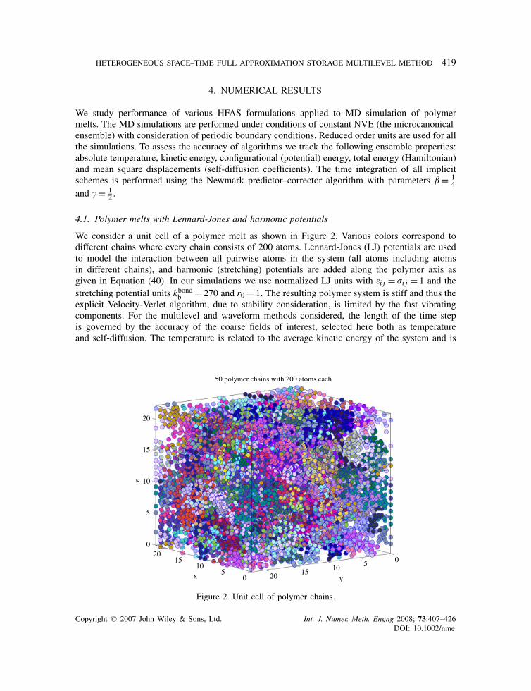
4.1. Polymer melts with Lennard-Jones and harmonic potentials

We consider a unit cell of a polymer melt as shown in Figure 2. Various colors correspond todifferent chains where every chain consists of 200 atoms. Lennard-Jones (LJ) potentials are usedto model the interaction between all pairwise atoms in the system (all atoms including atomsin different chains), and harmonic (stretching) potentials are added along the polymer axis asgiven in Equation (40). In our simulations we use normalized LJ units with �i j = �i j = 1 and thestretching potential units kbondb = 270 and r0= 1. The resulting polymer system is stiff and thus theexplicit Velocity-Verlet algorithm, due to stability consideration, is limited by the fast vibratingcomponents. For the multilevel and waveform methods considered, the length of the time stepis governed by the accuracy of the coarse fields of interest, selected here both as temperatureand self-diffusion. The temperature is related to the average kinetic energy of the system and is

05

1015

2005101520

0

5

10

15

20

y

50 polymer chains with 200 atoms each

x

z

Figure 2. Unit cell of polymer chains.



0 0.5 1 1.5 2 2.5 3 3.5 40

2

4

6

8

10

12

14

Normalized Integration Time

| (T

emp e

xp–T

emp i

mp)

/ T

emp e

xp |

× 10

0 [%

]

Integration error (3D Polymer chains)

∆ timp = 10 × ∆ texp




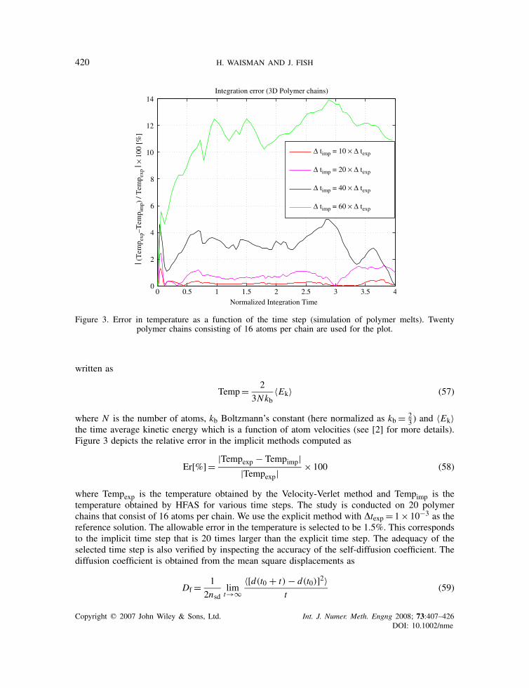
Figure 3. Error in temperature as a function of the time step (simulation of polymer melts). Twentypolymer chains consisting of 16 atoms per chain are used for the plot.

written as

Temp= 2

3Nkb〈Ek〉 (57)

where N is the number of atoms, kb Boltzmann’s constant (here normalized as kb= 23 ) and 〈Ek〉

the time average kinetic energy which is a function of atom velocities (see [2] for more details).Figure 3 depicts the relative error in the implicit methods computed as

Er[%]= |Tempexp − Tempimp||Tempexp|

× 100 (58)

where Tempexp is the temperature obtained by the Velocity-Verlet method and Tempimp is thetemperature obtained by HFAS for various time steps. The study is conducted on 20 polymerchains that consist of 16 atoms per chain. We use the explicit method with �texp= 1× 10−3 as thereference solution. The allowable error in the temperature is selected to be 1.5%. This correspondsto the implicit time step that is 20 times larger than the explicit time step. The adequacy of theselected time step is also verified by inspecting the accuracy of the self-diffusion coefficient. Thediffusion coefficient is obtained from the mean square displacements as

Df= 1

2nsdlimt→∞〈[d(t0 + t)− d(t0)]2〉

t(59)



0.4 0.5 0.6 0.7 0.8 0.9 10.04

0.06

0.08

0.1

0.12

0.14

0.16

mea

n sq

uare

dis

plac

emen

t

time

Self diffusion

Dexp=8.055801e – 002

Dimp=8.036291e – 002

implicit

explicit

Figure 4. Diffusion coefficient for both explicit and implicit methods. �timp= 20×�texp.

where nsd is the number of space dimensions and t0 the time origin for the ensemble time averages.For more details on diffusion coefficients we refer to [2]. Figure 4 illustrates the diffusion behavior(the slope) for both the explicit and implicit methods taken after long times. The comparisonof the diffusion coefficient for �timp= 20×�texp is given in Figure 4. The system is integratedover 40 000 explicit time steps. It can be seen that the multilevel method predicts the diffusioncoefficient with only 1% of error compared to the explicit method.

Tables I–III illustrate the performance of the WN and various multilevel methods as comparedto the popular Velocity-Verlet scheme. We study 10 polymer chains of short, medium and longlengths consisting of 10, 50 and 200 atoms, respectively. The WN and the variational multilevelscheme were reviewed in Section 2 (see Reference [13] for more details). Various HFAS schemeswere presented in Section 3. The system is first equilibrated over 1000 explicit steps by velocityscaling to a preset temperature. The methods are then compared in the production phase. We use thefollowing parameters in normalized units: box dimension of 22 units; the system is integrated over100 implicit steps (2000 explicit steps). The neighbor list [2] is updated every step for the implicitmethods and every 20 explicit steps. A cutoff radius of 8 units is employed for all simulations. Weadopt the notation given in Table IV for all methods considered. The diagonal terms of the Hessianmatrix in Equations (3)-(4) are computed analytically. One presmoothing of Jacobi WN is appliedfor all multilevel methods. The iteration is terminated when the residual in Equation (18) is lessthan 10−4 for all times within a window. For the numerical experiments considered the HFAS-IIImethod outperformed the explicit, WN and the other multilevel methods. The best performance isobtained when the window size is equal to the size of the time step.

Finally, we demonstrate stability properties of the implicit multilevel methods by considering along time interval. We integrate the system over 40 000 explicit time steps (2000 implicit steps).



Table I. CPU time and iteration summary for 10 polymer chains consisting of 10 atomsper chain (short chains).

Non-linear FunctionalMethod Winds dt Iteration iteration evaluation CPU (s)

VV 1 1× 10−3 — — 2001 611.19IN 1 20× 10−3 — 1441 1442 639.469WN 50 20× 10−3 460 — 750 325.94WN 100 20× 10−3 650 — 660 301.88ML-var 50 20× 10−3 200 760 1050 470.94ML-var 100 20× 10−3 218 654 873 383.906HFAS-I 50 20× 10−3 220 — 750 351.25HFAS-I 100 20× 10−3 263 — 527 235.203HFAS-II 50 20× 10−3 300 — 1075 498.83HFAS-II 100 20× 10−3 425 — 875 409.76HFAS-III 50 20× 10−3 220 720 730 340.78HFAS-III 100 20× 10−3 212 424 425 205.109

Table II. CPU time and iteration summary for 10 polymer chains consisting of 50 atomsper chain (medium length chains).


VV 1 1× 10−3 — — 2001 6625.9IN 1 20× 10−3 — 1670 1671 7802.8WN 50 20× 10−3 480 — 840 4061.3WN 100 20× 10−3 780 — 790 3966.4ML-var 50 20× 10−3 200 900 1750 8309.4ML-var 100 20× 10−3 260 260 530 2644.8HFAS-I 50 20× 10−3 260 — 890 4219.4HFAS-I 100 20× 10−3 280 — 570 2858.6HFAS-II 50 20× 10−3 500 — 1750 8696.1HFAS-II 100 20× 10−3 390 — 790 4063HFAS-III 50 20× 10−3 170 580 590 2874.7HFAS-III 100 20× 10−3 230 460 470 2391.6

Figure 5 depicts fluctuations in the configurational (potential) energy U and the total energy Etot(Hamiltonian). It can be seen that the proposed multilevel approach is stable as the Hamiltonianfluctuates around an average value. This average value differs by only %0.18 from the value obtainedby the explicit method. We note that the explicit fluctuations are much smaller as compared to theimplicit fluctuations.

Finally, we consider implementation of the explicit method and Picard iteration on a parallelmachine for Harmonic potentials. In the explicit method, matrix–vector operations are performedat every explicit time step, and communicated between the processors. In the Picard case, the



Table III. CPU time and iteration summary for 10 polymer chains consisting of 200 atomsper chain (long chains).


VV 1 1× 10−3 — — 2001 16 499.3IN 1 20× 10−3 — 2275 2300 33 378WN 50 20× 10−3 555 — 1115 16 805WN 100 20× 10−3 835 — 840 13 055ML-var 50 20× 10−3 200 700 1050 10 213ML-var 100 20× 10−3 310 310 625 9978ML-FAS-I 50 20× 10−3 300 — 975 14 664ML-FAS-I 100 20× 10−3 345 — 695 6747.1ML-FAS-II 50 20× 10−3 50 — 1850 17 736ML-FAS-II 100 20× 10−3 650 — 1350 13 658ML-FAS-III 50 20× 10−3 180 580 585 9811.7ML-FAS-III 100 20× 10−3 275 550 551 5804.9

Table IV. Notation used in the Tables I–III.

VV Velocity-VerletIN implicit Newmark (average acceleration)WN waveform NewtonML-var space–time multilevel variational schemeHFAS-I heterogeneous temporal multilevel FAS—PicardHFAS-II heterogeneous temporal multilevel FAS—constraintsHFAS-III heterogeneous temporal multilevel FAS—force field approximation

system is integrated implicitly and local matrix–matrix operations are performed at the end ofevery window (several time steps) and communicated between the processors. We use the librariesBLACS, PBLAS and ScaLAPACK for our parallel implementation. Figure 6 shows the timeparallelization effect on the speed-up factor over the explicit method. The results clearly showthat as the number of processors increases, the speed-up factor between the Picard and Velocity-Verlet methods increases. The main reason for the increase in the speed-up factor is due to theprocessors’ communication effect. In the case of standard explicit or implicit methods, processorsare communicating after every time step. However, in the Picard case the communication betweenprocessors only takes place at the end of each window. This results in superior parallel performance.

5. CONCLUSIONS

A heterogeneous full approximation storage (HFAS) multilevel formulation for molecular dynam-ics simulations has been developed. The formulation combines the basic principles of the fullapproximation storage (FAS) multigrid and the space–time variational multigrid approach devel-oped by Waisman and Fish [13]. It allows for different mathematical models to be considered at



0 0.5 1 1.5 2 2.5 3 3.5 4

x 104

0.95

1

1.05err= 1.422e+000 [%]

configurational (potential) energy

Number of explicit time steps

U(t

)/U

(0)

0 0.5 1 1.5 2 2.5 3 3.5 4

x 104

0.95

1

1.05total energy (Hamiltonian)

Eto

t(t)/

Eto

t(0) err= 1.828e – 001 [%]

Explicit averageImplicitImplicit average

Figure 5. Stability of multilevel method on a long time interval.

10 20 30 40 50 60

6.6

6.8

7

7.2

7.4

7.6

Number of Processors

Tex

p(n)

/Tpi

card

(n)

Parallel Results

N=10k

N=20k

N=30k

Figure 6. Speed-up ratio of Picard iteration over explicit method.



different scales. The temporal variant of the method, effectively uses two relaxation schemes: thewaveform Newton (WN) scheme, and the implicit integrator employing approximate force fieldcalculations. We study three variants of the method: Picard iteration, constrained dynamics andforce splitting. The methods are implicit in space and time, possess superior stability propertiesand consequently enable larger time steps governed by accuracy considerations of coarse-scalequantities of interest (e.g. temperature, energy, diffusion etc.). Performance studies on polymermelts have shown significant speed-up over the classical explicit methods and the variationalspace–time scheme. A parallel version of the Picard iteration has been developed for harmonicpotentials. Significant speed-ups over the standard explicit method have been observed primarilydue to reduced communication time between the processors. Finally, it is important to note thatthe formulation has been validated for interatomic potentials used to model polymer melts. Whilethe formulation is general it has not been tested for other molecular systems.

REFERENCES

1. de Gennes PG. Scaling Concepts in Polymer Physics. Cornell University Press: Ithaca, NY, 1979.2. Haile JM. Molecular Dynamics Simulation: Elementary Methods. Wiley: New York, 1992.3. Verlet L. Computer ‘experiments’ on classical fluids. I. Thermodynamical properties of Lennard-Jones molecules.

Physical Review 1967; 159(1):98–103.4. Swope WC, Anderson HC, Berens PH, Wilson KR. A computer simulation method for the calculation of

equilibrium constants for the formation of physical clusters of molecules: application to small water clusters.The Journal of Chemical Physics 1982; 76(1):637–649.

5. Gear CW. Numerical Initial Value Problems in Ordinary Differential Equations, Chapter 9. Prentice-Hall:Englewood Cliffs, NJ, 1971.

6. Bennemann C, Paul W, Binder K, Dunweg B. Molecular-dynamics simulations of the thermal glass transition inpolymer melts: -relaxation behavior. Physical Review E 1998; 57(1):843–851.

7. Rapaport DC. The Art of Molecular Dynamics Simulations. Cambridge University Press: Cambridge, MA, 1995.8. Anderson HC. Rattle: a velocity version of the shake algorithm for molecular dynamics calculations. Journal of

Computational Physics 1983; 52:24–34.9. Tuckerman M, Berne BJ, Martyna GJ. Reversible multiple time scale molecular dynamics. The Journal of

Chemical Physics 1992; 97(3):1990–2001.10. Garcia-Archilla B, Sanz-Serna JM, Skeel RD. The mollified impulse method for oscillatory differential equations.

SIAM Journal on Scientific Computing 1998; 20:930–963.11. Hairer E, Lubich C, Wanner G. Geometric Numerical Integration. Structure-Preserving Algorithms for Ordinary

Differential Equations. Springer: Berlin, 2002.12. Barash D, Yang L, Qian X, Schlick T. Inherent speedup limitations in multiple time step/particle mesh Ewald

algorithms. Journal of Computational Chemistry 2003; 24:77–88.13. Waisman H, Fish J. A space–time multilevel method for molecular dynamics simulations. Computer Methods in

Applied Mechanics and Engineering 2006; 195(44–47):6542–6559.14. Brandt A. Multi-level adaptive solutions to boundary-value problems. Mathematics of Computation 1977;

31(138):333–390.15. Lelarasmee E, Ruehli AE, Sangiovanni-Vincentelli AL. The waveform relaxation method for time-domain analysis

of large scale integrated circuits. IEEE Transactions on Computer-aided Design of Integrated Circuits and Systems1982; CAD-1(3):131–145.

16. Burrage K. Parallel and Sequential Methods for Ordinary Differential Equations. Oxford University Press:Oxford, 1995.

17. Saleh R, White J. Accelerating relaxation algorithms for circuit simulation using waveform-Newton and step-sizerefinement. IEEE Transactions on Computer-aided Design 1990; 9(9):951–958.

18. Lumsdaine A, Reichelt MW. Waveform iterative techniques for device transient simulation on parallel machines.Sixth SIAM Conference on Parallel Processing for Scientific Computing, Norfolk, VA, 1993.

19. Hughes TJR. The Finite Element Method. Linear Static and Dynamic Finite Element Analysis. Prentice-Hall:Englewood Cliffs, NJ, 1987.



20. Miekkala U, Nevanlinna O. Convergence of dynamic iteration methods for initial value problems. SIAM Journalon Scientific and Statistical Computing 1987; 8(4):459–482.

21. Giladi E, Keller HB. Space time domain decomposition for parabolic problems. Numerische Mathematik 2002;93(2):279–313.

22. Brandt A. Multilevel adaptive solutions to boundary-value problems. Mathematics of Computations 1977; 31:333–390.

23. Ortega JM, Rheinboldt WC. Iterative Solution of Nonlinear Equations in Several Variables. Academic Press:New York, 1970.

24. Briggs WL, Henson VE, McCormick SF. A Multigrid Tutorial (2nd edn). SIAM: Philadelphia, PA, 2000.25. Mavriplis DJ. An assessment of linear versus nonlinear multigrid methods for unstructured mesh solvers. Journal

of Computational Physics 2002; 175(1):302–325.26. Dumett MA, Vassilevski P, Woodward CS. A multigrid method for nonlinear unstructured finite element elliptic

equations. Technical Report UCRL-JC-150513, Lawrence Livermore National Laboratory, 2002.27. Henson VE. Multigrid methods for nonlinear problems: an overview. Technical Report UCRL-JC-150259,

Lawrence Livermore National Laboratory, 2003.28. Rudd RE, Broughton JQ. Coarse-grained molecular dynamics and the atomic limit of finite elements. Physical

Review B 1998; 58(10):R5893–R5896.29. Rudd RE. Coarse-grained molecular dynamics for computer modeling of nanomechanical systems. International

Journal for Multiscale Computational Engineering 2004; 2(2):203–220.30. Kutteh R. Rattle recipe for general holonomic constraints: angle and torsion constraints. CCP5 Newsletter 1998;

46:9–17.31. Ryckaert JP, Ciccotti G, Berendsen HJC. Numerical integration of the Cartesian equations of motion of a system

with constraints: molecular dynamics of n-alkanes. Journal of Computational Physics 1977; 23:327–341.


A heterogeneous space–time full approximation storage multilevel method for molecular dynamics...

Documents

Transcript of A heterogeneous space–time full approximation storage multilevel method for molecular dynamics...