Heterogeneous Computing - with OpenCL

Mem

bero

fthe

Hel

mho

ltz-A

ssoc

iatio

n

HeterogeneousComputingwith OpenCL

Wolfram Schenck Faculty of Eng. and Math., Bielefeld University of Applied Sciences

OpenCL Course, 22.11.2017

Mem

bero

fthe

Hel

mho

ltz-A

ssoc

iatio

n

Overview of the Lecture

1 Multi–Device: Data Partitioning

2 Multi–Device: Load–Balancing

3 Exercise

2

Multi–Device: Data Partitioning

Mem

bero

fthe

Hel

mho

ltz-A

ssoc

iatio

n

Multi–Device Programming

Misc. Scenarios

• Multi–GPU (also from differing manufacturers)• Multi–CPU• CPU(s) with GPU(s) (APU; „Heterogeneous Computing“)

Implementation with OpenCL

• Devices from same manufacturer (: same platform):Single shared context possible

• Devices from differing manufacturers (: multiple platforms):Separate contexts necessaryI . . . and separate program objects and kernels for each context

• In any case: A separate queue for each deviceI Synchronization between queues with events

4

Mem

bero

fthe

Hel

mho

ltz-A

ssoc

iatio

n

Multi–Device ProgrammingBasic Considerations

Important factors• Scheduling overhead:

I Startup time of each device?• Data location:

I On which device is the data located?• Task and data structure:

I How should the problem be partitioned?I How is the relation between data parallel and task parallel parts of the

algorithm?I How is the ratio between startup time and time for the main calculations?

• Relative performance of each device:I What is the best work distribution?: Load balancing

In the following: Example for data partitioning

5

Mem

bero

fthe

Hel

mho

ltz-A

ssoc

iatio

n

Example: ConvolutionFiltering an Image with a Convolution Kernel

mD : radius of the convolution kernel (“mask”)

6

Mem

bero

fthe

Hel

mho

ltz-A

ssoc

iatio

n

Example: Convolution (cont.)

7

Mem

bero

fthe

Hel

mho

ltz-A

ssoc

iatio

n


Mask: Edge length = (2mD + 1) pixels in each dimension

8

NotationI(x , y) : Pixel intensity in input

image at position (x , y)M(i, j) : Mask element at position

(i, j) within mask arrayIout(x , y) : Pixel intensity in output image

after convolution at position(x , y)

Mem

bero

fthe

Hel

mho

ltz-A

ssoc

iatio

n


Calculation of the intensity at the blue position (x0, y0):

Iout(x0, y0) =

2mD∑i=0

2mD∑j=0

M(i , j)I(x0 −mD + i , y0 −mD + j)

9

Mem

bero

fthe

Hel

mho

ltz-A

ssoc

iatio

n

ConvolutionBorder Handling

Problem: Divergence because of border handling

10

Mem

bero

fthe

Hel

mho

ltz-A

ssoc

iatio

n

ConvolutionBorder Handling (cont.)

(One possible) solution: Reduction of the size ot the output image so that themask can always be fully applied to the input image(output image = blue pixels)

11

Mem

bero

fthe

Hel

mho

ltz-A

ssoc

iatio

n

ConvolutionMisc. Convolution Kernels

MIdentity =

0 0 00 1 00 0 0

MLaplace =

1 2 12 −12 21 2 1

MBlurr =

1 1 1 1 11 1.5 2 1.5 11 2 10 2 11 1.5 2 1.5 11 1 1 1 1

Remark: Renormalization of image data not considered here!

12

Mem

bero

fthe

Hel

mho

ltz-A

ssoc

iatio

n

ConvolutionResult of Simple Convolution Operations

13

Original Laplace Blurr

Mem

bero

fthe

Hel

mho

ltz-A

ssoc

iatio

n

ConvolutionSobel Edge Filter (Scharr Version)

Convolution Kernels

MSobel,x =

3 0 −310 0 −103 0 −3

MSobel,y =

3 10 30 0 0−3 −10 −3

Convolution and Computation of the Output Image

Ix = MSobel,x ∗ IIy = MSobel,y ∗ I

Iout =√

I2x + I2

y (pixel-wise)

Remark: Renormalization of image data not considered here!

14

Mem

bero

fthe

Hel

mho

ltz-A

ssoc

iatio

n

ConvolutionResult of the Sobel Edge Filter

15

Ix Iy Iout

Mem

bero

fthe

Hel

mho

ltz-A

ssoc

iatio

n

Data PartitioningOutput Image

hout,full : Full height of the output imagewout : Width of the output image

16

Mem

bero

fthe

Hel

mho

ltz-A

ssoc

iatio

n

Data PartitioningOutput Image : Device 0 and 1

hout[0] : Height of part of the output image for device 0hout[1] : Height of part of the output image for device 1

17

Mem

bero

fthe

Hel

mho

ltz-A

ssoc

iatio

n

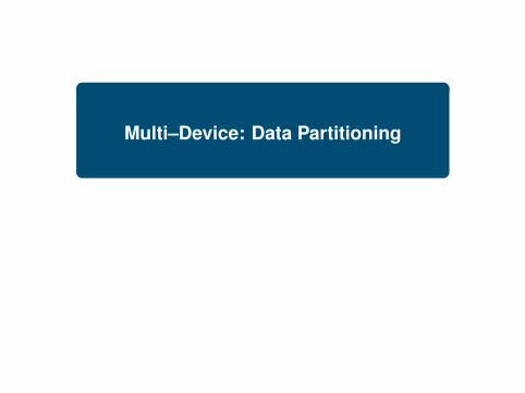
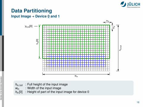
Data PartitioningInput Image : Device 0 and 1

hin,full : Full height of the input imagewin : Width of the input imagehin[0] : Height of part of the input image for device 0

18

Mem

bero

fthe

Hel

mho

ltz-A

ssoc

iatio

n

Data PartitioningInput Image : Device 0 and 1

hin,full : Full height of the input imagewin : Width of the input imagehin[1] : Height of part of the input image for device 1

: Data in border region has to be available on both devices!

19

Mem

bero

fthe

Hel

mho

ltz-A

ssoc

iatio

n

Data PartitioningResult for an Example Image

20

Original Image After Filtering

• Partitioning between device 0 and device 1: 60 % zu 40 %I Black background: Device 0I Inverse colors: Device 1

Multi–Device: Load–Balancing

Mem

bero

fthe

Hel

mho

ltz-A

ssoc

iatio

n

Load Balancing

Load BalancingDistribution of computational load on several devices with thegoal to use all devices evenly and to minimize the overall com-putation time

ExampleImage filtering executed by two devices in parallel (seepreceding slides)

22

Mem

bero

fthe

Hel

mho

ltz-A

ssoc

iatio

n

Study on Load BalancingTheoretical Analysis

• Overall problem size: N• Distribution of the problem on two devices:

Device 0 (N0) und Device 1 (N1)I N = N0 + N1I λ = N1

N• Computation times:

I Time required for device 0 to solve overall problem N: T0I Time required for device 1 to solve overall problem N: T1

23

Computation time when distributing load on both devices

• Assumption: Linear relationship between problem size andcomputation time (T ∈ O (N))⇒ Computation time on device 0: t0 = (1 − λ)T0⇒ Computation time on device 1: t1 = λT1

• Serial execution: T SER0+1 = t0 + t1 = (1− λ)T0 + λT1

• Parallel execution: T PAR0+1 = max (t0, t1) = max ((1− λ)T0, λT1)

Device 0

0 0.1 0.2 0.3 0.4 0.5 0.6 0.7 0.8 0.9 1250

300

350

400

450

500

550

600

650

700

Verhaeltnis λ zwischen der Device 1 zugewiesenen Teildatenmenge und der Gesamtdatenmenge

Au

sfu

eh

run

gs

ze

it [

ms

]

Ausfuehrungszeit (Device 0 mit Device 1)

Serielle Ausfuehrung

Parallele Ausfuehrung Device 1

0 0.1 0.2 0.3 0.4 0.5 0.6 0.7 0.8 0.9 1250

300

350

400

450

500

550

600

650

700

Verhaeltnis λ zwischen der Device 1 zugewiesenen Teildatenmenge und der Gesamtdatenmenge

Au

sfu

eh

run

gszeit

[m

s]

Ausfuehrungszeit (Device 0 mit Device 1)


Parallele Ausfuehrung

Derivation of the optimal value for λ (= λ∗)

• Assumption: Perfectly parallel execution with

T PAR0+1 = max ((1− λ)T0, λT1) .

• Approach: Minimum computation time with

(1− λ∗)T0 = λ∗T1 .

⇔ (1− λ∗)T0 − λ∗T1 = 0⇔ λ∗T0 + λ∗T1 = T0

⇔ λ∗ =T0

T0 + T1

Mem

bero

fthe

Hel

mho

ltz-A

ssoc

iatio

n

Study on Load BalancingDesign and Realization

OpenCL Configuration

• Two devices (when indicated from different platforms anddifferent type)

• Separate contexts and queues (in–order, synchronization afterlast memory transfer)

Realization

• Sobel filtering on an RGB image with a size of 10 megapixels(thus: problem size equiv. to amount of data in output image)

• Measurement of the computation (wall)time (data transfer andkernel execution) as mean value over 20 trials

• Systematic variation of λ

26

Mem

bero

fthe

Hel

mho

ltz-A

ssoc

iatio

n

Study on Load Balancing: Hints!

Correct Handling of Queues for two Devices

• Queue 0: Asynchronous call of memory transfer (H to D), kernelinvocation, memory transfer (D to H)

• Queue 1: Asynchronous call of memory transfer (H to D), kernelinvocation, memory transfer (D to H)

• Queue 0: clFlush(..)• Queue 1: clFlush(..)• Queue 0: Synchronization

(clFinish(..) or clWaitForEvents(..))• Queue 1: Synchronization

(clFinish(..) or clWaitForEvents(..))

Attention!• clFlush(..) enforces that all commands in the queue are sent

to the device for immediate execution. Important to use!

27

Mem

bero

fthe

Hel

mho

ltz-A

ssoc

iatio

n

Study on Load BalancingCore i7–2600 (CPU) vs. NVIDIA GTX 560Ti (GPU)

0 0.1 0.2 0.3 0.4 0.5 0.6 0.7 0.8 0.9 10

100

200

300

400

500

600

700

Verhaeltnis λ zwischen der Device 1 zugewiesenen Teilbildgroesse und der Gesamtbildgroesse

Au

sfu

eh

run

gs

ze

it [

ms

]

Ausfuehrungszeit Sobel−Filter



Messung: i7−2600 / GTX560Ti

• Platforms: Intel, NVIDIA: Only minimal gain if devices are from very different performance

classes

28

Mem

bero

fthe

Hel

mho

ltz-A

ssoc

iatio

n

Study on Load BalancingCore i7–2600 (CPU) vs. NVIDIA G210 (GPU)

0 0.1 0.2 0.3 0.4 0.5 0.6 0.7 0.8 0.9 1350

400

450

500

550

600

650

700

750

800


Au

sfu

eh

run

gs

ze

it [

ms

]




Messung: i7−2600 / G210

• Platforms: Intel, NVIDIA: Nice gain if CPU and GPU operate at same performance level: Worse than ideal parallel execution because CPU is also

required as host for GPU processing 29

Mem

bero

fthe

Hel

mho

ltz-A

ssoc

iatio

n

Study on Load BalancingCore i7–930 (CPU) vs. AMD HD 6970 (GPU)

0 0.1 0.2 0.3 0.4 0.5 0.6 0.7 0.8 0.9 1200

300

400

500

600

700

800

900

1000


Au

sfu

eh

run

gs

ze

it [

ms

]




Messung: i7−930 / HD6970

• Platforms: AMD: Parallel execution, but worse than ideal model because CPU is

also required as host for GPU processing

30

Mem

bero

fthe

Hel

mho

ltz-A

ssoc

iatio

n

Study on Load BalancingNVIDIA G210 (GPU) vs. NVIDIA GTX 560Ti (GPU)

0 0.1 0.2 0.3 0.4 0.5 0.6 0.7 0.8 0.9 10

100

200

300

400

500

600

700

800


Au

sfu

eh

run

gs

ze

it [

ms

]




Messung: G210 / GTX560Ti

• Platforms: NVIDIA: Ideal parallel execution with two GPUs from the same

manufacturer, but only minimal gain because of very differentbase performance

31

Mem

bero

fthe

Hel

mho

ltz-A

ssoc

iatio

n

Study on Load BalancingAMD HD 6970 (GPU) vs. NVIDIA GTX 570 (GPU)

0 0.1 0.2 0.3 0.4 0.5 0.6 0.7 0.8 0.9 10

50

100

150

200

250

300


Au

sfu

eh

run

gs

ze

it [

ms

]




Messung: HD6970 / GTX570

• Platforms: AMD und NVIDIA: Ideal parallel execution with two GPUs from different

manufacturers!

32

Mem

bero

fthe

Hel

mho

ltz-A

ssoc

iatio

n

Exkursus: Usage of Local MemoryAMD HD 6970 (GPU) vs. NVIDIA GTX 570 (GPU)

0 0.1 0.2 0.3 0.4 0.5 0.6 0.7 0.8 0.9 115

20

25

30

35

40

45

50

55

60


Au

sfu

eh

run

gs

ze

it [

ms

]




Messung: HD6970 / GTX570 (LM)

• Modified kernel using local memory as cache speeds upexecution on the Cayman–XT GPU

: Parallel execution even faster than expected from theoreticalmodel!

33

Mem

bero

fthe

Hel

mho

ltz-A

ssoc

iatio

n

Exkursus: Omission of clFlush(..)AMD HD 6970 (GPU) vs. NVIDIA GTX 570 (GPU)

0 0.1 0.2 0.3 0.4 0.5 0.6 0.7 0.8 0.9 115

20

25

30

35

40

45

50

55

60


Au

sfu

eh

run

gs

ze

it [

ms

]




Messung: HD6970 / GTX570 (LM)

• Setting: Different platforms and GPUs, kernel with localmemory

: Without clFlush(..) execution on GPUs is only serial!

34

Mem

bero

fthe

Hel

mho

ltz-A

ssoc

iatio

n

Study on Load BalancingConclusions

• CPU with GPU („Heterogeneous Computing“)I Parallel executionI Performance not as good as predicted by ideal parallel model

because CPU is required as host for GPU processingI Especially useful if CPU and GPU have roughly the same

base performance (see APU concept)• GPU with GPU

I Parallel execution as predicted by ideal parallel model(sometimes even better)

I Can be used with GPUs from the same platform or fromdifferent platforms (manufacturers)

I Even a weak GPU can support a strong GPU up to ameasurable effect (as predicted by the ideal parallel model;however, not that many good use cases exist for thisscenario)

35

Mem

bero

fthe

Hel

mho

ltz-A

ssoc

iatio

n

Load Balancing: General Hints

Consideration of the Capacity/Latency/Speed of the Devices

• Excessive demand on a weak device may hinder overallexecution

• Startup latency may become a limiting factor if data pieces aretoo small

Approach No 1

• Tests with small amounts of data/problem sizes• Profiling on various devices• Extrapolation for larger amounts of data/problem sizes (based

on an analytical or empirical performance model)• Production runs with enlarged data amounts/problem sizes to

minimize overhead

Approach No 2

• If one device is clearly superior to all others: Just use this one. . .

36

Exercise

Mem

bero

fthe

Hel

mho

ltz-A

ssoc

iatio

n

Exercise: Matrix Multiplication on two Devices

1 Modify example code so that both devices compute part of thetarget matrix C.

2 Determine λ value with minimum overall execution timeaccording to theoretical model.

3 Check if this corresponds to the empirical minimum.38

Heterogeneous Computing - with OpenCL

Documents

Transcript of Heterogeneous Computing - with OpenCL