Heterogeneous mathematical models in fluid dynamics

and associated solution algorithms

Marco Discacciati♯ and Paola Gervasio and Alfio Quarteroni

January 16, 2010

♯ IACS–CMCS, Ecole Polytechnique Federale de Lausanne (EPFL)CH-1015 Lausanne, Switzerlandmarco.discacciati@epfl.ch

Dipartimento di Matematica, University of Bresciavia Valotti 9, 25133 Brescia, Italy

gervasio@ing.unibs.it

MOX – Modellistica e Calcolo ScientificoDipartimento di Matematica “F. Brioschi”

Politecnico di Milanovia Bonardi 9, 20133 Milano, Italy

and IACS–CMCS, Ecole Polytechnique Federale de Lausanne (EPFL)CH-1015 Lausanne, Switzerland

alfio.quarteroni@epfl.ch

Abstract

Mathematical models of complex physical problems can be based onheterogeneous differential equations, i.e. on boundary-value problems ofdifferent kind in different subregions of the computational domain. In thispresentation we will introduce a few representative examples, we will illus-trate the way the coupling conditions between the different models can bedevised, then we will address several solution algorithms and discuss theirproperties of convergence as well as their robustness with respect to thevariation of the physical parameters that characterize the submodels.

1 Introduction and motivation

For the description and simulation of complex physical phenomena, combinationof hierarchical mathematical models can be set up with the aim of reducingthe computational complexity. This gives rise to a system of heterogeneousproblems, where different kind of differential problems are set up in subdomains

1

(either disjoint or overlapping) of the original computational domain. Whenfacing this kind of coupled problems, two natural issues arise. The former isconcerned with the way interface coupling conditions can be devised, the latterwith the construction of suitable solution algorithms that can take advantage ofthe intrinsic splitting nature of the problem at hand. This work will focus onboth issues, in the context of heterogeneous boundary-value problems that canbe used for fluid dynamics applications.The outline of this presentation is as follows. After giving the motivation forthis investigation, we will present two different approaches for the derivation andanalysis of the interface coupling conditions: the one based on the variational for-mulation, the other on virtual controls. For the former we will consider at firstadvection-diffusion problems. After carrying out their variational analysis wepropose domain decomposition algorithms for their solution, in particular thosebased on Dirichlet-Neumann, adaptive Robin-Neumann, or Steklov-Poincare it-erations. Then, we will focus on Navier-Stokes/Darcy or Stokes/potential cou-pled problem presenting their asymptotic analysis together with possible solutiontechniques.For the virtual control approach, we will study the case of non-overlapping sub-domains for advection-diffusion problems considering in particular possible tech-niques to solve the optimality system and we will present some numerical results.Then, we will consider the case of domain decomposition with overlap, namelySchwarz methods with Dirichlet/Robin interface conditions. We will investigatethe virtual control approach with overlap for the advection-diffusion equationsincluding the case of three virtual controls and we will present some numericalresults. Finally, we will illustrate this framework for the case of the Stokes-Darcycoupled problem, and for the coupling of incompressible flows.

In order to motivate our investigation, we begin to analyze the advection-diffusion problem.Let us consider a bounded domain Ω ⊂ Rd (d = 1, 2, 3) with Lipschitz boundaryand the advection-diffusion equation

Au ≡ div(−ν∇u+~bu) + b0u = f in Ωu = g on ∂Ω,

(1)

where ν > 0 is a characteristic parameter of the problem,~b = ~b(~x) a d−dimensionalvector valued function, b0 = b0(~x) and f = f(~x) scalar functions, all assigned inΩ, while g = g(~x) is assigned on ∂Ω.The characteristic parameter ν can either represent the thermal diffusivity inheat transfer problems, or the inverse of the Reynolds number in incompressiblefluid-dynamics, or another suitable parameter.Denoting by

Peg(~x) =|~b(~x)|2ν

(2)

2

Ω

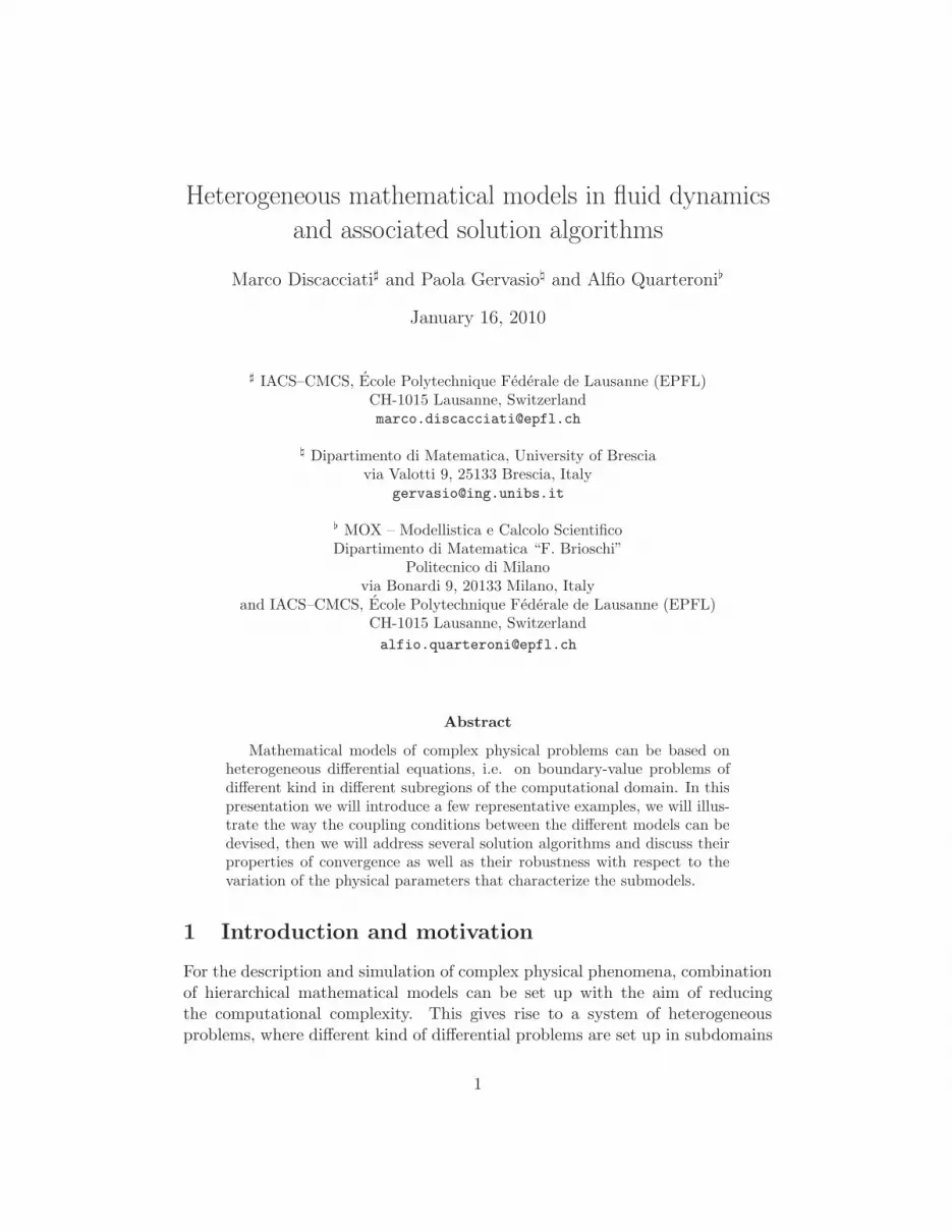
Au = div(−ν∇u+~bu) + b0u = f

layer

Figure 1: A simple computational domain and the localization of the boundarylayer

the global Peclet number, we call (1) an advection-dominated problem whenPeg(~x) ≫ 1.We are interested in treating advection dominated problems with boundary lay-ers (see, e.g., Fig. 1), that arise when boundary data are incompatible withthe limit (as ν → 0) of the advection-diffusion equation. As an example, let usconsider the one-dimensional advection-diffusion equation

−νu′′(x) + bu′(x) = 0, 0 < x < 1,

u(0) = 0, u(1) = 1,(3)

with ν > 0 and b > 0. Problem (3) can be solved exactly and its solution reads

u(x) =ebx/ν − 1

eb/ν − 1.

Such solution exhibits a boundary layer of width O(ν/b) near to x = 1 when theratio ν/b is small enough, that is when

Peg(~x) ≫ 1. (4)

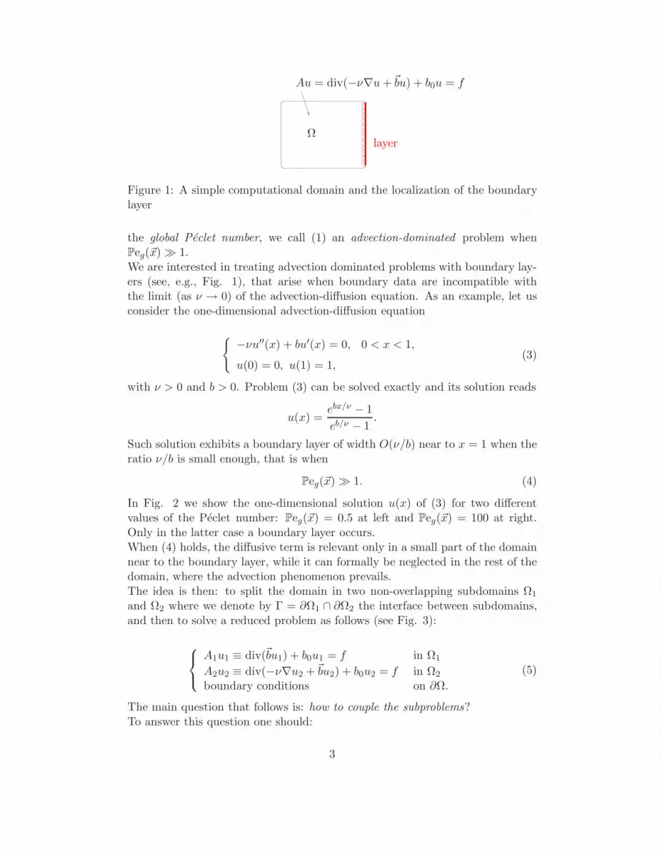
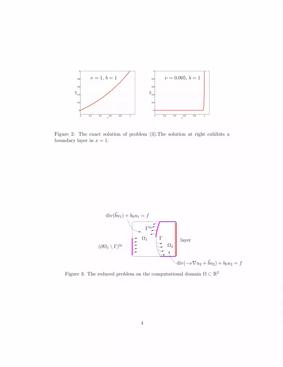
In Fig. 2 we show the one-dimensional solution u(x) of (3) for two differentvalues of the Peclet number: Peg(~x) = 0.5 at left and Peg(~x) = 100 at right.Only in the latter case a boundary layer occurs.When (4) holds, the diffusive term is relevant only in a small part of the domainnear to the boundary layer, while it can formally be neglected in the rest of thedomain, where the advection phenomenon prevails.The idea is then: to split the domain in two non-overlapping subdomains Ω1

and Ω2 where we denote by Γ = ∂Ω1 ∩ ∂Ω2 the interface between subdomains,and then to solve a reduced problem as follows (see Fig. 3):

A1u1 ≡ div(~bu1) + b0u1 = f in Ω1

A2u2 ≡ div(−ν∇u2 +~bu2) + b0u2 = f in Ω2

boundary conditions on ∂Ω.

(5)

The main question that follows is: how to couple the subproblems?To answer this question one should:

3

0 0.2 0.4 0.6 0.8 1

0

0.2

0.4

0.6

0.8

1

x

u(x)

ν = 1, b = 1

0 0.2 0.4 0.6 0.8 1

0

0.2

0.4

0.6

0.8

1

x

u(x)

ν = 0.005, b = 1

Figure 2: The exact solution of problem (3).The solution at right exhibits aboundary layer in x = 1.

Ω1

Ω2

Γ

Γin

(∂Ω1 \ Γ)in

div(~bu1) + b0u1 = f

div(−ν∇u2 +~bu2) + b0u2 = f

layer

Figure 3: The reduced problem on the computational domain Ω ⊂ R2

4

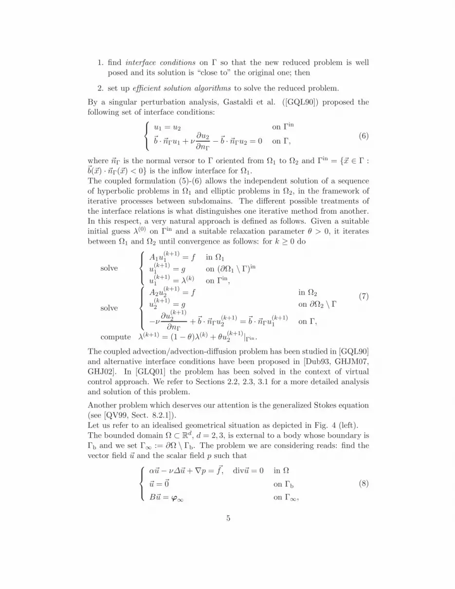
1. find interface conditions on Γ so that the new reduced problem is wellposed and its solution is “close to” the original one; then

2. set up efficient solution algorithms to solve the reduced problem.

By a singular perturbation analysis, Gastaldi et al. ([GQL90]) proposed thefollowing set of interface conditions:

u1 = u2 on Γin

~b · ~nΓu1 + ν∂u2

∂nΓ−~b · ~nΓu2 = 0 on Γ,

(6)

where ~nΓ is the normal versor to Γ oriented from Ω1 to Ω2 and Γin = ~x ∈ Γ :~b(~x) · ~nΓ(~x) < 0 is the inflow interface for Ω1.The coupled formulation (5)-(6) allows the independent solution of a sequenceof hyperbolic problems in Ω1 and elliptic problems in Ω2, in the framework ofiterative processes between subdomains. The different possible treatments ofthe interface relations is what distinguishes one iterative method from another.In this respect, a very natural approach is defined as follows. Given a suitableinitial guess λ(0) on Γin and a suitable relaxation parameter θ > 0, it iteratesbetween Ω1 and Ω2 until convergence as follows: for k ≥ 0 do

solve

A1u(k+1)1 = f in Ω1

u(k+1)1 = g on (∂Ω1 \ Γ)in

u(k+1)1 = λ(k) on Γin,

solve

A2u(k+1)2 = f in Ω2

u(k+1)2 = g on ∂Ω2 \ Γ

−ν ∂u(k+1)2

∂nΓ+~b · ~nΓu

(k+1)2 = ~b · ~nΓu

(k+1)1 on Γ,

compute λ(k+1) = (1 − θ)λ(k) + θu(k+1)2 |Γin .

(7)

The coupled advection/advection-diffusion problem has been studied in [GQL90]and alternative interface conditions have been proposed in [Dub93, GHJM07,GHJ02]. In [GLQ01] the problem has been solved in the context of virtualcontrol approach. We refer to Sections 2.2, 2.3, 3.1 for a more detailed analysisand solution of this problem.

Another problem which deserves our attention is the generalized Stokes equation(see [QV99, Sect. 8.2.1]).Let us refer to an idealised geometrical situation as depicted in Fig. 4 (left).The bounded domain Ω ⊂ Rd, d = 2, 3, is external to a body whose boundary isΓb and we set Γ∞ := ∂Ω \ Γb. The problem we are considering reads: find thevector field ~u and the scalar field p such that

α~u− ν∆~u+ ∇p = ~f, div~u = 0 in Ω

~u = ~0 on Γb

B~u = ϕ∞ on Γ∞,

(8)

5

ΩΓb

Γ∞

Ω1 Ω2

Γ

Γb

Γ∞

Figure 4: The geometrical configuration for an external problem (left) and apossible non overlapping decomposition of the computational domain (right)

where ~f and φ∞ are given functions, B denotes the boundary operator on Γ∞,while α ≥ 0 is a given parameter. To take α = 0 corresponds to solve theStokes problem. Nevertheless, this problem may arise in the process of solvingthe full Navier–Stokes equations, when the discretisation of the time derivativeis performed by means of a scheme that is explicit in the non-linear convectiveterm. In this case, the parameter α > 0 represents the inverse of the time-stepand the function ~f , in fact, depends on the solution at the previous step, i.e.~f = ~f(~u(n)).The boundary conditions on Γ∞ have to be prescribed in a suitable way forassuring well-posedness. In this respect, on a portion Γin

∞ of Γ∞ an onset flow~u = ~uin

∞ is given. However, assigning conditions on the outflow section Γout∞

may not be simple. It is also clear that all interesting flow features occur in thevicinity of the body due to the role of viscosity in this area.For this reason, Schenk and Hebeker ([SH93]) have proposed the replacement ofproblem (8) with a reduced one far from the obstacle.The computational domain Ω is partitioned into a subdomain Ω2, next to thebody, and a far field subdomain Ω1; the interface between Ω1 and Ω2 is denotedby Γ, ~nΓ is the unit normal vector on Γ directed from Ω1 to Ω2, and ~n the unitoutward normal vector on ∂Ω. The global Stokes equation (8) is replaced withthe following coupled problem, where the viscosity ν is set to 0 in Ω1:

α~u1 + ∇p1 = ~f, div~u1 = 0 in Ω1

~u1 = ~uin∞ on Γin

∞

p1 = 0 on Γout∞

α~u2 − ν∆~u2 + ∇p2 = ~f, div~u2 = 0 in Ω2

~u2 = ~0 on Γb,

(9)

or equivalently, by applying the divergence operator to equation (9)1:

6

Ω1

Ω1

Ω1

Ω2

Γ

Γin∞ Γout

∞

Figure 5: The domain decomposition configuration for an internal problem

∆p1 = div~f in Ω1

∂p1

∂n= (~f − α~uin

∞) · ~n on Γin∞

p1 = 0 on Γout∞

α~u2 − ν∆~u2 + ∇p2 = ~f, div~u2 = 0 in Ω2

~u2 = ~0 on Γb.

(10)

Either problem (9) and (10) are incomplete, because the matching conditionsthat have to be fulfilled on Γ are missing.In [SH93] these conditions are recovered through a singular perturbation analysissimilar to that carried out for the advection–diffusion problem in [GQL90] andthey read:

∂p1

∂nΓ= (~f − α~u2) · ~nΓ on Γ

p1~nΓ = −ν(~nΓ · ∇)~u2 + p2~nΓ on Γ.(11)

The coupled problem (10)-(11) can be used also for the simulation of the fluidmotion inside a bounded domain, as depicted in Fig. 5. In this case the domainΩ1, in which the reduced problem is solved, is non-connected and separates theinterior domain from both inflow and outflow interfaces.We observe that the system (10)-(11) models two possible different coupled prob-lems. The first one, when α = 0, is a Stokes/potential coupling, the vector field~f is independent of the velocity ~u and the pressure p1 is indipendent of thesolution (~u2, p2). Such coupling can be used to model external flows.The second one, when α > 0, corresponds to the single step of a time-dependentNavier-Stokes/potential coupling where, as said above, the vector field ~f dependson the solution at the previous step. This is the case of the simulation of eitherthe flow inside a channel (or the blood flow in the carotid) or a far field condition.

7

As in the case of the advection–diffusion problem, the interface conditions (11)could be used to set-up an iterative algorithm by subdomains as follows.

Assume that λ(0)

is given and satisfies

∫

Γλ

(0) · ~nΓ = 0; for any k ≥ 0 solve

∆p(k+1)1 = div~f in Ω1

∂p(k+1)1

∂n= (~f − α~uin

∞) · ~n on Γin∞

p(k+1)1 = 0 on Γout

∞

∂p(k+1)1

∂nΓ= (~f − αλ

(k)) · ~nΓ on Γ,

(12)

then solve

α~u(k+1)2 − ν∆~u

(k+1)2 + ∇p(k+1)

2 = ~f, div~u(k+1)2 = 0 in Ω2

~u(k+1)2 = ~0 on Γb

ν(~nΓ · ∇)~u(k+1)2 − p

(k+1)2 ~nΓ = −p(k+1)

1 ~nΓ on Γ

(13)

and finally set

λ(k+1)

= (1 − θ)λ(k)

+ θ~u(k+1)2|Γ , (14)

where θ > 0 is a relaxation parameter.

Since div~u(k+1)2 = 0 in Ω2, the trace ~u

(k+1)2|Γ satisfies

∫

Γ~u

(k+1)2|Γ · ~nΓ = 0,

whence

∫

Γλ

(k) · ~nΓ = 0 for each k ≥ 0.

The analysis of the coupled problem (10)-(11) and the proof of convergence ofthe above iterative process (12)-(14) are reported in [SH93]. The analysis canbe performed also by writing the problem in terms of the associated Steklov–Poincare operators, and then proving convergence by applying an abstract result(see [QV99, Thm 4.2.2]).

Finally, we introduce a coupled free/porous-media flow problem.The computational domain is a region naturally split into two parts: one occu-pied by the fluid, the other by the porous media. More precisely, let Ω ⊂ Rd

(d = 2, 3) be a bounded domain, partitioned into two non intersecting subdo-mains Ωf and Ωp separated by an interface Γ, i.e. Ω = Ωf ∪ Ωp, Ωf ∩ Ωp = ∅and Ωf ∩ Ωp = Γ. We suppose the boundaries ∂Ωf and ∂Ωp to be Lipschitz con-tinuous. From the physical point of view, Γ is a surface separating the domainΩf filled by a fluid, from a domain Ωp formed by a porous medium. We assume

8

Ωf

Ωpnf

npΓinf

Γf

Γf

Γp Γp

Γbp

Γ

Figure 6: Representation of a 2D section of a possible computational domain for theStokes/Darcy coupling

that Ωf has a fixed surface, i.e., we neglect here the case of free-surface flows.The fluid in Ωf can filtrate through the adjacent porous medium.The Navier-Stokes equations describe the motion of the fluid in Ωf : ∀t > 0,

∂tuf − div T(uf , pf ) + (uf · ∇)uf = f in Ωf

div uf = 0 in Ωf ,(15)

where T(uf , pf ) = ν(∇uf +∇Tuf )− pf I is the Cauchy stress tensor, I being theidentity tensor. ν > 0 is the kinematic viscosity of the fluid, f a given volumetricforce, while uf and pf are the fluid velocity and pressure, respectively.The filtration of an incompressible fluid through porous media is often describedby Darcy’s law. The latter provides the simplest linear relation between velocityand pressure in porous media under the physically reasonable assumption thatfluid flows are usually very slow and all the inertial (non-linear) terms may beneglected.Darcy’s law introduces a fictitious flow velocity, the Darcy velocity or specificdischarge q through a given cross section of the porous medium, rather than thetrue velocity up with respect to the porous matrix:

up =q

n, (16)

with n being the volumetric porosity, defined as the ratio between the volume ofvoid space and the total volume of the porous medium.To introduce Darcy’s law, we define a scalar quantity ϕ called piezometric headwhich essentially represents the fluid pressure in Ωp:

ϕ = z +ppg, (17)

where z is the elevation from a reference level, accounting for the potential energyper unit weight of fluid, pp is the ratio between the fluid pressure in Ωp and itsviscosity ρf , and g is the gravity acceleration.

9

Then, Darcy’s law can be written as

q = −K∇ϕ, (18)

where K is a symmetric positive definite diagonal tensor K = (Kij)i,j=1,...,d,Kij ∈ L∞(Ωp), Kij > 0, Kij = Kji, called hydraulic conductivity tensor, whichdepends on the properties of the fluid as well as on the characteristics of theporous medium. Let us denote K = K/n.In conclusion, the motion of an incompressible fluid through a saturated porousmedium is described by the following equations:

up = −K∇ϕ in Ωp

div up = 0 in Ωp.(19)

Finally, to represent the filtration of the free fluid through the porous medium,we have to introduce suitable coupling conditions between the Navier-Stokes andDarcy equations across the common interface Γ. In particular we consider thefollowing three conditions.

1. Continuity of the normal component of the velocity:

uf · n = up · n, (20)

where we have indicated n = nf = −np on Γ. This condition is a conse-quence of the incompressibility of the fluid.

2. Continuity of the normal stresses across Γ (see, e.g., [JM96]):

−n · T(uf , pf ) · n = gϕ. (21)

Remark that pressures may be discontinuous across the interface.

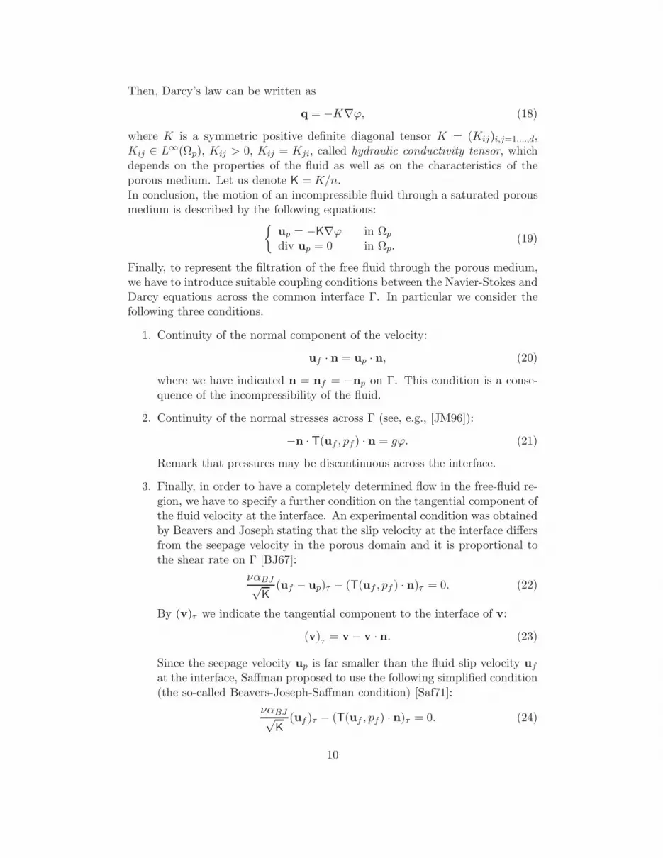
3. Finally, in order to have a completely determined flow in the free-fluid re-gion, we have to specify a further condition on the tangential component ofthe fluid velocity at the interface. An experimental condition was obtainedby Beavers and Joseph stating that the slip velocity at the interface differsfrom the seepage velocity in the porous domain and it is proportional tothe shear rate on Γ [BJ67]:

ναBJ√K

(uf − up)τ − (T(uf , pf ) · n)τ = 0. (22)

By (v)τ we indicate the tangential component to the interface of v:

(v)τ = v − v · n. (23)

Since the seepage velocity up is far smaller than the fluid slip velocity ufat the interface, Saffman proposed to use the following simplified condition(the so-called Beavers-Joseph-Saffman condition) [Saf71]:

ναBJ√K

(uf )τ − (T(uf , pf ) · n)τ = 0. (24)

10

This condition was later derived mathematically by means of homogeniza-tion by Jager and Mikelic [JM96, JM00, JMN01].

The three coupling conditions described in this section have been extensivelystudied and analysed also in [DMQ02, DQ09, LSY03, PS98, RY05].In conclusion, the coupled Navier-Stokes/Darcy model reads:

∂tuf − div T(uf , pf ) + (uf · ∇)uf = f in Ωf

div uf = 0 in Ωf

up = −K∇ϕ in Ωp

div up = 0 in Ωp

uf · n = up · n on Γ−n · T(uf , pf ) · n = gϕ on ΓναBJ√

K(uf )τ − (T(uf , pf ) · n)τ = 0 on Γ.

(25)

Using Darcy’s law we can rewrite the system (19) as an elliptic equation for thescalar unknown ϕ:

−∇ · (K∇ϕ) = 0 in Ωp. (26)

In this case, the differential formulation of the coupled Navier-Stokes/Darcyproblem becomes:

∂tuf − div T(uf , pf ) + (uf · ∇)uf = f in Ωf

div uf = 0 in Ωf

−div (K∇ϕ) = 0 in Ωp,(27)

with the interface conditions on Γ:

uf · n = −K∂ϕ

∂n−n · T(uf , pf ) · n = gϕναBJ√

K(uf )τ − (T(uf , pf ) · n)τ = 0.

(28)

We refer to Sections 2.6, 2.7, 3.4 for a more exhaustive analysis of the Stokes/Darcycoupling.

2 Variational formulation approach

The reduced problems presented above will be analysed in this Section in avariational setting, in order to deduce suitable interface conditions which can berigorously justified. Moreover, different iterative algorithms to solve the reducedproblems will be presented.

11

2.1 The advection-diffusion problem

We consider an open bounded domain Ω ⊂ Rd (d = 2, 3) with Lipschitz boundary∂Ω, and we split it into two open subsets Ω1 and Ω2 such that

Ω = Ω1 ∪ Ω2, Ω1 ∩ Ω2 = ∅. (29)

Then, we denote byΓ = ∂Ω1 ∩ ∂Ω2 (30)

the interface between the subdomains (see Fig. 3) and we assume that Γ is of

class C1,1;Γ will denote the interior of Γ.

Given two scalar functions f and b0 defined in Ω, a positive function ν defined

in Ω2 ∪Γ, a d−dimensional vector valued function ~b defined in Ω satisfying the

following inequalities:

∃ν0 ∈ R : ν(~x) ≥ ν0 > 0 ∀~x ∈ Ω2 ∪Γ,

∃σ0 ∈ R : b0(~x) +1

2div~b(~x) ≥ σ0 > 0 ∀~x ∈ Ω,

(31)

we are interested in finding two functions u1 and u2 (defined in Ω1 and Ω2,respectively) such that u1 statisfies the advection-reaction equation

A1u1 ≡ div(~bu1) + b0u1 = f in Ω1, (32)

while u2 satisfies the advection-diffusion-reaction equation

A2u2 ≡ −div(ν∇u2) + div(~bu2) + b0u2 = f in Ω2. (33)

For each subdomain, we distinguish between the external (or physical) boundary∂Ω ∩ ∂Ωk = ∂Ωk \ Γ (for k = 1, 2) and the internal one, i.e. the interface Γ.Moreover, for any non-empty subset S ⊆ ∂Ω1, we define:

the inflow part of S : Sin = ~x ∈ S : ~b(~x) · ~n(~x) < 0, (34)

where ~n(~x) is the outward unit normal vector on S,

the outflow part of S : Sout = ~x ∈ S : ~b(~x) · ~n(~x) ≥ 0. (35)

Boundary conditions for problem (32) must be assigned on ∂Ωin1 .

For a given suitable function g defined on ∂Ω, we denote by g1 and g2 therestriction of g to (∂Ω1 \Γ)in and ∂Ω2 \Γ, respectively, and we set the followingDirichlet boundary conditions on the external boundaries:

u1 = g1 on (∂Ω1 \ Γ)in,

u2 = g2 on ∂Ω2 \ Γ.(36)

Finally, let us denote by ~nΓ the normal versor to Γ oriented from Ω1 to Ω2, sothat ~nΓ(~x) = ~n1(~x) = −~n2(~x), ∀~x ∈ Γ.

12

Ω1 Ω2

ν

ενε

Ω

ν∗ε

Figure 7: The viscosity ν∗ε for the regularized problem. νε|Ω2→ ν when (ε→ 0)

2.2 Variational analysis for the advection-diffusion equation

The basic steps of the analysis carried out in [GQL90] are summarized here.1. Given a positive function ν in Ω, we denote by PΩ(ν) the advection-diffusionproblem (1) in Ω. For any ε > 0, we introduce a smooth function νε defined inΩ2, which is a regularization of ν according with continuity to ε on Γ. Then, ν∗εis the globally defined viscosity defined as (see Fig. 7)

ν∗ε =

ε in Ω1

νε in Ω2 .

We denote by PΩ(ν∗ε ) ≡ [PΩ1(ε)/PΩ2

(νε)] the following advection-diffusion prob-lem

−ε∆u1,ε + div(~bu1,ε) + b0u1,ε = f in Ω1

div(−νε∇u2,ε +~bu2,ε) + b0u2,ε = f in Ω2

ǫ∂u1,ǫ

∂nΓ−~b · ~nΓu1,ǫ = νǫ

∂u2,ǫ

∂nΓ−~b · ~nΓu2,ǫ on Γ

u1,ǫ = u2,ǫ on Γ

u = g on ∂Ω.

(37)

2. For any ε > 0, let VΩ(ε) be the variational formulation associated to PΩ(ε).Solving VΩ(ε) means to look for the solution uε ∈ V of

aε(uε, wε) = F (wε), ∀wε ∈ V. (38)

If we take g ≡ 0, this means to set V = H10 (Ω) and to solve

aε(uε, wε) =

∫

Ω

[(ε∇uε −~buε) · ∇wε + b0uεwε

]d~x, F (wε) =

∫

Ωfwεd~x

(39)for any wε ∈ V .Otherwise, if g 6= 0 the formulation is the same, however the right hand side hasto be modified as follows:

Fg(wε) = F (wε) − aε(Rg, wε)

13

where Rg is a suitable lifting of the boundary data g, so that the final solutionreads uε +Rg (see [Qua09]).3. By asymptotic analysis on VΩ1

(ε), recover the reduced problem PΩ1(0), so

that

PΩ(ν∗ε ) → [PΩ1(0)/PΩ2

(ν)] when ε→ 0 .

The new coupled problem [PΩ1(0)/PΩ2

(ν)] inherits from the limit process aproper set of interface conditions.According to the analysis performed in [GQL90], u1,ǫ converges weakly in L2(Ω1)and u2,ǫ converges weakly in H1(Ω2) when ǫ→ 0, moreover the limit (u1, u2) ∈L2(Ω1) ×H1(Ω2) satisfies the following reduced coupled problem:

div(~bu1) + b0u1 = f in Ω1

div(−ν∇u2 +~bu2) + b0u2 = f in Ω2

−~b · ~nΓu1 = ν∂u2

∂nΓ−~b · ~nΓu2 on Γ

u1 = u2 on Γin

u1 = g1 on (∂Ω1 \ Γ)in

u2 = g2 on ∂Ω2 \ Γ.

(40)

The interface conditions (40)3,4 express the continuity of the flux across thewhole interface Γ and the continuity of the solution across the inflow interfaceΓin, respectively. No continuity condition is imposed on Γout, as a matter of fact,u1 and u2 exhibit a jump across Γout which is proportional to ν|Γ.Note that the interface conditions (40)3,4 can be equivalently expressed as:

u1 = u2 on Γin,

~b · ~nΓu1 + ν∂u2

∂nΓ−~b · ~nΓu2 = 0 on Γout

ν∂u2

∂nΓ= 0 on Γin.

(41)

In order to proceed with the analysis of the coupled problem, we introduce thefollowing notations. Let A be an open bounded subset in Rd, with Lipschitzcontinuous boundary. For any open subset Γ ⊂ ∂A, we define the weightedL2-space

L2~b(Γ) = ϕ : Γ → R :

√|~b · ~nΓ|ϕ ∈ L2(Γ), (42)

and the trace space

H1/200 (Γ) = ϕ ∈ L2(Γ) : ∃ϕ ∈ H1/2(∂A) : ϕ|Γ = ϕ, ϕ|∂A\Γ = 0. (43)

14

The space L2~b(Γ) endowed with the norm

‖ϕ‖L2~b(Γ) =

(∫

Γ|~b · ~nΓ|ϕ2dΓ

)1/2

is a Hilbert space.The following result has been proved in [GQL90]:

Theorem 2.1 Assume the following regularity properties on the data: ∂Ω1 and∂Ω2 are Lipschitz continuous, piecewise C1,1; Γ is of class C1,1;

ν ∈ L∞(Ω2), ~b ∈[W 1,∞(Ω)

]2, b0 ∈ L∞(Ω), f ∈ L2(Ω), (44)

g ∈ H−1/2(∂Ω) : g1 ∈ L2~b((∂Ω1 \ Γ)in), g2 ∈ H1/2(∂Ω2 \ Γ).

Finally assume (31).Then there is a unique pair (u1, u2) ∈ L2(Ω1)×H1(Ω2) which solves (40), where:equations (40)1 and (40)2 hold in the sense of distributions in Ω1 and Ω2, re-spectively; interface condition (41)1 holds a.e. on Γin, interface condition (41)2

holds in (H1/200 (Γout))′; interface condition (41)3 holds in (H

1/200 (Γin))′. Finally,

problem (40) is limit of a family of globally elliptic variational problems.

From now on, the solution (u1, u2) of the heterogeneous problem (40) will benamed heterogeneous solution.

Other interface conditions have been proposed in the literature to close system(32), (33), (36). For instance, the conditions

−~b · ~nΓu1 = ν∂u2

∂~nΓ−~b · ~nΓu2 on Γout

u1 = u2,∂u1

∂~nΓ=∂u2

∂~nΓon Γin,

(45)

have been proposed in [Dub93] and are based on absorbing boundary conditiontheory. The following set (see [GHJ02, GHJM07])

u1 = u2 on Γ

∂u1

∂~nΓ=∂u2

∂~nΓon Γin

(46)

takes into account the requirement of glueing the solutions across the interfacewith high regularity.However, the coupled problem with either one of these set of conditions ((45),(46)) cannot be regarded as a limit of the original complete variational problemas the viscosity ε tends to zero in Ω1.Another possible approach to set suitable interface conditions was proposed in[GHJM09] for the one-dimensional case with constant coefficients and it is based

15

on the factorization of the differential operator. To briefly explain it, let us takeΩ = (x1, x2) and let x0 ∈ Ω denote the position of the interface between Ω1 andΩ2, i.e. Ω1 = (x1, x0) and Ω2 = (x0, x2). The method consists in the followingsteps:- factorize the differential operator A2· = −ν∂2

x · +b∂x · +b0· as

A2 = (b∂x − bλ+)(−νb∂x +

ν

bλ−),

where λ± = (b±√b2 + 4νb0)/(2ν), with λ+ > 0 and λ− < 0;

- compute the function u1(x) = u1(x1)eλ+(x−x1) + 1

b

∫ xx1f(t)eλ

+(x−t)dt, which is

the solution of the modified advection-reaction equation A1u1 = bu′1−bλ+u′1 = fin Ω1 with a suitable boundary condition at x = x1;- solve the advection diffusion problem A2u2 = f in Ω2 with the following inter-face condition at x = x0:

−νbu′2(x0) +

ν

bλ−u2(x0) =

(−νbu′1(x1) +

ν

bλ−u1(x1) − u1(x1)

)e−λ

+x1 + u1(x0)

- solve the advection reaction problem A1u1 = bu′1 + b0u1 = f in Ω1 with eitheru1(x0) = u2(x0) if b < 0, or a suitable boundary condition at x = x1 if b > 0.It is shown in [GHJM09] that the L2−norm error between the heterogeneoussolution and the global elliptic one behaves like ν (for ν → 0) in the domain Ω1,while in Ω2 it exponentially decreases with ν when b < 0 and it behaves likeνm (m = 1, 2, . . .) when b > 0. The integer m depends on the accuarcy of theboundary condition imposed at x = x1.

2.3 Domain decomposition algorithms for the solution of thereduced advection-diffusion problem

In this Section we will present two iterative domain decomposition methods tosolve the coupled problem (40), starting from the interface conditions (40)3,4.Moreover we will reformulate the heterogeneous problem in terms of the Steklov-Poincare equation at the interface.

2.3.1 Dirichlet-Neumann algorithm

The interface conditions (40)3 and (40)4 provide, respectively, Dirichlet or Neu-mann data at the interface Γ. Then we can use the condition (40)3 as an inflow(Dirichlet) condition for the advection problem in Ω1 and the condition (40)4as a Neumann condition for the elliptic problem in Ω2. The algorithm, named

Dirichlet-Neumann (DN) method, produces two sequences of functions u(k)1

and u(k)2 converging to the solutions u1 and u2, respectively, of the heteroge-

neous problem as follows.

16

Given λ(0) ∈ L2~b(Γin), for k ≥ 0 do:

solve

A1u(k+1)1 = f in Ω1

u(k+1)1 = g on (∂Ω1 \ Γ)in

u(k+1)1 = λ(k) on Γin,

solve

A2u(k+1)2 = f in Ω2

u(k+1)2 = g on ∂Ω2 \ Γ

−ν ∂u(k+1)2

∂nΓ+~b · ~nΓu

(k+1)2 = ~b · ~nΓu

(k+1)1 on Γ,

compute λ(k+1) = (1 − θ)λ(k) + θu(k+1)2 |Γin ,

(47)

where θ > 0 is a suitable relaxation parameter.

The convergence properties of this method are analysed in [GQL90], while severalnumerical results can be found in [FPQ93]. The convergence of DN method isguaranteed by the following theorem ([GQL90]).

Theorem 2.2 Let us consider the assumptions of Theorem 2.1. There exists

δ > 0 such that, if λ(0) ∈ L2~b(Γin) and θ ∈ (0, 1+δ), then the sequence (u

(k)1 , u

(k)2 )

converges to a limit pair (u1, u2) in the following sense:

u(k)1 → u1 in L2(Ω1), u

(k)2 → u2 in H1(Ω2).

The limit pair provides the unique solution to the coupled problem (40).

Other research papers connected with this approach are [GQ89, Scr90, CM94,AL94].We note that, when Γout = Γ, the DN algorithm (47) converges in one iteration,since the solution in Ω1 is independent of the solution in Ω2 and, once u1 isknown, the solution in Ω2 is obtained by a single “Neumann step”.On the contrary, when Γin = Γ, the coupled problem (40) can be solved withoutiterations. As a matter of fact, by re-writing the interface condition (47)6 as in(41), we note that the solution in Ω2 is uniquely determined, independently ofa trace function λ on Γ. Consequently, the solution in Ω1 is uniquely defined bythe interface condition (41)1.

2.3.2 Adaptive Robin Neumann algorithm

Another iterative algorithm, that can be invoked to solve the reduced advection-diffusion problem (40) reads as follows. Given the functions λ(0) ∈ L2

~b(Γin),

µ(0) ∈ L2~b(Γout) and u

(0)2 ∈ H1(Ω2), for k ≥ 0 do:

17

solve

div(~bu(k+1)1 ) + b0u

(k+1)1 = f in Ω1

u(k+1)1 = g on (∂Ω1 \ Γ)in

−~b · ~nΓu(k+1)1 = ν

∂u(k)2

∂nΓ−~b · ~nΓλ

(k) on Γin,

solve

div(−ν∇u(k+1)2 +~bu

(k+1)2 ) + b0u

(k+1)2 = f in Ω2

u(k+1)2 = g on ∂Ω2 \ Γ

ν∂u

(k+1)2

∂nΓ−~b · ~nΓu

(k+1)2 = −~b · ~nΓµ

(k) on Γout

ν∂u

(k+1)2

∂nΓ= 0 on Γin,

compute

λ(k+1) = (1 − θ)λ(k) + θu

(k+1)2 on Γin

µ(k+1) = (1 − θ)µ(k) + θu(k+1)1 on Γout.

(48)

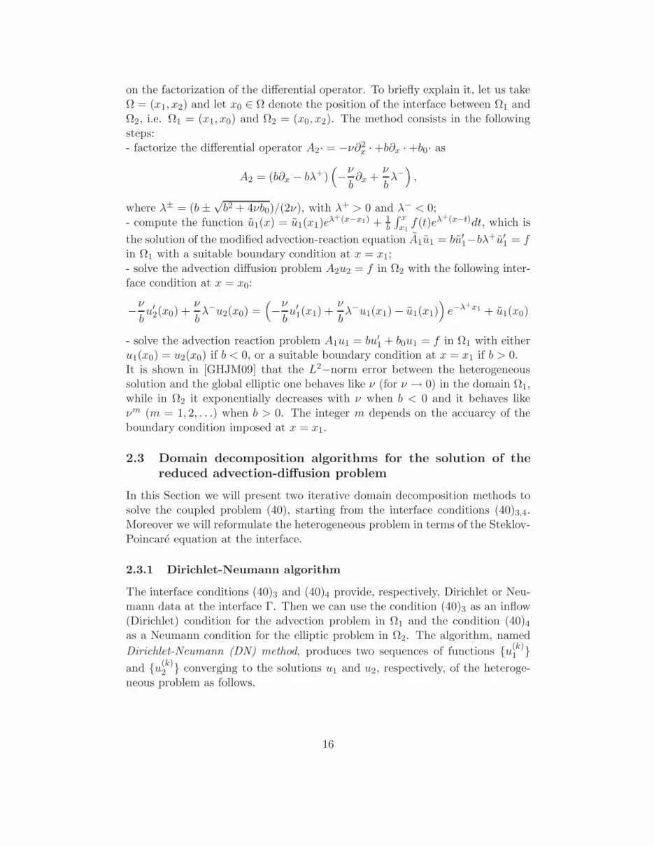
The algorithm (48) is obtained as the limit, when ε→ 0, of the Adaptive-Robin-Neumann (ARN) method proposed in [CQ95] for the homogeneous global elliptic

problem (37). In its original form, ARN method reads: given λ(0), µ(0) and u(0)2 ,

for k ≥ 0 do

solve

−ε∆u(k+1)1,ε + div(~bu

(k+1)1,ε ) + b0u

(k+1)1,ε = f in Ω1

u(k+1)1,ε = g on (∂Ω1 \ Γ)in

ε∂u

(k+1)1,ε

∂nΓ−~b · ~nΓu

(k+1)1,ε = νε

∂u(k)2,ε

∂nΓ−~b · ~nΓλ

(k) on Γin1 = Γin

ε∂u

(k+1)1,ε

∂nΓ= νε

∂u(k)2,ε

∂nΓon Γout

1 = Γout,

solve

div(−νε∇u(k+1)2,ε +~bu

(k+1)2,ε ) + b0u

(k+1)2,ε = f in Ω2

u(k+1)2,ε = g on ∂Ω2 \ Γ

νε∂u

(k+1)2,ε

∂nΓ−~b · ~nΓu

(k+1)2,ε = ε

∂u(k+1)1,ε

∂nΓ−~b · ~nΓµ

(k) on Γin2 = Γout

νε∂u

(k+1)2,ε

∂nΓ= ε

∂u(k+1)1,ε

∂nΓon Γout

2 = Γin,

compute

λ(k+1) = (1 − θ)λ(k) + θu

(k+1)2,ε on Γin

µ(k+1) = (1 − θ)µ(k) + θu(k+1)1,ε on Γout.

(49)

18

The idea of this method is to impose a Robin interface condition on the local(i.e. referred to that subdomain) inflow interface Γin

i (i = 1, 2) and a Neumanninterface condition on the local outflow interface Γout

i (i = 1, 2).Coming back to the heterogeneous coupling, it is straightforward to prove that,if the choice of θ guarantees the convergence of ARN method, then the limitsolution of ARN (48) coincides with the solution of the heterogeneous problem

(40). Moreover, if u(0)2 is chosen with null normal derivative on the interface Γ

and θ = 1, then ARN (48) and DN (47) methods coincide.When either Γin = Γ or Γout = Γ we can conclude that no iterations are needfor ARN method, as for DN.

Remark 2.1 We want to remark here that in the Dirichlet/Neumann method,the Neumann condition (47)6 is in fact a conormal derivative associated to thedifferential operator A2. On the contrary, in the ARN method the Neumann con-dition (as (48)7) is a pure normal derivative on the interface, while the conormalderivative (48)6 is called Robin condition, in agreement with the classical defi-nition of Robin boundary condition. Following the latter notation, actually theDirichlet/Neumann method should be a Dirichlet/Robin method.

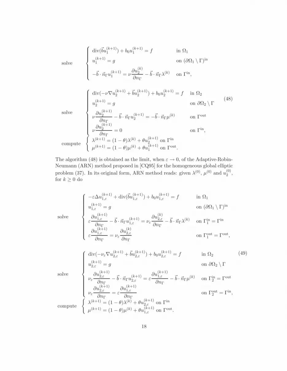
2.3.3 Steklov-Poincare based solution algorithms

Let us consider the heterogeneous problem (40) with homogeneous Dirichlet

conditions on ∂Ω, i.e., g ≡ 0. Let λ ∈ H1/200 (Γ) denote the unknown trace of the

solution u2 on Γ. Thanks to the interface condition (40)4, the solution (u1, u2)of (40) can be written as

u1 = uλ1 + w1, u2 = uλ2 + w2,

where:w1 and w2 depend on the assigned function f and are the solution of

A1w1 = f in Ω1

w1 = 0 on ∂Ωin1 ,

A2w2 = f in Ω2

w2 = 0 on ∂Ω2,(50)

while uλ1 and uλ2 are the solutions of

A1uλ1 = 0 in Ω1

uλ1 = 0 on (∂Ω1 \ Γ)in

uλ1 = λ|Γin on Γin,

A2uλ2 = 0 in Ω2

u2 = 0 on ∂Ω2 \ Γuλ2 = λ on Γ.

(51)

Given λ ∈ H1/200 (Γ), we define the Steklov-Poincare operators S1 and S2 such

that

S1λ =

~b · ~nΓu

λ1 on Γout

0 on Γin(52)

19

and

S2λ =

ν∂uλ2∂nΓ

−~b · ~nΓuλ2 on Γout

ν∂uλ2∂nΓ

on Γin.

(53)

Actually, S1λ depends only on the values of λ on Γin.Then the interface conditions (40)3 can be equivalently expressed in terms ofSteklov-Poincare operators as

Sλ ≡ S1λ+ S2λ = χ, (54)

where

χ =

−~b · ~nΓw1 − ν∂w2

∂nΓ+~b · ~nΓw2 on Γout

−ν ∂w2

∂nΓon Γin.

(55)

The operator S : H1/200 (Γ) → (H

1/200 (Γ))′ is the so-called Steklov-Poincare oper-

ator and the equation (54) is the Steklov-Poincare equation associated to theheterogeneous problem (40). The solution of (40) can be reached by sequentiallysolving the problems (50), (54) and (51).Several methods may be invoked to solve the Steklov-Poincare equation (54).To start, let us consider the preconditioned Richardson method

λ(0) given

P (λ(k+1) − λ(k)) = θ(χ− Sλ(k)), for k ≥ 0,(56)

where P is the preconditioner and θ > 0 an acceleration parameter.Thanks to the well-posedness of the ellitpic problem in Ω2, the operator S2 isinvertible and we can use it as preconditioner, so that (56) becomes:

λ(0) given

λ(k+1) = (1 − θ)λ(k) + θS−12 (χ− S1λ

(k)), for k ≥ 0.(57)

By comparing (57) with (47), we recognize that the Dirichlet-Neumann methodis equivalent to the Richardson iterative method applied to the Steklov-Poincare

equation (54) with preconditioner S2, since the identity u(k+1)2 |Γ = S−1

2 (χ −S1λ

(k)) holds.After a discretization of the heterogeneous problem (by, e.g., finite elements orspectral methods) it is possible to write the discrete counterpart of both theSteklov-Poincare equation (54) and the Dirichlet-Neumann algorithm (47).It can be be proven that the Dirichlet-Neumann algorithm converges, for suit-able choices of the relaxation parameter θ, independently of the discretizationparameter h for finite elements or N for spectral methods (see, e.g., [GQL90] for

20

a proof in the spectral method context). This because the local Steklov-Poincareoperator S2 is spectrally equivalent to the global Steklov-Poincare operator S.Krylov methods are valid alternatives to Richardson iterations to solve the pre-conditioned Steklov-Poincare equation

S−12 Sλ = S−1

2 χ. (58)

In the next section we will provide numerical results about the numerical so-lution of the coupled problem (40) by using either Dirichlet-Neumann method(47), Adaptive Robin-Neumann method (48) and the preconditioned Bi-CGStab([vdV92]) on the equation (58).

2.4 Numerical results for the advection-diffusion problem

In this Section we will provide the numerical solution of a test case in two-dimensional computational domains. The discretization of the differential equa-tion inside each subdomain is performed by quadrilateral conformal SpectralElement Methods (SEM). We refer to [CHQZ07] for a detailed description ofthese methods, while here we recall in brief their basic features.Let T = TmMm=1 be a partition of the computational domain Ω ⊂ Rd, whereeach element Tm is obtained by a bijective and differentiable transformation Fmfrom the reference (or parent) element Ωd = (−1, 1)d. On the reference elementwe define the finite dimensional space QN = spanxj11 · · · xjdd : 0 ≤ j1, . . . , jd ≤N and, for any Tm ∈ T : Tm = ~Fm(Ωd), set hm = diam(Tm) and

VNm(Tm) = v : v = v ~F−1m for some v ∈ QNm.

The SEM multidimensional space is

Xδ = v ∈ C0(Ω) : v|Tm∈ VNm(Tm), ∀Tm ∈ T

where δ is an abridged notation for “discrete”, that accounts for the local geo-metric sizes hm and the local polynomial degrees Nm, for m = 1, . . . ,M .Let us consider the variational formulation (38) and, for simplicity, impose thehomogeneous Dirichlet condition on the boundary (i.e. g ≡ 0). The SEMapproximation of the solution of (38) is the function uδ ∈ Vδ = Xδ ∩ H1

0 (Ω),such that ∑

m

aTm(uδ, vδ) =∑

m

(f, vδ)Tm ∀vδ ∈ Vδ (59)

holds, where aTm and (f, v)Tm denote the restrictions to Tm of the bilinear formand the L2-inner product (respectively) defined in (39).Since the high computational cost in evaluating integrals in (59), the bilinearform aTm and the L2-inner product (f, v)Tm are often approximated by a dis-crete bilinear form aNm,Tm and a discrete inner product (f, v)Nm,Tm, respectively,in which exact integrals are replaced by Numerical Integration (NI) based on

21

layer

Ω1

Ω2

5.787×10−7

1.000×100

x

−1

0

1 y−1

0

1

5.787×10−7

1.000×100

x

−1

0

1 y−1

0

1

Figure 8: Test case #1. The data of the test case (left) and the heterogeneoussolution for ν = 0.01 (left) and ν = 0.001 (right)

Legendre-Gauss-Lobatto formulas.The SEM-NI approximation of the solution of (38) will be the function uδ ∈ Vδsuch that ∑

m

aNm,Tm(uδ , vδ) =∑

m

(f, vδ)Nm,Tm ∀vδ ∈ Vδ. (60)

We consider now a test case and we compare the convergence rate of the it-erative methods explained in Section 2.3. We will denote by DN the DirichletNeumann method (47), by ARN the Adaptive Robin-Neumann method (48) andby BiCGStab-SP the preconditioned BiCGstab method applied to the precon-ditioned Steklov-Poincare equation (58). Our aim is twofold. From one handwe will represent the numerical solution of the heterogeneous problem (40), onthe other hand we want to investigate and compare the convergence rate of theiterative methods versus the magnitude of the viscosity ν and the discretizationsize (i.e. the local geometric sizes hm and the local polynomial degrees Nm).

Test case #1Let us consider problem (40). The computational domain Ω = (−1, 1)2 is splitin Ω1 = (−1, 0.8) × (−1, 1) and Ω2 = (0.8, 1) × (−1, 1). The interface is Γ =0.8 × (−1, 1). The data of the problem are: ~b = [y, 0]t, b0 = 1, f = 1 andthe inflow interface is Γin = 0.8 × (−1, 0). Dirichlet boundary conditions areimposed on the vertical sides of Ω, precisely g = 1 on −1 × (0, 1), g = 0on 1 × (−1, 1), while homogeneous Neumann conditions are imposed on thehorizontal sides of Ω2. The viscosity will be specified below.In Fig. 8 the SEM-NI solutions for ν = 10−2 and ν = 10−3 are shown. Anon-uniform partition in 3 × 6 (4 × 6, resp.) quadrilaterals has been consideredin Ω1 (Ω2, resp.). The same polynomial degree N = 8 has been fixed inside eachspectral element. The jump of the solution across Γout is evident for ν = 0.01,in particular we have obtained ‖u1 − u2‖L∞(Γout) ≃ 0.237 when ν = 0.01 and‖u1 − u2‖L∞(Γout) ≃ 0.020 when ν = 0.001.Now we want to compare DN, ARN and BiCGStab-SP methods for what con-cerns the convergence rate and the computational efficiency.

22

0.5 0.6 0.7 0.8 0.9 1 1.1 1.2 1.30

5

10

15

20

25

DNARN

θ

Iter

atio

ns

Figure 9: Test case #1 with ν = 0.01. DN and ARN iterations to satisfy thestopping test (61) versus the relaxation parameter θ

The convergence of both DN and ARN is measured by the stopping test on thedifference between two iterates, i.e.

‖λ(k+1) − λ(k)‖ ≤ ǫ for DN

max‖λ(k+1) − λ(k)‖, ‖µ(k+1) − µ(k)‖ ≤ ǫ for ARN,(61)

while the convergence of BiCGStab-SP is measured by the stopping test on theresidual r(k+1) = χ− Sλ(k+1), i.e.

‖r(k+1)‖‖r(0)‖ ≤ ǫ. (62)

The convergence of both DN and ARN methods depends on the choice of therelaxation parameter θ, on the contrary, the BiCGStab-SP algorithm does notrequire to set any acceleration parameter.In Fig. 9 we report the number of iterations of both DN and ARN methodsin order to converge up to a tolerance of 10−6 for ν = 0.01 and we concludethat, for this test case, the optimal value of θ is θopt = 1. Analogous results areobtained for smaller values of the viscosity.In Table 1 we report the number of iterations needed by every iterative scheme(DN, ARN, BiCGstab-SP) to converge up to a tolerance of 10−6, versus thepolynomial degree N . For both DN and ARN method we set θ = 1. Thepartition of Ω is not uniform and it coincides with that used to represent thenumerical solutions in Fig. 8. The discretization we have used is fine enough toguarantee the absence of spurious oscillations due to large Peclet number.As we can see, the convergence rate of all methods is independent of both poly-nomial degree N and viscosity ν.The BiCGStab-SP method requires the smallest number of iterations, neverthe-less each Bi-CGStab iteration costs about two and a half iterations of either

23

ν = 0.1 ν = 0.01 ν = 0.001

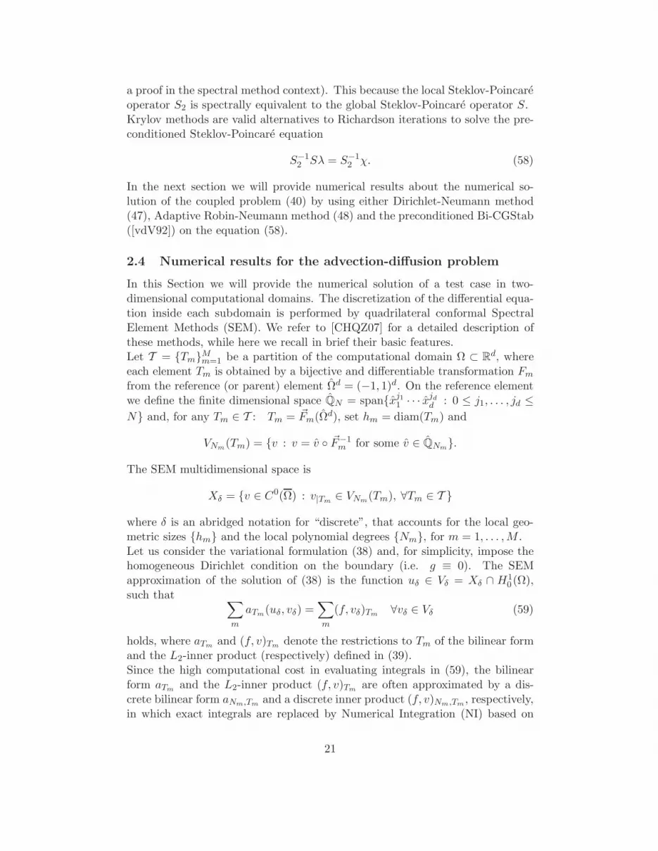
N DN ARN SP DN ARN SP DN ARN SP

4 2 3 1 2 3 1 2 3 16 2 3 1 2 3 1 2 3 18 2 3 1 2 3 1 2 3 110 2 3 1 2 3 1 2 3 112 2 3 1 2 3 1 2 3 114 2 3 1 2 3 1 2 3 116 2 3 1 2 3 1 2 3 1

Table 1: Test case #1. Number of iterations to satisfy stopping test with ǫ =10−6. The relaxation parameter is θ = 1 in both DN and ARN. SP is an abridgednotation for BiCGStab-SP method.

DN or ARN. As a matter of fact, each iteration of DN (or equivalenlty ARN)requires the solution of an advection problem in Ω1 plus the solution of an el-liptic problem in Ω2. On the contrary, each iteration of BiCGstab-SP requirestwo matrix vector products to compute the residual r(k) = χ − Sλ(k) plus thesolution of two linear systems on the preconditioner S2z

(k) = r(k), meaning thatwe have to solve two advection problems in Ω1 plus three elliptic problems inΩ2 at each iteration.For this test case, we conclude that all three methods are very efficient and theircomputational costs are comparable. Nevertheless, both DN and ARN methodsrequire a-priori knowledge of the optimal relaxation parameter θ.

2.5 Navier-Stokes/potential coupled problem

Models similar to the (Navier-)Stokes/Darcy problem introduced in Sect. 1 canbe used in external aerodynamics to describe the motion of an incompressiblefluid around a body such as, for example, a ship, a boat or a submerged bodyin a water basin. In fact, such problems can be studied by decomposing thecomputational domain into two parts: a region Ω2 close to the body where, dueto the viscosity effects, all the interesting features of the flow occur, and an outerregion Ω1 far away from the body where one can neglect the viscosity effects.See, e.g., Fig. 10.Therefore, suitable heterogeneous differential models comprising Navier-Stokesequations, Euler equations, potential flows and other models from fluid dynamicscould be envisaged (see, e.g., [BCR89, IC03]).Here, we present a simple model where in Ω2 we consider the full Navier-Stokesequations, while in Ω1 we adopt a Laplace equation for the velocity potential.A coupled heterogeneous model of this kind has been studied in [SH93] consid-ering a computational domain as in Fig. 11 and the following generalized Stokes

24

Ω1

Ω2

Γ

Potential

Navier-Stokes

Figure 10: Flow around a cylinder computed using a Navier-Stokes/potentialcoupled problem.

problem:

α~uǫ − νǫ∆~uǫ + ∇pǫ = ~f in Ω∇ · ~uǫ = 0 in Ω

~uǫ = ~0 on Γb,

(63)

with suitable boundary conditions on the outer boundary Γ∞. The viscosity isνǫ = ν in Ω2, while νǫ = ǫ in Ω1.

Γ∞

Γb

Ω1

Γ

body

Ω2

~n

inflow

Figure 11: Representation of the computational domain for an external aerody-namics problem

In [SH93] a vanishing viscosity argument is used letting ǫ → 0 in Ω1 in orderto set up a suitable global model and to define the correct interface conditionsacross Γ. Precisely, the following limit coupled problem was characterized:

α~u− ν∆~u+ ∇p = ~f in Ω2

∇ · ~u = 0 in Ω2

∆q = ∇ · ~f in Ω1

(64)

25

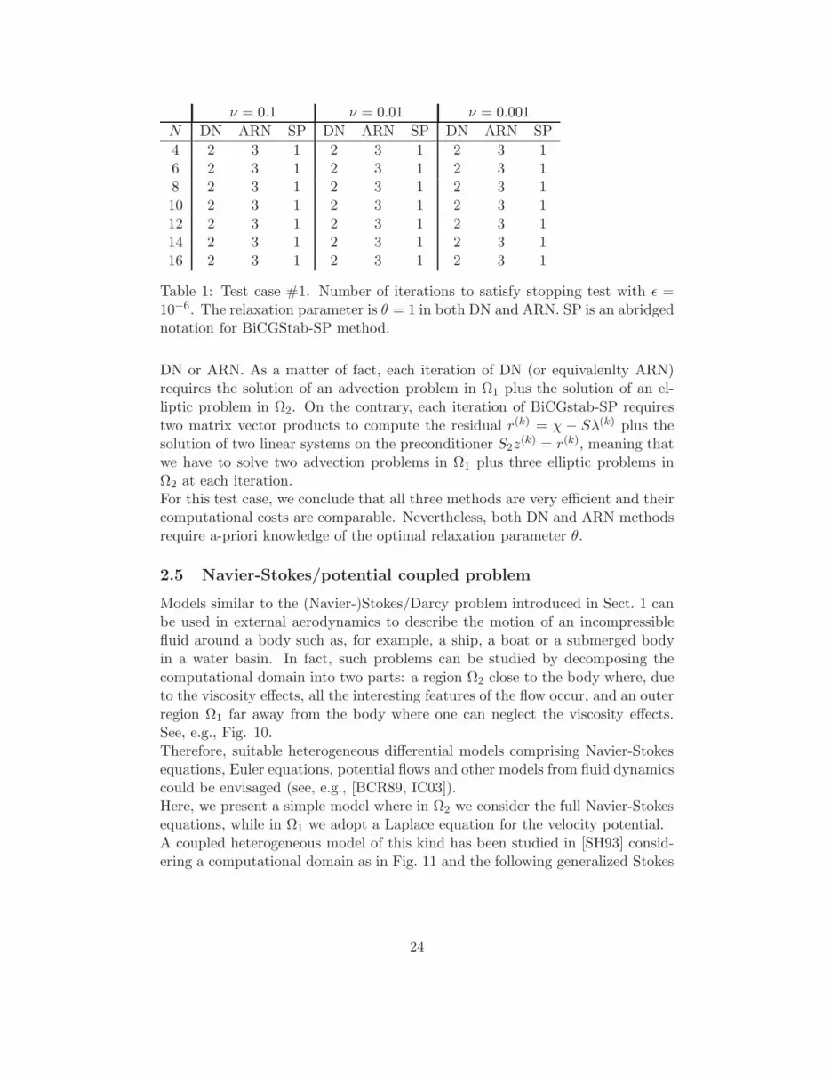
with suitable boundary conditions and the coupling conditions across the inter-face Γ

∂q

∂~nΓ= (~f − α~u) · ~nΓ on Γ

−ν ∂~u∂~nΓ

+ p~nΓ = q~nΓ on Γ.

(65)

~nΓ denotes the unit normal vector on Γ directed from Ω2 to Ω1. We remarkthat, apart from the physical meaning of the variables, the coupling conditions(65) are similar in their structure to those used for the Navier-Stokes/Darcycoupling (28). In fact, (65)1 corresponds to (28)1, and in (65)2 the pressure isstill discontinuous across the interface, even if there is no distinction betweenthe normal and the tangential components of the stress tensor as in (28)2 and(28)3.Because of these similarities, the analysis that we shall develop in Sect. 2.6 forthe Navier-Stokes/Darcy problem could be accommodated to account also forthe heterogenous coupling (64)-(65).However, one has to keep in mind that the physical meaning of the two coupledproblems is very different. In the Navier-Stokes/Darcy case we have two viscousmodels where Darcy equation and the coupling conditions can be obtained byhomgenization in the limit ǫ→ 0 in Ωp, where ǫ represents the size of the poresin the porous medium. On the other hand, the Navier-Stokes/potential modelcouples viscous and inviscid equations, the latter being obtained in the limitν → 0 like also the corresponding coupling conditions.

2.6 Asymptotic analysis of the coupled Navier-Stokes/Darcyproblem

We focus now on the coupled Navier-Stokes/Darcy problem (27)-(28), howeverwe confine ourselves to the steady problem by dropping the time-derivative inthe momentum equation (27)1:

−div T(uf , pf ) + (uf · ∇)uf = f in Ωf . (66)

Even when considering the time-dependent problem, a similar kind of “steady”problem can be found when using an implicit finite difference time-advancingscheme. In that case, however, an extra reaction term αuf would show up onthe left-hand side of (66), where the positive coefficient α plays the role of inverseof the time-step. This reaction term would not affect our forthcoming analysis,though.

To discuss possible boundary conditions on the external boundary of Ωf and Ωp,let us split the boundaries ∂Ωf and ∂Ωp as ∂Ωf = Γ∪Γinf and ∂Ωp = Γ∪Γp∪Γbp,as shown in Fig. 6, left.For the Darcy equation we assign the piezometric head ϕ = ϕp on Γp; moreover,we require that the normal component of the velocity vanishes on the bottomsurface, that is, up · np = 0 on Γbp.

26

For the Navier-Stokes problem, several combinations of boundary conditions arepossible, representing different kinds of flow problems. Here, we assign a non-null inflow uf = uin on Γinf and a no-slip condition uf = 0 on the remainingboundary Γf .To summarize, the coupled problem (66)-(28) is supplemented with the boundaryconditions:

uf = uin on Γinf , uf = 0 on Γf ,

ϕ = ϕp on Γp, K∂ϕ

∂n= 0 on Γbp.

(67)

We introduce the following functional spaces:

Hf = v ∈ (H1(Ωf ))d : v = 0 on Γf ∪ Γinf ,

Hf = v ∈ (H1(Ωf ))d : v = 0 on Γf ∪ Γ,

Q = L2(Ωf ), Hp = ψ ∈ H1(Ωp) : ψ = 0 on Γp.(68)

We denote by | · |1 and ‖ · ‖1 the H1–seminorm and norm, respectively, andby ‖ · ‖0 the L2–norm; it will always be clear form the context whether we arereferring to spaces on Ωf or Ωp.The space W = Hf ×Hp is a Hilbert space with norm

‖w‖W =(‖w‖2

1 + ‖ψ‖21

)1/2 ∀w = (w, ψ) ∈W.

Finally, we consider on Γ the trace space Λ = H1/200 (Γ) and denote its norm by

‖ · ‖Λ (see [LM68]).

We introduce a continuous extension operator

Ef : (H1/2(Γinf ))d → Hf . (69)

Then ∀uin ∈ (H1/200 (Γinf ))d we can construct a vector function Efuin ∈ Hf such

that Efuin|Γinf

= uin.

We introduce another continuous extension operator:

Ep : H1/2(Γbp) → H1(Ωp) such that Epϕp = 0 on Γ. (70)

Then, for all ϕ ∈ H1(Ωp) we define the function ϕ0 = ϕ− Epϕp.

Finally, we define the following bilinear forms:

af (v,w) =

∫

Ωf

ν

2(∇v + ∇Tv) · (∇w + ∇Tw) ∀v,w ∈ (H1(Ωf ))

d,

bf (v, q) = −∫

Ωf

q div v ∀v ∈ (H1(Ωf ))d, ∀q ∈ Q,

ap(ϕ,ψ) =

∫

Ωp

∇ψ · K∇ϕ ∀ϕ,ψ ∈ H1(Ωp) ,

(71)

27

and, for all v,w, z ∈ (H1(Ωf ))d, the trilinear form

cf (w; z,v) =

∫

Ωf

[(w · ∇)z] · v =d∑

i,j=1

∫

Ωf

wj∂zi∂xj

vi . (72)

Now, if we multiply (66) by v ∈ Hf and integrate by parts we obtain

af (uf ,v) + cf (uf ;uf ,v) + bf (v, pf ) −∫

Γn · T(uf , pf )v =

∫

Ωf

f · v .

Notice that we can write

−∫

Γn · T(uf , pf )v = −

∫

Γ[n · T(uf , pf ) · n]v · n −

∫

Γ(T(uf , pf ) · n)τ · (v)τ ,

so that we can incorporate in weak form the interface conditions (28)2 and (28)3as follows:

−∫

Γn · T(uf , pf )v =

∫

Γgϕ(v · n) +

∫

Γ

ναBJ√K

(uf )τ · (v)τ .

Finally, we consider the lifting Efuin of the boundary datum and we split uf =u0f +Efuin with u0

f ∈ Hf ; we recall that Efuin = 0 on Γ and we get

af (u0f ,v) + cf (u

0f + Efuin;u

0f + Efuin,v) + bf (v, pf )

+

∫

Γgϕ(v · n) +

∫

Γ

ναBJ√K

(uf )τ · (v)τ =

∫

Ωf

f · v − af (Efuin,v). (73)

From (27)2 we find

bf (u0f , q) = −bf (Efuin, q) ∀q ∈ Q. (74)

On the other hand, if we multiply (27)3 by ψ ∈ Hp and integrate by parts weget

ap(ϕ,ψ) +

∫

ΓK∂ϕ

∂nψ = 0 .

Now we incorporate the interface condition (28)1 in weak form as

ap(ϕ,ψ) −∫

Γ(uf · n)ψ = 0,

and, considering the splitting ϕ = ϕ0 + Epϕp we obtain

ap(ϕ0, ψ) −∫

Γ(uf · n)ψ = −ap(Epϕp, ψ). (75)

28

We multiply (75) by g and sum to (73) and (74); then, we define

A(v,w) = af (v,w) + g ap(ϕ,ψ) +

∫

Γg ϕ(w · n) −

∫

Γg ψ(v · n)

+

∫

Γ

ναBJ√K

(w)τ · (v)τ ,

C(v;w, u) = cf (v;w,u),B(w, q) = bf (w, q),

(76)

for all v = (v, ϕ), w = (w, ψ), u = (u, ξ) ∈ W , q ∈ Q. Finally, we define thefollowing linear functionals:

〈F , w〉 =

∫

Ωf

f ·w − af (Efuin,w) − g ap(Epϕp, ψ),

〈G, q〉 = −bf (Efuin, q),(77)

for all w = (w, ψ) ∈W , q ∈ Q.Adopting these notations, the weak formulation of the coupled Navier-Stokes/Darcyproblem reads:

find u = (u0f , ϕ0) ∈W , pf ∈ Q such that

A(u, v) + C(u+ u∗;u+ u∗, v) + B(v, pf ) = 〈F , v〉 ∀v = (v, ψ) ∈WB(u, q) = 〈G, q〉 ∀q ∈ Q,

(78)with u∗ = (Efuin, 0) ∈ Hf ×H1(Ωp).

Remark that the interface conditions (28) have been incorporated in the weakformulation as natural conditions on Γ: in particular, (28)2 and (28)3 are nat-ural conditions for the Navier-Stokes problem, while (28)1 becomes a naturalcondition for Darcy’s problem.The well-posedness of (78) can be proved quite easily in the case of the Stokes/Darcycoupling, i.e. when we neglect the trilinear form C(·; ·, ·). Indeed, in this casethe existence and uniqueness of the solution follows from the classical theoryof Brezzi for saddle-point problems after proving the continuity of A(·, ·), itscoerciveness on the kernel of B(·, ·) and that an inf-sup condition holds betweenthe spaces W and Q. For details of this analysis we refer to [DQ03].The case of the Navier-Stokes/Darcy problem is more involved. In particular, inthis case we could prove the well-posedness only under some hypotheses on thedata similar to those required for the sole Navier-Stokes equations. Moreover,uniqueness is guaranteed only in the case of small enough filtration velocitiesuf · n across Γ. The analysis that we have carried out is based on classicalresults for nonlinear saddle-point problems (see, e.g., [GR86]). We refer thereader to [BDQ08, DQ09]. Similar results have been proved using a differentapproach in [GR07].

29

2.7 Solution techniques for the Navier-Stokes/Darcy coupling

A possible approach to solve the Navier-Stokes/Darcy problem is to exploit itsnaturally decoupled structure keeping separated the fluid and the porous mediaparts and exchanging information between surface and groundwater flows onlythrough boundary conditions at the interface. From the computational point ofview, this strategy is useful at the stage of setting up effective methods to solvethe problem numerically.Therefore, we apply a domain decomposition technique at the differential levelto study the Navier-Stokes/Darcy coupled problem. Our aim will be to intro-duce and analyze a generalized Steklov-Poincare interface equation (see [QV99])associated to our problem, in order to reformulate it solely in terms of inter-face unknowns. This re-interpretation is crucial to set up iterative proceduresbetween the subdomains Ωf and Ωp, that can be used at the discrete level.Here we illustrate the main ideas behind this approach, and refer to [DQ09] fora complete analysis.We choose a suitable governing variable on the interface Γ. Considering theinterface conditions (28)1 and (28)2, we can foresee two different strategies toselect the interface variable:

1. we can set the interface variable λ as the trace of the normal velocity onthe interface:

λ = uf · n = −K∂ϕ

∂n; (79)

2. we can define the interface variable σ as the trace of the piezometric headon Γ:

σ = ϕ = −1

gn · T(uf , pf ) · n. (80)

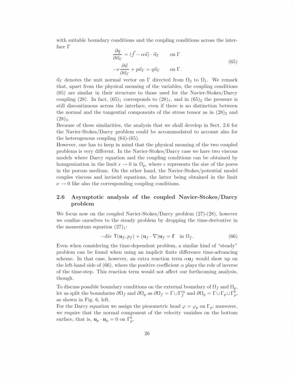
Both choices are suitable from the mathematical viewpoint since they guaranteewell-posed subproblems in the fluid and the porous medium part.We discuss here the approach in the case of the Stokes/Darcy coupling consid-ering the choice of the interface variable λ as in (79). We refer the reader to[Dis04a] for the second case (80).For simplicity, from now on we consider the following condition on the interface:

(uf )τ = 0 on Γ (81)

instead of (28)3.

Consider the auxiliary problems:

−div T(u∗, p∗) = f in Ωf

div u∗ = 0 in Ωf

u∗ = uin on Γinf(u∗)τ = 0 on Γu∗ · n = 0 on Γ,

−div (K∇ϕ∗) = 0 in Ωp

ϕ∗ = ϕp on Γp

K∂ϕ∗

∂n= 0 on Γbp

K∂ϕ∗

∂n= 0 on Γ.

(82)

30

Then, assuming to know the value of λ ∈ Λ0, with

Λ0 = µ ∈ H1/200 (Γ) :

∫Γ µ = 0,

we consider the problems:

−div T(uλ, pλ) = 0 in Ωf

div uλ = 0 in Ωf

uλ = 0 on Γinf(uλ)τ = 0 on Γuλ · n = λ on Γ,

−div (K∇ϕλ) = 0 in Ωp

ϕλ = 0 on Γp

K∂ϕλ

∂n= 0 on Γbp

K∂ϕλ

∂n= λ on Γ.

(83)

We can prove that the solution of the Stokes-Darcy problem can be expressedas: uf = uλ + u∗, pf = pλ + p∗, ϕ = ϕλ + ϕ∗, where λ ∈ Λ0 is the solution ofthe Steklov-Poincare equation

(Sf + Sp)λ = χ on Γ. (84)

Sf and Sp are the local Steklov-Poincare operators formally defined as:

Sf : Λ0 → Λ′0 such that Sfλ = n · T(uλ, pλ) · n on Γ,

whileSp : Λ0 → Λ′

0 such that Spλ = gϕλ on Γ.

Finally,χ = −n · T(u∗, p∗) · n− gϕ∗ on Γ.

The analysis of the operators Sf and Sp as well as the study of the well-posednessof the interface equation (84) have been carried out in [DQ03]. In particular, wehave proved that the operator Sf is invertible on the trace space Λ0 and it isspectrally equivalent to Sf + Sp, i.e., there exist two positive constants k1 andk2 (independent of η) such that

k1〈Sfη, η〉 ≤ 〈Sη, η〉 ≤ k2〈Sfη, η〉 ∀η ∈ Λ0.

The same property holds at the discrete level considering conforming finite ele-ment approximations of Sf and Sp with constants k1 and k2 that do not dependon the grid size h. This property makes the operator Sf an attractive precon-ditioner to solve the interface problem (84) via an iterative method like, e.g.,Richardson or the Conjugate Gradient, yielding a convergence rate independentof h.For example, we can consider the following Richardson iterations: given λ(0)inΛ0,for k ≥ 0,

λ(k+1) = λ(k) + θS−1f (χ− (Sf + Sp)λ

(k)) on Γ, (85)

where 0 < θ < 1 is a suitable relaxation parameter.

31

This method requires at each step to apply Sp and S−1f , i.e., recalling the defi-

nitions of these operators, to solve a Darcy problem in Ωp with given flux acrossΓ and a Stokes problem in Ωf with assigned normal stress on Γ. More precisely,we can rewrite (85) as: let λ(0) ∈ Λ be an initial guess; for k ≥ 0,

solve

−div (K∇ϕ(k+1)) = 0 in Ωp

ϕ(k+1) = ϕp on Γp

K∂ϕ(k+1)

∂n= 0 on Γbp

K∂ϕ(k+1)

∂n= λ(k) on Γ,

solve

−div T(u(k+1), p(k+1)) = f in Ωf

div u(k+1) = 0 in Ωf

u(k+1) = uin on Γinf(u(k+1))τ = 0 on Γ

−n · T(u(k+1), p(k+1)) · n = gϕ(k+1) on Γ,

compute λ(k+1) = (1 − θ)λ(k) + θu(k+1) · n on Γ.

(86)

Remark that this algorithm has the same structure as the Dirichlet-Neumannmethod in the domain decomposition framework.

Another possible algorithm that we have studied in [DQV07] is a sequentialRobin-Robin method which at each iteration requires to solve a Darcy problemin Ωp followed by a Stokes problem in Ωf , both with Robin conditions on Γ.Precisely, the algorithm reads as follows.Having assigned a trace function η0 ∈ L2(Γ), and two acceleration parametersγf ≥ 0 and γp > 0, for each k ≥ 0:

32

solve

−div (K∇ϕ(k+1)) = 0 in Ωp

ϕ(k+1) = ϕp on Γp

K∂ϕ(k+1)

∂n= 0 on Γbp

−γpK∂ϕ(k+1)

∂n+ gϕ

(k+1)|Γ = η(k) on Γ,

solve

−div T(u(k+1), p(k+1)) = f in Ωf

div u(k+1) = 0 in Ωf

u(k+1) = uin on Γinf(u(k+1))τ = 0 on Γ

n · T(uk+1f , pk+1

f ) · n + γfu(k+1)f · n

= −gϕ(k+1)|Γ − γfK

∂ϕ(k+1)

∂non Γ,

compute η(k+1) = −n · T(u(k+1)f , p

(k+1)f ) · n + γpu

(k+1)f · n on Γ.

(87)

Both the Stokes problem in Ωf and the Darcy problem in Ωp are well-posed and,at convergence, we recover the solution (uf , pf ) ∈ Hf × Q and ϕ ∈ Hp of thecoupled Stokes/Darcy problem. Indeed, denoting by ϕ∗ the limit of the sequenceϕk in H1(Ωp) and by (u∗

f , p∗f ) that of (ukf , p

kf ) in (H1(Ωf ))

d ×Q, we obtain

−γpK∂ϕ∗

∂n+ gϕ∗

|Γ = −n · T(u∗f , p

∗f ) · n + γpu

∗f · n on Γ , (88)

so that we have

(γf + γp)u∗f · n = −(γf + γp)K

∂ϕ∗

∂non Γ ,

yielding, since γf + γp 6= 0, u∗f · n = −K

∂ϕ∗

∂n on Γ, and also, from (88), thatn · T(u∗

f , p∗f ) · n = −gϕ∗

|Γ on Γ. Thus, the two interface conditions (28)1 and

(28)2 are satisfied, and we can conclude that the limit functions ϕ∗ ∈ Hp and(u∗

f , p∗f ) ∈ Hf ×Q are the solutions of the coupled Stokes/Darcy problem.

A proof of convergence is presented in [DQV07] and it follows the guidelines ofthe theory by P.-L. Lions [Lio90] for the Robin-Robin method (see also [QV99,Sect. 4.5]).A crucial point in the algorithm is the choice of the acceleration parameters γfand γp. A general strategy is not available, but thanks to a reinterpretationof the Robin-Robin method as an alternating direction scheme a la Peaceman-Rachford (see [PR55]), we were able to give some hints on how to choose them.We refer to [DQV07].

We will illustrate the numerical behavior of the Dirichlet-Neumann and of theRobin-Robin algorithms in Sect. 2.8.

33

Finally, we address the case of the Navier-Stokes/Darcy coupling. Also to thisnonlinear problem we can asociate an interface equation similar to (84) stillinvolving the operator Sp but a nonlinear operator Sf analogous to Sf . Formally,we can represent Sf : Λ0 → Λ′

0 as the operator associated to the Navier-Stokesproblem:

−div T(uλ, pλ) + (uλ · ∇)uλ = 0 in Ωf

div uλ = 0 in Ωf

uλ = 0 on Γinf(uλ)τ = 0 on Γuλ · n = λ on Γ,

(89)

such that Sfλ = n · T(uλ, pλ) · n on Γ.Then, we can write the interface problem:

find λ ∈ Λ0 : Sf (λ) + Spλ = χp on Γ, (90)

with χp =, and prove its equivalence to the global coupled problem.A rigorous presentation of this approach can be found in [BDQ08].The set-up of effective iterative methods for the interface problem (90) is notstraightforward. In particular, no results are available yet on the characterizationof suitable operators spectrally equivalent to Sf + Sp. In [BDQ08, DQ09] wehave proposed and analyzed two classical schemes, fixed-point or Newton, for(90) showing their equivalence to the following algorithms, respectively.

Fixed-point iterations. Given u0f ∈ Hf , for k ≥ 1, find u

(k)f ∈ Hf , p

(k)f ∈ Q,

ϕ(k) ∈ Hp such that, for all v ∈ Hf , q ∈ Q, ψ ∈ Hp,

af (u(k)f ,v) + cf (u

(k−1)f ;u

(k)f ,v) + bf (v, p

(k)f )

+

∫

Γg ϕ(k)(v · n) +

∫

Γ

ναBJ√K

(u(k)f )τ · (v)τ =

∫

Ωf

f · v

bf (u(k)f , q) = 0

ap(ϕ(k), ψ) =

∫

Γψ(u

(k)f · n) .

(91)

Newton-like methods. Let u0f ∈ Hf be given; then, for k ≥ 1, find u

(k)f ∈ Hf ,

p(k)f ∈ Q, ϕ(k) ∈ Hp such that, for all v ∈ Hf , q ∈ Q, ψ ∈ Hp,

af (u(k)f ,v) + cf (u

(k)f ;u

(k−1)f ,v) + cf (u

(k−1)f ;u

(k)f ,v) + bf (v, p

(k)f )

+

∫

Γgϕn(v · n) +

∫

Γ

ναBJ√K

(u(k)f )τ · (v)τ

= cf (u(k−1)f ;u

(k−1)f ,v) +

∫

Ωf

f · v

bf (u(k)f , q) = 0

ap(ϕ(k), ψ) =

∫

Γψ(u

(k)f · n) .

(92)

34

Some numerical results will be presented in Sect. 2.8

2.8 Numerical results for the Navier-Stokes/Darcy problem

We consider a regular triangulation Th of the domain Ωf ∪ Ωp, depending on apositive parameter h > 0, made up of triangles T . We assume that the triangu-lations Tfh and Tph induced on the subdomains Ωf and Ωp are compatible on Γ,that is they share the same edges therein. Finally, we suppose the triangulationinduced on Γ to be quasi-uniform (see, e.g., [Qua09]).Several choices of finite element spaces can be made. If we indicate by Wh andQh the finite element spaces which approximate the velocity and pressure fields,respectively, for the Navier-Stokes problem, there must exist a positive constantβ∗ > 0, independent of h, such that the classical inf-sup condition is satisfied,i.e., ∀qh ∈ Qh, ∃vh ∈ Wh, vh 6= 0, such that

∫

Ωf

qh div vh ≥ β∗‖vh‖H1(Ωf )‖qh‖L2(Ωf ).

No additional compatibility condition is required when coupling with the Darcyequations. Thus, for our tests we use the P2 − P1 Taylor-Hood finite elementsfor Stokes or Navier-Stokes and P2 elements for Darcy equation.

We investigate the convergence properties of algorithm (86) (or, equivalently,(85)) and the PCG algorithm for (84) with preconditioner S−1

f . For the momentwe set the physical parameters ν, K, g to 1. We consider the computationaldomain Ω ⊂ R2 with Ωf = (0, 1) × (1, 2), Ωp = (0, 1) × (0, 1) and the interfaceΓ = (0, 1) × 1. The boundary conditions and the forcing terms are chosen insuch a way that the exact solution of the coupled Stokes/Darcy problem is

(uf )1 = − cos(π

2y)

sin(π

2x), (uf )2 = sin

(π2y)

cos(π

2x)− 1 + x,

pf = 1 − x, ϕ =2

πcos(π

2x)

cos(π

2y)− y(x− 1),

where (uf )1 and (uf )2 are the components of the velocity field uf (see [DQ09]).Four different regular conforming meshes have been considered whose numberof elements in Ω and of nodes on Γ are reported in Table 2, together with thenumber of iterations to convergence. A tolerance 10−10 has been prescribed forthe convergence tests based on the relative residues. In the Dirichlet-Neumann-like algorithm (86) we set the relaxation parameter θ = 0.7.Figure 12 shows the computed residues for the adopted iterative methods whenusing the finest mesh (logarithmic scale on the y-axis).These numerical tests show that the discrete preconditioner Sf is optimal withrespect to the grid parameter h since the corresponding preconditioned methodsyield convergence in a number of iterations independent of h.

We consider now the influence of the physical parameters, which govern the cou-pled problem, on the convergence rate. We use the PCG method as it embeds

35

Table 2: Number of iterations obtained on different grids.

Number of Number of Algorithm (86) PCG for (84)mesh elements nodes on Γ (θ = 0.7) (preconditioner S−1

f )

172 13 18 5688 27 18 52752 55 18 511008 111 18 5

0 5 10 15 2010

−12

10−10

10−8

10−6

10−4

10−2

100

102

Iterations

Algorithm (86)PCG for (84)

Figure 12: Computed relative residues for the interface variable λ.

the choice of dynamic optimal acceleration parameters. We take the same com-putational domain, but here the boundary data and the forcing terms are chosenin such a way that the exact solution of the coupled problem is (see [DQ09]):

(uf )1 = y2 − 2y + 1, (uf )2 = x2 − x, pf = 2ν(x+ y − 1) +g

3K,

ϕ =1

K

(x(1 − x)(y − 1) +

y3

3− y2 + y

)+

2ν

gx.

The most relevant physical quantities for the coupling are the fluid viscosity νand the hydraulic conductivity K. Therefore, we test our algorithms with respectto different values of ν and K, and set the other physical parameters to 1. Weconsider a convergence test based on the relative residue with tolerance 10−10.In Table 3 we report the number of iterations necessary for several choices of νand K. The symbol # indicates that the method did not converge within 150iterations.We can see that the convergence of the algorithm is troublesome when the valuesof ν and K decrease. In fact, in that case the method converges in a large numberof iterations which increases when h decreases, losing its optimality properties.The subdomain iterative method that we have proposed is then effective onlywhen the product νK is sufficiently large, while dealing with small values causessevere difficulties.

36

Table 3: Iterations using the PCG method (preconditioner S−1f ) with respect to

several values of ν and K.

ν K h = 1/7 h = 1/14 h = 1/28 h = 1/561 1 5 5 5 5

10−1 10−1 11 11 10 1010−2 10−1 15 19 18 1710−3 10−2 20 54 73 5610−4 10−3 20 59 # #10−6 10−4 20 59 148 #

However, the algorithm still performs well if, instead of the steady Stokes prob-lem, one considers the generalized Stokes momentum equation:

γuf − div T(uf , pf ) = f in Ωf , (93)

where γ can represent the inverse of a time step within a time discretizationusing, e.g., the implicit Euler method. Some numerical results are reported inTable 4 (see also [Dis04b]).

Table 4: Number of iterations to solve problem the modified Stokes/Darcy prob-lem using (93) for different values of ν, K and γ.

Iterations on the mesh with grid sizeν K γ h = 1/7 h = 1/14 h = 1/28 h = 1/56

10 15 24 28 2810−3 10−2 102 12 14 16 14

103 8 9 9 8103 15 23 28 33

10−6 10−4 104 13 14 17 18105 8 9 9 9

On the other hand, the Robin-Robin method (87) performs quite well in presenceof small values of ν and K. We present hereafter a test considering the samesetting as for Table 3. The analogy with the Peaceman-Rachford method hassuggested us to set γf = 0.3 and γp = 0.1 (see [Dis04a] for more details). InTable 5 we report the number of iterations obtained using the Robin-Robinmethod for some small values of ν and K and for four different computationalgrids. A convergence test based on the relative increment of the trace of thediscrete normal velocity on the interface ukfh · n|Γ has been considered with

tolerance 10−9. (See [DQV07].)

Finally, we present some numerical tests for the Navier-Stokes/Darcy couplingusing the fixed-point and Newton algorithms of Sect. 2.7. The computational

37

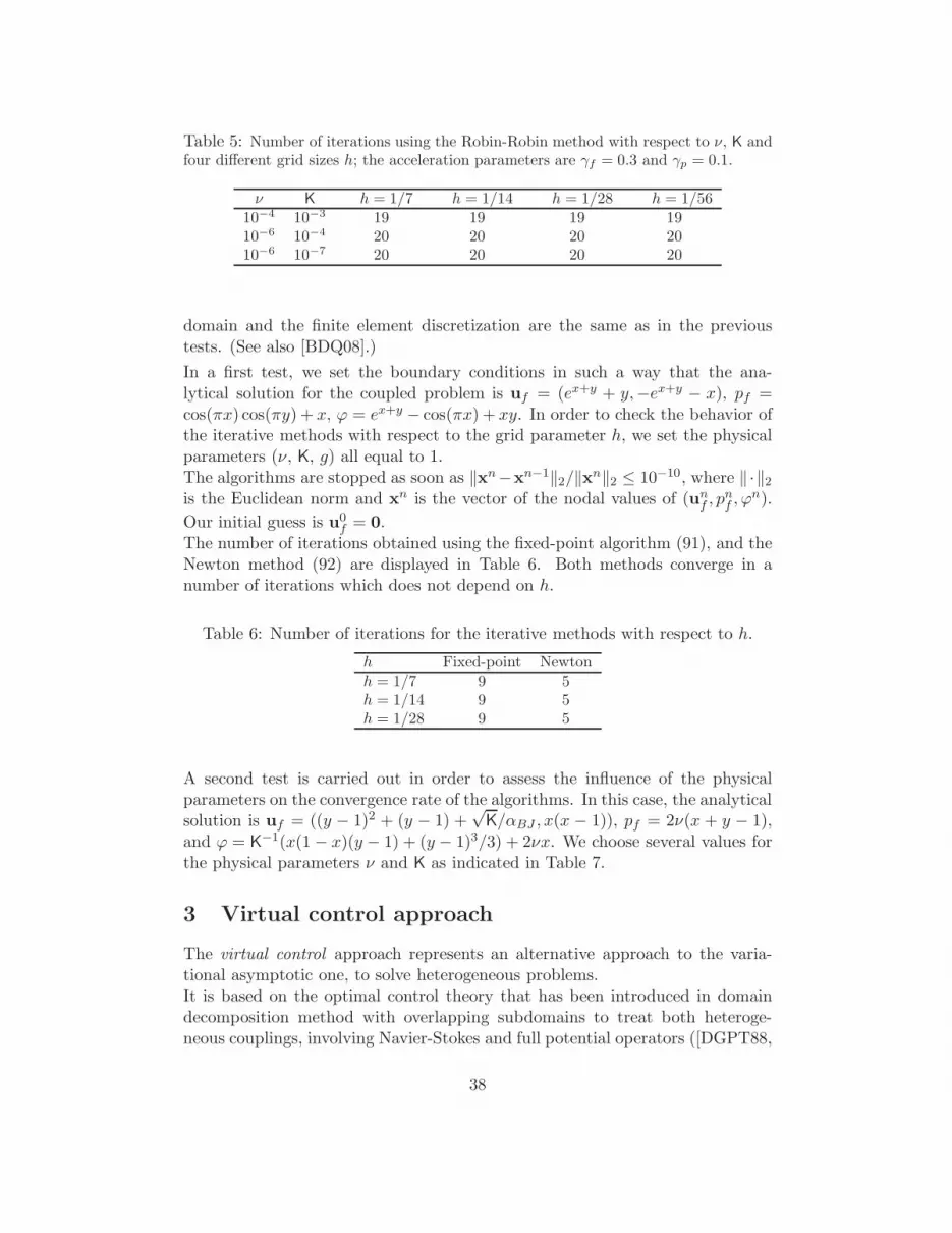
Table 5: Number of iterations using the Robin-Robin method with respect to ν, K andfour different grid sizes h; the acceleration parameters are γf = 0.3 and γp = 0.1.

ν K h = 1/7 h = 1/14 h = 1/28 h = 1/5610−4 10−3 19 19 19 1910−6 10−4 20 20 20 2010−6 10−7 20 20 20 20

domain and the finite element discretization are the same as in the previoustests. (See also [BDQ08].)

In a first test, we set the boundary conditions in such a way that the ana-lytical solution for the coupled problem is uf = (ex+y + y,−ex+y − x), pf =cos(πx) cos(πy) + x, ϕ = ex+y − cos(πx) + xy. In order to check the behavior ofthe iterative methods with respect to the grid parameter h, we set the physicalparameters (ν, K, g) all equal to 1.The algorithms are stopped as soon as ‖xn−xn−1‖2/‖xn‖2 ≤ 10−10, where ‖·‖2

is the Euclidean norm and xn is the vector of the nodal values of (unf , pnf , ϕ

n).

Our initial guess is u0f = 0.

The number of iterations obtained using the fixed-point algorithm (91), and theNewton method (92) are displayed in Table 6. Both methods converge in anumber of iterations which does not depend on h.

Table 6: Number of iterations for the iterative methods with respect to h.

h Fixed-point Newtonh = 1/7 9 5h = 1/14 9 5h = 1/28 9 5

A second test is carried out in order to assess the influence of the physicalparameters on the convergence rate of the algorithms. In this case, the analyticalsolution is uf = ((y − 1)2 + (y − 1) +

√K/αBJ , x(x − 1)), pf = 2ν(x + y − 1),

and ϕ = K−1(x(1 − x)(y − 1) + (y − 1)3/3) + 2νx. We choose several values for

the physical parameters ν and K as indicated in Table 7.

3 Virtual control approach

The virtual control approach represents an alternative approach to the varia-tional asymptotic one, to solve heterogeneous problems.It is based on the optimal control theory that has been introduced in domaindecomposition method with overlapping subdomains to treat both heteroge-neous couplings, involving Navier-Stokes and full potential operators ([DGPT88,

38

Table 7: Number of iterations of the fixed-point (FP) and Newton (N) methodswith respect to the parameters ν and K.

ν K h = 1/7 h = 1/14 h = 1/28FP N FP N FP N

1 1 7 5 7 5 7 51 10−4 5 4 5 4 5 4

10−1 10−1 10 5 10 5 10 510−2 10−1 17 6 17 6 17 610−2 10−3 14 5 14 5 14 5

GPT90]), and homogeneous problems, either elliptic and parabolic (see [DGP80,GPD82, LP98a, LP98b, LP99]). In the pioneering papers of Glowinski et al.([DGP80, GPD82]), this method was referred to as a Least Square formulationof the multi domain problem.The basic idea of this approach consists in introducing two “virtual” controlswhich play the role of unknown Dirichlet data on the interfaces of the decompo-sition and in minimizing the L2−norm of the difference between the hyperbolicand the elliptic solutions (defined inside the two subdomains) on the overlap.The virtual control approach for heterogeneous advection-diffusion operatorswas introduced and analysed in [GLQ01] and there it has been extended to non-overlapping subdomain decompositions (with sharp interfaces). In the lattersituation, the virtual controls are defined on the unique interface and the costfunctional to be minimized has to be chosen accurately in order to guaranteethe well posedness of the optimal control problem.Finally, in [AGQ06] two different formulations of the heterogeneous advection-diffusion problem with either two and three virtual controls have been analysedfor overlapping decompositions.In the following subsection we will give a detailed description of virtual controlapproach with either overlapping and non-overlapping decompositions for theheterogeneous problems introduced in Section 1.Here we only note that the virtual control approach without overlap is moreefficient than the overlapping version, however the former requires a more definitea-priori knowledge on structure of interface conditions. On the contrary, thevirtual control approach with overlap is more general and it can be regarded asa rigorous translation of a common practice in engineering community based onsolving both problems in a common region and using simple “Dirichlet” typeconditions at subdomain boundaries.

3.1 Virtual control approach without overlap for AD problems

The idea of this approach consists in formulating an optimal control problem([Lio71]) featuring both control and observation on the interface Γ. We in-

39

Ω1

Ω1

Ω2

Ω2

Γ ΓΓinλ1 λ2

Figure 13: Virtual control without overlap

troduce two functions λ1 and λ2 defined on the interface Γ and called virtualcontrols, such that they represent the unknown Dirichlet data on Γ for u1 andu2, respectively, i.e.

u1 = λ1 on Γin, u2 = λ2 on Γ. (94)

By collecting differential equations (32) and (33), the external boundary condi-tions (36) and the interface condition (94), we consider the following problem:given λ1, λ2, find u1 = u1(λ1) and u2 = u2(λ2) such that

A1u1 = div(~bu1) + b0u1 = f in Ω1

u1 = g1 on (∂Ω1 \ Γ)in

u1 = λ1 on Γin

(95)

and

A2u2 = −div(ν∇u2) + div(~bu2) + b0u2 = f in Ω2

u2 = g2 on ∂Ω2 \ Γu2 = λ2 on Γ.

(96)

In the case where Γin = ∅, no λ1 is needed since there is no need to prescribeany boundary data on Γin for problem (95).The virtual controls λ1 and λ2 are determined in such a way that the solutionsu1 and u2 of (95) and (96) adjust in the best possible way on Γ. More precisely,we look for the solution of the minimization problem

infλ1, λ2

J(λ1, λ2), (97)

where J(λ1, λ2) is a suitably chosen cost functional.Various instances have been proposed and analyzed in [GLQ01]. Consider, forexample,

J(λ1, λ2) =1

2‖u1(λ1) − u2(λ2)‖2

L2~b(Γin) +

1

2‖φ1(λ1) + φ2(λ2)‖2

H−1/2(Γ) , (98)

40

where

φ1(λ1) = −~b · ~nΓu1(λ1), φ2(λ2) = −ν ∂u2(λ2)

∂~nΓ+~b · ~nΓu2(λ2) (99)

are the fluxes on Γ associated to the differential operators A1 and A2 (respec-

tively) andH−1/2(Γ) is the dual space ofH1/200 (Γ). Denoting by −∆Γ the Laplace

Beltrami operator on Γ, for any ψ, φ ∈ H−1/2(Γ) we define the following innerproduct (see, e.g., [Lio71]):

(ψ, φ)H−1/2(Γ) =

∫

Γ(−∆Γ)−1/4ψ (−∆Γ)−1/4φdΓ =

∫

Γ(−∆Γ)−1/2ψ φdΓ (100)

and the related norm ‖ψ‖H−1/2(Γ) = (ψ,ψ)1/2

H−1/2(Γ).

We note that the observation is performed on the whole interface Γ for whatconcerns the gap on the fluxes, whereas it is restricted to the inflow interface Γin

for that on the velocities.From now on, by solution of the virtual control approach we will mean the so-lution of the minimization problem (97), with J defined in (98) and with ui(λi)(for i = 1, 2) the solutions of problems (95) and (96), respectively.Problems (95) and (96) are well posed. As a matter of fact, the following resultholds (see, e.g., [GQL90]):

Theorem 3.1 Under assumptions (44), if g1 ∈ L2~b((∂Ω1\Γ)in) and λ1 ∈ L2

~b(Γin),

then the first-order problem (95) admits a unique solution u1 = u1(λ1) ∈ L2(Ω1).Moreover u1 ∈ L2

~b(∂Ω1) and div(~bu1) ∈ L2(Ω1).

As of problem (96), if g2 ∈ H1/2(∂Ω2 \ Γ) and λ2 ∈ H1/2(Γ), and moreoverthere exists a function µ ∈ H1/2(∂Ω2) with g2 = µ|(∂Ω2\Γ) and λ2 = µ|Γ, thenthere exists a unique solution u2(λ2) of (96) belonging to H1(Ω2). (See, e.g.,[GQL90].)We introduce the following spaces

V1 = w ∈ L2(Ω1) : div(~bw) ∈ L2(Ω1), w|Γ ∈ L2~b(Γ), Λ1 = L2

~b(Γin),

V2 = H1(Ω2),

Λ2 =λ2 ∈ H1/2(Γ) : ∃µ ∈ H1/2(∂Ω2) s.t. λ2 = µ|Γ and g2 = µ|∂Ω2\Γ

,

~V = V1 × V2, Λ = Λ1 × Λ2.

(101)

In order to prove the existence of solution of the minimization problem (97), wedefine two pairs of auxiliary problems:find (wf1 , w

f2 ) ∈ ~V such that

A1wf1 = f in Ω1

wf1 = g1 on (∂Ω1 \ Γ)in

wf1 = 0 on Γin,

A2wf2 = f in Ω2

wf2 = g2 on ∂Ω2 \ Γ

wf2 = 0 on Γ,

(102)

41

and find (uλ1

1 , uλ2

2 ) ∈ ~V such that

A1uλ1

1 = 0 in Ω1

uλ1

1 = 0 on (∂Ω1 \ Γ)in

uλ1

1 = λ1 on Γin,

A2uλ2

2 = 0 in Ω2

uλ2

2 = 0 on ∂Ω2 \ Γ

uλ2

2 = λ2 on Γ.

(103)

Moreover we define the fluxes on the interface Γ associated to the solutions uλ1

1

and uλ2

2 as

φλ1

1 = −~b · ~nΓuλ1

1 , φλ2

2 = −ν ∂uλ2

2

∂~nΓ+~b · ~nΓu

λ2

2 , (104)

while those associated to the solutions wf1 and wf2 are

χ1 = −~b · ~nΓwf1 , χ2 = −ν ∂w

f2

∂~nΓ+~b · ~nΓw

f2 . (105)

The cost functional J can be split as

J(λ1, λ2) = J0(λ1, λ2) + A(λ1, λ2) (106)

where

J0(λ1, λ2) =1

2‖λ1 − λ2‖2

L2~b(Γin) +

1

2

∥∥∥φλ1

1 + φλ2

2

∥∥∥2

H−1/2(Γ),

while A is an affine functional which reads

A(λ1, λ2) =1

2‖χ1 + χ2‖2

H−1/2(Γ) +(χ1 + χ2, φ

λ1

1 + φλ2

2

)H−1/2(Γ)

.

If all data are smooth enough, the existence of λ = (λ1, λ2) achieving infJ(λ1, λ2)in a possibly very large abstract spaceΛ, follows from the property of (J0(λ1, λ2))

1/2

to be a norm (see [GLQ01, Sect. 5]).

3.1.1 The optimality system

By following standard arguments of optimal control theory for elliptic problems(see [Lio71]), we derive now the optimality system corresponding to the mini-mization problem (97).Let us write the minimization problem (97) in a variational setting, i.e., we lookfor the solution λ = (λ1, λ2) ∈ Λ such that

〈∇J(λ),µ〉 = 0 ∀µ ∈ Λ. (107)

The partial derivative of J are

〈 ∂J∂λ1

, µ1〉 = (λ1 − λ2, µ1)L2~b(Γin) + (φ1(λ1) + φ1(λ2), φ

µ1

1 )H−1/2(Γ) ∀µ1 ∈ Λ1,

〈 ∂J∂λ2

, µ2〉 = − (λ1 − λ2, µ2)L2~b(Γin) + (φ1(λ1) + φ1(λ2), φ

µ2

2 )H−1/2(Γ) ∀µ2 ∈ Λ2,

(108)

42

where, for any (µ1, µ2) ∈ Λ, φµ1

1 and φµ2

2 follow the definition of the fluxes as in(104), while uµ1

1 , uµ2

2 are defined as in (103).From the definition (100), for i = 1, 2 we obtain

(φ1(λ1) + φ1(λ2), φµii )H−1/2(Γ) =

∫

Γ(−∆Γ)−1/2(φ1(λ1) + φ1(λ2)) φ

µii dΓ (109)

and, in particular for the flux φµ1

1 , it holds∫

Γ(−∆Γ)−1/2(φ1(λ1) + φ2(λ2)) φ

µ1

1 dΓ =

=

∫

Γin

(−∆Γ)−1/2(φ1(λ1) + φ2(λ2)) (−~b · ~nΓ)µ1dΓ

+

∫

Γout

(−∆Γ)−1/2(φ1(λ1) + φ1(λ2)) (−~b · ~nΓ)uµ1

1 dΓ.

(110)

By defining the adjoint problems

A∗1p1 ≡ −~b · ∇p1 + b0p1 = 0 in Ω1

p1 = 0 on (∂Ω1 \ Γ)out

p1 = (−∆Γ)−1/2(φ1(λ1) + φ2(λ2)) on Γout,

(111)

and

A∗2p2 ≡ −div(ν∇p2) −~b · ∇p2 + b0p2 = 0 in Ω2

p2 = 0 on ∂Ω2 \ Γ

p2 = (−∆Γ)−1/2(φ1(λ1) + φ2(λ2)) on Γ,

(112)

and, by making use of Green’s formula, we have:

∫

Γout

(−∆Γ)−1/2(φ1(λ1) + φ1(λ2)) (−~b · ~nΓ)uµ1

1 dΓ =

∫

Γout

p1 (−~b · ~nΓ)uµ1

1 dΓ

=

∫

Γin

(~b · ~nΓ)p1µ1dΓ

while∫

Γ(−∆Γ)−1/2(φ1(λ1) + φ1(λ2)) φ

µ2

2 dΓ =

∫

Γp2

(−ν ∂u

µ2

2

∂~nΓ+~b · ~nΓu

µ2

2

)dΓ

= −∫

Γν∂p2

∂~nΓµ2,

whence

〈 ∂J∂λ1

, µ1〉 =

∫

Γin

(−~b · ~nΓ) [(λ1 − λ2) + (p2 − p1)]µ1dΓ,

〈 ∂J∂λ2

, µ2〉 =

∫

Γin

(~b · ~nΓ)(λ1 − λ2)µ2dΓ −∫

Γν∂p2

∂~nΓµ2dΓ

(113)

43

for any µ1 ∈ Λ1 and µ2 ∈ Λ2. In conclusion, the solution of the minimizationproblem (97) satisfies the following optimality system (in distributional sense):

(OS)

- state equations (95) and (96);

- adjoint equations (111) and (112);

- Euler equations:

(λ1 − λ2) + p2 − p1 = 0 on Γin

~b · ~nΓ(λ1 − λ2) − ν∂p2

∂~nΓ= 0 on Γin

−ν ∂p2

∂~nΓ= 0 on Γout.

3.1.2 Computation of the Laplace-Beltrami operator

The computation of the discrete counterpart of (−∆Γ)−1/2(φ1(λ1)+φ2(λ2)) whenΩ ⊂ R2 can be made as follows.Given a differentiable function u in an open neighbourhood of Γ, the tangentialgradient of u is defined by (see, e.g., [DDE05])

∇Γu(~x) = ∇u(~x) − (∇u(~x) · ~nΓ(~x))~nΓ(~x), ∀~x ∈ Γ, (114)

where ∇ denotes the usual gradient in R2. The Laplace-Beltrami operator canbe defined through the weak relation

∫

Γ−∆Γu wdΓ =

∫

Γ∇Γu · ∇ΓwdΓ, (115)

for any function w differentiable in an open neighbourhood of Γ vanishing at theend-points of Γ. In particular, if Γ is a segment parallel to the y-axis, it reducesto ∫

Γ−∆Γu wdΓ =

∫

Γ

∂u

∂y

∂w

∂ydΓ. (116)

In a finite dimensional context, if AΓ,h denotes the symmetric positive definitematrix associated to the discretization of (116), we approximate (−∆Γ)1/2 by

the square root of AΓ,h, that is the s.p.d. matrix A1/2Γ,h defined by

A1/2Γ,h = PΛ1/2P T , (117)

where Λ and P are the eigenvalues and eigenvectors matrices, respectively, ofAΓ,h.Alternatively, the fractional Laplace-Beltrami operator (−∆Γ)−1/2 can be de-fined through a Neumann to Dirichlet map defined from H−1/2(Γ) to H1/2(Γ).

44

Precisely, for any φ ∈ H−1/2(Γ) we solve the problem

−∆u+ u = 0 in Ω1

∂u

∂~n= 0 on ∂Ω1 \ Γ

∂u

∂~nΓ= φ on Γ

(118)

and we set (−∆Γ)−1/2φ = u|Γ. The differential problem (118) may be solved inΩ2 instead of Ω1.

3.1.3 Recovering the interface conditions

In order to recover the interface conditions we are imposing on the interface Γ,we eliminate the adjoint state variables p1 and p2 from the optimality system(OS).

Let us set ~b = −~b, b0 = b0 − div~b and

Γinb = Γout, Γout

b = Γin, (∂Ω1 \ Γ)inb = (∂Ω1 \ Γ)out.

Thanks to (111), (112) and Euler equations in (OS), the functions p1 and p2

satisfy the following coupled problem in Ω

div(~bp1) + b0p1 = 0 in Ω1

−div(ν∇p2) + div(~bp2) + b0p2 = 0 in Ω2

p1 = 0 on (∂Ω1 \ Γ)inb

p2 = 0 on ∂Ω2 \ Γ

−ν ∂p2

∂~nΓ+ (~b · ~nΓ)p2 = (~b · ~nΓ)p1 on Γout

b

p1 = p2 on Γinb

ν∂p2

∂~nΓ= 0 on Γin

b .

(119)

By noting that b0 + 12div~b = b0 + 1

2div~b ≥ σ0 > 0 (see (31)) and by applyingTheorem 2.1, problem (119) admits the unique solution p1 = 0 in Ω1, p2 = 0 inΩ2. Therefore, (112)3 implies φ1(λ1) + φ2(λ2) = 0 on Γ, while the first Eulerequation in (OS) implies that λ1 − λ2 = 0 on Γin, i.e. the following conditionshold on the interface:

φ1(λ1) + φ2(λ2) = 0 on Γ

λ1 = λ2 on Γin.(120)

In conclusion the following result holds:

45

Theorem 3.2 If λ is the solution of the minimization problem (97) with Jdefined in (98), then the state solutions u1 and u2 of (95) and (96) satisfy theinterface conditions (120). Moreover the pair (u1(λ1), u2(λ2)), obtained by thevirtual control approach coincides with the solution of the heterogeneous problem(40).

Thanks to the interface condition (120)2, the virtual control problem may bereformulated in terms of a unique control function λ defined on Γ and coincidingwith λ2. The control λ1, previously introduced, will coincide now with therestriction of λ to Γin.By this reduction, the virtual control problem (97) becomes:look for the solution of the minimization problem

infλ∈Λ2

J1(λ) with J1(λ) =1

2‖φ1(λ) + φ2(λ)‖2

H−1/2(Γ), (121)

with

φ1(λ) = −~b · ~nΓu1(λ), φ2(λ) = −ν ∂u2(λ)

∂~nΓ+~b · ~nΓu2(λ) (122)

and u1 = u1(λ), u2 = u2(λ) solutions of (95) and (96) with λ2 = λ, λ1 = λ|Γin.By working as done for the two-controls formulation, the derivative of the costfunctional J1 reads:

〈J ′1(λ), µ〉 =

∫

Γin

(−~b · ~nΓ)(p2 − p1)µdΓ

−∫

Γν∂p2

∂~nΓµdΓ

(123)

for any µ ∈ Λ2.The corresponding optimality system (OS1) reads:

(OS1)

- state equations (95) and (96) with λ2 = λ, λ1 = λ|Γin

- adjoint equations (111) and (112) with φi(λ) instead of φi(λi), for i = 1, 2 ;

- Euler equations:

(~b · ~nΓ)(p2 − p1) + ν∂p2

∂~nΓ= 0 on Γin

ν∂p2

∂~nΓ= 0 on Γout

Remark 3.1 Another cost functional proposed in [GLQ01] is

J(λ1, λ2) =1

2‖u1(λ1) − u2(λ2)‖2

L2~b(Γ) +

1

2‖φ1(λ1) + φ2(λ2)‖2

H−1/2(Γ) . (124)

In this case the observation is performed on the whole interface for both fluxesand velocities. The minimization problem (97), in which the functional J isreplaced by J , admits a unique solution too (see [GLQ01]), however it is notguaranteed that inf J(λ1, λ2) = 0, so that no interface conditions are explicitelyassociated to this minimization problem.

46

Remark 3.2 We finally remark that the cost functional to be minimized isset up starting from known interface conditions, it is problem dependent andit requires a-priori knowledge of the coupled problem. When the latter arenot available, it is more suitable to consider the virtual control approach withoverlap, that we will introduce in Section 3.3.

3.1.4 How to solve the optimality system

A first intuitive way to solve the optimality system (OS1) consists in invokinga Krylov method to seek the solution λ of the Euler equation of (OS1). Let uswrite the Euler equation, in distributional sense, as

J ′1(λ) = 0. (125)

When we solve it by a Krylov method, like either GMRES or Bi-CGStab, wehave to evaluate the action of the functional J ′

1 on the iterate λ(k) at eachiteration k ≥ 0 and this means to perform the steps summarized in the followingalgorithm.

Algorithm 1

1. solve the primal problems (95) and (96) with λ(k) instead of λi, for i = 1, 2;

2. compute the fluxes φ1(λ(k)), φ2(λ

(k)) and the functions(k) = (−∆Γ)−1/2(φ1(λ

(k)) + φ2(λ(k)))

3. solve the dual problems (111), (112) with s(k) instead of (−∆Γ)−1/2(φ1(λ1)+φ2(λ2))

4. compute J ′1(λ

(k)) by (123), which reads (in distributional sense):

J ′1(λ) =

(−~b · ~nΓ)(p2 − p1) − ν∂p2

∂~nΓon Γin

−ν ∂p2

∂~nΓon Γout.

(126)

The solution of the Euler equation J ′1(λ) = 0, by a Krylov method with the use

of Algorithm 1, is an alternative to the solution of the Steklov-Poincare equation(54).By properly replacing the definition of both state and adjoint equations andby correctly writing the derivatives of the cost functional, Algorithm 1 can beadapted to solve the optimality system associated to the minimization of J .Solving J ′(λ) = 0 is equivalent to solve the Schur complement with respect tothe control variable λ derived from the optimal system (OS1).

47

J1(λ) J(λ1, λ2)

ν ‖u1 − u2‖L∞(Γout) inf J1 #it ‖u1 − u2‖L∞(Γout) inf J #it

0.1 2.330e-1 1.242e-12 18 1.367e-1 5.239e-6 440.05 1.221e-1 3.137e-12 27 5.275e-2 3.286e-7 610.01 1.346e-2 6.989e-11 60 7.146e-4 6.234e-10 1340.005 1.075e-2 2.294e-11 82 5.049e-4 8.749e-10 177

,

Table 8: Test case #1. Comparison between the cost functionals (121) and(124). #it stands for the number of Bi-CGStab-VC iterations

3.1.5 Numerical results for decompositions without overlap

Let us consider the Test case #1 introduced in Sect. 2.4. First of all we comparethe numerical solutions obtained by the virtual control approach by minimizingeither the cost functional J1(λ) defined in (121) (or, equivalently J(λ1, λ2) de-fined in (98)) and J(λ1, λ2) defined in (124). We have solved both the optimalitysystem (OS1) and that associated to the minimization of J by Bi-CGStab iter-ations and by following the steps summarized in Algorithm 1 (see Sect. 3.1.4).We will name Bi-CGStab-VC this approach.In Table 8 we report for both the functionals (121) and (124):- the L∞-norm on Γout of the jump of the solution, i.e., [u]Γout = ‖u1−u2‖L∞(Γout);- the infimum of the minimized cost functional;- the number of Bi-CGStab-VC iterations to converge up a tolerance ε = 10−8

versus the viscosity ν.A non-uniform spectral element discretization has been considered to solve theboundary-value problems in both Ω1 and Ω2. The domain Ω1 (Ω2, resp.) hasbeen split in 3× 6 (4× 6, resp.) quadrilaterals with the same polynomial degreeN = 16 in each spatial direction and in each element.First of all we note that not only the solution (u1, u2), obtained by minimizingthe cost functional J1, features a jump on Γout (in fact we know that it isdiscontinuous on Γout), but also the solution obtained by minimizing the costfunctional J is discontinuous on Γout. Moreover, as pointed out in Remark 3.1,we observe that the value inf J is not null for any considered viscosity, howeverinf J → 0 as ν → 0.We have observed that the reached value inf J1 is independent of the viscosityand it is very close to the machine accuracy.About the number of Bi-CGStab iterations needed to solve the variational equa-tion J ′

1(λ) = 0, we observe that the convergence rate linearly depends on thereciprocal of the viscosity, that the minimimiziation of J requires twice the iter-ations to minimize J1 and that the computational cost of each Bi-CGStab-VCiteration is the same for both the minimization problems. Then we concludethat the minimization of the cost functional J costs twice that of J1.

48

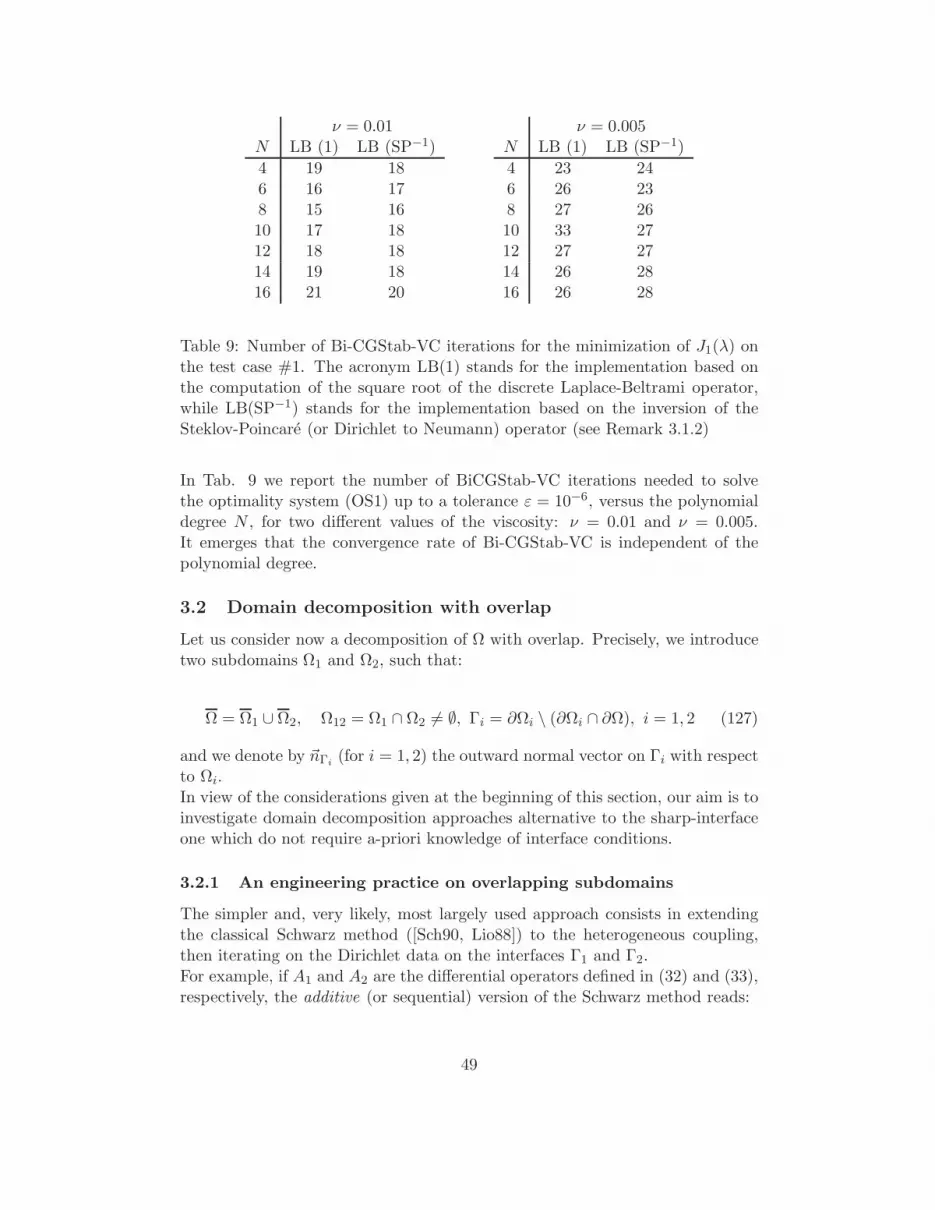
ν = 0.01N LB (1) LB (SP−1)

4 19 186 16 178 15 1610 17 1812 18 1814 19 1816 21 20

ν = 0.005N LB (1) LB (SP−1)

4 23 246 26 238 27 2610 33 2712 27 2714 26 2816 26 28

Table 9: Number of Bi-CGStab-VC iterations for the minimization of J1(λ) onthe test case #1. The acronym LB(1) stands for the implementation based onthe computation of the square root of the discrete Laplace-Beltrami operator,while LB(SP−1) stands for the implementation based on the inversion of theSteklov-Poincare (or Dirichlet to Neumann) operator (see Remark 3.1.2)

In Tab. 9 we report the number of BiCGStab-VC iterations needed to solvethe optimality system (OS1) up to a tolerance ε = 10−6, versus the polynomialdegree N , for two different values of the viscosity: ν = 0.01 and ν = 0.005.It emerges that the convergence rate of Bi-CGStab-VC is independent of thepolynomial degree.

3.2 Domain decomposition with overlap

Let us consider now a decomposition of Ω with overlap. Precisely, we introducetwo subdomains Ω1 and Ω2, such that:

Ω = Ω1 ∪ Ω2, Ω12 = Ω1 ∩ Ω2 6= ∅, Γi = ∂Ωi \ (∂Ωi ∩ ∂Ω), i = 1, 2 (127)

and we denote by ~nΓi (for i = 1, 2) the outward normal vector on Γi with respectto Ωi.In view of the considerations given at the beginning of this section, our aim is toinvestigate domain decomposition approaches alternative to the sharp-interfaceone which do not require a-priori knowledge of interface conditions.

3.2.1 An engineering practice on overlapping subdomains

The simpler and, very likely, most largely used approach consists in extendingthe classical Schwarz method ([Sch90, Lio88]) to the heterogeneous coupling,then iterating on the Dirichlet data on the interfaces Γ1 and Γ2.For example, if A1 and A2 are the differential operators defined in (32) and (33),respectively, the additive (or sequential) version of the Schwarz method reads:

49

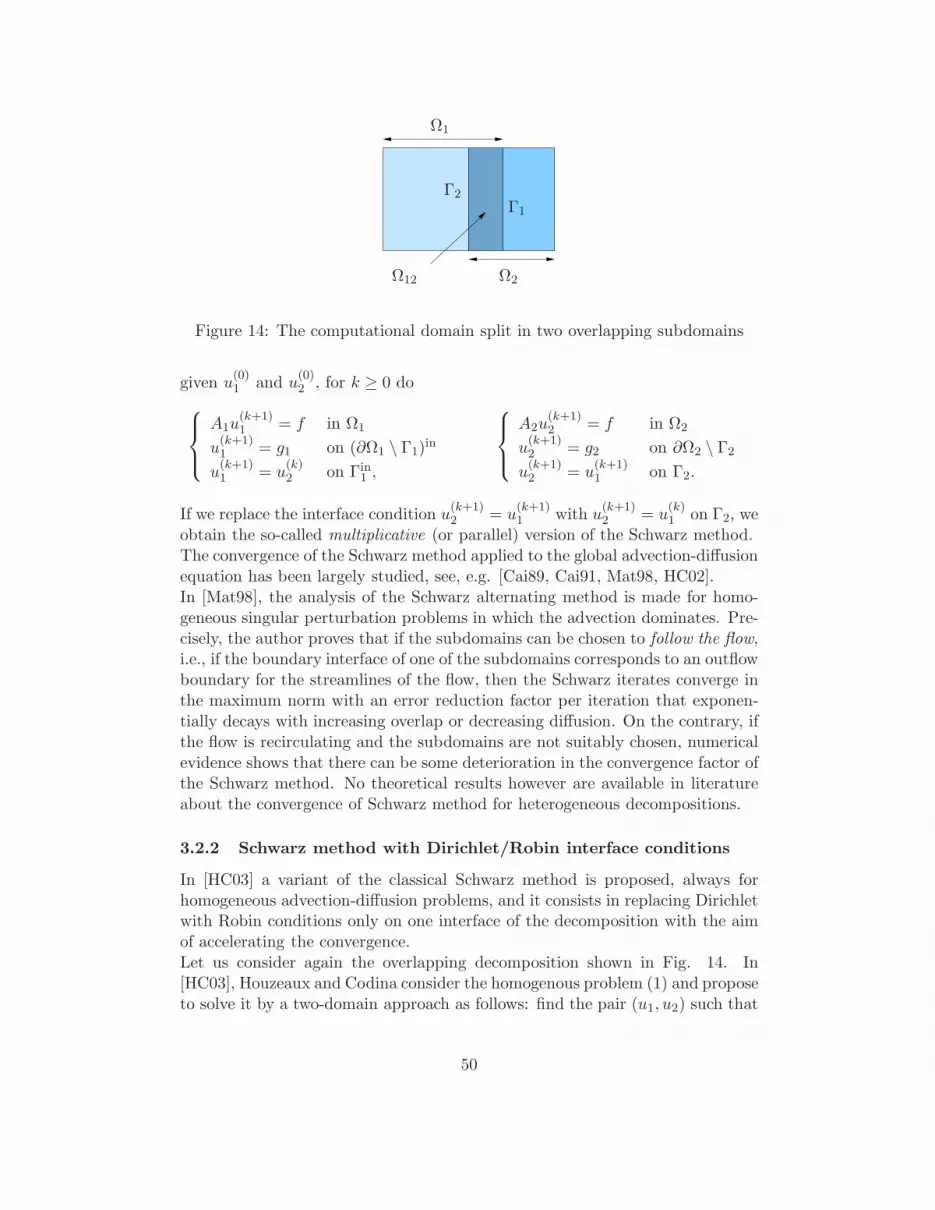
Ω12

Ω1

Ω2

Γ1

Γ2

Figure 14: The computational domain split in two overlapping subdomains

given u(0)1 and u

(0)2 , for k ≥ 0 do

A1u(k+1)1 = f in Ω1

u(k+1)1 = g1 on (∂Ω1 \ Γ1)

in

u(k+1)1 = u

(k)2 on Γin

1 ,

A2u(k+1)2 = f in Ω2

u(k+1)2 = g2 on ∂Ω2 \ Γ2

u(k+1)2 = u

(k+1)1 on Γ2.

If we replace the interface condition u(k+1)2 = u

(k+1)1 with u

(k+1)2 = u

(k)1 on Γ2, we

obtain the so-called multiplicative (or parallel) version of the Schwarz method.The convergence of the Schwarz method applied to the global advection-diffusionequation has been largely studied, see, e.g. [Cai89, Cai91, Mat98, HC02].In [Mat98], the analysis of the Schwarz alternating method is made for homo-geneous singular perturbation problems in which the advection dominates. Pre-cisely, the author proves that if the subdomains can be chosen to follow the flow,i.e., if the boundary interface of one of the subdomains corresponds to an outflowboundary for the streamlines of the flow, then the Schwarz iterates converge inthe maximum norm with an error reduction factor per iteration that exponen-tially decays with increasing overlap or decreasing diffusion. On the contrary, ifthe flow is recirculating and the subdomains are not suitably chosen, numericalevidence shows that there can be some deterioration in the convergence factor ofthe Schwarz method. No theoretical results however are available in literatureabout the convergence of Schwarz method for heterogeneous decompositions.

3.2.2 Schwarz method with Dirichlet/Robin interface conditions

In [HC03] a variant of the classical Schwarz method is proposed, always forhomogeneous advection-diffusion problems, and it consists in replacing Dirichletwith Robin conditions only on one interface of the decomposition with the aimof accelerating the convergence.Let us consider again the overlapping decomposition shown in Fig. 14. In[HC03], Houzeaux and Codina consider the homogenous problem (1) and proposeto solve it by a two-domain approach as follows: find the pair (u1, u2) such that

50

A2u1 = f in Ω1

u1 = g on ∂Ω1 \ Γ1

u1 = u2 on Γ1

A2u2 = f in Ω2

u2 = g on ∂Ω2 \ Γ2

ν∂u1

∂nΓ2

− 1

2(~b · ~nΓ2

)u1 = ν∂u2

∂nΓ2

− 1

2(~b · ~nΓ2

)u2 on Γ2.

(128)

By introducing Steklov-Poincare operators on the interfaces, they prove thatproblem (128) admits a unique solution (u1, u2) such that u1 = u2 on Ω12.Moreover, the function

u =

u1 in (Ω1 \ Ω12)u2 in Ω2

coincides with the solution of (1).However, in [HC03] an overlapping Dirichlet/Robin method is proposed for thesolution of the two advection-diffusion problems, with the purpose of inherit-ing the robustness properties of the classical Schwarz method, yet allowing thelimit case of zero (or extremely small) overlapping, for which Dirichlet/Dirichletmethod fails. Note that the interface condition (128)6 arises from writing theconvective term in skew-symmetric form.Problem (128) can be solved iterating by subdomains. The resulting method is

called Dirichlet-Robin method and it reads: given u(0)1 and u

(0)2 , for k ≥ 0 do

A2u(k+1)1 = f in Ω1

u(k+1)1 = g on ∂Ω1 \ Γ1

u(k+1)1 = θu

(k)2 + (1 − θ)u

(k)1 on Γ1

A2u(k+1)2 = f in Ω2

u(k+1)2 = g on ∂Ω2 \ Γ2

ν∂u

(k+1)2

∂nΓ2

− 1

2(~b · ~nΓ2

)u(k+1)2 = ν

∂u(k+1)1

∂nΓ2

− 1

2(~b · ~nΓ2

)u(k+1)1 on Γ2,

(129)

where θ > 0 is a suitable relaxation parameter. As alternative to the relaxation ofDirichlet data (129)3, the authors propose to relax the Robin data (129)6. Undersuitable choices of the relaxation parameter the Dirichlet-Robin algorithm (129)converges to the solution of the advection-diffusion problem (128).When the heterogeneous coupling is considered, the Robin interface condition(128)6 could be replaced by the following one:

−1

2(~b · ~nΓ2

)u1 = ν∂u2

∂nΓ2

− 1

2(~b · ~nΓ2

)u2 on Γ2 (130)

51

so that the iterative Dirichlet-Robin algorithm for the coupled advection/advection-diffusion problem should read:

given u(0)1 and u

(0)2 , for k ≥ 0 do

A1u(k+1)1 = f in Ω1

u(k+1)1 = g on (∂Ω1 \ Γ1)

in

u(k+1)1 = θu

(k)2 + (1 − θ)u

(k)1 on Γin

1

A2u(k+1)2 = f in Ω2

u(k+1)2 = g on ∂Ω2 \ Γ2

ν∂u

(k+1)2

∂nΓ2

− 1

2(~b · ~nΓ2

)u(k+1)2 = −1

2(~b · ~nΓ2

)u(k+1)1 on Γ2.

(131)

We note that algorithm (131) coincides with the Dirichlet-Neumann algorithm(47) when the overlap reduces to the empty set. We refer to Remark 2.1 in Sect.3.3.2 about the classification of Neumann and Robin interface conditions.

3.3 Virtual control approach with overlap for the advection-diffusion equation

Let us consider an overlapping decomposition of Ω as in (127). As done forthe non-overlapping situation presented in Sect. 3.1, we introduce the Dirichletvirtual controls λ1 ∈ L2

~b(Γin

1 ) and λ2 ∈ H1/2(Γ2) and we look for the solution ofthe following minimization problem:

infλ1,λ2

J(λ1, λ2), (132)

with

J(λ1, λ2) =

∫

Ω12

(u1(λ1) − u2(λ2))2dΩ, (133)

and u1 = u1(λ1), u2 = u2(λ2) solutions of

A1u1 = f in Ω1

u1 = g1 on (∂Ω1 \ Γ1)in

u1 = λ1 on Γin1 ,

A2u2 = f in Ω2

u2 = g2 on ∂Ω2 \ Γ2

u2 = λ2 on Γ2.(134)

The minimization problem (132) has been studied in [GLQ01, AGQ06].Along this section we set

Λ1 = L2~b(Γin

1 ),

Λ2 =λ2 ∈ H1/2(Γ2) : ∃µ ∈ H1/2(∂Ω2) s.t. λ2 = µ|Γ2

and g2 = µ|∂Ω2\Γ2

,(135)

The following result is stated in [GLQ01].

52

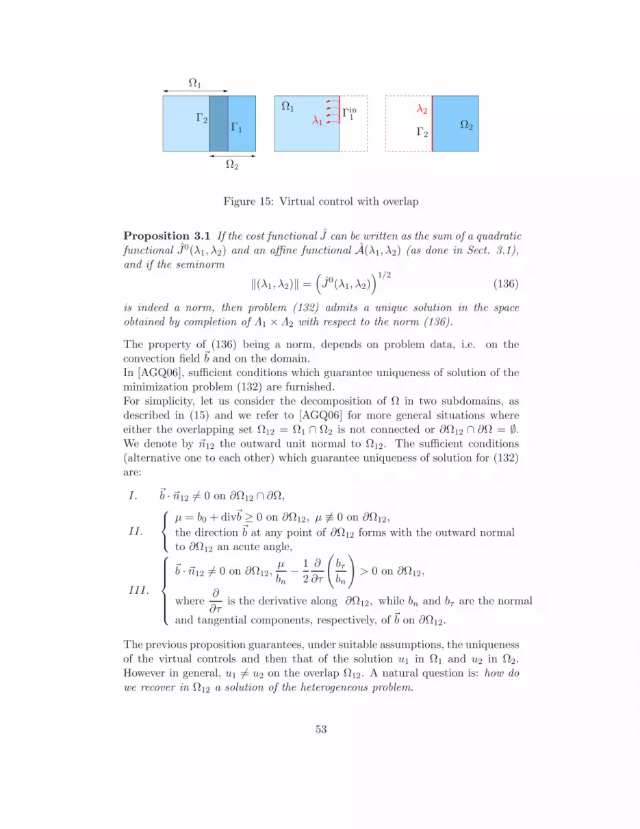
Ω1

Ω1

Ω2

Ω2

Γin1

Γ1 Γ2

Γ2 λ1

λ2

Figure 15: Virtual control with overlap

Proposition 3.1 If the cost functional J can be written as the sum of a quadraticfunctional J0(λ1, λ2) and an affine functional A(λ1, λ2) (as done in Sect. 3.1),and if the seminorm

‖(λ1, λ2)‖ =(J0(λ1, λ2)

)1/2(136)

is indeed a norm, then problem (132) admits a unique solution in the spaceobtained by completion of Λ1 × Λ2 with respect to the norm (136).

The property of (136) being a norm, depends on problem data, i.e. on theconvection field ~b and on the domain.In [AGQ06], sufficient conditions which guarantee uniqueness of solution of theminimization problem (132) are furnished.For simplicity, let us consider the decomposition of Ω in two subdomains, asdescribed in (15) and we refer to [AGQ06] for more general situations whereeither the overlapping set Ω12 = Ω1 ∩ Ω2 is not connected or ∂Ω12 ∩ ∂Ω = ∅.We denote by ~n12 the outward unit normal to Ω12. The sufficient conditions(alternative one to each other) which guarantee uniqueness of solution for (132)are:

I. ~b · ~n12 6= 0 on ∂Ω12 ∩ ∂Ω,

II.

µ = b0 + div~b ≥ 0 on ∂Ω12, µ 6≡ 0 on ∂Ω12,

the direction ~b at any point of ∂Ω12 forms with the outward normalto ∂Ω12 an acute angle,

III.

~b · ~n12 6= 0 on ∂Ω12,µ

bn− 1

2

∂

∂τ

(bτbn

)> 0 on ∂Ω12,

where∂

∂τis the derivative along ∂Ω12, while bn and bτ are the normal

and tangential components, respectively, of ~b on ∂Ω12.

The previous proposition guarantees, under suitable assumptions, the uniquenessof the virtual controls and then that of the solution u1 in Ω1 and u2 in Ω2.However in general, u1 6= u2 on the overlap Ω12. A natural question is: how dowe recover in Ω12 a solution of the heterogeneous problem.

53

The following result ensures that the difference between u1 and u2 in the L2(Ω12)norm annihilates when the viscosity vanishes (see [GLQ01]).

Theorem 3.3 If we set

φ(ν) = infλ1,λ2

J(λ1, λ2) (137)

and if we let ν → 0, all other data being fixed, then

φ(ν) → 0 as ν → 0. (138)

The optimality system associated to the minimization problem (132) can bederived by proceeding as in Sect. 3.1.For any µ1 ∈ Λ1, µ2 ∈ Λ2, we introduce the auxiliary problems as follows

A1uµ1

1 = 0 in Ω1

uµ1

1 = 0 on (∂Ω1 \ Γ1)in

uµ1

1 = µ1 on Γin1 ,

A2uµ2

2 = 0 in Ω2

uµ2

2 = 0 on ∂Ω2 \ Γ2

uµ2

2 = µ2 on Γ2,(139)

and we differentiate the functional J :

〈 ∂J∂λ1

, µ1〉 = (u1(λ1) − u2(λ2), uµ1

1 )L2(Ω12) ∀µ1 ∈ Λ1,

〈 ∂J∂λ2

, µ2〉 = − (u1(λ1) − u2(λ2), uµ2

2 )L2(Ω12) ∀µ2 ∈ Λ2.

(140)

We define the adjoint problems:A∗

1p1 = χ12(u1(λ1) − u2(λ2)) in Ω1

p1 = 0 on ∂Ωout1

(141)

and A∗

2p2 = −χ12(u1(λ1) − u2(λ2)) in Ω2

p2 = 0 on ∂Ω2,(142)

(where χ12 denotes the characteristic function of the overlapping set Ω12) and,by Green’s formulas and the boundary conditions set in (139), (141) and (142),the optimality system associated to the minimization problem (132) reads (indistributional sense):

(OS2)

- state equations (134);

- adjoint equations (141) and (142);

- Euler equations:

(−~b · ~nΓ1)p1 = 0 on Γin

1

ν∂p2

∂~nΓ2

= 0 on Γ2

The optimality system (OS2) can be solved as described in Sect. 3.1.4 by aBi-CGStab method.

54

3.3.1 Using three virtual controls

In order to force the solutions u1 and u2 to coincide in Ω12, a virtual control prob-lem with three controls has been proposed and studied in [AGQ06]. Precisely, inaddition to the Dirichlet controls λ1 and λ2, a distributed control λ3 ∈ L2(Ω12)is used as forcing term in the hyperbolic equation in Ω1.Let Λ1 and Λ2 the spaces defined in (135), then we set

Λ3 = L2(Ω12). (143)

The three virtual controls problem is defined as follows. We seek λ = (λ1, λ2, λ3) ∈Λ1 × Λ2 × Λ3 solution of the regularized minimization problem

infλ1,λ2,λ3

ˆJα(λ1, λ2, λ3), (144)

where:

ˆJα(λ1, λ2, λ3) =

1

2

∫

Ω12

(u1(λ1, λ3) − u2(λ2))2dΩ

+α

2

(‖λ1‖2

Λ1+ ‖λ2‖2

Λ2+ ‖ωλ3‖2

Λ3

),

(145)

u1 = u1(λ1, λ3) and u2 = u2(λ2) are the solutions of the state equations

A1u1 = f + ωλ3 in Ω1

u1 = g on (∂Ω1 \ Γ1)in

u1 = λ1 on Γin1

A2u2 = f in Ω2

u2 = g on ∂Ω2 \ Γ2

u2 = λ2 on Γ2,(146)

α ≥ 0 is a penalization coefficient and, finally, ω is a smooth function in Ω suchthat

0 ≤ ω(~x) ≤ 1 in Ω, ω = 0 in Ω\Ω12, ω > 0 in Ω12.

The optimality system associated to (145) reads (in variational form):

(OS3)

- state equations (146);

- adjoint equations (141) and (142);

- Euler-Lagrange equations:

(−~b · ~nΓ1)(p1 + αλ1) = 0 on Γin

1

ν∂p2

∂~nΓ2

+ αλ2 = 0 on Γ2

αωλ3 + ωp1 = 0 in Ω12.

The following Theorem is proved in [AGQ06]:

Theorem 3.4 For any α > 0, the minimization problem (144) has a uniquesolution depending on α, say (λ1, λ2, λ3) = (λ1(α), λ2(α), λ3(α)), such that

‖u1(λ1(α), λ3(α)) − u2(λ2(α))‖L2(Ω12) → 0 as α→ 0. (147)

55

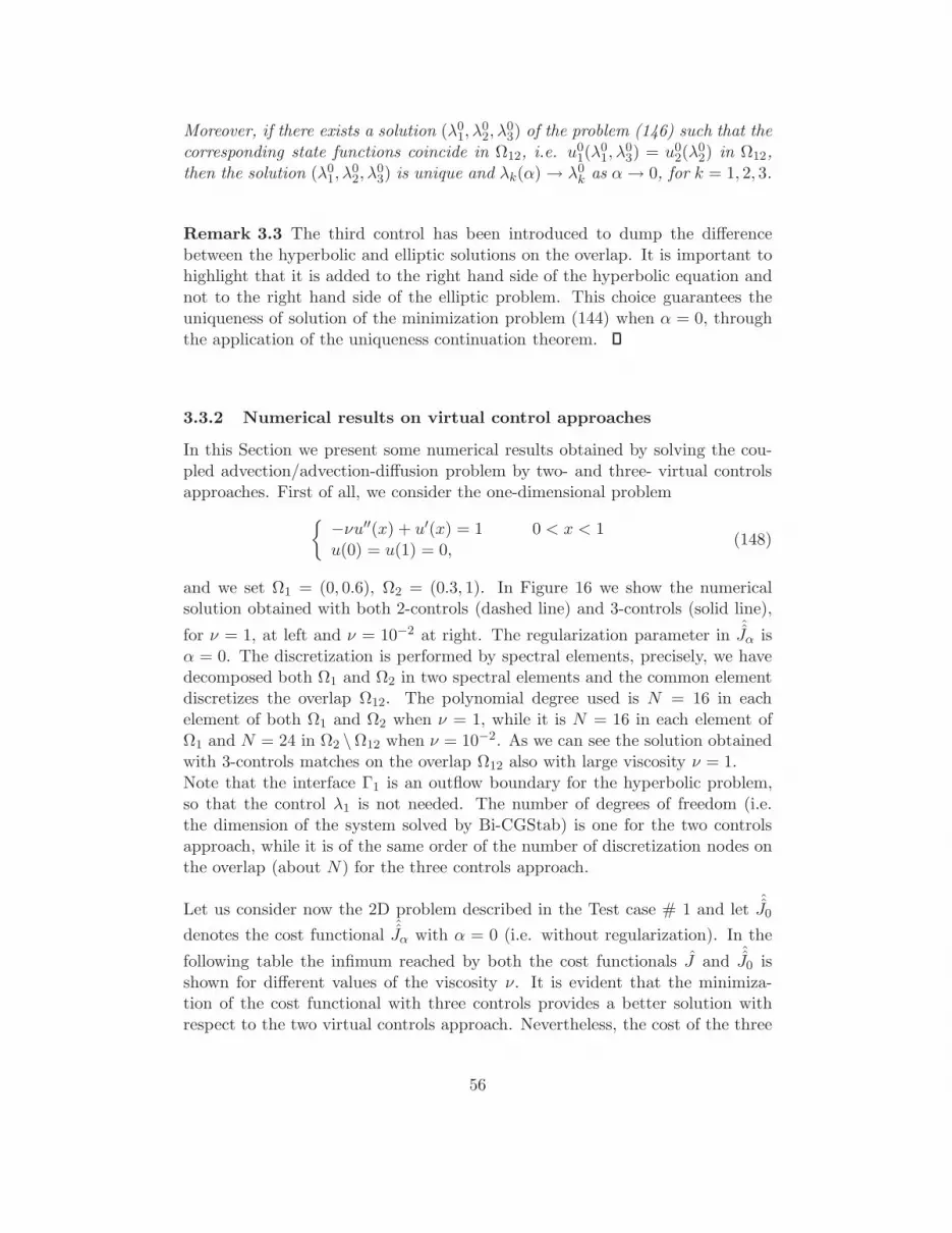
Moreover, if there exists a solution (λ01, λ

02, λ

03) of the problem (146) such that the

corresponding state functions coincide in Ω12, i.e. u01(λ

01, λ

03) = u0

2(λ02) in Ω12,

then the solution (λ01, λ

02, λ

03) is unique and λk(α) → λ0

k as α→ 0, for k = 1, 2, 3.

Remark 3.3 The third control has been introduced to dump the differencebetween the hyperbolic and elliptic solutions on the overlap. It is important tohighlight that it is added to the right hand side of the hyperbolic equation andnot to the right hand side of the elliptic problem. This choice guarantees theuniqueness of solution of the minimization problem (144) when α = 0, throughthe application of the uniqueness continuation theorem.

3.3.2 Numerical results on virtual control approaches

In this Section we present some numerical results obtained by solving the cou-pled advection/advection-diffusion problem by two- and three- virtual controlsapproaches. First of all, we consider the one-dimensional problem

−νu′′(x) + u′(x) = 1 0 < x < 1u(0) = u(1) = 0,

(148)

and we set Ω1 = (0, 0.6), Ω2 = (0.3, 1). In Figure 16 we show the numericalsolution obtained with both 2-controls (dashed line) and 3-controls (solid line),

for ν = 1, at left and ν = 10−2 at right. The regularization parameter inˆJα is

α = 0. The discretization is performed by spectral elements, precisely, we havedecomposed both Ω1 and Ω2 in two spectral elements and the common elementdiscretizes the overlap Ω12. The polynomial degree used is N = 16 in eachelement of both Ω1 and Ω2 when ν = 1, while it is N = 16 in each element ofΩ1 and N = 24 in Ω2 \Ω12 when ν = 10−2. As we can see the solution obtainedwith 3-controls matches on the overlap Ω12 also with large viscosity ν = 1.Note that the interface Γ1 is an outflow boundary for the hyperbolic problem,so that the control λ1 is not needed. The number of degrees of freedom (i.e.the dimension of the system solved by Bi-CGStab) is one for the two controlsapproach, while it is of the same order of the number of discretization nodes onthe overlap (about N) for the three controls approach.

Let us consider now the 2D problem described in the Test case # 1 and letˆJ0

denotes the cost functionalˆJα with α = 0 (i.e. without regularization). In the

following table the infimum reached by both the cost functionals J andˆJ0 is

shown for different values of the viscosity ν. It is evident that the minimiza-tion of the cost functional with three controls provides a better solution withrespect to the two virtual controls approach. Nevertheless, the cost of the three

56

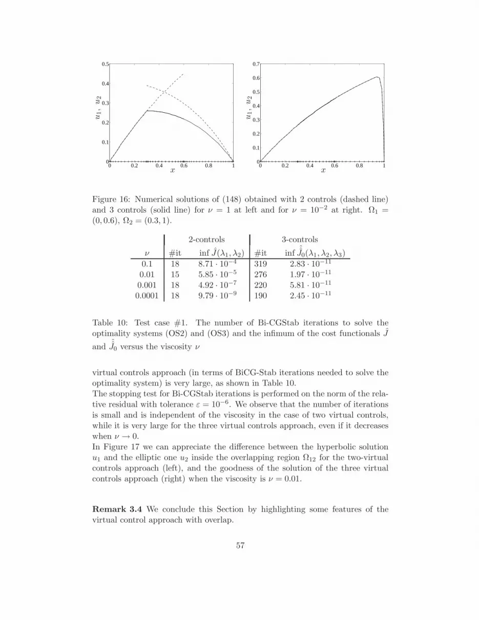
0 0.2 0.4 0.6 0.8 10

0.1

0.2

0.3

0.4

0.5

x

u1,u

2

0 0.2 0.4 0.6 0.8 10

0.1

0.2

0.3

0.4

0.5

0.6

0.7

x

u1,u

2

Figure 16: Numerical solutions of (148) obtained with 2 controls (dashed line)and 3 controls (solid line) for ν = 1 at left and for ν = 10−2 at right. Ω1 =(0, 0.6), Ω2 = (0.3, 1).

2-controls 3-controls

ν #it inf J(λ1, λ2) #it infˆJ0(λ1, λ2, λ3)

0.1 18 8.71 · 10−4 319 2.83 · 10−11

0.01 15 5.85 · 10−5 276 1.97 · 10−11

0.001 18 4.92 · 10−7 220 5.81 · 10−11

0.0001 18 9.79 · 10−9 190 2.45 · 10−11

Table 10: Test case #1. The number of Bi-CGStab iterations to solve theoptimality systems (OS2) and (OS3) and the infimum of the cost functionals J

andˆJ0 versus the viscosity ν

virtual controls approach (in terms of BiCG-Stab iterations needed to solve theoptimality system) is very large, as shown in Table 10.The stopping test for Bi-CGStab iterations is performed on the norm of the rela-tive residual with tolerance ε = 10−6. We observe that the number of iterationsis small and is independent of the viscosity in the case of two virtual controls,while it is very large for the three virtual controls approach, even if it decreaseswhen ν → 0.In Figure 17 we can appreciate the difference between the hyperbolic solutionu1 and the elliptic one u2 inside the overlapping region Ω12 for the two-virtualcontrols approach (left), and the goodness of the solution of the three virtualcontrols approach (right) when the viscosity is ν = 0.01.

Remark 3.4 We conclude this Section by highlighting some features of thevirtual control approach with overlap.

57

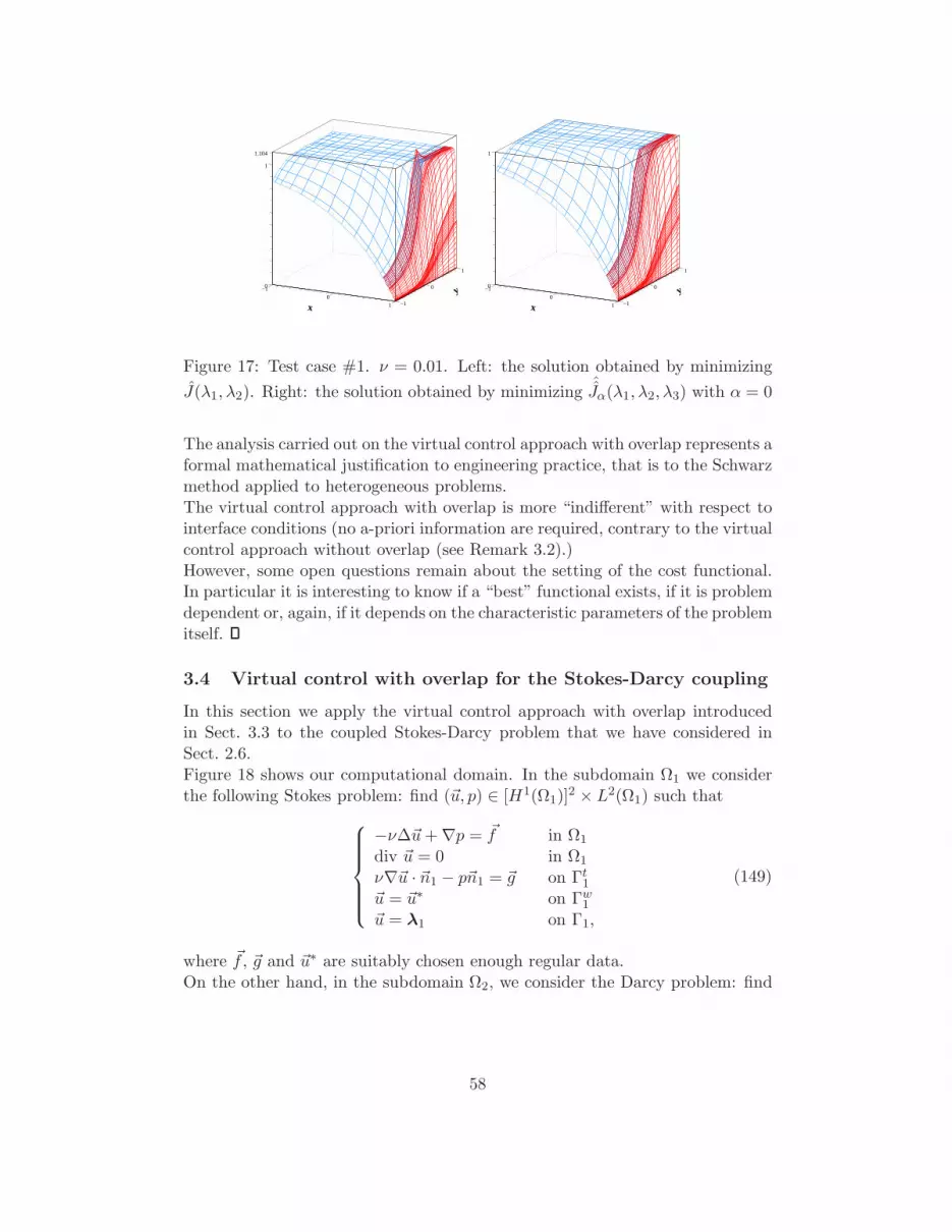
0

1

1.104

x

−1

0

1

y−1

0

1

0

1

x

−1

0

1

y−1

0

1

Figure 17: Test case #1. ν = 0.01. Left: the solution obtained by minimizing

J(λ1, λ2). Right: the solution obtained by minimizingˆJα(λ1, λ2, λ3) with α = 0

The analysis carried out on the virtual control approach with overlap represents aformal mathematical justification to engineering practice, that is to the Schwarzmethod applied to heterogeneous problems.The virtual control approach with overlap is more “indifferent” with respect tointerface conditions (no a-priori information are required, contrary to the virtualcontrol approach without overlap (see Remark 3.2).)However, some open questions remain about the setting of the cost functional.In particular it is interesting to know if a “best” functional exists, if it is problemdependent or, again, if it depends on the characteristic parameters of the problemitself.

3.4 Virtual control with overlap for the Stokes-Darcy coupling

In this section we apply the virtual control approach with overlap introducedin Sect. 3.3 to the coupled Stokes-Darcy problem that we have considered inSect. 2.6.Figure 18 shows our computational domain. In the subdomain Ω1 we considerthe following Stokes problem: find (~u, p) ∈ [H1(Ω1)]

2 × L2(Ω1) such that

−ν∆~u+ ∇p = ~f in Ω1

div ~u = 0 in Ω1

ν∇~u · ~n1 − p~n1 = ~g on Γt1~u = ~u∗ on Γw1~u = λ1 on Γ1,

(149)

where ~f , ~g and ~u∗ are suitably chosen enough regular data.On the other hand, in the subdomain Ω2, we consider the Darcy problem: find

58

Ω1

Ω1

Γw1 Γw1

Γt1

Γ1

Ω2

Ω2Γw2 Γw2

Γb2

Γ2Ω12

Γ

Figure 18: Schematic representation of the computational domain.

the piezometric head ϕ ∈ H1(Ω2) such that

−div (K∇ϕ) = 0 in Ω2

K∇ϕ · ~n2 = ψN on Γw2ϕ = ψD on Γb2ϕ = λ2 on Γ2,

(150)

where ψN and ψD are suitable boundary data.We refer to Fig. 18 for the notation of the boundaries.

λ1 and λ2 are the controls variables which have to be seeked in the followingspaces, respectively:

Λ1 =µ ∈ [H1/2(Γ1)]

2 : ∃~v ∈ [H1(Ω1)]2, ~v = µ on Γ1, ~v = ~0 on Γw1

, (151)

Λ2 =µ ∈ H1/2(Γ2) : ∃ψ ∈ H1(Ω2), ψ = µ on Γ2, ∇ϕ · ~n2 = 0 on Γw2 ,

ψ = 0 on Γb2

. (152)

λ1 and λ2 are the solutions of the following minimization problem:

infλ1,λ2

J(λ1, λ2) with J(λ1, λ2) =1

2

∫

Ω12

(~u+K∇ϕ)2 . (153)

Remark 3.5 Other functionals may be considered for the minimization problem(153) instead of J . For example, we may minimize the jump of pressures in theoverlapping region, thus considering:

infλ1,λ2

J(λ1, λ2) with J(λ1, λ2) =1

2

∫

Ω12

(p − gϕ)2 . (154)

59

Moreover, we could take into account some continuity condition (i.e., the con-tinuity of the normal velocities) on the physical interface Γ ⊂ Ω12 between thefluid and the porous-media regions. In this case we consider the functional

J(λ1, λ2) =1

2

∫

Γ(~u · ~n+K∇ϕ · ~n)2 +

1

2

∫

Ω12

(p− gϕ)2 , (155)

where ~n is the normal unit vector on Γ directed outwards of the fluid domain.

We introduce now the following auxiliary problems:

find (~uf , pf ) ∈ [H1(Ω1)]2 × L2(Ω1) such that

−ν∆~uf + ∇pf = ~f in Ω1

div ~uf = 0 in Ω1

ν∇~uf · ~n1 − pf~n1 = ~g on Γt1~uf = ~u∗ on Γw1~uf = ~0 on Γ1,

(156)

and find ϕ∗ ∈ H1(Ω2) such that

−div (K∇ϕ∗) = 0 in Ω2

K∇ϕ∗ · ~n2 = ψN on Γw2ϕ∗ = ψD on Γb2ϕ∗ = 0 on Γ2.

(157)

Moreover, we consider the following problems depending only on the controlvariables:

find (~uλ1 , pλ1) ∈ [H1(Ω1)]2 × L2(Ω1) such that

−ν∆~uλ1 + ∇pλ1 = ~0 in Ω1

div ~uλ1 = 0 in Ω1

ν∇~uλ1 · ~n1 − pλ1~n1 = ~0 on Γt1~uλ1 = ~0 on Γw1~uλ1 = λ1 on Γ1,

(158)

and find ϕλ2 ∈ H1(Ω2) such that

−div (K∇ϕλ2) = 0 in Ω2

K∇ϕλ2 · ~n2 = ~0 on Γw2ϕλ2 = 0 on Γb2ϕλ2 = λ2 on Γ2.

(159)

Then, we can split

~u = ~uf + ~uλ1 , p = pf + pλ1 , ϕ = ϕ∗ + ϕλ2 . (160)

60

In this way we can rewrite the functional J(λ1, λ2) in (153) as

J(λ1, λ2) = J0(λ1, λ2) + A(λ1, λ2), (161)

where J0(λ1, λ2) is the quadratic functional

J0(λ1, λ2) =1

2

∫

Ω12

(~uλ1 +K∇ϕλ2)2 (162)

while A(λ1, λ2) is the affine functional

A(λ1, λ2) =1

2

∫

Ω12

(~uf +K∇ϕ∗)2 +

∫

Ω12

(~uλ1 +K∇ϕλ2) · (~uf +K∇ϕ∗). (163)

We compute now ∇J = ∇J0 + ∇A.We have:

〈∂J0

∂λ1,µ1〉 =

∫

Ω12

~uµ1 · (~uλ1 +K∇ϕλ2) (164)

Considering the dual problem:

−ν∆~v + ∇q = (~uλ1 +K∇ϕλ2)χΩ12in Ω1

div ~v = 0 in Ω1

ν∇~v · ~n1 − q~n1 = ~0 on Γt1~v = ~0 on Γw1~v = ~0 on Γ1,

(165)

we can characterize the operator (164) as

〈∂J0

∂λ1,µ1〉 = −

∫

Γ1

(ν∇~v · ~n1 − q~n1) · µ ∀µ ∈ Λ1. (166)

On the other hand, we have:

〈∂J0

∂λ2, µ2〉 =

∫

Ω12

−div(K(~uλ1 +K∇ϕλ2)χΩ12)ϕµ2 , (167)

and, using the dual problem:

−div (K∇ψ) = −div(K(~uλ1 + ∇ϕλ2)χΩ12) in Ω2

K∇ψ · ~n2 = ~0 on Γw2ψ = 0 on Γb2ψ = 0 on Γ2,

(168)

we obtain

〈∂J0

∂λ2, µ2〉 = −

∫

Γ2

K∇ψ · ~n2 µ2 ∀µ2 ∈ Λ2. (169)

61

We proceed in a similar way to characterize the affine functional A. In this case,we have

〈 ∂A∂λ1

,µ1〉 = −∫

Γ1

(ν∇~v · ~n1 − q~n1

)· µ ∀µ ∈ Λ1, (170)

〈 ∂A∂λ2

, µ2〉 = −∫

Γ2

K∇ψ · ~n2 µ2 ∀µ2 ∈ Λ2. (171)

(~v, q) ∈ [H1(Ω1)]2×L2(Ω1) is the solution of the dual problem (165) with forcing

term (~uf +K∇ϕ∗)χΩ12, while ψ ∈ H1(Ω2) is the solution of the dual problem

(168) with forcing term −div(K(~uf +K∇ϕ∗)χΩ12).

To solve the minimization problem (153) we use the following algorithm:

1. Solve (156) and (157) to get ~uf , pf and ϕ∗.

2. Compute ∇A:

• solve (165) with forcing term (~uf +K∇ϕ∗)χΩ12and compute (170);

• solve (168) with forcing term −div(K(~uf +K∇ϕ∗)χΩ12) and compute

(171).

3. Find (λ1, λ2) ∈ Λ1×Λ2 such that ∇J0 = −∇A. To this aim we use an iter-ative method like Bi-CGStab. At each iteration, to compute ∇J0(λ1, λ2)we do

• solve (158) and (159);

• compute ~uλ1 +K∇ϕλ2 in Ω12;

• solve (165) to get (166);

• solve (168) to get (169).

4. Finally, solve (158) and (159) using the functions λ1 and λ2 computed atstep 3 and use (160) to obtain the desired solutions.

3.4.1 Stokes / Darcy coupling with 3 virtual controls

A three virtual controls approach for the Stokes/Darcy coupling with overlapcan be formulated as follows:

α~u− ν∆~u+ (~u · ∇)~u+ ∇p = ~0 in Ω1

div~u = 0 in Ω1

ν∇~u · ~n1 − p~n1 = ~g on Γt1~u = ~u∗ on Γw1~u = λ1 on Γ1

−div(K∇ϕ) = χΩ12λ3 in Ω2

K∇ϕ · ~n2 = ψN on Γw2ϕ = ψD on Γb2ϕ = λ2 on Γ2,

62

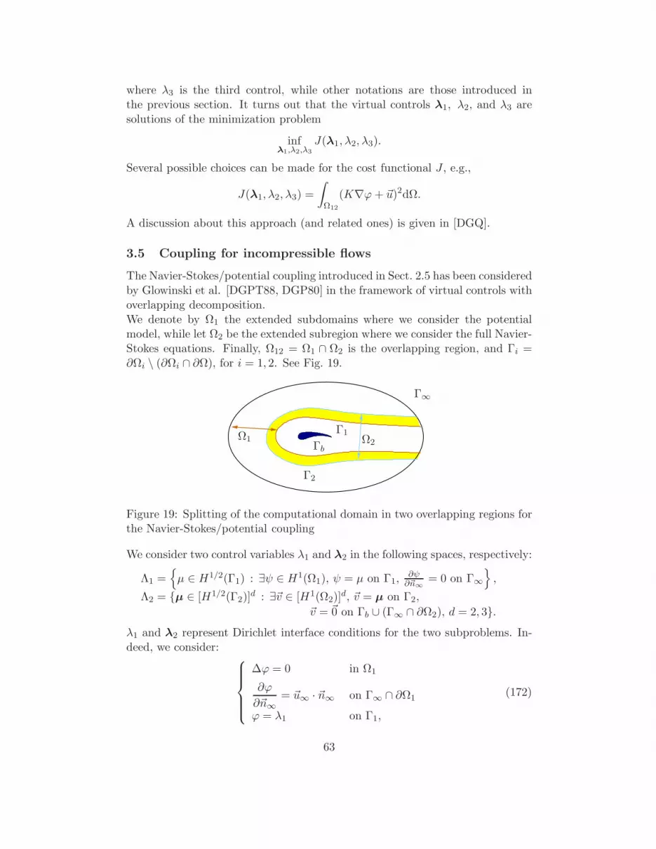
where λ3 is the third control, while other notations are those introduced inthe previous section. It turns out that the virtual controls λ1, λ2, and λ3 aresolutions of the minimization problem

infλ1,λ2,λ3

J(λ1, λ2, λ3).

Several possible choices can be made for the cost functional J , e.g.,

J(λ1, λ2, λ3) =

∫

Ω12

(K∇ϕ+ ~u)2dΩ.

A discussion about this approach (and related ones) is given in [DGQ].

3.5 Coupling for incompressible flows

The Navier-Stokes/potential coupling introduced in Sect. 2.5 has been consideredby Glowinski et al. [DGPT88, DGP80] in the framework of virtual controls withoverlapping decomposition.We denote by Ω1 the extended subdomains where we consider the potentialmodel, while let Ω2 be the extended subregion where we consider the full Navier-Stokes equations. Finally, Ω12 = Ω1 ∩ Ω2 is the overlapping region, and Γi =∂Ωi \ (∂Ωi ∩ ∂Ω), for i = 1, 2. See Fig. 19.

Ω1 Ω2

Γ1

Γ2

Γb

Γ∞

Figure 19: Splitting of the computational domain in two overlapping regions forthe Navier-Stokes/potential coupling

We consider two control variables λ1 and λ2 in the following spaces, respectively:

Λ1 =µ ∈ H1/2(Γ1) : ∃ψ ∈ H1(Ω1), ψ = µ on Γ1,

∂ψ∂~n∞

= 0 on Γ∞

,

Λ2 = µ ∈ [H1/2(Γ2)]d : ∃~v ∈ [H1(Ω2)]

d, ~v = µ on Γ2,

~v = ~0 on Γb ∪ (Γ∞ ∩ ∂Ω2), d = 2, 3.λ1 and λ2 represent Dirichlet interface conditions for the two subproblems. In-deed, we consider:

∆ϕ = 0 in Ω1

∂ϕ

∂~n∞= ~u∞ · ~n∞ on Γ∞ ∩ ∂Ω1

ϕ = λ1 on Γ1,

(172)

63

and

α~u− ν∆~u+ (~u · ∇)~u+ ∇p = ~f in Ω2

div ~u = 0 in Ω2

~u = ~0 on Γb ∪ (Γ∞ ∩ ∂Ω2)u = λ2 on Γ2.

(173)

The unknown Dirichlet data λ1 and λ2 are the solutions of the minimizationproblem:

infλ1,λ2

J(λ1,λ2) with J(λ1,λ2) =1

2

∫

Ω12

(∇ϕ− u)2dΩ (174)

and satisfying the condition

∫

Γ2

λ2 · ~nΓ2dΓ +

∫

Γ∞∩∂Ω2

~u∞ · ~n∞dΓ = 0.

We refer the interested reader to [DGPT88, DGP80]. A similar approach for thecase of compressible flows is presented in [GPT90].

References

[AGQ06] V.I. Agoshkov, P. Gervasio, and A. Quarteroni. Optimal con-trol in heterogeneous domain decomposition methods for advection-diffusion equations. Mediterr. J. Math., 3(2):147–176, 2006.

[AL94] G. Aguilar and F. Lisbona. Interface conditions for a kind of nonlinear elliptic hyperbolic problems. In A. Quarteroni, J. Perieaux,Y.A. Kuznetsov, and O.B. Widlund, editors, Domain DecompositionMethods for Partial Differential Equations, pages 89–95, Providence,1994. American Mathematical Society.

[BCR89] F. Brezzi, C. Canuto, and A. Russo. A self-adaptive formulation forthe Euler/Navier-Stokes coupling. Comput. Methods Appl. Mech.Engrg., 73:317–330, 1989.

[BDQ08] L. Badea, M. Discacciati, and A. Quarteroni. Numerical analysis ofthe Navier-Stokes/Darcy coupling. Technical report, Ecole Polytech-nique Federale de Lausanne, IACS-CMCS, 2008.

[BJ67] G.S. Beavers and D.D. Joseph. Boundary conditions at a naturallypermeable wall. J. Fluid Mech., 30:197–207, 1967.

[Cai89] X.C. Cai. Some Domain Decompostion Algorithms for Nonselfad-joint Elliptic and Parabolic Partial Differential Equations. TechnicalReport TR-461, Department of Computer Science, Courant Insti-tute, September 1989.

64

[Cai91] Xiao-Chuan Cai. Additive Schwarz algorithms for parabolicconvection-diffusion equations. Numer. Math., 60(1):41–61, 1991.

[CHQZ07] C. Canuto, M. Y. Hussaini, A. Quarteroni, and T. A. Zang. Spec-tral Methods. Evolution to Complex Geometries and Application s toFluid Dynamics . Springer, Heidelberg, 2007.

[CM94] T.F. Chan and T.P. Mathew. Domain decomposition algorithms. InActa Numerica, pages 61–143. Cambridge Univ. Press, 1994.

[CQ95] C. Carlenzoli and A. Quarteroni. Adaptive domain decompositionmethods for advection-diffusion problems. In Modeling, mesh gener-ation, and adaptive numerical methods for partial differential equa-tions (Minneapolis, MN, 1993), volume 75 of IMA Vol. Math. Appl.,pages 165–186. Springer, New York, 1995.

[DDE05] K. Deckelnick, G. Dziuk, and C.M. Elliott. Computation of geometricpartial differential equations and mean curvature flow. Acta Numer.,14:139–232, 2005.

[DGP80] Q.V. Dinh, R. Glowinski, and J. Periaux. Applications of domaindecomposition techniques to the numerical solution of the Navier-Stokes equations. In Numerical methods for engineering, 1 (Paris,1980), pages 383–404. Dunod, Paris, 1980.

[DGPT88] Q.V. Dinh, R. Glowinski, J. Periaux, and G. Terrasson. On the cou-pling of viscous and inviscid models for incompressible fluid flows viadomain decomposition. In G.A. Meurant R. Glowinski, G.H. Goluband J. Periaux, editors, First Conf. on Domain Decomposition Meth-ods for Partial Differential Equations, pages 350–368, Philadelphia,1988. SIAM.

[DGQ] M. Discacciati, P. Gervasio, and A. Quarteroni. Virtual controls forheterogeneous problems. Technical report. In progress.

[Dis04a] M. Discacciati. Domain Decomposition Methods for the Coupling ofSurface and Groundwater Flows. PhD thesis, Ecole PolytechniqueFederale de Lausanne, Switzerland, 2004.

[Dis04b] M. Discacciati. Iterative methods for Stokes/Darcy coupling. InR. Kornhuber et al., editor, Domain Decomposition Methods in Sci-ence and Engineering. Lecture Notes in Computational Science andEngineering (40), pages 563–570. Springer, Berlin and Heidelberg,2004.

[DMQ02] M. Discacciati, E. Miglio, and A. Quarteroni. Mathematical andnumerical models for coupling surface and groundwater flows. Appl.Numer. Math., 43:57–74, 2002.

65

[DQ03] M. Discacciati and A. Quarteroni. Analysis of a domain decompo-sition method for the coupling of Stokes and Darcy equations. InF. Brezzi, A. Buffa, S. Corsaro, and A. Murli, editors, NumericalMathematics and Advanced Applications, ENUMATH 2001, pages3–20. Springer. Milan, 2003.

[DQ09] M. Discacciati and A. Quarteroni. Navier-Stokes/Darcy coupling:modeling, analysis, and numerical approximation. Rev. Mat. Com-plut., 22(2):315–426, 2009.

[DQV07] M. Discacciati, A. Quarteroni, and A. Valli. Robin-Robin domaindecomposition methods for the Stokes-Darcy coupling. SIAM J. Nu-mer. Anal., 45(3):1246–1268 (electronic), 2007.

[Dub93] E. Dubach. Contribution a la resolution des equations fluides endomaine non borne. PhD thesis, Universite Paris 13, 1993.

[FPQ93] A. Frati, F. Pasquarelli, and A. Quarteroni. Spectral approximationto advection-diffusion problems by the fictitious interface method.J.Comput.Phys., 107(2):201–211, 1993.

[GHJ02] M.J. Gander, L. Halpern, and C. Japhet. Optimized Schwarz algo-rithms for coupling convection and convection-diffusion problems. InDomain decomposition methods in science and engineering (Lyon,2000), Theory Eng. Appl. Comput. Methods, pages 255–262. Inter-nat. Center Numer. Methods Eng. (CIMNE), Barcelona, 2002.

[GHJM07] M.J. Gander, L. Halpern, C. Japhet, and V. Martin. Advectiondiffusion problems with pure advection approximation in subregions.In Domain decomposition methods in science and engineering XVI,volume 55 of Lect. Notes Comput. Sci. Eng., pages 239–246. Springer,Berlin, 2007.

[GHJM09] M.J. Gander, L. Halpern, C. Japhet, and V. Martin. Viscous prob-lems with a vanishing viscosity approximation in subregions: a newapproach based on operator factorization. In ESAIM Proc, vol-ume 27, pages 272–288, 2009.

[GLQ01] P. Gervasio, J.-L. Lions, and A. Quarteroni. Heterogeneous Couplingby Virtual Control Methods. Numerische Mathematik, 90(2):241–264, 2001.

[GPD82] R. Glowinski, J. Periaux, and Q.V. Dinh. Domain decompositionmethods for non linear problems in fluid dynamics. Technical ReportRR-0147, INRIA, 07 1982.

66

[GPT90] R. Glowinski, J. Periaux, and G. Terrasson. On the coupling of vis-cous and inviscid models for compressible fluid flows via domain de-composition. In Third International Symposium on Domain Decom-position Methods for Partial Differential Equations (Houston, TX,1989), pages 64–97, Philadelphia, PA, 1990. SIAM.

[GQ89] F. Gastaldi and A. Quarteroni. On the coupling of hyperbolic andparabolic systems: analytical and numerical approach. Appl. Numer.Math., 6(1):3–31, 1989.

[GQL90] F. Gastaldi, A. Quarteroni, and G. Sacchi Landriani. On the cou-pling of two dimensional hyperbolic and elliptic equations: analyticaland numerical approach. In J.Perieaux T.F.Chan, R.Glowinski andO.B.Widlund, editors, Third International Symposium on DomainDecomposition Methods for Partial Differential Equations, pages 22–63, Philadelphia, 1990. SIAM.

[GR86] V. Girault and P.A. Raviart. Finite Element Methods for Navier-Stokes Equations. Theory and Algorithms. Springer, Berlin, 1986.

[GR07] V. Girault and B. Riviere. DG approximation of coupled Navier-Stokes and Darcy equations by Beaver-Joseph-Saffman interface con-dition. Technical Report TR-MATH 07-09, University of Pittsburgh,Department of Mathematics, 2007.

[HC02] G. Houzeaux and R. Codina. A geometrical domain decompositionmethod in computational fluid dynamics, volume 70 of MonographCIMNE. International Center for Numerical Methods in Engineering(CIMNE), Barcelona, 2002.

[HC03] G. Houzeaux and R. Codina. An iteration-by-subdomain overlap-ping Dirichlet/Robin domain decomposition method for advection-diffusion problems. J. Comput. Appl. Math., 158(2):243–276, 2003.

[IC03] A. Iafrati and E.F. Campana. A domain decomposition approach tocompute wave breaking (wave-breaking flows). Int. J. Numer. Meth.Fluids, 41:419–445, 2003.

[JM96] W. Jager and A. Mikelic. On the boundary conditions at the contactinterface between a porous medium and a free fluid. Ann. ScuolaNorm. Sup. Pisa Cl. Sci., 23:403–465, 1996.

[JM00] W. Jager and A. Mikelic. On the interface boundary condition ofBeavers, Joseph and Saffman. SIAM J. Appl. Math., 60(4):1111–1127, 2000.

67

[JMN01] W. Jager, A. Mikelic, and N. Neuss. Asymptotic analysis of thelaminar viscous flow over a porous bed. SIAM J. Sci. Comput.,22(6):2006–2028, 2001.

[Lio71] J.-L. Lions. Optimal control of systems governed by partial differen-tial equations. Springer-Verlag, New York, 1971.

[Lio88] P.-L. Lions. On the Schwarz alternating method. I. In First Inter-national Symposium on Domain Decomposition Methods for PartialDifferential Equations (Paris, 1987), pages 1–42. SIAM, Philadel-phia, PA, 1988.

[Lio90] P.L. Lions. On the Schwarz alternating method III: a variant fornon-overlapping subdomains. In T.F. Chan et al., editor, Third Inter-national Symposium on Domain Decomposition Methods for PartialDifferential Equations, pages 202–231. SIAM, Philadelphia, 1990.

[LM68] J.L. Lions and E. Magenes. Problemes aux Limites Non Homogeneset Applications, volume 1. Dunod, Paris, 1968.

[LP98a] J.-L. Lions and O. Pironneau. Algorithmes paralleles pour la solutionde problemes aux limites. C. R. Acad. Sci. Paris Ser. I Math., t.327:947–952, 1998.

[LP98b] J.-L. Lions and O. Pironneau. Sur le controle parallele des systemesdistribues. C. R. Acad. Sci. Paris Ser. I Math., t. 327:993–998, 1998.

[LP99] J.-L. Lions and O. Pironneau. Domain decomposition methods forCAD. C. R. Acad. Sci. Paris Ser. I Math., t. 328:73–80, 1999.

[LSY03] W.L. Layton, F. Schieweck, and I. Yotov. Coupling fluid flow withporous media flow. SIAM J. Num. Anal., 40:2195–2218, 2003.

[Mat98] T.P. Mathew. Uniform convergence of the Schwarz alternatingmethod for solving singularly perturbed advection-diffusion equa-tions. SIAM J. Numer. Anal., 35(4):1663–1683, 1998.

[PR55] D. Peaceman and H. Rachford. The numerical solution of parabolicand elliptic differential equations. J. SIAM, 3:28–41, 1955.

[PS98] L.E. Payne and B. Straughan. Analysis of the boundary conditionat the interface between a viscous fluid and a porous medium andrelated modelling questions. J. Math. Pures Appl., 77:317–354, 1998.

[Qua09] A. Quarteroni. Numerical Models for Differential Problems. SeriesMS&A, Vol. 2. Springer, Milan, 2009.

68

[QV99] A. Quarteroni and A. Valli. Domain Decomposition Methods forPartial Differential Equations. Numerical Mathematics and ScientificComputation. The Clarendon Press Oxford University Press, NewYork, 1999.

[RY05] B. Riviere and I. Yotov. Locally conservative coupling of Stokes andDarcy flows. SIAM J. Numer. Anal., 42(5):1959–1977, 2005.

[Saf71] P.G. Saffman. On the boundary condition at the interface of a porousmedium. Stud. Appl. Math., 1:93–101, 1971.

[Sch90] H.A. Schwarz. Uber einige abbildungsaufgaben. Ges. Math. Abh.,pages 65–83, 1890.

[Scr90] J.S. Scroggs. A parallel algorithm for nonlinear convection-diffusionequations. In Third International Symposium on Domain Decom-position Methods for Partial Differential Equations (Houston, TX,1989), pages 373–384. SIAM, Philadelphia, PA, 1990.

[SH93] K. Schenk and F.K. Hebeker. Coupling of two dimensional vis-cous and inviscid incompressible Stokes equtions. Technical ReportPreprint 93-68 (SFB 359), Heidelberg University, 1993.

[vdV92] H.A. van der Vorst. Bi-CGSTAB: a fast and smoothly convergingvariant of Bi-CG for the solution of nonsymmetric linear systems.SIAM J. Sci. Statist. Comput., 13(2):631–644, 1992.

69