High-frequency dynamics of heterogeneous slender structures

Contents lists available at SciVerse ScienceDirect

Journal of Sound and Vibration

Journal of Sound and Vibration 332 (2013) 2461–2487

0022-46

http://d

n Tel.:

E-m

journal homepage: www.elsevier.com/locate/jsvi

High-frequency dynamics of heterogeneous slender structures

Eric Savin n

ONERA—The French Aerospace Lab, F-92322 Chatillon, France

a r t i c l e i n f o

Article history:

Accepted 9 October 2012

Handling Editor: G. Degrande

This paper gives an overview of the theoretical modeling of high-frequency linear

dynamics of built-up structures including the influence of uncertainties by a probabil-

istic approach. Its analytical developments are enlightened by a preliminary discussion

0X/$ - see front matter & 2012 Elsevier Ltd.

x.doi.org/10.1016/j.jsv.2012.10.009

þ33 146 73 46 45; fax: þ33 146 73 41 43.

ail address: [email protected]

a b s t r a c t

on the vibrational responses of such systems as observed from some experiments

conducted in a broad frequency range of excitation. The paper first reviews the main

engineering approaches used so far to address the higher frequency domain, namely the

statistical energy analysis and the vibrational conductivity analogy. Both methods

establish heuristic steady diffusion equations to describe the spatial distribution of the

vibrational energy. It is then argued that several limitations and assumptions which

restrict their range of validity may be released if a wave transport model is invoked. The

latter describes the multiple reflections of high-frequency elastic waves in hetero-

geneous (possibly random) media adopting a kinetic point of view pertaining to the

associated energy density. Transient transport equations evolve into unsteady diffusion

equations after long times, supporting in this respect the engineering approaches.

Thus the second part of the paper is devoted to a generic presentation of some recent

works on kinetic transport models for application to structural dynamics. This objective

requires the extension of the existing results of that theory to include dissipation and

boundary effects. The proposed models are illustrated by a numerical example showing

their consistency with an SEA computation, and the concurrence of a time domain

simulation with a frequency domain result.

& 2012 Elsevier Ltd. All rights reserved.

1. Overview of the paper

The dynamic response of built-up engineering structures to low-frequency (LF) excitations can be predicted efficientlyby reduced models derived from modal analyses. Throughout the paper the terminology ‘‘built-up structure’’ refers to amechanical system constituted by the assembly of (i) several more simple subsystems, such as beams, plates, cylindricalshells, etc., or (ii) secondary equipments attached to a main structure, such as electromechanical or hydraulic devices. Inthe former case, the substructures may have high stiffness contrasts or exhibit a repetitive, indeed periodic pattern. Thissituation is however not considered in this paper because it is anticipated that actual structures would never be perfectlyperiodic even if they are designed to be so. Built-up systems such as aircraft fuselages, ship hulls, or car bodies typicallyshow such features. Modal models, when eventually updated by appropriate methods [1], compare usually very wellwith experimental data at low frequencies. However, they may deteriorate rapidly when the frequency is increased,mainly because of the increased influence of the irreducible uncertainties related to the higher-order natural modes and

All rights reserved.

www.elsevier.com/locate/jsvi

www.elsevier.com/locate/jsvi

dx.doi.org/10.1016/j.jsv.2012.10.009

dx.doi.org/10.1016/j.jsv.2012.10.009

dx.doi.org/10.1016/j.jsv.2012.10.009

mailto:[email protected]

dx.doi.org/10.1016/j.jsv.2012.10.009

E. Savin / Journal of Sound and Vibration 332 (2013) 2461–24872462

frequencies [2], which contribute to lower the quality of the computed modal reduction bases. So built-up structures havevery different dynamic responses at higher frequencies (HF) as compared to the ones observed in the low-frequency modalrange [3,4]; this issue is discussed in greater detail in Section 2. Alternative modeling strategies have thus to be developedfor the simulation and prediction of HF responses. In particular they should take into account the various sources ofuncertainties. Wave transport models provide a relevant description of HF vibrations and wave propagation phenomena inheterogeneous media, as we try to demonstrate it subsequently. The aforementioned heterogeneous media are typicallynot known precisely and are thus modeled as realisations of random media with known statistics, e.g. unknown arbitrarysamples among a parent population of presumed identical structures. The derivation and tentative validation of thesemodels is addressed in Sections 3 and 4, which constitute the main contribution of the paper. The motivations for thesedevelopments are clarified below.

Transport and diffusion in built-up structures: As seen from the experiments expounded in [3,4], engineering structuresexhibit a typical diffusive behaviour in their higher frequency ranges of vibration. Here the qualification ‘‘high’’corresponds to frequency bands extending to many times the fundamental natural frequencies of the systems inconsideration. Such vibrational responses can be estimated by the statistical energy analysis (SEA, see [2,5–13] or [14,Chapter V, Section 8; 15, Chapter 7] for short introductions) or the vibrational conductivity analogy (VCA, see [16–24]) forsteady or unsteady excitations of which spectra extend to the HF ranges. The loads may be either deterministic or random,such as turbulent boundary layers, external pressure fields, or track and road profiles. The quantities computed in SEA arethe averaged (in a sense precised in Section 2.3) vibrational energies integrated over subsystems in a built-up structure.This lack of spatial resolution has prompted the development of local energetic approaches, among which VCA hasemerged as a possible alternative to SEA. SEA and VCA both predict a diffuse vibrational state of the components of thesystem, relying however on some crucial assumptions in order to effectively obtain diffusion. These methods are reviewedin Section 2 with a particular focus on their range of validity in this respect.

The main argument elaborated subsequently in Section 3 is that diffusion models can rather be derived from wavetransport models. Indeed the HF responses in [3,4] may be described by linear transport equations for the energy density

associated to the strongly oscillating (HF waves) solutions of the elastic wave equation modeling transient structuraldynamics. More generally this result holds for all classical and quantum wave systems, including acoustic or electro-magnetic waves [25–34]. It has been specialised to slender viscoelastic structures, typically beams, plates and shells, andfluid-saturated poro-viscoelastic media in [35–38] for applications to built-up systems. The mathematical model is derivedfrom the semiclassical analysis of HF solutions of wave equations. It also allows to track the energy paths (rays) within thepropagation medium, thus describing all energy fluxes in slender structures. For these reasons the underlying theory isbelieved to provide a rational framework for the validation, and generalisation, of SEA and VCA. Although it has received aconsiderable attention in the last decades in the physics literature [39–48], this approach is however less developed in thestructural–acoustics literature [49–54]. In addition, it is applicable in the transient domain, contrary to SEA or VCA whichessentially focus on the frequency domain. This refinement is needed in order to capture the reflection and scatteringphenomena of HF vibrational waves, as they traverse and re-traverse a structure or a component many times. Indeed, byrepeatedly encountering changes of geometry and dynamic properties of their supporting medium, waves are partiallyreflected, transmitted or diffracted leading to a redistribution of the incident energy into many directions. The strengthof reflection and scattering increases as the frequency increases, or as the wavelength decreases. These phenomenaultimately yield the aforementioned diffusive regime once the incident wave energy has been spread rather uniformlyover its whole support. Transport models are constructed adopting a kinetic point of view of wave propagation, by whichwaves are described in the phase space position �wave vector. The significance of using such a description isdiscussed next.

Kinetic models for structural dynamics: The relevance of a local wave approach to the analysis of HF vibrations of built-up systems has already been recognised for a long time in the structural–acoustics literature; see for exampleRefs. [49,55–60]. In these works the wave fields are often resolved into a direct, ballistic field and a scattered, reverberantor diffuse field. This idealisation is not necessary in the proposed kinetic models of wave propagation, since theyencompass both the direct and scattered fields in a unique description. The natural tool to derive kinetic equations forclassical or quantum waves is the Wigner transform of two such wave fields [61]. It is adapted to the characterisation ofmultiply scattered wave fields propagating in many directions at each point in the physical space since it is a distributionin phase space. The Wigner transform of finite-energy wave fields converges to a positive Hermitian measure, called theWigner measure, as their wavelength decreases (HF limit). The Wigner measure is related to the energy density of thewaves in this very limit (under suitable hypotheses [26, Proposition 1.7]). It is also shown to satisfy a Liouville transportequation in a slowly varying medium with respect to the small wavelength, or a radiative transfer equation if thecorrelation length of the heterogeneities is comparable to the wavelength [27–33], or a Fokker–Planck diffusion equationif some heterogeneities have correlation length much larger than the wavelength [33,62]. All of them ultimately evolve intoclassical spatial diffusion equations of heat conduction type at large times and/or propagation distances [28,33,63–68]; theseasymptotics are recognised as the diffusion limit invoked in SEA and VCA.

A close perspective is given by the geometrical optics approach of HF wave propagation phenomena; see e.g. [69–73]. Infact ray methods are the oldest and best known techniques in this field and have been used in structural dynamics for along time [74–81]. Replacing the solution of a wave equation by its ray approximation yields an eikonal and a transportequation for the phase and the amplitudes at increasing orders, respectively. Re-interpreting it in a Lagrangian kinematical

E. Savin / Journal of Sound and Vibration 332 (2013) 2461–2487 2463

description, the latter is a Liouville equation in phase space. Hence the semiclassical analysis of wave systems has deepconnections with geometrical optics and can be understood in this more familiar framework. The Wigner measure may beseen as a phase space density of energy ‘‘particles’’ in this setting, such that a kinetic equation is a natural candidate tofollow its evolution in an heterogeneous medium. This point of view is elaborated further on in Section 3.

Now boundary conditions and dissipation effects have not been considered so far, though they are essential for thedescription of the dynamic response of a built-up structure. The kinetic models outlined above have to be supplementedby ad hoc boundary and/or interface conditions in order to define a well-posed boundary value problem [63,64]. Thederivation of boundary and interface conditions for energetic (quadratic) quantities consistent with the boundary andinterface conditions imposed to the underlying wave fields has been addressed in [82–86]. They may be written as powerflow reflection/transmission operators for the energy rays—along the same lines as in geometrical optics [72]. Specular-like transverse boundary reflections, diffuse reflections, or fluid–structure coupling for example may be treated as aparticular case. A formal derivation of these operators at interfaces between slender substructures such as beams or shellsin the HF limit has been proposed in [38,87]. More recently, a systematic derivation of the elastic energy density boundaryconditions has been developed in [34]. The analysis however does not account for the glancing set (at critical incidence)and the transport of energy along interfaces by the so-called gliding rays. In fact the occurrence of critical incidences,diffraction phenomena and polarisation conversions as in classical elastic wave propagation [88] raises some serioustheoretical difficulties yet partially unsolved. Regarding dissipation phenomena, they can be accounted for with a viscositycoefficient (or a rate of relaxation) stemming from a memoryless Kelvin–Voigt constitutive model [89,90], since it may beshown that memory effects in viscoelastic materials have no influence on the HF transport regimes [36,91]. Then kineticmodels in bounded, dissipative media with general transverse or diffuse boundary conditions for the energy fluxes maybe derived from these results [92,93]. They are detailed in Section 4, together with some elements for the numericalresolution of transport equations. Here a numerical example is also presented, dealing with an assembly of thick shells.The emergence of a diffusive regime at late times is demonstrated, and it is argued that the latter is precisely the oneinvoked in SEA and VCA to derive steady-state global or local diffusion equations by heuristic arguments. This examplethus enlightens the consistency of the proposed theory with the engineering approaches.

Outline of the paper: In short, Section 2 below reviews some experimental data dealing with HF vibrations of built-upstructures and summarises the usual SEA and VCA approaches for interpreting them. Its purpose is to introduce andmotivate the theoretical developments presented in the subsequent sections: kinetic equations for elastic wavepropagation in heterogeneous media (Section 3), and extensions of kinetic models for their application to structuraldynamics, as well as a brief overview of some dedicated numerical methods with an example (Section 4). Conclusions andperspectives of future researches are offered in Section 5.

2. Existing energy approaches for mid- and high-frequency vibrations

In this section, the distinguishing features of mid- to high-frequency structural dynamic responses are first introducedqualitatively and quantitatively, as well as some clarifications of the terminology used in the remaining of the paper. Itcontinues with a presentation of the main analytical models used by engineers to predict the structural vibrations in theHF ranges, namely the statistical energy analysis (SEA) in Section 2.3 and the vibrational conductivity analogy (VCA) inSection 2.4. The links between the former global approach and the latter local approach are established in the frame of theclassical setting of three-dimensional elastodynamics. The merits and weaknesses of these methods are discussed as well,in order to introduce the research strategy described in Section 2.5. The main conclusions obtained from this discussion areconsidered as keys for understanding the motivations and objectives of the different results presented in the subsequentsections of this paper. Thus the following introductory presentation does not pretend to be exhaustive; its purpose israther to initiate the approach developed in Sections 3 and 4 from the observations summarised here.

2.1. Frequency response function of built-up systems

The vibrational responses observed for a large-scale experimental model in [3] provide a good illustration of the mainconcerns raised by the higher frequency ranges. Fig. 1 shows an overall CAD view of this structure and a sketch of thelocations of the excitations as well as the four sets of accelerometers spread on it. The structure is divided along itslongitudinal axis (denoted by y on these sketches) into nine segments separated by vertical bulkheads constituted by non-stiffened plates. The segments were assigned different lengths to break the periodicity. White-noise forces are successivelyapplied at four points at one end, say segment #1. To eliminate the contribution of internal acoustics, foams have beensuspended in all cavities. The structure is made from an aluminium alloy, and reciprocity measurements have shown thatit globally has a linear behaviour for the entire frequency range considered, namely Iexp ¼ ½50�5000� Hz. The plate bendingwavelength at this maximum frequency is about 5 cm. This example and the various conclusions which have arisen fromits detailed examination are expounded in [3], together with a discussion on the numerical simulations performed in thefrequency range Inum ¼ ½100�1000� Hz. As an example of the various measurements done on this structure, Fig. 2 displaysthe estimated mechanical energies as densities vs. the circular frequency in different segments. Three characteristicfrequency domains denoted by ‘‘LF’’, ‘‘MF’’ and ‘‘HF’’ are shown in Fig. 2. In the low-frequency range labelled LF, here forfrequencies f up to about 250 Hz, the estimated mechanical energies have the same average levels for the three segments.

Fig. 1. (a) CAD view of the experimental structure: length ¼ 5.3 m, width ¼ 2.5 m, height ¼1.4 m, and plate thickness ¼1.2 mm. (b) Location of the

excitations and accelerometers. After [3].

500 1000 1500 2000 2500 3000 3500 4000 4500 5000−120

−110

−100

−90

−80

−70

−60

frequency [Hz]

<e(ω

)> [d

B]

LF MF HF

segment 1segment 5segment 9

Fig. 2. Estimated mechanical energy densities of the experimental structure of Fig. 1 for segments #1 (at the end of the structure where the loads are

applied), #5 (intermediate) and #9 (the other end) considering the excitation ‘‘FX3’’ in the frequency range Iexp. These estimates are computed as the

mass-weighted mean square velocities of the plates constituting each segment as measured by the randomly distributed accelerometers and

dBref ¼ 10� log10ð1 kg m2=s2Þ. After [3].


Thus for such frequencies the vibratory energy propagates broadly to the entire structure, and does not remain localisednear the excitation. On the contrary in the high-frequency range labelled HF (f \1200 Hz), the energy levels decreasesignificantly when observed at increased distances from the excitation. They are also steadily decreasing with thefrequency. Thus for such frequencies the vibratory energy remains localised close to the excitation and diffuses onlyweakly to the other parts of the structure. For the intermediate frequencies, the so-called mid-frequency range labelledMF, the general trend is that the energy levels in segments #5 and #9 are comparable but lower than the one in segment#1. Thus the vibratory energy gets only partially localised close to the excitation, the remaining being distributed in theentire structure.

The differences between these different behaviours are also particularly appealing on the experimental resultsdescribed in [4]. Here the authors consider the surface and interior response of a Cessna Citation fuselage section (seeFig. 3) under different forcing functions evaluated through spatially dense scanning measurements. The experiment wascarried out in a laboratory environment in the frequency range Iexp ¼ ½10�1000� Hz, for which the minimum bendingwavelength of the aluminium fuselage shell is about 9 cm. Contrary to the previous example, the contribution of internalacoustics has been fully accounted for in the measurements and numerical simulations. Fig. 4 displays the recorded phaseof the normal surface velocity field for a point force applied at a rib/stringer intersection at one end of the fuselage. Fig. 5displays the magnitude of the normal surface velocity field for the same point force excitation. It compares the measuredand numerically predicted distributions, using a finite/infinite element model accounting for both internal and externalacoustic media. The other excitations considered in this study, namely a point force applied to a flexible thin walled panelarea between stiffeners at one end of the fuselage, and external acoustic source, exhibit however a similar categorisation asunderlined by the authors. Fig. 5 shows marked modal localisation and clustering effects, whereas the phase patterns inFig. 4 as the frequency increases are clear manifestations of the aforementioned energy transfer phenomena. Indeed,energy flows in an elastic medium are proportional, in a first approximation, to the gradient of the phase of the velocityfield. At low frequencies, all the energies are concentrated on the global eigenmodes and no spatial transfer occurs because

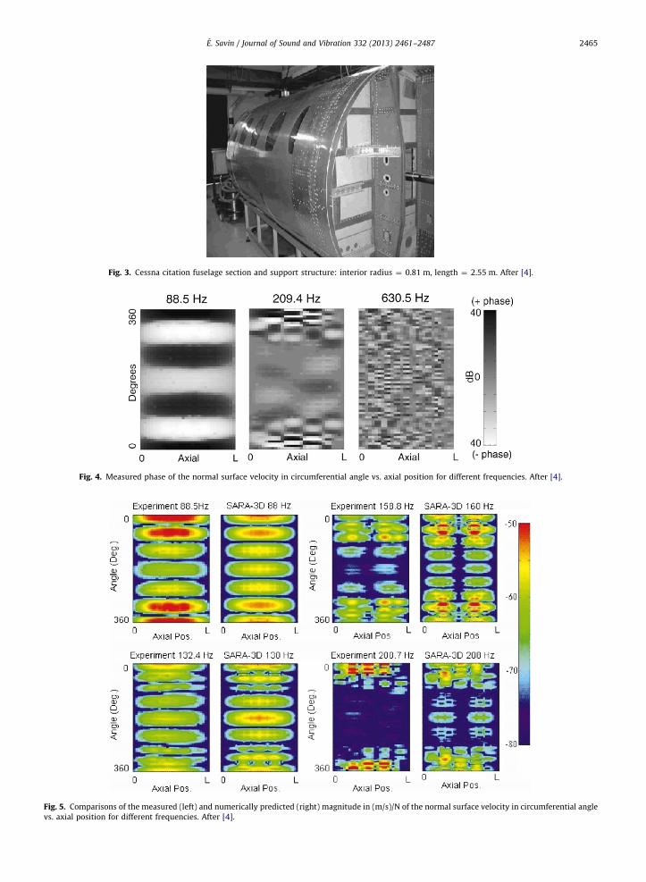
Fig. 3. Cessna citation fuselage section and support structure: interior radius ¼ 0.81 m, length ¼ 2.55 m. After [4].

Fig. 4. Measured phase of the normal surface velocity in circumferential angle vs. axial position for different frequencies. After [4].

Fig. 5. Comparisons of the measured (left) and numerically predicted (right) magnitude in (m/s)/N of the normal surface velocity in circumferential angle

vs. axial position for different frequencies. After [4].



that phase is nearly piecewise constant. But at the intermediate frequencies, the energy transfers become important fromone substructure to another, as the vibrational energy is carried by their local modes. At higher frequencies, these transfersare smoothed out since the diffusive regime by which the energy amplitudes within the subsystems have stabilised, hasbeen reached. Diffusion is manifested in the noisy pattern of the phase in this range. Note that the same conclusions weredrawn in [3] from the analysis of the phase trends for the experimental structure of Fig. 1. Incidentally, these observationsimply that smoothened amplitudes are not sufficient to describe mid-frequency vibrations, as one may be able to providean information on the phase as well; this important point was also emphasised in [94].

2.2. Influence of uncertainties

The three frequency domains discussed in the previous section are characterised in the following way [3,95,96],provided that it is understood that the terms low-, mid- and high-frequency have a relative connotation requiring a moreprecise qualification on a case by case basis, for the particular system in consideration:

�
A low-frequency response chiefly involves global, low-order structural eigenmodes which concentrate most of thevibrational energy. � A mid-frequency response is characterised by the superposition of some global eigenmodes (as in the low frequency
range) and clusters of local eigenmodes [97], which have an influence on both the local and global behaviours of thestructure in the narrow frequency band where they are packed. Energy transfers between subsystems are important,and the phase can change significantly from one point to another in the overall system [98,99].
� At last, a high-frequency response involves numerous local eigenmodes which contribute to localise the vibrational
energy. It is better characterised by quadratic observables smoothing out the contributions from the various localeigenmodes in given frequency bands, because the phase does not bring any additional information. Energy transfersbetween substructures are weak, may be negligible. The significance of choosing energy-type quantities in this rangeshall be addressed in more details in Section 3.3.2 below.

Because of the involvement of local modes, the predictive and irreducible uncertainties (as defined in [2]) and thestructural complexity are two factors which influence heavily the structural responses in the mid- to high-frequency ranges.This may be shown invoking simple analytical arguments as well [3,100] (see also [101, Appendix 10] and [102]). Thosefactors chiefly arise for built-up structures having a repetitive pattern of any kind, but not necessarily periodic, as forexample the above experimental structures or three-dimensional beam trusses [103]. Such structures actually haveneighbouring, indeed merged multiple eigenfrequencies because they are constituted by assemblies of nearly identicalsubsystems exhibiting themselves comparable eigenfrequencies when they are considered in isolation. Multiple eigenfre-quencies are attached to clusters of local eigenmodes for the different subsystems constituting the entire structure, whichhave a non-negligible, nay, dominant contribution to the overall vibrational energy in the higher frequency ranges.

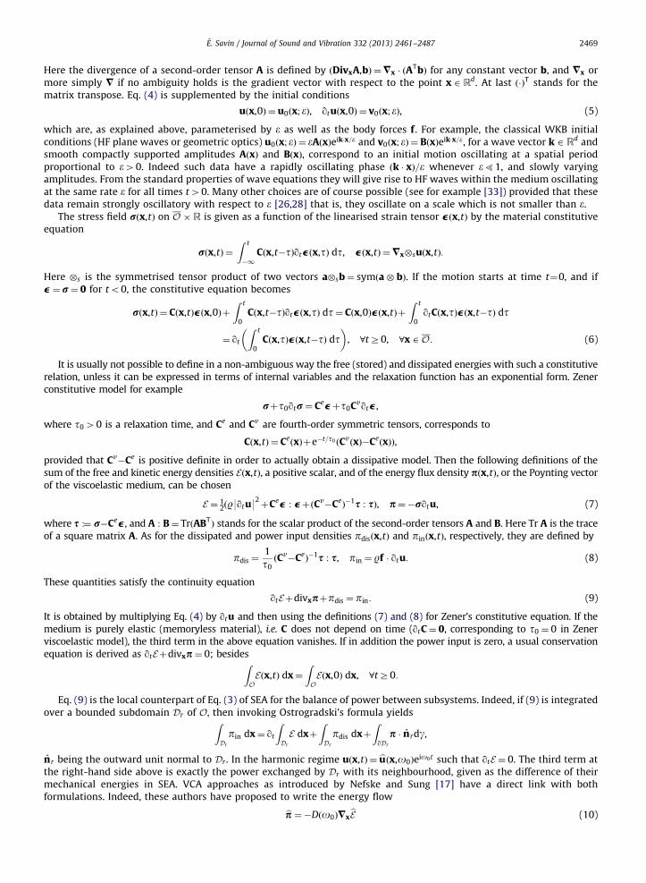
More generally, the theory of symmetric, positive random matrices proposed by Soize [104–106] shows that thedispersion of structural dynamic responses increases when the frequency increases, for a fixed level of dispersion ofthe structural mass, stiffness and/or damping matrices. This theoretical result is confirmed by several experiments onengineering structures, notably in the automotive industry [107,108]. Fig. 6 for example displays the magnitudes ofstructure-borne frequency response functions measured by a microphone at the driver’s head position for 99 samplesof pickup trucks [108]. This example illustrates the main difficulties arising in the analyses of HF structural dynamics:the vibrational energy is spread over a large number of local, higher-order eigenmodes, none of them prevailing overthe others in the overall system response, and the damping loss factors are small. It indicates that nominal responsesobtained from a particular model are not particularly useful unless they are understood in a statistical sense, thusoutlining the limitations of this model—especially in the HF range. These observations have prompted thedevelopment by engineers of the statistical energy analysis (SEA) of structural-acoustics systems. This globalapproach is briefly exposed in subsequent Section 2.3, before a more recent, though still heuristic local approach isintroduced in Section 2.4.

2.3. Global approach: statistical energy analysis (SEA)

SEA characterises the HF dynamic properties of linear structures including the effects of uncertainties in energetic andstatistical terms, hence the terminology. Indeed, the average mechanical energy within each substructure of the overallsystem constitutes the primal variable in the SEA formulation. This energy represents a response level integrated over asubstructure, rather than a local estimation. The selection of subsystems should be guided by geometrical and/or physical(mechanical) considerations, provided that the assumptions upon which SEA is based are satisfied. For example, anassembly of two plates may be split into two substructures, one for each plate, but each of them may support several wavetypes – bending, shear, etc. – and therefore more than one SEA subsystem. The method is statistical in the sense that themechanical parameters describing the dynamic response of the subsystems are uncertain and modeled by random

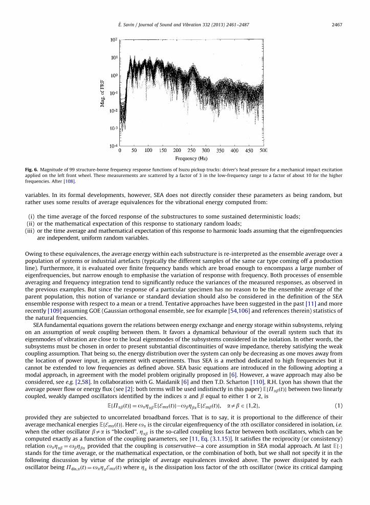
Fig. 6. Magnitude of 99 structure-borne frequency response functions of Isuzu pickup trucks: driver’s head pressure for a mechanical impact excitation

applied on the left front wheel. These measurements are scattered by a factor of 3 in the low-frequency range to a factor of about 10 for the higher

frequencies. After [108].


variables. In its formal developments, however, SEA does not directly consider these parameters as being random, butrather uses some results of average equivalences for the vibrational energy computed from:

(i)
the time average of the forced response of the substructures to some sustained deterministic loads; (ii) or the mathematical expectation of this response to stationary random loads;
(iii)
or the time average and mathematical expectation of this response to harmonic loads assuming that the eigenfrequenciesare independent, uniform random variables.
Owing to these equivalences, the average energy within each substructure is re-interpreted as the ensemble average over apopulation of systems or industrial artefacts (typically the different samples of the same car type coming off a productionline). Furthermore, it is evaluated over finite frequency bands which are broad enough to encompass a large number ofeigenfrequencies, but narrow enough to emphasise the variation of response with frequency. Both processes of ensembleaveraging and frequency integration tend to significantly reduce the variances of the measured responses, as observed inthe previous examples. But since the response of a particular specimen has no reason to be the ensemble average of theparent population, this notion of variance or standard deviation should also be considered in the definition of the SEAensemble response with respect to a mean or a trend. Tentative approaches have been suggested in the past [11] and morerecently [109] assuming GOE (Gaussian orthogonal ensemble, see for example [54,106] and references therein) statistics ofthe natural frequencies.

SEA fundamental equations govern the relations between energy exchange and energy storage within subsystems, relyingon an assumption of weak coupling between them. It favors a dynamical behaviour of the overall system such that itseigenmodes of vibration are close to the local eigenmodes of the subsystems considered in the isolation. In other words, thesubsystems must be chosen in order to present substantial discontinuities of wave impedance, thereby satisfying the weakcoupling assumption. That being so, the energy distribution over the system can only be decreasing as one moves away fromthe location of power input, in agreement with experiments. Thus SEA is a method dedicated to high frequencies but itcannot be extended to low frequencies as defined above. SEA basic equations are introduced in the following adopting amodal approach, in agreement with the model problem originally proposed in [6]. However, a wave approach may also beconsidered, see e.g. [2,58]. In collaboration with G. Maidanik [6] and then T.D. Scharton [110], R.H. Lyon has shown that theaverage power flow or energy flux (see [2]: both terms will be used indistinctly in this paper) EfPabðtÞg between two linearlycoupled, weakly damped oscillators identified by the indices a and b equal to either 1 or 2, is

EfPabðtÞg ¼oaZabEfEmaðtÞg�obZbaEfEmbðtÞg, aab 2 f1,2g, (1)

provided they are subjected to uncorrelated broadband forces. That is to say, it is proportional to the difference of theiraverage mechanical energies EfEmaðtÞg. Here oa is the circular eigenfrequency of the ath oscillator considered in isolation, i.e.

when the other oscillator baa is ‘‘blocked’’. Zab is the so-called coupling loss factor between both oscillators, which can becomputed exactly as a function of the coupling parameters, see [11, Eq. (3.1.15)]. It satisfies the reciprocity (or consistency)relation oaZab ¼obZba provided that the coupling is conservative—a core assumption in SEA modal approach. At last Ef�gstands for the time average, or the mathematical expectation, or the combination of both, but we shall not specify it in thefollowing discussion by virtue of the principle of average equivalences invoked above. The power dissipated by eachoscillator being Pdis,aðtÞ ¼oaZaEmaðtÞ where Za is the dissipation loss factor of the ath oscillator (twice its critical damping


rate), the average energetic balance for each oscillator thus reads

EfPin,aðtÞg ¼oaZaEfEmaðtÞgþoaZabðEfEmaðtÞg�EfEmbðtÞgÞ,

aab 2 f1,2g, which constitutes the fundamental SEA equation for the coupling between the ath and baa oscillators. Itrelates their average mechanical energies, forming the basic unknowns of the SEA method, with three of the fundamentalmechanical parameters of this approach:

(i)
the (small) dissipation loss factors Za; (ii) the coupling loss factors Zab;
(iii)
the power inputs Pin,aðtÞ induced by the applied loads.
In SEA it is subsequently assumed that this result extends to the conservative coupling of two continuous subsystems r

and sar 2 f1,2g considered as groups of Nr local eigenmodes only slightly modified by the coupling in a given frequencyrange of excitation I0 ¼ ½o0�Do=2,o0þDo=2�. Let or,a and Zr,a be the circular eigenfrequencies and dissipation lossfactors of the rth substructure when it is taken in isolation and is uncoupled from the other substructure, enforcing someboundary conditions on the interface as in e.g. [111]. Then let I r ¼ fa;or,a 2 I0g so that Nr ¼ card I r . The power exchangedbetween both substructures is written by analogy with Eq. (1)

EfPrsðtÞgCo0ZrsEfEmrðtÞg�o0ZsrEfEmsðtÞg, ras 2 f1,2g, (2)

where EmrðtÞ ¼MrP

a2I r_q2

r,aðtÞ, the sum of the contributions of the generalised coordinates qr,aðtÞ for the response of the rthsubstructure projected on its local eigenmodes (normalised with respect to the mass; Mr being therefore the total mass ofthe rth subsystem) in the frequency range I0. Zrs, Zsr are the average coupling loss factors of the substructures satisfying thereciprocity relation NrZrs ¼NsZsr . The latter involves the fourth fundamental mechanical parameter of SEA, the modaldensity nrðo0Þ ¼Nr=Do. The average energetic balance for each subsystem is for ras 2 f1,2g

EfPin,rðtÞg ¼o0ZrEfEmrðtÞgþo0ðZrsEfEmrðtÞg�ZsrEfEmsðtÞgÞ, (3)

where Zrðo0Þ is the average dissipation loss factor of the rth substructure defined by o0ZrEmrðtÞCMrP

a2I ror,aZr,a _q

2r,aðtÞ.

The last step in the SEA formulation is to assume that Eq. (2) further applies to the weak, conservative coupling of Nacoustical or mechanical subsystems. The average vibrational energies are then computed from the N �N matrixequation derived from Eq. (3) when it is written for each subsystem.

It may be seen from this discussion that SEA is based on successive assumptions, though it is observed in practice thatthis approach is rather effective. This is notably the case for the coupling of elastic structures with acoustic cavities, asituation where the hypotheses needed for these generalisations are actually fulfilled. Yet it should be noted that theapproximation (2) above is in fact rigorously wrong as soon as the number of dofs exceeds two [112]. It is however ratherwell satisfied by reverberant subsystems, and this is the reason why SEA is a method dedicated to the HF range. Moreover,it does not have any straightforward extension to the transient regime.

2.4. Local approach: continuity equation and vibrational conductivity analogy (VCA)

Besides this limitation, SEA does not give any information more precise than the average vibrational energy integratedover substructures. Approaches based on an analogy with heat conduction, referred to as vibrational conductivity analogy(VCA) [16–24], are aimed at describing locally how this energy is spread. They are derived from a standard continuityequation (local balance of energy) in elastodynamics including dissipation phenomena. This derivation is detailed below,starting from the equilibrium and constitutive equations pertaining to structural dynamics. Several assumptions will beintroduced in the course of the analysis, which limit the range of applicability of VCA. The purpose of this section is thus toexplain how VCA equations are obtained, and then underline these limitations in order to motivate the developmentspresented in Sections 3 and 4. Here a possible strategy for the improvement of SEA or VCA modeling is proposed, based onthe restrictions identified for those existing engineering approaches. This section also introduces some basic notationsused subsequently in Section 3.

Let ODRd be an open domain occupied by an heterogeneous linear viscoelastic material, where d¼1,2 or 3 is thephysical space dimension. Its density is denoted by RðxÞ and its fourth-order relaxation tensor is denoted by Cðx,tÞ, x 2 O,t 2 Rþ . We consider the vibrations of that medium about a static equilibrium configuration considered as its natural state(neglecting prestress) when it is subjected to HF initial conditions and body forces. The latter are characterised by theirhighly oscillatory feature, which is embodied in a small parameter e40. It is for example the rate of variation of theseloads with respect to the typical size of the medium, but it could be any other parameter which recall their HF content;there is no need to clarify what it is exactly for the subsequent analysis. Then the displacement field uðx,tÞ of the mediumabout its reference configuration will be parameterised by e as well, and will have the same oscillatory feature as the loadswhich have generated it. Thus let rðx,tÞ be the second-order Cauchy stress tensor of the medium. The balance ofmomentum in a fixed reference frame considering the action of body forces given by their density RðxÞfðx,t; eÞ is

Rq2t u¼DivxrþRf, x,t 2 O�R: (4)


Here the divergence of a second-order tensor A is defined by ðDivxA,bÞ ¼=x � ðATbÞ for any constant vector b, and =x or

more simply = if no ambiguity holds is the gradient vector with respect to the point x 2 Rd. At last ð�ÞT stands for thematrix transpose. Eq. (4) is supplemented by the initial conditions

uðx,0Þ ¼ u0ðx; eÞ, qtuðx,0Þ ¼ v0ðx; eÞ, (5)

which are, as explained above, parameterised by e as well as the body forces f. For example, the classical WKB initialconditions (HF plane waves or geometric optics) u0ðx; eÞ ¼ eAðxÞeik�x=e and v0ðx; eÞ ¼ BðxÞeik�x=e, for a wave vector k 2 Rd andsmooth compactly supported amplitudes AðxÞ and BðxÞ, correspond to an initial motion oscillating at a spatial periodproportional to e40. Indeed such data have a rapidly oscillating phase ðk � xÞ=e whenever e51, and slowly varyingamplitudes. From the standard properties of wave equations they will give rise to HF waves within the medium oscillatingat the same rate e for all times t40. Many other choices are of course possible (see for example [33]) provided that thesedata remain strongly oscillatory with respect to e [26,28] that is, they oscillate on a scale which is not smaller than e.

The stress field rðx,tÞ on O �R is given as a function of the linearised strain tensor e ðx,tÞ by the material constitutiveequation

rðx,tÞ ¼

Z t

�1

Cðx,t�tÞqte ðx,tÞ dt, e ðx,tÞ ¼=x�suðx,tÞ:

Here �s is the symmetrised tensor product of two vectors a�sb¼ symða� bÞ. If the motion starts at time t¼0, and ife ¼ r¼ 0 for to0, the constitutive equation becomes

rðx,tÞ ¼ Cðx,tÞe ðx,0Þþ

Z t

0Cðx,t�tÞqte ðx,tÞ dt¼ Cðx,0Þe ðx,tÞþ

Z t

0qtCðx,tÞe ðx,t�tÞ dt

¼ qt

Z t

0Cðx,tÞe ðx,t�tÞ dt

� �, 8tZ0, 8x 2 O: (6)

It is usually not possible to define in a non-ambiguous way the free (stored) and dissipated energies with such a constitutiverelation, unless it can be expressed in terms of internal variables and the relaxation function has an exponential form. Zenerconstitutive model for example

rþt0qtr¼ Ceeþt0Cvqte ,

where t040 is a relaxation time, and Ce and Cv are fourth-order symmetric tensors, corresponds to

Cðx,tÞ ¼ CeðxÞþe�t=t0 ðCv

ðxÞ�CeðxÞÞ,

provided that Cv�Ce is positive definite in order to actually obtain a dissipative model. Then the following definitions of the

sum of the free and kinetic energy densities Eðx,tÞ, a positive scalar, and of the energy flux density pðx,tÞ, or the Poynting vectorof the viscoelastic medium, can be chosen

E ¼ 12ðR9qtu9

2þCee : eþðCv

�CeÞ�1s : sÞ, p¼�rqtu, (7)

where s :¼ r�Cee , and A : B¼ TrðABTÞ stands for the scalar product of the second-order tensors A and B. Here Tr A is the trace

of a square matrix A. As for the dissipated and power input densities pdisðx,tÞ and pinðx,tÞ, respectively, they are defined by

pdis ¼1

t0ðCv�CeÞ�1s : s, pin ¼ Rf � qtu: (8)

These quantities satisfy the continuity equation

qtEþdivxpþpdis ¼ pin: (9)

It is obtained by multiplying Eq. (4) by qtu and then using the definitions (7) and (8) for Zener’s constitutive equation. If themedium is purely elastic (memoryless material), i.e. C does not depend on time (qtC¼ 0, corresponding to t0 ¼ 0 in Zenerviscoelastic model), the third term in the above equation vanishes. If in addition the power input is zero, a usual conservationequation is derived as qtEþdivxp¼ 0; besidesZ

OEðx,tÞ dx¼

ZOEðx,0Þ dx, 8tZ0:

Eq. (9) is the local counterpart of Eq. (3) of SEA for the balance of power between subsystems. Indeed, if (9) is integratedover a bounded subdomain Dr of O, then invoking Ostrogradski’s formula yieldsZ

Dr

pin dx¼ qt

ZDr

E dxþ

ZDr

pdis dxþ

ZqDr

p � nrdg,

nr being the outward unit normal to Dr . In the harmonic regime uðx,tÞ ¼ buðx,o0Þeio0t such that qtE ¼ 0. The third term at

the right-hand side above is exactly the power exchanged by Dr with its neighbourhood, given as the difference of theirmechanical energies in SEA. VCA approaches as introduced by Nefske and Sung [17] have a direct link with bothformulations. Indeed, these authors have proposed to write the energy flowbp ¼�Dðo0Þ=x

bE (10)


invoking a Fourier-like, or Fick-like law as the frequency increases. Dðo0Þ is a diffusion coefficient depending on the (large)central circular frequency o0 of the frequency range I0 of the loads in a steady-state regime. In this respect, (10) is a localcounterpart of (2), whereas (9) becomes a diffusion equation yielding, once it is integrated over the subdomain DrZ

Dr

bpin dx¼ZDr

bpdis dx�ZqDr

Dðo0Þqn rbE dg

to be compared with (3). VCA approaches have only been applied to simple systems until now, namely homogeneous

beams and thin plates, since they are based, as seen here, on the assumption (10). Although it may have a rather firmtheoretical basis for one-dimensional waveguides (rods), this conjecture is very restrictive, and even gets wrong for otherstructures or higher physical dimensions (d¼2 or 3, see for instance the discussions in [20,21]). This issue will beaddressed further on in Section 3.4.

2.5. Research needs and objectives

The previous presentation of SEA and VCA has shown that both approaches rely on some crucial assumptions, namely(2) and (10) respectively, though they may be very effective in the current engineering practice. This observation motivatesthe consideration of an alternative point of view, which should be able to release the limitations imposed in SEA and VCAderivations. It is argued in the remaining of the paper that kinetic models of wave propagation phenomena may be welladapted to this objective. This is because they describe highly oscillating waves adopting an energetic point of view inthe phase space position�wave vectors, and they apply to heterogeneous (possibly random) media. They also allow toderive rigorously diffusion limits for multiply scattered waves, a situation pertaining to the engineering appraisal of HFvibrations. These models are described in Section 3 in the context of the different regimes applicable to wave propagationphenomena, depending of the scaling of the wavelength vs. a typical size of the inhomogeneities. The different resultspresented there apply to open, non-dissipative media. The implementation of kinetic models in structural dynamics thusrequires two important extensions: (i) the consideration of dissipative phenomena, paying particular attention to theconstruction of models consistent with the use of energetic observables; and (ii) the consideration of dedicated boundaryconditions for such quantities, consistent with the boundary conditions imposed to the underlying wave fields. Both issuesare addressed in Section 4. Damping modeling and boundary conditions for kinetic equations are outlined in Sections 4.1and 4.2, respectively, and an overall assessment of the various developments presented in the paper is given in Section 4.3.The objectives of this research are twofold. As regards modeling issues on one hand, kinetic models are aimed at justifyingand possibly extending the SEA and VCA approaches on the basis of a firm, more general theoretical ground and weakenedassumptions. It is also focused on the transient domain for which the existing literature and results are rather sparse.Regarding the applications on the other hand, the proposed models are dedicated to the computation of the dynamicresponses of built-up structures impacted by mechanical, acoustical or aerodynamic loads either in the transient or thesteady-state regimes. Examples include cars, railway trains, aircrafts, spacecrafts, ships, pipelines, buildings, or industrialplants.

3. High-frequency elastic wave propagation in heterogeneous media

Electromagnetic, acoustic or elastic waves in an homogeneous medium have a fairly well identified behaviour, even inthe presence of a smooth boundary as a free surface for example. This is no longer the case in an heterogeneous medium ora piecewise homogeneous medium, not to mention a random medium. Wave propagation in heterogeneous media is thesubject of intense, multidisciplinary researches in order to exhibit, on one hand, some new phenomena such as anisotropicdiffusion (strong localisation) or coherent back-scattering effects (weak localisation), and to take advantage, on the otherhand, of these effects in applications such as time reversal techniques. This issue is less studied in continuum mechanics,beside some early works in seismology and surface geophysics [113]. However, it is essential in the understanding of theHF vibrational phenomena described in the previous section. The purpose of this section is therefore to present thedifferent approaches invoked in modeling wave propagation in heterogeneous media, although such a description cannotpretend to be exhaustive in view of the considerable existing literature on the subject. Refs. [46–48] for example, so as tocite only recent works, develop a thorough and much more relevant analysis than the simple ideas expounded below.These different approaches are emphasised here in view of introducing the kinetic modeling strategy adopted for thedescription of HF vibrations of slender structures, which is explained in subsequent Section 4.

3.1. Characteristic scales

The identification of wave propagation phenomena in heterogeneous media is based on the formal identificationof several characteristic scales: the wavelength l, the characteristic length of heterogeneities ‘ in the medium or theircorrelation length ‘c if they are random, and the size of the sample, or the observation/propagation distance L. These scalesallow to gradually distinguish local to global effects. One can then identify the so-called microscopic, mesoscopic, andmacroscopic regimes depending on, roughly speaking, the ratio of the wavelength l to the scale ‘, d¼ l=‘; one also


introduces k¼ ‘=L or ‘c=L (the Knudsen number) in the subsequent analyses. These different regimes are characterised asfollows:

�
Microscopic regime d41: The relevant evolution model is the wave equation. The location and shape of all heterogeneities,inclusions, holes, boundaries, interfaces, stiffeners in a structure, have to be known precisely. If distances between theseheterogeneities are comparable to the wavelength, resonance phenomena basically arise. � Mesoscopic regime d� 1: The relevant evolution model is the transport equation, or the radiative transfer (linear
Boltzmann) equation in a ‘‘high-frequency’’ random medium where the correlation length is comparable to thewavelength. The characteristic parameters of this medium are its scattering mean free paths or the transport velocities,which are derived from the microscopic regime. At these scales complex weak or strong localisation phenomena mayarise, as a result of the interaction of scattered waves with heterogeneities. These phenomena will not be addressed inthis discussion.
� Macroscopic regime do1: The relevant evolution model is the diffusion equation. It is characterised by a diffusion
coefficient which is derived from the mesoscopic parameters. In this regime all interferences of waves with hetero-geneities are smoothed out and angularly averaged intensities are considered.

A fourth scale, the absorption length La for optical systems or the incoherence length Li for electronic systems, is alsointroduced by physicists. The whole Section 3 is focused on non-dissipative media, and weakly dissipative structures areconsidered in Section 4.1; thus one always has La ¼ þ1 or at least L5La, and this scale is ignored.

Of course several characteristic lengths and wavelengths can coexist. The following discussion is only a crude and naivesimplification of a much more complex reality where different phenomena interact at different scales, described by different,possibly competing models. Another difficulty is raised by the polarised feature of elastic waves: if materials are isotropic,they are constituted by a single compressional mode (denoted by P) similarly to acoustic waves, and a twofold shearmode (denoted by S) similarly to electromagnetic waves, with possible conversions between both modes. This additionalcomplexity has a direct influence on the understanding of the various phenomena to be identified, because they may arise forP and S waves simultaneously. Finally, it is also of note to mention that the behaviour of the waves near and at the transitionbetween the different regimes outlined above is not well understood, and the models should ideally be improved in order toexplain it. Now the microscopic, mesoscopic and macroscopic regimes are reviewed in the next three sections.

3.2. Microscopic regime

If ‘ is the scale of variations of the mechanical parameters of the medium and if these variations can be described fairlywell, then as soon as l is greater than ‘ the propagation regime is the low-frequency microscopic regime; the relevantevolution model is the balance equation of elastodynamics in O�R

Rq2t ue ¼=x � ðC

e : =x � ueÞþRfe: (11)

Eq. (11) is nothing but Eq. (4) ignoring dissipation. Also the displacement field u has been indexed by e in order to recallthat it is parameterised by this parameter since the applied loads (initial conditions (5) and body forces f) are; typicallye¼ l=L, the normalised wavelength of the waves they generate within the medium. The dominant physical phenomena inthis case are (i) single scattering, corresponding to the interaction of an incident wave with a bounded, well identifiedinhomogeneity backscattering waves at different frequencies, directions and polarisations, and (ii) resonance, as a result ofconstructive interferences at particular frequencies. In soil–structure interaction for example resonant modes almostidentical to the structural modes in vacuo arise. However, some specific interaction modes may appear as well, for thecase of stiff media coupled to a flexible one, or modes related to the system shape (a stratified medium, typically, for acomposite structure or a soil); see [114] and references therein.

The limit case db1, where mechanical parameters of the medium vary rapidly, can be treated by homogenisationtechniques or an effective medium theory; see for example [115,116] for applications in elastodynamics. Both approachesapply to the case of randomly distributed inclusions of which number increases indefinitely at a constant volumic fraction inan homogeneous background medium. They are relevant as long as the propagation distance L remains comparable to thewavelength, e� 1. They are very effective for steady-state problems in enclosed area, but they do not account for propagationand transport effects (of the associated energy) when e51. This is the mesoscopic regime outlined in the next section.

3.3. Mesoscopic regime

For short wavelengths with respect to the observation distance within the propagation medium, considering first thatits mechanical parameters vary slowly, the relevant evolution model is the transport equation. It describes the mesoscopicregime of propagation, corresponding to the mid- to high-frequency vibrations of bounded structures. Therefore, thesubsequent presentation introduces the main notations and concepts which will be used in Section 4 to elaborate atransient transport model for the response of slender structures to high-frequency excitations. It starts with a short surveyof classical WKBJ, or ray methods which is primarily aimed at expounding the notations and the Lagrangian approach of


wave front tracking for short wavelengths. The latter is formally generalised in Sections 3.3.2 and 3.3.3 which summarisethe main concepts invoked in kinetic models.

3.3.1. Ray methods

The transport model is known in room acoustics [117] or seismology [71,72], among others, in the form of the raytheory:

(i)

Fig.(c). A

with a real phase, or WKBJ method, after the physicists G. Wentzel, H. Kramers and L. Brillouin, and the mathematicianH. Jeffreys who independently formalised it in 1920s; a first evidence can be found in the early works of F. Carlini(1817) or G. Green and J. Liouville (1837) as reviewed in [70];

(ii)
or with a complex phase, for example the method of Gaussian beams [118], widely used in elastodynamics [119],underwater acoustics [120], or electromagnetism [121].
It consists in seeking a solution of Eq. (11) in the form

ueðx,tÞCeiSðx,tÞ=eX1k ¼ 0

ekUkðx,tÞ, e¼ lL51, (12)

where the phase function Sðx,tÞ is either real in the WKBJ method, or complex for a Gaussian beam. Plugging the ansatz(12) into Eq. (11), it is shown, adopting an Eulerian point of view (see Fig. 7(b)), that the phase function satisfies an eikonalequation and that the density 9U09

2satisfies a linear transport equation of which coefficients depend on the phase

function. Indeed, starting from (11) in the homogeneous case fe 0 (the elastic wave equation), the acoustic, or Christoffeltensor Cðx,kÞ, and the dispersion matrix Hðs,nÞ of the propagation medium are introduced as follows:

Cðx,kÞU¼ RðxÞ�1ðCeðxÞ : U� kÞk, U 2 Rn, (13a)

Hðs,nÞ ¼ RðxÞðCðx,kÞ�o2InÞ, (13b)

where s¼ ðx,tÞ, n¼ ðk,oÞ, ðs,nÞ 2 TnðO�RÞ :¼ O�Rt �Rd

k �Ro, and In is the identity matrix of Rn. Here n is thedimension of the wave system, which is d in elastodynamics but may be greater than the physical space dimension forwave systems arising from reduced kinematics as with thick beams or shells. H does not depend on the scale e, that is tosay we consider high-frequency wave propagation e51 in a slowly varying ‘‘low frequency’’ medium k� 1. The eikonaland zeroth-order transport read

Hðs=sSÞU0 ¼ 0, (14a)

=s � ðUT0=nHðs,=sSÞU0Þ ¼ 0, (14b)

respectively. Adopting a Lagrangian point of view (see Fig. 7(c)), the pair ðs,=sSÞ is the solution of the Hamiltonian systemassociated to the elastic wave equation, which consists in solving the eikonal equation by the method of characteristics, orray tracing. Thus introducing the Hamiltonian H¼ det H, the usual properties of the acoustic tensor C are such that

Hðs,nÞ ¼Yn

a ¼ 1

Haðs,nÞ, Haðs,nÞ ¼ RðxÞðl2aðx,kÞ�o2Þ, (15)

where l2a stands for the ath (positive) eigenvalue of C with 1rarn. Considering isotropic elasticity for instance,

Cðx,kÞ ¼ l2Pðx,kÞk � kþl2

S ðx,kÞðId�k � kÞ and laðx,kÞ ¼ caðxÞ9k9 of multiplicity 1 if a¼ P or 2 if a¼ S, cP and cS being theelastic compressional and shear wave velocities, respectively, such that cSocP . It is assumed subsequently that theeigenvalues of the acoustic tensor are distinct. The case of multiple eigenvalues with constant multiplicity, as for isotropicelasticity, is dealt with along the same lines although the writing is more involved; see [26,28,34]. So for systems such thatnZd, n eigenvalues shall be considered altogether, counting for their orders of multiplicity.

Then the corresponding Hamiltonian equations for 1rarn are

ds

dt ¼=nHaðsðtÞ,nðtÞÞ, sð0Þ ¼ s0,

dn

dt ¼�=sHaðsðtÞ,nðtÞÞ, nð0Þ ¼ n0a0, (16)

7. Ray method with real phase for acoustic wave propagation with two monopoles A and B: exact solution (a), viscosity solution (b), and ray tracing

fter [73].


in TnðO�RÞ\fðs,nÞ; n¼ 0g, with an initial condition ðs0,n0Þ satisfying Haðs0,n0Þ ¼ 0. Note that it follows from this condition

that HaðsðtÞ,nðtÞÞ ¼ 0 for all t. The rays strictly speaking are defined as the projections on O�Rt of the bicharacteristiccurves t/ðsaðtÞ,naðtÞÞ solving (16), that is t/saðtÞ. These rays are space–time curves parameterised by t (a curvilinearabscissa, or a time in R) associated to propagation modes, or polarisations a defined by the dispersion relations Haðs,nÞ ¼ 0.This interpretation extends to randomly perturbed homogeneous media considering (16) as a system of stochasticdifferential equations for a transport process fðSt,NtÞ,tZ0g [122]. The ray method with a real phase has some majordrawbacks from either an Eulerian point of view or a Lagrangian point of view. The nonlinearity of the eikonal equationdoes not allow to superpose different phases, as required in Fig. 7(a). One way to circumvent this difficulty is to considerthe notion of viscosity solution [123], as in Fig. 7(b). From the Lagrangian point of view, ray tracing is no longer possible onthe caustics, where the rays stack, because the amplitudes Uk rapidly increase in their neighbourhood, and even blow upon the rays themselves. Using a complex phase function Sðx,tÞ with real values on the rays solely, and such that theimaginary part of its Hessian =x �=xS is positive definite on the rays [118], is a mean to release these restrictions. Indeed,if ðsðtÞ,kðtÞÞ stands for a solution of the associated Hamiltonian system, and if y is orthogonal to xðtÞ and =xSðsðtÞÞ ¼ kðtÞ,taking the Taylor expansion of the phase about a ray for 9y959xðtÞ9 yields

ueðxðtÞþy,tðtÞÞ U0ðsðtÞÞeifSðsðtÞÞþ ð1=2ÞyT ½=x�=xSðsðtÞÞ�yg=e (17)

as an approximate solution of (11). It is concentrated on the ray, but also defined away from it with a Gaussian profilewhich narrows when the frequency increases (or e-0). The advantage of this ansatz is that it is no longer necessary tosatisfy the eikonal equation exactly, but only its Taylor expansion up to a given order controlling the accuracy of theapproximate solution. It constitutes an alternative approach to the usual WKBJ method in order to describe the rays awayfrom the caustics and globally in time.

Applications of such ray methods for elastic wave propagation in open media or slender structures are too numerous to belisted here exhaustively; however, some classical and more recent references are (but not limited to) [69–81,119–121,124].

3.3.2. Transport model

The ansatz (12) of the ray theory is only one a priori particular construction of high-frequency solutions of the elasticwave equation. This approach also requires rather strong regularity assumptions for the initial conditions of the phase S

and amplitude U0. The more recent works of Tartar [125], Gerard et al. [26,126], Lions and Paul [25], Papanicolaou andRyzhik [28], or Bal [30] on the microlocal analysis of wave systems have generalised this theory for weaker assumptions ontheir high-frequency solutions and the initial conditions. These authors have shown that the energy density associated toall oscillating solutions (not only those having the form of Eq. (12)), resolved in the phase space position �wave vector,satisfies a Liouville-type transport equation. These results are now well established in physics [39–48], but have been lessconsidered in the engineering mechanics or engineering materials community [49–54]. The main mathematical tool forthe derivation of a transport equation from a wave equation is the Wigner transform, of which high-frequency limit e-0,the so-called Wigner measure, captures the vibrational energy density in phase space. The advantage of this newrepresentation is that it clears all classical difficulties inherited from ray methods, and it yields global propagationproperties of the energy for weakened regularity assumptions of the initial conditions [127]. In return, the explicitknowledge of the phase is lost. The eikonal equation is replaced by the dependence of the Wigner measure vs. n, whichgives its propagation directions as obtained from the dispersion equation Hðs,nÞ ¼ 0.

Going back to the system (16) and considering its solutions t/ðsðtÞ,nðtÞÞ ¼Ftðs0,n0Þ as the paths in phase space ofsome energy ‘‘particles’’ with an overall density denoted by WðsðtÞ,nðtÞÞ, then

dW

dt¼ fH,Wg ¼ 0, (18)

where ff ,gg :¼ =nf �=sg�=sf �=ng is the usual Poisson bracket. Eq. (18) is the Liouville equation which is the expression ofthe conservation of W in phase space starting from the initial data Wðs0,n0Þ :¼W0ðs,nÞ. As the dispersion matrix H isindependent of time, Eq. (16) yields do=dt¼ 0 and W has on X :¼ Tn

ðO�RÞ\fk¼ 0g the form

W ¼Xn

a ¼ 1

WadðHaÞ, (19)

where dð�Þ is the usual Dirac measure, and the Wa’s are referred to as specific intensities in the dedicated literature. Theycharacterise the amount of energy density concentrated on the different rays existing for the different polarisation modesa given by the dispersion relations Ha ¼ 0. Thus we will also refer to them as energy rays in some instances in theremaining of this paper. The total energy is finally recovered by transporting the initial energy along the particle paths inphase space Z

Xjðs,nÞWðds,dnÞ ¼

Xn

a ¼ 1

ZXa

jðFtðs,nÞÞW0ðds,dnÞ,

for all continuous (test) functions j with compact support in TnðO�RÞ, introducing the sets

Xa ¼ fðs,nÞ 2 X ; Haðs,nÞ ¼ 0g: (20)


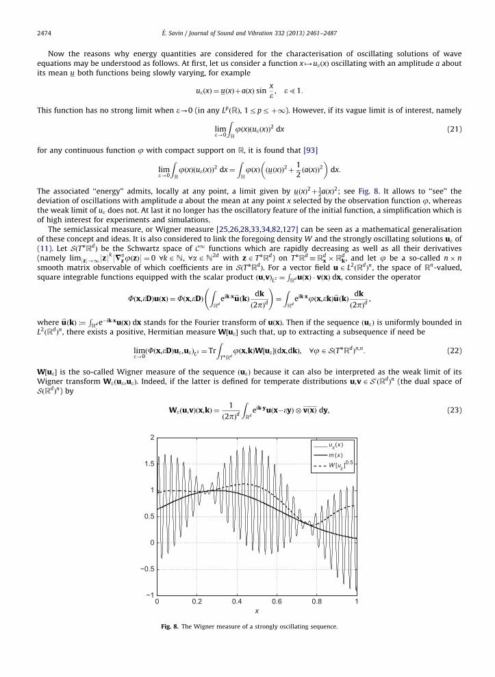
Now the reasons why energy quantities are considered for the characterisation of oscillating solutions of waveequations may be understood as follows. At first, let us consider a function x/ueðxÞ oscillating with an amplitude a aboutits mean u both functions being slowly varying, for example

ueðxÞ ¼ uðxÞþaðxÞ sinx

e , e51:

This function has no strong limit when e-0 (in any LpðRÞ, 1rprþ1). However, if its vague limit is of interest, namely

lime-0

ZRjðxÞðueðxÞÞ2 dx (21)

for any continuous function j with compact support on R, it is found that [93]

lime-0

ZRjðxÞðueðxÞÞ2 dx¼

ZRjðxÞ ðuðxÞÞ2þ 1

2ðaðxÞÞ2

� �dx:

The associated ‘‘energy’’ admits, locally at any point, a limit given by uðxÞ2þ12aðxÞ2; see Fig. 8. It allows to ‘‘see’’ the

deviation of oscillations with amplitude a about the mean at any point x selected by the observation function j, whereasthe weak limit of ue does not. At last it no longer has the oscillatory feature of the initial function, a simplification which isof high interest for experiments and simulations.

The semiclassical measure, or Wigner measure [25,26,28,33,34,82,127] can be seen as a mathematical generalisationof these concept and ideas. It is also considered to link the foregoing density W and the strongly oscillating solutions ue of(11). Let SðTnRd

Þ be the Schwartz space of C1 functions which are rapidly decreasing as well as all their derivatives(namely lim9z9-19z9

k9=azjðzÞ9¼ 0 8k 2 N, 8a 2 N2d with z 2 TnRd) on TnRd

Rdx �Rd

k, and let j be a so-called n� n

smooth matrix observable of which coefficients are in SðTnRdÞ. For a vector field u 2 L2

ðRdÞn, the space of Rn-valued,

square integrable functions equipped with the scalar product ðu,vÞL2 ¼RRd uðxÞ � vðxÞ dx, consider the operator

Fðx,eDÞuðxÞ ¼Fðx,eDÞZRd

eik�xbuðkÞ dk

ð2pÞd

!¼

ZRd

eik�xjðx,ekÞbuðkÞ dk

ð2pÞd,

where buðkÞ :¼ RRd e�ik�xuðxÞ dx stands for the Fourier transform of uðxÞ. Then if the sequence ðueÞ is uniformly bounded in

L2ðRdÞn, there exists a positive, Hermitian measure W½ue� such that, up to extracting a subsequence if need be

lime-0ðFðx,eDÞue,ueÞL2 ¼ Tr

ZTnRd

jðx,kÞW½ue�ðdx,dkÞ, 8j 2 SðTnRdÞn,n: (22)

W½ue� is the so-called Wigner measure of the sequence ðueÞ because it can also be interpreted as the weak limit of itsWigner transform Weðue,ueÞ. Indeed, if the latter is defined for temperate distributions u,v 2 S0ðRd

Þn (the dual space of

SðRdÞn) by

Weðu,vÞðx,kÞ ¼1

ð2pÞd

ZRd

eik�yuðx�eyÞ � vðxÞ dy, (23)

0 0.2 0.4 0.6 0.8 1−1

−0.5

0

0.5

1

1.5

2

x

uε(x )

m (x )

W [uε ]0.5

Fig. 8. The Wigner measure of a strongly oscillating sequence.


then one has

ðFðx,eDÞu,vÞL2 ¼ Tr

ZTnRd

jðx,kÞWeðu,vÞðdx,dkÞ:

Thus W½ue� describes the limit energy of the sequence ðueÞ. As in Eq. (21), the matrix function jðx,kÞ is used to select anyquadratic observable or quantity of interest associated to this energy: the kinetic energy, or the free energy, or the powerflow, etc. For example, the high-frequency (e-0) strain energy VeðtÞ :¼ 1

2

ROCee e : e e dx in O (see Eq. (7)) with e e ¼=x�sue

may be estimated using jðx,kÞ RðxÞCðx,kÞ, the acoustic tensor (13a) of the background medium

lime-0VeðtÞ ¼

1

2

ZO�Rd

RðxÞCðx,kÞ : W½ueð�,tÞ�ðdx,dkÞ,

up to some possible boundary effects on qO. Similarly, the kinetic energy T eðtÞ :¼ 12

ROR9qtue9

2dx is estimated by

lime-0T eðtÞ ¼

1

2

ZO�Rd

RðxÞTr W½qtueð�,tÞ�ðdx,dkÞ:

A close concept is H-measure, or microlocal defect measure [125,126,128]. The main difference is that the latter isassociated to any mean-zero square integrable sequence, and it does not require any explicit scale e as in (23). However, itis defined on the unit cosphere bundle SnRd

Rdx �Sd�1

k , where Sd�1 is the unit sphere of Rd, that is it contains slightlyless information than the Wigner measure since it does not depend on the norm of the wave vector.

Since the sequence ue considered above satisfies the wave equation (11), it can also be shown that: (i) its Wignermeasure can be expanded on the eigenspaces of the dispersion matrix H, i.e. into the sum of Wigner measures Wa for eachmode (this is the meaning of Eq. (19)); and (ii) each term in this expansion satisfies a transport equation of the formfHa,Tr Wag ¼ 0. A general mathematical framework for the direct passage from a wave equation with slowly varyingcoefficients to a transport equation for the phase space energy density of the high-frequency solutions of the former ispresented in Refs. [26,34].

3.3.3. Radiative transfer model

The transport model above can be extended to propagation media with rapidly varying parameters, at the same scale eas the wavelength. More generally, considering random perturbations of these parameters with a correlation length ‘c ofthe same order as the wavelength, k� e, the interactions of high-frequency waves with such ‘‘high-frequency’’ media aredepicted by a radiative transfer equation. It has the same characteristics as the transport equation (18), and the passagefrom a wave equation with oscillating coefficients to a radiative transfer equation is carried on using the samemathematical tools. However, only weak fluctuations have to be considered in order to observe an effective propagationpattern, otherwise the energy remains localised near its source. This passage is based on multiscale expansions and is onlyformal, in other words no rigorous proof exists except for some particular cases [29,32]. Nevertheless, the radiativetransfer model has been widely tested and validated by its numerous applications in neutronic transfers, thermal transfers,the analyses of the optical or acoustical properties of scattering media (in astrophysics, seismology, medical imaging,multiphase flows, room acoustics, etc.), time reversal techniques, etc.; see for example [28,39,40,44,129–132]. As for thedynamics of built-up systems, considering for instance the experimental structure depicted in Fig. 1, it may be observedthat the bending wavelength at the maximum experimental frequency is several fractions of the scattering mean free path,estimated by the average distance between stiffeners (about 20 cm). Thus they shall contribute, together with thejunctions, to multiply scatter the waves, playing the same role as the random perturbations in the above discussion. This isalso the argument developed in [132] for multiply scattered acoustic waves in fitted rooms. The radiative transfer modelalso allows to exhibit the diffusive behaviour of the waves at late times, as explained below in Section 3.4.

In this model, the influence of random perturbations or inclusions on the transport regime is characterised by anintegral operator, the so-called collision operator, on the right-hand side of the Liouville equation

fH,Wg ¼QðWÞ: (24)

Its effect is to modify the transport regime of the energy rays by multiple scattering, and possibly conversions of theirpolarisation modes a—see the expansion (19) of the density W

QðWÞðs,nÞ ¼

ZRdþ 1

~sðs,n,n0ÞðWðs,n0Þ�Wðs,nÞÞ dn0, (25)

where the scattering cross-section ~sðs,n,n0Þ is written explicitly as a function of the power spectral densities of randomperturbations [27–33]. The radiative transfer equation (24) is conservative in the sense that

RRdþ 1QðWÞðs,nÞ dn¼ 0.

Moreover, since do=dt¼ 0 and considering (19) one can remark that ~s necessarily has the form

~sðs,n,n0Þ ¼Xn

a,b ¼ 1

laðx,kÞlbðx,k0Þsabðx,k,k0Þdðlbðx,k0Þ�laðx,kÞÞ: (26)

The kernel sabðx,k,k0Þ gives the rate of conversion of an incident energy ray travelling in the direction of k0 and thepolarisation b into a ray travelling in the direction of k and the polarisation a when it is diffracted on randomheterogeneities located at x. They may be computed explicitly as functions of the auto- and cross-power spectra of the


fluctuations in randomly perturbed heterogeneous media with correlation lengths comparable to the wavelengths k� e[27–32]. The scattering processes described by Eq. (26) are such that the Hamiltonian Ha of Eq. (16) is preserved, asrequested, that is laðx,kÞ ¼ lbðx,k0Þ :¼ o 2 R is constant along the energy paths.

In transport and radiative transfer models, the relevant scale ‘ to describe the medium heterogeneities is the scatteringmean free path ‘sc, which is defined as the mean square distance travelled by the rays between two successive diffractions

‘sc ¼9c9~S

, ~Sðs,nÞ ¼

ZRdþ 1

~sðs,n,n0Þ dn0, (27)

with the group velocity c :¼ =nH and the total scattering cross-section ~S. Scattering cross-sections of the form of Eq. (26)induce different scattering mean free paths ‘a ¼ 9ca9=Sa for the different polarisations of which group velocities areca :¼ =nHa. Accordingly, the total scattering cross-sections are

Saðx,kÞ ¼Xn

b ¼ 1

l2aðx,kÞ

ZRdsabðx,k,k0Þdðlbðx,k0Þ�laðx,kÞÞ dk0 ¼

Xn

b ¼ 1

ZSd�1

Sabðx,k; k0

Þ dOðk0

Þ, (28)

where O is the uniform probability measure on the unit sphere Sd�1 of which surface is Sd�1 ¼

RSd�1 dO (with the

convention S0¼ f�1,þ1g), and u :¼ u=9u9 2 Sd�1 for any vector u 2 Rd

\f0g. The variation scale k� e of the heterogeneitiesis no longer observable by these models. The latter still holds relevance as long as lo‘scoL. As soon as ‘sc5L, multiplescattering render them too much demanding in terms of accuracy and then inappropriate for measurements. Diffusion is amuch more relevant model in this case. This regime is outlined in Section 3.4 below.

3.3.4. Applications

Transport and radiative transfer models for slender structures such as beams, plates or shells have been derived in[35,38,92,52], or for poro-viscoelastic media in [36]. The kinematics used until now for slender structures is of the firstorder (Timoshenko hypotheses for beams, Naghdi–Cooper hypotheses – for example – for shells). Higher-order kinematicsshall be investigated in future researches. Indeed, a first-order kinematic assumption may be not refined enough to dealwith short wavelengths with respect to the transverse dimensions of a beam or a shell. Regarding beams or plates forexample, a Rayleigh–Lamb model in dimension one or two could be considered for application to non-destructiveevaluation or structural health monitoring by ultrasonic waves. The Lamb model for plates has been studied in [133,134].Yet the numerical simulations carried out with first-order kinematic models of beams and shells yield convincing results,both qualitatively and quantitatively [35,37,38,87,93,135]. Above all, a rational framework for the analyses and validationsof the heuristic approaches outlined in Section 2, namely SEA (Section 2.3) or VCA (Section 2.4), can be proposed based onthese derivations. They also allow to release some restrictive assumptions at the foundations of these formulations. Asalready noted in Section 2.5, the energy transport models are referred to as kinetic models in the literature, and we willstick to this terminology in the following.

3.4. Macroscopic regime

Now if the characteristic scale ‘ cannot be shorter than the size of a sample or a substructure, in other words if itbecomes large with respect to the scattering mean free path of the medium, waves can no longer ‘‘see’’ its heterogeneitiesalthough they have significantly modified their amplitudes and phases. This is the macroscopic regime corresponding tothe high-frequency range of vibrations of bounded structures as considered in SEA. The relevant evolution model in thiscase is the diffusion equation. Here the directions of the energy rays are lost because they have been diffracted, thusdiverted, numerously. Corollarily, the power flows tend to vanish when the energy rays are diffusively spread within themedium by multiple scattering. Strictly speaking, the radiative transfer model in the mesoscopic regime perfectly accountsfor these phenomena at long times of for short scattering mean free paths with respect to the dimensions of the sample ofthe propagation/observation distances L, after numerous diffractions. However, introducing a judicious rescaling and usinga formal asymptotic expansion, the long-time limit of the radiative transfer equation can be exhibited: it has precisely theform of a diffusion equation. The mathematical structure of the corresponding diffusion operator depends on the shape ofthe random heterogeneities occupying the propagation medium, which in return define the mathematical properties of thecollision operator. The diffusion regime is characterised by universal energy partition rules between different propagationmodes in relation to the properties of the scattering cross-sections, in particular if the latter are isotropic

~sðs,n,n0Þ ¼9c9

9n09dsðs,9n9,n � n

0

Þ: (29)

On the contrary, localisation phenomena occur for strongly anisotropic scattering cross-sections (the case of anisomericmedia [136,137]). The characteristic length of these phenomena is the transport mean free path ‘%, which is the meansquare distance travelled by the energy rays up to the complete loss of their directivity pattern. ‘% is defined from themesoscopic parameter ‘sc (the scattering mean free path) by selecting the forward component–without diffraction—of the


total scattering cross-section

‘% ¼9c9

S, Sðs,9n9Þ ¼

ZSdsðs,9n9,n � n

0

Þð1�n � n0

Þ dOðn0

Þ:

This is now the relevant lengthscale ‘ for the description of the heterogeneities in the propagation medium since it is nolonger conceivable to follow in detail all scattered energy paths in the diffusion regime. The energy equipartition ruleinvoked above reads

EaEb¼

rarb

lbla

�� d, EaðsÞ ¼ZXa

Waðs,dnÞ, (30)

as soon as t4S�1

independently of the initial condition and of the random heterogeneities ; here ra stands for the order ofmultiplicity of the mode a with an energy density Ea inO�R, such that

Pra ¼ n. These issues constitute an active and fruitful

research topic in the mathematical and physical literature; they are enlighten by numerous experiments performed amongothers geophysicists or acousticians (the works of Campillo, Larose, Margerin, van Tiggelen et al. [136,138–141], Fink et al.[142], Page et al. [143], Picaut et al. [144,145], Scales [146], Turner, Weaver et al. [50–53,137,147], etc.).

The diffusion macroscopic regime also arises from the mesoscopic regime when the transport parameters are randomlyperturbed, for example the group velocity c in Eq. (18). If these perturbations have a small correlation length ‘c withrespect to the size of the sample or the propagation distance, yet large with respect to the wavelength e5k51, theLiouville equation reduces to a Fokker–Planck equation (ray diffusion) because it still depends on the propagationdirection n; its diffusion matrix depends on the auto-correlation function of the perturbations of the group velocity [33,62].The Fokker–Planck equation itself reduces to a spatial diffusion equation for long propagation times/distances. Anotherusual case, yielding the Laplace–Beltrami diffusion regime, is the strongly forward-peaked collision operator—the so-called grazing collisions: ~sðs,n,n0ÞC ~Sðx,nÞdð1�n � n

0

Þ [148,149].An implementation of these models for homogeneous slender structures with random perturbations is detailed in the

papers [35,150,151]. The paper [68] offers a general analysis for heterogeneous thick beams or plates. The paper [36]outlines the diffusion regime for a randomly perturbed, poro-viscoelastic homogeneous background medium. At last anexample of Fokker–Planck diffusion in a random thick plate is outlined in [151]. These different results partly justify theheuristic model of energy diffusion in the vibrational conductivity analogy of Section 2.4. One can in fact formally obtain aFourier-like law (10) [68] but the derivation of the diffusive regime from the transport regime explicitly requires theconsideration of the influence of random heterogeneities or boundaries (as done in the next section) in order to ‘‘mix’’efficiently the different propagation directions n. This requirement is in basic contradiction with the derivation of Nefskeand Sung [17] and subsequent research works [18–24]. All have used an original result by Rybak [152], who obtained theFourier law and a diffusion equation starting directly from a bending or a membrane equation for a thin plate with delta-correlated random inclusions; however, these random heterogeneities within the medium have generally been discardedin the derivations. But if that medium is perfectly homogeneous, the scattering mean free path (27) is infinite and diffusionis, as a rule, never reached.

4. Application to structural dynamics

The issue of modeling dissipation effects and boundary conditions has not been addressed in the previous exposition ofkinetic models. Their consideration is however a central concern for the application of the latter to structural dynamics,since it deals with damped, bounded media. Several results on dissipation phenomena in kinetic equations and boundaryand interface conditions adapted to these models are outlined in Sections 4.1 and 4.2 below, respectively. This section isclosed in Section 4.3 by the proposal of a transport model for the transient dynamics of elastic structures impacted by HFloads, presented as an outcome of the research works carried on until now. The continuity equation (9) in the HF limit e-0is ultimately given the form of a system of conservation equations for the different energy rays (the ‘‘component modes’’ inthis very limit), supplemented with dedicated boundary and interface conditions for the reflections and transmissions ofthe associated power flows. This setting embodies dissipation phenomena at the boundaries should the correspondingreflection/transmission operators be non-conservative.

4.1. Damping modeling

The influence of memory effects in viscoelastic materials can be considered starting from a stress-strain constitutiverelation of the form (6). It has been shown [91] that the memory term (the integral term) has no influence on the kineticequations obtained for the evolution of the high-frequency energy density. As for poro-viscoelastic media, the solid andfluid phases memory effects (the viscosity and compressibility are time-dependent) are also ineffective on the transportregime. The analysis in [36] is done along the same lines as in [91]. These results are in basic agreement with the currentpractical observations: viscoelastic materials tend to respond as purely elastic materials when they are forced by high-frequency harmonic motions (see for example [153, p. 22–23]). This conclusion does not mean however that no internaldissipation occurs in the high-frequency range, it rather indicates that the viscous model (6) may be irrelevant inthe transport regime. The radiative transfer equation (24) embodies dissipative phenomena if for example its collision


operator Q has the form

QðWÞ ¼Qð0ÞðWÞ�ZW ,

ZRdþ 1QðWÞðs,nÞ dno0, (31)

where Qð0Þ is the conservative part and Z40 is a loss factor (in s �1) which describes the absorption rate of energy‘‘particles’’ in the collision process. Q is said to be subcritical in this case. The solution W of the radiative transfer equation(24) is in this case

WðsðtÞ,nðtÞÞ ¼ e�ZtW ð0ÞðsðtÞ,nðtÞÞ, (32)

where W ð0Þ is the solution – if any – without absorption. Thus the model of Eq. (31) is representative of an energy densitydecreasing exponentially along its paths in phase space.

The issue of establishing the constitutive equation yielding a given form of subcritical collisions and the reverse thenarises. In [89,90] the authors have shown that for a scalar wave equation (4) and a Kelvin–Voigt constitutive equation,r¼ CeeþCv _e , the loss factor is

Zðx,kÞ ¼ 2CeðxÞk � k

CvðxÞk � k

,

that is to say Z is twice the rate of relaxation, as expected. For more general forms of subcritical collision operators, thisissue is still rather open and raises difficult questions. It is the subject of ongoing researches in the applied mathematicscommunity.

4.2. Boundary and interface conditions

Boundary conditions for quadratic quantities such as the vibrational energy density shall be constructed on the basis ofthe boundary conditions applied to the underlying displacement and stress fields, for example Dirichlet or Neumannboundary conditions, or interface jump conditions between substructures (assuming that the thickness of that interface ismuch smaller than the wavelength) [82–86]. They basically translate into reflection/transmission operators for the energyfluxes. The consideration of boundary conditions in kinetic models raises some significant theoretical difficulties related tothe polarisation and the possible conversion of waves in elastodynamics, as well as in electromagnetism, and to the criticalangles of incidence arising for either transmission or reflection problems [88]. Indeed, the energy ‘‘density’’ W having itssupport in the sets Xa by Eq. (19), the condition Haðs,nÞ ¼ 0 has yet to be satisfied on the boundary qO�R, or on aninterface SD � O�R oriented by its normal ðn,ntÞ. Commonly for acoustic or elastic waves in three-dimensional mediaand slender structures, the eigenvalues l2

a of the Christoffel tensor C have the form laðx,kÞ ¼ caðxÞ9k9 where ca40 is thephase velocity of the ath mode. Thus this very condition reads

Haðs,nÞ ¼ RðxÞc2aðxÞk

2nþHaðs,k%,oÞ ¼ 0, (33)

isolating the normal component kn ¼ k � n of the wave vector, while k%

¼ ðId�n � nÞk is its tangential component. Eq. (33)is a simple quadratic equation for kn, parameterised by k%. It has real or purely imaginary solutions if Haðs,k%,oÞo0 orHaðs,k%,oÞ40, respectively, since RðxÞc2

aðxÞ40. Thus the cotangent bundle to the boundary TnqO�R splits as TnqO�R¼Ha [ Ea [ Ga (for all modes a, see for example [84]), where the different diffraction regions on qO�R are defined by

Ha ¼ fðs,k%,oÞ 2 TnqO�R; Haðs,k%,oÞo0g ðhyperbolicÞ,

Ea ¼ fðs,k%,oÞ 2 TnqO�R; Haðs,k%,oÞ40g ðellipticÞ,

Ga ¼ fðs,k%,oÞ 2 TnqO�R; Haðs,k%,oÞ ¼ 0g ðtangentÞ:

The first one corresponds to the transverse rays (below critical incidence) for which kn is real, the second one correspondsto the totally reflected rays (above critical incidence) for which kn is purely imaginary, and the third one corresponds to thetangent rays (critical or tangential incidence) for which kn ¼ 0 in the local frame of the tangent plane to the boundary at s.As for an interface, these definitions have to be extended on both sides since the acoustic tensor, and thus its eigenvalues,are a priori different; TnSD is then the union of all these regions [84], but the latter are not necessarily disjoint. Similarly tothe collisions of the rays on random heterogeneities of the medium detailed in Section 3.3.3, mode conversions a2bin Ha \Hb or Ha \ Eb are driven by the condition do=dt¼ 0 derived from Eq. (16). It enforces the conservation ofthe Hamiltonian, that is laðxðt�0 Þ,kðt�0 ÞÞ ¼ lbðxðtþ0 Þ,kðt

þ0 ÞÞ on any discontinuity front SD of the density W given by

SD ¼ fðs,nÞ 2 TnðO�RÞ; Sðs,nÞ ¼ 0g, where therefore t040 is such that Sðsðt0Þ,nðt0ÞÞ ¼ 0. Besides, the Rankine–Hugoniot

condition on SD \ ðSn

a ¼ 1 XaÞ is for the transport or radiative transfer equation

1fH,SgWU¼ 0,

where 1fU¼ f ðtþ0 Þ�f ðt�0 Þ stands for the jump of f on the front. This condition expresses the conservation of the normalenergy flux on the discontinuity, but it does not describe a priori how the energy density is distributed among the differentmodes by the reflections and transmissions on an interface (a junction) SD independent of time for example. However,solving a Riemann problem at that interface gives a decomposition of the normal energy flux into rays moving forward andbackward from it, including the effects of reflection and transmission. Thus the power flow reflection and transmission


coefficients for the transport problem may be derived and understood in terms of some particular Riemann solutions[73,154]. It may be observed in addition that since Wb is necessarily zero in a neighbourhood of Eb (away from TnSD)because its support is in Xb, its trace on TnSD is zero as well, thus Wb 0 by the mode conversion a-b within Ha \ Eb.

The strategy adopted in [155] (see also [156,157]) consists in constructing an approximate solution of the waveequation (11) for which an explicit expression of its energy density is known, since the latter is also the one of the exacthigh-frequency solution. This approximation is chosen for instance as an infinite sum of Gaussian beams weighted by theFourier–Bros–Iagolnitzer (FBI, see for example [158, Chapter 3]) transform of the initial conditions, provided that theirsupport is disconnected from the boundary. The whole analysis is however restricted to transverse reflections solely (inHP \HS) for an isotropic elastic medium. For slender structures such as thick beams or plates, the power flow reflection/transmission coefficients at boundaries or interfaces can be computed directly on the basis of the dispersion properties ofthe constitutive and balance equations for these systems [38,92]. For Mindlin–Reissner–Uflyand’s thick plate kinematicmodel, the energy density is split into three propagative modes a 2 fT,S,Pg of multiplicity 1, 2 and 2 respectively (thusn¼ 5), with laðx,kÞ ¼ caðxÞ9k9 such that cT ocSocP . Polarisation T corresponds to transverse shear and the polarisations S,P correspond to bending and in-plane vibrational energies in the mean surface of the plate. The normal power flowreflection/transmission coefficients at the junction of plates and at a fixed or a free boundary are derived for the hyperbolicregions and the hyperbolic–elliptic region as functions of the angle between the plates.

In these various works the energy possibly guided by interfaces and boundaries in the so-called glancing regions Ga isactually ignored, not because it is negligible, but because a theoretical model lacks at present for the elastic case. However,it may be observed in practice that a significant part of the energy flows is likely to travel along the interfaces, junctions orstiffeners: it is therefore necessary to take it into account in the analysis and models. Ref. [84] develops a rigorous, yet stillpartial, mathematical analysis of the Wigner measure of acoustic waves in the glancing region. In [159] a finite differencenumerical scheme in phase space is proposed in order to deal with all diffractive regions at a curved interface between twoacoustic media, including the glancing one. However, the diffraction models implemented in this approach do not seem tobe coherent with a kinetic model for energetic quantities.

The influence of irregularities or non-smoothness of the boundary and interfaces, such as corners or wedges, is alsoignored. Keller’s geometrical theory of diffraction (GTD) [160] has been introduced as a corrector in ray methods toaccount for these effects. The theory should be extended to kinetic models (18)—a perspective which seems today out ofreach owing to its deep theoretical difficulty. Ref. [161] is a first attempt, to our knowledge, to construct a numericalmethod for the simulation of high-frequency acoustic waves diffraction by a half-plane, relying on GTD.

4.3. Outcome: multigroup radiative transfer equations

From the previous considerations and the results outlined in Section 3.3, a kinetic model of transient structuraldynamics for high-frequency loads is derived as follows. To begin with, the Liouville equation (18) or the radiative transferequation (24) is written in the form of a first-order system of so-called multigroup transport equations, invoking Eq. (19)to single out the rays t/xaðtÞ and the densities t/WaðtÞ of the different modes a. Let E¼ f1,2, . . . ,ng be the discrete set ofthese propagative modes, corresponding to the different groups in the terminology of neutron or thermal transfers [131].Also let z¼ ðx,kÞ 2 TnO :¼ O�Rd, and w¼ ðW1,W2, . . . ,WnÞ

T2 ðRþ Þ

n; the linear flux operator F is defined by

F ðwÞ ¼ ðW1F1,W2F2, . . .WnFnÞT, FaðzÞ ¼

=kla�=xla

!,

where a 2 E (thus F ðwÞ is a n� 2d real matrix). Typically in acoustics, elastodynamics or for the vibrations of slenderstructures, the group velocities are caðzÞ :¼ =klaðzÞ ¼ caðxÞk where ca40 is the phase velocity of waves for the polarisationmode a (see also Section 4.2) and k 2 Sd�1. Hence the multigroup radiative transfer equations (MRTE) read

qtwþDivzF ðwÞ ¼QðwÞ: (34)

Indeed, it is deduced from Eq. (16) that dt=dt¼�2oRðxÞ where o is a non-zero constant; the radiative transfer equation(24) has the form (34) up to the multiplicative constant o, and the latter does not come up in the subsequent analyses. Theright-hand side is the integral collision operator Q 2 L1

kðRdÞ of Eq. (24), which is assumed to be independent of time from

now on. It can be seen as a linear combination of source and absorption contributions. However, it remains globallyconservative in the sense that

RRdQðwÞðx,kÞ dk¼ 0, 8x 2 O. The model (34) is supplemented by the initial condition

wðz,0Þ ¼w0ðzÞ such that w0ðdx,fk¼ 0gÞ ¼ 0. Hence, the radiative transfer equation (24) has the form of a system of linearconservation equations (34) for the n energy densities Wa, a 2 E, lying in a domain W � ðRþ Þn; it can be compared toEq. (9) of Section 2. One may first observe that the constant function wðz,tÞ ¼w is a trivial solution of (34). In return for aclassical hyperbolicity assumption, that is to say the (dispersion) matrix Cðw,fÞ :¼ f � DwF ðwÞ is diagonalisable on R

uniformly with respect to ðw,fÞ 2W �R2d\f0g, the Cauchy problem associated to Eq. (34) is well-posed in L2

ðTnOÞn [162,Chapter 2]. The Maxwell equations in electromagnetism, the Euler equations for non-viscous gas dynamics, the Navier–Stokes equations for viscous fluid dynamics, or the elastic wave equations can all be written in the form (34)—possiblywith a nonlinear flux operator. Most of these systems satisfy in addition a symmetrisability property [162, Chapter 13],which implies that the Cauchy problem admits a regular solution locally in time, but the latter usually blows up aftera finite time. Therefore, weak solutions have to be considered, that is in the sense of distributions, which may exhibit


discontinuities. Piecewise regular solutions are the easiest ones to describe: they are continuous out of an at mostcountable set of discontinuity fronts (shocks) corresponding to hypersurfaces Sðz,tÞ ¼ 0 of TnO�Rþt where they satisfy inaddition the Rankine–Hugoniot jump condition

1wUntþ1F ðwÞUn¼ 0, (35)

1fU standing for the jump of f on a discontinuity front oriented by its normal vector ðn,ntÞ.For applications to structural dynamics, the previous system is subsequently considered in a bounded domain DDO.

Boundary conditions on G7ðqDÞ must be added to Eq. (34) in order to formulate a well-posed initial-boundary value

problem [63,64]. The inward and outward boundaries are defined by

G7ðMÞ :¼ fðx,kÞ 2M�Rd; 7 k � nðxÞ40g

for a smooth manifoldM of Rd oriented by its unit outward normal n. These boundary conditions read F ðwÞnþf ¼ 0 onG�ðqDÞ, where fðz,tÞ is a given function. Invoking the results presented in the previous section, the outward energy fluxeson Gþ ðqDÞ are either totally or partially reflected by the boundary, so they take part in the inward fluxes. In this respect,the boundary conditions on G�ðqDÞ can be generalised as

F ðwÞnþRxðwÞþf ¼ 0, z 2 G�ðqDÞ, t40, (36)

where Rx is a bounded linear operator from Gþ ðqDÞ (outward boundary) to G�ðqDÞ and n is the unit outward normal toqD. It depends locally on the geometry of qD, and describes how the outward normal fluxes F ðwÞn, k � n40, are reflectedinto inward normal fluxes �F ðwÞn, k � no0, with potential mode conversions. Here the glancing sets k � n ¼ 0 areignored, see Section 4.2. As already mentioned above, a rigorous derivation of this operator is proposed in [155] for theacoustic and elastic cases with Dirichlet or Neumann boundary conditions; this analysis is carried out in [34] usingsemiclassical (Wigner) measures. Integrating Eq. (34) on TnD� E¼D�Rd

� E and using Ostrogradski’s formula, yields theenergy balance X

a2E

qt

ZTnD

Waðdz,tÞ ¼Xa2E

ZG�ðqDÞ

f aðz,tÞ dgðzÞ, (37)

where dg is the natural measure of qD�Rd. The reflection operator has however to be non-dissipative, that isXa2E

ZG�ðqDÞ

ðRxðvÞÞadgðzÞ ¼Xa2E

ZGþ ðqDÞ

ðF ðvÞnÞadgðzÞ, 8v 2W:

It is dissipative if the left-hand side is strictly lower to the right-hand side.Finally, it is assume that the physical domain D is partitioned into non-overlapping subdomains with different group

velocities, for example structural junctions of beams or shells. Their interface SD � D is a smooth, bounded manifold ofcodimension 1 oriented by its unit normal nD, ignoring edges and corners at a first glance. More specifically, SD is any interfacebetween these subdomains or between a subdomain and the exterior of D and consequently, it may also be a part or the wholeof qD. The Rankine–Hugoniot condition (35) satisfied by the piecewise continuous (weak) solutions w – if any – isX

a2E

1ðnD � caÞWaU¼ 0:

It states that the total normal energy flux density remains continuous across that front; in return the specific intensities (Wa)themselves have no reason to be continuous. If the phase velocities ca ¼ 9ca9 are continuous across SD, the continuity ofthe normal energy flux on SD is ensured by the conditions F ðwþ ÞnD ¼F ðw�ÞnD if k � nD40 (forward flux) and�F ðw�ÞnD ¼�F ðwþ ÞnD if k � nDo0 (backward flux), where w7 ðx,k,tÞ ¼ limhk0wðx7hnD,k,tÞ for a.e. x 2 SD, andwþ ðx,k,tÞ ¼ 0 whenever x 2 qD; likewise, c7

a ðxÞ ¼ limhk0caðx7hnDÞ a.e. x 2 SD. If however the velocities ca are discontinuousacross SD, such that cþa ac�a , these expressions may be generalised to the form

F ðwþ ÞnD ¼RþD ðwþ ÞþT �D ðw�Þ, z 2 Gþ ðSDÞ,

�F ðw�ÞnD ¼R�D ðw�ÞþT þD ðwþ Þ, z 2 G�ðSDÞ, (38)

t40, where R7D : G8

ðSDÞ-G7ðSDÞ and T 8

D : G7ðSDÞ-G7

ðSDÞ are the upstream (–) and downstream (þ) reflection andtransmission operators, respectively, of the interface SD. These relations show how the inward and outward normal energyfluxes are distributed on the interface: the outward flows are the sum of reflected and transmitted flows, taking into accountpossible mode conversions in E, on either side of that interface; see Fig. 9. These reflection and transmission operators satisfyX

a2E

ZG7ðSDÞ

ðT 8D ðvÞÞa dgðzÞþ

ZG8ðSDÞ

ðR8D ðvÞÞa dgðzÞ

� �¼ 7

Xa2E

ZG7ðSDÞ

ðF ðvÞnDÞa dgðzÞ, 8v 2W,

or a strict inequality if the interface is dissipative. Their explicit derivation for junctions of thick beams or shells is outlined in[38]. The consideration of absorbing boundaries and/or interfaces is a subject of ongoing research in the dedicated literature;see e.g. [163–167]. It should be noted to conclude on this topic that the above reflection/transmission operators need not bediffusive in order to yield diffuse waves and rays within the medium; see for example [135] and many applications in roomacoustics [117,132], among others. The onset of a diffusive regime at late times is prompted by both the multiple scattering ofenergy rays on random heterogeneities, and to a greater extent on boundaries and interfaces as seen in [35,87,92,93,135].

Fig. 9. Reflected and transmitted fluxes on an interface SD: (a) backward flux k � nD o0, (b) forward flux k � nD 40.


4.4. Numerical methods and example

This presentation of kinetic models for structural dynamics is concluded by a brief overview of numerical issues and anexample showing their consistency with the engineering approaches. Transport and diffusion equations can be solvednumerically by various methods [65,73,131,168]. Two classes of numerical methods, namely Monte-Carlo methods [122]and nodal/spectral discontinuous finite element methods [169–173], have been particularly considered. Indeed, numericalmethods with low numerical dispersion and dissipation errors are needed to perform long-time simulations of theMRTE (34) in order to reach its diffusion limit, if any. The aforementioned methods both have these properties. Theirimplementation for the MRTE (34) is described in more detail in [93,135].

4.4.1. Monte-Carlo methods

Monte-Carlo methods are easy to implement since they are based on a physical interpretation of the radiative transferequations. They also allow to compute local solutions, a decisive advantage over energetic methods (such as finiteelements) for large-scale computations. They converge slowly, but it is always possible to control their accuracy. Theirmain drawback is their lack of versatility for complex geometries as typically encountered in structural dynamics. TheMonte-Carlo method for solving a transport partial differential equation or a radiative transfer integro-differentialequation is based on its interpretation as a Fokker–Planck equation for the marginal probability density of an underlyinghomogeneous Markov chain having its values in TnRd

� E [122]. The latter corresponds to the position and velocity ofparticles with different polarisations in E, and the algorithm consists in simulating trajectories of these particles andsubsequently averaging over these paths. It extends to a bounded domain D by constructing those trajectories from thebroken bicharacteristic flow within TnD, assuming that its intersection with the glancing set remains empty for all times.This is practically done by reflecting and transmitting the energy rays in D according to Snell–Descartes laws with allpossible mode conversions in E. If the energy densities Wa are matrices as in [26,28,34,36], this algorithm is less standardand has to be modified as done in [174] for matrix transport equations. Note that it can also be adapted to theconsideration of a subcritical collision operator of the form (31) [122]. Numerical examples using the Monte-Carlo methodfor the simulation of energy transfers in slender structures or the Earth crust may be found in [35,38,93,135,175,176]. Themethod applies to a diffusion equation as well, the underlying stochastic process being an homogeneous diffusion solutionof a stochastic differential equation in the Ito sense. This representation has been used in [151] for the numericalresolution of a ray diffusion equation, describing the evolution of the bending energy density in a thick plate with arandomly perturbed group velocity.

4.4.2. Discontinuous finite elements

Finite element methods are, on the contrary, much more flexible and can be applied to truly complex geometries.Among these methods, the discontinuous ‘‘Galerkin’’ (DG) finite element method has originally been introduced by Reedand Hill [169] and Lesaint and Raviart [170] to compute neutronic transfers; it is therefore adapted to the integrationof radiative transfer equations. In the DG method, boundary fluxes at the edges or faces of the elements maintain theconsistency of the numerical solution with the continuous, non-discretised kinetic equations, which are otherwisediscretised on each element without any continuity relation between elements. The numerical fluxes are thus constructedin order to get to satisfy the boundary and interface conditions (36) and (38). As shown in [93,135], the DG formulationembodies, in its various forms, the penalisation method applied to the boundary fluxes of subdomains (or elements), orthe ultra-weak variational formulation originally proposed by Despres [177]. Depending on the choice of the trial spaceand the numerical fluxes, the latter is also a generic formulation for wave-based methods, Trefftz methods, least-squaremethods, etc., as discussed extensively in, e.g., Refs. [178–180]. Numerical examples using the DG method for thesimulation of energy transfers in slender structures may be found in [37,38,87,93,135].


4.4.3. A numerical example and connections with SEA

This example is taken from [93]. It deals with an assembly of two thick cylindrical shells, the first one with a constantradius (shell #1) and the second one with a variable radius (shell #2). Both cylinders have the same length L which is alsotwice the constant radius of the first shell. Five types of energy rays propagate in such a system: a pure shear transversemode at the velocities cTj (j¼1 or 2 for either shell #1 or shell #2) denoted by subscript a¼ T, and coupled longitudinal andtransverse modes a¼ P and a¼ S each of multiplicity 2 corresponding to either in-plane (subscript n) or bending energies(subscript b), at the velocities cPj and cSj respectively; see [35] for the details on the derivation. Then the energy densityevolution in this system is depicted by five coupled radiative transfer equations (34) with n¼ 5 – since E¼ fT ,Pb,Pn,Sb,Sng– and d¼2, where the coupling is ensured by the left (�) and right (þ) power reflection and transmission operators R7

D ,T 7

D (see Eq. (38)) of the shell junction. Their expressions as functions of the angle between the shells, their mechanicaland geometrical characteristics, and the incident wave vector on the junction are derived in [38]. Neumann boundaryconditions are considered at the extremities of the shells; the corresponding power reflection coefficients have beenderived in [38] as well. Here it has been shown that the shear mode is uncoupled to the in-plane and bending modes byboundary reflections; however, the longitudinal P and transverse S modes are coupled. Otherwise all these modes are fullycoupled by the junction.

Both shells have the same thicknesses and average Young’s modulii and densities, their Poisson’s ratio being n1 ¼ 0:3and n2 ¼ 0:2 respectively. However, Young’s modulus and density of shell #1 are randomly perturbed such that the energytransport regime in it is described by a radiative transfer equation. The corresponding scattering cross-sections of Eq. (28)are derived in [35,93] for statistically isotropic perturbations. The coupled radiative transfer equations (34) are solved inthis example by the direct Monte-Carlo method briefly exposed in Section 4.4.1. About 106 sample paths have beensimulated for the estimation of their solution, as in [93]. The initial condition is an isotropic shear impact W0

T ðx,kÞ ¼dðx�x0Þ, independently of k, all other modes being initially unloaded. A Gaussian model of correlation of randominhomogeneities is used for shell #1, while shell #2 remains unperturbed; no damping is accounted for either in bothshells. Fig. 10 displays the ratios Eh

PjðtÞ=EhSjðtÞ of the total bending/longitudinal and transverse energies within each shell,

respectively

EhPjðtÞ ¼

Xa ¼ Pn,Pb

ZDj�S

1Wh

aðx,k,tÞ dx dOðkÞ, j¼ 1,2,

and a similar expression for EhSjðtÞ; Wh

aðx,k,tÞ being the numerical solutions of Eq. (34) and Dj the mean surface of shell #j.The time scale is T ¼ L=cT2. For an isotropic collision operator, the diffusive limit at large times of Eh

PjðtÞ=EhSjðtÞ has been

shown to be the ratio cSj=cPj to the power of the physical dimension d¼2, independently of the source type and scatterers[28,68]. This universal equilibration rule is recovered by the Monte-Carlo scheme, as seen in Fig. 10.

It is noteworthy that these time-domain simulations meet with the frequency domain results of an SEA computation(see Section 2.3). The modal densities naðoÞ for bending and shear eigenmodes of an isotropic plate of area A andperimeter P are given by [11]

naðoÞ ¼Ao

2pc2aþPgðoÞ, a¼ T,P,S, (39)

where o/gðoÞ depends on the boundary conditions but is such that limo-þ1gðoÞ ¼ 0. Sub-structuring each shell inthe SEA sense into three subsystems, one for shear (subsystem #1) and two for bending motions corresponding to the

0 10 20 30 400

1

2

3

4

5

6

7

8

9

10

× Tt

c P2 E

h P(t)

/cS2 E

h S(t)

Fig. 10. Evolution of the ratios c2PjE

hPjðtÞ=c2

SjEhSjðtÞ, j¼1,2, of the total bending/longitudinal and transverse energies in an assembly of two randomly

heterogeneous cylindrical shells. Solid line: shell #1 (j¼1), dashed line: shell #2 (j¼2). After [93].


velocities cS (subsystem #2) and cP (subsystem #3), their respective mean vibrational energies EfEmrðtÞg satisfy, forr¼ 1,2,3

ZrEfEmrðtÞgþXsar

ðZrsEfEmrðtÞg�ZsrEfEmsðtÞgÞ ¼1

oEfPin,rg:

In this example power is injected in subsystem #1 solely, such that the above equations yield

EfEm3ðtÞg

EfEm2ðtÞg¼

n3

n2

Z31ðZ2þZ21þZ23ÞþZ21Z32

Z21ðZ3þZ31þZ32ÞþZ31Z23

� �,

invoking the reciprocity relation nrZrs ¼ nsZsr for ras. For weakly damped systems Zr 5P

sarZrs, and this reduces to

EfEm3ðtÞg

EfEm2ðtÞgC

n3

n2¼

c2S

c2P

from Eq. (39). The above result is exactly the limit exhibited in Fig. 10. The same analyses and conclusions hold for beamassemblies as shown by the examples in [87,93,135]. It should be reminded, however, that these computations ignore thecontribution of the glancing rays possibly trapped by the boundaries and the junction line, because a theoretical modellacks at present to describe them. Indeed it is known from experiments that the vibrational energy is very much likely tobe guided by the interfaces, stiffeners or junctions in built-up structure, so these effects should not be disregarded. Furtherdevelopments are needed on this issue.

5. Conclusions

Unsteady kinetic models for the vibrational energy evolution in (possibly random) heterogeneous slender structureshave been outlined in this paper. The transport model equations can be solved numerically by Eulerian (discontinuousfinite elements) and Lagrangian (Monte-Carlo) methods. A numerical example using the Monte-Carlo method for a shellassembly has been presented in order to illustrate the connection of the proposed theory with SEA. Other direct numericalsimulations for different structural assemblies in [35,38,87,93,135] illustrate the transport regime for these systems, andthe onset of a diffusive regime at late times. The latter is characterised by energy equilibration rules very much comparableto the assumption of modal equipartition invoked in the statistical energy analysis (SEA) of structural-acoustics systems[11]. The proposed approach is however believed to provide a rational theoretical framework for the validation andgeneralisation of heuristics such as SEA or the vibrational conductivity analogy (VCA). Both SEA and VCA are based onsteady global or local diffusion equations established on some rather restrictive hypotheses.

The development of transport and diffusion kinetic models has been very active in the last twenty years, both in theapplied mathematics and physics literature. Among the actual and future researches to be undertaken the following topicsmay be emphasised:

�
extending the existing models to anisotropic media, such as composite structures, a task for which a robust theoreticalframework has already been developed [26,34]; � extending the existing models to higher-order kinematics for slender structures, since they shall be more adapted to
the high-frequency range than the first-order kinematics considered up to now;
� extending the existing models for the consideration of dissipative structural joints. The proposed theoretical approach
is indeed clearly consistent with the experimental approach used to define losses at structural joints by equilibratingthe power flows at interfaces.

Deriving boundary conditions for quadratic quantities such as the energy or power flow densities still constitutes an open,difficult issue. This holds especially true in the glancing set of energy rays – the diffractive and gliding ones – for the part ofthe power flows possibly trapped by the interfaces and junctions in built-up systems. This is critical for applications instructural dynamics, non-destructive evaluation techniques, or the development of theoretical and numerical models formultiphysics coupling. The different works undertaken in this direction shall benefit from the multimodel feature of theproposed approach in that it handles scalar energetic observables which are consistent from one physical domain toanother. The analysis of approximate diffusion models for the transport regime, in particular the ones corresponding tomultiple scattering at the boundaries and interfaces, shall be continued as well. The objectives are to identify characteristictransport and diffusion parameters for high-frequency structural dynamics, such as a diffusion coefficient or a meanfree path related to the multiple scattering of waves at the boundaries and interfaces. These are typically the physicalparameters considered in room acoustics, e.g. for the design of concert halls or sound insulation devices [117]. Theadvantages of diffusive models are twofold. First, diffusion equations are easier to solve numerically than transportequations. Second, they constitute a robust theoretical basis for the analysis of complex phenomena such as the weak andstrong localisation of waves, the dynamic behaviour of heterogeneous materials, or the assessment of the range of validityof engineering methods such as SEA or VCA. It should be noted to conclude that the theoretical framework outlined aboveis not restricted to elastic waves although the latter were primarily investigated in this paper. All results apply to acoustic,


electromagnetic or quantum waves as well. They shall be extended straightforwardly to applications in optics, underwateracoustics, or aeroacoustics for example.

Acknowledgments

The author is indebted to J.-L. Akian (ONERA) for numerous insightful discussions and comments.

References

[1] M.J. Friswell, J.E. Mottershead, Finite Element Model Updating in Structural Dynamics, Kluwer, Dordrecht, 1995.[2] R.S. Langley, F.J. Fahy, High-frequency structural vibration, in: F.J. Fahy, J. Walker (Eds.), Advanced Applications in Acoustics, Noise and Vibration, Spon

Press, London2004, pp. 490–529.[3] E. Savin, Midfrequency vibrations of a complex structure: experiments and comparison with numerical simulations, AIAA Journal 40 (9) (2002)

1876–1884, http://dx.doi.org/10.2514/2.1867.[4] P.C. Herdic, B.H. Houston, M.H. Marcus, E.G. Williams, A.M. Baz, The vibro-acoustic response and analysis of a full-scale aircraft fuselage section for

interior noise reduction, Journal of the Acoustical Society of America 117 (6) (2005) 3667–3678.[5] W. Westphal, Ausbreitung von Korperschall in Gebauden, Acustica 7 ((Heft) 1) (1957) S335–S348. propagation of sound in buildings (in German).[6] R.H. Lyon, G. Maidanik, Power flow between linearly coupled oscillators, Journal of the Acoustical Society of America 34 (5) (1962) 623–639.[7] P.W. Smith Jr., Response and radiation of structural modes excited by sound, Journal of the Acoustical Society of America 34 (5) (1962) 640–647.[8] P.W. Smith Jr., R.H. Lyon, Sound and structural vibration, Technical Report CR 160, National Aeronautics and Space Administration, Washington, DC,

March 1965.[9] E.E. Ungar, Statistical energy analysis of vibrating systems, ASME Journal of Engineering for Industry 89 (series B 4) (1967) 626–632.

[10] W.G. Price, A.J. Keane (Eds.), Statistical energy analysis—a theme issue, Philosophical Transactions of the Royal Society of London A 346 (1681)(1994) 429–552.

[11] R.H. Lyon, R.G. DeJong, Theory and Application of Statistical Energy Analysis, second ed. Butterworth-Heinemann, Boston, MA, 1995.[12] F.J. Fahy, W.G. Price (Eds.), IUTAM Symposium on Statistical Energy Analysis, Kluwer, Dordrecht, 1999.[13] A.K. Belyaev, R.S. Langley (Eds.), IUTAM Symposium on Vibration Analysis of Structures with Uncertainties, IUTAM Book Series, vol. 27, Springer,

Dordrecht, 2011.[14] L. Cremer, M. Heckl, E.E. Ungar, Structure-Borne Sound. Structural Vibrations and Sound Radiation at Audio Frequencies, second ed. Springer-Verlag,

New York, NY, 1988.[15] C. Lesueur, Sound Radiation by Structures (in French), Collection de la Direction des Etudes et Recherches d’Electricite de France, vol. 66, Editions

Eyrolles, Paris, 1988.[16] A.K. Belyaev, V.A. Palmov, Integral theories of random vibration of complex structures, I. Elishakoff, R.H. Lyon (Eds.), Random Vibration—Status and

Recent Developments, Studies in Applied Mechanics, vol. 14, Elsevier Science, Amsterdam1986, pp. 19–38.[17] D.J. Nefske, S.H. Sung, Power flow finite element analysis of dynamic systems: basic theory and application to beams, ASME Journal of Vibration,

Acoustics, Stress and Reliability in Design 111 (1) (1989) 94–100.[18] O.M. Bouthier, R.J. Bernhard, Models of space-averaged energetics of plates, AIAA Journal 30 (3) (1992) 616–623.[19] H.S. Kim, H.J. Kang, J.S. Kim, A vibration analysis of plates at high frequencies by the power flow method, Journal of Sound and Vibration 174 (4)

(1994) 493–504.[20] A. Carcaterra, A. Sestieri, Energy density equations and power flow in structures, Journal of Sound and Vibration 188 (2) (1995) 269–282.[21] R.S. Langley, On the vibrational conductivity approach to high frequency dynamics for two-dimensional structural components, Journal of Sound

and Vibration 182 (4) (1995) 637–657.[22] Y. Lase, M.N. Ichchou, L. Jezequel, Energy flow analysis of bars and beams: theoretical formulations, Journal of Sound and Vibration 192 (1) (1996)

281–305.[23] M.J. Smith, A hybrid energy method for predicting high frequency vibrational response of point-loaded plates, Journal of Sound and Vibration 202 (3)

(1997) 375–394.[24] N. Vlahopoulos, L.O. Garza-Rios, C. Mollo, Numerical implementation, validation, and marine applications of an energy finite element formulation,

Journal of Ship Research 43 (3) (1999) 143–156.[25] P.-L. Lions, T. Paul, Sur les mesures de Wigner (On Wigner measures), Revista Matematica Iberoamericana 9 (3) (1993) 553–618.[26] P. Gerard, P.A. Markowich, N.J. Mauser, F. Poupaud, Homogenization limits and Wigner transforms, Communications on Pure and Applied

Mathematics L (4) (1997) 323–379.[27] M. Guo, X.-P. Wang, Transport equations for a general class of evolution equations with random perturbations, Journal of Mathematical Physics 40

(10) (1999) 4828–4858.[28] G.C. Papanicolaou, L.V. Ryzhik, Waves and transport, in: L. Caffarelli, W.E (Eds.), Hyperbolic Equations and Frequency Interactions, IAS/Park City

Mathematics Series, vol. 5, American Mathematical Society, Providence, RI, 1999, pp. 305–382.[29] L. Erdos, H.-T. Yau, Linear Boltzmann equation as the weak coupling limit of a random Schrodinger equation, Communications on Pure and Applied

Mathematics LIII (6) (2000) 667–735.[30] G. Bal, Kinetics of scalar wave fields in random media, Wave Motion 43 (2) (2005) 132–157.[31] J.M. Powell, J. Vanneste, Transport equations for waves in randomly perturbed Hamiltonian systems, with application to Rossby waves, Wave

Motion 42 (4) (2005) 289–308.[32] J. Lukkarinen, H. Spohn, Kinetic limit for wave propagation in a random medium, Archive for Rational Mechanics and Analysis 183 (1) (2007) 93–162.[33] G. Bal, T. Komorowski, L.V. Ryzhik, Kinetic limits for waves in a random medium, Kinetic and Related Models 3 (4) (2010) 529–644.[34] J.-L. Akian, Space–time semiclassical measures for three-dimensional elastodynamics: boundary conditions for the hyperbolic set, Asymptotic Analysis

78 (1–2) (2012) 37–83, http://dx.doi.org/10.3233/ASY-2011-1084.[35] E. Savin, Transient transport equations for high-frequency power flow in heterogeneous cylindrical shells, Waves in Random Media 14 (3) (2004)

303–325, http://dx.doi.org/10.1088/0959-7174/14/3/007.[36] E. Savin, Radiative transfer theory for high-frequency power flows in fluid-saturated, poro-visco-elastic media, Journal of the Acoustical Society of

America 117 (3) (2005) 1020–1031, http://dx.doi.org/10.1121/1.1856271.[37] E. Savin, High-frequency vibrational power flows in randomly heterogeneous structures, in: G. Augusti, G.I. Schueller, M. Ciampoli (Eds.),

Proceedings of the Ninth International Conference on Structural Safety and Reliability ICOSSAR 2005, Rome, 19–23 June 2005, Millpress SciencePublishers, Rotterdam, 2005, pp. 2467–2474.

[38] E. Savin, A transport model for high-frequency vibrational power flows in coupled heterogeneous structures, Interaction and Multiscale Mechanics 1(1) (2007) 53–81.

[39] P.M. Morse, H. Feshbach, Methods of Theoretical Physics Part I, McGraw-Hill, New York, NY, 1953.[40] S. Chandrasekhar, Radiative Transfer, Dover Publications, Mineola, NY, 1960.

dx.doi.org/10.2514/2.1867

dx.doi.org/10.2514/2.1867

dx.doi.org/10.2514/2.1867

dx.doi.org/10.3233/ASY-2011-1084

dx.doi.org/10.3233/ASY-2011-1084

dx.doi.org/10.3233/ASY-2011-1084

dx.doi.org/10.1088/0959-7174/14/3/007

dx.doi.org/10.1088/0959-7174/14/3/007

dx.doi.org/10.1088/0959-7174/14/3/007

dx.doi.org/10.1121/1.1856271

dx.doi.org/10.1121/1.1856271

dx.doi.org/10.1121/1.1856271


[41] Y.N. Barabanenkov, V.M. Finkel’berg, Radiation transport equation for correlated scatterers, Soviet Physics JETP 26 (3) (1968) 587–591.[42] P.E. Stott, A transport equation for the multiple scattering of electromagnetic waves by a turbulent plasma, Journal of Physics A 1 (1968) 675–689.[43] H. Bremmer, General remarks concerning theories dealing with scattering and diffraction in random media, Radio Science 8 (6) (1973) 511–534.[44] A. Ishimaru, Wave Propagation and Scattering in Random Media, Single Scattering and Transport Theory, vol. 1, Academic Press, New York, NY,

1978.[45] M.J. Bastiaans, Transport equations for the Wigner distribution function, Optica Acta 26 (10) (1979) 1265–1272.[46] M.C.W. van Rossum, T.M. Nieuwenhuizen, Multiple scattering of classical waves: microscopy, mesoscopy, and diffusion, Reviews of Modern Physics 71

(1) (1999) 313–371.[47] P. Sheng, Introduction to Wave Scattering, Localization and Mesoscopic Phenomena, second ed. Springer-Verlag, Berlin, 2006.[48] E. Akkermans, G. Montambaux, Mesoscopic Physics of Electrons and Photons, Cambridge University Press, Cambridge, 2007.[49] C.H. Hodges, J. Woodhouse, Theories of noise and vibration transmission in complex structures, Reports on Progress in Physics 49 (2) (1986) 107–170.[50] R.L. Weaver, Diffusivity of ultrasound in polycrystals, Journal of the Mechanics and Physics of Solids 38 (1) (1990) 55–86.[51] J.A. Turner, R.L. Weaver, Radiative transfer of ultrasound, Journal of the Acoustical Society of America 96 (6) (1994) 3654–3674.[52] J.A. Turner, R.L. Weaver, Diffuse energy propagation on heterogeneous plates: structural acoustics radiative transfer theory, Journal of the Acoustical

Society of America 100 (6) (1996) 3686–3695.[53] R.L. Weaver, Transport and localization amongst coupled substructures, Physical Review E 73 (3) (2006) 036610.[54] M. Wright, R.L. Weaver (Eds.), New Directions in Linear Acoustics and Vibration, Cambridge University Press, Cambridge, 2010.[55] R.S. Langley, A wave intensity technique for the analysis of high frequency vibrations, Journal of Sound and Vibration 159 (3) (1992) 483–502.[56] A. Le Bot, A vibroacoustic model for high frequency analysis, Journal of Sound and Vibration 211 (4) (1998) 537–554.[57] K.-S. Chae, J.-G. Ih, Prediction of vibrational energy distribution in the thin plate at high-frequency bands by using the ray tracing method, Journal of

Sound and Vibration 240 (2) (2001) 263–292.[58] P.J. Shorter, R.S. Langley, Vibro-acoustic analysis of complex systems, Journal of Sound and Vibration 288 (3) (2005) 669–699.[59] E.C.N. Wester, B.R. Mace, Wave component analysis of energy flow in complex structures. Part I: a deterministic model, Journal of Sound and Vibration

285 (1–2) (2005) 209–227.[60] G. Tanner, Dynamical energy analysis—determining wave energy distributions in vibro-acoustical structures in the high-frequency regime, Journal

of Sound and Vibration 320 (4–5) (2009) 1023–1038.[61] E. Wigner, On the quantum correction for thermodynamic equilibrium, Physical Review 40 (5) (1932) 749–759.[62] G. Bal, T. Komorowski, L.V. Ryzhik, Self-averaging of Wigner transforms in random media, Communications in Mathematical Physics 242 (1–2) (2003)

81–135.[63] A. Bensoussan, J.-L. Lions, G. C. Papanicolaou, Boundary layers and homogenization of transport processes, Publications of the Research Institute for

Mathematical Sciences, Kyoto University 15 (1979) 53–157.[64] R. Sentis, Transport Equations with Boundary Conditions of Reflection Type (in French), Research Report 162, INRIA, Rocquencourt, September 1982.[65] R. Dautray, J.-L. Lions, Mathematical Analysis and Numerical Methods for Science and Technology, vol. 6, Springer, Berlin, 1993.[66] C. Costantini, T.G. Kurtz, Diffusion approximation for transport processes with general reflection boundary conditions, Mathematical Models and

Methods in Applied Sciences 16 (5) (2006) 717–762.[67] M. Portilheiro, A.E. Tzavaras, Hydrodynamic limits for kinetic equations and the diffusive approximation of radiative transport for acoustic waves,

Transactions of the American Mathematical Society 359 (2) (2007) 529–565.[68] E. Savin, Diffusion regime for high-frequency vibrations of randomly heterogeneous structures, Journal of the Acoustical Society of America 124 (6)

(2008) 3507–3520, http://dx.doi.org/10.1121/1.3003088.[69] F.C. Karal Jr., J.B. Keller, Elastic wave propagation in homogeneous and inhomogeneous media, Journal of the Acoustical Society of America 31 (6)

(1959) 694–705.[70] C.R. Steele, Application of the WKB method in solid mechanics, S. Nemat-Nasser (Ed.), Mechanics Today, vol. 3, Franklin Book Company, Elkins Park,

PA1976, pp. 243–295.[71] V. Cerveny, Seismic Ray Theory, Cambridge University Press, Cambridge, 2001.[72] M.M. Popov, Ray Theory and Gaussian Beam Method for Geophysicists, Editora de Universidade Federal da Bahia, Salvador, BA, 2002.[73] B. Engquist, O. Runborg, Computational high frequency wave propagation, Acta Numerica 12 (2003) 181–266.[74] C.R. Steele, Asymptotic analysis of stress waves in inhomogeneous elastic solids, AIAA Journal 7 (5) (1969) 896–902.[75] A.D. Pierce, Physical interpretation of the WKB or Eikonal approximation for waves and vibrations in inhomogeneous beams and plates, Journal of

the Acoustical Society of America 48 (1) (1970) 275–284.[76] O.A. Germogenova, Geometrical theory for flexural waves in shells, Journal of the Acoustical Society of America 53 (2) (1973) 535–540.[77] C.R. Steele, Bending waves in shells, Quarterly of Applied Mathematics XXXIV (4) (1977) 385–392.[78] V.V. Kucerenko, V.A. Popov, On high frequency oscillations of plates, Soviet Mathematics Doklady 20 (1) (1979) 120–124.[79] G. Chen, J. Zhou, Vibration and Damping of Distributed Systems, WKB and Wave Methods, Visualization and Experimentation, vol. II, CRC Press,

Boca Raton, FL, 1993.[80] A.N. Norris, Rays, beams and quasimodes on thin shell structures, Wave Motion 21 (2) (1995) 127–147.[81] Y. Yang, A.N. Norris, L.S. Couchman, Acoustic scattering from fluid-loaded elastic shells: a Gaussian beam approach, Journal of the Acoustical Society of

America 98 (1) (1995) 611–622.[82] L.V. Ryzhik, G.C. Papanicolaou, J.B. Keller, Transport equations for waves in a half space, Communications in Partial Differential Equations 22 (11–12)

(1997) 1869–1910.[83] G. Bal, J.B. Keller, G.C. Papanicolaou, L.V. Ryzhik, Transport theory for acoustic waves with reflection and transmission at interfaces, Wave Motion 30

(4) (1999) 303–327.[84] L. Miller, Refraction of high-frequency waves density by sharp interfaces and semiclassical measures at the boundary, Journal de Mathematiques

Pures et Appliquees 79 (3) (2000) 227–269.[85] S. Jin, X. Liao, A Hamiltonian-preserving scheme for high frequency elastic waves in heterogeneous media, Journal of Hyperbolic Differential

Equations 3 (4) (2006) 741–777.[86] E. Fouassier, High frequency limit of Helmholtz equations: refraction by sharp interfaces, Journal de Mathematiques Pures et Appliquees 87 (2) (2007)

144–192.[87] Y. Le Guennec, E. Savin, A transport model and numerical simulation of the high-frequency dynamics of three-dimensional beam trusses, Journal of

the Acoustical Society of America 130 (6) (2011) 3706–3722, http://dx.doi.org/10.1121/1.3651819.[88] J. Miklowitz, The Theory of Elastic Waves and Waveguides, Applied Mathematics and Mechanics, vol. 22, North-Holland Publishing Company,

Amsterdam, 1978.[89] M. Petrini, Behaviour of the energy density associated to a Kelvin–Voight model in viscoelasticity, Asymptotic Analysis 34 (3–4) (2003) 261–273.[90] A. Atallah-Baraket, C. Fermanian Kammerer, High frequency analysis of families of solutions to the equation of viscoelasticity of Kelvin–Voigt,

Journal of Hyperbolic Differential Equations 1 (4) (2004) 789–812.[91] J.-L. Akian, Wigner Measures for High-Frequency Energy Propagation in Visco-Elastic Media, Technical Report RT 2/07950 DDSS, ONERA, Chatillon,

December 2003.[92] E. Savin, High-frequency vibrational power flows in randomly heterogeneous structures, in: A.K. Belyaev, R.S. Langley (Eds.), IUTAM Symposium on

Vibration Analysis of Structures with Uncertainties, IUTAM Bookseries, vol. 27. Springer, Dordrecht, 2011. pp. 229–242.

dx.doi.org/10.1121/1.3003088

dx.doi.org/10.1121/1.3003088

dx.doi.org/10.1121/1.3003088

dx.doi.org/10.1121/1.3651819

dx.doi.org/10.1121/1.3651819

dx.doi.org/10.1121/1.3651819


[93] E. Savin, Transient vibrational power flows in slender random structures: theoretical modeling and numerical simulations, Probabilistic EngineeringMechanics 28 (2012) 194–205, http://dx.doi.org/10.1016/j.probengmech.2011.08.012.

[94] N. Vlahopoulos, X. Zhao, Basic development of hybrid finite element method for mid-frequency structural vibrations, AIAA Journal 37 (11) (1999)1495–1505.

[95] R. Ohayon, C. Soize, Structural Acoustics and Vibration, Academic Press, London, 1998.[96] C. Pierre, M.P. Castanier, Mid-frequency Dynamics of Complex Structural Systems: Assessing the State of the Art and Defining Future Research

Directions, Technical Report AFRL-SR-AR-TR-02-0444, Air Force Office of Scientific Research, Arlington, VA, November 2002.[97] Ph. Gibert, Low and medium frequencies in highly heterogeneous structures, Comptes Rendus de l’Academie des Sciences Serie II 295 (1982) 951–954.[98] R.H. Lyon, Progressive phase trends in multi-degree-of-freedom systems, Journal of the Acoustical Society of America 73 (4) (1983) 1223–1228.[99] R.H. Lyon, Range and frequency dependence of transfer function phase, Journal of the Acoustical Society of America 76 (5) (1984) 1433–1437.

[100] H.J.-P. Morand, Dynamic analysis of evolutionary conservative systems. Discussion of mode crossing (in French), Bulletin de l’Association TechniqueMaritime et Aeronautique session 1976 (1976) 329–352.

[101] V. Arnol’d, Mathematical Methods of Classical Mechanics, Springer-Verlag, New York, NY, 1978.[102] E. Balmes, High modal density, curve veering, localization: a different perspective on the structural response, Journal of Sound and Vibration 161 (2)

(1993) 358–363.[103] X. Ma, A.F. Vakakis, Karhunen–Lo�eve decomposition of the transient dynamics of a multibay truss, AIAA Journal 37 (8) (1999) 939–946.[104] C. Soize, A nonparametric model of random uncertainties for reduced matrix models in structural dynamics, Probabilistic Engineering Mechanics 15

(3) (2000) 277–294.[105] C. Soize, A comprehensive overview of a non-parametric probabilistic approach of model uncertainties for predictive models in structural

dynamics, Journal of Sound and Vibration 288 (3) (2005) 623–652.[106] C. Soize, Stochastic modeling of uncertainties in computational structural dynamics—recent theoretical advances, Journal of Sound and Vibration, in

this issue, http://dx.doi.org/10.1016/j.jsv.2011.10.010.[107] L.A. Wood, C.A. Joachim, Interior noise scatter in four-cylinder sedans and wagons, International Journal of Vehicle Design 8 (4–5–6) (1987) 428–438.[108] M.S. Kompella, R.J. Bernhard, Measurement of the statistical variation of structural-acoustic characteristics of automotive vehicles, Proceedings of

the SAE Noise & Vibration Conference, Society of Automotive Engineers, Troy, MI, 1993, Traverse City MI, USA, 1993, pp. 65–81, SAE paper 931272.[109] R.S. Langley, V. Cotoni, Response variance prediction in the statistical energy analysis of built-up systems, Journal of the Acoustical Society of America

115 (2) (2004) 706–718.[110] T.D. Scharton, R.H. Lyon, Power flow and energy sharing in random vibration, Journal of the Acoustical Society of America 43 (6) (1968) 1332–1343.[111] D. Karnopp, Coupled vibratory-system analysis, using the dual formulation, Journal of the Acoustical Society of America 40 (2) (1966) 380–384.[112] J. Woodhouse, An approach to the theoretical background of statistical energy analysis applied to structural vibration, Journal of the Acoustical

Society of America 69 (6) (1981) 1695–1709.[113] D. Clouteau, Waves in Heterogeneous and Random Media: Simulations and Applications in Engineering Mechanics (in French), Habilitation Thesis,

Joseph–Fourier University, Grenoble, October 2001.[114] D. Clouteau, R. Cottereau, G. Lombaert, Dynamics of structures coupled with elastic media—a review of numerical models and methods, Journal of

Sound and Vibration, in this issue, http://dx.doi.org/10.1016/j.jsv.2012.10.011.[115] J. Fish, W. Chen, Space–time multiscale model for wave propagation in heterogeneous media, Computer Methods in Applied Mechanics and

Engineering 193 (45–47) (2004) 4837–4856.[116] Y. Capdeville, J.-J. Marigo, Second order homogenization of the elastic wave equation for non-periodic layered media, Geophysical Journal

International 170 (2) (2007) 823–838, http://dx.doi.org/10.1111/j.1365-246X.2007.03462.x.[117] H. Kuttruff, Room Acoustics, fourth ed. Spon Press, London, 2000.[118] J. Ralston, Gaussian beams and the propagation of singularities, W. Littman (Ed.), Studies in Partial Differential Equations, MAA Studies in

Mathematics, vol. 23, Mathematical Association of America, Washington, DC1982, pp. 206–248.[119] V. Cerveny, I. Psencık, Gaussian beams and paraxial ray approximation in three-dimensional elastic inhomogeneous media, Journal of Geophysics 53

(1983) 1–15.[120] M.B. Porter, H.P. Bucker, Gaussian beam tracing for computing ocean acoustic fields, Journal of the Acoustical Society of America 82 (4) (1987)

1349–1359.[121] L.B. Felsen, Real spectra, complex spectra, compact spectra, Journal of the Optical Society of America A 3 (4) (1986) 486–496.[122] B. Lapeyre, E. Pardoux, R. Sentis, Introduction to Monte-Carlo Methods for Transport and Diffusion Equations, Oxford Texts in Applied and

Engineering Mathematics, vol. 6, Oxford University Press, Oxford, 2003.[123] M.G. Crandall, P.-L. Lions, Viscosity solutions of Hamilton–Jacobi equations, Transactions of the American Mathematical Society 277 (1) (1983) 1–42.[124] N. Ross Hill, Gaussian beam migration, Geophysics 55 (11) (1990) 1416–1428.[125] L. Tartar, H-measures, a new approach for studying homogenisation, oscillations and concentration effects in partial differential equations,

Proceedings of the Royal Society of Edinburgh 115A (3-4) (1990) 193–230.[126] P. Gerard, Microlocal defect measures, Communications in Partial Differential Equations 16 (11) (1991) 1761–1794.[127] C. Sparber, P.A. Markowich, N.J. Mauser, Wigner functions versus WKB—methods in multivalued geometrical optics, Asymptotic Analysis 33 (2)

(2003) 153–187.[128] G.A. Francfort, F. Murat, Oscillations and energy densities in the wave equation, Communications in Partial Differential Equations 17 (11–12) (1992)

1785–1865.[129] G. Allaire, F. Golse, Transport and Diffusion (in French), Ecole Polytechnique, Palaiseau, 2009.[130] K.M. Case, P.F. Zweifel, Linear Transport Theory, Addison-Wesley Publishing Company, Reading, MA, 1967.[131] J.J. Duderstadt, W.R. Martin, Transport Theory, John Wiley & Sons, New York, NY, 1979.[132] J.M. Navarro, F. Jacobsen, J. Escolano, J.J. Lopez, A theoretical approach to room acoustic simulations based on a radiative transfer model, Acta

Acustica united with Acustica 96 (6) (2010) 1078–1089.[133] N.P. Tregour�es, B.A. van Tiggelen, Quasi-two-dimensional transfer of elastic waves, Physical Review E 66 (3) (2002) 036601.[134] J. Staudacher, Transport Equations for Lamb Waves in a Random Strip (in French), MSc Thesis, Ecole Normale Superieure de Cachan, Cachan, October

2007.[135] E. Savin, Numerical simulation of transient vibrational power flows in slender heterogeneous structures, in: B.H.V. Topping, J.M. Adam, F.J. Pallares,

R. Bru, M.L. Romero (Eds.), Proceedings of the 10th International Conference on Computational Structures Technology, Valencia, 14–17 September 2010,CD-Rom (paper #193, 19 pages), Civil-Comp Press, Stirlingshire, 2010 http://dx.doi.org/10.4203/ccp.93.193.

[136] L. Margerin, Attenuation, transport and diffusion of scalar waves in textured random media, Tectonophysics 416 (1–4) (2006) 229–244.[137] O.I. Lobkis, R.L. Weaver, Anderson localization of ultrasound in plates: further experimental results, Journal of the Acoustical Society of America 124 (6)

(2008) 3528–3533.[138] R. Hennino, N.P. Tregour�es, N.M. Shapiro, L. Margerin, M. Campillo, B.A. van Tiggelen, R.L. Weaver, Observation of equipartition of seismic waves,

Physical Review Letters 86 (15) (2001) 3447–3450.[139] E. Larose, Mesoscopics of ultrasound and seismic waves: application to passive imaging, Annales de Physique 31 (3) (2006) 1–126.[140] L. Margerin, M. Campillo, B.A. Van Tiggelen, R. Hennino, Energy partition of seismic coda waves in layered media: theory and application to Pinyon

Flats Observatory, Geophysical Journal International 177 (2) (2009) 571–585.[141] N.P. Tregour�es, B.A. van Tiggelen, Generalized diffusion equation for multiple scattered elastic waves, Waves in Random Media 12 (1) (2002) 21–38.[142] A. Tourin, M. Fink, A. Derode, Multiple scattering of sound, Waves in Random Media 10 (4) (2000) R31–R60.

dx.doi.org/10.1016/j.probengmech.2011.08.012



dx.doi.org/10.1016/j.jsv.2011.10.010

dx.doi.org/10.1016/j.jsv.2012.10.011

dx.doi.org/10.1111/j.1365-246X.2007.03462.x

dx.doi.org/10.1111/j.1365-246X.2007.03462.x

dx.doi.org/10.1111/j.1365-246X.2007.03462.x

dx.doi.org/http://dx.doi.org/10.4203/ccp.93.193


[143] J.H. Page, H.P. Schriemer, A.E. Bailey, D.A. Weitz, Experimental test of the diffusion approximation for multiply scattered sound, Physical Review E52 (3) (1995) 3106–3114.

[144] J. Picaut, L. Simon, J.-D. Polack, A mathematical model of diffuse sound field based on a diffusion equation, Acta Acustica united with Acustica 83 (4)(1997) 614–621.

[145] T. Le Poll�es, J. Picaut, M. Berengier, C. Bardos, Sound field modeling in a street canyon with partially diffusely reflecting boundaries by the transporttheory, Journal of the Acoustical Society of America 116 (5) (2004) 2969–2983.

[146] J.A. Scales, A.E. Malcolm, Laser characterization of ultrasonic wave propagation in random media, Physical Review E 67 (4) (2003) 046618.[147] J.A. Turner, Scattering and diffusion of seismic waves, Bulletin of the Seismological Society of America 88 (1) (1998) 276–283.[148] G.C. Pomraning, The Fokker–Planck operator as an asymptotic limit, Mathematical Models and Methods in Applied Sciences 2 (1) (1992) 21–36.[149] C.L. Leakeas, E.W. Larsen, Generalized Fokker–Planck approximations of particle transport with highly forward-peaked scattering, Nuclear Science

and Engineering 137 (3) (2001) 236–250.[150] E. Savin, Diffusive regime for the high-frequency dynamics of randomly heterogeneous plates, in: G. Cohen, E. Heikkola, P. Joly, P. Neittaanmaki

(Eds.), Proceedings of the Sixth International Conference on Mathematical and Numerical Aspects of Wave Propagation, Jyvaskyla, 30 June–4 July2003, Springer, Berlin, 2003, pp. 357–362.

[151] E. Savin, Derivation of diffusion equations for high-frequency vibrations of randomly heterogeneous structures, in: B.H.V. Topping, G. Montero, R.Montenegro (Eds.), Proceedings of the Eighth International Conference on Computational Structures Technology CST2006, Las Palmas de GranCanaria, 12–15 September 2006, CD-Rom (paper #238, 14 pages), Civil-Comp Press, Stirlingshire, 2006 http://dx.doi.org/10.4203/ccp.83.238.

[152] S.A. Rybak, Waves in a plate containing random inhomogeneities, Soviet Physics—Acoustics 17 (3) (1972) 345–349.[153] R.M. Christensen, Theory of Viscoelasticity, second ed. Dover Publications, Mineola, NY, 2003.[154] R.J. LeVeque, Finite-Volume Methods for Hyperbolic Problems, Cambridge Texts in Applied Mathematics, Cambridge University Press, Cambridge, 2004.[155] S. Bougacha, High Frequency Oscillations in Bounded Elastic Media, PhD Thesis, University of Evry-Val-d’Essonne, Evry, January 2010.[156] S. Bougacha, J.-L. Akian, R. Alexandre, Gaussian beams summation for the wave equation in a convex domain, Communications in Mathematical

Sciences 7 (4) (2009) 973–1008.[157] J.-L. Akian, R. Alexandre, S. Bougacha, A Gaussian beam approach for computing Wigner measures in convex domains, Kinetic and Related Models 4

(3) (2011) 589–631, http://dx.doi.org/10.3934/krm.2011.4.589.[158] A. Martinez, An Introduction to Semiclassical and Microlocal Analysis, Springer, Berlin, 2002.[159] S. Jin, D. Yin, Computational high frequency waves through curved interfaces via the Liouville equation and geometric theory of diffraction, Journal

of Computational Physics 227 (12) (2008) 6106–6139.[160] J.B. Keller, Geometrical theory of diffraction, Journal of the Optical Society of America 52 (2) (1962) 116–130.[161] S. Jin, D. Yin, Computation of high frequency wave diffraction by a half plane via the Liouville equation and geometric theory of diffraction,

Communications in Computational Physics 4 (5) (2008) 1106–1128.[162] S. Benzoni-Gavage, D. Serre, Multidimensional Hyperbolic Partial Differential Equations: First-order Systems and Applications, Oxford University Press,

Oxford, 2007.[163] G. Chen, S.G. Krantz, D.L. Russell, C.E. Wayne, H.H. West, M.P. Coleman, Analysis, designs, and behavior of dissipative joints for coupled beams, SIAM

Journal on Applied Mathematics 49 (6) (1989) 1665–1693.[164] M. Beshara, A.J. Keane, Vibrational energy flows in beam networks with compliant and dissipative couplings, Journal of Sound and Vibration 203 (2)

(1997) 321–339.[165] M. Beshara, A.J. Keane, Vibrational energy flows between plates with compliant and dissipative couplings, Journal of Sound and Vibration 213 (3)

(1998) 511–535.[166] J.-C. Pascal, X. Carniel, J.-F. Li, Characterisation of a dissipative assembly using structural intensity measurements and energy conservation

equation, Mechanical Systems and Signal Processing 20 (6) (2006) 1300–1311.[167] J.-H. Song, S.-Y. Hong, Development of non-conservative joints in beam networks for vibration energy flow analysis, Shock and Vibration 14 (1)

(2007) 15–28.[168] S. Jin, Recent computational methods for high frequency waves in heterogeneous media, T.-T. Li, P. Zhang (Eds.), Industrial and Applied Mathematics

in China, Series in Contemporary Applied Mathematics, vol. 10, Higher Education Press, Beijing2009, pp. 49–64.[169] W.H. Reed, T.R. Hill, Triangular Mesh Methods for the Neutron Transport Equation, Technical Report LA-UR-73-479, Los Alamos Scientific

Laboratory, Los Alamos, NM, 1973.[170] P. Lesaint, P.-A. Raviart, On a finite element method for solving the neutron transport equation, in: C. De Boor (Ed.), Mathematical Aspects of Finite

Elements in Partial Differential Equations, Mathematics Research Center, the University of Wisconsin, Madison WI, Academic Press, New York, NY1974,pp. 89–123.

[171] B. Cockburn, G.E. Karniadakis, C.-W. Shu (Eds.), Discontinuous Galerkin Methods. Theory, Computation and Applications, Springer-Verlag, Berlin, 2000.[172] F. Brezzi, L.D. Marini, E. Suli, Discontinuous Galerkin methods for first-order hyperbolic problems, Mathematical Models and Methods in Applied

Sciences 14 (12) (2004) 1893–1903.[173] J.S. Hesthaven, T. Warburton, Nodal Discontinuous Galerkin Methods, Texts in Applied Mathematics, vol. 54, Springer, New York, NY, 2008.[174] G. Bal, G.C. Papanicolaou, L.V. Ryzhik, Probabilistic theory of transport processes with polarization, SIAM Journal on Applied Mathematics 60 (5)

(2000) 1639–1666.[175] G. Bal, M. Moscoso, Polarization effects of seismic waves on the basis of radiative transport theory, Geophysical Journal International 142 (2) (2000)

571–585.[176] L. Margerin, M. Campillo, B.A. van Tiggelen, Monte-Carlo simulation of multiple scattering of elastic waves, Journal of Geophysical Research 105 (B4)

(2000) 7873–7892.[177] B. Despres, Sur une formulation variationnelle de type ultra-faible (An ultra-weak variational formulation), Comptes Rendus de l’Academie des

Sciences Serie I 318 (1994) 939–944.[178] G. Gabard, Discontinuous Galerkin methods with plane waves for time-harmonic problems, Journal of Computational Physics 225 (2) (2007)

1961–1984.[179] G. Gabard, P. Gamallo, T. Huttunen, A comparison of wave-based discontinuous Galerkin, ultra-weak and least-square methods for wave problems,

International Journal for Numerical Methods in Engineering 85 (3) (2011) 380–402.[180] D. Wang, R. Tezaur, J. Toivanen, C. Farhat, Overview of the discontinuous enrichment method, the ultra-weak variational formulation, and the

partition of unity method for acoustic scattering in the medium frequency regime and performance comparisons, International Journal forNumerical Methods in Engineering 89 (4) (2012) 403–417.

dx.doi.org/http://dx.doi.org/10.4203/ccp.83.238

dx.doi.org/10.3934/krm.2011.4.589

dx.doi.org/10.3934/krm.2011.4.589

dx.doi.org/10.3934/krm.2011.4.589

High-frequency dynamics of heterogeneous slender structures

Documents

Transcript of High-frequency dynamics of heterogeneous slender structures