ANALYZING VIBROIMPACTS OF SLENDER BEAMS THROUGHKARHUNEN-LOEVE EXPANSION

Claudio WolterLaboratorio de Dinamica e Vibracoes, Pontifıcia Universidade Catolica do Rio de Janeiro, 22453-900cwolter@mec.puc-rio.brMarcelo A. TrindadeLaboratorio de Dinamica e Vibracoes, Pontifıcia Universidade Catolica do Rio de Janeiro, 22453-900trindade@mec.puc-rio.brRubens SampaioLaboratorio de Dinamica e Vibracoes, Pontifıcia Universidade Catolica do Rio de Janeiro, 22453-900rsampaio@mec.puc-rio.br

Abstract. This work presents a study of the oscillations of a non-rotating drillstring, representedhere by a vertical slender beam, clamped in its upper extreme, pinned in its lower one and con-strained inside an outer cylinder in its lower portion. The beam is subjected to distributed axialloads, due to its own weight, leading to geometric softening of its lower portion and thus yieldinga large number of vibroimpacts with the outer cylinder. This is due to the axial-bending coupling,often called geometric stiffening and largely discussed in the last two decades. Here, it is accountedfor by using a non-linear finite element model proposed in a previous work, in which non-linearstrain-displacement relations are considered. To help understand this nonlinear coupled vibroimpactproblem, the Karhunen-Loeve decomposition, also known as the proper orthogonal decomposition,is applied to its simulated dynamics. The results show that the micro-impacts, accompanying thebottom-hole impacts and mainly due to the beam compressive softening, and the reaction forces atthe bottom position, are well represented only when using a non-linear axial/bending coupling. It isalso shown that 15 proper orthogonal modes are sufficient to reconstruct the dynamics of the impact-ing beam under a 3% error margin.

Keywords: Karhunen-Loeve Expansion, Vibroimpact, Axial-Bending Coupling, Finite Element

1. INTRODUCTION

It is well-known that flexible beams subjected to axial loads present strong stiffness variations.This is due to what is often called geometric stiffening effect in the literature (Sharf, 1995). It may alsobe seen as a consequence of the coupling between axial and bending strains. In the last two decades,several methodologies have been proposed to account for the geometric stiffening effect. In particular,Simo and Vu-Quoc (1987) showed that modeling beams under large rotations using linear beam the-ories results in a spurious loss of stiffness and hence they proposed a “consistent” linearization usingsteady-state values for the axial internal force. Kane et al. (1987) proposed a methodology, that useshigher order strain measures, and applied it to the dynamics of a cantilever beam under prescribedlarge translation and rotation. Some of these models were summarized and compared by Trindade andSampaio (2002) using a general non-linear model, resulting from non-linear strain-displacement re-lations. Their conclusion is that a non-linear model with coupled axial/bending vibrations is requiredfor an accurate representation of the dynamics of slender beams.

Due to the non-linearity induced by the geometric stiffening, augmented by the intrinsic non-linear behavior of dynamics of structures subjected to impacts, one is obliged to consider non-linearanalysis techniques. The Karhunen-Loeve (KL) decomposition, also known as the proper orthogonaldecomposition, is a powerful tool for obtaining spatial information and providing a basis for modelreduction of non-linear structural systems (Sirovich, 1987). It consists in obtaining a set of orthogo-nal eigenfunctions (or proper orthogonal modes) where the dynamics is to be projected. This set ofKL modes are optimal in the sense that it minimizes the error of the approximation for any numberof modes considered, meaning that no other linear expansion may lead to a better representation ofthe response with the same number of modes. Indeed, Steindl and Troger (2001) concluded that KLmodes are by far the best choice for a standard Galerkin approximation. Practically, the KL decom-position is obtained by constructing a spatial autocorrelation tensor from the simulated or measureddynamics of the system. Thereafter, performing its spectral decomposition, one finds that the spatialautocorrelation tensor eigenfunctions provide the required proper orthogonal modes and its eigenval-ues represent the mean energy contained in that projection. This technique was previously used forthe analysis of vibroimpact problems by Azeez and Vakakis (2001) and Wolter and Sampaio (2001).

Here, the vibrations of a non-rotating drillstring, represented here by a vertical slender beam,clamped in its upper extreme, pinned in its lower one and constrained inside an outer cylinder in itslower portion, are studied. The beam is subjected to distributed axial loads, due to its own weight,leading to geometric softening of its lower portion and, thus, to vibroimpacts with the outer cylinder.To help understand this nonlinear vibroimpact problem, the KL decomposition is applied to its sim-ulated dynamics, which is evaluated using an extension of the non-linear finite element (FE) modelproposed in a previous work (Trindade and Sampaio, 2002).

2. NON-LINEAR MODEL FORMULATION

Let us consider an initially straight and slender cylinder, of undeformed length L and outer andinner radii Ro and Ri, undergoing large displacements and small deformations.

2.1. Theoretical Formulation

Small deformations are assumed so that the beam cross-section rotation angle β is small. Also,the assumption of negligible shear strains, leading to β = −v′, is considered. Notice that the primedenotes the derivative with respect to the axial coordinate x. Consequently, the displacement vector pof a given point with position X in the xz plane is

p =

{

u− zv′

v

}

, for X =

{

xz

}

(1)

where x and z directions are such that 0 ≤ x ≤ L and −Ro ≤ z ≤ Ro. Here, only the axial componentof the Lagrangian strain tensor εxx ≡ E11 is considered. Therefore, defining the axial displacement asu0 = u− zv′, the non-linear axial strain εxx may be written in the following form

εxx = u′0 +12

[

(u′0)2 +(v′)2] (2)

From the assumption of negligible shear strains and also neglecting the contribution of transversenormal stress σzz, the strain potential energy of the beam is

H =12

�Eε2

xx dV =12

� L

0

[

EA

(

u′2 +u′v′2 +1/4v′4 +u′3 +1/4u′4 +1/2u′2v′2)

+EI

(

v′′2 +3u′v′′2 +3/2u′2v′′2 +3h2/20v′′4 +1/2v′2v′′2)]

dx (3)

where E is the Young’s modulus of the beam and by considering a symmetric beam cross-sectionwith respect to z-axis and using (2), the potential energy of the beam was written in terms of themean axial u and transversal v displacements only. A and I are the area and moment of inertia of thebeam cross-section. Single underlined terms in (3) are due to the presence of term (v′)2, quadraticin the cross-section rotation angle β = −v′, in the axial strain εxx. Notice that they appear onlyin the membrane strain component, unlike double and triple underlined terms that are present inboth membrane and bending components of the strain energy. The term (u′

0)2, quadratic in the axial

displacement derivative, of the axial strain (2) leads to the double underlined terms in the strain energyfunction, while triple underlined terms are due to the coupling between the two quadratic terms of theaxial strain. It is worthwhile to notice also that the assumption of linear strain-displacement relationeliminates all underlined terms of (3).

In the present work, only the contributions of cubic and lower order terms in u′0 and v′ are retained

in the potential energy (3). From the definition of u0, this leads to a potential energy,

Hs =12

� L

0

[

EA(

u′2 +u′v′2 +u′3)

+EI(

v′′2 +3u′v′′2)]

dx (4)

The kinetic energy of the beam may also be written in terms of the main variables u and v. Hence,starting from the general form of the kinetic energy in terms of the total displacement of the beam andthen using (1) and assuming symmetric beam cross-section with respect to z-axis, the kinetic energyof the beam, in terms of the main variables u and v, is

T =12

�ρpT p dV =

12

� L

0

[

ρA(

u2 + v2)+ρIv′2]

dx (5)

where ρ is the beam mass density and p is the velocity vector. The terms in (5) correspond to inertiacontributions due to translation, in x and z directions, and cross-section rotation.

The beam is subjected to its own weight, which may be expressed as vertical forces (in x-direction)due to the gravity field. Assuming symmetric cross-section, their work may be written as

W =�

pT fg dV =� L

0ρgAu dx ; with fg =

{

ρg0

}

(6)

Using the expressions for strain (4) and kinetic (5) energies and work due to gravity forces (6)presented above, a variational formulation is used in this section to derive the FE model.

The virtual variation of the simplified strain energy Hs is decomposed in linear and non-linearcontributions arising from the non-linear strain-displacement relations (2) and, hence, is written as

δHs = δHsl +δHsn (7)

where the linear δHsl and non-linear δHsn contributions are expressed in terms of the variations δu′,δv′ and δv′′ as follows

δHsl =� L

0

(

δu′EAu′+δv′′EIv′′)

dx (8)

δHsn =

� L

0

[

12

δu′EA(

3u′2 + v′2)

+32

δu′EIv′′2 +3δv′′EIu′v′′+δv′EAu′v′]

dx (9)

Notice that the non-linear contributions δHsn come from the underlined terms in (4). On the otherhand, the linear contributions δHsl are the standard ones for Euler-Bernoulli beams.

The virtual variation of the kinetic energy T may be derived from (5), which through integrationin time is equivalent to

� t2

t1δT = −

� t2

t1

� L

0

[

ρA(δuu+δvv)+ρIδv′v′]

dx (10)

This expression may also be interpreted as the virtual work done by the inertial forces, composed oftranslation in x and z directions and cross-section rotation in the xz plane.

The virtual work done by the gravity forces is obtained from (6) and is written in terms of δu onlysince these forces keep their vertical x direction under deformation.

δW =� L

0ρgAδu dx (11)

2.2. Non-linear Finite Element Model

The FE model is constructed through discretization of the virtual variations of strain (7) and kinetic(10) energies. Although some terms in the strain energy (3) were still neglected, it is assumed fornow that the main contributions to the axial-bending coupling should be accounted for by the termsconsidered in (4). The discretization is carried out using Lagrange linear shape functions for the axialdisplacement u and Hermite cubic ones for the transversal deflection v. This leads to six degrees offreedom qT = {u1 v1 β1 u2 v2 β2}, where (β1,β2) = (v′1,v

′2). Moreover, the axial and transversal

displacements are discretized as follows

u = Nuq ; v = Nvq (12)

where, the operators Nu and Nv are written in terms of the adimensional axial position ξ = x/L, asNu = [1− ξ 0 0 ξ 0 0] and Nv = [0 1− 3ξ2 + 2ξ3 ξL(1 − ξ)2 0 ξ2(3− 2ξ) ξ2L(ξ − 1)]. Replac-ing the discrete expressions for the displacements and their derivatives in the linear and non-linearcontributions to the virtual variation of strain energy, (8) and (9), leads to

δHsl = δqT Keq ; δHsn = δqT Kgq (13)

where these define the linear elastic stiffness Ke and non-linear geometric stiffness Kg matrices.The discretization of the virtual work of inertial (10) and gravity (11) forces, yields

� t2

t1δT dt = −

� t2

t1δqT Mq dt and δW = δqT Fg (14)

Therefore, the discretized virtual variations may be introduced in Hamilton’s principle, which,from (13) and (14) and after assembling all elements, yields the following equations of motion

Mq +[Ke +Kg(q)]q = Fg (15)

where q defines the acceleration vector. Point forces and damping matrices may be imposed a pos-teriori to the system. The symmetric linear elastic stiffness matrix Ke corresponds to the standardEuler-Bernoulli beam with axial and bending stiffnesses. Kg states for the geometric stiffness which,as presented previously, depends on the configuration and thus corresponds to the non-linear termsin the equations of motion. These mass and stiffness matrices are not presented here due to lack ofspace. However, as shown by Trindade and Sampaio (2002), the bending stiffness varies linearly withthe relative axial displacement u = u2 − u1. That is, this stiffness increases when u is positive anddecreases in the opposite case. This is in agreement with the notion that the beam is stiffer whenunder extension and, on the contrary, it is less stiff when under axial compression.

2.3. Accounting for Initial Deformed Configuration

In this section, the non-linear FE model is applied to a vertical slender beam clamped at its topposition, axially sliding at its bottom position and subjected to its own weight. Hence, the boundaryconditions considered here are: all degrees of freedom locked at the top position and transversaldisplacement locked at the bottom position. Figure 1 presents the idealized undeformed and deformed

configurations for the vertical slender beam. In addition to gravity forces, a negative axial force isapplied at the bottom position to simulate the static reaction force when the beam touches the bottom.Therefore, the equations of motion (15) may be rewritten as

Mq +[Ke +Kg(q)]q = Fg −F f (16)

In the practical case, the beam is lowered until its free end touches the bottom position, which isinside the hole. In the event of continued lowering of the beam, the reaction force F f , applied tothe beam free end, grows and the lower part of the beam is compressed. In the present work, it issupposed that after this quasi-static lowering and when the reaction force reaches a given value, theaxial displacement of the beam tip is locked (Figure 1b). Therefore, further motions occur around thisdeformed configuration, which is the solution of the following equation,

qs = K−1e (Fg −F f ) (17)

s

x, u

z, v

1

2

3

L

L

L

d

(a) (b) (c)

Figure 1: Undeformed and deformed configurations for the vertical slender beam.

Let us define then a new displacement vector q relative to the static one qs, as q = q−qs. Substi-tuting q by q+qs in (16) and accounting for (17), one may write a new set of equations of motion interms of the relative displacements vector q. The axial displacement of the beam bottom tip is thenlocked into its static value, such that uL = 0, or uL = uL

s . The equations of motion then become,

Mr ¨qr +[Ker +Kgr(q+qs)]qr = 0 (18)

Notice that the reduced mass and stiffness matrices are those for axial and transversal displacementslocked at the bottom position (that is, a clamped-hinged beam, as shown in Figure 1c). The globalresponse is then obtained through summation of the relative displacements, augmented by the nilrelative axial displacement at bottom position {qT

r 0}T , with the static displacements qs.To account for bottom-hole impacts, an additional point force vector Fc is included in the model.

Since it is supposed that the impacts occur only after lowering and locking the beam, the impact forcesvector may be included directly in the equations of motion (18). Hence, the vector Fc is composedof nodal impact forces f j

c that depend on whether the corresponding node j is in contact with theborehole, and respects the following law

f jc (t) =

{

0, if |v j(t)| ≤ ε,−k{|v j(t)|− ε sign[v j(t)]}, if |v j(t)|> ε, (19)

where ε is the distance between the outer surface of the beam and the borehole wall and v j is thetransversal displacement of the node j. One may notice from (19) that the impact force is supposed tobe linear elastic, with spring constant k, when there exists bottom-hole contact and zero otherwise. Itis also supposed to be composed of a transversal component only, that is, friction effect is neglected.Hence, the equations of motion (18) are rewritten to account for the bottom-hole impact forces as

Mr ¨qr +[Ker +Kgr(q+qs)]qr = Fc (20)

3. NUMERICAL RESULTS

In the two following sections, the dynamics of a slender beam of special interest is simulated withMATLAB ode15s algorithm, using the non-linear FE model presented previously, and analyzed withthe help of the KL decomposition. The strategy shown in the previous section to account for theinitial deformation state is also used. A slender steel cylinder, representing a typical configurationof a drillstring used for oilwell drilling (Sotomayor, Placido and Cunha, 1997), is considered here.Its geometrical properties are: Ro1 = 0.064 m, Ri1 = 0.054 m, L1 = 1700 m; Ro2 = 0.064 m, Ri2 =0.038 m, L2 = 100 m; and Ro3 = 0.102 m, Ri3 = 0.038 m, L3 = 200 m. The cylinder is divided in threedifferent cross-sections. The upper portion, composed of drill pipes, is normally subjected to largetraction forces and hence is much less flexible in bending than the rest of the drillstring, consequentlypossessing small outer diameter and thin wall. On the other hand, the lower portion, denoted as drillcollars, is highly compressed by the weight of the upper part and thus is subjected to higher bendingeffects. That is why its outer diameter is much larger and its wall much ticker. As for the transitionportion, denoted as heavy weight drill pipes, located between the drill pipes and the drill collars, ithas the outer diameter of the drill pipes and the inner diameter of the drill collars.

The lower portion of the drillstring is confined inside a borehole of radius Rh = 0.156 m and hastwo stabilizers located 25 and 50 meters away from the drill bit. In this work, the stabilizers areaccounted for by locking the beam transversal displacements at their positions. The spring constantconsidered for the elastic impact forces is k = 108 N/m and the clearance ε is obtained from thedifference between the radii of the borehole and drillstring sections, ε = Rh −Ro. As explained inthe previous section, the axial displacement of the drill bit is locked into its static deformed position.A static axial reaction force at the bottom position of f = 200 KN is considered. In addition, asinusoidal perturbation moment, 50sin2πt KN.m, is applied to the hinged bottom position to simulatebit-formation induced lateral vibration. The axial displacements, which are supposed to be initially attheir static values, can be excited only through coupling with bending vibrations.

3.1. Drillstring Dynamics Simulation

The evolution of axial displacement at a position 6.25 m from the drill bit is shown in Figure 2,for both linear and non-linear models. One may observe that the axial displacement is very small forthe linear model. This is due to the fact that, in this model, axial displacement is not coupled to thetransversal displacement, which is the only one excited by the perturbation force considered. Indeed,these values for the axial displacement are believed to be due to numerical integration errors. On theother hand, it is clear from the results for the non-linear model (Figure 2b) that the axial displacementis not that small. Although much smaller than the static axial displacement, which is the reason whyit is generally neglected, the effect of its variation relative to the static one will be evidenced later.

0 2 4 6 8 10−6

−4

−2

0

2

4

6x 10

−9

Time (sec)

Var

iatio

n of

axi

al d

isp.

rela

tive

to s

tatic

one

0 2 4 6 8 100

0.5

1

1.5

2

2.5

3

3.5x 10

−4

Time (sec)

Var

iatio

n of

axi

al d

isp.

rela

tive

to s

tatic

one

(a) (b)

Figure 2: Axial displacement at 6.25 m from the drill bit using linear (a) and non-linear (b) models.

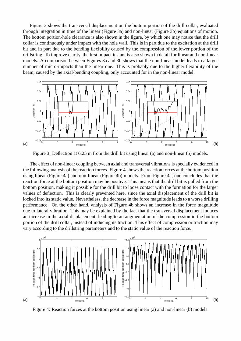
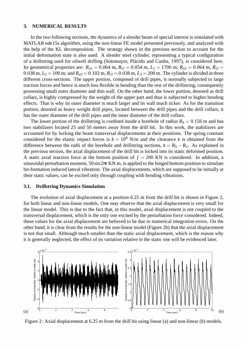
Figure 3 shows the transversal displacement on the bottom portion of the drill collar, evaluatedthrough integration in time of the linear (Figure 3a) and non-linear (Figure 3b) equations of motion.The bottom portion-hole clearance is also shown in the figure, by which one may notice that the drillcollar is continuously under impact with the hole wall. This is in part due to the excitation at the drillbit and in part due to the bending flexibility caused by the compression of the lower portion of thedrillstring. To improve clarity, the first impact instant is also shown in detail for linear and non-linearmodels. A comparison between Figures 3a and 3b shows that the non-linear model leads to a largernumber of micro-impacts than the linear one. This is probably due to the higher flexibility of thebeam, caused by the axial-bending coupling, only accounted for in the non-linear model.

0 2 4 6 8 10−0.06

−0.04

−0.02

0

0.02

0.04

0.06

Time (sec)

Def

lect

ion

(m)

0 2 4 6 8 10−0.06

−0.04

−0.02

0

0.02

0.04

0.06

Time (sec)

Def

lect

ion

(m)

(a) (b)

Figure 3: Deflection at 6.25 m from the drill bit using linear (a) and non-linear (b) models.

The effect of non-linear coupling between axial and transversal vibrations is specially evidenced inthe following analysis of the reaction forces. Figure 4 shows the reaction forces at the bottom positionusing linear (Figure 4a) and non-linear (Figure 4b) models. From Figure 4a, one concludes that thereaction force at the bottom position may be positive. This means that the drill bit is pulled from thebottom position, making it possible for the drill bit to loose contact with the formation for the largervalues of deflection. This is clearly prevented here, since the axial displacement of the drill bit islocked into its static value. Nevertheless, the decrease in the force magnitude leads to a worse drillingperformance. On the other hand, analysis of Figure 4b shows an increase in the force magnitudedue to lateral vibration. This may be explained by the fact that the transversal displacement inducesan increase in the axial displacement, leading to an augmentation of the compression in the bottomportion of the drill collar, instead of inducing its traction. This effect of compression or traction mayvary according to the drillstring parameters and to the static value of the reaction force.

0 2 4 6 8 10−2

−1.5

−1

−0.5

0

0.5

1x 10

5

Time (sec.)

Rea

ctio

n fo

rce

at b

otto

m p

ositi

on (N

)

0 2 4 6 8 10−3.2

−3

−2.8

−2.6

−2.4

−2.2

−2

−1.8x 10

5

Time (sec.)

Rea

ctio

n fo

rce

at b

otto

m p

ositi

on (N

)

(a) (b)

Figure 4: Reaction forces at the bottom position using linear (a) and non-linear (b) models.

3.2. Karhunen-Loeve Decomposition of the Response

In this section, the direct method of Karhunen-Loeve decomposition (Wolter and Sampaio, 2001)is applied to the drillstring dynamics. For this purpose, the time response q(t) is subtracted from itsmean E[q(t)] to obtain the deviation qd(t) = q(t)−E[q(t)] of the time response. Consequently, thenew vector qd(t) has elements with zero mean. As the time response q(t), and thus also qd(t), resultsfrom time integration of the discretized equations of motion (20), it is in fact sampled in M instantsof time t1, t2, . . . , tM, chosen in the time integration algorithm. Hence, the time response q(t) may bewritten as a sampling matrix of dimension M×N,

q =

q1(t1) q2(t1) . . . qN(t1)q1(t2) q2(t2) . . . qN(t2)

......

. . ....

q1(tM) q2(tM) . . . qN(tM)

(21)

where each column represents the time response of a given degree of freedom from the FE mesh,with N being the total number of degrees of freedom or the dimension of q(t). Alternatively, eachrow represents the spatial distribution of the response at a given time instant, that is, a point in theN-dimensional phase space.

Using the ergodicity assumption, the mean value E[q(t)] may be obtained by the time average ofq, that is ∑M

i q(ti)/M. Hence, the deviation qd(t) with respect to the mean may also be written as asampling matrix, obtained by subtracting from each line of q the time average of all rows,

qd = q−qE ; where qE =1M

∑Mi=1 q1(ti) ∑M

i=1 q2(ti) . . . ∑Mi=1 qN(ti)

......

. . ....

∑Mi=1 q1(ti) ∑M

i=1 q2(ti) . . . ∑Mi=1 qN(ti)

(22)

The spatial autocorrelation matrix is then written in terms of the zero-mean time response sam-pling matrix as

R =1M

qTd qd (23)

where R is, by definition, symmetric and positive semi-definite. Hence, its eigenvectors form anorthogonal basis and its eigenvalues are non-negative. In this case, the eigenvectors Ψ j are the coher-ent structures or proper orthogonal modes (POMs) and the corresponding eigenvalues λ j, or properorthogonal values (POVs), give a measure of the mean energy contained in each mode, defined as

R Ψ = ΛΨ ; with Ψ = [Ψ1 Ψ2 · · · ΨN ] and Λ = diag(λ1,λ2, . . . ,λN) (24)

Notice that the autocorrelation matrix R has dimension N ×N. Hence, its dimension, and so thenumber of proper orthogonal modes and values, depend only on the number of degrees of freedomand not on the time instants used for the sampling of the time response.

The time response sampling matrix q may then be reconstructed, in a truncated basis, by express-ing q in terms of its time average matrix qE and a reduced number K of evaluated POMs as

q =K

∑j=1

A jΨTj +qE (25)

where the vectors of time coefficients A j are easily found by projecting the time response onto eachPOM Ψ j, that is, A j = qΨ j. Notice that, by definition, the POVs also respect the following relationwith the time coefficients

λ j =1M

M

∑i=1

ATj A j (26)

Next, this procedure is applied to the drillstring dynamics response resulting from the integrationof the equations of motion (20). Moreover, one expects to obtain additional information throughanalysis of the POMs and POVs. These are also used to construct an optimal basis, with minimumdimension, that allows us to project the equations of motion and obtain a reduced order model, wellrepresenting the main features of the response.

Figure 5 shows the first five POMs evaluated from the drillstring dynamics response q, zoomedin its bottom portion, and the corresponding proper orthogonal values λ j. It is worthwhile noting thatthe POVs where normalized so their sum is unitary. One may observe that most of the energy (89%) iscontained in the first two POMs and that only the bottom portion of the drillstring presents transversaldeflections. This is clearly due to the fact that the upper portion of the drillstring is under traction andthus is much stiffer in bending than the bottom portion that is under compression.

1200

1300

1400

1500

1600

1700

1800

1900

2000

λ1 = 0.55 λ

2 = 0.34 λ

3 = 0.03 λ

4 = 0.02 λ

5 = 0.02

Figure 5: First five proper orthogonal modesevaluated from the transversal displacement re-sponse.

0 2 4 6 8 10−0.06

−0.04

−0.02

0

0.02

0.04

0.06

Time (sec)

Def

lect

ion

(m) Full

5 POMs (14%) 9 POMs (8%)15 POMs (3%)30 POMs (1%)

Figure 6: Reconstruction of the transversal dis-placement response using the first five, nine, fif-teen and thirty proper orthogonal modes.

The first five POMs are responsible for 97% of the response. However, it is generally recom-mended to consider a number of modes sufficient to sum 99.9% of the response energy (Sirovich,1987). Figure 6 shows the reconstruction of the transversal displacement response using the first 5,9, 15 and 30 POMs. The percentage of the energy contained in these first POMs are respectively,96.6567%, 99.1286%, 99.8613% and 99.9918%. Thus, 15 modes are needed to reconstruct the re-sponse, which is a great reduction of the model dimension, since the FE model contains 87 degrees offreedom. Nevertheless, one could also use other measures to quantify the quality of the reconstruc-tion. Indeed, from Figure 6, one may observe that the overall behavior of the transversal displacementis captured even with only 5 POMs, the effect of bottom-hole impact being the main source of error.Another measure of the reconstruction quality was then considered, consisting of the time average ofthe relative error modulus between the reconstructed response vR and the response of the full modelvF , e = ∑M

j=1 |1− v jF/v j

R|/M. Using this measure, one may see that using only the first 5 POMs leadsto a reconstruction within 14% response error. This error drops to 8%, 3% and less than 1% whenusing the first 9, 15 and 30 POMs respectively. The zoomed window in Figure 6 shows that there isa clear improvement in the reconstruction of the response when the number of POMs is increased.In fact, when using the first 30 POMs one may capture precisely all the micro-impacts observed inthe response. Nevertheless, although using only the first 15 POMs leads to small differences in theresponse inside the impact region, one may observe that the main micro-impacts effects are accountedfor since this reconstructed response follows almost exactly the full model response just after the im-pact. This means that this reconstruction, within a 3% error, may be reasonably accurate to consideronly the first 15 POMs in the reduced order model.

4. CONCLUSIONS

The oscillations of a non-rotating drillstring, represented here by a vertical slender beam, clampedin its upper extreme, pinned in its lower one and constrained inside an outer cylinder in its lowerportion, were studied. The beam was supposed as being subjected to distributed axial loads, due toits own weight, leading to geometric softening of its lower portion and, thus, to a large number ofvibroimpacts with the outer cylinder. It was shown that one should account for the axial displacementdynamics, using non-linear strain-displacement relations, since the axial/bending dynamical couplingis very important in slender beams dynamics. In particular, the micro-impacts, accompanying thebottom-hole impacts and mainly due to the beam compressive softening, were well represented onlyby the non-linear model. Moreover, standard linear beam models yield false predictions of the reactionforces at the drillstring bottom position, that is the forces at the formation.

Then, the KL expansion was applied to the simulated dynamics to obtain additional informationon the system through analysis of the POMs and POVs and also to construct an optimal reduced ordermodel. The results have shown that at least 15 POMs are required to reconstruct the dynamics ofthe impacting drillstring under a 3% error margin. This result is encouraging if one compares thedimension of the reduction basis (15) with that of the original FE model (87). Future works are beingdirected to the application of the reduced order model to other external and loading conditions.

5. ACKNOWLEDGMENTS

The authors gratefully acknowledge the financial support of “Fundacao Carlos Chagas Filhode Amparo a Pesquisa do Estado do Rio de Janeiro” (FAPERJ), through grants nos. 172.038/00,151.188/00 and 150.687/00.

6. REFERENCES

Azeez, M.F.A. and Vakakis, A.F., 2001, “Proper orthogonal decomposition (POD) of a class ofvibroimpact oscillations”, Journal of Sound and Vibration, Vol. 240, No. 5, pp. 859–889.

Kane, T.R., Ryan, R.R., and Banerjee, A.K., 1987, “Dynamics of a cantilever beam attached to amoving base”, Journal of Guidance, Control, and Dynamics, Vol. 10, No. 2, pp. 139–151.

Sharf, I., 1995, “Geometric stiffening in multibody dynamics formulations”, Journal of Guidance,Control, and Dynamics, Vol. 18, No. 4, pp. 882–890.

Simo, J. and Vu-Quoc, L., 1987, “The role of non-linear theories in transient dynamic analysis offlexible structures”, Journal of Sound and Vibration, Vol. 119, No. 3, pp. 487–508.

Sirovich, L., 1987, “Turbulence and the dynamics of coherent structures part I: coherent structures”,Quarterly of Applied Mathematics, Vol. 45, No. 3, pp. 561–571.

Sotomayor, G.P.G., Placido, J.C., and Cunha, J.C., 1997, “Drill string vibration: How to identifyand suppress”, In Proceedings of 5th Latin American and Caribbean Petroleum EngineeringConference and Exhibition, paper no. SPE 39002.

Steindl, A. and Troger, H., 2001, “Methods for dimension reduction and their application in non-linear dynamics”, International Journal of Solids and Structures, Vol. 38, No. 10-13, pp.2131–2147.

Trindade, M.A. and Sampaio, R., 2002, “Dynamics of beams undergoing large rotations accountingfor arbitrary axial deformation”, to appear in the Journal of Guidance, Control, and Dynamics.

Wolter, C. and Sampaio, R., 2001, “Bases de Karhunen-Loeve: Aplicacoes a mecanica dos solidos”,In Proceedings of the 1st Brazilian Workshop in Aplications of Dynamics and Control (Aplicon2001), ABCM/SBMAC, Sao Carlos, pp. 129–172.

Wolter, C., Trindade, M.A., and Sampaio, R., 2001, “Obtaining mode shapes through the Karhunen-Loeve expansion for distributed-parameter linear systems”, In Proceedings of the 16th BrazilianCongress of Mechanical Engineering, ABCM, Uberlandia, Vol. 10, pp. 444–452.