The spatial resolution of velocity and velocity gradientturbulence statistics measured with

multi-sensor hot-wire probes

P.V. Vukoslavčević, Univ. of Montenegro

N. Beratlis, E. Balaras and J.M. Wallace, Univ. of Maryland

•Background

•Operational principles of 12-sensor hot-wire probes

•Resolution of a 12-sensor Hot-wire probe

•Highly resolved DNS of a Narrow Channel Turbulent Flow at Rτ = 200

•Resolution effects on velocity component statistics

•Resolution effects on vorticity component statistics

•Summary and Conclusions

Overview

12- sensor probe used to measure velocity and velocity gradient properties of turbulent flows

Dimensions in mm

P. Vukoslavčević, J.M. Wallace & J.-L. Balint (1991) J. Fluid Mech. 228A. Tsinober, E. Kit & T. Dracos (1992) J. Fluid Mech. 242B. Marasli, P. Nguyen , J.M. Wallace (1993) Exp. Fluids. 15P. Vukoslavčević & J.M. Wallace (1996) Meas. Sci. Technol. 7A. Honkan & Y. Andreopoulos (1997) J. Fluid Mech. 350L. Ong & J.M. Wallace (1998) J. Fluid Mech. 367R. Loucks (1998) Ph.D. Dissertation, University of Maryland

12-sensor Hot-wire Probe

Operational principles of hot-wire probe

.222222btne UhUkUU ++=

.5432

22

122

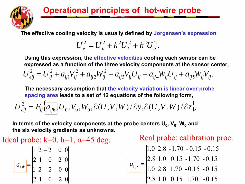
ijijijijijijijijijijijijijijeij VWaUWaUVaWaVaUU +++++=

The necessary assumption that the velocity variation is linear over probe spacing area leads to a set of 12 equations of the following form,

02012002210201200221

1

−−

=jka

0.15- 1.70 0.15 1.0 2.80.15- 0.15- 1.70 2.8 1.00.15- 1.70- 0.15 1.0 2.80.15- 0.15- 1.70- 2.8 1.0

1 =jka

Real probe: calibration proc.Ideal probe: k=0, h=1, α=45 deg.

The effective cooling velocity is usually defined by Jorgensen’s expression

{ },/),,(,/),,(,,,, 0002 zWVUyWVUWVUaFU ijkijeij ∂∂∂∂=

In terms of the velocity components at the probe centers U0, V0, W0 and the six velocity gradients as unknowns.

Using this expression, the effective velocities cooling each sensor can be expressed as a function of the three velocity components at the sensor center,

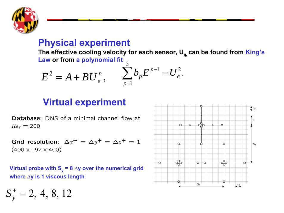
Physical experimentThe effective cooling velocity for each sensor, Uij, can be found from King’s Law or from a polynomial fit

,2 neBUAE += .2

5

1

1e

p

pp UEb =∑

=

−

Virtual experiment

Virtual probe with Sy = 8 ∆y over the numerical grid where ∆y is 1 viscous length

12,8,4,2=+yS

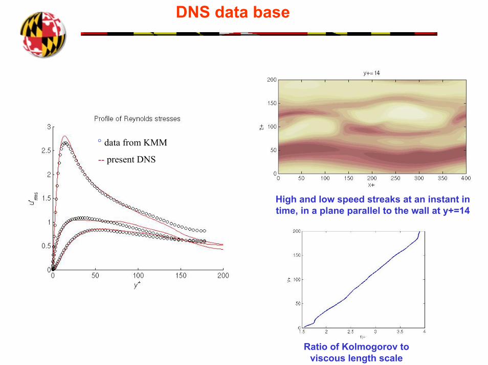
DNS data base

High and low speed streaks at an instant in time, in a plane parallel to the wall at y+=14

Ratio of Kolmogorov to viscous length scale

° data from KMM

-- present DNS

Velocity Statistics - RMS

0

0.5

1

1.5

2

2.5

3

3.5

0 20 40 60 80 100 120 140 160 180 200

y+

u'/u

t

0

0.5

1

1.5

2

2.5

3

3.5

0 20 40 60 80 100 120 140 160 180 200

y+

v'/u

t

0

0.5

1

1.5

2

2.5

3

3.5

0 20 40 60 80 100 120 140 160 180 200

y+

w'/u

t

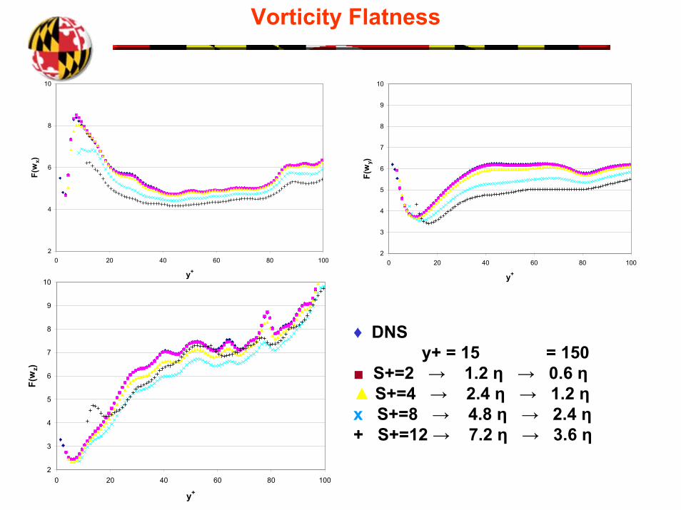
♦ DNSy+ = 15 = 150

■ S+=2 → 1.2 η → 0.6 η▲ S+=4 → 2.4 η → 1.2 ηx S+=8 → 4.8 η → 2.4 η+ S+=12 → 7.2 η → 3.6 η

♦ DNSy+ = 15 = 150

■ S+=2 → 1.2 η → 0.6 η▲ S+=4 → 2.4 η → 1.2 ηx S+=8 → 4.8 η → 2.4 η+ S+=12 → 7.2 η → 3.6 η

-0.8

-0.6

-0.4

-0.2

0

0.2

0.4

0.6

0.8

1

0 20 40 60 80 100

y+

S(u)

-1

-0.8

-0.6

-0.4

-0.2

0

0.2

0.4

0.6

0.8

1

0 20 40 60 80 100

y+

S(v)

-1

-0.8

-0.6

-0.4

-0.2

0

0.2

0.4

0.6

0.8

1

0 20 40 60 80 100

y+

S(w

)Velocity Skewness

2

3

4

5

6

7

8

0 20 40 60 80 100

y+

F(u)

2

3

4

5

6

7

8

0 10 20 30 40 50 60 70 80 90 100

y+

F(v)

2

3

4

5

6

7

8

0 20 40 60 80 100

y+

F(w

)

♦ DNSy+ = 15 = 150

■ S+=2 → 1.2 η → 0.6 η▲ S+=4 → 2.4 η → 1.2 ηx S+=8 → 4.8 η → 2.4 η+ S+=12 → 7.2 η → 3.6 η

Velocity Flatness

Comparison of ideal and real probe response

0

0.5

1

1.5

2

2.5

3

3.5

0 20 40 60 80 100 120 140 160 180 200

y+

u'/u

t

0

0.5

1

1.5

2

2.5

3

3.5

0 20 40 60 80 100 120 140 160 180 200

y+

v'/u

t

0

0.5

1

1.5

2

2.5

3

3.5

0 20 40 60 80 100 120 140 160 180 200

y+

w'/u

t

S+=8♦, DNS x, ideal probe -, real probe

Vorticity Statistics - RMS

0

0.1

0.2

0.3

0.4

0.5

0 20 40 60 80 100 120 140 160 180 200

y+

wx'n

/ut

2

0

0.1

0.2

0.3

0.4

0.5

0 20 40 60 80 100 120 140 160 180 200

y+

wy'n

/ut

2

0

0.1

0.2

0.3

0.4

0.5

0 20 40 60 80 100 120 140 160 180 200

y+

wz'n

/ut

2

♦ DNSy+ = 15 = 150

■ S+=2 → 1.2 η → 0.6 η▲ S+=4 → 2.4 η → 1.2 ηx S+=8 → 4.8 η → 2.4 η+ S+=12 → 7.2 η → 3.6 η

-1.5

-1.25

-1

-0.75

-0.5

-0.25

0

0.25

0.5

0.75

1

0 20 40 60 80 100

y+

S(w

x)

-1.5

-1.25

-1

-0.75

-0.5

-0.25

0

0.25

0.5

0.75

1

0 10 20 30 40 50 60 70 80 90 100

y+

S(w

y)

-1.5

-1.25

-1

-0.75

-0.5

-0.25

0

0.25

0.5

0.75

1

0 10 20 30 40 50 60 70 80 90 100

y+

S(w

z)

♦ DNSy+ = 15 = 150

■ S+=2 → 1.2 η → 0.6 η▲ S+=4 → 2.4 η → 1.2 ηx S+=8 → 4.8 η → 2.4 η+ S+=12 → 7.2 η → 3.6 η

Vorticity Skewness

2

4

6

8

10

0 20 40 60 80 100

y+

F(w

x)

2

3

4

5

6

7

8

9

10

0 20 40 60 80 100

y+

F(w

y)

2

3

4

5

6

7

8

9

10

0 20 40 60 80 100

y+

F(w

z)

♦ DNSy+ = 15 = 150

■ S+=2 → 1.2 η → 0.6 η▲ S+=4 → 2.4 η → 1.2 ηx S+=8 → 4.8 η → 2.4 η+ S+=12 → 7.2 η → 3.6 η

Vorticity Flatness

Comparison of ideal and real probe response

0

0.1

0.2

0.3

0.4

0.5

0 20 40 60 80 100 120 140 160 180 200

y+

wx'n

/ut

2

0

0.1

0.2

0.3

0.4

0.5

0 20 40 60 80 100 120 140 160 180 200

y+

wy'n

/ut

2

0

0.1

0.2

0.3

0.4

0.5

0 20 40 60 80 100 120 140 160 180 200

y+

wz'n

/ut

2

S+=8♦, DNS x, ideal probe -, real probe

0

0.2

0.4

0.6

0.8

1

1.2

1.4

1.6

-10 -8 -6 -4 -2 0 2 4 6 8 10

u+

PDF(

u+ )

Velocity PDFs of real and ideal probe response at y+=12.5

♦, DNS ■, s+=4, ideal probe response▲, s+=4, real probe response x, s+=8, ideal probe response+, s+=8, real probe response

0

0.2

0.4

0.6

0.8

1

1.2

1.4

1.6

-4 -2 0 2 4

v+

PDF(

v+ )

0

0.2

0.4

0.6

0.8

1

1.2

1.4

1.6

-6 -4 -2 0 2 4 6

w+

PDF(

w+ )

Vorticity PDFs of real and ideal probe response at y+=12.5

0

0.5

1

1.5

2

2.5

3

3.5

4

4.5

5

-2 -1.5 -1 -0.5 0 0.5 1 1.5 2

wx+

PDF(

wx+ )

0

0.5

1

1.5

2

2.5

3

3.5

4

4.5

5

-2 -1.5 -1 -0.5 0 0.5 1 1.5 2

wy+

PDF(

wy+ )

0

0.5

1

1.5

2

2.5

3

3.5

4

4.5

5

-2 -1.5 -1 -0.5 0 0.5 1 1.5 2

wz+

PDF(

wz+ ) ♦, DNS

■, s+=4, ideal probe response▲, s+=4, real probe response x, s+=8, ideal probe response+, s+=8, real probe response

Velocity Spectra

@ y+ = 20

Probe scale S+ = 8

__ DNSy+ = 15 = 150

__ S+ = 2 → 1.2 η → 0.6 η__ S+ = 4 → 2.4 η → 1.2 η__ S+ = 8 → 4.8 η → 2.4 η__ S+ = 12 → 7.2 η → 3.6 η

Vorticity Spectra

@ y+ = 20

Probe scaleS+ = 8

__ DNSy+ = 15 = 150

__ S+ = 2 → 1.2 η → 0.6 η__ S+ = 4 → 2.4 η → 1.2 η__ S+ = 8 → 4.8 η → 2.4 η__ S+ = 12 → 7.2 η → 3.6 η

k1η

Kim and Antonia isotropic

Eω

xυ1

/4/ε3

/4Eω

yυ1

/4/ε3

/4Eω

zυ1

/4/ε3

/4

dissipation range

inertial subrange

Kim and Antonia (1993) , channel flow DNS, JFM 251

12- sensor probe scale

NASA Ames 80´ x 120´ Wind Tunnel

Ong & Wallace (1994), experiment, Proc. ETC V

Local Isotropy of the Vorticity Field in a High Reynolds Number Turbulent Boundary Layer

probe location

Summary & Conclusions

Spatial resolution of 12-sensor hot-wire probe investigated using highly resolved minimal channel flow DNS.

Virtual probe with 12 point sensors varied so that spacing between arrays is 2, 4, 8 and 12 viscous lengths.

The velocity component rms values are attenuated les then 10%everywhere in the flow for s+<8.

The skewness factor of the wall normal velocity fluctuations, S(v),display stronger dependence on spatial resolution.

In the wall layer all the vorticity component rms values are strongly influenced by spatial resolution for S+ = 8 and 12.

The statistics from the ideal and real probe responses are nearly identical.

The shapes of the velocity and vorticity pdfs reflect the resolution effects.

Spectra demonstrate the attenuation due to spatial resolution

-1

-0.8

-0.6

-0.4

-0.2

0

0.2

0.4

0.6

0.8

1

0 20 40 60 80 100

y+

S(u)

-1

-0.8

-0.6

-0.4

-0.2

0

0.2

0.4

0.6

0.8

1

0 20 40 60 80 100

y+

S(v)

-1

-0.8

-0.6

-0.4

-0.2

0

0.2

0.4

0.6

0.8

1

0 20 40 60 80 100

y+

S(w

)

S+=8♦, DNS x, ideal probe -, real probe

Comparison of ideal and real probe response

2

4

6

8

0 20 40 60 80 100

y+

F(u)

2

3

4

5

6

7

8

0 20 40 60 80 100

y+

F(v)

2

3

4

5

6

7

8

0 20 40 60 80 100

y+

F(w

)

S+=8♦, DNS

x, ideal probe -, real probe

Comparison of ideal and real probe response

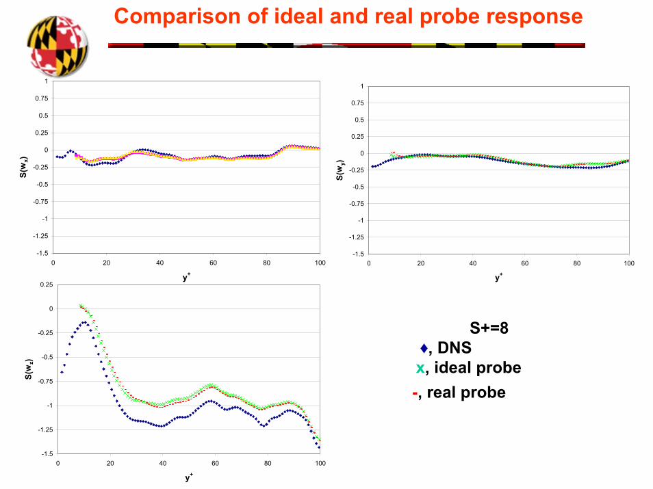
Comparison of ideal and real probe response

-1.5

-1.25

-1

-0.75

-0.5

-0.25

0

0.25

0.5

0.75

1

0 20 40 60 80 100

y+

S(w

x)

-1.5

-1.25

-1

-0.75

-0.5

-0.25

0

0.25

0.5

0.75

1

0 20 40 60 80 100

y+

S(w

y)

-1.5

-1.25

-1

-0.75

-0.5

-0.25

0

0.25

0 20 40 60 80 100

y+

S(w

z)

S+=8♦, DNS x, ideal probe -, real probe

Comparison of ideal and real probe response

2

3

4

5

6

7

8

9

10

11

12

0 20 40 60 80 100

y+

F(w

x)

2

3

4

5

6

7

8

9

10

0 20 40 60 80 100

y+

F(w

y)

2

3

4

5

6

7

8

9

10

0 20 40 60 80 100

y+

F(w

z)

S+=8♦, DNS

x, ideal probe -, real probe