
Field velocity vs. split velocity method - Archive ouverte HAL
22
Journal of Wind Engineering & Industrial Aerodynamics 218 (2021) 104790 0167-6105/© 2021 The Authors. Published by Elsevier Ltd. This is an open access article under the CC BY license (http://creativecommons.org/licenses/by/4.0/). Contents lists available at ScienceDirect Journal of Wind Engineering & Industrial Aerodynamics journal homepage: www.elsevier.com/locate/jweia Assessment of two wind gust injection methods: Field velocity vs. split velocity method Khaled Boulbrachene, Guillaume De Nayer, Michael Breuer ∗ Professur für Strömungsmechanik, Helmut-Schmidt-Universität Hamburg, D-22043 Hamburg, Germany ARTICLE INFO Keywords: Field velocity method Split velocity method Vertical and horizontal wind gust Feedback effect ECG ABSTRACT The objective of the present paper is to revisit two well-known wind gust injection methods in a consistent manner and to assess their performance based on different application cases. These are the field velocity method (FVM) and the split velocity method (SVM). For this purpose, both methods are consistently derived pointing out the link to the Arbitrary Lagrangian Eulerian formulation and the geometric conservation law. Furthermore, the differences between FVM and SVM are worked out and the advantages and disadvantages are compared. Based on a well-known test case considering a vertical gust hitting a plate and a newly developed case taking additionally a horizontal gust into account, the methods are evaluated and the deviations resulting from the disregard of the feedback effect in FVM are assessed. The results show that the deviations between the predictions by FVM and SVM are more pronounced for the horizontal gust justifying the introduction of this new test case. The main reason is that the additional source term in SVM responsible for the feedback effect of the surrounding flow on the gust itself nearly vanishes for the vertical gust, whereas it has a significant impact on the flow field and the resulting drag and lift coefficients for the horizontal gust. Furthermore, the correct formulation of the viscous stress tensor relying on the total velocity as done in case of SVM plays an important role, but is found to be negligible for the chosen Reynolds number of the present test cases. The study reveals that SVM is capable of delivering physical results in contradiction to FVM. It paves the way for investigating further complex gust configurations (e.g., inclined gusts) and practical applications towards coupled fluid–structure interaction simulations of engineering structures impacted by wind gusts. 1. Introduction The study of extreme events constitutes an important aspect of many engineering applications nowadays. Investigating extreme events was found to enable the design of safe components that will withstand harsh conditions and circumvent any sudden failure which may occur. In the field of fluid mechanics, wind gusts represent a typical example of such extreme phenomena which might lead to devastating conse- quences on flexible as well as rigid structures. For instance, aircraft design requires the study of different load cases and the evaluation of their aerodynamic responses (Wu et al., 2019). This ensures that the encounter of aircraft by wake vortices of a preceding plane (Sitaraman and Baeder, 2006; Gordnier and Visbal, 2015), a streamwise wind gust (Granlund et al., 2014) or an impulsive change in the angle of attack (Parameswaran and Baeder, 1997; Singh and Baeder, 1997) is controlled properly. In order to guarantee the safety of trains moving over bridges and to evaluate the risk of derailment, Montenegro et al. (2020) simulated the effect of discrete gusts and turbulent wind models on aerodynamic forces. That allows to determine critical wind speeds, ∗ Corresponding author. E-mail address: [email protected] (M. Breuer). which is especially of interest for high-speed trains. Beside aeronautics and rail transport, the wind energy sector is constantly dealing with the design of structurally reliable wind turbine tower systems (Kwon et al., 2012) and especially wind turbine blades (for example, see Onol and Yesilyurt (2017)). A turbine blade is, like a helicopter blade, exposed to trailing-edge vortices in the wake of other blades as well as to potential gusts which may strip it away. For example, Hawbecker et al. (2017) reported on extreme structural damages to turbines of the Buffalo Ridge Wind Farm in Minesota in 2011. Blades from multiple turbines broke away and a tower buckled in the intense winds. They attempted to characterize meteorological conditions over the wind farm area during this event and carried out weather research and forecasting model simulations of the event that considered current and anticipated future operational model setups. More recently, lightweight thin structures such as membrane- covered and tensile-membrane structures have become widely used in civil engineering applications. Due to the unique flexible charac- teristics of the fabric membranes such structures allow the engineers https://doi.org/10.1016/j.jweia.2021.104790 Received 6 April 2021; Received in revised form 21 September 2021; Accepted 22 September 2021
-
Upload
khangminh22 -
Category
Documents
-
view
2 -
download
0
Transcript of Field velocity vs. split velocity method - Archive ouverte HAL

Journal of Wind Engineering & Industrial Aerodynamics 218 (2021) 104790
0
Contents lists available at ScienceDirect
Journal of Wind Engineering & Industrial Aerodynamics
journal homepage: www.elsevier.com/locate/jweia
Assessment of two wind gust injection methods: Field velocity vs. splitvelocity methodKhaled Boulbrachene, Guillaume De Nayer, Michael Breuer ∗
Professur für Strömungsmechanik, Helmut-Schmidt-Universität Hamburg, D-22043 Hamburg, Germany
A R T I C L E I N F O
Keywords:Field velocity methodSplit velocity methodVertical and horizontal wind gustFeedback effectECG
A B S T R A C T
The objective of the present paper is to revisit two well-known wind gust injection methods in a consistentmanner and to assess their performance based on different application cases. These are the field velocitymethod (FVM) and the split velocity method (SVM). For this purpose, both methods are consistently derivedpointing out the link to the Arbitrary Lagrangian Eulerian formulation and the geometric conservation law.Furthermore, the differences between FVM and SVM are worked out and the advantages and disadvantages arecompared. Based on a well-known test case considering a vertical gust hitting a plate and a newly developedcase taking additionally a horizontal gust into account, the methods are evaluated and the deviations resultingfrom the disregard of the feedback effect in FVM are assessed. The results show that the deviations between thepredictions by FVM and SVM are more pronounced for the horizontal gust justifying the introduction of thisnew test case. The main reason is that the additional source term in SVM responsible for the feedback effectof the surrounding flow on the gust itself nearly vanishes for the vertical gust, whereas it has a significantimpact on the flow field and the resulting drag and lift coefficients for the horizontal gust. Furthermore, thecorrect formulation of the viscous stress tensor relying on the total velocity as done in case of SVM plays animportant role, but is found to be negligible for the chosen Reynolds number of the present test cases. Thestudy reveals that SVM is capable of delivering physical results in contradiction to FVM. It paves the wayfor investigating further complex gust configurations (e.g., inclined gusts) and practical applications towardscoupled fluid–structure interaction simulations of engineering structures impacted by wind gusts.
1. Introduction
The study of extreme events constitutes an important aspect of manyengineering applications nowadays. Investigating extreme events wasfound to enable the design of safe components that will withstand harshconditions and circumvent any sudden failure which may occur. Inthe field of fluid mechanics, wind gusts represent a typical exampleof such extreme phenomena which might lead to devastating conse-quences on flexible as well as rigid structures. For instance, aircraftdesign requires the study of different load cases and the evaluation oftheir aerodynamic responses (Wu et al., 2019). This ensures that theencounter of aircraft by wake vortices of a preceding plane (Sitaramanand Baeder, 2006; Gordnier and Visbal, 2015), a streamwise windgust (Granlund et al., 2014) or an impulsive change in the angle ofattack (Parameswaran and Baeder, 1997; Singh and Baeder, 1997) iscontrolled properly. In order to guarantee the safety of trains movingover bridges and to evaluate the risk of derailment, Montenegro et al.(2020) simulated the effect of discrete gusts and turbulent wind modelson aerodynamic forces. That allows to determine critical wind speeds,
∗ Corresponding author.E-mail address: [email protected] (M. Breuer).
which is especially of interest for high-speed trains. Beside aeronauticsand rail transport, the wind energy sector is constantly dealing with thedesign of structurally reliable wind turbine tower systems (Kwon et al.,2012) and especially wind turbine blades (for example, see Onol andYesilyurt (2017)). A turbine blade is, like a helicopter blade, exposed totrailing-edge vortices in the wake of other blades as well as to potentialgusts which may strip it away. For example, Hawbecker et al. (2017)reported on extreme structural damages to turbines of the Buffalo RidgeWind Farm in Minesota in 2011. Blades from multiple turbines brokeaway and a tower buckled in the intense winds. They attempted tocharacterize meteorological conditions over the wind farm area duringthis event and carried out weather research and forecasting modelsimulations of the event that considered current and anticipated futureoperational model setups.
More recently, lightweight thin structures such as membrane-covered and tensile-membrane structures have become widely usedin civil engineering applications. Due to the unique flexible charac-teristics of the fabric membranes such structures allow the engineers
167-6105/© 2021 The Authors. Published by Elsevier Ltd. This is an open access ar
https://doi.org/10.1016/j.jweia.2021.104790Received 6 April 2021; Received in revised form 21 September 2021; Accepted 22
ticle under the CC BY license (http://creativecommons.org/licenses/by/4.0/).September 2021

Journal of Wind Engineering & Industrial Aerodynamics 218 (2021) 104790K. Boulbrachene et al.
to create visually exciting and iconic structures while maintaining afaster installation and an overall lower cost in comparison to traditionalconstructions. However, these structures are vulnerable to wind eventsand to determine to what extent the aerodynamic loads influence theirintegrity is essential (for example, see Gross et al. (2013)). Although de-sign standards are prescribed to provide guidelines in order to take suchevents into account (for example, see Frost et al. (1978), IEC-Standard(2002), Burton et al. (2001), Kasperski (2007)), these are based onsimplifying assumptions to facilitate the design process. Therefore, thedevelopment of methods capable of providing a rapid and comprehen-sive investigation of proposed designs would substantially contributeto the design procedure. Highly resolved numerical simulations of theflow field (and the resulting deformations) are considered to be areliable and powerful method for this objective. That was recentlyshown in De Nayer et al. (2014), De Nayer and Breuer (2014), De Nayeret al. (2018) and Apostolatos et al. (2019), so far not for gusts but atleast for turbulent flows around flexible membranous structures.
In the following, the description is restricted to wind gusts andmethodologies to take these short but often violent phenomenon intoaccount. One of the conventional approaches to inject wind gusts intothe computational domain is to superimpose them at the inlet bound-ary and to allow the gusts to freely propagate through the domain.This technique is known in the literature as the far-field boundarycondition (FBC) method. To avoid the violation of the global massbalance especially for incompressible fluid flows, this method requiresthe dynamic adaptation of the inlet velocity away from the gust toensure a constant total mass flow through the inlet (Norris et al., 2010;De Nayer et al., 2019). Such a requirement is necessary for the con-vergence of incompressible flow solvers. Owing to the fact that inflowboundaries are often far away from the region of interest, a relativelycoarse grid resolution is used in the upstream region to reduce thecomputational costs. Consequently, numerical dissipation is prevalentin these regions and the induced disturbances are strongly dampedwhile being convected through the flow domain. To circumvent thisproblem, one would have to use a highly resolved grid throughout theentire computational domain, or a secondary fine moving mesh trans-porting the gust within the computational domain (e.g., an overset-gridtechnique such as the resolved gust approach of Heinrich (2014)).Nevertheless, the aforementioned remedies are computationally highlydemanding leading to long simulation times.
Several approaches have been proposed to overcome the require-ment of using fine grids throughout the computational domain. Acategory of these methods is referred to as the pure source-term for-mulation method. Recently, De Nayer and Breuer (2020) proposed anoriginal method for injecting wind gusts in the computational domainbased on a source-term formulation. The authors derived a source-term formulation for the momentum conservation equations whichallows to place the injection region of the gust close to the region ofinterest. The gust can then freely propagate through the domain and,consequently, the full coupling (i.e., interaction) between the gust andthe surrounding flow is captured.
Contrary to the aforementioned methods which allow gusts to freelytravel after the injection phase, another family of methods which de-fines the position of the imposed field at each instant in time is denotedthe prescribed velocity methods. There exist two prescribed velocitymethods, namely, the field velocity method (FVM) and the split veloc-ity method (SVM). The field velocity or grid velocity approach (alsodenoted the disturbance velocity approach by Heinrich and Reimer(2013)) was initially proposed by Parameswaran and Baeder (1997)and Singh and Baeder (1997). FVM works by incorporating gust veloci-ties by suitably modifying the grid velocity and consequently modifyingthe grid time metrics. However, this modification does not lead to a realgrid deformation. Hence, a pseudo grid motion is simulated without anactual grid variation. FVM could be thought of as an extension of thesurface transpiration method (Sankar et al., 1986), where instead of
2
applying the velocity correction only to the surface, it is applied to the
entire flow field. Since FVM is similar to moving grid problems, gridtime metrics have to be consistently evaluated to satisfy the geometricconservation law (GCL) (Sitaraman and Baeder, 2006).
The history of FVM started in the field of aeronautics, where itsmain objective was to tackle the problem of evaluating indicial re-sponses (i.e., aerodynamic loads) due to a step change in one ofthe influencing parameters (e.g., angle of attack or pitch rate) inthe context of inviscid three-dimensional compressible flows whilehaving full insight into the flow features (velocity and pressure distri-butions) (Parameswaran and Baeder, 1997; Singh and Baeder, 1997).The method could successfully solve the challenge of decoupling thestep change in the angle of attack from the pitch rate, deliveredresults that agree with the attainable analytical results, and avoidednumerical instabilities associated with this problem. Moreover, in thecontext of inviscid Euler equations FVM was employed to simulate theresponse of an airfoil penetrating through a sharp-edged vertical gust(Parameswaran and Baeder, 1997; Sitaraman and Baeder, 2000), andto model the interaction of an isolated vortex with a rotor blade (Singhand Baeder, 1996). Furthermore, FVM was used to aid the prediction ofaerodynamic loads on a helicopter blade by incorporating the velocityfield caused by trailed tip vortices from all other blades (Sitaraman,2003; Sitaraman and Baeder, 2006). Nevertheless, FVM is incapable ofaccounting for the effect of the surrounding fluid flow on the inducedfield.
In contrast, SVM (originally proposed by Wales et al. (2014)) fullycaptures the interaction between the gust and the object of interest.SVM is based on decomposing the velocity field to a prescribed gustvelocity and the remaining velocity (or background velocity as denotedby Huntley et al. (2017)). The momentum equations are effectivelyrearranged to be solved for the background velocity. As a result, addi-tional source terms are derived to account for the feedback effect whichis missing in FVM. Initial applications of SVM concentrated on applying1-cosine vertical gusts on several NACA airfoils with different gustlengths and amplitudes (Wales et al., 2014). The simulations, however,were performed in the context of two-dimensional Euler equations.Later, Huntley et al. (2017) extended SVM to investigate the gustresponse of a flexible aircraft to a series of 1-cosine gusts in the contextof three-dimensional viscous flows. Both research groups comparedtheir results with those obtained by FVM and found SVM to be moreaccurate when short wavelength gusts are imposed. Recently, Bileret al. (2019), Badrya and Baeder (2019) and Badrya et al. (2021)investigated the flow physics resulting from a flat plate-gust encounter.The analysis showed the ability of analytical models (Küssner’s solu-tion (Küssner, 1936)) in predicting gust response for a 0◦ geometricangle of attack while the need for CFD solutions remains in order toformulate empirical formulas predicting responses for high angles ofattack.
The steps in this paper are as follows:
1. Provide a comprehensive description of the FVM and SVM meth-ods along with the modifications needed to be made in thegoverning equations.
2. Deliver best practice guidelines describing the implementationof the methods in a finite-volume code thoroughly.
3. Apply the methods to simulate the encounter of a vertical as wellas a horizontal gust (which can be said to be relevant for manyengineering applications) on a horizontal flat plate.
4. Highlight the differences among the methods and their limita-tions.
The main objective is to figure out the most appropriate method-ology to simulate the effect of wind gusts impacting on mechanicalor civil engineering structures. For the latter especially flexible mem-branous structures impacted by horizontal gusts are in the focus ofmedium-term interest, whereby such kind of complex fluid–structureinteraction problems are to be simulated by high-fidelity eddy-resolving
schemes such as the large-eddy simulation (LES) technique.
Journal of Wind Engineering & Industrial Aerodynamics 218 (2021) 104790K. Boulbrachene et al.
Li
2
fdtpn
iSLgf
ltl
∫
wg
pubc
vttn
icrtis(cttc
m
2. Prescribed gust methods
In the following, two well-established methods for injecting gustsinto a CFD simulation by prescribing the position in the computationaldomain, the shape and the velocity of the gusts at each time stepare introduced. In the present work the gust velocity is denoted 𝑢𝑔,𝑖(𝑖 ∈ {1, 2, 3}) in Cartesian coordinates. The flow field surrounding thegust is denoted as the background velocity field �̃�𝑖. The Navier–Stokesequations for an incompressible fluid are solved for this backgroundvelocity. The prescribed velocity methods postulate that the divergenceof the background velocity is equal to zero (i.e.,
𝜕�̃�𝑖𝜕𝑥𝑖
= 0). To presentthe total flow field 𝑢𝑖 containing the resolved flow field and the pre-scribed gust, the sum of both contributions (i.e., 𝑢𝑖 = �̃�𝑖 + 𝑢𝑔,𝑖) has tobe considered by superposition. Since the divergence of the prescribed
gust velocity on a fixed grid (i.e.,𝜕𝑢𝑔,𝑖𝜕𝑥𝑖
) is not necessarily equal to zero,the divergence of the total velocity will not automatically be zero. Inorder to introduce the prescribed gust velocity into the Navier–Stokesequations while maintaining the postulate of
𝜕�̃�𝑖𝜕𝑥𝑖
= 0, the Arbitraryagrangian Eulerian (ALE) formulation of the Navier–Stokes equationss required as described below.
.1. Field Velocity Method (FVM)
The original idea of this method is the incorporation of unsteadylow conditions via a pseudo-grid movement in the computationalomain according to the Arbitrary Lagrangian Eulerian (ALE) formula-ion. In this way, disturbance velocities (e.g., gust velocities) could berescribed by changing the grid time metrics while the grid is actuallyot altered or distorted.
In the context of a temporally varying domain (as in fluid–structurenteraction (FSI), see Breuer et al. (2012) for example) the Navier–tokes equations (mass and momentum) are written in the Arbitraryagrangian Eulerian (ALE) form. For an incompressible fluid, the inte-ral form of these equations read (here in a Cartesian coordinate systemor the sake of simplicity):
𝑑𝑑𝑡 ∫𝑉 (𝑡)
𝜌 𝑑𝑉 + ∫𝑆(𝑡)𝜌 (�̃�𝑗 − 𝑢grid
𝑗 ) ⋅ 𝑛𝑗 𝑑𝑆 = 0 , (1)
𝑑𝑑𝑡 ∫𝑉 (𝑡)
𝜌 �̃�𝑖 𝑑𝑉 + ∫𝑆(𝑡)𝜌 �̃�𝑖(�̃�𝑗 − 𝑢grid
𝑗 ) ⋅ 𝑛𝑗 𝑑𝑆
= −∫𝑆(𝑡)𝜏𝑖𝑗 ⋅ 𝑛𝑗 𝑑𝑆 − ∫𝑆(𝑡)
𝑝 ⋅ 𝑛𝑖 𝑑𝑆. (2)
Here, the control volumes (CV) have time-dependent volumes 𝑉 (𝑡)and surfaces 𝑆(𝑡). Since in this case the grid is deformable, the gridvelocity with which the surface of a CV is moving, is taken into accountvia 𝑢grid
𝑖 . �̃�𝑖 describes the velocity of the flow field. A grid deformationin the inner domain will not affect �̃�𝑖. However, the flow velocity �̃�𝑖changes due to movements or deformations of walls. 𝜏𝑖𝑗 is the stresstensor based on the flow velocity �̃�𝑖.
In the context of a temporally varying domain the ALE formu-lation has to additionally satisfy the so-called space conservation law(SCL) (Demirdžić and Perić, 1988, 1990) or geometric conservation law(GCL) (Lesoinne and Farhat, 1996):𝑑𝑑𝑡 ∫𝑉 (𝑡)
𝑑𝑉 − ∫𝑆(𝑡)𝑢grid𝑗 ⋅ 𝑛𝑗 𝑑𝑆 = 0 . (3)
This extra conservation law is necessary to assure that no space isost during the change of CVs. Employing the GCL, the contribution ofhe grid movement to the mass fluxes will cancel the unsteady termeading to the reduction of the mass conservation equation to:
𝑆(𝑡)𝜌 �̃�𝑗 ⋅ 𝑛𝑗 𝑑𝑆 = 0 , (4)
hich is equivalent to the mass conservation equation on a fixedrid. Consequently, the pressure-correction equation in the context of
3
rojection methods does not have to be modified. The discrete GCL issed to evaluate the additional grid fluxes in the momentum equationy evaluating the change of the position or the shape of a CV toompute the unknown grid velocity 𝑢grid
𝑖 .The field velocity approach is built per analogy based on the pre-
iously written ALE formulation. The grid is now undeformed andhus fixed, i.e., the cell volumes 𝑉 and surfaces 𝑆 are no longerime-dependent. Furthermore, the grid velocity 𝑢grid
𝑖 is replaced by theegative gust velocity −𝑢𝑔,𝑖. Thus, the equations read:
𝑑𝑑𝑡 ∫𝑉
𝜌 𝑑𝑉 + ∫𝑆𝜌 (�̃�𝑗 + 𝑢𝑔,𝑗 ) ⋅ 𝑛𝑗 𝑑𝑆 = 0 , (5)
𝑑𝑑𝑡 ∫𝑉
𝜌 �̃�𝑖 𝑑𝑉 + ∫𝑆𝜌 �̃�𝑖(�̃�𝑗 + 𝑢𝑔,𝑗 ) ⋅ 𝑛𝑗 𝑑𝑆
= −∫𝑆𝜏𝑖𝑗 ⋅ 𝑛𝑗 𝑑𝑆 − ∫𝑆
𝑝 ⋅ 𝑛𝑖 𝑑𝑆. (6)
Even though the grid is fixed, it is still necessary to satisfy a GCLn the context of FVM due to the fact that the prescribed gust velocityomponent is not necessarily divergence-free. This will again enable theeduction of the mass conservation equation (i.e., Eq. (5) to Eq. (4)) andhus the pressure-correction equation still remains unaffected. Hence, its clear that a rigorous fulfillment of the GCL will suppress any spuriousource terms that might be generated. Despite the undeformed grid𝑉 grid is the real volume of the cell and taken as constant) a pseudohange in the cell volumes (denoted 𝛥𝑉 = 𝑉 ∗ − 𝑉 grid and referredo as apparent grid movement in Sitaraman and Baeder (2006)) haso be taken into account in order to ensure the pseudo geometriconservation law:𝑑𝑑𝑡 ∫𝑉 grid→𝑉 ∗
𝑑𝑉 + ∫𝑆∗𝑢𝑔,𝑗 ⋅ 𝑛𝑗 𝑑𝑆 = 0 . (7)
Since the pseudo updated surface 𝑆∗ of each CV is not available, thepseudo geometric conservation law is rewritten applying the Gaussianintegral theorem:
𝑑𝑑𝑡 ∫𝑉 grid→𝑉 ∗
𝑑𝑉 + ∫𝑉 ∗
𝜕𝑢𝑔,𝑗𝜕𝑥𝑗
𝑑𝑉 = 0 .
In a first approximation, when a second-order approximation of thevolume integral such as the mid-point rule is employed in the contextof a finite-volume scheme, it follows:
𝑑𝑑𝑡 ∫𝑉 grid→𝑉 ∗
𝑑𝑉 + 𝛾 ∫𝑉 grid
𝜕𝑢𝑔,𝑗𝜕𝑥𝑗
𝑑𝑉 = 0 ,
where the scaling factor 𝛾 is defined as 𝛾 = 𝑉 ∗
𝑉 grid . A back transforma-tion leads to:𝑑𝑑𝑡 ∫𝑉 grid→𝑉 ∗
𝑑𝑉 + 𝛾 ∫𝑆𝑢𝑔,𝑗 ⋅ 𝑛𝑗 𝑑𝑆 = 0 . (8)
The derived pseudo geometric conservation law now only dependson the pseudo updated volume 𝑉 ∗. 𝑆 is the current real surface of thegrid and thus denoted 𝑆grid in the following.
Coming back to the mass and momentum conservation equations,the contributions due to the pseudo grid movement have to be eval-uated on the updated volumes 𝑉 ∗ and surfaces 𝑆∗, whereas all otherterms related to the background velocity are computed on the real grid:𝑑𝑑𝑡 ∫𝑉 grid→𝑉 ∗
𝜌 𝑑𝑉 + ∫𝑆grid𝜌 �̃�𝑗 ⋅ 𝑛𝑗 𝑑𝑆 + ∫𝑆∗
𝜌 𝑢𝑔,𝑗 ⋅ 𝑛𝑗 𝑑𝑆 = 0 , (9)
𝑑𝑑𝑡 ∫𝑉 grid→𝑉 ∗
𝜌 �̃�𝑖 𝑑𝑉 + ∫𝑆grid𝜌 �̃�𝑖 �̃�𝑗 ⋅ 𝑛𝑗 𝑑𝑆 + ∫𝑆∗
𝜌 �̃�𝑖 𝑢𝑔,𝑗 ⋅ 𝑛𝑗 𝑑𝑆
= −∫𝑆grid𝜏𝑖𝑗 ⋅ 𝑛𝑗 𝑑𝑆 − ∫𝑆grid
𝑝 ⋅ 𝑛𝑖 𝑑𝑆. (10)
Applying the methodology mentioned above to the mass and mo-entum conservation leads to:
𝑑𝑑𝑡 ∫𝑉 grid→𝑉 ∗
𝜌 𝑑𝑉 + ∫𝑆grid𝜌 �̃�𝑗 ⋅ 𝑛𝑗 𝑑𝑆 + 𝛾 ∫𝑆grid
𝜌 𝑢𝑔,𝑗 ⋅ 𝑛𝑗 𝑑𝑆 = 0 , (11)
𝑑 𝜌 �̃�𝑖 𝑑𝑉 + 𝜌 �̃�𝑖�̃�𝑗 ⋅ 𝑛𝑗 𝑑𝑆 + 𝛾 𝜌 �̃�𝑖 𝑢𝑔,𝑗 ⋅ 𝑛𝑗 𝑑𝑆
𝑑𝑡 ∫𝑉 grid→𝑉 ∗ ∫𝑆grid ∫𝑆grid
Journal of Wind Engineering & Industrial Aerodynamics 218 (2021) 104790K. Boulbrachene et al.
mostt
oaiMtptbigtawtfuGpattvoopu
2
Anntat
d
∫
fbtti
𝑆
tv
= −∫𝑆grid𝜏𝑖𝑗 ⋅ 𝑛𝑗 𝑑𝑆 − ∫𝑆grid
𝑝 ⋅ 𝑛𝑖 𝑑𝑆. (12)
Note that in analogy to the ALE approach, employing the GCL to theass conservation equation (11) allows to cancel out the contribution
f the pseudo-grid movement to the mass fluxes with the unsteady termuch that the mass conservation equation again reduces to Eq. (4). Sincehe gust velocity is a prescribed velocity, the additional mass fluxes inhe momentum equation can be directly evaluated.
For a flow solver already able to solve ALE problems, the integrationf the FVM is straightforward. Further advantages and disadvantagesre as follows. In FVM the gust is prescribed and the remaining fields solved, hence no numerical dissipation of the gust is appearing.oreover, the gust shape and position can be prescribed at any time in
he computational domain. It has the advantage that even when the am-litude of the gust is significantly larger than the background velocity,he simulation will converge. Despite the reasonable results deliveredy FVM, it is not supported by a clear description of simplifications usedn its derivation. Even though FVM accounts for the influence of theust on the surrounding flow field, its major drawback lies on its failureo capture the effect of the surrounding on the gust itself (often denoteds the feedback effect). In addition, FVM was found to be accuratehen solving the Euler equations. The reason is that the gust velocity is
aken into account when the convective fluxes are calculated across cellaces. However, when solving the Navier–Stokes equations with a non-niform gust velocity distribution, viscous flux correction is required.u et al. (2012) demonstrated this issue for accurately simulatingractical flow phenomena (such as pitching and plunging motions ofn airfoil). Their contribution relies on the principle of relative motiono show that the velocity which needs to be used for the calculation ofhe viscous fluxes must be a summation of the background and the gustelocity. They show that this correction is indispensable if the gradientf the gust velocity is different from zero. Consequently, the magnitudef the applied correction is depending on how steep the gust velocityrofile is. The drawbacks of the original FVM are not existent whensing the split velocity method (SVM) explained next.
.2. Split Velocity Method (SVM)
The split velocity method was proposed by Wales et al. (2014).s before, the total velocity 𝑢𝑖 is decomposed into two components,amely, a background �̃�𝑖 and a prescribed gust velocity 𝑢𝑔,𝑖. However,ow the governing equations are written on a fixed grid based onhe total velocity 𝑢𝑖 and rearranged on that grid without the need forny simplifying assumptions. As explained below, in order to fulfillhe postulate of
𝜕�̃�𝑖𝜕𝑥𝑖
= 0, the ALE formulation of the Navier–Stokesequations is used once more including the necessary application of thepseudo GCL. The SVM has been applied to 2-D Euler equations (Waleset al., 2014) and to simulate 2-D as well as 3-D viscous flows (Huntleyet al., 2016).
The formulation starts by writing the integral form of the Navier–Stokes equations on a fixed grid:
∫𝑉 grid
𝜕𝜌𝜕𝑡
𝑑𝑉 + ∫𝑆grid𝜌 𝑢𝑖 ⋅ 𝑛𝑖 𝑑𝑆 = 0 , (13)
∫𝑉 grid
𝜕(
𝜌 𝑢𝑖)
𝜕𝑡𝑑𝑉 + ∫𝑆grid
𝜌 𝑢𝑖 𝑢𝑗 ⋅ 𝑛𝑗 𝑑𝑆
= −∫𝑆grid𝜏𝑖𝑗 ⋅ 𝑛𝑗 𝑑𝑆 − ∫𝑆grid
𝑝 ⋅ 𝑛𝑖 𝑑𝑆. (14)
𝜏𝑖𝑗 is the stress tensor based on the total velocity 𝑢𝑖. Substituting theecomposed total velocity 𝑢𝑖, the conservation equations read:
𝑉 grid
𝜕𝜌𝜕𝑡
𝑑𝑉 + ∫𝑆grid𝜌 (�̃�𝑗 + 𝑢𝑔,𝑗 ) ⋅ 𝑛𝑗 𝑑𝑆 = 0 , (15)
𝜕(
𝜌 (�̃�𝑖 + 𝑢𝑔,𝑖))
𝑑𝑉 + 𝜌 (�̃�𝑖 + 𝑢𝑔,𝑖) (�̃�𝑗 + 𝑢𝑔,𝑗 ) ⋅ 𝑛𝑗 𝑑𝑆
4
∫𝑉 grid 𝜕𝑡 ∫𝑆grid
= −∫𝑆grid𝜏𝑖𝑗 ⋅ 𝑛𝑗 𝑑𝑆 − ∫𝑆grid
𝑝 ⋅ 𝑛𝑖 𝑑𝑆. (16)
The terms of the momentum equation are rewritten as follows:
1. Transient term (note that in the context of fixed grids, thetemporal derivative inside the volume integral can be directlyreplaced by a temporal derivative outside the integral):
∫𝑉 grid
𝜕(
𝜌 (�̃�𝑖 + 𝑢𝑔,𝑖))
𝜕𝑡𝑑𝑉
= ∫𝑉 grid
𝜕(
𝜌 �̃�𝑖)
𝜕𝑡𝑑𝑉 + ∫𝑉 grid
𝜕(
𝜌 𝑢𝑔,𝑖)
𝜕𝑡𝑑𝑉
= 𝜕𝜕𝑡 ∫𝑉 grid
𝜌 �̃�𝑖 𝑑𝑉 + ∫𝑉 grid𝜌𝜕𝑢𝑔,𝑖𝜕𝑡
𝑑𝑉 + ∫𝑉 grid𝑢𝑔,𝑖
𝜕𝜌𝜕𝑡
𝑑𝑉⏟⏞⏞⏞⏞⏞⏞⏞⏞⏞⏟⏞⏞⏞⏞⏞⏞⏞⏞⏞⏟
∙
. (17)
2. Convection term:
∫𝑆grid𝜌 (�̃�𝑖 + 𝑢𝑔,𝑖) (�̃�𝑗 + 𝑢𝑔,𝑗 ) ⋅ 𝑛𝑗 𝑑𝑆
= ∫𝑉 grid
𝜕𝜕𝑥𝑗
(
𝜌 (�̃�𝑖 + 𝑢𝑔,𝑖) (�̃�𝑗 + 𝑢𝑔,𝑗 ))
𝑑𝑉
= ∫𝑉 grid
𝜕𝜕𝑥𝑗
(
𝜌 �̃�𝑖 (�̃�𝑗 + 𝑢𝑔,𝑗 ))
𝑑𝑉 + ∫𝑉 grid𝑢𝑔,𝑖
𝜕𝜕𝑥𝑗
(
𝜌 (�̃�𝑗 + 𝑢𝑔,𝑗 ))
𝑑𝑉
+ ∫𝑉 grid𝜌 (�̃�𝑗 + 𝑢𝑔,𝑗 )
𝜕𝑢𝑔,𝑖𝜕𝑥𝑗
𝑑𝑉
= ∫𝑆grid𝜌 �̃�𝑖 (�̃�𝑗 + 𝑢𝑔,𝑗 ) ⋅ 𝑛𝑗 𝑑𝑆 + ∫𝑉 grid
𝑢𝑔,𝑖𝜕𝜕𝑥𝑗
(
𝜌 (�̃�𝑗 + 𝑢𝑔,𝑗 ))
𝑑𝑉
⏟⏞⏞⏞⏞⏞⏞⏞⏞⏞⏞⏞⏞⏞⏞⏞⏞⏞⏞⏞⏞⏞⏞⏞⏟⏞⏞⏞⏞⏞⏞⏞⏞⏞⏞⏞⏞⏞⏞⏞⏞⏞⏞⏞⏞⏞⏞⏞⏟∙
+ ∫𝑉 grid𝜌 (�̃�𝑗 + 𝑢𝑔,𝑗 )
𝜕𝑢𝑔,𝑖𝜕𝑥𝑗
𝑑𝑉 . (18)
The summation of the terms marked by ∙ represents the productof the gust velocity 𝑢𝑔,𝑖 with the mass conservation equation (13)expressed by 𝑢𝑖 = �̃�𝑖 + 𝑢𝑔,𝑖:
∫𝑉 grid𝑢𝑔,𝑖
𝜕𝜌𝜕𝑡
𝑑𝑉 + ∫𝑉 grid𝑢𝑔,𝑖
𝜕𝜕𝑥𝑗
(
𝜌 𝑢𝑖)
𝑑𝑉
= ∫𝑉 grid𝑢𝑔,𝑖��
����⌃0
(𝜕𝜌𝜕𝑡
+𝜕(𝜌𝑢𝑗 )𝜕𝑥𝑗
) 𝑑𝑉 = 0 . (19)
Hence, the momentum equation can be rewritten in its simplifiedform as:𝜕𝜕𝑡 ∫𝑉 grid
𝜌 �̃�𝑖 𝑑𝑉 + ∫𝑆grid𝜌 �̃�𝑖 (�̃�𝑗 + 𝑢𝑔,𝑗 ) ⋅ 𝑛𝑗 𝑑𝑆
= −∫𝑉 grid𝜌𝜕𝑢𝑔,𝑖𝜕𝑡
𝑑𝑉 − ∫𝑉 grid𝜌 (�̃�𝑗 + 𝑢𝑔,𝑗 )
𝜕𝑢𝑔,𝑖𝜕𝑥𝑗
𝑑𝑉
⏟⏞⏞⏞⏞⏞⏞⏞⏞⏞⏞⏞⏞⏞⏞⏞⏞⏞⏞⏞⏞⏞⏞⏞⏞⏞⏞⏞⏞⏞⏞⏞⏞⏞⏞⏞⏞⏞⏞⏞⏟⏞⏞⏞⏞⏞⏞⏞⏞⏞⏞⏞⏞⏞⏞⏞⏞⏞⏞⏞⏞⏞⏞⏞⏞⏞⏞⏞⏞⏞⏞⏞⏞⏞⏞⏞⏞⏞⏞⏞⏟−𝑆momentum,𝑖
− ∫𝑆grid𝜏𝑖𝑗 ⋅ 𝑛𝑗 𝑑𝑆 − ∫𝑆grid
𝑝 ⋅ 𝑛𝑖 𝑑𝑆 . (20)
In this formulation the convective fluxes are described by massluxes, which are predicted by the total velocity (i.e., the sum of theackground and the gust velocity). Furthermore, the decomposition ofhe velocity leads to the formation of a source term. This term modelshe convective effect of the object being hit by the gust on the gusttself. The source term can be written in its general form as:
momentum,𝑖 = ∫𝑉𝜌{ 𝜕𝑢𝑔,𝑖
𝜕𝑡+ (�̃�𝑗 + 𝑢𝑔,𝑗 )
𝜕𝑢𝑔,𝑖𝜕𝑥𝑗
}
𝑑𝑉 . (21)
In the framework of fixed grids, the partial derivative in time insidehe volume integral can be replaced by a total derivative outside theolume integral. Hence, the mass conservation equation (15) reads:
𝑑 𝜌 𝑑𝑉 + 𝜌 (�̃�𝑗 + 𝑢𝑔,𝑗 ) ⋅ 𝑛𝑗 𝑑𝑆 = 0. (22)
𝑑𝑡 ∫𝑉 grid ∫𝑆grid
Journal of Wind Engineering & Industrial Aerodynamics 218 (2021) 104790K. Boulbrachene et al.
ct
met
g
ca(aactFfsam
aftpd
2
tdtaptF
3
(ls
i(
𝐮
i(𝐓
Ui
o
The transient term in Eq. (22) vanishes for an incompressible fluidimplying that the divergence of the total velocity field is equal to zero.Since the prescribed velocity is not necessarily divergence-free, thepostulate
𝜕�̃�𝑖𝜕𝑥𝑖
= 0 might not be fulfilled. In order to comply with thisondition, the pseudo GCL (i.e., Eq. (7)) is employed on the transienterm of Eq. (22):
𝑑𝑑𝑡 ∫𝑉 grid→𝑉 ∗
𝜌 𝑑𝑉 = −∫𝑆∗𝜌 𝑢𝑔,𝑗 ⋅ 𝑛𝑗 𝑑𝑆 . (23)
Substituting Eq. (23) into Eq. (22), Eq. (4) is retrieved. In a similaranner, the partial temporal derivative in time in the momentum
quation (20) on a fixed grid is substituted by a total derivative andhe ALE formulation is employed consistently:
𝑑𝑑𝑡 ∫𝑉 grid→𝑉 ∗
𝜌 �̃�𝑖 𝑑𝑉 + ∫𝑆grid𝜌 �̃�𝑖 �̃�𝑗 ⋅ 𝑛𝑗 𝑑𝑆
+ ∫𝑆∗𝜌 �̃�𝑖 𝑢𝑔,𝑗 ⋅ 𝑛𝑗 𝑑𝑆 = −𝑆momentum,𝑖
− ∫𝑆grid𝜏𝑖𝑗 ⋅ 𝑛𝑗 𝑑𝑆 − ∫𝑆grid
𝑝 ⋅ 𝑛𝑖 𝑑𝑆 . (24)
Employing equation (8) deduced in the FVM section, the finaloverning equations solved for SVM containing the scaling factor 𝛾 are:
𝑑𝑑𝑡 ∫𝑉 grid→𝑉 ∗
𝜌 𝑑𝑉 + ∫𝑆grid𝜌 �̃�𝑗 ⋅ 𝑛𝑗 𝑑𝑆 + 𝛾 ∫𝑆grid
𝜌 𝑢𝑔,𝑗 ⋅ 𝑛𝑗 𝑑𝑆 = 0, (25)
𝑑𝑑𝑡 ∫𝑉 grid→𝑉 ∗
𝜌 �̃�𝑖 𝑑𝑉 + ∫𝑆grid𝜌 �̃�𝑖�̃�𝑗 ⋅ 𝑛𝑗 𝑑𝑆
+ 𝛾 ∫𝑆grid𝜌 �̃�𝑖 𝑢𝑔,𝑗 ⋅ 𝑛𝑗 𝑑𝑆 = −𝑆momentum,𝑖
− ∫𝑆grid𝜏𝑖𝑗 ⋅ 𝑛𝑗 𝑑𝑆 − ∫𝑆grid
𝑝 ⋅ 𝑛𝑖 𝑑𝑆. (26)
Comparing the mass conservation equation (11) for FVM with theorresponding equation (25) for SVM, both formulations are identicalnd both allow a reduction to the original mass conservation equation4) by the GCL. Obviously, the differences between both approachesrise from the momentum equations. In comparison to the field velocitypproach, the evaluation of the additional source terms in Eq. (21)onstitutes an important aspect of the split velocity method, as theseerms enable to capture the effect of the body on the wind gust.urthermore, in contrast to FVM, SVM uses the total velocity fieldor the computation of the viscous fluxes. Hence, it is suitable for theimulation of viscous flow problems. So the major drawbacks of FVMre not present in SVM. However, the implementation of SVM needsore changes in the code than FVM.
Note that even in case of LES predictions the viscous terms cannotlways be neglected in comparison with the resolved stresses. Forlow problems with separation for example at curved walls or withransition to turbulence, the viscous stresses are decisive for the correctrediction of the location of these phenomena and thus the entire flowevelopment.
.3. Boundary conditions
At the boundary patches of a computational domain, velocities haveo be assigned and convective and diffusive fluxes have to be computedepending on the boundary condition type (e.g., inlet, outlet, symme-ry, periodic and wall). The distinction made between the backgroundnd gust velocities in the prescribed velocity methods may act as aotential source of misconception. Therefore, special care has to beaken on the application of the boundary conditions in the context ofVM and SVM.
1. Velocities: In both methods, the variable for which the mo-mentum equations are solved is the background velocity �̃�𝑖.Therefore, velocities at the faces belonging to a boundary patch
5
are assigned based on this velocity. For example, for a stationary
Fig. 1. Local basis definition 1 = (𝐠1 , 𝐠2 , 𝐠3) of the gust.
wall, the total velocity is equal to zero fulfilling the no-slip andimpermeability conditions. Hence, the background flow velocityat the wall is set to −𝑢𝑔.𝑖. Similarly, the velocities at the inlet,outlet and symmetry faces are assigned based on the primaryvariable �̃�𝑖.
2. Convective fluxes: In both methods, the convective fluxesshould eventually include the contribution of both velocities(i.e., the background as well as the gust velocity). For example,at a no-slip wall, mass fluxes are first computed based on theassigned background velocity and then corrected using the gustvelocity. Hence, this yields a mass flux fulfilling the imperme-ability condition of a no-slip wall. The same treatment is appliedto all boundary conditions.
3. Diffusive fluxes: The only difference between FVM and SVM inthe application of boundary conditions lies on the computationof the diffusive fluxes. While the diffusive fluxes on boundaryfaces (e.g., wall shear stress of a no-slip wall or the wall nor-mal stress of a symmetry patch) are solely computed based onthe background velocity in FVM, these are evaluated using thecontribution of both velocities in SVM.
. Definition of the gust shape
The gust shape is defined in the local orthonormal basis 1 =𝐠1, 𝐠2, 𝐠3) depicted in Fig. 1 assuming that the only non-zero gust ve-ocity component is that of the first basis vector of the local coordinateystem (i.e., of 𝐠1).
Letting 𝑢𝑔,𝑗 and 𝜃𝑗 denote the components of the gust velocity vectorn the Cartesian basis 0 =
(
𝐞𝟏, 𝐞𝟐, 𝐞𝟑)
and in the local basis 1 =𝐠1, 𝐠2, 𝐠3
)
, respectively, the gust velocity reads:
𝑔 = 𝑢𝑔,1 𝐞1 + 𝑢𝑔,2 𝐞2 + 𝑢𝑔,3 𝐞3 = 𝜃1 𝐠1 +���0
𝜃2 𝐠2 +��70
𝜃3 𝐠3 = 𝜃1 𝐠1. (27)
The first basis vector of the local coordinate system, i.e., 𝐠1 ismposed by the user. 𝐠2 and 𝐠3 can be imposed or computed so that𝐠1, 𝐠2, 𝐠3) forms an orthonormal basis. The transformation matrix1→0
from the local basis 1 to the Cartesian basis 0 is required.
sing the abbreviation 𝛽𝑖𝑗 =𝜕𝑢𝑔,𝑗𝜕𝜃𝑖
, one could write the transformationn a matrix notation as:
[
𝐠𝑖]
=[
𝛽𝑖𝑗] [
𝐞𝑗]
,
⎡
⎢
⎢
⎣
𝐠1𝐠2𝐠3
⎤
⎥
⎥
⎦
⏟⏟⏟ld basis
=
⎡
⎢
⎢
⎢
⎢
⎢
⎢
⎣
𝜕𝑢𝑔,1𝜕𝜃1
𝜕𝑢𝑔,2𝜕𝜃1
𝜕𝑢𝑔,3𝜕𝜃1
𝜕𝑢𝑔,1𝜕𝜃2
𝜕𝑢𝑔,2𝜕𝜃2
𝜕𝑢𝑔,3𝜕𝜃2
𝜕𝑢𝑔,1𝜕𝜃3
𝜕𝑢𝑔,2𝜕𝜃3
𝜕𝑢𝑔,3𝜕𝜃3
⎤
⎥
⎥
⎥
⎥
⎥
⎥
⎦
⏟⏞⏞⏞⏞⏞⏞⏞⏞⏞⏞⏞⏞⏞⏞⏞⏞⏟⏞⏞⏞⏞⏞⏞⏞⏞⏞⏞⏞⏞⏞⏞⏞⏞⏟𝐓1→0
⎡
⎢
⎢
⎣
𝐞1𝐞2𝐞3
⎤
⎥
⎥
⎦
⏟⏟⏟new basis
=⎡
⎢
⎢
⎣
𝛽11 𝛽12 𝛽13𝛽21 𝛽22 𝛽23𝛽31 𝛽32 𝛽33
⎤
⎥
⎥
⎦
⎡
⎢
⎢
⎣
𝐞1𝐞2𝐞3
⎤
⎥
⎥
⎦
. (28)

Journal of Wind Engineering & Industrial Aerodynamics 218 (2021) 104790K. Boulbrachene et al.
Using the relation deduced in Eq. (28), the definition of the gustvelocity with respect to the physical Cartesian basis reads:
𝐮𝑔 = 𝜃1 𝐠1 = 𝜃1(
𝛽11 𝐞1 + 𝛽12 𝐞2 + 𝛽13 𝐞3)
. (29)
In the context of deterministic gust models, the gust velocity com-ponent 𝜃1 describes the spatial and temporal distributions of the gustusing analytic functions:
𝜃1(𝑡, 𝜉, 𝜂, 𝜁 ) = 𝐴g 𝑓t(𝑡) 𝑓1(𝜉) 𝑓2(𝜂) 𝑓3(𝜁 ). (30)
𝐴𝑔 is the user-defined amplitude of the gust. 𝑓𝑡, 𝑓1, 𝑓2 and 𝑓3 areuser-defined analytic functions representing the shape of the gust intime and space (in 𝐠1-, 𝐠2- and 𝐠3-direction), respectively. 𝜉, 𝜂, 𝜁 are thespatial coordinates in the local orthonormal basis (𝐠1, 𝐠2, 𝐠3). The localcoordinates 𝜉, 𝜂 and 𝜁 can be expressed depending on the Cartesiancoordinates (see De Nayer and Breuer (2020) for more details).
Typically used deterministic functions required by Eq. (30) for thespatial and temporal distributions related to a gust are the ExtremeCoherent Gust (ECG) and the Extreme Operating Gust (EOG) definedin the IEC-Standard (2002). Other options are a Gaussian distributionor the model recently proposed by Knigge and Raasch (2016). Thelatter was derived from turbulent flow fields computed by LES and issupposed to describe gusts more realistically. Here, solely the ECG isapplied which relies on the ‘‘1-cosine’’ shape. The original ‘‘1-cosine’’shape found in the literature (IEC-Standard, 2002) is expressed asfollows:
𝑓𝑖(𝜙) =
⎧
⎪
⎨
⎪
⎩
12
(
1 − cos
(
𝜋𝜙
𝐿𝜙g
))
for 𝜙 ∈[
0, 𝐿𝜙g
]
0 else .(31)
In order to achieve more control, the original shape is adaptedintroducing the central value 𝜙g (De Nayer et al., 2019):
𝑓𝑖(𝜙) =
⎧
⎪
⎨
⎪
⎩
12
(
1 + cos
(
2𝜋(
𝜙 − 𝜙g)
𝐿𝜙g
))
for(
𝜙 − 𝜙𝑔)
∈[
−𝐿𝜙
g2 ,
𝐿𝜙g2
]
0 else .
(32)
The subscript 𝑖 is equal to 1, 2, 3 or t. The variable 𝜙 correspondsto the coordinate 𝜉, 𝜂, 𝜁 or to the time 𝑡 for 𝑖 = 1, 2, 3 or t, respectively.The constant 𝜙g is the user-defined central value of the gust distributionfor the corresponding 𝜙 and 𝐿𝜙
g is its user-defined length or time scale.Note that the present methodology allows to prescribe the wind gust asa three-dimensional instantaneous phenomenon.
4. Implementation into a finite-volume NS solver
4.1. Flow solver
The prescribed gust injection techniques mentioned above are incor-porated into an incompressible Navier–Stokes solver, i.e., an enhancedand well validated (De Nayer et al., 2014; De Nayer and Breuer, 2014)version of FASTEST-3D (Durst and Schäfer, 1996; Breuer et al., 2012).The Navier–Stokes equations are discretized based on the finite-volumetechnique on a curvilinear, block-structured body-fitted grid with acollocated variable arrangement. The surface and volume integrals areapproximated by the midpoint rule. Most flow variables are linearlyinterpolated to the cell faces leading to a second-order accurate centralscheme. The convective fluxes are approximated by the technique offlux blending (Khosla and Rubin, 1974; Ferziger and Perić, 2002) tostabilize the simulation. For the current case the flux blending includes3% of a first-order accurate upwind scheme and 97% of a second-order accurate central scheme. In order to avoid unwanted oscillations,the momentum interpolation technique of Rhie and Chow (1983) fornon-staggered grids is applied to couple the pressure and the velocityfields.
6
A semi-implicit predictor–corrector scheme (Breuer et al., 2012) ofsecond-order accuracy is used to solve the pressure–velocity couplingproblem. First, the momentum equations are time-marched by a low-storage multi-stage Runge–Kutta method to obtain an intermediatevelocity. Then, the corrector step ensures that mass conservation isachieved in form of a divergence-free velocity field. For this purpose,a Poisson equation for the pressure correction is solved by an incom-plete LU decomposition method (Stone, 1968). The whole procedureprovides second-order accuracy in space and time. The solver canbe applied for direct numerical simulations and large-eddy simula-tions (Breuer et al., 2012; De Nayer et al., 2014; De Nayer and Breuer,2014, 2020).
4.2. Additional implementations for FVM and SVM
In order to implement the field and the split velocity method intoa CFD code, the gust velocity 𝑢𝑔,𝑖 is prescribed in the domain at thebeginning of each time step. The pseudo updated volume 𝑉 ∗ is thencomputed and applied to the time discretization during the solution ofthe momentum equation. The momentum equation includes convectivefluxes relying on 𝑢𝑔,𝑖 and �̃�𝑖. For a three-dimensional finite-volume CFDsolver working on curvilinear grids (see Section 4.1) these steps aredetailed below:
• The gust shape is prescribed as described in Section 3.• Based on the definition of the gust velocity, the volumetric flow
rate 𝑄 through the faces of a finite volume due to the gust velocityreads:
𝑄 = 𝜃1(
𝛽11 𝐴𝑥 + 𝛽12 𝐴𝑦 + 𝛽13 𝐴𝑧)
. (33)
𝐴𝑥, 𝐴𝑦 and 𝐴𝑧 are the face area projected on 𝐞1, 𝐞2 and 𝐞3,respectively.
• In the context of the prescribed gust methods, a volume changedue to a pseudo grid movement takes place if a gust velocitycomponent varies along its direction. The pseudo cell volume 𝑉 ∗
is computed based on the definition of the pseudo GCL accordingto Eq. (8):
𝑑𝑑𝑡 ∫𝑉 grid→𝑉 ∗
𝑑𝑉 = 𝛾∑
𝑎 ∫𝑆𝑎
−𝑢𝑔,𝑗 ⋅ 𝑛𝑗 𝑑𝑆,
𝑉 ∗ − 𝑉 grid
𝛥𝑡= − 𝑉 ∗
𝑉 grid(
𝑄𝑒 +𝑄𝑤 +𝑄𝑛 +𝑄𝑠 +𝑄𝑡 +𝑄𝑏)
,
which leads to:
𝑉 ∗ = 𝑉 grid
1 + 𝛥𝑡𝑉 grid
(
𝑄𝑒 +𝑄𝑤 +𝑄𝑛 +𝑄𝑠 +𝑄𝑡 +𝑄𝑏)
. (34)
{e,w,n,s,t,b} are the indices of the east, west, north, south, topand bottom faces of a hexahedral control volume, respectively.
• The additional mass fluxes due to the prescribed gust methods cannow be evaluated based on the previously mentioned volumetricflow rate and the pseudo updated volume. For example, for theeast face the additional mass flux �̇�𝑒 reads:
�̇�𝑒 = ∫𝑆∗𝑒
𝜌 𝑢𝑔,𝑗 ⋅ 𝑛𝑗 𝑑𝑆 ≈ 𝜌 𝑉 ∗
𝑉 grid⏟⏟⏟
𝛾
𝜃1(
𝛽11 𝐴𝑥,𝑒 + 𝛽12 𝐴𝑦,𝑒 + 𝛽13 𝐴𝑧,𝑒)
⏟⏞⏞⏞⏞⏞⏞⏞⏞⏞⏞⏞⏞⏞⏞⏞⏞⏞⏞⏞⏞⏞⏞⏞⏟⏞⏞⏞⏞⏞⏞⏞⏞⏞⏞⏞⏞⏞⏞⏞⏞⏞⏞⏞⏞⏞⏞⏞⏟𝑄𝑒 from Eq. (33)
= 𝜌 𝛾 𝑄𝑒. (35)
• Similar to moving grids, the pseudo change in volume has to bealso included in the integration scheme in time. In FASTEST-3D,a three-substeps second-order explicit Runge–Kutta time integra-tion scheme is employed to march the solution in time. For aconserved quantity the momentum equation is integrated with

Journal of Wind Engineering & Industrial Aerodynamics 218 (2021) 104790K. Boulbrachene et al.
respect to time as follows:
∫
𝑡𝑛+1
𝑡𝑛
𝑑𝑑𝑡
(𝜌𝜙𝑉 ) 𝑑𝑡 = ∫
𝑡𝑛+1
𝑡𝑛RHS 𝑑𝑡,
[𝜌𝜙𝑉 ]𝑛+1 − [𝜌𝜙𝑉 ]𝑛 = 𝛥𝑡 RHS(𝜙𝑛),
[𝜌𝜙]𝑛+1 𝑉 ∗ − [𝜌𝜙]𝑛 𝑉 grid = 𝛥𝑡 RHS(𝜙𝑛),
𝜙𝑛+1 =(
𝑉 grid 𝜙𝑛 + 𝛥𝑡𝜌
RHS(𝜙𝑛))
1𝑉 ∗ .
(36)
Incorporating Runge–Kutta coefficients (𝛼𝑘, 𝑘 = 1, 2, 3), the con-served quantity is advanced from the time step 𝑡𝑛 to 𝑡𝑛+1 insubsteps by:
𝜙𝑘 =(
𝑉 grid 𝜙𝑛 + 𝛼𝑘𝛥𝑡𝜌
RHS(𝜙𝑘−1))
1𝑉 ∗ .
Following the work of Münsch (2015), a linear variation of thevolume of the cell is assumed within the Runge–Kutta substeps:
𝜙𝑘 =(
𝑉 grid 𝜙𝑛 + 𝛼𝑘𝛥𝑡𝜌
RHS(𝜙𝑘−1))
1𝑉 grid + 𝛼𝑘
(
𝑉 ∗ − 𝑉 grid).
The momentum equation is solved for the background veloc-ity �̃�𝑖. Replacing the quantity 𝜙 by �̃�𝑖 delivers the final timediscretization scheme:
�̃�𝑘𝑖 =(
𝑉 grid �̃�𝑛𝑖 + 𝛼𝑘𝛥𝑡𝜌
RHS(�̃�𝑘−1𝑖 ))
1𝑉 grid + 𝛼𝑘
(
𝑉 ∗ − 𝑉 grid). (37)
• The prescribed gust methods can be coupled with a temporallyvarying domain in case of FSI. In the case of moving grids,the temporally discretized momentum equation is (Breuer et al.,2012):
�̃�𝑘𝑖 =(
𝑉 𝑛 �̃�𝑛𝑖 + 𝛼𝑘𝛥𝑡𝜌
RHS(�̃�𝑘−1𝑖 ))
1𝑉 𝑛 + 𝛼𝑘
(
𝑉 𝑛+1 − 𝑉 𝑛) .
where 𝑉 𝑛 and 𝑉 𝑛+1 are the geometric cell volumes correspondingto the deformed grid at 𝑡𝑛 and 𝑡𝑛+1, respectively. The insertion ofthe prescribed gust methods relies on the addition of the pseudovolume change to the geometric cell volumes of the currentdeformed grid, i.e., 𝑉 𝑛+1. Hence, the solution is now marchedin time using the updated cell volume (i.e., (𝑉 𝑛+1)∗ evaluated byEq. (34)) as:
�̃�𝑘𝑖 =(
𝑉 𝑛 �̃�𝑛𝑖 + 𝛼𝑘𝛥𝑡𝜌
RHS(�̃�𝑘−1𝑖 ))
1𝑉 𝑛 + 𝛼𝑘
(
(𝑉 𝑛+1)∗ − 𝑉 𝑛) . (38)
The implementation of the additional source terms required for SVMis straightforward and thus needs no further explanation.
5. Test case: Flat plate with rounded edges
The aim of the present test cases originally defined in Biler et al.(2019), Badrya and Baeder (2019) and Badrya et al. (2021) is to com-pare the impact of gusts prescribed by FVM or SVM on the aerodynamicforces of a fixed rigid body. To allow a direct comparison with someof the results of these previous studies, the geometry of the flat plate,the Reynolds number and the properties of the vertical gusts are takenover. However, since different numerical methods (structured oversetgrid vs. curvilinear, block-structured body-fitted grid) are applied, thecomputational domain and the numerical grid have to be adjustedaccordingly.
5.1. Setup and initial conditions
The geometry of the body is taken as simple as possible: A thin flatplate (chord 𝑐) with a small thickness (ℎ = 3×10⁻² 𝑐 ≪ 𝑐) and roundedfront and rear edges (half-cylinder with a radius of ℎ∕2) is orientedalong the horizontal axis 𝐞𝟏 = 𝐞𝐱 as depicted in Fig. 2. Rounded edgeshave the advantage that in comparison to a sharp edge the location ofseparation is not fixed, which renders the test case more challenging
7
Fig. 2. Geometry of the test case and definition of the boundary conditions.
Table 1Geometrical setup of the flat plate case.Plate thickness ℎ∕𝑐 = 3 × 10⁻²
Plate width 𝐵∕𝑐 = 4
Domain length 𝐷∕𝑐 = 14Domain height 𝐻∕𝑐 = 13.5Domain width 𝑊 ∕𝑐 = 14
for the prediction of viscous flows. The separation point depends onthe Reynolds number chosen, which is not the case for the sharpcounterpart. The plate has a finite width of 𝐵 = 4 𝑐. The side edges ofthe plate are sharp. The 𝑥-𝑦-cross-section of the computational domainis ovally shaped with its center at the center of the plate. Its largeradius oriented in streamwise direction is equal to 𝑅 = 7 𝑐 and its smallradius oriented in wall-normal direction is equal to 𝑅 = 6.75 𝑐. Thus, theboundaries of the domain are far away from the plate to avoid spuriousnumerical effects in the far-field when gusts encounter the body. Notethat the distances are above the recommendations provided by classicalbest practice guidelines (Franke and Baklanov, 2007; Franke et al.,2011). In spanwise direction the domain has a width of 14 𝑐. The plateis in the middle and two spanwise side domains with a width of 5 𝑐 arepresent. Thus, the recommendations provided by classical best practiceguidelines are also satisfied in the lateral direction.
In the far-field the flow has a uniform inlet velocity(
𝑢inlet1 = 𝑢∞, 𝑢inlet
2= 0, 𝑢inlet
3 = 0)
. No-slip and impermeability boundary conditions areapplied on the surface of the plate. Symmetry boundary conditions areassumed on the lateral sides of the domain in the spanwise direction. Inorder to avoid reflections and disturbances at the outlet, a convectiveboundary condition (Breuer, 2002) is defined on the outlet patch witha convective velocity
(
𝑢conv1 = 𝑢∞, 𝑢conv
2 = 0, 𝑢conv3 = 0
)
.The geometrical and physical characteristics of the test case are
summarized in Table 1. Based on the chord length 𝑐 of the plate, thefar-field velocity 𝑢∞, the density 𝜌 and the dynamic viscosity 𝜇 of thefluid, the Reynolds number Re𝑐 = 𝜌 𝑐 𝑢∞ ∕𝜇 is set to 20,000.
One of the important aspects that has to be taken into account whengenerating a grid for such a test case is to guarantee a reasonablyfine grid near the plate to capture the flow details near the boundary.These viscous effects are significant and lead to the formation of thinboundary layers at the wall. In order to quantify the maximum cellsize in the vicinity of the wall, the flat-plate boundary layer theory isemployed. For a Reynolds number of Re𝑐 = 20,000, the flow is assumedto be laminar. Hence, the skin friction coefficient at the trailing edge

Journal of Wind Engineering & Industrial Aerodynamics 218 (2021) 104790K. Boulbrachene et al.
Fig. 3. 𝑥-𝑦 plane of the computational O–type grid. Only every second grid line ineach direction is shown.
of the plate can be evaluated to 𝑐𝑓 = 0.664∕√
Re𝑐 = 4.7 × 10⁻³. Thewall shear stress at this position is equal to 𝜏𝑤 = 𝑐𝑓 𝜌 𝑢2∞∕2 and thefriction velocity normalized by the free-stream velocity is given by𝑢𝜏∕𝑢∞ =
√
𝜏𝑤∕(𝜌 𝑢2∞) =√
𝑐𝑓∕2 = 4.85× 10⁻². Hence to resolve the near-wall region by a few grid points one could approximate the maximumheight of the first grid cell off the wall (𝛥𝑦) resulting in 𝑦+𝑐𝑐 = 0.2 atthe cell center by 𝛥𝑦∕𝑐 = 2 × 0.2 ∕(Re𝑐
√
𝑐𝑓∕2) ≈ 4 × 10⁻⁴. Therefore, adimensionless spacing of 4 × 10⁻⁴ is used in the wall-normal directionand the grid is stretched according to a geometric series with a mildstretching factor of 1.05. A zoom of the O-type grid in the 𝑥-𝑦 plane inthe vicinity of the flat plate is shown in Fig. 3. Note that at the leadingedge the skin friction theoretically rises to infinity. An estimation ata distance of 5% chord length from the leading edge shows that evenin this region the current wall-normal resolution satisfies the conditionthat the first cell center is below 𝑦+𝑐𝑐 = 1.
An equidistant grid spacing of 2 × 10⁻²𝑐 is assigned in the spanwisedirection to the cells of the middle block (4 𝑐) above and below theplate to capture the three-dimensional flow structures during the gustencounter. To guarantee a smooth grid transition on the side edges inthe spanwise direction of the other blocks, a first cell size of 2 × 10⁻² 𝑐and a stretching factor of 1.05 are set. A summary of the fine grid onwhich the simulations are performed is provided in Table 2. In additionto this grid, two coarser grids are applied for a grid convergence study(see Appendix B).
To ensure the stability of the explicit time integration scheme usedin the following simulations, a dimensionless time step size of 𝛥𝑡 𝑢∞∕𝑐 =2×10⁻⁴ is applied. That leads to a CFL number of 0.35, where in case ofan incompressible fluid CFL is based on the characteristic fluid velocity𝑢∞ instead of the speed of sound.
The initial flow conditions are taken from the quasi steady-stateflow solution in order to suppress the effects of the flow developmentstage. The drag and lift coefficients are chosen as the parameters in-dicating whether the simulation reaches its quasi steady-state solution.The dimensionless force coefficients are defined as the force compo-nents normalized by the product of the dynamic pressure (i.e., 1
2 𝜌 𝑢2∞)
and the area of the plate (i.e., 𝐴 = 𝑐 𝐵):
𝐶𝐷 =𝐹𝐷
12 𝜌 𝑢
2∞ 𝐴
, 𝐶𝐿 =𝐹𝐿
12 𝜌 𝑢
2∞ 𝐴
. (39)
The simulation was carried out for a total dimensionless time in-terval of 𝑡∗ = 𝑡 𝑢∞ ∕ 𝑐 = 10 starting from initial conditions given by aparallel flow with 𝑢 = 𝑢∞. The force coefficients recorded are shown inFig. 4.
While the drag coefficient has converged to a value of about 0.025,the lift coefficient is fluctuating around a mean value of zero. This wasexpected as a result of the flow separation and the resulting vortexshedding taking place at the trailing edge of the plate depicted by theflow fields shown in Fig. 5. Note that the amplitudes of the lift variationare small compared to those expected by the vertical gusts.
8
5.2. Vertical gusts
The first configuration is devoted to the modeling of gusts hav-ing their direction perpendicular to the streamwise direction of themain flow. Hence, the name vertical gust is used in the present work.Note that wind gusts are in general three-dimensional structures. Asmentioned above, the methodology described in Section 3 allows toprescribe the gust in this manner. However, for fundamental investiga-tions canonical one-dimensional wind gusts are more suitable and arethus considered here.
A generic vertical gust configuration allows the evaluation of therapid increase in lift forces when a structure is subjected to a verticalwind gust. These gusts are widely used in the literature (Sitaraman,2003; Zaide and Raveh, 2006; Heinrich and Reimer, 2013; Wales et al.,2014; Ghoreyshi et al., 2018; Biler et al., 2019; Badrya et al., 2021)to investigate the response of an airfoil penetrating through a gustand consequently facilitating the design optimization process. In theseinvestigations, a variety of gust shapes is employed. However, thecurrent work is restricted to the application of gusts with an ECG shapenot varying in time (see Heinrich and Reimer (2013), Biler et al. (2019)and Badrya et al. (2021)).
Based on the definition of the gust introduced in Section 3, thebasis vector 𝐠1 (defining the gust direction) has to be oriented towardsthe basis vector 𝐞2. The gust velocity component 𝜃1 given by Eq. (30)is defined as follows. The amplitude 𝐴𝑔 is set to 0.8 as in Badryaand Baeder (2019) and Badrya et al. (2021). Since the gust shape isindependent of time, because it is purely convected downstream, thetemporal shape function 𝑓t(𝑡) is a uniform value (i.e., 𝑓t(𝑡) = 1). Alongthe 𝐠1 and 𝐠3 directions (i.e., the vertical and spanwise directions,respectively), the gust is uniform. Hence, a uniform value is assignedto 𝑓1(𝜉) and 𝑓3(𝜁 ). Along the 𝐠2 direction (i.e., the streamwise directionin the case of a vertical gust), the ECG shape is set (𝑓2(𝜂) = 𝐸𝐶𝐺). Thecenter 𝜂𝑔 of the ECG shape is convected downstream in time. In thisvertical configuration, the displacement of the gust in the streamwisedirection is prescribed by the convective velocity 𝑢conv = 𝑢∞ leading to𝜂𝑔 = 𝜂0𝑔 +
(
𝑡 − 𝑡0)
𝑢conv. At 𝑡 = 𝑡0, the gust is prescribed at the center 𝜂0𝑔 .Different gust wavelengths 𝐿𝜂
𝑔 in 𝐠2-direction are evaluated. The valueof 𝜂0𝑔 is chosen so that the front of the widest gust, i.e., 𝐿𝜂
𝑔 = 4 𝑐, startsjust before the leading edge of the plate. Thus, if the origin of the frameis taken at the leading edge, 𝜂0𝑔 = −2.1 𝑐. The gust characteristics of thesimulations performed are summarized in Table 3.
The length scale of the gust is chosen between 0.5 and 4 times thechord length 𝑐 of the plate. As mentioned in the introduction, in theintermediate run investigation of the effect of wind gusts on flexible(mechanical and civil engineering) structures are intended. Thus, thisis the range of length scales which might be most important for thestructural integrity and safety of the design. If the scales of the windgusts are much smaller, the length scales can be considered as a partof the spectrum of the turbulent flow. If the scales are much larger, thecorresponding flow fields are seen as long-term variations of the flowwhich are less critical than short-term highly instantaneous loads. Thelatter may lead to high tensile stresses, which might exceed the yieldstress of the material and thus are critical for the safety. That explainsthe range of the investigated length scales.
5.3. Horizontal gusts
The second configuration is devoted to the modeling of gusts (alsowith an ECG shape) having their direction parallel to the streamwise di-rection of the main flow. Such a gust configuration is often experiencedin engineering applications. For example, civil engineers are concernedwith the effect of horizontal gusts on the integrity of flexible structuresas well as on the stability of bridges and high-rise buildings. Moreover,energy harvesting wind turbines are also vulnerable to such gusts andthis has consequently drawn the attention of the wind energy sector. Apractical application in the field of aeronautics, where such a test case

Journal of Wind Engineering & Industrial Aerodynamics 218 (2021) 104790K. Boulbrachene et al.
Table 2Grid information for the fine grid.Grid Total no. of CVs CVs along
streamwisedirection
CVs inwall-normaldirection
CVs inspanwisedirection
Middle block 27, 014, 400 1008 134 200Side blocks 2 × 7, 934, 400 – – 50
Fig. 4. Time history of the drag and lift coefficients.
Fig. 5. Snapshot of the quasi-steady flow fields.
Table 3Vertical gust characteristics.𝐠1 𝐴𝑔 𝑓t(𝑡) = 1 𝑓1(𝜉) = 1 𝑓2(𝜂)=ECG 𝑓3(𝜁 ) = 1
𝜂0𝑔 𝐿𝜂𝑔
𝐞2 0.8 – – −2.1 𝑐 0.5 𝑐 1 𝑐 1.5 𝑐 2 𝑐 4 𝑐 –
is critical, can be found in high-altitude and long-endurance aircraftemploying high aspect-ratio wings. Such wings are susceptible to flow-induced vibrations (i.e., flutter) and associated instabilities. Subjectingsuch a geometry to a horizontal gust may amplify the streamwisevelocity to levels exceeding the critical flutter speed.
Here, the vector 𝐠1 is oriented towards the streamwise direction𝐞1. The horizontal gust was chosen to vary solely in the streamwisedirection and the computation of the gust velocity component 𝜃1 wasas follows. The same amplitude 𝐴𝑔 as for the previous configuration isused (i.e., 𝐴𝑔 = 0.8). Again, no gust shape variation in time is allowed.Therefore, the temporal shape function 𝑓t(𝑡) is set to a uniform value(i.e., 𝑓t(𝑡) = 1). Along the 𝐠1 direction (i.e., the streamwise direction),the gust varies with an ECG shape function (𝑓1(𝜉) = 𝐸𝐶𝐺). The centercoordinate 𝜉𝑔 of the ECG shape is convected downstream in time.In this configuration, the displacement of the gust in the streamwisedirection is prescribed by the convective velocity 𝑢conv = 𝑢∞ following𝜉𝑔 = 𝜉0𝑔 +
(
𝑡 − 𝑡0)
𝑢conv. At 𝑡 = 𝑡0, the gust is introduced at the gustcenter coordinate 𝜉0𝑔 . Different gust wavelengths 𝐿𝜉
𝑔 in 𝐠1 direction areinvestigated (see Table 4). As for the vertical gust, 𝜉0𝑔 is set so that thefront of the widest gust, i.e., 𝐿𝜉
𝑔 = 4 𝑐, starts just before the leadingedge of the plate. Along the 𝐠2 and 𝐠3 directions (i.e., the verticaland spanwise directions, respectively), uniform values 𝑓2(𝜂) = 1 and𝑓3(𝜁 ) = 1 are used. As motivated in Section 5.2, the length scale of thegust is again chosen between 0.5 and 4 times the chord length 𝑐 of theplate.
9
6. Results: FVM vs. SVM
In the following, the results of both methods are evaluated basedon the vertical as well as the horizontal gust configurations. In a firststep, the flow field of one specific setup with an intermediate gustlength of 2 𝑐 is visualized at different characteristic instants in time inorder to illustrate the flow development when the gust encounters theplate. This also allows to work out deviations observed between thepredictions based on FVM and SVM and to illuminate the resulting timehistories of the lift and drag coefficients. In a second step, the full rangeof gust lengths is exploited and the resulting time histories of the forcecoefficients are evaluated.
6.1. Vertical gusts
6.1.1. Flow development at 𝐿𝜂𝑔 = 2 𝑐
Fig. 7 depicts the flow field based on the vertical background veloc-ity �̃�2∕𝑢∞, the total vertical velocity 𝑢2∕𝑢∞ and the pressure normalizedby 𝜌 𝑢2∞. Six instants in time are chosen to present the development ofthe flow. At the first snapshot (see Fig. 6, time 1) the vertical gust isstill in front of the plate and the ECG shape just reaches the leadingedge of the plate. As expected in both predictions the velocity field isthe same as shown in Fig. 5 for the quasi-steady initial conditions. Atthe second snapshot (see Fig. 6, time 2) the center of the gust is at theleading edge of the plate as visible in the contours of the total verticalvelocity. The gust hits the plate from below leading to a flow separation

Journal of Wind Engineering & Industrial Aerodynamics 218 (2021) 104790K. Boulbrachene et al.
gtltbad
Table 4Horizontal gust characteristics.𝐠1 𝐴𝑔 𝑓t(𝑡) = 1 𝑓1(𝜉)=ECG 𝑓2(𝜂)=1 𝑓3(𝜁 ) = 1
𝜉0𝑔 𝐿𝜉𝑔
𝐞1 0.8 – −2.1 𝑐 0.5 𝑐 1 𝑐 1.5 𝑐 2 𝑐 4 𝑐 – –
t
tS
6
6
2s𝑢d
on the top and the development of a strong vortical clockwise rotatingstructure as visible in the pressure minimum in the vicinity of theleading edge. At this stage already some first small deviations betweenthe results achieved by FVM and SVM are obvious. The third instant intime (see Fig. 7, time 3) is the one at which the plate experiences thelargest lift force. The center of the ECG shape is at a distance of about0.2 𝑐 from the leading edge. A second pressure minimum indicating afurther strong clockwise rotating vortical structure can be seen close tothe leading edge. Again small deviations between the results of FVMand SVM are apparent, but the differences have not grown visibly.At the fourth snapshot (see Fig. 7, time 4) the center of the gust islocated at the center of the plate. The two leading-edge vortices (LEV)are convected downstream in comparison to time 3. At this phasethe lift force is already decreasing again. At the fifth instant in time(see Fig. 8, time 5) the center of the gust reaches the trailing edgeof the plate. Now the first LEV is located further downstream andits strength has significantly decreased, whereas the second vorticalstructure is hardly visible in the FVM prediction but still apparent in theSVM results. At the last snapshot (see Fig. 8, time 6) the gust alreadydetaches from the plate completely. Now the deviations between theFVM and SVM predictions are the largest. Nevertheless, the deviationsobserved between FVM and SVM are rather small. This is especiallytrue for the pressure field. The reason for this behavior is the nearlyvanishing source term in the SVM prediction in case of the verticalgust (see Appendix A.1). As will be shown below, the source termis not disappearing in the horizontal gust case and thus significantdifferences between FVM and SVM results occur. Furthermore, in caseof the vertical gust no unphysical flow phenomena are observed eitherfor FVM nor for SVM.
6.1.2. Force coefficients and effect of gust lengthBeside the focus of this configuration to illustrate the effect of the
ust width on the forces of the flat plate, it was also used to validatehe implementation of SVM in FASTEST-3D based on the results in theiterature (Badrya and Baeder, 2019; Badrya et al., 2021). Fig. 9 showshe agreement achieved between the aerodynamic responses predictedy SVM using FASTEST-3D and those from the literature. Here, theerodynamic responses of the plate are plotted as a function of theimensionless time 𝑡∗.1 Small deviations (see Table 5) are observed
among the responses and this could be related to the use of differ-ent discretization schemes of the underlying equations. For instance,Badrya and Baeder (2019) and Badrya et al. (2021) employed theMonotonic Upstream-centered Scheme for Conservation Laws (MUSCL)for the computation of the inviscid terms. The use of flux limitersmakes the solution total variation diminishing and, therefore, spuriousoscillation free. On the contrary, FASTEST-3D relies on a second-orderaccurate central scheme with 3% flux blending of a first-order accurateupwind scheme. Such a low-dissipative scheme is favored since it doesnot damp out small-scale structures typically occurring in large-eddysimulations which are the final objective of this study. Obviously, suchsmall-scale structures develop in the present simulations leading tolocal maxima for example in the time history of the lift coefficient. De-spite the small deviations between the present results and the literaturedata (see Table 5), a good arrangement is achieved for the purpose ofSVM validation.
1 𝑡∗ = 𝑢∞𝑡∕𝑐 is the convective time defined in terms of the number of chordstraveled by the gust.
10
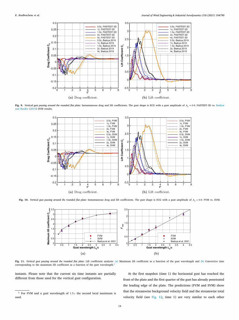
At 𝑡∗ = 0, the plate-gust interaction commence at the leading edgeof the plate yielding an increase in the lift and a drop in the dragcoefficients. While the rise in the lift coefficients is a consequence of anincrease in the effective angle of attack of the plate, the drop in the dragcoefficients is due to the formation of a clockwise rotating leading-edgevortex (LEV). The elevation in the lift coefficients continues until a peakvalue is reached. Then, these coefficients start decaying to eventuallyrecover the steady-state values when the gusts have completely left theplate. On the other hand, drag coefficients keep on decreasing until theleading edge vortex has reached its largest size. Finally, the steady-statevalues of the drag coefficient are retrieved following the convectionof the leading-edge vortex downstream along the chord length of theplate.
In Fig. 10 the aerodynamic responses of the plate due to the gustencounter predicted by FVM are plotted against those delivered bySVM. One could notice that only some minor deviations are presentbetween the results of the two methods (see Table 5). These deviationscan be detected in the lift coefficients of gusts with short wavelengths(e.g., 0.5 𝑐, 1 𝑐 and 1.5 𝑐), where FVM predicts a second local peak whenhe gusts have entirely left the plate.
Based on the results found, one could deduce three main effects ofhe gust width on the aerodynamic responses appearing in FVM andVM:
1. The rate at which the forces change: It could be observed thatthe shorter the gust is, the higher is the rate at which the forcesincrease. This could be related to the fact that a gust with ashorter wavelength has larger gradients along its profile, andtherefore, leads to higher force rates.
2. The peak forces recorded: The instantaneous lift coefficientsteadily increases to reach a maximum value which is dependingon the gust width. In fact, the maximum lift coefficient non-linearly increases with the gust width as found in (Biler et al.,2019) and shown in Fig. 11(a), where the slope decreases forlarger gust lengths. This behavior is expected since for a widergust, the plate experiences a higher effective angle of attackalong the chord for a longer period of time. Fig. 11(a) alsoshows that the current results of both SVM and FVM are in closeagreement with the predicted data by Badrya et al. (2021) (seeTable 5).
3. The instant in time at which the peaks are recorded: It wasfound that the peak lift occurs when the center of the gust islocated between the leading edge and the mid-chord of the plate.Since wider gusts require more time to reach this region, theirresulting maximum peak values occur at later times. It was alsofound in Biler et al. (2019) that the convective time associatedwith the maximum lift linearly increases with the gust width asshown in Fig. 11(b). Again the present results are found to bein good agreement with the predictions in Badrya et al. (2021)(see Table 5).
.2. Horizontal gusts
.2.1. Flow development at 𝐿𝜉𝑔 = 2 𝑐
The flow fields induced by a prescribed horizontal gust of 𝐿𝜉𝑔 =
𝑐 are depicted in Figs. 12 and 13 at six instants in time using thetreamwise background velocity �̃�1∕𝑢∞, the streamwise total velocity1∕𝑢∞ and the pressure normalized by 𝜌 𝑢2∞. Fig. 14 highlights theifferences in the results between both methods at the same time

Journal of Wind Engineering & Industrial Aerodynamics 218 (2021) 104790K. Boulbrachene et al.
Fig. 6. Vertical gust passing around the rounded flat plate: Predictions based on FVM (left) and SVM (right) at time 1 and 2.
11

Journal of Wind Engineering & Industrial Aerodynamics 218 (2021) 104790K. Boulbrachene et al.
Fig. 7. Vertical gust passing around the rounded flat plate: Predictions based on FVM (left) and SVM (right) at time 3 and 4.
12

Journal of Wind Engineering & Industrial Aerodynamics 218 (2021) 104790K. Boulbrachene et al.
Fig. 8. Vertical gust passing around the rounded flat plate: Predictions based on FVM (left) and SVM (right) at time 5 and 6.
13
Journal of Wind Engineering & Industrial Aerodynamics 218 (2021) 104790K. Boulbrachene et al.
id
Fig. 9. Vertical gust passing around the rounded flat plate: Instantaneous drag and lift coefficients. The gust shape is ECG with a gust amplitude of 𝐴𝑔 = 0.8: FASTEST-3D vs. Badryaand Baeder (2019) SVM results.
Fig. 10. Vertical gust passing around the rounded flat plate: Instantaneous drag and lift coefficients. The gust shape is ECG with a gust amplitude of 𝐴𝑔 = 0.8: FVM vs. SVM.
Fig. 11. Vertical gust passing around the rounded flat plate: Lift coefficient analysis: (a) Maximum lift coefficient as a function of the gust wavelength and (b) Convective timecorresponding to the maximum lift coefficient as a function of the gust wavelength.2
nstants. Please note that the current six time instants are partiallyifferent from those used for the vertical gust configuration.
2 For FVM and a gust wavelength of 1.5 𝑐 the second local maximum isused.
14
At the first snapshot (time 1) the horizontal gust has reached the
front of the plate and the first quarter of the gust has already penetrated
the leading edge of the plate. The predictions (FVM and SVM) show
that the streamwise background velocity field and the streamwise total
velocity field (see Fig. 12, time 1) are very similar to each other

Journal of Wind Engineering & Industrial Aerodynamics 218 (2021) 104790K. Boulbrachene et al.
pa
Table 5Normalized root-mean-square error of the lift and drag coefficients found in Fig. 9 (present simulationvs. Badrya and Baeder (2019)) and Fig. 10 (FVM vs. SVM). The relative errors are normalized by thecorresponding ranges (maximum–minimum).Case Normalized RMSE [%] 0.5 𝑐 1.0 𝑐 1.5 𝑐 2.0 𝑐 4.0 𝑐
Present sim. vs. B&B 𝛥𝐶𝐷 5.0 4.9 6.3 4.9 4.7𝛥𝐶𝐿 5.0 4.6 4.6 2.8 1.3
FVM vs. SVM 𝛥𝐶𝐷 3.5 4.6 4.4 4.3 2.4𝛥𝐶𝐿 3.5 3.3 2.2 3.3 3.5
btptocflvvAot
tdfot
and also very similar to the quasi-steady flow shown in Fig. 5. How-ever, strong differences are visible in the pressure distribution (seeFig. 14(a)). In case of SVM an area of negative pressure forms at theprescribed gust location3. Obviously, the observed pressure distributionis due to the contribution of the SVM source term (see Appendix A.2for further details), since a similar observation cannot be made for theFVM prediction, which does not use such a source term. A region witha strong pressure drop at the location of the gust is reasonable, since anincrease of the total streamwise velocity occurs. Therefore, the pressuresinks. At the second snapshot (Fig. 12, time 2) the center of the gust isexactly at the leading edge of the plate. A minor augmentation of thebackground velocity is observed at the leading edge. This accelerationof the flow is more pronounced in the SVM results. The previouslymentioned area of the pressure drop follows the gust prescribed bySVM. For FVM a locally occurring pressure reduction is observed nearthe leading edge, where the flow is locally accelerated during thedeflection around the leading edge. That is also the case in the SVMprediction. However, it is not visible due to the presence of the largeregion of negative pressure. Contrary to the vertical gust configurationthe gust hits a much smaller area of the plate. Therefore, no strongvortical structure is shed in the vicinity of the front of the plate. Atthe third instant in time (Fig. 12, time 3) the center of the gust islocated at the center of the plate. The largest deviations are againfound in the pressure. Assuming that the wide area of negative pressurefollowing the gust observed in SVM is physical (velocity increases,thus the pressure decreases), the pressure field connected with FVM ismore doubtful. The gust velocity prescribed by FVM does not directlyinfluence the pressure. Only two negative pressure areas are observedat both plate ends, where the flow is accelerated due to the deflectioninduced by the plate. In the middle of the structure, where the gust isthe strongest, only a mild decrease of the pressure is visible. Contraryto time 1 and 2, the streamwise background velocity field predicted byFVM and SVM starts to differ in the vicinity of the plate and in thewake (see Fig. 14(c)). The additional source term and the evaluation ofthe shear stress tensor based on the total velocity are the two decisivedifferences characterizing SVM.
In order to track which of these two issues is responsible for thedifference observed in the background velocity, an altered SVM simula-tion, where the shear stress tensor is evaluated based on the backgroundvelocity (as for FVM) instead of the total velocity, is carried out. Sincethe streamwise background velocity field predicted by SVM and thealtered SVM are in close agreement, it can be concluded that the SVMsource term is responsible for the change in the streamwise backgroundvelocity field near the plate. The SVM source term generates thepreviously mentioned pressure drop area, which implies an accelerationof the flow in the tail of the gust and a deceleration in front of the gust(particularly visible near the plate in Fig. 14(c)).
The gust reaches the trailing edge of the plate in the fourth snapshot(Fig. 13, time 4). Looking at the pressure field, where the changesare most obvious, it can be noticed that the vortex shedding at thetrailing edge becomes stronger in both simulations. This can be further
3 Note that the reference point of the pressure is located just after the inletatch at the height of the plate. Thus, a negative pressure has to be interpreteds the difference to the pressure at the reference point.
15
o
observed at the fifth instant in time (Fig. 13, time 5), when the plate isexposed to the last quarter of the gust. In this snapshot the backgroundvelocity predicted by FVM strongly differs from the SVM results (seeFig. 14(e)). Several short local areas of increased streamwise velocityconnected with negative pressure areas are present in the vicinity ofthe plate in case of FVM (see Fig. 13, time 5). These small vortices arelocated near the plate in the tail of the gust. These strong unphysicalvortical structures are neither present in SVM nor in the altered SVM.The physical explanation is that the acceleration of the flow fieldgenerated by the SVM pressure drop area induced by the source termin the tail of the gust avoids the formation of these vortices. At the lastsnapshot (Fig. 13, time 6) the gust detaches from the plate completely.In case of SVM the flow looks very similar to the quasi-steady case (seeFig. 5). However, the unphysical vortices are further present in the FVMsimulation (see Fig. 13, time 6 and Fig. 14(f)).
In summary, the test case of the horizontal gust reveals two findings,which are not so clearly visible in the vertical gust case. These aredirectly related to the differences in the formulation of the FVM andSVM methods. First, the additional source term in SVM is responsiblefor a meaningful forecast of the pressure field and consequently of thebackground velocity field near the structure (feedback effect). Second,the difference in the formulation of the viscous shear stresses betweenFVM and SVM does not have a major effect on the predictions, atleast for the present configuration. This could be related to the factthat the diffusive contribution of the gust velocity (i.e., 𝜏𝑖𝑗 (𝑢𝑔,𝑖)) isdepending on two main parameters, namely, the gust profile and thereciprocal of the Reynolds number. In the present case, the productof the spatial derivative of the gust profile with the reciprocal of theReynolds number has an order of magnitude which is significantlysmaller than that of the SVM source term.
6.2.2. Force coefficients and effect of gust lengthSimilar to the vertical gust case Fig. 15 depicts the time histories
of the drag and lift coefficients for the case of the horizontal gust. Toensure a better visibility of the results, separate subfigures are providedfor each gust length. At the dimensionless time instant 𝑡∗ = 0 theranch of the gust reaches the leading edge of the plate. As visible fromhe drag coefficient depicted in Fig. 15(a), the duration of the gust-late interaction lasts slightly longer than about 1 + 𝐿𝜉
𝑔∕𝑐 convectiveime units, which is the time the gusts needs to travel completelyver the plate. Obviously, the deviations observed between the dragoefficients predicted by FVM and SVM are significantly larger thanor the vertical gust case. Furthermore, the lift coefficient has obviouslyess importance. However, it is directly connected to the van Kármánortex shedding occurring at the trailing edge. The frequency of theortex shedding rises during the passage of the gust over the plate.ssuming a constant Strouhal number of the shedding process the risef the frequency can be explained by the increase of the velocity dueo the horizontal gust.
In order to better understand the time history of the drag coefficient,he pressure part of the drag coefficient 𝐶𝑝
𝐷 and the shear part of therag coefficient 𝐶𝜏
𝐷 are separately plotted in Fig. 16 for FVM and SVMor the gust length of 𝐿𝜉
𝑔 = 2 𝑐. It is obvious that the temporal evolutionf the drag coefficient 𝐶𝐷 predicted by FVM mainly corresponds to theemporal evolution of its shear contribution. On the contrary, the curvef 𝐶 obtained by SVM is directly connected to the pressure part. This
𝐷
Journal of Wind Engineering & Industrial Aerodynamics 218 (2021) 104790K. Boulbrachene et al.
Fig. 12. Horizontal gust passing around the rounded flat plate: Predictions based on FVM (left) and SVM (right) at time 1, 2 and 3.
16

Journal of Wind Engineering & Industrial Aerodynamics 218 (2021) 104790K. Boulbrachene et al.
Fig. 13. Horizontal gust passing around the rounded flat plate: Predictions based on FVM (left) and SVM (right) at time 4, 5 and 6.
17

Journal of Wind Engineering & Industrial Aerodynamics 218 (2021) 104790K. Boulbrachene et al.
Fig. 14. Horizontal gust passing around the rounded flat plate: Flow differences between FVM and SVM at six instants in time.
18

Journal of Wind Engineering & Industrial Aerodynamics 218 (2021) 104790K. Boulbrachene et al.
Fig. 15. Horizontal gust passing around the rounded flat plate: Instantaneous drag and lift coefficients for different gust lengths.
fits to the observations made on the flow fields in the previous section.The SVM source term significantly influences the pressure distributionat the gust location and this has a strong impact on the temporalevolution of the pressure part of the drag coefficient.
At 𝑡∗ = 1, the center of the gust reaches the leading edge. Conse-quently, the maximum pressure drop is also located at the leading edge.Therefore, a decrease in the drag coefficient is observed at this timeinstant. At 𝑡∗ = 2, the center of the gust reaches the trailing edge andthe pressure drop is located at this end of the plate. Thus, a maximumof the drag coefficient occurs at this instant in time. Of further interestis also the temporal evolution of the shear stresses. In case of SVM theshear stress part of the drag coefficient looks like the shape of the gust.On the contrary, the time history of 𝐶𝜏
𝐷 obtained by FVM reveals thatthe shear part of the drag coefficient temporarily drops below the quasi-steady value. This observation is made for the second half of the periodof the gust-plate interaction and can hardly be explained by the physicsof the event. The additional source term and the evaluation of the shearstress tensor based on the total velocity are the two main differencesbetween FVM and SVM.
As in the previous section, the altered SVM simulation, where theshear stress tensor is evaluated based on the background velocity (as forFVM) instead of the total velocity is applied to clarify the source of thechanges. The temporal evolution of the force coefficients predicted bySVM and the altered SVM are quasi identical. This means that the SVMsource term is responsible for the change in the 𝐶𝜏
𝐷 shape. As explainedin the previous section, this outcome is expected as the SVM sourceterm contribution is more pronounced.
Please note that the evaluation of the shear stress tensor based onthe total velocity does not have a major impact in the present caseowing to the currently selected gust configuration. Indeed, the gustshape only changes in 𝐠1-direction. If the gust would also vary in 𝐠2-and/or 𝐠3-direction, a shear stress tensor based on the total velocitywould have a stronger effect on the results.
7. Conclusions
The field velocity method and the split velocity method are windgust injection methods which are often used in the literature. Never-theless, a comprehensive and comprehensible derivation in the context
19
of a finite-volume scheme applying the Arbitrary Lagrangian Eulerian
formulation and the geometric conservation law was missing. Such aconsistent derivation is provided here. This works out the similaritiesbetween the two approaches but also their differences. Their effects onthe results are assessed based on vertical and horizontal gusts hitting aplate. The following results can be recorded:
• The derivation has highlighted that both methods are stronglylinked to the Arbitrary Lagrangian Eulerian formulation and thegeometric conservation law. The difference between both ap-proaches are on the one hand the additional source terms in SVMdescribing the feedback effect of the surrounding flow field on thegust itself and the formulation of the viscous stress tensor by thebackground and the total velocity, respectively.
• From the numerical point of view and the required computa-tional effort both methods are more or less equivalent. There-fore, using FVM does not really make sense anymore. This state-ment is supported by the computational results achieved by bothmethods.
• For the classical case of a vertical gust often used in the contextof aircraft, the deviations in the results (flow field and force co-efficients) are rather small, i.e., the normalized root-mean-squareerrors are in the range between 2.4% and 4.6%. An analyticalderivation revealed that the source term vanishes in the regionswhere the dimensionless background velocity �̃�1 is equal to unity(e.g., the far-field region), which explains its minor impact on thepredictions in the vertical gust case.
• For the newly introduced horizontal gust hitting a plate theobserved differences both in the flow field and in the resultingforce coefficients are significantly more pronounced. The non-vanishing source term as well as the modified formulation of theviscous shear stresses can be made responsible for this observa-tion. However, an additional study clearly showed that for thechosen Reynolds number the consideration of the feedback effectdue to the source term is the decisive difference between FVMand SVM, which prevents unphysical flow structures from beingobserved on the plate.
The significance of the outcome of this study lies on the assessmentof the capability of the prescribed velocity methods to introduce windgusts of different configurations. Especially the horizontal gust case re-
veals the shortcomings of the underlying assumptions used in FVM and
Journal of Wind Engineering & Industrial Aerodynamics 218 (2021) 104790K. Boulbrachene et al.
d
svpgt
C
ViMioS
D
ci
A
d1
A
A
am
Fig. 16. Horizontal gust passing around the rounded flat plate: Time history of the drag coefficient 𝐶𝐷 , of the pressure part of the drag coefficient 𝐶𝑝𝐷 and of the shear part of the
rag coefficient 𝐶𝜏𝐷 for FVM and SVM. The gust has the length of 𝐿𝜉
𝑔 = 2 𝑐.
𝑥
uggests the use of SVM for the injection of gusts having a streamwiseelocity component. That will allow to tackle practically relevant flowroblems in the near future, e.g., to predict the impact of strong windusts on flexible membranous structures and to answer the question ofheir structural integrity.
RediT authorship contribution statement
Khaled Boulbrachene: Conceptualization, Methodology, Software,alidation, Investigation, Visualization, Writing – original draft, Writ-
ng – review & editing. Guillaume De Nayer: Conceptualization,ethodology, Software, Validation, Investigation, Visualization, Writ-
ng – original draft. Michael Breuer: Conceptualization, Methodol-gy, Resources, Writing – original draft, Writing – review & editing,upervision, Project administration, Funding acquisition.
eclaration of competing interest
The authors declare that they have no known competing finan-ial interests or personal relationships that could have appeared tonfluence the work reported in this paper.
cknowledgments
The project is financially supported by the German Research Foun-ation (Deutsche Forschungsgemeinschaft) under the contract number BR847/17-1.
ppendix A. Evaluation and effect of the svm source term
.1. Vertical gusts
For a vertical gust, the gust velocity points only in the 𝑦-directionnd is given by 𝐮𝑔 =
[
0, 𝑢𝑔,2(𝑥, 𝑡), 0]
. Hence, the source terms of theomentum equations simplify to 𝐒 =
[
0, 𝑆2(𝑢𝑔,2(𝑥, 𝑡)), 0]
. EmployingEq. (21), the simplified source term of the 𝑦-momentum equation reads:
𝑆2 = 𝜌{ 𝜕𝑢𝑔,2
𝜕𝑡+ �̃�1
𝜕𝑢𝑔,2𝜕𝑥1
}
. (A.1)
The vertical gust component can be written in the Cartesian basis as:
𝑢𝑔,2(𝑥, 𝑡) =
⎧
⎪
⎪
⎪
⎨
⎪
⎪
⎪
𝑣𝑔,max2
(
1 + cos
(
2𝜋(
𝑥1 − 𝑥g,1(𝑡))
𝐿𝑥1g
))
for(
𝑥1 − 𝑥𝑔,1)
∈
[
−𝐿𝑥1
g
2,𝐿𝑥1
g
2
]
0 else,
(A.2)
20
⎩
with the convected gust center defined as:
𝑥g(𝑡) = 𝑥0g + (𝑡 − 𝑡0) 𝑢∞. (A.3)
The derivatives in Eq. (A.2) are then:
𝜕𝑢𝑔,2𝜕𝑡
= +𝜋 𝑣𝑔,max 𝑢∞
𝐿𝑥1g
sin
(
2𝜋(
𝑥1 − 𝑥g,1(𝑡))
𝐿𝑥g
)
,
𝜕𝑢𝑔,2𝜕𝑥1
= −𝜋 𝑣𝑔,max
𝐿𝑥1g
sin
(
2𝜋(
𝑥1 − 𝑥g,1(𝑡))
𝐿𝑥1g
)
.
(A.4)
The derivatives are therefore nearly identical but of opposite signs.Consequently, the source term (Eq. (A.1)) would vanish if the back-ground velocity �̃�1 is equal to 𝑢∞. In fact, this is the case in the far-fieldregion (far away from the plate), where the background velocity �̃�1 isequal to the free-stream velocity 𝑢∞. In that region, the source termplays no role and has no effect on the pressure field in contrast to theeffects remarked in the horizontal gust configuration. As a result, nomajor deviations between FVM and SVM are realized for the verticalgust configuration (see Figs. 6 to 8).
A.2. Horizontal gusts
For a horizontal gust, the gust velocity points only in the 𝑥-directionand is given by 𝐮𝑔 =
[
𝑢𝑔,1(𝑥, 𝑡), 0, 0]
. Hence, the source terms of themomentum equations simplify to 𝐒 =
[
𝑆1(𝑢𝑔,1(𝑥, 𝑡)), 0, 0]
. Employing Eq. (21), the simplified source termof the 𝑥-momentum equation reads:
𝑆1 = 𝜌{ 𝜕𝑢𝑔,1
𝜕𝑡+(
�̃�1 + 𝑢𝑔,1)𝜕𝑢𝑔,1𝜕𝑥1
}
. (A.5)
The horizontal gust component can be written in the Cartesian basis as:
𝑢𝑔,1(𝑥, 𝑡) =
⎧
⎪
⎪
⎪
⎨
⎪
⎪
⎪
⎩
𝑢𝑔,max2
(
1 + cos
(
2𝜋(
𝑥1 − 𝑥g,1(𝑡))
𝐿𝑥1g
))
for(
𝑥1 − 𝑥𝑔,1)
∈
[
−𝐿𝑥1
g
2,𝐿𝑥1
g
2
]
0 else ,
(A.6)
with the convected gust center defined as:
g(𝑡) = 𝑥0g + (𝑡 − 𝑡0) 𝑢∞. (A.7)
The derivatives in Eq. (A.2) are then:
𝜕𝑢𝑔,1𝜕𝑡
= +𝜋 𝑢𝑔,max 𝑢∞
𝐿𝑥g
sin
(
2𝜋(
𝑥1 − 𝑥g,1(𝑡))
𝐿𝑥1g
)
,
𝜕𝑢𝑔,1 = −𝜋 𝑢𝑔,max
𝑥 sin
(
2𝜋(
𝑥1 − 𝑥g,1(𝑡))
𝑥1
)
.
(A.8)
𝜕𝑥1 𝐿g 𝐿g
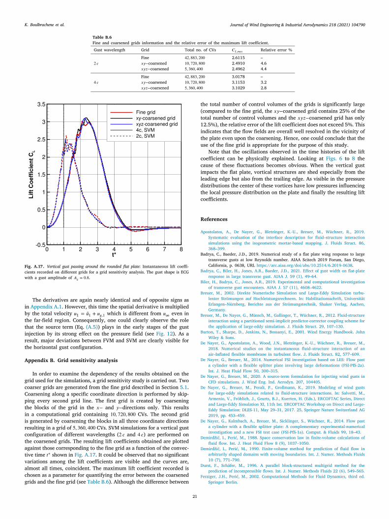
Journal of Wind Engineering & Industrial Aerodynamics 218 (2021) 104790K. Boulbrachene et al.
ibttirt
A
gcCptiirc
Table B.6Fine and coarsened grids information and the relative error of the maximum lift coefficient.Gust wavelength Grid Total no. of CVs 𝐶𝐿,𝑚𝑎𝑥 Relative error %
2 𝑐Fine 42, 883, 200 2.6115 –𝑥𝑦−coarsened 10, 720, 800 2.4910 4.6𝑥𝑦𝑧−coarsened 5, 360, 400 2.4962 4.4
4 𝑐Fine 42, 883, 200 3.0178 –𝑥𝑦−coarsened 10, 720, 800 3.1153 3.2𝑥𝑦𝑧−coarsened 5, 360, 400 3.1029 2.8
1itu
ccildtc
R
A
B
B
B
B
B
B
D
D
D
D
D
D
D
D
F
Fig. A.17. Vertical gust passing around the rounded flat plate: Instantaneous lift coeffi-cients recorded on different grids for a grid sensitivity analysis. The gust shape is ECGwith a gust amplitude of 𝐴𝑔 = 0.8.
The derivatives are again nearly identical and of opposite signs asn Appendix A.1. However, this time the spatial derivative is multipliedy the total velocity 𝑢1 = �̃�1 + 𝑢𝑔,1 which is different from 𝑢∞ even inhe far-field region. Consequently, one could clearly observe the rolehat the source term (Eq. (A.5)) plays in the early stages of the gustnjection by its strong effect on the pressure field (see Fig. 12). As aesult, major deviations between FVM and SVM are clearly visible forhe horizontal gust configuration.
ppendix B. Grid sensitivity analysis
In order to examine the dependency of the results obtained on therid used for the simulations, a grid sensitivity study is carried out. Twooarser grids are generated from the fine grid described in Section 5.1.oarsening along a specific coordinate direction is performed by skip-ing every second grid line. The first grid is created by coarseninghe blocks of the grid in the 𝑥− and 𝑦−directions only. This resultsn a computational grid containing 10, 720, 800 CVs. The second grids generated by coarsening the blocks in all three coordinate directionsesulting in a grid of 5, 360, 400 CVs. SVM simulations for a vertical gustonfiguration of different wavelengths (2 𝑐 and 4 𝑐) are performed on
the coarsened grids. The resulting lift coefficients obtained are plottedagainst those corresponding to the fine grid as a function of the convec-tive time 𝑡∗ shown in Fig. A.17. It could be observed that no significantvariations among the lift coefficients are visible and the curves are,almost all times, coincident. The maximum lift coefficient recorded ischosen as a parameter for quantifying the error between the coarsened
21
grids and the fine grid (see Table B.6). Although the difference between
the total number of control volumes of the grids is significantly large(compared to the fine grid, the 𝑥𝑦−coarsened grid contains 25% of thetotal number of control volumes and the 𝑥𝑦𝑧−coarsened grid has only2.5%), the relative error of the lift coefficient does not exceed 5%. Thisndicates that the flow fields are overall well resolved in the vicinity ofhe plate even upon the coarsening. Hence, one could conclude that these of the fine grid is appropriate for the purpose of this study.
Note that the oscillations observed in the time histories of the liftoefficient can be physically explained. Looking at Figs. 6 to 8 theause of these fluctuations becomes obvious. When the vertical gustmpacts the flat plate, vortical structures are shed especially from theeading edge but also from the trailing edge. As visible in the pressureistributions the center of these vortices have low pressures influencinghe local pressure distribution on the plate and finally the resulting liftoefficients.
eferences
postolatos, A., De Nayer, G., Bletzinger, K.-U., Breuer, M., Wüchner, R., 2019.Systematic evaluation of the interface description for fluid–structure interactionsimulations using the isogeometric mortar-based mapping. J. Fluids Struct. 86,368–399.
adrya, C., Baeder, J.D., 2019. Numerical study of a flat plate wing response to largetransverse gusts at low Reynolds number. AIAA Scitech 2019 Forum, San Diego,California, p. 0638, URL https://arc.aiaa.org/doi/abs/10.2514/6.2019-0638.
adrya, C., Biler, H., Jones, A.R., Baeder, J.D., 2021. Effect of gust width on flat-plateresponse in large transverse gust. AIAA J. 59 (1), 49–64.
iler, H., Badrya, C., Jones, A.R., 2019. Experimental and computational investigationof transverse gust encounters. AIAA J. 57 (11), 4608–4622.
reuer, M., 2002. Direkte Numerische Simulation und Large-Eddy Simulation turbu-lenter Strömungen auf Hochleistungsrechnern. In: Habilitationsschrift, UniversitätErlangen–Nürnberg, Berichte aus der Strömungstechnik, Shaker Verlag, Aachen,Germany.
reuer, M., De Nayer, G., Münsch, M., Gallinger, T., Wüchner, R., 2012. Fluid-structureinteraction using a partitioned semi-implicit predictor-corrector coupling scheme forthe application of large-eddy simulation. J. Fluids Struct. 29, 107–130.
urton, T., Sharpe, D., Jenkins, N., Bossanyi, E., 2001. Wind Energy Handbook. JohnWiley & Sons.
e Nayer, G., Apostolatos, A., Wood, J.N., Bletzinger, K.-U., Wüchner, R., Breuer, M.,2018. Numerical studies on the instantaneous fluid–structure interaction of anair–Inflated flexible membrane in turbulent flow. J. Fluids Struct. 82, 577–609.
e Nayer, G., Breuer, M., 2014. Numerical FSI investigation based on LES: Flow pasta cylinder with a flexible splitter plate involving large deformations (FSI-PfS-2a).Int. J. Heat Fluid Flow 50, 300–315.
e Nayer, G., Breuer, M., 2020. A source-term formulation for injecting wind gusts inCFD simulations. J. Wind Eng. Ind. Aerodyn. 207, 104405.
e Nayer, G., Breuer, M., Perali, P., Grollmann, K., 2019. Modeling of wind gustsfor large-eddy simulations related to fluid-structure interactions. In: Salvetti, M.,Armenio, V., Fröhlich, J., Geurts, B.J., Kuerten, H. (Eds.), ERCOFTAC Series, Directand Large-Eddy Simulation XI, 11th Int. ERCOFTAC Workshop on Direct and Large-Eddy Simulation: DLES-11, May 29–31, 2017. 25, Springer Nature Switzerland AG2019, pp. 453–459.
e Nayer, G., Kalmbach, A., Breuer, M., Sicklinger, S., Wüchner, R., 2014. Flow pasta cylinder with a flexible splitter plate: A complementary experimental-numericalinvestigation and a new FSI test case (FSI-PfS-1a). Comput. & Fluids 99, 18–43.
emirdžić, I., Perić, M., 1988. Space conservation law in finite-volume calculations offluid flow. Int. J. Heat Fluid Flow 8 (9), 1037–1050.
emirdžić, I., Perić, M., 1990. Finite-volume method for prediction of fluid flow inarbitrarily shaped domains with moving boundaries. Int. J. Numer. Methods Fluids10 (7), 771–790.
urst, F., Schäfer, M., 1996. A parallel block-structured multigrid method for theprediction of incompressible flows. Int. J. Numer. Methods Fluids 22 (6), 549–565.
erziger, J.H., Perić, M., 2002. Computational Methods for Fluid Dynamics, third ed.Springer Berlin.

Journal of Wind Engineering & Industrial Aerodynamics 218 (2021) 104790K. Boulbrachene et al.
Franke, J., Baklanov, A., 2007. Best practice guideline for the CFD simulation of flows inthe urban environment. In: COST Action 732 Quality Assurance and Improvementof Microscale Meteorological Models. University of Hamburg, Germany.
Franke, J., Hellsten, A., Schlünzen, K.H., Carissimo, B., 2011. The COST 732 bestpractice guideline for CFD simulation of flows in the urban environment: Asummary. Int. J. Environ. Pollut. 44 (1–4), 419–427.
Frost, W., Long, B.H., Turner, R.E., 1978. Engineering handbook on the atmosphericenvironmental guidelines for use in wind turbine generator development. Ten-nessee Univ., Tullahoma (USA). Space Inst.; National Aeronautics and SpaceAdministration, Huntsville, AL (USA). George C. Marshall Space Flight Center.
Ghoreyshi, M., Jirasek, A., Greisz, I., Satchell, M., 2018. Indicial aerodynamic modelingfor arbitrary gust responses, in: Applied Aerodynamics Conference, June 25–29,2018, Atlanta, Georgia, AIAA-2018-3965.
Gordnier, R.E., Visbal, M.R., 2015. Impact of a vortical gust on the aerodynamics of afinite aspect-ratio wing. In: 45th AIAA Fluid Dynamics Conference. pp. 1–18, URLhttps://arc.aiaa.org/doi/abs/10.2514/6.2015-3072.
Granlund, K., Monnier, B., Ol, M., Williams, D., 2014. Airfoil longitudinal gust responsein separated vs. attached flows. Phys. Fluids 26 (2), 027103.
Gross, J.L., Main, J.A., Phan, L.T., Sadek, F.H., Cauffman, S.A., Jorgensen, D.P., 2013.Final report on the collapse of the Dallas Cowboys indoor practice facility, May 2,2009.
Gu, N., Lu, Z., Guo, T., 2012. Simulation of viscous flows around a moving airfoil byfield velocity method with viscous flux correction. Adv. Appl. Math. Mech. 4 (3),294–310.
Hawbecker, P., Basu, S., Manuel, L., 2017. Realistic simulations of the July 1, 2011severe wind event over the Buffalo Ridge Wind Farm. Wind Energy 20 (11),1803–1822.
Heinrich, R., 2014. Simulation of interaction of aircraft and gust using the TAU-code.In: Dillmann, A., Heller, G., Krämer, E., Kreplin, H.-P., Nitsche, W., Rist, U. (Eds.),New Results in Numerical and Experimental Fluid Mechanics IX: Contributions tothe 18th STAB/DGLR Symposium, Stuttgart, Germany, 2012. Springer InternationalPublishing, Cham, pp. 503–511.
Heinrich, R., Reimer, L., 2013. Comparison of different approaches for gust modeling inthe CFD code TAU. In: International Forum on Aeroelasticity & Structural Dynamics2013. URL https://elib.dlr.de/85834/.
Huntley, S., Jones, D., Gaitonde, A., 2016. 2D and 3D gust response using a prescribedvelocity method in viscous flows, in: 46th AIAA Fluid Dynamics Conference.
Huntley, S.J., Jones, D., Gaitonde, A., 2017. Aeroelastic gust response of an aircraftusing a prescribed velocity method in viscous flows. In: 23rd AIAA ComputationalFluid Dynamics Conference. Denver, Colorado, URL https://arc.aiaa.org/doi/abs/10.2514/6.2017-3616.
IEC-Standard, 2002. 61400-21, Measurement and Assessment of Power Quality of GridConnected Wind Turbines.
Kasperski, M., 2007. A consistent model for the codification of wind loads. J. WindEng. Ind. Aerodyn. 95 (9), 1114–1124.
Khosla, P.K., Rubin, S.G., 1974. A diagonally dominant second-order accurate implicitscheme. Comput. & Fluids 2 (2), 207–209.
22
Knigge, C., Raasch, S., 2016. Improvement and development of one- and two-dimensional discrete gust models using a large-eddy simulation model. J. WindEng. Ind. Aerodyn. 153, 46–59.
Küssner, H.G., 1936. Zusammenfassender Bericht über den instationären Auftrieb vonFlügeln. Luftfahrtforschung 13 (12), 410–424.
Kwon, D.K., Kareem, A., Butler, K., 2012. Gust-front loading effects on wind turbinetower systems. J. Wind Eng. Ind. Aerodyn. 104–106, 109–115.
Lesoinne, M., Farhat, C., 1996. Geometric conservation laws for flow problems withmoving boundaries and deformable meshes, and their impact on aeroelasticcomputations. Comput. Methods Appl. Mech. Engrg. 134 (1–2), 71–90.
Montenegro, P.A., Heleno, R., Carvalho, H., Calcada, R., Baker, C.J., 2020. A compar-ative study on the running safety of trains subjected to crosswinds simulated withdifferent wind models. J. Wind Eng. Ind. Aerodyn. 207, 104398.
Münsch, M., 2015. Entwicklung und Anwendung eines semi-impliziten Kopplungsver-fahrens zur numerischen Berechnung der Fluid-Struktur-Wechselwirkung in turbu-lenten Strömungen mittels Large-Eddy Simulationen. (Ph.D. thesis). University ofErlangen-Nuremberg, Germany.
Norris, S.E., Cater, J.E., Stol, K.A., Unsworth, C.P., 2010. Wind turbine wake modellingusing large-eddy simulation. In: Proceedings of the 17th Australian Fluid MechanicsConference. Curran Associates, Inc., University of Auckland, Australia.
Onol, A.O., Yesilyurt, S., 2017. Effects of wind gusts on a vertical axis wind turbinewith high solidity. J. Wind Eng. Ind. Aerodyn. 162, 1–11.
Parameswaran, V., Baeder, J.D., 1997. Indicial aerodynamics in compressibleflow–Direct computational fluid dynamic calculations. J. Aircr. 34 (1), 131–133.
Rhie, C.M., Chow, W.L., 1983. Numerical study of the turbulent flow past an airfoilwith trailing-edge separation. AIAA J. 21 (11), 1525–1532.
Sankar, L.N., Rou, S.Y., Malone, J.B., 1986. Application of surface transpiration incomputational aerodynamics. In: 24th Aerospace Sciences Meeting. Reno, NV, USA,URL https://arc.aiaa.org/doi/abs/10.2514/6.1986-511.
Singh, R., Baeder, J.D., 1996. On the significance of transonic effects on aerody-namics and acoustics of blade-vortex interactions. In: Aeroacoustics Conference.Pennsylvania, USA, URL https://arc.aiaa.org/doi/abs/10.2514/6.1996-1697.
Singh, R., Baeder, J.D., 1997. Direct calculation of three-dimensional indicial liftresponse using computational fluid dynamics. J. Aircr. 34 (4), 465–471.
Sitaraman, J., 2003. CFD Based unsteady aerodynamic modeling for rotor aeroelasticanalysis. (Ph.D. thesis). University of Maryland, College Park, USA.
Sitaraman, J., Baeder, J.D., 2000. Enhanced unsteady airload models using CFD. In:Fluids 2000 Conference and Exhibit. Denver, Colorado, URL https://arc.aiaa.org/doi/abs/10.2514/6.2000-2465.
Sitaraman, J., Baeder, J.D., 2006. Field velocity approach and geometric conservationlaw for unsteady flow simulations. AIAA J. 44 (9), 2084–2094.
Stone, H.L., 1968. Iterative solution of implicit approximations of multidimensionalpartial differential equations. SIAM J. Numer. Anal. 5 (3), 530–558.
Wales, C., Jones, D., Gaitonde, A., 2014. Prescribed velocity method for simulation ofaerofoil gust responses. J. Aircr. 52 (1), 64–76.
Wu, Z., Cao, Y., Ismail, M., 2019. Gust loads on aircraft. Aeronaut. J. 123 (1266),1216–1274.
Zaide, A., Raveh, D.E., 2006. Numerical simulation and reduced-order modeling ofairfoil gust response. AIAA J. 44 (8), 1826–1834.