The Ray Optics Module User's Guide - COMSOL Documentation

Ray Optics ModuleUser’s Guide

C o n t a c t I n f o r m a t i o n

Visit the Contact COMSOL page at www.comsol.com/contact to submit general inquiries, contact Technical Support, or search for an address and phone number. You can also visit the Worldwide Sales Offices page at www.comsol.com/contact/offices for address and contact information.

If you need to contact Support, an online request form is located at the COMSOL Access page at www.comsol.com/support/case. Other useful links include:

• Support Center: www.comsol.com/support

• Product Download: www.comsol.com/product-download

• Product Updates: www.comsol.com/support/updates

• COMSOL Blog: www.comsol.com/blogs

• Discussion Forum: www.comsol.com/community

• Events: www.comsol.com/events

• COMSOL Video Gallery: www.comsol.com/video

• Support Knowledge Base: www.comsol.com/support/knowledgebase

Part number: CM024201

R a y O p t i c s M o d u l e U s e r ’ s G u i d e © 1998–2019 COMSOL

Protected by patents listed on www.comsol.com/patents, and U.S. Patents 7,519,518; 7,596,474; 7,623,991; 8,457,932; 8,954,302; 9,098,106; 9,146,652; 9,323,503; 9,372,673; 9,454,625; and 10,019,544. Patents pending.

This Documentation and the Programs described herein are furnished under the COMSOL Software License Agreement (www.comsol.com/comsol-license-agreement) and may be used or copied only under the terms of the license agreement.

COMSOL, the COMSOL logo, COMSOL Multiphysics, COMSOL Desktop, COMSOL Compiler, COMSOL Server, and LiveLink are either registered trademarks or trademarks of COMSOL AB. All other trademarks are the property of their respective owners, and COMSOL AB and its subsidiaries and products are not affiliated with, endorsed by, sponsored by, or supported by those trademark owners. For a list of such trademark owners, see www.comsol.com/trademarks.

Version: COMSOL 5.5

www.comsol.com/patents/

http://www.comsol.com/comsol-license-agreement/

http://www.comsol.com/contact/

http://www.comsol.com/contact/offices/

http://www.comsol.com/support/case/

http://www.comsol.com/support/

http://www.comsol.com/product-download/

http://www.comsol.com/support/updates/

http://www.comsol.com/trademarks/

http://www.comsol.com/blogs/

http://www.comsol.com/community/

http://www.comsol.com/events/

http://www.comsol.com/video/

http://www.comsol.com/support/knowledgebase/

C o n t e n t s

C h a p t e r 1 : I n t r o d u c t i o n

About the Ray Optics Module 8

The Ray Optics Module Physics Interface Guide . . . . . . . . . . . 8

Common Physics Interface and Feature Settings and Nodes . . . . . . 9

Where Do I Access the Documentation and Application Libraries? . . . . 9

Overview of the User’s Guide 14

C h a p t e r 2 : R a y O p t i c s M o d e l i n g

Essentials of Ray Tracing 16

The Ray Tracing Algorithm . . . . . . . . . . . . . . . . . . . 16

Basic Requirements of a Ray Optics Model . . . . . . . . . . . . . 17

Geometry and Meshing 19

Creating a Geometry . . . . . . . . . . . . . . . . . . . . . 19

Domain Selection . . . . . . . . . . . . . . . . . . . . . . 21

Meshing and Discretization Error. . . . . . . . . . . . . . . . . 22

Meshing Guidelines for Geometrical Optics Simulation . . . . . . . . 23

Boundary Conditions 25

Reflection and Refraction. . . . . . . . . . . . . . . . . . . . 25

Primary and Secondary Ray Releases . . . . . . . . . . . . . . . 26

Wall Conditions . . . . . . . . . . . . . . . . . . . . . . . 28

Special Boundary Conditions . . . . . . . . . . . . . . . . . . 29

Ray Release Features 30

Grid-Based Release . . . . . . . . . . . . . . . . . . . . . . 30

Release from Domains, Boundaries, Edges, or Points . . . . . . . . . 30

Specialized Release Features . . . . . . . . . . . . . . . . . . 31

Release Features for Multiscale Modeling . . . . . . . . . . . . . . 31

C O N T E N T S | 3

4 | C O N T E N T S

Additional Variables Solved For 32

Modeling Polychromatic Radiation . . . . . . . . . . . . . . . . 32

Intensity, Polarization, and Power . . . . . . . . . . . . . . . . 33

Other Dependent Variables . . . . . . . . . . . . . . . . . . . 35

Order of Initialization of Auxiliary Dependent Variables . . . . . . . . 36

Study Types 37

Ray Tracing Study Step . . . . . . . . . . . . . . . . . . . . 37

Bidirectionally Coupled Ray Tracing Study Step . . . . . . . . . . . 39

Results Analysis and Visualization 41

Ray Trajectories Plot . . . . . . . . . . . . . . . . . . . . . 41

Ray Plot . . . . . . . . . . . . . . . . . . . . . . . . . . 42

Interference Pattern Plot . . . . . . . . . . . . . . . . . . . . 43

Spot Diagram Plot . . . . . . . . . . . . . . . . . . . . . . 44

Optical Aberration Plot and Aberration Evaluation . . . . . . . . . . 47

Variables and Nonlocal Couplings 50

Ray Statistics . . . . . . . . . . . . . . . . . . . . . . . . 50

Global Variables . . . . . . . . . . . . . . . . . . . . . . . 51

Variables for Average Ray Position . . . . . . . . . . . . . . . . 52

Using Ray Detectors . . . . . . . . . . . . . . . . . . . . . 52

Nonlocal Couplings . . . . . . . . . . . . . . . . . . . . . . 53

C h a p t e r 3 : R a y O p t i c s I n t e r f a c e s

The Geometrical Optics Interface 58

Geometrical Optics Physics Interface Settings . . . . . . . . . . . . 58

List of Geometrical Optics Interface Physics Features . . . . . . . . . 66

Ray Properties . . . . . . . . . . . . . . . . . . . . . . . . 67

Medium Properties . . . . . . . . . . . . . . . . . . . . . . 68

Material Discontinuity . . . . . . . . . . . . . . . . . . . . . 72

Thin Dielectric Film . . . . . . . . . . . . . . . . . . . . . . 77

Wall . . . . . . . . . . . . . . . . . . . . . . . . . . . 77

Mirror . . . . . . . . . . . . . . . . . . . . . . . . . . . 81

Axial Symmetry . . . . . . . . . . . . . . . . . . . . . . . 82

Release . . . . . . . . . . . . . . . . . . . . . . . . . . 82

Release from Boundary . . . . . . . . . . . . . . . . . . . . 90

Release from Symmetry Axis . . . . . . . . . . . . . . . . . . 94

Release from Edge . . . . . . . . . . . . . . . . . . . . . . 95

Release from Point . . . . . . . . . . . . . . . . . . . . . . 95

Release from Point on Axis . . . . . . . . . . . . . . . . . . . 95

Release from Grid . . . . . . . . . . . . . . . . . . . . . . 96

Release from Grid on Axis . . . . . . . . . . . . . . . . . . . 99

Release from Data File. . . . . . . . . . . . . . . . . . . . 100

Photometric Data Import . . . . . . . . . . . . . . . . . . 101

Illuminated Surface . . . . . . . . . . . . . . . . . . . . . 102

Solar Radiation . . . . . . . . . . . . . . . . . . . . . . 104

Ray Termination . . . . . . . . . . . . . . . . . . . . . . 107

Release from Electric Field . . . . . . . . . . . . . . . . . . 109

Release from Far-Field Radiation Pattern . . . . . . . . . . . . . 111

Grating . . . . . . . . . . . . . . . . . . . . . . . . . 114

Diffraction Order (Grating) . . . . . . . . . . . . . . . . . . 118

Cross Grating . . . . . . . . . . . . . . . . . . . . . . . 119

Diffraction Order (Cross Grating) . . . . . . . . . . . . . . . 121

Linear Polarizer . . . . . . . . . . . . . . . . . . . . . . 122

Ideal Depolarizer . . . . . . . . . . . . . . . . . . . . . . 123

Linear Wave Retarder . . . . . . . . . . . . . . . . . . . . 123

Circular Wave Retarder . . . . . . . . . . . . . . . . . . . 124

Mueller Matrix . . . . . . . . . . . . . . . . . . . . . . . 125

Deposited Ray Power (Domain) . . . . . . . . . . . . . . . . 126

Deposited Ray Power (Boundary) . . . . . . . . . . . . . . . 126

Accumulator (Domain) . . . . . . . . . . . . . . . . . . . 126

Accumulator (Boundary) . . . . . . . . . . . . . . . . . . . 127

Nonlocal Accumulator. . . . . . . . . . . . . . . . . . . . 129

Auxiliary Dependent Variable . . . . . . . . . . . . . . . . . 130

Ray Continuity. . . . . . . . . . . . . . . . . . . . . . . 131

Ray Detector . . . . . . . . . . . . . . . . . . . . . . . 131

Theory for the Geometrical Optics Interface 132

Introduction to Geometrical Optics . . . . . . . . . . . . . . 132

Optical Dispersion Models . . . . . . . . . . . . . . . . . . 133

Thermo-Optic Dispersion Models . . . . . . . . . . . . . . . 136

Initial Conditions: Direction. . . . . . . . . . . . . . . . . . 137

C O N T E N T S | 5

6 | C O N T E N T S

Material Discontinuity Theory . . . . . . . . . . . . . . . . . 138

Intensity, Wavefront Curvature, and Polarization. . . . . . . . . . 139

Wavefront Curvature Calculation in Graded Media . . . . . . . . . 149

Refraction in Strongly Absorbing Media . . . . . . . . . . . . . 153

Attenuation Within Domains . . . . . . . . . . . . . . . . . 156

Ray Termination Theory . . . . . . . . . . . . . . . . . . . 157

Illuminated Surface Theory . . . . . . . . . . . . . . . . . . 159

Theory of Mueller Matrices and Optical Components . . . . . . . . 162

Thin Dielectric Film Theory. . . . . . . . . . . . . . . . . . 164

Diffraction Grating Theory . . . . . . . . . . . . . . . . . . 170

Interference Pattern Theory . . . . . . . . . . . . . . . . . 174

Monochromatic Aberrations and the Zernike Polynomials . . . . . . 176

Accumulator Theory: Domains . . . . . . . . . . . . . . . . 179

Accumulator Theory: Boundaries . . . . . . . . . . . . . . . 180

References for the Geometrical Optics Interface . . . . . . . . . . 182

C h a p t e r 4 : M u l t i p h y s i c s I n t e r f a c e s a n d C o u p l i n g s

The Ray Heating Interface 186

Ray Heat Source . . . . . . . . . . . . . . . . . . . . . . 188

Theory for the Ray Heating Interface 189

Unidirectional and Bidirectional Couplings . . . . . . . . . . . . 189

Coupled Heat Transfer and Ray Tracing Equations . . . . . . . . . 189

Heat Source Calculation . . . . . . . . . . . . . . . . . . . 191

C h a p t e r 5 : G l o s s a r y

Glossary of Terms 194

Index 199

1

I n t r o d u c t i o n

This guide describes the Ray Optics Module, an optional add-on package for COMSOL Multiphysics®.

This chapter introduces you to the capabilities of this module. A summary of the physics interfaces and where you can find documentation and model examples is also included. The last section is a brief overview with links to each chapter in this guide.

In this chapter:

• About the Ray Optics Module

• Overview of the User’s Guide

7

8 | C H A P T E R

Abou t t h e Ra y Op t i c s Modu l e

These topics are included in this section:

• The Ray Optics Module Physics Interface Guide

• Common Physics Interface and Feature Settings and Nodes

• Where Do I Access the Documentation and Application Libraries?

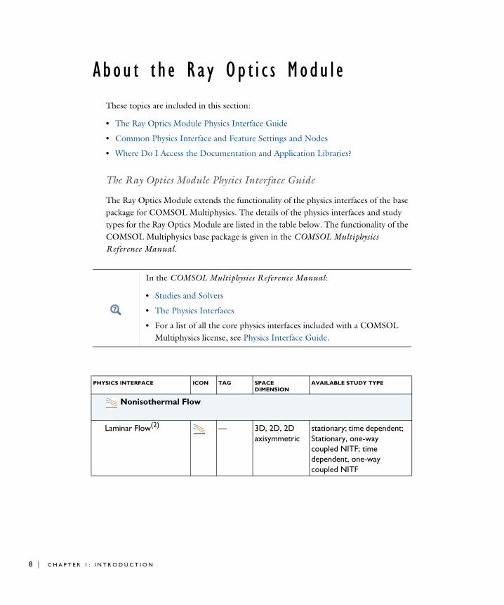
The Ray Optics Module Physics Interface Guide

The Ray Optics Module extends the functionality of the physics interfaces of the base package for COMSOL Multiphysics. The details of the physics interfaces and study types for the Ray Optics Module are listed in the table below. The functionality of the COMSOL Multiphysics base package is given in the COMSOL Multiphysics Reference Manual.

In the COMSOL Multiphysics Reference Manual:

• Studies and Solvers

• The Physics Interfaces

• For a list of all the core physics interfaces included with a COMSOL Multiphysics license, see Physics Interface Guide.

PHYSICS INTERFACE ICON TAG SPACE DIMENSION

AVAILABLE STUDY TYPE

Nonisothermal Flow

Laminar Flow(2) — 3D, 2D, 2D axisymmetric

stationary; time dependent; Stationary, one-way coupled NITF; time dependent, one-way coupled NITF

1 : I N T R O D U C T I O N

Common Physics Interface and Feature Settings and Nodes

There are several common settings and sections available for the physics interfaces and feature nodes. Some of these sections also have similar settings or are implemented in the same way no matter the physics interface or feature being used. There are also some physics feature nodes that display in COMSOL Multiphysics.

In each module’s documentation, only unique or extra information is included; standard information and procedures are centralized in the COMSOL Multiphysics Reference Manual.

Where Do I Access the Documentation and Application Libraries?

A number of internet resources have more information about COMSOL, including licensing and technical information. The electronic documentation, topic-based (or

Optics

Ray Optics

Geometrical Optics gop 3D, 2D, 2D axisymmetric

ray tracing; bidirectionally coupled ray tracing; time dependent

Ray Heating — 3D, 2D, 2D axisymmetric

ray tracing; bidirectionally coupled ray tracing; time dependent

PHYSICS INTERFACE ICON TAG SPACE DIMENSION

AVAILABLE STUDY TYPE

In the COMSOL Multiphysics Reference Manual see Table 2-4 for links to common sections and Table 2-5 to common feature nodes. You can also search for information: press F1 to open the Help window or Ctrl+F1 to open the Documentation window.

A B O U T T H E R A Y O P T I C S M O D U L E | 9

10 | C H A P T E R

context-based) help, and the application libraries are all accessed through the COMSOL Desktop.

T H E D O C U M E N T A T I O N A N D O N L I N E H E L P

The COMSOL Multiphysics Reference Manual describes the core physics interfaces and functionality included with the COMSOL Multiphysics license. This book also has instructions about how to use COMSOL Multiphysics and how to access the electronic Documentation and Help content.

Opening Topic-Based HelpThe Help window is useful as it is connected to the features in the COMSOL Desktop. To learn more about a node in the Model Builder, or a window on the Desktop, click to highlight a node or window, then press F1 to open the Help window, which then displays information about that feature (or click a node in the Model Builder followed by the Help button ( ). This is called topic-based (or context) help.

If you are reading the documentation as a PDF file on your computer, the blue links do not work to open an application or content referenced in a different guide. However, if you are using the Help system in COMSOL Multiphysics, these links work to open other modules, application examples, and documentation sets.

To open the Help window:

• In the Model Builder, Application Builder, or Physics Builder click a node or window and then press F1.

• On any toolbar (for example, Home, Definitions, or Geometry), hover the mouse over a button (for example, Add Physics or Build All) and then press F1.

• From the File menu, click Help ( ).

• In the upper-right corner of the COMSOL Desktop, click the Help ( ) button.


Opening the Documentation Window

T H E A P P L I C A T I O N L I B R A R I E S W I N D O W

Each model or application includes documentation with the theoretical background and step-by-step instructions to create a model or application. The models and applications are available in COMSOL Multiphysics as MPH files that you can open for further investigation. You can use the step-by-step instructions and the actual models as templates for your own modeling. In most models, SI units are used to describe the relevant properties, parameters, and dimensions, but other unit systems are available.

Once the Application Libraries window is opened, you can search by name or browse under a module folder name. Click to view a summary of the model or application and its properties, including options to open it or its associated PDF document.

To open the Help window:

• In the Model Builder or Physics Builder click a node or window and then press F1.

• On the main toolbar, click the Help ( ) button.

• From the main menu, select Help>Help.

To open the Documentation window:

• Press Ctrl+F1.

• From the File menu select Help>Documentation ( ).

To open the Documentation window:

• Press Ctrl+F1.

• On the main toolbar, click the Documentation ( ) button.

• From the main menu, select Help>Documentation.

The Application Libraries Window in the COMSOL Multiphysics Reference Manual.


12 | C H A P T E R

Opening the Application Libraries WindowTo open the Application Libraries window ( ):

C O N T A C T I N G C O M S O L B Y E M A I L

For general product information, contact COMSOL at [email protected].

C O M S O L A C C E S S A N D T E C H N I C A L S U P P O R T

To receive technical support from COMSOL for the COMSOL products, please contact your local COMSOL representative or send your questions to [email protected]. An automatic notification and a case number are sent to you by email. You can also access technical support, software updates, license information, and other resources by registering for a COMSOL Access account.

• From the Home toolbar, Windows menu, click ( ) Applications

Libraries.

• From the File menu select Application Libraries.

To include the latest versions of model examples, from the File>Help menu, select ( ) Update COMSOL Application Library.

Select Application Libraries from the main File> or Windows> menus.

To include the latest versions of model examples, from the Help menu select ( ) Update COMSOL Application Library.


C O M S O L O N L I N E R E S O U R C E S

COMSOL website www.comsol.com

Contact COMSOL www.comsol.com/contact

COMSOL Access www.comsol.com/access

Support Center www.comsol.com/support

Product Download www.comsol.com/product-download

Product Updates www.comsol.com/support/updates

COMSOL Blog www.comsol.com/blogs

Discussion Forum www.comsol.com/community

Events www.comsol.com/events

COMSOL Video Gallery www.comsol.com/video

Support Knowledge Base www.comsol.com/support/knowledgebase


https://www.comsol.com

https://www.comsol.com/contact/

https://www.comsol.com/access

https://www.comsol.com/support/

https://www.comsol.com/product-download/

https://www.comsol.com/support/updates

https://www.comsol.com/blogs/

https://www.comsol.com/community

https://www.comsol.com/events/

http://www.comsol.com/video/

http://www.comsol.com/support/knowledgebase/

14 | C H A P T E R

Ove r v i ew o f t h e U s e r ’ s Gu i d e

The Ray Optics Module User’s Guide gets you started with modeling using COMSOL Multiphysics. The information in this guide is specific to this module. Instructions how to use COMSOL in general are included with the COMSOL Multiphysics Reference Manual.

T A B L E O F C O N T E N T S A N D I N D E X

To help you navigate through this guide, see the Contents and Index.

R A Y O P T I C S M O D E L I N G

The Ray Optics Modeling chapter provides an overview of ray tracing simulation. It begins with an overview of the Essentials of Ray Tracing. It then describes the major functionality groups that are included in The Geometrical Optics Interface, including topics such as Geometry and Meshing, Ray Release Features, Study Types, and Results Analysis and Visualization.

R A Y O P T I C S I N T E R F A C E S

The Ray Optics Interfaces chapter describes The Geometrical Optics Interface and includes the Theory for the Geometrical Optics Interface.

M U L T I P H Y S I C S I N T E R F A C E S A N D C O U P L I N G S

The Multiphysics Interfaces and Couplings chapter describes The Ray Heating Interface, a dedicated Multiphysics interface for computing heat sources generated by attenuation of rays in absorbing media, and includes the Theory for the Ray Heating Interface.

As detailed in the section Where Do I Access the Documentation and Application Libraries? this information can also be searched from the COMSOL Multiphysics software Help menu.


2

R a y O p t i c s M o d e l i n g

This chapter gives an overview of the most important considerations when creating a ray optics model. The most significant modeling decisions include the means of geometry setup, the choice of optical material properties, ray releases, and handling of ray interactions with surfaces in the geometry.

In this chapter:

• Essentials of Ray Tracing

• Geometry and Meshing

• Boundary Conditions

• Ray Release Features

• Additional Variables Solved For

• Study Types

• Results Analysis and Visualization

• Variables and Nonlocal Couplings

16 | C H A P T E R

E s s e n t i a l s o f R a y T r a c i n g

The Geometrical Optics interface can be used to simulate cameras, telescopes, laser and illumination systems, spectrometers, solar collectors, and much more. However, certain essential elements of the ray optics approach are common to all of these application areas. These universal concepts in ray optics simulation are outlined below.

In this section:

• The Ray Tracing Algorithm

• Basic Requirements of a Ray Optics Model

The Ray Tracing Algorithm

The Geometrical Optics interface solves for the position and wave vector of individual rays. It also allows them to interact with boundaries that intersect their paths.

Ray tracing is usually a reasonable approach to model electromagnetic wave propagation if the wavelength of the radiation is small compared to the smallest geometric detail in the surroundings, since diffraction is ignored. As long as this criterion is met, ray tracing can be used for nearly any part of the electromagnetic spectrum, including radio waves, microwaves, visible light, and UV radiation. Note that x-ray modeling may require the consideration of diffraction effects because x-rays can interact with matter on an atomic level.

If the geometry is on the wavelength scale, you might also consider a multiscale approach by first solving for the electric field in the frequency domain using the finite element method (FEM), and using the FEM solution to define a ray release.

While propagating through a homogeneous medium (one in which the refractive index is spatially uniform), a ray simply goes in a straight line at speed c/n, where c = 299,792,458 m/s is the speed of light in a vacuum and n (dimensionless) is the absolute refractive index of the medium. In a graded-index medium, the ray can follow a curved path, which is determined by integrating coupled first-order ordinary differential equations over time.

To learn more about the equations of ray propagation and their derivation, see Introduction to Geometrical Optics in the Theory for the Geometrical Optics Interface chapter.

2 : R A Y O P T I C S M O D E L I N G

The Geometrical Optics interface is compatible with the Ray Tracing and Time

Dependent study steps. These study types are very similar, except that the Ray Tracing study step allows you to specify either a list of optical path length intervals or a list of time steps. (Internally, the optical path lengths are converted to the corresponding times, so this is just a matter of convenience.)

For simple ray tracing models, only the first and last path lengths or time steps might be needed. Then the behavior of rays at any intermediate time can be accurately interpolated. If rays interact with boundaries in-between the stored time steps, then the exact time and position of each ray-boundary interaction is also stored and readily available.

Finer stepping in time or path length may be needed when modeling ray propagation in graded-index media, when rays pass through attenuating media and generate heat in their surroundings, or when using specialized postprocessing features.

Every time the intersection of a ray with a surface is detected, a wide variety of ray-boundary interactions may apply. These include specular reflection, diffuse reflection, refraction, and several different types of absorption.

Along each ray, it is possible to evaluate expressions that involve variables defined on the ray itself (such as optical path length, intensity, and wavelength) and variables defined at the ray’s position in the modeling domain (such as temperature and refractive index). For example, to determine the refractive index in an optically dispersive medium, on each ray an expression is evaluated that combines the ray’s wavelength or frequency with a function queried from the domain the ray occupies. Similarly, when a ray hits a boundary, the new direction of the ray can depend on a combination of ray variables (like wavelength) and surface variables (like surface normal direction and Gaussian curvature).

Basic Requirements of a Ray Optics Model

Although geometrical optics models vary tremendously in application area and scope, every geometrical optics model requires at least the following basic features:

• A geometry must be present, with at least one surface that can interact with the rays.

• The refractive index must be specified. If any domains are present, use the Medium Properties node to either specify the refractive index directly or specify which material controls it.

• The model must have at least one Boundary condition, such as the Material Discontinuity or Wall node. By default, every boundary adjacent to at least one

E S S E N T I A L S O F R A Y T R A C I N G | 17

18 | C H A P T E R

domain in the model is treated as a Material Discontinuity that can reflect and refract rays. See Boundary Conditions for more information.

• Every model includes the Ray Properties node, a default node that cannot be removed. This node defines the equations of ray propagation. If the radiation is monochromatic, this is also where the frequency or wavelength is specified.

• Some rays must be released into the model. This requires at least one ray release feature, such as the Release, Release from Boundary, or Release from Grid node. See Ray Release Features for more details.

• The ray tracing algorithm detects ray-boundary interactions using the underlying finite element mesh. At the very least, a surface mesh is needed. For multiphysics modeling in which field variables like temperature are solved for, a domain mesh is also necessary. Some related topics are discussed in the Geometry and Meshing. section.

• A study is necessary to compute the ray paths. The Geometrical Optics interface is compatible with the Time Dependent, Ray Tracing, and Bidirectionally Coupled Ray

Tracing study steps. Ray Tracing is recommended for most models. See Study Types for more information.

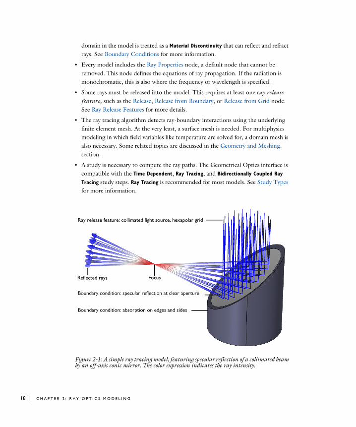
Figure 2-1: A simple ray tracing model, featuring specular reflection of a collimated beam by an off-axis conic mirror. The color expression indicates the ray intensity.

Boundary condition: specular reflection at clear aperture

Boundary condition: absorption on edges and sides

Ray release feature: collimated light source, hexapolar grid

Reflected rays Focus


Geome t r y and Me s h i n g

Electromagnetic radiation can interact with a wide variety of geometric entities. In ray optics simulation, the most common elements include lenses, mirrors, prisms, beam splitters, light pipes, and various obstructions. Rays may also interact with buildings, vehicles, people, planets, and more.

In this section, various considerations for setting up the model geometry and the associated finite element mesh are considered in more detail:

• Creating a Geometry

• Domain Selection

• Meshing and Discretization Error

• Meshing Guidelines for Geometrical Optics Simulation

Creating a Geometry

The Geometrical Optics interface supports interaction with any geometric entity. The geometry can be constructed from built-in primitives like circles and line segments, loaded from various CAD formats, or constructed with parts from the Ray Optics Part Library. Rays can interact with both deformed and undeformed geometries, for example, when an object undergoes thermal expansion.

P A R T L I B R A R I E S

In ray optics models, it is often necessary to set up geometry sequences consisting of entities that are more complex than simple geometry primitives such as spheres, cones, blocks, etc. Instead it might be necessary to insert lenses with different thicknesses and radii of curvature, off-axis conic mirrors, and parabolic concentrators. The entity shapes might need to be resolved to extremely high precision. This can be conveniently accomplished using the Part Libraries for the Ray Optics Module.

The Ray Optics Module Part Libraries contain fully parameterized sequences of geometry instructions that produce more complex shapes frequently required for geometrical optics simulation, including the following:

• Spherical lenses and mirrors,

• Conic lenses and mirrors,

• Aspheric lenses and mirrors (even, odd, and Q-type),

G E O M E T R Y A N D M E S H I N G | 19

20 | C H A P T E R

• Doublet and triplet lenses,

• Cylindrical lenses,

• Beam splitters,

• Polygonal mirrors,

• Prisms,

• Circular and rectangular annuli, and

• Retroreflectors.

For example, you can load the Spherical Lens 3D part into a model and then specify the radii of curvature of each lens surface, along with the lens thickness and diameter.

Parts can include predefined selections that make it easy to apply boundary conditions or material properties to multiple entities at the same time. Some parts also include multiple variants, or different sets of inputs that you can choose between. For example, you could either specify the off axis distance or off axis angle for a conic mirror.

In addition, many parts automatically define work planes so that the parts and other features can more easily be positioned and oriented with respect to each other.

R A Y T R A C I N G I N A N I M P O R T E D M E S H

It is possible to compute ray trajectories in an imported mesh. The mesh can be imported from a COMSOL Multiphysics file (.mphbin for a binary file format or .mphtxt for a text file format) or from a NASTRAN file (.nas, .bdf, .nastran, or .dat).

If the mesh is imported from a COMSOL Multiphysics file, the imported mesh always uses a linear geometry shape order for the purpose of modeling ray-boundary

Many Ray Optics tutorials use the Part Library to create their geometry sequences. To learn more, see the following models:

• Newtonian Telescope: Application Library path Ray_Optics_Module/

Lenses_Cameras_and_Telescopes/newtonian_telescope

• Petzval Lens: Application Library path Ray_Optics_Module/

Lenses_Cameras_and_Telescopes/petzval_lens

Part Libraries in the COMSOL Multiphysics Reference Manual.


interactions, even if the model used to generate the mesh had a higher geometry shape order.

If the mesh is imported from a NASTRAN file, the ray-boundary interactions may be modeled using either a linear or higher geometry shape order. If Export as linear

elements is selected when generating the NASTRAN file, or if Import as linear elements is selected when importing the file, then linear geometry shape order will be used.

Domain Selection

It is possible for rays to pass through domains in the geometry and to propagate in the void region outside these domains. Boundary conditions can be specified at any boundary, including boundaries that are not adjacent to any domain in the geometry. This means that rays can be reflected or absorbed by a surface in 3D, or a line segment in 2D, even if it isn’t attached to any other object. The ray tracing algorithm can also detect boundary interactions in any order, without this order being specified.

In the physics interface Material Properties of Exterior and Unmeshed Domains section, the Optical dispersion model is specified. This determines the Refractive index of exterior

domains, real part. This refractive index is used in any domains outside of the selection for the Geometrical Optics interface, as well as the void domain outside the geometry. It is a spatially uniform, scalar-valued quantity. The refractive index outside the domain selection cannot depend on field variables such as temperature or pressure and cannot be a graded-index medium. Domains with temperature-dependent or spatially nonuniform refractive indices should instead use the Medium Properties node.

Usually, the domain selection for the Geometrical Optics interface should include all objects that the rays might pass through. In a lens system, this would mean all lenses are included, but not necessarily the mount for these lenses.

Domains that are not included in the selection for the physics interface do not need to be meshed. However, these domains would still require a mesh if some other variables, like displacement and temperature, are solved for there. See Meshing Guidelines for Geometrical Optics Simulation for more details.

Some physics features require a domain mesh and will not function on domains outside the physics interface selection. This includes all types of Accumulator (Domain) feature, such as the dedicated Ray Heat Source multiphysics feature.


22 | C H A P T E R

Meshing and Discretization Error

In the Geometrical Optics interface, rays interact with a surface when they hit a mesh element in that surface’s boundary mesh. When rays need information about the surface they hit, such as the surface normal direction which controls the direction of reflected and refracted rays, this information is also evaluated on the boundary mesh. Thus, having a high-quality mesh is an integral part of ray optics simulation.

The use of a boundary mesh to detect and apply ray-boundary interactions makes the Geometrical Optics interface readily extensible to high-fidelity multiphysics simulation, including such effects as translational motion, rotation, and structural deformation of the geometry (including thermal stress). In addition, this implementation allows rays to be traced through geometric entities of arbitrary shape, not just simple shapes for which a parametric representation is readily available.

Since rays interact with a mesh representation of the geometry, the mesh must be adequately refined so that the coordinates of points along the surface are sufficiently accurate. The level of mesh refinement also affects the accuracy of the tangential and normal unit vectors that are defined on the boundary elements, as well as the Gaussian curvatures that may be used to calculate the intensity along rays. Very high accuracy can be achieved with a coarse mesh on planar surfaces because even a small number of linear boundary elements can represent a planar surface to machine precision. Accurately discretizing the geometry becomes more important when the surfaces are curved, as in spherical lenses and conic mirrors, or when the surfaces may be deformed.

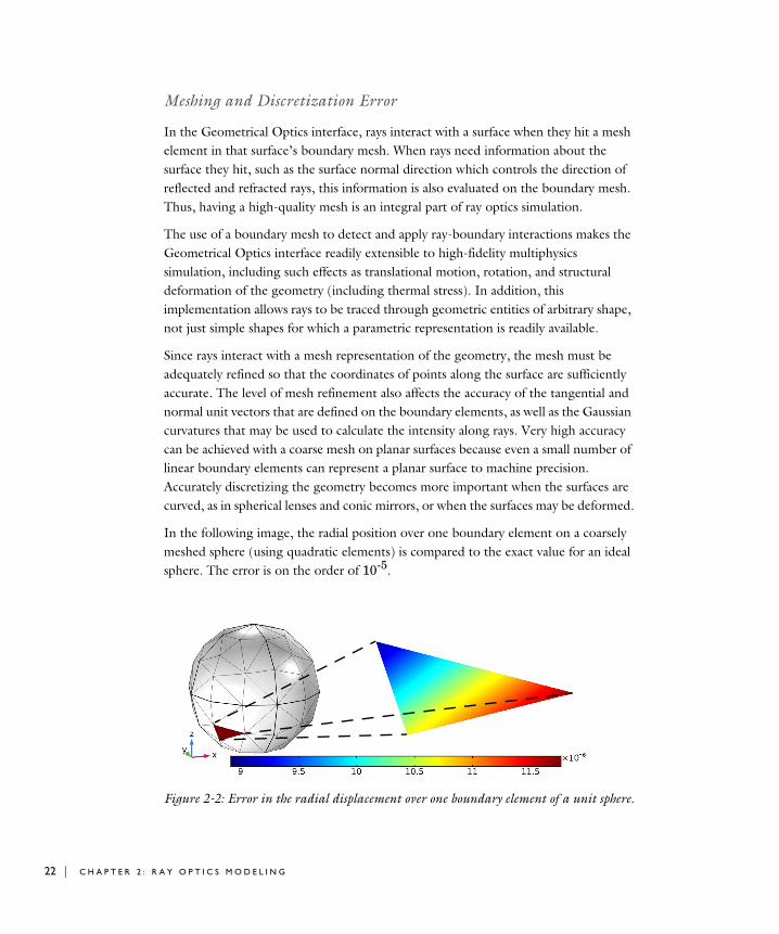
In the following image, the radial position over one boundary element on a coarsely meshed sphere (using quadratic elements) is compared to the exact value for an ideal sphere. The error is on the order of 10-5.

Figure 2-2: Error in the radial displacement over one boundary element of a unit sphere.


A relative error like the one shown above (10-5) might be sufficiently small for some simulation results, but in geometrical optics such an error might translate to tens of additional wavelengths in spot size — large enough to invalidate the results of the simulation entirely, unless adequate precautions are taken. Similarly, in models with mesh deformation, the degrees of freedom for the displacement field must be solved for extremely accurately for the results of a coupled multiphysics model to be trusted. A good practice, as with other types of simulation, is to perform a mesh refinement study, ensuring that the results do not change appreciably when the mesh element size is reduced further.

Note that ray tracing in COMSOL uses double precision floating point arithmetic, in for which machine precision is of order 10-16.

Meshing Guidelines for Geometrical Optics Simulation

• Flat edges (2D) and planar surfaces (3D) can be coarsely meshed, unless they meet one of the criteria described below.

• Curved surfaces that can interact with rays should always be finely meshed. The tighter the curvature of such surfaces, the finer the mesh should be.

• In 3D, the row of curved boundary elements adjacent to a curved edge are more susceptible to mesh discretization error than boundary elements that are not adjacent to an edge. For this reason, avoid unnecessary interior edges in 3D.

• Domains usually don’t need to be as finely meshed as boundaries. A convenient way to refine the mesh in the vicinity of the boundaries is to reduce the Curvature factor in the Size settings window in the mesh sequence. This results in a finer mesh only where the radius of curvature of the surface is small. You might also have to reduce the Minimum element size to avoid warnings in the mesh sequence.

• Features that compute the density of some quantity on a domain or boundary usually require a finer mesh, because the density term is piecewise discontinuous across elements. This includes the Accumulator (Boundary), Accumulator (Domain), and Deposited Ray Power (Boundary) features. If the mesh is too fine, rays might entirely miss some elements, and then it is necessary to increase the number of rays to avoid “holes” in the deposited power or other density field.

• Whenever possible, use parts from the Ray Optics Module Part Libraries, rather than constructing complicated shapes from geometry primitives like the sphere and cylinder. Many of these parts use high-accuracy geometry representations of the surfaces which reduce the numerical error when rays interact with them.


24 | C H A P T E R

• When using the built-in geometry Parts for aspheric lenses or mirrors, consider enabling the built-in extra points (see the Input Parameters section), especially if higher-order polynomial terms are included.

• Consider changing the Geometry shape order in the model component settings. Using Cubic or Quartic causes the boundaries to be discretized using higher-order polynomials, which can reduce error by several orders of magnitude.

Similarly, with physics interfaces that solve for a displacement field, such as Solid Mechanics, locate the physics interface Discretization section. A higher shape order such as Cubic Lagrange should be selected if rays are traced in the deformed geometry

• If the geometry uses parts or primitives, you can reduce discretization error by selecting Use geometry normals for ray-boundary interactions in the physics interface Ray Release and Propagation section. However, this only improves the accuracy if the geometry is undeformed; it has no effect if the geometry is subjected to thermal stress or some other type of deformation.


Bounda r y Cond i t i o n s

This section describes the boundary conditions of the Geometrical Optics interface in greater detail:

• Reflection and Refraction

• Primary and Secondary Ray Releases

• Wall Conditions

• Special Boundary Conditions

Reflection and Refraction

The default boundary condition is the Material Discontinuity condition on all interior and exterior boundaries. The Material Discontinuity causes rays to be reflected and refracted if the two adjacent domains have different refractive indices.

The direction of the refracted ray is based on Snell’s law. If the ray intensity or power is solved for, then they are reinitialized according to the Fresnel equations. You can modify the application of Fresnel equations by adding one or more thin dielectric layers to the surface.

S U P P R E S S I N G T H E R E L E A S E O F R E F L E C T E D R A Y S

The total number of released secondary rays in a model can sometimes grow rapidly and exhaust all of the preallocated secondary degrees of freedom. For example, a single ray reflecting back and forth between two Material Discontinuity boundaries can create an inordinately large number of rays, each with extremely low intensity. Remember that the total number of secondary rays that can be produced in the model is limited by the number specified in the Maximum number of secondary rays field.

It can be useful to constrain the release of secondary rays at boundaries so that only the most important rays are produced. If reflected rays are not of any interest, then in the Rays to Release section, select Never from the Release reflected rays list. If reflected rays are only relevant to the model under a certain condition, such as hitting a specific

Material Discontinuity Theory and Intensity, Wavefront Curvature, and Polarization in Theory for the Geometrical Optics Interface.

B O U N D A R Y C O N D I T I O N S | 25

26 | C H A P T E R

part of the surface or having a certain direction, instead select Based on logical

expression and then enter a user-defined Evaluation expression that must be satisfied.

If ray intensity is solved for, you can also specify a Threshold intensity. If a reflected ray would have intensity below the threshold, it isn’t released at all. Similarly, if ray power is solved for, you can specify a Threshold power.

Primary and Secondary Ray Releases

In the Geometrical Optics interface, a ray is released when it begins to propagate. The physics features that control where and how rays are released are called ray release features or simply release features. These features are separated into two categories, called primary release features and secondary release features. Similarly, the rays created by each feature are either primary rays or secondary rays.

P R I M A R Y R A Y S

A primary release feature allows the initial position and direction of rays to be specified directly. For the release positions, either specify the grid points directly (as in the Release from Grid feature) or choose the geometric entities that produce the rays (as in the Release, Release from Boundary, Release from Edge, and Release from Point features). The initial direction can be specified directly or sampled from a distribution.

Primary rays are released directly by a release feature. They are called primary rays because their release is not contingent on the prior existence of any other ray.

S E C O N D A R Y R A Y S

Secondary rays are released when an existing ray is subjected to certain boundary conditions. This existing ray might be a primary ray, or it could be a different secondary ray that was released earlier in the simulation.

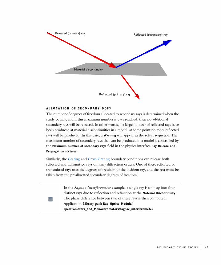
For example, the following diagram shows an incident ray being split into reflected and refracted rays at a Material Discontinuity where the refractive indices on either side differ. The Geometrical Optics interface always applies deterministic ray splitting at such boundaries, so when one ray reaches the surface, two rays emerge from it. The refracted ray is a continuation of the incident ray because it has the same index and uses the same degrees of freedom. The reflected ray is a secondary ray.

Note that total internal reflection is automatically detected. In this case the incident ray is simply reflected and no refracted ray appears. Therefore, total internal reflection does not require the release of a secondary ray.


A L L O C A T I O N O F S E C O N D A R Y D O F S

The number of degrees of freedom allocated to secondary rays is determined when the study begins, and if this maximum number is ever reached, then no additional secondary rays will be released. In other words, if a large number of reflected rays have been produced at material discontinuities in a model, at some point no more reflected rays will be produced. In this case, a Warning will appear in the solver sequence. The maximum number of secondary rays that can be produced in a model is controlled by the Maximum number of secondary rays field in the physics interface Ray Release and

Propagation section.

Similarly, the Grating and Cross Grating boundary conditions can release both reflected and transmitted rays of many diffraction orders. One of these reflected or transmitted rays uses the degrees of freedom of the incident ray, and the rest must be taken from the preallocated secondary degrees of freedom.

Released (primary) ray

Material discontinuity

Refracted (primary) ray

Reflected (secondary) ray

In the Sagnac Interferometer example, a single ray is split up into four distinct rays due to reflection and refraction at the Material Discontinuity. The phase difference between two of these rays is then computed. Application Library path Ray_Optics_Module/

Spectrometers_and_Monochromators/sagnac_interferometer


28 | C H A P T E R

Wall Conditions

For most boundary conditions other than refraction, the Wall feature can be used. It includes a wide variety of boundary conditions including the following:

• Specular reflection,

• Diffuse reflection,

• Isotropic reflection,

• Combination of diffuse and specular reflection,

• User-defined reflection,

• Pass through, and

• Several varieties of absorption condition (see below).

In this context “Diffuse reflection” means Lambertian scattering, following the cosine law; as opposed to isotropic scattering in which reflected light has an equal probability of being reflected in any direction to one side of the boundary.

If you choose Mixed diffuse and specular reflection you can assign some probability that the ray is reflected specularly; otherwise it is reflected diffusely.

The Diffuse scattering and Mixed diffuse and specular reflection rely on pseudorandom number generation, so they are not guaranteed to give exactly the same numeric results in different software versions or on different architectures.

T Y P E S O F R A Y A B S O R P T I O N

There are several different types of absorption condition, classified by the type of information that they retain about the ray.

• The Disappear condition annihilates the ray completely. After the ray disappears, its position and other degrees of freedom evaluate to not-a-number (NaN).

• The Freeze condition retains the ray position and direction after the ray hits the boundary, although these quantities no longer change over time.

• The Stick condition retains the ray position, but all other degrees of freedom are set to zero.

If the model includes several different types of boundary condition and you want to know what type of condition was applied to each ray, select the Store ray status data check box. This will store a variable that indicates the final status of each ray: whether it has not been released yet, is still propagating, or has been absorbed.


C O N D I T I O N A L R A Y - W A L L I N T E R A C T I O N S

The Wall feature also support conditional ray-wall interactions. For example, you could cause rays to Freeze if a logical expression is satisfied — for example, having optical path length greater than a specified threshold — and subject them to Specular reflection otherwise. Together with the Mixed diffuse and specular reflection condition, it is possible to prescribe up to 3 different types of wall interaction at a single boundary.

Special Boundary Conditions

More specialized boundary conditions are available for some application areas.

The Grating and Cross Grating boundary conditions, together with the Diffraction Order (Grating) and Diffraction Order (Cross Grating) subnodes, respectively, are used to model the separation of rays by diffraction at a periodic microstructure. Typically, the unit cell of the microstructure is comparable to the wavelength. The Grating is periodic in one direction and homogeneous in the orthogonal direction, whereas the Cross Grating is periodic in two directions. Either boundary condition can reflect or transmit rays and emit secondary rays. You can specify the direction of periodicity and the size of the unit cell.

The Mirror boundary condition is a simplified Wall that only causes specular reflection.

The Axial Symmetry boundary condition is only available in 2D axisymmetric models. It is automatically applied at the axis of symmetry and can’t be applied anywhere else.

Optical devices like the Linear Polarizer and Linear Wave Retarder are available when ray intensity or power is computed. They don’t have any effect on the ray direction but they can affect the ray polarization.

Czerny-Turner Monochromator: Application Library path Ray_Optics_Module/Spectrometers_and_Monochromators/

czerny_turner_monochromator

White Pupil Échelle Spectrograph: Application Library path Ray_Optics_Module/Spectrometers_and_Monochromators/

white_pupil_echelle_spectrograph

Cross Grating Échelle Spectrograph: Application Library path Ray_Optics_Module/Spectrometers_and_Monochromators/

cross_grating_echelle_spectrograph


30 | C H A P T E R

Ra y R e l e a s e F e a t u r e s

To trace rays it is first necessary to prescribe their initial position and direction. This process is called releasing rays. The physics features used to enter this information are called release features or ray release features. If other quantities are being solved for along the rays, such as the intensity and polarization, then these quantities are initialized by the ray release features.

In this section:

• Grid-Based Release

• Release from Domains, Boundaries, Edges, or Points

• Specialized Release Features

• Release Features for Multiscale Modeling

Grid-Based Release

Use the Release from Grid feature to specify the initial positions of rays using a grid of points. It is useful to release rays from a grid when the initial ray position is known exactly. A grid-based release may be used, for example, when rays are released from the focus of a lens or when a system is excited by a laser. This is the easiest way to release rays from known locations in the void region outside the geometry.

Alternatively, you can load the ray release positions and directions from a text file, using the Release from Data File node.

Release from Domains, Boundaries, Edges, or Points

There are ray release features for every geometric entity level:

• Use the Release feature to release rays from domains in 2D or 3D.

• Use the Release from Boundary feature to release edges (2D) or surfaces (3D).

• Use the Release from Edge feature to release rays from edges in 3D.

• Use the Release from Point feature to release rays from points in 2D or 3D.

Releasing rays from a domain, surface, or edge initializes the ray position based on the underlying finite element mesh, which discretizes the geometry. A side effect is that the ray positions can change slightly when switching between geometry kernels. Ray


release can be uniform or proportional to a user-defined expression, which is specified in the Density proportional to text field.

Specialized Release Features

The Illuminated Surface is a specialized ray release feature that produces reflected or refracted light directly at a surface. This can be used, for example, when the direction of incident radiation is known, but its propagation is not interesting until it has already been reflected once by an object.

The Solar Radiation computes the initial direction of rays as if they were solar rays being released at a specified latitude, longitude, date, and time. Instead of the latitude an longitude, you can also select from a list of built-in cities.

Release Features for Multiscale Modeling

The Ray Optics Module also supports multiscale electromagnetics simulation, in which the electric field is first computed in the frequency domain over a length scale of several wavelengths, then propagated over a much longer distance using a ray tracing approach. For more details, see Release from Electric Field and Release from Far-Field Radiation Pattern.

The following examples involve buildings or other objects being illuminated by solar radiation in a specific direction:

• Solar Dish Receiver: Application Library path Ray_Optics_Module/

Solar_Radiation/solar_dish_receiver

• Vdara® Caustic Surface: Application Library path Ray_Optics_Module/Solar_Radiation/vdara_caustic_surface

R A Y R E L E A S E F E A T U R E S | 31

32 | C H A P T E R

Add i t i o n a l V a r i a b l e s S o l v e d Fo r

The Geometrical Optics interface always solves for the ray position q (SI unit: m) and wave vector k (SI unit: rad/m). This section lists the optional quantities that can be solved for in addition to these required variables.

In this section:

• Modeling Polychromatic Radiation

• Intensity, Polarization, and Power

• Other Dependent Variables

• Order of Initialization of Auxiliary Dependent Variables

Modeling Polychromatic Radiation

By default, the rays released in a model are monochromatic with a ray frequency or free-space wavelength defined in the Ray Properties settings window. However, you can trace polychromatic rays by specifying different frequencies or vacuum wavelengths in each ray release feature.

To allow the rays to be polychromatic, in the settings window for the Geometrical Optics interface locate the Ray Release and Propagation section. By default, Monochromatic is selected from the Wavelength distribution of released rays list. Select Polychromatic, specify vacuum wavelength to release polychromatic rays by entering an expression for the vacuum wavelength or sampling it from a distribution. Alternatively, select Polychromatic, specify frequency to define an expression or distribution for the ray frequency. These expressions are defined in the Vacuum Wavelength and Initial Ray

Frequency sections in each ray release feature.

When modeling polychromatic light, the number of degrees of freedom in the model increases by one per ray because the wavelength or frequency is stored as an auxiliary dependent variable on each ray.

Czerny-Turner Monochromator: Application Library path Ray_Optics_Module/Spectrometers_and_Monochromators/

czerny_turner_monochromator


Intensity, Polarization, and Power

Ray intensity is computed using a variant of the Stokes-Mueller calculus in which both the amplitude and polarization are tracked along individual rays.

L I S T O F A V A I L A B L E S E T T I N G S

To decide whether intensity is computed, select an option from the Intensity

Computation list. The following options are available.

• None: Does not compute any intensity information.

• Compute intensity: Solves for intensity, which typically increases as rays are focused and decreases as they diverge. Also affected by reflection, refraction, and attenuating media. Only valid when the media are homogeneous.

• Compute power: Solves for power, which is unaffected by the convergence or divergence of rays but is still affected by reflection, refraction, and attenuating media. Can be used to compute heat source terms in attenuating domains, or heat flux terms on absorbing boundaries the rays hit.

• Compute intensity and power: Combines the capabilities of Compute intensity and Compute power, at the cost of a few extra degrees of freedom per ray.

• Compute intensity in graded media: Similar to Compute intensity, but is also applicable to graded-index media. The trade-off is that this method is slower and less accurate for homogeneous media.

• Compute intensity and power in graded media: Similar to Compute intensity in graded

media, but can also be used to generate heat sources in attenuating domains and heat flux terms at boundaries.

H A N D L I N G P O L A R I Z A T I O N

Whenever intensity or power is solved for, the polarization of every ray is known. Rays can have any degree of polarization, ranging from 0 (unpolarized) to 1 (fully polarized) and anything in-between. When rays have some degree of polarization, they can be linearly, elliptically, or circularly polarized.

When rays are reflected and refracted at boundaries, the intensity, polarization, and power are updated based on the Fresnel equations, which automatically take the polarization direction into account.

The polarization is determined based on the Stokes parameters, which are allocated as extra degrees of freedom along each ray. For more information, see The Stokes Parameters in the Theory for the Geometrical Optics Interface chapter.

A D D I T I O N A L V A R I A B L E S S O L V E D F O R | 33

34 | C H A P T E R

W A V E F R O N T C U R V A T U R E

When the ray intensity is solved for, it increases where rays are focused together and decreases where rays diverge. This is accomplished by treating each ray as a wavefront and storing its principal radii of curvature as extra degrees of freedom. In this way, all released rays are treated as points on planar, spherical, or ellipsoid-shaped wavefronts.

For more information on wavefront radii of curvature and their effect on intensity, see Principal Radii of Curvature in the Theory for the Geometrical Optics Interface chapter.

C O M P U T I N G D E P O S I T E D R A Y P O W E R

The options Compute power, Compute intensity and power, and Compute intensity and

power in graded media all allow heat sources to be defined on domains or boundaries. As rays propagate through an attenuating medium — that is, a medium where the refractive index is complex-valued — some energy is lost from the ray. The corresponding heat source on the surrounding domain can be computed using either the Deposited Ray Power (Boundary) subnode or the Ray Heat Source multiphysics node. A Ray Heat Source node is automatically created when using selecting The Ray Heating Interface in the Model Wizard. The heat generated as rays propagate in an attenuating medium can be used to define a heat source in the Heat Transfer in Solids interface or another interface that computes a temperature field.

In the following examples, ray polarization is manipulated in an instructive way:

• Total Internal Reflection Thin-Film Achromatic Phase Shifter (TIRTF APS): Application Library path Ray_Optics_Module/

Prisms_and_Coatings/achromatic_phase_shifter

• Linear Wave Retarder: Application Library path Ray_Optics_Module/

Tutorials/linear_wave_retarder

Thermally Induced Focal Shift in High-Power Laser Focusing Systems: Application Library path Ray_Optics_Module/

Structural_Thermal_Optical_Performance_Analysis/

thermally_induced_focal_shift


T O T A L P O W E R T R A N S M I T T E D A N D R E F L E C T E D A T G R A T I N G S

The Grating feature is used to model the transmission and reflection of rays at diffraction gratings. It includes a Diffraction Order (Grating) subnode to specify which diffraction orders to release. When the ray power is solved for, the Store total

transmitted power and Store total reflected power check boxes are shown in the Grating settings window. Selecting either of these check boxes causes an auxiliary dependent variable to be declared, storing the total power of the transmitted and reflected rays of all diffraction orders.

Other Dependent Variables

It is possible to define an auxiliary dependent variable for the optical path length by selecting the Compute optical path length check box in the Additional Variables section of the physics interface node’s Settings window. Initially the optical path length is set to 0 for all released rays. It is possible to reset the optical path length to 0 when the rays interact with boundaries.

The phase of a ray is necessary for some applications that require information about the instantaneous electric fields of multiple rays, such as interferometers. To define an auxiliary dependent variable for phase, select the Compute phase check box in the Intensity Computation section of the physics interface node’s Settings window. This check box is only available if the ray intensity is computed.

The instantaneous phase can be used to visualize interference patterns where the rays intersect a surface. See the Results Analysis and Visualization section.

Other dependent variables can also be assigned, including:

• Number times each ray has been reflected.

• Help variables for more accurately tracing rays in strongly absorbing media, where the real and imaginary parts of the refractive index are comparable in magnitude.

• Help variables used to apply perturbations in ray direction due to rough surfaces.

• User-defined Auxiliary Dependent Variable nodes.

Diffraction Grating: Application Library path Ray_Optics_Module/

Tutorials/diffraction_grating

A D D I T I O N A L V A R I A B L E S S O L V E D F O R | 35

36 | C H A P T E R

Order of Initialization of Auxiliary Dependent Variables

When rays are released, the variables defined for each ray are initialized in a specific order. The initial values of ray variables can only depend on the values of variables that have already been defined. The order of dependent variable initialization is governed by the following rules:

• The initial ray position is always determined first.

• By default, user-defined auxiliary dependent variables (that is, those that are defined by adding an Auxiliary Dependent Variable node to the physics interface) are initialized after all other variables. They can instead be initialized immediately after the ray position vector components by selecting the Initialize before wave vector

check box shown in the release feature Initial Value of Auxiliary Dependent Variables section.

• If more than one user-defined auxiliary dependent variable is present, these variables are initialized in the order in which the corresponding Auxiliary Dependent Variable nodes appear in the Model Builder.

• The remaining degrees of freedom are defined in the following order (each listed group is initialized simultaneously, and the variables within a group cannot reliably be initialized in terms of each other):

- Help variable for the perturbation of initial ray direction at illuminated surfaces,

- Ray frequency or vacuum wavelength,

- The wave vector components, optical path length, and total power transmitted and reflected by gratings,

- The integral of the attenuation coefficient along ray paths and the components of the unit vector that indicates the direction corresponding to one of the principal radii of curvature,

- The principal radii of curvature, initial principal radii of curvature, intensity, Stokes parameters, and help variables for computing the curvature tensor and intensity, and

- The total power transmitted by the ray.

Items in each bullet point may not be initialized as functions of items in a later bullet point. For example, the initial ray direction vector may depend on the ray frequency, but the initial principal radii of curvature may not depend on the total power transmitted by the ray.


S t u d y T yp e s

The Geometrical Optics interface is compatible with three study types: Ray Tracing, Time Dependent, and Bidirectionally Coupled Ray Tracing. In this section some of the more relevant study settings are explored in greater detail.

In this section:

• Ray Tracing Study Step

• Bidirectionally Coupled Ray Tracing Study Step

Ray Tracing Study Step

The Ray Tracing and Time Dependent study steps are very similar, and either one could be used for the vast majority of geometrical optics models. The Ray Tracing study step has some additional features that make it more convenient to use, such as more reasonable default values and built-in stop conditions.

A N O T E O N G E O M E T R I C N O N L I N E A R I T Y

If a physics interface solves for the displacement field, such as the Solid Mechanics interface, then the check box Include geometric nonlinearity appears in the Study

Settings section. It is very important to select this check box when tracing rays in a system that is deformed due to external forces or thermal stress. If the check box is cleared, then rays are instead traced in the undeformed geometry.

T I M E S T E P S A N D O P T I C A L P A T H L E N G T H I N T E R V A L S

By default, the Ray Tracing study step computes ray trajectories from t = 0 to t = 1 ns with a time step size of 0.01 ns. However, it is often useful to think of ray tracing in terms of the maximum distance of ray propagation instead of the maximum time. To express the duration of the study in terms of a maximum optical path length, change the Time step specification setting from the default, Specify time steps, to Specify

maximum path length. Then select a Length unit (default m), enter a set of Lengths (default range(0,0.01,1)), and enter a Characteristic group velocity (default c_const, a built-in constant for the speed of light in a vacuum). With the default solver settings, the time-dependent solver must take at least one time step whenever the optical path length of a ray moving at the Characteristic group velocity would have reached one of the values in the list of Lengths.

S T U D Y T Y P E S | 37

38 | C H A P T E R

B U I L T - I N S T O P C O N D I T I O N S

The Ray Tracing study step includes options to create a Stop condition node in the default solver sequence. The Stop condition node can terminate the study before the full range of specified times or optical path lengths has been simulated, if a condition is met before then.

To use one of the built-in stop conditions, select one of the following options from the Stop condition list in the Study Settings:

• None: The study ends at the specified maximum time or maximum optical path length.

• No active rays remaining: The study terminates if all rays have been stopped or absorbed. A ray can be absorbed by a boundary, or it can be removed by the Ray Termination domain feature.

• Active rays have intensity below threshold: This option is only available when ray intensity is computed. The study terminates if every ray in the model is either stopped, absorbed, or has sufficiently low intensity.

• Active rays exceed maximum number of reflections: This option is only usable when the Count reflections check box is selected in the physics interface Additional Variables section. The study terminates if every ray in the model is either stopped, absorbed, or has been reflected the specified number of times.

C O U P L E D P H Y S I C S I N T E R F A C E S

If other physics interfaces are also solved for in the Ray Tracing study step, it is assumed that these other fields vary over the same time scale as the ray propagation. This is seldom true. If instead the coupled physics do not change over the time scale for ray propagation, consider a study with two steps: Stationary for all other fields and Ray

Tracing just for the rays.

Stop Condition in the COMSOL Multiphysics Reference Manual.


• Ray Tracing



Bidirectionally Coupled Ray Tracing Study Step

The Bidirectionally coupled ray tracing study step is a dedicated study step for ray heating and similar applications.

It should only be used if all of the following criteria are met:

1 Rays are being traced.

2 Some other field, such as temperature or structural displacement, is solved for in a domain where the rays are being traced.

3 All fields, apart from the ray paths themselves, are stationary.

4 The ray paths are affected by the field being solved for. This could include rays interacting with a deformed geometry, or a refractive index that depends on the values of field variables like strain or temperature.

5 The rays generate enough heat to significantly affect one of the fields being solved for in the domain, usually temperature.

If condition 4 isn’t satisfied, instead use a Stationary study step for the fields, followed by a Ray Tracing study step for the rays.

In addition to the settings that are available for the Ray tracing study step, it is possible to specify a Number of iterations. The default value is 5. If the Bidirectionally coupled

ray tracing study step is used with The Ray Heating Interface, the following iterative solver loop is automatically set up to compute the ray trajectories and temperature:

1 Solve for the temperature field, assuming that the rays do not generate any heat source.

2 Using the temperature computed during the previous step, compute the ray paths and any heat sources that occur due to ray attenuation in an absorbing medium.

3 Using the heat source computed in the previous step, compute the temperature field.

4 Alternate between steps 2 and 3 for the specified Number of iterations, or specify a Global variable whose convergence will be used to terminate the loop.

The result of the iterative solver loop is that the heat source generated by the attenuation of rays is taken into account when computing the temperature. By including a thermo-optic dispersion model, such as the Temperature-dependent

Sellmeier model, the temperature in turn affects the ray paths. Thus, a bidirectional coupling is established between the two physics interfaces.

S T U D Y T Y P E S | 39

40 | C H A P T E R

Like any COMSOL Multiphysics simulation, it is possible to extend this bidirectional coupling to include other physical effects. For example, to include structural deformation due to thermal stress, add the Solid Mechanics physics interface and the Thermal Expansion Multiphysics coupling.

Thermally Induced Focal Shift in High-Power Laser Focusing Systems: Application Library path Ray_Optics_Module/

Structural_Thermal_Optical_Performance_Analysis/

thermally_induced_focal_shift


• Bidirectionally Coupled Ray Tracing



Re s u l t s Ana l y s i s a nd V i s u a l i z a t i o n

The results of a ray tracing simulation can be interpreted and visualized using a variety of built-in features. In the following, some dedicated features are discussed in detail.

In this section:

• Ray Trajectories Plot

• Ray Plot

• Interference Pattern Plot

• Spot Diagram Plot

• Optical Aberration Plot and Aberration Evaluation

Ray Trajectories Plot

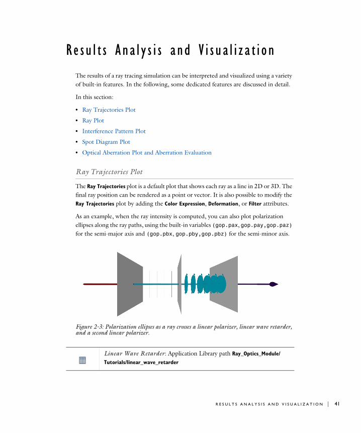
The Ray Trajectories plot is a default plot that shows each ray as a line in 2D or 3D. The final ray position can be rendered as a point or vector. It is also possible to modify the Ray Trajectories plot by adding the Color Expression, Deformation, or Filter attributes.

As an example, when the ray intensity is computed, you can also plot polarization ellipses along the ray paths, using the built-in variables (gop.pax, gop.pay,gop.paz) for the semi-major axis and (gop.pbx, gop.pby,gop.pbz) for the semi-minor axis.

Figure 2-3: Polarization ellipses as a ray crosses a linear polarizer, linear wave retarder, and a second linear polarizer.

Linear Wave Retarder: Application Library path Ray_Optics_Module/

Tutorials/linear_wave_retarder

R E S U L T S A N A L Y S I S A N D V I S U A L I Z A T I O N | 41

42 | C H A P T E R

Ray Plot

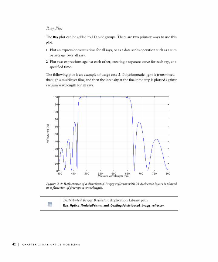
The Ray plot can be added to 1D plot groups. There are two primary ways to use this plot:

1 Plot an expression versus time for all rays, or as a data series operation such as a sum or average over all rays.

2 Plot two expressions against each other, creating a separate curve for each ray, at a specified time.

The following plot is an example of usage case 2. Polychromatic light is transmitted through a multilayer film, and then the intensity at the final time step is plotted against vacuum wavelength for all rays.

Figure 2-4: Reflectance of a distributed Bragg reflector with 21 dielectric layers is plotted as a function of free-space wavelength.

Distributed Bragg Reflector: Application Library path Ray_Optics_Module/Prisms_and_Coatings/distributed_bragg_reflector


Interference Pattern Plot

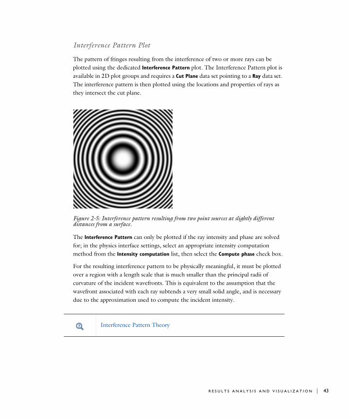
The pattern of fringes resulting from the interference of two or more rays can be plotted using the dedicated Interference Pattern plot. The Interference Pattern plot is available in 2D plot groups and requires a Cut Plane data set pointing to a Ray data set. The interference pattern is then plotted using the locations and properties of rays as they intersect the cut plane.

Figure 2-5: Interference pattern resulting from two point sources at slightly different distances from a surface.

The Interference Pattern can only be plotted if the ray intensity and phase are solved for; in the physics interface settings, select an appropriate intensity computation method from the Intensity computation list, then select the Compute phase check box.

For the resulting interference pattern to be physically meaningful, it must be plotted over a region with a length scale that is much smaller than the principal radii of curvature of the incident wavefronts. This is equivalent to the assumption that the wavefront associated with each ray subtends a very small solid angle, and is necessary due to the approximation used to compute the incident intensity.

Interference Pattern Theory


44 | C H A P T E R

Spot Diagram Plot

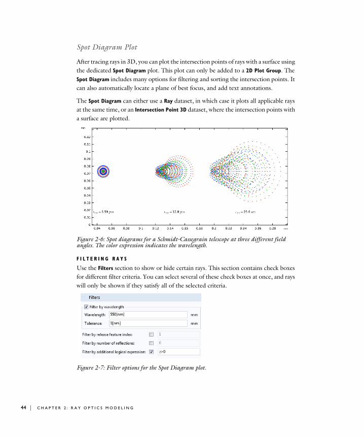
After tracing rays in 3D, you can plot the intersection points of rays with a surface using the dedicated Spot Diagram plot. This plot can only be added to a 2D Plot Group. The Spot Diagram includes many options for filtering and sorting the intersection points. It can also automatically locate a plane of best focus, and add text annotations.

The Spot Diagram can either use a Ray dataset, in which case it plots all applicable rays at the same time, or an Intersection Point 3D dataset, where the intersection points with a surface are plotted.

Figure 2-6: Spot diagrams for a Schmidt-Cassegrain telescope at three different field angles. The color expression indicates the wavelength.

F I L T E R I N G R A Y S

Use the Filters section to show or hide certain rays. This section contains check boxes for different filter criteria. You can select several of these check boxes at once, and rays will only be shown if they satisfy all of the selected criteria.

Figure 2-7: Filter options for the Spot Diagram plot.


For example, you can select Filter by wavelength to hide rays of all wavelengths except a selected value; then select Filter by release feature index to only show rays that are released by a specific feature (e.g. Release from Grid 1). In many examples of cameras and telescopes in the Application Libraries, each release feature corresponds to a distinct field angle for light entering the optical system.

The check box Filter by number of reflections should only be used if you previously selected Count reflections in the physics interface Additional Variables section.

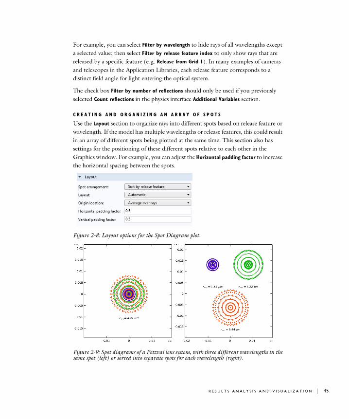
C R E A T I N G A N D O R G A N I Z I N G A N A R R A Y O F S P O T S

Use the Layout section to organize rays into different spots based on release feature or wavelength. If the model has multiple wavelengths or release features, this could result in an array of different spots being plotted at the same time. This section also has settings for the positioning of these different spots relative to each other in the Graphics window. For example, you can adjust the Horizontal padding factor to increase the horizontal spacing between the spots.

Figure 2-8: Layout options for the Spot Diagram plot.

Figure 2-9: Spot diagrams of a Petzval lens system, with three different wavelengths in the same spot (left) or sorted into separate spots for each wavelength (right).


46 | C H A P T E R

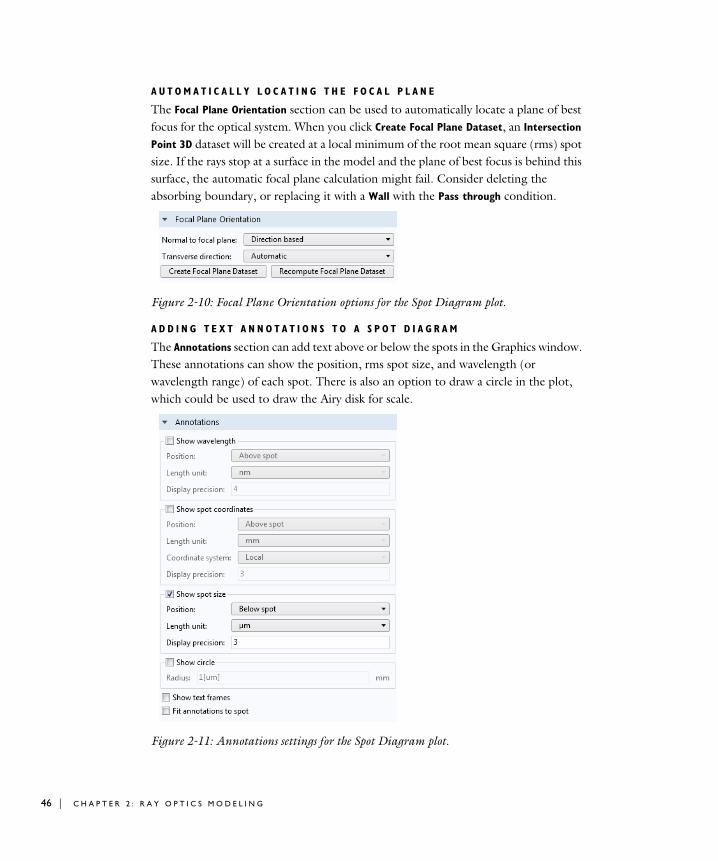
A U T O M A T I C A L L Y L O C A T I N G T H E F O C A L P L A N E

The Focal Plane Orientation section can be used to automatically locate a plane of best focus for the optical system. When you click Create Focal Plane Dataset, an Intersection

Point 3D dataset will be created at a local minimum of the root mean square (rms) spot size. If the rays stop at a surface in the model and the plane of best focus is behind this surface, the automatic focal plane calculation might fail. Consider deleting the absorbing boundary, or replacing it with a Wall with the Pass through condition.

Figure 2-10: Focal Plane Orientation options for the Spot Diagram plot.

A D D I N G T E X T A N N O T A T I O N S T O A S P O T D I A G R A M

The Annotations section can add text above or below the spots in the Graphics window. These annotations can show the position, rms spot size, and wavelength (or wavelength range) of each spot. There is also an option to draw a circle in the plot, which could be used to draw the Airy disk for scale.

Figure 2-11: Annotations settings for the Spot Diagram plot.


Optical Aberration Plot and Aberration Evaluation

The Optical Aberration plot can be added in a 2D Plot Group whereas the Aberration

Evaluation node is available under Derived Values. Both of these postprocessing features serve a similar purpose: to quantify the monochromatic aberrations of an imaging system and express them in terms of Zernike polynomial coefficients. In order to use the Optical Aberration plot, the following prerequisites must be met:

• The model component must be 3D.

• An instance of the Geometrical Optics interface must be present and solved for.

• The Compute optical path length check box must be selected in the Geometrical Optics Settings window before solving.

• An Intersection Point 3D dataset must be created. This data set must point to a Ray data set. Optionally, this dataset can be automatically generated (see below). In the Settings window for the Intersection Point 3D dataset, Hemisphere must be selected from the Surface type list. The Center is the location of the focus and the Axis

direction points from the focus toward the center of the exit pupil.

Using the hemisphere defined in the Intersection Point 3D dataset, a Gaussian reference sphere is defined. The optical path difference among intersection points with this sphere is then expressed as a sum of Zernike polynomials.

A U T O M A T I C D A T A S E T G E N E R A T I O N

Alternatively, using the Optical Aberration plot, you can use the Create Reference

Hemisphere Dataset button in the Focal Plane Orientation section to automatically generate a reference hemisphere at the location of the rms focus. However, note that the defocus term Z(2,0) might be larger for the rms focus than it would for some other definitions of the image plane, such as the marginal focus.

The monochromatic aberrations in a double Gauss lens system are shown in Figure 2-12. The circle on the left shows the sum of all Zernike coefficients. The circle on the right ignores the defocus term Z(2,0) and the piston term Z(0,0). Usually, lower-order Zernike terms can be reduced by correcting misalignments in the optical system or adjusting the nominal focus. Higher-order terms are consequences of the type of lens or mirror used in an optical system; for example, a single spherical lens will always demonstrate some spherical aberration, for any position of the nominal focus.

The Optical Aberration plot always shows the optical path differences on a unit circle. The color expression is the wavefront error in microns. In the circle on the right in Figure 2-12, the largest contribution is from the spherical aberration term Z(4,0).


48 | C H A P T E R

Figure 2-12: Monochromatic aberrations in a double Gauss lens system.

For a list of Zernike polynomials and their derivation, see Monochromatic Aberrations and the Zernike Polynomials in Theory for the Geometrical Optics Interface.

Double Gauss Lens: Application Library path Ray_Optics_Module/

Lenses_Cameras_and_Telescopes/double_gauss_lens



• Spot Diagram

• Interference Pattern

• Optical Aberration

• Aberration Evaluation

• Ray (Plot)

• Ray Trajectories

• Filter for Ray and Ray Trajectories

• Phase Portrait

• Poincaré Map

• Ray (Dataset) and Datasets

• Ray Bin

• Intersection Point 2D and Intersection Point 3D

• Ray Evaluation and Derived Values, Evaluation Groups, and Tables

• Plot Groups and Plots


50 | C H A P T E R

V a r i a b l e s and Non l o c a l C oup l i n g s

This section lists some built-in nonlocal couplings and variables for the Geometrical Optics interface.

In this section:

• Ray Statistics

• Global Variables

• Variables for Average Ray Position

• Using Ray Detectors

• Nonlocal Couplings

Ray Statistics

The Geometrical Optics interface defines a number of special variables, some of which can only be used during results processing. These variables can be found in the Ray

statistics section in the Add/Replace Expression menus.

In the variable names below, gop is the physics interface tag. If multiple instances of the Geometrical Optics interface are different, this tag may differ.

The following variables are defined for each ray:

• Ray index gop.pidx. Each ray is assigned a unique index starting from 1 up to the total number of rays. This expression can be used as an input argument to a function. For example, randomnormal(gop.pidx) would sample pseudorandom numbers from a normal distribution with unit variance. The random numbers would be distinct for each ray.

• Ray release feature gop.prf. If there are multiple release features in a model, it is useful to visualize which rays correspond to each release feature. Rays from each release feature are assigned a unique integer, starting at 1. This variable can also be used to filter ray trajectories in postprocessing so that only the rays released by a specific feature are shown.

• Ray release time gop.prt. Usually, all primary rays are released at t = 0. To allow other release times to be specified, select the Allow multiple release times check box in the physics interface Advanced Settings section.


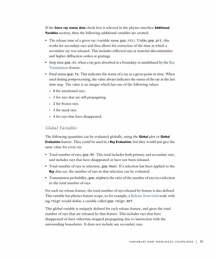
If the Store ray status data check box is selected in the physics interface Additional

Variables section, then the following additional variables are created:

• The release time of a given ray (variable name gop.rti). Unlike gop.prt, this works for secondary rays and thus allows for extraction of the time at which a secondary ray was released. This includes reflected rays at material discontinuities and higher diffraction orders at gratings.

• Stop time gop.st, when a ray gets absorbed at a boundary or annihilated by the Ray Termination feature.

• Final status gop.fs. This indicates the status of a ray at a given point in time. When used during postprocessing, the value always indicates the status of the ray at the last time step. The value is an integer which has one of the following values:

- 0 for unreleased rays.

- 1 for rays that are still propagating.

- 2 for frozen rays.

- 3 for stuck rays.

- 4 for rays that have disappeared.

Global Variables

The following quantities can be evaluated globally, using the Global plot or Global

Evaluation feature. They could be used in a Ray Evaluation, but they would just give the same value for every ray.

• Total number of rays, gop.Nt. This total includes both primary and secondary rays, and includes rays that have disappeared or have not been released.

• Total number of rays in selection, gop.Nsel. If a selection has been applied to the Ray data set, the number of rays in that selection can be evaluated.

• Transmission probability, gop.alpha is the ratio of the number of rays in a selection to the total number of rays.

For each ray release feature, the total number of rays released by feature is also defined. This variable has physics feature scope, so for example, a Release from Grid node with tag relg1 would define a variable called gop.relg1.Ntf.

This global variable is uniquely defined for each release feature, and gives the total number of rays that are released by that feature. This includes rays that have disappeared or have otherwise stopped propagating due to interaction with the surrounding boundaries. It does not include any secondary rays.

V A R I A B L E S A N D N O N L O C A L C O U P L I N G S | 51

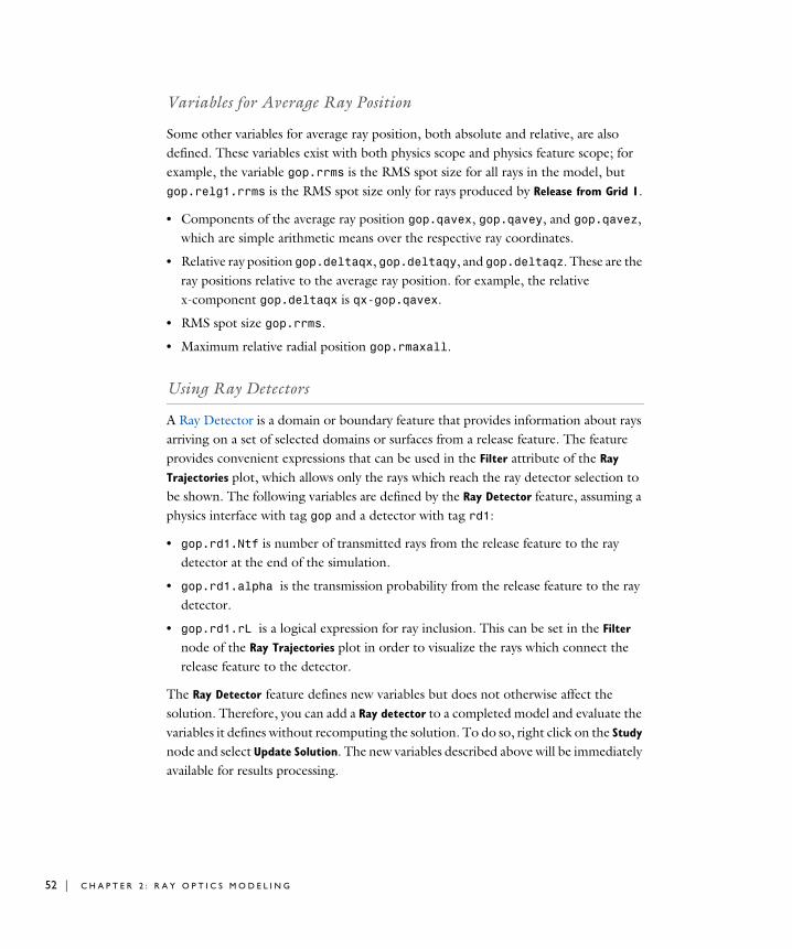
52 | C H A P T E R

Variables for Average Ray Position

Some other variables for average ray position, both absolute and relative, are also defined. These variables exist with both physics scope and physics feature scope; for example, the variable gop.rrms is the RMS spot size for all rays in the model, but gop.relg1.rrms is the RMS spot size only for rays produced by Release from Grid 1.

• Components of the average ray position gop.qavex, gop.qavey, and gop.qavez, which are simple arithmetic means over the respective ray coordinates.

• Relative ray position gop.deltaqx, gop.deltaqy, and gop.deltaqz. These are the ray positions relative to the average ray position. for example, the relative x-component gop.deltaqx is qx-gop.qavex.

• RMS spot size gop.rrms.

• Maximum relative radial position gop.rmaxall.

Using Ray Detectors

A Ray Detector is a domain or boundary feature that provides information about rays arriving on a set of selected domains or surfaces from a release feature. The feature provides convenient expressions that can be used in the Filter attribute of the Ray

Trajectories plot, which allows only the rays which reach the ray detector selection to be shown. The following variables are defined by the Ray Detector feature, assuming a physics interface with tag gop and a detector with tag rd1:

• gop.rd1.Ntf is number of transmitted rays from the release feature to the ray detector at the end of the simulation.

• gop.rd1.alpha is the transmission probability from the release feature to the ray detector.

• gop.rd1.rL is a logical expression for ray inclusion. This can be set in the Filter node of the Ray Trajectories plot in order to visualize the rays which connect the release feature to the detector.

The Ray Detector feature defines new variables but does not otherwise affect the solution. Therefore, you can add a Ray detector to a completed model and evaluate the variables it defines without recomputing the solution. To do so, right click on the Study node and select Update Solution. The new variables described above will be immediately available for results processing.


Nonlocal Couplings

The purpose of a model is often to compute the sum, average, maximum value, or minimum value of a quantity over a group of rays, such as the average intensity or the maximum path length. An instance of the Geometrical Optics interface with physics interface tag gop creates the following nonlocal couplings:

• gop.gopop1(expr) evaluates the sum of the expression expr over the rays. The sum includes all rays that are active, frozen, or stuck to boundaries. It excludes rays that have not yet been released and those that have disappeared.

• gop.gopop_all1(expr) evaluates the sum of the expression expr over all rays, including rays those that are not yet released or have disappeared. Since the coordinates of unreleased and disappeared rays are not-a-number (NaN), the sum may return NaN if the model includes unreleased or disappeared rays. An expression such as gop.gopop1(isnan(qx)) can be used to compute the total number of unreleased and disappeared rays.

• gop.gopaveop1(expr) evaluates the average of the expression expr over the active, frozen, and stuck rays. Unreleased and disappeared rays contribute to neither the numerator nor the denominator of the arithmetic mean.

• gop.gopaveop_all1(expr) evaluates the average of the expression expr over all rays. It is likely to return NaN if the model includes unreleased or disappeared rays.

• gop.gopmaxop1(expr) evaluates the maximum value of the expression expr over all active, frozen, and stuck rays.

• gop.gopmaxop_all1(expr) evaluates the maximum value of the expression expr over all rays.

The treatment of NaN values in nonlocal maximum couplings can be platform-dependent, so use caution when evaluating the maximum over all rays including disappeared and unreleased rays.

• gop.gopminop1(expr) evaluates the minimum value of the expression expr over the active, frozen, and stuck rays.

• gop.gopminop_all1(expr) evaluates the minimum value of the expression expr over all rays.

The treatment of NaN values in nonlocal minimum couplings can be platform-dependent, so use caution when evaluating the minimum over all rays including disappeared and unreleased rays.

• gop.gopmaxop1(expr, evalExpr) evaluates the expression evalExpr for the ray that has the maximum value of the expression expr out of all active, frozen, and

V A R I A B L E S A N D N O N L O C A L C O U P L I N G S | 53

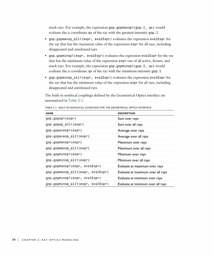
54 | C H A P T E R

stuck rays. For example, the expression gop.gopmaxop1(gop.I, qx) would evaluate the x-coordinate qx of the ray with the greatest intensity gop.I.

• gop.gopmaxop_all1(expr, evalExpr) evaluates the expression evalExpr for the ray that has the maximum value of the expression expr for all rays, including disappeared and unreleased rays.

• gop.gopminop1(expr, evalExpr) evaluates the expression evalExpr for the ray that has the minimum value of the expression expr out of all active, frozen, and stuck rays. For example, the expression gop.gopminop1(gop.I, qx) would evaluate the x-coordinate qx of the ray with the minimum intensity gop.I.

• gop.gopminop_all1(expr, evalExpr) evaluates the expression evalExpr for the ray that has the minimum value of the expression expr for all rays, including disappeared and unreleased rays.

The built-in nonlocal couplings defined by the Geometrical Optics interface are summarized in Table 2-1.

TABLE 2-1: BUILT-IN NONLOCAL COUPLINGS FOR THE GEOMETRICAL OPTICS INTERFACE

NAME DESCRIPTION

gop.gopop1(expr) Sum over rays

gop.gopop_all1(expr) Sum over all rays

gop.gopaveop1(expr) Average over rays

gop.gopaveop_all1(expr) Average over all rays

gop.gopmaxop1(expr) Maximum over rays

gop.gopmaxop_all1(expr) Maximum over all rays

gop.gopminop1(expr) Minimum over rays

gop.gopminop_all1(expr) Minimum over all rays

gop.gopmaxop1(expr, evalExpr) Evaluate at maximum over rays

gop.gopmaxop_all1(expr, evalExpr) Evaluate at maximum over all rays

gop.gopminop1(expr, evalExpr) Evaluate at minimum over rays

gop.gopminop_all1(expr, evalExpr) Evaluate at minimum over all rays


3

R a y O p t i c s I n t e r f a c e s

This chapter describes the physics interfaces found under the Optics>Ray Optics

branch ( ).

In this chapter:

• The Geometrical Optics Interface

• Theory for the Geometrical Optics Interface

58 | C H A P T E R

Th e Geome t r i c a l Op t i c s I n t e r f a c e

The Geometrical Optics (gop) interface ( ), found under the Optics>Ray Optics

branch ( ) when adding a physics interface, computes the paths of electromagnetic waves in the high frequency limit. The wavefronts are treated as rays that can propagate through optically large geometries and reflect or refract at boundaries. The Geometrical Optics interface includes built-in options to compute the ray intensity, polarization, phase, and optical path length. It is also fully compatible with deformed geometries such as systems with thermal stress.

When this physics interface is added, these default nodes are also added to the Model

Builder: Medium Properties, Material Discontinuity, and Ray Properties. Then, from the Physics toolbar, add other nodes that implement, for example, light sources or boundary conditions. You can also right-click Geometrical Optics to select physics features from the context menu.

Geometrical Optics Physics Interface Settings

The Label is the physics interface name. The default is Geometrical Optics.

The Name is used primarily as a scope prefix for variables defined by the physics interface. Refer to such physics interface variables in expressions using the pattern <name>.<variable_name>. In order to distinguish between variables belonging to different physics interfaces, the name string must be unique. Only letters, numbers, and underscores (_) are permitted in the Name field. The first character must be a letter.

The default Name (for the first physics interface in the model) is gop.

R A Y R E L E A S E A N D P R O P A G A T I O N

The settings in this section affect the way in which primary and secondary rays are released.

Wavelength Distribution of Released RaysSelect an option from the Wavelength distribution of released rays list: Monochromatic (the default), Polychromatic, specify vacuum wavelength, or Polychromatic, specify

frequency.

• For Monochromatic, all rays in the model have the same vacuum wavelength and frequency, which is entered as a value or expression in the Ray Properties node.

3 : R A Y O P T I C S I N T E R F A C E S

• For Polychromatic, specify vacuum wavelength, a degree of freedom is allocated for the vacuum wavelength of each ray in the model. These degrees of freedom are initialized when the rays are released and are controlled by the Vacuum Wavelength section in the settings for the ray release features, such as Release from Grid.

• For Polychromatic, specify frequency, a degree of freedom is allocated for the frequency of each ray in the model. These degrees of freedom are initialized when the rays are released, and are controlled by the Initial Ray Frequency section in the settings for the ray release features, such as Release from Grid.

Maximum Number of Secondary RaysThe Maximum number of secondary rays limits the total number of secondary rays that can be created by capping them at the specified number. Secondary rays are released when an existing ray is subjected to certain boundary conditions. For example, when a ray undergoes refraction at a Material Discontinuity between different media, the incident ray is refracted and a reflected ray is created; the degrees of freedom for this reflected ray are taken from one of the available secondary rays, which are preallocated when the study begins. Secondary rays are also used to model the interaction of rays with diffraction gratings, using the Grating boundary condition.

If an insufficient number of secondary rays are preallocated, a reflected ray may not be released when an existing ray undergoes refraction, even if some radiation should be reflected at the material discontinuity, and a warning message will be generated by the study. However, if a very large number of secondary rays are preallocated, then the number of degrees of freedom may become unnecessarily large. Thus, the Maximum

number of secondary rays should only be large enough that all reflected rays which significantly affect the solution can be released. Rays that undergo total internal reflection at material discontinuities are not considered secondary rays and do not require extra preallocated degrees of freedom.

Use Geometry Normals for Ray-Boundary InteractionsBy default the Use geometry normals for ray-boundary interactions check box is cleared. Then, whenever rays are reflected or refracted at boundaries, the surface normal is computed using the underlying mesh discretization of the boundary rather than the exact shape of the geometry itself. If this check box is selected, then the surface normal will instead be computed from an analytic representation of the geometry surfaces, if such an analytic representation can be obtained.

For the simple case of ray reflection by a parabolic edge in 2D, three example plots are shown in Figure 3-1 below. In the leftmost plot, linear geometry shape order has been specified; in other words, Linear has been selected from the Geometry shape order list

T H E G E O M E T R I C A L O P T I C S I N T E R F A C E | 59

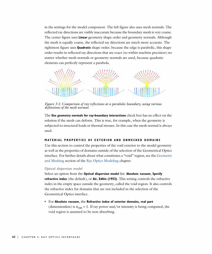
60 | C H A P T E R

in the settings for the model component. The left figure also uses mesh normals. The reflected ray directions are visibly inaccurate because the boundary mesh is very coarse. The center figure uses Linear geometry shape order and geometry normals. Although the mesh is equally coarse, the reflected ray directions are much more accurate. The rightmost figure uses Quadratic shape order; because the edge is parabolic, this shape order results in reflected ray directions that are exact (to within machine precision) no matter whether mesh normals or geometry normals are used, because quadratic elements can perfectly represent a parabola.

Figure 3-1: Comparison of ray reflections at a parabolic boundary, using various definitions of the mesh normal.

The Use geometry normals for ray-boundary interactions check box has no effect on the solution if the mesh can deform. This is true, for example, when the geometry is subjected to structural loads or thermal stresses. In this case the mesh normal is always used.

M A T E R I A L P R O P E R T I E S O F E X T E R I O R A N D U N M E S H E D D O M A I N S

Use this section to control the properties of the void exterior to the model geometry as well as the properties of domains outside of the selection of the Geometrical Optics interface. For further details about what constitutes a “void” region, see the Geometry and Meshing section of the Ray Optics Modeling chapter.

Optical dispersion modelSelect an option from the Optical dispersion model list: Absolute vacuum, Specify

refractive index (the default), or Air, Edlén (1953). This setting controls the refractive index in the empty space outside the geometry, called the void region. It also controls the refractive index for domains that are not included in the selection of the Geometrical Optics interface.

• For Absolute vacuum, the Refractive index of exterior domains, real part

(dimensionless) is next = 1. If ray power and/or intensity is being computed, the void region is assumed to be non-absorbing.


• For Specify refractive index, enter a value or expression for the Refractive index of

exterior domains, real part. The default is next = 1. Enter a user defined value for Refractive index of exterior domains, imaginary part if power and/or intensity is being computed. The default is kext = 0.

• For Air, Edlén (1953), the temperature and pressure dependent Refractive index of

exterior domains, real part is computed using the model described in Ref. 2. The model accepts user defined values of the Exterior domain temperature

Text (SI unit: K) and Exterior domain pressure Pext (SI unit: Pa). The defaults are Text = 293.15K and Pext = 1 atm. See the Optical Dispersion Models, The Refractive Index of Air for details.

For any type of optical dispersion model in the exterior and unmeshed domains, the algorithm to trace rays assumes that the medium is homogeneous. If a graded-index material is present, then its domain should be included in the selection of the Geometrical Optics interface and the spatial dependence of the refractive index should be controlled from the Medium Properties node.

I N T E N S I T Y C O M P U T A T I O N

The settings in this section control the treatment of ray intensity and polarization. These settings are also important in multiphysics applications such as ray heating.

Intensity ComputationSelect an option from the Intensity computation list: None (the default), Compute

intensity, Compute power, Compute intensity and power, Compute intensity in graded

media, or Compute intensity and power in graded media. For None no additional variables are computed along the rays. For other options, the ray intensity or ray power is computed as described below.

• For Compute intensity, auxiliary dependent variables are used to compute the intensity and polarization of each ray. For a complete list of the auxiliary dependent variables that are defined, see Intensity, Wavefront Curvature, and Polarization in Theory for the Geometrical Optics Interface. This option is only valid for computing intensity in homogeneous media; for graded-index media, use Compute

intensity in graded media instead. The refractive index can still change discontinuously at boundaries, where the Fresnel equations are automatically used to compute the intensity of the reflected and refracted rays.

The default name for the intensity variable is gop.I.

• For Compute power, the total power transmitted by each ray is defined as an auxiliary dependent variable. Information about the ray polarization is also available. The


62 | C H A P T E R

Deposited Ray Power (Boundary) subnode is available for the Wall feature. In addition, if a heat transfer interface such as the Heat Transfer in Solids interface is included in the model, the Ray Heat Source multiphysics node can be used to compute the heat source due to attenuation of rays within domains.

The default name for the power variable is gop.Q.

• The option Compute intensity and power functions as a combination of the Compute

intensity and Compute power options.

• The Compute intensity in graded media option functions like Compute intensity but is valid for both homogeneous and graded-index media. If all media in the model are homogeneous then it is recommended to select Compute intensity instead, since it is the more accurate method.

• The Compute intensity and power in graded media option functions like Compute

intensity and power but is valid for both homogeneous and graded-index media. If all media in the model are homogeneous then it is recommended to select Compute

intensity and power instead, since it is the more accurate method.

Compute PhaseThe Compute phase check box is only shown if the ray intensity is computed. Select the check box to allocate an auxiliary dependent variable for the phase of each ray. When the phase of each ray is computed, it is possible to plot interference patterns and visualize the instantaneous electric field components of polarized rays in postprocessing. When this check box is selected, the total number of degrees of freedom increases by 1 per ray. This option is based on the assumption that the coherence length of the radiation is arbitrarily large.

Use Corrections for Strongly Absorbing MediaThe Use corrections for strongly absorbing media check box is shown if the ray intensity is computed. Select the check box to accurately model reflection and refraction of rays at boundaries between strongly absorbing media, in which the imaginary part of the refractive index is very large. This option allocates two or three auxiliary dependent variables per ray based on space dimension. For more information about the way this option affects the intensity calculation, see Refraction in Strongly Absorbing Media in Theory for the Geometrical Optics Interface.

Tolerance for Curvature Tensor ComputationWhen the Intensity computation is set to Compute intensity in graded media or Compute

intensity and power in graded media enter a Tolerance for curvature tensor computation (dimensionless). This tolerance is used internally when computing the principal radii


of curvature of propagating wavefronts in a graded medium. A larger tolerance makes the solution less accurate but more stable.

A D D I T I O N A L V A R I A B L E S

The options in this section can be used to solve for additional variables other than those that are used to compute intensity or define the ray frequency. By default, all of the check boxes in this section are cleared so that these variables are not solved for.

Compute Optical Path LengthSelect the Compute optical path length check box to allocate an auxiliary dependent variable for the optical path length of each ray. The default variable name is gop.L. It is possible to reset the optical path length to 0 when rays interact with boundaries.

Count ReflectionsSelect the Count reflections check box to allocate an auxiliary dependent variable for the number of reflections undergone by each ray, including reflections by the Wall and Material Discontinuity features. The default variable name is gop.Nrefl. The auxiliary variable begins at 0 when rays are released and is incremented by 1 every time a ray is reflected at a boundary.

Store Ray Status DataSelect the Store ray status data check box to add new variables for quantities that cannot necessarily be recovered from the ray trajectory data alone. This is especially true if automatic remeshing is used in a model. The variables created include the following, all of which would be preceded by the physics interface tag (e.g. gop.):

• The release time of a given ray (variable name rti).

• The time at which a ray stopped at a boundary (variable name st).

• The final status of the ray (variable name fs). This indicates the status of a ray at the final time step. The value is an integer which has one of the following values:

- 0 for unreleased rays

- 1 for rays that are still in the modeling domain

- 2 for frozen rays

- 3 for stuck rays

- 4 for rays that have disappeared


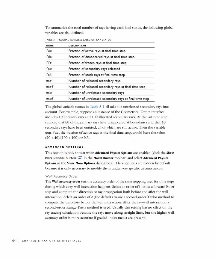
64 | C H A P T E R

To summarize the total number of rays having each final status, the following global variables are also defined.

The global variable names in Table 3-1 all take the unreleased secondary rays into account. For example, suppose an instance of the Geometrical Optics interface includes 100 primary rays and 100 allocated secondary rays. At the last time step, suppose that 80 of the primary rays have disappeared at boundaries and that 40 secondary rays have been emitted, all of which are still active. Then the variable gop.fac, the fraction of active rays at the final time step, would have the value (20 + 40)/(100 + 100) or 0.3.

A D V A N C E D S E T T I N G S

This section is only shown when Advanced Physics Options are enabled (click the Show

More Options button in the Model Builder toolbar, and select Advanced Physics

Options in the Show More Options dialog box). These options are hidden by default because it is only necessary to modify them under very specific circumstances.

Wall Accuracy OrderThe Wall accuracy order sets the accuracy order of the time stepping used for time steps during which a ray-wall interaction happens. Select an order of 1 to use a forward Euler step and compute the direction or ray propagation both before and after the wall interaction. Select an order of 2 (the default) to use a second-order Taylor method to compute the trajectory before the wall interaction. After the ray-wall interaction a second-order Runge-Kutta method is used. Usually this setting has no effect on the ray tracing calculation because the rays move along straight lines, but the higher wall accuracy order is more accurate if graded-index media are present.

TABLE 3-1: GLOBAL VARIABLES BASED ON RAY STATUS

NAME DESCRIPTION

fac Fraction of active rays at final time step

fds Fraction of disappeared rays at final time step

ffr Fraction of frozen rays at final time step

fse Fraction of secondary rays released

fst Fraction of stuck rays at final time step

nsr Number of released secondary rays

nsrf Number of released secondary rays at final time step

nsu Number of unreleased secondary rays

nsuf Number of unreleased secondary rays at final time step


Arguments for Random Number GenerationSelect an option from the Arguments for random number generation list: Generate unique

arguments (the default), Generate random arguments, or User defined. This setting determines how the additional argument to random functions is defined in features such as the Wall boundary condition with the Diffuse scattering wall condition. Typically the random numbers are functions of the ray index, position, time, and another argument i, defined as follows:

• For Generate unique arguments the additional argument is based on the position of each node in the Model Builder. As a result, random numbers generated in different nodes are created independently of each other, but the same result can be reproduced by running the same study several times.

• For Generate random arguments the additional argument is randomly created.

• For User defined the additional argument is defined by a user input in the Settings window for each feature. Independent solutions can be obtained by running a parametric sweep for different values of i.

Allow Multiple Release TimesThe Allow multiple release times check box, which is cleared by default, allows an array of release times for the rays to be specified in any of the ray release features. If the check box is cleared, all rays are released at time t = 0.

Exclude Jacobian Contributions from Ray EquationsBy default the Exclude Jacobian contributions from ray equations check box is cleared. If this check box is selected, then expressions for the time derivatives of the degrees of freedom on rays are not included in the Jacobian matrix. Excluding contributions to the Jacobian can significantly improve solution time if the number of rays in the model is very large. The drawback is that the Jacobian is not exact, so smaller time steps or path length intervals may be needed to obtain an accurate solution. This drawback is most noticeable when computing the ray intensity or power in an absorbing medium.

Treat Unmeshed Releasing Entities as ErrorsBy default the Treat unmeshed releasing entities as errors check box is selected. Certain ray release features, such as the Release and Release from Boundary features, compute the ray release positions based on a geometric entity, which must be meshed. While this check box is selected, failure to mesh the selections of such features will result in an error message when running any study in the model. If this check box is cleared, failure to mesh the selections of such features will result in them releasing zero rays, but will otherwise not interrupt the computation. Other physics features will still be able to release rays normally.


66 | C H A P T E R

Maximum Number of Wall Interactions per Time StepEnter a value for the Maximum number of wall interactions per time step. The default value is 1000. If a ray undergoes more than the specified number of boundary interactions in a single time step taken by the solver, the ray will disappear. This is included as a safeguard to prevent rays from getting stuck in infinite loops if the time between successive ray-wall interactions becomes infinitesimally small.

D E P E N D E N T V A R I A B L E S

The dependent variables (field variables) are the components of the Ray position and Wave vector. The name can be changed but the names of fields and dependent variables must be unique within a model. In 3D, the default ray position vector components are qx, qy, and qz; and the default wave vector components are kx, ky, and kz.

List of Geometrical Optics Interface Physics Features

The Geometrical Optics Interface has the following nodes and subnodes (listed in alphabetical order) available from the Physics ribbon toolbar (Windows users), Physics context menu (Mac or Linux users), or right-click to access the context menu (all users).

Theory for the Geometrical Optics Interface

In general, to add a node, go to the Physics toolbar, no matter what operating system you are using. Subnodes are available by clicking the parent node and selecting it from the Attributes menu.


Ray Properties

The Ray Properties node is added by default. Only one instance of this node can exist for each physics interface. The Ray Properties node defines the equations for ray propagation and may also include inputs for some ray properties.

R A Y P R O P E R T I E S

This section is shown when Monochromatic is selected from the Wavelength distribution

of released rays list in the physics interface Ray Release and Propagation section. Otherwise the frequency or vacuum wavelength of released rays is controlled separately by each ray release feature, such as Release or Release from Grid.

• Accumulator (Boundary)

• Accumulator (Domain)

• Auxiliary Dependent Variable

• Axial Symmetry

• Circular Wave Retarder

• Cross Grating

• Deposited Ray Power (Boundary)

• Deposited Ray Power (Domain)

• Diffraction Order (Grating)

• Diffraction Order (Cross Grating)

• Grating

• Ideal Depolarizer

• Illuminated Surface

• Release from Boundary

• Release from Symmetry Axis

• Linear Polarizer

• Linear Wave Retarder

• Material Discontinuity

• Medium Properties

• Mirror

• Mueller Matrix

• Nonlocal Accumulator

• Photometric Data Import

• Ray Continuity

• Ray Detector

• Ray Properties

• Ray Termination

• Release

• Release from Data File

• Release from Edge

• Release from Electric Field

• Release from Far-Field Radiation Pattern

• Release from Grid

• Release from Grid on Axis

• Release from Point

• Release from Point on Axis

• Solar Radiation

• Thin Dielectric Film

• Wall


68 | C H A P T E R

Select an option from the Ray property specification list: Specify vacuum wavelength (the default) or Specify frequency.

• For Specify vacuum wavelength enter a Vacuum wavelength λ0 (SI unit: m). The default is 660 nm.

• For Specify frequency enter a Ray frequency v (SI unit: Hz). The default is 4.54 × 1014 Hz.

Medium Properties

Use the Medium Properties node to specify the refractive index of the medium. An instance of this feature is created by default, including all of the selected domains for the physics interface. For the region outside the geometry and for any domains not included in the physics interface selection, the refractive index is instead controlled by the Optical dispersion model in the physics interface Material Properties of Exterior and

Unmeshed Domains section.

M E D I U M P R O P E R T I E S

Use the settings in this section to specify how the real part of the refractive index is defined. If the ray intensity or power is computed, then you can also specify the imaginary part of the refractive index, which is used to describe absorption within the medium.

Optical Dispersion ModelsIt is possible to specify the Refractive index, real part, n (dimensionless) using one of several optical dispersion models. The options are:

• Specify refractive index (the default): use this option to enter a value or expression for the real part of the refractive index n directly. By default the Refractive index, real

part uses values From material. It is also possible to enter a User defined value or expression. Only ray propagation in isotropic media can be modeled with the Geometrical Optics interface.

• Get dispersion model from material: the dispersion model in each domain is automatically deduced from the Material nodes and their selections. This allows different optical dispersion models to be used in different domains in the geometry.

For example, suppose that a model contains two lenses consisting of two different glasses, and that the first glass is defined using Sellmeier coefficients whereas the second glass is defined using Schott coefficients. Then selecting Get dispersion model

from material will automatically express the refractive index using the Sellmeier


equation in the first lens and the Schott (polynomial) equation in the second. An alternative way to use different optical dispersion models in different domains is to use more than one instance of the Medium Properties node and select the dispersion models manually.

• An optical dispersion model where the refractive index is a function of wavelength may be selected. The following built-in dispersion models are available:

- Cauchy,

- Conrady,

- Herzberger,

- Schott,

- Schott extended,

- Sellmeier,

- Sellmeier modified, type 1,

- Sellmeier modified, type 2, or

- Temperature-dependent Sellmeier.

For more information on each optical dispersion model, see Table 3-3 in Theory for the Geometrical Optics Interface, Optical Dispersion Models section.

The coefficients for each of these dispersion models are taken From material by default. Alternatively, User defined coefficients may be entered.

For the options Specify refractive index and Temperature-dependent Sellmeier, the refractive index is assumed to be absolute, such that n = 1 is the refractive index of an ideal vacuum. For all other optical dispersion models, however, the refractive index computed by the dispersion equation is a relative index defined with respect to air at a specified reference temperature and pressure. Thus, for each of these other optical dispersion models, the Reference temperature Tref (SI unit: K) and Reference pressure Pref (SI unit: Pa) can either be taken From material (the default) or User defined.

For the built-in optical dispersion models, the wavelength is always assumed to be in units of microns (μm). For example, in the Schott (polynomial) model, the coefficients A0, A1, A2, A3, etc. have units of 1, μm, μm2, μm3, and so on. If another source were to provide these coefficients using nanometers instead of microns, then some manual conversion would be required.


70 | C H A P T E R

If the reference pressure Pref ≠ 0, then it is assumed that the refractive indices are relative to air at the reference temperature and pressure; that is n = nrel × nair. The conversion from relative to absolute refractive index is made using the Edlén model (Ref. 2) for the refractive index of air. The Temperature-dependent Sellmeier model always returns absolute indices. If User defined coefficients are selected, the default coefficients for each of the built-in dispersion models give nrel = 1 (or, n = 1, if Pref = 0). See Optical Dispersion Models for further details.

If ray intensity or power is computed, specify the Refractive index, imaginary part k (dimensionless). By default the Refractive index, imaginary part k uses values From

material. For User defined enter a value or expression. The convention followed by the Geometrical Optics interface is that the imaginary part of the refractive index is negative in absorbing media. A positive value indicates a gain medium in which the intensity increases as the ray propagates.

How to Automatically Detect Optical Dispersion ModelsThe option Get dispersion model from material is unique because it allows a single Medium Properties node to detect different optical dispersion models from a large number of different materials having different domain selections. For example, the materials used in the Petzval Lens tutorial are shown in Figure 3-2 below. To automatically detect the optical dispersion models of the loaded glasses, take the following steps:

1 Add materials to the model using the Optical Material Library. Most of the glasses in this material library use an optical dispersion model to define the refractive index. As the materials are added, the coefficients used by the optical dispersion model are automatically loaded.

2 Locate the default Medium Properties node.

3 From the Optical dispersion model list, select Get dispersion model from material. If the glasses loaded in step 1 also provide thermo-optic coefficients, it is important to specify an accurate value of the Temperature as well.


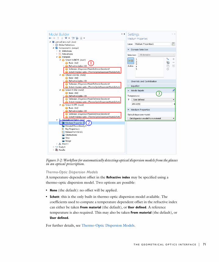
Figure 3-2: Workflow for automatically detecting optical dispersion models from the glasses in an optical prescription.

Thermo-Optic Dispersion ModelsA temperature-dependent offset in the Refractive index may be specified using a thermo-optic dispersion model. Two options are possible:

• None (the default): no offset will be applied.

• Schott: this is the only built-in thermo-optic dispersion model available. The coefficients used to compute a temperature dependent offset in the refractive index can either be taken From material (the default), or User defined. A reference temperature is also required. This may also be taken From material (the default), or User defined.

For further details, see Thermo-Optic Dispersion Models.

1

2

3


72 | C H A P T E R

Material Discontinuity

The Material Discontinuity node is the default feature on all boundaries.

The Geometrical Optics interface always applies reflection and refraction at boundaries between different media using a deterministic ray splitting approach. The direction of the refracted ray is computed using Snell’s law, based on the refractive index on either side. If extra degrees of freedom have been allocated for secondary rays, a reflected ray is also released. If the incident ray undergoes total internal reflection, no refracted ray is produced and no secondary rays are needed to release the reflected ray.

You can use the Rays to Release section (see below) to decide whether to split the incident ray into reflected and refracted rays, or to ignore the reflected ray.

If the ray intensity or power is solved for in the model, the Material Discontinuity feature computes the new values of these variables for the reflected and refracted rays. This reinitialization uses the Fresnel Equations while accounting for the incident ray polarization and the influence of any dielectric films on the surface reflectance.

The Accumulator (Boundary) subnode is available from the context menu (right-click the parent node) or from the Physics toolbar, Attributes menu. The Thin Dielectric Film subnode is also available if the following conditions are met:

• The ray intensity or power is being computed, and

• One of the following options is selected from the Thin dielectric films on boundary list in the Coatings section: Add layers to surface or Add layers to surface, repeating.

C O A T I N G S

This section is available if ray intensity or power is being computed in the model. Use the options in this section to add thin dielectric layers to the boundary between the media. These thin dielectric layers are used, together with the refractive indices on either side, to modify the Fresnel equations for the reflection and transmission coefficients at the boundary.

The maximum number of reflected rays can be controlled via the Maximum number of secondary rays text field, which is found under the Ray

Release and Propagation section for the physics interface.

If a reflected ray should be produced, but all of the preallocated secondary rays have already been released, the study will produce a Warning node.


The thicknesses of the thin dielectric layers must be small relative to the coherence length of the radiation. They are usually comparable in length scale to the free-space wavelength.

Select an option from the Thin dielectric films on boundary list. The default is None. The following options are available.

• None: no dielectric films are on the boundary. The intensity of the reflected and refracted light is computed solely using the Fresnel equations with the refractive indices of the two adjacent domains.

• Add layers to surface: you can add any number of thin dielectric films to the boundary by adding one or more Thin Dielectric Film subnodes; right click the Material Discontinuity node or select Thin Dielectric Film from the Physics toolbar, Attributes menu. If multiple thin films are added to a single surface, they are arranged in the same order as the corresponding Thin Dielectric Film subnodes in the Model Builder, from the upside of the boundary toward the downside.

• Add layers to surface, repeating: this option functions like the Add layers to surface option described above. Add individual dielectric coatings to the boundary using the Thin Dielectric Film subnode. In addition, enter a value or expression for the Number of repeating unit cells N (dimensionless). The default value is 3. In the settings windows for the Thin Dielectric Film subnodes, you can decide which layers constitute a unit cell that will be repeated the specified number of times. Use this option to specify periodic arrangements with a large number of repeatind dielectric layers, without having to add each layer manually.

• Anti-reflective coating: the incident ray is refracted with unit transmittance and zero reflectance.

• Single-layer coating, specified thickness: this is a simplified version of the Add layers to

surface option that only allows a single dielectric layer. Enter a value or expression for the Film refractive index n (dimensionless). The default value is 1. Then enter a value or expression for the Film thickness t (SI unit: m). The default value is 1 μm.

Anti-Reflective Coating with Multiple Layers: Application Library path Ray_Optics_Module/Prisms_and_Coatings/antireflective_coating_multilayer

Distributed Bragg Reflector: Application Library path Ray_Optics_Module/Prisms_and_Coatings/distributed_bragg_reflector


74 | C H A P T E R

• Specify reflectance: enter a value or expression for the reflectance at the boundary directly. Enter a value or expression for the Reflectance R (dimensionless). The default is 0.1. If the Specify different values for s- and p-polarization check box is selected, you can instead enter separate values for the reflectance of p- and s-polarized light, called Rp and Rs, respectively. The layers are considered nonabsorbing so that the sum of the reflectance and transmittance is unity.

• Specify transmittance: enter a value or expression for the transmittance at the boundary directly. Enter a value or expression for the Transmittance T (dimensionless). The default is 0.9. If the Specify different values for s- and

p-polarization check box is selected, you can instead enter separate values for the transmittance of p- and s-polarized light, called Tp and Ts, respectively. The layers are considered nonabsorbing so that the sum of the reflectance and transmittance is unity.

Real and Ideal Optical CoatingsThe options Anti-reflective coating, Specify reflectance, and Specify transmittance all include a check box called Treat as single layer dielectric film, which is cleared by default. While this check box is cleared, the specified reflectance or transmittance applies to all rays, regardless of wavelength or angle of incidence, and the remaining inputs in this section are not shown. This makes complicated multilayer films easier to set up because you can enter the reflectance or transmittance explicitly without having to know the properties of each layer in the coating. If the coating properties depend on the wavelength or angle of incidence, you can usually build this dependence into the model by defining the film reflectance or transmittance as an Interpolation function of the ray properties. The tradeoff is that accurate information about the discontinuities in ray phase is lost, even if the Compute phase check box is selected in the physics interface Intensity Computation section, because this information depends on the complex-valued Fresnel coefficients.

If the Treat as single layer dielectric film check box is selected, then instead the Material

Discontinuity automatically computes the thickness of a single layer needed to produce the given reflectance or transmittance. The drawback is that the specified value will only be attained for rays at a specific wavelength and angle of incidence.

The following inputs are only shown when Treat as single layer dielectric film is selected.

For Specify reflectance and Specify transmittance enter the Film refractive index n (dimensionless). The default is 1. If it is impossible to construct a single layer of this refractive index and obtain the specified reflectance or transmittance, then the boundary is treated as having no dielectric films. For Anti-reflective coating, the


refractive index of the coating is not an input because it is always the geometric mean of the refractive indices in the two adjacent domains.

For Anti-reflective coating, Specify reflectance, and Specify transmittance enter the following:

• Vacuum wavelength for specified film properties λ0 (SI unit: m). The default is 660 nm.

• Angle of incidence for specified film properties θi (SI unit: m). The default is 0.

• Select an option from the Angle of incidence specification list: With respect to upside (the default) or With respect to downside. You can see which side is the upside by selecting the Show boundary normal check box (see Advanced Settings below); the normal vector rendered in the Graphics window points from the upside to the downside.

• Select an option from the Specified film behavior applies to list: S-polarized radiation (the default) or P-polarized radiation.

R A Y S T O R E L E A S E

Use the inputs in this section to control whether the incident ray is split into a reflected and refracted ray at the material discontinuity. Select an option from the Release

reflected rays list: Always (the default), Never, or Based on logical expression.

• If Always is selected, whenever a ray hits the material discontinuity, the incident ray is refracted across the boundary, and a reflected ray is produces using some of the preallocated degrees of freedom for secondary rays.

• If Never is selected, the incident ray is refracted, but no reflected ray is produced. This does not prevent a ray from undergoing total internal reflection at the boundary.

• If Based on logical expression is selected, enter a value or expression for the Evaluation

expression e (dimensionless). The default is 1. A reflected ray is produced only if the value of this expression is nonzero for the incident ray.

If the ray intensity is solved for in the model, enter a Threshold intensity Ith (SI unit: W/m2). The default is 1 mW/m2. If the interaction of a ray with a material discontinuity would create a reflected ray of intensity less than the threshold intensity, the release of this reflected ray is suppressed.

If the ray power is solved for in the model, enter a Threshold power Qth (SI unit: W). The default is 10-3 mW. If the interaction of a ray with a material discontinuity would create a reflected ray of power less than the threshold power, the release of this


76 | C H A P T E R

reflected ray is suppressed. Suppressing the release of reflected rays of extremely low intensity or power is a convenient way to avoid wasting computational resources.

If both the Evaluation expression and the Threshold intensity are specified, a reflected ray is only released if the value of the expression is nonzero and the intensity of the reflected ray exceeds the threshold. In other words, a ray must satisfy all of the criteria in the Rays to Release section in order to be released, not just one of them.

A U X I L I A R Y D E P E N D E N T V A R I A B L E S , R E F R A C T E D R A Y

This section includes a check box (cleared by default) and an edit field (default 0) for every Auxiliary Dependent Variable in the model. Select the check box to activate the edit field, which controls the new value of this auxiliary dependent variable for the refracted ray. If the check box is cleared, the new value equals that of the incident ray.

The value can be a function of any combinations of ray variables and variables defined on the boundary. For example, to increment the value of psi by 1 when a ray touches or crosses a boundary, enter psi+1 in the text field for psinew.

A U X I L I A R Y D E P E N D E N T V A R I A B L E S , R E F L E C T E D R A Y

This section is the same as Auxiliary Dependent Variables, Refracted Ray, except that the expressions are used to auxiliary dependent variables for the reflected ray.


Select the Show boundary normal check box to view the boundary normal in the Graphics window.

If the Compute optical path length check box is selected in the physics interface Additional Variables section, select the Reset optical path length check box to set the optical path length of reflected and refracted rays to 0. Otherwise both the reflected and refracted ray inherit the optical path length of the incident ray.

Visualization of the boundary normal is important when adding multiple Thin Dielectric Film subnodes, since the thin films are oriented from the upside of the boundary to the downside in the same order as their corresponding nodes in the Model Builder.

Material Discontinuity Theory


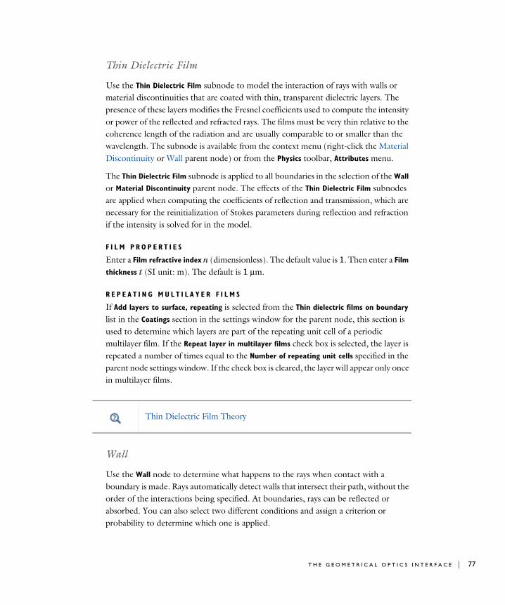
Thin Dielectric Film

Use the Thin Dielectric Film subnode to model the interaction of rays with walls or material discontinuities that are coated with thin, transparent dielectric layers. The presence of these layers modifies the Fresnel coefficients used to compute the intensity or power of the reflected and refracted rays. The films must be very thin relative to the coherence length of the radiation and are usually comparable to or smaller than the wavelength. The subnode is available from the context menu (right-click the Material Discontinuity or Wall parent node) or from the Physics toolbar, Attributes menu.

The Thin Dielectric Film subnode is applied to all boundaries in the selection of the Wall or Material Discontinuity parent node. The effects of the Thin Dielectric Film subnodes are applied when computing the coefficients of reflection and transmission, which are necessary for the reinitialization of Stokes parameters during reflection and refraction if the intensity is solved for in the model.

F I L M P R O P E R T I E S

Enter a Film refractive index n (dimensionless). The default value is 1. Then enter a Film

thickness t (SI unit: m). The default is 1 μm.

R E P E A T I N G M U L T I L A Y E R F I L M S

If Add layers to surface, repeating is selected from the Thin dielectric films on boundary list in the Coatings section in the settings window for the parent node, this section is used to determine which layers are part of the repeating unit cell of a periodic multilayer film. If the Repeat layer in multilayer films check box is selected, the layer is repeated a number of times equal to the Number of repeating unit cells specified in the parent node settings window. If the check box is cleared, the layer will appear only once in multilayer films.

Wall

Use the Wall node to determine what happens to the rays when contact with a boundary is made. Rays automatically detect walls that intersect their path, without the order of the interactions being specified. At boundaries, rays can be reflected or absorbed. You can also select two different conditions and assign a criterion or probability to determine which one is applied.

Thin Dielectric Film Theory


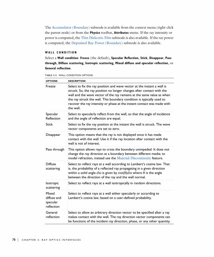
78 | C H A P T E R

The Accumulator (Boundary) subnode is available from the context menu (right-click the parent node) or from the Physics toolbar, Attributes menu. If the ray intensity or power is computed, the Thin Dielectric Film subnode is also available. If the ray power is computed, the Deposited Ray Power (Boundary) subnode is also available.

W A L L C O N D I T I O N

Select a Wall condition: Freeze (the default), Specular Reflection, Stick, Disappear, Pass

through, Diffuse scattering, Isotropic scattering, Mixed diffuse and specular reflection, or General reflection.

TABLE 3-2: WALL CONDITION OPTIONS

OPTIONS DESCRIPTION

Freeze Select to fix the ray position and wave vector at the instant a wall is struck. So, the ray position no longer changes after contact with the wall and the wave vector of the ray remains at the same value as when the ray struck the wall. This boundary condition is typically used to recover the ray intensity or phase at the instant contact was made with the wall.

Specular Reflection

Select to specularly reflect from the wall, so that the angle of incidence and the angle of reflection are equal.

Stick Select to fix the ray position at the instant the wall is struck. The wave vector components are set to zero.

Disappear This option means that the ray is not displayed once it has made contact with the wall. Use it if the ray location after contact with the wall is not of interest.

Pass through This option allows rays to cross the boundary unimpeded. It does not change the ray direction at a boundary between different media; to model refraction, instead use the Material Discontinuity feature.

Diffuse scattering

Select to reflect rays at a wall according to Lambert’s cosine law. That is, the probability of a reflected ray propagating in a given direction within a solid angle dω is given by cos(θ)dω where θ is the angle between the direction of the ray and the wall normal.

Isotropic scattering

Select to reflect rays at a wall isotropically in random directions.

Mixed diffuse and specular reflection

Select to reflect rays at a wall either specularly or according to Lambert’s cosine law, based on a user-defined probability.

General reflection

Select to allow an arbitrary direction vector to be specified after a ray makes contact with the wall. The ray direction vector components can be functions of the incident ray direction, phase, or any other quantity.


G E N E R A L R E F L E C T I O N S E T T I N G S

This section is available when General reflection (see Table 3-2) is selected as the Wall

condition.

Enter values for the Reflected ray direction vector Lp (dimensionless) either in Cartesian coordinates (x, y, z) (the default) or select the Specify tangential and normal direction

vector components check box to enter coordinates in the tangent-normal coordinate system (t1, t2, n). In this case the normal direction is selected so that an incident ray is reflected back into the domain it previously occupied if the specified normal direction vector component is positive. The tangential directions are oriented so that they form a right-handed coordinate system, together with the normal direction.

P R I M A R Y R A Y C O N D I T I O N

Use this section to apply two different wall conditions on the same set of boundaries based on a probability or logical expression.

Select a Primary ray condition: None (the default), Probability, or Expression. When the default, None, is kept, it means that the Wall condition is always respected by the incident rays.

ProbabilityIf Probability is selected, the Wall condition is applied with a certain probability. Enter a value for the Probability, γ (dimensionless). If the Wall condition is not used, the ray instead behaves according to the Otherwise setting.

For example, if the Wall condition is set to:

• Freeze and γ is set to 0.1, then for every 10 rays that strike the wall, on average one freezes and the remaining 9 rays behave according to the Otherwise setting.

• Stick and γ is set to 0.5 then on average half of the rays stick to the wall and the other half behave according to the Otherwise setting.

ExpressionIf Expression is selected, the Evaluation expression e (dimensionless) is evaluated whenever a ray strikes the wall. The default expression is 1. If the Evaluation expression is nonzero, the ray behaves according to the Wall condition, otherwise the ray behaves according to the Otherwise setting.

The value of γ should always be between 0 and 1.


80 | C H A P T E R

OtherwiseThe options available for the Otherwise setting are the same as for the Wall Condition, except that General reflection and Mixed diffuse and specular reflection are not available. The Otherwise setting can be used to make rays interact with a wall differently with a certain probability or when a certain condition is satisfied. For example, to model reflection at a partially specular surface in which 50% of the ray intensity is absorbed and 30% is reflected specularly:

• Select Mixed diffuse and specular reflection as the Wall condition,

• set the Probability of specular reflection to 0.3/(1-0.5),

• set the Primary ray condition to Probability,

• set the Probability to 1-0.5, and

• select Freeze as the Otherwise option.

A B S O R P T I O N C O E F F I C I E N T

This section is available when

• the ray intensity or power is solved for in the model, and

• the Wall condition is set to any option that can reflect rays, including the following:

- Specular Reflection,

- Diffuse scattering,

- Isotropic scattering,

- General reflection, or

- Mixed diffuse and specular reflection.

Select one of the following from the Compute reflected intensity using list: Absorption

coefficients or Reflection coefficients.

For Absorption coefficients enter the Absorption coefficient α (dimensionless). The default is 0. The intensity or power of the reflected ray will be proportional to 1 − α.

For Reflection coefficients enter the Reflection coefficient r (dimensionless). The default value is 1. The intensity or power of the reflected ray will be proportional to r2.

If the Wall condition is set to Mixed diffuse and specular reflection, this section is instead called Absorption Coefficients and the absorption coefficients for the diffusely and specularly reflected rays are specified separately. All of the text fields are given subscripts s and d for specularly and diffusely reflected rays, respectively.


N E W V A L U E O F A U X I L I A R Y D E P E N D E N T V A R I A B L E S

This section is available if an Auxiliary Dependent Variable has been added to the model.

When a ray crosses or touches a boundary, the values of the user-defined auxiliary dependent variables can be changed. The value can be a function of any combinations of ray variables and variables defined on the boundary.

Select the Assign new value to auxiliary variable check box or boxes based on the number of auxiliary variables in the model. Then enter the new value or expression in the field. For example, if there is an auxiliary variable, psi, then enter a value for psinew in the field. So, to increment the value of psi by 1 when a ray touches or crosses a boundary, enter psi+1 in the text field for psinew.


If the Primary ray condition is set to Probability, or if the Diffuse scattering, Isotropic

scattering, or Mixed diffuse and specular reflection wall condition is used, then the Wall feature generates random numbers.

If, in addition, the Arguments for random number generation setting is set to User defined in the physics interface Advanced Settings section, the Advanced Settings section is available.

Enter the Additional input argument to random number generator i (dimensionless). The default value is 1.

The Advanced Settings section is also shown if the Compute optical path length check box is selected under the physics interface Additional Variables section. Select the Reset

optical path length check box to set the optical path length to 0 when a ray touches the wall.

Mirror

Use the Mirror node to specularly reflect rays at a boundary. This feature functions as a special case of the Wall node, except that the wall condition is always specular reflection.

See Wall for information on the following sections: Absorption Coefficient, New Value of

Auxiliary Dependent Variables, and Advanced Settings.


82 | C H A P T E R

Axial Symmetry

The Axial Symmetry node is automatically added to 2D axisymmetric models. The options available for the feature are the same as for Wall, except as follows.

The Boundary Selection is locked and is only applicable to edges on the symmetry axis. The only wall conditions available are Specular reflection (the default), Freeze, Stick, and Disappear. In addition, the Primary Ray Condition section is not included. The Axial

Symmetry boundary condition does not affect ray intensity or polarization, except to introduce a phase delay of π in reflected rays to compensate for the change in the principal curvature direction.

Release

Use the Release node to release rays within domains based on arbitrary expressions or based on the positions of the mesh elements.

R E L E A S E T I M E S

This section is only available when the Allow multiple release times check box has been selected in the physics interface Advanced Settings section. Enter Release times (SI unit: s) or click the Range button ( ) to select and define a range of specific times. At each release time, rays are released with initial position and ray direction vector as defined next.

I N I T I A L P O S I T I O N

Select an Initial position: Density (the default) or Mesh based.

The Axial Symmetry condition only applies to straight boundaries that are both on the axis of symmetry and adjacent to a domain in the selection of the physics interface. If rays are propagating in the void region outside of the selected domains, it is possible for the rays to enter the region where r < 0, even though no geometry is defined there.

To ensure that rays cannot propagate into the region where r < 0, draw line segments on the parts of the symmetry axis where no geometric entities exist, then add the Wall node to these edges. Keep in mind that rays can only be subjected to boundary conditions if the corresponding boundaries are meshed.


DensityFor Density enter a value for the Number of rays per release N (dimensionless). The default is 100. Then enter a value or expression for the Density proportional to ρ (dimensionless). The default is 1.

The Density proportional to ρ can be an expression rather than a number; the resulting ray distribution approximately has a number density that is proportional to this expression. The resulting distribution looks a bit random, and it depends on the order in which the mesh elements are numbered. The distribution is probably not exactly the same in different COMSOL Multiphysics versions, but the total number of rays released is always N.

Advanced Options for Density-Based ReleaseThe following options can be adjusted to make the number density of rays more closely conform to the Density proportional to expression.

Select a Release distribution accuracy order between 1 and 5 (the default is 5), which determines the integration order that is used when computing the number of rays to release within each mesh element. The higher the accuracy order, the more accurately rays will be distributed among the mesh elements.

The Position refinement factor (default 0) must be a nonnegative integer. When the refinement factor is 0, each ray is always assigned a unique position, but the density is taken as a uniform value over each mesh element. If the refinement factor is a positive integer, the distribution of rays within each mesh element is weighted according to the density, but it is possible for some rays to occupy the same initial position. Further increasing the Position refinement factor increases the number of evaluation points within each mesh element to reduce the probability of multiple rays occupying the same initial position.

Mesh BasedFor Mesh based the rays are released from a set of positions determined by a selection of geometric entities (of arbitrary dimension) in the mesh. Given a Refinement factor between 1 and 5, the centers of the refined mesh elements are used. Thus, the number of positions per mesh element is refine^dim, except for pyramids, where it is (4*refine2-1)*refine/3.

The Density proportional to expression must be strictly positive.


84 | C H A P T E R

R A Y D I R E C T I O N V E C T O R

Select an option from the Ray direction vector list: Expression (the default), Spherical, Hemispherical, Conical, or Lambertian (3D only).

• For Expression a single ray is released in the specified direction. Enter coordinates for the Ray direction vector L0 (dimensionless) based on space dimension.

• For Spherical a number of rays are released at each point, sampled from a spherical distribution in wave vector space. Enter the Number of rays in wave vector space Nw (dimensionless). The default is 50.

• For Hemispherical a number of rays are released at each point, sampled from a hemispherical distribution in wave vector space. Enter the Number of rays in wave

vector space Nw (dimensionless). The default is 50. Then enter coordinates for the Hemisphere axis r based on space dimension.

• For Conical a number of rays are released at each point, sampled from a conical distribution in wave vector space. Enter the Number of rays in wave vector space Nw (dimensionless). The default is 50. Then enter coordinates for the Cone axis r based on space dimension. Then enter the Cone angle α (SI unit: rad). The default is π/3 radians.

• The Lambertian option is only available in 3D. A number of rays are released at each point, sampled from a hemisphere in wave vector space with probability density based on the cosine law. Enter the Number of rays in wave vector space Nw (dimensionless). The default is 50. Then enter coordinates for the Hemisphere axis r based on space dimension.

If Conical is selected, select an option from the Conical distribution list: Uniform density (the default), Specify polar and azimuthal distributions, Hexapolar, Marginal rays only, or Marginal and axial rays only.

• For Uniform density rays are released with polar angles from 0 to the specified cone angle. The rays are distributed in wave vector space so that each ray subtends approximately the same solid angle.

• For Specify polar and azimuthal distributions specify the Number of polar angles Nθ (dimensionless) and the Number of azimuthal angles Nϕ (dimensionless). Rays are released at uniformly distributed polar angles from 0 to the specified cone angle. A single axial ray (θ = 0) is also released. For each value of the polar angle, rays are released at uniformly distributed azimuthal angles from 0 to 2π. Unlike other options for specifying the conical distribution, it is not necessary to directly specify the Number of rays in wave vector space Nw (dimensionless), which is instead derived from the relation Nw = Nθ × Nϕ + 1.


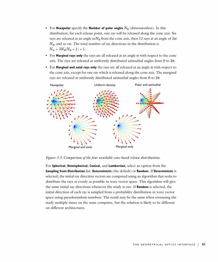
• For Hexapolar specify the Number of polar angles Nθ (dimensionless). In this distribution, for each release point, one ray will be released along the cone axis. Six rays are released at an angle α/Nθ from the cone axis, then 12 rays at an angle of 2α/Nθ, and so on. The total number of ray directions in the distribution is Nw = 3Nθ(Nθ + 1) + 1.

• For Marginal rays only the rays are all released at an angle α with respect to the cone axis. The rays are released at uniformly distributed azimuthal angles from 0 to 2π.

• For Marginal and axial rays only the rays are all released at an angle α with respect to the cone axis, except for one ray which is released along the cone axis. The marginal rays are released at uniformly distributed azimuthal angles from 0 to 2π.

Figure 3-3: Comparison of the four available cone-based release distributions.

For Spherical, Hemispherical, Conical, and Lambertian, select an option from the Sampling from Distribution list: Deterministic (the default) or Random. If Deterministic is selected, the initial ray direction vectors are computed using an algorithm that seeks to distribute the rays as evenly as possible in wave vector space. This algorithm will give the same initial ray directions whenever the study is run. If Random is selected, the initial direction of each ray is sampled from a probability distribution in wave vector space using pseudorandom numbers. The result may be the same when rerunning the study multiple times on the same computer, but the solution is likely to be different on different architectures.

Hexapolar Uniform density Polar and azimuthal

Marginal and axial Marginal only


86 | C H A P T E R

I N I T I A L R A Y F R E Q U E N C Y

This section is available when Polychromatic, specify frequency is selected from the Wavelength distribution of released rays list in the physics interface Ray Release and


Select a Distribution function: None (the default), Normal, Lognormal, Uniform, or List of

values.

When None is selected, enter an initial value ν0 (SI unit: Hz). The default value is 4.54 × 1014 Hz.

Select Normal to create a normal distribution function, Lognormal to create a log-normal distribution function, or Uniform to create a uniform distribution function. For any of these selections, the Number of values sets the number of points in the distribution function. Enter a user-defined Mean (default 4.54 × 1014 Hz) and Standard deviation (default 1014 Hz). Select List of values to enter a list of distinct frequency values.

V A C U U M W A V E L E N G T H

This section is available when Polychromatic, specify vacuum wavelength is selected from the Wavelength distribution of released rays list in the physics interface Ray Release and


Select a Distribution function: None (the default), Normal, Lognormal, Uniform, or List of

values.

When None is selected, enter a value or expression for the Vacuum wavelength λ0 (SI unit: m). The default is 660 nm. All rays released by this feature will have the same wavelength.

Select Normal to create a normal distribution function, Lognormal to create a log-normal distribution function, or Uniform to create a uniform distribution function. For any of these selections, the Number of values sets the number of points in the distribution function. Enter a user-defined Mean (default 660 nm) and Standard

deviation (default 100 nm). Select List of values to enter a list of distinct wavelength values directly.

I N I T I A L P H A S E

This section is available when the Compute phase check box is selected under the physics interface Intensity Computation section. Enter an Initial phase Ψ0 (SI unit: rad). The default value is 0.


I N I T I A L I N T E N S I T Y

This section is available when the ray intensity is solved for in the model and Expression is selected as the Ray direction vector. Enter a value for the Initial intensity I0 (SI unit: W/m2). The default is 1000 W/m2.

I N I T I A L R A D I I O F C U R V A T U R E

This section is available when the ray intensity is solved for in the model and Expression is selected as the Ray direction vector. Select a Wavefront shape. In 3D the available options are Plane wave (the default), Spherical wave, and Ellipsoid. In 2D the available options are Plane wave (the default) and Cylindrical wave.

• For an idealized plane wave the radii of curvature would be infinite. However, because the algorithm used to compute intensity requires finite values, when Plane

wave is selected the initial radii of curvature are instead given an initial value that is 108 times greater than the characteristic size of the geometry.

• For a Spherical wave or Cylindrical wave, enter the Initial radius of curvature r0 (SI unit: m).

• For an Ellipsoid, enter the Initial radius of curvature, 1 r1,0 (SI unit: m) and the Initial

radius of curvature, 2 r2,0 (SI unit: m). Also enter the Initial principal curvature

direction, 1 e1,0 (dimensionless).

I N I T I A L P O L A R I Z A T I O N

This section is available when the ray intensity or power is solved for.

Select an Initial polarization type: Unpolarized (the default), Fully polarized, or Partially

polarized.

For spherical and cylindrical waves the Initial radius of curvature must be nonzero. To release a ray such that the initial wavefront radius of curvature is zero, instead select a different option such as Conical from the Ray direction vector list.

Principal Radii of Curvature


88 | C H A P T E R

Select an Initial polarization: Along principal curvature direction (the default) or User

defined.

• For Fully polarized and Partially polarized rays in 3D enter an Initial polarization

parallel to reference direction a1,0 (dimensionless), Initial polarization perpendicular

to reference direction a2,0 (dimensionless), and Initial phase difference δ0 (SI unit: rad).

• For Fully polarized and Partially polarized rays in 2D enter an Initial polarization, in

plane axy,1 (dimensionless), Initial polarization, out of plane az,0 (dimensionless), and Initial phase difference δ0 (SI unit: rad).

• For User defined also enter an Initial polarization reference direction u (dimensionless).

For Partially polarized, also enter an Initial degree of polarization P0 (dimensionless).

T O T A L S O U R C E P O W E R

This section is available:

• when the ray intensity is solved for, and

• when Spherical, Hemispherical, or Conical is selected as the Ray direction vector.

• It is also available when the ray power is solved for, and then any choice of Ray

direction vector displays this section.

Select an option from the Intensity initialization list. By default Uniform distribution is selected. If any Photometric Data Import nodes have been added to the model then they can also be selected from the list.

If Uniform distribution is selected, enter a Total source power Psrc (SI unit: W). The default is 1 W. In 2D, instead enter the Total source power per unit thickness Psrc (SI unit: W/m). The default is 1 W/m. If any Photometric Data Import feature is selected from the list, the source power is instead obtained directly from the imported photometric data (IES) file. Enter values or expressions for the components of the


Photometric horizontal ph (dimensionless) and Photometric zero pz (dimensionless). By default, these vectors point in the directions of the positive x- and z-axes, respectively.

I N I T I A L V A L U E O F A U X I L I A R Y D E P E N D E N T V A R I A B L E S

For each of the Auxiliary Dependent Variable nodes added to the model, select a Distribution function for the initial value of the auxiliary dependent variables and whether the initial value of the auxiliary dependent variables should be a scalar value or sampled from a distribution function.

The number of rays simulated can increase substantially and the following options are available for each Auxiliary Dependent Variable added to the model.

When None is selected, enter an initial value. The symbol for the initial value is the auxiliary variable name followed by a subscript 0, so for the default name rp the initial value has symbol rp0.

For the initial value of the auxiliary dependent variables, select Normal to create a normal distribution function, Lognormal to create a log-normal distribution function, or Uniform to create a uniform distribution function. For any selection, the Number of

values sets the number of points in the distribution function. Enter a user-defined Mean (default 0) and Standard deviation (default 1). Select List of values to enter a set of numerical values directly.

By default auxiliary dependent variables are initialized after all other degrees of freedom. Select the Initialize before wave vector check box to compute the initial value of the auxiliary dependent variable immediately after computing the initial wave vectors of the rays. By selecting this check box it is possible to define the initial ray direction as a function of the auxiliary dependent variables.

The relationship between the photometric horizontal, photometric vertical, and ray direction vector, and its effect on the initial ray intensity, is explained in ANSI/IESNA LM-63-02 (R2008), IESNA Standard file format for the electronic transfer of photometric data and related information, Illuminating Engineering Society (2002).

The Photometric Data Import feature does not support the options TILT=INCLUDE or TILT=<FILENAME> that are included in some IES files. Only TILT=NONE is allowed.


90 | C H A P T E R

Release from Boundary

Use the Release from Boundary node to determine how to release rays on an interior or exterior boundary in a specific direction.

The Nonlocal Accumulator subnode is available from the context menu (right-click the parent node) or from the Physics toolbar, Attributes menu.

See Release for information on the following sections: Release Times, Initial Ray

Frequency, Vacuum Wavelength, Initial Phase, Initial Intensity, Total Source Power, Initial

Polarization, and Initial Value of Auxiliary Dependent Variables.

C O O R D I N A T E S Y S T E M S E L E C T I O N

It is possible to specify the initial ray direction in terms of the global coordinates or in another coordinate system defined for the model Component. Select an option from the Coordinate system list. By default Global coordinate system is selected. If other coordinate systems are defined, they can also be selected from the list. When specifying the initial ray direction (see the Ray Direction Vector section), direction components can be specified using the basis vectors of whichever coordinate system has been selected from the list.

When a coordinate system other than Global coordinate system is selected from the Coordinate system list, arrows will appear in the Graphics window to indicate the orientation of the basis vectors of the coordinate system on the selected boundaries.


Select an Initial position: Uniform distribution (the default for 2D components) Projected plane grid (the default for 3D components), Mesh based, or Density. Mesh based and Density have the same settings as described for the Release node.

For 2D components, if Uniform distribution is selected, enter the Number

of rays per release N (dimensionless). The union of the selected boundaries is divided into N segments of approximately equal length, and a ray is placed in the middle of each segment.

For 3D components, if Projected plane grid is selected, enter the Number

of rays per release N (dimensionless). The rays are distributed on a plane grid in planes that are approximately tangential to the selected boundaries (for a plane boundary, you get a uniform distribution).



Select an option from the Ray direction vector list: Expression (the default), Hemispherical, Conical, or Lambertian (3D only).

• For Expression a single ray is released in the specified direction. Enter coordinates for the Ray direction vector L0 (dimensionless) based on space dimension. Select the Specify tangential and normal vector components check box to specify the initial direction using a coordinate system based on the directions tangential and normal to the surface (t1, t2, n).


vector space Nw (dimensionless). The default is 50. Then enter coordinates for the Hemisphere axis r based on space dimension. Select the Specify tangential and normal

vector components check box to specify the hemisphere axis using a coordinate system based on the directions tangential and normal to the surface (t1, t2, n).

• For Conical a number of rays are released at each point, sampled from a conical distribution in wave vector space. Enter the Number of rays in wave vector space Nw (dimensionless). The default is 50. Then enter coordinates for the Cone axis r based on space dimension. Then enter the Cone angle α (SI unit: rad). The default is π/3 radians. Select the Specify tangential and normal vector components check box to specify the cone axis using a coordinate system based on the directions tangential and normal to the surface (t1, t2, n).

• The Lambertian option is only available in 3D. A number of rays are released at each point, sampled from a hemisphere in wave vector space with probability density based on the cosine law. Enter the Number of rays in wave vector space Nw (dimensionless). The default is 50. Then enter coordinates for the Hemisphere axis r based on space dimension. Select the Specify tangential and normal vector

components check box to specify the hemisphere axis using a coordinate system based on the directions tangential and normal to the surface (t1, t2, n)


92 | C H A P T E R

If Conical is selected, select an option from the Conical distribution list: Uniform density (the default), Specify polar and azimuthal distributions, Hexapolar, Marginal rays only, or Marginal and axial rays only.

• For Uniform density rays are released with polar angles from 0 to the specified cone angle. The rays are distributed in wave vector space so that each ray subtends approximately the same solid angle.

• For Specify polar and azimuthal distributions specify the Number of polar angles Nθ (dimensionless) and the Number of azimuthal angles Nϕ (dimensionless). Rays are released at uniformly distributed polar angles from 0 to the specified cone angle. A single axial ray (θ = 0) is also released. For each value of the polar angle, rays are released at uniformly distributed azimuthal angles from 0 to 2π. Unlike other options for specifying the conical distribution, it is not necessary to directly specify the Number of rays in wave vector space Nw (dimensionless), which is instead derived from the relation Nw = Nθ × Nϕ + 1.

• For Hexapolar specify the Number of polar angles Nθ (dimensionless). In this distribution, for each release point, one ray will be released along the cone axis. Six rays are released at an angle α/Nθ from the cone axis, then 12 rays at an angle of 2α/Nθ, and so on. The total number of ray directions in the distribution is Nw = 3Nθ(Nθ + 1) + 1.

When the Specify tangential and normal vector components check box is selected, arrows indicating the normal direction on the selected boundaries will appear in the Graphics window.

Note that the normal direction may be opposite the built-in variable for the boundary normal (for example, nx, ny, and nz) to ensure that a positive value causes rays to be released into the simulation domain. This often occurs when the release is applied to exterior boundaries.

When the normal direction used by the Release from Boundary feature is opposite the normal vector defined by the geometry, the tangential directions are similarly inverted to ensure that the boundary coordinate system is right-handed.


• For Marginal rays only the rays are all released at an angle α with respect to the cone axis. The rays are released at uniformly distributed azimuthal angles from 0 to 2π.

• For Marginal and axial rays only the rays are all released at an angle α with respect to the cone axis, except for one ray which is released along the cone axis. The marginal rays are released at uniformly distributed azimuthal angles from 0 to 2π.

The four Conical distribution options are illustrated in Figure 3-3.

For Hemispherical, Conical, and Lambertian, select an option from the Sampling from

Distribution list: Deterministic (the default) or Random. If Deterministic is selected, the initial ray direction vectors are computed using the same algorithm, which seeks to distribute the rays as evenly as possible in wave vector space, whenever the study is run. If Random is selected, the initial direction of each ray is sampled from a probability distribution in wave vector space using pseudo-random numbers.

I N I T I A L R A D I I O F C U R V A T U R E

This section is available when the ray intensity is solved for in the model and Expression is selected as the Ray direction vector. Select a Wavefront shape. In 3D the available options are From surface curvature (the default), Plane wave, Spherical wave, and Ellipsoid. In 2D the available options are Plane wave (the default) and Cylindrical wave.

• For a Spherical wave or Cylindrical wave, enter the Initial radius of curvature r0 (SI unit: m).

• For an Ellipsoid (3D only), enter the Initial radius of curvature, 1 r1,0 (SI unit: m) and the Initial radius of curvature, 2 r2,0 (SI unit: m). Also enter the Initial principal

curvature direction, 1 e1,0 (dimensionless).

For spherical and cylindrical waves the Initial radius of curvature must be nonzero. To release a ray such that the initial wavefront radius of curvature is zero, instead select a different option such as Conical from the Ray direction vector list.

Principal Radii of Curvature


94 | C H A P T E R

Release from Symmetry Axis

Use the Release from Symmetry Axis node to release rays from specified edges along the axis of symmetry in a 2D axisymmetric geometry. It functions like the Release from Boundary node, except that it can only be applied to the axis of symmetry and that the options in the Ray Direction Vector section are slightly different.


Frequency, Vacuum Wavelength, Initial Phase, Initial Intensity, Initial Radii of Curvature, Total Source Power, Initial Polarization, and Initial Value of Auxiliary Dependent Variables.


Select an Initial position: Uniform distribution (the default), Mesh based, or Density. Mesh

based and Density have the same settings as described for the Release node.

If Uniform distribution is selected, enter the Number of rays per release N (dimensionless). The default is 100. The set of the selected boundaries is divided into N segments of approximately equal length, with one ray at the middle of each segment.


Select an option from the Ray direction vector list: Expression (the default), Spherical, or Conical.

• For Expression a single ray is released in the specified direction. Enter the radial and axial components of the Ray direction vector L0 (dimensionless).

• For Spherical a number of rays are released at each point, from the negative z direction to the positive z direction in the half plane with r > 0. These rays are sampled from an anisotropic hemispherical distribution in wave vector space, so that rays are more heavily weighted toward the r direction rather than the ±z directions. In 3D this would correspond to a spherical distribution of rays such that each ray subtends approximately the same solid angle in wave vector space.

Enter the Number of rays in wave vector space Nw (dimensionless). The default is 50. Then enter coordinates for the Hemisphere axis r based on space dimension. Select the Specify tangential and normal vector components check box to specify the hemisphere axis using a coordinate system based on the directions tangential and normal to the surface (t1, t2, n).

• For Conical a number of rays are released at each point, sampled from a conical distribution in wave vector space. Enter the Number of rays in wave vector space Nw (dimensionless). The default is 50. Then enter coordinates for the Cone axis r based on space dimension. Then enter the Cone angle α (SI unit: rad). The default is π/


3 radians. Unlike the Spherical distribution, the rays in the Conical distribution each subtend the same angle in 2D, not the same solid angle in 3D.

For Hemispherical and Conical, select an option from the Sampling from Distribution list: Deterministic (the default) or Random. If Deterministic is selected, the initial ray direction vectors are computed using the same algorithm, which seeks to distribute the rays as evenly as possible in wave vector space, whenever the study is run. If Random is selected, the initial direction of each ray is sampled from a probability distribution in wave vector space using pseudo-random numbers.

Release from Edge

Use the Release from Edge node to release rays from positions along a set of edges in a 3D geometry.

The Initial Position section is described below. For all other sections, see Release.


Select an Initial position: Mesh based (the default), Uniform distribution, or Density. Mesh based and Density have the same settings as described for the Release node. If Uniform

distribution is selected, enter the Number of rays per release N (dimensionless). The union of the selected edges is divided into N segments of approximately equal length, and a ray is released from the middle of each segment.

Release from Point

Use the Release from Point node to release rays from a set of points in a geometry. By default one ray is released at every selected point, although it is possible to release multiple rays at each point if the initial direction or an auxiliary dependent variable is sampled from a distribution.

For information on the settings, see Release.

Release from Point on Axis

The Release from Point on Axis feature is similar to the Release from Point feature, except that the points must be on the axis of symmetry in a 2D axisymmetric geometry.

See Release from Boundary for information on the Ray Direction Vector section.

For all other sections, see Release from Point.


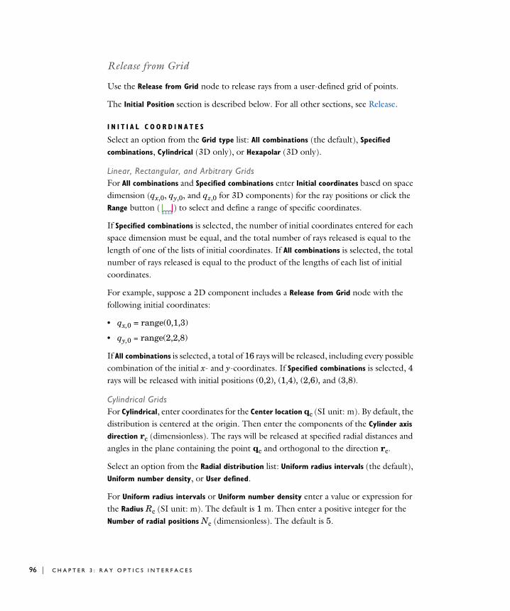
96 | C H A P T E R

Release from Grid

Use the Release from Grid node to release rays from a user-defined grid of points.

The Initial Position section is described below. For all other sections, see Release.

I N I T I A L C O O R D I N A T E S

Select an option from the Grid type list: All combinations (the default), Specified

combinations, Cylindrical (3D only), or Hexapolar (3D only).

Linear, Rectangular, and Arbitrary GridsFor All combinations and Specified combinations enter Initial coordinates based on space dimension (qx,0, qy,0, and qz,0 for 3D components) for the ray positions or click the Range button ( ) to select and define a range of specific coordinates.

If Specified combinations is selected, the number of initial coordinates entered for each space dimension must be equal, and the total number of rays released is equal to the length of one of the lists of initial coordinates. If All combinations is selected, the total number of rays released is equal to the product of the lengths of each list of initial coordinates.

For example, suppose a 2D component includes a Release from Grid node with the following initial coordinates:

• qx,0 = range(0,1,3)

• qy,0 = range(2,2,8)

If All combinations is selected, a total of 16 rays will be released, including every possible combination of the initial x- and y-coordinates. If Specified combinations is selected, 4 rays will be released with initial positions (0,2), (1,4), (2,6), and (3,8).

Cylindrical GridsFor Cylindrical, enter coordinates for the Center location qc (SI unit: m). By default, the distribution is centered at the origin. Then enter the components of the Cylinder axis

direction rc (dimensionless). The rays will be released at specified radial distances and angles in the plane containing the point qc and orthogonal to the direction rc.

Select an option from the Radial distribution list: Uniform radius intervals (the default), Uniform number density, or User defined.

For Uniform radius intervals or Uniform number density enter a value or expression for the Radius Rc (SI unit: m). The default is 1 m. Then enter a positive integer for the Number of radial positions Nc (dimensionless). The default is 5.


For User defined enter a list of Radial coordinates qr (SI unit: m) directly. An arbitrary number of radial coordinates can be entered in the list. The default is 1 m.

The effect of the Radial distribution setting on the resulting ray placement is illustrated in Figure 3-4. For Uniform radius intervals, the distances between the concentric rings of rays are all equal, but the number density of rays is greater at the center of the distribution than at the outer edge. The option Uniform number density corrects this imbalance by defining nonuniform increments in the radial position between the concentric rings.

Enter a positive integer for the Number of angles Nϕ (dimensionless). The default is 10.

The total number of rays released (before accounting for distributions of ray direction or auxiliary dependent variables at each release point) is because a single ray is also released at the center of the distribution.

Figure 3-4: Comparison of the cylindrical release in which rays are positioned at uniform radius intervals (left), with uniform number density (center), or at user-defined radii (right).

Hexapolar GridsFor Hexapolar, enter coordinates for the Center location qc (SI unit: m). By default, the distribution is centered at the origin. Then enter the components of the Cylinder axis

direction rc (dimensionless). The rays will be released at specified radial distances and angles in the plane containing the point qc and orthogonal to the direction rc.

Enter a value or expression for the Radius Rc (SI unit: m). The default is 1 m. Then enter a positive integer for the Number of radial positions Nc (dimensionless). The default is 5.

Unlike the Cylindrical grid types described in the previous section, each concentric ring of the Hexapolar grid releases a different number of rays, as shown in Figure 3-5. One ray is always released at the center. The first ring of rays surrounding the center has 6 rays arranged in a regular hexagon. Each ring of rays beyond the first has 6 more rays

Nc Nφ 1+×


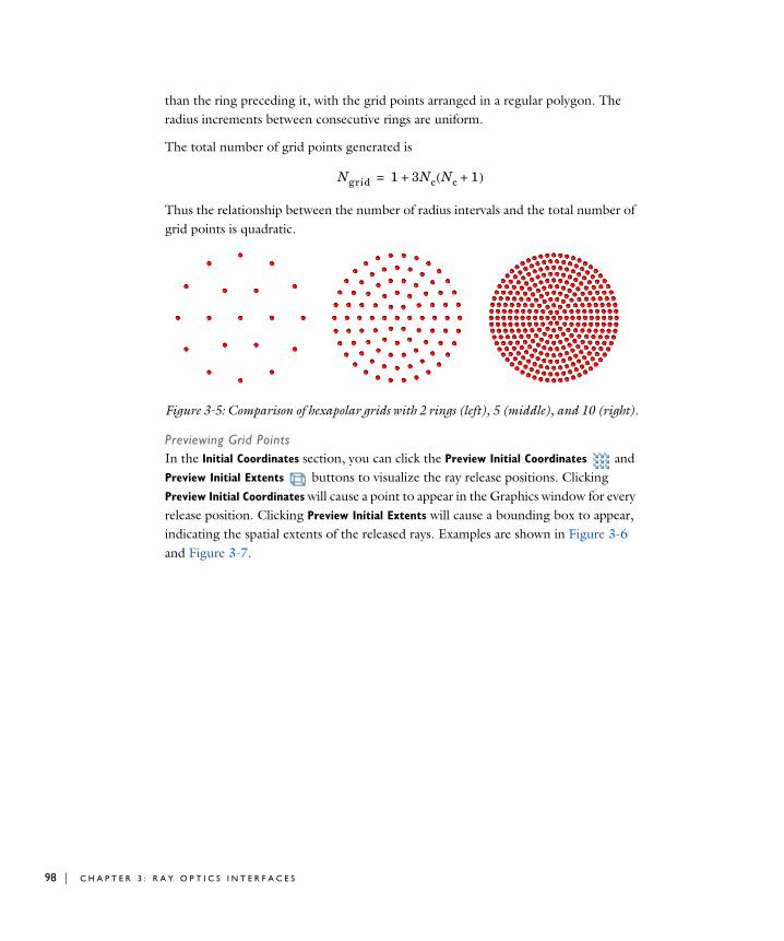
98 | C H A P T E R

than the ring preceding it, with the grid points arranged in a regular polygon. The radius increments between consecutive rings are uniform.

The total number of grid points generated is

Thus the relationship between the number of radius intervals and the total number of grid points is quadratic.

Figure 3-5: Comparison of hexapolar grids with 2 rings (left), 5 (middle), and 10 (right).

Previewing Grid PointsIn the Initial Coordinates section, you can click the Preview Initial Coordinates and Preview Initial Extents buttons to visualize the ray release positions. Clicking Preview Initial Coordinates will cause a point to appear in the Graphics window for every release position. Clicking Preview Initial Extents will cause a bounding box to appear, indicating the spatial extents of the released rays. Examples are shown in Figure 3-6 and Figure 3-7.

Ngrid 1 3Nc Nc 1+( )+=


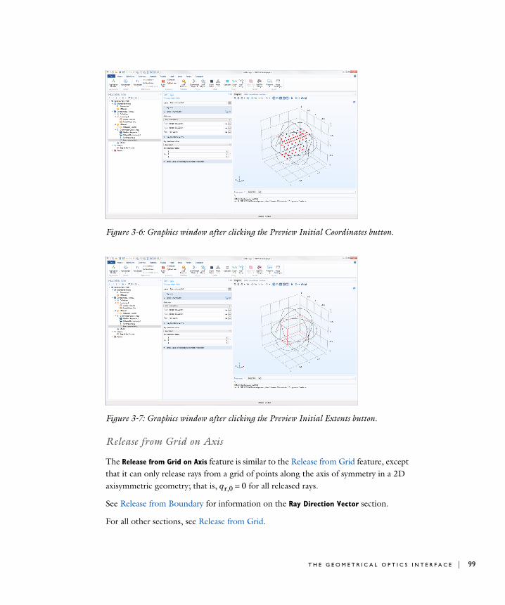
Figure 3-6: Graphics window after clicking the Preview Initial Coordinates button.

Figure 3-7: Graphics window after clicking the Preview Initial Extents button.

Release from Grid on Axis

The Release from Grid on Axis feature is similar to the Release from Grid feature, except that it can only release rays from a grid of points along the axis of symmetry in a 2D axisymmetric geometry; that is, qr,0 = 0 for all released rays.

See Release from Boundary for information on the Ray Direction Vector section.

For all other sections, see Release from Grid.


100 | C H A P T E

Release from Data File

Use a Release from Data File node to specify the initial ray position, direction, and values of auxiliary dependent variables using data from a text file.


Frequency, Vacuum Wavelength, Initial Phase, Initial Intensity, Initial Radii of Curvature, Total Source Power, and Initial Polarization.

Formatting Guidelines for Files Containing Ray DataThe imported data file should be a text file (*.txt) arranged in a spreadsheet format; that is, each row corresponds to a distinct ray and should have the same number of columns as all other rows. Columns can be separated by spaces, tabs, or a combination of the two. Begin a line with the percent (“%”) character to include comments or empty lines in the data file.

For example, a data file containing the following text would release rays at the positions (0.1, 0.2, 0.6) and (0.2, 0.4, 0.8) in a three-dimensional geometry:

% Ray release positions% qx0 qy0 qz00.1 0.2 0.60.2 0.4 0.8


Browse your computer to select a text file, then click Import to import the data. To remove the imported data, click Discard. Enter the Index of first column containing

position data i to indicate which column represents the first coordinate of the ray position vectors. The default value, 0, indicates the first column.


Select an option from the Ray direction vector list: Expression (the default), From file, Spherical, Hemispherical, Conical, or Lambertian (3D only).

• For From file, enter the Index of first column containing velocity data i. The default is 3. The columns are zero-indexed; that is, an index of 0 corresponds to the first column.

• For all other settings, the settings are the same as for the Release node.

I N I T I A L V A L U E O F A U X I L I A R Y D E P E N D E N T V A R I A B L E S


R 3 : R A Y O P T I C S I N T E R F A C E S

For each of the active Auxiliary Dependent Variable nodes in the model, choose an option from the Distribution function list: From file, None (the default), Normal, Lognormal, Uniform, or List of Values.

• When From file is selected, enter the Index of column containing data. The default value is 3. The columns are zero-indexed; that is, an index of 0 corresponds to the first column.

For all other options, the settings are the same as for the Release node.

Photometric Data Import

Use the Photometric Data Import node to import photometric data files that can be used to initialize the ray intensity and power as a function of the initial ray direction. The Photometric Data Import node supports the *.ies file extension, the standard photometric data file format of the Illuminating Engineering Society of North America (IESNA).

P H O T O M E T R I C D A T A I M P O R T

Enter a File name, or click the Browse button to locate a photometric data file. When a valid file path has been entered, click the Import button to load the photometric data into the model. A shortened version of the name of the photometric data file will then be displayed, along with a Discard button. Click the Discard button to discard the loaded photometric data and clear the File name field.

Photometric Data FormattingThe format of the imported photometric data file must be consistent with ANSI/IESNA LM-63-02 (R2008), IESNA Standard file format for the electronic transfer of photometric data and related information, Illuminating Engineering Society (2002).

The Photometric Data Import node is only available in 3D, and only if the ray intensity is solved for in the model.


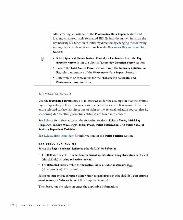
102 | C H A P T E

Illuminated Surface

Use the Illuminated Surface node to release rays under the assumption that the emitted rays are specularly reflected from an external radiation source. It is assumed that the entire selected surface has direct line of sight to the external radiation source; that is, shadowing due to other geometric entities is not taken into account.


Frequency, Vacuum Wavelength, Initial Phase, Initial Polarization, and Initial Value of

Auxiliary Dependent Variables.

See Release from Boundary for information on the Initial Position section.


Select the Rays to release: Reflected (the default) or Refracted.

• For Reflected select the Reflection coefficient specification: Using absorption coefficient (the default) or Using refractive indices.

• For Refracted enter a value for Refractive index of exterior domains next (dimensionless). The default is 1.

Select an Incident ray direction vector: User-defined direction (the default), User-defined

point source, or Solar radiation (3D components only).

Then based on the selection enter the applicable information:

After creating an instance of the Photometric Data Import feature and loading an appropriately formatted IES file into the model, initialize the ray intensity as a function of initial ray direction by changing the following settings in a ray release feature such as the Release or Release from Grid feature:

• Select Spherical, Hemispherical, Conical, or Lambertian from the Ray

direction vector list in the physics feature Ray Direction Vector section.

• Locate the Total Source Power section. From the Intensity initialization list, select an instance of the Photometric Data Import feature.

• Enter values or expressions for the Photometric horizontal and Photometric zero directions.


For User-defined direction enter the components of the Incident ray direction vector Li (dimensionless) based on space dimension.

• For User-defined point source enter the Point source location rsrc (SI unit: m).

• For Solar radiation see Solar Radiation for information about the options.

A N G U L A R P E R T U R B A T I O N S

If User-defined direction or Solar radiation is selected from the Incident ray direction

vector list, you can include small perturbation factors designed to take the finite size of the sun (or another light source) into account. Select an option from the Corrections

for finite source diameter list: None (the default), Create light cones at release points, or Sample from conical distribution.

• For None no perturbation to the initial ray direction is applied.

• For Create light cones at release points a cone-shaped distribution of rays is released at each point. Enter a value for the Number of rays in wave vector space (dimensionless) Nw (dimensionless). The default is 50. A cone-shaped distribution containing Nw rays is released at each point, which may cause a very large number of rays to be released.

• For Sample from conical distribution a single ray is released at each release point. This ray is given a random perturbation with uniform probability density within a cone-shaped distribution in wave vector space.

For Create light cones at release points and Sample from conical distribution, specify the Maximum disc angle Ψm (SI unit: rad). The default is 4.65 mrad, approximately the size of the solar disc when viewed from Earth.

For Create light cones at release points and Sample from conical distribution, select a Limb

darkening model: None (the default), Empirical power law, Linear, or User defined. The limb darkening model reduces the intensity of solar radiation that is released from the periphery of the solar disk, relative to radiation that is released near the center. For Linear enter a Limb darkening coefficient β (dimensionless). The default value is 0.8. For User defined enter a Limb darkening coefficient fL (dimensionless). The default value is 1.

Select the Include surface roughness check box to include an additional perturbation term based on uncertainty in the orientation of the surface normal, which is common in imperfect reflecting surfaces. Enter a value or expression for the Surface slope error σφ (SI unit: rad). The default is 1 mrad. The surface normal is then perturbed by a random angle, which is sampled from a Rayleigh distribution.


104 | C H A P T E

I N C I D E N T R A Y I N T E N S I T Y

This section is available when the ray intensity is solved for. Enter a value for the Incident ray intensity Ii (SI unit: W/m2). The default is 1000 W/m2.

T O T A L S O U R C E P O W E R

This section is available:

• when the ray intensity is solved for, and

• when Spherical, Hemispherical, or Conical is selected as the Ray direction vector.

• It is also available when the ray power is solved for, and then any choice of Ray

direction vector displays this section.

Enter a Total source power Psrc (SI unit: W). The default is 1 W. In 2D, instead enter the Total source power per unit thickness Psrc (SI unit: W/m). The default is 1 W/m.

Solar Radiation

The Solar Radiation node uses the solar position to specify the initial direction vector of rays. The node is selected from the Physics toolbar, Global menu.


Frequency, Vacuum Wavelength, Initial Phase, and Initial Value of Auxiliary Dependent

Variables.

Illuminated Surface Theory

The following examples involve buildings or other objects being illuminated by solar radiation in a specific direction:

• Solar Dish Receiver: Application Library path Ray_Optics_Module/

Solar_Radiation/solar_dish_receiver

• Vdara® Caustic Surface: Application Library path Ray_Optics_Module/Solar_Radiation/vdara_caustic_surface



These settings are the same as for the Release from Grid node.

S O U R C E

Select an option from the Location defined by list: Coordinates (the default) or City.

For City select a predefined city and country combination from the list. Click to select the Include daylight saving time (Time zone + 1) check box to add one hour to the default setting for the city selected. For example, if New York City, USA is selected and the default standard time zone is UTC −5 hours. If the check box is selected, the daylight savings time is used instead (UTC −4 hours). This feature does not automatically deduce whether daylight savings should be applied based on the selected city and date; you must specify it explicitly.

If Coordinates is selected, or your city is not listed, in the Location table define the:

• Latitude, a decimal value, positive in the northern hemisphere (the default is Las Vegas, USA latitude, 36.1). Enter a value without a unit to avoid double conversion. This is because the latitude value is expected to represent degrees but the model’s unit for angles may be different (for example, the SI unit for the angle is radians).

• Longitude, a decimal value, positive at the East of the Prime Meridian (the default is Las Vegas, USA longitude, −115.2). Enter a value without a unit to avoid double conversion. This is because the latitude value is expected to represent degrees but the model’s unit for angles may be different (for example, the SI unit for the angle is radians).

• Time zone, the number of hours to add to UTC to get local time (the default is Las Vegas, USA time zone, −8). For example in New York City, USA the time zone is UTC −5 hours (standard time zone) or UTC −4 hours (with daylight savings time).

For either selection, in the Date table enter the:

• Day, the default is 01. Enter a value without a unit to avoid double conversion. This is because the value is expected to represent days but the model’s unit for time may be different (for example, the SI unit for time is second).

North, West, and the up directions correspond to the x, y, and z directions, respectively.


106 | C H A P T E

• Month, the default is 10 (October). Enter a value without a unit to avoid double conversion. This is because the value is expected to represent months but the model’s unit for time may be different (for example, the SI unit for time is second).

• Year, the default is 2014. Enter a value without a unit to avoid double conversion. This is because the value is expected to represent years but the model’s unit for time may be different (for example, the SI unit for time is second). The solar position is accurate for a date between 2000 and 2199.

For either selection, in the Local time table enter the:

• Hour, the default is 12. Enter a value without a unit to avoid double conversion. This is because the value is expected to represent hours but the model’s unit for time may be different (for example, the SI unit for time is second).

• Minute, the default is 0. Enter a value without a unit to avoid double conversion. This is because the value is expected to represent minutes but the model’s unit for time may be different (for example, the SI unit for time is second).

• Second, the default is 0.

For either selection, in the Solar irradiance field Is (SI unit: W/m2) define the incident radiative intensity coming from the sun.

A N G U L A R P E R T U R B A T I O N S

Select an option from the Corrections for finite source diameter list: None (the default), Create light cones at release points, or Sample from conical distribution.

• For None no perturbation to the initial ray direction is applied.

• For Create light cones at release points a cone-shaped distribution of rays is released at each point. Enter a value for the Number of rays in wave vector space

The sun position is updated if the location, date, or local time changes during a simulation. Because the time scale of ray propagation is typically many orders of magnitude smaller than the time scale for significant changes in solar position, modeling ray propagation at different times of day typically requires a Parametric Sweep over the larger time scale. Note that no validity range is prescribed on the time inputs. It is possible to enter values that exceed the expected boundary. For example, entering 5h 2min 81s is equivalent to 5h 3min 21s. This makes it easier, for example, to run a Parametric Sweep over the time of day using only a single parameter.


(dimensionless) Nw (dimensionless). The default is 50. A cone-shaped distribution containing Nw rays is released at each point, which may cause a very large number of rays to be released.

• For Sample from conical distribution a single ray is released at each release point. This ray is given a random perturbation with uniform probability density within a cone-shaped distribution in wave vector space.

For Create light cones at release points and Sample from conical distribution, specify the Maximum disc angle Ψm (SI unit: rad). The default is 4.65 mrad.

For Create light cones at release points and Sample from conical distribution, select a Limb

darkening model: None (the default), Empirical power law, Linear, or User defined. The limb darkening model is typically used to reduce the intensity of solar radiation that is released from the periphery of the solar disk, relative to radiation that is released near the center. For Linear enter a Limb darkening coefficient β (dimensionless). The default value is 0.8. For User defined enter a Limb darkening coefficient fL (dimensionless). The default value is 1.

Ray Termination

Use the Ray Termination feature to remove rays from the model as they exit the geometry, or to annihilate rays of sufficiently low intensity or power. Only one Ray

Termination node can be added to the model, but it is possible to combine position-based and intensity-based criteria for removing rays if the ray intensity or power is computed by the model.

T E R M I N A T I O N C R I T E R I A

Select an option from the Spatial extents of ray propagation list: Bounding box, from

geometry (the default), Bounding box, user defined, or None. This list controls whether rays are terminated based on their positions.

• For Bounding box, from geometry, a ray is immediately terminated if it reaches the surface of the bounding box of the geometry, defined as the smallest rectangle or rectangular prism with edges parallel to the axes of the global coordinate system that encloses all of the geometric entities. This bounding box is extended by 5% in each direction so that rays can still interact with boundaries that coincide with the

The options for accounting for finite source diameter and solar limb darkening are discussed in the Illuminated Surface Theory section.


108 | C H A P T E

perimeter of the bounding box. Therefore rays can propagate a short distance away from the geometry before disappearing.

• For Bounding box, user defined, a ray is immediately terminated if it reaches the surface of a box of user-specified dimensions. To define the box, enter maximum and minimum values of each spatial coordinate.

• For None, the rays that propagate outward from the geometry will continue to propagate until the study is complete. If the maximum path length for the Ray Tracing study step is too large, this may result in trajectories that are extremely long relative to the characteristic geometry size.

If rays are released from outside the bounding box, they won’t immediately disappear; instead, they will only disappear if they enter the bounding box and then exit it again.

Intensity- and Power-Based Termination CriteriaIf the ray intensity or power is being computed in the model, you can then terminate rays based on either or both of these quantities.

Select an option from the Additional termination criteria list. None (the default) is always available. If ray intensity is solved for, then Intensity is available. If ray power is solved for, then Power is available. If both ray intensity and power are solved for, the Intensity

and Power option is also shown.

• For Intensity or Intensity and power, enter the Threshold intensity Ith (SI unit: W/m2). The default is 1 mW/m2. Rays will be removed from the model if their intensity decreases below the specified value.

• For Power or Intensity and power, enter the Threshold power Qth (SI unit: W). The default is 10-3 mW.


Release from Electric Field

Use the Release from Electric Field node to release rays from selected boundaries, with initial intensity and polarization based on the incident electric field at that boundary. The electric field may be user defined or solved for in a previous study.

See Release for information on the Initial Values of Auxiliary Dependent Variables section and the optional Release Times section. See Release from Boundary for information on the Initial Position section.


The rays are always released in a direction normal to the selected boundaries. Select the Reverse direction check box to release rays in the normal direction on the opposite side of the selected boundaries. The direction of the released rays is indicated by an arrow in the Graphics window.

The Ray Termination feature can terminate rays at the exact time at which their intensity or power reaches the specified threshold (to within numerical precision), if there exists a closed-form analytic expression for this time. Such a closed-form analytic solution exists if:

• The rays represent planar wavefronts in an absorbing medium, or

• The rays represent spherical or ellipsoidal wavefronts in a nonabsorbing medium.

Otherwise, the rays are stopped at the first discrete time step taken by the solver for which the intensity or power is less than the threshold value.

Ray Termination Theory

This feature is only available if the ray intensity or power is solved for. Select an appropriate option from the Intensity computation list in the physics interface Intensity Computation section.


110 | C H A P T E

I N C I D E N T E L E C T R I C F I E L D

Enter values or expressions in the table for the Electric field E (SI unit: V/m) based on space dimension. If the electric field is computed by another physics interface then it can be selected from the list.

The Use frequency from the coupled physics interface as the ray frequency check box is cleared by default. If this check box is cleared, the wavelength or frequency of the released rays may be specified depending on the option selected from the Wavelength

distribution of released rays list in the physics interface Ray Release and Propagation section:

• If Polychromatic, specify vacuum wavelength is selected, enter the Vacuum wavelength λ0 (SI unit: m). The default is 660 nm.

• If Polychromatic, specify frequency is selected, enter the Ray frequency ν (SI unit: 1/s). The default is 4.54 × 1014 Hz.

If this check box is selected, then the frequency or wavelength of the released rays will be determined by the Frequency Domain or Wavelength Domain study in the Values of

Variables not Solved For section of the Time Dependent solver settings. Typically this Frequency Domain or Wavelength Domain study would first be used to solve for the electric field, using either the Electromagnetic Waves, Frequency Domain interface or the Electromagnetic Waves, Beam Envelopes interface.

Selecting this check box may also cause the frequency or wavelength specified in the Ray Properties node to be ignored while the Release from Electric Field node is active.

In the Geometrical Optics interface, ray intensity is stored in the Stokes parameters for each ray. For more information, see Intensity, Wavefront Curvature, and Polarization in Theory for the Geometrical Optics Interface.

Ray Release Based on a Plane Electromagnetic Wave: Application Library path Ray_Optics_Module/Tutorials/plane_em_wave_to_ray_release


Release from Far-Field Radiation Pattern

Use the Release from Far-Field Radiation Pattern node to release rays with an intensity and power distribution based on a far-field radiation pattern. The far-field radiation pattern must first be solved for in a previous study.

The Release from Far-Field Radiation Pattern node can be used for multiscale electromagnetics modeling. First, the Electromagnetic Waves, Frequency Domain interface should be used to compute the electric field in the immediate vicinity of a radiation source, such as an antenna or waveguide. The Far-Field Domain node and its default subnode, Far-Field Calculation, should be added to this instance of the Electromagnetic Waves, Frequency Domain interface. In this wavelength-scale model, the mesh must be fine enough to resolve individual oscillations of the electric field, fulfilling the Nyquist criterion. Typically this requires 10 linear elements or 5 second-order elements per wavelength.

Then, in the same model component or a different component, the Geometrical Optics interface can be used to extend the far field over an arbitrarily large number of wavelengths, because the ray tracing approach does not require a finite element mesh fine enough to resolve individual oscillations of the electric field.

The Release from Far-Field Radiation Pattern node is only available in 3D. However, the far-field function is uses to initialize the ray intensity and polarization can be defined either in a 3D model component or a 2D axisymmetric model component. If the previous model component was a 2D axisymmetric component, the intensity distribution of released rays will also be assumed to be axisymmetric.

See Release for information on the Initial Values of Auxiliary Dependent Variables section and the optional Release Times section.


Select an option from the Grid type list: All combinations (the default) or Specified

combinations.

This feature requires at least one of the following licenses: RF Module, Wave Optics Module.

In addition, this feature is only available if the ray intensity or power is solved for. Select an appropriate option from the Intensity computation list in the physics interface Intensity Computation section.


112 | C H A P T E

Linear, Rectangular, and Arbitrary GridsEnter Initial coordinates based on space dimension (qx,0, qy,0, and qz,0) for the ray positions or click the Range button ( ) to select and define a range of specific coordinates.

If Specified combinations is selected, the number of initial coordinates entered for each space dimension must be equal, and the total number of rays released is equal to the length of one of the lists of initial coordinates. If All combinations is selected, the total number of rays released is equal to the product of the lengths of each list of initial coordinates.


Select an option from the Ray direction vector list: Spherical (the default), Hemispherical, or Conical.

• For Spherical a number of rays are released at each point, sampled from a spherical distribution in wave vector space. Enter the Number of rays in wave vector space Nw (dimensionless). The default is 50.


vector space Nw (dimensionless). The default is 50. Then enter coordinates for the Hemisphere axis r based on space dimension.

• For Conical a number of rays are released at each point, sampled from a conical distribution in wave vector space. Enter the Number of rays in wave vector space Nw (dimensionless). The default is 50. Then enter coordinates for the Cone axis r based on space dimension. Then enter the Cone angle α (SI unit: rad). The default is π/3 radians.

Note that unlike the Release from Grid feature, the options Expression and Lambertian are not available here. In addition, if Conical is selected, the cone must be isotropic. This is because each ray is assumed to subtend approximately the same solid angle, so direction distributions that give unequal weight to some directions (like Lambertian) or options with no direction distribution at all (like Expression) cannot initialize the ray intensity and power in a consistent and physically meaningful way.

F A R - F I E L D V A R I A B L E N A M E

Enter an expression for the Far-field variable name. The default expression is Efar. This expression must match the variable name in a corresponding Far-Field Calculation feature.


S O U R C E O R I E N T A T I O N

Use the settings in this section to orient the ray source. This allows, for example, the release of rays from an antenna to be modeled with the antenna oriented in many different directions, while only solving for the far-field radiation pattern once.

Enter the Euler angles (Z-X-Z). The labels Z-X-Z indicate the order in which rotation about the different axes is performed. First, the local coordinate system of the radiation pattern is rotated about its Z-axis by the angle α. Then it is rotated about its X-axis (which is now at an angle α to the global x-axis) by the angle β. Finally, this local coordinate system is rotated about its new Z-axis by the angle γ. All three inputs are plane angles (SI unit: rad) with default values of 0.


This section is only shown if Monochromatic is selected from the Wavelength distribution

of released rays list in the physics interface Ray Release and Propagation section.

The Use frequency from the far-field calculation as the ray frequency check box is selected by default. While this check box is selected and the Release from Far-Field Radiation

Pattern feature is active, the frequency or vacuum wavelength of released rays will be determined by the Frequency Domain or Wavelength Domain study in the Values of

Variables not Solved For section of the Time Dependent solver settings. Usually, this previous study was used to solve for the far-field radiation pattern using the Electromagnetic Waves, Frequency Domain interface.

While this check box is selected and the Release from Far-Field Radiation Pattern node is active, the frequency or wavelength specified in the Ray Properties node is ignored.

In the Geometrical Optics interface, ray intensity is stored in the Stokes parameters for each ray. For more information, see Intensity, Wavefront Curvature, and Polarization in the theory section.

Ray Release from a Dipole Antenna Source (3D): Application Library path Ray_Optics_Module/Tutorials/

ray_release_from_dipole_antenna_source_3d

Ray Release from a Dipole Antenna Source (2D Axisymmetric): Application Library path Ray_Optics_Module/Tutorials/

ray_release_from_dipole_antenna_source_2daxi


114 | C H A P T E

Grating

Use the Grating node to treat a boundary as a diffraction grating that can release reflected and transmitted rays into multiple diffraction orders. A Diffraction Order (Grating) subnode for reflected and transmitted rays of order m = 0 is added by default. Change the settings for this default subnode to release rays of a different diffraction order. You can also release rays of multiple diffraction orders from the same boundary by adding more Diffraction Order subnodes from the from the context menu (right-click the parent node) or from the Physics toolbar, Attributes menu.

The Accumulator (Boundary) subnode is also available from the context menu (right-click the parent node) or from the Physics toolbar, Attributes menu.

Releasing Secondary RaysWhen two or more rays are released from a Grating boundary, one of the released rays uses the same degrees of freedom as the incident ray. The remaining degrees of freedom must be preallocated in memory as secondary rays. The total number of secondary rays that can be released in the model is controlled by the Maximum number

of secondary rays field in the physics interface Ray Release and Propagation section.

For example, if both reflected and transmitted rays of diffraction orders m = −1, m = 0, and m = 1 are released from a boundary, then for every incident ray, a total of five secondary rays are released. If the diffraction order m = −1 is the first subnode to appear in the Model Builder, then the transmitted ray of order m = −1 uses the same degree of freedom as the incident ray, and the other rays are secondary rays. If the Maximum number of secondary rays is 500 and more than 100 rays interact with the grating, then no more secondary rays are emitted and a warning is generated by the solver, indicating that the Maximum number of secondary rays should be increased.

D E V I C E P R O P E R T I E S

Select an option from the Rays to release list: Reflected and transmitted (the default), Reflected, or Transmitted. Then enter the a Grating constant d (SI unit: m), which is the distance between consecutive lines in the grating, i.e. the length of one unit cell. The default is 5 µm.

Select Use relative order numbers if the grating blaze angle is known, and diffraction into the highest-efficiency orders is desired. Then enter the Grating blaze angle θB (SI unit: rad). The default is 0. The absolute order number will be computed based on the blaze angle and the refractive indices of the adjacent domains.


If Use relative order numbers is not selected, then the Automatic Diffraction Order

Calculation section will be present. This will be discussed below.

If the ray power is solved for, the Store total transmitted power and Store total reflected

power check boxes are shown. Select them to declare auxiliary dependent variables for the total power of all transmitted and reflected diffraction orders, respectively.

G R A T I N G O R I E N T A T I O N

In 2D, select an option from the Direction of periodicity list: Forward (the default) or Reverse. For either setting, an arrow appears in the Graphics window, lying tangent to the selected edges. Reflected and refracted rays from positive diffraction orders have a larger ray direction component in the direction of this arrow, compared to rays from negative diffraction orders.

In 3D, select an option from the Grating orientation list: Specify direction of periodicity

(the default) or Specify direction of grating lines.

• If Specify direction of periodicity is selected, select an option from the Direction of

periodicity list: User defined (the default) or Parallel to reference edge. For User

defined enter the components of the direction of periodicity Tp (dimensionless) directly. The default is the positive x-axis. For Parallel to reference edge, the Reference

Edge Selection section is shown in the Settings window. Select a single edge, which must be adjacent to at least one boundary in the selection for the Grating feature.

• If Specify direction of grating lines is selected, select an option from the Direction of

grating lines list: User defined (the default) or Parallel to reference edge. For User

defined enter the components of the direction of grating lines Tl (dimensionless) directly. The default is the positive y-axis. For Parallel to reference edge, the Reference

Edge Selection section is shown in the Settings window. Select a single edge, which must be adjacent to at least one boundary in the selection for the Grating feature.

Regardless of how Tp or Tl has been specified, the direction of periodicity projected onto the grating surface Tg will be computed. This is shown in Figure 3-8 for 2D and Figure 3-9 for 3D.


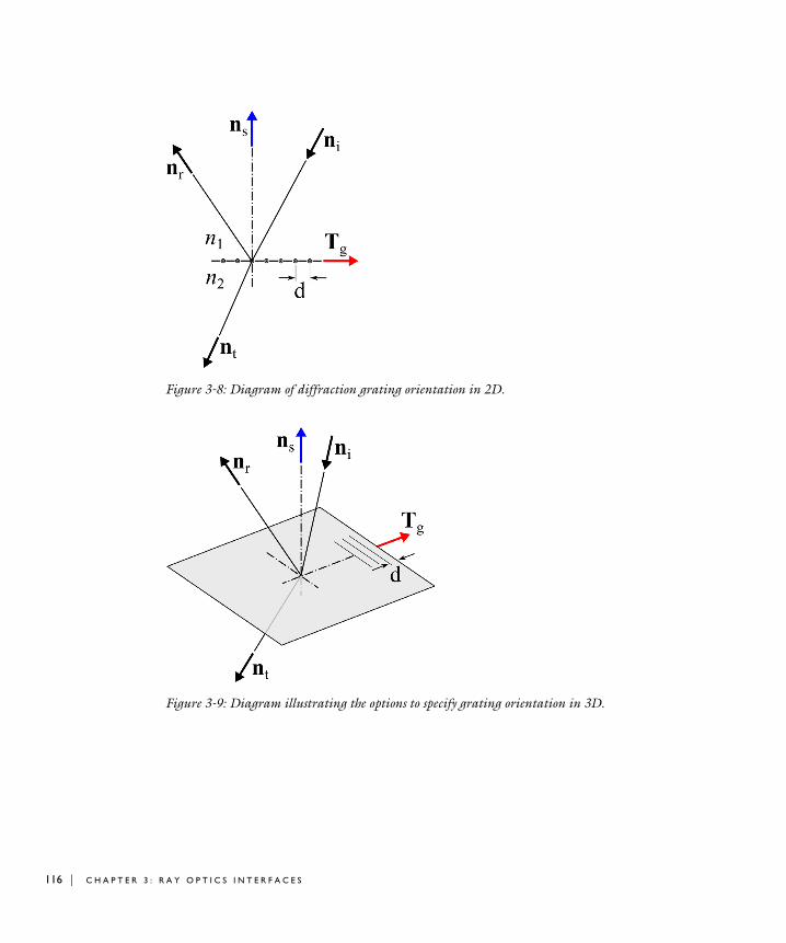
116 | C H A P T E

Figure 3-8: Diagram of diffraction grating orientation in 2D.

Figure 3-9: Diagram illustrating the options to specify grating orientation in 3D.


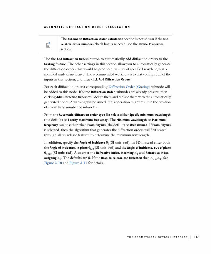
A U T O M A T I C D I F F R A C T I O N O R D E R C A L C U L A T I O N

Use the Add Diffraction Orders button to automatically add diffraction orders to the Grating feature. The other settings in this section allow you to automatically generate the diffraction orders that would be produced by a ray of specified wavelength at a specified angle of incidence. The recommended workflow is to first configure all of the inputs in this section, and then click Add Diffraction Orders.

For each diffraction order a corresponding Diffraction Order (Grating) subnode will be added to this node. If some Diffraction Order subnodes are already present, then clicking Add Diffraction Orders will delete them and replace them with the automatically generated nodes. A warning will be issued if this operation might result in the creation of a very large number of subnodes.

From the Automatic diffraction order type list select either Specify minimum wavelength

(the default) or Specify maximum frequency. The Minimum wavelength or Maximum

frequency can be either taken From Physics (the default) or User defined. If From Physics

is selected, then the algorithm that generates the diffraction orders will first search through all ray release features to determine the minimum wavelength.

In addition, specify the Angle of incidence θi (SI unit: rad). In 3D, instead enter both the Angle of incidence, in plane θi,in (SI unit: rad) and the Angle of incidence, out of plane θi,out (SI unit: rad). Also enter the Refractive index, incoming n1 and Refractive index,

outgoing n2. The defaults are 0. If the Rays to release are Reflected then n2 = n1. See Figure 3-10 and Figure 3-11 for details.

The Automatic Diffraction Order Calculation section is not shown if the Use

relative order numbers check box is selected; see the Device Properties section.


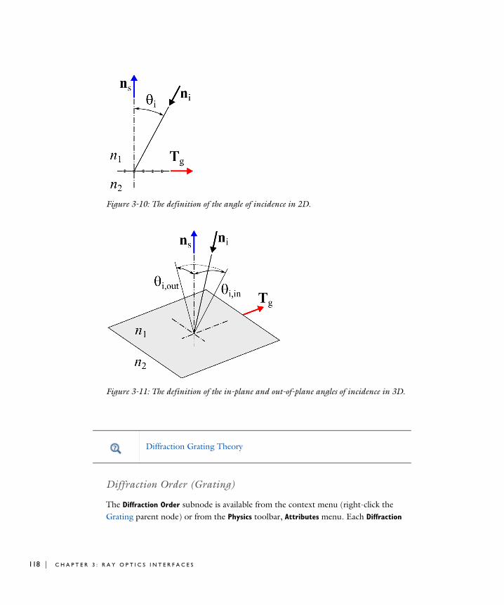
118 | C H A P T E

Figure 3-10: The definition of the angle of incidence in 2D.

Figure 3-11: The definition of the in-plane and out-of-plane angles of incidence in 3D.

Diffraction Order (Grating)

The Diffraction Order subnode is available from the context menu (right-click the Grating parent node) or from the Physics toolbar, Attributes menu. Each Diffraction

Diffraction Grating Theory


Order subnode can either release transmitted rays, reflected rays, or both transmitted and reflected rays of a specified diffraction order, depending on the option selected from the Rays to release list in the parent Grating node.


If the Use relative order numbers is not selected in the settings for the parent Grating node, then enter a Diffraction order m (dimensionless). The default is m = 0 for the first Diffraction Order added. When more diffraction orders are added to the model, the new default is the highest diffraction order currently present, plus 1.

If Use relative order numbers is selected in the settings for the parent Grating node, then enter a Relative diffraction order Δm (dimensionless). As above, the default is Δm = 0 if no other Diffraction Order subnode exists; otherwise the default is 1 greater than the highest relative order that is currently present.

When the ray intensity or power is solved for, enter the Reflectance R and the Transmittance T (both dimensionless). If the reflectance or transmittance of a certain diffraction order is exactly zero, that diffraction order will not be released.


This section is available if an Auxiliary Dependent Variable has been added to the model. The settings are the same as for the Material Discontinuity feature.



Cross Grating

Use the Cross Grating node to treat a boundary as a diffraction grating that can release reflected and transmitted rays into multiple diffraction orders. Unlike a standard Grating, a Cross Grating can have two directions of periodicity; the boundary is treated

If relative order numbers are being used then the absolute order number can be tracked using an auxiliary dependent variable.

This feature is only available in 3D.


120 | C H A P T E

as a general two-dimensional periodic substructure. A Diffraction Order (Cross Grating) subnode for reflected and transmitted rays in order m = n = 0 is added by default. Change the settings for this default subnode to release rays into different diffraction orders. You can also release rays of multiple diffraction order pairs from the same boundary by adding more Diffraction Order subnodes from the from the context menu (right-click the parent node) or from the Physics toolbar, Attributes menu.

The Accumulator (Boundary) subnode is also available from the context menu (right-click the parent node) or from the Physics toolbar, Attributes menu.

Releasing Secondary RaysWhen two or more rays are released from a Cross Grating boundary, one of the released rays uses the same degrees of freedom as the incident ray. The remaining degrees of freedom must be preallocated in memory as secondary rays. The total number of secondary rays that can be released in the model is controlled by the Maximum number

of secondary rays field in the physics interface Ray Release and Propagation section. See the Grating feature for further details.


Select an option from the Rays to release list: Reflected and transmitted (the default), Reflected, or Transmitted. Then enter the Grating constant, direction 1 d1 (SI unit: m) and the Grating constant, direction 2 d2 (SI unit: m). The defaults are d1 = 1 μm and d2 = 2 μm.

If the ray power is solved for, the Store total transmitted power and Store total reflected

power check boxes are shown. Select them to declare auxiliary dependent variables for the total power of all transmitted and reflected diffraction orders, respectively.

G R A T I N G O R I E N T A T I O N

The Cross Grating requires two grating orientations to be specified. For each of Grating

orientation 1 and Grating orientation 2 select either Specify direction of periodicity (the default) or Specify direction of grating lines. The Grating orientation 2 may also be Orthogonal to grating orientation 1.

• If Specify direction of periodicity is selected, select an option from the Direction of

periodicity 1 (or 2) list: User defined (the default) or Parallel to reference edge. For User defined enter the components of the direction of periodicity Tp,1 or Tp,2 (dimensionless) directly. The defaults for Tp,1 and Tp,2 are the positive x-axis and positive y-axis respectively. For Parallel to reference edge, the Reference Edge

Selection, Direction 1 and/or Reference Edge Selection, Direction 2 sections are shown.


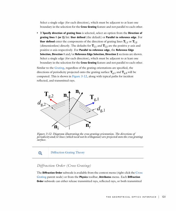
Select a single edge (for each direction), which must be adjacent to at least one boundary in the selection for the Cross Grating feature and not parallel to each other.

• If Specify direction of grating lines is selected, select an option from the Direction of

grating lines 1 (or 2) list: User defined (the default) or Parallel to reference edge. For User defined enter the components of the direction of grating lines Tl,1 or Tl,2 (dimensionless) directly. The defaults for Tl,1 and Tl,2 are the positive y-axis and positive x-axis respectively. For Parallel to reference edge, the Reference Edge

Selection, Direction 1 and/or Reference Edge Selection, Direction 2 sections are shown. Select a single edge (for each direction), which must be adjacent to at least one boundary in the selection for the Cross Grating feature and not parallel to each other.

Similar to the Grating, regardless of the grating orientations are specified, the directions of periodicity projected onto the grating surface Tg,1 and Tg,2 will be computed. This is shown in Figure 3-12, along with typical paths for incident reflected, and transmitted rays.

Figure 3-12: Diagram illustrating the cross grating orientation. The directions of periodicity and/or lines (which need not be orthogonal) are projected onto the cross grating surface.

Diffraction Order (Cross Grating)

The Diffraction Order subnode is available from the context menu (right-click the Cross Grating parent node) or from the Physics toolbar, Attributes menu. Each Diffraction

Order subnode can either release transmitted rays, reflected rays, or both transmitted



122 | C H A P T E

and reflected rays of the specified order, depending on the option selected from the Rays to release list in the parent Cross Grating node.


Enter the Diffraction orders m and n (dimensionless). The default is m = n = 0 for the first Diffraction Order subnode added. When more diffraction orders are added to the model, the new default created by adding 1 to either m or n, whichever is lowest. If m and n are equal, then m is incremented by 1.

When the ray intensity or power is solved for, enter the Reflectance R and the Transmittance T (both dimensionless). If the reflectance or transmittance of a certain diffraction order is exactly zero, that diffraction order will not be released.




This section is available if an Auxiliary Dependent Variable has been added to the model. The settings are the same as for the Material Discontinuity feature

Linear Polarizer

Use the Linear Polarizer node to define a linear polarizer on a boundary selection. Add this node from the Optical Devices submenu when ray intensity or power is solved for in the model. The Accumulator (Boundary) subnode is available from the context menu (right-click the parent node) or from the Physics toolbar, Attributes menu.


Select a Transmission axis specification:

• User defined (the default). Then enter coordinates for the Transmission axis T (dimensionless).

• Parallel to reference edge (for 3D components). The Reference Edge Selection section is then shown. Add an edge to this selection to specify the transmission axis orientation. Only a single edge may be selected. The edge must be adjacent to a boundary in the physics feature selection.

• In-plane or Out-of-plane (for 2D and 2D axisymmetric components)



This section is available if an Auxiliary Dependent Variable has been added to the model. The settings are the same as for the Wall feature.

Ideal Depolarizer

Use the Ideal Depolarizer node to reinitialize the Stokes parameters so that the outgoing ray is completely unpolarized. Add this node from the Optical Devices submenu when ray intensity or power is solved for in the model. The Accumulator (Boundary) subnode is available from the context menu (right-click the parent node) or from the Physics toolbar, Attributes menu.



Linear Wave Retarder

Use the Linear Wave Retarder node to define a linear wave retarder on a boundary selection. Add this node from the Optical Devices submenu when ray intensity or power is solved for in the model. The Accumulator (Boundary) subnode is available from the context menu (right-click the parent node) or from the Physics toolbar, Attributes menu.


Select a Fast axis specification:

• User defined (the default). Then enter coordinates for the Fast axis F (dimensionless).

• Parallel to reference edge (for 3D components). The Reference Edge Selection section is then shown. Add an edge to this selection to specify the fast axis orientation. Only

Linear Polarizer Theory

Ideal Depolarizer Theory


124 | C H A P T E

a single edge may be selected. The edge must be adjacent to a boundary in the physics feature selection.

• In-plane or Out-of-plane (for 2D and 2D axisymmetric components)

For any selection, enter a value for the Retardance δ (SI unit: rad).



Circular Wave Retarder

Use the Circular Wave Retarder node to define a circular wave retarder on a boundary selection. Add this node from the Optical Devices submenu when ray intensity or power is solved for in the model. The Accumulator (Boundary) subnode is available from the context menu (right-click the parent node) or from the Physics toolbar, Attributes menu.


Enter a value for the Retardance δ (SI unit: rad).

By default the Sense of rotation depends on ray trajectory check box is not selected. This means a positive value of the retardance always corresponds to clockwise rotation of the polarization ellipse. Select the check box then a positive value of the retardance corresponds to clockwise rotation of the polarization ellipse only when the ray crosses the boundary in the direction indicated by the normal vector in the Graphics window.

The Reverse sense of rotation check box is available when the Sense of rotation depends

on ray trajectory check box is selected. Click to select this check box to reverse the direction of the normal vector shown in the Graphics window.

Linear Wave Retarder Theory




Mueller Matrix

Use the Mueller Matrix node to define Mueller matrices for customized optical components. Add this node from the Optical Devices submenu when ray intensity or power is solved for in the model. The Accumulator (Boundary) subnode is available from the context menu (right-click the parent node) or from the Physics toolbar, Attributes menu.


Select a Reference axis specification:

• User defined (default). Enter coordinates for the Reference axis R (dimensionless).

• Parallel to reference edge (for 3D components). The Reference Edge Selection section is then shown. Add an edge to this selection to specify the reference direction orientation. Only a single edge may be selected. The edge must be adjacent to a boundary in the physics feature selection.

• In-plane or Out-of-plane (for 2D and 2D axisymmetric components).

For any choice, select Isotropic (the default), Diagonal, Symmetric, or Full from the list. Then enter a value or expression for the Mueller matrix M in the matrix or field.



Circular Wave Retarder Theory

Theory of Mueller Matrices and Optical Components


126 | C H A P T E

Deposited Ray Power (Domain)

The Deposited Ray Power node is used to compute a heat source based on the attenuation of rays as they propagate through a domain with a complex refractive index. This feature is available when the ray power is solved for. The Deposited Ray

Power node defines a dependent variable with default name <name>.Qsrc, where <name> is the name of the Geometrical Optics physics interface, for example gop.Qsrc.

Deposited Ray Power (Boundary)

When the ray power is solved for, the Deposited Ray Power subnode is available from the context menu (right-click the Wall, parent node) or from the Physics toolbar, Attributes menu. The Deposited Ray Power subnode computes the total incident energy flux on a surface based on the power of incident rays.

S M O O T H I N G

Select the Compute smoothed accumulated variable check box to enter a Smoothing

radius r (SI unit: m) The smoothing radius functions like the corresponding setting for the Accumulator (Boundary) node.

Accumulator (Domain)

Use the Accumulator node to define additional degrees of freedom on a domain. Each Accumulator defines a variable, called the accumulated variable, on each domain element in the selection list. The values of the accumulated variables are determined by the properties of rays in each domain element.

A C C U M U L A T O R S E T T I N G S

Select an Accumulator type: Density (default) or Count.

• For Density the accumulated variable is divided by the volume of the mesh element where it is defined.

• For Count the accumulated variable is unaffected by the element size.

Attenuation Within Domains


Select an option from the Accumulate over list: Elements (the default) or Elements and

time.

• For Elements the value of the accumulated variable in an element is the sum of the source terms of all rays in that element. If the Accumulator type is set to Density, this sum is divided by the mesh element volume.

• For Elements and time the time derivative of the accumulated variable in an element is the sum of the source terms of all rays in that element. If the Accumulator type is set to Density, this sum is divided by the mesh element volume. As each ray propagates through a series of mesh elements, it leaves behind a contribution to the accumulated variable that remains even after the ray has moved on.

Enter the Accumulated variable name. The default is rpd. The accumulated variable is defined as <name>.<varname>, where <name> is the physics interface name and <varname> is the accumulated variable name. For example, in an instance of the Geometrical Optics interface with default name gop and default accumulated variable name rpd, the variable would be named gop.rpd.

Enter a Source R. The unit of the source depends on the settings in the Units section. The source term is used to calculate the accumulated variable in a manner specified by the Accumulate over and Accumulator type settings.

If Elements and time is selected from the Accumulate over list, select an option from the Source interpolation list: Constant, Linear (the default), Quadratic, or Exponential. The Source interpolation determines what functional form the Source is assumed to follow during each time step taken by the solver. This information is used to compute the accumulated variable in mesh elements that the rays pass through during each time step.

U N I T S

Select a Dependent variable quantity from the list; the default is Dimensionless [1]. To enter a unit, select None from the list and in the Unit field enter a value, for example, K, m/s, or mol/m^3.

Accumulator (Boundary)

The Accumulator subnode is available from the context menu (right-click the Wall or Material Discontinuity parent node) or from the Physics toolbar, Attributes menu. Each Accumulator subnode defines a variable, called the accumulated variable, on each


128 | C H A P T E

boundary element in the selection of the parent node. The accumulated variables are incremented when rays interact with the boundaries where they are defined.


Select an option from the Accumulator type list: Density (default) or Count.

• For Density the accumulated variable is divided by the surface area of the boundary element where it is defined.

• For Count the accumulated variable is the sum of the source terms of all rays that hit the boundary element, and is unaffected by the boundary element size.

Select an option from the Accumulate over list: Ray-wall interactions (the default) or Rays in boundary elements.

• For Ray-wall interactions the accumulated variable is affected by all rays that hit the boundary element.

• For Rays in boundary elements the accumulated variable is only affected by rays that freeze or stick to the boundary element.

Enter the Accumulated variable name. The default is rpb. The accumulated variable is defined as <scope>.<name>, where <scope> includes the name of the physics interface node, parent boundary condition, and the Accumulator node, and <name> is the accumulated variable name.

For example, if the Accumulator subnode is added to a Wall node in an instance of the Geometrical Optics interface using the default variable name rpb, the accumulated variable name might be gop.wall1.bacc1.rpb.

Enter a Source R. The unit of the source term depends on the settings in the Units section. Whenever a ray collides with a boundary element in the selection of the parent node, the accumulated variable in that element is incremented by the source term. If the Accumulator type is set to Density, the source term is divided by the area of the boundary element (in 3D) or the length of the boundary element (in 2D).

For example, if the source is 1 and Count is selected from the Accumulator type list, a variable is created to store the number of times each boundary element is hit by a ray.

U N I T S

Select a Dependent variable quantity from the list; the default is Dimensionless [1]. To enter a unit, select None from the list and in the Unit field enter a value, for example, K, m/s, or mol/m^3.


S M O O T H I N G

The accumulated variables are computed using discontinuous shape functions. Select the Compute smoothed accumulated variable check box to compute a smoothed accumulated variable by computing the average value of the variable within a sphere of a user-defined radius. Then enter a Smoothing radius r (SI unit: m). The default is 1 m.

Nonlocal Accumulator

Use the Nonlocal Accumulator subnode to communicate information from a ray’s current position to the position from which it was released.

The subnode is available from the context menu (right-click the Release from Boundary parent node) or from the Physics toolbar, Attributes menu.

Each Nonlocal accumulator subnode defines a variable, called the accumulated variable, that is computed using variables defined on rays released by the parent Release from

Boundary node or on domains and boundaries encountered by such rays.


Select an Accumulator type: Density (default) or Count.

• For Density the accumulated variable is divided by the volume of the mesh element where it is defined.

• For Count the accumulated variable is unaffected by the element size.

Select an option from the Accumulate over list: Elements (default) or Elements and

time.

• For Elements the accumulated variable is proportional to the instantaneous value of the Source term R for all applicable rays.

• For Elements and time the time derivative of the accumulated variable is proportional to the instantaneous value of the Source term R for all applicable rays, and thus the accumulated variable considers the time history of rays in the modeling domain instead of just their current values.

Enter the Accumulated variable name. The default is rpi.

Accumulator Theory: Boundaries


130 | C H A P T E

Enter a Source R. The unit of the source depends on the settings in the Units section. The source term is used to calculate the accumulated variable in a manner specified by the Accumulate over and Accumulator type settings.

Select a Source geometric entity level: Domains, Boundaries, or Domains and boundaries.

• If Domains is selected, rays only contribute to the accumulated variable on their releasing surface while they are active (still propagating through a domain).

• If Boundaries is selected, the rays only contribute to the accumulated variable if they have become stuck or frozen to a boundary somewhere in the model.

• If Domains and boundaries is selected, all of the active, stuck, and frozen rays released by a feature can contribute to the accumulated variable.

U N I T S

Select a Dependent variable quantity from the list; the default is Dimensionless [1]. To enter a unit, select None from the list and in the Unit field enter a value.

S M O O T H I N G

Select the Compute smoothed accumulated variable check box to enter a Smoothing

radius r (SI unit: m). The default is 0.1 m.

Auxiliary Dependent Variable

Use the Auxiliary Dependent Variable node to solve additional first-order ordinary differential equations for each ray released.

A U X I L I A R Y D E P E N D E N T V A R I A B L E

Enter a Field variable name. The default is rp and can be changed to anything provided it does not conflict with the name of the variables for the position or momentum degrees of freedom, or with other auxiliary dependent variables.

Enter a Source R. The unit of the source depends on the unit of the auxiliary dependent variable and the option selected from the Integrate list described below.

Select a way to Integrate the equation you have defined: With respect to time or Along

ray trajectory. For example, to reproduce the variable for optical path length, you could set the Source to 1 and set Integrate to Along ray trajectory. To compute the length of the ray trajectory you can set the Source to 1 and set Integrate to Along ray trajectories.

U N I T S

These settings are the same as for Accumulator (Domain).


Ray Continuity

Use the Ray Continuity node to specify that rays should cross a pair boundary as if it were invisible. Pair boundaries appear when the geometry sequence ends in Form

Assembly instead of Form Union. Such boundaries require special handling because the mesh elements on either side of the pair boundary aren’t required to match up exactly.

P A I R S E L E C T I O N

Select one or more identity pairs to allow rays to cross between the source and destination boundaries of these pairs. Such identity pairs are typically created automatically on interior boundaries when the geometry sequence ends in a Form

Assembly node instead of a Form Union node.

Ray Detector

Use the Ray Detector feature to compute information about rays that are located in a set of selected domains or on a set of selected boundaries. The detector may detect all rays or only the rays released by a specified release feature. Computed variables are the number of rays transmitted, the transmission probability, and a logical expression which can be used to filter the rendered rays during results processing.

The Ray Detector feature is also capable of computing the total transmitted ray power. If the ray power is solved for, then a global variable for the total power transmitted to the detector is available.

R A Y D E T E C T O R

Select an option from the Release feature list: All (the default), or any of the features which are capable of releasing rays. When All is selected, the variables computed are summed over all release features in the model.

The Ray Continuity node does not cause the ray position components to change discontinuously; the source and destination boundaries for the identity pairs must be overlapping.

If the geometry sequence ends in a Form Union node, the Ray Continuity node usually isn’t necessary because rays can freely cross interior boundaries where no boundary condition has been applied.


132 | C H A P T E

Th eo r y f o r t h e Geome t r i c a l Op t i c s I n t e r f a c e

The Geometrical Optics Interface theory is described in this section:

• Introduction to Geometrical Optics

• Optical Dispersion Models

• Thermo-Optic Dispersion Models

• Initial Conditions: Direction

• Material Discontinuity Theory

• Intensity, Wavefront Curvature, and Polarization

• Wavefront Curvature Calculation in Graded Media

• Refraction in Strongly Absorbing Media

• Attenuation Within Domains

• Ray Termination Theory

• Illuminated Surface Theory

• Theory of Mueller Matrices and Optical Components

• Thin Dielectric Film Theory

• Diffraction Grating Theory

• Interference Pattern Theory

• Monochromatic Aberrations and the Zernike Polynomials

• Accumulator Theory: Domains

• Accumulator Theory: Boundaries

• References for the Geometrical Optics Interface

Introduction to Geometrical Optics

Assume that the electric field E of an electromagnetic wave can be represented in the form

E aeiΨ=


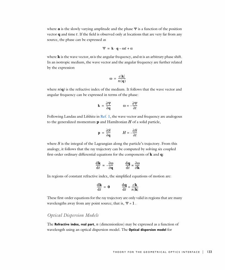
where a is the slowly varying amplitude and the phase Ψ is a function of the position vector q and time t. If the field is observed only at locations that are very far from any source, the phase can be expressed as

where k is the wave vector, ω is the angular frequency, and α is an arbitrary phase shift. In an isotropic medium, the wave vector and the angular frequency are further related by the expression

where n(q) is the refractive index of the medium. It follows that the wave vector and angular frequency can be expressed in terms of the phase:

Following Landau and Lifshitz in Ref. 1, the wave vector and frequency are analogous to the generalized momentum p and Hamiltonian H of a solid particle,

where S is the integral of the Lagrangian along the particle’s trajectory. From this analogy, it follows that the ray trajectory can be computed by solving six coupled first-order ordinary differential equations for the components of k and q:

In regions of constant refractive index, the simplified equations of motion are:

These first-order equations for the ray trajectory are only valid in regions that are many wavelengths away from any point source; that is, .

Optical Dispersion Models

The Refractive index, real part, n (dimensionless) may be expressed as a function of wavelength using an optical dispersion model. The Optical dispersion model for

Ψ k q ωt– α+⋅=

ω c kn q( )------------=

k ∂Ψ∂q-------- ω ∂Ψ

∂t--------–==

p ∂S∂q------- H ∂S

∂t-------–==

dkdt------- ∂ω

∂q------- dq

dt------- ∂ω

∂k-------=–=

dkdt------- 0 dq

dt------- ck

n k----------==

Ψ 1»

T H E O R Y F O R T H E G E O M E T R I C A L O P T I C S I N T E R F A C E | 133

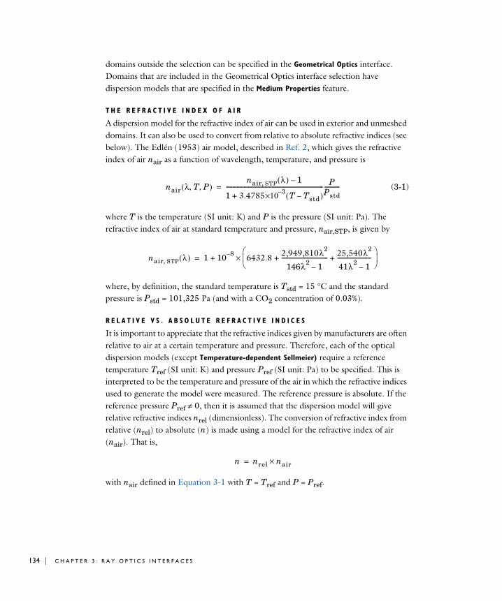
134 | C H A P T E

domains outside the selection can be specified in the Geometrical Optics interface. Domains that are included in the Geometrical Optics interface selection have dispersion models that are specified in the Medium Properties feature.

T H E R E F R A C T I V E I N D E X O F A I R

A dispersion model for the refractive index of air can be used in exterior and unmeshed domains. It can also be used to convert from relative to absolute refractive indices (see below). The Edlén (1953) air model, described in Ref. 2, which gives the refractive index of air nair as a function of wavelength, temperature, and pressure is

(3-1)

where T is the temperature (SI unit: K) and P is the pressure (SI unit: Pa). The refractive index of air at standard temperature and pressure, nair,STP, is given by

where, by definition, the standard temperature is Tstd = 15 °C and the standard pressure is Pstd = 101,325 Pa (and with a CO2 concentration of 0.03%).

R E L A T I V E V S . A B S O L U T E R E F R A C T I V E I N D I C E S

It is important to appreciate that the refractive indices given by manufacturers are often relative to air at a certain temperature and pressure. Therefore, each of the optical dispersion models (except Temperature-dependent Sellmeier) require a reference temperature Tref (SI unit: K) and pressure Pref (SI unit: Pa) to be specified. This is interpreted to be the temperature and pressure of the air in which the refractive indices used to generate the model were measured. The reference pressure is absolute. If the reference pressure Pref ≠ 0, then it is assumed that the dispersion model will give relative refractive indices nrel (dimensionless). The conversion of refractive index from relative (nrel) to absolute (n) is made using a model for the refractive index of air (nair). That is,

with nair defined in Equation 3-1 with T = Tref and P = Pref.

nair λ T P, ,( )nair STP, λ( ) 1–

1 3.4785+3–×10 T Tstd–( )

---------------------------------------------------------------------- PPstd-----------=

nair STP, λ( ) 1 10 8– 6432.8 2,949,810λ2

146λ2 1–--------------------------------- 25,540λ2

41λ2 1–------------------------+ +

×+=

n nrel nair×=


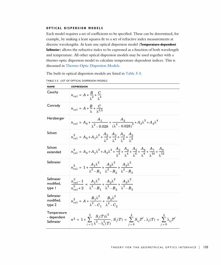
O P T I C A L D I S P E R S I O N M O D E L S

Each model requires a set of coefficients to be specified. These can be determined, for example, by making a least squares fit to a set of refractive index measurements at discrete wavelengths. At least one optical dispersion model (Temperature-dependent

Sellmeier) allows the refractive index to be expressed as a function of both wavelength and temperature. All other optical dispersion models may be used together with a thermo-optic dispersion model to calculate temperature-dependent indices. This is discussed in Thermo-Optic Dispersion Models.

The built-in optical dispersion models are listed in Table 3-3.

TABLE 3-3: LIST OF OPTICAL DISPERSION MODELS

NAME EXPRESSION

Cauchy

Conrady

Herzberger

Schott

Schott extended

Sellmeier

Sellmeier modified, type 1

Sellmeier modified, type 2

Temperature- dependent Sellmeier , ,

nrel A B

λ2------ C

λ4------+ +=

nrel A Bλ---- C

λ3.5----------+ +=

nrel A0A1

λ2 0.028–---------------------------

A2

λ2 0.028–( )2

---------------------------------- A3λ2 A4λ4+ + + +=

nrel2 A0 A1λ2 A2

λ2-------

A3

λ4-------

A4

λ6-------

A5

λ8-------+ + + + +=

nrel2 A0 A1λ2 A2λ4 A3

λ2-------

A4

λ4-------

A5

λ6-------

A6

λ8-------

A7

λ10--------

A8

λ12--------+ + + + + + + +=

nrel2 1

A1λ2

λ2 B1–-------------------

A2λ2

λ2 B2–-------------------

A3λ2

λ2 B3–-------------------+ + +=

nrel2 1–

nrel2 2+--------------------

A1λ2

λ2 B1–-------------------

A2λ2

λ2 B2–-------------------

A3λ2

λ2 B3–-------------------+ +=

nrel2 A

B1λ2

λ2 C1–-------------------

B2λ2

λ2 C2–-------------------+ +=

n2 1Si T( )λ2

λ2 λi2 T( )–

---------------------------i 1=

3

+= Si T( ) SijTj

j 0=

4

= λi T( ) λijTj

j 0=

4

=


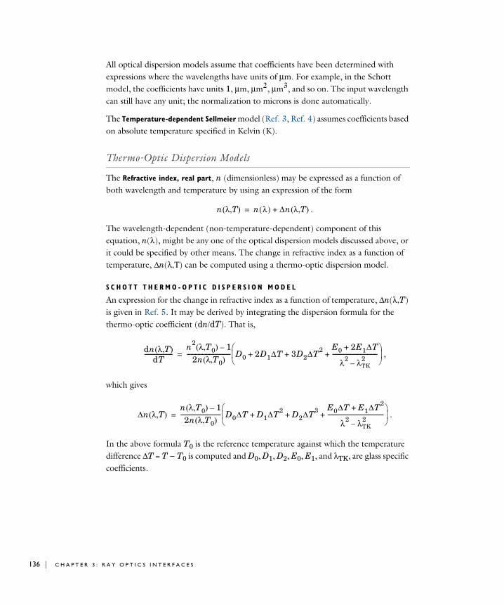
136 | C H A P T E

All optical dispersion models assume that coefficients have been determined with expressions where the wavelengths have units of μm. For example, in the Schott model, the coefficients have units 1, μm, μm2, μm3, and so on. The input wavelength can still have any unit; the normalization to microns is done automatically.

The Temperature-dependent Sellmeier model (Ref. 3, Ref. 4) assumes coefficients based on absolute temperature specified in Kelvin (K).

Thermo-Optic Dispersion Models

The Refractive index, real part, n (dimensionless) may be expressed as a function of both wavelength and temperature by using an expression of the form

.

The wavelength-dependent (non-temperature-dependent) component of this equation, n(λ), might be any one of the optical dispersion models discussed above, or it could be specified by other means. The change in refractive index as a function of temperature, Δn(λ,Τ) can be computed using a thermo-optic dispersion model.

S C H O T T T H E R M O - O P T I C D I S P E R S I O N M O D E L

An expression for the change in refractive index as a function of temperature, Δn(λ,T) is given in Ref. 5. It may be derived by integrating the dispersion formula for the thermo-optic coefficient (dn/dT). That is,

,

which gives

.

In the above formula T0 is the reference temperature against which the temperature difference ΔT = T − T0 is computed and D0, D1, D2, E0, E1, and λTK, are glass specific coefficients.

n λ T( , ) n λ( ) Δn λ T( , )+=

dn λ T( , )dT

--------------------n2 λ T0( , ) 1–

2n λ T0( , )------------------------------- D0 2D1ΔT 3D2ΔT2 E0 2E1ΔT+

λ2 λTK2

–--------------------------------+ + +

=

Δn λ T( , )n λ T0( , ) 1–

2n λ T0( , )----------------------------- D0ΔT D1ΔT2 D2ΔT3 E0ΔT E1ΔT2

+

λ2 λTK2

–----------------------------------------+ + +

=


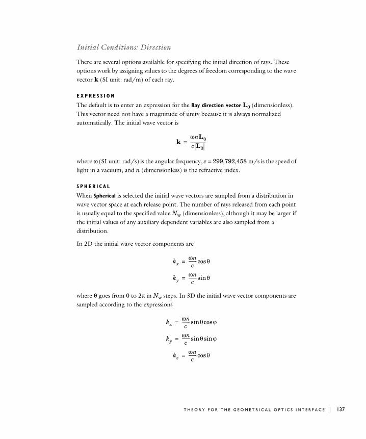
Initial Conditions: Direction

There are several options available for specifying the initial direction of rays. These options work by assigning values to the degrees of freedom corresponding to the wave vector k (SI unit: rad/m) of each ray.

E X P R E S S I O N

The default is to enter an expression for the Ray direction vector L0 (dimensionless). This vector need not have a magnitude of unity because it is always normalized automatically. The initial wave vector is

where ω (SI unit: rad/s) is the angular frequency, c = 299,792,458 m/s is the speed of light in a vacuum, and n (dimensionless) is the refractive index.

S P H E R I C A L

When Spherical is selected the initial wave vectors are sampled from a distribution in wave vector space at each release point. The number of rays released from each point is usually equal to the specified value Nw (dimensionless), although it may be larger if the initial values of any auxiliary dependent variables are also sampled from a distribution.

In 2D the initial wave vector components are

where θ goes from 0 to 2π in Nw steps. In 3D the initial wave vector components are sampled according to the expressions

kωnL0c L0---------------=

kxωnc-------- θcos=

kyωnc-------- θsin=

kxωnc-------- θ ϕcossin=

kyωnc-------- θsin ϕsin=

kzωnc-------- θcos=


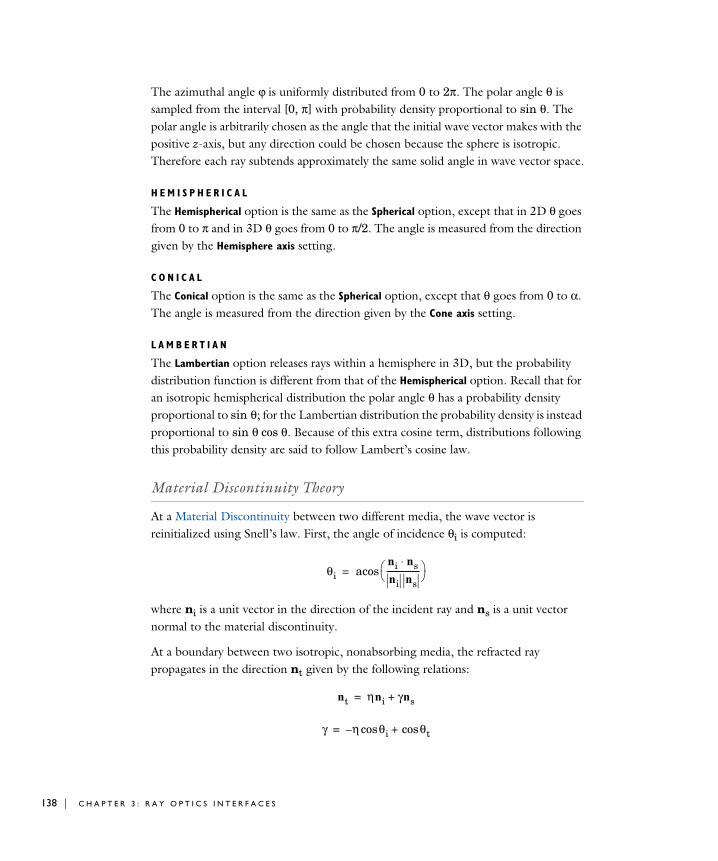
138 | C H A P T E

The azimuthal angle ϕ is uniformly distributed from 0 to 2π. The polar angle θ is sampled from the interval [0, π] with probability density proportional to sin θ. The polar angle is arbitrarily chosen as the angle that the initial wave vector makes with the positive z-axis, but any direction could be chosen because the sphere is isotropic. Therefore each ray subtends approximately the same solid angle in wave vector space.

H E M I S P H E R I C A L

The Hemispherical option is the same as the Spherical option, except that in 2D θ goes from 0 to π and in 3D θ goes from 0 to π/2. The angle is measured from the direction given by the Hemisphere axis setting.

C O N I C A L

The Conical option is the same as the Spherical option, except that θ goes from 0 to α. The angle is measured from the direction given by the Cone axis setting.

L A M B E R T I A N

The Lambertian option releases rays within a hemisphere in 3D, but the probability distribution function is different from that of the Hemispherical option. Recall that for an isotropic hemispherical distribution the polar angle θ has a probability density proportional to sin θ; for the Lambertian distribution the probability density is instead proportional to sin θ cos θ. Because of this extra cosine term, distributions following this probability density are said to follow Lambert’s cosine law.

Material Discontinuity Theory

At a Material Discontinuity between two different media, the wave vector is reinitialized using Snell’s law. First, the angle of incidence θi is computed:

where ni is a unit vector in the direction of the incident ray and ns is a unit vector normal to the material discontinuity.

At a boundary between two isotropic, nonabsorbing media, the refracted ray propagates in the direction nt given by the following relations:

θini ns⋅ni ns----------------- acos=

nt ηni γns+=

γ η θi θtcos+cos–=


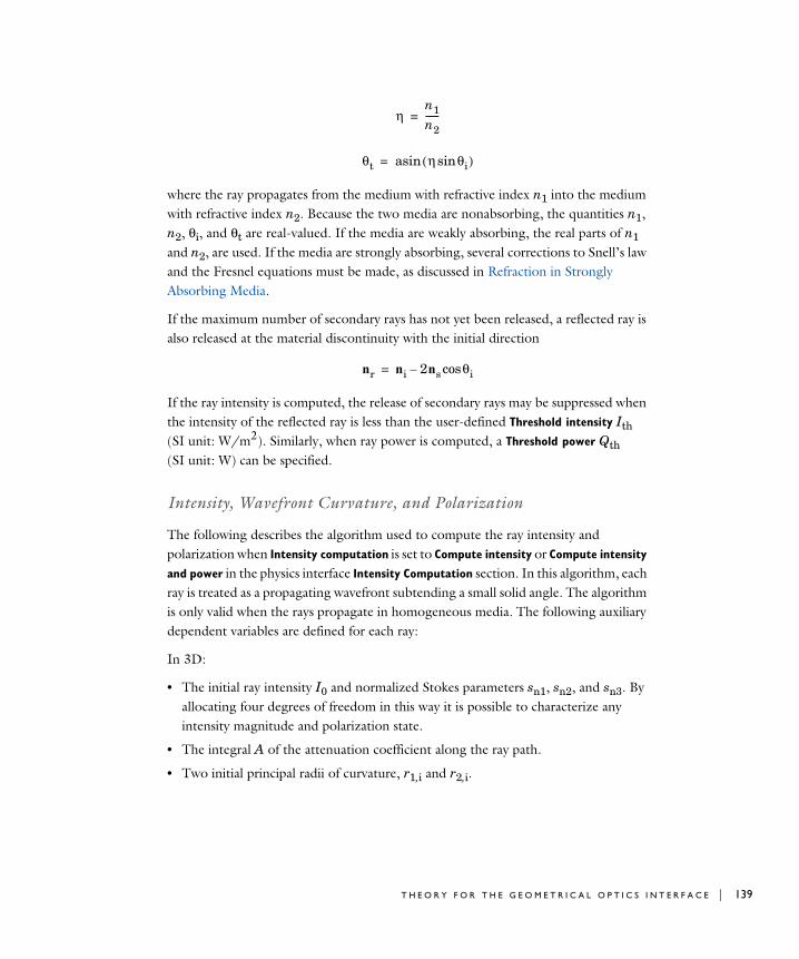
where the ray propagates from the medium with refractive index n1 into the medium with refractive index n2. Because the two media are nonabsorbing, the quantities n1, n2, θi, and θt are real-valued. If the media are weakly absorbing, the real parts of n1 and n2, are used. If the media are strongly absorbing, several corrections to Snell’s law and the Fresnel equations must be made, as discussed in Refraction in Strongly Absorbing Media.

If the maximum number of secondary rays has not yet been released, a reflected ray is also released at the material discontinuity with the initial direction

If the ray intensity is computed, the release of secondary rays may be suppressed when the intensity of the reflected ray is less than the user-defined Threshold intensity Ith (SI unit: W/m2). Similarly, when ray power is computed, a Threshold power Qth (SI unit: W) can be specified.

Intensity, Wavefront Curvature, and Polarization

The following describes the algorithm used to compute the ray intensity and polarization when Intensity computation is set to Compute intensity or Compute intensity

and power in the physics interface Intensity Computation section. In this algorithm, each ray is treated as a propagating wavefront subtending a small solid angle. The algorithm is only valid when the rays propagate in homogeneous media. The following auxiliary dependent variables are defined for each ray:

In 3D:

• The initial ray intensity I0 and normalized Stokes parameters sn1, sn2, and sn3. By allocating four degrees of freedom in this way it is possible to characterize any intensity magnitude and polarization state.

• The integral A of the attenuation coefficient along the ray path.

• Two initial principal radii of curvature, r1,i and r2,i.

ηn1n2------=

θt η θisin( )asin=

nr ni 2ns θicos–=


140 | C H A P T E

• Two principal radii of curvature, r1 and r2, which represent the maximum and minimum radii of curvature of the intersection of the wavefront with an arbitrary plane.

• Three components of a unit vector e1 in the direction corresponding to the first principal radius of curvature. This information is used to reinitialize the principal radii of curvature at curved boundaries.

In 2D:

• The initial ray intensity I0 and normalized Stokes parameters sn1, sn2, and sn3.


• One initial principal radius of curvature, r1,i.

• One radius of curvature r1 of the wavefront. All wavefronts are assumed to be converging or diverging cylindrical waves, so it is not necessary to define a second radius of curvature.

A different algorithm is used to compute the intensity and polarization of each ray if the Intensity computation is instead set to Compute intensity in graded media or Compute

intensity and power in graded media. This algorithm accounts for the effect of graded media on the ray intensity, but it is also slower and less accurate for homogeneous media. The following auxiliary dependent variables are defined for each ray:

In 3D:

• The intensity help variable Γ and the normalized Stokes parameters sn01, sn02, and sn03, which characterize the intensity and polarization of the ray. They are reinitialized at material discontinuities and walls.


• Two principal curvature calculation help variables α1 and α2 and the rotation angle φ which indicates the orientation of the principal curvature directions. An additional help variable is used internally to detect poles in the local coordinate system definition and to redefine the local coordinate system accordingly.

In 2D:

• The intensity help variable Γ and the normalized Stokes parameters sn01, sn02, and sn03, which characterize the intensity and polarization of the ray. They are reinitialized at material discontinuities and walls.


• One principal curvature calculation help variable α1.


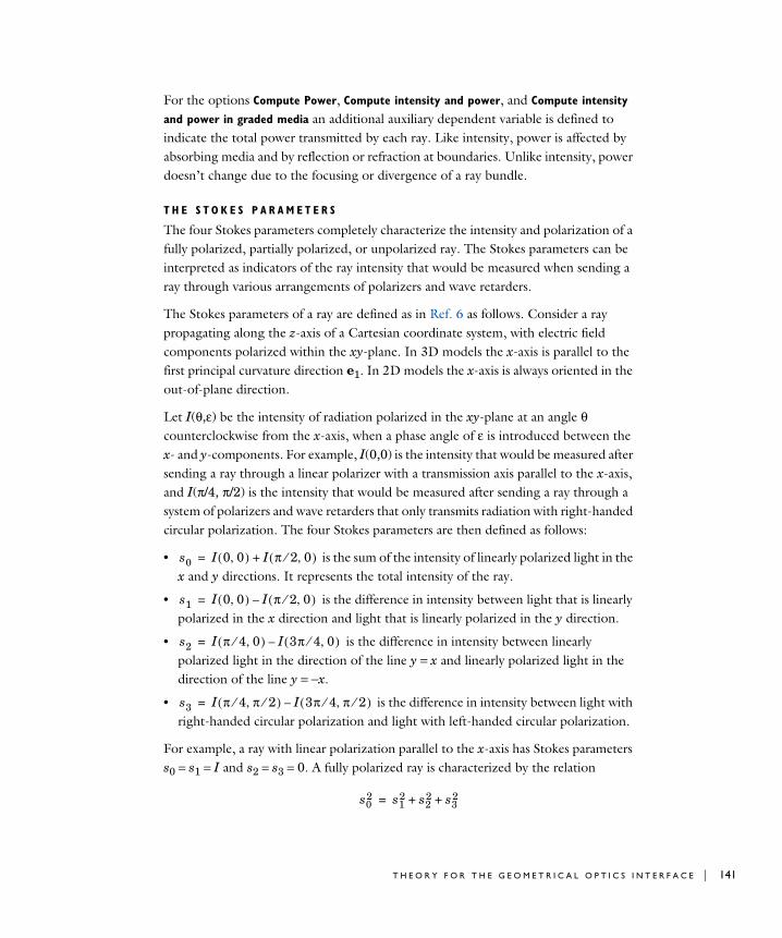
For the options Compute Power, Compute intensity and power, and Compute intensity

and power in graded media an additional auxiliary dependent variable is defined to indicate the total power transmitted by each ray. Like intensity, power is affected by absorbing media and by reflection or refraction at boundaries. Unlike intensity, power doesn’t change due to the focusing or divergence of a ray bundle.

T H E S T O K E S P A R A M E T E R S

The four Stokes parameters completely characterize the intensity and polarization of a fully polarized, partially polarized, or unpolarized ray. The Stokes parameters can be interpreted as indicators of the ray intensity that would be measured when sending a ray through various arrangements of polarizers and wave retarders.

The Stokes parameters of a ray are defined as in Ref. 6 as follows. Consider a ray propagating along the z-axis of a Cartesian coordinate system, with electric field components polarized within the xy-plane. In 3D models the x-axis is parallel to the first principal curvature direction e1. In 2D models the x-axis is always oriented in the out-of-plane direction.

Let I(θ,ε) be the intensity of radiation polarized in the xy-plane at an angle θ counterclockwise from the x-axis, when a phase angle of ε is introduced between the x- and y-components. For example, I(0,0) is the intensity that would be measured after sending a ray through a linear polarizer with a transmission axis parallel to the x-axis, and I(π/4, π/2) is the intensity that would be measured after sending a ray through a system of polarizers and wave retarders that only transmits radiation with right-handed circular polarization. The four Stokes parameters are then defined as follows:

• is the sum of the intensity of linearly polarized light in the x and y directions. It represents the total intensity of the ray.

• is the difference in intensity between light that is linearly polarized in the x direction and light that is linearly polarized in the y direction.

• is the difference in intensity between linearly polarized light in the direction of the line y = x and linearly polarized light in the direction of the line y = −x.

• is the difference in intensity between light with right-handed circular polarization and light with left-handed circular polarization.

For example, a ray with linear polarization parallel to the x-axis has Stokes parameters s0 = s1 = I and s2 = s3 = 0. A fully polarized ray is characterized by the relation

s0 I 0 0,( ) I π 2⁄ 0,( )+=

s1 I 0 0,( ) I π 2⁄ 0,( )–=

s2 I π 4⁄ 0,( ) I 3π 4⁄ 0,( )–=

s3 I π 4⁄ π 2⁄,( ) I 3π 4⁄ π 2⁄,( )–=

s02 s1

2 s22 s3

2+ +=


142 | C H A P T E

A partially polarized or unpolarized ray is characterized by the relation

The degree of polarization P is defined as

A degree of polarization P = 1 corresponds to fully polarized radiation, whereas a degree of polarization P = 0 corresponds to unpolarized radiation.

In the COMSOL implementation of ray intensity calculation, the degrees of freedom are not the Stokes parameters themselves, but rather normalized Stokes parameters sn1, sn2, and sn3. Then the actual Stokes parameters are recovered through the relations s1 = Isn1, s2 = Isn2, and s3 = Isn3. The reason for this decoupling is that the normalized Stokes parameters remain bounded, enabling accurate reinitialization of ray power, even if a ray is reflected or refracted very close to a caustic, where the intensity (in the geometrical optics limit) can become arbitrarily large.

P R I N C I P A L R A D I I O F C U R V A T U R E

In 3D models, each ray is treated as a wavefront for which two principal radii of curvature, r1 and r2, are defined. In addition, the values of the two principal radii of curvature are stored as r1,i and r2,i whenever the ray reaches a boundary.

Within domains, the equations

are solved. Negative radii of curvature indicate that the wavefront is expanding as the ray propagates, while positive radii of curvature indicate that the wavefront is converging. A continuous locus of points at which either of the principal radii of curvature equals zero is called a caustic surface. The unit vector e1 is defined so that r1 is the radius of curvature of the intersection of the wavefront with the plane tangent to e1 and the wave vector k. Similarly, if a vector e2 is defined so that

s02 s1

2 s22 s3

2+ +≥

Ps1

2 s22 s3

2+ +

s0----------------------------------=

dr1ds--------- 1

dr2ds--------- 1–=–=

e2k e× 1k e× 1------------------=


Then r2 is the radius of curvature of the intersection of the wavefront with a plane tangent to e2 and k. The components of e1 are stored as auxiliary dependent variables for each ray. The components of e2 can then be derived from e1 and k at any time.

The principal radii of curvature are reinitialized at material discontinuities, and the orientation of the unit vectors e1 and e2 may change. If the unit vector in the direction of the incident ray ni is not parallel to the surface normal ns, then it is possible to define a unique tangent plane, called the plane of incidence, that contains the incident, reflected, and refracted rays. The unit vector normal to this plane, u0, is defined as

If the ray is normal to the surface, then the incident ray is parallel to the refracted ray and antiparallel to the reflected ray, and u0 can be any arbitrary unit vector orthogonal to ni. In addition to the unit vector normal to the plane of incidence, the following unit vectors tangent to the incident wavefront, refracted wavefront, reflected wavefront, and surface normal are defined:

where the subscripts i, t, and r denote the incident, refracted, and reflected wavefronts, respectively. For a wavefront propagating in a direction n, with principal curvatures k1 = 1/r1 and k2 = 1/r2 defined for directions e1 and e2, the principal curvatures in two other orthogonal directions e1' and e2' (both orthogonal to n) are

(3-2)

where θ is the angle of rotation about n which transforms the vectors e1 and e2 to e1' and e2', respectively. Because k1' and k2' are not principal curvatures, it is necessary to include off-diagonal elements of the wavefront curvature tensor equal to k12'.

The following algorithm is used to reinitialize the principal radii of curvature of the wavefront and their orientations. The reinitialization of the curvature variables follows the method of Stavroudis in Ref. 7.

u0ni ns×ni ns×--------------------=

ui ni u0×ut nt u0×ur nr u0×us ns u0×=

===

k1' k1 θcos2 k2 θsin2

k2'+

k1 θsin2 k2 θcos2

k12'+

k1 k2–( ) θ θsincos

=

=

=


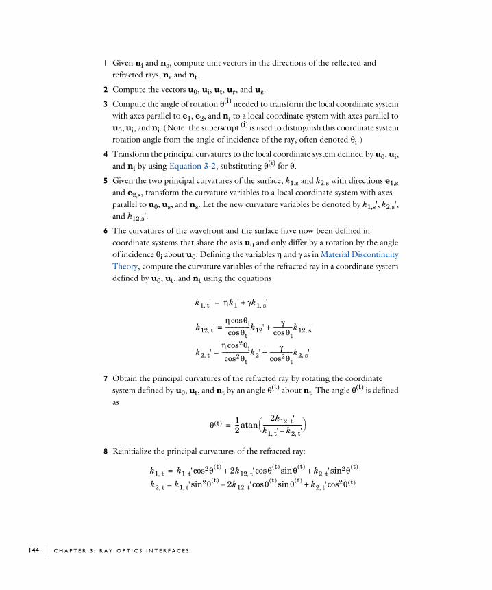
144 | C H A P T E

1 Given ni and ns, compute unit vectors in the directions of the reflected and refracted rays, nr and nt.

2 Compute the vectors u0, ui, ut, ur, and us.

3 Compute the angle of rotation θ(i) needed to transform the local coordinate system with axes parallel to e1, e2, and ni to a local coordinate system with axes parallel to u0, ui, and ni. (Note: the superscript (i) is used to distinguish this coordinate system rotation angle from the angle of incidence of the ray, often denoted θi.)

4 Transform the principal curvatures to the local coordinate system defined by u0, ui, and ni by using Equation 3-2, substituting θ(i) for θ.

5 Given the two principal curvatures of the surface, k1,s and k2,s with directions e1,s and e2,s, transform the curvature variables to a local coordinate system with axes parallel to u0, us, and ns. Let the new curvature variables be denoted by k1,s', k2,s', and k12,s'.

6 The curvatures of the wavefront and the surface have now been defined in coordinate systems that share the axis u0 and only differ by a rotation by the angle of incidence θi about u0. Defining the variables η and γ as in Material Discontinuity Theory, compute the curvature variables of the refracted ray in a coordinate system defined by u0, ut, and nt using the equations

7 Obtain the principal curvatures of the refracted ray by rotating the coordinate system defined by u0, ut, and nt by an angle θ(t) about nt. The angle θ(t) is defined as

8 Reinitialize the principal curvatures of the refracted ray:

k1 t, ' ηk1' γk1 s, '

k12 t, 'η θicos

θtcos------------------k12'

γθtcos

--------------k12 s, '

k2 t, 'η θicos2

θtcos2--------------------k2'

γθtcos2

-----------------k2 s, '+=

+=

+=

θ t( ) 12---

2k12 t, 'k1 t, ' k2 t, '–---------------------------- atan=

k1 t, k1 t, ' θ t( )cos2 2k12 t, ' θ t( ) θ t( )sincos k2 t, ' θ t( )sin2

k2 t, k1 t, ' θ t( )sin2 2k12 t, ' θ t( ) θ t( )sincos– k2 t, ' θ t( )cos2+=

+ +=


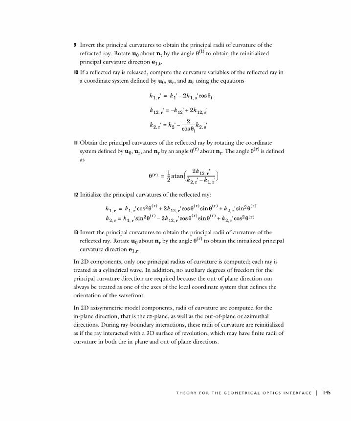
9 Invert the principal curvatures to obtain the principal radii of curvature of the refracted ray. Rotate u0 about nt by the angle θ(t) to obtain the reinitialized principal curvature direction e1,t.

10 If a reflected ray is released, compute the curvature variables of the reflected ray in a coordinate system defined by u0, ur, and nr using the equations

11 Obtain the principal curvatures of the reflected ray by rotating the coordinate system defined by u0, ur, and nr by an angle θ(r) about nr. The angle θ(r) is defined as

12 Initialize the principal curvatures of the reflected ray:

13 Invert the principal curvatures to obtain the principal radii of curvature of the reflected ray. Rotate u0 about nr by the angle θ(r) to obtain the initialized principal curvature direction e1,r.

In 2D components, only one principal radius of curvature is computed; each ray is treated as a cylindrical wave. In addition, no auxiliary degrees of freedom for the principal curvature direction are required because the out-of-plane direction can always be treated as one of the axes of the local coordinate system that defines the orientation of the wavefront.

In 2D axisymmetric model components, radii of curvature are computed for the in-plane direction, that is the rz-plane, as well as the out-of-plane or azimuthal directions. During ray-boundary interactions, these radii of curvature are reinitialized as if the ray interacted with a 3D surface of revolution, which may have finite radii of curvature in both the in-plane and out-of-plane directions.

k1 r, ' k1' 2k1 s, ' θi

k12 r, ' k– 12' 2k12 s, '

k2 r, ' k2'2

θicos--------------k2 s, '–=

+=

cos–=

θ r( ) 12---

2k12 r, 'k2 r, ' k1 r, '–----------------------------- atan=

k1 r, k1 r, ' θ r( )cos2 2k12 r, ' θ r( ) θ r( )sincos k2 r, ' θ r( )sin2

k2 r, k1 r, ' θ r( )sin2 2k12 r, ' θ r( ) θ r( )sincos– k2 r, ' θ r( )cos2+=

+ +=


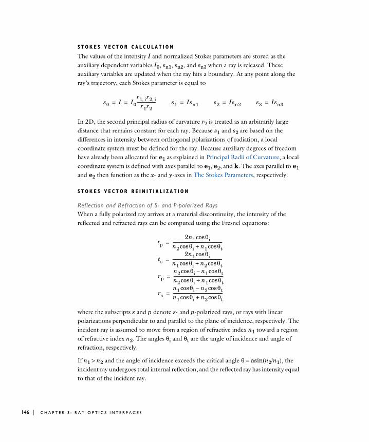
146 | C H A P T E

S T O K E S V E C T O R C A L C U L A T I O N

The values of the intensity I and normalized Stokes parameters are stored as the auxiliary dependent variables I0, sn1, sn2, and sn3 when a ray is released. These auxiliary variables are updated when the ray hits a boundary. At any point along the ray’s trajectory, each Stokes parameter is equal to

In 2D, the second principal radius of curvature r2 is treated as an arbitrarily large distance that remains constant for each ray. Because s1 and s2 are based on the differences in intensity between orthogonal polarizations of radiation, a local coordinate system must be defined for the ray. Because auxiliary degrees of freedom have already been allocated for e1 as explained in Principal Radii of Curvature, a local coordinate system is defined with axes parallel to e1, e2, and k. The axes parallel to e1 and e2 then function as the x- and y-axes in The Stokes Parameters, respectively.

S T O K E S V E C T O R R E I N I T I A L I Z A T I O N

Reflection and Refraction of S- and P-polarized RaysWhen a fully polarized ray arrives at a material discontinuity, the intensity of the reflected and refracted rays can be computed using the Fresnel equations:

where the subscripts s and p denote s- and p-polarized rays, or rays with linear polarizations perpendicular to and parallel to the plane of incidence, respectively. The incident ray is assumed to move from a region of refractive index n1 toward a region of refractive index n2. The angles θi and θt are the angle of incidence and angle of refraction, respectively.

If n1 > n2 and the angle of incidence exceeds the critical angle θ = asin(n2/n1), the incident ray undergoes total internal reflection, and the reflected ray has intensity equal to that of the incident ray.

s0 I I0r1 i, r2 i,

r1r2------------------= = s1 Isn1= s2 Isn2= s3 Isn3=

tp2n1 θicos

n2 θi n1 θtcos+cos------------------------------------------------

ts2n1 θicos

n1 θi n2 θtcos+cos------------------------------------------------

rpn2 θi n1 θtcos–cosn2 θi n1 θtcos+cos------------------------------------------------

rsn1 θi n2 θtcos–cosn1 θi n2 θtcos+cos------------------------------------------------

=

=

=

=


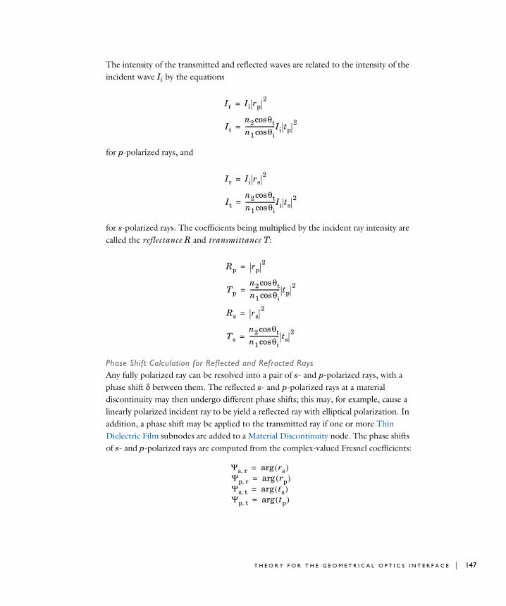
The intensity of the transmitted and reflected waves are related to the intensity of the incident wave Ii by the equations

for p-polarized rays, and

for s-polarized rays. The coefficients being multiplied by the incident ray intensity are called the reflectance R and transmittance T:

Phase Shift Calculation for Reflected and Refracted RaysAny fully polarized ray can be resolved into a pair of s- and p-polarized rays, with a phase shift δ between them. The reflected s- and p-polarized rays at a material discontinuity may then undergo different phase shifts; this may, for example, cause a linearly polarized incident ray to be yield a reflected ray with elliptical polarization. In addition, a phase shift may be applied to the transmitted ray if one or more Thin Dielectric Film subnodes are added to a Material Discontinuity node. The phase shifts of s- and p-polarized rays are computed from the complex-valued Fresnel coefficients:

Ir Ii rp2

Itn2 θtcosn1 θicos---------------------Ii tp

2

=

=

Ir Ii rs2

Itn2 θtcosn1 θicos---------------------Ii ts

2

=

=

Rp rp2

Tpn2 θtcosn1 θicos--------------------- tp

2

Rs rs2

Tsn2 θtcosn1 θicos--------------------- ts

2

=

=

=

=

Ψs r, rs( )Ψp r,

argrp( )

Ψs t,

argts( )

Ψp t,

argtp( )arg

====


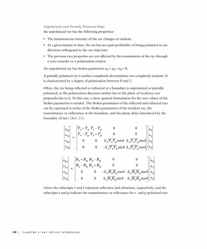
148 | C H A P T E

Unpolarized and Partially Polarized RaysAn unpolarized ray has the following properties:

• The instantaneous intensity of the ray changes at random.

• At a given instant in time, the ray has an equal probability of being polarized in any direction orthogonal to the ray trajectory.

• The previous two properties are not affected by the transmission of the ray through a wave retarder or a polarization rotator.

An unpolarized ray has Stokes parameters s1 = s2 = s3 = 0.

A partially polarized ray is neither completely deterministic nor completely random. It is characterized by a degree of polarization between 0 and 1.

Often, the ray being reflected or refracted at a boundary is unpolarized or partially polarized; or the polarization direction neither lies in the plane of incidence nor perpendicular to it. In this case, a more general formulation for the new values of the Stokes parameters is needed. The Stokes parameters of the reflected and refracted rays can be expressed in terms of the Stokes parameters of the incident ray, the transmittance or reflectance at the boundary, and the phase delay introduced by the boundary (if any) (Ref. 11):

where the subscripts r and t represent reflection and refraction, respectively; and the subscripts s and p indicate the transmittance or reflectance for s- and p-polarized rays.

s0t

s1t

s2t

s3t

Ts Tp+ Ts Tp– 0 0

Ts Tp– Ts Tp+ 0 0

0 0 2 TsTp δcos 2 TsTp δsin

0 0 2 TsTp δsin– 2 TsTp δcos

s0

s1

s2

s3

=

s0r

s1r

s2r

s3r

Rs Rp+ Rs Rp– 0 0

Rs Rp– Rs Rp+ 0 0

0 0 2 RsRp δcos– 2 RsRp δsin–

0 0 2 RsRp δsin 2 RsRp δcos–

s0

s1

s2

s3

=


Wavefront Curvature Calculation in Graded Media

It is possible to compute the ray intensity by changing Intensity computation to Compute intensity or Compute intensity in graded media in the physics interface Intensity

Computation section. The options Compute intensity and power and Compute intensity

and power in graded media can also be used to compute intensity, with the only difference being that these options define an additional auxiliary dependent variable for the total power transferred by the ray. The setting Compute intensity is more robust and accurate than Compute intensity in graded media, but is only applicable to homogeneous media. The setting Compute intensity in graded media can be used for both homogeneous and graded media, but it introduces more numerical error than Compute intensity.

A S S U M P T I O N S F O R C O M P U T I N G I N T E N S I T Y I N H O M O G E N E O U S M E D I A

When Compute intensity is selected, the ray intensity is computed along each ray path using the following assumptions:

1 The wavefront represented by each ray subtends a constant plane angle (2D) or solid angle (3D), which can change only when rays are reflected or refracted at boundaries.

2 Given the radii of curvature at two positions within the same domain and the intensity at one of these two positions, the intensity at the other position can be computed using the relationship

3 Except when rays are reflected or refracted at boundaries, the principal radii of curvature change at a constant rate:

4 The principal curvature directions do not change, except when rays are reflected or refracted at boundaries.

These assumptions are not valid in graded media, in which the refractive index changes continuously as a function of position. It is possible for the angle between two different rays to change as they propagate through the medium, so the solid angle subtended by the wavefront is no longer constant. As a result, the ray intensity cannot be expressed using the ratio of initial and final principal radii of curvature.

I I0r1 0, r2 0,

r1r2---------------------=

dr1ds---------

dr2ds--------- 1–= =


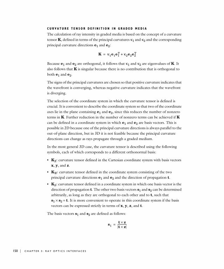
150 | C H A P T E

C U R V A T U R E T E N S O R D E F I N I T I O N I N G R A D E D M E D I A

The calculation of ray intensity in graded media is based on the concept of a curvature tensor K, defined in terms of the principal curvatures κ1 and κ2 and the corresponding principal curvature directions e1 and e2:

Because e1 and e2 are orthogonal, it follows that κ1 and κ2 are eigenvalues of K. It also follows that K is singular because there is no contribution that is orthogonal to both e1 and e2.

The signs of the principal curvatures are chosen so that positive curvature indicates that the wavefront is converging, whereas negative curvature indicates that the wavefront is diverging.

The selection of the coordinate system in which the curvature tensor is defined is crucial. It is convenient to describe the coordinate system so that two of the coordinate axes lie in the plane containing e1 and e2, since this reduces the number of nonzero terms in K. Further reduction in the number of nonzero terms can be achieved if K can be defined in a coordinate system in which e1 and e2 are basis vectors. This is possible in 2D because one of the principal curvature directions is always parallel to the out-of-plane direction, but in 3D it is not feasible because the principal curvature directions can change as rays propagate through a graded medium.

In the most general 3D case, the curvature tensor is described using the following symbols, each of which corresponds to a different orthonormal basis:

• KX: curvature tensor defined in the Cartesian coordinate system with basis vectors x, y, and z.

• KW: curvature tensor defined in the coordinate system consisting of the two principal curvature directions e1 and e2 and the direction of propagation t.

• KS: curvature tensor defined in a coordinate system in which one basis vector is the direction of propagation t. The other two basis vectors s1 and s2 can be determined arbitrarily, as long as they are orthogonal to each other and to t, such that s1 × s2 = t. It is more convenient to operate in this coordinate system if the basis vectors can be expressed strictly in terms of x, y, z, and t.

The basis vectors s1 and s2 are defined as follows:

K κ1e1e1T κ2e2e2

T+=

s1t z×t z×---------------=


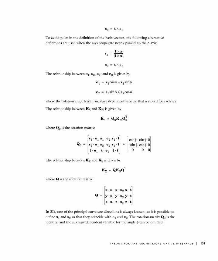
To avoid poles in the definition of the basis vectors, the following alternative definitions are used when the rays propagate nearly parallel to the z-axis:

The relationship between s1, s2, e1, and e2 is given by

where the rotation angle φ is an auxiliary dependent variable that is stored for each ray.

The relationship between KS and KW is given by

where Q0 is the rotation matrix:

The relationship between KX and KS is given by

where Q is the rotation matrix:

In 2D, one of the principal curvature directions is always known, so it is possible to define s1 and s2 so that they coincide with e1 and e2. The rotation matrix Q0 is the identity, and the auxiliary dependent variable for the angle φ can be omitted.

s2 t s1×=

s1t x×t x×---------------=

s2 t s1×=

e1 s1 φ s2 φsin–cos=

e2 s1 φ s2 φcos+sin=

KS Q0KWQ0T

=

Q0

s1 e1⋅ s1 e2⋅ s1 t⋅

s2 e1⋅ s2 e2⋅ s2 t⋅

t e1⋅ t e2⋅ t t⋅

φcos φsin 0φsin– φcos 0

0 0 0

= =

KX QKSQT=

Q

x s1⋅ x s2⋅ x t⋅

y s1⋅ y s2⋅ y t⋅

z s1⋅ z s2⋅ z t⋅

=


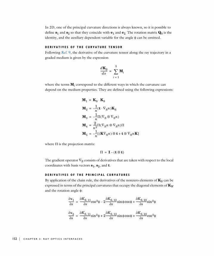
152 | C H A P T E

In 2D, one of the principal curvature directions is always known, so it is possible to define s1 and s2 so that they coincide with e1 and e2. The rotation matrix Q0 is the identity, and the auxiliary dependent variable for the angle φ can be omitted.

D E R I V A T I V E S O F T H E C U R V A T U R E T E N S O R

Following Ref. 9, the derivative of the curvature tensor along the ray trajectory in a graded medium is given by the expression

where the terms Mi correspond to the different ways in which the curvature can depend on the medium properties. They are defined using the following expressions:

where Π is the projection matrix:

The gradient operator ∇S consists of derivatives that are taken with respect to the local coordinates with basis vectors s1, s2, and t.

D E R I V A T I V E S O F T H E P R I N C I P A L C U R V A T U R E S

By application of the chain rule, the derivatives of the nonzero elements of KS can be expressed in terms of the principal curvatures that occupy the diagonal elements of KW and the rotation angle φ:

dKSds------------ Mi

i 1=

5

=

M1 KS KS

M2

⋅

1n--- t ∇Sn⋅( )KS

M3

–

1n---Π ∇S ∇Sn⊗( )

M4

–

2n2------Π ∇Sn ∇Sn⊗( )Π

M51n--- K∇Sn( ) t t ∇SnK⊗+⊗[ ]–

=

=

=

=

=

Π I t t⊗( )–=

∂κ1∂s---------

∂KS 11,∂s

------------------cos2φ 2∂KS 12,

∂s------------------ φ φ

∂KS 22,∂s

------------------sin2φ+cossin–=

∂κ2∂s---------

∂KS 11,∂s

------------------sin2φ 2∂KS 12,

∂s------------------ φ φ

∂KS 22,∂s

------------------cos2φ+cossin+=


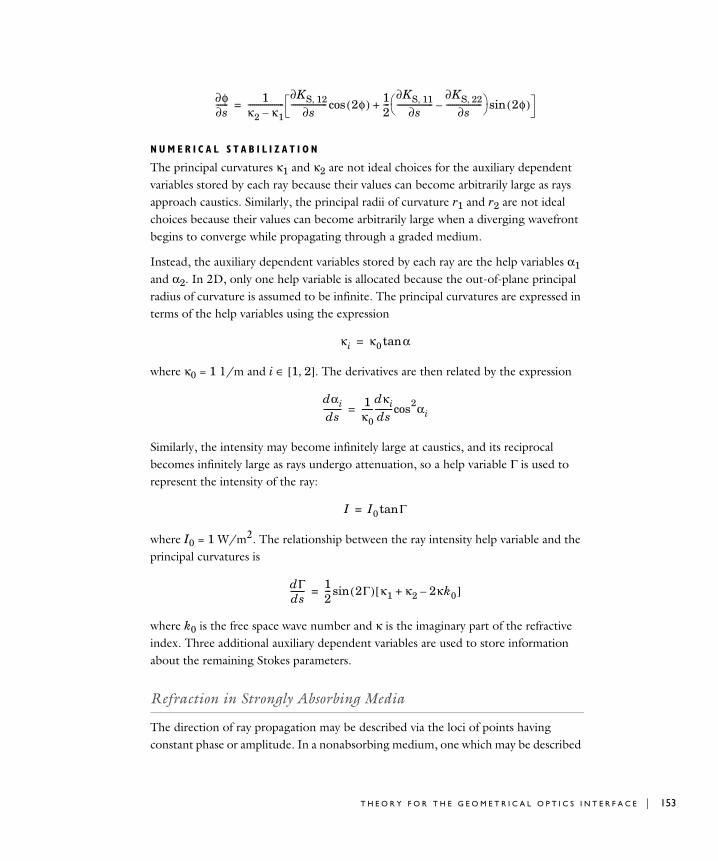
N U M E R I C A L S T A B I L I Z A T I O N

The principal curvatures κ1 and κ2 are not ideal choices for the auxiliary dependent variables stored by each ray because their values can become arbitrarily large as rays approach caustics. Similarly, the principal radii of curvature r1 and r2 are not ideal choices because their values can become arbitrarily large when a diverging wavefront begins to converge while propagating through a graded medium.

Instead, the auxiliary dependent variables stored by each ray are the help variables α1 and α2. In 2D, only one help variable is allocated because the out-of-plane principal radius of curvature is assumed to be infinite. The principal curvatures are expressed in terms of the help variables using the expression

where κ0 = 1 1/m and i ∈ [1, 2]. The derivatives are then related by the expression

Similarly, the intensity may become infinitely large at caustics, and its reciprocal becomes infinitely large as rays undergo attenuation, so a help variable Γ is used to represent the intensity of the ray:

where I0 = 1 W/m2. The relationship between the ray intensity help variable and the principal curvatures is

where k0 is the free space wave number and κ is the imaginary part of the refractive index. Three additional auxiliary dependent variables are used to store information about the remaining Stokes parameters.

Refraction in Strongly Absorbing Media

The direction of ray propagation may be described via the loci of points having constant phase or amplitude. In a nonabsorbing medium, one which may be described

∂φ∂s------ 1

κ2 κ1–------------------

∂KS 12,∂s

------------------ 2φ( ) 12---

∂KS 11,∂s

------------------∂KS 22,

∂s------------------–

2φ( )sin+cos=

κi κ0 αtan=

dαi

ds--------- 1

κ0------

dκids---------cos2αi=

I I0 Γtan=

dΓds------- 1

2--- 2Γ( ) κ1 κ2 2κk0–+[ ]sin=


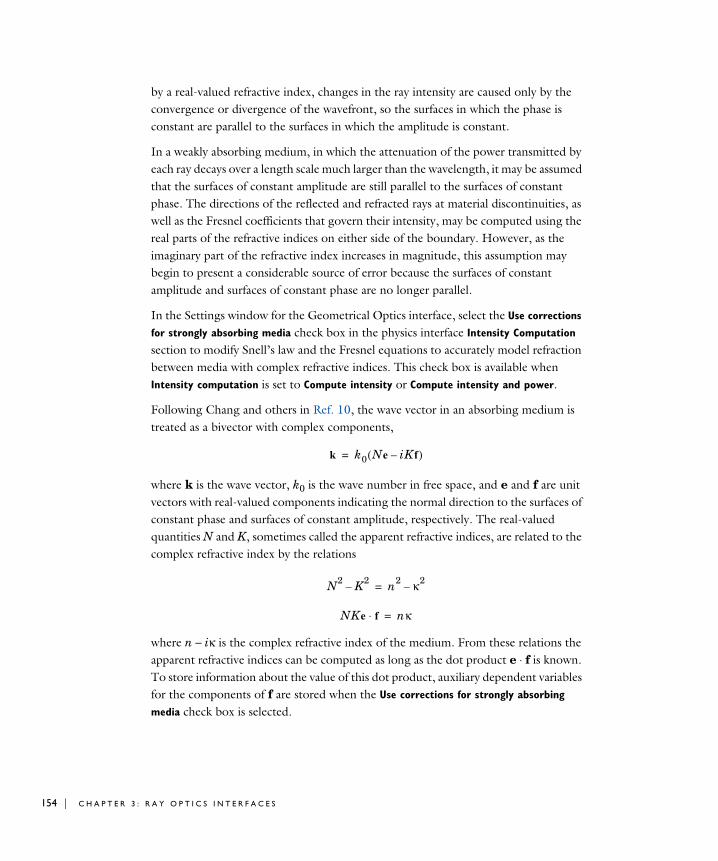
154 | C H A P T E

by a real-valued refractive index, changes in the ray intensity are caused only by the convergence or divergence of the wavefront, so the surfaces in which the phase is constant are parallel to the surfaces in which the amplitude is constant.

In a weakly absorbing medium, in which the attenuation of the power transmitted by each ray decays over a length scale much larger than the wavelength, it may be assumed that the surfaces of constant amplitude are still parallel to the surfaces of constant phase. The directions of the reflected and refracted rays at material discontinuities, as well as the Fresnel coefficients that govern their intensity, may be computed using the real parts of the refractive indices on either side of the boundary. However, as the imaginary part of the refractive index increases in magnitude, this assumption may begin to present a considerable source of error because the surfaces of constant amplitude and surfaces of constant phase are no longer parallel.

In the Settings window for the Geometrical Optics interface, select the Use corrections

for strongly absorbing media check box in the physics interface Intensity Computation section to modify Snell’s law and the Fresnel equations to accurately model refraction between media with complex refractive indices. This check box is available when Intensity computation is set to Compute intensity or Compute intensity and power.

Following Chang and others in Ref. 10, the wave vector in an absorbing medium is treated as a bivector with complex components,

where k is the wave vector, k0 is the wave number in free space, and e and f are unit vectors with real-valued components indicating the normal direction to the surfaces of constant phase and surfaces of constant amplitude, respectively. The real-valued quantities N and K, sometimes called the apparent refractive indices, are related to the complex refractive index by the relations

where n − iκ is the complex refractive index of the medium. From these relations the apparent refractive indices can be computed as long as the dot product e ⋅ f is known. To store information about the value of this dot product, auxiliary dependent variables for the components of f are stored when the Use corrections for strongly absorbing

media check box is selected.

k k0 Ne iKf–( )=

N2 K2– n2 κ2

–=

NKe f⋅ nκ=


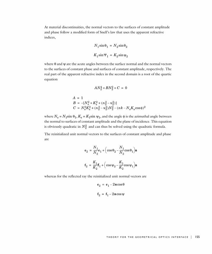
At material discontinuities, the normal vectors to the surfaces of constant amplitude and phase follow a modified form of Snell’s law that uses the apparent refractive indices,

where θ and ψ are the acute angles between the surface normal and the normal vectors to the surfaces of constant phase and surfaces of constant amplitude, respectively. The real part of the apparent refractive index in the second domain is a root of the quartic equation

where Ns = N1sin θ1, Ks = K1sin ψ1, and the angle φ is the azimuthal angle between the normal to surfaces of constant amplitude and the plane of incidence. This equation is obviously quadratic in and can thus be solved using the quadratic formula.

The reinitialized unit normal vectors to the surfaces of constant amplitude and phase are

whereas for the reflected ray the reinitialized unit normal vectors are

N1 θ1sin N2 θ2sin=

K1 Ψ1sin K2 ψ2sin=

AN24 BN2

2 C+ + 0=

A 1B Ns

2 Ks2 n2

2 κ22–( )+ +[ ]

C–

Ns2Ks

2 n22 κ2

2–( )N22 nk NsKs φcos–( )2–+

=

=

=

N22

e2N1N2-------e1 θ2

N1N2------- θ1cos–cos

n+=

f2K1K2-------f1 ψ2

K1K2------- ψ1cos–cos

n+=

e2 e1 2n θcos–=

f2 f1 2n ψcos–=


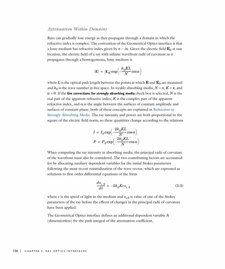
156 | C H A P T E

Attenuation Within Domains

Rays can gradually lose energy as they propagate through a domain in which the refractive index is complex. The convention of the Geometrical Optics interface is that a lossy medium has refractive index given by n − iκ. Given the electric field E0 at one location, the electric field of a ray with infinite wavefront radii of curvature as it propagates through a homogeneous, lossy medium is

where L is the optical path length between the points at which E and E0 are measured and k0 is the wave number in free space. In weakly absorbing media, N = n, K = κ, and α = 0. If the Use corrections for strongly absorbing media check box is selected, N is the real part of the apparent refractive index, K is the complex part of the apparent refractive index, and α is the angle between the surfaces of constant amplitude and surfaces of constant phase; both of these concepts are explained in Refraction in Strongly Absorbing Media. The ray intensity and power are both proportional to the square of the electric field norm, so these quantities change according to the relations

When computing the ray intensity in absorbing media, the principal radii of curvature of the wavefront must also be considered. The two contributing factors are accounted for by allocating auxiliary dependent variables for the initial Stokes parameters following the most recent reinitialization of the wave vector, which are expressed as solutions to first-order differential equations of the form

(3-3)

where c is the speed of light in the medium and si,0 is value of one of the Stokes parameters of the ray before the effects of changes in the principal radii of curvature have been applied.

The Geometrical Optics interface defines an additional dependent variable A (dimensionless) for the path integral of the attenuation coefficient,

E E0k0KL

N--------------- αcos–

exp=

I I02k0KL

N------------------- αcos–

P

exp

P02k0KL

N------------------- αcos–

exp

=

=

dsi 0,dt------------- 2k0Kcsi 0,–=


(3-4)

Despite requiring an extra degree of freedom per ray, the advantage of Equation 3-4 over Equation 3-3 is that the dependent variables in Equation 3-4 all vary linearly within a homogeneous medium. This makes Equation 3-4 much less prone to numerical stiffness; that is, it remains more accurate when the solver takes long time steps, compared to Equation 3-3, potentially reducing solution time and improving accuracy.

Ray Termination Theory

The Ray Termination feature can annihilate rays when their intensity or power decreases below a specified threshold.

If the ray intensity is computed, then the threshold ray intensity Ith (SI unit: W/m2) can be specified. Then the termination criterion is

If the ray power is computed, then the threshold ray power Qth (SI unit: W) can be specified. Then the termination criterion is

It is also possible to specify termination criteria based on both intensity and power; in this case, the rays terminate if either criterion is satisfied.

Whenever possible, the Ray Termination feature attempts to stop rays at the exact instant when the ray intensity or power reaches a specified threshold value. A closed-form analytic solution for the exact stop time is available under the following circumstances:

• The rays represent planar wavefronts in an absorbing medium, or

• The rays represent spherical or ellipsoidal wavefronts in a nonabsorbing medium.

If neither of these special conditions is met, the ray can only terminate if the termination criterion is met at the beginning of a time step taken by the solver; the ray intensity or power at the instant the ray is stopped may be less than the threshold.

dI0dt--------- 0

I I0 A( )

dAdt--------

exp

2k0Kc–

=

=

=

I Ith<

Q Qth<


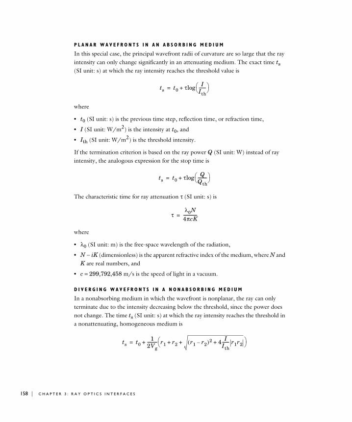
158 | C H A P T E

P L A N A R W A V E F R O N T S I N A N A B S O R B I N G M E D I U M

In this special case, the principal wavefront radii of curvature are so large that the ray intensity can only change significantly in an attenuating medium. The exact time ts (SI unit: s) at which the ray intensity reaches the threshold value is

where

• t0 (SI unit: s) is the previous time step, reflection time, or refraction time,

• I (SI unit: W/m2) is the intensity at t0, and

• Ith (SI unit: W/m2) is the threshold intensity.

If the termination criterion is based on the ray power Q (SI unit: W) instead of ray intensity, the analogous expression for the stop time is

The characteristic time for ray attenuation τ (SI unit: s) is

where

• λ0 (SI unit: m) is the free-space wavelength of the radiation,

• N − iK (dimensionless) is the apparent refractive index of the medium, where N and K are real numbers, and

• c = 299,792,458 m/s is the speed of light in a vacuum.

D I V E R G I N G W A V E F R O N T S I N A N O N A B S O R B I N G M E D I U M

In a nonabsorbing medium in which the wavefront is nonplanar, the ray can only terminate due to the intensity decreasing below the threshold, since the power does not change. The time ts (SI unit: s) at which the ray intensity reaches the threshold in a nonattenuating, homogeneous medium is

ts t0 τ IIth------- log+=

ts t0 τ QQth--------- log+=

τλ0N

4πcK--------------=

ts t01

2Vg---------- r1 r2 r1 r2–( )2 4 I

Ith------- r1r2++ +

+=


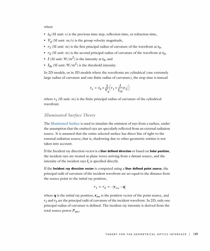
where

• t0 (SI unit: s) is the previous time step, reflection time, or refraction time,

• Vg (SI unit: m/s) is the group velocity magnitude,

• r1 (SI unit: m) is the first principal radius of curvature of the wavefront at t0,

• r2 (SI unit: m) is the second principal radius of curvature of the wavefront at t0,

• I (SI unit: W/m2) is the intensity at t0, and

• Ith (SI unit: W/m2) is the threshold intensity.

In 2D models, or in 3D models where the wavefronts are cylindrical (one extremely large radius of curvature and one finite radius of curvature), the stop time is instead

where r1 (SI unit: m) is the finite principal radius of curvature of the cylindrical wavefront.

Illuminated Surface Theory

The Illuminated Surface is used to simulate the emission of rays from a surface, under the assumption that the emitted rays are specularly reflected from an external radiation source. It is assumed that the entire selected surface has direct line of sight to the external radiation source; that is, shadowing due to other geometric entities is not taken into account.

If the Incident ray direction vector is a User defined direction or based on Solar position, the incident rays are treated as plane waves arriving from a distant source, and the intensity of the incident rays Ii is specified directly.

If the Incident ray direction vector is computed using a User defined point source, the principal radii of curvature of the incident wavefront are set equal to the distance from the source point to the initial ray position,

where q is the initial ray position, rsrc is the position vector of the point source, and r1 and r2 are the principal radii of curvature of the incident wavefront. In 2D, only one principal radius of curvature is defined. The incident ray intensity is derived from the total source power Psrc,

ts t01

Vg------ r1

IIth------- r1+

+=

r1 r2 rsrc q––= =


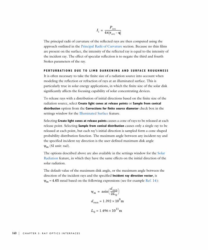
160 | C H A P T E

The principal radii of curvature of the reflected rays are then computed using the approach outlined in the Principal Radii of Curvature section. Because no thin films are present on the surface, the intensity of the reflected ray is equal to the intensity of the incident ray. The effect of specular reflection is to negate the third and fourth Stokes parameters of the ray.

P E R T U R B A T I O N S D U E T O L I M B D A R K E N I N G A N D S U R F A C E R O U G H N E S S

It is often necessary to take the finite size of a radiation source into account when modeling the reflection or refraction of rays at an illuminated surface. This is particularly true in solar energy applications, in which the finite size of the solar disk significantly affects the focusing capability of solar concentrating devices.

To release rays with a distribution of initial directions based on the finite size of the radiation source, select Create light cones at release points or Sample from conical

distribution option from the Corrections for finite source diameter check box in the settings window for the Illuminated Surface feature.

Selecting Create light cones at release points causes a cone of rays to be released at each release point. Selecting Sample from conical distribution causes only a single ray to be released at each point, but each ray’s initial direction is sampled form a cone-shaped probability distribution function. The maximum angle between any incident ray and the specified incident ray direction is the user-defined maximum disk angle ψm (SI unit: rad).

The options described above are also available in the settings window for the Solar Radiation feature, in which they have the same effects on the initial direction of the solar radiation.

The default value of the maximum disk angle, or the maximum angle between the direction of the incident rays and the specified Incident ray direction vector, is ψm = 4.65 mrad based on the following expressions (see for example Ref. 14):

IiPsrc

4π rsrc q–----------------------------=

ψmdsun2L0------------

dsun 1.392 109× m

L0 1.496 1011× m

=

=

asin=


When the finite size of the sun is taken into account, radiation from the center of the solar disc tends to be greater in intensity than radiation from the edges of the disc, a phenomenon known as limb darkening. If Empirical power law is selected from the Limb

darkening model list in the settings window for the Illuminated Surface or Solar Radiation feature, the solar radiation is assumed to follow a power law distribution. Given the intensity I(0) of radiation along a line intersecting the center of the sun, the incident solar radiation from any other point on the sun is given by the expression

where

and ψs is the angle between a line of sight to the center of the sun and a line from the center of the sun to another visible point on its surface. The exponent α can vary from 0, for which all solar radiation is of uniform intensity, to 1, at which the intensity of solar radiation falls off linearly as a function of radial position on the visible solar disc. Based on Ref. 14 the exponent α is given as a function of the free-space wavelength λ0:

If Linear is selected from the Limb darkening model list, the distribution of solar intensity is instead

It is also possible to include the effect of surface roughness when computing the incident ray direction vector at illuminated surfaces by selecting the Include surface

roughness check box. The value of the Surface slope error σφ is used as the standard deviation in a Rayleigh distribution of perturbation angles about the unperturbed ray direction vector, from which a user-defined number of rays are sampled.

I ψs( )I 0( )-------------- μα λ0( )

=

μ ψscos=

a λ0( )

0.023– 0.292λ01–

+ λ01– 2.4μm 1–≤

0.3778 0.125λ01–

+ 2.4μm 1– λ01– 2.8μm 1–≤ ≤

0.507– 0.441λ01–

+ 2.8μm 1– λ01–≤

=

I ψs( )I 0( )-------------- 1 βμ+

1 β+----------------=


162 | C H A P T E

Theory of Mueller Matrices and Optical Components

Optical devices such as polarizers and wave retarders are often used to manipulate the polarization of radiation. These devices can be modeled by multiplying the Stokes vector of the incident ray si by a Mueller matrix M,

As explained in The Stokes Parameters, the Stokes vector requires a set of orthogonal coordinate axes to be defined at the location of a propagating ray. The x-axis of this local coordinate system, e1, is the first principal curvature direction in 3D models and the out-of-plane direction in 2D models.

Similarly, the Mueller matrix of an optical device is defined with respect to a local coordinate system. This system need not coincide with the coordinate system that defines the Stokes vector of the incident ray. Therefore it is usually necessary to apply a rotation to one of these local coordinate systems before applying the Mueller matrix:

where R is the rotation matrix

where θ is the angle by which the local coordinate system of the ray must be rotated so that the x-axes of the two local coordinate systems both lie in the plane of incidence and the y-axes are parallel.

Mueller matrices of some common optical devices are tabulated in Ref. 11.

L I N E A R P O L A R I Z E R T H E O R Y

A Linear Polarizer is an optical device that produces linearly polarized light. An ideal linear polarizer transmits radiation that is polarized in one direction, indicated by the transmission axis T, while completely preventing the transmission of radiation polarized in the orthogonal direction.

In a local coordinate system in which the x-axis is parallel to the transmission axis, the Mueller matrix of the ideal linear polarizer is

s Msi=

s R 1– MRsi=

R

1 0 0 00 2θ( )cos 2θ( )sin 00 2θ( )sin– 2θ( )cos 00 0 0 1

=


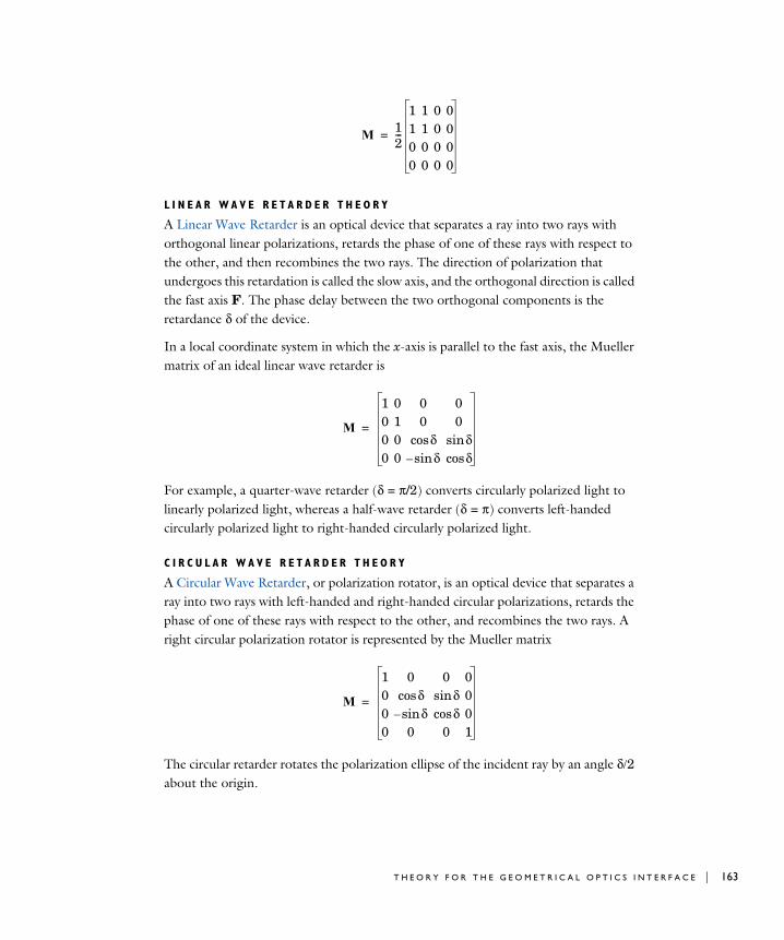
L I N E A R W A V E R E T A R D E R T H E O R Y

A Linear Wave Retarder is an optical device that separates a ray into two rays with orthogonal linear polarizations, retards the phase of one of these rays with respect to the other, and then recombines the two rays. The direction of polarization that undergoes this retardation is called the slow axis, and the orthogonal direction is called the fast axis F. The phase delay between the two orthogonal components is the retardance δ of the device.

In a local coordinate system in which the x-axis is parallel to the fast axis, the Mueller matrix of an ideal linear wave retarder is

For example, a quarter-wave retarder (δ = π/2) converts circularly polarized light to linearly polarized light, whereas a half-wave retarder (δ = π) converts left-handed circularly polarized light to right-handed circularly polarized light.

C I R C U L A R W A V E R E T A R D E R T H E O R Y

A Circular Wave Retarder, or polarization rotator, is an optical device that separates a ray into two rays with left-handed and right-handed circular polarizations, retards the phase of one of these rays with respect to the other, and recombines the two rays. A right circular polarization rotator is represented by the Mueller matrix

The circular retarder rotates the polarization ellipse of the incident ray by an angle δ/2 about the origin.

M 12---

1 1 0 01 1 0 00 0 0 00 0 0 0

=

M

1 0 0 00 1 0 00 0 δcos δsin0 0 δsin– δcos

=

M

1 0 0 00 δcos δsin 00 δsin– δcos 00 0 0 1

=


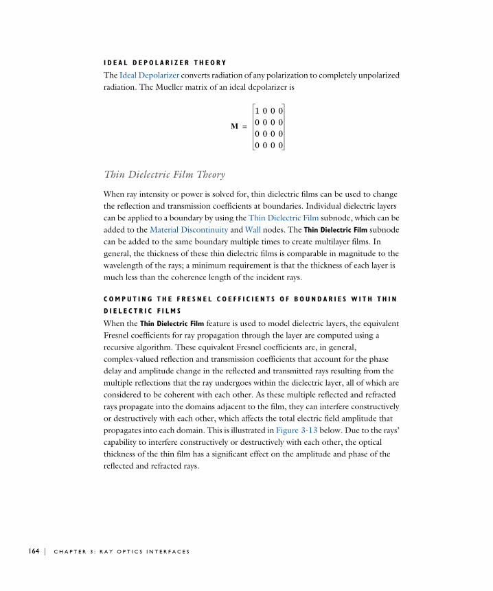
164 | C H A P T E

I D E A L D E P O L A R I Z E R T H E O R Y

The Ideal Depolarizer converts radiation of any polarization to completely unpolarized radiation. The Mueller matrix of an ideal depolarizer is

Thin Dielectric Film Theory

When ray intensity or power is solved for, thin dielectric films can be used to change the reflection and transmission coefficients at boundaries. Individual dielectric layers can be applied to a boundary by using the Thin Dielectric Film subnode, which can be added to the Material Discontinuity and Wall nodes. The Thin Dielectric Film subnode can be added to the same boundary multiple times to create multilayer films. In general, the thickness of these thin dielectric films is comparable in magnitude to the wavelength of the rays; a minimum requirement is that the thickness of each layer is much less than the coherence length of the incident rays.

C O M P U T I N G T H E F R E S N E L C O E F F I C I E N T S O F B O U N D A R I E S W I T H T H I N

D I E L E C T R I C F I L M S

When the Thin Dielectric Film feature is used to model dielectric layers, the equivalent Fresnel coefficients for ray propagation through the layer are computed using a recursive algorithm. These equivalent Fresnel coefficients are, in general, complex-valued reflection and transmission coefficients that account for the phase delay and amplitude change in the reflected and transmitted rays resulting from the multiple reflections that the ray undergoes within the dielectric layer, all of which are considered to be coherent with each other. As these multiple reflected and refracted rays propagate into the domains adjacent to the film, they can interfere constructively or destructively with each other, which affects the total electric field amplitude that propagates into each domain. This is illustrated in Figure 3-13 below. Due to the rays’ capability to interfere constructively or destructively with each other, the optical thickness of the thin film has a significant effect on the amplitude and phase of the reflected and refracted rays.

M

1 0 0 00 0 0 00 0 0 00 0 0 0

=


Figure 3-13: One incident ray enters a thin dielectric film and produces a large number of coherent reflected and refracted rays in the adjacent semi-infinite media. These rays can interfere constructively or destructively with each other.

Consider, as shown above, a thin film of thickness d and refractive index n2 bounded by semi-infinite domains with refractive indices n1 and n3. Also consider a linearly polarized ray with electric field amplitude E0 that propagates through the domain of refractive index n1 and interacts with the thin film. Let the coefficients of refraction and transmission for a ray moving from the domain of refractive index na to the domain of refractive index nb be denoted rab and tab, respectively. When the ray arrives at the film, the refracted ray undergoes a series of reflections at the boundaries between the film and either adjacent domain. Following Ref. 6, the amplitudes of the refracted rays in either domain form a pair of converging geometric series with sums

for rays returning to the domain of refractive index n1, and

for rays entering the domain of refractive index n3. The angle β is the phase delay that is introduced when a ray propagates from one surface of the film to the other,

reqE1E0------- r12 t12t21r23e2iβ r21r23e2iβ( )k

k 0=

∞

+r12 r23e2iβ+

1 r12r23e2iβ+-------------------------------------= = =

teqE3E0------- t12t23eiβ r21r23e2iβ( )k

k 0=

∞

t12t23eiβ

1 r12r23e2iβ+-------------------------------------= = =


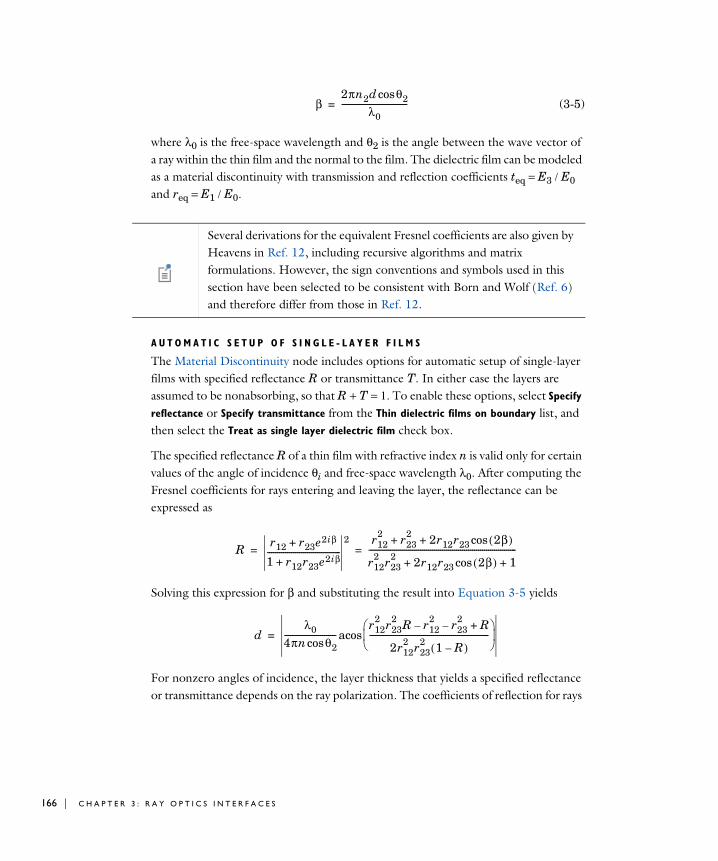
166 | C H A P T E

(3-5)

where λ0 is the free-space wavelength and θ2 is the angle between the wave vector of a ray within the thin film and the normal to the film. The dielectric film can be modeled as a material discontinuity with transmission and reflection coefficients teq = E3 / E0 and req = E1 / E0.

A U T O M A T I C S E T U P O F S I N G L E - L A Y E R F I L M S

The Material Discontinuity node includes options for automatic setup of single-layer films with specified reflectance R or transmittance T. In either case the layers are assumed to be nonabsorbing, so that R + T = 1. To enable these options, select Specify

reflectance or Specify transmittance from the Thin dielectric films on boundary list, and then select the Treat as single layer dielectric film check box.

The specified reflectance R of a thin film with refractive index n is valid only for certain values of the angle of incidence θi and free-space wavelength λ0. After computing the Fresnel coefficients for rays entering and leaving the layer, the reflectance can be expressed as

Solving this expression for β and substituting the result into Equation 3-5 yields

For nonzero angles of incidence, the layer thickness that yields a specified reflectance or transmittance depends on the ray polarization. The coefficients of reflection for rays

β2πn2d θ2cos

λ0---------------------------------=

Several derivations for the equivalent Fresnel coefficients are also given by Heavens in Ref. 12, including recursive algorithms and matrix formulations. However, the sign conventions and symbols used in this section have been selected to be consistent with Born and Wolf (Ref. 6) and therefore differ from those in Ref. 12.

Rr12 r23e2iβ+

1 r12r23e2iβ+-------------------------------------

2 r122 r23

2 2r12r23 2β( )cos+ +

r122 r23

2 2r12r23 2β( )cos 1+ +--------------------------------------------------------------------------= =

dλ0

4πn θ2cos--------------------------

r122 r23

2 R r122

– r232

– R+

2r122 r23

2 1 R–( )------------------------------------------------------------

acos=


propagating into or out of the layer are either those for S- or P-polarized radiation, depending on the selected option in the Specified film behavior applies to list.

A U T O M A T I C S E T U P O F A N T I - R E F L E C T I V E C O A T I N G S

To automatically compute the refractive index and thickness of a single-layer anti-reflective coating between two dielectric media, in the settings for the Material Discontinuity node select Anti-reflective coating from the Thin dielectric films on

boundary list. By default the anti-reflective coating is ideal, in the sense that is always has a reflectance of zero for rays of any wavelength and any angle of incidence. However, if you select the Treat as single layer dielectric film check box, then instead the single-layer coating only has a reflectance of zero for rays at a specific angle of incidence θi (SI unit: rad) and vacuum wavelength λ0 (SI unit: m).

For oblique incidence, the refractive index of the ideal single-layer coating differs for s- and p-polarized rays. For s-polarized rays, the refractive index n2 of a film between media with refractive indices n1 and n3 is

For p-polarized rays, the refractive index is

where

Either equation returns the value of n2 for which r12 = r23 for rays of the specified polarization at the specified angle of incidence. An ideal anti-reflective coating is obtained when the magnitude of the equivalent reflection coefficient is 0. This can be

In some cases, the specified transmittance or reflectance will be impossible to achieve, given the refractive indices of the layer and the surrounding media. In such cases, rays will pass through the boundary as if no dielectric layers were present.

n2 n1 θisin( )2 n1 θi n32 n1 θisin( )2

–cos+=

n22

2-------

θinan1 n3 n32 4 θisin2θinan1n3cos–+( )cos

na θicos--------------------------------------------------------------------------------------------------------------------------=

nan3

2 n1 θisin( )2–

n32

-----------------------------------------≡


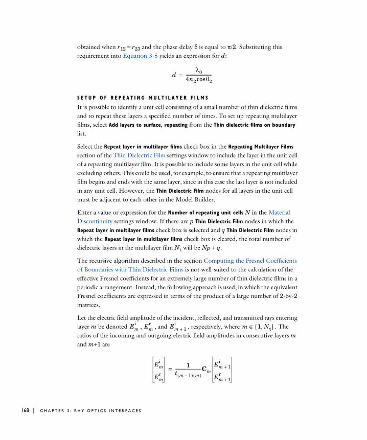
168 | C H A P T E

obtained when r12 = r23 and the phase delay δ is equal to π/2. Substituting this requirement into Equation 3-5 yields an expression for d:

S E T U P O F R E P E A T I N G M U L T I L A Y E R F I L M S

It is possible to identify a unit cell consisting of a small number of thin dielectric films and to repeat these layers a specified number of times. To set up repeating multilayer films, select Add layers to surface, repeating from the Thin dielectric films on boundary

list.

Select the Repeat layer in multilayer films check box in the Repeating Multilayer Films section of the Thin Dielectric Film settings window to include the layer in the unit cell of a repeating multilayer film. It is possible to include some layers in the unit cell while excluding others. This could be used, for example, to ensure that a repeating multilayer film begins and ends with the same layer, since in this case the last layer is not included in any unit cell. However, the Thin Dielectric Film nodes for all layers in the unit cell must be adjacent to each other in the Model Builder.

Enter a value or expression for the Number of repeating unit cells N in the Material Discontinuity settings window. If there are p Thin Dielectric Film nodes in which the Repeat layer in multilayer films check box is selected and q Thin Dielectric Film nodes in which the Repeat layer in multilayer films check box is cleared, the total number of dielectric layers in the multilayer film Nt will be Np + q.

The recursive algorithm described in the section Computing the Fresnel Coefficients of Boundaries with Thin Dielectric Films is not well-suited to the calculation of the effective Fresnel coefficients for an extremely large number of thin dielectric films in a periodic arrangement. Instead, the following approach is used, in which the equivalent Fresnel coefficients are expressed in terms of the product of a large number of 2-by-2 matrices.

Let the electric field amplitude of the incident, reflected, and transmitted rays entering layer m be denoted , , and , respectively, where . The ratios of the incoming and outgoing electric field amplitudes in consecutive layers m and m+1 are

dλ0

4n2 θ2cos-------------------------=

Emi Em

r Em 1+i m 1 Nt,[ ]∈

Emi

Emr

1t m 1–( ) m( )-------------------------Cm

Em 1+i

Em 1+r

=


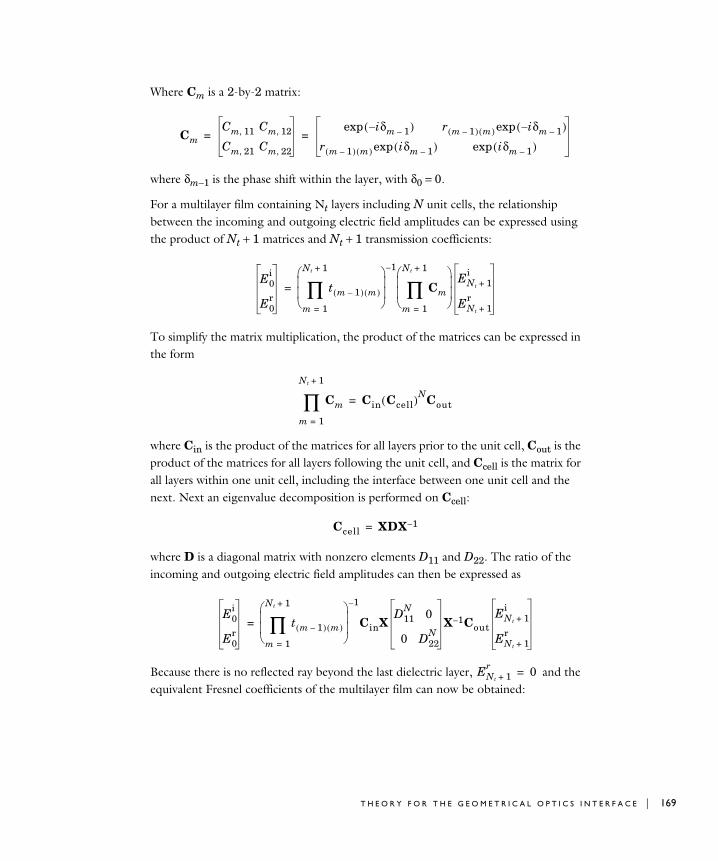
Where Cm is a 2-by-2 matrix:

where δm−1 is the phase shift within the layer, with δ0 = 0.

For a multilayer film containing Nt layers including N unit cells, the relationship between the incoming and outgoing electric field amplitudes can be expressed using the product of Nt + 1 matrices and Nt + 1 transmission coefficients:

To simplify the matrix multiplication, the product of the matrices can be expressed in the form

where Cin is the product of the matrices for all layers prior to the unit cell, Cout is the product of the matrices for all layers following the unit cell, and Ccell is the matrix for all layers within one unit cell, including the interface between one unit cell and the next. Next an eigenvalue decomposition is performed on Ccell:

where D is a diagonal matrix with nonzero elements D11 and D22. The ratio of the incoming and outgoing electric field amplitudes can then be expressed as

Because there is no reflected ray beyond the last dielectric layer, and the equivalent Fresnel coefficients of the multilayer film can now be obtained:

CmCm 11, Cm 12,

Cm 21, Cm 22,

iδm 1––( )exp r m 1–( ) m( ) iδm 1––( )exp

r m 1–( ) m( ) iδm 1–( )exp iδm 1–( )exp= =

E0i

E0r

t m 1–( ) m( )

m 1=

Nt 1+

∏ 1–

Cm

m 1=

Nt 1+

∏ ENt 1+

i

ENt 1+r

=

Cm

m 1=

Nt 1+

∏ Cin Ccell( )NCout=

Ccell XDX 1–=

E0i

E0r

t m 1–( ) m( )

m 1=

Nt 1+

∏ 1–

CinXD11

N 0

0 D22N

X 1– CoutENt 1+

i

ENt 1+r

=

ENt 1+r 0=


170 | C H A P T E


The Grating and Cross Grating features are boundary conditions that release rays into one or more diffraction orders whenever a ray hits a boundary. In reality, the grating surface is a periodic substructure in which the unit cells can be smaller than the electromagnetic wavelength, but the substructure geometry is not explicitly modeled as part of the ray optics simulation. Based on the unit cell size and wavelength, rays that hit the grating will propagate into specific directions (the diffraction orders) in which waves from neighboring unit cells would constructively interfere.

Although the substructure of a grating or cross grating may contain many fine details, typically on the micron scale, from a ray optics perspective it is not necessary to explicitly model the substructure geometry. Instead the grating is approximated as a featureless surface where diffraction orders are released in directions computed from the specified unit cell size and the electromagnetic wavelength.

D E F I N I T I O N S

Unless otherwise stated, in this section, the term “grating” will be used to refer to a surface whose substructure is periodic in one direction and homogeneous in the orthogonal direction. The term “cross grating” will be used for a surface whose substructure exhibits periodicity in two different directions.

Consider an electromagnetic wave incident on the grating or cross grating surface with vacuum wavelength λ0 (SI unit: m). It therefore has angular frequency ω = 2π/λ0 (SI unit: rad/m). Assuming the surrounding media are transparent or weakly absorbing, the ray propagates in the direction of its wave vector k (SI unit: rad/m) which has magnitude k = ωn/c. Here n (dimensionless) is the absolute refractive index of the material and c = 299,792,458 m/s is the speed of light in a vacuum.

G R A T I N G

The effect of a grating is to offset the in-plane components of the wave vector by an integer multiple of the reciprocal lattice vector G (SI unit: rad/m), given by

reqE0

r

E0i-------=

teq

ENt 1+i

E0i

-----------------=


,

Here d (SI unit: m) is the grating constant, i.e. the width of each unit cell of the periodic substructure; and Tg (dimensionless) is a unit vector that lies in the grating surface and indicates the direction of periodicity. By definition, Tg is orthogonal to the surface normal ns.

The wave vector k of the incident ray can be treated as the vector sum of two constituent vectors, one parallel to the surface (kp) and one perpendicular to it (kn):

,

The in-plane component of the outgoing wave vector is given by

(3-6)

where m (dimensionless) is an integer known as the diffraction order. For m = 0 the ray is specularly reflected if it propagates into the same medium as the incident ray, or refracted (as in Snell’s law) if it propagates into the medium on the opposite side of the grating. The diffraction order m can be any integer but (as detailed in a later section) rays of a given diffraction order can only propagate if the out-of-plane wave vector component remains real-valued while the in-plane component satisfies Equation 3-6.

C R O S S G R A T I N G

In a Cross Grating, the in-plane component of the wave vector is offset by integer multiples of two different reciprocal lattice vectors corresponding to two directions of periodicity in the grating surface,

(3-7)

where m and n are the diffraction order numbers. The two reciprocal lattice vectors G1 and G2 (SI unit: rad/m) are defined as

(3-8)

where d1 and d2 (SI unit: m) are the dimensions of one unit cell in the two-dimensional periodic substructure, and Tg,1 and Tg,2 (dimensionless) are unit vectors indicating the corresponding directions of periodicity.

G 2πTgd-------=

kp ns k ns×( )×= kn k ns⋅( )ns=

kp out, kp mG+=

kp out, kp mG1 nG2+ +=

G1 2πd2 ns×

d1 d2 ns×( )⋅-----------------------------------= G2 2π

ns d1×d2 ns d1×( )⋅-----------------------------------=

d1 d1Tg 1,≡ d2 d2Tg 2,≡


172 | C H A P T E

Note that Tg,1 and Tg,2 are not required to be perpendicular to each other, but they cannot be parallel or antiparallel. By definition, both Tg,1 and Tg,2 are orthogonal to the surface normal ns. For the simplified case where Tg,1 and Tg,2 are perpendicular, Equation 3-8 simplifies to

Similar to a grating with a single direction of periodicity, the two diffraction orders m and n can take on any integer values, but that diffraction order can only propagate if the out-of-plane wave vector component can be real-valued while the in-plane component satisfies Equation 3-7.

W A V E V E C T O R R E I N I T I A L I Z A T I O N

The magnitude of the outgoing perpendicular component of the reflected and transmitted wavefront can be found from the requirement that the magnitude of the outgoing wave vector kout is equal to the wave number; that is, ||kout|| = k0n, where k0 = ω/c is the wave number in free space. The projections of the reflected and transmitted wave vectors onto the surface normal kn,r and kn,t therefore have magnitudes

(3-9)

where n1 and n2 are the refractive indices on the incoming (reflected) and outgoing (transmitted) side of the grating, respectively. The outgoing reflected and transmitted wave vectors kr and kt are therefore given by

A given order will only exist if the magnitude of the parallel (in-plane) wave vector is less than the magnitude of each out-going wave vector. That is

for rays on the incoming side (reflected rays) and

G1 2πTg 1,d1------------= G2 2π

Tg 2,d2------------=

kn r, k0n1( )2 kp out,2

–=

kn t, k0n2( )2 kp out,2

–=

kr kp out, kn r, ns+=

kt kp out, kn t, ns+=

kp out, k0n1<

kp out, k0n2<


for rays on the outgoing side (transmitted rays). Each is equivalent to requiring one of the square roots in Equation 3-9 to return a positive real value.

R E L A T I V E O R D E R N U M B E R S

For the Grating (but not the Cross Grating) it is possible to specify relative diffraction order numbers instead of absolute orders. This is particularly useful for blazed gratings.

In a blazed grating, the main detail of the grating microstructure is an array of facets that make an angle θB (SI unit: rad) with respect to the grating normal. This angle is known as the blaze angle. The absolute order number m in which maximum diffraction efficiency occurs can be found from the general grating equation

,

where the angles α and β (SI unit: rad) are defined as

where θ and γ are the angles of incidence with respect to the grating normal in-plane and out-of-plane respectively. At the peak of the blaze function the angle of diffraction with respect to the grating normal (θ') is equal to θ. Therefore, for any given wavelength λ, the absolute order number is given by

,

where Δm is the order number relative to the order in which this wavelength is closest to the blaze peak. The in-plane and out-of-plane angles can be derived from the incoming wave vector components. First, we have the component in the direction of the grating normal

.

The in-plane and out-of-plane components are

and

where kp is the incoming wave vector projected onto the grating surface. This gives the angle θ and γ as

mλ0 ndg γ α βsin+sin( )cos=

α θB θ+= β θB θ′–=

m round2ndg

λ-------------- γ θB θcossincos Δm+=

kn k ns⋅=

kp in, kp Tg⋅=

kp out, kp ns T× g( )⋅=


174 | C H A P T E

and

.

Interference Pattern Theory

The Interference Pattern plot can be used to visualize the fringes resulting from the interference of two or more rays at a surface. The interference pattern is only valid when it is plotted over an area with a length scale that is much smaller than the principal radius of curvature of any incident wavefront. This is a consequence of the treatment of each ray as a wavefront that subtends a small solid angle. Furthermore, this plot type requires calculation of the ray intensity and instantaneous phase.

Given the phase Ψ0 of a ray at the point (qx, qy) where the ray intersects a plane, the phase Ψ at a nearby point (qx + Δx, qy + Δy) is computed as follows. Without loss of generality assume that the x- and y-axes are oriented so that they are parallel to the projections of the principal curvature directions onto the cut plane. For a spherical wavefront, the orientations of these axes may be determined arbitrarily as long as they are orthogonal. Let ni,x and ni,y denote the x- and y- components, respectively, of the normalized ray direction vector. Let r1 and r2 denote the principal radii of curvature in the directions parallel to the x- and y-axes, respectively. For an incident ray with wave vector magnitude k, the phase at (qx + Δx, qy) is

Where Δr1 is the change in the principal radius of curvature of the wavefront when moving between the two points.

Further simplification yields

This equation yields an indeterminate form in the limit of infinite radii of curvature, making it unsuitable for computing interference patterns involving plane waves. The

θkp in,

kn------------- atan– θB–=

γkp out, θBcos

kn-------------------------------- atan–=

Ψ qx Δx qy,+( ) Ψ qx qy,( ) kΔr1+=

r1 Δr1+( )2 r12 ni x, r1( )2

–[ ] ni x, r1 Δx+( )2+=

Δr1 r12 2ni x, r1Δx Δx2

+ + r1–=


equation can be made more robust for plane waves by applying a Taylor series approximation about Δx = 0,

Discarding terms of order Δx3 or higher yields

Similarly, the change in principal radius of curvature due to a small perturbation in the y direction is

The rationale for discarding higher-order terms is that they all involve division by higher powers of r1 and r2. Therefore this series approximation is only valid when the perturbations in the x and y directions are much smaller than the principal radii of curvature. To assume otherwise would mean that the incident wavefronts subtend very large solid angles.

Combining the perturbations in the two principal radii of curvature yields an expression for the phase at any point (qx + Δx, qy + Δy) on the cut plane,

The incident Stokes vector is then converted to an incident electric field using the relation

and the electric field at the intersection of the ray with the cut plane can be used to compute the electric field at a nearby point using the relation

where it is again assumed that the ray subtends a small solid angle so that the intensity of the incident ray is approximately uniform over the region in which the interference

r12 2ni x, r1Δx Δx2

+ + r1 ni x, Δx 12r1--------- 1 ni x,

2–( )Δx2 O Δx3( )+ + +=

Δr1 ni x, Δx 12r1--------- 1 ni x,

2–( )Δx2+=

Δr2 ni y, Δy 12r2--------- 1 ni y,

2–( )Δy2+=

Ψ Ψ0 k ni x, Δx 12r1--------- 1 ni x,

2–( )Δx2 ni y, Δy 12r2--------- 1 ni y,

2–( )Δy2+ + ++=

I n2---

ε0μ0------ E E∗⋅( )=

E qx Δx qy Δy+,+( ) E qx qy,( ) Ψ qx Δx qy Δy+,+( ) Ψ0–[ ]exp=


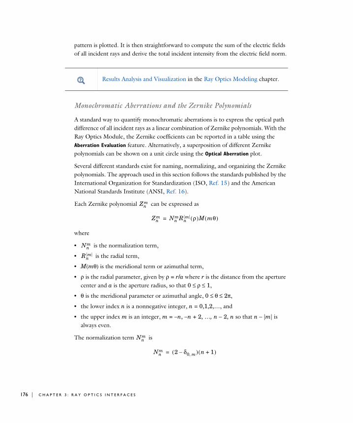
176 | C H A P T E

pattern is plotted. It is then straightforward to compute the sum of the electric fields of all incident rays and derive the total incident intensity from the electric field norm.

Monochromatic Aberrations and the Zernike Polynomials

A standard way to quantify monochromatic aberrations is to express the optical path difference of all incident rays as a linear combination of Zernike polynomials. With the Ray Optics Module, the Zernike coefficients can be reported in a table using the Aberration Evaluation feature. Alternatively, a superposition of different Zernike polynomials can be shown on a unit circle using the Optical Aberration plot.

Several different standards exist for naming, normalizing, and organizing the Zernike polynomials. The approach used in this section follows the standards published by the International Organization for Standardization (ISO, Ref. 15) and the American National Standards Institute (ANSI, Ref. 16).

Each Zernike polynomial can be expressed as

where

• is the normalization term,

• is the radial term,

• M(mθ) is the meridional term or azimuthal term,

• ρ is the radial parameter, given by ρ = r/a where r is the distance from the aperture center and a is the aperture radius, so that 0 ≤ ρ ≤ 1,

• θ is the meridional parameter or azimuthal angle, 0 ≤ θ ≤ 2π,

• the lower index n is a nonnegative integer, n = 0,1,2,…, and

• the upper index m is an integer, m = −n, −n + 2, …, n − 2, n so that n − |m| is always even.

The normalization term is

Results Analysis and Visualization in the Ray Optics Modeling chapter.

Znm

Znm Nn

mRnm ρ( )M mθ( )=

Nnm

Rnm

Nnm

Nnm 2 δ0 m,–( ) n 1+( )=


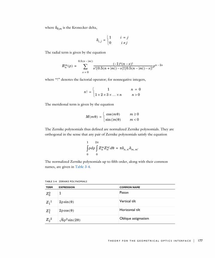
where δ0,m is the Kronecker delta,

The radial term is given by the equation

where “!” denotes the factorial operator; for nonnegative integers,

The meridional term is given by the equation

The Zernike polynomials thus defined are normalized Zernike polynomials. They are orthogonal in the sense that any pair of Zernike polynomials satisfy the equation

The normalized Zernike polynomials up to fifth order, along with their common names, are given in Table 3-4.

TABLE 3-4: ZERNIKE POLYNOMIALS

TERM EXPRESSION COMMON NAME

Piston

Vertical tilt

Horizontal tilt

Oblique astigmatism

δi j,10

=i j=

i j≠

Rnm ρ( ) 1–( )s n s–( )!

s! 0.5 n m+( ) s–[ ]! 0.5 n m–( ) s–[ ]!---------------------------------------------------------------------------------------------------ρn 2s–

s 0=

0.5 n m–( )

=

n!1

1 2 3 … n××××

=n 0=

n 0>

M mθ( )mθ( )cosm θ( )sin

=m 0≥m 0<

ρ ρ ZnmZn'

m' θd

0

2π

d

0

1

πδn n', δm m',=

Z00 1

Z11– 2ρ θ( )sin

Z11 2ρ θ( )cos

Z22– 6ρ2 2θ( )sin


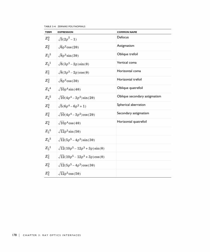
178 | C H A P T E

Defocus

Astigmatism

Oblique trefoil

Vertical coma

Horizontal coma

Horizontal trefoil

Oblique quatrefoil

Oblique secondary astigmatism

Spherical aberration

Secondary astigmatism

Horizontal quatrefoil

TABLE 3-4: ZERNIKE POLYNOMIALS

TERM EXPRESSION COMMON NAME

Z20 3 2ρ2 1–( )

Z22 6ρ2 2θ( )cos

Z33– 8ρ3 3θ( )sin

Z31– 8 3ρ3 2ρ–( ) θ( )sin

Z31 8 3ρ3 2ρ–( ) θ( )cos

Z33 8ρ3 3θ( )cos

Z44– 10ρ4 4θ( )sin

Z42– 10 4ρ4 3ρ2–( ) 2θ( )sin

Z40 5 6ρ4 6ρ2– 1+( )

Z42 10 4ρ4 3ρ2–( ) 2θ( )cos

Z44 10ρ4 4θ( )cos

Z55– 12ρ5 5θ( )sin

Z53– 12 5ρ5 4ρ3–( ) 3θ( )sin

Z51– 12 10ρ5 12ρ3– 3ρ+( ) θ( )sin

Z51 12 10ρ5 12ρ3– 3ρ+( ) θ( )cos

Z53 12 5ρ5 4ρ3–( ) 3θ( )cos

Z55 12ρ5 5θ( )cos


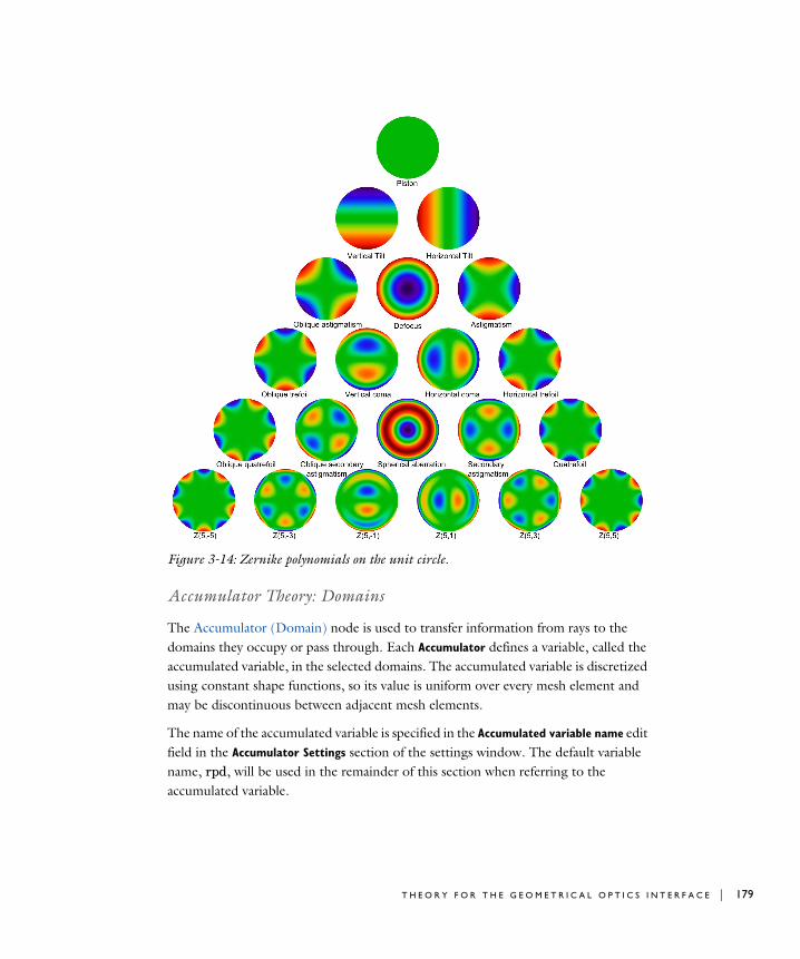
Figure 3-14: Zernike polynomials on the unit circle.

Accumulator Theory: Domains

The Accumulator (Domain) node is used to transfer information from rays to the domains they occupy or pass through. Each Accumulator defines a variable, called the accumulated variable, in the selected domains. The accumulated variable is discretized using constant shape functions, so its value is uniform over every mesh element and may be discontinuous between adjacent mesh elements.

The name of the accumulated variable is specified in the Accumulated variable name edit field in the Accumulator Settings section of the settings window. The default variable name, rpd, will be used in the remainder of this section when referring to the accumulated variable.


180 | C H A P T E

A C C U M U L A T O R T Y P E

The options in the Accumulator type list are Density and Count. If Density is selected, the source term is divided by the area or volume of the mesh element when calculating each ray’s contribution to the accumulated variable. If Count is selected, no division by the area or volume of the mesh element occurs.

The equations in the following section are valid for the Density type. The corresponding value of the accumulated variable for the Count type is

where V is the mesh element volume (in 3D) or area (in 2D).

A C C U M U L A T I O N O V E R E L E M E N T S

When Elements is selected from the Accumulate over list, the value of the accumulated variable in a mesh element is the sum of the source terms Ri evaluated for all rays in that mesh element:

where N is the total number of rays in the element and V is the area or volume of the mesh element. In other words, the contribution of each ray to the accumulated variable is distributed uniformly over the mesh element the ray is in, regardless of the ray’s exact position within the element.

If Elements and time is selected from the Accumulate over list, then the sum of the source terms for rays in the mesh element is used to define the time derivative of the accumulated variable, rather than its instantaneous value:

Thus the value of the accumulated variable depends on the time history of rays in the mesh element, instead of the instantaneous positions of the rays. As each ray propagates, it will leave behind a trail based on its contributions to the accumulated variables in mesh elements it has traversed. The algorithm for accumulating over time takes into account the fraction of a time step taken by the solver that the ray spends in each mesh element, even if it crosses between elements during the time step.

rpdcount rpddensity V×=

rpd 1V---- Ri

i 1=

N

=

d rpd( )dt

------------------ 1V---- Ri

i 1=

N

=


Accumulator Theory: Boundaries

The Accumulator (Boundary) feature transfers information from rays to the boundaries they hit or pass through. Each Accumulator defines a variable, called the accumulated variable, on the selected boundaries. The accumulated variable is discretized using constant shape functions, so its value if uniform over every mesh element and may be discontinuous between adjacent mesh elements.

The name of the accumulated variable is specified in the Accumulated variable name edit field in the Accumulator Settings section of the settings window. The default variable name, rpb, will be used in the remainder of this section when referring to the accumulated variable.

The options in the Accumulator type list are Density and Count. If Density is selected, the source term is divided by the surface area or length of the boundary mesh element when calculating each ray’s contribution to the accumulated variable. If Count is selected, no division by the surface area or length of the boundary element occurs.

The equations in the following section are valid for the Density type. The corresponding value of the accumulated variable for the Count type is

where V is the boundary element surface area (in 3D) or length (in 2D).

When Rays in boundary elements is selected from the Accumulate over list, the accumulated variable in a boundary element gets incremented by the source term R whenever a ray freezes or sticks to the boundary:

where division by the mesh element area or length occurs because the accumulator is assumed to be of type Density. Thus the source term evaluated for an incident ray is uniformly distributed over the boundary element it freezes or sticks to.

If instead Ray-wall interactions is selected from the Accumulate over list, then the accumulated variable gets incremented regardless of what type of ray-wall interaction occurs. Thus, it is possible for the same ray to increment the accumulated variable in many different boundary elements, or even in the same element multiple times.

rpbcount rpbdensity V×=

rpbnew rpb RV----+=


182 | C H A P T E

B U I L T - I N G L O B A L V A R I A B L E S

By default, the boundary Accumulator defines the following global variables:

Here, <scope> includes the physics interface name and the names the Accumulator and parent feature. For example, the average of the accumulated variable over a boundary may be called gop.wall1.bacc1.rpb_ave, where gop is the name of the Geometrical Optics interface, wall1 is the name of the parent Wall node, bacc1 is the name of the Accumulator node, and rpb is the accumulated variable name. These variables are all available in the Add/Replace Expression menus during results evaluation.

These global variables are computed by defining a set of nonlocal couplings on the selection of the parent physics feature, such as the Wall feature to which the Accumulators are added. The following expressions for the global variables are used.

Here, <wscope> is the scope of the parent boundary feature, e.g. gop.wall1.

References for the Geometrical Optics Interface

1. L.D. Landau and E.M. Lifshitz, The Classical Theory of Fields, 4th ed., Butterworth-Heinemann, Oxford, 1975.

2. B. Edlén, “The dispersion of standard air”, J. Optical Society of America, vol. 2, pp. 339-344, 1953.

TABLE 3-5: BUILT-IN GLOBAL VARIABLES FOR BOUNDARY ACCUMULATORS

NAME EXPRESSION

<scope>.<name>_ave Average of accumulated variable

<scope>.<name>_int Integral of accumulated variable

<scope>.<name>_max Maximum of accumulated variable

<scope>.<name>_min Minimum of accumulated variable

<scope>.<name>_sum Sum of accumulated variable over elements

TABLE 3-6: BUILT-IN GLOBAL VARIABLE DEFINITIONS FOR BOUNDARY ACCUMULATORS

NAME EXPRESSION

<scope>.<name>_ave <wscope>.aveop(<scope>.<name>)

<scope>.<name>_int <wscope>.intop(<scope>.<name>)

<scope>.<name>_max <wscope>.maxop(<scope>.<name>)

<scope>.<name>_min <wscope>.minop(<scope>.<name>)

<scope>.<name>_sum <wscope>.intop(<scope>.<name>/<scope>.meshVol)


3. W.J. Tropf, “Temperature-dependent refractive index models for BaF2, CaF2, MgF2, SrF2, LiF, NaF, KCL, ZnS, and ZnSe”, Optical Engineering, vol. 34, pp. 1369-1373, 1995.

4. B.J. Frey, D.B. Leviton, and T.J. Madison, “Temperature-dependent refractive index of silicon and germanium”, Optomechanical Technologies for Astronomy, Proc. SPIE, vol. 6273, 2006.

5. H.J. Hoffmann, W.W. Jochs, and G. Westenberger, “Dispersion formula for the thermo-optic coefficient of optical glass”, Proc. SPIE, vol. 1327, 1990.

6. M. Born and E. Wolf, Principles of Optics, 7th ed., Cambridge, 1999.

7. O.N. Stavroudis, The Optics of Rays, Wavefronts, and Caustics, Academic, 1972.

8. B.E.A. Saleh and M.C.Teich, Fundamentals of Photonics, Wiley, 1991.

9. R.M. More and K. Kosaka, “Wave-front curvature in geometrical optics”, Phys. Rev. E, vol. 57, no. 5, pp. 6127–6134, 1998.

10. P.C.Y. Chang, J.G. Walker, and K.I. Hopcraft, “Ray tracing in absorbing media”, J. Quantitative Spectroscopy & Radiative Transfer, vol. 96, pp. 327–341, 2005.

11. W.A. Shurcliff, Polarized Light: Production and Use, Harvard, 1962.

12. O. S. Heavens, Optical Properties of Thin Solid Films, Dover, 1991.

13. H. Anders, Thin Films in Optics, Focal Press, 1967.

14. D. Hestroffer and C. Magnan, “Wavelength dependency of the Solar limb darkening”, Astron. Astrophysl, vol. 333, pp. 338–342, 1998.

15. ISO 24157:2008: Ophthalmic optics and instruments — Reporting aberrations of the human eye, International Organization for Standardization, Geneva, Switzerland. Amendment 1, ibid., 2019.

16. ANSI Z80.28-2017: American National Standard for Ophthalmics — Methods of Reporting Optical Aberrations of Eyes. American National Standards Institute, Alexandria VA.


184 | C H A P T E

4

M u l t i p h y s i c s I n t e r f a c e s a n d C o u p l i n g s

The Ray Optics Module contains predefined multiphysics interfaces and couplings to facilitate easy setup of models of ray propagation with significant attenuation and heating. The Ray Heating physics interface described in this chapter is found under the Optics>Ray Optics branch ( ) when adding a physics interface.

In this chapter:

• The Ray Heating Interface

• Theory for the Ray Heating Interface

185

186 | C H A P T E

Th e Ra y Hea t i n g I n t e r f a c e

The Ray Heating interface ( ) combines the Geometrical Optics interface with the Heat Transfer in Solids interface. The Ray Heat Source multiphysics feature is added automatically. The Ray Heating interface is used to model electromagnetic wave propagation in optically large systems in which the refractive index is temperature dependent. The energy lost due to the attenuation of rays in an absorbing medium creates a heat source that is included in the temperature computation.

When a predefined Ray Heating interface is added from the Optics>Ray Optics

branch ( ) of the Model Wizard or Add Physics windows, Geometrical Optics and Heat

Transfer in Solids interfaces are added to the Model Builder. A Multiphysics node is also added, which automatically includes the multiphysics coupling feature Ray Heat Source.

On the Constituent Physics InterfacesThe Geometrical Optics interface is used to model electromagnetic wave propagation when the wavelength is much smaller than the smallest geometric entity in the model. It includes built-in tools for computing the intensity, phase, and optical path length of rays. The rays can be polarized, unpolarized, or partially polarized. Frequency distributions and ray propagation in absorbing media are also supported.

The Heat Transfer in Solids interface is used to model heat transfer by conduction, convection, and radiation. A Heat Transfer in Solids model is active by default on all domains and a Heat Transfer in Fluids model is added with an empty selection. All functionality for including other domain types, such as a fluid domain, is also available. The temperature equation defined in solid domains corresponds to the differential form of the Fourier’s law that may contain additional contributions like heat sources.

S E T T I N G S F O R P H Y S I C S I N T E R F A C E S A N D C O U P L I N G F E A T U R E S

When physics interfaces are added using the predefined couplings, for example Ray

Heating, specific settings are included with the physics interfaces and the coupling features.

However, if physics interfaces are added one at a time, followed by the coupling features, these modified settings are not automatically included.

R 4 : M U L T I P H Y S I C S I N T E R F A C E S A N D C O U P L I N G S

For example, if single Geometrical Optics and Heat Transfer in Solids interfaces are added, COMSOL adds an empty Multiphysics node. You can choose from the available coupling features but the modified settings are not included.

P H Y S I C S I N T E R F A C E S A N D C O U P L I N G F E A T U R E S

Coupling FeaturesThe Ray Heat Source coupling feature node is described in this section.

Physics Interface FeaturesPhysics nodes are available from the Physics ribbon toolbar (Windows users), Physics context menu (Mac or Linux users), or right-click to access the context menu (all users).

Coupling features are available from the context menu (right-click the Multiphysics node) or from the Physics toolbar, Multiphysics menu.

TABLE 4-1: MODIFIED SETTINGS FOR A RAY HEATING INTERFACE

PHYSICS INTERFACE OR COUPLING FEATURE

MODIFIED SETTINGS (IF ANY)

Geometrical Optics Compute intensity and power is selected from the Intensity computation list in the physics interface Ray Properties section.

Heat Transfer in Solids No changes.

Ray Heat Source The Domain Selection is the same as that of the participating physics interfaces.

The corresponding Geometrical Optics and Heat Transfer in Solids interfaces are preselected in the Ray Heat Source section.

Use the online help in COMSOL Multiphysics to locate and search all the documentation. All these links also work directly in COMSOL Multiphysics when using the Help system.

In general, to add a node, go to the Physics toolbar, no matter what operating system you are using. Subnodes are available by clicking the parent node and selecting it from the Attributes menu.

T H E R A Y H E A T I N G I N T E R F A C E | 187

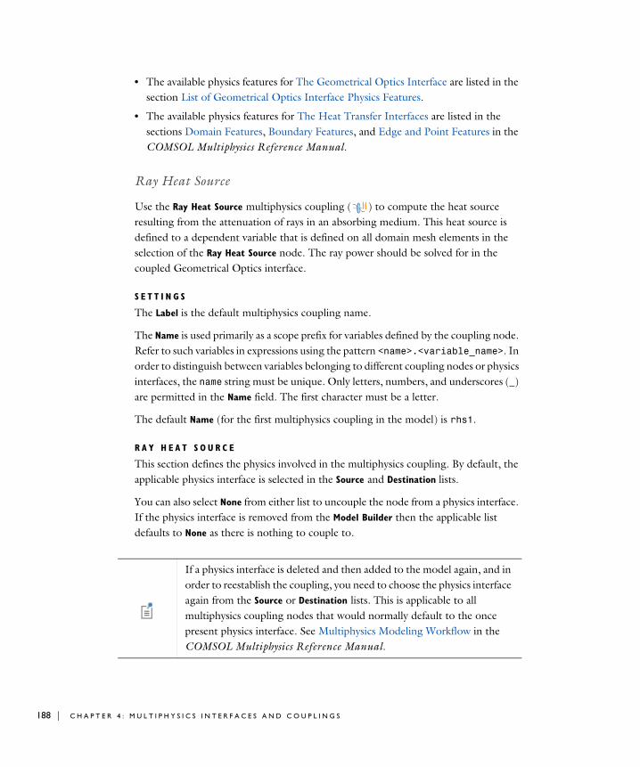
188 | C H A P T E

• The available physics features for The Geometrical Optics Interface are listed in the section List of Geometrical Optics Interface Physics Features.

• The available physics features for The Heat Transfer Interfaces are listed in the sections Domain Features, Boundary Features, and Edge and Point Features in the COMSOL Multiphysics Reference Manual.

Ray Heat Source

Use the Ray Heat Source multiphysics coupling ( ) to compute the heat source resulting from the attenuation of rays in an absorbing medium. This heat source is defined to a dependent variable that is defined on all domain mesh elements in the selection of the Ray Heat Source node. The ray power should be solved for in the coupled Geometrical Optics interface.

S E T T I N G S

The Label is the default multiphysics coupling name.

The Name is used primarily as a scope prefix for variables defined by the coupling node. Refer to such variables in expressions using the pattern <name>.<variable_name>. In order to distinguish between variables belonging to different coupling nodes or physics interfaces, the name string must be unique. Only letters, numbers, and underscores (_) are permitted in the Name field. The first character must be a letter.

The default Name (for the first multiphysics coupling in the model) is rhs1.

R A Y H E A T S O U R C E

This section defines the physics involved in the multiphysics coupling. By default, the applicable physics interface is selected in the Source and Destination lists.

You can also select None from either list to uncouple the node from a physics interface. If the physics interface is removed from the Model Builder then the applicable list defaults to None as there is nothing to couple to.

If a physics interface is deleted and then added to the model again, and in order to reestablish the coupling, you need to choose the physics interface again from the Source or Destination lists. This is applicable to all multiphysics coupling nodes that would normally default to the once present physics interface. See Multiphysics Modeling Workflow in the COMSOL Multiphysics Reference Manual.


Th eo r y f o r t h e Ra y Hea t i n g I n t e r f a c e

The Ray Heating Interface theory is described in this section:

• Unidirectional and Bidirectional Couplings

• Coupled Heat Transfer and Ray Tracing Equations

• Heat Source Calculation

Unidirectional and Bidirectional Couplings

The Ray Heating multiphysics interface combines geometrical optics with heat transfer to compute the heat source that is generated as rays propagate through an absorbing medium. The Ray Heating interface can either be used to set up a unidirectional or bidirectional coupling between the constituent physics interfaces.

If the medium properties are not temperature dependent and the domains do not undergo significant thermal expansion, then a unidirectional coupling is appropriate. The heat source generated by the attenuation of rays can be included in the heat transfer simulation by first computing the ray trajectories using a Ray Tracing study step, then computing the temperature using a Stationary study step. Both study steps are described in the COMSOL Multiphysics Reference Manual.

If the refractive index of the medium is temperature dependent, a more accurate approach is to set up a bidirectional coupling in which the attenuation of ray power affects the temperature distribution, which in turn affects the ray trajectories. The two physics can be solved for using an iterative solver loop consisting of a time-dependent solver for the ray trajectories and a stationary solver for the temperature. Such a solver sequence can be set up automatically using the Bidirectionally Coupled Ray Tracing study step, also described in the COMSOL Multiphysics Reference Manual.

Coupled Heat Transfer and Ray Tracing Equations

Under static conditions, the heat equation can be written as

ρCpu ∇T⋅ ∇ q⋅+ Q=

q k∇T–=

T H E O R Y F O R T H E R A Y H E A T I N G I N T E R F A C E | 189

190 | C H A P T E

where

• ρ (SI unit: kg/m3) is the density,

• Cp (SI unit: J/(kg·K)) is the heat capacity at constant pressure,

• T (SI unit: K) is the temperature,

• Q (SI unit: W/m3) is the heat source, and

• k (SI unit: W/(m·K)) is the thermal conductivity.

The propagation of each ray can be modeled using a set of coupled first-order equations:

where k (SI unit: rad/m) is the wave vector, ω (SI unit: rad/s) is the angular frequency, t (SI unit: s) is time, and q (SI unit: m) is the ray position vector. In an isotropic medium, the frequency and wave vector are related by the expression

where c = 299,792,458 m/s is the speed of light in a vacuum and n (dimensionless) is the refractive index. If the medium is absorbing, then the intensity of the ray decreases and it deposits some power in the domain as it passes through. This is described in greater detail in the section Attenuation Within Domains in Theory for the Geometrical Optics Interface.

A bidirectional coupling between the Geometrical Optics and Heat Transfer interfaces may be required for any of the following reasons:

• The refractive index is temperature dependent.

• The medium undergoes thermal expansion and the refractive index is strain dependent.

• The medium undergoes thermal expansion, causing rays be reflected or refracted at different angles when entering or leaving the medium.

When none of these conditions is met, the Geometrical Optics interface affects the Heat Transfer interface, and a unidirectional coupling is sufficient.

dkdt------- ∂ω

∂q------- dq

dt------- ∂ω

∂k-------=–=

ω c kn q( )------------=


Heat Source Calculation

Consider a ray j transferring an amount of power Qj through a domain. During a small time interval Δt, the ray propagates a short distance Δs from initial position qj to position qj+Δqj and its power decreases by an amount ΔQ. Then conservation of energy dictates that the deposited ray power in the domain should increase by ΔQ:

where δ is the Dirac delta function. In the limit as this time derivative becomes arbitrarily small, this expression can be rewritten as

In this expression, every ray is treated as an infinitesimally small point source. This can lead to numerical issues because the heat source becomes infinitely large at the location of each point source. In the following section an alternative expression for the domain heat source is given.

C R E A T I N G A B O U N D E D H E A T S O U R C E T E R M

The Ray Heat Source node defines a variable for the contribution to the heat source by rays in each mesh element. This variable uses constant shape functions, so it may be discontinuous across boundaries between elements. For a mesh element j with volume Vj the average heat source Qsrc,j changes according to the expression

The integral on the right-hand side is a volume integral over element j. The resulting time derivative of the heat source is the average value over the mesh element, which may be written more concisely as

where the sum is taken over all rays that are within mesh element j.

Qsrc r t Δt+,( ) Qsrc r t,( )∂Qj

∂t---------Δtδ r qj–( )

j 1=

N

–≈

dQsrcdt

---------------∂Qj

∂t---------δ r qj–( )

j 1=

N

–=

dQsrcdt

--------------- 1Vj-----

∂Qj∂t--------- δ r qj–( ) Vd

j 1=

N

–=

dQsrc j,dt

------------------- 1Vj-----–

∂Qj∂t---------

i 1=

Nj

=

T H E O R Y F O R T H E R A Y H E A T I N G I N T E R F A C E | 191

192 | C H A P T E

5

G l o s s a r y

This Glossary of Terms contains modeling terms in a ray optics context. For mathematical terms as well as geometry and CAD terms specific to the COMSOL Multiphysics® software and documentation, see the glossary in the COMSOL Multiphysics Reference Manual. For references to more information about a term, see the index.

193

194 | C H A P T E

G l o s s a r y o f T e rm scoherence The degree to which two rays interfere with each other, or to which a ray may interfere with itself when subjected to a time delay.

cross grating A type of diffraction grating with periodicity in two directions.

diffraction grating A periodic structure from which transmitted and reflected radiation can only propagate in specific directions governed by the frequency of radiation and the size of the unit cell.

diffraction order In a diffraction grating, an integer indicating the number of wavelengths between waves emanating from adjacent unit cells before they constructively interfere.

diffuse reflection Reflection at a surface in a random direction, following a probability distribution based on Lambert's cosine law.

Fresnel equations A set of equations for computing the reflection coefficients and transmission coefficients for rays as they cross a boundary between two media with different refractive indices.

geometrical optics The analysis of electromagnetic wave propagation through electrically large domains by treating the electromagnetic waves as rays.

grating See diffraction grating and cross grating.

intensity A measure of the energy density of an electromagnetic wave; for a plane polarized wave, the intensity is equal to the magnitude of the time-averaged Poynting vector.

marginal ray The ray that is released from the center of the object at the maximum aperture. This ray will pass through the edge of the aperture stop.

monochromatic light Light of uniform frequency or wavelength.

Mueller matrix A 4-by-4 matrix which can be multiplied by the Stokes vector to apply the effects of various optical components to a ray.

R 5 : G L O S S A R Y

optical dispersion model A function giving the refractive index as a function of wavelength. The coefficients for any given model will usually be determined empirically.

optical axis For simply rotationally symmetric optics, this is the axis of rotational symmetry. The optical axis will pass through the center of curvature.

optical path length The integral of refractive index along the ray trajectory. Over a given time interval, the optical path length of a ray is equal to the distance the ray would have propagated in a vacuum.

part IA subsequence of geometry instructions, usually comprising several geometry primitives, that can be added repeatedly to a COMSOL geometry sequence to avoid repetitive steps in geometry setup.

phase The quantity that indicates the variation of the instantaneous electric field with respect to time and position.

plane of incidence For nonnormal incidence of a ray at a surface, the unique plane containing the surface normal and the incident ray direction vector. For normal incidence, any plane containing the surface normal may be selected.

polarization A description of the orientation of the electric field for a polarized or partially polarized ray, and for the way in which this electric field varies as the ray propagates.

polarization, circular The state of polarization in which the electric field amplitude has two orthogonal components of equal magnitude, with a phase shift of π/2 between them, such that the electric field vector traces a helical pattern as the ray propagates.

polarization, linear The state of polarization in which the electric field only oscillates within a single plane.

power The energy transferred per unit time.

Poynting vector The vector representing the directional energy flux of an electromagnetic field.

primary ray A ray that is released into a model independently of the trajectories of other rays. Primary rays are created by release features.

G L O S S A R Y O F T E R M S | 195

196 | C H A P T E

principal curvature direction A unit vector which, together with the normal to a surface, defines a plane in which one of the principal radii of curvature of a surface is defined.

polychromatic light Light with a distribution of frequencies or wavelengths.

principal curvature The reciprocal of one of the principal radii of curvature of a surface.

principal radii of curvature The maximum and minimum values of the radius of curvature of curves that can be obtained via the intersection of a surface with a plane.

quasi-monochromatic light Light with a distribution of frequencies in which the changes in free-space wavelength are much smaller than the average free-space wavelength.

reflection coefficient A dimensionless coefficient that is used to compute the intensity of reflected rays. At boundaries between media, reflection coefficients are computed using the Fresnel equations.

refractive index The ratio of the speed of light in a vacuum to the speed of light in a medium. This is also known as the absolute refractive index.

refractive index, relative The ratio of the absolute refractive index to the refractive index of air.

release feature A feature that releases a predetermined number of rays and assigns initial values to dependent variables associated with the rays.

secondary ray A ray that is produced by the interaction of existing rays with a domain or boundary feature. The degrees of freedom for all secondary rays are preallocated when beginning to run a study.

Snell’s law The set of equations that indicates the directions in which reflected and refracted rays will propagate when a ray interacts with a boundary between two media.

specular reflection Idealized reflection at a smooth surface in which the reflected ray lies within the plane of incidence and the angles of incidence and reflection are equal.


spot diagram A type of plot for visualizing the focusing capability of an optical system. It displays the intersection points of rays with a surface, which is often the image plane of the optical system.

Stokes parameters The four Stokes parameters completely characterize the intensity and polarization of a fully polarized, partially polarized, or unpolarized ray. The Stokes parameters can be interpreted as indicators of the ray intensity that would be measured when sending a ray through various arrangements of polarizers and wave retarders.

thermo-optic dispersion model A function giving the change in refractive index as a function of wavelength and temperature.

transmission coefficient A dimensionless coefficient that is used to compute the intensity of refracted rays at boundaries between media. Transmission coefficients are computed using the Fresnel equations.

wave vector A vector in the direction of ray propagation, which indicates the spatial dependence of the instantaneous electric field for coherent radiation.

wave number The magnitude of the wave vector, equal to ω/c, where ω is the angular frequency and c is the speed of light in the medium.

wave retarder An optical component that applies a phase shift to radiation of a specific polarization with respect to radiation of an orthogonal polarization.

Zernike polynomial A type of polynomial basis that is orthonormal on the unit circle in 2D. Each term comprises a radial component and an azimuthal component, which are multiplied together. The Zernike polynomial basis is used to report optical path differences when interpreting monochromatic optical aberrations.

G L O S S A R Y O F T E R M S | 197

198 | C H A P T E

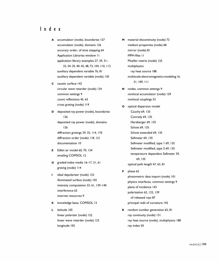
I n d e x

A accumulator (node), boundaries 127

accumulator (node), domains 126

accuracy order, of time stepping 64

Application Libraries window 11

application library examples 27, 29, 31–

32, 34–35, 40–42, 48, 73, 104, 110, 113

auxiliary dependent variable 76, 81

auxiliary dependent variable (node) 130

C caustic surface 142

circular wave retarder (node) 124

common settings 9

count reflections 45, 63

cross grating (node) 119

D deposited ray power (node), boundaries

126

deposited ray power (node), domains

126

diffraction gratings 29, 35, 114, 170

diffraction order (node) 118, 121

documentation 10

E Edlén air model 60, 70, 134

emailing COMSOL 12

G graded-index media 16–17, 21, 61

grating (node) 114

I ideal depolarizer (node) 123

illuminated surface (node) 102

intensity computation 33, 61, 139–140

interference 62

internet resources 9

K knowledge base, COMSOL 13

L latitude 105

linear polarizer (node) 122

linear wave retarder (node) 123

longitude 105

M material discontinuity (node) 72

medium properties (node) 68

mirror (node) 81

MPH-files 11

Mueller matrix (node) 125

multiphysics

ray heat source 188

multiscale electromagnetics modeling 16,

31, 109, 111

N nodes, common settings 9

nonlocal accumulator (node) 129

nonlocal couplings 53

O optical dispersion model

Cauchy 69, 135

Conrady 69, 135

Herzberger 69, 135

Schott 69, 135

Schott extended 69, 135

Sellmeier 69, 135

Sellmeier modified, type 1 69, 135

Sellmeier modified, type 2 69, 135

temperature dependent Sellmeier 39,

69, 135

optical path length 47, 63, 81

P phase 62

photometric data import (node) 101

physics interfaces, common settings 9

plane of incidence 143

polarization 62, 122, 139

of released rays 87

principal radii of curvature 142

R random number generation 65, 81

ray continuity (node) 131

ray heat source (node), multiphysics 188

ray index 50

I N D E X | 199

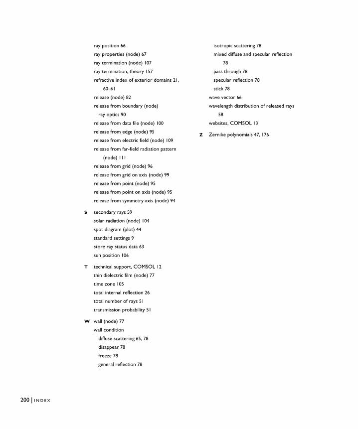
200 | I N D E X

ray position 66

ray properties (node) 67

ray termination (node) 107

ray termination, theory 157

refractive index of exterior domains 21,

60–61

release (node) 82

release from boundary (node)

ray optics 90

release from data file (node) 100

release from edge (node) 95

release from electric field (node) 109

release from far-field radiation pattern

(node) 111

release from grid (node) 96

release from grid on axis (node) 99

release from point (node) 95

release from point on axis (node) 95

release from symmetry axis (node) 94

S secondary rays 59

solar radiation (node) 104

spot diagram (plot) 44

standard settings 9

store ray status data 63

sun position 106

T technical support, COMSOL 12

thin dielectric film (node) 77

time zone 105

total internal reflection 26

total number of rays 51

transmission probability 51

W wall (node) 77

wall condition

diffuse scattering 65, 78

disappear 78

freeze 78

general reflection 78

isotropic scattering 78

mixed diffuse and specular reflection

78

pass through 78

specular reflection 78

stick 78

wave vector 66

wavelength distribution of released rays

58

websites, COMSOL 13

Z Zernike polynomials 47, 176

The Ray Optics Module User's Guide - COMSOL Documentation

Documents

Transcript of The Ray Optics Module User's Guide - COMSOL Documentation