Clifford Documentation
172
Clifford Documentation Release 1.4.0 Clifford Team Jul 20, 2021
-
Upload
khangminh22 -
Category
Documents
-
view
1 -
download
0
Transcript of Clifford Documentation

Clifford DocumentationRelease 1.4.0
Clifford Team
Jul 20, 2021

CONTENTS
1 Installation 31.1 conda . . . . . . . . . . . . . . . . . . . . . . . . . . . . . . . . . . . . . . . . . . . . . . . . . . . 31.2 PyPI . . . . . . . . . . . . . . . . . . . . . . . . . . . . . . . . . . . . . . . . . . . . . . . . . . . 3
2 API 52.1 clifford (clifford) . . . . . . . . . . . . . . . . . . . . . . . . . . . . . . . . . . . . . . . . . . . 5
2.1.1 Constructing algebras . . . . . . . . . . . . . . . . . . . . . . . . . . . . . . . . . . . . . . 52.1.2 Global configuration functions . . . . . . . . . . . . . . . . . . . . . . . . . . . . . . . . . 162.1.3 Miscellaneous classes . . . . . . . . . . . . . . . . . . . . . . . . . . . . . . . . . . . . . . 172.1.4 Miscellaneous functions . . . . . . . . . . . . . . . . . . . . . . . . . . . . . . . . . . . . 18
2.2 cga (clifford.cga) . . . . . . . . . . . . . . . . . . . . . . . . . . . . . . . . . . . . . . . . . . . 192.2.1 The CGA . . . . . . . . . . . . . . . . . . . . . . . . . . . . . . . . . . . . . . . . . . . . 192.2.2 Objects . . . . . . . . . . . . . . . . . . . . . . . . . . . . . . . . . . . . . . . . . . . . . 212.2.3 Operators . . . . . . . . . . . . . . . . . . . . . . . . . . . . . . . . . . . . . . . . . . . . 252.2.4 Meta-Class . . . . . . . . . . . . . . . . . . . . . . . . . . . . . . . . . . . . . . . . . . . 29
2.3 tools (clifford.tools) . . . . . . . . . . . . . . . . . . . . . . . . . . . . . . . . . . . . . . . . 302.3.1 Tools for specific ga’s . . . . . . . . . . . . . . . . . . . . . . . . . . . . . . . . . . . . . . 312.3.2 Classifying conformal GAs . . . . . . . . . . . . . . . . . . . . . . . . . . . . . . . . . . . 572.3.3 Determining Rotors From Frame Pairs or Orthogonal Matrices . . . . . . . . . . . . . . . . 59
2.4 operator functions (clifford.operator) . . . . . . . . . . . . . . . . . . . . . . . . . . . . . . . 622.5 transformations (clifford.transformations) . . . . . . . . . . . . . . . . . . . . . . . . . . . . 62
2.5.1 Base classes . . . . . . . . . . . . . . . . . . . . . . . . . . . . . . . . . . . . . . . . . . . 622.5.2 Matrix-backed implementations . . . . . . . . . . . . . . . . . . . . . . . . . . . . . . . . 632.5.3 Helper functions . . . . . . . . . . . . . . . . . . . . . . . . . . . . . . . . . . . . . . . . 65
2.6 taylor_expansions (clifford.taylor_expansions) . . . . . . . . . . . . . . . . . . . . . . . . . 652.6.1 Implemented functions . . . . . . . . . . . . . . . . . . . . . . . . . . . . . . . . . . . . . 66
2.7 numba extension support (clifford.numba) . . . . . . . . . . . . . . . . . . . . . . . . . . . . . . 662.7.1 Supported operations . . . . . . . . . . . . . . . . . . . . . . . . . . . . . . . . . . . . . . 672.7.2 Performance considerations . . . . . . . . . . . . . . . . . . . . . . . . . . . . . . . . . . . 68
3 Predefined Algebras 69
4 Changelog 714.1 Changes in 1.4.x . . . . . . . . . . . . . . . . . . . . . . . . . . . . . . . . . . . . . . . . . . . . . 71
4.1.1 Bugs fixed . . . . . . . . . . . . . . . . . . . . . . . . . . . . . . . . . . . . . . . . . . . . 714.1.2 Compatibility notes . . . . . . . . . . . . . . . . . . . . . . . . . . . . . . . . . . . . . . . 72
4.2 Changes in 1.3.x . . . . . . . . . . . . . . . . . . . . . . . . . . . . . . . . . . . . . . . . . . . . . 724.2.1 Bugs fixed . . . . . . . . . . . . . . . . . . . . . . . . . . . . . . . . . . . . . . . . . . . . 734.2.2 Compatibility notes . . . . . . . . . . . . . . . . . . . . . . . . . . . . . . . . . . . . . . . 734.2.3 Patch releases . . . . . . . . . . . . . . . . . . . . . . . . . . . . . . . . . . . . . . . . . . 74
i
4.3 Changes in 1.2.x . . . . . . . . . . . . . . . . . . . . . . . . . . . . . . . . . . . . . . . . . . . . . 744.3.1 Bugs fixed . . . . . . . . . . . . . . . . . . . . . . . . . . . . . . . . . . . . . . . . . . . . 744.3.2 Compatibility notes . . . . . . . . . . . . . . . . . . . . . . . . . . . . . . . . . . . . . . . 74
4.4 Changes in 1.1.x . . . . . . . . . . . . . . . . . . . . . . . . . . . . . . . . . . . . . . . . . . . . . 744.4.1 Compatibility notes . . . . . . . . . . . . . . . . . . . . . . . . . . . . . . . . . . . . . . . 754.4.2 Bugs fixed . . . . . . . . . . . . . . . . . . . . . . . . . . . . . . . . . . . . . . . . . . . . 754.4.3 Internal changes . . . . . . . . . . . . . . . . . . . . . . . . . . . . . . . . . . . . . . . . . 75
4.5 Changes 0.6-0.7 . . . . . . . . . . . . . . . . . . . . . . . . . . . . . . . . . . . . . . . . . . . . . 754.6 Changes 0.5-0.6 . . . . . . . . . . . . . . . . . . . . . . . . . . . . . . . . . . . . . . . . . . . . . 754.7 Acknowledgements . . . . . . . . . . . . . . . . . . . . . . . . . . . . . . . . . . . . . . . . . . . . 76
5 Issues 77
6 Quick Start (G2) 796.1 Setup . . . . . . . . . . . . . . . . . . . . . . . . . . . . . . . . . . . . . . . . . . . . . . . . . . . 796.2 Basics . . . . . . . . . . . . . . . . . . . . . . . . . . . . . . . . . . . . . . . . . . . . . . . . . . . 796.3 Reflection . . . . . . . . . . . . . . . . . . . . . . . . . . . . . . . . . . . . . . . . . . . . . . . . . 806.4 Rotation . . . . . . . . . . . . . . . . . . . . . . . . . . . . . . . . . . . . . . . . . . . . . . . . . 80
7 The Algebra Of Space (G3) 817.1 Setup . . . . . . . . . . . . . . . . . . . . . . . . . . . . . . . . . . . . . . . . . . . . . . . . . . . 817.2 Basics . . . . . . . . . . . . . . . . . . . . . . . . . . . . . . . . . . . . . . . . . . . . . . . . . . . 82
7.2.1 Products . . . . . . . . . . . . . . . . . . . . . . . . . . . . . . . . . . . . . . . . . . . . . 827.2.2 Defects in Precedence . . . . . . . . . . . . . . . . . . . . . . . . . . . . . . . . . . . . . . 827.2.3 Multivectors . . . . . . . . . . . . . . . . . . . . . . . . . . . . . . . . . . . . . . . . . . . 837.2.4 Reversion . . . . . . . . . . . . . . . . . . . . . . . . . . . . . . . . . . . . . . . . . . . . 837.2.5 Grade Projection . . . . . . . . . . . . . . . . . . . . . . . . . . . . . . . . . . . . . . . . 837.2.6 Magnitude . . . . . . . . . . . . . . . . . . . . . . . . . . . . . . . . . . . . . . . . . . . . 847.2.7 Inverse . . . . . . . . . . . . . . . . . . . . . . . . . . . . . . . . . . . . . . . . . . . . . . 847.2.8 Dual . . . . . . . . . . . . . . . . . . . . . . . . . . . . . . . . . . . . . . . . . . . . . . . 847.2.9 Pretty, Ugly, and Display Precision . . . . . . . . . . . . . . . . . . . . . . . . . . . . . . . 84
7.3 Applications . . . . . . . . . . . . . . . . . . . . . . . . . . . . . . . . . . . . . . . . . . . . . . . 857.3.1 Reflections . . . . . . . . . . . . . . . . . . . . . . . . . . . . . . . . . . . . . . . . . . . 857.3.2 Rotations . . . . . . . . . . . . . . . . . . . . . . . . . . . . . . . . . . . . . . . . . . . . 867.3.3 Some Ways to use Functions . . . . . . . . . . . . . . . . . . . . . . . . . . . . . . . . . . 86
7.4 Changing Basis Names . . . . . . . . . . . . . . . . . . . . . . . . . . . . . . . . . . . . . . . . . . 88
8 Rotations in Space: Euler Angles, Matrices, and Quaternions 898.1 Euler Angles with Rotors . . . . . . . . . . . . . . . . . . . . . . . . . . . . . . . . . . . . . . . . 898.2 Implementation of Euler Angles . . . . . . . . . . . . . . . . . . . . . . . . . . . . . . . . . . . . . 908.3 Convert to Quaternions . . . . . . . . . . . . . . . . . . . . . . . . . . . . . . . . . . . . . . . . . . 908.4 Convert to Rotation Matrix . . . . . . . . . . . . . . . . . . . . . . . . . . . . . . . . . . . . . . . . 918.5 Convert a Rotation Matrix to a Rotor . . . . . . . . . . . . . . . . . . . . . . . . . . . . . . . . . . 91
9 Space Time Algebra 939.1 Intro . . . . . . . . . . . . . . . . . . . . . . . . . . . . . . . . . . . . . . . . . . . . . . . . . . . 939.2 Setup . . . . . . . . . . . . . . . . . . . . . . . . . . . . . . . . . . . . . . . . . . . . . . . . . . . 939.3 The Space Time Split . . . . . . . . . . . . . . . . . . . . . . . . . . . . . . . . . . . . . . . . . . 949.4 Splitting a space-time vector (an event) . . . . . . . . . . . . . . . . . . . . . . . . . . . . . . . . . 949.5 Splitting a Bivector . . . . . . . . . . . . . . . . . . . . . . . . . . . . . . . . . . . . . . . . . . . . 959.6 Lorentz Transformations . . . . . . . . . . . . . . . . . . . . . . . . . . . . . . . . . . . . . . . . . 959.7 Lorentz Invariants . . . . . . . . . . . . . . . . . . . . . . . . . . . . . . . . . . . . . . . . . . . . 96
10 Interfacing Other Mathematical Systems 9710.1 Complex Numbers . . . . . . . . . . . . . . . . . . . . . . . . . . . . . . . . . . . . . . . . . . . . 97
ii
10.2 Quaternions . . . . . . . . . . . . . . . . . . . . . . . . . . . . . . . . . . . . . . . . . . . . . . . 99
11 Writing high(ish) performance code with Clifford and Numba via Numpy 10311.1 First import the Clifford library as well as numpy and numba . . . . . . . . . . . . . . . . . . . . . . 10311.2 Choose a specific space . . . . . . . . . . . . . . . . . . . . . . . . . . . . . . . . . . . . . . . . . 10311.3 Performance of mathematically idiomatic Clifford algorithms . . . . . . . . . . . . . . . . . . . . . 10411.4 Canonical blade coefficient representation in Clifford . . . . . . . . . . . . . . . . . . . . . . . . . . 10511.5 Exploiting blade representation to write a fast function . . . . . . . . . . . . . . . . . . . . . . . . . 10511.6 Composing larger functions . . . . . . . . . . . . . . . . . . . . . . . . . . . . . . . . . . . . . . . 10711.7 Algorithms exploiting known sparseness of MultiVector value array . . . . . . . . . . . . . . . . . . 10811.8 Future work on performance . . . . . . . . . . . . . . . . . . . . . . . . . . . . . . . . . . . . . . . 111
12 Conformal Geometric Algebra 11312.1 Using conformalize() . . . . . . . . . . . . . . . . . . . . . . . . . . . . . . . . . . . . . . . . . 11312.2 Operations . . . . . . . . . . . . . . . . . . . . . . . . . . . . . . . . . . . . . . . . . . . . . . . . 115
12.2.1 Versors purely in 𝐸0 . . . . . . . . . . . . . . . . . . . . . . . . . . . . . . . . . . . . . . 11512.2.2 Versors partly in 𝐸0 . . . . . . . . . . . . . . . . . . . . . . . . . . . . . . . . . . . . . . . 11612.2.3 Versors Out of 𝐸0 . . . . . . . . . . . . . . . . . . . . . . . . . . . . . . . . . . . . . . . . 11712.2.4 Combinations of Operations . . . . . . . . . . . . . . . . . . . . . . . . . . . . . . . . . . 118
12.3 More examples . . . . . . . . . . . . . . . . . . . . . . . . . . . . . . . . . . . . . . . . . . . . . . 11812.3.1 Visualization tools . . . . . . . . . . . . . . . . . . . . . . . . . . . . . . . . . . . . . . . 11912.3.2 Object Oriented CGA . . . . . . . . . . . . . . . . . . . . . . . . . . . . . . . . . . . . . . 12312.3.3 Example 1 Interpolating Conformal Objects . . . . . . . . . . . . . . . . . . . . . . . . . . 12712.3.4 Example 2 Clustering Geometric Objects . . . . . . . . . . . . . . . . . . . . . . . . . . . 13012.3.5 Application to Robotic Manipulators . . . . . . . . . . . . . . . . . . . . . . . . . . . . . . 133
13 Linear transformations 14313.1 Vector transformations in linear algebra . . . . . . . . . . . . . . . . . . . . . . . . . . . . . . . . . 14313.2 Multivector transformations in geometric algebra . . . . . . . . . . . . . . . . . . . . . . . . . . . . 144
13.2.1 Matrix representation . . . . . . . . . . . . . . . . . . . . . . . . . . . . . . . . . . . . . . 145
14 Working with custom algebras 14714.1 Visualization . . . . . . . . . . . . . . . . . . . . . . . . . . . . . . . . . . . . . . . . . . . . . . . 14814.2 Apollonius’ problem in R2 with circles . . . . . . . . . . . . . . . . . . . . . . . . . . . . . . . . . 14914.3 Apollonius’ problem in R3 with spheres . . . . . . . . . . . . . . . . . . . . . . . . . . . . . . . . . 150
15 Other resources for clifford 15115.1 Slide Decks . . . . . . . . . . . . . . . . . . . . . . . . . . . . . . . . . . . . . . . . . . . . . . . . 15115.2 Videos . . . . . . . . . . . . . . . . . . . . . . . . . . . . . . . . . . . . . . . . . . . . . . . . . . 151
16 Other resources for Geometric Algebra 15316.1 Links . . . . . . . . . . . . . . . . . . . . . . . . . . . . . . . . . . . . . . . . . . . . . . . . . . . 15316.2 Introductory textbooks . . . . . . . . . . . . . . . . . . . . . . . . . . . . . . . . . . . . . . . . . . 153
17 Bibliography 155
Bibliography 157
Python Module Index 159
Index 161
iii

iv
Clifford Documentation, Release 1.4.0
In [1]: from clifford.g3 import * # import GA for 3D space
In [2]: import math
In [3]: a = e1 + 2*e2 + 3*e3 # vector
In [4]: R = math.e**(math.pi/4*e12) # rotor
In [5]: R*a*~R # rotate the vectorOut[5]: (2.0^e1) - (1.0^e2) + (3.0^e3)
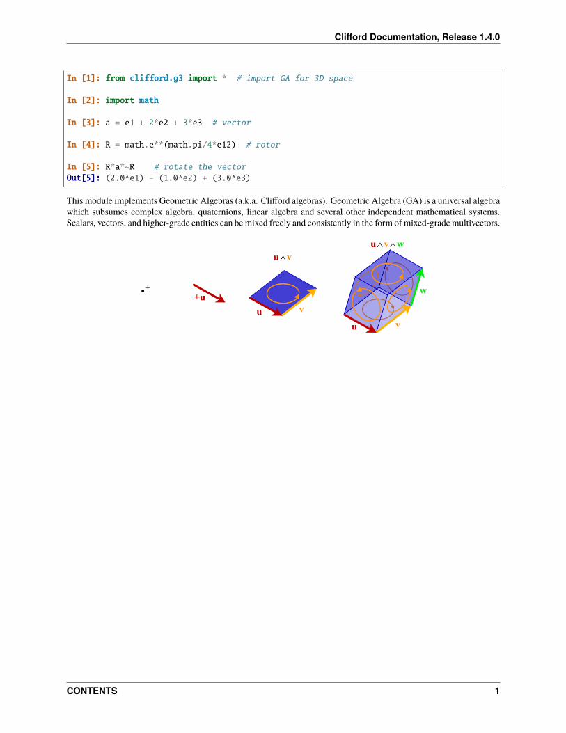
This module implements Geometric Algebras (a.k.a. Clifford algebras). Geometric Algebra (GA) is a universal algebrawhich subsumes complex algebra, quaternions, linear algebra and several other independent mathematical systems.Scalars, vectors, and higher-grade entities can be mixed freely and consistently in the form of mixed-grade multivectors.
CONTENTS 1

Clifford Documentation, Release 1.4.0
2 CONTENTS
CHAPTER
ONE
INSTALLATION
Clifford can be installed via the standard mechanisms for Python packages, and is available through both PyPI andAnaconda.
1.1 conda
If you are using the Anaconda python distribution, then you should install using the conda command.
Once you have anaconda installed you can install clifford from the conda-forge channel with the command:
conda install -c conda-forge clifford
1.2 PyPI
If you are not using Anaconda, you can install clifford from PyPI using the pip command that comes with Python:
pip3 install clifford
Note: The 1.3 release and older are not compatible with numba 0.50.0, and emit a large number of warnings on 0.49.0.To avoid these warnings, install with:
pip3 install clifford "numba~=0.48.0" "sparse~=0.9.0"
If you want the development version of clifford you can pip install from the latest master with:
pip3 install git+https://github.com/pygae/clifford.git@master
If you want to modify clifford itself, then you should use an editable (-e) installation:
git clone https://github.com/pygae/clifford.gitpip3 install -e ./clifford
If you are not running as sudo, and your python installation is system-wide, you will need to pass --user to theinvocations above.
3

Clifford Documentation, Release 1.4.0
4 Chapter 1. Installation
CHAPTER
TWO
API
2.1 clifford (clifford)
The top-level module. Provides two core classes, Layout and MultiVector, along with several helper functions toimplement the algebras.
2.1.1 Constructing algebras
Note that typically the Predefined Algebras are sufficient, and there is no need to build an algebra from scratch.
Cl([p, q, r, sig, names, firstIdx, mvClass]) Returns a Layout and basis blade MultiVectors forthe geometric algebra 𝐶𝑙𝑝,𝑞,𝑟.
conformalize(layout[, added_sig, mvClass]) Conformalize a Geometric Algebra
clifford.Cl
clifford.Cl(p: int = 0, q: int = 0, r: int = 0, sig=None, names=None, firstIdx=1, mvClass=<class'clifford._multivector.MultiVector'>)→ Tuple[clifford._layout.Layout, Dict[str,clifford._multivector.MultiVector]]
Returns a Layout and basis blade MultiVectors for the geometric algebra 𝐶𝑙𝑝,𝑞,𝑟.
The notation 𝐶𝑙𝑝,𝑞,𝑟 means that the algebra is 𝑝 + 𝑞 + 𝑟-dimensional, with the first 𝑝 vectors with positivesignature, the next 𝑞 vectors negative, and the final 𝑟 vectors with null signature.
Parameters
• p (int) – number of positive-signature basis vectors
• q (int) – number of negative-signature basis vectors
• r (int) – number of zero-signature basis vectors
• sig – See the docs for clifford.Layout. If sig is passed, then p, q, and r are ignored.
• names – See the docs for clifford.Layout.
• firstIdx – See the docs for clifford.Layout.
Returns
• layout (Layout) – The resulting layout
• blades (Dict[str, MultiVector]) – The blades of the returned layout, equivalent to layout.blades.
5
Clifford Documentation, Release 1.4.0
clifford.conformalize
clifford.conformalize(layout: clifford._layout.Layout, added_sig=[1, -1], *, mvClass=<class'clifford._multivector.MultiVector'>, **kwargs)
Conformalize a Geometric Algebra
Given the Layout for a GA of signature (p, q), this will produce a GA of signature (p+1, q+1), as well as returna new list of blades and some stuff. stuff is a dict containing the null basis blades, and some up/down functionsfor projecting in/out of the CGA.
Parameters
• layout (clifford.Layout) – layout of the GA to conformalize (the base)
• added_sig (list-like) – list of +1, -1 denoted the added signatures
• **kwargs – extra arguments to pass on into the Layout constructor.
Returns
• layout_c (ConformalLayout) – layout of the base GA
• blades_c (dict) – blades for the CGA
• stuff (dict) – dict mapping the following members of ConformalLayout by their names,for easy unpacking into the global namespace:
up(x) up-project a vector from GA to CGAdown(x) down-project a vector from CGA to GAhomo(x) homogenize a CGA vector
Examples
>>> from clifford import Cl, conformalize>>> G2, blades = Cl(2)>>> G2c, bladesc, stuff = conformalize(G2)>>> locals().update(bladesc)>>> locals().update(stuff)
Whether you construct your algebras from scratch, or use the predefined ones, you’ll end up working with the followingtypes:
MultiVector(layout[, value, string]) An element of the algebraLayout(sig, *[, ids, order, names]) Layout stores information regarding the geometric alge-
bra itself and the internal representation of multivectors.ConformalLayout(*args[, layout]) A layout for a conformal algebra, which adds extra con-
stants and helpers.
6 Chapter 2. API
Clifford Documentation, Release 1.4.0
clifford.MultiVector
class clifford.MultiVector(layout, value=None, string=None, *, dtype: numpy.dtype = <class'numpy.float64'>)
An element of the algebra
Parameters
• layout (instance of clifford.Layout) – The layout of the algebra
• value (sequence of length layout.gaDims) – The coefficients of the base blades
• dtype (numpy.dtype) – The datatype to use for the multivector, if no value was passed.
New in version 1.1.0.
Notes
The following operators are overloaded:
• A * B : geometric product
• A ^ B : outer product
• A | B : inner product
• A << B : left contraction
• ~M : reversion
• M(N) : grade or subspace projection
• M[N] : blade projection
exp()→ clifford._multivector.MultiVector
cos()→ clifford._multivector.MultiVector
sin()→ clifford._multivector.MultiVector
tan()→ clifford._multivector.MultiVector
sinh()→ clifford._multivector.MultiVector
cosh()→ clifford._multivector.MultiVector
tanh()→ clifford._multivector.MultiVector
vee(other)→ clifford._multivector.MultiVectorVee product 𝐴 ∨𝐵.
This is often defined as:
(𝐴 ∨𝐵)* = 𝐴* ∧𝐵*
=⇒ 𝐴 ∨𝐵 = (𝐴* ∧𝐵*)−*
This is very similar to the meet() function, but always uses the dual in the full space .
Internally, this is actually implemented using the complement functions instead, as these work in degeneratemetrics like PGA too, and are equivalent but faster in other metrics.
__and__(other)→ clifford._multivector.MultiVectorself & other, an alias for vee()
__mul__(other)→ clifford._multivector.MultiVectorself * other, the geometric product 𝑀𝑁
2.1. clifford (clifford) 7
Clifford Documentation, Release 1.4.0
__xor__(other)→ clifford._multivector.MultiVectorself ^ other, the Outer product 𝑀 ∧𝑁
__or__(other)→ clifford._multivector.MultiVectorself | other, the inner product 𝑀 ·𝑁
__add__(other)→ clifford._multivector.MultiVectorself + other, addition
__sub__(other)→ clifford._multivector.MultiVectorself - other, Subtraction
right_complement()→ clifford._multivector.MultiVector
left_complement()→ clifford._multivector.MultiVector
as_array()→ numpy.ndarray
mag2()→ numbers.NumberMagnitude (modulus) squared, |𝑀 |2
Note in mixed signature spaces this may be negative
adjoint()→ clifford._multivector.MultiVectorAdjoint / reversion, �̃�
Aliased as ~M to reflect �̃� , one of several conflicting notations.
Note that ~(N * M) == ~M * ~N.
__invert__()→ clifford._multivector.MultiVectorAdjoint / reversion, �̃�
Aliased as ~M to reflect �̃� , one of several conflicting notations.
Note that ~(N * M) == ~M * ~N.
__getitem__(key: Union[clifford._multivector.MultiVector, tuple, int])→ numbers.Numbervalue = self[key].
If key is a blade tuple (e.g. (0, 1) or (1, 3)), or a blade, (e.g. e12), then return the (real) value of thatblade’s coefficient.
Deprecated since version 1.4.0: If an integer is passed, it is treated as an index into self.value. Useself.value[i] directly.
__call__(other, *others)→ clifford._multivector.MultiVectorReturn a new multi-vector projected onto a grade or another MultiVector
M(g1, ... gn) gives ⟨𝑀⟩𝑔1 + · · · + ⟨𝑀⟩𝑔𝑛M(N) calls project() as N.project(M).
Changed in version 1.4.0: Grades larger than the dimension of the multivector now return 0 instead oferroring.
8 Chapter 2. API
Clifford Documentation, Release 1.4.0
Examples
>>> from clifford.g2 import *>>> M = 1 + 2*e1 + 3*e12>>> M(0)1>>> M(0, 2)1 + (3^e12)
clean(eps=None)→ clifford._multivector.MultiVectorSets coefficients whose absolute value is < eps to exactly 0.
eps defaults to the current value of the global _settings._eps.
round(eps=None)→ clifford._multivector.MultiVectorRounds all coefficients according to Python’s rounding rules.
eps defaults to the current value of the global _settings._eps.
lc(other)→ clifford._multivector.MultiVectorThe left-contraction of two multivectors, 𝑀⌋𝑁
property pseudoScalar: clifford._multivector.MultiVectorReturns a MultiVector that is the pseudoscalar of this space.
property I: clifford._multivector.MultiVectorReturns a MultiVector that is the pseudoscalar of this space.
invPS()→ clifford._multivector.MultiVectorReturns the inverse of the pseudoscalar of the algebra.
isScalar()→ boolReturns true iff self is a scalar.
isBlade()→ boolReturns true if multivector is a blade.
isVersor()→ boolReturns true if multivector is a versor. From [DFM09] section 21.5, definition from 7.6.4
grades(eps=None)→ Set[int]Return the grades contained in the multivector.
Changed in version 1.1.0: Now returns a set instead of a list
Changed in version 1.3.0: Accepts an eps argument
property blades_list: List[clifford._multivector.MultiVector]ordered list of blades present in this MV
normal()→ clifford._multivector.MultiVectorReturn the (mostly) normalized multivector.
The _mostly_ comes from the fact that some multivectors have a negative squared-magnitude. So, withoutintroducing formally imaginary numbers, we can only fix the normalized multivector’s magnitude to +-1.𝑀|𝑀 | up to a sign
hitzer_inverse()Obtain the inverse 𝑀−1 via the algorithm in the paper [HS17].
New in version 1.4.0.
2.1. clifford (clifford) 9
Clifford Documentation, Release 1.4.0
Raises NotImplementedError : – on algebras with more than 5 non-null dimensions
shirokov_inverse()Obtain the inverse 𝑀−1 via the algorithm in Theorem 4, page 16 of Dmitry Shirokov’s ICCA 2020 paper[Shi20].
New in version 1.4.0.
leftLaInv()→ clifford._multivector.MultiVectorReturn left-inverse using a computational linear algebra method proposed by Christian Perwass.
normalInv(check=True)→ clifford._multivector.MultiVectorThe inverse of itself if 𝑀�̃� = |𝑀 |2.
𝑀−1 = �̃�/(𝑀�̃�)
Parameters check (bool) – When true, the default, validate that it is appropriate to use thismethod of inversion.
inv()→ clifford._multivector.MultiVectorObtain the inverse 𝑀−1.
This tries a handful of approaches in order:
• If 𝑀�̃� = |𝑀 |2, then this uses normalInv().
• If 𝑀 is of sufficiently low dimension, this uses hitzer_inverse().
• Otherwise, this uses leftLaInv().
Note that shirokov_inverse() is not used as its numeric stability is unknown.
Changed in version 1.4.0: Now additionally tries hitzer_inverse() before falling back to leftLaInv().
leftInv()→ clifford._multivector.MultiVectorReturn left-inverse using a computational linear algebra method proposed by Christian Perwass.
rightInv()→ clifford._multivector.MultiVectorReturn left-inverse using a computational linear algebra method proposed by Christian Perwass.
dual(I=None)→ clifford._multivector.MultiVectorThe dual of the multivector against the given subspace I, �̃� = 𝑀𝐼−1
I defaults to the pseudoscalar.
commutator(other)→ clifford._multivector.MultiVectorThe commutator product of two multivectors.
[𝑀,𝑁 ] = 𝑀 ×𝑁 = (𝑀𝑁 +𝑁𝑀)/2
x(other)→ clifford._multivector.MultiVectorThe commutator product of two multivectors.
[𝑀,𝑁 ] = 𝑀 ×𝑁 = (𝑀𝑁 +𝑁𝑀)/2
anticommutator(other)→ clifford._multivector.MultiVectorThe anti-commutator product of two multivectors, (𝑀𝑁 +𝑁𝑀)/2
gradeInvol()→ clifford._multivector.MultiVectorThe grade involution of the multivector.
𝑀* =
dims∑︁𝑖=0
(−1)𝑖 ⟨𝑀⟩𝑖
10 Chapter 2. API

Clifford Documentation, Release 1.4.0
property even: clifford._multivector.MultiVectorEven part of this multivector
defined as M + M.gradInvol()
property odd: clifford._multivector.MultiVectorOdd part of this mulitvector
defined as M +- M.gradInvol()
conjugate()→ clifford._multivector.MultiVectorThe Clifford conjugate (reversion and grade involution).
𝑀* = (~M).gradeInvol()
project(other)→ clifford._multivector.MultiVectorProjects the multivector onto the subspace represented by this blade.
𝑃𝐴(𝑀) = (𝑀⌋𝐴)𝐴−1
factorise()→ Tuple[List[clifford._multivector.MultiVector], numbers.Number]Factorises a blade into basis vectors and an overall scale.
Uses the algorithm from [DFM09], section 21.6.
basis()→ List[clifford._multivector.MultiVector]Finds a vector basis of this subspace.
join(other)→ clifford._multivector.MultiVectorThe join of two blades, 𝐽 = 𝐴 ∪𝐵
Similar to the wedge, 𝑊 = 𝐴 ∧𝐵, but without decaying to 0 for blades which share a vector.
meet(other, subspace=None)→ clifford._multivector.MultiVectorThe meet of two blades, 𝐴 ∩𝐵.
Computation is done with respect to a subspace that defaults to the join() if none is given.
Similar to the vee(), 𝑉 = 𝐴 ∨𝐵, but without decaying to 0 for blades lying in the same subspace.
astype(*args, **kwargs)Change the underlying scalar type of this vector.
Can be used to force lower-precision floats or integers
See np.ndarray.astype for argument descriptions.
clifford.Layout
class clifford.Layout(sig, *, ids=None, order=None, names=None)Layout stores information regarding the geometric algebra itself and the internal representation of multivectors.
Parameters
• sig (List[int]) – The signature of the vector space. This should be a list of positive andnegative numbers where the sign determines the sign of the inner product of the correspond-ing vector with itself. The values are irrelevant except for sign. This list also determines thedimensionality of the vectors.
Examples:
sig=[+1, -1, -1, -1] # Hestenes', et al. Space-Time Algebrasig=[+1, +1, +1] # 3-D Euclidean signature
2.1. clifford (clifford) 11
Clifford Documentation, Release 1.4.0
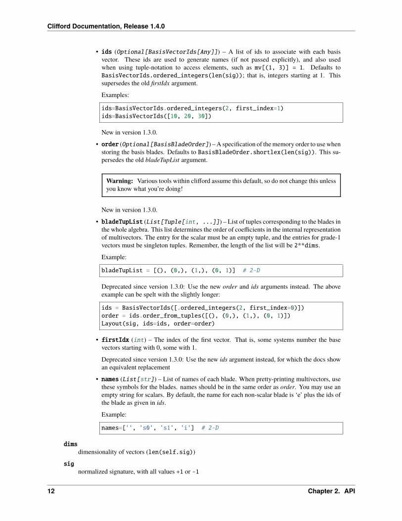
• ids (Optional[BasisVectorIds[Any]]) – A list of ids to associate with each basisvector. These ids are used to generate names (if not passed explicitly), and also usedwhen using tuple-notation to access elements, such as mv[(1, 3)] = 1. Defaults toBasisVectorIds.ordered_integers(len(sig)); that is, integers starting at 1. Thissupersedes the old firstIdx argument.
Examples:
ids=BasisVectorIds.ordered_integers(2, first_index=1)ids=BasisVectorIds([10, 20, 30])
New in version 1.3.0.
• order (Optional[BasisBladeOrder]) – A specification of the memory order to use whenstoring the basis blades. Defaults to BasisBladeOrder.shortlex(len(sig)). This su-persedes the old bladeTupList argument.
Warning: Various tools within clifford assume this default, so do not change this unlessyou know what you’re doing!
New in version 1.3.0.
• bladeTupList (List[Tuple[int, ...]]) – List of tuples corresponding to the blades inthe whole algebra. This list determines the order of coefficients in the internal representationof multivectors. The entry for the scalar must be an empty tuple, and the entries for grade-1vectors must be singleton tuples. Remember, the length of the list will be 2**dims.
Example:
bladeTupList = [(), (0,), (1,), (0, 1)] # 2-D
Deprecated since version 1.3.0: Use the new order and ids arguments instead. The aboveexample can be spelt with the slightly longer:
ids = BasisVectorIds([.ordered_integers(2, first_index=0)])order = ids.order_from_tuples([(), (0,), (1,), (0, 1)])Layout(sig, ids=ids, order=order)
• firstIdx (int) – The index of the first vector. That is, some systems number the basevectors starting with 0, some with 1.
Deprecated since version 1.3.0: Use the new ids argument instead, for which the docs showan equivalent replacement
• names (List[str]) – List of names of each blade. When pretty-printing multivectors, usethese symbols for the blades. names should be in the same order as order. You may use anempty string for scalars. By default, the name for each non-scalar blade is ‘e’ plus the ids ofthe blade as given in ids.
Example:
names=['', 's0', 's1', 'i'] # 2-D
dimsdimensionality of vectors (len(self.sig))
signormalized signature, with all values +1 or -1
12 Chapter 2. API
Clifford Documentation, Release 1.4.0
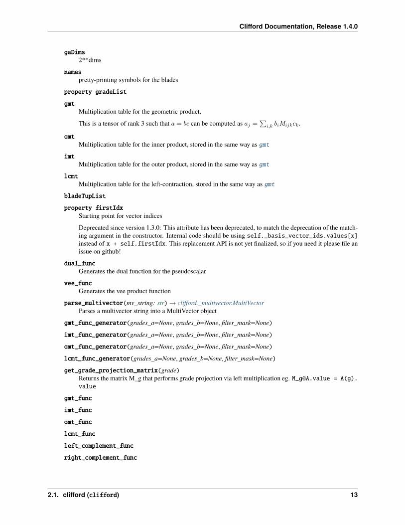
gaDims2**dims
namespretty-printing symbols for the blades
property gradeList
gmtMultiplication table for the geometric product.
This is a tensor of rank 3 such that 𝑎 = 𝑏𝑐 can be computed as 𝑎𝑗 =∑︀
𝑖,𝑘 𝑏𝑖M𝑖𝑗𝑘𝑐𝑘.
omtMultiplication table for the inner product, stored in the same way as gmt
imtMultiplication table for the outer product, stored in the same way as gmt
lcmtMultiplication table for the left-contraction, stored in the same way as gmt
bladeTupList
property firstIdxStarting point for vector indices
Deprecated since version 1.3.0: This attribute has been deprecated, to match the deprecation of the match-ing argument in the constructor. Internal code should be using self._basis_vector_ids.values[x]instead of x + self.firstIdx. This replacement API is not yet finalized, so if you need it please file anissue on github!
dual_funcGenerates the dual function for the pseudoscalar
vee_funcGenerates the vee product function
parse_multivector(mv_string: str)→ clifford._multivector.MultiVectorParses a multivector string into a MultiVector object
gmt_func_generator(grades_a=None, grades_b=None, filter_mask=None)
imt_func_generator(grades_a=None, grades_b=None, filter_mask=None)
omt_func_generator(grades_a=None, grades_b=None, filter_mask=None)
lcmt_func_generator(grades_a=None, grades_b=None, filter_mask=None)
get_grade_projection_matrix(grade)Returns the matrix M_g that performs grade projection via left multiplication eg. [email protected] = A(g).value
gmt_func
imt_func
omt_func
lcmt_func
left_complement_func
right_complement_func
2.1. clifford (clifford) 13

Clifford Documentation, Release 1.4.0
adjoint_funcThis function returns a fast jitted adjoint function
inv_funcGet a function that returns left-inverse using a computational linear algebra method proposed by ChristianPerwass.
Computes 𝑀−1 where 𝑀−1𝑀 = 1.
get_left_gmt_matrix(x)This produces the matrix X that performs left multiplication with x eg. X@b == (x*b).value
get_right_gmt_matrix(x)This produces the matrix X that performs right multiplication with x eg. X@b == (b*x).value
load_ga_file(filename: str)→ clifford._mvarray.MVArrayLoads the data from a ga file, checking it matches this layout.
grade_mask(grade: int)→ numpy.ndarray
property rotor_mask: numpy.ndarray
property metric: numpy.ndarray
property scalar: clifford._multivector.MultiVectorthe scalar of value 1, for this GA (a MultiVector object)
useful for forcing a MultiVector type
property pseudoScalar: clifford._multivector.MultiVectorThe pseudoscalar, 𝐼 .
property I: clifford._multivector.MultiVectorThe pseudoscalar, 𝐼 .
randomMV(n=1, **kwargs)→ clifford._multivector.MultiVectorConvenience method to create a random multivector.
see clifford.randomMV for details
randomV(n=1, **kwargs)→ clifford._multivector.MultiVectorgenerate n random 1-vector s
randomRotor(**kwargs)→ clifford._multivector.MultiVectorgenerate a random Rotor.
this is created by muliplying an N unit vectors, where N is the dimension of the algebra if its even; else itsone less.
property basis_vectors: Dict[str, clifford._multivector.MultiVector]dictionary of basis vectors
property basis_names: List[str]Get the names of the basis vectors, in the order they are stored.
Changed in version 1.3.0: Returns a list instead of a numpy array
property basis_vectors_lst: List[clifford._multivector.MultiVector]Like blades_of_grade(1), but ordered based on the ids parameter passed at construction.
blades_of_grade(grade: int)→ List[clifford._multivector.MultiVector]return all blades of a given grade,
property blades_list: List[clifford._multivector.MultiVector]List of blades in this layout matching the order argument this layout was constructed from.
14 Chapter 2. API
Clifford Documentation, Release 1.4.0
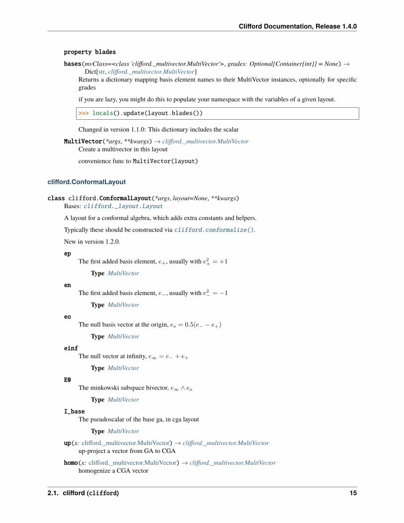
property blades
bases(mvClass=<class 'clifford._multivector.MultiVector'>, grades: Optional[Container[int]] = None)→Dict[str, clifford._multivector.MultiVector]
Returns a dictionary mapping basis element names to their MultiVector instances, optionally for specificgrades
if you are lazy, you might do this to populate your namespace with the variables of a given layout.
>>> locals().update(layout.blades())
Changed in version 1.1.0: This dictionary includes the scalar
MultiVector(*args, **kwargs)→ clifford._multivector.MultiVectorCreate a multivector in this layout
convenience func to MultiVector(layout)
clifford.ConformalLayout
class clifford.ConformalLayout(*args, layout=None, **kwargs)Bases: clifford._layout.Layout
A layout for a conformal algebra, which adds extra constants and helpers.
Typically these should be constructed via clifford.conformalize().
New in version 1.2.0.
epThe first added basis element, 𝑒+, usually with 𝑒2+ = +1
Type MultiVector
enThe first added basis element, 𝑒−, usually with 𝑒2− = −1
Type MultiVector
eoThe null basis vector at the origin, 𝑒𝑜 = 0.5(𝑒− − 𝑒+)
Type MultiVector
einfThe null vector at infinity, 𝑒∞ = 𝑒− + 𝑒+
Type MultiVector
E0The minkowski subspace bivector, 𝑒∞ ∧ 𝑒𝑜
Type MultiVector
I_baseThe pseudoscalar of the base ga, in cga layout
Type MultiVector
up(x: clifford._multivector.MultiVector)→ clifford._multivector.MultiVectorup-project a vector from GA to CGA
homo(x: clifford._multivector.MultiVector)→ clifford._multivector.MultiVectorhomogenize a CGA vector
2.1. clifford (clifford) 15
Clifford Documentation, Release 1.4.0
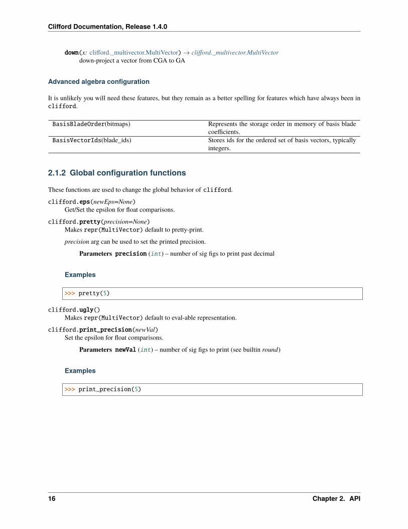
down(x: clifford._multivector.MultiVector)→ clifford._multivector.MultiVectordown-project a vector from CGA to GA
Advanced algebra configuration
It is unlikely you will need these features, but they remain as a better spelling for features which have always been inclifford.
BasisBladeOrder(bitmaps) Represents the storage order in memory of basis bladecoefficients.
BasisVectorIds(blade_ids) Stores ids for the ordered set of basis vectors, typicallyintegers.
2.1.2 Global configuration functions
These functions are used to change the global behavior of clifford.
clifford.eps(newEps=None)Get/Set the epsilon for float comparisons.
clifford.pretty(precision=None)Makes repr(MultiVector) default to pretty-print.
precision arg can be used to set the printed precision.
Parameters precision (int) – number of sig figs to print past decimal
Examples
>>> pretty(5)
clifford.ugly()Makes repr(MultiVector) default to eval-able representation.
clifford.print_precision(newVal)Set the epsilon for float comparisons.
Parameters newVal (int) – number of sig figs to print (see builtin round)
Examples
>>> print_precision(5)
16 Chapter 2. API
Clifford Documentation, Release 1.4.0
2.1.3 Miscellaneous classes
MVArray(input_array) MultiVector ArrayFrame(input_array) A frame of vectorsBladeMap(blades_map[, map_scalars]) A Map Relating Blades in two different algebras
clifford.Frame
class clifford.Frame(input_array)Bases: clifford._mvarray.MVArray
A frame of vectors
property En: clifford._multivector.MultiVectorVolume element for this frame, 𝐸𝑛 = 𝑒1 ∧ 𝑒2 ∧ · · · ∧ 𝑒𝑛
property inv: clifford._frame.FrameThe inverse frame of self
is_innermorphic_to(other: clifford._frame.Frame, eps: Optional[float] = None)→ boolIs this frame innermorphic to other?
innermorphic means both frames share the same inner-product between corresponding vectors. This im-plies that the two frames are related by an orthogonal transform.
clifford.BladeMap
class clifford.BladeMap(blades_map, map_scalars=True)A Map Relating Blades in two different algebras
Examples
>>> from clifford import Cl>>> # Dirac Algebra `D`>>> D, D_blades = Cl(1, 3, firstIdx=0, names='d')>>> locals().update(D_blades)
>>> # Pauli Algebra `P`>>> P, P_blades = Cl(3, names='p')>>> locals().update(P_blades)>>> sta_split = BladeMap([(d01, p1),... (d02, p2),... (d03, p3),... (d12, p12),... (d23, p23),... (d13, p13)])
property b1
property b2
property layout1
property layout2
2.1. clifford (clifford) 17
Clifford Documentation, Release 1.4.0
2.1.4 Miscellaneous functions
grade_obj(objin[, threshold]) Returns the modal grade of a multivectorrandomMV(layout[, min, max, grades, . . . ]) n Random MultiVectors with given layout.
clifford.grade_obj
clifford.grade_obj(objin, threshold=1e-07)Returns the modal grade of a multivector
clifford.randomMV
clifford.randomMV(layout: clifford._layout.Layout, min=-2.0, max=2.0, grades=None, mvClass=<class'clifford._multivector.MultiVector'>, uniform=None, n=1, normed: bool = False, rng=None)
n Random MultiVectors with given layout.
Coefficients are between min and max, and if grades is a list of integers, only those grades will be non-zero.
Parameters
• layout (Layout) – the layout
• min (Number) – range of values from which to uniformly sample coefficients
• max (Number) – range of values from which to uniformly sample coefficients
• grades (int, List[int]) – grades which should have non-zero coefficients. If None,defaults to all grades. A single integer is treated as a list of one integers.
• uniform (Callable[[Number, Number, Tuple[int, ...]], np.ndarray]) – Afunction like np.random.uniform. Defaults to rng.uniform.
• n (int) – The number of samples to generate. If n > 1, this function returns a list insteadof a single multivector
• normed (bool) – If true, call MultiVector.normal() on each multivector. Note that thisdoes not result in a uniform sampling of directions.
• rng – The random number state to use. Typical use would be to construct a generator withnumpy.random.default_rng().
Examples
>>> randomMV(layout, min=-2.0, max=2.0, grades=None, uniform=None, n=2)
18 Chapter 2. API
Clifford Documentation, Release 1.4.0
2.2 cga (clifford.cga)
Object Oriented Conformal Geometric Algebra.
Examples
>>> from clifford import Cl>>> from clifford.cga import CGA>>> g3, blades = Cl(3)>>> locals().update(blades)>>> g3c = CGA(g3)>>> C = g3c.round(3) # create random sphere>>> T = g3c.translation(e1+e2) # create translation>>> C_ = T(C) # translate the sphere>>> C_.center # compute center of sphere-(1.0^e4) - (1.0^e5)
2.2.1 The CGA
CGA(layout_orig) Conformal Geometric Algebra
clifford.cga.CGA
class clifford.cga.CGA(layout_orig)Conformal Geometric Algebra
conformalizes the layout_orig, and provides several methods and for objects/operators
Parameters layout_orig ([clifford.Layout, int]) – a layout for the base geometric algebra which isconformalized if given as an int, then generates a euclidean space of given dimension
Examples
>>> from clifford import Cl>>> from clifford.cga import CGA>>> g3, blades = Cl(3)>>> g3c = CGA(g3)>>> g3c = CGA(3)
2.2. cga (clifford.cga) 19
Clifford Documentation, Release 1.4.0
Methods
__init__ Initialize self.base_vector random vector in the lower(original) spacedilation see Dilationflat see Flatnull_vector generates random null vector if x is None, or returns a
null vector from base vector x, if x^self.I_base ==0 re-turns x,
rotation see Rotationround see Roundstraight_up place a vector from layout_orig into this CGA, without
up()translation see Translationtransversion see Transversion
clifford.cga.CGA.__init__
CGA.__init__(layout_orig)→ NoneInitialize self. See help(type(self)) for accurate signature.
clifford.cga.CGA.base_vector
CGA.base_vector()→ clifford._multivector.MultiVectorrandom vector in the lower(original) space
clifford.cga.CGA.dilation
CGA.dilation(*args)→ clifford.cga.Dilationsee Dilation
clifford.cga.CGA.flat
CGA.flat(*args)→ clifford.cga.Flatsee Flat
clifford.cga.CGA.null_vector
CGA.null_vector(x=None)→ clifford._multivector.MultiVectorgenerates random null vector if x is None, or returns a null vector from base vector x, if x^self.I_base ==0 returnsx,
a null vector will lay on the horisphere
20 Chapter 2. API
Clifford Documentation, Release 1.4.0
clifford.cga.CGA.rotation
CGA.rotation(*args)→ clifford.cga.Rotationsee Rotation
clifford.cga.CGA.round
CGA.round(*args)→ clifford.cga.Roundsee Round
clifford.cga.CGA.straight_up
CGA.straight_up(x)→ clifford._multivector.MultiVectorplace a vector from layout_orig into this CGA, without up()
clifford.cga.CGA.translation
CGA.translation(*args)→ clifford.cga.Translationsee Translation
clifford.cga.CGA.transversion
CGA.transversion(*args)→ clifford.cga.Transversionsee Transversion
2.2.2 Objects
Flat(cga, *args) A line, plane, or hyperplane.Round(cga, *args) A point pair, circle, sphere or hyper-sphere.
clifford.cga.Flat
class clifford.cga.Flat(cga, *args)A line, plane, or hyperplane.
Typically constructed as method of existing cga, like cga.flat()
multivector is accessable by mv property
Parameters
• cga (CGA) – the cga object
• args ([int, Multivector, Multivectors]) –
– if nothing supplied, generate a flat of highest dimension
– int: dimension of flat (2=line, 3=plane, etc)
– Multivector : can be * existing Multivector representing the Flat * vectors on the flat
2.2. cga (clifford.cga) 21
Clifford Documentation, Release 1.4.0
Examples
>>> cga = CGA(3)>>> locals().update(cga.blades)>>> F = cga.flat() # from None>>> F = cga.flat(2) # from dim of space>>> F = cga.flat(e1, e2) # from points>>> F = cga.flat(cga.flat().mv) # from existing multivector
Methods
__init__ Initialize self.inverted inverted version of this thing.involuted inverted version of this thing.
clifford.cga.Flat.__init__
Flat.__init__(cga, *args)→ NoneInitialize self. See help(type(self)) for accurate signature.
clifford.cga.Flat.inverted
Flat.inverted()→ clifford._multivector.MultiVectorinverted version of this thing.
self -> ep*self*ep
where ep is the positive added basis vector
clifford.cga.Flat.involuted
Flat.involuted()→ clifford._multivector.MultiVectorinverted version of this thing.
self -> E0*self*E0
where E0 is the added minkowski bivector
clifford.cga.Round
class clifford.cga.Round(cga, *args)A point pair, circle, sphere or hyper-sphere.
Typically constructed as method of existing cga, like cga.round()
multivector is accessable by mv property
Parameters
• cga (CGA) – the cga object
• args ([int, Multivector, Multivectors]) –
22 Chapter 2. API
Clifford Documentation, Release 1.4.0
– if nothing supplied, generate a round of highest dimension
– int: dimension of flat (2=point pair, 3=circle, etc)
– Multivector : can be * existing Multivector representing the round * vectors on the round
Examples
>>> cga = CGA(3)>>> locals().update(cga.blades)>>> cga.round() # from NoneSphere>>> cga.round(2) # from dim of spaceSphere>>> cga.round(e1, e2, -e1) # from pointsCircle>>> cga.round(cga.flat().mv) # from existing multivectorSphere
Attributes
center center of this round, as a null vectorcenter_down center of this round, as a down-projected vector (in
I_base)dim dimension of this rounddual self.mv* self.layout.Iradius radius of the round (a float)
clifford.cga.Round.center
property Round.centercenter of this round, as a null vector
clifford.cga.Round.center_down
property Round.center_downcenter of this round, as a down-projected vector (in I_base)
(but still in cga’s layout)
2.2. cga (clifford.cga) 23
Clifford Documentation, Release 1.4.0
clifford.cga.Round.dim
property Round.dimdimension of this round
clifford.cga.Round.dual
property Round.dualself.mv* self.layout.I
clifford.cga.Round.radius
property Round.radiusradius of the round (a float)
Methods
__init__ Initialize self.from_center_radius construct a round from center/radiusinverted inverted version of this thing.involuted inverted version of this thing.
clifford.cga.Round.__init__
Round.__init__(cga, *args)→ NoneInitialize self. See help(type(self)) for accurate signature.
clifford.cga.Round.from_center_radius
Round.from_center_radius(center, radius)construct a round from center/radius
clifford.cga.Round.inverted
Round.inverted()→ clifford._multivector.MultiVectorinverted version of this thing.
self -> ep*self*ep
where ep is the positive added basis vector
24 Chapter 2. API
Clifford Documentation, Release 1.4.0
clifford.cga.Round.involuted
Round.involuted()→ clifford._multivector.MultiVectorinverted version of this thing.
self -> E0*self*E0
where E0 is the added minkowski bivector
2.2.3 Operators
Rotation(cga, *args) A RotationDilation(cga, *args) A global dilationTranslation(cga, *args) A TranslationTransversion(cga, *args) A Transversion
clifford.cga.Rotation
class clifford.cga.Rotation(cga, *args)A Rotation
Can be constructed from a generator, rotor, or none
Parameters args ([none, clifford.Multivector]) – if none, a random translation will be generatedseveral types of Multivectors can be used:
• bivector - interpreted as the generator
• existing translation rotor
Examples
>>> cga = CGA(3)>>> locals().update(cga.blades)>>> R = cga.rotation() # from None>>> R = cga.rotation(e12+e23) # from bivector>>> R = cga.rotation(R.mv) # from bivector
Methods
__init__ Initialize self.inverted inverted version of this thing.involuted inverted version of this thing.
2.2. cga (clifford.cga) 25
Clifford Documentation, Release 1.4.0
clifford.cga.Rotation.__init__
Rotation.__init__(cga, *args)→ NoneInitialize self. See help(type(self)) for accurate signature.
clifford.cga.Rotation.inverted
Rotation.inverted()→ clifford._multivector.MultiVectorinverted version of this thing.
self -> ep*self*ep
where ep is the positive added basis vector
clifford.cga.Rotation.involuted
Rotation.involuted()→ clifford._multivector.MultiVectorinverted version of this thing.
self -> E0*self*E0
where E0 is the added minkowski bivector
clifford.cga.Dilation
class clifford.cga.Dilation(cga, *args)A global dilation
Parameters args ([none, number]) – if none, a random dilation will be generated if a number,dilation of given amount
Examples
>>> cga = CGA(3)>>> D = cga.dilation() # from none>>> D = cga.dilation(.4) # from number
Methods
__init__ Initialize self.inverted inverted version of this thing.involuted inverted version of this thing.
26 Chapter 2. API
Clifford Documentation, Release 1.4.0
clifford.cga.Dilation.__init__
Dilation.__init__(cga, *args)→ NoneInitialize self. See help(type(self)) for accurate signature.
clifford.cga.Dilation.inverted
Dilation.inverted()→ clifford._multivector.MultiVectorinverted version of this thing.
self -> ep*self*ep
where ep is the positive added basis vector
clifford.cga.Dilation.involuted
Dilation.involuted()→ clifford._multivector.MultiVectorinverted version of this thing.
self -> E0*self*E0
where E0 is the added minkowski bivector
clifford.cga.Translation
class clifford.cga.Translation(cga, *args)A Translation
Can be constructed from a vector in base space or a null vector, or nothing.
Parameters args ([none, clifford.Multivector]) – if none, a random translation will be generatedseveral types of Multivectors can be used:
• base vector - vector in base space
• null vector
• existing translation rotor
Examples
>>> cga = CGA(3)>>> locals().update(cga.blades)>>> T = cga.translation() # from None>>> T = cga.translation(e1+e2) # from base vector>>> T = cga.translation(cga.up(e1+e2)) # from null vector>>> T = cga.translation(T.mv) # from existing translation rotor
2.2. cga (clifford.cga) 27
Clifford Documentation, Release 1.4.0
Methods
__init__ Initialize self.inverted inverted version of this thing.involuted inverted version of this thing.
clifford.cga.Translation.__init__
Translation.__init__(cga, *args)→ NoneInitialize self. See help(type(self)) for accurate signature.
clifford.cga.Translation.inverted
Translation.inverted()→ clifford._multivector.MultiVectorinverted version of this thing.
self -> ep*self*ep
where ep is the positive added basis vector
clifford.cga.Translation.involuted
Translation.involuted()→ clifford._multivector.MultiVectorinverted version of this thing.
self -> E0*self*E0
where E0 is the added minkowski bivector
clifford.cga.Transversion
class clifford.cga.Transversion(cga, *args)A Transversion
A transversion is a combination of an inversion-translation-inversion, or in other words an inverted translationoperator. This inherits from Translation
Can be constructed from a vector in base space or a null vector, or nothing.
Parameters args ([none, clifford.Multivector]) – if none, a random transversion will be generatedseveral types of Multivectors can be used:
• base vector - vector in base space
• null vector
• existing transversion rotor
28 Chapter 2. API

Clifford Documentation, Release 1.4.0
Examples
>>> cga = CGA(3)>>> locals().update(cga.blades)>>> K = cga.transversion() # from None>>> K = cga.transversion(e1+e2) # from base vector>>> K = cga.transversion(cga.up(e1+e2)) # from null vector>>> T = cga.translation()>>> K = cga.transversion(T.mv) # from existing translation rotor
Methods
__init__ Initialize self.inverted inverted version of this thing.involuted inverted version of this thing.
clifford.cga.Transversion.__init__
Transversion.__init__(cga, *args)→ NoneInitialize self. See help(type(self)) for accurate signature.
clifford.cga.Transversion.inverted
Transversion.inverted()→ clifford._multivector.MultiVectorinverted version of this thing.
self -> ep*self*ep
where ep is the positive added basis vector
clifford.cga.Transversion.involuted
Transversion.involuted()→ clifford._multivector.MultiVectorinverted version of this thing.
self -> E0*self*E0
where E0 is the added minkowski bivector
2.2.4 Meta-Class
CGAThing(cga) base class for cga objects and operators.
2.2. cga (clifford.cga) 29
Clifford Documentation, Release 1.4.0
clifford.cga.CGAThing
class clifford.cga.CGAThing(cga: clifford.cga.CGA)base class for cga objects and operators.
maps versor product to __call__.
Methods
__init__ Initialize self.inverted inverted version of this thing.involuted inverted version of this thing.
clifford.cga.CGAThing.__init__
CGAThing.__init__(cga: clifford.cga.CGA)→ NoneInitialize self. See help(type(self)) for accurate signature.
clifford.cga.CGAThing.inverted
CGAThing.inverted()→ clifford._multivector.MultiVectorinverted version of this thing.
self -> ep*self*ep
where ep is the positive added basis vector
clifford.cga.CGAThing.involuted
CGAThing.involuted()→ clifford._multivector.MultiVectorinverted version of this thing.
self -> E0*self*E0
where E0 is the added minkowski bivector
2.3 tools (clifford.tools)
Algorithms and tools of various kinds.
30 Chapter 2. API

Clifford Documentation, Release 1.4.0
2.3.1 Tools for specific ga’s
g3 Tools for 3DGA (g3)g3c Tools for 3DCGA (g3c)
clifford.tools.g3
Tools for 3DGA (g3)
3DGA Tools
Rotation Conversion Methods
quaternion_to_rotor(quaternion) Converts a quaternion into a pure rotation rotorrotor_to_quaternion(R) Converts a pure rotation rotor into a quaternionquaternion_to_matrix(q) Converts a quaternion into a rotation matrixrotation_matrix_to_quaternion(a) Converts a rotation matrix into a quaternion
clifford.tools.g3.quaternion_to_rotor
clifford.tools.g3.quaternion_to_rotor(quaternion)Converts a quaternion into a pure rotation rotor
clifford.tools.g3.rotor_to_quaternion
clifford.tools.g3.rotor_to_quaternion(R)Converts a pure rotation rotor into a quaternion
clifford.tools.g3.quaternion_to_matrix
clifford.tools.g3.quaternion_to_matrix(q)Converts a quaternion into a rotation matrix
clifford.tools.g3.rotation_matrix_to_quaternion
clifford.tools.g3.rotation_matrix_to_quaternion(a)Converts a rotation matrix into a quaternion
2.3. tools (clifford.tools) 31
Clifford Documentation, Release 1.4.0
Generation Methods
random_unit_vector([rng]) Creates a random unit vectorrandom_euc_mv([l_max, rng]) Creates a random vector normally distributed with
length l_maxgenerate_rotation_rotor(theta, euc_vector_m,. . . )
Generates a rotation of angle theta in the m, n plane
random_rotation_rotor([max_angle, rng]) Creates a random rotation rotor
clifford.tools.g3.random_unit_vector
clifford.tools.g3.random_unit_vector(rng=None)Creates a random unit vector
clifford.tools.g3.random_euc_mv
clifford.tools.g3.random_euc_mv(l_max=10, rng=None)Creates a random vector normally distributed with length l_max
clifford.tools.g3.generate_rotation_rotor
clifford.tools.g3.generate_rotation_rotor(theta, euc_vector_m, euc_vector_n)Generates a rotation of angle theta in the m, n plane
clifford.tools.g3.random_rotation_rotor
clifford.tools.g3.random_rotation_rotor(max_angle=3.141592653589793, rng=None)Creates a random rotation rotor
Misc
angle_between_vectors(v1, v2) Returns the angle between two conformal vectorsnp_to_euc_mv(np_in) Converts a 3d numpy vector to a 3d GA pointeuc_mv_to_np(euc_point) Converts a 3d GA point to a 3d numpy vectoreuc_cross_prod(euc_a, euc_b) Implements the cross product in GArotor_vector_to_vector(v1, v2) Creates a rotor that takes one vector into anothercorrelation_matrix(u_list, v_list) Creates a correlation matrix between vector listsGA_SVD(u_list, v_list) Does SVD on a pair of GA vectorsrotation_matrix_align_vecs(u_list, v_list) Returns the rotation matrix that aligns the set of vectors
u and vrotor_align_vecs(u_list, v_list) Returns the rotation rotor that aligns the set of vectors u
and v
32 Chapter 2. API
Clifford Documentation, Release 1.4.0
clifford.tools.g3.angle_between_vectors
clifford.tools.g3.angle_between_vectors(v1, v2)Returns the angle between two conformal vectors
clifford.tools.g3.np_to_euc_mv
clifford.tools.g3.np_to_euc_mv(np_in)Converts a 3d numpy vector to a 3d GA point
clifford.tools.g3.euc_mv_to_np
clifford.tools.g3.euc_mv_to_np(euc_point)Converts a 3d GA point to a 3d numpy vector
clifford.tools.g3.euc_cross_prod
clifford.tools.g3.euc_cross_prod(euc_a, euc_b)Implements the cross product in GA
clifford.tools.g3.rotor_vector_to_vector
clifford.tools.g3.rotor_vector_to_vector(v1, v2)Creates a rotor that takes one vector into another
clifford.tools.g3.correlation_matrix
clifford.tools.g3.correlation_matrix(u_list, v_list)Creates a correlation matrix between vector lists
clifford.tools.g3.GA_SVD
clifford.tools.g3.GA_SVD(u_list, v_list)Does SVD on a pair of GA vectors
clifford.tools.g3.rotation_matrix_align_vecs
clifford.tools.g3.rotation_matrix_align_vecs(u_list, v_list)Returns the rotation matrix that aligns the set of vectors u and v
2.3. tools (clifford.tools) 33
Clifford Documentation, Release 1.4.0
clifford.tools.g3.rotor_align_vecs
clifford.tools.g3.rotor_align_vecs(u_list, v_list)Returns the rotation rotor that aligns the set of vectors u and v
clifford.tools.g3c
Tools for 3DCGA (g3c)
3DCGA Tools
Generation Methods
Changed in version 1.4.0: Many of these functions accept an rng arguments, which if provided should be the result ofcalling numpy.random.default_rng() or similar.
random_bivector(*[, rng]) Creates a random bivector on the form described by R.standard_point_pair_at_origin() Creates a standard point pair at the originrandom_point_pair_at_origin(*[, rng]) Creates a random point pair bivector object at the originrandom_point_pair(*[, rng]) Creates a random point pair bivector objectstandard_line_at_origin() Creates a standard line at the originrandom_line_at_origin(*[, rng]) Creates a random line at the originrandom_line(*[, rng]) Creates a random linerandom_circle_at_origin(*[, rng]) Creates a random circle at the originrandom_circle(*[, rng]) Creates a random circlerandom_sphere_at_origin(*[, rng]) Creates a random sphere at the originrandom_sphere(*[, rng]) Creates a random sphererandom_plane_at_origin(*[, rng]) Creates a random plane at the originrandom_plane(*[, rng]) Creates a random planegenerate_n_clusters(object_generator, . . . [, rng]) Creates n_clusters of random objectsgenerate_random_object_cluster(n_objects, . . . ) Creates a cluster of random objectsrandom_translation_rotor([. . . ]) generate a random translation rotorrandom_rotation_translation_rotor([. . . ]) generate a random combined rotation and translation ro-
torrandom_conformal_point([l_max, rng]) Creates a random conformal pointgenerate_dilation_rotor(scale) Generates a rotor that performs dilation about the origingenerate_translation_rotor(euc_vector_a) Generates a rotor that translates objects along the eu-
clidean vector euc_vector_a
34 Chapter 2. API
Clifford Documentation, Release 1.4.0
clifford.tools.g3c.random_bivector
clifford.tools.g3c.random_bivector(*, rng=None)Creates a random bivector on the form described by R. Wareham in Mesh Vertex Pose and Position Interpolationusing Geometric Algebra. $$ B = ab + c*n_{inf}$$ where $a, b, c in mathcal(R)^3$
clifford.tools.g3c.standard_point_pair_at_origin
clifford.tools.g3c.standard_point_pair_at_origin()Creates a standard point pair at the origin
clifford.tools.g3c.random_point_pair_at_origin
clifford.tools.g3c.random_point_pair_at_origin(*, rng=None)Creates a random point pair bivector object at the origin
clifford.tools.g3c.random_point_pair
clifford.tools.g3c.random_point_pair(*, rng=None)Creates a random point pair bivector object
clifford.tools.g3c.standard_line_at_origin
clifford.tools.g3c.standard_line_at_origin()Creates a standard line at the origin
clifford.tools.g3c.random_line_at_origin
clifford.tools.g3c.random_line_at_origin(*, rng=None)Creates a random line at the origin
clifford.tools.g3c.random_line
clifford.tools.g3c.random_line(*, rng=None)Creates a random line
clifford.tools.g3c.random_circle_at_origin
clifford.tools.g3c.random_circle_at_origin(*, rng=None)Creates a random circle at the origin
2.3. tools (clifford.tools) 35
Clifford Documentation, Release 1.4.0
clifford.tools.g3c.random_circle
clifford.tools.g3c.random_circle(*, rng=None)Creates a random circle
clifford.tools.g3c.random_sphere_at_origin
clifford.tools.g3c.random_sphere_at_origin(*, rng=None)Creates a random sphere at the origin
clifford.tools.g3c.random_sphere
clifford.tools.g3c.random_sphere(*, rng=None)Creates a random sphere
clifford.tools.g3c.random_plane_at_origin
clifford.tools.g3c.random_plane_at_origin(*, rng=None)Creates a random plane at the origin
clifford.tools.g3c.random_plane
clifford.tools.g3c.random_plane(*, rng=None)Creates a random plane
clifford.tools.g3c.generate_n_clusters
clifford.tools.g3c.generate_n_clusters(object_generator, n_clusters, n_objects_per_cluster, *,rng=None)
Creates n_clusters of random objects
clifford.tools.g3c.generate_random_object_cluster
clifford.tools.g3c.generate_random_object_cluster(n_objects, object_generator,max_cluster_trans=1.0,max_cluster_rot=0.39269908169872414, *,rng=None)
Creates a cluster of random objects
36 Chapter 2. API
Clifford Documentation, Release 1.4.0
clifford.tools.g3c.random_translation_rotor
clifford.tools.g3c.random_translation_rotor(maximum_translation=10.0, *, rng=None)generate a random translation rotor
clifford.tools.g3c.random_rotation_translation_rotor
clifford.tools.g3c.random_rotation_translation_rotor(maximum_translation=10.0,maximum_angle=3.141592653589793, *,rng=None)
generate a random combined rotation and translation rotor
clifford.tools.g3c.random_conformal_point
clifford.tools.g3c.random_conformal_point(l_max=10, *, rng=None)Creates a random conformal point
clifford.tools.g3c.generate_dilation_rotor
clifford.tools.g3c.generate_dilation_rotor(scale)Generates a rotor that performs dilation about the origin
clifford.tools.g3c.generate_translation_rotor
clifford.tools.g3c.generate_translation_rotor(euc_vector_a)Generates a rotor that translates objects along the euclidean vector euc_vector_a
Geometry Methods
intersect_line_and_plane_to_point(line, plane) Returns the point at the intersection of a line and planeIf there is no intersection it returns None
val_intersect_line_and_plane_to_point(. . . )
quaternion_and_vector_to_rotor(quaternion,. . . )
Takes in a quaternion and a vector and returns a confor-mal rotor that implements the transformation
get_center_from_sphere(sphere) Returns the conformal point at the centre of a sphere byreflecting the point at infinity
get_radius_from_sphere(sphere) Returns the radius of a spherepoint_pair_to_end_points(T) Extracts the end points of a point pair bivectorval_point_pair_to_end_points(T)
get_circle_in_euc(circle) Extracts all the normal stuff for a circlecircle_to_sphere(C) returns the sphere for which the input circle is the
perimeterline_to_point_and_direction(line) converts a line to the conformal nearest point to the ori-
gin and a euc direction vector in direction of the lineget_plane_origin_distance(plane) Get the distance between a given plane and the origin
continues on next page
2.3. tools (clifford.tools) 37
Clifford Documentation, Release 1.4.0
Table 25 – continued from previous pageget_plane_normal(plane) Get the normal to the planeget_nearest_plane_point(plane) Get the nearest point to the origin on the planeval_convert_2D_polar_line_to_conformal_line(. . . )Converts a 2D polar line to a conformal lineconvert_2D_polar_line_to_conformal_line(rho,. . . )
Converts a 2D polar line to a conformal line
val_convert_2D_point_to_conformal(x, y)
convert_2D_point_to_conformal(x, y) Convert a 2D point to conformalval_distance_point_to_line(point, line) Returns the euclidean distance between a point and a linedistance_polar_line_to_euc_point_2d(rho, . . . ) Return the distance between a polar line and a euclidean
point in 2Dmidpoint_between_lines(L1, L2) Gets the point that is maximally close to both lines Had-
field and Lasenby AGACSE2018val_midpoint_between_lines(L1_val, L2_val)
midpoint_of_line_cluster(line_cluster) Gets a center point of a line cluster Hadfield and LasenbyAGACSE2018
val_midpoint_of_line_cluster(array_line_cluster) Gets a center point of a line cluster Hadfield and LasenbyAGACSE2018
val_midpoint_of_line_cluster_grad(. . . ) Gets an approximate center point of a line cluster Had-field and Lasenby AGACSE2018
get_line_intersection(L3, Ldd) Gets the point of intersection of two orthogo-nal lines that meet Xdd = Ldd*no*Ldd + noXddd = L3*Xdd*L3 Pd = 0.5*(Xdd+Xddd) P =-(Pd*ninf*Pd)(1)/(2*(Pd|einf)**2)[0]
val_get_line_intersection(L3_val, Ldd_val)
project_points_to_plane(point_list, plane) Takes a load of points and projects them onto a planeproject_points_to_sphere(point_list, sphere) Takes a load of points and projects them onto a sphereproject_points_to_circle(point_list, circle) Takes a load of point and projects them onto a circle The
closest flag determines if it should be the closest or fur-thest point on the circle
project_points_to_line(point_list, line) Takes a load of points and projects them onto a lineiterative_closest_points_on_circles(C1, C2) Given two circles C1 and C2 this calculates the closest
points on each of them to the otherclosest_point_on_line_from_circle(C, L[, eps]) Returns the point on the line L that is closest to the cir-
cle C Uses the algorithm described in Appendix A ofAndreas Aristidou’s PhD thesis
closest_point_on_circle_from_line(C, L[, eps]) Returns the point on the circle C that is closest to theline L Uses the algorithm described in Appendix A ofAndreas Aristidou’s PhD thesis
iterative_closest_points_circle_line(C, L[,. . . ])
Given a circle C and line L this calculates the closestpoints on each of them to the other.
iterative_furthest_points_on_circles(C1,C2)
Given two circles C1 and C2 this calculates the closestpoints on each of them to the other
sphere_beyond_plane(sphere, plane) Check if the sphere is fully beyond the plane in the di-rection of the plane normal
sphere_behind_plane(sphere, plane) Check if the sphere is fully behind the plane in thedirection of the plane normal, ie the opposite ofsphere_beyond_plane
38 Chapter 2. API
Clifford Documentation, Release 1.4.0
clifford.tools.g3c.intersect_line_and_plane_to_point
clifford.tools.g3c.intersect_line_and_plane_to_point(line, plane)Returns the point at the intersection of a line and plane If there is no intersection it returns None
clifford.tools.g3c.val_intersect_line_and_plane_to_point
clifford.tools.g3c.val_intersect_line_and_plane_to_point(line_val, plane_val)
clifford.tools.g3c.quaternion_and_vector_to_rotor
clifford.tools.g3c.quaternion_and_vector_to_rotor(quaternion, vector)Takes in a quaternion and a vector and returns a conformal rotor that implements the transformation
clifford.tools.g3c.get_center_from_sphere
clifford.tools.g3c.get_center_from_sphere(sphere)Returns the conformal point at the centre of a sphere by reflecting the point at infinity
clifford.tools.g3c.get_radius_from_sphere
clifford.tools.g3c.get_radius_from_sphere(sphere)Returns the radius of a sphere
clifford.tools.g3c.point_pair_to_end_points
clifford.tools.g3c.point_pair_to_end_points(T)Extracts the end points of a point pair bivector
clifford.tools.g3c.val_point_pair_to_end_points
clifford.tools.g3c.val_point_pair_to_end_points(T)
clifford.tools.g3c.get_circle_in_euc
clifford.tools.g3c.get_circle_in_euc(circle)Extracts all the normal stuff for a circle
2.3. tools (clifford.tools) 39
Clifford Documentation, Release 1.4.0
clifford.tools.g3c.circle_to_sphere
clifford.tools.g3c.circle_to_sphere(C)returns the sphere for which the input circle is the perimeter
clifford.tools.g3c.line_to_point_and_direction
clifford.tools.g3c.line_to_point_and_direction(line)converts a line to the conformal nearest point to the origin and a euc direction vector in direction of the line
clifford.tools.g3c.get_plane_origin_distance
clifford.tools.g3c.get_plane_origin_distance(plane)Get the distance between a given plane and the origin
clifford.tools.g3c.get_plane_normal
clifford.tools.g3c.get_plane_normal(plane)Get the normal to the plane
clifford.tools.g3c.get_nearest_plane_point
clifford.tools.g3c.get_nearest_plane_point(plane)Get the nearest point to the origin on the plane
clifford.tools.g3c.val_convert_2D_polar_line_to_conformal_line
clifford.tools.g3c.val_convert_2D_polar_line_to_conformal_line(rho, theta)Converts a 2D polar line to a conformal line
clifford.tools.g3c.convert_2D_polar_line_to_conformal_line
clifford.tools.g3c.convert_2D_polar_line_to_conformal_line(rho, theta)Converts a 2D polar line to a conformal line
clifford.tools.g3c.val_convert_2D_point_to_conformal
clifford.tools.g3c.val_convert_2D_point_to_conformal(x, y)
40 Chapter 2. API
Clifford Documentation, Release 1.4.0
clifford.tools.g3c.convert_2D_point_to_conformal
clifford.tools.g3c.convert_2D_point_to_conformal(x, y)Convert a 2D point to conformal
clifford.tools.g3c.val_distance_point_to_line
clifford.tools.g3c.val_distance_point_to_line(point, line)Returns the euclidean distance between a point and a line
clifford.tools.g3c.distance_polar_line_to_euc_point_2d
clifford.tools.g3c.distance_polar_line_to_euc_point_2d(rho, theta, x, y)Return the distance between a polar line and a euclidean point in 2D
clifford.tools.g3c.midpoint_between_lines
clifford.tools.g3c.midpoint_between_lines(L1, L2)Gets the point that is maximally close to both lines Hadfield and Lasenby AGACSE2018
clifford.tools.g3c.val_midpoint_between_lines
clifford.tools.g3c.val_midpoint_between_lines(L1_val, L2_val)
clifford.tools.g3c.midpoint_of_line_cluster
clifford.tools.g3c.midpoint_of_line_cluster(line_cluster)Gets a center point of a line cluster Hadfield and Lasenby AGACSE2018
clifford.tools.g3c.val_midpoint_of_line_cluster
clifford.tools.g3c.val_midpoint_of_line_cluster(array_line_cluster)Gets a center point of a line cluster Hadfield and Lasenby AGACSE2018
clifford.tools.g3c.val_midpoint_of_line_cluster_grad
clifford.tools.g3c.val_midpoint_of_line_cluster_grad(array_line_cluster)Gets an approximate center point of a line cluster Hadfield and Lasenby AGACSE2018
2.3. tools (clifford.tools) 41
Clifford Documentation, Release 1.4.0
clifford.tools.g3c.get_line_intersection
clifford.tools.g3c.get_line_intersection(L3, Ldd)Gets the point of intersection of two orthogonal lines that meet Xdd = Ldd*no*Ldd + no Xddd = L3*Xdd*L3Pd = 0.5*(Xdd+Xddd) P = -(Pd*ninf*Pd)(1)/(2*(Pd|einf)**2)[0]
clifford.tools.g3c.val_get_line_intersection
clifford.tools.g3c.val_get_line_intersection(L3_val, Ldd_val)
clifford.tools.g3c.project_points_to_plane
clifford.tools.g3c.project_points_to_plane(point_list, plane)Takes a load of points and projects them onto a plane
clifford.tools.g3c.project_points_to_sphere
clifford.tools.g3c.project_points_to_sphere(point_list, sphere, closest=True)Takes a load of points and projects them onto a sphere
clifford.tools.g3c.project_points_to_circle
clifford.tools.g3c.project_points_to_circle(point_list, circle, closest=True)Takes a load of point and projects them onto a circle The closest flag determines if it should be the closest orfurthest point on the circle
clifford.tools.g3c.project_points_to_line
clifford.tools.g3c.project_points_to_line(point_list, line)Takes a load of points and projects them onto a line
clifford.tools.g3c.iterative_closest_points_on_circles
clifford.tools.g3c.iterative_closest_points_on_circles(C1, C2, niterations=20)Given two circles C1 and C2 this calculates the closest points on each of them to the other
Changed in version 1.3: Renamed from closest_points_on_circles
42 Chapter 2. API
Clifford Documentation, Release 1.4.0
clifford.tools.g3c.closest_point_on_line_from_circle
clifford.tools.g3c.closest_point_on_line_from_circle(C, L, eps=1e-06)Returns the point on the line L that is closest to the circle C Uses the algorithm described in Appendix A ofAndreas Aristidou’s PhD thesis
New in version 1.3.
clifford.tools.g3c.closest_point_on_circle_from_line
clifford.tools.g3c.closest_point_on_circle_from_line(C, L, eps=1e-06)Returns the point on the circle C that is closest to the line L Uses the algorithm described in Appendix A ofAndreas Aristidou’s PhD thesis
New in version 1.3.
clifford.tools.g3c.iterative_closest_points_circle_line
clifford.tools.g3c.iterative_closest_points_circle_line(C, L, niterations=20)Given a circle C and line L this calculates the closest points on each of them to the other.
This is an iterative algorithm based on heuristics Nonetheless it appears to give results on par withclosest_point_on_circle_from_line().
Changed in version 1.3: Renamed from closest_points_circle_line
clifford.tools.g3c.iterative_furthest_points_on_circles
clifford.tools.g3c.iterative_furthest_points_on_circles(C1, C2, niterations=20)Given two circles C1 and C2 this calculates the closest points on each of them to the other
Changed in version 1.3: Renamed from furthest_points_on_circles
clifford.tools.g3c.sphere_beyond_plane
clifford.tools.g3c.sphere_beyond_plane(sphere, plane)Check if the sphere is fully beyond the plane in the direction of the plane normal
clifford.tools.g3c.sphere_behind_plane
clifford.tools.g3c.sphere_behind_plane(sphere, plane)Check if the sphere is fully behind the plane in the direction of the plane normal, ie the opposite ofsphere_beyond_plane
2.3. tools (clifford.tools) 43
Clifford Documentation, Release 1.4.0
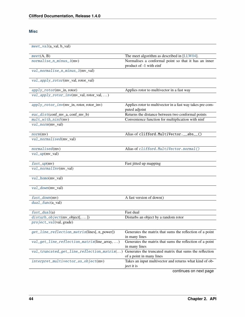
Misc
meet_val(a_val, b_val)
meet(A, B) The meet algorithm as described in [LLW04].normalise_n_minus_1(mv) Normalises a conformal point so that it has an inner
product of -1 with einfval_normalise_n_minus_1(mv_val)
val_apply_rotor(mv_val, rotor_val)
apply_rotor(mv_in, rotor) Applies rotor to multivector in a fast wayval_apply_rotor_inv(mv_val, rotor_val, . . . )
apply_rotor_inv(mv_in, rotor, rotor_inv) Applies rotor to multivector in a fast way takes pre com-puted adjoint
euc_dist(conf_mv_a, conf_mv_b) Returns the distance between two conformal pointsmult_with_ninf (mv) Convenience function for multiplication with ninfval_norm(mv_val)
norm(mv) Alias of clifford.MultiVector.__abs__()val_normalised(mv_val)
normalised(mv) Alias of clifford.MultiVector.normal()val_up(mv_val)
fast_up(mv) Fast jitted up mappingval_normalInv(mv_val)
val_homo(mv_val)
val_down(mv_val)
fast_down(mv) A fast version of down()dual_func(a_val)
fast_dual(a) Fast dualdisturb_object(mv_object[, . . . ]) Disturbs an object by a random rotorproject_val(val, grade)
get_line_reflection_matrix(lines[, n_power]) Generates the matrix that sums the reflection of a pointin many lines
val_get_line_reflection_matrix(line_array, . . . ) Generates the matrix that sums the reflection of a pointin many lines
val_truncated_get_line_reflection_matrix(. . . ) Generates the truncated matrix that sums the reflectionof a point in many lines
interpret_multivector_as_object(mv) Takes an input multivector and returns what kind of ob-ject it is
continues on next page
44 Chapter 2. API
Clifford Documentation, Release 1.4.0
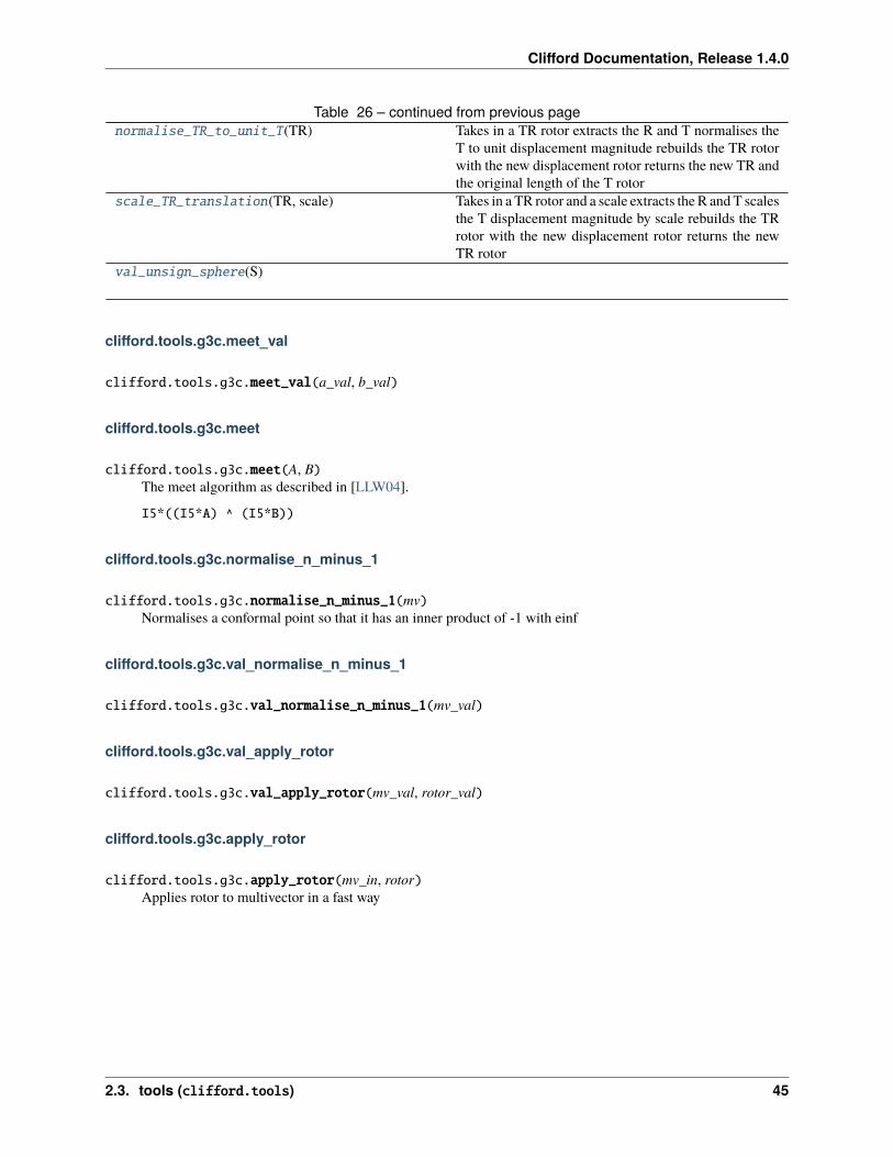
Table 26 – continued from previous pagenormalise_TR_to_unit_T(TR) Takes in a TR rotor extracts the R and T normalises the
T to unit displacement magnitude rebuilds the TR rotorwith the new displacement rotor returns the new TR andthe original length of the T rotor
scale_TR_translation(TR, scale) Takes in a TR rotor and a scale extracts the R and T scalesthe T displacement magnitude by scale rebuilds the TRrotor with the new displacement rotor returns the newTR rotor
val_unsign_sphere(S)
clifford.tools.g3c.meet_val
clifford.tools.g3c.meet_val(a_val, b_val)
clifford.tools.g3c.meet
clifford.tools.g3c.meet(A, B)The meet algorithm as described in [LLW04].
I5*((I5*A) ^ (I5*B))
clifford.tools.g3c.normalise_n_minus_1
clifford.tools.g3c.normalise_n_minus_1(mv)Normalises a conformal point so that it has an inner product of -1 with einf
clifford.tools.g3c.val_normalise_n_minus_1
clifford.tools.g3c.val_normalise_n_minus_1(mv_val)
clifford.tools.g3c.val_apply_rotor
clifford.tools.g3c.val_apply_rotor(mv_val, rotor_val)
clifford.tools.g3c.apply_rotor
clifford.tools.g3c.apply_rotor(mv_in, rotor)Applies rotor to multivector in a fast way
2.3. tools (clifford.tools) 45
Clifford Documentation, Release 1.4.0
clifford.tools.g3c.val_apply_rotor_inv
clifford.tools.g3c.val_apply_rotor_inv(mv_val, rotor_val, rotor_val_inv)
clifford.tools.g3c.apply_rotor_inv
clifford.tools.g3c.apply_rotor_inv(mv_in, rotor, rotor_inv)Applies rotor to multivector in a fast way takes pre computed adjoint
clifford.tools.g3c.euc_dist
clifford.tools.g3c.euc_dist(conf_mv_a, conf_mv_b)Returns the distance between two conformal points
clifford.tools.g3c.mult_with_ninf
clifford.tools.g3c.mult_with_ninf(mv)Convenience function for multiplication with ninf
clifford.tools.g3c.val_norm
clifford.tools.g3c.val_norm(mv_val)
clifford.tools.g3c.norm
clifford.tools.g3c.norm(mv)Alias of clifford.MultiVector.__abs__()
clifford.tools.g3c.val_normalised
clifford.tools.g3c.val_normalised(mv_val)
clifford.tools.g3c.normalised
clifford.tools.g3c.normalised(mv)Alias of clifford.MultiVector.normal()
46 Chapter 2. API
Clifford Documentation, Release 1.4.0
clifford.tools.g3c.val_up
clifford.tools.g3c.val_up(mv_val)
clifford.tools.g3c.fast_up
clifford.tools.g3c.fast_up(mv)Fast jitted up mapping
clifford.tools.g3c.val_normalInv
clifford.tools.g3c.val_normalInv(mv_val)
clifford.tools.g3c.val_homo
clifford.tools.g3c.val_homo(mv_val)
clifford.tools.g3c.val_down
clifford.tools.g3c.val_down(mv_val)
clifford.tools.g3c.fast_down
clifford.tools.g3c.fast_down(mv)A fast version of down()
clifford.tools.g3c.dual_func
clifford.tools.g3c.dual_func(a_val)
clifford.tools.g3c.fast_dual
clifford.tools.g3c.fast_dual(a)Fast dual
clifford.tools.g3c.disturb_object
clifford.tools.g3c.disturb_object(mv_object, maximum_translation=0.01, maximum_angle=0.01, *,rng=None)
Disturbs an object by a random rotor
2.3. tools (clifford.tools) 47
Clifford Documentation, Release 1.4.0
clifford.tools.g3c.project_val
clifford.tools.g3c.project_val(val, grade)
clifford.tools.g3c.get_line_reflection_matrix
clifford.tools.g3c.get_line_reflection_matrix(lines, n_power=1)Generates the matrix that sums the reflection of a point in many lines
clifford.tools.g3c.val_get_line_reflection_matrix
clifford.tools.g3c.val_get_line_reflection_matrix(line_array: numpy.ndarray, n_power: int)→numpy.ndarray
Generates the matrix that sums the reflection of a point in many lines
clifford.tools.g3c.val_truncated_get_line_reflection_matrix
clifford.tools.g3c.val_truncated_get_line_reflection_matrix(line_array: numpy.ndarray, n_power:int)→ numpy.ndarray
Generates the truncated matrix that sums the reflection of a point in many lines
clifford.tools.g3c.interpret_multivector_as_object
clifford.tools.g3c.interpret_multivector_as_object(mv)Takes an input multivector and returns what kind of object it is
-1 -> not a blade 0 -> a 1 vector but not a point 1 -> a euclidean point 2 -> a conformal point 3 -> a point pair 4-> a circle 5 -> a line 6 -> a sphere 7 -> a plane
Similar to clifford.tools.classify.classify(), although that function does a little more work in orderto produce full characterizations.
clifford.tools.g3c.normalise_TR_to_unit_T
clifford.tools.g3c.normalise_TR_to_unit_T(TR)Takes in a TR rotor extracts the R and T normalises the T to unit displacement magnitude rebuilds the TR rotorwith the new displacement rotor returns the new TR and the original length of the T rotor
clifford.tools.g3c.scale_TR_translation
clifford.tools.g3c.scale_TR_translation(TR, scale)Takes in a TR rotor and a scale extracts the R and T scales the T displacement magnitude by scale rebuilds theTR rotor with the new displacement rotor returns the new TR rotor
48 Chapter 2. API
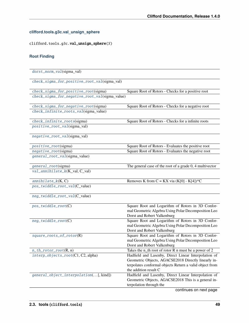
Clifford Documentation, Release 1.4.0
clifford.tools.g3c.val_unsign_sphere
clifford.tools.g3c.val_unsign_sphere(S)
Root Finding
dorst_norm_val(sigma_val)
check_sigma_for_positive_root_val(sigma_val)
check_sigma_for_positive_root(sigma) Square Root of Rotors - Checks for a positive rootcheck_sigma_for_negative_root_val(sigma_value)
check_sigma_for_negative_root(sigma) Square Root of Rotors - Checks for a negative rootcheck_infinite_roots_val(sigma_value)
check_infinite_roots(sigma) Square Root of Rotors - Checks for a infinite rootspositive_root_val(sigma_val)
negative_root_val(sigma_val)
positive_root(sigma) Square Root of Rotors - Evaluates the positive rootnegative_root(sigma) Square Root of Rotors - Evaluates the negative rootgeneral_root_val(sigma_value)
general_root(sigma) The general case of the root of a grade 0, 4 multivectorval_annihilate_k(K_val, C_val)
annihilate_k(K, C) Removes K from C = KX via (K[0] - K[4])*Cpos_twiddle_root_val(C_value)
neg_twiddle_root_val(C_value)
pos_twiddle_root(C) Square Root and Logarithm of Rotors in 3D Confor-mal Geometric Algebra Using Polar Decomposition LeoDorst and Robert Valkenburg
neg_twiddle_root(C) Square Root and Logarithm of Rotors in 3D Confor-mal Geometric Algebra Using Polar Decomposition LeoDorst and Robert Valkenburg
square_roots_of_rotor(R) Square Root and Logarithm of Rotors in 3D Confor-mal Geometric Algebra Using Polar Decomposition LeoDorst and Robert Valkenburg
n_th_rotor_root(R, n) Takes the n_th root of rotor R n must be a power of 2interp_objects_root(C1, C2, alpha) Hadfield and Lasenby, Direct Linear Interpolation of
Geometric Objects, AGACSE2018 Directly linearly in-terpolates conformal objects Return a valid object fromthe addition result C
general_object_interpolation(. . . [, kind]) Hadfield and Lasenby, Direct Linear Interpolation ofGeometric Objects, AGACSE2018 This is a general in-terpolation through the
continues on next page
2.3. tools (clifford.tools) 49
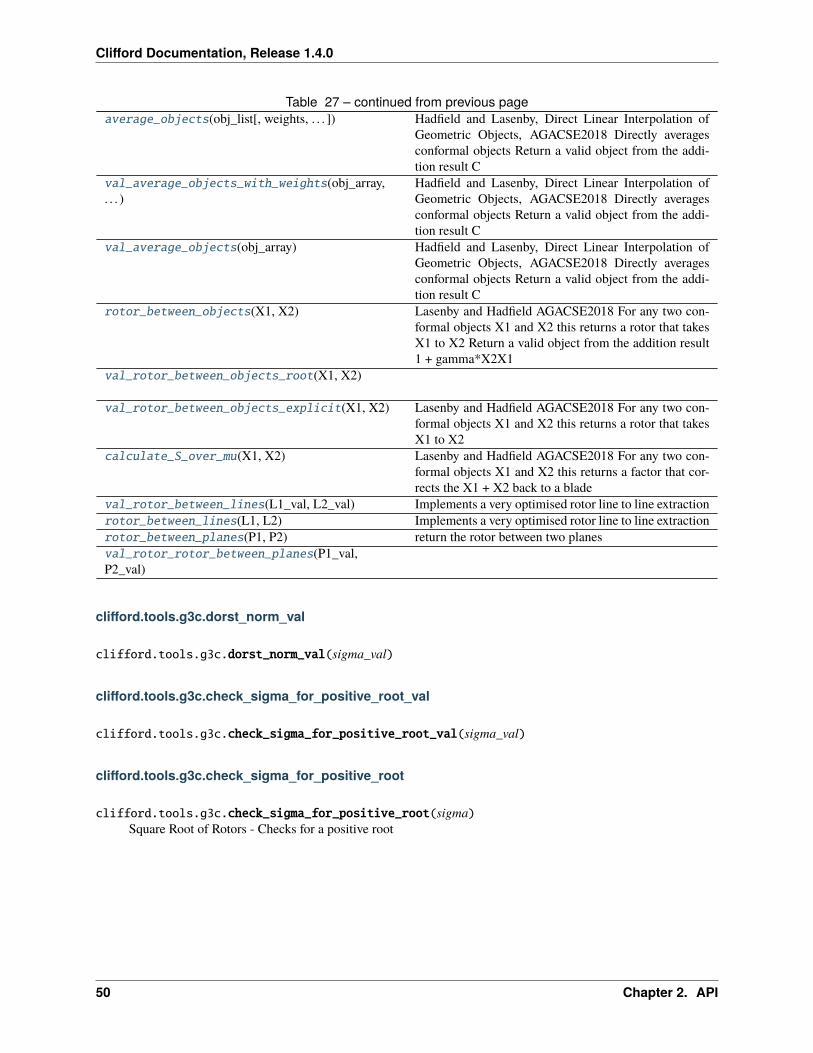
Clifford Documentation, Release 1.4.0
Table 27 – continued from previous pageaverage_objects(obj_list[, weights, . . . ]) Hadfield and Lasenby, Direct Linear Interpolation of
Geometric Objects, AGACSE2018 Directly averagesconformal objects Return a valid object from the addi-tion result C
val_average_objects_with_weights(obj_array,. . . )
Hadfield and Lasenby, Direct Linear Interpolation ofGeometric Objects, AGACSE2018 Directly averagesconformal objects Return a valid object from the addi-tion result C
val_average_objects(obj_array) Hadfield and Lasenby, Direct Linear Interpolation ofGeometric Objects, AGACSE2018 Directly averagesconformal objects Return a valid object from the addi-tion result C
rotor_between_objects(X1, X2) Lasenby and Hadfield AGACSE2018 For any two con-formal objects X1 and X2 this returns a rotor that takesX1 to X2 Return a valid object from the addition result1 + gamma*X2X1
val_rotor_between_objects_root(X1, X2)
val_rotor_between_objects_explicit(X1, X2) Lasenby and Hadfield AGACSE2018 For any two con-formal objects X1 and X2 this returns a rotor that takesX1 to X2
calculate_S_over_mu(X1, X2) Lasenby and Hadfield AGACSE2018 For any two con-formal objects X1 and X2 this returns a factor that cor-rects the X1 + X2 back to a blade
val_rotor_between_lines(L1_val, L2_val) Implements a very optimised rotor line to line extractionrotor_between_lines(L1, L2) Implements a very optimised rotor line to line extractionrotor_between_planes(P1, P2) return the rotor between two planesval_rotor_rotor_between_planes(P1_val,P2_val)
clifford.tools.g3c.dorst_norm_val
clifford.tools.g3c.dorst_norm_val(sigma_val)
clifford.tools.g3c.check_sigma_for_positive_root_val
clifford.tools.g3c.check_sigma_for_positive_root_val(sigma_val)
clifford.tools.g3c.check_sigma_for_positive_root
clifford.tools.g3c.check_sigma_for_positive_root(sigma)Square Root of Rotors - Checks for a positive root
50 Chapter 2. API
Clifford Documentation, Release 1.4.0
clifford.tools.g3c.check_sigma_for_negative_root_val
clifford.tools.g3c.check_sigma_for_negative_root_val(sigma_value)
clifford.tools.g3c.check_sigma_for_negative_root
clifford.tools.g3c.check_sigma_for_negative_root(sigma)Square Root of Rotors - Checks for a negative root
clifford.tools.g3c.check_infinite_roots_val
clifford.tools.g3c.check_infinite_roots_val(sigma_value)
clifford.tools.g3c.check_infinite_roots
clifford.tools.g3c.check_infinite_roots(sigma)Square Root of Rotors - Checks for a infinite roots
clifford.tools.g3c.positive_root_val
clifford.tools.g3c.positive_root_val(sigma_val)
clifford.tools.g3c.negative_root_val
clifford.tools.g3c.negative_root_val(sigma_val)
clifford.tools.g3c.positive_root
clifford.tools.g3c.positive_root(sigma)Square Root of Rotors - Evaluates the positive root
clifford.tools.g3c.negative_root
clifford.tools.g3c.negative_root(sigma)Square Root of Rotors - Evaluates the negative root
clifford.tools.g3c.general_root_val
clifford.tools.g3c.general_root_val(sigma_value)
2.3. tools (clifford.tools) 51
Clifford Documentation, Release 1.4.0
clifford.tools.g3c.general_root
clifford.tools.g3c.general_root(sigma)The general case of the root of a grade 0, 4 multivector
Square Root and Logarithm of Rotors in 3D Conformal Geometric Algebra Using Polar Decomposition LeoDorst and Robert Valkenburg
clifford.tools.g3c.val_annihilate_k
clifford.tools.g3c.val_annihilate_k(K_val, C_val)
clifford.tools.g3c.annihilate_k
clifford.tools.g3c.annihilate_k(K, C)Removes K from C = KX via (K[0] - K[4])*C
clifford.tools.g3c.pos_twiddle_root_val
clifford.tools.g3c.pos_twiddle_root_val(C_value)
clifford.tools.g3c.neg_twiddle_root_val
clifford.tools.g3c.neg_twiddle_root_val(C_value)
clifford.tools.g3c.pos_twiddle_root
clifford.tools.g3c.pos_twiddle_root(C)Square Root and Logarithm of Rotors in 3D Conformal Geometric Algebra Using Polar Decomposition LeoDorst and Robert Valkenburg
clifford.tools.g3c.neg_twiddle_root
clifford.tools.g3c.neg_twiddle_root(C)Square Root and Logarithm of Rotors in 3D Conformal Geometric Algebra Using Polar Decomposition LeoDorst and Robert Valkenburg
clifford.tools.g3c.square_roots_of_rotor
clifford.tools.g3c.square_roots_of_rotor(R)Square Root and Logarithm of Rotors in 3D Conformal Geometric Algebra Using Polar Decomposition LeoDorst and Robert Valkenburg
52 Chapter 2. API
Clifford Documentation, Release 1.4.0
clifford.tools.g3c.n_th_rotor_root
clifford.tools.g3c.n_th_rotor_root(R, n)Takes the n_th root of rotor R n must be a power of 2
clifford.tools.g3c.interp_objects_root
clifford.tools.g3c.interp_objects_root(C1, C2, alpha)Hadfield and Lasenby, Direct Linear Interpolation of Geometric Objects, AGACSE2018 Directly linearly inter-polates conformal objects Return a valid object from the addition result C
clifford.tools.g3c.general_object_interpolation
clifford.tools.g3c.general_object_interpolation(object_alpha_array, object_list, new_alpha_array,kind='linear')
Hadfield and Lasenby, Direct Linear Interpolation of Geometric Objects, AGACSE2018 This is a general inter-polation through the
clifford.tools.g3c.average_objects
clifford.tools.g3c.average_objects(obj_list, weights=[], check_grades=True)Hadfield and Lasenby, Direct Linear Interpolation of Geometric Objects, AGACSE2018 Directly averages con-formal objects Return a valid object from the addition result C
clifford.tools.g3c.val_average_objects_with_weights
clifford.tools.g3c.val_average_objects_with_weights(obj_array, weights_array)Hadfield and Lasenby, Direct Linear Interpolation of Geometric Objects, AGACSE2018 Directly averages con-formal objects Return a valid object from the addition result C
clifford.tools.g3c.val_average_objects
clifford.tools.g3c.val_average_objects(obj_array)Hadfield and Lasenby, Direct Linear Interpolation of Geometric Objects, AGACSE2018 Directly averages con-formal objects Return a valid object from the addition result C
clifford.tools.g3c.rotor_between_objects
clifford.tools.g3c.rotor_between_objects(X1, X2)Lasenby and Hadfield AGACSE2018 For any two conformal objects X1 and X2 this returns a rotor that takes X1to X2 Return a valid object from the addition result 1 + gamma*X2X1
2.3. tools (clifford.tools) 53

Clifford Documentation, Release 1.4.0
clifford.tools.g3c.val_rotor_between_objects_root
clifford.tools.g3c.val_rotor_between_objects_root(X1, X2)
clifford.tools.g3c.val_rotor_between_objects_explicit
clifford.tools.g3c.val_rotor_between_objects_explicit(X1, X2)Lasenby and Hadfield AGACSE2018 For any two conformal objects X1 and X2 this returns a rotor that takes X1to X2
Implements an optimised version of:
gamma1 = (X1 * X1)[0]gamma2 = (X2 * X2)[0]
M12 = X1*X2 + X2*X1K = 2 + gamma1*M12
if np.sum(np.abs(K.value)) < 0.0000001:return 1 + 0*e1
if sum(np.abs(M12(4).value)) > 0.0000001:lamb = (-(K(4) * K(4)))[0]mu = K[0]**2 + lambroot_mu = np.sqrt(mu)if abs(lamb) < 0.0000001:
beta = 1.0/(2*np.sqrt(K[0]))else:
beta_sqrd = 1/(2*(root_mu + K[0]))beta = np.sqrt(beta_sqrd)
R = ( beta*K(4) - (1/(2*beta)) )*(1 + gamma1*X2*X1)/(root_mu)return R
else:return (1 + gamma1*X2*X1)/(np.sqrt(abs(K[0])))
clifford.tools.g3c.calculate_S_over_mu
clifford.tools.g3c.calculate_S_over_mu(X1, X2)Lasenby and Hadfield AGACSE2018 For any two conformal objects X1 and X2 this returns a factor that correctsthe X1 + X2 back to a blade
clifford.tools.g3c.val_rotor_between_lines
clifford.tools.g3c.val_rotor_between_lines(L1_val, L2_val)Implements a very optimised rotor line to line extraction
54 Chapter 2. API

Clifford Documentation, Release 1.4.0
clifford.tools.g3c.rotor_between_lines
clifford.tools.g3c.rotor_between_lines(L1, L2)Implements a very optimised rotor line to line extraction
clifford.tools.g3c.rotor_between_planes
clifford.tools.g3c.rotor_between_planes(P1, P2)return the rotor between two planes
clifford.tools.g3c.val_rotor_rotor_between_planes
clifford.tools.g3c.val_rotor_rotor_between_planes(P1_val, P2_val)
Submodules
object_fitting Tools for fitting geometric primitives to point clouds
clifford.tools.g3c.object_fitting
Tools for fitting geometric primitives to point clouds
Object Fitting
fit_circle(point_list) Performs Leo Dorsts circle fitting techniqueval_fit_circle(point_list) Performs Leo Dorsts circle fitting techniquefit_line(point_list) Does line fitting with combo J.Lasenbys method and L.val_fit_line(point_list) Does line fitting with combo J.Lasenbys method and L.fit_sphere(point_list) Performs Leo Dorsts sphere fitting techniqueval_fit_sphere(point_list) Performs Leo Dorsts sphere fitting techniquefit_plane(point_list) Does plane fitting with combo J.Lasenbys method and
L.val_fit_plane(point_list) Does plane fitting with combo J.Lasenbys method and
L.
2.3. tools (clifford.tools) 55
Clifford Documentation, Release 1.4.0
clifford.tools.g3c.object_fitting.fit_circle
clifford.tools.g3c.object_fitting.fit_circle(point_list)Performs Leo Dorsts circle fitting technique
clifford.tools.g3c.object_fitting.val_fit_circle
clifford.tools.g3c.object_fitting.val_fit_circle(point_list)Performs Leo Dorsts circle fitting technique
clifford.tools.g3c.object_fitting.fit_line
clifford.tools.g3c.object_fitting.fit_line(point_list)Does line fitting with combo J.Lasenbys method and L. Dorsts
clifford.tools.g3c.object_fitting.val_fit_line
clifford.tools.g3c.object_fitting.val_fit_line(point_list)Does line fitting with combo J.Lasenbys method and L. Dorsts
clifford.tools.g3c.object_fitting.fit_sphere
clifford.tools.g3c.object_fitting.fit_sphere(point_list)Performs Leo Dorsts sphere fitting technique
clifford.tools.g3c.object_fitting.val_fit_sphere
clifford.tools.g3c.object_fitting.val_fit_sphere(point_list)Performs Leo Dorsts sphere fitting technique
clifford.tools.g3c.object_fitting.fit_plane
clifford.tools.g3c.object_fitting.fit_plane(point_list)Does plane fitting with combo J.Lasenbys method and L. Dorsts
clifford.tools.g3c.object_fitting.val_fit_plane
clifford.tools.g3c.object_fitting.val_fit_plane(point_list)Does plane fitting with combo J.Lasenbys method and L. Dorsts
56 Chapter 2. API
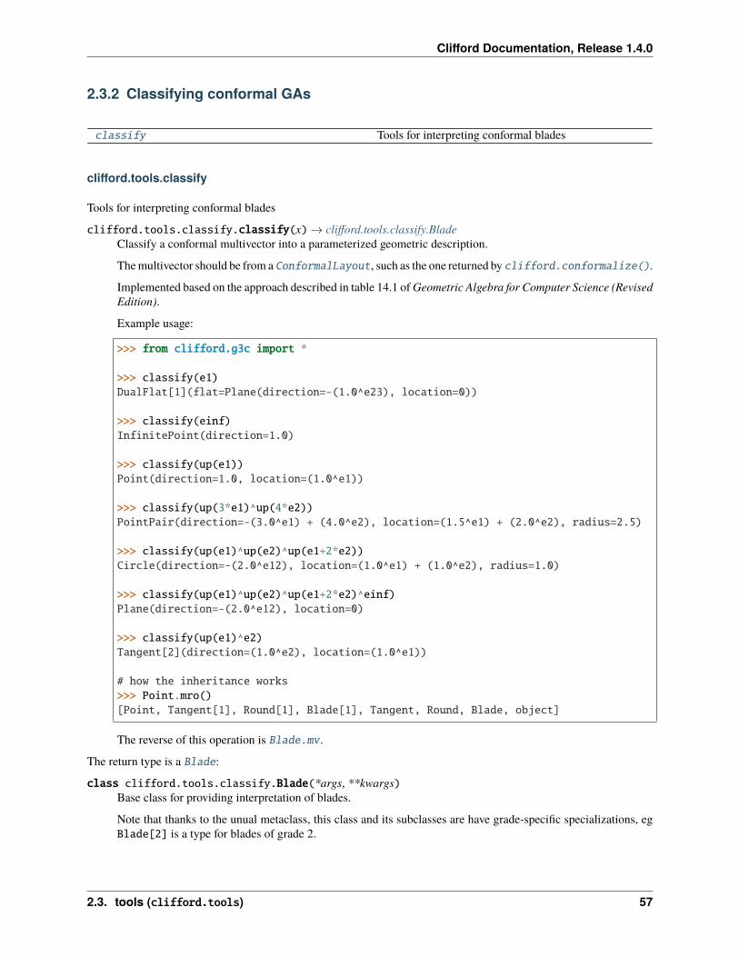
Clifford Documentation, Release 1.4.0
2.3.2 Classifying conformal GAs
classify Tools for interpreting conformal blades
clifford.tools.classify
Tools for interpreting conformal blades
clifford.tools.classify.classify(x)→ clifford.tools.classify.BladeClassify a conformal multivector into a parameterized geometric description.
The multivector should be from a ConformalLayout, such as the one returned by clifford.conformalize().
Implemented based on the approach described in table 14.1 of Geometric Algebra for Computer Science (RevisedEdition).
Example usage:
>>> from clifford.g3c import *
>>> classify(e1)DualFlat[1](flat=Plane(direction=-(1.0^e23), location=0))
>>> classify(einf)InfinitePoint(direction=1.0)
>>> classify(up(e1))Point(direction=1.0, location=(1.0^e1))
>>> classify(up(3*e1)^up(4*e2))PointPair(direction=-(3.0^e1) + (4.0^e2), location=(1.5^e1) + (2.0^e2), radius=2.5)
>>> classify(up(e1)^up(e2)^up(e1+2*e2))Circle(direction=-(2.0^e12), location=(1.0^e1) + (1.0^e2), radius=1.0)
>>> classify(up(e1)^up(e2)^up(e1+2*e2)^einf)Plane(direction=-(2.0^e12), location=0)
>>> classify(up(e1)^e2)Tangent[2](direction=(1.0^e2), location=(1.0^e1))
# how the inheritance works>>> Point.mro()[Point, Tangent[1], Round[1], Blade[1], Tangent, Round, Blade, object]
The reverse of this operation is Blade.mv.
The return type is a Blade:
class clifford.tools.classify.Blade(*args, **kwargs)Base class for providing interpretation of blades.
Note that thanks to the unual metaclass, this class and its subclasses are have grade-specific specializations, egBlade[2] is a type for blades of grade 2.
2.3. tools (clifford.tools) 57
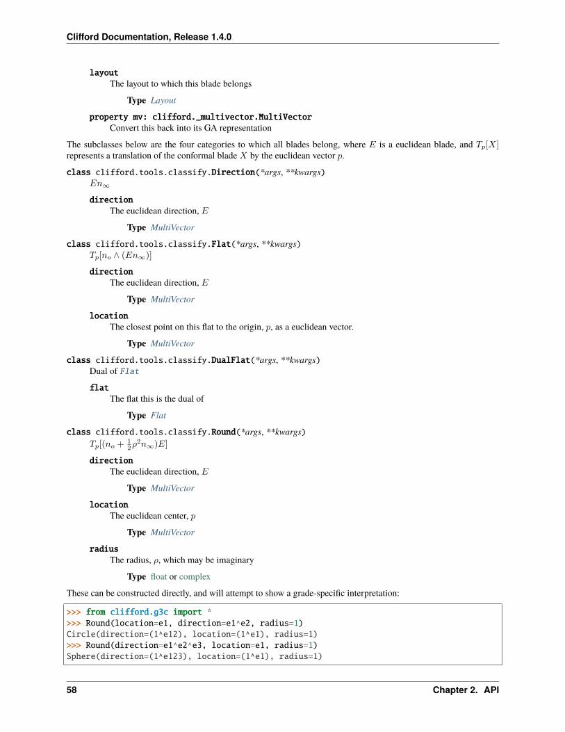
Clifford Documentation, Release 1.4.0
layoutThe layout to which this blade belongs
Type Layout
property mv: clifford._multivector.MultiVectorConvert this back into its GA representation
The subclasses below are the four categories to which all blades belong, where 𝐸 is a euclidean blade, and 𝑇𝑝[𝑋]represents a translation of the conformal blade 𝑋 by the euclidean vector 𝑝.
class clifford.tools.classify.Direction(*args, **kwargs)𝐸𝑛∞
directionThe euclidean direction, 𝐸
Type MultiVector
class clifford.tools.classify.Flat(*args, **kwargs)𝑇𝑝[𝑛𝑜 ∧ (𝐸𝑛∞)]
directionThe euclidean direction, 𝐸
Type MultiVector
locationThe closest point on this flat to the origin, 𝑝, as a euclidean vector.
Type MultiVector
class clifford.tools.classify.DualFlat(*args, **kwargs)Dual of Flat
flatThe flat this is the dual of
Type Flat
class clifford.tools.classify.Round(*args, **kwargs)𝑇𝑝[(𝑛𝑜 + 1
2𝜌2𝑛∞)𝐸]
directionThe euclidean direction, 𝐸
Type MultiVector
locationThe euclidean center, 𝑝
Type MultiVector
radiusThe radius, 𝜌, which may be imaginary
Type float or complex
These can be constructed directly, and will attempt to show a grade-specific interpretation:
>>> from clifford.g3c import *>>> Round(location=e1, direction=e1^e2, radius=1)Circle(direction=(1^e12), location=(1^e1), radius=1)>>> Round(direction=e1^e2^e3, location=e1, radius=1)Sphere(direction=(1^e123), location=(1^e1), radius=1)
58 Chapter 2. API
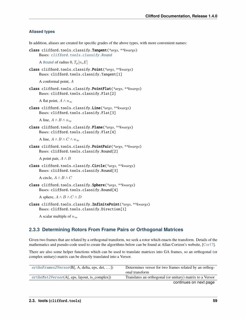
Clifford Documentation, Release 1.4.0
Aliased types
In addition, aliases are created for specific grades of the above types, with more convenient names:
class clifford.tools.classify.Tangent(*args, **kwargs)Bases: clifford.tools.classify.Round
A Round of radius 0, 𝑇𝑝[𝑛𝑜𝐸]
class clifford.tools.classify.Point(*args, **kwargs)Bases: clifford.tools.classify.Tangent[1]
A conformal point, 𝐴
class clifford.tools.classify.PointFlat(*args, **kwargs)Bases: clifford.tools.classify.Flat[2]
A flat point, 𝐴 ∧ 𝑛∞class clifford.tools.classify.Line(*args, **kwargs)
Bases: clifford.tools.classify.Flat[3]
A line, 𝐴 ∧𝐵 ∧ 𝑛∞class clifford.tools.classify.Plane(*args, **kwargs)
Bases: clifford.tools.classify.Flat[4]
A line, 𝐴 ∧𝐵 ∧ 𝐶 ∧ 𝑛∞class clifford.tools.classify.PointPair(*args, **kwargs)
Bases: clifford.tools.classify.Round[2]
A point pair, 𝐴 ∧𝐵
class clifford.tools.classify.Circle(*args, **kwargs)Bases: clifford.tools.classify.Round[3]
A circle, 𝐴 ∧𝐵 ∧ 𝐶
class clifford.tools.classify.Sphere(*args, **kwargs)Bases: clifford.tools.classify.Round[4]
A sphere, 𝐴 ∧𝐵 ∧ 𝐶 ∧𝐷
class clifford.tools.classify.InfinitePoint(*args, **kwargs)Bases: clifford.tools.classify.Direction[1]
A scalar multiple of 𝑛∞
2.3.3 Determining Rotors From Frame Pairs or Orthogonal Matrices
Given two frames that are related by a orthogonal transform, we seek a rotor which enacts the transform. Details of themathematics and pseudo-code used to create the algorithms below can be found at Allan Cortzen’s website, [Cor17].
There are also some helper functions which can be used to translate matrices into GA frames, so an orthogonal (orcomplex unitary) matrix can be directly translated into a Versor.
orthoFrames2Versor(B[, A, delta, eps, det, . . . ]) Determines versor for two frames related by an orthog-onal transform
orthoMat2Versor(A[, eps, layout, is_complex]) Translates an orthogonal (or unitary) matrix to a Versorcontinues on next page
2.3. tools (clifford.tools) 59
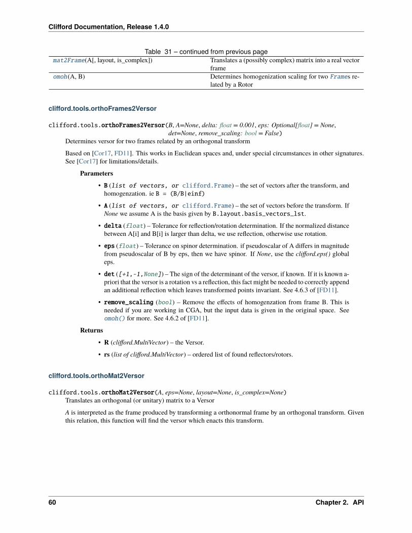
Clifford Documentation, Release 1.4.0
Table 31 – continued from previous pagemat2Frame(A[, layout, is_complex]) Translates a (possibly complex) matrix into a real vector
frameomoh (A, B) Determines homogenization scaling for two Frames re-
lated by a Rotor
clifford.tools.orthoFrames2Versor
clifford.tools.orthoFrames2Versor(B, A=None, delta: float = 0.001, eps: Optional[float] = None,det=None, remove_scaling: bool = False)
Determines versor for two frames related by an orthogonal transform
Based on [Cor17, FD11]. This works in Euclidean spaces and, under special circumstances in other signatures.See [Cor17] for limitations/details.
Parameters
• B (list of vectors, or clifford.Frame) – the set of vectors after the transform, andhomogenzation. ie B = (B/B|einf)
• A (list of vectors, or clifford.Frame) – the set of vectors before the transform. IfNone we assume A is the basis given by B.layout.basis_vectors_lst.
• delta (float) – Tolerance for reflection/rotation determination. If the normalized distancebetween A[i] and B[i] is larger than delta, we use reflection, otherwise use rotation.
• eps (float) – Tolerance on spinor determination. if pseudoscalar of A differs in magnitudefrom pseudoscalar of B by eps, then we have spinor. If None, use the clifford.eps() globaleps.
• det ([+1,-1,None]) – The sign of the determinant of the versor, if known. If it is known a-priori that the versor is a rotation vs a reflection, this fact might be needed to correctly appendan additional reflection which leaves transformed points invariant. See 4.6.3 of [FD11].
• remove_scaling (bool) – Remove the effects of homogenzation from frame B. This isneeded if you are working in CGA, but the input data is given in the original space. Seeomoh() for more. See 4.6.2 of [FD11].
Returns
• R (clifford.MultiVector) – the Versor.
• rs (list of clifford.MultiVector) – ordered list of found reflectors/rotors.
clifford.tools.orthoMat2Versor
clifford.tools.orthoMat2Versor(A, eps=None, layout=None, is_complex=None)Translates an orthogonal (or unitary) matrix to a Versor
A is interpreted as the frame produced by transforming a orthonormal frame by an orthogonal transform. Giventhis relation, this function will find the versor which enacts this transform.
60 Chapter 2. API
Clifford Documentation, Release 1.4.0
clifford.tools.mat2Frame
clifford.tools.mat2Frame(A: numpy.ndarray, layout: Optional[clifford._layout.Layout] = None, is_complex:Optional[bool] = None)→ Tuple[List[clifford._multivector.MultiVector],clifford._layout.Layout]
Translates a (possibly complex) matrix into a real vector frame
The rows and columns of A are interpreted as follows
• M, N = A.shape
• M: dimension of space
• N: number of vectors
If A is complex M and N are doubled.
Parameters A (ndarray) – MxN matrix representing vectors
Returns
• a (list of clifford.MultiVector) – The resulting vectors
• layout (clifford.Layout) – The layout of the vectors in a.
clifford.tools.omoh
clifford.tools.omoh(A: Union[clifford._frame.Frame, List[clifford._multivector.MultiVector]], B:Union[clifford._frame.Frame, List[clifford._multivector.MultiVector]])→ numpy.ndarray
Determines homogenization scaling for two Frames related by a Rotor
This is used as part of the orthoFrames2Versor() algorithm, when the frames are given in CGA. It is re-quired because the model assumes, B = R*A*~R, but if data is given in the original space, only lambda*B' ==homo(B) is observable.
We need to determine lambda before the Cartan-based algorithm can be used. The name of this function is thereverse of homo(), which is the method used to homogenize.
Parameters
• A (list of vectors, or clifford.Frame) – the set of vectors before the transform
• B (list of vectors, or clifford.Frame) – the set of vectors after the transform, andhomogenzation. ie B=B/(B|einf)
Returns out – weights on B, which produce inhomogenous versions of B. If you multiply the inputB by lam, it will fulfill B = R*A*~R
Return type array of floats
Examples
>>> lam = omoh(A, B)>>> B_ohom = Frame([B[k]*lam[k] for k in range(len(B)])
2.3. tools (clifford.tools) 61
Clifford Documentation, Release 1.4.0
2.4 operator functions (clifford.operator)
This module exists to enable functional programming via functools.reduce(). It can be thought of as equivalentto the builtin operator module, but for the operators from geometric algebra.
>>> import functools>>> import clifford.operator>>> from clifford.g3 import *>>> Ms = [e1, e1 + e2, e2 + e3] # list of multivectors>>> assert functools.reduce(clifford.operator.op, Ms) == Ms[0] ^ Ms[1] ^ Ms[2]
clifford.operator.gp(M, N)Geometric product function 𝑀𝑁 , equivalent to M * N.
M and N must be from the same layout
clifford.operator.op(M, N)Outer product function 𝑀 ∧𝑁 , equivalent to M ^ N.
M and N must be from the same layout
clifford.operator.ip(M, N)Hestenes inner product function 𝑀 ∙𝑁 , equivalent to M | N.
M and N must be from the same layout
Changed in version 1.3.0: These functions used to be in clifford , but have been moved to this submodule.
2.5 transformations (clifford.transformations)
New in version 1.3.0.
This module may in future become the home for optimized rotor transformations, or non-linear transformations.
See the Linear transformations tutorial for an introduction to how to use parts of this module.
2.5.1 Base classes
clifford.transformations.TransformationA callable mapping one MultiVector to another.
alias of Callable[[clifford._multivector.MultiVector], clifford._multivector.MultiVector]
class clifford.transformations.Linear(*args, **kwds)A transformation which is linear, such that for scalar 𝑎𝑖, 𝑓(𝑎1𝑥1 + 𝑎2𝑥2) = 𝑎1𝑓(𝑥1) + 𝑎2𝑓(𝑥2).
class clifford.transformations.FixedLayout(layout_src: clifford._layout.Layout, layout_dst:Optional[clifford._layout.Layout] = None)
A transformation with a fixed source and destination layout.
Parameters
• layout_src (Layout of S dimensions) – The layout from which this transformation takesmultivectors as input
• layout_dst (Layout of D dimensions) – The layout in which this transformation producesmultivectors as output. Defaults to the same as the input.
62 Chapter 2. API
Clifford Documentation, Release 1.4.0
2.5.2 Matrix-backed implementations
class clifford.transformations.LinearMatrix(matrix, layout_src: clifford._layout.Layout, layout_dst:Optional[clifford._layout.Layout] = None)
Linear transformation implemented by a matrix
Transformations need not be grade preserving.
Parameters
• matrix ((2**D, 2**S) array_like) – A matrix that transforms multivectors fromlayout_src with 2𝑆 elements to multivectors in layout_dst with 2𝐷 elements, by left-multiplication.
• layout_src (Layout of S dimensions) – Passed on to FixedLayout.
• layout_dst (Layout of D dimensions) – Passed on to FixedLayout.
See also:
clifford.BladeMap A faster but less general approach that works on basis blades
property adjoint: clifford.transformations.LinearMatrixThe adjoint transformation
classmethod from_function(func: Callable[[clifford._multivector.MultiVector],clifford._multivector.MultiVector], layout_src: clifford._layout.Layout,layout_dst: Optional[clifford._layout.Layout] = None)→clifford.transformations.LinearMatrix
Build a linear transformation from the result of a function applied to each basis blade.
Parameters
• func – A function taking basis blades from layout_src that produces multivectors in lay-out_dst.
• layout_src (Layout of S dimensions) – The layout to pass into the generating func-tion
• layout_dst (Layout of D dimensions) – The layout the generating function is ex-pected to produce. If not passed, this is inferred.
Example
>>> from clifford import transformations, Layout>>> l = Layout([1, 1])>>> e1, e2 = l.basis_vectors_lst>>> rot_90 = transformations.LinearMatrix.from_function(lambda x: (1 +␣→˓e1*e2)*x*(1 - e1*e2)/2, l)>>> rot_90(e1)(1.0^e2)>>> rot_90(e2)-(1.0^e1)>>> rot_90(e1*e2)(1.0^e12)
See also:
2.5. transformations (clifford.transformations) 63
Clifford Documentation, Release 1.4.0
LinearMatrix.from_rotor a shorter way to spell the above example
clifford.linear_operator_as_matrix a lower-level function for working with a subset of basisblades
classmethod from_rotor(rotor: clifford._multivector.MultiVector)→clifford.transformations.LinearMatrix
Build a linear transformation from the result of applying a rotor sandwich.
The resulting transformation operates within the algebra of the provided rotor.
Parameters rotor – The rotor to apply
Example
>>> from clifford import transformations, Layout>>> l = Layout([1, 1])>>> e1, e2 = l.basis_vectors_lst>>> rot_90 = transformations.LinearMatrix.from_rotor(1 + e1*e2)>>> rot_90(e1)(1.0^e2)>>> rot_90(e2)-(1.0^e1)>>> rot_90(e1*e2)(1.0^e12)
class clifford.transformations.OutermorphismMatrix(matrix, layout_src: clifford._layout.Layout,layout_dst: Optional[clifford._layout.Layout] =None)
A generalization of a linear transformation to vectors via the outer product.
Namely, given a linear transformation𝐹 (𝑢) → 𝑣, this generalizes to the blades by outermorphism, 𝐹 (𝑢1∧𝑢2) →𝐹 (𝑢1) ∧ 𝐹 (𝑢2), and to the multivectors by distributivity.
Such a transformation is grade preserving.
See [DFM09] Chapter 4 for more information
Parameters
• matrix ((D, S) array_like) – A matrix that transforms vectors from layout_src of sizeS to vectors in layout_dst of size D by left-multiplication.
• layout_src (Layout of S dimensions) – Passed on to FixedLayout.
• layout_dst (Layout of D dimensions) – Passed on to FixedLayout.
Example
We can construct a simple transformation that permutes and non-uniformly scales the basis vectors:
>>> from clifford import transformations, Layout>>> layout = Layout([1, 1, 1])>>> e1, e2, e3 = layout.basis_vectors_lst>>> layout_new = Layout([1, 1, 1], names='f')>>> m = np.array([[0, 1, 0],... [0, 0, 2],
(continues on next page)
64 Chapter 2. API
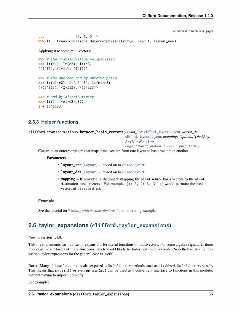
Clifford Documentation, Release 1.4.0
(continued from previous page)
... [3, 0, 0]])>>> lt = transformations.OutermorphismMatrix(m, layout, layout_new)
Applying it to some multivectors:
>>> # the transformation we specified>>> lt(e1), lt(e2), lt(e3)((3^f3), (1^f1), (2^f2))
>>> # the one deduced by outermorphism>>> lt(e1^e2), lt(e2^e3), lt(e1^e3)(-(3^f13), (2^f12), -(6^f23))
>>> # and by distributivity>>> lt(1 + (e1^e2^e3))1 + (6^f123)
2.5.3 Helper functions
clifford.transformations.between_basis_vectors(layout_src: clifford._layout.Layout, layout_dst:clifford._layout.Layout, mapping: Optional[Dict[Any,Any]] = None)→clifford.transformations.OutermorphismMatrix
Construct an outermorphism that maps basis vectors from one layout to basis vectors in another.
Parameters
• layout_src (Layout) – Passed on to FixedLayout.
• layout_dst (Layout) – Passed on to FixedLayout.
• mapping – If provided, a dictionary mapping the ids of source basis vectors to the ids ofdestination basis vectors. For example, {1: 2, 2: 3, 3: 1} would permute the basisvectors of clifford.g3.
Example
See the tutorial on Working with custom algebras for a motivating example.
2.6 taylor_expansions (clifford.taylor_expansions)
New in version 1.4.0.
This file implements various Taylor expansions for useful functions of multivectors. For some algebra signatures theremay exist closed forms of these functions which would likely be faster and more accurate. Nonetheless, having pre-written taylor expansions for the general case is useful.
Note: Many of these functions are also exposed as MultiVectormethods, such as clifford.MultiVector.sin().This means that mv.sin() or even np.sin(mv) can be used as a convenient interface to functions in this module,without having to import it directly.
For example:
2.6. taylor_expansions (clifford.taylor_expansions) 65
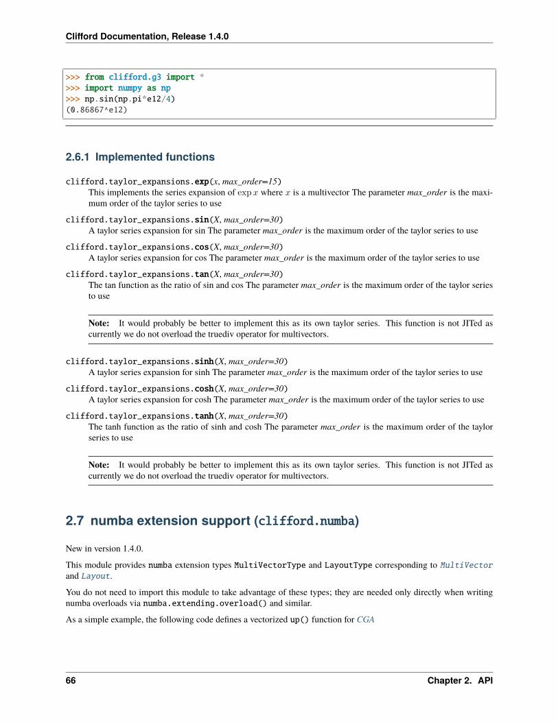
Clifford Documentation, Release 1.4.0
>>> from clifford.g3 import *>>> import numpy as np>>> np.sin(np.pi*e12/4)(0.86867^e12)
2.6.1 Implemented functions
clifford.taylor_expansions.exp(x, max_order=15)This implements the series expansion of exp𝑥 where 𝑥 is a multivector The parameter max_order is the maxi-mum order of the taylor series to use
clifford.taylor_expansions.sin(X, max_order=30)A taylor series expansion for sin The parameter max_order is the maximum order of the taylor series to use
clifford.taylor_expansions.cos(X, max_order=30)A taylor series expansion for cos The parameter max_order is the maximum order of the taylor series to use
clifford.taylor_expansions.tan(X, max_order=30)The tan function as the ratio of sin and cos The parameter max_order is the maximum order of the taylor seriesto use
Note: It would probably be better to implement this as its own taylor series. This function is not JITed ascurrently we do not overload the truediv operator for multivectors.
clifford.taylor_expansions.sinh(X, max_order=30)A taylor series expansion for sinh The parameter max_order is the maximum order of the taylor series to use
clifford.taylor_expansions.cosh(X, max_order=30)A taylor series expansion for cosh The parameter max_order is the maximum order of the taylor series to use
clifford.taylor_expansions.tanh(X, max_order=30)The tanh function as the ratio of sinh and cosh The parameter max_order is the maximum order of the taylorseries to use
Note: It would probably be better to implement this as its own taylor series. This function is not JITed ascurrently we do not overload the truediv operator for multivectors.
2.7 numba extension support (clifford.numba)
New in version 1.4.0.
This module provides numba extension types MultiVectorType and LayoutType corresponding to MultiVectorand Layout.
You do not need to import this module to take advantage of these types; they are needed only directly when writingnumba overloads via numba.extending.overload() and similar.
As a simple example, the following code defines a vectorized up() function for CGA
66 Chapter 2. API
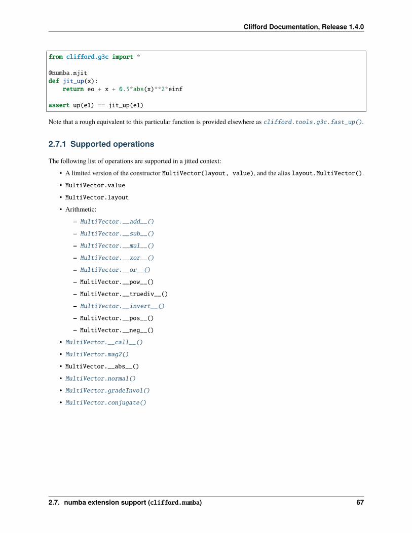
Clifford Documentation, Release 1.4.0
from clifford.g3c import *
@numba.njitdef jit_up(x):
return eo + x + 0.5*abs(x)**2*einf
assert up(e1) == jit_up(e1)
Note that a rough equivalent to this particular function is provided elsewhere as clifford.tools.g3c.fast_up().
2.7.1 Supported operations
The following list of operations are supported in a jitted context:
• A limited version of the constructor MultiVector(layout, value), and the alias layout.MultiVector().
• MultiVector.value
• MultiVector.layout
• Arithmetic:
– MultiVector.__add__()
– MultiVector.__sub__()
– MultiVector.__mul__()
– MultiVector.__xor__()
– MultiVector.__or__()
– MultiVector.__pow__()
– MultiVector.__truediv__()
– MultiVector.__invert__()
– MultiVector.__pos__()
– MultiVector.__neg__()
• MultiVector.__call__()
• MultiVector.mag2()
• MultiVector.__abs__()
• MultiVector.normal()
• MultiVector.gradeInvol()
• MultiVector.conjugate()
2.7. numba extension support (clifford.numba) 67

Clifford Documentation, Release 1.4.0
2.7.2 Performance considerations
While the resulted jitted code is typically faster, there are two main performance issues to consider. The first is thestartup time of @jiting. This can be quite substantial, although can be somewhat alleviated by using the cache=Trueargument to numba.jit(). The second is the time taken for numba to find the appropriate dispatch loop given thePython types of its arguments, which adds overhead to every call.
clifford tries as hard as possible to reduce this second overhead, by using the undocumented _numba_type_attribute and keeping our own optimized cache instead of going through the recommended @numba.extending.typeof_impl.register(LayoutType) mechanism. However, this overhead can still be slow compared to elemen-tary operations. The following code is significantly impacted by this overhead:
from clifford.g3c import *import numba
@numba.njitdef mul(a, b):
return a * b
# 286 ms, ignoring jitting timex = e1for i in range(10000):
x = mul(x, x + e2)
as each iteration of the loop pays it again. The overhead can be avoided by jitting the entire loop:
from clifford.g3c import *import numba
@numba.njitdef mul(a, b):
return a * b
@numba.njitdef the_loop(x):
for i in range(1000):x = mul(x, x + e1)
return x
# 2.4 ms, ignoring jitting timex = the_loop(eq)
68 Chapter 2. API
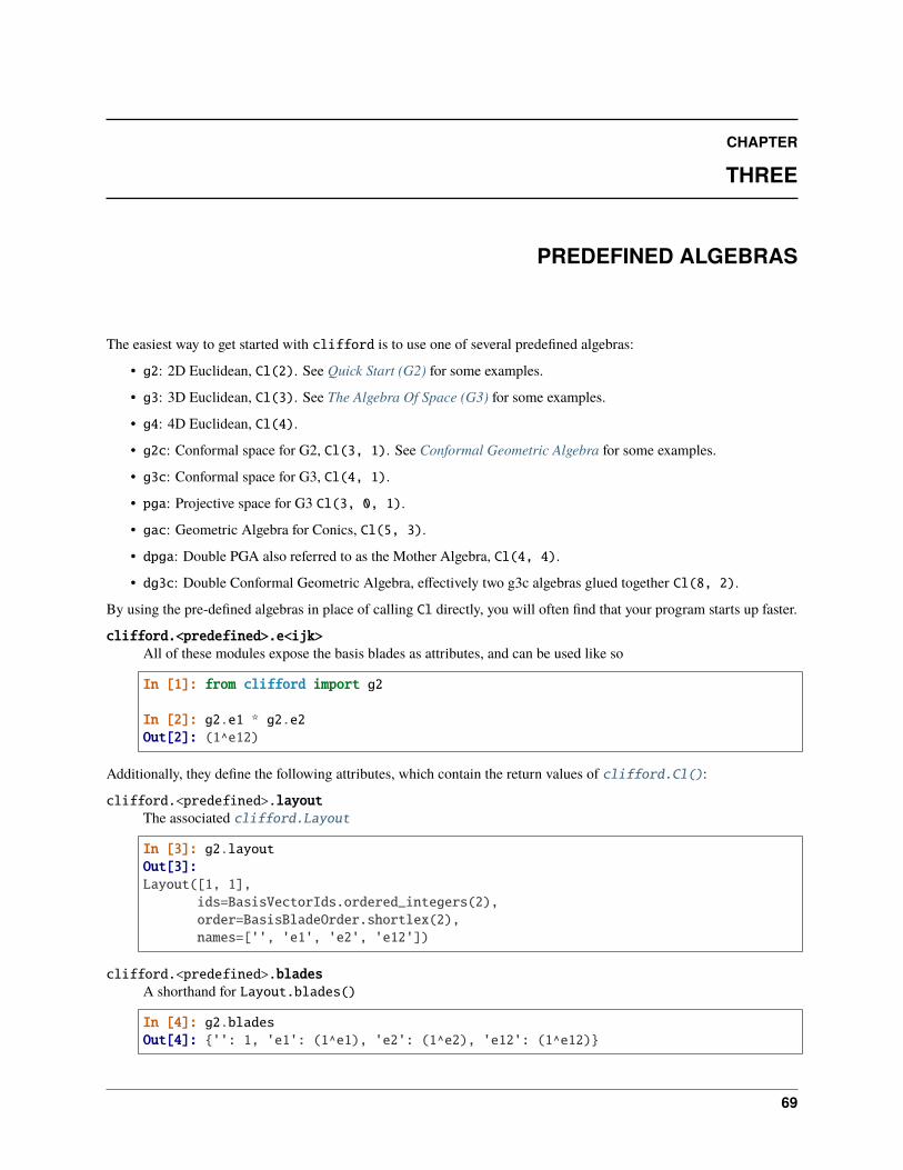
CHAPTER
THREE
PREDEFINED ALGEBRAS
The easiest way to get started with clifford is to use one of several predefined algebras:
• g2: 2D Euclidean, Cl(2). See Quick Start (G2) for some examples.
• g3: 3D Euclidean, Cl(3). See The Algebra Of Space (G3) for some examples.
• g4: 4D Euclidean, Cl(4).
• g2c: Conformal space for G2, Cl(3, 1). See Conformal Geometric Algebra for some examples.
• g3c: Conformal space for G3, Cl(4, 1).
• pga: Projective space for G3 Cl(3, 0, 1).
• gac: Geometric Algebra for Conics, Cl(5, 3).
• dpga: Double PGA also referred to as the Mother Algebra, Cl(4, 4).
• dg3c: Double Conformal Geometric Algebra, effectively two g3c algebras glued together Cl(8, 2).
By using the pre-defined algebras in place of calling Cl directly, you will often find that your program starts up faster.
clifford.<predefined>.e<ijk>All of these modules expose the basis blades as attributes, and can be used like so
In [1]: from clifford import g2
In [2]: g2.e1 * g2.e2Out[2]: (1^e12)
Additionally, they define the following attributes, which contain the return values of clifford.Cl():
clifford.<predefined>.layoutThe associated clifford.Layout
In [3]: g2.layoutOut[3]:Layout([1, 1],
ids=BasisVectorIds.ordered_integers(2),order=BasisBladeOrder.shortlex(2),names=['', 'e1', 'e2', 'e12'])
clifford.<predefined>.bladesA shorthand for Layout.blades()
In [4]: g2.bladesOut[4]: {'': 1, 'e1': (1^e1), 'e2': (1^e2), 'e12': (1^e12)}
69

Clifford Documentation, Release 1.4.0
For interactive use, it’s very handy to use import *
In [5]: from clifford.g2 import *
In [6]: e1, e2, e12Out[6]: ((1^e1), (1^e2), (1^e12))
For the conformal layouts g2c and g3c, the full contents of the stuff result of clifford.conformalize() is alsoexposed as members of the module.
70 Chapter 3. Predefined Algebras
CHAPTER
FOUR
CHANGELOG
4.1 Changes in 1.4.x
• Python 3.9 is officially supported.
• MultiVector is now supported directly within @numba.njited code. See the documentation for this featurein the clifford.numba module for more details.
• New algorithms for the multivector inverse MultiVector.inv():
– Inverting a non-blade multivector in algebras where 𝑝 = 𝑞 ≤ 5 now falls back on the approach described in[HS17] instead of using a linear algebra approach. This algorithm can be used directly via MultiVector.hitzer_inverse().
– An additional method is available, MultiVector.shirokov_inverse(), which is the arbitrary signaturealgorithm described in [Shi20].
• A new clifford.taylor_expansionsmodule for Taylor series of various multivector functions, starting withcommon trigonometric functions. These functions are additionally exposed via methods on MultiVector likeMultiVector.cos().
• Random functions now accept an rng keyword argument that accepts the object returned by numpy.random.default_rng(), for deterministic randomness.
• Projection using MultiVector.__call__() as mv(grade) no longer raises ValueError for grades not presentin the algebra, and instead just returns zero.
• Some JIT-ed code is now cached when clifford is imported for the very first time, speeding up subsequentimports.
• Improved citations in the documentation.
4.1.1 Bugs fixed
• Where possible, MultiVectors preserve their data type in the dual, and the right and left complements.
• MVArray no longer errantly promotes 0-dimensional arrays to 1-dimensional arrays.
• MultiVectors with complex coefficients are now printed correctly.
• cga.Round.radius() is no longer always 1.
71
Clifford Documentation, Release 1.4.0
4.1.2 Compatibility notes
• This will be the last release to support Python 3.5 and 3.6, as the former reached its end-of-life during our lastrelease cycle, and the latter is expected to before our next release.
• clifford.general_exp() is deprecated in favor of clifford.taylor_expansions.exp(), although typ-ically clifford.MultiVector.exp() is a better choice
• Transparently treating a MultiVector as a flat array of coefficients is deprecated, and so mv[i] andlen(mv) both emit DeprecationWarning`s. If the underlying storage order is of interest,use ``mv.value[i]` and len(mv)``respectively. To obtain the scalar part of a :class:`MultiVector`, use ``mv[()] instead of mv[0].
• Layout.gradeList has been removed. If still needed, it can be recovered as an ndarray isntead of a list viathe private attribute layout._basis_blade_order.grades (BasisBladeOrder.grades).
4.2 Changes in 1.3.x
• Python 3.8 is officially supported. 1.2.0 was pinned to a bad numba version that was incompatible with 3.8.
• A new clifford.operator module to contain the previously undocumented gp(), op(), and ip() helpers.
• A new clifford.transformations module for linear transformations.
• Two new Predefined Algebras, clifford.dpga and clifford.dg3c.
• Improvements throughout the documentation:
– Better overall structure, visible in the docs sidebar.
– New tutorials for Conformal Geometric Algebra on visualization and applications.
– New tutorial on Working with custom algebras.
– New tutorial on Linear transformations.
– New links at the top of each notebook tutorial, to run examples from the browser.
• Faster algebra construction. Cl(3) is now 100× faster, and Cl(6) is 20× faster. This is achieved by deferringproduct JIT compilation until the product is used for the first time.
• Additional testing and assorted improvements for clifford.tools.g3c:
– closest_point_on_circle_from_line() has now been implemented roughly following the proceduredescribed in Appendix A of Andreas Aristidou’s PhD thesis.
– closest_point_on_line_from_circle() has now also been added, projecting the result ofclosest_point_on_circle_from_line() to the line.
• clifford.ugly() now results in less ugly output for Predefined Algebras.
72 Chapter 4. Changelog
Clifford Documentation, Release 1.4.0
4.2.1 Bugs fixed
• MultiVector.meet() no longer produces zero erroneously.
• mv[e1 + e12] now raises ValueError, rather than being interpreted as mv[e1].
• ip() (the inner product) no longer performs the outer product.
• Layout.parse_multivector() now throws SyntaxError on invalid input, rather than silenltly producingnonsense.
• Layout.parse_multivector() supports basis vector names which do not start with e.
• In clifford.tools.g3c:
– val_midpoint_between_lines() now handles the case that the two lines are touching.
– val_fit_circle() now correctly selects the first and second eigenvalue regardless of order.
– sphere_beyond_plane() now tested and correct.
– sphere_behind_plane() now tested and correct.
– val_unsign_sphere() is now jitted, as it should have been from the start.
– get_nearest_plane_point() correctly returns the conformal point rather than the 3D point.
4.2.2 Compatibility notes
• clifford.grades_present is deprecated in favor of MultiVector.grades(), the latter of which now takesan eps argument.
• del mv[i] is no longer legal, the equivalent mv[i] = 0 should be used instead.
• Layout.dict_to_multivector has been removed. It was accidentally broken in 1.0.5, so there is little pointdeprecating it.
• Layout.basis_names() now returns a list of str, rather than a numpy array of bytes. The result nowmatches the construction order, rather than being sorted alphabetically. The order of Layout.metric() hasbeen adjusted for consistency.
• The imt_prod_mask, omt_prod_mask, and lcmt_prod_mask attributes of Layout objects have been removed,as these were an unnecessary intermediate computation that had no need to be public.
• Some functions in clifford.tools.g3c have been renamed:
– closest_points_on_circles has been renamed to iterative_closest_points_on_circles().
– closest_points_circle_line has been renamed to iterative_closest_points_circle_line().
– furthest_points_on_circles has been renamed to iterative_furthest_points_on_circles().
• While this release is compatible with numba version 0.49.0, it is recommended to use 0.48.0 which does not emitas many warnings. See the Installation instructions for how to follow this guidance.
4.2. Changes in 1.3.x 73
Clifford Documentation, Release 1.4.0
4.2.3 Patch releases
• 1.3.1: Added compatibility with numba version 0.50.0.
4.3 Changes in 1.2.x
• layout.isconformal, layout.einf, and layout.eo, which were added in 1.0.4, have been removed. Thefirst can now be spelt isinstance(layout, clifford.ConformalLayout), and the other properties nowexist only on ConformalLayout objects.
• MultiVector.left_complement() has been added for consistency with MultiVector.right_complement().
• A new clifford.tools.classify module has been added for classifying blades.
• Layout objects print slightly more cleanly in Jupyter notebooks.
• Layout.scalar is now integral rather than floating point
4.3.1 Bugs fixed
• pow(mv, 0) gives the right result
• nan is now printed correctly when it appears in multivectors. Previously it was hidden
• MultiVector.right_complement() no longer performs the left complement.
• MultiVector.vee() has been corrected to have the same sign as MultiVector.meet()
4.3.2 Compatibility notes
• Layout.scalar is now integral rather than floating point, to match Layout.pseudoScalar.
4.4 Changes in 1.1.x
• Restores layout.gmt, Layout.omt, Layout.imt, and Layout.lcmt. A few releases ago, these existed butwere dense. For memory reasons, they were then removed entirely. They have now been reinstated as sparse.COO matrix objects, which behave much the same as the original dense arrays.
• MultiVectors preserve their data type in addition, subtraction, and products. This means that integers remainintegers until combined with floats. Note that this means in principle integer overflow is possible, so workingwith floats is still recommended. This also adds support for floating point types of other precision, such asnp.float32.
• setup.py is now configured such that pip2 install clifford will not attempt to download this version,since it does not work at all on python 2.
• Documentation now includes examples of pyganja visualizations.
74 Chapter 4. Changelog
Clifford Documentation, Release 1.4.0
4.4.1 Compatibility notes
• Layout.blades() now includes the scalar 1, as do other similar functions.
• MultiVector.grades() now returns a set not a list. This means code like mv.grades() == [0] willneed to change to mv.grades() == {0}, or to work both before and after this change, set(mv.grades())== {0}.
4.4.2 Bugs fixed
• mv[(i, j)] would sometimes fail if the indices were not in canonical order.
• mv == None and layout == None would crash rather than return False.
• blade.isVersor() would return False.
• layout.blades_of_grade(0) would not return the list it claimed to return.
4.4.3 Internal changes
• Switch to pytest for testing.
• Enable code coverage.
• Split into smaller files.
• Remove python 2 compatibility code, which already no longer worked.
4.5 Changes 0.6-0.7
• Added a real license.
• Convert to NumPy instead of Numeric.
4.6 Changes 0.5-0.6
• join() and meet() actually work now, but have numerical accuracy problems
• added clean() to MultiVector
• added leftInv() and rightInv() to MultiVector
• moved pseudoScalar() and invPS() to MultiVector (so we can derive new classes from MultiVector)
• changed all of the instances of creating a new MultiVector to create an instance of self.__class__ for properinheritance
• fixed bug in laInv()
• fixed the massive confusion about how dot() works
• added left-contraction
• fixed embarrassing bug in gmt generation
• added normal() and anticommutator() methods
• fixed dumb bug in elements() that limited it to 4 dimensions
4.5. Changes 0.6-0.7 75

Clifford Documentation, Release 1.4.0
4.7 Acknowledgements
Konrad Hinsen fixed a few bugs in the conversion to numpy and adding some unit tests.
76 Chapter 4. Changelog
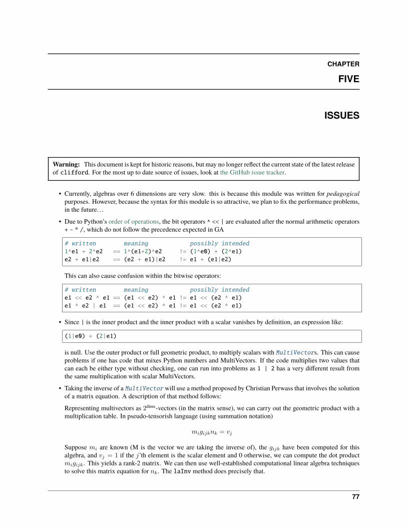
CHAPTER
FIVE
ISSUES
Warning: This document is kept for historic reasons, but may no longer reflect the current state of the latest releaseof clifford. For the most up to date source of issues, look at the GitHub issue tracker.
• Currently, algebras over 6 dimensions are very slow. this is because this module was written for pedagogicalpurposes. However, because the syntax for this module is so attractive, we plan to fix the performance problems,in the future. . .
• Due to Python’s order of operations, the bit operators ^ << | are evaluated after the normal arithmetic operators+ - * /, which do not follow the precedence expected in GA
# written meaning possibly intended1^e1 + 2^e2 == 1^(e1+2)^e2 != (1^e0) + (2^e1)e2 + e1|e2 == (e2 + e1)|e2 != e1 + (e1|e2)
This can also cause confusion within the bitwise operators:
# written meaning possibly intendede1 << e2 ^ e1 == (e1 << e2) ^ e1 != e1 << (e2 ^ e1)e1 ^ e2 | e1 == (e1 << e2) ^ e1 != e1 << (e2 ^ e1)
• Since | is the inner product and the inner product with a scalar vanishes by definition, an expression like:
(1|e0) + (2|e1)
is null. Use the outer product or full geometric product, to multiply scalars with MultiVectors. This can causeproblems if one has code that mixes Python numbers and MultiVectors. If the code multiplies two values thatcan each be either type without checking, one can run into problems as 1 | 2 has a very different result fromthe same multiplication with scalar MultiVectors.
• Taking the inverse of a MultiVector will use a method proposed by Christian Perwass that involves the solutionof a matrix equation. A description of that method follows:
Representing multivectors as 2dims-vectors (in the matrix sense), we can carry out the geometric product with amultiplication table. In pseudo-tensorish language (using summation notation)
𝑚𝑖𝑔𝑖𝑗𝑘𝑛𝑘 = 𝑣𝑗
Suppose 𝑚𝑖 are known (M is the vector we are taking the inverse of), the 𝑔𝑖𝑗𝑘 have been computed for thisalgebra, and 𝑣𝑗 = 1 if the 𝑗’th element is the scalar element and 0 otherwise, we can compute the dot product𝑚𝑖𝑔𝑖𝑗𝑘. This yields a rank-2 matrix. We can then use well-established computational linear algebra techniquesto solve this matrix equation for 𝑛𝑘. The laInv method does precisely that.
77
Clifford Documentation, Release 1.4.0
The usual, analytic, method for computing inverses (𝑀−1 = �̃�/(𝑀�̃�) iff 𝑀�̃� = |𝑀 |2) fails for thosemultivectors where M*~M is not a scalar. It is onl)y used if the invmethod is manually set to point to normalInv.
My testing suggests that laInv works. In the cases where normalInv works, laInv returns the same result(within _eps). In all cases, M * M.laInv() == 1.0 (within _eps). Use whichever you feel comfortable with.
Of course, a new issue arises with this method. The inverses found are sometimes dependant on the order ofmultiplication. That is:
M.laInv() * M == 1.0M * M.laInv() != 1.0
XXX Thus, there are two other methods defined, leftInv and rightInv which point to leftLaInv andrightLaInv. The method inv points to rightInv. Should the user choose, leftInv and rightInv willboth point to normalInv, which yields a left- and right-inverse that are the same should either exist (the proofis fairly simple).
• The basis vectors of any algebra will be orthonormal unless you supply your own multiplication tables (whichyou are free to do after the Layout constructor is called). A derived class could be made to calculate these tablesfor you (and include methods for generating reciprocal bases and the like).
• No care is taken to preserve the dtype of the arrays. The purpose of this module is pedagogical. If your applicationrequires so many multivectors that storage becomes important, the class structure here is unsuitable for youanyways. Instead, use the algorithms from this module and implement application-specific data structures.
• Conversely, explicit typecasting is rare. MultiVectors will have integer coefficients if you instantiate them thatway. Dividing them by Python integers will have the same consequences as normal integer division. Publicoutcry will convince me to add the explicit casts if this becomes a problem.
Happy hacking!
Robert Kern
The following section was generated from docs/tutorials/g2-quick-start.ipynb . . . . . . . . . . . . . . . . . . . . . . . . . . . . . . . . . . . . . . . . . . . . . . . . . . . . . . . . . . . . . . . . . . . . . . .
78 Chapter 5. Issues
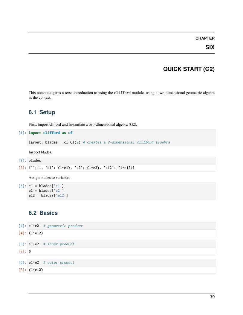
CHAPTER
SIX
QUICK START (G2)
This notebook gives a terse introduction to using the clifford module, using a two-dimensional geometric algebraas the context.
6.1 Setup
First, import clifford and instantiate a two-dimensional algebra (G2),
[1]: import clifford as cf
layout, blades = cf.Cl(2) # creates a 2-dimensional clifford algebra
Inspect blades.
[2]: blades
[2]: {'': 1, 'e1': (1^e1), 'e2': (1^e2), 'e12': (1^e12)}
Assign blades to variables
[3]: e1 = blades['e1']e2 = blades['e2']e12 = blades['e12']
6.2 Basics
[4]: e1*e2 # geometric product
[4]: (1^e12)
[5]: e1|e2 # inner product
[5]: 0
[6]: e1^e2 # outer product
[6]: (1^e12)
79
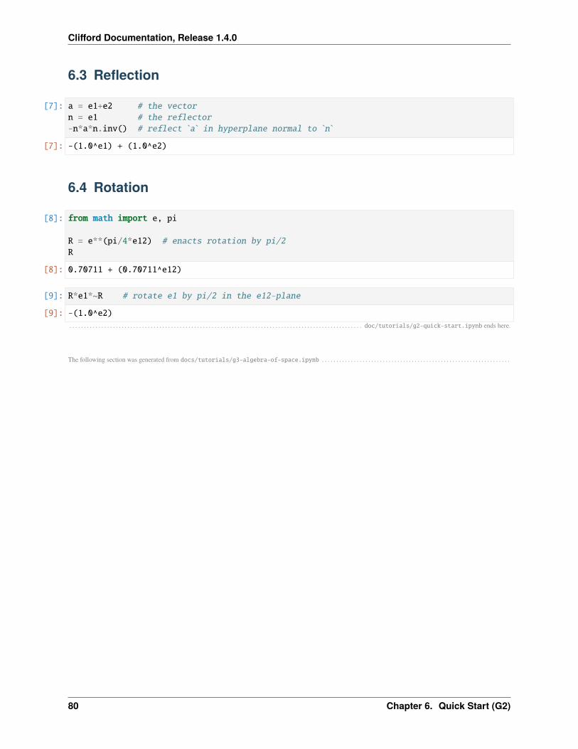
Clifford Documentation, Release 1.4.0
6.3 Reflection
[7]: a = e1+e2 # the vectorn = e1 # the reflector-n*a*n.inv() # reflect `a` in hyperplane normal to `n`
[7]: -(1.0^e1) + (1.0^e2)
6.4 Rotation
[8]: from math import e, pi
R = e**(pi/4*e12) # enacts rotation by pi/2R
[8]: 0.70711 + (0.70711^e12)
[9]: R*e1*~R # rotate e1 by pi/2 in the e12-plane
[9]: -(1.0^e2)
. . . . . . . . . . . . . . . . . . . . . . . . . . . . . . . . . . . . . . . . . . . . . . . . . . . . . . . . . . . . . . . . . . . . . . . . . . . . . . . . . . . . . . . . . . . . . . . . . . . . . doc/tutorials/g2-quick-start.ipynb ends here.
The following section was generated from docs/tutorials/g3-algebra-of-space.ipynb . . . . . . . . . . . . . . . . . . . . . . . . . . . . . . . . . . . . . . . . . . . . . . . . . . . . . . . . . . . . . . . . .
80 Chapter 6. Quick Start (G2)
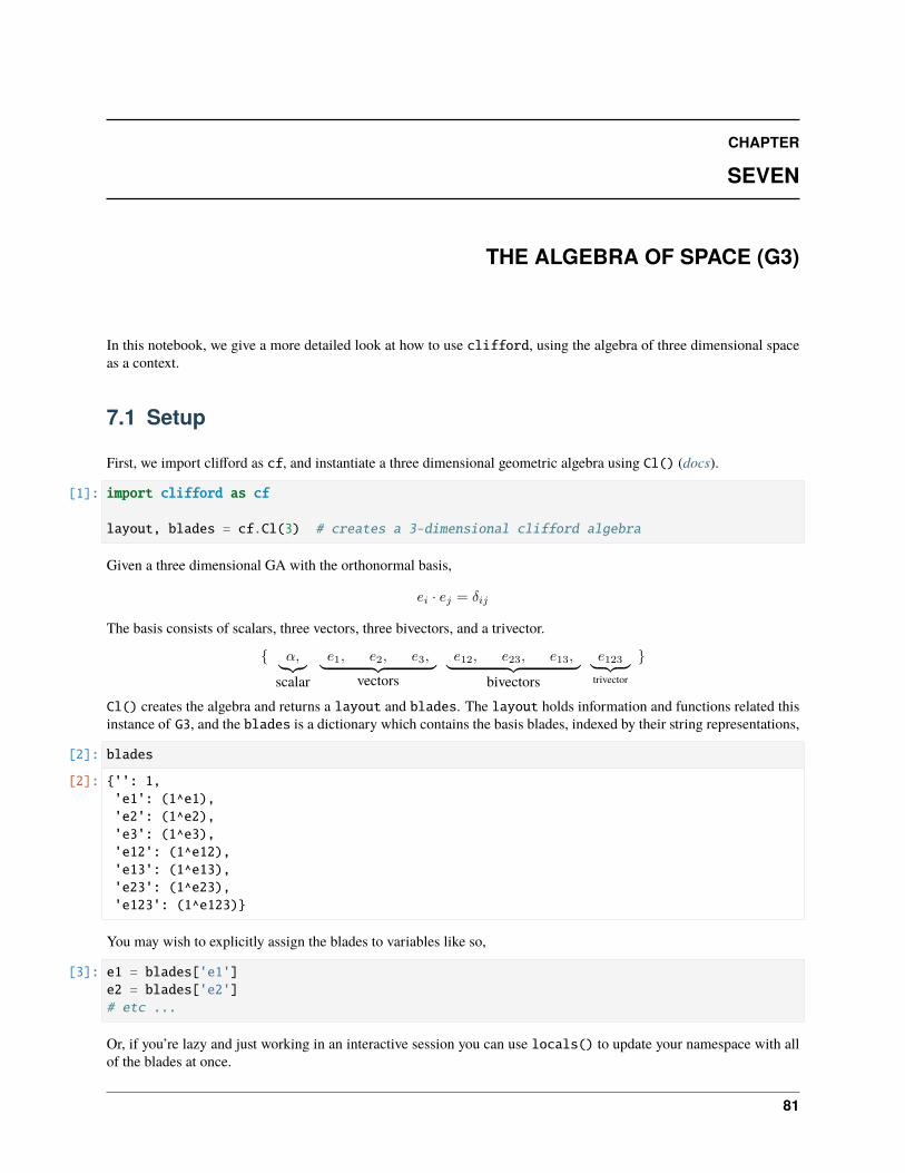
CHAPTER
SEVEN
THE ALGEBRA OF SPACE (G3)
In this notebook, we give a more detailed look at how to use clifford, using the algebra of three dimensional spaceas a context.
7.1 Setup
First, we import clifford as cf, and instantiate a three dimensional geometric algebra using Cl() (docs).
[1]: import clifford as cf
layout, blades = cf.Cl(3) # creates a 3-dimensional clifford algebra
Given a three dimensional GA with the orthonormal basis,
𝑒𝑖 · 𝑒𝑗 = 𝛿𝑖𝑗
The basis consists of scalars, three vectors, three bivectors, and a trivector.
{ 𝛼,⏟ ⏞ scalar
𝑒1, 𝑒2, 𝑒3,⏟ ⏞ vectors
𝑒12, 𝑒23, 𝑒13,⏟ ⏞ bivectors
𝑒123⏟ ⏞ trivector
}
Cl() creates the algebra and returns a layout and blades. The layout holds information and functions related thisinstance of G3, and the blades is a dictionary which contains the basis blades, indexed by their string representations,
[2]: blades
[2]: {'': 1,'e1': (1^e1),'e2': (1^e2),'e3': (1^e3),'e12': (1^e12),'e13': (1^e13),'e23': (1^e23),'e123': (1^e123)}
You may wish to explicitly assign the blades to variables like so,
[3]: e1 = blades['e1']e2 = blades['e2']# etc ...
Or, if you’re lazy and just working in an interactive session you can use locals() to update your namespace with allof the blades at once.
81
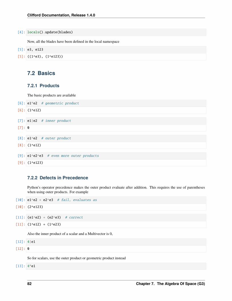
Clifford Documentation, Release 1.4.0
[4]: locals().update(blades)
Now, all the blades have been defined in the local namespace
[5]: e3, e123
[5]: ((1^e3), (1^e123))
7.2 Basics
7.2.1 Products
The basic products are available
[6]: e1*e2 # geometric product
[6]: (1^e12)
[7]: e1|e2 # inner product
[7]: 0
[8]: e1^e2 # outer product
[8]: (1^e12)
[9]: e1^e2^e3 # even more outer products
[9]: (1^e123)
7.2.2 Defects in Precedence
Python’s operator precedence makes the outer product evaluate after addition. This requires the use of parentheseswhen using outer products. For example
[10]: e1^e2 + e2^e3 # fail, evaluates as
[10]: (2^e123)
[11]: (e1^e2) + (e2^e3) # correct
[11]: (1^e12) + (1^e23)
Also the inner product of a scalar and a Multivector is 0,
[12]: 4|e1
[12]: 0
So for scalars, use the outer product or geometric product instead
[13]: 4*e1
82 Chapter 7. The Algebra Of Space (G3)
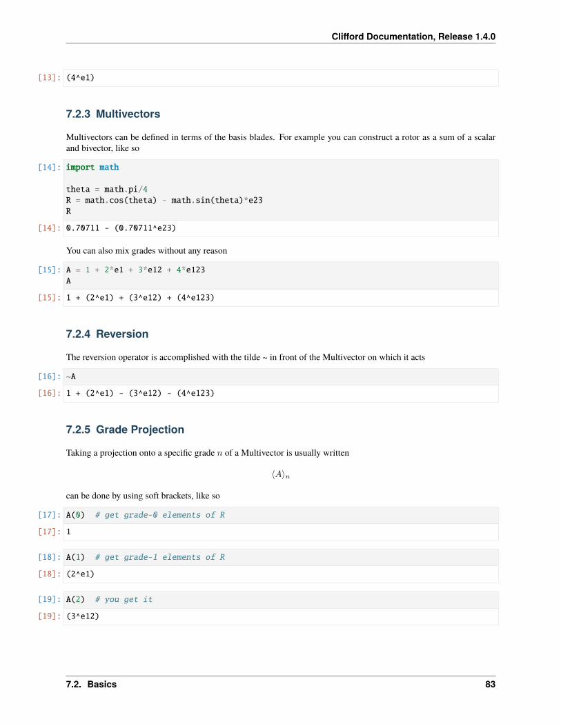
Clifford Documentation, Release 1.4.0
[13]: (4^e1)
7.2.3 Multivectors
Multivectors can be defined in terms of the basis blades. For example you can construct a rotor as a sum of a scalarand bivector, like so
[14]: import math
theta = math.pi/4R = math.cos(theta) - math.sin(theta)*e23R
[14]: 0.70711 - (0.70711^e23)
You can also mix grades without any reason
[15]: A = 1 + 2*e1 + 3*e12 + 4*e123A
[15]: 1 + (2^e1) + (3^e12) + (4^e123)
7.2.4 Reversion
The reversion operator is accomplished with the tilde ~ in front of the Multivector on which it acts
[16]: ~A
[16]: 1 + (2^e1) - (3^e12) - (4^e123)
7.2.5 Grade Projection
Taking a projection onto a specific grade 𝑛 of a Multivector is usually written
⟨𝐴⟩𝑛
can be done by using soft brackets, like so
[17]: A(0) # get grade-0 elements of R
[17]: 1
[18]: A(1) # get grade-1 elements of R
[18]: (2^e1)
[19]: A(2) # you get it
[19]: (3^e12)
7.2. Basics 83
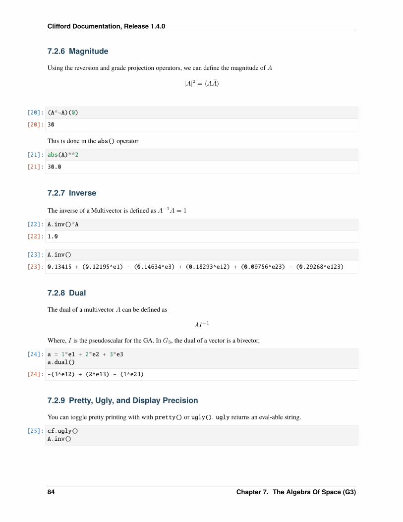
Clifford Documentation, Release 1.4.0
7.2.6 Magnitude
Using the reversion and grade projection operators, we can define the magnitude of 𝐴
|𝐴|2 = ⟨𝐴𝐴⟩
[20]: (A*~A)(0)
[20]: 30
This is done in the abs() operator
[21]: abs(A)**2
[21]: 30.0
7.2.7 Inverse
The inverse of a Multivector is defined as 𝐴−1𝐴 = 1
[22]: A.inv()*A
[22]: 1.0
[23]: A.inv()
[23]: 0.13415 + (0.12195^e1) - (0.14634^e3) + (0.18293^e12) + (0.09756^e23) - (0.29268^e123)
7.2.8 Dual
The dual of a multivector 𝐴 can be defined as
𝐴𝐼−1
Where, 𝐼 is the pseudoscalar for the GA. In 𝐺3, the dual of a vector is a bivector,
[24]: a = 1*e1 + 2*e2 + 3*e3a.dual()
[24]: -(3^e12) + (2^e13) - (1^e23)
7.2.9 Pretty, Ugly, and Display Precision
You can toggle pretty printing with with pretty() or ugly(). ugly returns an eval-able string.
[25]: cf.ugly()A.inv()
84 Chapter 7. The Algebra Of Space (G3)

Clifford Documentation, Release 1.4.0
[25]: MultiVector(Layout([1, 1, 1],ids=BasisVectorIds.ordered_integers(3),order=BasisBladeOrder.shortlex(3),names=['', 'e1', 'e2', 'e3', 'e12', 'e13', 'e23', 'e123']),
[0.13414634146341464, 0.12195121951219512, 0.0, -0.14634146341463414, 0.→˓18292682926829268, 0.0, 0.0975609756097561, -0.2926829268292683])
You can also change the displayed precision
[26]: cf.pretty(precision=2)
A.inv()
[26]: 0.13 + (0.12^e1) - (0.15^e3) + (0.18^e12) + (0.1^e23) - (0.29^e123)
This does not effect the internal precision used for computations.
7.3 Applications
7.3.1 Reflections
Reflecting a vector 𝑐 about a normalized vector 𝑛 is pretty simple,
𝑐→ 𝑛𝑐𝑛
[27]: c = e1+e2+e3 # a vectorn = e1 # the reflectorn*c*n # reflect `a` in hyperplane normal to `n`
[27]: (1^e1) - (1^e2) - (1^e3)
Because we have the inv() available, we can equally well reflect in un-normalized vectors using,
𝑎→ 𝑛𝑎𝑛−1
[28]: a = e1+e2+e3 # the vectorn = 3*e1 # the reflectorn*a*n.inv()
[28]: (1.0^e1) - (1.0^e2) - (1.0^e3)
Reflections can also be made with respect to the a ‘hyperplane normal to the vector 𝑛’, in this case the formula isnegated
𝑐→ −𝑛𝑐𝑛−1
7.3. Applications 85
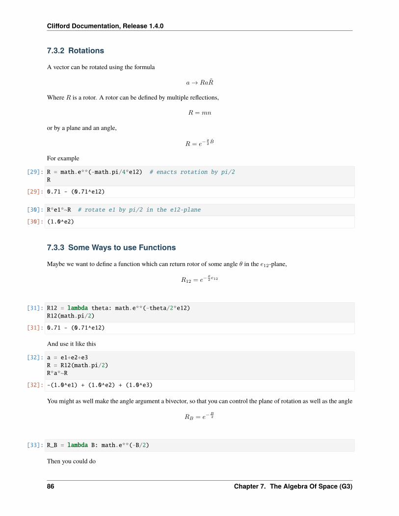
Clifford Documentation, Release 1.4.0
7.3.2 Rotations
A vector can be rotated using the formula
𝑎→ 𝑅𝑎�̃�
Where 𝑅 is a rotor. A rotor can be defined by multiple reflections,
𝑅 = 𝑚𝑛
or by a plane and an angle,
𝑅 = 𝑒−𝜃2 �̂�
For example
[29]: R = math.e**(-math.pi/4*e12) # enacts rotation by pi/2R
[29]: 0.71 - (0.71^e12)
[30]: R*e1*~R # rotate e1 by pi/2 in the e12-plane
[30]: (1.0^e2)
7.3.3 Some Ways to use Functions
Maybe we want to define a function which can return rotor of some angle 𝜃 in the 𝑒12-plane,
𝑅12 = 𝑒−𝜃2 𝑒12
[31]: R12 = lambda theta: math.e**(-theta/2*e12)R12(math.pi/2)
[31]: 0.71 - (0.71^e12)
And use it like this
[32]: a = e1+e2+e3R = R12(math.pi/2)R*a*~R
[32]: -(1.0^e1) + (1.0^e2) + (1.0^e3)
You might as well make the angle argument a bivector, so that you can control the plane of rotation as well as the angle
𝑅𝐵 = 𝑒−𝐵2
[33]: R_B = lambda B: math.e**(-B/2)
Then you could do
86 Chapter 7. The Algebra Of Space (G3)
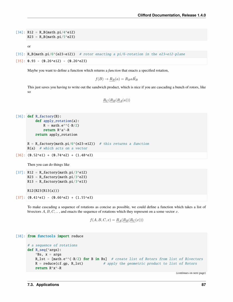
Clifford Documentation, Release 1.4.0
[34]: R12 = R_B(math.pi/4*e12)R23 = R_B(math.pi/5*e23)
or
[35]: R_B(math.pi/6*(e23+e12)) # rotor enacting a pi/6-rotation in the e23+e12-plane
[35]: 0.93 - (0.26^e12) - (0.26^e23)
Maybe you want to define a function which returns a function that enacts a specified rotation,
𝑓(𝐵) → 𝑅𝐵(𝑎) = 𝑅𝐵𝑎𝑅𝐵
This just saves you having to write out the sandwich product, which is nice if you are cascading a bunch of rotors, likeso
𝑅𝐶(𝑅𝐵(𝑅𝐴(𝑎)))
[36]: def R_factory(B):def apply_rotation(a):
R = math.e**(-B/2)return R*a*~R
return apply_rotation
R = R_factory(math.pi/6*(e23+e12)) # this returns a functionR(a) # which acts on a vector
[36]: (0.52^e1) + (0.74^e2) + (1.48^e3)
Then you can do things like
[37]: R12 = R_factory(math.pi/3*e12)R23 = R_factory(math.pi/3*e23)R13 = R_factory(math.pi/3*e13)
R12(R23(R13(a)))
[37]: (0.41^e1) - (0.66^e2) + (1.55^e3)
To make cascading a sequence of rotations as concise as possible, we could define a function which takes a list ofbivectors 𝐴,𝐵,𝐶, .. , and enacts the sequence of rotations which they represent on a some vector 𝑥.
𝑓(𝐴,𝐵,𝐶, 𝑥) = 𝑅𝐴(𝑅𝐵(𝑅𝐶(𝑥)))
[38]: from functools import reduce
# a sequence of rotationsdef R_seq(*args):
*Bs, x = argsR_lst = [math.e**(-B/2) for B in Bs] # create list of Rotors from list of BivectorsR = reduce(cf.gp, R_lst) # apply the geometric product to list of Rotorsreturn R*x*~R
(continues on next page)
7.3. Applications 87
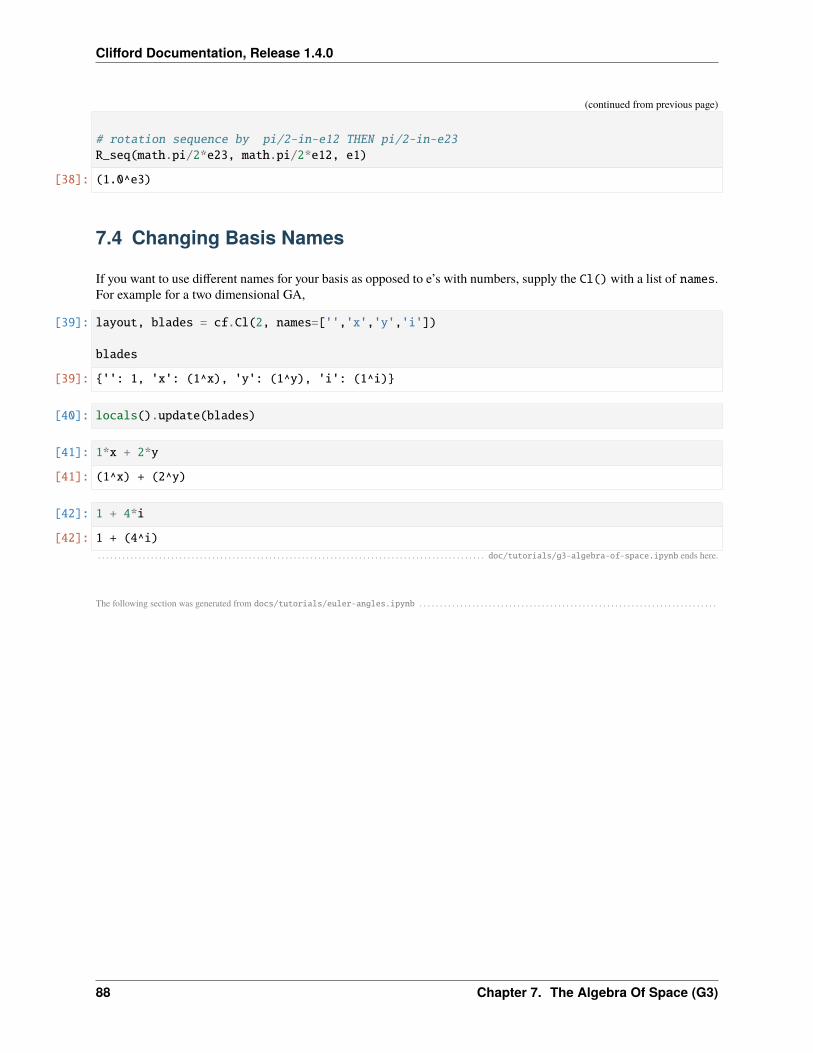
Clifford Documentation, Release 1.4.0
(continued from previous page)
# rotation sequence by pi/2-in-e12 THEN pi/2-in-e23R_seq(math.pi/2*e23, math.pi/2*e12, e1)
[38]: (1.0^e3)
7.4 Changing Basis Names
If you want to use different names for your basis as opposed to e’s with numbers, supply the Cl() with a list of names.For example for a two dimensional GA,
[39]: layout, blades = cf.Cl(2, names=['','x','y','i'])
blades
[39]: {'': 1, 'x': (1^x), 'y': (1^y), 'i': (1^i)}
[40]: locals().update(blades)
[41]: 1*x + 2*y
[41]: (1^x) + (2^y)
[42]: 1 + 4*i
[42]: 1 + (4^i)
. . . . . . . . . . . . . . . . . . . . . . . . . . . . . . . . . . . . . . . . . . . . . . . . . . . . . . . . . . . . . . . . . . . . . . . . . . . . . . . . . . . . . . . . . . . . . . . doc/tutorials/g3-algebra-of-space.ipynb ends here.
The following section was generated from docs/tutorials/euler-angles.ipynb . . . . . . . . . . . . . . . . . . . . . . . . . . . . . . . . . . . . . . . . . . . . . . . . . . . . . . . . . . . . . . . . . . . . . . . . .
88 Chapter 7. The Algebra Of Space (G3)

CHAPTER
EIGHT
ROTATIONS IN SPACE: EULER ANGLES, MATRICES, ANDQUATERNIONS
This notebook demonstrates how to use clifford to implement rotations in three dimensions using euler angles,rotation matices and quaternions. All of these forms are derived from the more general rotor form, which is providedby GA. Conversion from the rotor form to a matrix representation is shown, and takes about three lines of code. Westart with euler angles.
8.1 Euler Angles with Rotors
A common way to parameterize rotations in three dimensions is through Euler Angles.
Any orientation can be achieved by composing three elemental rotations. The elemental rotations caneither occur about the axes of the fixed coordinate system (extrinsic rotations) or about the axes of arotating coordinate system, which is initially aligned with the fixed one, and modifies its orientation aftereach elemental rotation (intrinsic rotations). — wikipedia
The animation below shows an intrinsic rotation model as each elemental rotation is applied.Label the left, right, andvertical blue-axes as 𝑒1, 𝑒2, and 𝑒3, respectively. The series of rotations can be described:
1. rotate about 𝑒3-axis
2. rotate about the rotated 𝑒1-axis, call it 𝑒′13. rotate about the twice rotated axis of 𝑒3-axis, call it 𝑒′′3
So the elemental rotations are about 𝑒3, 𝑒′
1, 𝑒′′
3 -axes, respectively.
(taken from wikipedia)
Following Sec. 2.7.5 from [DL03], we first rotate an angle 𝜑 about the 𝑒3-axis, which is equivalent to rotating in the𝑒12-plane. This is done with the rotor
𝑅𝜑 = 𝑒−𝜑2 𝑒12
Next we rotate about the rotated 𝑒1-axis, which we label 𝑒′1. To find where this is, we can rotate the axis,
𝑒′
1 = 𝑅𝜑𝑒1𝑅𝜑
The plane corresponding to this axis is found by taking the dual of 𝑒′1
𝐼𝑅𝜑𝑒1𝑅𝜑 = 𝑅𝜑𝑒23𝑅𝜑
Where we have made use of the fact that the pseudo-scalar commutes in G3. Using this result, the second rotation byangle 𝜃 about the 𝑒′1-axis is then ,
𝑅𝜃 = 𝑒𝜃2𝑅𝜑𝑒23𝑅𝜑
89
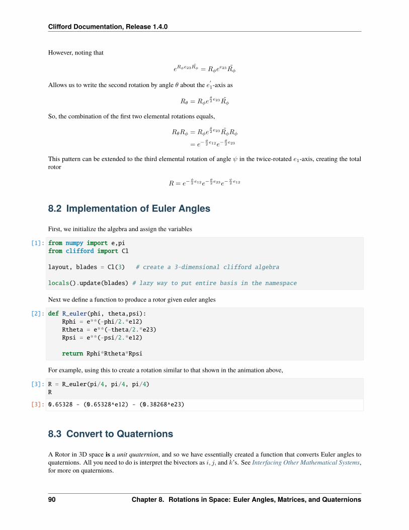
Clifford Documentation, Release 1.4.0
However, noting that
𝑒𝑅𝜑𝑒23𝑅𝜑 = 𝑅𝜑𝑒𝑒23𝑅𝜑
Allows us to write the second rotation by angle 𝜃 about the 𝑒′1-axis as
𝑅𝜃 = 𝑅𝜑𝑒𝜃2 𝑒23𝑅𝜑
So, the combination of the first two elemental rotations equals,
𝑅𝜃𝑅𝜑 = 𝑅𝜑𝑒𝜃2 𝑒23𝑅𝜑𝑅𝜑
= 𝑒−𝜑2 𝑒12𝑒−
𝜃2 𝑒23
This pattern can be extended to the third elemental rotation of angle 𝜓 in the twice-rotated 𝑒1-axis, creating the totalrotor
𝑅 = 𝑒−𝜑2 𝑒12𝑒−
𝜃2 𝑒23𝑒−
𝜓2 𝑒12
8.2 Implementation of Euler Angles
First, we initialize the algebra and assign the variables
[1]: from numpy import e,pifrom clifford import Cl
layout, blades = Cl(3) # create a 3-dimensional clifford algebra
locals().update(blades) # lazy way to put entire basis in the namespace
Next we define a function to produce a rotor given euler angles
[2]: def R_euler(phi, theta,psi):Rphi = e**(-phi/2.*e12)Rtheta = e**(-theta/2.*e23)Rpsi = e**(-psi/2.*e12)
return Rphi*Rtheta*Rpsi
For example, using this to create a rotation similar to that shown in the animation above,
[3]: R = R_euler(pi/4, pi/4, pi/4)R
[3]: 0.65328 - (0.65328^e12) - (0.38268^e23)
8.3 Convert to Quaternions
A Rotor in 3D space is a unit quaternion, and so we have essentially created a function that converts Euler angles toquaternions. All you need to do is interpret the bivectors as 𝑖, 𝑗, and 𝑘’s. See Interfacing Other Mathematical Systems,for more on quaternions.
90 Chapter 8. Rotations in Space: Euler Angles, Matrices, and Quaternions
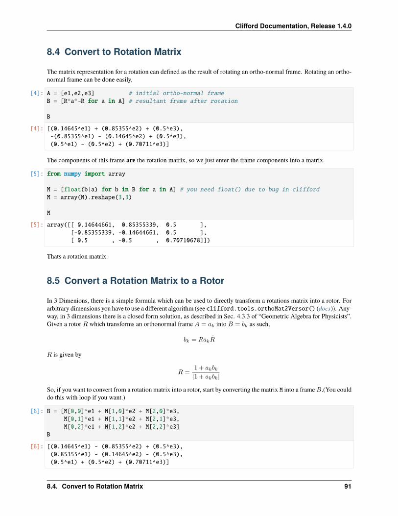
Clifford Documentation, Release 1.4.0
8.4 Convert to Rotation Matrix
The matrix representation for a rotation can defined as the result of rotating an ortho-normal frame. Rotating an ortho-normal frame can be done easily,
[4]: A = [e1,e2,e3] # initial ortho-normal frameB = [R*a*~R for a in A] # resultant frame after rotation
B
[4]: [(0.14645^e1) + (0.85355^e2) + (0.5^e3),-(0.85355^e1) - (0.14645^e2) + (0.5^e3),(0.5^e1) - (0.5^e2) + (0.70711^e3)]
The components of this frame are the rotation matrix, so we just enter the frame components into a matrix.
[5]: from numpy import array
M = [float(b|a) for b in B for a in A] # you need float() due to bug in cliffordM = array(M).reshape(3,3)
M
[5]: array([[ 0.14644661, 0.85355339, 0.5 ],[-0.85355339, -0.14644661, 0.5 ],[ 0.5 , -0.5 , 0.70710678]])
Thats a rotation matrix.
8.5 Convert a Rotation Matrix to a Rotor
In 3 Dimenions, there is a simple formula which can be used to directly transform a rotations matrix into a rotor. Forarbitrary dimensions you have to use a different algorithm (see clifford.tools.orthoMat2Versor() (docs)). Any-way, in 3 dimensions there is a closed form solution, as described in Sec. 4.3.3 of “Geometric Algebra for Physicists”.Given a rotor 𝑅 which transforms an orthonormal frame 𝐴 = 𝑎𝑘 into 𝐵 = 𝑏𝑘 as such,
𝑏𝑘 = 𝑅𝑎𝑘�̃�
𝑅 is given by
𝑅 =1 + 𝑎𝑘𝑏𝑘|1 + 𝑎𝑘𝑏𝑘|
So, if you want to convert from a rotation matrix into a rotor, start by converting the matrix M into a frame𝐵.(You coulddo this with loop if you want.)
[6]: B = [M[0,0]*e1 + M[1,0]*e2 + M[2,0]*e3,M[0,1]*e1 + M[1,1]*e2 + M[2,1]*e3,M[0,2]*e1 + M[1,2]*e2 + M[2,2]*e3]
B
[6]: [(0.14645^e1) - (0.85355^e2) + (0.5^e3),(0.85355^e1) - (0.14645^e2) - (0.5^e3),(0.5^e1) + (0.5^e2) + (0.70711^e3)]
8.4. Convert to Rotation Matrix 91
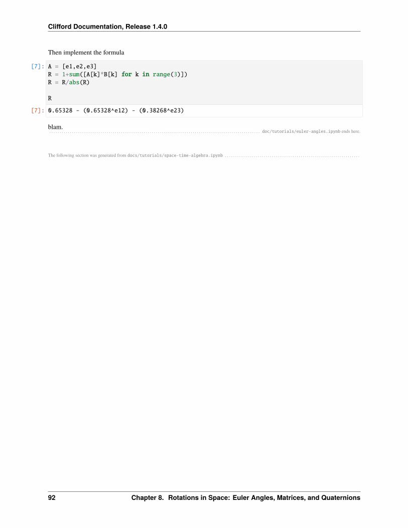
Clifford Documentation, Release 1.4.0
Then implement the formula
[7]: A = [e1,e2,e3]R = 1+sum([A[k]*B[k] for k in range(3)])R = R/abs(R)
R
[7]: 0.65328 - (0.65328^e12) - (0.38268^e23)
blam.. . . . . . . . . . . . . . . . . . . . . . . . . . . . . . . . . . . . . . . . . . . . . . . . . . . . . . . . . . . . . . . . . . . . . . . . . . . . . . . . . . . . . . . . . . . . . . . . . . . . . . . doc/tutorials/euler-angles.ipynb ends here.
The following section was generated from docs/tutorials/space-time-algebra.ipynb . . . . . . . . . . . . . . . . . . . . . . . . . . . . . . . . . . . . . . . . . . . . . . . . . . . . . . . . . . . . . . . . . .
92 Chapter 8. Rotations in Space: Euler Angles, Matrices, and Quaternions
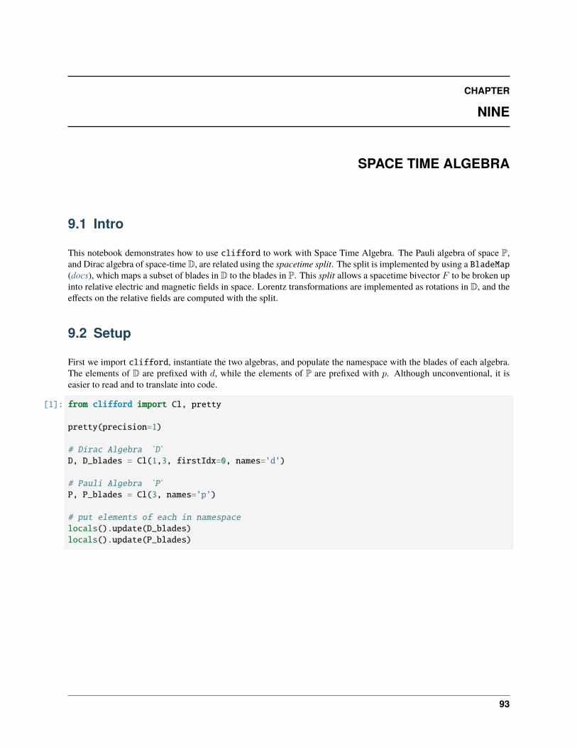
CHAPTER
NINE
SPACE TIME ALGEBRA
9.1 Intro
This notebook demonstrates how to use clifford to work with Space Time Algebra. The Pauli algebra of space P,and Dirac algebra of space-time D, are related using the spacetime split. The split is implemented by using a BladeMap(docs), which maps a subset of blades in D to the blades in P. This split allows a spacetime bivector 𝐹 to be broken upinto relative electric and magnetic fields in space. Lorentz transformations are implemented as rotations in D, and theeffects on the relative fields are computed with the split.
9.2 Setup
First we import clifford, instantiate the two algebras, and populate the namespace with the blades of each algebra.The elements of D are prefixed with 𝑑, while the elements of P are prefixed with 𝑝. Although unconventional, it iseasier to read and to translate into code.
[1]: from clifford import Cl, pretty
pretty(precision=1)
# Dirac Algebra `D`D, D_blades = Cl(1,3, firstIdx=0, names='d')
# Pauli Algebra `P`P, P_blades = Cl(3, names='p')
# put elements of each in namespacelocals().update(D_blades)locals().update(P_blades)
93
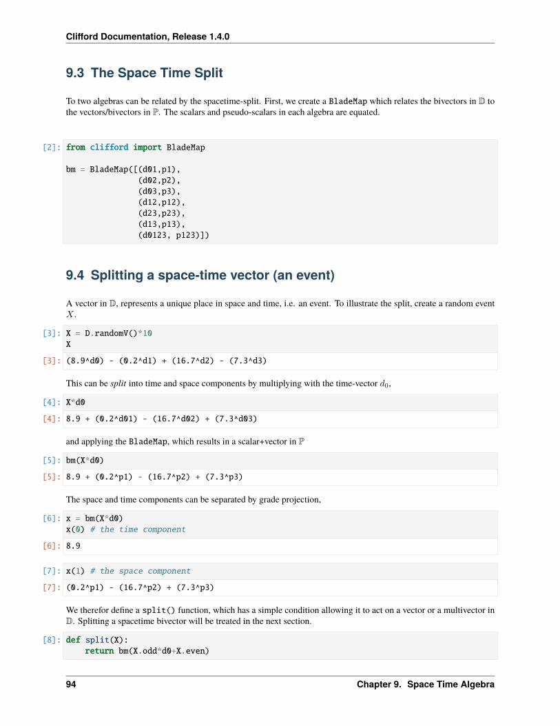
Clifford Documentation, Release 1.4.0
9.3 The Space Time Split
To two algebras can be related by the spacetime-split. First, we create a BladeMap which relates the bivectors in D tothe vectors/bivectors in P. The scalars and pseudo-scalars in each algebra are equated.
[2]: from clifford import BladeMap
bm = BladeMap([(d01,p1),(d02,p2),(d03,p3),(d12,p12),(d23,p23),(d13,p13),(d0123, p123)])
9.4 Splitting a space-time vector (an event)
A vector in D, represents a unique place in space and time, i.e. an event. To illustrate the split, create a random event𝑋 .
[3]: X = D.randomV()*10X
[3]: (8.9^d0) - (0.2^d1) + (16.7^d2) - (7.3^d3)
This can be split into time and space components by multiplying with the time-vector 𝑑0,
[4]: X*d0
[4]: 8.9 + (0.2^d01) - (16.7^d02) + (7.3^d03)
and applying the BladeMap, which results in a scalar+vector in P
[5]: bm(X*d0)
[5]: 8.9 + (0.2^p1) - (16.7^p2) + (7.3^p3)
The space and time components can be separated by grade projection,
[6]: x = bm(X*d0)x(0) # the time component
[6]: 8.9
[7]: x(1) # the space component
[7]: (0.2^p1) - (16.7^p2) + (7.3^p3)
We therefor define a split() function, which has a simple condition allowing it to act on a vector or a multivector inD. Splitting a spacetime bivector will be treated in the next section.
[8]: def split(X):return bm(X.odd*d0+X.even)
94 Chapter 9. Space Time Algebra
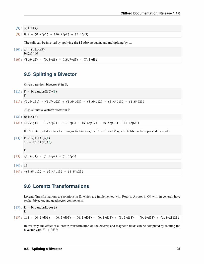
Clifford Documentation, Release 1.4.0
[9]: split(X)
[9]: 8.9 + (0.2^p1) - (16.7^p2) + (7.3^p3)
The split can be inverted by applying the BladeMap again, and multiplying by 𝑑0
[10]: x = split(X)bm(x)*d0
[10]: (8.9^d0) - (0.2^d1) + (16.7^d2) - (7.3^d3)
9.5 Splitting a Bivector
Given a random bivector 𝐹 in D,
[11]: F = D.randomMV()(2)F
[11]: (1.5^d01) - (1.7^d02) + (1.6^d03) - (0.6^d12) - (0.4^d13) - (1.6^d23)
𝐹 splits into a vector/bivector in P
[12]: split(F)
[12]: (1.5^p1) - (1.7^p2) + (1.6^p3) - (0.6^p12) - (0.4^p13) - (1.6^p23)
If 𝐹 is interpreted as the electromagnetic bivector, the Electric and Magnetic fields can be separated by grade
[13]: E = split(F)(1)iB = split(F)(2)
E
[13]: (1.5^p1) - (1.7^p2) + (1.6^p3)
[14]: iB
[14]: -(0.6^p12) - (0.4^p13) - (1.6^p23)
9.6 Lorentz Transformations
Lorentz Transformations are rotations in D, which are implemented with Rotors. A rotor in G4 will, in general, havescalar, bivector, and quadvector components.
[15]: R = D.randomRotor()R
[15]: 1.2 - (0.5^d01) + (0.2^d02) - (4.0^d03) - (0.5^d12) + (3.9^d13) - (0.4^d23) + (1.2^d0123)
In this way, the effect of a lorentz transformation on the electric and magnetic fields can be computed by rotating thebivector with 𝐹 → 𝑅𝐹�̃�
9.5. Splitting a Bivector 95
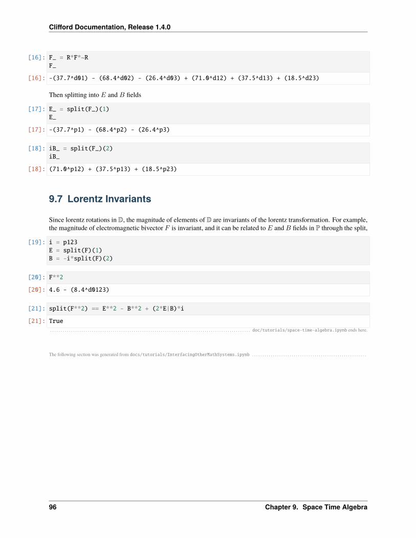
Clifford Documentation, Release 1.4.0
[16]: F_ = R*F*~RF_
[16]: -(37.7^d01) - (68.4^d02) - (26.4^d03) + (71.0^d12) + (37.5^d13) + (18.5^d23)
Then splitting into 𝐸 and 𝐵 fields
[17]: E_ = split(F_)(1)E_
[17]: -(37.7^p1) - (68.4^p2) - (26.4^p3)
[18]: iB_ = split(F_)(2)iB_
[18]: (71.0^p12) + (37.5^p13) + (18.5^p23)
9.7 Lorentz Invariants
Since lorentz rotations in D, the magnitude of elements of D are invariants of the lorentz transformation. For example,the magnitude of electromagnetic bivector 𝐹 is invariant, and it can be related to 𝐸 and 𝐵 fields in P through the split,
[19]: i = p123E = split(F)(1)B = -i*split(F)(2)
[20]: F**2
[20]: 4.6 - (8.4^d0123)
[21]: split(F**2) == E**2 - B**2 + (2*E|B)*i
[21]: True
. . . . . . . . . . . . . . . . . . . . . . . . . . . . . . . . . . . . . . . . . . . . . . . . . . . . . . . . . . . . . . . . . . . . . . . . . . . . . . . . . . . . . . . . . . . . . . . . doc/tutorials/space-time-algebra.ipynb ends here.
The following section was generated from docs/tutorials/InterfacingOtherMathSystems.ipynb . . . . . . . . . . . . . . . . . . . . . . . . . . . . . . . . . . . . . . . . . . . . . . . . . . . . . . .
96 Chapter 9. Space Time Algebra
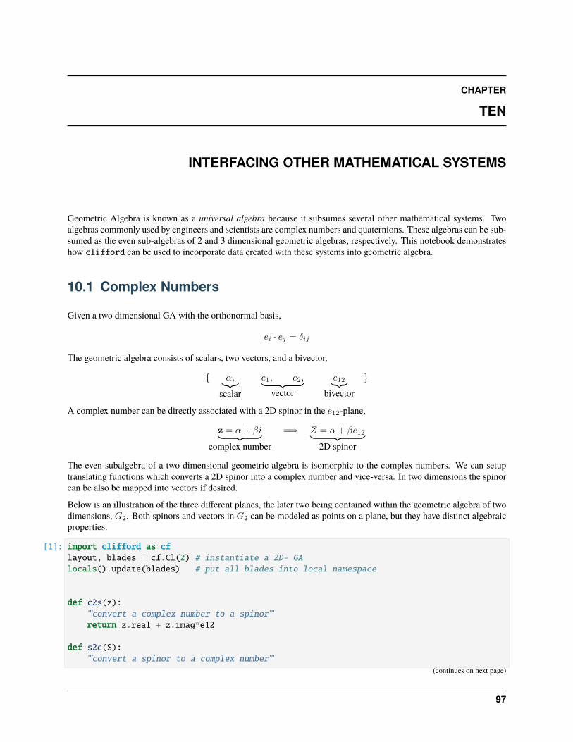
CHAPTER
TEN
INTERFACING OTHER MATHEMATICAL SYSTEMS
Geometric Algebra is known as a universal algebra because it subsumes several other mathematical systems. Twoalgebras commonly used by engineers and scientists are complex numbers and quaternions. These algebras can be sub-sumed as the even sub-algebras of 2 and 3 dimensional geometric algebras, respectively. This notebook demonstrateshow clifford can be used to incorporate data created with these systems into geometric algebra.
10.1 Complex Numbers
Given a two dimensional GA with the orthonormal basis,
𝑒𝑖 · 𝑒𝑗 = 𝛿𝑖𝑗
The geometric algebra consists of scalars, two vectors, and a bivector,
{ 𝛼,⏟ ⏞ scalar
𝑒1, 𝑒2,⏟ ⏞ vector
𝑒12⏟ ⏞ bivector
}
A complex number can be directly associated with a 2D spinor in the 𝑒12-plane,
z = 𝛼+ 𝛽𝑖⏟ ⏞ complex number
=⇒ 𝑍 = 𝛼+ 𝛽𝑒12⏟ ⏞ 2D spinor
The even subalgebra of a two dimensional geometric algebra is isomorphic to the complex numbers. We can setuptranslating functions which converts a 2D spinor into a complex number and vice-versa. In two dimensions the spinorcan be also be mapped into vectors if desired.
Below is an illustration of the three different planes, the later two being contained within the geometric algebra of twodimensions, 𝐺2. Both spinors and vectors in 𝐺2 can be modeled as points on a plane, but they have distinct algebraicproperties.
[1]: import clifford as cflayout, blades = cf.Cl(2) # instantiate a 2D- GAlocals().update(blades) # put all blades into local namespace
def c2s(z):'''convert a complex number to a spinor'''return z.real + z.imag*e12
def s2c(S):'''convert a spinor to a complex number'''
(continues on next page)
97
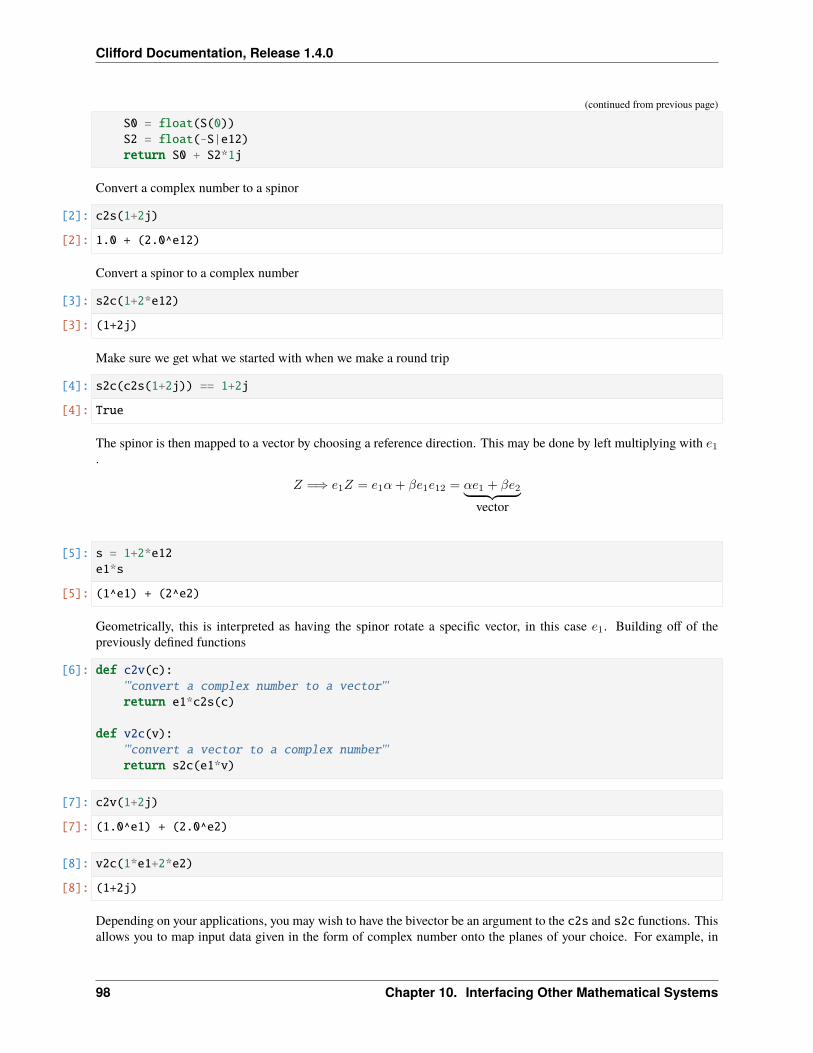
Clifford Documentation, Release 1.4.0
(continued from previous page)
S0 = float(S(0))S2 = float(-S|e12)return S0 + S2*1j
Convert a complex number to a spinor
[2]: c2s(1+2j)
[2]: 1.0 + (2.0^e12)
Convert a spinor to a complex number
[3]: s2c(1+2*e12)
[3]: (1+2j)
Make sure we get what we started with when we make a round trip
[4]: s2c(c2s(1+2j)) == 1+2j
[4]: True
The spinor is then mapped to a vector by choosing a reference direction. This may be done by left multiplying with 𝑒1.
𝑍 =⇒ 𝑒1𝑍 = 𝑒1𝛼+ 𝛽𝑒1𝑒12 = 𝛼𝑒1 + 𝛽𝑒2⏟ ⏞ vector
[5]: s = 1+2*e12e1*s
[5]: (1^e1) + (2^e2)
Geometrically, this is interpreted as having the spinor rotate a specific vector, in this case 𝑒1. Building off of thepreviously defined functions
[6]: def c2v(c):'''convert a complex number to a vector'''return e1*c2s(c)
def v2c(v):'''convert a vector to a complex number'''return s2c(e1*v)
[7]: c2v(1+2j)
[7]: (1.0^e1) + (2.0^e2)
[8]: v2c(1*e1+2*e2)
[8]: (1+2j)
Depending on your applications, you may wish to have the bivector be an argument to the c2s and s2c functions. Thisallows you to map input data given in the form of complex number onto the planes of your choice. For example, in
98 Chapter 10. Interfacing Other Mathematical Systems
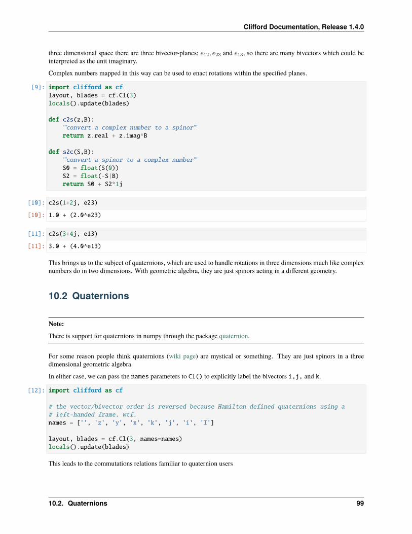
Clifford Documentation, Release 1.4.0
three dimensional space there are three bivector-planes; 𝑒12, 𝑒23 and 𝑒13, so there are many bivectors which could beinterpreted as the unit imaginary.
Complex numbers mapped in this way can be used to enact rotations within the specified planes.
[9]: import clifford as cflayout, blades = cf.Cl(3)locals().update(blades)
def c2s(z,B):'''convert a complex number to a spinor'''return z.real + z.imag*B
def s2c(S,B):'''convert a spinor to a complex number'''S0 = float(S(0))S2 = float(-S|B)return S0 + S2*1j
[10]: c2s(1+2j, e23)
[10]: 1.0 + (2.0^e23)
[11]: c2s(3+4j, e13)
[11]: 3.0 + (4.0^e13)
This brings us to the subject of quaternions, which are used to handle rotations in three dimensions much like complexnumbers do in two dimensions. With geometric algebra, they are just spinors acting in a different geometry.
10.2 Quaternions
Note:
There is support for quaternions in numpy through the package quaternion.
For some reason people think quaternions (wiki page) are mystical or something. They are just spinors in a threedimensional geometric algebra.
In either case, we can pass the names parameters to Cl() to explicitly label the bivectors i,j, and k.
[12]: import clifford as cf
# the vector/bivector order is reversed because Hamilton defined quaternions using a# left-handed frame. wtf.names = ['', 'z', 'y', 'x', 'k', 'j', 'i', 'I']
layout, blades = cf.Cl(3, names=names)locals().update(blades)
This leads to the commutations relations familiar to quaternion users
10.2. Quaternions 99
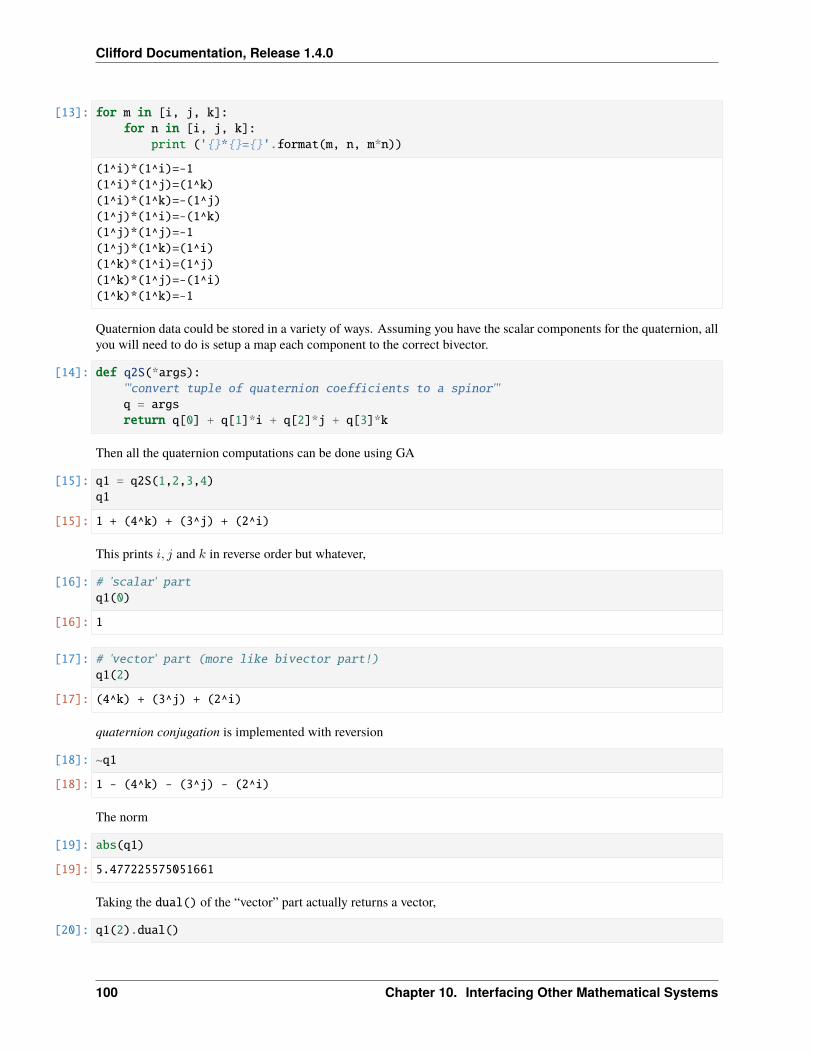
Clifford Documentation, Release 1.4.0
[13]: for m in [i, j, k]:for n in [i, j, k]:
print ('{}*{}={}'.format(m, n, m*n))
(1^i)*(1^i)=-1(1^i)*(1^j)=(1^k)(1^i)*(1^k)=-(1^j)(1^j)*(1^i)=-(1^k)(1^j)*(1^j)=-1(1^j)*(1^k)=(1^i)(1^k)*(1^i)=(1^j)(1^k)*(1^j)=-(1^i)(1^k)*(1^k)=-1
Quaternion data could be stored in a variety of ways. Assuming you have the scalar components for the quaternion, allyou will need to do is setup a map each component to the correct bivector.
[14]: def q2S(*args):'''convert tuple of quaternion coefficients to a spinor'''q = argsreturn q[0] + q[1]*i + q[2]*j + q[3]*k
Then all the quaternion computations can be done using GA
[15]: q1 = q2S(1,2,3,4)q1
[15]: 1 + (4^k) + (3^j) + (2^i)
This prints 𝑖, 𝑗 and 𝑘 in reverse order but whatever,
[16]: # 'scalar' partq1(0)
[16]: 1
[17]: # 'vector' part (more like bivector part!)q1(2)
[17]: (4^k) + (3^j) + (2^i)
quaternion conjugation is implemented with reversion
[18]: ~q1
[18]: 1 - (4^k) - (3^j) - (2^i)
The norm
[19]: abs(q1)
[19]: 5.477225575051661
Taking the dual() of the “vector” part actually returns a vector,
[20]: q1(2).dual()
100 Chapter 10. Interfacing Other Mathematical Systems
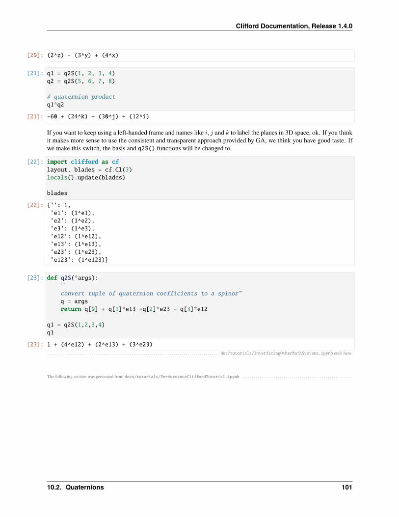
Clifford Documentation, Release 1.4.0
[20]: (2^z) - (3^y) + (4^x)
[21]: q1 = q2S(1, 2, 3, 4)q2 = q2S(5, 6, 7, 8)
# quaternion productq1*q2
[21]: -60 + (24^k) + (30^j) + (12^i)
If you want to keep using a left-handed frame and names like 𝑖, 𝑗 and 𝑘 to label the planes in 3D space, ok. If you thinkit makes more sense to use the consistent and transparent approach provided by GA, we think you have good taste. Ifwe make this switch, the basis and q2S() functions will be changed to
[22]: import clifford as cflayout, blades = cf.Cl(3)locals().update(blades)
blades
[22]: {'': 1,'e1': (1^e1),'e2': (1^e2),'e3': (1^e3),'e12': (1^e12),'e13': (1^e13),'e23': (1^e23),'e123': (1^e123)}
[23]: def q2S(*args):'''convert tuple of quaternion coefficients to a spinor'''q = argsreturn q[0] + q[1]*e13 +q[2]*e23 + q[3]*e12
q1 = q2S(1,2,3,4)q1
[23]: 1 + (4^e12) + (2^e13) + (3^e23)
. . . . . . . . . . . . . . . . . . . . . . . . . . . . . . . . . . . . . . . . . . . . . . . . . . . . . . . . . . . . . . . . . . . . . . . . . . . . . . . . . . . . . . doc/tutorials/InterfacingOtherMathSystems.ipynb ends here.
The following section was generated from docs/tutorials/PerformanceCliffordTutorial.ipynb . . . . . . . . . . . . . . . . . . . . . . . . . . . . . . . . . . . . . . . . . . . . . . . . . . . . . . .
10.2. Quaternions 101

Clifford Documentation, Release 1.4.0
102 Chapter 10. Interfacing Other Mathematical Systems
CHAPTER
ELEVEN
WRITING HIGH(ISH) PERFORMANCE CODE WITH CLIFFORD ANDNUMBA VIA NUMPY
This document describes how to take algorithms developed in the clifford package with notation that is close to the mathsand convert it into numerically efficient and fast running code. To do this we will expose the underlying representationof multivector as a numpy array of canonical basis vector coefficients and operate directly on these arrays in a mannerthat is conducive to JIT compilation with numba.
11.1 First import the Clifford library as well as numpy and numba
[1]: import clifford as cfimport numpy as npimport numba
11.2 Choose a specific space
For this document we will use 3d euclidean space embedded in the conformal framework giving a Cl(4,1) algebra. Wewill also rename some of the variables to match the notation that used by Lasenby et al. in “A Covariant Approach toGeometry using Geometric Algebra”
[2]: from clifford import g3c# Get the layout in our local namespace etc etclayout = g3c.layoutlocals().update(g3c.blades)
ep, en, up, down, homo, E0, ninf, no = (g3c.stuff["ep"], g3c.stuff["en"],g3c.stuff["up"], g3c.stuff["down"], g3c.stuff[
→˓"homo"],g3c.stuff["E0"], g3c.stuff["einf"], -g3c.stuff[
→˓"eo"])# Define a few useful termsE = ninf^(no)I5 = e12345I3 = e123
103
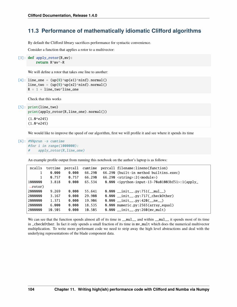
Clifford Documentation, Release 1.4.0
11.3 Performance of mathematically idiomatic Clifford algorithms
By default the Clifford library sacrifices performance for syntactic convenience.
Consider a function that applies a rotor to a multivector:
[3]: def apply_rotor(R,mv):return R*mv*~R
We will define a rotor that takes one line to another:
[4]: line_one = (up(0)^up(e1)^ninf).normal()line_two = (up(0)^up(e2)^ninf).normal()R = 1 + line_two*line_one
Check that this works
[5]: print(line_two)print(apply_rotor(R,line_one).normal())
(1.0^e245)(1.0^e245)
We would like to improve the speed of our algorithm, first we will profile it and see where it spends its time
[6]: #%%prun -s cumtime#for i in range(1000000):# apply_rotor(R,line_one)
An example profile output from running this notebook on the author’s laptop is as follows:
ncalls tottime percall cumtime percall filename:lineno(function)1 0.000 0.000 66.290 66.290 {built-in method builtins.exec}1 0.757 0.757 66.290 66.290 <string>:2(<module>)
1000000 3.818 0.000 65.534 0.000 <ipython-input-13-70a01003bf51>:1(apply_→˓rotor)2000000 9.269 0.000 55.641 0.000 __init__.py:751(__mul__)2000000 3.167 0.000 29.900 0.000 __init__.py:717(_checkOther)2000000 1.371 0.000 19.906 0.000 __init__.py:420(__ne__)2000000 6.000 0.000 18.535 0.000 numeric.py:2565(array_equal)2000000 10.505 0.000 10.505 0.000 __init__.py:260(mv_mult)
We can see that the function spends almost all of its time in __mul__ and within __mul__ it spends most of its timein _checkOther. In fact it only spends a small fraction of its time in mv_mult which does the numerical multivectormultiplication. To write more performant code we need to strip away the high level abstractions and deal with theunderlying representations of the blade component data.
104 Chapter 11. Writing high(ish) performance code with Clifford and Numba via Numpy
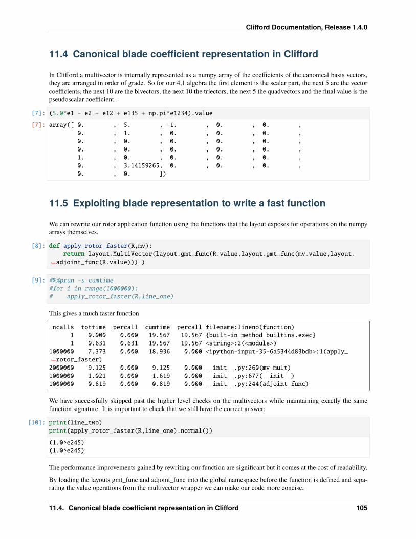
Clifford Documentation, Release 1.4.0
11.4 Canonical blade coefficient representation in Clifford
In Clifford a multivector is internally represented as a numpy array of the coefficients of the canonical basis vectors,they are arranged in order of grade. So for our 4,1 algebra the first element is the scalar part, the next 5 are the vectorcoefficients, the next 10 are the bivectors, the next 10 the triectors, the next 5 the quadvectors and the final value is thepseudoscalar coefficient.
[7]: (5.0*e1 - e2 + e12 + e135 + np.pi*e1234).value
[7]: array([ 0. , 5. , -1. , 0. , 0. ,0. , 1. , 0. , 0. , 0. ,0. , 0. , 0. , 0. , 0. ,0. , 0. , 0. , 0. , 0. ,1. , 0. , 0. , 0. , 0. ,0. , 3.14159265, 0. , 0. , 0. ,0. , 0. ])
11.5 Exploiting blade representation to write a fast function
We can rewrite our rotor application function using the functions that the layout exposes for operations on the numpyarrays themselves.
[8]: def apply_rotor_faster(R,mv):return layout.MultiVector(layout.gmt_func(R.value,layout.gmt_func(mv.value,layout.
→˓adjoint_func(R.value))) )
[9]: #%%prun -s cumtime#for i in range(1000000):# apply_rotor_faster(R,line_one)
This gives a much faster function
ncalls tottime percall cumtime percall filename:lineno(function)1 0.000 0.000 19.567 19.567 {built-in method builtins.exec}1 0.631 0.631 19.567 19.567 <string>:2(<module>)
1000000 7.373 0.000 18.936 0.000 <ipython-input-35-6a5344d83bdb>:1(apply_→˓rotor_faster)2000000 9.125 0.000 9.125 0.000 __init__.py:260(mv_mult)1000000 1.021 0.000 1.619 0.000 __init__.py:677(__init__)1000000 0.819 0.000 0.819 0.000 __init__.py:244(adjoint_func)
We have successfully skipped past the higher level checks on the multivectors while maintaining exactly the samefunction signature. It is important to check that we still have the correct answer:
[10]: print(line_two)print(apply_rotor_faster(R,line_one).normal())
(1.0^e245)(1.0^e245)
The performance improvements gained by rewriting our function are significant but it comes at the cost of readability.
By loading the layouts gmt_func and adjoint_func into the global namespace before the function is defined and sepa-rating the value operations from the multivector wrapper we can make our code more concise.
11.4. Canonical blade coefficient representation in Clifford 105
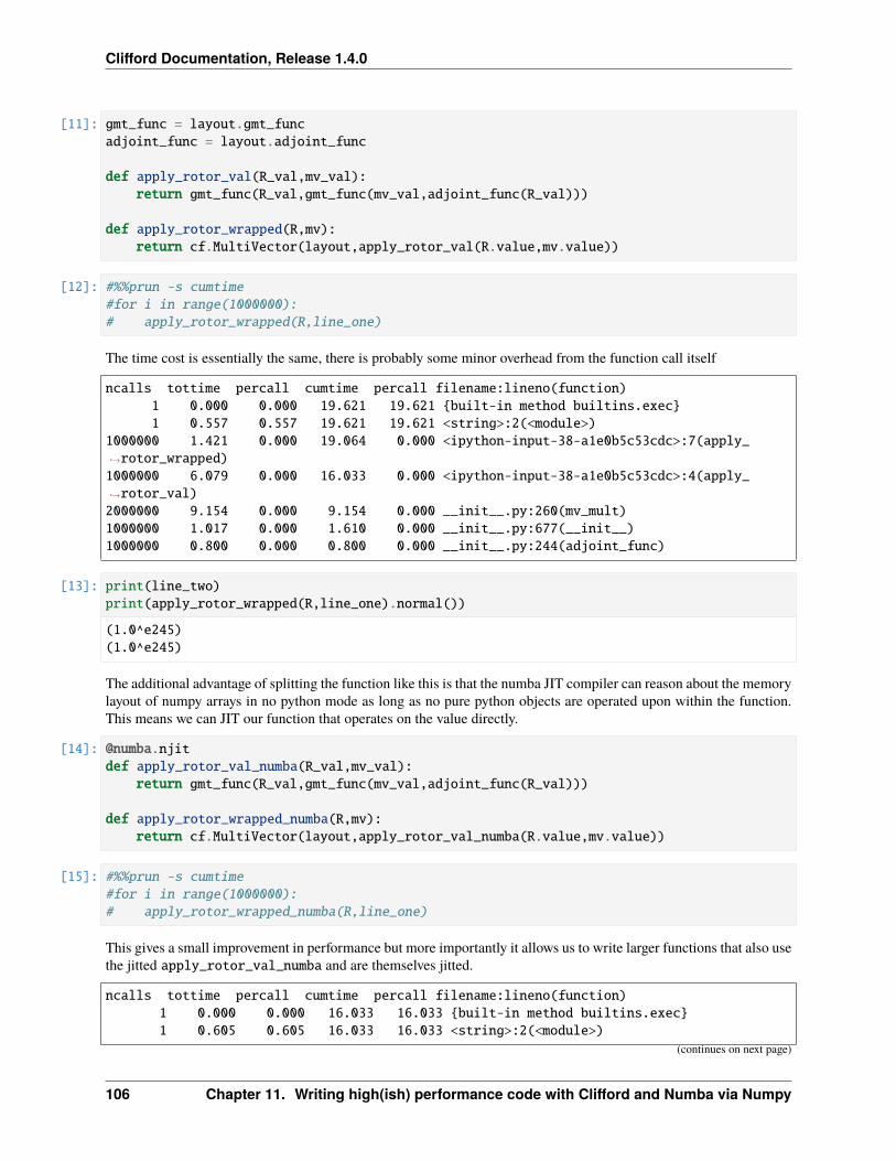
Clifford Documentation, Release 1.4.0
[11]: gmt_func = layout.gmt_funcadjoint_func = layout.adjoint_func
def apply_rotor_val(R_val,mv_val):return gmt_func(R_val,gmt_func(mv_val,adjoint_func(R_val)))
def apply_rotor_wrapped(R,mv):return cf.MultiVector(layout,apply_rotor_val(R.value,mv.value))
[12]: #%%prun -s cumtime#for i in range(1000000):# apply_rotor_wrapped(R,line_one)
The time cost is essentially the same, there is probably some minor overhead from the function call itself
ncalls tottime percall cumtime percall filename:lineno(function)1 0.000 0.000 19.621 19.621 {built-in method builtins.exec}1 0.557 0.557 19.621 19.621 <string>:2(<module>)
1000000 1.421 0.000 19.064 0.000 <ipython-input-38-a1e0b5c53cdc>:7(apply_→˓rotor_wrapped)1000000 6.079 0.000 16.033 0.000 <ipython-input-38-a1e0b5c53cdc>:4(apply_→˓rotor_val)2000000 9.154 0.000 9.154 0.000 __init__.py:260(mv_mult)1000000 1.017 0.000 1.610 0.000 __init__.py:677(__init__)1000000 0.800 0.000 0.800 0.000 __init__.py:244(adjoint_func)
[13]: print(line_two)print(apply_rotor_wrapped(R,line_one).normal())
(1.0^e245)(1.0^e245)
The additional advantage of splitting the function like this is that the numba JIT compiler can reason about the memorylayout of numpy arrays in no python mode as long as no pure python objects are operated upon within the function.This means we can JIT our function that operates on the value directly.
[14]: @numba.njitdef apply_rotor_val_numba(R_val,mv_val):
return gmt_func(R_val,gmt_func(mv_val,adjoint_func(R_val)))
def apply_rotor_wrapped_numba(R,mv):return cf.MultiVector(layout,apply_rotor_val_numba(R.value,mv.value))
[15]: #%%prun -s cumtime#for i in range(1000000):# apply_rotor_wrapped_numba(R,line_one)
This gives a small improvement in performance but more importantly it allows us to write larger functions that also usethe jitted apply_rotor_val_numba and are themselves jitted.
ncalls tottime percall cumtime percall filename:lineno(function)1 0.000 0.000 16.033 16.033 {built-in method builtins.exec}1 0.605 0.605 16.033 16.033 <string>:2(<module>)
(continues on next page)
106 Chapter 11. Writing high(ish) performance code with Clifford and Numba via Numpy
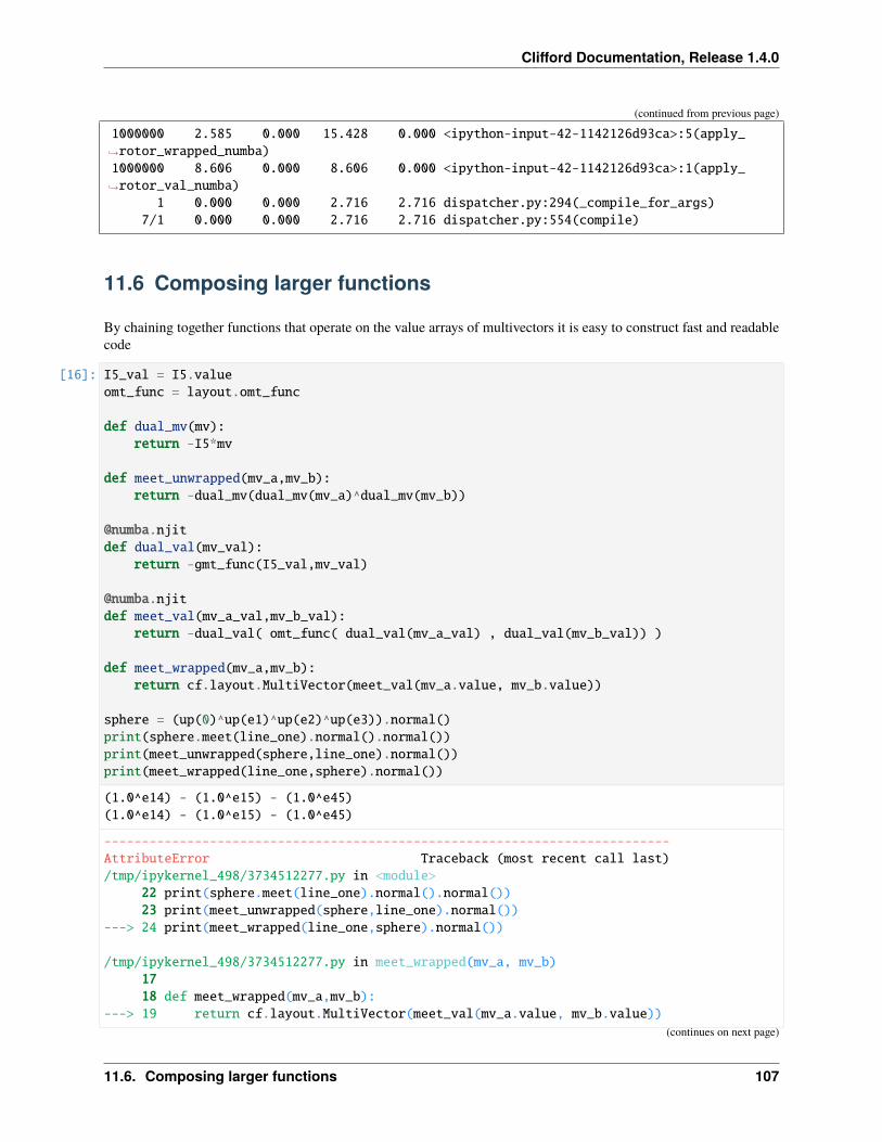
Clifford Documentation, Release 1.4.0
(continued from previous page)
1000000 2.585 0.000 15.428 0.000 <ipython-input-42-1142126d93ca>:5(apply_→˓rotor_wrapped_numba)1000000 8.606 0.000 8.606 0.000 <ipython-input-42-1142126d93ca>:1(apply_→˓rotor_val_numba)
1 0.000 0.000 2.716 2.716 dispatcher.py:294(_compile_for_args)7/1 0.000 0.000 2.716 2.716 dispatcher.py:554(compile)
11.6 Composing larger functions
By chaining together functions that operate on the value arrays of multivectors it is easy to construct fast and readablecode
[16]: I5_val = I5.valueomt_func = layout.omt_func
def dual_mv(mv):return -I5*mv
def meet_unwrapped(mv_a,mv_b):return -dual_mv(dual_mv(mv_a)^dual_mv(mv_b))
@numba.njitdef dual_val(mv_val):
return -gmt_func(I5_val,mv_val)
@numba.njitdef meet_val(mv_a_val,mv_b_val):
return -dual_val( omt_func( dual_val(mv_a_val) , dual_val(mv_b_val)) )
def meet_wrapped(mv_a,mv_b):return cf.layout.MultiVector(meet_val(mv_a.value, mv_b.value))
sphere = (up(0)^up(e1)^up(e2)^up(e3)).normal()print(sphere.meet(line_one).normal().normal())print(meet_unwrapped(sphere,line_one).normal())print(meet_wrapped(line_one,sphere).normal())
(1.0^e14) - (1.0^e15) - (1.0^e45)(1.0^e14) - (1.0^e15) - (1.0^e45)
---------------------------------------------------------------------------AttributeError Traceback (most recent call last)/tmp/ipykernel_498/3734512277.py in <module>
22 print(sphere.meet(line_one).normal().normal())23 print(meet_unwrapped(sphere,line_one).normal())
---> 24 print(meet_wrapped(line_one,sphere).normal())
/tmp/ipykernel_498/3734512277.py in meet_wrapped(mv_a, mv_b)1718 def meet_wrapped(mv_a,mv_b):
---> 19 return cf.layout.MultiVector(meet_val(mv_a.value, mv_b.value))(continues on next page)
11.6. Composing larger functions 107
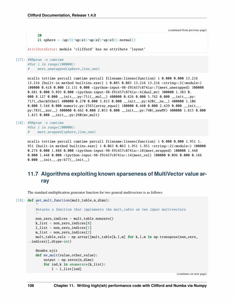
Clifford Documentation, Release 1.4.0
(continued from previous page)
2021 sphere = (up(0)^up(e1)^up(e2)^up(e3)).normal()
AttributeError: module 'clifford' has no attribute 'layout'
[17]: #%%prun -s cumtime#for i in range(100000):# meet_unwrapped(sphere,line_one)
ncalls tottime percall cumtime percall filename:lineno(function) 1 0.000 0.000 13.21613.216 {built-in method builtins.exec} 1 0.085 0.085 13.216 13.216 <string>:2(<module>)100000 0.418 0.000 13.131 0.000 <ipython-input-98-f91457c8741a>:7(meet_unwrapped) 3000000.681 0.000 9.893 0.000 <ipython-input-98-f91457c8741a>:4(dual_mv) 300000 1.383 0.000 8.127 0.000 __init__.py:751(__mul__) 400000 0.626 0.000 5.762 0.000 __init__.py:717(_checkOther) 400000 0.270 0.000 3.815 0.000 __init__.py:420(__ne__) 400000 1.1060.000 3.544 0.000 numeric.py:2565(array_equal) 100000 0.460 0.000 2.439 0.000 __init__.py:783(__xor__) 800000 0.662 0.000 2.053 0.000 __init__.py:740(_newMV) 400000 1.815 0.0001.815 0.000 __init__.py:260(mv_mult)
[18]: #%%prun -s cumtime#for i in range(100000):# meet_wrapped(sphere,line_one)
ncalls tottime percall cumtime percall filename:lineno(function) 1 0.000 0.000 1.951 1.951 {built-in method builtins.exec} 1 0.063 0.063 1.951 1.951 <string>:2(<module>) 1000000.274 0.000 1.888 0.000 <ipython-input-98-f91457c8741a>:18(meet_wrapped) 100000 1.4480.000 1.448 0.000 <ipython-input-98-f91457c8741a>:14(meet_val) 100000 0.096 0.000 0.1660.000 __init__.py:677(__init__)
11.7 Algorithms exploiting known sparseness of MultiVector value ar-ray
The standard multiplication generator function for two general multivectors is as follows:
[19]: def get_mult_function(mult_table,n_dims):'''Returns a function that implements the mult_table on two input multivectors'''non_zero_indices = mult_table.nonzero()k_list = non_zero_indices[0]l_list = non_zero_indices[1]m_list = non_zero_indices[2]mult_table_vals = np.array([mult_table[k,l,m] for k,l,m in np.transpose(non_zero_
→˓indices)],dtype=int)
@numba.njitdef mv_mult(value,other_value):
output = np.zeros(n_dims)for ind,k in enumerate(k_list):
l = l_list[ind](continues on next page)
108 Chapter 11. Writing high(ish) performance code with Clifford and Numba via Numpy
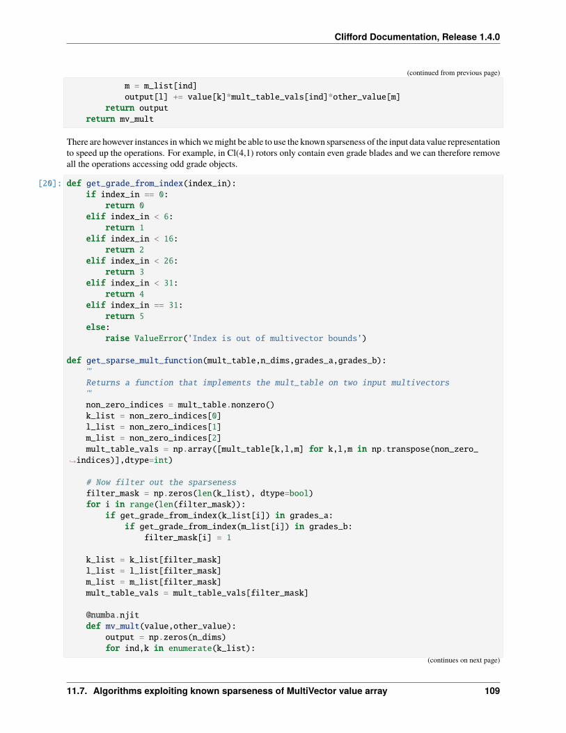
Clifford Documentation, Release 1.4.0
(continued from previous page)
m = m_list[ind]output[l] += value[k]*mult_table_vals[ind]*other_value[m]
return outputreturn mv_mult
There are however instances in which we might be able to use the known sparseness of the input data value representationto speed up the operations. For example, in Cl(4,1) rotors only contain even grade blades and we can therefore removeall the operations accessing odd grade objects.
[20]: def get_grade_from_index(index_in):if index_in == 0:
return 0elif index_in < 6:
return 1elif index_in < 16:
return 2elif index_in < 26:
return 3elif index_in < 31:
return 4elif index_in == 31:
return 5else:
raise ValueError('Index is out of multivector bounds')
def get_sparse_mult_function(mult_table,n_dims,grades_a,grades_b):'''Returns a function that implements the mult_table on two input multivectors'''non_zero_indices = mult_table.nonzero()k_list = non_zero_indices[0]l_list = non_zero_indices[1]m_list = non_zero_indices[2]mult_table_vals = np.array([mult_table[k,l,m] for k,l,m in np.transpose(non_zero_
→˓indices)],dtype=int)
# Now filter out the sparsenessfilter_mask = np.zeros(len(k_list), dtype=bool)for i in range(len(filter_mask)):
if get_grade_from_index(k_list[i]) in grades_a:if get_grade_from_index(m_list[i]) in grades_b:
filter_mask[i] = 1
k_list = k_list[filter_mask]l_list = l_list[filter_mask]m_list = m_list[filter_mask]mult_table_vals = mult_table_vals[filter_mask]
@numba.njitdef mv_mult(value,other_value):
output = np.zeros(n_dims)for ind,k in enumerate(k_list):
(continues on next page)
11.7. Algorithms exploiting known sparseness of MultiVector value array 109
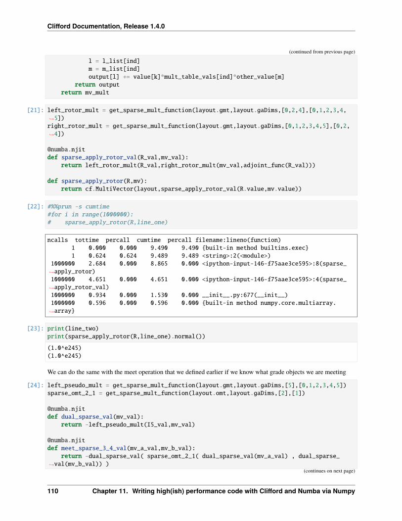
Clifford Documentation, Release 1.4.0
(continued from previous page)
l = l_list[ind]m = m_list[ind]output[l] += value[k]*mult_table_vals[ind]*other_value[m]
return outputreturn mv_mult
[21]: left_rotor_mult = get_sparse_mult_function(layout.gmt,layout.gaDims,[0,2,4],[0,1,2,3,4,→˓5])right_rotor_mult = get_sparse_mult_function(layout.gmt,layout.gaDims,[0,1,2,3,4,5],[0,2,→˓4])
@numba.njitdef sparse_apply_rotor_val(R_val,mv_val):
return left_rotor_mult(R_val,right_rotor_mult(mv_val,adjoint_func(R_val)))
def sparse_apply_rotor(R,mv):return cf.MultiVector(layout,sparse_apply_rotor_val(R.value,mv.value))
[22]: #%%prun -s cumtime#for i in range(1000000):# sparse_apply_rotor(R,line_one)
ncalls tottime percall cumtime percall filename:lineno(function)1 0.000 0.000 9.490 9.490 {built-in method builtins.exec}1 0.624 0.624 9.489 9.489 <string>:2(<module>)
1000000 2.684 0.000 8.865 0.000 <ipython-input-146-f75aae3ce595>:8(sparse_→˓apply_rotor)1000000 4.651 0.000 4.651 0.000 <ipython-input-146-f75aae3ce595>:4(sparse_→˓apply_rotor_val)1000000 0.934 0.000 1.530 0.000 __init__.py:677(__init__)1000000 0.596 0.000 0.596 0.000 {built-in method numpy.core.multiarray.→˓array}
[23]: print(line_two)print(sparse_apply_rotor(R,line_one).normal())
(1.0^e245)(1.0^e245)
We can do the same with the meet operation that we defined earlier if we know what grade objects we are meeting
[24]: left_pseudo_mult = get_sparse_mult_function(layout.gmt,layout.gaDims,[5],[0,1,2,3,4,5])sparse_omt_2_1 = get_sparse_mult_function(layout.omt,layout.gaDims,[2],[1])
@numba.njitdef dual_sparse_val(mv_val):
return -left_pseudo_mult(I5_val,mv_val)
@numba.njitdef meet_sparse_3_4_val(mv_a_val,mv_b_val):
return -dual_sparse_val( sparse_omt_2_1( dual_sparse_val(mv_a_val) , dual_sparse_→˓val(mv_b_val)) )
(continues on next page)
110 Chapter 11. Writing high(ish) performance code with Clifford and Numba via Numpy
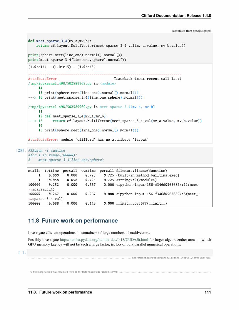
Clifford Documentation, Release 1.4.0
(continued from previous page)
def meet_sparse_3_4(mv_a,mv_b):return cf.layout.MultiVector(meet_sparse_3_4_val(mv_a.value, mv_b.value))
print(sphere.meet(line_one).normal().normal())print(meet_sparse_3_4(line_one,sphere).normal())
(1.0^e14) - (1.0^e15) - (1.0^e45)
---------------------------------------------------------------------------AttributeError Traceback (most recent call last)/tmp/ipykernel_498/502589969.py in <module>
1415 print(sphere.meet(line_one).normal().normal())
---> 16 print(meet_sparse_3_4(line_one,sphere).normal())
/tmp/ipykernel_498/502589969.py in meet_sparse_3_4(mv_a, mv_b)1112 def meet_sparse_3_4(mv_a,mv_b):
---> 13 return cf.layout.MultiVector(meet_sparse_3_4_val(mv_a.value, mv_b.value))1415 print(sphere.meet(line_one).normal().normal())
AttributeError: module 'clifford' has no attribute 'layout'
[25]: #%%prun -s cumtime#for i in range(100000):# meet_sparse_3_4(line_one,sphere)
ncalls tottime percall cumtime percall filename:lineno(function)1 0.000 0.000 0.725 0.725 {built-in method builtins.exec}1 0.058 0.058 0.725 0.725 <string>:2(<module>)
100000 0.252 0.000 0.667 0.000 <ipython-input-156-f346d0563682>:12(meet_→˓sparse_3_4)100000 0.267 0.000 0.267 0.000 <ipython-input-156-f346d0563682>:8(meet_→˓sparse_3_4_val)100000 0.088 0.000 0.148 0.000 __init__.py:677(__init__)
11.8 Future work on performance
Investigate efficient operations on containers of large numbers of multivectors.
Possibly investigate http://numba.pydata.org/numba-doc/0.13/CUDAJit.html for larger algebras/other areas in whichGPU memory latency will not be such a large factor, ie, lots of bulk parallel numerical operations.
[ ]:
. . . . . . . . . . . . . . . . . . . . . . . . . . . . . . . . . . . . . . . . . . . . . . . . . . . . . . . . . . . . . . . . . . . . . . . . . . . . . . . . . . . . . . doc/tutorials/PerformanceCliffordTutorial.ipynb ends here.
The following section was generated from docs/tutorials/cga/index.ipynb . . . . . . . . . . . . . . . . . . . . . . . . . . . . . . . . . . . . . . . . . . . . . . . . . . . . . . . . . . . . . . . . . . . . . . . . . . . . .
11.8. Future work on performance 111

Clifford Documentation, Release 1.4.0
112 Chapter 11. Writing high(ish) performance code with Clifford and Numba via Numpy
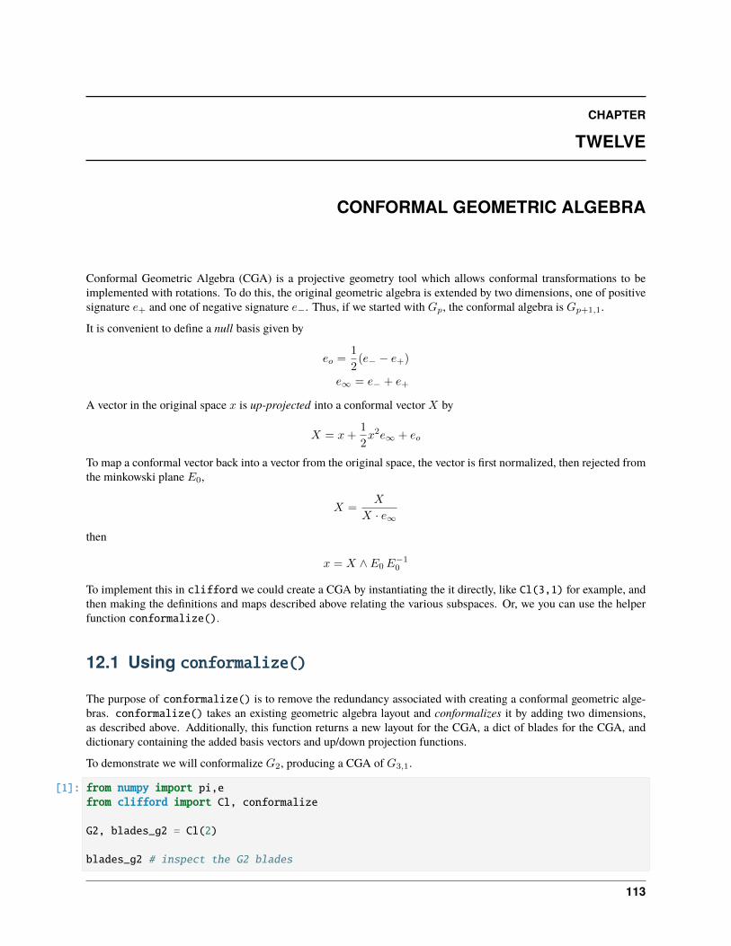
CHAPTER
TWELVE
CONFORMAL GEOMETRIC ALGEBRA
Conformal Geometric Algebra (CGA) is a projective geometry tool which allows conformal transformations to beimplemented with rotations. To do this, the original geometric algebra is extended by two dimensions, one of positivesignature 𝑒+ and one of negative signature 𝑒−. Thus, if we started with 𝐺𝑝, the conformal algebra is 𝐺𝑝+1,1.
It is convenient to define a null basis given by
𝑒𝑜 =1
2(𝑒− − 𝑒+)
𝑒∞ = 𝑒− + 𝑒+
A vector in the original space 𝑥 is up-projected into a conformal vector 𝑋 by
𝑋 = 𝑥+1
2𝑥2𝑒∞ + 𝑒𝑜
To map a conformal vector back into a vector from the original space, the vector is first normalized, then rejected fromthe minkowski plane 𝐸0,
𝑋 =𝑋
𝑋 · 𝑒∞then
𝑥 = 𝑋 ∧ 𝐸0𝐸−10
To implement this in clifford we could create a CGA by instantiating the it directly, like Cl(3,1) for example, andthen making the definitions and maps described above relating the various subspaces. Or, we you can use the helperfunction conformalize().
12.1 Using conformalize()
The purpose of conformalize() is to remove the redundancy associated with creating a conformal geometric alge-bras. conformalize() takes an existing geometric algebra layout and conformalizes it by adding two dimensions,as described above. Additionally, this function returns a new layout for the CGA, a dict of blades for the CGA, anddictionary containing the added basis vectors and up/down projection functions.
To demonstrate we will conformalize 𝐺2, producing a CGA of 𝐺3,1.
[1]: from numpy import pi,efrom clifford import Cl, conformalize
G2, blades_g2 = Cl(2)
blades_g2 # inspect the G2 blades
113
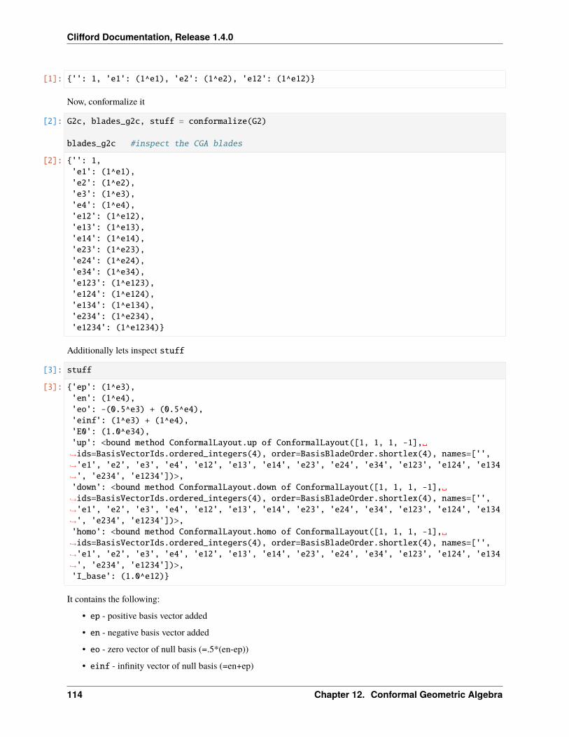
Clifford Documentation, Release 1.4.0
[1]: {'': 1, 'e1': (1^e1), 'e2': (1^e2), 'e12': (1^e12)}
Now, conformalize it
[2]: G2c, blades_g2c, stuff = conformalize(G2)
blades_g2c #inspect the CGA blades
[2]: {'': 1,'e1': (1^e1),'e2': (1^e2),'e3': (1^e3),'e4': (1^e4),'e12': (1^e12),'e13': (1^e13),'e14': (1^e14),'e23': (1^e23),'e24': (1^e24),'e34': (1^e34),'e123': (1^e123),'e124': (1^e124),'e134': (1^e134),'e234': (1^e234),'e1234': (1^e1234)}
Additionally lets inspect stuff
[3]: stuff
[3]: {'ep': (1^e3),'en': (1^e4),'eo': -(0.5^e3) + (0.5^e4),'einf': (1^e3) + (1^e4),'E0': (1.0^e34),'up': <bound method ConformalLayout.up of ConformalLayout([1, 1, 1, -1],␣→˓ids=BasisVectorIds.ordered_integers(4), order=BasisBladeOrder.shortlex(4), names=['',→˓'e1', 'e2', 'e3', 'e4', 'e12', 'e13', 'e14', 'e23', 'e24', 'e34', 'e123', 'e124', 'e134→˓', 'e234', 'e1234'])>,'down': <bound method ConformalLayout.down of ConformalLayout([1, 1, 1, -1],␣→˓ids=BasisVectorIds.ordered_integers(4), order=BasisBladeOrder.shortlex(4), names=['',→˓'e1', 'e2', 'e3', 'e4', 'e12', 'e13', 'e14', 'e23', 'e24', 'e34', 'e123', 'e124', 'e134→˓', 'e234', 'e1234'])>,'homo': <bound method ConformalLayout.homo of ConformalLayout([1, 1, 1, -1],␣→˓ids=BasisVectorIds.ordered_integers(4), order=BasisBladeOrder.shortlex(4), names=['',→˓'e1', 'e2', 'e3', 'e4', 'e12', 'e13', 'e14', 'e23', 'e24', 'e34', 'e123', 'e124', 'e134→˓', 'e234', 'e1234'])>,'I_base': (1.0^e12)}
It contains the following:
• ep - positive basis vector added
• en - negative basis vector added
• eo - zero vector of null basis (=.5*(en-ep))
• einf - infinity vector of null basis (=en+ep)
114 Chapter 12. Conformal Geometric Algebra
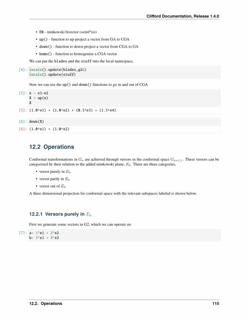
Clifford Documentation, Release 1.4.0
• E0 - minkowski bivector (=einf^eo)
• up() - function to up-project a vector from GA to CGA
• down() - function to down-project a vector from CGA to GA
• homo() - function to homogenize a CGA vector
We can put the blades and the stuff into the local namespace,
[4]: locals().update(blades_g2c)locals().update(stuff)
Now we can use the up() and down() functions to go in and out of CGA
[5]: x = e1+e2X = up(x)X
[5]: (1.0^e1) + (1.0^e2) + (0.5^e3) + (1.5^e4)
[6]: down(X)
[6]: (1.0^e1) + (1.0^e2)
12.2 Operations
Conformal transformations in 𝐺𝑛 are achieved through versors in the conformal space 𝐺𝑛+1,1. These versors can becategorized by their relation to the added minkowski plane, 𝐸0. There are three categories,
• versor purely in 𝐸0
• versor partly in 𝐸0
• versor out of 𝐸0
A three dimensional projection for conformal space with the relevant subspaces labeled is shown below.
12.2.1 Versors purely in 𝐸0
First we generate some vectors in G2, which we can operate on
[7]: a= 1*e1 + 2*e2b= 3*e1 + 4*e2
12.2. Operations 115
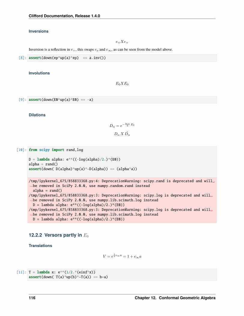
Clifford Documentation, Release 1.4.0
Inversions
𝑒+𝑋𝑒+
Inversion is a reflection in 𝑒+, this swaps 𝑒𝑜 and 𝑒∞, as can be seen from the model above.
[8]: assert(down(ep*up(a)*ep) == a.inv())
Involutions
𝐸0𝑋𝐸0
[9]: assert(down(E0*up(a)*E0) == -a)
Dilations
𝐷𝛼 = 𝑒−ln𝛼2 𝐸0
𝐷𝛼𝑋𝐷𝛼
[10]: from scipy import rand,log
D = lambda alpha: e**((-log(alpha)/2.)*(E0))alpha = rand()assert(down( D(alpha)*up(a)*~D(alpha)) == (alpha*a))
/tmp/ipykernel_675/858833368.py:4: DeprecationWarning: scipy.rand is deprecated and will␣→˓be removed in SciPy 2.0.0, use numpy.random.rand insteadalpha = rand()
/tmp/ipykernel_675/858833368.py:3: DeprecationWarning: scipy.log is deprecated and will␣→˓be removed in SciPy 2.0.0, use numpy.lib.scimath.log insteadD = lambda alpha: e**((-log(alpha)/2.)*(E0))
/tmp/ipykernel_675/858833368.py:3: DeprecationWarning: scipy.log is deprecated and will␣→˓be removed in SciPy 2.0.0, use numpy.lib.scimath.log insteadD = lambda alpha: e**((-log(alpha)/2.)*(E0))
12.2.2 Versors partly in 𝐸0
Translations
𝑉 = 𝑒12 𝑒∞𝑎 = 1 + 𝑒∞𝑎
[11]: T = lambda x: e**(1/2.*(einf*x))assert(down( T(a)*up(b)*~T(a)) == b+a)
116 Chapter 12. Conformal Geometric Algebra
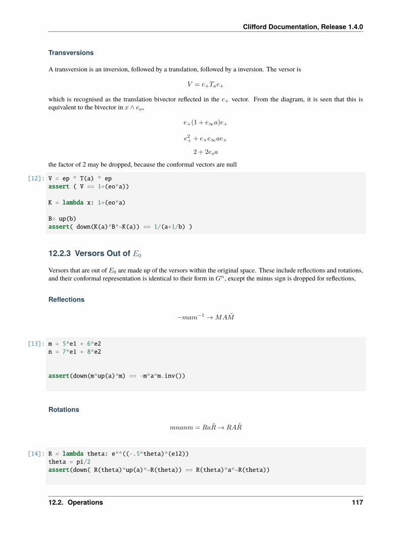
Clifford Documentation, Release 1.4.0
Transversions
A transversion is an inversion, followed by a translation, followed by a inversion. The versor is
𝑉 = 𝑒+𝑇𝑎𝑒+
which is recognised as the translation bivector reflected in the 𝑒+ vector. From the diagram, it is seen that this isequivalent to the bivector in 𝑥 ∧ 𝑒𝑜,
𝑒+(1 + 𝑒∞𝑎)𝑒+
𝑒2+ + 𝑒+𝑒∞𝑎𝑒+
2 + 2𝑒𝑜𝑎
the factor of 2 may be dropped, because the conformal vectors are null
[12]: V = ep * T(a) * epassert ( V == 1+(eo*a))
K = lambda x: 1+(eo*a)
B= up(b)assert( down(K(a)*B*~K(a)) == 1/(a+1/b) )
12.2.3 Versors Out of 𝐸0
Versors that are out of 𝐸0 are made up of the versors within the original space. These include reflections and rotations,and their conformal representation is identical to their form in 𝐺𝑛, except the minus sign is dropped for reflections,
Reflections
−𝑚𝑎𝑚−1 →𝑀𝐴�̃�
[13]: m = 5*e1 + 6*e2n = 7*e1 + 8*e2
assert(down(m*up(a)*m) == -m*a*m.inv())
Rotations
𝑚𝑛𝑎𝑛𝑚 = 𝑅𝑎�̃�→ 𝑅𝐴�̃�
[14]: R = lambda theta: e**((-.5*theta)*(e12))theta = pi/2assert(down( R(theta)*up(a)*~R(theta)) == R(theta)*a*~R(theta))
12.2. Operations 117
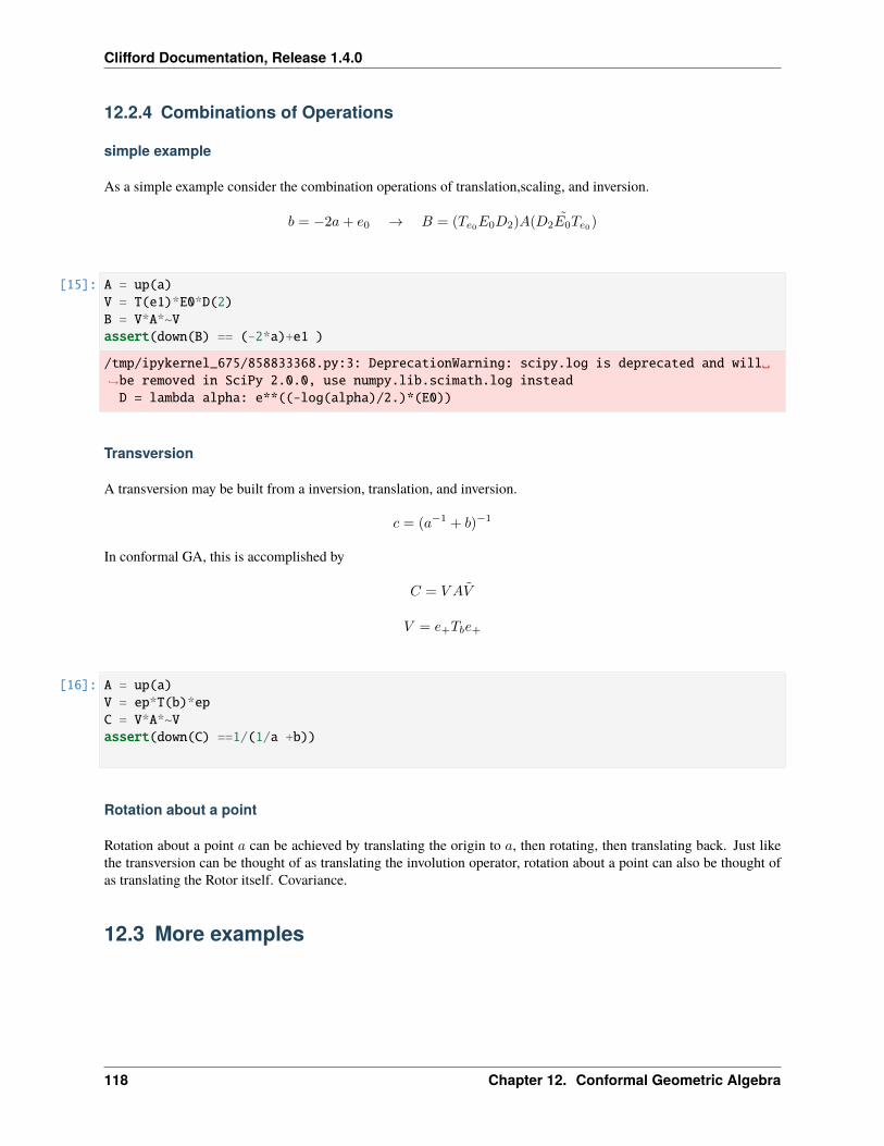
Clifford Documentation, Release 1.4.0
12.2.4 Combinations of Operations
simple example
As a simple example consider the combination operations of translation,scaling, and inversion.
𝑏 = −2𝑎+ 𝑒0 → 𝐵 = (𝑇𝑒0𝐸0𝐷2)𝐴 ˜(𝐷2𝐸0𝑇𝑒0)
[15]: A = up(a)V = T(e1)*E0*D(2)B = V*A*~Vassert(down(B) == (-2*a)+e1 )
/tmp/ipykernel_675/858833368.py:3: DeprecationWarning: scipy.log is deprecated and will␣→˓be removed in SciPy 2.0.0, use numpy.lib.scimath.log insteadD = lambda alpha: e**((-log(alpha)/2.)*(E0))
Transversion
A transversion may be built from a inversion, translation, and inversion.
𝑐 = (𝑎−1 + 𝑏)−1
In conformal GA, this is accomplished by
𝐶 = 𝑉 𝐴𝑉
𝑉 = 𝑒+𝑇𝑏𝑒+
[16]: A = up(a)V = ep*T(b)*epC = V*A*~Vassert(down(C) ==1/(1/a +b))
Rotation about a point
Rotation about a point 𝑎 can be achieved by translating the origin to 𝑎, then rotating, then translating back. Just likethe transversion can be thought of as translating the involution operator, rotation about a point can also be thought ofas translating the Rotor itself. Covariance.
12.3 More examples
118 Chapter 12. Conformal Geometric Algebra
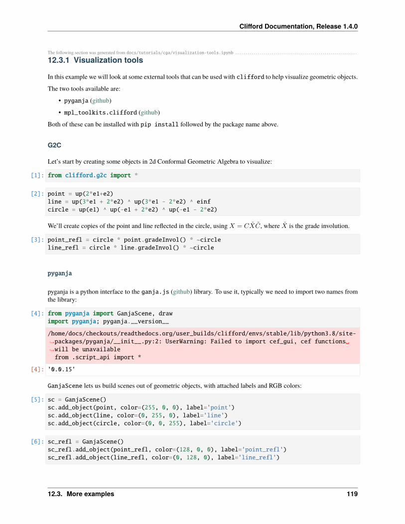
Clifford Documentation, Release 1.4.0
The following section was generated from docs/tutorials/cga/visualization-tools.ipynb . . . . . . . . . . . . . . . . . . . . . . . . . . . . . . . . . . . . . . . . . . . . . . . . . . . . . . . . . . . .
12.3.1 Visualization tools
In this example we will look at some external tools that can be used with clifford to help visualize geometric objects.
The two tools available are:
• pyganja (github)
• mpl_toolkits.clifford (github)
Both of these can be installed with pip install followed by the package name above.
G2C
Let’s start by creating some objects in 2d Conformal Geometric Algebra to visualize:
[1]: from clifford.g2c import *
[2]: point = up(2*e1+e2)line = up(3*e1 + 2*e2) ^ up(3*e1 - 2*e2) ^ einfcircle = up(e1) ^ up(-e1 + 2*e2) ^ up(-e1 - 2*e2)
We’ll create copies of the point and line reflected in the circle, using 𝑋 = 𝐶�̂�𝐶, where �̂� is the grade involution.
[3]: point_refl = circle * point.gradeInvol() * ~circleline_refl = circle * line.gradeInvol() * ~circle
pyganja
pyganja is a python interface to the ganja.js (github) library. To use it, typically we need to import two names fromthe library:
[4]: from pyganja import GanjaScene, drawimport pyganja; pyganja.__version__
/home/docs/checkouts/readthedocs.org/user_builds/clifford/envs/stable/lib/python3.8/site-→˓packages/pyganja/__init__.py:2: UserWarning: Failed to import cef_gui, cef functions␣→˓will be unavailablefrom .script_api import *
[4]: '0.0.15'
GanjaScene lets us build scenes out of geometric objects, with attached labels and RGB colors:
[5]: sc = GanjaScene()sc.add_object(point, color=(255, 0, 0), label='point')sc.add_object(line, color=(0, 255, 0), label='line')sc.add_object(circle, color=(0, 0, 255), label='circle')
[6]: sc_refl = GanjaScene()sc_refl.add_object(point_refl, color=(128, 0, 0), label='point_refl')sc_refl.add_object(line_refl, color=(0, 128, 0), label='line_refl')
12.3. More examples 119
Clifford Documentation, Release 1.4.0
Once we’ve built our scene, we can draw it, specifying a scale (which here we use to zoom out), and the signature ofour algebra (which defaults to conformal 3D):
[7]: draw(sc, sig=layout.sig, scale=0.5)
<IPython.core.display.Javascript object>
A cool feature of GanjaScene is the ability to use + to draw both scenes together:
[8]: draw(sc + sc_refl, sig=layout.sig, scale=0.5)
<IPython.core.display.Javascript object>
mpl_toolkits.clifford
While ganja.js produces great diagrams, it’s hard to combine them with other plotting tools. mpl_toolkits.clifford works within matplotlib.
[9]: from matplotlib import pyplot as pltplt.ioff() # we'll ask for plotting when we want it
# if you're editing this locally, you'll get an interactive UI if you uncomment the␣→˓following## %matplotlib notebook
from mpl_toolkits.clifford import plotimport mpl_toolkits.clifford; mpl_toolkits.clifford.__version__
/home/docs/checkouts/readthedocs.org/user_builds/clifford/envs/stable/lib/python3.8/site-→˓packages/traitlets/traitlets.py:3030: FutureWarning: --rc={'figure.dpi': 96, 'savefig.→˓transparent': True} for dict-traits is deprecated in traitlets 5.0. You can pass --rc→˓<key=value> ... multiple times to add items to a dict.warn(
[9]: '0.0.3'
Assembling the plot is a lot more work, but we also get much more control:
[10]: # standard matplotlib stuff - construct empty plots side-by-side, and set the scalingfig, (ax_before, ax_both) = plt.subplots(1, 2, sharex=True, sharey=True)ax_before.set(xlim=[-4, 4], ylim=[-4, 4], aspect='equal')ax_both.set(xlim=[-4, 4], ylim=[-4, 4], aspect='equal')
# plot the objects before reflection on both plotsfor ax in (ax_before, ax_both):
plot(ax, [point], color='tab:blue', label='point', marker='x', linestyle=' ')plot(ax, [line], color='tab:green', label='line')plot(ax, [circle], color='tab:red', label='circle')
# plot the objects after reflection, with thicker linesplot(ax_both, [point_refl], color='tab:blue', label='point_refl', marker='x', linestyle=→˓' ', markeredgewidth=2)plot(ax_both, [line_refl], color='tab:green', label='line_refl', linewidth=2)
(continues on next page)
120 Chapter 12. Conformal Geometric Algebra
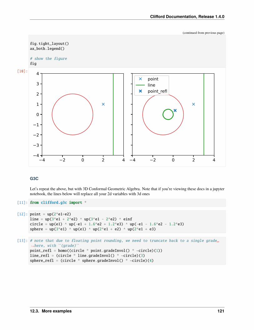
Clifford Documentation, Release 1.4.0
(continued from previous page)
fig.tight_layout()ax_both.legend()
# show the figurefig
[10]:
4 2 0 2 44
3
2
1
0
1
2
3
4
4 2 0 2 4
pointlinepoint_refl
G3C
Let’s repeat the above, but with 3D Conformal Geometric Algebra. Note that if you’re viewing these docs in a jupyternotebook, the lines below will replace all your 2d variables with 3d ones
[11]: from clifford.g3c import *
[12]: point = up(2*e1+e2)line = up(3*e1 + 2*e2) ^ up(3*e1 - 2*e2) ^ einfcircle = up(e1) ^ up(-e1 + 1.6*e2 + 1.2*e3) ^ up(-e1 - 1.6*e2 - 1.2*e3)sphere = up(3*e1) ^ up(e1) ^ up(2*e1 + e2) ^ up(2*e1 + e3)
[13]: # note that due to floating point rounding, we need to truncate back to a single grade␣→˓here, with ``(grade)``point_refl = homo((circle * point.gradeInvol() * ~circle)(1))line_refl = (circle * line.gradeInvol() * ~circle)(3)sphere_refl = (circle * sphere.gradeInvol() * ~circle)(4)
12.3. More examples 121
Clifford Documentation, Release 1.4.0
pyganja
Once again, we can create a pair of scenes exactly as before
[14]: sc = GanjaScene()sc.add_object(point, color=(255, 0, 0), label='point')sc.add_object(line, color=(0, 255, 0), label='line')sc.add_object(circle, color=(0, 0, 255), label='circle')sc.add_object(sphere, color=(0, 255, 255), label='sphere')
[15]: sc_refl = GanjaScene()sc_refl.add_object(point_refl, color=(128, 0, 0), label='point_refl')sc_refl.add_object(line_refl.normal(), color=(0, 128, 0), label='line_refl')sc_refl.add_object(sphere_refl.normal(), color=(0, 128, 128), label='sphere_refl')
But this time, when we draw them we don’t need to pass sig. Better yet, we can rotate the 3D world around using leftclick, pan with right click, and zoom with the scroll wheel.
[16]: draw(sc + sc_refl, scale=0.5)
<IPython.core.display.Javascript object>
Some more example of using pyganja to visualize 3D CGA can be found in the interpolation and clustering notebooks.
mpl_toolkits.clifford
The 3D approach for matplotlib is much the same. Note that due to poor handling of rounding errors in clifford.tools.classify, a call to .normal() is needed. Along with explicit grade selection, this is a useful trick to try andget something to render which otherwise would not.
[17]: # standard matplotlib stuff - construct empty plots side-by-side, and set the scalingfig, (ax_before, ax_both) = plt.subplots(1, 2, subplot_kw=dict(projection='3d'),␣→˓figsize=(8, 4))ax_before.set(xlim=[-4, 4], ylim=[-4, 4], zlim=[-4, 4])ax_both.set(xlim=[-4, 4], ylim=[-4, 4], zlim=[-4, 4])
# plot the objects before reflection on both plotsfor ax in (ax_before, ax_both):
plot(ax, [point], color='tab:red', label='point', marker='x', linestyle=' ')plot(ax, [line], color='tab:green', label='line')plot(ax, [circle], color='tab:blue', label='circle')plot(ax, [sphere], color='tab:cyan') # labels do not work for spheres: pygae/mpl_
→˓toolkits.clifford#5
# plot the objects after reflectionplot(ax_both, [point_refl], color='tab:red', label='point_refl', marker='x', linestyle='→˓', markeredgewidth=2)plot(ax_both, [line_refl.normal()], color='tab:green', label='line_refl', linewidth=2)plot(ax_both, [sphere_refl], color='tab:cyan')
fig.tight_layout()ax_both.legend()
(continues on next page)
122 Chapter 12. Conformal Geometric Algebra

Clifford Documentation, Release 1.4.0
(continued from previous page)
# show the figurefig
/home/docs/checkouts/readthedocs.org/user_builds/clifford/envs/stable/lib/python3.8/site-→˓packages/IPython/core/pylabtools.py:134: MatplotlibDeprecationWarning: The 'renderer'␣→˓parameter of do_3d_projection() was deprecated in Matplotlib 3.4 and will be removed␣→˓two minor releases later.fig.canvas.print_figure(bytes_io, **kw)
/home/docs/checkouts/readthedocs.org/user_builds/clifford/envs/stable/lib/python3.8/site-→˓packages/IPython/core/pylabtools.py:134: MatplotlibDeprecationWarning:The M attribute was deprecated in Matplotlib 3.4 and will be removed two minor releases␣→˓later. Use self.axes.M instead.fig.canvas.print_figure(bytes_io, **kw)
[17]:
4 3 2 1 0 1 2 3 4 43
210
12
34
4321
01234
4 3 2 1 0 1 2 3 4 43
210
12
34
4321
01234
pointlinepoint_reflcircleline_refl
Some more example of using mpl_toolkits.clifford to visualize 3D CGA can be found in the examples folderof the mpl_toolkits.clifford repositiory, here.. . . . . . . . . . . . . . . . . . . . . . . . . . . . . . . . . . . . . . . . . . . . . . . . . . . . . . . . . . . . . . . . . . . . . . . . . . . . . . . . . . . . . . . . . . doc/tutorials/cga/visualization-tools.ipynb ends here.
The following section was generated from docs/tutorials/cga/object-oriented.ipynb . . . . . . . . . . . . . . . . . . . . . . . . . . . . . . . . . . . . . . . . . . . . . . . . . . . . . . . . . . . . . . . . .
12.3.2 Object Oriented CGA
This is a shelled out demo for a object-oriented approach to CGA with clifford. The CGA object holds the originallayout for an arbitrary geometric algebra , and the conformalized version. It provides up/down projections, as well aseasy ways to generate objects and operators.
12.3. More examples 123
Clifford Documentation, Release 1.4.0
Quick Use Demo
[1]: from clifford.cga import CGA, Round, Translationfrom clifford import Cl
g3,blades = Cl(3)
cga = CGA(g3) # make cga from existing ga# orcga = CGA(3) # generate cga from dimension of 'base space'
locals().update(cga.blades) # put ga's blades in local namespace
C = cga.round(e1,e2,e3,-e2) # generate unit sphere from pointsC
/home/docs/checkouts/readthedocs.org/user_builds/clifford/envs/stable/lib/python3.8/site-→˓packages/pyganja/__init__.py:2: UserWarning: Failed to import cef_gui, cef functions␣→˓will be unavailablefrom .script_api import *
[1]: Sphere
[2]: ## Objectscga.round() # from Nonecga.round(3) # from dim of spacecga.round(e1,e2,e3,-e2) # from pointscga.round(e1,e2,e3) # from pointscga.round(e1,e2) # from pointscga.round((e1,3)) # from center, radiuscga.round(cga.round().mv)# from existing multivector
cga.flat() # from Nonecga.flat(2) # from dim of spacecga.flat(e1,e2) # from pointscga.flat(cga.flat().mv) # from existing multivector
## Operationscga.dilation() # from from Nonecga.dilation(.4) # from int
cga.translation() # from Nonecga.translation(e1+e2) # from vectorcga.translation(cga.down(cga.null_vector()))
cga.rotation() # from Nonecga.rotation(e12+e23) # from bivector
cga.transversion(e1+e2).mv
124 Chapter 12. Conformal Geometric Algebra
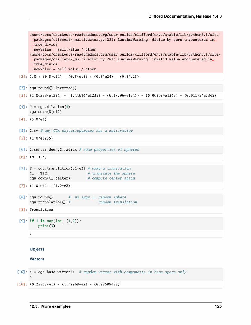
Clifford Documentation, Release 1.4.0
/home/docs/checkouts/readthedocs.org/user_builds/clifford/envs/stable/lib/python3.8/site-→˓packages/clifford/_multivector.py:281: RuntimeWarning: divide by zero encountered in␣→˓true_dividenewValue = self.value / other
/home/docs/checkouts/readthedocs.org/user_builds/clifford/envs/stable/lib/python3.8/site-→˓packages/clifford/_multivector.py:281: RuntimeWarning: invalid value encountered in␣→˓true_dividenewValue = self.value / other
[2]: 1.0 + (0.5^e14) - (0.5^e15) + (0.5^e24) - (0.5^e25)
[3]: cga.round().inverted()
[3]: (1.06278^e1234) - (1.44694^e1235) - (0.17796^e1245) - (0.06362^e1345) - (0.01175^e2345)
[4]: D = cga.dilation(5)cga.down(D(e1))
[4]: (5.0^e1)
[5]: C.mv # any CGA object/operator has a multivector
[5]: (1.0^e1235)
[6]: C.center_down,C.radius # some properties of spheres
[6]: (0, 1.0)
[7]: T = cga.translation(e1+e2) # make a translationC_ = T(C) # translate the spherecga.down(C_.center) # compute center again
[7]: (1.0^e1) + (1.0^e2)
[8]: cga.round() # no args == random spherecga.translation() # random translation
[8]: Translation
[9]: if 1 in map(int, [1,2]):print(3)
3
Objects
Vectors
[10]: a = cga.base_vector() # random vector with components in base space onlya
[10]: (0.23563^e1) - (1.72068^e2) - (0.98589^e3)
12.3. More examples 125
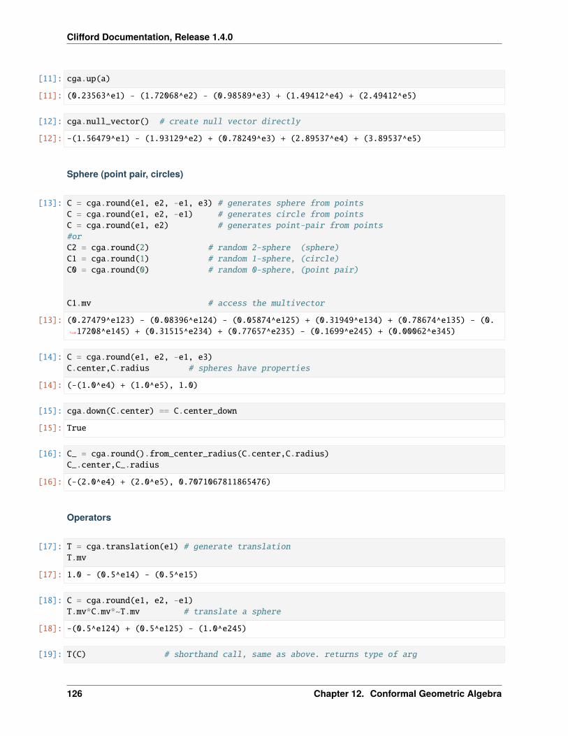
Clifford Documentation, Release 1.4.0
[11]: cga.up(a)
[11]: (0.23563^e1) - (1.72068^e2) - (0.98589^e3) + (1.49412^e4) + (2.49412^e5)
[12]: cga.null_vector() # create null vector directly
[12]: -(1.56479^e1) - (1.93129^e2) + (0.78249^e3) + (2.89537^e4) + (3.89537^e5)
Sphere (point pair, circles)
[13]: C = cga.round(e1, e2, -e1, e3) # generates sphere from pointsC = cga.round(e1, e2, -e1) # generates circle from pointsC = cga.round(e1, e2) # generates point-pair from points#orC2 = cga.round(2) # random 2-sphere (sphere)C1 = cga.round(1) # random 1-sphere, (circle)C0 = cga.round(0) # random 0-sphere, (point pair)
C1.mv # access the multivector
[13]: (0.27479^e123) - (0.08396^e124) - (0.05874^e125) + (0.31949^e134) + (0.78674^e135) - (0.→˓17208^e145) + (0.31515^e234) + (0.77657^e235) - (0.1699^e245) + (0.00062^e345)
[14]: C = cga.round(e1, e2, -e1, e3)C.center,C.radius # spheres have properties
[14]: (-(1.0^e4) + (1.0^e5), 1.0)
[15]: cga.down(C.center) == C.center_down
[15]: True
[16]: C_ = cga.round().from_center_radius(C.center,C.radius)C_.center,C_.radius
[16]: (-(2.0^e4) + (2.0^e5), 0.7071067811865476)
Operators
[17]: T = cga.translation(e1) # generate translationT.mv
[17]: 1.0 - (0.5^e14) - (0.5^e15)
[18]: C = cga.round(e1, e2, -e1)T.mv*C.mv*~T.mv # translate a sphere
[18]: -(0.5^e124) + (0.5^e125) - (1.0^e245)
[19]: T(C) # shorthand call, same as above. returns type of arg
126 Chapter 12. Conformal Geometric Algebra
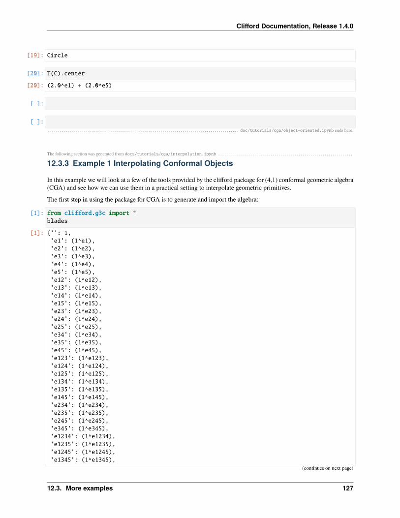
Clifford Documentation, Release 1.4.0
[19]: Circle
[20]: T(C).center
[20]: (2.0^e1) + (2.0^e5)
[ ]:
[ ]:
. . . . . . . . . . . . . . . . . . . . . . . . . . . . . . . . . . . . . . . . . . . . . . . . . . . . . . . . . . . . . . . . . . . . . . . . . . . . . . . . . . . . . . . . . . . . . . . doc/tutorials/cga/object-oriented.ipynb ends here.
The following section was generated from docs/tutorials/cga/interpolation.ipynb . . . . . . . . . . . . . . . . . . . . . . . . . . . . . . . . . . . . . . . . . . . . . . . . . . . . . . . . . . . . . . . . . . .
12.3.3 Example 1 Interpolating Conformal Objects
In this example we will look at a few of the tools provided by the clifford package for (4,1) conformal geometric algebra(CGA) and see how we can use them in a practical setting to interpolate geometric primitives.
The first step in using the package for CGA is to generate and import the algebra:
[1]: from clifford.g3c import *blades
[1]: {'': 1,'e1': (1^e1),'e2': (1^e2),'e3': (1^e3),'e4': (1^e4),'e5': (1^e5),'e12': (1^e12),'e13': (1^e13),'e14': (1^e14),'e15': (1^e15),'e23': (1^e23),'e24': (1^e24),'e25': (1^e25),'e34': (1^e34),'e35': (1^e35),'e45': (1^e45),'e123': (1^e123),'e124': (1^e124),'e125': (1^e125),'e134': (1^e134),'e135': (1^e135),'e145': (1^e145),'e234': (1^e234),'e235': (1^e235),'e245': (1^e245),'e345': (1^e345),'e1234': (1^e1234),'e1235': (1^e1235),'e1245': (1^e1245),'e1345': (1^e1345),
(continues on next page)
12.3. More examples 127

Clifford Documentation, Release 1.4.0
(continued from previous page)
'e2345': (1^e2345),'e12345': (1^e12345)}
This creates an algebra with the required signature and imports the basis blades into the current workspace. We cancheck our metric by squaring our grade 1 multivectors.
[2]: print('e1*e1 ', e1*e1)print('e2*e2 ', e2*e2)print('e3*e3 ', e3*e3)print('e4*e4 ', e4*e4)print('e5*e5 ', e5*e5)
e1*e1 1e2*e2 1e3*e3 1e4*e4 1e5*e5 -1
As expected this gives us 4 basis vectors that square to 1.0 and one that squares to -1.0, therefore confirming our metricis (4,1).
The up() function implements the mapping of vectors from standard 3D space to conformal space. We can use this toconstruct conformal objects to play around with.
For example a line at the origin:
[3]: line_a = ( up(0)^up(e1+e2)^einf ).normal()print(line_a)
(0.70711^e145) + (0.70711^e245)
The tools submodule of the clifford package contains a wide array of algorithms and tools that can be useful for ma-nipulating objects in CGA. We will use these tools to generate rotors that rotate and translate objects:
[4]: from clifford.tools.g3 import *from clifford.tools.g3c import *from numpy import pi
rotation_radians = pi/4euc_vector_in_plane_m = e1euc_vector_in_plane_n = e3
euc_translation = -5.2*e1 + 3*e2 - pi*e3
rotor_rotation = generate_rotation_rotor(rotation_radians, euc_vector_in_plane_m, euc_→˓vector_in_plane_n)rotor_translation = generate_translation_rotor(euc_translation)print(rotor_rotation)print(rotor_translation)
combined_rotor = (rotor_translation*rotor_rotation).normal()
line_b = (combined_rotor*line_a*~combined_rotor).normal()print(line_b)
128 Chapter 12. Conformal Geometric Algebra
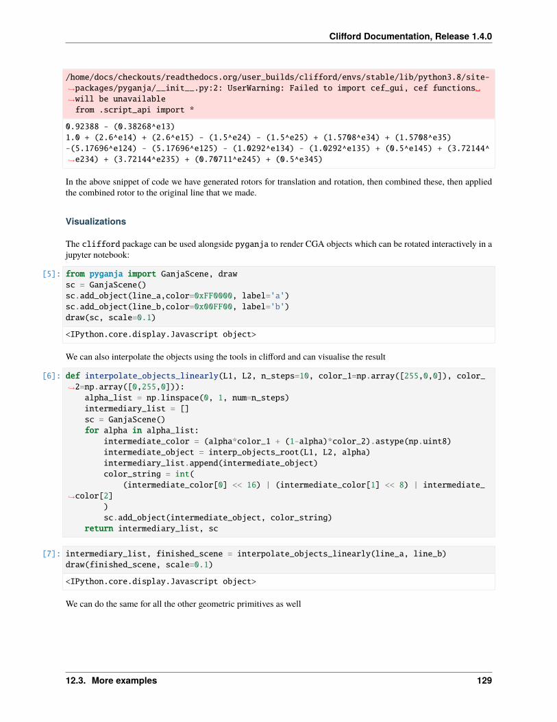
Clifford Documentation, Release 1.4.0
/home/docs/checkouts/readthedocs.org/user_builds/clifford/envs/stable/lib/python3.8/site-→˓packages/pyganja/__init__.py:2: UserWarning: Failed to import cef_gui, cef functions␣→˓will be unavailablefrom .script_api import *
0.92388 - (0.38268^e13)1.0 + (2.6^e14) + (2.6^e15) - (1.5^e24) - (1.5^e25) + (1.5708^e34) + (1.5708^e35)-(5.17696^e124) - (5.17696^e125) - (1.0292^e134) - (1.0292^e135) + (0.5^e145) + (3.72144^→˓e234) + (3.72144^e235) + (0.70711^e245) + (0.5^e345)
In the above snippet of code we have generated rotors for translation and rotation, then combined these, then appliedthe combined rotor to the original line that we made.
Visualizations
The clifford package can be used alongside pyganja to render CGA objects which can be rotated interactively in ajupyter notebook:
[5]: from pyganja import GanjaScene, drawsc = GanjaScene()sc.add_object(line_a,color=0xFF0000, label='a')sc.add_object(line_b,color=0x00FF00, label='b')draw(sc, scale=0.1)
<IPython.core.display.Javascript object>
We can also interpolate the objects using the tools in clifford and can visualise the result
[6]: def interpolate_objects_linearly(L1, L2, n_steps=10, color_1=np.array([255,0,0]), color_→˓2=np.array([0,255,0])):
alpha_list = np.linspace(0, 1, num=n_steps)intermediary_list = []sc = GanjaScene()for alpha in alpha_list:
intermediate_color = (alpha*color_1 + (1-alpha)*color_2).astype(np.uint8)intermediate_object = interp_objects_root(L1, L2, alpha)intermediary_list.append(intermediate_object)color_string = int(
(intermediate_color[0] << 16) | (intermediate_color[1] << 8) | intermediate_→˓color[2]
)sc.add_object(intermediate_object, color_string)
return intermediary_list, sc
[7]: intermediary_list, finished_scene = interpolate_objects_linearly(line_a, line_b)draw(finished_scene, scale=0.1)
<IPython.core.display.Javascript object>
We can do the same for all the other geometric primitives as well
12.3. More examples 129

Clifford Documentation, Release 1.4.0
Circles
[8]: circle_a = (up(0)^up(e1)^up(e2)).normal()circle_b = (combined_rotor*circle_a*~combined_rotor).normal()intermediary_list, finished_scene = interpolate_objects_linearly(circle_a, circle_b)draw(finished_scene, scale=0.1)
<IPython.core.display.Javascript object>
Point pairs
[9]: point_pair_a = (up(e3)^up(e1+e2)).normal()point_pair_b = (combined_rotor*point_pair_a*~combined_rotor).normal()intermediary_list, finished_scene = interpolate_objects_linearly(point_pair_a, point_→˓pair_b)draw(finished_scene, scale=0.1)
<IPython.core.display.Javascript object>
Planes
[10]: plane_a = (up(0)^up(e1)^up(e2)^einf).normal()plane_b = (combined_rotor*plane_a*~combined_rotor).normal()intermediary_list, finished_scene = interpolate_objects_linearly(plane_a, plane_b)draw(finished_scene)
<IPython.core.display.Javascript object>
Spheres
[11]: sphere_a = (up(0)^up(e1)^up(e2)^up(e3)).normal()sphere_b = (combined_rotor*sphere_a*~combined_rotor).normal()intermediary_list, finished_scene = interpolate_objects_linearly(sphere_a, sphere_b)draw(finished_scene, scale=0.1)
<IPython.core.display.Javascript object>
. . . . . . . . . . . . . . . . . . . . . . . . . . . . . . . . . . . . . . . . . . . . . . . . . . . . . . . . . . . . . . . . . . . . . . . . . . . . . . . . . . . . . . . . . . . . . . . . . . doc/tutorials/cga/interpolation.ipynb ends here.
The following section was generated from docs/tutorials/cga/clustering.ipynb . . . . . . . . . . . . . . . . . . . . . . . . . . . . . . . . . . . . . . . . . . . . . . . . . . . . . . . . . . . . . . . . . . . . . . .
12.3.4 Example 2 Clustering Geometric Objects
In this example we will look at a few of the tools provided by the clifford package for (4,1) conformal geometric algebra(CGA) and see how we can use them in a practical setting to cluster geometric objects via the simple K-means clusteringalgorithm provided in clifford.tools
As before the first step in using the package for CGA is to generate and import the algebra:
130 Chapter 12. Conformal Geometric Algebra
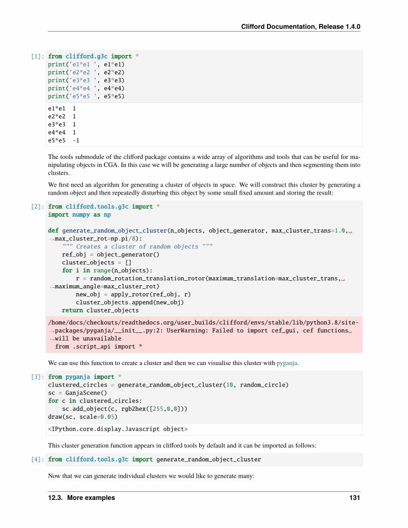
Clifford Documentation, Release 1.4.0
[1]: from clifford.g3c import *print('e1*e1 ', e1*e1)print('e2*e2 ', e2*e2)print('e3*e3 ', e3*e3)print('e4*e4 ', e4*e4)print('e5*e5 ', e5*e5)
e1*e1 1e2*e2 1e3*e3 1e4*e4 1e5*e5 -1
The tools submodule of the clifford package contains a wide array of algorithms and tools that can be useful for ma-nipulating objects in CGA. In this case we will be generating a large number of objects and then segmenting them intoclusters.
We first need an algorithm for generating a cluster of objects in space. We will construct this cluster by generating arandom object and then repeatedly disturbing this object by some small fixed amount and storing the result:
[2]: from clifford.tools.g3c import *import numpy as np
def generate_random_object_cluster(n_objects, object_generator, max_cluster_trans=1.0,␣→˓max_cluster_rot=np.pi/8):""" Creates a cluster of random objects """ref_obj = object_generator()cluster_objects = []for i in range(n_objects):
r = random_rotation_translation_rotor(maximum_translation=max_cluster_trans,␣→˓maximum_angle=max_cluster_rot)
new_obj = apply_rotor(ref_obj, r)cluster_objects.append(new_obj)
return cluster_objects
/home/docs/checkouts/readthedocs.org/user_builds/clifford/envs/stable/lib/python3.8/site-→˓packages/pyganja/__init__.py:2: UserWarning: Failed to import cef_gui, cef functions␣→˓will be unavailablefrom .script_api import *
We can use this function to create a cluster and then we can visualise this cluster with pyganja.
[3]: from pyganja import *clustered_circles = generate_random_object_cluster(10, random_circle)sc = GanjaScene()for c in clustered_circles:
sc.add_object(c, rgb2hex([255,0,0]))draw(sc, scale=0.05)
<IPython.core.display.Javascript object>
This cluster generation function appears in clifford tools by default and it can be imported as follows:
[4]: from clifford.tools.g3c import generate_random_object_cluster
Now that we can generate individual clusters we would like to generate many:
12.3. More examples 131

Clifford Documentation, Release 1.4.0
[5]: def generate_n_clusters( object_generator, n_clusters, n_objects_per_cluster ):object_clusters = []for i in range(n_clusters):
cluster_objects = generate_random_object_cluster(n_objects_per_cluster, object_→˓generator,
max_cluster_trans=0.5, max_→˓cluster_rot=np.pi / 16)
object_clusters.append(cluster_objects)all_objects = [item for sublist in object_clusters for item in sublist]return all_objects, object_clusters
Again this function appears by default in clifford tools and we can easily visualise the result:
[6]: from clifford.tools.g3c import generate_n_clusters
all_objects, object_clusters = generate_n_clusters(random_circle, 2, 5)sc = GanjaScene()for c in all_objects:
sc.add_object(c, rgb2hex([255,0,0]))draw(sc, scale=0.05)
<IPython.core.display.Javascript object>
Given that we can now generate multiple clusters of objects we can test algorithms for segmenting them.
The function run_n_clusters below generates a lot of objects distributed into n clusters and then attempts to segmentthe objects to recover the clusters.
[7]: from clifford.tools.g3c.object_clustering import n_clusters_objectsimport time
def run_n_clusters( object_generator, n_clusters, n_objects_per_cluster, n_shotgunning):all_objects, object_clusters = generate_n_clusters( object_generator, n_clusters, n_
→˓objects_per_cluster )[new_labels, centroids, start_labels, start_centroids] = n_clusters_objects(n_
→˓clusters, all_objects,initial_
→˓centroids=None,n_
→˓shotgunning=n_shotgunning,␣
→˓averaging_method='unweighted')return all_objects, new_labels, centroids
Lets try it!
[8]: def visualise_n_clusters(all_objects, centroids, labels,color_1=np.array([255, 0, 0]),color_2=np.array([0, 255, 0])):
"""Utility method for visualising several clusters and their respective centroidsusing pyganja"""alpha_list = np.linspace(0, 1, num=len(centroids))
(continues on next page)
132 Chapter 12. Conformal Geometric Algebra
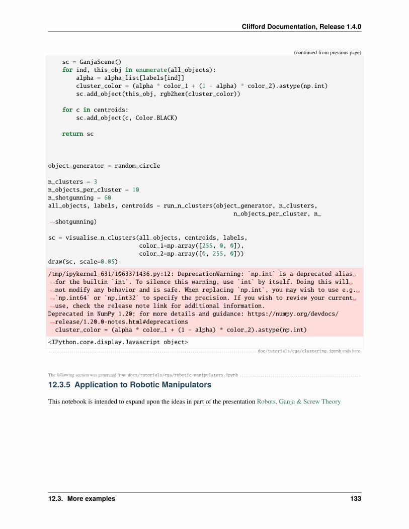
Clifford Documentation, Release 1.4.0
(continued from previous page)
sc = GanjaScene()for ind, this_obj in enumerate(all_objects):
alpha = alpha_list[labels[ind]]cluster_color = (alpha * color_1 + (1 - alpha) * color_2).astype(np.int)sc.add_object(this_obj, rgb2hex(cluster_color))
for c in centroids:sc.add_object(c, Color.BLACK)
return sc
object_generator = random_circle
n_clusters = 3n_objects_per_cluster = 10n_shotgunning = 60all_objects, labels, centroids = run_n_clusters(object_generator, n_clusters,
n_objects_per_cluster, n_→˓shotgunning)
sc = visualise_n_clusters(all_objects, centroids, labels,color_1=np.array([255, 0, 0]),color_2=np.array([0, 255, 0]))
draw(sc, scale=0.05)
/tmp/ipykernel_631/1063371436.py:12: DeprecationWarning: `np.int` is a deprecated alias␣→˓for the builtin `int`. To silence this warning, use `int` by itself. Doing this will␣→˓not modify any behavior and is safe. When replacing `np.int`, you may wish to use e.g.␣→˓`np.int64` or `np.int32` to specify the precision. If you wish to review your current␣→˓use, check the release note link for additional information.Deprecated in NumPy 1.20; for more details and guidance: https://numpy.org/devdocs/→˓release/1.20.0-notes.html#deprecationscluster_color = (alpha * color_1 + (1 - alpha) * color_2).astype(np.int)
<IPython.core.display.Javascript object>
. . . . . . . . . . . . . . . . . . . . . . . . . . . . . . . . . . . . . . . . . . . . . . . . . . . . . . . . . . . . . . . . . . . . . . . . . . . . . . . . . . . . . . . . . . . . . . . . . . . . . doc/tutorials/cga/clustering.ipynb ends here.
The following section was generated from docs/tutorials/cga/robotic-manipulators.ipynb . . . . . . . . . . . . . . . . . . . . . . . . . . . . . . . . . . . . . . . . . . . . . . . . . . . . . . . . . . .
12.3.5 Application to Robotic Manipulators
This notebook is intended to expand upon the ideas in part of the presentation Robots, Ganja & Screw Theory
12.3. More examples 133
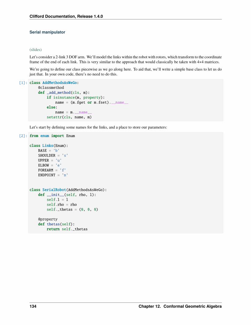
Clifford Documentation, Release 1.4.0
Serial manipulator
(slides)
Let’s consider a 2-link 3 DOF arm. We’ll model the links within the robot with rotors, which transform to the coordinateframe of the end of each link. This is very similar to the approach that would classically be taken with 4×4 matrices.
We’re going to define our class piecewise as we go along here. To aid that, we’ll write a simple base class to let us dojust that. In your own code, there’s no need to do this.
[1]: class AddMethodsAsWeGo:@classmethoddef _add_method(cls, m):
if isinstance(m, property):name = (m.fget or m.fset).__name__
else:name = m.__name__
setattr(cls, name, m)
Let’s start by defining some names for the links, and a place to store our parameters:
[2]: from enum import Enum
class Links(Enum):BASE = 'b'SHOULDER = 's'UPPER = 'u'ELBOW = 'e'FOREARM = 'f'ENDPOINT = 'n'
class SerialRobot(AddMethodsAsWeGo):def __init__(self, rho, l):
self.l = lself.rho = rhoself._thetas = (0, 0, 0)
@propertydef thetas(self):
return self._thetas
134 Chapter 12. Conformal Geometric Algebra
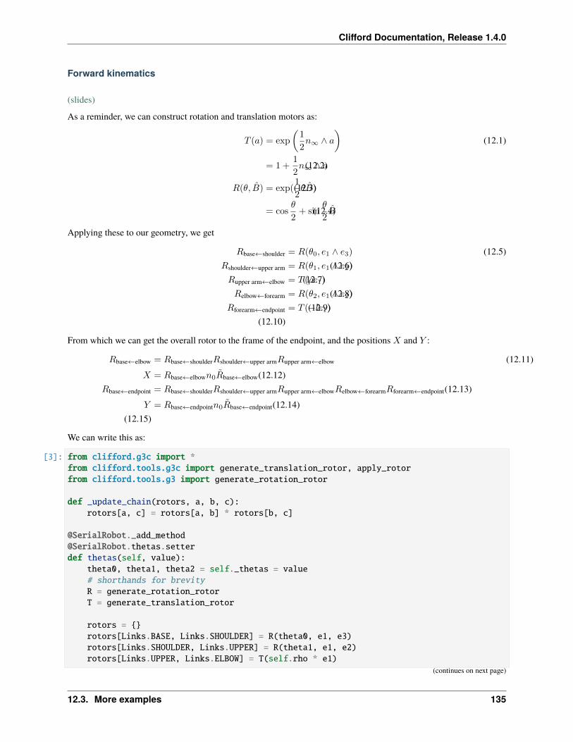
Clifford Documentation, Release 1.4.0
Forward kinematics
(slides)
As a reminder, we can construct rotation and translation motors as:
𝑇 (𝑎) = exp
(︂1
2𝑛∞ ∧ 𝑎
)︂(12.1)
= 1 +1
2𝑛∞ ∧ 𝑎(12.2)
𝑅(𝜃, �̂�) = exp(1
2𝜃�̂�)(12.3)
= cos𝜃
2+ sin
𝜃
2�̂�(12.4)
Applying these to our geometry, we get
𝑅base←shoulder = 𝑅(𝜃0, 𝑒1 ∧ 𝑒3) (12.5)𝑅shoulder←upper arm = 𝑅(𝜃1, 𝑒1 ∧ 𝑒2)(12.6)𝑅upper arm←elbow = 𝑇 (𝜌𝑒1)(12.7)𝑅elbow←forearm = 𝑅(𝜃2, 𝑒1 ∧ 𝑒2)(12.8)
𝑅forearm←endpoint = 𝑇 (−𝑙𝑒1)(12.9)(12.10)
From which we can get the overall rotor to the frame of the endpoint, and the positions 𝑋 and 𝑌 :
𝑅base←elbow = 𝑅base←shoulder𝑅shoulder←upper arm𝑅upper arm←elbow (12.11)
𝑋 = 𝑅base←elbow𝑛0�̃�base←elbow(12.12)𝑅base←endpoint = 𝑅base←shoulder𝑅shoulder←upper arm𝑅upper arm←elbow𝑅elbow←forearm𝑅forearm←endpoint(12.13)
𝑌 = 𝑅base←endpoint𝑛0�̃�base←endpoint(12.14)(12.15)
We can write this as:
[3]: from clifford.g3c import *from clifford.tools.g3c import generate_translation_rotor, apply_rotorfrom clifford.tools.g3 import generate_rotation_rotor
def _update_chain(rotors, a, b, c):rotors[a, c] = rotors[a, b] * rotors[b, c]
@[email protected] thetas(self, value):
theta0, theta1, theta2 = self._thetas = value# shorthands for brevityR = generate_rotation_rotorT = generate_translation_rotor
rotors = {}rotors[Links.BASE, Links.SHOULDER] = R(theta0, e1, e3)rotors[Links.SHOULDER, Links.UPPER] = R(theta1, e1, e2)rotors[Links.UPPER, Links.ELBOW] = T(self.rho * e1)
(continues on next page)
12.3. More examples 135
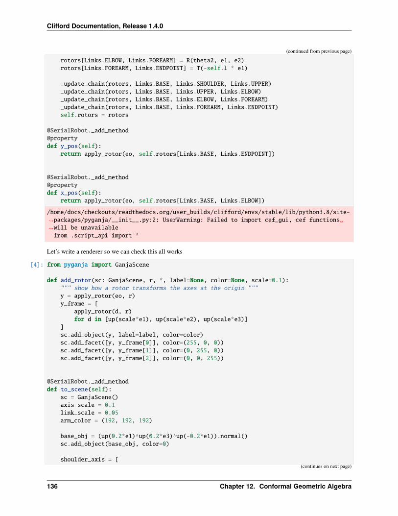
Clifford Documentation, Release 1.4.0
(continued from previous page)
rotors[Links.ELBOW, Links.FOREARM] = R(theta2, e1, e2)rotors[Links.FOREARM, Links.ENDPOINT] = T(-self.l * e1)
_update_chain(rotors, Links.BASE, Links.SHOULDER, Links.UPPER)_update_chain(rotors, Links.BASE, Links.UPPER, Links.ELBOW)_update_chain(rotors, Links.BASE, Links.ELBOW, Links.FOREARM)_update_chain(rotors, Links.BASE, Links.FOREARM, Links.ENDPOINT)self.rotors = rotors
@SerialRobot._add_method@propertydef y_pos(self):
return apply_rotor(eo, self.rotors[Links.BASE, Links.ENDPOINT])
@SerialRobot._add_method@propertydef x_pos(self):
return apply_rotor(eo, self.rotors[Links.BASE, Links.ELBOW])
/home/docs/checkouts/readthedocs.org/user_builds/clifford/envs/stable/lib/python3.8/site-→˓packages/pyganja/__init__.py:2: UserWarning: Failed to import cef_gui, cef functions␣→˓will be unavailablefrom .script_api import *
Let’s write a renderer so we can check this all works
[4]: from pyganja import GanjaScene
def add_rotor(sc: GanjaScene, r, *, label=None, color=None, scale=0.1):""" show how a rotor transforms the axes at the origin """y = apply_rotor(eo, r)y_frame = [
apply_rotor(d, r)for d in [up(scale*e1), up(scale*e2), up(scale*e3)]
]sc.add_object(y, label=label, color=color)sc.add_facet([y, y_frame[0]], color=(255, 0, 0))sc.add_facet([y, y_frame[1]], color=(0, 255, 0))sc.add_facet([y, y_frame[2]], color=(0, 0, 255))
@SerialRobot._add_methoddef to_scene(self):
sc = GanjaScene()axis_scale = 0.1link_scale = 0.05arm_color = (192, 192, 192)
base_obj = (up(0.2*e1)^up(0.2*e3)^up(-0.2*e1)).normal()sc.add_object(base_obj, color=0)
shoulder_axis = [(continues on next page)
136 Chapter 12. Conformal Geometric Algebra
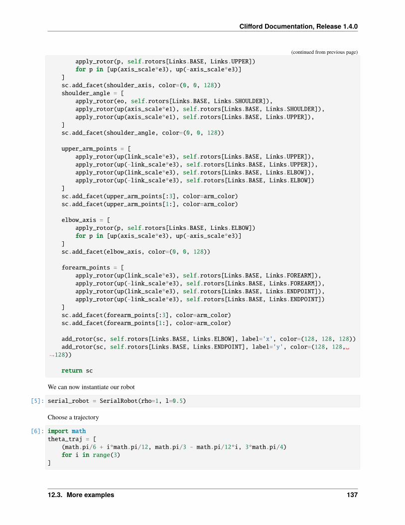
Clifford Documentation, Release 1.4.0
(continued from previous page)
apply_rotor(p, self.rotors[Links.BASE, Links.UPPER])for p in [up(axis_scale*e3), up(-axis_scale*e3)]
]sc.add_facet(shoulder_axis, color=(0, 0, 128))shoulder_angle = [
apply_rotor(eo, self.rotors[Links.BASE, Links.SHOULDER]),apply_rotor(up(axis_scale*e1), self.rotors[Links.BASE, Links.SHOULDER]),apply_rotor(up(axis_scale*e1), self.rotors[Links.BASE, Links.UPPER]),
]sc.add_facet(shoulder_angle, color=(0, 0, 128))
upper_arm_points = [apply_rotor(up(link_scale*e3), self.rotors[Links.BASE, Links.UPPER]),apply_rotor(up(-link_scale*e3), self.rotors[Links.BASE, Links.UPPER]),apply_rotor(up(link_scale*e3), self.rotors[Links.BASE, Links.ELBOW]),apply_rotor(up(-link_scale*e3), self.rotors[Links.BASE, Links.ELBOW])
]sc.add_facet(upper_arm_points[:3], color=arm_color)sc.add_facet(upper_arm_points[1:], color=arm_color)
elbow_axis = [apply_rotor(p, self.rotors[Links.BASE, Links.ELBOW])for p in [up(axis_scale*e3), up(-axis_scale*e3)]
]sc.add_facet(elbow_axis, color=(0, 0, 128))
forearm_points = [apply_rotor(up(link_scale*e3), self.rotors[Links.BASE, Links.FOREARM]),apply_rotor(up(-link_scale*e3), self.rotors[Links.BASE, Links.FOREARM]),apply_rotor(up(link_scale*e3), self.rotors[Links.BASE, Links.ENDPOINT]),apply_rotor(up(-link_scale*e3), self.rotors[Links.BASE, Links.ENDPOINT])
]sc.add_facet(forearm_points[:3], color=arm_color)sc.add_facet(forearm_points[1:], color=arm_color)
add_rotor(sc, self.rotors[Links.BASE, Links.ELBOW], label='x', color=(128, 128, 128))add_rotor(sc, self.rotors[Links.BASE, Links.ENDPOINT], label='y', color=(128, 128,␣
→˓128))
return sc
We can now instantiate our robot
[5]: serial_robot = SerialRobot(rho=1, l=0.5)
Choose a trajectory
[6]: import maththeta_traj = [
(math.pi/6 + i*math.pi/12, math.pi/3 - math.pi/12*i, 3*math.pi/4)for i in range(3)
]
12.3. More examples 137
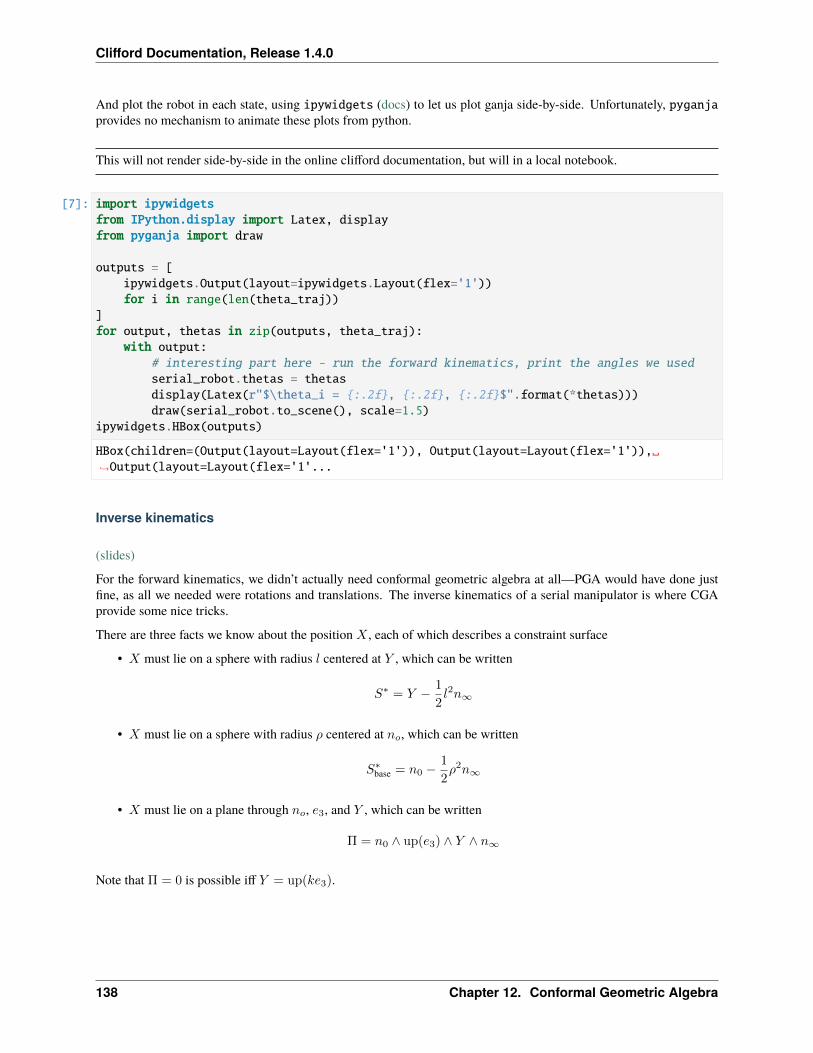
Clifford Documentation, Release 1.4.0
And plot the robot in each state, using ipywidgets (docs) to let us plot ganja side-by-side. Unfortunately, pyganjaprovides no mechanism to animate these plots from python.
This will not render side-by-side in the online clifford documentation, but will in a local notebook.
[7]: import ipywidgetsfrom IPython.display import Latex, displayfrom pyganja import draw
outputs = [ipywidgets.Output(layout=ipywidgets.Layout(flex='1'))for i in range(len(theta_traj))
]for output, thetas in zip(outputs, theta_traj):
with output:# interesting part here - run the forward kinematics, print the angles we usedserial_robot.thetas = thetasdisplay(Latex(r"$\theta_i = {:.2f}, {:.2f}, {:.2f}$".format(*thetas)))draw(serial_robot.to_scene(), scale=1.5)
ipywidgets.HBox(outputs)
HBox(children=(Output(layout=Layout(flex='1')), Output(layout=Layout(flex='1')),␣→˓Output(layout=Layout(flex='1'...
Inverse kinematics
(slides)
For the forward kinematics, we didn’t actually need conformal geometric algebra at all—PGA would have done justfine, as all we needed were rotations and translations. The inverse kinematics of a serial manipulator is where CGAprovide some nice tricks.
There are three facts we know about the position 𝑋 , each of which describes a constraint surface
• 𝑋 must lie on a sphere with radius 𝑙 centered at 𝑌 , which can be written
𝑆* = 𝑌 − 1
2𝑙2𝑛∞
• 𝑋 must lie on a sphere with radius 𝜌 centered at 𝑛𝑜, which can be written
𝑆*base = 𝑛0 −1
2𝜌2𝑛∞
• 𝑋 must lie on a plane through 𝑛𝑜, 𝑒3, and 𝑌 , which can be written
Π = 𝑛0 ∧ up(𝑒3) ∧ 𝑌 ∧ 𝑛∞
Note that Π = 0 is possible iff 𝑌 = up(𝑘𝑒3).
138 Chapter 12. Conformal Geometric Algebra
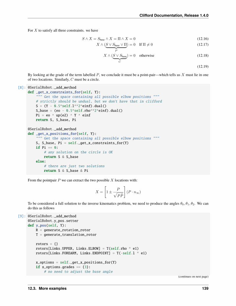
Clifford Documentation, Release 1.4.0
For 𝑋 to satisfy all three constraints. we have
𝑆 ∧𝑋 = 𝑆base ∧𝑋 = Π ∧𝑋 = 0 (12.16)𝑋 ∧ (𝑆 ∨ 𝑆base ∨ Π⏟ ⏞
𝑃
) = 0 If Π ̸= 0 (12.17)
𝑋 ∧ (𝑆 ∨ 𝑆base⏟ ⏞ 𝐶
) = 0 otherwise (12.18)
(12.19)
By looking at the grade of the term labelled 𝑃 , we conclude it must be a point-pair—which tells us 𝑋 must lie in oneof two locations. Similarly, 𝐶 must be a circle.
[8]: @SerialRobot._add_methoddef _get_x_constraints_for(self, Y):
""" Get the space containing all possible elbow positions """# strictly should be undual, but we don't have that in cliffordS = (Y - 0.5*self.l**2*einf).dual()S_base = (eo - 0.5*self.rho**2*einf).dual()Pi = eo ^ up(e2) ^ Y ^ einfreturn S, S_base, Pi
@SerialRobot._add_methoddef _get_x_positions_for(self, Y):
""" Get the space containing all possible elbow positions """S, S_base, Pi = self._get_x_constraints_for(Y)if Pi == 0:
# any solution on the circle is OKreturn S & S_base
else:# there are just two solutionsreturn S & S_base & Pi
From the pointpair 𝑃 we can extract the two possible 𝑋 locations with:
𝑋 =
[︃1 ± 𝑃√︀
𝑃𝑃
]︃(𝑃 · 𝑛∞)
To be considered a full solution to the inverse kinematics problem, we need to produce the angles 𝜃0, 𝜃1, 𝜃2. We cando this as follows
[9]: @[email protected]_pos.setterdef y_pos(self, Y):
R = generate_rotation_rotorT = generate_translation_rotor
rotors = {}rotors[Links.UPPER, Links.ELBOW] = T(self.rho * e1)rotors[Links.FOREARM, Links.ENDPOINT] = T(-self.l * e1)
x_options = self._get_x_positions_for(Y)if x_options.grades == {3}:
# no need to adjust the base angle(continues on next page)
12.3. More examples 139
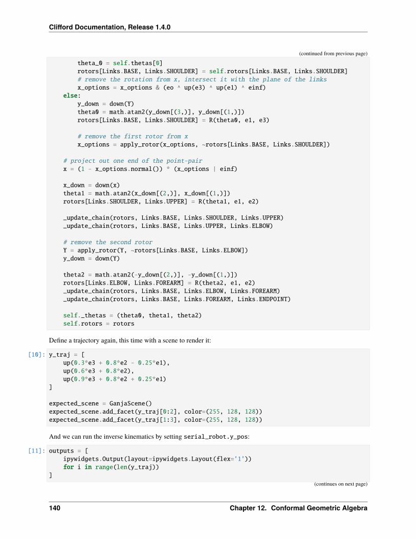
Clifford Documentation, Release 1.4.0
(continued from previous page)
theta_0 = self.thetas[0]rotors[Links.BASE, Links.SHOULDER] = self.rotors[Links.BASE, Links.SHOULDER]# remove the rotation from x, intersect it with the plane of the linksx_options = x_options & (eo ^ up(e3) ^ up(e1) ^ einf)
else:y_down = down(Y)theta0 = math.atan2(y_down[(3,)], y_down[(1,)])rotors[Links.BASE, Links.SHOULDER] = R(theta0, e1, e3)
# remove the first rotor from xx_options = apply_rotor(x_options, ~rotors[Links.BASE, Links.SHOULDER])
# project out one end of the point-pairx = (1 - x_options.normal()) * (x_options | einf)
x_down = down(x)theta1 = math.atan2(x_down[(2,)], x_down[(1,)])rotors[Links.SHOULDER, Links.UPPER] = R(theta1, e1, e2)
_update_chain(rotors, Links.BASE, Links.SHOULDER, Links.UPPER)_update_chain(rotors, Links.BASE, Links.UPPER, Links.ELBOW)
# remove the second rotorY = apply_rotor(Y, ~rotors[Links.BASE, Links.ELBOW])y_down = down(Y)
theta2 = math.atan2(-y_down[(2,)], -y_down[(1,)])rotors[Links.ELBOW, Links.FOREARM] = R(theta2, e1, e2)_update_chain(rotors, Links.BASE, Links.ELBOW, Links.FOREARM)_update_chain(rotors, Links.BASE, Links.FOREARM, Links.ENDPOINT)
self._thetas = (theta0, theta1, theta2)self.rotors = rotors
Define a trajectory again, this time with a scene to render it:
[10]: y_traj = [up(0.3*e3 + 0.8*e2 - 0.25*e1),up(0.6*e3 + 0.8*e2),up(0.9*e3 + 0.8*e2 + 0.25*e1)
]
expected_scene = GanjaScene()expected_scene.add_facet(y_traj[0:2], color=(255, 128, 128))expected_scene.add_facet(y_traj[1:3], color=(255, 128, 128))
And we can run the inverse kinematics by setting serial_robot.y_pos:
[11]: outputs = [ipywidgets.Output(layout=ipywidgets.Layout(flex='1'))for i in range(len(y_traj))
](continues on next page)
140 Chapter 12. Conformal Geometric Algebra
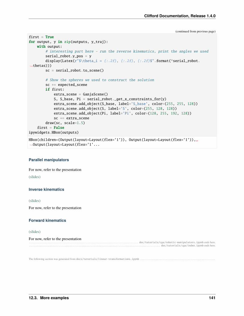
Clifford Documentation, Release 1.4.0
(continued from previous page)
first = Truefor output, y in zip(outputs, y_traj):
with output:# interesting part here - run the reverse kinematics, print the angles we usedserial_robot.y_pos = ydisplay(Latex(r"$\theta_i = {:.2f}, {:.2f}, {:.2f}$".format(*serial_robot.
→˓thetas)))sc = serial_robot.to_scene()
# Show the spheres we used to construct the solutionsc += expected_sceneif first:
extra_scene = GanjaScene()S, S_base, Pi = serial_robot._get_x_constraints_for(y)extra_scene.add_object(S_base, label='S_base', color=(255, 255, 128))extra_scene.add_object(S, label='S', color=(255, 128, 128))extra_scene.add_object(Pi, label='Pi', color=(128, 255, 192, 128))sc += extra_scene
draw(sc, scale=1.5)first = False
ipywidgets.HBox(outputs)
HBox(children=(Output(layout=Layout(flex='1')), Output(layout=Layout(flex='1')),␣→˓Output(layout=Layout(flex='1'...
Parallel manipulators
For now, refer to the presentation
(slides)
Inverse kinematics
(slides)
For now, refer to the presentation
Forward kinematics
(slides)
For now, refer to the presentation. . . . . . . . . . . . . . . . . . . . . . . . . . . . . . . . . . . . . . . . . . . . . . . . . . . . . . . . . . . . . . . . . . . . . . . . . . . . . . . . . . . . . . . . . doc/tutorials/cga/robotic-manipulators.ipynb ends here.. . . . . . . . . . . . . . . . . . . . . . . . . . . . . . . . . . . . . . . . . . . . . . . . . . . . . . . . . . . . . . . . . . . . . . . . . . . . . . . . . . . . . . . . . . . . . . . . . . . . . . . . . . . doc/tutorials/cga/index.ipynb ends here.
The following section was generated from docs/tutorials/linear-transformations.ipynb . . . . . . . . . . . . . . . . . . . . . . . . . . . . . . . . . . . . . . . . . . . . . . . . . . . . . . . . . . . . .
12.3. More examples 141

Clifford Documentation, Release 1.4.0
142 Chapter 12. Conformal Geometric Algebra
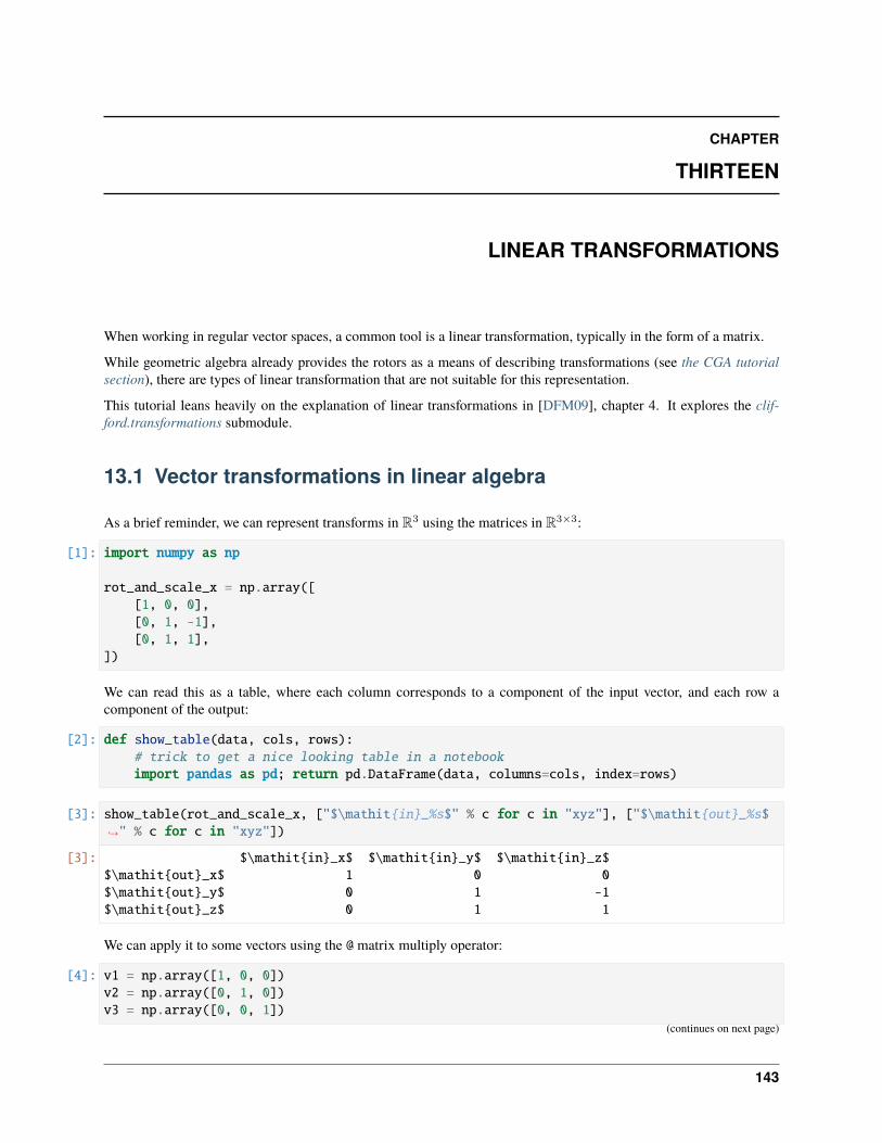
CHAPTER
THIRTEEN
LINEAR TRANSFORMATIONS
When working in regular vector spaces, a common tool is a linear transformation, typically in the form of a matrix.
While geometric algebra already provides the rotors as a means of describing transformations (see the CGA tutorialsection), there are types of linear transformation that are not suitable for this representation.
This tutorial leans heavily on the explanation of linear transformations in [DFM09], chapter 4. It explores the clif-ford.transformations submodule.
13.1 Vector transformations in linear algebra
As a brief reminder, we can represent transforms in R3 using the matrices in R3×3:
[1]: import numpy as np
rot_and_scale_x = np.array([[1, 0, 0],[0, 1, -1],[0, 1, 1],
])
We can read this as a table, where each column corresponds to a component of the input vector, and each row acomponent of the output:
[2]: def show_table(data, cols, rows):# trick to get a nice looking table in a notebookimport pandas as pd; return pd.DataFrame(data, columns=cols, index=rows)
[3]: show_table(rot_and_scale_x, ["$\mathit{in}_%s$" % c for c in "xyz"], ["$\mathit{out}_%s$→˓" % c for c in "xyz"])
[3]: $\mathit{in}_x$ $\mathit{in}_y$ $\mathit{in}_z$$\mathit{out}_x$ 1 0 0$\mathit{out}_y$ 0 1 -1$\mathit{out}_z$ 0 1 1
We can apply it to some vectors using the @ matrix multiply operator:
[4]: v1 = np.array([1, 0, 0])v2 = np.array([0, 1, 0])v3 = np.array([0, 0, 1])
(continues on next page)
143
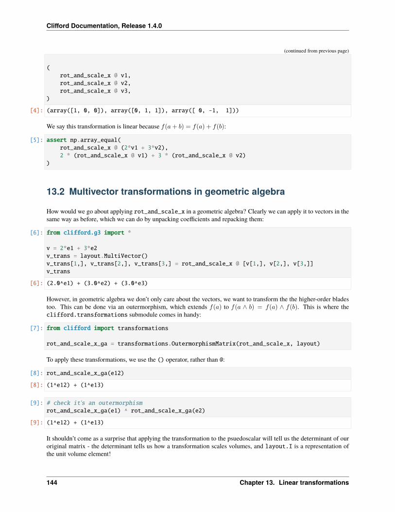
Clifford Documentation, Release 1.4.0
(continued from previous page)
(rot_and_scale_x @ v1,rot_and_scale_x @ v2,rot_and_scale_x @ v3,
)
[4]: (array([1, 0, 0]), array([0, 1, 1]), array([ 0, -1, 1]))
We say this transformation is linear because 𝑓(𝑎+ 𝑏) = 𝑓(𝑎) + 𝑓(𝑏):
[5]: assert np.array_equal(rot_and_scale_x @ (2*v1 + 3*v2),2 * (rot_and_scale_x @ v1) + 3 * (rot_and_scale_x @ v2)
)
13.2 Multivector transformations in geometric algebra
How would we go about applying rot_and_scale_x in a geometric algebra? Clearly we can apply it to vectors in thesame way as before, which we can do by unpacking coefficients and repacking them:
[6]: from clifford.g3 import *
v = 2*e1 + 3*e2v_trans = layout.MultiVector()v_trans[1,], v_trans[2,], v_trans[3,] = rot_and_scale_x @ [v[1,], v[2,], v[3,]]v_trans
[6]: (2.0^e1) + (3.0^e2) + (3.0^e3)
However, in geometric algebra we don’t only care about the vectors, we want to transform the the higher-order bladestoo. This can be done via an outermorphism, which extends 𝑓(𝑎) to 𝑓(𝑎 ∧ 𝑏) = 𝑓(𝑎) ∧ 𝑓(𝑏). This is where theclifford.transformations submodule comes in handy:
[7]: from clifford import transformations
rot_and_scale_x_ga = transformations.OutermorphismMatrix(rot_and_scale_x, layout)
To apply these transformations, we use the () operator, rather than @:
[8]: rot_and_scale_x_ga(e12)
[8]: (1^e12) + (1^e13)
[9]: # check it's an outermorphismrot_and_scale_x_ga(e1) ^ rot_and_scale_x_ga(e2)
[9]: (1^e12) + (1^e13)
It shouldn’t come as a surprise that applying the transformation to the psuedoscalar will tell us the determinant of ouroriginal matrix - the determinant tells us how a transformation scales volumes, and layout.I is a representation ofthe unit volume element!
144 Chapter 13. Linear transformations
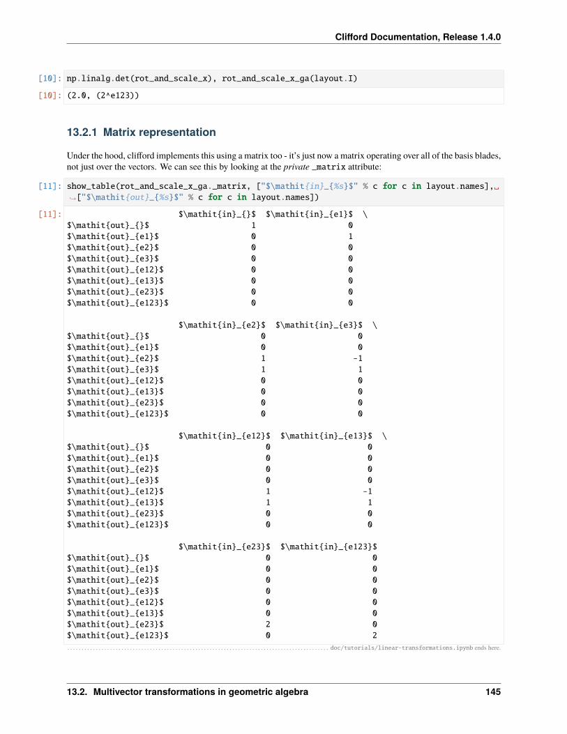
Clifford Documentation, Release 1.4.0
[10]: np.linalg.det(rot_and_scale_x), rot_and_scale_x_ga(layout.I)
[10]: (2.0, (2^e123))
13.2.1 Matrix representation
Under the hood, clifford implements this using a matrix too - it’s just now a matrix operating over all of the basis blades,not just over the vectors. We can see this by looking at the private _matrix attribute:
[11]: show_table(rot_and_scale_x_ga._matrix, ["$\mathit{in}_{%s}$" % c for c in layout.names],␣→˓["$\mathit{out}_{%s}$" % c for c in layout.names])
[11]: $\mathit{in}_{}$ $\mathit{in}_{e1}$ \$\mathit{out}_{}$ 1 0$\mathit{out}_{e1}$ 0 1$\mathit{out}_{e2}$ 0 0$\mathit{out}_{e3}$ 0 0$\mathit{out}_{e12}$ 0 0$\mathit{out}_{e13}$ 0 0$\mathit{out}_{e23}$ 0 0$\mathit{out}_{e123}$ 0 0
$\mathit{in}_{e2}$ $\mathit{in}_{e3}$ \$\mathit{out}_{}$ 0 0$\mathit{out}_{e1}$ 0 0$\mathit{out}_{e2}$ 1 -1$\mathit{out}_{e3}$ 1 1$\mathit{out}_{e12}$ 0 0$\mathit{out}_{e13}$ 0 0$\mathit{out}_{e23}$ 0 0$\mathit{out}_{e123}$ 0 0
$\mathit{in}_{e12}$ $\mathit{in}_{e13}$ \$\mathit{out}_{}$ 0 0$\mathit{out}_{e1}$ 0 0$\mathit{out}_{e2}$ 0 0$\mathit{out}_{e3}$ 0 0$\mathit{out}_{e12}$ 1 -1$\mathit{out}_{e13}$ 1 1$\mathit{out}_{e23}$ 0 0$\mathit{out}_{e123}$ 0 0
$\mathit{in}_{e23}$ $\mathit{in}_{e123}$$\mathit{out}_{}$ 0 0$\mathit{out}_{e1}$ 0 0$\mathit{out}_{e2}$ 0 0$\mathit{out}_{e3}$ 0 0$\mathit{out}_{e12}$ 0 0$\mathit{out}_{e13}$ 0 0$\mathit{out}_{e23}$ 2 0$\mathit{out}_{e123}$ 0 2
. . . . . . . . . . . . . . . . . . . . . . . . . . . . . . . . . . . . . . . . . . . . . . . . . . . . . . . . . . . . . . . . . . . . . . . . . . . . . . . . . . . . . . . . . . . . doc/tutorials/linear-transformations.ipynb ends here.
13.2. Multivector transformations in geometric algebra 145

Clifford Documentation, Release 1.4.0
The following section was generated from docs/tutorials/apollonius-cga-augmented.ipynb . . . . . . . . . . . . . . . . . . . . . . . . . . . . . . . . . . . . . . . . . . . . . . . . . . . . . . . . . . .
146 Chapter 13. Linear transformations
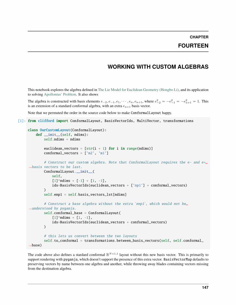
CHAPTER
FOURTEEN
WORKING WITH CUSTOM ALGEBRAS
This notebook explores the algebra defined in The Lie Model for Euclidean Geometry (Hongbo Li), and its applicationto solving Apollonius’ Problem. It also shows
The algebra is constructed with basis elements 𝑒−2, 𝑒−1, 𝑒1, · · · , 𝑒𝑛, 𝑒𝑛+1, where 𝑒2−2 = −𝑒2−1 = −𝑒2𝑛+1 = 1. Thisis an extension of a standard conformal algebra, with an extra 𝑒𝑛+1 basis vector.
Note that we permuted the order in the source code below to make ConformalLayout happy.
[1]: from clifford import ConformalLayout, BasisVectorIds, MultiVector, transformations
class OurCustomLayout(ConformalLayout):def __init__(self, ndims):
self.ndims = ndims
euclidean_vectors = [str(i + 1) for i in range(ndims)]conformal_vectors = ['m2', 'm1']
# Construct our custom algebra. Note that ConformalLayout requires the e- and e+␣→˓basis vectors to be last.
ConformalLayout.__init__(self,[1]*ndims + [-1] + [1, -1],ids=BasisVectorIds(euclidean_vectors + ['np1'] + conformal_vectors)
)self.enp1 = self.basis_vectors_lst[ndims]
# Construct a base algebra without the extra `enp1`, which would not be␣→˓understood by pyganja.
self.conformal_base = ConformalLayout([1]*ndims + [1, -1],ids=BasisVectorIds(euclidean_vectors + conformal_vectors)
)
# this lets us convert between the two layoutsself.to_conformal = transformations.between_basis_vectors(self, self.conformal_
→˓base)
The code above also defines a stardard conformal R𝑁+1,1 layout without this new basis vector. This is primarily tosupport rendering with pyganja, which doesn’t support the presence of this extra vector. BasisVectorMap defaults topreserving vectors by name between one algebra and another, while throwing away blades containing vectors missingfrom the destination algebra.
147

Clifford Documentation, Release 1.4.0
We define an ups function which maps conformal dual-spheres into this algebra, as 𝑠′ = 𝑠 + |𝑠| 𝑒𝑛+1, and a downsthat applies the correct sign. The s suffix here is chosen to mean sphere.
[2]: def ups(self, s):return s + self.enp1*abs(s)
OurCustomLayout.ups = ups; del ups
def downs(self, mv):if (mv | self.enp1)[()] > 0:
mv = -mvreturn mv
OurCustomLayout.downs = downs; del downs
Before we start looking at specified dimensions of euclidean space, we build a helper to construct conformal dual circlesand spheres, with the word round being a general term intended to cover both circles and spheres.
[3]: def dual_round(at, r):l = at.layoutreturn l.up(at) - 0.5*l.einf*r*r
In order to render with pyganja, we’ll need a helper to convert from our custom R𝑁+1,2 layout into a standardconformal R𝑁+1,1 layout. clifford maps indices in .value to basis blades via layout._basis_blade_order.index_to_bitmap, which we can use to convert the indices in one layout to the indices in another.
14.1 Visualization
Finally, we’ll define a plotting function, which plots the problem and solution circles in suitable colors via pyganja.Note that this all works because of our definition of the to_conformal BasisVectorMap.
[4]: import itertoolsfrom pyganja import GanjaScene, draw
def plot_rounds(in_rounds, out_rounds, scale=1):colors = itertools.cycle([
(255, 0, 0),(0, 255, 0),(0, 0, 255),(0, 255, 255),
])# note: .dual() neede here because we're passing in dual rounds, but ganja expects␣
→˓direct roundss = GanjaScene()for r, color in zip(in_rounds, colors):
s.add_object(r.layout.to_conformal(r).dual(), color=color)for r in out_rounds:
s.add_object(r.layout.to_conformal(r).dual(), color=(64, 64, 64))draw(s, sig=r.layout.conformal_base.sig, scale=scale)
148 Chapter 14. Working with custom algebras
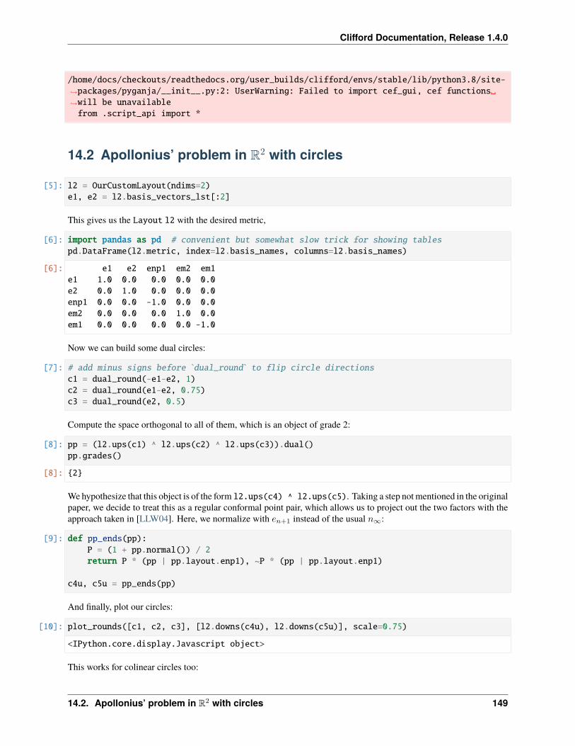
Clifford Documentation, Release 1.4.0
/home/docs/checkouts/readthedocs.org/user_builds/clifford/envs/stable/lib/python3.8/site-→˓packages/pyganja/__init__.py:2: UserWarning: Failed to import cef_gui, cef functions␣→˓will be unavailablefrom .script_api import *
14.2 Apollonius’ problem in R2 with circles
[5]: l2 = OurCustomLayout(ndims=2)e1, e2 = l2.basis_vectors_lst[:2]
This gives us the Layout l2 with the desired metric,
[6]: import pandas as pd # convenient but somewhat slow trick for showing tablespd.DataFrame(l2.metric, index=l2.basis_names, columns=l2.basis_names)
[6]: e1 e2 enp1 em2 em1e1 1.0 0.0 0.0 0.0 0.0e2 0.0 1.0 0.0 0.0 0.0enp1 0.0 0.0 -1.0 0.0 0.0em2 0.0 0.0 0.0 1.0 0.0em1 0.0 0.0 0.0 0.0 -1.0
Now we can build some dual circles:
[7]: # add minus signs before `dual_round` to flip circle directionsc1 = dual_round(-e1-e2, 1)c2 = dual_round(e1-e2, 0.75)c3 = dual_round(e2, 0.5)
Compute the space orthogonal to all of them, which is an object of grade 2:
[8]: pp = (l2.ups(c1) ^ l2.ups(c2) ^ l2.ups(c3)).dual()pp.grades()
[8]: {2}
We hypothesize that this object is of the form l2.ups(c4) ^ l2.ups(c5). Taking a step not mentioned in the originalpaper, we decide to treat this as a regular conformal point pair, which allows us to project out the two factors with theapproach taken in [LLW04]. Here, we normalize with 𝑒𝑛+1 instead of the usual 𝑛∞:
[9]: def pp_ends(pp):P = (1 + pp.normal()) / 2return P * (pp | pp.layout.enp1), ~P * (pp | pp.layout.enp1)
c4u, c5u = pp_ends(pp)
And finally, plot our circles:
[10]: plot_rounds([c1, c2, c3], [l2.downs(c4u), l2.downs(c5u)], scale=0.75)
<IPython.core.display.Javascript object>
This works for colinear circles too:
14.2. Apollonius’ problem in R2 with circles 149
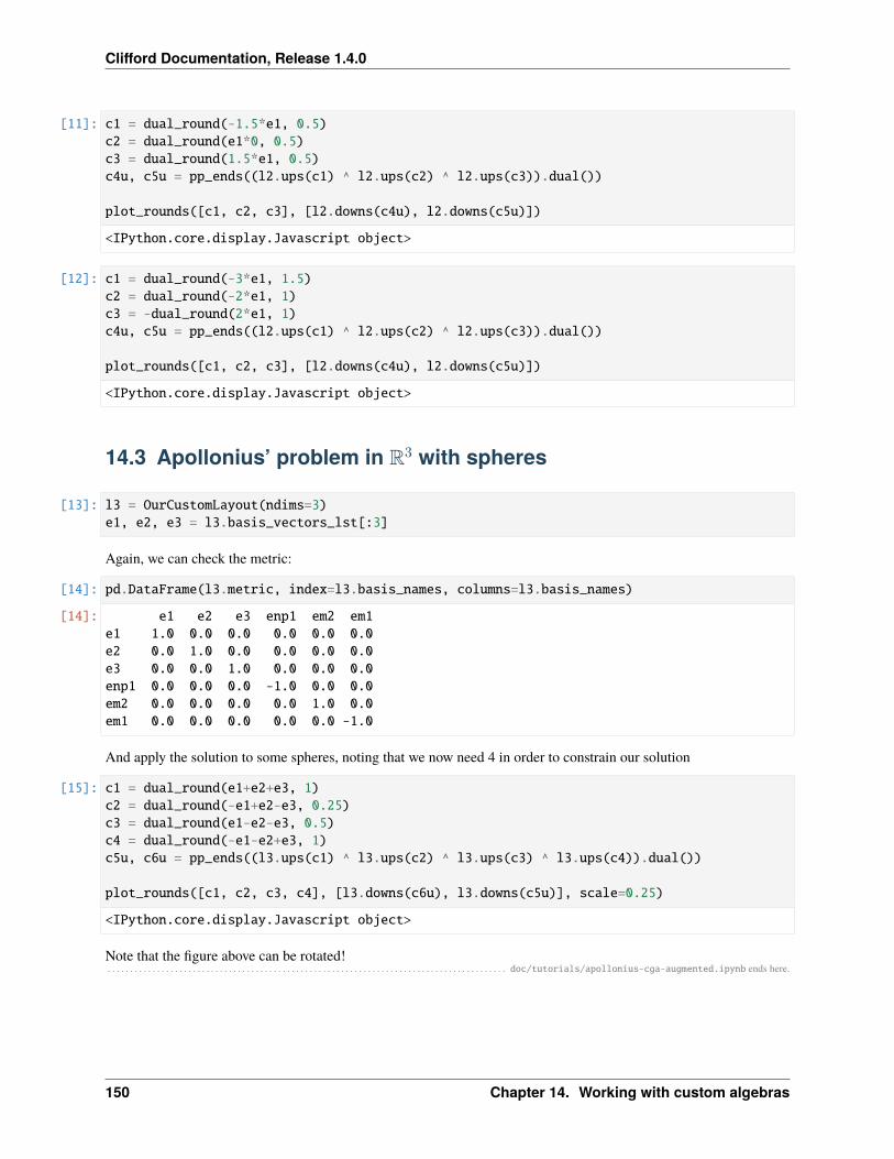
Clifford Documentation, Release 1.4.0
[11]: c1 = dual_round(-1.5*e1, 0.5)c2 = dual_round(e1*0, 0.5)c3 = dual_round(1.5*e1, 0.5)c4u, c5u = pp_ends((l2.ups(c1) ^ l2.ups(c2) ^ l2.ups(c3)).dual())
plot_rounds([c1, c2, c3], [l2.downs(c4u), l2.downs(c5u)])
<IPython.core.display.Javascript object>
[12]: c1 = dual_round(-3*e1, 1.5)c2 = dual_round(-2*e1, 1)c3 = -dual_round(2*e1, 1)c4u, c5u = pp_ends((l2.ups(c1) ^ l2.ups(c2) ^ l2.ups(c3)).dual())
plot_rounds([c1, c2, c3], [l2.downs(c4u), l2.downs(c5u)])
<IPython.core.display.Javascript object>
14.3 Apollonius’ problem in R3 with spheres
[13]: l3 = OurCustomLayout(ndims=3)e1, e2, e3 = l3.basis_vectors_lst[:3]
Again, we can check the metric:
[14]: pd.DataFrame(l3.metric, index=l3.basis_names, columns=l3.basis_names)
[14]: e1 e2 e3 enp1 em2 em1e1 1.0 0.0 0.0 0.0 0.0 0.0e2 0.0 1.0 0.0 0.0 0.0 0.0e3 0.0 0.0 1.0 0.0 0.0 0.0enp1 0.0 0.0 0.0 -1.0 0.0 0.0em2 0.0 0.0 0.0 0.0 1.0 0.0em1 0.0 0.0 0.0 0.0 0.0 -1.0
And apply the solution to some spheres, noting that we now need 4 in order to constrain our solution
[15]: c1 = dual_round(e1+e2+e3, 1)c2 = dual_round(-e1+e2-e3, 0.25)c3 = dual_round(e1-e2-e3, 0.5)c4 = dual_round(-e1-e2+e3, 1)c5u, c6u = pp_ends((l3.ups(c1) ^ l3.ups(c2) ^ l3.ups(c3) ^ l3.ups(c4)).dual())
plot_rounds([c1, c2, c3, c4], [l3.downs(c6u), l3.downs(c5u)], scale=0.25)
<IPython.core.display.Javascript object>
Note that the figure above can be rotated!. . . . . . . . . . . . . . . . . . . . . . . . . . . . . . . . . . . . . . . . . . . . . . . . . . . . . . . . . . . . . . . . . . . . . . . . . . . . . . . . . . . . . . . . . doc/tutorials/apollonius-cga-augmented.ipynb ends here.
150 Chapter 14. Working with custom algebras

CHAPTER
FIFTEEN
OTHER RESOURCES FOR CLIFFORD
15.1 Slide Decks
• Installation
• Conformal Geometric Algebra with Python, Part 1
• Conformal Geometric Algebra with Python, Part 2
15.2 Videos
• Intro to Clifford
151

Clifford Documentation, Release 1.4.0
152 Chapter 15. Other resources for clifford

CHAPTER
SIXTEEN
OTHER RESOURCES FOR GEOMETRIC ALGEBRA
If you think Geometric Algebra looks interesting and want to learn more, check out these websites and textbooks
16.1 Links
• galgebra, a symbolic geometric algebra module for Python
• The Cambridge University Geometric Algebra Research Group home page
• David Hestenes’ Geometric Calculus R & D Home Page
16.2 Introductory textbooks
• Geometric Algebra for Physicists, by Doran and Lasenby
• Geometric Algebra for Computer Science, by Dorst, Fontijne and Mann
• New Foundations for Classical Mechanics, by David Hestenes
153

Clifford Documentation, Release 1.4.0
154 Chapter 16. Other resources for Geometric Algebra

CHAPTER
SEVENTEEN
BIBLIOGRAPHY
155

Clifford Documentation, Release 1.4.0
156 Chapter 17. Bibliography
BIBLIOGRAPHY
[Cor17] Allan Cortzen. Geometric algebra algorithm representing an orthogonal isomorphism in versor form v2.03.Available online, 10 2017. URL: https://ctz.dk/geometric-algebra/frames-to-versor-algorithm/.
[DL03] Chris Doran and Anthony Lasenby. Geometric Algebra for Physicists. Cambridge University Press, 2003.URL: http://www.mrao.cam.ac.uk/~clifford.
[DFM09] Leo Dorst, Daniel Fontijne, and Stephen Mann. Geometric Algebra for Computer Science: An Object-Oriented Approach to Geometry. Morgan Kaufmann Publishers Inc., 2009. ISBN 9780080553108.
[DV11] Leo Dorst and Robert Valkenburg. Square Root and Logarithm of Rotors in 3D Conformal Geometric AlgebraUsing Polar Decomposition, pages 81–104. Springer London, 01 2011. doi:10.1007/978-0-85729-811-9_5.
[FD11] Daniel Fontijne and Leo Dorst. Reconstructing rotations and rigid body motions from exact point corre-spondences through reflections. Journal of Theoretical Biology - J THEOR BIOL, pages 63–78, 01 2011.doi:10.1007/978-0-85729-811-9_4.
[HL19] Hugo Hadfield and Joan Lasenby. Direct linear interpolation of geometric objects in conformal geometricalgebra. Advances in Applied Clifford Algebras, 29:, 09 2019. doi:10.1007/s00006-019-1003-y.
[Hes15] David Hestenes. Space-time algebra. Springer Berlin Heidelberg, New York, second edition edition, 2015.ISBN 978-3-319-18412-8 978-3-319-18413-5.
[HS17] Eckhard Hitzer and Stephen Sangwine. Multivector and multivector matrix inverses in real clifford algebras.Applied Mathematics and Computation, 311:375–389, Oct 2017. doi:10.1016/j.amc.2017.05.027.
[LLW04] Anthony Lasenby, Joan Lasenby, and Rich Wareham. A Covariant Approach to Geometry using GeometricAlgebra. Technical Report F-INFENG/TR-483, Department of Engineering, University of Cambridge, 2004.URL: https://pdfs.semanticscholar.org/baba/976fd7f6577eeaa1d3ef488c1db13ec24652.pdf.
[LHL19] Joan Lasenby, Hugo Hadfield, and Anthony Lasenby. Calculating the rotor between conformal objects. Ad-vances in Applied Clifford Algebras, 29:102, 10 2019. doi:10.1007/s00006-019-1014-8.
[Shi20] D. S. Shirokov. On determinant, other characteristic polynomial coefficients, and inverses in clifford algebrasof arbitrary dimension. 2020. arXiv:2005.04015.
[WCL05] Rich Wareham, Jonathan Cameron, and Joan Lasenby. Applications of conformal geometric algebra in com-puter vision and graphics. In Hongbo Li, Peter J. Olver, and Gerald Sommer, editors, Computer Algebra andGeometric Algebra with Applications, 329–349. Berlin, Heidelberg, 2005. Springer Berlin Heidelberg.
[WL08] Rich Wareham and Joan Lasenby. Mesh vertex pose and position interpolation using geometric algebra. InArticulated Motion and Deformable Objects, 122–131. Berlin, Heidelberg, 2008. Springer Berlin Heidelberg.
157

Clifford Documentation, Release 1.4.0
158 Bibliography

PYTHON MODULE INDEX
cclifford, 5clifford.cga, 18clifford.dg3c, 69clifford.dpga, 69clifford.g2, 69clifford.g2c, 69clifford.g3, 69clifford.g3c, 69clifford.g4, 69clifford.gac, 69clifford.numba, 66clifford.operator, 61clifford.pga, 69clifford.taylor_expansions, 65clifford.tools, 30clifford.tools.classify, 57clifford.tools.g3, 31clifford.tools.g3c, 34clifford.tools.g3c.object_fitting, 55clifford.transformations, 62
159

Clifford Documentation, Release 1.4.0
160 Python Module Index
INDEX
Symbols__add__() (clifford.MultiVector method), 8__and__() (clifford.MultiVector method), 7__call__() (clifford.MultiVector method), 8__getitem__() (clifford.MultiVector method), 8__init__() (clifford.cga.CGA method), 20__init__() (clifford.cga.CGAThing method), 30__init__() (clifford.cga.Dilation method), 27__init__() (clifford.cga.Flat method), 22__init__() (clifford.cga.Rotation method), 26__init__() (clifford.cga.Round method), 24__init__() (clifford.cga.Translation method), 28__init__() (clifford.cga.Transversion method), 29__invert__() (clifford.MultiVector method), 8__mul__() (clifford.MultiVector method), 7__or__() (clifford.MultiVector method), 8__sub__() (clifford.MultiVector method), 8__xor__() (clifford.MultiVector method), 8
Aadjoint (clifford.transformations.LinearMatrix prop-
erty), 63adjoint() (clifford.MultiVector method), 8adjoint_func (clifford.Layout attribute), 13angle_between_vectors() (in module clif-
ford.tools.g3), 33annihilate_k() (in module clifford.tools.g3c), 52anticommutator() (clifford.MultiVector method), 10apply_rotor() (in module clifford.tools.g3c), 45apply_rotor_inv() (in module clifford.tools.g3c), 46as_array() (clifford.MultiVector method), 8astype() (clifford.MultiVector method), 11average_objects() (in module clifford.tools.g3c), 53
Bb1 (clifford.BladeMap property), 17b2 (clifford.BladeMap property), 17base_vector() (clifford.cga.CGA method), 20bases() (clifford.Layout method), 15basis() (clifford.MultiVector method), 11basis_names (clifford.Layout property), 14basis_vectors (clifford.Layout property), 14
basis_vectors_lst (clifford.Layout property), 14between_basis_vectors() (in module clif-
ford.transformations), 65Blade (class in clifford.tools.classify), 57BladeMap (class in clifford), 17blades (clifford.Layout property), 14blades (in module clifford.<predefined>), 69blades_list (clifford.Layout property), 14blades_list (clifford.MultiVector property), 9blades_of_grade() (clifford.Layout method), 14bladeTupList (clifford.Layout attribute), 13
Ccalculate_S_over_mu() (in module clifford.tools.g3c),
54center (clifford.cga.Round property), 23center_down (clifford.cga.Round property), 23CGA (class in clifford.cga), 19CGAThing (class in clifford.cga), 30check_infinite_roots() (in module clif-
ford.tools.g3c), 51check_infinite_roots_val() (in module clif-
ford.tools.g3c), 51check_sigma_for_negative_root() (in module clif-
ford.tools.g3c), 51check_sigma_for_negative_root_val() (in module
clifford.tools.g3c), 51check_sigma_for_positive_root() (in module clif-
ford.tools.g3c), 50check_sigma_for_positive_root_val() (in module
clifford.tools.g3c), 50Circle (class in clifford.tools.classify), 59circle_to_sphere() (in module clifford.tools.g3c), 40Cl() (in module clifford), 5classify() (in module clifford.tools.classify), 57clean() (clifford.MultiVector method), 9clifford
module, 5clifford.cga
module, 18clifford.dg3c
module, 69
161
Clifford Documentation, Release 1.4.0
clifford.dpgamodule, 69
clifford.g2module, 69
clifford.g2cmodule, 69
clifford.g3module, 69
clifford.g3cmodule, 69
clifford.g4module, 69
clifford.gacmodule, 69
clifford.numbamodule, 66
clifford.operatormodule, 61
clifford.pgamodule, 69
clifford.taylor_expansionsmodule, 65
clifford.toolsmodule, 30
clifford.tools.classifymodule, 57
clifford.tools.g3module, 31
clifford.tools.g3cmodule, 34
clifford.tools.g3c.object_fittingmodule, 55
clifford.transformationsmodule, 62
closest_point_on_circle_from_line() (in moduleclifford.tools.g3c), 43
closest_point_on_line_from_circle() (in moduleclifford.tools.g3c), 43
commutator() (clifford.MultiVector method), 10conformalize() (in module clifford), 6ConformalLayout (class in clifford), 15conjugate() (clifford.MultiVector method), 11convert_2D_point_to_conformal() (in module clif-
ford.tools.g3c), 41convert_2D_polar_line_to_conformal_line() (in
module clifford.tools.g3c), 40correlation_matrix() (in module clifford.tools.g3),
33cos() (clifford.MultiVector method), 7cos() (in module clifford.taylor_expansions), 66cosh() (clifford.MultiVector method), 7cosh() (in module clifford.taylor_expansions), 66
DDilation (class in clifford.cga), 26dilation() (clifford.cga.CGA method), 20dim (clifford.cga.Round property), 24dims (clifford.Layout attribute), 12Direction (class in clifford.tools.classify), 58direction (clifford.tools.classify.Direction attribute), 58direction (clifford.tools.classify.Flat attribute), 58direction (clifford.tools.classify.Round attribute), 58distance_polar_line_to_euc_point_2d() (in mod-
ule clifford.tools.g3c), 41disturb_object() (in module clifford.tools.g3c), 47dorst_norm_val() (in module clifford.tools.g3c), 50down() (clifford.ConformalLayout method), 15dual (clifford.cga.Round property), 24dual() (clifford.MultiVector method), 10dual_func (clifford.Layout attribute), 13dual_func() (in module clifford.tools.g3c), 47DualFlat (class in clifford.tools.classify), 58
EE0 (clifford.ConformalLayout attribute), 15einf (clifford.ConformalLayout attribute), 15en (clifford.ConformalLayout attribute), 15En (clifford.Frame property), 17eo (clifford.ConformalLayout attribute), 15ep (clifford.ConformalLayout attribute), 15eps() (in module clifford), 16euc_cross_prod() (in module clifford.tools.g3), 33euc_dist() (in module clifford.tools.g3c), 46euc_mv_to_np() (in module clifford.tools.g3), 33even (clifford.MultiVector property), 10exp() (clifford.MultiVector method), 7exp() (in module clifford.taylor_expansions), 66
Ffactorise() (clifford.MultiVector method), 11fast_down() (in module clifford.tools.g3c), 47fast_dual() (in module clifford.tools.g3c), 47fast_up() (in module clifford.tools.g3c), 47firstIdx (clifford.Layout property), 13fit_circle() (in module clif-
ford.tools.g3c.object_fitting), 56fit_line() (in module clifford.tools.g3c.object_fitting),
56fit_plane() (in module clif-
ford.tools.g3c.object_fitting), 56fit_sphere() (in module clif-
ford.tools.g3c.object_fitting), 56FixedLayout (class in clifford.transformations), 62Flat (class in clifford.cga), 21Flat (class in clifford.tools.classify), 58flat (clifford.tools.classify.DualFlat attribute), 58
162 Index
Clifford Documentation, Release 1.4.0
flat() (clifford.cga.CGA method), 20Frame (class in clifford), 17from_center_radius() (clifford.cga.Round method),
24from_function() (clif-
ford.transformations.LinearMatrix classmethod), 63
from_rotor() (clifford.transformations.LinearMatrixclass method), 64
GGA_SVD() (in module clifford.tools.g3), 33gaDims (clifford.Layout attribute), 13general_object_interpolation() (in module clif-
ford.tools.g3c), 53general_root() (in module clifford.tools.g3c), 52general_root_val() (in module clifford.tools.g3c), 51generate_dilation_rotor() (in module clif-
ford.tools.g3c), 37generate_n_clusters() (in module clifford.tools.g3c),
36generate_random_object_cluster() (in module clif-
ford.tools.g3c), 36generate_rotation_rotor() (in module clif-
ford.tools.g3), 32generate_translation_rotor() (in module clif-
ford.tools.g3c), 37get_center_from_sphere() (in module clif-
ford.tools.g3c), 39get_circle_in_euc() (in module clifford.tools.g3c),
39get_grade_projection_matrix() (clifford.Layout
method), 13get_left_gmt_matrix() (clifford.Layout method), 14get_line_intersection() (in module clif-
ford.tools.g3c), 42get_line_reflection_matrix() (in module clif-
ford.tools.g3c), 48get_nearest_plane_point() (in module clif-
ford.tools.g3c), 40get_plane_normal() (in module clifford.tools.g3c), 40get_plane_origin_distance() (in module clif-
ford.tools.g3c), 40get_radius_from_sphere() (in module clif-
ford.tools.g3c), 39get_right_gmt_matrix() (clifford.Layout method), 14gmt (clifford.Layout attribute), 13gmt_func (clifford.Layout attribute), 13gmt_func_generator() (clifford.Layout method), 13gp() (in module clifford.operator), 62grade_mask() (clifford.Layout method), 14grade_obj() (in module clifford), 18gradeInvol() (clifford.MultiVector method), 10gradeList (clifford.Layout property), 13
grades() (clifford.MultiVector method), 9
Hhitzer_inverse() (clifford.MultiVector method), 9homo() (clifford.ConformalLayout method), 15
II (clifford.Layout property), 14I (clifford.MultiVector property), 9I_base (clifford.ConformalLayout attribute), 15imt (clifford.Layout attribute), 13imt_func (clifford.Layout attribute), 13imt_func_generator() (clifford.Layout method), 13InfinitePoint (class in clifford.tools.classify), 59interp_objects_root() (in module clifford.tools.g3c),
53interpret_multivector_as_object() (in module
clifford.tools.g3c), 48intersect_line_and_plane_to_point() (in module
clifford.tools.g3c), 39inv (clifford.Frame property), 17inv() (clifford.MultiVector method), 10inv_func (clifford.Layout attribute), 14inverted() (clifford.cga.CGAThing method), 30inverted() (clifford.cga.Dilation method), 27inverted() (clifford.cga.Flat method), 22inverted() (clifford.cga.Rotation method), 26inverted() (clifford.cga.Round method), 24inverted() (clifford.cga.Translation method), 28inverted() (clifford.cga.Transversion method), 29involuted() (clifford.cga.CGAThing method), 30involuted() (clifford.cga.Dilation method), 27involuted() (clifford.cga.Flat method), 22involuted() (clifford.cga.Rotation method), 26involuted() (clifford.cga.Round method), 25involuted() (clifford.cga.Translation method), 28involuted() (clifford.cga.Transversion method), 29invPS() (clifford.MultiVector method), 9ip() (in module clifford.operator), 62is_innermorphic_to() (clifford.Frame method), 17isBlade() (clifford.MultiVector method), 9isScalar() (clifford.MultiVector method), 9isVersor() (clifford.MultiVector method), 9iterative_closest_points_circle_line() (in
module clifford.tools.g3c), 43iterative_closest_points_on_circles() (in mod-
ule clifford.tools.g3c), 42iterative_furthest_points_on_circles() (in
module clifford.tools.g3c), 43
Jjoin() (clifford.MultiVector method), 11
Index 163
Clifford Documentation, Release 1.4.0
LLayout (class in clifford), 11layout (clifford.tools.classify.Blade attribute), 57layout (in module clifford.<predefined>), 69layout1 (clifford.BladeMap property), 17layout2 (clifford.BladeMap property), 17lc() (clifford.MultiVector method), 9lcmt (clifford.Layout attribute), 13lcmt_func (clifford.Layout attribute), 13lcmt_func_generator() (clifford.Layout method), 13left_complement() (clifford.MultiVector method), 8left_complement_func (clifford.Layout attribute), 13leftInv() (clifford.MultiVector method), 10leftLaInv() (clifford.MultiVector method), 10Line (class in clifford.tools.classify), 59line_to_point_and_direction() (in module clif-
ford.tools.g3c), 40Linear (class in clifford.transformations), 62LinearMatrix (class in clifford.transformations), 63load_ga_file() (clifford.Layout method), 14location (clifford.tools.classify.Flat attribute), 58location (clifford.tools.classify.Round attribute), 58
Mmag2() (clifford.MultiVector method), 8mat2Frame() (in module clifford.tools), 61meet() (clifford.MultiVector method), 11meet() (in module clifford.tools.g3c), 45meet_val() (in module clifford.tools.g3c), 45metric (clifford.Layout property), 14midpoint_between_lines() (in module clif-
ford.tools.g3c), 41midpoint_of_line_cluster() (in module clif-
ford.tools.g3c), 41module
clifford, 5clifford.cga, 18clifford.dg3c, 69clifford.dpga, 69clifford.g2, 69clifford.g2c, 69clifford.g3, 69clifford.g3c, 69clifford.g4, 69clifford.gac, 69clifford.numba, 66clifford.operator, 61clifford.pga, 69clifford.taylor_expansions, 65clifford.tools, 30clifford.tools.classify, 57clifford.tools.g3, 31clifford.tools.g3c, 34
clifford.tools.g3c.object_fitting, 55clifford.transformations, 62
mult_with_ninf() (in module clifford.tools.g3c), 46MultiVector (class in clifford), 7MultiVector() (clifford.Layout method), 15mv (clifford.tools.classify.Blade property), 58
Nn_th_rotor_root() (in module clifford.tools.g3c), 53names (clifford.Layout attribute), 13neg_twiddle_root() (in module clifford.tools.g3c), 52neg_twiddle_root_val() (in module clif-
ford.tools.g3c), 52negative_root() (in module clifford.tools.g3c), 51negative_root_val() (in module clifford.tools.g3c),
51norm() (in module clifford.tools.g3c), 46normal() (clifford.MultiVector method), 9normalInv() (clifford.MultiVector method), 10normalise_n_minus_1() (in module clifford.tools.g3c),
45normalise_TR_to_unit_T() (in module clif-
ford.tools.g3c), 48normalised() (in module clifford.tools.g3c), 46np_to_euc_mv() (in module clifford.tools.g3), 33null_vector() (clifford.cga.CGA method), 20
Oodd (clifford.MultiVector property), 11omoh() (in module clifford.tools), 61omt (clifford.Layout attribute), 13omt_func (clifford.Layout attribute), 13omt_func_generator() (clifford.Layout method), 13op() (in module clifford.operator), 62orthoFrames2Versor() (in module clifford.tools), 60orthoMat2Versor() (in module clifford.tools), 60OutermorphismMatrix (class in clif-
ford.transformations), 64
Pparse_multivector() (clifford.Layout method), 13Plane (class in clifford.tools.classify), 59Point (class in clifford.tools.classify), 59point_pair_to_end_points() (in module clif-
ford.tools.g3c), 39PointFlat (class in clifford.tools.classify), 59PointPair (class in clifford.tools.classify), 59pos_twiddle_root() (in module clifford.tools.g3c), 52pos_twiddle_root_val() (in module clif-
ford.tools.g3c), 52positive_root() (in module clifford.tools.g3c), 51positive_root_val() (in module clifford.tools.g3c),
51
164 Index

Clifford Documentation, Release 1.4.0
pretty() (in module clifford), 16print_precision() (in module clifford), 16project() (clifford.MultiVector method), 11project_points_to_circle() (in module clif-
ford.tools.g3c), 42project_points_to_line() (in module clif-
ford.tools.g3c), 42project_points_to_plane() (in module clif-
ford.tools.g3c), 42project_points_to_sphere() (in module clif-
ford.tools.g3c), 42project_val() (in module clifford.tools.g3c), 48pseudoScalar (clifford.Layout property), 14pseudoScalar (clifford.MultiVector property), 9
Qquaternion_and_vector_to_rotor() (in module clif-
ford.tools.g3c), 39quaternion_to_matrix() (in module clif-
ford.tools.g3), 31quaternion_to_rotor() (in module clifford.tools.g3),
31
Rradius (clifford.cga.Round property), 24radius (clifford.tools.classify.Round attribute), 58random_bivector() (in module clifford.tools.g3c), 35random_circle() (in module clifford.tools.g3c), 36random_circle_at_origin() (in module clif-
ford.tools.g3c), 35random_conformal_point() (in module clif-
ford.tools.g3c), 37random_euc_mv() (in module clifford.tools.g3), 32random_line() (in module clifford.tools.g3c), 35random_line_at_origin() (in module clif-
ford.tools.g3c), 35random_plane() (in module clifford.tools.g3c), 36random_plane_at_origin() (in module clif-
ford.tools.g3c), 36random_point_pair() (in module clifford.tools.g3c),
35random_point_pair_at_origin() (in module clif-
ford.tools.g3c), 35random_rotation_rotor() (in module clif-
ford.tools.g3), 32random_rotation_translation_rotor() (in module
clifford.tools.g3c), 37random_sphere() (in module clifford.tools.g3c), 36random_sphere_at_origin() (in module clif-
ford.tools.g3c), 36random_translation_rotor() (in module clif-
ford.tools.g3c), 37random_unit_vector() (in module clifford.tools.g3),
32
randomMV() (clifford.Layout method), 14randomMV() (in module clifford), 18randomRotor() (clifford.Layout method), 14randomV() (clifford.Layout method), 14right_complement() (clifford.MultiVector method), 8right_complement_func (clifford.Layout attribute), 13rightInv() (clifford.MultiVector method), 10Rotation (class in clifford.cga), 25rotation() (clifford.cga.CGA method), 21rotation_matrix_align_vecs() (in module clif-
ford.tools.g3), 33rotation_matrix_to_quaternion() (in module clif-
ford.tools.g3), 31rotor_align_vecs() (in module clifford.tools.g3), 34rotor_between_lines() (in module clifford.tools.g3c),
55rotor_between_objects() (in module clif-
ford.tools.g3c), 53rotor_between_planes() (in module clif-
ford.tools.g3c), 55rotor_mask (clifford.Layout property), 14rotor_to_quaternion() (in module clifford.tools.g3),
31rotor_vector_to_vector() (in module clif-
ford.tools.g3), 33Round (class in clifford.cga), 22Round (class in clifford.tools.classify), 58round() (clifford.cga.CGA method), 21round() (clifford.MultiVector method), 9
Sscalar (clifford.Layout property), 14scale_TR_translation() (in module clif-
ford.tools.g3c), 48shirokov_inverse() (clifford.MultiVector method), 10sig (clifford.Layout attribute), 12sin() (clifford.MultiVector method), 7sin() (in module clifford.taylor_expansions), 66sinh() (clifford.MultiVector method), 7sinh() (in module clifford.taylor_expansions), 66Sphere (class in clifford.tools.classify), 59sphere_behind_plane() (in module clifford.tools.g3c),
43sphere_beyond_plane() (in module clifford.tools.g3c),
43square_roots_of_rotor() (in module clif-
ford.tools.g3c), 52standard_line_at_origin() (in module clif-
ford.tools.g3c), 35standard_point_pair_at_origin() (in module clif-
ford.tools.g3c), 35straight_up() (clifford.cga.CGA method), 21
Index 165
Clifford Documentation, Release 1.4.0
Ttan() (clifford.MultiVector method), 7tan() (in module clifford.taylor_expansions), 66Tangent (class in clifford.tools.classify), 59tanh() (clifford.MultiVector method), 7tanh() (in module clifford.taylor_expansions), 66Transformation (in module clifford.transformations),
62Translation (class in clifford.cga), 27translation() (clifford.cga.CGA method), 21Transversion (class in clifford.cga), 28transversion() (clifford.cga.CGA method), 21
Uugly() (in module clifford), 16up() (clifford.ConformalLayout method), 15
Vval_annihilate_k() (in module clifford.tools.g3c), 52val_apply_rotor() (in module clifford.tools.g3c), 45val_apply_rotor_inv() (in module clifford.tools.g3c),
46val_average_objects() (in module clifford.tools.g3c),
53val_average_objects_with_weights() (in module
clifford.tools.g3c), 53val_convert_2D_point_to_conformal() (in module
clifford.tools.g3c), 40val_convert_2D_polar_line_to_conformal_line()
(in module clifford.tools.g3c), 40val_distance_point_to_line() (in module clif-
ford.tools.g3c), 41val_down() (in module clifford.tools.g3c), 47val_fit_circle() (in module clif-
ford.tools.g3c.object_fitting), 56val_fit_line() (in module clif-
ford.tools.g3c.object_fitting), 56val_fit_plane() (in module clif-
ford.tools.g3c.object_fitting), 56val_fit_sphere() (in module clif-
ford.tools.g3c.object_fitting), 56val_get_line_intersection() (in module clif-
ford.tools.g3c), 42val_get_line_reflection_matrix() (in module clif-
ford.tools.g3c), 48val_homo() (in module clifford.tools.g3c), 47val_intersect_line_and_plane_to_point() (in
module clifford.tools.g3c), 39val_midpoint_between_lines() (in module clif-
ford.tools.g3c), 41val_midpoint_of_line_cluster() (in module clif-
ford.tools.g3c), 41val_midpoint_of_line_cluster_grad() (in module
clifford.tools.g3c), 41
val_norm() (in module clifford.tools.g3c), 46val_normalInv() (in module clifford.tools.g3c), 47val_normalise_n_minus_1() (in module clif-
ford.tools.g3c), 45val_normalised() (in module clifford.tools.g3c), 46val_point_pair_to_end_points() (in module clif-
ford.tools.g3c), 39val_rotor_between_lines() (in module clif-
ford.tools.g3c), 54val_rotor_between_objects_explicit() (in mod-
ule clifford.tools.g3c), 54val_rotor_between_objects_root() (in module clif-
ford.tools.g3c), 54val_rotor_rotor_between_planes() (in module clif-
ford.tools.g3c), 55val_truncated_get_line_reflection_matrix()
(in module clifford.tools.g3c), 48val_unsign_sphere() (in module clifford.tools.g3c),
49val_up() (in module clifford.tools.g3c), 47vee() (clifford.MultiVector method), 7vee_func (clifford.Layout attribute), 13
Xx() (clifford.MultiVector method), 10
166 Index