IDAES Documentation
493
IDAES Documentation Release 1.7.0 IDAES team Oct 08, 2020
-
Upload
khangminh22 -
Category
Documents
-
view
4 -
download
0
Transcript of IDAES Documentation
IDAES DocumentationRelease 1.7.0
IDAES team
Oct 08, 2020

Contents
1 Project Goals 1
2 Collaborating institutions 3
3 Contact, contributions and more information 5
4 Contents 74.1 Getting Started . . . . . . . . . . . . . . . . . . . . . . . . . . . . . . . . . . . . . . . . . . . . . . 74.2 User Guide . . . . . . . . . . . . . . . . . . . . . . . . . . . . . . . . . . . . . . . . . . . . . . . . 94.3 Advanced User Guide . . . . . . . . . . . . . . . . . . . . . . . . . . . . . . . . . . . . . . . . . . 1914.4 Tutorials and Examples . . . . . . . . . . . . . . . . . . . . . . . . . . . . . . . . . . . . . . . . . 2354.5 Technical Specifications . . . . . . . . . . . . . . . . . . . . . . . . . . . . . . . . . . . . . . . . . 2354.6 License . . . . . . . . . . . . . . . . . . . . . . . . . . . . . . . . . . . . . . . . . . . . . . . . . . 4664.7 Copyright . . . . . . . . . . . . . . . . . . . . . . . . . . . . . . . . . . . . . . . . . . . . . . . . . 467
5 Indices and tables 469
Python Module Index 471
Index 473
i

ii
CHAPTER 1
Project Goals
The Institute for the Design of Advanced Energy Systems (IDAES) will be the world’s premier resource for thedevelopment and analysis of innovative advanced energy systems through the use of process systems engineeringtools and approaches. IDAES and its capabilities will be applicable to the development of the full range of advancedfossil energy systems, including chemical looping and other transformational CO2 capture technologies, as well asintegration with other new technologies such as supercritical CO2.
1

IDAES Documentation, Release 1.7.0
2 Chapter 1. Project Goals
CHAPTER 2
Collaborating institutions
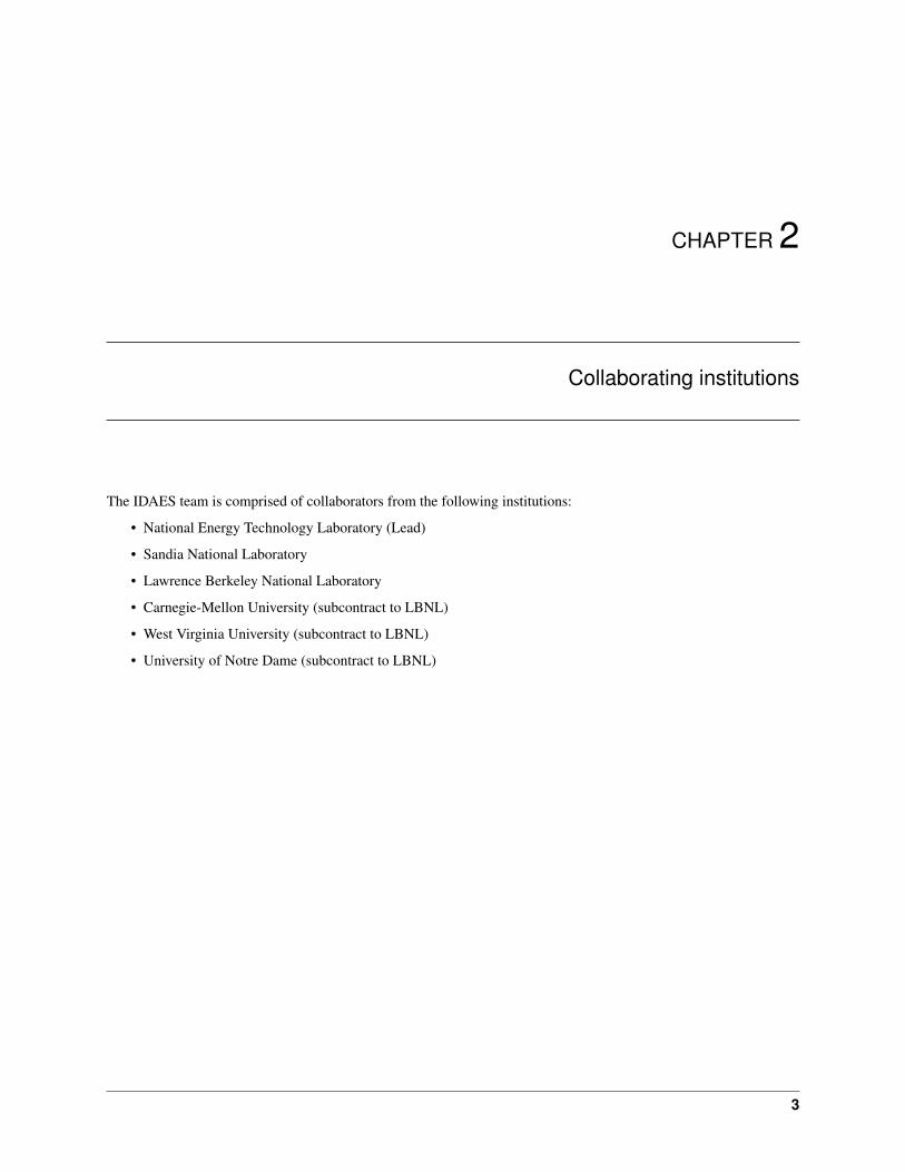
The IDAES team is comprised of collaborators from the following institutions:
• National Energy Technology Laboratory (Lead)
• Sandia National Laboratory
• Lawrence Berkeley National Laboratory
• Carnegie-Mellon University (subcontract to LBNL)
• West Virginia University (subcontract to LBNL)
• University of Notre Dame (subcontract to LBNL)
3
IDAES Documentation, Release 1.7.0
4 Chapter 2. Collaborating institutions

CHAPTER 3
Contact, contributions and more information
General, background and overview information is available at the IDAES main website. Framework developmenthappens at our GitHub repo where you can report issues/bugs or make contributions. For further enquiries, send anemail to: <[email protected]>
5
IDAES Documentation, Release 1.7.0
6 Chapter 3. Contact, contributions and more information
CHAPTER 4
Contents
4.1 Getting Started
4.1.1 Installation
To install the IDAES PSE framework, follow the set of instructions below that are appropriate for your needs andoperating system. If you get stuck, please contact [email protected].
After installing and testing IDAES, it is strongly recommended to do the IDAES tutorials located on the examplesonline documentation page.
If you expect to develop custom models, we recommend following the advanced user installation.
The OS specific instructions provide information about optionally installing Miniconda. If you already have a Pythoninstallation you prefer, you can skip the Miniconda install section.
Note: IDAES supports Python 3.6 and above.
System SectionLinux LinuxWindows WindowsMac OSX Mac/OSXGeneric Generic install
Warning: If you are using Python for other complex projects, you may want to consider using environments ofsome sort to avoid conflicting dependencies. There are several good options including conda environments if youuse Anaconda.
7
IDAES Documentation, Release 1.7.0
4.1.2 Windows
Install Miniconda (optional)
1. Download: https://repo.anaconda.com/miniconda/Miniconda3-latest-Windows-x86_64.exe
2. Install anaconda from the downloaded file in (1).
3. Open the Anaconda Prompt (Start -> “Anaconda Prompt”).
4. In the Anaconda Prompt, follow the Generic install instructions.
4.1.3 Linux
Install Miniconda (optional)
1. Download: https://repo.anaconda.com/miniconda/Miniconda3-latest-Linux-x86_64.sh
2. Open a terminal window
3. Run the script you downloaded in (1).
Install Dependencies
1. The IPOPT solver depends on the GNU FORTRAN, GOMP, Blas, and Lapack libraries, If these libraries arenot already installed on your Linux system, you or your system administrator can use the sample commandsbelow to install them. If you have a Linux distribution that is not listed, IPOPT should still work, but you thecommands to install the required libraries may differ. If these libraries are already installed, you can skip thisand proceed with the next step.
Note: Depending on your distribution, you may need to prepend sudo to these commands or switch to the“root” user.
apt-get (Current Ubuntu based distributions):
sudo apt-get install libgfortran4 libgomp1 liblapack3 libblas3
yum (Current RedHat based distributions, including CentOS):
yum install lapack blas libgfortran libgomp
Complete Generic Install
Follow the Generic install instructions.
4.1.4 Mac/OSX
Install Miniconda (optional)
1. Download: https://repo.anaconda.com/miniconda/Miniconda3-latest-MacOSX-x86_64.sh
2. For the next steps, open a terminal window
3. Run the script you downloaded in (1).
Complete Generic Install
Follow the Generic install instructions.
8 Chapter 4. Contents
IDAES Documentation, Release 1.7.0
4.1.5 Generic install
The remaining steps performed in either the Linux or OSX Terminal or Powershell. If you installed Miniconda onWindows use the Anaconda Prompt or Anaconda Powershell Prompt. Regardless of OS and shell, the following stepsare the same.
Install IDAES
1. Install IDAES with pip:
pip install idaes-pse
2. Run the idaes get-extensions command to install the compiled binaries:
idaes get-extensions
Warning: The IDAES binary extensions are not yet supported on Mac/OSX.
As fallback (assuming you are uisng a conda env) you can install the generic ipopt solver with thecommand conda install -c conda-forge ipopt though this will not have all the featuresof our extentions package.
3. Run the idaes get-examples command to download and install the example files:
idaes get-examples
By default this will install in a folder “examples” in the current directory. The command has many options,but an important one is –dir, which specifies the folder in which to install.
for Mac and Linux users this would look like:
idaes get-examples --dir ~/idaes/examples
or, for Windows users, it would look like:
idaes get-examples --dir C:\Users\MyName\IDAES\Examples
Refer to the full idaes get-examples command documentation for more information.
4. Run tests:
pytest --pyargs idaes -W ignore
5. You should see the tests run and all should pass to ensure the installation worked. You may see some “Error”level log messages, but they are okay, and produced by tests for error handling. The number of tests that failedand succeeded is reported at the end of the pytest output. You can report problems on the Github issues page(Please try to be specific about the command and the offending output.)
4.2 User Guide
4.2.1 Why IDAES
The National Energy Technology Laboratory’s Institute for the Design of Advanced Energy Systems (IDAES) is apowerful and versatile computational platform offering next-generation engineering capabilities for optimizing the
4.2. User Guide 9
IDAES Documentation, Release 1.7.0
design and operation of innovative chemical process and energy systems beyond current constraints on complexity,uncertainty, and scales ranging from materials to process to market.
The IDAES Integrated Platform was conceived in 2016 to specifically address the gaps between state-of-the-art simu-lation packages and algebraic modeling languages.
Major strengths of commercial simulation packages are their libraries of unit models and thermophysical properties.However, such simulation packages often have difficulty optimizing flowsheets and have limited support for incorpo-rating models of non-standard, dynamic units, such as solids handling, and uncertainty quantification. On the otherhand, AMLs are eminently flexible and readily support large-scale optimization, but considerable work is required toconstruct process models, which are often only useful for a one-time application.
The IDAES Integrated Platform represents an innovative approach for the design and optimization of chemical andenergy processes by integrating an extensible, equation-oriented process model library with Pyomo (a Python-basedAML). Built specifically to enable rigorous large-scale mathematical optimization, the platform includes capabilitiesfor conceptual design, steady-state and dynamic optimization, multi-scale modeling, uncertainty quantification, andthe automated development of thermodynamic, physical property, and kinetic sub-models from experimental data.
Key Features
Open Source
All IDAES Code is completely free and redistributable, the license is avaliable here. Users are free to modify andredistribute code, and community development is encouraged.
Equation Oriented
By using an equation-oriented platform, users gain access to a wide range of highly efficient, derivative-based numeri-cal solvers for a wide range of problem types, including support for both linear and non-linear problems, ordinary andpartial differential equations, and problems involving binary and integer variables.
Fully-Featured Programming Environment
By building off of Python, a fully-featured programming environment, users gain access to a wide range of librariesfor tools such as data visualization and management.
Extensible
The source code for all models and tools is fully-open and visible to the user. This allows users to both see andunderstand what is happening in each model, but also modify and extend models to suit their needs.
Flexible Form
No single model form is best suited to all applications, thus the IDAES Integrated Platform is built to provide userswith access to a range of different model forms. This allows users to easily pick-and-choose from the available modelforms to find the one best suited to their particular application.
10 Chapter 4. Contents
IDAES Documentation, Release 1.7.0
Access to Advanced Capabilities
IDAES aims to provide an integrated platform for development of not just process models but also tools for solving andanalyzing these problems. The platform supports conceptual design, parameter estimation, model predictive control,uncertainty quantification, and surrogate modeling.
4.2.2 Concepts
The IDAES Integrated Platform combines an extensible, equation-oriented process modeling framework with ad-vanced solver and computer architectures to enable advanced process systems engineering capabilities. The platformis based on the Python-based algebraic modeling language Pyomo, and while not necessary, users may benefit from abasic familiarity with Pyomo (link to documentation).
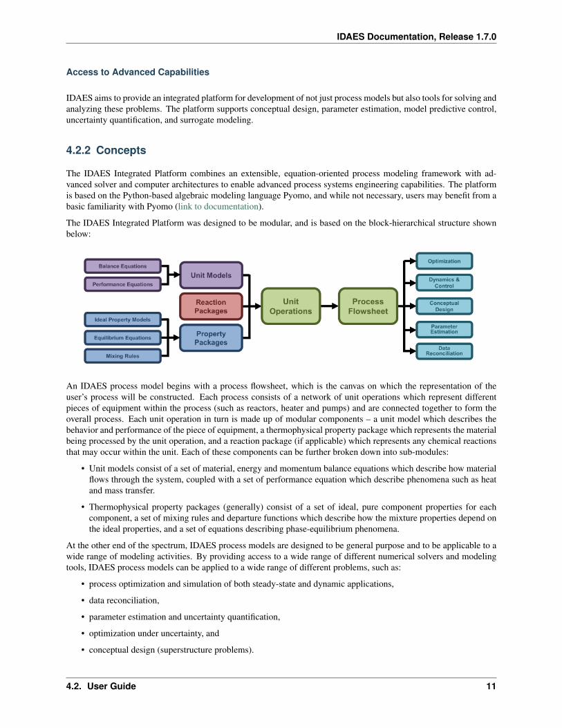
The IDAES Integrated Platform was designed to be modular, and is based on the block-hierarchical structure shownbelow:
An IDAES process model begins with a process flowsheet, which is the canvas on which the representation of theuser’s process will be constructed. Each process consists of a network of unit operations which represent differentpieces of equipment within the process (such as reactors, heater and pumps) and are connected together to form theoverall process. Each unit operation in turn is made up of modular components – a unit model which describes thebehavior and performance of the piece of equipment, a thermophysical property package which represents the materialbeing processed by the unit operation, and a reaction package (if applicable) which represents any chemical reactionsthat may occur within the unit. Each of these components can be further broken down into sub-modules:
• Unit models consist of a set of material, energy and momentum balance equations which describe how materialflows through the system, coupled with a set of performance equation which describe phenomena such as heatand mass transfer.
• Thermophysical property packages (generally) consist of a set of ideal, pure component properties for eachcomponent, a set of mixing rules and departure functions which describe how the mixture properties depend onthe ideal properties, and a set of equations describing phase-equilibrium phenomena.
At the other end of the spectrum, IDAES process models are designed to be general purpose and to be applicable to awide range of modeling activities. By providing access to a wide range of different numerical solvers and modelingtools, IDAES process models can be applied to a wide range of different problems, such as:
• process optimization and simulation of both steady-state and dynamic applications,
• data reconciliation,
• parameter estimation and uncertainty quantification,
• optimization under uncertainty, and
• conceptual design (superstructure problems).
4.2. User Guide 11
IDAES Documentation, Release 1.7.0
Modeling Components
The IDAES Integrated Platform represents each level within the hierarchy above using “modeling components”. Eachof these components represents a part of the overall model structure and form the basic building blocks of any IDAESprocess model. An introduction to each of the IDAES modeling components can be found here.
Model Libraries
To provide a starting point for modelers in using the process modeling tools, the IDAES Integrated Platform containsa library of models for common unit operations and thermophysical properties. Modelers can use these out-of-the-boxmodels to represent their process applications or as building blocks for developing their own models. All modelswithin IDAES are designed to be fully open and extensible, allowing users to inspect and modify them to suit theirneeds. Documentation of the available model libraries can be found here.
Modeling Extensions
The IDAES Integrated Platform also provides users with access to a number of cutting edge tools not directly relatedto process modeling. These tools are collected under the heading of Modeling Extensions, and information on themcan be found here.
4.2.3 Components
The purpose of this section of the documentation is to provide a general introduction to the top level components ofthe IDAES Integrated Platform. Each component is described in greater detail with a link in their description.
Note: IDAES is based on python-based algebraic modeling language, Pyomo. The documentation for its compo-nents (i.e. sets, parameters, variables, objectives, constraints, expressions, and suffixes) are provided in the Pyomodocumentation.
Flowsheet
Time Domain
Time domain is an essential component of the IDAES framework. When a user first declares a Flowsheet model a timedomain is created, the form of which depends on whether the Flowsheet is declared to be dynamic or steady-state (seeFlowsheetBlock). In situations where the user makes use of nested flowsheets, each sub-flowsheet refers to its parentflowsheet for the time domain.
Different models may handle the time domain differently, but in general all IDAES models refer to the time domainof their parent flowsheet. The only exception to this are blocks associated with Property calculations. PropertyBlocks(i.e. StateBlocks and ReactionBlocks) represent the state of the material at a single point in space and time, and thusdo not contain the time domain. Instead, PropertyBlocks are indexed by time (and space where applicable) - i.e. thereis a separate StateBlock for each point in time. The user should keep this in mind when working with IDAES models,as it is important for understanding where the time index appears within a model.
In order to facilitate referencing of the time domain, all Flowsheet objects have a time configuration argument whichis a reference to the time domain for that flowsheet. All IDAES models contain a flowsheet method which returnsthe parent flowsheet object, thus a reference to the time domain can always be found using the following code: flow-sheet().config.time.
12 Chapter 4. Contents
IDAES Documentation, Release 1.7.0
Another important thing to note is that steady-state models do contain a time domain. While the time domain forsteady-stage models is a single point at time = 0.0, they still contain a reference to the time domain and the components(e.g. StateBlocks) are indexed by time.
Flowsheet models are the top level of the IDAES modeling hierarchy. The flowsheet is implemented with a Flow-sheetBlock, which provides a container for other components. Flowsheet models generally contain three types ofcomponents:
1. Unit models, representing unit operations
2. Property packages, representing the parameters and relationships for property calculations
3. Arcs, representing connections between unit models
The FlowsheetBlock is also where the time domain is implemented. While the time domain is essential for dynamicmodeling, the time domain exists even for steady state models (single point in time).
Flowsheet models may also contain additional constraints relating to how different unit models behave and interact,such as control and operational constraints. Generally speaking, if a constraint is purely internal to a single unit, anddoes not depend on information from other units in the flowsheet, then the constraint should be placed inside therelevant unit model. Otherwise, the constraint should be placed at the flowsheet level.
Property Package
• Overview
• Units of Measurement
• Physical properties
• Reaction properties
• Component and Phase Objects
• As Needed Properties
• Generic Property Package Framework
• Generic Reaction Package Framework
Overview
Component Object
Component objects are used to identify the chemical species of interest in a property package and to contain informa-tion describing the behavior of that component (such as properties of that component). Additional information on theComponent Class is provided in the technical specifications.
The following types of components are currently supported.
• Component - general purpose object for representing chemical species.
• Solute - component object for representing species which should be treated as a solute in a LiquidPhase.
• Solvent - component object for representing species which should be treated as a solvent in a LiquidPhase.
• Ion - general purpose component object for representing ion species (LiquidPhase only). Users should generallyuse the Anion or Cation components instead.
4.2. User Guide 13
IDAES Documentation, Release 1.7.0
• Anion - component object for representing ion species with a negative charge (LiquidPhase only).
• Cation - component object for representing ion species with a positive charger(LiquidPhase only).
Component objects are intended to store all the necessary information regarding a given chemical species for usewithin a process model. Examples of such information include the methods and parameters required for calculatingthermophysical properties. Additionally, certain unit operations handle components in different ways depending oncertain criteria. An example of this is Reverse Osmosis, where the driving force across the membrane is calculateddifferently for solvent species and solute species.
Component objects implement the following methods for determining species behavior:
• is_solute() - returns True if species is a solute (Solute, Ion, Anion or Cation component objects), otherwise False.
• is_solvent() - returns True if species is a solvent (Solvent component object), otherwise False.
Note: The general purpose Component object does not distinguish solutes and solvents, and these methods will willraise a TypeError instead.
Phase Object
Phase objects are used to identify the thermodynamic phases of interest in a property package and to contain informa-tion describing the behavior of that phase (for example the equation of state which describes that phase). Additionalinformation on the Phase Class is provided in the technical specifications.
TThe following types of phases, along with a generic Phase object, are supported:
• LiquidPhase
• SolidPhase
• VaporPhase
In a number of unit operations, different phases behave in different ways. For example, in a Flash operation, the vaporphase exits through the top outlet whilst liquid phase(s) (and any solids) exit through the bottom outlet. In order todetermine how a given phase should behave in these situations, each Phase object implements the following threemethods:
• is_liquid_phase()
• is_solid_phase()
• is_vapor_phase()
These methods return a boolean (True or False) indicating whether the unit operation should treat the phase as beingof the specified type in order to decide on how it should behave. Each type of phase returns True for its type andFalse for all other types (e.g. LiquidPhase returns True for is_liquid_phase() and False for is_solid_phase() andis_vapor_phase().
The generic Phase object determines what to return for each method based on the user-provided name for the instanceof the Phase object as shown below:
• is_liquid_phase() returns True if the Phase name contains the string Liq, otherwise it returns False.
• is_solid_phase() returns True if the Phase name contains the string Sol, otherwise it returns False.
• is_vapor_phase() returns True if the Phase name contains the string Vap, otherwise it returns False.
Users should avoid using the generic Phase object, as this is primarily intended as a base class for the specific phaseclasses and for backwards compatibility.
14 Chapter 4. Contents
IDAES Documentation, Release 1.7.0
Physical Parameter Block
PhysicalParameterBlocks serve as a central location for linking to a property package, and contain all the parametersand indexing sets used by a given property package.
The role of the PhysicalParameterBlock Class is to set up the references required by the rest of the IDAES CoreModeling Framework for constructing instances of StateBlocks and attaching these to the PhysicalParameterBlock forease of use. This allows other models to be pointed to the PhysicalParameterBlock in order to collect the necessaryinformation and to construct the necessary StateBlocks without the need for the user to do this manually.
Several attributes in the PhysicalParameterBlock are used to inform the construction of other components. Theseattributes include:
• state_block_class - a pointer to the associated class that should be called when constructing StateBlocks. Thisshould only be set by the property package developer.
• phase_list - a Pyomo Set object defining the valid phases of the mixture of interest.
• component_list - a Pyomo Set defining the names of the chemical species present in the mixture.
• element_list - (optional) a Pyomo Set defining the names of the chemical elements that make up the specieswithin the mixture. This is used when doing elemental material balances.
• element_comp - (optional) a dictionary-like object which defines the elemental composition of each species incomponent_list. Form: component: element_1: value, element_2: value, . . . .
• supported properties metadata - a dictionary of supported physical properties that the property package supports,along with instruction to construct the associated variables and constraints, and the units of measurement usedfor the property. This information is set using the add_properties attribute of the define_metadata class method.
Reaction Block
ReactionBlocks are used within IDAES UnitModels (generally within ControlVolumeBlocks) in order to calculatereaction properties given the state of the material (provided by an associated StateBlock). ReactionBlocks are no-tably different to other types of Blocks within IDAES as they are always indexed by time (and possibly space aswell), and are also not fully self contained (in that they depend upon the associated state block for certain variables).ReactionBlocks are composed of two parts:
• ReactionBlockDataBase forms the base class for all ReactionBlockData objects, which contain the instructionson how to construct each instance of a Reaction Block.
• ReactionBlockBase is used for building classes which contain methods to be applied to sets of Indexed ReactionBlocks (or to a subset of these). See the documentation on declare_process_block_class and the IDAES tutorialsand examples for more information.
ReactionBlocks can be constructed directly from the associated ReactionParameterBlock by calling thebuild_reaction_block() method on the ReactionParameterBlock. The parameters construction argument will be auto-matically set, and any other arguments (including indexing sets) may be provided to the build_reaction_block methodas usual.
Additional details on ReactionBlocks are located in the technical specifications.
Reaction Parameter Block
ReactionParameterBlocks serve as a central location for linking to a property package, and contain all the parametersand indexing sets used by a given property package.
4.2. User Guide 15
IDAES Documentation, Release 1.7.0
The role of the ReactionParameterBlock Class is to set up the references required by the rest of the IDAES frameworkfor constructing instances of ReactionBlocks and attaching these to the ReactionParameterBlock for ease of use. Thisallows other models to be pointed to the ReactionParameterBlock in order to collect the necessary information and toconstruct the necessary ReactionBlocks without the need for the user to do this manually.
Reaction property packages are used by all of the other modeling components to inform them of what needs to beconstructed when dealing with chemical reactions. In order to do this, the IDAES modeling framework looks for anumber of attributes in the ReactionParameterBlock which are used to inform the construction of other components.These attributes include:
• reaction_block_class - a pointer to the associated class that should be called when constructing ReactionBlocks.This should only be set by the property package developer.
• phase_list - a Pyomo Set object defining the valid phases of the mixture of interest.
• component_list - a Pyomo Set defining the names of the chemical species present in the mixture.
• rate_reaction_idx - a Pyomo Set defining a list of names for the kinetically controlled reactions of interest.
• rate_reaction_stoichiometry - a dict-like object defining the stoichiometry of the kinetically controlled reactions.Keys should be tuples of (rate_reaction_idx, phase_list, component_list) and values equal to the stoichiometriccoefficient for that index.
• equilibrium_reaction_idx - a Pyomo Set defining a list of names for the equilibrium controlled reactions ofinterest.
• equilibrium_reaction_stoichiometry - a dict-like object defining the stoichiometry of the equilibrium controlledreactions. Keys should be tuples of (equilibrium_reaction_idx, phase_list, component_list) and values equal tothe stoichiometric coefficient for that index.
• supported properties metadata - a list of supported reaction properties that the property package supports, alongwith instruction to construct the associated variables and constraints, and the units of measurement used for theproperty. This information is set using the add_properties attribute of the define_metadata class method.
• required properties metadata - a list of physical properties that the reaction property calculations depend upon,and must be supported by the associated StateBlock. This information is set using the add_required_propertiesattribute of the define_metadata class method.
State Block
StateBlocks are used within all IDAES UnitModels (generally within ControlVolumeBlocks) in order to calculatephysical properties given the state of the material. StateBlocks are notably different to other types of Blocks withinIDAES as they are always indexed by time (and possibly space as well). StateBlocks consist of two parts:
• StateBlockData forms the base class for all StateBlockData objects, which contain the instructions on how toconstruct each instance of a State Block.
• StateBlock is used for building classes which contain methods to be applied to sets of Indexed State Blocks(or to a subset of these). See the documentation on declare_process_block_class and the IDAES tutorials andexamples for more information.
StateBlocks can be constructed directly from the associated PhysicalParameterBlock by calling the build_state_block()method on the PhysicalParameterBlock. The parameters construction argument will be automatically set, and anyother arguments (including indexing sets) may be provided to the build_state_block method as usual.
Additional details on State Blocks are located in the technical specifications.
16 Chapter 4. Contents
IDAES Documentation, Release 1.7.0
Defining Units of Measurement
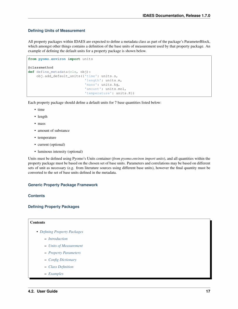
All property packages within IDAES are expected to define a metadata class as part of the package’s ParameterBlock,which amongst other things contains a definition of the base units of measurement used by that property package. Anexample of defining the default units for a property package is shown below.
from pyomo.environ import units
@classmethoddef define_metadata(cls, obj):
obj.add_default_units('time': units.s,'length': units.m,'mass': units.kg,'amount': units.mol,'temperature': units.K)
Each property package should define a default units for 7 base quantities listed below:
• time
• length
• mass
• amount of substance
• temperature
• current (optional)
• luminous intensity (optional)
Units must be defined using Pyomo’s Units container (from pyomo.environ import units), and all quantities within theproperty package must be based on the chosen set of base units. Parameters and correlations may be based on differentsets of unit as necessary (e.g. from literature sources using different base units), however the final quantity must beconverted to the set of base units defined in the metadata.
Generic Property Package Framework
Contents
Defining Property Packages
Contents
• Defining Property Packages
– Introduction
– Units of Measurement
– Property Parameters
– Config Dictionary
– Class Definition
– Examples
4.2. User Guide 17
IDAES Documentation, Release 1.7.0
Introduction
In order to create and use a property package using the IDAES Generic Property Package Framework, users mustprovide a definition for the material they wish to model. The framework supports two approaches for defining theproperty package, which are described below, both of which are equivalent in practice.
Units of Measurement
When defining a property package using the generic framework, users must define the base units for the propertypackage (see link). The approach for setting the base units depends on the approach used to define the propertypackage, and is discussed in more detail in each section.
The Generic Property Package Framework includes the necessary code to convert between different units of mea-surement as required, allowing users to combine property methods with different sets of units into a single propertypackage. In these cases, each property method is written in its natural units (including parameters), and the final resultis automatically converted to the base units.
For example, the Antoine equation is generally written with pressure in bars and temperature in either Kelvin orCelsius (depending on source). Using the generic property framework, the users provide the Antoine coefficients intheir original units (i.e. bar and Kelvin/Celsius) and the property calculation is written in these units. However, thefinal result (saturation pressure) is then converted to the base units specified in the property package definition.
Property Parameters
Thermophysical property models all depend upon a set of parameters to describe the fundamental behavior of thesystem. For the purposes of the Generic Property Framework, these parameters are grouped into three types:
1. Component-specific parameters - these are parameters that are specific to a given chemical species, and aredefined in the parameter_data argument for each component and stored in the associated Component block.Examples of these parameters include those used to calculate the ideal, pure component properties.
2. Phase-specific parameters - these are parameters that are specific to a given phase, and are defined in the pa-rameter_data argument for each phase and stored in the associated Phase block. These types of parameters arerelatively uncommon.
3. Package-wide parameters - these are parameters that are not necessarily confined to a single phase or species,and are defined in the parameter_data argument of the overall property package and stored in the main PhysicalParameter block. Examples of these types of parameters include binary interaction parameters, which involvemultiple species and can be used in multiple phases.
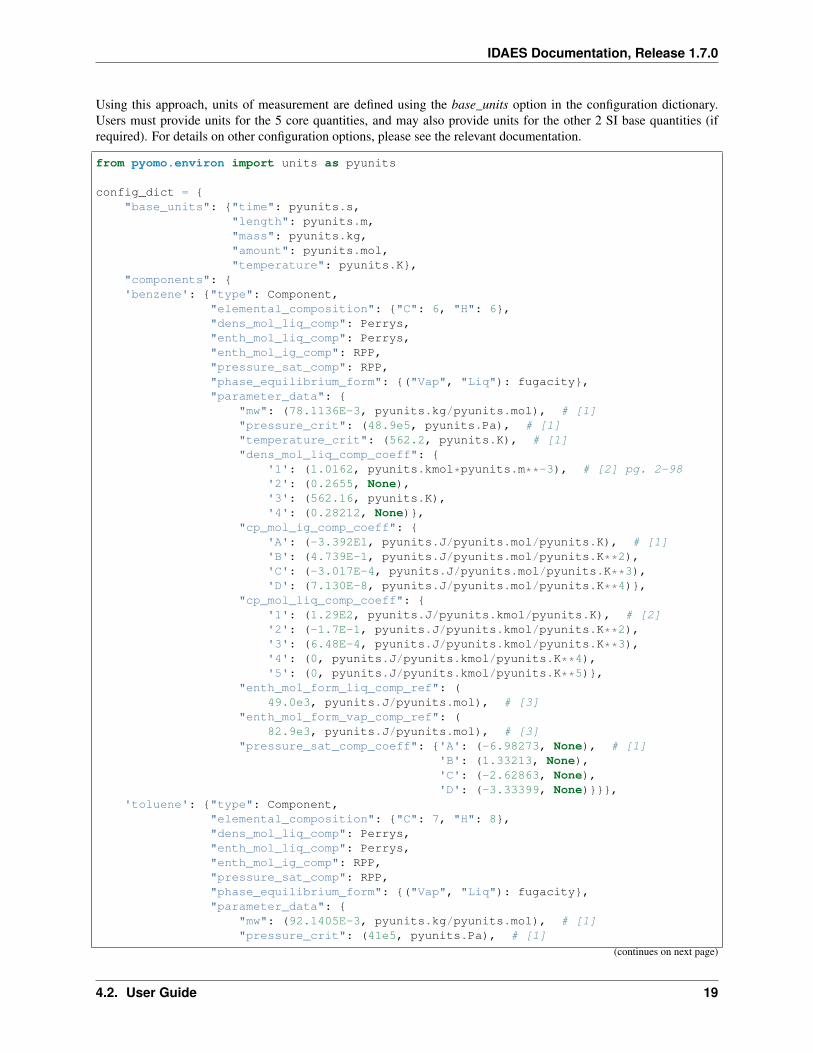
Config Dictionary
The most common way to use the Generic Property Package Framework is to create an instance of the GenericParam-eterBlock component and provide it with a dictionary of configuration arguments, as shown below:
m = ConcreteModel()
m.fs = FlowsheetBlock()
m.fs.properties = GenericParameterBlock(default=config_dict)
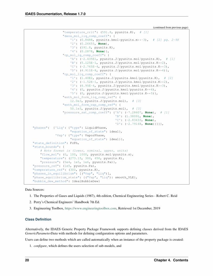
Users need to populate config_dict with the desired options for their system as described in the other parts of thisdocumentation. An example of a configuration dictionary for a benzene-toluene VLE system is shown below.
18 Chapter 4. Contents
IDAES Documentation, Release 1.7.0
Using this approach, units of measurement are defined using the base_units option in the configuration dictionary.Users must provide units for the 5 core quantities, and may also provide units for the other 2 SI base quantities (ifrequired). For details on other configuration options, please see the relevant documentation.
from pyomo.environ import units as pyunits
config_dict = "base_units": "time": pyunits.s,
"length": pyunits.m,"mass": pyunits.kg,"amount": pyunits.mol,"temperature": pyunits.K,
"components": 'benzene': "type": Component,
"elemental_composition": "C": 6, "H": 6,"dens_mol_liq_comp": Perrys,"enth_mol_liq_comp": Perrys,"enth_mol_ig_comp": RPP,"pressure_sat_comp": RPP,"phase_equilibrium_form": ("Vap", "Liq"): fugacity,"parameter_data":
"mw": (78.1136E-3, pyunits.kg/pyunits.mol), # [1]"pressure_crit": (48.9e5, pyunits.Pa), # [1]"temperature_crit": (562.2, pyunits.K), # [1]"dens_mol_liq_comp_coeff":
'1': (1.0162, pyunits.kmol*pyunits.m**-3), # [2] pg. 2-98'2': (0.2655, None),'3': (562.16, pyunits.K),'4': (0.28212, None),
"cp_mol_ig_comp_coeff": 'A': (-3.392E1, pyunits.J/pyunits.mol/pyunits.K), # [1]'B': (4.739E-1, pyunits.J/pyunits.mol/pyunits.K**2),'C': (-3.017E-4, pyunits.J/pyunits.mol/pyunits.K**3),'D': (7.130E-8, pyunits.J/pyunits.mol/pyunits.K**4),
"cp_mol_liq_comp_coeff": '1': (1.29E2, pyunits.J/pyunits.kmol/pyunits.K), # [2]'2': (-1.7E-1, pyunits.J/pyunits.kmol/pyunits.K**2),'3': (6.48E-4, pyunits.J/pyunits.kmol/pyunits.K**3),'4': (0, pyunits.J/pyunits.kmol/pyunits.K**4),'5': (0, pyunits.J/pyunits.kmol/pyunits.K**5),
"enth_mol_form_liq_comp_ref": (49.0e3, pyunits.J/pyunits.mol), # [3]
"enth_mol_form_vap_comp_ref": (82.9e3, pyunits.J/pyunits.mol), # [3]
"pressure_sat_comp_coeff": 'A': (-6.98273, None), # [1]'B': (1.33213, None),'C': (-2.62863, None),'D': (-3.33399, None),
'toluene': "type": Component,"elemental_composition": "C": 7, "H": 8,"dens_mol_liq_comp": Perrys,"enth_mol_liq_comp": Perrys,"enth_mol_ig_comp": RPP,"pressure_sat_comp": RPP,"phase_equilibrium_form": ("Vap", "Liq"): fugacity,"parameter_data":
"mw": (92.1405E-3, pyunits.kg/pyunits.mol), # [1]"pressure_crit": (41e5, pyunits.Pa), # [1]
(continues on next page)
4.2. User Guide 19
IDAES Documentation, Release 1.7.0
(continued from previous page)
"temperature_crit": (591.8, pyunits.K), # [1]"dens_mol_liq_comp_coeff":
'1': (0.8488, pyunits.kmol*pyunits.m**-3), # [2] pg. 2-98'2': (0.26655, None),'3': (591.8, pyunits.K),'4': (0.2878, None),
"cp_mol_ig_comp_coeff": 'A': (-2.435E1, pyunits.J/pyunits.mol/pyunits.K), # [1]'B': (5.125E-1, pyunits.J/pyunits.mol/pyunits.K**2),'C': (-2.765E-4, pyunits.J/pyunits.mol/pyunits.K**3),'D': (4.911E-8, pyunits.J/pyunits.mol/pyunits.K**4),
"cp_mol_liq_comp_coeff": '1': (1.40E2, pyunits.J/pyunits.kmol/pyunits.K), # [2]'2': (-1.52E-1, pyunits.J/pyunits.kmol/pyunits.K**2),'3': (6.95E-4, pyunits.J/pyunits.kmol/pyunits.K**3),'4': (0, pyunits.J/pyunits.kmol/pyunits.K**4),'5': (0, pyunits.J/pyunits.kmol/pyunits.K**5),
"enth_mol_form_liq_comp_ref": (12.0e3, pyunits.J/pyunits.mol), # [3]
"enth_mol_form_vap_comp_ref": (50.1e3, pyunits.J/pyunits.mol), # [3]
"pressure_sat_comp_coeff": 'A': (-7.28607, None), # [1]'B': (1.38091, None),'C': (-2.83433, None),'D': (-2.79168, None),
"phases": 'Liq': "type": LiquidPhase,"equation_of_state": ideal,
'Vap': "type": VaporPhase,"equation_of_state": ideal,
"state_definition": FcPh,"state_bounds":
# Note format is (lower, nominal, upper, units)"flow_mol": (0, 100, 1000, pyunits.mol/pyunits.s),"temperature": (273.15, 300, 450, pyunits.K),"pressure": (5e4, 1e5, 1e6, pyunits.Pa),
"pressure_ref": (1e5, pyunits.Pa),"temperature_ref": (300, pyunits.K),"phases_in_equilibrium": [("Vap", "Liq")],"phase_equilibrium_state": ("Vap", "Liq"): smooth_VLE,"bubble_dew_method": IdealBubbleDew
Data Sources:
1. The Properties of Gases and Liquids (1987), 4th edition, Chemical Engineering Series - Robert C. Reid
2. Perry’s Chemical Engineers’ Handbook 7th Ed.
3. Engineering Toolbox, https://www.engineeringtoolbox.com, Retrieved 1st December, 2019
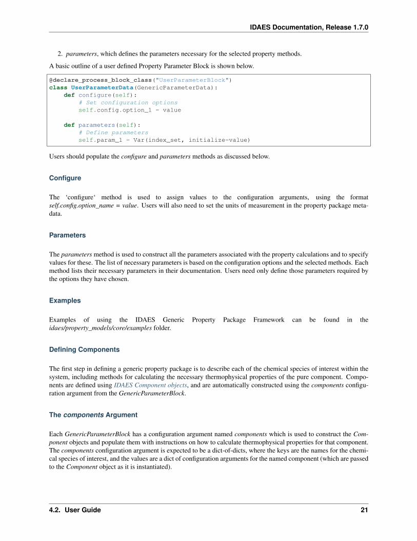
Class Definition
Alternatively, the IDAES Generic Property Package Framework supports defining classes derived from the IDAESGenericParameterData with methods for defining configuration options and parameters.
Users can define two methods which are called automatically when an instance of the property package is created:
1. configure, which defines the users selection of sub-models, and
20 Chapter 4. Contents
IDAES Documentation, Release 1.7.0
2. parameters, which defines the parameters necessary for the selected property methods.
A basic outline of a user defined Property Parameter Block is shown below.
@declare_process_block_class("UserParameterBlock")class UserParameterData(GenericParameterData):
def configure(self):# Set configuration optionsself.config.option_1 = value
def parameters(self):# Define parametersself.param_1 = Var(index_set, initialize=value)
Users should populate the configure and parameters methods as discussed below.
Configure
The ‘configure‘ method is used to assign values to the configuration arguments, using the formatself.config.option_name = value. Users will also need to set the units of measurement in the property package meta-data.
Parameters
The parameters method is used to construct all the parameters associated with the property calculations and to specifyvalues for these. The list of necessary parameters is based on the configuration options and the selected methods. Eachmethod lists their necessary parameters in their documentation. Users need only define those parameters required bythe options they have chosen.
Examples
Examples of using the IDAES Generic Property Package Framework can be found in theidaes/property_models/core/examples folder.
Defining Components
The first step in defining a generic property package is to describe each of the chemical species of interest within thesystem, including methods for calculating the necessary thermophysical properties of the pure component. Compo-nents are defined using IDAES Component objects, and are automatically constructed using the components configu-ration argument from the GenericParameterBlock.
The components Argument
Each GenericParameterBlock has a configuration argument named components which is used to construct the Com-ponent objects and populate them with instructions on how to calculate thermophysical properties for that component.The components configuration argument is expected to be a dict-of-dicts, where the keys are the names for the chemi-cal species of interest, and the values are a dict of configuration arguments for the named component (which are passedto the Component object as it is instantiated).
4.2. User Guide 21
IDAES Documentation, Release 1.7.0
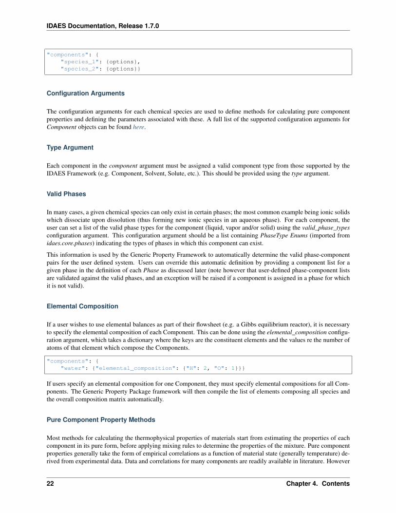
"components": "species_1": options,"species_2": options
Configuration Arguments
The configuration arguments for each chemical species are used to define methods for calculating pure componentproperties and defining the parameters associated with these. A full list of the supported configuration arguments forComponent objects can be found here.
Type Argument
Each component in the component argument must be assigned a valid component type from those supported by theIDAES Framework (e.g. Component, Solvent, Solute, etc.). This should be provided using the type argument.
Valid Phases
In many cases, a given chemical species can only exist in certain phases; the most common example being ionic solidswhich dissociate upon dissolution (thus forming new ionic species in an aqueous phase). For each component, theuser can set a list of the valid phase types for the component (liquid, vapor and/or solid) using the valid_phase_typesconfiguration argument. This configuration argument should be a list containing PhaseType Enums (imported fromidaes.core.phases) indicating the types of phases in which this component can exist.
This information is used by the Generic Property Framework to automatically determine the valid phase-componentpairs for the user defined system. Users can override this automatic definition by providing a component list for agiven phase in the definition of each Phase as discussed later (note however that user-defined phase-component listsare validated against the valid phases, and an exception will be raised if a component is assigned in a phase for whichit is not valid).
Elemental Composition
If a user wishes to use elemental balances as part of their flowsheet (e.g. a Gibbs equilibrium reactor), it is necessaryto specify the elemental composition of each Component. This can be done using the elemental_composition configu-ration argument, which takes a dictionary where the keys are the constituent elements and the values re the number ofatoms of that element which compose the Components.
"components": "water": "elemental_composition": "H": 2, "O": 1
If users specify an elemental composition for one Component, they must specify elemental compositions for all Com-ponents. The Generic Property Package framework will then compile the list of elements composing all species andthe overall composition matrix automatically.
Pure Component Property Methods
Most methods for calculating the thermophysical properties of materials start from estimating the properties of eachcomponent in its pure form, before applying mixing rules to determine the properties of the mixture. Pure componentproperties generally take the form of empirical correlations as a function of material state (generally temperature) de-rived from experimental data. Data and correlations for many components are readily available in literature. However
22 Chapter 4. Contents
IDAES Documentation, Release 1.7.0
due to the empirical nature of these correlations and the wide range of data available, different sources use differentforms for their correlations.
Within the IDAES Generic Property Package Framework, pure component property correlations can be provided aseither Python functions or classes;
• functions are used for self-contained correlations with hard-coded parameters,
• classes are used for more generic correlations which require associated parameters.
When providing a method via the components configuration argument, users can either provide a pointer to the de-sired class/method directly, or to a Python module containing a class or method with the same name as the propertyto be calculated. More details on the uses of these and how to construct your own can be found in the developerdocumentation.
Pure Component Libraries
As a starting point for users, the IDAES Generic Property Package Framework contains a library of some commonmethods for calculating properties of interest. These libraries are organized by source, and are listed below.
Note: Users should be careful about mixing-and-matching methods from different libraries, especially for the samecomponent. Thermodynamic properties are intrinsically coupled, thus many correlations are also linked and oftenshare parameters. Mixing-and-matching correlations may result in two correlations using parameters with the samename but with different expectations.
Additionally, sources often use different approaches for defining the thermodynamic reference state of the material,thus users need to ensure that a consistent reference state is being used when combining methods from differentsources.
NIST Webbook (NIST)
Contents
• NIST Webbook (NIST)
– Source
– Ideal Gas Molar Heat Capacity (Constant Pressure)
– Ideal Gas Molar Enthalpy
– Ideal Gas Molar Entropy
– Saturation (Vapor) Pressure
Source
Pure component properties as used by the NIST WebBook, https://webbook.nist.gov/chemistry/ Retrieved: September13th, 2019
4.2. User Guide 23
IDAES Documentation, Release 1.7.0
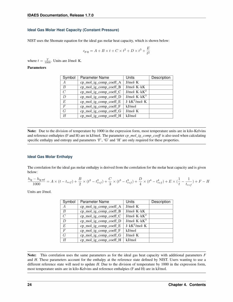
Ideal Gas Molar Heat Capacity (Constant Pressure)
NIST uses the Shomate equation for the ideal gas molar heat capacity, which is shown below:
𝑐p ig = 𝐴+𝐵 × 𝑡+ 𝐶 × 𝑡2 +𝐷 × 𝑡3 +𝐸
𝑡2
where 𝑡 = 𝑇1000 . Units are J/mol·K.
Parameters
Symbol Parameter Name Units Description𝐴 cp_mol_ig_comp_coeff_A J/mol·K𝐵 cp_mol_ig_comp_coeff_B J/mol·K· kK𝐶 cp_mol_ig_comp_coeff_C J/mol·K· kK2
𝐷 cp_mol_ig_comp_coeff_D J/mol·K· kK3
𝐸 cp_mol_ig_comp_coeff_E J· kK2/mol·K𝐹 cp_mol_ig_comp_coeff_F kJ/mol𝐺 cp_mol_ig_comp_coeff_G J/mol·K𝐻 cp_mol_ig_comp_coeff_H kJ/mol
Note: Due to the division of temperature by 1000 in the expression form, most temperature units are in kilo-Kelvinsand reference enthalpies (F and H) are in kJ/mol. The parameter cp_mol_ig_comp_coeff is also used when calculatingspecific enthalpy and entropy and parameters ‘F’, ‘G’ and ‘H’ are only required for these properties.
Ideal Gas Molar Enthalpy
The correlation for the ideal gas molar enthalpy is derived from the correlation for the molar heat capacity and is givenbelow:
ℎig − ℎig ref
1000= 𝐴× (𝑡− 𝑡𝑟𝑒𝑓 ) +
𝐵
2× (𝑡2 − 𝑡2𝑟𝑒𝑓 ) +
𝐶
3× (𝑡3 − 𝑡3𝑟𝑒𝑓 ) +
𝐷
4× (𝑡4 − 𝑡4𝑟𝑒𝑓 ) + 𝐸 × (
1
𝑡− 1
𝑡𝑟𝑒𝑓) + 𝐹 −𝐻
Units are J/mol.
Symbol Parameter Name Units Description𝐴 cp_mol_ig_comp_coeff_A J/mol·K𝐵 cp_mol_ig_comp_coeff_B J/mol·K· kK𝐶 cp_mol_ig_comp_coeff_C J/mol·K· kK2
𝐷 cp_mol_ig_comp_coeff_D J/mol·K· kK3
𝐸 cp_mol_ig_comp_coeff_E J· kK2/mol·K𝐹 cp_mol_ig_comp_coeff_F kJ/mol𝐺 cp_mol_ig_comp_coeff_G J/mol·K𝐻 cp_mol_ig_comp_coeff_H kJ/mol
Note: This correlation uses the same parameters as for the ideal gas heat capacity with additional parameters Fand H. These parameters account for the enthalpy at the reference state defined by NIST. Users wanting to use adifferent reference state will need to update H. Due to the division of temperature by 1000 in the expression form,most temperature units are in kilo-Kelvins and reference enthalpies (F and H) are in kJ/mol.
24 Chapter 4. Contents
IDAES Documentation, Release 1.7.0
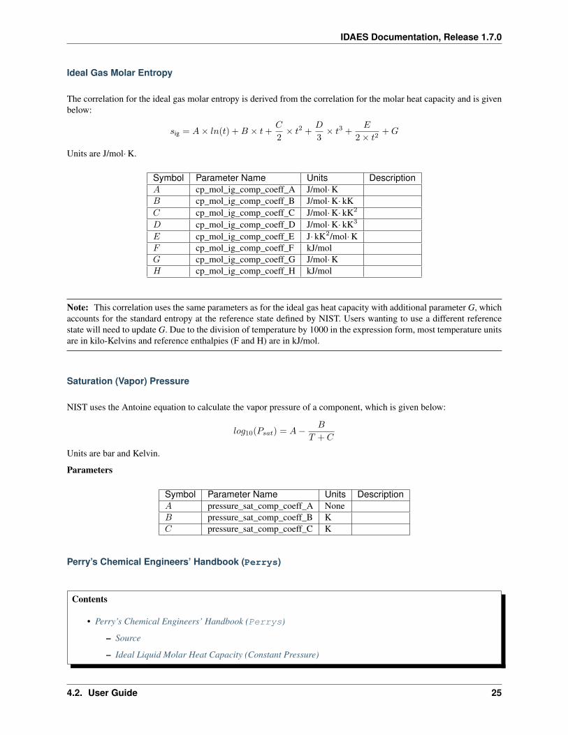
Ideal Gas Molar Entropy
The correlation for the ideal gas molar entropy is derived from the correlation for the molar heat capacity and is givenbelow:
𝑠ig = 𝐴× 𝑙𝑛(𝑡) +𝐵 × 𝑡+𝐶
2× 𝑡2 +
𝐷
3× 𝑡3 +
𝐸
2 × 𝑡2+𝐺
Units are J/mol·K.
Symbol Parameter Name Units Description𝐴 cp_mol_ig_comp_coeff_A J/mol·K𝐵 cp_mol_ig_comp_coeff_B J/mol·K· kK𝐶 cp_mol_ig_comp_coeff_C J/mol·K· kK2
𝐷 cp_mol_ig_comp_coeff_D J/mol·K· kK3
𝐸 cp_mol_ig_comp_coeff_E J· kK2/mol·K𝐹 cp_mol_ig_comp_coeff_F kJ/mol𝐺 cp_mol_ig_comp_coeff_G J/mol·K𝐻 cp_mol_ig_comp_coeff_H kJ/mol
Note: This correlation uses the same parameters as for the ideal gas heat capacity with additional parameter G, whichaccounts for the standard entropy at the reference state defined by NIST. Users wanting to use a different referencestate will need to update G. Due to the division of temperature by 1000 in the expression form, most temperature unitsare in kilo-Kelvins and reference enthalpies (F and H) are in kJ/mol.
Saturation (Vapor) Pressure
NIST uses the Antoine equation to calculate the vapor pressure of a component, which is given below:
𝑙𝑜𝑔10(𝑃𝑠𝑎𝑡) = 𝐴− 𝐵
𝑇 + 𝐶
Units are bar and Kelvin.
Parameters
Symbol Parameter Name Units Description𝐴 pressure_sat_comp_coeff_A None𝐵 pressure_sat_comp_coeff_B K𝐶 pressure_sat_comp_coeff_C K
Perry’s Chemical Engineers’ Handbook (Perrys)
Contents
• Perry’s Chemical Engineers’ Handbook (Perrys)
– Source
– Ideal Liquid Molar Heat Capacity (Constant Pressure)
4.2. User Guide 25
IDAES Documentation, Release 1.7.0
– Ideal Liquid Molar Enthalpy
– Ideal Liquid Molar Entropy
– Liquid Molar Density
Source
Methods for calculating pure component properties from:
Perry’s Chemical Engineers’ Handbook, 7th Edition Perry, Green, Maloney, 1997, McGraw-Hill
Ideal Liquid Molar Heat Capacity (Constant Pressure)
Perry’s Handbook uses the following correlation for ideal liquid molar heat capacity:
𝑐p liq = 𝐶1 + 𝐶2 × 𝑇 + 𝐶3 × 𝑇 2 + 𝐶4 × 𝑇 3 + 𝐶5 × 𝑇 4
Units are J/kmol·K.
Parameters
Symbol Parameter Name Units Description𝐶1 cp_mol_ig_comp_coeff_1 J/kmol·K𝐶2 cp_mol_ig_comp_coeff_2 J/kmol·K2
𝐶3 cp_mol_ig_comp_coeff_3 J/kmol·K3
𝐶4 cp_mol_ig_comp_coeff_4 J/kmol·K4
𝐶5 cp_mol_ig_comp_coeff_5 J/kmol·K5
Ideal Liquid Molar Enthalpy
The correlation for the ideal liquid molar enthalpy is derived from the correlation for the molar heat capacity and isgiven below:
ℎliq − ℎliq ref = 𝐶1 × (𝑇 − 𝑇𝑟𝑒𝑓 ) +𝐶2
2× (𝑇 2 − 𝑇 2
𝑟𝑒𝑓 ) +𝐶3
3× (𝑇 3 − 𝑇 3
𝑟𝑒𝑓 ) +𝐶4
4× (𝑇 4 − 𝑇 4
𝑟𝑒𝑓 ) +𝐶5
5× (𝑇 5 − 𝑇 5
𝑟𝑒𝑓 ) + ∆ℎform, Liq
Units are J/kmol.
Parameters
Symbol Parameter Name Units Description𝐶1 cp_mol_ig_comp_coeff_1 J/kmol·K𝐶2 cp_mol_ig_comp_coeff_2 J/kmol·K2
𝐶3 cp_mol_ig_comp_coeff_3 J/kmol·K3
𝐶4 cp_mol_ig_comp_coeff_4 J/kmol·K4
𝐶5 cp_mol_ig_comp_coeff_5 J/kmol·K5
∆ℎform, Liq enth_mol_form_liq_comp_ref J/kmol Molar heat of formation at reference state
Note: This correlation uses the same parameters as the ideal liquid heat capacity.
26 Chapter 4. Contents
IDAES Documentation, Release 1.7.0
Ideal Liquid Molar Entropy
The correlation for the ideal liquid molar entropy is derived from the correlation for the molar heat capacity and isgiven below:
𝑠liq − 𝑠liq ref = 𝐶1 × 𝑙𝑛(𝑇/𝑇𝑟𝑒𝑓 ) + 𝐶2 × (𝑇 − 𝑇𝑟𝑒𝑓 ) +𝐶3
2× (𝑇 2 − 𝑇 2
𝑟𝑒𝑓 ) +𝐶4
3× (𝑇 3 − 𝑇 3
𝑟𝑒𝑓 ) +𝐶5
4× (𝑇 4 − 𝑇 4
𝑟𝑒𝑓 ) + 𝑠form, Liq
Units are J/kmol·K.
Parameters
Symbol Parameter Name Units Description𝐶1 cp_mol_ig_comp_coeff_1 J/kmol·K𝐶2 cp_mol_ig_comp_coeff_2 J/kmol·K2
𝐶3 cp_mol_ig_comp_coeff_3 J/kmol·K3
𝐶4 cp_mol_ig_comp_coeff_4 J/kmol·K4
𝐶5 cp_mol_ig_comp_coeff_5 J/kmol·K5
𝑠form, Liq entr_mol_form_liq_comp_ref J/kmol·K Standard molar entropy of formation at reference state
Note: This correlation uses the same parameters as the ideal liquid heat capacity.
Liquid Molar Density
Perry’s Handbook uses the following correlation for liquid molar density:
𝜌𝑙𝑖𝑞 =𝐶1
𝐶1+(1− 𝑇
𝐶3)𝐶4
2
Units are kmol/m3.
Parameters
Symbol Parameter Name Units Description𝐶1 dens_mol_comp_liq_coeff_1 kmol/m3
𝐶2 dens_mol_comp_liq_coeff_2 None𝐶3 dens_mol_comp_liq_coeff_3 K𝐶4 dens_mol_comp_liq_coeff_4 None‘
Note: Currently, only the most common correlation form from Perry’s Handbook is implemented. Some componentsuse different forms which are not yet supported.
Properties of Gases and Liquids (RPP)
Contents
4.2. User Guide 27
IDAES Documentation, Release 1.7.0
• Properties of Gases and Liquids (RPP)
– Source
– Ideal Gas Molar Heat Capacity (Constant Pressure)
– Ideal Gas Molar Enthalpy
– Ideal Gas Molar Entropy
– Saturation (Vapor) Pressure
Source
Methods for calculating pure component properties from:
The Properties of Gases & Liquids, 4th Edition Reid, Prausnitz and Polling, 1987, McGraw-Hill
All methods use SI units.
Ideal Gas Molar Heat Capacity (Constant Pressure)
Properties of Gases and Liquids uses the following correlation for the ideal gas molar heat capacity:
𝑐p ig = 𝐴+𝐵 × 𝑇 + 𝐶 × 𝑇 2 +𝐷 × 𝑇 3
Parameters
Symbol Parameter Name Units Description𝐴 cp_mol_ig_comp_coeff_A J/mol·K𝐵 cp_mol_ig_comp_coeff_B J/mol·K2
𝐶 cp_mol_ig_comp_coeff_C J/mol·K3
𝐷 cp_mol_ig_comp_coeff_D J/mol·K4
Ideal Gas Molar Enthalpy
The correlation for the ideal gas molar enthalpy is derived from the correlation for the molar heat capacity and is givenbelow:
ℎig − ℎig ref = 𝐴× (𝑇 − 𝑇𝑟𝑒𝑓 ) +𝐵
2× (𝑇 2 − 𝑇 2
𝑟𝑒𝑓 ) +𝐶
3× (𝑇 3 − 𝑇 3
𝑟𝑒𝑓 ) +𝐷
4× (𝑇 4 − 𝑇 4
𝑟𝑒𝑓 ) + ∆ℎform, Vap
Parameters
Symbol Parameter Name Units Description𝐴 cp_mol_ig_comp_coeff_A J/mol·K𝐵 cp_mol_ig_comp_coeff_B J/mol·K2
𝐶 cp_mol_ig_comp_coeff_C J/mol·K3
𝐷 cp_mol_ig_comp_coeff_D J/mol·K4
∆ℎform, Vap enth_mol_form_vap_comp_ref J/mol Molar heat of formation at reference state
Note: This correlation uses the same parameters as the ideal gas heat capacity correlation.
28 Chapter 4. Contents
IDAES Documentation, Release 1.7.0
Ideal Gas Molar Entropy
The correlation for the ideal gas molar entropy is derived from the correlation for the molar heat capacity and is givenbelow:
𝑠ig = 𝐴× 𝑙𝑛(𝑇/𝑇𝑟𝑒𝑓 ) +𝐵 × (𝑇 − 𝑇𝑟𝑒𝑓 ) +𝐶
2× (𝑇 2 − 𝑇 2
𝑟𝑒𝑓 ) +𝐷
3× (𝑇 3 − 𝑇 3
𝑟𝑒𝑓 ) + 𝑠form, Vap
Parameters
Symbol Parameter Name Units Description𝐴 cp_mol_ig_comp_coeff_A J/mol·K𝐵 cp_mol_ig_comp_coeff_B J/mol·K2
𝐶 cp_mol_ig_comp_coeff_C J/mol·K3
𝐷 cp_mol_ig_comp_coeff_D J/mol·K4
𝑠form, Vap entr_mol_form_vap_comp_ref J/mol·K Standard molar entropy of formation at reference state
Note: This correlation uses the same parameters as the ideal gas heat capacity correlation .
Saturation (Vapor) Pressure
Properties of Gases and Liquids uses the following correlation to calculate the vapor pressure of a component:
𝑙𝑛(𝑃𝑠𝑎𝑡
𝑃𝑐𝑟𝑖𝑡) × (1 − 𝑥) = 𝐴× 𝑥+𝐵 × 𝑥1.5 + 𝐶 × 𝑥3 +𝐷 × 𝑥6
where 𝑥 = 1 − 𝑇𝑇𝑐𝑟𝑖𝑡
.
Symbol Parameter Name Units Description𝐴 pressure_sat_comp_coeff_A None𝐵 pressure_sat_comp_coeff_B None𝐶 pressure_sat_comp_coeff_C None𝐷 pressure_sat_comp_coeff_D None𝑃𝑐𝑟𝑖𝑡 pressure_crit_comp Same as system pressure Critical pressure𝑇𝑐𝑟𝑖𝑡 temperature_crit_comp Same as system temperature Critical temperature
Note: This correlation is only valid at temperatures below the critical temperature. Above this point, there is no realsolution to the equation.
Properties of Gases and Liquids 3rd edition (RPP3)
Contents
• Properties of Gases and Liquids 3rd edition (RPP3)
– Source
4.2. User Guide 29
IDAES Documentation, Release 1.7.0
– Ideal Gas Molar Heat Capacity (Constant Pressure)
– Ideal Gas Molar Enthalpy
– Ideal Gas Molar Entropy
– Saturation (Vapor) Pressure
Source
Methods for calculating pure component properties from:
The Properties of Gases & Liquids, 3rd Edition Reid, Prausnitz and Polling, 1977, McGraw-Hill
Ideal Gas Molar Heat Capacity (Constant Pressure)
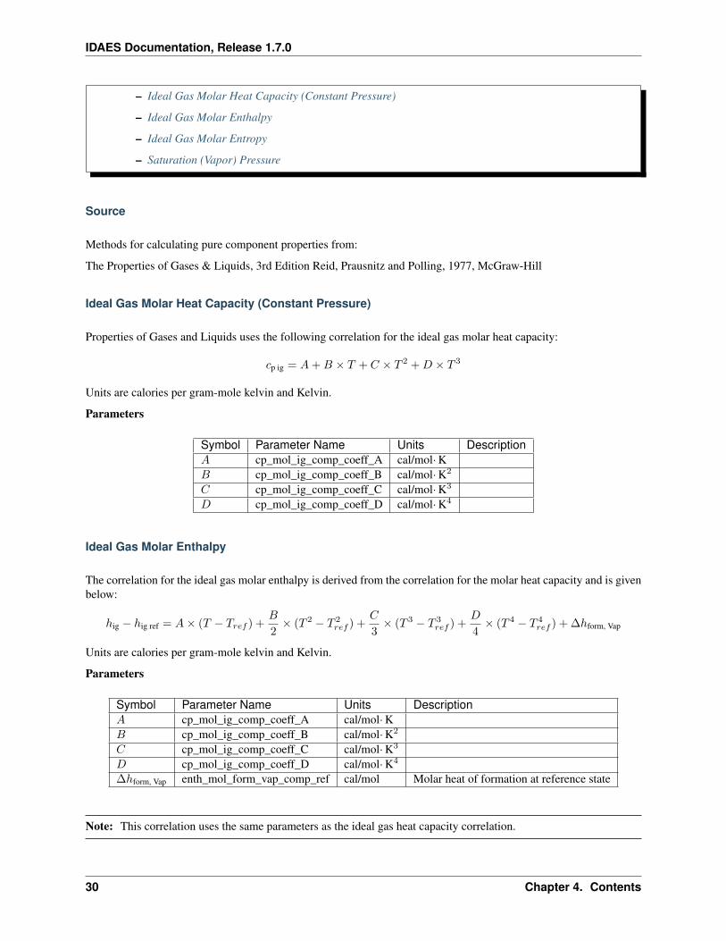
Properties of Gases and Liquids uses the following correlation for the ideal gas molar heat capacity:
𝑐p ig = 𝐴+𝐵 × 𝑇 + 𝐶 × 𝑇 2 +𝐷 × 𝑇 3
Units are calories per gram-mole kelvin and Kelvin.
Parameters
Symbol Parameter Name Units Description𝐴 cp_mol_ig_comp_coeff_A cal/mol·K𝐵 cp_mol_ig_comp_coeff_B cal/mol·K2
𝐶 cp_mol_ig_comp_coeff_C cal/mol·K3
𝐷 cp_mol_ig_comp_coeff_D cal/mol·K4
Ideal Gas Molar Enthalpy
The correlation for the ideal gas molar enthalpy is derived from the correlation for the molar heat capacity and is givenbelow:
ℎig − ℎig ref = 𝐴× (𝑇 − 𝑇𝑟𝑒𝑓 ) +𝐵
2× (𝑇 2 − 𝑇 2
𝑟𝑒𝑓 ) +𝐶
3× (𝑇 3 − 𝑇 3
𝑟𝑒𝑓 ) +𝐷
4× (𝑇 4 − 𝑇 4
𝑟𝑒𝑓 ) + ∆ℎform, Vap
Units are calories per gram-mole kelvin and Kelvin.
Parameters
Symbol Parameter Name Units Description𝐴 cp_mol_ig_comp_coeff_A cal/mol·K𝐵 cp_mol_ig_comp_coeff_B cal/mol·K2
𝐶 cp_mol_ig_comp_coeff_C cal/mol·K3
𝐷 cp_mol_ig_comp_coeff_D cal/mol·K4
∆ℎform, Vap enth_mol_form_vap_comp_ref cal/mol Molar heat of formation at reference state
Note: This correlation uses the same parameters as the ideal gas heat capacity correlation.
30 Chapter 4. Contents
IDAES Documentation, Release 1.7.0
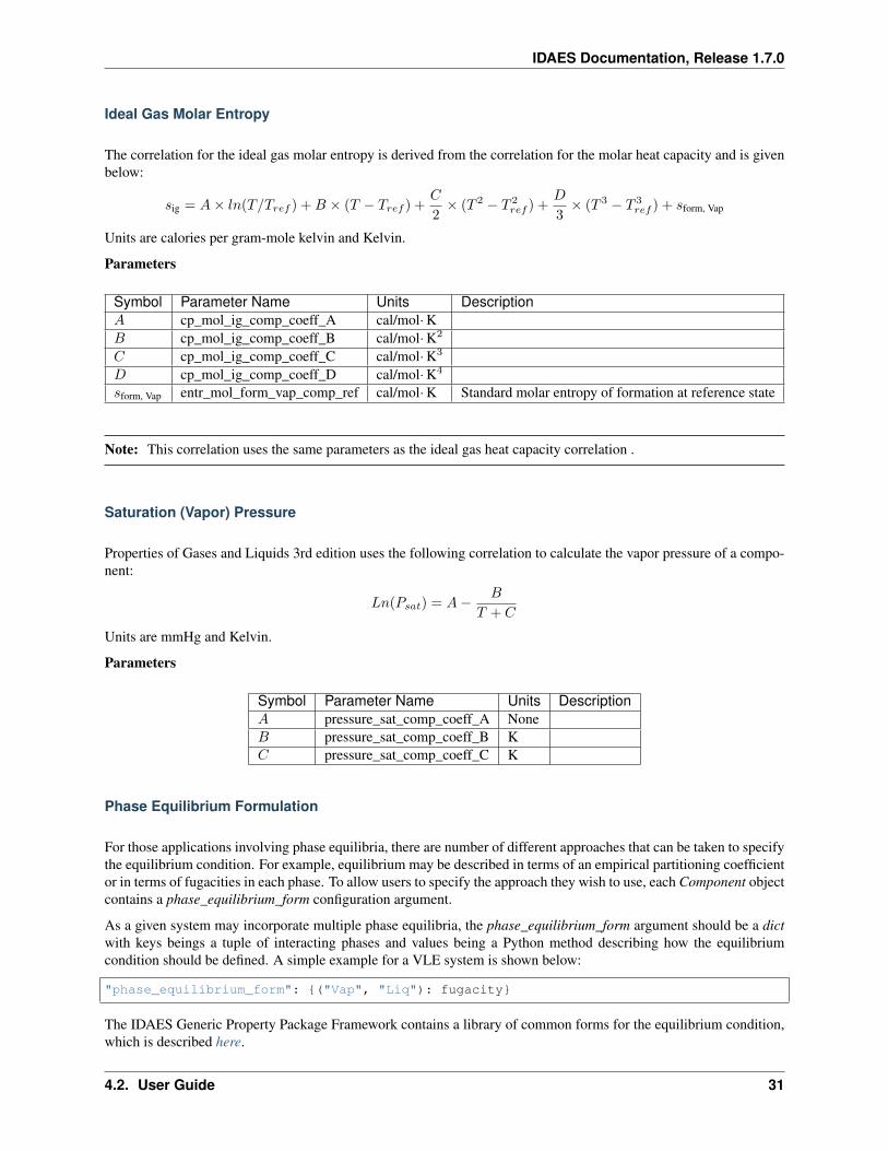
Ideal Gas Molar Entropy
The correlation for the ideal gas molar entropy is derived from the correlation for the molar heat capacity and is givenbelow:
𝑠ig = 𝐴× 𝑙𝑛(𝑇/𝑇𝑟𝑒𝑓 ) +𝐵 × (𝑇 − 𝑇𝑟𝑒𝑓 ) +𝐶
2× (𝑇 2 − 𝑇 2
𝑟𝑒𝑓 ) +𝐷
3× (𝑇 3 − 𝑇 3
𝑟𝑒𝑓 ) + 𝑠form, Vap
Units are calories per gram-mole kelvin and Kelvin.
Parameters
Symbol Parameter Name Units Description𝐴 cp_mol_ig_comp_coeff_A cal/mol·K𝐵 cp_mol_ig_comp_coeff_B cal/mol·K2
𝐶 cp_mol_ig_comp_coeff_C cal/mol·K3
𝐷 cp_mol_ig_comp_coeff_D cal/mol·K4
𝑠form, Vap entr_mol_form_vap_comp_ref cal/mol·K Standard molar entropy of formation at reference state
Note: This correlation uses the same parameters as the ideal gas heat capacity correlation .
Saturation (Vapor) Pressure
Properties of Gases and Liquids 3rd edition uses the following correlation to calculate the vapor pressure of a compo-nent:
𝐿𝑛(𝑃𝑠𝑎𝑡) = 𝐴− 𝐵
𝑇 + 𝐶
Units are mmHg and Kelvin.
Parameters
Symbol Parameter Name Units Description𝐴 pressure_sat_comp_coeff_A None𝐵 pressure_sat_comp_coeff_B K𝐶 pressure_sat_comp_coeff_C K
Phase Equilibrium Formulation
For those applications involving phase equilibria, there are number of different approaches that can be taken to specifythe equilibrium condition. For example, equilibrium may be described in terms of an empirical partitioning coefficientor in terms of fugacities in each phase. To allow users to specify the approach they wish to use, each Component objectcontains a phase_equilibrium_form configuration argument.
As a given system may incorporate multiple phase equilibria, the phase_equilibrium_form argument should be a dictwith keys beings a tuple of interacting phases and values being a Python method describing how the equilibriumcondition should be defined. A simple example for a VLE system is shown below:
"phase_equilibrium_form": ("Vap", "Liq"): fugacity
The IDAES Generic Property Package Framework contains a library of common forms for the equilibrium condition,which is described here.
4.2. User Guide 31
IDAES Documentation, Release 1.7.0
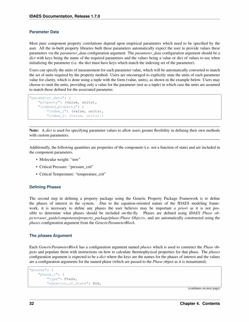
Parameter Data
Most pure component property correlations depend upon empirical parameters which need to be specified by theuser. All the in-built property libraries built these parameters automatically expect the user to provide values theseparameters via the parameter_data configuration argument. The parameter_data configuration argument should be adict with keys being the name of the required parameters and the values being a value or dict of values to use wheninitializing the parameter (i.e. the dict must have keys which match the indexing set of the parameter).
Users can specify the units of measurement for each parameter value, which will be automatically converted to matchthe set of units required by the property method. Users are encouraged to explicitly state the units of each parametervalue for clarity, which is done using a tuple with the form (value, units), as shown in the example below. Users maychoose to omit the units, providing only a value for the parameter (not as a tuple) in which case the units are assumedto match those defined for the associated parameter.
"parameter_data": "property": (value, units),"indexed_property":
"index_1": (value, units),"index_2: (value, units)
Note: A dict is used for specifying parameter values to allow users greater flexibility in defining their own methodswith custom parameters.
Additionally, the following quantities are properties of the component (i.e. not a function of state) and are included inthe component parameters.
• Molecular weight: “mw”
• Critical Pressure: “pressure_crit”
• Critical Temperature: “temperature_crit”
Defining Phases
The second step in defining a property package using the Generic Property Package Framework is to definethe phases of interest in the system. Due to the equation-oriented nature of the IDAES modeling frame-work, it is necessary to define any phases the user believes may be important a priori as it is not pos-sible to determine what phases should be included on-the-fly. Phases are defined using IDAES Phase ob-jects<user_guide/components/property_package/phase:Phase Object>, and are automatically constructed using thephases configuration argument from the GenericParameterBlock.
The phases Argument
Each GenericParameterBlock has a configuration argument named phases which is used to construct the Phase ob-jects and populate them with instructions on how to calculate thermophysical properties for that phase. The phasesconfiguration argument is expected to be a dict where the keys are the names for the phases of interest and the valuesare a configuration arguments for the named phase (which are passed to the Phase object as it is instantiated).
"phases": "phase_1":
"type": Phase,"equation_of_state": EoS,
(continues on next page)
32 Chapter 4. Contents
IDAES Documentation, Release 1.7.0
(continued from previous page)
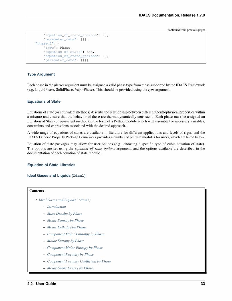
"equation_of_state_options": ,"parameter_data": ,
"phase_2": "type": Phase,"equation_of_state": EoS,"equation_of_state_options": ,"parameter_data":
Type Argument
Each phase in the phases argument must be assigned a valid phase type from those supported by the IDAES Framework(e.g. LiquidPhase, SolidPhase, VaporPhase). This should be provided using the type argument.
Equations of State
Equations of state (or equivalent methods) describe the relationship between different thermophysical properties withina mixture and ensure that the behavior of these are thermodynamically consistent. Each phase must be assigned anEquation of State (or equivalent method) in the form of a Python module which will assemble the necessary variables,constraints and expressions associated with the desired approach.
A wide range of equations of states are available in literature for different applications and levels of rigor, and theIDAES Generic Property Package Framework provides a number of prebuilt modules for users, which are listed below.
Equation of state packages may allow for user options (e.g. choosing a specific type of cubic equation of state).The options are set using the equation_of_state_options argument, and the options available are described in thedocumentation of each equation of state module.
Equation of State Libraries
Ideal Gases and Liquids (Ideal)
Contents
• Ideal Gases and Liquids (Ideal)
– Introduction
– Mass Density by Phase
– Molar Density by Phase
– Molar Enthalpy by Phase
– Component Molar Enthalpy by Phase
– Molar Entropy by Phase
– Component Molar Entropy by Phase
– Component Fugacity by Phase
– Component Fugacity Coefficient by Phase
– Molar Gibbs Energy by Phase
4.2. User Guide 33
IDAES Documentation, Release 1.7.0
– Component Gibbs Energy by Phase
Introduction
Ideal behavior represents the simplest possible equation of state that ensures thermodynamic consistency betweendifferent properties.
Mass Density by Phase
The following equation is used for both liquid and vapor phases, where 𝑝 indicates a given phase:
𝜌𝑚𝑎𝑠𝑠,𝑝 = 𝜌𝑚𝑜𝑙,𝑝 ×𝑀𝑊𝑝
where 𝑀𝑊𝑝 is the mixture molecular weight of phase 𝑝.
Molar Density by Phase
For the vapor phase, the Ideal Gas Equation is used to calculate the molar density;
𝜌𝑚𝑜𝑙,𝑉 𝑎𝑝 =𝑃
𝑅𝑇
whilst for the liquid phase the molar density is the weighted sum of the pure component liquid densities:
𝜌𝑚𝑜𝑙,𝐿𝑖𝑞 =∑𝑗
𝑥𝐿𝑖𝑞,𝑗 × 𝜌𝐿𝑖𝑞,𝑗
where 𝑥𝐿𝑖𝑞,𝑗 is the mole fraction of component 𝑗 in the liquid phase.
Molar Enthalpy by Phase
For both liquid and vapor phases, the molar enthalpy is calculated as the weighted sum of the component molarenthalpies for the given phase:
ℎ𝑚𝑜𝑙,𝑝 =∑𝑗
𝑥𝑝,𝑗 × ℎ𝑚𝑜𝑙,𝑝,𝑗
where 𝑥𝑝,𝑗 is the mole fraction of component 𝑗 in the phase 𝑝.
Component Molar Enthalpy by Phase
Component molar enthalpies by phase are calculated using the pure component method provided by the users in theproperty package configuration arguments.
Molar Entropy by Phase
For both liquid and vapor phases, the molar entropy is calculated as the weighted sum of the component molar entropiesfor the given phase:
𝑠𝑚𝑜𝑙,𝑝 =∑𝑗
𝑥𝑝,𝑗 × 𝑠𝑚𝑜𝑙,𝑝,𝑗
where 𝑥𝑝,𝑗 is the mole fraction of component 𝑗 in the phase 𝑝.
34 Chapter 4. Contents
IDAES Documentation, Release 1.7.0
Component Molar Entropy by Phase
Component molar entropies by phase are calculated using the pure component method provided by the users in theproperty package configuration arguments.
Component Fugacity by Phase
For the vapor phase, ideal behavior is assumed:
𝑓𝑉 𝑎𝑝,𝑗 = 𝑃
For the liquid phase, Raoult’s Law is used:
𝑓𝐿𝑖𝑞,𝑗 = 𝑃𝑠𝑎𝑡,𝑗
Component Fugacity Coefficient by Phase
Ideal behavior is assumed, so all 𝜑𝑝,𝑗 = 1 for all components and phases.
Molar Gibbs Energy by Phase
For both liquid and vapor phases, the molar Gibbs energy is calculated as the weighted sum of the component molarGibbs energies for the given phase:
𝑔𝑚𝑜𝑙,𝑝 =∑𝑗
𝑥𝑝,𝑗 × 𝑔𝑚𝑜𝑙,𝑝,𝑗
where 𝑥𝑝,𝑗 is the mole fraction of component 𝑗 in the phase 𝑝.
Component Gibbs Energy by Phase
Component molar Gibbs energies are calculated using the definition of Gibbs energy:
𝑔𝑚𝑜𝑙,𝑝,𝑗 = ℎ𝑚𝑜𝑙,𝑝,𝑗 − 𝑠𝑚𝑜𝑙,𝑝,𝑗 × 𝑇
Cubic Equations of State (Cubic)
Contents
• Cubic Equations of State (Cubic)
– Introduction
– General Cubic Equation of State
– Property Package Options
– Required Parameters
– Calculation of Properties
4.2. User Guide 35
IDAES Documentation, Release 1.7.0
– Mass Density by Phase
– Molar Density by Phase
– Molar Enthalpy by Phase
– Component Molar Enthalpy by Phase
– Molar Entropy by Phase
– Component Molar Entropy by Phase
– Component Fugacity by Phase
– Component Fugacity Coefficient by Phase
– Molar Gibbs Energy by Phase
– Component Gibbs Energy by Phase
Introduction
This module implements a general form of a cubic equation of state which can be used for most cubic-type equationsof state. The following forms are currently supported:
• Peng-Robinson
• Soave-Redlich-Kwong
General Cubic Equation of State
All equations come from “The Properties of Gases and Liquids, 4th Edition” by Reid, Prausnitz and Poling. Thegeneral cubic equation of state is represented by the following equations:
𝑃 =𝑅𝑇
𝑉 − 𝑏− 𝑎
𝑉 2 − 𝑢𝑏𝑉 + 𝑤𝑏2
An equivalent form of the previous equation is:
0 = 𝑍3 − (1 +𝐵 − 𝑢𝐵)𝑍2 + (𝐴− 𝑢𝐵 − (𝑢− 𝑤)𝐵2)𝑍 −𝐴𝐵 − 𝑤𝐵2 − 𝑤𝐵3
𝐴 =𝑎𝑚𝑃
𝑅2𝑇 2
𝐵 =𝑏𝑚𝑃
𝑅𝑇
where 𝑍 is the compressibility factor of the mixture, 𝑎𝑚 and 𝑏𝑚 are properties of the mixture and 𝑢 and 𝑤 areparameters which depend on the specific equation of state being used as show in the table below.
Equation 𝑢 𝑤 𝑂𝑚𝑒𝑔𝑎𝐴 𝑂𝑚𝑒𝑔𝑎𝐵 𝑎𝑙𝑝ℎ𝑎𝑗Peng-Robinson 2 -1 0.45724 0.07780 (1 + (1− 𝑇 2
𝑟 )(0.37464 + 1.54226𝜔𝑗 − 0.26992𝜔2𝑗 ))2
Soave-Redlich-Kwong
1 0 0.42748 0.08664 (1 + (1 − 𝑇 2𝑟 )(0.48 + 1.574𝜔𝑗 − 0.176𝜔2
𝑗 ))2
The properties 𝑎𝑚 and 𝑏𝑚 are calculated from component specific properties 𝑎𝑗 and 𝑏𝑗 as shown below:
𝑎𝑗 =Ω𝐴𝑅
2𝑇 2𝑐,𝑗
𝑃𝑐,𝑗𝛼𝑗
36 Chapter 4. Contents
IDAES Documentation, Release 1.7.0
𝑏𝑗 =Ω𝐵𝑅𝑇𝑐,𝑗𝑃𝑐,𝑗
𝑎𝑚 =∑𝑖
∑𝑗
𝑦𝑖𝑦𝑗(𝑎𝑖𝑎𝑗)1/2(1 − 𝜅𝑖𝑗)
𝑏𝑚 =∑𝑖
𝑦𝑖𝑏𝑖
where 𝑃𝑐,𝑗 and 𝑇𝑐,𝑗 are the component critical pressures and temperatures, 𝑦𝑗 is the mole fraction of component 𝑗, 𝜅𝑖𝑗are a set of binary interaction parameters which are specific to the equation of state and Ω𝐴, Ω𝐵 and 𝛼𝑗 are taken fromthe table above. 𝜔𝑗 is the Pitzer acentric factor of each component.
The cubic equation of state is solved for each phase via a call to an external function which automatically identifiesthe correct root of the cubic and returns the value of 𝑍 as a function of 𝐴 and 𝐵 along with the first and second partialderivatives.
Property Package Options
When using the general cubic equation of state module, users must specify the type of cubic to use. This is done byproviding a type option in the equation_of_state_options argument in the Phase definition, as shown in the examplebelow.
from idaes.generic_models.properties.core.eos.ceos import Cubic, CubicType
configuration = "phases":
"Liquid": "type": LiquidPhase,"equation_of_state": Cubic,"equation_of_state_options":
"type": CubicType.PR
Required Parameters
Cubic equations of state require the following parameters to be defined:
1. omega (Pitzer acentricity factor) needs to be defined for each component (in the parameter_data for each com-ponent).
2. kappa (binary interaction parameters) needs to be defined for each component pair in the system. This parameterneeds to be defined in the general parameter_data argument for the overall property package (as it can be usedin multiple phases).
Calculation of Properties
Many thermophysical properties are calculated using an ideal and residual term, such that:
𝑝 = 𝑝0 + 𝑝𝑟
The residual term is derived from the partial derivatives of the cubic equation of state, whilst the ideal term is deter-mined using pure component properties for the ideal gas phase defined for each component.
4.2. User Guide 37
IDAES Documentation, Release 1.7.0
Mass Density by Phase
The following equation is used for both liquid and vapor phases, where 𝑝 indicates a given phase:
𝜌𝑚𝑎𝑠𝑠,𝑝 = 𝜌𝑚𝑜𝑙,𝑝 ×𝑀𝑊𝑝
where 𝑀𝑊𝑝 is the mixture molecular weight of phase 𝑝.
Molar Density by Phase
Molar density is calculated using the following equation
𝜌𝑚𝑜𝑙,𝑉 𝑎𝑝 =𝑃
𝑍𝑅𝑇
Molar Enthalpy by Phase
The residual enthalpy term is given by:
ℎ𝑟𝑖 𝑏𝑚√𝑢2 − 4𝑤 =
(𝑇𝑑𝑎
𝑑𝑇− 𝑎𝑚
)ln
(2𝑍 +𝐵(𝑢+
√𝑢2 − 4𝑤)
2𝑍 +𝐵(𝑢−√𝑢2 − 4𝑤)
)+𝑅𝑇 (𝑍 − 1)𝑏𝑚
√𝑢2 − 4𝑤
𝑑𝑎
𝑑𝑇
√𝑇 = −𝑅
2
√Ω𝐴
∑𝑖
∑𝑗
𝑦𝑖𝑦𝑗(1 − 𝑘𝑖𝑗)
(𝑓𝑤,𝑗
√𝑎𝑖𝑇𝑐,𝑗𝑃𝑐,𝑗
+ 𝑓𝑤,𝑖
√𝑎𝑗𝑇𝑐,𝑖𝑃𝑐,𝑖
)The ideal component is calculated from the weighted sum of the (ideal) component molar enthalpies.
Component Molar Enthalpy by Phase
Component molar enthalpies by phase are calculated using the pure component method provided by the users in theproperty package configuration arguments.
Molar Entropy by Phase
The residual entropy term is given by:
𝑠𝑟𝑖 𝑏𝑚√𝑢2 − 4𝑤 = 𝑅 ln
𝑍 −𝐵
𝑍𝑏𝑚√𝑢2 − 4𝑤 +𝑅 ln
𝑍𝑃 𝑟𝑒𝑓
𝑃𝑏𝑚√𝑢2 − 4𝑤 +
𝑑𝑎
𝑑𝑇ln
(2𝑍 +𝐵(𝑢+
√𝑢2 − 4𝑤)
2𝑍 +𝐵(𝑢−√𝑢2 − 4𝑤)
)The ideal component is calculated from the weighted sum of the (ideal) components molar enthalpies.
Component Molar Entropy by Phase
Component molar entropies by phase are calculated using the pure component methods provided by the users in theproperty package configuration arguments.
Component Fugacity by Phase
Fugacity is calculated from the system pressure and fugacity coefficients as follows:
𝑓𝑖,𝑝 = 𝜑𝑖,𝑝𝑃
38 Chapter 4. Contents
IDAES Documentation, Release 1.7.0
Component Fugacity Coefficient by Phase
The fugacity coefficient is calculated from the departure function of the cubic equation of state as shown below:
ln𝜑𝑖 =𝑏𝑖𝑏𝑚
(𝑍 − 1) − ln (𝑍 −𝐵) +𝐴
𝐵√𝑢2 − 4𝑤
(𝑏𝑖𝑏𝑚
− 𝛿𝑖
)ln
(2𝑍 +𝐵(𝑢+
√𝑢2 − 4𝑤)
2𝑍 +𝐵(𝑢−√𝑢2 − 4𝑤)
)
𝛿𝑖 =2𝑎
1/2𝑖
𝑎𝑚
∑𝑗
𝑥𝑗𝑎1/2𝑗 (1 − 𝑘𝑖𝑗)
Molar Gibbs Energy by Phase
For both liquid and vapor phases, the molar Gibbs energy is calculated as the weighted sum of the component molarGibbs energies for the given phase:
𝑔𝑚𝑜𝑙,𝑝 =∑𝑗
𝑥𝑝,𝑗 × 𝑔𝑚𝑜𝑙,𝑝,𝑗
where 𝑥𝑝,𝑗 is the mole fraction of component 𝑗 in the phase 𝑝.
Component Gibbs Energy by Phase
Component molar Gibbs energies are calculated using the definition of Gibbs energy:
𝑔𝑚𝑜𝑙,𝑝,𝑗 = ℎ𝑚𝑜𝑙,𝑝,𝑗 − 𝑠𝑚𝑜𝑙,𝑝,𝑗 × 𝑇
Phase-Specific Parameter
In some cases, a property package may include parameters which are specific to a given phase. In these cases, theseparameters are stored as part of the associated Phase object and the values of these set using the parameter_dataargument when declaring the phase. This is done in the same fashion as for component specific parameters.
Phases with Partial Component Lists
In many applications a mixture will contain species that only appear in a single phase (either by nature or assumption).Common examples include crystalline solids and non-condensable gases. The IDAES Generic Property PackageFramework provides support for these behaviors and allows users to specify phase-specific component lists (i.e. a listof components which appear in a given phase).
This is done by providing a phase with a component_list argument, which provides a list of component names whichappear in the phase. The framework automatically validates the component_list argument to ensure that it is a sub-set of the master component list for the property package, and will inform the user if an unrecognized component isincluded. If a phase is not provided with a component_list argument it is assumed that all components defined in themaster component list may be present in the phase.
4.2. User Guide 39
IDAES Documentation, Release 1.7.0
State Definition
Defining State Variables
An important part of defining a set of property calculations is choosing the set of variables which will describe thestate of the material. The set of state variables needs to include information on the extensive flow, composition andthermodynamic state of the material. However, there are many ways in which this information can be described, andthe best choice of state variables depends on many factors.
Within the IDAES Generic Property Package Framework, the definition of state variables is done using sub-moduleswhich create the necessary variables supporting information for the property package. A state definition sub-modulemay define any set of state variables the user feel appropriate, but must define the following components as either statevariables or functions of the state variables:
• temperature (must be a Pyomo Var)
• pressure
• mole_frac_phase_comp
• phase_frac
The IDAES Generic Property Package Framework has a library of prebuilt state definition sub-modules for users touse which are listed below.
State Definition Libraries
FTPx
Contents
• FTPx
– State Definition
– Application
– Bounds
– Supporting Variables and Constraints
– Default Balance Types and Flow Basis
State Definition
This approach describes the material state in terms of total flow (𝐹 : flow_mol), overall (mixture) mole fractions (𝑥𝑗 :mole_frac_comp), temperature (𝑇 : temperature) and pressure (𝑃 : pressure). As such, there are 3 +𝑁𝑐𝑜𝑚𝑝𝑜𝑛𝑒𝑛𝑡𝑠 statevariables, however only 2 +𝑁𝑐𝑜𝑚𝑝𝑜𝑛𝑒𝑛𝑡𝑠 are independent as the mole fraction must sum to 1.
Application
This is the simplest approach to fully defining the state of a material, and one of the most easily accessible to the useras it is defined in terms of variables that are easily measured and understood. However, this approach has a number oflimitations which the user should be aware of:
40 Chapter 4. Contents
IDAES Documentation, Release 1.7.0
• If the property package is set up for multiphase flow, an equilibrium calculation is required at the inlet of eachunit, as the state definition does not contain information on multiphase flow. This increases the number ofcomplex equilibrium calculations that must be performed, which could be avoided by using a different statedefinition.
• State becomes ill-defined when only one component is present and multiphase behavior can occur, as tempera-ture and pressure are insufficient to fully define the thermodynamic state under these conditions.
Bounds
The FTPx module supports bounding of the following variables through the state_bounds configuration argument:
• flow_mol
• temperature
• pressure
Note that mole fractions are automatically assigned a lower bound of 0, but the upper bound is left free as this isimplicitly defined by the sum of mole fractions constraint.
Supporting Variables and Constraints
In addition to the state variables, this definition of state creates a number of supporting variables and constraints.
Variables
• flow_mol_phase (𝐹𝑚𝑜𝑙,𝑝)
• mole_frac_phase_comp (𝑥𝑝,𝑗)
• phase_frac (𝜓𝑝)
Constraints
In all cases, a constraint is written for the sum of the overall mole fractions.∑𝑗
𝑥𝑗 = 1
Note: The sum of mole fractions constraint is not written at inlet states, as all mole fractions should be defined in theinlet stream.
If the property package supports only one phase:
𝐹𝑚𝑜𝑙,𝑝 = 𝐹𝑚𝑜𝑙
𝑥𝑝,𝑗 = 𝑥𝑗 for all 𝑗
𝜓𝑝 = 1
4.2. User Guide 41
IDAES Documentation, Release 1.7.0
If the property package supports only two phases, the Rachford-Rice formulation is used:∑𝑝
𝐹𝑚𝑜𝑙,𝑝 = 𝐹𝑚𝑜𝑙
𝐹𝑚𝑜𝑙 × 𝑥𝑗 =∑𝑝
𝐹𝑚𝑜𝑙,𝑝 × 𝑥𝑝,𝑗 for all 𝑗
∑𝑗
𝑥phase 1,𝑗 −∑𝑗
𝑥phase 2,𝑗 = 0
𝜓𝑝 × 𝐹𝑚𝑜𝑙 = 𝐹𝑚𝑜𝑙,𝑝 for all 𝑝
If the property package supports more than two phases, the following general formulation is used:
𝐹𝑚𝑜𝑙 × 𝑥𝑗 =∑𝑝
𝐹𝑚𝑜𝑙,𝑝 × 𝑥𝑝,𝑗 for all 𝑗
∑𝑗
𝑥𝑝,𝑗 = 1 for all 𝑝
𝜓𝑝 × 𝐹𝑚𝑜𝑙 = 𝐹𝑚𝑜𝑙,𝑝 for all 𝑝
Default Balance Types and Flow Basis
The following defaults are specified for Unit Models using this state definition:
• Material balances: total component balances
• Material flow basis: molar flow
• Energy balances: total enthalpy
FcTP
Contents
• FcTP
– State Definition
– Application
– Bounds
– Supporting Variables and Constraints
– Default Balance Types and Flow Basis
State Definition
This approach describes the material state in terms of total component flow (𝐹 : flow_mol_comp), temperature (𝑇 :temperature) and pressure (𝑃 : pressure). As such, there are 2 +𝑁𝑐𝑜𝑚𝑝𝑜𝑛𝑒𝑛𝑡𝑠 state variables.
42 Chapter 4. Contents
IDAES Documentation, Release 1.7.0
Application
This approach is similar to using total flow rate and mole fractions as state variable, and is generally accessible to theuser as the state variables are easily measured and understood. Compared to using total flow rate and mole fractions,this approach changes how the bilinear terms (flow rate times mole fraction) appear in the problem structure, and mayresult in improved performance for some applications. However, this approach has a number of limitations which theuser should be aware of:
• If the property package is set up for multiphase flow, an equilibrium calculation is required at the inlet of eachunit, as the state definition does not contain information on multiphase flow. This increases the number ofcomplex equilibrium calculations that must be performed, which could be avoided by using a different statedefinition.
• State becomes ill-defined when only one component is present and multiphase behavior can occur, as tempera-ture and pressure are insufficient to fully define the thermodynamic state under these conditions.
Bounds
The FcTP module supports bounding of the following variables through the state_bounds configuration argument:
• flow_mol_comp
• temperature
• pressure
Supporting Variables and Constraints
In addition to the state variables, this definition of state creates a number of supporting variables and constraints.
Variables
• flow_mol_phase (𝐹𝑚𝑜𝑙,𝑝)
• mole_frac_comp (𝑥𝑗)
• mole_frac_phase_comp (𝑥𝑝,𝑗)
• phase_frac (𝜓𝑝)
Expressions
An Expression is created for the total flowrate such that 𝐹 =∑𝐹𝑗
Constraints
In all cases, a constraint is created to calculate component mole fractions from the component flow rates.
𝐹𝑗 = 𝑥𝑗 ×∑
𝐹𝑗
Note: If only one component is present in the property package, this is simplified to 𝑥𝑗 = 1.
4.2. User Guide 43
IDAES Documentation, Release 1.7.0
If the property package supports only one phase:
𝐹𝑚𝑜𝑙,𝑝 = 𝐹𝑚𝑜𝑙
𝑥𝑝,𝑗 = 𝑥𝑗 for all 𝑗
𝜓𝑝 = 1
If the property package supports only two phases, the Rachford-Rice formulation is used:∑𝑝
𝐹𝑚𝑜𝑙,𝑝 = 𝐹𝑚𝑜𝑙
𝐹𝑚𝑜𝑙,𝑗 =∑𝑝
(𝐹𝑚𝑜𝑙,𝑝 × 𝑥𝑝,𝑗) for all 𝑗
∑𝑗
𝑥phase 1,𝑗 −∑𝑗
𝑥phase 2,𝑗 = 0
𝜓𝑝 × 𝐹𝑚𝑜𝑙 = 𝐹𝑚𝑜𝑙,𝑝 for all 𝑝
If the property package supports more than two phases, the following general formulation is used:
𝐹𝑚𝑜𝑙,𝑗 =∑𝑝
(𝐹𝑚𝑜𝑙,𝑝 × 𝑥𝑝,𝑗) for all 𝑗
∑𝑗
𝑥𝑝,𝑗 = 1 for all 𝑝
𝜓𝑝 × 𝐹𝑚𝑜𝑙 = 𝐹𝑚𝑜𝑙,𝑝 for all 𝑝
Default Balance Types and Flow Basis
The following defaults are specified for Unit Models using this state definition:
• Material balances: total component balances
• Material flow basis: molar flow
• Energy balances: total enthalpy
FPhx
Contents
• FPhx
– State Definition
– Application
– Bounds
– Supporting Variables and Constraints
– Default Balance Types and Flow Basis
44 Chapter 4. Contents
IDAES Documentation, Release 1.7.0
State Definition
This approach describes the material state in terms of total flow (𝐹 : flow_mol), overall (mixture) mole fractions (𝑥𝑗 :mole_frac_comp), total molar enthalpy (ℎ: enth_mol) and pressure (𝑃 : pressure). As such, there are 3 +𝑁𝑐𝑜𝑚𝑝𝑜𝑛𝑒𝑛𝑡𝑠
state variables, however only 2 +𝑁𝑐𝑜𝑚𝑝𝑜𝑛𝑒𝑛𝑡𝑠 are independent as the mole fraction must sum to 1.
Application
This approach is commonly used by other process simulation tools as it avoids the issues associated with using tem-perature and pressure as state variables in single component systems. However, as the user generally does not knowthe specific enthalpy of their feed streams, this approach requires some method to calculate this for feed streams. Thiscan generally be done by specifying temperature of the feed, and then solving for the specific enthalpy.
This approach suffers from the following limitation which the user should be aware of:
• If the property package is set up for multiphase flow, an equilibrium calculation is required at the inlet of eachunit, as the state definition does not contain information on multiphase flow. This increases the number ofcomplex equilibrium calculations that must be performed, which could be avoided by using a different statedefinition.
Bounds
The FPhx module supports bounding of the following variables through the state_bounds configuration argument:
• flow_mol
• enth_mol
• pressure
• temperature
Supplying bounds for temperature is supported as these are often known to greater accuracy than the enthalpy bounds,and specifying these can help the solver find a feasible solution.
Note that mole fractions are automatically assigned a lower bound of 0, but the upper bound is left free as this isimplicitly defined by the sum of mole fractions constraint.
Supporting Variables and Constraints
In addition to the state variables, this definition of state creates a number of supporting variables and constraints.
Variables
• flow_mol_phase (𝐹𝑚𝑜𝑙,𝑝)
• mole_frac_phase_comp (𝑥𝑝,𝑗)
• temperature (𝑇 )
• phase_frac (𝜓𝑝)
4.2. User Guide 45
IDAES Documentation, Release 1.7.0
Constraints
In all cases, a constraint is written for the sum of the overall mole fractions.∑𝑗
𝑥𝑗 = 1
Note: The sum of mole fractions constraint is not written at inlet states, as all mole fractions should be defined in theinlet stream.
Additionally, a constraint relating the total specific enthalpy to the specific enthalpy of each phase is written.
ℎ𝑚𝑜𝑙 =∑𝑗
𝜓𝑝 × ℎ𝑚𝑜𝑙,𝑝
If the property package supports only one phase:
𝐹𝑚𝑜𝑙,𝑝 = 𝐹𝑚𝑜𝑙
𝑥𝑝,𝑗 = 𝑥𝑗 for all 𝑗
𝜓𝑝 = 1
If the property package supports only two phases, the Rachford-Rice formulation is used:∑𝑝
𝐹𝑚𝑜𝑙,𝑝 = 𝐹𝑚𝑜𝑙
𝐹𝑚𝑜𝑙 × 𝑥𝑗 =∑𝑝
𝐹𝑚𝑜𝑙,𝑝 × 𝑥𝑝,𝑗 for all 𝑗
∑𝑗
𝑥phase 1,𝑗 −∑𝑗
𝑥phase 2,𝑗 = 0
𝜓𝑝 × 𝐹𝑚𝑜𝑙 = 𝐹𝑚𝑜𝑙,𝑝 for all 𝑝
If the property package supports more than two phases, the following general formulation is used:
𝐹𝑚𝑜𝑙 × 𝑥𝑗 =∑𝑝
𝐹𝑚𝑜𝑙,𝑝 × 𝑥𝑝,𝑗 for all 𝑗
∑𝑗
𝑥𝑝,𝑗 = 1 for all 𝑝
𝜓𝑝 × 𝐹𝑚𝑜𝑙 = 𝐹𝑚𝑜𝑙,𝑝 for all 𝑝
Default Balance Types and Flow Basis
The following defaults are specified for Unit Models using this state definition:
• Material balances: total component balances
• Material flow basis: molar flow
• Energy balances: total enthalpy
46 Chapter 4. Contents
IDAES Documentation, Release 1.7.0
FcPh
Contents
• FcPh
– State Definition
– Application
– Bounds
– Supporting Variables and Constraints
– Default Balance Types and Flow Basis
State Definition
This approach describes the material state in terms of total component flow (𝐹 : flow_mol_comp), total specific en-thalpy (ℎ: enth_mol) and pressure (𝑃 : pressure). As such, there are 2 +𝑁𝑐𝑜𝑚𝑝𝑜𝑛𝑒𝑛𝑡𝑠 state variables.
Application
This approach is similar to the FPhx formulation used by many process simulators, with the exception that componentflow rates are used in place of total flow and mole fractions. This changes where the bilinear terms (flow rate time molefractions) appear in the problem structure and may improve robustness in some cases. The use of pressure and enthalpyas state variables avoids the issues related to using temperature and pressure as state variables for single componentsystems. However, as the user generally does not know the specific enthalpy of their feed streams, this approachrequires some method to calculate this for feed streams. This can generally be done by specifying temperature of thefeed, and then solving for the specific enthalpy.
This approach suffers from the following limitation which the user should be aware of:
• If the property package is set up for multiphase flow, an equilibrium calculation is required at the inlet of eachunit, as the state definition does not contain information on multiphase flow. This increases the number ofcomplex equilibrium calculations that must be performed, which could be avoided by using a different statedefinition.
Bounds
The FcPh module supports bounding of the following variables through the state_bounds configuration argument:
• flow_mol_comp
• enth_mol
• pressure
• temperature
Supplying bounds for temperature is supported as these are often known to greater accuracy than the enthalpy bounds,and specifying these can help the solver find a feasible solution.
4.2. User Guide 47
IDAES Documentation, Release 1.7.0
Supporting Variables and Constraints
In addition to the state variables, this definition of state creates a number of supporting variables and constraints.
Variables
• flow_mol_phase (𝐹𝑚𝑜𝑙,𝑝)
• mole_frac_comp (𝑥𝑗)
• mole_frac_phase_comp (𝑥𝑝,𝑗)
• temperature (𝑇 )
• phase_frac (𝜓𝑝)
Expressions
An Expression is created for the total flowrate such that 𝐹 =∑𝐹𝑗
Constraints
In all cases, a constraint is created to calculate component mole fractions from the component flow rates.
𝐹𝑗 = 𝑥𝑗 ×∑
𝐹𝑗
Note: If only one component is present in the property package, this is simplified to 𝑥𝑗 = 1.
If the property package supports only one phase:
𝐹𝑚𝑜𝑙,𝑝 = 𝐹𝑚𝑜𝑙
𝑥𝑝,𝑗 = 𝑥𝑗 for all 𝑗
𝜓𝑝 = 1
If the property package supports only two phases, the Rachford-Rice formulation is used:∑𝑝
𝐹𝑚𝑜𝑙,𝑝 = 𝐹𝑚𝑜𝑙
𝐹𝑚𝑜𝑙,𝑗 =∑𝑝
(𝐹𝑚𝑜𝑙,𝑝 × 𝑥𝑝,𝑗) for all 𝑗
∑𝑗
𝑥phase 1,𝑗 −∑𝑗
𝑥phase 2,𝑗 = 0
𝜓𝑝 × 𝐹𝑚𝑜𝑙 = 𝐹𝑚𝑜𝑙,𝑝 for all 𝑝
If the property package supports more than two phases, the following general formulation is used:
𝐹𝑚𝑜𝑙,𝑗 =∑𝑝
(𝐹𝑚𝑜𝑙,𝑝 × 𝑥𝑝,𝑗) for all 𝑗
∑𝑗
𝑥𝑝,𝑗 = 1 for all 𝑝
𝜓𝑝 × 𝐹𝑚𝑜𝑙 = 𝐹𝑚𝑜𝑙,𝑝 for all 𝑝
48 Chapter 4. Contents
IDAES Documentation, Release 1.7.0
Default Balance Types and Flow Basis
The following defaults are specified for Unit Models using this state definition:
• Material balances: total component balances
• Material flow basis: molar flow
• Energy balances: total enthalpy
FpcTP
Contents
• FpcTP
– State Definition
– Application
– Bounds
– Supporting Variables and Constraints
– Default Balance Types and Flow Basis
State Definition
This approach describes the material state in terms of phase-component flow (𝐹𝑝,𝑗 : flow_mol_phase_comp), tempera-ture (𝑇 : temperature) and pressure (𝑃 : pressure). As such, there are 2 + 𝑝ℎ𝑎𝑠𝑒𝑠 *𝑁𝑐𝑜𝑚𝑝𝑜𝑛𝑒𝑛𝑡𝑠 state variables.
Application
This approach required knowledge of the phase-equilibrium of the material in order to define the state variables.Compared to using total flow rate and mole fractions, this approach contains full information on the phase equilibriawithin the state variables, and thus avoids the needs for flash calculations in many cases. This can greatly reduce thecomplexity of the problem, and results can significantly affect the tractablity of the problem. However, this approachhas a number of limitations which the user should be aware of:
• Users must have knowledge of , or calculate, the phase-component flows of all inlet streams. For sinlge phaseflows this is often known, but for streasm with potetnial two-phase behaviour this can reqruire a set of flashcalculations for the feed streasm (users can make use of Feed blocks to assist with this).
• State becomes ill-defined when only one component is present and multiphase behavior can occur, as tempera-ture and pressure are insufficient to fully define the thermodynamic state under these conditions.
Bounds
The FpcTP module supports bounding of the following variables through the state_bounds configuration argument:
• flow_mol_phase_comp
• temperature
4.2. User Guide 49
IDAES Documentation, Release 1.7.0
• pressure
Supporting Variables and Constraints
In addition to the state variables, this definition of state creates a number of supporting variables and constraints.
Variables
• mole_frac_phase_comp (𝑥𝑝,𝑗)
Expressions
• flow_mol (𝐹 =∑𝐹𝑝,𝑗)
• flow_mol_phase (𝐹𝑝 =∑𝐹𝑝,𝑗𝑗)
• flow_mol_comp (𝐹𝑗 =∑𝐹𝑝,𝑗𝑝)
• mole_frac_comp (𝑥𝑗 =∑
𝐹𝑝,𝑗
𝐹 )
• phase_frac (𝜓𝑝 =𝐹𝑝
𝐹 or 𝜓𝑝 = 1 if only single phase)
Constraints
A set of constraints is created to calculate phase-component mole fractions from the phase-component flow rates.
𝐹𝑗 = 𝑥𝑝,𝑗 ×∑
𝐹𝑝 = 𝐹𝑝,𝑗
Default Balance Types and Flow Basis
The following defaults are specified for Unit Models using this state definition:
• Material balances: total component balances
• Material flow basis: molar flow
• Energy balances: total enthalpy
Setting Bounds on State Variables
For optimization applications, it is important to specify a good initial guess and bounds on the state variables in orderto improve the robustness of the problem. Further, due to the empirical nature of most thermophysical correlationsthese correlations are only valid in specific range of states. Users should set the state_bounds configuration argumentto define the bounds on the state variables of their property package.
The state_bounds configuration argument should be a dict where the keys are the names of the state variables (usingthe standard naming convention) and the values should be a tuple with the form (lower, nominal, upper, units). Thelower and upper values are used to set the lower and upper bounds respectively, whilst the nominal value is used to setthe initial value for the state variable. The units value is optional, and is used to specify the units of measurement forthe values provided, which will be used to automatically convert these values to the base set of units defined for the
50 Chapter 4. Contents
IDAES Documentation, Release 1.7.0
property package if required. If the units value is omitted, it is assumed that the values provided are in the base unitset for the property package.
Note: Some state definitions allow for setting on additional variables beyond the chosen state variables (temperatureis a common example). See the documentation for your state definition for more information on what bounds can beset using the state_bounds argument.
Reference State
Many thermophysical properties are relative quantities, and require the definition of a thermodynamic reference state.Whilst some simpler models and correlations forego this or define the reference state implicitly, the IDAES GenericProperty Package requires the user to specify the thermodynamic reference state (even if it is not used explicitly).
As such, users must provide the following two configuration arguments:
• pressure_ref - pressure at reference state
• temperature_ref - temperature at reference state
Defining Phase Equilibria
Phase equilibrium and separation is a key part of almost all chemical processes, and also represent some of the mostcomplex and non-linear constraints in a model, especially when dealing with systems which may cross phase bound-aries. Systems may also include multiple interacting phases with equilibrium, which further complicates the problem.As such, good formulations of these constraints is key to a robust and tractable model.
The IDAES Generic Property Package framework supports a range of phase equilibrium behaviors, including multiplephases in equilibrium and different formulations for describing the equilibria. These are all optional, and users do notneed to define phase equilibria if it is not required for their system.
Setting up phase equilibrium within the framework is done using three configuration arguments as discussed below.However, users should be aware that some of these options require definition of further properties, such as bubble anddew point calculations.
Define Phases in Equilibrium
The first step in setting up phase equilibrium in the framework is to describe which phases are in equilibrium witheach other. In general, for phases to be in equilibrium with each other, the following conditions need to be met:
1. Phases must be in direct contact with each other, and
2. At least one component must appear in both phases (equilibria involving chemical reactions are handled byReactionBlocks).
In order to describe which phases are in equilibrium, the user needs to set the phase_in_equilibrium constructionargument, which should be a list of 2-tuples where each tuple describes a pair of phases which are in equilibrium. Anycomponent which appears in both phases in a pair is assumed to be in equilibrium.
A simple example for a VLE system is shown below.
"phases_in_equilibrium" = [("Vap", "Liq")]
4.2. User Guide 51
IDAES Documentation, Release 1.7.0
Note: Users should take care not to over define their system. For example, in a VLSE system a user could potentiallywrite three sets of equilibrium constraints (VL, LS and VS). However, this would result in an over defined system, asonly two of these three are independent. For most situations, a user would consider only the VL and LS equilibria,with the VS being implicitly defined.
Define Equilibrium State Formulation
Next, for each pair of phases in equilibrium, the user must define a formulation for the equilibrium state. To handle thecomplexities of disappearing phases, the IDAES Generic Property Package Framework allows for phase equilibriumto be solved at a separate equilibrium state rather than the actual state of the material. This allows for formulationswhich avoid disappearing phases by limiting the equilibrium state to exist within the valid two-phase region, whilstreturning a negligible amount of any phase which is not valid at the actual material state.
The equilibrium state formulation is set using the phase_equilibrium_state configuration argument. This should be adict where the keys are 2-tuples of phases in equilibrium (matching those defined in the phases_in_equilibrium argu-ment) and values are a phase equilibrium state formulation method. The IDAES Generic Property Package Frameworkcontains a library of methods for the formulation of the phase equilibrium state, which is shown below.
Phase Equilibrium State Libraries
Smooth Vapor-Liquid Equilibrium Formulation (smooth_VLE)
Contents
• Smooth Vapor-Liquid Equilibrium Formulation (smooth_VLE)
– Source
– Introduction
– Formulation
Source
Burgard, A.P., Eason, J.P., Eslick, J.C., Ghouse, J.H., Lee, A., Biegler, L.T., Miller, D.C., 2018, A Smooth, SquareFlash Formulation for Equation-Oriented Flowsheet Optimization. Proceedings of the 13th International Symposiumon Process Systems Engineering – PSE 2018, July 1-5, 2018, San Diego.
Introduction
Typically, equilibrium calculations are only used when the user knows the current state is within the two-phase enve-lope. For simulation only studies, the user may know a priori the condition of the stream but when the same set ofequations are used for optimization, there is a high probability that the specifications can transcend the phase enve-lope. In these situations, the equilibrium calculations become trivial, thus it is necessary to find a formulation that hasnon-trivial solutions at all states.
To address this, the smooth vapor-liquid equilibrium (VLE) formulation always solves the equilibrium calculationsat a condition where a valid two-phase solution exists. In situations where only a single phase is present, the phase
52 Chapter 4. Contents
IDAES Documentation, Release 1.7.0
equilibrium is solved at the either the bubble or dew point, where the non-existent phase exists but in negligibleamounts. In this way, a non-trivial solution is guaranteed but still gives near-zero material in the non-existent phase inthe single phase regions.
Formulation
The approach used by the smooth VLE formulation is to define an “equilibrium temperature” (𝑇𝑒𝑞) at which theequilibrium calculations will be performed. The equilibrium temperature is computed as follows:
𝑇1 = 𝑚𝑎𝑥(𝑇𝑏𝑢𝑏𝑏𝑙𝑒, 𝑇 )
𝑇𝑒𝑞 = 𝑚𝑖𝑛(𝑇1, 𝑇𝑑𝑒𝑤)
where 𝑇 is the actual stream temperature, 𝑇1 is an intermediate temperature variable and 𝑇𝑏𝑢𝑏𝑏𝑙𝑒 and 𝑇𝑑𝑒𝑤 are thebubble and dew point temperature of mixture. In order to express the maximum and minimum operators in a tractableform, these equations are reformulated using the IDAES smooth_max and smooth_min operators which results in thefollowing equations:
𝑇1 = 0.5
[𝑇 + 𝑇𝑏𝑢𝑏𝑏𝑙𝑒 +
√(𝑇 − 𝑇𝑏𝑢𝑏𝑏𝑙𝑒)2 + 𝜖21
]
𝑇𝑒𝑞 = 0.5
[𝑇1 + 𝑇𝑑𝑒𝑤 −
√(𝑇 − 𝑇𝑑𝑒𝑤)2 + 𝜖22
]where 𝜖1 and 𝜖2 are smoothing parameters(mutable Params named eps_1 and eps_2). The default values are 0.01and 0.0005 respectively, and it is recommended that 𝜖1 > 𝜖2. It can be seen that if the stream temperature is lessthan that of the bubble point temperature, the VLE calculations will be computed at the bubble point. Similarly, ifthe stream temperature is greater than the dew point temperature, then the VLE calculations are computed at the dewpoint temperature. For all other conditions, the equilibrium calculations will be computed at the actual temperature.
Finally, the phase equilibrium is expressed using the following equation:
ΦVap,𝑗(𝑇𝑒𝑞) = ΦLiq,𝑗(𝑇𝑒𝑞)
where Φ𝑝,𝑗(𝑇𝑒𝑞) is the fugacity of component 𝑗 in the phase 𝑝 calculated at 𝑇𝑒𝑞 . The fugacities are calculated usingmethods defined by the equation of state chosen by the user for each phase.
Necessary Properties
Next, any component which is involved in a phase equilibrium interaction (i,e, appears in both phases of an interactingpair) must define a form for the required equilibrium constraint. There are a number of ways these constraints can bewritten depending on the equation of state and scaling of the problem. This is set using the phase_equilibrium_formconfiguration argument in the Component objects, and takes the form of a dict where the keys are 2-tuples of interactingphases and the value is the formulation to use for the current component across the given phase pair. For example:
parameters.component_1.config.phase_equilibrium_form = (phase_1, phase_2):→˓formulation
A library of common forms for equilibrium constraints is available, and is shown below.
Library of Common Equilibrium Forms
The IDAES Generic Property Package Framework contains a library of common forms for phase equilibrium condi-tions.
4.2. User Guide 53
IDAES Documentation, Release 1.7.0
Contents
• Library of Common Equilibrium Forms
– Fugacity (fugacity)
Fugacity (fugacity)
Fugacity of each component must be equal between interacting phases
𝑥𝑝1,𝑗 × 𝑓𝑝1,𝑗 = 𝑥𝑝2,𝑗 × 𝑓𝑝2,𝑗
Bubble and Dew Point Calculations
Bubble and dew points are often of interest to process engineers for designing process equipment, and appear in somecalculations of other thermodynamic properties. They are also useful in getting initial guesses for states in phaseequilibrium problems, and some equilibrium state formulations rely on these properties.
Whilst calculation of the saturation pressure for single components is relatively simple, calculating the bubble and dewpoints of mixtures is more challenging due to the non-linear nature of the equations. Calculation of these propertiesis generally done through calculations based on the equations of state for the liquid and vapor phases, however thesecalculations can be greatly simplified if ideal behavior is assumed for both phases (i.e. ideal gas and Raoult’s law). Toallow for both cases, the IDAES Generic Property Package Framework provides a library of different formulations forthe bubble and dew point calculations, which can be set using the following arguments:
• bubble_dew_method
A list of available methods is given below:
Bubble and Dew Point Methods
Contents
• Bubble and Dew Point Methods
– Ideal Assumptions (IdealBubbleDew)
* Ideal Bubble Pressure
* Ideal Bubble Temperature
* Ideal Dew Pressure
* Ideal Dew Temperature
– Equal Fugacity (log form) (LogBubbleDew)
* Bubble Pressure (log form)
* Bubble Temperature (log form)
* Dew Pressure (log form)
* Dew Temperature (log form)
54 Chapter 4. Contents
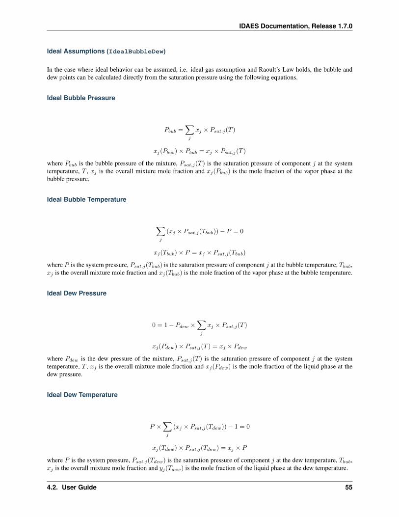
IDAES Documentation, Release 1.7.0
Ideal Assumptions (IdealBubbleDew)
In the case where ideal behavior can be assumed, i.e. ideal gas assumption and Raoult’s Law holds, the bubble anddew points can be calculated directly from the saturation pressure using the following equations.
Ideal Bubble Pressure
𝑃𝑏𝑢𝑏 =∑𝑗
𝑥𝑗 × 𝑃𝑠𝑎𝑡,𝑗(𝑇 )
𝑥𝑗(𝑃𝑏𝑢𝑏) × 𝑃𝑏𝑢𝑏 = 𝑥𝑗 × 𝑃𝑠𝑎𝑡,𝑗(𝑇 )
where 𝑃𝑏𝑢𝑏 is the bubble pressure of the mixture, 𝑃𝑠𝑎𝑡,𝑗(𝑇 ) is the saturation pressure of component 𝑗 at the systemtemperature, 𝑇 , 𝑥𝑗 is the overall mixture mole fraction and 𝑥𝑗(𝑃𝑏𝑢𝑏) is the mole fraction of the vapor phase at thebubble pressure.
Ideal Bubble Temperature
∑𝑗
(𝑥𝑗 × 𝑃𝑠𝑎𝑡,𝑗(𝑇𝑏𝑢𝑏)) − 𝑃 = 0
𝑥𝑗(𝑇𝑏𝑢𝑏) × 𝑃 = 𝑥𝑗 × 𝑃𝑠𝑎𝑡,𝑗(𝑇𝑏𝑢𝑏)
where 𝑃 is the system pressure, 𝑃𝑠𝑎𝑡,𝑗(𝑇𝑏𝑢𝑏) is the saturation pressure of component 𝑗 at the bubble temperature, 𝑇𝑏𝑢𝑏,𝑥𝑗 is the overall mixture mole fraction and 𝑥𝑗(𝑇𝑏𝑢𝑏) is the mole fraction of the vapor phase at the bubble temperature.
Ideal Dew Pressure
0 = 1 − 𝑃𝑑𝑒𝑤 ×∑𝑗
𝑥𝑗 × 𝑃𝑠𝑎𝑡,𝑗(𝑇 )
𝑥𝑗(𝑃𝑑𝑒𝑤) × 𝑃𝑠𝑎𝑡,𝑗(𝑇 ) = 𝑥𝑗 × 𝑃𝑑𝑒𝑤
where 𝑃𝑑𝑒𝑤 is the dew pressure of the mixture, 𝑃𝑠𝑎𝑡,𝑗(𝑇 ) is the saturation pressure of component 𝑗 at the systemtemperature, 𝑇 , 𝑥𝑗 is the overall mixture mole fraction and 𝑥𝑗(𝑃𝑑𝑒𝑤) is the mole fraction of the liquid phase at thedew pressure.
Ideal Dew Temperature
𝑃 ×∑𝑗
(𝑥𝑗 × 𝑃𝑠𝑎𝑡,𝑗(𝑇𝑑𝑒𝑤)) − 1 = 0
𝑥𝑗(𝑇𝑑𝑒𝑤) × 𝑃𝑠𝑎𝑡,𝑗(𝑇𝑑𝑒𝑤) = 𝑥𝑗 × 𝑃
where 𝑃 is the system pressure, 𝑃𝑠𝑎𝑡,𝑗(𝑇𝑑𝑒𝑤) is the saturation pressure of component 𝑗 at the dew temperature, 𝑇𝑏𝑢𝑏,𝑥𝑗 is the overall mixture mole fraction and 𝑦𝑗(𝑇𝑑𝑒𝑤) is the mole fraction of the liquid phase at the dew temperature.
4.2. User Guide 55
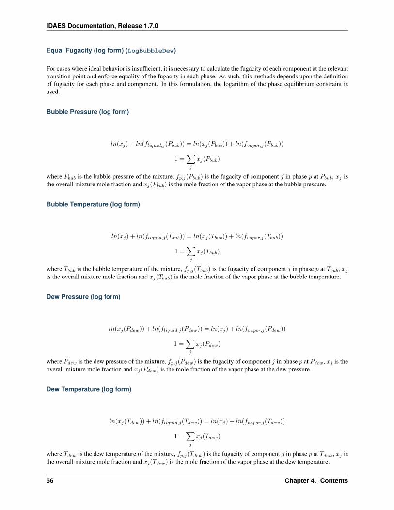
IDAES Documentation, Release 1.7.0
Equal Fugacity (log form) (LogBubbleDew)
For cases where ideal behavior is insufficient, it is necessary to calculate the fugacity of each component at the relevanttransition point and enforce equality of the fugacity in each phase. As such, this methods depends upon the definitionof fugacity for each phase and component. In this formulation, the logarithm of the phase equilibrium constraint isused.
Bubble Pressure (log form)
𝑙𝑛(𝑥𝑗) + 𝑙𝑛(𝑓𝑙𝑖𝑞𝑢𝑖𝑑,𝑗(𝑃𝑏𝑢𝑏)) = 𝑙𝑛(𝑥𝑗(𝑃𝑏𝑢𝑏)) + 𝑙𝑛(𝑓𝑣𝑎𝑝𝑜𝑟,𝑗(𝑃𝑏𝑢𝑏))
1 =∑𝑗
𝑥𝑗(𝑃𝑏𝑢𝑏)
where 𝑃𝑏𝑢𝑏 is the bubble pressure of the mixture, 𝑓𝑝,𝑗(𝑃𝑏𝑢𝑏) is the fugacity of component 𝑗 in phase 𝑝 at 𝑃𝑏𝑢𝑏, 𝑥𝑗 isthe overall mixture mole fraction and 𝑥𝑗(𝑃𝑏𝑢𝑏) is the mole fraction of the vapor phase at the bubble pressure.
Bubble Temperature (log form)
𝑙𝑛(𝑥𝑗) + 𝑙𝑛(𝑓𝑙𝑖𝑞𝑢𝑖𝑑,𝑗(𝑇𝑏𝑢𝑏)) = 𝑙𝑛(𝑥𝑗(𝑇𝑏𝑢𝑏)) + 𝑙𝑛(𝑓𝑣𝑎𝑝𝑜𝑟,𝑗(𝑇𝑏𝑢𝑏))
1 =∑𝑗
𝑥𝑗(𝑇𝑏𝑢𝑏)
where 𝑇𝑏𝑢𝑏 is the bubble temperature of the mixture, 𝑓𝑝,𝑗(𝑇𝑏𝑢𝑏) is the fugacity of component 𝑗 in phase 𝑝 at 𝑇𝑏𝑢𝑏, 𝑥𝑗is the overall mixture mole fraction and 𝑥𝑗(𝑇𝑏𝑢𝑏) is the mole fraction of the vapor phase at the bubble temperature.
Dew Pressure (log form)
𝑙𝑛(𝑥𝑗(𝑃𝑑𝑒𝑤)) + 𝑙𝑛(𝑓𝑙𝑖𝑞𝑢𝑖𝑑,𝑗(𝑃𝑑𝑒𝑤)) = 𝑙𝑛(𝑥𝑗) + 𝑙𝑛(𝑓𝑣𝑎𝑝𝑜𝑟,𝑗(𝑃𝑑𝑒𝑤))
1 =∑𝑗
𝑥𝑗(𝑃𝑑𝑒𝑤)
where 𝑃𝑑𝑒𝑤 is the dew pressure of the mixture, 𝑓𝑝,𝑗(𝑃𝑑𝑒𝑤) is the fugacity of component 𝑗 in phase 𝑝 at 𝑃𝑑𝑒𝑤, 𝑥𝑗 is theoverall mixture mole fraction and 𝑥𝑗(𝑃𝑑𝑒𝑤) is the mole fraction of the vapor phase at the dew pressure.
Dew Temperature (log form)
𝑙𝑛(𝑥𝑗(𝑇𝑑𝑒𝑤)) + 𝑙𝑛(𝑓𝑙𝑖𝑞𝑢𝑖𝑑,𝑗(𝑇𝑑𝑒𝑤)) = 𝑙𝑛(𝑥𝑗) + 𝑙𝑛(𝑓𝑣𝑎𝑝𝑜𝑟,𝑗(𝑇𝑑𝑒𝑤))
1 =∑𝑗
𝑥𝑗(𝑇𝑑𝑒𝑤)
where 𝑇𝑑𝑒𝑤 is the dew temperature of the mixture, 𝑓𝑝,𝑗(𝑇𝑑𝑒𝑤) is the fugacity of component 𝑗 in phase 𝑝 at 𝑇𝑑𝑒𝑤, 𝑥𝑗 isthe overall mixture mole fraction and 𝑥𝑗(𝑇𝑑𝑒𝑤) is the mole fraction of the vapor phase at the dew temperature.
56 Chapter 4. Contents
IDAES Documentation, Release 1.7.0
Developing New Property Libraries
Information on how to develop new components for the IDAES Generic Property Package Framework are given in thefollowing sections.
Contents
Developing Pure Component Methods
Contents
• Developing Pure Component Methods
– Naming Methods
– Method Arguments
– Method Parameters
– Method Body
– Example
The most common task developers of new property packages will need to do is writing methods for new pure compo-nent property calculations. Most equation of state type approaches rely on a set of calculations for pure componentsunder ideal conditions which are then modified to account for mixing and deviations from ideality. These pure com-ponent property calculations tend to be empirical correlations based on experimental data (generally as functions oftemperature) and due to their empirical nature a wide range of forms have been used in literature.
In order to support different forms for these calculations, the IDAES Generic Property Package Framework uses Pythonmethods to define the form of pure component property calculations. This allows developers and users to easily enterthe form they wish to use for their application with a minimum amount of code.
Naming Methods
The IDAES Generic Property Package Framework supports two ways of providing pure component property methods:
1. Providing the method directly - users may directly provide their method of choice as a config argument (con-fig.property_name) in the PropertyParameterBlock, in which case the method can use any name the user desires.
2. Providing a library module - alternatively, users can provide a module containing a library of methods as theconfig argument (config.property_name), in which case the framework searches the module for a method withthe same name as the property (and the config argument). E.g., for the property enth_mol_phase_comp themethod name would be enth_mol_phase_comp (as would the associated config argument).
Method Arguments
Note: Currently, the IDAES Generic Property Package Framework assumes pure component property calculationswill be a function of only temperature. If additional functionality is required, please contact the IDAES Developers.
4.2. User Guide 57
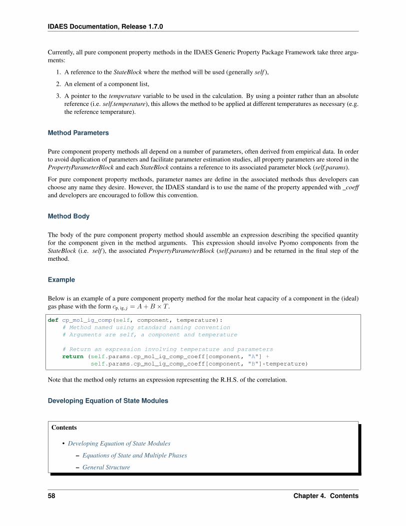
IDAES Documentation, Release 1.7.0
Currently, all pure component property methods in the IDAES Generic Property Package Framework take three argu-ments:
1. A reference to the StateBlock where the method will be used (generally self ),
2. An element of a component list,
3. A pointer to the temperature variable to be used in the calculation. By using a pointer rather than an absolutereference (i.e. self.temperature), this allows the method to be applied at different temperatures as necessary (e.g.the reference temperature).
Method Parameters
Pure component property methods all depend on a number of parameters, often derived from empirical data. In orderto avoid duplication of parameters and facilitate parameter estimation studies, all property parameters are stored in thePropertyParameterBlock and each StateBlock contains a reference to its associated parameter block (self.params).
For pure component property methods, parameter names are define in the associated methods thus developers canchoose any name they desire. However, the IDAES standard is to use the name of the property appended with _coeffand developers are encouraged to follow this convention.
Method Body
The body of the pure component property method should assemble an expression describing the specified quantityfor the component given in the method arguments. This expression should involve Pyomo components from theStateBlock (i.e. self ), the associated PropertyParameterBlock (self.params) and be returned in the final step of themethod.
Example
Below is an example of a pure component property method for the molar heat capacity of a component in the (ideal)gas phase with the form 𝑐p, ig,𝑗 = 𝐴+𝐵 × 𝑇 .
def cp_mol_ig_comp(self, component, temperature):# Method named using standard naming convention# Arguments are self, a component and temperature
# Return an expression involving temperature and parametersreturn (self.params.cp_mol_ig_comp_coeff[component, "A"] +
self.params.cp_mol_ig_comp_coeff[component, "B"]*temperature)
Note that the method only returns an expression representing the R.H.S. of the correlation.
Developing Equation of State Modules
Contents
• Developing Equation of State Modules
– Equations of State and Multiple Phases
– General Structure
58 Chapter 4. Contents
IDAES Documentation, Release 1.7.0
– Phase Equilibrium
– Accessing Pure Component Property Methods
– Common Methods
– Mixture Property Methods
– Example
The central part of any property package are the equations of state or equivalent models which describe how themixture behaves under the conditions of interest. For systems with multiple phases and phase equilibrium, each phasemust have its own equation of state (or equivalent), which must provide information on phase equilibrium which iscompatible with the other phases in the system.
Equations of State and Multiple Phases
The IDAES Generic Property Package Framework requires users to assign an equation of state module for each phasein their system, thus equations of state can be written for specific phases (e.g. an ideal gas equation of state). In somecases, developers may wish to write equations of state for multiple phases, and the generic framework supports this byindexing all properties by phase.
Developers are encouraged to add checks to their methods to ensure their equations of state are only applied to phaseswhere they are appropriate (e.g. an ideal gas equation of state should raise an exception if the phase argument is not“Vap”).
General Structure
Equation of State Modules in the IDAES Generic Property Package Framework are files (modules) containing a num-ber of methods which describe the behavior of the material. These method define how each of the properties associatedwith a given phase should be calculated, and the list of properties supported for a given phase is limited by the methodsprovided by the developer of the equation of state.
Phase Equilibrium
When calculating phase equilibrium, the IDAES Generic Property Package Framework uses the general formΦ𝑒
phase 1, j = Φ𝑒phase 2, j where Φ𝑒
𝑝,𝑗 is the fugacity of component 𝑗 in phase 𝑝 calculated at the equilibrium tempearture(𝑇𝑒𝑞 , variable name self._teq). The equilibrium temperature is calculated using the users’ choice of phase equilibriumformulation and determines how the property packge will handle phase transitions.
All equation of state methods should contain a method for calculating fugacity if they are to support phase equilibriumcalculations.
Accessing Pure Component Property Methods
In most cases, property calculations in the equation of state methods will require calculations of the purecomponent properties for the system. These can be accessed using get_method (imported from fromidaes.property_models.core.generic.generic_property) using the form get_method(self, “property_name”). This willreturn the method defined by the user in the PropertyParameterBlock for the named property, which can then be usedin the equation of state methods (note that users will need to call the method and provide it with the required arguments- generally self, component and a pointer to temperature).
4.2. User Guide 59
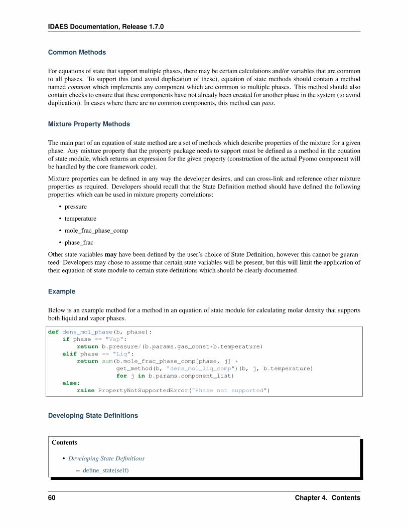
IDAES Documentation, Release 1.7.0
Common Methods
For equations of state that support multiple phases, there may be certain calculations and/or variables that are commonto all phases. To support this (and avoid duplication of these), equation of state methods should contain a methodnamed common which implements any component which are common to multiple phases. This method should alsocontain checks to ensure that these components have not already been created for another phase in the system (to avoidduplication). In cases where there are no common components, this method can pass.
Mixture Property Methods
The main part of an equation of state method are a set of methods which describe properties of the mixture for a givenphase. Any mixture property that the property package needs to support must be defined as a method in the equationof state module, which returns an expression for the given property (construction of the actual Pyomo component willbe handled by the core framework code).
Mixture properties can be defined in any way the developer desires, and can cross-link and reference other mixtureproperties as required. Developers should recall that the State Definition method should have defined the followingproperties which can be used in mixture property correlations:
• pressure
• temperature
• mole_frac_phase_comp
• phase_frac
Other state variables may have been defined by the user’s choice of State Definition, however this cannot be guaran-teed. Developers may chose to assume that certain state variables will be present, but this will limit the application oftheir equation of state module to certain state definitions which should be clearly documented.
Example
Below is an example method for a method in an equation of state module for calculating molar density that supportsboth liquid and vapor phases.
def dens_mol_phase(b, phase):if phase == "Vap":
return b.pressure/(b.params.gas_const*b.temperature)elif phase == "Liq":
return sum(b.mole_frac_phase_comp[phase, j] *get_method(b, "dens_mol_liq_comp")(b, j, b.temperature)for j in b.params.component_list)
else:raise PropertyNotSupportedError("Phase not supported")
Developing State Definitions
Contents
• Developing State Definitions
– define_state(self)
60 Chapter 4. Contents
IDAES Documentation, Release 1.7.0
* State Variables
* define_state_vars
* Auxiliary Variables
* Supporting Constraints
* always_flash
* get_material_flow_terms(phase, comp)
* get_enthalpy_flow_terms(phase)
* get_material_density_terms(phase, component)
* get_energy_density_terms(phase)
* get_material_flow_basis()
* default_material_balance_type()
* default_energy_balance_type()
* define_port_members()
* define_display_vars()
– state_initialization(self)
– self.do_not_initialize
The primary purpose of the State Definition method is to define the state variables which will be used to describethe state of the mixture in the property package. However, a number of other key aspects of the property packagedefinition are tied to the choice of state variables and must be declared here as well.
State definitions are defined as Python modules with two methods and one list, which are describe below.
define_state(self)
The first method in a State Definition module is the define_state method. This method is used to define the statevariables and associated components and methods. The define_state method must define the following things:
State Variables
The most important part of a State Definition module is the definition of the state variables that should be used in theresulting property package. The choice of state variables is up to the module developer, however the set of variablesselected must contain sufficient information to fully define the extensive and intensive state of the material. That is,if all the state variables are fixed, the resulting set of variables and constraints should form a square problem (i.e. 0degrees of freedom). Beyond this requirement however, developers may choose any combination of state variablesthey wish.
State variables should be defined as Pyomo Vars with names drawn from the IDAES naming standard, and shouldinclude initial values and bounds. The Generic Property Package Framework includes an optional user input of boundsfor the state variables (config.state_bounds) which developers are encouraged to make use of when setting bounds andinitializing variables.
4.2. User Guide 61
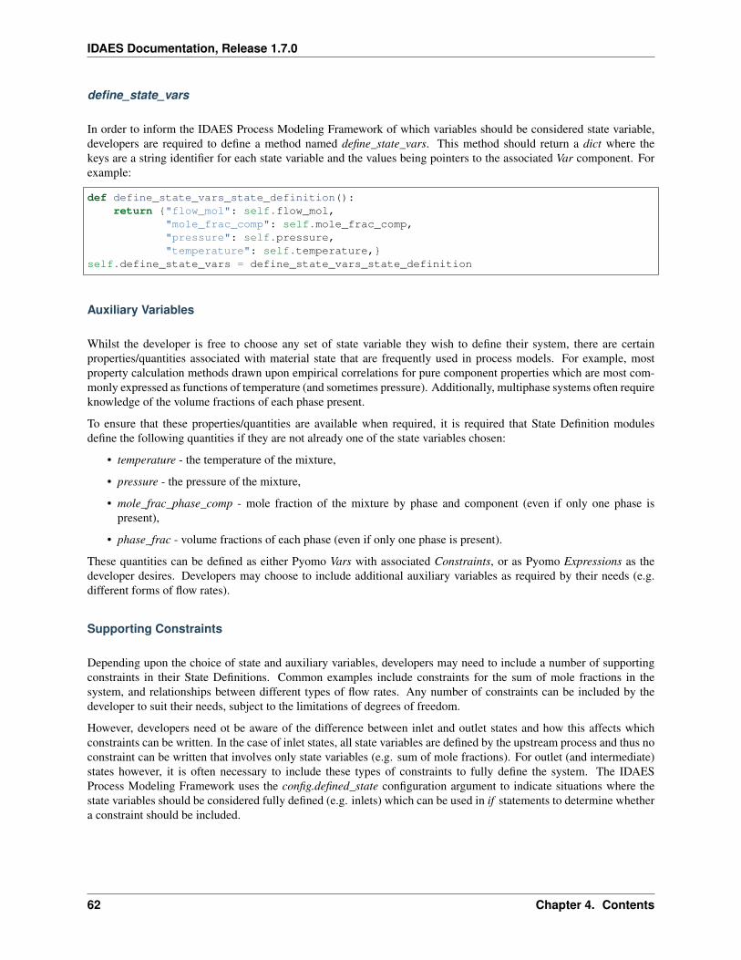
IDAES Documentation, Release 1.7.0
define_state_vars
In order to inform the IDAES Process Modeling Framework of which variables should be considered state variable,developers are required to define a method named define_state_vars. This method should return a dict where thekeys are a string identifier for each state variable and the values being pointers to the associated Var component. Forexample:
def define_state_vars_state_definition():return "flow_mol": self.flow_mol,
"mole_frac_comp": self.mole_frac_comp,"pressure": self.pressure,"temperature": self.temperature,
self.define_state_vars = define_state_vars_state_definition
Auxiliary Variables
Whilst the developer is free to choose any set of state variable they wish to define their system, there are certainproperties/quantities associated with material state that are frequently used in process models. For example, mostproperty calculation methods drawn upon empirical correlations for pure component properties which are most com-monly expressed as functions of temperature (and sometimes pressure). Additionally, multiphase systems often requireknowledge of the volume fractions of each phase present.
To ensure that these properties/quantities are available when required, it is required that State Definition modulesdefine the following quantities if they are not already one of the state variables chosen:
• temperature - the temperature of the mixture,
• pressure - the pressure of the mixture,
• mole_frac_phase_comp - mole fraction of the mixture by phase and component (even if only one phase ispresent),
• phase_frac - volume fractions of each phase (even if only one phase is present).
These quantities can be defined as either Pyomo Vars with associated Constraints, or as Pyomo Expressions as thedeveloper desires. Developers may choose to include additional auxiliary variables as required by their needs (e.g.different forms of flow rates).
Supporting Constraints
Depending upon the choice of state and auxiliary variables, developers may need to include a number of supportingconstraints in their State Definitions. Common examples include constraints for the sum of mole fractions in thesystem, and relationships between different types of flow rates. Any number of constraints can be included by thedeveloper to suit their needs, subject to the limitations of degrees of freedom.
However, developers need ot be aware of the difference between inlet and outlet states and how this affects whichconstraints can be written. In the case of inlet states, all state variables are defined by the upstream process and thus noconstraint can be written that involves only state variables (e.g. sum of mole fractions). For outlet (and intermediate)states however, it is often necessary to include these types of constraints to fully define the system. The IDAESProcess Modeling Framework uses the config.defined_state configuration argument to indicate situations where thestate variables should be considered fully defined (e.g. inlets) which can be used in if statements to determine whethera constraint should be included.
62 Chapter 4. Contents
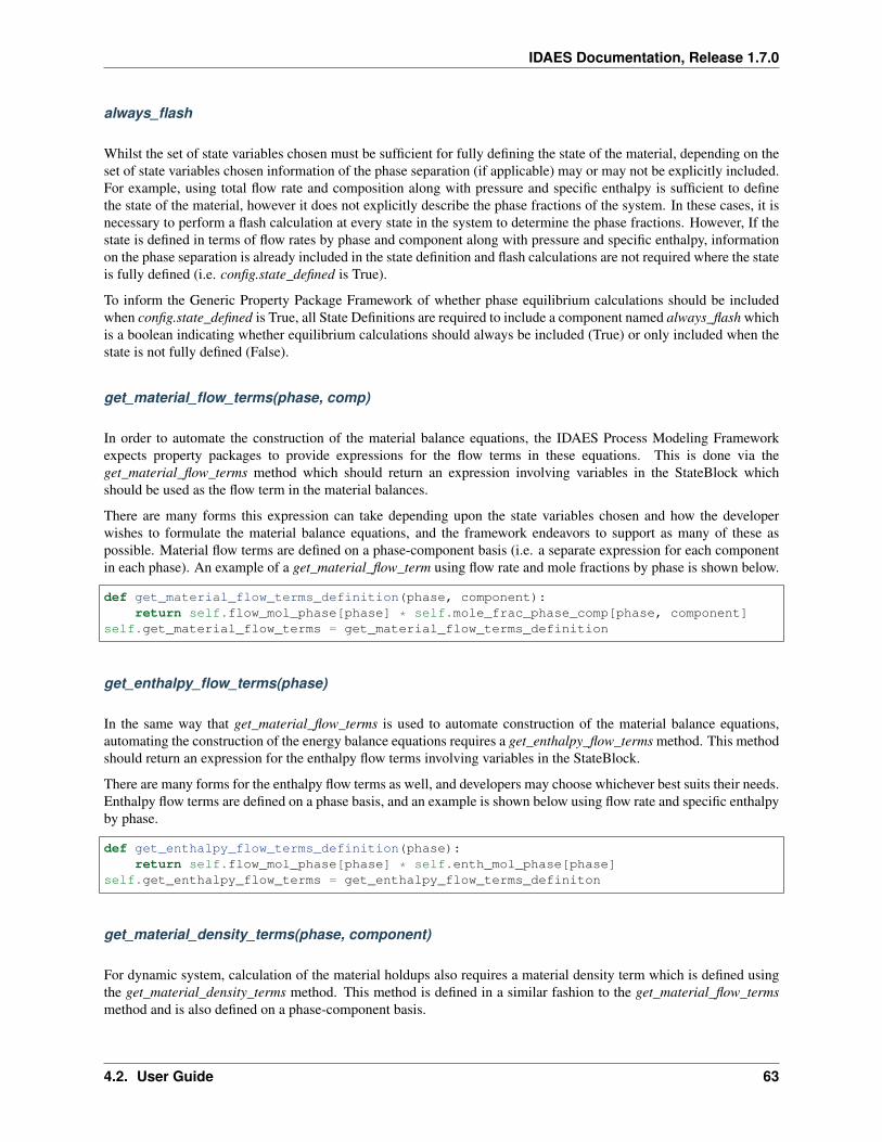
IDAES Documentation, Release 1.7.0
always_flash
Whilst the set of state variables chosen must be sufficient for fully defining the state of the material, depending on theset of state variables chosen information of the phase separation (if applicable) may or may not be explicitly included.For example, using total flow rate and composition along with pressure and specific enthalpy is sufficient to definethe state of the material, however it does not explicitly describe the phase fractions of the system. In these cases, it isnecessary to perform a flash calculation at every state in the system to determine the phase fractions. However, If thestate is defined in terms of flow rates by phase and component along with pressure and specific enthalpy, informationon the phase separation is already included in the state definition and flash calculations are not required where the stateis fully defined (i.e. config.state_defined is True).
To inform the Generic Property Package Framework of whether phase equilibrium calculations should be includedwhen config.state_defined is True, all State Definitions are required to include a component named always_flash whichis a boolean indicating whether equilibrium calculations should always be included (True) or only included when thestate is not fully defined (False).
get_material_flow_terms(phase, comp)
In order to automate the construction of the material balance equations, the IDAES Process Modeling Frameworkexpects property packages to provide expressions for the flow terms in these equations. This is done via theget_material_flow_terms method which should return an expression involving variables in the StateBlock whichshould be used as the flow term in the material balances.
There are many forms this expression can take depending upon the state variables chosen and how the developerwishes to formulate the material balance equations, and the framework endeavors to support as many of these aspossible. Material flow terms are defined on a phase-component basis (i.e. a separate expression for each componentin each phase). An example of a get_material_flow_term using flow rate and mole fractions by phase is shown below.
def get_material_flow_terms_definition(phase, component):return self.flow_mol_phase[phase] * self.mole_frac_phase_comp[phase, component]
self.get_material_flow_terms = get_material_flow_terms_definition
get_enthalpy_flow_terms(phase)
In the same way that get_material_flow_terms is used to automate construction of the material balance equations,automating the construction of the energy balance equations requires a get_enthalpy_flow_terms method. This methodshould return an expression for the enthalpy flow terms involving variables in the StateBlock.
There are many forms for the enthalpy flow terms as well, and developers may choose whichever best suits their needs.Enthalpy flow terms are defined on a phase basis, and an example is shown below using flow rate and specific enthalpyby phase.
def get_enthalpy_flow_terms_definition(phase):return self.flow_mol_phase[phase] * self.enth_mol_phase[phase]
self.get_enthalpy_flow_terms = get_enthalpy_flow_terms_definiton
get_material_density_terms(phase, component)
For dynamic system, calculation of the material holdups also requires a material density term which is defined usingthe get_material_density_terms method. This method is defined in a similar fashion to the get_material_flow_termsmethod and is also defined on a phase-component basis.
4.2. User Guide 63
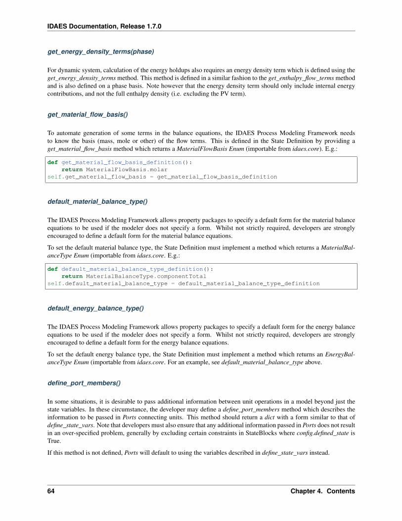
IDAES Documentation, Release 1.7.0
get_energy_density_terms(phase)
For dynamic system, calculation of the energy holdups also requires an energy density term which is defined using theget_energy_density_terms method. This method is defined in a similar fashion to the get_enthalpy_flow_terms methodand is also defined on a phase basis. Note however that the energy density term should only include internal energycontributions, and not the full enthalpy density (i.e. excluding the PV term).
get_material_flow_basis()
To automate generation of some terms in the balance equations, the IDAES Process Modeling Framework needsto know the basis (mass, mole or other) of the flow terms. This is defined in the State Definition by providing aget_material_flow_basis method which returns a MaterialFlowBasis Enum (importable from idaes.core). E.g.:
def get_material_flow_basis_definition():return MaterialFlowBasis.molar
self.get_material_flow_basis = get_material_flow_basis_definition
default_material_balance_type()
The IDAES Process Modeling Framework allows property packages to specify a default form for the material balanceequations to be used if the modeler does not specify a form. Whilst not strictly required, developers are stronglyencouraged to define a default form for the material balance equations.
To set the default material balance type, the State Definition must implement a method which returns a MaterialBal-anceType Enum (importable from idaes.core. E.g.:
def default_material_balance_type_definition():return MaterialBalanceType.componentTotal
self.default_material_balance_type = default_material_balance_type_definition
default_energy_balance_type()
The IDAES Process Modeling Framework allows property packages to specify a default form for the energy balanceequations to be used if the modeler does not specify a form. Whilst not strictly required, developers are stronglyencouraged to define a default form for the energy balance equations.
To set the default energy balance type, the State Definition must implement a method which returns an EnergyBal-anceType Enum (importable from idaes.core. For an example, see default_material_balance_type above.
define_port_members()
In some situations, it is desirable to pass additional information between unit operations in a model beyond just thestate variables. In these circumstance, the developer may define a define_port_members method which describes theinformation to be passed in Ports connecting units. This method should return a dict with a form similar to that ofdefine_state_vars. Note that developers must also ensure that any additional information passed in Ports does not resultin an over-specified problem, generally by excluding certain constraints in StateBlocks where config.defined_state isTrue.
If this method is not defined, Ports will default to using the variables described in define_state_vars instead.
64 Chapter 4. Contents
IDAES Documentation, Release 1.7.0
define_display_vars()
Developers may also define a define_display_vars method which is used by the IDAES report methods to determinewhat information should be displayed for each state. The define_display_vars method should return a dict containingthe information to display with the keys being the display name for the information and value being the quantity todisplay (similar to the define_state_Vars method). If this method is not defined then the define_state_vars method isused by the report methods instead.
state_initialization(self)
The state_initialization method is called as part of the Generic Property Package Framework initialize method and isexpected to set initial guesses for any auxiliary variables defined by the State Definition based on the current values ofthe state variables. Note that the state variables will have been provided with initial guesses for the current state of thematerial from the process models, and thus will likely not be at their pre-defined initial conditions.
self.do_not_initialize
The do_not_initialize component is a list containing a list of Constraint names which should remain deactivated duringinitialization of the StateBlock and only reactivated during the final step on initialization. Common examples of theseare those constraints that are only written for outlet Blocks (i.e. those when config.defined_state is False), such asoverall sum of mole fraction constraints.
Developing Phase Equilibrium Methods
Contents
• Developing Phase Equilibrium Methods
– phase_equil(self)
– phase_equil_initialization(self)
Handling phase equilibrium and phase transitions within an equation oriented framework can be challenging as it isnecessary to ensure that all constraints and variables has feasible solution at all states. When dealing with disappearingphases and correlations that can become ill-defined or singular outside of the two phase envelope, it is necessary toeither bound the problem to the two-phase region or reformulate the problem.
The IDAES Generic Property Package Framework provides support for reformulating the problem by defining an“equilibrium temperature” (self._teq) at which all phase equilibrium calculations are performed. Issues surroundingphase transitions can be avoided by providing a definition for the equilibrium temperature that satisfies the followingconstraints:
𝑇bubble <= 𝑇𝑒𝑞 <= 𝑇dew
The Phase Equilibrium module allows users to provide a definition for the equilibrium temperature, along with anynecessary instructions on how to initialize the components associated with this definition.
A Phase Equilibrium module consists of two methods , which are described below.
4.2. User Guide 65
IDAES Documentation, Release 1.7.0
phase_equil(self)
The phase_equil method is responsible for defining the variables and constraints necessary for calculating the equi-librium temperature, and at a minimum must contain one constraint relating the equilibrium temperature (self._teq) tothe system temperature (self.temperature).
phase_equil_initialization(self)
This method is called by the Generic Property Package Framework initialization routine and should initialize theconstraints associated with the phase equilibrium definition.
Note that the Generic Property Package Framework beings by deactivating all constraints in the StateBlock so the firststep in the phase_equil_initialization method should be to activate any constraints defined in phase_equil. Addition-ally, this method may calculate initial values for any supporting variables defined in phase_equil based on variablesthat have already been initialized (primarily temperature and bubble and dew points if used). Developers should becareful however to fully understand the initialization sequence of the Generic Property Package Framework to under-stand which variables may have been initialized at this point.
Introduction
Note: The generic property package framework is still under development. Whilst the current framework is func-tional, features are still being developed and added.
The generic property package framework builds upon the existing framework for implementing property packageswithin IDAES, and will not prevent the use of custom written property packages in the future. Due to the complexnature of thermophysical property calculations, the generic property framework cannot support all possible materialsand applications. Whilst it is hoped that the generic framework will be able to handle most common applications, userswith more unusual systems or those solving computationally intensive problems may need to write custom propertypackages for their cases.
Property packages represent the core of any process model, and having a suitable property package is key to suc-cessfully modeling any process system. However, developing property packages is a significant challenge even forexperienced modelers as they involve large numbers of tightly coupled constraints and parameters. The goal of theIDAES Generic Property Package Framework is to provide a flexible platform on which users can build propertypackages for common types of systems by calling upon libraries of modular sub-models to build up complex propertycalculations with the least effort possible.
The Generic Property Package Framework breaks down property packages into a number of components which canbe assembled in a modular fashion. Users need only provide those components which they require for their system ofinterest, and components can be drawn from libraries of existing components or provided by the user as custom code.Details on how to set up the definition of a property package using the generic framework are given here.
The components which make up a generic property package are as follows:
1. Choose a base set of units of measurement for the property package.
2. Define the components which make up the material of interest, including methods for calculating the purecomponent properties of interest in the system.
3. Define the phases of interest for the application, including equations of state and other phase specific decisions.
4. Choose the set of state variables you wish to use and a reference state for the system.
5. (Optional) Define any phase equilibria which occurs in the system and methods associated with calculating this.
66 Chapter 4. Contents
IDAES Documentation, Release 1.7.0
The following sections will describe how to define a property package using the Generic Property Package Frameworkalong with the libraries of sub-models currently available. Finally, the developers section describes how to go aboutdefining your own custom components to use when creating custom property packages.
Note: Within most IDAES models “parameters” are in fact defined as Pyomo ‘Vars’ (i.e. variables) which are fixedat their defined values. Whilst Params would seem to be the logical choice for these, parameter estimation problemsrequire the parameters being estimated to be defined as Vars so that the solver is free to vary them.
Generic Reaction Package Framework
Contents
Defining Reaction Packages
Contents
• Defining Reaction Packages
– Introduction
– Units of Measurement
– Config Dictionary
– Class Definition
Introduction
In order to create and use a property package using the IDAES Generic Reaction Package Framework, users mustprovide a definition for the system they wish to model. The framework supports two approaches for defining theproperty package, which are described below, both of which are equivalent in practice.
Units of Measurement
As with generic thermophysical property packages, when defining a reaction package using the generic frameworkusers must define the base units for the reaction package (see link). The approach for setting the base units and unitsfor all parameters is the same as for thermophysical property packages and depends on the approach used to define thereaction package.
Config Dictionary
The most common way to use the Generic Reaction Package Framework is to create an instance of the GenericReac-tionParameterBlock component and provide it with a dictionary of configuration arguments, as shown below:
m = ConcreteModel()
m.fs = FlowsheetBlock()
(continues on next page)
4.2. User Guide 67
IDAES Documentation, Release 1.7.0
(continued from previous page)
m.fs.thermo_properties = PhysicalParameterBlock()
m.fs.reaction_properties = GenericReactionParameterBlock(default="property_package":→˓m.fs.thermo_properties, config_dict)
In the above example, the PhysicalParameterBlock object can be from any thermophysical property package suitablefor the user’s application.
Users need to populate config_dict with the desired options for their system as described in the other parts of this docu-mentation. An example of a configuration dictionary can be found later on this page. For details on each configurationoption, please see the relevant documentation.
Using this approach, units of measurement are defined using the base_units option in the configuration dictionary.Users must provide units for the 5 core quantities, and may also provide units for the other 2 SI base quantities (ifrequired). For details on other configuration options, please see the relevant documentation.
Linking to a Thermophysical Property Package
As state information is defined by thermophysical property packages in IDAES, each reaction package must be linkedto an appropriate thermophysical property package. This linkage is used by the reaction package to find the stateinformation required to calculate the reaction properties, and thus the thermophysical property package must supportall the properties required by the reaction package.
Setting Reaction Basis
Many reaction properties (e.g. reaction rates) can be defined on different bases, such as a mass or molar basis.All properties within a package must use the same basis, which can be set using the “reaction_basis” configurationargument (see below). This must be done using the MaterialFlowBasis Enum, which can be imported from idaes.core.
Configuration Example
from pyomo.environ import units as pyunits
from idaes.core import MaterialFlowBasis
config_dict = "base_units": "time": pyunits.s,
"length": pyunits.m,"mass": pyunits.kg,"amount": pyunits.mol,"temperature": pyunits.K,
"rate_reactions": "R1": "stoichiometry": ("Liq", "A"): -1,
("Liq", "B"): -1,("Liq", "C"): 2,
"heat_of_reaction": constant_dh_rxn,"rate_constant": arrhenius,"rate_form": power_law_rate,"concentration_form": ConcentrationForm.moleFraction,"parameter_data":
"dh_rxn_ref": (-10000, pyunits.J/pyunits.mol),"arrhenius_const": (1, pyunits.mol/pyunits.m**3/pyunits.s),
(continues on next page)
68 Chapter 4. Contents
IDAES Documentation, Release 1.7.0
(continued from previous page)
"energy_activation": (1000, pyunits.J/pyunits.mol),"equilibrium_reactions":
"R2": "stoichiometry": ("Liq", "B"): -1,("Liq", "C"): -1,("Liq", "D"): 1,
"heat_of_reaction": constant_dh_rxn,"equilibrium_constant": van_t_hoff,"equilibrium_form": power_law_equil,"concentration_form": ConcentrationForm.moleFraction,"parameter_data":
"dh_rxn_ref": (-20000, pyunits.J/pyunits.mol),"k_eq_ref": (100, None),"T_eq_ref": (350, pyunits.K)
Class Definition
Alternatively, the IDAES Generic Reaction Package Framework supports defining classes derived from the IDAESGenericReactionParameterData class with methods for defining configuration options and parameters.
Users can define two methods which are called automatically when an instance of the property package is created:
1. configure, which defines the users selection of sub-models, and
2. parameters, which defines the parameters necessary for the selected property methods.
A basic outline of a user defined Reaction Parameter Block is shown below.
@declare_process_block_class("UserReactionParameterBlock")class UserReactionParameterData(GenericReactionParameterData):
def configure(self):# Set configuration optionsself.config.option_1 = value
def parameters(self):# Define parametersself.param_1 = Var(index_set, initialize=value)
Users should populate the configure and parameters methods as discussed below.
Configure
The ‘configure‘ method is used to assign values to the configuration arguments, using the formatself.config.option_name = value. Users will also need to set the units of measurement in the property package meta-data.
Parameters
The parameters method is used to construct all the parameters associated with the property calculations and to specifyvalues for these. The list of necessary parameters is based on the configuration options and the selected methods. Eachmethod lists their necessary parameters in their documentation. Users need only define those parameters required bythe options they have chosen.
4.2. User Guide 69
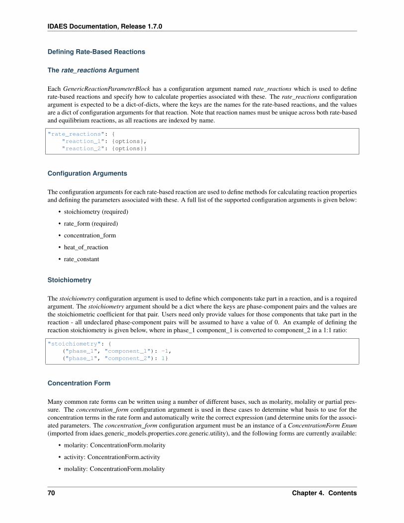
IDAES Documentation, Release 1.7.0
Defining Rate-Based Reactions
The rate_reactions Argument
Each GenericReactionParameterBlock has a configuration argument named rate_reactions which is used to definerate-based reactions and specify how to calculate properties associated with these. The rate_reactions configurationargument is expected to be a dict-of-dicts, where the keys are the names for the rate-based reactions, and the valuesare a dict of configuration arguments for that reaction. Note that reaction names must be unique across both rate-basedand equilibrium reactions, as all reactions are indexed by name.
"rate_reactions": "reaction_1": options,"reaction_2": options
Configuration Arguments
The configuration arguments for each rate-based reaction are used to define methods for calculating reaction propertiesand defining the parameters associated with these. A full list of the supported configuration arguments is given below:
• stoichiometry (required)
• rate_form (required)
• concentration_form
• heat_of_reaction
• rate_constant
Stoichiometry
The stoichiometry configuration argument is used to define which components take part in a reaction, and is a requiredargument. The stoichiometry argument should be a dict where the keys are phase-component pairs and the values arethe stoichiometric coefficient for that pair. Users need only provide values for those components that take part in thereaction - all undeclared phase-component pairs will be assumed to have a value of 0. An example of defining thereaction stoichiometry is given below, where in phase_1 component_1 is converted to component_2 in a 1:1 ratio:
"stoichiometry": ("phase_1", "component_1"): -1,("phase_1", "component_2"): 1
Concentration Form
Many common rate forms can be written using a number of different bases, such as molarity, molality or partial pres-sure. The concentration_form configuration argument is used in these cases to determine what basis to use for theconcentration terms in the rate form and automatically write the correct expression (and determine units for the associ-ated parameters. The concentration_form configuration argument must be an instance of a ConcentrationForm Enum(imported from idaes.generic_models.properties.core.generic.utility), and the following forms are currently available:
• molarity: ConcentrationForm.molarity
• activity: ConcentrationForm.activity
• molality: ConcentrationForm.molality
70 Chapter 4. Contents
IDAES Documentation, Release 1.7.0
• mole fractions: ConcentrationForm.moleFraction
• mass fractions: ConcentrationForm.massFraction
• partial pressure: ConcentrationForm.partialPressure
Other Reaction Properties
The remaining configuration arguments are used to define how different properties should be calculated for eachreaction. The rate_form argument is required, however all other properties need only be defined if needed for theuser’s application. These arguments should be provided as either Python functions or classes;
• functions are used for self-contained correlations with hard-coded parameters,
• classes are used for more generic correlations which require associated parameters.
A list of the libraries of methods available in the IDAES Framework can be found here.
Defining Equilibrium Reactions
The equilibrium_reactions Argument
Each GenericReactionParameterBlock has a configuration argument named equilibrium_reactions which is used todefine equilibrium reactions and specify how to calculate properties associated with these. The equilibrium_reactionsconfiguration argument is expected to be a dict-of-dicts, where the keys are the names for the equilibrium reactions,and the values are a dict of configuration arguments for that reaction. Note that reaction names must be unique acrossboth rate-based and equilibrium reactions, as all reactions are indexed by name.
"equilibrium_reactions": "reaction_1": options,"reaction_2": options
Configuration Arguments
The configuration arguments for each equilibrium reaction are used to define methods for calculating reaction prop-erties and defining the parameters associated with these. A full list of the supported configuration arguments is givenbelow:
• stoichiometry (required)
• equilibrium_form (required)
• concentration_form
• heat_of_reaction
• equilibrium_constant
Stoichiometry
The stoichiometry configuration argument is used to define which components take part in a reaction, and is a requiredargument. The stoichiometry argument should be a dict where the keys are phase-component pairs and the values arethe stoichiometric coefficient for that pair. Users need only provide values for those components that take part in thereaction - all undeclared phase-component pairs will be assumed to have a value of 0. An example of defining thereaction stoichiometry is given below, where in phase_1 component_1 is converted to component_2 in a 1:1 ratio:
4.2. User Guide 71
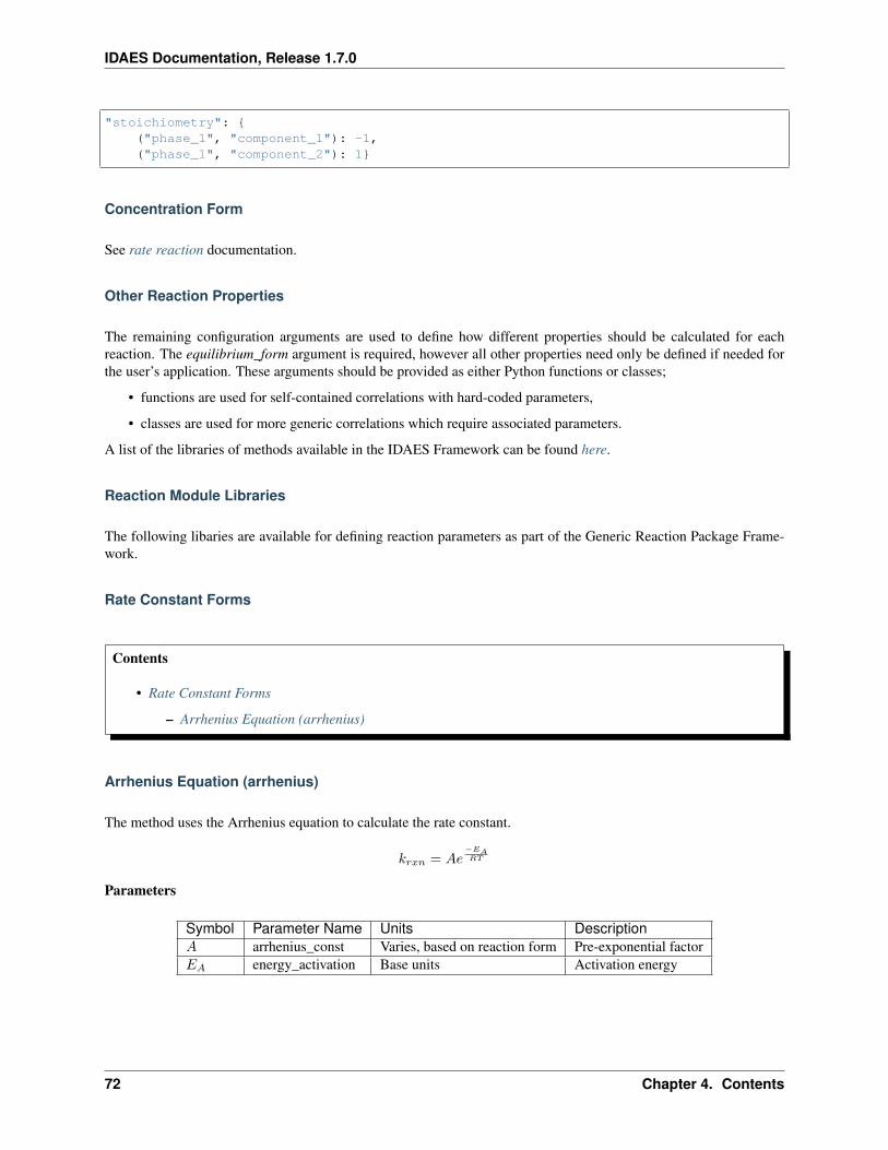
IDAES Documentation, Release 1.7.0
"stoichiometry": ("phase_1", "component_1"): -1,("phase_1", "component_2"): 1
Concentration Form
See rate reaction documentation.
Other Reaction Properties
The remaining configuration arguments are used to define how different properties should be calculated for eachreaction. The equilibrium_form argument is required, however all other properties need only be defined if needed forthe user’s application. These arguments should be provided as either Python functions or classes;
• functions are used for self-contained correlations with hard-coded parameters,
• classes are used for more generic correlations which require associated parameters.
A list of the libraries of methods available in the IDAES Framework can be found here.
Reaction Module Libraries
The following libaries are available for defining reaction parameters as part of the Generic Reaction Package Frame-work.
Rate Constant Forms
Contents
• Rate Constant Forms
– Arrhenius Equation (arrhenius)
Arrhenius Equation (arrhenius)
The method uses the Arrhenius equation to calculate the rate constant.
𝑘𝑟𝑥𝑛 = 𝐴𝑒−𝐸𝐴𝑅𝑇
Parameters
Symbol Parameter Name Units Description𝐴 arrhenius_const Varies, based on reaction form Pre-exponential factor𝐸𝐴 energy_activation Base units Activation energy
72 Chapter 4. Contents
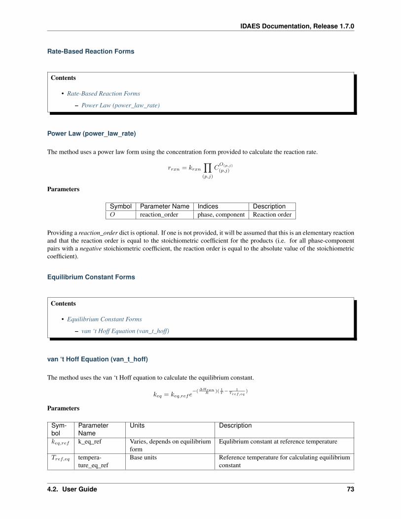
IDAES Documentation, Release 1.7.0
Rate-Based Reaction Forms
Contents
• Rate-Based Reaction Forms
– Power Law (power_law_rate)
Power Law (power_law_rate)
The method uses a power law form using the concentration form provided to calculate the reaction rate.
𝑟𝑟𝑥𝑛 = 𝑘𝑟𝑥𝑛∏(𝑝,𝑗)
𝐶𝑂(𝑝,𝑗)
(𝑝,𝑗)
Parameters
Symbol Parameter Name Indices Description𝑂 reaction_order phase, component Reaction order
Providing a reaction_order dict is optional. If one is not provided, it will be assumed that this is an elementary reactionand that the reaction order is equal to the stoichiometric coefficient for the products (i.e. for all phase-componentpairs with a negative stoichiometric coefficient, the reaction order is equal to the absolute value of the stoichiometriccoefficient).
Equilibrium Constant Forms
Contents
• Equilibrium Constant Forms
– van ‘t Hoff Equation (van_t_hoff)
van ‘t Hoff Equation (van_t_hoff)
The method uses the van ‘t Hoff equation to calculate the equilibrium constant.
𝑘𝑒𝑞 = 𝑘𝑒𝑞,𝑟𝑒𝑓𝑒−(Δ𝐻𝑟𝑥𝑛
𝑅 )( 1𝑇 − 1
𝑇𝑟𝑒𝑓,𝑒𝑞)
Parameters
Sym-bol
ParameterName
Units Description
𝑘𝑒𝑞,𝑟𝑒𝑓 k_eq_ref Varies, depends on equilibriumform
Equlibrium constant at reference temperature
𝑇𝑟𝑒𝑓,𝑒𝑞 tempera-ture_eq_ref
Base units Reference temperature for calculating equilibriumconstant
4.2. User Guide 73
IDAES Documentation, Release 1.7.0
Equilibrium Reaction Forms
Contents
• Equilibrium Reaction Forms
– Power Law (power_law_equil)
Power Law (power_law_equil)
The method uses a power law form using the concentration form provided to calculate the reaction rate.
𝑘𝑒𝑞 =∏(𝑝,𝑗)
𝑥𝑂(𝑝,𝑗)
(𝑝,𝑗)
Parameters
Symbol Parameter Name Indices Description𝑂 reaction_order phase, component Reaction order
Providing a reaction_order dict is optional. If one is not provided, it will be assumed that this is an elementaryreaction and that the reaction order is equal to the stoichiometric coefficient for all component in non-solid phases (thecontribution of solid phases is assumed to be constant and included in the equilibrium constant, thus an order of zerois assumed).
Heat of Reaction Forms
Contents
• Heat of Reaction Forms
– Constant Heat of Reaction (constant_dh_rxn)
Constant Heat of Reaction (constant_dh_rxn)
The simplest form for calculating the heat of reaction, this method assumes a constant value provided by the user.
∆ℎ𝑟𝑥𝑛 = ∆ℎ𝑟𝑥𝑛,𝑟𝑒𝑓
Parameters
Symbol Parameter Name Indices Description∆ℎ𝑟𝑥𝑛,𝑟𝑒𝑓 dh_rxn_ref Heat of reaction
74 Chapter 4. Contents
IDAES Documentation, Release 1.7.0
Introduction
Note: The generic reaction package framework is still under development. Whilst the current framework is functional,features are still being developed and added.
The generic reaction package framework builds upon the existing framework for implementing reaction packageswithin IDAES, and will not prevent the use of custom written reaction packages in the future. Whilst it is hoped thatthe generic framework will be able to handle most common applications, users with more unusual systems or thosesolving computationally intensive problems may need to write custom reaction packages for their cases.
The Generic Reaction Package Framework breaks down reaction packages into a number of components which canbe assembled in a modular fashion. Users need only provide those components which they require for their system ofinterest, and components can be drawn from libraries of existing components or provided by the user as custom code.Details on how to set up the definition of a reaction package using the generic framework are given here.
The components which make up a generic reaction package are as follows:
1. Choose a base set of units of measurement for the property package.
2. Associate the reaction package with an appropriate thermodynamic property package. The thermodynamicproperty package must use the same set of base units of measurement,
3. Define the basis of the reaction terms for the reaction package.
4. Define the rate-based reactions of interest in the system.
5. Define the equilibrium-based reactions of interest in the system. Nore that phase equilibrium is generallyhandled in the thermodynamic property package.
The following sections will describe how to define a reaction package using the Generic Reaction Package Frameworkalong with the libraries of sub-models currently available. Finally, the developers section describes how to go aboutdefining your own custom components to use when creating custom property packages.
Note: Within most IDAES models “parameters” are in fact defined as Pyomo ‘Vars’ (i.e. variables) which are fixedat their defined values. Whilst Params would seem to be the logical choice for these, parameter estimation problemsrequire the parameters being estimated to be defined as Vars so that the solver is free to vary them.
Property packages provide the relationships and parameters necessary to determine the properties of process streams.They may be general in purpose, such as ideal gas equations, or specific to a certain application. Property packagesare separated into two categories:
• physical and transport properties
• chemical reaction properties
While several standard property packages are provided in the IDAES model libraries, many process modeling appli-cations will require specific property packages. Information on developing custom property packages is provided inthe advanced user guide.
Since the effort to develop a custom property package is substantial, the IDAES modeling framework provides aGeneric Property Package Framework and Generic Reaction Package Framework to make it easier to create a packagefor common property and reaction models.
4.2. User Guide 75
IDAES Documentation, Release 1.7.0
Units of Measurement
One of the most important roles property packages play within the modeling framework is to define the units ofmeasurement that will be used for those models which use the property packages. Any variable which is created ina unit model will derive its units of measurement from those defined in the associated property package in order toensure consistency of units.
Defining units of measurement in property packages is discussed here.
Physical properties
Almost all process models depend on physical properties to some extent, such as calculation of specific enthalpy orinternal energy for energy balances. These properties only depend on the material being considered and are indepen-dent of the unit operations in which they are used. As such, physical property calculations can be separated from theunit model calculations and treated as a separate submodel which is called by the unit model. Each unit model canthen create instances of these submodels as required to calculate those properties required by each unit.
Within IDAES, this is handled by StateBlock objects – these are self-contained submodels containing the calculationsfor all necessary thermophysical properties for a given material at a given point in space and time. IDAES UnitModelscreate instances of these StateBlocks wherever they need to calculate physical properties and link to variables withinthe StateBlock within the unit model constraints.
However, physical property calculations depend on a set of parameters which are specific to a given material ormixture. Thus, each instance of a StateBlock for a material use the same set of parameters. To avoid duplicatingthese parameters in every instance of a StateBlock for a given material, these parameters are instead grouped in aPhysicalParameterBlock for that material which the StateBlocks link to. In this way, there is a single common locationfor all parameters.
In summary, physical property packages consist of two parts:
• PhysicalParameterBlocks, which contain a set of parameters associated with the specific material(s) being mod-eled
• StateBlocks, which contain the actual calculations of the state variables and functions
Reaction properties
Reaction property packages represent a collection of calculations necessary to determine the reaction behavior of amixture at a given state. Reaction properties depend upon the state and physical properties of the material, and thusmust be linked to a StateBlock which provides the necessary state and physical property information.
Reaction property packages consist of two parts:
• ReactionParameterBlocks, which contain a set of parameters associated with the specific reaction(s) being mod-eled, and
• ReactionBlocks, which contain the actual calculations of the reaction behavior.
Component and Phase Objects
Property packages also rely on component and phase objects.
Component Objects are used to identify the chemical species of interest in a property package and to contain informa-tion describing the behavior of that component (such as properties of that component).
76 Chapter 4. Contents
IDAES Documentation, Release 1.7.0
Phase Objects are used to identify the thermodynamic phases of interest in a property package and to contain infor-mation describing the behavior of that phase (for example the equation of state which describes that phase).
As Needed Properties
Process flow sheets often require a large number of properties to be calculate, but not all of these are required in everyunit operation. Calculating additional properties that are not required is undesirable, as it leads to larger problem sizesand unnecessary complexity of the resulting model.
To address this, IDAES supports “as needed” construction of properties, where the variables and constraints requiredto calculate a given quantity are not added to a model unless the model calls for this quantity. To designate a propertyas an “as needed” quantity, a method can be declared in the associated property BlockData class (StateBlockDataor ReactionBlockData) which contains the instructions for constructing the variables and constraints associated withthe quantity (rather than declaring these within the BlockData’s build method). The name of this method can thenbe associated with the property via the add_properties metadata in the property packages ParameterBlock, whichindicates that when this property is called for, the associated method should be run.
The add_properties metadata can also indicate that a property should always be present (i.e. constructed in the Block-Data’s build method) by setting the method to None, or that it is not supported by setting the method to False.
Generic Property Package Framework
Property packages represent the core of any process model, and having a suitable property package is key to suc-cessfully modeling any process system. However, developing property packages is a significant challenge even forexperienced modelers as they involve large numbers of tightly coupled constraints and parameters. The Generic Prop-erty Package Framework was designed to help users build property packages with the least effort possible by levarginglibraries of modular sub-models that include common types of property calculations.
Generic Reaction Package Framework
Similar to the Generic Property Package Framework, the Generic Reaction Package Framework helps users createreaction property packages for common systems.
Unit Model
Control Volume
• Overview
• Common Control Volume Tasks
• Setting up the time domain
• Getting Property Package Information
• Collecting Indexing Sets for Property Package
• ControlVolume and ControlVolumeBlockData Classes
4.2. User Guide 77
IDAES Documentation, Release 1.7.0
Overview
Control volumes serve as the fundamental building block of all unit operations. Control Volumes represent a single,well-defined volume of material over which material, energy and/or momentum balances will be performed.
The IDAES ControlVolume classes are designed to facilitate the construction of these balance equations by providingthe model developer with a set of pre-built methods to perform the most common tasks in developing models of unitoperations. The ControlVolume classes contain methods for creating and linking the necessary property calculationsand writing common forms of the balance equations so that the model developer can focus their time on the aspectsthat make each unit model unique.
The IDAES process modeling framework currently supports two types of ControlVolumes:
• ControlVolume0DBlock represents a single well-mixed volume of material with a single inlet and a single outlet.This type of control volume is sufficient to model most inlet-outlet type unit operations which do not requirespatial discretization.
• ControlVolume1DBlock represents a volume with spatial variation in one dimension parallel to the material flow.This type of control volume is useful for representing flow in pipes and simple 1D flow reactors.
Common Control Volume Tasks
All of the IDAES ControlVolume classes are built on a common core ControlVolumeBlockData which defines a setof common tasks required for all Control Volumes. The more specific ControlVolume classes then build upon thesecommon tasks to provide tools appropriate for their specific application.
All ControlVolume classes begin with the following tasks:
• Determine if the ControlVolume should be steady-state or dynamic.
• Get the time domain.
• Determine whether material and energy holdups should be calculated.
• Collect information necessary for creating StateBlocks and ReactionBlocks.
• Create references to phase_list and component_list Sets in the PhysicalParameterBlock
Setting up the time domain
The first common task the ControlVolumeBlock performs is to determine if it should be dynamic or steady-state andto collect the time domain from the UnitModel. ControlVolumeBlocks have an argument dynamic which can beprovided during construction which specifies if the Control Volume should be dynamic (dynamic=True) or steady-state (dynamic=False). If the argument is not provided, the ControlVolumeBlock will inherit this argument from itsparent Unit model.
Finally, the ControlVolume checks that the has_holdup argument is consistent with the dynamic argument, and raisesa ConfigurationError if it is not.
Getting Property Package Information
If a reference to a property package was not provided by the UnitModel as an argument, the Control Volume firstchecks to see if the unit model has a property_package argument set, and uses this if present. Otherwise, the Con-trolVolumeBlock begins searching up the model tree looking for an argument named default_property_package anduses the first of these that it finds. If no default_property_package is found, a ConfigurationError is returned.
78 Chapter 4. Contents
IDAES Documentation, Release 1.7.0
Collecting Indexing Sets for Property Package
The final common step for all ControlVolumes is to collect any required indexing sets from the physical propertypackage (for example component and phase lists). These are used by the Control Volume for determining whatbalance equations need to be written, and what terms to create.
The indexing sets the ControlVolume looks for are:
• component_list - used to determine what components are present, and thus what material balances are required
• phase_list - used to determine what phases are present, and thus what balance equations are required
ControlVolume and ControlVolumeBlockData Classes
A key purpose of ControlVolumes is to automate as much of the task of writing a unit model as possible. For thispurpose, ControlVolumes support a number of methods for common tasks model developers may want to perform.The specifics of these methods will be different between different types of ControlVolumes, and certain methods maynot be applicable to some types of Control Volumes (in which case a NotImplementedError will be returned). A fulllist of potential methods is provided here, however users should check the documentation for the specific ControlVolume they are using for more details on what methods are supported in that specific Control Volume.
A key feature of the IDAES Core Modeling Framework is the use of ControlVolumeBlocks. ControlVolumes representa volume of material over which material, energy and/or momentum balances can be performed. ControlVolumeBlockscontain methods to automate the task of writing common forms of these balance equations. ControlVolumeBlocks canalso automate the creation of StateBlocks and ReactionBlocks associated with the control volume.
Unit models represent pieces of equipment and their processes. These models contain the unit performance constraintsand associated variables for the equipment, such as:
• constraints relating balance terms to physical phenomena or properties (e.g. relating extent of reaction to reac-tion rate and volume)
• constraints describing flow of material into or out of unit (e.g. pressure driven flow constraints)
• unit level efficiency constraints (e.g. relating mechanical work to fluid work)
IDAES includes libraries of UnitModel classes. These models are composed of the following components:
1. ControlVolumeBlocks, which represent volume of material over which we wish to perform material, energyand/or momentum balances
2. StateBlocks and ReactionBlocks, which represent the thermophysical, transport and reaction properties of thematerial at a specific point in space and time
3. Inlets and Outlets, which allow UnitModels to connect to other UnitModels
Data Management Framework
DMF Overview
The Data Management Framework (DMF) is used to manage all the data needed by the IDAES framework, includingflowsheets, models, and results. It stores metadata and data in persistent storage. It does not require that the user run aserver or connect to a remote service. The DMF can be accessed through its API or command-line interfaces.
• Concepts
4.2. User Guide 79
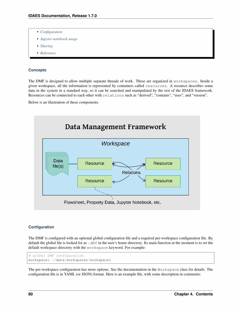
IDAES Documentation, Release 1.7.0
• Configuration
• Jupyter notebook usage
• Sharing
• Reference
Concepts
The DMF is designed to allow multiple separate threads of work. These are organized in workspaces. Inside agiven workspace, all the information is represented by containers called resources. A resource describes somedata in the system in a standard way, so it can be searched and manipulated by the rest of the IDAES framework.Resources can be connected to each other with relations such as “derived”, “contains”, “uses”, and “version”.
Below is an illustration of these components.
Configuration
The DMF is configured with an optional global configuration file and a required per-workspace configuration file. Bydefault the global file is looked for as .dmf in the user’s home directory. Its main function at the moment is to set thedefault workspace directory with the workspace keyword. For example:
# global DMF configurationworkspace: ~/data/workspaces/workspace1
The per-workspace configuration has more options. See the documentation in the Workspace class for details. Theconfiguration file is in YAML (or JSON) format. Here is an example file, with some description in comments:
80 Chapter 4. Contents
IDAES Documentation, Release 1.7.0
settings: # Global settingsworkspace: /home/myuser/ws # Path to current workspace
workspace: # Per-workspace settingslocation: /home/myuser/ws # Path to this workspacename: myws # Name of this workspacedescription: my workspace # Description (if any) of this workspacecreated: 2019-04-09 12:55:05 # Date workspace was createdmodified: 2019-04-09 12:55:05 # Date workspace was modifiedfiles: # Basic information about data filescount: 3 # How many filestotal_size: 1.3 MB # Total size of the files
html_documentation_paths: # List of paths for HTML documentation-: /home/myuser/idaes/docs/build
logging: # Logging configurationidaes.dmf: # Name of the logger
level: DEBUG # Log level (Python logging constant)output: /tmp/debug.log # File path or "_stdout_" or "_stderr_"
This configuration file is used whether you use the DMF from the command-line, Jupyter notebook, or in a Pythonprogram. For details see the DMF package documentation.
Jupyter notebook usage
In the Jupyter Notebook, there are some “magics” defined that make initializing the DMF pretty easy. For example:
from idaes.dmf import magics%dmf init path/to/workspace
The code above loads the “%dmf” line magic in the first line, then uses it to initialize the DMF with the workspace at“path/to/workspace”.
From there, other “line magics” will operate in the context of that DMF workspace.
• %dmf help - Provide help on IDAES objects and classes. See dmf-help.
• %dmf info - Provide information about DMF current state for whatever ‘topics’ are provided
• %dmf list - List resources in the current workspace
• %dmf workspaces - List DMF workspaces; you can do this before %dmf init
DMF help
The IDAES Python interfaces are documented with Sphinx. This includes automatic translation of the comments andstructure of the code into formatted and hyperlinked HTML pages. The %dmf help command lets you easily pullup this documentation for an IDAES module, class, or object. Below are a couple of examples:
# Initialize the DMF firstfrom idaes.dmf import magics%dmf init path/to/workspace create
# Get help on a module (imported)from idaes.core import control_volume1d%dmf help control_volume1d
# Get help on a module (by name, no import)
(continues on next page)
4.2. User Guide 81
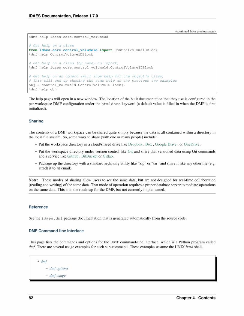
IDAES Documentation, Release 1.7.0
(continued from previous page)
%dmf help idaes.core.control_volume0d
# Get help on a classfrom idaes.core.control_volume1d import ControlVolume1DBlock%dmf help ControlVolume1DBlock
# Get help on a class (by name, no import)%dmf help idaes.core.control_volume1d.ControlVolume1DBlock
# Get help on an object (will show help for the object's class)# This will end up showing the same help as the previous two examplesobj = control_volume1d.ControlVolume1DBlock()%dmf help obj
The help pages will open in a new window. The location of the built documentation that they use is configured in theper-workspace DMF configuration under the htmldocs keyword (a default value is filled in when the DMF is firstinitialized).
Sharing
The contents of a DMF workspace can be shared quite simply because the data is all contained within a directory inthe local file system. So, some ways to share (with one or many people) include:
• Put the workspace directory in a cloud/shared drive like Dropbox , Box , Google Drive , or OneDrive .
• Put the workspace directory under version control like Git and share that versioned data using Git commandsand a service like Github , BitBucket or Gitlab.
• Package up the directory with a standard archiving utility like “zip” or “tar” and share it like any other file (e.g.attach it to an email).
Note: These modes of sharing allow users to see the same data, but are not designed for real-time collaboration(reading and writing) of the same data. That mode of operation requires a proper database server to mediate operationson the same data. This is in the roadmap for the DMF, but not currently implemented.
Reference
See the idaes.dmf package documentation that is generated automatically from the source code.
DMF Command-line Interface
This page lists the commands and options for the DMF command-line interface, which is a Python program calleddmf. There are several usage examples for each sub-command. These examples assume the UNIX bash shell.
• dmf
– dmf options
– dmf usage
82 Chapter 4. Contents
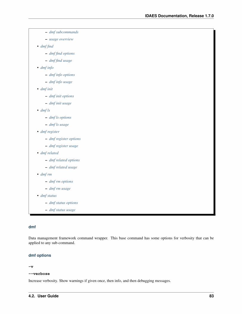
IDAES Documentation, Release 1.7.0
– dmf subcommands
– usage overview
• dmf find
– dmf find options
– dmf find usage
• dmf info
– dmf info options
– dmf info usage
• dmf init
– dmf init options
– dmf init usage
• dmf ls
– dmf ls options
– dmf ls usage
• dmf register
– dmf register options
– dmf register usage
• dmf related
– dmf related options
– dmf related usage
• dmf rm
– dmf rm options
– dmf rm usage
• dmf status
– dmf status options
– dmf status usage
dmf
Data management framework command wrapper. This base command has some options for verbosity that can beapplied to any sub-command.
dmf options
-v
--verbose
Increase verbosity. Show warnings if given once, then info, and then debugging messages.
4.2. User Guide 83
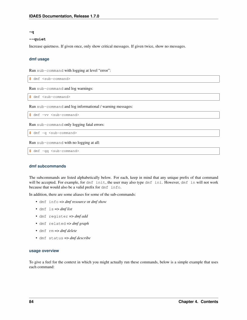
IDAES Documentation, Release 1.7.0
-q
--quiet
Increase quietness. If given once, only show critical messages. If given twice, show no messages.
dmf usage
Run sub-command with logging at level “error”:
$ dmf <sub-command>
Run sub-command and log warnings:
$ dmf <sub-command>
Run sub-command and log informational / warning messages:
$ dmf -vv <sub-command>
Run sub-command only logging fatal errors:
$ dmf -q <sub-command>
Run sub-command with no logging at all:
$ dmf -qq <sub-command>
dmf subcommands
The subcommands are listed alphabetically below. For each, keep in mind that any unique prefix of that commandwill be accepted. For example, for dmf init, the user may also type dmf ini. However, dmf in will not workbecause that would also be a valid prefix for dmf info.
In addition, there are some aliases for some of the sub-commands:
• dmf info => dmf resource or dmf show
• dmf ls => dmf list
• dmf register => dmf add
• dmf related => dmf graph
• dmf rm => dmf delete
• dmf status => dmf describe
usage overview
To give a feel for the context in which you might actually run these commands, below is a simple example that useseach command:
84 Chapter 4. Contents
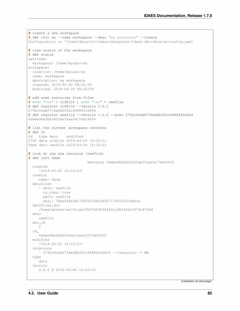
IDAES Documentation, Release 1.7.0
# create a new workspace$ dmf init ws --name workspace --desc "my workspace" --createConfiguration in '/home/dang/src/idaes/dangunter/idaes-dev/docs/ws/config.yaml
# view status of the workspace$ dmf statussettings:
workspace: /home/myuser/wsworkspace:
location: /home/myuser/wsname: workspacedescription: my workspacecreated: 2019-04-20 08:32:59modified: 2019-04-20 08:32:59
# add some resources from files$ echo "one" > oldfile ; echo "two" > newfile$ dmf register oldfile --version 0.0.12792c0ceb0734ed4b302c44884f2d404$ dmf register newfile --version 0.0.2 --prev 2792c0ceb0734ed4b302c44884f2d4046ddee9bb2bb3420ab10aaf4c74d186f6
# list the current workspace contents$ dmf lsid type desc modified2792 data oldfile 2019-04-20 15:33:116dde data newfile 2019-04-20 15:33:23
# look at one one resource (newfile)$ dmf info 6dde
Resource 6ddee9bb2bb3420ab10aaf4c74d186f6created
'2019-04-20 15:33:23'creator
name: dangdatafiles
- desc: newfileis_copy: truepath: newfilesha1: 7bbef45b3bc70855010e02460717643125c3beca
datafiles_dir/home/myuser/ws/files/8027bf92628f41a0b146a5167d147e9d
descnewfile
doc_id2
id_6ddee9bb2bb3420ab10aaf4c74d186f6
modified'2019-04-20 15:33:23'
relations- 2792c0ceb0734ed4b302c44884f2d404 --[version]--> ME
typedata
version0.0.2 @ 2019-04-20 15:33:23
(continues on next page)
4.2. User Guide 85
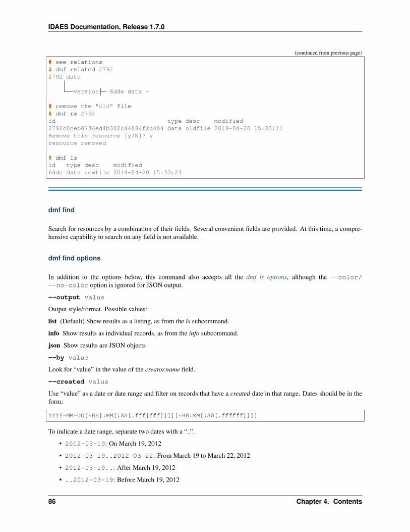
IDAES Documentation, Release 1.7.0
(continued from previous page)
# see relations$ dmf related 27922792 data
version 6dde data -
# remove the "old" file$ dmf rm 2792id type desc modified2792c0ceb0734ed4b302c44884f2d404 data oldfile 2019-04-20 15:33:11Remove this resource [y/N]? yresource removed
$ dmf lsid type desc modified6dde data newfile 2019-04-20 15:33:23
dmf find
Search for resources by a combination of their fields. Several convenient fields are provided. At this time, a compre-hensive capability to search on any field is not available.
dmf find options
In addition to the options below, this command also accepts all the dmf ls options, although the --color/--no-color option is ignored for JSON output.
--output value
Output style/format. Possible values:
list (Default) Show results as a listing, as from the ls subcommand.
info Show results as individual records, as from the info subcommand.
json Show results are JSON objects
--by value
Look for “value” in the value of the creator.name field.
--created value
Use “value” as a date or date range and filter on records that have a created date in that range. Dates should be in theform:
YYYY-MM-DD[*HH[:MM[:SS[.fff[fff]]]][+HH:MM[:SS[.ffffff]]]]
To indicate a date range, separate two dates with a “..”.
• 2012-03-19: On March 19, 2012
• 2012-03-19..2012-03-22: From March 19 to March 22, 2012
• 2012-03-19..: After March 19, 2012
• ..2012-03-19: Before March 19, 2012
86 Chapter 4. Contents

IDAES Documentation, Release 1.7.0
Note that times may also be part of the date strings.
--file value
Look for “value” in the value of the desc field in one of the datafiles.
--modified value
Use “value” as a date or date range and filter on records that have a modified date in that range. See --created fordetails on the date format.
--name value
Look for “value” as one of the values of the alias field.
--type value
Look for “value” as the value of the type field.
dmf find usage
By default, find will essentially provide a filtered listing of resources. If used without options, it is basically an aliasfor ls.
$ dmf lsid type desc modified2517 data file1.txt 2019-04-29 17:29:00344c data file2.txt 2019-04-29 17:29:015d98 data A 2019-04-29 17:28:41602a data B 2019-04-29 17:28:568c55 data C 2019-04-29 17:28:589cbe data D 2019-04-29 17:28:59$ dmf findid type desc modified2517 data file1.txt 2019-04-29 17:29:00344c data file2.txt 2019-04-29 17:29:015d98 data A 2019-04-29 17:28:41602a data B 2019-04-29 17:28:568c55 data C 2019-04-29 17:28:589cbe data D 2019-04-29 17:28:59
The find-specific options add filters. In the example below, the find filters for files that were modified after the givendate and time.
$ dmf find --modified 2019-04-29T17:29:00..id type desc modified2517 data file1.txt 2019-04-29 17:29:00344c data file2.txt 2019-04-29 17:29:01
dmf info
Show detailed information about a resource. This command may also be referred to as dmf show.
4.2. User Guide 87
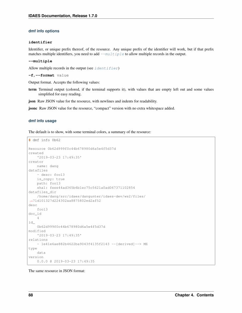
IDAES Documentation, Release 1.7.0
dmf info options
identifier
Identifier, or unique prefix thereof, of the resource. Any unique prefix of the identifier will work, but if that prefixmatches multiple identifiers, you need to add --multiple to allow multiple records in the output.
--multiple
Allow multiple records in the output (see identifier)
-f,--format value
Output format. Accepts the following values:
term Terminal output (colored, if the terminal supports it), with values that are empty left out and some valuessimplified for easy reading.
json Raw JSON value for the resource, with newlines and indents for readability.
jsonc Raw JSON value for the resource, “compact” version with no extra whitespace added.
dmf info usage
The default is to show, with some terminal colors, a summary of the resource:
$ dmf info 0b62
Resource 0b62d999f0c44b678980d6a5e4f5d37dcreated
'2019-03-23 17:49:35'creator
name: dangdatafiles
- desc: foo13is_copy: truepath: foo13sha1: feee44ad365b6b1ec75c5621a0ad067371102854
datafiles_dir/home/dang/src/idaes/dangunter/idaes-dev/ws2/files/
→˓71d101327d224302aa8875802ed2af52desc
foo13doc_id
4id_
0b62d999f0c44b678980d6a5e4f5d37dmodified
'2019-03-23 17:49:35'relations
- 1e41e6ae882b4622ba9043f4135f2143 --[derived]--> MEtype
dataversion
0.0.0 @ 2019-03-23 17:49:35
The same resource in JSON format:
88 Chapter 4. Contents
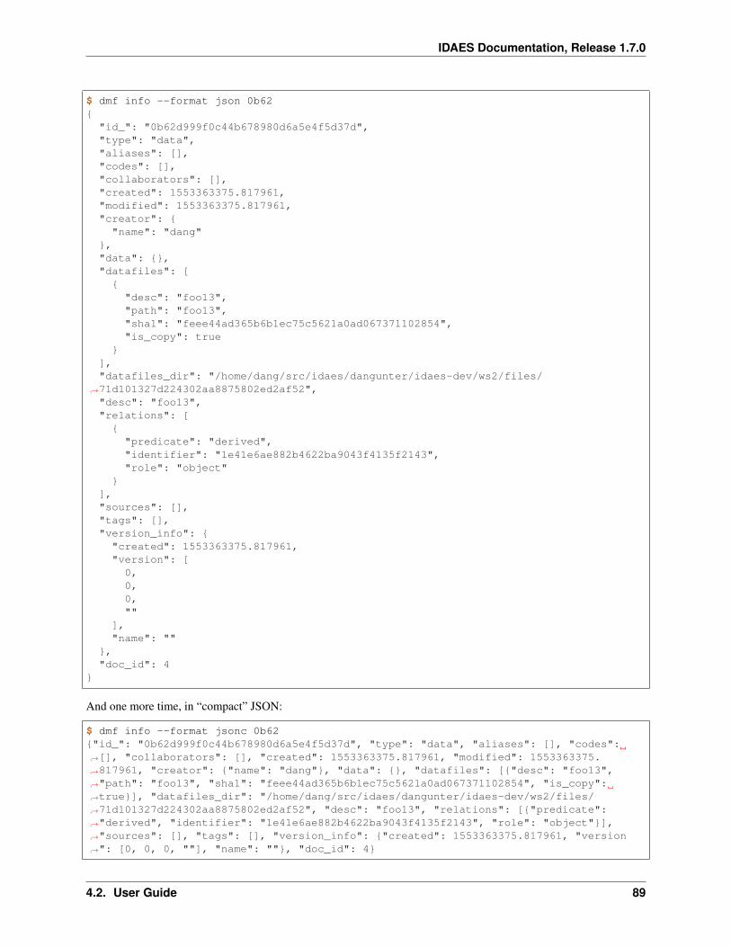
IDAES Documentation, Release 1.7.0
$ dmf info --format json 0b62
"id_": "0b62d999f0c44b678980d6a5e4f5d37d","type": "data","aliases": [],"codes": [],"collaborators": [],"created": 1553363375.817961,"modified": 1553363375.817961,"creator": "name": "dang"
,"data": ,"datafiles": [
"desc": "foo13","path": "foo13","sha1": "feee44ad365b6b1ec75c5621a0ad067371102854","is_copy": true
],"datafiles_dir": "/home/dang/src/idaes/dangunter/idaes-dev/ws2/files/
→˓71d101327d224302aa8875802ed2af52","desc": "foo13","relations": [
"predicate": "derived","identifier": "1e41e6ae882b4622ba9043f4135f2143","role": "object"
],"sources": [],"tags": [],"version_info": "created": 1553363375.817961,"version": [
0,0,0,""
],"name": ""
,"doc_id": 4
And one more time, in “compact” JSON:
$ dmf info --format jsonc 0b62"id_": "0b62d999f0c44b678980d6a5e4f5d37d", "type": "data", "aliases": [], "codes":→˓[], "collaborators": [], "created": 1553363375.817961, "modified": 1553363375.→˓817961, "creator": "name": "dang", "data": , "datafiles": ["desc": "foo13",→˓"path": "foo13", "sha1": "feee44ad365b6b1ec75c5621a0ad067371102854", "is_copy":→˓true], "datafiles_dir": "/home/dang/src/idaes/dangunter/idaes-dev/ws2/files/→˓71d101327d224302aa8875802ed2af52", "desc": "foo13", "relations": ["predicate":→˓"derived", "identifier": "1e41e6ae882b4622ba9043f4135f2143", "role": "object"],→˓"sources": [], "tags": [], "version_info": "created": 1553363375.817961, "version→˓": [0, 0, 0, ""], "name": "", "doc_id": 4
4.2. User Guide 89
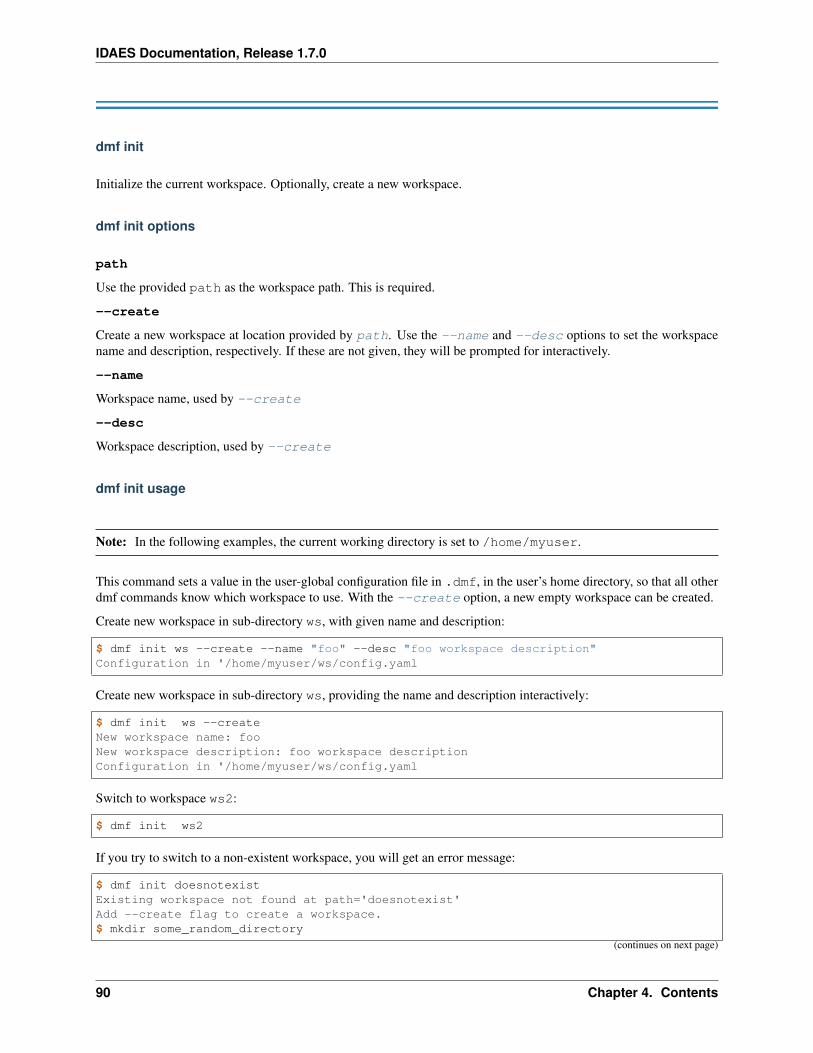
IDAES Documentation, Release 1.7.0
dmf init
Initialize the current workspace. Optionally, create a new workspace.
dmf init options
path
Use the provided path as the workspace path. This is required.
--create
Create a new workspace at location provided by path. Use the --name and --desc options to set the workspacename and description, respectively. If these are not given, they will be prompted for interactively.
--name
Workspace name, used by --create
--desc
Workspace description, used by --create
dmf init usage
Note: In the following examples, the current working directory is set to /home/myuser.
This command sets a value in the user-global configuration file in .dmf, in the user’s home directory, so that all otherdmf commands know which workspace to use. With the --create option, a new empty workspace can be created.
Create new workspace in sub-directory ws, with given name and description:
$ dmf init ws --create --name "foo" --desc "foo workspace description"Configuration in '/home/myuser/ws/config.yaml
Create new workspace in sub-directory ws, providing the name and description interactively:
$ dmf init ws --createNew workspace name: fooNew workspace description: foo workspace descriptionConfiguration in '/home/myuser/ws/config.yaml
Switch to workspace ws2:
$ dmf init ws2
If you try to switch to a non-existent workspace, you will get an error message:
$ dmf init doesnotexistExisting workspace not found at path='doesnotexist'Add --create flag to create a workspace.$ mkdir some_random_directory
(continues on next page)
90 Chapter 4. Contents
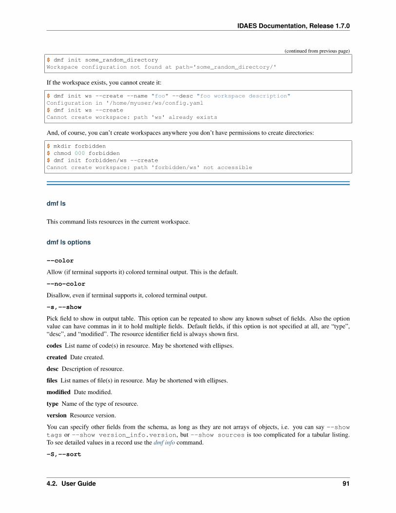
IDAES Documentation, Release 1.7.0
(continued from previous page)
$ dmf init some_random_directoryWorkspace configuration not found at path='some_random_directory/'
If the workspace exists, you cannot create it:
$ dmf init ws --create --name "foo" --desc "foo workspace description"Configuration in '/home/myuser/ws/config.yaml$ dmf init ws --createCannot create workspace: path 'ws' already exists
And, of course, you can’t create workspaces anywhere you don’t have permissions to create directories:
$ mkdir forbidden$ chmod 000 forbidden$ dmf init forbidden/ws --createCannot create workspace: path 'forbidden/ws' not accessible
dmf ls
This command lists resources in the current workspace.
dmf ls options
--color
Allow (if terminal supports it) colored terminal output. This is the default.
--no-color
Disallow, even if terminal supports it, colored terminal output.
-s,--show
Pick field to show in output table. This option can be repeated to show any known subset of fields. Also the optionvalue can have commas in it to hold multiple fields. Default fields, if this option is not specified at all, are “type”,“desc”, and “modified”. The resource identifier field is always shown first.
codes List name of code(s) in resource. May be shortened with ellipses.
created Date created.
desc Description of resource.
files List names of file(s) in resource. May be shortened with ellipses.
modified Date modified.
type Name of the type of resource.
version Resource version.
You can specify other fields from the schema, as long as they are not arrays of objects, i.e. you can say --showtags or --show version_info.version, but --show sources is too complicated for a tabular listing.To see detailed values in a record use the dmf info command.
-S,--sort
4.2. User Guide 91
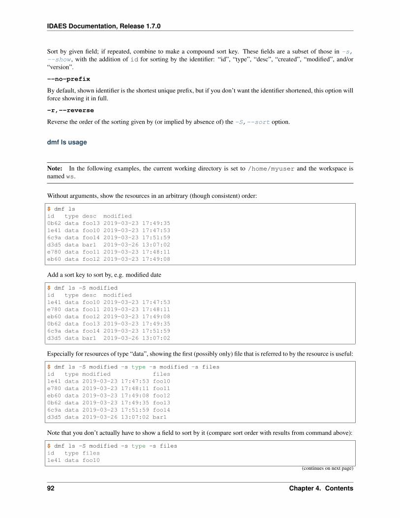
IDAES Documentation, Release 1.7.0
Sort by given field; if repeated, combine to make a compound sort key. These fields are a subset of those in -s,--show , with the addition of id for sorting by the identifier: “id”, “type”, “desc”, “created”, “modified”, and/or“version”.
--no-prefix
By default, shown identifier is the shortest unique prefix, but if you don’t want the identifier shortened, this option willforce showing it in full.
-r,--reverse
Reverse the order of the sorting given by (or implied by absence of) the -S,--sort option.
dmf ls usage
Note: In the following examples, the current working directory is set to /home/myuser and the workspace isnamed ws.
Without arguments, show the resources in an arbitrary (though consistent) order:
$ dmf lsid type desc modified0b62 data foo13 2019-03-23 17:49:351e41 data foo10 2019-03-23 17:47:536c9a data foo14 2019-03-23 17:51:59d3d5 data bar1 2019-03-26 13:07:02e780 data foo11 2019-03-23 17:48:11eb60 data foo12 2019-03-23 17:49:08
Add a sort key to sort by, e.g. modified date
$ dmf ls -S modifiedid type desc modified1e41 data foo10 2019-03-23 17:47:53e780 data foo11 2019-03-23 17:48:11eb60 data foo12 2019-03-23 17:49:080b62 data foo13 2019-03-23 17:49:356c9a data foo14 2019-03-23 17:51:59d3d5 data bar1 2019-03-26 13:07:02
Especially for resources of type “data”, showing the first (possibly only) file that is referred to by the resource is useful:
$ dmf ls -S modified -s type -s modified -s filesid type modified files1e41 data 2019-03-23 17:47:53 foo10e780 data 2019-03-23 17:48:11 foo11eb60 data 2019-03-23 17:49:08 foo120b62 data 2019-03-23 17:49:35 foo136c9a data 2019-03-23 17:51:59 foo14d3d5 data 2019-03-26 13:07:02 bar1
Note that you don’t actually have to show a field to sort by it (compare sort order with results from command above):
$ dmf ls -S modified -s type -s filesid type files1e41 data foo10
(continues on next page)
92 Chapter 4. Contents

IDAES Documentation, Release 1.7.0
(continued from previous page)
e780 data foo11eb60 data foo120b62 data foo136c9a data foo14d3d5 data bar1
Add --no-prefix to show the full identifier:
$ dmf ls -S modified -s type -s files --no-prefixid type files1e41e6ae882b4622ba9043f4135f2143 data foo10e7809d25b390453487998e1f1ef0e937 data foo11eb606172dde74aa79eea027e7eb6a1b6 data foo120b62d999f0c44b678980d6a5e4f5d37d data foo136c9a85629cb24e9796a2d123e9b03601 data foo14d3d5981106ce4d9d8cccd4e86c2cd184 data bar1
dmf register
Register a new resource with the DMF, using a file as an input. An alias for this command is dmf add.
dmf register options
--no-copy
Do not copy the file, instead remember path to current location. Default is to copy the file under the workspacedirectory.
-t,--type
Explicitly specify the type of resource. If this is not given, then try to infer the resource type from the file. The defaultwill be ‘data’. The full list of resource types is in idaes.dmf.resource.RESOURCE_TYPES
--strict
If inferring the type fails, report an error. With --no-strict, or no option, if inferring the type fails, fall back toimporting as a generic file.
--no-unique
Allow duplicate files. The default is --unique, which will stop and print an error if another resource has a filematching this file’s name and contents.
--contained resource
Add a ‘contained in’ relation to the given resource.
--derived resource
Add a ‘derived from’ relation to the given resource.
--used resource
Add a ‘used by’ relation to the given resource.
--prev resource
4.2. User Guide 93
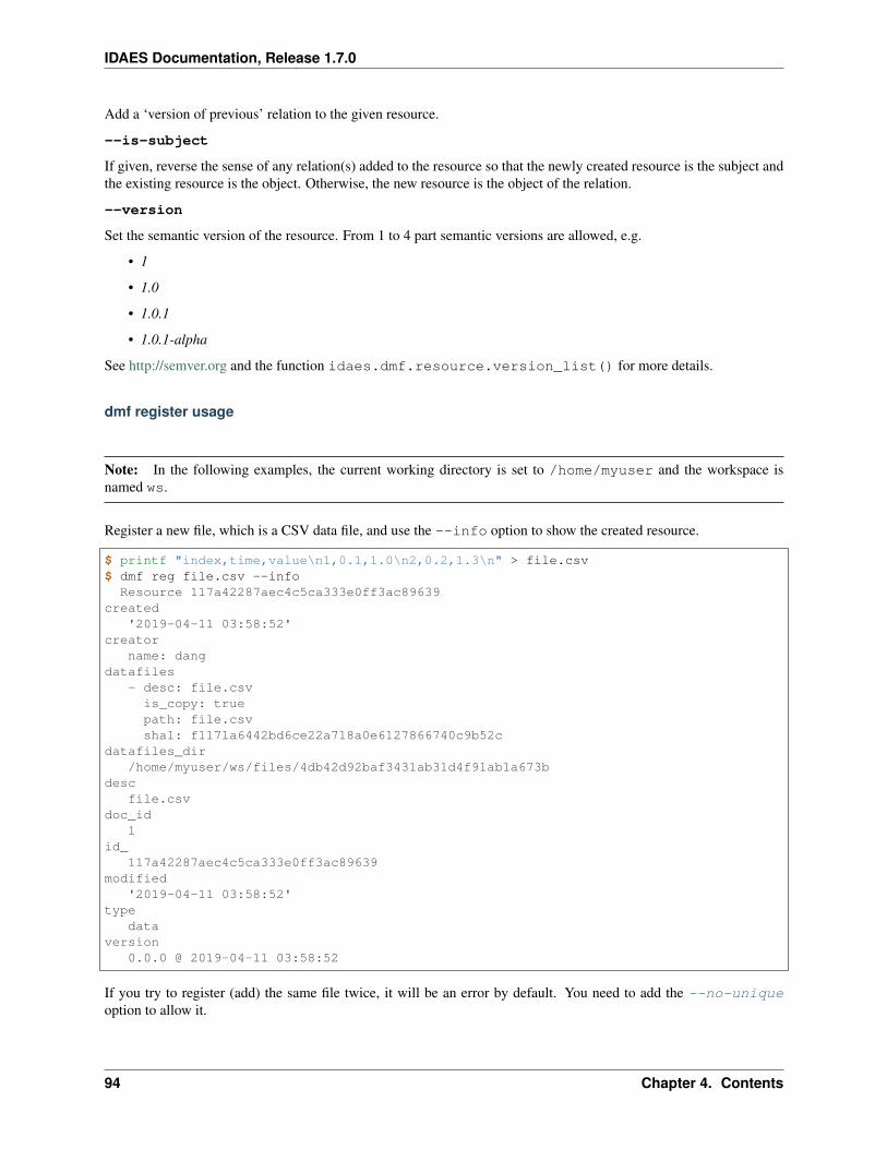
IDAES Documentation, Release 1.7.0
Add a ‘version of previous’ relation to the given resource.
--is-subject
If given, reverse the sense of any relation(s) added to the resource so that the newly created resource is the subject andthe existing resource is the object. Otherwise, the new resource is the object of the relation.
--version
Set the semantic version of the resource. From 1 to 4 part semantic versions are allowed, e.g.
• 1
• 1.0
• 1.0.1
• 1.0.1-alpha
See http://semver.org and the function idaes.dmf.resource.version_list() for more details.
dmf register usage
Note: In the following examples, the current working directory is set to /home/myuser and the workspace isnamed ws.
Register a new file, which is a CSV data file, and use the --info option to show the created resource.
$ printf "index,time,value\n1,0.1,1.0\n2,0.2,1.3\n" > file.csv$ dmf reg file.csv --info
Resource 117a42287aec4c5ca333e0ff3ac89639created
'2019-04-11 03:58:52'creator
name: dangdatafiles
- desc: file.csvis_copy: truepath: file.csvsha1: f1171a6442bd6ce22a718a0e6127866740c9b52c
datafiles_dir/home/myuser/ws/files/4db42d92baf3431ab31d4f91ab1a673b
descfile.csv
doc_id1
id_117a42287aec4c5ca333e0ff3ac89639
modified'2019-04-11 03:58:52'
typedata
version0.0.0 @ 2019-04-11 03:58:52
If you try to register (add) the same file twice, it will be an error by default. You need to add the --no-uniqueoption to allow it.
94 Chapter 4. Contents
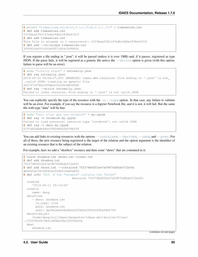
IDAES Documentation, Release 1.7.0
$ printf "index,time,value\n1,0.1,1.0\n2,0.2,1.3\n" > timeseries.csv$ dmf add timeseries.csv2315bea239c147e4bc6d2e1838e4101f$ dmf add timeseries.csvThis file is already in 1 resource(s): 2315bea239c147e4bc6d2e1838e4101f$ dmf add --no-unique timeseries.csv3f95851e4931491b995726f410998491
If you register a file ending in “.json”, it will be parsed (unless it is over 1MB) and, if it passes, registered as typeJSON. If the parse fails, it will be registerd as a generic file unless the --strict option is given (with this option,failure to parse will be an error):
$ echo "totally bogus" > notreally.json$ dmf reg notreally.json2019-04-12 06:06:47,003 [WARNING] idaes.dmf.resource: File ending in '.json' is not→˓valid JSON: treating as generic filed22727c678a1499ab2c5224e2d83d9df$ dmf reg --strict notreally.jsonFailed to infer resource: File ending in '.json' is not valid JSON
You can explicitly specify the type of the resource with the -t,--type option. In that case, any failure to validatewill be an error. For example, if you say the resource is a Jupyter Notebook file, and it is not, it will fail. But the samefile with type “data” will be fine:
$ echo "Ceci n'est pas une notebook" > my.ipynb$ dmf reg -t notebook my.ipynbFailed to load resource: resource type 'notebook': not valid JSON$ dmf reg -t data my.ipynb0197a82abab44ecf980d6e42e299b258
You can add links to existing resources with the options --contained, --derived, --used, and --prev . Forall of these, the new resource being registered is the target of the relation and the option argument is the identifier ofan existing resource that is the subject of the relation.
For example, here we add a “shoebox” resource and then some “shoes” that are contained in it:
$ touch shoebox.txt shoes.txt closet.txt$ dmf add shoebox.txt755374b6503a47a09870dfbdc572e561$ dmf add shoes.txt --contained 755374b6503a47a09870dfbdc572e561dba0a5dc7d194040ac646bf18ab5eb50$ dmf info 7553 # the "shoebox" contains the "shoes"
Resource 755374b6503a47a09870dfbdc572e561created
'2019-04-11 20:16:50'creator
name: dangdatafiles
- desc: shoebox.txtis_copy: truepath: shoebox.txtsha1: da39a3ee5e6b4b0d3255bfef95601890afd80709
datafiles_dir/home/dang/src/idaes/dangunter/idaes-dev/docs/ws/files/
→˓7f3ff820676b41689bb32bc325fd2d1bdesc
shoebox.txt
(continues on next page)
4.2. User Guide 95
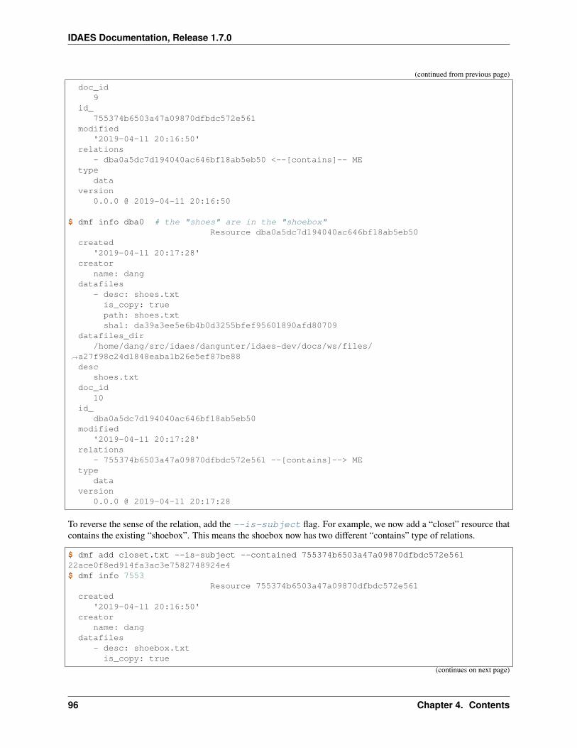
IDAES Documentation, Release 1.7.0
(continued from previous page)
doc_id9
id_755374b6503a47a09870dfbdc572e561
modified'2019-04-11 20:16:50'
relations- dba0a5dc7d194040ac646bf18ab5eb50 <--[contains]-- ME
typedata
version0.0.0 @ 2019-04-11 20:16:50
$ dmf info dba0 # the "shoes" are in the "shoebox"Resource dba0a5dc7d194040ac646bf18ab5eb50
created'2019-04-11 20:17:28'
creatorname: dang
datafiles- desc: shoes.txt
is_copy: truepath: shoes.txtsha1: da39a3ee5e6b4b0d3255bfef95601890afd80709
datafiles_dir/home/dang/src/idaes/dangunter/idaes-dev/docs/ws/files/
→˓a27f98c24d1848eaba1b26e5ef87be88desc
shoes.txtdoc_id
10id_
dba0a5dc7d194040ac646bf18ab5eb50modified
'2019-04-11 20:17:28'relations
- 755374b6503a47a09870dfbdc572e561 --[contains]--> MEtype
dataversion
0.0.0 @ 2019-04-11 20:17:28
To reverse the sense of the relation, add the --is-subject flag. For example, we now add a “closet” resource thatcontains the existing “shoebox”. This means the shoebox now has two different “contains” type of relations.
$ dmf add closet.txt --is-subject --contained 755374b6503a47a09870dfbdc572e56122ace0f8ed914fa3ac3e7582748924e4$ dmf info 7553
Resource 755374b6503a47a09870dfbdc572e561created
'2019-04-11 20:16:50'creator
name: dangdatafiles
- desc: shoebox.txtis_copy: true
(continues on next page)
96 Chapter 4. Contents
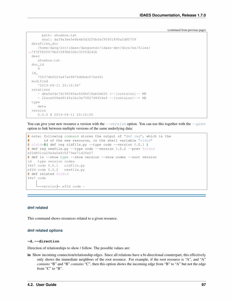
IDAES Documentation, Release 1.7.0
(continued from previous page)
path: shoebox.txtsha1: da39a3ee5e6b4b0d3255bfef95601890afd80709
datafiles_dir/home/dang/src/idaes/dangunter/idaes-dev/docs/ws/files/
→˓7f3ff820676b41689bb32bc325fd2d1bdesc
shoebox.txtdoc_id
9id_
755374b6503a47a09870dfbdc572e561modified
'2019-04-11 20:16:50'relations
- dba0a5dc7d194040ac646bf18ab5eb50 <--[contains]-- ME- 22ace0f8ed914fa3ac3e7582748924e4 --[contains]--> ME
typedata
version0.0.0 @ 2019-04-11 20:16:50
You can give your new resource a version with the --version option. You can use this together with the --prevoption to link between multiple versions of the same underlying data:
# note: following command stores the output of "dmf reg", which is the# id of the new resource, in the shell variable "oldid"$ oldid=$( dmf reg oldfile.py --type code --version 0.0.1 )$ dmf reg newfile.py --type code --version 0.0.2 --prev $oldidef2d801ca29a4a0a8c6f79ee71d3fe07$ dmf ls --show type --show version --show codes --sort versionid type version codes44e7 code 0.0.1 oldfile.pyef2d code 0.0.2 newfile.py$ dmf related $oldid44e7 code
version ef2d code -
dmf related
This command shows resources related to a given resource.
dmf related options
-d,--direction
Direction of relationships to show / follow. The possible values are:
in Show incoming connection/relationship edges. Since all relations have a bi-directional counterpart, this effectivelyonly shows the immediate neighbors of the root resource. For example, if the root resource is “A”, and “A”contains “B” and “B” contains “C”, then this option shows the incoming edge from “B” to “A” but not the edgefrom “C” to “B”.
4.2. User Guide 97
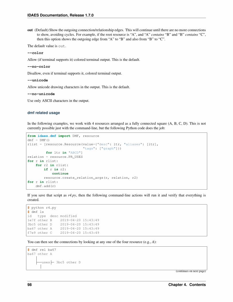
IDAES Documentation, Release 1.7.0
out (Default) Show the outgoing connection/relationship edges. This will continue until there are no more connectionsto show, avoiding cycles. For example, if the root resource is “A”, and “A” contains “B” and “B” contains “C”,then this option shows the outgoing edge from “A” to “B” and also from “B” to “C”.
The default value is out.
--color
Allow (if terminal supports it) colored terminal output. This is the default.
--no-color
Disallow, even if terminal supports it, colored terminal output.
--unicode
Allow unicode drawing characters in the output. This is the default.
--no-unicode
Use only ASCII characters in the output.
dmf related usage
In the following examples, we work with 4 resources arranged as a fully connected square (A, B, C, D). This is notcurrently possible just with the command-line, but the following Python code does the job:
from idaes.dmf import DMF, resourcedmf = DMF()rlist = [resource.Resource(value="desc": ltr, "aliases": [ltr],
"tags": ["graph"])for ltr in "ABCD"]
relation = resource.PR_USESfor r in rlist:
for r2 in rlist:if r is r2:
continueresource.create_relation_args(r, relation, r2)
for r in rlist:dmf.add(r)
If you save that script as r4.py, then the following command-line actions will run it and verify that everything iscreated.
$ python r4.py$ dmf lsid type desc modified1e7f other B 2019-04-20 15:43:493bc5 other D 2019-04-20 15:43:49ba67 other A 2019-04-20 15:43:49f7e9 other C 2019-04-20 15:43:49
You can then see the connections by looking at any one of the four resource (e.g., A):
$ dmf rel ba67ba67 other A
uses 3bc5 other D
(continues on next page)
98 Chapter 4. Contents
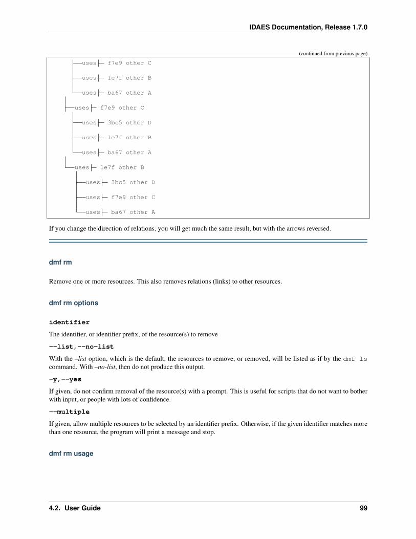
IDAES Documentation, Release 1.7.0
(continued from previous page)
uses f7e9 other C
uses 1e7f other B
uses ba67 other A
uses f7e9 other C
uses 3bc5 other D
uses 1e7f other B
uses ba67 other A
uses 1e7f other B
uses 3bc5 other D
uses f7e9 other C
uses ba67 other A
If you change the direction of relations, you will get much the same result, but with the arrows reversed.
dmf rm
Remove one or more resources. This also removes relations (links) to other resources.
dmf rm options
identifier
The identifier, or identifier prefix, of the resource(s) to remove
--list,--no-list
With the –list option, which is the default, the resources to remove, or removed, will be listed as if by the dmf lscommand. With –no-list, then do not produce this output.
-y,--yes
If given, do not confirm removal of the resource(s) with a prompt. This is useful for scripts that do not want to botherwith input, or people with lots of confidence.
--multiple
If given, allow multiple resources to be selected by an identifier prefix. Otherwise, if the given identifier matches morethan one resource, the program will print a message and stop.
dmf rm usage
4.2. User Guide 99
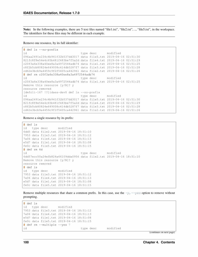
IDAES Documentation, Release 1.7.0
Note: In the following examples, there are 5 text files named “file1.txt”, “file2.txt”, .., “file5.txt”, in the workspace.The identifiers for these files may be different in each example.
Remove one resource, by its full identifier:
$ dmf ls --no-prefixid type desc modified096aa2491e234c4b941f32b537dd3017 data file5.txt 2019-04-16 02:51:30821fc8f8e54e4c65b481f483be7f5a2d data file4.txt 2019-04-16 02:51:29c20f3a6e338a40ee8a3a4972544adb74 data file1.txt 2019-04-16 02:51:25c8f2b5cb80824e649008c414db5287f7 data file3.txt 2019-04-16 02:51:28cd62e3bcb9a4459c9f2f5405ca442961 data file2.txt 2019-04-16 02:51:26$ dmf rm c20f3a6e338a40ee8a3a4972544adb74id type desc modifiedc20f3a6e338a40ee8a3a4972544adb74 data file1.txt 2019-04-16 02:51:25Remove this resource [y/N]? yresource removed[dmfcli-167 !?]idaes-dev$ dmf ls --no-prefixid type desc modified096aa2491e234c4b941f32b537dd3017 data file5.txt 2019-04-16 02:51:30821fc8f8e54e4c65b481f483be7f5a2d data file4.txt 2019-04-16 02:51:29c8f2b5cb80824e649008c414db5287f7 data file3.txt 2019-04-16 02:51:28cd62e3bcb9a4459c9f2f5405ca442961 data file2.txt 2019-04-16 02:51:26
Remove a single resource by its prefix:
$ dmf lsid type desc modified6dd5 data file2.txt 2019-04-16 18:51:107953 data file3.txt 2019-04-16 18:51:127a06 data file4.txt 2019-04-16 18:51:13e5d7 data file1.txt 2019-04-16 18:51:08fe0c data file5.txt 2019-04-16 18:51:15$ dmf rm 6did type desc modified6dd57ecc50a24efb824a66109dda0956 data file2.txt 2019-04-16 18:51:10Remove this resource [y/N]? yresource removed$ dmf lsid type desc modified7953 data file3.txt 2019-04-16 18:51:127a06 data file4.txt 2019-04-16 18:51:13e5d7 data file1.txt 2019-04-16 18:51:08fe0c data file5.txt 2019-04-16 18:51:15
Remove multiple resources that share a common prefix. In this case, use the -y,--yes option to remove withoutprompting.
$ dmf lsid type desc modified7953 data file3.txt 2019-04-16 18:51:127a06 data file4.txt 2019-04-16 18:51:13e5d7 data file1.txt 2019-04-16 18:51:08fe0c data file5.txt 2019-04-16 18:51:15$ dmf rm --multiple --yes 7id type desc modified
(continues on next page)
100 Chapter 4. Contents
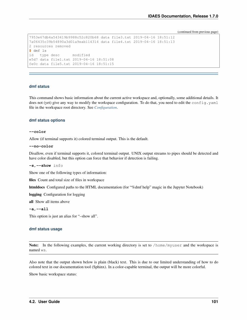
IDAES Documentation, Release 1.7.0
(continued from previous page)
7953e67db4a543419b9988c52c820b68 data file3.txt 2019-04-16 18:51:127a06435c39b54890a3d01a9eab114314 data file4.txt 2019-04-16 18:51:132 resources removed$ dmf lsid type desc modifiede5d7 data file1.txt 2019-04-16 18:51:08fe0c data file5.txt 2019-04-16 18:51:15
dmf status
This command shows basic information about the current active workspace and, optionally, some additional details. Itdoes not (yet) give any way to modify the workspace configuration. To do that, you need to edit the config.yamlfile in the workspace root directory. See Configuration.
dmf status options
--color
Allow (if terminal supports it) colored terminal output. This is the default.
--no-color
Disallow, even if terminal supports it, colored terminal output. UNIX output streams to pipes should be detected andhave color disabled, but this option can force that behavior if detection is failing.
-s,--show info
Show one of the following types of information:
files Count and total size of files in workspace
htmldocs Configured paths to the HTML documentation (for “%dmf help” magic in the Jupyter Notebook)
logging Configuration for logging
all Show all items above
-a,--all
This option is just an alias for “–show all”.
dmf status usage
Note: In the following examples, the current working directory is set to /home/myuser and the workspace isnamed ws.
Also note that the output shown below is plain (black) text. This is due to our limited understanding of how to docolored text in our documentation tool (Sphinx). In a color-capable terminal, the output will be more colorful.
Show basic workspace status:
4.2. User Guide 101
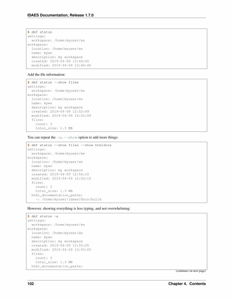
IDAES Documentation, Release 1.7.0
$ dmf statussettings:
workspace: /home/myuser/wsworkspace:
location: /home/myuser/wsname: mywsdescription: my workspacecreated: 2019-04-09 12:46:40modified: 2019-04-09 12:46:40
Add the file information:
$ dmf status --show filessettings:
workspace: /home/myuser/wsworkspace:
location: /home/myuser/wsname: mywsdescription: my workspacecreated: 2019-04-09 12:52:49modified: 2019-04-09 12:52:49files:count: 3total_size: 1.3 MB
You can repeat the -s,--show option to add more things:
$ dmf status --show files --show htmldocssettings:
workspace: /home/myuser/wsworkspace:
location: /home/myuser/wsname: mywsdescription: my workspacecreated: 2019-04-09 12:54:10modified: 2019-04-09 12:54:10files:count: 3total_size: 1.3 MB
html_documentation_paths:-: /home/myuser/idaes/docs/build
However, showing everything is less typing, and not overwhelming:
$ dmf status -asettings:
workspace: /home/myuser/wsworkspace:
location: /home/myuser/wsname: mywsdescription: my workspacecreated: 2019-04-09 12:55:05modified: 2019-04-09 12:55:05files:count: 3total_size: 1.3 MB
html_documentation_paths:
(continues on next page)
102 Chapter 4. Contents
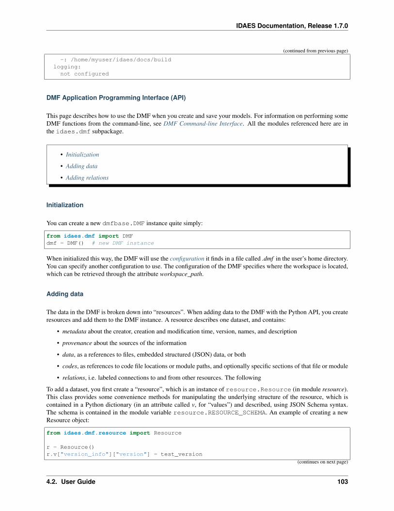
IDAES Documentation, Release 1.7.0
(continued from previous page)
-: /home/myuser/idaes/docs/buildlogging:not configured
DMF Application Programming Interface (API)
This page describes how to use the DMF when you create and save your models. For information on performing someDMF functions from the command-line, see DMF Command-line Interface. All the modules referenced here are inthe idaes.dmf subpackage.
• Initialization
• Adding data
• Adding relations
Initialization
You can create a new dmfbase.DMF instance quite simply:
from idaes.dmf import DMFdmf = DMF() # new DMF instance
When initialized this way, the DMF will use the configuration it finds in a file called .dmf in the user’s home directory.You can specify another configuration to use. The configuration of the DMF specifies where the workspace is located,which can be retrieved through the attribute workspace_path.
Adding data
The data in the DMF is broken down into “resources”. When adding data to the DMF with the Python API, you createresources and add them to the DMF instance. A resource describes one dataset, and contains:
• metadata about the creator, creation and modification time, version, names, and description
• provenance about the sources of the information
• data, as a references to files, embedded structured (JSON) data, or both
• codes, as references to code file locations or module paths, and optionally specific sections of that file or module
• relations, i.e. labeled connections to and from other resources. The following
To add a dataset, you first create a “resource”, which is an instance of resource.Resource (in module resource).This class provides some convenience methods for manipulating the underlying structure of the resource, which iscontained in a Python dictionary (in an attribute called v, for “values”) and described, using JSON Schema syntax.The schema is contained in the module variable resource.RESOURCE_SCHEMA. An example of creating a newResource object:
from idaes.dmf.resource import Resource
r = Resource()r.v["version_info"]["version"] = test_version
(continues on next page)
4.2. User Guide 103
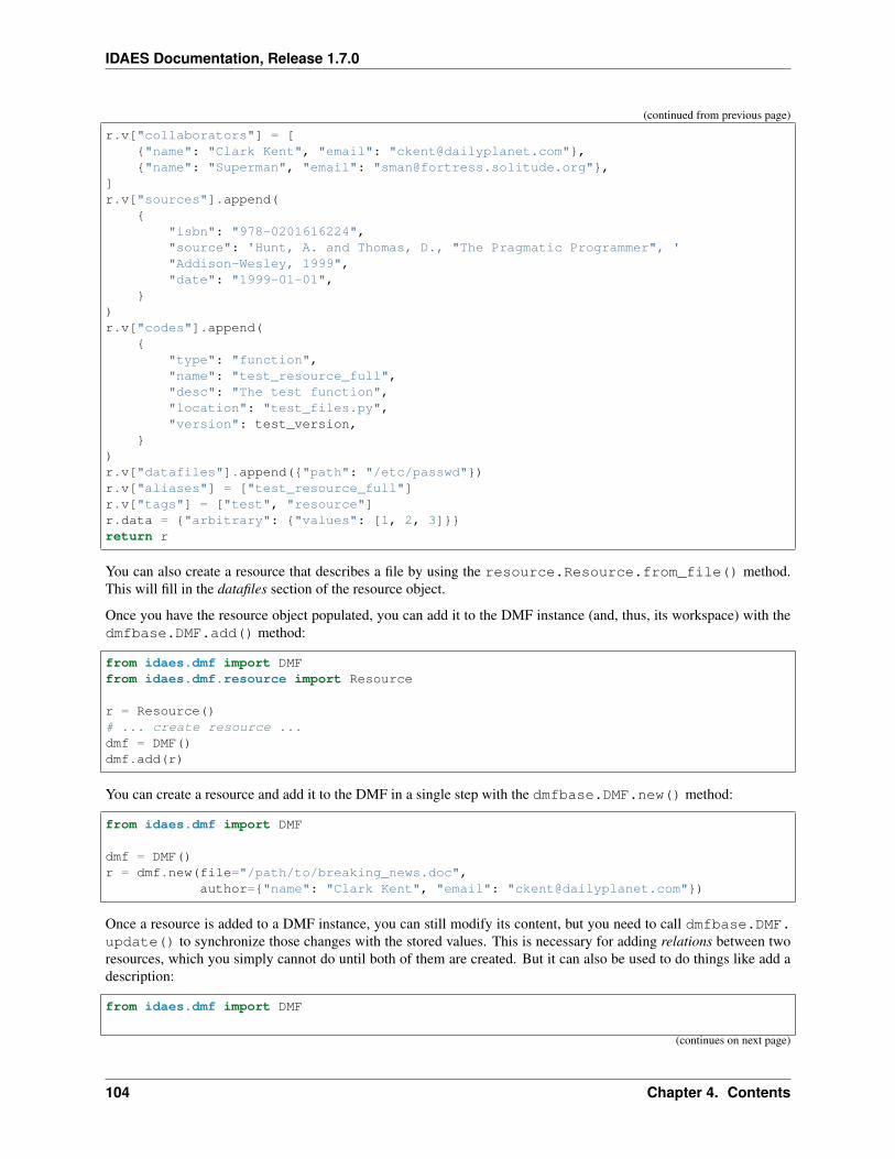
IDAES Documentation, Release 1.7.0
(continued from previous page)
r.v["collaborators"] = ["name": "Clark Kent", "email": "[email protected]","name": "Superman", "email": "[email protected]",
]r.v["sources"].append(
"isbn": "978-0201616224","source": 'Hunt, A. and Thomas, D., "The Pragmatic Programmer", '"Addison-Wesley, 1999","date": "1999-01-01",
)r.v["codes"].append(
"type": "function","name": "test_resource_full","desc": "The test function","location": "test_files.py","version": test_version,
)r.v["datafiles"].append("path": "/etc/passwd")r.v["aliases"] = ["test_resource_full"]r.v["tags"] = ["test", "resource"]r.data = "arbitrary": "values": [1, 2, 3]return r
You can also create a resource that describes a file by using the resource.Resource.from_file() method.This will fill in the datafiles section of the resource object.
Once you have the resource object populated, you can add it to the DMF instance (and, thus, its workspace) with thedmfbase.DMF.add() method:
from idaes.dmf import DMFfrom idaes.dmf.resource import Resource
r = Resource()# ... create resource ...dmf = DMF()dmf.add(r)
You can create a resource and add it to the DMF in a single step with the dmfbase.DMF.new() method:
from idaes.dmf import DMF
dmf = DMF()r = dmf.new(file="/path/to/breaking_news.doc",
author="name": "Clark Kent", "email": "[email protected]")
Once a resource is added to a DMF instance, you can still modify its content, but you need to call dmfbase.DMF.update() to synchronize those changes with the stored values. This is necessary for adding relations between tworesources, which you simply cannot do until both of them are created. But it can also be used to do things like add adescription:
from idaes.dmf import DMF
(continues on next page)
104 Chapter 4. Contents
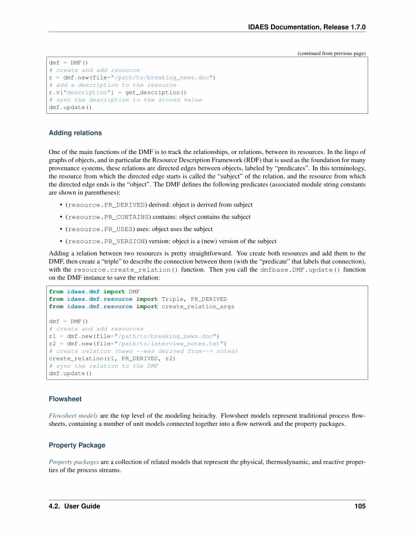
IDAES Documentation, Release 1.7.0
(continued from previous page)
dmf = DMF()# create and add resourcer = dmf.new(file="/path/to/breaking_news.doc")# add a description to the resourcer.v["description"] = get_description()# sync the description to the stored valuedmf.update()
Adding relations
One of the main functions of the DMF is to track the relationships, or relations, between its resources. In the lingo ofgraphs of objects, and in particular the Resource Description Framework (RDF) that is used as the foundation for manyprovenance systems, these relations are directed edges between objects, labeled by “predicates”. In this terminology,the resource from which the directed edge starts is called the “subject” of the relation, and the resource from whichthe directed edge ends is the “object”. The DMF defines the following predicates (associated module string constantsare shown in parentheses):
• (resource.PR_DERIVED) derived: object is derived from subject
• (resource.PR_CONTAINS) contains: object contains the subject
• (resource.PR_USES) uses: object uses the subject
• (resource.PR_VERSION) version: object is a (new) version of the subject
Adding a relation between two resources is pretty straightforward. You create both resources and add them to theDMF, then create a “triple” to describe the connection between them (with the “predicate” that labels that connection),with the resource.create_relation() function. Then you call the dmfbase.DMF.update() functionon the DMF instance to save the relation:
from idaes.dmf import DMFfrom idaes.dmf.resource import Triple, PR_DERIVEDfrom idaes.dmf.resource import create_relation_args
dmf = DMF()# create and add resourcesr1 = dmf.new(file="/path/to/breaking_news.doc")r2 = dmf.new(file="/path/to/interview_notes.txt")# create relation (news --was derived from--> notes)create_relation(r1, PR_DERIVED, r2)# sync the relation to the DMFdmf.update()
Flowsheet
Flowsheet models are the top level of the modeling heirachy. Flowsheet models represent traditional process flow-sheets, containing a number of unit models connected together into a flow network and the property packages.
Property Package
Property packages are a collection of related models that represent the physical, thermodynamic, and reactive proper-ties of the process streams.
4.2. User Guide 105
IDAES Documentation, Release 1.7.0
Unit Model
Unit models represent individual pieces of equipment and their processes.
Data Management Framework
The Data Management Framework is used to manage all the data needed by the platform, including flowsheets,models, and results. It stores metadata and data in persistent storage.
4.2.4 Conventions
• Units of Measurement and Reference States
• Standard Variable Names
– Standard Naming Format
– Constants
– Thermophysical and Transport Properties
– Reaction Properties
– Solid Properties
– Naming Examples
Units of Measurement and Reference States
Due to the flexibility provided by the IDAES Integrated Platform, there is no standard set of units of measurement orstandard reference state that should be used in models. Units of measurement are defined by the modeler for the 7base quantities (time, length, mass, amount, temperature, current and luminous intensity) in each property package,and the platform makes use of this and Pyomo’s Units container to automatically determine the units of all variablesand expressions within a model. Thus, all components within a model using a given property package must use unitsbased on the units chosen for the base quantities (to ensure consistency of units). However, flowsheets may containproperty packages which use different sets of base units, however users should be careful to ensure units are convertedcorrectly where property packages interact. For more detail on defining units of measurement see Defining Units ofMeasurement.
Pyomo also provides convenient tools for converting between different units of measurement and checking for unitconsistency, of which a few are highlighted below:
• units.convert(var, to_units=units) - returns a Pyomo expression including the variable var andthe necessary conversion factors to convert it to the desired set of units (units). This method will return anException if the units of var are not consistent with those requested by the user.
• units.assert_units_consistent(object) - checks for consistency of units in object and raises anAssertionError if they are not. object may be a Block, Constraint or Expression.
The IDAES developers have generally used SI units without prefixes (i.e. Pa, not kPa) within models developed bythe institute, with a default thermodynamic reference state of 298.15 K and 101325 Pa. Supercritical fluids have beenconsider to be part of the liquid phase, as they will be handled via pumps rather than compressors.
106 Chapter 4. Contents
IDAES Documentation, Release 1.7.0
Standard Variable Names
In order for different models to communicate information effectively, it is necessary to have a standard naming conven-tion for any variable that may need to be shared between different models. Within IDAES, this occurs most frequentlywhen information regarding the state and properties of the material, which is calculated in specialized PropertyBlocks,is used in others parts of the model.
Standard Naming Format
There are a wide range of different variables which may be of interest to modelers, and a number of different waysin which these quantities can be expressed. In order to facilitate communication between different parts of models, anaming convention has been established to standardize the naming of variables across models. Variable names withinIDAES follow to the format below:
property_name_basis_state_condition
Here, property_name is the name of the quantity in question, and should be drawn from the list of standard variablenames given later in this document. If a particular quantity is not included in the list of standard names, users areencouraged to contact the IDAES developers so that it can be included in a future release. This is followed by anumber of qualifiers which further indicate the specific conditions under which the quantity is being calculated. Thesequalifiers are described below, and some examples are given at the end of this document.
Basis Qualifier
Many properties of interest to modelers are most conveniently represented on an intensive basis, that is quantity perunit amount of material. There are a number of different bases that can be used when expressing intensive quantities,and a list of standard basis qualifiers are given below.
Basis Standard NameMass Basis massMolar Basis molVolume Basis vol
State Qualifier
Many quantities can be calculated either for the whole or a part of a mixture. In these cases, a qualifier is added to thequantity to indicate which part of the mixture the quantity applies to. In these cases, quantities may also be indexedby a Pyomo Set.
Basis Standard Name CommentsComponent comp Indexed by component listPhase phase Indexed by phase listPhase & Component phase_comp Indexed by phase and component listTotal Mixture No state qualifier
4.2. User Guide 107
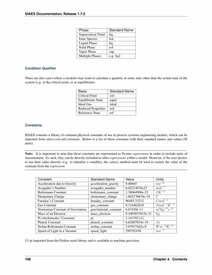
IDAES Documentation, Release 1.7.0
Phase Standard NameSupercritical Fluid liqIonic Species ionLiquid Phase liqSolid Phase solVapor Phase vapMultiple Phases e.g. liq1
Condition Qualifier
There are also cases where a modeler may want to calculate a quantity at some state other than the actual state of thesystem (e.g. at the critical point, or at equilibrium).
Basis Standard NameCritical Point critEquilibrium State equilIdeal Gas idealReduced Properties redReference State ref
Constants
IDAES contains a library of common physical constants of use in process systems engineering models, which can beimported from idaes.core.util.constants. Below is a list of these constants with their standard names and values (SIunits).
Note: It is important to note that these constants are represented as Pyomo expressions in order to include units ofmeasurement. As such, they can be directly included in other expressions within a model. However, if the user desiresto use their value directly (e.g. to initialize a variable), the value() method must be used to extract the value of theconstant from the expression.
Constant Standard Name Value UnitsAcceleration due to Gravity acceleration_gravity 9.80665 𝑚𝑠−2
Avogadro’s Number avogadro_number 6.02214076e23 𝑚𝑜𝑙−1
Boltzmann Constant boltzmann_constant 1.38064900e-23 𝐽𝐾−1
Elementary Charge elementary_charge 1.602176634e-19 𝐶Faraday’s Constant faraday_constant 96485.33212 𝐶𝑚𝑜𝑙−1
Gas Constant gas_constant 8.314462618 𝐽𝑚𝑜𝑙−1𝐾−1
Newtonian Constant of Gravitation gravitational_constant 6.67430e-11 𝑚3𝑘𝑔−1𝑠−2
Mass of an Electron mass_electron 9.1093837015e-31 𝑘𝑔Pi (Archimedes’ Constant) pi 3.141592 [1]Planck Constant planck_constant 6.62607015e-34 𝐽𝑠Stefan-Boltzmann Constant stefan_constant 5.67037442e-8 𝑊𝑚−2𝐾−4
Speed of Light in a Vacuum speed_light 299792458 𝑚𝑠−1
[1] pi imported from the Python math library and is available to machine precision.
108 Chapter 4. Contents
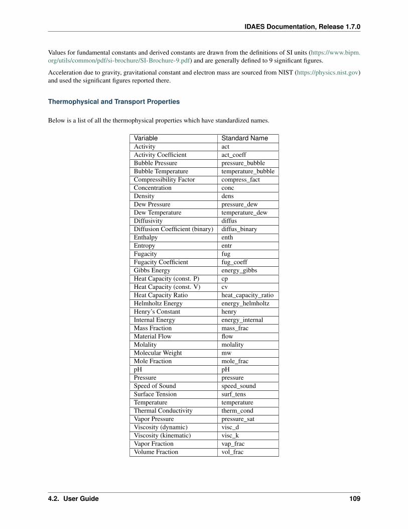
IDAES Documentation, Release 1.7.0
Values for fundamental constants and derived constants are drawn from the definitions of SI units (https://www.bipm.org/utils/common/pdf/si-brochure/SI-Brochure-9.pdf) and are generally defined to 9 significant figures.
Acceleration due to gravity, gravitational constant and electron mass are sourced from NIST (https://physics.nist.gov)and used the significant figures reported there.
Thermophysical and Transport Properties
Below is a list of all the thermophysical properties which have standardized names.
Variable Standard NameActivity actActivity Coefficient act_coeffBubble Pressure pressure_bubbleBubble Temperature temperature_bubbleCompressibility Factor compress_factConcentration concDensity densDew Pressure pressure_dewDew Temperature temperature_dewDiffusivity diffusDiffusion Coefficient (binary) diffus_binaryEnthalpy enthEntropy entrFugacity fugFugacity Coefficient fug_coeffGibbs Energy energy_gibbsHeat Capacity (const. P) cpHeat Capacity (const. V) cvHeat Capacity Ratio heat_capacity_ratioHelmholtz Energy energy_helmholtzHenry’s Constant henryInternal Energy energy_internalMass Fraction mass_fracMaterial Flow flowMolality molalityMolecular Weight mwMole Fraction mole_fracpH pHPressure pressureSpeed of Sound speed_soundSurface Tension surf_tensTemperature temperatureThermal Conductivity therm_condVapor Pressure pressure_satViscosity (dynamic) visc_dViscosity (kinematic) visc_kVapor Fraction vap_fracVolume Fraction vol_frac
4.2. User Guide 109
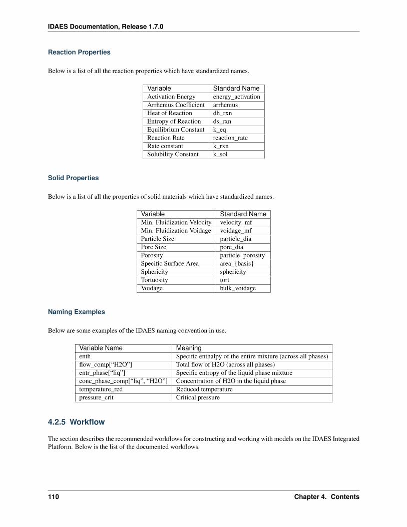
IDAES Documentation, Release 1.7.0
Reaction Properties
Below is a list of all the reaction properties which have standardized names.
Variable Standard NameActivation Energy energy_activationArrhenius Coefficient arrheniusHeat of Reaction dh_rxnEntropy of Reaction ds_rxnEquilibrium Constant k_eqReaction Rate reaction_rateRate constant k_rxnSolubility Constant k_sol
Solid Properties
Below is a list of all the properties of solid materials which have standardized names.
Variable Standard NameMin. Fluidization Velocity velocity_mfMin. Fluidization Voidage voidage_mfParticle Size particle_diaPore Size pore_diaPorosity particle_porositySpecific Surface Area area_basisSphericity sphericityTortuosity tortVoidage bulk_voidage
Naming Examples
Below are some examples of the IDAES naming convention in use.
Variable Name Meaningenth Specific enthalpy of the entire mixture (across all phases)flow_comp[“H2O”] Total flow of H2O (across all phases)entr_phase[“liq”] Specific entropy of the liquid phase mixtureconc_phase_comp[“liq”, “H2O”] Concentration of H2O in the liquid phasetemperature_red Reduced temperaturepressure_crit Critical pressure
4.2.5 Workflow
The section describes the recommended workflows for constructing and working with models on the IDAES IntegratedPlatform. Below is the list of the documented workflows.
110 Chapter 4. Contents
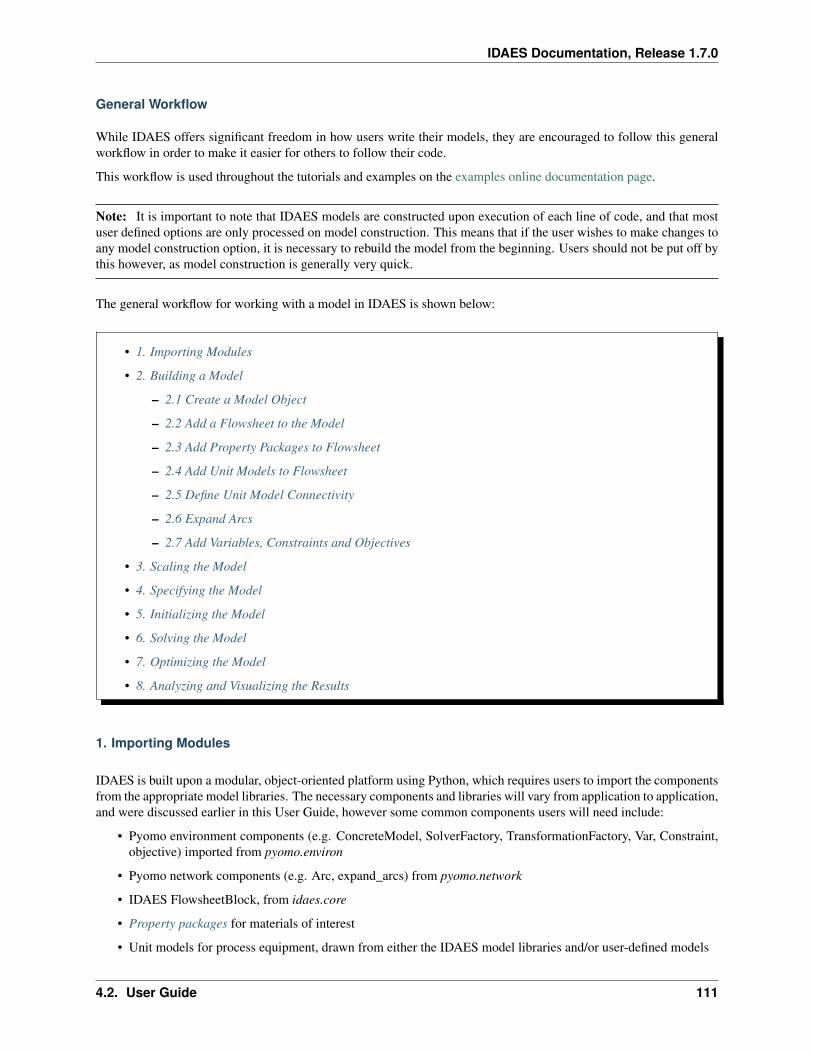
IDAES Documentation, Release 1.7.0
General Workflow
While IDAES offers significant freedom in how users write their models, they are encouraged to follow this generalworkflow in order to make it easier for others to follow their code.
This workflow is used throughout the tutorials and examples on the examples online documentation page.
Note: It is important to note that IDAES models are constructed upon execution of each line of code, and that mostuser defined options are only processed on model construction. This means that if the user wishes to make changes toany model construction option, it is necessary to rebuild the model from the beginning. Users should not be put off bythis however, as model construction is generally very quick.
The general workflow for working with a model in IDAES is shown below:
• 1. Importing Modules
• 2. Building a Model
– 2.1 Create a Model Object
– 2.2 Add a Flowsheet to the Model
– 2.3 Add Property Packages to Flowsheet
– 2.4 Add Unit Models to Flowsheet
– 2.5 Define Unit Model Connectivity
– 2.6 Expand Arcs
– 2.7 Add Variables, Constraints and Objectives
• 3. Scaling the Model
• 4. Specifying the Model
• 5. Initializing the Model
• 6. Solving the Model
• 7. Optimizing the Model
• 8. Analyzing and Visualizing the Results
1. Importing Modules
IDAES is built upon a modular, object-oriented platform using Python, which requires users to import the componentsfrom the appropriate model libraries. The necessary components and libraries will vary from application to application,and were discussed earlier in this User Guide, however some common components users will need include:
• Pyomo environment components (e.g. ConcreteModel, SolverFactory, TransformationFactory, Var, Constraint,objective) imported from pyomo.environ
• Pyomo network components (e.g. Arc, expand_arcs) from pyomo.network
• IDAES FlowsheetBlock, from idaes.core
• Property packages for materials of interest
• Unit models for process equipment, drawn from either the IDAES model libraries and/or user-defined models
4.2. User Guide 111
IDAES Documentation, Release 1.7.0
• Data visualization and analysis tools. Common tools include degrees of freedom and scaling, a full list isprovided here.
• External packages of interest to the user. Being built upon Python, users have access to the full range of Pythonlibraries for working with and analyzing their models.
2. Building a Model
The next step in the workflow is to create a model object which represents the problem to be solved. The steps involvedin this may vary depending on the problem being solved, but the general procedure is as follows:
2.1 Create a Model Object
The foundation of any model in IDAES is a Pyomo ConcreteModel object, which is created as follows:
m = ConcreteModel()
Note: IDAES does not support the use of Pyomo AbstractModels
2.2 Add a Flowsheet to the Model
The foundation of a process model within IDAES is the FlowsheetBlock, which forms the canvas upon which theprocess will be constructed. A key aspect of the FlowsheetBlock is to define whether the model will be steady-state ordynamic, and to define the time domain as appropriate.
m.fs = FlowsheetBlock(default="dynamic": False
Note: IDAES supports nested flowsheets to allow complex processes to be broken down into smaller sub-processes.
2.3 Add Property Packages to Flowsheet
All process models depend on calculations of thermophysical and chemical reaction properties, which are representedin IDAES using property packages. Users need to add the property packages they intend to use to the flowsheet.
m.fs.properties_1 = MyPropertyPackage.PhysicalParameterBlock()
Note: Users can add as many property packages as they need to a flowsheet, and can determine which propertypackage will be used for each unit operation as it is created.
2.4 Add Unit Models to Flowsheet
Next, the user can add Unit Models to their flowsheet to represent each unit operation in the process.
112 Chapter 4. Contents
IDAES Documentation, Release 1.7.0
m.fs.unit01 = UnitModel(default="property_package": m.fs.properties_1)
2.5 Define Unit Model Connectivity
In order to describe the flow of material between unit operations, users must declare Arcs (or streams) which connectthe outlet of each unit operation to the inlet of the next.
m.fs.arc_1 = Arc(source=m.fs.unit01.outlet, destination=m.fs.unit02.inlet)
2.6 Expand Arcs
It is important to note that Arcs only define the connectivity between unit operations, but do not create the actual modelconstraints needed to describe this. Once all Arcs in a flowsheet have been defined, it is necessary to expand these Arcsusing the Pyomo TransformationFactory.
TransformationFactory("network.expand_arcs").apply_to(m)
Note: Pyomo provides a number of other Transformations and tools that may be useful to the user depending on theapplication. Examples include the gdp and dae transformations.
2.7 Add Variables, Constraints and Objectives
Finally, users can add any additional variables, constraints and objectives to their model. These could include theobjective function for which they wish to optimize, additional constraints that provide limits on process performance,or simply additional quantities that the user wishes to use in analyzing or visualizing the results.
3. Scaling the Model
Note: The IDAES scaling tools are currently under development.
Ensuring that a model is well scaled is important for increasing the efficiency and reliability of solvers, and usersshould consider model scaling as an integral part of the modeling process. IDAES provides a number of tool forassisting users with scaling their models, and details on these can be found here.
4. Specifying the Model
Note: IDAES is in the process of developing a set of tools to assist users with working with units of measurementwhen fixing and displaying values.
The next step is to specify the model by fixing variables. which can be done using the form variable_name.fix(value).The variables that need to be fixed are application dependent, but commonly include the feed state variables.
4.2. User Guide 113
IDAES Documentation, Release 1.7.0
In order to prepare the model for initialization, it is necessary to fully specify the model, such that there are nodegrees of freedom. IDAES provides a tools for counting and reporting the degrees of freedom in any model (orsub-model/block):
from idaes.core.util.model_statistics import degrees_of_freedom
print(degrees_of_freedom(m))
Note: Whilst it is not always necessary to fully define a model before initialization, it is much safer to do so asit ensures the model is well-defined. Most IDAES initialization tools check that the model is well-defined beforeproceeding, and will raise an Exception if it is not.
Note: Depending on the solver to be used during initialization, it can be better to avoid putting bounds on variablesand adding inequality constraints at this stage. For solving square problems (i.e. zero degrees of freedom), somesolvers (e.g. IPOPT) perform better without bounds on the problem. These bounds and constraints can be added laterwhen it comes time to optimize the problem.
5. Initializing the Model
The next step is to initialize the model. All IDAES models have established initialization methods that can be calledusing model.initialize() which can be expected to take a model from its initial state to a feasible solution for a set ofinitial guesses (within the models expected operating range).
IDEAS workflows generally use a sequential-modular approach to initialize flowsheets, where unit models are ini-tialized sequentially, passing the outlet state from one unit as the initial state for the next. An automated sequential-modular tool is available through Pyomo and demonstrated in the tutorials.
6. Solving the Model
Important: The sequential-modular approach initializes each unit model individually, thus it is important to do afinal solve of the overall flowsheet/model in order to complete the initialization process. In most cases, this final solveshould only take a few iterations, as the state of each unit model should be at or near the final solution already.
In order to solve the model, it is necessary to create a solve object and set any desired solver options (such as tolerances,iteration limits etc.).
solver = SolverFactory('solver_name')solver.options = 'tol': 1d-6
results = solver.solve(m)
Users should check the output from the solver to ensure a feasible solution was found using the following:
print(results.solver.termination_condition)
Different problems will require different solvers, and users will need to experiment to find those that work best fortheir problems. The default solver for most IDAES applications is IPOPT, which can be downloaded using the idaesget-extensions command line.
114 Chapter 4. Contents
IDAES Documentation, Release 1.7.0
7. Optimizing the Model
Once an initial solution has been found, users can proceed to solving the optimization problem of interest. Thisprocedure will vary by application but generally involves the following steps:
7.1) Unfix some degrees of freedom to provide the problem with decision variables, variable_name.unfix().
7.2) Add bounds to variables and inequality constraints to constrain solution space, variable_name.setlb(value) andvar_name.setub(value)
7.3) Call a solver and check the termination conditions, see step 6 Solving the Model.
Note: Users may wish/need to use different solvers for initialization and optimization. IDAES and Pyomo supportthe use of multiple solvers as part of the same workflow for solving different types of problems.
8. Analyzing and Visualizing the Results
One of the benefits of the IDAES Integrated Platform is that it operates in a fully featured programming language,which provides users a high degree of flexibility in analyzing their models. For example, users can automate thesimulation of the model across multiple objectives or a range of parameters, store and save results from one or multiplesolutions. Users also have access to a wide range of tools for manipulating, plotting and visualizing the results.
Data Reconciliation and Parameter Estimation
This workflow generally describes features of the IDAES framework that are useful for data reconciliation and param-eter estimation. Many of these features can be used for any task where plant data is to be used in conjunction with aprocess model. It is assumed that the user is familiar with the IDAES modeling platform and Pyomo. See the GeneralWorkflow for more information on how to set up a model.
This provides general information about IDAES functionality laid out in terms of typical use cases. See Tutorialsand Examples, for specific complete examples of data reconciliation and parameter estimation examples. Relevanttutorials can be found in tutorials/advanced/data_recon_and_parameter_estimation.
Data Management
IDAES has functions to read and mange process data process data. Data management functions are contained in theidaes.dmf.model_data module.
Reading Data
A set of process data can be stored in two files, a data file and a metadata file. The data file is a CSV file where thefirst column contains a data point index, usually a timestamp. The first row contains a header with the measurementtag names. The rest of the files contains measurement data. The data file format is shown in the table below.
index tag (optional) tag 1 tag 2 . . .index 1 data(1,1) data(1,2) . . .index 2 data(2,1) data(2,2) . . .. . . . . . . . . . . .
4.2. User Guide 115
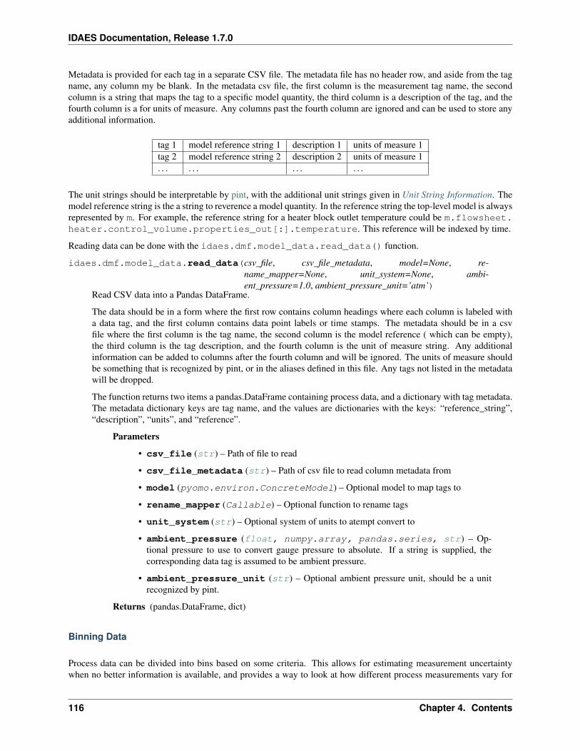
IDAES Documentation, Release 1.7.0
Metadata is provided for each tag in a separate CSV file. The metadata file has no header row, and aside from the tagname, any column my be blank. In the metadata csv file, the first column is the measurement tag name, the secondcolumn is a string that maps the tag to a specific model quantity, the third column is a description of the tag, and thefourth column is a for units of measure. Any columns past the fourth column are ignored and can be used to store anyadditional information.
tag 1 model reference string 1 description 1 units of measure 1tag 2 model reference string 2 description 2 units of measure 1. . . . . . . . . . . .
The unit strings should be interpretable by pint, with the additional unit strings given in Unit String Information. Themodel reference string is the a string to reverence a model quantity. In the reference string the top-level model is alwaysrepresented by m. For example, the reference string for a heater block outlet temperature could be m.flowsheet.heater.control_volume.properties_out[:].temperature. This reference will be indexed by time.
Reading data can be done with the idaes.dmf.model_data.read_data() function.
idaes.dmf.model_data.read_data(csv_file, csv_file_metadata, model=None, re-name_mapper=None, unit_system=None, ambi-ent_pressure=1.0, ambient_pressure_unit=’atm’)
Read CSV data into a Pandas DataFrame.
The data should be in a form where the first row contains column headings where each column is labeled witha data tag, and the first column contains data point labels or time stamps. The metadata should be in a csvfile where the first column is the tag name, the second column is the model reference ( which can be empty),the third column is the tag description, and the fourth column is the unit of measure string. Any additionalinformation can be added to columns after the fourth column and will be ignored. The units of measure shouldbe something that is recognized by pint, or in the aliases defined in this file. Any tags not listed in the metadatawill be dropped.
The function returns two items a pandas.DataFrame containing process data, and a dictionary with tag metadata.The metadata dictionary keys are tag name, and the values are dictionaries with the keys: “reference_string”,“description”, “units”, and “reference”.
Parameters
• csv_file (str) – Path of file to read
• csv_file_metadata (str) – Path of csv file to read column metadata from
• model (pyomo.environ.ConcreteModel) – Optional model to map tags to
• rename_mapper (Callable) – Optional function to rename tags
• unit_system (str) – Optional system of units to atempt convert to
• ambient_pressure (float, numpy.array, pandas.series, str) – Op-tional pressure to use to convert gauge pressure to absolute. If a string is supplied, thecorresponding data tag is assumed to be ambient pressure.
• ambient_pressure_unit (str) – Optional ambient pressure unit, should be a unitrecognized by pint.
Returns (pandas.DataFrame, dict)
Binning Data
Process data can be divided into bins based on some criteria. This allows for estimating measurement uncertaintywhen no better information is available, and provides a way to look at how different process measurements vary for
116 Chapter 4. Contents

IDAES Documentation, Release 1.7.0
operating conditions that should be similar in some way. As an example, power plant data could be binned by poweroutput, and assuming that operating procedures are standard, it could be assumed that measurements in each bin shouldbe about the same. The variance of a measurement in a bin could be used a an approximation of uncertainty. Binningthe data by load and time could show how process measurements change over time and be useful for things like faultdetection and equipment degradation.
Adding bin information to a data frame is done with the idaes.dmf.model_data.bin_data() function.
idaes.dmf.model_data.bin_data(df, bin_by, bin_no, bin_nom, bin_size, min_value=None,max_value=None)
Sort data into bins by a column value. If the min or max are given and the value in bin_by for a row is out of therange [min, max], the row is dropped from the data frame.
Parameters
• df (pandas.DataFrame) – Data frame to add bin information to
• bin_by (str) – A column for values to bin by
• bin_no (str) – A new column for bin number
• bin_nom (str) – A new column for the mid-point value of bin_by
• bin_size (float) – size of a bin
• min_value (in float, None) – Smallest value to keep or None for no lower
• max_value (in (float, None) – Largest value to keep or None for no upper
Returns
returns the data frame, and a dictionary with the number of rows in each bin.
Return type (dict)
The idaes.dmf.model_data.bin_stdev() function can be used to calculate the standard deviation for eachmeasurement in each bin.
idaes.dmf.model_data.bin_stdev(df, bin_no, min_data=4)Calculate the standard deviation for each column in each bin.
Parameters
• df (pandas.DataFrame) – pandas data frame that is a bin number column
• bin_no (str) – Column to group by, usually contains bin number
• min_data (int) – Minimum number of data points requitred to calculate standard devia-tion for a bin (default=4)
Returns
key is the bin number and the value is a pandas.Serries with column standard deviations
Return type dict
The function idaes.dmf.model_data.data_plot_book() creates a multipage PDF containing box plotsfor all the measurements based on the bins.
idaes.dmf.model_data.data_plot_book(df, bin_nom, file=’data_plot_book.pdf’,tmp_dir=’tmp_plots’, xlabel=None, metadata=None,cols=None, skip_cols=[])
Make box and whisker plots from process data based on bins from the bin_data() function.
Parameters
• df – data frame
4.2. User Guide 117
IDAES Documentation, Release 1.7.0
• bin_nom – bin mid-point value column
• file – path for generated pdf
• tmp_dir – a directory to store temporary plots in
• xlabel – Label for x axis
• metadata – tag meta data dictionary
Returns None
To compare reconciled data to original measurements the idaes.dmf.data_rec_plot_book() is used. Foreach bin there are two box plots one for the original data and one for reconciled data.
idaes.dmf.model_data.data_rec_plot_book(df_data, df_rec, bin_nom,file=’data_rec_plot_book.pdf’,tmp_dir=’tmp_plots’, xlabel=None, meta-data=None, cols=None, skip_cols=[])
Make box and whisker plots from process data compared to data rec results based on bins from the bin_data()function. The df_data and df_rec data frames should have the same index set and the df_data data frame containsthe bin data. This will plot the intersection of columns containg numerical data.
Parameters
• df_data – data frame with original data
• df_rec – data frame with reconciled data
• bin_nom – bin mid-point value column
• file – path for generated pdf
• tmp_dir – a directory to store temporary plots in
• xlabel – Label for x axis
• metadata – tag meta data dictionary
• cols – List of columns to plot, if None plot all
• skip_cols – List of columns not to plot, this overrides cols
Returns None
Tagging the Model
Mapping process data to a model is typically done by creating model tag dictionaries. Where the dictionary key is ameasurement tag and the value is a reference to a model variable, expression, or parameter. The tags may be processmeasurement tags, or any other convenient string. IDAES has some utilities to help facilitate tagging of models.
If model reference strings where provided in the tag metadata file, the tag metadata from the idaes.dmf.model_data.read_data() will contain model references. These references can be accessed in the metadatadictionary as metadata[tag]["reference"].
The reference strings are optional in the tag metadata file and can be added after reading thedata. To add a reference string to the metadata, you can update the metadata dictionary likemetadata[tag]["reference_string"] = reference_string. If you update the reference string, theidaes.dmf.model_data.upadate_metadata_model_references()‘‘ function can be used to update the references in thetag metadata.
idaes.dmf.model_data.upadate_metadata_model_references(model, metadata)Create model references from refernce strings in the metadata. This updates the ‘reference’ field in the metadata.
118 Chapter 4. Contents
IDAES Documentation, Release 1.7.0
Parameters
• model (pyomo.environ.Block) – Pyomo model
• metadata (dict) – Tag metadata dictionary
Returns None
An easy way to create a new tag dictionary from tag metadata is to use dictionary comprehension like so: data_tags= k:v["reference"][0] for k, v in metadata.items() if v["reference"] is notNone
Often data reconciliation is performed using process data as the first step of parameter estimation or model validation.Data reconciliation can often fill in information for many unmeasured quantities. Most of this data can be associatedwith process streams. To make managing proliferation of data tags easier, it is often desirable to create a new set oftags based on stream (Arc) names that can be automatically obtained from the model.
The first step to creating a new set of tags based on streams is to get a dictionary of streams and their associated stateblocks, with can be done with the idaes.core.util.tables.arcs_to_stream_dict() function.
idaes.core.util.tables.arcs_to_stream_dict(blk, additional=None, descend_into=True,sort=False, prepend=None, s=)
Creates a stream dictionary from the Arcs in a model, using the Arc names as keys. This can be used toautomate the creation of the streams dictionary needed for the create_stream_table_dataframe()and stream_states_dict() functions.
Parameters
• blk (pyomo.environ._BlockData) – Pyomo model to search for Arcs
• additional (dict) – Additional states to add to the stream dictionary, which aren’trepresented by arcs in blk, for example feed or product streams without Arcs attached orstates internal to a unit model.
• descend_into (bool) – If True, search subblocks for Arcs as well. The default is True.
• sort (bool) – If True sort keys and return an OrderedDict
• prepend (str) – Prepend a string to the arc name joined with a ‘.’. This can be usefulto prevent conflicting names when sub blocks contain Arcs that have the same names whenused in combination with descend_into=False.
• s (dict) – Add streams to an existing stream dict.
Returns Dictionary with Arc names as keys and the Arcs as values.
The stream dictionary can be converted to a corresponding dictionary of state at a specific time with the idaes.core.util.tables.stream_states_dict() function.
idaes.core.util.tables.stream_states_dict(streams, time_point=0)Method to create a dictionary of state block representing stream states. This takes a dict with stream name keysand stream values.
Parameters
• streams – dict with name keys and stream values. Names will be used as display namesfor stream table, and streams may be Arcs, Ports or StateBlocks.
• time_point – point in the time domain at which to generate stream table (default = 0)
Returns A pandas DataFrame containing the stream table data.
With the dictionary of states, a tag dictionary can be created automatically with the idaes.core.util.tables.stream_states_dict() function.
4.2. User Guide 119
IDAES Documentation, Release 1.7.0
idaes.core.util.tables.stream_states_dict(streams, time_point=0)Method to create a dictionary of state block representing stream states. This takes a dict with stream name keysand stream values.
Parameters
• streams – dict with name keys and stream values. Names will be used as display namesfor stream table, and streams may be Arcs, Ports or StateBlocks.
• time_point – point in the time domain at which to generate stream table (default = 0)
Returns A pandas DataFrame containing the stream table data.
Objective Function
For either parameter estimation or data reconciliation the objective function is often written in the form:
min∑𝑖
(𝑥data,𝑖 − 𝑥model,𝑖)2
𝜎2𝑖
To add the data to be used in the objective standard practice has been to add a mutable parameter for data and standarddeviation indexed by measurement tags. The parameter values can be set from the measurement data frame to aspecific index.
The following code snippet exemplifies the use of data parameters in a model.
# df is from reading process data into a pandas.DataFrame. bin_stdev comes# from binning the data and calculating the standard deviations, as described# in the Data Management section.
# Add data parametersm.data = pyo.Param(data_tags, mutable=True)m.data_stdev = pyo.Param(data_tags, mutable=True)
# A function to set the data parameters from measurement datadef set_data(m, df, data_tags, index=None):m.bin_no = df.iloc[index]["bin_no"]for t in data_tags:
m.data[t] = df.iloc[index][t]m.data_stdev[t] = bin_stdev[m.bin_no][t]
# Expressions for error in the objective [email protected](data_tags)def err(m, i):
return (m.data[i] - data_tags[i])/m.data_stdev[i]
Parameter Estimation
For parameter estimation and data reconciliation, it is recommended to use Paramest. If more control is needed a usercan also set up their own parameter estimation problem, by combining multiple process models into a larger parameterestimation model.
APPENDIX: Unit String Information
This section provides additional detail about units strings that can be used to read data with the read_data()function.
120 Chapter 4. Contents
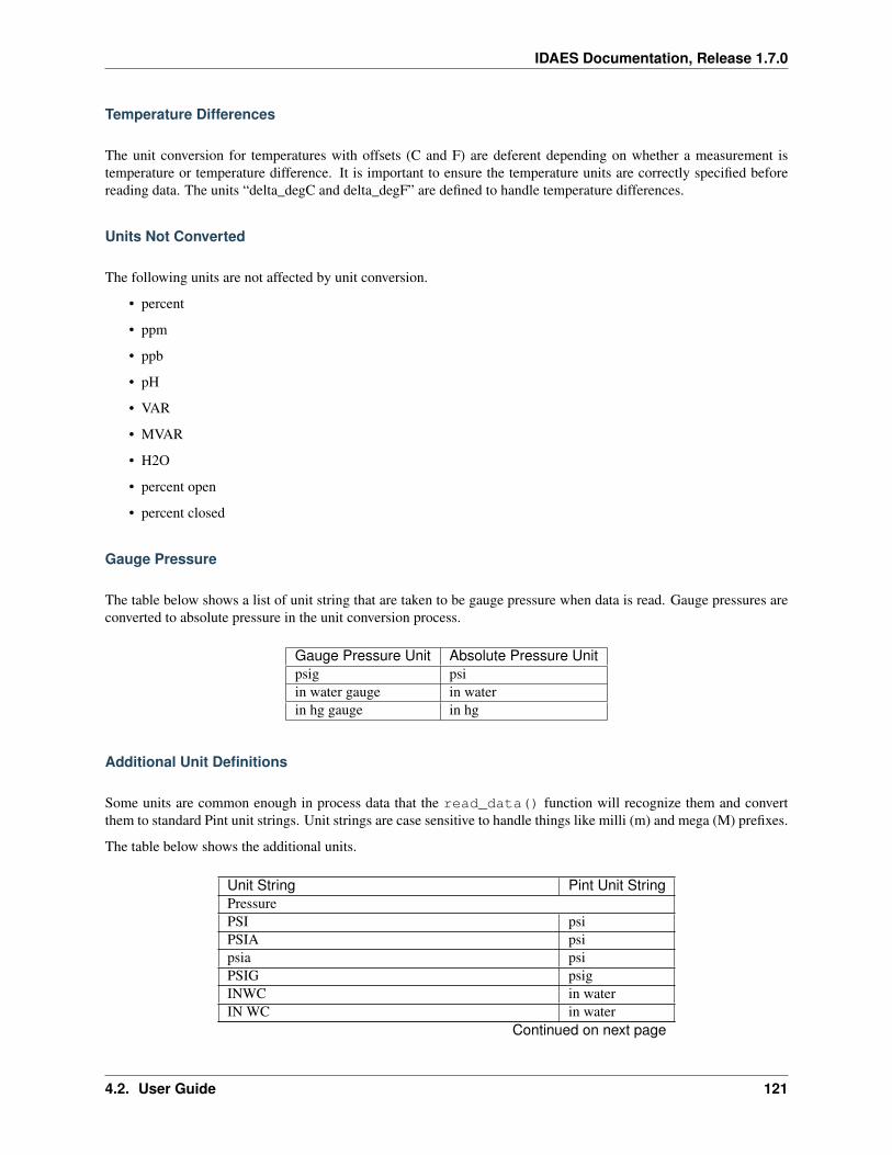
IDAES Documentation, Release 1.7.0
Temperature Differences
The unit conversion for temperatures with offsets (C and F) are deferent depending on whether a measurement istemperature or temperature difference. It is important to ensure the temperature units are correctly specified beforereading data. The units “delta_degC and delta_degF” are defined to handle temperature differences.
Units Not Converted
The following units are not affected by unit conversion.
• percent
• ppm
• ppb
• pH
• VAR
• MVAR
• H2O
• percent open
• percent closed
Gauge Pressure
The table below shows a list of unit string that are taken to be gauge pressure when data is read. Gauge pressures areconverted to absolute pressure in the unit conversion process.
Gauge Pressure Unit Absolute Pressure Unitpsig psiin water gauge in waterin hg gauge in hg
Additional Unit Definitions
Some units are common enough in process data that the read_data() function will recognize them and convertthem to standard Pint unit strings. Unit strings are case sensitive to handle things like milli (m) and mega (M) prefixes.
The table below shows the additional units.
Unit String Pint Unit StringPressurePSI psiPSIA psipsia psiPSIG psigINWC in waterIN WC in water
Continued on next page
4.2. User Guide 121
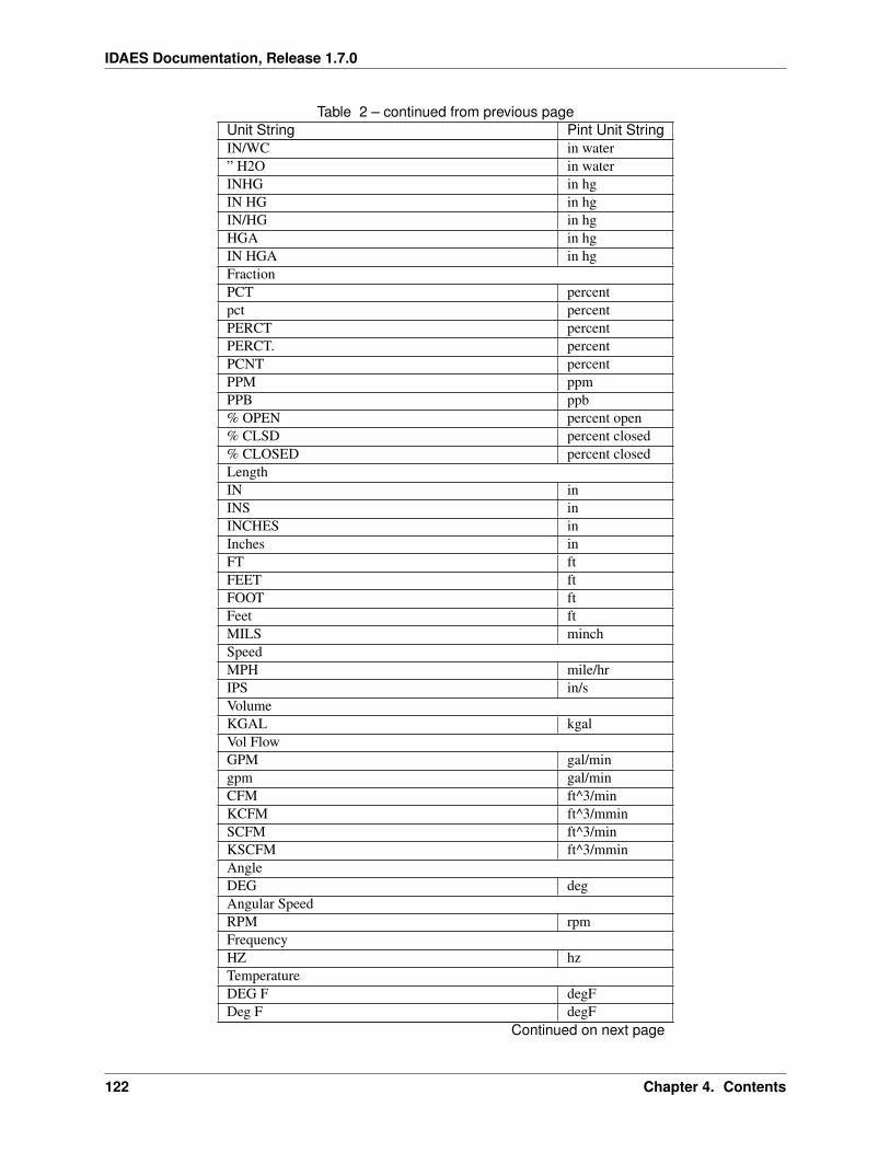
IDAES Documentation, Release 1.7.0
Table 2 – continued from previous pageUnit String Pint Unit StringIN/WC in water” H2O in waterINHG in hgIN HG in hgIN/HG in hgHGA in hgIN HGA in hgFractionPCT percentpct percentPERCT percentPERCT. percentPCNT percentPPM ppmPPB ppb% OPEN percent open% CLSD percent closed% CLOSED percent closedLengthIN inINS inINCHES inInches inFT ftFEET ftFOOT ftFeet ftMILS minchSpeedMPH mile/hrIPS in/sVolumeKGAL kgalVol FlowGPM gal/mingpm gal/minCFM ft^3/minKCFM ft^3/mminSCFM ft^3/minKSCFM ft^3/mminAngleDEG degAngular SpeedRPM rpmFrequencyHZ hzTemperatureDEG F degFDeg F degF
Continued on next page
122 Chapter 4. Contents
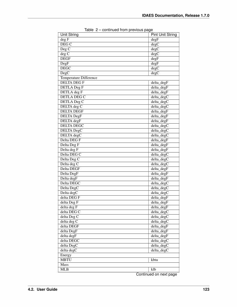
IDAES Documentation, Release 1.7.0
Table 2 – continued from previous pageUnit String Pint Unit Stringdeg F degFDEG C degCDeg C degCdeg C degCDEGF degFDegF degFDEGC degCDegC degCTemperature DifferenceDELTA DEG F delta_degFDETLA Deg F delta_degFDETLA deg F delta_degFDETLA DEG C delta_degCDETLA Deg C delta_degCDELTA deg C delta_degCDELTA DEGF delta_degFDELTA DegF delta_degFDELTA degF delta_degFDELTA DEGC delta_degCDELTA DegC delta_degCDELTA degC delta_degCDelta DEG F delta_degFDelta Deg F delta_degFDelta deg F delta_degFDelta DEG C delta_degCDelta Deg C delta_degCDelta deg C delta_degCDelta DEGF delta_degFDelta DegF delta_degFDelta degF delta_degFDelta DEGC delta_degCDelta DegC delta_degCDelta degC delta_degCdelta DEG F delta_degFdelta Deg F delta_degFdelta deg F delta_degFdelta DEG C delta_degCdelta Deg C delta_degCdelta deg C delta_degCdelta DEGF delta_degFdelta DegF delta_degFdelta degF delta_degFdelta DEGC delta_degCdelta DegC delta_degCdelta degC delta_degCEnergyMBTU kbtuMassMLB klb
Continued on next page
4.2. User Guide 123
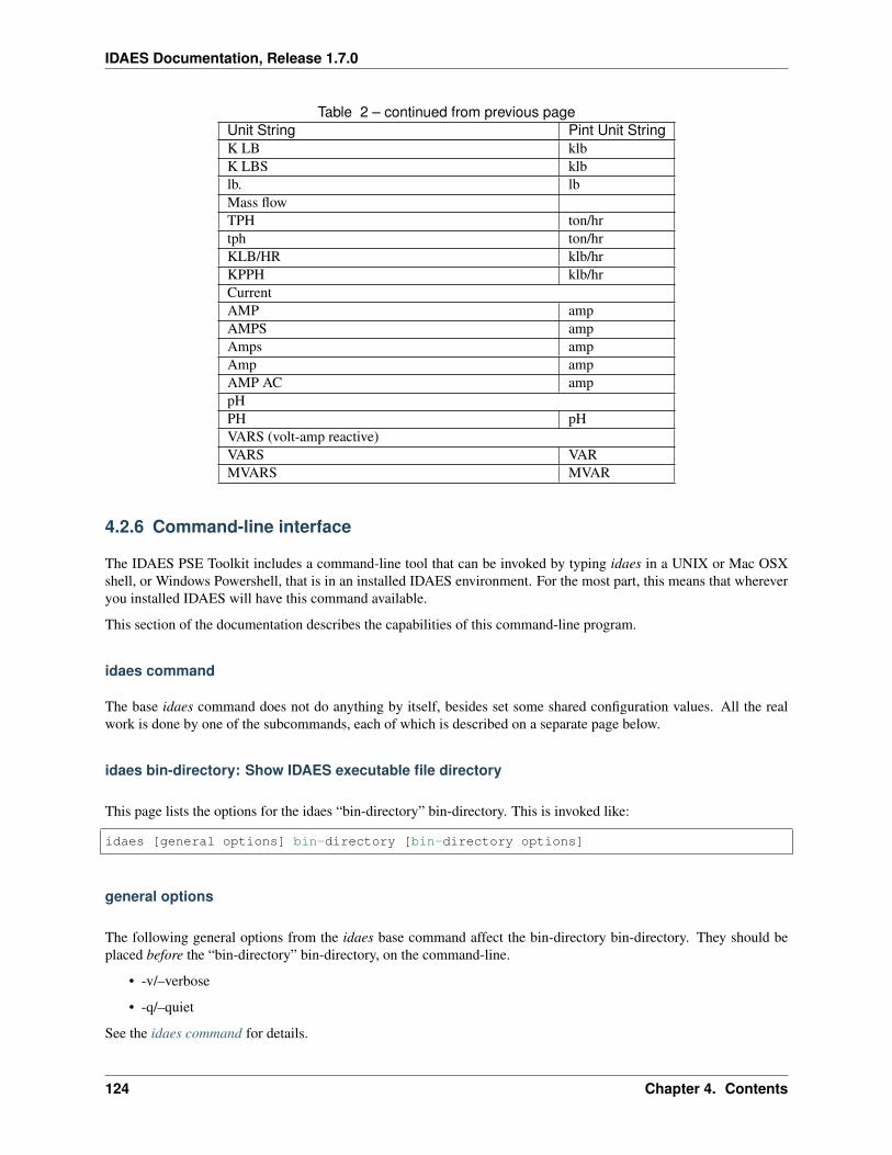
IDAES Documentation, Release 1.7.0
Table 2 – continued from previous pageUnit String Pint Unit StringK LB klbK LBS klblb. lbMass flowTPH ton/hrtph ton/hrKLB/HR klb/hrKPPH klb/hrCurrentAMP ampAMPS ampAmps ampAmp ampAMP AC amppHPH pHVARS (volt-amp reactive)VARS VARMVARS MVAR
4.2.6 Command-line interface
The IDAES PSE Toolkit includes a command-line tool that can be invoked by typing idaes in a UNIX or Mac OSXshell, or Windows Powershell, that is in an installed IDAES environment. For the most part, this means that whereveryou installed IDAES will have this command available.
This section of the documentation describes the capabilities of this command-line program.
idaes command
The base idaes command does not do anything by itself, besides set some shared configuration values. All the realwork is done by one of the subcommands, each of which is described on a separate page below.
idaes bin-directory: Show IDAES executable file directory
This page lists the options for the idaes “bin-directory” bin-directory. This is invoked like:
idaes [general options] bin-directory [bin-directory options]
general options
The following general options from the idaes base command affect the bin-directory bin-directory. They should beplaced before the “bin-directory” bin-directory, on the command-line.
• -v/–verbose
• -q/–quiet
See the idaes command for details.
124 Chapter 4. Contents
IDAES Documentation, Release 1.7.0
idaes bin-directory
This subcommand shows the IDAES executable file directory.
options
--helpShow the help message and exit.
--existsShow if the directory exists.
--createCreate the directory.
idaes copyright: Show IDAES copyright information
This page lists the options for the idaes “copyright” subcommand. This is invoked like:
idaes [general options] copyright [subcommand options]
general options
The following general options from the idaes base command affect the copyright subcommand. They should be placedbefore the “copyright” subcommand, on the command-line.
• -v/–verbose
• -q/–quiet
See the idaes command for details.
idaes copyright
This subcommand prints the IDAES copyright notice to standard output.
options
--helpShow the help message and exit.
idaes data-directory: Show IDAES data directory
This page lists the options for the idaes “data-directory” subcommand. This is invoked like:
idaes [general options] data-directory [subcommand options]
4.2. User Guide 125
IDAES Documentation, Release 1.7.0
general options
The following general options from the idaes base command affect the data-directory subcommand. They should beplaced before the “data-directory” subcommand, on the command-line.
• -v/–verbose
• -q/–quiet
See the idaes command for details.
idaes data-directory
This subcommand shows the IDAES data directory.
options
--helpShow the help message and exit.
--existsShow if the directory exists.
--createCreate the directory.
idaes get-examples: Fetch example scripts and Jupyter Notebooks
This page lists the options for the idaes “get-examples” subcommand. This is invoked like:
idaes [general options] get-examples [subcommand options]
general options
The following general options from the idaes base command affect the get-examples subcommand. They should beplaced before the “get-examples” subcommand, on the command-line.
• -v/–verbose
• -q/–quiet
See the idaes command for details.
idaes get-examples
This subcommand fetches example scripts and Jupyter Notebooks from a given release in Github. and puts them in adirectory of the users’ choosing. If the user does not specify a directory, the default is examples.
126 Chapter 4. Contents
IDAES Documentation, Release 1.7.0
options
--helpShow the help message and exit.
-d,--dir TEXT
Select the installation target directory. See example usage for several examples of this option.
-I, --no-install
Do not install examples into ‘idaes_examples’ package. Examples are installed by default so they can be importeddirectly from Python. Not installing them might cause some tests, which import the examples, to fail.
-l, --list-releases
List all available released versions, and stop. This lets people browse the releases and select one. By default, therelease that matches the version of the currently installed “idaes” package is used. See also the –unstable option.
-N, --no-download
Do not download anything. If the –no-install option is also given, this means the command will essentially do nothing.Or, looked at another way, this option means that only action will be the installation of the “idaes_examples” packagefrom the selected directory.
-U, --unstable
Allow and list unstable/pre-release versions. This applies to both download and the –list-releases option. Unstablereleases are marked with “rcN” or similar suffixes.
-V, --version TEXT
Version of examples to download. The default version, which is shown for the –help option, is the same as the versionof the IDAES PSE toolkit for which the idaes command is installed. If the version to install is unstable (ends with“rcN”) then you will need to add the –unstable option to avoid errors.
example usage
idaes get-examples Download examples from release matching release for the idaes command, install them in theexamples subdirectory of this directory, and install the modules found under examples/src as a package namedidaes_examples. The examples directory must not exist, i.e. the program will refuse to overwrite the contents ofan existing directory.
idaes get-examples -d /tmp/examples Same as above, but put downloaded code in /tmp/examples instead.
idaes get-examples -d /tmp/examples -I Download to /tmp/examples, but do not install.
idaes get-examples -d /tmp/examples -N Install the examples found under /tmp/examples.
idaes get-examples –version 1.4.2-pre Download examples from release 1.4.2-pre, install them in the examplessubdirectory of this directory, and install the modules found under examples/src as a package namedidaes_examples.
idaes get-examples –list-releases List available releases of the examples in Github repository, idaes/examples-pse.Do not attempt to download or install anything.
idaes get-examples –list-releases –unstable Same as above, but include non-stable releases.
4.2. User Guide 127
IDAES Documentation, Release 1.7.0
idaes get-extensions: Get solvers and libraries
This page lists the options for the idaes “get-extensions” subcommand. This is invoked like:
idaes [general options] get-extensions [subcommand options]
general options
The following general options from the idaes base command affect the get-extensions subcommand. They should beplaced before the “get-extensions” subcommand, on the command-line.
• -v/–verbose
• -q/–quiet
See idaes command for details.
idaes get-extensions
This subcommand gets the compiled solvers and libraries from a remote repository, and installs them locally.
options
--helpShow the help message and exit.
--urlURL from which to download the solvers/libraries.
idaes lib-directory: Show IDAES library file directory
This page lists the options for the idaes “lib-directory” subcommand. This is invoked like:
idaes [general options] lib-directory [subcommand options]
general options
The following general options from the idaes base command affect the lib-directory subcommand. They should beplaced before the “lib-directory” subcommand, on the command-line.
• -v/–verbose
• -q/–quiet
See the idaes command for details.
idaes lib-directory
This subcommand shows the IDAES library file directory.
128 Chapter 4. Contents
IDAES Documentation, Release 1.7.0
options
--helpShow the help message and exit.
--existsShow if the directory exists.
--createCreate the directory.
IDAES Versioning
The IDAES Python package is versioned according to the general guidelines of semantic versioning, following therecommendations of PEP 440 with respect to extended versioning descriptors (alpha, beta, release candidate, etc.).
Basic usage
You can see the version of the package at any time interactively by printing out the __version__ variable in the top-levelpackage:
import idaesprint(idaes.__version__)# prints a version like "1.2.3"
Advanced usage
This section describes the module’s variables and classes.
Overview
The API in this module is mostly for internal use, e.g. from ‘setup.py’ to get the version of the package. But Versionhas been written to be usable as a general versioning interface.
Example of using the class directly:
>>> from idaes.ver import Version>>> my_version = Version(1, 2, 3)>>> print(my_version)1.2.3>>> tuple(my_version)(1, 2, 3)>>> my_version = Version(1, 2, 3, 'alpha')>>> print(my_version)1.2.3.a>>> tuple(my_version)(1, 2, 3, 'alpha')>>> my_version = Version(1, 2, 3, 'candidate', 1)>>> print(my_version)1.2.3.rc1>>> tuple(my_version)(1, 2, 3, 'candidate', 1)
4.2. User Guide 129
IDAES Documentation, Release 1.7.0
If you want to add a version to a class, e.g. a model, then simply inherit from HasVersion and initialize it with thesame arguments you would give the Version constructor:
>>> from idaes.ver import HasVersion>>> class MyClass(HasVersion):... def __init__(self):... super(MyClass, self).__init__(1, 2, 3, 'alpha')...>>> obj = MyClass()>>> print(obj.version)1.2.3.a
idaes.ver.package_version = <idaes.ver.Version object>Package’s version as an object
idaes.ver.__version__ = '1.7.0'Package’s version as a simple string
Version class
The versioning semantics are encapsulated in a class called Version.
class idaes.ver.Version(major, minor, micro, releaselevel=’final’, serial=None, label=None)This class attempts to be compliant with a subset of PEP 440.
Note: If you actually happen to read the PEP, you will notice that pre- and post- releases, as well as “releaseepochs”, are not supported.
__init__(major, minor, micro, releaselevel=’final’, serial=None, label=None)Create new version object.
Provided arguments are stored in public class attributes by the same name.
Parameters
• major (int) – Major version
• minor (int) – Minor version
• micro (int) – Micro (aka patchlevel) version
• releaselevel (str) – Optional PEP 440 specifier
• serial (int) – Optional number associated with releaselevel
• label (str) – Optional local version label
__iter__()Return version information as a sequence.
__str__()Return version information as a string.
HasVersion class
For adding versions to other classes in a simple and standard way, you can use the HasVersion mixin class.
class idaes.ver.HasVersion(*args)Interface for a versioned class.
130 Chapter 4. Contents
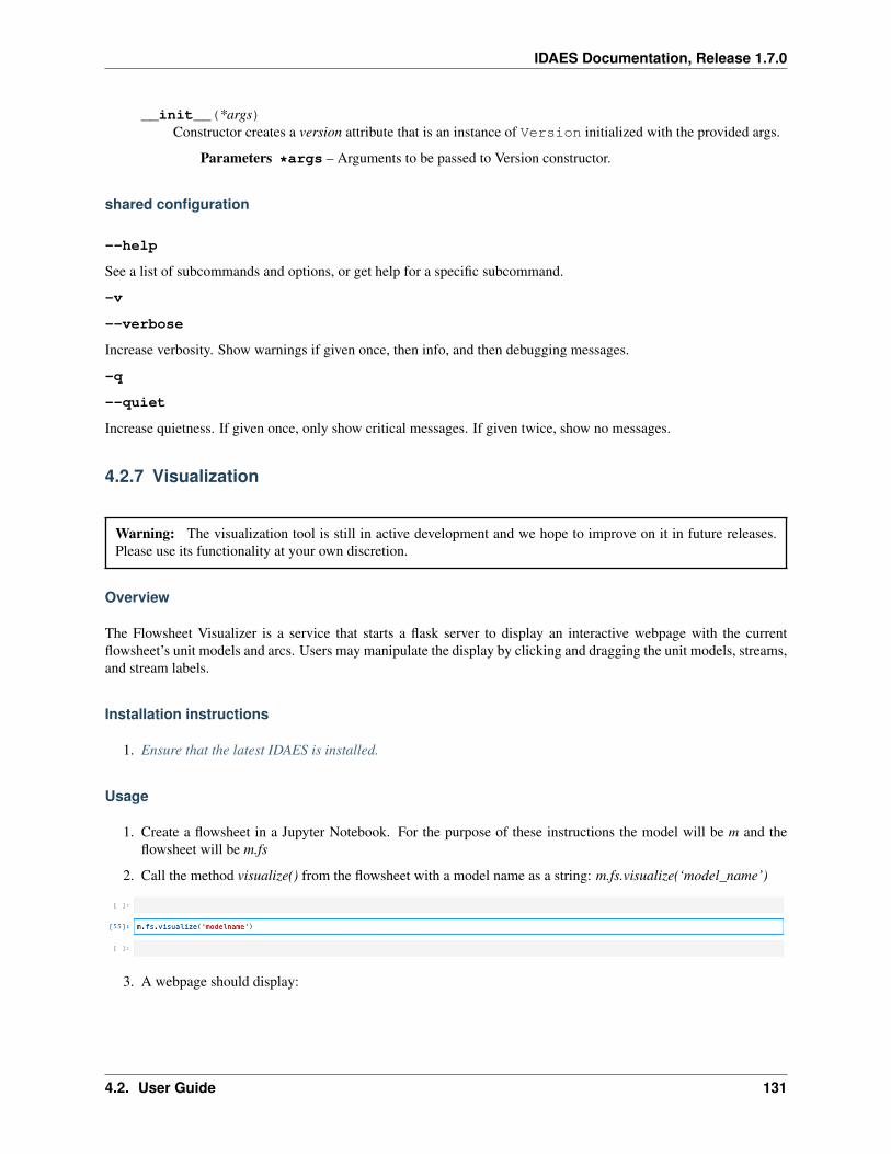
IDAES Documentation, Release 1.7.0
__init__(*args)Constructor creates a version attribute that is an instance of Version initialized with the provided args.
Parameters *args – Arguments to be passed to Version constructor.
shared configuration
--help
See a list of subcommands and options, or get help for a specific subcommand.
-v
--verbose
Increase verbosity. Show warnings if given once, then info, and then debugging messages.
-q
--quiet
Increase quietness. If given once, only show critical messages. If given twice, show no messages.
4.2.7 Visualization
Warning: The visualization tool is still in active development and we hope to improve on it in future releases.Please use its functionality at your own discretion.
Overview
The Flowsheet Visualizer is a service that starts a flask server to display an interactive webpage with the currentflowsheet’s unit models and arcs. Users may manipulate the display by clicking and dragging the unit models, streams,and stream labels.
Installation instructions
1. Ensure that the latest IDAES is installed.
Usage
1. Create a flowsheet in a Jupyter Notebook. For the purpose of these instructions the model will be m and theflowsheet will be m.fs
2. Call the method visualize() from the flowsheet with a model name as a string: m.fs.visualize(‘model_name’)
3. A webpage should display:
4.2. User Guide 131
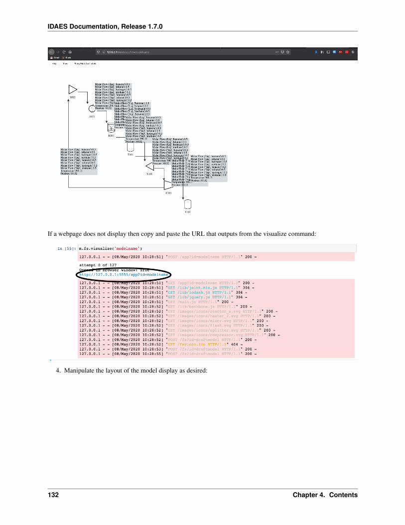
IDAES Documentation, Release 1.7.0
If a webpage does not display then copy and paste the URL that outputs from the visualize command:
4. Manipulate the layout of the model display as desired:
132 Chapter 4. Contents
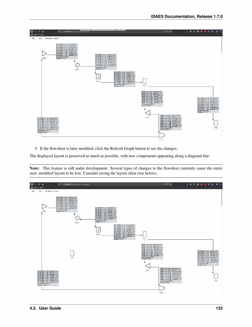
IDAES Documentation, Release 1.7.0
5. If the flowsheet is later modified, click the Refresh Graph button to see the changes.
The displayed layout is preserved as much as possible, with new components appearing along a diagonal line.
Note: This feature is still under development. Several types of changes to the flowsheet currently cause the entireuser- modified layout to be lost. Consider saving the layout often (see below).
4.2. User Guide 133
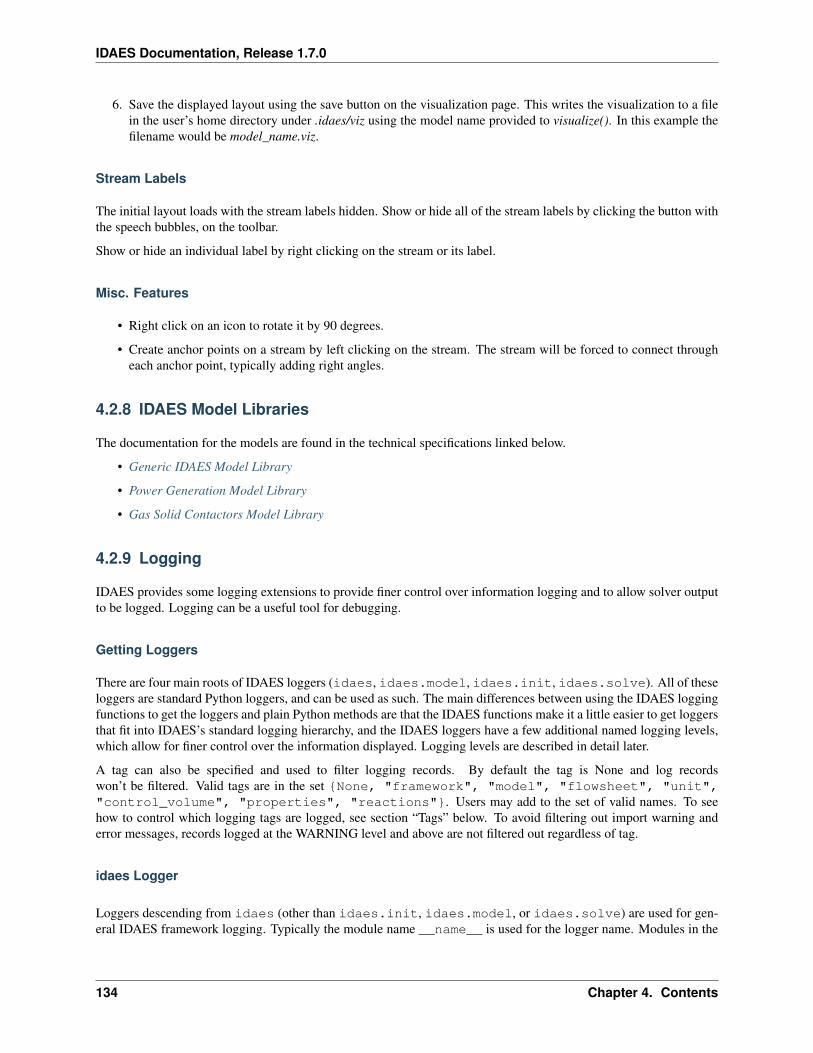
IDAES Documentation, Release 1.7.0
6. Save the displayed layout using the save button on the visualization page. This writes the visualization to a filein the user’s home directory under .idaes/viz using the model name provided to visualize(). In this example thefilename would be model_name.viz.
Stream Labels
The initial layout loads with the stream labels hidden. Show or hide all of the stream labels by clicking the button withthe speech bubbles, on the toolbar.
Show or hide an individual label by right clicking on the stream or its label.
Misc. Features
• Right click on an icon to rotate it by 90 degrees.
• Create anchor points on a stream by left clicking on the stream. The stream will be forced to connect througheach anchor point, typically adding right angles.
4.2.8 IDAES Model Libraries
The documentation for the models are found in the technical specifications linked below.
• Generic IDAES Model Library
• Power Generation Model Library
• Gas Solid Contactors Model Library
4.2.9 Logging
IDAES provides some logging extensions to provide finer control over information logging and to allow solver outputto be logged. Logging can be a useful tool for debugging.
Getting Loggers
There are four main roots of IDAES loggers (idaes, idaes.model, idaes.init, idaes.solve). All of theseloggers are standard Python loggers, and can be used as such. The main differences between using the IDAES loggingfunctions to get the loggers and plain Python methods are that the IDAES functions make it a little easier to get loggersthat fit into IDAES’s standard logging hierarchy, and the IDAES loggers have a few additional named logging levels,which allow for finer control over the information displayed. Logging levels are described in detail later.
A tag can also be specified and used to filter logging records. By default the tag is None and log recordswon’t be filtered. Valid tags are in the set None, "framework", "model", "flowsheet", "unit","control_volume", "properties", "reactions". Users may add to the set of valid names. To seehow to control which logging tags are logged, see section “Tags” below. To avoid filtering out import warning anderror messages, records logged at the WARNING level and above are not filtered out regardless of tag.
idaes Logger
Loggers descending from idaes (other than idaes.init, idaes.model, or idaes.solve) are used for gen-eral IDAES framework logging. Typically the module name __name__ is used for the logger name. Modules in the
134 Chapter 4. Contents
IDAES Documentation, Release 1.7.0
idaes package already start with idaes, but if an IDAES logger is requested for a module outside of the idaespackage idaes. is prepended to the name.
idaes.logger.getLogger(name, level=None, tag=None)Return an idaes logger.
Parameters
• name – usually __name__
• level – standard IDAES logging level (default use IDAES config)
• tag – logger tag for filtering, see valid_log_tags()
Returns logger
Example
import idaes.logger as idaeslog
_log = idaeslog.getLogger(__name__, tag="framework")
idaes.init Loggers
The init logger will always descend from “idaes.init”. This logger is used in IDAES model initialization methods, andcan be used in user models as well. Initialization methods are usually attached to a Pyomo Block. Blocks have a nameattribute. So the logger name is usually given as the block name, and the getInitLogger() function prependsidaes.init.. The advantage of using the block name over the module name is that users can see exactly whichmodel instance the initialization log messages are coming from.
idaes.logger.getInitLogger(name, level=None, tag=None)Get a model initialization logger
Parameters
• name – Object name (usually Pyomo Component name)
• level – Log level
• tag – logger tag for filtering, see valid_log_tags()
Returns logger
Example
import idaes.logger as idaeslog
class DummyBlock(object):"""A dummy block for demonstration purposes"""def __init__(name):self.name = name
def initialize(outlvl=idaeslog.INFO):init_log = idaeslog.getInitLogger(self.name, level=outlvl, tag="unit")
idaes.model Loggers
The model logger is used to provide a standard way to produce log messages from user models that are not part ofthe idaes package. The logger name has idaes.model prepended to the name provided by the user. This is
4.2. User Guide 135
IDAES Documentation, Release 1.7.0
convenient because it provides a way to use a standard configuration system for user model loggers. The user canchoose any name they like for these loggers.
idaes.logger.getModelLogger(name, level=None, tag=None)Get a logger for an IDAES model. This function helps users keep their loggers in a standard location and usethe IDAES logging config.
Parameters
• name – Name (usually __name__). Any starting ‘idaes.’ is stripped off, so if a model ispart of the idaes package, ‘idaes’ won’t be repeated.
• level – Standard Python logging level (default use IDAES config)
• tag – logger tag for filtering, see valid_log_tags()
Returns logger
Example
import idaes.logger as idaeslog
_log = idaeslog.getModelLogger("my_model", level=idaeslog.DEBUG, tag="model")
idaes.solve Loggers
The solve logger will always descend from “idaes.solve”. This logger is used to log solver output. Since solvers mayproduce a lot of output, it can be useful to specify different handlers for the solve logger to direct it to a separate file.
idaes.logger.getSolveLogger(name, level=None, tag=None)Get a solver logger
Parameters
• name – logger name is “idaes.solve.” + name (if name starts with “idaes.” it is removedbefore creating the logger name)
• level – Log level
• tag – logger tag for filtering, see valid_log_tags()
Returns logger
Tags
Logger tags are provided to allow control over what types of log records to display. The logger tag is just a string thatgets attached to a logger, which specifies that a logger generates records of a certain type. You can then specify whattags you want to see information from. A filter removes any tags that are not in the list of tags to display at levelsbelow WARNING.
The set of tags to display information from is a global setting in the idaes.logger module. When getting a logger, youcan set its tag by providing the tag argument, see “Getting Loggers” above.
The following functions can be used to specify which logging tags to display:
idaes.logger.log_tags()Returns a set of logging tags to be logged.
Returns (set) tags to be logged
136 Chapter 4. Contents
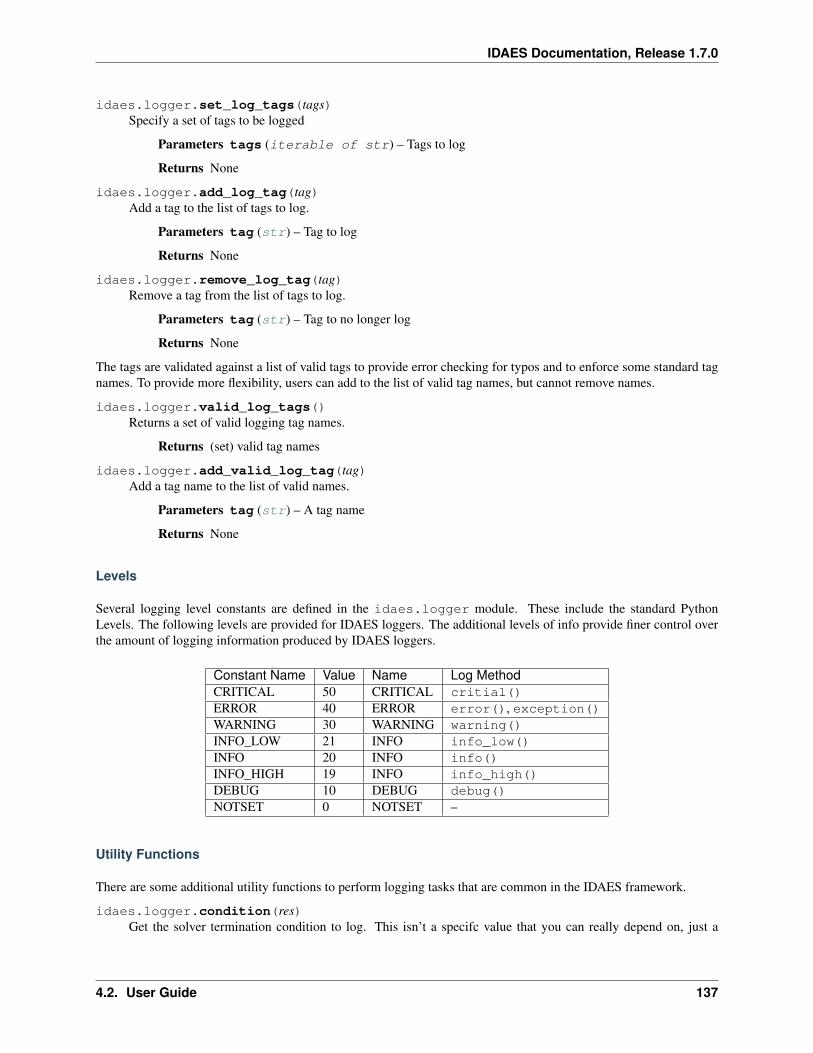
IDAES Documentation, Release 1.7.0
idaes.logger.set_log_tags(tags)Specify a set of tags to be logged
Parameters tags (iterable of str) – Tags to log
Returns None
idaes.logger.add_log_tag(tag)Add a tag to the list of tags to log.
Parameters tag (str) – Tag to log
Returns None
idaes.logger.remove_log_tag(tag)Remove a tag from the list of tags to log.
Parameters tag (str) – Tag to no longer log
Returns None
The tags are validated against a list of valid tags to provide error checking for typos and to enforce some standard tagnames. To provide more flexibility, users can add to the list of valid tag names, but cannot remove names.
idaes.logger.valid_log_tags()Returns a set of valid logging tag names.
Returns (set) valid tag names
idaes.logger.add_valid_log_tag(tag)Add a tag name to the list of valid names.
Parameters tag (str) – A tag name
Returns None
Levels
Several logging level constants are defined in the idaes.logger module. These include the standard PythonLevels. The following levels are provided for IDAES loggers. The additional levels of info provide finer control overthe amount of logging information produced by IDAES loggers.
Constant Name Value Name Log MethodCRITICAL 50 CRITICAL critial()ERROR 40 ERROR error(), exception()WARNING 30 WARNING warning()INFO_LOW 21 INFO info_low()INFO 20 INFO info()INFO_HIGH 19 INFO info_high()DEBUG 10 DEBUG debug()NOTSET 0 NOTSET –
Utility Functions
There are some additional utility functions to perform logging tasks that are common in the IDAES framework.
idaes.logger.condition(res)Get the solver termination condition to log. This isn’t a specifc value that you can really depend on, just a
4.2. User Guide 137
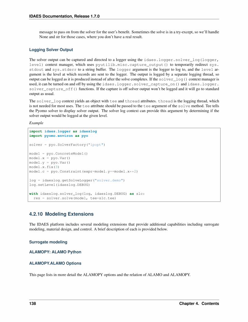
IDAES Documentation, Release 1.7.0
message to pass on from the solver for the user’s benefit. Sometimes the solve is in a try-except, so we’ll handleNone and str for those cases, where you don’t have a real result.
Logging Solver Output
The solver output can be captured and directed to a logger using the idaes.logger.solver_log(logger,level) context manager, which uses pyutilib.misc.capture_output() to temporarily redirect sys.stdout and sys.stderr to a string buffer. The logger argument is the logger to log to, and the level ar-gument is the level at which records are sent to the logger. The output is logged by a separate logging thread, sooutput can be logged as it is produced instead of after the solve completes. If the solver_log() context manager isused, it can be turned on and off by using the idaes.logger.solver_capture_on() and idaes.logger.solver_capture_off() functions. If the capture is off solver output won’t be logged and it will go to standardoutput as usual.
The solver_log context yields an object with tee and thread attributes. thread is the logging thread, whichis not needed for most uses. The tee attribute should be passed to the tee argument of the solve method. Tee tellsthe Pyomo solver to display solver output. The solver log context can provide this argument by determining if thesolver output would be logged at the given level.
Example
import idaes.logger as idaeslogimport pyomo.environ as pyo
solver = pyo.SolverFactory("ipopt")
model = pyo.ConcreteModel()model.x = pyo.Var()model.y = pyo.Var()model.x.fix(3)model.c = pyo.Constraint(expr=model.y==model.x**2)
log = idaeslog.getSolveLogger("solver.demo")log.setLevel(idaeslog.DEBUG)
with idaeslog.solver_log(log, idaeslog.DEBUG) as slc:res = solver.solve(model, tee=slc.tee)
4.2.10 Modeling Extensions
The IDAES platform includes several modeling extensions that provide additional capabilities including surrogatemodeling, material design, and control. A brief description of each is provided below.
Surrogate modeling
ALAMOPY: ALAMO Python
ALAMOPY.ALAMO Options
This page lists in more detail the ALAMOPY options and the relation of ALAMO and ALAMOPY.
138 Chapter 4. Contents
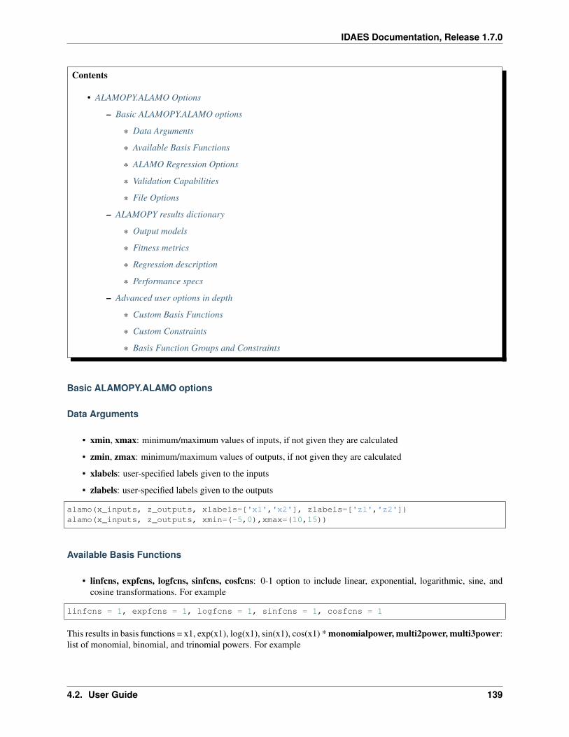
IDAES Documentation, Release 1.7.0
Contents
• ALAMOPY.ALAMO Options
– Basic ALAMOPY.ALAMO options
* Data Arguments
* Available Basis Functions
* ALAMO Regression Options
* Validation Capabilities
* File Options
– ALAMOPY results dictionary
* Output models
* Fitness metrics
* Regression description
* Performance specs
– Advanced user options in depth
* Custom Basis Functions
* Custom Constraints
* Basis Function Groups and Constraints
Basic ALAMOPY.ALAMO options
Data Arguments
• xmin, xmax: minimum/maximum values of inputs, if not given they are calculated
• zmin, zmax: minimum/maximum values of outputs, if not given they are calculated
• xlabels: user-specified labels given to the inputs
• zlabels: user-specified labels given to the outputs
alamo(x_inputs, z_outputs, xlabels=['x1','x2'], zlabels=['z1','z2'])alamo(x_inputs, z_outputs, xmin=(-5,0),xmax=(10,15))
Available Basis Functions
• linfcns, expfcns, logfcns, sinfcns, cosfcns: 0-1 option to include linear, exponential, logarithmic, sine, andcosine transformations. For example
linfcns = 1, expfcns = 1, logfcns = 1, sinfcns = 1, cosfcns = 1
This results in basis functions = x1, exp(x1), log(x1), sin(x1), cos(x1) * monomialpower, multi2power, multi3power:list of monomial, binomial, and trinomial powers. For example
4.2. User Guide 139
IDAES Documentation, Release 1.7.0
monomialpower = (2,3,4), multi2power = (1,2,3), multi3power = (1,2,3)
This results in the following basis functions:
• Monomial functions = x^2, x^3, x^4
• Binomial functions = x1*x2, (x1*x2)^2, (x1*x2)^3
• Trinomial functions = (x1*x2*x3), (x1*x2*x3)^2, (x1*x2*x3)^3
• ratiopower: list of ratio powers. For example
ratiopower = (1,2,3)
This results in basis functions = (x1/x2), (x1/x2)^2, (x1/x2)^3
alamo(x_inputs, z_outputs, linfcns=1, logfcns=1, expfcns=1)alamo(x_inputs, z_outputs, linfcns=1, multi2power=(2,3))
Note: Custom basis functions are discussed in the Advanced User Section.
ALAMO Regression Options
• showalm: print ALAMO output to the screen
• expandoutput: add a key to the output dictionary for multiple outputs
• solvemip, builder, linearerror: A 01 indicator to solve with an optimizer (GAMSSOLVER), use a greedyheuristic, or use a linear objective instead of squared error.
• modeler: Fitness metric to beused for model building (1-8)
– 1. BIC: Bayesian infromation criterion
– 2. Cp: Mallow’s Cp
– 3. AICc: the corrected Akaike’s information criterion
– 4. HQC: the Hannan-Quinn information criterion
– 5. MSE: mean square error
– 6. SSEp: sum of square error plus a penalty proportional to the model size (Note: convpen is the weightof the penalty)
– 7. RIC: the risk information criterion
– 8. MADp: the maximum absolute eviation plus a penalty proportional to model size (Note: convpen isthe weight of the penalty)
• regularizer: Regularization method used to reduce the number of potential basis functions before optimizationof the selected fitness metric. Possible values are 0 and 1, corresponding to no regularization and regularizationwith the lasso, respectively.
• maxterms: Maximum number of terms to be fit in the model
• convpen: When MODELER is set to 6 or 8 the size of the model is weighted by CONVPEN.
• almopt: name of the alamo option file
• simulator: a python function to be used as a simulator for ALAMO, a variable that is a python function (not astring)
• maxiter: max iteration of runs
140 Chapter 4. Contents
IDAES Documentation, Release 1.7.0
Validation Capabilities
• xval, zval: validation input/output variables
• loo: leave-one-out evaluation
• lmo: leave-many-out evaluation
• cvfun: cross-validation function (True/False)
File Options
• almname: specify a name for the .alm file
• savescratch: saves .alm and .lst
• savetrace: saves tracefile
• saveopt: save .opt options file
• savegams: save the .gms gams file
ALAMOPY results dictionary
The results from alamopy.alamo are returned as a python dictionary. The data can be accessed by using the dictionarykeys listed below. For example
regression_results = doalamo(x_input, z_output, **kargs)model = regression_results['model']
Output models
• f(model): A callable function
• pymodel: name of the python model written
• model: string of the regressed model
Note: A python script named after the output variables is written to the current directory. The model can be importedand used for further evaluation, for example to evaluate residuals:
import z1residuals = [y-z1.f(inputs[0],inputs[1]) for y,inputs in zip(z,x)]
Fitness metrics
• size: number of terms chosen in the regression
• R2: R2 value of the regression
• Objective value metrics: ssr, rmse, madp
4.2. User Guide 141
IDAES Documentation, Release 1.7.0
Regression description
• version: Version of ALAMO
• xlabels, zlabels: The labels used for the inputs/outputs
• xdata, zdata: array of xdata/zdata
• ninputs, nbas: number of inputs/basis functions
Performance specs
There are three types of regression problems that are used: ordinary linear regression (olr), classic linear regression(clr), and a mixed integer program (mip). Performance metrics include the number of each problems and the timespent on each type of problem. Additionally, the time spent on other operations and the total time are included.
• numolr, olrtime, numclr, clrtime, nummip, miptime: number of type of regression problems solved and time
• othertime: Time spent on other operations
• totaltime: Total time spent on the regression
Advanced user options in depth
Similar to ALAMO, there are advanced capabilities for customization and constrained regression facilitated by meth-ods in ALAMOPY including custom basis functions, custom constraints on the response surface, and basis functiongroups. These methods interact with the regression using the alamo option file.
Custom Basis Functions
Custom basis functions can be added to the built-in functions to expand the functional forms available. In ALAMO,this can be done with the following syntax
NCUSTOMBAS #BEGIN_CUSTOMBASx1^2 * x2^2END_CUSTOMBAS
To use this advanced capability in ALAMOPY, the following function is called. Note it is necessary to use the xlabelsassigned to the input parameters.
addCustomFunctions(fcn_list)addCustomFunctions(["x1^2 * x2^2", "...", "..." ...])
Custom Constraints
Custom constraints can be placed on response surface or regressed function of the output variable. In ALAMO, this iscontrolled using custom constraints, CUSTOMCON. The constraints, a function g(x_inputs, z_outputs) are appliedto a specific output variable, which is the index of the output variable, and are less than or equal to 0 (g <= 0).
142 Chapter 4. Contents
IDAES Documentation, Release 1.7.0
CRNCUSTOM #BEGIN_CUSTOMCON1 z1 - x1 + x2 + 1END_CUSTOMCON
To use this advanced capability in ALAMOPY, the following function is called. Note it is necessary to use the xlabelsassigned to the input parameters.
addCustomConstraints(custom_constraint_list, **kargs)addCustomConstraints(["1 z1 - x1 + x2 +1", "...", "..." ...])
Basis Function Groups and Constraints
In addition to imposing constraints on the response surface it produces, ALAMO has the ability to enforce constraintson groups of selected basis functions. This can be accomplished using NGROUPS and identifying groups of basisfunctions. For ALAMO, this is achieved by first defining the groups with
NGROUPS 3BEGIN_GROUPS# Group-id Member-type Member-indices <Powers>1 LIN 1 22 MONO 1 23 GRP 1 2END_GROUPS
To add groups to ALAMOPY, you can use the following methods. Each Basis group has an index number that will beused as reference in the group constraints. The groups are defined by three or four parameters. Options for Member-type are LIN, LOG, EXP, SIN, COS, MONO, MULTI2, MULTI3, RATIO, GRP, RBF, and CUST.
addBasisGroup(type_of_function, input_indices, powers)addBasisGroups(groups)
addBasisGroup("MONO", "1", "2")addBasisGroups([["LIN","1 2"],["MONO","1","2"],["GRP","1 2"]])
With the groups defined, constraints can be placed on the groups using the constraint-types NMT (no-more-than), ATL(at-least), REQ (requires), and XCL (exclude). For NMT and ATL the integer-parameter is the number of membersin the group that should be selected based on the constraint. For REQ and XCL the integer-parameter is the group-idnumber of excluded or required basis functions.
BEGIN_GROUPCON# Group-id Output-id Constraint-type Integer-parameter3 1 NMT 1END_GROUPCON
To add the basis constraints to alamopy, you can use the following methods.
addBasisConstraint(group_id, output_id, constraint_type, intParam)addBasisConstraints(groups_constraint_list)
addBasisConstraint(3,1,"NMT",1)addBasisConstraints([[3,1,"NMT",1]])
The purpose of ALAMOPY (Automatic Learning of Algebraic MOdels PYthon wrapper) is to provide a wrapperfor the software ALAMO which generates algebraic surrogate models of black-box systems for which a simulator or
4.2. User Guide 143
IDAES Documentation, Release 1.7.0
experimental setup is available. Consider a system for which the outputs z are an unknown function f of the systeminputs x. The software identifies a function f, i.e., a relationship between the inputs and outputs of the system, thatbest matches data (pairs of x and corresponding z values) that are collected via simulation or experimentation.
Basic Usage
ALAMOPY’s main function is alamopy.alamo. Data can be read in or simulated using available python packages.The main arguments of the alamopy.alamo python function are inputs and outputs, which are 2D arrays of data. Forexample
regression_results =alamopy.alamo(x_inputs, z_outputs, **kargs)
where **kargs is a set of named keyword arguments than can be passed to the alamo python function to customizethe basis function set, names of output files, and other options available in ALAMO.
Warning: The alamopy.doalamo function is deprecated. It is being replaced with alamopy.alamo
Options for alamopy.alamo
Possible arguments to be passed to ALAMO through do alamo and additional arguments that govern the behavior ofdoalamo.
• xlabels - list of strings to label the input variables
• zlabels - list of strings to label the output variables
• functions - logfcns, expfcns, cosfcns, sinfcns, linfcns, intercept. These are ‘0-1’ options to activate these func-tions
• monomialpower, multi2power, multi3power, ratiopower. List of terms to be used in the respective basis func-tions
• modeler - integer 1-7 determines the choice of fitness metrice
• solvemip - ‘0-1’ option that will force the solving of the .gms file
These options are specific to alamopy and will not change the behavior of the underlying .alm file.
• expandoutput - ‘0-1’ option that can be used to collect more information from the ALAMO .lst and .trc file
• showalm - ‘0-1’ option that controlif the ALAMO output is printed to screen
• almname - A string that will assign the name of the .alm file
• outkeys - ‘0-1’ option for dictionary indexing according to the output labels
• outkeys - ‘0-1’ option for dictionary indexing according to the output labels
• outkeys - ‘0-1’ option for dictionary indexing according to the output labels
• savetrace - ‘0-1’ option that controls the status of the trace file
• savescratch - ‘0-1’ option to save the .alm and .lst files
• almopt - A string option that will append a text file of the same name to the end of each .alm fille to faciliateadvanced user access in an automated fashion
144 Chapter 4. Contents
IDAES Documentation, Release 1.7.0
ALAMOPY Output
There are mutliple outputs from the running alamopy.alamo. Outputs include:
• f(model): A callable function
• pymodel: name of the python model written
• model: string of the regressed model
Note: A python script named after the output variables is written to the current directory. The model can be importedand used for further evaluation, for example to evaluate residuals:
import z1residuals = [y-z1.f(inputs[0],inputs[1]) for y,inputs in zip(z,x)]
Additional Results
After the regression of a model, ALAMOPY provides confidence interval analysis and plotting capabilities using theresults output.
Plotting
The plotting capabilities of ALAMOPY are available in the almplot function. Almplot will plot the function based onone of the inputs.
result = alamopy.alamo(x_in, z_out, kargs)alamopy.almplot(result)
Confidence intervals
Confidence intervals can similarly be calculated for the weighting of selected basis functions using the almconfidencefunction.
This adds conf_inv (confidence intervals) and covariance (covariance matrix) to the results dictionary. This also getsincorporated into the plotting function if it is available.
result = alamopy.alamo(x_in, z_out, kargs)result = alamopy.almconfidence(result)alamopy.almplot(result)
4.2. User Guide 145
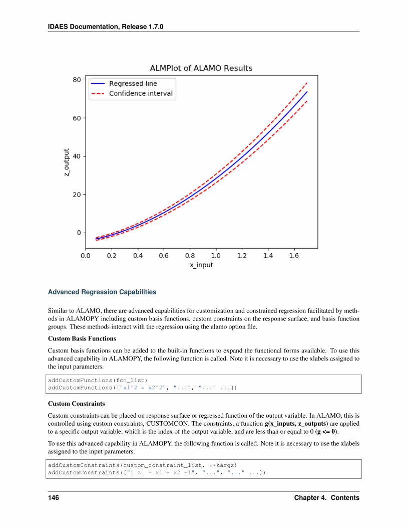
IDAES Documentation, Release 1.7.0
Advanced Regression Capabilities
Similar to ALAMO, there are advanced capabilities for customization and constrained regression facilitated by meth-ods in ALAMOPY including custom basis functions, custom constraints on the response surface, and basis functiongroups. These methods interact with the regression using the alamo option file.
Custom Basis Functions
Custom basis functions can be added to the built-in functions to expand the functional forms available. To use thisadvanced capability in ALAMOPY, the following function is called. Note it is necessary to use the xlabels assigned tothe input parameters.
addCustomFunctions(fcn_list)addCustomFunctions(["x1^2 * x2^2", "...", "..." ...])
Custom Constraints
Custom constraints can be placed on response surface or regressed function of the output variable. In ALAMO, this iscontrolled using custom constraints, CUSTOMCON. The constraints, a function g(x_inputs, z_outputs) are appliedto a specific output variable, which is the index of the output variable, and are less than or equal to 0 (g <= 0).
To use this advanced capability in ALAMOPY, the following function is called. Note it is necessary to use the xlabelsassigned to the input parameters.
addCustomConstraints(custom_constraint_list, **kargs)addCustomConstraints(["1 z1 - x1 + x2 +1", "...", "..." ...])
146 Chapter 4. Contents
IDAES Documentation, Release 1.7.0
Basis Function Groups and Constraints
In addition to imposing constraints on the response surface it produces, ALAMO has the ability to enforce constraintson groups of selected basis functions. To define groups in ALAMOPY, you can use the following methods. Each Basisgroup has an index number that will be used as reference in the group constraints. The groups are defined by threeor four parameters. Options for Member-type are LIN, LOG, EXP, SIN, COS, MONO, MULTI2, MULTI3, RATIO,GRP, RBF, and CUST.
addBasisGroup(type_of_function, input_indices, powers)addBasisGroups(groups)
addBasisGroup("MONO", "1", "2")addBasisGroups([["LIN","1 2"],["MONO","1","2"],["GRP","1 2"]])
With the groups defined, constraints can be placed on the groups using the constraint-types NMT (no-more-than), ATL(at-least), REQ (requires), and XCL (exclude). For NMT and ATL the integer-parameter is the number of membersin the group that should be selected based on the constraint. For REQ and XCL the integer-parameter is the group-idnumber of excluded or required basis functions.
To add the basis constraints to alamopy, you can use the following methods.
addBasisConstraint(group_id, output_id, constraint_type, intParam)addBasisConstraints(groups_constraint_list)
addBasisConstraint(3,1,"NMT",1)addBasisConstraints([[3,1,"NMT",1]])
ALAMOPY Examples
Three examples are included with ALMAOPY. These examples demonstrate different use cases, and provide a templatefor utilizing user-defined mechanisms.
• ackley.py
• branin.py
• camel6.py with a Jupyter notebok
RIPE: Reaction Identification and Parameter Estimation
The RIPE module provides tools for reaction network identification. RIPE uses reactor data consisting of concen-tration, or conversion, values for multiple species that are obtained dynamically, or at multiple process conditions(temperatures, flow rates, working volumes) to identify probable reaction kinetics. The RIPE module also containstools to facilitate adaptive experimental design. The experimental design tools in RIPE require the use of the pythonpackage RBFopt. More information for RBFopt is availible at www.github.com/coin-or/rbfopt
Basic Usage
RIPE can be used to build models for static datasets through the function ripe.ripemodel
ripe_results = ripe.ripemodel(data, kwargs)
• data is provided to RIPE as one, two, or three dimensional python data structures, where the first axis corre-sponds to observations at different process conditions, the second axis corresponds to observations of different
4.2. User Guide 147
IDAES Documentation, Release 1.7.0
chemical species, and the third axis corresponds to dynamic observation of a chemical species at a specifiedprocess condition.
RIPE adaptive experimental design can be accessed using ripe.ems
[proposed_x, errors] = ripe.ems(ripe_results, simulator, l_bounds, u_bounds, n_→˓species, kwargs)
• ripe_results - The results from ripe.ripemodel, additional information provided in the results section
• simulator - a black-box simulator for the unknown process.
• l_bounds/u_bounds - lower and upper bounds for the input variables in the adaptive design
• nspecies - the number of chemical species present in the black-box system
Reaction stoichiometries and mechanisms are provided explicitly to ripemodel through the keyword arguments mech-anisms and stoichiometry. Detailed explanations of the forms of these arguments are provided in the stoiciometry andmechanism specification section. Additional keyword arguments can be found in the additional options section.
RIPE Output
By default, one file will be generated
• riperesults.txt - a file containing the selected reactions and parameter estimates
Reaction Stiochiometry and Mechanism Specification
Considered reaction stiochiometries are provided through keyword arguments.
Stoichiometry
Considered reaction stoichiometries are defiend as a list of list, where reactants and products are defined as negativeand positive integers , respectively, according to their stoichiometric coefficeints. A set of considered reaction stoi-chiometries must be provided. If process data consists of species conversion, a positive coefficient should be specified.
Mechanisms
Considered reaction mechanisms are provided explicitly to RIPE through q keyword argument. If no kinetic mech-anisms are specified, mass action kinetics are ascribed to every considered stoichiometry. RIPE contains kineticmechanisms defined internally, and called through ripe.mechs.<mechanism>. The availible mechanisms include:
• massact - mass action kinetics, order informed by reaction stoichiometry
19 empirical rate forms included relate specifically to catalyst conversion in chemical looping combustion reactorsinclude:
• Random nucleation
• Power law models
• Avrami-Erofeev models
These internal kinetics can be specified by calling ripe.mechs.massact or ripe.mechs.clcforms respectively. User-defined kinetic mechanisms can also be supplied to RIPE as python functions. An example is provided in the filecrac.py.
148 Chapter 4. Contents
IDAES Documentation, Release 1.7.0
Additional Results and Options
In addition to the arguments stoichiometry and mechanism, a number of other optional arguments are availible, in-cluding:
Arguments relating to process conditions
• x0 - initial concentration at each process condition for every species
• time - time associated with dynamic samples for every process condition
• temp - temperature associated with every process condition
• flow - flow rate at every process condition for every species
• vol - reactor volume at every process condition
Arguments related to RIPE algorithmic function
• tref - reference termpeature for reformulated Arrhenius models
• ccon - specified cardinality constraint instead of BIC objective
• sigma - expected variance of noise, estimated if not provided
• onemechper - one mechanism per stoichiometry in selected model, true by default
Additional arguments
• minlp_path - path to baron or other minlp solver, can also be set in shared.py
• alamo_path - path to alamo, can also be set in shared.py
• expand_output - provide estimates for noise variance in model resutls
• zscale - linear scaling of observed responses between -1 and 1
• ascale - linear scaling of activities between -1 and 1
• hide_output - surpress output to terminal
• keepfiles - keep scratch files for debugging
• showpyomo - show pyomo output to terminal, false by default
RIPE Examples
Three examples are included with RIPE. These examples demonstrate different use cases, and provide a template forutilizing user-defined mechanisms.
• clc.py - a chemical looping combustion example in which catalyst conversion is observed over time
• isoT.py - an example that utilizes both ripe.ripemodel and ripe.ems
• crac.py - an example that utilizes user-defined reaction mechanisms
All of these examples are built for Linux machines. They can be called from the command line by calling pythondirectly, or can be called from inside a python environment using execfile().
HELMET: HELMholtz Energy Thermodynamics
The purpose of HELMET (HELMholtz Energy Thermodynamics) is to provide a framework for regressing multi-parameter equations of state that identify an equation for Helmholtz energy and multiple thermodynamic propertiessimultaneously. HELMET uses best subset selection to simultaneously model various thermodynamic properties based
4.2. User Guide 149
IDAES Documentation, Release 1.7.0
on the properties thermodynamic relation to Helmholtz energy. The generated model is a function of reduced den-sity and inverse reduced temperature and uses partial derivatives to calculate the different properties. Constraints areplaced on the regression to maintain thermodynamically feasible values and improve extrapolation and behavior of themodel based on physical restrictions.
Warning: This is the first public release of HELMET. Future work will include mixtures, regression using Pyomomodels, and increased plotting and preprocessing capabilities.
Basic Usage
Warning: To use this software, ALAMOPY and the solver BARON are required.
For the basic use of HELMET, the main regression steps can be imported from helmet.HELMET. These functionsprovide general capabilities of HELMET for new users.
import helmet.Helmet as Helmet
The methods available in helmet.Helmet peform the necessary steps of the regression properties.
1. initialize(**kargs)
Initializes key thermodynamic constants, the location of data and sampling, properties to be fit, and optimizationsettings
• molecule - name of the chemical of interest, directs naming of files and where the data should exist
• fluid_data - a tuple containing key thermodynamic constants (critical temperature, critical pressure, criticaldensity, molecular weight, triple point, accentric factor)
• filename - used for location of data
• gamsname - used for naming of files
• max_time - max time used for the solver
• props - list of thermodynamic properties to be fit
Supported thermodynamic properties are
– Pressure: ‘PVT’
– Isochoric heat capacity: ‘CV’
– Isobaric heat capacity: ‘CP’
– Speed of Sound: ‘SND’
• sample - sample ratio, ex. sample = 3 then a third of datapoints will be used
2. prepareAncillaryEquations(plot=True)
Fits equations to saturated vapor and liquid density and vapor pressure. The keyword argument plotdefaults to False
3. viewPropertyData()
Plots the different thermodynamic properties available and a way to check that the importing of data issuccessful
150 Chapter 4. Contents
IDAES Documentation, Release 1.7.0
4. setupRegression(numTerms = 12, gams=True)
Writes the optimization program for modelling the thermodynamic properties. Currently this is throughGAMS but in the future it can also be solved using Pyomo.
5. runRegression()
Begins the modelling of the multiparameter equation
6. viewResults(filename)
Based on the optimization settings, the solution of the regression is parsed and fitness metrics are calcu-lated. The results can be visualized with different plots.
HELMET Output
The output for HELMET is a single equation representing Helmholtz energy. Partial derivatives of this equation willgive you the fit thermodynamic properties as well as other properties related to Helmholtz energy.
HELMET Examples
The provided HELMET example uses data modified for this application and made available by the IAPWS orgnizationat http://www.iapws.org/95data.html for IAPWS Formulation 1995 for Thermodynamic Properties of Odrinary WaterSubstance for General and Scientific Use.
PySMO: Python-based Surrogate Modelling Objects
The PySMO toolbox provides tools for generating different types of reduced order models. It provides IDAES userswith a set of surrogate modeling tools which supports flowsheeting and direct integration into an equation-orientedmodeling framework. It allows users to directly integrate reduced order models with algebraic high-fidelity processmodels within an single IDAES flowsheet.
PySMO provides two sets of tools necessary for sampling and surrogate model generation.
Surrogate Generation
PySMO offers tools for generating three types of surrogates:
Generating Polynomial Models with PySMO
The pysmo.polynomial_regression method learns polynomial models from data. Presented with a small number ofsamples generated from experiments or computer simulations, the approach determines the most accurate polynomialapproximation by comparing the accuracy and performance of polynomials of different orders and basis functionforms.
pysmo.polynomial_regression considers three types of basis functions
• univariate polynomials,
• second-degree bivariate pilynomials, and
• user-specified basis functions.
4.2. User Guide 151
IDAES Documentation, Release 1.7.0
Thus, for a problem with 𝑚 sample points and 𝑛 input variables, the resulting polynomial is of the form
𝑦𝑘 =
𝑛∑𝑖=1
𝛽𝑖𝑥𝛼𝑖𝑘 +
𝑛∑𝑖,𝑗>𝑖
𝛽𝑖𝑗𝑥𝑖𝑘𝑥𝑗𝑘 + 𝛽ΦΦ (𝑥𝑖𝑘) 𝑖, 𝑗 = 1, . . . , 𝑛; 𝑖 = 𝑗; 𝑘 = 1, . . . ,𝑚;𝛼 ≤ 10 (4.1)
Basic Usage
To generate a polynomial model with PySMO, the pysmo.polynomial_regression class is first initialized, and then themethod training is called on the initialized object:
# Required imports>>> from idaes.surrogates.pysmo import polynomial_regression>>> import pandas as pd
# Load dataset from a csv file>>> xy_data = pd.read_csv('data.csv', header=None, index_col=0)
# Initialize the PolynomialRegression class, extract the list of features and train→˓the model>>> pr_init = polynomial_regression.PolynomialRegression(xy_data, xy_data, maximum_→˓polynomial_order=3, *kwargs)>>> features = pr_init.get_feature_vector()>>> pr_init.training()
• xy_data is a two-dimensional python data structure containing the input and output training data. The outputvalues MUST be in the last column.
• maximum_polynomial_order refers to the maximum polynomial order to be considered when training thesurrogate.
Optional Arguments
• multinomials - boolean option which determines whether bivariate terms are considered in polynomial genera-tion.
• training_split - option which determines fraction of training data to be used for training (the rest will be fortesting). Default is 0.8.
• number_of_crossvalidations - Number of cross-validations during training. Default number is 3.
pysmo.polynomial_regression Output
The result of the pysmo.polynomial_regression method is a python object containing information about theproblem set-up, the final optimal polynomial order, the polynomial coefficients and different error and quality-of-fitmetrics such as the mean-squared-error (MSE) and the 𝑅2 coefficient-of-fit. A Pyomo expression can be generatedfrom the object simply passing a list of variables into the function generate_expression:
# Create a python list from the headers of the dataset supplied for training>>> list_vars = []>>> for i in features.keys():>>> list_vars.append(features[i])
(continues on next page)
152 Chapter 4. Contents
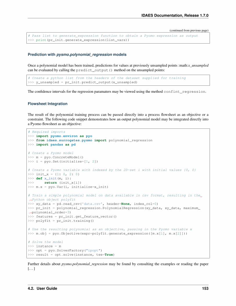
IDAES Documentation, Release 1.7.0
(continued from previous page)
# Pass list to generate_expression function to obtain a Pyomo expression as output>>> print(pr_init.generate_expression(list_vars))
Prediction with pysmo.polynomial_regression models
Once a polynomial model has been trained, predictions for values at previously unsampled points :math:x_unsampledcan be evaluated by calling the predict_output() method on the unsampled points:
# Create a python list from the headers of the dataset supplied for training>>> y_unsampled = pr_init.predict_output(x_unsampled)
The confidence intervals for the regression paramaters may be viewed using the method confint_regression.
Flowsheet Integration
The result of the polynomial training process can be passed directly into a process flowsheet as an objective or aconstraint. The following code snippet demonstrates how an output polynomial model may be integrated directly intoa Pyomo flowsheet as an objective:
# Required imports>>> import pyomo.environ as pyo>>> from idaes.surrogates.pysmo import polynomial_regression>>> import pandas as pd
# Create a Pyomo model>>> m = pyo.ConcreteModel()>>> i = pyo.Set(initialize=[1, 2])
# Create a Pyomo variable with indexed by the 2D-set i with initial values 0, 0>>> init_x = 1: 0, 2: 0>>> def x_init(m, i):>>> return (init_x[i])>>> m.x = pyo.Var(i, initialize=x_init)
# Train a simple polynomial model on data available in csv format, resulting in the→˓Python object polyfit>>> xy_data = pd.read_csv('data.csv', header=None, index_col=0)>>> pr_init = polynomial_regression.PolynomialRegression(xy_data, xy_data, maximum_→˓polynomial_order=3)>>> features = pr_init.get_feature_vector()>>> polyfit = pr_init.training()
# Use the resulting polynomial as an objective, passing in the Pyomo variable x>>> m.obj = pyo.Objective(expr=polyfit.generate_expression([m.x[1], m.x[2]]))
# Solve the model>>> instance = m>>> opt = pyo.SolverFactory("ipopt")>>> result = opt.solve(instance, tee=True)
Further details about pysmo.polynomial_regression may be found by consulting the examples or reading the paper[. . . ]
4.2. User Guide 153
IDAES Documentation, Release 1.7.0
Available Methods
class idaes.surrogate.pysmo.polynomial_regression.FeatureScalingA class for scaling and unscaling input and output data. The class contains two main methods: data_scalingand data_unscaling
static data_scaling(data)data_scaling performs column-wise minimax scaling on the input dataset.
Parameters data – The input data set to be scaled. Must be a numpy array or dataframe.
Returns
tuple containing:
• scaled_data : A 2-D Numpy Array containing the scaled data. All array values will bebetween [0, 1].
• data_minimum : A 2-D row vector containing the column-wise minimums of the inputdata.
• data_maximum : A 2-D row vector containing the column-wise maximums of theinput data.
Return type (tuple)
Raises TypeError – Raised when the input data is not a numpy array or dataframe
static data_unscaling(x_scaled, x_min, x_max)data_unscaling performs column-wise un-scaling on the a minmax-scaled input dataset.
Parameters
• x_scaled (NumPy Array) – Data to be un-scaled. Data values should be between 0and 1.
• x_min (NumPy vector) – 𝑛× 1 vector containing the actual minimum value for eachcolumn. Must contain same number of elements as the number of columns in x_scaled.
• x_max (NumPy vector) – 𝑛 × 1 vector vector containing the actual minimum valuefor each column. Must contain same number of elements as the number of columns inx_scaled.
Returns A 2-D numpy array containing the scaled data, 𝑥𝑚𝑖𝑛 + 𝑥𝑠𝑐𝑎𝑙𝑒𝑑 * (𝑥𝑚𝑎𝑥 − 𝑥𝑚𝑖𝑛)
Return type NumPy Array
Raises IndexError – Raised when the dimensions of the arrays are inconsistent.
154 Chapter 4. Contents
IDAES Documentation, Release 1.7.0
class idaes.surrogate.pysmo.polynomial_regression.PolynomialRegression(original_data_input,re-gres-sion_data_input,max-i-mum_polynomial_order,num-ber_of_crossvalidations=None,no_adaptive_samples=None,train-ing_split=None,max_fraction_training_samples=None,max_iter=None,so-lu-tion_method=None,multi-no-mi-als=None,fname=None,over-write=False)
The PolynomialRegression class performs polynomial regression on a training data set.
The class must first be initialized by calling PolynomialRegression. Regression is then carried out by callingpoly_training.
For a given dataset with 𝑛 features 𝑥1, 𝑥2, . . . , 𝑥𝑛, Polyregression is able to consider three types of basis functions:
(a) Mononomial terms (𝑥𝑝𝑖 , 𝑝 ≤ 10) for all individual features. The maximum degree to be consideredcan be set by the user (maximum_polynomial_order)
(b) All first order interaction terms 𝑥1𝑥2, 𝑥1𝑥3 etc. This can be turned on or off by the user (set multino-mials)
(c) User defined input features, e.g. sin(𝑥1). These must be Pyomo functions and should be provided as alist by the user calling set_additional_terms method before the polynomial training is done.
Example:
# Initialize the class and set additional terms>>> d = PolynomialRegression(full_data, training_data, maximum_polynomial_order=2,→˓ max_iter=20, multinomials=1, solution_method='pyomo')>>> p = d.get_feature_vector()>>> d.set_additional_terms([...extra terms...])
# Train polynomial model and predict output for an test data x_test>>> results = d.poly_training()>>> predictions = d.poly_predict_output(results, x_test)
Parameters
• regression_data_input (NumPy Array of Pandas Dataframe) – Thedataset for regression training. It is expected to contain the features (X) and output (Y)data, with the output values (Y) in the last column.
4.2. User Guide 155
IDAES Documentation, Release 1.7.0
• original_data_input (NumPy Array of Pandas Dataframe) – If regres-sion_data_input was drawn from a larger dataset by some sampling approach, the largerdataset may be provided here. When additional data is not available, the same data suppliedfor training_data can be supplied - this tells the algorithm not to carry out adaptive sampling.
• maximum_polynomial_order (int) – The maximum polynomial order to be consid-ered.
Further details about the optional inputs may be found under the __init__ method.
__init__(original_data_input, regression_data_input, maximum_polynomial_order, num-ber_of_crossvalidations=None, no_adaptive_samples=None, training_split=None,max_fraction_training_samples=None, max_iter=None, solution_method=None, multino-mials=None, fname=None, overwrite=False)
Initialization of PolynomialRegression class.
Parameters
• regression_data_input (NumPy Array of Pandas Dataframe) – Thedataset for regression training. It is expected to contain features and output data, withthe output values (Y) in the last column.
• original_data_input (NumPy Array of Pandas Dataframe) – If regres-sion_data_input was drawn from a larger dataset by some sampling approach, the largerdataset may be provided here.
• maximum_polynomial_order (int) – The maximum polynomial order to be con-sidered.
Keyword Arguments
• number_of_crossvalidations (int) – The number of polynomial fittings andcross-validations to be carried out for each polynomial function/expression. Must be apositive, non-zero integer. Default=3.
• training_split (float) – The training/test split to be used for regres-sion_data_input. Must be between 0 and 1. Default = 0.75
• solution_method (str) – The method to be used for solving the least squares opti-mization problem for polynomial regression. Three options are available:
(a) ”MLE” : The mle (maximum likelihood estimate) method solves the least squares prob-lem using linear algebra. Details of the method may be found in Forrester et al.
(b) ”BFGS” : This approach solves the least squares problem using scipy’s BFGS algo-rithm.
(c) ”pyomo”: This option solves the optimization problem in pyomo with IPOPT as solver.This is the default option.
• multinomials (bool) – This option determines whether or not multinomial terms areconsidered during polynomial fitting. Takes 0 for No and 1 for Yes. Default = 1.
Returns self object containing all the input information.
Raises
• ValueError – - The input datasets (original_data_input or regression_data_input)are of the wrong type (not Numpy arrays or Pandas Dataframes)
• Exception – * maximum_polynomial_order is not a positive, non-zero integer ormaximum_polynomial_order is higher than the number of training samples available
• Exception – * solution_method is not ‘mle’, ‘pyomo’ or ‘bfgs
156 Chapter 4. Contents
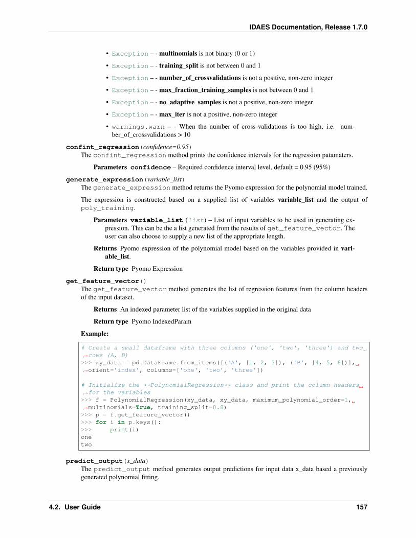
IDAES Documentation, Release 1.7.0
• Exception – - multinomials is not binary (0 or 1)
• Exception – - training_split is not between 0 and 1
• Exception – - number_of_crossvalidations is not a positive, non-zero integer
• Exception – - max_fraction_training_samples is not between 0 and 1
• Exception – - no_adaptive_samples is not a positive, non-zero integer
• Exception – - max_iter is not a positive, non-zero integer
• warnings.warn – - When the number of cross-validations is too high, i.e. num-ber_of_crossvalidations > 10
confint_regression(confidence=0.95)The confint_regression method prints the confidence intervals for the regression patamaters.
Parameters confidence – Required confidence interval level, default = 0.95 (95%)
generate_expression(variable_list)The generate_expression method returns the Pyomo expression for the polynomial model trained.
The expression is constructed based on a supplied list of variables variable_list and the output ofpoly_training.
Parameters variable_list (list) – List of input variables to be used in generating ex-pression. This can be the a list generated from the results of get_feature_vector. Theuser can also choose to supply a new list of the appropriate length.
Returns Pyomo expression of the polynomial model based on the variables provided in vari-able_list.
Return type Pyomo Expression
get_feature_vector()The get_feature_vector method generates the list of regression features from the column headersof the input dataset.
Returns An indexed parameter list of the variables supplied in the original data
Return type Pyomo IndexedParam
Example:
# Create a small dataframe with three columns ('one', 'two', 'three') and two→˓rows (A, B)>>> xy_data = pd.DataFrame.from_items([('A', [1, 2, 3]), ('B', [4, 5, 6])],→˓orient='index', columns=['one', 'two', 'three'])
# Initialize the **PolynomialRegression** class and print the column headers→˓for the variables>>> f = PolynomialRegression(xy_data, xy_data, maximum_polynomial_order=1,→˓multinomials=True, training_split=0.8)>>> p = f.get_feature_vector()>>> for i in p.keys():>>> print(i)onetwo
predict_output(x_data)The predict_output method generates output predictions for input data x_data based a previouslygenerated polynomial fitting.
4.2. User Guide 157
IDAES Documentation, Release 1.7.0
Parameters x_data – Numpy array of designs for which the output is to be evalu-ated/predicted.
Returns Output variable predictions based on the polynomial fit.
Return type Numpy Array
set_additional_terms(term_list)set_additional_terms accepts additional user-defined features for consideration during regression.
Parameters term_list (list) – List of additional terms to be considered as regression fea-tures. Each term in the list must be a Pyomo-supported intrinsic function.
Example:
# To add the sine and cosine of a variable with header 'X1' in the dataset as→˓additional regression features:>>> xy_data = pd.DataFrame.from_items([('A', [1, 2, 3]), ('B', [4, 5, 6])],→˓orient='index', columns=['X1', 'X2', 'Y'])>>> A = PolynomialRegression(xy_data, xy_data, maximum_polynomial_order=5)>>> p = A.get_feature_vector()>>> A.set_additional_terms([ pyo.sin(p['X1']) , pyo.cos(p['X1']) ])
training()The training method trains a polynomial model to an input dataset. It calls the core method whichis called in the PolynomialRegression class (polynomial_regression_fitting). It accepts no user input,inheriting the information passed in class initialization.
Returns
Python Object (results) containing the results of the polynomial regression process including:
• the polynomial order (self.final_polynomial_order)
• polynomial coefficients (self.optimal_weights_array), and
• MAE and MSE errors as well as the 𝑅2 (results.errors).
Return type tuple
References:
[1] Forrester et al.’s book “Engineering Design via Surrogate Modelling: A Practical Guide”, https://onlinelibrary.wiley.com/doi/pdf/10.1002/9780470770801
Generating Radial Basis Function (RBF) models with PySMO
The pysmo.radial_basis_function package has the capability to generate different types of RBF surrogates from databased on the basis function selected. RBFs models are usually of the form where
𝑦𝑘 =
Ω∑𝑗=1
𝑤𝑗𝜓 (‖𝑥𝑘 − 𝑧𝑗‖) 𝑘 = 1, . . . ,𝑚 (4.2)
158 Chapter 4. Contents
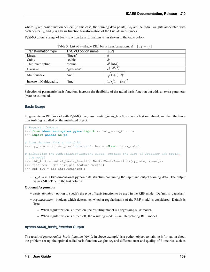
IDAES Documentation, Release 1.7.0
where 𝑧𝑗 are basis function centers (in this case, the training data points), 𝑤𝑗 are the radial weights associated witheach center 𝑧𝑗 , and 𝜓 is a basis function transformation of the Euclidean distances.
PySMO offers a range of basis function transformations 𝜓, as shown in the table below.
Table 3: List of available RBF basis transformations, 𝑑 =‖ 𝑥𝑘 − 𝑧𝑗 ‖Transformation type PySMO option name 𝜓(𝑑)Linear ‘linear’ 𝑑Cubic ‘cubic’ 𝑑3
Thin-plate spline ‘spline’ 𝑑2 ln(𝑑)
Gaussian ‘gaussian’ 𝑒(−𝑑2𝜎2)
Multiquadric ‘mq’√
1 + (𝜎𝑑)2
Inverse mMultiquadric ‘imq’ 1/
√1 + (𝜎𝑑)
2
Selection of parametric basis functions increase the flexibility of the radial basis function but adds an extra parameter(𝜎)to be estimated.
Basic Usage
To generate an RBF model with PySMO, the pysmo.radial_basis_function class is first initialized, and then the func-tion training is called on the initialized object:
# Required imports>>> from idaes.surrogates.pysmo import radial_basis_function>>> import pandas as pd
# Load dataset from a csv file>>> xy_data = pd.read_csv('data.csv', header=None, index_col=0)
# Initialize the RadialBasisFunctions class, extract the list of features and train→˓the model>>> rbf_init = radial_basis_function.RadialBasisFunctions(xy_data, *kwargs)>>> features = rbf_init.get_feature_vector()>>> rbf_fit = rbf_init.training()
• xy_data is a two-dimensional python data structure containing the input and output training data. The outputvalues MUST be in the last column.
Optional Arguments
• basis_function - option to specify the type of basis function to be used in the RBF model. Default is ‘gaussian’.
• regularization - boolean which determines whether regularization of the RBF model is considered. Default isTrue.
– When regularization is turned on, the resulting model is a regressing RBF model.
– When regularization is turned off, the resulting model is an interpolating RBF model.
pysmo.radial_basis_function Output
The result of pysmo.radial_basis_function (rbf_fit in above example) is a python object containing information aboutthe problem set-up, the optimal radial basis function weights 𝑤𝑗 and different error and quality-of-fit metrics such as
4.2. User Guide 159
IDAES Documentation, Release 1.7.0
the mean-squared-error (MSE) and the 𝑅2 coefficient-of-fit. A Pyomo expression can be generated from the objectsimply passing a list of variables into the function generate_expression:
# Create a python list from the headers of the dataset supplied for training>>> list_vars = []>>> for i in features.keys():>>> list_vars.append(features[i])
# Pass list to generate_expression function to obtain a Pyomo expression as output>>> print(rbf_init.generate_expression(list_vars))
Similar to the pysmo.polynomial_regression module, the output of the generate_expression function can be passedinto an IDAES or Pyomo module as a constraint, objective or expression.
Prediction with pysmo.radial_basis_function models
Once an RBF model has been trained, predictions for values at previously unsampled points x_unsampled can beevaluated by calling the predict_output() function on the unsampled points:
# Create a python list from the headers of the dataset supplied for training>>> y_unsampled = rbf_init.predict_output(x_unsampled)
Further details about pysmo.radial_basis_function module may be found by consulting the examples or reading thepaper [. . . ]
Available Methods
class idaes.surrogate.pysmo.radial_basis_function.FeatureScalingA class for scaling and unscaling input and output data. The class contains two main methods:data_scaling_minmax and data_unscaling_minmax
static data_scaling_minmax(data)data_scaling_minmax performs column-wise min-max scaling on the input dataset.
Parameters data – The input data set to be scaled. Must be a numpy array or dataframe.
Returns
tuple containing:
• scaled_data : A 2-D Numpy Array containing the scaled data. All array values will bebetween [0, 1].
• data_minimum : A 2-D row vector containing the column-wise minimums of the inputdata.
• data_maximum : A 2-D row vector containing the column-wise maximums of theinput data.
Return type (tuple)
Raises TypeError – Raised when the input data is not a numpy array or dataframe
static data_unscaling_minmax(x_scaled, x_min, x_max)data_unscaling_minmax performs column-wise un-scaling on the a minmax-scaled input dataset.
Parameters
160 Chapter 4. Contents
IDAES Documentation, Release 1.7.0
• x_scaled (NumPy Array) – Data to be un-scaled. Data values should be between 0and 1.
• x_min (NumPy vector) – 𝑛× 1 vector containing the actual minimum value for eachcolumn. Must contain same number of elements as the number of columns in x_scaled.
• x_max (NumPy vector) – 𝑛 × 1 vector vector containing the actual minimum valuefor each column. Must contain same number of elements as the number of columns inx_scaled.
Returns A 2-D numpy array containing the scaled data, 𝑥𝑚𝑖𝑛 + 𝑥𝑠𝑐𝑎𝑙𝑒𝑑 * (𝑥𝑚𝑎𝑥 − 𝑥𝑚𝑖𝑛)
Return type NumPy Array
Raises IndexError – Raised when the dimensions of the arrays are inconsistent.
class idaes.surrogate.pysmo.radial_basis_function.RadialBasisFunctions(XY_data,ba-sis_function=None,so-lu-tion_method=None,reg-u-lar-iza-tion=None,fname=None,over-write=False)
The RadialBasisFunctions class generates a radial basis function fitting for a training data set.
The class must first be initialized by calling RadialBasisFunctions. Regression is then carried out by callingthe method rbf_training.
For a given dataset with n features 𝑥1, . . . , 𝑥𝑛, RadialBasisFunctions is able to consider six types of basis transformations:
• Linear (‘linear’)
• Cubic (‘cubic’)
• Gaussian (‘gaussian’)
• Multiquadric (‘mq’)
• Inverse multiquadric (‘imq’)
• Thin-plate spline (‘spline’)
rbf_training selects the best hyperparameters (regularization parameter 𝜆 and shape parameter 𝜎, wherenecessary) by evaluating the leave-one-out cross-validation error for each (𝜆, 𝜎) pair.
It should be noted that the all the training points are treated as centres for the RBF, resulting in a square system.
Example:
# Initialize the class>>> d = RadialBasisFunctions(training_data, basis_function='gaussian', solution_→˓method='pyomo', regularization=True))>>> p = d.get_feature_vector()
# Train RBF model and predict output for an test data x_test(continues on next page)
4.2. User Guide 161
IDAES Documentation, Release 1.7.0
(continued from previous page)
>>> results = d.rbf_training()>>> predictions = d.rbf_predict_output(results, x_test)
Parameters XY_data (Numpy Array or Pandas Dataframe) – The dataset for RBFtraining. XY_data is expected to contain the features (X) and output (Y) data, with the out-put values (Y) in the last column.
Further details about the optional inputs may be found under the __init__ method.
__init__(XY_data, basis_function=None, solution_method=None, regularization=None,fname=None, overwrite=False)
Initialization of RadialBasisFunctions class.
Parameters XY_data (Numpy Array or Pandas Dataframe) – The dataset for RBFtraining. XY_data is expected to contain feature and output information, with the outputvalues (y) in the last column.
Keyword Arguments
• basis_function (str) – The basis function transformation to be applied to the train-ing data. Two classes of basis transformations are available for selection:
– Fixed basis transformations, which require no shape parameter 𝜎 :
(a) ’cubic’ : Cubic basis transformation
(b) ’linear’ : Linear basis transformation
(c) ’spline’ : Thin-plate spline basis transformation
– Parametric basis transformations which require a shape parameter:
(a) ’gaussian’ : Gaussian basis transformation (Default)
(b) ’mq’ : Multiquadric basis transformation
(c) ’imq’ : Inverse multiquadric basis transformation
• solution_method (str) – The method to be used for solving the RBF least squaresoptimization problem. Three options are available:
(a) ’algebraic’ : The explicit algebraic method solves the least squares problem using linearalgebra.
(b) ’BFGS’ : This approach solves the least squares problem using SciPy’s BFGS algo-rithm.
(c) ’pyomo’ : This option solves the optimization problem in Pyomo with IPOPT as solver.This is the default.
• regularization (bool) – This option determines whether or not the regularizationparameter 𝜆 is considered during RBF fitting. Default setting is True.
Returns self object with the input information
Raises
• ValueError – The input dataset is of the wrong type (not a NumPy array or PandasDataframe)
• Exception – * basis_function entry is not valid.
• Exception – * solution_method is not ‘algebraic’, ‘pyomo’ or ‘bfgs’.
162 Chapter 4. Contents
IDAES Documentation, Release 1.7.0
• Exception – - 𝜆 is not boolean.
Example:
# Specify the gaussian basis transformation>>> d = RadialBasisFunctions(XY_data, basis_function='gaussian')
generate_expression(variable_list)The generate_expression method returns the Pyomo expression for the RBF model trained.
The expression is constructed based on the supplied list of variables variable_list and the results of theprevious RBF training process.
Parameters variable_list (list) – List of input variables to be used in generating ex-pression. This can be the a list generated from the output of get_feature_vector. Theuser can also choose to supply a new list of the appropriate length.
Returns Pyomo expression of the RBF model based on the variables provided in variable_list
Return type Pyomo Expression
get_feature_vector()The get_feature_vector method generates the list of regression features from the column headersof the input dataset.
Returns An indexed parameter list of the variables supplied in the original data
Return type Pyomo IndexedParam
Example:
# Create a small dataframe with three columns ('one', 'two', 'three') and two→˓rows (A, B)>>> xy_data = pd.DataFrame.from_items([('A', [1, 2, 3]), ('B', [4, 5, 6])],→˓orient='index', columns=['one', 'two', 'three'])
# Initialize the **RadialBasisFunctions** class with a linear kernel and→˓print the column headers for the variables>>> f = RadialBasisFunctions(xy_data, basis_function='linear')>>> p = f.get_feature_vector()>>> for i in p.keys():>>> print(i)onetwo
predict_output(x_data)The predict_output method generates output predictions for input data x_data based a previouslygenerated RBF fitting.
Parameters x_data (NumPy Array) – Designs for which the output is to be evalu-ated/predicted.
Returns Output variable predictions based on the rbf fit.
Return type Numpy Array
static r2_calculation(y_true, y_predicted)r2_calculation returns the𝑅2 as a measure-of-fit between the true and predicted values of the outputvariable.
Parameters
• y_true (NumPy Array) – Vector of actual values of the output variable
4.2. User Guide 163
IDAES Documentation, Release 1.7.0
• y_predicted (NumPy Array) – Vector of predictions for the output variable basedon the surrogate
Returns 𝑅2 measure-of-fit between actual and predicted data
Return type float
training()Main function for RBF training.
To train the RBF:
(1) The best values of the hyperparameters (𝜎, 𝜆) are selected via LOOCV.
(2) The necessary basis transformation at the optimal hyperparameters is generated.
(3) The condition number for the transformed matrix is calculated.
(4) The optimal radial weights are evaluated using the selected optimization method.
(5) The training predictions, prediction errors and r-square coefficient of fit are evaluated by callingthe methods error_calculation and r2_calculation
(6) A results object is generated by calling the ResultsReport class.
The LOOCV error for each (𝜎, 𝜆) pair is evaluated by calling the functionloo_error_estimation_with_rippa_method.
The pre-defined shape parameter set considers 24 irregularly spaced values ranging between 0.001 - 1000,while the regularization parameter set considers 21 values ranging between 0.00001 - 1.
Returns
self object (results) containing the all information about the best RBF fitting obtained, including:
• the optimal radial weights (results.radial_weights),
• when relevant, the optimal shape parameter found 𝜎 (results.sigma),
• when relevant, the optimal regularization parameter found 𝜆 (results.regularization),
• the RBF predictions for the training data (results.output_predictions), and
• the 𝑅2 value on the training data (results.R2)
Return type tuple
References:
[1] Forrester et al.’s book “Engineering Design via Surrogate Modelling: A Practical Guide”, https://onlinelibrary.wiley.com/doi/pdf/10.1002/9780470770801
[2] Hongbing Fang & Mark F. Horstemeyer (2006): Global response approximation with radial basis functions, https://www.tandfonline.com/doi/full/10.1080/03052150500422294
[3] Rippa, S. (1999): An algorithm for selecting a good value for the parameter c in radial basis function interpolation,https://doi.org/10.1023/A:1018975909870
[4] Mongillo M.A. (2011) Choosing Basis Functions and Shape Parameters for Radial Basis Function Methods, https://doi.org/10.1137/11S010840
164 Chapter 4. Contents
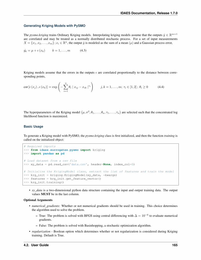
IDAES Documentation, Release 1.7.0
Generating Kriging Models with PySMO
The pysmo.kriging trains Ordinary Kriging models. Interpolating kriging models assume that the outputs 𝑦 ∈ R𝑚×1
are correlated and may be treated as a normally distributed stochastic process. For a set of input measurements𝑋 = 𝑥1, 𝑥2, . . . , 𝑥𝑚 ;𝑥𝑖 ∈ R𝑛, the output 𝑦 is modeled as the sum of a mean (𝜇) and a Gaussian process error,
𝑦𝑘 = 𝜇+ 𝜖 (𝑥𝑘) 𝑘 = 1, . . . ,𝑚 (4.3)
Kriging models assume that the errors in the outputs 𝜖 are correlated proportionally to the distance between corre-sponding points,
cor [𝜖 (𝑥𝑗) , 𝜖 (𝑥𝑘)] = exp
(−
𝑛∑𝑖=1
𝜃𝑖 | 𝑥𝑖𝑗 − 𝑥𝑖𝑘 |𝜏𝑖)
𝑗, 𝑘 = 1, . . . ,𝑚; 𝜏𝑖 ∈ [1, 2] ; 𝜃𝑖 ≥ 0 (4.4)
The hyperparameters of the Kriging model(𝜇, 𝜎2, 𝜃1, . . . , 𝜃𝑛, 𝜏1, . . . , 𝜏𝑛
)are selected such that the concentrated log
likelihood function is maximized.
Basic Usage
To generate a Kriging model with PySMO, the pysmo.kriging class is first initialized, and then the function training iscalled on the initialized object:
# Required imports>>> from idaes.surrogates.pysmo import kriging>>> import pandas as pd
# Load dataset from a csv file>>> xy_data = pd.read_csv('data.csv', header=None, index_col=0)
# Initialize the KrigingModel class, extract the list of features and train the model>>> krg_init = kriging.KrigingModel(xy_data, *kwargs)>>> features = krg_init.get_feature_vector()>>> krg_init.training()
• xy_data is a two-dimensional python data structure containing the input and output training data. The outputvalues MUST be in the last column.
Optional Arguments
• numerical_gradients: Whether or not numerical gradients should be used in training. This choice determinesthe algorithm used to solve the problem.
– True: The problem is solved with BFGS using central differencing with ∆ = 10−6 to evaluate numericalgradients.
– False: The problem is solved with Basinhopping, a stochastic optimization algorithm.
• regularization - Boolean option which determines whether or not regularization is considered during Krigingtraining. Default is True.
4.2. User Guide 165
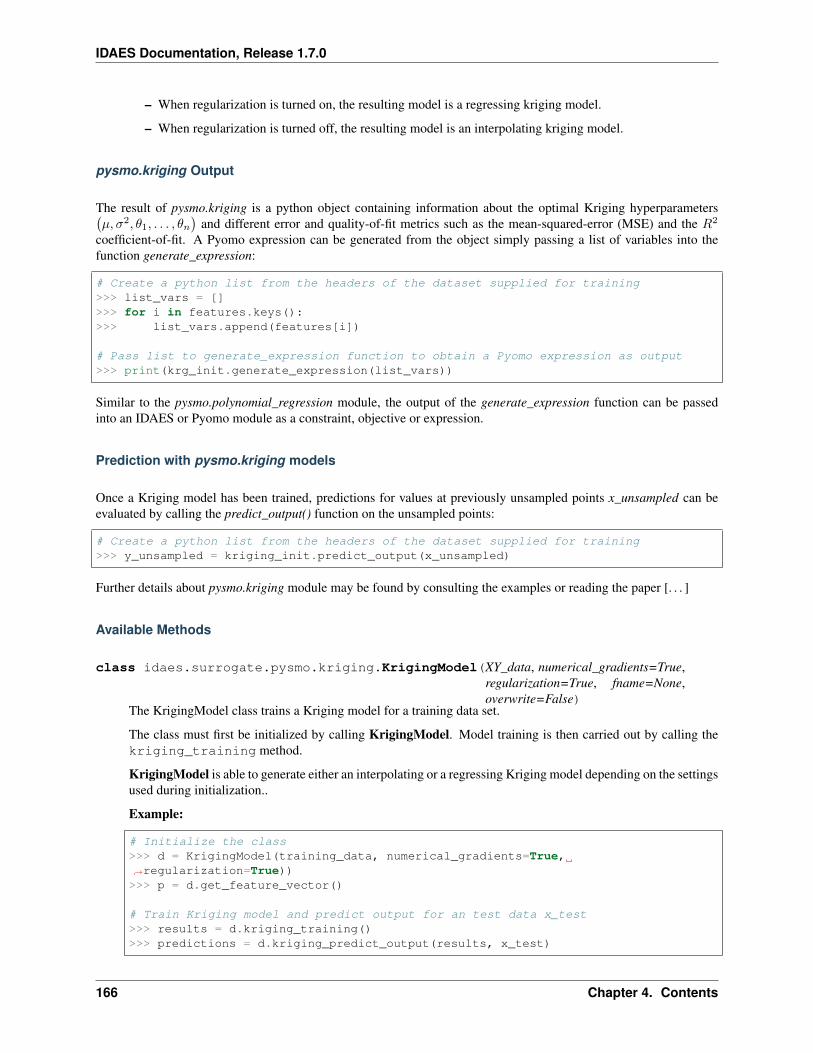
IDAES Documentation, Release 1.7.0
– When regularization is turned on, the resulting model is a regressing kriging model.
– When regularization is turned off, the resulting model is an interpolating kriging model.
pysmo.kriging Output
The result of pysmo.kriging is a python object containing information about the optimal Kriging hyperparameters(𝜇, 𝜎2, 𝜃1, . . . , 𝜃𝑛
)and different error and quality-of-fit metrics such as the mean-squared-error (MSE) and the 𝑅2
coefficient-of-fit. A Pyomo expression can be generated from the object simply passing a list of variables into thefunction generate_expression:
# Create a python list from the headers of the dataset supplied for training>>> list_vars = []>>> for i in features.keys():>>> list_vars.append(features[i])
# Pass list to generate_expression function to obtain a Pyomo expression as output>>> print(krg_init.generate_expression(list_vars))
Similar to the pysmo.polynomial_regression module, the output of the generate_expression function can be passedinto an IDAES or Pyomo module as a constraint, objective or expression.
Prediction with pysmo.kriging models
Once a Kriging model has been trained, predictions for values at previously unsampled points x_unsampled can beevaluated by calling the predict_output() function on the unsampled points:
# Create a python list from the headers of the dataset supplied for training>>> y_unsampled = kriging_init.predict_output(x_unsampled)
Further details about pysmo.kriging module may be found by consulting the examples or reading the paper [. . . ]
Available Methods
class idaes.surrogate.pysmo.kriging.KrigingModel(XY_data, numerical_gradients=True,regularization=True, fname=None,overwrite=False)
The KrigingModel class trains a Kriging model for a training data set.
The class must first be initialized by calling KrigingModel. Model training is then carried out by calling thekriging_training method.
KrigingModel is able to generate either an interpolating or a regressing Kriging model depending on the settingsused during initialization..
Example:
# Initialize the class>>> d = KrigingModel(training_data, numerical_gradients=True,→˓regularization=True))>>> p = d.get_feature_vector()
# Train Kriging model and predict output for an test data x_test>>> results = d.kriging_training()>>> predictions = d.kriging_predict_output(results, x_test)
166 Chapter 4. Contents
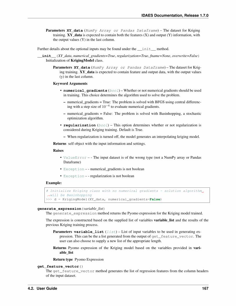
IDAES Documentation, Release 1.7.0
Parameters XY_data (NumPy Array or Pandas Dataframe) – The dataset for Krigingtraining. XY_data is expected to contain both the features (X) and output (Y) information, withthe output values (Y) in the last column.
Further details about the optional inputs may be found under the __init__ method.
__init__(XY_data, numerical_gradients=True, regularization=True, fname=None, overwrite=False)Initialization of KrigingModel class.
Parameters XY_data (NumPy Array or Pandas Dataframe) – The dataset for Krig-ing training. XY_data is expected to contain feature and output data, with the output values(y) in the last column.
Keyword Arguments
• numerical_gradients (bool) – Whether or not numerical gradients should be usedin training. This choice determines the algorithm used to solve the problem.
– numerical_gradients = True: The problem is solved with BFGS using central differenc-ing with a step size of 10−6 to evaluate numerical gradients.
– numerical_gradients = False: The problem is solved with Basinhopping, a stochasticoptimization algorithm.
• regularization (bool) – This option determines whether or not regularization isconsidered during Kriging training. Default is True.
– When regularization is turned off, the model generates an interpolating kriging model.
Returns self object with the input information and settings.
Raises
• ValueError – - The input dataset is of the wrong type (not a NumPy array or PandasDataframe)
• Exception – - numerical_gradients is not boolean
• Exception – - regularization is not boolean
Example:
# Initialize Kriging class with no numerical gradients - solution algorithm→˓will be Basinhopping>>> d = KrigingModel(XY_data, numerical_gradients=False)
generate_expression(variable_list)The generate_expression method returns the Pyomo expression for the Kriging model trained.
The expression is constructed based on the supplied list of variables variable_list and the results of theprevious Kriging training process.
Parameters variable_list (list) – List of input variables to be used in generating ex-pression. This can be the a list generated from the output of get_feature_vector. Theuser can also choose to supply a new list of the appropriate length.
Returns Pyomo expression of the Kriging model based on the variables provided in vari-able_list
Return type Pyomo Expression
get_feature_vector()The get_feature_vector method generates the list of regression features from the column headersof the input dataset.
4.2. User Guide 167
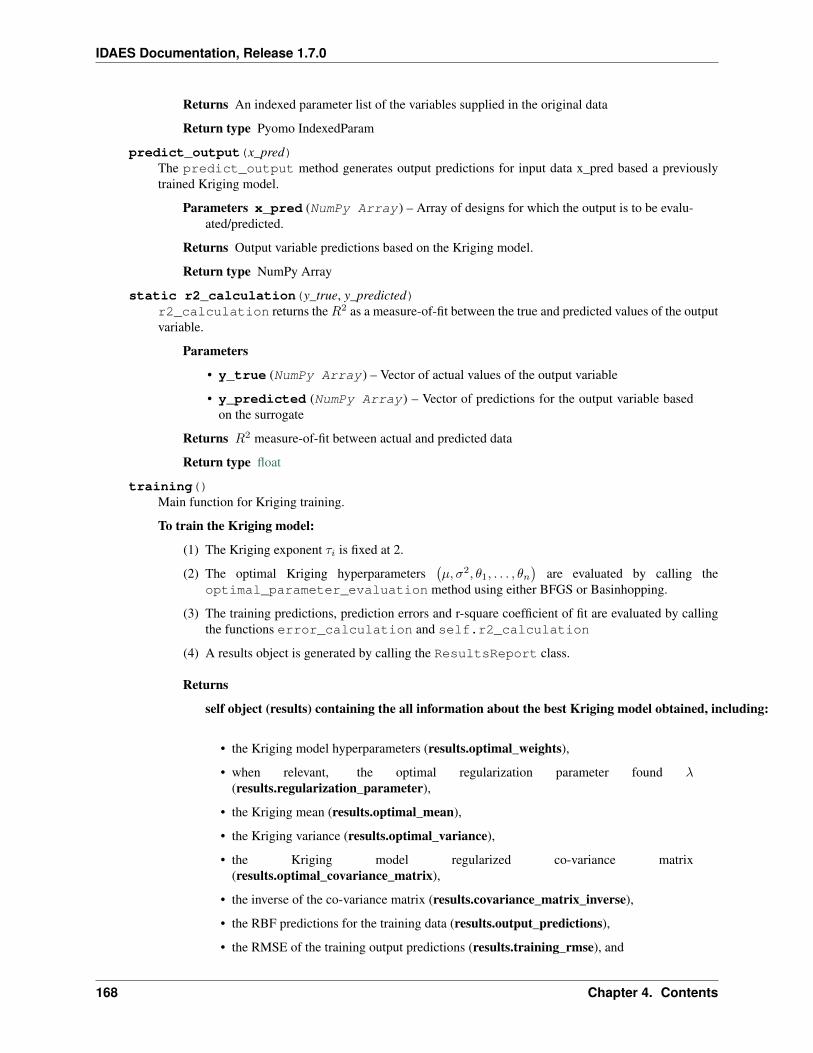
IDAES Documentation, Release 1.7.0
Returns An indexed parameter list of the variables supplied in the original data
Return type Pyomo IndexedParam
predict_output(x_pred)The predict_output method generates output predictions for input data x_pred based a previouslytrained Kriging model.
Parameters x_pred (NumPy Array) – Array of designs for which the output is to be evalu-ated/predicted.
Returns Output variable predictions based on the Kriging model.
Return type NumPy Array
static r2_calculation(y_true, y_predicted)r2_calculation returns the𝑅2 as a measure-of-fit between the true and predicted values of the outputvariable.
Parameters
• y_true (NumPy Array) – Vector of actual values of the output variable
• y_predicted (NumPy Array) – Vector of predictions for the output variable basedon the surrogate
Returns 𝑅2 measure-of-fit between actual and predicted data
Return type float
training()Main function for Kriging training.
To train the Kriging model:
(1) The Kriging exponent 𝜏𝑖 is fixed at 2.
(2) The optimal Kriging hyperparameters(𝜇, 𝜎2, 𝜃1, . . . , 𝜃𝑛
)are evaluated by calling the
optimal_parameter_evaluation method using either BFGS or Basinhopping.
(3) The training predictions, prediction errors and r-square coefficient of fit are evaluated by callingthe functions error_calculation and self.r2_calculation
(4) A results object is generated by calling the ResultsReport class.
Returns
self object (results) containing the all information about the best Kriging model obtained, including:
• the Kriging model hyperparameters (results.optimal_weights),
• when relevant, the optimal regularization parameter found 𝜆(results.regularization_parameter),
• the Kriging mean (results.optimal_mean),
• the Kriging variance (results.optimal_variance),
• the Kriging model regularized co-variance matrix(results.optimal_covariance_matrix),
• the inverse of the co-variance matrix (results.covariance_matrix_inverse),
• the RBF predictions for the training data (results.output_predictions),
• the RMSE of the training output predictions (results.training_rmse), and
168 Chapter 4. Contents
IDAES Documentation, Release 1.7.0
• the 𝑅2 value on the training data (results.R2)
Return type tuple
References:
[1] Forrester et al.’s book “Engineering Design via Surrogate Modelling: A Practical Guide”, https://onlinelibrary.wiley.com/doi/pdf/10.1002/9780470770801
[2] D. R. Jones, A taxonomy of global optimization methods based on response surfaces, Journal of Global Optimiza-tion, https://link.springer.com/article/10.1023%2FA%3A1012771025575
Sampling
The PySMO package offers five common sampling methods for one-shot design:
Latin Hypercube Sampling (LHS)
LHS is a stratified random sampling method originally developed for efficient uncertainty assessment. LHS partitionsthe parameter space into bins of equal probability with the goal of attaining a more even distribution of sample pointsin the parameter space that would be possible with pure random sampling.
The pysmo.sampling.LatinHypercubeSampling method carries out Latin Hypercube sampling. This canbe done in two modes:
• The samples can be selected from a user-provided dataset, or
• The samples can be generated from a set of provided bounds.
Available Methods
class idaes.surrogate.pysmo.sampling.LatinHypercubeSampling(data_input, num-ber_of_samples=None,sam-pling_type=None)
A class that performs Latin Hypercube Sampling. The function returns LHS samples which have been selectedrandomly after sample space stratification.
It should be noted that no minimax criterion has been used in this implementation, so the LHS samples selectedwill not have space-filling properties.
To use: call class with inputs, and then run sample_points method.
Example:
# To select 10 LHS samples from "data">>> b = rbf.LatinHypercubeSampling(data, 10, sampling_type="selection")>>> samples = b.sample_points()
__init__(data_input, number_of_samples=None, sampling_type=None)Initialization of LatinHypercubeSampling class. Two inputs are required.
Parameters
• data_input (NumPy Array, Pandas Dataframe or list) – The input dataset or range to be sampled.
4.2. User Guide 169
IDAES Documentation, Release 1.7.0
– When the aim is to select a set of samples from an existing dataset, the dataset mustbe a NumPy Array or a Pandas Dataframe and sampling_type option must be set to“selection”. The output variable (y) is assumed to be supplied in the last column.
– When the aim is to generate a set of samples from a data range, the dataset must be alist containing two lists of equal lengths which contain the variable bounds and sam-pling_type option must be set to “creation”. It is assumed that no range contains nooutput variable information in this case.
• number_of_samples (int) – The number of samples to be generated. Should be apositive integer less than or equal to the number of entries (rows) in data_input.
• sampling_type (str) – Option which determines whether the algorithm selects sam-ples from an existing dataset (“selection”) or attempts to generate sample from a suppliedrange (“creation”). Default is “creation”.
Returns self function containing the input information
Raises
• ValueError – The input data (data_input) is the wrong type.
• Exception – When number_of_samples is invalid (not an integer, too large, zero, ornegative)
sample_points()sample_points generates or selects Latin Hypercube samples from an input dataset or data range.When called, it:
1. generates samples points from stratified regions by calling the lhs_points_generation,
2. generates potential sample points by random shuffling, and
3. when a dataset is provided, selects the closest available samples to the theoretical sample points fromwithin the input data.
Returns A numpy array or Pandas dataframe containing number_of_samples points selectedor generated by LHS.
Return type NumPy Array or Pandas Dataframe
References
[1] Loeven et al paper titled “A Probabilistic Radial Basis Function Approach for Uncertainty Quantification” https://pdfs.semanticscholar.org/48a0/d3797e482e37f73e077893594e01e1c667a2.pdf
[2] Webpage on low discrepancy sampling methods: http://planning.cs.uiuc.edu/node210.html
[3] Swiler, Laura and Slepoy, Raisa and Giunta, Anthony: “Evaluation of sampling methods in constructing responsesurface approximations” https://arc.aiaa.org/doi/abs/10.2514/6.2006-1827
Full-Factorial Sampling
The pysmo.sampling.UniformSampling method carries out Uniform (full-factorial) sampling. This can bedone in two modes:
• The samples can be selected from a user-provided dataset, or
• The samples can be generated from a set of provided bounds.
170 Chapter 4. Contents
IDAES Documentation, Release 1.7.0
Available Methods
class idaes.surrogate.pysmo.sampling.UniformSampling(data_input,list_of_samples_per_variable,sampling_type=None,edges=None)
A class that performs Uniform Sampling. Depending on the settings, the algorithm either returns samples froman input dataset which have been selected using Euclidean distance minimization after the uniform samples havebeen generated, or returns samples from a supplied data range.
Full-factorial samples are based on dividing the space of each variable randomly and then generating all possiblevariable combinations.
• The number of points to be sampled per variable needs to be specified in a list.
To use: call class with inputs, and then sample_points function
Example:
# To select 50 samples on a (10 x 5) grid in a 2D space:>>> b = rbf.UniformSampling(data, [10, 5], sampling_type="selection")>>> samples = b.sample_points()
__init__(data_input, list_of_samples_per_variable, sampling_type=None, edges=None)Initialization of UniformSampling class. Three inputs are required.
Parameters
• data_input (NumPy Array, Pandas Dataframe or list) – The input dataset or range to be sampled.
– When the aim is to select a set of samples from an existing dataset, the dataset mustbe a NumPy Array or a Pandas Dataframe and sampling_type option must be set to“selection”. The output variable (Y) is assumed to be supplied in the last column.
– When the aim is to generate a set of samples from a data range, the dataset must be alist containing two lists of equal lengths which contain the variable bounds and sam-pling_type option must be set to “creation”. It is assumed that no range contains nooutput variable information in this case.
• list_of_samples_per_variable (list) – The list containing the number ofsubdivisions for each variable. Each dimension (variable) must be represented by a posi-tive integer variable greater than 1.
• sampling_type (str) – Option which determines whether the algorithm selects sam-ples from an existing dataset (“selection”) or attempts to generate sample from a suppliedrange (“creation”). Default is “creation”.
Keyword Arguments edges (bool) – Boolean variable representing bow the points shouldbe selected. A value of True (default) indicates the points should be equally spaced edge toedge, otherwise they will be in the centres of the bins filling the unit cube
Returns self function containing the input information
Raises
• ValueError – The data_input is the wrong type
• ValueError – When list_of_samples_per_variable is of the wrong length, is not a listor contains elements other than integers
• Exception – When edges entry is not Boolean
4.2. User Guide 171
IDAES Documentation, Release 1.7.0
sample_points()sample_points generates or selects full-factorial designs from an input dataset or data range.
Returns A numpy array or Pandas dataframe containing the sample points generated or selectedby full-factorial sampling.
Return type NumPy Array or Pandas Dataframe
References
[1] Loeven et al paper titled “A Probabilistic Radial Basis Function Approach for Uncertainty Quantification” https://pdfs.semanticscholar.org/48a0/d3797e482e37f73e077893594e01e1c667a2.pdf
Halton Sampling
Halton sampling is a low-discrepancy sampling method. It is a deterministic sampling method based on the Haltonsequence, a sequence constructed by a set of co-prime bases. The Halton sequence is an n-dimensional extension ofthe Van der Corput sequence; each individual Halton sequence is based on a radix inverse function defined on a primenumber.
The pysmo.sampling.HaltonSampling method carries out Halton sampling. This can be done in two modes:
• The samples can be selected from a user-provided dataset, or
• The samples can be generated from a set of provided bounds.
The Halton sampling method is only available for low-dimensional problems 𝑛 ≤ 10. At higher dimensions, theperformance of the sampling method has been shown to degrade.
Available Methods
class idaes.surrogate.pysmo.sampling.HaltonSampling(data_input, num-ber_of_samples=None, sam-pling_type=None)
A class that performs Halton Sampling.
Halton samples are based on the reversing/flipping the base conversion of numbers using primes.
To generate n samples in a 𝑝-dimensional space, the first 𝑝 prime numbers are used to generate the samples.
Note: Use of this method is limited to use in low-dimensionality problems (less than 10 variables). At higherdimensions, the performance of the sampling method has been shown to degrade.
To use: call class with inputs, and then sample_points function.
Example:
# For the first 10 Halton samples in a 2-D space:>>> b = rbf.HaltonSampling(data, 10, sampling_type="selection")>>> samples = b.sample_points()
__init__(data_input, number_of_samples=None, sampling_type=None)Initialization of HaltonSampling class. Two inputs are required.
Parameters
172 Chapter 4. Contents
IDAES Documentation, Release 1.7.0
• data_input (NumPy Array, Pandas Dataframe or list) – The input dataset or range to be sampled.
– When the aim is to select a set of samples from an existing dataset, the dataset mustbe a NumPy Array or a Pandas Dataframe and sampling_type option must be set to“selection”. The output variable (Y) is assumed to be supplied in the last column.
– When the aim is to generate a set of samples from a data range, the dataset must be alist containing two lists of equal lengths which contain the variable bounds and sam-pling_type option must be set to “creation”. It is assumed that no range contains nooutput variable information in this case.
• number_of_samples (int) – The number of samples to be generated. Should be apositive integer less than or equal to the number of entries (rows) in data_input.
• sampling_type (str) – Option which determines whether the algorithm selects sam-ples from an existing dataset (“selection”) or attempts to generate sample from a suppliedrange (“creation”). Default is “creation”.
Returns self function containing the input information.
Raises
• ValueError – The data_input is the wrong type.
• Exception – When the number_of_samples is invalid (not an integer, too large, zeroor negative.)
sample_points()The sample_points method generates the Halton samples. The steps followed here are:
1. Determine the number of features in the input data.
2. Generate the list of primes to be considered by calling prime_number_generator from thesampling superclass.
3. Create the first number_of_samples elements of the Halton sequence for each prime.
4. Create the Halton samples by combining the corresponding elements of the Halton sequences for eachprime.
5. When in “selection” mode, determine the closest corresponding point in the input dataset using Eu-clidean distance minimization. This is done by calling the nearest_neighbours method in thesampling superclass.
Returns A numpy array or Pandas dataframe containing number_of_samples Halton samplepoints.
Return type NumPy Array or Pandas Dataframe
References
[1] Loeven et al paper titled “A Probabilistic Radial Basis Function Approach for Uncertainty Quantification” https://pdfs.semanticscholar.org/48a0/d3797e482e37f73e077893594e01e1c667a2.pdf
[2] Webpage on low discrepancy sampling methods: http://planning.cs.uiuc.edu/node210.html
4.2. User Guide 173
IDAES Documentation, Release 1.7.0
Hammersley Sampling
Hammersley sampling is a low-discrepancy sampling method based on the Hammersley sequence. The Hammersleysequence is the same as the Halton sequence except in the first dimension where points are located equidistant fromeach other.
The pysmo.sampling.HammersleySampling method carries out Hammersley sampling. This can be done intwo modes:
• The samples can be selected from a user-provided dataset, or
• The samples can be generated from a set of provided bounds.
The Hammersley sampling method is only available for low-dimensional problems 𝑛 ≤ 10. At higher dimensions, theperformance of the sampling method has been shown to degrade.
Available Methods
class idaes.surrogate.pysmo.sampling.HammersleySampling(data_input, num-ber_of_samples=None,sampling_type=None)
A class that performs Hammersley Sampling.
Hammersley samples are generated in a similar way to Halton samples - based on the reversing/flipping the baseconversion of numbers using primes.
To generate 𝑛 samples in a 𝑝-dimensional space, the first (𝑝− 1) prime numbers are used to generate thesamples. The first dimension is obtained by uniformly dividing the region into no_samples points.
Note: Use of this method is limited to use in low-dimensionality problems (less than 10 variables). At higherdimensionalities, the performance of the sampling method has been shown to degrade.
To use: call class with inputs, and then sample_points function.
Example:
# For the first 10 Hammersley samples in a 2-D space:>>> b = rbf.HammersleySampling(data, 10, sampling_type="selection")>>> samples = b.sample_points()
__init__(data_input, number_of_samples=None, sampling_type=None)Initialization of HammersleySampling class. Two inputs are required.
Parameters
• data_input (NumPy Array, Pandas Dataframe or list) – The input dataset or range to be sampled.
– When the aim is to select a set of samples from an existing dataset, the dataset mustbe a NumPy Array or a Pandas Dataframe and sampling_type option must be set to“selection”. The output variable (Y) is assumed to be supplied in the last column.
– When the aim is to generate a set of samples from a data range, the dataset must be alist containing two lists of equal lengths which contain the variable bounds and sam-pling_type option must be set to “creation”. It is assumed that no range contains nooutput variable information in this case.
174 Chapter 4. Contents
IDAES Documentation, Release 1.7.0
• number_of_samples (int) – The number of samples to be generated. Should be apositive integer less than or equal to the number of entries (rows) in data_input.
• sampling_type (str) – Option which determines whether the algorithm selects sam-ples from an existing dataset (“selection”) or attempts to generate sample from a suppliedrange (“creation”). Default is “creation”.
• Returns – self function containing the input information.
• Raises – ValueError: When data_input is the wrong type.
Exception: When the number_of_samples is invalid (not an integer, too large, zero, neg-ative)
sample_points()The sampling_type method generates the Hammersley sample points. The steps followed here are:
1. Determine the number of features 𝑛𝑓 in the input data.
2. Generate the list of (𝑛𝑓 − 1) primes to be considered by calling prime_number_generator.
3. Divide the space [0,**number_of_samples**-1] into number_of_samples places to obtain the firstdimension for the Hammersley sequence.
4. For the other (𝑛𝑓 − 1) dimensions, create first number_of_samples elements of the Hammersleysequence for each of the (𝑛𝑓 − 1) primes.
5. Create the Hammersley samples by combining the corresponding elements of the Hammersley se-quences created in steps 3 and 4
6. When in “selection” mode, determine the closest corresponding point in the input dataset using Eu-clidean distance minimization. This is done by calling the nearest_neighbours method in thesampling superclass.
Returns A numpy array or Pandas dataframe containing number_of_samples Hammersleysample points.
Return type NumPy Array or Pandas Dataframe
References
[1] Loeven et al paper titled “A Probabilistic Radial Basis Function Approach for Uncertainty Quantification” https://pdfs.semanticscholar.org/48a0/d3797e482e37f73e077893594e01e1c667a2.pdf
[2] Webpage on low discrepancy sampling methods: http://planning.cs.uiuc.edu/node210.html
[3] Holger Dammertz’s webpage titled “Hammersley Points on the Hemisphere” which discusses Hammersley pointset generation in two dimensional spaces, http://holger.dammertz.org/stuff/notes_HammersleyOnHemisphere.html
Centroidal voronoi tessellation (CVT) sampling
In CVT, the generating point of each Voronoi cell coincides with its center of mass; CVT sampling locates the designsamples at the centroids of each Voronoi cell in the input space. CVT sampling is a geometric, space-filling samplingmethod which is similar to k-means clustering in its simplest form.
The pysmo.sampling.CVTSampling method carries out CVT sampling. This can be done in two modes:
• The samples can be selected from a user-provided dataset, or
• The samples can be generated from a set of provided bounds.
4.2. User Guide 175
IDAES Documentation, Release 1.7.0
The CVT sampling algorithm implemented here is based on McQueen’s method which involves a series of randomsampling and averaging steps, see http://kmh-lanl.hansonhub.com/uncertainty/meetings/gunz03vgr.pdf.
Available Methods
class idaes.surrogate.pysmo.sampling.CVTSampling(data_input, num-ber_of_samples=None, toler-ance=None, sampling_type=None)
A class that constructs Centroidal Voronoi Tessellation (CVT) samples.
CVT sampling is based on the generation of samples in which the generators of the Voronoi tessellations andthe mass centroids coincide.
To use: call class with inputs, and then sample_points function.
Example:
# For the first 10 CVT samples in a 2-D space:>>> b = rbf.CVTSampling(data_bounds, 10, tolerance = 1e-5, sampling_type="creation→˓")>>> samples = b.sample_points()
__init__(data_input, number_of_samples=None, tolerance=None, sampling_type=None)Initialization of CVTSampling class. Two inputs are required, while an optional option to control thesolution accuracy may be specified.
Parameters
• data_input (NumPy Array, Pandas Dataframe or list) – The input dataset or range to be sampled.
– When the aim is to select a set of samples from an existing dataset, the dataset mustbe a NumPy Array or a Pandas Dataframe and sampling_type option must be set to“selection”. The output variable (Y) is assumed to be supplied in the last column.
– When the aim is to generate a set of samples from a data range, the dataset must be alist containing two lists of equal lengths which contain the variable bounds and sam-pling_type option must be set to “creation”. It is assumed that no range contains nooutput variable information in this case.
• number_of_samples (int) – The number of samples to be generated. Should be apositive integer less than or equal to the number of entries (rows) in data_input.
• sampling_type (str) – Option which determines whether the algorithm selects sam-ples from an existing dataset (“selection”) or attempts to generate sample from a suppliedrange (“creation”). Default is “creation”.
Keyword Arguments tolerance (float) – Maximum allowable Euclidean distance be-tween centres from consectutive iterations of the algorithm. Termination condition for al-gorithm.
• The smaller the value of tolerance, the better the solution but the longer the algorithmrequires to converge. Default value is 10−7.
Returns self function containing the input information.
Raises
• ValueError – When data_input is the wrong type.
176 Chapter 4. Contents
IDAES Documentation, Release 1.7.0
• Exception – When the number_of_samples is invalid (not an integer, too large, zero,negative)
• Exception – When the tolerance specified is too loose (tolerance > 0.1) or invalid
• warnings.warn – when the tolerance specified by the user is too tight (tolerance <10−9)
sample_points()The sample_points method determines the best/optimal centre points (centroids) for a data set basedon the minimization of the total distance between points and centres.
Procedure based on McQueen’s algorithm: iteratively minimize distance, and re-position centroids. Centrere-calculation done as the mean of each data cluster around each centre.
Returns A numpy array or Pandas dataframe containing the final number_of_samples centroidsobtained by the CVT algorithm.
Return type NumPy Array or Pandas Dataframe
References
[1] Loeven et al paper titled “A Probabilistic Radial Basis Function Approach for Uncertainty Quantification” https://pdfs.semanticscholar.org/48a0/d3797e482e37f73e077893594e01e1c667a2.pdf
[2] Centroidal Voronoi Tessellations: Applications and Algorithms by Qiang Du, Vance Faber, and Max Gunzburgerhttps://doi.org/10.1137/S0036144599352836
[3] D. G. Loyola, M. Pedergnana, S. G. García, “Smart sampling and incremental function learning for very large highdimensional data” https://www.sciencedirect.com/science/article/pii/S0893608015001768?via%3Dihub
More Information about PySMO’s Sampling Methods
The sampling methods are able to generate samples based from variable bounds or select samples from a user-provided dataset. To use any of the method, the class is first initialized with the required parameters, and then thesample_points method is called.
Examples
The following code snippet shows basic usage of the package for generating samples from a set of bounds:
# Required imports>>> from idaes.surrogates.pysmo import sampling as sp
# Declaration of lower and upper bounds of 3D space to be sampled>>> bounds = [[0, 0, 0], [1.2, 0.1, 1]]
# Initialize the Halton sampling method and generate 10 samples>>> space_init = sp.HaltonSampling(bounds_list, sampling_type='creation', number_of_→˓samples=10)>>> samples = space_init.sample_points()
The following code snippet shows basic usage of the package for selecting sample points from an existing dataset:
4.2. User Guide 177
IDAES Documentation, Release 1.7.0
# Required imports>>> from idaes.surrogates.pysmo import sampling as sp>>> import pandas as pd
# Load dataset from a csv file>>> xy_data = pd.read_csv('data.csv', header=None, index_col=0)
# Initialize the CVT sampling method and generate 25 samples>>> space_init = sp.CVTSampling(xy_data, sampling_type='selection', number_of_→˓samples=25)>>> samples = space_init.sample_points()
Note: The results of the sampling process will be a Numpy array or Pandas dataframe, depending on the format ofthe input data.
Characteristics of sampling methods available in PySMO
Table 4: Characteristics of the different sampling methodsDeterministic Stochastic Low-discrepancy Space-filling Geometric
LHS X XFull-factorial X XHalton X XHammersley X XCVT X X X
Further information about the sampling tools and their input options may be found by accessing the individual sam-pling methods. Examples and details of the characteristics of the sampling methods may be found at More Informationabout PySMO’s Sampling Methods.
ALAMOpy, RIPE, and HELMET are data driven machine learning (ddm-learning) tools. They are regression tools forthe development of property models for kinetics and thermodynamics of a system. The provided tools include bothALAMOpy and RIPE that can access ALAMO and other solvers through the Python API.
178 Chapter 4. Contents
IDAES Documentation, Release 1.7.0
Python-based Surrogate Modeling Objects (PySMO) is a framework for general-purpose surrogate modeling tech-niques, integrated with the Pyomo mathematical optimization framework (on which IDAES is also based).
MatOpt: Nanomaterials Optimization
The MatOpt module provides tools for nanomaterials design using Mathematical Optimization. MatOpt can be usedto design crystalline nanostructured materials, including but not limited to particles, wires, surfaces, and periodic bulkstructures.
The main goals of this package are as follows:
• To automate many of the steps that are necessary for utilizing mathematical optimization to design materials,speeding up the development of new mathematical models and accelerating new materials discovery.
• To simplify the representation of nanostructured materials and their structure-function relationships as Pyomoobjects, streamlining the creation of materials optimization problems in the Pyomo modeling language.
• To provide a simple interface so that users need not handle the details of casting efficient mathematical op-timization models, invoking mathematical optimization solvers, or utilizing specialized Pyomo syntax to dothis.
Thank you for your interest in MatOpt. We would love to hear your feedback! Please report any thoughts, questionsor bugs to: [email protected]
If you are using MatOpt, please consider citing:
• Hanselman, C.L., Yin, X., Miller, D.C. and Gounaris, C.E., 2020. MatOpt: A Python package for nanomaterialsdesign using discrete optimization. In preparation.
Basic Usage
There are two main sub-modules contained in the package serving two distinct purposes:
• The matopt.materials module contains objects and methods for efficiently representing and manipulatinga nanomaterial and its design space.
• The matopt.opt module contains objects and methods for speeding up the casting of a Mixed-integer LinearProgramming (MILP) model with simplified modeling syntax and automatic model formulation.
Dependencies
User access to the MILP solver CPLEX through Pyomo is assumed. For users who do not have access to CPLEX, theuse of NEOS-CPLEX is suggested as an alternative.
Define design canvas
Several pieces of information about the material and design space need to be specified in order to formulate a materialsoptimization problem. To fulfill this need, the matopt.materials module defines generic and simple objects fordescribing the type of material to be designed and its design space, also referred to as a “canvas”.
Some key objects are listed as follows:
class idaes.apps.matopt.materials.lattices.lattice.LatticeA class used to represent crystal lattice locations.
The class encodes methods for determining which Cartesian coordinates to consider as sites on an infinite crystallattice. A Lattice can be constructed from a point on the lattice (i.e., a shift from the origin), an alignment(i.e., rotation from a nominal orientation), and appropriate scaling factors. With these attributes, we generallysupport the translation, rotation, and rescaling of lattices. Additionally, Lattice objects include a method fordetermining which sites should be considered neighbors.
4.2. User Guide 179
IDAES Documentation, Release 1.7.0
class idaes.apps.matopt.materials.canvas.Canvas(Points=None, NeighborhoodIn-dexes=None, DefaultNN=0)
A class for combining geometric points and neighbors.
This class contains a list of Cartesian points coupled with a graph of nodes for sites and arcs for bonds. ACanvas object establishes a mapping from the abstract, mathematical modeling of materials as graphs to thegeometry of the material lattice. The list of points and neighbor connections necessary to create a Canvasobject can be obtained from the combination of Lattice, Shape, and Tiling objects.
class idaes.apps.matopt.materials.design.Design(Canvas_=None, Contents=None)A class used to represent material designs.
This class combines a Canvas objects and a list of contents. It assigns an element (possibly None) to eachpoint in the Canvas. This generally works for any type of content, but it is intended to work with Atom objectsand can be used to generate CFG, PDB, POSCAR, and XYZ files.
Build model via descriptors
The material type and design space specified provide indices, sets, and parameters for the optimization model. Usingsimple syntax, inspired by materials-related terminology, MatOpt users define a MatOptModel object, which willbe translated into a Pyomo ConcreteModel object automatically.
MatOpt uses MaterialDescriptor objects to represent variables, constraints, and objectives. A MatOptModelobject holds lists of MaterialDescriptor objects. By default, several universal site descriptors are pre-definedin the model.
Descriptor ExplanationYik Presence of a building block of type k at site iYi Presence of any type of building block at site iXijkl Presence of a building block of type k at site i and a building block of type l at site jXij Presence of any building block at site i and any building block at site jCikl Count of neighbors of type l next to a building block of type k at site iCi Count of any type of neighbors next to a building block at site i
User-specified descriptors are defined by DescriptorRule objects in conjunction with Expr expression objects.Available expressions include:
Expression ExplanationLinearExpr Multiplication and addition of coefficients to distinct descriptorsSiteCombination Summation of site contributions from two sitesSumNeighborSites Summation of site contributions from all neighboring sitesSumNeighborBonds Summation of bond contributions to all neighboring sitesSumSites Summation across sitesSumBonds Summation across bondsSumSiteTypes Summation across site typesSumBondTypes Summation across bond typesSumSitesAndTypes Summation across sites and site typesSumBondsAndTypes Summation across bonds and bond typesSumConfs Summation across conformation typesSumSitesAndConfs Summation across sites and conformation types
Several types of DescriptorRules are available.
180 Chapter 4. Contents
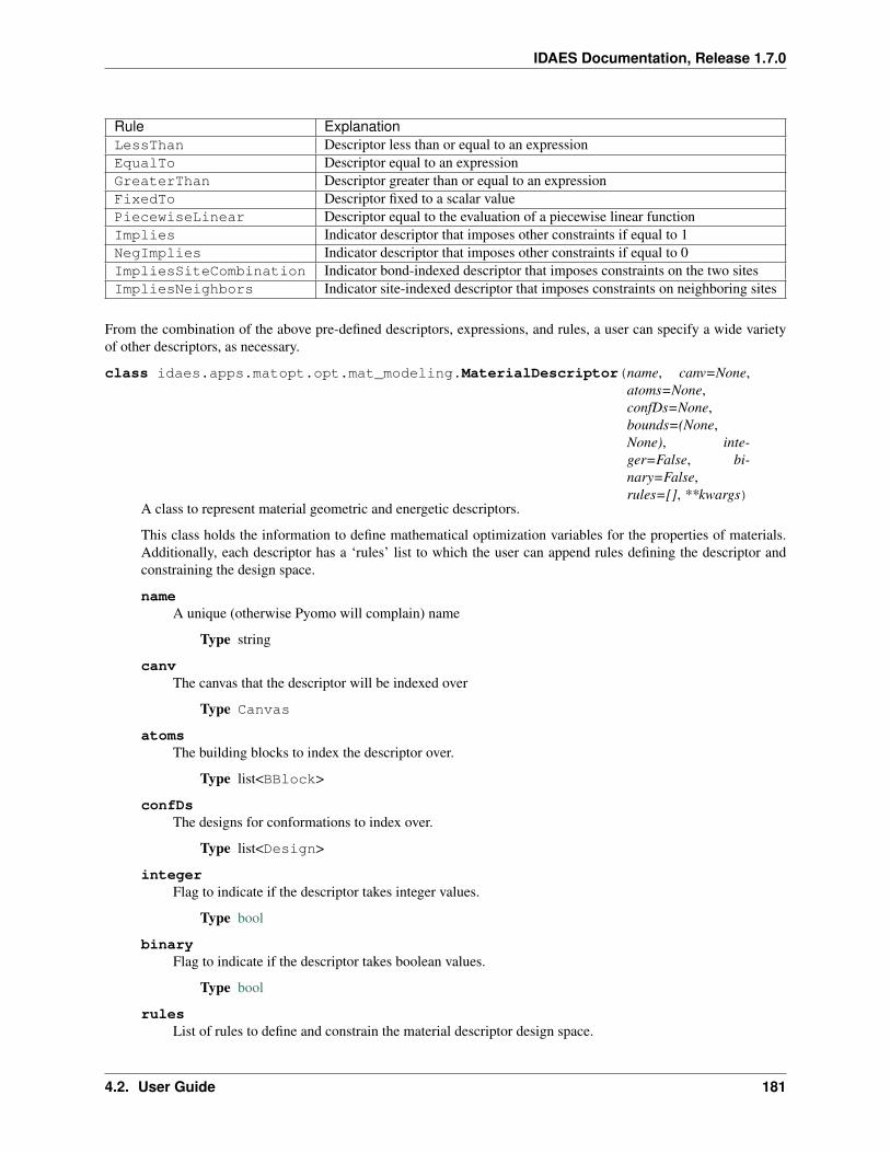
IDAES Documentation, Release 1.7.0
Rule ExplanationLessThan Descriptor less than or equal to an expressionEqualTo Descriptor equal to an expressionGreaterThan Descriptor greater than or equal to an expressionFixedTo Descriptor fixed to a scalar valuePiecewiseLinear Descriptor equal to the evaluation of a piecewise linear functionImplies Indicator descriptor that imposes other constraints if equal to 1NegImplies Indicator descriptor that imposes other constraints if equal to 0ImpliesSiteCombination Indicator bond-indexed descriptor that imposes constraints on the two sitesImpliesNeighbors Indicator site-indexed descriptor that imposes constraints on neighboring sites
From the combination of the above pre-defined descriptors, expressions, and rules, a user can specify a wide varietyof other descriptors, as necessary.
class idaes.apps.matopt.opt.mat_modeling.MaterialDescriptor(name, canv=None,atoms=None,confDs=None,bounds=(None,None), inte-ger=False, bi-nary=False,rules=[], **kwargs)
A class to represent material geometric and energetic descriptors.
This class holds the information to define mathematical optimization variables for the properties of materials.Additionally, each descriptor has a ‘rules’ list to which the user can append rules defining the descriptor andconstraining the design space.
nameA unique (otherwise Pyomo will complain) name
Type string
canvThe canvas that the descriptor will be indexed over
Type Canvas
atomsThe building blocks to index the descriptor over.
Type list<BBlock>
confDsThe designs for conformations to index over.
Type list<Design>
integerFlag to indicate if the descriptor takes integer values.
Type bool
binaryFlag to indicate if the descriptor takes boolean values.
Type bool
rulesList of rules to define and constrain the material descriptor design space.
4.2. User Guide 181
IDAES Documentation, Release 1.7.0
Type list<DescriptorRules>
boundsIf tuple, the lower and upper bounds on the descriptor values across all indices. If dict, the bounds can beindividually set for each index.
Type tuple/dict/func
See IndexedElem for more information on indexing. See DescriptorRule for information on definingdescriptors.
Solve optimization model
Once the model is fully specified, the user can optimize it in light of a chosen descriptor to serve as the objective to bemaximized or minimized, as appropriate. Several functions are provided for users to choose from.
class idaes.apps.matopt.opt.mat_modeling.MatOptModel(canv, atoms=None,confDs=None)
A class for the specification of a materials optimization problem.
Once all the material information is specified, we use this class to specify the material design problem of interest.This class is intended to be interpretable without mathematical optimization background while the conversionto Pyomo optimization models happens automatically.
canvThe canvas of the material design space
Type Canvas
atomsThe list of building blocks to consider. Note: This list does not need to include a void-atom type. We use‘None’ to represent the absence of any building block at a given site.
Type list<BBlock>
confDsThe list of conformations to consider.
Type list<Design>
maximize(func, **kwargs)Method to maximize a target functionality of the material model.
Parameters
• func (MaterialDescriptor/Expr) – Material functionality to optimize.
• **kwargs – Arguments to MatOptModel.optimize
Returns (Design/list<Design>) Optimal designs.
Raises pyutilib.ApplicationError if MatOpt can not find usable solver (CPLEX orNEOS-CPLEX)
See MatOptModel.optimize method for details.
minimize(func, **kwargs)Method to minimize a target functionality of the material model.
Parameters
• func (MaterialDescriptor/Expr) – Material functionality to optimize.
• **kwargs – Arguments to MatOptModel.optimize
Returns (Design/list<Design>) Optimal designs.
182 Chapter 4. Contents
IDAES Documentation, Release 1.7.0
Raises pyutilib.ApplicationError if MatOpt can not find usable solver (CPLEX orNEOS-CPLEX)
See MatOptModel.optimize method for details.
optimize(func, sense, nSolns=1, tee=True, disp=1, keepfiles=False, tilim=3600, trelim=None,solver=’cplex’)
Method to create and optimize the materials design problem.
This method automatically creates a new optimization model every time it is called. Then, it solves themodel via Pyomo with the CPLEX solver.
If multiple solutions (called a ‘solution pool’) are desired, then the nSolns argument can be provided andthe populate method will be called instead.
Parameters
• func (MaterialDescriptor/Expr) – Material functionality to optimize.
• sense (int) – flag to indicate the choice to minimize or maximize the functionality ofinterest. Choices: minimize/maximize (Pyomo constants 1,-1 respectively)
• nSolns (int) – Optional, number of Design objects to return. Default: 1 (SeeMatOptModel.populate for more information)
• tee (bool) – Optional, flag to turn on solver output. Default: True
• disp (int) – Optional, flag to control level of MatOpt output. Choices: 0: No MatOptoutput (other than solver tee) 1: MatOpt output for outer level method 2: MatOpt outputfor solution pool & individual solns. Default: 1
• keepfiles (bool) – Optional, flag to save temporary pyomo files. Default: True
• tilim (float) – Optional, solver time limit (in seconds). Default: 3600
• trelim (float) – Optional, solver tree memeory limit (in MB). Default: None (i.e.,Pyomo/CPLEX default)
• solver (str) – Solver choice. Currently only cplex or neos-cplex are supported Default:cplex
Returns (Design/list<Design>) Optimal design or designs, depending on the number of so-lutions requested by argument nSolns.
Raises pyutilib.ApplicationError if MatOpt can not find usable solver (CPLEX orNEOS-CPLEX)
populate(func, sense, nSolns, tee=True, disp=1, keepfiles=False, tilim=3600, trelim=None,solver=’cplex’)
Method to a pool of solutions that optimize the material model.
This method automatically creates a new optimization model every time it is called. Then, it solves themodel via Pyomo with the CPLEX solver.
The populate method iteratively solves the model, interprets the solution as a Design object, creates aconstraint to disallow that design, and resolves to find the next best design. We build a pool of Designsthat are gauranteed to be the nSolns-best solutions in the material design space.
Parameters
• func (MaterialDescriptor/Expr) – Material functionality to optimize.
• sense (int) – flag to indicate the choice to minimize or maximize the functionality ofinterest. Choices: minimize/maximize (Pyomo constants 1,-1 respectively)
4.2. User Guide 183
IDAES Documentation, Release 1.7.0
• nSolns (int) – Optional, number of Design objects to return. Default: 1 (SeeMatOptModel.populate for more information)
• tee (bool) – Optional, flag to turn on solver output. Default: True
• disp (int) – Optional, flag to control level of MatOpt output. Choices: 0: No MatOptoutput (other than solver tee) 1: MatOpt output for outer level method 2: MatOpt outputfor solution pool & individual solns. Default: 1
• keepfiles (bool) – Optional, flag to save temporary pyomo files. Default: True
• tilim (float) – Optional, solver time limit (in seconds). Default: 3600
• trelim (float) – Optional, solver tree memeory limit (in MB). Default: None (i.e.,Pyomo/CPLEX default)
• solver (str) – Solver choice. Currently only cplex or neos-cplex are supported Default:cplex
Returns (list<Design>) A list of optimal Designs in order of decreasing optimality.
Raises pyutilib.ApplicationError if MatOpt can not find usable solver (CPLEX orNEOS-CPLEX)
MatOpt Output
The results of the optimization process will be loaded into Design objects automatically. Users can then save materialdesign(s) into files for further analysis and visualization using suitable functions provided. MatOpt provides interfacesto several standard crystal structure file formats, including CFG, PDB, POSCAR, and XYZ.
MatOpt Examples
Five case studies are provided to illustrate the detailed usage of MatOpt. In each case, a Jupyter notebook withexplanations as well as an equivalent Python script is provided.
References
• Hanselman, C.L. and Gounaris, C.E., 2016. A mathematical optimization framework for the design of nanopat-terned surfaces. AIChE Journal, 62(9), pp.3250-3263.
• Hanselman, C.L., Alfonso, D.R., Lekse, J.W., Matranga, C., Miller, D.C. and Gounaris, C.E., 2019. A frame-work for optimizing oxygen vacancy formation in doped perovskites. Computers & Chemical Engineering, 126,pp.168-177.
• Hanselman, C.L., Zhong, W., Tran, K., Ulissi, Z.W. and Gounaris, C.E., 2019. Optimization-based design ofactive and stable nanostructured surfaces. The Journal of Physical Chemistry C, 123(48), pp.29209-29218.
• Isenberg, N.M., Taylor, M.G., Yan, Z., Hanselman, C.L., Mpourmpakis, G. and Gounaris, C.E., 2020. Identifi-cation of optimally stable nanocluster geometries via mathematical optimization and density-functional theory.Molecular Systems Design & Engineering.
• Yin, X., Isenberg, N.M., Hanselman, C.L., Mpourmpakis, G. and Gounaris, C.E., 2020. A mathematicaloptimization-based design framework for identifying stable bimetallic nanoclusters. In preparation.
• Hanselman, C.L., Yin, X., Miller, D.C. and Gounaris, C.E., 2020. MatOpt: A Python package for nanomaterialsdesign using discrete optimization. In preparation.
184 Chapter 4. Contents
IDAES Documentation, Release 1.7.0
Caprese
Nonlinear Model Predictive Control
Nonlinear Model Predictive Control (NMPC) is control strategy in which control inputs are determined by the solutionof an optimization problem every time the plant is sampled.
Optimization Problem
An explanation of the optimization problem solved in this implementation of NMPC is forthcoming.
Available Methods
Class for performing NMPC simulations of IDAES flowsheets
class idaes.apps.caprese.nmpc.NMPCSim(plant_model=None, plant_time_set=None, con-troller_model=None, controller_time_set=None,inputs_at_t0=None, sample_time=None, **kwargs)
Main class for NMPC simulations of Pyomo models.
classmethod add_namespace_to(model, time)Adds the _NMPC_NAMESPACE block a model with a given time set. All necessary model-specificattributes, including constraints and objectives, will be added to this block.
Parameters
• model – Model to which to add the namespace
• time – Set to treat as time in the given model
add_objective_function(model, name=’objective’, state_weight=1, control_weight=1,**kwargs)
Adds an objective function based on already calculated weights and setpoint values to the_NMPC_NAMESPACE of a model.
Parameters
• model – Model to which to add objective function
• name – Name of objective function to add
• state_weight – Additional weight factor to apply to each state term in the objectivefunction. Intended for a user that wants to weigh states and controls differently
• control_weight – Addtional weight factor to apply to each control term in the objec-tive function. Intended for a user that wants to weigh states and controls differently
add_setpoint_to_controller(objective_name=’tracking_objective’, **kwargs)User-facing function for the addition of a setpoint to the controller. Assumes the controller model’s setpointattributes have been populated with desired values. This function first calculates weights, then adds anobjective function based on those weights and existing setpoint values.
Parameters objective_name – Name to use for the objective function added
calculate_error_between_states(mod1, mod2, t1, t2, Q_matrix=[], cate-gories=[<VariableCategory.DIFFERENTIAL: 51>],**kwargs)
Calculates the normalized (by the weighting matrix already calculated) error between the differential vari-ables in different models and at different points in time.
4.2. User Guide 185
IDAES Documentation, Release 1.7.0
Parameters
• mod1 – First flowsheet model
• mod2 – Second flowsheet model (may be same as the first)
• t1 – Time point of interest in first model
• t2 – Time point of interest in second model
• Q_matrix – List of weights by which to weigh the error for each state. Default is to usethe same weights calculated for the controller objective function.
calculate_full_state_setpoint(setpoint, require_steady=True, allow_inconsistent=True,**kwargs)
Given a user-defined setpoint, i.e. a list of VarData, value tuples, calculates a full-state setpoint to be usedin the objective function of the dynamic optimization problem. This is done by solving a single- time pointoptimization problem with the user’s setpoint in the objective function.
The solve is performed in the first time point blocks/constraints of the controller model. The procedure is:
i. Check for inconsistent initial conditions. Warn user if found.
ii. Populate controller setpoint attributes with user-defined values.
iii. Populate reference attributes with (now consistent) initial conditions.
iv. Calculate weights for variables specified.
v. Add objective function based on these weights and setpoint values.
vi. Solve for setpoint.
vii. Deactivate just-added objective function.
Parameters
• setpoint – List of VarData, value tuples to be used in the objective function of thesingle-time point optimization problem
• require_steady – Bool telling whether or not to fix derivatives to zero when perform-ing optimization
constrain_control_inputs_piecewise_constant(**kwargs)Function to add piecewise constant (PWC) constraints to controller model. Requires model’s_NMPC_NAMESPACE to know about input vars and to have as an attribute a sample points list.
construct_objective_weights(model, categories=[<VariableCategory.DIFFERENTIAL:51>, <VariableCategory.ALGEBRAIC: 52>, <VariableCat-egory.DERIVATIVE: 53>, <VariableCategory.INPUT: 54>],**kwargs)
Constructs the objective weight values for the specified variable categories of a specified model. Weightsare calculated for each variable in each group by taking the difference between the initial value and thesetpoint value, making sure it is above a tolerance, and taking its reciprocal. Weights can be overridden bya list of VarData, value tuples passed in as the “objective_weight_override” config argument.
Parameters
• model – Model whose variables will be accessed to calculate weights, and whose weightattributes will be set.
• categories – List of VariableCategory enum items for which to calculate weights.Default is DIFFERENTIAL, ALGEBRAIC, DERIVATIVE, and INPUT
186 Chapter 4. Contents
IDAES Documentation, Release 1.7.0
has_consistent_initial_conditions(model, **kwargs)Finds constraints at time.first() that are violated by more than tolerance. Returns True if any are found.
initialize_by_solving_elements(model, time, input_type=<ElementInitializationInputOption.SET_POINT:21>, objective_name=’tracking_objective’, **kwargs)
Initializes the controller model by solving (a square simulation for) each time element.
Parameters
• model – Model to initialize
• time – Set to treat as time
• input_type – ElementInitializationInputOption enum item telling how to fix the inputsfor the simulation
initialize_control_problem(**kwargs)Function to initialize the controller model before solving the optimal control problem. Possible strategiesare to use the initial conditions, to perform a simulation, or to use the results of the previous solve. Initial-ization from a previous (optimization) solve can only be done if an optimization solve has been performedsince the last initialization. The strategy may be passed in as the control_init_option keyword (config)argument, otherwise the default will be used.
initialize_from_initial_conditions(model, categories=[<VariableCategory.DERIVATIVE:53>, <VariableCategory.DIFFERENTIAL: 51>,<VariableCategory.ALGEBRAIC: 52>], **kwargs)
Set values of differential, algebraic, and derivative variables to their values at the initial conditions. Animplicit assumption here is that the initial conditions are consistent.
Parameters
• model – Flowsheet model whose variables are initialized
• categories – List of VariableCategory enum items to initialize. Default containsDERIVATIVE, DIFFERENTIAL, and ALGEBRAIC.
initialize_from_previous_sample(model, categories=[<VariableCategory.DIFFERENTIAL:51>, <VariableCategory.ALGEBRAIC: 52>, <Vari-ableCategory.DERIVATIVE: 53>, <VariableCate-gory.INPUT: 54>], **kwargs)
Re-initializes values of variables in model to the values one sampling time in the future. Values for the lastsampling time are currently set to values in the steady state model, assumed to be the set point.
Parameters
• model – Flowsheet model to initialize
• categories – List of VariableCategory enum items to initialize. Default contains DIF-FERENTIAL, ALGEBRAIC, DERIVATIVE, and INPUT
inject_control_inputs_into_plant(t_plant, **kwargs)Injects input variables from the first sampling time in the controller model to the sampling period in theplant model that starts at the specified time, adding noise if desired.
Parameters t_plant – First time point in plant model where inputs will be applied.
set_bounds_from_initial(vargroup)Builds lists of lower bound, upper bound tuples as attributes of the input model, based on the currentbounds (and domains) of differential, algebraic, and input variables.
Parameters model – Model whose variables will be checked for bounds.
set_reference_values_from_initial(vargroup, t0=None)Sets the values in the reference list of an NMPCVarGroup from the values of the group’s variables at t0
4.2. User Guide 187
IDAES Documentation, Release 1.7.0
Parameters
• vargroup – NMPCVarGroup instance whose reference values to set
• t0 – Point in time at which variable values will be used to set reference values
simulate_plant(t_start, **kwargs)Function for simulating plant model for one sampling period after inputs have been assigned from solve ofcontroller model.
Parameters t_start – Beginning of timespan over which to simulate
solve_consistent_initial_conditions(model, **kwargs)Uses pyomo.dae.initialization solve_consistent_initial_conditions function to solve for consistent initialconditions. Inputs are fixed at time.first() in attempt to eliminate degrees of freedom.
solve_control_problem(**kwargs)Function for solving optimal control problem, which calculates control inputs for the plant.
transfer_current_plant_state_to_controller(t_plant, **kwargs)Transfers values of the initial condition variables at a specified time in the plant model to the initial timepoint of the controller model, adding noise if desired.
Parameters t_plant – Time point in plant model whose values will be transferred
validate_fixedness(*models)Makes sure that assumptions regarding fixedness for different points in time are valid. Differential, alge-braic, and derivative variables may be fixed only at t0, only if they are initial conditions. Fixed variablesmust be fixed at all points in time, except possibly initial conditions.
Expects to find “alg,” “diff,” “deriv,” and “fixed” vars on each model’s _NMPC_NAMESPACE, as well asa var_locator ComponentMap.
Parameters models – Models for which to validate fixedness
validate_sample_time(sample_time, *models, **kwargs)Makes sure sample points, or integer multiple of sample time-offsets from time.first(), lie on finite elementboundaries, and that the horizon of each model is an integer multiple of sample time. Assembles a list ofsample points and a dictionary mapping sample points to the number of finite elements in the precedingsampling period, and adds them as attributes to _NMPC_NAMESPACE.
Parameters
• sample_time – Sample time to check
• models – List of flowsheet models to check
validate_slices(tgt_model, src_model, src_time, src_slices)Given list of time-only slices in a source model, attempts to find each of them in the target model andreturns a list of the found slices in the same order. Expects to find a var_locator ComponentMap attributein the _NMPC_NAMESPACE of the target model.
Parameters
• tgt_model – Model to search for time-slices
• src_model – Model containing the slices to search for
• src_slices – List of time-only slices of variables in the source model
Returns List of time-only slices to same-named variables in the target model
188 Chapter 4. Contents
IDAES Documentation, Release 1.7.0
Moving Horizon Estimation
Caprese is actively under development. A module for MHE is forthcoming.
Caprese is a module for simulation of IDAES flowsheets with nonlinear program (NLP)-based control and estimationstrategies, namely Nonlinear Model Predictive Control (NMPC) and Moving Horizon Estimation (MHE).
ALAMOPY: ALAMO Python
ALAMOPY provides a wrapper for the software ALAMO which generates algebraic surrogate models of black-boxsystems for which a simulator or experimental setup is available.
RIPE: Reaction Identification and Parameter Estimation
RIPE provides tools for reaction network identification. RIPE uses reactor data consisting of concentration, or con-version, values for multiple species that are obtained dynamically, or at multiple process conditions (temperatures,flow rates, working volumes) to identify probable reaction kinetics. The RIPE module also contains tools to facilitateadaptive experimental design.
HELMET: HELMholtz Energy Thermodynamics
HELMET provides a framework for regressing multiparameter equations of state that identify an equation forHelmholtz energy and multiple thermodynamic properties simultaneously.
PySMO: Python-based Surrogate Modelling Objects
PySMO provides tools for generating different types of reduced order models. It provides IDAES users with a setof surrogate modeling tools which supports flowsheeting and direct integration into an equation-oriented modelingframework. It allows users to directly integrate reduced order models with algebraic high-fidelity process modelswithin an single IDAES flowsheet.
4.2. User Guide 189

IDAES Documentation, Release 1.7.0
MatOpt: Nanomaterials Optimization
MatOpt provides tools for nanomaterials design using Mathematical Optimization. MatOpt can be used to designcrystalline nanostructured materials, including but not limited to particles, wires, surfaces, and periodic bulk structures.
Caprese
Caprese is a module for the simulation of IDAES flowsheets with nonlinear program (NLP)-based control and estima-tion strategies, namely Nonlinear Model Predictive Control (NMPC) and Moving Horizon Estimation (MHE).
190 Chapter 4. Contents
IDAES Documentation, Release 1.7.0
4.3 Advanced User Guide
4.3.1 Advanced User Installation
Advanced users who plan to develop their own models or tools are encouraged to install IDAES using Git and GitHubas described in this section, rather than using the instructions in the getting started section. These advanced users willgreatly benefit from improved version control and code integration capabilities.
• Git and GitHub Basics
• Installation with GitHub
– Github Setup
– Fork the Repository
– Clone Your Fork
– Add Upstream Remote
– Create the Python Environment
– Finish the Installation
– Update IDAES
Git and GitHub Basics
Git is a distributed version control system that keeps track of changes in a set of files, while GitHub is a hosting servicefor Git repositories that adds many other features that are useful for collaborative software development.
Both Git and GitHub are widely used and there are excellent tutorials and resources for each. See Atlassian Githubtutorials , GitHub help, and Git documentation.
4.3. Advanced User Guide 191
IDAES Documentation, Release 1.7.0
A limited reference for Git and GitHub terminology and commands is provided here, users that are new to Git andGitHub are strongly encouraged to use the more detailed resources above.
Terminology and Commands
This section gives a high-level introduction to Git and GitHub terminology and commands.
More details resources include Atlassian Github tutorials , GitHub help, and Git documentation.
• Terminology
– Summary
– Branches
– Forks
– Pull Requests
• Git Commands
Terminology
Summary
branch A name for a series of commits. See Branches.
fork Copy of a repository in GitHub. See Forks.
pull request (PR) A request to compare and merge code in a GitHub repository. See Pull Requests.
Branches
A branch is a series of commits that allows you to separate the code development from the main code. There is a gooddescription of what Git branches are and how they work here. Understanding this takes a little study, but this pays offby making Git’s behavior much less mysterious. The short, practical version is that a branch is a name for a series ofcommits that you want to group together, and keep separable from other series of commits. From Git’s perspective,the branch is just a name for the first commit in that series.
It is recommended that you create new branches on which to develop your work, and reserve the “master” branchfor merging in work that has been completed and approved on GitHub. One way to do this is to create branches thatcorrespond directly to issues on GitHub, and include the issue number in the branch name.
Forks
A fork is a copy of a repository, in the GitHub shared space (a copy of a repository from GitHub down to your localdisk is called a “clone”). In this context, that means a copy of the “idaes-dev” repository from the IDAES organiza-tion (https://github.com/IDAES/idaes-dev) to your own user space, e.g., https://github.com/myname/idaes-dev). Themechanics of creating and using forks on GitHub are given here.
192 Chapter 4. Contents
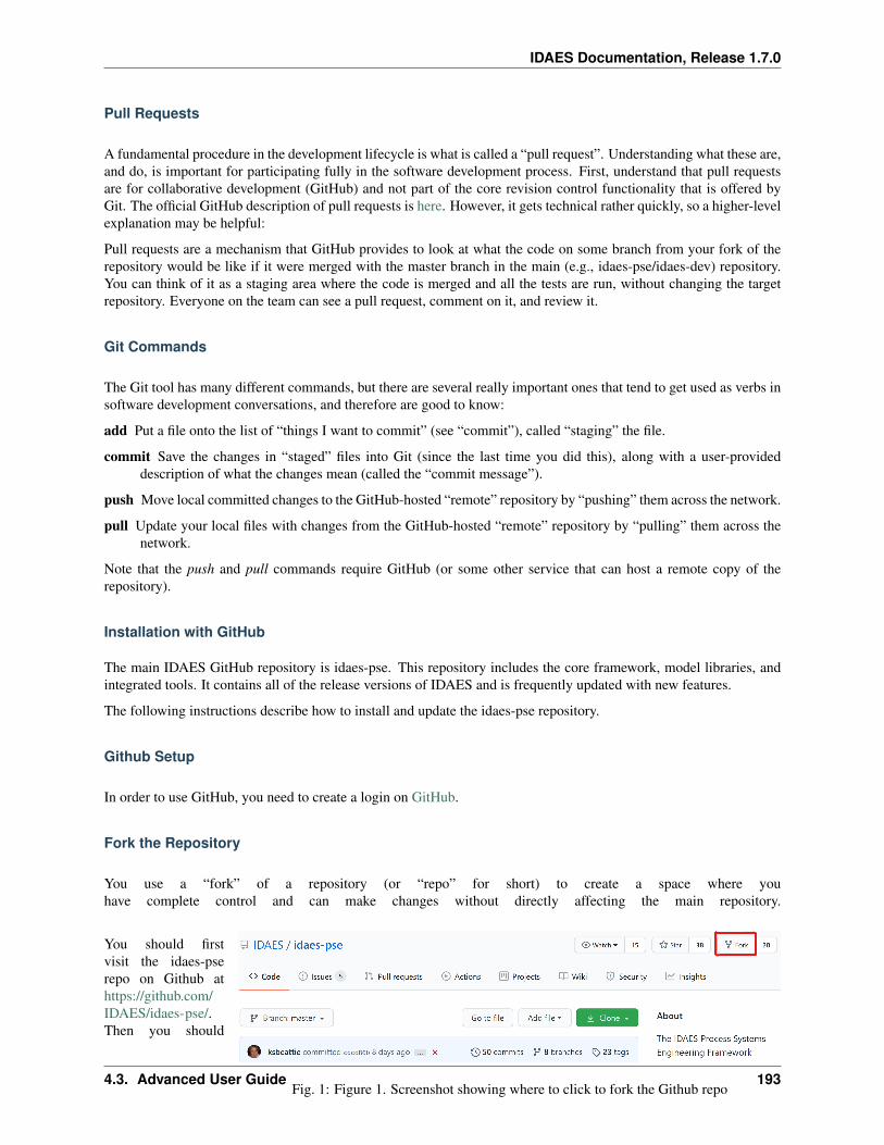
IDAES Documentation, Release 1.7.0
Pull Requests
A fundamental procedure in the development lifecycle is what is called a “pull request”. Understanding what these are,and do, is important for participating fully in the software development process. First, understand that pull requestsare for collaborative development (GitHub) and not part of the core revision control functionality that is offered byGit. The official GitHub description of pull requests is here. However, it gets technical rather quickly, so a higher-levelexplanation may be helpful:
Pull requests are a mechanism that GitHub provides to look at what the code on some branch from your fork of therepository would be like if it were merged with the master branch in the main (e.g., idaes-pse/idaes-dev) repository.You can think of it as a staging area where the code is merged and all the tests are run, without changing the targetrepository. Everyone on the team can see a pull request, comment on it, and review it.
Git Commands
The Git tool has many different commands, but there are several really important ones that tend to get used as verbs insoftware development conversations, and therefore are good to know:
add Put a file onto the list of “things I want to commit” (see “commit”), called “staging” the file.
commit Save the changes in “staged” files into Git (since the last time you did this), along with a user-provideddescription of what the changes mean (called the “commit message”).
push Move local committed changes to the GitHub-hosted “remote” repository by “pushing” them across the network.
pull Update your local files with changes from the GitHub-hosted “remote” repository by “pulling” them across thenetwork.
Note that the push and pull commands require GitHub (or some other service that can host a remote copy of therepository).
Installation with GitHub
The main IDAES GitHub repository is idaes-pse. This repository includes the core framework, model libraries, andintegrated tools. It contains all of the release versions of IDAES and is frequently updated with new features.
The following instructions describe how to install and update the idaes-pse repository.
Github Setup
In order to use GitHub, you need to create a login on GitHub.
Fork the Repository
You use a “fork” of a repository (or “repo” for short) to create a space where youhave complete control and can make changes without directly affecting the main repository.
Fig. 1: Figure 1. Screenshot showing where to click to fork the Github repo
You should firstvisit the idaes-pserepo on Github athttps://github.com/IDAES/idaes-pse/.Then you should
4.3. Advanced User Guide 193
IDAES Documentation, Release 1.7.0
click on the forkicon in the top rightand click on yourusername. Thesesteps will havecreated your own fork of the repo with the same name under your username.
Clone Your Fork
A “clone” is a copy of a Github repository on your local machine. This is what you need to do in order to actually editand change the files. To make a clone of the fork you created in the previous step, change to a directory where youwant to put the source code and run the command:
git clone https://github.com/MYNAME/idaes-pse.gitcd idaes-pse
Of course, replace MYNAME with your username. This will download all the files in the latest version of the reposi-tory onto your local disk.
Note: After the git clone, subsequent Git commands should be performed from the “idaes-pse” directory.
Add Upstream Remote
In order to guarantee that your fork can be synchronized with the “main” idaes-pse repo in the GitHub IDAES orga-nization, you need to add a pointer to that repository as a remote. This repository will be called upstream and linkedwith the following command:
git remote add upstream https://github.com/IDAES/idaes-pse.git
To check to see if you added the remote correctly use the following command:
git remote -v
You should see that there are two remotes, origin and upstream. Both have two lines showing the remote name, theurl, and the access (fetch or push). Origin is the pointer to your fork and was automatically added with the clonecommand, while upstream is the pointer to the main idaes-pse repo that you just added.
Create the Python Environment
Once you have the repo cloned, you can change into that directory (by default, it will be called “idaes-pse” like therepo) and install the Python packages.
But before you do that, you need to get the Python package manager fully up and running. We use a Python packagingsystem called Conda and we specifically use its minimal version Miniconda. If you do not already have Conda, pleasefollow the installation instructions for your operating system in getting started.
After Miniconda is installed, we recommend creating a separate conda environment for IDAES. If you are unfamil-iar with environments, a good starting guide is here. Create and activate a conda environment for the new IDAESinstallation with the following commands (we officially support python 3.7, but you may choose a version you prefer):
conda create -n idaes python=3.7conda activate idaes
194 Chapter 4. Contents
IDAES Documentation, Release 1.7.0
Note: When setting up a conda environment like this, you must conda activate idaes whenever you open afresh terminal window and wish to use IDAES.
Finish the Installation
Now that conda and pip are installed, and you are in the “idaes” conda environment, you can run the followingcommands to install the requirements for IDAES and get the extensions (e.g. binaries for the solver IPOPT and otherexternal function calls):
pip install .idaes get-extensions
Warning: The IDAES binary extensions are not yet supported on Mac/OSX
Note: There are a few options for installing the requirements.
1) pip install . - basic install using what is in setup.py
2) pip install .[dev] - basic install as above and also installs the Sphinx doc tools for buildingthe documentation locally
3) pip install -r requirements.txt - same as # 1 but installs our “development” Pyomoand PyUtilib
4) pip install -r requirements-dev.txt - same as # 3 with the Sphinx doc tools
Also note that these pip installs would override any package within the conda environment, so if youwould like a specific package (e.g. git clone Pyomo), you should look at the requirements files and onlyinstall the packages you need.
You can test that everything is installed properly by running the tests with Pytest:
pytest -m "not integration"
The not integration tag skips some tests that are slow. If you like, you can run all of the tests with just pytest.
Update IDAES
The master branch of idaes-pse is frequently updated and a new IDAES release occurs quarterly. It is recommendedthat you update your fork and local repositories and conda environment periodically.
pip install -U idaes-psepip install -U .
4.3.2 Developer Documentation
This section of the documentation is intended for developers, and much of it is targeted at the IDAES internal team.Hopefully many of the principles and ideas are also applicable to external contributors.
4.3. Advanced User Guide 195
IDAES Documentation, Release 1.7.0
Developer Contents
IDAES Contributor Guide
About
This page tries to give all the essential information needed to contribute software to the IDAES project. It is designedto be useful to both internal and external collaborators.
Code and other file locations
Source code The main Python package is under the idaes/ directory. Sub-directories, aka subpackages, should bedocumented elsewhere. If you add a new directory in this tree, be sure to add a __init__.py in that directory soPython knows it is a subpackage with Python modules. Code that is not part of the core package is under apps/.This code can have any layout that the creator wants.
Documentation The documentation for the core package is under docs.
Examples Examples are under the examples/ directory. Tutorials from workshops are under the examples/workshops/subdirectory.
Developer environment
Development of IDAES will require an extra set of required package not needed by regular users. To install those extradeveloper tools use the command pip install -r requirements-dev.txt rather than pip install-r requirements.txt
Code style
The code style is not entirely consistent. But some general guidelines are:
• follow the PEP8 style (or variants such as Black)
• use Google-style docstrings on classes, methods, and functions
• format your docstrings as reStructuredText so they can be nicely rendered as HTML by Sphinx
• add logging to your code by creating and using a global log object named for the module, which can be createdlike: _log = logging.getLogger(__name__)
• take credit by adding a global author variable: __author__ = 'yourname'
Tests
For general information about writing tests in Python, see Testing.
There are three types of tests:
Python source code The Python tests are integrated into the Python source code directories. Every package (directorywith .py modules and an __init__.py file) should also have a tests/ sub-package, in which are test files. These,by convention are named test_<something>.py.
Doctests With some special reStructuredText “directives” (see “Writing tests”), the documentation can contain tests.This is particularly useful for making sure examples in the documentation still run without errors.
196 Chapter 4. Contents
IDAES Documentation, Release 1.7.0
Jupyter notebook tests (coming soon)
Writing tests
We use pytest to run our tests. The main advantage of this framework over the built-in unittest that comes with Pythonis that almost no boilerplate code is required. You write a function named test_<something>() and, inside it, use the(pytest-modified) assert keyword to check that things are correct.
Writing the Python unit tests in the tests/ directory is, hopefully, quite straightforward. Here is an example (out ofcontext) that tests a couple of things related to configuration in the core unit model library:
def test_config_block():m = ConcreteModel()
m.u = Unit()
assert len(m.u. config) == 2assert m.u.config.dynamic == useDefault
See the existing tests for many more examples.
For tests in the documentation, you need to wrap the test itself in a directive called testcode. Here is an example:
.. testcode::
from pyomo.environ import *from pyomo.common.config import ConfigValuefrom idaes.core import ProcessBlockData, declare_process_block_class
@declare_process_block_class("MyBlock")class MyBlockData(ProcessBlockData):
CONFIG = ProcessBlockData.CONFIG()CONFIG.declare("xinit", ConfigValue(default=1001, domain=float))CONFIG.declare("yinit", ConfigValue(default=1002, domain=float))def build(self):
super(MyBlockData, self).build()self.x = Var(initialize=self.config.xinit)self.y = Var(initialize=self.config.yinit)
First, note that reStructuredText directive and indented Python code. The indentation of the Python code is important.You have to write an entire program here, so all the imports are necessary (unless you use the testsetup and testcleanupdirectives, but honestly this isn’t worth it unless you are doing a lot of tests in one file). Then you write your Pythoncode as usual.
Running tests
Running all tests is done by, at the top directory, running the command: pytest.
The documentation test code will actually be run by a special hook in the pytest configuration that treats the Makefilelike a special kind of test. As a result, when you run pytest in any way that includes the “docs/” directory (includingthe all tests mode), then all the documentation tests will run, and errors/etc. will be reported through pytest. A usefulcorollary is that, to run documentation tests, do: pytest docs/Makefile
You can run specific tests using the pytest syntax, see its documentation or pytest -h for details.
4.3. Advanced User Guide 197
IDAES Documentation, Release 1.7.0
Documentation
The documentation is built from its sources with a tool called Sphinx. The sources for the documentation are:
• hand-written text files, under docs/, with the extension “.rst” for reStructuredText.
• the Python source code
• selected Jupyter Notebooks
Building documentation
Note: To build the documentation locally, you will need to have the Sphinx tools installed. This will be done foryou by running pip install requirements-dev.txt (“developer” setup) as opposed to the regular pipinstall requirements.txt (“user” setup).
To build the documentation locally, use our custom build.py script.
cd docs python build.py
The above commands will do a completely clean build to create HTML output.
If the command succeeds, the final line will look like:
=== SUCCESS
If it fails, it will instead print something like:
*** ERROR in 'html'
****** message about the command that failed
*** and any additional info
***
If you want to see the commands actually being run, add -v to the command line.
By default the build command removes all existing built files before running the Sphinx commands. To turn this off,and rebuild only “new” things, add –dirty to the command line.
Previewing documentation
The generated documentation can be previewed locally by opening the generated HTML files in a web browser. Thefiles are under the docs/build/ directory, so you can open the file docs/build/index.html to get started.
Github Repository Overview
This section describes the layout of the Github repositories. Later sections will give guidelines for contributing codeto these repositories.
198 Chapter 4. Contents
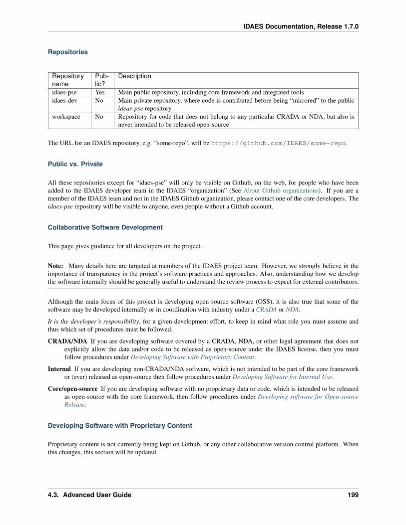
IDAES Documentation, Release 1.7.0
Repositories
Repositoryname
Pub-lic?
Description
idaes-pse Yes Main public repository, including core framework and integrated toolsidaes-dev No Main private repository, where code is contributed before being “mirrored” to the public
ideas-pse repositoryworkspace No Repository for code that does not belong to any particular CRADA or NDA, but also is
never intended to be released open-source
The URL for an IDAES repository, e.g. “some-repo”, will be https://github.com/IDAES/some-repo.
Public vs. Private
All these repositories except for “idaes-pse” will only be visible on Github, on the web, for people who have beenadded to the IDAES developer team in the IDAES “organization” (See About Github organizations). If you are amember of the IDAES team and not in the IDAES Github organization, please contact one of the core developers. Theidaes-pse repository will be visible to anyone, even people without a Github account.
Collaborative Software Development
This page gives guidance for all developers on the project.
Note: Many details here are targeted at members of the IDAES project team. However, we strongly believe in theimportance of transparency in the project’s software practices and approaches. Also, understanding how we developthe software internally should be generally useful to understand the review process to expect for external contributors.
Although the main focus of this project is developing open source software (OSS), it is also true that some of thesoftware may be developed internally or in coordination with industry under a CRADA or NDA.
It is the developer’s responsibility, for a given development effort, to keep in mind what role you must assume andthus which set of procedures must be followed.
CRADA/NDA If you are developing software covered by a CRADA, NDA, or other legal agreement that does notexplicitly allow the data and/or code to be released as open-source under the IDAES license, then you mustfollow procedures under Developing Software with Proprietary Content.
Internal If you are developing non-CRADA/NDA software, which is not intended to be part of the core frameworkor (ever) released as open-source then follow procedures under Developing Software for Internal Use.
Core/open-source If you are developing software with no proprietary data or code, which is intended to be releasedas open-source with the core framework, then follow procedures under Developing software for Open-sourceRelease.
Developing Software with Proprietary Content
Proprietary content is not currently being kept on Github, or any other collaborative version control platform. Whenthis changes, this section will be updated.
4.3. Advanced User Guide 199
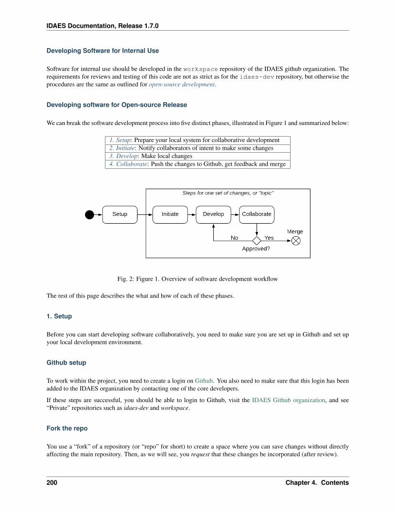
IDAES Documentation, Release 1.7.0
Developing Software for Internal Use
Software for internal use should be developed in the workspace repository of the IDAES github organization. Therequirements for reviews and testing of this code are not as strict as for the idaes-dev repository, but otherwise theprocedures are the same as outlined for open-source development.
Developing software for Open-source Release
We can break the software development process into five distinct phases, illustrated in Figure 1 and summarized below:
1. Setup: Prepare your local system for collaborative development2. Initiate: Notify collaborators of intent to make some changes3. Develop: Make local changes4. Collaborate: Push the changes to Github, get feedback and merge
Fig. 2: Figure 1. Overview of software development workflow
The rest of this page describes the what and how of each of these phases.
1. Setup
Before you can start developing software collaboratively, you need to make sure you are set up in Github and set upyour local development environment.
Github setup
To work within the project, you need to create a login on Github. You also need to make sure that this login has beenadded to the IDAES organization by contacting one of the core developers.
If these steps are successful, you should be able to login to Github, visit the IDAES Github organization, and see“Private” repositories such as idaes-dev and workspace.
Fork the repo
You use a “fork” of a repository (or “repo” for short) to create a space where you can save changes without directlyaffecting the main repository. Then, as we will see, you request that these changes be incorporated (after review).
200 Chapter 4. Contents
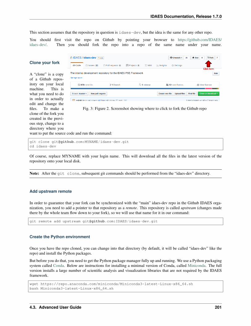
IDAES Documentation, Release 1.7.0
This section assumes that the repository in question is idaes-dev, but the idea is the same for any other repo.
You should first visit the repo on Github by pointing your browser to https://github.com/IDAES/idaes-dev/. Then you should fork the repo into a repo of the same name under your name.
Fig. 3: Figure 2. Screenshot showing where to click to fork the Github repo
Clone your fork
A “clone” is a copyof a Github repos-itory on your localmachine. This iswhat you need to doin order to actuallyedit and change thefiles. To make aclone of the fork youcreated in the previ-ous step, change to adirectory where youwant to put the source code and run the command:
git clone [email protected]:MYNAME/idaes-dev.gitcd idaes-dev
Of course, replace MYNAME with your login name. This will download all the files in the latest version of therepository onto your local disk.
Note: After the git clone, subsequent git commands should be performed from the “idaes-dev” directory.
Add upstream remote
In order to guarantee that your fork can be synchronized with the “main” idaes-dev repo in the Github IDAES orga-nization, you need to add a pointer to that repository as a remote. This repository is called upstream (changes madethere by the whole team flow down to your fork), so we will use that name for it in our command:
git remote add upstream [email protected]:IDAES/idaes-dev.git
Create the Python environment
Once you have the repo cloned, you can change into that directory (by default, it will be called “idaes-dev” like therepo) and install the Python packages.
But before you do that, you need to get the Python package manager fully up and running. We use a Python packagingsystem called Conda. Below are instructions for installing a minimal version of Conda, called Miniconda. The fullversion installs a large number of scientific analysis and visualization libraries that are not required by the IDAESframework.
wget https://repo.anaconda.com/miniconda/Miniconda3-latest-Linux-x86_64.shbash Miniconda3-latest-Linux-x86_64.sh
4.3. Advanced User Guide 201
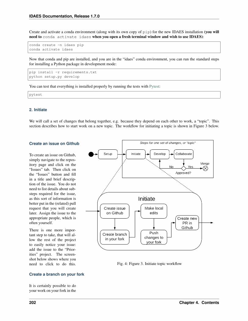
IDAES Documentation, Release 1.7.0
Create and activate a conda environment (along with its own copy of pip) for the new IDAES installation (you willneed to conda activate idaes when you open a fresh terminal window and wish to use IDAES):
conda create -n idaes pipconda activate idaes
Now that conda and pip are installed, and you are in the “idaes” conda environment, you can run the standard stepsfor installing a Python package in development mode:
pip install -r requirements.txtpython setup.py develop
You can test that everything is installed properly by running the tests with Pytest:
pytest
2. Initiate
We will call a set of changes that belong together, e.g. because they depend on each other to work, a “topic”. Thissection describes how to start work on a new topic. The workflow for initiating a topic is shown in Figure 3 below.
Fig. 4: Figure 3. Initiate topic workflow
Create an issue on Github
To create an issue on Github,simply navigate to the repos-itory page and click on the“Issues” tab. Then click onthe “Issues” button and fillin a title and brief descrip-tion of the issue. You do notneed to list details about sub-steps required for the issue,as this sort of information isbetter put in the (related) pullrequest that you will createlater. Assign the issue to theappropriate people, which isoften yourself.
There is one more impor-tant step to take, that will al-low the rest of the projectto easily notice your issue:add the issue to the “Prior-ities” project. The screen-shot below shows where youneed to click to do this.
Create a branch on your fork
It is certainly possible to doyour work on your fork in the
202 Chapter 4. Contents
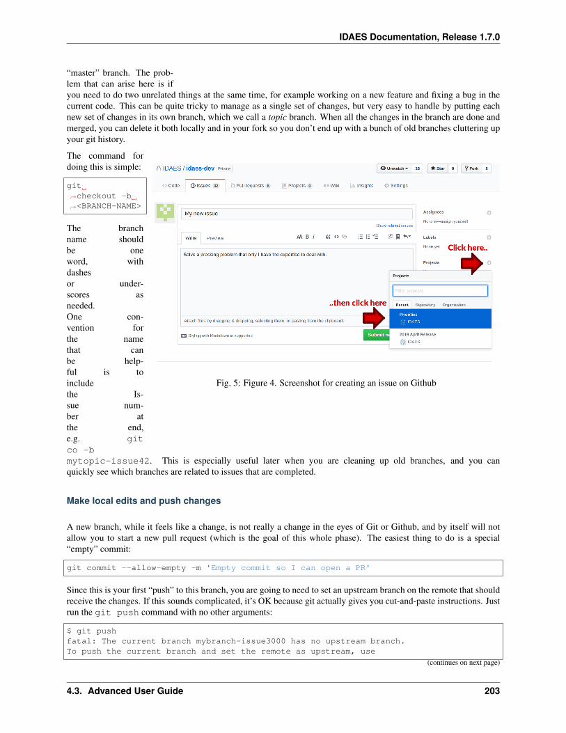
IDAES Documentation, Release 1.7.0
“master” branch. The prob-lem that can arise here is ifyou need to do two unrelated things at the same time, for example working on a new feature and fixing a bug in thecurrent code. This can be quite tricky to manage as a single set of changes, but very easy to handle by putting eachnew set of changes in its own branch, which we call a topic branch. When all the changes in the branch are done andmerged, you can delete it both locally and in your fork so you don’t end up with a bunch of old branches cluttering upyour git history.
Fig. 5: Figure 4. Screenshot for creating an issue on Github
The command fordoing this is simple:
git→˓checkout -b→˓<BRANCH-NAME>
The branchname shouldbe oneword, withdashesor under-scores asneeded.One con-vention forthe namethat canbe help-ful is toincludethe Is-sue num-ber atthe end,e.g. gitco -bmytopic-issue42. This is especially useful later when you are cleaning up old branches, and you canquickly see which branches are related to issues that are completed.
Make local edits and push changes
A new branch, while it feels like a change, is not really a change in the eyes of Git or Github, and by itself will notallow you to start a new pull request (which is the goal of this whole phase). The easiest thing to do is a special“empty” commit:
git commit --allow-empty -m 'Empty commit so I can open a PR'
Since this is your first “push” to this branch, you are going to need to set an upstream branch on the remote that shouldreceive the changes. If this sounds complicated, it’s OK because git actually gives you cut-and-paste instructions. Justrun the git push command with no other arguments:
$ git pushfatal: The current branch mybranch-issue3000 has no upstream branch.To push the current branch and set the remote as upstream, use
(continues on next page)
4.3. Advanced User Guide 203
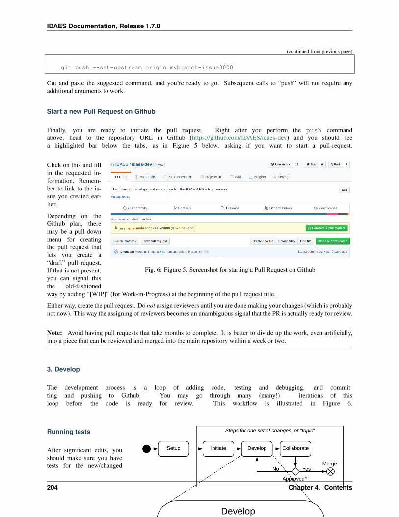
IDAES Documentation, Release 1.7.0
(continued from previous page)
git push --set-upstream origin mybranch-issue3000
Cut and paste the suggested command, and you’re ready to go. Subsequent calls to “push” will not require anyadditional arguments to work.
Start a new Pull Request on Github
Finally, you are ready to initiate the pull request. Right after you perform the push commandabove, head to the repository URL in Github (https://github.com/IDAES/idaes-dev) and you should seea highlighted bar below the tabs, as in Figure 5 below, asking if you want to start a pull-request.
Fig. 6: Figure 5. Screenshot for starting a Pull Request on Github
Click on this and fillin the requested in-formation. Remem-ber to link to the is-sue you created ear-lier.
Depending on theGithub plan, theremay be a pull-downmenu for creatingthe pull request thatlets you create a“draft” pull request.If that is not present,you can signal thisthe old-fashionedway by adding “[WIP]” (for Work-in-Progress) at the beginning of the pull request title.
Either way, create the pull request. Do not assign reviewers until you are done making your changes (which is probablynot now). This way the assigning of reviewers becomes an unambiguous signal that the PR is actually ready for review.
Note: Avoid having pull requests that take months to complete. It is better to divide up the work, even artificially,into a piece that can be reviewed and merged into the main repository within a week or two.
3. Develop
The development process is a loop of adding code, testing and debugging, and commit-ting and pushing to Github. You may go through many (many!) iterations of thisloop before the code is ready for review. This workflow is illustrated in Figure 6.
Fig. 7: Figure 6. Software development workflow
Running tests
After significant edits, youshould make sure you havetests for the new/changed
204 Chapter 4. Contents
IDAES Documentation, Release 1.7.0
functionality. This involveswriting Unit tests as well asrunning the test suite and ex-amining the results of theCode coverage.
This project uses Pytest tohelp with running the unittests. From the top-level di-rectory of the working tree,type:
pytest
Alternatively users of an IDElike PyCharm can run thetests from within the IDE.
Commit changes
The commands: git add, gitstatus, and git commit are allused in combination to savea snapshot of a Git project’scurrent state.1.
The commit command is theequivalent of “saving” yourchanges. But unlike editing adocument, the set of changesmay cover multiple files, in-cluding newly created files.To allow the user flexibility in specifying exactly which changes to save with each commit, the add command isused first to indicate files to “stage” for the next commit command. The status command is used to show the currentstatus of the working tree.
A typical workflow goes like this:
$ lsfile1 file2$ echo 'a' > file1 # edit existing file$ echo '1' > file3 # create new file$ git status --short # shows changed/unstaged and unknown fileM file1
?? file3$ git add file1 file3 # stage file1, file3 for commit$ git status --short # M=modified, A=addedM file1A file3$ git commit -m "made some changes"[master 067c16e] made some changes2 files changed, 2 insertions(+)create mode 100644 file3
1 Git has an additional saving mechanism called ‘the stash’. The stash is an ephemeral storage area for changes that are not ready to be committed.The stash operates on the working directory and has extensive usage options.* See the documentation for git stash for more information.
4.3. Advanced User Guide 205
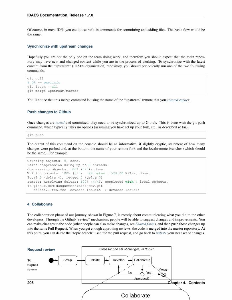
IDAES Documentation, Release 1.7.0
Of course, in most IDEs you could use built-in commands for committing and adding files. The basic flow would bethe same.
Synchronize with upstream changes
Hopefully you are not the only one on the team doing work, and therefore you should expect that the main repos-itory may have new and changed content while you are in the process of working. To synchronize with the latestcontent from the “upstream” (IDAES organization) repository, you should periodically run one of the two followingcommands:
git pull# OR -- explicitgit fetch --allgit merge upstream/master
You’ll notice that this merge command is using the name of the “upstream” remote that you created earlier.
Push changes to Github
Once changes are tested and committed, they need to be synchronized up to Github. This is done with the git pushcommand, which typically takes no options (assuming you have set up your fork, etc., as described so far):
git push
The output of this command on the console should be an informative, if slightly cryptic, statement of how manychanges were pushed and, at the bottom, the name of your remote fork and the local/remote branches (which shouldbe the same). For example:
Counting objects: 5, done.Delta compression using up to 8 threads.Compressing objects: 100% (5/5), done.Writing objects: 100% (5/5), 528 bytes | 528.00 KiB/s, done.Total 5 (delta 4), reused 0 (delta 0)remote: Resolving deltas: 100% (4/4), completed with 4 local objects.To github.com:dangunter/idaes-dev.git
d535552..fe61fcc devdocs-issue65 -> devdocs-issue65
4. Collaborate
The collaboration phase of our journey, shown in Figure 7, is mostly about communicating what you did to the otherdevelopers. Through the Github “review” mechanism, people will be able to suggest changes and improvements. Youcan make changes to the code (other people can also make changes, see Shared forks), and then push those changes upinto the same Pull Request. When you get enough approving reviews, the code is merged into the master repository. Atthis point, you can delete the “topic branch” used for the pull request, and go back to initiate your next set of changes.
Fig. 8: Figure 7. Collaborate phase workflow
Request review
Torequestreview
206 Chapter 4. Contents
IDAES Documentation, Release 1.7.0
of apullrequest,navi-gate tothe pullrequestin themain(e.g.,“idaes-dev”)repos-itoryandselectsomenamesin the“Re-view-ers”pull-downon theright-hand side. You need to have two approving reviews. The reviewers should get an email, but you can also “@”people in a comment in the pull request to give them a little extra nudge.
See the full code review procedure for more details.
Make changes
You need to keep track of the comments and reviews, and make changes accordingly. Think of a pull request as adiscussion. Normally, the person who made the pull request will make any requested edits. Occasionally, it may makesense for one or more other developers to jump in and make edits too, so how to do this is covered in the sub-sectionbelow.
Changes made while the code is being reviewed use the normal Develop workflow.
Shared forks
Other developers can also make changes in your fork. All they need to do is git clone your fork (not the mainrepository), switch to the correct topic branch, and then git push work directly to that branch. Note since this doesnot use the whole pull-request mechanism, all developers working on the same branch this way need to make sure thegit pull to synchronize with updates from the other developers.
For example, if Jack wants to make some edits on Rose’s fork, on a topic branch called “changes-issue51” he coulddo the following:
$ git clone https://github.com/rose/idaes-dev # clone Rose's fork$ git checkout changes-issue51 # checkout the topic branch$ echo "Hello" >> README.txt # make some important changes$ pytest # always run tests!!
(continues on next page)
4.3. Advanced User Guide 207
IDAES Documentation, Release 1.7.0
(continued from previous page)
$ git add README.txt ; git commit -m "important changes"$ git push # push changes to the fork
Hopefully it also is obvious that developers working this way have less safeguards for overwriting each other’s work,and thus should make an effort to communicate clearly and in a timely manner.
Merge
Once all the tests pass and you have enough approving reviews, it’s time to merge the code! This is the easy part: goto the bottom of the Pull Request and hit the big green “merge” button.
Before you close the laptop and go down to the pub, you should tidy up. First, delete your local branch (you can alsodelete that branch on Github):
git checkout master # switch back to master branchgit branch -d mychanges-issue3000
Next, you should make sure your master reflects the current state of the main master branch, i.e. go back and synchro-nize with the upstream remote, i.e. run git pull.
Now you can go and enjoy a tasty beverage. Cheers!
Developer Standards
Contents
• Developer Standards
– Model Formatting and General Standards
* Headers and Meta-data
* Coding Standard
* Model Organization
* Commenting
– Units of Measurement and Reference States
– Standard Variable Names
– Testing
208 Chapter 4. Contents
IDAES Documentation, Release 1.7.0
Model Formatting and General Standards
The section describes the recommended formatting used within the IDAES framework. Users are strongly encouragedto follow these standards in developing their models in order to improve readability of their code.
Headers and Meta-data
Model developers are encouraged to include some documentation in the header of their model files which provides abrief description of the purpose of the model and how it was developed. Some suggested information to include is:
• Model name,
• Model publication date,
• Model author
• Any necessary licensing and disclaimer information (see below).
• Any additional information the modeler feels should be included.
Coding Standard
All code developed as part of IDAES should conform to the PEP-8 standard.
Model Organization
Whilst the overall IDAES modeling framework enforces a hierarchical structure on models, model developers arestill encouraged to arrange their models in a logical fashion to aid other users in understanding the model. Modelconstraints should be grouped with similar constraints, and each grouping of constraints should be clearly commented.
For property packages, it is recommended that all the equations necessary for calculating a given property be groupedtogether, clearly separated and identified by using comments.
Additionally, model developers are encouraged to consider breaking their model up into a number of smaller methodswhere this makes sense. This can facilitate modification of the code by allowing future users to inherit from the basemodel and selectively overload sub-methods where desired.
Commenting
To help other modelers and users understand the how a model works, model builders are strongly encouraged tocomment their code. It is suggested that every constraint should be commented with a description of the purposeof the constraint, and if possible/necessary a reference to a source or more detailed explanation. Any deviationsfrom standard units or formatting should be clearly identified here. Any initialization procedures, or other proceduresrequired to get the model to converge should be clearly commented and explained where they appear in the code.Additionally, modelers are strongly encouraged to add additional comments explaining how their model works to aidothers in understanding the model.
Units of Measurement and Reference States
Due to the flexibility provided by the IDAES modeling framework, there is no standard set of units of measurementor standard reference state that should be used in models. This places the onus on the user to understand the units ofmeasurement being used within their models and to ensure that they are consistent.
4.3. Advanced User Guide 209
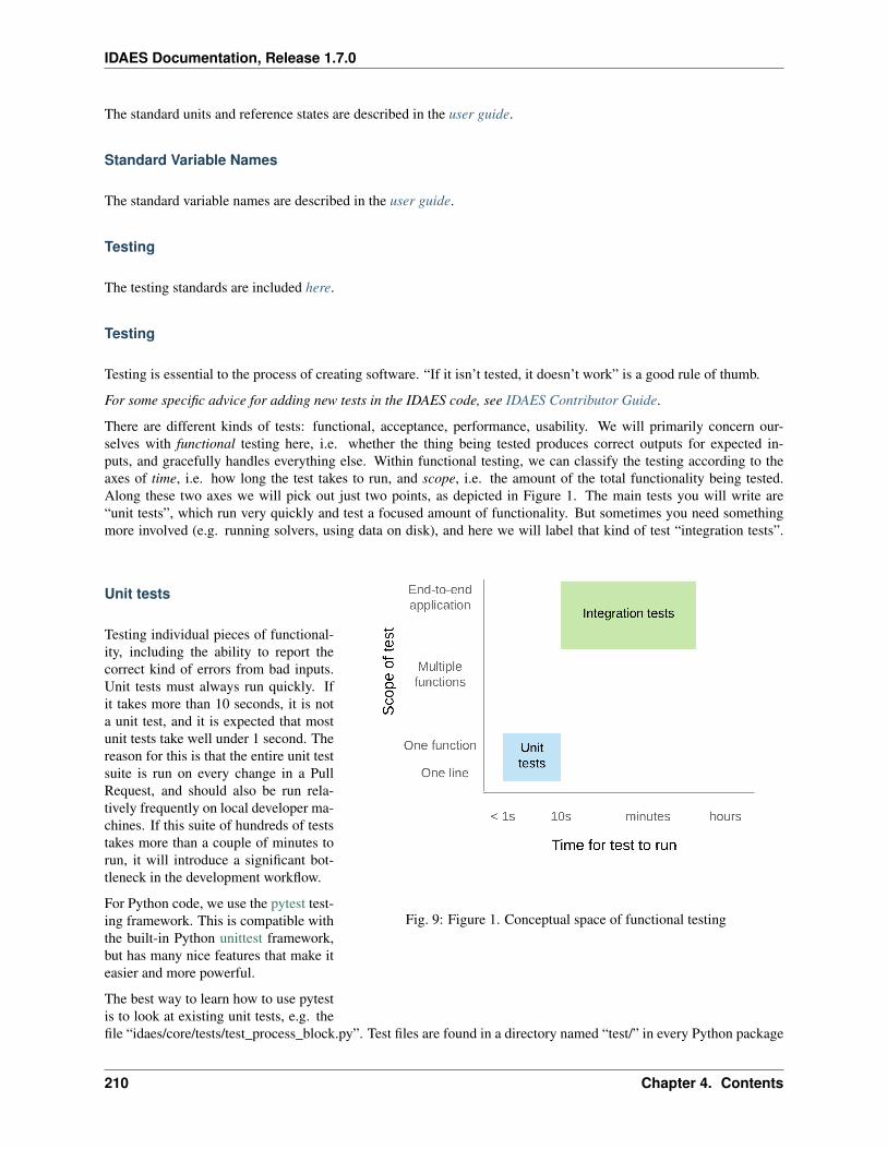
IDAES Documentation, Release 1.7.0
The standard units and reference states are described in the user guide.
Standard Variable Names
The standard variable names are described in the user guide.
Testing
The testing standards are included here.
Testing
Testing is essential to the process of creating software. “If it isn’t tested, it doesn’t work” is a good rule of thumb.
For some specific advice for adding new tests in the IDAES code, see IDAES Contributor Guide.
There are different kinds of tests: functional, acceptance, performance, usability. We will primarily concern our-selves with functional testing here, i.e. whether the thing being tested produces correct outputs for expected in-puts, and gracefully handles everything else. Within functional testing, we can classify the testing according to theaxes of time, i.e. how long the test takes to run, and scope, i.e. the amount of the total functionality being tested.Along these two axes we will pick out just two points, as depicted in Figure 1. The main tests you will write are“unit tests”, which run very quickly and test a focused amount of functionality. But sometimes you need somethingmore involved (e.g. running solvers, using data on disk), and here we will label that kind of test “integration tests”.
Fig. 9: Figure 1. Conceptual space of functional testing
Unit tests
Testing individual pieces of functional-ity, including the ability to report thecorrect kind of errors from bad inputs.Unit tests must always run quickly. Ifit takes more than 10 seconds, it is nota unit test, and it is expected that mostunit tests take well under 1 second. Thereason for this is that the entire unit testsuite is run on every change in a PullRequest, and should also be run rela-tively frequently on local developer ma-chines. If this suite of hundreds of teststakes more than a couple of minutes torun, it will introduce a significant bot-tleneck in the development workflow.
For Python code, we use the pytest test-ing framework. This is compatible withthe built-in Python unittest framework,but has many nice features that make iteasier and more powerful.
The best way to learn how to use pytestis to look at existing unit tests, e.g. thefile “idaes/core/tests/test_process_block.py”. Test files are found in a directory named “test/” in every Python package
210 Chapter 4. Contents
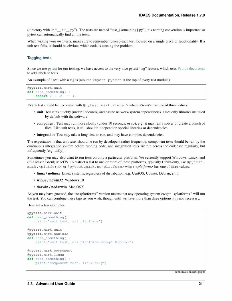
IDAES Documentation, Release 1.7.0
(directory with an “__init__.py”). The tests are named “test_something.py”; this naming convention is important sopytest can automatically find all the tests.
When writing your own tests, make sure to remember to keep each test focused on a single piece of functionality. If aunit test fails, it should be obvious which code is causing the problem.
Tagging tests
Since we use pytest for our testing, we have access to the very nice pytest “tag” feature, which uses Python decoratorsto add labels to tests.
An example of a test with a tag is (assume import pytest at the top of every test module):
@pytest.mark.unitdef test_something():
assert 2. + 2. == 4.
Every test should be decorated with @pytest.mark.<level> where <level> has one of three values:
• unit Test runs quickly (under 2 seconds) and has no network/system dependencies. Uses only libraries installedby default with the software
• component Test may run more slowly (under 10 seconds, or so), e.g. it may run a solver or create a bunch offiles. Like unit tests, it still shouldn’t depend on special libraries or dependencies.
• integration Test may take a long time to run, and may have complex dependencies.
The expectation is that unit tests should be run by developers rather frequently, component tests should be run by thecontinuous integration system before running code, and integration tests are run across the codebase regularly, butinfrequently (e.g. daily).
Sometimes you may also want to run tests on only a particular platform. We currently support Windows, Linux, and(to a lesser extent) MacOS. To restrict a test to one or more of these platforms, typically Linux-only, use @pytest.mark.<platform>, or @pytest.mark.no<platform> where <platform> has one of three values:
• linux / nolinux Linux systems, regardless of distribution, e.g. CentOS, Ubuntu, Debian, et al.
• win32 / nowin32 Windows 10
• darwin / nodarwin Mac OSX
As you may have guessed, the “no<platform>” version means that any operating system except “<platform>” will runthe test. You can combine these tags as you wish, though until we have more than three options it is not necessary.
Here are a few examples:
@pytest.mark.unitdef test_something():
print("unit test, all platforms")
@[email protected] test_something():
print("unit test, all platforms except Windows")
@[email protected] test_something():
print("component test, linux-only")
(continues on next page)
4.3. Advanced User Guide 211
IDAES Documentation, Release 1.7.0
(continued from previous page)
@[email protected] test_something():
print("integration test, all platforms except MacOS")
Mocking
Mocking is a common, but important, technique for avoiding dependencies that make your tests slow, fragile, andharder to understand. The basic idea is to replace dependencies with fake, or “mock”, versions of them that willprovide just enough realism for the test. Python provides a library, unittest.mock, to help with this process by providingobjects that can report how they were used, and easily pretend to have certain functionality (returning, for example,fixed values). To make this all more concrete, consider a simple problem where you want to test a function that makesa system call (in this case, os.remove):
# file: mymodule.pyimport osdef rm(filename):
os.remove(filename)
Normally, to test this you would create a temporary file, and then see if it got removed. However, with mocking youcan take a different approach entirely:
# file: test_mymodule.pyfrom mymodule import rmfrom unittest import mock
@mock.patch('mymodule.os')def test_rm(mock_os):
rm("any path")# test that rm called os.remove with the right parametersmock_os.remove.assert_called_with("any path")
Here, we have “patched” the os module that got imported into “mymodule” (note: had to do mymodule.os insteadof simply os, or the one mymodule uses would not get patched) so that when rm calls os.remove, it is really callinga fake method in mock_os that does nothing but record how it was called. The patched module is passed in to thetest as an argument so you can examine it. So, now, you are not doing any OS operations at all! You can imagine howthis is very useful with large files or external services.
Integration tests
Integration tests exercise an end-to-end slice of the overall functionality. At this time, the integration tests are allhoused in Jupyter Notebooks, which serve double-duty as examples and tutorials for end users. We execute thesenotebooks and verify that they run correctly to completion at least once before each new release of the software.
Code coverage
The “coverage” of the code refers to what percentage of the code (“lines covered” divided by total lines) is executed bythe automated tests. This is important because passing automated tests is only meaningful if the automated tests coverthe majority of the code’s behavior. This is not a perfect measure, of course, since simply executing a line of codeunder one condition does not mean it would execute correctly under all conditions. The code coverage is evaluatedlocally and then integrated with Github through a tool called Coveralls.
212 Chapter 4. Contents
IDAES Documentation, Release 1.7.0
Code Review
“It’s a simple 3-step process. Step one: Fix! Step two: It! Step three: Fix it!” – Oscar Rogers (Kenan Thompson),Saturday Night Live, 2/2009
Code review is the last line of defense between a mistake that the IDAES team will see and a mistake the whole worldwill see. In the case of that mistake being a leak of proprietary information, the entire project is jeopardized, so weneed to take this process seriously.
Summary
Warning: This section is an incomplete set of notes
Every piece of code must be reviewed by at least two people.
In every case, one of those people will be a designated “gatekeeper” and the one or more others will be “technicalreviewers”.
The technical reviewers are expected to consider various aspects of the proposed changes (details below), and engagethe author in a discussion on any aspects that are deemed lacking or missing.
The gatekeeper is expected to make sure all criteria have been met, and actually merge the PR.
Assigning Roles
The gatekeeper is a designated person, who will always be added to review a Pull Request (PR)
Gatekeeper is a role that will be one (?) person for some period like a week or two weeks
The role should rotate around the team, it’s expected to be a fair amount of work and should be aligned with availabilityand paper deadlines, etc.
The originator of the PR will add as reviewers the gatekeeper and 1+ technical reviewers.
Originator responsibilities
The originator of the PR should include in the PR itself information about where to find:
Changes to code/data
Tests of the changes
Documentation of the changes
The originator should be responsive to the reviewers
Technical reviewer responsibilities
The technical reviewer(s) should look at the proposed changes for
Technical correctness (runs properly, good style, internal code documentation, etc.)
Tests
Documentation
No proprietary / sensitive information
Until they approve, the conversation in the PR is between the technical reviewers and the originator (the gatekeeper isnot required to participate, assuming they have many PRs to worry about)
Gatekeeper responsibilities
4.3. Advanced User Guide 213
IDAES Documentation, Release 1.7.0
The gatekeeper does not need to engage until there is at least one approving technical review.
Once there is, they should verify that:
Changes do not contain proprietary data
Tests are adequate and do not fail
Documentation is adequate
Once everything is verified, the gatekeeper merges the PR
Automated Checks
The first level of code review is a set of automated checks that must pass before the code is ready for people to reviewit. These checks will run on the initiation of a pull request and on every new commit to that pull request that is pushedto Github (thus the name “continuous integration”).
The “continuous integration” of the code is hosted by an online service – we use CircleCI – that can automaticallyrerun the tests after every change (in this case, every new Pull Request or update to the code in an existing PullRequest) and report the results back to Github for display in the web pages. This status information can then be usedas an automatic gatekeeper on whether the code can be merged into the master branch – if tests fail, then no merge isallowed. Following this procedure, it is not possible for the master branch to ever be failing its own tests.
Docker Container
This page documents information needed by developers for working with the IDAES docker container.
As is expected by Docker, the main file for creating the Docker image is the “Dockerfile” in the top-level directory.
docker-idaes script
You can build new Docker images using the create option to the docker-idaes script. For example:
./docker-idaes create
You need to have the IDAES installation activated. The script will automatically find the current version and attemptto build a Docker image with the same version. If it detects an existing image, it will skip the image build. Next,the script will try to use docker save to save the image as a compressed archive. This will also be skipped if anexisting image file, with the same version as the “idaes” Python package, is detected.
Pushing an image to S3
The Docker images are stored on Amazon S3. Before you can upload a new image, you need to be part of the “IDAES-admin” group that is part of Amazon’s IAM (Identity Access Management) system. Please contact one of the coredevelopers to learn how to join this IAM group.
Once you have the IAM keys, you need to create a file ~/.aws/credentials that has the access key id and keyfrom the IAM account. It will look like this:
[default]aws_access_key_id = IDGOESHEREaws_secret_access_key = accesskeygoeshere
214 Chapter 4. Contents
IDAES Documentation, Release 1.7.0
The values for the ID and Access key are available from the AWS “IAM” service console.
Next you need to use the AWS command-line tools to copy the local image up to Amazon S3. For example, if theimage was version “1.0.1”, you would use the following command:
aws s3 cp idaes-pse-docker-1.0.1.tgz \s3://idaes/idaes-pse/idaes-pse-docker-1.0.1.tgz
If the new image should be the latest, you also need to do an S3 -> S3 copy to create a new latest image:
aws s3 cp s3://idaes/idaes-pse/idaes-pse-docker-1.0.1.tgz \s3://idaes/idaes-pse/idaes-pse-docker-latest.tgz
Glossary
API Acronym for “Application Programming Interface”, this is the set of functions used by an external programto invoke the functionality of a library or application. For IDAES, it usually refers to Python functions andclasses/methods in a Python module. By analogy, the APIs are to the IDAES library what a steering wheel,gearshift and pedals are to a car.
CRADA Cooperative Research and Development Agreement. A legal agreement between two or more parties thatinvolves a statement of work and terms for sharing non-public data.
NDA Non-Disclosure Agreement. A legal agreement between two or more parties that involves terms for sharingnon-public data.
4.3.3 Developing Custom Models
It is difficult to build a single model library that will suit all modeling needs, and thus users will inevitably encountersituations where they need to create new models to represent their processes. The IDAES Process Modeling Frame-work has been developed with this in mind, and all components of the framework have been designed to be fullyaccessible and modifiable. This section of the documentation will explain how users can develop new models, ormodify existing models, for use within the IDAES modeling environment.
• Creating New Modeling Components
• Defining New Model Classes
• Inheriting from Existing Models
• Config Blocks
• The build Method
• Types of Models
Creating New Modeling Components
All models within the IDAES Process Modeling Framework, be they models of unit operations of thermodynamicproperties, are constructed in the same way and user defined models follow the same structure. Each model componentis a set of instructions on how to assemble a Pyomo ‘Block’ containing the necessary variables, expressions andconstraints to describe the desired process. These instructions are contained within Python classes which can bewritten and modified by the user.
4.3. Advanced User Guide 215
IDAES Documentation, Release 1.7.0
Details on what is required when constructing custom models of different types will be provided in subsequent sectionsof this documentation, however there are some steps common to all types of models which will be discussed here.
Defining New Model Classes
There is a significant amount of work that has to be done behind the scenes in order to create a new model componentand integrate it into the IDAES modeling framework. Rather than force the user to understand and implement thisthemselves, IDAES provides a number of standard tools which users can use to automate this when creating newmodels. These tools are used when declaring new components, and should be used in most cases when a user iscreating a new model (exceptions are mentioned in the detailed documentation for each type of model).
An example of declaring new model (named NewModel) is shown below:
@declare_process_block_class("NewModel")class NewModelData(BaseClass):
The first part of the declaration is the declare_process_block_class decorator, which automates all the code required tocreate a new type of Pyomo Block. This decorator needs to be provided with a name for the new model (NewModel).Understanding the details of class decoration within Python and the function of the declare_process_block_classdecorator are not necessary for developing new models, however users who wish to read more can see the technicalspecifications.
The second part of the declaration creates a NewModelData class which inherits from an existing BaseClass. TheNewModelData class needs to contain the instructions necessary for building the desired model and must be populatedby the user. In practice, each type of model (unit operation, thermophysical properties, etc.) has a set of commontasks which appear in most models of that type. To assist users with developing new model and reduce the need forthem to rewrite these common tasks, IDAES provides a set of base classes which contain many of these commoninstructions. Model developers can use these base classes as a foundation for their new models using what is referredto as “inheritance”, as shown in the example above. In doing so, the new model class automatically gains access to allof the common instructions in the base class which can be used in constructing the new model.
Inheriting from Existing Models
In addition to inheriting from the IDAES base classes, it is also possible to inherit from existing models, which providesan easy way to build off an existing model instead of starting afresh. When inheriting from an existing model, yougain access to all the instructions written for constructing that model and can then add to or modify those instructionsas needed. All of the models in the core IDAES model library were written with this in mind, and were designed toprovide a core model representing the simplest representation of each piece of process equipment possible to allowusers to easily build upon these as a foundation.
A useful concept when modifying existing models through inheritance is “overloading” of methods. Any methoddefined by the inherited class can be overloaded and replaced by a new method of the same name defined in the newclass. Thus, it is possible to selectively modify and replace parts of the existing model if they were defined usingmethods. For example, suppose there is an existing model that meets most of a user’s needs, but the user would liketo use a different equation for efficiency. If the existing model defined a method specifically for writing the efficiencyconstraint, then this can be replaced by inheriting the existing model and writing a new method for efficiency with thedesired equation. This will overload the method in the original model, creating a new model which uses the desiredequation. This requires little effort on the part of the user, but does require the original model to use modular methodsfor each performance equation however.
Config Blocks
Whilst the model class contains the instructions necessary to build a model object, it is often necessary to provideadditional information when creating an instance of a model. One example of this is informing a unit model of which
216 Chapter 4. Contents
IDAES Documentation, Release 1.7.0
property package to use for a given instance. When creating a new model class, it is necessary to define the informationthat a user may pass to the class when creating an instance of the new model, which is done using configuration blocks(config blocks for short) – this is where the information in the “default” keyword is sent when an instance of a modelis created.
Configuration blocks are defined by declaring a CONFIG object for each new model data class, as shown in theexample below. The CONFIG object should be an instance of a Pyomo ConfigBlock.
@declare_process_block_class("NewModel")class NewModelData(BaseClass):
CONFIG = BaseClass.CONFIG()
Each type of model has a set of expected inputs (or arguments) which are determined by the type of model and canbe inherited from the appropriate base class (as shown above). Users may also add custom configuration arguments totheir models as needed by declaring new entries to the CONFIG block as shown below:
from pyomo.common.config import ConfigValue
@declare_process_block_class("NewModel")class NewModelData(BaseClass):
CONFIG = BaseClass.CONFIG()CONFIG.declare("new_argument", ConfigValue(
default = # default value for argument,domain = # condition input must satisfy,description = "short description of argument",doc = "longer description of argument"))
Note: Configuration arguments are set when an instance of a model is created and are generally only used at build-time. That is, once a model has been constructed changing a configuration argument has no effect on the modelstructure.
The build Method
Finally, the core of any IDAES model class is the build method, which contains the set of instructions to be executedwhen a model is created. The build method acts as the rule for constructing the resulting Pyomo Block, and needs tocontain the instructions necessary for constructing the variable, expressions and constraints which describe the model.The build method is written in Python code and should construct the necessary Pyomo components, and may makeuse of sub-methods to modularize the model construction.
In almost all cases, the first instruction in a build method should be to call the build method of the inherited (base)class. This is necessary to execute the instructions in the base class, and can be done with the following line of code:
super().build()
Types of Models
Custom Unit Models
• UnitModelBlockData
4.3. Advanced User Guide 217
IDAES Documentation, Release 1.7.0
• Unit Model Configuration
• Unit Model build Method
– Control Volumes
• Unit Model Initialization
• Unit Model Report
• Tutorials
UnitModelBlockData
The starting point for all unit models within the IDAES Process Modeling Framework is the UnitModelBlockDatabase class. This class contains a number of methods to assist users with creating new unit models including:
• checking and validating the “dynamic” and “has_holdup” configuration arguments to ensure consistency,
• adding Port objects to the model,
• creating simple material balances between states (equal flow of each component in each phase), and,
• a method for initializing simple unit models.
More details on the UnitModelBlockData class can be found in the technical specifications.
Unit Model Configuration
Configuration arguments in unit models allow model developers to provide the end-user with the ability to configurethe model to suit the needs of the flowsheet they are simulating. The most common aspects that need to be configuredare:
• whether the model should be dynamic or steady-state, and
• what property package to use when calculating thermophysical properties.
The UnitModelBlockData class contains a simple configuration block which includes two configuration arguments;“dynamic” and “has_holdup”. These arguments are required for any model which is expected to be used in bothsteady-state and dynamic flowsheets and are used to determine whether accumulation and holdup terms should beconstructed and included in the material balance equations. There are some situations whoever where a model isinherently steady-state (even if it is included in a dynamic flowsheet), notably those where outlet conditions are afunction solely of the inlet conditions. Examples of these include:
• unit operations involving equilibrium where the outlet condition can be calculated directly from the inlet condi-tion.
• unit operations with negligible holdup where (total) flow out of the unit is always equal to the (total) flow in.
In general, a unit model is not written with a specific flowsheet or set of thermophysical property calculations inmind, thus it is necessary to provide a configuration argument (or arguments in cases where multiple streams inter-act) to allow the end-user to specify a property package to use with the model. The example below shows how todeclare a configuration argument for a single property package, along with a second argument that allows users to passconfiguration arguments to the instances of the property packages when they are created.
@declare_process_block_class("NewUnit")class NewUnitDataData(UnitModelBlockData):
CONFIG = UnitModelBlockData.CONFIG()
(continues on next page)
218 Chapter 4. Contents
IDAES Documentation, Release 1.7.0
(continued from previous page)
CONFIG.declare("property_package", ConfigValue(default=useDefault,domain=is_physical_parameter_block,description="Property package to use for control volume",doc="""Property parameter object used to define property calculations."""))
CONFIG.declare("property_package_args", ConfigBlock(implicit=True,description="Arguments to use for constructing property packages",doc="""A ConfigBlock with arguments to be passed to a property block(s) and
→˓used when constructing these."""))
For unit models involving multiple property packages, or those that include reaction packages, additional pairs ofconfiguration arguments are required for each of these. Model developers must provide unique names for each con-figuration argument, and are encourage to use meaningful names to assist end-users in understanding what packageshould be linked to each argument.
Model developers may also declare additional configuration arguments to give end-users the ability to change thebehavior of different parts of the model. For example, the core IDAES Unit Model Library makes use of these toprovide flexibility in the form of the balance equations. Use of additional configuration arguments is entirely optional.
Unit Model build Method
The build method for a unit model must include all the instructions necessary for constructing the representation ofthe unit operation. This generally involves the following steps:
1. Calling super().build() to trigger the behind-the-scenes code.
2. Adding any variables and constraints required to describe the system geometry.
3. Adding State Blocks to the model to represent each of the material states in the system.
4. Adding the necessary material balances and associated variable to describe the flow of material between eachstate.
5. Adding the necessary energy balances and associated variable to describe the flow of energy between each state.
6. Adding the necessary momentum balances and associated variable to describe the flow of momentum betweeneach state.
7. Adding any additional performance equations and associated variable that govern the behavior of the unit oper-ation.
8. Adding the required inlet and outlet Ports to allow the unit model to be included in a flowsheet.
For some applications, not all of these steps will be required (e.g. a process in which pressure drop is negligible maybe able to skip adding momentum balances).
The above steps represent a significant amount of work, and in many cases require a detailed understanding of how theIDAES framework is structured. To reduce the effort and knowledge required to create new models, the frameworkprovides a number of tools to automate these steps for common cases. Users are encouraged to familiarize themselveswith the methods available in UnitModelBlockData and the use of control volumes.
Control Volumes
The IDAES Process Modeling Framework includes tools to assist users with creating new models in the form of theControl Volume libraries. These libraries contain methods for performing the common task associated with building
4.3. Advanced User Guide 219
IDAES Documentation, Release 1.7.0
unit models, such as creating material, energy and momentum balances. Users are free to choose whether or not touse these libraries, but are encouraged to understand what is available in these as they can greatly reduce the amountof effort required by the user.
The IDAES Process Modeling Framework currently includes two types of Control Volumes:
1. ControlVolume0D for inlet-outlet type models where spatial variation are not significant.
2. ControlVolume1D for models where spatial variation in one-dimension are required.
Unit Model Initialization
Whilst the UnitModelBlockData class contains a pre-built initialize method, this method is relatively simple and isunlikely to work for more complex models. For these situations, model developers will need to write their owninitialize methods as part of their new unit model.
To create a custom initialization routine, model developers must create an initialize method as part of their model,and provide a sequence of steps intended to build up a feasible solution. Developing initialization routines is oneof the hardest aspects of model development, and generally involves starting with a simplified form of the modeland progressively adding complexity. Initialization routines generally make use of Pyomo’s tools for activating anddeactivating constraints and often involve solving multiple sub-problems whilst building up an initial state.
The example below shows the general form used when declaring a new initialization method:
def initialize(blk, state_args=None, outlvl=idaeslog.NOTSET,solver='ipopt', optarg='tol': 1e-6):
• blk – local name for the block to be initialized.
• state_args – initial guesses for the state variables. The form of this may vary depending on the number and typeof inlets to the unit model.
• outlvl – optional argument to allow users to control the amount of diagnostic output from the initializationprocedure. His requires the use of the IDAES logger tools to function.
• solver – allows the user to set a solver to use for initialization.
• optarg – dict of options to pass to the solver; used to adjust solver behavior.
Unit Model Report
Users are likely already aware of the report method which is available in all IDAES models and prints a summary ofthe current state of a given model. This functionality is also part of UnitModelBlockData and is thus included in allcustom unit models, however model developers need to define what information should be included in the output.
The report method will automatically search for and identify all Ports in the model to be included in the summarystream table, however model developers must identify any performance variables they wish to include in the summary.This is done by declaring a _get_performance_contents method as shown in the example below:
def _get_performance_contents(self, time_point=0):var_dict = "display name": self.var[time_point]expr_dict = "display name": self.expr[time_point]param_dict = "display name": self.param[time_point]
return "vars": var_dict, "exprs": expr_dict, "params": param_dict
The _get_performance_contents method should take two arguments, the first being the model object and the secondbeing a time point at which to report the model state. The method should return a dictionary-of-dictionaries with one
220 Chapter 4. Contents
IDAES Documentation, Release 1.7.0
to three keys; “vars”, “exprs” and “params”. The entries from these will be included in the model summary under theheadings of Variables, Expressions and Parameters respectively.
Tutorials
Tutorials demonstrating how to create custom unit models are found here.
Custom Property Packages
• Property Package Classes
• Build-on-Demand Properties
• The Physical Parameter Block
– Physical Parameter Block Configuration
– The Physical Parameter Block build Method
– Defining Property Metadata
* Setting Default Units
* Setting Properties Metadata
• The State Block
– The State Block Data class
* State Block Data Configuration Arguments
* The State Block build Method
* State Variables and Properties
* Required Methods
– The State Block Methods class
* Declaration and Base Class
* The initialize and release_state Methods
• Tutorials
Warning: This section is currently being developed
Physical property packages form the core of all IDAES process models, and the ability for users to develop theirown property formulations is a key aspect of the IDAES modeling paradigm. In order to support the flexibility ofthe IDAES Process Modeling Framework, property packages define a number of key aspects that inform the eventualstructure of the final process model. This however places the burden of making these decisions on the developer ofeach property package, which are implemented as part of the property package classes.
4.3. Advanced User Guide 221
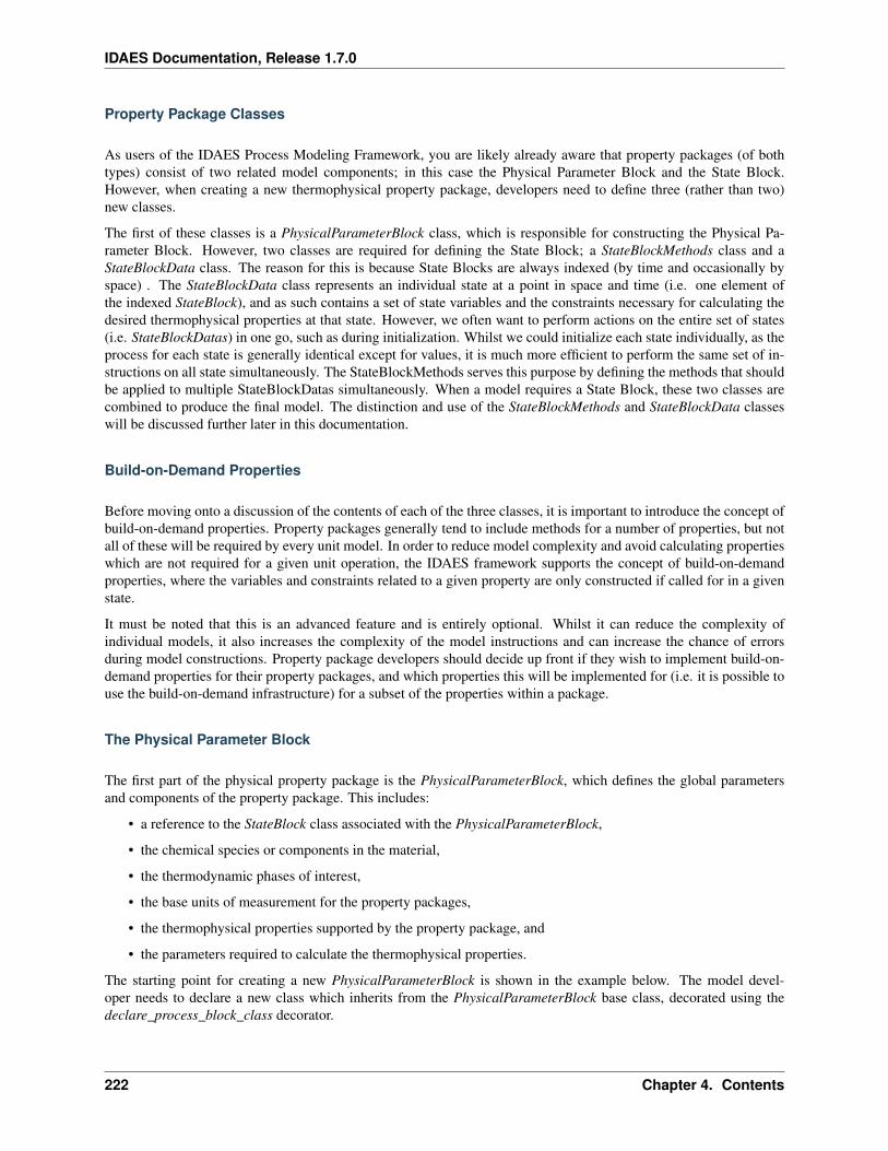
IDAES Documentation, Release 1.7.0
Property Package Classes
As users of the IDAES Process Modeling Framework, you are likely already aware that property packages (of bothtypes) consist of two related model components; in this case the Physical Parameter Block and the State Block.However, when creating a new thermophysical property package, developers need to define three (rather than two)new classes.
The first of these classes is a PhysicalParameterBlock class, which is responsible for constructing the Physical Pa-rameter Block. However, two classes are required for defining the State Block; a StateBlockMethods class and aStateBlockData class. The reason for this is because State Blocks are always indexed (by time and occasionally byspace) . The StateBlockData class represents an individual state at a point in space and time (i.e. one element ofthe indexed StateBlock), and as such contains a set of state variables and the constraints necessary for calculating thedesired thermophysical properties at that state. However, we often want to perform actions on the entire set of states(i.e. StateBlockDatas) in one go, such as during initialization. Whilst we could initialize each state individually, as theprocess for each state is generally identical except for values, it is much more efficient to perform the same set of in-structions on all state simultaneously. The StateBlockMethods serves this purpose by defining the methods that shouldbe applied to multiple StateBlockDatas simultaneously. When a model requires a State Block, these two classes arecombined to produce the final model. The distinction and use of the StateBlockMethods and StateBlockData classeswill be discussed further later in this documentation.
Build-on-Demand Properties
Before moving onto a discussion of the contents of each of the three classes, it is important to introduce the concept ofbuild-on-demand properties. Property packages generally tend to include methods for a number of properties, but notall of these will be required by every unit model. In order to reduce model complexity and avoid calculating propertieswhich are not required for a given unit operation, the IDAES framework supports the concept of build-on-demandproperties, where the variables and constraints related to a given property are only constructed if called for in a givenstate.
It must be noted that this is an advanced feature and is entirely optional. Whilst it can reduce the complexity ofindividual models, it also increases the complexity of the model instructions and can increase the chance of errorsduring model constructions. Property package developers should decide up front if they wish to implement build-on-demand properties for their property packages, and which properties this will be implemented for (i.e. it is possible touse the build-on-demand infrastructure) for a subset of the properties within a package.
The Physical Parameter Block
The first part of the physical property package is the PhysicalParameterBlock, which defines the global parametersand components of the property package. This includes:
• a reference to the StateBlock class associated with the PhysicalParameterBlock,
• the chemical species or components in the material,
• the thermodynamic phases of interest,
• the base units of measurement for the property packages,
• the thermophysical properties supported by the property package, and
• the parameters required to calculate the thermophysical properties.
The starting point for creating a new PhysicalParameterBlock is shown in the example below. The model devel-oper needs to declare a new class which inherits from the PhysicalParameterBlock base class, decorated using thedeclare_process_block_class decorator.
222 Chapter 4. Contents
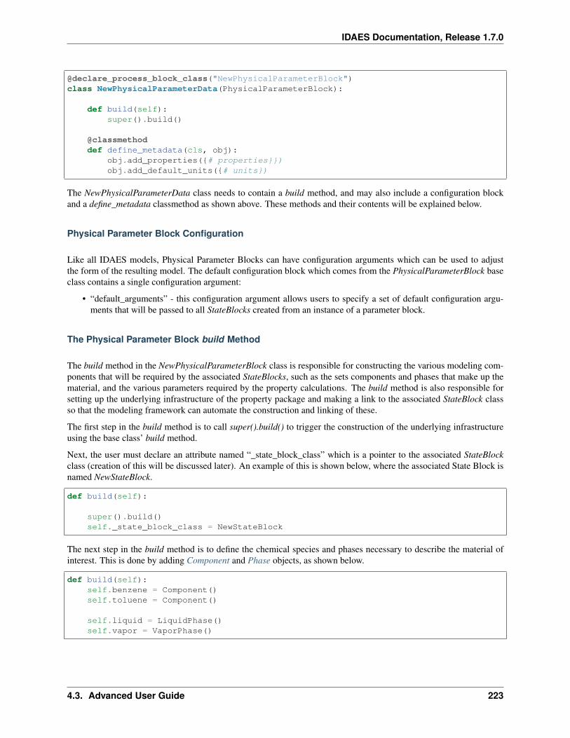
IDAES Documentation, Release 1.7.0
@declare_process_block_class("NewPhysicalParameterBlock")class NewPhysicalParameterData(PhysicalParameterBlock):
def build(self):super().build()
@classmethoddef define_metadata(cls, obj):
obj.add_properties(# properties)obj.add_default_units(# units)
The NewPhysicalParameterData class needs to contain a build method, and may also include a configuration blockand a define_metadata classmethod as shown above. These methods and their contents will be explained below.
Physical Parameter Block Configuration
Like all IDAES models, Physical Parameter Blocks can have configuration arguments which can be used to adjustthe form of the resulting model. The default configuration block which comes from the PhysicalParameterBlock baseclass contains a single configuration argument:
• “default_arguments” - this configuration argument allows users to specify a set of default configuration argu-ments that will be passed to all StateBlocks created from an instance of a parameter block.
The Physical Parameter Block build Method
The build method in the NewPhysicalParameterBlock class is responsible for constructing the various modeling com-ponents that will be required by the associated StateBlocks, such as the sets components and phases that make up thematerial, and the various parameters required by the property calculations. The build method is also responsible forsetting up the underlying infrastructure of the property package and making a link to the associated StateBlock classso that the modeling framework can automate the construction and linking of these.
The first step in the build method is to call super().build() to trigger the construction of the underlying infrastructureusing the base class’ build method.
Next, the user must declare an attribute named “_state_block_class” which is a pointer to the associated StateBlockclass (creation of this will be discussed later). An example of this is shown below, where the associated State Block isnamed NewStateBlock.
def build(self):
super().build()self._state_block_class = NewStateBlock
The next step in the build method is to define the chemical species and phases necessary to describe the material ofinterest. This is done by adding Component and Phase objects, as shown below.
def build(self):self.benzene = Component()self.toluene = Component()
self.liquid = LiquidPhase()self.vapor = VaporPhase()
4.3. Advanced User Guide 223
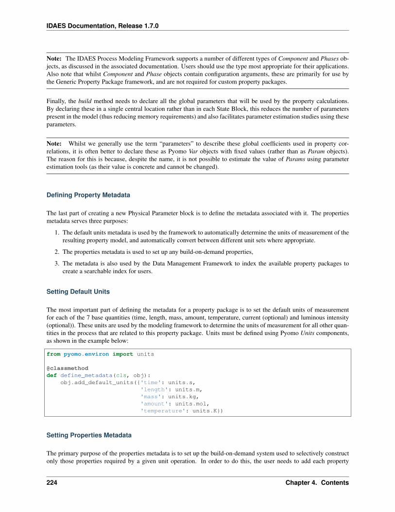
IDAES Documentation, Release 1.7.0
Note: The IDAES Process Modeling Framework supports a number of different types of Component and Phases ob-jects, as discussed in the associated documentation. Users should use the type most appropriate for their applications.Also note that whilst Component and Phase objects contain configuration arguments, these are primarily for use bythe Generic Property Package framework, and are not required for custom property packages.
Finally, the build method needs to declare all the global parameters that will be used by the property calculations.By declaring these in a single central location rather than in each State Block, this reduces the number of parameterspresent in the model (thus reducing memory requirements) and also facilitates parameter estimation studies using theseparameters.
Note: Whilst we generally use the term “parameters” to describe these global coefficients used in property cor-relations, it is often better to declare these as Pyomo Var objects with fixed values (rather than as Param objects).The reason for this is because, despite the name, it is not possible to estimate the value of Params using parameterestimation tools (as their value is concrete and cannot be changed).
Defining Property Metadata
The last part of creating a new Physical Parameter block is to define the metadata associated with it. The propertiesmetadata serves three purposes:
1. The default units metadata is used by the framework to automatically determine the units of measurement of theresulting property model, and automatically convert between different unit sets where appropriate.
2. The properties metadata is used to set up any build-on-demand properties,
3. The metadata is also used by the Data Management Framework to index the available property packages tocreate a searchable index for users.
Setting Default Units
The most important part of defining the metadata for a property package is to set the default units of measurementfor each of the 7 base quantities (time, length, mass, amount, temperature, current (optional) and luminous intensity(optional)). These units are used by the modeling framework to determine the units of measurement for all other quan-tities in the process that are related to this property package. Units must be defined using Pyomo Units components,as shown in the example below:
from pyomo.environ import units
@classmethoddef define_metadata(cls, obj):
obj.add_default_units('time': units.s,'length': units.m,'mass': units.kg,'amount': units.mol,'temperature': units.K)
Setting Properties Metadata
The primary purpose of the properties metadata is to set up the build-on-demand system used to selectively constructonly those properties required by a given unit operation. In order to do this, the user needs to add each property
224 Chapter 4. Contents
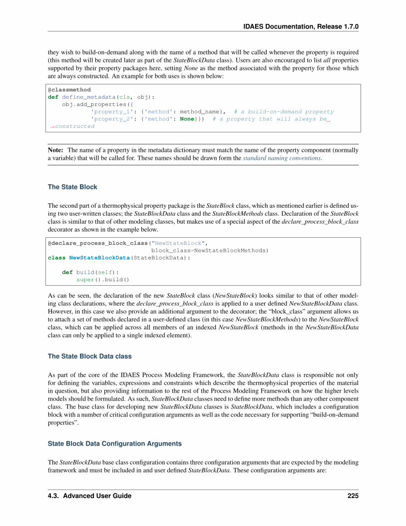
IDAES Documentation, Release 1.7.0
they wish to build-on-demand along with the name of a method that will be called whenever the property is required(this method will be created later as part of the StateBlockData class). Users are also encouraged to list all propertiessupported by their property packages here, setting None as the method associated with the property for those whichare always constructed. An example for both uses is shown below:
@classmethoddef define_metadata(cls, obj):
obj.add_properties('property_1': 'method': method_name, # a build-on-demand property'property_2': 'method': None) # a property that will always be
→˓constructed
Note: The name of a property in the metadata dictionary must match the name of the property component (normallya variable) that will be called for. These names should be drawn form the standard naming conventions.
The State Block
The second part of a thermophysical property package is the StateBlock class, which as mentioned earlier is defined us-ing two user-written classes; the StateBlockData class and the StateBlockMethods class. Declaration of the StateBlockclass is similar to that of other modeling classes, but makes use of a special aspect of the declare_process_block_classdecorator as shown in the example below.
@declare_process_block_class("NewStateBlock",block_class=NewStateBlockMethods)
class NewStateBlockData(StateBlockData):
def build(self):super().build()
As can be seen, the declaration of the new StateBlock class (NewStateBlock) looks similar to that of other model-ing class declarations, where the declare_process_block_class is applied to a user defined NewStateBlockData class.However, in this case we also provide an additional argument to the decorator; the “block_class” argument allows usto attach a set of methods declared in a user-defined class (in this case NewStateBlockMethods) to the NewStateBlockclass, which can be applied across all members of an indexed NewStateBlock (methods in the NewStateBlockDataclass can only be applied to a single indexed element).
The State Block Data class
As part of the core of the IDAES Process Modeling Framework, the StateBlockData class is responsible not onlyfor defining the variables, expressions and constraints which describe the thermophysical properties of the materialin question, but also providing information to the rest of the Process Modeling Framework on how the higher levelsmodels should be formulated. As such, StateBlockData classes need to define more methods than any other componentclass. The base class for developing new StateBlockData classes is StateBlockData, which includes a configurationblock with a number of critical configuration arguments as well as the code necessary for supporting “build-on-demandproperties”.
State Block Data Configuration Arguments
The StateBlockData base class configuration contains three configuration arguments that are expected by the modelingframework and must be included in and user defined StateBlockData. These configuration arguments are:
4.3. Advanced User Guide 225
IDAES Documentation, Release 1.7.0
• “parameters” – this argument is used to provide a link back to the associated PhysicalParameterBlock, and isgenerally automatically passed to the StateBlock when it is constructed.
• “defined_state” – this argument is used to indicate whether this state represents a point in the process where allstate variables are defined. The most common case for this is for inlets to unit models, where all inlets states areknown from the outlet of the previous unit model. In these cases, it is not possible to write certain constraints,such as the sum of mole fractions, without over specifying the system of equations; this argument identifiesthese cases so that generation of these constraints can be automatically skipped.
• “has_phase_equilibrium” – this argument indicates whether phase equilibrium will be considered for this state.Phase equilibrium constraints decrease the degrees of freedom in the system thus it is important to determinewhen and where these constraints should be written. Note that equilibrium constraints can never be writtenfor cases where the state is fully defined (as above), thus both this and the defined_state arguments must beconsidered when determining whether to include equilibrium constraints.
The State Block build Method
As with all IDAES components, the build method forms the core of a StateBlockData class, and contains the in-structions on how to construct the variables, expressions and constraints required by the thermophysical model. Asusual, the first step in the build method should be to call super().build() to trigger the construction of the underlyingcomponents required for State Blocks to function.
State Variables and Properties
The most important part of the construction of a State Block is defining the necessary set of variables, expressionand constraints that make up the property model. There are many different ways in which these can be defined andformulated, and there is no single “best” way to do this; different approaches may work better for different applications.However, there are some general rules that should be followed when defining the variables which make up a StateBlock.
1. All state variables and properties should use the IDAES naming conventions. Standard names allow linkingbetween different types of models to be automated, as no cross-referencing of names is required.
2. All properties within a property package should use a consistent set of base units. This is most easily accom-plished by selecting a set of units for the 7 base SI quantities (time, length, mass, amount, temperature, currentand luminous intensity) and deriving units for all quantities from these. Modelers should also select units basedsolely on convenience or ease of use – scaling of variables and equations is better handled separately using theIDAES scaling tools.
Beyond these requirements, modelers are free to choose the form of their model to best suit theirs needs and makethe most tractable problem possible. Modelers are also free to combine variable and constraints with expression forsome quantities as needed. The IDAES Process Modeling Framework is concerned only that the expected quantitiesare present (i.e. the expected variable/expression names), not their exact form or how they are calculated.
As described throughout this page, IDAES supports “build-on-demand” for property correlations. Details on how todefine methods for building properties on demand is demonstrated in the tutorials (see link at bottom of page).
Required Methods
As the foundation of the entire Process Modeling Framework, the definition of a new StateBlockData class needs toinclude a number of methods that the framework relies on for determining the formulation of the higher level models.
Below is a list of the required methods, along with a short description.
226 Chapter 4. Contents
IDAES Documentation, Release 1.7.0
• get_material_flow_basis(block) – this method is used to define the basis on which material balance terms willbe expressed. This is used by the framework to automatically convert between mass and mole basis if required,and the method needs to return a MaterialFlowBasis Enum.
• get_material_flow_terms(block, phase, component) – this method is used to determine the form of the materialflow terms that are constructed as part of the material balance equations in each unit model. This method needsto take three arguments; a reference to the current state block, a phase name and a component name, and mustreturn an expression for the material flow term for the given phase and component.
• get_material_density_terms(block, phase, component) – similar to the get_material_flow_terms method, thismethod is used to determine the form of the density term which should be used when constructing materialholdup terms in the material balances. This method also needs to take three arguments; a reference to thecurrent state block, a phase name and a component name, and must return an expression for the material densityterm for the given phase and component.
• get_material_diffusion_terms(block, phase, component) – Support for this is not currently implemented.
• get_enthalpy_flow_terms(block, phase) – this method is used to determine the form of the enthalpy flow termsthat are constructed as part of the energy balance equations in each unit model. This method needs to taketwo arguments; a reference to the current state block and a phase name, and must return an expression for theenthalpy flow term for the given phase and component.
• get_energy_density_terms(block, phase) – this method is used to determine the form of the energy density termsthat are required for the holdup terms in the energy balance equations. This method needs to take two arguments;a reference to the current state block and a phase name, and must return an expression for the energy densityterm for the given phase and component. Note that the holdup/density term needs to be in terms of internalenergy, not enthalpy.
• get_energy_diffusion_terms(block, phase) – Support for this is not currently implemented.
• default_material_balance_type(block) – this method is used to set a default for the type of material balance tobe written by a Control Volume if the user does not specify which type to use. This method needs to return aMaterialBalanceType Enum.
• default_energy_balance_type(block) – this method is used to set a default for the type of energy balance to bewritten by a Control Volume if the user does not specify which type to use. This method needs to return aEnergyBalanceType Enum.
• define_state_vars(block) – this method is used to define the set of state variables which should be considered thestate variables for the property package, and is used in a number of methods associated with model initializationto determine which variables should be fixed. This method must return a Python dict, where the keys are thevariable name as a string, and the values are the variables.
• define_port_members(block) – similar to the define_state_vars method, this method is used to define what vari-ables should be part of the inlet/outlet ports of a unit model. In many cases, these variables are equivalent to thestate variables of the property package and if so this method can be skipped (if undefined define_state_vars iscalled instead). This method is similar to the one in the above method, however in this case the key names canbe defined by the user for improved readability (instead of having to be the variable name).
• define_display_vars(block) – similar again to the define_state_vars method, this method is used to define a setof variables which should be used when generating the output of the report method for this property package.Again, this is often the same as the state variables, but allows modelers to include additional variables beyondjust the state variables (or port members). Similarly to the define_port_members method, this method can beskipped (in which case it defaults to define_state_vars) and the key names in the dict can be defined by the user.
4.3. Advanced User Guide 227
IDAES Documentation, Release 1.7.0
The State Block Methods class
The purpose of the StateBlockMethods class is to define methods which can be applied to to an entire set of indexedStateBlocks simultaneously. Whilst the StateBlockData class contain the instructions for how to build the variables andconstraints that describe the state of a material at a single point in space and time, the StateBlockMethods class definedmethods for interacting with multiple states across space and time simultaneously. The most common application forthis is during initialization of StateBlocks, where the same set of instructions needs to to be performed on each indexedstate; whilst this could be done by iterating over each state and performing the set of instructions, it is generally moreefficient to apply the instructions simultaneously across all states.
Declaration and Base Class
Due to the way the StateBlockMethods class is provided to the declare_process_block_class decorator on the New-StateBlockData class, this is one of the few cases where the decorator is not required when declaring a class withinIDAES. An example of declaring a new StateBlockMethods class is shown below, using the StateBlock base class:
class NewStateBlockMethods(StateBlock):
As the StateBlockMethods class is designed to contain methods that can be applied to multiple existing StateBlockDataobject, rather than construct a model itself, the StateBlockMethods class does not need a build method either, nor is itnecessary to call super().build() as is normal for other modeling components.
Instead, the StateBlockMethods class should contain a set of methods which can be called and applied to an indexedStateBlock as required. The two methods that must be declared are:
• initialize
• release_state
The initialize and release_state Methods
When initializing a unit model, most IDAES models use a hierarchical approach where each state in the model (i.e.each StateBlockData) is first initialized at some initial state, after which the unit model attempts to build up andsolve the material, energy and momentum balances, etc. The purpose of the initialize method is to provide a set ofinstructions which can take a state from its initial state to a solvable final state at the set of initial conditions (providedas arguments to the initialize method). This is generally done by:
1. fixing the state variables at the initial conditions,
2. performing a series of steps to build up the final solution,
3. solving the full state model, and
4. unfixing the state variables (unless they were already fixed when the process began).
However, in order to fully initialize the unit operation (which contains these material state) it is necessary for the unitmodel to be fully defined (with zero degrees of freedom, i.e. a square model). In order for this to be true however, itis necessary for the inlet states to remain fixed until the unit model has finished initializing. This requires step 4 aboveto be postponed for inlet states until the unit model has finished initializing, thus the above process is broken into twomethods.
1. The initialize method covers steps 1-3 above, and is called at the beginning of the unit model initializationprocess.
2. The release_state method covers step 4; for inlet states this is called when the unit model has finished initializa-tion, whilst for all other states it is called immediately by the initialize methods when it finishes.
More details on writing initialization methods will be provided elsewhere in the documentation of tutorials.
228 Chapter 4. Contents
IDAES Documentation, Release 1.7.0
Tutorials
Tutorials demonstrating how to create custom property packages are being developed. Once they are created, they willbe found here.
Custom Reaction Packages
• What Belongs in a Reaction Package?
• Reaction Package Classes
• Build-on-Demand Properties
• The Reaction Parameter Block
– Reaction Parameter Block Configuration
– The Reaction Parameter Block build Method
– Defining Reaction Metadata
* Setting Default Units
* Setting Reaction Metadata
• The Reaction Block
– The Reaction Block Data Class
* Reaction Block Data Configuration Arguments
* The Reaction Block build Method
* Variables and Properties
* Required Methods
– The Reaction Block Methods Class
* The initialize Method
• Tutorials
Warning: This section is currently being developed
Chemical reactions are a fundamental part of most processes, and models for these come in a wide range of differentforms. Much like thermophysical property packages, the ability for users to define custom reaction formulations is akey aspect of the IDAES modeling paradigm.
Reaction packages within IDAES share many similarities with thermophysical property packages, both in form andcontent. Rather than repeat much of that documentation here, users should start by reading the thermophysical propertypackage documentation, as this document will focus on the content of the reaction package.
What Belongs in a Reaction Package?
Chemical reactions are fundamentally governed by the same laws of thermodynamics as thermophysical properties,thus the separation of these into thermophysical and reaction packages is somewhat arbitrary. In IDAES, this separa-
4.3. Advanced User Guide 229
IDAES Documentation, Release 1.7.0
tion between thermophysical and reaction packages was based on their expected frequency of use. All unit operationsrequire some set of property calculations (e.g. enthalpy) and these types of calculations were grouped in the thermo-physical package, whereas only a small subset of unit operations have chemical reactions and these types of calcula-tions were grouped in the reaction package. This separation benefits the user in that they only need to be concernedabout reactions in the unit operations that require them.
Important: For the context of IDAES, chemical reactions are defined as phenomena where one chemical species isconverted into another. This includes both rate limited and equilibrium reactions.
On the other hand, phase equilibrium phenomena (where a chemical species changes phase) are handled via thethermophysical property package.
However, users should note that reaction properties are fundamentally linked to the thermophysical properties, and thata reaction package should only be used with the thermophysical property package they were developed with (in theoryat least). Due to this, when a reactions package is added to a model it must be coupled to a thermophysical propertypackage. The modeling framework performs some limited checks to ensure the two packages are compatible (e.g.same set of base units) and that each reaction packages is only used in conjunction with its coupled thermophysicalproperty package in unit models.
Reaction Package Classes
Like thermophysical property packages, reaction property packages consist of two related model components; theReaction Parameter Block and the Reaction Block, which are analogous to the Physical Parameter Block and StateBlock components. Similarly, when creating a custom reaction package users need to declare three new classes; theReaction Parameter Block Data class, the Reaction Block Data class and the Reaction Block Methods class.
Build-on-Demand Properties
IDAES reaction packages also support build-on-demand properties using the same approach as for thermophysicalproperties.
The Reaction Parameter Block
The first part of the reaction package is the ReactionParameterBlock, which defines the global parameters and compo-nents of the property package. This includes:
• a reference to the ReactionBlock class associated with the ReactionParameterBlock,
• a Pyomo Set listing names for all rate-based reactions,
• a dict defining stoichiometric coefficients for all rate-based reactions,
• a Pyomo Set listing names for all equilibrium reactions,
• a dict defining stoichiometric coefficients for all equilibrium reactions,
• the base units of measurement for the property packages,
• the reaction properties supported by the property package, and
• the parameters required to calculate the reaction properties.
The starting point for creating a new ReactionParameterBlock is shown in the example below. The model devel-oper needs to declare a new class which inherits from the ReactionParameterBlock base class, decorated using thedeclare_process_block_class decorator.
230 Chapter 4. Contents
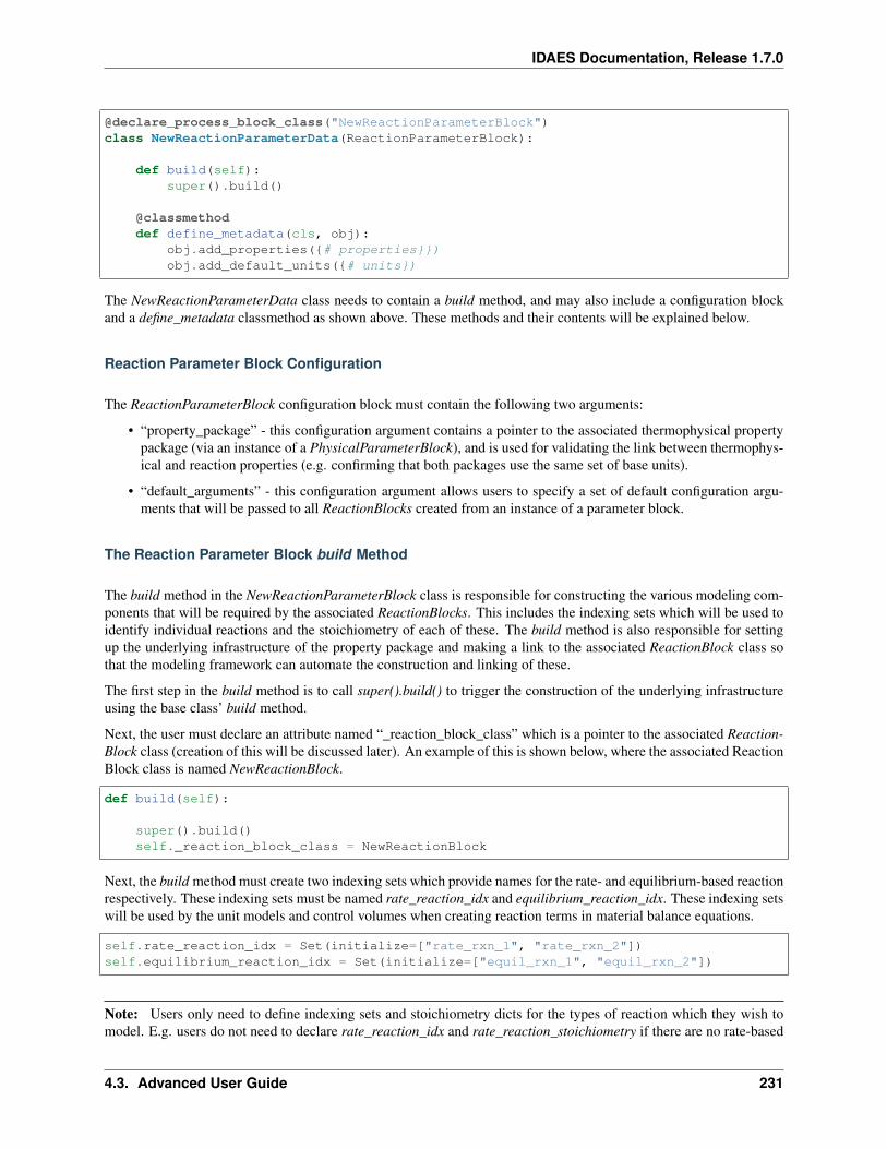
IDAES Documentation, Release 1.7.0
@declare_process_block_class("NewReactionParameterBlock")class NewReactionParameterData(ReactionParameterBlock):
def build(self):super().build()
@classmethoddef define_metadata(cls, obj):
obj.add_properties(# properties)obj.add_default_units(# units)
The NewReactionParameterData class needs to contain a build method, and may also include a configuration blockand a define_metadata classmethod as shown above. These methods and their contents will be explained below.
Reaction Parameter Block Configuration
The ReactionParameterBlock configuration block must contain the following two arguments:
• “property_package” - this configuration argument contains a pointer to the associated thermophysical propertypackage (via an instance of a PhysicalParameterBlock), and is used for validating the link between thermophys-ical and reaction properties (e.g. confirming that both packages use the same set of base units).
• “default_arguments” - this configuration argument allows users to specify a set of default configuration argu-ments that will be passed to all ReactionBlocks created from an instance of a parameter block.
The Reaction Parameter Block build Method
The build method in the NewReactionParameterBlock class is responsible for constructing the various modeling com-ponents that will be required by the associated ReactionBlocks. This includes the indexing sets which will be used toidentify individual reactions and the stoichiometry of each of these. The build method is also responsible for settingup the underlying infrastructure of the property package and making a link to the associated ReactionBlock class sothat the modeling framework can automate the construction and linking of these.
The first step in the build method is to call super().build() to trigger the construction of the underlying infrastructureusing the base class’ build method.
Next, the user must declare an attribute named “_reaction_block_class” which is a pointer to the associated Reaction-Block class (creation of this will be discussed later). An example of this is shown below, where the associated ReactionBlock class is named NewReactionBlock.
def build(self):
super().build()self._reaction_block_class = NewReactionBlock
Next, the build method must create two indexing sets which provide names for the rate- and equilibrium-based reactionrespectively. These indexing sets must be named rate_reaction_idx and equilibrium_reaction_idx. These indexing setswill be used by the unit models and control volumes when creating reaction terms in material balance equations.
self.rate_reaction_idx = Set(initialize=["rate_rxn_1", "rate_rxn_2"])self.equilibrium_reaction_idx = Set(initialize=["equil_rxn_1", "equil_rxn_2"])
Note: Users only need to define indexing sets and stoichiometry dicts for the types of reaction which they wish tomodel. E.g. users do not need to declare rate_reaction_idx and rate_reaction_stoichiometry if there are no rate-based
4.3. Advanced User Guide 231
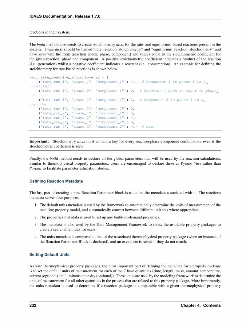
IDAES Documentation, Release 1.7.0
reactions in their system.
The build method also needs to create stoichiometry dicts for the rate- and equilibrium-based reactions present in thesystem. These dicts should be named “rate_reaction_stoichiometry” and “equilibrium_reaction_stoichiometry” andhave keys with the form (reaction_index, phase, component) and values equal to the stoichiometric coefficient forthe given reaction, phase and component. A positive stoichiometric coefficient indicates a product of the reaction(i.e. generation) whilst a negative coefficient indicates a reactant (i.e. consumption). An example for defining thestoichiometry for rate-based reactions is shown below.
self.rate_reaction_stoichiometry = ("rate_rxn_1", "phase_1", "component_1"): -1, # Component 1 in phase 1 is a
→˓reactant("rate_rxn_1", "phase_2", "component_1"): 0, # Reaction 1 does no occur is phase
→˓2("rate_rxn_1", "phase_1", "component_2"): 2, # Component 2 in phase 1 is a
→˓product("rate_rxn_1", "phase_2", "component_2"): 0,("rate_rxn_2", "phase_1", "component_1"): 0,("rate_rxn_2", "phase_2", "component_1"): -1,("rate_rxn_2", "phase_1", "component_2"): 0,("rate_rxn_2", "phase_2", "component_2"): -1 # etc.
Important: Stoichiometry dicts must contain a key for every reaction-phase-component combination, even if thestoichiometric coefficient is zero.
Finally, the build method needs to declare all the global parameters that will be used by the reaction calculations.Similar to thermophysical property parameters, users are encouraged to declare these as Pyomo Vars rather thanParams to facilitate parameter estimation studies.
Defining Reaction Metadata
The last part of creating a new Reaction Parameter block is to define the metadata associated with it. The reactionsmetadata serves four purposes:
1. The default units metadata is used by the framework to automatically determine the units of measurement of theresulting property model, and automatically convert between different unit sets where appropriate.
2. The properties metadata is used to set up any build-on-demand properties,
3. The metadata is also used by the Data Management Framework to index the available property packages tocreate a searchable index for users.
4. The units metadata is compared to that of the associated thermophysical property package (when an instance ofthe Reaction Parameter Block is declared), and an exception is raised if they do not match.
Setting Default Units
As with thermophysical property packages, the most important part of defining the metadata for a property packageis to set the default units of measurement for each of the 7 base quantities (time, length, mass, amount, temperature,current (optional) and luminous intensity (optional)). These units are used by the modeling framework to determine theunits of measurement for all other quantities in the process that are related to this property package. More importantly,the units metadata is used to determine if a reaction package is comparable with a given thermophysical property
232 Chapter 4. Contents
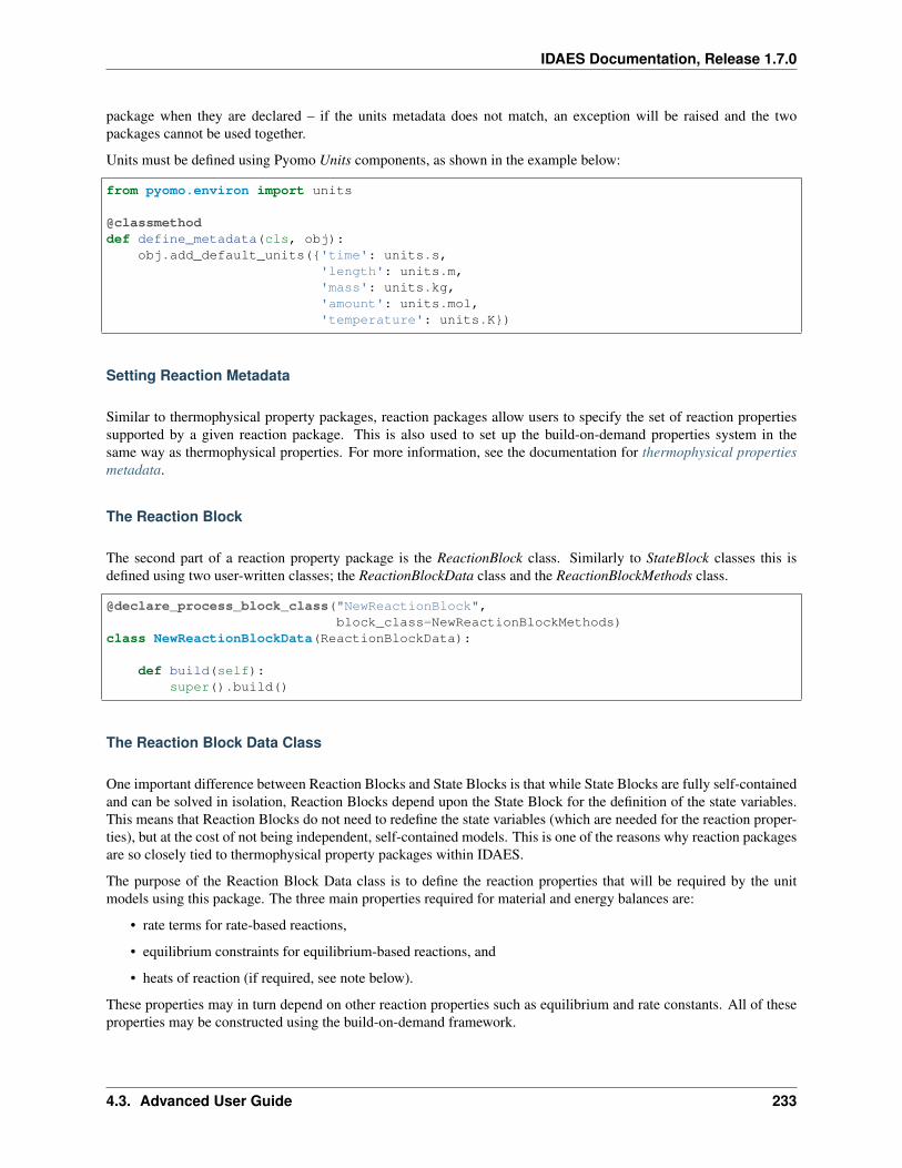
IDAES Documentation, Release 1.7.0
package when they are declared – if the units metadata does not match, an exception will be raised and the twopackages cannot be used together.
Units must be defined using Pyomo Units components, as shown in the example below:
from pyomo.environ import units
@classmethoddef define_metadata(cls, obj):
obj.add_default_units('time': units.s,'length': units.m,'mass': units.kg,'amount': units.mol,'temperature': units.K)
Setting Reaction Metadata
Similar to thermophysical property packages, reaction packages allow users to specify the set of reaction propertiessupported by a given reaction package. This is also used to set up the build-on-demand properties system in thesame way as thermophysical properties. For more information, see the documentation for thermophysical propertiesmetadata.
The Reaction Block
The second part of a reaction property package is the ReactionBlock class. Similarly to StateBlock classes this isdefined using two user-written classes; the ReactionBlockData class and the ReactionBlockMethods class.
@declare_process_block_class("NewReactionBlock",block_class=NewReactionBlockMethods)
class NewReactionBlockData(ReactionBlockData):
def build(self):super().build()
The Reaction Block Data Class
One important difference between Reaction Blocks and State Blocks is that while State Blocks are fully self-containedand can be solved in isolation, Reaction Blocks depend upon the State Block for the definition of the state variables.This means that Reaction Blocks do not need to redefine the state variables (which are needed for the reaction proper-ties), but at the cost of not being independent, self-contained models. This is one of the reasons why reaction packagesare so closely tied to thermophysical property packages within IDAES.
The purpose of the Reaction Block Data class is to define the reaction properties that will be required by the unitmodels using this package. The three main properties required for material and energy balances are:
• rate terms for rate-based reactions,
• equilibrium constraints for equilibrium-based reactions, and
• heats of reaction (if required, see note below).
These properties may in turn depend on other reaction properties such as equilibrium and rate constants. All of theseproperties may be constructed using the build-on-demand framework.
4.3. Advanced User Guide 233
IDAES Documentation, Release 1.7.0
All reaction properties depend upon the state of the material, which is defined in the State Block; thus it is necessary toreference the associated State Block whenever these are needed. In order to facilitate this, the ReactionBlockData baseclass establishes a reference to the associated State Block which users can use to obtain state variables and propertiesfrom the State Block. For example, temperature can be referenced from the state block as shown below:
temperature = self.state_ref.temperature
Note: There are multiple ways in which heat of reaction may be included in a model, and users should consider whichis most suitable for their application. The two most common approaches are to include an explicit heat of reactionterm in the energy balance equations, or to incorporate heat of reaction into the specific enthalpy terms (generally viaheats of formation). The IDAES Process Modeling Framework supports both of these approaches.
Reaction Block Data Configuration Arguments
The ReactionBlockData base class defines three configuration arguments that are required for all Reaction Block Dataclasses.
• “parameters” – this argument is used to provide a link back to the associated ReactionParameterBlock, and isgenerally automatically passed to the ReactionBlock when it is constructed.
• “state_block” – this argument is used to provide a link to the State Block associated with this Reaction Block,as is generally passed to the ReactionBlock by the unit model when it is constructed. This argument is used tothe state_ref attribute shown above for referencing properties from the State Block.
• “has_equilibrium” – this argument indicates whether equilibrium reaction will be considered for this state. Inmost cases, this argument will always be True, however this allows users the ability to turn off equilibriumreactions if they desire.
The Reaction Block build Method
As with all IDAES components, the build method forms the core of a ReactionBlockData class, and contains theinstructions on how to construct the variables, expressions and constraints required by the reaction model. As usual, thefirst step in the build method should be to call super().build() to trigger the construction of the underlying componentsrequired for Reaction Blocks to function.
Variables and Properties
The same set of guidelines for defining thermophysical properties apply to reaction properties, which can be foundhere.
Required Methods
In addition to the build method, Reaction Blocks require one additional method which is used to define the basis forthe reaction terms.
• get_reaction_rate_basis - must return a MaterialFlowBasis Enum, and is used to automatically convert reactionterms between mass and mole basis in control volumes.
234 Chapter 4. Contents
IDAES Documentation, Release 1.7.0
The Reaction Block Methods Class
The Reaction Block Methods class is very similar to the State Block Methods class. The Reaction Block Methodsclass needs to contain an initialize method (however a release_state method is not required as Reaction Blocks do notcontain state variables).
The initialize Method
Initialization of Reaction Blocks is complicated by the fact that they depend upon the State Block for the state variables,and thus cannot be solved as a stand-alone model. Within the wider IDAES modeling framework, this is handled byinitializing the Reaction Block after the State Block initialization method has been called (and thus all state variablesand properties are initialized) but before the release_State method is called (thus all state variables are fixed). Thus,the Reaction Block can assume that the state is fully defined and initialized (although it may not be possible to use asolver as part of the Reaction Block’s initialization procedure).
However, Reaction Blocks also tend to be much simpler than State Blocks, involving fewer properties which are gen-erally much less tightly coupled (most reaction properties are functions solely of the state variables), which simplifiesthe requirements of initializing the sub-model.
Tutorials
Tutorials demonstrating how to create custom reaction packages are being developed. Once they are created, they willbe found here.
4.4 Tutorials and Examples
Tutorials and examples for IDAES are located on the examples online documentation page.
These tutorials and examples are maintained on the IDAES examples repository. You can install the associated fileswithin an IDAES installation by running idaes get-examples in a command-line shell, additional details areprovided here.
If you are new to IDAES, it is strongly recommended to start with the tutorials.
If you want to develop custom unit and property models refer to the advanced user guide.
4.5 Technical Specifications
4.5.1 Core
Process Block
Example
ProcessBlock is used to simplify inheritance of Pyomo’s Block. The code below provides an example of how a newProcessBlock class can be implemented. The new ProcessBlock class has a ConfigBlock that allows each element ofthe block to be passed configuration options that affect how a block is built. ProcessBlocks have a rule set by defaultthat calls the build method of the contained ProcessBlockData class.
4.4. Tutorials and Examples 235
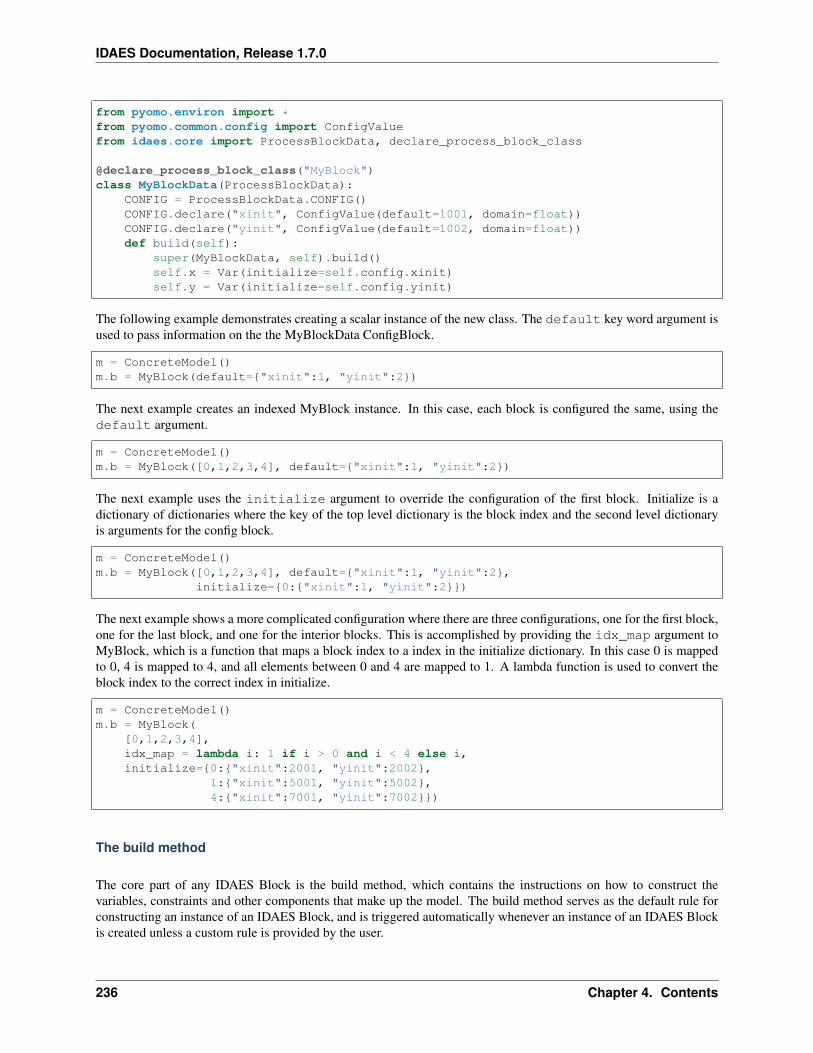
IDAES Documentation, Release 1.7.0
from pyomo.environ import *from pyomo.common.config import ConfigValuefrom idaes.core import ProcessBlockData, declare_process_block_class
@declare_process_block_class("MyBlock")class MyBlockData(ProcessBlockData):
CONFIG = ProcessBlockData.CONFIG()CONFIG.declare("xinit", ConfigValue(default=1001, domain=float))CONFIG.declare("yinit", ConfigValue(default=1002, domain=float))def build(self):
super(MyBlockData, self).build()self.x = Var(initialize=self.config.xinit)self.y = Var(initialize=self.config.yinit)
The following example demonstrates creating a scalar instance of the new class. The default key word argument isused to pass information on the the MyBlockData ConfigBlock.
m = ConcreteModel()m.b = MyBlock(default="xinit":1, "yinit":2)
The next example creates an indexed MyBlock instance. In this case, each block is configured the same, using thedefault argument.
m = ConcreteModel()m.b = MyBlock([0,1,2,3,4], default="xinit":1, "yinit":2)
The next example uses the initialize argument to override the configuration of the first block. Initialize is adictionary of dictionaries where the key of the top level dictionary is the block index and the second level dictionaryis arguments for the config block.
m = ConcreteModel()m.b = MyBlock([0,1,2,3,4], default="xinit":1, "yinit":2,
initialize=0:"xinit":1, "yinit":2)
The next example shows a more complicated configuration where there are three configurations, one for the first block,one for the last block, and one for the interior blocks. This is accomplished by providing the idx_map argument toMyBlock, which is a function that maps a block index to a index in the initialize dictionary. In this case 0 is mappedto 0, 4 is mapped to 4, and all elements between 0 and 4 are mapped to 1. A lambda function is used to convert theblock index to the correct index in initialize.
m = ConcreteModel()m.b = MyBlock(
[0,1,2,3,4],idx_map = lambda i: 1 if i > 0 and i < 4 else i,initialize=0:"xinit":2001, "yinit":2002,
1:"xinit":5001, "yinit":5002,4:"xinit":7001, "yinit":7002)
The build method
The core part of any IDAES Block is the build method, which contains the instructions on how to construct thevariables, constraints and other components that make up the model. The build method serves as the default rule forconstructing an instance of an IDAES Block, and is triggered automatically whenever an instance of an IDAES Blockis created unless a custom rule is provided by the user.
236 Chapter 4. Contents
IDAES Documentation, Release 1.7.0
ProcessBlock Class
idaes.core.process_block.declare_process_block_class(name, block_class=<class’idaes.core.process_block.ProcessBlock’>,doc=”)
Declare a new ProcessBlock subclass.
This is a decorator function for a class definition, where the class is derived from Pyomo’s _BlockData. It createsa ProcessBlock subclass to contain the decorated class. The only requirment is that the subclass of _BlockDatacontain a build() method. The purpose of this decorator is to simplify subclassing Pyomo’s block class.
Parameters
• name – name of class to create
• block_class – ProcessBlock or a subclass of ProcessBlock, this allows you to use asubclass of ProcessBlock if needed. The typical use case for Subclassing ProcessBlock is toimpliment methods that operate on elements of an indexed block.
• doc – Documentation for the class. This should play nice with sphinx.
Returns Decorator function
class idaes.core.process_block.ProcessBlock(*args, **kwargs)ProcessBlock is a Pyomo Block that is part of a system to make Pyomo Block easier to subclass. The maindifference between a Pyomo Block and ProcessBlock from the user perspective is that a ProcessBlock has a ruleassigned by default that calls the build() method for the contained ProcessBlockData objects. The default rulecan be overridden, but the new rule should always call build() for the ProcessBlockData object.
Parameters
• rule (function) – A rule function or None. Default rule calls build().
• concrete (bool) – If True, make this a toplevel model. Default - False.
• ctype (str) – Pyomo ctype of the block. Default - “Block”
• default (dict) – Default ProcessBlockData config
• initialize (dict) – ProcessBlockData config for individual elements. Keys are Block-Data indexes and values are dictionaries described under the “default” argument above.
• idx_map (function) – Function to take the index of a BlockData element and return theindex in the initialize dict from which to read arguments. This can be provided to overidethe default behavior of matching the BlockData index exactly to the index in initialize.
Returns (ProcessBlock) New instance
classmethod base_class_module()Return module of the associated ProcessBase class.
Returns (str) Module of the class.
Raises AttributeError, if no base class module was set, e.g. this class – was not wrapped by thedeclare_process_block_class decorator.
classmethod base_class_name()Name given by the user to the ProcessBase class.
Returns (str) Name of the class.
Raises AttributeError, if no base class name was set, e.g. this class – was not wrapped by thedeclare_process_block_class decorator.
4.5. Technical Specifications 237
IDAES Documentation, Release 1.7.0
class idaes.core.process_base.ProcessBlockData(component)Base class for most IDAES process models and classes.
The primary purpose of this class is to create the local config block to handle arguments provided by the userwhen constructing an object and to ensure that these arguments are stored in the config block.
Additionally, this class contains a number of methods common to all IDAES classes.
build()The build method is called by the default ProcessBlock rule. If a rule is sepecified other than the default itis important to call ProcessBlockData’s build method to put information from the “default” and “initialize”arguments to a ProcessBlock derived class into the BlockData object’s ConfigBlock.
The the build method should usually be overloaded in a subclass derived from ProcessBlockData. Thismethod would generally add Pyomo components such as variables, expressions, and constraints to theobject. It is important for build() methods implimented in derived classes to call build() from the superclass.
Parameters None –
Returns None
fix_initial_conditions(state=’steady-state’)This method fixes the initial conditions for dynamic models.
Parameters state – initial state to use for simulation (default = ‘steady-state’)
Returns : None
flowsheet()This method returns the components parent flowsheet object, i.e. the flowsheet component to which themodel is attached. If the component has no parent flowsheet, the method returns None.
Parameters None –
Returns Flowsheet object or None
unfix_initial_conditions()This method unfixed the initial conditions for dynamic models.
Parameters None –
Returns : None
Flowsheet Block
Default Property Packages
Flowsheet Blocks may assign a property package to use as a default for all UnitModels within the Flowsheet. If aspecific property package is not provided as an argument when constructing a UnitModel, the UnitModel will searchup the model tree until it finds a default property package declared. The UnitModel will use the first default propertypackage it finds during the search, and will return an error if no default is found.
Flowsheet Configuration Arguments
Flowsheet blocks have three configuration arguments which are stored within a Config block (flowsheet.config). Thesearguments can be set by passing arguments when instantiating the class, and are described below:
238 Chapter 4. Contents
IDAES Documentation, Release 1.7.0
• dynamic - indicates whether the flowsheet should be dynamic or steady-state. If dynamic = True, the flowsheetis declared to be a dynamic flowsheet, and the time domain will be a Pyomo ContinuousSet. If dynamic = False,the flowsheet is declared to be steady-state, and the time domain will be an ordered Pyomo Set. For top levelFlowsheets, dynamic defaults to False if not provided. For lower level Flowsheets, the dynamic will take thesame value as that of the parent model if not provided. It is possible to declare steady-state sub-Flowsheets aspart of dynamic Flowsheets if desired, however the reverse is not true (cannot have dynamic Flowsheets withinsteady-state Flowsheets).
• time - a reference to the time domain for the flowsheet. During flowsheet creation, users may provide a Set orContinuousSet that the flowsheet should use as the time domain. If not provided, then the flowsheet will look fora parent flowsheet and set this equal to the parent’s time domain, otherwise a new time domain will be createdand assigned here.
• time_units - used to specify the units of the time domain, and must be a Pyomo Unit object (cannot be acompound unit). This is necessary for dynamic flowsheets, but can be neglected in steady-state cases. In caseswhere the time domain is inherited from a parent flowsheet, the time units will also be inherited.
• time_set - used to initialize the time domain in top-level Flowsheets. When constructing the time domain intop-level Flowsheets, time_set is used to initialize the ContinuousSet or Set created. This can be used to set startand end times, and to establish points of interest in time (e.g. times when disturbances will occur). If dynamic= True, time_set defaults to [0.0, 1.0] if not provided, if dynamic = False time_set defaults to [0.0]. time_set isnot used in sub-Flowsheets and will be ignored.
• default_property_package - can be used to assign the default property package for a Flowsheet. Defaults toNone if not provided.
Flowsheet Classes
class idaes.core.flowsheet_model.FlowsheetBlockData(component)The FlowsheetBlockData Class forms the base class for all IDAES process flowsheet models. The main purposeof this class is to automate the tasks common to all flowsheet models and ensure that the necessary attributes ofa flowsheet model are present.
The most signfiicant role of the FlowsheetBlockData class is to automatically create the time domain for theflowsheet.
build()General build method for FlowsheetBlockData. This method calls a number of sub-methods which auto-mate the construction of expected attributes of flowsheets.
Inheriting models should call super().build.
Parameters None –
Returns None
is_flowsheet()Method which returns True to indicate that this component is a flowsheet.
Parameters None –
Returns True
model_check()This method runs model checks on all unit models in a flowsheet.
This method searches for objects which inherit from UnitModelBlockData and executes the model_checkmethod if it exists.
Parameters None –
4.5. Technical Specifications 239
IDAES Documentation, Release 1.7.0
Returns None
stream_table(true_state=False, time_point=0, orient=’columns’)Method to generate a stream table by iterating over all Arcs in the flowsheet.
Parameters
• true_state – whether the state variables (True) or display variables (False, default)from the StateBlocks should be used in the stream table.
• time_point – point in the time domain at which to create stream table (default = 0)
• orient – whether stream should be shown by columns (“columns”) or rows (“index”)
Returns A pandas dataframe containing stream table information
visualize(model_name, browser=True, overwrite=False)Starts up a flask server that serializes the model and pops up a webpage with the visualization
Parameters
• model_name – The name of the model that flask will use as an argument for the webpage
• browser – If True a browser window/tab will be opened with the visualization. Defaultsto True
• overwrite – If True the visualization ignores any saved visualization file
Returns None
class idaes.core.flowsheet_model.FlowsheetBlock(*args, **kwargs)FlowsheetBlock is a specialized Pyomo block for IDAES flowsheet models, and contains instances of Flow-sheetBlockData.
Parameters
• rule (function) – A rule function or None. Default rule calls build().
• concrete (bool) – If True, make this a toplevel model. Default - False.
• ctype (str) – Pyomo ctype of the block. Default - “Block”
• default (dict) – Default ProcessBlockData config
Keys
dynamic Indicates whether this model will be dynamic, default - useDefault. Validvalues: useDefault - get flag from parent or False, True - set as a dynamic model,False - set as a steady-state model.
time Pointer to the time domain for the flowsheet. Users may provide an existing timedomain from another flowsheet, otherwise the flowsheet will search for a parent with atime domain or create a new time domain and reference it here.
time_set Set of points for initializing time domain. This should be a list of floating pointnumbers, default - [0].
time_units Pyomo Units object describing the units of the time domain. This must bedefined for dynamic simulations, default = None.
default_property_package Indicates the default property package to be used by modelswithin this flowsheet if not otherwise specified, default - None. Valid values: None- no default property package, a ParameterBlock object.
• initialize (dict) – ProcessBlockData config for individual elements. Keys are Block-Data indexes and values are dictionaries described under the “default” argument above.
240 Chapter 4. Contents
IDAES Documentation, Release 1.7.0
• idx_map (function) – Function to take the index of a BlockData element and return theindex in the initialize dict from which to read arguments. This can be provided to overidethe default behavior of matching the BlockData index exactly to the index in initialize.
Returns (FlowsheetBlock) New instance
0D Control Volume Class
Contents
• 0D Control Volume Class
– ControlVolume0DBlock Equations
The ControlVolume0DBlock block is the most commonly used Control Volume class, and is used for systems wherethere is a well-mixed volume of fluid, or where variations in spatial domains are considered to be negligible. Con-trolVolume0DBlock blocks generally contain two StateBlocks - one for the incoming material and one for the materialwithin and leaving the volume - and one StateBlocks.
class idaes.core.control_volume0d.ControlVolume0DBlock(*args, **kwargs)ControlVolume0DBlock is a specialized Pyomo block for IDAES non-discretized control volume blocks, andcontains instances of ControlVolume0DBlockData.
ControlVolume0DBlock should be used for any control volume with a defined volume and distinct inlets andoutlets which does not require spatial discretization. This encompases most basic unit models used in processmodeling.
Parameters
• rule (function) – A rule function or None. Default rule calls build().
• concrete (bool) – If True, make this a toplevel model. Default - False.
• ctype (str) – Pyomo ctype of the block. Default - “Block”
• default (dict) – Default ProcessBlockData config
Keys
dynamic Indicates whether this model will be dynamic, default - useDefault. Validvalues: useDefault - get flag from parent, True - set as a dynamic model, False - setas a steady-state model
has_holdup Indicates whether holdup terms should be constructed or not. Must be Trueif dynamic = True, default - False. Valid values: True - construct holdup terms,False - do not construct holdup terms
property_package Property parameter object used to define property calculations, de-fault - useDefault. Valid values: useDefault - use default package from parentmodel or flowsheet, PropertyParameterObject - a PropertyParameterBlock object.
property_package_args A ConfigBlock with arguments to be passed to a propertyblock(s) and used when constructing these, default - None. Valid values: see prop-erty package for documentation.
reaction_package Reaction parameter object used to define reaction calculations, de-fault - None. Valid values: None - no reaction package, ReactionParameterBlock- a ReactionParameterBlock object.
4.5. Technical Specifications 241
IDAES Documentation, Release 1.7.0
reaction_package_args A ConfigBlock with arguments to be passed to a reactionblock(s) and used when constructing these, default - None. Valid values: see re-action package for documentation.
auto_construct If set to True, this argument will trigger the auto_construct methodwhich will attempt to construct a set of material, energy and momentum balance equa-tions based on the parent unit’s config block. The parent unit must have a config blockwhich derives from CONFIG_Base, default - False. Valid values: True - use auto-matic construction, False - do not use automatic construciton.
• initialize (dict) – ProcessBlockData config for individual elements. Keys are Block-Data indexes and values are dictionaries described under the “default” argument above.
• idx_map (function) – Function to take the index of a BlockData element and return theindex in the initialize dict from which to read arguments. This can be provided to overidethe default behavior of matching the BlockData index exactly to the index in initialize.
Returns (ControlVolume0DBlock) New instance
class idaes.core.control_volume0d.ControlVolume0DBlockData(component)0-Dimensional (Non-Discretised) ControlVolume Class
This class forms the core of all non-discretized IDAES models. It provides methods to build property andreaction blocks, and add mass, energy and momentum balances. The form of the terms used in these constraintsis specified in the chosen property package.
add_geometry()Method to create volume Var in ControlVolume.
Parameters None –
Returns None
add_phase_component_balances(has_rate_reactions=False, has_equilibrium_reactions=False,has_phase_equilibrium=False, has_mass_transfer=False,custom_molar_term=None, custom_mass_term=None)
This method constructs a set of 0D material balances indexed by time, phase and component.
Parameters
• has_rate_reactions – whether default generation terms for rate reactions should beincluded in material balances
• has_equilibrium_reactions – whether generation terms should for chemicalequilibrium reactions should be included in material balances
• has_phase_equilibrium – whether generation terms should for phase equilibriumbehaviour should be included in material balances
• has_mass_transfer – whether generic mass transfer terms should be included inmaterial balances
• custom_molar_term – a Pyomo Expression representing custom terms to be includedin material balances on a molar basis. Expression must be indexed by time, phase list andcomponent list
• custom_mass_term – a Pyomo Expression representing custom terms to be includedin material balances on a mass basis. Expression must be indexed by time, phase list andcomponent list
Returns Constraint object representing material balances
add_phase_energy_balances(*args, **kwargs)Method for adding energy balances (including kinetic energy) indexed by phase to the control volume.
242 Chapter 4. Contents
IDAES Documentation, Release 1.7.0
See specific control volume documentation for details.
add_phase_enthalpy_balances(*args, **kwargs)Method for adding enthalpy balances indexed by phase to the control volume.
See specific control volume documentation for details.
add_phase_momentum_balances(*args, **kwargs)Method for adding momentum balances indexed by phase to the control volume.
See specific control volume documentation for details.
add_phase_pressure_balances(*args, **kwargs)Method for adding pressure balances indexed by phase to the control volume.
See specific control volume documentation for details.
add_reaction_blocks(has_equilibrium=None)This method constructs the reaction block for the control volume.
Parameters
• has_equilibrium – indicates whether equilibrium calculations will be required inreaction block
• package_arguments – dict-like object of arguments to be passed to reaction block asconstruction arguments
Returns None
add_state_blocks(information_flow=<FlowDirection.forward: 1>,has_phase_equilibrium=None)
This method constructs the inlet and outlet state blocks for the control volume.
Parameters
• information_flow – a FlowDirection Enum indicating whether information flowsfrom inlet-to-outlet or outlet-to-inlet
• has_phase_equilibrium – indicates whether equilibrium calculations will be re-quired in state blocks
• package_arguments – dict-like object of arguments to be passed to state blocks asconstruction arguments
Returns None
add_total_component_balances(has_rate_reactions=False, has_equilibrium_reactions=False,has_phase_equilibrium=False, has_mass_transfer=False,custom_molar_term=None, custom_mass_term=None)
This method constructs a set of 0D material balances indexed by time and component.
Parameters
• - whether default generation terms for rate(has_rate_reactions) – reactions should be included in material balances
• - whether generation terms should for (has_equilibrium_reactions)– chemical equilibrium reactions should be included in material balances
• - whether generation terms should for phase(has_phase_equilibrium) – equilibrium behaviour should be included inmaterial balances
• - whether generic mass transfer terms should be(has_mass_transfer) – included in material balances
4.5. Technical Specifications 243
IDAES Documentation, Release 1.7.0
• - a Pyomo Expression representing custom terms to(custom_mass_term) – be included in material balances on a molar basis. Ex-pression must be indexed by time, phase list and component list
• - a Pyomo Expression representing custom terms to – be included inmaterial balances on a mass basis. Expression must be indexed by time, phase list andcomponent list
Returns Constraint object representing material balances
add_total_element_balances(has_rate_reactions=False, has_equilibrium_reactions=False,has_phase_equilibrium=False, has_mass_transfer=False,custom_elemental_term=None)
This method constructs a set of 0D element balances indexed by time.
Parameters
• - whether default generation terms for rate(has_rate_reactions) – reactions should be included in material balances
• - whether generation terms should for (has_equilibrium_reactions)– chemical equilibrium reactions should be included in material balances
• - whether generation terms should for phase(has_phase_equilibrium) – equilibrium behaviour should be included inmaterial balances
• - whether generic mass transfer terms should be(has_mass_transfer) – included in material balances
• - a Pyomo Expression representing custom(custom_elemental_term) – terms to be included in material balances on amolar elemental basis. Expression must be indexed by time and element list
Returns Constraint object representing material balances
add_total_energy_balances(*args, **kwargs)Method for adding a total energy balance (including kinetic energy) to the control volume.
See specific control volume documentation for details.
add_total_enthalpy_balances(has_heat_of_reaction=False, has_heat_transfer=False,has_work_transfer=False, has_enthalpy_transfer=False,custom_term=None)
This method constructs a set of 0D enthalpy balances indexed by time and phase.
Parameters
• - whether terms for heat of reaction should(has_heat_of_reaction) – be included in enthalpy balance
• - whether terms for heat transfer should be(has_heat_transfer) – included in enthalpy balances
• - whether terms for work transfer should be(has_work_transfer) – included in enthalpy balances
• - whether terms for enthalpy transfer due to(has_enthalpy_transfer) – mass transfer should be included in enthalpybalance. This should generally be the same as the has_mas_trasnfer argument in thematerial balance methods
244 Chapter 4. Contents
IDAES Documentation, Release 1.7.0
• - a Pyomo Expression representing custom terms to(custom_term) – be included in enthalpy balances. Expression must be indexedby time and phase list
Returns Constraint object representing enthalpy balances
add_total_material_balances(*args, **kwargs)Method for adding a total material balance to the control volume.
See specific control volume documentation for details.
add_total_momentum_balances(*args, **kwargs)Method for adding a total momentum balance to the control volume.
See specific control volume documentation for details.
add_total_pressure_balances(has_pressure_change=False, custom_term=None)This method constructs a set of 0D pressure balances indexed by time.
Parameters
• - whether terms for pressure change should be(has_pressure_change) – included in enthalpy balances
• - a Pyomo Expression representing custom terms to(custom_term) – be included in pressure balances. Expression must be indexedby time
Returns Constraint object representing pressure balances
build()Build method for ControlVolume0DBlock blocks.
Returns None
initialize(state_args=None, outlvl=0, optarg=None, solver=’ipopt’, hold_state=True)Initialization routine for 0D control volume (default solver ipopt)
Keyword Arguments
• state_args – a dict of arguments to be passed to the property package(s) to provide aninitial state for initialization (see documentation of the specific property package) (default= ).
• outlvl – sets output log level of initialization routine
• optarg – solver options dictionary object (default=None)
• solver – str indicating whcih solver to use during initialization (default = ‘ipopt’)
• hold_state – flag indicating whether the initialization routine should unfix any statevariables fixed during initialization, default - True. Valid values: True - states vari-ables are not unfixed, and a dict of returned containing flags for which states were fixedduring initialization, False - state variables are unfixed after initialization by calling therelease_state method.
Returns If hold_states is True, returns a dict containing flags for which states were fixed duringinitialization.
model_check()This method executes the model_check methods on the associated state blocks (if they exist). This methodis generally called by a unit model as part of the unit’s model_check method.
Parameters None –
4.5. Technical Specifications 245
IDAES Documentation, Release 1.7.0
Returns None
release_state(flags, outlvl=0)Method to release state variables fixed during initialization.
Keyword Arguments
• flags – dict containing information of which state variables were fixed during initializa-tion, and should now be unfixed. This dict is returned by initialize if hold_state = True.
• outlvl – sets output level of logging
Returns None
ControlVolume0DBlock Equations
This section documents the variables and constraints created by each of the methods provided by the ControlVol-ume0DBlock class.
• 𝑡 indicates time index
• 𝑝 indicates phase index
• 𝑗 indicates component index
• 𝑒 indicates element index
• 𝑟 indicates reaction name index
add_geometry
The add_geometry method creates a single variable within the control volume named volume indexed by time (allow-ing for varying volume over time). A number of other methods depend on this variable being present, thus this methodshould generally be called first.
Variables
Variable Name Symbol Indices Conditionsvolume 𝑉𝑡 t None
Constraints
No additional constraints
add_phase_component_balances
Material balances are written for each component in each phase (e.g. separate balances for liquid water and steam).Physical property packages may include information to indicate that certain species do not appear in all phases, andmaterial balances will not be written in these cases (if has_holdup is True holdup terms will still appear for thesespecies, however these will be set to 0).
Variables
246 Chapter 4. Contents
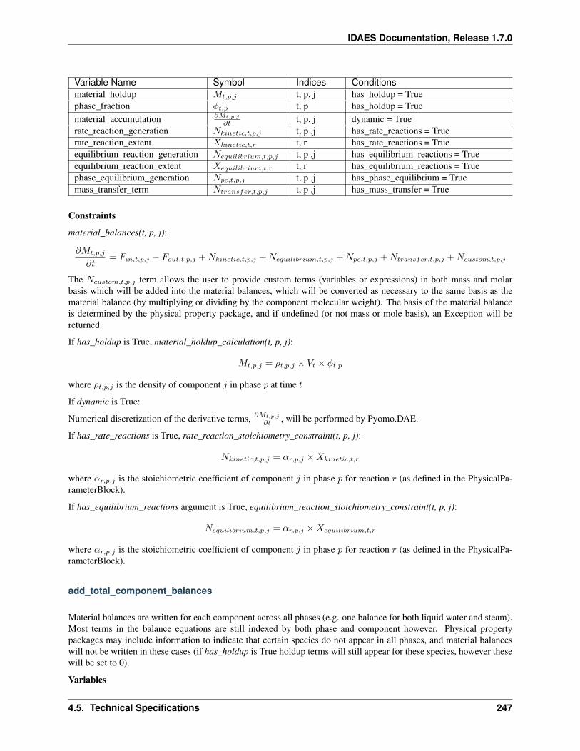
IDAES Documentation, Release 1.7.0
Variable Name Symbol Indices Conditionsmaterial_holdup 𝑀𝑡,𝑝,𝑗 t, p, j has_holdup = Truephase_fraction 𝜑𝑡,𝑝 t, p has_holdup = Truematerial_accumulation 𝜕𝑀𝑡,𝑝,𝑗
𝜕𝑡 t, p, j dynamic = Truerate_reaction_generation 𝑁𝑘𝑖𝑛𝑒𝑡𝑖𝑐,𝑡,𝑝,𝑗 t, p ,j has_rate_reactions = Truerate_reaction_extent 𝑋𝑘𝑖𝑛𝑒𝑡𝑖𝑐,𝑡,𝑟 t, r has_rate_reactions = Trueequilibrium_reaction_generation 𝑁𝑒𝑞𝑢𝑖𝑙𝑖𝑏𝑟𝑖𝑢𝑚,𝑡,𝑝,𝑗 t, p ,j has_equilibrium_reactions = Trueequilibrium_reaction_extent 𝑋𝑒𝑞𝑢𝑖𝑙𝑖𝑏𝑟𝑖𝑢𝑚,𝑡,𝑟 t, r has_equilibrium_reactions = Truephase_equilibrium_generation 𝑁𝑝𝑒,𝑡,𝑝,𝑗 t, p ,j has_phase_equilibrium = Truemass_transfer_term 𝑁𝑡𝑟𝑎𝑛𝑠𝑓𝑒𝑟,𝑡,𝑝,𝑗 t, p ,j has_mass_transfer = True
Constraints
material_balances(t, p, j):
𝜕𝑀𝑡,𝑝,𝑗
𝜕𝑡= 𝐹𝑖𝑛,𝑡,𝑝,𝑗 − 𝐹𝑜𝑢𝑡,𝑡,𝑝,𝑗 +𝑁𝑘𝑖𝑛𝑒𝑡𝑖𝑐,𝑡,𝑝,𝑗 +𝑁𝑒𝑞𝑢𝑖𝑙𝑖𝑏𝑟𝑖𝑢𝑚,𝑡,𝑝,𝑗 +𝑁𝑝𝑒,𝑡,𝑝,𝑗 +𝑁𝑡𝑟𝑎𝑛𝑠𝑓𝑒𝑟,𝑡,𝑝,𝑗 +𝑁𝑐𝑢𝑠𝑡𝑜𝑚,𝑡,𝑝,𝑗
The 𝑁𝑐𝑢𝑠𝑡𝑜𝑚,𝑡,𝑝,𝑗 term allows the user to provide custom terms (variables or expressions) in both mass and molarbasis which will be added into the material balances, which will be converted as necessary to the same basis as thematerial balance (by multiplying or dividing by the component molecular weight). The basis of the material balanceis determined by the physical property package, and if undefined (or not mass or mole basis), an Exception will bereturned.
If has_holdup is True, material_holdup_calculation(t, p, j):
𝑀𝑡,𝑝,𝑗 = 𝜌𝑡,𝑝,𝑗 × 𝑉𝑡 × 𝜑𝑡,𝑝
where 𝜌𝑡,𝑝,𝑗 is the density of component 𝑗 in phase 𝑝 at time 𝑡
If dynamic is True:
Numerical discretization of the derivative terms, 𝜕𝑀𝑡,𝑝,𝑗
𝜕𝑡 , will be performed by Pyomo.DAE.
If has_rate_reactions is True, rate_reaction_stoichiometry_constraint(t, p, j):
𝑁𝑘𝑖𝑛𝑒𝑡𝑖𝑐,𝑡,𝑝,𝑗 = 𝛼𝑟,𝑝,𝑗 ×𝑋𝑘𝑖𝑛𝑒𝑡𝑖𝑐,𝑡,𝑟
where 𝛼𝑟,𝑝.𝑗 is the stoichiometric coefficient of component 𝑗 in phase 𝑝 for reaction 𝑟 (as defined in the PhysicalPa-rameterBlock).
If has_equilibrium_reactions argument is True, equilibrium_reaction_stoichiometry_constraint(t, p, j):
𝑁𝑒𝑞𝑢𝑖𝑙𝑖𝑏𝑟𝑖𝑢𝑚,𝑡,𝑝,𝑗 = 𝛼𝑟,𝑝,𝑗 ×𝑋𝑒𝑞𝑢𝑖𝑙𝑖𝑏𝑟𝑖𝑢𝑚,𝑡,𝑟
where 𝛼𝑟,𝑝.𝑗 is the stoichiometric coefficient of component 𝑗 in phase 𝑝 for reaction 𝑟 (as defined in the PhysicalPa-rameterBlock).
add_total_component_balances
Material balances are written for each component across all phases (e.g. one balance for both liquid water and steam).Most terms in the balance equations are still indexed by both phase and component however. Physical propertypackages may include information to indicate that certain species do not appear in all phases, and material balanceswill not be written in these cases (if has_holdup is True holdup terms will still appear for these species, however thesewill be set to 0).
Variables
4.5. Technical Specifications 247
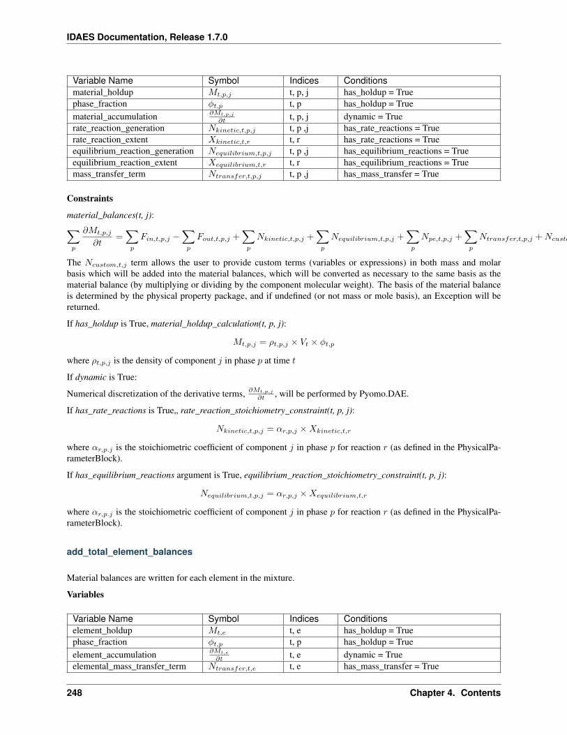
IDAES Documentation, Release 1.7.0
Variable Name Symbol Indices Conditionsmaterial_holdup 𝑀𝑡,𝑝,𝑗 t, p, j has_holdup = Truephase_fraction 𝜑𝑡,𝑝 t, p has_holdup = Truematerial_accumulation 𝜕𝑀𝑡,𝑝,𝑗
𝜕𝑡 t, p, j dynamic = Truerate_reaction_generation 𝑁𝑘𝑖𝑛𝑒𝑡𝑖𝑐,𝑡,𝑝,𝑗 t, p ,j has_rate_reactions = Truerate_reaction_extent 𝑋𝑘𝑖𝑛𝑒𝑡𝑖𝑐,𝑡,𝑟 t, r has_rate_reactions = Trueequilibrium_reaction_generation 𝑁𝑒𝑞𝑢𝑖𝑙𝑖𝑏𝑟𝑖𝑢𝑚,𝑡,𝑝,𝑗 t, p ,j has_equilibrium_reactions = Trueequilibrium_reaction_extent 𝑋𝑒𝑞𝑢𝑖𝑙𝑖𝑏𝑟𝑖𝑢𝑚,𝑡,𝑟 t, r has_equilibrium_reactions = Truemass_transfer_term 𝑁𝑡𝑟𝑎𝑛𝑠𝑓𝑒𝑟,𝑡,𝑝,𝑗 t, p ,j has_mass_transfer = True
Constraints
material_balances(t, j):∑𝑝
𝜕𝑀𝑡,𝑝,𝑗
𝜕𝑡=∑𝑝
𝐹𝑖𝑛,𝑡,𝑝,𝑗 −∑𝑝
𝐹𝑜𝑢𝑡,𝑡,𝑝,𝑗 +∑𝑝
𝑁𝑘𝑖𝑛𝑒𝑡𝑖𝑐,𝑡,𝑝,𝑗 +∑𝑝
𝑁𝑒𝑞𝑢𝑖𝑙𝑖𝑏𝑟𝑖𝑢𝑚,𝑡,𝑝,𝑗 +∑𝑝
𝑁𝑝𝑒,𝑡,𝑝,𝑗 +∑𝑝
𝑁𝑡𝑟𝑎𝑛𝑠𝑓𝑒𝑟,𝑡,𝑝,𝑗 +𝑁𝑐𝑢𝑠𝑡𝑜𝑚,𝑡,𝑗
The 𝑁𝑐𝑢𝑠𝑡𝑜𝑚,𝑡,𝑗 term allows the user to provide custom terms (variables or expressions) in both mass and molarbasis which will be added into the material balances, which will be converted as necessary to the same basis as thematerial balance (by multiplying or dividing by the component molecular weight). The basis of the material balanceis determined by the physical property package, and if undefined (or not mass or mole basis), an Exception will bereturned.
If has_holdup is True, material_holdup_calculation(t, p, j):
𝑀𝑡,𝑝,𝑗 = 𝜌𝑡,𝑝,𝑗 × 𝑉𝑡 × 𝜑𝑡,𝑝
where 𝜌𝑡,𝑝,𝑗 is the density of component 𝑗 in phase 𝑝 at time 𝑡
If dynamic is True:
Numerical discretization of the derivative terms, 𝜕𝑀𝑡,𝑝,𝑗
𝜕𝑡 , will be performed by Pyomo.DAE.
If has_rate_reactions is True„ rate_reaction_stoichiometry_constraint(t, p, j):
𝑁𝑘𝑖𝑛𝑒𝑡𝑖𝑐,𝑡,𝑝,𝑗 = 𝛼𝑟,𝑝,𝑗 ×𝑋𝑘𝑖𝑛𝑒𝑡𝑖𝑐,𝑡,𝑟
where 𝛼𝑟,𝑝.𝑗 is the stoichiometric coefficient of component 𝑗 in phase 𝑝 for reaction 𝑟 (as defined in the PhysicalPa-rameterBlock).
If has_equilibrium_reactions argument is True, equilibrium_reaction_stoichiometry_constraint(t, p, j):
𝑁𝑒𝑞𝑢𝑖𝑙𝑖𝑏𝑟𝑖𝑢𝑚,𝑡,𝑝,𝑗 = 𝛼𝑟,𝑝,𝑗 ×𝑋𝑒𝑞𝑢𝑖𝑙𝑖𝑏𝑟𝑖𝑢𝑚,𝑡,𝑟
where 𝛼𝑟,𝑝.𝑗 is the stoichiometric coefficient of component 𝑗 in phase 𝑝 for reaction 𝑟 (as defined in the PhysicalPa-rameterBlock).
add_total_element_balances
Material balances are written for each element in the mixture.
Variables
Variable Name Symbol Indices Conditionselement_holdup 𝑀𝑡,𝑒 t, e has_holdup = Truephase_fraction 𝜑𝑡,𝑝 t, p has_holdup = Trueelement_accumulation 𝜕𝑀𝑡,𝑒
𝜕𝑡 t, e dynamic = Trueelemental_mass_transfer_term 𝑁𝑡𝑟𝑎𝑛𝑠𝑓𝑒𝑟,𝑡,𝑒 t, e has_mass_transfer = True
248 Chapter 4. Contents
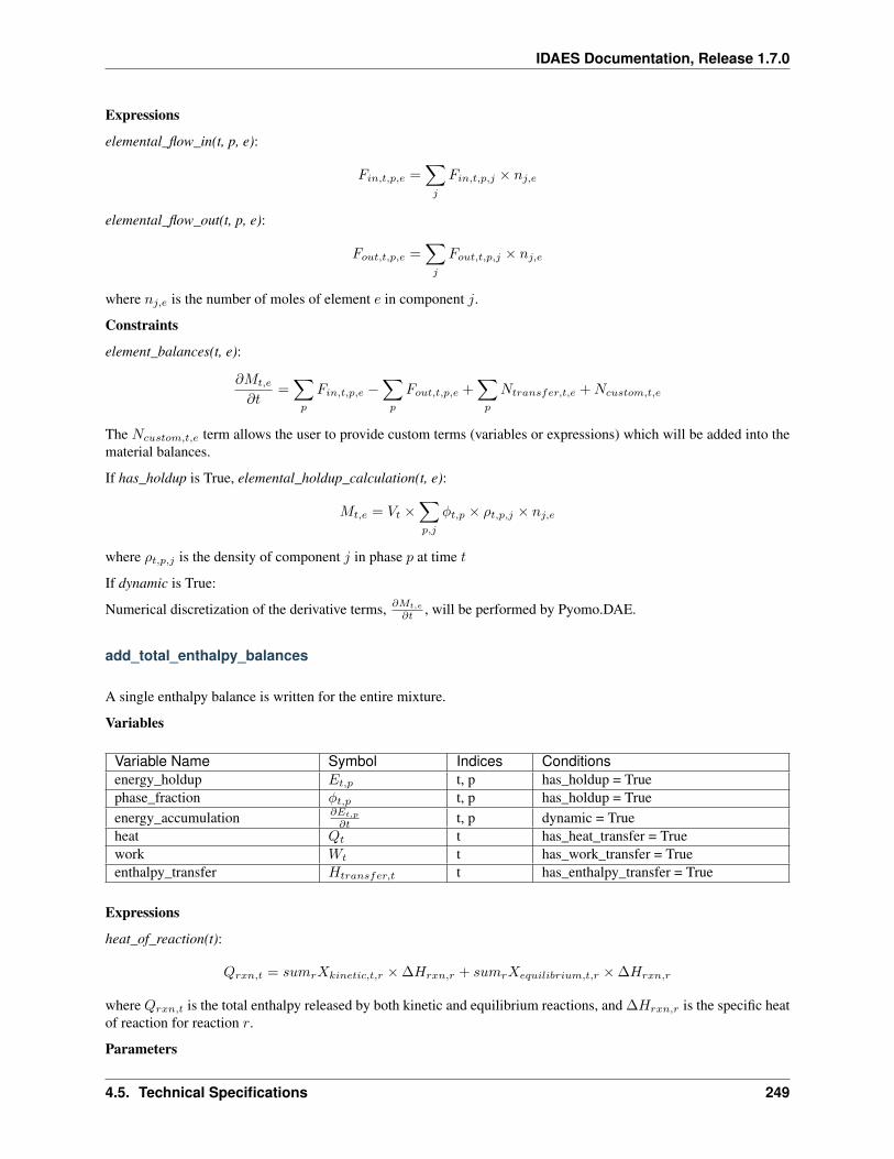
IDAES Documentation, Release 1.7.0
Expressions
elemental_flow_in(t, p, e):
𝐹𝑖𝑛,𝑡,𝑝,𝑒 =∑𝑗
𝐹𝑖𝑛,𝑡,𝑝,𝑗 × 𝑛𝑗,𝑒
elemental_flow_out(t, p, e):
𝐹𝑜𝑢𝑡,𝑡,𝑝,𝑒 =∑𝑗
𝐹𝑜𝑢𝑡,𝑡,𝑝,𝑗 × 𝑛𝑗,𝑒
where 𝑛𝑗,𝑒 is the number of moles of element 𝑒 in component 𝑗.
Constraints
element_balances(t, e):
𝜕𝑀𝑡,𝑒
𝜕𝑡=∑𝑝
𝐹𝑖𝑛,𝑡,𝑝,𝑒 −∑𝑝
𝐹𝑜𝑢𝑡,𝑡,𝑝,𝑒 +∑𝑝
𝑁𝑡𝑟𝑎𝑛𝑠𝑓𝑒𝑟,𝑡,𝑒 +𝑁𝑐𝑢𝑠𝑡𝑜𝑚,𝑡,𝑒
The 𝑁𝑐𝑢𝑠𝑡𝑜𝑚,𝑡,𝑒 term allows the user to provide custom terms (variables or expressions) which will be added into thematerial balances.
If has_holdup is True, elemental_holdup_calculation(t, e):
𝑀𝑡,𝑒 = 𝑉𝑡 ×∑𝑝,𝑗
𝜑𝑡,𝑝 × 𝜌𝑡,𝑝,𝑗 × 𝑛𝑗,𝑒
where 𝜌𝑡,𝑝,𝑗 is the density of component 𝑗 in phase 𝑝 at time 𝑡
If dynamic is True:
Numerical discretization of the derivative terms, 𝜕𝑀𝑡,𝑒
𝜕𝑡 , will be performed by Pyomo.DAE.
add_total_enthalpy_balances
A single enthalpy balance is written for the entire mixture.
Variables
Variable Name Symbol Indices Conditionsenergy_holdup 𝐸𝑡,𝑝 t, p has_holdup = Truephase_fraction 𝜑𝑡,𝑝 t, p has_holdup = Trueenergy_accumulation 𝜕𝐸𝑡,𝑝
𝜕𝑡 t, p dynamic = Trueheat 𝑄𝑡 t has_heat_transfer = Truework 𝑊𝑡 t has_work_transfer = Trueenthalpy_transfer 𝐻𝑡𝑟𝑎𝑛𝑠𝑓𝑒𝑟,𝑡 t has_enthalpy_transfer = True
Expressions
heat_of_reaction(t):
𝑄𝑟𝑥𝑛,𝑡 = 𝑠𝑢𝑚𝑟𝑋𝑘𝑖𝑛𝑒𝑡𝑖𝑐,𝑡,𝑟 × ∆𝐻𝑟𝑥𝑛,𝑟 + 𝑠𝑢𝑚𝑟𝑋𝑒𝑞𝑢𝑖𝑙𝑖𝑏𝑟𝑖𝑢𝑚,𝑡,𝑟 × ∆𝐻𝑟𝑥𝑛,𝑟
where 𝑄𝑟𝑥𝑛,𝑡 is the total enthalpy released by both kinetic and equilibrium reactions, and ∆𝐻𝑟𝑥𝑛,𝑟 is the specific heatof reaction for reaction 𝑟.
Parameters
4.5. Technical Specifications 249
IDAES Documentation, Release 1.7.0
Parameter Name Symbol Default Valuescaling_factor_energy 𝑠𝑒𝑛𝑒𝑟𝑔𝑦 1E-6
Constraints
enthalpy_balance(t):
𝑠𝑒𝑛𝑒𝑟𝑔𝑦 ×∑𝑝
𝜕𝐸𝑡,𝑝
𝜕𝑡= 𝑠𝑒𝑛𝑒𝑟𝑔𝑦 ×
∑𝑝
𝐻𝑖𝑛,𝑡,𝑝 − 𝑠𝑒𝑛𝑒𝑟𝑔𝑦 ×∑𝑝
𝐻𝑜𝑢𝑡,𝑡,𝑝 + 𝑠𝑒𝑛𝑒𝑟𝑔𝑦 ×𝑄𝑡 + 𝑠𝑒𝑛𝑒𝑟𝑔𝑦 ×𝑊𝑡 + +𝑠𝑒𝑛𝑒𝑟𝑔𝑦 ×𝐻𝑡𝑟𝑎𝑛𝑠𝑓𝑒𝑟,𝑡 + 𝑠𝑒𝑛𝑒𝑟𝑔𝑦 ×𝑄𝑟𝑥𝑛,𝑡 + 𝑠𝑒𝑛𝑒𝑟𝑔𝑦 × 𝐸𝑐𝑢𝑠𝑡𝑜𝑚,𝑡
The 𝐸𝑐𝑢𝑠𝑡𝑜𝑚,𝑡 term allows the user to provide custom terms which will be added into the energy balance.
If has_holdup is True, enthalpy_holdup_calculation(t, p):
𝐸𝑡,𝑝 = 𝑢𝑡,𝑝 × 𝑉𝑡 × 𝜑𝑡,𝑝
where 𝑢𝑡,𝑝 is the internal energy density (specific internal energy) of phase 𝑝 at time 𝑡
If dynamic is True:
Numerical discretization of the derivative terms, 𝜕𝐸𝑡,𝑝
𝜕𝑡 , will be performed by Pyomo.DAE.
add_total_pressure_balances
A single pressure balance is written for the entire mixture.
Variables
Variable Name Symbol Indices ConditionsdeltaP ∆𝑃𝑡 t has_pressure_change = True
Parameters
Parameter Name Symbol Default Valuescaling_factor_pressure 𝑠𝑝𝑟𝑒𝑠𝑠𝑢𝑟𝑒 1E-4
Constraints
pressure_balance(t):
0 = 𝑠𝑝𝑟𝑒𝑠𝑠𝑢𝑟𝑒 × 𝑃𝑖𝑛,𝑡 − 𝑠𝑝𝑟𝑒𝑠𝑠𝑢𝑟𝑒 × 𝑃𝑜𝑢𝑡,𝑡 + 𝑠𝑝𝑟𝑒𝑠𝑠𝑢𝑟𝑒 × ∆𝑃𝑡 + 𝑠𝑝𝑟𝑒𝑠𝑠𝑢𝑟𝑒 × ∆𝑃𝑐𝑢𝑠𝑡𝑜𝑚,𝑡
The ∆𝑃𝑐𝑢𝑠𝑡𝑜𝑚,𝑡 term allows the user to provide custom terms which will be added into the pressure balance.
1D Control Volume Class
Contents
• 1D Control Volume Class
– ControlVolume1DBlock Equations
250 Chapter 4. Contents
IDAES Documentation, Release 1.7.0
The ControlVolume1DBlock block is used for systems with one spatial dimension where material flows parallel tothe spatial domain. Examples of these types of unit operations include plug flow reactors and pipes. ControlVol-ume1DBlock blocks are discretized along the length domain and contain one StateBlock and one ReactionBlock (ifapplicable) at each point in the domain (including the inlet and outlet).
class idaes.core.control_volume1d.ControlVolume1DBlock(*args, **kwargs)ControlVolume1DBlock is a specialized Pyomo block for IDAES control volume blocks discretized in onespatial direction, and contains instances of ControlVolume1DBlockData.
ControlVolume1DBlock should be used for any control volume with a defined volume and distinct inlets andoutlets where there is a single spatial domain parallel to the material flow direction. This encompases unitoperations such as plug flow reactors and pipes.
Parameters
• rule (function) – A rule function or None. Default rule calls build().
• concrete (bool) – If True, make this a toplevel model. Default - False.
• ctype (str) – Pyomo ctype of the block. Default - “Block”
• default (dict) – Default ProcessBlockData config
Keys
dynamic Indicates whether this model will be dynamic, default - useDefault. Validvalues: useDefault - get flag from parent, True - set as a dynamic model, False - setas a steady-state model
has_holdup Indicates whether holdup terms should be constructed or not. Must be Trueif dynamic = True, default - False. Valid values: True - construct holdup terms,False - do not construct holdup terms
property_package Property parameter object used to define property calculations, de-fault - useDefault. Valid values: useDefault - use default package from parentmodel or flowsheet, PropertyParameterObject - a PropertyParameterBlock object.
property_package_args A ConfigBlock with arguments to be passed to a propertyblock(s) and used when constructing these, default - None. Valid values: see prop-erty package for documentation.
reaction_package Reaction parameter object used to define reaction calculations, de-fault - None. Valid values: None - no reaction package, ReactionParameterBlock- a ReactionParameterBlock object.
reaction_package_args A ConfigBlock with arguments to be passed to a reactionblock(s) and used when constructing these, default - None. Valid values: see re-action package for documentation.
auto_construct If set to True, this argument will trigger the auto_construct methodwhich will attempt to construct a set of material, energy and momentum balance equa-tions based on the parent unit’s config block. The parent unit must have a config blockwhich derives from CONFIG_Base, default - False. Valid values: True - use auto-matic construction, False - do not use automatic construciton.
area_definition Argument defining whether area variable should be spatially variant ornot. default - DistributedVars.uniform. Valid values: DistributedVars.uniform - areadoes not vary across spatial domian, DistributedVars.variant - area can vary over thedomain and is indexed by time and space.
transformation_method Method to use to transform domain. Must be a method recog-nised by the Pyomo TransformationFactory.
4.5. Technical Specifications 251
IDAES Documentation, Release 1.7.0
transformation_scheme Scheme to use when transformating domain. See Pyomo doc-umentation for supported schemes.
finite_elements Number of finite elements to use in transformation (equivalent to Pyomonfe argument).
collocation_points Number of collocation points to use (equivalent to Pyomo ncp argu-ment).
• initialize (dict) – ProcessBlockData config for individual elements. Keys are Block-Data indexes and values are dictionaries described under the “default” argument above.
• idx_map (function) – Function to take the index of a BlockData element and return theindex in the initialize dict from which to read arguments. This can be provided to overidethe default behavior of matching the BlockData index exactly to the index in initialize.
Returns (ControlVolume1DBlock) New instance
class idaes.core.control_volume1d.ControlVolume1DBlockData(component)1-Dimensional ControlVolume Class
This class forms the core of all 1-D IDAES models. It provides methods to build property and reaction blocks,and add mass, energy and momentum balances. The form of the terms used in these constraints is specified inthe chosen property package.
add_geometry(length_domain=None, length_domain_set=[0.0, 1.0],flow_direction=<FlowDirection.forward: 1>)
Method to create spatial domain and volume Var in ControlVolume.
Parameters
• - (length_domain_set) – domain for the ControlVolume. If not provided, a newContinuousSet will be created (default=None). ContinuousSet should be normalized torun between 0 and 1.
• - – a new ContinuousSet if length_domain is not provided (default = [0.0, 1.0]).
• - argument indicating direction of material flow(flow_direction) –
relative to length domain. Valid values:
– FlowDirection.forward (default), flow goes from 0 to 1.
– FlowDirection.backward, flow goes from 1 to 0
Returns None
add_phase_component_balances(has_rate_reactions=False, has_equilibrium_reactions=False,has_phase_equilibrium=False, has_mass_transfer=False,custom_molar_term=None, custom_mass_term=None)
This method constructs a set of 1D material balances indexed by time, length, phase and component.
Parameters
• has_rate_reactions – whether default generation terms for rate reactions should beincluded in material balances
• has_equilibrium_reactions – whether generation terms should for chemicalequilibrium reactions should be included in material balances
• has_phase_equilibrium – whether generation terms should for phase equilibriumbehaviour should be included in material balances
252 Chapter 4. Contents
IDAES Documentation, Release 1.7.0
• has_mass_transfer – whether generic mass transfer terms should be included inmaterial balances
• custom_molar_term – a Pyomo Expression representing custom terms to be includedin material balances on a molar basis. Expression must be indexed by time, length domain,phase list and component list
• custom_mass_term – a Pyomo Expression representing custom terms to be includedin material balances on a mass basis. Expression must be indexed by time, length domain,phase list and component list
Returns Constraint object representing material balances
add_phase_energy_balances(*args, **kwargs)Method for adding energy balances (including kinetic energy) indexed by phase to the control volume.
See specific control volume documentation for details.
add_phase_enthalpy_balances(*args, **kwargs)Method for adding enthalpy balances indexed by phase to the control volume.
See specific control volume documentation for details.
add_phase_momentum_balances(*args, **kwargs)Method for adding momentum balances indexed by phase to the control volume.
See specific control volume documentation for details.
add_phase_pressure_balances(*args, **kwargs)Method for adding pressure balances indexed by phase to the control volume.
See specific control volume documentation for details.
add_reaction_blocks(has_equilibrium=None)This method constructs the reaction block for the control volume.
Parameters
• has_equilibrium – indicates whether equilibrium calculations will be required inreaction block
• package_arguments – dict-like object of arguments to be passed to reaction block asconstruction arguments
Returns None
add_state_blocks(information_flow=<FlowDirection.forward: 1>,has_phase_equilibrium=None)
This method constructs the state blocks for the control volume.
Parameters
• information_flow – a FlowDirection Enum indicating whether information flowsfrom inlet-to-outlet or outlet-to-inlet
• has_phase_equilibrium – indicates whether equilibrium calculations will be re-quired in state blocks
• package_arguments – dict-like object of arguments to be passed to state blocks asconstruction arguments
Returns None
4.5. Technical Specifications 253
IDAES Documentation, Release 1.7.0
add_total_component_balances(has_rate_reactions=False, has_equilibrium_reactions=False,has_phase_equilibrium=False, has_mass_transfer=False,custom_molar_term=None, custom_mass_term=None)
This method constructs a set of 1D material balances indexed by time length and component.
Parameters
• has_rate_reactions – whether default generation terms for rate reactions should beincluded in material balances
• has_equilibrium_reactions – whether generation terms should for chemicalequilibrium reactions should be included in material balances
• has_phase_equilibrium – whether generation terms should for phase equilibriumbehaviour should be included in material balances
• has_mass_transfer – whether generic mass transfer terms should be included inmaterial balances
• custom_molar_term – a Pyomo Expression representing custom terms to be includedin material balances on a molar basis. Expression must be indexed by time, length domainand component list
• custom_mass_term – a Pyomo Expression representing custom terms to be includedin material balances on a mass basis. Expression must be indexed by time, length domainand component list
Returns Constraint object representing material balances
add_total_element_balances(has_rate_reactions=False, has_equilibrium_reactions=False,has_phase_equilibrium=False, has_mass_transfer=False,custom_elemental_term=None)
This method constructs a set of 1D element balances indexed by time and length.
Parameters
• - whether default generation terms for rate(has_rate_reactions) – reactions should be included in material balances
• - whether generation terms should for (has_equilibrium_reactions)– chemical equilibrium reactions should be included in material balances
• - whether generation terms should for phase(has_phase_equilibrium) – equilibrium behaviour should be included inmaterial balances
• - whether generic mass transfer terms should be(has_mass_transfer) – included in material balances
• - a Pyomo Expression representing custom(custom_elemental_term) – terms to be included in material balances on amolar elemental basis. Expression must be indexed by time, length and element list
Returns Constraint object representing material balances
add_total_energy_balances(*args, **kwargs)Method for adding a total energy balance (including kinetic energy) to the control volume.
See specific control volume documentation for details.
add_total_enthalpy_balances(has_heat_of_reaction=False, has_heat_transfer=False,has_work_transfer=False, has_enthalpy_transfer=False,custom_term=None)
This method constructs a set of 1D enthalpy balances indexed by time and phase.
254 Chapter 4. Contents
IDAES Documentation, Release 1.7.0
Parameters
• - whether terms for heat of reaction should(has_heat_of_reaction) – be included in enthalpy balance
• - whether terms for heat transfer should be(has_heat_transfer) – included in enthalpy balances
• - whether terms for work transfer should be(has_work_transfer) – included in enthalpy balances
• - whether terms for enthalpy transfer due to(has_enthalpy_transfer) – mass transfer should be included in enthalpybalance. This should generally be the same as the has_mas_trasnfer argument in thematerial balance methods
• - a Pyomo Expression representing custom terms to(custom_term) – be included in enthalpy balances. Expression must be indexedby time, length and phase list
Returns Constraint object representing enthalpy balances
add_total_material_balances(*args, **kwargs)Method for adding a total material balance to the control volume.
See specific control volume documentation for details.
add_total_momentum_balances(*args, **kwargs)Method for adding a total momentum balance to the control volume.
See specific control volume documentation for details.
add_total_pressure_balances(has_pressure_change=False, custom_term=None)This method constructs a set of 1D pressure balances indexed by time.
Parameters
• - whether terms for pressure change should be(has_pressure_change) – included in enthalpy balances
• - a Pyomo Expression representing custom terms to(custom_term) – be included in pressure balances. Expression must be indexedby time and length domain
Returns Constraint object representing pressure balances
apply_transformation()Method to apply DAE transformation to the Control Volume length domain. Transformation applied willbe based on the Control Volume configuration arguments.
build()Build method for ControlVolume1DBlock blocks.
Returns None
initialize(state_args=None, outlvl=0, optarg=None, solver=’ipopt’, hold_state=True)Initialization routine for 1D control volume (default solver ipopt)
Keyword Arguments
• state_args – a dict of arguments to be passed to the property package(s) to provide aninitial state for initialization (see documentation of the specific property package) (default= ).
• outlvl – sets output level of initialization routine
4.5. Technical Specifications 255
IDAES Documentation, Release 1.7.0
• optarg – solver options dictionary object (default=None)
• solver – str indicating whcih solver to use during initialization (default = ‘ipopt’)
• hold_state – flag indicating whether the initialization routine should unfix any statevariables fixed during initialization, default - True. Valid values: True - states vari-ables are not unfixed, and a dict of returned containing flags for which states were fixedduring initialization, False - state variables are unfixed after initialization by calling therelease_state method.
Returns If hold_states is True, returns a dict containing flags for which states were fixed duringinitialization else the release state is triggered.
model_check()This method executes the model_check methods on the associated state blocks (if they exist). This methodis generally called by a unit model as part of the unit’s model_check method.
Parameters None –
Returns None
release_state(flags, outlvl=0)Method to release state variables fixed during initialization.
Keyword Arguments
• flags – dict containing information of which state variables were fixed during initializa-tion, and should now be unfixed. This dict is returned by initialize if hold_state = True.
• outlvl – sets output level of logging
Returns None
report(time_point=0, dof=False, ostream=None, prefix=”)No report method defined for ControlVolume1D class. This is due to the difficulty of presenting spatiallydiscretized data in a readable form without plotting.
ControlVolume1DBlock Equations
This section documents the variables and constraints created by each of the methods provided by the ControlVol-ume0DBlock class.
• 𝑡 indicates time index
• 𝑥 indicates spatial (length) index
• 𝑝 indicates phase index
• 𝑗 indicates component index
• 𝑒 indicates element index
• 𝑟 indicates reaction name index
Most terms within the balance equations written by ControlVolume1DBlock are on a basis of per unit length (e.g.𝑚𝑜𝑙/𝑚 · 𝑠).
add_geometry
The add_geometry method creates the normalized length domain for the control volume (or a reference to an externaldomain). All constraints in ControlVolume1DBlock assume a normalized length domain, with values between 0 and1.
256 Chapter 4. Contents
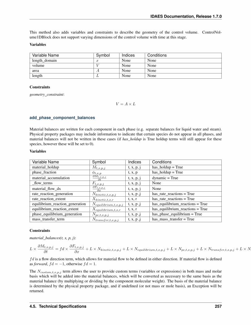
IDAES Documentation, Release 1.7.0
This method also adds variables and constraints to describe the geometry of the control volume. ControlVol-ume1DBlock does not support varying dimensions of the control volume with time at this stage.
Variables
Variable Name Symbol Indices Conditionslength_domain 𝑥 None Nonevolume 𝑉 None Nonearea 𝐴 None Nonelength 𝐿 None None
Constraints
geometry_constraint:
𝑉 = 𝐴× 𝐿
add_phase_component_balances
Material balances are written for each component in each phase (e.g. separate balances for liquid water and steam).Physical property packages may include information to indicate that certain species do not appear in all phases, andmaterial balances will not be written in these cases (if has_holdup is True holdup terms will still appear for thesespecies, however these will be set to 0).
Variables
Variable Name Symbol Indices Conditionsmaterial_holdup 𝑀𝑡,𝑥,𝑝,𝑗 t, x, p, j has_holdup = Truephase_fraction 𝜑𝑡,𝑥,𝑝 t, x, p has_holdup = Truematerial_accumulation 𝜕𝑀𝑡,𝑥,𝑝,𝑗
𝜕𝑡 t, x, p, j dynamic = True_flow_terms 𝐹𝑡,𝑥,𝑝,𝑗 t, x, p, j Nonematerial_flow_dx 𝜕𝐹𝑡,𝑥,𝑝,𝑗
𝜕𝑥 t, x, p, j Nonerate_reaction_generation 𝑁𝑘𝑖𝑛𝑒𝑡𝑖𝑐,𝑡,𝑥,𝑝,𝑗 t, x, p ,j has_rate_reactions = Truerate_reaction_extent 𝑋𝑘𝑖𝑛𝑒𝑡𝑖𝑐,𝑡,𝑥,𝑟 t, x, r has_rate_reactions = Trueequilibrium_reaction_generation 𝑁𝑒𝑞𝑢𝑖𝑙𝑖𝑏𝑟𝑖𝑢𝑚,𝑡,𝑥,𝑝,𝑗 t, x, p ,j has_equilibrium_reactions = Trueequilibrium_reaction_extent 𝑋𝑒𝑞𝑢𝑖𝑙𝑖𝑏𝑟𝑖𝑢𝑚,𝑡,𝑥,𝑟 t, x, r has_equilibrium_reactions = Truephase_equilibrium_generation 𝑁𝑝𝑒,𝑡,𝑥,𝑝,𝑗 t, x, p ,j has_phase_equilibrium = Truemass_transfer_term 𝑁𝑡𝑟𝑎𝑛𝑠𝑓𝑒𝑟,𝑡,𝑥,𝑝,𝑗 t, x, p ,j has_mass_transfer = True
Constraints
material_balances(t, x, p, j):
𝐿× 𝜕𝑀𝑡,𝑥,𝑝,𝑗
𝜕𝑡= 𝑓𝑑× 𝜕𝐹𝑡,𝑥,𝑝,𝑗
𝜕𝑥+ 𝐿×𝑁𝑘𝑖𝑛𝑒𝑡𝑖𝑐,𝑡,𝑥,𝑝,𝑗 + 𝐿×𝑁𝑒𝑞𝑢𝑖𝑙𝑖𝑏𝑟𝑖𝑢𝑚,𝑡,𝑥,𝑝,𝑗 + 𝐿×𝑁𝑝𝑒,𝑡,𝑥,𝑝,𝑗 + 𝐿×𝑁𝑡𝑟𝑎𝑛𝑠𝑓𝑒𝑟,𝑡,𝑥,𝑝,𝑗 + 𝐿×𝑁𝑐𝑢𝑠𝑡𝑜𝑚,𝑡,𝑥,𝑝,𝑗
𝑓𝑑 is a flow direction term, which allows for material flow to be defined in either direction. If material flow is definedas forward, 𝑓𝑑 = −1, otherwise 𝑓𝑑 = 1.
The 𝑁𝑐𝑢𝑠𝑡𝑜𝑚,𝑡,𝑥,𝑝,𝑗 term allows the user to provide custom terms (variables or expressions) in both mass and molarbasis which will be added into the material balances, which will be converted as necessary to the same basis as thematerial balance (by multiplying or dividing by the component molecular weight). The basis of the material balanceis determined by the physical property package, and if undefined (or not mass or mole basis), an Exception will bereturned.
4.5. Technical Specifications 257
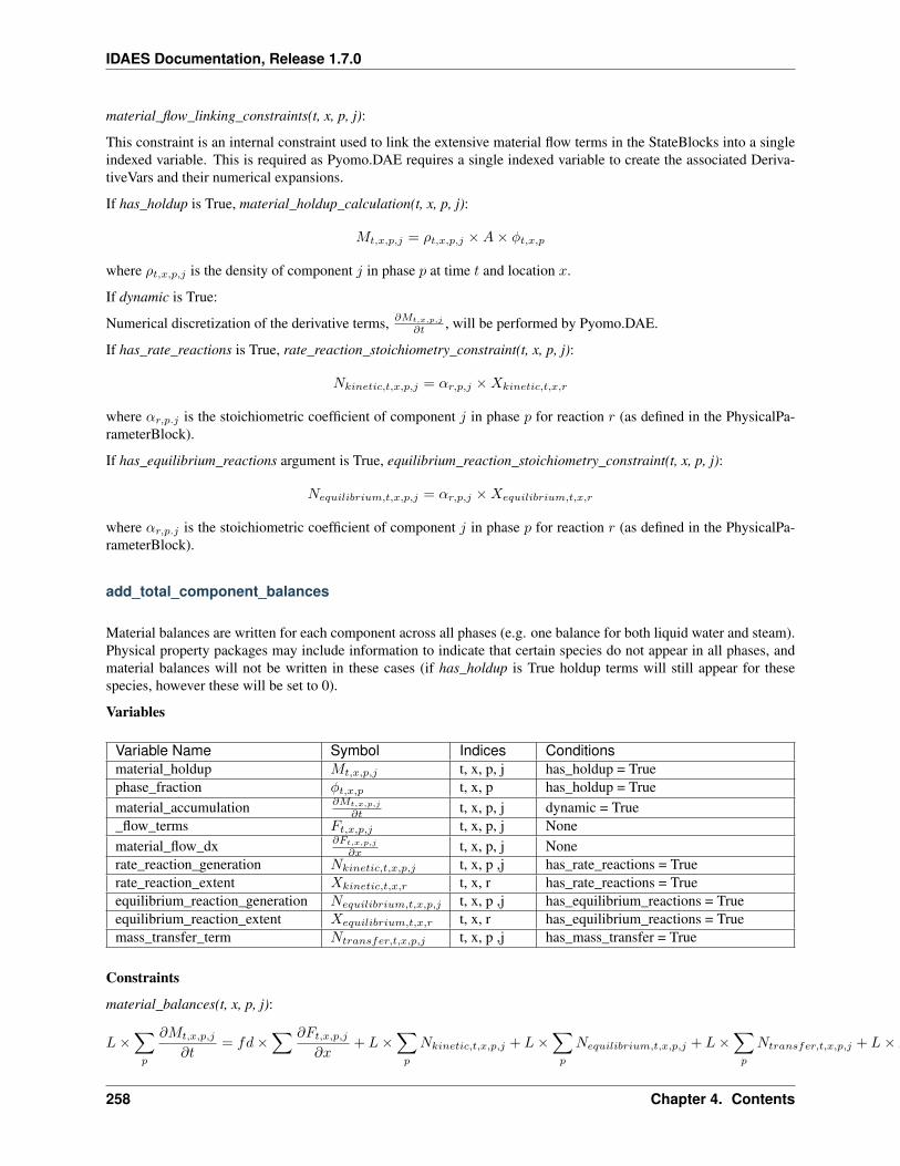
IDAES Documentation, Release 1.7.0
material_flow_linking_constraints(t, x, p, j):
This constraint is an internal constraint used to link the extensive material flow terms in the StateBlocks into a singleindexed variable. This is required as Pyomo.DAE requires a single indexed variable to create the associated Deriva-tiveVars and their numerical expansions.
If has_holdup is True, material_holdup_calculation(t, x, p, j):
𝑀𝑡,𝑥,𝑝,𝑗 = 𝜌𝑡,𝑥,𝑝,𝑗 ×𝐴× 𝜑𝑡,𝑥,𝑝
where 𝜌𝑡,𝑥,𝑝,𝑗 is the density of component 𝑗 in phase 𝑝 at time 𝑡 and location 𝑥.
If dynamic is True:
Numerical discretization of the derivative terms, 𝜕𝑀𝑡,𝑥,𝑝,𝑗
𝜕𝑡 , will be performed by Pyomo.DAE.
If has_rate_reactions is True, rate_reaction_stoichiometry_constraint(t, x, p, j):
𝑁𝑘𝑖𝑛𝑒𝑡𝑖𝑐,𝑡,𝑥,𝑝,𝑗 = 𝛼𝑟,𝑝,𝑗 ×𝑋𝑘𝑖𝑛𝑒𝑡𝑖𝑐,𝑡,𝑥,𝑟
where 𝛼𝑟,𝑝.𝑗 is the stoichiometric coefficient of component 𝑗 in phase 𝑝 for reaction 𝑟 (as defined in the PhysicalPa-rameterBlock).
If has_equilibrium_reactions argument is True, equilibrium_reaction_stoichiometry_constraint(t, x, p, j):
𝑁𝑒𝑞𝑢𝑖𝑙𝑖𝑏𝑟𝑖𝑢𝑚,𝑡,𝑥,𝑝,𝑗 = 𝛼𝑟,𝑝,𝑗 ×𝑋𝑒𝑞𝑢𝑖𝑙𝑖𝑏𝑟𝑖𝑢𝑚,𝑡,𝑥,𝑟
where 𝛼𝑟,𝑝.𝑗 is the stoichiometric coefficient of component 𝑗 in phase 𝑝 for reaction 𝑟 (as defined in the PhysicalPa-rameterBlock).
add_total_component_balances
Material balances are written for each component across all phases (e.g. one balance for both liquid water and steam).Physical property packages may include information to indicate that certain species do not appear in all phases, andmaterial balances will not be written in these cases (if has_holdup is True holdup terms will still appear for thesespecies, however these will be set to 0).
Variables
Variable Name Symbol Indices Conditionsmaterial_holdup 𝑀𝑡,𝑥,𝑝,𝑗 t, x, p, j has_holdup = Truephase_fraction 𝜑𝑡,𝑥,𝑝 t, x, p has_holdup = Truematerial_accumulation 𝜕𝑀𝑡,𝑥,𝑝,𝑗
𝜕𝑡 t, x, p, j dynamic = True_flow_terms 𝐹𝑡,𝑥,𝑝,𝑗 t, x, p, j Nonematerial_flow_dx 𝜕𝐹𝑡,𝑥,𝑝,𝑗
𝜕𝑥 t, x, p, j Nonerate_reaction_generation 𝑁𝑘𝑖𝑛𝑒𝑡𝑖𝑐,𝑡,𝑥,𝑝,𝑗 t, x, p ,j has_rate_reactions = Truerate_reaction_extent 𝑋𝑘𝑖𝑛𝑒𝑡𝑖𝑐,𝑡,𝑥,𝑟 t, x, r has_rate_reactions = Trueequilibrium_reaction_generation 𝑁𝑒𝑞𝑢𝑖𝑙𝑖𝑏𝑟𝑖𝑢𝑚,𝑡,𝑥,𝑝,𝑗 t, x, p ,j has_equilibrium_reactions = Trueequilibrium_reaction_extent 𝑋𝑒𝑞𝑢𝑖𝑙𝑖𝑏𝑟𝑖𝑢𝑚,𝑡,𝑥,𝑟 t, x, r has_equilibrium_reactions = Truemass_transfer_term 𝑁𝑡𝑟𝑎𝑛𝑠𝑓𝑒𝑟,𝑡,𝑥,𝑝,𝑗 t, x, p ,j has_mass_transfer = True
Constraints
material_balances(t, x, p, j):
𝐿×∑𝑝
𝜕𝑀𝑡,𝑥,𝑝,𝑗
𝜕𝑡= 𝑓𝑑×
∑ 𝜕𝐹𝑡,𝑥,𝑝,𝑗
𝜕𝑥+ 𝐿×
∑𝑝
𝑁𝑘𝑖𝑛𝑒𝑡𝑖𝑐,𝑡,𝑥,𝑝,𝑗 + 𝐿×∑𝑝
𝑁𝑒𝑞𝑢𝑖𝑙𝑖𝑏𝑟𝑖𝑢𝑚,𝑡,𝑥,𝑝,𝑗 + 𝐿×∑𝑝
𝑁𝑡𝑟𝑎𝑛𝑠𝑓𝑒𝑟,𝑡,𝑥,𝑝,𝑗 + 𝐿×𝑁𝑐𝑢𝑠𝑡𝑜𝑚,𝑡,𝑥,𝑗
258 Chapter 4. Contents
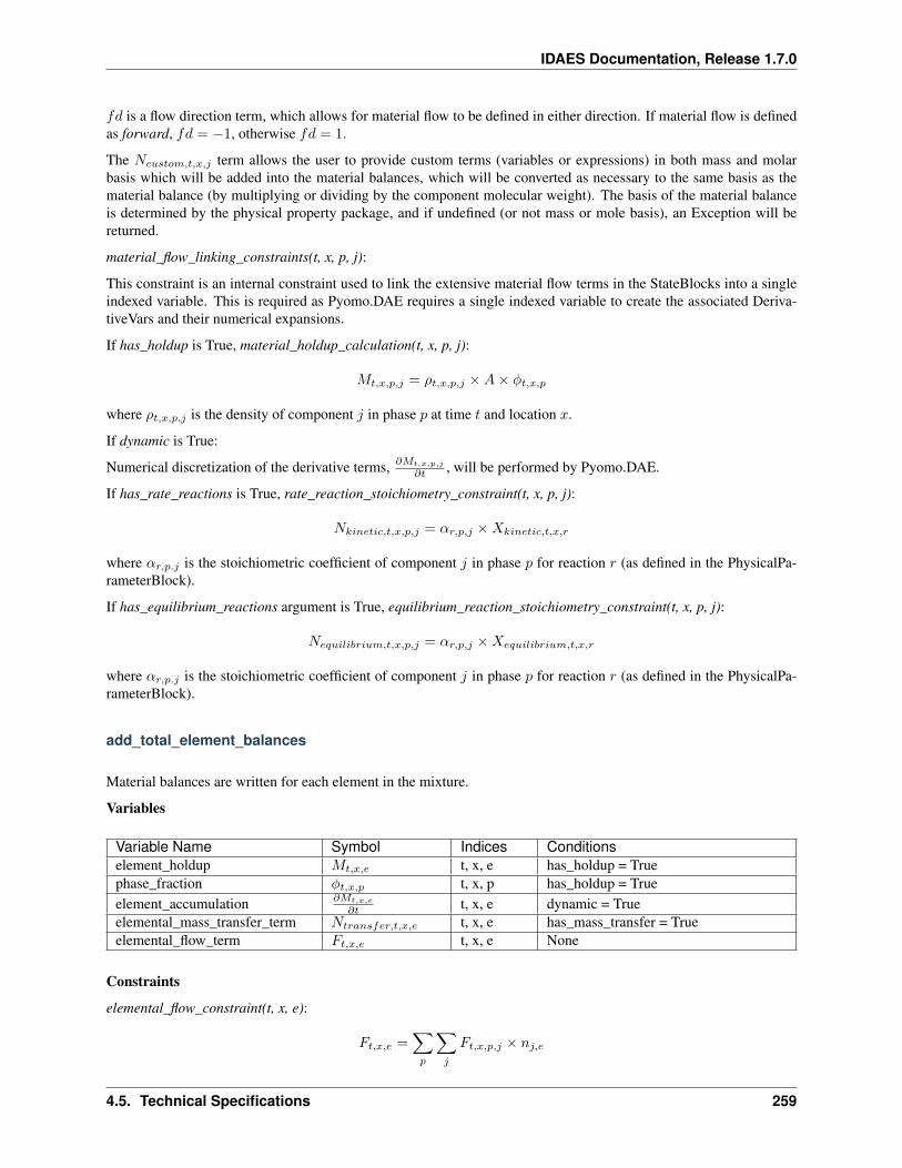
IDAES Documentation, Release 1.7.0
𝑓𝑑 is a flow direction term, which allows for material flow to be defined in either direction. If material flow is definedas forward, 𝑓𝑑 = −1, otherwise 𝑓𝑑 = 1.
The 𝑁𝑐𝑢𝑠𝑡𝑜𝑚,𝑡,𝑥,𝑗 term allows the user to provide custom terms (variables or expressions) in both mass and molarbasis which will be added into the material balances, which will be converted as necessary to the same basis as thematerial balance (by multiplying or dividing by the component molecular weight). The basis of the material balanceis determined by the physical property package, and if undefined (or not mass or mole basis), an Exception will bereturned.
material_flow_linking_constraints(t, x, p, j):
This constraint is an internal constraint used to link the extensive material flow terms in the StateBlocks into a singleindexed variable. This is required as Pyomo.DAE requires a single indexed variable to create the associated Deriva-tiveVars and their numerical expansions.
If has_holdup is True, material_holdup_calculation(t, x, p, j):
𝑀𝑡,𝑥,𝑝,𝑗 = 𝜌𝑡,𝑥,𝑝,𝑗 ×𝐴× 𝜑𝑡,𝑥,𝑝
where 𝜌𝑡,𝑥,𝑝,𝑗 is the density of component 𝑗 in phase 𝑝 at time 𝑡 and location 𝑥.
If dynamic is True:
Numerical discretization of the derivative terms, 𝜕𝑀𝑡,𝑥,𝑝,𝑗
𝜕𝑡 , will be performed by Pyomo.DAE.
If has_rate_reactions is True, rate_reaction_stoichiometry_constraint(t, x, p, j):
𝑁𝑘𝑖𝑛𝑒𝑡𝑖𝑐,𝑡,𝑥,𝑝,𝑗 = 𝛼𝑟,𝑝,𝑗 ×𝑋𝑘𝑖𝑛𝑒𝑡𝑖𝑐,𝑡,𝑥,𝑟
where 𝛼𝑟,𝑝.𝑗 is the stoichiometric coefficient of component 𝑗 in phase 𝑝 for reaction 𝑟 (as defined in the PhysicalPa-rameterBlock).
If has_equilibrium_reactions argument is True, equilibrium_reaction_stoichiometry_constraint(t, x, p, j):
𝑁𝑒𝑞𝑢𝑖𝑙𝑖𝑏𝑟𝑖𝑢𝑚,𝑡,𝑥,𝑝,𝑗 = 𝛼𝑟,𝑝,𝑗 ×𝑋𝑒𝑞𝑢𝑖𝑙𝑖𝑏𝑟𝑖𝑢𝑚,𝑡,𝑥,𝑟
where 𝛼𝑟,𝑝.𝑗 is the stoichiometric coefficient of component 𝑗 in phase 𝑝 for reaction 𝑟 (as defined in the PhysicalPa-rameterBlock).
add_total_element_balances
Material balances are written for each element in the mixture.
Variables
Variable Name Symbol Indices Conditionselement_holdup 𝑀𝑡,𝑥,𝑒 t, x, e has_holdup = Truephase_fraction 𝜑𝑡,𝑥,𝑝 t, x, p has_holdup = Trueelement_accumulation 𝜕𝑀𝑡,𝑥,𝑒
𝜕𝑡 t, x, e dynamic = Trueelemental_mass_transfer_term 𝑁𝑡𝑟𝑎𝑛𝑠𝑓𝑒𝑟,𝑡,𝑥,𝑒 t, x, e has_mass_transfer = Trueelemental_flow_term 𝐹𝑡,𝑥,𝑒 t, x, e None
Constraints
elemental_flow_constraint(t, x, e):
𝐹𝑡,𝑥,𝑒 =∑𝑝
∑𝑗
𝐹𝑡,𝑥,𝑝,𝑗 × 𝑛𝑗,𝑒
4.5. Technical Specifications 259
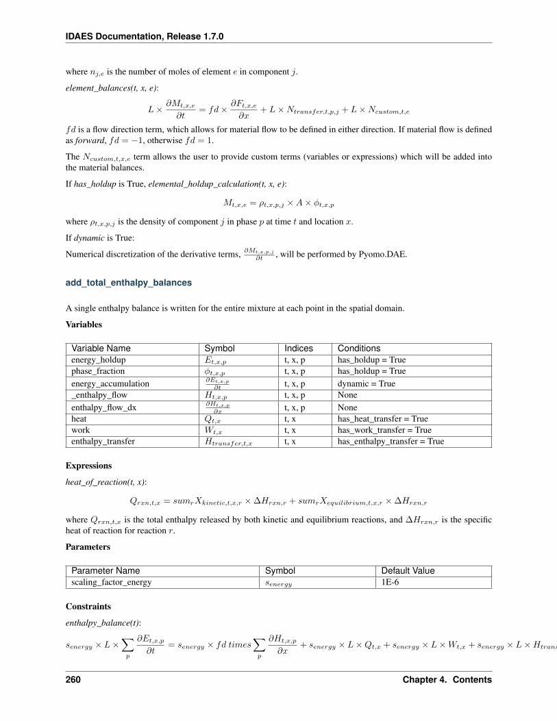
IDAES Documentation, Release 1.7.0
where 𝑛𝑗,𝑒 is the number of moles of element 𝑒 in component 𝑗.
element_balances(t, x, e):
𝐿× 𝜕𝑀𝑡,𝑥,𝑒
𝜕𝑡= 𝑓𝑑× 𝜕𝐹𝑡,𝑥,𝑒
𝜕𝑥+ 𝐿×𝑁𝑡𝑟𝑎𝑛𝑠𝑓𝑒𝑟,𝑡,𝑝,𝑗 + 𝐿×𝑁𝑐𝑢𝑠𝑡𝑜𝑚,𝑡,𝑒
𝑓𝑑 is a flow direction term, which allows for material flow to be defined in either direction. If material flow is definedas forward, 𝑓𝑑 = −1, otherwise 𝑓𝑑 = 1.
The 𝑁𝑐𝑢𝑠𝑡𝑜𝑚,𝑡,𝑥,𝑒 term allows the user to provide custom terms (variables or expressions) which will be added intothe material balances.
If has_holdup is True, elemental_holdup_calculation(t, x, e):
𝑀𝑡,𝑥,𝑒 = 𝜌𝑡,𝑥,𝑝,𝑗 ×𝐴× 𝜑𝑡,𝑥,𝑝
where 𝜌𝑡,𝑥,𝑝,𝑗 is the density of component 𝑗 in phase 𝑝 at time 𝑡 and location 𝑥.
If dynamic is True:
Numerical discretization of the derivative terms, 𝜕𝑀𝑡,𝑥,𝑝,𝑗
𝜕𝑡 , will be performed by Pyomo.DAE.
add_total_enthalpy_balances
A single enthalpy balance is written for the entire mixture at each point in the spatial domain.
Variables
Variable Name Symbol Indices Conditionsenergy_holdup 𝐸𝑡,𝑥,𝑝 t, x, p has_holdup = Truephase_fraction 𝜑𝑡,𝑥,𝑝 t, x, p has_holdup = Trueenergy_accumulation 𝜕𝐸𝑡,𝑥,𝑝
𝜕𝑡 t, x, p dynamic = True_enthalpy_flow 𝐻𝑡,𝑥,𝑝 t, x, p Noneenthalpy_flow_dx 𝜕𝐻𝑡,𝑥,𝑝
𝜕𝑥 t, x, p Noneheat 𝑄𝑡,𝑥 t, x has_heat_transfer = Truework 𝑊𝑡,𝑥 t, x has_work_transfer = Trueenthalpy_transfer 𝐻𝑡𝑟𝑎𝑛𝑠𝑓𝑒𝑟,𝑡,𝑥 t, x has_enthalpy_transfer = True
Expressions
heat_of_reaction(t, x):
𝑄𝑟𝑥𝑛,𝑡,𝑥 = 𝑠𝑢𝑚𝑟𝑋𝑘𝑖𝑛𝑒𝑡𝑖𝑐,𝑡,𝑥,𝑟 × ∆𝐻𝑟𝑥𝑛,𝑟 + 𝑠𝑢𝑚𝑟𝑋𝑒𝑞𝑢𝑖𝑙𝑖𝑏𝑟𝑖𝑢𝑚,𝑡,𝑥,𝑟 × ∆𝐻𝑟𝑥𝑛,𝑟
where 𝑄𝑟𝑥𝑛,𝑡,𝑥 is the total enthalpy released by both kinetic and equilibrium reactions, and ∆𝐻𝑟𝑥𝑛,𝑟 is the specificheat of reaction for reaction 𝑟.
Parameters
Parameter Name Symbol Default Valuescaling_factor_energy 𝑠𝑒𝑛𝑒𝑟𝑔𝑦 1E-6
Constraints
enthalpy_balance(t):
𝑠𝑒𝑛𝑒𝑟𝑔𝑦 × 𝐿×∑𝑝
𝜕𝐸𝑡,𝑥,𝑝
𝜕𝑡= 𝑠𝑒𝑛𝑒𝑟𝑔𝑦 × 𝑓𝑑 𝑡𝑖𝑚𝑒𝑠
∑𝑝
𝜕𝐻𝑡,𝑥,𝑝
𝜕𝑥+ 𝑠𝑒𝑛𝑒𝑟𝑔𝑦 × 𝐿×𝑄𝑡,𝑥 + 𝑠𝑒𝑛𝑒𝑟𝑔𝑦 × 𝐿×𝑊𝑡,𝑥 + 𝑠𝑒𝑛𝑒𝑟𝑔𝑦 × 𝐿×𝐻𝑡𝑟𝑎𝑛𝑠𝑓𝑒𝑟,𝑡,𝑥 + 𝑠𝑒𝑛𝑒𝑟𝑔𝑦 × 𝐿×𝑄𝑟𝑥𝑛,𝑡,𝑥 + 𝑠𝑒𝑛𝑒𝑟𝑔𝑦 × 𝐿× 𝐸𝑐𝑢𝑠𝑡𝑜𝑚,𝑡,𝑥
260 Chapter 4. Contents
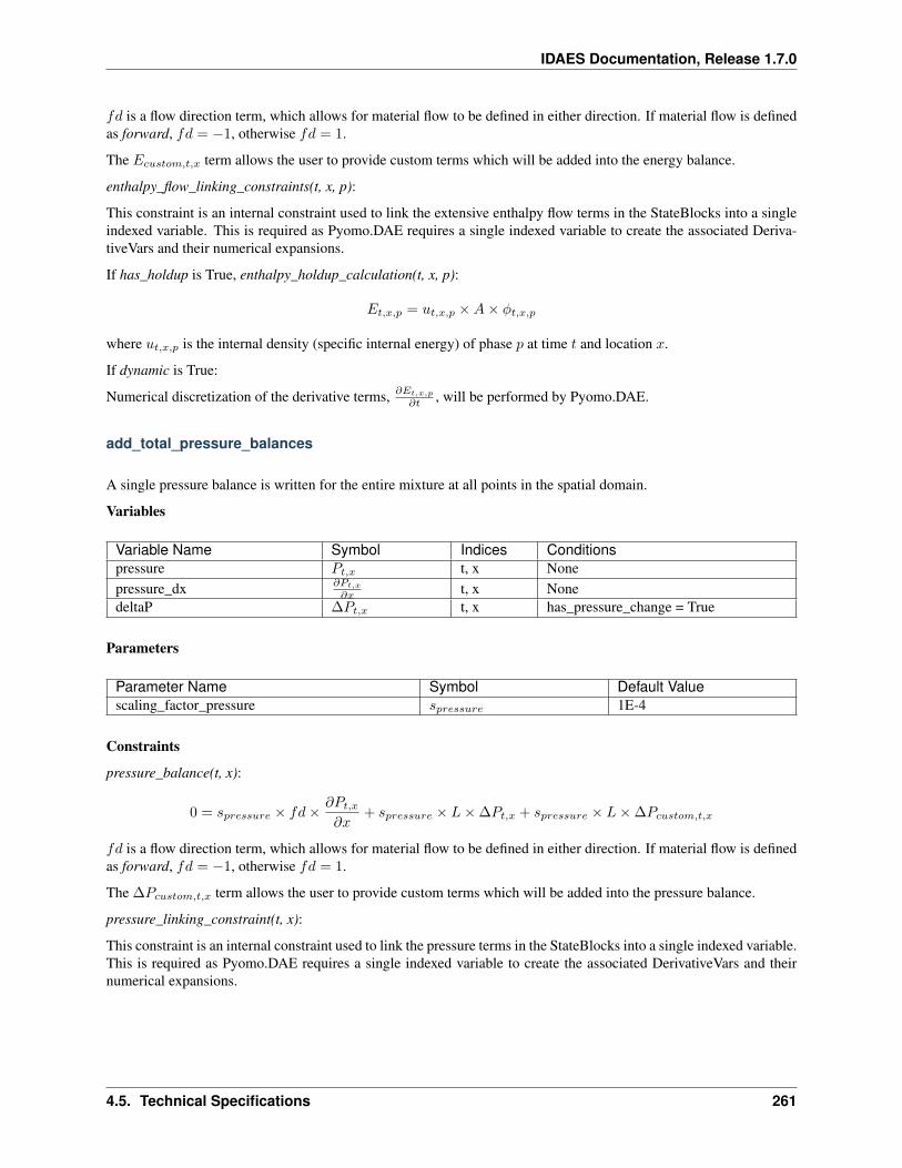
IDAES Documentation, Release 1.7.0
𝑓𝑑 is a flow direction term, which allows for material flow to be defined in either direction. If material flow is definedas forward, 𝑓𝑑 = −1, otherwise 𝑓𝑑 = 1.
The 𝐸𝑐𝑢𝑠𝑡𝑜𝑚,𝑡,𝑥 term allows the user to provide custom terms which will be added into the energy balance.
enthalpy_flow_linking_constraints(t, x, p):
This constraint is an internal constraint used to link the extensive enthalpy flow terms in the StateBlocks into a singleindexed variable. This is required as Pyomo.DAE requires a single indexed variable to create the associated Deriva-tiveVars and their numerical expansions.
If has_holdup is True, enthalpy_holdup_calculation(t, x, p):
𝐸𝑡,𝑥,𝑝 = 𝑢𝑡,𝑥,𝑝 ×𝐴× 𝜑𝑡,𝑥,𝑝
where 𝑢𝑡,𝑥,𝑝 is the internal density (specific internal energy) of phase 𝑝 at time 𝑡 and location 𝑥.
If dynamic is True:
Numerical discretization of the derivative terms, 𝜕𝐸𝑡,𝑥,𝑝
𝜕𝑡 , will be performed by Pyomo.DAE.
add_total_pressure_balances
A single pressure balance is written for the entire mixture at all points in the spatial domain.
Variables
Variable Name Symbol Indices Conditionspressure 𝑃𝑡,𝑥 t, x Nonepressure_dx 𝜕𝑃𝑡,𝑥
𝜕𝑥 t, x NonedeltaP ∆𝑃𝑡,𝑥 t, x has_pressure_change = True
Parameters
Parameter Name Symbol Default Valuescaling_factor_pressure 𝑠𝑝𝑟𝑒𝑠𝑠𝑢𝑟𝑒 1E-4
Constraints
pressure_balance(t, x):
0 = 𝑠𝑝𝑟𝑒𝑠𝑠𝑢𝑟𝑒 × 𝑓𝑑× 𝜕𝑃𝑡,𝑥
𝜕𝑥+ 𝑠𝑝𝑟𝑒𝑠𝑠𝑢𝑟𝑒 × 𝐿× ∆𝑃𝑡,𝑥 + 𝑠𝑝𝑟𝑒𝑠𝑠𝑢𝑟𝑒 × 𝐿× ∆𝑃𝑐𝑢𝑠𝑡𝑜𝑚,𝑡,𝑥
𝑓𝑑 is a flow direction term, which allows for material flow to be defined in either direction. If material flow is definedas forward, 𝑓𝑑 = −1, otherwise 𝑓𝑑 = 1.
The ∆𝑃𝑐𝑢𝑠𝑡𝑜𝑚,𝑡,𝑥 term allows the user to provide custom terms which will be added into the pressure balance.
pressure_linking_constraint(t, x):
This constraint is an internal constraint used to link the pressure terms in the StateBlocks into a single indexed variable.This is required as Pyomo.DAE requires a single indexed variable to create the associated DerivativeVars and theirnumerical expansions.
4.5. Technical Specifications 261
IDAES Documentation, Release 1.7.0
Physical Property Package Classes
Contents
• Physical Property Package Classes
– Physical Parameter Blocks
– State Blocks
Physical property packages represent a collection of calculations necessary to determine the state properties of a givenmaterial. Property calculations form a critical part of any process model, and thus property packages form the core ofthe IDAES modeling framework.
Physical property packages consist of two parts:
• PhysicalParameterBlocks, which contain a set of parameters associated with the specific material(s) being mod-eled, and
• StateBlocks, which contain the actual calculations of the state variables and functions.
Physical Parameter Blocks
Physical Parameter blocks serve as a central location for linking to a property package, and contain all the parametersand indexing sets used by a given property package.
PhysicalParameterBlock Class
The role of the PhysicalParameterBlock class is to set up the references required by the rest of the IDAES frameworkfor constructing instances of StateBlocks and attaching these to the PhysicalParameter block for ease of use. Thisallows other models to be pointed to the PhysicalParameter block in order to collect the necessary information and toconstruct the necessary StateBlocks without the need for the user to do this manually.
Physical property packages form the core of any process model in the IDAES modeling framework, and are used byall of the other modeling components to inform them of what needs to be constructed. In order to do this, the IDAESmodeling framework looks for a number of attributes in the PhysicalParameter block which are used to inform theconstruction of other components.
• state_block_class - a pointer to the associated class that should be called when constructing StateBlocks. Thisshould only be set by the property package developer.
• phase_list - a Pyomo Set object defining the valid phases of the mixture of interest.
• component_list - a Pyomo Set defining the names of the chemical species present in the mixture.
• element_list - (optional) a Pyomo Set defining the names of the chemical elements that make up the specieswithin the mixture. This is used when doing elemental material balances.
• element_comp - (optional) a dict-like object which defines the elemental composition of each species in com-ponent_list. Form: component: element_1: value, element_2: value, . . . .
• supported properties metadata - a list of supported physical properties that the property package supports, alongwith instruction to the framework on how to construct the associated variables and constraints, and the unitsof measurement used for the property. This information is set using the add_properties attribute of the de-fine_metadata class method.
262 Chapter 4. Contents
IDAES Documentation, Release 1.7.0
Physical Parameter Configuration Arguments
Physical Parameter blocks have one standard configuration argument:
• default_arguments - this allows the user to provide a set of default values for construction arguments in associ-ated StateBlocks, which will be passed to all StateBlocks when they are constructed.
class idaes.core.property_base.PhysicalParameterBlock(component)This is the base class for thermophysical parameter blocks. These are blocks that contain a set of parametersassociated with a specific thermophysical property package, and are linked to by all instances of that propertypackage.
build()General build method for PropertyParameterBlocks. Inheriting models should call super().build.
Parameters None –
Returns None
build_state_block(*args, **kwargs)Methods to construct a StateBlock assoicated with this PhysicalParameterBlock. This will automaticallyset the parameters construction argument for the StateBlock.
Returns StateBlock
get_component(comp)Method to retrieve a Component object based on a name from the component_list.
Parameters comp – name of Component object to retrieve
Returns Component object
get_default_scaling(attrbute, index=None)Returns a default scale factor for a property
Parameters
• attribute – property attribute name
• index – optional index for indexed properties
Returns None
get_phase(phase)Method to retrieve a Phase object based on a name from the phase_list.
Parameters phase – name of Phase object to retrieve
Returns Phase object
get_phase_component_set()Method to get phase-component set for property package. If a phase- component set has not been con-structed yet, this method will construct one.
Parameters None –
Returns Phase-Component Set object
set_default_scaling(attrbute, value, index=None)Set a default scaling factor for a property.
Parameters
• attribute – property attribute name
• value – default scaling factor
4.5. Technical Specifications 263
IDAES Documentation, Release 1.7.0
• index – for indexed properties, if this is not provied the scaling factor default applies toall indexed elements where specific indexes are no specifcally specified.
Returns None
unset_default_scaling(attrbute, index=None)Remove a previously set default value
Parameters
• attribute – property attribute name
• index – optional index for indexed properties
Returns None
State Blocks
State Blocks are used within all IDAES Unit models (generally within ControlVolume Blocks) in order to calculatephysical properties given the state of the material. State Blocks are notably different to other types of Blocks withinIDAES as they are always indexed by time (and possibly space as well). There are two base Classes associated withState Blocks:
• StateBlockData forms the base class for all StateBlockData objects, which contain the instructions on how toconstruct each instance of a State Block.
• StateBlock is used for building classes which contain methods to be applied to sets of Indexed State Blocks(or to a subset of these). See the documentation on declare_process_block_class and the IDAES tutorials andexamples for more information.
State Block Construction Arguments
State Blocks have the following construction arguments:
• parameters - a reference to the associated Physical Parameter block which will be used to make references to allnecessary parameters.
• defined_state - this argument indicates whether the State Block should expect the material state to be fullydefined by another part of the flowsheet (such as by an upstream unit operation). This argument is used todetermine whether constraints such as sums of mole fractions should be enforced.
• has_phase_equilibrium - indicates whether the associated Control Volume or Unit model expects phase equilib-rium to be enforced (if applicable).
Constructing State Blocks
State Blocks can be constructed directly from the associated Physical Parameter Block by calling thebuild_state_block() method on the Physical Parameter Block. The parameters construction argument will be auto-matically set, and any other arguments (including indexing sets) may be provided to the build_state_block method asususal.
StateBlockData Class
StateBlockData contains the code necessary for implementing the as needed construction of variables and constraints.
264 Chapter 4. Contents
IDAES Documentation, Release 1.7.0
class idaes.core.property_base.StateBlockData(*args, **kwargs)This is the base class for state block data objects. These are blocks that contain the Pyomo components associ-ated with calculating a set of thermophysical and transport properties for a given material.
build()General build method for StateBlockDatas.
Parameters None –
Returns None
calculate_bubble_point_pressure(*args, **kwargs)Method which computes the bubble point pressure for a multi- component mixture given a temperatureand mole fraction.
calculate_bubble_point_temperature(*args, **kwargs)Method which computes the bubble point temperature for a multi- component mixture given a pressureand mole fraction.
calculate_dew_point_pressure(*args, **kwargs)Method which computes the dew point pressure for a multi- component mixture given a temperature andmole fraction.
calculate_dew_point_temperature(*args, **kwargs)Method which computes the dew point temperature for a multi- component mixture given a pressure andmole fraction.
define_display_vars()Method used to specify components to use to generate stream tables and other outputs. Defaults to de-fine_state_vars, and developers should overload as required.
define_port_members()Method used to specify components to populate Ports with. Defaults to define_state_vars, and developersshould overload as required.
define_state_vars()Method that returns a dictionary of state variables used in property package. Implement a placeholdermethod which returns an Exception to force users to overload this.
get_energy_density_terms(*args, **kwargs)Method which returns a valid expression for enthalpy density to use in the energy balances.
get_energy_diffusion_terms(*args, **kwargs)Method which returns a valid expression for energy diffusion to use in the energy balances.
get_enthalpy_flow_terms(*args, **kwargs)Method which returns a valid expression for enthalpy flow to use in the energy balances.
get_material_density_terms(*args, **kwargs)Method which returns a valid expression for material density to use in the material balances .
get_material_diffusion_terms(*args, **kwargs)Method which returns a valid expression for material diffusion to use in the material balances.
get_material_flow_basis(*args, **kwargs)Method which returns an Enum indicating the basis of the material flow term.
get_material_flow_terms(*args, **kwargs)Method which returns a valid expression for material flow to use in the material balances.
is_property_constructed(attr)Returns True if the attribute attr already exists, or false if it would be added in __getattr__, or doesnot exist.
4.5. Technical Specifications 265
IDAES Documentation, Release 1.7.0
Parameters attr (str) – Attribute name to check
Returns True if the attribute is already constructed, False otherwise
lock_attribute_creation_context()Returns a context manager that does not allow attributes to be created while in the context and allowsattributes to be created normally outside the context.
StateBlock Class
class idaes.core.property_base.StateBlock(*args, **kwargs)This is the base class for state block objects. These are used when constructing the SimpleBlock or IndexedBlockwhich will contain the PropertyData objects, and contains methods that can be applied to multiple StateBlock-Data objects simultaneously.
initialize(*args, **kwargs)This is a default initialization routine for StateBlocks to ensure that a routine is present. All StateBlockDataclasses should overload this method with one suited to the particular property package
Parameters None –
Returns None
report(index=0, true_state=False, dof=False, ostream=None, prefix=”)Default report method for StateBlocks. Returns a Block report populated with either the display or statevariables defined in the StateBlockData class.
Parameters
• index – tuple of Block indices indicating which point in time (and space if applicable)to report state at.
• true_state – whether to report the display variables (False default) or the actual statevariables (True)
• dof – whether to show local degrees of freedom in the report (default=False)
• ostream – output stream to write report to
• prefix – string to append to the beginning of all output lines
Returns Printed output to ostream
Reaction Property Package Classes
Contents
• Reaction Property Package Classes
– Consistency with Thermophysical Properties
– Reaction Parameter Blocks
– Reaction Blocks
Reaction property packages represent a collection of calculations necessary to determine the reaction behavior of amixture at a given state. Reaction properties depend upon the state and physical properties of the material, and thusmust be linked to a StateBlock which provides the necessary state and physical property information.
266 Chapter 4. Contents
IDAES Documentation, Release 1.7.0
Reaction property packages consist of two parts:
• ReactionParameterBlocks, which contain a set of parameters associated with the specific reaction(s) being mod-eled, and
• ReactionBlocks, which contain the actual calculations of the reaction behavior.
Consistency with Thermophysical Properties
Within the IDAES modeling framework, all reaction packages are coupled with a thermophysical property package.The thermophysical property package contains the state variables required for calculating reaction properties, andin some cases may also provide thermophysical properties required by reaction calculations. Due to this, reactionpackages must be consistent with the thermophysical property package they are linked to and the modeling frameworkperforms some checks to ensure this. Notably, the default units of measurement defined for the reaction package andthe thermophysical property package must match.
Reaction Parameter Blocks
Reaction Parameter blocks serve as a central location for linking to a reaction property package, and contain all theparameters and indexing sets used by a given reaction package.
ReactionParameterBlock Class
The role of the ReactionParameterBlock class is to set up the references required by the rest of the IDAES frameworkfor constructing instances of ReactionBlocks and attaching these to the ReactionParameter block for ease of use. Thisallows other models to be pointed to the ReactionParameter block in order to collect the necessary information and toconstruct the necessary ReactionBlocks without the need for the user to do this manually.
Reaction property packages are used by all of the other modeling components to inform them of what needs to beconstructed when dealing with chemical reactions. In order to do this, the IDAES modeling framework looks for anumber of attributes in the ReactionParameter block which are used to inform the construction of other components.
• reaction_block_class - a pointer to the associated class that should be called when constructing ReactionBlocks.This should only be set by the property package developer.
• phase_list - a Pyomo Set object defining the valid phases of the mixture of interest.
• component_list - a Pyomo Set defining the names of the chemical species present in the mixture.
• rate_reaction_idx - a Pyomo Set defining a list of names for the kinetically controlled reactions of interest.
• rate_reaction_stoichiometry - a dict-like object defining the stoichiometry of the kinetically controlled reactions.Keys should be tuples of (rate_reaction_idx, phase_list, component_list) and values equal to the stoichiometriccoefficient for that index.
• equilibrium_reaction_idx - a Pyomo Set defining a list of names for the equilibrium controlled reactions ofinterest.
• equilibrium_reaction_stoichiometry - a dict-like object defining the stoichiometry of the equilibrium controlledreactions. Keys should be tuples of (equilibrium_reaction_idx, phase_list, component_list) and values equal tothe stoichiometric coefficient for that index.
• supported properties metadata - a list of supported reaction properties that the property package supports, alongwith instruction to the framework on how to construct the associated variables and constraints, and the unitsof measurement used for the property. This information is set using the add_properties attribute of the de-fine_metadata class method.
4.5. Technical Specifications 267
IDAES Documentation, Release 1.7.0
• required properties metadata - a list of physical properties that the reaction property calculations depend upon,and must be supported by the associated StateBlock. This information is set using the add_required_propertiesattribute of the define_metadata class method.
Reaction Parameter Configuration Arguments
Reaction Parameter blocks have two standard configuration arguments:
• property_package - a pointer to a PhysicalParameterBlock which will be used to construct the StateBlocks towhich associated ReactionBlocks will be linked. Reaction property packages must be tied to a single Physicalproperty package, and this is used to validate the connections made later when constructing ReactionBlocks.
• default_arguments - this allows the user to provide a set of default values for construction arguments in associ-ated ReactionBlocks, which will be passed to all ReactionBlocks when they are constructed.
class idaes.core.reaction_base.ReactionParameterBlock(*args, **kwargs)This is the base class for reaction parameter blocks. These are blocks that contain a set of parameters associatedwith a specific reaction package, and are linked to by all instances of that reaction package.
build()General build method for ReactionParameterBlocks. Inheriting models should call super().build.
Parameters None –
Returns None
build_reaction_block(*args, **kwargs)Methods to construct a ReactionBlock assoicated with this ReactionParameterBlock. This will automati-cally set the parameters construction argument for the ReactionBlock.
Returns ReactionBlock
Reaction Blocks
Reaction Blocks are used within IDAES Unit models (generally within ControlVolume Blocks) in order to calculatereaction properties given the state of the material (provided by an associated StateBlock). Reaction Blocks are notablydifferent to other types of Blocks within IDAES as they are always indexed by time (and possibly space as well), andare also not fully self contained (in that they depend upon the associated state block for certain variables). There aretwo bases Classes associated with Reaction Blocks:
• ReactionBlockDataBase forms the base class for all ReactionBlockData objects, which contain the instructionson how to construct each instance of a Reaction Block.
• ReactionBlockBase is used for building classes which contain methods to be applied to sets of Indexed ReactionBlocks (or to a subset of these). See the documentation on declare_process_block_class and the IDAES tutorialsand examples for more information.
Reaction Block Construction Arguments
Reaction Blocks have the following construction arguments:
• parameters - a reference to the associated Reaction Parameter block which will be used to make references toall necessary parameters.
• state_block - a reference to the associated StateBlock which will provide the necessary state and physical prop-erty information.
268 Chapter 4. Contents
IDAES Documentation, Release 1.7.0
• has_equilibrium - indicates whether the associated Control Volume or Unit model expects chemical equilibriumto be enforced (if applicable).
Constructing Reaction Blocks
Reaction Blocks can be constructed directly from the associated Reaction Parameter Block by calling thebuild_reaction_block() method on the Reaction Parameter Block. The parameters construction argument will beautomatically set, and any other arguments (including indexing sets) may be provided to the build_reaction_blockmethod as ususal.
ReactionBlockDataBase Class
ReactionBlockDataBase contains the code necessary for implementing the as needed construction of variables andconstraints.
class idaes.core.reaction_base.ReactionBlockDataBase(*args, **kwargs)This is the base class for reaction block data objects. These are blocks that contain the Pyomo componentsassociated with calculating a set of reacion properties for a given material.
build()General build method for PropertyBlockDatas. Inheriting models should call super().build.
Parameters None –
Returns None
get_reaction_rate_basis()Method which returns an Enum indicating the basis of the reaction rate term.
is_property_constructed(attr)Returns True if the attribute attr already exists, or false if it would be added in __getattr__, or doesnot exist.
Parameters attr (str) – Attribute name to check
Returns True if the attribute is already constructed, False otherwise
lock_attribute_creation_context()Returns a context manager that does not allow attributes to be created while in the context and allowsattributes to be created normally outside the context.
ReactionBlockBase Class
class idaes.core.reaction_base.ReactionBlockBase(*args, **kwargs)This is the base class for reaction block objects. These are used when constructing the SimpleBlock or In-dexedBlock which will contain the PropertyData objects, and contains methods that can be applied to multipleReactionBlockData objects simultaneously.
initialize(*args)This is a default initialization routine for ReactionBlocks to ensure that a routine is present. All Reaction-BlockData classes should overload this method with one suited to the particular reaction package
Parameters None –
Returns None
4.5. Technical Specifications 269
IDAES Documentation, Release 1.7.0
Unit Model Class
The UnitModelBlock is class is designed to form the basis of all IDAES Unit Models, and contains a number ofmethods which are common to all Unit Models.
UnitModelBlock Construction Arguments
The UnitModelBlock class by default has only one construction argument, which is listed below. However, mostmodels inheriting from UnitModelBlock should declare their own set of configuration arguments which contain moreinformation on how the model should be constructed.
• dynamic - indicates whether the Unit model should be dynamic or steady-state, and if dynamic = True, theunit is declared to be a dynamic model. dynamic defaults to useDefault if not provided when instantiating theUnit model (see below for more details). It is possible to declare steady-state Unit models as part of dynamicFlowsheets if desired, however the reverse is not true (cannot have dynamic Unit models within steady-stateFlowsheets).
Collecting Time Domain
The next task of the UnitModelBlock class is to establish the time domain for the unit by collecting the necessaryinformation from the parent Flowsheet model. If the dynamic construction argument is set to useDefault then the Unitmodel looks to its parent model for the dynamic argument, otherwise the value provided at construction is used.
Finally, if the Unit model has a construction argument named “has_holdup” (not part of the base class), then this ischecked to ensure that if dynamic = True then has_holdup is also True. If this check fails then a ConfigurationErrorexception will be thrown.
Modeling Support Methods
The UnitModelBlock class also contains a number of methods designed to facilitate the construction of commoncomponents of a model, and these are described below.
Build Inlets Method
All (or almost all) Unit Models will have inlets and outlets which allow material to flow in and out of the unit beingmodeled. In order to save the model developer from having to write the code for each inlet themselves, UnitModel-Block contains a method named build_inlet_port which can automatically create an inlet to a specified ControlVolumeblock (or linked to a specified StateBlock). The build_inlet_port method is described in more detail in the documen-tation below.
Build Outlets Method
Similar to build_inlet_port, UnitModelBlock also has a method named build_outlet_port for constructing outlets fromUnit models. The build_outlet_port method is described in more detail in the documentation below.
270 Chapter 4. Contents
IDAES Documentation, Release 1.7.0
Model Check Method
In order to support the IDAES Model Check tools, UnitModelBlock contains a simple model_check method whichassumes a single Holdup block and calls the model_check method on this block. Model developers are encouraged tocreate their own model_check methods for their particular applications.
Initialization Routine
All Unit Models need to have an initialization routine, which should be customized for each Unit model, In order toensure that all Unit models have at least a basic initialization routine, UnitModelBlock contains a generic initializationprocedure which may be sufficient for simple models with only one Holdup Block. Model developers are stronglyencouraged to write their own initialization routines rather than relying on the default method.
UnitModelBlock Classes
class idaes.core.unit_model.UnitModelBlockData(component)This is the class for process unit operations models. These are models that would generally appear in a processflowsheet or superstructure.
add_inlet_port(name=None, block=None, doc=None)This is a method to build inlet Port objects in a unit model and connect these to a specified control volumeor state block.
The name and block arguments are optional, but must be used together. i.e. either both arguments areprovided or neither.
Keyword Arguments
• name – name to use for Port object (default = “inlet”).
• block – an instance of a ControlVolume or StateBlock to use as the source to populatethe Port object. If a ControlVolume is provided, the method will use the inlet state blockas defined by the ControlVolume. If not provided, method will attempt to default to anobject named control_volume.
• doc – doc string for Port object (default = “Inlet Port”)
Returns A Pyomo Port object and associated components.
add_outlet_port(name=None, block=None, doc=None)This is a method to build outlet Port objects in a unit model and connect these to a specified control volumeor state block.
The name and block arguments are optional, but must be used together. i.e. either both arguments areprovided or neither.
Keyword Arguments
• name – name to use for Port object (default = “outlet”).
• block – an instance of a ControlVolume or StateBlock to use as the source to populatethe Port object. If a ControlVolume is provided, the method will use the outlet state blockas defined by the ControlVolume. If not provided, method will attempt to default to anobject named control_volume.
• doc – doc string for Port object (default = “Outlet Port”)
Returns A Pyomo Port object and associated components.
4.5. Technical Specifications 271
IDAES Documentation, Release 1.7.0
add_port(name=None, block=None, doc=None)This is a method to build Port objects in a unit model and connect these to a specified StateBlock.
Keyword Arguments
• name – name to use for Port object.
• block – an instance of a StateBlock to use as the source to populate the Port object
• doc – doc string for Port object
Returns A Pyomo Port object and associated components.
add_state_material_balances(balance_type, state_1, state_2)Method to add material balances linking two State Blocks in a Unit Model. This method is not intended toreplace Control Volumes, but to automate writing material balances linking isolated State Blocks in thosemodels where this is required.
Parameters
• - a MaterialBalanceType Enum indicating the type(balance_type) – of material balances to write
• - first State Block to be linked by balances (state_1) –
• - second State Block to be linked by balances (state_2) –
Returns None
build()General build method for UnitModelBlockData. This method calls a number of sub-methods which auto-mate the construction of expected attributes of unit models.
Inheriting models should call super().build.
Parameters None –
Returns None
initialize(state_args=None, outlvl=0, solver=’ipopt’, optarg=’tol’: 1e-06)This is a general purpose initialization routine for simple unit models. This method assumes a singleControlVolume block called controlVolume, and first initializes this and then attempts to solve the entireunit.
More complex models should overload this method with their own initialization routines,
Keyword Arguments
• state_args – a dict of arguments to be passed to the property package(s) to provide aninitial state for initialization (see documentation of the specific property package) (default= ).
• outlvl – sets output level of initialization routine
• optarg – solver options dictionary object (default=‘tol’: 1e-6)
• solver – str indicating which solver to use during initialization (default = ‘ipopt’)
Returns None
model_check()This is a general purpose initialization routine for simple unit models. This method assumes a singleControlVolume block called controlVolume and tries to call the model_check method of the controlVolumeblock. If an AttributeError is raised, the check is passed.
272 Chapter 4. Contents
IDAES Documentation, Release 1.7.0
More complex models should overload this method with a model_check suited to the particular application,especially if there are multiple ControlVolume blocks present.
Parameters None –
Returns None
class idaes.core.unit_model.UnitModelBlock(*args, **kwargs)
Parameters
• rule (function) – A rule function or None. Default rule calls build().
• concrete (bool) – If True, make this a toplevel model. Default - False.
• ctype (str) – Pyomo ctype of the block. Default - “Block”
• default (dict) – Default ProcessBlockData config
Keys
dynamic Indicates whether this model will be dynamic or not, default = useDefault.Valid values: useDefault - get flag from parent (default = False), True - set as adynamic model, False - set as a steady-state model.
has_holdup Indicates whether holdup terms should be constructed or not. Must be Trueif dynamic = True, default - False. Valid values: useDefault - get flag from parent(default = False), True - construct holdup terms, False - do not construct holdup terms
• initialize (dict) – ProcessBlockData config for individual elements. Keys are Block-Data indexes and values are dictionaries described under the “default” argument above.
• idx_map (function) – Function to take the index of a BlockData element and return theindex in the initialize dict from which to read arguments. This can be provided to overidethe default behavior of matching the BlockData index exactly to the index in initialize.
Returns (UnitModelBlock) New instance
Component Class
This is a general purpose Component object, and is suitable for general cases where the user is not concerned aboutdistinguishing solutes from solvents (is_solute() and is_solvent() will both raise TypeErrors). This also forms the baseclass for all other Component types.
class idaes.core.components.Component(*args, **kwargs)
Parameters
• rule (function) – A rule function or None. Default rule calls build().
• concrete (bool) – If True, make this a toplevel model. Default - False.
• ctype (str) – Pyomo ctype of the block. Default - “Block”
• default (dict) – Default ProcessBlockData config
Keys
valid_phase_types List of valid PhaseTypes (Enums) for this Component.
elemental_composition Dict containing elemental composition in the form element :stoichiometry
henry_component Dict indicating phases in which component follows Herny’s Law(keys) with values indicating form of law.
4.5. Technical Specifications 273
IDAES Documentation, Release 1.7.0
dens_mol_liq_comp Method to use to calculate liquid phase molar density
enth_mol_liq_comp Method to calculate liquid component molar enthalpies
enth_mol_ig_comp Method to calculate ideal gas component molar enthalpies
entr_mol_liq_comp Method to calculate liquid component molar entropies
entr_mol_ig_comp Method to calculate ideal gas component molar entropies
pressure_sat_comp Method to use to calculate saturation pressure
phase_equilibrium_form Form of phase equilibrium constraints for component
parameter_data Dict containing initialization data for parameters
_component_list_exists Internal config argument indicating whether component_listneeds to be populated.
• initialize (dict) – ProcessBlockData config for individual elements. Keys are Block-Data indexes and values are dictionaries described under the “default” argument above.
• idx_map (function) – Function to take the index of a BlockData element and return theindex in the initialize dict from which to read arguments. This can be provided to overidethe default behavior of matching the BlockData index exactly to the index in initialize.
Returns (Component) New instance
Solute Class
The component object is suitable for species which should be treated as solutes in a LiquidPhase. The only differencebetween this and a general Component is that is_solute() returns True and is_solvent() returns False.
Solvent Class
The component object is suitable for species which should be treated as solvents in a LiquidPhase. The only differencebetween this and a general Component is that is_solute() returns False and is_solvent() returns True.
Ion Class
The Ion class is suitable for ionic species which appear in LiquidPhases. This is similar to the Solute class, in thatis_solute() returns True and is_solvent() returns False. Additionally, Ion objects have a charge configuration argumentfor recording the charge on the ion (must be an integer) and do not have a valid_phase_types argument (as it is assumedthey can only exist in LiquidPhases).
Note: Users are encouraged to use the Anion and Cation classes instead of the generic Ion class, as these validate thatsign of the charge configuration argument.
Anion Class
The Anion class is suitable for anionic species (i.e. negatively charged) which appear in LiquidPhases. This is asubclass of Ion, which enforces that the sign on the charge configuration argument be negative.
274 Chapter 4. Contents
IDAES Documentation, Release 1.7.0
Cation Class
The Cation class is suitable for cationic species (i.e. positively charged) which appear in LiquidPhases. This is asubclass of Ion, which enforces that the sign on the charge configuration argument be positive.
Phase Class
class idaes.core.phases.Phase(*args, **kwargs)
Parameters
• rule (function) – A rule function or None. Default rule calls build().
• concrete (bool) – If True, make this a toplevel model. Default - False.
• ctype (str) – Pyomo ctype of the block. Default - “Block”
• default (dict) – Default ProcessBlockData config
Keys
component_list List of components which are present in phase. This is used to constructthe phase-component Set for the property package.
equation_of_state A valid Python class with the necessary methods for constructing thedesired equation of state (or similar model).
equation_of_state_options A dict or ConfigBlock of options to be used when setting upequation of state for phase.
parameter_data Dict containing initialization data for parameters
_phase_list_exists Internal config argument indicating whether phase_list needs to bepopulated.
• initialize (dict) – ProcessBlockData config for individual elements. Keys are Block-Data indexes and values are dictionaries described under the “default” argument above.
• idx_map (function) – Function to take the index of a BlockData element and return theindex in the initialize dict from which to read arguments. This can be provided to overidethe default behavior of matching the BlockData index exactly to the index in initialize.
Returns (Phase) New instance
Phase Type Enum
In some cases, it is useful to be able to indicate a given type of phase, rather than an instance specific Phase class; anexample would be indicating the set of valid phases for a given chemical species. In these cases, the PhaseType Enumcan be used, which enumerates the different types of phases recognized by the IDAES framework.
The PhaseType Enum has the following possible values:
• liquidPhase (1)
• vaporPhase (2)
• solidPhase (3)
4.5. Technical Specifications 275
IDAES Documentation, Release 1.7.0
Utility Methods
Utilities for Dynamic Flowsheets
These are utility functions for working with dynamic IDAES flowsheets.
Methods
This module contains utility functions for dynamic IDAES models.
idaes.core.util.dyn_utils.copy_non_time_indexed_values(fs_tgt, fs_src,copy_fixed=True, outlvl=0)
Function to set the values of all variables that are not (implicitly or explicitly) indexed by time to their values ina different flowsheet.
Parameters
• fs_tgt – Flowsheet into which values will be copied.
• fs_src – Flowsheet from which values will be copied.
• copy_fixed – Bool marking whether or not to copy over fixed variables in the targetflowsheet.
• outlvl – Outlevel for the IDAES logger.
Returns None
idaes.core.util.dyn_utils.copy_values_at_time(fs_tgt, fs_src, t_target, t_source,copy_fixed=True, outlvl=0)
Function to set the values of all (explicitly or implicitly) time-indexed variables in a flowsheet to similar values(with the same name) but at different points in time and (potentially) in different flowsheets.
Parameters
• fs_tgt – Target flowsheet, whose variables’ values will get set
• fs_src – Source flowsheet, whose variables’ values will be used to set those of the targetflowsheet. Could be the target flowsheet
• t_target – Target time point
• t_source – Source time point
• copy_fixed – Bool of whether or not to copy over fixed variables in target model
• outlvl – IDAES logger output level
Returns None
idaes.core.util.dyn_utils.deactivate_constraints_unindexed_by(b, time)Searches block b for and constraints not indexed by time and deactivates them.
Parameters
• b – Block to search
• time – Set with respect to which to find unindexed constraints
Returns List of constraints deactivated
idaes.core.util.dyn_utils.deactivate_model_at(b, cset, pts, outlvl=0)Finds any block or constraint in block b, indexed explicitly (and not implicitly) by cset, and deactivates it
276 Chapter 4. Contents
IDAES Documentation, Release 1.7.0
at points specified. Implicitly indexed components are excluded because one of their parent blocks will bedeactivated, so deactivating them too would be redundant.
Parameters
• b – Block to search
• cset – ContinuousSet of interest
• pts – Value or list of values, in ContinuousSet, to deactivate at
Returns A dictionary mapping points in pts to lists of component data that have been deactivatedthere
idaes.core.util.dyn_utils.find_comp_in_block(tgt_block, src_block, src_comp, al-low_miss=False)
This function finds a component in a source block, then uses the same local names and indices to try to find acorresponding component in a target block. This is used when we would like to verify that a component of thesame name exists in the target block, as in model predictive control where certain variables must be correllatedbetween plant and controller model.
Parameters
• tgt_block – Target block that will be searched for component
• src_block – Source block in which the original component is located
• src_comp – Component whose name will be searched for in target block
• allow_miss – If True, will ignore attribute and key errors due to searching for non-existant components in the target model
Returns Component with the same name in the target block
idaes.core.util.dyn_utils.find_comp_in_block_at_time(tgt_block, src_block, src_comp,time, t0, allow_miss=False)
This function finds a component in a source block, then uses the same local names and indices to try to find acorresponding component in a target block, with the exception of time index in the target component, which isreplaced by a specified time point. This is used for validation of a component by its name in the case whereblocks may differ by at most time indices, for example validating a steady-state model or a model with a differenttime discretization.
Parameters
• tgt_block – Target block that will be searched for component
• src_block – Source block in which the original component is located
• src_comp – Component whose name will be searched for in target block
• time – Set whose index will be replaced in the target component
• t0 – Index of the time set that will be used in the target component
• allow_miss – If True, will ignore attribute and key errors due to searching for non-existant components in the target model
idaes.core.util.dyn_utils.fix_vars_unindexed_by(b, time)Searches block b for variables not indexed by time and fixes them.
Parameters
• b – Block to search
• time – Set with respect to which to find unindexed variables
Returns List of variables fixed
4.5. Technical Specifications 277
IDAES Documentation, Release 1.7.0
idaes.core.util.dyn_utils.get_activity_dict(b)Function that builds a dictionary telling whether or not each ConstraintData and BlockData object in a model isactive. Uses the objects’ ids as the hash.
Parameters b – A Pyomo Block to be searched for active components
Returns A dictionary mapping id of constraint and block data objects to a bool indicating if they areactive
idaes.core.util.dyn_utils.get_derivatives_at(b, time, pts)Finds derivatives with respect to time at points specified. No distinction made for multiple derivatives or mixedpartials.
Parameters
• b – Block to search for derivatives
• time – ContinuousSet to look for derivatives with respect to
• pts – Value or list of values in time set at which to return derivatives
Returns Dictionary mapping time points to lists of derivatives at those points
idaes.core.util.dyn_utils.get_fixed_dict(b)Function that builds a dictionary telling whether or not each VarData object in a model is fixed. Uses the objects’ids as the hash.
Parameters b – A Pyomo block to be searched for fixed variables
Returns A dictionary mapping id of VarData objects to a bool indicating if they are fixed
idaes.core.util.dyn_utils.get_implicit_index_of_set(comp, wrt)For some data object contained (at some level of the hierarchy) in a block indexed by wrt, returns the indexcorresponding to wrt in that block.
Parameters
• comp – Component data object whose (parent blocks’) indices will be searched
• wrt – Set whose index will be searched for
Returns Value of the specified set
idaes.core.util.dyn_utils.get_index_of_set(comp, wrt)For some data object of an indexed component, gets the value of the index corresponding to some 1-dimensionalpyomo set.
Parameters
• comp – Component data object whose index will be searched
• wrt – Set whose index will be searched for
Returns Value of the specified set in the component data object
idaes.core.util.dyn_utils.get_location_of_coordinate_set(setprod, subset)For a SetProduct and some 1-dimensional coordinate set of that SetProduct, returns the location of an index ofthe coordinate set within the index of the setproduct.
Parameters
• setprod – SetProduct containing the subset of interest
• subset – 1-dimensional set whose location will be found in the SetProduct
Returns Integer location of the subset within the SetProduct
278 Chapter 4. Contents
IDAES Documentation, Release 1.7.0
idaes.core.util.dyn_utils.path_from_block(comp, blk, include_comp=False)Returns a list of tuples with (local_name, index) pairs required to locate comp from blk
Parameters
• comp – Component(Data) object to locate
• blk – Block(Data) to locate comp from
• include_comp – Bool of whether or not to include the local_name, index of the compo-nent itself
Returns A list of string, index tuples that can be used to locate comp from blk
Homotopy Meta-Solver
The IDAES homotopy meta-solver is useful for cases where a user has a feasible solution to a well-defined (i.e.square) problem at one set of conditions (i.e. value of fixed variables), and wishes to find a feasible solution to thesame problem at a different set of conditions. In many situations this can be achieved by directly changing the valuesof the fixed variables to their new values and solving the problem, but cases exist where this is challenging. Homotopysolvers try to find a feasible path to the new solution by taking smaller steps in the value of the fixed variables toprogressively find a solution at the new point.
Note: A homotopy solver should not be considered a fix to a poorly posed or ill-conditioned problem, and usersshould first consider whether their problem can be reformulated for better performance.
Homotopy Routine
The IDAES homotopy routine starts from a feasible solution to the problem at the initial values for the fixed variables(𝑣0) and a set of target values for these (𝑡). The routine then calculates a set of new values for the fixed variables duringthe first homotopy evaluation based on an initial step size 𝑠0 such that:
𝑣1 = 𝑡× 𝑠0 + 𝑣0 × (1 − 𝑠0)
The problem is then passed to Ipopt to try to find a solution at the current values for the fixed variables. Based on thesuccess or failure of the solver step, the following occurs:
1. If the solver returns an optimal solution, the step is accepted and the solution to the current state of the model issaved (to provide a feasible point to revert to in case a future step fails). If the current meta-solver progress is1 (i.e. it has converged to the target values), the meta-solver terminates otherwise the meta-solver progress (𝑝𝑖)is then updated, 𝑝𝑖 = 𝑝𝑖−1 + 𝑠𝑖, and the size of the next homotopy step is then calculated based on an adaptivestep size method such that:
𝑠𝑖+1 = 𝑠𝑖 ×(
1 + 𝑎×[𝐼𝑡𝐼𝑎
− 1
])where 𝐼𝑎 is the number of solver iterations required in the current homotopy step, 𝐼𝑡 is the desired number of solveriterations per homotopy step (an input parameter to the homotopy routine) and 𝑎 is a step size acceleration factor(another input parameter). As such, the size of the homotopy step is adjusted to try to achieve a desired number ofsolver iterations per step as a proxy for difficulty in solving each step. If new step would overshoot the target values,then the step size is cut back to match the target values. The user can also specify a maximum and/or minimum sizefor the homotopy which can be used to limit the homotopy step.
A new set of values for the fixed variables is calculated using 𝑣𝑖+1 = 𝑡× (𝑝𝑖 + 𝑠𝑖+1) + 𝑣0 × (1− (𝑝𝑖 + 𝑠𝑖+1)) and theprocess repeated.
4.5. Technical Specifications 279
IDAES Documentation, Release 1.7.0
2. If the solver fails to find an optimal solution (for any reason), the current step is rejected and solution to theprevious successful step is reloaded. If the last homotopy step was equal to the minimum homotopy step size,the meta-solver terminates, otherwise, a reduced homotopy step is calculated using:
𝑠𝑖+1 = 𝑠𝑖 × 𝑐
where 𝑐 is a step cut factor (an input parameter between 0.1 and 0.9). If the new step homotopy step is less than theminimum homotopy step size, the minimum step is used instead.
A new set of fixed variable values are then calculated and another attempt to solve the problem is made.
Possible Termination Conditions
The homotopy meta-solver has the following possible termination conditions (using the Pyomo TerminationConditionEnum):
• TerminationCondition.optimal - meta-solver successfully converged at the target values for the fixed variables.
• TerminationCondition.other - the meta-solver successfully converged at the target values for the fixed variables,but with regularization of during final step. Users are recommended to discard this solution.
• TerminationCondition.minStepLength - the meta-solver was unable to find a feasible path to the target values, asthe solver failed to find a solution using the minimum homotopy step size.
• TerminationCondition.maxEvaluations - the meta-solver terminated due to reaching the maximum allowed num-ber of attempted homotopy steps
• TerminationCondition.infeasible - could not find feasible solution to the problem at the initial values for thefixed variables.
Available Methods
IDAES Homotopy meta-solver routine.
idaes.core.util.homotopy.homotopy(model, variables, targets, max_solver_iterations=50,max_solver_time=10, step_init=0.1, step_cut=0.5,iter_target=4, step_accel=0.5, max_step=1,min_step=0.05, max_eval=200)
Homotopy meta-solver routine using Ipopt as the non-linear solver. This routine takes a model along with a listof fixed variables in that model and a list of target values for those variables. The routine then tries to iterativelymove the values of the fixed variables to their target values using an adaptive step size.
Parameters
• model – model to be solved
• variables – list of Pyomo Var objects to be varied using homotopy. Variables must befixed.
• targets – list of target values for each variable
• max_solver_iterations – maximum number of solver iterations per homotopy step(default=50)
• max_solver_time – maximum cpu time for the solver per homotopy step (default=10)
• step_init – initial homotopy step size (default=0.1)
• step_cut – factor by which to reduce step size on failed step (default=0.5)
• step_accel – acceleration factor for adjusting step size on successful step (default=0.5)
280 Chapter 4. Contents
IDAES Documentation, Release 1.7.0
• iter_target – target number of solver iterations per homotopy step (default=4)
• max_step – maximum homotopy step size (default=1)
• min_step – minimum homotopy step size (default=0.05)
• max_eval – maximum number of homotopy evaluations (both successful and unsuccess-ful) (default=200)
Returns
A Pyomo TerminationCondition Enum indicating how the meta-solver terminated (see doc-umentation)
Solver Progress [a fraction indication how far the solver progressed] from the initial values tothe target values
Number of Iterations [number of homotopy evaluations before solver] terminated
Return type Termination Condition
Initialization Methods
The IDAES toolset contains a number of utility functions to assist users with initializing models.
Available Methods
This module contains utility functions for initialization of IDAES models.
idaes.core.util.initialization.fix_state_vars(blk, state_args=)Method for fixing state variables within StateBlocks. Method takes an optional argument of values to use whenfixing variables.
Parameters
• blk – An IDAES StateBlock object in which to fix the state variables
• state_args – a dict containing values to use when fixing state variables. Keys mustmatch with names used in the define_state_vars method, and indices of any variables mustagree.
Returns A dict keyed by block index, state variable name (as defined by define_state_variables) andvariable index indicating the fixed status of each variable before the fix_state_vars method wasapplied.
idaes.core.util.initialization.initialize_by_time_element(fs, time, **kwargs)Function to initialize Flowsheet fs element-by-element along ContinuousSet time. Assumes sufficient initializa-tion/correct degrees of freedom such that the first finite element can be solved immediately and each subsequentfinite element can be solved by fixing differential and derivative variables at the initial time point of that finiteelement.
Parameters
• fs – Flowsheet to initialize
• time – Set whose elements will be solved for individually
• solver – Pyomo solver object initialized with user’s desired options
• outlvl – IDAES logger outlvl
• ignore_dof – Bool. If True, checks for square problems will be skipped.
4.5. Technical Specifications 281
IDAES Documentation, Release 1.7.0
Returns None
idaes.core.util.initialization.propagate_state(stream, direction=’forward’)This method propagates values between Ports along Arcs. Values can be propagated in either direction usingthe direction argument.
Parameters
• stream – Arc object along which to propagate values
• direction – direction in which to propagate values. Default = ‘forward’ Valid value:‘forward’, ‘backward’.
Returns None
idaes.core.util.initialization.revert_state_vars(blk, flags)Method to revert the fixed state of the state variables within an IDAES StateBlock based on a set of flags of theprevious state.
Parameters
• blk – an IDAES StateBlock
• flags – a dict of bools indicating previous state with keys in the form (StateBlock index,state variable name (as defined by define_state_vars), var indices).
Returns None
idaes.core.util.initialization.solve_indexed_blocks(solver, blocks, **kwds)This method allows for solving of Indexed Block components as if they were a single Block. A temporary Blockobject is created which is populated with the contents of the objects in the blocks argument and then solved.
Parameters
• solver – a Pyomo solver object to use when solving the Indexed Block
• blocks – an object which inherits from Block, or a list of Blocks
• kwds – a dict of argumnets to be passed to the solver
Returns A Pyomo solver results object
Model State Serialization
The IDAES framework has some utility functions for serializing the state of a Pyomo model. These functions cansave and load attributes of Pyomo components, but cannot reconstruct the Pyomo objects (it is not a replacement forpickle). It does have some advantages over pickle though. Not all Pyomo models are picklable. Serialization anddeserialization of the model state to/from json is more secure in that it only deals with data and not executable code. Itshould be safe to use the from_json() function with data from untrusted sources, while, unpickling an object froman untrusted source is not secure. Storing a model state using these functions is also probably more robust againstPython and Python package version changes, and possibly more suitable for long-term storage of results.
Below are a few example use cases for this module.
• Some models are very complex and may take minutes to initialize. Once a model is initialized it’s state can besaved. For future runs, the initialized state can be reloaded instead of rerunning the initialization procedure.
• Results can be stored for later evaluation without needing to rerun the model. These results can be archived in adata management system if needed later.
• These functions may be useful in writing initialization procedures. For example, a model may be constructedand ready to run but first it may need to be initialized. Which components are active and which variables arefixed can be stored. The initialization can change which variables are fixed and which components are active.
282 Chapter 4. Contents
IDAES Documentation, Release 1.7.0
The original state can be read back after initialization, but where only values of variables that were originallyfixed are read back in. This is an easy way to ensure that whatever the initialization procedure may do, the resultis exactly the same problem (with only better initial values for unfixed variables).
• These functions can be used to send and receive model data to/from JavaScript user interface components.
Examples
This section provides a few very simple examples of how to use these functions.
Example Models
This section provides some boilerplate and functions to create a couple simple test models. The second model is alittle more complicated and includes suffixes.
from pyomo.environ import *from idaes.core.util import to_json, from_json, StoreSpec
def setup_model01():model = ConcreteModel()model.b = Block([1,2,3])a = model.b[1].a = Var(bounds=(-100, 100), initialize=2)b = model.b[1].b = Var(bounds=(-100, 100), initialize=20)model.b[1].c = Constraint(expr=b==10*a)a.fix(2)return model
def setup_model02():model = ConcreteModel()a = model.a = Param(default=1, mutable=True)b = model.b = Param(default=2, mutable=True)c = model.c = Param(initialize=4)x = model.x = Var([1,2], initialize=1:1.5, 2:2.5, bounds=(-10,10))model.f = Objective(expr=(x[1] - a)**2 + (x[2] - b)**2)model.g = Constraint(expr=x[1] + x[2] - c >= 0)model.dual = Suffix(direction=Suffix.IMPORT)model.ipopt_zL_out = Suffix(direction=Suffix.IMPORT)model.ipopt_zU_out = Suffix(direction=Suffix.IMPORT)return model
Serialization
These examples can be appended to the boilerplate code above.
The first example creates a model, saves the state, changes a value, then reads back the initial state.
model = setup_model01()to_json(model, fname="ex.json.gz", gz=True, human_read=True)model.b[1].a = 3000.4from_json(model, fname="ex.json.gz", gz=True)print(value(model.b[1].a))
2
4.5. Technical Specifications 283
IDAES Documentation, Release 1.7.0
This next example show how to save only suffixes.
model = setup_model02()# Suffixes here are read back from solver, so to have suffix data,# need to solve firstsolver = SolverFactory("ipopt")solver.solve(model)store_spec = StoreSpec.suffix()to_json(model, fname="ex.json", wts=store_spec)# Do something and now I want my suffixes backfrom_json(model, fname="ex.json", wts=store_spec)
to_json
Despite the name of the to_json function it is capable of creating Python dictionaries, json files, gzipped json files,and json strings. The function documentation is below. A StoreSpec object provides the function with details on whatto store and how to handle special cases of Pyomo component attributes.
idaes.core.util.model_serializer.to_json(o, fname=None, human_read=False, wts=None,metadata=, gz=None, return_dict=False, re-turn_json_string=False)
Save the state of a model to a Python dictionary, and optionally dump it to a json file. To load a model state, amodel with the same structure must exist. The model itself cannot be recreated from this.
Parameters
• o – The Pyomo component object to save. Usually a Pyomo model, but could also be asubcomponent of a model (usually a sub-block).
• fname – json file name to save model state, if None only create python dict
• gz – If fname is given and gv is True gzip the json file. The default is True if the file nameends with ‘.gz’ otherwise False.
• human_read – if True, add indents and spacing to make the json file more readable, iffalse cut out whitespace and make as compact as possilbe
• metadata – A dictionary of addtional metadata to add.
• wts – is What To Save, this is a StoreSpec object that specifies what object types andattributes to save. If None, the default is used which saves the state of the compelte modelstate.
• metadata – addtional metadata to save beyond the standard format_version, date, andtime.
• return_dict – default is False if true returns a dictionary representation
• return_json_string – default is False returns a json string
Returns If return_dict is True returns a dictionary serialization of the Pyomo component. If re-turn_dict is False and return_json_string is True returns a json string dump of the dict. If fnameis given the dictionary is also written to a json file. If gz is True and fname is given, writes agzipped json file.
from_json
The from_json function puts data from Python dictionaries, json files, gzipped json files, and json strings back intoa Pyomo model. The function documentation is below. A StoreSpec object provides the function with details on what
284 Chapter 4. Contents
IDAES Documentation, Release 1.7.0
to read and how to handle special cases of Pyomo component attributes.
idaes.core.util.model_serializer.from_json(o, sd=None, fname=None, s=None,wts=None, gz=None)
Load the state of a Pyomo component state from a dictionary, json file, or json string. Must only specify oneof sd, fname, or s as a non-None value. This works by going through the model and loading the state of eachsub-compoent of o. If the saved state contains extra information, it is ignored. If the save state doesn’t containan enetry for a model component that is to be loaded an error will be raised, unless ignore_missing = True.
Parameters
• o – Pyomo component to for which to load state
• sd – State dictionary to load, if None, check fname and s
• fname – JSON file to load, only used if sd is None
• s – JSON string to load only used if both sd and fname are None
• wts – StoreSpec object specifying what to load
• gz – If True assume the file specified by fname is gzipped. The default is True if fnameends with ‘.gz’ otherwise False.
Returns Dictionary with some perfomance information. The keys are “etime_load_file”, how longin seconds it took to load the json file “etime_read_dict”, how long in seconds it took to readmodels state “etime_read_suffixes”, how long in seconds it took to read suffixes
StoreSpec
StoreSpec is a class for objects that tell the to_json() and from_json() functions how to read and writePyomo component attributes. The default initialization provides an object that would load and save attributes usuallyneeded to save a model state. There are several other class methods that provide canned objects for specific uses.Through initialization arguments, the behavior is highly customizable. Attributes can be read or written using callbackfunctions to handle attributes that can not be directly read or written (e.g. a variable lower bound is set by callingsetlb()). See the class documentation below.
4.5. Technical Specifications 285
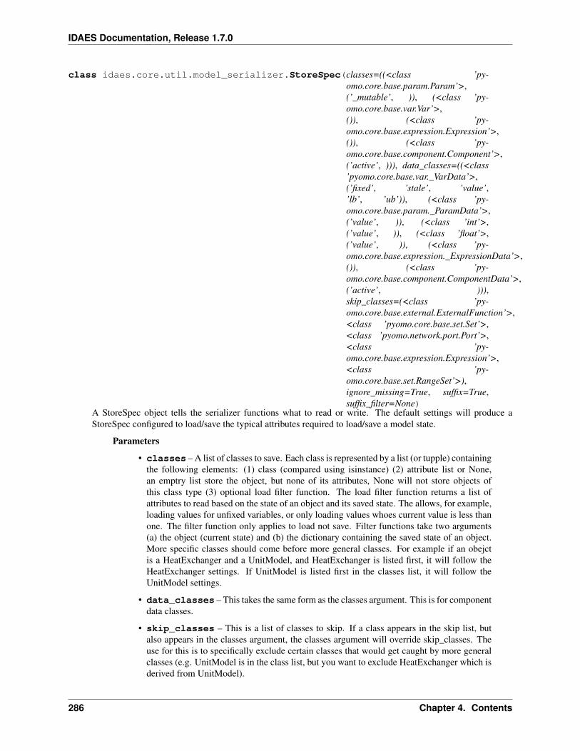
IDAES Documentation, Release 1.7.0
class idaes.core.util.model_serializer.StoreSpec(classes=((<class ’py-omo.core.base.param.Param’>,(’_mutable’, )), (<class ’py-omo.core.base.var.Var’>,()), (<class ’py-omo.core.base.expression.Expression’>,()), (<class ’py-omo.core.base.component.Component’>,(’active’, ))), data_classes=((<class’pyomo.core.base.var._VarData’>,(’fixed’, ’stale’, ’value’,’lb’, ’ub’)), (<class ’py-omo.core.base.param._ParamData’>,(’value’, )), (<class ’int’>,(’value’, )), (<class ’float’>,(’value’, )), (<class ’py-omo.core.base.expression._ExpressionData’>,()), (<class ’py-omo.core.base.component.ComponentData’>,(’active’, ))),skip_classes=(<class ’py-omo.core.base.external.ExternalFunction’>,<class ’pyomo.core.base.set.Set’>,<class ’pyomo.network.port.Port’>,<class ’py-omo.core.base.expression.Expression’>,<class ’py-omo.core.base.set.RangeSet’>),ignore_missing=True, suffix=True,suffix_filter=None)
A StoreSpec object tells the serializer functions what to read or write. The default settings will produce aStoreSpec configured to load/save the typical attributes required to load/save a model state.
Parameters
• classes – A list of classes to save. Each class is represented by a list (or tupple) containingthe following elements: (1) class (compared using isinstance) (2) attribute list or None,an emptry list store the object, but none of its attributes, None will not store objects ofthis class type (3) optional load filter function. The load filter function returns a list ofattributes to read based on the state of an object and its saved state. The allows, for example,loading values for unfixed variables, or only loading values whoes current value is less thanone. The filter function only applies to load not save. Filter functions take two arguments(a) the object (current state) and (b) the dictionary containing the saved state of an object.More specific classes should come before more general classes. For example if an obejctis a HeatExchanger and a UnitModel, and HeatExchanger is listed first, it will follow theHeatExchanger settings. If UnitModel is listed first in the classes list, it will follow theUnitModel settings.
• data_classes – This takes the same form as the classes argument. This is for componentdata classes.
• skip_classes – This is a list of classes to skip. If a class appears in the skip list, butalso appears in the classes argument, the classes argument will override skip_classes. Theuse for this is to specifically exclude certain classes that would get caught by more generalclasses (e.g. UnitModel is in the class list, but you want to exclude HeatExchanger which isderived from UnitModel).
286 Chapter 4. Contents
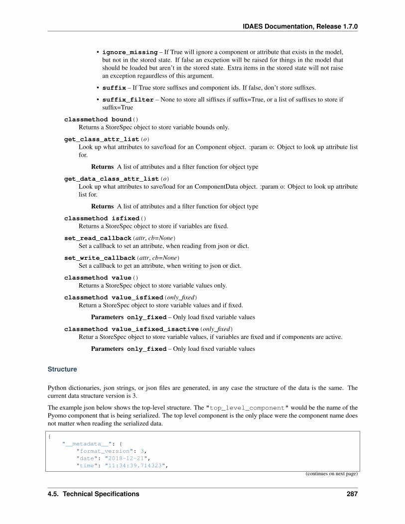
IDAES Documentation, Release 1.7.0
• ignore_missing – If True will ignore a component or attribute that exists in the model,but not in the stored state. If false an excpetion will be raised for things in the model thatshould be loaded but aren’t in the stored state. Extra items in the stored state will not raisean exception regaurdless of this argument.
• suffix – If True store suffixes and component ids. If false, don’t store suffixes.
• suffix_filter – None to store all siffixes if suffix=True, or a list of suffixes to store ifsuffix=True
classmethod bound()Returns a StoreSpec object to store variable bounds only.
get_class_attr_list(o)Look up what attributes to save/load for an Component object. :param o: Object to look up attribute listfor.
Returns A list of attributes and a filter function for object type
get_data_class_attr_list(o)Look up what attributes to save/load for an ComponentData object. :param o: Object to look up attributelist for.
Returns A list of attributes and a filter function for object type
classmethod isfixed()Returns a StoreSpec object to store if variables are fixed.
set_read_callback(attr, cb=None)Set a callback to set an attribute, when reading from json or dict.
set_write_callback(attr, cb=None)Set a callback to get an attribute, when writing to json or dict.
classmethod value()Returns a StoreSpec object to store variable values only.
classmethod value_isfixed(only_fixed)Return a StoreSpec object to store variable values and if fixed.
Parameters only_fixed – Only load fixed variable values
classmethod value_isfixed_isactive(only_fixed)Retur a StoreSpec object to store variable values, if variables are fixed and if components are active.
Parameters only_fixed – Only load fixed variable values
Structure
Python dictionaries, json strings, or json files are generated, in any case the structure of the data is the same. Thecurrent data structure version is 3.
The example json below shows the top-level structure. The "top_level_component" would be the name of thePyomo component that is being serialized. The top level component is the only place were the component name doesnot matter when reading the serialized data.
"__metadata__":
"format_version": 3,"date": "2018-12-21","time": "11:34:39.714323",
(continues on next page)
4.5. Technical Specifications 287
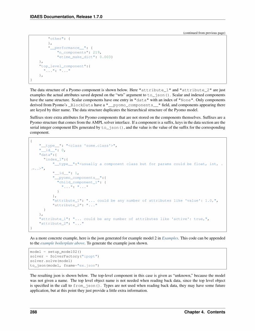
IDAES Documentation, Release 1.7.0
(continued from previous page)
"other": ,"__performance__":
"n_components": 219,"etime_make_dict": 0.003
,"top_level_component":
"...": "...",
The data structure of a Pyomo component is shown below. Here "attribute_1" and "attribute_2" are justexamples the actual attributes saved depend on the “wts” argument to to_json(). Scalar and indexed componentshave the same structure. Scalar components have one entry in "data" with an index of "None". Only componentsderived from Pyomo’s _BlockData have a "__pyomo_components__" field, and components appearing thereare keyed by thier name. The data structure duplicates the hierarchical structure of the Pyomo model.
Suffixes store extra attributes for Pyomo components that are not stored on the components themselves. Suffixes are aPyomo structure that comes from the AMPL solver interface. If a component is a suffix, keys in the data section are theserial integer component IDs generated by to_json(), and the value is the value of the suffix for the correspondingcomponent.
"__type__": "<class 'some.class'>","__id__": 0,"data":
"index_1":"__type__":"<usually a component class but for params could be float, int, .
→˓..>","__id__": 1,"__pyomo_components__":"child_component_1": "...": "..."
,"attribute_1": "... could be any number of attributes like 'value': 1.0,","attribute_2": "..."
,"attribute_1": "... could be any number of attributes like 'active': true,","attribute_2": "..."
As a more concrete example, here is the json generated for example model 2 in Examples. This code can be appendedto the example boilerplate above. To generate the example json shown.
model = setup_model02()solver = SolverFactory("ipopt")solver.solve(model)to_json(model, fname="ex.json")
The resulting json is shown below. The top-level component in this case is given as “unknown,” because the modelwas not given a name. The top level object name is not needed when reading back data, since the top level objectis specified in the call to from_json(). Types are not used when reading back data, they may have some futureapplication, but at this point they just provide a little extra information.
288 Chapter 4. Contents
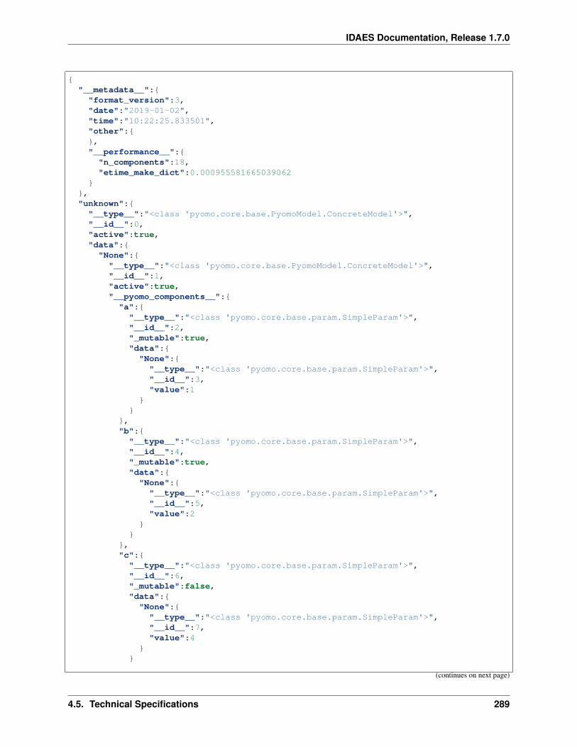
IDAES Documentation, Release 1.7.0
"__metadata__":"format_version":3,"date":"2019-01-02","time":"10:22:25.833501","other":,"__performance__":
"n_components":18,"etime_make_dict":0.000955581665039062
,"unknown":"__type__":"<class 'pyomo.core.base.PyomoModel.ConcreteModel'>","__id__":0,"active":true,"data":
"None":"__type__":"<class 'pyomo.core.base.PyomoModel.ConcreteModel'>","__id__":1,"active":true,"__pyomo_components__":"a":"__type__":"<class 'pyomo.core.base.param.SimpleParam'>","__id__":2,"_mutable":true,"data":"None":
"__type__":"<class 'pyomo.core.base.param.SimpleParam'>","__id__":3,"value":1
,"b":
"__type__":"<class 'pyomo.core.base.param.SimpleParam'>","__id__":4,"_mutable":true,"data":"None":
"__type__":"<class 'pyomo.core.base.param.SimpleParam'>","__id__":5,"value":2
,"c":
"__type__":"<class 'pyomo.core.base.param.SimpleParam'>","__id__":6,"_mutable":false,"data":"None":
"__type__":"<class 'pyomo.core.base.param.SimpleParam'>","__id__":7,"value":4
(continues on next page)
4.5. Technical Specifications 289
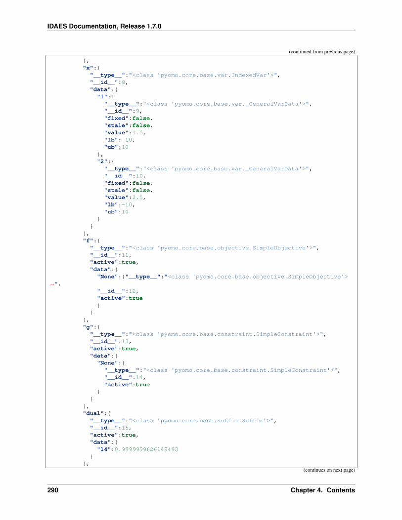
IDAES Documentation, Release 1.7.0
(continued from previous page)
,"x":"__type__":"<class 'pyomo.core.base.var.IndexedVar'>","__id__":8,"data":"1":"__type__":"<class 'pyomo.core.base.var._GeneralVarData'>","__id__":9,"fixed":false,"stale":false,"value":1.5,"lb":-10,"ub":10
,"2":"__type__":"<class 'pyomo.core.base.var._GeneralVarData'>","__id__":10,"fixed":false,"stale":false,"value":2.5,"lb":-10,"ub":10
,"f":
"__type__":"<class 'pyomo.core.base.objective.SimpleObjective'>","__id__":11,"active":true,"data":"None":"__type__":"<class 'pyomo.core.base.objective.SimpleObjective'>
→˓","__id__":12,"active":true
,"g":
"__type__":"<class 'pyomo.core.base.constraint.SimpleConstraint'>","__id__":13,"active":true,"data":"None":
"__type__":"<class 'pyomo.core.base.constraint.SimpleConstraint'>","__id__":14,"active":true
,"dual":
"__type__":"<class 'pyomo.core.base.suffix.Suffix'>","__id__":15,"active":true,"data":"14":0.9999999626149493
,
(continues on next page)
290 Chapter 4. Contents
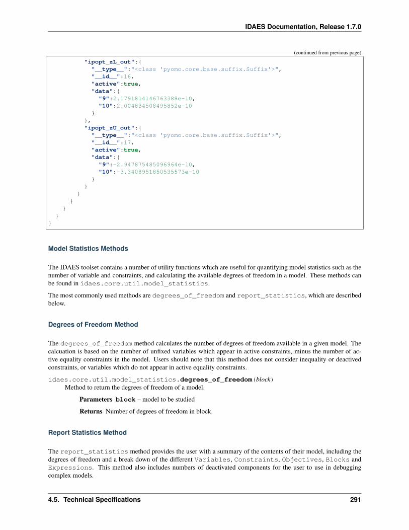
IDAES Documentation, Release 1.7.0
(continued from previous page)
"ipopt_zL_out":"__type__":"<class 'pyomo.core.base.suffix.Suffix'>","__id__":16,"active":true,"data":"9":2.1791814146763388e-10,"10":2.004834508495852e-10
,"ipopt_zU_out":
"__type__":"<class 'pyomo.core.base.suffix.Suffix'>","__id__":17,"active":true,"data":"9":-2.947875485096964e-10,"10":-3.3408951850535573e-10
Model Statistics Methods
The IDAES toolset contains a number of utility functions which are useful for quantifying model statistics such as thenumber of variable and constraints, and calculating the available degrees of freedom in a model. These methods canbe found in idaes.core.util.model_statistics.
The most commonly used methods are degrees_of_freedom and report_statistics, which are describedbelow.
Degrees of Freedom Method
The degrees_of_freedom method calculates the number of degrees of freedom available in a given model. Thecalcuation is based on the number of unfixed variables which appear in active constraints, minus the number of ac-tive equality constraints in the model. Users should note that this method does not consider inequality or deactivedconstraints, or variables which do not appear in active equality constraints.
idaes.core.util.model_statistics.degrees_of_freedom(block)Method to return the degrees of freedom of a model.
Parameters block – model to be studied
Returns Number of degrees of freedom in block.
Report Statistics Method
The report_statistics method provides the user with a summary of the contents of their model, including thedegrees of freedom and a break down of the different Variables, Constraints, Objectives, Blocks andExpressions. This method also includes numbers of deactivated components for the user to use in debuggingcomplex models.
4.5. Technical Specifications 291
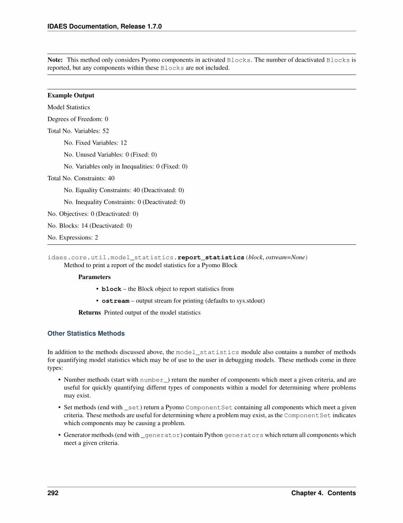
IDAES Documentation, Release 1.7.0
Note: This method only considers Pyomo components in activated Blocks. The number of deactivated Blocks isreported, but any components within these Blocks are not included.
Example Output
Model Statistics
Degrees of Freedom: 0
Total No. Variables: 52
No. Fixed Variables: 12
No. Unused Variables: 0 (Fixed: 0)
No. Variables only in Inequalities: 0 (Fixed: 0)
Total No. Constraints: 40
No. Equality Constraints: 40 (Deactivated: 0)
No. Inequality Constraints: 0 (Deactivated: 0)
No. Objectives: 0 (Deactivated: 0)
No. Blocks: 14 (Deactivated: 0)
No. Expressions: 2
idaes.core.util.model_statistics.report_statistics(block, ostream=None)Method to print a report of the model statistics for a Pyomo Block
Parameters
• block – the Block object to report statistics from
• ostream – output stream for printing (defaults to sys.stdout)
Returns Printed output of the model statistics
Other Statistics Methods
In addition to the methods discussed above, the model_statistics module also contains a number of methodsfor quantifying model statistics which may be of use to the user in debugging models. These methods come in threetypes:
• Number methods (start with number_) return the number of components which meet a given criteria, and areuseful for quickly quantifying differnt types of components within a model for determining where problemsmay exist.
• Set methods (end with _set) return a Pyomo ComponentSet containing all components which meet a givencriteria. These methods are useful for determining where a problem may exist, as the ComponentSet indicateswhich components may be causing a problem.
• Generator methods (end with _generator) contain Python generatorswhich return all components whichmeet a given criteria.
292 Chapter 4. Contents
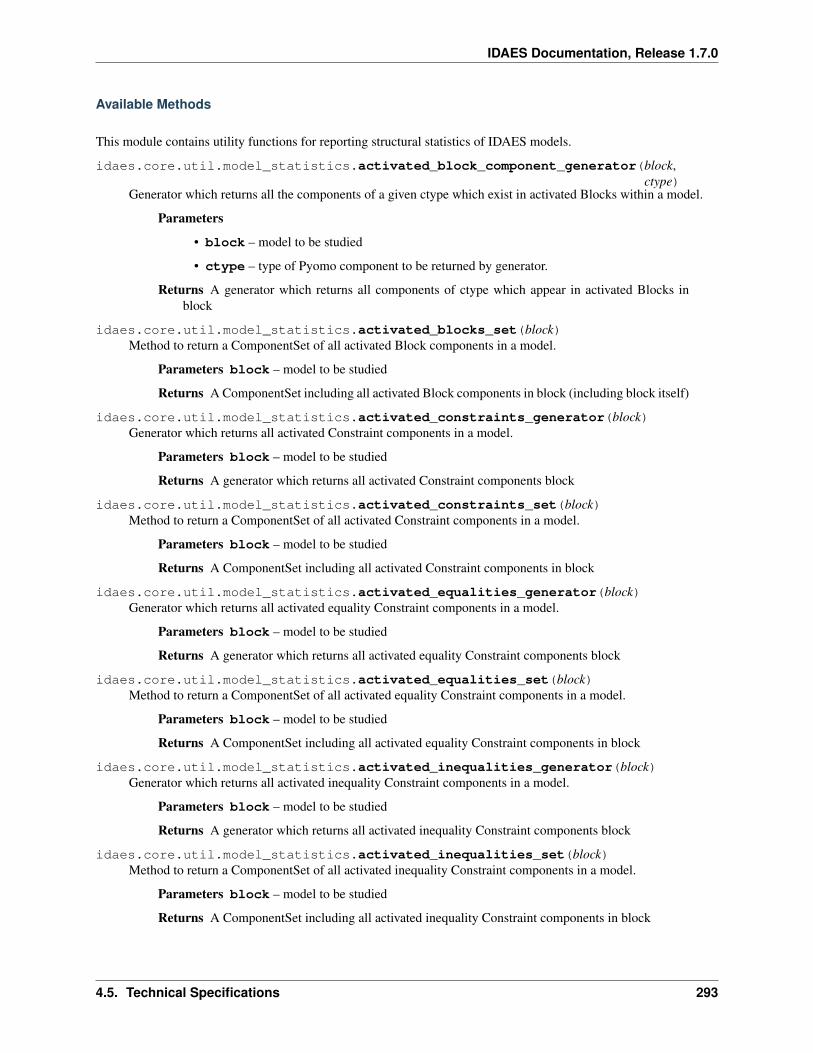
IDAES Documentation, Release 1.7.0
Available Methods
This module contains utility functions for reporting structural statistics of IDAES models.
idaes.core.util.model_statistics.activated_block_component_generator(block,ctype)
Generator which returns all the components of a given ctype which exist in activated Blocks within a model.
Parameters
• block – model to be studied
• ctype – type of Pyomo component to be returned by generator.
Returns A generator which returns all components of ctype which appear in activated Blocks inblock
idaes.core.util.model_statistics.activated_blocks_set(block)Method to return a ComponentSet of all activated Block components in a model.
Parameters block – model to be studied
Returns A ComponentSet including all activated Block components in block (including block itself)
idaes.core.util.model_statistics.activated_constraints_generator(block)Generator which returns all activated Constraint components in a model.
Parameters block – model to be studied
Returns A generator which returns all activated Constraint components block
idaes.core.util.model_statistics.activated_constraints_set(block)Method to return a ComponentSet of all activated Constraint components in a model.
Parameters block – model to be studied
Returns A ComponentSet including all activated Constraint components in block
idaes.core.util.model_statistics.activated_equalities_generator(block)Generator which returns all activated equality Constraint components in a model.
Parameters block – model to be studied
Returns A generator which returns all activated equality Constraint components block
idaes.core.util.model_statistics.activated_equalities_set(block)Method to return a ComponentSet of all activated equality Constraint components in a model.
Parameters block – model to be studied
Returns A ComponentSet including all activated equality Constraint components in block
idaes.core.util.model_statistics.activated_inequalities_generator(block)Generator which returns all activated inequality Constraint components in a model.
Parameters block – model to be studied
Returns A generator which returns all activated inequality Constraint components block
idaes.core.util.model_statistics.activated_inequalities_set(block)Method to return a ComponentSet of all activated inequality Constraint components in a model.
Parameters block – model to be studied
Returns A ComponentSet including all activated inequality Constraint components in block
4.5. Technical Specifications 293
IDAES Documentation, Release 1.7.0
idaes.core.util.model_statistics.activated_objectives_generator(block)Generator which returns all activated Objective components in a model.
Parameters block – model to be studied
Returns A generator which returns all activated Objective components block
idaes.core.util.model_statistics.activated_objectives_set(block)Method to return a ComponentSet of all activated Objective components which appear in a model.
Parameters block – model to be studied
Returns A ComponentSet including all activated Objective components which appear in block
idaes.core.util.model_statistics.active_variables_in_deactivated_blocks_set(block)Method to return a ComponentSet of any Var components which appear within an active Constraint but belongto a deacitvated Block in a model.
Parameters block – model to be studied
Returns A ComponentSet including any Var components which belong to a deacitvated Block butappear in an activate Constraint in block
idaes.core.util.model_statistics.deactivated_blocks_set(block)Method to return a ComponentSet of all deactivated Block components in a model.
Parameters block – model to be studied
Returns A ComponentSet including all deactivated Block components in block (including blockitself)
idaes.core.util.model_statistics.deactivated_constraints_generator(block)Generator which returns all deactivated Constraint components in a model.
Parameters block – model to be studied
Returns A generator which returns all deactivated Constraint components block
idaes.core.util.model_statistics.deactivated_constraints_set(block)Method to return a ComponentSet of all deactivated Constraint components in a model.
Parameters block – model to be studied
Returns A ComponentSet including all deactivated Constraint components in block
idaes.core.util.model_statistics.deactivated_equalities_generator(block)Generator which returns all deactivated equality Constraint components in a model.
Parameters block – model to be studied
Returns A generator which returns all deactivated equality Constraint components block
idaes.core.util.model_statistics.deactivated_equalities_set(block)Method to return a ComponentSet of all deactivated equality Constraint components in a model.
Parameters block – model to be studied
Returns A ComponentSet including all deactivated equality Constraint components in block
idaes.core.util.model_statistics.deactivated_inequalities_generator(block)Generator which returns all deactivated inequality Constraint components in a model.
Parameters block – model to be studied
Returns A generator which returns all indeactivated equality Constraint components block
294 Chapter 4. Contents
IDAES Documentation, Release 1.7.0
idaes.core.util.model_statistics.deactivated_inequalities_set(block)Method to return a ComponentSet of all deactivated inequality Constraint components in a model.
Parameters block – model to be studied
Returns A ComponentSet including all deactivated inequality Constraint components in block
idaes.core.util.model_statistics.deactivated_objectives_generator(block)Generator which returns all deactivated Objective components in a model.
Parameters block – model to be studied
Returns A generator which returns all deactivated Objective components block
idaes.core.util.model_statistics.deactivated_objectives_set(block)Method to return a ComponentSet of all deactivated Objective components which appear in a model.
Parameters block – model to be studied
Returns A ComponentSet including all deactivated Objective components which appear in block
idaes.core.util.model_statistics.derivative_variables_set(block)Method to return a ComponentSet of all DerivativeVar components which appear in a model. Users should notethat DerivativeVars are converted to ordinary Vars when a DAE transformation is applied. Thus, this method isuseful for detecting any DerivativeVars which were do transformed.
Parameters block – model to be studied
Returns A ComponentSet including all DerivativeVar components which appear in block
idaes.core.util.model_statistics.expressions_set(block)Method to return a ComponentSet of all Expression components which appear in a model.
Parameters block – model to be studied
Returns A ComponentSet including all Expression components which appear in block
idaes.core.util.model_statistics.fixed_unused_variables_set(block)Method to return a ComponentSet of all fixed Var components which do not appear within any activated Con-straint in a model.
Parameters block – model to be studied
Returns A ComponentSet including all fixed Var components which do not appear within any Con-straints in block
idaes.core.util.model_statistics.fixed_variables_generator(block)Generator which returns all fixed Var components in a model.
Parameters block – model to be studied
Returns A generator which returns all fixed Var components block
idaes.core.util.model_statistics.fixed_variables_in_activated_equalities_set(block)Method to return a ComponentSet of all fixed Var components which appear within an equality Constraint in amodel.
Parameters block – model to be studied
Returns A ComponentSet including all fixed Var components which appear within activated equal-ity Constraints in block
idaes.core.util.model_statistics.fixed_variables_only_in_inequalities(block)Method to return a ComponentSet of all fixed Var components which appear only within activated inequalityConstraints in a model.
4.5. Technical Specifications 295
IDAES Documentation, Release 1.7.0
Parameters block – model to be studied
Returns A ComponentSet including all fixed Var components which appear only within activatedinequality Constraints in block
idaes.core.util.model_statistics.fixed_variables_set(block)Method to return a ComponentSet of all fixed Var components in a model.
Parameters block – model to be studied
Returns A ComponentSet including all fixed Var components in block
idaes.core.util.model_statistics.large_residuals_set(block, tol=1e-05)Method to return a ComponentSet of all Constraint components with a residual greater than a given thresholdwhich appear in a model.
Parameters
• block – model to be studied
• tol – residual threshold for inclusion in ComponentSet
Returns A ComponentSet including all Constraint components with a residual greater than tol whichappear in block
idaes.core.util.model_statistics.number_activated_blocks(block)Method to return the number of activated Block components in a model.
Parameters block – model to be studied
Returns Number of activated Block components in block (including block itself)
idaes.core.util.model_statistics.number_activated_constraints(block)Method to return the number of activated Constraint components in a model.
Parameters block – model to be studied
Returns Number of activated Constraint components in block
idaes.core.util.model_statistics.number_activated_equalities(block)Method to return the number of activated equality Constraint components in a model.
Parameters block – model to be studied
Returns Number of activated equality Constraint components in block
idaes.core.util.model_statistics.number_activated_inequalities(block)Method to return the number of activated inequality Constraint components in a model.
Parameters block – model to be studied
Returns Number of activated inequality Constraint components in block
idaes.core.util.model_statistics.number_activated_objectives(block)Method to return the number of activated Objective components which appear in a model.
Parameters block – model to be studied
Returns Number of activated Objective components which appear in block
idaes.core.util.model_statistics.number_active_variables_in_deactivated_blocks(block)Method to return the number of Var components which appear within an active Constraint but belong to adeacitvated Block in a model.
Parameters block – model to be studied
296 Chapter 4. Contents
IDAES Documentation, Release 1.7.0
Returns Number of Var components which belong to a deacitvated Block but appear in an activateConstraint in block
idaes.core.util.model_statistics.number_deactivated_blocks(block)Method to return the number of deactivated Block components in a model.
Parameters block – model to be studied
Returns Number of deactivated Block components in block (including block itself)
idaes.core.util.model_statistics.number_deactivated_constraints(block)Method to return the number of deactivated Constraint components in a model.
Parameters block – model to be studied
Returns Number of deactivated Constraint components in block
idaes.core.util.model_statistics.number_deactivated_equalities(block)Method to return the number of deactivated equality Constraint components in a model.
Parameters block – model to be studied
Returns Number of deactivated equality Constraint components in block
idaes.core.util.model_statistics.number_deactivated_inequalities(block)Method to return the number of deactivated inequality Constraint components in a model.
Parameters block – model to be studied
Returns Number of deactivated inequality Constraint components in block
idaes.core.util.model_statistics.number_deactivated_objectives(block)Method to return the number of deactivated Objective components which appear in a model.
Parameters block – model to be studied
Returns Number of deactivated Objective components which appear in block
idaes.core.util.model_statistics.number_derivative_variables(block)Method to return the number of DerivativeVar components which appear in a model. Users should note thatDerivativeVars are converted to ordinary Vars when a DAE transformation is applied. Thus, this method isuseful for detecting any DerivativeVars which were do transformed.
Parameters block – model to be studied
Returns Number of DerivativeVar components which appear in block
idaes.core.util.model_statistics.number_expressions(block)Method to return the number of Expression components which appear in a model.
Parameters block – model to be studied
Returns Number of Expression components which appear in block
idaes.core.util.model_statistics.number_fixed_unused_variables(block)Method to return the number of fixed Var components which do not appear within any activated Constraint in amodel.
Parameters block – model to be studied
Returns Number of fixed Var components which do not appear within any activated Constraints inblock
idaes.core.util.model_statistics.number_fixed_variables(block)Method to return the number of fixed Var components in a model.
Parameters block – model to be studied
4.5. Technical Specifications 297
IDAES Documentation, Release 1.7.0
Returns Number of fixed Var components in block
idaes.core.util.model_statistics.number_fixed_variables_in_activated_equalities(block)Method to return the number of fixed Var components which appear within activated equality Constraints in amodel.
Parameters block – model to be studied
Returns Number of fixed Var components which appear within activated equality Constraints inblock
idaes.core.util.model_statistics.number_fixed_variables_only_in_inequalities(block)Method to return the number of fixed Var components which only appear within activated inequality Constraintsin a model.
Parameters block – model to be studied
Returns Number of fixed Var components which only appear within activated inequality Constraintsin block
idaes.core.util.model_statistics.number_large_residuals(block, tol=1e-05)Method to return the number Constraint components with a residual greater than a given threshold which appearin a model.
Parameters
• block – model to be studied
• tol – residual threshold for inclusion in ComponentSet
Returns Number of Constraint components with a residual greater than tol which appear in block
idaes.core.util.model_statistics.number_total_blocks(block)Method to return the number of Block components in a model.
Parameters block – model to be studied
Returns Number of Block components in block (including block itself)
idaes.core.util.model_statistics.number_total_constraints(block)Method to return the total number of Constraint components in a model.
Parameters block – model to be studied
Returns Number of Constraint components in block
idaes.core.util.model_statistics.number_total_equalities(block)Method to return the total number of equality Constraint components in a model.
Parameters block – model to be studied
Returns Number of equality Constraint components in block
idaes.core.util.model_statistics.number_total_inequalities(block)Method to return the total number of inequality Constraint components in a model.
Parameters block – model to be studied
Returns Number of inequality Constraint components in block
idaes.core.util.model_statistics.number_total_objectives(block)Method to return the number of Objective components which appear in a model
Parameters block – model to be studied
Returns Number of Objective components which appear in block
298 Chapter 4. Contents
IDAES Documentation, Release 1.7.0
idaes.core.util.model_statistics.number_unfixed_variables(block)Method to return the number of unfixed Var components in a model.
Parameters block – model to be studied
Returns Number of unfixed Var components in block
idaes.core.util.model_statistics.number_unfixed_variables_in_activated_equalities(block)Method to return the number of unfixed Var components which appear within activated equality Constraints ina model.
Parameters block – model to be studied
Returns Number of unfixed Var components which appear within activated equality Constraints inblock
idaes.core.util.model_statistics.number_unused_variables(block)Method to return the number of Var components which do not appear within any activated Constraint in a model.
Parameters block – model to be studied
Returns Number of Var components which do not appear within any activagted Constraints in block
idaes.core.util.model_statistics.number_variables(block)Method to return the number of Var components in a model.
Parameters block – model to be studied
Returns Number of Var components in block
idaes.core.util.model_statistics.number_variables_in_activated_constraints(block)Method to return the number of Var components that appear within active Constraints in a model.
Parameters block – model to be studied
Returns Number of Var components which appear within active Constraints in block
idaes.core.util.model_statistics.number_variables_in_activated_equalities(block)Method to return the number of Var components which appear within activated equality Constraints in a model.
Parameters block – model to be studied
Returns Number of Var components which appear within activated equality Constraints in block
idaes.core.util.model_statistics.number_variables_in_activated_inequalities(block)Method to return the number of Var components which appear within activated inequality Constraints in a model.
Parameters block – model to be studied
Returns Number of Var components which appear within activated inequality Constraints in block
idaes.core.util.model_statistics.number_variables_near_bounds(block,tol=0.0001)
Method to return the number of all Var components in a model which have a value within tol (relative) of abound.
Parameters
• block – model to be studied
• tol – relative tolerance for inclusion in generator (default = 1e-4)
Returns Number of components block that are close to a bound
idaes.core.util.model_statistics.number_variables_only_in_inequalities(block)Method to return the number of Var components which appear only within activated inequality Constraints in amodel.
4.5. Technical Specifications 299
IDAES Documentation, Release 1.7.0
Parameters block – model to be studied
Returns Number of Var components which appear only within activated inequality Constraints inblock
idaes.core.util.model_statistics.total_blocks_set(block)Method to return a ComponentSet of all Block components in a model.
Parameters block – model to be studied
Returns A ComponentSet including all Block components in block (including block itself)
idaes.core.util.model_statistics.total_constraints_set(block)Method to return a ComponentSet of all Constraint components in a model.
Parameters block – model to be studied
Returns A ComponentSet including all Constraint components in block
idaes.core.util.model_statistics.total_equalities_generator(block)Generator which returns all equality Constraint components in a model.
Parameters block – model to be studied
Returns A generator which returns all equality Constraint components block
idaes.core.util.model_statistics.total_equalities_set(block)Method to return a ComponentSet of all equality Constraint components in a model.
Parameters block – model to be studied
Returns A ComponentSet including all equality Constraint components in block
idaes.core.util.model_statistics.total_inequalities_generator(block)Generator which returns all inequality Constraint components in a model.
Parameters block – model to be studied
Returns A generator which returns all inequality Constraint components block
idaes.core.util.model_statistics.total_inequalities_set(block)Method to return a ComponentSet of all inequality Constraint components in a model.
Parameters block – model to be studied
Returns A ComponentSet including all inequality Constraint components in block
idaes.core.util.model_statistics.total_objectives_generator(block)Generator which returns all Objective components in a model.
Parameters block – model to be studied
Returns A generator which returns all Objective components block
idaes.core.util.model_statistics.total_objectives_set(block)Method to return a ComponentSet of all Objective components which appear in a model.
Parameters block – model to be studied
Returns A ComponentSet including all Objective components which appear in block
idaes.core.util.model_statistics.unfixed_variables_generator(block)Generator which returns all unfixed Var components in a model.
Parameters block – model to be studied
Returns A generator which returns all unfixed Var components block
300 Chapter 4. Contents
IDAES Documentation, Release 1.7.0
idaes.core.util.model_statistics.unfixed_variables_in_activated_equalities_set(block)Method to return a ComponentSet of all unfixed Var components which appear within an activated equalityConstraint in a model.
Parameters block – model to be studied
Returns A ComponentSet including all unfixed Var components which appear within activatedequality Constraints in block
idaes.core.util.model_statistics.unfixed_variables_set(block)Method to return a ComponentSet of all unfixed Var components in a model.
Parameters block – model to be studied
Returns A ComponentSet including all unfixed Var components in block
idaes.core.util.model_statistics.unused_variables_set(block)Method to return a ComponentSet of all Var components which do not appear within any activated Constraintin a model.
Parameters block – model to be studied
Returns A ComponentSet including all Var components which do not appear within any Constraintsin block
idaes.core.util.model_statistics.variables_in_activated_constraints_set(block)Method to return a ComponentSet of all Var components which appear within a Constraint in a model.
Parameters block – model to be studied
Returns A ComponentSet including all Var components which appear within activated Constraintsin block
idaes.core.util.model_statistics.variables_in_activated_equalities_set(block)Method to return a ComponentSet of all Var components which appear within an equality Constraint in a model.
Parameters block – model to be studied
Returns A ComponentSet including all Var components which appear within activated equalityConstraints in block
idaes.core.util.model_statistics.variables_in_activated_inequalities_set(block)Method to return a ComponentSet of all Var components which appear within an inequality Constraint in amodel.
Parameters block – model to be studied
Returns A ComponentSet including all Var components which appear within activated inequalityConstraints in block
idaes.core.util.model_statistics.variables_near_bounds_generator(block,tol=0.0001)
Generator which returns all Var components in a model which have a value within tol (relative) of a bound.
Parameters
• block – model to be studied
• tol – relative tolerance for inclusion in generator (default = 1e-4)
Returns A generator which returns all Var components block that are close to a bound
idaes.core.util.model_statistics.variables_near_bounds_set(block, tol=0.0001)Method to return a ComponentSet of all Var components in a model which have a value within tol (relative) ofa bound.
4.5. Technical Specifications 301
IDAES Documentation, Release 1.7.0
Parameters
• block – model to be studied
• tol – relative tolerance for inclusion in generator (default = 1e-4)
Returns A ComponentSet including all Var components block that are close to a bound
idaes.core.util.model_statistics.variables_only_in_inequalities(block)Method to return a ComponentSet of all Var components which appear only within inequality Constraints in amodel.
Parameters block – model to be studied
Returns A ComponentSet including all Var components which appear only within inequality Con-straints in block
idaes.core.util.model_statistics.variables_set(block)Method to return a ComponentSet of all Var components in a model.
Parameters block – model to be studied
Returns A ComponentSet including all Var components in block
Scaling Methods
This section describes scaling utility functions and methods.
Context
Creating well scaled models is important for increasing the efficiency and reliability of solvers. Depending on propertypackage units of measure and process scale, variables and constraints are often badly scaled.
Scaling factors can be specified for any variable or constraint. Pyomo and many solvers support thescaling_factor suffix. To eliminate the possibility of defining conflicting scaling factors in various places inthe model, the IDAES standard is to define the scaling_factor suffixes in the same block as the variable or con-straint that they are scaling. This ensures that each scale factor is defined in only one place, and is organized based onthe model block structure.
Scaling factors in IDAES (and Pyomo) are multiplied by the variable or constraint they scale. For example, a Pressurevariable in Pa units may be expected to have a magnitude of around 106 for a specific process. To scale the variable toa more reasonable magnitude, the scale factor for the variable could be defined to be 1 × 10⁻⁵.
While many scaling factors should be give good default values in the property packages, some (e.g. flow rates ormaterial holdups) must be given scale factors by the user for a specific process model. Still other scale factors canbe calculated from supplied scale factors, for example, mass balance scale factors could be determined from flow ratescale factors. To calculate scale factors, models may have a standard calculate_scaling_factors() method.For more specific scaling information, see the model documentation.
For much of the core IDAES framework, model constraints are automatically scaled via a simple transformation whereboth sides of the constraint are multiplied by a scale factor determined based on supplied variable and expressionscaling factors. The goal of this is to ensure that solver tolerances are meaningful for each constraint. A constraintviolation of 1× 10⁻⁸ should be acceptable, but not too tight to achieve given machine precision limits. IDAES modelconstraints should conform approximately to this guideline after the calculate_scaling_factors() methodis executed. Users should follow this guideline for constraints they write. The scaling of constraints for reasonableresidual tolerances is done as a constraint transformation independent of the scaling factor suffix. Scaling factors forconstraints can still be set based on other methods such as reducing very large Jacobian matrix entries.
302 Chapter 4. Contents
IDAES Documentation, Release 1.7.0
Specifying Scaling
Suffixes are used to specify scaling factors for IDAES models. These suffixes are created when needed by calling theset_scaling_factor() function. Using the set_scaling_factor(), get_scaling_factor(), andunset_scaling_factor() eliminates the need to deal directly with scaling suffixes, and ensures that scalingfactors are stored in the IDAES standard location.
idaes.core.util.scaling.set_scaling_factor(c, v, data_objects=True)Set a scaling factor for a model component. This function creates the scaling_factor suffix if needed.
Parameters
• c – component to supply scaling factor for
• v – scaling factor
Returns None
idaes.core.util.scaling.get_scaling_factor(c, default=None, warning=False, excep-tion=False)
Get a component scale factor.
Parameters
• c – component
• default – value to return if no scale factor exists (default=None)
idaes.core.util.scaling.unset_scaling_factor(c, data_objects=True)Delete a component scaling factor.
Parameters c – component
Returns None
Constraint Transformation
As mentioned previously, constraints in the IDAES framework are transformed such that 1 × 10⁻⁸ is a reasonablecriteria for convergence before any other scaling factors are applied. There are a few utility functions for scalingtransformation of constraints. When transforming constraints with these functions, the scaling applies to the originalconstraint, not combined with any previous transformation.
idaes.core.util.scaling.constraint_scaling_transform(c, s)This transforms a constraint by the argument s. The scaling factor applies to original constraint (e.g. if onewhere to call this twice in a row for a constraint with a scaling factor of 2, the original constraint would still,only be scaled by a factor of 2.)
Parameters
• c – Pyomo constraint
• s – scale factor applied to the constraint as originally written
Returns None
idaes.core.util.scaling.constraint_scaling_transform_undo(c)The undoes the scaling transforms previously applied to a constraint.
Parameters c – Pyomo constraint
Returns None
4.5. Technical Specifications 303
IDAES Documentation, Release 1.7.0
idaes.core.util.scaling.get_constraint_transform_applied_scaling_factor(c,de-fault=None)
Get a the scale factor that was used to transform a constraint.
Parameters
• c – constraint data object
• default – value to return if no scaling factor exisits (default=None)
Returns The scaling factor that has been used to transform the constraint or the default.
Calculation in Model
Some scaling factors may also be calculated by a call to a model’s calculate_scaling_factors() method.For more information see specific model documentation.
Sometimes a scaling factor may be set on an indexed component and prorogated to it’s data objects later can be usefulfor example in models that use the DAE transformation, not all data objects exist until after the transformation.
idaes.core.util.scaling.propagate_indexed_component_scaling_factors(blk,typ=(<class’py-omo.core.base.var.Var’>,<class’py-omo.core.base.constraint.Constraint’>,<class’py-omo.core.base.expression.Expression’>),over-write=False,de-scend_into=True)
Use the parent component scaling factor to set all component data object scaling factors.
Parameters
• blk – The block on which to search for components
• typ – Component type(s) (default=(Var, Constraint, Expression, Param))
• overwrite – if a data object already has a scaling factor should it be overwrittten (de-fault=False)
• descend_into – descend into child blocks (default=True)
Constraint Auto-Scaling
Constraints can be scaled to automatically reduce very large entries in the Jacobian matrix with theconstraint_autoscale_large_jac() function.
304 Chapter 4. Contents
IDAES Documentation, Release 1.7.0
idaes.core.util.scaling.constraint_autoscale_large_jac(m, ig-nore_constraint_scaling=False,ig-nore_variable_scaling=False,max_grad=100,min_scale=1e-06,no_scale=False)
Automatically scale constraints based on the Jacobian. This function immitates Ipopt’s default constraint scal-ing. This scales constraints down to avoid extremely large values in the Jacobian
Parameters
• m – model to scale
• ignore_constraint_scaling – ignore existing constraint scaling
• ignore_variable_scaling – ignore existing variable scaling
• max_grad – maximum value in Jacobian after scaling, subject to minimum scaling factorrestriction.
• min_scale – minimum scaling factor allowed, keeps constraints from being scaled toomuch.
• no_scale – just calculate the Jacobian and scaled Jacobian, don’t scale anything
Inspect Scaling
Models can be large, so it is often difficult to identify where scaling is needed and where the problemmay be poorly scaled. The functions below may be helpful in inspecting a models scaling. Additionallyconstraint_autoscale_large_jac() described above can provide Jacobian information at the current vari-able values.
idaes.core.util.scaling.badly_scaled_var_generator(blk, large=10000.0, small=0.001,zero=1e-10, descend_into=True,include_fixed=False)
This provides a rough check for variables with poor scaling based on their current scale factors and values. Foreach potentially poorly scaled variable it returns the var and its current scaled value.
Parameters
• blk – pyomo block
• large – Magnitude that is considered to be too large
• small – Magnitude that is considered to be too small
• zero – Magnitude that is considered to be zero, variables with a value of zero are okay, andnot reported.
Yields variable data object, current absolute value of scaled value
idaes.core.util.scaling.unscaled_variables_generator(blk, descend_into=True, in-clude_fixed=False)
Generator for unscaled variables
Parameters block –
Yields variables with no scale factor
idaes.core.util.scaling.unscaled_constraints_generator(blk, descend_into=True)Generator for unscaled constraints
4.5. Technical Specifications 305
IDAES Documentation, Release 1.7.0
Parameters block –
Yields constraints with no scale factor
idaes.core.util.scaling.map_scaling_factor(iter, default=1, warning=False, func=<built-in function min>)
Map get_scaling_factor to an iterable of Pyomo components, and call func on the result. This could be use, forexample, to get the minimum or maximum scaling factor of a set of components.
Parameters
• iter – Iterable yeilding Pyomo componentes
• default – The default value used when a scaling factor is missing. The default is de-fault=1.
• warning – Log a warning for missing scaling factors
• func – The function to call on the resulting iterable of scaling factors. The default is min().
Returns The result of func on the set of scaling factors
idaes.core.util.scaling.min_scaling_factor(iter, default=1, warning=True)Map get_scaling_factor to an iterable of Pyomo components, and get the minimum caling factor.
Parameters
• iter – Iterable yeilding Pyomo componentes
• default – The default value used when a scaling factor is missing. If None, this will raisean exception when scaling factors are missing. The default is default=1.
• warning – Log a warning for missing scaling factors
Returns Minimum scaling factor of the components in iter
Applying Scaling
Scale factor suffixes can be passed directly to a solver. How the scale factors are used may vary by solver. Pyomo alsocontains tools to transform a problem to a scaled version.
Ipopt is the standard solver in IDAES. To use scale factors with Ipopt, the nlp_scaling_method option shouldbe set to user-scaling. Be aware that this deactivates any NLP automatic scaling.
Table Methods
The IDAES toolset contians a number of methods for generating and dislpaying summary tables of data in the form ofpandas DataFrames.
Available Methods
idaes.core.util.tables.arcs_to_stream_dict(blk, additional=None, descend_into=True,sort=False, prepend=None, s=)
Creates a stream dictionary from the Arcs in a model, using the Arc names as keys. This can be used toautomate the creation of the streams dictionary needed for the create_stream_table_dataframe()and stream_states_dict() functions.
Parameters
• blk (pyomo.environ._BlockData) – Pyomo model to search for Arcs
306 Chapter 4. Contents
IDAES Documentation, Release 1.7.0
• additional (dict) – Additional states to add to the stream dictionary, which aren’trepresented by arcs in blk, for example feed or product streams without Arcs attached orstates internal to a unit model.
• descend_into (bool) – If True, search subblocks for Arcs as well. The default is True.
• sort (bool) – If True sort keys and return an OrderedDict
• prepend (str) – Prepend a string to the arc name joined with a ‘.’. This can be usefulto prevent conflicting names when sub blocks contain Arcs that have the same names whenused in combination with descend_into=False.
• s (dict) – Add streams to an existing stream dict.
Returns Dictionary with Arc names as keys and the Arcs as values.
idaes.core.util.tables.create_stream_table_dataframe(streams, true_state=False,time_point=0, ori-ent=’columns’)
Method to create a stream table in the form of a pandas dataframe. Method takes a dict with name keys andstream values. Use an OrderedDict to list the streams in a specific order, otherwise the dataframe can be sortedlater.
Parameters
• streams – dict with name keys and stream values. Names will be used as display namesfor stream table, and streams may be Arcs, Ports or StateBlocks.
• true_state – indicated whether the stream table should contain the display variablesdefine in the StateBlock (False, default) or the state variables (True).
• time_point – point in the time domain at which to generate stream table (default = 0)
• orient – orientation of stream table. Accepted values are ‘columns’ (default) wherestreams are displayed as columns, or ‘index’ where stream are displayed as rows.
Returns A pandas DataFrame containing the stream table data.
idaes.core.util.tables.generate_table(blocks, attributes, heading=None, exception=True)Create a Pandas DataFrame that contains a list of user-defined attributes from a set of Blocks.
Parameters
• blocks (dict) – A dictionary with name keys and BlockData objects for values. Anyname can be associated with a block. Use an OrderedDict to show the blocks in a specificorder, otherwise the dataframe can be sorted later.
• attributes (list or tuple of strings) – Attributes to report from a Block,can be a Var, Param, or Expression. If an attribute doesn’t exist or doesn’t have a validvalue, it will be treated as missing data.
• heading (list or tuple of srings) – A list of strings that will be used as col-umn headings. If None the attribute names will be used.
• exception (bool) – If True, raise exceptions releated to invalid or missing indexes. Iffalse missing or bad indexes are ignored and None is used for the table value. Setting this toFalse allows tables where some state blocks have the same attributes with differnt indexing.(default is True)
Returns A Pandas dataframe containing a data table
Return type (DataFrame)
4.5. Technical Specifications 307
IDAES Documentation, Release 1.7.0
idaes.core.util.tables.stream_states_dict(streams, time_point=0)Method to create a dictionary of state block representing stream states. This takes a dict with stream name keysand stream values.
Parameters
• streams – dict with name keys and stream values. Names will be used as display namesfor stream table, and streams may be Arcs, Ports or StateBlocks.
• time_point – point in the time domain at which to generate stream table (default = 0)
Returns A pandas DataFrame containing the stream table data.
idaes.core.util.tables.stream_table_dataframe_to_string(stream_table, **kwargs)Method to print a stream table from a dataframe. Method takes any argument understood by DataFrame.to_string
idaes.core.util.tables.tag_state_quantities(blocks, attributes, labels, exception=False)Take a stream states dictionary, and return a tag dictionary for stream quantities. This takes a dictionary (blk)that has state block labels as keys and state blocks as values. The attributes are a list of attributes to tag. If anelement of the attribute list is list-like, the fist element is the attribute and the remaining elements are indexes.Lables provides a list of attribute lables to be used to create the tag. Tags are blk_key + label for the attribute.
Parameters
• blocks (dict) – Dictionary of state blocks. The key is the block label to be used in thetag, and the value is a state block.
• attributes (list-like) – A list of attriutes to tag. It is okay if a particular attributedoes not exist in a state bock. This allows you to mix state blocks with differnt sets ofattributes. If an attribute is indexed, the attribute can be specified as a list or tuple where thefirst element is the attribute and the remaining elements are indexes.
• labels (list-like) – These are attribute lables. The order corresponds to the attributelist. They are used to create the tags. Tags are in the form blk.key + label.
• exception (bool) – If True, raise exceptions releated to invalid or missing indexes. Iffalse missing or bad indexes are ignored and None is used for the table value. Setting this toFalse allows tables where some state blocks have the same attributes with differnt indexing.(default is True)
Returns
Dictionary where the keys are tags and the values are model attributes, usually Pyomocomponent data objects.
Return type (dict)
Unit Model Costing
The IDAES Process Modeling Framework includes support for incorporating costing of unit operations into a flowsheetto allow for calculation and optimization of process costs. Cost Correlations are implemented using unit costing sub-modules to allow users to easily develop and incorporate their own costing models.
Contents
• Unit Model Costing
– Introduction
– Example
308 Chapter 4. Contents
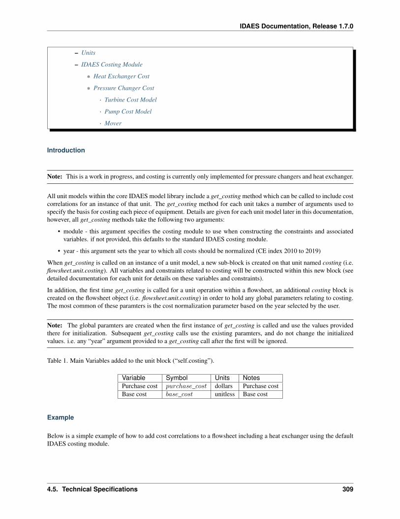
IDAES Documentation, Release 1.7.0
– Units
– IDAES Costing Module
* Heat Exchanger Cost
* Pressure Changer Cost
· Turbine Cost Model
· Pump Cost Model
· Mover
Introduction
Note: This is a work in progress, and costing is currently only implemented for pressure changers and heat exchanger.
All unit models within the core IDAES model library include a get_costing method which can be called to include costcorrelations for an instance of that unit. The get_costing method for each unit takes a number of arguments used tospecify the basis for costing each piece of equipment. Details are given for each unit model later in this documentation,however, all get_costing methods take the following two arguments:
• module - this argument specifies the costing module to use when constructing the constraints and associatedvariables. if not provided, this defaults to the standard IDAES costing module.
• year - this argument sets the year to which all costs should be normalized (CE index 2010 to 2019)
When get_costing is called on an instance of a unit model, a new sub-block is created on that unit named costing (i.e.flowsheet.unit.costing). All variables and constraints related to costing will be constructed within this new block (seedetailed documentation for each unit for details on these variables and constraints).
In addition, the first time get_costing is called for a unit operation within a flowsheet, an additional costing block iscreated on the flowsheet object (i.e. flowsheet.unit.costing) in order to hold any global parameters relating to costing.The most common of these paramters is the cost normalization parameter based on the year selected by the user.
Note: The global paramters are created when the first instance of get_costing is called and use the values providedthere for initialization. Subsequent get_costing calls use the existing paramters, and do not change the initializedvalues. i.e. any “year” argument provided to a get_costing call after the first will be ignored.
Table 1. Main Variables added to the unit block (“self.costing”).
Variable Symbol Units NotesPurchase cost 𝑝𝑢𝑟𝑐ℎ𝑎𝑠𝑒_𝑐𝑜𝑠𝑡 dollars Purchase costBase cost 𝑏𝑎𝑠𝑒_𝑐𝑜𝑠𝑡 unitless Base cost
Example
Below is a simple example of how to add cost correlations to a flowsheet including a heat exchanger using the defaultIDAES costing module.
4.5. Technical Specifications 309
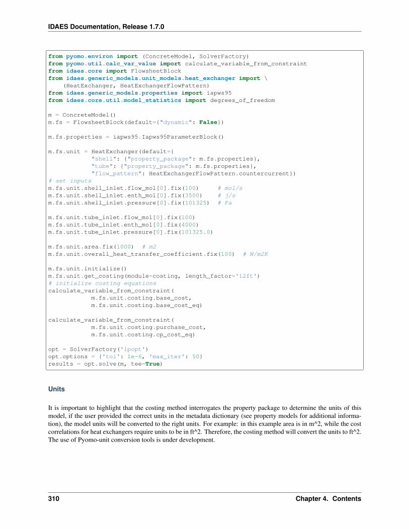
IDAES Documentation, Release 1.7.0
from pyomo.environ import (ConcreteModel, SolverFactory)from pyomo.util.calc_var_value import calculate_variable_from_constraintfrom idaes.core import FlowsheetBlockfrom idaes.generic_models.unit_models.heat_exchanger import \
(HeatExchanger, HeatExchangerFlowPattern)from idaes.generic_models.properties import iapws95from idaes.core.util.model_statistics import degrees_of_freedom
m = ConcreteModel()m.fs = FlowsheetBlock(default="dynamic": False)
m.fs.properties = iapws95.Iapws95ParameterBlock()
m.fs.unit = HeatExchanger(default="shell": "property_package": m.fs.properties,"tube": "property_package": m.fs.properties,"flow_pattern": HeatExchangerFlowPattern.countercurrent)
# set inputsm.fs.unit.shell_inlet.flow_mol[0].fix(100) # mol/sm.fs.unit.shell_inlet.enth_mol[0].fix(3500) # j/sm.fs.unit.shell_inlet.pressure[0].fix(101325) # Pa
m.fs.unit.tube_inlet.flow_mol[0].fix(100)m.fs.unit.tube_inlet.enth_mol[0].fix(4000)m.fs.unit.tube_inlet.pressure[0].fix(101325.0)
m.fs.unit.area.fix(1000) # m2m.fs.unit.overall_heat_transfer_coefficient.fix(100) # W/m2K
m.fs.unit.initialize()m.fs.unit.get_costing(module=costing, length_factor='12ft')# initialize costing equationscalculate_variable_from_constraint(
m.fs.unit.costing.base_cost,m.fs.unit.costing.base_cost_eq)
calculate_variable_from_constraint(m.fs.unit.costing.purchase_cost,m.fs.unit.costing.cp_cost_eq)
opt = SolverFactory('ipopt')opt.options = 'tol': 1e-6, 'max_iter': 50results = opt.solve(m, tee=True)
Units
It is important to highlight that the costing method interrogates the property package to determine the units of thismodel, if the user provided the correct units in the metadata dictionary (see property models for additional informa-tion), the model units will be converted to the right units. For example: in this example area is in m^2, while the costcorrelations for heat exchangers require units to be in ft^2. Therefore, the costing method will convert the units to ft^2.The use of Pyomo-unit conversion tools is under development.
310 Chapter 4. Contents
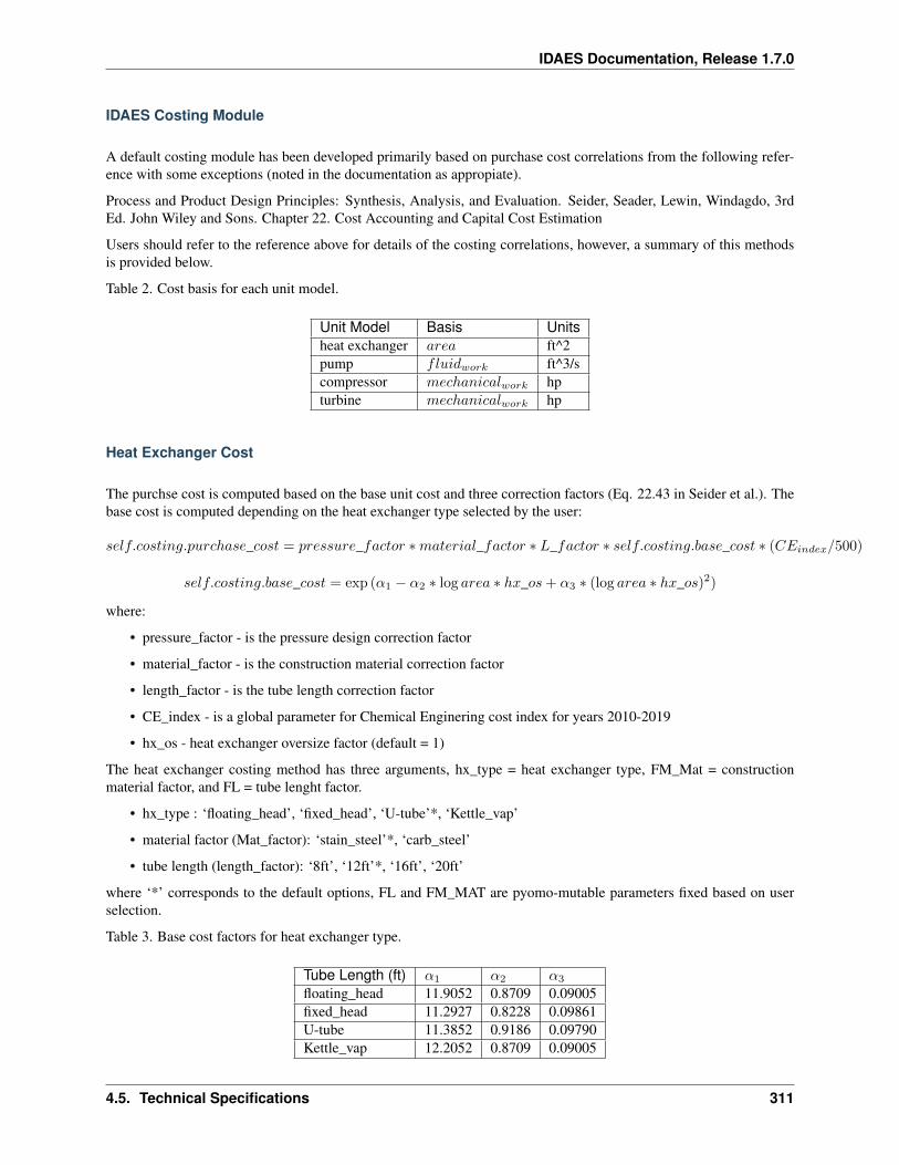
IDAES Documentation, Release 1.7.0
IDAES Costing Module
A default costing module has been developed primarily based on purchase cost correlations from the following refer-ence with some exceptions (noted in the documentation as appropiate).
Process and Product Design Principles: Synthesis, Analysis, and Evaluation. Seider, Seader, Lewin, Windagdo, 3rdEd. John Wiley and Sons. Chapter 22. Cost Accounting and Capital Cost Estimation
Users should refer to the reference above for details of the costing correlations, however, a summary of this methodsis provided below.
Table 2. Cost basis for each unit model.
Unit Model Basis Unitsheat exchanger 𝑎𝑟𝑒𝑎 ft^2pump 𝑓𝑙𝑢𝑖𝑑𝑤𝑜𝑟𝑘 ft^3/scompressor 𝑚𝑒𝑐ℎ𝑎𝑛𝑖𝑐𝑎𝑙𝑤𝑜𝑟𝑘 hpturbine 𝑚𝑒𝑐ℎ𝑎𝑛𝑖𝑐𝑎𝑙𝑤𝑜𝑟𝑘 hp
Heat Exchanger Cost
The purchse cost is computed based on the base unit cost and three correction factors (Eq. 22.43 in Seider et al.). Thebase cost is computed depending on the heat exchanger type selected by the user:
𝑠𝑒𝑙𝑓.𝑐𝑜𝑠𝑡𝑖𝑛𝑔.𝑝𝑢𝑟𝑐ℎ𝑎𝑠𝑒_𝑐𝑜𝑠𝑡 = 𝑝𝑟𝑒𝑠𝑠𝑢𝑟𝑒_𝑓𝑎𝑐𝑡𝑜𝑟 *𝑚𝑎𝑡𝑒𝑟𝑖𝑎𝑙_𝑓𝑎𝑐𝑡𝑜𝑟 * 𝐿_𝑓𝑎𝑐𝑡𝑜𝑟 * 𝑠𝑒𝑙𝑓.𝑐𝑜𝑠𝑡𝑖𝑛𝑔.𝑏𝑎𝑠𝑒_𝑐𝑜𝑠𝑡 * (𝐶𝐸𝑖𝑛𝑑𝑒𝑥/500)
𝑠𝑒𝑙𝑓.𝑐𝑜𝑠𝑡𝑖𝑛𝑔.𝑏𝑎𝑠𝑒_𝑐𝑜𝑠𝑡 = exp (𝛼1 − 𝛼2 * log 𝑎𝑟𝑒𝑎 * ℎ𝑥_𝑜𝑠+ 𝛼3 * (log 𝑎𝑟𝑒𝑎 * ℎ𝑥_𝑜𝑠)2)
where:
• pressure_factor - is the pressure design correction factor
• material_factor - is the construction material correction factor
• length_factor - is the tube length correction factor
• CE_index - is a global parameter for Chemical Enginering cost index for years 2010-2019
• hx_os - heat exchanger oversize factor (default = 1)
The heat exchanger costing method has three arguments, hx_type = heat exchanger type, FM_Mat = constructionmaterial factor, and FL = tube lenght factor.
• hx_type : ‘floating_head’, ‘fixed_head’, ‘U-tube’*, ‘Kettle_vap’
• material factor (Mat_factor): ‘stain_steel’*, ‘carb_steel’
• tube length (length_factor): ‘8ft’, ‘12ft’*, ‘16ft’, ‘20ft’
where ‘*’ corresponds to the default options, FL and FM_MAT are pyomo-mutable parameters fixed based on userselection.
Table 3. Base cost factors for heat exchanger type.
Tube Length (ft) 𝛼1 𝛼2 𝛼3
floating_head 11.9052 0.8709 0.09005fixed_head 11.2927 0.8228 0.09861U-tube 11.3852 0.9186 0.09790Kettle_vap 12.2052 0.8709 0.09005
4.5. Technical Specifications 311
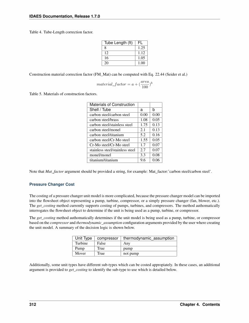
IDAES Documentation, Release 1.7.0
Table 4. Tube-Length correction factor.
Tube Length (ft) FL8 1.2512 1.1216 1.0520 1.00
Construction material correction factor (FM_Mat) can be computed with Eq. 22.44 (Seider et al.)
𝑚𝑎𝑡𝑒𝑟𝑖𝑎𝑙_𝑓𝑎𝑐𝑡𝑜𝑟 = 𝑎+ (𝑎𝑟𝑒𝑎
100)𝑏
Table 5. Materials of construction factors.
Materials of ConstructionShell / Tube a bcarbon steel/carbon steel 0.00 0.00carbon steel/brass 1.08 0.05carbon steel/stainless steel 1.75 0.13carbon steel/monel 2.1 0.13carbon steel/titanium 5.2 0.16carbon steel/Cr-Mo steel 1.55 0.05Cr-Mo steel/Cr-Mo steel 1.7 0.07stainless steel/stainless steel 2.7 0.07monel/monel 3.3 0.08titanium/titanium 9.6 0.06
Note that Mat_factor argument should be provided a string, for example: Mat_factor:’carbon steel/carbon steel’.
Pressure Changer Cost
The costing of a pressure changer unit model is more complicated, because the pressure changer model can be importedinto the flowsheet object representing a pump, turbine, compressor, or a simply pressure changer (fan, blower, etc.).The get_costing method currently supports costing of pumps, turbines, and compressors. The method authomaticallyinterrogates the flowsheet object to determine if the unit is being used as a pump, turbine, or compressor.
The get_costing method authomatically determines if the unit model is being used as a pump, turbine, or compressorbased on the compressor and thermodynamic_assumption configuration arguments provided by the user where creatingthe unit model. A summary of the decision logic is shown below.
Unit Type compressor thermodynamic_assumptionTurbine False AnyPump True pumpMover True not pump
Additionally, some unit types have different sub-types which can be costed appropiately. In these cases, an additionalargument is provided to get_costing to identify the sub-type to use which is detailed below.
312 Chapter 4. Contents
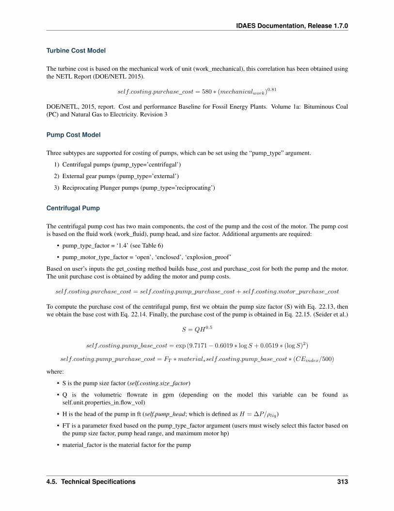
IDAES Documentation, Release 1.7.0
Turbine Cost Model
The turbine cost is based on the mechanical work of unit (work_mechanical), this correlation has been obtained usingthe NETL Report (DOE/NETL 2015).
𝑠𝑒𝑙𝑓.𝑐𝑜𝑠𝑡𝑖𝑛𝑔.𝑝𝑢𝑟𝑐ℎ𝑎𝑠𝑒_𝑐𝑜𝑠𝑡 = 580 * (𝑚𝑒𝑐ℎ𝑎𝑛𝑖𝑐𝑎𝑙𝑤𝑜𝑟𝑘)0.81
DOE/NETL, 2015, report. Cost and performance Baseline for Fossil Energy Plants. Volume 1a: Bituminous Coal(PC) and Natural Gas to Electricity. Revision 3
Pump Cost Model
Three subtypes are supported for costing of pumps, which can be set using the “pump_type” argument.
1) Centrifugal pumps (pump_type=’centrifugal’)
2) External gear pumps (pump_type=’external’)
3) Reciprocating Plunger pumps (pump_type=’reciprocating’)
Centrifugal Pump
The centrifugal pump cost has two main components, the cost of the pump and the cost of the motor. The pump costis based on the fluid work (work_fluid), pump head, and size factor. Additional arguments are required:
• pump_type_factor = ‘1.4’ (see Table 6)
• pump_motor_type_factor = ‘open’, ‘enclosed’, ‘explosion_proof’
Based on user’s inputs the get_costing method builds base_cost and purchase_cost for both the pump and the motor.The unit purchase cost is obtained by adding the motor and pump costs.
𝑠𝑒𝑙𝑓.𝑐𝑜𝑠𝑡𝑖𝑛𝑔.𝑝𝑢𝑟𝑐ℎ𝑎𝑠𝑒_𝑐𝑜𝑠𝑡 = 𝑠𝑒𝑙𝑓.𝑐𝑜𝑠𝑡𝑖𝑛𝑔.𝑝𝑢𝑚𝑝_𝑝𝑢𝑟𝑐ℎ𝑎𝑠𝑒_𝑐𝑜𝑠𝑡+ 𝑠𝑒𝑙𝑓.𝑐𝑜𝑠𝑡𝑖𝑛𝑔.𝑚𝑜𝑡𝑜𝑟_𝑝𝑢𝑟𝑐ℎ𝑎𝑠𝑒_𝑐𝑜𝑠𝑡
To compute the purchase cost of the centrifugal pump, first we obtain the pump size factor (S) with Eq. 22.13, thenwe obtain the base cost with Eq. 22.14. Finally, the purchase cost of the pump is obtained in Eq. 22.15. (Seider et al.)
𝑆 = 𝑄𝐻0.5
𝑠𝑒𝑙𝑓.𝑐𝑜𝑠𝑡𝑖𝑛𝑔.𝑝𝑢𝑚𝑝_𝑏𝑎𝑠𝑒_𝑐𝑜𝑠𝑡 = exp (9.7171 − 0.6019 * log𝑆 + 0.0519 * (log𝑆)2)
𝑠𝑒𝑙𝑓.𝑐𝑜𝑠𝑡𝑖𝑛𝑔.𝑝𝑢𝑚𝑝_𝑝𝑢𝑟𝑐ℎ𝑎𝑠𝑒_𝑐𝑜𝑠𝑡 = 𝐹𝑇 *𝑚𝑎𝑡𝑒𝑟𝑖𝑎𝑙*𝑠𝑒𝑙𝑓.𝑐𝑜𝑠𝑡𝑖𝑛𝑔.𝑝𝑢𝑚𝑝_𝑏𝑎𝑠𝑒_𝑐𝑜𝑠𝑡 * (𝐶𝐸𝑖𝑛𝑑𝑒𝑥/500)
where:
• S is the pump size factor (self.costing.size_factor)
• Q is the volumetric flowrate in gpm (depending on the model this variable can be found asself.unit.properties_in.flow_vol)
• H is the head of the pump in ft (self.pump_head; which is defined as 𝐻 = ∆𝑃/𝜌𝑙𝑖𝑞)
• FT is a parameter fixed based on the pump_type_factor argument (users must wisely select this factor based onthe pump size factor, pump head range, and maximum motor hp)
• material_factor is the material factor for the pump
4.5. Technical Specifications 313
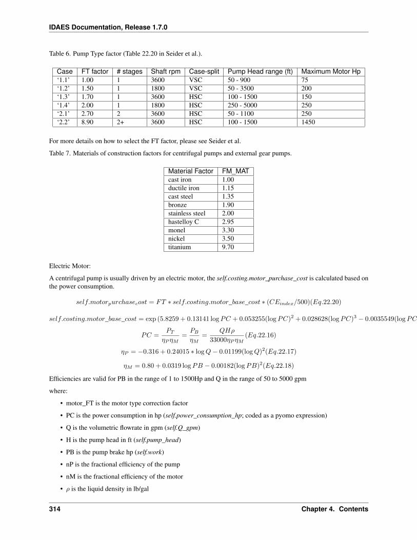
IDAES Documentation, Release 1.7.0
Table 6. Pump Type factor (Table 22.20 in Seider et al.).
Case FT factor # stages Shaft rpm Case-split Pump Head range (ft) Maximum Motor Hp‘1.1’ 1.00 1 3600 VSC 50 - 900 75‘1.2’ 1.50 1 1800 VSC 50 - 3500 200‘1.3’ 1.70 1 3600 HSC 100 - 1500 150‘1.4’ 2.00 1 1800 HSC 250 - 5000 250‘2.1’ 2.70 2 3600 HSC 50 - 1100 250‘2.2’ 8.90 2+ 3600 HSC 100 - 1500 1450
For more details on how to select the FT factor, please see Seider et al.
Table 7. Materials of construction factors for centrifugal pumps and external gear pumps.
Material Factor FM_MATcast iron 1.00ductile iron 1.15cast steel 1.35bronze 1.90stainless steel 2.00hastelloy C 2.95monel 3.30nickel 3.50titanium 9.70
Electric Motor:
A centrifugal pump is usually driven by an electric motor, the self.costing.motor_purchase_cost is calculated based onthe power consumption.
𝑠𝑒𝑙𝑓.𝑚𝑜𝑡𝑜𝑟𝑝𝑢𝑟𝑐ℎ𝑎𝑠𝑒𝑐𝑜𝑠𝑡 = 𝐹𝑇 * 𝑠𝑒𝑙𝑓.𝑐𝑜𝑠𝑡𝑖𝑛𝑔.𝑚𝑜𝑡𝑜𝑟_𝑏𝑎𝑠𝑒_𝑐𝑜𝑠𝑡 * (𝐶𝐸𝑖𝑛𝑑𝑒𝑥/500)(𝐸𝑞.22.20)
𝑠𝑒𝑙𝑓.𝑐𝑜𝑠𝑡𝑖𝑛𝑔.𝑚𝑜𝑡𝑜𝑟_𝑏𝑎𝑠𝑒_𝑐𝑜𝑠𝑡 = exp (5.8259 + 0.13141 log𝑃𝐶 + 0.053255(log𝑃𝐶)2 + 0.028628(log𝑃𝐶)3 − 0.0035549(log𝑃𝐶)4)(𝐸𝑞.22.19)
𝑃𝐶 =𝑃𝑇
𝜂𝑃 𝜂𝑀=𝑃𝐵
𝜂𝑀=
𝑄𝐻𝜌
33000𝜂𝑃 𝜂𝑀(𝐸𝑞.22.16)
𝜂𝑃 = −0.316 + 0.24015 * log𝑄− 0.01199(log𝑄)2(𝐸𝑞.22.17)
𝜂𝑀 = 0.80 + 0.0319 log𝑃𝐵 − 0.00182(log𝑃𝐵)2(𝐸𝑞.22.18)
Efficiencies are valid for PB in the range of 1 to 1500Hp and Q in the range of 50 to 5000 gpm
where:
• motor_FT is the motor type correction factor
• PC is the power consumption in hp (self.power_consumption_hp; coded as a pyomo expression)
• Q is the volumetric flowrate in gpm (self.Q_gpm)
• H is the pump head in ft (self.pump_head)
• PB is the pump brake hp (self.work)
• nP is the fractional efficiency of the pump
• nM is the fractional efficiency of the motor
• 𝜌 is the liquid density in lb/gal
314 Chapter 4. Contents
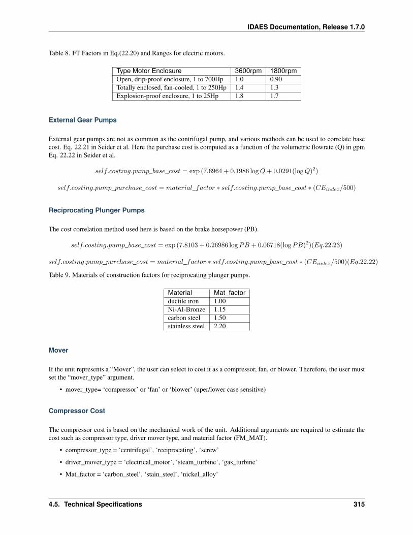
IDAES Documentation, Release 1.7.0
Table 8. FT Factors in Eq.(22.20) and Ranges for electric motors.
Type Motor Enclosure 3600rpm 1800rpmOpen, drip-proof enclosure, 1 to 700Hp 1.0 0.90Totally enclosed, fan-cooled, 1 to 250Hp 1.4 1.3Explosion-proof enclosure, 1 to 25Hp 1.8 1.7
External Gear Pumps
External gear pumps are not as common as the contrifugal pump, and various methods can be used to correlate basecost. Eq. 22.21 in Seider et al. Here the purchase cost is computed as a function of the volumetric flowrate (Q) in gpmEq. 22.22 in Seider et al.
𝑠𝑒𝑙𝑓.𝑐𝑜𝑠𝑡𝑖𝑛𝑔.𝑝𝑢𝑚𝑝_𝑏𝑎𝑠𝑒_𝑐𝑜𝑠𝑡 = exp (7.6964 + 0.1986 log𝑄+ 0.0291(log𝑄)2)
𝑠𝑒𝑙𝑓.𝑐𝑜𝑠𝑡𝑖𝑛𝑔.𝑝𝑢𝑚𝑝_𝑝𝑢𝑟𝑐ℎ𝑎𝑠𝑒_𝑐𝑜𝑠𝑡 = 𝑚𝑎𝑡𝑒𝑟𝑖𝑎𝑙_𝑓𝑎𝑐𝑡𝑜𝑟 * 𝑠𝑒𝑙𝑓.𝑐𝑜𝑠𝑡𝑖𝑛𝑔.𝑝𝑢𝑚𝑝_𝑏𝑎𝑠𝑒_𝑐𝑜𝑠𝑡 * (𝐶𝐸𝑖𝑛𝑑𝑒𝑥/500)
Reciprocating Plunger Pumps
The cost correlation method used here is based on the brake horsepower (PB).
𝑠𝑒𝑙𝑓.𝑐𝑜𝑠𝑡𝑖𝑛𝑔.𝑝𝑢𝑚𝑝_𝑏𝑎𝑠𝑒_𝑐𝑜𝑠𝑡 = exp (7.8103 + 0.26986 log𝑃𝐵 + 0.06718(log𝑃𝐵)2)(𝐸𝑞.22.23)
𝑠𝑒𝑙𝑓.𝑐𝑜𝑠𝑡𝑖𝑛𝑔.𝑝𝑢𝑚𝑝_𝑝𝑢𝑟𝑐ℎ𝑎𝑠𝑒_𝑐𝑜𝑠𝑡 = 𝑚𝑎𝑡𝑒𝑟𝑖𝑎𝑙_𝑓𝑎𝑐𝑡𝑜𝑟 * 𝑠𝑒𝑙𝑓.𝑐𝑜𝑠𝑡𝑖𝑛𝑔.𝑝𝑢𝑚𝑝_𝑏𝑎𝑠𝑒_𝑐𝑜𝑠𝑡 * (𝐶𝐸𝑖𝑛𝑑𝑒𝑥/500)(𝐸𝑞.22.22)
Table 9. Materials of construction factors for reciprocating plunger pumps.
Material Mat_factorductile iron 1.00Ni-Al-Bronze 1.15carbon steel 1.50stainless steel 2.20
Mover
If the unit represents a “Mover”, the user can select to cost it as a compressor, fan, or blower. Therefore, the user mustset the “mover_type” argument.
• mover_type= ‘compressor’ or ‘fan’ or ‘blower’ (uper/lower case sensitive)
Compressor Cost
The compressor cost is based on the mechanical work of the unit. Additional arguments are required to estimate thecost such as compressor type, driver mover type, and material factor (FM_MAT).
• compressor_type = ‘centrifugal’, ‘reciprocating’, ‘screw’
• driver_mover_type = ‘electrical_motor’, ‘steam_turbine’, ‘gas_turbine’
• Mat_factor = ‘carbon_steel’, ‘stain_steel’, ‘nickel_alloy’
4.5. Technical Specifications 315
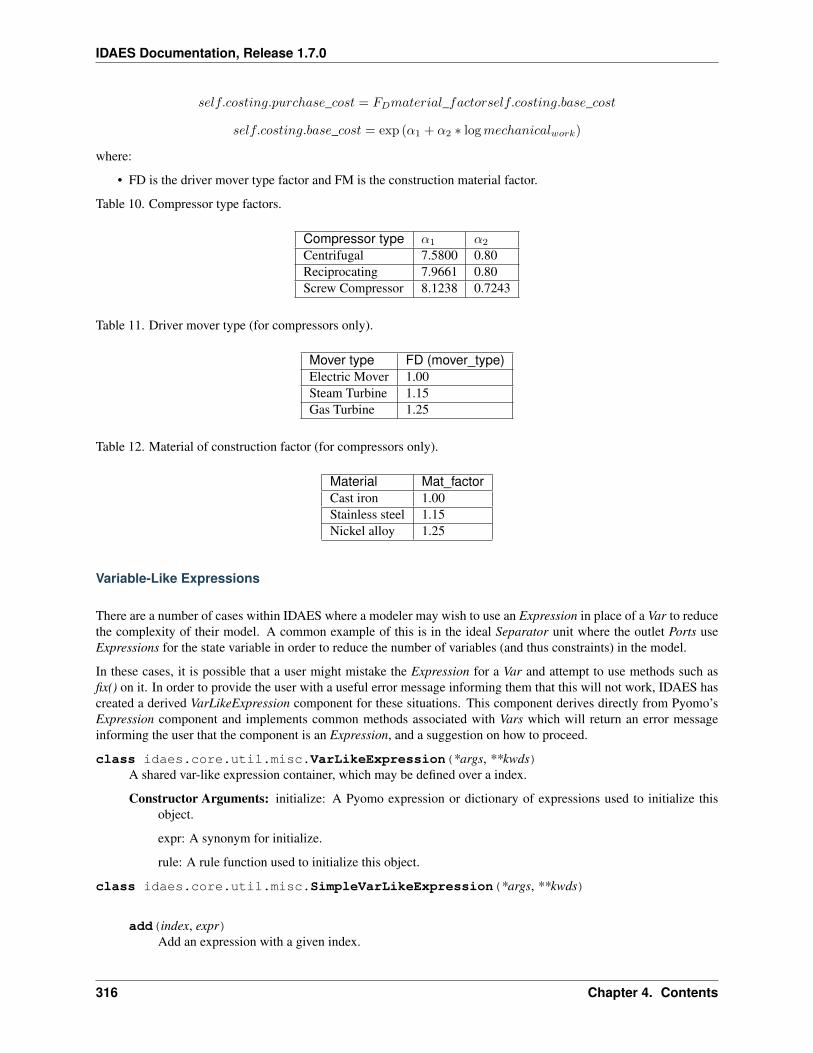
IDAES Documentation, Release 1.7.0
𝑠𝑒𝑙𝑓.𝑐𝑜𝑠𝑡𝑖𝑛𝑔.𝑝𝑢𝑟𝑐ℎ𝑎𝑠𝑒_𝑐𝑜𝑠𝑡 = 𝐹𝐷𝑚𝑎𝑡𝑒𝑟𝑖𝑎𝑙_𝑓𝑎𝑐𝑡𝑜𝑟𝑠𝑒𝑙𝑓.𝑐𝑜𝑠𝑡𝑖𝑛𝑔.𝑏𝑎𝑠𝑒_𝑐𝑜𝑠𝑡
𝑠𝑒𝑙𝑓.𝑐𝑜𝑠𝑡𝑖𝑛𝑔.𝑏𝑎𝑠𝑒_𝑐𝑜𝑠𝑡 = exp (𝛼1 + 𝛼2 * log𝑚𝑒𝑐ℎ𝑎𝑛𝑖𝑐𝑎𝑙𝑤𝑜𝑟𝑘)
where:
• FD is the driver mover type factor and FM is the construction material factor.
Table 10. Compressor type factors.
Compressor type 𝛼1 𝛼2
Centrifugal 7.5800 0.80Reciprocating 7.9661 0.80Screw Compressor 8.1238 0.7243
Table 11. Driver mover type (for compressors only).
Mover type FD (mover_type)Electric Mover 1.00Steam Turbine 1.15Gas Turbine 1.25
Table 12. Material of construction factor (for compressors only).
Material Mat_factorCast iron 1.00Stainless steel 1.15Nickel alloy 1.25
Variable-Like Expressions
There are a number of cases within IDAES where a modeler may wish to use an Expression in place of a Var to reducethe complexity of their model. A common example of this is in the ideal Separator unit where the outlet Ports useExpressions for the state variable in order to reduce the number of variables (and thus constraints) in the model.
In these cases, it is possible that a user might mistake the Expression for a Var and attempt to use methods such asfix() on it. In order to provide the user with a useful error message informing them that this will not work, IDAES hascreated a derived VarLikeExpression component for these situations. This component derives directly from Pyomo’sExpression component and implements common methods associated with Vars which will return an error messageinforming the user that the component is an Expression, and a suggestion on how to proceed.
class idaes.core.util.misc.VarLikeExpression(*args, **kwds)A shared var-like expression container, which may be defined over a index.
Constructor Arguments: initialize: A Pyomo expression or dictionary of expressions used to initialize thisobject.
expr: A synonym for initialize.
rule: A rule function used to initialize this object.
class idaes.core.util.misc.SimpleVarLikeExpression(*args, **kwds)
add(index, expr)Add an expression with a given index.
316 Chapter 4. Contents
IDAES Documentation, Release 1.7.0
class idaes.core.util.misc.IndexedVarLikeExpression(*args, **kwds)
add(index, expr)Add an expression with a given index.
class idaes.core.util.misc._GeneralVarLikeExpressionData(expr=None, compo-nent=None)
An object derived from _GeneralExpressionData which implements methods for common APIs on Vars.
Constructor Arguments: expr: The Pyomo expression stored in this expression.
component: The Expression object that owns this data.
Public Class Attributes: expr: The expression owned by this data.
Private class attributes: _component: The expression component.
4.5.2 Model Libaries
Generic IDAES Model Library
This library contains a suite of generic models that are applicable across most process applications. This library alsoforms the foundation for many of the specialized application libraries which build off these models.
Property Models
Cubic Equations of State
This property package implements a general form of a cubic equation of state which can be used for most cubic-typeequations of state. This package supports phase equilibrium calculations with a smooth phase transition formulationthat makes it amenable for equation oriented optimization. The following equations of state are currently supported:
• Peng-Robinson
• Soave-Redlich-Kwong
Flow basis: Molar
Units: SI units
State Variables:
The state block uses the following state variables:
Inputs
When instantiating the parameter block that uses this particular state block, 1 optional argument can be passed:
The valid_phase argument denotes the valid phases for a given set of inlet conditions. For example, if the userknows a priori that the it will only be a single phase (for example liquid only), then it is best not to include the complexflash equilibrium constraints in the model. If the user does not specify any option, then the package defaults to a 2phase assumption meaning that the constraints to compute the phase equilibrium will be computed.
4.5. Technical Specifications 317
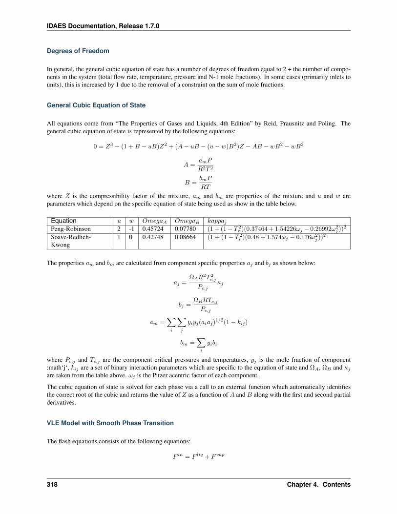
IDAES Documentation, Release 1.7.0
Degrees of Freedom
In general, the general cubic equation of state has a number of degrees of freedom equal to 2 + the number of compo-nents in the system (total flow rate, temperature, pressure and N-1 mole fractions). In some cases (primarily inlets tounits), this is increased by 1 due to the removal of a constraint on the sum of mole fractions.
General Cubic Equation of State
All equations come from “The Properties of Gases and Liquids, 4th Edition” by Reid, Prausnitz and Poling. Thegeneral cubic equation of state is represented by the following equations:
0 = 𝑍3 − (1 +𝐵 − 𝑢𝐵)𝑍2 + (𝐴− 𝑢𝐵 − (𝑢− 𝑤)𝐵2)𝑍 −𝐴𝐵 − 𝑤𝐵2 − 𝑤𝐵3
𝐴 =𝑎𝑚𝑃
𝑅2𝑇 2
𝐵 =𝑏𝑚𝑃
𝑅𝑇
where 𝑍 is the compressibility factor of the mixture, 𝑎𝑚 and 𝑏𝑚 are properties of the mixture and 𝑢 and 𝑤 areparameters which depend on the specific equation of state being used as show in the table below.
Equation 𝑢 𝑤 𝑂𝑚𝑒𝑔𝑎𝐴 𝑂𝑚𝑒𝑔𝑎𝐵 𝑘𝑎𝑝𝑝𝑎𝑗Peng-Robinson 2 -1 0.45724 0.07780 (1 + (1− 𝑇 2
𝑟 )(0.37464 + 1.54226𝜔𝑗 − 0.26992𝜔2𝑗 ))2
Soave-Redlich-Kwong
1 0 0.42748 0.08664 (1 + (1 − 𝑇 2𝑟 )(0.48 + 1.574𝜔𝑗 − 0.176𝜔2
𝑗 ))2
The properties 𝑎𝑚 and 𝑏𝑚 are calculated from component specific properties 𝑎𝑗 and 𝑏𝑗 as shown below:
𝑎𝑗 =Ω𝐴𝑅
2𝑇 2𝑐,𝑗
𝑃𝑐,𝑗𝜅𝑗
𝑏𝑗 =Ω𝐵𝑅𝑇𝑐,𝑗𝑃𝑐,𝑗
𝑎𝑚 =∑𝑖
∑𝑗
𝑦𝑖𝑦𝑗(𝑎𝑖𝑎𝑗)1/2(1 − 𝑘𝑖𝑗)
𝑏𝑚 =∑𝑖
𝑦𝑖𝑏𝑖
where 𝑃𝑐,𝑗 and 𝑇𝑐,𝑗 are the component critical pressures and temperatures, 𝑦𝑗 is the mole fraction of component:math‘j‘, 𝑘𝑖𝑗 are a set of binary interaction parameters which are specific to the equation of state and Ω𝐴, Ω𝐵 and 𝜅𝑗are taken from the table above. 𝜔𝑗 is the Pitzer acentric factor of each component.
The cubic equation of state is solved for each phase via a call to an external function which automatically identifiesthe correct root of the cubic and returns the value of 𝑍 as a function of 𝐴 and 𝐵 along with the first and second partialderivatives.
VLE Model with Smooth Phase Transition
The flash equations consists of the following equations:
𝐹 𝑖𝑛 = 𝐹 𝑙𝑖𝑞 + 𝐹 𝑣𝑎𝑝
318 Chapter 4. Contents
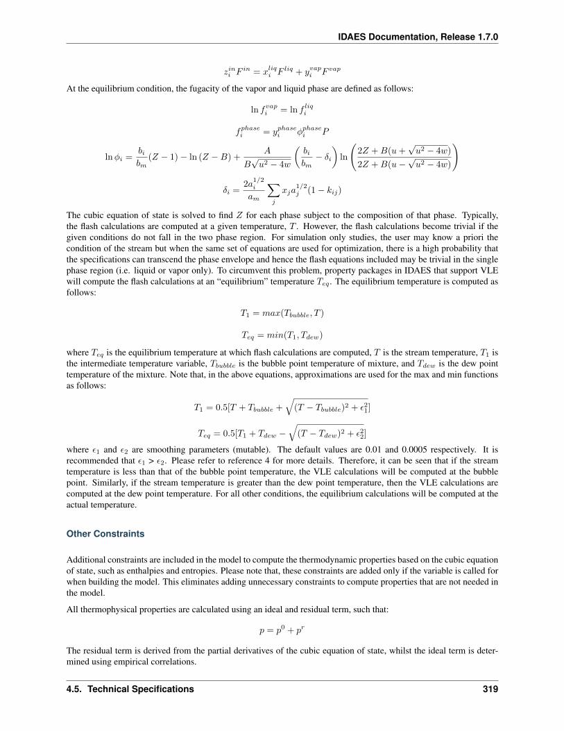
IDAES Documentation, Release 1.7.0
𝑧𝑖𝑛𝑖 𝐹𝑖𝑛 = 𝑥𝑙𝑖𝑞𝑖 𝐹 𝑙𝑖𝑞 + 𝑦𝑣𝑎𝑝𝑖 𝐹 𝑣𝑎𝑝
At the equilibrium condition, the fugacity of the vapor and liquid phase are defined as follows:
ln 𝑓𝑣𝑎𝑝𝑖 = ln 𝑓 𝑙𝑖𝑞𝑖
𝑓𝑝ℎ𝑎𝑠𝑒𝑖 = 𝑦𝑝ℎ𝑎𝑠𝑒𝑖 𝜑𝑝ℎ𝑎𝑠𝑒𝑖 𝑃
ln𝜑𝑖 =𝑏𝑖𝑏𝑚
(𝑍 − 1) − ln (𝑍 −𝐵) +𝐴
𝐵√𝑢2 − 4𝑤
(𝑏𝑖𝑏𝑚
− 𝛿𝑖
)ln
(2𝑍 +𝐵(𝑢+
√𝑢2 − 4𝑤)
2𝑍 +𝐵(𝑢−√𝑢2 − 4𝑤)
)
𝛿𝑖 =2𝑎
1/2𝑖
𝑎𝑚
∑𝑗
𝑥𝑗𝑎1/2𝑗 (1 − 𝑘𝑖𝑗)
The cubic equation of state is solved to find 𝑍 for each phase subject to the composition of that phase. Typically,the flash calculations are computed at a given temperature, 𝑇 . However, the flash calculations become trivial if thegiven conditions do not fall in the two phase region. For simulation only studies, the user may know a priori thecondition of the stream but when the same set of equations are used for optimization, there is a high probability thatthe specifications can transcend the phase envelope and hence the flash equations included may be trivial in the singlephase region (i.e. liquid or vapor only). To circumvent this problem, property packages in IDAES that support VLEwill compute the flash calculations at an “equilibrium” temperature 𝑇𝑒𝑞 . The equilibrium temperature is computed asfollows:
𝑇1 = 𝑚𝑎𝑥(𝑇𝑏𝑢𝑏𝑏𝑙𝑒, 𝑇 )
𝑇𝑒𝑞 = 𝑚𝑖𝑛(𝑇1, 𝑇𝑑𝑒𝑤)
where 𝑇𝑒𝑞 is the equilibrium temperature at which flash calculations are computed, 𝑇 is the stream temperature, 𝑇1 isthe intermediate temperature variable, 𝑇𝑏𝑢𝑏𝑏𝑙𝑒 is the bubble point temperature of mixture, and 𝑇𝑑𝑒𝑤 is the dew pointtemperature of the mixture. Note that, in the above equations, approximations are used for the max and min functionsas follows:
𝑇1 = 0.5[𝑇 + 𝑇𝑏𝑢𝑏𝑏𝑙𝑒 +√
(𝑇 − 𝑇𝑏𝑢𝑏𝑏𝑙𝑒)2 + 𝜖21]
𝑇𝑒𝑞 = 0.5[𝑇1 + 𝑇𝑑𝑒𝑤 −√
(𝑇 − 𝑇𝑑𝑒𝑤)2 + 𝜖22]
where 𝜖1 and 𝜖2 are smoothing parameters (mutable). The default values are 0.01 and 0.0005 respectively. It isrecommended that 𝜖1 > 𝜖2. Please refer to reference 4 for more details. Therefore, it can be seen that if the streamtemperature is less than that of the bubble point temperature, the VLE calculations will be computed at the bubblepoint. Similarly, if the stream temperature is greater than the dew point temperature, then the VLE calculations arecomputed at the dew point temperature. For all other conditions, the equilibrium calculations will be computed at theactual temperature.
Other Constraints
Additional constraints are included in the model to compute the thermodynamic properties based on the cubic equationof state, such as enthalpies and entropies. Please note that, these constraints are added only if the variable is called forwhen building the model. This eliminates adding unnecessary constraints to compute properties that are not needed inthe model.
All thermophysical properties are calculated using an ideal and residual term, such that:
𝑝 = 𝑝0 + 𝑝𝑟
The residual term is derived from the partial derivatives of the cubic equation of state, whilst the ideal term is deter-mined using empirical correlations.
4.5. Technical Specifications 319
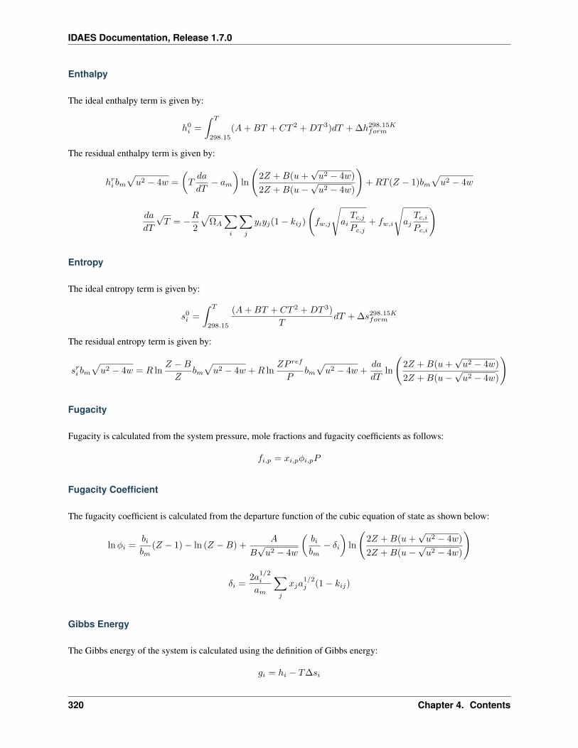
IDAES Documentation, Release 1.7.0
Enthalpy
The ideal enthalpy term is given by:
ℎ0𝑖 =
∫ 𝑇
298.15
(𝐴+𝐵𝑇 + 𝐶𝑇 2 +𝐷𝑇 3)𝑑𝑇 + ∆ℎ298.15𝐾𝑓𝑜𝑟𝑚
The residual enthalpy term is given by:
ℎ𝑟𝑖 𝑏𝑚√𝑢2 − 4𝑤 =
(𝑇𝑑𝑎
𝑑𝑇− 𝑎𝑚
)ln
(2𝑍 +𝐵(𝑢+
√𝑢2 − 4𝑤)
2𝑍 +𝐵(𝑢−√𝑢2 − 4𝑤)
)+𝑅𝑇 (𝑍 − 1)𝑏𝑚
√𝑢2 − 4𝑤
𝑑𝑎
𝑑𝑇
√𝑇 = −𝑅
2
√Ω𝐴
∑𝑖
∑𝑗
𝑦𝑖𝑦𝑗(1 − 𝑘𝑖𝑗)
(𝑓𝑤,𝑗
√𝑎𝑖𝑇𝑐,𝑗𝑃𝑐,𝑗
+ 𝑓𝑤,𝑖
√𝑎𝑗𝑇𝑐,𝑖𝑃𝑐,𝑖
)
Entropy
The ideal entropy term is given by:
𝑠0𝑖 =
∫ 𝑇
298.15
(𝐴+𝐵𝑇 + 𝐶𝑇 2 +𝐷𝑇 3)
𝑇𝑑𝑇 + ∆𝑠298.15𝐾𝑓𝑜𝑟𝑚
The residual entropy term is given by:
𝑠𝑟𝑖 𝑏𝑚√𝑢2 − 4𝑤 = 𝑅 ln
𝑍 −𝐵
𝑍𝑏𝑚√𝑢2 − 4𝑤 +𝑅 ln
𝑍𝑃 𝑟𝑒𝑓
𝑃𝑏𝑚√𝑢2 − 4𝑤 +
𝑑𝑎
𝑑𝑇ln
(2𝑍 +𝐵(𝑢+
√𝑢2 − 4𝑤)
2𝑍 +𝐵(𝑢−√𝑢2 − 4𝑤)
)
Fugacity
Fugacity is calculated from the system pressure, mole fractions and fugacity coefficients as follows:
𝑓𝑖,𝑝 = 𝑥𝑖,𝑝𝜑𝑖,𝑝𝑃
Fugacity Coefficient
The fugacity coefficient is calculated from the departure function of the cubic equation of state as shown below:
ln𝜑𝑖 =𝑏𝑖𝑏𝑚
(𝑍 − 1) − ln (𝑍 −𝐵) +𝐴
𝐵√𝑢2 − 4𝑤
(𝑏𝑖𝑏𝑚
− 𝛿𝑖
)ln
(2𝑍 +𝐵(𝑢+
√𝑢2 − 4𝑤)
2𝑍 +𝐵(𝑢−√𝑢2 − 4𝑤)
)
𝛿𝑖 =2𝑎
1/2𝑖
𝑎𝑚
∑𝑗
𝑥𝑗𝑎1/2𝑗 (1 − 𝑘𝑖𝑗)
Gibbs Energy
The Gibbs energy of the system is calculated using the definition of Gibbs energy:
𝑔𝑖 = ℎ𝑖 − 𝑇∆𝑠𝑖
320 Chapter 4. Contents
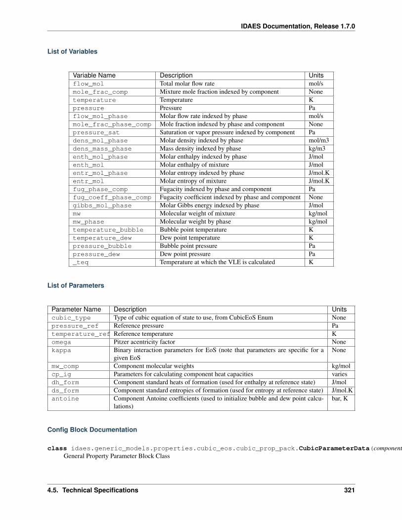
IDAES Documentation, Release 1.7.0
List of Variables
Variable Name Description Unitsflow_mol Total molar flow rate mol/smole_frac_comp Mixture mole fraction indexed by component Nonetemperature Temperature Kpressure Pressure Paflow_mol_phase Molar flow rate indexed by phase mol/smole_frac_phase_comp Mole fraction indexed by phase and component Nonepressure_sat Saturation or vapor pressure indexed by component Padens_mol_phase Molar density indexed by phase mol/m3dens_mass_phase Mass density indexed by phase kg/m3enth_mol_phase Molar enthalpy indexed by phase J/molenth_mol Molar enthalpy of mixture J/molentr_mol_phase Molar entropy indexed by phase J/mol.Kentr_mol Molar entropy of mixture J/mol.Kfug_phase_comp Fugacity indexed by phase and component Pafug_coeff_phase_comp Fugacity coefficient indexed by phase and component Nonegibbs_mol_phase Molar Gibbs energy indexed by phase J/molmw Molecular weight of mixture kg/molmw_phase Molecular weight by phase kg/moltemperature_bubble Bubble point temperature Ktemperature_dew Dew point temperature Kpressure_bubble Bubble point pressure Papressure_dew Dew point pressure Pa_teq Temperature at which the VLE is calculated K
List of Parameters
Parameter Name Description Unitscubic_type Type of cubic equation of state to use, from CubicEoS Enum Nonepressure_ref Reference pressure Patemperature_ref Reference temperature Komega Pitzer acentricity factor Nonekappa Binary interaction parameters for EoS (note that parameters are specific for a
given EoSNone
mw_comp Component molecular weights kg/molcp_ig Parameters for calculating component heat capacities variesdh_form Component standard heats of formation (used for enthalpy at reference state) J/molds_form Component standard entropies of formation (used for entropy at reference state) J/mol.Kantoine Component Antoine coefficients (used to initialize bubble and dew point calcu-
lations)bar, K
Config Block Documentation
class idaes.generic_models.properties.cubic_eos.cubic_prop_pack.CubicParameterData(component)General Property Parameter Block Class
4.5. Technical Specifications 321
IDAES Documentation, Release 1.7.0
build()Callable method for Block construction.
classmethod define_metadata(obj)Define properties supported and units.
class idaes.generic_models.properties.cubic_eos.cubic_prop_pack.CubicStateBlock(*args,**kwargs)
Parameters
• rule (function) – A rule function or None. Default rule calls build().
• concrete (bool) – If True, make this a toplevel model. Default - False.
• ctype (str) – Pyomo ctype of the block. Default - “Block”
• default (dict) – Default ProcessBlockData config
Keys
parameters A reference to an instance of the Property Parameter Block associated withthis property package.
defined_state Flag indicating whether the state should be considered fully defined, andthus whether constraints such as sum of mass/mole fractions should be included, de-fault - False. Valid values: True - state variables will be fully defined, False - statevariables will not be fully defined.
has_phase_equilibrium Flag indicating whether phase equilibrium constraints shouldbe constructed in this state block, default - True. Valid values: True - StateBlockshould calculate phase equilibrium, False - StateBlock should not calculate phase equi-librium.
• initialize (dict) – ProcessBlockData config for individual elements. Keys are Block-Data indexes and values are dictionaries described under the “default” argument above.
• idx_map (function) – Function to take the index of a BlockData element and return theindex in the initialize dict from which to read arguments. This can be provided to overidethe default behavior of matching the BlockData index exactly to the index in initialize.
Returns (CubicStateBlock) New instance
class idaes.generic_models.properties.cubic_eos.cubic_prop_pack.CubicStateBlockData(*args,**kwargs)
An general property package for cubic equations of state with VLE.
build()Callable method for Block construction.
define_display_vars()Method used to specify components to use to generate stream tables and other outputs. Defaults to de-fine_state_vars, and developers should overload as required.
define_state_vars()Define state vars.
get_energy_density_terms(p)Create energy density terms.
get_enthalpy_flow_terms(p)Create enthalpy flow terms.
get_material_density_terms(p, j)Create material density terms.
322 Chapter 4. Contents
IDAES Documentation, Release 1.7.0
get_material_flow_basis()Method which returns an Enum indicating the basis of the material flow term.
get_material_flow_terms(p, j)Create material flow terms for control volume.
model_check()Model checks for property block.
Vapor-Liquid Equilibrium Property Models (Ideal Gas - Non-ideal Liquids)
This property package supports phase equilibrium calucations with a smooth phase transition formulation that makes itamenable for equation oriented optimization. The gas phase is assumed to be ideal and for the liquid phase, the packagesupports an ideal liquid or a non-ideal liquid using an activity coefficient model. To compute the activity coefficient,the package currently supports the Non Random Two Liquid Model (NRTL) or the Wilson model. Therefore, thisproperty package supports the following combinations for gas-liquid mixtures for VLE calculations:
1. Ideal (vapor) - Ideal (liquid)
2. Ideal (vapor) - NRTL (liquid)
3. Ideal (vapor) - Wilson (liquid)
Flow basis: Molar
Units: SI units
State Variables:
The state block supports the following two sets of state variables:
Option 1 - “FTPz”:
Option 2 - “FcTP”:
The user can specify the choice of state variables while instantiating the parameter block. See the Inputs section formore details.
Support for other combinations of state variables will be made available in the future.
Inputs
When instantiating the parameter block that uses this particular state block, 2 arguments can be passed:
The valid_phase argument denotes the valid phases for a given set of inlet conditions. For example, if the userknows a priori that the it will only be a single phase (for example liquid only), then it is best not to include the complexflash equilibrium constraints in the model. If the user does not specify any option, then the package defaults to a 2phase assumption meaning that the constraints to compute the phase equilibrium will be computed.
The activity_coeff_model denotes the liquid phase assumption to be used. If the user does not specify anyoption, then the package defaults to asuming an ideal liquid assumption.
The state_vars denotes the preferred set of state variables to be used. If the user does not specify any option, thenthe package defaults to using the total flow, mixture mole fraction, temperature and pressure as the state variables.
4.5. Technical Specifications 323
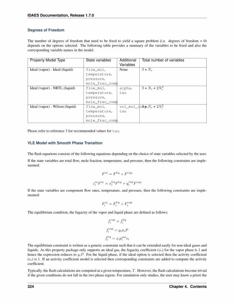
IDAES Documentation, Release 1.7.0
Degrees of Freedom
The number of degrees of freedom that need to be fixed to yield a square problem (i.e. degrees of freedom = 0)depends on the options selected. The following table provides a summary of the variables to be fixed and also thecorresponding variable names in the model.
Property Model Type State variables AdditionalVariables
Total number of variables
Ideal (vapor) - Ideal (liquid) flow_mol,temperature,pressure,mole_frac_comp
None 3 + 𝑁𝑐
Ideal (vapor) - NRTL (liquid) flow_mol,temperature,pressure,mole_frac_comp
alpha,tau
3 + 𝑁𝑐 + 2𝑁2𝑐
Ideal (vapor) - Wilson (liquid) flow_mol,temperature,pressure,mole_frac_comp
vol_mol_comp,tau
3 + 𝑁𝑐 + 2𝑁2𝑐
Please refer to reference 3 for recommended values for tau.
VLE Model with Smooth Phase Transition
The flash equations consists of the following equations depending on the choice of state variables selected by the user.
If the state variables are total flow, mole fraction, temperature, and pressure, then the following constraints are imple-mented:
𝐹 𝑖𝑛 = 𝐹 𝑙𝑖𝑞 + 𝐹 𝑣𝑎𝑝
𝑧𝑖𝑛𝑖 𝐹𝑖𝑛 = 𝑥𝑙𝑖𝑞𝑖 𝐹 𝑙𝑖𝑞 + 𝑦𝑣𝑎𝑝𝑖 𝐹 𝑣𝑎𝑝
If the state variables are component flow rates, temperature, and pressure, then the following constraints are imple-mented:
𝐹 𝑖𝑛𝑖 = 𝐹 𝑙𝑖𝑞
𝑖 + 𝐹 𝑣𝑎𝑝𝑖
The equilibrium condition, the fugacity of the vapor and liquid phase are defined as follows:
𝑓𝑣𝑎𝑝𝑖 = 𝑓 𝑙𝑖𝑞𝑖
𝑓𝑣𝑎𝑝𝑖 = 𝑦𝑖𝜑𝑖𝑃
𝑓 𝑙𝑖𝑞𝑖 = 𝑥𝑖𝑝𝑠𝑎𝑡𝑖 𝜈𝑖
The equilibrium constraint is written as a generic constraint such that it can be extended easily for non-ideal gases andliquids. As this property package only supports an ideal gas, the fugacity coefficient (𝜑𝑖) for the vapor phase is 1 andhence the expression reduces to 𝑦𝑖𝑃 . For the liquid phase, if the ideal option is selected then the activity coefficient(𝜈𝑖) is 1. If an activity coefficient model is selected then corresponding constraints are added to compute the activitycoefficient.
Typically, the flash calculations are computed at a given temperature, 𝑇 . However, the flash calculations become trivialif the given conditions do not fall in the two phase region. For simulation only studies, the user may know a priori the
324 Chapter 4. Contents
IDAES Documentation, Release 1.7.0
condition of the stream but when the same set of equations are used for optimization, there is a high probablity thatthe specifications can transcend the phase envelope and hence the flash equations included may be trivial in the singlephase region (i.e. liquid or vapor only). To circumvent this problem, property packages in IDAES that support VLEwill compute the flash calculations at an “equilibrium” temperature 𝑇𝑒𝑞 . The equilibrium temperature is computed asfollows:
𝑇1 = 𝑚𝑎𝑥(𝑇𝑏𝑢𝑏𝑏𝑙𝑒, 𝑇 )
𝑇𝑒𝑞 = 𝑚𝑖𝑛(𝑇1, 𝑇𝑑𝑒𝑤)
where 𝑇𝑒𝑞 is the equilibrium temperature at which flash calculations are computed, 𝑇 is the stream temperature, 𝑇1 isthe intermediate temperature variable, 𝑇𝑏𝑢𝑏𝑏𝑙𝑒 is the bubble point temperature of mixture, and 𝑇𝑑𝑒𝑤 is the dew pointtemperature of the mixture. Note that, in the above equations, approximations are used for the max and min functionsas follows:
𝑇1 = 0.5[𝑇 + 𝑇𝑏𝑢𝑏𝑏𝑙𝑒 +√
(𝑇 − 𝑇𝑏𝑢𝑏𝑏𝑙𝑒)2 + 𝜖21]
𝑇𝑒𝑞 = 0.5[𝑇1 + 𝑇𝑑𝑒𝑤 −√
(𝑇 − 𝑇𝑑𝑒𝑤)2 + 𝜖22]
where 𝜖1 and 𝜖2 are smoothing parameters(mutable). The default values are 0.01 and 0.0005 respectively. It is rec-ommended that 𝜖1 > 𝜖2. Please refer to reference 4 for more details. Therefore, it can be seen that if the streamtemperature is less than that of the bubble point temperature, the VLE calucalations will be computed at the bubblepoint. Similarly, if the stream temperature is greater than the dew point temperature, then the VLE calculations arecomputed at the dew point temperature. For all other conditions, the equilibrium calcualtions will be computed at theactual temperature.
Additional constraints are included in the model to compute the thermodynamic properties such as component satu-ration pressure, enthalpy, specific heat capacity. Please note that, these constraints are added only if the variable iscalled for when building the model. This eliminates adding unnecessary constraints to compute properties that are notneeded in the model.
The saturation or vapor pressure (pressure_sat) for component 𝑖 is computed using the following correlation[1]:
log𝑃 𝑠𝑎𝑡
𝑃𝑐=𝐴𝑥+𝐵𝑥1.5 + 𝐶𝑥3 +𝐷𝑥6
1 − 𝑥
𝑥 = 1 − 𝑇𝑒𝑞𝑇𝑐
where 𝑃𝑐 is the critical pressure, 𝑇𝑐 is the critical temperature of the component and 𝑇𝑒𝑞 is the equilibrium temperatureat which the saturation pressure is computed. Please note that when using this expression, 𝑇𝑒𝑞 < 𝑇𝑐 is required andwhen violated it results in a negative number raised to the power of a fraction.
The specific enthalpy (enthalpy_comp_liq) for component 𝑖 is computed using the following expression for theliquid phase:
ℎ𝑙𝑖𝑞𝑖 = ∆ℎ𝑓𝑜𝑟𝑚,𝐿𝑖𝑞,𝑖 +
∫ 𝑇
298.15
(𝐴+𝐵𝑇 + 𝐶𝑇 2 +𝐷𝑇 3 + 𝐸𝑇 4)𝑑𝑇
The specific enthalpy (enthalpy_comp_vap) for component 𝑖 is computed using the following expression for thevapor phase:
ℎ𝑣𝑎𝑝𝑖 = ∆ℎ𝑓𝑜𝑟𝑚,𝑉 𝑎𝑝,𝑖 +
∫ 𝑇
298.15
(𝐴+𝐵𝑇 + 𝐶𝑇 2 +𝐷𝑇 3 + 𝐸𝑇 4)𝑑𝑇
The mixture specific enthapies (enthalpy_liq & enthalpy_vap) are computed using the following expressionsfor the liquid and vapor phase respectively:
𝐻 𝑙𝑖𝑞 =∑𝑖
ℎ𝑙𝑖𝑞𝑖 𝑥𝑖
4.5. Technical Specifications 325
IDAES Documentation, Release 1.7.0
𝐻𝑣𝑎𝑝 =∑𝑖
ℎ𝑣𝑎𝑝𝑖 𝑦𝑖
Similarly, specific entropies are calcuated as follows. The specific entropy (entropy_comp_liq) for component 𝑖is computed using the following expression for the liquid phase:
𝑠𝑙𝑖𝑞𝑖 = ∆𝑠𝑓𝑜𝑟𝑚,𝐿𝑖𝑞,𝑖 +
∫ 𝑇
298.15
(𝐴/𝑇 +𝐵 + 𝐶𝑇 +𝐷𝑇 2 + 𝐸𝑇 3)𝑑𝑇
The specific entropy (entropy_comp_vap) for component 𝑖 is computed using the following expression for thevapor phase:
𝑠𝑣𝑎𝑝𝑖 = ∆𝑠𝑓𝑜𝑟𝑚,𝑉 𝑎𝑝,𝑖 +
∫ 𝑇
298.15
(𝐴/𝑇 +𝐵 + 𝐶𝑇 +𝐷𝑇 2 + 𝐸𝑇 3)𝑑𝑇
Please refer to references 1 and 2 to get parameters for different components.
Activity Coefficient Model - NRTL
The activity coefficient for component 𝑖 is computed using the following equations when using the Non-Random TwoLiquid model [3]:
log 𝛾𝑖 =
∑𝑗 𝑥𝑗𝜏𝑗𝐺𝑗𝑖∑𝑘 𝑥𝑘𝐺𝑘𝑖
+∑𝑗
𝑥𝑗𝐺𝑖𝑗∑𝑘 𝑥𝑘𝐺𝑘𝑗
[𝜏𝑖𝑗 −∑
𝑚 𝑥𝑚𝜏𝑚𝑗𝐺𝑚𝑗∑𝑘 𝑥𝑘𝐺𝑘𝑗
]
𝐺𝑖𝑗 = exp(−𝛼𝑖𝑗𝜏𝑖𝑗)
where 𝛼𝑖𝑗 is the non-randomness parameter and 𝜏𝑖𝑗 is the binary interaction parameter for the NRTL model. Notethat in the IDAES implementation, these are declared as variables that allows for more flexibility and the ability touse these in a parameter estimation problem. These NRTL model specific variables need to be either fixed for a givencomponent set or need to be estimated from VLE data.
The bubble point is computed by enforcing the following condition:∑𝑖
[𝑧𝑖𝑝𝑠𝑎𝑡𝑖 (𝑇𝑏𝑢𝑏𝑏𝑙𝑒)𝜈𝑖] − 𝑃 = 0
Activity Coefficient Model - Wilson
The activity coefficient for component 𝑖 is computed using the following equations when using the Wilson model [3]:
log 𝛾𝑖 = 1 − log∑𝑗
𝑥𝑗𝐺𝑗𝑖 −∑𝑗
𝑥𝑗𝐺𝑖𝑗∑𝑘 𝑥𝑘𝐺𝑘𝑗
𝐺𝑖𝑗 = (𝑣𝑖/𝑣𝑗) exp(−𝜏𝑖𝑗)
where 𝑣𝑖 is the molar volume of component 𝑖 and 𝜏𝑖𝑗 is the binary interaction parameter. These are Wilson modelspecific variables that either need to be fixed for a given component set or need to be estimated from VLE data.
The bubble point is computed by enforcing the following condition:∑𝑖
[𝑧𝑖𝑝𝑠𝑎𝑡𝑖 (𝑇𝑏𝑢𝑏𝑏𝑙𝑒)𝜈𝑖] − 𝑃 = 0
326 Chapter 4. Contents
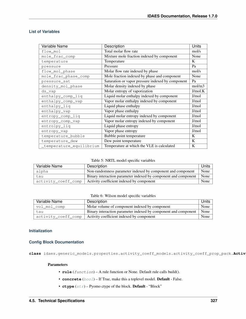
IDAES Documentation, Release 1.7.0
List of Variables
Variable Name Description Unitsflow_mol Total molar flow rate mol/smole_frac_comp Mixture mole fraction indexed by component Nonetemperature Temperature Kpressure Pressure Paflow_mol_phase Molar flow rate indexed by phase mol/smole_frac_phase_comp Mole fraction indexed by phase and component Nonepressure_sat Saturation or vapor pressure indexed by component Padensity_mol_phase Molar density indexed by phase mol/m3ds_vap Molar entropy of vaporization J/mol.Kenthalpy_comp_liq Liquid molar enthalpy indexed by component J/molenthalpy_comp_vap Vapor molar enthalpy indexed by component J/molenthalpy_liq Liquid phase enthalpy J/molenthalpy_vap Vapor phase enthalpy J/molentropy_comp_liq Liquid molar entropy indexed by component J/molentropy_comp_vap Vapor molar entropy indexed by component J/molentrolpy_liq Liquid phase entropy J/molentropy_vap Vapor phase entropy J/moltemperature_bubble Bubble point temperature Ktemperature_dew Dew point temperature K_temperature_equilibrium Temperature at which the VLE is calculated K
Table 5: NRTL model specific variablesVariable Name Description Unitsalpha Non-randomness parameter indexed by component and component Nonetau Binary interaction parameter indexed by component and component Noneactivity_coeff_comp Activity coefficient indexed by component None
Table 6: Wilson model specific variablesVariable Name Description Unitsvol_mol_comp Molar volume of component indexed by component Nonetau Binary interaction parameter indexed by component and component Noneactivity_coeff_comp Activity coefficient indexed by component None
Initialization
Config Block Documentation
class idaes.generic_models.properties.activity_coeff_models.activity_coeff_prop_pack.ActivityCoeffParameterBlock(*args,**kwargs)
Parameters
• rule (function) – A rule function or None. Default rule calls build().
• concrete (bool) – If True, make this a toplevel model. Default - False.
• ctype (str) – Pyomo ctype of the block. Default - “Block”
4.5. Technical Specifications 327
IDAES Documentation, Release 1.7.0
• default (dict) – Default ProcessBlockData config
Keys
default_arguments Default arguments to use with Property Package
activity_coeff_model Flag indicating the activity coefficient model to be used for thenon-ideal liquid, and thus corresponding constraints should be included, default - Idealliquid. Valid values: “NRTL” - Non Random Two Liquid Model, “Wilson” - Wil-son Liquid Model,
state_vars Flag indicating the choice for state variables to be used for the state block,and thus corresponding constraints should be included, default - FTPz Valid values: “FTPx” - Total flow, Temperature, Pressure and Mole fraction, “FcTP” - Componentflow, Temperature and Pressure
valid_phase Flag indicating the valid phase for a given set of conditions, and thus cor-responding constraints should be included, default - (“Vap”, “Liq”). Valid values: “Liq” - Liquid only, “Vap” - Vapor only, (“Vap”, “Liq”) - Vapor-liquid equilibrium,(“Liq”, “Vap”) - Vapor-liquid equilibrium,
• initialize (dict) – ProcessBlockData config for individual elements. Keys are Block-Data indexes and values are dictionaries described under the “default” argument above.
• idx_map (function) – Function to take the index of a BlockData element and return theindex in the initialize dict from which to read arguments. This can be provided to overidethe default behavior of matching the BlockData index exactly to the index in initialize.
Returns (ActivityCoeffParameterBlock) New instance
class idaes.generic_models.properties.activity_coeff_models.activity_coeff_prop_pack.ActivityCoeffStateBlock(*args,**kwargs)
Parameters
• rule (function) – A rule function or None. Default rule calls build().
• concrete (bool) – If True, make this a toplevel model. Default - False.
• ctype (str) – Pyomo ctype of the block. Default - “Block”
• default (dict) – Default ProcessBlockData config
Keys
parameters A reference to an instance of the Property Parameter Block associated withthis property package.
defined_state Flag indicating whether the state should be considered fully defined, andthus whether constraints such as sum of mass/mole fractions should be included, de-fault - False. Valid values: True - state variables will be fully defined, False - statevariables will not be fully defined.
has_phase_equilibrium Flag indicating whether phase equilibrium constraints shouldbe constructed in this state block, default - True. Valid values: True - StateBlockshould calculate phase equilibrium, False - StateBlock should not calculate phase equi-librium.
• initialize (dict) – ProcessBlockData config for individual elements. Keys are Block-Data indexes and values are dictionaries described under the “default” argument above.
• idx_map (function) – Function to take the index of a BlockData element and return theindex in the initialize dict from which to read arguments. This can be provided to overidethe default behavior of matching the BlockData index exactly to the index in initialize.
328 Chapter 4. Contents
IDAES Documentation, Release 1.7.0
Returns (ActivityCoeffStateBlock) New instance
class idaes.generic_models.properties.activity_coeff_models.activity_coeff_prop_pack.ActivityCoeffStateBlockData(*args,**kwargs)
An example property package for ideal VLE.
build()Callable method for Block construction.
define_state_vars()Define state vars.
get_energy_density_terms(p)Create enthalpy density terms.
get_enthalpy_flow_terms(p)Create enthalpy flow terms.
get_material_density_terms(p, j)Create material density terms.
get_material_flow_basis()Declare material flow basis.
get_material_flow_terms(p, j)Create material flow terms for control volume.
model_check()Model checks for property block.
References
1. “The properties of gases and liquids by Robert C. Reid”
2. “Perry’s Chemical Engineers Handbook by Robert H. Perry”.
3. H. Renon and J.M. Prausnitz, “Local compositions in thermodynamic excess functions for liquid mixtures.”,AIChE Journal Vol. 14, No.1, 1968.
4. AP Burgard, JP Eason, JC Eslick, JH Ghouse, A Lee, LT Biegler, DC Miller. “A Smooth, Square Flash For-mulation for Equation Oriented Flowsheet Optimization”, Computer Aided Chemical Engineering 44, 871-876,2018
Water/Steam - IAPWS95
Accurate and thermodynamically consistent steam properties are provided for the IDAES framework by implementingthe International Association for the Properties of Water and Steam’s “Revised Release on the IAPWS Formulation1995 for the Thermodynamic Properties of Ordinary Water Substance for General and Scientific Use.” Non-analyticterms designed to improve accuracy very near the critical point were omitted, because they cause a singularity at thecritical point, a feature which is undesirable in optimization problems. The IDAES implementation provides featureswhich make the water and steam property calculations amenable to rigorous mathematical optimization.
Example
Theses modules can be imported as:
4.5. Technical Specifications 329
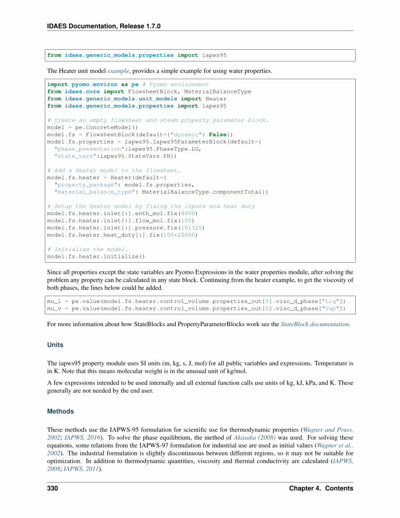
IDAES Documentation, Release 1.7.0
from idaes.generic_models.properties import iapws95
The Heater unit model example, provides a simple example for using water properties.
import pyomo.environ as pe # Pyomo environmentfrom idaes.core import FlowsheetBlock, MaterialBalanceTypefrom idaes.generic_models.unit_models import Heaterfrom idaes.generic_models.properties import iapws95
# Create an empty flowsheet and steam property parameter block.model = pe.ConcreteModel()model.fs = FlowsheetBlock(default="dynamic": False)model.fs.properties = iapws95.Iapws95ParameterBlock(default=
"phase_presentation":iapws95.PhaseType.LG,"state_vars":iapws95.StateVars.PH)
# Add a Heater model to the flowsheet.model.fs.heater = Heater(default=
"property_package": model.fs.properties,"material_balance_type": MaterialBalanceType.componentTotal)
# Setup the heater model by fixing the inputs and heat dutymodel.fs.heater.inlet[:].enth_mol.fix(4000)model.fs.heater.inlet[:].flow_mol.fix(100)model.fs.heater.inlet[:].pressure.fix(101325)model.fs.heater.heat_duty[:].fix(100*20000)
# Initialize the model.model.fs.heater.initialize()
Since all properties except the state variables are Pyomo Expressions in the water properties module, after solving theproblem any property can be calculated in any state block. Continuing from the heater example, to get the viscosity ofboth phases, the lines below could be added.
mu_l = pe.value(model.fs.heater.control_volume.properties_out[0].visc_d_phase["Liq"])mu_v = pe.value(model.fs.heater.control_volume.properties_out[0].visc_d_phase["Vap"])
For more information about how StateBlocks and PropertyParameterBlocks work see the StateBlock documentation.
Units
The iapws95 property module uses SI units (m, kg, s, J, mol) for all public variables and expressions. Temperature isin K. Note that this means molecular weight is in the unusual unit of kg/mol.
A few expressions intended to be used internally and all external function calls use units of kg, kJ, kPa, and K. Thesegenerally are not needed by the end user.
Methods
These methods use the IAPWS-95 formulation for scientific use for thermodynamic properties (Wagner and Pruss,2002; IAPWS, 2016). To solve the phase equilibrium, the method of Akasaka (2008) was used. For solving theseequations, some relations from the IAPWS-97 formulation for industrial use are used as initial values (Wagner et al.,2002). The industrial formulation is slightly discontinuous between different regions, so it may not be suitable foroptimization. In addition to thermodynamic quantities, viscosity and thermal conductivity are calculated (IAPWS,2008; IAPWS, 2011).
330 Chapter 4. Contents
IDAES Documentation, Release 1.7.0
External Functions
The IAPWS-95 formulation uses density and temperature as state variables. For most applications those state variablesare not the most convenient choices. Using other state variables requires solving equations to get density and temper-ature from the chosen state variables. These equations can have numerous solutions only one of which is physicallymeaningful. Rather than solve these equations as part of the full process simulation, external functions were developedthat can solve the equations required to change state variables and guarantee the correct roots.
The external property functions are written in C++ and complied such that they can be called by AMPL solvers. Theexternal functions provide both first and second derivatives for all property function calls, however at phase transitionssome of these functions may be non-smooth.
IDAES Framework Wrapper
A wrapper for the external functions is provided for compatibility with the IDAES framework. Most properties areavailable as Pyomo Expressions from the wrapper. Only the state variables are model variables. Benefits of usingmostly expressions in the property package are: no initialization is required specifically for the property package, themodel has fewer equations, and all properties can be easily calculated after the model is solved from the state variablevalues even if they were not used in the model. Calls to the external functions are used within expressions so usersdo not need to directly call any functions. The potential downside of the extensive use of expressions here is thatcombining the expressions to form constraints could yield equations that are more difficult to solve than, they wouldhave been if an equivalent system of equations was written with more variables and simpler equations. Quantifyingthe effect of writing larger equations with fewer variables is difficult. Experience suggests in this particular case moreexpressions and fewer variables is better.
Although not generally used, the wrapper provides direct access to the ExternalFunctions, including intermediatefunctions. For more information see section ExternalFunctions. These are mostly available for testing purposes.
Phase Presentation
The property package wrapper can present fluid phase information to the IDAES framework in different ways. Seethe class reference for details on how to set these options. The phase_presentation=PhaseType.MIX optionlooks like one phase called “Mix” to the IDAES framework. The property package will calculate a phase fraction. Thiswill bypass any two phase handling equations written for unit models, and should work with any unit model optionsas long as you do not want to separate the phases. The benefit of this option is that it can potentially lead to a simplerset of equations.
The phase_presentation=PhaseType.LG option appears to the IDAES framework to be two phases “Vap”and “Liq”. This option requires one of two unit model options to be set. You can use the total material balance optionfor unit models, to specify that only one material balance equation should be written not one per phase. The otherpossible option is to specify has_phase_equlibrium=True. This will still write a material balance per phase,but will add a phase generation term to the model. For the IAPWS-95 package, it is generally recommended thatspecifying total material balances is best because it results in a problem with fewer variables.
There are also two single phase options phase_presentation=PhaseType.L andphase_presentation=PhaseType.G, these present a single phase “Liq” or “Vap” to the framework.The vapor fraction will also always return 0 or 1 as appropriate. These options can be used when the phase of a fluidis know for certain to only be liquid or only be vapor. For the temperature-pressure-vapor fraction formulation, thiseliminates the complementarity constraint, but for the enthalpy-pressure formulation, where the vapor fraction isalways calculated, the single phase options probably do not provide any real benefit.
4.5. Technical Specifications 331
IDAES Documentation, Release 1.7.0
Pressure-Enthalpy Formulation
The advantage of this choice of state variables is that it is very robust when phase changes occur, and is especiallyuseful when it is not known if a phase change will occur. The disadvantage of this choice of state variables is that forequations like heat transfer equations that are highly dependent on temperature, a model could be harder to solve nearregions with phase change. Temperature is a non-smooth function with non-smoothness when transitioning from thesingle-phase to the two-phase region. Temperature also has a zero derivative with respect to enthalpy in the two-phaseregion, so near the two-phase region solving a constraint that specifies a specific temperature may not be possible.
The variables for this form are flow_mol (mol/s), pressure (Pa), and enth_mol (J/mol).
Since temperature and vapor fraction are not state variables in this formulation, they are provided by expressions, andcannot be fixed. For example, to set a temperature to a specific value, a constraint could be added which says thetemperature expression equals a fixed value.
These expressions are specific to the P-H formulation:
temperature Expression that calculates temperature by calling an ExternalFunction of enthalpy and pressure. Thisexpression is non-smooth in the transition from single-phase to two-phase and has a zero derivative with respectto enthalpy in the two-phase region.
vapor_frac Expression that calculates vapor fraction by calling an ExternalFunction of enthalpy and pressure.This expression is non-smooth in the transition from single-phase to two-phase and has a zero derivative withrespect to enthalpy in the single-phase region, where the value is 0 (liquid) or 1 (vapor).
Temperature-Pressure-Vapor Fraction
This formulation uses temperature (K), pressure (Pa), and vapor fraction as state variables. When a single phase optionis given, the vapor fraction is fixed to the appropriate value and not included in the state variable set. For single phase,the complementarity constraint is also deactivated.
A complementarity constraint is required for the T-P-x formulation. First, two expressions are defined below where𝑃− is pressure under saturation pressure and 𝑃+ is pressure over saturation pressure. The max function is providedby an IDAES utility function which provides a smooth max expression.
𝑃− = max(0, 𝑃sat − 𝑃 )
𝑃+ = max(0, 𝑃 − 𝑃sat)
With the pressure over and pressure under saturated pressure expressions a complementarity constraint can be written.If the pressure under saturation is more than zero, only vapor exists. If the pressure over saturation is greater than zeroonly a liquid exists. If both are about zero two phases can exist. The saturation pressure function maxes out at thecritical pressure and any temperature above the critical temperature will yield a saturation pressure that is the criticalpressure, so supercritical fluids will be classified as liquids as the convention for this property package.
0 = 𝑥𝑃+ − (1 − 𝑥)𝑃−
Assuming the vapor fraction (𝑥) is positive and noting that only one of 𝑃+ and 𝑃− can be nonzero (approximately),the complementarity equation above requires 𝑥 to be 0 when 𝑃+ is not zero (liquid) or 𝑥 to be 1 when 𝑃− is not zero(vapor). When both 𝑃+ and 𝑃− are about 0, the complementarity constraint says nothing about x, but it does provideanother constraint, that 𝑃 = 𝑃sat. When two phases are present 𝑥 can be found by the unit model energy balance andthe temperature will be 𝑇sat.
An alternative approach is sometimes useful. If you know for certain that you have two phases, the complementarityconstraint can be deactivated and a 𝑃 = 𝑃sat or 𝑇 = 𝑇sat constraint can be added.
Using the T-P-x formulation requires better initial guesses than the P-H form. It is not strictly necessary but it is bestto try to get an initial guess that is in the correct phase region for the expected result model.
332 Chapter 4. Contents
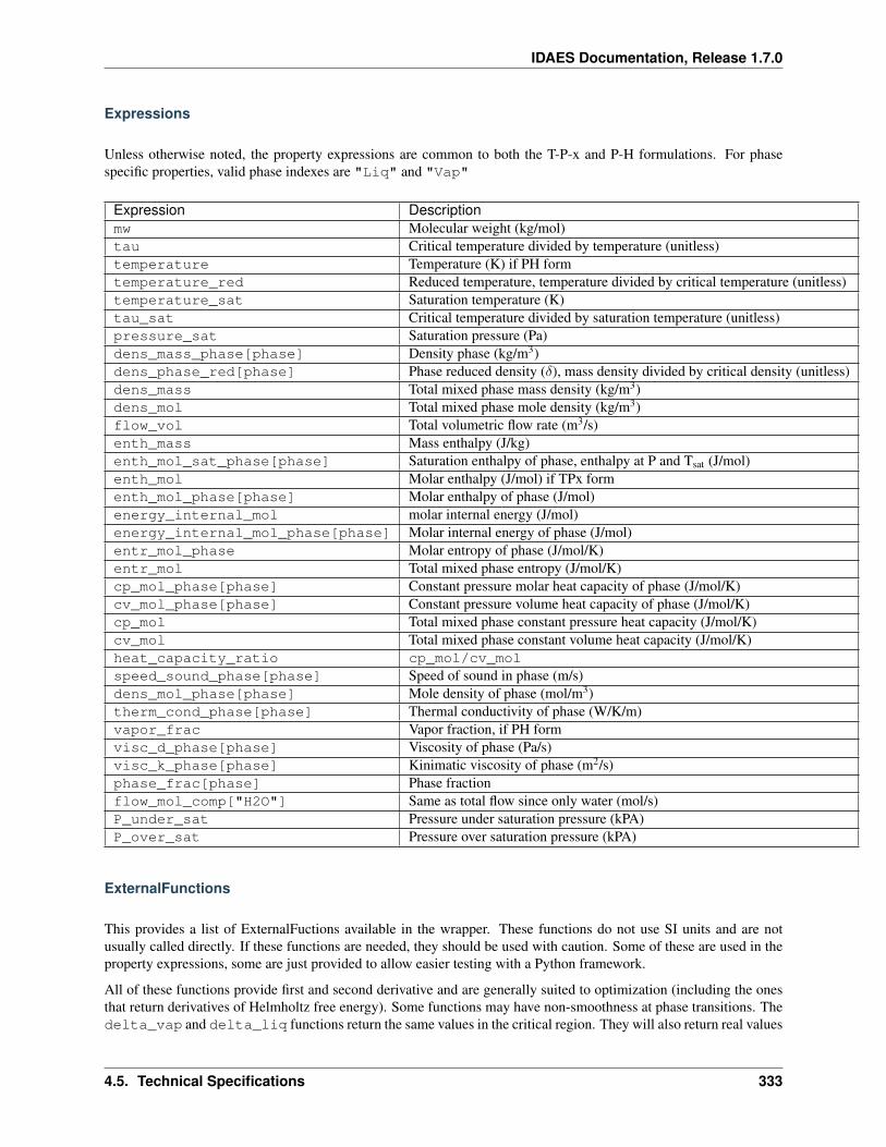
IDAES Documentation, Release 1.7.0
Expressions
Unless otherwise noted, the property expressions are common to both the T-P-x and P-H formulations. For phasespecific properties, valid phase indexes are "Liq" and "Vap"
Expression Descriptionmw Molecular weight (kg/mol)tau Critical temperature divided by temperature (unitless)temperature Temperature (K) if PH formtemperature_red Reduced temperature, temperature divided by critical temperature (unitless)temperature_sat Saturation temperature (K)tau_sat Critical temperature divided by saturation temperature (unitless)pressure_sat Saturation pressure (Pa)dens_mass_phase[phase] Density phase (kg/m3)dens_phase_red[phase] Phase reduced density (𝛿), mass density divided by critical density (unitless)dens_mass Total mixed phase mass density (kg/m3)dens_mol Total mixed phase mole density (kg/m3)flow_vol Total volumetric flow rate (m3/s)enth_mass Mass enthalpy (J/kg)enth_mol_sat_phase[phase] Saturation enthalpy of phase, enthalpy at P and Tsat (J/mol)enth_mol Molar enthalpy (J/mol) if TPx formenth_mol_phase[phase] Molar enthalpy of phase (J/mol)energy_internal_mol molar internal energy (J/mol)energy_internal_mol_phase[phase] Molar internal energy of phase (J/mol)entr_mol_phase Molar entropy of phase (J/mol/K)entr_mol Total mixed phase entropy (J/mol/K)cp_mol_phase[phase] Constant pressure molar heat capacity of phase (J/mol/K)cv_mol_phase[phase] Constant pressure volume heat capacity of phase (J/mol/K)cp_mol Total mixed phase constant pressure heat capacity (J/mol/K)cv_mol Total mixed phase constant volume heat capacity (J/mol/K)heat_capacity_ratio cp_mol/cv_molspeed_sound_phase[phase] Speed of sound in phase (m/s)dens_mol_phase[phase] Mole density of phase (mol/m3)therm_cond_phase[phase] Thermal conductivity of phase (W/K/m)vapor_frac Vapor fraction, if PH formvisc_d_phase[phase] Viscosity of phase (Pa/s)visc_k_phase[phase] Kinimatic viscosity of phase (m2/s)phase_frac[phase] Phase fractionflow_mol_comp["H2O"] Same as total flow since only water (mol/s)P_under_sat Pressure under saturation pressure (kPA)P_over_sat Pressure over saturation pressure (kPA)
ExternalFunctions
This provides a list of ExternalFuctions available in the wrapper. These functions do not use SI units and are notusually called directly. If these functions are needed, they should be used with caution. Some of these are used in theproperty expressions, some are just provided to allow easier testing with a Python framework.
All of these functions provide first and second derivative and are generally suited to optimization (including the onesthat return derivatives of Helmholtz free energy). Some functions may have non-smoothness at phase transitions. Thedelta_vap and delta_liq functions return the same values in the critical region. They will also return real values
4.5. Technical Specifications 333
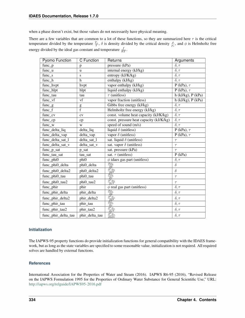
IDAES Documentation, Release 1.7.0
when a phase doesn’t exist, but those values do not necessarily have physical meaning.
There are a few variables that are common to a lot of these functions, so they are summarized here 𝜏 is the criticaltemperature divided by the temperature 𝑇𝑐
𝑇 , 𝛿 is density divided by the critical density 𝜌𝜌𝑐
, and 𝜑 is Helmholtz free
energy divided by the ideal gas constant and temperature 𝑓𝑅𝑇 .
Pyomo Function C Function Returns Argumentsfunc_p p pressure (kPa) 𝛿, 𝜏func_u u internal energy (kJ/kg) 𝛿, 𝜏func_s s entropy (kJ/K/kg) 𝛿, 𝜏func_h h enthalpy (kJ/kg) 𝛿, 𝜏func_hvpt hvpt vapor enthalpy (kJ/kg) P (kPa), 𝜏func_hlpt hlpt liquid enthalpy (kJ/kg) P (kPa), 𝜏func_tau tau 𝜏 (unitless) h (kJ/kg), P (kPa)func_vf vf vapor fraction (unitless) h (kJ/kg), P (kPa)func_g g Gibbs free energy (kJ/kg) 𝛿, 𝜏func_f f Helmholtz free energy (kJ/kg) 𝛿, 𝜏func_cv cv const. volume heat capacity (kJ/K/kg) 𝛿, 𝜏func_cp cp const. pressure heat capacity (kJ/K/kg) 𝛿, 𝜏func_w w speed of sound (m/s) 𝛿, 𝜏func_delta_liq delta_liq liquid 𝛿 (unitless) P (kPa), 𝜏func_delta_vap delta_vap vapor 𝛿 (unitless) P (kPa), 𝜏func_delta_sat_l delta_sat_l sat. liquid 𝛿 (unitless) 𝜏func_delta_sat_v delta_sat_v sat. vapor 𝛿 (unitless) 𝜏func_p_sat p_sat sat. pressure (kPa) 𝜏func_tau_sat tau_sat sat. 𝜏 (unitless) P (kPa)func_phi0 phi0 𝜑 idaes gas part (unitless) 𝛿, 𝜏
func_phi0_delta phi0_delta 𝜕𝜑0
𝜕𝛿 𝛿
func_phi0_delta2 phi0_delta2 𝜕2𝜑0
𝜕𝛿2 𝛿
func_phi0_tau phi0_tau 𝜕𝜑0
𝜕𝜏 𝜏
func_phi0_tau2 phi0_tau2 𝜕2𝜑0
𝜕𝜏2 𝜏func_phir phir 𝜑 real gas part (unitless) 𝛿, 𝜏
func_phir_delta phir_delta 𝜕𝜑𝑟
𝜕𝛿 𝛿, 𝜏
func_phir_delta2 phir_delta2 𝜕2𝜑𝑟
𝜕𝛿2 𝛿, 𝜏
func_phir_tau phir_tau 𝜕𝜑𝑟
𝜕𝜏 𝛿, 𝜏
func_phir_tau2 phir_tau2 𝜕2𝜑𝑟
𝜕𝜏2 𝛿, 𝜏
func_phir_delta_tau phir_delta_tau 𝜕2𝜑𝑟
𝜕𝛿𝜕𝜏 𝛿, 𝜏
Initialization
The IAPWS-95 property functions do provide initialization functions for general compatibility with the IDAES frame-work, but as long as the state variables are specified to some reasonable value, initialization is not required. All requiredsolves are handled by external functions.
References
International Association for the Properties of Water and Steam (2016). IAPWS R6-95 (2016), “Revised Releaseon the IAPWS Formulation 1995 for the Properties of Ordinary Water Substance for General Scientific Use,” URL:http://iapws.org/relguide/IAPWS95-2016.pdf
334 Chapter 4. Contents
IDAES Documentation, Release 1.7.0
Wagner, W., A. Pruss (2002). “The IAPWS Formulation 1995 for the Thermodynamic Properties of Ordinary WaterSubstance for General and Scientific Use.” J. Phys. Chem. Ref. Data, 31, 387-535.
Wagner, W. et al. (2000). “The IAPWS Industrial Formulation 1997 for the Thermodynamic Properties of Water andSteam,” ASME J. Eng. Gas Turbines and Power, 122, 150-182.
Akasaka, R. (2008). “A Reliable and Useful Method to Determine the Saturation State from Helmholtz Energy Equa-tions of State.” Journal of Thermal Science and Technology, 3(3), 442-451.
International Association for the Properties of Water and Steam (2011). IAPWS R15-11, “Release on the IAPWS For-mulation 2011 for the Thermal Conductivity of Ordinary Water Substance,” URL: http://iapws.org/relguide/ThCond.pdf.
International Association for the Properties of Water and Steam (2008). IAPWS R12-08, “Release on the IAPWSFormulation 2008 for the Viscosity of Ordinary Water Substance,” URL: http://iapws.org/relguide/visc.pdf.
Convenience Functions
idaes.generic_models.properties.iapws95.htpx(T, P=None, x=None)Convenience function to calculate steam enthalpy from temperature and either pressure or vapor fraction. Thisfunction can be used for inlet streams and initialization where temperature is known instead of enthalpy.
User must provided values for one (and only one) of arguments P and x.
Parameters
• T – Temperature [K] (between 200 and 3000)
• P – Pressure [Pa] (between 1 and 1e9), None if saturated steam
• x – Vapor fraction [mol vapor/mol total] (between 0 and 1), None if
• or subcooled (superheated) –
Returns Total molar enthalpy [J/mol].
Iapws95StateBlock Class
class idaes.generic_models.properties.iapws95.Iapws95StateBlock(*args,**kwargs)
This is some placeholder doc.
Parameters
• rule (function) – A rule function or None. Default rule calls build().
• concrete (bool) – If True, make this a toplevel model. Default - False.
• ctype (str) – Pyomo ctype of the block. Default - “Block”
• default (dict) – Default ProcessBlockData config
Keys
parameters A reference to an instance of the Property Parameter Block associated withthis property package.
defined_state Flag indicating whether the state should be considered fully defined, andthus whether constraints such as sum of mass/mole fractions should be included, de-fault - False. Valid values: True - state variables will be fully defined, False - statevariables will not be fully defined.
4.5. Technical Specifications 335

IDAES Documentation, Release 1.7.0
has_phase_equilibrium Flag indicating whether phase equilibrium constraints shouldbe constructed in this state block, default - True. Valid values: True - StateBlockshould calculate phase equilibrium, False - StateBlock should not calculate phase equi-librium.
• initialize (dict) – ProcessBlockData config for individual elements. Keys are Block-Data indexes and values are dictionaries described under the “default” argument above.
• idx_map (function) – Function to take the index of a BlockData element and return theindex in the initialize dict from which to read arguments. This can be provided to overidethe default behavior of matching the BlockData index exactly to the index in initialize.
Returns (Iapws95StateBlock) New instance
Iapws95StateBlockData Class
class idaes.generic_models.properties.iapws95.Iapws95StateBlockData(*args,**kwargs)
This is a property package for calculating thermophysical properties of water.
build(*args)Callable method for Block construction
Iapws95ParameterBlock Class
class idaes.generic_models.properties.iapws95.Iapws95ParameterBlock(*args,**kwargs)
Parameters
• rule (function) – A rule function or None. Default rule calls build().
• concrete (bool) – If True, make this a toplevel model. Default - False.
• ctype (str) – Pyomo ctype of the block. Default - “Block”
• default (dict) – Default ProcessBlockData config
Keys
default_arguments Default arguments to use with Property Package
phase_presentation Set the way phases are presented to models. The MIX option ap-pears to the framework to be a mixed phase containing liquid and/or vapor. The mixedoption can simplify calculations at the unit model level since it can be treated as asingle phase, but unit models such as flash vessels will not be able to treat the phasesindependently. The LG option presents as two separate phases to the framework. TheL or G options can be used if it is known for sure that only one phase is present. de-fault - PhaseType.MIX Valid values: PhaseType.MIX - Present a mixed phase withliquid and/or vapor, PhaseType.LG - Present a liquid and vapor phase, PhaseType.L -Assume only liquid can be present, PhaseType.G - Assume only vapor can be present
state_vars The set of state variables to use. Depending on the use, one state variable setor another may be better computationally. Usually pressure and enthalpy are the bestchoice because they are well behaved during a phase change. default - StateVars.PHValid values: StateVars.PH - Pressure-Enthalpy, StateVars.TPX - Temperature-Pressure-Quality
336 Chapter 4. Contents
IDAES Documentation, Release 1.7.0
• initialize (dict) – ProcessBlockData config for individual elements. Keys are Block-Data indexes and values are dictionaries described under the “default” argument above.
• idx_map (function) – Function to take the index of a BlockData element and return theindex in the initialize dict from which to read arguments. This can be provided to overidethe default behavior of matching the BlockData index exactly to the index in initialize.
Returns (Iapws95ParameterBlock) New instance
Iapws95ParameterBlockData Class
class idaes.generic_models.properties.iapws95.Iapws95ParameterBlockData(component)
build()General build method for PropertyParameterBlocks. Inheriting models should call super().build.
Parameters None –
Returns None
Property Interrogator Tool
When preparing to model a process flowsheet, it is necessary to specify models for all the thermophysical and kineticproperties that will be required by the different unit operations to simulate the process. However, it is often difficult toknow what properties will be required a priori. The IDAES Property Interrogator tool allows a user to define a generalflowsheet structure and interrogate it for the full list of properties that will be required, thus informing them of whatmethods they will need to define in their property package(s).
Tool Usage
The IDAES Properties Interrogator tool consists of two classes; a PropertiesInterrogatorBlock and a ReactionInter-rogatorBlock. These blocks are used in place of the normal PhysicalParameterBlock and ReactionParameterBlockwhilst declaring a flowsheet, however rather than constructing a solvable flowsheet they record all calls for propertiesmade whilst constructing the flowsheet. These Blocks then contain a number of methods for reporting the loggedproperty calls for the user.
An example of how Property Interrogator tool is used is shown below:
import pyomo.environ as pyo # Pyomo environmentfrom idaes.core import FlowsheetBlockfrom idaes.generic_models.unit_models import CSTRfrom idaes.generic_models.properties.interrogator import PropertyInterrogatorBlock,→˓ReactionInterrogatorBlock
m = pyo.ConcreteModel()m.fs = FlowsheetBlock(default="dynamic": True)
m.fs.params = PropertyInterrogatorBlock()m.fs.rxn_params = ReactionInterrogatorBlock(
default="property_package": m.fs.params)
m.fs.R01 = CSTR(default="property_package": m.fs.params,"reaction_package": m.fs.rxn_params,"has_heat_of_reaction": True)
4.5. Technical Specifications 337
IDAES Documentation, Release 1.7.0
Note: Flowsheets constructed using the Property Interrogator tools are not solvable flowsheets, and will result inerrors if sent to a solver.
Output and Display Methods
Both the PropertiesInterrogatorBlock and ReactionInterrogatorBlock support the following methods for reporting theresults of the flowsheet interrogation. The PropertiesInterrogatorBlock will contain a summary of all thermophysicalproperties expected of a StateBlock in the flowsheet, whilst the ReactionInterrogatorBlock will contain a summary ofall reaction related properties required of a ReactionBlock.
• list_required_properties() - returns a list containing all properties called for by the flowsheet.
• print_required_properties() - prints a summary of the required properties
• list_models_requiring_property(property) - returns a list of unit models within the flowsheet that require thegiven property
• print_models_requiring_property(property) - prints the name of all unit models within the flowsheet that requirethe given property
• list_properties_required_by_model(model) - returns a list of all properties required by a given unit model in theflowsheet
• print_properties_required_by_model(model) - prints a summary of all properties required by a given unit modelin the flowsheet
For more details on these methods, see the detailed class documentation below.
Additionally, the PropertiesInterrogatorBlock and ReactionInterrogatorBlock contain a dict named re-quired_properties which stores the data regarding the properties required by the model. The keys of this dict arethe names of all the properties required (as strings) and the values are a list of names for the unit models requiring thegiven property.
Class Documentation
class idaes.generic_models.properties.interrogator.properties_interrogator.PropertyInterrogatorBlock(*args,**kwargs)
Parameters
• rule (function) – A rule function or None. Default rule calls build().
• concrete (bool) – If True, make this a toplevel model. Default - False.
• ctype (str) – Pyomo ctype of the block. Default - “Block”
• default (dict) – Default ProcessBlockData config
Keys
default_arguments Default arguments to use with Property Package
• initialize (dict) – ProcessBlockData config for individual elements. Keys are Block-Data indexes and values are dictionaries described under the “default” argument above.
• idx_map (function) – Function to take the index of a BlockData element and return theindex in the initialize dict from which to read arguments. This can be provided to overidethe default behavior of matching the BlockData index exactly to the index in initialize.
338 Chapter 4. Contents
IDAES Documentation, Release 1.7.0
Returns (PropertyInterrogatorBlock) New instance
class idaes.generic_models.properties.interrogator.properties_interrogator.PropertyInterrogatorData(component)Interrogator Parameter Block Class
This class contains the methods and attributes for recording and displaying the properties requried by the flow-sheet.
build()Callable method for Block construction.
classmethod define_metadata(obj)Set all the metadata for properties and units.
This method should be implemented by subclasses. In the implementation, they should set informationinto the object provided as an argument.
Parameters pcm (PropertyClassMetadata) – Add metadata to this object.
Returns None
list_models_requiring_property(prop)Method to list all models in the flowsheet requiring the given property.
Parameters prop – the property of interest
Returns A list of unit model names which require prop
list_properties_required_by_model(model)Method to list all thermophysical properties required by a given unit model.
Parameters model – the unit model of interest. Can be given as either a model component orthe unit name as a string
Returns A list of thermophysical properties required by model
list_required_properties()Method to list all thermophysical properties required by the flowsheet.
Parameters None –
Returns A list of properties required
print_models_requiring_property(prop, ostream=None)Method to print a summary of the models in the flowsheet requiring a given property.
Parameters
• prop – the property of interest.
• ostream – output stream to print to. If not provided will print to sys.stdout
Returns None
print_properties_required_by_model(model, ostream=None)Method to print a summary of the thermophysical properties required by a given unit model.
Parameters
• model – the unit model of interest.
• ostream – output stream to print to. If not provided will print to sys.stdout
Returns None
print_required_properties(ostream=None)Method to print a summary of the thermophysical properties required by the flowsheet.
4.5. Technical Specifications 339
IDAES Documentation, Release 1.7.0
Parameters ostream – output stream to print to. If not provided will print to sys.stdout
Returns None
class idaes.generic_models.properties.interrogator.reactions_interrogator.ReactionInterrogatorBlock(*args,**kwargs)
Parameters
• rule (function) – A rule function or None. Default rule calls build().
• concrete (bool) – If True, make this a toplevel model. Default - False.
• ctype (str) – Pyomo ctype of the block. Default - “Block”
• default (dict) – Default ProcessBlockData config
Keys
property_package Reference to associated PropertyPackageParameter object
default_arguments Default arguments to use with Property Package
• initialize (dict) – ProcessBlockData config for individual elements. Keys are Block-Data indexes and values are dictionaries described under the “default” argument above.
• idx_map (function) – Function to take the index of a BlockData element and return theindex in the initialize dict from which to read arguments. This can be provided to overidethe default behavior of matching the BlockData index exactly to the index in initialize.
Returns (ReactionInterrogatorBlock) New instance
class idaes.generic_models.properties.interrogator.reactions_interrogator.ReactionInterrogatorData(*args,**kwargs)
Interrogator Parameter Block Class
This class contains the methods and attributes for recording and displaying the reaction properties requried bythe flowsheet.
build()Callable method for Block construction.
classmethod define_metadata(obj)Set all the metadata for properties and units.
This method should be implemented by subclasses. In the implementation, they should set informationinto the object provided as an argument.
Parameters pcm (PropertyClassMetadata) – Add metadata to this object.
Returns None
list_models_requiring_property(prop)Method to list all models in the flowsheet requiring the given property.
Parameters prop – the property of interest
Returns A list of unit model names which require prop
list_properties_required_by_model(model)Method to list all reaction properties required by a given unit model.
Parameters model – the unit model of interest. Can be given as either a model component orthe unit name as a string
Returns A list of reaction properties required by model
340 Chapter 4. Contents
IDAES Documentation, Release 1.7.0
list_required_properties()Method to list all reaction properties required by the flowsheet.
Parameters None –
Returns A list of properties required
print_models_requiring_property(prop, ostream=None)Method to print a summary of the models in the flowsheet requiring a given property.
Parameters
• prop – the property of interest.
• ostream – output stream to print to. If not provided will print to sys.stdout
Returns None
print_properties_required_by_model(model, ostream=None)Method to print a summary of the reaction properties required by a given unit model.
Parameters
• model – the unit model of interest.
• ostream – output stream to print to. If not provided will print to sys.stdout
Returns None
print_required_properties(ostream=None)Method to print a summary of the reaction properties required by the flowsheet.
Parameters ostream – output stream to print to. If not provided will print to sys.stdout
Returns None
Unit Models
Compressor
The Compressor model is a PressureChanger, where the configuration is set so that the “compressor” option can onlybe True, and the default “thermodynamic_assumption” is “isentropic.” See the PressureChanger documentation fordetails.
Example
The example below demonstrates the basic Compressor model usage:
import pyomo.environ as pyofrom idaes.core import FlowsheetBlockfrom idaes.generic_models.unit_models import Compressorfrom idaes.generic_models.properties import iapws95
m = pyo.ConcreteModel()m.fs = FlowsheetBlock(default="dynamic": False)m.fs.properties = iapws95.Iapws95ParameterBlock()m.fs.unit = Compressor(default="property_package": m.fs.properties)
m.fs.unit.inlet.flow_mol[0].fix(100)
(continues on next page)
4.5. Technical Specifications 341
IDAES Documentation, Release 1.7.0
(continued from previous page)
m.fs.unit.inlet.enth_mol[0].fix(4000)m.fs.unit.inlet.pressure[0].fix(101325)
m.fs.unit.deltaP.fix(50000)m.fs.unit.efficiency_isentropic.fix(0.9)
Continuous Stirred Tank Reactor
The IDAES CSTR model represents a unit operation where a material stream undergoes some chemical reaction(s) ina well-mixed vessel.
Degrees of Freedom
CSTRs generally have one degree of freedom. Typically, the fixed variable is reactor volume.
Model Structure
The core CSTR unit model consists of a single ControlVolume0D (named control_volume) with one InletPort (named inlet) and one Outlet Port (named outlet).
Additional Constraints
CSTR units write the following additional Constraints beyond those written by the ControlVolume Block.
𝑋𝑡,𝑟 = 𝑉𝑡 × 𝑟𝑡,𝑟
where 𝑋𝑡,𝑟 is the extent of reaction of reaction 𝑟 at time 𝑡, 𝑉𝑡 is the volume of the reacting material at time 𝑡 (allowsfor varying reactor volume with time) and 𝑟𝑡,𝑟 is the volumetric rate of reaction of reaction 𝑟 at time 𝑡 (from the outletproperty package).
Variables
CSTR units add the following additional Variables beyond those created by the ControlVolume Block.
Vari-able
Name Notes
𝑉𝑡 vol-ume
If has_holdup = True this is a reference to control_volume.volume, otherwise a Varattached to the Unit Model
𝑄𝑡 heat Only if has_heat_transfer = True, reference to control_volume.heat
CSTR Class
class idaes.generic_models.unit_models.cstr.CSTR(*args, **kwargs)
Parameters
• rule (function) – A rule function or None. Default rule calls build().
342 Chapter 4. Contents
IDAES Documentation, Release 1.7.0
• concrete (bool) – If True, make this a toplevel model. Default - False.
• ctype (str) – Pyomo ctype of the block. Default - “Block”
• default (dict) – Default ProcessBlockData config
Keys
dynamic Indicates whether this model will be dynamic or not, default = useDefault.Valid values: useDefault - get flag from parent (default = False), True - set as adynamic model, False - set as a steady-state model.
has_holdup Indicates whether holdup terms should be constructed or not. Must be Trueif dynamic = True, default - False. Valid values: useDefault - get flag from parent(default = False), True - construct holdup terms, False - do not construct holdup terms
material_balance_type Indicates what type of mass balance should be con-structed, default - MaterialBalanceType.useDefault. Valid values: Ma-terialBalanceType.useDefault - refer to property package for default bal-ance type **MaterialBalanceType.none - exclude material balances, Materi-alBalanceType.componentPhase - use phase component balances, MaterialBal-anceType.componentTotal - use total component balances, MaterialBalance-Type.elementTotal - use total element balances, MaterialBalanceType.total - usetotal material balance.
energy_balance_type Indicates what type of energy balance should be constructed,default - EnergyBalanceType.useDefault. Valid values: EnergyBalance-Type.useDefault - refer to property package for default balance type **Energy-BalanceType.none - exclude energy balances, EnergyBalanceType.enthalpyTotal -single enthalpy balance for material, EnergyBalanceType.enthalpyPhase - enthalpybalances for each phase, EnergyBalanceType.energyTotal - single energy balance formaterial, EnergyBalanceType.energyPhase - energy balances for each phase.
momentum_balance_type Indicates what type of momentum balance should be con-structed, default - MomentumBalanceType.pressureTotal. Valid values: Mo-mentumBalanceType.none - exclude momentum balances, MomentumBalance-Type.pressureTotal - single pressure balance for material, MomentumBalance-Type.pressurePhase - pressure balances for each phase, MomentumBalance-Type.momentumTotal - single momentum balance for material, MomentumBalance-Type.momentumPhase - momentum balances for each phase.
has_heat_transfer Indicates whether terms for heat transfer should be constructed, de-fault - False. Valid values: True - include heat transfer terms, False - exclude heattransfer terms.
has_pressure_change Indicates whether terms for pressure change should be con-structed, default - False. Valid values: True - include pressure change terms, False- exclude pressure change terms.
has_equilibrium_reactions Indicates whether terms for equilibrium controlled reac-tions should be constructed, default - True. Valid values: True - include equilibriumreaction terms, False - exclude equilibrium reaction terms.
has_phase_equilibrium Indicates whether terms for phase equilibrium should be con-structed, default = False. Valid values: True - include phase equilibrium termsFalse - exclude phase equilibrium terms.
has_heat_of_reaction Indicates whether terms for heat of reaction terms should be con-structed, default - False. Valid values: True - include heat of reaction terms, False- exclude heat of reaction terms.
4.5. Technical Specifications 343
IDAES Documentation, Release 1.7.0
property_package Property parameter object used to define property calculations, de-fault - useDefault. Valid values: useDefault - use default package from parentmodel or flowsheet, PhysicalParameterObject - a PhysicalParameterBlock object.
property_package_args A ConfigBlock with arguments to be passed to a propertyblock(s) and used when constructing these, default - None. Valid values: see prop-erty package for documentation.
reaction_package Reaction parameter object used to define reaction calculations, de-fault - None. Valid values: None - no reaction package, ReactionParameterBlock- a ReactionParameterBlock object.
reaction_package_args A ConfigBlock with arguments to be passed to a reactionblock(s) and used when constructing these, default - None. Valid values: see re-action package for documentation.
• initialize (dict) – ProcessBlockData config for individual elements. Keys are Block-Data indexes and values are dictionaries described under the “default” argument above.
• idx_map (function) – Function to take the index of a BlockData element and return theindex in the initialize dict from which to read arguments. This can be provided to overidethe default behavior of matching the BlockData index exactly to the index in initialize.
Returns (CSTR) New instance
CSTRData Class
class idaes.generic_models.unit_models.cstr.CSTRData(component)Standard CSTR Unit Model Class
build()Begin building model (pre-DAE transformation). :param None:
Returns None
Equilibrium Reactor
The IDAES Equilibrium reactor model represents a unit operation where a material stream undergoes some chemicalreaction(s) to reach an equilibrium state. This model is for systems with reaction with equilibrium coefficients - forGibbs energy minimization see Gibbs reactor documentation.
Degrees of Freedom
Equilibrium reactors generally have 1 degree of freedom.
Typical fixed variables are:
• reactor heat duty (has_heat_transfer = True only).
Model Structure
The core Equilibrium reactor unit model consists of a single ControlVolume0D (named control_volume) withone Inlet Port (named inlet) and one Outlet Port (named outlet).
344 Chapter 4. Contents
IDAES Documentation, Release 1.7.0
Additional Constraints
Equilibrium reactors units write the following additional Constraints beyond those written by the Control Volume ifrate controlled reactions are present.
𝑟𝑡,𝑟 = 0
where 𝑟𝑡,𝑟 is the rate of reaction for reaction 𝑟 at time 𝑡. This enforces equilibrium in any reversible rate controlledreactions which are present. Any non-reversible reaction that may be present will proceed to completion.
Variables
Equilibrium reactor units add the following additional Variables beyond those created by the Control Volume.
Vari-able
Name Notes
𝑉𝑡 vol-ume
If has_holdup = True this is a reference to control_volume.volume, otherwise a Varattached to the Unit Model
𝑄𝑡 heat Only if has_heat_transfer = True, reference to control_volume.heat
EquilibriumReactor Class
class idaes.generic_models.unit_models.equilibrium_reactor.EquilibriumReactor(*args,**kwargs)
Parameters
• rule (function) – A rule function or None. Default rule calls build().
• concrete (bool) – If True, make this a toplevel model. Default - False.
• ctype (str) – Pyomo ctype of the block. Default - “Block”
• default (dict) – Default ProcessBlockData config
Keys
dynamic Indicates whether this model will be dynamic or not, default = False. Equilib-rium Reactors do not support dynamic behavior.
has_holdup Indicates whether holdup terms should be constructed or not. default -False. Equilibrium reactors do not have defined volume, thus this must be False.
material_balance_type Indicates what type of mass balance should be con-structed, default - MaterialBalanceType.useDefault. Valid values: Ma-terialBalanceType.useDefault - refer to property package for default bal-ance type **MaterialBalanceType.none - exclude material balances, Materi-alBalanceType.componentPhase - use phase component balances, MaterialBal-anceType.componentTotal - use total component balances, MaterialBalance-Type.elementTotal - use total element balances, MaterialBalanceType.total - usetotal material balance.
energy_balance_type Indicates what type of energy balance should be constructed,default - EnergyBalanceType.useDefault. Valid values: EnergyBalance-Type.useDefault - refer to property package for default balance type **Energy-BalanceType.none - exclude energy balances, EnergyBalanceType.enthalpyTotal -
4.5. Technical Specifications 345
IDAES Documentation, Release 1.7.0
single enthalpy balance for material, EnergyBalanceType.enthalpyPhase - enthalpybalances for each phase, EnergyBalanceType.energyTotal - single energy balance formaterial, EnergyBalanceType.energyPhase - energy balances for each phase.
momentum_balance_type Indicates what type of momentum balance should be con-structed, default - MomentumBalanceType.pressureTotal. Valid values: Mo-mentumBalanceType.none - exclude momentum balances, MomentumBalance-Type.pressureTotal - single pressure balance for material, MomentumBalance-Type.pressurePhase - pressure balances for each phase, MomentumBalance-Type.momentumTotal - single momentum balance for material, MomentumBalance-Type.momentumPhase - momentum balances for each phase.
has_rate_reactions Indicates whether terms for rate controlled reactions should be con-structed, along with constraints equating these to zero, default - True. Valid values: True - include rate reaction terms, False - exclude rate reaction terms.
has_equilibrium_reactions Indicates whether terms for equilibrium controlled reac-tions should be constructed, default - True. Valid values: True - include equilibriumreaction terms, False - exclude equilibrium reaction terms.
has_phase_equilibrium Indicates whether terms for phase equilibrium should be con-structed, default - True. Valid values: True - include phase equilibrium term, False- exclude phase equlibirum terms.
has_heat_transfer Indicates whether terms for heat transfer should be constructed, de-fault - False. Valid values: True - include heat transfer terms, False - exclude heattransfer terms.
has_heat_of_reaction Indicates whether terms for heat of reaction terms should be con-structed, default - False. Valid values: True - include heat of reaction terms, False- exclude heat of reaction terms.
has_pressure_change Indicates whether terms for pressure change should be con-structed, default - False. Valid values: True - include pressure change terms, False- exclude pressure change terms.
property_package Property parameter object used to define property calculations, de-fault - useDefault. Valid values: useDefault - use default package from parentmodel or flowsheet, PhysicalParameterObject - a PhysicalParameterBlock object.
property_package_args A ConfigBlock with arguments to be passed to a propertyblock(s) and used when constructing these, default - None. Valid values: see prop-erty package for documentation.
reaction_package Reaction parameter object used to define reaction calculations, de-fault - None. Valid values: None - no reaction package, ReactionParameterBlock- a ReactionParameterBlock object.
reaction_package_args A ConfigBlock with arguments to be passed to a reactionblock(s) and used when constructing these, default - None. Valid values: see re-action package for documentation.
• initialize (dict) – ProcessBlockData config for individual elements. Keys are Block-Data indexes and values are dictionaries described under the “default” argument above.
• idx_map (function) – Function to take the index of a BlockData element and return theindex in the initialize dict from which to read arguments. This can be provided to overidethe default behavior of matching the BlockData index exactly to the index in initialize.
Returns (EquilibriumReactor) New instance
346 Chapter 4. Contents
IDAES Documentation, Release 1.7.0
EquilibriumReactorData Class
class idaes.generic_models.unit_models.equilibrium_reactor.EquilibriumReactorData(component)Standard Equilibrium Reactor Unit Model Class
build()Begin building model.
Parameters None –
Returns None
Feed Block
Feed Blocks are used to represent sources of material in Flowsheets. Feed blocks do not calculate phase equilibriumof the feed stream, and the composition of the material in the outlet stream will be exactly as specified in the input.For applications where the users wishes the outlet stream to be in phase equilibrium, see the Feed_Flash unit model.
Degrees of Freedom
The degrees of freedom of Feed blocks depends on the property package being used and the number of state variablesnecessary to fully define the system. Users should refer to documentation on the property package they are using.
Model Structure
Feed Blocks consists of a single StateBlock (named properties), each with one Outlet Port (named outlet). Feed Blocksalso contain References to the state variables defined within the StateBlock
Additional Constraints
Feed Blocks write no additional constraints to the model.
Variables
Feed blocks add no additional Variables.
Feed Class
class idaes.generic_models.unit_models.feed.Feed(*args, **kwargs)
Parameters
• rule (function) – A rule function or None. Default rule calls build().
• concrete (bool) – If True, make this a toplevel model. Default - False.
• ctype (str) – Pyomo ctype of the block. Default - “Block”
• default (dict) – Default ProcessBlockData config
Keys
4.5. Technical Specifications 347
IDAES Documentation, Release 1.7.0
dynamic Indicates whether this model will be dynamic or not, default = False. Feedblocks are always steady-state.
has_holdup Feed blocks do not contain holdup, thus this must be False.
property_package Property parameter object used to define property calculations, de-fault - useDefault. Valid values: useDefault - use default package from parentmodel or flowsheet, PhysicalParameterObject - a PhysicalParameterBlock object.
property_package_args A ConfigBlock with arguments to be passed to a propertyblock(s) and used when constructing these, default - None. Valid values: see prop-erty package for documentation.
• initialize (dict) – ProcessBlockData config for individual elements. Keys are Block-Data indexes and values are dictionaries described under the “default” argument above.
• idx_map (function) – Function to take the index of a BlockData element and return theindex in the initialize dict from which to read arguments. This can be provided to overidethe default behavior of matching the BlockData index exactly to the index in initialize.
Returns (Feed) New instance
FeedData Class
class idaes.generic_models.unit_models.feed.FeedData(component)Standard Feed Block Class
build()Begin building model.
Parameters None –
Returns None
initialize(state_args=None, outlvl=0, solver=’ipopt’, optarg=’tol’: 1e-06)This method calls the initialization method of the state block.
Keyword Arguments
• state_args – a dict of arguments to be passed to the property package(s) to provide aninitial state for initialization (see documentation of the specific property package) (default= None).
• outlvl – sets output level of initialization routine
• optarg – solver options dictionary object (default=‘tol’: 1e-6)
• solver – str indicating which solver to use during initialization (default = ‘ipopt’)
Returns None
Feed Block with Flash
Feed Blocks are used to represent sources of material in Flowsheets. In some cases, users may have a situation wherea feed stream may be in a multi-phase state, but may not know the full details of the equilibrium state. The IDAESFeed Block with Flash (FeedFlash) allows users to define a feed block where the outlet is in phase equilibrium basedon calculations from the chosen property package and a sufficient set of state variables prior to being passed to the firstunit operation. The phase equilibrium is performed assuming an isobaric and isothermal flash operation.
348 Chapter 4. Contents
IDAES Documentation, Release 1.7.0
A Feed Block with Flash is only required in cases where the feed may be in phase equilibrium AND the chosenproperty package uses a state definition that includes phase separations. Some property packages support phase equi-librium, but use a state definition that involves only total flows - in these cases a flash calculation is performed at theinlet of every unit and thus it is not necessary to perform a flash calculation at the feed block.
Degrees of Freedom
The degrees of freedom of FeedFlash blocks depends on the property package being used and the number of statevariables necessary to fully define the system. Users should refer to documentation on the property package they areusing.
Model Structure
FeedFlash Blocks contain a single ControlVolume0D (named control_volume) with one Outlet Port (namedoutlet). FeedFlash Blocks also contain References to the state variables defined within the inlet StateBlock of theControlVolume (representing the unflashed state of the feed).
FeedFlash Blocks do not write a set of energy balances within the Control Volume - instead a constraint is writtenwhich enforces an isothermal flash.
Additional Constraints
The FeedFlash Block writes one additional constraint to enforce isothermal behavior.
𝑇𝑖𝑛,𝑡 = 𝑇𝑜𝑢𝑡,𝑡
where 𝑇𝑖𝑛,𝑡 and 𝑇𝑜𝑢𝑡,𝑡 are the temperatures of the material before and after the flash operation.
Variables
FeedFlash blocks add no additional Variables.
FeedFlash Class
class idaes.generic_models.unit_models.feed_flash.FeedFlash(*args, **kwargs)
Parameters
• rule (function) – A rule function or None. Default rule calls build().
• concrete (bool) – If True, make this a toplevel model. Default - False.
• ctype (str) – Pyomo ctype of the block. Default - “Block”
• default (dict) – Default ProcessBlockData config
Keys
dynamic Feed units do not support dynamic behavior.
has_holdup Feed units do not have defined volume, thus this must be False.
4.5. Technical Specifications 349
IDAES Documentation, Release 1.7.0
material_balance_type Indicates what type of mass balance should be con-structed, default - MaterialBalanceType.useDefault. Valid values: Ma-terialBalanceType.useDefault - refer to property package for default bal-ance type **MaterialBalanceType.none - exclude material balances, Materi-alBalanceType.componentPhase - use phase component balances, MaterialBal-anceType.componentTotal - use total component balances, MaterialBalance-Type.elementTotal - use total element balances, MaterialBalanceType.total - usetotal material balance.
flash_type Indicates what type of flash operation should be used. default -FlashType.isothermal. Valid values: FlashType.isothermal - specify temperature,FlashType.isenthalpic - specify enthalpy.
property_package Property parameter object used to define property calculations, de-fault - useDefault. Valid values: useDefault - use default package from parentmodel or flowsheet, PhysicalParameterObject - a PhysicalParameterBlock object.
property_package_args A ConfigBlock with arguments to be passed to a propertyblock(s) and used when constructing these, default - None. Valid values: see prop-erty package for documentation.
• initialize (dict) – ProcessBlockData config for individual elements. Keys are Block-Data indexes and values are dictionaries described under the “default” argument above.
• idx_map (function) – Function to take the index of a BlockData element and return theindex in the initialize dict from which to read arguments. This can be provided to overidethe default behavior of matching the BlockData index exactly to the index in initialize.
Returns (FeedFlash) New instance
FeedFlashData Class
class idaes.generic_models.unit_models.feed_flash.FeedFlashData(component)Standard Feed block with phase equilibrium
build()Begin building model.
Parameters None –
Returns None
Flash Unit
The IDAES Flash model represents a unit operation where a single stream undergoes a flash separation into two phases.The Flash model supports mutile types of flash operations, including pressure changes and addition or removal of heat.
Degrees of Freedom
Flash units generally have 2 degrees of freedom.
Typical fixed variables are:
• heat duty or outlet temperature (see note),
• pressure change or outlet pressure.
350 Chapter 4. Contents
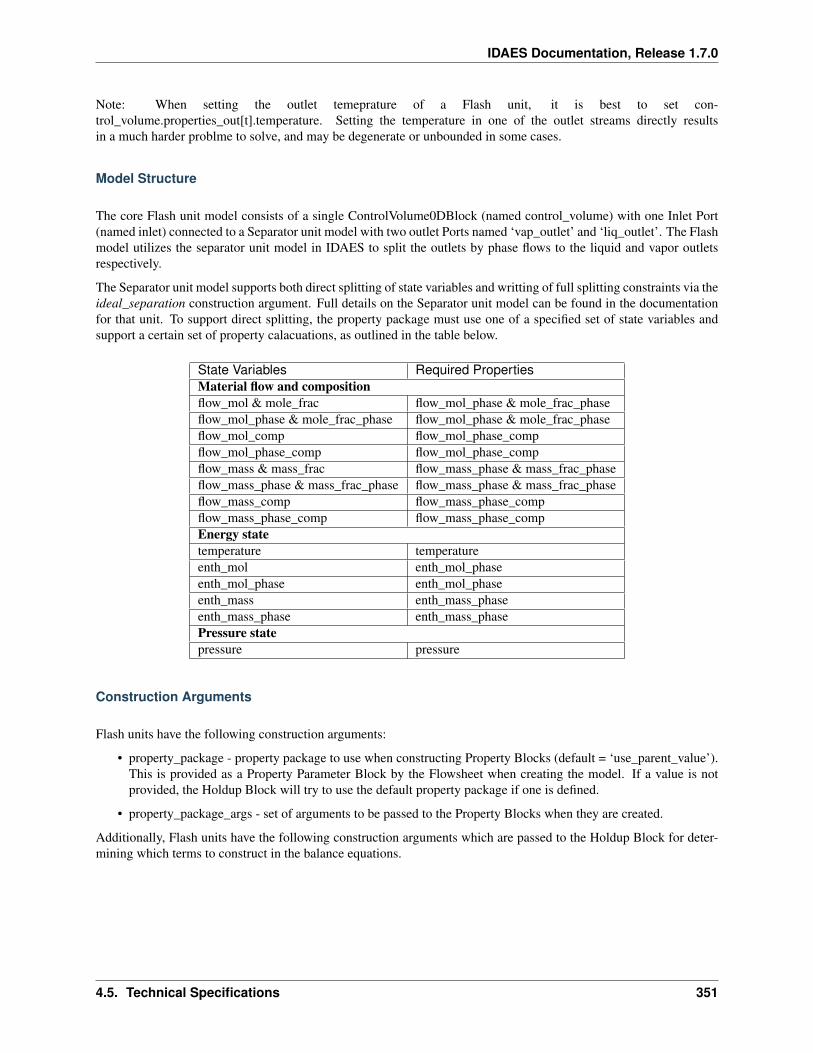
IDAES Documentation, Release 1.7.0
Note: When setting the outlet temeprature of a Flash unit, it is best to set con-trol_volume.properties_out[t].temperature. Setting the temperature in one of the outlet streams directly resultsin a much harder problme to solve, and may be degenerate or unbounded in some cases.
Model Structure
The core Flash unit model consists of a single ControlVolume0DBlock (named control_volume) with one Inlet Port(named inlet) connected to a Separator unit model with two outlet Ports named ‘vap_outlet’ and ‘liq_outlet’. The Flashmodel utilizes the separator unit model in IDAES to split the outlets by phase flows to the liquid and vapor outletsrespectively.
The Separator unit model supports both direct splitting of state variables and writting of full splitting constraints via theideal_separation construction argument. Full details on the Separator unit model can be found in the documentationfor that unit. To support direct splitting, the property package must use one of a specified set of state variables andsupport a certain set of property calacuations, as outlined in the table below.
State Variables Required PropertiesMaterial flow and compositionflow_mol & mole_frac flow_mol_phase & mole_frac_phaseflow_mol_phase & mole_frac_phase flow_mol_phase & mole_frac_phaseflow_mol_comp flow_mol_phase_compflow_mol_phase_comp flow_mol_phase_compflow_mass & mass_frac flow_mass_phase & mass_frac_phaseflow_mass_phase & mass_frac_phase flow_mass_phase & mass_frac_phaseflow_mass_comp flow_mass_phase_compflow_mass_phase_comp flow_mass_phase_compEnergy statetemperature temperatureenth_mol enth_mol_phaseenth_mol_phase enth_mol_phaseenth_mass enth_mass_phaseenth_mass_phase enth_mass_phasePressure statepressure pressure
Construction Arguments
Flash units have the following construction arguments:
• property_package - property package to use when constructing Property Blocks (default = ‘use_parent_value’).This is provided as a Property Parameter Block by the Flowsheet when creating the model. If a value is notprovided, the Holdup Block will try to use the default property package if one is defined.
• property_package_args - set of arguments to be passed to the Property Blocks when they are created.
Additionally, Flash units have the following construction arguments which are passed to the Holdup Block for deter-mining which terms to construct in the balance equations.
4.5. Technical Specifications 351
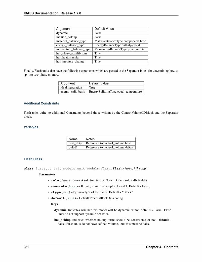
IDAES Documentation, Release 1.7.0
Argument Default Valuedynamic Falseinclude_holdup Falsematerial_balance_type MaterialBalanceType.componentPhaseenergy_balance_type EnergyBalanceType.enthalpyTotalmomentum_balance_type MomentumBalanceType.pressureTotalhas_phase_equilibrium Truehas_heat_transfer Truehas_pressure_change True
Finally, Flash units also have the following arguments which are passed to the Separator block for determining how tosplit to two-phase mixture.
Argument Default Valueideal_separation Trueenergy_split_basis EnergySplittingType.equal_temperature
Additional Constraints
Flash units write no additional Constraints beyond those written by the ControlVolume0DBlock and the Separatorblock.
Variables
Name Notesheat_duty Reference to control_volume.heatdeltaP Reference to control_volume.deltaP
Flash Class
class idaes.generic_models.unit_models.flash.Flash(*args, **kwargs)
Parameters
• rule (function) – A rule function or None. Default rule calls build().
• concrete (bool) – If True, make this a toplevel model. Default - False.
• ctype (str) – Pyomo ctype of the block. Default - “Block”
• default (dict) – Default ProcessBlockData config
Keys
dynamic Indicates whether this model will be dynamic or not, default = False. Flashunits do not support dynamic behavior.
has_holdup Indicates whether holdup terms should be constructed or not. default -False. Flash units do not have defined volume, thus this must be False.
352 Chapter 4. Contents
IDAES Documentation, Release 1.7.0
material_balance_type Indicates what type of mass balance should be con-structed, default - MaterialBalanceType.useDefault. Valid values: Ma-terialBalanceType.useDefault - refer to property package for default bal-ance type **MaterialBalanceType.none - exclude material balances, Materi-alBalanceType.componentPhase - use phase component balances, MaterialBal-anceType.componentTotal - use total component balances, MaterialBalance-Type.elementTotal - use total element balances, MaterialBalanceType.total - usetotal material balance.
energy_balance_type Indicates what type of energy balance should be constructed,default - EnergyBalanceType.useDefault. Valid values: EnergyBalance-Type.useDefault - refer to property package for default balance type **Energy-BalanceType.none - exclude energy balances, EnergyBalanceType.enthalpyTotal -single enthalpy balance for material, EnergyBalanceType.enthalpyPhase - enthalpybalances for each phase, EnergyBalanceType.energyTotal - single energy balance formaterial, EnergyBalanceType.energyPhase - energy balances for each phase.
momentum_balance_type Indicates what type of momentum balance should be con-structed, default - MomentumBalanceType.pressureTotal. Valid values: Mo-mentumBalanceType.none - exclude momentum balances, MomentumBalance-Type.pressureTotal - single pressure balance for material, MomentumBalance-Type.pressurePhase - pressure balances for each phase, MomentumBalance-Type.momentumTotal - single momentum balance for material, MomentumBalance-Type.momentumPhase - momentum balances for each phase.
energy_split_basis Argument indicating basis to use for splitting energy this is not usedfor when ideal_separation == True. default - EnergySplittingType.equal_temperature.Valid values: EnergySplittingType.equal_temperature - outlet temperatures equalinlet EnergySplittingType.equal_molar_enthalpy - oulet molar enthalpies equal in-let, EnergySplittingType.enthalpy_split - apply split fractions to enthalpy flows.
ideal_separation Argument indicating whether ideal splitting should be used. Idealsplitting assumes perfect separation of material, and attempts to avoid duplication ofStateBlocks by directly partitioning outlet flows to ports, default - True. Valid values: True - use ideal splitting methods. Cannot be combined with has_phase_equilibrium= True, False - use explicit splitting equations with split fractions.
has_heat_transfer Indicates whether terms for heat transfer should be constructed, de-fault - False. Valid values: True - include heat transfer terms, False - exclude heattransfer terms.
has_pressure_change Indicates whether terms for pressure change should be con-structed, default - True. Valid values: True - include pressure change terms, False- exclude pressure change terms.
property_package Property parameter object used to define property calculations, de-fault - useDefault. Valid values: useDefault - use default package from parentmodel or flowsheet, PropertyParameterObject - a PropertyParameterBlock object.
property_package_args A ConfigBlock with arguments to be passed to a propertyblock(s) and used when constructing these, default - None. Valid values: see prop-erty package for documentation.
• initialize (dict) – ProcessBlockData config for individual elements. Keys are Block-Data indexes and values are dictionaries described under the “default” argument above.
• idx_map (function) – Function to take the index of a BlockData element and return theindex in the initialize dict from which to read arguments. This can be provided to overidethe default behavior of matching the BlockData index exactly to the index in initialize.
4.5. Technical Specifications 353
IDAES Documentation, Release 1.7.0
Returns (Flash) New instance
FlashData Class
class idaes.generic_models.unit_models.flash.FlashData(component)Standard Flash Unit Model Class
build()Begin building model (pre-DAE transformation).
Parameters None –
Returns None
Gibbs Reactor
The IDAES Gibbs reactor model represents a unit operation where a material stream undergoes some set of reactionssuch that the Gibbs energy of the resulting mixture is minimized. Gibbs reactors rely on conservation of individualelements within the system, and thus require element balances, and make use of Lagrange multipliers to find theminimum Gibbs energy state of the system.
Configuration Arguments
The Gibbs Reactor unit model allows users to specify a list of components which should be considered to be inertswithin the reactor. This is done using the “inert_species” configuration argument, which should be a list of valid com-ponent names. These components will be considered inert, such that flows in and out of the unit for those componentsin each phase are equal.
Degrees of Freedom
Gibbs reactors generally have between 0 and 2 degrees of freedom, depending on construction arguments.
Typical fixed variables are:
• reactor heat duty (has_heat_transfer = True only).
• reactor pressure change (has_pressure_change = True only).
Model Structure
The core Gibbs reactor unit model consists of a single ControlVolume0DBlock (named control_volume) with one InletPort (named inlet) and one Outlet Port (named outlet).
Variables
Gibbs reactor units add the following additional Variables beyond those created by the Control Volume Block.
Variable Name Symbol Noteslagrange_mult 𝐿𝑡,𝑒 Lagrange multipliersheat_duty 𝑄𝑡 Only if has_heat_transfer = True, referencedeltaP ∆𝑃𝑡 Only if has_pressure_change = True, reference
354 Chapter 4. Contents
IDAES Documentation, Release 1.7.0
Parameters
The Gibbs reactor unit model includes a scaling parameter for the Gibbs energy minimization constraint, which isnamed “gibbs_scaling”. The default value is 1 and users may adjust the value of this parameter is required.
Constraints
Gibbs reactor models write the following additional constraints to calculate the state that corresponds to the minimumGibbs energy of the system.
gibbs_minimization(time, phase, component):
0 = ×𝑔𝑝𝑎𝑟𝑡𝑖𝑎𝑙,𝑡,𝑗 + ×∑𝑒
(𝐿𝑡,𝑒 × 𝛼𝑗,𝑒)
where 𝑔𝑝𝑎𝑟𝑡𝑖𝑎𝑙,𝑡,𝑗 is the partial molar Gibbs energy of component 𝑗 at time 𝑡, 𝐿𝑡,𝑒 is the Lagrange multiplier forelement 𝑒 at time 𝑡 and 𝛼𝑗,𝑒 is the number of moles of element 𝑒 in one mole of component 𝑗. 𝑔𝑝𝑎𝑟𝑡𝑖𝑎𝑙,𝑡,𝑗 and 𝛼𝑗,𝑒
come from the outlet StateBlock. 𝑡, 𝑒𝑝𝑠 is the gibbs_scaling parameter. In cases where inert species are present, theseare excluded from the 𝑠𝑢𝑚𝑒 term.
In cases where inerts are present, the following additional constraint is written for each inert component and phase:
0 = 𝐹𝑖𝑛,𝑝,𝑗 − 𝐹𝑜𝑢𝑡,𝑝,𝑗
GibbsReactor Class
class idaes.generic_models.unit_models.gibbs_reactor.GibbsReactor(*args,**kwargs)
Parameters
• rule (function) – A rule function or None. Default rule calls build().
• concrete (bool) – If True, make this a toplevel model. Default - False.
• ctype (str) – Pyomo ctype of the block. Default - “Block”
• default (dict) – Default ProcessBlockData config
Keys
dynamic Gibbs reactors do not support dynamic models, thus this must be False.
has_holdup Gibbs reactors do not have defined volume, thus this must be False.
energy_balance_type Indicates what type of energy balance should be constructed,default - EnergyBalanceType.useDefault. Valid values: EnergyBalance-Type.useDefault - refer to property package for default balance type **Energy-BalanceType.none - exclude energy balances, EnergyBalanceType.enthalpyTotal -single enthalpy balance for material, EnergyBalanceType.enthalpyPhase - enthalpybalances for each phase, EnergyBalanceType.energyTotal - single energy balance formaterial, EnergyBalanceType.energyPhase - energy balances for each phase.
momentum_balance_type Indicates what type of momentum balance should be con-structed, default - MomentumBalanceType.pressureTotal. Valid values: Mo-mentumBalanceType.none - exclude momentum balances, MomentumBalance-Type.pressureTotal - single pressure balance for material, MomentumBalance-Type.pressurePhase - pressure balances for each phase, MomentumBalance-Type.momentumTotal - single momentum balance for material, MomentumBalance-Type.momentumPhase - momentum balances for each phase.
4.5. Technical Specifications 355
IDAES Documentation, Release 1.7.0
has_heat_transfer Indicates whether terms for heat transfer should be constructed, de-fault - False. Valid values: True - include heat transfer terms, False - exclude heattransfer terms.
has_pressure_change Indicates whether terms for pressure change should be con-structed, default - False. Valid values: True - include pressure change terms, False- exclude pressure change terms.
property_package Property parameter object used to define property calculations, de-fault - useDefault. Valid values: useDefault - use default package from parentmodel or flowsheet, PropertyParameterObject - a PropertyParameterBlock object.
property_package_args A ConfigBlock with arguments to be passed to a propertyblock(s) and used when constructing these, default - None. Valid values: see prop-erty package for documentation.
inert_species List of species which do not take part in reactions.
• initialize (dict) – ProcessBlockData config for individual elements. Keys are Block-Data indexes and values are dictionaries described under the “default” argument above.
• idx_map (function) – Function to take the index of a BlockData element and return theindex in the initialize dict from which to read arguments. This can be provided to overidethe default behavior of matching the BlockData index exactly to the index in initialize.
Returns (GibbsReactor) New instance
GibbsReactorData Class
class idaes.generic_models.unit_models.gibbs_reactor.GibbsReactorData(component)Standard Gibbs Reactor Unit Model Class
This model assume all possible reactions reach equilibrium such that the system partial molar Gibbs free energyis minimized. Since some species mole flow rate might be very small, the natural log of the species molar flowrate is used. Instead of specifying the system Gibbs free energy as an objective function, the equations for zeropartial derivatives of the grand function with Lagrangian multiple terms with repect to product species moleflow rates and the multiples are specified as constraints.
build()Begin building model (pre-DAE transformation).
Parameters None –
Returns None
Heater
The Heater model is a simple 0D model that adds or removes heat from a material stream.
Example
import pyomo.environ as pe # Pyomo environmentfrom idaes.core import FlowsheetBlock, StateBlockfrom idaes.generic_models.unit_models import Heaterfrom idaes.generic_models.properties import iapws95
(continues on next page)
356 Chapter 4. Contents
IDAES Documentation, Release 1.7.0
(continued from previous page)
# Create an empty flowsheet and steam property parameter block.model = pe.ConcreteModel()model.fs = FlowsheetBlock(default="dynamic": False)model.fs.properties = iapws95.Iapws95ParameterBlock()
# Add a Heater model to the flowsheet.model.fs.heater = Heater(default="property_package": model.fs.properties)
# Setup the heater model by fixing the inputs and heat dutymodel.fs.heater.inlet[:].enth_mol.fix(4000)model.fs.heater.inlet[:].flow_mol.fix(100)model.fs.heater.inlet[:].pressure.fix(101325)model.fs.heater.heat_duty[:].fix(100*20000)
# Initialize the model.model.fs.heater.initialize()
Degrees of Freedom
Aside from the inlet conditions, a heater model usually has one degree of freedom, which is the heat duty.
Model Structure
A heater model contains one ControlVolume0DBlock block.
Variables
The heat_duty variable is a reference to control_volume.heat.
Constraints
A heater model contains no additional constraints beyond what are contained in a ControlVolume0DBlockmodel.
Heater Class
class idaes.generic_models.unit_models.heater.Heater(*args, **kwargs)Simple 0D heater/cooler model.
Parameters
• rule (function) – A rule function or None. Default rule calls build().
• concrete (bool) – If True, make this a toplevel model. Default - False.
• ctype (str) – Pyomo ctype of the block. Default - “Block”
• default (dict) – Default ProcessBlockData config
Keys
4.5. Technical Specifications 357
IDAES Documentation, Release 1.7.0
dynamic Indicates whether this model will be dynamic or not, default = useDefault.Valid values: useDefault - get flag from parent (default = False), True - set as adynamic model, False - set as a steady-state model.
has_holdup Indicates whether holdup terms should be constructed or not. Must be Trueif dynamic = True, default - False. Valid values: useDefault - get flag from parent(default = False), True - construct holdup terms, False - do not construct holdup terms
material_balance_type Indicates what type of mass balance should be con-structed, default - MaterialBalanceType.useDefault. Valid values: Ma-terialBalanceType.useDefault - refer to property package for default bal-ance type **MaterialBalanceType.none - exclude material balances, Materi-alBalanceType.componentPhase - use phase component balances, MaterialBal-anceType.componentTotal - use total component balances, MaterialBalance-Type.elementTotal - use total element balances, MaterialBalanceType.total - usetotal material balance.
energy_balance_type Indicates what type of energy balance should be constructed,default - EnergyBalanceType.useDefault. Valid values: EnergyBalance-Type.useDefault - refer to property package for default balance type **Energy-BalanceType.none - exclude energy balances, EnergyBalanceType.enthalpyTotal -single enthalpy balance for material, EnergyBalanceType.enthalpyPhase - enthalpybalances for each phase, EnergyBalanceType.energyTotal - single energy balance formaterial, EnergyBalanceType.energyPhase - energy balances for each phase.
momentum_balance_type Indicates what type of momentum balance should be con-structed, default - MomentumBalanceType.pressureTotal. Valid values: Mo-mentumBalanceType.none - exclude momentum balances, MomentumBalance-Type.pressureTotal - single pressure balance for material, MomentumBalance-Type.pressurePhase - pressure balances for each phase, MomentumBalance-Type.momentumTotal - single momentum balance for material, MomentumBalance-Type.momentumPhase - momentum balances for each phase.
has_phase_equilibrium Indicates whether terms for phase equilibrium should be con-structed, default = False. Valid values: True - include phase equilibrium termsFalse - exclude phase equilibrium terms.
has_pressure_change Indicates whether terms for pressure change should be con-structed, default - False. Valid values: True - include pressure change terms, False- exclude pressure change terms.
property_package Property parameter object used to define property calculations, de-fault - useDefault. Valid values: useDefault - use default package from parentmodel or flowsheet, PropertyParameterObject - a PropertyParameterBlock object.
property_package_args A ConfigBlock with arguments to be passed to a propertyblock(s) and used when constructing these, default - None. Valid values: see prop-erty package for documentation.
• initialize (dict) – ProcessBlockData config for individual elements. Keys are Block-Data indexes and values are dictionaries described under the “default” argument above.
• idx_map (function) – Function to take the index of a BlockData element and return theindex in the initialize dict from which to read arguments. This can be provided to overidethe default behavior of matching the BlockData index exactly to the index in initialize.
Returns (Heater) New instance
358 Chapter 4. Contents
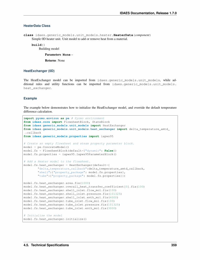
IDAES Documentation, Release 1.7.0
HeaterData Class
class idaes.generic_models.unit_models.heater.HeaterData(component)Simple 0D heater unit. Unit model to add or remove heat from a material.
build()Building model
Parameters None –
Returns None
HeatExchanger (0D)
The HeatExchanger model can be imported from idaes.generic_models.unit_models, while ad-ditional rules and utility functions can be imported from idaes.generic_models.unit_models.heat_exchanger.
Example
The example below demonstrates how to initialize the HeatExchanger model, and override the default temperaturedifference calculation.
import pyomo.environ as pe # Pyomo environmentfrom idaes.core import FlowsheetBlock, StateBlockfrom idaes.generic_models.unit_models import HeatExchangerfrom idaes.generic_models.unit_models.heat_exchanger import delta_temperature_amtd_→˓callbackfrom idaes.generic_models.properties import iapws95
# Create an empty flowsheet and steam property parameter block.model = pe.ConcreteModel()model.fs = FlowsheetBlock(default="dynamic": False)model.fs.properties = iapws95.Iapws95ParameterBlock()
# Add a Heater model to the flowsheet.model.fs.heat_exchanger = HeatExchanger(default=
"delta_temperature_callback":delta_temperature_amtd_callback,"shell":"property_package": model.fs.properties,"tube":"property_package": model.fs.properties)
model.fs.heat_exchanger.area.fix(1000)model.fs.heat_exchanger.overall_heat_transfer_coefficient[0].fix(100)model.fs.heat_exchanger.shell_inlet.flow_mol.fix(100)model.fs.heat_exchanger.shell_inlet.pressure.fix(101325)model.fs.heat_exchanger.shell_inlet.enth_mol.fix(4000)model.fs.heat_exchanger.tube_inlet.flow_mol.fix(100)model.fs.heat_exchanger.tube_inlet.pressure.fix(101325)model.fs.heat_exchanger.tube_inlet.enth_mol.fix(3000)
# Initialize the modelmodel.fs.heat_exchanger.initialize()
4.5. Technical Specifications 359
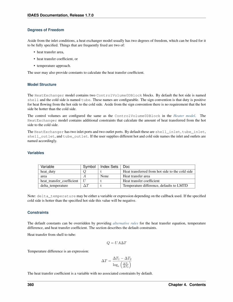
IDAES Documentation, Release 1.7.0
Degrees of Freedom
Aside from the inlet conditions, a heat exchanger model usually has two degrees of freedom, which can be fixed for itto be fully specified. Things that are frequently fixed are two of:
• heat transfer area,
• heat transfer coefficient, or
• temperature approach.
The user may also provide constants to calculate the heat transfer coefficient.
Model Structure
The HeatExchanger model contains two ControlVolume0DBlock blocks. By default the hot side is namedshell and the cold side is named tube. These names are configurable. The sign convention is that duty is positivefor heat flowing from the hot side to the cold side. Aside from the sign convention there is no requirement that the hotside be hotter than the cold side.
The control volumes are configured the same as the ControlVolume0DBlock in the Heater model. TheHeatExchanger model contains additional constraints that calculate the amount of heat transferred from the hotside to the cold side.
The HeatExchanger has two inlet ports and two outlet ports. By default these are shell_inlet, tube_inlet,shell_outlet, and tube_outlet. If the user supplies different hot and cold side names the inlet and outlets arenamed accordingly.
Variables
Variable Symbol Index Sets Docheat_duty 𝑄 t Heat transferred from hot side to the cold sidearea 𝐴 None Heat transfer areaheat_transfer_coefficient 𝑈 t Heat transfer coefficientdelta_temperature ∆𝑇 t Temperature difference, defaults to LMTD
Note: delta_temperature may be either a variable or expression depending on the callback used. If the specifiedcold side is hotter than the specified hot side this value will be negative.
Constraints
The default constants can be overridden by providing alternative rules for the heat transfer equation, temperaturedifference, and heat transfer coefficient. The section describes the default constraints.
Heat transfer from shell to tube:
𝑄 = 𝑈𝐴∆𝑇
Temperature difference is an expression:
∆𝑇 =∆𝑇1 − ∆𝑇2
log𝑒
(Δ𝑇1
Δ𝑇2
)The heat transfer coefficient is a variable with no associated constraints by default.
360 Chapter 4. Contents
IDAES Documentation, Release 1.7.0
Class Documentation
Note: The hot_side_config and cold_side_config can also be supplied using the name of the hot andcold sides (shell and tube by default) as in the example.
class idaes.generic_models.unit_models.heat_exchanger.HeatExchanger(*args,**kwargs)
Simple 0D heat exchanger model.
Parameters
• rule (function) – A rule function or None. Default rule calls build().
• concrete (bool) – If True, make this a toplevel model. Default - False.
• ctype (str) – Pyomo ctype of the block. Default - “Block”
• default (dict) – Default ProcessBlockData config
Keys
dynamic Indicates whether this model will be dynamic or not, default = useDefault.Valid values: useDefault - get flag from parent (default = False), True - set as adynamic model, False - set as a steady-state model.
has_holdup Indicates whether holdup terms should be constructed or not. Must be Trueif dynamic = True, default - False. Valid values: useDefault - get flag from parent(default = False), True - construct holdup terms, False - do not construct holdup terms
hot_side_name Hot side name, sets control volume and inlet and outlet names
cold_side_name Cold side name, sets control volume and inlet and outlet names
hot_side_config A config block used to construct the hot side control volume. Thisconfig can be given by the hot side name instead of hot_side_config.
material_balance_type Indicates what type of mass balance should be con-structed, default - MaterialBalanceType.useDefault. Valid values: Ma-terialBalanceType.useDefault - refer to property package for default bal-ance type **MaterialBalanceType.none - exclude material balances, Material-BalanceType.componentPhase - use phase component balances, MaterialBal-anceType.componentTotal - use total component balances, MaterialBalance-Type.elementTotal - use total element balances, MaterialBalanceType.total - usetotal material balance.
energy_balance_type Indicates what type of energy balance should be constructed,default - EnergyBalanceType.useDefault. Valid values: EnergyBalance-Type.useDefault - refer to property package for default balance type **Energy-BalanceType.none - exclude energy balances, EnergyBalanceType.enthalpyTotal- single enthalpy balance for material, EnergyBalanceType.enthalpyPhase - en-thalpy balances for each phase, EnergyBalanceType.energyTotal - single energybalance for material, EnergyBalanceType.energyPhase - energy balances for eachphase.
momentum_balance_type Indicates what type of momentum balance should be con-structed, default - MomentumBalanceType.pressureTotal. Valid values: Mo-mentumBalanceType.none - exclude momentum balances, MomentumBalance-Type.pressureTotal - single pressure balance for material, MomentumBalance-Type.pressurePhase - pressure balances for each phase, MomentumBalance-
4.5. Technical Specifications 361
IDAES Documentation, Release 1.7.0
Type.momentumTotal - single momentum balance for material, MomentumBal-anceType.momentumPhase - momentum balances for each phase.
has_phase_equilibrium Indicates whether terms for phase equilibrium should beconstructed, default = False. Valid values: True - include phase equilibriumterms False - exclude phase equilibrium terms.
has_pressure_change Indicates whether terms for pressure change should be con-structed, default - False. Valid values: True - include pressure change terms,False - exclude pressure change terms.
property_package Property parameter object used to define property calculations, de-fault - useDefault. Valid values: useDefault - use default package from parentmodel or flowsheet, PropertyParameterObject - a PropertyParameterBlock ob-ject.
property_package_args A ConfigBlock with arguments to be passed to a propertyblock(s) and used when constructing these, default - None. Valid values: seeproperty package for documentation.
cold_side_config A config block used to construct the cold side control volume. Thisconfig can be given by the cold side name instead of cold_side_config.
material_balance_type Indicates what type of mass balance should be con-structed, default - MaterialBalanceType.useDefault. Valid values: Ma-terialBalanceType.useDefault - refer to property package for default bal-ance type **MaterialBalanceType.none - exclude material balances, Material-BalanceType.componentPhase - use phase component balances, MaterialBal-anceType.componentTotal - use total component balances, MaterialBalance-Type.elementTotal - use total element balances, MaterialBalanceType.total - usetotal material balance.
energy_balance_type Indicates what type of energy balance should be constructed,default - EnergyBalanceType.useDefault. Valid values: EnergyBalance-Type.useDefault - refer to property package for default balance type **Energy-BalanceType.none - exclude energy balances, EnergyBalanceType.enthalpyTotal- single enthalpy balance for material, EnergyBalanceType.enthalpyPhase - en-thalpy balances for each phase, EnergyBalanceType.energyTotal - single energybalance for material, EnergyBalanceType.energyPhase - energy balances for eachphase.
momentum_balance_type Indicates what type of momentum balance should be con-structed, default - MomentumBalanceType.pressureTotal. Valid values: Mo-mentumBalanceType.none - exclude momentum balances, MomentumBalance-Type.pressureTotal - single pressure balance for material, MomentumBalance-Type.pressurePhase - pressure balances for each phase, MomentumBalance-Type.momentumTotal - single momentum balance for material, MomentumBal-anceType.momentumPhase - momentum balances for each phase.
has_phase_equilibrium Indicates whether terms for phase equilibrium should beconstructed, default = False. Valid values: True - include phase equilibriumterms False - exclude phase equilibrium terms.
has_pressure_change Indicates whether terms for pressure change should be con-structed, default - False. Valid values: True - include pressure change terms,False - exclude pressure change terms.
property_package Property parameter object used to define property calculations, de-fault - useDefault. Valid values: useDefault - use default package from parent
362 Chapter 4. Contents
IDAES Documentation, Release 1.7.0
model or flowsheet, PropertyParameterObject - a PropertyParameterBlock ob-ject.
property_package_args A ConfigBlock with arguments to be passed to a propertyblock(s) and used when constructing these, default - None. Valid values: seeproperty package for documentation.
delta_temperature_callback Callback for for temperature difference calculations
flow_pattern Heat exchanger flow pattern, default - HeatExchangerFlowPat-tern.countercurrent. Valid values: HeatExchangerFlowPattern.countercurrent- countercurrent flow, HeatExchangerFlowPattern.cocurrent - cocurrent flow,HeatExchangerFlowPattern.crossflow - cross flow, factor times countercurrenttemperature difference.
• initialize (dict) – ProcessBlockData config for individual elements. Keys are Block-Data indexes and values are dictionaries described under the “default” argument above.
• idx_map (function) – Function to take the index of a BlockData element and return theindex in the initialize dict from which to read arguments. This can be provided to overidethe default behavior of matching the BlockData index exactly to the index in initialize.
Returns (HeatExchanger) New instance
class idaes.generic_models.unit_models.heat_exchanger.HeatExchangerData(component)Simple 0D heat exchange unit. Unit model to transfer heat from one material to another.
build()Building model
Parameters None –
Returns None
initialize(state_args_1=None, state_args_2=None, outlvl=0, solver=’ipopt’, optarg=’tol’: 1e-06, duty=None)
Heat exchanger initialization method.
Parameters
• state_args_1 – a dict of arguments to be passed to the property initialization forside_1 (see documentation of the specific property package) (default = ).
• state_args_2 – a dict of arguments to be passed to the property initialization forside_2 (see documentation of the specific property package) (default = ).
• outlvl – sets output level of initialization routine
• optarg – solver options dictionary object (default=‘tol’: 1e-6)
• solver – str indicating which solver to use during initialization (default = ‘ipopt’)
• duty – an initial guess for the amount of heat transfered. This should be a tuple in theform (value, units), (default = (1000 J/s))
Returns None
Callbacks
A selection of functions for constructing the delta_temperature variable or expression are provided in theidaes.generic_models.unit_models.heat_exchanger module. The user may also provide their ownfunction. These callbacks should all take one argument (the HeatExchanger block). With the block argument, the
4.5. Technical Specifications 363
IDAES Documentation, Release 1.7.0
function can add any additional variables, constraints, and expressions needed. The only requirement is that either avariable or expression called delta_temperature must be added to the block.
Defined Callbacks for the delta_temperature_callback Option
These callbacks provide expressions for the temperature difference used in the heat transfer equations.
idaes.generic_models.unit_models.heat_exchanger.delta_temperature_lmtd_callback(b)This is a callback for a temperature difference expression to calculate ∆𝑇 in the heat exchanger model usinglog-mean temperature difference (LMTD). It can be supplied to “delta_temperature_callback” HeatExchangerconfiguration option.
idaes.generic_models.unit_models.heat_exchanger.delta_temperature_amtd_callback(b)This is a callback for a temperature difference expression to calculate ∆𝑇 in the heat exchanger model usingarithmetic-mean temperature difference (AMTD). It can be supplied to “delta_temperature_callback” HeatEx-changer configuration option.
idaes.generic_models.unit_models.heat_exchanger.delta_temperature_underwood_callback(b)This is a callback for a temperature difference expression to calculate ∆𝑇 in the heat exchanger model usinglog-mean temperature difference (LMTD) approximation given by Underwood (1970). It can be supplied to“delta_temperature_callback” HeatExchanger configuration option. This uses a cube root function that workswith negative numbers returning the real negative root. This should always evaluate successfully.
Heat Exchangers (1D)
Heat Exchanger models represents a unit operation with two material streams which exchange heat. The IDAES 1-DHeat Exchanger model is used for detailed modeling of heat exchanger units with variations in one spatial dimension.For a simpler representation of a heat exchanger unit see Heat Exchanger (0-D).
Degrees of Freedom
1-D Heat Exchangers generally have 7 degrees of freedom.
Typical fixed variables are:
• shell length and diameter,
• tube length and diameter,
• number of tubes,
• heat transfer coefficients (at all spatial points) for both shell and tube sides.
Model Structure
The core 1-D Heat Exchanger Model unit model consists of two ControlVolume1DBlock Blocks (named shell andtube), each with one Inlet Port (named shell_inlet and tube_inlet) and one Outlet Port (named shell_outlet andtube_outlet).
Construction Arguments
1-D Heat Exchanger units have construction arguments specific to the shell side, tube side and for the unit as a whole.
Arguments that are applicable to the heat exchanger unit are as follows:
364 Chapter 4. Contents
IDAES Documentation, Release 1.7.0
• flow_type - indicates the flow arrangement within the unit to be modeled. Options are:
– ‘co-current’ - (default) shell and tube both flow in the same direction (from x=0 to x=1)
– ‘counter-current’ - shell and tube flow in opposite directions (shell from x=0 to x=1 and tube from x=1 tox=0).
• finite_elements - sets the number of finite elements to use when discretizing the spatial domains (default = 20).This is used for both shell and tube side domains.
• collocation_points - sets the number of collocation points to use when discretizing the spatial domains (default= 5, collocation methods only). This is used for both shell and tube side domains.
• has_wall_conduction - option to enable a model for heat conduction across the tube wall:
– ‘none’ - 0D wall model
– ‘1D’ - 1D heat conduction equation along the thickness of the tube wall
– ‘2D’ - 2D heat conduction equation along the length and thickness of the tube wall
Arguments that are applicable to the shell side:
• property_package - property package to use when constructing shell side Property Blocks (default =‘use_parent_value’). This is provided as a Physical Parameter Block by the Flowsheet when creating the model.If a value is not provided, the ControlVolume Block will try to use the default property package if one is defined.
• property_package_args - set of arguments to be passed to the shell side Property Blocks when they are created.
• transformation_method - argument to specify the DAE transformation method for the shell side; should becompatible with the Pyomo DAE TransformationFactory
• transformation_scheme - argument to specify the scheme to use for the selected DAE transformation method;should be compatible with the Pyomo DAE TransformationFactory
Arguments that are applicable to the tube side:
• property_package - property package to use when constructing tube side Property Blocks (default =‘use_parent_value’). This is provided as a Property Parameter Block by the Flowsheet when creating the model.If a value is not provided, the ControlVolume Block will try to use the default property package if one is defined.
• property_package_args - set of arguments to be passed to the tube side Property Blocks when they are created.
• transformation_method - argument to specify the DAE transformation method for the tube side; should becompatible with the Pyomo DAE TransformationFactory
• transformation_scheme - argument to specify the scheme to use for the selected DAE transformation method;should be compatible with the Pyomo DAE TransformationFactory
Additionally, 1-D Heat Exchanger units have the following construction arguments which are passed to the Con-trolVolume1DBlock Block for determining which terms to construct in the balance equations for the shell and tubeside.
Argument Default Valuedynamic useDefaulthas_holdup Falsematerial_balance_type ‘componentTotal’energy_balance_type ‘enthalpyTotal’momentum_balance_type ‘pressureTotal’has_phase_equilibrium Falsehas_heat_transfer Truehas_pressure_change False
4.5. Technical Specifications 365
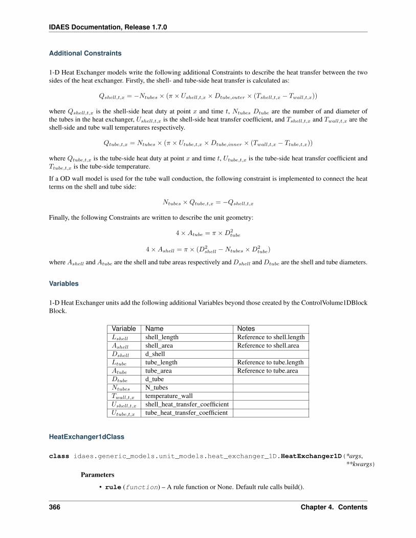
IDAES Documentation, Release 1.7.0
Additional Constraints
1-D Heat Exchanger models write the following additional Constraints to describe the heat transfer between the twosides of the heat exchanger. Firstly, the shell- and tube-side heat transfer is calculated as:
𝑄𝑠ℎ𝑒𝑙𝑙,𝑡,𝑥 = −𝑁𝑡𝑢𝑏𝑒𝑠 × (𝜋 × 𝑈𝑠ℎ𝑒𝑙𝑙,𝑡,𝑥 ×𝐷𝑡𝑢𝑏𝑒,𝑜𝑢𝑡𝑒𝑟 × (𝑇𝑠ℎ𝑒𝑙𝑙,𝑡,𝑥 − 𝑇𝑤𝑎𝑙𝑙,𝑡,𝑥))
where 𝑄𝑠ℎ𝑒𝑙𝑙,𝑡,𝑥 is the shell-side heat duty at point 𝑥 and time 𝑡, 𝑁𝑡𝑢𝑏𝑒𝑠 𝐷𝑡𝑢𝑏𝑒 are the number of and diameter ofthe tubes in the heat exchanger, 𝑈𝑠ℎ𝑒𝑙𝑙,𝑡,𝑥 is the shell-side heat transfer coefficient, and 𝑇𝑠ℎ𝑒𝑙𝑙,𝑡,𝑥 and 𝑇𝑤𝑎𝑙𝑙,𝑡,𝑥 are theshell-side and tube wall temperatures respectively.
𝑄𝑡𝑢𝑏𝑒,𝑡,𝑥 = 𝑁𝑡𝑢𝑏𝑒𝑠 × (𝜋 × 𝑈𝑡𝑢𝑏𝑒,𝑡,𝑥 ×𝐷𝑡𝑢𝑏𝑒,𝑖𝑛𝑛𝑒𝑟 × (𝑇𝑤𝑎𝑙𝑙,𝑡,𝑥 − 𝑇𝑡𝑢𝑏𝑒,𝑡,𝑥))
where 𝑄𝑡𝑢𝑏𝑒,𝑡,𝑥 is the tube-side heat duty at point 𝑥 and time 𝑡, 𝑈𝑡𝑢𝑏𝑒,𝑡,𝑥 is the tube-side heat transfer coefficient and𝑇𝑡𝑢𝑏𝑒,𝑡,𝑥 is the tube-side temperature.
If a OD wall model is used for the tube wall conduction, the following constraint is implemented to connect the heatterms on the shell and tube side:
𝑁𝑡𝑢𝑏𝑒𝑠 ×𝑄𝑡𝑢𝑏𝑒,𝑡,𝑥 = −𝑄𝑠ℎ𝑒𝑙𝑙,𝑡,𝑥
Finally, the following Constraints are written to describe the unit geometry:
4 ×𝐴𝑡𝑢𝑏𝑒 = 𝜋 ×𝐷2𝑡𝑢𝑏𝑒
4 ×𝐴𝑠ℎ𝑒𝑙𝑙 = 𝜋 × (𝐷2𝑠ℎ𝑒𝑙𝑙 −𝑁𝑡𝑢𝑏𝑒𝑠 ×𝐷2
𝑡𝑢𝑏𝑒)
where𝐴𝑠ℎ𝑒𝑙𝑙 and𝐴𝑡𝑢𝑏𝑒 are the shell and tube areas respectively and𝐷𝑠ℎ𝑒𝑙𝑙 and𝐷𝑡𝑢𝑏𝑒 are the shell and tube diameters.
Variables
1-D Heat Exchanger units add the following additional Variables beyond those created by the ControlVolume1DBlockBlock.
Variable Name Notes𝐿𝑠ℎ𝑒𝑙𝑙 shell_length Reference to shell.length𝐴𝑠ℎ𝑒𝑙𝑙 shell_area Reference to shell.area𝐷𝑠ℎ𝑒𝑙𝑙 d_shell𝐿𝑡𝑢𝑏𝑒 tube_length Reference to tube.length𝐴𝑡𝑢𝑏𝑒 tube_area Reference to tube.area𝐷𝑡𝑢𝑏𝑒 d_tube𝑁𝑡𝑢𝑏𝑒𝑠 N_tubes𝑇𝑤𝑎𝑙𝑙,𝑡,𝑥 temperature_wall𝑈𝑠ℎ𝑒𝑙𝑙,𝑡,𝑥 shell_heat_transfer_coefficient𝑈𝑡𝑢𝑏𝑒,𝑡,𝑥 tube_heat_transfer_coefficient
HeatExchanger1dClass
class idaes.generic_models.unit_models.heat_exchanger_1D.HeatExchanger1D(*args,**kwargs)
Parameters
• rule (function) – A rule function or None. Default rule calls build().
366 Chapter 4. Contents
IDAES Documentation, Release 1.7.0
• concrete (bool) – If True, make this a toplevel model. Default - False.
• ctype (str) – Pyomo ctype of the block. Default - “Block”
• default (dict) – Default ProcessBlockData config
Keys
dynamic Indicates whether this model will be dynamic or not, default = useDefault.Valid values: useDefault - get flag from parent (default = False), True - set as adynamic model, False - set as a steady-state model.
has_holdup Indicates whether holdup terms should be constructed or not. Must be Trueif dynamic = True, default - False. Valid values: useDefault - get flag from parent(default = False), True - construct holdup terms, False - do not construct holdup terms
shell_side shell side config arguments
dynamic Indicates whether this model will be dynamic or not, default = useDefault.Valid values: useDefault - get flag from parent (default = False), True - set as adynamic model, False - set as a steady-state model.
has_holdup Indicates whether holdup terms should be constructed or not. Must beTrue if dynamic = True, default - False. Valid values: useDefault - get flag fromparent (default = False), True - construct holdup terms, False - do not constructholdup terms
material_balance_type Indicates what type of mass balance should be con-structed, default - MaterialBalanceType.useDefault. Valid values: Ma-terialBalanceType.useDefault - refer to property package for default bal-ance type **MaterialBalanceType.none - exclude material balances, Material-BalanceType.componentPhase - use phase component balances, MaterialBal-anceType.componentTotal - use total component balances, MaterialBalance-Type.elementTotal - use total element balances, MaterialBalanceType.total - usetotal material balance.
energy_balance_type Indicates what type of energy balance should be constructed,default - EnergyBalanceType.useDefault. Valid values: EnergyBalance-Type.useDefault - refer to property package for default balance type **Energy-BalanceType.none - exclude energy balances, EnergyBalanceType.enthalpyTotal- single enthalpy balance for material, EnergyBalanceType.enthalpyPhase - en-thalpy balances for each phase, EnergyBalanceType.energyTotal - single energybalance for material, EnergyBalanceType.energyPhase - energy balances for eachphase.
momentum_balance_type Indicates what type of momentum balance should be con-structed, default - MomentumBalanceType.pressureTotal. Valid values: Mo-mentumBalanceType.none - exclude momentum balances, MomentumBalance-Type.pressureTotal - single pressure balance for material, MomentumBalance-Type.pressurePhase - pressure balances for each phase, MomentumBalance-Type.momentumTotal - single momentum balance for material, MomentumBal-anceType.momentumPhase - momentum balances for each phase.
has_pressure_change Indicates whether terms for pressure change should be con-structed, default - False. Valid values: True - include pressure change terms,False - exclude pressure change terms.
has_phase_equilibrium Argument to enable phase equilibrium on the shell side. -True - include phase equilibrium term - False - do not include phase equilibriumterm
4.5. Technical Specifications 367
IDAES Documentation, Release 1.7.0
property_package Property parameter object used to define property calculations (de-fault = ‘use_parent_value’) - ‘use_parent_value’ - get package from parent (default= None) - a ParameterBlock object
property_package_args A dict of arguments to be passed to the Property-BlockData and used when constructing these (default = ‘use_parent_value’) -‘use_parent_value’ - get package from parent (default = None) - a dict (see prop-erty package for documentation)
transformation_method Discretization method to use for DAE transformation. SeePyomo documentation for supported transformations.
transformation_scheme Discretization scheme to use when transformating domain.See Pyomo documentation for supported schemes.
tube_side tube side config arguments
dynamic Indicates whether this model will be dynamic or not, default = useDefault.Valid values: useDefault - get flag from parent (default = False), True - set as adynamic model, False - set as a steady-state model.
has_holdup Indicates whether holdup terms should be constructed or not. Must beTrue if dynamic = True, default - False. Valid values: useDefault - get flag fromparent (default = False), True - construct holdup terms, False - do not constructholdup terms
material_balance_type Indicates what type of mass balance should be con-structed, default - MaterialBalanceType.useDefault. Valid values: Ma-terialBalanceType.useDefault - refer to property package for default bal-ance type **MaterialBalanceType.none - exclude material balances, Material-BalanceType.componentPhase - use phase component balances, MaterialBal-anceType.componentTotal - use total component balances, MaterialBalance-Type.elementTotal - use total element balances, MaterialBalanceType.total - usetotal material balance.
energy_balance_type Indicates what type of energy balance should be constructed,default - EnergyBalanceType.useDefault. Valid values: EnergyBalance-Type.useDefault - refer to property package for default balance type **Energy-BalanceType.none - exclude energy balances, EnergyBalanceType.enthalpyTotal- single enthalpy balance for material, EnergyBalanceType.enthalpyPhase - en-thalpy balances for each phase, EnergyBalanceType.energyTotal - single energybalance for material, EnergyBalanceType.energyPhase - energy balances for eachphase.
momentum_balance_type Indicates what type of momentum balance should be con-structed, default - MomentumBalanceType.pressureTotal. Valid values: Mo-mentumBalanceType.none - exclude momentum balances, MomentumBalance-Type.pressureTotal - single pressure balance for material, MomentumBalance-Type.pressurePhase - pressure balances for each phase, MomentumBalance-Type.momentumTotal - single momentum balance for material, MomentumBal-anceType.momentumPhase - momentum balances for each phase.
has_pressure_change Indicates whether terms for pressure change should be con-structed, default - False. Valid values: True - include pressure change terms,False - exclude pressure change terms.
has_phase_equilibrium Argument to enable phase equilibrium on the shell side. -True - include phase equilibrium term - False - do not include phase equilibriumterm
368 Chapter 4. Contents
IDAES Documentation, Release 1.7.0
property_package Property parameter object used to define property calculations (de-fault = ‘use_parent_value’) - ‘use_parent_value’ - get package from parent (default= None) - a ParameterBlock object
property_package_args A dict of arguments to be passed to the Property-BlockData and used when constructing these (default = ‘use_parent_value’) -‘use_parent_value’ - get package from parent (default = None) - a dict (see prop-erty package for documentation)
transformation_method Discretization method to use for DAE transformation. SeePyomo documentation for supported transformations.
transformation_scheme Discretization scheme to use when transformating domain.See Pyomo documentation for supported schemes.
finite_elements Number of finite elements to use when discretizing length domain (de-fault=20)
collocation_points Number of collocation points to use per finite element when dis-cretizing length domain (default=3)
flow_type Flow configuration of heat exchanger - HeatExchangerFlowPattern.cocurrent:shell and tube flows from 0 to 1 (default) - HeatExchangerFlowPattern.countercurrent:shell side flows from 0 to 1 tube side flows from 1 to 0
has_wall_conduction Argument to enable type of wall heat conduction model. -WallConductionType.zero_dimensional - 0D wall model (default), - WallConduction-Type.one_dimensional - 1D wall model along the thickness of the tube, - WallCon-ductionType.two_dimensional - 2D wall model along the lenghth and thickness of thetube
• initialize (dict) – ProcessBlockData config for individual elements. Keys are Block-Data indexes and values are dictionaries described under the “default” argument above.
• idx_map (function) – Function to take the index of a BlockData element and return theindex in the initialize dict from which to read arguments. This can be provided to overidethe default behavior of matching the BlockData index exactly to the index in initialize.
Returns (HeatExchanger1D) New instance
HeatExchanger1dDataClass
class idaes.generic_models.unit_models.heat_exchanger_1D.HeatExchanger1DData(component)Standard Heat Exchanger 1D Unit Model Class.
build()Begin building model (pre-DAE transformation).
Parameters None –
Returns None
initialize(shell_state_args=None, tube_state_args=None, outlvl=0, solver=’ipopt’, optarg=’tol’:1e-06)
Initialization routine for the unit (default solver ipopt).
Keyword Arguments
• state_args – a dict of arguments to be passed to the property package(s) to provide aninitial state for initialization (see documentation of the specific property package) (default= ).
4.5. Technical Specifications 369
IDAES Documentation, Release 1.7.0
• outlvl – sets output level of initialization routine
• optarg – solver options dictionary object (default=‘tol’: 1e-6)
• solver – str indicating whcih solver to use during initialization (default = ‘ipopt’)
Returns None
Mixer
The IDAES Mixer unit model represents operations where multiple streams of material are combined into a singleflow. The Mixer class can be used to create either a stand-alone mixer unit, or as part of a unit model where multiplestreams need to be mixed.
Degrees of Freedom
Mixer units have zero degrees of freedom.
Model Structure
The IDAES Mixer unit model does not use ControlVolumes, and instead writes a set of material, energy and momentumbalances to combine the inlet streams into a single mixed stream. Mixer models have a user-defined number of inletPorts (by default named inlet_1, inlet_2, etc.) and one outlet Port (named outlet).
Mixed State Block
If a mixed state block is provided in the construction arguments, the Mixer model will use this as the StateBlock for themixed stream in the resulting balance equations. This allows a Mixer unit to be used as part of a larger unit operationby linking multiple inlet streams to a single existing StateBlock.
Variables
Mixer units have the following variables (𝑖 indicates index by inlet):
Variable Name Sym-bol
Notes
phase_equilibrium_generation 𝑋𝑒𝑞,𝑡,𝑟 Only if has_phase_equilibrium = True, Generation term for phase equi-librium
minimum_pressure 𝑃𝑚𝑖𝑛,𝑡,𝑖 Only if momentum_mixing_type = MomemntumMixingType.minimize
Parameters
Mixer units have the following parameters:
VariableName
Sym-bol
Notes
eps_pressure 𝜖 Only if momentum_mixing_type = MomemntumMixingType.minimize, smooth mini-mum parameter
370 Chapter 4. Contents
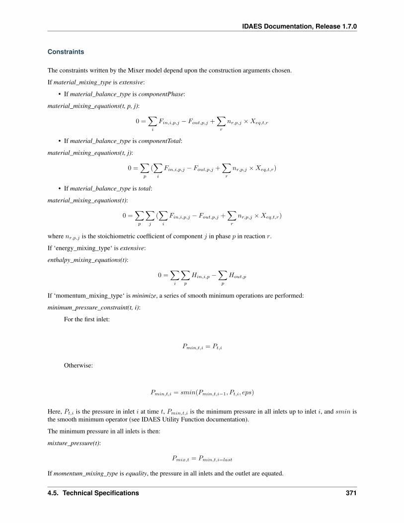
IDAES Documentation, Release 1.7.0
Constraints
The constraints written by the Mixer model depend upon the construction arguments chosen.
If material_mixing_type is extensive:
• If material_balance_type is componentPhase:
material_mixing_equations(t, p, j):
0 =∑𝑖
𝐹𝑖𝑛,𝑖,𝑝,𝑗 − 𝐹𝑜𝑢𝑡,𝑝,𝑗 +∑𝑟
𝑛𝑟,𝑝,𝑗 ×𝑋𝑒𝑞,𝑡,𝑟
• If material_balance_type is componentTotal:
material_mixing_equations(t, j):
0 =∑𝑝
(∑𝑖
𝐹𝑖𝑛,𝑖,𝑝,𝑗 − 𝐹𝑜𝑢𝑡,𝑝,𝑗 +∑𝑟
𝑛𝑟,𝑝,𝑗 ×𝑋𝑒𝑞,𝑡,𝑟)
• If material_balance_type is total:
material_mixing_equations(t):
0 =∑𝑝
∑𝑗
(∑𝑖
𝐹𝑖𝑛,𝑖,𝑝,𝑗 − 𝐹𝑜𝑢𝑡,𝑝,𝑗 +∑𝑟
𝑛𝑟,𝑝,𝑗 ×𝑋𝑒𝑞,𝑡,𝑟)
where 𝑛𝑟,𝑝,𝑗 is the stoichiometric coefficient of component 𝑗 in phase 𝑝 in reaction 𝑟.
If ‘energy_mixing_type‘ is extensive:
enthalpy_mixing_equations(t):
0 =∑𝑖
∑𝑝
𝐻𝑖𝑛,𝑖,𝑝 −∑𝑝
𝐻𝑜𝑢𝑡,𝑝
If ‘momentum_mixing_type‘ is minimize, a series of smooth minimum operations are performed:
minimum_pressure_constraint(t, i):
For the first inlet:
𝑃𝑚𝑖𝑛,𝑡,𝑖 = 𝑃𝑡,𝑖
Otherwise:
𝑃𝑚𝑖𝑛,𝑡,𝑖 = 𝑠𝑚𝑖𝑛(𝑃𝑚𝑖𝑛,𝑡,𝑖−1, 𝑃𝑡,𝑖, 𝑒𝑝𝑠)
Here, 𝑃𝑡,𝑖 is the pressure in inlet 𝑖 at time 𝑡, 𝑃𝑚𝑖𝑛,𝑡,𝑖 is the minimum pressure in all inlets up to inlet 𝑖, and 𝑠𝑚𝑖𝑛 isthe smooth minimum operator (see IDAES Utility Function documentation).
The minimum pressure in all inlets is then:
mixture_pressure(t):
𝑃𝑚𝑖𝑥,𝑡 = 𝑃𝑚𝑖𝑛,𝑡,𝑖=𝑙𝑎𝑠𝑡
If momentum_mixing_type is equality, the pressure in all inlets and the outlet are equated.
4.5. Technical Specifications 371
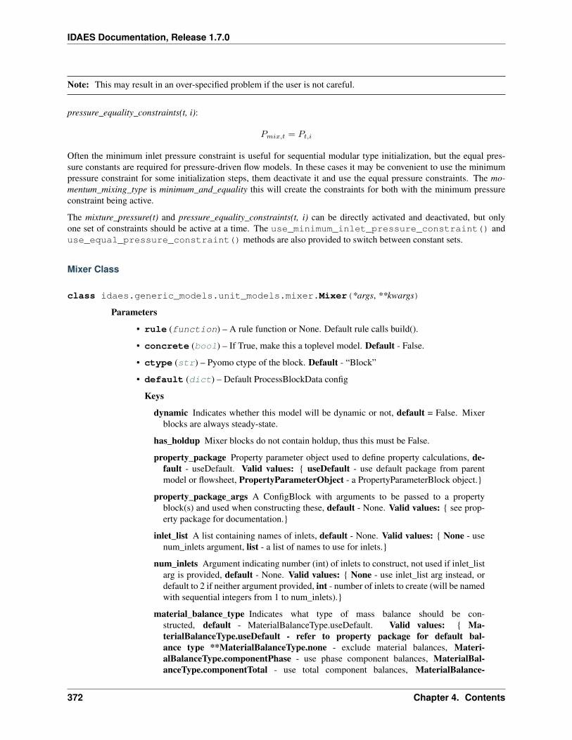
IDAES Documentation, Release 1.7.0
Note: This may result in an over-specified problem if the user is not careful.
pressure_equality_constraints(t, i):
𝑃𝑚𝑖𝑥,𝑡 = 𝑃𝑡,𝑖
Often the minimum inlet pressure constraint is useful for sequential modular type initialization, but the equal pres-sure constants are required for pressure-driven flow models. In these cases it may be convenient to use the minimumpressure constraint for some initialization steps, them deactivate it and use the equal pressure constraints. The mo-mentum_mixing_type is minimum_and_equality this will create the constraints for both with the minimum pressureconstraint being active.
The mixture_pressure(t) and pressure_equality_constraints(t, i) can be directly activated and deactivated, but onlyone set of constraints should be active at a time. The use_minimum_inlet_pressure_constraint() anduse_equal_pressure_constraint() methods are also provided to switch between constant sets.
Mixer Class
class idaes.generic_models.unit_models.mixer.Mixer(*args, **kwargs)
Parameters
• rule (function) – A rule function or None. Default rule calls build().
• concrete (bool) – If True, make this a toplevel model. Default - False.
• ctype (str) – Pyomo ctype of the block. Default - “Block”
• default (dict) – Default ProcessBlockData config
Keys
dynamic Indicates whether this model will be dynamic or not, default = False. Mixerblocks are always steady-state.
has_holdup Mixer blocks do not contain holdup, thus this must be False.
property_package Property parameter object used to define property calculations, de-fault - useDefault. Valid values: useDefault - use default package from parentmodel or flowsheet, PropertyParameterObject - a PropertyParameterBlock object.
property_package_args A ConfigBlock with arguments to be passed to a propertyblock(s) and used when constructing these, default - None. Valid values: see prop-erty package for documentation.
inlet_list A list containing names of inlets, default - None. Valid values: None - usenum_inlets argument, list - a list of names to use for inlets.
num_inlets Argument indicating number (int) of inlets to construct, not used if inlet_listarg is provided, default - None. Valid values: None - use inlet_list arg instead, ordefault to 2 if neither argument provided, int - number of inlets to create (will be namedwith sequential integers from 1 to num_inlets).
material_balance_type Indicates what type of mass balance should be con-structed, default - MaterialBalanceType.useDefault. Valid values: Ma-terialBalanceType.useDefault - refer to property package for default bal-ance type **MaterialBalanceType.none - exclude material balances, Materi-alBalanceType.componentPhase - use phase component balances, MaterialBal-anceType.componentTotal - use total component balances, MaterialBalance-
372 Chapter 4. Contents
IDAES Documentation, Release 1.7.0
Type.elementTotal - use total element balances, MaterialBalanceType.total - usetotal material balance.
has_phase_equilibrium Argument indicating whether phase equilibrium should be cal-culated for the resulting mixed stream, default - False. Valid values: True - calcu-late phase equilibrium in mixed stream, False - do not calculate equilibrium in mixedstream.
energy_mixing_type Argument indicating what method to use when mixing energyflows of incoming streams, default - MixingType.extensive. Valid values: Mix-ingType.none - do not include energy mixing equations, MixingType.extensive - mixtotal enthalpy flows of each phase.
momentum_mixing_type Argument indicating what method to use when mixing mo-mentum/ pressure of incoming streams, default - MomentumMixingType.minimize.Valid values: MomentumMixingType.none - do not include momentum mixingequations, MomentumMixingType.minimize - mixed stream has pressure equal tothe minimimum pressure of the incoming streams (uses smoothMin operator), Mo-mentumMixingType.equality - enforces equality of pressure in mixed and all incom-ing streams., MomentumMixingType.minimize_and_equality - add constraints forpressure equal to the minimum pressure of the inlets and constraints for equality ofpressure in mixed and all incoming streams. When the model is initially built, theequality constraints are deactivated. This option is useful for switching between flowand pressure driven simulations.
mixed_state_block An existing state block to use as the outlet stream from the Mixerblock, default - None. Valid values: None - create a new StateBlock for the mixedstream, StateBlock - a StateBock to use as the destination for the mixed stream.
construct_ports Argument indicating whether model should construct Port objectslinked to all inlet states and the mixed state, default - True. Valid values: True- construct Ports for all states, False - do not construct Ports.
• initialize (dict) – ProcessBlockData config for individual elements. Keys are Block-Data indexes and values are dictionaries described under the “default” argument above.
• idx_map (function) – Function to take the index of a BlockData element and return theindex in the initialize dict from which to read arguments. This can be provided to overidethe default behavior of matching the BlockData index exactly to the index in initialize.
Returns (Mixer) New instance
MixerData Class
class idaes.generic_models.unit_models.mixer.MixerData(component)This is a general purpose model for a Mixer block with the IDAES modeling framework. This block can be usedeither as a stand-alone Mixer unit operation, or as a sub-model within another unit operation.
This model creates a number of StateBlocks to represent the incoming streams, then writes a set of phase-component material balances, an overall enthalpy balance and a momentum balance (2 options) linked to amixed-state StateBlock. The mixed-state StateBlock can either be specified by the user (allowing use as asub-model), or created by the Mixer.
When being used as a sub-model, Mixer should only be used when a set of new StateBlocks are required for thestreams to be mixed. It should not be used to mix streams from mutiple ControlVolumes in a single unit model- in these cases the unit model developer should write their own mixing equations.
4.5. Technical Specifications 373
IDAES Documentation, Release 1.7.0
add_energy_mixing_equations(inlet_blocks, mixed_block)Add energy mixing equations (total enthalpy balance).
add_inlet_state_blocks(inlet_list)Construct StateBlocks for all inlet streams.
Parameters of strings to use as StateBlock names (list) –
Returns list of StateBlocks
add_material_mixing_equations(inlet_blocks, mixed_block, mb_type)Add material mixing equations.
add_mixed_state_block()Constructs StateBlock to represent mixed stream.
Returns New StateBlock object
add_port_objects(inlet_list, inlet_blocks, mixed_block)Adds Port objects if required.
Parameters
• list of inlet StateBlock objects (a) –
• mixed state StateBlock object (a) –
Returns None
add_pressure_equality_equations(inlet_blocks, mixed_block)Add pressure equality equations. Note that this writes a number of constraints equal to the number ofinlets, enforcing equality between all inlets and the mixed stream.
add_pressure_minimization_equations(inlet_blocks, mixed_block)Add pressure minimization equations. This is done by sequential comparisons of each inlet to the minimumpressure so far, using the IDAES smooth minimum fuction.
build()General build method for MixerData. This method calls a number of sub-methods which automate theconstruction of expected attributes of unit models.
Inheriting models should call super().build.
Parameters None –
Returns None
create_inlet_list()Create list of inlet stream names based on config arguments.
Returns list of strings
get_mixed_state_block()Validates StateBlock provided in user arguments for mixed stream.
Returns The user-provided StateBlock or an Exception
initialize(outlvl=6, optarg=, solver=’ipopt’, hold_state=False)Initialization routine for mixer (default solver ipopt)
Keyword Arguments
• outlvl – sets output level of initialization routine
• optarg – solver options dictionary object (default=)
• solver – str indicating whcih solver to use during initialization (default = ‘ipopt’)
374 Chapter 4. Contents
IDAES Documentation, Release 1.7.0
• hold_state – flag indicating whether the initialization routine should unfix any statevariables fixed during initialization, default - False. Valid values: True - states vari-ables are not unfixed, and a dict of returned containing flags for which states were fixedduring initialization, False - state variables are unfixed after initialization by calling therelease_state method.
Returns If hold_states is True, returns a dict containing flags for which states were fixed duringinitialization.
model_check()This method executes the model_check methods on the associated state blocks (if they exist). This methodis generally called by a unit model as part of the unit’s model_check method.
Parameters None –
Returns None
release_state(flags, outlvl=0)Method to release state variables fixed during initialization.
Keyword Arguments
• flags – dict containing information of which state variables were fixed during initializa-tion, and should now be unfixed. This dict is returned by initialize if hold_state = True.
• outlvl – sets output level of logging
Returns None
use_equal_pressure_constraint()Deactivate the mixer pressure = mimimum inlet pressure constraint and activate the mixer pressure andall inlet pressures are equal constraints. This should only be used when momentum_mixing_type ==MomentumMixingType.minimize_and_equality.
use_minimum_inlet_pressure_constraint()Activate the mixer pressure = mimimum inlet pressure constraint and deactivate the mixer pressure andall inlet pressures are equal constraints. This should only be used when momentum_mixing_type ==MomentumMixingType.minimize_and_equality.
Plug Flow Reactor
The IDAES Plug Flow Reactor (PFR) model represents a unit operation where a material stream passes through alinear reactor vessel whilst undergoing some chemical reaction(s). This model requires modeling the system in onespatial dimension.
Degrees of Freedom
PFRs generally have at least 2 degrees of freedom.
Typical fixed variables are:
• 2 of reactor length, area and volume.
Model Structure
The core PFR unit model consists of a single ControlVolume1DBlock (named control_volume) with one Inlet Port(named inlet) and one Outlet Port (named outlet).
4.5. Technical Specifications 375
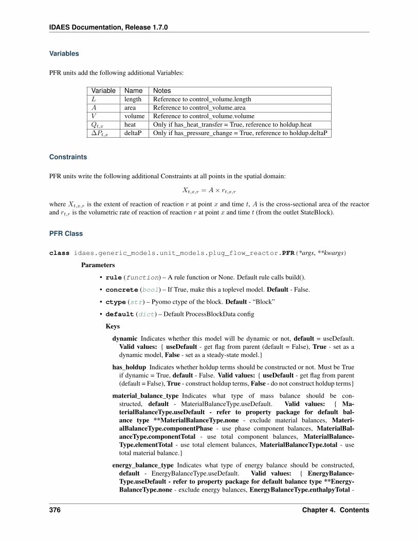
IDAES Documentation, Release 1.7.0
Variables
PFR units add the following additional Variables:
Variable Name Notes𝐿 length Reference to control_volume.length𝐴 area Reference to control_volume.area𝑉 volume Reference to control_volume.volume𝑄𝑡,𝑥 heat Only if has_heat_transfer = True, reference to holdup.heat∆𝑃𝑡,𝑥 deltaP Only if has_pressure_change = True, reference to holdup.deltaP
Constraints
PFR units write the following additional Constraints at all points in the spatial domain:
𝑋𝑡,𝑥,𝑟 = 𝐴× 𝑟𝑡,𝑥,𝑟
where 𝑋𝑡,𝑥,𝑟 is the extent of reaction of reaction 𝑟 at point 𝑥 and time 𝑡, 𝐴 is the cross-sectional area of the reactorand 𝑟𝑡,𝑟 is the volumetric rate of reaction of reaction 𝑟 at point 𝑥 and time 𝑡 (from the outlet StateBlock).
PFR Class
class idaes.generic_models.unit_models.plug_flow_reactor.PFR(*args, **kwargs)
Parameters
• rule (function) – A rule function or None. Default rule calls build().
• concrete (bool) – If True, make this a toplevel model. Default - False.
• ctype (str) – Pyomo ctype of the block. Default - “Block”
• default (dict) – Default ProcessBlockData config
Keys
dynamic Indicates whether this model will be dynamic or not, default = useDefault.Valid values: useDefault - get flag from parent (default = False), True - set as adynamic model, False - set as a steady-state model.
has_holdup Indicates whether holdup terms should be constructed or not. Must be Trueif dynamic = True, default - False. Valid values: useDefault - get flag from parent(default = False), True - construct holdup terms, False - do not construct holdup terms
material_balance_type Indicates what type of mass balance should be con-structed, default - MaterialBalanceType.useDefault. Valid values: Ma-terialBalanceType.useDefault - refer to property package for default bal-ance type **MaterialBalanceType.none - exclude material balances, Materi-alBalanceType.componentPhase - use phase component balances, MaterialBal-anceType.componentTotal - use total component balances, MaterialBalance-Type.elementTotal - use total element balances, MaterialBalanceType.total - usetotal material balance.
energy_balance_type Indicates what type of energy balance should be constructed,default - EnergyBalanceType.useDefault. Valid values: EnergyBalance-Type.useDefault - refer to property package for default balance type **Energy-BalanceType.none - exclude energy balances, EnergyBalanceType.enthalpyTotal -
376 Chapter 4. Contents
IDAES Documentation, Release 1.7.0
single enthalpy balance for material, EnergyBalanceType.enthalpyPhase - enthalpybalances for each phase, EnergyBalanceType.energyTotal - single energy balance formaterial, EnergyBalanceType.energyPhase - energy balances for each phase.
momentum_balance_type Indicates what type of momentum balance should be con-structed, default - MomentumBalanceType.pressureTotal. Valid values: Mo-mentumBalanceType.none - exclude momentum balances, MomentumBalance-Type.pressureTotal - single pressure balance for material, MomentumBalance-Type.pressurePhase - pressure balances for each phase, MomentumBalance-Type.momentumTotal - single momentum balance for material, MomentumBalance-Type.momentumPhase - momentum balances for each phase.
has_equilibrium_reactions Indicates whether terms for equilibrium controlled reac-tions should be constructed, default - True. Valid values: True - include equilibriumreaction terms, False - exclude equilibrium reaction terms.
has_phase_equilibrium Indicates whether terms for phase equilibrium should be con-structed, default = False. Valid values: True - include phase equilibrium termsFalse - exclude phase equilibrium terms.
has_heat_of_reaction Indicates whether terms for heat of reaction terms should be con-structed, default - False. Valid values: True - include heat of reaction terms, False- exclude heat of reaction terms.
has_heat_transfer Indicates whether terms for heat transfer should be constructed, de-fault - False. Valid values: True - include heat transfer terms, False - exclude heattransfer terms.
has_pressure_change Indicates whether terms for pressure change should be con-structed, default - False. Valid values: True - include pressure change terms, False- exclude pressure change terms.
property_package Property parameter object used to define property calculations, de-fault - useDefault. Valid values: useDefault - use default package from parentmodel or flowsheet, PropertyParameterObject - a PropertyParameterBlock object.
property_package_args A ConfigBlock with arguments to be passed to a propertyblock(s) and used when constructing these, default - None. Valid values: see prop-erty package for documentation.
reaction_package Reaction parameter object used to define reaction calculations, de-fault - None. Valid values: None - no reaction package, ReactionParameterBlock- a ReactionParameterBlock object.
reaction_package_args A ConfigBlock with arguments to be passed to a reactionblock(s) and used when constructing these, default - None. Valid values: see re-action package for documentation.
length_domain_set A list of values to be used when constructing the length domain ofthe reactor. Point must lie between 0.0 and 1.0, default - [0.0, 1.0]. Valid values: alist of floats
transformation_method Method to use to transform domain. Must be a method recog-nised by the Pyomo TransformationFactory, default - “dae.finite_difference”.
transformation_scheme Scheme to use when transformating domain. See Pyomo doc-umentation for supported schemes, default - “BACKWARD”.
finite_elements Number of finite elements to use when transforming length domain, de-fault - 20.
4.5. Technical Specifications 377
IDAES Documentation, Release 1.7.0
collocation_points Number of collocation points to use when transforming length do-main, default - 3.
• initialize (dict) – ProcessBlockData config for individual elements. Keys are Block-Data indexes and values are dictionaries described under the “default” argument above.
• idx_map (function) – Function to take the index of a BlockData element and return theindex in the initialize dict from which to read arguments. This can be provided to overidethe default behavior of matching the BlockData index exactly to the index in initialize.
Returns (PFR) New instance
PFRData Class
class idaes.generic_models.unit_models.plug_flow_reactor.PFRData(component)Standard Plug Flow Reactor Unit Model Class
build()Begin building model (pre-DAE transformation).
Parameters None –
Returns None
Pressure Changer
The IDAES Pressure Changer model represents a unit operation with a single stream of material which undergoes achange in pressure due to the application of a work. The Pressure Changer model contains support for a number ofdifferent thermodynamic assumptions regarding the working fluid.
Degrees of Freedom
Pressure Changer units generally have one or more degrees of freedom, depending on the thermodynamic assumptionused.
Typical fixed variables are:
• outlet pressure, 𝑃𝑟𝑎𝑡𝑖𝑜 or ∆𝑃 ,
• unit efficiency (isentropic or pump assumption).
Model Structure
The core Pressure Changer unit model consists of a single ControlVolume0D (named control_volume) withone Inlet Port (named inlet) and one Outlet Port (named outlet). Additionally, if an isentropic pressure changeris used, the unit model contains an additional StateBlock named properties_isentropic at the unit modellevel.
Variables
Pressure Changers contain the following Variables (not including those contained within the control volume Block):
378 Chapter 4. Contents
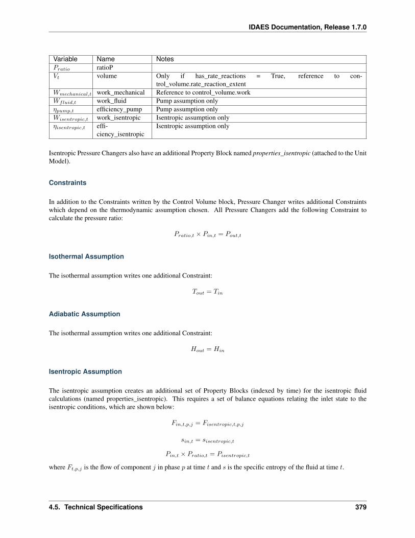
IDAES Documentation, Release 1.7.0
Variable Name Notes𝑃𝑟𝑎𝑡𝑖𝑜 ratioP𝑉𝑡 volume Only if has_rate_reactions = True, reference to con-
trol_volume.rate_reaction_extent𝑊𝑚𝑒𝑐ℎ𝑎𝑛𝑖𝑐𝑎𝑙,𝑡 work_mechanical Reference to control_volume.work𝑊𝑓𝑙𝑢𝑖𝑑,𝑡 work_fluid Pump assumption only𝜂𝑝𝑢𝑚𝑝,𝑡 efficiency_pump Pump assumption only𝑊𝑖𝑠𝑒𝑛𝑡𝑟𝑜𝑝𝑖𝑐,𝑡 work_isentropic Isentropic assumption only𝜂𝑖𝑠𝑒𝑛𝑡𝑟𝑜𝑝𝑖𝑐,𝑡 effi-
ciency_isentropicIsentropic assumption only
Isentropic Pressure Changers also have an additional Property Block named properties_isentropic (attached to the UnitModel).
Constraints
In addition to the Constraints written by the Control Volume block, Pressure Changer writes additional Constraintswhich depend on the thermodynamic assumption chosen. All Pressure Changers add the following Constraint tocalculate the pressure ratio:
𝑃𝑟𝑎𝑡𝑖𝑜,𝑡 × 𝑃𝑖𝑛,𝑡 = 𝑃𝑜𝑢𝑡,𝑡
Isothermal Assumption
The isothermal assumption writes one additional Constraint:
𝑇𝑜𝑢𝑡 = 𝑇𝑖𝑛
Adiabatic Assumption
The isothermal assumption writes one additional Constraint:
𝐻𝑜𝑢𝑡 = 𝐻𝑖𝑛
Isentropic Assumption
The isentropic assumption creates an additional set of Property Blocks (indexed by time) for the isentropic fluidcalculations (named properties_isentropic). This requires a set of balance equations relating the inlet state to theisentropic conditions, which are shown below:
𝐹𝑖𝑛,𝑡,𝑝,𝑗 = 𝐹𝑖𝑠𝑒𝑛𝑡𝑟𝑜𝑝𝑖𝑐,𝑡,𝑝,𝑗
𝑠𝑖𝑛,𝑡 = 𝑠𝑖𝑠𝑒𝑛𝑡𝑟𝑜𝑝𝑖𝑐,𝑡
𝑃𝑖𝑛,𝑡 × 𝑃𝑟𝑎𝑡𝑖𝑜,𝑡 = 𝑃𝑖𝑠𝑒𝑛𝑡𝑟𝑜𝑝𝑖𝑐,𝑡
where 𝐹𝑡,𝑝,𝑗 is the flow of component 𝑗 in phase 𝑝 at time 𝑡 and 𝑠 is the specific entropy of the fluid at time 𝑡.
4.5. Technical Specifications 379
IDAES Documentation, Release 1.7.0
Next, the isentropic work is calculated as follows:
𝑊𝑖𝑠𝑒𝑛𝑡𝑟𝑜𝑝𝑖𝑐,𝑡 =∑𝑝
𝐻𝑖𝑠𝑒𝑛𝑡𝑟𝑜𝑝𝑖𝑐,𝑡,𝑝 −∑𝑝
𝐻𝑖𝑛,𝑡,𝑝
where 𝐻𝑡,𝑝 is the total energy flow of phase 𝑝 at time 𝑡. Finally, a constraint which relates the fluid work to the actualmechanical work via an efficiency term 𝜂.
If compressor is True, 𝑊𝑖𝑠𝑒𝑛𝑡𝑟𝑜𝑝𝑖𝑐,𝑡 = 𝑊𝑚𝑒𝑐ℎ𝑎𝑛𝑖𝑐𝑎𝑙,𝑡 × 𝜂𝑡
If compressor is False, 𝑊𝑖𝑠𝑒𝑛𝑡𝑟𝑜𝑝𝑖𝑐,𝑡 × 𝜂𝑡 = 𝑊𝑚𝑒𝑐ℎ𝑎𝑛𝑖𝑐𝑎𝑙,𝑡
Pump (Incompressible Fluid) Assumption
The incompressible fluid assumption writes two additional constraints. Firstly, a Constraint is written which relatesfluid work to the pressure change of the fluid.
𝑊𝑓𝑙𝑢𝑖𝑑,𝑡 = (𝑃𝑜𝑢𝑡,𝑡 − 𝑃𝑖𝑛,𝑡) × 𝐹𝑣𝑜𝑙,𝑡
where 𝐹𝑣𝑜𝑙,𝑡 is the total volumetric flowrate of material at time 𝑡 (from the outlet Property Block). Secondly, aconstraint which relates the fluid work to the actual mechanical work via an efficiency term 𝜂.
If compressor is True, 𝑊𝑓𝑙𝑢𝑖𝑑,𝑡 = 𝑊𝑚𝑒𝑐ℎ𝑎𝑛𝑖𝑐𝑎𝑙,𝑡 × 𝜂𝑡
If compressor is False, 𝑊𝑓𝑙𝑢𝑖𝑑,𝑡 × 𝜂𝑡 = 𝑊𝑚𝑒𝑐ℎ𝑎𝑛𝑖𝑐𝑎𝑙,𝑡
PressureChanger Class
class idaes.generic_models.unit_models.pressure_changer.PressureChanger(*args,**kwargs)
Parameters
• rule (function) – A rule function or None. Default rule calls build().
• concrete (bool) – If True, make this a toplevel model. Default - False.
• ctype (str) – Pyomo ctype of the block. Default - “Block”
• default (dict) – Default ProcessBlockData config
Keys
dynamic Indicates whether this model will be dynamic or not, default = useDefault.Valid values: useDefault - get flag from parent (default = False), True - set as adynamic model, False - set as a steady-state model.
has_holdup Indicates whether holdup terms should be constructed or not. Must be Trueif dynamic = True, default - False. Valid values: useDefault - get flag from parent(default = False), True - construct holdup terms, False - do not construct holdup terms
material_balance_type Indicates what type of mass balance should be con-structed, default - MaterialBalanceType.useDefault. Valid values: Ma-terialBalanceType.useDefault - refer to property package for default bal-ance type **MaterialBalanceType.none - exclude material balances, Materi-alBalanceType.componentPhase - use phase component balances, MaterialBal-anceType.componentTotal - use total component balances, MaterialBalance-Type.elementTotal - use total element balances, MaterialBalanceType.total - usetotal material balance.
380 Chapter 4. Contents
IDAES Documentation, Release 1.7.0
energy_balance_type Indicates what type of energy balance should be constructed,default - EnergyBalanceType.useDefault. Valid values: EnergyBalance-Type.useDefault - refer to property package for default balance type **Energy-BalanceType.none - exclude energy balances, EnergyBalanceType.enthalpyTotal -single enthalpy balance for material, EnergyBalanceType.enthalpyPhase - enthalpybalances for each phase, EnergyBalanceType.energyTotal - single energy balance formaterial, EnergyBalanceType.energyPhase - energy balances for each phase.
momentum_balance_type Indicates what type of momentum balance should be con-structed, default - MomentumBalanceType.pressureTotal. Valid values: Mo-mentumBalanceType.none - exclude momentum balances, MomentumBalance-Type.pressureTotal - single pressure balance for material, MomentumBalance-Type.pressurePhase - pressure balances for each phase, MomentumBalance-Type.momentumTotal - single momentum balance for material, MomentumBalance-Type.momentumPhase - momentum balances for each phase.
has_phase_equilibrium Indicates whether terms for phase equilibrium should be con-structed, default = False. Valid values: True - include phase equilibrium termsFalse - exclude phase equilibrium terms.
compressor Indicates whether this unit should be considered a compressor (True (de-fault), pressure increase) or an expander (False, pressure decrease).
thermodynamic_assumption Flag to set the thermodynamic assumption to use forthe unit. - ThermodynamicAssumption.isothermal (default) - ThermodynamicAs-sumption.isentropic - ThermodynamicAssumption.pump - ThermodynamicAssump-tion.adiabatic
property_package Property parameter object used to define property calculations, de-fault - useDefault. Valid values: useDefault - use default package from parentmodel or flowsheet, PropertyParameterObject - a PropertyParameterBlock object.
property_package_args A ConfigBlock with arguments to be passed to a propertyblock(s) and used when constructing these, default - None. Valid values: see prop-erty package for documentation.
• initialize (dict) – ProcessBlockData config for individual elements. Keys are Block-Data indexes and values are dictionaries described under the “default” argument above.
• idx_map (function) – Function to take the index of a BlockData element and return theindex in the initialize dict from which to read arguments. This can be provided to overidethe default behavior of matching the BlockData index exactly to the index in initialize.
Returns (PressureChanger) New instance
PressureChangerData Class
class idaes.generic_models.unit_models.pressure_changer.PressureChangerData(component)Standard Compressor/Expander Unit Model Class
add_adiabatic()Add constraints for adiabatic assumption.
Parameters None –
Returns None
add_isentropic()Add constraints for isentropic assumption.
4.5. Technical Specifications 381
IDAES Documentation, Release 1.7.0
Parameters None –
Returns None
add_isothermal()Add constraints for isothermal assumption.
Parameters None –
Returns None
add_pump()Add constraints for the incompressible fluid assumption
Parameters None –
Returns None
build()
Parameters None –
Returns None
init_isentropic(state_args, outlvl, solver, optarg)Initialization routine for unit (default solver ipopt)
Keyword Arguments
• state_args – a dict of arguments to be passed to the property package(s) to provide aninitial state for initialization (see documentation of the specific property package) (default= ).
• outlvl – sets output level of initialization routine
• optarg – solver options dictionary object (default=‘tol’: 1e-6)
• solver – str indicating whcih solver to use during initialization (default = ‘ipopt’)
Returns None
initialize(state_args=None, routine=None, outlvl=0, solver=’ipopt’, optarg=’tol’: 1e-06)General wrapper for pressure changer initialization routines
Keyword Arguments
• routine – str stating which initialization routine to execute * None - use routine match-ing thermodynamic_assumption * ‘isentropic’ - use isentropic initialization routine *‘isothermal’ - use isothermal initialization routine
• state_args – a dict of arguments to be passed to the property package(s) to provide aninitial state for initialization (see documentation of the specific property package) (default= ).
• outlvl – sets output level of initialization routine
• optarg – solver options dictionary object (default=‘tol’: 1e-6)
• solver – str indicating whcih solver to use during initialization (default = ‘ipopt’)
Returns None
model_check()Check that pressure change matches with compressor argument (i.e. if compressor = True, pressure shouldincrease or work should be positive)
Parameters None –
382 Chapter 4. Contents
IDAES Documentation, Release 1.7.0
Returns None
Product Block
Product Blocks are used to represent sinks of material in Flowsheets. These can be used as a conventient way to markthe final destination of a material stream and to view the state of that material.
Degrees of Freedom
Product blocks generally have zero degrees of freedom.
Model Structure
Product Blocks consists of a single StateBlock (named properties), each with one Inlet Port (named inlet). ProductBlocks also contain References to the state variables defined within the StateBlock
Additional Constraints
Product Blocks write no additional constraints to the model.
Variables
Product blocks add no additional Variables.
Product Class
class idaes.generic_models.unit_models.product.Product(*args, **kwargs)
Parameters
• rule (function) – A rule function or None. Default rule calls build().
• concrete (bool) – If True, make this a toplevel model. Default - False.
• ctype (str) – Pyomo ctype of the block. Default - “Block”
• default (dict) – Default ProcessBlockData config
Keys
dynamic Indicates whether this model will be dynamic or not, default = False. Productblocks are always steady- state.
has_holdup Product blocks do not contain holdup, thus this must be False.
property_package Property parameter object used to define property calculations, de-fault - useDefault. Valid values: useDefault - use default package from parentmodel or flowsheet, PhysicalParameterObject - a PhysicalParameterBlock object.
property_package_args A ConfigBlock with arguments to be passed to a propertyblock(s) and used when constructing these, default - None. Valid values: see prop-erty package for documentation.
4.5. Technical Specifications 383
IDAES Documentation, Release 1.7.0
• initialize (dict) – ProcessBlockData config for individual elements. Keys are Block-Data indexes and values are dictionaries described under the “default” argument above.
• idx_map (function) – Function to take the index of a BlockData element and return theindex in the initialize dict from which to read arguments. This can be provided to overidethe default behavior of matching the BlockData index exactly to the index in initialize.
Returns (Product) New instance
ProductData Class
class idaes.generic_models.unit_models.product.ProductData(component)Standard Product Block Class
build()Begin building model.
Parameters None –
Returns None
initialize(state_args=, outlvl=0, solver=’ipopt’, optarg=’tol’: 1e-06)This method calls the initialization method of the state block.
Keyword Arguments
• state_args – a dict of arguments to be passed to the property package(s) to provide aninitial state for initialization (see documentation of the specific property package) (default= ).
• outlvl – sets output level of initialization routine
• optarg – solver options dictionary object (default=‘tol’: 1e-6)
• solver – str indicating which solver to use during initialization (default = ‘ipopt’)
Returns None
Pump
The Pump model is a PressureChanger, where the configuration is set so that the “compressor” option can only beTrue, and the default “thermodynamic_assumption” is “pump.” See the PressureChanger documentation for details.
Example
The example below demonstrates the basic Pump model usage:
import pyomo.environ as pyofrom idaes.core import FlowsheetBlockfrom idaes.generic_models.unit_models import Pumpfrom idaes.generic_models.properties import iapws95
m = pyo.ConcreteModel()m.fs = FlowsheetBlock(default="dynamic": False)m.fs.properties = iapws95.Iapws95ParameterBlock()m.fs.unit = Pump(default="property_package": m.fs.properties)
(continues on next page)
384 Chapter 4. Contents
IDAES Documentation, Release 1.7.0
(continued from previous page)
m.fs.unit.inlet.flow_mol[0].fix(100)m.fs.unit.inlet.enth_mol[0].fix(2000)m.fs.unit.inlet.pressure[0].fix(101325)
m.fs.unit.deltaP.fix(100000)m.fs.unit.efficiency_pump.fix(0.8)
Separator
The IDAES Separator unit model represents operations where a single stream is split into multiple flows. The Separatormodel supports separation using split fractions, or by ideal separation of flows. The Separator class can be used tocreate either a stand-alone separator unit, or as part of a unit model where a flow needs to be separated.
Degrees of Freedom
Separator units have a number of degrees of freedom based on the separation type chosen.
• If split_basis = ‘phaseFlow’, degrees of freedom are generally (𝑛𝑜.𝑜𝑢𝑡𝑙𝑒𝑡𝑠− 1) × 𝑛𝑜.𝑝ℎ𝑎𝑠𝑒𝑠
• If split_basis = ‘componentFlow’, degrees of freedom are generally (𝑛𝑜.𝑜𝑢𝑡𝑙𝑒𝑡𝑠− 1) × 𝑛𝑜.𝑐𝑜𝑚𝑝𝑜𝑛𝑒𝑛𝑡𝑠
• If split_basis = ‘phaseComponentFlow’, degrees of freedom are generally (𝑛𝑜.𝑜𝑢𝑡𝑙𝑒𝑡𝑠 − 1) × 𝑛𝑜.𝑝ℎ𝑎𝑠𝑒𝑠 ×𝑛𝑜.𝑐𝑜𝑚𝑝𝑜𝑛𝑒𝑛𝑡𝑠
• If split_basis = ‘totalFlow’, degrees of freedom are generally (𝑛𝑜.𝑜𝑢𝑡𝑙𝑒𝑡𝑠− 1)×𝑛𝑜.𝑝ℎ𝑎𝑠𝑒𝑠×𝑛𝑜.𝑐𝑜𝑚𝑝𝑜𝑛𝑒𝑛𝑡𝑠
Typical fixed variables are:
• split fractions.
Model Structure
The IDAES Separator unit model does not use ControlVolumes, and instead writes a set of material, energy andmomentum balances to split the inlet stream into a number of outlet streams. Separator models have a single inlet Port(named inlet) and a user-defined number of outlet Ports (by default named outlet_1, outlet_2, etc.).
Mixed State Block
If a mixed state block is provided in the construction arguments, the Mixer model will use this as the StateBlock for themixed stream in the resulting balance equations. This allows a Mixer unit to be used as part of a larger unit operationby linking to an existing StateBlock.
Ideal Separation
The IDAES Separator model supports ideal separations, where all of a given subset of the mixed stream is sent to asingle outlet (i.e. split fractions are equal to zero or one). In these cases, no Constraints are necessary for performingthe separation, as the mixed stream states can be directly partitioned to the outlets.
Ideal separations will not work for all choices of state variables, and thus will not work for all property packages. Touse ideal separations, the user must provide a map of what part of the mixed flow should be partitioned to each outlet.The ideal_split_map should be a dict-like object with keys as tuples matching the split_basis argument and valuesindicating which outlet this subset should be partitioned to.
4.5. Technical Specifications 385
IDAES Documentation, Release 1.7.0
Variables
Separator units have the following variables (𝑜 indicates index by outlet):
Variable Name Symbol Notessplit_fraction 𝜑𝑡,𝑜,* Indexing sets depend upon split_basis
Constraints
Separator units have the following Constraints, unless ideal_separation is True.
• If material_balance_type is componentPhase:
material_splitting_eqn(t, o, p, j):
𝐹𝑖𝑛,𝑡,𝑝,𝑗 = 𝜑𝑡,𝑝,* × 𝐹𝑡,𝑜,𝑝,𝑗
• If material_balance_type is componentTotal:
material_splitting_eqn(t, o, j): ∑𝑝
𝐹𝑖𝑛,𝑡,𝑝,𝑗 =∑𝑝
𝜑𝑡,𝑝,* × 𝐹𝑡,𝑜,𝑝,𝑗
• If material_balance_type is total:
material_splitting_eqn(t, o): ∑𝑝
∑𝑗
𝐹𝑖𝑛,𝑡,𝑝,𝑗 =∑𝑝
∑𝑗
𝜑𝑡,𝑝,* × 𝐹𝑡,𝑜,𝑝,𝑗
If energy_split_basis is equal_temperature:
temperature_equality_eqn(t, o):
𝑇𝑖𝑛,𝑡 = 𝑇𝑡,𝑜
If energy_split_basis is equal_molar_enthalpy:
molar_enthalpy_equality_eqn(t, o):
ℎ𝑖𝑛,𝑡 = ℎ𝑡,𝑜
If energy_split_basis is enthalpy_split:
molar_enthalpy_splitting_eqn(t, o):
𝑠𝑢𝑚𝑝ℎ𝑖𝑛,𝑡,𝑝 * 𝑠𝑓𝑡,𝑜,𝑝 = 𝑠𝑢𝑚𝑝ℎ𝑡,𝑜,𝑝
pressure_equality_eqn(t, o):
𝑃𝑖𝑛,𝑡 = 𝑃𝑡,𝑜
386 Chapter 4. Contents
IDAES Documentation, Release 1.7.0
Separator Class
class idaes.generic_models.unit_models.separator.Separator(*args, **kwargs)
Parameters
• rule (function) – A rule function or None. Default rule calls build().
• concrete (bool) – If True, make this a toplevel model. Default - False.
• ctype (str) – Pyomo ctype of the block. Default - “Block”
• default (dict) – Default ProcessBlockData config
Keys
dynamic Indicates whether this model will be dynamic or not, default = False. Productblocks are always steady- state.
has_holdup Product blocks do not contain holdup, thus this must be False.
property_package Property parameter object used to define property calculations, de-fault - useDefault. Valid values: useDefault - use default package from parentmodel or flowsheet, PropertyParameterObject - a PropertyParameterBlock object.
property_package_args A ConfigBlock with arguments to be passed to a propertyblock(s) and used when constructing these, default - None. Valid values: see prop-erty package for documentation.
outlet_list A list containing names of outlets, default - None. Valid values: None -use num_outlets argument, list - a list of names to use for outlets.
num_outlets Argument indicating number (int) of outlets to construct, not used if out-let_list arg is provided, default - None. Valid values: None - use outlet_list arginstead, or default to 2 if neither argument provided, int - number of outlets to create(will be named with sequential integers from 1 to num_outlets).
split_basis Argument indicating basis to use for splitting mixed stream, default - Split-tingType.totalFlow. Valid values: SplittingType.totalFlow - split based on totalflow (split fraction indexed only by time and outlet), SplittingType.phaseFlow - splitbased on phase flows (split fraction indexed by time, outlet and phase), Splitting-Type.componentFlow - split based on component flows (split fraction indexed by time,outlet and components), SplittingType.phaseComponentFlow - split based on phase-component flows ( split fraction indexed by both time, outlet, phase and components).
material_balance_type Indicates what type of mass balance should be con-structed, default - MaterialBalanceType.useDefault. Valid values: Ma-terialBalanceType.useDefault - refer to property package for default bal-ance type **MaterialBalanceType.none - exclude material balances, Materi-alBalanceType.componentPhase - use phase component balances, MaterialBal-anceType.componentTotal - use total component balances, MaterialBalance-Type.elementTotal - use total element balances, MaterialBalanceType.total - usetotal material balance.
has_phase_equilibrium Argument indicating whether phase equilibrium should be cal-culated for the resulting mixed stream, default - False. Valid values: True - calcu-late phase equilibrium in mixed stream, False - do not calculate equilibrium in mixedstream.
energy_split_basis Argument indicating basis to use for splitting energy this is not usedfor when ideal_separation == True. default - EnergySplittingType.equal_temperature.Valid values: EnergySplittingType.equal_temperature - outlet temperatures equal
4.5. Technical Specifications 387
IDAES Documentation, Release 1.7.0
inlet EnergySplittingType.equal_molar_enthalpy - oulet molar enthalpies equal in-let, EnergySplittingType.enthalpy_split - apply split fractions to enthalpy flows.Does not work with component or phase-component splitting.
ideal_separation Argument indicating whether ideal splitting should be used. Idealsplitting assumes perfect spearation of material, and attempts to avoid duplication ofStateBlocks by directly partitioning outlet flows to ports, default - False. Valid values: True - use ideal splitting methods. Cannot be combined with has_phase_equilibrium= True, False - use explicit splitting equations with split fractions.
ideal_split_map Dictionary containing information on how extensive variables shouldbe partitioned when using ideal splitting (ideal_separation = True). default - None.Valid values: dict with keys of indexing set members and values indicating whichoutlet this combination of keys should be partitioned to. E.g. (“Vap”, “H2”): “out-let_1”
mixed_state_block An existing state block to use as the source stream from the Sepa-rator block, default - None. Valid values: None - create a new StateBlock for themixed stream, StateBlock - a StateBock to use as the source for the mixed stream.
construct_ports Argument indicating whether model should construct Port objectslinked the mixed state and all outlet states, default - True. Valid values: True -construct Ports for all states, False - do not construct Ports.
• initialize (dict) – ProcessBlockData config for individual elements. Keys are Block-Data indexes and values are dictionaries described under the “default” argument above.
• idx_map (function) – Function to take the index of a BlockData element and return theindex in the initialize dict from which to read arguments. This can be provided to overidethe default behavior of matching the BlockData index exactly to the index in initialize.
Returns (Separator) New instance
SeparatorData Class
class idaes.generic_models.unit_models.separator.SeparatorData(component)This is a general purpose model for a Separator block with the IDAES modeling framework. This block can beused either as a stand-alone Separator unit operation, or as a sub-model within another unit operation.
This model creates a number of StateBlocks to represent the outgoing streams, then writes a set of phase-component material balances, an overall enthalpy balance (2 options), and a momentum balance (2 options)linked to a mixed-state StateBlock. The mixed-state StateBlock can either be specified by the user (allowing useas a sub-model), or created by the Separator.
When being used as a sub-model, Separator should only be used when a set of new StateBlocks are requiredfor the streams to be separated. It should not be used to separate streams to go to mutiple ControlVolumes in asingle unit model - in these cases the unit model developer should write their own splitting equations.
add_energy_splitting_constraints(mixed_block)Creates constraints for splitting the energy flows - done by equating temperatures in outlets.
add_inlet_port_objects(mixed_block)Adds inlet Port object if required.
Parameters mixed state StateBlock object (a) –
Returns None
add_material_splitting_constraints(mixed_block)Creates constraints for splitting the material flows
388 Chapter 4. Contents
IDAES Documentation, Release 1.7.0
add_mixed_state_block()Constructs StateBlock to represent mixed stream.
Returns New StateBlock object
add_momentum_splitting_constraints(mixed_block)Creates constraints for splitting the momentum flows - done by equating pressures in outlets.
add_outlet_port_objects(outlet_list, outlet_blocks)Adds outlet Port objects if required.
Parameters list of outlet StateBlock objects (a) –
Returns None
add_outlet_state_blocks(outlet_list)Construct StateBlocks for all outlet streams.
Parameters of strings to use as StateBlock names (list) –
Returns list of StateBlocks
add_split_fractions(outlet_list)Creates outlet Port objects and tries to partiton mixed stream flows between these
Parameters
• representing the mixed flow to be split (StateBlock) –
• list of names for outlets (a) –
Returns None
build()General build method for SeparatorData. This method calls a number of sub-methods which automate theconstruction of expected attributes of unit models.
Inheriting models should call super().build.
Parameters None –
Returns None
create_outlet_list()Create list of outlet stream names based on config arguments.
Returns list of strings
get_mixed_state_block()Validates StateBlock provided in user arguments for mixed stream.
Returns The user-provided StateBlock or an Exception
initialize(outlvl=0, optarg=, state_args=None, solver=’ipopt’, hold_state=False)Initialization routine for separator (default solver ipopt)
Keyword Arguments
• outlvl – sets output level of initialization routine
• optarg – solver options dictionary object (default=None)
• solver – str indicating whcih solver to use during initialization (default = ‘ipopt’)
• state_args – unused, but retained for consistency with other initialization methods
4.5. Technical Specifications 389
IDAES Documentation, Release 1.7.0
• hold_state – flag indicating whether the initialization routine should unfix any statevariables fixed during initialization, default - False. Valid values: True - states vari-ables are not unfixed, and a dict of returned containing flags for which states were fixedduring initialization, False - state variables are unfixed after initialization by calling therelease_state method.
Returns If hold_states is True, returns a dict containing flags for which states were fixed duringinitialization.
model_check()This method executes the model_check methods on the associated state blocks (if they exist). This methodis generally called by a unit model as part of the unit’s model_check method.
Parameters None –
Returns None
partition_outlet_flows(mb, outlet_list)Creates outlet Port objects and tries to partiton mixed stream flows between these
Parameters
• representing the mixed flow to be split (StateBlock) –
• list of names for outlets (a) –
Returns None
release_state(flags, outlvl=0)Method to release state variables fixed during initialization.
Keyword Arguments
• flags – dict containing information of which state variables were fixed during initializa-tion, and should now be unfixed. This dict is returned by initialize if hold_state = True.
• outlvl – sets output level of logging
Returns None
StateJunction Block
The IDAES StateJunction block represents a pass-through unit or simple pipe with no holdup. The primary use forthis unit is in conceptual design applications for linking Arcs to/from different process alternatives.
Degrees of Freedom
StateJunctions have no degrees of freedom.
Model Structure
A StateJunction consists of a single StateBlock with two Ports (inlet and outlet), where the state variables in the stateblock are simultaneously connected to both Ports.
Additional Constraints
StateJunctions write no additional constraints beyond those in the StateBlock.
390 Chapter 4. Contents
IDAES Documentation, Release 1.7.0
Variables
StateJunctions have no additional variables.
StateJunction Class
class idaes.generic_models.unit_models.statejunction.StateJunction(*args,**kwargs)
Parameters
• rule (function) – A rule function or None. Default rule calls build().
• concrete (bool) – If True, make this a toplevel model. Default - False.
• ctype (str) – Pyomo ctype of the block. Default - “Block”
• default (dict) – Default ProcessBlockData config
Keys
dynamic Indicates whether this unit will be dynamic or not, default = False.
has_holdup Indicates whether holdup terms should be constructed or not. default -False. StateJunctions do not have defined volume, thus this must be False.
property_package Property parameter object used to define property state block, de-fault - useDefault. Valid values: useDefault - use default package from parentmodel or flowsheet, PhysicalParameterObject - a PhysicalParameterBlock object.
property_package_args A ConfigBlock with arguments to be passed to a propertyblock(s) and used when constructing these, default - None. Valid values: see prop-erty package for documentation.
• initialize (dict) – ProcessBlockData config for individual elements. Keys are Block-Data indexes and values are dictionaries described under the “default” argument above.
• idx_map (function) – Function to take the index of a BlockData element and return theindex in the initialize dict from which to read arguments. This can be provided to overidethe default behavior of matching the BlockData index exactly to the index in initialize.
Returns (StateJunction) New instance
StateJunctionData Class
class idaes.generic_models.unit_models.statejunction.StateJunctionData(component)Standard StateJunction Unit Model Class
build()Begin building model. :param None:
Returns None
initialize(state_args=, outlvl=0, solver=’ipopt’, optarg=’tol’: 1e-06)This method initializes the StateJunction block by calling the initialize method on the property block.
Keyword Arguments
• state_args – a dict of arguments to be passed to the property package(s) to provide aninitial state for initialization (see documentation of the specific property package) (default= ).
4.5. Technical Specifications 391
IDAES Documentation, Release 1.7.0
• outlvl – sets output level of initialization routine
• optarg – solver options dictionary object (default=‘tol’: 1e-6)
• solver – str indicating which solver to use during initialization (default = ‘ipopt’)
Returns None
Stoichiometric (Yield) Reactor
The IDAES Stoichiometric reactor model represents a unit operation where a single material stream undergoes somechemical reaction(s) subject to a set of extent or yield specifications.
Degrees of Freedom
Stoichiometric reactors generally have degrees of freedom equal to the number of reactions + 1.
Typical fixed variables are:
• reaction extents or yields (1 per reaction),
• reactor heat duty (has_heat_transfer = True only).
Model Structure
The core Stoichiometric reactor unit model consists of a single ControlVolume0DBlock (named control_volume) withone Inlet Port (named inlet) and one Outlet Port (named outlet).
Variables
Stoichiometric reactors units add the following variables:
Variable Name Notes𝑄𝑡 heat Only if has_heat_transfer = True, reference to control_volume.heat𝑑𝑒𝑙𝑡𝑎𝑃𝑡 pressure change Only if has_pressure_change = True, reference to control_volume.deltaP
Constraints
Stoichiometric reactor units write no additional Constraints beyond those written by the control_volume Block.
StoichiometricReactor Class
class idaes.generic_models.unit_models.stoichiometric_reactor.StoichiometricReactor(*args,**kwargs)
Parameters
• rule (function) – A rule function or None. Default rule calls build().
• concrete (bool) – If True, make this a toplevel model. Default - False.
• ctype (str) – Pyomo ctype of the block. Default - “Block”
392 Chapter 4. Contents
IDAES Documentation, Release 1.7.0
• default (dict) – Default ProcessBlockData config
Keys
dynamic Indicates whether this model will be dynamic or not, default = useDefault.Valid values: useDefault - get flag from parent (default = False), True - set as adynamic model, False - set as a steady-state model.
has_holdup Indicates whether holdup terms should be constructed or not. Must be Trueif dynamic = True, default - False. Valid values: useDefault - get flag from parent(default = False), True - construct holdup terms, False - do not construct holdup terms
material_balance_type Indicates what type of mass balance should be con-structed, default - MaterialBalanceType.useDefault. Valid values: Ma-terialBalanceType.useDefault - refer to property package for default bal-ance type **MaterialBalanceType.none - exclude material balances, Materi-alBalanceType.componentPhase - use phase component balances, MaterialBal-anceType.componentTotal - use total component balances, MaterialBalance-Type.elementTotal - use total element balances, MaterialBalanceType.total - usetotal material balance.
energy_balance_type Indicates what type of energy balance should be constructed,default - EnergyBalanceType.useDefault. Valid values: EnergyBalance-Type.useDefault - refer to property package for default balance type **Energy-BalanceType.none - exclude energy balances, EnergyBalanceType.enthalpyTotal -single enthalpy balance for material, EnergyBalanceType.enthalpyPhase - enthalpybalances for each phase, EnergyBalanceType.energyTotal - single energy balance formaterial, EnergyBalanceType.energyPhase - energy balances for each phase.
momentum_balance_type Indicates what type of momentum balance should be con-structed, default - MomentumBalanceType.pressureTotal. Valid values: Mo-mentumBalanceType.none - exclude momentum balances, MomentumBalance-Type.pressureTotal - single pressure balance for material, MomentumBalance-Type.pressurePhase - pressure balances for each phase, MomentumBalance-Type.momentumTotal - single momentum balance for material, MomentumBalance-Type.momentumPhase - momentum balances for each phase.
has_heat_of_reaction Indicates whether terms for heat of reaction terms should be con-structed, default - False. Valid values: True - include heat of reaction terms, False- exclude heat of reaction terms.
has_heat_transfer Indicates whether terms for heat transfer should be constructed, de-fault - False. Valid values: True - include heat transfer terms, False - exclude heattransfer terms.
has_pressure_change Indicates whether terms for pressure change should be con-structed, default - False. Valid values: True - include pressure change terms, False- exclude pressure change terms.
property_package Property parameter object used to define property calculations, de-fault - useDefault. Valid values: useDefault - use default package from parentmodel or flowsheet, PropertyParameterObject - a PropertyParameterBlock object.
property_package_args A ConfigBlock with arguments to be passed to a propertyblock(s) and used when constructing these, default - None. Valid values: see prop-erty package for documentation.
reaction_package Reaction parameter object used to define reaction calculations, de-fault - None. Valid values: None - no reaction package, ReactionParameterBlock- a ReactionParameterBlock object.
4.5. Technical Specifications 393
IDAES Documentation, Release 1.7.0
reaction_package_args A ConfigBlock with arguments to be passed to a reactionblock(s) and used when constructing these, default - None. Valid values: see re-action package for documentation.
• initialize (dict) – ProcessBlockData config for individual elements. Keys are Block-Data indexes and values are dictionaries described under the “default” argument above.
• idx_map (function) – Function to take the index of a BlockData element and return theindex in the initialize dict from which to read arguments. This can be provided to overidethe default behavior of matching the BlockData index exactly to the index in initialize.
Returns (StoichiometricReactor) New instance
StoichiometricReactorData Class
class idaes.generic_models.unit_models.stoichiometric_reactor.StoichiometricReactorData(component)Standard Stoichiometric Reactor Unit Model Class This model assumes that all given reactions are irreversible,and that each reaction has a fixed rate_reaction extent which has to be specified by the user.
build()Begin building model (pre-DAE transformation). :param None:
Returns None
Translator Block
Translator blocks are used in complex flowsheets where the user desires to use different property packages for differentparts of the flowsheet. In order to link two streams using different property packages, a translator block is required.
The core translator block provides a general framework for constructing Translator Blocks, however users need to addconstraints to map the incoming states to the outgoing states as required by their specific application.
Degrees of Freedom
The degrees of freedom of Translator blocks depends on the property packages being used, and the user should writea sufficient number of constraints mapping inlet states to outlet states to satisfy these degrees of freedom.
Model Structure
The core Translator Block consists of two State Blocks, names properties_in and properties_out, whichare linked to two Ports names inlet and outlet respectively.
Additional Constraints
The core Translator Block writes no additional constraints. Users should add constraints to their instances as required.
Variables
Translator blocks add no additional Variables.
394 Chapter 4. Contents
IDAES Documentation, Release 1.7.0
Translator Class
class idaes.generic_models.unit_models.translator.Translator(*args, **kwargs)
Parameters
• rule (function) – A rule function or None. Default rule calls build().
• concrete (bool) – If True, make this a toplevel model. Default - False.
• ctype (str) – Pyomo ctype of the block. Default - “Block”
• default (dict) – Default ProcessBlockData config
Keys
dynamic Translator blocks are always steady-state.
has_holdup Translator blocks do not contain holdup.
outlet_state_defined Indicates whether unit model will fully define outlet state. If False,the outlet property package will enforce constraints such as sum of mole fractionsand phase equilibrium. default - True. Valid values: True - outlet state will befully defined, False - outlet property package should enforce sumation and equilibriumconstraints.
has_phase_equilibrium Indicates whether outlet property package should enforce phaseequilibrium constraints. default - False. Valid values: True - outlet property pack-age should calculate phase equilibrium, False - outlet property package should notcal-culate phase equilibrium.
inlet_property_package Property parameter object used to define property calculationsfor the incoming stream, default - None. Valid values: PhysicalParameterObject- a PhysicalParameterBlock object.
inlet_property_package_args A ConfigBlock with arguments to be passed to the prop-erty block associated with the incoming stream, default - None. Valid values: seeproperty package for documentation.
outlet_property_package Property parameter object used to define property calcula-tions for the outgoing stream, default - None. Valid values: PhysicalParameter-Object - a PhysicalParameterBlock object.
outlet_property_package_args A ConfigBlock with arguments to be passed to theproperty block associated with the outgoing stream, default - None. Valid values: see property package for documentation.
• initialize (dict) – ProcessBlockData config for individual elements. Keys are Block-Data indexes and values are dictionaries described under the “default” argument above.
• idx_map (function) – Function to take the index of a BlockData element and return theindex in the initialize dict from which to read arguments. This can be provided to overidethe default behavior of matching the BlockData index exactly to the index in initialize.
Returns (Translator) New instance
TranslatorData Class
class idaes.generic_models.unit_models.translator.TranslatorData(component)Standard Translator Block Class
4.5. Technical Specifications 395
IDAES Documentation, Release 1.7.0
build()Begin building model.
Parameters None –
Returns None
initialize(state_args_in=, state_args_out=, outlvl=0, solver=’ipopt’, optarg=’tol’: 1e-06)This method calls the initialization method of the state blocks.
Keyword Arguments
• state_args_in – a dict of arguments to be passed to the inlet property package (to pro-vide an initial state for initialization (see documentation of the specific property package)(default = ).
• state_args_out – a dict of arguments to be passed to the outlet property package(to provide an initial state for initialization (see documentation of the specific propertypackage) (default = ).
• outlvl – sets output level of initialization routine
• optarg – solver options dictionary object (default=‘tol’: 1e-6)
• solver – str indicating which solver to use during initialization (default = ‘ipopt’)
Returns None
Turbine
The Turbine model is a PressureChanger, where the configuration is set so that the “compressor” option can onlybe False, and the default “thermodynamic_assumption” is “isentropic.” See the PressureChanger documentation fordetails.
Example
The example below demonstrates the basic Turbine model usage:
import pyomo.environ as pyofrom idaes.core import FlowsheetBlockfrom idaes.generic_models.unit_models import Turbinefrom idaes.generic_models.properties import iapws95
m = pyo.ConcreteModel()m.fs = FlowsheetBlock(default="dynamic": False)m.fs.properties = iapws95.Iapws95ParameterBlock()m.fs.unit = Turbine(default="property_package": m.fs.properties)
m.fs.unit.inlet.flow_mol[0].fix(1000)m.fs.unit.inlet.enth_mol[0].fix(iapws95.htpx(T=800, P=1e7))m.fs.unit.inlet.pressure[0].fix(1e7)m.fs.unit.deltaP.fix(-2e6)m.fs.unit.efficiency_isentropic.fix(0.9)
Control Models
This section contains documentation for core IDAES control models.
396 Chapter 4. Contents
IDAES Documentation, Release 1.7.0
Contents
Proportional-Integral-Derivative (PID) Controller
The IDAES framework contains a basic PID control implementation, which is described in this section.
Example
The following code demonstrated the creation of a PIDBlock, but for simplicity, it does not create a dynamic processmodel. A full example of a dynamic process with PID control is being prepared for the IDAES examples repositoryand will be referenced here once completed.
The valve opening is the controlled output variable and pressure “1” is the measured variable. The controller outputfor the valve opening is restricted to be between 0 and 1. The measured and output variables should be indexed onlyby time. Fortunately there is no need to create new variables if the variables are in a property block or not indexedonly by time. Pyomo’s Reference objects can be use to create references to existing variables with the proper indexingas shown in the example.
The calculate_initial_integral option calculates the integral error in the first time step to match the initialcontroller output. This keeps the controller output from immediately jumping to a new value. Unless the initial integralerror is known, this option should usually be True.
The controller should be added after the DAE expansion is done. There are several variables in the controller that areusually meant to be fixed; as shown in the example, they are gain, time_i, time_d, and setpoint. For moreinformation about the variables, expressions, and parameters in the PIDBlock, model see Variables and Expressions.
from idaes.generic_models.control import PIDBlock, PIDFormfrom idaes.core import FlowsheetBlockimport pyomo.environ as pyo
m = pyo.ConcreteModel(name="PID Example")m.fs = FlowsheetBlock(default="dynamic":True, "time_set":[0,10])
m.fs.valve_opening = pyo.Var(m.fs.time, doc="Valve opening")m.fs.pressure = pyo.Var(m.fs.time, [1,2], doc="Pressure in unit 1 and 2")
pyo.TransformationFactory('dae.finite_difference').apply_to(m.fs,nfe=10,wrt=m.fs.time,scheme='BACKWARD',
)
m.fs.measured_variable = pyo.Reference(m.fs.pressure[:,1])
m.fs.ctrl = PIDBlock(default=
"pv":m.fs.measured_variable,"output":m.fs.valve_opening,"upper":1.0,"lower":0.0,"calculate_initial_integral":True,"pid_form":PIDForm.velocity,
)
(continues on next page)
4.5. Technical Specifications 397
IDAES Documentation, Release 1.7.0
(continued from previous page)
m.fs.ctrl.gain.fix(1e-6)m.fs.ctrl.time_i.fix(0.1)m.fs.ctrl.time_d.fix(0.1)m.fs.ctrl.setpoint.fix(3e5)
Controller Windup
The current PID controller model has no integral windup prevention. This will be added to the model in the nearfuture.
Class Documentation
class idaes.generic_models.control.pid_controller.PIDBlock(*args, **kwargs)This is a PID controller block. The PID Controller block must be added after the DAE transformation.
Args: rule (function): A rule function or None. Default rule calls build(). concrete (bool): If True,make this a toplevel model. Default - False. ctype (str): Pyomo ctype of the block. Default -“Block” default (dict): Default ProcessBlockData config
Keys
pv A Pyomo Var, Expression, or Reference for the measured process variable.Should be indexed by time.
output A Pyomo Var, Expression, or Reference for the controlled process variable.Should be indexed by time.
upper The upper limit for the controller output, default=1
lower The lower limit for the controller output, default=0
calculate_initial_integral Calculate the initial integral term value if true, otherwiseprovide a variable err_i0, which can be fixed, default=True
pid_form Velocity or standard form
initialize (dict): ProcessBlockData config for individual elements. Keys are BlockData in-dexes and values are dictionaries described under the “default” argument above.
idx_map (function): Function to take the index of a BlockData element and return the in-dex in the initialize dict from which to read arguments. This can be provided to overidethe default behavior of matching the BlockData index exactly to the index in initialize.
Returns: (PIDBlock) New instance
class idaes.generic_models.control.pid_controller.PIDBlockData(component)
build()Build the PID block
398 Chapter 4. Contents
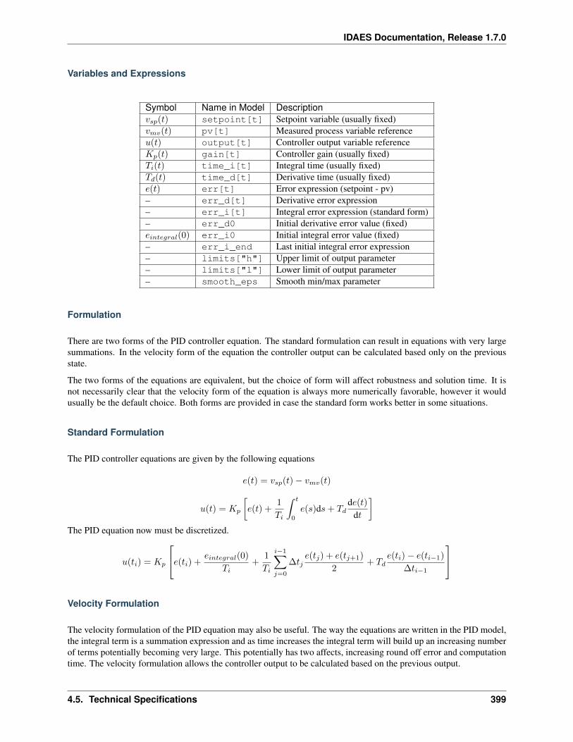
IDAES Documentation, Release 1.7.0
Variables and Expressions
Symbol Name in Model Description𝑣𝑠𝑝(𝑡) setpoint[t] Setpoint variable (usually fixed)𝑣𝑚𝑣(𝑡) pv[t] Measured process variable reference𝑢(𝑡) output[t] Controller output variable reference𝐾𝑝(𝑡) gain[t] Controller gain (usually fixed)𝑇𝑖(𝑡) time_i[t] Integral time (usually fixed)𝑇𝑑(𝑡) time_d[t] Derivative time (usually fixed)𝑒(𝑡) err[t] Error expression (setpoint - pv)– err_d[t] Derivative error expression– err_i[t] Integral error expression (standard form)– err_d0 Initial derivative error value (fixed)𝑒𝑖𝑛𝑡𝑒𝑔𝑟𝑎𝑙(0) err_i0 Initial integral error value (fixed)– err_i_end Last initial integral error expression– limits["h"] Upper limit of output parameter– limits["l"] Lower limit of output parameter– smooth_eps Smooth min/max parameter
Formulation
There are two forms of the PID controller equation. The standard formulation can result in equations with very largesummations. In the velocity form of the equation the controller output can be calculated based only on the previousstate.
The two forms of the equations are equivalent, but the choice of form will affect robustness and solution time. It isnot necessarily clear that the velocity form of the equation is always more numerically favorable, however it wouldusually be the default choice. Both forms are provided in case the standard form works better in some situations.
Standard Formulation
The PID controller equations are given by the following equations
𝑒(𝑡) = 𝑣𝑠𝑝(𝑡) − 𝑣𝑚𝑣(𝑡)
𝑢(𝑡) = 𝐾𝑝
[𝑒(𝑡) +
1
𝑇𝑖
∫ 𝑡
0
𝑒(𝑠)d𝑠+ 𝑇𝑑d𝑒(𝑡)
d𝑡
]The PID equation now must be discretized.
𝑢(𝑡𝑖) = 𝐾𝑝
⎡⎣𝑒(𝑡𝑖) +𝑒𝑖𝑛𝑡𝑒𝑔𝑟𝑎𝑙(0)
𝑇𝑖+
1
𝑇𝑖
𝑖−1∑𝑗=0
∆𝑡𝑗𝑒(𝑡𝑗) + 𝑒(𝑡𝑗+1)
2+ 𝑇𝑑
𝑒(𝑡𝑖) − 𝑒(𝑡𝑖−1)
∆𝑡𝑖−1
⎤⎦
Velocity Formulation
The velocity formulation of the PID equation may also be useful. The way the equations are written in the PID model,the integral term is a summation expression and as time increases the integral term will build up an increasing numberof terms potentially becoming very large. This potentially has two affects, increasing round off error and computationtime. The velocity formulation allows the controller output to be calculated based on the previous output.
4.5. Technical Specifications 399
IDAES Documentation, Release 1.7.0
First the usual PID controller equation can be rearranged to solve for the integral error.
1
𝑇𝑖
∫ 𝑡
0
𝑒(𝑠)d𝑠 =𝑢(𝑡)
𝐾𝑝− 𝑒(𝑡) − 𝑇𝑑
d𝑒(𝑡)d𝑡
The PID equation for some time (𝑡+ ∆𝑡) is
𝑢(𝑡+ ∆𝑡) = 𝐾𝑝
[𝑒(𝑡+ ∆𝑡) +
1
𝑇𝑖
∫ 𝑡+Δ𝑡
0
𝑒(𝑠)d𝑠+ 𝑇𝑑d𝑒(𝑡+ ∆𝑡)
d𝑡
]
𝑢(𝑡+ ∆𝑡) = 𝐾𝑝
[𝑒(𝑡+ ∆𝑡) +
1
𝑇𝑖
∫ 𝑡+Δ𝑡
𝑡
𝑒(𝑠)d𝑠+1
𝑇𝑖
∫ 𝑡
0
𝑒(𝑠)d𝑠+ 𝑇𝑑d𝑒(𝑡+ ∆𝑡)
d𝑡
]
𝑢(𝑡+ ∆𝑡) = 𝑢(𝑡) +𝐾𝑝
[𝑒(𝑡+ ∆𝑡) − 𝑒(𝑡) +
1
𝑇𝑖
∫ 𝑡+Δ𝑡
𝑡
𝑒(𝑠)d𝑠+ 𝑇𝑑
(d𝑒(𝑡+ ∆𝑡)
d𝑡− d𝑒(𝑡)
d𝑡
)]Now we can discretize the equation using the trapezoid rule for the integral.
𝑢(𝑡+ ∆𝑡) = 𝑢(𝑡) +𝐾𝑝
[𝑒(𝑡+ ∆𝑡) − 𝑒(𝑡) +
∆𝑡
𝑇𝑖
(𝑒(𝑡+ ∆𝑡) + 𝑒(𝑡)
2
)+ 𝑇𝑑
(d𝑒(𝑡+ ∆𝑡)
d𝑡− d𝑒(𝑡)
d𝑡
)]Since the derivative error term will require the error at the previous time step to calculate, this form will still result ina large summation being formed since in the model there is no derivative error variable. To avoid this problem, thederivative error term can equivalently be replaced with the derivative of the negative measured process variable.
𝑢(𝑡+ ∆𝑡) = 𝑢(𝑡) +𝐾𝑝
[𝑒(𝑡+ ∆𝑡) − 𝑒(𝑡) +
∆𝑡
𝑇𝑖
(𝑒(𝑡+ ∆𝑡) + 𝑒(𝑡)
2
)+ 𝑇𝑑
(d𝑣𝑚𝑣(𝑡+ ∆𝑡)
d𝑡− d𝑣𝑚𝑣(𝑡)
d𝑡
)]Now the velocity form of the PID controller equation can be calculated at each time point from just the state at theprevious time point.
Substitution
In both the proportional and integral terms, error can be replaced with the negative measured process variable yieldingequivalent results. This substitution is provided by the PID class and is done by default.
Output Limits
Smooth min and smooth max expressions are used to keep the controller output between a minimum and maximumvalue.
Power Generation Model Library
The IDAES Process Modeling Framework contains a library of models specifically developed for modeling powergeneration systems. These models all built off of the core IDAES modeling framework and model libraries.
Unit Models
Feedwater Heater (0D)
The FWH0D model is a 0D feedwater heater model suitable for steady state modeling. It is intended to be usedprimarily used with the IAWPS95 property package. The feedwater heater is split into three sections the condensingsection is required while the desuperheating and drain cooling sections are optional. There is also an optional mixerfor adding a drain stream from another feedwater heater to the condensing section. The figure below shows the layoutof the feedwater heater. All but the condensing section are optional.
400 Chapter 4. Contents
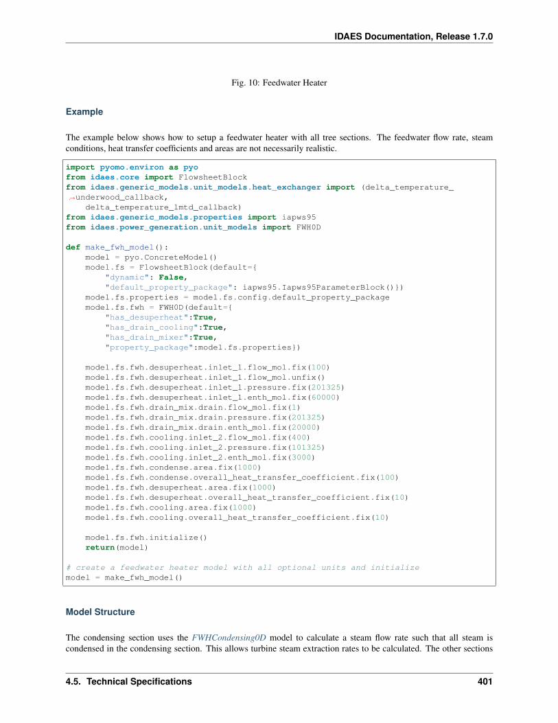
IDAES Documentation, Release 1.7.0
Fig. 10: Feedwater Heater
Example
The example below shows how to setup a feedwater heater with all tree sections. The feedwater flow rate, steamconditions, heat transfer coefficients and areas are not necessarily realistic.
import pyomo.environ as pyofrom idaes.core import FlowsheetBlockfrom idaes.generic_models.unit_models.heat_exchanger import (delta_temperature_→˓underwood_callback,
delta_temperature_lmtd_callback)from idaes.generic_models.properties import iapws95from idaes.power_generation.unit_models import FWH0D
def make_fwh_model():model = pyo.ConcreteModel()model.fs = FlowsheetBlock(default=
"dynamic": False,"default_property_package": iapws95.Iapws95ParameterBlock())
model.fs.properties = model.fs.config.default_property_packagemodel.fs.fwh = FWH0D(default=
"has_desuperheat":True,"has_drain_cooling":True,"has_drain_mixer":True,"property_package":model.fs.properties)
model.fs.fwh.desuperheat.inlet_1.flow_mol.fix(100)model.fs.fwh.desuperheat.inlet_1.flow_mol.unfix()model.fs.fwh.desuperheat.inlet_1.pressure.fix(201325)model.fs.fwh.desuperheat.inlet_1.enth_mol.fix(60000)model.fs.fwh.drain_mix.drain.flow_mol.fix(1)model.fs.fwh.drain_mix.drain.pressure.fix(201325)model.fs.fwh.drain_mix.drain.enth_mol.fix(20000)model.fs.fwh.cooling.inlet_2.flow_mol.fix(400)model.fs.fwh.cooling.inlet_2.pressure.fix(101325)model.fs.fwh.cooling.inlet_2.enth_mol.fix(3000)model.fs.fwh.condense.area.fix(1000)model.fs.fwh.condense.overall_heat_transfer_coefficient.fix(100)model.fs.fwh.desuperheat.area.fix(1000)model.fs.fwh.desuperheat.overall_heat_transfer_coefficient.fix(10)model.fs.fwh.cooling.area.fix(1000)model.fs.fwh.cooling.overall_heat_transfer_coefficient.fix(10)
model.fs.fwh.initialize()return(model)
# create a feedwater heater model with all optional units and initializemodel = make_fwh_model()
Model Structure
The condensing section uses the FWHCondensing0D model to calculate a steam flow rate such that all steam iscondensed in the condensing section. This allows turbine steam extraction rates to be calculated. The other sections
4.5. Technical Specifications 401
IDAES Documentation, Release 1.7.0
are regular HeatExchanger models. The table below shows the unit models which make up the feedwater heater, andthe option to include or exclude them.
Unit Option Doccondense – Condensing section (FWHCondensing0D)desuperheat has_desuperheat Desuperheating section (HeatExchanger)cooling has_drain_cooling Drain cooling section (HeatExchanger)drain_mix has_drain_mixer Mixer for steam and other FWH drain (Mixer)
Degrees of Freedom
The area and overall_heat_transfer_coefficient should be fixed or constraints should be provided tocalculate overall_heat_transfer_coefficient. If the inlets are also fixed except for the inlet steam flowrate (inlet_1.flow_mol), the model will have 0 degrees of freedom.
See FWH0D and FWH0DData for full Python class details.
Feedwater Heater (Condensing Section 0D)
The condensing feedwater heater is the same as the HeatExchanger model with one additional constraint to calculatethe inlet flow rate such that all the entering steam is condensed. This model is suitable for steady state modeling, andis intended to be used with the IAWPS95 property package. For dynamic modeling, the 1D feedwater heater modelsshould be used (not yet publicly available).
Degrees of Freedom
Usually area and overall_heat_transfer_coefficient are fixed or constraints are provided to calcu-late overall_heat_transfer_coefficient. If the inlets are also fixed except for the inlet steam flow rate(inlet_1.flow_mol), the model will have 0 degrees of freedom.
Variables
The variables are the same as HeatExchanger.
Constraints
In addition to the HeatExchanger constraints, there is one additional constraint to calculate the inlet steam flow suchthat all steam condenses. The constraint is called extraction_rate_constraint, and is defined below.
ℎ𝑠𝑡𝑒𝑎𝑚,𝑜𝑢𝑡 = ℎ𝑠𝑎𝑡,𝑙𝑖𝑞𝑢𝑖𝑑(𝑃 )
Where ℎ is molar enthalpy, and the saturated liquid enthalpy is a function of pressure.
FWHCondensing0D Class
class idaes.power_generation.unit_models.feedwater_heater_0D.FWHCondensing0D(*args,**kwargs)
Feedwater Heater Condensing Section The feedwater heater condensing section model is a normal 0D heat
402 Chapter 4. Contents
IDAES Documentation, Release 1.7.0
exchanger model with an added constraint to calculate the steam flow such that the outlet of shell is a saturatedliquid.
Args: rule (function): A rule function or None. Default rule calls build(). concrete (bool): If True,make this a toplevel model. Default - False. ctype (str): Pyomo ctype of the block. Default -“Block” default (dict): Default ProcessBlockData config
Keys
dynamic Indicates whether this model will be dynamic or not, default = useDefault.Valid values: useDefault - get flag from parent (default = False), True - set as adynamic model, False - set as a steady-state model.
has_holdup Indicates whether holdup terms should be constructed or not. Must beTrue if dynamic = True, default - False. Valid values: useDefault - get flag fromparent (default = False), True - construct holdup terms, False - do not constructholdup terms
hot_side_name Hot side name, sets control volume and inlet and outlet names
cold_side_name Cold side name, sets control volume and inlet and outlet names
hot_side_config A config block used to construct the hot side control volume. Thisconfig can be given by the hot side name instead of hot_side_config.
material_balance_type Indicates what type of mass balance should be con-structed, default - MaterialBalanceType.useDefault. Valid values: Materi-alBalanceType.useDefault - refer to property package for default balancetype **MaterialBalanceType.none - exclude material balances, MaterialBal-anceType.componentPhase - use phase component balances, MaterialBal-anceType.componentTotal - use total component balances, MaterialBalance-Type.elementTotal - use total element balances, MaterialBalanceType.total -use total material balance.
energy_balance_type Indicates what type of energy balance should be con-structed, default - EnergyBalanceType.useDefault. Valid values: Ener-gyBalanceType.useDefault - refer to property package for default bal-ance type **EnergyBalanceType.none - exclude energy balances, Energy-BalanceType.enthalpyTotal - single enthalpy balance for material, Energy-BalanceType.enthalpyPhase - enthalpy balances for each phase, EnergyBal-anceType.energyTotal - single energy balance for material, EnergyBalance-Type.energyPhase - energy balances for each phase.
momentum_balance_type Indicates what type of momentum balance should beconstructed, default - MomentumBalanceType.pressureTotal. Valid values: MomentumBalanceType.none - exclude momentum balances, Momentum-BalanceType.pressureTotal - single pressure balance for material, Momen-tumBalanceType.pressurePhase - pressure balances for each phase, Momen-tumBalanceType.momentumTotal - single momentum balance for material,MomentumBalanceType.momentumPhase - momentum balances for eachphase.
has_phase_equilibrium Indicates whether terms for phase equilibrium should beconstructed, default = False. Valid values: True - include phase equilibriumterms False - exclude phase equilibrium terms.
has_pressure_change Indicates whether terms for pressure change should beconstructed, default - False. Valid values: True - include pressure changeterms, False - exclude pressure change terms.
4.5. Technical Specifications 403
IDAES Documentation, Release 1.7.0
property_package Property parameter object used to define property calcula-tions, default - useDefault. Valid values: useDefault - use default packagefrom parent model or flowsheet, PropertyParameterObject - a PropertyParam-eterBlock object.
property_package_args A ConfigBlock with arguments to be passed to a prop-erty block(s) and used when constructing these, default - None. Valid values: see property package for documentation.
cold_side_config A config block used to construct the cold side control volume.This config can be given by the cold side name instead of cold_side_config.
material_balance_type Indicates what type of mass balance should be con-structed, default - MaterialBalanceType.useDefault. Valid values: Materi-alBalanceType.useDefault - refer to property package for default balancetype **MaterialBalanceType.none - exclude material balances, MaterialBal-anceType.componentPhase - use phase component balances, MaterialBal-anceType.componentTotal - use total component balances, MaterialBalance-Type.elementTotal - use total element balances, MaterialBalanceType.total -use total material balance.
energy_balance_type Indicates what type of energy balance should be con-structed, default - EnergyBalanceType.useDefault. Valid values: Ener-gyBalanceType.useDefault - refer to property package for default bal-ance type **EnergyBalanceType.none - exclude energy balances, Energy-BalanceType.enthalpyTotal - single enthalpy balance for material, Energy-BalanceType.enthalpyPhase - enthalpy balances for each phase, EnergyBal-anceType.energyTotal - single energy balance for material, EnergyBalance-Type.energyPhase - energy balances for each phase.
momentum_balance_type Indicates what type of momentum balance should beconstructed, default - MomentumBalanceType.pressureTotal. Valid values: MomentumBalanceType.none - exclude momentum balances, Momentum-BalanceType.pressureTotal - single pressure balance for material, Momen-tumBalanceType.pressurePhase - pressure balances for each phase, Momen-tumBalanceType.momentumTotal - single momentum balance for material,MomentumBalanceType.momentumPhase - momentum balances for eachphase.
has_phase_equilibrium Indicates whether terms for phase equilibrium should beconstructed, default = False. Valid values: True - include phase equilibriumterms False - exclude phase equilibrium terms.
has_pressure_change Indicates whether terms for pressure change should beconstructed, default - False. Valid values: True - include pressure changeterms, False - exclude pressure change terms.
property_package Property parameter object used to define property calcula-tions, default - useDefault. Valid values: useDefault - use default packagefrom parent model or flowsheet, PropertyParameterObject - a PropertyParam-eterBlock object.
property_package_args A ConfigBlock with arguments to be passed to a prop-erty block(s) and used when constructing these, default - None. Valid values: see property package for documentation.
delta_temperature_callback Callback for for temperature difference calculations
404 Chapter 4. Contents
IDAES Documentation, Release 1.7.0
flow_pattern Heat exchanger flow pattern, default - HeatExchanger-FlowPattern.countercurrent. Valid values: HeatExchangerFlowPat-tern.countercurrent - countercurrent flow, HeatExchangerFlowPat-tern.cocurrent - cocurrent flow, HeatExchangerFlowPattern.crossflow -cross flow, factor times countercurrent temperature difference.
initialize (dict): ProcessBlockData config for individual elements. Keys are BlockData in-dexes and values are dictionaries described under the “default” argument above.
idx_map (function): Function to take the index of a BlockData element and return the in-dex in the initialize dict from which to read arguments. This can be provided to overidethe default behavior of matching the BlockData index exactly to the index in initialize.
Returns: (FWHCondensing0D) New instance
FWHCondensing0DData Class
class idaes.power_generation.unit_models.feedwater_heater_0D.FWHCondensing0DData(component)
build()Building model
Parameters None –
Returns None
initialize(*args, **kwargs)Use the regular heat exchanger initialization, with the extraction rate constraint deactivated; then it acti-vates the constraint and calculates a steam inlet flow rate.
Turbine (Inlet Stage)
This is a steam power generation turbine model for the inlet stage. The turbine inlet model is based on:
Liese, (2014). “Modeling of a Steam Turbine Including Partial Arc Admission for Use in a Process SimulationSoftware Environment.” Journal of Engineering for Gas Turbines and Power. v136.
Example
from pyomo.environ import ConcreteModel, SolverFactory, TransformationFactoryfrom idaes.core import FlowsheetBlockfrom idaes.power_generation.unit_models import TurbineInletStagefrom idaes.generic_models.properties import iapws95
m = ConcreteModel()m.fs = FlowsheetBlock(default="dynamic": False)m.fs.properties = iapws95.Iapws95ParameterBlock()m.fs.turb = TurbineInletStage(default="property_package": m.fs.properties)hin = iapws95.htpx(T=880, P=2.4233e7)# set inletm.fs.turb.inlet[:].enth_mol.fix(hin)m.fs.turb.inlet[:].flow_mol.fix(26000/4.0)m.fs.turb.inlet[:].pressure.fix(2.4233e7)
(continues on next page)
4.5. Technical Specifications 405
IDAES Documentation, Release 1.7.0
(continued from previous page)
m.fs.turb.eff_nozzle.fix(0.95)m.fs.turb.blade_reaction.fix(0.9)m.fs.turb.flow_coeff.fix(1.053/3600.0)m.fs.turb.blade_velocity.fix(110.0)m.fs.turb.efficiency_mech.fix(0.98)
m.fs.turb.initialize()
Degrees of Freedom
Usually the inlet stream, or the inlet stream minus flow rate plus discharge pressure are fixed. There are also a fewvariables which are turbine parameters and are usually fixed. See the variables section for more information.
Model Structure
The turbine inlet stage model contains one ControlVolume0DBlock block called control_volume and inherits the Pres-sureChanger model using the isentropic option.
Variables
The variables below are defined in the TurbineInletStage model. Additional variables are inherited from the Pres-sureChanger model model.
Variable Sym-bol
IndexSets
Doc
blade_reaction 𝑅 None Blade reactioneff_nozzle 𝜂𝑛𝑜𝑧𝑧𝑙𝑒 None Nozzle efficiencyefficiency_mech 𝜂𝑚𝑒𝑐ℎ None Mechanical Efficiency (accounts for losses in bearings. . . )flow_coeff 𝐶𝑓𝑙𝑜𝑤 None Turbine stage flow coefficient [kg*C^0.5/Pa/s]blade_velocity 𝑉𝑟𝑏𝑙 None Turbine blade velocity (should be constant while running)
[m/s]delta_enth_isentropic∆ℎ𝑖𝑠𝑒𝑛 time Isentropic enthalpy change through stage [J/mol]
The table below shows important variables inherited from the pressure changer model.
Variable Symbol Index Sets Docefficiency_isentropic 𝜂𝑖𝑠𝑒𝑛 time Isentropic efficiencydeltaP ∆𝑃 time Pressure change (𝑃𝑜𝑢𝑡 − 𝑃𝑖𝑛) [Pa]
ratioP 𝑃𝑟𝑎𝑡𝑖𝑜 time Ratio of discharge pressure to inlet pressure(
𝑃𝑜𝑢𝑡
𝑃𝑖𝑛
)
406 Chapter 4. Contents
IDAES Documentation, Release 1.7.0
Expressions
Variable Sym-bol
IndexSets
Doc
power_thermo 𝑡ℎ𝑒𝑟𝑚𝑜 time Turbine stage power output not including mechanical loss[W]
power_shaft 𝑠ℎ𝑎𝑓𝑡 time Turbine stage power output including mechanical loss (bear-ings. . . ) [W]
steam_entering_velocity𝑉0 time Steam velocity entering stage [m/s]
The expression defined below provides a calculation for steam velocity entering the stage, which is used in the effi-ciency calculation.
𝑉0 = 1.414
√−(1 −𝑅)∆ℎ𝑖𝑠𝑒𝑛𝑊𝑇𝑖𝑛𝜂𝑛𝑜𝑧𝑧𝑒𝑙
Constraints
In addition to the constraints inherited from the PressureChanger model with the isentropic options, this model con-tains two more constraints, one to estimate efficiency and one pressure-flow relation. From the isentropic pressurechanger model, these constraints eliminate the need to specify efficiency and either inlet flow or outlet pressure.
The isentropic efficiency is given by:
𝜂𝑖𝑠𝑒𝑛 = 2𝑉𝑟𝑏𝑙𝑉0
⎡⎣(√1 −𝑅− 𝑉𝑟𝑏𝑙𝑉0
)+
√(√1 −𝑅− 𝑉𝑟𝑏𝑙
𝑉0
)2
+𝑅
⎤⎦The pressure-flow relation is given by:
= 𝐶𝑓𝑙𝑜𝑤𝑃𝑖𝑛√
𝑇𝑖𝑛 − 273.15
⎯ 𝛾
𝛾 − 1
[(𝑃𝑜𝑢𝑡
𝑃𝑖𝑛
) 2𝛾
−(𝑃𝑜𝑢𝑡
𝑃𝑖𝑛
) 𝛾+1𝛾
]
Initialization
The initialization method for this model will save the current state of the model before commencing initialization andreloads it afterwards. The state of the model will be the same after initialization, only the initial guesses for unfixedvariables will be changed. To initialize this model, provide a starting value for the inlet port variables. Then provide aguess for one of: discharge pressure, deltaP, or ratioP.
The model should initialize readily, but it is possible to provide a flow coefficient that is incompatible with the givenflow rate resulting in an infeasible problem.
TurbineInletStage Class
class idaes.power_generation.unit_models.turbine_inlet.TurbineInletStage(*args,**kwargs)
Inlet stage steam turbine model
Parameters
4.5. Technical Specifications 407
IDAES Documentation, Release 1.7.0
• rule (function) – A rule function or None. Default rule calls build().
• concrete (bool) – If True, make this a toplevel model. Default - False.
• ctype (str) – Pyomo ctype of the block. Default - “Block”
• default (dict) – Default ProcessBlockData config
Keys
dynamic Indicates whether this model will be dynamic or not, default = useDefault.Valid values: useDefault - get flag from parent (default = False), True - set as adynamic model, False - set as a steady-state model.
has_holdup Indicates whether holdup terms should be constructed or not. Must be Trueif dynamic = True, default - False. Valid values: useDefault - get flag from parent(default = False), True - construct holdup terms, False - do not construct holdup terms
material_balance_type Indicates what type of mass balance should be con-structed, default - MaterialBalanceType.useDefault. Valid values: Ma-terialBalanceType.useDefault - refer to property package for default bal-ance type **MaterialBalanceType.none - exclude material balances, Materi-alBalanceType.componentPhase - use phase component balances, MaterialBal-anceType.componentTotal - use total component balances, MaterialBalance-Type.elementTotal - use total element balances, MaterialBalanceType.total - usetotal material balance.
energy_balance_type Indicates what type of energy balance should be constructed,default - EnergyBalanceType.useDefault. Valid values: EnergyBalance-Type.useDefault - refer to property package for default balance type **Energy-BalanceType.none - exclude energy balances, EnergyBalanceType.enthalpyTotal -single enthalpy balance for material, EnergyBalanceType.enthalpyPhase - enthalpybalances for each phase, EnergyBalanceType.energyTotal - single energy balance formaterial, EnergyBalanceType.energyPhase - energy balances for each phase.
momentum_balance_type Indicates what type of momentum balance should be con-structed, default - MomentumBalanceType.pressureTotal. Valid values: Mo-mentumBalanceType.none - exclude momentum balances, MomentumBalance-Type.pressureTotal - single pressure balance for material, MomentumBalance-Type.pressurePhase - pressure balances for each phase, MomentumBalance-Type.momentumTotal - single momentum balance for material, MomentumBalance-Type.momentumPhase - momentum balances for each phase.
has_phase_equilibrium Indicates whether terms for phase equilibrium should be con-structed, default = False. Valid values: True - include phase equilibrium termsFalse - exclude phase equilibrium terms.
compressor Indicates whether this unit should be considered a compressor (True (de-fault), pressure increase) or an expander (False, pressure decrease).
thermodynamic_assumption Flag to set the thermodynamic assumption to use forthe unit. - ThermodynamicAssumption.isothermal (default) - ThermodynamicAs-sumption.isentropic - ThermodynamicAssumption.pump - ThermodynamicAssump-tion.adiabatic
property_package Property parameter object used to define property calculations, de-fault - useDefault. Valid values: useDefault - use default package from parentmodel or flowsheet, PropertyParameterObject - a PropertyParameterBlock object.
property_package_args A ConfigBlock with arguments to be passed to a property
408 Chapter 4. Contents
IDAES Documentation, Release 1.7.0
block(s) and used when constructing these, default - None. Valid values: see prop-erty package for documentation.
• initialize (dict) – ProcessBlockData config for individual elements. Keys are Block-Data indexes and values are dictionaries described under the “default” argument above.
• idx_map (function) – Function to take the index of a BlockData element and return theindex in the initialize dict from which to read arguments. This can be provided to overidethe default behavior of matching the BlockData index exactly to the index in initialize.
Returns (TurbineInletStage) New instance
TurbineInletStageData Class
class idaes.power_generation.unit_models.turbine_inlet.TurbineInletStageData(component)
build()
Parameters None –
Returns None
initialize(state_args=, outlvl=0, solver=’ipopt’, optarg=’max_iter’: 30, ’tol’: 1e-06)Initialize the inlet turbine stage model. This deactivates the specialized constraints, then does the isentropicturbine initialization, then reactivates the constraints and solves.
Parameters
• state_args (dict) – Initial state for property initialization
• outlvl (int) – Amount of output (0 to 3) 0 is lowest
• solver (str) – Solver to use for initialization
• optarg (dict) – Solver arguments dictionary
Turbine (Outlet Stage)
This is a steam power generation turbine model for the outlet stage. The turbine outlet model is based on:
Liese, (2014). “Modeling of a Steam Turbine Including Partial Arc Admission for Use in a Process SimulationSoftware Environment.” Journal of Engineering for Gas Turbines and Power. v136.
Example
from pyomo.environ import ConcreteModel, SolverFactoryfrom idaes.core import FlowsheetBlockfrom idaes.power_generation.unit_models import TurbineOutletStagefrom idaes.generic_models.properties import iapws95
m = ConcreteModel()m.fs = FlowsheetBlock(default="dynamic": False)m.fs.properties = iapws95.Iapws95ParameterBlock()m.fs.turb = TurbineOutletStage(default="property_package": m.fs.properties)# set inletm.fs.turb.inlet[:].enth_mol.fix(47115)
(continues on next page)
4.5. Technical Specifications 409
IDAES Documentation, Release 1.7.0
(continued from previous page)
m.fs.turb.inlet[:].flow_mol.fix(15000)m.fs.turb.inlet[:].pressure.fix(8e4)
m.fs.turb.initialize()
Degrees of Freedom
Usually the inlet stream, or the inlet stream minus flow rate plus discharge pressure are fixed. There are also a fewvariables which are turbine parameters and are usually fixed. See the variables section for more information.
Model Structure
The turbine outlet stage model contains one ControlVolume0DBlock block called control_volume and inherits thePressureChanger model using the isentropic option.
Variables
The variables below are defined int the TurbineInletStage model. Additional variables are in inherited from the Pres-sureChanger model model.
Variable Symbol IndexSets
Doc
eff_dry 𝜂𝑑𝑟𝑦 None Turbine efficiency when no liquid is present.efficiency_mech 𝜂𝑚𝑒𝑐ℎ None Mechanical Efficiency (accounts for losses in bear-
ings. . . )flow_coeff 𝐶𝑓𝑙𝑜𝑤 None Turbine stage flow coefficient [kg*C^0.5/Pa/s]design_exhaust_flow_vol𝑉𝑑𝑒𝑠,𝑒𝑥ℎ𝑎𝑢𝑠𝑡 None Design volumetric flow out of stage [m^3/s]
The table below shows important variables inherited from the pressure changer model.
Variable Symbol Index Sets Docefficiency_isentropic 𝜂𝑖𝑠𝑒𝑛 time Isentropic efficiencydeltaP ∆𝑃 time Pressure change (𝑃𝑜𝑢𝑡 − 𝑃𝑖𝑛) [Pa]
ratioP 𝑃𝑟𝑎𝑡𝑖𝑜 time Ratio of discharge pressure to inlet pressure(
𝑃𝑜𝑢𝑡
𝑃𝑖𝑛
)
Expressions
Variable Sym-bol
IndexSets
Doc
power_thermo 𝑡ℎ𝑒𝑟𝑚𝑜 time Turbine stage power output not including mechanical loss [W]power_shaft 𝑠ℎ𝑎𝑓𝑡 time Turbine stage power output including mechanical loss (bearings. . . )
[W]tel TEL time Total exhaust loss [J/mol]
410 Chapter 4. Contents
IDAES Documentation, Release 1.7.0
The expression defined below provides a total exhaust loss.
TEL = 1 × 10⁶ *(−0.0035𝑓5 + 0.022𝑓4 − 0.0542𝑓3 + 0.0638𝑓2 − 0.0328𝑓 + 0.0064
)Where 𝑓 is the total volumetric flow of the exhaust divided by the design flow.
Constraints
In addition to the constraints inherited from the PressureChanger model with the isentropic options, this model con-tains two more constraints, one to estimate efficiency and one pressure-flow relation. From the isentropic pressurechanger model, these constraints eliminate the need to specify efficiency and either inlet flow or outlet pressure.
The isentropic efficiency is given by:
𝜂𝑖𝑠𝑒𝑛 = 𝜂𝑑𝑟𝑦𝑥 (1 − 0.65(1 − 𝑥)) *(
1 +TEL
∆ℎ𝑖𝑠𝑒𝑛
)Where 𝑥 is the steam quality (vapor fraction).
The pressure-flow relation is given by the Stodola Equation:
√𝑇𝑖𝑛− 273.15 = 𝐶𝑓𝑙𝑜𝑤𝑃𝑖𝑛
√1 − 𝑃𝑟2
Initialization
The initialization method for this model will save the current state of the model before commencing initialization andreloads it afterwards. The state of the model will be the same after initialization, only the initial guesses for unfixedvariables will be changed. To initialize this model, provide a starting value for the inlet port variables. Then provide aguess for one of: discharge pressure, deltaP, or ratioP.
The model should initialize readily, but it is possible to provide a flow coefficient that is incompatible with the givenflow rate resulting in an infeasible problem.
TurbineOutletStage Class
class idaes.power_generation.unit_models.turbine_outlet.TurbineOutletStage(*args,**kwargs)
Outlet stage steam turbine model
Parameters
• rule (function) – A rule function or None. Default rule calls build().
• concrete (bool) – If True, make this a toplevel model. Default - False.
• ctype (str) – Pyomo ctype of the block. Default - “Block”
• default (dict) – Default ProcessBlockData config
Keys
dynamic Indicates whether this model will be dynamic or not, default = useDefault.Valid values: useDefault - get flag from parent (default = False), True - set as adynamic model, False - set as a steady-state model.
has_holdup Indicates whether holdup terms should be constructed or not. Must be Trueif dynamic = True, default - False. Valid values: useDefault - get flag from parent(default = False), True - construct holdup terms, False - do not construct holdup terms
4.5. Technical Specifications 411
IDAES Documentation, Release 1.7.0
material_balance_type Indicates what type of mass balance should be con-structed, default - MaterialBalanceType.useDefault. Valid values: Ma-terialBalanceType.useDefault - refer to property package for default bal-ance type **MaterialBalanceType.none - exclude material balances, Materi-alBalanceType.componentPhase - use phase component balances, MaterialBal-anceType.componentTotal - use total component balances, MaterialBalance-Type.elementTotal - use total element balances, MaterialBalanceType.total - usetotal material balance.
energy_balance_type Indicates what type of energy balance should be constructed,default - EnergyBalanceType.useDefault. Valid values: EnergyBalance-Type.useDefault - refer to property package for default balance type **Energy-BalanceType.none - exclude energy balances, EnergyBalanceType.enthalpyTotal -single enthalpy balance for material, EnergyBalanceType.enthalpyPhase - enthalpybalances for each phase, EnergyBalanceType.energyTotal - single energy balance formaterial, EnergyBalanceType.energyPhase - energy balances for each phase.
momentum_balance_type Indicates what type of momentum balance should be con-structed, default - MomentumBalanceType.pressureTotal. Valid values: Mo-mentumBalanceType.none - exclude momentum balances, MomentumBalance-Type.pressureTotal - single pressure balance for material, MomentumBalance-Type.pressurePhase - pressure balances for each phase, MomentumBalance-Type.momentumTotal - single momentum balance for material, MomentumBalance-Type.momentumPhase - momentum balances for each phase.
has_phase_equilibrium Indicates whether terms for phase equilibrium should be con-structed, default = False. Valid values: True - include phase equilibrium termsFalse - exclude phase equilibrium terms.
compressor Indicates whether this unit should be considered a compressor (True (de-fault), pressure increase) or an expander (False, pressure decrease).
thermodynamic_assumption Flag to set the thermodynamic assumption to use forthe unit. - ThermodynamicAssumption.isothermal (default) - ThermodynamicAs-sumption.isentropic - ThermodynamicAssumption.pump - ThermodynamicAssump-tion.adiabatic
property_package Property parameter object used to define property calculations, de-fault - useDefault. Valid values: useDefault - use default package from parentmodel or flowsheet, PropertyParameterObject - a PropertyParameterBlock object.
property_package_args A ConfigBlock with arguments to be passed to a propertyblock(s) and used when constructing these, default - None. Valid values: see prop-erty package for documentation.
• initialize (dict) – ProcessBlockData config for individual elements. Keys are Block-Data indexes and values are dictionaries described under the “default” argument above.
• idx_map (function) – Function to take the index of a BlockData element and return theindex in the initialize dict from which to read arguments. This can be provided to overidethe default behavior of matching the BlockData index exactly to the index in initialize.
Returns (TurbineOutletStage) New instance
TurbineOutletStageData Class
class idaes.power_generation.unit_models.turbine_outlet.TurbineOutletStageData(component)
412 Chapter 4. Contents
IDAES Documentation, Release 1.7.0
build()
Parameters None –
Returns None
initialize(state_args=, outlvl=0, solver=’ipopt’, optarg=’max_iter’: 30, ’tol’: 1e-06)Initialize the outlet turbine stage model. This deactivates the specialized constraints, then does the isen-tropic turbine initialization, then reactivates the constraints and solves.
Parameters
• state_args (dict) – Initial state for property initialization
• outlvl – sets output level of initialization routine
• solver (str) – Solver to use for initialization
• optarg (dict) – Solver arguments dictionary
Turbine (Stage)
This is a steam power generation turbine model for the stages between the inlet and outlet. This model inherits thePressureChanger model with the isentropic options. The initialization scheme is the same as the TurbineInletStagemodel.
Example
from pyomo.environ import ConcreteModel, SolverFactory
from idaes.core import FlowsheetBlockfrom idaes.power_generation.unit_models import TurbineStagefrom idaes.generic_models.properties import iapws95
m = ConcreteModel()m.fs = FlowsheetBlock(default="dynamic": False)m.fs.properties = iapws95.Iapws95ParameterBlock()m.fs.turb = TurbineStage(default="property_package": m.fs.properties)# set inletm.fs.turb.inlet[:].enth_mol.fix(70000)m.fs.turb.inlet[:].flow_mol.fix(15000)m.fs.turb.inlet[:].pressure.fix(8e6)m.fs.turb.efficiency_isentropic[:].fix(0.8)m.fs.turb.ratioP[:].fix(0.7)m.fs.turb.initialize()
Variables
This model adds a variable to the base PressureChanger model to account for mechanical efficiency .
Variable Symbol Index Sets Docefficiency_mech 𝜂𝑚𝑒𝑐ℎ None Mechanical Efficiency (accounts for losses in bearings. . . )
The table below shows important variables inherited from the pressure changer model.
4.5. Technical Specifications 413
IDAES Documentation, Release 1.7.0
Variable Symbol Index Sets Docefficiency_isentropic 𝜂𝑖𝑠𝑒𝑛 time Isentropic efficiencydeltaP ∆𝑃 time Pressure change (𝑃𝑜𝑢𝑡 − 𝑃𝑖𝑛) [Pa]
ratioP 𝑃𝑟𝑎𝑡𝑖𝑜 time Ratio of discharge pressure to inlet pressure(
𝑃𝑜𝑢𝑡
𝑃𝑖𝑛
)𝜂𝑖𝑠𝑒𝑛𝑡𝑟𝑜𝑝𝑖𝑐,𝑡 efficiency_isentropic Isentropic assumption only
Expressions
This model provides two expressions that are not available in the pressure changer model.
Variable Sym-bol
IndexSets
Doc
power_thermo 𝑡ℎ𝑒𝑟𝑚𝑜 time Turbine stage power output not including mechanical loss [W]power_shaft 𝑠ℎ𝑎𝑓𝑡 time Turbine stage power output including mechanical loss (bearings. . . )
[W]
Constraints
There are no additional constraints.
Initialization
This just calls the initialization routine from PressureChanger, but it is wrapped in a function to ensure the stateafter initialization is the same as before initialization. The arguments to the initialization method are the same asPressureChanger.
TurbineStage Class
class idaes.power_generation.unit_models.turbine_stage.TurbineStage(*args,**kwargs)
Basic steam turbine model
Parameters
• rule (function) – A rule function or None. Default rule calls build().
• concrete (bool) – If True, make this a toplevel model. Default - False.
• ctype (str) – Pyomo ctype of the block. Default - “Block”
• default (dict) – Default ProcessBlockData config
Keys
dynamic Indicates whether this model will be dynamic or not, default = useDefault.Valid values: useDefault - get flag from parent (default = False), True - set as adynamic model, False - set as a steady-state model.
has_holdup Indicates whether holdup terms should be constructed or not. Must be Trueif dynamic = True, default - False. Valid values: useDefault - get flag from parent(default = False), True - construct holdup terms, False - do not construct holdup terms
414 Chapter 4. Contents
IDAES Documentation, Release 1.7.0
material_balance_type Indicates what type of mass balance should be con-structed, default - MaterialBalanceType.useDefault. Valid values: Ma-terialBalanceType.useDefault - refer to property package for default bal-ance type **MaterialBalanceType.none - exclude material balances, Materi-alBalanceType.componentPhase - use phase component balances, MaterialBal-anceType.componentTotal - use total component balances, MaterialBalance-Type.elementTotal - use total element balances, MaterialBalanceType.total - usetotal material balance.
energy_balance_type Indicates what type of energy balance should be constructed,default - EnergyBalanceType.useDefault. Valid values: EnergyBalance-Type.useDefault - refer to property package for default balance type **Energy-BalanceType.none - exclude energy balances, EnergyBalanceType.enthalpyTotal -single enthalpy balance for material, EnergyBalanceType.enthalpyPhase - enthalpybalances for each phase, EnergyBalanceType.energyTotal - single energy balance formaterial, EnergyBalanceType.energyPhase - energy balances for each phase.
momentum_balance_type Indicates what type of momentum balance should be con-structed, default - MomentumBalanceType.pressureTotal. Valid values: Mo-mentumBalanceType.none - exclude momentum balances, MomentumBalance-Type.pressureTotal - single pressure balance for material, MomentumBalance-Type.pressurePhase - pressure balances for each phase, MomentumBalance-Type.momentumTotal - single momentum balance for material, MomentumBalance-Type.momentumPhase - momentum balances for each phase.
has_phase_equilibrium Indicates whether terms for phase equilibrium should be con-structed, default = False. Valid values: True - include phase equilibrium termsFalse - exclude phase equilibrium terms.
compressor Indicates whether this unit should be considered a compressor (True (de-fault), pressure increase) or an expander (False, pressure decrease).
thermodynamic_assumption Flag to set the thermodynamic assumption to use forthe unit. - ThermodynamicAssumption.isothermal (default) - ThermodynamicAs-sumption.isentropic - ThermodynamicAssumption.pump - ThermodynamicAssump-tion.adiabatic
property_package Property parameter object used to define property calculations, de-fault - useDefault. Valid values: useDefault - use default package from parentmodel or flowsheet, PropertyParameterObject - a PropertyParameterBlock object.
property_package_args A ConfigBlock with arguments to be passed to a propertyblock(s) and used when constructing these, default - None. Valid values: see prop-erty package for documentation.
• initialize (dict) – ProcessBlockData config for individual elements. Keys are Block-Data indexes and values are dictionaries described under the “default” argument above.
• idx_map (function) – Function to take the index of a BlockData element and return theindex in the initialize dict from which to read arguments. This can be provided to overidethe default behavior of matching the BlockData index exactly to the index in initialize.
Returns (TurbineStage) New instance
TurbineStageData Class
class idaes.power_generation.unit_models.turbine_stage.TurbineStageData(component)
4.5. Technical Specifications 415
IDAES Documentation, Release 1.7.0
build()
Parameters None –
Returns None
initialize(state_args=, outlvl=0, solver=’ipopt’, optarg=’max_iter’: 30, ’tol’: 1e-06)Initialize the turbine stage model. This deactivates the specialized constraints, then does the isentropicturbine initialization, then reactivates the constraints and solves.
Parameters
• state_args (dict) – Initial state for property initialization
• outlvl – sets output level of initialization routine
• solver (str) – Solver to use for initialization
• optarg (dict) – Solver arguments dictionary
Turbine (Multistage)
This is a composite model for a power plant turbine with high, intermediate and low pressure sections. This modelcontains an inlet stage with throttle valves for partial arc admission and optional splitters for steam extraction.
The figure below shows the layout of the mutistage turbine model. Optional splitters provide for steam extraction. Thesplitters can have two or more outlets (one being the main steam outlet). The streams that connect one stage to thenext can also be omitted. This allows for connecting additional unit models (usually reheaters) between stages.
Fig. 11: MultiStage Turbine Model
Example
This example sets up a turbine multistage turbine model similar to what could be found in a power plant steam cycle.There are 7 high-pressure stages, 14 intermediate-pressure stages, and 11 low-pressure stages. Steam extractions areprovided after stages hp4, hp7, ip5, ip14, lp4, lp7, lp9, lp11. The extraction at ip14 uses a splitter with three outlets,one for the main steam, one for the boiler feed pump, and one for a feedwater heater. There is a disconnection betweenthe HP and IP sections so that steam can be sent to a reheater. In this example, a heater block is a stand-in for a reheatermodel.
from pyomo.environ import (ConcreteModel, SolverFactory, TransformationFactory,Constraint, value)
from pyomo.network import Arc
from idaes.core import FlowsheetBlockfrom idaes.unit_models import Heaterfrom idaes.power_generation.unit_models import (
TurbineMultistage, TurbineStage, TurbineInletStage, TurbineOutletStage)from idaes.generic_models.properties import iapws95
solver = SolverFactory('ipopt')solver.options = 'tol': 1e-6
m = ConcreteModel()m.fs = FlowsheetBlock(default="dynamic": False)m.fs.properties = iapws95.Iapws95ParameterBlock()
(continues on next page)
416 Chapter 4. Contents
IDAES Documentation, Release 1.7.0
(continued from previous page)
m.fs.turb = TurbineMultistage(default="property_package": m.fs.properties,"num_hp": 7,"num_ip": 14,"num_lp": 11,"hp_split_locations": [4,7],"ip_split_locations": [5, 14],"lp_split_locations": [4,7,9,11],"hp_disconnect": [7], # 7 is last stage in hp so disconnect hp from ip"ip_split_num_outlets": 14:3)
# Add reheater (for example using a simple heater block)m.fs.reheat = Heater(default="property_package": m.fs.properties)# Add Arcs (streams) to connect the HP and IP sections through reheaterm.fs.hp_to_reheat = Arc(source=m.fs.turb.hp_split[7].outlet_1,
destination=m.fs.reheat.inlet)m.fs.reheat_to_ip = Arc(source=m.fs.reheat.outlet,
destination=m.fs.turb.ip_stages[1].inlet)# Set the turbine inlet conditions and an initial flow guessp = 2.4233e7hin = iapws95.htpx(T=880, P=p)m.fs.turb.inlet_split.inlet.enth_mol[0].fix(hin)m.fs.turb.inlet_split.inlet.flow_mol[0].fix(26000)m.fs.turb.inlet_split.inlet.pressure[0].fix(p)
# Set the inlet of the ip section for initialization, since it is disconnectedp = 7.802e+06hin = iapws95.htpx(T=880, P=p)m.fs.turb.ip_stages[1].inlet.enth_mol[0].value = hinm.fs.turb.ip_stages[1].inlet.flow_mol[0].value = 25220.0m.fs.turb.ip_stages[1].inlet.pressure[0].value = p# Set the efficency and pressure ratios of stages other than inlet and outletfor i, s in turb.hp_stages.items():
s.ratioP[:] = 0.88s.efficiency_isentropic[:] = 0.9
for i, s in turb.ip_stages.items():s.ratioP[:] = 0.85s.efficiency_isentropic[:] = 0.9
for i, s in turb.lp_stages.items():s.ratioP[:] = 0.82s.efficiency_isentropic[:] = 0.9
# Usually these fractions would be determined by the boiler feed water heater# network. Since this example doesn't include them, just fix split fractionsturb.hp_split[4].split_fraction[0,"outlet_2"].fix(0.03)turb.hp_split[7].split_fraction[0,"outlet_2"].fix(0.03)turb.ip_split[5].split_fraction[0,"outlet_2"].fix(0.04)turb.ip_split[14].split_fraction[0,"outlet_2"].fix(0.04)turb.ip_split[14].split_fraction[0,"outlet_3"].fix(0.15)turb.lp_split[4].split_fraction[0,"outlet_2"].fix(0.04)turb.lp_split[7].split_fraction[0,"outlet_2"].fix(0.04)turb.lp_split[9].split_fraction[0,"outlet_2"].fix(0.04)turb.lp_split[11].split_fraction[0,"outlet_2"].fix(0.04)# unfix inlet flow for pressure driven simulationturb.inlet_split.inlet.flow_mol.unfix()# Set the inlet steam mixer to use the constraints that the pressures of all# inlet streams are equalturb.inlet_mix.use_equal_pressure_constraint()# Initialize turbine
(continues on next page)
4.5. Technical Specifications 417
IDAES Documentation, Release 1.7.0
(continued from previous page)
turb.initialize(outlvl=1)# Copy conditions out of turbine to initialize the reheaterfor t in m.fs.time:
m.fs.reheat.inlet.flow_mol[t].value = \value(turb.hp_split[7].outlet_1_state[t].flow_mol)
m.fs.reheat.inlet.enth_mol[t].value = \value(turb.hp_split[7].outlet_1_state[t].enth_mol)
m.fs.reheat.inlet.pressure[t].value = \value(turb.hp_split[7].outlet_1_state[t].pressure)
# initialize the reheaterm.fs.reheat.initialize(outlvl=4)# Add constraint to the reheater to result in 880K outlet temperaturedef reheat_T_rule(b, t):
return m.fs.reheat.control_volume.properties_out[t].temperature == 880m.fs.reheat.temperature_out_equation = Constraint(m.fs.reheat.time_ref,
rule=reheat_T_rule)# Expand the Arcs connecting the turbine to the reheaterTransformationFactory("network.expand_arcs").apply_to(m)# Fix the outlet pressure (usually determined by condenser)m.fs.turb.outlet_stage.control_volume.properties_out[0].pressure.fix()
# Solve the pressure driven flow model with reheatsolver.solve(m, tee=True)
Unit Models
The multistage turbine model contains the models in the table below. The splitters for steam extraction are not presentif a turbine section contains no steam extractions.
Unit Index Sets Docinlet_split None Splitter to split the main steam feed into steams for each arc (Separator)throttle_valve Admission Arcs Throttle valves for each admission arc (SteamValve)inlet_stage Admission Arcs Parallel inlet turbine stages that represent admission arcs (TurbineInlet)inlet_mix None Mixer to combine the streams from each arc back to one stream (Mixer)hp_stages HP stages Turbine stages in the high-pressure section (TurbineStage)ip_stages IP stages Turbine stages in the intermediate-pressure section (TurbineStage)lp_stages LP stages Turbine stages in the low-pressure section (TurbineStage)hp_splits subset of HP
stagesExtraction splitters in the high-pressure section (Separator)
ip_splits subset of IPstages
Extraction splitters in the high-pressure section (Separator)
lp_splits subset of LPstages
Extraction splitters in the high-pressure section (Separator)
outlet_stage None The final stage in the turbine, which calculates exhaust losses (Turbine-Outlet)
Initialization
The initialization approach is to sequentially initialize each sub-unit using the outlet of the previous model. Beforeinitializing the model, the inlet of the turbine, and any stage that is disconnected should be given a reasonable guess.The efficiency and pressure ration of the stages in the HP, IP and LP sections should be specified. For the inlet and
418 Chapter 4. Contents
IDAES Documentation, Release 1.7.0
outlet stages the flow coefficient should be specified. Valve coefficients should also be specified. A reasonable guessfor split fractions should also be given for any extraction splitters present. The most likely cause of initialization failureis flow coefficients in inlet stage, outlet stage, or valves that do not pair well with the specified flow rates.
TurbineMultistage Class
class idaes.power_generation.unit_models.turbine_multistage.TurbineMultistage(*args,**kwargs)
Multistage steam turbine with optional reheat and extraction
Parameters
• rule (function) – A rule function or None. Default rule calls build().
• concrete (bool) – If True, make this a toplevel model. Default - False.
• ctype (str) – Pyomo ctype of the block. Default - “Block”
• default (dict) – Default ProcessBlockData config
Keys
dynamic Indicates whether the model is dynamic.
has_holdup Indicates whether holdup terms should be constructed or not. Must be Trueif dynamic = True, default - False. Valid values: True - construct holdup terms,False - do not construct holdup terms
has_phase_equilibrium Argument indicating whether phase equilibrium should be cal-culated for the resulting mixed stream, default - False. Valid values: True - calcu-late phase equilibrium in mixed stream, False - do not calculate equilibrium in mixedstream.
material_balance_type Indicates what type of mass balance should be constructed, de-fault - MaterialBalanceType.componentTotal‘. Valid values: MaterialBalance-Type.none - exclude material balances, MaterialBalanceType.componentPhase - usephase component balances, MaterialBalanceType.componentTotal - use total com-ponent balances, MaterialBalanceType.elementTotal - use total element balances,MaterialBalanceType.total - use total material balance.
property_package Property parameter object used to define property calculations, de-fault - useDefault. Valid values: useDefault - use default package from parentmodel or flowsheet, PropertyParameterObject - a PropertyParameterBlock object.
property_package_args A ConfigBlock with arguments to be passed to a propertyblock(s) and used when constructing these, default - None. Valid values: see prop-erty package for documentation.
num_parallel_inlet_stages Number of parallel inlet stages to simulate partial arc admis-sion. Default=4
num_hp Number of high pressure stages not including inlet stage
num_ip Number of intermediate pressure stages
num_lp Number of low pressure stages not including outlet stage
hp_split_locations A list of index locations of splitters in the HP section. The indexesindicate after which stage to include splitters. 0 is between the inlet stage and the firstregular HP stage.
4.5. Technical Specifications 419
IDAES Documentation, Release 1.7.0
ip_split_locations A list of index locations of splitters in the IP section. The indexesindicate after which stage to include splitters.
lp_split_locations A list of index locations of splitters in the LP section. The indexesindicate after which stage to include splitters.
hp_disconnect HP Turbine stages to not connect to next with an arc. This is usually usedto insert addtional units between stages on a flowsheet, such as a reheater
ip_disconnect IP Turbine stages to not connect to next with an arc. This is usually usedto insert addtional units between stages on a flowsheet, such as a reheater
lp_disconnect LP Turbine stages to not connect to next with an arc. This is usually usedto insert addtional units between stages on a flowsheet, such as a reheater
hp_split_num_outlets Dict, hp split index: number of splitter outlets, if not 2
ip_split_num_outlets Dict, ip split index: number of splitter outlets, if not 2
lp_split_num_outlets Dict, lp split index: number of splitter outlets, if not 2
• initialize (dict) – ProcessBlockData config for individual elements. Keys are Block-Data indexes and values are dictionaries described under the “default” argument above.
• idx_map (function) – Function to take the index of a BlockData element and return theindex in the initialize dict from which to read arguments. This can be provided to overidethe default behavior of matching the BlockData index exactly to the index in initialize.
Returns (TurbineMultistage) New instance
TurbineMultistageData Class
class idaes.power_generation.unit_models.turbine_multistage.TurbineMultistageData(component)
build()General build method for UnitModelBlockData. This method calls a number of sub-methods which auto-mate the construction of expected attributes of unit models.
Inheriting models should call super().build.
Parameters None –
Returns None
initialize(outlvl=0, solver=’ipopt’, optarg=’max_iter’: 35, ’tol’: 1e-06,copy_disconneted_flow=True)
Initialize
throttle_cv_fix(value)Fix the thottle valve coefficients. These are generally the same for each of the parallel stages so thisprovides a convenient way to set them.
Parameters value – The value to fix the turbine inlet flow coefficients at
turbine_inlet_cf_fix(value)Fix the inlet turbine stage flow coefficient. These are generally the same for each of the parallel stages sothis provides a convenient way to set them.
Parameters value – The value to fix the turbine inlet flow coefficients at
420 Chapter 4. Contents
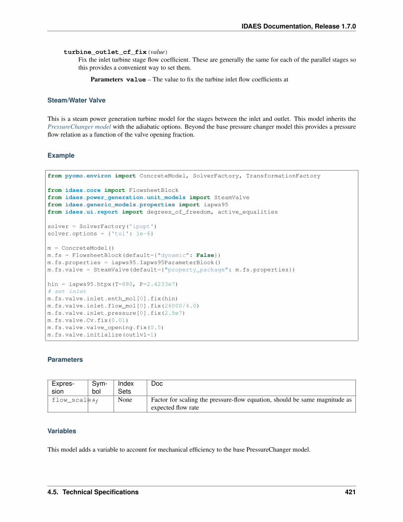
IDAES Documentation, Release 1.7.0
turbine_outlet_cf_fix(value)Fix the inlet turbine stage flow coefficient. These are generally the same for each of the parallel stages sothis provides a convenient way to set them.
Parameters value – The value to fix the turbine inlet flow coefficients at
Steam/Water Valve
This is a steam power generation turbine model for the stages between the inlet and outlet. This model inherits thePressureChanger model with the adiabatic options. Beyond the base pressure changer model this provides a pressureflow relation as a function of the valve opening fraction.
Example
from pyomo.environ import ConcreteModel, SolverFactory, TransformationFactory
from idaes.core import FlowsheetBlockfrom idaes.power_generation.unit_models import SteamValvefrom idaes.generic_models.properties import iapws95from idaes.ui.report import degrees_of_freedom, active_equalities
solver = SolverFactory('ipopt')solver.options = 'tol': 1e-6
m = ConcreteModel()m.fs = FlowsheetBlock(default="dynamic": False)m.fs.properties = iapws95.Iapws95ParameterBlock()m.fs.valve = SteamValve(default="property_package": m.fs.properties)
hin = iapws95.htpx(T=880, P=2.4233e7)# set inletm.fs.valve.inlet.enth_mol[0].fix(hin)m.fs.valve.inlet.flow_mol[0].fix(26000/4.0)m.fs.valve.inlet.pressure[0].fix(2.5e7)m.fs.valve.Cv.fix(0.01)m.fs.valve.valve_opening.fix(0.5)m.fs.valve.initialize(outlvl=1)
Parameters
Expres-sion
Sym-bol
IndexSets
Doc
flow_scale 𝑠𝑓 None Factor for scaling the pressure-flow equation, should be same magnitude asexpected flow rate
Variables
This model adds a variable to account for mechanical efficiency to the base PressureChanger model.
4.5. Technical Specifications 421
IDAES Documentation, Release 1.7.0
Variable Symbol Index Sets DocCv 𝐶𝑣 None Valve coefficient for liquid [mol/s/Pa^0.5] for vapor [mol/s/Pa]valve_opening 𝑥 time The fraction that the valve is open from 0 to 1
Expressions
Currently this model provides two additional expressions, with are not available in the pressure changer model.
Expression Sym-bol
IndexSets
Doc
valve_function 𝑓(𝑥) time This is a valve function that describes how the fraction open affectsflow.
Constraints
The pressure flow relation is added to the inherited constraints from the PressureChanger model.
If the phase option is set to "Liq" the following equation describes the pressure-flow relation.
1
𝑠2𝑓𝐹 2 =
1
𝑠2𝑓𝐶2
𝑣 (𝑃𝑖𝑛 − 𝑃𝑜𝑢𝑡) 𝑓(𝑥)2
If the phase option is set to "Vap" the following equation describes the pressure-flow relation.
1
𝑠2𝑓𝐹 2 =
1
𝑠2𝑓𝐶2
𝑣
(𝑃 2𝑖𝑛 − 𝑃 2
𝑜𝑢𝑡
)𝑓(𝑥)2
Initialization
This just calls the initialization routine from PressureChanger, but it is wrapped in a function to ensure the stateafter initialization is the same as before initialization. The arguments to the initialization method are the same asPressureChanger.
SteamValve Class
class idaes.power_generation.unit_models.valve_steam.SteamValve(*args,**kwargs)
Basic steam valve models
Parameters
• rule (function) – A rule function or None. Default rule calls build().
• concrete (bool) – If True, make this a toplevel model. Default - False.
• ctype (str) – Pyomo ctype of the block. Default - “Block”
• default (dict) – Default ProcessBlockData config
Keys
dynamic Indicates whether this model will be dynamic or not, default = useDefault.Valid values: useDefault - get flag from parent (default = False), True - set as adynamic model, False - set as a steady-state model.
422 Chapter 4. Contents
IDAES Documentation, Release 1.7.0
has_holdup Indicates whether holdup terms should be constructed or not. Must be Trueif dynamic = True, default - False. Valid values: useDefault - get flag from parent(default = False), True - construct holdup terms, False - do not construct holdup terms
material_balance_type Indicates what type of mass balance should be con-structed, default - MaterialBalanceType.useDefault. Valid values: Ma-terialBalanceType.useDefault - refer to property package for default bal-ance type **MaterialBalanceType.none - exclude material balances, Materi-alBalanceType.componentPhase - use phase component balances, MaterialBal-anceType.componentTotal - use total component balances, MaterialBalance-Type.elementTotal - use total element balances, MaterialBalanceType.total - usetotal material balance.
energy_balance_type Indicates what type of energy balance should be constructed,default - EnergyBalanceType.useDefault. Valid values: EnergyBalance-Type.useDefault - refer to property package for default balance type **Energy-BalanceType.none - exclude energy balances, EnergyBalanceType.enthalpyTotal -single enthalpy balance for material, EnergyBalanceType.enthalpyPhase - enthalpybalances for each phase, EnergyBalanceType.energyTotal - single energy balance formaterial, EnergyBalanceType.energyPhase - energy balances for each phase.
momentum_balance_type Indicates what type of momentum balance should be con-structed, default - MomentumBalanceType.pressureTotal. Valid values: Mo-mentumBalanceType.none - exclude momentum balances, MomentumBalance-Type.pressureTotal - single pressure balance for material, MomentumBalance-Type.pressurePhase - pressure balances for each phase, MomentumBalance-Type.momentumTotal - single momentum balance for material, MomentumBalance-Type.momentumPhase - momentum balances for each phase.
has_phase_equilibrium Indicates whether terms for phase equilibrium should be con-structed, default = False. Valid values: True - include phase equilibrium termsFalse - exclude phase equilibrium terms.
compressor Indicates whether this unit should be considered a compressor (True (de-fault), pressure increase) or an expander (False, pressure decrease).
thermodynamic_assumption Flag to set the thermodynamic assumption to use forthe unit. - ThermodynamicAssumption.isothermal (default) - ThermodynamicAs-sumption.isentropic - ThermodynamicAssumption.pump - ThermodynamicAssump-tion.adiabatic
property_package Property parameter object used to define property calculations, de-fault - useDefault. Valid values: useDefault - use default package from parentmodel or flowsheet, PropertyParameterObject - a PropertyParameterBlock object.
property_package_args A ConfigBlock with arguments to be passed to a propertyblock(s) and used when constructing these, default - None. Valid values: see prop-erty package for documentation.
valve_function The type of valve function, if custom provide an expression rule withthe valve_function_rule argument. default - ValveFunctionType.linear Valid val-ues - ValveFunctionType.linear, ValveFunctionType.quick_opening, ValveFunction-Type.equal_percentage, ValveFunctionType.custom
valve_function_rule This is a rule that returns a time indexed valve function expression.This is required only if valve_function==ValveFunctionType.custom
phase Expected phase of fluid in valve in “Liq”, “Vap”
4.5. Technical Specifications 423
IDAES Documentation, Release 1.7.0
• initialize (dict) – ProcessBlockData config for individual elements. Keys are Block-Data indexes and values are dictionaries described under the “default” argument above.
• idx_map (function) – Function to take the index of a BlockData element and return theindex in the initialize dict from which to read arguments. This can be provided to overidethe default behavior of matching the BlockData index exactly to the index in initialize.
Returns (SteamValve) New instance
SteamValveData Class
class idaes.power_generation.unit_models.valve_steam.SteamValveData(component)
build()
Parameters None –
Returns None
initialize(state_args=, outlvl=0, solver=’ipopt’, optarg=’max_iter’: 30, ’tol’: 1e-06)Initialize the turbine stage model. This deactivates the specialized constraints, then does the isentropicturbine initialization, then reactivates the constraints and solves.
Parameters
• state_args (dict) – Initial state for property initialization
• outlvl – sets output level of initialization routine
• solver (str) – Solver to use for initialization
• optarg (dict) – Solver arguments dictionary
BoilerHeatExchanger
The BoilerHeatExchanger model can be used to represent boiler heat exchangers in sub-critical and super criticalpower plant flowsheets (i.e. econmizer, primary superheater, secondary superheater, finishing superheater, reheater,etc.). The model consists of a shell and tube crossflow heat exchanger, in which the shell is used as the gas side andthe tube is used as the water or steam side. Rigorous heat transfer calculations (convective heat transfer for shell side,and convective heat transfer for tube side) and shell and tube pressure drop calculations have been included.
The BoilerHeatExchanger model can be imported from idaes.power_generation.unit_models, whileadditional rules and utility functions can be imported from idaes.power_generation.unit_models.boiler_heat_exchanger.
Example
The example below demonstrates how to initialize the BoilerHeatExchanger model, and override the default tempera-ture difference calculation.
# Import Pyomo librariesfrom pyomo.environ import ConcreteModel, SolverFactory, value# Import IDAES corefrom idaes.core import FlowsheetBlock# Import Unit Model Modulesfrom idaes.generic_models.properties import iapws95
(continues on next page)
424 Chapter 4. Contents
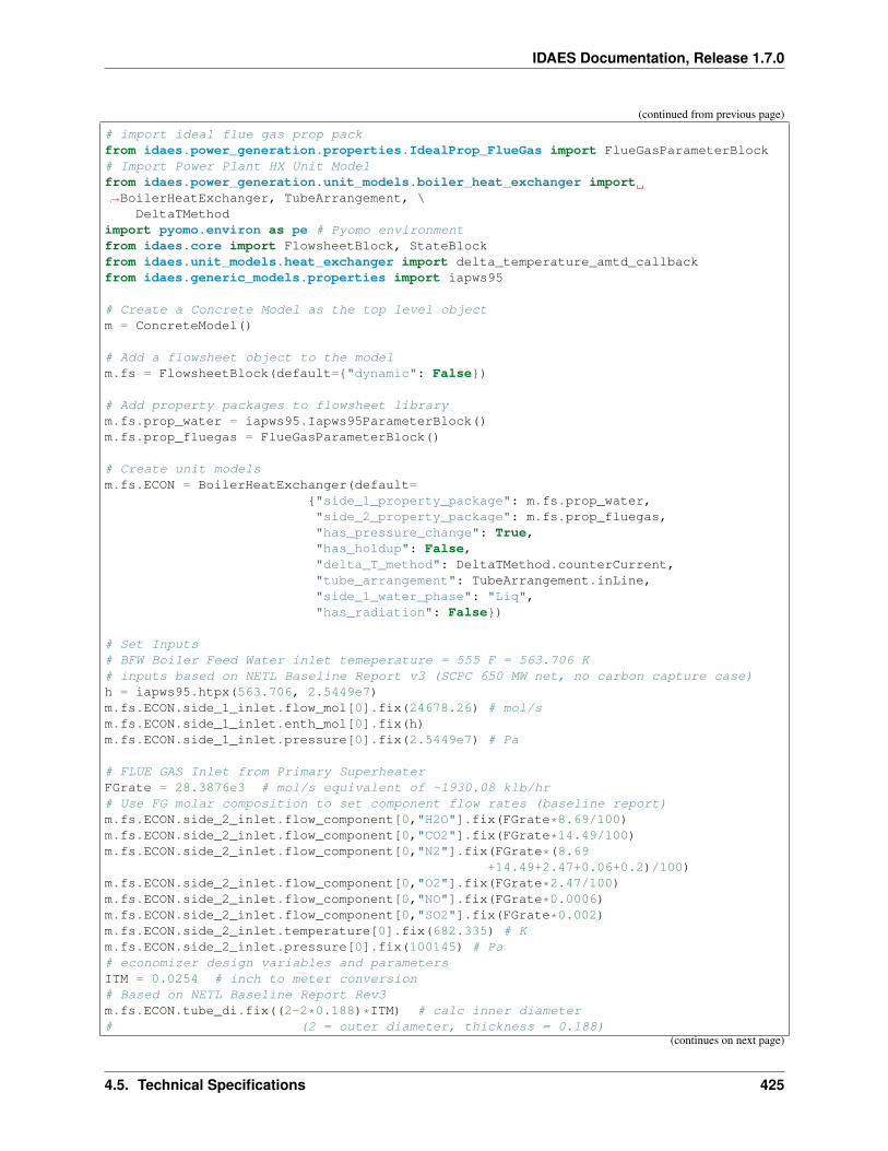
IDAES Documentation, Release 1.7.0
(continued from previous page)
# import ideal flue gas prop packfrom idaes.power_generation.properties.IdealProp_FlueGas import FlueGasParameterBlock# Import Power Plant HX Unit Modelfrom idaes.power_generation.unit_models.boiler_heat_exchanger import→˓BoilerHeatExchanger, TubeArrangement, \
DeltaTMethodimport pyomo.environ as pe # Pyomo environmentfrom idaes.core import FlowsheetBlock, StateBlockfrom idaes.unit_models.heat_exchanger import delta_temperature_amtd_callbackfrom idaes.generic_models.properties import iapws95
# Create a Concrete Model as the top level objectm = ConcreteModel()
# Add a flowsheet object to the modelm.fs = FlowsheetBlock(default="dynamic": False)
# Add property packages to flowsheet librarym.fs.prop_water = iapws95.Iapws95ParameterBlock()m.fs.prop_fluegas = FlueGasParameterBlock()
# Create unit modelsm.fs.ECON = BoilerHeatExchanger(default=
"side_1_property_package": m.fs.prop_water,"side_2_property_package": m.fs.prop_fluegas,"has_pressure_change": True,"has_holdup": False,"delta_T_method": DeltaTMethod.counterCurrent,"tube_arrangement": TubeArrangement.inLine,"side_1_water_phase": "Liq","has_radiation": False)
# Set Inputs# BFW Boiler Feed Water inlet temeperature = 555 F = 563.706 K# inputs based on NETL Baseline Report v3 (SCPC 650 MW net, no carbon capture case)h = iapws95.htpx(563.706, 2.5449e7)m.fs.ECON.side_1_inlet.flow_mol[0].fix(24678.26) # mol/sm.fs.ECON.side_1_inlet.enth_mol[0].fix(h)m.fs.ECON.side_1_inlet.pressure[0].fix(2.5449e7) # Pa
# FLUE GAS Inlet from Primary SuperheaterFGrate = 28.3876e3 # mol/s equivalent of ~1930.08 klb/hr# Use FG molar composition to set component flow rates (baseline report)m.fs.ECON.side_2_inlet.flow_component[0,"H2O"].fix(FGrate*8.69/100)m.fs.ECON.side_2_inlet.flow_component[0,"CO2"].fix(FGrate*14.49/100)m.fs.ECON.side_2_inlet.flow_component[0,"N2"].fix(FGrate*(8.69
+14.49+2.47+0.06+0.2)/100)m.fs.ECON.side_2_inlet.flow_component[0,"O2"].fix(FGrate*2.47/100)m.fs.ECON.side_2_inlet.flow_component[0,"NO"].fix(FGrate*0.0006)m.fs.ECON.side_2_inlet.flow_component[0,"SO2"].fix(FGrate*0.002)m.fs.ECON.side_2_inlet.temperature[0].fix(682.335) # Km.fs.ECON.side_2_inlet.pressure[0].fix(100145) # Pa# economizer design variables and parametersITM = 0.0254 # inch to meter conversion# Based on NETL Baseline Report Rev3m.fs.ECON.tube_di.fix((2-2*0.188)*ITM) # calc inner diameter# (2 = outer diameter, thickness = 0.188)
(continues on next page)
4.5. Technical Specifications 425
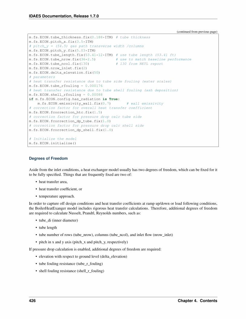
IDAES Documentation, Release 1.7.0
(continued from previous page)
m.fs.ECON.tube_thickness.fix(0.188*ITM) # tube thicknessm.fs.ECON.pitch_x.fix(3.5*ITM)# pitch_y = (54.5) gas path transverse width /columnsm.fs.ECON.pitch_y.fix(5.03*ITM)m.fs.ECON.tube_length.fix(53.41*12*ITM) # use tube length (53.41 ft)m.fs.ECON.tube_nrow.fix(36*2.5) # use to match baseline performancem.fs.ECON.tube_ncol.fix(130) # 130 from NETL reportm.fs.ECON.nrow_inlet.fix(2)m.fs.ECON.delta_elevation.fix(50)# parameters# heat transfer resistance due to tube side fouling (water scales)m.fs.ECON.tube_rfouling = 0.000176# heat transfer resistance due to tube shell fouling (ash deposition)m.fs.ECON.shell_rfouling = 0.00088if m.fs.ECON.config.has_radiation is True:
m.fs.ECON.emissivity_wall.fix(0.7) # wall emissivity# correction factor for overall heat transfer coefficientm.fs.ECON.fcorrection_htc.fix(1.5)# correction factor for pressure drop calc tube sidem.fs.ECON.fcorrection_dp_tube.fix(1.0)# correction factor for pressure drop calc shell sidem.fs.ECON.fcorrection_dp_shell.fix(1.0)
# Initialize the modelm.fs.ECON.initialize()
Degrees of Freedom
Aside from the inlet conditions, a heat exchanger model usually has two degrees of freedom, which can be fixed for itto be fully specified. Things that are frequently fixed are two of:
• heat transfer area,
• heat transfer coefficient, or
• temperature approach.
In order to capture off design conditions and heat transfer coefficients at ramp up/down or load following conditions,the BoilerHeatExanger model includes rigorous heat transfer calculations. Therefore, additional degrees of freedomare required to calculate Nusselt, Prandtl, Reynolds numbers, such as:
• tube_di (inner diameter)
• tube length
• tube number of rows (tube_nrow), columns (tube_ncol), and inlet flow (nrow_inlet)
• pitch in x and y axis (pitch_x and pitch_y, respectively)
If pressure drop calculation is enabled, additional degrees of freedom are required:
• elevation with respect to ground level (delta_elevation)
• tube fouling resistance (tube_r_fouling)
• shell fouling resistance (shell_r_fouling)
426 Chapter 4. Contents
IDAES Documentation, Release 1.7.0
Model Structure
The BoilerHeatExchanger model contains two ControlVolume0DBlock blocks. By default the gas side isnamed shell and the water/steam side is named tube. These names are configurable. The sign convention is thatduty is positive for heat flowing from the hot side to the cold side.
The control volumes are configured the same as the ControlVolume0DBlock in the Heater model. TheBoilerHeatExchanger model contains additional constraints that calculate the amount of heat transferred fromthe hot side to the cold side.
The BoilerHeatExchanger has two inlet ports and two outlet ports. By default these are shell_inlet,tube_inlet, shell_outlet, and tube_outlet. If the user supplies different hot and cold side names theinlet and outlets are named accordingly.
Variables
Variable Symbol Index Sets Docheat_duty 𝑄 time Heat transferred from hot side to the cold sidearea 𝐴 None Heat transfer areaU 𝑈 time Heat transfer coefficientdelta_temperature ∆𝑇 time Temperature difference, defaults to LMTD
Note: delta_temperature may be either a variable or expression depending on the callback used. If the specifiedcold side is hotter than the specified hot side this value will be negative.
Constraints
The default constraints can be overridden by providing alternative rules for the heat transfer equation, temperaturedifference, heat transfer coefficient, shell and tube pressure drop. This section describes the default constraints.
Heat transfer from shell to tube:
𝑄 = 𝑈𝐴∆𝑇
Temperature difference is:
∆𝑇 =∆𝑇1 − ∆𝑇2
log𝑒
(Δ𝑇1
Δ𝑇2
)The overall heat transfer coefficient is calculated as a function of convective heat transfer shell and tube, and wallconduction heat transfer resistance.
Convective heat transfer equations:
1
𝑈* 𝑓𝑐𝑜𝑟𝑟𝑒𝑐𝑡𝑖𝑜𝑛ℎ𝑡𝑐 = [
1
ℎ𝑐𝑜𝑛𝑣𝑡𝑢𝑏𝑒+
1
ℎ𝑐𝑜𝑛𝑣𝑠ℎ𝑒𝑙𝑙+ 𝑟 + 𝑡𝑢𝑏𝑒𝑟𝑓𝑜𝑢𝑙𝑖𝑛𝑔 + 𝑠ℎ𝑒𝑙𝑙𝑟𝑓𝑜𝑢𝑙𝑖𝑛𝑔]
ℎ𝑐𝑜𝑛𝑣𝑡𝑢𝑏𝑒 =𝑁𝑢𝑡𝑢𝑏𝑒𝑘
𝑡𝑢𝑏𝑒𝑑𝑖
𝑁𝑢𝑡𝑢𝑏𝑒 = 0.023𝑅𝑒0.8𝑡𝑢𝑏𝑒𝑃𝑟0.4𝑡𝑢𝑏𝑒
𝑃𝑟𝑡𝑢𝑏𝑒 =𝐶𝑝𝜇
𝑘𝑀𝑤
4.5. Technical Specifications 427
IDAES Documentation, Release 1.7.0
𝑅𝑒𝑡𝑢𝑏𝑒 =𝑡𝑢𝑏𝑒𝑑𝑖𝑉 𝜌
𝜇
ℎ𝑐𝑜𝑛𝑣𝑠ℎ𝑒𝑙𝑙 =𝑁𝑢𝑠ℎ𝑒𝑙𝑙𝑘𝑓𝑙𝑢𝑒𝑔𝑎𝑠
𝑡𝑢𝑏𝑒𝑑𝑜
𝑁𝑢𝑠ℎ𝑒𝑙𝑙 = 𝑓𝑎𝑟𝑟𝑎𝑛𝑔𝑒𝑚𝑒𝑛𝑡0.33𝑅𝑒0.6𝑡𝑢𝑏𝑒𝑃𝑟0.3333𝑡𝑢𝑏𝑒
𝑃𝑟𝑠ℎ𝑒𝑙𝑙 =𝐶𝑝𝜇
𝑘𝑀𝑤
𝑅𝑒𝑠ℎ𝑒𝑙𝑙 =𝑡𝑢𝑏𝑒𝑑𝑜𝑉 𝜌
𝜇
𝑡𝑢𝑏𝑒𝑑𝑜 = 2 * 𝑡𝑢𝑏𝑒𝑡ℎ𝑖𝑐𝑘𝑛𝑒𝑠𝑠 + 𝑡𝑢𝑏𝑒𝑑𝑖
Wall heat conduction resistance equation:
𝑟 = 0.5 * 𝑡𝑢𝑏𝑒𝑑𝑜 * log (𝑡𝑢𝑏𝑒𝑑𝑜𝑡𝑢𝑏𝑒𝑑𝑖
) * 𝑘
where:
• hconv_tube : convective heat transfer resistance tube side (fluid water/steam) (W / m2 / K)
• hconv_shell : convective heat transfer resistance shell side (fluid Flue Gas) (W / m2 / K )
• Nu : Nusselt number
• Pr : Prandtl number
• Re : Reynolds number
• V: velocity (m/s)
• tube_di : inner diameter of the tube (m)
• tube_do : outer diameter of the tube (m) (expression calculated by the model)
• tube_thickness : tube thickness (m)
• r = wall heat conduction resistance (K m^2 / W)
• k : thermal conductivity of the tube wall (W / m / K)
• 𝜌 : density (kg/m^3)
• 𝜇 : viscocity (kg/m/s)
• tube_r_fouling : tube side fouling resistance (K m^2 / W)
• shell_r_fouling : shell side fouling resistance (K m^2 / W)
• fcorrection_htc: correction factor for overall heat trasnfer
• f_arrangement: tube arrangement factor
Note: by default fcorrection_htc is set to 1, however, this variable can be used to match unit performance (i.e. as aparameter estimation problem using real plant data).
Tube arrangement factor is a config argument with two different type of arrangements supported at the moment: 1.-In-line tube arrangement factor (f_arrangement = 0.788), and 2.- Staggered tube arrangement factor (f_arrangement =1). f_arrangement is a parameter that can be adjusted by the user.
The BoilerHeatExchanger includes an argument to compute heat tranfer due to radiation of the flue gases.If has_radiation = True the model builds additional heat transfer calculations that will be added to the hconv_shell
428 Chapter 4. Contents
IDAES Documentation, Release 1.7.0
resistances. Radiation effects are calculated based on the gas gray fraction and gas-surface radiation (between gas andshell).
𝐺𝑎𝑠𝑔𝑟𝑎𝑦𝑓𝑟𝑎𝑐 = 𝑓(𝑔𝑎𝑠𝑒𝑚𝑖𝑠𝑠𝑖𝑣𝑖𝑡𝑦)
𝑓𝑟𝑎𝑑𝑔𝑎𝑠𝑔𝑟𝑎𝑦𝑓𝑟𝑎𝑐 = 𝑓(𝑤𝑎𝑙𝑙𝑒𝑚𝑖𝑠𝑠𝑖𝑣𝑖𝑡𝑦, 𝑔𝑎𝑠𝑒𝑚𝑖𝑠𝑠𝑖𝑣𝑖𝑡𝑦)
ℎ𝑐𝑜𝑛𝑣𝑠ℎ𝑒𝑙𝑙𝑟𝑎𝑑 = 𝑓(𝑘𝑏𝑜𝑙𝑡𝑧𝑚𝑎𝑛𝑛, 𝑓𝑟𝑎𝑑𝑔𝑎𝑠𝑔𝑟𝑎𝑦𝑓𝑟𝑎𝑐, 𝑇𝑔𝑎𝑠𝑖𝑛, 𝑇𝑔𝑎𝑠𝑜𝑢𝑡, 𝑇𝑓𝑙𝑢𝑖𝑑𝑖𝑛, 𝑇𝑓𝑙𝑢𝑖𝑑𝑜𝑢𝑡)
Note: Gas emissivity is calculated with surrogate models (see more details in boiler_heat_exchanger.py). Radiation =True when flue gas temperatures are higher than 700 K (for example, when the model is used for units like Primarysuperheater, Reheater, or Finishing Superheater; while Radiation = False when the model is used to represent theeconomizer in a power plant flowsheet).
If pressure change is set to True, 𝑑𝑒𝑙𝑡𝑎𝑃𝑢𝑡𝑢𝑟𝑛𝑎𝑛𝑑𝑓𝑟𝑖𝑐𝑡𝑖𝑜𝑛𝑓𝑎𝑐𝑡𝑜𝑟 are calculated
Tube side:
∆𝑃𝑡𝑢𝑏𝑒 = ∆𝑃𝑡𝑢𝑏𝑒𝑓𝑟𝑖𝑐𝑡𝑖𝑜𝑛 + ∆𝑃𝑡𝑢𝑏𝑒𝑢𝑡𝑢𝑟𝑛 − 𝑒𝑙𝑒𝑣𝑎𝑡𝑖𝑜𝑛 * 𝑔 * 𝜌𝑖𝑛 + 𝜌𝑜𝑢𝑡2
∆𝑃𝑡𝑢𝑏𝑒𝑓𝑟𝑖𝑐𝑡𝑖𝑜𝑛 = 𝑓(𝑡𝑢𝑏𝑒𝑑𝑖𝜌, 𝑉𝑡𝑢𝑏𝑒, 𝑛𝑢𝑚𝑏𝑒𝑟𝑜𝑓𝑡𝑢𝑏𝑒𝑠, 𝑡𝑢𝑏𝑒𝑙𝑒𝑛𝑔𝑡ℎ)
∆𝑃𝑡𝑢𝑏𝑒𝑢𝑡𝑢𝑟𝑛 = 𝑓(𝜌, 𝑣𝑡𝑢𝑏𝑒, 𝑘𝑙𝑜𝑠𝑠𝑢𝑡𝑢𝑟𝑛)
where:
• 𝑘𝑙𝑜𝑠𝑠𝑢𝑡𝑢𝑟𝑛 : pressure loss coeficient of a tube u-turn
• g : is the acceleration of gravity 9.807 (m/s^2)
Shell side:
∆𝑃𝑠ℎ𝑒𝑙𝑙 = 1.4∆𝑃𝑠ℎ𝑒𝑙𝑙𝑓𝑟𝑖𝑐𝑡𝑖𝑜𝑛𝜌𝑉2𝑠ℎ𝑒𝑙𝑙
∆𝑃𝑠ℎ𝑒𝑙𝑙𝑓𝑟𝑖𝑐𝑡𝑖𝑜𝑛 is calculated based on the tube arrangement type:
In-line: ∆𝑃𝑠ℎ𝑒𝑙𝑙𝑓𝑟𝑖𝑐𝑡𝑖𝑜𝑛 =
0.044+0.08(
𝑃𝑥𝑡𝑢𝑏𝑒𝑑𝑜
)
(𝑃𝑦
𝑡𝑢𝑏𝑒𝑑𝑜−1)
0.43+ 1.13
(𝑃𝑥
𝑡𝑢𝑏𝑒𝑑𝑜)
𝑅𝑒0.15
Staggered: ∆𝑃𝑠ℎ𝑒𝑙𝑙𝑓𝑟𝑖𝑐𝑡𝑖𝑜𝑛 =
0.25+ 0.118
(𝑃𝑦
𝑡𝑢𝑏𝑒𝑑𝑜−1)1.08
𝑅𝑒0.16
Figure. Tube Arrangement
Class Documentation
Note: The hot_side_config and cold_side_config can also be supplied using the name of the hot andcold sides (shell and tube by default) as in the example.
class idaes.power_generation.unit_models.boiler_heat_exchanger.BoilerHeatExchanger(*args,**kwargs)
Parameters
• rule (function) – A rule function or None. Default rule calls build().
• concrete (bool) – If True, make this a toplevel model. Default - False.
4.5. Technical Specifications 429
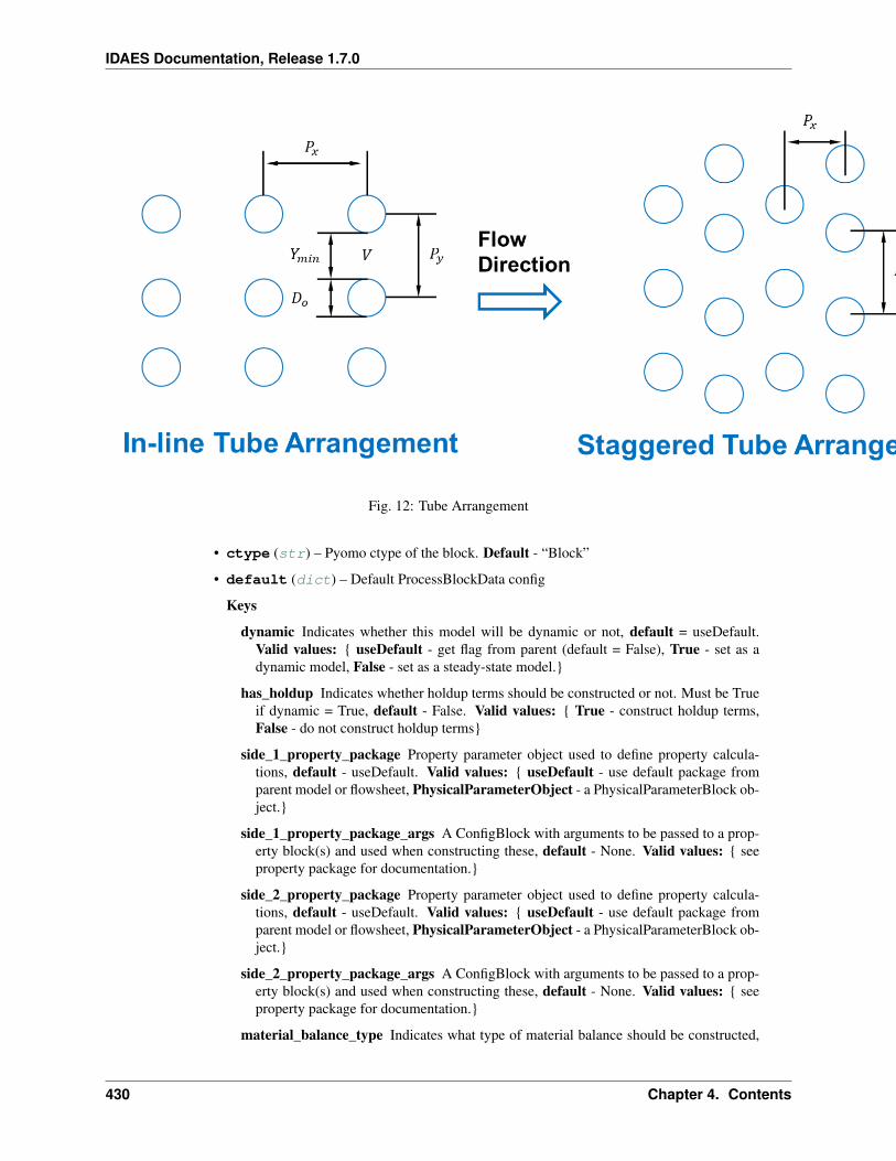
IDAES Documentation, Release 1.7.0
Fig. 12: Tube Arrangement
• ctype (str) – Pyomo ctype of the block. Default - “Block”
• default (dict) – Default ProcessBlockData config
Keys
dynamic Indicates whether this model will be dynamic or not, default = useDefault.Valid values: useDefault - get flag from parent (default = False), True - set as adynamic model, False - set as a steady-state model.
has_holdup Indicates whether holdup terms should be constructed or not. Must be Trueif dynamic = True, default - False. Valid values: True - construct holdup terms,False - do not construct holdup terms
side_1_property_package Property parameter object used to define property calcula-tions, default - useDefault. Valid values: useDefault - use default package fromparent model or flowsheet, PhysicalParameterObject - a PhysicalParameterBlock ob-ject.
side_1_property_package_args A ConfigBlock with arguments to be passed to a prop-erty block(s) and used when constructing these, default - None. Valid values: seeproperty package for documentation.
side_2_property_package Property parameter object used to define property calcula-tions, default - useDefault. Valid values: useDefault - use default package fromparent model or flowsheet, PhysicalParameterObject - a PhysicalParameterBlock ob-ject.
side_2_property_package_args A ConfigBlock with arguments to be passed to a prop-erty block(s) and used when constructing these, default - None. Valid values: seeproperty package for documentation.
material_balance_type Indicates what type of material balance should be constructed,
430 Chapter 4. Contents
IDAES Documentation, Release 1.7.0
default - MaterialBalanceType.componentPhase. Valid values: MaterialBalance-Type.none - exclude material balances, MaterialBalanceType.componentPhase - usephase component balances, MaterialBalanceType.componentTotal - use total com-ponent balances, MaterialBalanceType.elementTotal - use total element balances,MaterialBalanceType.total - use total material balance.
energy_balance_type Indicates what type of energy balance should be constructed, de-fault - EnergyBalanceType.enthalpyTotal. Valid values: EnergyBalanceType.none- exclude energy balances, EnergyBalanceType.enthalpyTotal - single ethalpy bal-ance for material, EnergyBalanceType.enthalpyPhase - ethalpy balances for eachphase, EnergyBalanceType.energyTotal - single energy balance for material, Ener-gyBalanceType.energyPhase - energy balances for each phase.
momentum_balance_type Indicates what type of momentum balance should be con-structed, default - MomentumBalanceType.pressureTotal. Valid values: Mo-mentumBalanceType.none - exclude momentum balances, MomentumBalance-Type.pressureTotal - single pressure balance for material, MomentumBalance-Type.pressurePhase - pressure balances for each phase, MomentumBalance-Type.momentumTotal - single momentum balance for material, MomentumBalance-Type.momentumPhase - momentum balances for each phase.
has_pressure_change Indicates whether terms for pressure change should be con-structed, default - False. Valid values: True - include pressure change terms, False- exclude pressure change terms.
delta_T_method Flag indicating type of flow arrangement to use for delta default -DeltaTMethod.counterCurrent Valid values: DeltaTMethod.counterCurrent
tube_arrangement Tube arrangement could be in-line and staggered
side_1_water_phase Define water phase for property calls
has_radiation Define if side 2 gas radiation is to be considered
• initialize (dict) – ProcessBlockData config for individual elements. Keys are Block-Data indexes and values are dictionaries described under the “default” argument above.
• idx_map (function) – Function to take the index of a BlockData element and return theindex in the initialize dict from which to read arguments. This can be provided to overidethe default behavior of matching the BlockData index exactly to the index in initialize.
Returns (BoilerHeatExchanger) New instance
class idaes.power_generation.unit_models.boiler_heat_exchanger.BoilerHeatExchangerData(component)Standard Heat Exchanger Unit Model Class
build()Build method for Boiler heat exchanger model
Parameters None –
Returns None
initialize(state_args_1=, state_args_2=, outlvl=0, solver=’ipopt’, optarg=’max_iter’: 100,’tol’: 1e-06)
General Heat Exchanger initialisation routine.
Keyword Arguments
• state_args_1 – a dict of arguments to be passed to the property package(s) for side 1of the heat exchanger to provide an initial state for initialization (see documentation of thespecific property package) (default = ).
4.5. Technical Specifications 431
IDAES Documentation, Release 1.7.0
• state_args_2 – a dict of arguments to be passed to the property package(s) for side 2of the heat exchanger to provide an initial state for initialization (see documentation of thespecific property package) (default = ).
• outlvl – sets output level of initialisation routine
– 0 = no output (default)
– 1 = return solver state for each step in routine
– 2 = return solver state for each step in subroutines
– 3 = include solver output infomation (tee=True)
• optarg – solver options dictionary object (default=‘tol’: 1e-6)
• solver – str indicating whcih solver to use during initialization (default = ‘ipopt’)
Returns None
model_check()Model checks for unit - calls model checks for both control volume Blocks.
Parameters None –
Returns None
WaterWall Model
Introduction
The waterwall section model simulates the water hydraulics and the heat transfer inside typical membrane waterwalltubes. The fluid flowing inside the tubes is either liquid water or a mixture of liquid water and steam (two-phase flow).A boiler is typically discretized in multiple zones or sections along its height and a waterwall section model representsone section of the waterwall. It is usually coupled with IDAES’ 1-D fire-side model to solve the wall temperaturesand heat transfer rate in each section. Figure 1 shows a schematic representation of the integrated boiler fire-sideand fluid-side models, in which the sum of the net radiation and convective heat fluxes (𝑞𝑓𝑖𝑟𝑒𝑟𝑎𝑑 and 𝑞𝑓𝑖𝑟𝑒𝑐𝑜𝑛𝑣) at the slagouter layer is an output of the fire-side model and an input of the waterwall section model (the fluid-side model) andthe temperature of the outer slag layer 𝑇𝑤,𝑠𝑙𝑎𝑔 is an output of the fluid-side model and an input (boundary condition)of the fire-side model. The heat conduction through the slag and tube layers is a part of the fluid-side model. At asteady state, the amount of the heat transferred at the outer slag surface (𝑞𝑓𝑖𝑟𝑒𝑟𝑎𝑑 and 𝑞𝑓𝑖𝑟𝑒𝑐𝑜𝑛𝑣) is equal to the heat conductedthrough the slag and tube layers, which is equal to the heat convected to the fluid 𝑞𝑓𝑙𝑢𝑖𝑑𝑐𝑜𝑛𝑣 .
Property package: This model requires the Helmholtz EoS (IAPWS95) property package with the mixed phase option,therefore, the phase equilibrium calculations are handled by the property package.
Figure 1 shows the schematic representation of the coupled fire-side and fluid-side waterwall model. Since, the wa-terwall section is connected with a fire-side section of the boiler, the user must set the number of waterwall sectionsequal to the number of zones in the fire-side model. The first (the lowest) section is generally connected with thewater liquid from a downcomer for a subcritical boiler or the water from the outlet of an economizer for a supercriticalboiler. Other sections are generally connected with their neighboring sections below them via Pyomo Arcs. Finally,the last section is generally connected either to a drum for a subcritical boiler or a superheater for a supercritical boiler.
Model inputs (variable name):
• number of zones (ww_zones)
• number of tubes around the perimeter of the boiler (number_tubes)
• heat duty of individual zone from fire-side model (sum of net radiation and convection) (heat_fireside)
• tube dimensions (length, inside diameter and thickness) (tube_length, tube_diameter, tube_thickness)
432 Chapter 4. Contents
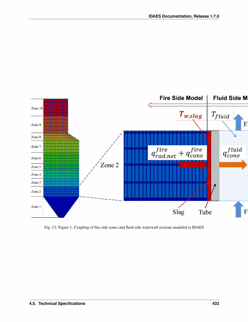
IDAES Documentation, Release 1.7.0
Fig. 13: Figure 1. Coupling of fire-side zones and fluid-side waterwall sections modeled in IDAES
4.5. Technical Specifications 433
IDAES Documentation, Release 1.7.0
• projected membrane wall area (projected_area)
• fin dimension of membrane wall (width and thickness) (fin_length, fin_thickness)
• slag layer thickness (slag_thickness)
• water/steam flow rate and states at inlet (flow_mol, enth_mol, pressure)
• properties of slag and tube metal (thermal conductivity, heat capacity, density) (therm_cond_slag,therm_cond_metal, dens_metal, dens_slag)
• pressure drop correction factor (fcorrection_dp)
Model Outputs:
• temperatures of tube metal at inner wetted surface and at center of the tube thickness (temp_tube_boundary,temp_tube_center)
• temperatures of slag layer at outer surface and at the center of the slag layer (temp_slag_boundary,temp_slag_center)
• pressure drop through each section and heat added to each section (deltaP)
• water/steam flow rate and states at outlet (flow_mol, enth_mol, pressure)
Figure 2 illustrates the physics and main variables in a single waterwall section model. This model assumes thatthe net radiation and convective heat fluxes are given from the fire-side model for the corresponding zone. Themembrane wall geometry and slag layer thickness are the given input variables along with the fluid inlet flow rate andstate conditions. In case of 2-phase flow, the volume fraction of the vapor phase is calculated based on an empiricalcorrelation that calculates the slip velocity between the two phases due to their density difference. The pressure drop ofthe 2-phase flow is calculated based on the liquid-only velocity, Reynolds number and friction factors corrected for thevolume fraction of vapor. Likewise, the convective heat transfer coefficient h_conv on the fluid side is calculated fromempirical correlations for nucleate boiling with forced convection enhancement factor and pool boiling suppressionfactor. The overall heat transfer coefficient is the reciprocal of the overall heat transfer resistance (𝑟ℎ𝑡 in Figure 2).Finally, The heat duty from fire-side model is provided by the user, while the heat conduction model solves the slagouter surface temperature 𝑇𝑤,𝑠𝑙𝑎𝑔, slag layer center point temperature 𝑇𝑐,𝑠𝑙𝑎𝑔, tube center point temperature 𝑇𝑐,𝑡𝑢𝑏𝑒,and tube inner wall temperature 𝑇𝑤,𝑡𝑢𝑏𝑒. The center point temperatures are used to calculate the energy stored inthe slag and tube layers for dynamic simulations. The single waterwall section model eventually calculates the heattransfer rate to the fluid, pressure drop of the fluid in the waterwall section, and the slag outer wall temperature, whichis required as the boundary condition input for the fire-side model. The heat duty from fire-side model is generallyobtained from a surrogate model, the surrogate model must be trained using a rigorous 2-D model under differentoperating conditions. The rigorous 2-D simulates the heat conduction through the complicated geometry of the slagand tube layers and heat convection between the inner tube wall and the fluid. [1]
[1] Ma, J., Eason, J. P., Dowling, A. W., Biegler, L. T., Miller, D. C. (2016). Development of a first-principles hybridboiler model for oxy-combustion power generation system. Int. J. of Greenhouse Gas Contr., 46, pp. 136-157.
Degrees of Freedom
As mentioned above, the water wall section model has been modeled as an index set block, therefore, the numberof zones must be selected during the construction of this model. Each waterwall section is then considered a singlemodel. Aside from the inlet conditions and tube dimensions, a waterwall section model usually has two degrees offreedom, which can be fixed for it to be fully specified. Things that are frequently fixed are two of:
• tube dimensions and number of tubes,
• heat loss to the water wall,
• ash or slag thickness
434 Chapter 4. Contents
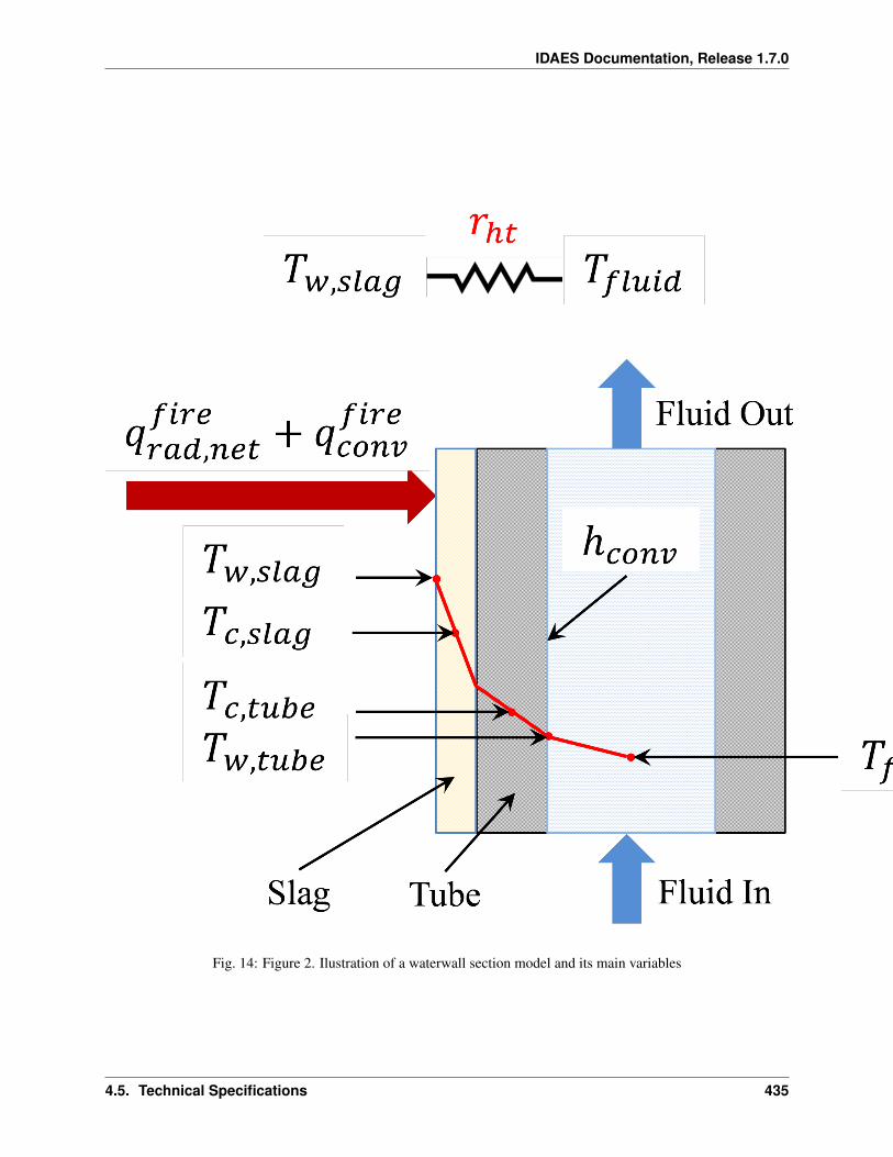
IDAES Documentation, Release 1.7.0
Fig. 14: Figure 2. Ilustration of a waterwall section model and its main variables
4.5. Technical Specifications 435
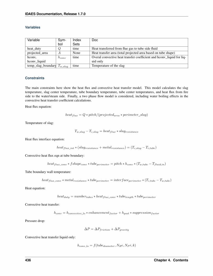
IDAES Documentation, Release 1.7.0
Variables
Variable Sym-bol
IndexSets
Doc
heat_duty 𝑄 time Heat transferred from flue gas to tube side fluidprojected_area 𝐴 None Heat transfer area (total projected area based on tube shape)hconv,hconv_liquid
ℎ𝑐𝑜𝑛𝑣 time Overal convective heat transfer coefficient and hconv_liquid for liq-uid only
temp_slag_boundary 𝑇𝑤,𝑠𝑙𝑎𝑔 time Temperature of the slag
Constraints
The main constraints here show the heat flux and convective heat transfer model. This model calculates the slagtemperature, slag center temperature, tube boundary temperature, tube center temperatures, and heat flux from fireside to the water/steam side. Finally, a two phase flow model is considered, including water boiling effects in theconvective heat transfer coefficient calculations.
Heat flux equation:
ℎ𝑒𝑎𝑡𝑓𝑙𝑢𝑥 = 𝑄 * 𝑝𝑖𝑡𝑐ℎ/(𝑝𝑟𝑜𝑗𝑒𝑐𝑡𝑒𝑑𝑎𝑟𝑒𝑎 * 𝑝𝑒𝑟𝑖𝑚𝑒𝑡𝑒𝑟_𝑠𝑙𝑎𝑔)
Temperature of slag:
𝑇𝑤,𝑠𝑙𝑎𝑔 − 𝑇𝑐,𝑠𝑙𝑎𝑔 = ℎ𝑒𝑎𝑡𝑓𝑙𝑢𝑥 * 𝑠𝑙𝑎𝑔𝑟𝑒𝑠𝑖𝑠𝑡𝑎𝑛𝑐𝑒
Heat flux interface equation:
ℎ𝑒𝑎𝑡𝑓𝑙𝑢𝑥_𝑖𝑛𝑡 * (𝑠𝑙𝑎𝑔𝑟𝑒𝑠𝑖𝑠𝑡𝑎𝑛𝑐𝑒 +𝑚𝑒𝑡𝑎𝑙𝑟𝑒𝑠𝑖𝑠𝑡𝑎𝑛𝑐𝑒) = (𝑇𝑐,𝑠𝑙𝑎𝑔 − 𝑇𝑐,𝑡𝑢𝑏𝑒)
Convective heat flux eqn at tube boundary:
ℎ𝑒𝑎𝑡𝑓𝑙𝑢𝑥_𝑐𝑜𝑛𝑣 * 𝑓𝑠ℎ𝑎𝑝𝑒𝑐𝑜𝑛𝑣 * 𝑡𝑢𝑏𝑒𝑝𝑒𝑟𝑖𝑚𝑒𝑡𝑒𝑟 = 𝑝𝑖𝑡𝑐ℎ * ℎ𝑐𝑜𝑛𝑣 * (𝑇𝑤,𝑡𝑢𝑏𝑒 − 𝑇𝑓𝑙𝑢𝑖𝑑,𝑖𝑛)
Tube boundary wall temperature:
ℎ𝑒𝑎𝑡𝑓𝑙𝑢𝑥_𝑐𝑜𝑛𝑣 *𝑚𝑒𝑡𝑎𝑙𝑟𝑒𝑠𝑖𝑠𝑡𝑎𝑛𝑐𝑒 * 𝑡𝑢𝑏𝑒𝑝𝑒𝑟𝑖𝑚𝑒𝑡𝑒𝑟 = 𝑖𝑛𝑡𝑒𝑟𝑓𝑎𝑐𝑒𝑝𝑒𝑟𝑖𝑚𝑒𝑡𝑒𝑟 * (𝑇𝑐,𝑡𝑢𝑏𝑒 − 𝑇𝑤,𝑡𝑢𝑏𝑒)
Heat equation:
ℎ𝑒𝑎𝑡𝑑𝑢𝑡𝑦 = 𝑛𝑢𝑚𝑏𝑒𝑟𝑡𝑢𝑏𝑒𝑠 * ℎ𝑒𝑎𝑡𝑓𝑙𝑢𝑥_𝑐𝑜𝑛𝑣 * 𝑡𝑢𝑏𝑒𝑙𝑒𝑛𝑔𝑡ℎ * 𝑡𝑢𝑏𝑒𝑝𝑒𝑟𝑖𝑚𝑒𝑡𝑒𝑟
Convective heat transfer:
ℎ𝑐𝑜𝑛𝑣 = ℎ𝑐𝑜𝑛𝑣𝑒𝑐𝑡𝑖𝑣𝑒_𝑙𝑜 * 𝑒𝑛ℎ𝑎𝑛𝑐𝑒𝑚𝑒𝑛𝑡𝑓𝑎𝑐𝑡𝑜𝑟 + ℎ𝑝𝑜𝑜𝑙 * 𝑠𝑢𝑝𝑝𝑟𝑒𝑠𝑠𝑖𝑜𝑛𝑓𝑎𝑐𝑡𝑜𝑟
Pressure drop:
∆𝑃 = ∆𝑃𝑓𝑟𝑖𝑐𝑡𝑖𝑜𝑛 + ∆𝑃𝑔𝑟𝑎𝑣𝑖𝑡𝑦
Convective heat transfer liquid only:
ℎ𝑐𝑜𝑛𝑣_𝑙𝑜 = 𝑓(𝑡𝑢𝑏𝑒𝑑𝑖𝑎𝑚𝑒𝑡𝑒𝑟, 𝑁𝑅𝑒,𝑁𝑃 𝑟, 𝑘)
436 Chapter 4. Contents
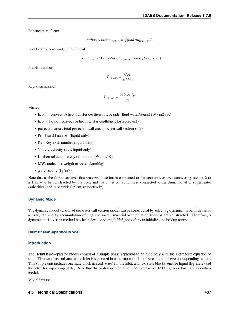
IDAES Documentation, Release 1.7.0
Enhancement factor:
𝑒𝑛ℎ𝑎𝑛𝑐𝑒𝑚𝑒𝑛𝑡𝑓𝑎𝑐𝑡𝑜𝑟 = 𝑓(𝑏𝑜𝑖𝑙𝑖𝑛𝑔𝑛𝑢𝑚𝑏𝑒𝑟)
Pool boiling heat tranfeer coefficient:
ℎ𝑝𝑜𝑜𝑙 = 𝑓(𝑀𝑊, 𝑟𝑒𝑑𝑢𝑐𝑒𝑑𝑝𝑟𝑒𝑠𝑠𝑢𝑟𝑒, ℎ𝑒𝑎𝑡𝑓𝑙𝑢𝑥_𝑐𝑜𝑛𝑣)
Prandtl number:
𝑃𝑟𝑡𝑢𝑏𝑒 =𝐶𝑝𝜇
𝑘𝑀𝑤
Reynolds number:
𝑅𝑒𝑡𝑢𝑏𝑒 =𝑡𝑢𝑏𝑒𝑑𝑖𝑉 𝜌
𝜇
where:
• hconv : convective heat transfer coefficient tube side (fluid water/steam) (W / m2 / K)
• hconv_liquid : convective heat transfer coefficient for liquid only
• projected_area : total projected wall area of waterwall section (m2)
• Pr : Prandtl number (liquid only)
• Re : Reynolds number (liquid only)
• V: fluid velocity (m/s, liquid only)
• k : thermal conductivity of the fluid (W / m / K)
• MW: molecular weigth of water (kmol/kg)
• 𝜇 : viscocity (kg/m/s)
Note that at the flowsheet level first waterwall section is connected to the economizer, arcs connecting section 2 ton-1 have to be constructed by the user, and the outlet of section n is connected to the drum model or superheater(subcritical and supercritical plant, respectively)
Dynamic Model
The dynamic model version of the waterwall section model can be constructed by selecting dynamic=True. If dynamic= True, the energy accumulation of slag and metal, material accumulation holdups are constructed. Therefore, adynamic initialization method has been developed set_initial_conditions to initialize the holdup terms.
HelmPhaseSeparator Model
Introduction
The HelmPhaseSeparator model consist of a simple phase separator to be used only with the Helmholtz equation ofstate. The two-phase mixture at the inlet is separated into the vapor and liquid streams at the two corresponding outlets.This simple unit includes one state block (mixed_state) for the inlet, and two state blocks, one for liquid (liq_state) andthe other for vapor (vap_state). Note that this water-specific flash model replaces IDAES’ generic flash unit operationmodel.
Model inputs:
4.5. Technical Specifications 437
IDAES Documentation, Release 1.7.0
• mixed_state, variables (flow_mol, enth_mol, and pressure), port name = inlet
Model Outputs:
• liq_state, variables (flow_mol, enth_mol, and pressure), port name = liq_outlet
• vap_state, variables (flow_mol, enth_mol, and pressure), port name = vap_outlet
Degrees of Freedom
The HelmPhaseSeparator model consist of nine variables and six constraints. By fixing the inlet state(self.inlet.flow_mol,self.inlet.flow_mol, and self.inlet.flow_mol) or three degrees of freedom, the system will be fullyspecified.
Variables
Variable Symbol Index Sets Docflow_mol 𝐹 time molar flowrateenth_mol ℎ time molar enthalpypressure 𝑃 time pressure
Constraints
The phase separator model uses the IAPWS95 property package to calculate the vapor fraction and enthalpies of thevapor and liquid phases at the inlet of the unit. The flowrates of the vap_outlet and liq_outlet streams are calculate asthe products of the inlet flow rate and corresponding phase fractions for vapor and liquid, respectively. The enthalpiesof the vapor and liquid phases in the inlet stream are assigned to the enthalpies of the vap_outlet and the liq_outletstreams, respectively. The pressure of the two outlet streams are identical to that of the inlet stream.
Material Balances: Vapor State:
𝑓𝑙𝑜𝑤_𝑚𝑜𝑙𝑚𝑖𝑥𝑒𝑑_𝑠𝑡𝑎𝑡𝑒 * 𝑣𝑎𝑝𝑜𝑟_𝑓𝑟𝑎𝑐𝑚𝑖𝑥𝑒𝑑_𝑠𝑡𝑎𝑡𝑒 = 𝑓𝑙𝑜𝑤_𝑚𝑜𝑙𝑣𝑎𝑝𝑜𝑢𝑡𝑙𝑒𝑡
Liquid State:
𝑓𝑙𝑜𝑤_𝑚𝑜𝑙𝑚𝑖𝑥𝑒𝑑_𝑠𝑡𝑎𝑡𝑒 * (1 − 𝑣𝑎𝑝𝑜𝑟_𝑓𝑟𝑎𝑐𝑚𝑖𝑥𝑒𝑑_𝑠𝑡𝑎𝑡𝑒) = 𝑓𝑙𝑜𝑤_𝑚𝑜𝑙𝑙𝑖𝑞𝑜𝑢𝑡𝑙𝑒𝑡
Energy Balances:
𝑒𝑛𝑡ℎ_𝑚𝑜𝑙_𝑝ℎ𝑎𝑠𝑒𝑚𝑖𝑥𝑒𝑑_𝑠𝑡𝑎𝑡𝑒[𝑉 𝑎𝑝] = 𝑒𝑛𝑡ℎ_𝑚𝑜𝑙𝑣𝑎𝑝_𝑠𝑡𝑎𝑡𝑒
𝑒𝑛𝑡ℎ_𝑚𝑜𝑙_𝑝ℎ𝑎𝑠𝑒𝑚𝑖𝑥𝑒𝑑_𝑠𝑡𝑎𝑡𝑒[𝐿𝑖𝑞] = 𝑒𝑛𝑡ℎ_𝑚𝑜𝑙𝑙𝑖𝑞_𝑠𝑡𝑎𝑡𝑒
Momentum Balances:
𝑝𝑟𝑒𝑠𝑠𝑢𝑟𝑒𝑚𝑖𝑥𝑒𝑑_𝑠𝑡𝑎𝑡𝑒[𝐿𝑖𝑞] = 𝑝𝑟𝑒𝑠𝑠𝑢𝑟𝑒𝑙𝑖𝑞_𝑠𝑡𝑎𝑡𝑒 = 𝑝𝑟𝑒𝑠𝑠𝑢𝑟𝑒𝑣𝑎𝑝_𝑠𝑡𝑎𝑡𝑒
Drum Model
Introduction
The drum model consists of three main sub-unit operations:
438 Chapter 4. Contents
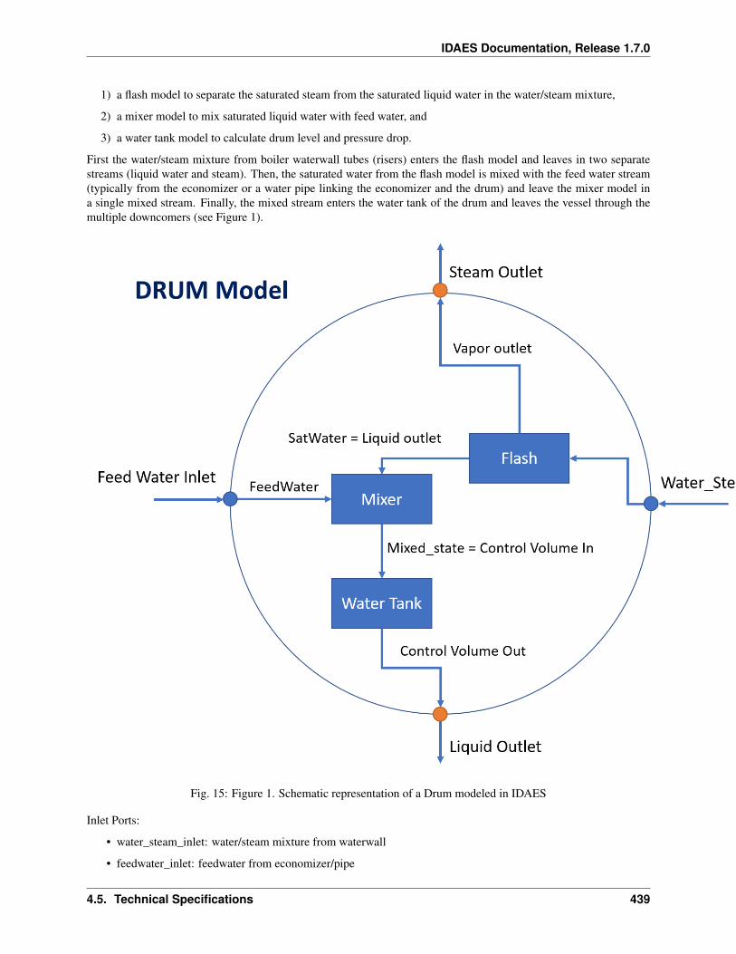
IDAES Documentation, Release 1.7.0
1) a flash model to separate the saturated steam from the saturated liquid water in the water/steam mixture,
2) a mixer model to mix saturated liquid water with feed water, and
3) a water tank model to calculate drum level and pressure drop.
First the water/steam mixture from boiler waterwall tubes (risers) enters the flash model and leaves in two separatestreams (liquid water and steam). Then, the saturated water from the flash model is mixed with the feed water stream(typically from the economizer or a water pipe linking the economizer and the drum) and leave the mixer model ina single mixed stream. Finally, the mixed stream enters the water tank of the drum and leaves the vessel through themultiple downcomers (see Figure 1).
Fig. 15: Figure 1. Schematic representation of a Drum modeled in IDAES
Inlet Ports:
• water_steam_inlet: water/steam mixture from waterwall
• feedwater_inlet: feedwater from economizer/pipe
4.5. Technical Specifications 439
IDAES Documentation, Release 1.7.0
Outlet Ports:
• liquid_outlet: liquid to downcomer
• steam_outlet: saturated steam leaving the drum
Variables
Model inputs (variable name):
• water/steam inlet (water_steam_inlet: flow_mol, enth_mol, pressure)
• feedwater inlet (feedwater_inlet: flow_mol, enth_mol, pressure)
• drum diameter (drum_diameter)
• drum length (drum_length)
• number of downcomer tubes (number_downcomers)
• downcomer diameter (downcomer_diameter)
• drum level (drum_level)
• heat duty (heat_duty)
Model Outputs:
• vapor outlet (vap_outlet: flow_mol, enth_mol, pressure)
• liquid outlet (liq_outlet: flow_mol, enth_mol, pressure)
Constraints
As mentioned above, the drum model imports a HelmPhaseSeparator and mixer models, specific documentation forthese models can be obtained in: Once the water enters the tank model the main equations calculate water velocity andpressure drop calculation due to gravity based on water level and contraction to downcomer. Water level (drum_leve)is either fixed for steady state simulation or calculated for dynamic model (Dynamic = True)
Main assumptions:
1) Heat loss is a variable given by the user (zero heat loss can be specified if adiabatic)
2) Pressure change due to gravity based on water level and contraction to downcomer is calculated
3) Water level is either fixed for steady-state model or calculated for dynamic model
4) Assume enthalpy_in == enthalpy_out + heat loss + energy accumulation
5) Subcooled water from economizer and saturated water from waterwall are well mixed before entering the drum
Pressure equality constraint:
𝑃𝑆𝑎𝑡𝑢𝑟𝑎𝑡𝑒𝑑𝑊𝑎𝑡𝑒𝑟 = 𝑃𝐹𝑒𝑒𝑑𝑊𝑎𝑡𝑒𝑟
Pressure drop in unit:
𝑑𝑒𝑙𝑡𝑎𝑃 = 𝑑𝑒𝑙𝑡𝑎𝑃𝑐𝑜𝑛𝑡𝑟𝑎𝑐𝑡𝑖𝑜𝑛 + 𝑑𝑒𝑙𝑡𝑎𝑃𝑔𝑟𝑎𝑣𝑖𝑡𝑦
𝑑𝑒𝑙𝑡𝑎𝑃𝑔𝑟𝑎𝑣𝑖𝑡𝑦 = 𝑓(𝜌𝑙𝑖𝑞𝑢𝑖𝑑, 𝑎𝑐𝑐𝑒𝑙𝑒𝑟𝑎𝑡𝑖𝑜𝑛𝑔𝑟𝑎𝑣𝑖𝑡𝑦, 𝑑𝑟𝑢𝑚_𝑙𝑒𝑣𝑒𝑙)
𝑑𝑒𝑙𝑡𝑎𝑃𝑐𝑜𝑛𝑡𝑟𝑎𝑐𝑡𝑖𝑜𝑛 = 𝑓(𝜌𝑙𝑖𝑞𝑢𝑖𝑑, 𝑉 )
440 Chapter 4. Contents
IDAES Documentation, Release 1.7.0
where: * V: fluid velocity (m/s, liquid only)
Note that the model builds an Pyomo Arc to connect the Liquid_outlet from the self.aFlash unit to the Satu-ratedWater inlet port of the mixer, and the mixed_state (Mixer outlet) is directly constructed as the Drum con-trol_volume.properties_in. Once the Drum model is constructed, the mixer and flash blocks can be found asself.aDrum.aMixer and self.aDrum.aFlash
Degrees of Freedom
Once the unit dimensions have been fixed, the model generally has 5 degrees of freedom. The water/steam mixtureinlet state (flow_mol, enth_mol, and pressure) and feewater inlet state (flow_mol and enth_mol). The feedwater inletpressure is usually free due to the pressure equality mentioned above.
Dynamic Model
The dynamic model version of the drum model can be constructed by selecting dynamic=True. If dynamic = True,material accumulation, energy accumulation, and drum level must be calculated. Therefore, a dynamic initializationmethod has been developed set_initial_conditions to initialize the holdup terms.
Downcomer Model
Introduction
The Downcomer model consist of a simple pipe model (or a set of pipes) where the inlet stream is the Drum outletand the outlet stream connects with the WaterWall (section 1). The model simply calculates the pressure change dueto friction and gravity, which involves the calculation of fluid velocity, Reynolds number, and friction factor (usingDarcy’s correlation).
Property package: This model requires the Helmholtz EoS (IAPWS95) property package with the mixed phase option,therefore, the phase equilibrium calculations are handled by the property package.
Model inputs (variable name):
• inlet stream (flow_mol, enth_mol, pressure)
• number of downcomer pipes (number_downcomers) same as Drum model
• height of the tubes (height)
• inner diameter of the tubes (diameter)
• heat duty (heat_duty), heat_duty = 0 if adiabatic
Model Outputs:
• outlet stream (flow_mol, enth_mol, pressure)
• pressure change (deltaP) due to gravity and friction
Degrees of Freedom
By specifying the inlet conditions and downcomer dimensions, the model will be fully specified. Things that arefrequently fixed are:
• inlet state vars (generally flow_mol, enth_mol, pressure)
4.5. Technical Specifications 441
IDAES Documentation, Release 1.7.0
• heat_duty to the downcomer (if applicable)
• number_downcomers, height, diameter
Variables
Variable Symbol Index Sets Docheat_duty 𝑄 time Heat transferred from flue gas to tube side fluiddeltaP 𝑑𝑒𝑙𝑡𝑎𝑃 time Pressure change in the unit
Constraints
The main constraints in the model calculate the pressure drop, which is given by deltaP_friction and deltaP_gravity.
Pressure drop:
∆𝑃 = ∆𝑃𝑓𝑟𝑖𝑐𝑡𝑖𝑜𝑛 + ∆𝑃𝑔𝑟𝑎𝑣𝑖𝑡𝑦
Friction:
∆𝑃𝑓𝑟𝑖𝑐𝑡𝑖𝑜𝑛 = 𝑓(𝐹𝑟𝑖𝑐𝑡𝑖𝑜𝑛𝑓𝑎𝑐𝑡𝑜𝑟, 𝜌𝑙𝑖𝑞𝑢𝑖𝑑, 𝑉, 𝑑𝑖𝑎𝑚𝑒𝑡𝑒𝑟)
Friction factor (Darcy’s correlation’):
𝐹𝑟𝑖𝑐𝑡𝑖𝑜𝑛𝑓𝑎𝑐𝑡𝑜𝑟 =0.3164
𝑅𝑒0.25
deltaP gravity:
∆𝑃𝑔𝑟𝑎𝑣𝑖𝑡𝑦 = 𝜌𝑙𝑖𝑞𝑢𝑖𝑑 * 𝑎𝑐𝑐𝑒𝑙𝑒𝑟𝑎𝑡𝑖𝑜𝑛𝑔𝑟𝑎𝑣𝑖𝑡𝑦 * ℎ𝑒𝑖𝑔ℎ𝑡
Reynolds number:
𝑅𝑒 =𝑡𝑢𝑏𝑒𝑑𝑖𝑉 𝜌
𝜇
where:
• Re : Reynolds number (liquid)
• V: fluid velocity (m/s, liquid)
• 𝜌𝑙𝑖𝑞𝑢𝑖𝑑: mass density of liquid (kg/m3)
• 𝜇 : viscocity (kg/m/s)
Dynamic Model
The downcomer dynamic model can be constructed by selecting dynamic=True and hold_up=True. If dynamic andholdup = True, the energy accumulation and material accumulation variables are constructed, which are the derivativesof the corresponding holdup terms with respect to time and are included in the material and energy conservationequations. A dynamic model also requires the specification of initial conditions related to the accumulation variables.The user needs to provide the initial values for the accumulation variables at all time points and fix the initial conditionsto solve the dynamic problem. Therefore, a dynamic initialization method has been developed set_initial_conditionsto initialize the values of the time-indexed accumulation variables to zero and fix the variables at the first time point tozero.
442 Chapter 4. Contents
IDAES Documentation, Release 1.7.0
Property Models
Flue Gas Property Package
A flue gas property package has been developed to provide properties of combustion gases and air. The ideal gasproperty package includes the main components in flue gas: O2, N2, NO, CO2, H2O, SO2
Main parameters:
• molecular weight in kg/kg-mol indexed by component list,
• reference pressure & temperature in Pa and Kelvin,
• critical pressure and temperature in Pa and Kelvin indexed by component list,
• gas constant in J/(mol K),
• constants for specific heat capacity in J/(mol K) indexed by component list and parameter A to H,
• vapor pressure coefficients (Antoine Eq.) P in Bar and T in K indexed by component list and parameters A to C,
Source: NIST webbook (last update: 01/08/2020)
The main methods supported are:
• heat capacity in J/(mol K),
• enthalpy in J/mol,
• entropy in J/(mol K),
• volumetric flowrate m3/s,
• viscosity of mixture in kg/(m s),
• thermal conductivity mixture in J / (m K s),
• molar density m3/mol,
• reduced pressure and temperature (unitless),
Flowsheet Models
Supercritical Coal-Fired Power Plant Flowsheet
This is an example supercritical pulverized coal (SCPC) power plant.This simulation model consist of a ~595 MW gross coal fired power plant.The dimensions and operating conditions used for this simulation do not represent any specific coal-fired powerplant.
This model is for demonstration and tutorial purposes only. Before looking at the model, it may be useful to look atthe process flow diagram (PFD).
SCPC Power Plant (simplified description)
Inputs:
• Throttle valve opening,
• Feed water pump pressure,
• BFW - boiler feed water (from Feed water heaters),
• Coal from pulverizers
4.5. Technical Specifications 443
IDAES Documentation, Release 1.7.0
Main Assumptions:
Coal flowrate is a function of the plant load, the coal HHV is fixed and heat dutty from fire side to waterwall and platen superheater are fixed.
Boiler heat exchanger network:
Water Flow: Fresh water -> FWH’s -> Economizer -> Water Wall -> Primary SH -> Platen SH ->Finishing Superheate -> HP Turbine -> Reheater -> IP Turbine
Flue Gas Flow:
Fire Ball -> Platen SH -> Finishing SH -> Reheater -> o -> Economizer -> Air Preheater-> Primary SH –^
Steam Flow: Boiler -> HP Turbine -> Reheater -> IP Turbine -> Condenser HP, IP, and LP steamextractions to Feed Water Heaters
Main Models used:
• Mixers: Attemperator, Flue gas mix
• Heater: Platen SH, Fire/Water side (simplified model), Feed Water Heaters, Hot Tank, Condenser
• BoilerHeatExchanger: Economizer, Primary SH, Finishing SH, Reheater
– Shell and tube heat exchanger
* tube side: Steam (side 1 holdup)
* shell side: flue gas (side 2 holdup)
• Steam Turbines
• Pumps
Property packages used:
• IAPWS: Water/steam side
• IDEAL GAS: Flue Gas side
Figures Process Flow Diagram:
Gas Solid Contactors Model Library
This specialized IDAES application library contains a suite of generic advanced models that are applicable to gas-solidprocesses. The axially discretized models are one dimensional, with two phases (gas and solid).
Gas Solid Contactors Flowsheets
Contents
ss_BFB_methane_combustion
Gas Solid Contactors Unit Models
Contents
444 Chapter 4. Contents
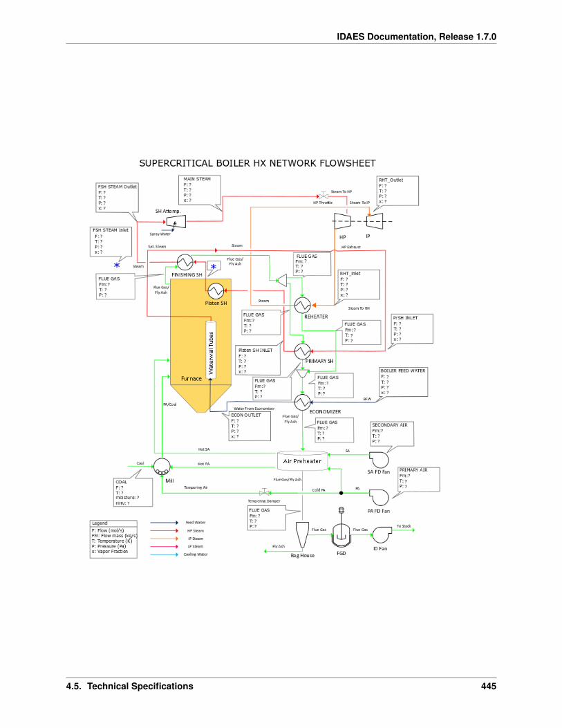
IDAES Documentation, Release 1.7.0
4.5. Technical Specifications 445
IDAES Documentation, Release 1.7.0
Bubbling Fluidized Bed Reactor
The IDAES Bubbling Fluidized Bed Reactor (BFBR) model represents a unit operation where two material streams, asolid phase and a gas phase, pass through a linear vessel while undergoing chemical reaction(s). The BFBR model isrepresented as a 1-D axially discretized model with two phases (gas and solid), and two regions (bubble and emulsion).The model captures the gas-solid interaction between both phases and regions through reaction, mass and heat transfer.
Assumptions:
• Cloud-wake region effects are negligigble and are not modelled.
• Gas emulsion is at minimum fluidization conditions.
• Gas feeds into emulsion region before the excess enters into the bubble region.
• Gas and solids are well mixed in the radial direction but vary axially.
Requirements:
• Property package contains temperature and pressure variables.
• Property package contains minimum fluidization velocity and voidage parameters.
The BFBR model equations are derived from:
• A. Lee, D.C. Miller. A one-dimensional (1-D) three-region model for a bubbling fluidized-bed adsorber, Ind.Eng. Chem. Res. 52 (2013) 469–484.
Degrees of Freedom
BFBRs generally have at least 3 (or more) degrees of freedom, consisting of design and operating variables. The designvariables of reactor length, diameter and number of orifices in the distributor are typically the minimum variables tobe fixed.
Model Structure
The core BFBR unit model consists of two inlet ports (named gas_inlet and solid_inlet), two outlet ports (namedgas_outlet and solid_outlet), and three ControlVolume1DBlock Blocks (named bubble_region, gas_emulsion_regionand solid_emulsion_region).
Construction Arguments
The IDAES BFBR model has construction arguments specific to the whole unit and to the individual regions.
Arguments that are applicable to the BFBR unit as a whole are:
• finite_elements - sets the number of finite elements to use when discretizing the spatial domains (default = 10).
• length_domain_set - sets the list of point to use to initialize a new ContinuousSet (default = [0.0, 1.0]).
• transformation_method - sets the discretization method to use by the Pyomo TransformationFactory to transformthe spatial domain (default = dae.finite_difference):
– dae.finite_difference - finite difference method.
– dae.collocation - orthogonal collocation method.
• transformation_scheme - sets the scheme to use when transforming a domain. Selected schemes should becompatible with the transformation_method chosen (default = None):
446 Chapter 4. Contents
IDAES Documentation, Release 1.7.0
– None - defaults to “BACKWARD” for finite difference transformation method and to “LAGRANGE-RADAU” for collocation transformation method
– BACKWARD - use a finite difference transformation method.
– FORWARD - use a finite difference transformation method.
– LAGRANGE-RADAU - use a collocation transformation method.
• collocation_points - sets the number of collocation points to use when discretizing the spatial domains (default= 3, collocation methods only).
• flow_type - indicates the flow arrangement within the unit to be modeled. Options are:
– ‘co-current’ - (default) gas and solid streams both flow in the same direction (from x=0 to x=1)
– ‘counter-current’ - gas and solid streams flow in opposite directions (gas from x=0 to x=1 and solid fromx=1 to x=0).
• material_balance_type - indicates what type of energy balance should be constructed (default = MaterialBal-anceType.componentTotal).
– MaterialBalanceType.componentTotal - use total component balances.
– MaterialBalanceType.total - use total material balance.
• energy_balance_type - indicates what type of energy balance should be constructed (default = EnergyBalance-Type.enthalpyTotal).
– EnergyBalanceType.none - excludes energy balances.
– EnergyBalanceType.enthalpyTotal - single enthalpy balance for material.
• momentum_balance_type - indicates what type of momentum balance should be constructed (default = Momen-tumBalanceType.pressureTotal).
– MomentumBalanceType.none - exclude momentum balances.
– MomentumBalanceType.pressureTotal - single pressure balance for material.
• has_pressure_change - indicates whether terms for pressure change should be constructed (default = True).
– True - include pressure change terms.
– False - exclude pressure change terms.
Arguments that are applicable to the gas phase:
• property_package - property package to use when constructing bubble region Property Blocks (default =‘use_parent_value’). This is provided as a Physical Parameter Block by the Flowsheet when creating the model.If a value is not provided, the ControlVolume Block will try to use the default property package if one is defined.
• property_package_args - set of arguments to be passed to the bubble region Property Blocks when they arecreated (default = ‘use_parent_value’).
• reaction_package - reaction package to use when constructing bubble region Reaction Blocks (default = None).This is provided as a Reaction Parameter Block by the Flowsheet when creating the model. If a value is notprovided, the ControlVolume Block will try to use the default property package if one is defined.
• reaction_package_args - set of arguments to be passed to the bubble region Reaction Blocks when they arecreated (default = None).
• has_equilibrium_reactions - sets flag to indicate if terms of equilibrium controlled reactions should be con-structed (default = False).
Arguments that are applicable to the solid phase:
4.5. Technical Specifications 447
IDAES Documentation, Release 1.7.0
• property_package - property package to use when constructing bubble region Property Blocks (default =‘use_parent_value’). This is provided as a Physical Parameter Block by the Flowsheet when creating the model.If a value is not provided, the ControlVolume Block will try to use the default property package if one is defined.
• property_package_args - set of arguments to be passed to the bubble region Property Blocks when they arecreated (default = ‘use_parent_value’).
• reaction_package - reaction package to use when constructing bubble region Reaction Blocks (default = None).This is provided as a Reaction Parameter Block by the Flowsheet when creating the model. If a value is notprovided, the ControlVolume Block will try to use the default property package if one is defined.
• reaction_package_args - set of arguments to be passed to the bubble region Reaction Blocks when they arecreated (default = None).
• has_equilibrium_reactions - sets flag to indicate if terms of equilibrium controlled reactions should be con-structed (default = False).
Additionally, BFBR units have the following construction arguments which are passed to all the ControlVol-ume1DBlock Blocks and are always specified to their default values.
Argument Default Valuedynamic useDefaulthas_holdup useDefault
Constraints
Geometric Constraints
Area of orifice:
𝐴𝑜𝑟 =1
𝑛𝑜𝑟
Bed cross-sectional area:
𝐴𝑏𝑒𝑑 = 𝜋𝐷2
𝑏𝑒𝑑
4
Area of bubble region:
𝐴𝑏,𝑡,𝑥 = 𝛿𝑡,𝑥𝐴𝑏𝑒𝑑
Area of gas emulsion region:
𝐴𝑔𝑒,𝑡,𝑥 = 𝛿𝑒,𝑡,𝑥𝜀𝑒,𝑡,𝑥𝐴𝑏𝑒𝑑
Area of solid emulsion region:
𝐴𝑠𝑒,𝑡,𝑥 = 𝛿𝑒,𝑡,𝑥(1 − 𝜀𝑒,𝑡,𝑥)𝐴𝑏𝑒𝑑
Length of bubble region:
𝐿𝑏 = 𝐿𝑏𝑒𝑑
Length of gas emulsion region:
𝐿𝑔𝑒 = 𝐿𝑏𝑒𝑑
448 Chapter 4. Contents
IDAES Documentation, Release 1.7.0
Length of solid emulsion region:
𝐿𝑠𝑒 = 𝐿𝑏𝑒𝑑
Hydrodynamic Constraints
Emulsion region volume fraction:
𝛿𝑒,𝑡,𝑥 = 1 − 𝛿𝑡,𝑥
Average cross-sectional voidage:
𝜀𝑡,𝑥 = 1 − (1 − 𝜀𝑒,𝑡,𝑥) (1 − 𝛿𝑡,𝑥)
Emulsion region voidage:
𝜀𝑒,𝑡,𝑥 = 𝜀𝑚𝑓,𝑠𝑒
Bubble growth coefficient:
𝛾𝑡,𝑥 =0.0256
𝑣𝑚𝑓,𝑠𝑒
(𝐷𝑏𝑒𝑑
𝑔
)0.5
Maximum bubble diameter:
𝑑5𝑏𝑚,𝑡,𝑥𝑔 = 2.595([𝑣𝑔,𝑡,𝑥 − 𝑣𝑔𝑒,𝑡,𝑥]𝐴𝑏𝑒𝑑)2
Bubble diameter (gas inlet, x = 0):
𝑑𝑏,𝑡,𝑥 = 1.38𝑔−0.2([𝑣𝑔,𝑡,𝑥 − 𝑣𝑔𝑒,𝑡,𝑥]𝐴𝑜𝑟)0.4
Bubble diameter (x > 0):
𝑑𝑑𝑏,𝑡,𝑥𝑑𝑥
=0.3
𝐷𝑏𝑒𝑑𝐿𝑏𝑒𝑑
(𝑑𝑏𝑚,𝑡,𝑥 − 𝑑𝑏,𝑡,𝑥 − 𝛾𝑡,𝑥(𝐷𝑏𝑒𝑑𝑑𝑏,𝑡,𝑥)
0.5)
Bubble rise velocity:
𝑣2𝑏𝑟,𝑡,𝑥 = 0.7112𝑔𝑑𝑏,𝑡,𝑥
Bubble velocity:
𝑣𝑏,𝑡,𝑥 = 𝑣𝑔,𝑡,𝑥 − 𝑣𝑚𝑓,𝑠𝑒 + 𝑣𝑏𝑟,𝑡,𝑥
Emulsion region gas velocity:
𝑣𝑔𝑒,𝑡,𝑥 = 𝑣𝑚𝑓,𝑠𝑒
Superficial gas velocity:
𝑣𝑔,𝑡,𝑥 = 𝑣𝑏,𝑡,𝑥𝛿𝑡,𝑥 + 𝑣𝑔𝑒,𝑡,𝑥𝛿𝑒,𝑡,𝑥
Gas emulsion pressure drop:
if ‘has_pressure_change’ is ‘True’:
∆𝑃𝑔𝑒,𝑡,𝑥 = −𝑔(1 − 𝜀𝑒,𝑡,𝑥)𝜌𝑚𝑎𝑠𝑠,𝑠𝑒,𝑡,𝑥
elif ‘has_pressure_change’ is ‘False’:
𝑃𝑔𝑒,𝑡,𝑥 = 𝑃𝑔,𝑡,𝑖𝑛𝑙𝑒𝑡
4.5. Technical Specifications 449
IDAES Documentation, Release 1.7.0
Mass Transfer Constraints
Bubble to emulsion gas mass transfer coefficient:
𝐾𝑏𝑒,𝑡,𝑥,𝑗𝑑1.25𝑏,𝑡,𝑥 = 5.94𝑣𝑚𝑓,𝑠𝑒𝑑
0.25𝑏,𝑡,𝑥 + 5.85𝐷0.5
𝑣𝑎𝑝,𝑔𝑒,𝑡,𝑥,𝑗𝑔0.25
Bulk gas mass transfer:
if 𝐶𝑔𝑒,𝑡𝑜𝑡𝑎𝑙,𝑡,𝑥 > 𝐶𝑏,𝑡𝑜𝑡𝑎𝑙,𝑡,𝑥:
𝐾𝑔𝑏𝑢𝑙𝑘𝑐,𝑡,𝑥,𝑗 = 6𝐾𝑑𝛿𝑡,𝑥𝐴𝑏𝑒𝑑(𝐶𝑔𝑒,𝑡𝑜𝑡𝑎𝑙,𝑡,𝑥 − 𝐶𝑏,𝑡𝑜𝑡𝑎𝑙,𝑡,𝑥)𝑑𝑏,𝑡,𝑥𝑦𝑔𝑒,𝑡,𝑥,𝑗
else:
𝐾𝑔𝑏𝑢𝑙𝑘𝑐,𝑡,𝑥,𝑗 = 6𝐾𝑑𝛿𝑡,𝑥𝐴𝑏𝑒𝑑(𝐶𝑔𝑒,𝑡𝑜𝑡𝑎𝑙,𝑡,𝑥 − 𝐶𝑏,𝑡𝑜𝑡𝑎𝑙,𝑡,𝑥)𝑑𝑏,𝑡,𝑥𝑦𝑏,𝑡,𝑥,𝑗
Heat Transfer Constraints
Bubble to emulsion gas heat transfer coefficient:
𝐻𝑏𝑒,𝑡,𝑥,𝑗𝑑1.25𝑏,𝑡,𝑥 = 4.5𝑣𝑚𝑓,𝑠𝑒𝑐𝑝_𝑣𝑎𝑝,𝑏,𝑡,𝑥𝐶𝑏,𝑡𝑜𝑡𝑎𝑙,𝑡,𝑥𝑑
0.25𝑏,𝑡,𝑥 + 5.85(𝑘𝑣𝑎𝑝,𝑏,𝑡,𝑥𝐶𝑏,𝑡𝑜𝑡𝑎𝑙,𝑡,𝑥𝑐𝑝_𝑣𝑎𝑝,𝑏,𝑡,𝑥)
0.5𝑔0.25
Convective heat transfer coefficient:
ℎ𝑡𝑐,𝑡,𝑥𝑑𝑝,𝑠𝑒 = 0.03𝑘𝑣𝑎𝑝,𝑒,𝑡,𝑥
(𝑣𝑔𝑒,𝑡,𝑥𝑑𝑝,𝑠𝑒
𝐶𝑔𝑒,𝑡𝑜𝑡𝑎𝑙,𝑡,𝑥
𝜇𝑣𝑎𝑝,𝑔𝑒,𝑡,𝑥
)1.3
Emulsion region gas-solids convective heat transfer:
ℎ𝑡_𝑔𝑠,𝑡,𝑥𝑑𝑝,𝑠𝑒 = 6𝛿𝑒,𝑡,𝑥(1 − 𝜀𝑒,𝑡,𝑥)ℎ𝑡𝑐,𝑡,𝑥(𝑇𝑔𝑒,𝑡,𝑥 − 𝑇𝑠𝑒,𝑡,𝑥)
Bulk gas heat transfer:
if 𝐶𝑔𝑒,𝑡𝑜𝑡𝑎𝑙,𝑡,𝑥 > 𝐶𝑏,𝑡𝑜𝑡𝑎𝑙,𝑡,𝑥:
𝐻𝑔𝑏𝑢𝑙𝑘,𝑡,𝑥 = 𝐾𝑑𝛿𝑡,𝑥𝐴𝑏𝑒𝑑(𝐶𝑔𝑒,𝑡𝑜𝑡𝑎𝑙,𝑡,𝑥 − 𝐶𝑏,𝑡𝑜𝑡𝑎𝑙,𝑡,𝑥)𝑑𝑏,𝑡,𝑥𝐻𝑔𝑒,𝑡,𝑥
else:
𝐻𝑔𝑏𝑢𝑙𝑘,𝑡,𝑥 = 𝐾𝑑𝛿𝑡,𝑥𝐴𝑏𝑒𝑑(𝐶𝑔𝑒,𝑡𝑜𝑡𝑎𝑙,𝑡,𝑥 − 𝐶𝑏,𝑡𝑜𝑡𝑎𝑙,𝑡,𝑥)𝑑𝑏,𝑡,𝑥𝐻𝑏,𝑡,𝑥
Mass and heat transfer terms in control volumes
Bubble mass transfer ‘(p=vap)’:
𝑀𝑡𝑟,𝑏,𝑡,𝑥,𝑝,𝑗 = 𝐾𝑔𝑏𝑢𝑙𝑘𝑐,𝑡,𝑥,𝑗 −𝐴𝑏,𝑡,𝑥𝐾𝑏𝑒,𝑡,𝑥,𝑗(𝐶𝑏,𝑡𝑜𝑡𝑎𝑙,𝑡,𝑥 − 𝐶𝑔𝑒,𝑡𝑜𝑡𝑎𝑙,𝑡,𝑥)
Gas emulsion mass transfer ‘(p=vap)’:
𝑀𝑡𝑟,𝑔𝑒,𝑡,𝑥,𝑝,𝑗 = −𝐾𝑔𝑏𝑢𝑙𝑘𝑐,𝑡,𝑥,𝑗 +𝐴𝑏,𝑡,𝑥𝐾𝑏𝑒,𝑡,𝑥,𝑗(𝐶𝑏,𝑡𝑜𝑡𝑎𝑙,𝑡,𝑥 − 𝐶𝑔𝑒,𝑡𝑜𝑡𝑎𝑙,𝑡,𝑥) + 𝑟ℎ𝑒𝑡𝑒𝑟𝑜,𝑔𝑒,𝑡,𝑥,𝑗
if ‘energy_balance_type’ is not ‘EnergyBalanceType.none’:
Bubble heat transfer:
𝐻𝑡𝑟,𝑏,𝑡,𝑥 = 𝐻𝑔𝑏𝑢𝑙𝑘,𝑡,𝑥 −𝐴𝑏,𝑡,𝑥𝐻𝑏𝑒,𝑡,𝑥,𝑗(𝑇𝑏,𝑡,𝑥 − 𝑇𝑔𝑒,𝑡,𝑥)
Gas emulsion heat transfer:
𝐻𝑡𝑟,𝑔𝑒,𝑡,𝑥 = −𝐻𝑔𝑏𝑢𝑙𝑘,𝑡,𝑥 +𝐴𝑏,𝑡,𝑥𝐻𝑏𝑒,𝑡,𝑥,𝑗(𝑇𝑏,𝑡,𝑥 − 𝑇𝑔𝑒,𝑡,𝑥) − ℎ𝑡_𝑔𝑠,𝑡,𝑥𝐴𝑏𝑒𝑑
Solid emulsion heat transfer:
𝐻𝑡𝑟,𝑠𝑒,𝑡,𝑥 = ℎ𝑡_𝑔𝑠,𝑡,𝑥𝐴𝑏𝑒𝑑
450 Chapter 4. Contents
IDAES Documentation, Release 1.7.0
Reaction constraints
if ‘homogeneous reaction package’ is not ‘None’:
Bubble rate reaction extent:
𝑟𝑒𝑥𝑡,𝑏,𝑡,𝑥,𝑟 = 𝐴𝑏,𝑡,𝑥𝑟𝑏,𝑡,𝑥,𝑟
Gas emulsion rate reaction extent:
𝑟𝑒𝑥𝑡,𝑔𝑒,𝑡,𝑥,𝑟 = 𝐴𝑔𝑒,𝑡,𝑥𝑟𝑔𝑒,𝑡,𝑥,𝑟
if ‘heterogeneous reaction package’ is not ‘None’:
Solid emulsion rate reaction extent:
𝑟𝑒𝑥𝑡,𝑠𝑒,𝑡,𝑥,𝑟 = 𝐴𝑠𝑒,𝑡,𝑥𝑟𝑠𝑒,𝑡,𝑥,𝑟
Gas emulsion heterogeneous rate reaction extent:
𝑟ℎ𝑒𝑡𝑒𝑟𝑜,𝑔𝑒,𝑡,𝑥,𝑗 = 𝐴𝑠𝑒,𝑡,𝑥
𝑟𝑒𝑎𝑐𝑡𝑖𝑜𝑛𝑠∑𝑟
𝑠𝑠𝑒,𝑗,𝑟𝑟𝑠𝑒,𝑡,𝑥,𝑟
Flowrate constraints
Bubble gas flowrate:
𝐹𝑚𝑜𝑙,𝑏,𝑡,𝑥 = 𝐴𝑏𝑒𝑑𝛿𝑡,𝑥𝑣𝑏,𝑡,𝑥𝐶𝑏,𝑡𝑜𝑡𝑎𝑙,𝑡,𝑥
Emulsion gas flowrate:
𝐹𝑚𝑜𝑙,𝑔𝑒,𝑡,𝑥 = 𝐴𝑏𝑒𝑑𝑣𝑔𝑒,𝑡,𝑥𝐶𝑔𝑒,𝑡𝑜𝑡𝑎𝑙,𝑡,𝑥
Inlet boundary conditions
if ‘has_pressure_change’ is ‘True’:
Gas emulsion pressure at inlet:
𝑃𝑔𝑒,𝑡,0 = 𝑃𝑔,𝑡,𝑖𝑛𝑙𝑒𝑡 − ∆𝑃𝑜𝑟
Total gas balance at inlet:
𝐹𝑚𝑜𝑙,𝑏,𝑡,0 + 𝐹𝑚𝑜𝑙,𝑔𝑒,𝑡,0 = 𝐹𝑚𝑜𝑙,𝑔,𝑡,𝑖𝑛𝑙𝑒𝑡
Superficial gas velocity at inlet:
𝑣𝑔,𝑡,0 =𝐹𝑚𝑜𝑙,𝑔,𝑡,𝑖𝑛𝑙𝑒𝑡
𝐶𝑔𝑒,𝑡𝑜𝑡𝑎𝑙,𝑡,0𝐴𝑏𝑒𝑑
Bubble mole fraction at inlet:
𝑦𝑏,𝑡,0,𝑗 = 𝑦𝑔,𝑡,𝑖𝑛𝑙𝑒𝑡,𝑗
Gas emulsion mole fraction at inlet:
𝑦𝑔𝑒,𝑡,0,𝑗 = 𝑦𝑔,𝑡,𝑖𝑛𝑙𝑒𝑡,𝑗
Solid emulsion mass flow at inlet:
4.5. Technical Specifications 451
IDAES Documentation, Release 1.7.0
if ‘flow_type’ is ‘co_current’ x = 0 else if ‘flow_type’ is ‘counter_current’ x = 1:
𝐹𝑚𝑎𝑠𝑠,𝑠𝑒,𝑡,𝑥 = 𝐹𝑚𝑎𝑠𝑠,𝑠,𝑡,𝑖𝑛𝑙𝑒𝑡
Solid emulsion mass fraction at inlet:
if ‘flow_type’ is ‘co_current’ x = 0 else if ‘flow_type’ is ‘counter_current’ x = 1:
𝑥𝑠𝑒,𝑡,𝑥 = 𝑥𝑠,𝑡,𝑖𝑛𝑙𝑒𝑡
if ‘energy_balance_type’ is not ‘EnergyBalanceType.none’:
Gas inlet energy balance:
𝐻𝑏,𝑡,0 +𝐻𝑔𝑒,𝑡,0 = 𝐻𝑔,𝑡,𝑖𝑛𝑙𝑒𝑡
Gas emulsion temperature at inlet:
𝑇𝑔𝑒,𝑡,0 = 𝑇𝑔,𝑡,𝑖𝑛𝑙𝑒𝑡
elif ‘energy_balance_type’ is ‘EnergyBalanceType.none’:
Isothermal bubble region:
𝑇𝑏,𝑡,𝑥 = 𝑇𝑔,𝑡,𝑖𝑛𝑙𝑒𝑡
Isothermal gas emulsion region:
𝑇𝑔𝑒,𝑡,𝑥 = 𝑇𝑔,𝑡,𝑖𝑛𝑙𝑒𝑡
Isothermal solid emulsion region:
𝑇𝑠𝑒,𝑡,𝑥 = 𝑇𝑠,𝑡,𝑖𝑛𝑙𝑒𝑡
if ‘flow_type’ is ‘co_current’ x = 0 else if ‘flow_type’ is ‘counter_current’ x = 1:
Solid inlet energy balance:
𝐻𝑠𝑒,𝑡,𝑥 = 𝐻𝑠,𝑡,𝑖𝑛𝑙𝑒𝑡
Outlet boundary conditions
Gas emulsion pressure at outlet:
𝑃𝑔,𝑡,𝑜𝑢𝑡𝑙𝑒𝑡 = 𝑃𝑔𝑒,𝑡,1
Total gas balance at outlet:
𝐹𝑚𝑜𝑙,𝑔,𝑡,𝑜𝑢𝑡𝑙𝑒𝑡 = 𝐹𝑚𝑜𝑙,𝑏,𝑡,1 + 𝐹𝑚𝑜𝑙,𝑔𝑒,𝑡,1
Solid outlet material balance:
if ‘flow_type’ is ‘co_current’ x = 1 else if ‘flow_type’ is ‘counter_current’ x = 0:
𝐹𝑚𝑎𝑠𝑠,𝑠,𝑡,𝑜𝑢𝑡𝑙𝑒𝑡 = 𝐹𝑚𝑎𝑠𝑠,𝑠𝑒,𝑡,𝑥
452 Chapter 4. Contents
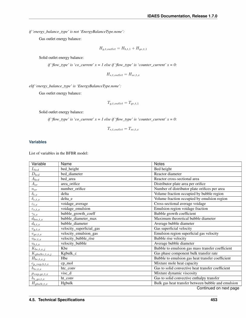
IDAES Documentation, Release 1.7.0
if ‘energy_balance_type’ is not ‘EnergyBalanceType.none’:
Gas outlet energy balance:
𝐻𝑔,𝑡,𝑜𝑢𝑡𝑙𝑒𝑡 = 𝐻𝑏,𝑡,1 +𝐻𝑔𝑒,𝑡,1
Solid outlet energy balance:
if ‘flow_type’ is ‘co_current’ x = 1 else if ‘flow_type’ is ‘counter_current’ x = 0:
𝐻𝑠,𝑡,𝑜𝑢𝑡𝑙𝑒𝑡 = 𝐻𝑠𝑒,𝑡,𝑥
elif ‘energy_balance_type’ is ‘EnergyBalanceType.none’:
Gas outlet energy balance:
𝑇𝑔,𝑡,𝑜𝑢𝑡𝑙𝑒𝑡 = 𝑇𝑔𝑒,𝑡,1
Solid outlet energy balance:
if ‘flow_type’ is ‘co_current’ x = 1 else if ‘flow_type’ is ‘counter_current’ x = 0:
𝑇𝑠,𝑡,𝑜𝑢𝑡𝑙𝑒𝑡 = 𝑇𝑠𝑒,𝑡,𝑥
Variables
List of variables in the BFBR model:
Variable Name Notes𝐿𝑏𝑒𝑑 bed_height Bed height𝐷𝑏𝑒𝑑 bed_diameter Reactor diameter𝐴𝑏𝑒𝑑 bed_area Reactor cross-sectional area𝐴𝑜𝑟 area_orifice Distributor plate area per orifice𝑛𝑜𝑟 number_orifice Number of distributor plate orifices per area𝛿𝑡,𝑥 delta Volume fraction occupied by bubble region𝛿𝑒,𝑡,𝑥 delta_e Volume fraction occupied by emulsion region𝜀𝑡,𝑥 voidage_average Cross-sectional average voidage𝜀𝑒,𝑡,𝑥 voidage_emulsion Emulsion region voidage fraction𝛾𝑡,𝑥 bubble_growth_coeff Bubble growth coefficient𝑑𝑏𝑚,𝑡,𝑥 bubble_diameter_max Maximum theoretical bubble diameter𝑑𝑏,𝑡,𝑥 bubble_diameter Average bubble diameter𝑣𝑔,𝑡,𝑥 velocity_superficial_gas Gas superficial velocity𝑣𝑔𝑒,𝑡,𝑥 velocity_emulsion_gas Emulsion region superficial gas velocity𝑣𝑏𝑟,𝑡,𝑥 velocity_bubble_rise Bubble rise velocity𝑣𝑏,𝑡,𝑥 velocity_bubble Average bubble diameter𝐾𝑏𝑒,𝑡,𝑥,𝑗 Kbe Bubble to emulsion gas mass transfer coefficient𝐾𝑔𝑏𝑢𝑙𝑘𝑐,𝑡,𝑥,𝑗 Kgbulk_c Gas phase component bulk transfer rate𝐻𝑏𝑒,𝑡,𝑥,𝑗 Hbe Bubble to emulsion gas heat transfer coefficient𝑐𝑝_𝑣𝑎𝑝,𝑏,𝑡,𝑥 cp_mol Mixture mole heat capacityℎ𝑡𝑐,𝑡,𝑥 htc_conv Gas to solid convective heat transfer coefficient𝜇𝑣𝑎𝑝,𝑔𝑒,𝑡,𝑥 visc_d Mixture dynamic viscosityℎ𝑡_𝑔𝑠,𝑡,𝑥 ht_conv Gas to solid convective enthalpy transfer𝐻𝑔𝑏𝑢𝑙𝑘,𝑡,𝑥 Hgbulk Bulk gas heat transfer between bubble and emulsion
Continued on next page
4.5. Technical Specifications 453
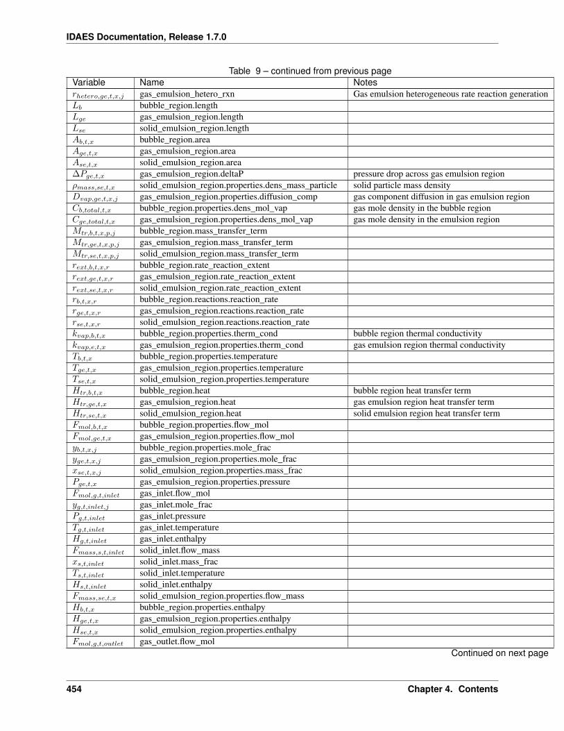
IDAES Documentation, Release 1.7.0
Table 9 – continued from previous pageVariable Name Notes𝑟ℎ𝑒𝑡𝑒𝑟𝑜,𝑔𝑒,𝑡,𝑥,𝑗 gas_emulsion_hetero_rxn Gas emulsion heterogeneous rate reaction generation𝐿𝑏 bubble_region.length𝐿𝑔𝑒 gas_emulsion_region.length𝐿𝑠𝑒 solid_emulsion_region.length𝐴𝑏,𝑡,𝑥 bubble_region.area𝐴𝑔𝑒,𝑡,𝑥 gas_emulsion_region.area𝐴𝑠𝑒,𝑡,𝑥 solid_emulsion_region.area∆𝑃𝑔𝑒,𝑡,𝑥 gas_emulsion_region.deltaP pressure drop across gas emulsion region𝜌𝑚𝑎𝑠𝑠,𝑠𝑒,𝑡,𝑥 solid_emulsion_region.properties.dens_mass_particle solid particle mass density𝐷𝑣𝑎𝑝,𝑔𝑒,𝑡,𝑥,𝑗 gas_emulsion_region.properties.diffusion_comp gas component diffusion in gas emulsion region𝐶𝑏,𝑡𝑜𝑡𝑎𝑙,𝑡,𝑥 bubble_region.properties.dens_mol_vap gas mole density in the bubble region𝐶𝑔𝑒,𝑡𝑜𝑡𝑎𝑙,𝑡,𝑥 gas_emulsion_region.properties.dens_mol_vap gas mole density in the emulsion region𝑀𝑡𝑟,𝑏,𝑡,𝑥,𝑝,𝑗 bubble_region.mass_transfer_term𝑀𝑡𝑟,𝑔𝑒,𝑡,𝑥,𝑝,𝑗 gas_emulsion_region.mass_transfer_term𝑀𝑡𝑟,𝑠𝑒,𝑡,𝑥,𝑝,𝑗 solid_emulsion_region.mass_transfer_term𝑟𝑒𝑥𝑡,𝑏,𝑡,𝑥,𝑟 bubble_region.rate_reaction_extent𝑟𝑒𝑥𝑡,𝑔𝑒,𝑡,𝑥,𝑟 gas_emulsion_region.rate_reaction_extent𝑟𝑒𝑥𝑡,𝑠𝑒,𝑡,𝑥,𝑟 solid_emulsion_region.rate_reaction_extent𝑟𝑏,𝑡,𝑥,𝑟 bubble_region.reactions.reaction_rate𝑟𝑔𝑒,𝑡,𝑥,𝑟 gas_emulsion_region.reactions.reaction_rate𝑟𝑠𝑒,𝑡,𝑥,𝑟 solid_emulsion_region.reactions.reaction_rate𝑘𝑣𝑎𝑝,𝑏,𝑡,𝑥 bubble_region.properties.therm_cond bubble region thermal conductivity𝑘𝑣𝑎𝑝,𝑒,𝑡,𝑥 gas_emulsion_region.properties.therm_cond gas emulsion region thermal conductivity𝑇𝑏,𝑡,𝑥 bubble_region.properties.temperature𝑇𝑔𝑒,𝑡,𝑥 gas_emulsion_region.properties.temperature𝑇𝑠𝑒,𝑡,𝑥 solid_emulsion_region.properties.temperature𝐻𝑡𝑟,𝑏,𝑡,𝑥 bubble_region.heat bubble region heat transfer term𝐻𝑡𝑟,𝑔𝑒,𝑡,𝑥 gas_emulsion_region.heat gas emulsion region heat transfer term𝐻𝑡𝑟,𝑠𝑒,𝑡,𝑥 solid_emulsion_region.heat solid emulsion region heat transfer term𝐹𝑚𝑜𝑙,𝑏,𝑡,𝑥 bubble_region.properties.flow_mol𝐹𝑚𝑜𝑙,𝑔𝑒,𝑡,𝑥 gas_emulsion_region.properties.flow_mol𝑦𝑏,𝑡,𝑥,𝑗 bubble_region.properties.mole_frac𝑦𝑔𝑒,𝑡,𝑥,𝑗 gas_emulsion_region.properties.mole_frac𝑥𝑠𝑒,𝑡,𝑥,𝑗 solid_emulsion_region.properties.mass_frac𝑃𝑔𝑒,𝑡,𝑥 gas_emulsion_region.properties.pressure𝐹𝑚𝑜𝑙,𝑔,𝑡,𝑖𝑛𝑙𝑒𝑡 gas_inlet.flow_mol𝑦𝑔,𝑡,𝑖𝑛𝑙𝑒𝑡,𝑗 gas_inlet.mole_frac𝑃𝑔,𝑡,𝑖𝑛𝑙𝑒𝑡 gas_inlet.pressure𝑇𝑔,𝑡,𝑖𝑛𝑙𝑒𝑡 gas_inlet.temperature𝐻𝑔,𝑡,𝑖𝑛𝑙𝑒𝑡 gas_inlet.enthalpy𝐹𝑚𝑎𝑠𝑠,𝑠,𝑡,𝑖𝑛𝑙𝑒𝑡 solid_inlet.flow_mass𝑥𝑠,𝑡,𝑖𝑛𝑙𝑒𝑡 solid_inlet.mass_frac𝑇𝑠,𝑡,𝑖𝑛𝑙𝑒𝑡 solid_inlet.temperature𝐻𝑠,𝑡,𝑖𝑛𝑙𝑒𝑡 solid_inlet.enthalpy𝐹𝑚𝑎𝑠𝑠,𝑠𝑒,𝑡,𝑥 solid_emulsion_region.properties.flow_mass𝐻𝑏,𝑡,𝑥 bubble_region.properties.enthalpy𝐻𝑔𝑒,𝑡,𝑥 gas_emulsion_region.properties.enthalpy𝐻𝑠𝑒,𝑡,𝑥 solid_emulsion_region.properties.enthalpy𝐹𝑚𝑜𝑙,𝑔,𝑡,𝑜𝑢𝑡𝑙𝑒𝑡 gas_outlet.flow_mol
Continued on next page
454 Chapter 4. Contents
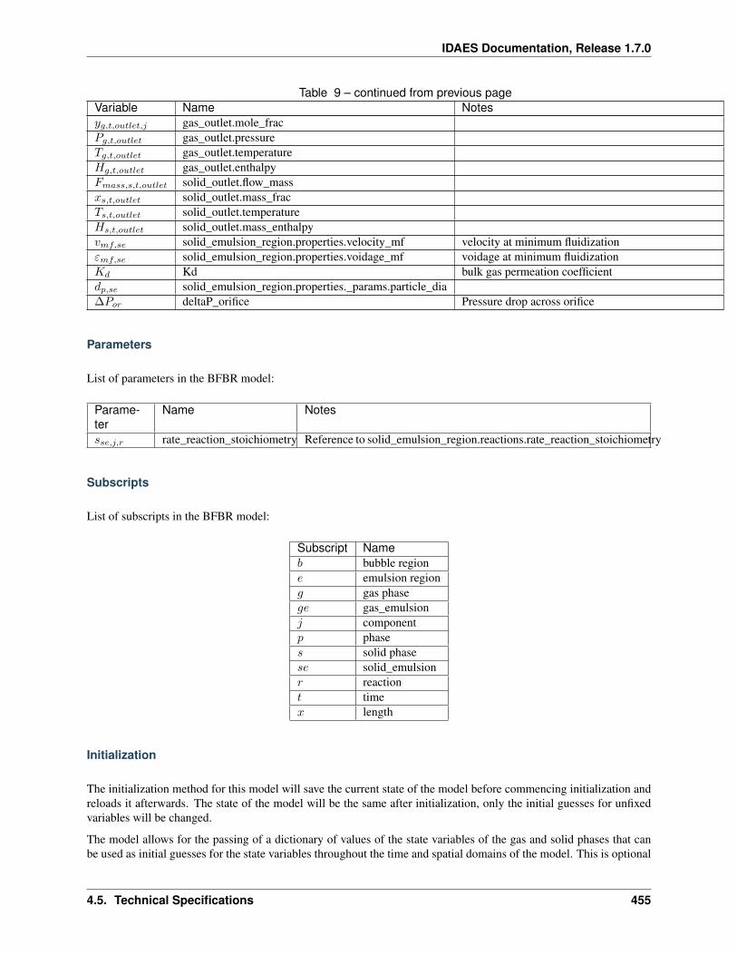
IDAES Documentation, Release 1.7.0
Table 9 – continued from previous pageVariable Name Notes𝑦𝑔,𝑡,𝑜𝑢𝑡𝑙𝑒𝑡,𝑗 gas_outlet.mole_frac𝑃𝑔,𝑡,𝑜𝑢𝑡𝑙𝑒𝑡 gas_outlet.pressure𝑇𝑔,𝑡,𝑜𝑢𝑡𝑙𝑒𝑡 gas_outlet.temperature𝐻𝑔,𝑡,𝑜𝑢𝑡𝑙𝑒𝑡 gas_outlet.enthalpy𝐹𝑚𝑎𝑠𝑠,𝑠,𝑡,𝑜𝑢𝑡𝑙𝑒𝑡 solid_outlet.flow_mass𝑥𝑠,𝑡,𝑜𝑢𝑡𝑙𝑒𝑡 solid_outlet.mass_frac𝑇𝑠,𝑡,𝑜𝑢𝑡𝑙𝑒𝑡 solid_outlet.temperature𝐻𝑠,𝑡,𝑜𝑢𝑡𝑙𝑒𝑡 solid_outlet.mass_enthalpy𝑣𝑚𝑓,𝑠𝑒 solid_emulsion_region.properties.velocity_mf velocity at minimum fluidization𝜀𝑚𝑓,𝑠𝑒 solid_emulsion_region.properties.voidage_mf voidage at minimum fluidization𝐾𝑑 Kd bulk gas permeation coefficient𝑑𝑝,𝑠𝑒 solid_emulsion_region.properties._params.particle_dia∆𝑃𝑜𝑟 deltaP_orifice Pressure drop across orifice
Parameters
List of parameters in the BFBR model:
Parame-ter
Name Notes
𝑠𝑠𝑒,𝑗,𝑟 rate_reaction_stoichiometry Reference to solid_emulsion_region.reactions.rate_reaction_stoichiometry
Subscripts
List of subscripts in the BFBR model:
Subscript Name𝑏 bubble region𝑒 emulsion region𝑔 gas phase𝑔𝑒 gas_emulsion𝑗 component𝑝 phase𝑠 solid phase𝑠𝑒 solid_emulsion𝑟 reaction𝑡 time𝑥 length
Initialization
The initialization method for this model will save the current state of the model before commencing initialization andreloads it afterwards. The state of the model will be the same after initialization, only the initial guesses for unfixedvariables will be changed.
The model allows for the passing of a dictionary of values of the state variables of the gas and solid phases that canbe used as initial guesses for the state variables throughout the time and spatial domains of the model. This is optional
4.5. Technical Specifications 455
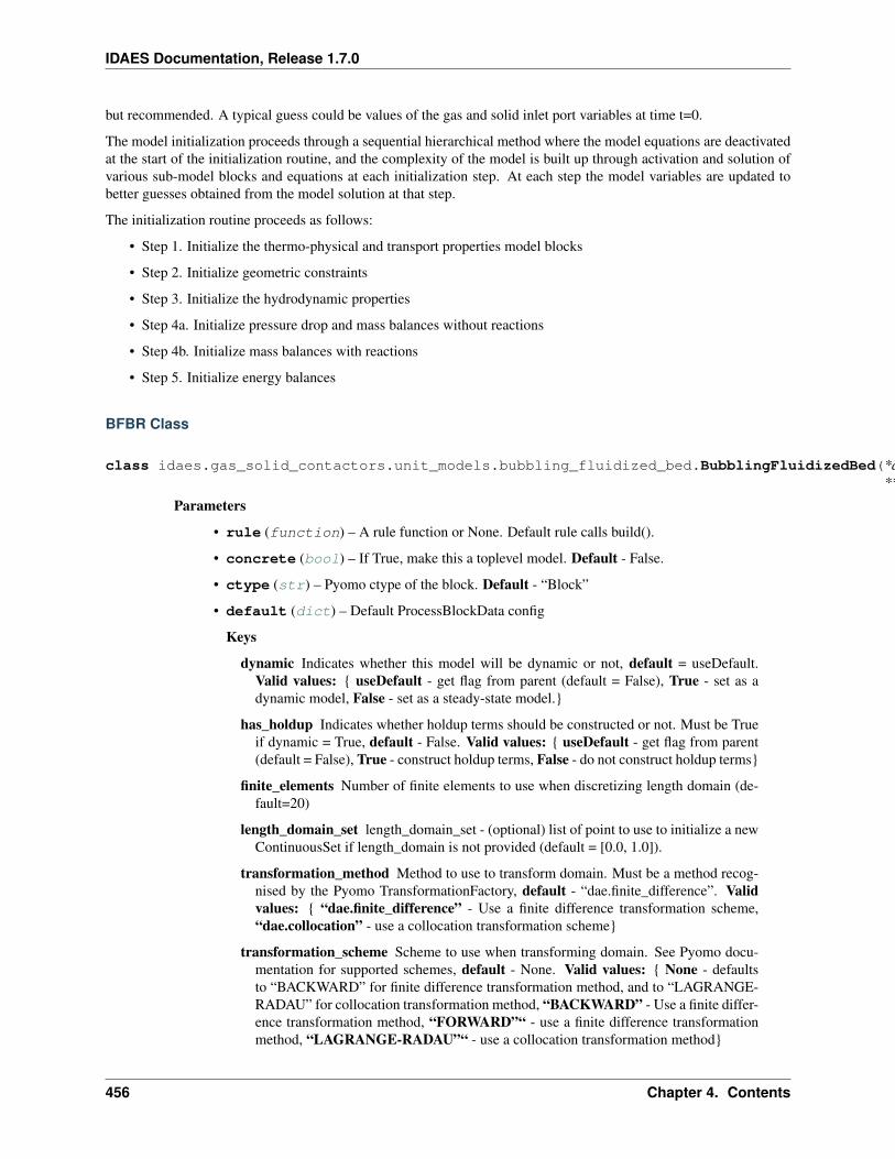
IDAES Documentation, Release 1.7.0
but recommended. A typical guess could be values of the gas and solid inlet port variables at time t=0.
The model initialization proceeds through a sequential hierarchical method where the model equations are deactivatedat the start of the initialization routine, and the complexity of the model is built up through activation and solution ofvarious sub-model blocks and equations at each initialization step. At each step the model variables are updated tobetter guesses obtained from the model solution at that step.
The initialization routine proceeds as follows:
• Step 1. Initialize the thermo-physical and transport properties model blocks
• Step 2. Initialize geometric constraints
• Step 3. Initialize the hydrodynamic properties
• Step 4a. Initialize pressure drop and mass balances without reactions
• Step 4b. Initialize mass balances with reactions
• Step 5. Initialize energy balances
BFBR Class
class idaes.gas_solid_contactors.unit_models.bubbling_fluidized_bed.BubblingFluidizedBed(*args,**kwargs)
Parameters
• rule (function) – A rule function or None. Default rule calls build().
• concrete (bool) – If True, make this a toplevel model. Default - False.
• ctype (str) – Pyomo ctype of the block. Default - “Block”
• default (dict) – Default ProcessBlockData config
Keys
dynamic Indicates whether this model will be dynamic or not, default = useDefault.Valid values: useDefault - get flag from parent (default = False), True - set as adynamic model, False - set as a steady-state model.
has_holdup Indicates whether holdup terms should be constructed or not. Must be Trueif dynamic = True, default - False. Valid values: useDefault - get flag from parent(default = False), True - construct holdup terms, False - do not construct holdup terms
finite_elements Number of finite elements to use when discretizing length domain (de-fault=20)
length_domain_set length_domain_set - (optional) list of point to use to initialize a newContinuousSet if length_domain is not provided (default = [0.0, 1.0]).
transformation_method Method to use to transform domain. Must be a method recog-nised by the Pyomo TransformationFactory, default - “dae.finite_difference”. Validvalues: “dae.finite_difference” - Use a finite difference transformation scheme,“dae.collocation” - use a collocation transformation scheme
transformation_scheme Scheme to use when transforming domain. See Pyomo docu-mentation for supported schemes, default - None. Valid values: None - defaultsto “BACKWARD” for finite difference transformation method, and to “LAGRANGE-RADAU” for collocation transformation method, “BACKWARD” - Use a finite differ-ence transformation method, “FORWARD”“ - use a finite difference transformationmethod, “LAGRANGE-RADAU”“ - use a collocation transformation method
456 Chapter 4. Contents
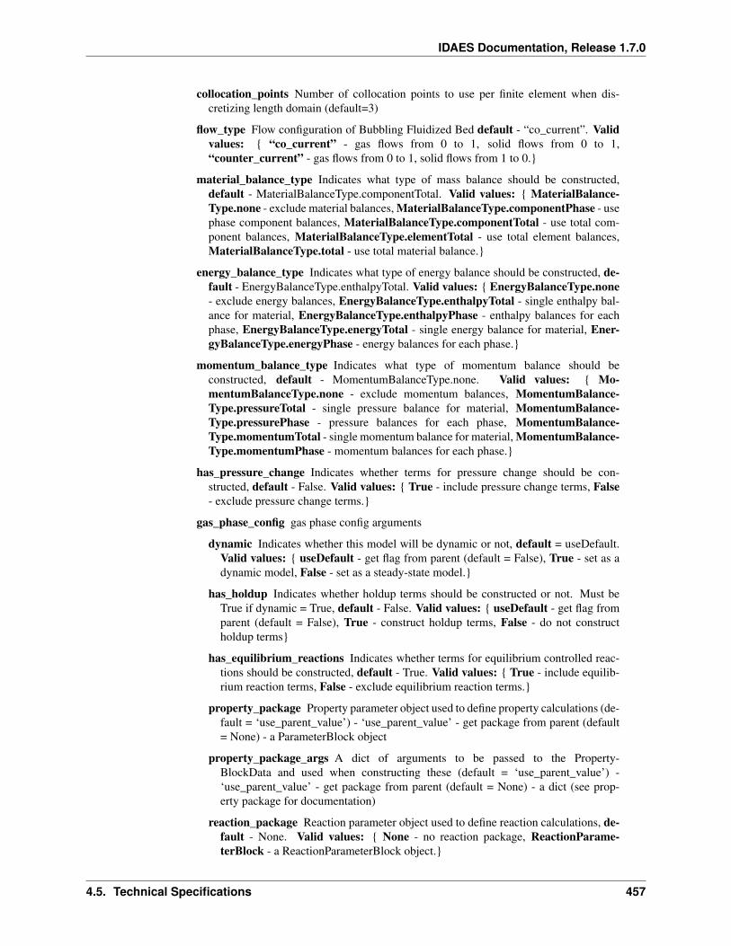
IDAES Documentation, Release 1.7.0
collocation_points Number of collocation points to use per finite element when dis-cretizing length domain (default=3)
flow_type Flow configuration of Bubbling Fluidized Bed default - “co_current”. Validvalues: “co_current” - gas flows from 0 to 1, solid flows from 0 to 1,“counter_current” - gas flows from 0 to 1, solid flows from 1 to 0.
material_balance_type Indicates what type of mass balance should be constructed,default - MaterialBalanceType.componentTotal. Valid values: MaterialBalance-Type.none - exclude material balances, MaterialBalanceType.componentPhase - usephase component balances, MaterialBalanceType.componentTotal - use total com-ponent balances, MaterialBalanceType.elementTotal - use total element balances,MaterialBalanceType.total - use total material balance.
energy_balance_type Indicates what type of energy balance should be constructed, de-fault - EnergyBalanceType.enthalpyTotal. Valid values: EnergyBalanceType.none- exclude energy balances, EnergyBalanceType.enthalpyTotal - single enthalpy bal-ance for material, EnergyBalanceType.enthalpyPhase - enthalpy balances for eachphase, EnergyBalanceType.energyTotal - single energy balance for material, Ener-gyBalanceType.energyPhase - energy balances for each phase.
momentum_balance_type Indicates what type of momentum balance should beconstructed, default - MomentumBalanceType.none. Valid values: Mo-mentumBalanceType.none - exclude momentum balances, MomentumBalance-Type.pressureTotal - single pressure balance for material, MomentumBalance-Type.pressurePhase - pressure balances for each phase, MomentumBalance-Type.momentumTotal - single momentum balance for material, MomentumBalance-Type.momentumPhase - momentum balances for each phase.
has_pressure_change Indicates whether terms for pressure change should be con-structed, default - False. Valid values: True - include pressure change terms, False- exclude pressure change terms.
gas_phase_config gas phase config arguments
dynamic Indicates whether this model will be dynamic or not, default = useDefault.Valid values: useDefault - get flag from parent (default = False), True - set as adynamic model, False - set as a steady-state model.
has_holdup Indicates whether holdup terms should be constructed or not. Must beTrue if dynamic = True, default - False. Valid values: useDefault - get flag fromparent (default = False), True - construct holdup terms, False - do not constructholdup terms
has_equilibrium_reactions Indicates whether terms for equilibrium controlled reac-tions should be constructed, default - True. Valid values: True - include equilib-rium reaction terms, False - exclude equilibrium reaction terms.
property_package Property parameter object used to define property calculations (de-fault = ‘use_parent_value’) - ‘use_parent_value’ - get package from parent (default= None) - a ParameterBlock object
property_package_args A dict of arguments to be passed to the Property-BlockData and used when constructing these (default = ‘use_parent_value’) -‘use_parent_value’ - get package from parent (default = None) - a dict (see prop-erty package for documentation)
reaction_package Reaction parameter object used to define reaction calculations, de-fault - None. Valid values: None - no reaction package, ReactionParame-terBlock - a ReactionParameterBlock object.
4.5. Technical Specifications 457
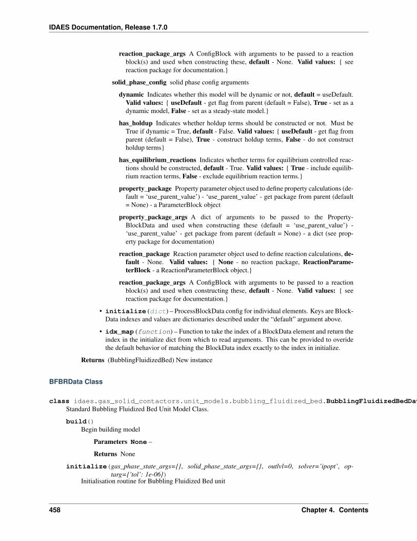
IDAES Documentation, Release 1.7.0
reaction_package_args A ConfigBlock with arguments to be passed to a reactionblock(s) and used when constructing these, default - None. Valid values: seereaction package for documentation.
solid_phase_config solid phase config arguments
dynamic Indicates whether this model will be dynamic or not, default = useDefault.Valid values: useDefault - get flag from parent (default = False), True - set as adynamic model, False - set as a steady-state model.
has_holdup Indicates whether holdup terms should be constructed or not. Must beTrue if dynamic = True, default - False. Valid values: useDefault - get flag fromparent (default = False), True - construct holdup terms, False - do not constructholdup terms
has_equilibrium_reactions Indicates whether terms for equilibrium controlled reac-tions should be constructed, default - True. Valid values: True - include equilib-rium reaction terms, False - exclude equilibrium reaction terms.
property_package Property parameter object used to define property calculations (de-fault = ‘use_parent_value’) - ‘use_parent_value’ - get package from parent (default= None) - a ParameterBlock object
property_package_args A dict of arguments to be passed to the Property-BlockData and used when constructing these (default = ‘use_parent_value’) -‘use_parent_value’ - get package from parent (default = None) - a dict (see prop-erty package for documentation)
reaction_package Reaction parameter object used to define reaction calculations, de-fault - None. Valid values: None - no reaction package, ReactionParame-terBlock - a ReactionParameterBlock object.
reaction_package_args A ConfigBlock with arguments to be passed to a reactionblock(s) and used when constructing these, default - None. Valid values: seereaction package for documentation.
• initialize (dict) – ProcessBlockData config for individual elements. Keys are Block-Data indexes and values are dictionaries described under the “default” argument above.
• idx_map (function) – Function to take the index of a BlockData element and return theindex in the initialize dict from which to read arguments. This can be provided to overidethe default behavior of matching the BlockData index exactly to the index in initialize.
Returns (BubblingFluidizedBed) New instance
BFBRData Class
class idaes.gas_solid_contactors.unit_models.bubbling_fluidized_bed.BubblingFluidizedBedData(component)Standard Bubbling Fluidized Bed Unit Model Class.
build()Begin building model
Parameters None –
Returns None
initialize(gas_phase_state_args=, solid_phase_state_args=, outlvl=0, solver=’ipopt’, op-targ=’tol’: 1e-06)
Initialisation routine for Bubbling Fluidized Bed unit
458 Chapter 4. Contents
IDAES Documentation, Release 1.7.0
Keyword Arguments
• state_args – a dict of arguments to be passed to the property package(s) to provide aninitial state for initialization (see documentation of the specific property package) (default= ).
• outlvl – sets output level of initialisation routine * 0 = no output (default) * 1 = returnsolver state for each step in routine * 2 = return solver state for each step in subroutines *3 = include solver output infomation (tee=True)
• optarg – solver options dictionary object (default=‘tol’: 1e-6)
• solver – str indicating whcih solver to use during initialization (default = ‘ipopt’)
Returns None
results_plot()Plot method for common bubbling fluidized bed variables
Variables plotted: Tge : temperature of gas in the emulsion region Tgb : temperature of gas in the bubbleregion Tse : temperature of solid in the emulsion region Ge : flowrate of gas in the emulsion regionGb : flowrate of gas in the bubble region cet : total concentration of gas in the emulsion region cbt :total concentration of gas in the bubble region y_b : mole fraction of gas components in the bubbleregion x_e : mass fraction of solid components in the emulsion region
Moving Bed Reactor
The IDAES Moving Bed Reactor (MBR) model represents a unit operation where two material streams – a solidphase and a gas phase – pass through a linear reactor vessel while undergoing chemical reaction(s). The two streamshave opposite flow directions (counter-flow). The MBR mathematical model is a 1-D rigorous first-principles modelconsisting of a set of differential equations obtained by applying the mass, energy (for each phase) and momentumbalance equations.
Assumptions:
• The radial concentration and temperature gradients are assumed to be negligible.
• The reactor is assumed to be adiabatic.
• The solid phase is assumed to be moving at a constant velocity determined by the solids feed rate to the reactor.
Requirements:
• Property package contains temperature and pressure variables.
• Property package contains minimum fluidization velocity.
The MBR model is based on:
A. Ostace, A. Lee, C.O. Okoli, A.P. Burgard, D.C. Miller, D. Bhattacharyya, Mathematical modeling of amoving-bed reactor for chemical looping combustion of methane, in: M.R. Eden, M. Ierapetritou, G.P. Towler(Eds.),13th Int. Symp. Process Syst. Eng. (PSE 2018), Computer-Aided Chemical Engineering 2018, pp.325–330 , San Diego, CA.
Degrees of Freedom
MBRs generally have at least 2 (or more) degrees of freedom, consisting of design and operating variables. The designvariables of reactor length and diameter are typically the minimum variables to be fixed.
4.5. Technical Specifications 459
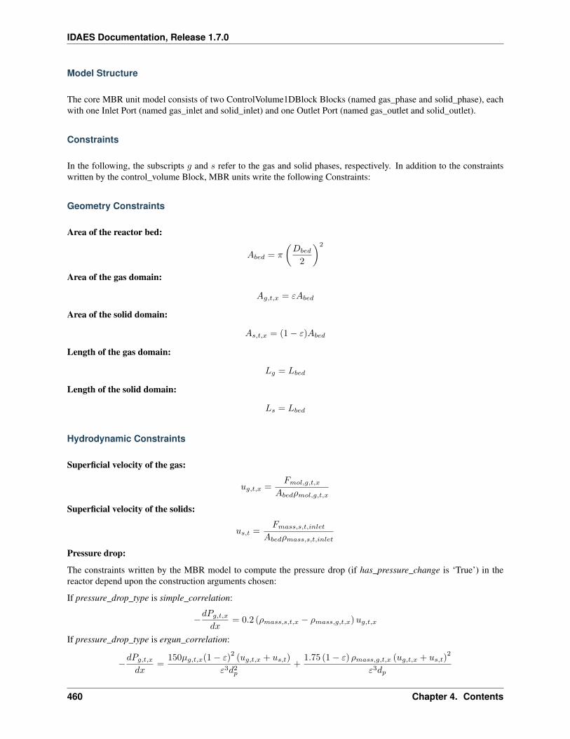
IDAES Documentation, Release 1.7.0
Model Structure
The core MBR unit model consists of two ControlVolume1DBlock Blocks (named gas_phase and solid_phase), eachwith one Inlet Port (named gas_inlet and solid_inlet) and one Outlet Port (named gas_outlet and solid_outlet).
Constraints
In the following, the subscripts 𝑔 and 𝑠 refer to the gas and solid phases, respectively. In addition to the constraintswritten by the control_volume Block, MBR units write the following Constraints:
Geometry Constraints
Area of the reactor bed:
𝐴𝑏𝑒𝑑 = 𝜋
(𝐷𝑏𝑒𝑑
2
)2
Area of the gas domain:
𝐴𝑔,𝑡,𝑥 = 𝜀𝐴𝑏𝑒𝑑
Area of the solid domain:
𝐴𝑠,𝑡,𝑥 = (1 − 𝜀)𝐴𝑏𝑒𝑑
Length of the gas domain:
𝐿𝑔 = 𝐿𝑏𝑒𝑑
Length of the solid domain:
𝐿𝑠 = 𝐿𝑏𝑒𝑑
Hydrodynamic Constraints
Superficial velocity of the gas:
𝑢𝑔,𝑡,𝑥 =𝐹𝑚𝑜𝑙,𝑔,𝑡,𝑥
𝐴𝑏𝑒𝑑𝜌𝑚𝑜𝑙,𝑔,𝑡,𝑥
Superficial velocity of the solids:
𝑢𝑠,𝑡 =𝐹𝑚𝑎𝑠𝑠,𝑠,𝑡,𝑖𝑛𝑙𝑒𝑡
𝐴𝑏𝑒𝑑𝜌𝑚𝑎𝑠𝑠,𝑠,𝑡,𝑖𝑛𝑙𝑒𝑡
Pressure drop:
The constraints written by the MBR model to compute the pressure drop (if has_pressure_change is ‘True’) in thereactor depend upon the construction arguments chosen:
If pressure_drop_type is simple_correlation:
−𝑑𝑃𝑔,𝑡,𝑥
𝑑𝑥= 0.2 (𝜌𝑚𝑎𝑠𝑠,𝑠,𝑡,𝑥 − 𝜌𝑚𝑎𝑠𝑠,𝑔,𝑡,𝑥)𝑢𝑔,𝑡,𝑥
If pressure_drop_type is ergun_correlation:
−𝑑𝑃𝑔,𝑡,𝑥
𝑑𝑥=
150𝜇𝑔,𝑡,𝑥(1 − 𝜀)2
(𝑢𝑔,𝑡,𝑥 + 𝑢𝑠,𝑡)
𝜀3𝑑2𝑝+
1.75 (1 − 𝜀) 𝜌𝑚𝑎𝑠𝑠,𝑔,𝑡,𝑥 (𝑢𝑔,𝑡,𝑥 + 𝑢𝑠,𝑡)2
𝜀3𝑑𝑝
460 Chapter 4. Contents
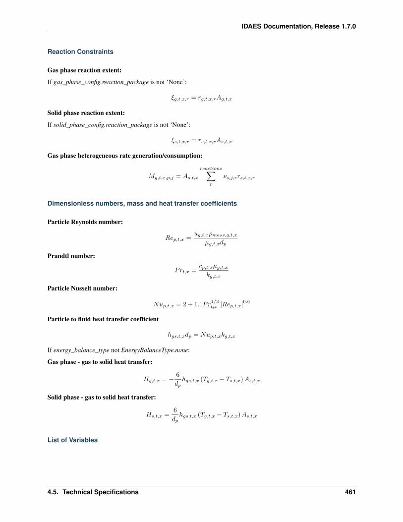
IDAES Documentation, Release 1.7.0
Reaction Constraints
Gas phase reaction extent:
If gas_phase_config.reaction_package is not ‘None’:
𝜉𝑔,𝑡,𝑥,𝑟 = 𝑟𝑔,𝑡,𝑥,𝑟𝐴𝑔,𝑡,𝑥
Solid phase reaction extent:
If solid_phase_config.reaction_package is not ‘None’:
𝜉𝑠,𝑡,𝑥,𝑟 = 𝑟𝑠,𝑡,𝑥,𝑟𝐴𝑠,𝑡,𝑥
Gas phase heterogeneous rate generation/consumption:
𝑀𝑔,𝑡,𝑥,𝑝,𝑗 = 𝐴𝑠,𝑡,𝑥
𝑟𝑒𝑎𝑐𝑡𝑖𝑜𝑛𝑠∑𝑟
𝜈𝑠,𝑗,𝑟𝑟𝑠,𝑡,𝑥,𝑟
Dimensionless numbers, mass and heat transfer coefficients
Particle Reynolds number:
𝑅𝑒𝑝,𝑡,𝑥 =𝑢𝑔,𝑡,𝑥𝜌𝑚𝑎𝑠𝑠,𝑔,𝑡,𝑥
𝜇𝑔,𝑡,𝑥𝑑𝑝
Prandtl number:
𝑃𝑟𝑡,𝑥 =𝑐𝑝,𝑡,𝑥𝜇𝑔,𝑡,𝑥
𝑘𝑔,𝑡,𝑥
Particle Nusselt number:
𝑁𝑢𝑝,𝑡,𝑥 = 2 + 1.1𝑃𝑟1/3𝑡,𝑥 |𝑅𝑒𝑝,𝑡,𝑥|0.6
Particle to fluid heat transfer coefficient
ℎ𝑔𝑠,𝑡,𝑥𝑑𝑝 = 𝑁𝑢𝑝,𝑡,𝑥𝑘𝑔,𝑡,𝑥
If energy_balance_type not EnergyBalanceType.none:
Gas phase - gas to solid heat transfer:
𝐻𝑔,𝑡,𝑥 = − 6
𝑑𝑝ℎ𝑔𝑠,𝑡,𝑥 (𝑇𝑔,𝑡,𝑥 − 𝑇𝑠,𝑡,𝑥)𝐴𝑠,𝑡,𝑥
Solid phase - gas to solid heat transfer:
𝐻𝑠,𝑡,𝑥 =6
𝑑𝑝ℎ𝑔𝑠,𝑡,𝑥 (𝑇𝑔,𝑡,𝑥 − 𝑇𝑠,𝑡,𝑥)𝐴𝑠,𝑡,𝑥
List of Variables
4.5. Technical Specifications 461
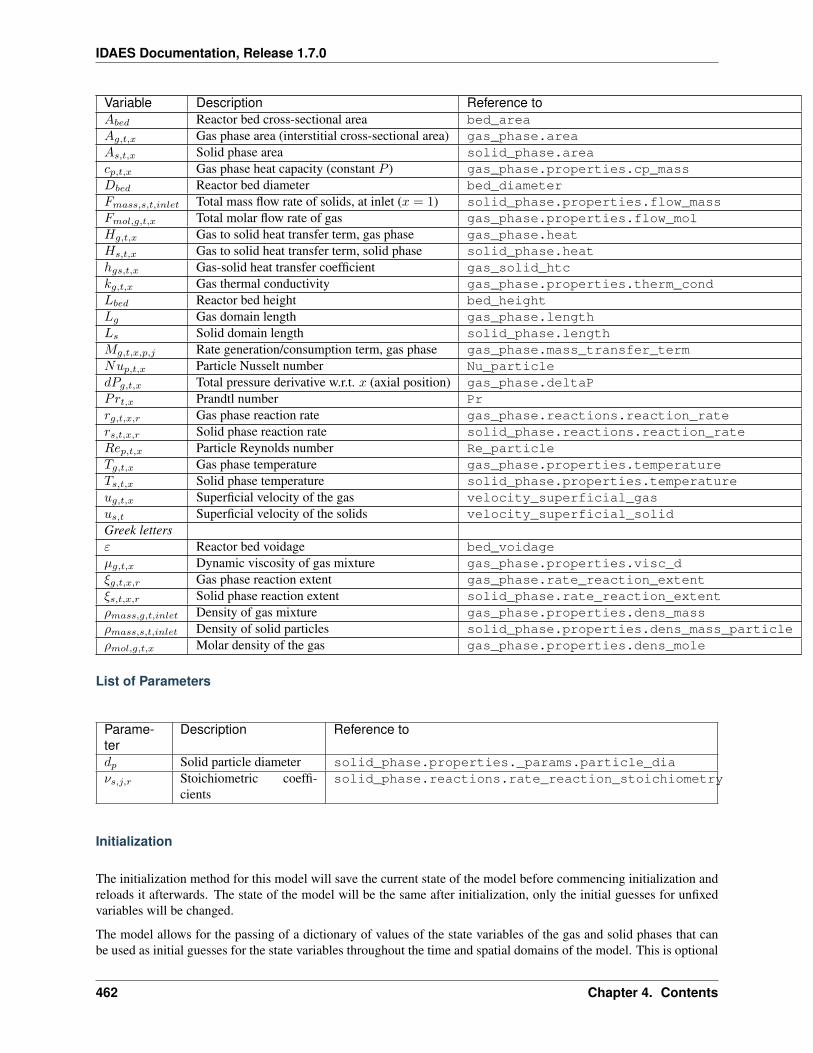
IDAES Documentation, Release 1.7.0
Variable Description Reference to𝐴𝑏𝑒𝑑 Reactor bed cross-sectional area bed_area𝐴𝑔,𝑡,𝑥 Gas phase area (interstitial cross-sectional area) gas_phase.area𝐴𝑠,𝑡,𝑥 Solid phase area solid_phase.area𝑐𝑝,𝑡,𝑥 Gas phase heat capacity (constant 𝑃 ) gas_phase.properties.cp_mass𝐷𝑏𝑒𝑑 Reactor bed diameter bed_diameter𝐹𝑚𝑎𝑠𝑠,𝑠,𝑡,𝑖𝑛𝑙𝑒𝑡 Total mass flow rate of solids, at inlet (𝑥 = 1) solid_phase.properties.flow_mass𝐹𝑚𝑜𝑙,𝑔,𝑡,𝑥 Total molar flow rate of gas gas_phase.properties.flow_mol𝐻𝑔,𝑡,𝑥 Gas to solid heat transfer term, gas phase gas_phase.heat𝐻𝑠,𝑡,𝑥 Gas to solid heat transfer term, solid phase solid_phase.heatℎ𝑔𝑠,𝑡,𝑥 Gas-solid heat transfer coefficient gas_solid_htc𝑘𝑔,𝑡,𝑥 Gas thermal conductivity gas_phase.properties.therm_cond𝐿𝑏𝑒𝑑 Reactor bed height bed_height𝐿𝑔 Gas domain length gas_phase.length𝐿𝑠 Solid domain length solid_phase.length𝑀𝑔,𝑡,𝑥,𝑝,𝑗 Rate generation/consumption term, gas phase gas_phase.mass_transfer_term𝑁𝑢𝑝,𝑡,𝑥 Particle Nusselt number Nu_particle𝑑𝑃𝑔,𝑡,𝑥 Total pressure derivative w.r.t. 𝑥 (axial position) gas_phase.deltaP𝑃𝑟𝑡,𝑥 Prandtl number Pr𝑟𝑔,𝑡,𝑥,𝑟 Gas phase reaction rate gas_phase.reactions.reaction_rate𝑟𝑠,𝑡,𝑥,𝑟 Solid phase reaction rate solid_phase.reactions.reaction_rate𝑅𝑒𝑝,𝑡,𝑥 Particle Reynolds number Re_particle𝑇𝑔,𝑡,𝑥 Gas phase temperature gas_phase.properties.temperature𝑇𝑠,𝑡,𝑥 Solid phase temperature solid_phase.properties.temperature𝑢𝑔,𝑡,𝑥 Superficial velocity of the gas velocity_superficial_gas𝑢𝑠,𝑡 Superficial velocity of the solids velocity_superficial_solidGreek letters𝜀 Reactor bed voidage bed_voidage𝜇𝑔,𝑡,𝑥 Dynamic viscosity of gas mixture gas_phase.properties.visc_d𝜉𝑔,𝑡,𝑥,𝑟 Gas phase reaction extent gas_phase.rate_reaction_extent𝜉𝑠,𝑡,𝑥,𝑟 Solid phase reaction extent solid_phase.rate_reaction_extent𝜌𝑚𝑎𝑠𝑠,𝑔,𝑡,𝑖𝑛𝑙𝑒𝑡 Density of gas mixture gas_phase.properties.dens_mass𝜌𝑚𝑎𝑠𝑠,𝑠,𝑡,𝑖𝑛𝑙𝑒𝑡 Density of solid particles solid_phase.properties.dens_mass_particle𝜌𝑚𝑜𝑙,𝑔,𝑡,𝑥 Molar density of the gas gas_phase.properties.dens_mole
List of Parameters
Parame-ter
Description Reference to
𝑑𝑝 Solid particle diameter solid_phase.properties._params.particle_dia𝜈𝑠,𝑗,𝑟 Stoichiometric coeffi-
cientssolid_phase.reactions.rate_reaction_stoichiometry
Initialization
The initialization method for this model will save the current state of the model before commencing initialization andreloads it afterwards. The state of the model will be the same after initialization, only the initial guesses for unfixedvariables will be changed.
The model allows for the passing of a dictionary of values of the state variables of the gas and solid phases that canbe used as initial guesses for the state variables throughout the time and spatial domains of the model. This is optional
462 Chapter 4. Contents
IDAES Documentation, Release 1.7.0
but recommended. A typical guess could be values of the gas and solid inlet port variables at time 𝑡 = 0.
The model initialization proceeds through a sequential hierarchical method where the model equations are deactivatedat the start of the initialization routine, and the complexity of the model is built up through activation and solution ofvarious sub-model blocks and equations at each initialization step. At each step the model variables are updated tobetter guesses obtained from the model solution at that step.
The initialization routine proceeds in as follows:
• Step 1: Initialize the thermo-physical and transport properties model blocks.
• Step 2: Initialize the hydrodynamic properties.
• Step 3a: Initialize mass balances without reactions and pressure drop.
• Step 3b: Initialize mass balances with reactions and without pressure drop.
• Step 3c: Initialize mass balances with reactions and pressure drop.
• Step 4: Initialize energy balances.
MBR Class
class idaes.gas_solid_contactors.unit_models.moving_bed.MBR(*args, **kwargs)
Parameters
• rule (function) – A rule function or None. Default rule calls build().
• concrete (bool) – If True, make this a toplevel model. Default - False.
• ctype (str) – Pyomo ctype of the block. Default - “Block”
• default (dict) – Default ProcessBlockData config
Keys
dynamic Indicates whether this model will be dynamic or not, default = useDefault.Valid values: useDefault - get flag from parent (default = False), True - set as adynamic model, False - set as a steady-state model.
has_holdup Indicates whether holdup terms should be constructed or not. Must be Trueif dynamic = True, default - False. Valid values: useDefault - get flag from parent(default = False), True - construct holdup terms, False - do not construct holdup terms
finite_elements Number of finite elements to use when discretizing length domain (de-fault=20)
length_domain_set length_domain_set - (optional) list of point to use to initialize a newContinuousSet if length_domain is not provided (default = [0.0, 1.0])
transformation_method Method to use to transform domain. Must be a method recog-nised by the Pyomo TransformationFactory, default - “dae.finite_difference”. Validvalues: “dae.finite_difference” - Use a finite difference transformation method,“dae.collocation” - use a collocation transformation method
transformation_scheme Scheme to use when transforming domain. See Pyomo docu-mentation for supported schemes, default - None. Valid values: None - defaultsto “BACKWARD” for finite difference transformation method, and to “LAGRANGE-RADAU” for collocation transformation method, “BACKWARD” - Use a finite differ-ence transformation method, “FORWARD”“ - use a finite difference transformationmethod, “LAGRANGE-RADAU”“ - use a collocation transformation method
4.5. Technical Specifications 463
IDAES Documentation, Release 1.7.0
collocation_points Number of collocation points to use per finite element when dis-cretizing length domain (default=3)
flow_type Flow configuration of Moving Bed - counter_current: gas side flows from 0to 1 solid side flows from 1 to 0
material_balance_type Indicates what type of mass balance should be constructed,default - MaterialBalanceType.componentTotal. Valid values: MaterialBalance-Type.none - exclude material balances, MaterialBalanceType.componentPhase - usephase component balances, MaterialBalanceType.componentTotal - use total com-ponent balances, MaterialBalanceType.elementTotal - use total element balances,MaterialBalanceType.total - use total material balance.
energy_balance_type Indicates what type of energy balance should be constructed, de-fault - EnergyBalanceType.enthalpyTotal. Valid values: EnergyBalanceType.none- exclude energy balances, EnergyBalanceType.enthalpyTotal - single enthalpy bal-ance for material, EnergyBalanceType.enthalpyPhase - enthalpy balances for eachphase, EnergyBalanceType.energyTotal - single energy balance for material, Ener-gyBalanceType.energyPhase - energy balances for each phase.
momentum_balance_type Indicates what type of momentum balance should be con-structed, default - MomentumBalanceType.pressureTotal. Valid values: Mo-mentumBalanceType.none - exclude momentum balances, MomentumBalance-Type.pressureTotal - single pressure balance for material, MomentumBalance-Type.pressurePhase - pressure balances for each phase, MomentumBalance-Type.momentumTotal - single momentum balance for material, MomentumBalance-Type.momentumPhase - momentum balances for each phase.
has_pressure_change Indicates whether terms for pressure change should be con-structed, default - False. Valid values: True - include pressure change terms, False- exclude pressure change terms.
pressure_drop_type Indicates what type of pressure drop correlation should be used,default - “simple_correlation”. Valid values: “simple_correlation” - Use a simpli-fied pressure drop correlation, “ergun_correlation” - Use the ergun equation.
gas_phase_config gas phase config arguments
dynamic Indicates whether this model will be dynamic or not, default = useDefault.Valid values: useDefault - get flag from parent (default = False), True - set as adynamic model, False - set as a steady-state model.
has_holdup Indicates whether holdup terms should be constructed or not. Must beTrue if dynamic = True, default - False. Valid values: useDefault - get flag fromparent (default = False), True - construct holdup terms, False - do not constructholdup terms
has_equilibrium_reactions Indicates whether terms for equilibrium controlled reac-tions should be constructed, default - True. Valid values: True - include equilib-rium reaction terms, False - exclude equilibrium reaction terms.
property_package Property parameter object used to define property calculations (de-fault = ‘use_parent_value’) - ‘use_parent_value’ - get package from parent (default= None) - a ParameterBlock object
property_package_args A dict of arguments to be passed to the Property-BlockData and used when constructing these (default = ‘use_parent_value’) -‘use_parent_value’ - get package from parent (default = None) - a dict (see prop-erty package for documentation)
464 Chapter 4. Contents
IDAES Documentation, Release 1.7.0
reaction_package Reaction parameter object used to define reaction calculations, de-fault - None. Valid values: None - no reaction package, ReactionParame-terBlock - a ReactionParameterBlock object.
reaction_package_args A ConfigBlock with arguments to be passed to a reactionblock(s) and used when constructing these, default - None. Valid values: seereaction package for documentation.
solid_phase_config solid phase config arguments
dynamic Indicates whether this model will be dynamic or not, default = useDefault.Valid values: useDefault - get flag from parent (default = False), True - set as adynamic model, False - set as a steady-state model.
has_holdup Indicates whether holdup terms should be constructed or not. Must beTrue if dynamic = True, default - False. Valid values: useDefault - get flag fromparent (default = False), True - construct holdup terms, False - do not constructholdup terms
has_equilibrium_reactions Indicates whether terms for equilibrium controlled reac-tions should be constructed, default - True. Valid values: True - include equilib-rium reaction terms, False - exclude equilibrium reaction terms.
property_package Property parameter object used to define property calculations (de-fault = ‘use_parent_value’) - ‘use_parent_value’ - get package from parent (default= None) - a ParameterBlock object
property_package_args A dict of arguments to be passed to the Property-BlockData and used when constructing these (default = ‘use_parent_value’) -‘use_parent_value’ - get package from parent (default = None) - a dict (see prop-erty package for documentation)
reaction_package Reaction parameter object used to define reaction calculations, de-fault - None. Valid values: None - no reaction package, ReactionParame-terBlock - a ReactionParameterBlock object.
reaction_package_args A ConfigBlock with arguments to be passed to a reactionblock(s) and used when constructing these, default - None. Valid values: seereaction package for documentation.
• initialize (dict) – ProcessBlockData config for individual elements. Keys are Block-Data indexes and values are dictionaries described under the “default” argument above.
• idx_map (function) – Function to take the index of a BlockData element and return theindex in the initialize dict from which to read arguments. This can be provided to overidethe default behavior of matching the BlockData index exactly to the index in initialize.
Returns (MBR) New instance
MBRData Class
class idaes.gas_solid_contactors.unit_models.moving_bed.MBRData(component)Standard Moving Bed Unit Model Class.
build()Begin building model (pre-DAE transformation).
Parameters None –
Returns None
4.5. Technical Specifications 465
IDAES Documentation, Release 1.7.0
initialize(gas_phase_state_args=, solid_phase_state_args=, outlvl=0, solver=’ipopt’, op-targ=’tol’: 1e-06)
Initialisation routine for MB unit (default solver ipopt).
Keyword Arguments
• state_args – a dict of arguments to be passed to the property package(s) to provide aninitial state for initialization (see documentation of the specific property package) (default= ).
• outlvl – sets output level of initialisation routine
• optarg – solver options dictionary object (default=‘tol’: 1e-6)
• solver – str indicating whcih solver to use during initialization (default = ‘ipopt’)
Returns None
results_plot()Plot method for common moving bed variables
Variables plotted: Tg : Temperature in gas phase Ts : Temperature in solid phase vg : Superficial gasvelocity P : Pressure in gas phase Ftotal : Total molar flowrate of gas Mtotal : Total mass flowrate ofsolid Cg : Concentration of gas components in the gas phase y_frac : Mole fraction of gas componentsin the gas phase x_frac : Mass fraction of solid components in the solid phase
Gas Solid Contactors Property Models
Contents
methane_iron_OC_reduction
Contents
4.6 License
Institute for the Design of Advanced Energy Systems Process Systems Engineering Framework (IDAES PSE Frame-work) Copyright (c) 2019, by the software owners: The Regents of the University of California, through LawrenceBerkeley National Laboratory, National Technology & Engineering Solutions of Sandia, LLC, Carnegie Mellon Uni-versity, West Virginia University Research Corporation, et al. All rights reserved.
Redistribution and use in source and binary forms, with or without modification, are permitted provided that thefollowing conditions are met:
1. Redistributions of source code must retain the above copyright notice, this list of conditions and the followingdisclaimer.
2. Redistributions in binary form must reproduce the above copyright notice, this list of conditions and the followingdisclaimer in the documentation and/or other materials provided with the distribution.
3. Neither the name of the Institute for the Design of Advanced Energy Systems (IDAES), University of Califor-nia, Lawrence Berkeley National Laboratory, National Technology & Engineering Solutions of Sandia, LLC, SandiaNational Laboratories, Carnegie Mellon University, West Virginia University Research Corporation, U.S. Dept. of En-ergy, nor the names of its contributors may be used to endorse or promote products derived from this software withoutspecific prior written permission.
THIS SOFTWARE IS PROVIDED BY THE COPYRIGHT HOLDERS AND CONTRIBUTORS “AS IS” AND ANYEXPRESS OR IMPLIED WARRANTIES, INCLUDING, BUT NOT LIMITED TO, THE IMPLIED WARRANTIES
466 Chapter 4. Contents
IDAES Documentation, Release 1.7.0
OF MERCHANTABILITY AND FITNESS FOR A PARTICULAR PURPOSE ARE DISCLAIMED. IN NO EVENTSHALL THE COPYRIGHT OWNER OR CONTRIBUTORS BE LIABLE FOR ANY DIRECT, INDIRECT, IN-CIDENTAL, SPECIAL, EXEMPLARY, OR CONSEQUENTIAL DAMAGES (INCLUDING, BUT NOT LIMITEDTO, PROCUREMENT OF SUBSTITUTE GOODS OR SERVICES; LOSS OF USE, DATA, OR PROFITS; OR BUSI-NESS INTERRUPTION) HOWEVER CAUSED AND ON ANY THEORY OF LIABILITY, WHETHER IN CON-TRACT, STRICT LIABILITY, OR TORT (INCLUDING NEGLIGENCE OR OTHERWISE) ARISING IN ANYWAY OUT OF THE USE OF THIS SOFTWARE, EVEN IF ADVISED OF THE POSSIBILITY OF SUCH DAM-AGE.
You are under no obligation whatsoever to provide any bug fixes, patches, or upgrades to the features, functionalityor performance of the source code (“Enhancements”) to anyone; however, if you choose to make your Enhancementsavailable either publicly, or directly to Lawrence Berkeley National Laboratory, without imposing a separate written li-cense agreement for such Enhancements, then you hereby grant Lawrence Berkeley National Laboratory the followinglicense: a non-exclusive, royalty-free perpetual license to install, use, modify, prepare derivative works, incorporateinto other computer software, distribute, and sublicense such enhancements or derivative works thereof, in binary andsource code form.
4.7 Copyright
Institute for the Design of Advanced Energy Systems Process Systems Engineering Framework (IDAES PSE Frame-work) was produced under the DOE Institute for the Design of Advanced Energy Systems (IDAES), and is copyright(c) 2018-2019 by the software owners: The Regents of the University of California, through Lawrence Berkeley Na-tional Laboratory, National Technology & Engineering Solutions of Sandia, LLC, Carnegie Mellon University, WestVirginia University Research Corporation, et al. All rights reserved.
NOTICE. This Software was developed under funding from the U.S. Department of Energy and the U.S. Governmentconsequently retains certain rights. As such, the U.S. Government has been granted for itself and others acting on itsbehalf a paid-up, nonexclusive, irrevocable, worldwide license in the Software to reproduce, distribute copies to thepublic, prepare derivative works, and perform publicly and display publicly, and to permit other to do so. Copyright(C) 2018-2019 IDAES - All Rights Reserved
4.7. Copyright 467

IDAES Documentation, Release 1.7.0
468 Chapter 4. Contents
CHAPTER 5
Indices and tables
• genindex
• modindex
• search
469

IDAES Documentation, Release 1.7.0
470 Chapter 5. Indices and tables
Python Module Index
iidaes.apps.caprese.nmpc, 185idaes.apps.matopt.materials.canvas, 179idaes.apps.matopt.materials.design, 180idaes.apps.matopt.materials.lattices.lattice,
179idaes.apps.matopt.opt.mat_modeling, 182idaes.core.components, 273idaes.core.control_volume0d, 241idaes.core.control_volume1d, 251idaes.core.flowsheet_model, 239idaes.core.phases, 275idaes.core.process_base, 237idaes.core.process_block, 237idaes.core.property_base, 263idaes.core.reaction_base, 268idaes.core.unit_model, 271idaes.core.util.dyn_utils, 276idaes.core.util.homotopy, 280idaes.core.util.initialization, 281idaes.core.util.misc, 316idaes.core.util.model_serializer, 282idaes.core.util.model_statistics, 293idaes.core.util.scaling, 302idaes.core.util.tables, 306idaes.core.util.unit_costing, 311idaes.gas_solid_contactors.unit_models.bubbling_fluidized_bed,
456idaes.gas_solid_contactors.unit_models.moving_bed,
463idaes.generic_models.properties.activity_coeff_models.activity_coeff_prop_pack,
327idaes.generic_models.properties.cubic_eos.cubic_prop_pack,
321idaes.generic_models.properties.iapws95,
329idaes.generic_models.unit_models.cstr,
342idaes.generic_models.unit_models.equilibrium_reactor,
345idaes.generic_models.unit_models.feed,
347idaes.generic_models.unit_models.feed_flash,
349idaes.generic_models.unit_models.flash,
352idaes.generic_models.unit_models.gibbs_reactor,
355idaes.generic_models.unit_models.heat_exchanger_1D,
366idaes.generic_models.unit_models.heater,
356idaes.generic_models.unit_models.mixer,
372idaes.generic_models.unit_models.plug_flow_reactor,
376idaes.generic_models.unit_models.pressure_changer,
380idaes.generic_models.unit_models.product,
383idaes.generic_models.unit_models.separator,
387idaes.generic_models.unit_models.statejunction,
391idaes.generic_models.unit_models.stoichiometric_reactor,
392idaes.generic_models.unit_models.translator,
394idaes.power_generation.unit_models.feedwater_heater_0D,
402idaes.power_generation.unit_models.turbine_inlet,
405idaes.power_generation.unit_models.turbine_multistage,
416idaes.power_generation.unit_models.turbine_outlet,
409idaes.power_generation.unit_models.turbine_stage,
413idaes.power_generation.unit_models.valve_steam,
471
IDAES Documentation, Release 1.7.0
421idaes.surrogate.pysmo.kriging, 166idaes.surrogate.pysmo.polynomial_regression,
153idaes.surrogate.pysmo.radial_basis_function,
160
472 Python Module Index
Index
Symbols-by value
dmf-find command line option, 86-color
dmf-ls command line option, 91dmf-related command line option, 98dmf-status command line option, 101
-contained resourcedmf-register command line option, 93
-createdmf-init command line option, 90idaes-bin-directory command line
option, 125idaes-data-directory command line
option, 126idaes-lib-directory command line
option, 129-created value
dmf-find command line option, 86-derived resource
dmf-register command line option, 93-desc
dmf-init command line option, 90-exists
idaes-bin-directory command lineoption, 125
idaes-data-directory command lineoption, 126
idaes-lib-directory command lineoption, 129
-file valuedmf-find command line option, 87
-helpcommand line option, 131idaes-bin-directory command line
option, 125idaes-copyright command line
option, 125idaes-data-directory command line
option, 126idaes-get-examples command line
option, 127idaes-get-extensions command line
option, 128idaes-lib-directory command line
option, 129-is-subject
dmf-register command line option, 94-list,-no-list
dmf-rm command line option, 99-modified value
dmf-find command line option, 87-multiple
dmf-info command line option, 88dmf-rm command line option, 99
-namedmf-init command line option, 90
-name valuedmf-find command line option, 87
-no-colordmf-ls command line option, 91dmf-related command line option, 98dmf-status command line option, 101
-no-copydmf-register command line option, 93
-no-prefixdmf-ls command line option, 92
-no-unicodedmf-related command line option, 98
-no-uniquedmf-register command line option, 93
-output valuedmf-find command line option, 86
-prev resourcedmf-register command line option, 93
-quietcommand line option, 131dmf command line option, 84
-strict
473
IDAES Documentation, Release 1.7.0
dmf-register command line option, 93-type value
dmf-find command line option, 87-unicode
dmf-related command line option, 98-url
idaes-get-extensions command lineoption, 128
-used resourcedmf-register command line option, 93
-verbosecommand line option, 131dmf command line option, 83
-versiondmf-register command line option, 94
-I, -no-installidaes-get-examples command line
option, 127-N, -no-download
idaes-get-examples command lineoption, 127
-S,-sortdmf-ls command line option, 91
-U, -unstableidaes-get-examples command line
option, 127-V, -version TEXT
idaes-get-examples command lineoption, 127
-a,-alldmf-status command line option, 101
-d,-dir TEXTidaes-get-examples command line
option, 127-d,-direction
dmf-related command line option, 97-f,-format value
dmf-info command line option, 88-l, -list-releases
idaes-get-examples command lineoption, 127
-qcommand line option, 131dmf command line option, 83
-r,-reversedmf-ls command line option, 92
-s,-showdmf-ls command line option, 91
-s,-show infodmf-status command line option, 101
-t,-typedmf-register command line option, 93
-vcommand line option, 131
dmf command line option, 83-y,-yes
dmf-rm command line option, 99_GeneralVarLikeExpressionData (class in
idaes.core.util.misc), 317__init__() (idaes.surrogate.pysmo.kriging.KrigingModel
method), 167__init__() (idaes.surrogate.pysmo.polynomial_regression.PolynomialRegression
method), 156__init__() (idaes.surrogate.pysmo.radial_basis_function.RadialBasisFunctions
method), 162__init__() (idaes.surrogate.pysmo.sampling.CVTSampling
method), 176__init__() (idaes.surrogate.pysmo.sampling.HaltonSampling
method), 172__init__() (idaes.surrogate.pysmo.sampling.HammersleySampling
method), 174__init__() (idaes.surrogate.pysmo.sampling.LatinHypercubeSampling
method), 169__init__() (idaes.surrogate.pysmo.sampling.UniformSampling
method), 171
Aactivated_block_component_generator()
(in module idaes.core.util.model_statistics),293
activated_blocks_set() (in moduleidaes.core.util.model_statistics), 293
activated_constraints_generator() (inmodule idaes.core.util.model_statistics), 293
activated_constraints_set() (in moduleidaes.core.util.model_statistics), 293
activated_equalities_generator() (in mod-ule idaes.core.util.model_statistics), 293
activated_equalities_set() (in moduleidaes.core.util.model_statistics), 293
activated_inequalities_generator() (inmodule idaes.core.util.model_statistics), 293
activated_inequalities_set() (in moduleidaes.core.util.model_statistics), 293
activated_objectives_generator() (in mod-ule idaes.core.util.model_statistics), 293
activated_objectives_set() (in moduleidaes.core.util.model_statistics), 294
active_variables_in_deactivated_blocks_set()(in module idaes.core.util.model_statistics),294
ActivityCoeffParameterBlock (class inidaes.generic_models.properties.activity_coeff_models.activity_coeff_prop_pack),327
ActivityCoeffStateBlock (class inidaes.generic_models.properties.activity_coeff_models.activity_coeff_prop_pack),328
ActivityCoeffStateBlockData (class in
474 Index
IDAES Documentation, Release 1.7.0
idaes.generic_models.properties.activity_coeff_models.activity_coeff_prop_pack),329
add() (idaes.core.util.misc.IndexedVarLikeExpressionmethod), 317
add() (idaes.core.util.misc.SimpleVarLikeExpressionmethod), 316
add_adiabatic() (idaes.generic_models.unit_models.pressure_changer.PressureChangerDatamethod), 381
add_energy_mixing_equations()(idaes.generic_models.unit_models.mixer.MixerDatamethod), 373
add_energy_splitting_constraints()(idaes.generic_models.unit_models.separator.SeparatorDatamethod), 388
add_geometry() (idaes.core.control_volume0d.ControlVolume0DBlockDatamethod), 242
add_geometry() (idaes.core.control_volume1d.ControlVolume1DBlockDatamethod), 252
add_inlet_port() (idaes.core.unit_model.UnitModelBlockDatamethod), 271
add_inlet_port_objects()(idaes.generic_models.unit_models.separator.SeparatorDatamethod), 388
add_inlet_state_blocks()(idaes.generic_models.unit_models.mixer.MixerDatamethod), 374
add_isentropic() (idaes.generic_models.unit_models.pressure_changer.PressureChangerDatamethod), 381
add_isothermal() (idaes.generic_models.unit_models.pressure_changer.PressureChangerDatamethod), 382
add_material_mixing_equations()(idaes.generic_models.unit_models.mixer.MixerDatamethod), 374
add_material_splitting_constraints()(idaes.generic_models.unit_models.separator.SeparatorDatamethod), 388
add_mixed_state_block()(idaes.generic_models.unit_models.mixer.MixerDatamethod), 374
add_mixed_state_block()(idaes.generic_models.unit_models.separator.SeparatorDatamethod), 388
add_momentum_splitting_constraints()(idaes.generic_models.unit_models.separator.SeparatorDatamethod), 389
add_namespace_to()(idaes.apps.caprese.nmpc.NMPCSim classmethod), 185
add_objective_function()(idaes.apps.caprese.nmpc.NMPCSim method),185
add_outlet_port()(idaes.core.unit_model.UnitModelBlockDatamethod), 271
add_outlet_port_objects()(idaes.generic_models.unit_models.separator.SeparatorDatamethod), 389
add_outlet_state_blocks()(idaes.generic_models.unit_models.separator.SeparatorDatamethod), 389
add_phase_component_balances()(idaes.core.control_volume0d.ControlVolume0DBlockDatamethod), 242
add_phase_component_balances()(idaes.core.control_volume1d.ControlVolume1DBlockDatamethod), 252
add_phase_energy_balances()(idaes.core.control_volume0d.ControlVolume0DBlockDatamethod), 242
add_phase_energy_balances()(idaes.core.control_volume1d.ControlVolume1DBlockDatamethod), 253
add_phase_enthalpy_balances()(idaes.core.control_volume0d.ControlVolume0DBlockDatamethod), 243
add_phase_enthalpy_balances()(idaes.core.control_volume1d.ControlVolume1DBlockDatamethod), 253
add_phase_momentum_balances()(idaes.core.control_volume0d.ControlVolume0DBlockDatamethod), 243
add_phase_momentum_balances()(idaes.core.control_volume1d.ControlVolume1DBlockDatamethod), 253
add_phase_pressure_balances()(idaes.core.control_volume0d.ControlVolume0DBlockDatamethod), 243
add_phase_pressure_balances()(idaes.core.control_volume1d.ControlVolume1DBlockDatamethod), 253
add_port() (idaes.core.unit_model.UnitModelBlockDatamethod), 271
add_port_objects()(idaes.generic_models.unit_models.mixer.MixerDatamethod), 374
add_pressure_equality_equations()(idaes.generic_models.unit_models.mixer.MixerDatamethod), 374
add_pressure_minimization_equations()(idaes.generic_models.unit_models.mixer.MixerDatamethod), 374
add_pump() (idaes.generic_models.unit_models.pressure_changer.PressureChangerDatamethod), 382
add_reaction_blocks()(idaes.core.control_volume0d.ControlVolume0DBlockDatamethod), 243
add_reaction_blocks()(idaes.core.control_volume1d.ControlVolume1DBlockData
Index 475
IDAES Documentation, Release 1.7.0
method), 253add_setpoint_to_controller()
(idaes.apps.caprese.nmpc.NMPCSim method),185
add_split_fractions()(idaes.generic_models.unit_models.separator.SeparatorDatamethod), 389
add_state_blocks()(idaes.core.control_volume0d.ControlVolume0DBlockDatamethod), 243
add_state_blocks()(idaes.core.control_volume1d.ControlVolume1DBlockDatamethod), 253
add_state_material_balances()(idaes.core.unit_model.UnitModelBlockDatamethod), 272
add_total_component_balances()(idaes.core.control_volume0d.ControlVolume0DBlockDatamethod), 243
add_total_component_balances()(idaes.core.control_volume1d.ControlVolume1DBlockDatamethod), 253
add_total_element_balances()(idaes.core.control_volume0d.ControlVolume0DBlockDatamethod), 244
add_total_element_balances()(idaes.core.control_volume1d.ControlVolume1DBlockDatamethod), 254
add_total_energy_balances()(idaes.core.control_volume0d.ControlVolume0DBlockDatamethod), 244
add_total_energy_balances()(idaes.core.control_volume1d.ControlVolume1DBlockDatamethod), 254
add_total_enthalpy_balances()(idaes.core.control_volume0d.ControlVolume0DBlockDatamethod), 244
add_total_enthalpy_balances()(idaes.core.control_volume1d.ControlVolume1DBlockDatamethod), 254
add_total_material_balances()(idaes.core.control_volume0d.ControlVolume0DBlockDatamethod), 245
add_total_material_balances()(idaes.core.control_volume1d.ControlVolume1DBlockDatamethod), 255
add_total_momentum_balances()(idaes.core.control_volume0d.ControlVolume0DBlockDatamethod), 245
add_total_momentum_balances()(idaes.core.control_volume1d.ControlVolume1DBlockDatamethod), 255
add_total_pressure_balances()(idaes.core.control_volume0d.ControlVolume0DBlockData
method), 245add_total_pressure_balances()
(idaes.core.control_volume1d.ControlVolume1DBlockDatamethod), 255
alamoalamopy, 138, 149
alamopyalamo, 138, 149
API, 215apply_transformation()
(idaes.core.control_volume1d.ControlVolume1DBlockDatamethod), 255
arcs_to_stream_dict() (in moduleidaes.core.util.tables), 306
atoms (idaes.apps.matopt.opt.mat_modeling.MaterialDescriptorattribute), 181
atoms (idaes.apps.matopt.opt.mat_modeling.MatOptModelattribute), 182
Bbadly_scaled_var_generator() (in module
idaes.core.util.scaling), 305base_class_module()
(idaes.core.process_block.ProcessBlock classmethod), 237
base_class_name()(idaes.core.process_block.ProcessBlock classmethod), 237
binary (idaes.apps.matopt.opt.mat_modeling.MaterialDescriptorattribute), 181
BoilerHeatExchangeridaes.power_generation.unit_models.boiler_heat_exchanger,
424BoilerHeatExchanger (class in
idaes.power_generation.unit_models.boiler_heat_exchanger),429
BoilerHeatExchangerData (class inidaes.power_generation.unit_models.boiler_heat_exchanger),431
bound() (idaes.core.util.model_serializer.StoreSpecclass method), 287
bounds (idaes.apps.matopt.opt.mat_modeling.MaterialDescriptorattribute), 182
BubblingFluidizedBed (class inidaes.gas_solid_contactors.unit_models.bubbling_fluidized_bed),456
BubblingFluidizedBedData (class inidaes.gas_solid_contactors.unit_models.bubbling_fluidized_bed),458
build() (idaes.core.control_volume0d.ControlVolume0DBlockDatamethod), 245
build() (idaes.core.control_volume1d.ControlVolume1DBlockDatamethod), 255
476 Index
IDAES Documentation, Release 1.7.0
build() (idaes.core.flowsheet_model.FlowsheetBlockDatamethod), 239
build() (idaes.core.process_base.ProcessBlockDatamethod), 238
build() (idaes.core.property_base.PhysicalParameterBlockmethod), 263
build() (idaes.core.property_base.StateBlockDatamethod), 265
build() (idaes.core.reaction_base.ReactionBlockDataBasemethod), 269
build() (idaes.core.reaction_base.ReactionParameterBlockmethod), 268
build() (idaes.core.unit_model.UnitModelBlockDatamethod), 272
build() (idaes.gas_solid_contactors.unit_models.bubbling_fluidized_bed.BubblingFluidizedBedDatamethod), 458
build() (idaes.gas_solid_contactors.unit_models.moving_bed.MBRDatamethod), 465
build() (idaes.generic_models.control.pid_controller.PIDBlockDatamethod), 398
build() (idaes.generic_models.properties.activity_coeff_models.activity_coeff_prop_pack.ActivityCoeffStateBlockDatamethod), 329
build() (idaes.generic_models.properties.cubic_eos.cubic_prop_pack.CubicParameterDatamethod), 321
build() (idaes.generic_models.properties.cubic_eos.cubic_prop_pack.CubicStateBlockDatamethod), 322
build() (idaes.generic_models.properties.iapws95.Iapws95ParameterBlockDatamethod), 337
build() (idaes.generic_models.properties.iapws95.Iapws95StateBlockDatamethod), 336
build() (idaes.generic_models.properties.interrogator.properties_interrogator.PropertyInterrogatorDatamethod), 339
build() (idaes.generic_models.properties.interrogator.reactions_interrogator.ReactionInterrogatorDatamethod), 340
build() (idaes.generic_models.unit_models.cstr.CSTRDatamethod), 344
build() (idaes.generic_models.unit_models.equilibrium_reactor.EquilibriumReactorDatamethod), 347
build() (idaes.generic_models.unit_models.feed.FeedDatamethod), 348
build() (idaes.generic_models.unit_models.feed_flash.FeedFlashDatamethod), 350
build() (idaes.generic_models.unit_models.flash.FlashDatamethod), 354
build() (idaes.generic_models.unit_models.gibbs_reactor.GibbsReactorDatamethod), 356
build() (idaes.generic_models.unit_models.heat_exchanger.HeatExchangerDatamethod), 363
build() (idaes.generic_models.unit_models.heat_exchanger_1D.HeatExchanger1DDatamethod), 369
build() (idaes.generic_models.unit_models.heater.HeaterDatamethod), 359
build() (idaes.generic_models.unit_models.mixer.MixerDatamethod), 374
build() (idaes.generic_models.unit_models.plug_flow_reactor.PFRDatamethod), 378
build() (idaes.generic_models.unit_models.pressure_changer.PressureChangerDatamethod), 382
build() (idaes.generic_models.unit_models.product.ProductDatamethod), 384
build() (idaes.generic_models.unit_models.separator.SeparatorDatamethod), 389
build() (idaes.generic_models.unit_models.statejunction.StateJunctionDatamethod), 391
build() (idaes.generic_models.unit_models.stoichiometric_reactor.StoichiometricReactorDatamethod), 394
build() (idaes.generic_models.unit_models.translator.TranslatorDatamethod), 395
build() (idaes.power_generation.unit_models.boiler_heat_exchanger.BoilerHeatExchangerDatamethod), 431
build() (idaes.power_generation.unit_models.feedwater_heater_0D.FWHCondensing0DDatamethod), 405
build() (idaes.power_generation.unit_models.turbine_inlet.TurbineInletStageDatamethod), 409
build() (idaes.power_generation.unit_models.turbine_multistage.TurbineMultistageDatamethod), 420
build() (idaes.power_generation.unit_models.turbine_outlet.TurbineOutletStageDatamethod), 412
build() (idaes.power_generation.unit_models.turbine_stage.TurbineStageDatamethod), 415
build() (idaes.power_generation.unit_models.valve_steam.SteamValveDatamethod), 424
build_reaction_block()(idaes.core.reaction_base.ReactionParameterBlockmethod), 268
build_state_block()(idaes.core.property_base.PhysicalParameterBlockmethod), 263
Ccalculate_bubble_point_pressure()
(idaes.core.property_base.StateBlockDatamethod), 265
calculate_bubble_point_temperature()(idaes.core.property_base.StateBlockDatamethod), 265
calculate_dew_point_pressure()(idaes.core.property_base.StateBlockDatamethod), 265
calculate_dew_point_temperature()(idaes.core.property_base.StateBlockDatamethod), 265
calculate_error_between_states()(idaes.apps.caprese.nmpc.NMPCSim method),185
calculate_full_state_setpoint()(idaes.apps.caprese.nmpc.NMPCSim method),186
Index 477
IDAES Documentation, Release 1.7.0
canv (idaes.apps.matopt.opt.mat_modeling.MaterialDescriptorattribute), 181
canv (idaes.apps.matopt.opt.mat_modeling.MatOptModelattribute), 182
Canvas (class in idaes.apps.matopt.materials.canvas),179
command line option-help, 131-quiet, 131-verbose, 131-q, 131-v, 131
Component (class in idaes.core.components), 273confDs (idaes.apps.matopt.opt.mat_modeling.MaterialDescriptor
attribute), 181confDs (idaes.apps.matopt.opt.mat_modeling.MatOptModel
attribute), 182confint_regression()
(idaes.surrogate.pysmo.polynomial_regression.PolynomialRegressionmethod), 157
constrain_control_inputs_piecewise_constant()(idaes.apps.caprese.nmpc.NMPCSim method),186
constraint_autoscale_large_jac() (in mod-ule idaes.core.util.scaling), 304
constraint_scaling_transform() (in moduleidaes.core.util.scaling), 303
constraint_scaling_transform_undo() (inmodule idaes.core.util.scaling), 303
construct_objective_weights()(idaes.apps.caprese.nmpc.NMPCSim method),186
ControlVolume0DBlock (class inidaes.core.control_volume0d), 241
ControlVolume0DBlockData (class inidaes.core.control_volume0d), 242
ControlVolume1DBlock (class inidaes.core.control_volume1d), 251
ControlVolume1DBlockData (class inidaes.core.control_volume1d), 252
copy_non_time_indexed_values() (in moduleidaes.core.util.dyn_utils), 276
copy_values_at_time() (in moduleidaes.core.util.dyn_utils), 276
CRADA, 215create_inlet_list()
(idaes.generic_models.unit_models.mixer.MixerDatamethod), 374
create_outlet_list()(idaes.generic_models.unit_models.separator.SeparatorDatamethod), 389
create_stream_table_dataframe() (in mod-ule idaes.core.util.tables), 307
CSTR (class in idaes.generic_models.unit_models.cstr),
342CSTRData (class in idaes.generic_models.unit_models.cstr),
344CubicParameterData (class in
idaes.generic_models.properties.cubic_eos.cubic_prop_pack),321
CubicStateBlock (class inidaes.generic_models.properties.cubic_eos.cubic_prop_pack),322
CubicStateBlockData (class inidaes.generic_models.properties.cubic_eos.cubic_prop_pack),322
CVTSampling (class inidaes.surrogate.pysmo.sampling), 176
Ddata_scaling() (idaes.surrogate.pysmo.polynomial_regression.FeatureScaling
static method), 154data_scaling_minmax()
(idaes.surrogate.pysmo.radial_basis_function.FeatureScalingstatic method), 160
data_unscaling() (idaes.surrogate.pysmo.polynomial_regression.FeatureScalingstatic method), 154
data_unscaling_minmax()(idaes.surrogate.pysmo.radial_basis_function.FeatureScalingstatic method), 160
deactivate_constraints_unindexed_by()(in module idaes.core.util.dyn_utils), 276
deactivate_model_at() (in moduleidaes.core.util.dyn_utils), 276
deactivated_blocks_set() (in moduleidaes.core.util.model_statistics), 294
deactivated_constraints_generator() (inmodule idaes.core.util.model_statistics), 294
deactivated_constraints_set() (in moduleidaes.core.util.model_statistics), 294
deactivated_equalities_generator() (inmodule idaes.core.util.model_statistics), 294
deactivated_equalities_set() (in moduleidaes.core.util.model_statistics), 294
deactivated_inequalities_generator() (inmodule idaes.core.util.model_statistics), 294
deactivated_inequalities_set() (in moduleidaes.core.util.model_statistics), 294
deactivated_objectives_generator() (inmodule idaes.core.util.model_statistics), 295
deactivated_objectives_set() (in moduleidaes.core.util.model_statistics), 295
declare_process_block_class() (in moduleidaes.core.process_block), 237
define_display_vars()(idaes.core.property_base.StateBlockDatamethod), 265
define_display_vars()
478 Index
IDAES Documentation, Release 1.7.0
(idaes.generic_models.properties.cubic_eos.cubic_prop_pack.CubicStateBlockDatamethod), 322
define_metadata()(idaes.generic_models.properties.cubic_eos.cubic_prop_pack.CubicParameterDataclass method), 322
define_metadata()(idaes.generic_models.properties.interrogator.properties_interrogator.PropertyInterrogatorDataclass method), 339
define_metadata()(idaes.generic_models.properties.interrogator.reactions_interrogator.ReactionInterrogatorDataclass method), 340
define_port_members()(idaes.core.property_base.StateBlockDatamethod), 265
define_state_vars()(idaes.core.property_base.StateBlockDatamethod), 265
define_state_vars()(idaes.generic_models.properties.activity_coeff_models.activity_coeff_prop_pack.ActivityCoeffStateBlockDatamethod), 329
define_state_vars()(idaes.generic_models.properties.cubic_eos.cubic_prop_pack.CubicStateBlockDatamethod), 322
degrees_of_freedom() (in moduleidaes.core.util.model_statistics), 291
delta_temperature_amtd_callback() (inmodule idaes.generic_models.unit_models.heat_exchanger),364
delta_temperature_lmtd_callback() (inmodule idaes.generic_models.unit_models.heat_exchanger),364
delta_temperature_underwood_callback()(in module idaes.generic_models.unit_models.heat_exchanger),364
derivative_variables_set() (in moduleidaes.core.util.model_statistics), 295
Design (class in idaes.apps.matopt.materials.design),180
DMFdmf, 79
dmfDMF, 79Help, 81
dmf command line option-quiet, 84-verbose, 83-q, 83-v, 83
dmf-find command line option-by value, 86-created value, 86-file value, 87-modified value, 87-name value, 87
-output value, 86-type value, 87
dmf-info command line option-multiple, 88-f,-format value, 88identifier, 88
dmf-init command line option-create, 90-desc, 90-name, 90path, 90
dmf-ls command line option-color, 91-no-color, 91-no-prefix, 92-S,-sort, 91-r,-reverse, 92-s,-show, 91
dmf-register command line option-contained resource, 93-derived resource, 93-is-subject, 94-no-copy, 93-no-unique, 93-prev resource, 93-strict, 93-used resource, 93-version, 94-t,-type, 93
dmf-related command line option-color, 98-no-color, 98-no-unicode, 98-unicode, 98-d,-direction, 97
dmf-rm command line option-list,-no-list, 99-multiple, 99-y,-yes, 99identifier, 99
dmf-status command line option-color, 101-no-color, 101-a,-all, 101-s,-show info, 101
Downcomeridaes.power_generation.unit_models.downcomer,
441Drum
idaes.power_generation.unit_models.drum,438
EEquilibriumReactor (class in
Index 479
IDAES Documentation, Release 1.7.0
idaes.generic_models.unit_models.equilibrium_reactor),345
EquilibriumReactorData (class inidaes.generic_models.unit_models.equilibrium_reactor),347
expressions_set() (in moduleidaes.core.util.model_statistics), 295
FFeatureScaling (class in
idaes.surrogate.pysmo.polynomial_regression),154
FeatureScaling (class inidaes.surrogate.pysmo.radial_basis_function),160
Feed (class in idaes.generic_models.unit_models.feed),347
FeedData (class in idaes.generic_models.unit_models.feed),348
FeedFlash (class inidaes.generic_models.unit_models.feed_flash),349
FeedFlashData (class inidaes.generic_models.unit_models.feed_flash),350
find_comp_in_block() (in moduleidaes.core.util.dyn_utils), 277
find_comp_in_block_at_time() (in moduleidaes.core.util.dyn_utils), 277
fix_initial_conditions()(idaes.core.process_base.ProcessBlockDatamethod), 238
fix_state_vars() (in moduleidaes.core.util.initialization), 281
fix_vars_unindexed_by() (in moduleidaes.core.util.dyn_utils), 277
fixed_unused_variables_set() (in moduleidaes.core.util.model_statistics), 295
fixed_variables_generator() (in moduleidaes.core.util.model_statistics), 295
fixed_variables_in_activated_equalities_set()(in module idaes.core.util.model_statistics),295
fixed_variables_only_in_inequalities()(in module idaes.core.util.model_statistics),295
fixed_variables_set() (in moduleidaes.core.util.model_statistics), 296
Flash (class in idaes.generic_models.unit_models.flash),352
FlashData (class inidaes.generic_models.unit_models.flash),354
flowsheet() (idaes.core.process_base.ProcessBlockDatamethod), 238
FlowsheetBlockidaes.core.flowsheet_model, 238
FlowsheetBlock (class inidaes.core.flowsheet_model), 240
FlowsheetBlockDataidaes.core.flowsheet_model, 238
FlowsheetBlockData (class inidaes.core.flowsheet_model), 239
FlueGasParameterBlockidaes.power_generation.properties.IdealProp_FlueGas,
443FlueGasParameterData
idaes.power_generation.properties.IdealProp_FlueGas,443
FlueGasStateBlockidaes.power_generation.properties.IdealProp_FlueGas,
443FlueGasStateBlockData
idaes.power_generation.properties.IdealProp_FlueGas,443
from_json() (in moduleidaes.core.util.model_serializer), 285
FWH0Didaes.power_generation.unit_models.feedwater_heater_0D,
400FWHCondensing0D
idaes.power_generation.unit_models.feedwater_heater_0D,402
FWHCondensing0D (class inidaes.power_generation.unit_models.feedwater_heater_0D),402
FWHCondensing0DData (class inidaes.power_generation.unit_models.feedwater_heater_0D),405
Ggenerate_expression()
(idaes.surrogate.pysmo.kriging.KrigingModelmethod), 167
generate_expression()(idaes.surrogate.pysmo.polynomial_regression.PolynomialRegressionmethod), 157
generate_expression()(idaes.surrogate.pysmo.radial_basis_function.RadialBasisFunctionsmethod), 163
generate_table() (in moduleidaes.core.util.tables), 307
get_activity_dict() (in moduleidaes.core.util.dyn_utils), 277
get_class_attr_list()(idaes.core.util.model_serializer.StoreSpecmethod), 287
480 Index
IDAES Documentation, Release 1.7.0
get_component() (idaes.core.property_base.PhysicalParameterBlockmethod), 263
get_constraint_transform_applied_scaling_factor()(in module idaes.core.util.scaling), 303
get_data_class_attr_list()(idaes.core.util.model_serializer.StoreSpecmethod), 287
get_default_scaling()(idaes.core.property_base.PhysicalParameterBlockmethod), 263
get_derivatives_at() (in moduleidaes.core.util.dyn_utils), 278
get_energy_density_terms()(idaes.core.property_base.StateBlockDatamethod), 265
get_energy_density_terms()(idaes.generic_models.properties.activity_coeff_models.activity_coeff_prop_pack.ActivityCoeffStateBlockDatamethod), 329
get_energy_density_terms()(idaes.generic_models.properties.cubic_eos.cubic_prop_pack.CubicStateBlockDatamethod), 322
get_energy_diffusion_terms()(idaes.core.property_base.StateBlockDatamethod), 265
get_enthalpy_flow_terms()(idaes.core.property_base.StateBlockDatamethod), 265
get_enthalpy_flow_terms()(idaes.generic_models.properties.activity_coeff_models.activity_coeff_prop_pack.ActivityCoeffStateBlockDatamethod), 329
get_enthalpy_flow_terms()(idaes.generic_models.properties.cubic_eos.cubic_prop_pack.CubicStateBlockDatamethod), 322
get_feature_vector()(idaes.surrogate.pysmo.kriging.KrigingModelmethod), 167
get_feature_vector()(idaes.surrogate.pysmo.polynomial_regression.PolynomialRegressionmethod), 157
get_feature_vector()(idaes.surrogate.pysmo.radial_basis_function.RadialBasisFunctionsmethod), 163
get_fixed_dict() (in moduleidaes.core.util.dyn_utils), 278
get_implicit_index_of_set() (in moduleidaes.core.util.dyn_utils), 278
get_index_of_set() (in moduleidaes.core.util.dyn_utils), 278
get_location_of_coordinate_set() (in mod-ule idaes.core.util.dyn_utils), 278
get_material_density_terms()(idaes.core.property_base.StateBlockDatamethod), 265
get_material_density_terms()
(idaes.generic_models.properties.activity_coeff_models.activity_coeff_prop_pack.ActivityCoeffStateBlockDatamethod), 329
get_material_density_terms()(idaes.generic_models.properties.cubic_eos.cubic_prop_pack.CubicStateBlockDatamethod), 322
get_material_diffusion_terms()(idaes.core.property_base.StateBlockDatamethod), 265
get_material_flow_basis()(idaes.core.property_base.StateBlockDatamethod), 265
get_material_flow_basis()(idaes.generic_models.properties.activity_coeff_models.activity_coeff_prop_pack.ActivityCoeffStateBlockDatamethod), 329
get_material_flow_basis()(idaes.generic_models.properties.cubic_eos.cubic_prop_pack.CubicStateBlockDatamethod), 322
get_material_flow_terms()(idaes.core.property_base.StateBlockDatamethod), 265
get_material_flow_terms()(idaes.generic_models.properties.activity_coeff_models.activity_coeff_prop_pack.ActivityCoeffStateBlockDatamethod), 329
get_material_flow_terms()(idaes.generic_models.properties.cubic_eos.cubic_prop_pack.CubicStateBlockDatamethod), 323
get_mixed_state_block()(idaes.generic_models.unit_models.mixer.MixerDatamethod), 374
get_mixed_state_block()(idaes.generic_models.unit_models.separator.SeparatorDatamethod), 389
get_phase() (idaes.core.property_base.PhysicalParameterBlockmethod), 263
get_phase_component_set()(idaes.core.property_base.PhysicalParameterBlockmethod), 263
get_reaction_rate_basis()(idaes.core.reaction_base.ReactionBlockDataBasemethod), 269
get_scaling_factor() (in moduleidaes.core.util.scaling), 303
GibbsReactor (class inidaes.generic_models.unit_models.gibbs_reactor),355
GibbsReactorData (class inidaes.generic_models.unit_models.gibbs_reactor),356
HHaltonSampling (class in
idaes.surrogate.pysmo.sampling), 172HammersleySampling (class in
idaes.surrogate.pysmo.sampling), 174
Index 481
IDAES Documentation, Release 1.7.0
has_consistent_initial_conditions()(idaes.apps.caprese.nmpc.NMPCSim method),186
Heateridaes.generic_models.unit_models.heater,
356Heater (class in idaes.generic_models.unit_models.heater),
357HeaterData (class in
idaes.generic_models.unit_models.heater),359
HeatExchangeridaes.generic_models.unit_models.heat_exchanger,
359HeatExchanger (class in
idaes.generic_models.unit_models.heat_exchanger),361
HeatExchanger1D (class inidaes.generic_models.unit_models.heat_exchanger_1D),366
HeatExchanger1DData (class inidaes.generic_models.unit_models.heat_exchanger_1D),369
HeatExchangerData (class inidaes.generic_models.unit_models.heat_exchanger),363
HelmPhaseSeparatoridaes.power_generation.unit_models.helm.phase_separator,
437Help
dmf, 81Home
idaes, 1homotopy() (in module idaes.core.util.homotopy), 280htpx() (in module idaes.generic_models.properties.iapws95),
335
IIapws95ParameterBlock (class in
idaes.generic_models.properties.iapws95),336
Iapws95ParameterBlockData (class inidaes.generic_models.properties.iapws95),337
Iapws95StateBlockidaes.generic_models.properties.iapws95,
329Iapws95StateBlock (class in
idaes.generic_models.properties.iapws95),335
Iapws95StateBlockData (class inidaes.generic_models.properties.iapws95),336
idaes
Home, 1idaes-bin-directory command line
option-create, 125-exists, 125-help, 125
idaes-copyright command line option-help, 125
idaes-data-directory command lineoption
-create, 126-exists, 126-help, 126
idaes-get-examples command line option-help, 127-I, -no-install, 127-N, -no-download, 127-U, -unstable, 127-V, -version TEXT, 127-d,-dir TEXT, 127-l, -list-releases, 127
idaes-get-extensions command lineoption
-help, 128-url, 128
idaes-lib-directory command lineoption
-create, 129-exists, 129-help, 129
idaes.apps.caprese.nmpc (module), 185idaes.apps.matopt.materials.canvas (mod-
ule), 179idaes.apps.matopt.materials.design (mod-
ule), 180idaes.apps.matopt.materials.lattices.lattice
(module), 179idaes.apps.matopt.opt.mat_modeling (mod-
ule), 182idaes.core.components (module), 273idaes.core.control_volume0d (module), 241idaes.core.control_volume1d (module), 251idaes.core.flowsheet_model
FlowsheetBlock, 238FlowsheetBlockData, 238
idaes.core.flowsheet_model (module), 239idaes.core.phases (module), 275idaes.core.process_base (module), 237idaes.core.process_block (module), 237idaes.core.property_base (module), 263idaes.core.reaction_base (module), 268idaes.core.unit_model (module), 271idaes.core.util.dyn_utils (module), 276idaes.core.util.homotopy (module), 280
482 Index
IDAES Documentation, Release 1.7.0
idaes.core.util.initialization (module),281
idaes.core.util.misc (module), 316idaes.core.util.model_serializer (mod-
ule), 282idaes.core.util.model_statistics (mod-
ule), 293idaes.core.util.scaling (module), 302idaes.core.util.tables (module), 306idaes.core.util.unit_costing (module), 311idaes.gas_solid_contactors.unit_models.bubbling_fluidized_bed
(module), 456idaes.gas_solid_contactors.unit_models.moving_bed
(module), 463idaes.generic_models.properties.activity_coeff_models.activity_coeff_prop_pack
(module), 327idaes.generic_models.properties.cubic_eos.cubic_prop_pack
(module), 321idaes.generic_models.properties.iapws95
Iapws95StateBlock, 329idaes.generic_models.properties.iapws95
(module), 329idaes.generic_models.unit_models.cstr
(module), 342idaes.generic_models.unit_models.equilibrium_reactor
(module), 345idaes.generic_models.unit_models.feed
(module), 347idaes.generic_models.unit_models.feed_flash
(module), 349idaes.generic_models.unit_models.flash
(module), 352idaes.generic_models.unit_models.gibbs_reactor
(module), 355idaes.generic_models.unit_models.heat_exchanger
HeatExchanger, 359idaes.generic_models.unit_models.heat_exchanger_1D
(module), 366idaes.generic_models.unit_models.heater
Heater, 356idaes.generic_models.unit_models.heater
(module), 356idaes.generic_models.unit_models.mixer
(module), 372idaes.generic_models.unit_models.plug_flow_reactor
(module), 376idaes.generic_models.unit_models.pressure_changer
(module), 380idaes.generic_models.unit_models.product
(module), 383idaes.generic_models.unit_models.separator
(module), 387idaes.generic_models.unit_models.statejunction
(module), 391
idaes.generic_models.unit_models.stoichiometric_reactor(module), 392
idaes.generic_models.unit_models.translator(module), 394
idaes.power_generation.properties.IdealProp_FlueGasFlueGasParameterBlock, 443FlueGasParameterData, 443FlueGasStateBlock, 443FlueGasStateBlockData, 443
idaes.power_generation.unit_models.boiler_heat_exchangerBoilerHeatExchanger, 424
idaes.power_generation.unit_models.downcomerDowncomer, 441
idaes.power_generation.unit_models.drumDrum, 438
idaes.power_generation.unit_models.feedwater_heater_0DFWH0D, 400FWHCondensing0D, 402
idaes.power_generation.unit_models.feedwater_heater_0D(module), 402
idaes.power_generation.unit_models.helm.phase_separatorHelmPhaseSeparator, 437
idaes.power_generation.unit_models.turbine_inletTurbineInletStage, 405
idaes.power_generation.unit_models.turbine_inlet(module), 405
idaes.power_generation.unit_models.turbine_multistageTurbineMultistage, 416
idaes.power_generation.unit_models.turbine_multistage(module), 416
idaes.power_generation.unit_models.turbine_outletTurbineOutletStage, 409
idaes.power_generation.unit_models.turbine_outlet(module), 409
idaes.power_generation.unit_models.turbine_stageTurbineStage, 413
idaes.power_generation.unit_models.turbine_stage(module), 413
idaes.power_generation.unit_models.valve_steamSteamValve, 421
idaes.power_generation.unit_models.valve_steam(module), 421
idaes.power_generation.unit_models.waterwallWaterwallSection, 432
idaes.surrogate.pysmo.kriging (module),166
idaes.surrogate.pysmo.polynomial_regression(module), 153
idaes.surrogate.pysmo.radial_basis_function(module), 160
idaes.unit_models.heat_exchangerProportional-Integral-Derivative
(PID) Controller, 397identifier
Index 483
IDAES Documentation, Release 1.7.0
dmf-info command line option, 88dmf-rm command line option, 99
IndexedVarLikeExpression (class inidaes.core.util.misc), 316
init_isentropic()(idaes.generic_models.unit_models.pressure_changer.PressureChangerDatamethod), 382
initialize() (idaes.core.control_volume0d.ControlVolume0DBlockDatamethod), 245
initialize() (idaes.core.control_volume1d.ControlVolume1DBlockDatamethod), 255
initialize() (idaes.core.property_base.StateBlockmethod), 266
initialize() (idaes.core.reaction_base.ReactionBlockBasemethod), 269
initialize() (idaes.core.unit_model.UnitModelBlockDatamethod), 272
initialize() (idaes.gas_solid_contactors.unit_models.bubbling_fluidized_bed.BubblingFluidizedBedDatamethod), 458
initialize() (idaes.gas_solid_contactors.unit_models.moving_bed.MBRDatamethod), 465
initialize() (idaes.generic_models.unit_models.feed.FeedDatamethod), 348
initialize() (idaes.generic_models.unit_models.heat_exchanger.HeatExchangerDatamethod), 363
initialize() (idaes.generic_models.unit_models.heat_exchanger_1D.HeatExchanger1DDatamethod), 369
initialize() (idaes.generic_models.unit_models.mixer.MixerDatamethod), 374
initialize() (idaes.generic_models.unit_models.pressure_changer.PressureChangerDatamethod), 382
initialize() (idaes.generic_models.unit_models.product.ProductDatamethod), 384
initialize() (idaes.generic_models.unit_models.separator.SeparatorDatamethod), 389
initialize() (idaes.generic_models.unit_models.statejunction.StateJunctionDatamethod), 391
initialize() (idaes.generic_models.unit_models.translator.TranslatorDatamethod), 396
initialize() (idaes.power_generation.unit_models.boiler_heat_exchanger.BoilerHeatExchangerDatamethod), 431
initialize() (idaes.power_generation.unit_models.feedwater_heater_0D.FWHCondensing0DDatamethod), 405
initialize() (idaes.power_generation.unit_models.turbine_inlet.TurbineInletStageDatamethod), 409
initialize() (idaes.power_generation.unit_models.turbine_multistage.TurbineMultistageDatamethod), 420
initialize() (idaes.power_generation.unit_models.turbine_outlet.TurbineOutletStageDatamethod), 413
initialize() (idaes.power_generation.unit_models.turbine_stage.TurbineStageDatamethod), 416
initialize() (idaes.power_generation.unit_models.valve_steam.SteamValveDatamethod), 424
initialize_by_solving_elements()
(idaes.apps.caprese.nmpc.NMPCSim method),187
initialize_by_time_element() (in moduleidaes.core.util.initialization), 281
initialize_control_problem()(idaes.apps.caprese.nmpc.NMPCSim method),187
initialize_from_initial_conditions()(idaes.apps.caprese.nmpc.NMPCSim method),187
initialize_from_previous_sample()(idaes.apps.caprese.nmpc.NMPCSim method),187
inject_control_inputs_into_plant()(idaes.apps.caprese.nmpc.NMPCSim method),187
integer (idaes.apps.matopt.opt.mat_modeling.MaterialDescriptorattribute), 181
is_flowsheet() (idaes.core.flowsheet_model.FlowsheetBlockDatamethod), 239
is_property_constructed()(idaes.core.property_base.StateBlockDatamethod), 265
is_property_constructed()(idaes.core.reaction_base.ReactionBlockDataBasemethod), 269
isfixed() (idaes.core.util.model_serializer.StoreSpecclass method), 287
KKrigingModel (class in
idaes.surrogate.pysmo.kriging), 166
Llarge_residuals_set() (in module
idaes.core.util.model_statistics), 296LatinHypercubeSampling (class in
idaes.surrogate.pysmo.sampling), 169Lattice (class in idaes.apps.matopt.materials.lattices.lattice),
179list_models_requiring_property()
(idaes.generic_models.properties.interrogator.properties_interrogator.PropertyInterrogatorDatamethod), 339
list_models_requiring_property()(idaes.generic_models.properties.interrogator.reactions_interrogator.ReactionInterrogatorDatamethod), 340
list_properties_required_by_model()(idaes.generic_models.properties.interrogator.properties_interrogator.PropertyInterrogatorDatamethod), 339
list_properties_required_by_model()(idaes.generic_models.properties.interrogator.reactions_interrogator.ReactionInterrogatorDatamethod), 340
list_required_properties()(idaes.generic_models.properties.interrogator.properties_interrogator.PropertyInterrogatorData
484 Index
IDAES Documentation, Release 1.7.0
method), 339list_required_properties()
(idaes.generic_models.properties.interrogator.reactions_interrogator.ReactionInterrogatorDatamethod), 340
lock_attribute_creation_context()(idaes.core.property_base.StateBlockDatamethod), 266
lock_attribute_creation_context()(idaes.core.reaction_base.ReactionBlockDataBasemethod), 269
Mmap_scaling_factor() (in module
idaes.core.util.scaling), 306MaterialDescriptor (class in
idaes.apps.matopt.opt.mat_modeling), 181MatOptModel (class in
idaes.apps.matopt.opt.mat_modeling), 182maximize() (idaes.apps.matopt.opt.mat_modeling.MatOptModel
method), 182MBR (class in idaes.gas_solid_contactors.unit_models.moving_bed),
463MBRData (class in idaes.gas_solid_contactors.unit_models.moving_bed),
465min_scaling_factor() (in module
idaes.core.util.scaling), 306minimize() (idaes.apps.matopt.opt.mat_modeling.MatOptModel
method), 182Mixer (class in idaes.generic_models.unit_models.mixer),
372MixerData (class in
idaes.generic_models.unit_models.mixer),373
model_check() (idaes.core.control_volume0d.ControlVolume0DBlockDatamethod), 245
model_check() (idaes.core.control_volume1d.ControlVolume1DBlockDatamethod), 256
model_check() (idaes.core.flowsheet_model.FlowsheetBlockDatamethod), 239
model_check() (idaes.core.unit_model.UnitModelBlockDatamethod), 272
model_check() (idaes.generic_models.properties.activity_coeff_models.activity_coeff_prop_pack.ActivityCoeffStateBlockDatamethod), 329
model_check() (idaes.generic_models.properties.cubic_eos.cubic_prop_pack.CubicStateBlockDatamethod), 323
model_check() (idaes.generic_models.unit_models.mixer.MixerDatamethod), 375
model_check() (idaes.generic_models.unit_models.pressure_changer.PressureChangerDatamethod), 382
model_check() (idaes.generic_models.unit_models.separator.SeparatorDatamethod), 390
model_check() (idaes.power_generation.unit_models.boiler_heat_exchanger.BoilerHeatExchangerDatamethod), 432
Nname (idaes.apps.matopt.opt.mat_modeling.MaterialDescriptor
attribute), 181NDA, 215NMPCSim (class in idaes.apps.caprese.nmpc), 185number_activated_blocks() (in module
idaes.core.util.model_statistics), 296number_activated_constraints() (in module
idaes.core.util.model_statistics), 296number_activated_equalities() (in module
idaes.core.util.model_statistics), 296number_activated_inequalities() (in mod-
ule idaes.core.util.model_statistics), 296number_activated_objectives() (in module
idaes.core.util.model_statistics), 296number_active_variables_in_deactivated_blocks()
(in module idaes.core.util.model_statistics),296
number_deactivated_blocks() (in moduleidaes.core.util.model_statistics), 297
number_deactivated_constraints() (in mod-ule idaes.core.util.model_statistics), 297
number_deactivated_equalities() (in mod-ule idaes.core.util.model_statistics), 297
number_deactivated_inequalities() (inmodule idaes.core.util.model_statistics), 297
number_deactivated_objectives() (in mod-ule idaes.core.util.model_statistics), 297
number_derivative_variables() (in moduleidaes.core.util.model_statistics), 297
number_expressions() (in moduleidaes.core.util.model_statistics), 297
number_fixed_unused_variables() (in mod-ule idaes.core.util.model_statistics), 297
number_fixed_variables() (in moduleidaes.core.util.model_statistics), 297
number_fixed_variables_in_activated_equalities()(in module idaes.core.util.model_statistics),298
number_fixed_variables_only_in_inequalities()(in module idaes.core.util.model_statistics),298
number_large_residuals() (in moduleidaes.core.util.model_statistics), 298
number_total_blocks() (in moduleidaes.core.util.model_statistics), 298
number_total_constraints() (in moduleidaes.core.util.model_statistics), 298
number_total_equalities() (in moduleidaes.core.util.model_statistics), 298
number_total_inequalities() (in moduleidaes.core.util.model_statistics), 298
number_total_objectives() (in moduleidaes.core.util.model_statistics), 298
Index 485
IDAES Documentation, Release 1.7.0
number_unfixed_variables() (in moduleidaes.core.util.model_statistics), 298
number_unfixed_variables_in_activated_equalities()(in module idaes.core.util.model_statistics),299
number_unused_variables() (in moduleidaes.core.util.model_statistics), 299
number_variables() (in moduleidaes.core.util.model_statistics), 299
number_variables_in_activated_constraints()(in module idaes.core.util.model_statistics),299
number_variables_in_activated_equalities()(in module idaes.core.util.model_statistics),299
number_variables_in_activated_inequalities()(in module idaes.core.util.model_statistics),299
number_variables_near_bounds() (in moduleidaes.core.util.model_statistics), 299
number_variables_only_in_inequalities()(in module idaes.core.util.model_statistics),299
Ooptimize() (idaes.apps.matopt.opt.mat_modeling.MatOptModel
method), 183
Ppartition_outlet_flows()
(idaes.generic_models.unit_models.separator.SeparatorDatamethod), 390
pathdmf-init command line option, 90
path_from_block() (in moduleidaes.core.util.dyn_utils), 278
PFR (class in idaes.generic_models.unit_models.plug_flow_reactor),376
PFRData (class in idaes.generic_models.unit_models.plug_flow_reactor),378
Phase (class in idaes.core.phases), 275PhysicalParameterBlock (class in
idaes.core.property_base), 263PIDBlock (class in idaes.generic_models.control.pid_controller),
398PIDBlockData (class in
idaes.generic_models.control.pid_controller),398
PolynomialRegression (class inidaes.surrogate.pysmo.polynomial_regression),154
populate() (idaes.apps.matopt.opt.mat_modeling.MatOptModelmethod), 183
predict_output() (idaes.surrogate.pysmo.kriging.KrigingModelmethod), 168
predict_output() (idaes.surrogate.pysmo.polynomial_regression.PolynomialRegressionmethod), 157
predict_output() (idaes.surrogate.pysmo.radial_basis_function.RadialBasisFunctionsmethod), 163
PressureChanger (class inidaes.generic_models.unit_models.pressure_changer),380
PressureChangerData (class inidaes.generic_models.unit_models.pressure_changer),381
print_models_requiring_property()(idaes.generic_models.properties.interrogator.properties_interrogator.PropertyInterrogatorDatamethod), 339
print_models_requiring_property()(idaes.generic_models.properties.interrogator.reactions_interrogator.ReactionInterrogatorDatamethod), 341
print_properties_required_by_model()(idaes.generic_models.properties.interrogator.properties_interrogator.PropertyInterrogatorDatamethod), 339
print_properties_required_by_model()(idaes.generic_models.properties.interrogator.reactions_interrogator.ReactionInterrogatorDatamethod), 341
print_required_properties()(idaes.generic_models.properties.interrogator.properties_interrogator.PropertyInterrogatorDatamethod), 339
print_required_properties()(idaes.generic_models.properties.interrogator.reactions_interrogator.ReactionInterrogatorDatamethod), 341
ProcessBlock (class in idaes.core.process_block),237
ProcessBlockData (class inidaes.core.process_base), 237
Product (class in idaes.generic_models.unit_models.product),383
ProductData (class inidaes.generic_models.unit_models.product),384
propagate_indexed_component_scaling_factors()(in module idaes.core.util.scaling), 304
propagate_state() (in moduleidaes.core.util.initialization), 282
PropertyInterrogatorBlock (class inidaes.generic_models.properties.interrogator.properties_interrogator),338
PropertyInterrogatorData (class inidaes.generic_models.properties.interrogator.properties_interrogator),339
Proportional-Integral-Derivative (PID)Controller
idaes.unit_models.heat_exchanger,397
486 Index
IDAES Documentation, Release 1.7.0
Rr2_calculation() (idaes.surrogate.pysmo.kriging.KrigingModel
static method), 168r2_calculation() (idaes.surrogate.pysmo.radial_basis_function.RadialBasisFunctions
static method), 163RadialBasisFunctions (class in
idaes.surrogate.pysmo.radial_basis_function),161
ReactionBlockBase (class inidaes.core.reaction_base), 269
ReactionBlockDataBase (class inidaes.core.reaction_base), 269
ReactionInterrogatorBlock (class inidaes.generic_models.properties.interrogator.reactions_interrogator),340
ReactionInterrogatorData (class inidaes.generic_models.properties.interrogator.reactions_interrogator),340
ReactionParameterBlock (class inidaes.core.reaction_base), 268
release_state() (idaes.core.control_volume0d.ControlVolume0DBlockDatamethod), 246
release_state() (idaes.core.control_volume1d.ControlVolume1DBlockDatamethod), 256
release_state() (idaes.generic_models.unit_models.mixer.MixerDatamethod), 375
release_state() (idaes.generic_models.unit_models.separator.SeparatorDatamethod), 390
report() (idaes.core.control_volume1d.ControlVolume1DBlockDatamethod), 256
report() (idaes.core.property_base.StateBlockmethod), 266
report_statistics() (in moduleidaes.core.util.model_statistics), 292
results_plot() (idaes.gas_solid_contactors.unit_models.bubbling_fluidized_bed.BubblingFluidizedBedDatamethod), 459
results_plot() (idaes.gas_solid_contactors.unit_models.moving_bed.MBRDatamethod), 466
revert_state_vars() (in moduleidaes.core.util.initialization), 282
rules (idaes.apps.matopt.opt.mat_modeling.MaterialDescriptorattribute), 181
Ssample_points() (idaes.surrogate.pysmo.sampling.CVTSampling
method), 177sample_points() (idaes.surrogate.pysmo.sampling.HaltonSampling
method), 173sample_points() (idaes.surrogate.pysmo.sampling.HammersleySampling
method), 175sample_points() (idaes.surrogate.pysmo.sampling.LatinHypercubeSampling
method), 170sample_points() (idaes.surrogate.pysmo.sampling.UniformSampling
method), 171
Separator (class inidaes.generic_models.unit_models.separator),387
SeparatorData (class inidaes.generic_models.unit_models.separator),388
set_additional_terms()(idaes.surrogate.pysmo.polynomial_regression.PolynomialRegressionmethod), 158
set_bounds_from_initial()(idaes.apps.caprese.nmpc.NMPCSim method),187
set_default_scaling()(idaes.core.property_base.PhysicalParameterBlockmethod), 263
set_read_callback()(idaes.core.util.model_serializer.StoreSpecmethod), 287
set_reference_values_from_initial()(idaes.apps.caprese.nmpc.NMPCSim method),187
set_scaling_factor() (in moduleidaes.core.util.scaling), 303
set_write_callback()(idaes.core.util.model_serializer.StoreSpecmethod), 287
SimpleVarLikeExpression (class inidaes.core.util.misc), 316
simulate_plant() (idaes.apps.caprese.nmpc.NMPCSimmethod), 188
solve_consistent_initial_conditions()(idaes.apps.caprese.nmpc.NMPCSim method),188
solve_control_problem()(idaes.apps.caprese.nmpc.NMPCSim method),188
solve_indexed_blocks() (in moduleidaes.core.util.initialization), 282
StateBlock (class in idaes.core.property_base), 266StateBlockData (class in idaes.core.property_base),
264StateJunction (class in
idaes.generic_models.unit_models.statejunction),391
StateJunctionData (class inidaes.generic_models.unit_models.statejunction),391
SteamValveidaes.power_generation.unit_models.valve_steam,
421SteamValve (class in
idaes.power_generation.unit_models.valve_steam),422
SteamValveData (class in
Index 487
IDAES Documentation, Release 1.7.0
idaes.power_generation.unit_models.valve_steam),424
StoichiometricReactor (class inidaes.generic_models.unit_models.stoichiometric_reactor),392
StoichiometricReactorData (class inidaes.generic_models.unit_models.stoichiometric_reactor),394
StoreSpec (class in idaes.core.util.model_serializer),285
stream_states_dict() (in moduleidaes.core.util.tables), 307
stream_table() (idaes.core.flowsheet_model.FlowsheetBlockDatamethod), 240
stream_table_dataframe_to_string() (inmodule idaes.core.util.tables), 308
Ttag_state_quantities() (in module
idaes.core.util.tables), 308throttle_cv_fix()
(idaes.power_generation.unit_models.turbine_multistage.TurbineMultistageDatamethod), 420
to_json() (in moduleidaes.core.util.model_serializer), 284
total_blocks_set() (in moduleidaes.core.util.model_statistics), 300
total_constraints_set() (in moduleidaes.core.util.model_statistics), 300
total_equalities_generator() (in moduleidaes.core.util.model_statistics), 300
total_equalities_set() (in moduleidaes.core.util.model_statistics), 300
total_inequalities_generator() (in moduleidaes.core.util.model_statistics), 300
total_inequalities_set() (in moduleidaes.core.util.model_statistics), 300
total_objectives_generator() (in moduleidaes.core.util.model_statistics), 300
total_objectives_set() (in moduleidaes.core.util.model_statistics), 300
training() (idaes.surrogate.pysmo.kriging.KrigingModelmethod), 168
training() (idaes.surrogate.pysmo.polynomial_regression.PolynomialRegressionmethod), 158
training() (idaes.surrogate.pysmo.radial_basis_function.RadialBasisFunctionsmethod), 164
transfer_current_plant_state_to_controller()(idaes.apps.caprese.nmpc.NMPCSim method),188
Translator (class inidaes.generic_models.unit_models.translator),395
TranslatorData (class in
idaes.generic_models.unit_models.translator),395
turbine_inlet_cf_fix()(idaes.power_generation.unit_models.turbine_multistage.TurbineMultistageDatamethod), 420
turbine_outlet_cf_fix()(idaes.power_generation.unit_models.turbine_multistage.TurbineMultistageDatamethod), 420
TurbineInletStageidaes.power_generation.unit_models.turbine_inlet,
405TurbineInletStage (class in
idaes.power_generation.unit_models.turbine_inlet),407
TurbineInletStageData (class inidaes.power_generation.unit_models.turbine_inlet),409
TurbineMultistageidaes.power_generation.unit_models.turbine_multistage,
416TurbineMultistage (class in
idaes.power_generation.unit_models.turbine_multistage),419
TurbineMultistageData (class inidaes.power_generation.unit_models.turbine_multistage),420
TurbineOutletStageidaes.power_generation.unit_models.turbine_outlet,
409TurbineOutletStage (class in
idaes.power_generation.unit_models.turbine_outlet),411
TurbineOutletStageData (class inidaes.power_generation.unit_models.turbine_outlet),412
TurbineStageidaes.power_generation.unit_models.turbine_stage,
413TurbineStage (class in
idaes.power_generation.unit_models.turbine_stage),414
TurbineStageData (class inidaes.power_generation.unit_models.turbine_stage),415
Uunfix_initial_conditions()
(idaes.core.process_base.ProcessBlockDatamethod), 238
unfixed_variables_generator() (in moduleidaes.core.util.model_statistics), 300
unfixed_variables_in_activated_equalities_set()(in module idaes.core.util.model_statistics),300
488 Index
IDAES Documentation, Release 1.7.0
unfixed_variables_set() (in moduleidaes.core.util.model_statistics), 301
UniformSampling (class inidaes.surrogate.pysmo.sampling), 171
UnitModelBlock (class in idaes.core.unit_model),273
UnitModelBlockData (class inidaes.core.unit_model), 271
unscaled_constraints_generator() (in mod-ule idaes.core.util.scaling), 305
unscaled_variables_generator() (in moduleidaes.core.util.scaling), 305
unset_default_scaling()(idaes.core.property_base.PhysicalParameterBlockmethod), 264
unset_scaling_factor() (in moduleidaes.core.util.scaling), 303
unused_variables_set() (in moduleidaes.core.util.model_statistics), 301
use_equal_pressure_constraint()(idaes.generic_models.unit_models.mixer.MixerDatamethod), 375
use_minimum_inlet_pressure_constraint()(idaes.generic_models.unit_models.mixer.MixerDatamethod), 375
Vvalidate_fixedness()
(idaes.apps.caprese.nmpc.NMPCSim method),188
validate_sample_time()(idaes.apps.caprese.nmpc.NMPCSim method),188
validate_slices()(idaes.apps.caprese.nmpc.NMPCSim method),188
value() (idaes.core.util.model_serializer.StoreSpecclass method), 287
value_isfixed() (idaes.core.util.model_serializer.StoreSpecclass method), 287
value_isfixed_isactive()(idaes.core.util.model_serializer.StoreSpecclass method), 287
variables_in_activated_constraints_set()(in module idaes.core.util.model_statistics),301
variables_in_activated_equalities_set()(in module idaes.core.util.model_statistics),301
variables_in_activated_inequalities_set()(in module idaes.core.util.model_statistics),301
variables_near_bounds_generator() (inmodule idaes.core.util.model_statistics), 301
variables_near_bounds_set() (in moduleidaes.core.util.model_statistics), 301
variables_only_in_inequalities() (in mod-ule idaes.core.util.model_statistics), 302
variables_set() (in moduleidaes.core.util.model_statistics), 302
VarLikeExpression (class in idaes.core.util.misc),316
visualize() (idaes.core.flowsheet_model.FlowsheetBlockDatamethod), 240
WWaterwallSection
idaes.power_generation.unit_models.waterwall,432
Index 489