sectionproperties Documentation
439
sectionproperties Documentation Release 2.1.2 Robbie van Leeuwen Jul 15, 2022
-
Upload
khangminh22 -
Category
Documents
-
view
2 -
download
0
Transcript of sectionproperties Documentation

sectionproperties DocumentationRelease 2.1.2
Robbie van Leeuwen
Jul 15, 2022


Contents:
1 Installation 3
2 Structure of an Analysis 5
3 Creating Geometries, Meshes, and Material Properties 11
4 Creating Section Geometries from the Section Library 29
5 Advanced Geometry Creation 95
6 Running an Analysis 107
7 Viewing the Results 115
8 Examples Gallery 161
9 Python API Reference 233
10 Theoretical Background 407
11 Testing and Results Validation 423
12 Support 427
13 License 429
Index 431
i

ii

sectionproperties Documentation, Release 2.1.2
sectionproperties is a python package for the analysis of arbitrary cross-sections using the finite element methodwritten by Robbie van Leeuwen. sectionproperties can be used to determine section properties to be used in structuraldesign and visualise cross-sectional stresses resulting from combinations of applied forces and bending moments.
A list of the current features of the package and implementation goals for future releases can be found in the READMEfile on github.
Contents: 1

sectionproperties Documentation, Release 2.1.2
2 Contents:

CHAPTER 1
Installation
These instructions will get you a copy of sectionproperties up and running on your local machine. You will need aworking copy of python 3.7, 3.8 or 3.9 on your machine.
1.1 Installing sectionproperties
sectionproperties uses shapely to prepare the cross-section geometry and triangle to efficiently generate a conformingtriangular mesh in order to perform a finite element analysis of the structural cross-section.
sectionproperties and all of its dependencies can be installed through the python package index:
pip install sectionproperties
Note that dependencies required for importing from rhino files are not included by default. To obtain these dependen-cies, install using the rhino option:
pip install sectionproperties[rhino]
1.2 Testing the Installation
Python pytest modules are located in the sectionproperties.tests package. To see if your installation is working cor-rectly, install pytest and run the following test:
pytest --pyargs sectionproperties
3

sectionproperties Documentation, Release 2.1.2
4 Chapter 1. Installation
CHAPTER 2
Structure of an Analysis
The process of performing a cross-section analysis with sectionproperties can be broken down into threestages:
1. Pre-Processor: The input geometry and finite element mesh is created.
2. Solver: The cross-section properties are determined.
3. Post-Processor: The results are presented in a number of different formats.
2.1 Creating a Geometry and Mesh
The dimensions and shape of the cross-section to be analysed define the geometry of the cross-section. The SectionLibrary provides a number of functions to easily generate either commonly used structural sections. Alternatively,arbitrary cross-sections can be built from a list of user-defined points, see Geometry from points, facets, holes, andcontrol points.
The final stage in the pre-processor involves generating a finite element mesh of the geometry that the solver can useto calculate the cross-section properties. This can easily be performed using the create_mesh() method that allGeometry objects have access to.
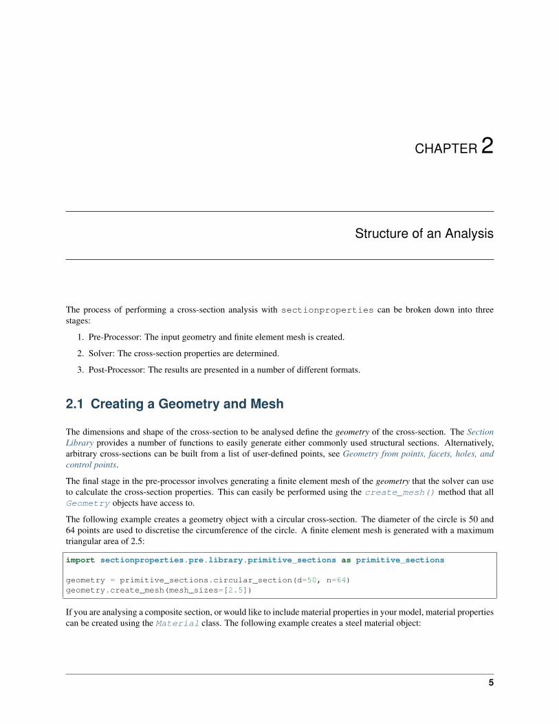
The following example creates a geometry object with a circular cross-section. The diameter of the circle is 50 and64 points are used to discretise the circumference of the circle. A finite element mesh is generated with a maximumtriangular area of 2.5:
import sectionproperties.pre.library.primitive_sections as primitive_sections
geometry = primitive_sections.circular_section(d=50, n=64)geometry.create_mesh(mesh_sizes=[2.5])
If you are analysing a composite section, or would like to include material properties in your model, material propertiescan be created using the Material class. The following example creates a steel material object:
5

sectionproperties Documentation, Release 2.1.2
Fig. 1: Finite element mesh generated by the above example.
from sectionproperties.pre.pre import Material
steel = Material(name='Steel', elastic_modulus=200e3, poissons_ratio=0.3, density=7.→˓85e-6,
yield_strength=500, color='grey')
Refer to Creating Geometries, Meshes, and Material Properties for a more detailed explanation of the pre-processingstage.
2.2 Running an Analysis
The solver operates on a Section object and can perform four different analysis types:
• Geometric Analysis: calculates area properties.
• Plastic Analysis: calculates plastic properties.
• Warping Analysis: calculates torsion and shear properties.
• Stress Analysis: calculates cross-section stresses.
The geometric analysis can be performed individually. However in order to perform a warping or plastic analysis,a geometric analysis must first be performed. Further, in order to carry out a stress analysis, both a geometric andwarping analysis must have already been executed. The program will display a helpful error if you try to run any ofthese analyses without first performing the prerequisite analyses.
The following example performs a geometric and warping analysis on the circular cross-section defined in the previoussection with steel used as the material property:
import sectionproperties.pre.library.primitive_sections as primitive_sectionsfrom sectionproperties.analysis.section import Sectionfrom sectionproperties.pre.pre import Material
(continues on next page)
6 Chapter 2. Structure of an Analysis

sectionproperties Documentation, Release 2.1.2
(continued from previous page)
steel = Material(name='Steel', elastic_modulus=200e3, poissons_ratio=0.3, density=7.→˓85e-6,
yield_strength=500, color='grey')geometry = primitive_sections.circular_section(d=50, n=64, material=steel)geometry.create_mesh(mesh_sizes=[2.5]) # Adds the mesh to the geometry
section = Section(geometry)section.calculate_geometric_properties()section.calculate_warping_properties()
Refer to Running an Analysis for a more detailed explanation of the solver stage.
2.3 Viewing the Results
Once an analysis has been performed, a number of methods belonging to the Section object can be called to presentthe cross-section results in a number of different formats. For example the cross-section properties can be printed tothe terminal, a plot of the centroids displayed and the cross-section stresses visualised in a contour plot.
The following example analyses a 200 PFC section. The cross-section properties are printed to the terminal and a plotof the centroids is displayed:
import sectionproperties.pre.library.steel_sections as steel_sectionsfrom sectionproperties.analysis.section import Section
geometry = steel_sections.channel_section(d=200, b=75, t_f=12, t_w=6, r=12, n_r=8)geometry.create_mesh(mesh_sizes=[2.5]) # Adds the mesh to the geometry
section = Section(geometry)section.calculate_geometric_properties()section.calculate_plastic_properties()section.calculate_warping_properties()
section.plot_centroids()section.display_results()
Output generated by the display_results() method:
Section Properties:A = 2.919699e+03Perim. = 6.776201e+02Qx = 2.919699e+05Qy = 7.122414e+04cx = 2.439434e+01cy = 1.000000e+02Ixx_g = 4.831277e+07Iyy_g = 3.392871e+06Ixy_g = 7.122414e+06Ixx_c = 1.911578e+07Iyy_c = 1.655405e+06Ixy_c = -6.519258e-09Zxx+ = 1.911578e+05Zxx- = 1.911578e+05
(continues on next page)
2.3. Viewing the Results 7

sectionproperties Documentation, Release 2.1.2
Fig. 2: Plot of the elastic centroid and shear centre for the above example generated by plot_centroids()
8 Chapter 2. Structure of an Analysis

sectionproperties Documentation, Release 2.1.2
(continued from previous page)
Zyy+ = 3.271186e+04Zyy- = 6.786020e+04rx = 8.091461e+01ry = 2.381130e+01phi = 0.000000e+00I11_c = 1.911578e+07I22_c = 1.655405e+06Z11+ = 1.911578e+05Z11- = 1.911578e+05Z22+ = 3.271186e+04Z22- = 6.786020e+04r11 = 8.091461e+01r22 = 2.381130e+01J = 1.011522e+05Iw = 1.039437e+10x_se = -2.505109e+01y_se = 1.000000e+02x_st = -2.505109e+01y_st = 1.000000e+02x1_se = -4.944543e+01y2_se = 4.905074e-06A_sx = 9.468851e+02A_sy = 1.106943e+03A_s11 = 9.468854e+02A_s22 = 1.106943e+03betax+ = 1.671593e-05betax- = -1.671593e-05betay+ = -2.013448e+02betay- = 2.013448e+02beta11+ = 1.671593e-05beta11- = -1.671593e-05beta22+ = -2.013448e+02beta22- = 2.013448e+02x_pc = 1.425046e+01y_pc = 1.000000e+02Sxx = 2.210956e+05Syy = 5.895923e+04SF_xx+ = 1.156613e+00SF_xx- = 1.156613e+00SF_yy+ = 1.802381e+00SF_yy- = 8.688337e-01x11_pc = 1.425046e+01y22_pc = 1.000000e+02S11 = 2.210956e+05S22 = 5.895923e+04SF_11+ = 1.156613e+00SF_11- = 1.156613e+00SF_22+ = 1.802381e+00SF_22- = 8.688337e-01
Refer to Viewing the Results for a more detailed explanation of the post-processing stage.
2.3. Viewing the Results 9

sectionproperties Documentation, Release 2.1.2
10 Chapter 2. Structure of an Analysis
CHAPTER 3
Creating Geometries, Meshes, and Material Properties
Before performing a cross-section analysis, the geometry of the cross-section and a finite element mesh must becreated. Optionally, material properties can be applied to different regions of the cross-section. If materials are notapplied, then a default material is used to report the geometric properties.
3.1 Section Geometry
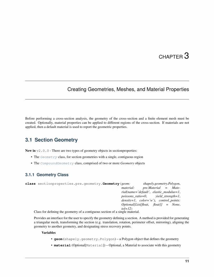
New in v2.0.0 - There are two types of geometry objects in sectionproperties:
• The Geometry class, for section geometries with a single, contiguous region
• The CompoundGeometry class, comprised of two or more Geometry objects
3.1.1 Geometry Class
class sectionproperties.pre.geometry.Geometry(geom: shapely.geometry.Polygon,material: pre.Material = Mate-rial(name=’default’, elastic_modulus=1,poissons_ratio=0, yield_strength=1,density=1, color=’w’), control_points:Optional[List[float, float]] = None,tol=12)
Class for defining the geometry of a contiguous section of a single material.
Provides an interface for the user to specify the geometry defining a section. A method is provided for generatinga triangular mesh, transforming the section (e.g. translation, rotation, perimeter offset, mirroring), aligning thegeometry to another geometry, and designating stress recovery points.
Variables
• geom (shapely.geometry.Polygon) – a Polygon object that defines the geometry
• material (Optional[Material]) – Optional, a Material to associate with this geometry
11

sectionproperties Documentation, Release 2.1.2
• control_point – Optional, an (x, y) coordinate within the geometry that representsa pre-assigned control point (aka, a region identification point) to be used instead of theautomatically assigned control point generated with shapely.geometry.Polygon.representative_point().
• tol – Optional, default is 12. Number of decimal places to round the geometry verticesto. A lower value may reduce accuracy of geometry but increases precision when aligninggeometries to each other.
A Geometry is instantiated with two arguments:
1. A shapely.geometry.Polygon object
2. An optional Material object
Note: If a Material is not given, then the default material is assigned to the Geometry.material attribute.The default material has an elastic modulus of 1, a Poisson’s ratio of 0 and a yield strength of 1.
3.1.2 CompoundGeometry Class
class sectionproperties.pre.geometry.CompoundGeometry(geoms:Union[shapely.geometry.multipolygon.MultiPolygon,List[sectionproperties.pre.geometry.Geometry]])
Class for defining a geometry of multiple distinct regions, each potentially having different material properties.
CompoundGeometry instances are composed of multiple Geometry objects. As with Geometry objects, Com-poundGeometry objects have methods for generating a triangular mesh over all geometries, transforming thecollection of geometries as though they were one (e.g. translation, rotation, and mirroring), and aligning theCompoundGeometry to another Geometry (or to another CompoundGeometry).
CompoundGeometry objects can be created directly between two or more Geometry objects by using the +operator.
Variables geoms (Union[shapely.geometry.MultiPolygon, List[Geometry]]) – eithera list of Geometry objects or a shapely.geometry.MultiPolygon instance.
A CompoundGeometry is instantiated with one argument which can be one of two types:
1. A list of Geometry objects; or
2. A shapely.geometry.MultiPolygon
Note: A CompoundGeometry does not have a .material attribute and therefore, a Material cannotbe assigned to a CompoundGeometry directly. Since a CompoundGeometry is simply a combination ofGeometry objects, the Material(s) should be assigned to the individual Geometry objects that comprise theCompoundGeometry . CompoundGeometry objects created from a shapely.geometry.MultiPolygonwill have its constituent Geometry objects assigned the default material.
3.1.3 Defining Material Properties
Materials are defined in sectionproperties by creating a Material object:
12 Chapter 3. Creating Geometries, Meshes, and Material Properties

sectionproperties Documentation, Release 2.1.2
class sectionproperties.pre.pre.Material(name: str, elastic_modulus: float, poissons_ratio:float, yield_strength: float, density: float, color:str)
Class for structural materials.
Provides a way of storing material properties related to a specific material. The color can be a multitude ofdifferent formats, refer to https://matplotlib.org/api/colors_api.html and https://matplotlib.org/examples/color/named_colors.html for more information.
Parameters
• name (string) – Material name
• elastic_modulus (float) – Material modulus of elasticity
• poissons_ratio (float) – Material Poisson’s ratio
• yield_strength (float) – Material yield strength
• density (float) – Material density (mass per unit volume)
• color (matplotlib.colors) – Material color for rendering
Variables
• name (string) – Material name
• elastic_modulus (float) – Material modulus of elasticity
• poissons_ratio (float) – Material Poisson’s ratio
• shear_modulus (float) – Material shear modulus, derived from the elastic modulusand Poisson’s ratio assuming an isotropic material
• density (float) – Material density (mass per unit volume)
• yield_strength (float) – Material yield strength
• color (matplotlib.colors) – Material color for rendering
The following example creates materials for concrete, steel and timber:
from sectionproperties.pre.pre import Material
concrete = Material(name='Concrete', elastic_modulus=30.1e3, poissons_ratio=0.2, density=2.4e-6,
yield_strength=32, color='lightgrey')steel = Material(
name='Steel', elastic_modulus=200e3, poissons_ratio=0.3, density=7.85e-6,yield_strength=500, color='grey'
)timber = Material(
name='Timber', elastic_modulus=8e3, poissons_ratio=0.35, density=6.5e-7,yield_strength=20, color='burlywood'
)
Each Geometry contains its own material definition, which is stored in the .material attribute. A geometry’smaterial may be altered at any time by simply assigning a new Material to the .material attribute.
Warning: To understand how material properties affect the results reported by sectionproperties, see How Mate-rial Properties Affect Results.
3.1. Section Geometry 13
sectionproperties Documentation, Release 2.1.2
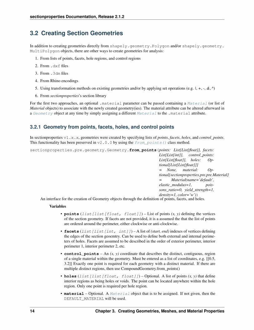
3.2 Creating Section Geometries
In addition to creating geometries directly from shapely.geometry.Polygon and/or shapely.geometry.MultiPolygon objects, there are other ways to create geometries for analysis:
1. From lists of points, facets, hole regions, and control regions
2. From .dxf files
3. From .3dm files
4. From Rhino encodings
5. Using transformation methods on existing geometries and/or by applying set operations (e.g. |, +, -, &, ^)
6. From sectionproperties’s section library
For the first two approaches, an optional .material parameter can be passed containing a Material (or list ofMaterial objects) to associate with the newly created geometry(ies). The material attribute can be altered afterward ina Geometry object at any time by simply assigning a different Material to the .material attribute.
3.2.1 Geometry from points, facets, holes, and control points
In sectionproperties v1.x.x, geometries were created by specifying lists of points, facets, holes, and control_points.This functionality has been preserved in v2.0.0 by using the from_points() class method.
sectionproperties.pre.geometry.Geometry.from_points(points: List[List[float]], facets:List[List[int]], control_points:List[List[float]], holes: Op-tional[List[List[float]]]= None, material: Op-tional[sectionproperties.pre.pre.Material]= Material(name=’default’,elastic_modulus=1, pois-sons_ratio=0, yield_strength=1,density=1, color=’w’))
An interface for the creation of Geometry objects through the definition of points, facets, and holes.
Variables
• points (list[list[float, float]]) – List of points (x, y) defining the verticesof the section geometry. If facets are not provided, it is a assumed the that the list of pointsare ordered around the perimeter, either clockwise or anti-clockwise.
• facets (list[list[int, int]]) – A list of (start, end) indexes of vertices definingthe edges of the section geoemtry. Can be used to define both external and internal perime-ters of holes. Facets are assumed to be described in the order of exterior perimeter, interiorperimeter 1, interior perimeter 2, etc.
• control_points – An (x, y) coordinate that describes the distinct, contiguous, regionof a single material within the geometry. Must be entered as a list of coordinates, e.g. [[0.5,3.2]] Exactly one point is required for each geometry with a distinct material. If there aremultiple distinct regions, then use CompoundGeometry.from_points()
• holes (list[list[float, float]]) – Optional. A list of points (x, y) that defineinterior regions as being holes or voids. The point can be located anywhere within the holeregion. Only one point is required per hole region.
• material – Optional. A Material object that is to be assigned. If not given, then theDEFAULT_MATERIAL will be used.
14 Chapter 3. Creating Geometries, Meshes, and Material Properties

sectionproperties Documentation, Release 2.1.2
For simple geometries (i.e. single-region shapes without holes), if the points are an ordered sequence of coordinates,only the points argument is required (facets, holes, and control_points are optional). If the geometry has holes, thenall arguments are required.
If the geometry has multiple regions, then the from_points() class method must be used.
sectionproperties.pre.geometry.CompoundGeometry.from_points(points:List[List[float]],facets:List[List[int]],control_points:List[List[float]],holes: Op-tional[List[List[float]]]= None, ma-terials: Op-tional[List[sectionproperties.pre.pre.Material]]= Mate-rial(name=’default’,elastic_modulus=1,poissons_ratio=0,yield_strength=1,density=1,color=’w’))
An interface for the creation of CompoundGeometry objects through the definition of points, facets, holes,and control_points. Geometries created through this method are expected to be non-ambiguous meaning that no“overlapping” geometries exists and that nodal connectivity is maintained (e.g. there are no nodes “overlapping”with facets without nodal connectivity).
Variables
• points (list[list[float]]) – List of points (x, y) defining the vertices of the sec-tion geometry. If facets are not provided, it is a assumed the that the list of points are orderedaround the perimeter, either clockwise or anti-clockwise
• facets (list[list[int]]) – A list of (start, end) indexes of vertices defining theedges of the section geoemtry. Can be used to define both external and internal perimetersof holes. Facets are assumed to be described in the order of exterior perimeter, interiorperimeter 1, interior perimeter 2, etc.
• control_points (list[list[float]]) – Optional. A list of points (x, y) thatdefine non-interior regions as being distinct, contiguous, and having one material. Thepoint can be located anywhere within region. Only one point is permitted per region.The order of control_points must be given in the same order as the order that polygonsare created by ‘facets’. If not given, then points will be assigned automatically usingshapely.geometry.Polygon.representative_point()
• holes (list[list[float]]) – Optional. A list of points (x, y) that define interiorregions as being holes or voids. The point can be located anywhere within the hole region.Only one point is required per hole region.
• materials (list[Material]) – Optional. A list of Material objects that are to beassigned, in order, to the regions defined by the given control_points. If not given, then theDEFAULT_MATERIAL will be used for each region.
See Creating Custom Geometry for an example of this implementation.
3.2. Creating Section Geometries 15
sectionproperties Documentation, Release 2.1.2
3.2.2 Geometry from .dxf Files
Geometries can now be created from .dxf files using the sectionproperties.pre.geometry.Geometry.from_dxf()method. The returned geometry will either be a Geometry or CompoundGeometry object depend-ing on the geometry in the file (i.e. the number of contiguous regions).
sectionproperties.pre.geometry.Geometry.from_dxf(dxf_filepath: Union[str,pathlib.Path]) →Union[sectionproperties.pre.geometry.Geometry,sectionproper-ties.pre.geometry.CompoundGeometry]
An interface for the creation of Geometry objects from CAD .dxf files.
Variables dxf_filepath (Union[str, pathlib.Path]) – A path-like object for the dxffile
sectionproperties.pre.geometry.CompoundGeometry.from_dxf(dxf_filepath: Union[str,pathlib.Path]) →Union[sectionproperties.pre.geometry.Geometry,sectionproper-ties.pre.geometry.CompoundGeometry]
An interface for the creation of Geometry objects from CAD .dxf files.
Variables dxf_filepath (Union[str, pathlib.Path]) – A path-like object for the dxffile
3.2.3 Geometry from Rhino
Geometries can now be created from .3dm files and BREP encodings. Various limitations and assumptions need to beacknowledged:
• sectional analysis is based in 2d and Rhino is a 3d environment.
• the recognised Rhino geometries are limited to planer-single-surfaced BREPs.
• Rhino uses NURBS for surface boundaries and sectionproperties uses piecewise linear boundaries.
• a search plane is defined.
See the keyword arguments below that are used to search and simplify the Rhino geometry.
Rhino files are read via the class methods sectionproperties.pre.geometry.Geometry.from_3dm()and sectionproperties.pre.geometry.CompoundGeometry.from_3dm(). Each class method re-turns the respective objects.
sectionproperties.pre.geometry.Geometry.from_3dm(filepath: Union[str, pathlib.Path],**kwargs) → sectionproper-ties.pre.geometry.Geometry
Class method to create a Geometry from the objects in a Rhino .3dm file.
Parameters
• filepath (Union[str, pathlib.Path]) – File path to the rhino .3dm file.
• kwargs – See below.
Raises RuntimeError – A RuntimeError is raised if two or more polygons are found. This isdependent on the keyword arguments. Try adjusting the keyword arguments if this error israised.
Returns A Geometry object.
16 Chapter 3. Creating Geometries, Meshes, and Material Properties

sectionproperties Documentation, Release 2.1.2
Return type Geometry
Keyword Arguments
• refine_num (int, optional) – Bézier curve interpolation number. In Rhino a sur-face’s edges are nurb based curves. Shapely does not support nurbs, so the individualBézier curves are interpolated using straight lines. This parameter sets the number ofstraight lines used in the interpolation. Default is 1.
• vec1 (numpy.ndarray, optional) – A 3d vector in the Shapely plane. Rhino is a3D geometry environment. Shapely is a 2D geometric library. Thus a 2D plane needs tobe defined in Rhino that represents the Shapely coordinate system. vec1 represents the1st vector of this plane. It will be used as Shapely’s x direction. Default is [1,0,0].
• vec2 (numpy.ndarray, optional) – Continuing from vec1, vec2 is another vectorto define the Shapely plane. It must not be [0,0,0] and it’s only requirement is that it isany vector in the Shapely plane (but not equal to vec1). Default is [0,1,0].
• plane_distance (float, optional) – The distance to the Shapely plane. Default is 0.
• project (boolean, optional) – Controls if the breps are projected onto the plane inthe direction of the Shapley plane’s normal. Default is True.
• parallel (boolean, optional) – Controls if only the rhino surfaces that have the samenormal as the Shapely plane are yielded. If true, all non parallel surfaces are filtered out.Default is False.
sectionproperties.pre.geometry.CompoundGeometry.from_3dm(filepath: Union[str, path-lib.Path], **kwargs)→ sectionproper-ties.pre.geometry.CompoundGeometry
Class method to create a CompoundGeometry from the objects in a Rhino 3dm file.
Parameters
• filepath (Union[str, pathlib.Path]) – File path to the rhino .3dm file.
• kwargs – See below.
Returns A CompoundGeometry object.
Return type CompoundGeometry
Keyword Arguments
• refine_num (int, optional) – Bézier curve interpolation number. In Rhino a sur-face’s edges are nurb based curves. Shapely does not support nurbs, so the individualBézier curves are interpolated using straight lines. This parameter sets the number ofstraight lines used in the interpolation. Default is 1.
• vec1 (numpy.ndarray, optional) – A 3d vector in the Shapely plane. Rhino is a3D geometry environment. Shapely is a 2D geometric library. Thus a 2D plane needs tobe defined in Rhino that represents the Shapely coordinate system. vec1 represents the1st vector of this plane. It will be used as Shapely’s x direction. Default is [1,0,0].
• vec2 (numpy.ndarray, optional) – Continuing from vec1, vec2 is another vectorto define the Shapely plane. It must not be [0,0,0] and it’s only requirement is that it isany vector in the Shapely plane (but not equal to vec1). Default is [0,1,0].
• plane_distance (float, optional) – The distance to the Shapely plane. Default is 0.
• project (boolean, optional) – Controls if the breps are projected onto the plane inthe direction of the Shapley plane’s normal. Default is True.
3.2. Creating Section Geometries 17
sectionproperties Documentation, Release 2.1.2
• parallel (boolean, optional) – Controls if only the rhino surfaces that have the samenormal as the Shapely plane are yielded. If true, all non parallel surfaces are filtered out.Default is False.
Geometry objects can also be created from encodings of Rhino BREP.
sectionproperties.pre.geometry.Geometry.from_rhino_encoding(r3dm_brep: str,**kwargs) →sectionproper-ties.pre.geometry.Geometry
Load an encoded single surface planer brep.
Parameters
• r3dm_brep (str) – A Rhino3dm.Brep encoded as a string.
• kwargs – See below.
Returns A Geometry object found in the encoded string.
Return type Geometry
Keyword Arguments
• refine_num (int, optional) – Bézier curve interpolation number. In Rhino a sur-face’s edges are nurb based curves. Shapely does not support nurbs, so the individualBézier curves are interpolated using straight lines. This parameter sets the number ofstraight lines used in the interpolation. Default is 1.
• vec1 (numpy.ndarray, optional) – A 3d vector in the Shapely plane. Rhino is a3D geometry environment. Shapely is a 2D geometric library. Thus a 2D plane needs tobe defined in Rhino that represents the Shapely coordinate system. vec1 represents the1st vector of this plane. It will be used as Shapely’s x direction. Default is [1,0,0].
• vec2 (numpy.ndarray, optional) – Continuing from vec1, vec2 is another vectorto define the Shapely plane. It must not be [0,0,0] and it’s only requirement is that it isany vector in the Shapely plane (but not equal to vec1). Default is [0,1,0].
• plane_distance (float, optional) – The distance to the Shapely plane. Default is 0.
• project (boolean, optional) – Controls if the breps are projected onto the plane inthe direction of the Shapley plane’s normal. Default is True.
• parallel (boolean, optional) – Controls if only the rhino surfaces that have the samenormal as the Shapely plane are yielded. If true, all non parallel surfaces are filtered out.Default is False.
More advanced filtering can be achieved by working with the Shapely geometries directly. These can be accessed byload_3dm() and load_rhino_brep_encoding().
sectionproperties.pre.rhino.load_3dm(r3dm_filepath: Union[pathlib.Path, str], **kwargs)→List[shapely.geometry.polygon.Polygon]
Load a Rhino .3dm file and import the single surface planer breps.
Parameters
• r3dm_filepath (pathlib.Path or string) – File path to the rhino .3dm file.
• kwargs – See below.
Raises RuntimeError – A RuntimeError is raised if no polygons are found in the file. Thisis dependent on the keyword arguments. Try adjusting the keyword arguments if this error israised.
Returns List of Polygons found in the file.
18 Chapter 3. Creating Geometries, Meshes, and Material Properties

sectionproperties Documentation, Release 2.1.2
Return type List[shapely.geometry.Polygon]
Keyword Arguments
• refine_num (int, optional) – Bézier curve interpolation number. In Rhino a sur-face’s edges are nurb based curves. Shapely does not support nurbs, so the individualBézier curves are interpolated using straight lines. This parameter sets the number ofstraight lines used in the interpolation. Default is 1.
• vec1 (numpy.ndarray, optional) – A 3d vector in the Shapely plane. Rhino is a3D geometry environment. Shapely is a 2D geometric library. Thus a 2D plane needs tobe defined in Rhino that represents the Shapely coordinate system. vec1 represents the1st vector of this plane. It will be used as Shapely’s x direction. Default is [1,0,0].
• vec2 (numpy.ndarray, optional) – Continuing from vec1, vec2 is another vectorto define the Shapely plane. It must not be [0,0,0] and it’s only requirement is that it isany vector in the Shapely plane (but not equal to vec1). Default is [0,1,0].
• plane_distance (float, optional) – The distance to the Shapely plane. Default is 0.
• project (boolean, optional) – Controls if the breps are projected onto the plane inthe direction of the Shapley plane’s normal. Default is True.
• parallel (boolean, optional) – Controls if only the rhino surfaces that have the samenormal as the Shapely plane are yielded. If true, all non parallel surfaces are filtered out.Default is False.
sectionproperties.pre.rhino.load_brep_encoding(brep: str, **kwargs) →shapely.geometry.polygon.Polygon
Load an encoded single surface planer brep.
Parameters
• brep (str) – Rhino3dm.Brep encoded as a string.
• kwargs – See below.
Raises RuntimeError – A RuntimeError is raised if no polygons are found in the encoding. Thisis dependent on the keyword arguments. Try adjusting the keyword arguments if this error israised.
Returns The Polygons found in the encoding string.
Return type shapely.geometry.Polygon
Keyword Arguments
• refine_num (int, optional) – Bézier curve interpolation number. In Rhino a sur-face’s edges are nurb based curves. Shapely does not support nurbs, so the individualBézier curves are interpolated using straight lines. This parameter sets the number ofstraight lines used in the interpolation. Default is 1.
• vec1 (numpy.ndarray, optional) – A 3d vector in the Shapely plane. Rhino is a3D geometry environment. Shapely is a 2D geometric library. Thus a 2D plane needs tobe defined in Rhino that represents the Shapely coordinate system. vec1 represents the1st vector of this plane. It will be used as Shapely’s x direction. Default is [1,0,0].
• vec2 (numpy.ndarray, optional) – Continuing from vec1, vec2 is another vectorto define the Shapely plane. It must not be [0,0,0] and it’s only requirement is that it isany vector in the Shapely plane (but not equal to vec1). Default is [0,1,0].
• plane_distance (float, optional) – The distance to the Shapely plane. Default is 0.
3.2. Creating Section Geometries 19
sectionproperties Documentation, Release 2.1.2
• project (boolean, optional) – Controls if the breps are projected onto the plane inthe direction of the Shapley plane’s normal. Default is True.
• parallel (boolean, optional) – Controls if only the rhino surfaces that have the samenormal as the Shapely plane are yielded. If true, all non parallel surfaces are filtered out.Default is False.
Note: Dependencies for importing files from rhino are not included by default. To obtain the required dependenciesinstall sectionproperties with the rhino option:
pip install sectionproperties[rhino]
3.2.4 Combining Geometries Using Set Operations
Both Geometry and CompoundGeometry objects can be manipulated using Python’s set operators:
• | Bitwise OR - Performs a union on the two geometries
• - Bitwise DIFFERENCE - Performs a subtraction, subtracting the second geometry from the first
• & Bitwise AND - Performs an intersection operation, returning the regions of geometry common to both
• ^ Bitwise XOR - Performs a symmetric difference operation, returning the regions of geometry that are notoverlapping
• + Addition - Combines two geometries into a CompoundGeometry
See Advanced Geometry Creation for an example using set operations.
3.2.5 sectionproperties Section Library
See Creating Section Geometries from the Section Library.
3.3 Manipulating Geometries
Each geometry instance is able to be manipulated in 2D space for the purpose of creating novel, custom sectiongeometries that the user may require.
Note: Operations on geometries are non-destructive. For each operation, a new geometry object is returned.
This gives sectionproperties geoemtries a fluent API meaning that transformation methods can be chained together.Please see Advanced Geometry Creation for examples.
3.3.1 Aligning
sectionproperties.pre.geometry.Geometry.align_center(self, align_to: Op-tional[sectionproperties.pre.geometry.Geometry]= None)
Returns a new Geometry object, translated in both x and y, so that the center-point of the new object’scentroid will be aligned with centroid of the object in ‘align_to’. If ‘align_to’ is None then the newobject will be aligned with it’s centroid at the origin.
20 Chapter 3. Creating Geometries, Meshes, and Material Properties
sectionproperties Documentation, Release 2.1.2
Parameters align_to (Optional[Geometry]) – Another Geometry to align to or None(default is None)
Returns Geometry object translated to new alignment
Return type Geometry
sectionproperties.pre.geometry.Geometry.align_to(self, other:Union[sectionproperties.pre.geometry.Geometry,Tuple[float, float]], on:str, inner: bool =False) → sectionproper-ties.pre.geometry.Geometry
Returns a new Geometry object, representing ‘self’ translated so that is aligned ‘on’ one of the outerbounding box edges of ‘other’.
If ‘other’ is a tuple representing an (x,y) coordinate, then the new Geometry object will represent‘self’ translated so that it is aligned ‘on’ that side of the point.
Parameters
• other (Union[Geometry , Tuple[float, float]]) – Either another Geometry or atuple representing an (x,y) coordinate point that ‘self’ should align to.
• on – A str of either “left”, “right”, “bottom”, or “top” indicating which side of‘other’ that self should be aligned to.
• inner (bool) – Default False. If True, align ‘self’ to ‘other’ in such a way that‘self’ is aligned to the “inside” of ‘other’. In other words, align ‘self’ to ‘other’ onthe specified edge so they overlap.
Returns Geometry object translated to alignment location
Return type Geometry
3.3.2 Mirroring
sectionproperties.pre.geometry.Geometry.mirror_section(self, axis:str = ’x’,mirror_point:Union[List[float],str] = ’center’)
Mirrors the geometry about a point on either the x or y-axis.
Parameters
• axis (string) – Axis about which to mirror the geometry, ‘x’ or ‘y’
• mirror_point (Union[list[float, float], str]) – Point aboutwhich to mirror the geometry (x, y). If no point is provided, mirrors the geome-try about the centroid of the shape’s bounding box. Default = ‘center’.
Returns New Geometry-object mirrored on ‘axis’ about ‘mirror_point’
Return type Geometry
The following example mirrors a 200PFC section about the y-axis and the point (0, 0):
import sectionproperties.pre.library.steel_sections as steel_sections
(continues on next page)
3.3. Manipulating Geometries 21

sectionproperties Documentation, Release 2.1.2
(continued from previous page)
geometry = steel_sections.channel_section(d=200, b=75, t_f=12, t_w=6,→˓r=12, n_r=8)new_geometry = geometry.mirror_section(axis='y', mirror_point=[0, 0])
3.3.3 Rotating
sectionproperties.pre.geometry.Geometry.rotate_section(self, angle:float, rot_point:Union[List[float],str] = ’center’,use_radians:bool = False)
Rotates the geometry and specified angle about a point. If the rotation point is not provided, rotatesthe section about the center of the geometry’s bounding box.
Parameters
• angle (float) – Angle (degrees by default) by which to rotate the section. Apositive angle leads to a counter-clockwise rotation.
• rot_point (list[float, float]) – Optional. Point (x, y) about which torotate the section. If not provided, will rotate about the center of the geometry’sbounding box. Default = ‘center’.
• use_radians – Boolean to indicate whether ‘angle’ is in degrees or radians. IfTrue, ‘angle’ is interpreted as radians.
Returns New Geometry-object rotated by ‘angle’ about ‘rot_point’
Return type Geometry
The following example rotates a 200UB25 section clockwise by 30 degrees:
import sectionproperties.pre.library.steel_sections as steel_sections
geometry = steel_sections.i_section(d=203, b=133, t_f=7.8, t_w=5.8, r=8.→˓9, n_r=8)new_geometry = geometry.rotate_section(angle=-30)
3.3.4 Shifting
sectionproperties.pre.geometry.Geometry.shift_points(self, point_idxs:Union[int,List[int]], dx:float = 0, dy:float = 0, abs_x:Optional[float]= None, abs_y:Optional[float]= None) →sectionproper-ties.pre.geometry.Geometry
Translates one (or many points) in the geometry by either a relative amount or to a new absolutelocation. Returns a new Geometry representing the original with the selected point(s) shifted to thenew location.
22 Chapter 3. Creating Geometries, Meshes, and Material Properties

sectionproperties Documentation, Release 2.1.2
Points are identified by their index, their relative location within the points list found in self.points. You can call self.plot_geometry(labels="points") to see a plot with thepoints labeled to find the appropriate point indexes.
Parameters
• point_idxs (Union[int, List[int]]) – An integer representing an indexlocation or a list of integer index locations.
• dx (float) – The number of units in the x-direction to shift the point(s) by
• dy (float) – The number of units in the y-direction to shift the point(s) by
• abs_x (Optional[float]) – Absolute x-coordinate in coordinate system toshift the point(s) to. If abs_x is provided, dx is ignored. If providing a list topoint_idxs, all points will be moved to this absolute location.
• abs_y (Optional[float]) – Absolute y-coordinate in coordinate system toshift the point(s) to. If abs_y is provided, dy is ignored. If providing a list topoint_idxs, all points will be moved to this absolute location.
Returns Geometry object with selected points translated to the new location.
Return type Geometry
The following example expands the sides of a rectangle, one point at a time, to make it a square:
import sectionproperties.pre.library.primitive_sections as primitive_→˓sections
geometry = primitive_sections.rectangular_section(d=200, b=150)
# Using relative shiftingone_pt_shifted_geom = geometry.shift_points(point_idxs=1, dx=50)
# Using absolute relocationboth_pts_shift_geom = one_pt_shift_geom.shift_points(point_idxs=2, abs_→˓x=200)
sectionproperties.pre.geometry.Geometry.shift_section(self, x_offset=0.0,y_offset=0.0)
Returns a new Geometry object translated by ‘x_offset’ and ‘y_offset’.
Parameters
• x_offset (float) – Distance in x-direction by which to shift the geometry.
• y_offset (float) – Distance in y-direction by which to shift the geometry.
Returns New Geometry-object shifted by ‘x_offset’ and ‘y_offset’
Return type Geometry
3.3. Manipulating Geometries 23
sectionproperties Documentation, Release 2.1.2
3.3.5 Splitting
sectionproperties.pre.geometry.Geometry.split_section(self, point_i:Tuple[float, float],point_j: Op-tional[Tuple[float,float]] =None, vector:Union[Tuple[float,float], None,numpy.ndarray]= None) → Tu-ple[List[sectionproperties.pre.geometry.Geometry],List[sectionproperties.pre.geometry.Geometry]]
Splits, or bisects, the geometry about a line, as defined by two points on the line or by one point onthe line and a vector. Either point_j or vector must be given. If point_j is given, vectoris ignored.
Returns a tuple of two lists each containing new Geometry instances representing the “top” and“bottom” portions, respectively, of the bisected geometry.
If the line is a vertical line then the “right” and “left” portions, respectively, are returned.
Parameters
• point_i (Tuple[float, float]) – A tuple of (x, y) coordinates to define afirst point on the line
• point_j (Tuple[float, float]) – Optional. A tuple of (x, y) coordinatesto define a second point on the line
• vector (Union[Tuple[float, float], numpy.ndarray]) – Op-tional. A tuple or numpy ndarray of (x, y) components to define the line direction.
Returns A tuple of lists containing Geometry objects that are bisected about the line de-fined by the two given points. The first item in the tuple represents the geometrieson the “top” of the line (or to the “right” of the line, if vertical) and the second itemrepresents the geometries to the “bottom” of the line (or to the “left” of the line, ifvertical).
Return type Tuple[List[Geometry], List[Geometry]]
The following example splits a 200PFC section about the y-axis:
import sectionproperties.pre.library.steel_sections as steel_sectionsfrom shapely.geometry import LineString
geometry = steel_sections.channel_section(d=200, b=75, t_f=12, t_w=6,→˓r=12, n_r=8)right_geom, left_geom = geometry.split_section((0, 0), (0, 1))
24 Chapter 3. Creating Geometries, Meshes, and Material Properties

sectionproperties Documentation, Release 2.1.2
3.3.6 Offsetting the Perimeter
sectionproperties.pre.geometry.Geometry.offset_perimeter(self, amount:float = 0,where: str= ’exterior’,resolution:float = 12)
Dilates or erodes the section perimeter by a discrete amount.
Parameters
• amount (float) – Distance to offset the section by. A -ve value “erodes” thesection. A +ve value “dilates” the section.
• where (str) – One of either “exterior”, “interior”, or “all” to specify which edgesof the geometry to offset. If geometry has no interiors, then this parameter has noeffect. Default is “exterior”.
• resolution (float) – Number of segments used to approximate a quarter circlearound a point
Returns Geometry object translated to new alignment
Return type Geometry
The following example erodes a 200PFC section by 2 mm:
import sectionproperties.pre.library.steel_sections as steel_sections
geometry = sections.channel_section(d=200, b=75, t_f=12, t_w=6, r=12, n_→˓r=8)new_geometry = geometry.offset_perimeter(amount=-2)
sectionproperties.pre.geometry.CompoundGeometry.offset_perimeter(self,amount:float=0,where=’exterior’,res-o-lu-tion:float=12)
Dilates or erodes the perimeter of a CompoundGeometry object by a discrete amount.
Parameters
• amount (float) – Distance to offset the section by. A -ve value “erodes” thesection. A +ve value “dilates” the section.
• where (str) – One of either “exterior”, “interior”, or “all” to specify which edgesof the geometry to offset. If geometry has no interiors, then this parameter has noeffect. Default is “exterior”.
• resolution (float) – Number of segments used to approximate a quarter circlearound a point
3.3. Manipulating Geometries 25
sectionproperties Documentation, Release 2.1.2
Returns Geometry object translated to new alignment
Return type Geometry
The following example erodes a 200UB25 with a 12 plate stiffener section by 2 mm:
import sectionproperties.pre.library.steel_sections as steel_sectionsimport sectionproperties.pre.library.primitive_sections as primitive_→˓sections
geometry_1 = steel_sections.i_section(d=203, b=133, t_f=7.8, t_w=5.8,→˓r=8.9, n_r=8)geometry_2 = primitive_sections.rectangular_section(d=12, b=133)compound = geometry_2.align_center(geometry_1).align_to(geometry_1, on=→˓"top") + geometry_1new_geometry = compound.offset_perimeter(amount=-2)
Note: If performing a positive offset on a CompoundGeometry with multiple materials, ensure thatthe materials propagate as desired by performing a .plot_mesh() prior to performing any analysis.
3.4 Visualising the Geometry
Visualisation of geometry objects is best performed in the Jupyter computing environment, however, most visualisationcan also be done in any environment which supports display of matplotlib plots.
There are generally two ways to visualise geometry objects:
1. In the Jupyter computing environment, geometry objects utilise their underlying shapely.geometry.Polygon object’s _repr_svg_ method to show the geometry as it’s own representation.
2. By using the plot_geometry() method
Geometry.plot_geometry(labels=[’control_points’], title=’Cross-Section Geometry’, cp=True, leg-end=True, **kwargs)
Plots the geometry defined by the input section.
Parameters
• labels (list[str]) – A list of str which indicate which labels to plot. Can be one ora combination of “points”, “facets”, “control_points”, or an empty list to indicate no labels.Default is [“control_points”]
• title (string) – Plot title
• cp (bool) – If set to True, plots the control points
• legend (bool) – If set to True, plots the legend
• kwargs – Passed to plotting_context()
Returns Matplotlib axes object
Return type matplotlib.axes
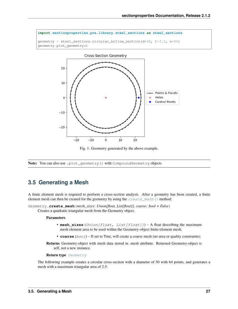
The following example creates a CHS discretised with 64 points, with a diameter of 48 and thickness of 3.2, andplots the geometry:
26 Chapter 3. Creating Geometries, Meshes, and Material Properties
sectionproperties Documentation, Release 2.1.2
import sectionproperties.pre.library.steel_sections as steel_sections
geometry = steel_sections.circular_hollow_section(d=48, t=3.2, n=64)geometry.plot_geometry()
Fig. 1: Geometry generated by the above example.
Note: You can also use .plot_geometry() with CompoundGeometry objects
3.5 Generating a Mesh
A finite element mesh is required to perform a cross-section analysis. After a geometry has been created, a finiteelement mesh can then be created for the geometry by using the create_mesh() method:
Geometry.create_mesh(mesh_sizes: Union[float, List[float]], coarse: bool = False)Creates a quadratic triangular mesh from the Geometry object.
Parameters
• mesh_sizes (Union[float, List[float]]) – A float describing the maximummesh element area to be used within the Geometry-object finite-element mesh.
• coarse (bool) – If set to True, will create a coarse mesh (no area or quality constraints)
Returns Geometry-object with mesh data stored in .mesh attribute. Returned Geometry-object isself, not a new instance.
Return type Geometry
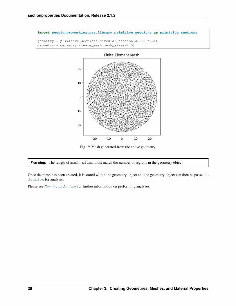
The following example creates a circular cross-section with a diameter of 50 with 64 points, and generates amesh with a maximum triangular area of 2.5:
3.5. Generating a Mesh 27
sectionproperties Documentation, Release 2.1.2
import sectionproperties.pre.library.primitive_sections as primitive_sections
geometry = primitive_sections.circular_section(d=50, n=64)geometry = geometry.create_mesh(mesh_sizes=2.5)
Fig. 2: Mesh generated from the above geometry.
Warning: The length of mesh_sizes must match the number of regions in the geometry object.
Once the mesh has been created, it is stored within the geometry object and the geometry object can then be passed toSection for analysis.
Please see Running an Analysis for further information on performing analyses.
28 Chapter 3. Creating Geometries, Meshes, and Material Properties

CHAPTER 4
Creating Section Geometries from the Section Library
In order to make your life easier, there are a number of built-in functions that generate typical structural cross-sections,resulting in Geometry objects. These typical cross-sections reside in the sectionproperties.pre.librarymodule.
29

sectionproperties Documentation, Release 2.1.2
4.1 Primitive Sections Library
4.1.1 Rectangular Section
sectionproperties.pre.library.primitive_sections.rectangular_section(b:float,d:float,mate-rial:sec-tion-proper-ties.pre.pre.Material=Mate-rial(name=’default’,elas-tic_modulus=1,pois-sons_ratio=0,yield_strength=1,den-sity=1,color=’w’))→ sec-tion-proper-ties.pre.geometry.Geometry
Constructs a rectangular section with the bottom left corner at the origin (0, 0), with depth d and width b.
Parameters
• d (float) – Depth (y) of the rectangle
• b (float) – Width (x) of the rectangle
• Optional[sectionproperties.pre.pre.Material] – Material to associatewith this geometry
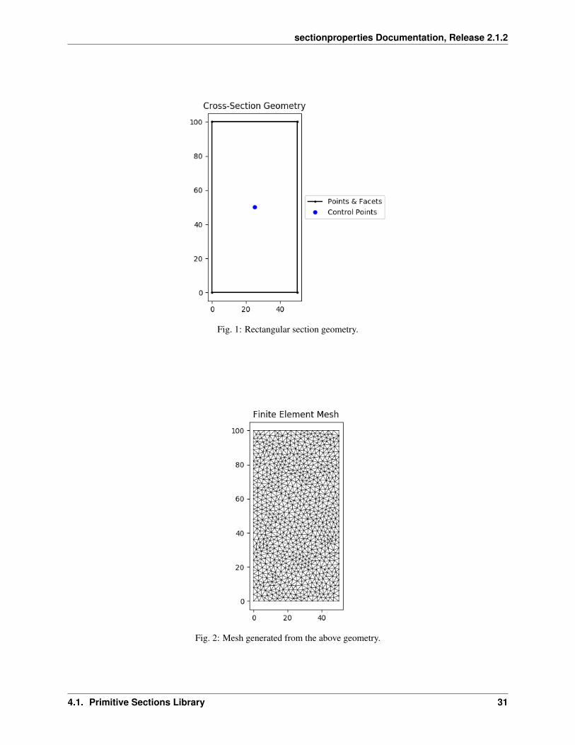
The following example creates a rectangular cross-section with a depth of 100 and width of 50, and generates amesh with a maximum triangular area of 5:
from sectionproperties.pre.library.primitive_sections import rectangular_section
geometry = rectangular_section(d=100, b=50)geometry.create_mesh(mesh_sizes=[5])
30 Chapter 4. Creating Section Geometries from the Section Library
sectionproperties Documentation, Release 2.1.2
Fig. 1: Rectangular section geometry.
Fig. 2: Mesh generated from the above geometry.
4.1. Primitive Sections Library 31

sectionproperties Documentation, Release 2.1.2
4.1.2 Circular Section
sectionproperties.pre.library.primitive_sections.circular_section(d: float, n:int, mate-rial: sec-tionproper-ties.pre.pre.Material= Mate-rial(name=’default’,elas-tic_modulus=1,pois-sons_ratio=0,yield_strength=1,density=1,color=’w’))→ sec-tionproper-ties.pre.geometry.Geometry
Constructs a solid circle centered at the origin (0, 0) with diameter d and using n points to construct the circle.
Parameters
• d (float) – Diameter of the circle
• n (int) – Number of points discretising the circle
• Optional[sectionproperties.pre.pre.Material] – Material to associatewith this geometry
The following example creates a circular geometry with a diameter of 50 with 64 points, and generates a meshwith a maximum triangular area of 2.5:
from sectionproperties.pre.library.primitive_sections import circular_section
geometry = circular_section(d=50, n=64)geometry.create_mesh(mesh_sizes=[2.5])
32 Chapter 4. Creating Section Geometries from the Section Library

sectionproperties Documentation, Release 2.1.2
Fig. 3: Circular section geometry.
Fig. 4: Mesh generated from the above geometry.
4.1. Primitive Sections Library 33

sectionproperties Documentation, Release 2.1.2
4.1.3 Circular Section By Area
sectionproperties.pre.library.primitive_sections.circular_section_by_area(area:float,n:int,ma-te-rial:sec-tion-prop-er-ties.pre.pre.Material=Ma-te-rial(name=’default’,elas-tic_modulus=1,pois-sons_ratio=0,yield_strength=1,den-sity=1,color=’w’))→sec-tion-prop-er-ties.pre.geometry.Geometry
Constructs a solid circle centered at the origin (0, 0) defined by its area, using n points to construct the circle.
Parameters
• area (float) – Area of the circle
• n (int) – Number of points discretising the circle
• Optional[sectionproperties.pre.pre.Material] – Material to associatewith this geometry
The following example creates a circular geometry with an area of 200 with 32 points, and generates a meshwith a maximum triangular area of 5:
from sectionproperties.pre.library.primitive_sections import circular_section_by_→˓area
geometry = circular_section_by_area(area=310, n=32)geometry.create_mesh(mesh_sizes=[5])
34 Chapter 4. Creating Section Geometries from the Section Library

sectionproperties Documentation, Release 2.1.2
Fig. 5: Circular section by area geometry.
Fig. 6: Mesh generated from the above geometry.
4.1. Primitive Sections Library 35

sectionproperties Documentation, Release 2.1.2
4.1.4 Elliptical Section
sectionproperties.pre.library.primitive_sections.elliptical_section(d_y:float,d_x:float, n:int, ma-terial:section-proper-ties.pre.pre.Material= Mate-rial(name=’default’,elas-tic_modulus=1,pois-sons_ratio=0,yield_strength=1,den-sity=1,color=’w’))→ sec-tion-proper-ties.pre.geometry.Geometry
Constructs a solid ellipse centered at the origin (0, 0) with vertical diameter d_y and horizontal diameter d_x,using n points to construct the ellipse.
Parameters
• d_y (float) – Diameter of the ellipse in the y-dimension
• d_x (float) – Diameter of the ellipse in the x-dimension
• n (int) – Number of points discretising the ellipse
• Optional[sectionproperties.pre.pre.Material] – Material to associatewith this geometry
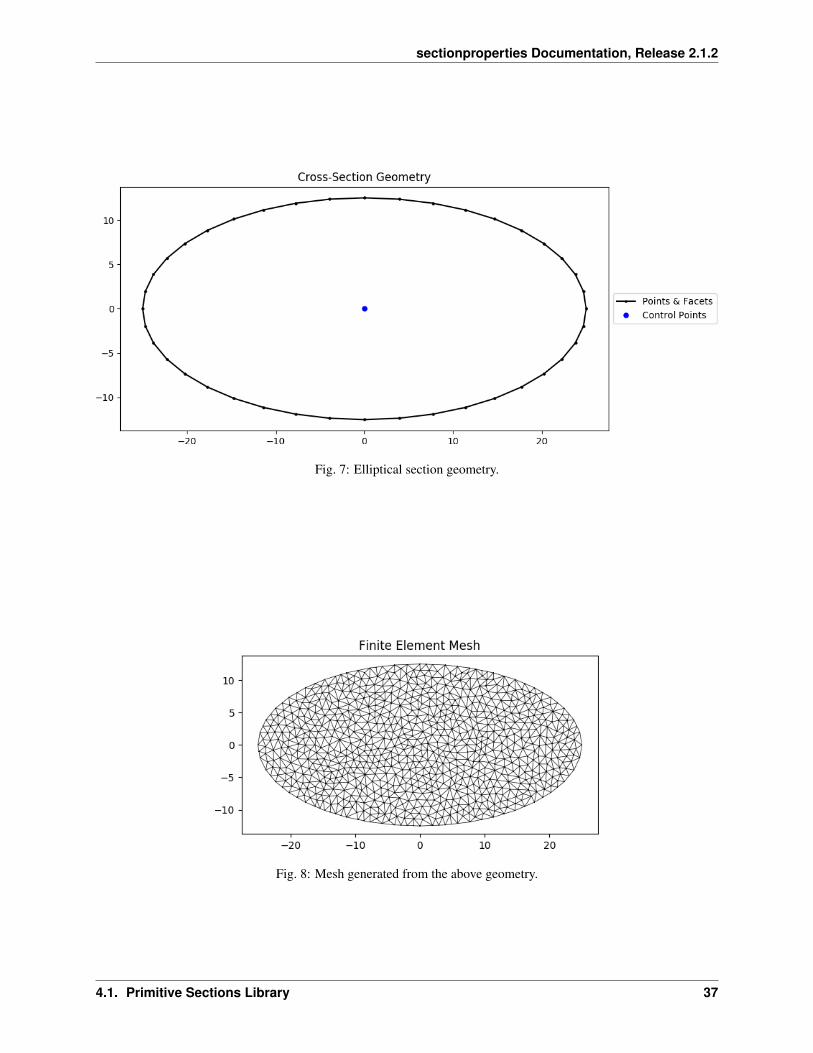
The following example creates an elliptical cross-section with a vertical diameter of 25 and horizontal diameterof 50, with 40 points, and generates a mesh with a maximum triangular area of 1.0:
from sectionproperties.pre.library.primitive_sections import elliptical_section
geometry = elliptical_section(d_y=25, d_x=50, n=40)geometry.create_mesh(mesh_sizes=[1.0])
36 Chapter 4. Creating Section Geometries from the Section Library
sectionproperties Documentation, Release 2.1.2
Fig. 7: Elliptical section geometry.
Fig. 8: Mesh generated from the above geometry.
4.1. Primitive Sections Library 37

sectionproperties Documentation, Release 2.1.2
4.1.5 Triangular Section
sectionproperties.pre.library.primitive_sections.triangular_section(b: float,h: float,mate-rial:section-proper-ties.pre.pre.Material= Mate-rial(name=’default’,elas-tic_modulus=1,pois-sons_ratio=0,yield_strength=1,den-sity=1,color=’w’))→ sec-tion-proper-ties.pre.geometry.Geometry
Constructs a right angled triangle with points (0, 0), (b, 0), (0, h).
Parameters
• b (float) – Base length of triangle
• h (float) – Height of triangle
• Optional[sectionproperties.pre.pre.Material] – Material to associatewith this geometry
The following example creates a triangular cross-section with a base width of 10 and height of 10, and generatesa mesh with a maximum triangular area of 0.5:
from sectionproperties.pre.library.primitive_sections import triangular_section
geometry = triangular_section(b=10, h=10)geometry.create_mesh(mesh_sizes=[0.5])
Fig. 9: Triangular section geometry.
38 Chapter 4. Creating Section Geometries from the Section Library

sectionproperties Documentation, Release 2.1.2
Fig. 10: Mesh generated from the above geometry.
4.1.6 Triangular Radius Section
sectionproperties.pre.library.primitive_sections.triangular_radius_section(b:float,n_r:float,ma-te-rial:sec-tion-prop-er-ties.pre.pre.Material=Ma-te-rial(name=’default’,elas-tic_modulus=1,pois-sons_ratio=0,yield_strength=1,den-sity=1,color=’w’))→sec-tion-prop-er-ties.pre.geometry.Geometry
Constructs a right angled isosceles triangle with points (0, 0), (b, 0), (0, h) and a concave radius on the hy-potenuse.
Parameters
• b (float) – Base length of triangle
4.1. Primitive Sections Library 39
sectionproperties Documentation, Release 2.1.2
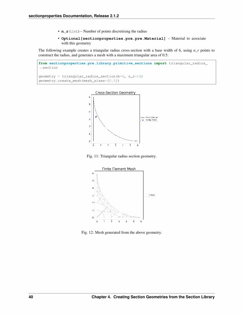
• n_r (int) – Number of points discretising the radius
• Optional[sectionproperties.pre.pre.Material] – Material to associatewith this geometry
The following example creates a triangular radius cross-section with a base width of 6, using n_r points toconstruct the radius, and generates a mesh with a maximum triangular area of 0.5:
from sectionproperties.pre.library.primitive_sections import triangular_radius_→˓section
geometry = triangular_radius_section(b=6, n_r=16)geometry.create_mesh(mesh_sizes=[0.5])
Fig. 11: Triangular radius section geometry.
Fig. 12: Mesh generated from the above geometry.
40 Chapter 4. Creating Section Geometries from the Section Library

sectionproperties Documentation, Release 2.1.2
4.1.7 Cruciform Section
sectionproperties.pre.library.primitive_sections.cruciform_section(d:float,b:float,t:float,r:float,n_r:int,ma-te-rial:sec-tion-prop-er-ties.pre.pre.Material=Ma-te-rial(name=’default’,elas-tic_modulus=1,pois-sons_ratio=0,yield_strength=1,den-sity=1,color=’w’))→sec-tion-prop-er-ties.pre.geometry.Geometry
Constructs a cruciform section centered at the origin (0, 0), with depth d, width b, thickness t androot radius r, using n_r points to construct the root radius.
Parameters
• d (float) – Depth of the cruciform section
• b (float) – Width of the cruciform section
• t (float) – Thickness of the cruciform section
• r (float) – Root radius of the cruciform section
• n_r (int) – Number of points discretising the root radius
• Optional[sectionproperties.pre.pre.Material] – Material to as-sociate with this geometry
The following example creates a cruciform section with a depth of 250, a width of 175, a thicknessof 12 and a root radius of 16, using 16 points to discretise the radius. A mesh is generated with a
4.1. Primitive Sections Library 41

sectionproperties Documentation, Release 2.1.2
maximum triangular area of 5.0:
from sectionproperties.pre.library.primitive_sections import cruciform_→˓section
geometry = cruciform_section(d=250, b=175, t=12, r=16, n_r=16)geometry.create_mesh(mesh_sizes=[5.0])
Fig. 13: Cruciform section geometry.
42 Chapter 4. Creating Section Geometries from the Section Library

sectionproperties Documentation, Release 2.1.2
Fig. 14: Mesh generated from the above geometry.
4.2 Steel Sections Library
4.2.1 Circular Hollow Section (CHS)
sectionproperties.pre.library.steel_sections.circular_hollow_section(d:float, t:float,n: int,mate-rial:sec-tion-proper-ties.pre.pre.Material=Mate-rial(name=’default’,elas-tic_modulus=1,pois-sons_ratio=0,yield_strength=1,den-sity=1,color=’w’))→ sec-tion-proper-ties.pre.geometry.Geometry
Constructs a circular hollow section (CHS) centered at the origin (0, 0), with diameter d and thickness t, usingn points to construct the inner and outer circles.
4.2. Steel Sections Library 43
sectionproperties Documentation, Release 2.1.2
Parameters
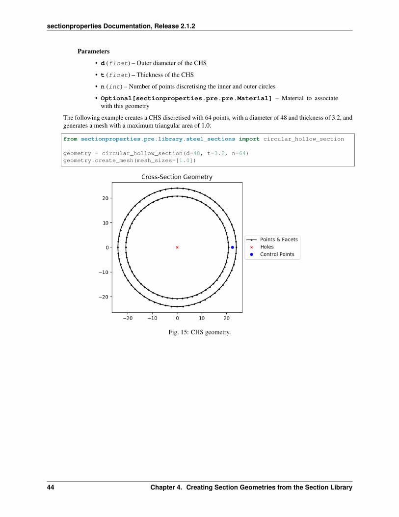
• d (float) – Outer diameter of the CHS
• t (float) – Thickness of the CHS
• n (int) – Number of points discretising the inner and outer circles
• Optional[sectionproperties.pre.pre.Material] – Material to associatewith this geometry
The following example creates a CHS discretised with 64 points, with a diameter of 48 and thickness of 3.2, andgenerates a mesh with a maximum triangular area of 1.0:
from sectionproperties.pre.library.steel_sections import circular_hollow_section
geometry = circular_hollow_section(d=48, t=3.2, n=64)geometry.create_mesh(mesh_sizes=[1.0])
Fig. 15: CHS geometry.
44 Chapter 4. Creating Section Geometries from the Section Library

sectionproperties Documentation, Release 2.1.2
Fig. 16: Mesh generated from the above geometry.
4.2. Steel Sections Library 45

sectionproperties Documentation, Release 2.1.2
4.2.2 Elliptical Hollow Section (EHS)
sectionproperties.pre.library.steel_sections.elliptical_hollow_section(d_y:float,d_x:float,t:float,n:int,ma-te-rial:sec-tion-prop-er-ties.pre.pre.Material=Ma-te-rial(name=’default’,elas-tic_modulus=1,pois-sons_ratio=0,yield_strength=1,den-sity=1,color=’w’))→sec-tion-prop-er-ties.pre.geometry.Geometry
Constructs an elliptical hollow section (EHS) centered at the origin (0, 0), with outer vertical diameter d_y, outerhorizontal diameter d_x, and thickness t, using n points to construct the inner and outer ellipses.
Parameters
• d_y (float) – Diameter of the ellipse in the y-dimension
• d_x (float) – Diameter of the ellipse in the x-dimension
• t (float) – Thickness of the EHS
• n (int) – Number of points discretising the inner and outer ellipses
• Optional[sectionproperties.pre.pre.Material] – Material to associatewith this geometry
The following example creates a EHS discretised with 30 points, with a outer vertical diameter of 25, outerhorizontal diameter of 50, and thickness of 2.0, and generates a mesh with a maximum triangular area of 0.5:
from sectionproperties.pre.library.steel_sections import elliptical_hollow_section
(continues on next page)
46 Chapter 4. Creating Section Geometries from the Section Library

sectionproperties Documentation, Release 2.1.2
(continued from previous page)
geometry = elliptical_hollow_section(d_y=25, d_x=50, t=2.0, n=64)geometry.create_mesh(mesh_sizes=[0.5])
Fig. 17: EHS geometry.
Fig. 18: Mesh generated from the above geometry.
4.2. Steel Sections Library 47
sectionproperties Documentation, Release 2.1.2
4.2.3 Rectangular Hollow Section (RHS)
sectionproperties.pre.library.steel_sections.rectangular_hollow_section(b:float,d:float,t:float,r_out:float,n_r:int,ma-te-rial:sec-tion-prop-er-ties.pre.pre.Material=Ma-te-rial(name=’default’,elas-tic_modulus=1,pois-sons_ratio=0,yield_strength=1,den-sity=1,color=’w’))→sec-tion-prop-er-ties.pre.geometry.Geometry
Constructs a rectangular hollow section (RHS) centered at (b/2, d/2), with depth d, width b, thickness t and outerradius r_out, using n_r points to construct the inner and outer radii. If the outer radius is less than the thicknessof the RHS, the inner radius is set to zero.
Parameters
• d (float) – Depth of the RHS
• b (float) – Width of the RHS
• t (float) – Thickness of the RHS
• r_out (float) – Outer radius of the RHS
• n_r (int) – Number of points discretising the inner and outer radii
• Optional[sectionproperties.pre.pre.Material] – Material to associatewith this geometry
The following example creates an RHS with a depth of 100, a width of 50, a thickness of 6 and an outer radius
48 Chapter 4. Creating Section Geometries from the Section Library

sectionproperties Documentation, Release 2.1.2
of 9, using 8 points to discretise the inner and outer radii. A mesh is generated with a maximum triangular areaof 2.0:
from sectionproperties.pre.library.steel_sections import rectangular_hollow_→˓section
geometry = rectangular_hollow_section(d=100, b=50, t=6, r_out=9, n_r=8)geometry.create_mesh(mesh_sizes=[2.0])
Fig. 19: RHS geometry.
4.2. Steel Sections Library 49

sectionproperties Documentation, Release 2.1.2
Fig. 20: Mesh generated from the above geometry.
50 Chapter 4. Creating Section Geometries from the Section Library

sectionproperties Documentation, Release 2.1.2
4.2.4 Polygon Hollow Section
sectionproperties.pre.library.steel_sections.polygon_hollow_section(d:float,t:float,n_sides:int,r_in:float=0,n_r:int=1,rot:float=0,ma-te-rial:sec-tion-prop-er-ties.pre.pre.Material=Ma-te-rial(name=’default’,elas-tic_modulus=1,pois-sons_ratio=0,yield_strength=1,den-sity=1,color=’w’))→sec-tion-prop-er-ties.pre.geometry.Geometry
Constructs a regular hollow polygon section centered at (0, 0), with a pitch circle diameter of bound-ing polygon d, thickness t, number of sides n_sides and an optional inner radius r_in, using n_rpoints to construct the inner and outer radii (if radii is specified).
Parameters
• d (float) – Pitch circle diameter of the outer bounding polygon (i.e. diameter ofcircle that passes through all vertices of the outer polygon)
• t (float) – Thickness of the polygon section wall
4.2. Steel Sections Library 51

sectionproperties Documentation, Release 2.1.2
• r_in (float) – Inner radius of the polygon corners. By default, if not specified, apolygon with no corner radii is generated.
• n_r (int) – Number of points discretising the inner and outer radii, ignored if noinner radii is specified
• rot (float) – Initial counterclockwise rotation in degrees. By default bottom faceis aligned with x axis.
• Optional[sectionproperties.pre.pre.Material] – Material to as-sociate with this geometry
Raises Exception – Number of sides in polygon must be greater than or equal to 3
The following example creates an Octagonal section (8 sides) with a diameter of 200, a thicknessof 6 and an inner radius of 20, using 12 points to discretise the inner and outer radii. A mesh isgenerated with a maximum triangular area of 5:
from sectionproperties.pre.library.steel_sections import polygon_hollow_→˓section
geometry = polygon_hollow_section(d=200, t=6, n_sides=8, r_in=20, n_r=12)geometry.create_mesh(mesh_sizes=[5])
Fig. 21: Octagonal section geometry.
52 Chapter 4. Creating Section Geometries from the Section Library

sectionproperties Documentation, Release 2.1.2
Fig. 22: Mesh generated from the above geometry.
4.2.5 I Section
sectionproperties.pre.library.steel_sections.i_section(d: float, b:float, t_f: float,t_w: float,r: float, n_r:int, material:sectionproper-ties.pre.pre.Material= Mate-rial(name=’default’,elas-tic_modulus=1,pois-sons_ratio=0,yield_strength=1,density=1,color=’w’)) →sectionproper-ties.pre.geometry.Geometry
Constructs an I Section centered at (b/2, d/2), with depth d, width b, flange thickness t_f, webthickness t_w, and root radius r, using n_r points to construct the root radius.
Parameters
• d (float) – Depth of the I Section
• b (float) – Width of the I Section
• t_f (float) – Flange thickness of the I Section
• t_w (float) – Web thickness of the I Section
• r (float) – Root radius of the I Section
4.2. Steel Sections Library 53

sectionproperties Documentation, Release 2.1.2
• n_r (int) – Number of points discretising the root radius
• Optional[sectionproperties.pre.pre.Material] – Material to as-sociate with this geometry
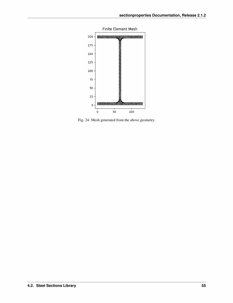
The following example creates an I Section with a depth of 203, a width of 133, a flange thicknessof 7.8, a web thickness of 5.8 and a root radius of 8.9, using 16 points to discretise the root radius.A mesh is generated with a maximum triangular area of 3.0:
from sectionproperties.pre.library.steel_sections import i_section
geometry = i_section(d=203, b=133, t_f=7.8, t_w=5.8, r=8.9, n_r=16)geometry.create_mesh(mesh_sizes=[3.0])
Fig. 23: I Section geometry.
54 Chapter 4. Creating Section Geometries from the Section Library
sectionproperties Documentation, Release 2.1.2
Fig. 24: Mesh generated from the above geometry.
4.2. Steel Sections Library 55
sectionproperties Documentation, Release 2.1.2
4.2.6 Monosymmetric I Section
sectionproperties.pre.library.steel_sections.mono_i_section(d: float,b_t:float,b_b:float,t_ft:float,t_fb:float,t_w:float,r: float,n_r: int,material:section-proper-ties.pre.pre.Material= Mate-rial(name=’default’,elas-tic_modulus=1,pois-sons_ratio=0,yield_strength=1,den-sity=1,color=’w’))→ sec-tion-proper-ties.pre.geometry.Geometry
Constructs a monosymmetric I Section centered at (max(b_t, b_b)/2, d/2), with depth d, top flangewidth b_t, bottom flange width b_b, top flange thickness t_ft, top flange thickness t_fb, web thicknesst_w, and root radius r, using n_r points to construct the root radius.
Parameters
• d (float) – Depth of the I Section
• b_t (float) – Top flange width
• b_b (float) – Bottom flange width
• t_ft (float) – Top flange thickness of the I Section
• t_fb (float) – Bottom flange thickness of the I Section
• t_w (float) – Web thickness of the I Section
• r (float) – Root radius of the I Section
• n_r (int) – Number of points discretising the root radius
• Optional[sectionproperties.pre.pre.Material] – Material to as-sociate with this geometry
The following example creates a monosymmetric I Section with a depth of 200, a top flange widthof 50, a top flange thickness of 12, a bottom flange width of 130, a bottom flange thickness of 8, a
56 Chapter 4. Creating Section Geometries from the Section Library

sectionproperties Documentation, Release 2.1.2
web thickness of 6 and a root radius of 8, using 16 points to discretise the root radius. A mesh isgenerated with a maximum triangular area of 3.0:
from sectionproperties.pre.library.steel_sections import mono_i_section
geometry = mono_i_section(d=200, b_t=50, b_b=130, t_ft=12, t_fb=8, t_w=6, r=8, n_r=16
)geometry.create_mesh(mesh_sizes=[3.0])
Fig. 25: I Section geometry.
4.2. Steel Sections Library 57

sectionproperties Documentation, Release 2.1.2
Fig. 26: Mesh generated from the above geometry.
58 Chapter 4. Creating Section Geometries from the Section Library

sectionproperties Documentation, Release 2.1.2
4.2.7 Tapered Flange I Section
sectionproperties.pre.library.steel_sections.tapered_flange_i_section(d:float,b:float,t_f:float,t_w:float,r_r:float,r_f:float,al-pha:float,n_r:int,ma-te-rial:sec-tion-prop-er-ties.pre.pre.Material=Ma-te-rial(name=’default’,elas-tic_modulus=1,pois-sons_ratio=0,yield_strength=1,den-sity=1,color=’w’))→sec-tion-prop-er-ties.pre.geometry.Geometry
Constructs a Tapered Flange I Section centered at (b/2, d/2), with depth d, width b, mid-flangethickness t_f, web thickness t_w, root radius r_r, flange radius r_f and flange angle alpha, using n_rpoints to construct the radii.
Parameters
• d (float) – Depth of the Tapered Flange I Section
• b (float) – Width of the Tapered Flange I Section
• t_f (float) – Mid-flange thickness of the Tapered Flange I Section (measured at
4.2. Steel Sections Library 59

sectionproperties Documentation, Release 2.1.2
the point equidistant from the face of the web to the edge of the flange)
• t_w (float) – Web thickness of the Tapered Flange I Section
• r_r (float) – Root radius of the Tapered Flange I Section
• r_f (float) – Flange radius of the Tapered Flange I Section
• alpha (float) – Flange angle of the Tapered Flange I Section (degrees)
• n_r (int) – Number of points discretising the radii
• Optional[sectionproperties.pre.pre.Material] – Material to as-sociate with this geometry
The following example creates a Tapered Flange I Section with a depth of 588, a width of 191, amid-flange thickness of 27.2, a web thickness of 15.2, a root radius of 17.8, a flange radius of 8.9and a flange angle of 8°, using 16 points to discretise the radii. A mesh is generated with a maximumtriangular area of 20.0:
from sectionproperties.pre.library.steel_sections import tapered_flange_→˓i_section
geometry = tapered_flange_i_section(d=588, b=191, t_f=27.2, t_w=15.2, r_r=17.8, r_f=8.9, alpha=8, n_r=16
)geometry.create_mesh(mesh_sizes=[20.0])
Fig. 27: I Section geometry.
60 Chapter 4. Creating Section Geometries from the Section Library

sectionproperties Documentation, Release 2.1.2
Fig. 28: Mesh generated from the above geometry.
4.2.8 Parallel Flange Channel (PFC) Section
sectionproperties.pre.library.steel_sections.channel_section(d: float,b: float,t_f:float,t_w:float, r:float,n_r:int, ma-terial:section-proper-ties.pre.pre.Material=Mate-rial(name=’default’,elas-tic_modulus=1,pois-sons_ratio=0,yield_strength=1,den-sity=1,color=’w’))→section-proper-ties.pre.geometry.Geometry
Constructs a parallel-flange channel (PFC) section with the bottom left corner at the origin (0, 0),with depth d, width b, flange thickness t_f, web thickness t_w and root radius r, using n_r points to
4.2. Steel Sections Library 61
sectionproperties Documentation, Release 2.1.2
construct the root radius.
Parameters
• d (float) – Depth of the PFC section
• b (float) – Width of the PFC section
• t_f (float) – Flange thickness of the PFC section
• t_w (float) – Web thickness of the PFC section
• r (float) – Root radius of the PFC section
• n_r (int) – Number of points discretising the root radius
• shift (list[float, float]) – Vector that shifts the cross-section by (x, y)
• Optional[sectionproperties.pre.pre.Material] – Material to as-sociate with this geometry
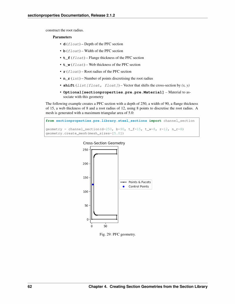
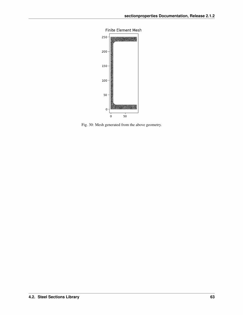
The following example creates a PFC section with a depth of 250, a width of 90, a flange thicknessof 15, a web thickness of 8 and a root radius of 12, using 8 points to discretise the root radius. Amesh is generated with a maximum triangular area of 5.0:
from sectionproperties.pre.library.steel_sections import channel_section
geometry = channel_section(d=250, b=90, t_f=15, t_w=8, r=12, n_r=8)geometry.create_mesh(mesh_sizes=[5.0])
Fig. 29: PFC geometry.
62 Chapter 4. Creating Section Geometries from the Section Library
sectionproperties Documentation, Release 2.1.2
Fig. 30: Mesh generated from the above geometry.
4.2. Steel Sections Library 63

sectionproperties Documentation, Release 2.1.2
4.2.9 Tapered Flange Channel Section
sectionproperties.pre.library.steel_sections.tapered_flange_channel(d:float,b:float,t_f:float,t_w:float,r_r:float,r_f:float,al-pha:float,n_r:int,ma-te-rial:sec-tion-prop-er-ties.pre.pre.Material=Ma-te-rial(name=’default’,elas-tic_modulus=1,pois-sons_ratio=0,yield_strength=1,den-sity=1,color=’w’))→sec-tion-prop-er-ties.pre.geometry.Geometry
Constructs a Tapered Flange Channel section with the bottom left corner at the origin (0, 0), withdepth d, width b, mid-flange thickness t_f, web thickness t_w, root radius r_r, flange radius r_f andflange angle alpha, using n_r points to construct the radii.
Parameters
• d (float) – Depth of the Tapered Flange Channel section
• b (float) – Width of the Tapered Flange Channel section
• t_f (float) – Mid-flange thickness of the Tapered Flange Channel section (mea-
64 Chapter 4. Creating Section Geometries from the Section Library

sectionproperties Documentation, Release 2.1.2
sured at the point equidistant from the face of the web to the edge of the flange)
• t_w (float) – Web thickness of the Tapered Flange Channel section
• r_r (float) – Root radius of the Tapered Flange Channel section
• r_f (float) – Flange radius of the Tapered Flange Channel section
• alpha (float) – Flange angle of the Tapered Flange Channel section (degrees)
• n_r (int) – Number of points discretising the radii
• Optional[sectionproperties.pre.pre.Material] – Material to as-sociate with this geometry
The following example creates a Tapered Flange Channel section with a depth of 10, a width of 3.5,a mid-flange thickness of 0.575, a web thickness of 0.475, a root radius of 0.575, a flange radiusof 0.4 and a flange angle of 8°, using 16 points to discretise the radii. A mesh is generated with amaximum triangular area of 0.02:
from sectionproperties.pre.library.steel_sections import tapered_flange_→˓channel
geometry = tapered_flange_channel(d=10, b=3.5, t_f=0.575, t_w=0.475, r_r=0.575, r_f=0.4, alpha=8, n_
→˓r=16)geometry.create_mesh(mesh_sizes=[0.02])
Fig. 31: Tapered flange channel geometry.
4.2. Steel Sections Library 65

sectionproperties Documentation, Release 2.1.2
Fig. 32: Mesh generated from the above geometry.
4.2.10 Tee Section
sectionproperties.pre.library.steel_sections.tee_section(d: float, b:float, t_f:float, t_w:float, r: float,n_r: int, ma-terial: sec-tionproper-ties.pre.pre.Material= Mate-rial(name=’default’,elas-tic_modulus=1,pois-sons_ratio=0,yield_strength=1,density=1,color=’w’))→ sec-tionproper-ties.pre.geometry.Geometry
Constructs a Tee section with the top left corner at (0, d), with depth d, width b, flange thickness t_f,web thickness t_w and root radius r, using n_r points to construct the root radius.
Parameters
• d (float) – Depth of the Tee section
• b (float) – Width of the Tee section
• t_f (float) – Flange thickness of the Tee section
• t_w (float) – Web thickness of the Tee section
66 Chapter 4. Creating Section Geometries from the Section Library

sectionproperties Documentation, Release 2.1.2
• r (float) – Root radius of the Tee section
• n_r (int) – Number of points discretising the root radius
• Optional[sectionproperties.pre.pre.Material] – Material to as-sociate with this geometry
The following example creates a Tee section with a depth of 200, a width of 100, a flange thicknessof 12, a web thickness of 6 and a root radius of 8, using 8 points to discretise the root radius. A meshis generated with a maximum triangular area of 3.0:
from sectionproperties.pre.library.steel_sections import tee_section
geometry = tee_section(d=200, b=100, t_f=12, t_w=6, r=8, n_r=8)geometry.create_mesh(mesh_sizes=[3.0])
Fig. 33: Tee section geometry.
4.2. Steel Sections Library 67
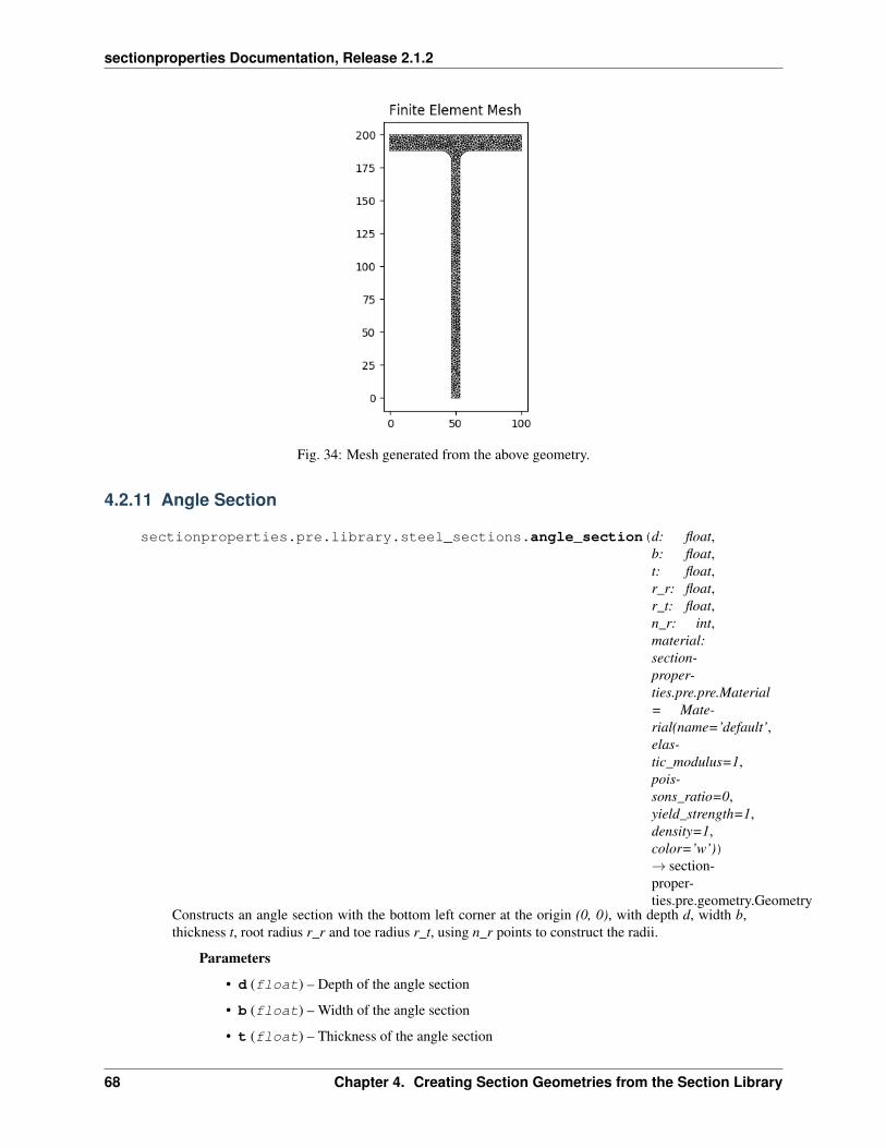
sectionproperties Documentation, Release 2.1.2
Fig. 34: Mesh generated from the above geometry.
4.2.11 Angle Section
sectionproperties.pre.library.steel_sections.angle_section(d: float,b: float,t: float,r_r: float,r_t: float,n_r: int,material:section-proper-ties.pre.pre.Material= Mate-rial(name=’default’,elas-tic_modulus=1,pois-sons_ratio=0,yield_strength=1,density=1,color=’w’))→ section-proper-ties.pre.geometry.Geometry
Constructs an angle section with the bottom left corner at the origin (0, 0), with depth d, width b,thickness t, root radius r_r and toe radius r_t, using n_r points to construct the radii.
Parameters
• d (float) – Depth of the angle section
• b (float) – Width of the angle section
• t (float) – Thickness of the angle section
68 Chapter 4. Creating Section Geometries from the Section Library

sectionproperties Documentation, Release 2.1.2
• r_r (float) – Root radius of the angle section
• r_t (float) – Toe radius of the angle section
• n_r (int) – Number of points discretising the radii
• Optional[sectionproperties.pre.pre.Material] – Material to as-sociate with this geometry
The following example creates an angle section with a depth of 150, a width of 100, a thickness of 8,a root radius of 12 and a toe radius of 5, using 16 points to discretise the radii. A mesh is generatedwith a maximum triangular area of 2.0:
from sectionproperties.pre.library.steel_sections import angle_section
geometry = angle_section(d=150, b=100, t=8, r_r=12, r_t=5, n_r=16)geometry.create_mesh(mesh_sizes=[2.0])
Fig. 35: Angle section geometry.
4.2. Steel Sections Library 69

sectionproperties Documentation, Release 2.1.2
4.2.12 Cee Section
sectionproperties.pre.library.steel_sections.cee_section(d: float,b: float, l:float, t: float,r_out: float,n_r: int, ma-terial: sec-tionproper-ties.pre.pre.Material= Mate-rial(name=’default’,elas-tic_modulus=1,pois-sons_ratio=0,yield_strength=1,density=1,color=’w’))→ sec-tionproper-ties.pre.geometry.Geometry
Constructs a Cee section (typical of cold-formed steel) with the bottom left corner at the origin (0,0), with depth d, width b, lip l, thickness t and outer radius r_out, using n_r points to construct theradius. If the outer radius is less than the thickness of the Cee Section, the inner radius is set to zero.
Parameters
• d (float) – Depth of the Cee section
• b (float) – Width of the Cee section
• l (float) – Lip of the Cee section
• t (float) – Thickness of the Cee section
• r_out (float) – Outer radius of the Cee section
70 Chapter 4. Creating Section Geometries from the Section Library
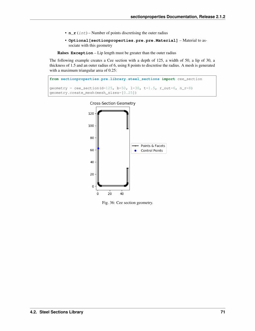
sectionproperties Documentation, Release 2.1.2
• n_r (int) – Number of points discretising the outer radius
• Optional[sectionproperties.pre.pre.Material] – Material to as-sociate with this geometry
Raises Exception – Lip length must be greater than the outer radius
The following example creates a Cee section with a depth of 125, a width of 50, a lip of 30, athickness of 1.5 and an outer radius of 6, using 8 points to discretise the radius. A mesh is generatedwith a maximum triangular area of 0.25:
from sectionproperties.pre.library.steel_sections import cee_section
geometry = cee_section(d=125, b=50, l=30, t=1.5, r_out=6, n_r=8)geometry.create_mesh(mesh_sizes=[0.25])
Fig. 36: Cee section geometry.
4.2. Steel Sections Library 71
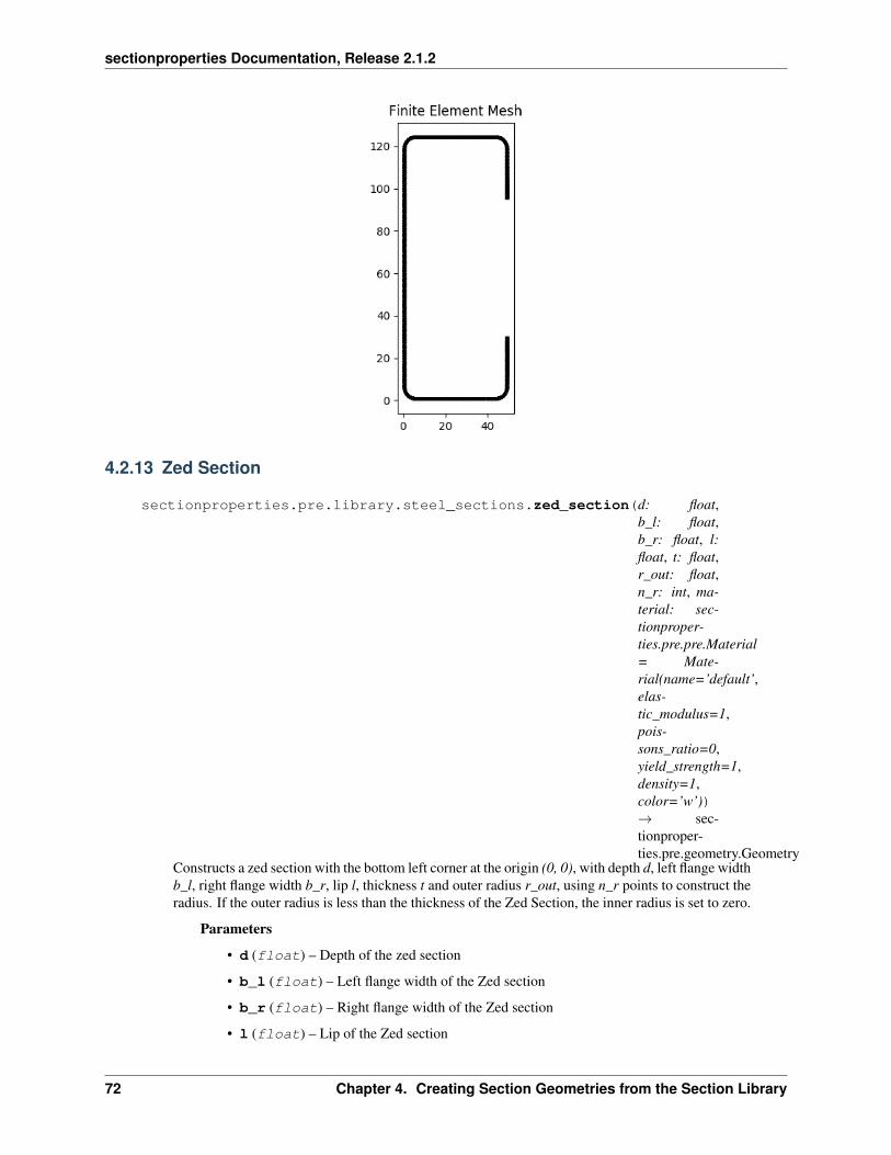
sectionproperties Documentation, Release 2.1.2
4.2.13 Zed Section
sectionproperties.pre.library.steel_sections.zed_section(d: float,b_l: float,b_r: float, l:float, t: float,r_out: float,n_r: int, ma-terial: sec-tionproper-ties.pre.pre.Material= Mate-rial(name=’default’,elas-tic_modulus=1,pois-sons_ratio=0,yield_strength=1,density=1,color=’w’))→ sec-tionproper-ties.pre.geometry.Geometry
Constructs a zed section with the bottom left corner at the origin (0, 0), with depth d, left flange widthb_l, right flange width b_r, lip l, thickness t and outer radius r_out, using n_r points to construct theradius. If the outer radius is less than the thickness of the Zed Section, the inner radius is set to zero.
Parameters
• d (float) – Depth of the zed section
• b_l (float) – Left flange width of the Zed section
• b_r (float) – Right flange width of the Zed section
• l (float) – Lip of the Zed section
72 Chapter 4. Creating Section Geometries from the Section Library

sectionproperties Documentation, Release 2.1.2
• t (float) – Thickness of the Zed section
• r_out (float) – Outer radius of the Zed section
• n_r (int) – Number of points discretising the outer radius
• Optional[sectionproperties.pre.pre.Material] – Material to as-sociate with this geometry
The following example creates a zed section with a depth of 100, a left flange width of 40, a rightflange width of 50, a lip of 20, a thickness of 1.2 and an outer radius of 5, using 8 points to discretisethe radius. A mesh is generated with a maximum triangular area of 0.15:
from sectionproperties.pre.library.steel_sections import zed_section
geometry = zed_section(d=100, b_l=40, b_r=50, l=20, t=1.2, r_out=5, n_→˓r=8)geometry.create_mesh(mesh_sizes=[0.15])
Fig. 37: zed section geometry.
4.2. Steel Sections Library 73

sectionproperties Documentation, Release 2.1.2
74 Chapter 4. Creating Section Geometries from the Section Library

sectionproperties Documentation, Release 2.1.2
4.2.14 Box Girder Section
sectionproperties.pre.library.steel_sections.box_girder_section(d:float,b_t:float,b_b:float,t_ft:float,t_fb:float,t_w:float,ma-te-rial:sec-tion-prop-er-ties.pre.pre.Material=Ma-te-rial(name=’default’,elas-tic_modulus=1,pois-sons_ratio=0,yield_strength=1,den-sity=1,color=’w’))
Constructs a box girder section centered at at (max(b_t, b_b)/2, d/2), with depth d, top width b_t,bottom width b_b, top flange thickness t_ft, bottom flange thickness t_fb and web thickness t_w.
Parameters
• d (float) – Depth of the Box Girder section
• b_t (float) – Top width of the Box Girder section
• b_b (float) – Bottom width of the Box Girder section
• t_ft (float) – Top flange thickness of the Box Girder section
• t_fb (float) – Bottom flange thickness of the Box Girder section
• t_w (float) – Web thickness of the Box Girder section
The following example creates a Box Girder section with a depth of 1200, a top width of 1200,a bottom width of 400, a top flange thickness of 16, a bottom flange thickness of 12 and a webthickness of 8. A mesh is generated with a maximum triangular area of 5.0:
from sectionproperties.pre.library.steel_sections import box_girder_→˓section
(continues on next page)
4.2. Steel Sections Library 75

sectionproperties Documentation, Release 2.1.2
(continued from previous page)
geometry = box_girder_section(d=1200, b_t=1200, b_b=400, t_ft=100, t_→˓fb=80, t_w=50)geometry.create_mesh(mesh_sizes=[200.0])
Fig. 38: Box Girder geometry.
4.2.15 Bulb Section
sectionproperties.pre.library.steel_sections.bulb_section(d: float,b: float,t: float,r: float,n_r: int,d_b: float =None, ma-terial: sec-tionproper-ties.pre.pre.Material= Mate-rial(name=’default’,elas-tic_modulus=1,pois-sons_ratio=0,yield_strength=1,density=1,color=’w’))→ sec-tionproper-ties.pre.geometry.Geometry
Constructs a bulb section with the bottom left corner at the point (-t / 2, 0), with depth d, bulb depth
76 Chapter 4. Creating Section Geometries from the Section Library

sectionproperties Documentation, Release 2.1.2
Fig. 39: Mesh generated from the above geometry.
d_b, bulb width b, web thickness t and radius r, using n_r points to construct the radius.
Parameters
• d (float) – Depth of the section
• b (float) – Bulb width
• t (float) – Web thickness
• r (float) – Bulb radius
• d_b (float) – Depth of the bulb (automatically calculated for standard sections,if provided the section may have sharp edges)
• n_r (int) – Number of points discretising the radius
• Optional[sectionproperties.pre.pre.Material] – Material to as-sociate with this geometry
The following example creates a bulb section with a depth of 240, a width of 34, a web thicknessof 12 and a bulb radius of 16, using 16 points to discretise the radius. A mesh is generated with amaximum triangular area of 5.0:
from sectionproperties.pre.library.steel_sections import bulb_section
geometry = bulb_section(d=240, b=34, t=12, r=10, n_r=16)geometry.create_mesh(mesh_sizes=[5.0])
4.2. Steel Sections Library 77

sectionproperties Documentation, Release 2.1.2
Fig. 40: Bulb section geometry.
Fig. 41: Mesh generated from the above geometry.
78 Chapter 4. Creating Section Geometries from the Section Library

sectionproperties Documentation, Release 2.1.2
4.2. Steel Sections Library 79

sectionproperties Documentation, Release 2.1.2
4.3 Concrete Sections Library
4.3.1 Concrete Rectangular Section
sectionproperties.pre.library.concrete_sections.concrete_rectangular_section(b:float,d:float,dia_top:float,n_top:int,dia_bot:float,n_bot:int,n_circle:int,cover:float,area_top:float=None,area_bot:float=None,conc_mat:sec-tion-prop-er-ties.pre.pre.Material=Ma-te-rial(name=’default’,elas-tic_modulus=1,pois-sons_ratio=0,yield_strength=1,den-sity=1,color=’w’),steel_mat:sec-tion-prop-er-ties.pre.pre.Material=Ma-te-rial(name=’default’,elas-tic_modulus=1,pois-sons_ratio=0,yield_strength=1,den-sity=1,color=’w’))→sec-tion-prop-er-ties.pre.geometry.CompoundGeometry
Constructs a concrete rectangular section of width b and depth d, with n_top top steel bars of diameter dia_top,
80 Chapter 4. Creating Section Geometries from the Section Library

sectionproperties Documentation, Release 2.1.2
n_bot bottom steel bars of diameter dia_bot, discretised with n_circle points with equal side and top/bottomcover to the steel.
Parameters
• b (float) – Concrete section width
• d (float) – Concrete section depth
• dia_top (float) – Diameter of the top steel reinforcing bars
• n_top (int) – Number of top steel reinforcing bars
• dia_bot (float) – Diameter of the bottom steel reinforcing bars
• n_bot (int) – Number of bottom steel reinforcing bars
• n_circle (int) – Number of points discretising the steel reinforcing bars
• cover (float) – Side and bottom cover to the steel reinforcing bars
• area_top (float) – If provided, constructs top reinforcing bars based on their area ratherthan diameter (prevents the underestimation of steel area due to circle discretisation)
• area_bot (float) – If provided, constructs bottom reinforcing bars based on their arearather than diameter (prevents the underestimation of steel area due to circle discretisation)
• conc_mat (Optional[sectionproperties.pre.pre.Material]) – Materialto associate with the concrete
• steel_mat (Optional[sectionproperties.pre.pre.Material]) – Mate-rial to associate with the steel
Raises ValueErorr – If the number of bars is not greater than or equal to 2 in an active layer
The following example creates a 600D x 300W concrete beam with 3N20 bottom steel reinforcing bars and 30mm cover:
from sectionproperties.pre.library.concrete_sections import concrete_rectangular_→˓sectionfrom sectionproperties.pre.pre import Material
concrete = Material(name='Concrete', elastic_modulus=30.1e3, poissons_ratio=0.2, yield_
→˓strength=32,density=2.4e-6, color='lightgrey'
)steel = Material(
name='Steel', elastic_modulus=200e3, poissons_ratio=0.3, yield_strength=500,density=7.85e-6, color='grey'
)
geometry = concrete_rectangular_section(b=300, d=600, dia_top=20, n_top=0, dia_bot=20, n_bot=3, n_circle=24, cover=30,conc_mat=concrete, steel_mat=steel
)geometry.create_mesh(mesh_sizes=[500])
4.3. Concrete Sections Library 81

sectionproperties Documentation, Release 2.1.2
Fig. 42: Concrete rectangular section geometry.
Fig. 43: Mesh generated from the above geometry.
82 Chapter 4. Creating Section Geometries from the Section Library

sectionproperties Documentation, Release 2.1.2
4.3. Concrete Sections Library 83

sectionproperties Documentation, Release 2.1.2
4.3.2 Concrete Tee Section
sectionproperties.pre.library.concrete_sections.concrete_tee_section(b:float,d:float,b_f:float,d_f:float,dia_top:float,n_top:int,dia_bot:float,n_bot:int,n_circle:int,cover:float,area_top:float =None,area_bot:float =None,conc_mat:sec-tion-proper-ties.pre.pre.Material=Mate-rial(name=’default’,elas-tic_modulus=1,pois-sons_ratio=0,yield_strength=1,den-sity=1,color=’w’),steel_mat:sec-tion-proper-ties.pre.pre.Material=Mate-rial(name=’default’,elas-tic_modulus=1,pois-sons_ratio=0,yield_strength=1,den-sity=1,color=’w’))→ sec-tion-proper-ties.pre.geometry.CompoundGeometry
Constructs a concrete tee section of width b, depth d, flange width b_f and flange depth d_f, with n_top top
84 Chapter 4. Creating Section Geometries from the Section Library

sectionproperties Documentation, Release 2.1.2
steel bars of diameter dia_top, n_bot bottom steel bars of diameter dia_bot, discretised with n_circle points withequal side and top/bottom cover to the steel.
Parameters
• b (float) – Concrete section width
• d (float) – Concrete section depth
• b_f (float) – Concrete section flange width
• d_f (float) – Concrete section flange depth
• dia_top (float) – Diameter of the top steel reinforcing bars
• n_top (int) – Number of top steel reinforcing bars
• dia_bot (float) – Diameter of the bottom steel reinforcing bars
• n_bot (int) – Number of bottom steel reinforcing bars
• n_circle (int) – Number of points discretising the steel reinforcing bars
• cover (float) – Side and bottom cover to the steel reinforcing bars
• area_top (float) – If provided, constructs top reinforcing bars based on their area ratherthan diameter (prevents the underestimation of steel area due to circle discretisation)
• area_bot (float) – If provided, constructs bottom reinforcing bars based on their arearather than diameter (prevents the underestimation of steel area due to circle discretisation)
• conc_mat (Optional[sectionproperties.pre.pre.Material]) – Materialto associate with the concrete
• steel_mat (Optional[sectionproperties.pre.pre.Material]) – Mate-rial to associate with the steel
Raises ValueErorr – If the number of bars is not greater than or equal to 2 in an active layer
The following example creates a 900D x 450W concrete beam with a 1200W x 250D flange, with 5N24 steelreinforcing bars and 30 mm cover:
from sectionproperties.pre.library.concrete_sections import concrete_tee_sectionfrom sectionproperties.pre.pre import Material
concrete = Material(name='Concrete', elastic_modulus=30.1e3, poissons_ratio=0.2, yield_
→˓strength=32,density=2.4e-6, color='lightgrey'
)steel = Material(
name='Steel', elastic_modulus=200e3, poissons_ratio=0.3, yield_strength=500,density=7.85e-6, color='grey'
)
geometry = concrete_tee_section(b=450, d=900, b_f=1200, d_f=250, dia_top=24, n_top=0, dia_bot=24, n_bot=5,n_circle=24, cover=30, conc_mat=concrete, steel_mat=steel
)geometry.create_mesh(mesh_sizes=[500])
4.3. Concrete Sections Library 85

sectionproperties Documentation, Release 2.1.2
Fig. 44: Concrete tee section geometry.
Fig. 45: Mesh generated from the above geometry.
86 Chapter 4. Creating Section Geometries from the Section Library

sectionproperties Documentation, Release 2.1.2
4.3.3 Concrete Circular Section
sectionproperties.pre.library.concrete_sections.concrete_circular_section(d:float,n:int,dia:float,n_bar:int,n_circle:int,cover:float,area_conc:float=None,area_bar:float=None,conc_mat:sec-tion-prop-er-ties.pre.pre.Material=Ma-te-rial(name=’default’,elas-tic_modulus=1,pois-sons_ratio=0,yield_strength=1,den-sity=1,color=’w’),steel_mat:sec-tion-prop-er-ties.pre.pre.Material=Ma-te-rial(name=’default’,elas-tic_modulus=1,pois-sons_ratio=0,yield_strength=1,den-sity=1,color=’w’))→sec-tion-prop-er-ties.pre.geometry.CompoundGeometry
Constructs a concrete circular section of diameter d discretised with n points, with n_bar steel bars of diameter
4.3. Concrete Sections Library 87

sectionproperties Documentation, Release 2.1.2
dia, discretised with n_circle points with equal side and bottom cover to the steel.
Parameters
• d (float) – Concrete diameter
• n (float) – Number of points discretising the concrete section
• dia (float) – Diameter of the steel reinforcing bars
• n_bar (int) – Number of steel reinforcing bars
• n_circle (int) – Number of points discretising the steel reinforcing bars
• cover (float) – Side and bottom cover to the steel reinforcing bars
• area_conc (float) – If provided, constructs the concrete based on its area rather thandiameter (prevents the underestimation of concrete area due to circle discretisation)
• area_bar (float) – If provided, constructs reinforcing bars based on their area ratherthan diameter (prevents the underestimation of steel area due to
• conc_mat (Optional[sectionproperties.pre.pre.Material]) – Materialto associate with the concrete
• steel_mat (Optional[sectionproperties.pre.pre.Material]) – Mate-rial to associate with the steel
Raises ValueErorr – If the number of bars is not greater than or equal to 2
The following example creates a 450DIA concrete column with with 6N20 steel reinforcing bars and 45 mmcover:
from sectionproperties.pre.library.concrete_sections import concrete_circular_→˓sectionfrom sectionproperties.pre.pre import Material
concrete = Material(name='Concrete', elastic_modulus=30.1e3, poissons_ratio=0.2, yield_
→˓strength=32,density=2.4e-6, color='lightgrey'
)steel = Material(
name='Steel', elastic_modulus=200e3, poissons_ratio=0.3, yield_strength=500,density=7.85e-6, color='grey'
)
geometry = concrete_circular_section(d=450, n=64, dia=20, n_bar=6, n_circle=24, cover=45, conc_mat=concrete, steel_
→˓mat=steel)geometry.create_mesh(mesh_sizes=[500])
88 Chapter 4. Creating Section Geometries from the Section Library

sectionproperties Documentation, Release 2.1.2
Fig. 46: Concrete circular section geometry.
Fig. 47: Mesh generated from the above geometry.
4.3. Concrete Sections Library 89

sectionproperties Documentation, Release 2.1.2
4.4 Bridge Sections Library
4.4.1 Super Tee Girder Section
sectionproperties.pre.library.bridge_sections.super_t_girder_section(girder_type:int,girder_subtype:int =2, w:float =2100,t_w:float =None,t_f:float =75, ma-terial:sec-tion-proper-ties.pre.pre.Material=Mate-rial(name=’default’,elas-tic_modulus=1,pois-sons_ratio=0,yield_strength=1,den-sity=1,color=’w’))→ sec-tion-proper-ties.pre.geometry.Geometry
Constructs a Super T Girder section to AS5100.5.
Parameters
• girder_type (int) – Type of Super T (1 to 5)
• girder_subtype (int) – Era Super T (1: pre-2001, 2:contemporary)
• w (float) – Overall width of top flange
• t_w (float) – Web thickness of the Super-T section (defaults to those of AS5100.5 TbD3(B))
• t_f (float) – Thickness of top flange (VIC (default) = 75 mm; NSW = 90 mm)
• Optional[sectionproperties.pre.pre.Material] – Material to associatewith this geometry
The following example creates a T5 Super-T section with a 180 mm overlay slab and assigns the differentmaterial properties:
90 Chapter 4. Creating Section Geometries from the Section Library
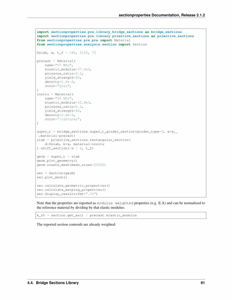
sectionproperties Documentation, Release 2.1.2
import sectionproperties.pre.library.bridge_sections as bridge_sectionsimport sectionproperties.pre.library.primitive_sections as primitive_sectionsfrom sectionproperties.pre.pre import Materialfrom sectionproperties.analysis.section import Section
Dslab, w, t_f = 180, 2100, 75
precast = Material(name="65 MPa",elastic_modulus=37.4e3,poissons_ratio=0.2,yield_strength=65,density=2.4e-6,color="grey",
)insitu = Material(
name="40 MPa",elastic_modulus=32.8e3,poissons_ratio=0.2,yield_strength=40,density=2.4e-6,color="lightgrey",
)
super_t = bridge_sections.super_t_girder_section(girder_type=5, w=w,→˓material=precast)slab = primitive_sections.rectangular_section(
d=Dslab, b=w, material=insitu).shift_section(-w / 2, t_f)
geom = super_t + slabgeom.plot_geometry()geom.create_mesh(mesh_sizes=[500])
sec = Section(geom)sec.plot_mesh()
sec.calculate_geometric_properties()sec.calculate_warping_properties()sec.display_results(fmt=".3f")
Note that the properties are reported as modulus weighted properties (e.g. E.A) and can be normalized tothe reference material by dividing by that elastic modulus:
A_65 = section.get_ea() / precast.elastic_modulus
The reported section centroids are already weighted.
4.4. Bridge Sections Library 91
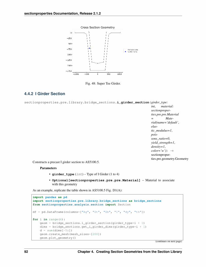
sectionproperties Documentation, Release 2.1.2
Fig. 48: Super Tee Girder.
4.4.2 I Girder Section
sectionproperties.pre.library.bridge_sections.i_girder_section(girder_type:int, material:sectionproper-ties.pre.pre.Material= Mate-rial(name=’default’,elas-tic_modulus=1,pois-sons_ratio=0,yield_strength=1,density=1,color=’w’)) →sectionproper-ties.pre.geometry.Geometry
Constructs a precast I girder section to AS5100.5.
Parameters
• girder_type (int) – Type of I Girder (1 to 4)
• Optional[sectionproperties.pre.pre.Material] – Material to associatewith this geometry
As an example, replicate the table shown in AS5100.5 Fig. D1(A):
import pandas as pdimport sectionproperties.pre.library.bridge_sections as bridge_sectionsfrom sectionproperties.analysis.section import Section
df = pd.DataFrame(columns=["Ag", "Zt", "Zb", "I", "dy", "th"])
for i in range(4):geom = bridge_sections.i_girder_section(girder_type=i + 1)dims = bridge_sections.get_i_girder_dims(girder_type=i + 1)d = sum(dims[-5:])geom.create_mesh(mesh_sizes=[200])geom.plot_geometry()
(continues on next page)
92 Chapter 4. Creating Section Geometries from the Section Library

sectionproperties Documentation, Release 2.1.2
(continued from previous page)
sec = Section(geom)sec.plot_mesh()sec.calculate_geometric_properties()sec.calculate_warping_properties()
A = sec.get_area()th = A / (sec.get_perimeter() / 2)
df.loc[i] = [A,
*(sec.get_z()[:2]),sec.get_ic()[0],d + sec.get_c()[1],th,
]
print(df)
Note that the section depth is obtained by summing the heights from the section dictionary inget_i_girder_dims().
Fig. 49: I Girder.
4.5 Nastran Sections Library
See nastran_sections Module.
4.5. Nastran Sections Library 93
sectionproperties Documentation, Release 2.1.2
94 Chapter 4. Creating Section Geometries from the Section Library

CHAPTER 5
Advanced Geometry Creation
The below tutorial was created to demonstrate the creation of valid geometries for section analysis by combiningmultiple shapes.
Some key points to remember:
1. Geometries of two different materials should not overlap (can create unpredictable results)
2. If two geometries of the same materials are overlapping, then you should perform a union on the two sections
3. Two different section geometries that share a common edge (facet) should also share the same nodes (do notleave “floating” nodes along common edges)
These are general points to remember for any finite element analysis.
Note: sectionproperties will not prevent the creation of these ambiguous sections. The flexibility of the new pre-processing engine (shapely) allows for a wide variety of intermediate modelling steps but the user must ensure that thefinal model is one that is appropriate for analysis.
5.1 Creating Merged Sections
For this example, we will create a custom section out of two similar “I” sections:
import sectionproperties.pre.library.steel_sections as steel_sectionsimport sectionproperties.analysis.section as cross_section
i_sec1 = steel_sections.i_section(d=250, b=150, t_f=13, t_w=10, r=12, n_r=12)i_sec2 = i_sec1.rotate_section(45)
Assign a unique material to each geometry:
95
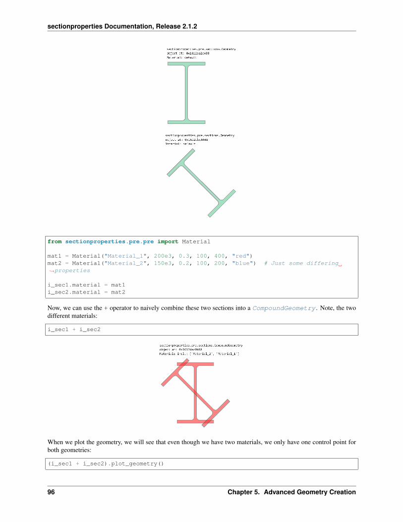
sectionproperties Documentation, Release 2.1.2
from sectionproperties.pre.pre import Material
mat1 = Material("Material_1", 200e3, 0.3, 100, 400, "red")mat2 = Material("Material_2", 150e3, 0.2, 100, 200, "blue") # Just some differing→˓properties
i_sec1.material = mat1i_sec2.material = mat2
Now, we can use the + operator to naively combine these two sections into a CompoundGeometry . Note, the twodifferent materials:
i_sec1 + i_sec2
When we plot the geometry, we will see that even though we have two materials, we only have one control point forboth geometries:
(i_sec1 + i_sec2).plot_geometry()
96 Chapter 5. Advanced Geometry Creation

sectionproperties Documentation, Release 2.1.2
If we went a few steps further by creating a mesh and then plotting that mesh as part of an analysis section, we wouldsee the unpredictable result of the mesh:
cross_section.Section((i_sec1 + i_sec2).create_mesh([10])).plot_mesh()
5.2 Preventing Ambiguity
To prevent ambiguity between geometries and their analytical regions, there are a few options we can take. We canperform a simple union operation but that will lose the material information for one of our sections: whichever sectioncomes first in the operation will have it’s information preserved. In this example, we will use | (union) with i_sec2taking precedence by being the first object in the operation:
i_sec2 | i_sec1
However, this is unsatisfactory as a solution. We want this section to more aptly represent a real section that might becreated by cutting and welding two sections together.
Lets say we want the upright “I” section to be our main section and the diagonal section will be added on to it.
5.2. Preventing Ambiguity 97

sectionproperties Documentation, Release 2.1.2
It is sometimes possible to do this in a quick operation, one which does not create nodes in common at the intersectionpoints. Here, we will simply “slice” i_sec2 with i_sec1 and add it to i_sec1. This will create “floating nodes”along the common edges of i_sec2 and i_sec1 because the nodes are not a part of i_sec1:
(i_sec2 - i_sec1) + i_sec1
Sometimes, we can get away with this as in this example. We can see in the plot that there are five distinct regionsindicated with five control points.
When we are “unlucky”, sometimes gaps can be created (due to floating point errors) where the two sections meet anda proper hole might not be detected, resulting in an incorrect section.
5.3 Creating Nodes in Common
It is best practice to first create nodes in common on both sections and then combine them. For this, an extra step isrequired:
cut_2_from_1 = (i_sec1 - i_sec2) # locates intersection nodessec_1_nodes_added = cut_2_from_1 | i_sec1
# This can also be done in one linesec_1_nodes_added = (i_sec1 - i_sec2) | i_sec1
Now, when we use .plot_geometry(), we can see the additional nodes added to “section 1”:
sec_1_nodes_added.plot_geometry()
At this point, we can use our “section 1 with additional nodes” to create our complete geometry:
98 Chapter 5. Advanced Geometry Creation

sectionproperties Documentation, Release 2.1.2
Fig. 1: The additional nodes from the cut portion are now merged as part of the “section 1” geometry.
analysis_geom = (i_sec2 - i_sec1) + sec_1_nodes_addedanalysis_geom.plot_geometry()
And when we create our mesh and analysis section:
analysis_geom.create_mesh([10])analysis_sec = cross_section.Section(analysis_geom)analysis_sec.plot_mesh()
We can see that the mesh represents how we expect the section to be.
5.3. Creating Nodes in Common 99

sectionproperties Documentation, Release 2.1.2
5.4 Another example
Here, we will simply combine two squares with the default material:
import sectionproperties.pre.library.primitive_sections as primitive_sectionsfrom sectionproperties.analysis.section import Section
s1 = primitive_sections.rectangular_section(1,1)s2 = primitive_sections.rectangular_section(0.5,0.5).shift_section(1,0.25)geometry = s1 + s2geometry
From the shapely vector representation, we can see that the squares are shaded red. This indicates an “invalid” geom-etry from shapely’s perspective because there are two polygons that share an edge. For this geometry, the intention isto have two squares that are connected on one side and so the red shading provided by the shapely representation tellsus that we are getting what we expect.
Now, say this is not our final geometry and we actually want to have it rotated by 30 degrees:
geometry = geometry.rotate_section(30)
Here, we can see that the shapely representation is now showing as green indicating a “valid” shapely geometry. Eventhough it is now valid for shapely, because it is green we know that these two polygons no longer share an edge becausethere is a miniscule separation between them as a result of a floating point error.
When we try to mesh this geometry, we will actually cause a crash with triangle, the meshing tool used behind-the-scenes by sectionproperties:
geometry.create_mesh(mesh_sizes=[0.2, 0.1]) # This may crash the kernel
The crash occurs because the distance between the two polygons is so small, even though they are separated and thespace between them will not be meshed. The same crash would occur if the polygons were overlapping by this samesmall distance.
If we plot the geometry, you can see that each of the two squares has only four nodes and four facets and theirrelationship is only incidental. If their edges happen to perfectly align, they will be considered as one continuoussection. If their edges do not perfectly align, they will be considered as discontinuous.
100 Chapter 5. Advanced Geometry Creation

sectionproperties Documentation, Release 2.1.2
To remedy this, take the same approach as in the preceding example by creating intermediate nodes where the twopolygons intersect by using set operations. If we subtract s2 from s1 then we will have the larger square withintermediate nodes created:
(s1 - s2).plot_geometry(labels=['points'])
Now, if we build the compound geometry up from this larger square with the intermediate points, then our section willwork.:
geometry_fixed = (s1 - s2) + s2geometry_fixed_rotated = geometry_fixed.rotate_section(angle=30)geometry_rot.create_mesh(mesh_sizes=[0.2, 0.1])geometry_rot.plot_geometry(labels=["points", "facets"])section = Section(geometry_rot)section.display_mesh_info()
5.5 Another example (but with nested geometries)
This example demonstrates creating nested geometries using two different approaches. These approaches reflect thedifferences between how shapely (geometry pre-processor) “perceives” geometry and how Triangle (meshing tool)“perceives” geometry and how the modeller might adapt their input style depending on the situation.
The nested geometry we are trying to create looks as follows:
In creating this geometry consider the following:
5.5. Another example (but with nested geometries) 101
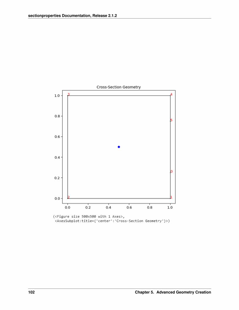
sectionproperties Documentation, Release 2.1.2
102 Chapter 5. Advanced Geometry Creation

sectionproperties Documentation, Release 2.1.2
5.5. Another example (but with nested geometries) 103
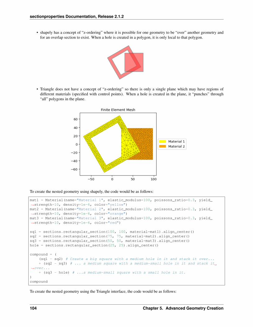
sectionproperties Documentation, Release 2.1.2
• shapely has a concept of “z-ordering” where it is possible for one geometry to be “over” another geometry andfor an overlap section to exist. When a hole is created in a polygon, it is only local to that polygon.
• Triangle does not have a concept of “z-ordering” so there is only a single plane which may have regions ofdifferent materials (specified with control points). When a hole is created in the plane, it “punches” through“all” polygons in the plane.
To create the nested geometry using shapely, the code would be as follows:
mat1 = Material(name="Material 1", elastic_modulus=100, poissons_ratio=0.3, yield_→˓strength=10, density=1e-6, color="yellow")mat2 = Material(name="Material 2", elastic_modulus=100, poissons_ratio=0.3, yield_→˓strength=10, density=1e-6, color="orange")mat3 = Material(name="Material 3", elastic_modulus=100, poissons_ratio=0.3, yield_→˓strength=10, density=1e-6, color="red")
sq1 = sections.rectangular_section(100, 100, material=mat1).align_center()sq2 = sections.rectangular_section(75, 75, material=mat2).align_center()sq3 = sections.rectangular_section(50, 50, material=mat3).align_center()hole = sections.rectangular_section(25, 25).align_center()
compound = ((sq1 - sq2) # Create a big square with a medium hole in it and stack it over...+ (sq2 - sq3) # ... a medium square with a medium-small hole in it and stack it
→˓over...+ (sq3 - hole) # ...a medium-small square with a small hole in it.
)compound
To create the nested geometry using the Triangle interface, the code would be as follows:
104 Chapter 5. Advanced Geometry Creation
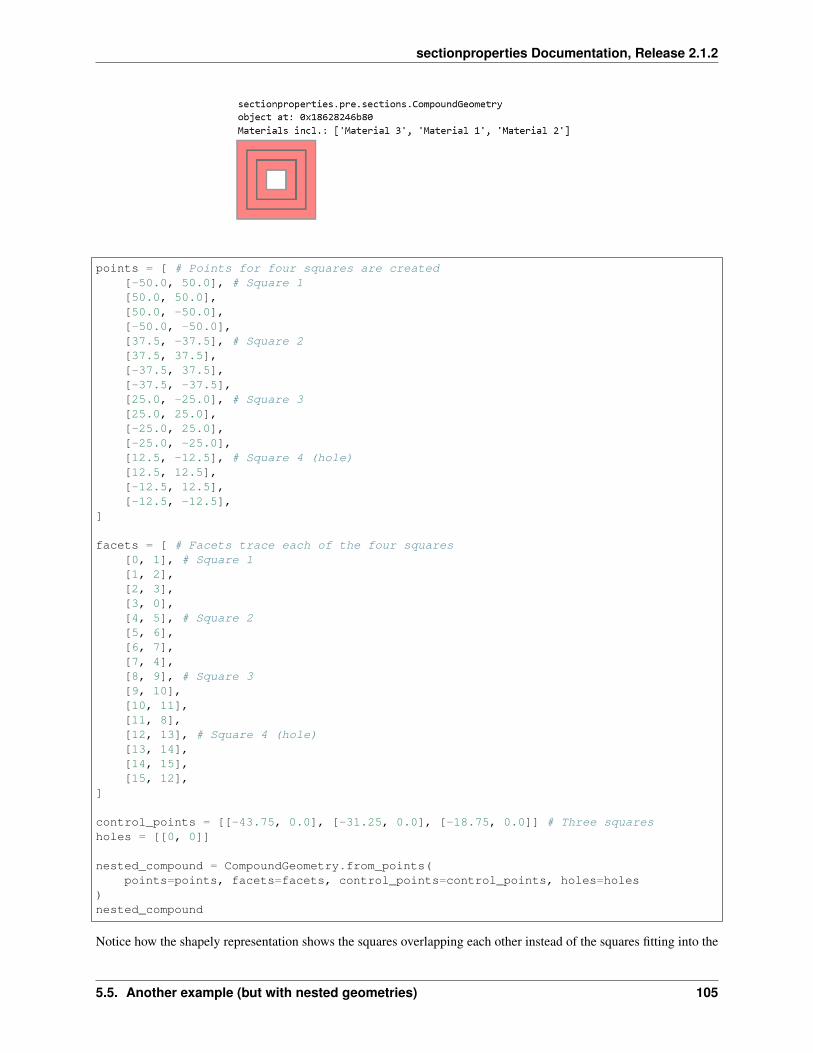
sectionproperties Documentation, Release 2.1.2
points = [ # Points for four squares are created[-50.0, 50.0], # Square 1[50.0, 50.0],[50.0, -50.0],[-50.0, -50.0],[37.5, -37.5], # Square 2[37.5, 37.5],[-37.5, 37.5],[-37.5, -37.5],[25.0, -25.0], # Square 3[25.0, 25.0],[-25.0, 25.0],[-25.0, -25.0],[12.5, -12.5], # Square 4 (hole)[12.5, 12.5],[-12.5, 12.5],[-12.5, -12.5],
]
facets = [ # Facets trace each of the four squares[0, 1], # Square 1[1, 2],[2, 3],[3, 0],[4, 5], # Square 2[5, 6],[6, 7],[7, 4],[8, 9], # Square 3[9, 10],[10, 11],[11, 8],[12, 13], # Square 4 (hole)[13, 14],[14, 15],[15, 12],
]
control_points = [[-43.75, 0.0], [-31.25, 0.0], [-18.75, 0.0]] # Three squaresholes = [[0, 0]]
nested_compound = CompoundGeometry.from_points(points=points, facets=facets, control_points=control_points, holes=holes
)nested_compound
Notice how the shapely representation shows the squares overlapping each other instead of the squares fitting into the
5.5. Another example (but with nested geometries) 105
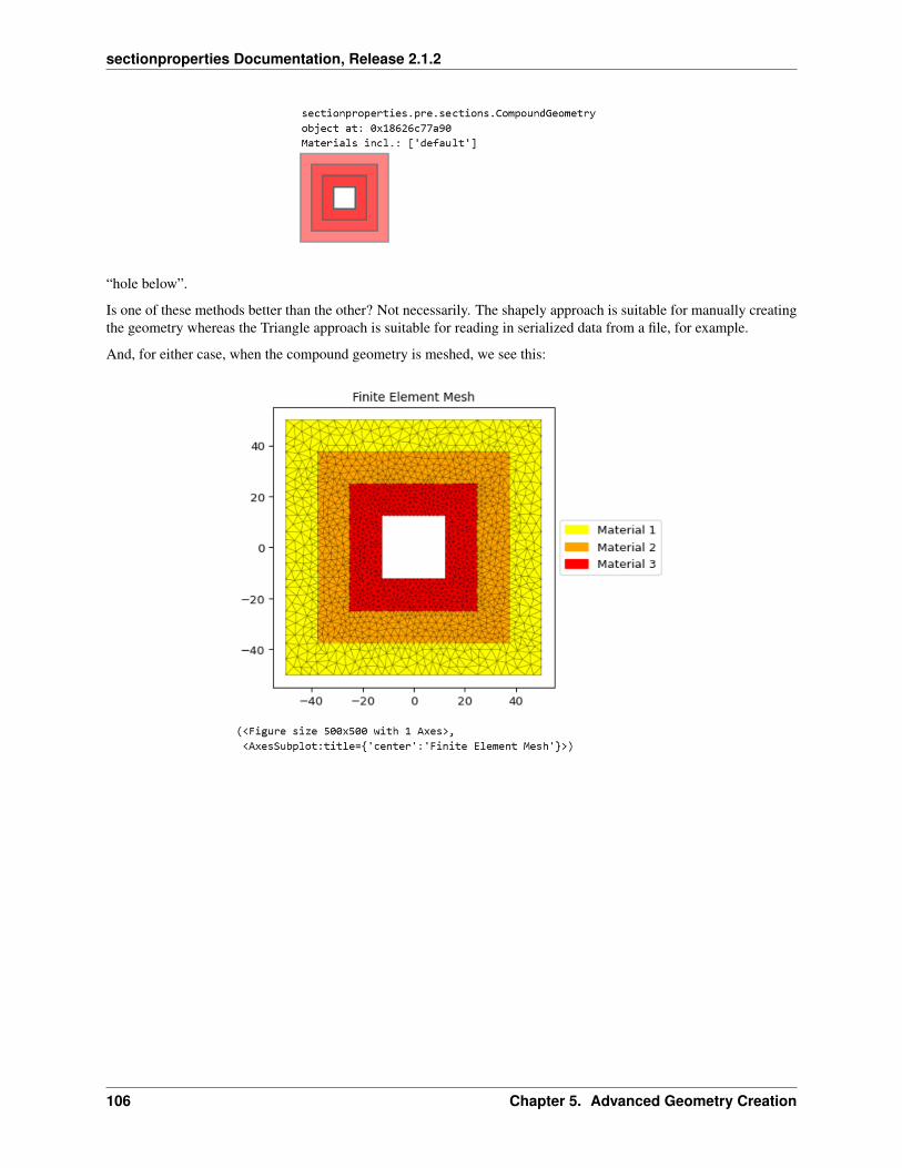
sectionproperties Documentation, Release 2.1.2
“hole below”.
Is one of these methods better than the other? Not necessarily. The shapely approach is suitable for manually creatingthe geometry whereas the Triangle approach is suitable for reading in serialized data from a file, for example.
And, for either case, when the compound geometry is meshed, we see this:
106 Chapter 5. Advanced Geometry Creation
CHAPTER 6
Running an Analysis
The first step in running a section analysis is the creation of a Section object. This class stores the structuralgeometry and finite element mesh and provides methods to perform various types of sectional analyses.
class sectionproperties.analysis.section.Section(geometry:Union[sectionproperties.pre.geometry.Geometry,sectionproper-ties.pre.geometry.CompoundGeometry],time_info: bool = False)
Class for structural cross-sections.
Stores the finite element geometry, mesh and material information and provides methods to compute the cross-section properties. The element type used in this program is the six-noded quadratic triangular element.
The constructor extracts information from the provided mesh object and creates and stores the correspondingTri6 finite element objects.
Parameters
• geometry (Geometry) – Cross-section geometry object used to generate the mesh
• time_info (bool) – If set to True, a detailed description of the computation and the timecost is printed to the terminal for every computation performed.
The following example creates a Section object of a 100D x 50W rectangle using a mesh size of 5:
import sectionproperties.pre.library.primitive_sections as primitive_sectionsfrom sectionproperties.analysis.section import Section
geometry = primitive_sections.rectangular_section(d=100, b=50)geometry.create_mesh(mesh_sizes=[5])section = Section(geometry)
Variables
• elements (list[Tri6]) – List of finite element objects describing the cross-section mesh
• num_nodes (int) – Number of nodes in the finite element mesh
107

sectionproperties Documentation, Release 2.1.2
• geometry (Geometry) – Cross-section geometry object used to generate the mesh
• mesh (dict(mesh)) – Mesh dict returned by triangle
• mesh_nodes (numpy.ndarray) – Array of node coordinates from the mesh
• mesh_elements (numpy.ndarray) – Array of connectivities from the mesh
• mesh_attributes (numpy.ndarray) – Array of attributes from the mesh
• materials – List of materials
• material_groups – List of objects containing the elements in each defined material
• section_props (SectionProperties) – Class to store calculated section properties
Raises
• AssertionError – If the number of materials does not equal the number of regions
• ValueError – If geometry does not contain a mesh
6.1 Checking the Mesh Quality
Before carrying out a section analysis it is a good idea to check the quality of the finite element mesh. Some usefulmethods are provided to display mesh statistics and to plot the finite element mesh:
Section.display_mesh_info()Prints mesh statistics (number of nodes, elements and regions) to the command window.
The following example displays the mesh statistics for a Tee section merged from two rectangles:
import sectionproperties.pre.library.primitive_sections as primitive_sectionsfrom sectionproperties.analysis.section import Section
rec1 = primitive_sections.rectangular_section(d=100, b=25)rec2 = primitive_sections.rectangular_section(d=25, b=100)rec1 = rec1.shift_section(x_offset=-12.5)rec2 = rec2.shift_section(x_offset=-50, y_offset=100)
geometry = rec1 + rec2geometry.create_mesh(mesh_sizes=[5, 2.5])section = Section(geometry)section.display_mesh_info()
>>>Mesh Statistics:>>>--4920 nodes>>>--2365 elements>>>--2 regions
Section.plot_mesh(alpha=0.5, materials=True, mask=None, title=’Finite Element Mesh’, **kwargs)Plots the finite element mesh.
Parameters
• alpha (float) – Transparency of the mesh outlines: 0 ≤ 𝛼 ≤ 1
• materials (bool) – If set to true shades the elements with the specified material colours
• mask (list[bool]) – Mask array, of length num_nodes, to mask out triangles
• title (string) – Plot title
108 Chapter 6. Running an Analysis

sectionproperties Documentation, Release 2.1.2
• kwargs – Passed to plotting_context()
Returns Matplotlib axes object
Return type matplotlib.axes
The following example plots the mesh generated for the second example listed under the Section objectdefinition:
import sectionproperties.pre.library.primitive_sections as primitive_sectionsfrom sectionproperties.pre.pre import Materialfrom sectionproperties.analysis.section import Section
steel = Material(name='Steel', elastic_modulus=200e3, poissons_ratio=0.3, density=7.85e-6,yield_strength=250, color='grey'
)timber = Material(
name='Timber', elastic_modulus=8e3, poissons_ratio=0.35, density=6.5e-7,yield_strength=20, color='burlywood'
)
geom_steel = primitive_sections.rectangular_section(d=50, b=50, material=steel)geom_timber = primitive_sections.rectangular_section(d=50, b=50, material=timber)geometry = geom_timber.align_to(geom_steel, on="right") + geom_steel
geometry.create_mesh(mesh_sizes=[10, 5])
section = Section(geometry)section.plot_mesh(materials=True, alpha=0.5)
Fig. 1: Finite element mesh generated by the above example.
6.1. Checking the Mesh Quality 109
sectionproperties Documentation, Release 2.1.2
6.2 Geometric Analysis
A geometric analysis calculates the area properties of the section.
Section.calculate_geometric_properties()Calculates the geometric properties of the cross-section and stores them in the SectionProperties objectcontained in the section_props class variable.
The following geometric section properties are calculated:
• Cross-sectional area
• Cross-sectional perimeter
• Cross-sectional mass
• Area weighted material properties, composite only 𝐸𝑒𝑓𝑓 , 𝐺𝑒𝑓𝑓 , 𝑛𝑢𝑒𝑓𝑓
• Modulus weighted area (axial rigidity)
• First moments of area
• Second moments of area about the global axis
• Second moments of area about the centroidal axis
• Elastic centroid
• Centroidal section moduli
• Radii of gyration
• Principal axis properties
If materials are specified for the cross-section, the moments of area and section moduli are elastic modulusweighted.
The following example demonstrates the use of this method:
section = Section(geometry)section.calculate_geometric_properties()
6.3 Plastic Analysis
A plastic analysis calculates the plastic properties of the section.
Note: A geometric analysis must be performed on the Section object before a plastic analysis is carried out.
Warning: The plastic analysis in sectionproperties assumes all materials are able to reach their yield stressdefined in the material properties. Care should be taken if analysing materials or cross-sections exhibiting non-linear behaviour, e.g. reinforced concrete or non-compact steel sections.
Section.calculate_plastic_properties(verbose=False)Calculates the plastic properties of the cross-section and stores them in the SectionProperties objectcontained in the section_props class variable.
Parameters verbose (bool) – If set to True, the number of iterations required for each plasticaxis is printed to the terminal.
110 Chapter 6. Running an Analysis
sectionproperties Documentation, Release 2.1.2
The following warping section properties are calculated:
• Plastic centroid for bending about the centroidal and principal axes
• Plastic section moduli for bending about the centroidal and principal axes
• Shape factors for bending about the centroidal and principal axes
If materials are specified for the cross-section, the plastic section moduli are displayed as plastic moments (i.e𝑀𝑝 = 𝑓𝑦𝑆) and the shape factors are not calculated.
Note that the geometric properties must be calculated before the plastic properties are calculated:
section = Section(geometry)section.calculate_geometric_properties()section.calculate_plastic_properties()
Raises RuntimeError – If the geometric properties have not been calculated prior to calling thismethod
6.4 Warping Analysis
A warping analysis calculates the torsion and shear properties of the section.
Note: A geometric analysis must be performed on the Section object before a warping analysis is carried out.
Warning: There must be connectivity between all elements of the mesh to perform a valid warping analysis. Thisis a limitation of the elastic theory that this implementation is based on, as there is no way to quantify the transferof shear and warping between two unconnected regions.
Section.calculate_warping_properties(solver_type=’direct’)Calculates all the warping properties of the cross-section and stores them in the SectionProperties objectcontained in the section_props class variable.
Parameters solver_type (string) – Solver used for solving systems of linear equations, ei-ther using the ‘direct’ method or ‘cgs’ iterative method
The following warping section properties are calculated:
• Torsion constant
• Shear centre
• Shear area
• Warping constant
• Monosymmetry constant
If materials are specified, the values calculated for the torsion constant, warping constant and shear area areelastic modulus weighted.
Note that the geometric properties must be calculated prior to the calculation of the warping properties:
section = Section(geometry)section.calculate_geometric_properties()section.calculate_warping_properties()
6.4. Warping Analysis 111

sectionproperties Documentation, Release 2.1.2
Raises RuntimeError – If the geometric properties have not been calculated prior to calling thismethod
6.5 Stress Analysis
A stress analysis calculates the section stresses arising from a set of forces and moments. Executing this methodreturns a StressResult object which stores the section stresses and provides stress plotting functions.
Note: A geometric and warping analysis must be performed on the Section object before a stress analysis is carriedout.
Warning: The stress analysis in sectionproperties is linear-elastic and does not account for the yielding ofmaterials or any non-linearities.
Section.calculate_stress(N=0, Vx=0, Vy=0, Mxx=0, Myy=0, M11=0, M22=0, Mzz=0)Calculates the cross-section stress resulting from design actions and returns a StressPost object allowingpost-processing of the stress results.
Parameters
• N (float) – Axial force
• Vx (float) – Shear force acting in the x-direction
• Vy (float) – Shear force acting in the y-direction
• Mxx (float) – Bending moment about the centroidal xx-axis
• Myy (float) – Bending moment about the centroidal yy-axis
• M11 (float) – Bending moment about the centroidal 11-axis
• M22 (float) – Bending moment about the centroidal 22-axis
• Mzz (float) – Torsion moment about the centroidal zz-axis
Returns Object for post-processing cross-section stresses
Return type StressPost
Note that a geometric and warping analysis must be performed before a stress analysis is carried out:
section = Section(geometry)section.calculate_geometric_properties()section.calculate_warping_properties()stress_post = section.calculate_stress(N=1e3, Vy=3e3, Mxx=1e6)
Raises RuntimeError – If a geometric and warping analysis have not been performed prior tocalling this method
6.6 Calculating Frame Properties
Calculates the section properties required for a 2D or 3D frame analysis.
112 Chapter 6. Running an Analysis

sectionproperties Documentation, Release 2.1.2
Note: This method is significantly faster than performing a geometric and a warping analysis and has no prerequisites.
Section.calculate_frame_properties(solver_type=’direct’)Calculates and returns the properties required for a frame analysis. The properties are also stored in theSectionProperties object contained in the section_props class variable.
Parameters solver_type (string) – Solver used for solving systems of linear equations, ei-ther using the ‘direct’ method or ‘cgs’ iterative method
Returns Cross-section properties to be used for a frame analysis (area, ixx, iyy, ixy, j, phi)
Return type tuple(float, float, float, float, float, float)
The following section properties are calculated:
• Cross-sectional area (area)
• Second moments of area about the centroidal axis (ixx, iyy, ixy)
• Torsion constant (j)
• Principal axis angle (phi)
If materials are specified for the cross-section, the area, second moments of area and torsion constant are elasticmodulus weighted.
The following example demonstrates the use of this method:
section = Section(geometry)(area, ixx, iyy, ixy, j, phi) = section.calculate_frame_properties()
6.6. Calculating Frame Properties 113

sectionproperties Documentation, Release 2.1.2
114 Chapter 6. Running an Analysis

CHAPTER 7
Viewing the Results
7.1 Printing a List of the Section Properties
A list of section properties that have been calculated by various analyses can be printed to the terminal using thedisplay_results() method that belongs to every Section object.
Section.display_results(fmt=’8.6e’)Prints the results that have been calculated to the terminal.
Parameters fmt (string) – Number formatting string
The following example displays the geometric section properties for a 100D x 50W rectangle with three digitsafter the decimal point:
import sectionproperties.pre.library.primitive_sections as primitive_sectionsfrom sectionproperties.analysis.section import Section
geometry = primitive_sections.rectangular_section(d=100, b=50)geometry.create_mesh(mesh_sizes=[5])
section = Section(geometry)section.calculate_geometric_properties()
section.display_results(fmt='.3f')
7.2 Getting Specific Section Properties
Alternatively, there are a number of methods that can be called on the Section object to return a specific sectionproperty:
115

sectionproperties Documentation, Release 2.1.2
7.2.1 Section Area
Section.get_area()
Returns Cross-section area
Return type float
section = Section(geometry)section.calculate_geometric_properties()area = section.get_area()
7.2.2 Section Perimeter
Section.get_perimeter()
Returns Cross-section perimeter
Return type float
section = Section(geometry)section.calculate_geometric_properties()perimeter = section.get_perimeter()
7.2.3 Section Mass
Section.get_mass()
Returns Cross-section mass
Return type float
section = Section(geometry)section.calculate_geometric_properties()perimeter = section.get_mass()
7.2.4 Axial Rigidity
If material properties have been specified, returns the axial rigidity of the section.
Section.get_ea()
Returns Modulus weighted area (axial rigidity)
Return type float
section = Section(geometry)section.calculate_geometric_properties()ea = section.get_ea()
7.2.5 First Moments of Area
Section.get_q()
Returns First moments of area about the global axis (qx, qy)
116 Chapter 7. Viewing the Results
sectionproperties Documentation, Release 2.1.2
Return type tuple(float, float)
section = Section(geometry)section.calculate_geometric_properties()(qx, qy) = section.get_q()
7.2.6 Second Moments of Area
Section.get_ig()
Returns Second moments of area about the global axis (ixx_g, iyy_g, ixy_g)
Return type tuple(float, float, float)
section = Section(geometry)section.calculate_geometric_properties()(ixx_g, iyy_g, ixy_g) = section.get_ig()
Section.get_ic()
Returns Second moments of area centroidal axis (ixx_c, iyy_c, ixy_c)
Return type tuple(float, float, float)
section = Section(geometry)section.calculate_geometric_properties()(ixx_c, iyy_c, ixy_c) = section.get_ic()
Section.get_ip()
Returns Second moments of area about the principal axis (i11_c, i22_c)
Return type tuple(float, float)
section = Section(geometry)section.calculate_geometric_properties()(i11_c, i22_c) = section.get_ip()
7.2.7 Elastic Centroid
Section.get_c()
Returns Elastic centroid (cx, cy)
Return type tuple(float, float)
section = Section(geometry)section.calculate_geometric_properties()(cx, cy) = section.get_c()
7.2.8 Section Moduli
Section.get_z()
Returns Elastic section moduli about the centroidal axis with respect to the top and bottom fibres(zxx_plus, zxx_minus, zyy_plus, zyy_minus)
7.2. Getting Specific Section Properties 117

sectionproperties Documentation, Release 2.1.2
Return type tuple(float, float, float, float)
section = Section(geometry)section.calculate_geometric_properties()(zxx_plus, zxx_minus, zyy_plus, zyy_minus) = section.get_z()
Section.get_zp()
Returns Elastic section moduli about the principal axis with respect to the top and bottom fibres(z11_plus, z11_minus, z22_plus, z22_minus)
Return type tuple(float, float, float, float)
section = Section(geometry)section.calculate_geometric_properties()(z11_plus, z11_minus, z22_plus, z22_minus) = section.get_zp()
7.2.9 Radii of Gyration
Section.get_rc()
Returns Radii of gyration about the centroidal axis (rx, ry)
Return type tuple(float, float)
section = Section(geometry)section.calculate_geometric_properties()(rx, ry) = section.get_rc()
Section.get_rp()
Returns Radii of gyration about the principal axis (r11, r22)
Return type tuple(float, float)
section = Section(geometry)section.calculate_geometric_properties()(r11, r22) = section.get_rp()
7.2.10 Principal Axis Angle
Section.get_phi()
Returns Principal bending axis angle
Return type float
section = Section(geometry)section.calculate_geometric_properties()phi = section.get_phi()
7.2.11 Effective Material Properties
Section.get_e_eff()
Returns Effective elastic modulus based on area
118 Chapter 7. Viewing the Results

sectionproperties Documentation, Release 2.1.2
Return type float
section = Section(geometry)section.calculate_warping_properties()e_eff = section.get_e_eff()
Section.get_g_eff()
Returns Effective shear modulus based on area
Return type float
section = Section(geometry)section.calculate_geometric_properties()g_eff = section.get_g_eff()
Section.get_nu_eff()
Returns Effective Poisson’s ratio
Return type float
section = Section(geometry)section.calculate_geometric_properties()nu_eff = section.get_nu_eff()
7.2.12 Torsion Constant
Section.get_j()
Returns St. Venant torsion constant
Return type float
section = Section(geometry)section.calculate_geometric_properties()section.calculate_warping_properties()j = section.get_j()
7.2.13 Shear Centre
Section.get_sc()
Returns Centroidal axis shear centre (elasticity approach) (x_se, y_se)
Return type tuple(float, float)
section = Section(geometry)section.calculate_geometric_properties()section.calculate_warping_properties()(x_se, y_se) = section.get_sc()
Section.get_sc_p()
Returns Principal axis shear centre (elasticity approach) (x11_se, y22_se)
Return type tuple(float, float)
7.2. Getting Specific Section Properties 119

sectionproperties Documentation, Release 2.1.2
section = Section(geometry)section.calculate_geometric_properties()section.calculate_warping_properties()(x11_se, y22_se) = section.get_sc_p()
7.2.14 Trefftz’s Shear Centre
Section.get_sc_t()
Returns Centroidal axis shear centre (Trefftz’s approach) (x_st, y_st)
Return type tuple(float, float)
section = Section(geometry)section.calculate_geometric_properties()section.calculate_warping_properties()(x_st, y_st) = section.get_sc_t()
7.2.15 Warping Constant
Section.get_gamma()
Returns Warping constant
Return type float
section = Section(geometry)section.calculate_geometric_properties()section.calculate_warping_properties()gamma = section.get_gamma()
7.2.16 Shear Area
Section.get_As()
Returns Shear area for loading about the centroidal axis (A_sx, A_sy)
Return type tuple(float, float)
section = Section(geometry)section.calculate_geometric_properties()section.calculate_warping_properties()(A_sx, A_sy) = section.get_As()
Section.get_As_p()
Returns Shear area for loading about the principal bending axis (A_s11, A_s22)
Return type tuple(float, float)
section = Section(geometry)section.calculate_geometric_properties()section.calculate_warping_properties()(A_s11, A_s22) = section.get_As_p()
120 Chapter 7. Viewing the Results

sectionproperties Documentation, Release 2.1.2
7.2.17 Monosymmetry Constants
Section.get_beta()
Returns Monosymmetry constant for bending about both global axes (beta_x_plus, beta_x_minus,beta_y_plus, beta_y_minus). The plus value relates to the top flange in compression and theminus value relates to the bottom flange in compression.
Return type tuple(float, float, float, float)
section = Section(geometry)section.calculate_geometric_properties()section.calculate_warping_properties()(beta_x_plus, beta_x_minus, beta_y_plus, beta_y_minus) = section.get_beta()
Section.get_beta_p()
Returns Monosymmetry constant for bending about both principal axes (beta_11_plus,beta_11_minus, beta_22_plus, beta_22_minus). The plus value relates to the top flange in com-pression and the minus value relates to the bottom flange in compression.
Return type tuple(float, float, float, float)
section = Section(geometry)section.calculate_geometric_properties()section.calculate_warping_properties()(beta_11_plus, beta_11_minus, beta_22_plus, beta_22_minus) = section.get_beta_p()
7.2.18 Plastic Centroid
Section.get_pc()
Returns Centroidal axis plastic centroid (x_pc, y_pc)
Return type tuple(float, float)
section = Section(geometry)section.calculate_geometric_properties()section.calculate_plastic_properties()(x_pc, y_pc) = section.get_pc()
Section.get_pc_p()
Returns Principal bending axis plastic centroid (x11_pc, y22_pc)
Return type tuple(float, float)
section = Section(geometry)section.calculate_geometric_properties()section.calculate_plastic_properties()(x11_pc, y22_pc) = section.get_pc_p()
7.2.19 Plastic Section Moduli
Section.get_s()
Returns Plastic section moduli about the centroidal axis (sxx, syy)
7.2. Getting Specific Section Properties 121

sectionproperties Documentation, Release 2.1.2
Return type tuple(float, float)
If material properties have been specified, returns the plastic moment 𝑀𝑝 = 𝑓𝑦𝑆.
section = Section(geometry)section.calculate_geometric_properties()section.calculate_plastic_properties()(sxx, syy) = section.get_s()
Section.get_sp()
Returns Plastic section moduli about the principal bending axis (s11, s22)
Return type tuple(float, float)
If material properties have been specified, returns the plastic moment 𝑀𝑝 = 𝑓𝑦𝑆.
section = Section(geometry)section.calculate_geometric_properties()section.calculate_plastic_properties()(s11, s22) = section.get_sp()
7.2.20 Shape Factors
Section.get_sf()
Returns Centroidal axis shape factors with respect to the top and bottom fibres (sf_xx_plus,sf_xx_minus, sf_yy_plus, sf_yy_minus)
Return type tuple(float, float, float, float)
section = Section(geometry)section.calculate_geometric_properties()section.calculate_plastic_properties()(sf_xx_plus, sf_xx_minus, sf_yy_plus, sf_yy_minus) = section.get_sf()
Section.get_sf_p()
Returns Principal bending axis shape factors with respect to the top and bottom fibres (sf_11_plus,sf_11_minus, sf_22_plus, sf_22_minus)
Return type tuple(float, float, float, float)
section = Section(geometry)section.calculate_geometric_properties()section.calculate_plastic_properties()(sf_11_plus, sf_11_minus, sf_22_plus, sf_22_minus) = section.get_sf_p()
7.3 How Material Properties Affect Results
If a Geometry containing a user defined Material is used to build a Section, sectionproperties will assume youare performing a composite analysis and this will affect the way some of the results are stored and presented.
In general, the calculation of gross composite section properties takes into account the elastic modulus, Poisson’s ratioand yield strength of each material in the section. Unlike many design codes, sectionproperties is ‘material propertyagnostic’ and does not transform sections based on a defined material property, e.g. in reinforced concrete analysis it iscommonplace to transform the reinforcing steel area based on the ratio between the elastic moduli, 𝑛 = 𝐸𝑠𝑡𝑒𝑒𝑙/𝐸𝑐𝑜𝑛𝑐.
122 Chapter 7. Viewing the Results

sectionproperties Documentation, Release 2.1.2
sectionproperties instead calculates the gross material weighted properties, which is analogous to transforming withrespect to a material property with elastic modulus, 𝐸 = 1.
Using the example of a reinforced concrete section, sectionproperties will calculate the gross section bending stiffness,(𝐸𝐼)𝑔 , rather than an effective concrete second moment of area, 𝐼𝑐,𝑒𝑓𝑓 :
(𝐸𝐼)𝑔 = 𝐸𝑠 × 𝐼𝑠 + 𝐸𝑐 × 𝐼𝑐
If the user wanted to obtain the effective concrete second moment of area for a code calculation, they could simplydivide the gross bending stiffness by the elastic modulus for concrete:
𝐼𝑐,𝑒𝑓𝑓 =(𝐸𝐼)𝑔𝐸𝑐
With reference to the get methods described in Printing a List of the Section Properties, a composite analysis willmodify the following properties:
• First moments of area get_q() - returns elastic modulus weighted first moments of area 𝐸.𝑄
• Second moments of area get_ig(), get_ic(), get_ip() - return elastic modulus weighted second mo-ments of area 𝐸.𝐼
• Section moduli get_z(), get_zp() - return elastic modulus weighted section moduli 𝐸.𝑍
• Torsion constant get_j() - returns elastic modulus weighted torsion constant 𝐸.𝐽
• Warping constant get_gamma() - returns elastic modulus weighted warping constant 𝐸.Γ
• Shear areas get_As(), get_As_p() - return elastic modulus weighted shear areas 𝐸.𝐴𝑠
• Plastic section moduli get_s(), get_sp() - return yield strength weighted plastic section moduli, i.e. plasticmoments 𝑀𝑝 = 𝑓𝑦.𝑆
A composite analysis will also enable the user to retrieve effective gross section area-weighted material properties:
• Effective elastic modulus 𝐸𝑒𝑓𝑓 - get_e_eff()
• Effective shear modulus 𝐺𝑒𝑓𝑓 - get_g_eff()
• Effective Poisson’s ratio 𝜈𝑒𝑓𝑓 - get_nu_eff()
These values may be used to transform composite properties output by sectionproperties for practical use, e.g. tocalculate torsional rigidity:
(𝐺𝐽)𝑔 =𝐺𝑒𝑓𝑓
𝐸𝑒𝑓𝑓(𝐸𝐽)𝑔
For further information, see the theoretical background to the calculation of Composite Cross-Sections.
7.4 Section Property Centroids Plots
A plot of the centroids (elastic, plastic and shear centre) can be produced with the finite element mesh in the back-ground:
Section.plot_centroids(title=’Centroids’, **kwargs)Plots the elastic centroid, the shear centre, the plastic centroids and the principal axis, if they have been calcu-lated, on top of the finite element mesh.
Parameters
• title (string) – Plot title
7.4. Section Property Centroids Plots 123

sectionproperties Documentation, Release 2.1.2
• kwargs – Passed to plotting_context()
Returns Matplotlib axes object
Return type matplotlib.axes
The following example analyses a 200 PFC section and displays a plot of the centroids:
import sectionproperties.pre.library.steel_sections as steel_sectionsfrom sectionproperties.analysis.section import Section
geometry = steel_sections.channel_section(d=200, b=75, t_f=12, t_w=6, r=12, n_r=8)geometry.create_mesh(mesh_sizes=[20])
section = Section(geometry)section.calculate_geometric_properties()section.calculate_warping_properties()section.calculate_plastic_properties()
section.plot_centroids()
Fig. 1: Plot of the centroids generated by the above example.
The following example analyses a 150x90x12 UA section and displays a plot of the centroids:
124 Chapter 7. Viewing the Results

sectionproperties Documentation, Release 2.1.2
import sectionproperties.pre.library.steel_sections as steel_sectionsfrom sectionproperties.analysis.section import Section
geometry = steel_sections.angle_section(d=150, b=90, t=12, r_r=10, r_t=5, n_r=8)geometry.create_mesh(mesh_sizes=[20])
section = Section(geometry)section.calculate_geometric_properties()section.calculate_warping_properties()section.calculate_plastic_properties()
section.plot_centroids()
Fig. 2: Plot of the centroids generated by the above example.
7.5 Plotting Section Stresses
There are a number of methods that can be called from a StressResult object to plot the various cross-sectionstresses. These methods take the following form:
StressResult.plot_(stress/vector)_(action)_(stresstype)
where:
• stress denotes a contour plot and vector denotes a vector plot.
• action denotes the type of action causing the stress e.g. mxx for bending moment about the x-axis. Note that theaction is omitted for stresses caused by the application of all actions.
7.5. Plotting Section Stresses 125

sectionproperties Documentation, Release 2.1.2
• stresstype denotes the type of stress that is being plotted e.g. zx for the x-component of shear stress.
The examples shown in the methods below are performed on a 150x90x12 UA (unequal angle) section. The Sectionobject is created below:
import sectionproperties.pre.library.steel_sections as steel_sectionsfrom sectionproperties.analysis.section import Section
geometry = steel_sections.AngleSection(d=150, b=90, t=12, r_r=10, r_t=5, n_r=8)mesh = geometry.create_mesh(mesh_sizes=[2.5])section = Section(geometry, mesh)
7.5.1 Primary Stress Plots
Axial Stress (𝜎𝑧𝑧,𝑁 )
StressPost.plot_stress_n_zz(title=’Stress Contour Plot - $\\sigma_zz, N$’, cmap=’coolwarm’,normalize=True, **kwargs)
Produces a contour plot of the normal stress 𝜎𝑧𝑧,𝑁 resulting from the axial load 𝑁 .
Parameters
• title (string) – Plot title
• cmap (string) – Matplotlib color map.
• normalize (bool) – If set to true, the CenteredNorm is used to scale the colormap. If setto false, the default linear scaling is used.
• kwargs – Passed to plotting_context()
Returns Matplotlib axes object
Return type matplotlib.axes
The following example plots the normal stress within a 150x90x12 UA section resulting from an axial force of10 kN:
import sectionproperties.pre.library.steel_sections as steel_sectionsfrom sectionproperties.analysis.section import Section
geometry = steel_sections.angle_section(d=150, b=90, t=12, r_r=10, r_t=5, n_r=8)geometry.create_mesh(mesh_sizes=[20])section = Section(geometry)
section.calculate_geometric_properties()section.calculate_warping_properties()stress_post = section.calculate_stress(N=10e3)
stress_post.plot_stress_n_zz()
Bending Stress (𝜎𝑧𝑧,𝑀𝑥𝑥)
StressPost.plot_stress_mxx_zz(title=’Stress Contour Plot - $\\sigma_zz, Mxx$’,cmap=’coolwarm’, normalize=True, **kwargs)
Produces a contour plot of the normal stress 𝜎𝑧𝑧,𝑀𝑥𝑥 resulting from the bending moment 𝑀𝑥𝑥.
Parameters
126 Chapter 7. Viewing the Results

sectionproperties Documentation, Release 2.1.2
Fig. 3: Contour plot of the axial stress.
• title (string) – Plot title
• cmap (string) – Matplotlib color map.
• normalize (bool) – If set to true, the CenteredNorm is used to scale the colormap. If setto false, the default linear scaling is used.
• kwargs – Passed to plotting_context()
Returns Matplotlib axes object
Return type matplotlib.axes
The following example plots the normal stress within a 150x90x12 UA section resulting from a bending momentabout the x-axis of 5 kN.m:
import sectionproperties.pre.library.steel_sections as steel_sectionsfrom sectionproperties.analysis.section import Section
geometry = steel_sections.angle_section(d=150, b=90, t=12, r_r=10, r_t=5, n_r=8)geometry.create_mesh(mesh_sizes=[20])section = Section(geometry)
section.calculate_geometric_properties()section.calculate_warping_properties()stress_post = section.calculate_stress(Mxx=5e6)
stress_post.plot_stress_mxx_zz()
Bending Stress (𝜎𝑧𝑧,𝑀𝑦𝑦)
StressPost.plot_stress_myy_zz(title=’Stress Contour Plot - $\\sigma_zz, Myy$’,cmap=’coolwarm’, normalize=True, **kwargs)
Produces a contour plot of the normal stress 𝜎𝑧𝑧,𝑀𝑦𝑦 resulting from the bending moment 𝑀𝑦𝑦.
Parameters
• title (string) – Plot title
• cmap (string) – Matplotlib color map.
7.5. Plotting Section Stresses 127
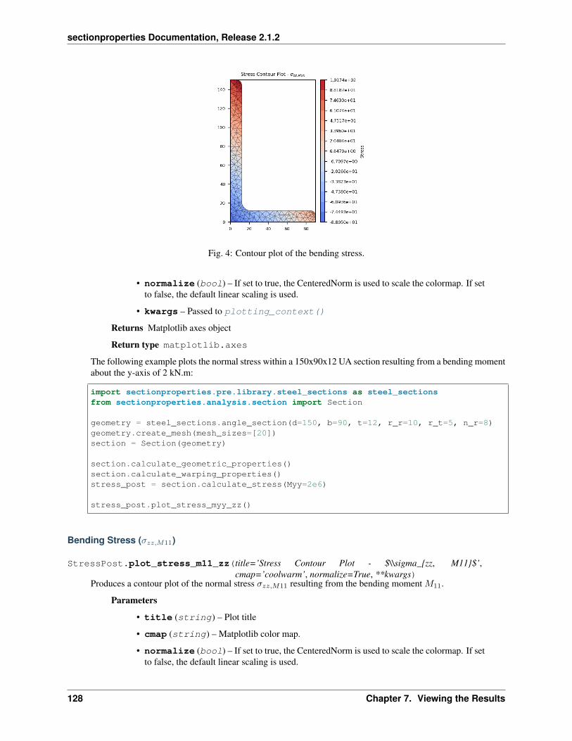
sectionproperties Documentation, Release 2.1.2
Fig. 4: Contour plot of the bending stress.
• normalize (bool) – If set to true, the CenteredNorm is used to scale the colormap. If setto false, the default linear scaling is used.
• kwargs – Passed to plotting_context()
Returns Matplotlib axes object
Return type matplotlib.axes
The following example plots the normal stress within a 150x90x12 UA section resulting from a bending momentabout the y-axis of 2 kN.m:
import sectionproperties.pre.library.steel_sections as steel_sectionsfrom sectionproperties.analysis.section import Section
geometry = steel_sections.angle_section(d=150, b=90, t=12, r_r=10, r_t=5, n_r=8)geometry.create_mesh(mesh_sizes=[20])section = Section(geometry)
section.calculate_geometric_properties()section.calculate_warping_properties()stress_post = section.calculate_stress(Myy=2e6)
stress_post.plot_stress_myy_zz()
Bending Stress (𝜎𝑧𝑧,𝑀11)
StressPost.plot_stress_m11_zz(title=’Stress Contour Plot - $\\sigma_zz, M11$’,cmap=’coolwarm’, normalize=True, **kwargs)
Produces a contour plot of the normal stress 𝜎𝑧𝑧,𝑀11 resulting from the bending moment 𝑀11.
Parameters
• title (string) – Plot title
• cmap (string) – Matplotlib color map.
• normalize (bool) – If set to true, the CenteredNorm is used to scale the colormap. If setto false, the default linear scaling is used.
128 Chapter 7. Viewing the Results
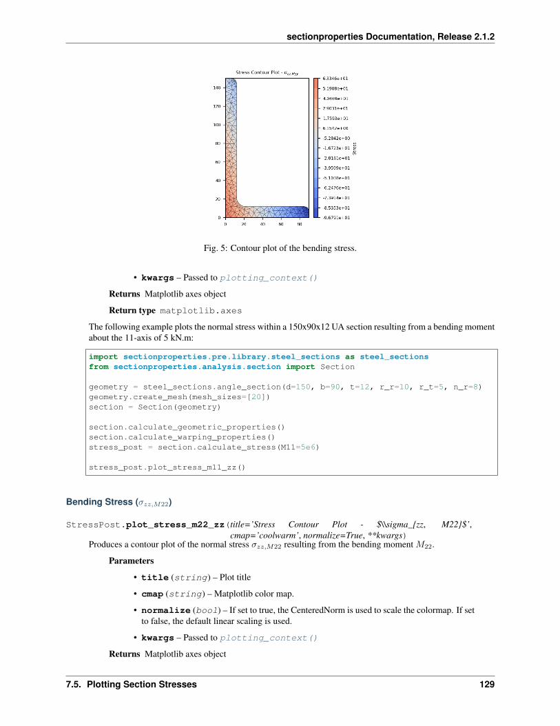
sectionproperties Documentation, Release 2.1.2
Fig. 5: Contour plot of the bending stress.
• kwargs – Passed to plotting_context()
Returns Matplotlib axes object
Return type matplotlib.axes
The following example plots the normal stress within a 150x90x12 UA section resulting from a bending momentabout the 11-axis of 5 kN.m:
import sectionproperties.pre.library.steel_sections as steel_sectionsfrom sectionproperties.analysis.section import Section
geometry = steel_sections.angle_section(d=150, b=90, t=12, r_r=10, r_t=5, n_r=8)geometry.create_mesh(mesh_sizes=[20])section = Section(geometry)
section.calculate_geometric_properties()section.calculate_warping_properties()stress_post = section.calculate_stress(M11=5e6)
stress_post.plot_stress_m11_zz()
Bending Stress (𝜎𝑧𝑧,𝑀22)
StressPost.plot_stress_m22_zz(title=’Stress Contour Plot - $\\sigma_zz, M22$’,cmap=’coolwarm’, normalize=True, **kwargs)
Produces a contour plot of the normal stress 𝜎𝑧𝑧,𝑀22 resulting from the bending moment 𝑀22.
Parameters
• title (string) – Plot title
• cmap (string) – Matplotlib color map.
• normalize (bool) – If set to true, the CenteredNorm is used to scale the colormap. If setto false, the default linear scaling is used.
• kwargs – Passed to plotting_context()
Returns Matplotlib axes object
7.5. Plotting Section Stresses 129

sectionproperties Documentation, Release 2.1.2
Fig. 6: Contour plot of the bending stress.
Return type matplotlib.axes
The following example plots the normal stress within a 150x90x12 UA section resulting from a bending momentabout the 22-axis of 2 kN.m:
import sectionproperties.pre.library.steel_sections as steel_sectionsfrom sectionproperties.analysis.section import Section
geometry = steel_sections.angle_section(d=150, b=90, t=12, r_r=10, r_t=5, n_r=8)geometry.create_mesh(mesh_sizes=[20])section = Section(geometry)
section.calculate_geometric_properties()section.calculate_warping_properties()stress_post = section.calculate_stress(M22=5e6)
stress_post.plot_stress_m22_zz()
Fig. 7: Contour plot of the bending stress.
130 Chapter 7. Viewing the Results

sectionproperties Documentation, Release 2.1.2
Bending Stress (𝜎𝑧𝑧,Σ𝑀 )
StressPost.plot_stress_m_zz(title=’Stress Contour Plot - $\\sigma_zz, \\Sigma M$’,cmap=’coolwarm’, normalize=True, **kwargs)
Produces a contour plot of the normal stress 𝜎𝑧𝑧,Σ𝑀 resulting from all bending moments 𝑀𝑥𝑥 +𝑀𝑦𝑦 +𝑀11 +𝑀22.
Parameters
• title (string) – Plot title
• cmap (string) – Matplotlib color map.
• normalize (bool) – If set to true, the CenteredNorm is used to scale the colormap. If setto false, the default linear scaling is used.
• kwargs – Passed to plotting_context()
Returns Matplotlib axes object
Return type matplotlib.axes
The following example plots the normal stress within a 150x90x12 UA section resulting from a bending momentabout the x-axis of 5 kN.m, a bending moment about the y-axis of 2 kN.m and a bending moment of 3 kN.mabout the 11-axis:
import sectionproperties.pre.library.steel_sections as steel_sectionsfrom sectionproperties.analysis.section import Section
geometry = steel_sections.angle_section(d=150, b=90, t=12, r_r=10, r_t=5, n_r=8)geometry.create_mesh(mesh_sizes=[20])section = Section(geometry)
section.calculate_geometric_properties()section.calculate_warping_properties()stress_post = section.calculate_stress(Mxx=5e6, Myy=2e6, M11=3e6)
stress_post.plot_stress_m_zz()
Fig. 8: Contour plot of the bending stress.
7.5. Plotting Section Stresses 131

sectionproperties Documentation, Release 2.1.2
Torsion Stress (𝜎𝑧𝑥,𝑀𝑧𝑧)
StressPost.plot_stress_mzz_zx(title=’Stress Contour Plot - $\\sigma_zx, Mzz$’,cmap=’coolwarm’, normalize=True, **kwargs)
Produces a contour plot of the x-component of the shear stress 𝜎𝑧𝑥,𝑀𝑧𝑧 resulting from the torsion moment 𝑀𝑧𝑧 .
Parameters
• title (string) – Plot title
• cmap (string) – Matplotlib color map.
• normalize (bool) – If set to true, the CenteredNorm is used to scale the colormap. If setto false, the default linear scaling is used.
• kwargs – Passed to plotting_context()
Returns Matplotlib axes object
Return type matplotlib.axes
The following example plots the x-component of the shear stress within a 150x90x12 UA section resulting froma torsion moment of 1 kN.m:
import sectionproperties.pre.library.steel_sections as steel_sectionsfrom sectionproperties.analysis.section import Section
geometry = steel_sections.angle_section(d=150, b=90, t=12, r_r=10, r_t=5, n_r=8)geometry.create_mesh(mesh_sizes=[20])section = Section(geometry)
section.calculate_geometric_properties()section.calculate_warping_properties()stress_post = section.calculate_stress(Mzz=1e6)
stress_post.plot_stress_mzz_zx()
Fig. 9: Contour plot of the shear stress.
132 Chapter 7. Viewing the Results

sectionproperties Documentation, Release 2.1.2
Torsion Stress (𝜎𝑧𝑦,𝑀𝑧𝑧)
StressPost.plot_stress_mzz_zy(title=’Stress Contour Plot - $\\sigma_zy, Mzz$’,cmap=’coolwarm’, normalize=True, **kwargs)
Produces a contour plot of the y-component of the shear stress 𝜎𝑧𝑦,𝑀𝑧𝑧 resulting from the torsion moment 𝑀𝑧𝑧 .
Parameters
• title (string) – Plot title
• cmap (string) – Matplotlib color map.
• normalize (bool) – If set to true, the CenteredNorm is used to scale the colormap. If setto false, the default linear scaling is used.
• kwargs – Passed to plotting_context()
Returns Matplotlib axes object
Return type matplotlib.axes
The following example plots the y-component of the shear stress within a 150x90x12 UA section resulting froma torsion moment of 1 kN.m:
import sectionproperties.pre.library.steel_sections as steel_sectionsfrom sectionproperties.analysis.section import Section
geometry = steel_sections.angle_section(d=150, b=90, t=12, r_r=10, r_t=5, n_r=8)geometry.create_mesh(mesh_sizes=[20])section = Section(geometry)
section.calculate_geometric_properties()section.calculate_warping_properties()stress_post = section.calculate_stress(Mzz=1e6)
stress_post.plot_stress_mzz_zy()
Fig. 10: Contour plot of the shear stress.
7.5. Plotting Section Stresses 133

sectionproperties Documentation, Release 2.1.2
Torsion Stress (𝜎𝑧𝑥𝑦,𝑀𝑧𝑧)
StressPost.plot_stress_mzz_zxy(title=’Stress Contour Plot - $\\sigma_zxy, Mzz$’,cmap=’coolwarm’, normalize=True, **kwargs)
Produces a contour plot of the resultant shear stress 𝜎𝑧𝑥𝑦,𝑀𝑧𝑧 resulting from the torsion moment 𝑀𝑧𝑧 .
Parameters
• title (string) – Plot title
• cmap (string) – Matplotlib color map.
• normalize (bool) – If set to true, the CenteredNorm is used to scale the colormap. If setto false, the default linear scaling is used.
• kwargs – Passed to plotting_context()
Returns Matplotlib axes object
Return type matplotlib.axes
The following example plots a contour of the resultant shear stress within a 150x90x12 UA section resultingfrom a torsion moment of 1 kN.m:
import sectionproperties.pre.library.steel_sections as steel_sectionsfrom sectionproperties.analysis.section import Section
geometry = steel_sections.angle_section(d=150, b=90, t=12, r_r=10, r_t=5, n_r=8)geometry.create_mesh(mesh_sizes=[20])section = Section(geometry)
section.calculate_geometric_properties()section.calculate_warping_properties()stress_post = section.calculate_stress(Mzz=1e6)
stress_post.plot_stress_mzz_zxy()
Fig. 11: Contour plot of the shear stress.
StressPost.plot_vector_mzz_zxy(title=’Stress Vector Plot - $\\sigma_zxy, Mzz$’,cmap=’YlOrBr’, normalize=False, **kwargs)
Produces a vector plot of the resultant shear stress 𝜎𝑧𝑥𝑦,𝑀𝑧𝑧 resulting from the torsion moment 𝑀𝑧𝑧 .
Parameters
134 Chapter 7. Viewing the Results
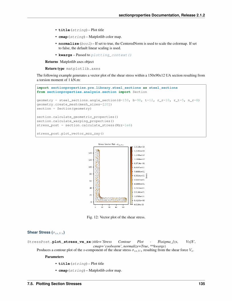
sectionproperties Documentation, Release 2.1.2
• title (string) – Plot title
• cmap (string) – Matplotlib color map.
• normalize (bool) – If set to true, the CenteredNorm is used to scale the colormap. If setto false, the default linear scaling is used.
• kwargs – Passed to plotting_context()
Returns Matplotlib axes object
Return type matplotlib.axes
The following example generates a vector plot of the shear stress within a 150x90x12 UA section resulting froma torsion moment of 1 kN.m:
import sectionproperties.pre.library.steel_sections as steel_sectionsfrom sectionproperties.analysis.section import Section
geometry = steel_sections.angle_section(d=150, b=90, t=12, r_r=10, r_t=5, n_r=8)geometry.create_mesh(mesh_sizes=[20])section = Section(geometry)
section.calculate_geometric_properties()section.calculate_warping_properties()stress_post = section.calculate_stress(Mzz=1e6)
stress_post.plot_vector_mzz_zxy()
Fig. 12: Vector plot of the shear stress.
Shear Stress (𝜎𝑧𝑥,𝑉 𝑥)
StressPost.plot_stress_vx_zx(title=’Stress Contour Plot - $\\sigma_zx, Vx$’,cmap=’coolwarm’, normalize=True, **kwargs)
Produces a contour plot of the x-component of the shear stress 𝜎𝑧𝑥,𝑉 𝑥 resulting from the shear force 𝑉𝑥.
Parameters
• title (string) – Plot title
• cmap (string) – Matplotlib color map.
7.5. Plotting Section Stresses 135

sectionproperties Documentation, Release 2.1.2
• normalize (bool) – If set to true, the CenteredNorm is used to scale the colormap. If setto false, the default linear scaling is used.
• kwargs – Passed to plotting_context()
Returns Matplotlib axes object
Return type matplotlib.axes
The following example plots the x-component of the shear stress within a 150x90x12 UA section resulting froma shear force in the x-direction of 15 kN:
import sectionproperties.pre.library.steel_sections as steel_sectionsfrom sectionproperties.analysis.section import Section
geometry = steel_sections.angle_section(d=150, b=90, t=12, r_r=10, r_t=5, n_r=8)geometry.create_mesh(mesh_sizes=[20])section = Section(geometry)
section.calculate_geometric_properties()section.calculate_warping_properties()stress_post = section.calculate_stress(Vx=15e3)
stress_post.plot_stress_vx_zx()
Fig. 13: Contour plot of the shear stress.
Shear Stress (𝜎𝑧𝑦,𝑉 𝑥)
StressPost.plot_stress_vx_zy(title=’Stress Contour Plot - $\\sigma_zy, Vx$’,cmap=’coolwarm’, normalize=True, **kwargs)
Produces a contour plot of the y-component of the shear stress 𝜎𝑧𝑦,𝑉 𝑥 resulting from the shear force 𝑉𝑥.
Parameters
• title (string) – Plot title
• cmap (string) – Matplotlib color map.
• normalize (bool) – If set to true, the CenteredNorm is used to scale the colormap. If setto false, the default linear scaling is used.
136 Chapter 7. Viewing the Results

sectionproperties Documentation, Release 2.1.2
• kwargs – Passed to plotting_context()
Returns Matplotlib axes object
Return type matplotlib.axes
The following example plots the y-component of the shear stress within a 150x90x12 UA section resulting froma shear force in the x-direction of 15 kN:
import sectionproperties.pre.library.steel_sections as steel_sectionsfrom sectionproperties.analysis.section import Section
geometry = steel_sections.angle_section(d=150, b=90, t=12, r_r=10, r_t=5, n_r=8)geometry.create_mesh(mesh_sizes=[20])section = Section(geometry)
section.calculate_geometric_properties()section.calculate_warping_properties()stress_post = section.calculate_stress(Vx=15e3)
stress_post.plot_stress_vx_zy()
Fig. 14: Contour plot of the shear stress.
Shear Stress (𝜎𝑧𝑥𝑦,𝑉 𝑥)
StressPost.plot_stress_vx_zxy(title=’Stress Contour Plot - $\\sigma_zz, Myy$’,cmap=’coolwarm’, normalize=True, **kwargs)
Produces a contour plot of the resultant shear stress 𝜎𝑧𝑥𝑦,𝑉 𝑥 resulting from the shear force 𝑉𝑥.
Parameters
• title (string) – Plot title
• cmap (string) – Matplotlib color map.
• normalize (bool) – If set to true, the CenteredNorm is used to scale the colormap. If setto false, the default linear scaling is used.
• kwargs – Passed to plotting_context()
Returns Matplotlib axes object
7.5. Plotting Section Stresses 137

sectionproperties Documentation, Release 2.1.2
Return type matplotlib.axes
The following example plots a contour of the resultant shear stress within a 150x90x12 UA section resultingfrom a shear force in the x-direction of 15 kN:
import sectionproperties.pre.library.steel_sections as steel_sectionsfrom sectionproperties.analysis.section import Section
geometry = steel_sections.angle_section(d=150, b=90, t=12, r_r=10, r_t=5, n_r=8)geometry.create_mesh(mesh_sizes=[20])section = Section(geometry)
section.calculate_geometric_properties()section.calculate_warping_properties()stress_post = section.calculate_stress(Vx=15e3)
stress_post.plot_stress_vx_zxy()
Fig. 15: Contour plot of the shear stress.
StressPost.plot_vector_vx_zxy(title=’Stress Vector Plot - $\\sigma_zxy, Vx$’, cmap=’YlOrBr’,normalize=False, **kwargs)
Produces a vector plot of the resultant shear stress 𝜎𝑧𝑥𝑦,𝑉 𝑥 resulting from the shear force 𝑉𝑥.
Parameters
• title (string) – Plot title
• cmap (string) – Matplotlib color map.
• normalize (bool) – If set to true, the CenteredNorm is used to scale the colormap. If setto false, the default linear scaling is used.
• kwargs – Passed to plotting_context()
Returns Matplotlib axes object
Return type matplotlib.axes
The following example generates a vector plot of the shear stress within a 150x90x12 UA section resulting froma shear force in the x-direction of 15 kN:
138 Chapter 7. Viewing the Results

sectionproperties Documentation, Release 2.1.2
import sectionproperties.pre.library.steel_sections as steel_sectionsfrom sectionproperties.analysis.section import Section
geometry = steel_sections.angle_section(d=150, b=90, t=12, r_r=10, r_t=5, n_r=8)geometry.create_mesh(mesh_sizes=[20])section = Section(geometry)
section.calculate_geometric_properties()section.calculate_warping_properties()stress_post = section.calculate_stress(Vx=15e3)
stress_post.plot_vector_vx_zxy()
Fig. 16: Vector plot of the shear stress.
Shear Stress (𝜎𝑧𝑥,𝑉 𝑦)
StressPost.plot_stress_vy_zx(title=’Stress Contour Plot - $\\sigma_zx, Vy$’,cmap=’coolwarm’, normalize=True, **kwargs)
Produces a contour plot of the x-component of the shear stress 𝜎𝑧𝑥,𝑉 𝑦 resulting from the shear force 𝑉𝑦 .
Parameters
• title (string) – Plot title
• cmap (string) – Matplotlib color map.
• normalize (bool) – If set to true, the CenteredNorm is used to scale the colormap. If setto false, the default linear scaling is used.
• kwargs – Passed to plotting_context()
Returns Matplotlib axes object
Return type matplotlib.axes
The following example plots the x-component of the shear stress within a 150x90x12 UA section resulting froma shear force in the y-direction of 30 kN:
7.5. Plotting Section Stresses 139

sectionproperties Documentation, Release 2.1.2
import sectionproperties.pre.library.steel_sections as steel_sectionsfrom sectionproperties.analysis.section import Section
geometry = steel_sections.angle_section(d=150, b=90, t=12, r_r=10, r_t=5, n_r=8)geometry.create_mesh(mesh_sizes=[20])section = Section(geometry)
section.calculate_geometric_properties()section.calculate_warping_properties()stress_post = section.calculate_stress(Vy=30e3)
stress_post.plot_stress_vy_zx()
Fig. 17: Contour plot of the shear stress.
Shear Stress (𝜎𝑧𝑦,𝑉 𝑦)
StressPost.plot_stress_vy_zy(title=’Stress Contour Plot - $\\sigma_zy, Vy$’,cmap=’coolwarm’, normalize=True, **kwargs)
Produces a contour plot of the y-component of the shear stress 𝜎𝑧𝑦,𝑉 𝑦 resulting from the shear force 𝑉𝑦 .
Parameters
• title (string) – Plot title
• cmap (string) – Matplotlib color map.
• normalize (bool) – If set to true, the CenteredNorm is used to scale the colormap. If setto false, the default linear scaling is used.
• kwargs – Passed to plotting_context()
Returns Matplotlib axes object
Return type matplotlib.axes
The following example plots the y-component of the shear stress within a 150x90x12 UA section resulting froma shear force in the y-direction of 30 kN:
140 Chapter 7. Viewing the Results
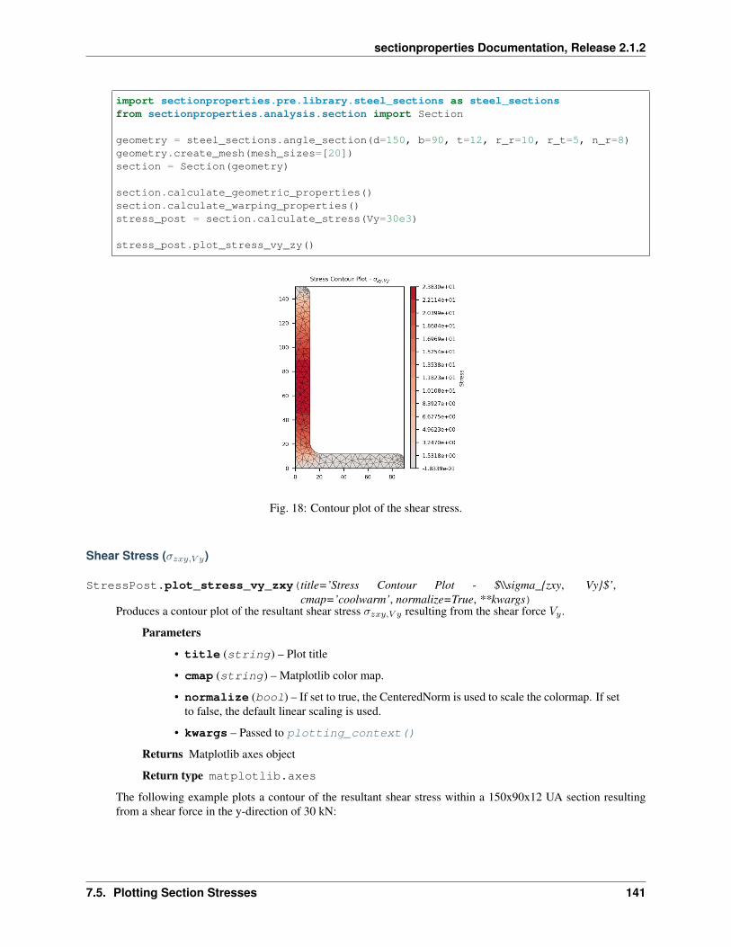
sectionproperties Documentation, Release 2.1.2
import sectionproperties.pre.library.steel_sections as steel_sectionsfrom sectionproperties.analysis.section import Section
geometry = steel_sections.angle_section(d=150, b=90, t=12, r_r=10, r_t=5, n_r=8)geometry.create_mesh(mesh_sizes=[20])section = Section(geometry)
section.calculate_geometric_properties()section.calculate_warping_properties()stress_post = section.calculate_stress(Vy=30e3)
stress_post.plot_stress_vy_zy()
Fig. 18: Contour plot of the shear stress.
Shear Stress (𝜎𝑧𝑥𝑦,𝑉 𝑦)
StressPost.plot_stress_vy_zxy(title=’Stress Contour Plot - $\\sigma_zxy, Vy$’,cmap=’coolwarm’, normalize=True, **kwargs)
Produces a contour plot of the resultant shear stress 𝜎𝑧𝑥𝑦,𝑉 𝑦 resulting from the shear force 𝑉𝑦 .
Parameters
• title (string) – Plot title
• cmap (string) – Matplotlib color map.
• normalize (bool) – If set to true, the CenteredNorm is used to scale the colormap. If setto false, the default linear scaling is used.
• kwargs – Passed to plotting_context()
Returns Matplotlib axes object
Return type matplotlib.axes
The following example plots a contour of the resultant shear stress within a 150x90x12 UA section resultingfrom a shear force in the y-direction of 30 kN:
7.5. Plotting Section Stresses 141

sectionproperties Documentation, Release 2.1.2
import sectionproperties.pre.library.steel_sections as steel_sectionsfrom sectionproperties.analysis.section import Section
geometry = steel_sections.angle_section(d=150, b=90, t=12, r_r=10, r_t=5, n_r=8)geometry.create_mesh(mesh_sizes=[20])section = Section(geometry)
section.calculate_geometric_properties()section.calculate_warping_properties()stress_post = section.calculate_stress(Vy=30e3)
stress_post.plot_stress_vy_zxy()
Fig. 19: Contour plot of the shear stress.
StressPost.plot_vector_vy_zxy(title=’Stress Vector Plot - $\\sigma_zxy, Vy$’, cmap=’YlOrBr’,normalize=False, **kwargs)
Produces a vector plot of the resultant shear stress 𝜎𝑧𝑥𝑦,𝑉 𝑦 resulting from the shear force 𝑉𝑦 .
Parameters
• title (string) – Plot title
• cmap (string) – Matplotlib color map.
• normalize (bool) – If set to true, the CenteredNorm is used to scale the colormap. If setto false, the default linear scaling is used.
• kwargs – Passed to plotting_context()
Returns Matplotlib axes object
Return type matplotlib.axes
The following example generates a vector plot of the shear stress within a 150x90x12 UA section resulting froma shear force in the y-direction of 30 kN:
import sectionproperties.pre.library.steel_sections as steel_sectionsfrom sectionproperties.analysis.section import Section
geometry = steel_sections.angle_section(d=150, b=90, t=12, r_r=10, r_t=5, n_r=8)geometry.create_mesh(mesh_sizes=[20])
(continues on next page)
142 Chapter 7. Viewing the Results

sectionproperties Documentation, Release 2.1.2
(continued from previous page)
section = Section(geometry)
section.calculate_geometric_properties()section.calculate_warping_properties()stress_post = section.calculate_stress(Vy=30e3)
stress_post.plot_vector_vy_zxy()
Fig. 20: Vector plot of the shear stress.
Shear Stress (𝜎𝑧𝑥,Σ𝑉 )
StressPost.plot_stress_v_zx(title=’Stress Contour Plot - $\\sigma_zx, \\Sigma V$’,cmap=’coolwarm’, normalize=True, **kwargs)
Produces a contour plot of the x-component of the shear stress 𝜎𝑧𝑥,Σ𝑉 resulting from the sum of the appliedshear forces 𝑉𝑥 + 𝑉𝑦 .
Parameters
• title (string) – Plot title
• cmap (string) – Matplotlib color map.
• normalize (bool) – If set to true, the CenteredNorm is used to scale the colormap. If setto false, the default linear scaling is used.
• kwargs – Passed to plotting_context()
Returns Matplotlib axes object
Return type matplotlib.axes
The following example plots the x-component of the shear stress within a 150x90x12 UA section resulting froma shear force of 15 kN in the x-direction and 30 kN in the y-direction:
import sectionproperties.pre.library.steel_sections as steel_sectionsfrom sectionproperties.analysis.section import Section
geometry = steel_sections.angle_section(d=150, b=90, t=12, r_r=10, r_t=5, n_r=8)geometry.create_mesh(mesh_sizes=[20])
(continues on next page)
7.5. Plotting Section Stresses 143
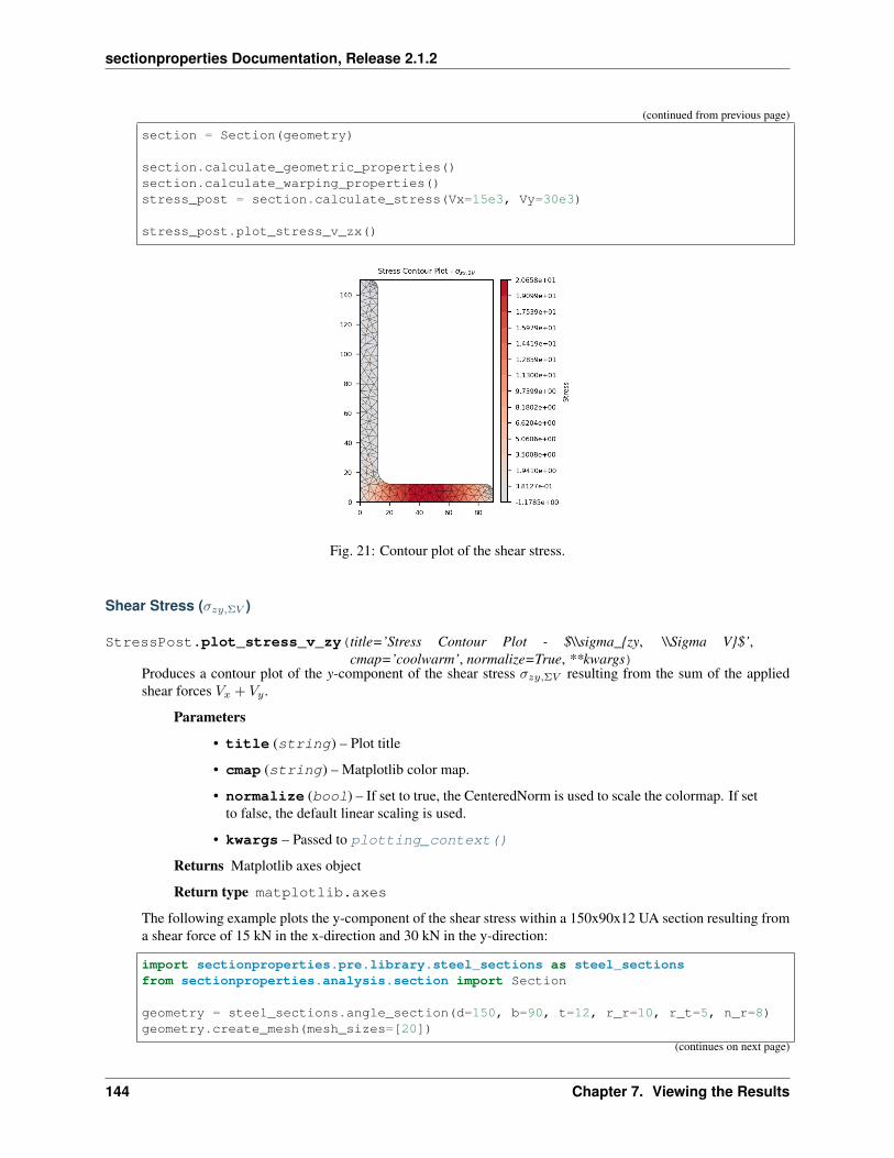
sectionproperties Documentation, Release 2.1.2
(continued from previous page)
section = Section(geometry)
section.calculate_geometric_properties()section.calculate_warping_properties()stress_post = section.calculate_stress(Vx=15e3, Vy=30e3)
stress_post.plot_stress_v_zx()
Fig. 21: Contour plot of the shear stress.
Shear Stress (𝜎𝑧𝑦,Σ𝑉 )
StressPost.plot_stress_v_zy(title=’Stress Contour Plot - $\\sigma_zy, \\Sigma V$’,cmap=’coolwarm’, normalize=True, **kwargs)
Produces a contour plot of the y-component of the shear stress 𝜎𝑧𝑦,Σ𝑉 resulting from the sum of the appliedshear forces 𝑉𝑥 + 𝑉𝑦 .
Parameters
• title (string) – Plot title
• cmap (string) – Matplotlib color map.
• normalize (bool) – If set to true, the CenteredNorm is used to scale the colormap. If setto false, the default linear scaling is used.
• kwargs – Passed to plotting_context()
Returns Matplotlib axes object
Return type matplotlib.axes
The following example plots the y-component of the shear stress within a 150x90x12 UA section resulting froma shear force of 15 kN in the x-direction and 30 kN in the y-direction:
import sectionproperties.pre.library.steel_sections as steel_sectionsfrom sectionproperties.analysis.section import Section
geometry = steel_sections.angle_section(d=150, b=90, t=12, r_r=10, r_t=5, n_r=8)geometry.create_mesh(mesh_sizes=[20])
(continues on next page)
144 Chapter 7. Viewing the Results
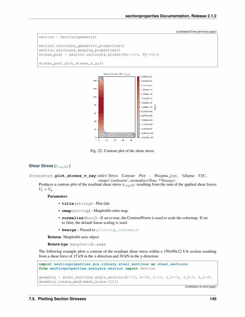
sectionproperties Documentation, Release 2.1.2
(continued from previous page)
section = Section(geometry)
section.calculate_geometric_properties()section.calculate_warping_properties()stress_post = section.calculate_stress(Vx=15e3, Vy=30e3)
stress_post.plot_stress_v_zy()
Fig. 22: Contour plot of the shear stress.
Shear Stress (𝜎𝑧𝑥𝑦,Σ𝑉 )
StressPost.plot_stress_v_zxy(title=’Stress Contour Plot - $\\sigma_zxy, \\Sigma V$’,cmap=’coolwarm’, normalize=True, **kwargs)
Produces a contour plot of the resultant shear stress 𝜎𝑧𝑥𝑦,Σ𝑉 resulting from the sum of the applied shear forces𝑉𝑥 + 𝑉𝑦 .
Parameters
• title (string) – Plot title
• cmap (string) – Matplotlib color map.
• normalize (bool) – If set to true, the CenteredNorm is used to scale the colormap. If setto false, the default linear scaling is used.
• kwargs – Passed to plotting_context()
Returns Matplotlib axes object
Return type matplotlib.axes
The following example plots a contour of the resultant shear stress within a 150x90x12 UA section resultingfrom a shear force of 15 kN in the x-direction and 30 kN in the y-direction:
import sectionproperties.pre.library.steel_sections as steel_sectionsfrom sectionproperties.analysis.section import Section
geometry = steel_sections.angle_section(d=150, b=90, t=12, r_r=10, r_t=5, n_r=8)geometry.create_mesh(mesh_sizes=[20])
(continues on next page)
7.5. Plotting Section Stresses 145

sectionproperties Documentation, Release 2.1.2
(continued from previous page)
section = Section(geometry)
section.calculate_geometric_properties()section.calculate_warping_properties()stress_post = section.calculate_stress(Vx=15e3, Vy=30e3)
stress_post.plot_stress_v_zxy()
Fig. 23: Contour plot of the shear stress.
StressPost.plot_vector_v_zxy(title=’Stress Vector Plot - $\\sigma_zxy, \\Sigma V$’,cmap=’YlOrBr’, normalize=False, **kwargs)
Produces a vector plot of the resultant shear stress 𝜎𝑧𝑥𝑦,Σ𝑉 resulting from the sum of the applied shear forces𝑉𝑥 + 𝑉𝑦 .
Parameters
• title (string) – Plot title
• cmap (string) – Matplotlib color map.
• normalize (bool) – If set to true, the CenteredNorm is used to scale the colormap. If setto false, the default linear scaling is used.
• kwargs – Passed to plotting_context()
Returns Matplotlib axes object
Return type matplotlib.axes
The following example generates a vector plot of the shear stress within a 150x90x12 UA section resulting froma shear force of 15 kN in the x-direction and 30 kN in the y-direction:
import sectionproperties.pre.library.steel_sections as steel_sectionsfrom sectionproperties.analysis.section import Section
geometry = steel_sections.angle_section(d=150, b=90, t=12, r_r=10, r_t=5, n_r=8)geometry.create_mesh(mesh_sizes=[20])section = Section(geometry)
section.calculate_geometric_properties()
(continues on next page)
146 Chapter 7. Viewing the Results
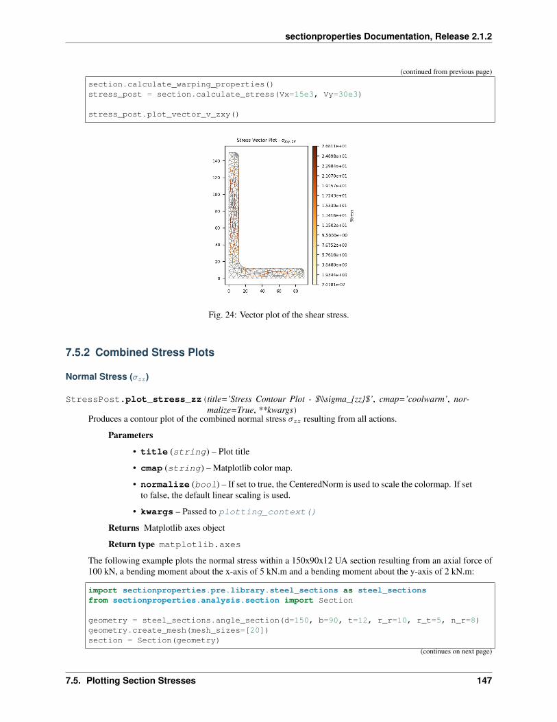
sectionproperties Documentation, Release 2.1.2
(continued from previous page)
section.calculate_warping_properties()stress_post = section.calculate_stress(Vx=15e3, Vy=30e3)
stress_post.plot_vector_v_zxy()
Fig. 24: Vector plot of the shear stress.
7.5.2 Combined Stress Plots
Normal Stress (𝜎𝑧𝑧)
StressPost.plot_stress_zz(title=’Stress Contour Plot - $\\sigma_zz$’, cmap=’coolwarm’, nor-malize=True, **kwargs)
Produces a contour plot of the combined normal stress 𝜎𝑧𝑧 resulting from all actions.
Parameters
• title (string) – Plot title
• cmap (string) – Matplotlib color map.
• normalize (bool) – If set to true, the CenteredNorm is used to scale the colormap. If setto false, the default linear scaling is used.
• kwargs – Passed to plotting_context()
Returns Matplotlib axes object
Return type matplotlib.axes
The following example plots the normal stress within a 150x90x12 UA section resulting from an axial force of100 kN, a bending moment about the x-axis of 5 kN.m and a bending moment about the y-axis of 2 kN.m:
import sectionproperties.pre.library.steel_sections as steel_sectionsfrom sectionproperties.analysis.section import Section
geometry = steel_sections.angle_section(d=150, b=90, t=12, r_r=10, r_t=5, n_r=8)geometry.create_mesh(mesh_sizes=[20])section = Section(geometry)
(continues on next page)
7.5. Plotting Section Stresses 147

sectionproperties Documentation, Release 2.1.2
(continued from previous page)
section.calculate_geometric_properties()section.calculate_warping_properties()stress_post = section.calculate_stress(N=100e3, Mxx=5e6, Myy=2e6)
stress_post.plot_stress_zz()
Fig. 25: Contour plot of the normal stress.
Shear Stress (𝜎𝑧𝑥)
StressPost.plot_stress_zx(title=’Stress Contour Plot - $\\sigma_zx$’, cmap=’coolwarm’, nor-malize=True, **kwargs)
Produces a contour plot of the x-component of the shear stress 𝜎𝑧𝑥 resulting from all actions.
Parameters
• title (string) – Plot title
• cmap (string) – Matplotlib color map.
• normalize (bool) – If set to true, the CenteredNorm is used to scale the colormap. If setto false, the default linear scaling is used.
• kwargs – Passed to plotting_context()
Returns Matplotlib axes object
Return type matplotlib.axes
The following example plots the x-component of the shear stress within a 150x90x12 UA section resulting froma torsion moment of 1 kN.m and a shear force of 30 kN in the y-direction:
import sectionproperties.pre.library.steel_sections as steel_sectionsfrom sectionproperties.analysis.section import Section
geometry = steel_sections.angle_section(d=150, b=90, t=12, r_r=10, r_t=5, n_r=8)geometry.create_mesh(mesh_sizes=[20])section = Section(geometry)
(continues on next page)
148 Chapter 7. Viewing the Results

sectionproperties Documentation, Release 2.1.2
(continued from previous page)
section.calculate_geometric_properties()section.calculate_warping_properties()stress_post = section.calculate_stress(Mzz=1e6, Vy=30e3)
stress_post.plot_stress_zx()
Fig. 26: Contour plot of the shear stress.
Shear Stress (𝜎𝑧𝑦)
StressPost.plot_stress_zy(title=’Stress Contour Plot - $\\sigma_zy$’, cmap=’coolwarm’, nor-malize=True, **kwargs)
Produces a contour plot of the y-component of the shear stress 𝜎𝑧𝑦 resulting from all actions.
Parameters
• title (string) – Plot title
• cmap (string) – Matplotlib color map.
• normalize (bool) – If set to true, the CenteredNorm is used to scale the colormap. If setto false, the default linear scaling is used.
• kwargs – Passed to plotting_context()
Returns Matplotlib axes object
Return type matplotlib.axes
The following example plots the y-component of the shear stress within a 150x90x12 UA section resulting froma torsion moment of 1 kN.m and a shear force of 30 kN in the y-direction:
import sectionproperties.pre.library.steel_sections as steel_sectionsfrom sectionproperties.analysis.section import Section
geometry = steel_sections.angle_section(d=150, b=90, t=12, r_r=10, r_t=5, n_r=8)geometry.create_mesh(mesh_sizes=[20])section = Section(geometry)
section.calculate_geometric_properties()
(continues on next page)
7.5. Plotting Section Stresses 149
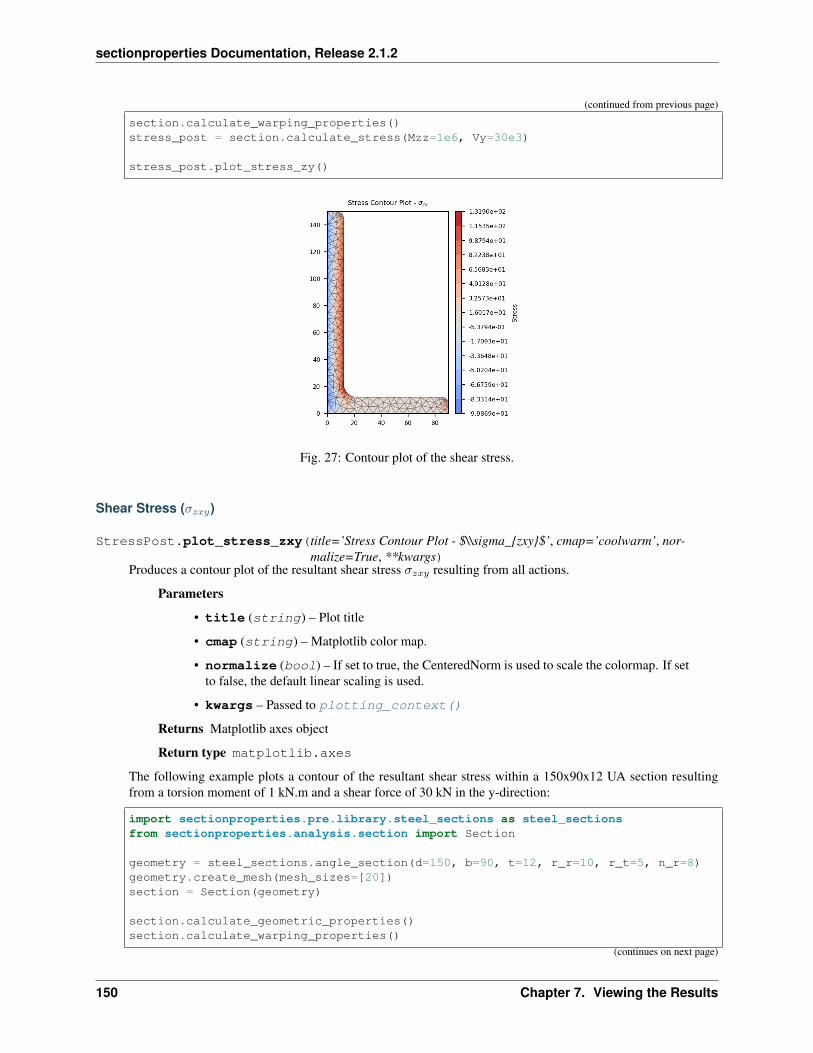
sectionproperties Documentation, Release 2.1.2
(continued from previous page)
section.calculate_warping_properties()stress_post = section.calculate_stress(Mzz=1e6, Vy=30e3)
stress_post.plot_stress_zy()
Fig. 27: Contour plot of the shear stress.
Shear Stress (𝜎𝑧𝑥𝑦)
StressPost.plot_stress_zxy(title=’Stress Contour Plot - $\\sigma_zxy$’, cmap=’coolwarm’, nor-malize=True, **kwargs)
Produces a contour plot of the resultant shear stress 𝜎𝑧𝑥𝑦 resulting from all actions.
Parameters
• title (string) – Plot title
• cmap (string) – Matplotlib color map.
• normalize (bool) – If set to true, the CenteredNorm is used to scale the colormap. If setto false, the default linear scaling is used.
• kwargs – Passed to plotting_context()
Returns Matplotlib axes object
Return type matplotlib.axes
The following example plots a contour of the resultant shear stress within a 150x90x12 UA section resultingfrom a torsion moment of 1 kN.m and a shear force of 30 kN in the y-direction:
import sectionproperties.pre.library.steel_sections as steel_sectionsfrom sectionproperties.analysis.section import Section
geometry = steel_sections.angle_section(d=150, b=90, t=12, r_r=10, r_t=5, n_r=8)geometry.create_mesh(mesh_sizes=[20])section = Section(geometry)
section.calculate_geometric_properties()section.calculate_warping_properties()
(continues on next page)
150 Chapter 7. Viewing the Results

sectionproperties Documentation, Release 2.1.2
(continued from previous page)
stress_post = section.calculate_stress(Mzz=1e6, Vy=30e3)
stress_post.plot_stress_zxy()
Fig. 28: Contour plot of the shear stress.
StressPost.plot_vector_zxy(title=’Stress Vector Plot - $\\sigma_zxy$’, cmap=’YlOrBr’, normal-ize=False, **kwargs)
Produces a vector plot of the resultant shear stress 𝜎𝑧𝑥𝑦 resulting from all actions.
Parameters
• title (string) – Plot title
• cmap (string) – Matplotlib color map.
• normalize (bool) – If set to true, the CenteredNorm is used to scale the colormap. If setto false, the default linear scaling is used.
• kwargs – Passed to plotting_context()
Returns Matplotlib axes object
Return type matplotlib.axes
The following example generates a vector plot of the shear stress within a 150x90x12 UA section resulting froma torsion moment of 1 kN.m and a shear force of 30 kN in the y-direction:
import sectionproperties.pre.library.steel_sections as steel_sectionsfrom sectionproperties.analysis.section import Section
geometry = steel_sections.angle_section(d=150, b=90, t=12, r_r=10, r_t=5, n_r=8)geometry.create_mesh(mesh_sizes=[20])section = Section(geometry)
section.calculate_geometric_properties()section.calculate_warping_properties()stress_post = section.calculate_stress(Mzz=1e6, Vy=30e3)
stress_post.plot_vector_zxy()
7.5. Plotting Section Stresses 151

sectionproperties Documentation, Release 2.1.2
Fig. 29: Vector plot of the shear stress.
Major Principal Stress (𝜎1)
StressPost.plot_stress_1(title=’Stress Contour Plot - $\\sigma_1$’, cmap=’coolwarm’, normal-ize=True, **kwargs)
Produces a contour plot of the major principal stress 𝜎1 resulting from all actions.
Parameters
• title (string) – Plot title
• cmap (string) – Matplotlib color map.
• normalize (bool) – If set to true, the CenteredNorm is used to scale the colormap. If setto false, the default linear scaling is used.
• kwargs – Passed to plotting_context()
Returns Matplotlib axes object
Return type matplotlib.axes
The following example plots a contour of the major principal stress within a 150x90x12 UA section resultingfrom the following actions:
• 𝑁 = 50 kN
• 𝑀𝑥𝑥 = −5 kN.m
• 𝑀22 = 2.5 kN.m
• 𝑀𝑧𝑧 = 1.5 kN.m
• 𝑉𝑥 = 10 kN
• 𝑉𝑦 = 5 kN
import sectionproperties.pre.library.steel_sections as steel_sectionsfrom sectionproperties.analysis.section import Section
geometry = steel_sections.angle_section(d=150, b=90, t=12, r_r=10, r_t=5, n_r=8)mesh = geometry.create_mesh(mesh_sizes=[2.5])section = CrossSection(geometry, mesh)
(continues on next page)
152 Chapter 7. Viewing the Results
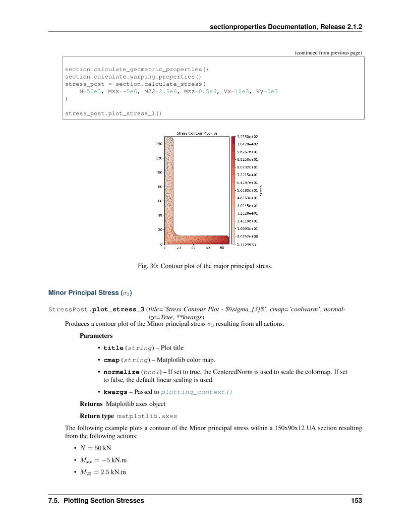
sectionproperties Documentation, Release 2.1.2
(continued from previous page)
section.calculate_geometric_properties()section.calculate_warping_properties()stress_post = section.calculate_stress(
N=50e3, Mxx=-5e6, M22=2.5e6, Mzz=0.5e6, Vx=10e3, Vy=5e3)
stress_post.plot_stress_1()
Fig. 30: Contour plot of the major principal stress.
Minor Principal Stress (𝜎3)
StressPost.plot_stress_3(title=’Stress Contour Plot - $\\sigma_3$’, cmap=’coolwarm’, normal-ize=True, **kwargs)
Produces a contour plot of the Minor principal stress 𝜎3 resulting from all actions.
Parameters
• title (string) – Plot title
• cmap (string) – Matplotlib color map.
• normalize (bool) – If set to true, the CenteredNorm is used to scale the colormap. If setto false, the default linear scaling is used.
• kwargs – Passed to plotting_context()
Returns Matplotlib axes object
Return type matplotlib.axes
The following example plots a contour of the Minor principal stress within a 150x90x12 UA section resultingfrom the following actions:
• 𝑁 = 50 kN
• 𝑀𝑥𝑥 = −5 kN.m
• 𝑀22 = 2.5 kN.m
7.5. Plotting Section Stresses 153

sectionproperties Documentation, Release 2.1.2
• 𝑀𝑧𝑧 = 1.5 kN.m
• 𝑉𝑥 = 10 kN
• 𝑉𝑦 = 5 kN
import sectionproperties.pre.library.steel_sections as steel_sectionsfrom sectionproperties.analysis.section import Section
geometry = steel_sections.angle_section(d=150, b=90, t=12, r_r=10, r_t=5, n_r=8)mesh = geometry.create_mesh(mesh_sizes=[2.5])section = CrossSection(geometry, mesh)
section.calculate_geometric_properties()section.calculate_warping_properties()stress_post = section.calculate_stress(
N=50e3, Mxx=-5e6, M22=2.5e6, Mzz=0.5e6, Vx=10e3, Vy=5e3)
stress_post.plot_stress_3()
Fig. 31: Contour plot of the minor principal stress.
von Mises Stress (𝜎𝑣𝑀 )
StressPost.plot_stress_vm(title=’Stress Contour Plot - $\\sigma_vM$’, cmap=’coolwarm’, nor-malize=True, **kwargs)
Produces a contour plot of the von Mises stress 𝜎𝑣𝑀 resulting from all actions.
Parameters
• title (string) – Plot title
• cmap (string) – Matplotlib color map.
• normalize (bool) – If set to true, the CenteredNorm is used to scale the colormap. If setto false, the default linear scaling is used.
• kwargs – Passed to plotting_context()
Returns Matplotlib axes object
154 Chapter 7. Viewing the Results

sectionproperties Documentation, Release 2.1.2
Return type matplotlib.axes
The following example plots a contour of the von Mises stress within a 150x90x12 UA section resulting fromthe following actions:
• 𝑁 = 50 kN
• 𝑀𝑥𝑥 = −5 kN.m
• 𝑀22 = 2.5 kN.m
• 𝑀𝑧𝑧 = 1.5 kN.m
• 𝑉𝑥 = 10 kN
• 𝑉𝑦 = 5 kN
import sectionproperties.pre.library.steel_sections as steel_sectionsfrom sectionproperties.analysis.section import Section
geometry = steel_sections.angle_section(d=150, b=90, t=12, r_r=10, r_t=5, n_r=8)geometry.create_mesh(mesh_sizes=[20])section = Section(geometry)
section.calculate_geometric_properties()section.calculate_warping_properties()stress_post = section.calculate_stress(
N=50e3, Mxx=-5e6, M22=2.5e6, Mzz=0.5e6, Vx=10e3, Vy=5e3)
stress_post.plot_stress_vm()
Fig. 32: Contour plot of the von Mises stress.
Mohr’s Circles for Stresses at a Point
StressPost.plot_mohrs_circles(x, y, title=None, **kwargs)Plots Mohr’s Circles of the 3D stress state at position x, y
Parameters
• x (float) – x-coordinate of the point to draw Mohr’s Circle
7.5. Plotting Section Stresses 155
sectionproperties Documentation, Release 2.1.2
• y (float) – y-coordinate of the point to draw Mohr’s Circle
• title (string) – Plot title
• kwargs – Passed to plotting_context()
Returns Matplotlib axes object
Return type matplotlib.axes
The following example plots the Mohr’s Circles for the 3D stress state within a 150x90x12 UA section resultingfrom the following actions:
• 𝑁 = 50 kN
• 𝑀𝑥𝑥 = −5 kN.m
• 𝑀22 = 2.5 kN.m
• 𝑀𝑧𝑧 = 1.5 kN.m
• 𝑉𝑥 = 10 kN
• 𝑉𝑦 = 5 kN
at the point (10, 88.9).
import sectionproperties.pre.library.steel_sections as steel_sectionsfrom sectionproperties.analysis.section import Section
geometry = steel_sections.angle_section(d=150, b=90, t=12, r_r=10, r_t=5, n_r=8)mesh = geometry.create_mesh(mesh_sizes=[2.5])section = Section(geometry, mesh)
section.calculate_geometric_properties()section.calculate_warping_properties()stress_post = section.calculate_stress(
N=50e3, Mxx=-5e6, M22=2.5e6, Mzz=0.5e6, Vx=10e3, Vy=5e3)
stress_post.plot_mohrs_circles(10, 88.9)
7.6 Retrieving Section Stress
All cross-section stresses can be recovered using the get_stress() method that belongs to every StressPostobject:
StressPost.get_stress()Returns the stresses within each material belonging to the current StressPost object.
Returns A list of dictionaries containing the cross-section stresses for each material.
Return type list[dict]
A dictionary is returned for each material in the cross-section, containing the following keys and values:
• ‘Material’: Material name
• ‘sig_zz_n’: Normal stress 𝜎𝑧𝑧,𝑁 resulting from the axial load 𝑁
• ‘sig_zz_mxx’: Normal stress 𝜎𝑧𝑧,𝑀𝑥𝑥 resulting from the bending moment 𝑀𝑥𝑥
• ‘sig_zz_myy’: Normal stress 𝜎𝑧𝑧,𝑀𝑦𝑦 resulting from the bending moment 𝑀𝑦𝑦
156 Chapter 7. Viewing the Results

sectionproperties Documentation, Release 2.1.2
Fig. 33: Mohr’s Circles of the 3D stress state at (10, 88.9).
7.6. Retrieving Section Stress 157
sectionproperties Documentation, Release 2.1.2
• ‘sig_zz_m11’: Normal stress 𝜎𝑧𝑧,𝑀11 resulting from the bending moment 𝑀11
• ‘sig_zz_m22’: Normal stress 𝜎𝑧𝑧,𝑀22 resulting from the bending moment 𝑀22
• ‘sig_zz_m’: Normal stress 𝜎𝑧𝑧,Σ𝑀 resulting from all bending moments
• ‘sig_zx_mzz’: x-component of the shear stress 𝜎𝑧𝑥,𝑀𝑧𝑧 resulting from the torsion moment
• ‘sig_zy_mzz’: y-component of the shear stress 𝜎𝑧𝑦,𝑀𝑧𝑧 resulting from the torsion moment
• ‘sig_zxy_mzz’: Resultant shear stress 𝜎𝑧𝑥𝑦,𝑀𝑧𝑧 resulting from the torsion moment
• ‘sig_zx_vx’: x-component of the shear stress 𝜎𝑧𝑥,𝑉 𝑥 resulting from the shear force 𝑉𝑥
• ‘sig_zy_vx’: y-component of the shear stress 𝜎𝑧𝑦,𝑉 𝑥 resulting from the shear force 𝑉𝑥
• ‘sig_zxy_vx’: Resultant shear stress 𝜎𝑧𝑥𝑦,𝑉 𝑥 resulting from the shear force 𝑉𝑥
• ‘sig_zx_vy’: x-component of the shear stress 𝜎𝑧𝑥,𝑉 𝑦 resulting from the shear force 𝑉𝑦
• ‘sig_zy_vy’: y-component of the shear stress 𝜎𝑧𝑦,𝑉 𝑦 resulting from the shear force 𝑉𝑦
• ‘sig_zxy_vy’: Resultant shear stress 𝜎𝑧𝑥𝑦,𝑉 𝑦 resulting from the shear force 𝑉𝑦
• ‘sig_zx_v’: x-component of the shear stress 𝜎𝑧𝑥,Σ𝑉 resulting from all shear forces
• ‘sig_zy_v’: y-component of the shear stress 𝜎𝑧𝑦,Σ𝑉 resulting from all shear forces
• ‘sig_zxy_v’: Resultant shear stress 𝜎𝑧𝑥𝑦,Σ𝑉 resulting from all shear forces
• ‘sig_zz’: Combined normal stress 𝜎𝑧𝑧 resulting from all actions
• ‘sig_zx’: x-component of the shear stress 𝜎𝑧𝑥 resulting from all actions
• ‘sig_zy’: y-component of the shear stress 𝜎𝑧𝑦 resulting from all actions
• ‘sig_zxy’: Resultant shear stress 𝜎𝑧𝑥𝑦 resulting from all actions
• ‘sig_1’: Major principal stress 𝜎1 resulting from all actions
• ‘sig_3’: Minor principal stress 𝜎3 resulting from all actions
• ‘sig_vm’: von Mises stress 𝜎𝑣𝑀 resulting from all actions
The following example returns stresses for each material within a composite section, note that a result is gen-erated for each node in the mesh for all materials irrespective of whether the materials exists at that point ornot.
import sectionproperties.pre.library.steel_sections as steel_sectionsfrom sectionproperties.analysis.section import Section
geometry = steel_sections.angle_section(d=150, b=90, t=12, r_r=10, r_t=5, n_r=8)geometry.create_mesh(mesh_sizes=[20])section = Section(geometry)
section.calculate_geometric_properties()section.calculate_warping_properties()stress_post = section.calculate_stress(
N=50e3, Mxx=-5e6, M22=2.5e6, Mzz=0.5e6, Vx=10e3, Vy=5e3)stresses = stress_post.get_stress()
print("Number of nodes: 0".format(section.num_nodes))
for stress in stresses:print('Material: 0'.format(stress['Material']))
(continues on next page)
158 Chapter 7. Viewing the Results

sectionproperties Documentation, Release 2.1.2
(continued from previous page)
print('List Size: 0'.format(len(stress['sig_zz_n'])))print('Normal Stresses: 0'.format(stress['sig_zz_n']))print('von Mises Stresses: 0'.format(stress['sig_vm']))
$ Number of nodes: 2465
$ Material: Timber$ List Size: 2465$ Normal Stresses: [0.76923077 0.76923077 0.76923077 ... 0.76923077 0.76923077 0.→˓76923077]$ von Mises Stresses: [7.6394625 5.38571866 3.84784964 ... 3.09532948 3.66992556→˓2.81976647]
$ Material: Steel$ List Size: 2465$ Normal Stresses: [19.23076923 0. 0. ... 0. 0. 0.]$ von Mises Stresses: [134.78886419 0. 0. ... 0. 0. 0.]
7.6. Retrieving Section Stress 159

sectionproperties Documentation, Release 2.1.2
160 Chapter 7. Viewing the Results
CHAPTER 8
Examples Gallery
Here is a gallery of examples demonstrating what sectionproperties can do!
8.1 Basic Examples
These are basic examples to calculate properties and results on a cross-section.
8.1.1 Simple Example
Calculate section properties of a circle.
The following example calculates the geometric, warping and plastic properties of a 50 mm diameter circle. The circleis discretised with 64 points and a mesh size of 2.5 mm2.
The geometry and mesh are plotted, and the mesh information printed to the terminal before the analysis is carriedout. Detailed time information is printed to the terminal during the cross-section analysis stage. Once the analysisis complete, the cross-section properties are printed to the terminal. The centroidal axis second moments of area andtorsion constant are saved to variables and it is shown that, for a circle, the torsion constant is equal to the sum of thesecond moments of area.
# sphinx_gallery_thumbnail_number = 1
import sectionproperties.pre.library.primitive_sections as sectionsfrom sectionproperties.analysis.section import Section
Create a 50 diameter circle discretised by 64 points
geometry = sections.circular_section(d=50, n=64)geometry.plot_geometry()
161
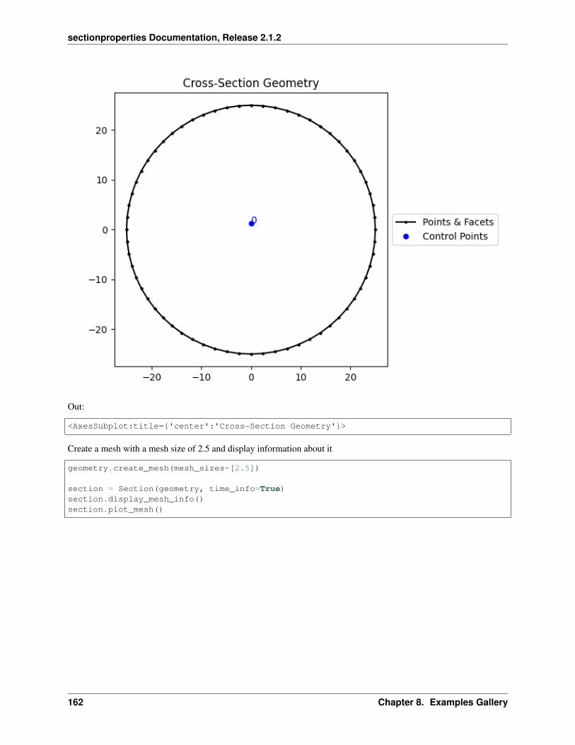
sectionproperties Documentation, Release 2.1.2
Out:
<AxesSubplot:title='center':'Cross-Section Geometry'>
Create a mesh with a mesh size of 2.5 and display information about it
geometry.create_mesh(mesh_sizes=[2.5])
section = Section(geometry, time_info=True)section.display_mesh_info()section.plot_mesh()
162 Chapter 8. Examples Gallery
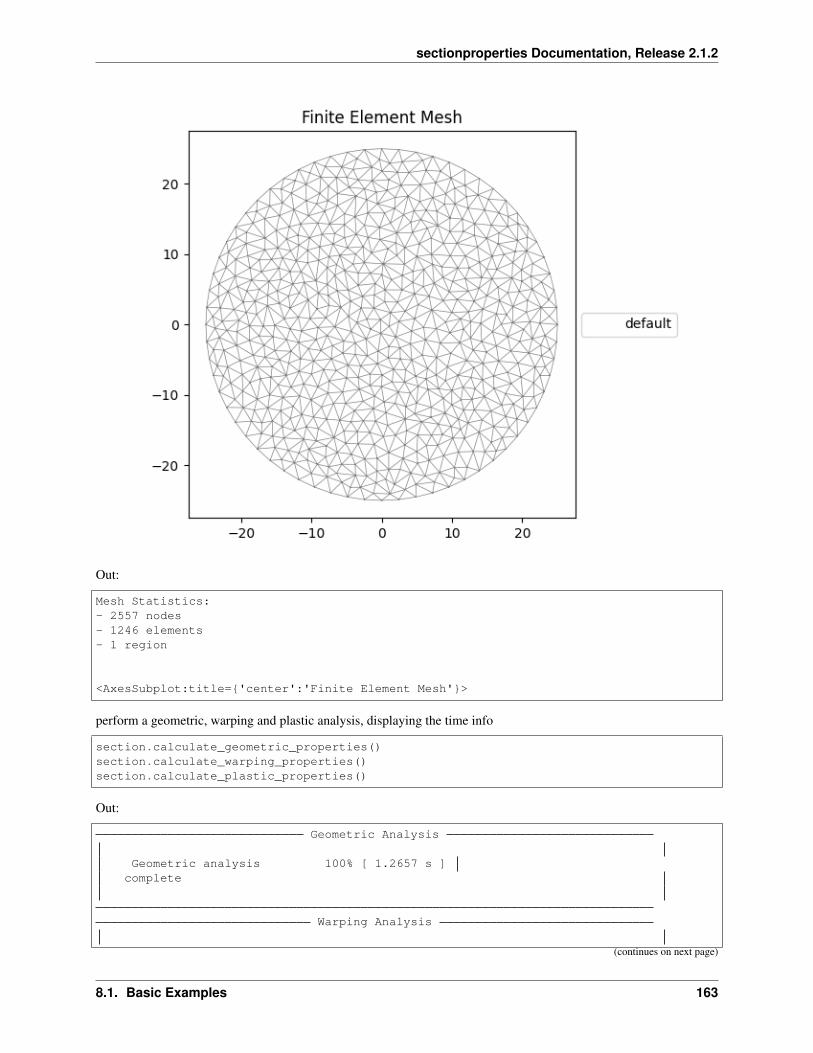
sectionproperties Documentation, Release 2.1.2
Out:
Mesh Statistics:- 2557 nodes- 1246 elements- 1 region
<AxesSubplot:title='center':'Finite Element Mesh'>
perform a geometric, warping and plastic analysis, displaying the time info
section.calculate_geometric_properties()section.calculate_warping_properties()section.calculate_plastic_properties()
Out:
Geometric Analysis
Geometric analysis 100% [ 1.2657 s ]complete
Warping Analysis
(continues on next page)
8.1. Basic Examples 163

sectionproperties Documentation, Release 2.1.2
(continued from previous page)
Warping analysis 100% [ 7.2666 s ]completed2557x2557 stiffness 100% [ 1.4611 s ]
matrix assembledWarping function solved 100% [ 0.1020 s ]
(direct)Shear function vectors 100% [ 1.7515 s ]
assembledShear functions solved 100% [ 0.1725 s ]
(direct)Shear and warping 100% [ 1.1271 s ]
integrals assembledShear deformation 100% [ 1.5121 s ]
coefficients assembledMonosymmetry integrals 100% [ 1.1341 s ]
assembled
Plastic Analysis
Plastic analysis complete 100% [ 0.0399 s ]
Print the results to the terminal
section.display_results()
Out:
Section Properties
Property Value
A 1.960343e+03Perim. 1.570166e+02Qx -8.764545e-12Qy 3.601119e-12cx 1.836985e-15cy -4.470924e-15Ixx_g 3.058119e+05Iyy_g 3.058119e+05Ixy_g 8.526513e-13Ixx_c 3.058119e+05Iyy_c 3.058119e+05Ixy_c 8.526513e-13Zxx+ 1.223248e+04Zxx- 1.223248e+04Zyy+ 1.223248e+04Zyy- 1.223248e+04rx 1.248996e+01ry 1.248996e+01phi 0.000000e+00I11_c 3.058119e+05I22_c 3.058119e+05Z11+ 1.223248e+04Z11- 1.223248e+04
(continues on next page)
164 Chapter 8. Examples Gallery

sectionproperties Documentation, Release 2.1.2
(continued from previous page)
Z22+ 1.223248e+04Z22- 1.223248e+04r11 1.248996e+01r22 1.248996e+01J 6.116238e+05Iw 1.588407e-21x_se -6.613922e-16y_se 1.426706e-15x_st -6.613922e-16y_st 1.426706e-15x1_se -2.498377e-15y2_se 5.897630e-15A_sx 1.680296e+03A_sy 1.680296e+03A_s11 1.680296e+03A_s22 1.680296e+03betax+ -8.344890e-15betax- 8.344890e-15betay+ 1.526682e-14betay- -1.526682e-14beta11+ -8.344890e-15beta11- 8.344890e-15beta22+ 1.526682e-14beta22- -1.526682e-14x_pc 1.836985e-15y_pc -4.470924e-15Sxx 2.078317e+04Syy 2.078317e+04SF_xx+ 1.699016e+00SF_xx- 1.699016e+00SF_yy+ 1.699016e+00SF_yy- 1.699016e+00x11_pc 1.836985e-15y22_pc -4.470924e-15S11 2.078317e+04S22 2.078317e+04SF_11+ 1.699016e+00SF_11- 1.699016e+00SF_22+ 1.699016e+00SF_22- 1.699016e+00
Get and print the second moments of area and the torsion constant
(ixx_c, iyy_c, ixy_c) = section.get_ic()j = section.get_j()print("Ixx + Iyy = 0:.3f".format(ixx_c + iyy_c))print("J = 0:.3f".format(j))
Out:
Ixx + Iyy = 611623.837J = 611623.837
Total running time of the script: ( 0 minutes 9.521 seconds)
8.1. Basic Examples 165
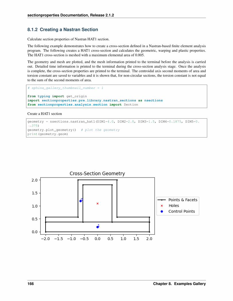
sectionproperties Documentation, Release 2.1.2
8.1.2 Creating a Nastran Section
Calculate section properties of Nastran HAT1 section.
The following example demonstrates how to create a cross-section defined in a Nastran-based finite element analysisprogram. The following creates a HAT1 cross-section and calculates the geometric, warping and plastic properties.The HAT1 cross-section is meshed with a maximum elemental area of 0.005.
The geometry and mesh are plotted, and the mesh information printed to the terminal before the analysis is carriedout. Detailed time information is printed to the terminal during the cross-section analysis stage. Once the analysisis complete, the cross-section properties are printed to the terminal. The centroidal axis second moments of area andtorsion constant are saved to variables and it is shown that, for non-circular sections, the torsion constant is not equalto the sum of the second moments of area.
# sphinx_gallery_thumbnail_number = 1
from typing import get_originimport sectionproperties.pre.library.nastran_sections as nsectionsfrom sectionproperties.analysis.section import Section
Create a HAT1 section
geometry = nsections.nastran_hat1(DIM1=4.0, DIM2=2.0, DIM3=1.5, DIM4=0.1875, DIM5=0.→˓375)geometry.plot_geometry() # plot the geometryprint(geometry.geom)
166 Chapter 8. Examples Gallery

sectionproperties Documentation, Release 2.1.2
Out:
MULTIPOLYGON (((-2 0.375, -0.5625 0.375, -0.5625 1.8125, 0.5625 1.8125, 0.5625 0.375,→˓2 0.375, 2 0.5625, 0.75 0.5625, 0.75 2, -0.75 2, -0.75 0.5625, -2 0.5625, -2 0.→˓375)), ((-2 0, 2 0, 2 0.375, -2 0.375, -2 0)))
Create a mesh with a maximum elemental area of 0.005
geometry.create_mesh(mesh_sizes=[0.005])
section = Section(geometry, time_info=True) # create a Section objectsection.display_mesh_info() # display the mesh informationsection.plot_mesh() # plot the generated mesh`
Out:
Mesh Statistics:- 2038 nodes- 926 elements- 2 regions
<AxesSubplot:title='center':'Finite Element Mesh'>
Perform a geometric, warping and plastic analysis, displaying the time info
8.1. Basic Examples 167

sectionproperties Documentation, Release 2.1.2
section.calculate_geometric_properties()section.calculate_warping_properties()section.calculate_plastic_properties()
section.display_results()
Out:
Geometric Analysis
Geometric analysis 100% [ 0.8720 s ]complete
Warping Analysis
Warping analysis 100% [ 5.0805 s ]completed2038x2038 stiffness 100% [ 1.0646 s ]
matrix assembledWarping function solved 100% [ 0.0610 s ]
(direct)Shear function vectors 100% [ 1.1446 s ]
assembledShear functions solved 100% [ 0.1095 s ]
(direct)Shear and warping 100% [ 0.7784 s ]
integrals assembledShear deformation 100% [ 1.0916 s ]
coefficients assembledMonosymmetry integrals 100% [ 0.8256 s ]
assembled
Plastic Analysis
Plastic analysis complete 100% [ 0.0815 s ]
Section Properties
Property Value
A 2.789062e+00Perim. 1.200000e+01Qx 1.626709e+00Qy -2.268151e-16cx -8.132306e-17cy 5.832458e-01Ixx_g 1.935211e+00Iyy_g 3.233734e+00Ixy_g -3.109492e-16Ixx_c 9.864400e-01Iyy_c 3.233734e+00Ixy_c -1.786602e-16Zxx+ 6.962676e-01Zxx- 1.691294e+00
(continues on next page)
168 Chapter 8. Examples Gallery

sectionproperties Documentation, Release 2.1.2
(continued from previous page)
Zyy+ 1.616867e+00Zyy- 1.616867e+00rx 5.947113e-01ry 1.076770e+00phi -9.000000e+01I11_c 3.233734e+00I22_c 9.864400e-01Z11+ 1.616867e+00Z11- 1.616867e+00Z22+ 1.691294e+00Z22- 6.962676e-01r11 1.076770e+00r22 5.947113e-01J 9.878443e-01Iw 1.160810e-01x_se 4.822719e-05y_se 4.674792e-01x_st 4.822719e-05y_st 4.674792e-01x1_se 1.157666e-01y2_se 4.822719e-05A_sx 1.648312e+00A_sy 6.979733e-01A_s11 6.979733e-01A_s22 1.648312e+00betax+ -2.746928e-01betax- 2.746928e-01betay+ 9.645438e-05betay- -9.645438e-05beta11+ 9.645438e-05beta11- -9.645438e-05beta22+ 2.746928e-01beta22- -2.746928e-01x_pc -8.132306e-17y_pc 3.486328e-01Sxx 1.140530e+00Syy 2.603760e+00SF_xx+ 1.638062e+00SF_xx- 6.743533e-01SF_yy+ 1.610373e+00SF_yy- 1.610373e+00x11_pc -1.711463e-16y22_pc 3.486328e-01S11 2.603760e+00S22 1.140530e+00SF_11+ 1.610373e+00SF_11- 1.610373e+00SF_22+ 6.743533e-01SF_22- 1.638062e+00
Get the second moments of area and the torsion constant
(ixx_c, iyy_c, ixy_c) = section.get_ic()j = section.get_j()print("Ixx + Iyy = 0:.3f".format(ixx_c + iyy_c))print("J = 0:.3f".format(j))
8.1. Basic Examples 169
sectionproperties Documentation, Release 2.1.2
Out:
Ixx + Iyy = 4.220J = 0.988
Total running time of the script: ( 0 minutes 6.559 seconds)
8.1.3 Creating Custom Geometry
Calculate section properties of a user-defined section from points and facets.
The following example demonstrates how geometry objects can be created from a list of points, facets, holes andcontrol points. An straight angle section with a plate at its base is created from a list of points and facets. The bottomplate is assigned a separate control point meaning two discrete regions are created. Creating separate regions allowsthe user to control the mesh size in each region and assign material properties to different regions. The geometry iscleaned to remove the overlapping facet at the junction of the angle and the plate. A geometric, warping and plasticanalysis is then carried out.
The geometry and mesh are plotted before the analysis is carried out. Once the analysis is complete, a plot of thevarious calculated centroids is generated.
# sphinx_gallery_thumbnail_number = 2
from sectionproperties.pre.geometry import CompoundGeometryfrom sectionproperties.analysis.section import Section
Define parameters for the angle section
a = 1b = 2t = 0.1
Build the lists of points, facets, holes and control points
points = [[-t / 2, -2 * a],[t / 2, -2 * a],[t / 2, -t / 2],[a, -t / 2],[a, t / 2],[-t / 2, t / 2],[-b / 2, -2 * a],[b / 2, -2 * a],[b / 2, -2 * a - t],[-b / 2, -2 * a - t],
]facets = [
[0, 1],[1, 2],[2, 3],[3, 4],[4, 5],[5, 0],[6, 7],[7, 8],[8, 9],[9, 6],
(continues on next page)
170 Chapter 8. Examples Gallery

sectionproperties Documentation, Release 2.1.2
(continued from previous page)
]holes = []control_points = [[0, 0], [0, -2 * a - t / 2]]
Because we have two separate geometry regions (as indicated by our control_points) we create a CompoundGeometryfrom points
geometry = CompoundGeometry.from_points(points, facets, control_points, holes)
Create the mesh and section. For the mesh, use a smaller refinement for the angle region.
geometry.create_mesh(mesh_sizes=[0.0005, 0.001])
section = Section(geometry)section.plot_mesh() # plot the generated mesh
Out:
<AxesSubplot:title='center':'Finite Element Mesh'>
Perform a geometric, warping and plastic analysis
section.calculate_geometric_properties()section.calculate_warping_properties()
(continues on next page)
8.1. Basic Examples 171

sectionproperties Documentation, Release 2.1.2
(continued from previous page)
section.calculate_plastic_properties()
section.plot_centroids()
Out:
<AxesSubplot:title='center':'Centroids'>
Total running time of the script: ( 0 minutes 8.952 seconds)
8.1.4 Creating a Built-Up Section
Merge two sections together into a single larger section.
The following example demonstrates how to combine multiple geometry objects into a single geometry object. A150x100x6 RHS is modelled with a solid 50x50 triangular section on its top and a 100x100x6 angle section on itsright side. The three geometry objects are combined together as a CompoundGeometry object using the + operator.
To manipulate individual geometries into the final shape, there are a variety of methods available to move and align.This example uses .align_center(), .align_to(), and .shift_section().
The geometry and mesh are plotted, and the mesh information printed to the terminal before the analysis is carriedout. Detailed time information is printed to the terminal during the cross-section analysis stage. Once the analysis iscomplete, the centroids are plotted.
172 Chapter 8. Examples Gallery

sectionproperties Documentation, Release 2.1.2
# sphinx_gallery_thumbnail_number = 1
import sectionproperties.pre.library.steel_sections as steel_sectionsfrom sectionproperties.pre.geometry import Geometryfrom sectionproperties.analysis.section import Section
Create a 150x100x6 RHS
rhs = steel_sections.rectangular_hollow_section(d=150, b=100, t=6, r_out=15, n_r=8)
Create a triangular section from points, facets, and control points
points = [[0, 0], [50, 0], [25, 50]]facets = [[0, 1], [1, 2], [2, 0]]control_points = [[25, 25]]triangle = Geometry.from_points(points, facets, control_points)triangle = triangle.align_center(rhs).align_to(rhs, on="top")
Create a 100x100x6 angle and position it on the right of the RHS
angle = steel_sections.angle_section(d=100, b=100, t=6, r_r=8, r_t=5, n_r=8)angle = angle.shift_section(x_offset=100, y_offset=25)
Combine the sections into a CompoundGeometry with + operator
geometry = rhs + triangle + anglegeometry.plot_geometry() # plot the geometry
8.1. Basic Examples 173

sectionproperties Documentation, Release 2.1.2
Out:
<AxesSubplot:title='center':'Cross-Section Geometry'>
Create a mesh and section. For the mesh, use a mesh size of 2.5 for the RHS, 5 for the triangle and 3 for the angle.
geometry.create_mesh(mesh_sizes=[2.5, 5, 3])
section = Section(geometry, time_info=True)section.display_mesh_info() # display the mesh informationsection.plot_mesh() # plot the generated mesh
174 Chapter 8. Examples Gallery
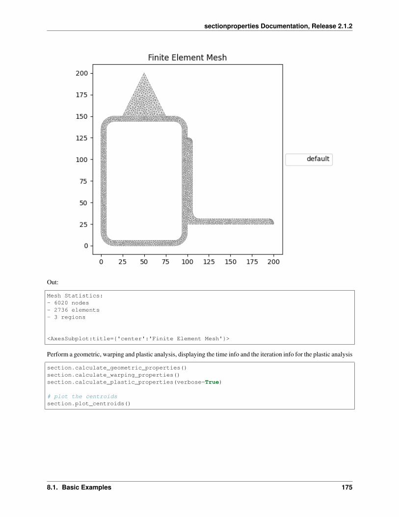
sectionproperties Documentation, Release 2.1.2
Out:
Mesh Statistics:- 6020 nodes- 2736 elements- 3 regions
<AxesSubplot:title='center':'Finite Element Mesh'>
Perform a geometric, warping and plastic analysis, displaying the time info and the iteration info for the plastic analysis
section.calculate_geometric_properties()section.calculate_warping_properties()section.calculate_plastic_properties(verbose=True)
# plot the centroidssection.plot_centroids()
8.1. Basic Examples 175
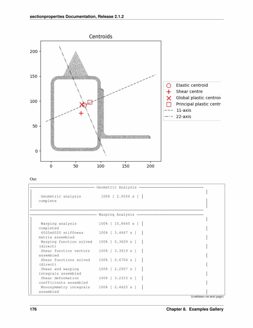
sectionproperties Documentation, Release 2.1.2
Out:
Geometric Analysis
Geometric analysis 100% [ 2.6556 s ]complete
Warping Analysis
Warping analysis 100% [ 15.8665 s ]completed6020x6020 stiffness 100% [ 3.4667 s ]
matrix assembledWarping function solved 100% [ 0.3609 s ]
(direct)Shear function vectors 100% [ 3.3919 s ]
assembledShear functions solved 100% [ 0.6704 s ]
(direct)Shear and warping 100% [ 2.2907 s ]
integrals assembledShear deformation 100% [ 3.2315 s ]
coefficients assembledMonosymmetry integrals 100% [ 2.4425 s ]
assembled(continues on next page)
176 Chapter 8. Examples Gallery
sectionproperties Documentation, Release 2.1.2
(continued from previous page)
d = -91.996268369166; f_norm = 1.0d = 108.003731630834; f_norm = -1.0d = 8.003731630833997; f_norm = -0.04433903442685115d = 3.5610941851785247; f_norm = -0.013257745358062492d = 1.6934563166381202; f_norm = -0.00019149964748535968d = 1.666207547083575; f_norm = -8.635909458075013e-07d = 1.6660841169311136; f_norm = -5.6994862781888e-11d = 1.666082783889055; f_norm = 9.269146437289895e-09---x-axis plastic centroid calculation converged at 1.66608e+00 in 7 iterations.d = -67.409490017714; f_norm = 1.0d = 132.590509982286; f_norm = -1.0d = 32.590509982285994; f_norm = -0.546379783397773d = -17.409490017714006; f_norm = 0.22681010830111303d = -2.742322822682775; f_norm = -0.043022470763644426d = -5.080875765477266; f_norm = -0.011205909614768165d = -5.8657449981455345; f_norm = 0.0004252464243683582d = -5.83704941245604; f_norm = -8.433780157994712e-06d = -5.837607455591706; f_norm = -6.102942204925805e-09d = -5.837610874395434; f_norm = 4.552923959027148e-08---y-axis plastic centroid calculation converged at -5.83761e+00 in 9 iterations.d = -106.16681282996608; f_norm = -1.0d = 113.67282241177986; f_norm = 1.0d = 3.7530047909068855; f_norm = 0.03943689434659865d = -0.588643873199409; f_norm = 0.006410315748600418d = -1.4248809343865845; f_norm = 4.912644827983057e-05d = -1.431330697831708; f_norm = 6.360699047308853e-08d = -1.4313390594743358; f_norm = 6.337318715773886e-13d = -1.4313402751438655; f_norm = -9.24687090782149e-09---11-axis plastic centroid calculation converged at -1.43134e+00 in 7 iterations.d = -96.43010376150622; f_norm = -1.0d = 93.41518522403116; f_norm = 1.0d = -1.5074592687375201; f_norm = 0.2499934430169193d = -26.81941205069321; f_norm = -0.5136606142451592d = -9.793701141307244; f_norm = 0.06969393886808824d = -12.614043035926043; f_norm = -0.015439988274393543d = -12.102542542006438; f_norm = 0.0009283409099111105d = -12.131552640019413; f_norm = 1.1002850184137821e-05d = -12.13190034875872; f_norm = -1.8901567849903257e-10d = -12.131893782808545; f_norm = 2.07588393504265e-07---22-axis plastic centroid calculation converged at -1.21319e+01 in 9 iterations.
Plastic Analysis
Plastic analysis complete 100% [ 0.1897 s ]
<AxesSubplot:title='center':'Centroids'>
Total running time of the script: ( 0 minutes 19.728 seconds)
8.1.5 Mirroring and Rotating Geometry
Mirror and rotate a cross section.
8.1. Basic Examples 177

sectionproperties Documentation, Release 2.1.2
The following example demonstrates how geometry objects can be mirrored and rotated. A 200PFC and 150PFC areplaced back-to-back by using the mirror_section() method and are rotated counter-clockwise by 30 degrees byusing the rotate_section() method. The geometry is cleaned to ensure there are no overlapping facets alongthe junction between the two PFCs. A geometric, warping and plastic analysis is then carried out.
The geometry and mesh are plotted, and the mesh information printed to the terminal before the analysis is carried out.Detailed time information is printed to the terminal during the cross-section analysis stage and iteration informationprinted for the plastic analysis. Once the analysis is complete, a plot of the various calculated centroids is generated.
# sphinx_gallery_thumbnail_number = 1
import sectionproperties.pre.library.steel_sections as steel_sectionsfrom sectionproperties.analysis.section import Section
Create a 200PFC and a 150PFC
pfc1 = steel_sections.channel_section(d=203, b=133, t_f=7.8, t_w=5.8, r=8.9, n_r=8)pfc2 = steel_sections.channel_section(
d=150, b=133, t_f=7.8, t_w=5.8, r=8.9, n_r=8).shift_section(0, 26.5)
Mirror the 200 PFC about the y-axis
pfc1 = pfc1.mirror_section(axis="y", mirror_point=[0, 0])
Merge the pfc sections
geometry = ((pfc1 - pfc2) | pfc1) + pfc2
Rotate the geometry counter-clockwise by 30 degrees
geometry = geometry.rotate_section(angle=30)geometry.plot_geometry()
178 Chapter 8. Examples Gallery

sectionproperties Documentation, Release 2.1.2
Out:
<AxesSubplot:title='center':'Cross-Section Geometry'>
Create a mesh and section. For the mesh, use a mesh size of 5 for the 200PFC and 4 for the 150PFC
geometry.create_mesh(mesh_sizes=[5, 4])
section = Section(geometry, time_info=True)section.display_mesh_info() # display the mesh informationsection.plot_mesh() # plot the generated mesh
8.1. Basic Examples 179

sectionproperties Documentation, Release 2.1.2
Out:
Mesh Statistics:- 4850 nodes- 2157 elements- 2 regions
<AxesSubplot:title='center':'Finite Element Mesh'>
Perform a geometric, warping and plastic analysis, displaying the time info and the iteration info for the plastic analysis
section.calculate_geometric_properties()section.calculate_warping_properties()section.calculate_plastic_properties(verbose=True)
section.plot_centroids()
180 Chapter 8. Examples Gallery
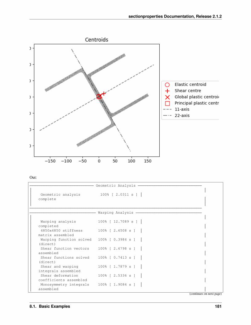
sectionproperties Documentation, Release 2.1.2
Out:
Geometric Analysis
Geometric analysis 100% [ 2.0311 s ]complete
Warping Analysis
Warping analysis 100% [ 12.7089 s ]completed4850x4850 stiffness 100% [ 2.6508 s ]
matrix assembledWarping function solved 100% [ 0.3984 s ]
(direct)Shear function vectors 100% [ 2.6798 s ]
assembledShear functions solved 100% [ 0.7413 s ]
(direct)Shear and warping 100% [ 1.7879 s ]
integrals assembledShear deformation 100% [ 2.5336 s ]
coefficients assembledMonosymmetry integrals 100% [ 1.9084 s ]
assembled(continues on next page)
8.1. Basic Examples 181

sectionproperties Documentation, Release 2.1.2
(continued from previous page)
d = -154.328341319365; f_norm = 1.0d = 131.525142448589; f_norm = -1.0d = -11.401599435387993; f_norm = 0.13458389687111885d = 5.55231463203793; f_norm = -0.021090896125661042d = 3.255390167671628; f_norm = -0.004055963678927537d = 2.724499194243151; f_norm = 0.00045100079082289346d = 2.7776241413031926; f_norm = -9.631031333251518e-06d = 2.7765133886258857; f_norm = -2.1922919066993703e-08d = 2.7765108545970905; f_norm = 5.977503270512459e-15---x-axis plastic centroid calculation converged at 2.77651e+00 in 8 iterations.d = -165.804528212969; f_norm = 1.0d = 152.808229193691; f_norm = -1.0d = -6.498149509638978; f_norm = 0.12894151075699403d = 11.696951784368366; f_norm = -0.11748181846161726d = 3.0224744372298193; f_norm = -5.230315361698405e-16d = 3.022472425992601; f_norm = 2.7238961090721597e-08---y-axis plastic centroid calculation converged at 3.02247e+00 in 5 iterations.d = -101.49999999999997; f_norm = -1.0d = 101.50000000000105; f_norm = 1.0d = 5.400124791776761e-13; f_norm = 4.10953349847732e-15d = -4.999994599877908e-07; f_norm = -1.905973318172039e-09---11-axis plastic centroid calculation converged at 5.40012e-13 in 3 iterations.d = -133.14647432951313; f_norm = -1.0d = 132.8535256704871; f_norm = 1.0d = -0.14647432951301198; f_norm = -0.05050838948742143d = 6.248158849099496; f_norm = 0.3421731433506338d = 0.6760309227208605; f_norm = 0.004360272672365583d = 0.6106685276300443; f_norm = -3.810658334951715e-15d = 0.6106693329643081; f_norm = 5.372319469831614e-08---22-axis plastic centroid calculation converged at 6.10669e-01 in 6 iterations.
Plastic Analysis
Plastic analysis complete 100% [ 0.1179 s ]
<AxesSubplot:title='center':'Centroids'>
Total running time of the script: ( 0 minutes 15.681 seconds)
8.1.6 Performing a Stress Analysis
Calculate and plot stresses on a section.
The following example demonstrates how a stress analysis can be performed on a cross-section. A 150x100x6 RHSis modelled on its side with a maximum mesh area of 2 mm2. The pre-requisite geometric and warping analyses areperformed before two separate stress analyses are undertaken. The first combines bending and shear about the x-axiswith a torsion moment and the second combines bending and shear about the y-axis with a torsion moment.
After the analysis is performed, various plots of the stresses are generated.
# sphinx_gallery_thumbnail_number = 1
(continues on next page)
182 Chapter 8. Examples Gallery
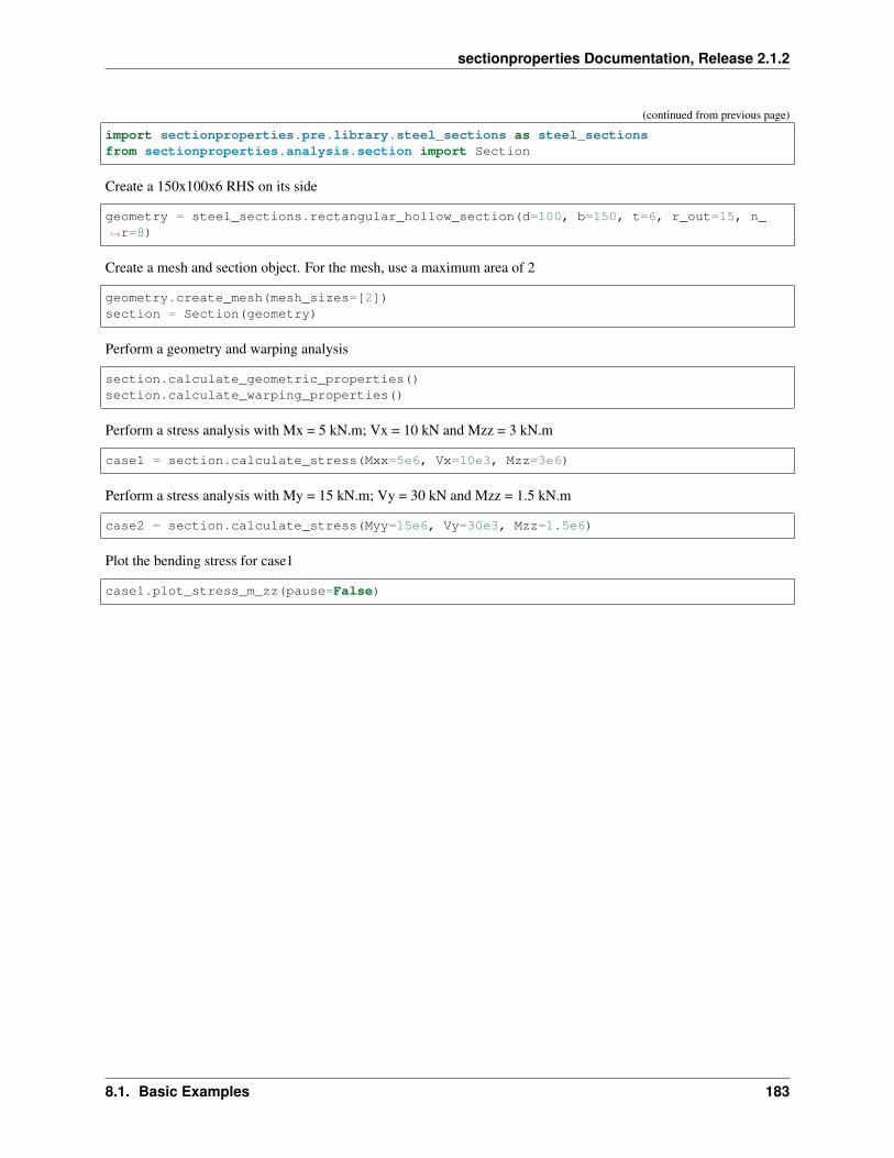
sectionproperties Documentation, Release 2.1.2
(continued from previous page)
import sectionproperties.pre.library.steel_sections as steel_sectionsfrom sectionproperties.analysis.section import Section
Create a 150x100x6 RHS on its side
geometry = steel_sections.rectangular_hollow_section(d=100, b=150, t=6, r_out=15, n_→˓r=8)
Create a mesh and section object. For the mesh, use a maximum area of 2
geometry.create_mesh(mesh_sizes=[2])section = Section(geometry)
Perform a geometry and warping analysis
section.calculate_geometric_properties()section.calculate_warping_properties()
Perform a stress analysis with Mx = 5 kN.m; Vx = 10 kN and Mzz = 3 kN.m
case1 = section.calculate_stress(Mxx=5e6, Vx=10e3, Mzz=3e6)
Perform a stress analysis with My = 15 kN.m; Vy = 30 kN and Mzz = 1.5 kN.m
case2 = section.calculate_stress(Myy=15e6, Vy=30e3, Mzz=1.5e6)
Plot the bending stress for case1
case1.plot_stress_m_zz(pause=False)
8.1. Basic Examples 183
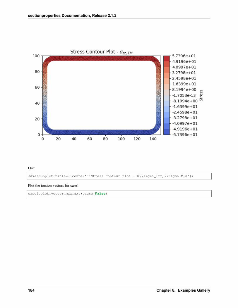
sectionproperties Documentation, Release 2.1.2
Out:
<AxesSubplot:title='center':'Stress Contour Plot - $\\sigma_zz,\\Sigma M$'>
Plot the torsion vectors for case1
case1.plot_vector_mzz_zxy(pause=False)
184 Chapter 8. Examples Gallery

sectionproperties Documentation, Release 2.1.2
Out:
<AxesSubplot:title='center':'Stress Vector Plot - $\\sigma_zxy,Mzz$'>
Plot the shear stress for case2
case2.plot_stress_v_zxy(pause=False)
8.1. Basic Examples 185
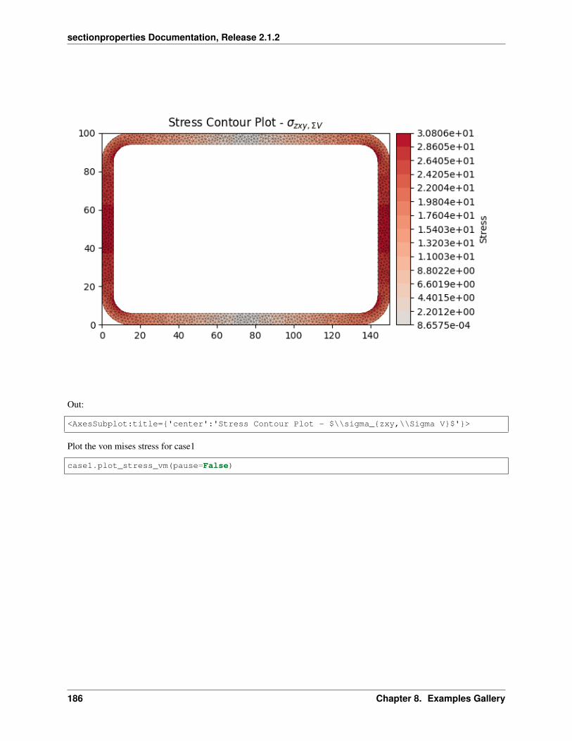
sectionproperties Documentation, Release 2.1.2
Out:
<AxesSubplot:title='center':'Stress Contour Plot - $\\sigma_zxy,\\Sigma V$'>
Plot the von mises stress for case1
case1.plot_stress_vm(pause=False)
186 Chapter 8. Examples Gallery

sectionproperties Documentation, Release 2.1.2
Out:
<AxesSubplot:title='center':'Stress Contour Plot - $\\sigma_vM$'>
Plot the von mises stress for case2
case2.plot_stress_vm()
8.1. Basic Examples 187

sectionproperties Documentation, Release 2.1.2
Out:
<AxesSubplot:title='center':'Stress Contour Plot - $\\sigma_vM$'>
Total running time of the script: ( 0 minutes 24.004 seconds)
8.1.7 Creating a Composite Section
Create a section of mixed materials.
The following example demonstrates how to create a composite cross-section by assigning different material propertiesto various regions of the mesh. A steel 310UB40.4 is modelled with a 50Dx600W timber panel placed on its top flange.
The geometry and mesh are plotted, and the mesh information printed to the terminal before the analysis is carriedout. All types of cross-section analyses are carried out, with an axial force, bending moment and shear force appliedduring the stress analysis. Once the analysis is complete, the cross-section properties are printed to the terminal and aplot of the centroids and cross-section stresses generated.
# sphinx_gallery_thumbnail_number = 2
import sectionproperties.pre.library.primitive_sections as sectionsimport sectionproperties.pre.library.steel_sections as steel_sectionsfrom sectionproperties.pre.geometry import CompoundGeometryfrom sectionproperties.pre.pre import Materialfrom sectionproperties.analysis.section import Section
188 Chapter 8. Examples Gallery

sectionproperties Documentation, Release 2.1.2
Create material properties
steel = Material(name="Steel",elastic_modulus=200e3,poissons_ratio=0.3,yield_strength=500,density=8.05e-6,color="grey",
)timber = Material(
name="Timber",elastic_modulus=8e3,poissons_ratio=0.35,yield_strength=20,density=0.78e-6,color="burlywood",
)
Create 310UB40.4
ub = steel_sections.i_section(d=304, b=165, t_f=10.2, t_w=6.1, r=11.4, n_r=8, material=steel
)
Create timber panel on top of the UB
panel = sections.rectangular_section(d=50, b=600, material=timber)panel = panel.align_center(ub).align_to(ub, on="top")# Create intermediate nodes in panel to match nodes in ubpanel = (panel - ub) | panel
Merge the two sections into one geometry object
section_geometry = CompoundGeometry([ub, panel])
Create a mesh and a Section object. For the mesh use a mesh size of 5 for the UB, 20 for the panel
section_geometry.create_mesh(mesh_sizes=[5, 20])comp_section = Section(section_geometry, time_info=True)comp_section.display_mesh_info() # display the mesh information
Out:
Mesh Statistics:- 9083 nodes- 4246 elements- 2 regions
Plot the mesh with coloured materials and a line transparency of 0.6
comp_section.plot_mesh(materials=True, alpha=0.6)
8.1. Basic Examples 189

sectionproperties Documentation, Release 2.1.2
Out:
<AxesSubplot:title='center':'Finite Element Mesh'>
Perform a geometric, warping and plastic analysis
comp_section.calculate_geometric_properties()comp_section.calculate_warping_properties()comp_section.calculate_plastic_properties(verbose=True)
Out:
Geometric Analysis
Geometric analysis 100% [ 4.0453 s ]complete
Warping Analysis
Warping analysis 100% [ 23.3987 s ]completed9083x9083 stiffness 100% [ 5.6556 s ]
matrix assembledWarping function solved 100% [ 0.0646 s ]
(direct)(continues on next page)
190 Chapter 8. Examples Gallery
sectionproperties Documentation, Release 2.1.2
(continued from previous page)
Shear function vectors 100% [ 5.2054 s ]assembledShear functions solved 100% [ 0.1200 s ]
(direct)Shear and warping 100% [ 3.5253 s ]
integrals assembledShear deformation 100% [ 5.0212 s ]
coefficients assembledMonosymmetry integrals 100% [ 3.7911 s ]
assembled
d = -185.130884950272; f_norm = 1.0d = 168.869115049728; f_norm = -1.0d = -8.13088495027199; f_norm = 0.13960518846748188d = 13.5521668722403; f_norm = 0.0983423820518058d = 60.60270845168366; f_norm = 0.008805290832494688d = 64.90008929872147; f_norm = 0.000627383246551551d = 65.22746216923495; f_norm = 4.393296043904811e-06d = 65.22976962543778; f_norm = 2.21127426308038e-09d = 65.2298027403226; f_norm = -6.080628894287011e-08---x-axis plastic centroid calculation converged at 6.52298e+01 in 8 iterations.d = -300.0; f_norm = 1.0d = 300.0; f_norm = -1.0d = 0.0; f_norm = 7.263545449900235e-17d = 5e-07; f_norm = -4.773093592438759e-08---y-axis plastic centroid calculation converged at 0.00000e+00 in 3 iterations.d = -185.130884950272; f_norm = 1.0d = 168.869115049728; f_norm = -1.0d = -8.13088495027199; f_norm = 0.13960518846748188d = 13.5521668722403; f_norm = 0.0983423820518058d = 60.60270845168366; f_norm = 0.008805290832494688d = 64.90008929872147; f_norm = 0.000627383246551551d = 65.22746216923495; f_norm = 4.393296043904811e-06d = 65.22976962543778; f_norm = 2.21127426308038e-09d = 65.2298027403226; f_norm = -6.080628894287011e-08---11-axis plastic centroid calculation converged at 6.52298e+01 in 8 iterations.d = -300.0; f_norm = 1.0d = 300.0; f_norm = -1.0d = 0.0; f_norm = 7.263545449900235e-17d = 5e-07; f_norm = -4.773093592438759e-08---22-axis plastic centroid calculation converged at 0.00000e+00 in 3 iterations.
Plastic Analysis
Plastic analysis complete 100% [ 0.0990 s ]
Perform a stress analysis with N = 100 kN, Mxx = 120 kN.m and Vy = 75 kN
stress_post = comp_section.calculate_stress(N=-100e3, Mxx=-120e6, Vy=-75e3)
Out:
Stress Analysis
Stress analysis complete 100% [ 5.9268 s ](continues on next page)
8.1. Basic Examples 191

sectionproperties Documentation, Release 2.1.2
(continued from previous page)
Print the results to the terminal
comp_section.display_results()
Out:
Section Properties
Property Value
A 3.521094e+04Perim. 2.206078e+03Mass 6.534804e-02E.A 1.282187e+09E.Qx 2.373725e+11E.Qy 1.057805e+11cx 8.250000e+01cy 1.851309e+02E.Ixx_g 6.740447e+13E.Iyy_g 1.745613e+13E.Ixy_g 1.958323e+13E.Ixx_c 2.345949e+13E.Iyy_c 8.729240e+12E.Ixy_c -3.906250e-03E.Zxx+ 1.389212e+11E.Zxx- 1.267184e+11E.Zyy+ 2.909747e+10E.Zyy- 2.909747e+10rx 1.352644e+02ry 8.251112e+01phi 0.000000e+00E.I11_c 2.345949e+13E.I22_c 8.729240e+12E.Z11+ 1.389212e+11E.Z11- 1.267184e+11E.Z22+ 2.909747e+10E.Z22- 2.909747e+10r11 1.352644e+02r22 8.251112e+01E_eff 3.641446e+04G_eff 1.390847e+04nu_eff 3.090753e-01J 3.768367e+11Iw 6.687734e+16x_se 8.250105e+01y_se 2.863411e+02x_st 8.250104e+01y_st 2.857085e+02x1_se 1.049231e-03y2_se 1.012102e+02E.A_sx 4.022647e+08E.A_sy 3.718571e+08E.A_s11 4.022647e+08E.A_s22 3.718571e+08
(continues on next page)
192 Chapter 8. Examples Gallery

sectionproperties Documentation, Release 2.1.2
(continued from previous page)
betax+ 2.039435e+02betax- -2.039435e+02betay+ 2.098462e-03betay- -2.098462e-03beta11+ 2.039435e+02beta11- -2.039435e+02beta22+ 2.098462e-03beta22- -2.098462e-03x_pc 8.250000e+01y_pc 2.503607e+02M_p,xx 4.238101e+08M_p,yy 4.226021e+08x11_pc 8.250000e+01y22_pc 2.503607e+02M_p,11 4.238101e+08M_p,22 4.226021e+08
Plot the centroids
comp_section.plot_centroids()
Out:
8.1. Basic Examples 193

sectionproperties Documentation, Release 2.1.2
<AxesSubplot:title='center':'Centroids'>
Plot the axial stress
stress_post.plot_stress_n_zz(pause=False)
Out:
<AxesSubplot:title='center':'Stress Contour Plot - $\\sigma_zz,N$'>
Plot the bending stress
stress_post.plot_stress_m_zz(pause=False)
194 Chapter 8. Examples Gallery

sectionproperties Documentation, Release 2.1.2
Out:
<AxesSubplot:title='center':'Stress Contour Plot - $\\sigma_zz,\\Sigma M$'>
Plot the shear stress
stress_post.plot_stress_v_zxy()
8.1. Basic Examples 195
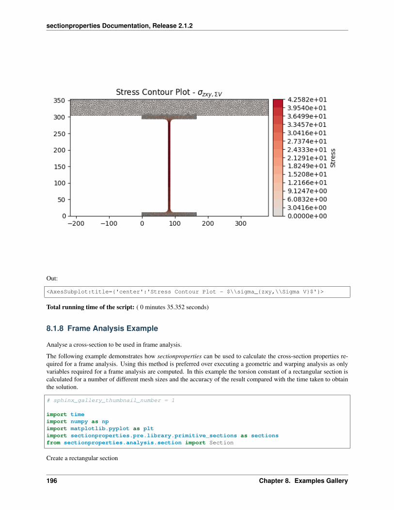
sectionproperties Documentation, Release 2.1.2
Out:
<AxesSubplot:title='center':'Stress Contour Plot - $\\sigma_zxy,\\Sigma V$'>
Total running time of the script: ( 0 minutes 35.352 seconds)
8.1.8 Frame Analysis Example
Analyse a cross-section to be used in frame analysis.
The following example demonstrates how sectionproperties can be used to calculate the cross-section properties re-quired for a frame analysis. Using this method is preferred over executing a geometric and warping analysis as onlyvariables required for a frame analysis are computed. In this example the torsion constant of a rectangular section iscalculated for a number of different mesh sizes and the accuracy of the result compared with the time taken to obtainthe solution.
# sphinx_gallery_thumbnail_number = 1
import timeimport numpy as npimport matplotlib.pyplot as pltimport sectionproperties.pre.library.primitive_sections as sectionsfrom sectionproperties.analysis.section import Section
Create a rectangular section
196 Chapter 8. Examples Gallery
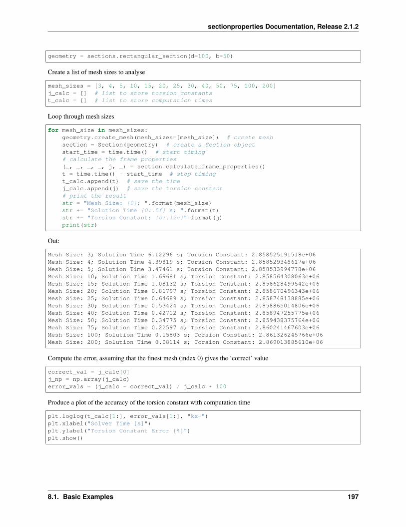
sectionproperties Documentation, Release 2.1.2
geometry = sections.rectangular_section(d=100, b=50)
Create a list of mesh sizes to analyse
mesh_sizes = [3, 4, 5, 10, 15, 20, 25, 30, 40, 50, 75, 100, 200]j_calc = [] # list to store torsion constantst_calc = [] # list to store computation times
Loop through mesh sizes
for mesh_size in mesh_sizes:geometry.create_mesh(mesh_sizes=[mesh_size]) # create meshsection = Section(geometry) # create a Section objectstart_time = time.time() # start timing# calculate the frame properties(_, _, _, _, j, _) = section.calculate_frame_properties()t = time.time() - start_time # stop timingt_calc.append(t) # save the timej_calc.append(j) # save the torsion constant# print the resultstr = "Mesh Size: 0; ".format(mesh_size)str += "Solution Time 0:.5f s; ".format(t)str += "Torsion Constant: 0:.12e".format(j)print(str)
Out:
Mesh Size: 3; Solution Time 6.12296 s; Torsion Constant: 2.858525191518e+06Mesh Size: 4; Solution Time 4.39819 s; Torsion Constant: 2.858529348617e+06Mesh Size: 5; Solution Time 3.47461 s; Torsion Constant: 2.858533994778e+06Mesh Size: 10; Solution Time 1.69681 s; Torsion Constant: 2.858564308063e+06Mesh Size: 15; Solution Time 1.08132 s; Torsion Constant: 2.858628499542e+06Mesh Size: 20; Solution Time 0.81797 s; Torsion Constant: 2.858670496343e+06Mesh Size: 25; Solution Time 0.64689 s; Torsion Constant: 2.858748138885e+06Mesh Size: 30; Solution Time 0.53424 s; Torsion Constant: 2.858865014806e+06Mesh Size: 40; Solution Time 0.42712 s; Torsion Constant: 2.858947255775e+06Mesh Size: 50; Solution Time 0.34775 s; Torsion Constant: 2.859438375764e+06Mesh Size: 75; Solution Time 0.22597 s; Torsion Constant: 2.860241467603e+06Mesh Size: 100; Solution Time 0.15803 s; Torsion Constant: 2.861326245766e+06Mesh Size: 200; Solution Time 0.08114 s; Torsion Constant: 2.869013885610e+06
Compute the error, assuming that the finest mesh (index 0) gives the ‘correct’ value
correct_val = j_calc[0]j_np = np.array(j_calc)error_vals = (j_calc - correct_val) / j_calc * 100
Produce a plot of the accuracy of the torsion constant with computation time
plt.loglog(t_calc[1:], error_vals[1:], "kx-")plt.xlabel("Solver Time [s]")plt.ylabel("Torsion Constant Error [%]")plt.show()
8.1. Basic Examples 197

sectionproperties Documentation, Release 2.1.2
Total running time of the script: ( 0 minutes 20.477 seconds)
8.1.9 Importing Geometry from CAD
Demonstrates loading Geometry and CompoundGeometry objects from .dxf and .3dm (Rhino) files.
# sphinx_gallery_thumbnail_number = 8
from sectionproperties.pre.geometry import Geometry, CompoundGeometryfrom sectionproperties.analysis.section import Section
Load a geometry with a single region from a dxf file
geom = Geometry.from_dxf(dxf_filepath="files/section_holes.dxf")geom.plot_geometry()
198 Chapter 8. Examples Gallery
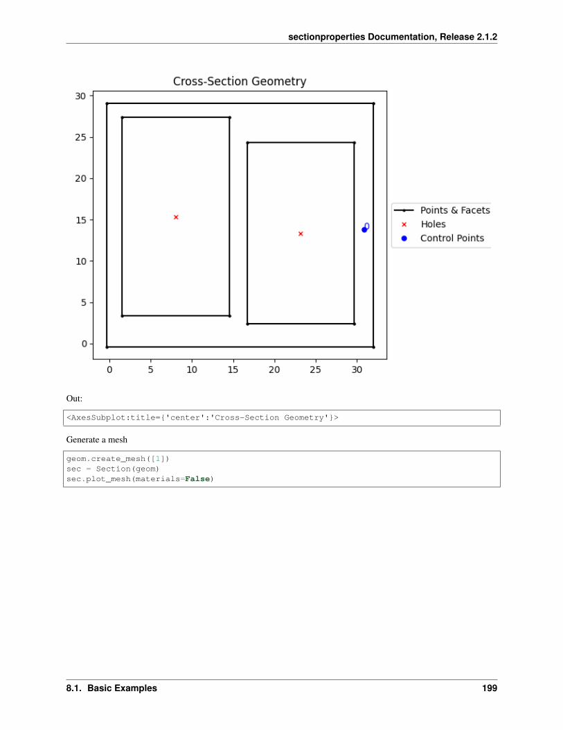
sectionproperties Documentation, Release 2.1.2
Out:
<AxesSubplot:title='center':'Cross-Section Geometry'>
Generate a mesh
geom.create_mesh([1])sec = Section(geom)sec.plot_mesh(materials=False)
8.1. Basic Examples 199

sectionproperties Documentation, Release 2.1.2
Out:
<AxesSubplot:title='center':'Finite Element Mesh'>
Conduct a geometric & plastic analysis
sec.calculate_geometric_properties()sec.calculate_plastic_properties()sec.plot_centroids()
200 Chapter 8. Examples Gallery

sectionproperties Documentation, Release 2.1.2
Out:
<AxesSubplot:title='center':'Centroids'>
Display the geometric & plastic properties
sec.display_results()
Out:
Section Properties
Property Value
A 3.543777e+02Perim. 1.235768e+02Qx 5.047390e+03Qy 5.923689e+03cx 1.671575e+01cy 1.424297e+01Ixx_g 1.137665e+05Iyy_g 1.387654e+05Ixy_g 8.892907e+04Ixx_c 4.187664e+04Iyy_c 3.974650e+04Ixy_c 4.558164e+03
(continues on next page)
8.1. Basic Examples 201

sectionproperties Documentation, Release 2.1.2
(continued from previous page)
Zxx+ 2.820099e+03Zxx- 2.860789e+03Zyy+ 2.606925e+03Zyy- 2.330570e+03rx 1.087058e+01ry 1.059049e+01phi -3.842404e+01I11_c 4.549251e+04I22_c 3.613063e+04Z11+ 2.155143e+03Z11- 2.061571e+03Z22+ 1.717082e+03Z22- 1.599443e+03r11 1.133018e+01r22 1.009728e+01x_pc 1.626707e+01y_pc 1.427513e+01Sxx 3.548750e+03Syy 3.153834e+03SF_xx+ 1.258378e+00SF_xx- 1.240479e+00SF_yy+ 1.209791e+00SF_yy- 1.353246e+00x11_pc 1.662479e+01y22_pc 1.427103e+01S11 3.492177e+03S22 2.898242e+03SF_11+ 1.620392e+00SF_11- 1.693940e+00SF_22+ 1.687888e+00SF_22- 1.812032e+00
Load a geometry with multiple holes from a dxf file
geom = Geometry.from_dxf(dxf_filepath="files/section_holes_complex.dxf")geom.plot_geometry()
202 Chapter 8. Examples Gallery

sectionproperties Documentation, Release 2.1.2
Out:
<AxesSubplot:title='center':'Cross-Section Geometry'>
Generate a mesh
geom.create_mesh([1])sec = Section(geom)sec.plot_mesh(materials=False)
8.1. Basic Examples 203
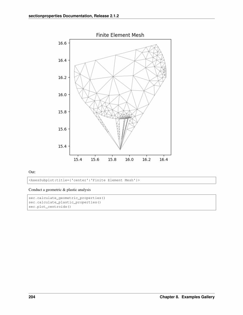
sectionproperties Documentation, Release 2.1.2
Out:
<AxesSubplot:title='center':'Finite Element Mesh'>
Conduct a geometric & plastic analysis
sec.calculate_geometric_properties()sec.calculate_plastic_properties()sec.plot_centroids()
204 Chapter 8. Examples Gallery

sectionproperties Documentation, Release 2.1.2
Out:
<AxesSubplot:title='center':'Centroids'>
Display the geometric & plastic properties
sec.display_results()
Out:
Section Properties
Property Value
A 6.997735e-01Perim. 3.531378e+00Qx 1.127282e+01Qy 1.113424e+01cx 1.591121e+01cy 1.610924e+01Ixx_g 1.816356e+02Iyy_g 1.772080e+02Ixy_g 1.793714e+02Ixx_c 3.907173e-02Iyy_c 4.872212e-02Ixy_c 7.193759e-03
(continues on next page)
8.1. Basic Examples 205

sectionproperties Documentation, Release 2.1.2
(continued from previous page)
Zxx+ 8.271797e-02Zxx- 5.195063e-02Zyy+ 9.416195e-02Zyy- 8.798053e-02rx 2.362939e-01ry 2.638665e-01phi -6.192581e+01I11_c 5.255906e-02I22_c 3.523478e-02Z11+ 8.973609e-02Z11- 1.082595e-01Z22+ 5.379674e-02Z22- 7.702330e-02r11 2.740596e-01r22 2.243918e-01x_pc 1.592489e+01y_pc 1.613076e+01Sxx 1.364187e-01Syy 1.554974e-01SF_xx+ 1.649203e+00SF_xx- 2.625929e+00SF_yy+ 1.651383e+00SF_yy- 1.767407e+00x11_pc 1.588269e+01y22_pc 1.611059e+01S11 1.620643e-01S22 1.302126e-01SF_11+ 1.806010e+00SF_11- 1.496999e+00SF_22+ 2.420454e+00SF_22- 1.690561e+00
Load a geometry from a 3dm (Rhino) file
geom = Geometry.from_3dm(filepath="files/complex_shape.3dm")geom.plot_geometry()
206 Chapter 8. Examples Gallery
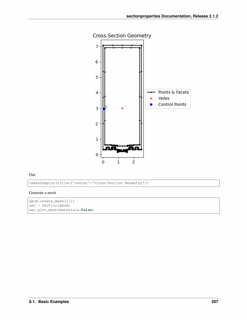
sectionproperties Documentation, Release 2.1.2
Out:
<AxesSubplot:title='center':'Cross-Section Geometry'>
Generate a mesh
geom.create_mesh([1])sec = Section(geom)sec.plot_mesh(materials=False)
8.1. Basic Examples 207

sectionproperties Documentation, Release 2.1.2
Out:
<AxesSubplot:title='center':'Finite Element Mesh'>
Conduct a geometric & plastic analysis
sec.calculate_geometric_properties()sec.calculate_plastic_properties()sec.plot_centroids()
208 Chapter 8. Examples Gallery

sectionproperties Documentation, Release 2.1.2
Out:
<AxesSubplot:title='center':'Centroids'>
Display the geometric & plastic properties
sec.display_results()
Out:
Section Properties
Property Value
A 2.602049e+00Perim. 2.130651e+01Qx 9.082300e+00Qy 3.252560e+00cx 1.249999e+00cy 3.490441e+00Ixx_g 4.773758e+01Iyy_g 6.824622e+00Ixy_g 1.135287e+01Ixx_c 1.603635e+01Iyy_c 2.758925e+00Ixy_c 5.755182e-06
(continues on next page)
8.1. Basic Examples 209

sectionproperties Documentation, Release 2.1.2
(continued from previous page)
Zxx+ 4.476583e+00Zxx- 4.813398e+00Zyy+ 2.207139e+00Zyy- 2.207142e+00rx 2.482533e+00ry 1.029704e+00phi 0.000000e+00I11_c 1.603635e+01I22_c 2.758925e+00Z11+ 4.476583e+00Z11- 4.813398e+00Z22+ 2.207139e+00Z22- 2.207142e+00r11 2.482533e+00r22 1.029704e+00x_pc 1.249996e+00y_pc 3.353406e+00Sxx 5.801661e+00Syy 2.504936e+00SF_xx+ 1.296002e+00SF_xx- 1.205315e+00SF_yy+ 1.134925e+00SF_yy- 1.134923e+00x11_pc 1.249996e+00y22_pc 3.353406e+00S11 5.801661e+00S22 2.504936e+00SF_11+ 1.296002e+00SF_11- 1.205315e+00SF_22+ 1.134925e+00SF_22- 1.134923e+00
Load a compound geometry with multiple regions from a 3dm (Rhino) file
geom = CompoundGeometry.from_3dm(filepath="files/compound_shape.3dm")geom.plot_geometry()
210 Chapter 8. Examples Gallery

sectionproperties Documentation, Release 2.1.2
Out:
<AxesSubplot:title='center':'Cross-Section Geometry'>
Generate a mesh
geom.create_mesh([1])sec = Section(geom)sec.plot_mesh(materials=False)
8.1. Basic Examples 211

sectionproperties Documentation, Release 2.1.2
Out:
<AxesSubplot:title='center':'Finite Element Mesh'>
Conduct a geometric & plastic analysis N.B a warping analysis would be invalid due to the lack of connectivitybetween the two regions
sec.calculate_geometric_properties()sec.calculate_plastic_properties()sec.plot_centroids()
212 Chapter 8. Examples Gallery
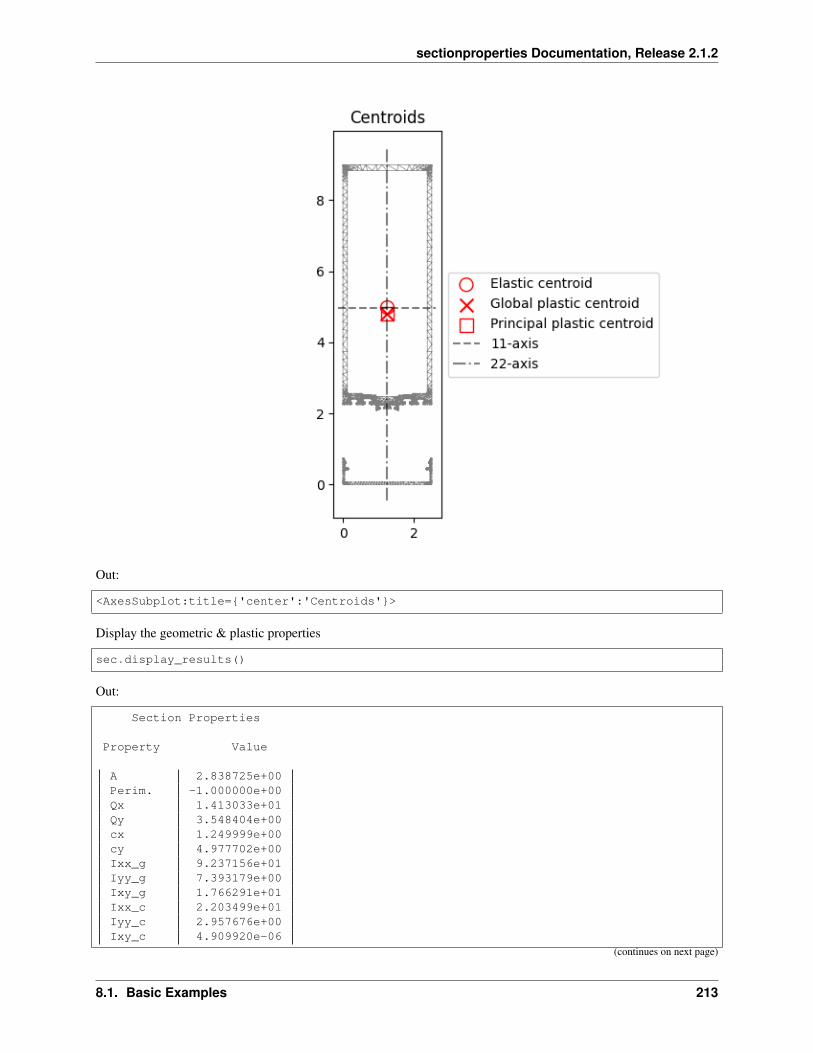
sectionproperties Documentation, Release 2.1.2
Out:
<AxesSubplot:title='center':'Centroids'>
Display the geometric & plastic properties
sec.display_results()
Out:
Section Properties
Property Value
A 2.838725e+00Perim. -1.000000e+00Qx 1.413033e+01Qy 3.548404e+00cx 1.249999e+00cy 4.977702e+00Ixx_g 9.237156e+01Iyy_g 7.393179e+00Ixy_g 1.766291e+01Ixx_c 2.203499e+01Iyy_c 2.957676e+00Ixy_c 4.909920e-06
(continues on next page)
8.1. Basic Examples 213

sectionproperties Documentation, Release 2.1.2
(continued from previous page)
Zxx+ 5.480936e+00Zxx- 4.426740e+00Zyy+ 2.366139e+00Zyy- 2.366142e+00rx 2.786088e+00ry 1.020736e+00phi 0.000000e+00I11_c 2.203499e+01I22_c 2.957676e+00Z11+ 5.480936e+00Z11- 4.426740e+00Z22+ 2.366139e+00Z22- 2.366142e+00r11 2.786088e+00r22 1.020736e+00x_pc 1.249996e+00y_pc 4.805339e+00Sxx 6.956641e+00Syy 2.699474e+00SF_xx+ 1.269243e+00SF_xx- 1.571504e+00SF_yy+ 1.140877e+00SF_yy- 1.140876e+00x11_pc 1.249996e+00y22_pc 4.805339e+00S11 6.956641e+00S22 2.699474e+00SF_11+ 1.269243e+00SF_11- 1.571504e+00SF_22+ 1.140877e+00SF_22- 1.140876e+00
Total running time of the script: ( 0 minutes 14.817 seconds)
8.2 Advanced Examples
The following examples demonstrates how sectionproperties can be used for more academic purposes.
8.2.1 Advanced Plotting
Harness some of the plotting features provided by plotting_context().
# sphinx_gallery_thumbnail_number = 1
import sectionproperties.pre.library.steel_sections as steel_sectionsfrom sectionproperties.analysis.section import Sectionimport matplotlib.pyplot as plt
The below example creates a 100x6 SHS and plots the geometry, mesh, centroids and torsion vectors in a 2x2 subplotarrangement.
214 Chapter 8. Examples Gallery

sectionproperties Documentation, Release 2.1.2
geometry = steel_sections.rectangular_hollow_section(d=100, b=100, t=6, r_out=15, n_→˓r=8)
# Plot the geometryax = geometry.plot_geometry(nrows=2, ncols=2, figsize=(12, 7), render=False,→˓labels=[])fig = ax.get_figure() # get the figure
# Create a mesh and section object, for the mesh, use a maximum area of 2geometry.create_mesh(mesh_sizes=[2])section = Section(geometry)section.plot_mesh(ax=fig.axes[1], materials=False) # plot the mesh
# Perform a geometry and warping analysissection.calculate_geometric_properties()section.calculate_warping_properties()section.plot_centroids(ax=fig.axes[2]) # plot the cetnroids
# Perform a stress analysis with Mzz = 10 kN.mstress = section.calculate_stress(Mzz=10e6)stress.plot_vector_mzz_zxy(
ax=fig.axes[3], title="Torsion Vectors") # plot the torsion vectorsplt.show() # show the plot
Total running time of the script: ( 0 minutes 14.605 seconds)
8.2.2 Mesh Refinement
Perform a mesh refinement study.
In this example the convergence of the torsion constant is investigated through an analysis of an I Section. The mesh
8.2. Advanced Examples 215

sectionproperties Documentation, Release 2.1.2
is refined both by modifying the mesh size and by specifying the number of points making up the root radius. Thefigure below the example code shows that mesh refinement adjacent to the root radius is a far more efficient method inobtaining fast convergence when compared to reducing the mesh area size for the entire section.
# sphinx_gallery_thumbnail_number = 1
import numpy as npimport matplotlib.pyplot as pltimport sectionproperties.pre.library.steel_sections as steel_sectionsfrom sectionproperties.analysis.section import Section
Define mesh sizes
mesh_size_list = [200, 100, 50, 20, 10, 5]nr_list = [4, 8, 12, 16, 20, 24, 32]
Initialise result lists
mesh_results = []mesh_elements = []nr_results = []nr_elements = []
Calculate reference solution
geometry = steel_sections.i_section(d=203, b=133, t_f=7.8, t_w=5.8, r=8.9, n_r=32)geometry.create_mesh(mesh_sizes=[5]) # create meshsection = Section(geometry) # create a Section objectsection.calculate_geometric_properties()section.calculate_warping_properties()j_reference = section.get_j() # get the torsion constant
Run through mesh_sizes with n_r = 8
for mesh_size in mesh_size_list:geometry = steel_sections.i_section(d=203, b=133, t_f=7.8, t_w=5.8, r=8.9, n_r=8)geometry.create_mesh(mesh_sizes=[mesh_size]) # create meshsection = Section(geometry) # create a Section objectsection.calculate_geometric_properties()section.calculate_warping_properties()
mesh_elements.append(len(section.elements))mesh_results.append(section.get_j())
Run through n_r with mesh_size = 10
for n_r in nr_list:geometry = steel_sections.i_section(d=203, b=133, t_f=7.8, t_w=5.8, r=8.9, n_r=n_
→˓r)geometry.create_mesh(mesh_sizes=[10]) # create meshsection = Section(geometry) # create a Section objectsection.calculate_geometric_properties()section.calculate_warping_properties()
nr_elements.append(len(section.elements))nr_results.append(section.get_j())
Convert results to a numpy array and compute the error
216 Chapter 8. Examples Gallery

sectionproperties Documentation, Release 2.1.2
mesh_results = np.array(mesh_results)nr_results = np.array(nr_results)mesh_error_vals = (mesh_results - j_reference) / mesh_results * 100nr_error_vals = (nr_results - j_reference) / nr_results * 100
Plot the results
(fig, ax) = plt.subplots()ax.loglog(mesh_elements, mesh_error_vals, "kx-", label="Mesh Size Refinement")ax.loglog(nr_elements, nr_error_vals, "rx-", label="Root Radius Refinement")plt.xlabel("Number of Elements")plt.ylabel("Torsion Constant Error [%]")plt.legend(loc="center left", bbox_to_anchor=(1, 0.5))plt.tight_layout()plt.show()
Total running time of the script: ( 1 minutes 3.174 seconds)
8.2.3 Torsion Constant of a Rectangle
Plot the variation of the torsion constant with aspect ratio of a rectangle section.
In this example, the aspect ratio of a rectangular section is varied whilst keeping a constant cross-sectional area andthe torsion constant calculated. The variation of the torsion constant with the aspect ratio is then plotted.
8.2. Advanced Examples 217

sectionproperties Documentation, Release 2.1.2
# sphinx_gallery_thumbnail_number = 1
import numpy as npimport matplotlib.pyplot as pltimport sectionproperties.pre.library.primitive_sections as sectionsfrom sectionproperties.analysis.section import Section
Rectangle dimensions
d_list = []b_list = np.linspace(0.2, 1, 20)j_list = [] # list holding torsion constant results
Number of elements for each analysis
n = 100
Loop through all the widths
for b in b_list:# calculate d assuming area = 1d = 1 / bd_list.append(d)
# compute mesh sizems = d * b / n
# perform a warping analysis on rectanglegeometry = sections.rectangular_section(d=d, b=b)geometry.create_mesh(mesh_sizes=[ms])section = Section(geometry)section.calculate_geometric_properties()section.calculate_warping_properties()
# get the torsion constantj = section.get_j()print("d/b = 0:.3f; J = 1:.5e".format(d / b, j))j_list.append(j)
Out:
d/b = 25.000; J = 1.30315e-02d/b = 17.060; J = 1.88338e-02d/b = 12.380; J = 2.55717e-02d/b = 9.391; J = 3.31309e-02d/b = 7.367; J = 4.14010e-02d/b = 5.934; J = 5.02289e-02d/b = 4.881; J = 5.95117e-02d/b = 4.086; J = 6.90261e-02d/b = 3.470; J = 7.86512e-02d/b = 2.983; J = 8.81645e-02d/b = 2.593; J = 9.73762e-02d/b = 2.274; J = 1.06053e-01d/b = 2.010; J = 1.14042e-01d/b = 1.790; J = 1.21141e-01d/b = 1.604; J = 1.27224e-01d/b = 1.446; J = 1.32194e-01
(continues on next page)
218 Chapter 8. Examples Gallery
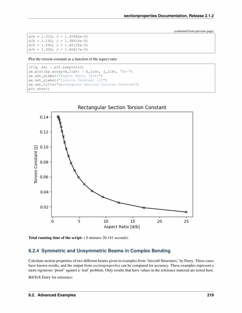
sectionproperties Documentation, Release 2.1.2
(continued from previous page)
d/b = 1.310; J = 1.35982e-01d/b = 1.192; J = 1.38616e-01d/b = 1.090; J = 1.40125e-01d/b = 1.000; J = 1.40617e-01
Plot the torsion constant as a function of the aspect ratio
(fig, ax) = plt.subplots()ax.plot(np.array(d_list) / b_list, j_list, "kx-")ax.set_xlabel("Aspect Ratio [d/b]")ax.set_ylabel("Torsion Constant [J]")ax.set_title("Rectangular Section Torsion Constant")plt.show()
Total running time of the script: ( 0 minutes 20.141 seconds)
8.2.4 Symmetric and Unsymmetric Beams in Complex Bending
Calculate section properties of two different beams given in examples from ‘Aircraft Structures,’ by Peery. These caseshave known results, and the output from sectionproperties can be compared for accuracy. These examples represent amore rigourous ‘proof’ against a ‘real’ problem. Only results that have values in the reference material are tested here.
BibTeX Entry for reference:
8.2. Advanced Examples 219
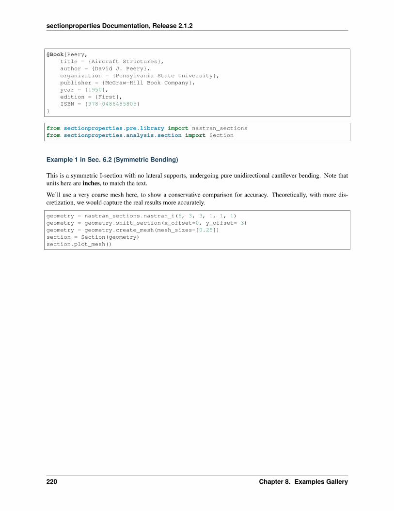
sectionproperties Documentation, Release 2.1.2
@BookPeery,title = Aircraft Structures,author = David J. Peery,organization = Pensylvania State University,publisher = McGraw-Hill Book Company,year = 1950,edition = First,ISBN = 978-0486485805
from sectionproperties.pre.library import nastran_sectionsfrom sectionproperties.analysis.section import Section
Example 1 in Sec. 6.2 (Symmetric Bending)
This is a symmetric I-section with no lateral supports, undergoing pure unidirectional cantilever bending. Note thatunits here are inches, to match the text.
We’ll use a very coarse mesh here, to show a conservative comparison for accuracy. Theoretically, with more dis-cretization, we would capture the real results more accurately.
geometry = nastran_sections.nastran_i(6, 3, 3, 1, 1, 1)geometry = geometry.shift_section(x_offset=0, y_offset=-3)geometry = geometry.create_mesh(mesh_sizes=[0.25])section = Section(geometry)section.plot_mesh()
220 Chapter 8. Examples Gallery

sectionproperties Documentation, Release 2.1.2
Out:
<AxesSubplot:title='center':'Finite Element Mesh'>
Perform a geometric analysis on the section, and plot properties We don’t need warping analysis for these simplechecks, but sectionproperties needs them before evaluating stress.
section.calculate_geometric_properties()section.calculate_warping_properties()section.plot_centroids()
8.2. Advanced Examples 221
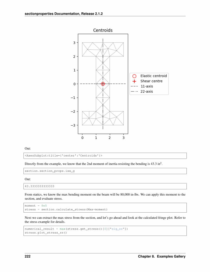
sectionproperties Documentation, Release 2.1.2
Out:
<AxesSubplot:title='center':'Centroids'>
Directly from the example, we know that the 2nd moment of inertia resisting the bending is 43.3 in4.
section.section_props.ixx_g
Out:
43.3333333333333
From statics, we know the max bending moment on the beam will be 80,000 in-lbs. We can apply this moment to thesection, and evaluate stress.
moment = 8e5stress = section.calculate_stress(Mxx=moment)
Next we can extract the max stress from the section, and let’s go ahead and look at the calculated fringe plot. Refer tothe stress example for details.
numerical_result = max(stress.get_stress()[0]["sig_zz"])stress.plot_stress_zz()
222 Chapter 8. Examples Gallery

sectionproperties Documentation, Release 2.1.2
Out:
<AxesSubplot:title='center':'Stress Contour Plot - $\\sigma_zz$'>
From the book, and simple statics, we know the max stress is 55,427.3 psi.
numerical_result
Out:
55384.61538461558
This example is admittedly more simple, but it’s still a nice check for the basics on validity of the package.
print(f"Theoretical Result = 55427 [psi]")print(f" Numerical Result = numerical_result:.0f [psi]")acc = (55427 - numerical_result) / 55427print(f" Accuracy = acc:%")
Out:
Theoretical Result = 55427 [psi]Numerical Result = 55385 [psi]
Accuracy = 0.076469%
8.2. Advanced Examples 223

sectionproperties Documentation, Release 2.1.2
Example 1 in Sec. 7.2. (Unsymmetric Bending)
Moving on to something a bit more advanced. . . This is an unsymmetric Z-section with no lateral supports. Note thatunits here are inches, to match the text.
base_geom = nastran_sections.nastran_zed(4, 2, 8, 12)base_geom = base_geom.shift_section(-5, -6)base_geom = base_geom.create_mesh([0.25])section = Section(base_geom)section.calculate_geometric_properties()section.calculate_warping_properties()section.plot_centroids()
Out:
<AxesSubplot:title='center':'Centroids'>
Checking each property against the reference text:
props = section.section_propsprint(" Property | Theoretical | Numerical")print(f" ixx_g | 693.3:<12.1f| props.ixx_g:<.1f")print(f" iyy_g | 173.3:<12.1f| props.iyy_g:<.1f")print(f" ixy_g | -240:<12.1f| props.ixy_g:<.1f")print(f" i11_c | 787:<12.1f| props.i11_c:<.1f")print(f" i22_c | 79.5:<12.1f| props.i22_c:<.1f")
224 Chapter 8. Examples Gallery

sectionproperties Documentation, Release 2.1.2
Out:
Property | Theoretical | Numericalixx_g | 693.3 | 693.3iyy_g | 173.3 | 173.3ixy_g | -240.0 | -240.0i11_c | 787.0 | 787.2i22_c | 79.5 | 79.5
Section properties all look good, so we can move on to some stress analysis. Before we do, we will need a quickfunction to pull stress at a certain point. This is a bit of a hack! Future versions of sectionproperties will have a muchmore robust system for getting stress at an arbitrary location. This particular function will work for the locations weneed, since we know a node will be there.
from typing import Tuple
def get_node(nodes, coord) -> Tuple[int, tuple]:"""This function will loop over the node list provided,finding the index of the coordinates you want.Returns the index in the nodes list, and the coords."""for index, var in enumerate(nodes):
if all(var == coord):return index, var
else:continue
raise ValueError(f"No node found with coordinates: coord")
The load applied in the reference is -100,000 in-lbs about the x-axis, and 10,000 inb-lbs about the y-axis.
stress = section.calculate_stress(Mxx=-1e5, Myy=1e4)
Check stress at location A (see docs page for details)
A = (-5, 4)text_result = 1210n, _ = get_node(section.mesh_nodes, A)numerical_result = stress.get_stress()[0]["sig_zz"][n]print(text_result, numerical_result)
Out:
1210 1210.2272727272666
Check stress at location B (see docs page for details)
B = (-5, 6)text_result = 580n, _ = get_node(section.mesh_nodes, B)numerical_result = stress.get_stress()[0]["sig_zz"][n]print(text_result, numerical_result)
Out:
8.2. Advanced Examples 225

sectionproperties Documentation, Release 2.1.2
580 579.545454545451
Check stress at location C (see docs page for details)
C = (1, 6)text_result = -2384n, _ = get_node(section.mesh_nodes, C)numerical_result = stress.get_stress()[0]["sig_zz"][n]print(text_result, numerical_result)
Out:
-2384 -2386.363636363626
Looking at total axial stress over the section.
stress.plot_stress_zz()
Out:
<AxesSubplot:title='center':'Stress Contour Plot - $\\sigma_zz$'>
Total running time of the script: ( 0 minutes 3.607 seconds)
226 Chapter 8. Examples Gallery

sectionproperties Documentation, Release 2.1.2
8.2.5 Approximation of Torsion Constant for Trapezoidal Sections
Trapezoidal elements or components of a cross-section are quite common in bridge structures, either concrete or steelcomposite construction. However, it’s common to determine the torsion constant of the trapezoidal section by using arectangular approximation. For example, this is done in the Autodesk Structural Bridge Design software when thereis a haunch in a Steel Composite Beam
The question then arises, when is it appropriate to make the rectangular approximation to a trapezoidal section, andwhat might the expected error be?
Define the Imports
Here we bring in the primative section shapes and also the more generic Shapely Polygon object.
import numpy as npimport matplotlib.pyplot as pltfrom shapely.geometry import Polygonimport sectionproperties.pre.geometry as geometryimport sectionproperties.pre.pre as preimport sectionproperties.pre.library.primitive_sections as sectionsfrom sectionproperties.analysis.section import Section
Define the Calculation Engine
It’s better to collect the relevant section property calculation in a single function. We are only interested in the torsionconstant, so this is straightforward enough. geom is the Section Property Geometry object; ms is the mesh size.
def get_section_j(geom, ms, plot_geom=False):geom.create_mesh(mesh_sizes=[ms])section = Section(geom)if plot_geom:
section.plot_mesh()section.calculate_geometric_properties()section.calculate_warping_properties()return section.get_j()
Define the Mesh Density
The number of elements per unit area is an important input to the calculations even though we are only examiningratios of the results. A nominal value of 100 is reasonable.
n = 100 # mesh density
Create and Analyse the Section
This function accepts the width b and a slope S to create the trapezoid. Since we are only interested in relative results,the nominal dimensions are immaterial. There are a few ways to parametrize the problem, but it has been found thatsetting the middle height of trapezoid (i.e. the average height) to a unit value works fine.
8.2. Advanced Examples 227

sectionproperties Documentation, Release 2.1.2
def do_section(b, S, d_mid=1, plot_geom=False):delta = S * d_midd1 = d_mid - deltad2 = d_mid + delta
# compute mesh sizems = d_mid * b / n
points = []points.append([0, 0])points.append([0, d1])points.append([b, d2])points.append([b, 0])if S < 1.0:
trap_geom = geometry.Geometry(Polygon(points))else:
trap_geom = sections.triangular_section(h=d2, b=b)jt = get_section_j(trap_geom, ms, plot_geom)
rect_geom = sections.rectangular_section(d=(d1 + d2) / 2, b=b)jr = get_section_j(rect_geom, ms, plot_geom)return jt, jr, d1, d2
Example Section
The analysis for a particular section looks as follows:
b, S = 4.0, 0.3jt, jr, d1, d2 = do_section(b, S, plot_geom=True)print(f"b=; S=; jr=; jt=; jr/jt")
228 Chapter 8. Examples Gallery

sectionproperties Documentation, Release 2.1.2
•
8.2. Advanced Examples 229

sectionproperties Documentation, Release 2.1.2
•
Out:
b=4.0; S=0.3; jr=1.1236937204755924; jt=1.1530949943412052; 0.9745022968533389
Create Loop Variables
The slope S is 0 for a rectangle, and 1 for a triangle and is defined per the plot below. A range of S, between 0.0 and1.0 and a range of b are considered, between 1 and 10 here (but can be extended)
b_list = np.logspace(0, np.log10(10), 10)S_list = np.linspace(0.0, 1.0, 10)j_rect = np.zeros((len(b_list), len(S_list)))j_trap = np.zeros((len(b_list), len(S_list)))
The Main Loop
Execute the double loop to get the ratios for combinations of S and b.
An optional deugging line is left in for development but commented out.
for i, b in enumerate(b_list):for j, S in enumerate(S_list):
jt, jr, d1, d2 = do_section(b, S)j_trap[i][j] = jt
(continues on next page)
230 Chapter 8. Examples Gallery
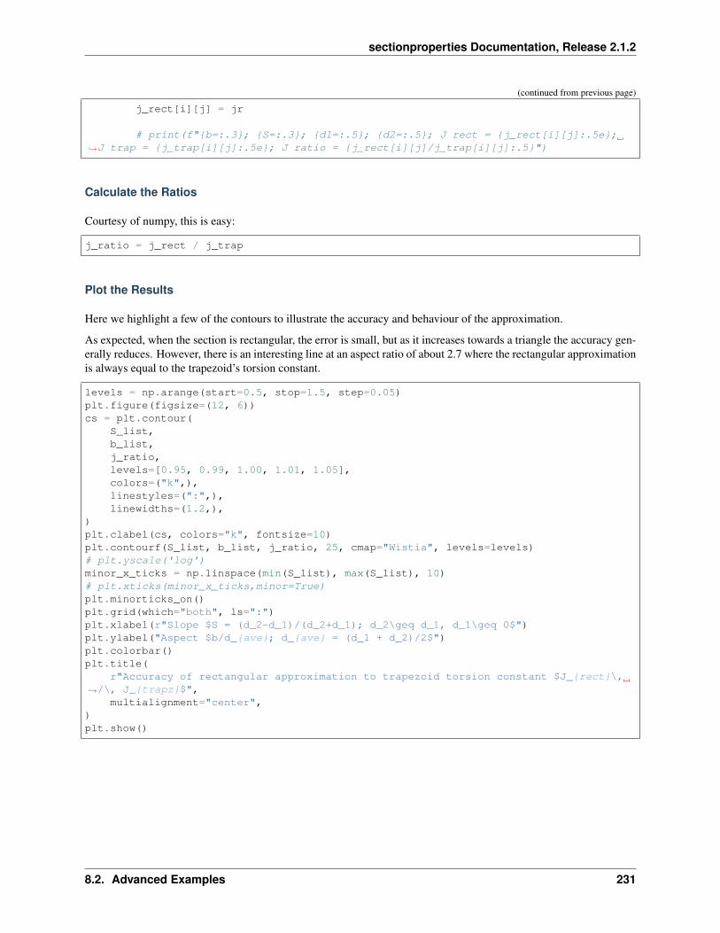
sectionproperties Documentation, Release 2.1.2
(continued from previous page)
j_rect[i][j] = jr
# print(f"b=:.3; S=:.3; d1=:.5; d2=:.5; J rect = j_rect[i][j]:.5e;→˓J trap = j_trap[i][j]:.5e; J ratio = j_rect[i][j]/j_trap[i][j]:.5")
Calculate the Ratios
Courtesy of numpy, this is easy:
j_ratio = j_rect / j_trap
Plot the Results
Here we highlight a few of the contours to illustrate the accuracy and behaviour of the approximation.
As expected, when the section is rectangular, the error is small, but as it increases towards a triangle the accuracy gen-erally reduces. However, there is an interesting line at an aspect ratio of about 2.7 where the rectangular approximationis always equal to the trapezoid’s torsion constant.
levels = np.arange(start=0.5, stop=1.5, step=0.05)plt.figure(figsize=(12, 6))cs = plt.contour(
S_list,b_list,j_ratio,levels=[0.95, 0.99, 1.00, 1.01, 1.05],colors=("k",),linestyles=(":",),linewidths=(1.2,),
)plt.clabel(cs, colors="k", fontsize=10)plt.contourf(S_list, b_list, j_ratio, 25, cmap="Wistia", levels=levels)# plt.yscale('log')minor_x_ticks = np.linspace(min(S_list), max(S_list), 10)# plt.xticks(minor_x_ticks,minor=True)plt.minorticks_on()plt.grid(which="both", ls=":")plt.xlabel(r"Slope $S = (d_2-d_1)/(d_2+d_1); d_2\geq d_1, d_1\geq 0$")plt.ylabel("Aspect $b/d_ave; d_ave = (d_1 + d_2)/2$")plt.colorbar()plt.title(
r"Accuracy of rectangular approximation to trapezoid torsion constant $J_rect\,→˓/\, J_trapz$",
multialignment="center",)plt.show()
8.2. Advanced Examples 231

sectionproperties Documentation, Release 2.1.2
Total running time of the script: ( 3 minutes 26.064 seconds)
232 Chapter 8. Examples Gallery

CHAPTER 9
Python API Reference
9.1 Pre-Processor Package
9.1.1 geometry Module
Geometry Class
class sectionproperties.pre.geometry.Geometry(geom: shapely.geometry.Polygon,material: pre.Material = Mate-rial(name=’default’, elastic_modulus=1,poissons_ratio=0, yield_strength=1,density=1, color=’w’), control_points:Optional[List[float, float]] = None,tol=12)
Class for defining the geometry of a contiguous section of a single material.
Provides an interface for the user to specify the geometry defining a section. A method is provided for generatinga triangular mesh, transforming the section (e.g. translation, rotation, perimeter offset, mirroring), aligning thegeometry to another geometry, and designating stress recovery points.
Variables
• geom (shapely.geometry.Polygon) – a Polygon object that defines the geometry
• material (Optional[Material]) – Optional, a Material to associate with this geometry
• control_point – Optional, an (x, y) coordinate within the geometry that representsa pre-assigned control point (aka, a region identification point) to be used instead of theautomatically assigned control point generated with shapely.geometry.Polygon.representative_point().
• tol – Optional, default is 12. Number of decimal places to round the geometry verticesto. A lower value may reduce accuracy of geometry but increases precision when aligninggeometries to each other.
233

sectionproperties Documentation, Release 2.1.2
align_center(align_to: Optional[sectionproperties.pre.geometry.Geometry] = None)Returns a new Geometry object, translated in both x and y, so that the center-point of the new object’scentroid will be aligned with centroid of the object in ‘align_to’. If ‘align_to’ is None then the new objectwill be aligned with it’s centroid at the origin.
Parameters align_to (Optional[Geometry]) – Another Geometry to align to or None (de-fault is None)
Returns Geometry object translated to new alignment
Return type Geometry
align_to(other: Union[sectionproperties.pre.geometry.Geometry, Tuple[float, float]], on: str, inner:bool = False)→ sectionproperties.pre.geometry.Geometry
Returns a new Geometry object, representing ‘self’ translated so that is aligned ‘on’ one of the outerbounding box edges of ‘other’.
If ‘other’ is a tuple representing an (x,y) coordinate, then the new Geometry object will represent ‘self’translated so that it is aligned ‘on’ that side of the point.
Parameters
• other (Union[Geometry , Tuple[float, float]]) – Either another Geometry or a tuplerepresenting an (x,y) coordinate point that ‘self’ should align to.
• on – A str of either “left”, “right”, “bottom”, or “top” indicating which side of ‘other’ thatself should be aligned to.
• inner (bool) – Default False. If True, align ‘self’ to ‘other’ in such a way that ‘self’ isaligned to the “inside” of ‘other’. In other words, align ‘self’ to ‘other’ on the specifiededge so they overlap.
Returns Geometry object translated to alignment location
Return type Geometry
assign_control_point(control_point: List[float, float])Returns a new Geometry object with ‘control_point’ assigned as the control point for the new Geometry.The assignment of a control point is intended to replace the control point automatically generated byshapely.geometry.Polygon.representative_point().
An assigned control point is carried through and transformed with the Geometry whenever it is shifted,aligned, mirrored, unioned, and/or rotated. If a perimeter_offset operation is applied, a check is performedto see if the assigned control point is still valid (within the new region) and, if so, it is kept. If not, a newcontrol point is auto-generated.
The same check is performed when the geometry undergoes a difference operation (with the ‘-’ operator) ora shift_points operation. If the assigned control point is valid, it is kept. If not, a new one is auto-generated.
For all other operations (e.g. symmetric difference, intersection, split, ), the assigned control point isdiscarded and a new one auto-generated.
Variables control_points – An (x, y) coordinate that describes the distinct, contiguous, re-gion of a single material within the geometry. Exactly one point is required for each geometrywith a distinct material.
calculate_area()Calculates the area of the geometry.
Returns Geometry area.
Return type float
234 Chapter 9. Python API Reference
sectionproperties Documentation, Release 2.1.2
calculate_centroid()Calculates the centroid of the geometry as a tuple of (x,y) coordinates.
Returns Geometry centroid.
Return type Tuple[float, float]
calculate_extents()Calculates the minimum and maximum x and y-values amongst the list of points; the points that describethe bounding box of the Geometry instance.
Returns Minimum and maximum x and y-values (x_min, x_max, y_min, y_max)
Return type tuple(float, float, float, float)
calculate_perimeter()Calculates the exterior perimeter of the geometry.
Returns Geometry perimeter.
Return type float
compile_geometry()Alters attributes .points, .facets, .holes, .control_points to represent the data in the shapely geometry.
create_mesh(mesh_sizes: Union[float, List[float]], coarse: bool = False)Creates a quadratic triangular mesh from the Geometry object.
Parameters
• mesh_sizes (Union[float, List[float]]) – A float describing the maximummesh element area to be used within the Geometry-object finite-element mesh.
• coarse (bool) – If set to True, will create a coarse mesh (no area or quality constraints)
Returns Geometry-object with mesh data stored in .mesh attribute. Returned Geometry-objectis self, not a new instance.
Return type Geometry
The following example creates a circular cross-section with a diameter of 50 with 64 points, and generatesa mesh with a maximum triangular area of 2.5:
import sectionproperties.pre.library.primitive_sections as primitive_sections
geometry = primitive_sections.circular_section(d=50, n=64)geometry = geometry.create_mesh(mesh_sizes=2.5)
classmethod from_3dm(filepath: Union[str, pathlib.Path], **kwargs) → sectionproper-ties.pre.geometry.Geometry
Class method to create a Geometry from the objects in a Rhino .3dm file.
Parameters
• filepath (Union[str, pathlib.Path]) – File path to the rhino .3dm file.
• kwargs – See below.
Raises RuntimeError – A RuntimeError is raised if two or more polygons are found. Thisis dependent on the keyword arguments. Try adjusting the keyword arguments if this error israised.
Returns A Geometry object.
Return type Geometry
9.1. Pre-Processor Package 235
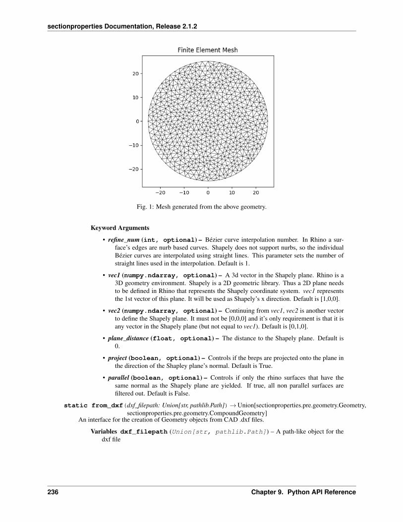
sectionproperties Documentation, Release 2.1.2
Fig. 1: Mesh generated from the above geometry.
Keyword Arguments
• refine_num (int, optional) – Bézier curve interpolation number. In Rhino a sur-face’s edges are nurb based curves. Shapely does not support nurbs, so the individualBézier curves are interpolated using straight lines. This parameter sets the number ofstraight lines used in the interpolation. Default is 1.
• vec1 (numpy.ndarray, optional) – A 3d vector in the Shapely plane. Rhino is a3D geometry environment. Shapely is a 2D geometric library. Thus a 2D plane needsto be defined in Rhino that represents the Shapely coordinate system. vec1 representsthe 1st vector of this plane. It will be used as Shapely’s x direction. Default is [1,0,0].
• vec2 (numpy.ndarray, optional) – Continuing from vec1, vec2 is another vectorto define the Shapely plane. It must not be [0,0,0] and it’s only requirement is that it isany vector in the Shapely plane (but not equal to vec1). Default is [0,1,0].
• plane_distance (float, optional) – The distance to the Shapely plane. Default is0.
• project (boolean, optional) – Controls if the breps are projected onto the plane inthe direction of the Shapley plane’s normal. Default is True.
• parallel (boolean, optional) – Controls if only the rhino surfaces that have thesame normal as the Shapely plane are yielded. If true, all non parallel surfaces arefiltered out. Default is False.
static from_dxf(dxf_filepath: Union[str, pathlib.Path])→ Union[sectionproperties.pre.geometry.Geometry,sectionproperties.pre.geometry.CompoundGeometry]
An interface for the creation of Geometry objects from CAD .dxf files.
Variables dxf_filepath (Union[str, pathlib.Path]) – A path-like object for thedxf file
236 Chapter 9. Python API Reference

sectionproperties Documentation, Release 2.1.2
static from_points(points: List[List[float]], facets: List[List[int]], control_points:List[List[float]], holes: Optional[List[List[float]]] = None, material:Optional[sectionproperties.pre.pre.Material] = Material(name=’default’,elastic_modulus=1, poissons_ratio=0, yield_strength=1, density=1,color=’w’))
An interface for the creation of Geometry objects through the definition of points, facets, and holes.
Variables
• points (list[list[float, float]]) – List of points (x, y) defining the verticesof the section geometry. If facets are not provided, it is a assumed the that the list of pointsare ordered around the perimeter, either clockwise or anti-clockwise.
• facets (list[list[int, int]]) – A list of (start, end) indexes of vertices defin-ing the edges of the section geoemtry. Can be used to define both external and internalperimeters of holes. Facets are assumed to be described in the order of exterior perimeter,interior perimeter 1, interior perimeter 2, etc.
• control_points – An (x, y) coordinate that describes the distinct, contiguous, regionof a single material within the geometry. Must be entered as a list of coordinates, e.g.[[0.5, 3.2]] Exactly one point is required for each geometry with a distinct material. Ifthere are multiple distinct regions, then use CompoundGeometry.from_points()
• holes (list[list[float, float]]) – Optional. A list of points (x, y) that defineinterior regions as being holes or voids. The point can be located anywhere within the holeregion. Only one point is required per hole region.
• material – Optional. A Material object that is to be assigned. If not given, then theDEFAULT_MATERIAL will be used.
classmethod from_rhino_encoding(r3dm_brep: str, **kwargs) → sectionproper-ties.pre.geometry.Geometry
Load an encoded single surface planer brep.
Parameters
• r3dm_brep (str) – A Rhino3dm.Brep encoded as a string.
• kwargs – See below.
Returns A Geometry object found in the encoded string.
Return type Geometry
Keyword Arguments
• refine_num (int, optional) – Bézier curve interpolation number. In Rhino a sur-face’s edges are nurb based curves. Shapely does not support nurbs, so the individualBézier curves are interpolated using straight lines. This parameter sets the number ofstraight lines used in the interpolation. Default is 1.
• vec1 (numpy.ndarray, optional) – A 3d vector in the Shapely plane. Rhino is a3D geometry environment. Shapely is a 2D geometric library. Thus a 2D plane needsto be defined in Rhino that represents the Shapely coordinate system. vec1 representsthe 1st vector of this plane. It will be used as Shapely’s x direction. Default is [1,0,0].
• vec2 (numpy.ndarray, optional) – Continuing from vec1, vec2 is another vectorto define the Shapely plane. It must not be [0,0,0] and it’s only requirement is that it isany vector in the Shapely plane (but not equal to vec1). Default is [0,1,0].
• plane_distance (float, optional) – The distance to the Shapely plane. Default is0.
9.1. Pre-Processor Package 237

sectionproperties Documentation, Release 2.1.2
• project (boolean, optional) – Controls if the breps are projected onto the plane inthe direction of the Shapley plane’s normal. Default is True.
• parallel (boolean, optional) – Controls if only the rhino surfaces that have thesame normal as the Shapely plane are yielded. If true, all non parallel surfaces arefiltered out. Default is False.
mirror_section(axis: str = ’x’, mirror_point: Union[List[float], str] = ’center’)Mirrors the geometry about a point on either the x or y-axis.
Parameters
• axis (string) – Axis about which to mirror the geometry, ‘x’ or ‘y’
• mirror_point (Union[list[float, float], str]) – Point about which tomirror the geometry (x, y). If no point is provided, mirrors the geometry about the centroidof the shape’s bounding box. Default = ‘center’.
Returns New Geometry-object mirrored on ‘axis’ about ‘mirror_point’
Return type Geometry
The following example mirrors a 200PFC section about the y-axis and the point (0, 0):
import sectionproperties.pre.library.steel_sections as steel_sections
geometry = steel_sections.channel_section(d=200, b=75, t_f=12, t_w=6, r=12, n_→˓r=8)new_geometry = geometry.mirror_section(axis='y', mirror_point=[0, 0])
offset_perimeter(amount: float = 0, where: str = ’exterior’, resolution: float = 12)Dilates or erodes the section perimeter by a discrete amount.
Parameters
• amount (float) – Distance to offset the section by. A -ve value “erodes” the section. A+ve value “dilates” the section.
• where (str) – One of either “exterior”, “interior”, or “all” to specify which edges of thegeometry to offset. If geometry has no interiors, then this parameter has no effect. Defaultis “exterior”.
• resolution (float) – Number of segments used to approximate a quarter circlearound a point
Returns Geometry object translated to new alignment
Return type Geometry
The following example erodes a 200PFC section by 2 mm:
import sectionproperties.pre.library.steel_sections as steel_sections
geometry = sections.channel_section(d=200, b=75, t_f=12, t_w=6, r=12, n_r=8)new_geometry = geometry.offset_perimeter(amount=-2)
plot_geometry(labels=[’control_points’], title=’Cross-Section Geometry’, cp=True, legend=True,**kwargs)
Plots the geometry defined by the input section.
Parameters
238 Chapter 9. Python API Reference

sectionproperties Documentation, Release 2.1.2
• labels (list[str]) – A list of str which indicate which labels to plot. Can be oneor a combination of “points”, “facets”, “control_points”, or an empty list to indicate nolabels. Default is [“control_points”]
• title (string) – Plot title
• cp (bool) – If set to True, plots the control points
• legend (bool) – If set to True, plots the legend
• kwargs – Passed to plotting_context()
Returns Matplotlib axes object
Return type matplotlib.axes
The following example creates a CHS discretised with 64 points, with a diameter of 48 and thickness of3.2, and plots the geometry:
import sectionproperties.pre.library.steel_sections as steel_sections
geometry = steel_sections.circular_hollow_section(d=48, t=3.2, n=64)geometry.plot_geometry()
Fig. 2: Geometry generated by the above example.
rotate_section(angle: float, rot_point: Union[List[float], str] = ’center’, use_radians: bool =False)
Rotates the geometry and specified angle about a point. If the rotation point is not provided, rotates thesection about the center of the geometry’s bounding box.
Parameters
• angle (float) – Angle (degrees by default) by which to rotate the section. A positiveangle leads to a counter-clockwise rotation.
• rot_point (list[float, float]) – Optional. Point (x, y) about which to rotatethe section. If not provided, will rotate about the center of the geometry’s bounding box.Default = ‘center’.
9.1. Pre-Processor Package 239

sectionproperties Documentation, Release 2.1.2
• use_radians – Boolean to indicate whether ‘angle’ is in degrees or radians. If True,‘angle’ is interpreted as radians.
Returns New Geometry-object rotated by ‘angle’ about ‘rot_point’
Return type Geometry
The following example rotates a 200UB25 section clockwise by 30 degrees:
import sectionproperties.pre.library.steel_sections as steel_sections
geometry = steel_sections.i_section(d=203, b=133, t_f=7.8, t_w=5.8, r=8.9, n_→˓r=8)new_geometry = geometry.rotate_section(angle=-30)
shift_points(point_idxs: Union[int, List[int]], dx: float = 0, dy: float = 0, abs_x: Optional[float] =None, abs_y: Optional[float] = None)→ sectionproperties.pre.geometry.Geometry
Translates one (or many points) in the geometry by either a relative amount or to a new absolute location.Returns a new Geometry representing the original with the selected point(s) shifted to the new location.
Points are identified by their index, their relative location within the points list found in self.points.You can call self.plot_geometry(labels="points") to see a plot with the points labeled tofind the appropriate point indexes.
Parameters
• point_idxs (Union[int, List[int]]) – An integer representing an index loca-tion or a list of integer index locations.
• dx (float) – The number of units in the x-direction to shift the point(s) by
• dy (float) – The number of units in the y-direction to shift the point(s) by
• abs_x (Optional[float]) – Absolute x-coordinate in coordinate system to shift thepoint(s) to. If abs_x is provided, dx is ignored. If providing a list to point_idxs, all pointswill be moved to this absolute location.
• abs_y (Optional[float]) – Absolute y-coordinate in coordinate system to shift thepoint(s) to. If abs_y is provided, dy is ignored. If providing a list to point_idxs, all pointswill be moved to this absolute location.
Returns Geometry object with selected points translated to the new location.
Return type Geometry
The following example expands the sides of a rectangle, one point at a time, to make it a square:
import sectionproperties.pre.library.primitive_sections as primitive_sections
geometry = primitive_sections.rectangular_section(d=200, b=150)
# Using relative shiftingone_pt_shifted_geom = geometry.shift_points(point_idxs=1, dx=50)
# Using absolute relocationboth_pts_shift_geom = one_pt_shift_geom.shift_points(point_idxs=2, abs_x=200)
shift_section(x_offset=0.0, y_offset=0.0)Returns a new Geometry object translated by ‘x_offset’ and ‘y_offset’.
Parameters
• x_offset (float) – Distance in x-direction by which to shift the geometry.
240 Chapter 9. Python API Reference
sectionproperties Documentation, Release 2.1.2
• y_offset (float) – Distance in y-direction by which to shift the geometry.
Returns New Geometry-object shifted by ‘x_offset’ and ‘y_offset’
Return type Geometry
split_section(point_i: Tuple[float, float], point_j: Optional[Tuple[float, float]]= None, vector: Union[Tuple[float, float], None, numpy.ndarray]= None) → Tuple[List[sectionproperties.pre.geometry.Geometry],List[sectionproperties.pre.geometry.Geometry]]
Splits, or bisects, the geometry about a line, as defined by two points on the line or by one point on the lineand a vector. Either point_j or vector must be given. If point_j is given, vector is ignored.
Returns a tuple of two lists each containing new Geometry instances representing the “top” and “bottom”portions, respectively, of the bisected geometry.
If the line is a vertical line then the “right” and “left” portions, respectively, are returned.
Parameters
• point_i (Tuple[float, float]) – A tuple of (x, y) coordinates to define a firstpoint on the line
• point_j (Tuple[float, float]) – Optional. A tuple of (x, y) coordinates to de-fine a second point on the line
• vector (Union[Tuple[float, float], numpy.ndarray]) – Optional. Atuple or numpy ndarray of (x, y) components to define the line direction.
Returns A tuple of lists containing Geometry objects that are bisected about the line defined bythe two given points. The first item in the tuple represents the geometries on the “top” of theline (or to the “right” of the line, if vertical) and the second item represents the geometries tothe “bottom” of the line (or to the “left” of the line, if vertical).
Return type Tuple[List[Geometry], List[Geometry]]
The following example splits a 200PFC section about the y-axis:
import sectionproperties.pre.library.steel_sections as steel_sectionsfrom shapely.geometry import LineString
geometry = steel_sections.channel_section(d=200, b=75, t_f=12, t_w=6, r=12, n_→˓r=8)right_geom, left_geom = geometry.split_section((0, 0), (0, 1))
CompoundGeometry Class
class sectionproperties.pre.geometry.CompoundGeometry(geoms:Union[shapely.geometry.multipolygon.MultiPolygon,List[sectionproperties.pre.geometry.Geometry]])
Bases: sectionproperties.pre.geometry.Geometry
Class for defining a geometry of multiple distinct regions, each potentially having different material properties.
CompoundGeometry instances are composed of multiple Geometry objects. As with Geometry objects, Com-poundGeometry objects have methods for generating a triangular mesh over all geometries, transforming thecollection of geometries as though they were one (e.g. translation, rotation, and mirroring), and aligning theCompoundGeometry to another Geometry (or to another CompoundGeometry).
CompoundGeometry objects can be created directly between two or more Geometry objects by using the +operator.
9.1. Pre-Processor Package 241

sectionproperties Documentation, Release 2.1.2
Variables geoms (Union[shapely.geometry.MultiPolygon, List[Geometry]]) – eithera list of Geometry objects or a shapely.geometry.MultiPolygon instance.
load_dxf
sectionproperties.pre.geometry.load_dxf(dxf_filepath: pathlib.Path)Import any-old-shape in dxf format for analysis. Code by aegis1980 and connorferster
create_facets
sectionproperties.pre.geometry.create_facets(points_list: list, connect_back: bool =False, offset: int = 0)→ list
Returns a list of lists of integers representing the “facets” connecting the list of coordinates in ‘loc’. It is assumedthat ‘loc’ coordinates are already in their order of connectivity.
‘loc’: a list of coordinates ‘connect_back’: if True, then the last facet pair will be [len(loc), offset] ‘offset’: aninteger representing the value that the facets should begin incrementing from.
create_exterior_points
sectionproperties.pre.geometry.create_exterior_points(shape:shapely.geometry.polygon.Polygon)→ list
Return a list of lists representing x,y pairs of the exterior perimeter of polygon.
create_interior_points
sectionproperties.pre.geometry.create_interior_points(lr:shapely.geometry.polygon.LinearRing)→ list
Return a list of lists representing x,y pairs of the exterior perimeter of polygon.
create_points_and_facets
sectionproperties.pre.geometry.create_points_and_facets(shape:shapely.geometry.polygon.Polygon,tol=12)→ tuple
Return a list of lists representing x,y pairs of the exterior perimeter of polygon.
9.1.2 pre Module
Material Class
class sectionproperties.pre.pre.Material(name: str, elastic_modulus: float,poissons_ratio: float, yield_strength:float, density: float, color: str)
Bases: object
Class for structural materials.
242 Chapter 9. Python API Reference

sectionproperties Documentation, Release 2.1.2
Provides a way of storing material properties related to a specific material. The color can be a mul-titude of different formats, refer to https://matplotlib.org/api/colors_api.html and https://matplotlib.org/examples/color/named_colors.html for more information.
Parameters
• name (string) – Material name
• elastic_modulus (float) – Material modulus of elasticity
• poissons_ratio (float) – Material Poisson’s ratio
• yield_strength (float) – Material yield strength
• density (float) – Material density (mass per unit volume)
• color (matplotlib.colors) – Material color for rendering
Variables
• name (string) – Material name
• elastic_modulus (float) – Material modulus of elasticity
• poissons_ratio (float) – Material Poisson’s ratio
• shear_modulus (float) – Material shear modulus, derived from the elasticmodulus and Poisson’s ratio assuming an isotropic material
• density (float) – Material density (mass per unit volume)
• yield_strength (float) – Material yield strength
• color (matplotlib.colors) – Material color for rendering
The following example creates materials for concrete, steel and timber:
from sectionproperties.pre.pre import Material
concrete = Material(name='Concrete', elastic_modulus=30.1e3, poissons_ratio=0.2,
→˓density=2.4e-6,yield_strength=32, color='lightgrey'
)steel = Material(
name='Steel', elastic_modulus=200e3, poissons_ratio=0.3, density=7.→˓85e-6,
yield_strength=500, color='grey')timber = Material(
name='Timber', elastic_modulus=8e3, poissons_ratio=0.35, density=6.→˓5e-7,
yield_strength=20, color='burlywood')
create_mesh
sectionproperties.pre.pre.create_mesh(points: List[List[float]], facets: List[List[float]],holes: List[List[float]], control_points:List[List[float]], mesh_sizes: Union[List[float],float], coarse: bool)
Creates a quadratic triangular mesh using the triangle module, which utilises the code ‘Triangle’, by JonathanShewchuk.
9.1. Pre-Processor Package 243
sectionproperties Documentation, Release 2.1.2
Parameters
• points (list[list[int, int]]) – List of points (x, y) defining the vertices of thecross-section
• facets – List of point index pairs (p1, p2) defining the edges of the cross-section
• holes (list[list[float, float]]) – List of points (x, y) defining the locationsof holes within the cross-section. If there are no holes, provide an empty list [].
• control_points (list[list[float, float]]) – A list of points (x, y) that de-fine different regions of the cross-section. A control point is an arbitrary point within aregion enclosed by facets.
• mesh_sizes (list[float]) – List of maximum element areas for each region definedby a control point
• coarse (bool) – If set to True, will create a coarse mesh (no area or quality constraints)
Returns Dictionary containing mesh data
Return type dict()
9.1.3 rhino Module
load_3dm
sectionproperties.pre.rhino.load_3dm(r3dm_filepath: Union[pathlib.Path, str], **kwargs)→List[shapely.geometry.polygon.Polygon]
Load a Rhino .3dm file and import the single surface planer breps.
Parameters
• r3dm_filepath (pathlib.Path or string) – File path to the rhino .3dm file.
• kwargs – See below.
Raises RuntimeError – A RuntimeError is raised if no polygons are found in the file. Thisis dependent on the keyword arguments. Try adjusting the keyword arguments if this error israised.
Returns List of Polygons found in the file.
Return type List[shapely.geometry.Polygon]
Keyword Arguments
• refine_num (int, optional) – Bézier curve interpolation number. In Rhino a sur-face’s edges are nurb based curves. Shapely does not support nurbs, so the individualBézier curves are interpolated using straight lines. This parameter sets the number ofstraight lines used in the interpolation. Default is 1.
• vec1 (numpy.ndarray, optional) – A 3d vector in the Shapely plane. Rhino is a3D geometry environment. Shapely is a 2D geometric library. Thus a 2D plane needs tobe defined in Rhino that represents the Shapely coordinate system. vec1 represents the1st vector of this plane. It will be used as Shapely’s x direction. Default is [1,0,0].
• vec2 (numpy.ndarray, optional) – Continuing from vec1, vec2 is another vectorto define the Shapely plane. It must not be [0,0,0] and it’s only requirement is that it isany vector in the Shapely plane (but not equal to vec1). Default is [0,1,0].
• plane_distance (float, optional) – The distance to the Shapely plane. Default is 0.
244 Chapter 9. Python API Reference

sectionproperties Documentation, Release 2.1.2
• project (boolean, optional) – Controls if the breps are projected onto the plane inthe direction of the Shapley plane’s normal. Default is True.
• parallel (boolean, optional) – Controls if only the rhino surfaces that have the samenormal as the Shapely plane are yielded. If true, all non parallel surfaces are filtered out.Default is False.
load_brep_encoding
sectionproperties.pre.rhino.load_brep_encoding(brep: str, **kwargs) →shapely.geometry.polygon.Polygon
Load an encoded single surface planer brep.
Parameters
• brep (str) – Rhino3dm.Brep encoded as a string.
• kwargs – See below.
Raises RuntimeError – A RuntimeError is raised if no polygons are found in the encoding. Thisis dependent on the keyword arguments. Try adjusting the keyword arguments if this error israised.
Returns The Polygons found in the encoding string.
Return type shapely.geometry.Polygon
Keyword Arguments
• refine_num (int, optional) – Bézier curve interpolation number. In Rhino a sur-face’s edges are nurb based curves. Shapely does not support nurbs, so the individualBézier curves are interpolated using straight lines. This parameter sets the number ofstraight lines used in the interpolation. Default is 1.
• vec1 (numpy.ndarray, optional) – A 3d vector in the Shapely plane. Rhino is a3D geometry environment. Shapely is a 2D geometric library. Thus a 2D plane needs tobe defined in Rhino that represents the Shapely coordinate system. vec1 represents the1st vector of this plane. It will be used as Shapely’s x direction. Default is [1,0,0].
• vec2 (numpy.ndarray, optional) – Continuing from vec1, vec2 is another vectorto define the Shapely plane. It must not be [0,0,0] and it’s only requirement is that it isany vector in the Shapely plane (but not equal to vec1). Default is [0,1,0].
• plane_distance (float, optional) – The distance to the Shapely plane. Default is 0.
• project (boolean, optional) – Controls if the breps are projected onto the plane inthe direction of the Shapley plane’s normal. Default is True.
• parallel (boolean, optional) – Controls if only the rhino surfaces that have the samenormal as the Shapely plane are yielded. If true, all non parallel surfaces are filtered out.Default is False.
9.1.4 bisect_section Module
9.1. Pre-Processor Package 245
sectionproperties Documentation, Release 2.1.2
create_line_segment
sectionproperties.pre.bisect_section.create_line_segment(point_on_line:Union[Tuple[float,float], numpy.ndarray],vector: numpy.ndarray,bounds: tuple)
Return a LineString of a line that contains ‘point_on_line’ in the direction of ‘unit_vector’ bounded by ‘bounds’.‘bounds’ is a tuple of float containing a max ordinate and min ordinate.
group_top_and_bottom_polys
sectionproperties.pre.bisect_section.group_top_and_bottom_polys(polys:shapely.geometry.collection.GeometryCollection,line:shapely.geometry.linestring.LineString)→ Tuple[list,list]
Returns tuple of two lists representing the list of Polygons in ‘polys’ on the “top” side of ‘line’ and the list ofPolygons on the “bottom” side of the ‘line’ after the original geometry has been split by ‘line’.
The 0-th tuple element is the “top” polygons and the 1-st element is the “bottom” polygons.
In the event that ‘line’ is a perfectly vertical line, the “top” polys are the polygons on the “right” of the ‘line’and the “bottom” polys are the polygons on the “left” of the ‘line’.
line_mx_plus_b
sectionproperties.pre.bisect_section.line_mx_plus_b(line:shapely.geometry.linestring.LineString)→ Tuple[float, float]
Returns a tuple representing the values of “m” and “b” from the definition of ‘line’ as “y = mx + b”.
perp_mx_plus_b
sectionproperties.pre.bisect_section.perp_mx_plus_b(m_slope: float, point_on_line:Tuple[float, float]) → Tu-ple[float, float]
Returns a tuple representing the values of “m” and “b” from for a line that is perpendicular to ‘m_slope’ andcontains the ‘point_on_line’, which represents an (x, y) coordinate.
line_intersection
sectionproperties.pre.bisect_section.line_intersection(m_1: float, b_1: float, m_2:float, b_2: float) → Op-tional[float]
Returns a float representing the x-ordinate of the intersection point of the lines defined by y = m_1*x + b_1 andy = m_2*x + b_2.
Returns None if the lines are parallel.
246 Chapter 9. Python API Reference
sectionproperties Documentation, Release 2.1.2
sum_poly_areas
sectionproperties.pre.bisect_section.sum_poly_areas(lop:List[shapely.geometry.polygon.Polygon])→ float
Returns a float representing the total area of all polygons in ‘lop’, the list of polygons.
9.1.5 primitive_sections Module
rectangular_section
sectionproperties.pre.library.primitive_sections.rectangular_section(b:float,d:float,mate-rial:sec-tion-proper-ties.pre.pre.Material=Mate-rial(name=’default’,elas-tic_modulus=1,pois-sons_ratio=0,yield_strength=1,den-sity=1,color=’w’))→ sec-tion-proper-ties.pre.geometry.Geometry
Constructs a rectangular section with the bottom left corner at the origin (0, 0), with depth d and width b.
Parameters
• d (float) – Depth (y) of the rectangle
• b (float) – Width (x) of the rectangle
• Optional[sectionproperties.pre.pre.Material] – Material to associatewith this geometry
The following example creates a rectangular cross-section with a depth of 100 and width of 50, and generates amesh with a maximum triangular area of 5:
from sectionproperties.pre.library.primitive_sections import rectangular_section
geometry = rectangular_section(d=100, b=50)geometry.create_mesh(mesh_sizes=[5])
9.1. Pre-Processor Package 247

sectionproperties Documentation, Release 2.1.2
Fig. 3: Rectangular section geometry.
Fig. 4: Mesh generated from the above geometry.
248 Chapter 9. Python API Reference

sectionproperties Documentation, Release 2.1.2
circular_section
sectionproperties.pre.library.primitive_sections.circular_section(d: float, n:int, mate-rial: sec-tionproper-ties.pre.pre.Material= Mate-rial(name=’default’,elas-tic_modulus=1,pois-sons_ratio=0,yield_strength=1,density=1,color=’w’))→ sec-tionproper-ties.pre.geometry.Geometry
Constructs a solid circle centered at the origin (0, 0) with diameter d and using n points to construct the circle.
Parameters
• d (float) – Diameter of the circle
• n (int) – Number of points discretising the circle
• Optional[sectionproperties.pre.pre.Material] – Material to associatewith this geometry
The following example creates a circular geometry with a diameter of 50 with 64 points, and generates a meshwith a maximum triangular area of 2.5:
from sectionproperties.pre.library.primitive_sections import circular_section
geometry = circular_section(d=50, n=64)geometry.create_mesh(mesh_sizes=[2.5])
9.1. Pre-Processor Package 249
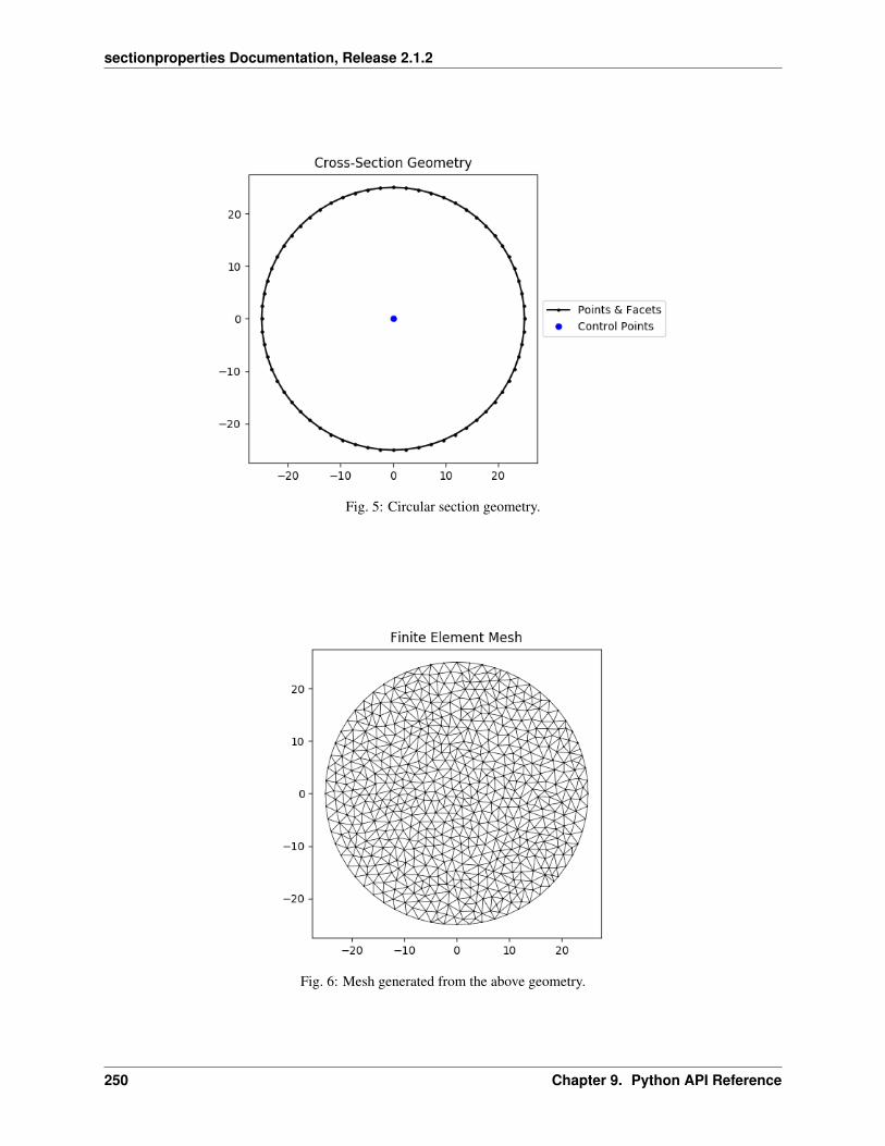
sectionproperties Documentation, Release 2.1.2
Fig. 5: Circular section geometry.
Fig. 6: Mesh generated from the above geometry.
250 Chapter 9. Python API Reference

sectionproperties Documentation, Release 2.1.2
circular_section_by_area
sectionproperties.pre.library.primitive_sections.circular_section_by_area(area:float,n:int,ma-te-rial:sec-tion-prop-er-ties.pre.pre.Material=Ma-te-rial(name=’default’,elas-tic_modulus=1,pois-sons_ratio=0,yield_strength=1,den-sity=1,color=’w’))→sec-tion-prop-er-ties.pre.geometry.Geometry
Constructs a solid circle centered at the origin (0, 0) defined by its area, using n points to construct the circle.
Parameters
• area (float) – Area of the circle
• n (int) – Number of points discretising the circle
• Optional[sectionproperties.pre.pre.Material] – Material to associatewith this geometry
The following example creates a circular geometry with an area of 200 with 32 points, and generates a meshwith a maximum triangular area of 5:
from sectionproperties.pre.library.primitive_sections import circular_section_by_→˓area
geometry = circular_section_by_area(area=310, n=32)geometry.create_mesh(mesh_sizes=[5])
9.1. Pre-Processor Package 251

sectionproperties Documentation, Release 2.1.2
Fig. 7: Circular section by area geometry.
Fig. 8: Mesh generated from the above geometry.
252 Chapter 9. Python API Reference
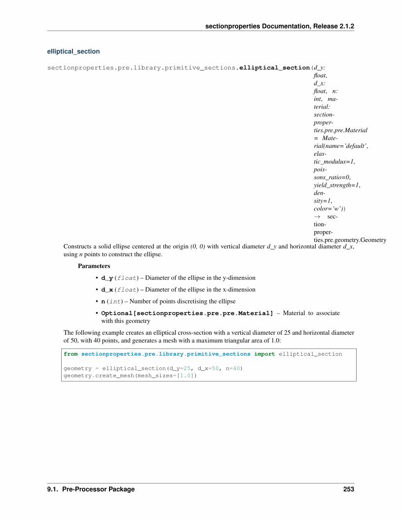
sectionproperties Documentation, Release 2.1.2
elliptical_section
sectionproperties.pre.library.primitive_sections.elliptical_section(d_y:float,d_x:float, n:int, ma-terial:section-proper-ties.pre.pre.Material= Mate-rial(name=’default’,elas-tic_modulus=1,pois-sons_ratio=0,yield_strength=1,den-sity=1,color=’w’))→ sec-tion-proper-ties.pre.geometry.Geometry
Constructs a solid ellipse centered at the origin (0, 0) with vertical diameter d_y and horizontal diameter d_x,using n points to construct the ellipse.
Parameters
• d_y (float) – Diameter of the ellipse in the y-dimension
• d_x (float) – Diameter of the ellipse in the x-dimension
• n (int) – Number of points discretising the ellipse
• Optional[sectionproperties.pre.pre.Material] – Material to associatewith this geometry
The following example creates an elliptical cross-section with a vertical diameter of 25 and horizontal diameterof 50, with 40 points, and generates a mesh with a maximum triangular area of 1.0:
from sectionproperties.pre.library.primitive_sections import elliptical_section
geometry = elliptical_section(d_y=25, d_x=50, n=40)geometry.create_mesh(mesh_sizes=[1.0])
9.1. Pre-Processor Package 253
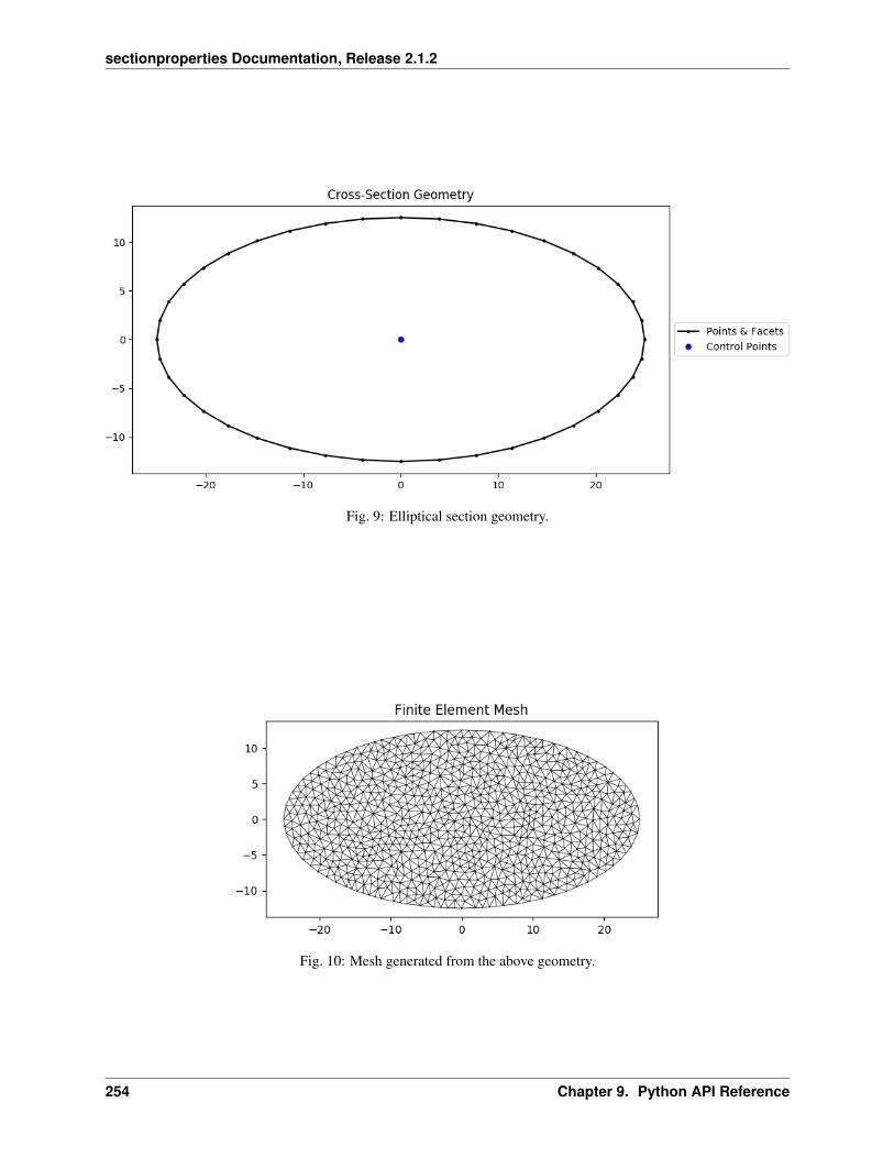
sectionproperties Documentation, Release 2.1.2
Fig. 9: Elliptical section geometry.
Fig. 10: Mesh generated from the above geometry.
254 Chapter 9. Python API Reference
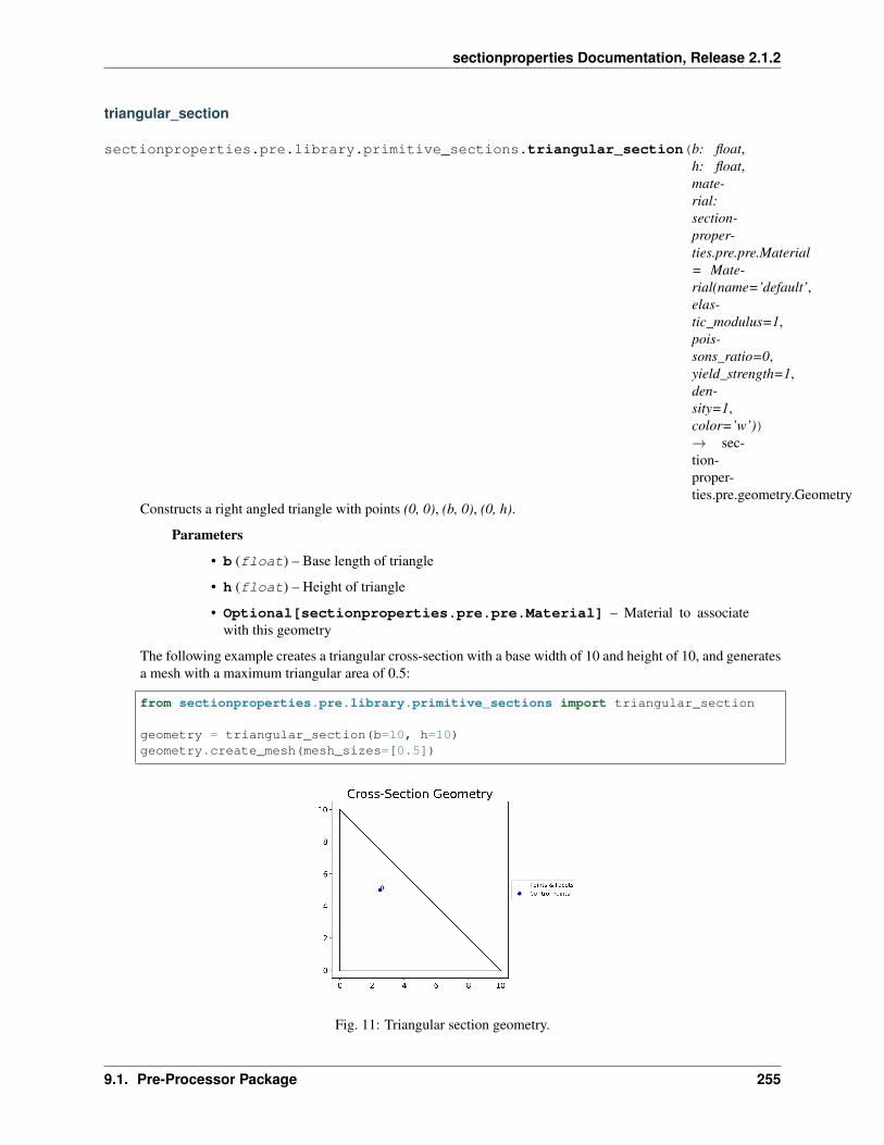
sectionproperties Documentation, Release 2.1.2
triangular_section
sectionproperties.pre.library.primitive_sections.triangular_section(b: float,h: float,mate-rial:section-proper-ties.pre.pre.Material= Mate-rial(name=’default’,elas-tic_modulus=1,pois-sons_ratio=0,yield_strength=1,den-sity=1,color=’w’))→ sec-tion-proper-ties.pre.geometry.Geometry
Constructs a right angled triangle with points (0, 0), (b, 0), (0, h).
Parameters
• b (float) – Base length of triangle
• h (float) – Height of triangle
• Optional[sectionproperties.pre.pre.Material] – Material to associatewith this geometry
The following example creates a triangular cross-section with a base width of 10 and height of 10, and generatesa mesh with a maximum triangular area of 0.5:
from sectionproperties.pre.library.primitive_sections import triangular_section
geometry = triangular_section(b=10, h=10)geometry.create_mesh(mesh_sizes=[0.5])
Fig. 11: Triangular section geometry.
9.1. Pre-Processor Package 255

sectionproperties Documentation, Release 2.1.2
Fig. 12: Mesh generated from the above geometry.
triangular_radius_section
sectionproperties.pre.library.primitive_sections.triangular_radius_section(b:float,n_r:float,ma-te-rial:sec-tion-prop-er-ties.pre.pre.Material=Ma-te-rial(name=’default’,elas-tic_modulus=1,pois-sons_ratio=0,yield_strength=1,den-sity=1,color=’w’))→sec-tion-prop-er-ties.pre.geometry.Geometry
Constructs a right angled isosceles triangle with points (0, 0), (b, 0), (0, h) and a concave radius on the hy-potenuse.
Parameters
• b (float) – Base length of triangle
256 Chapter 9. Python API Reference
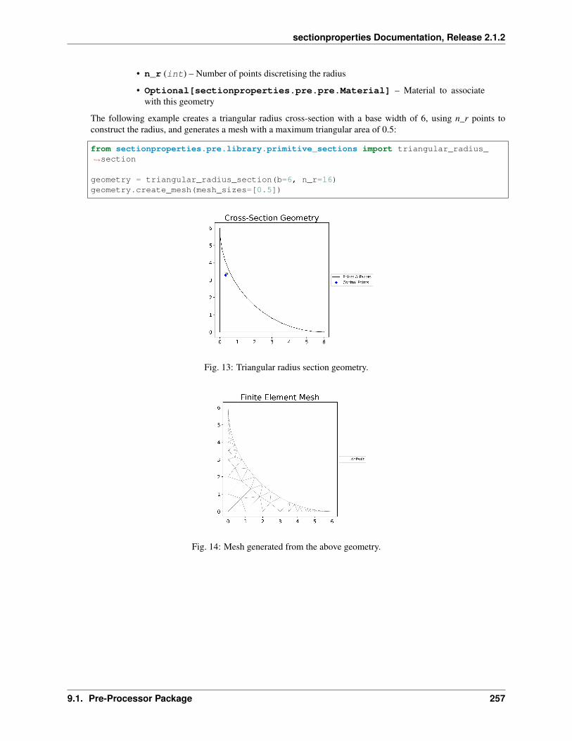
sectionproperties Documentation, Release 2.1.2
• n_r (int) – Number of points discretising the radius
• Optional[sectionproperties.pre.pre.Material] – Material to associatewith this geometry
The following example creates a triangular radius cross-section with a base width of 6, using n_r points toconstruct the radius, and generates a mesh with a maximum triangular area of 0.5:
from sectionproperties.pre.library.primitive_sections import triangular_radius_→˓section
geometry = triangular_radius_section(b=6, n_r=16)geometry.create_mesh(mesh_sizes=[0.5])
Fig. 13: Triangular radius section geometry.
Fig. 14: Mesh generated from the above geometry.
9.1. Pre-Processor Package 257
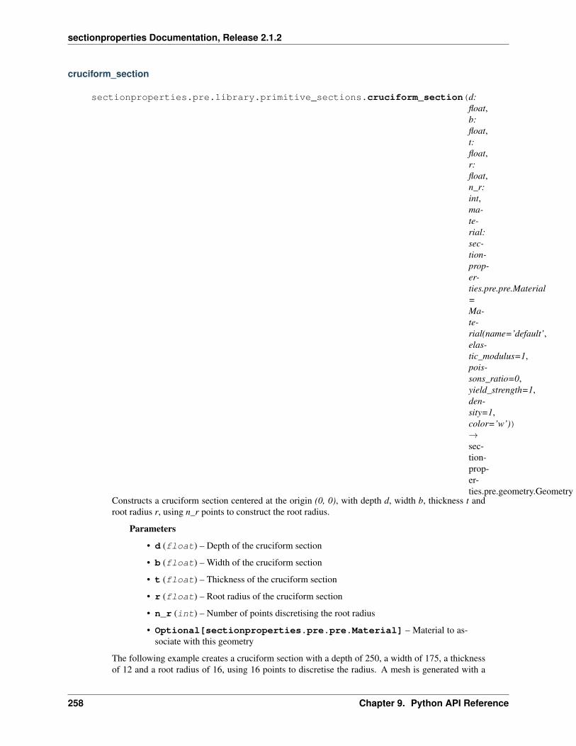
sectionproperties Documentation, Release 2.1.2
cruciform_section
sectionproperties.pre.library.primitive_sections.cruciform_section(d:float,b:float,t:float,r:float,n_r:int,ma-te-rial:sec-tion-prop-er-ties.pre.pre.Material=Ma-te-rial(name=’default’,elas-tic_modulus=1,pois-sons_ratio=0,yield_strength=1,den-sity=1,color=’w’))→sec-tion-prop-er-ties.pre.geometry.Geometry
Constructs a cruciform section centered at the origin (0, 0), with depth d, width b, thickness t androot radius r, using n_r points to construct the root radius.
Parameters
• d (float) – Depth of the cruciform section
• b (float) – Width of the cruciform section
• t (float) – Thickness of the cruciform section
• r (float) – Root radius of the cruciform section
• n_r (int) – Number of points discretising the root radius
• Optional[sectionproperties.pre.pre.Material] – Material to as-sociate with this geometry
The following example creates a cruciform section with a depth of 250, a width of 175, a thicknessof 12 and a root radius of 16, using 16 points to discretise the radius. A mesh is generated with a
258 Chapter 9. Python API Reference

sectionproperties Documentation, Release 2.1.2
maximum triangular area of 5.0:
from sectionproperties.pre.library.primitive_sections import cruciform_→˓section
geometry = cruciform_section(d=250, b=175, t=12, r=16, n_r=16)geometry.create_mesh(mesh_sizes=[5.0])
Fig. 15: Cruciform section geometry.
9.1.6 steel_sections Module
9.1. Pre-Processor Package 259

sectionproperties Documentation, Release 2.1.2
Fig. 16: Mesh generated from the above geometry.
circular_hollow_section
sectionproperties.pre.library.steel_sections.circular_hollow_section(d:float, t:float,n: int,mate-rial:sec-tion-proper-ties.pre.pre.Material=Mate-rial(name=’default’,elas-tic_modulus=1,pois-sons_ratio=0,yield_strength=1,den-sity=1,color=’w’))→ sec-tion-proper-ties.pre.geometry.Geometry
Constructs a circular hollow section (CHS) centered at the origin (0, 0), with diameter d and thickness t, usingn points to construct the inner and outer circles.
Parameters
• d (float) – Outer diameter of the CHS
260 Chapter 9. Python API Reference

sectionproperties Documentation, Release 2.1.2
• t (float) – Thickness of the CHS
• n (int) – Number of points discretising the inner and outer circles
• Optional[sectionproperties.pre.pre.Material] – Material to associatewith this geometry
The following example creates a CHS discretised with 64 points, with a diameter of 48 and thickness of 3.2, andgenerates a mesh with a maximum triangular area of 1.0:
from sectionproperties.pre.library.steel_sections import circular_hollow_section
geometry = circular_hollow_section(d=48, t=3.2, n=64)geometry.create_mesh(mesh_sizes=[1.0])
Fig. 17: CHS geometry.
9.1. Pre-Processor Package 261

sectionproperties Documentation, Release 2.1.2
Fig. 18: Mesh generated from the above geometry.
elliptical_hollow_section
sectionproperties.pre.library.steel_sections.elliptical_hollow_section(d_y:float,d_x:float,t:float,n:int,ma-te-rial:sec-tion-prop-er-ties.pre.pre.Material=Ma-te-rial(name=’default’,elas-tic_modulus=1,pois-sons_ratio=0,yield_strength=1,den-sity=1,color=’w’))→sec-tion-prop-er-ties.pre.geometry.Geometry
Constructs an elliptical hollow section (EHS) centered at the origin (0, 0), with outer vertical diameter d_y, outer
262 Chapter 9. Python API Reference

sectionproperties Documentation, Release 2.1.2
horizontal diameter d_x, and thickness t, using n points to construct the inner and outer ellipses.
Parameters
• d_y (float) – Diameter of the ellipse in the y-dimension
• d_x (float) – Diameter of the ellipse in the x-dimension
• t (float) – Thickness of the EHS
• n (int) – Number of points discretising the inner and outer ellipses
• Optional[sectionproperties.pre.pre.Material] – Material to associatewith this geometry
The following example creates a EHS discretised with 30 points, with a outer vertical diameter of 25, outerhorizontal diameter of 50, and thickness of 2.0, and generates a mesh with a maximum triangular area of 0.5:
from sectionproperties.pre.library.steel_sections import elliptical_hollow_section
geometry = elliptical_hollow_section(d_y=25, d_x=50, t=2.0, n=64)geometry.create_mesh(mesh_sizes=[0.5])
Fig. 19: EHS geometry.
9.1. Pre-Processor Package 263

sectionproperties Documentation, Release 2.1.2
Fig. 20: Mesh generated from the above geometry.
rectangular_hollow_section
sectionproperties.pre.library.steel_sections.rectangular_hollow_section(b:float,d:float,t:float,r_out:float,n_r:int,ma-te-rial:sec-tion-prop-er-ties.pre.pre.Material=Ma-te-rial(name=’default’,elas-tic_modulus=1,pois-sons_ratio=0,yield_strength=1,den-sity=1,color=’w’))→sec-tion-prop-er-ties.pre.geometry.Geometry
Constructs a rectangular hollow section (RHS) centered at (b/2, d/2), with depth d, width b, thickness t and outer
264 Chapter 9. Python API Reference

sectionproperties Documentation, Release 2.1.2
radius r_out, using n_r points to construct the inner and outer radii. If the outer radius is less than the thicknessof the RHS, the inner radius is set to zero.
Parameters
• d (float) – Depth of the RHS
• b (float) – Width of the RHS
• t (float) – Thickness of the RHS
• r_out (float) – Outer radius of the RHS
• n_r (int) – Number of points discretising the inner and outer radii
• Optional[sectionproperties.pre.pre.Material] – Material to associatewith this geometry
The following example creates an RHS with a depth of 100, a width of 50, a thickness of 6 and an outer radiusof 9, using 8 points to discretise the inner and outer radii. A mesh is generated with a maximum triangular areaof 2.0:
from sectionproperties.pre.library.steel_sections import rectangular_hollow_→˓section
geometry = rectangular_hollow_section(d=100, b=50, t=6, r_out=9, n_r=8)geometry.create_mesh(mesh_sizes=[2.0])
Fig. 21: RHS geometry.
9.1. Pre-Processor Package 265

sectionproperties Documentation, Release 2.1.2
Fig. 22: Mesh generated from the above geometry.
polygon_hollow_section
sectionproperties.pre.library.steel_sections.polygon_hollow_section(d:float,t:float,n_sides:int,r_in:float=0,n_r:int=1,rot:float=0,ma-te-rial:sec-tion-prop-er-ties.pre.pre.Material=Ma-te-rial(name=’default’,elas-tic_modulus=1,pois-sons_ratio=0,yield_strength=1,den-sity=1,color=’w’))→sec-tion-prop-er-ties.pre.geometry.Geometry
Constructs a regular hollow polygon section centered at (0, 0), with a pitch circle diameter of bound-
266 Chapter 9. Python API Reference
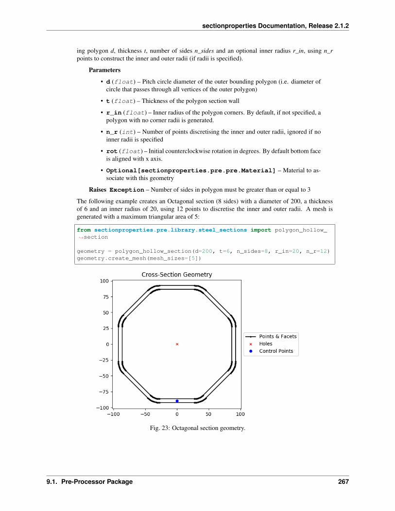
sectionproperties Documentation, Release 2.1.2
ing polygon d, thickness t, number of sides n_sides and an optional inner radius r_in, using n_rpoints to construct the inner and outer radii (if radii is specified).
Parameters
• d (float) – Pitch circle diameter of the outer bounding polygon (i.e. diameter ofcircle that passes through all vertices of the outer polygon)
• t (float) – Thickness of the polygon section wall
• r_in (float) – Inner radius of the polygon corners. By default, if not specified, apolygon with no corner radii is generated.
• n_r (int) – Number of points discretising the inner and outer radii, ignored if noinner radii is specified
• rot (float) – Initial counterclockwise rotation in degrees. By default bottom faceis aligned with x axis.
• Optional[sectionproperties.pre.pre.Material] – Material to as-sociate with this geometry
Raises Exception – Number of sides in polygon must be greater than or equal to 3
The following example creates an Octagonal section (8 sides) with a diameter of 200, a thicknessof 6 and an inner radius of 20, using 12 points to discretise the inner and outer radii. A mesh isgenerated with a maximum triangular area of 5:
from sectionproperties.pre.library.steel_sections import polygon_hollow_→˓section
geometry = polygon_hollow_section(d=200, t=6, n_sides=8, r_in=20, n_r=12)geometry.create_mesh(mesh_sizes=[5])
Fig. 23: Octagonal section geometry.
9.1. Pre-Processor Package 267

sectionproperties Documentation, Release 2.1.2
Fig. 24: Mesh generated from the above geometry.
i_section
sectionproperties.pre.library.steel_sections.i_section(d: float, b:float, t_f: float,t_w: float,r: float, n_r:int, material:sectionproper-ties.pre.pre.Material= Mate-rial(name=’default’,elas-tic_modulus=1,pois-sons_ratio=0,yield_strength=1,density=1,color=’w’)) →sectionproper-ties.pre.geometry.Geometry
Constructs an I Section centered at (b/2, d/2), with depth d, width b, flange thickness t_f, webthickness t_w, and root radius r, using n_r points to construct the root radius.
Parameters
• d (float) – Depth of the I Section
• b (float) – Width of the I Section
• t_f (float) – Flange thickness of the I Section
• t_w (float) – Web thickness of the I Section
• r (float) – Root radius of the I Section
268 Chapter 9. Python API Reference

sectionproperties Documentation, Release 2.1.2
• n_r (int) – Number of points discretising the root radius
• Optional[sectionproperties.pre.pre.Material] – Material to as-sociate with this geometry
The following example creates an I Section with a depth of 203, a width of 133, a flange thicknessof 7.8, a web thickness of 5.8 and a root radius of 8.9, using 16 points to discretise the root radius.A mesh is generated with a maximum triangular area of 3.0:
from sectionproperties.pre.library.steel_sections import i_section
geometry = i_section(d=203, b=133, t_f=7.8, t_w=5.8, r=8.9, n_r=16)geometry.create_mesh(mesh_sizes=[3.0])
Fig. 25: I Section geometry.
9.1. Pre-Processor Package 269
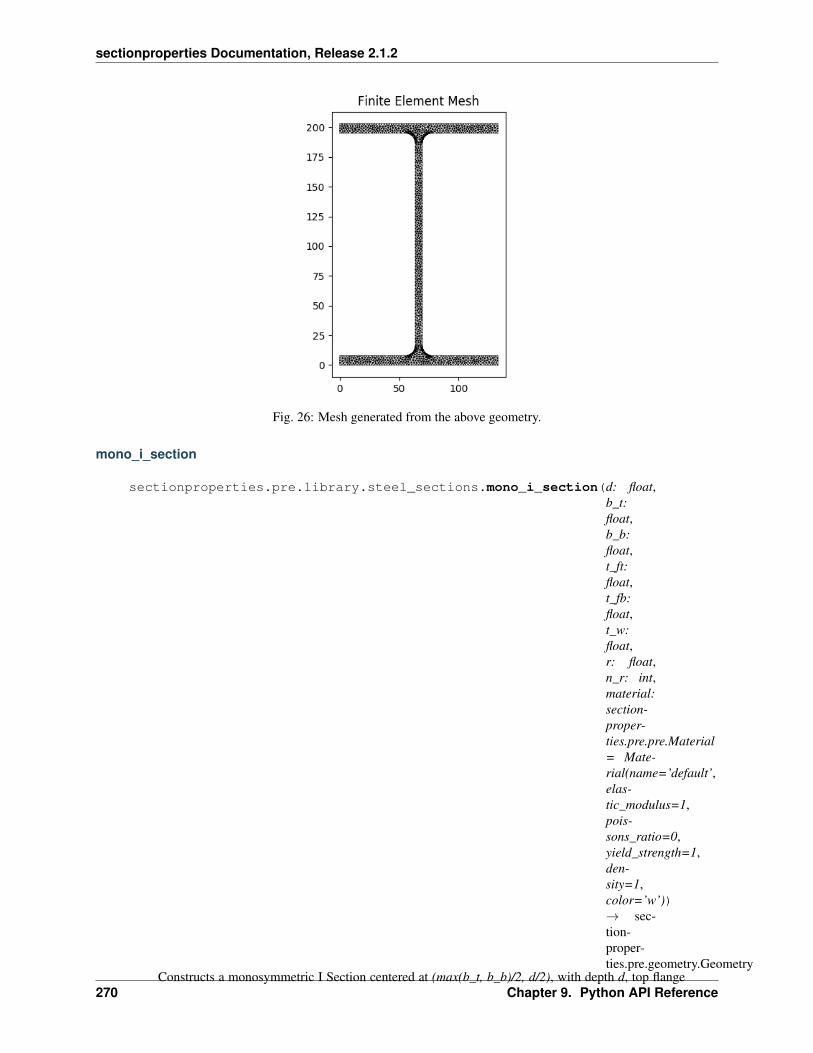
sectionproperties Documentation, Release 2.1.2
Fig. 26: Mesh generated from the above geometry.
mono_i_section
sectionproperties.pre.library.steel_sections.mono_i_section(d: float,b_t:float,b_b:float,t_ft:float,t_fb:float,t_w:float,r: float,n_r: int,material:section-proper-ties.pre.pre.Material= Mate-rial(name=’default’,elas-tic_modulus=1,pois-sons_ratio=0,yield_strength=1,den-sity=1,color=’w’))→ sec-tion-proper-ties.pre.geometry.Geometry
Constructs a monosymmetric I Section centered at (max(b_t, b_b)/2, d/2), with depth d, top flange270 Chapter 9. Python API Reference
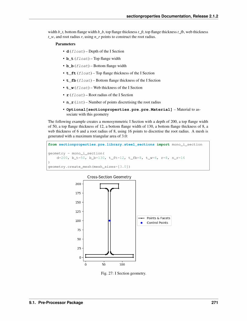
sectionproperties Documentation, Release 2.1.2
width b_t, bottom flange width b_b, top flange thickness t_ft, top flange thickness t_fb, web thicknesst_w, and root radius r, using n_r points to construct the root radius.
Parameters
• d (float) – Depth of the I Section
• b_t (float) – Top flange width
• b_b (float) – Bottom flange width
• t_ft (float) – Top flange thickness of the I Section
• t_fb (float) – Bottom flange thickness of the I Section
• t_w (float) – Web thickness of the I Section
• r (float) – Root radius of the I Section
• n_r (int) – Number of points discretising the root radius
• Optional[sectionproperties.pre.pre.Material] – Material to as-sociate with this geometry
The following example creates a monosymmetric I Section with a depth of 200, a top flange widthof 50, a top flange thickness of 12, a bottom flange width of 130, a bottom flange thickness of 8, aweb thickness of 6 and a root radius of 8, using 16 points to discretise the root radius. A mesh isgenerated with a maximum triangular area of 3.0:
from sectionproperties.pre.library.steel_sections import mono_i_section
geometry = mono_i_section(d=200, b_t=50, b_b=130, t_ft=12, t_fb=8, t_w=6, r=8, n_r=16
)geometry.create_mesh(mesh_sizes=[3.0])
Fig. 27: I Section geometry.
9.1. Pre-Processor Package 271

sectionproperties Documentation, Release 2.1.2
Fig. 28: Mesh generated from the above geometry.
272 Chapter 9. Python API Reference

sectionproperties Documentation, Release 2.1.2
tapered_flange_i_section
sectionproperties.pre.library.steel_sections.tapered_flange_i_section(d:float,b:float,t_f:float,t_w:float,r_r:float,r_f:float,al-pha:float,n_r:int,ma-te-rial:sec-tion-prop-er-ties.pre.pre.Material=Ma-te-rial(name=’default’,elas-tic_modulus=1,pois-sons_ratio=0,yield_strength=1,den-sity=1,color=’w’))→sec-tion-prop-er-ties.pre.geometry.Geometry
Constructs a Tapered Flange I Section centered at (b/2, d/2), with depth d, width b, mid-flangethickness t_f, web thickness t_w, root radius r_r, flange radius r_f and flange angle alpha, using n_rpoints to construct the radii.
Parameters
• d (float) – Depth of the Tapered Flange I Section
• b (float) – Width of the Tapered Flange I Section
• t_f (float) – Mid-flange thickness of the Tapered Flange I Section (measured at
9.1. Pre-Processor Package 273
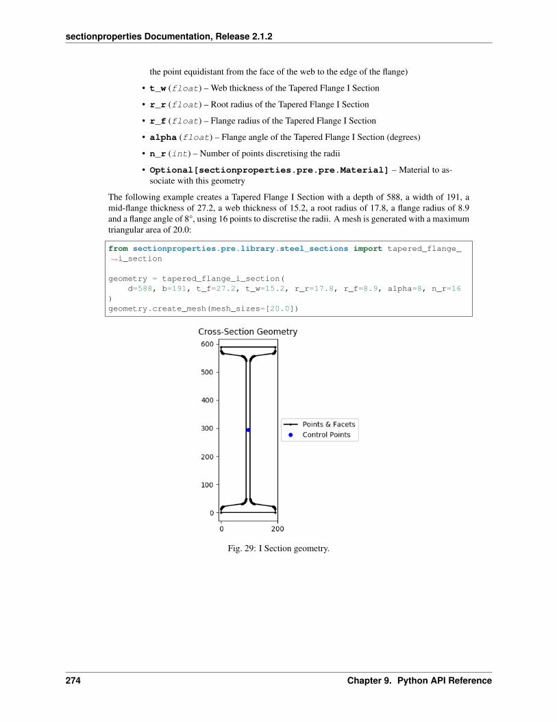
sectionproperties Documentation, Release 2.1.2
the point equidistant from the face of the web to the edge of the flange)
• t_w (float) – Web thickness of the Tapered Flange I Section
• r_r (float) – Root radius of the Tapered Flange I Section
• r_f (float) – Flange radius of the Tapered Flange I Section
• alpha (float) – Flange angle of the Tapered Flange I Section (degrees)
• n_r (int) – Number of points discretising the radii
• Optional[sectionproperties.pre.pre.Material] – Material to as-sociate with this geometry
The following example creates a Tapered Flange I Section with a depth of 588, a width of 191, amid-flange thickness of 27.2, a web thickness of 15.2, a root radius of 17.8, a flange radius of 8.9and a flange angle of 8°, using 16 points to discretise the radii. A mesh is generated with a maximumtriangular area of 20.0:
from sectionproperties.pre.library.steel_sections import tapered_flange_→˓i_section
geometry = tapered_flange_i_section(d=588, b=191, t_f=27.2, t_w=15.2, r_r=17.8, r_f=8.9, alpha=8, n_r=16
)geometry.create_mesh(mesh_sizes=[20.0])
Fig. 29: I Section geometry.
274 Chapter 9. Python API Reference
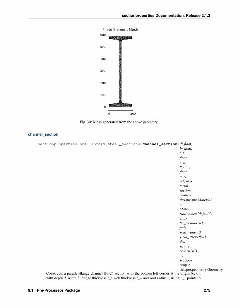
sectionproperties Documentation, Release 2.1.2
Fig. 30: Mesh generated from the above geometry.
channel_section
sectionproperties.pre.library.steel_sections.channel_section(d: float,b: float,t_f:float,t_w:float, r:float,n_r:int, ma-terial:section-proper-ties.pre.pre.Material=Mate-rial(name=’default’,elas-tic_modulus=1,pois-sons_ratio=0,yield_strength=1,den-sity=1,color=’w’))→section-proper-ties.pre.geometry.Geometry
Constructs a parallel-flange channel (PFC) section with the bottom left corner at the origin (0, 0),with depth d, width b, flange thickness t_f, web thickness t_w and root radius r, using n_r points to
9.1. Pre-Processor Package 275

sectionproperties Documentation, Release 2.1.2
construct the root radius.
Parameters
• d (float) – Depth of the PFC section
• b (float) – Width of the PFC section
• t_f (float) – Flange thickness of the PFC section
• t_w (float) – Web thickness of the PFC section
• r (float) – Root radius of the PFC section
• n_r (int) – Number of points discretising the root radius
• shift (list[float, float]) – Vector that shifts the cross-section by (x, y)
• Optional[sectionproperties.pre.pre.Material] – Material to as-sociate with this geometry
The following example creates a PFC section with a depth of 250, a width of 90, a flange thicknessof 15, a web thickness of 8 and a root radius of 12, using 8 points to discretise the root radius. Amesh is generated with a maximum triangular area of 5.0:
from sectionproperties.pre.library.steel_sections import channel_section
geometry = channel_section(d=250, b=90, t_f=15, t_w=8, r=12, n_r=8)geometry.create_mesh(mesh_sizes=[5.0])
Fig. 31: PFC geometry.
276 Chapter 9. Python API Reference

sectionproperties Documentation, Release 2.1.2
Fig. 32: Mesh generated from the above geometry.
tapered_flange_channel
sectionproperties.pre.library.steel_sections.tapered_flange_channel(d:float,b:float,t_f:float,t_w:float,r_r:float,r_f:float,al-pha:float,n_r:int,ma-te-rial:sec-tion-prop-er-ties.pre.pre.Material=Ma-te-rial(name=’default’,elas-tic_modulus=1,pois-sons_ratio=0,yield_strength=1,den-sity=1,color=’w’))→sec-tion-prop-er-ties.pre.geometry.Geometry
Constructs a Tapered Flange Channel section with the bottom left corner at the origin (0, 0), with
9.1. Pre-Processor Package 277
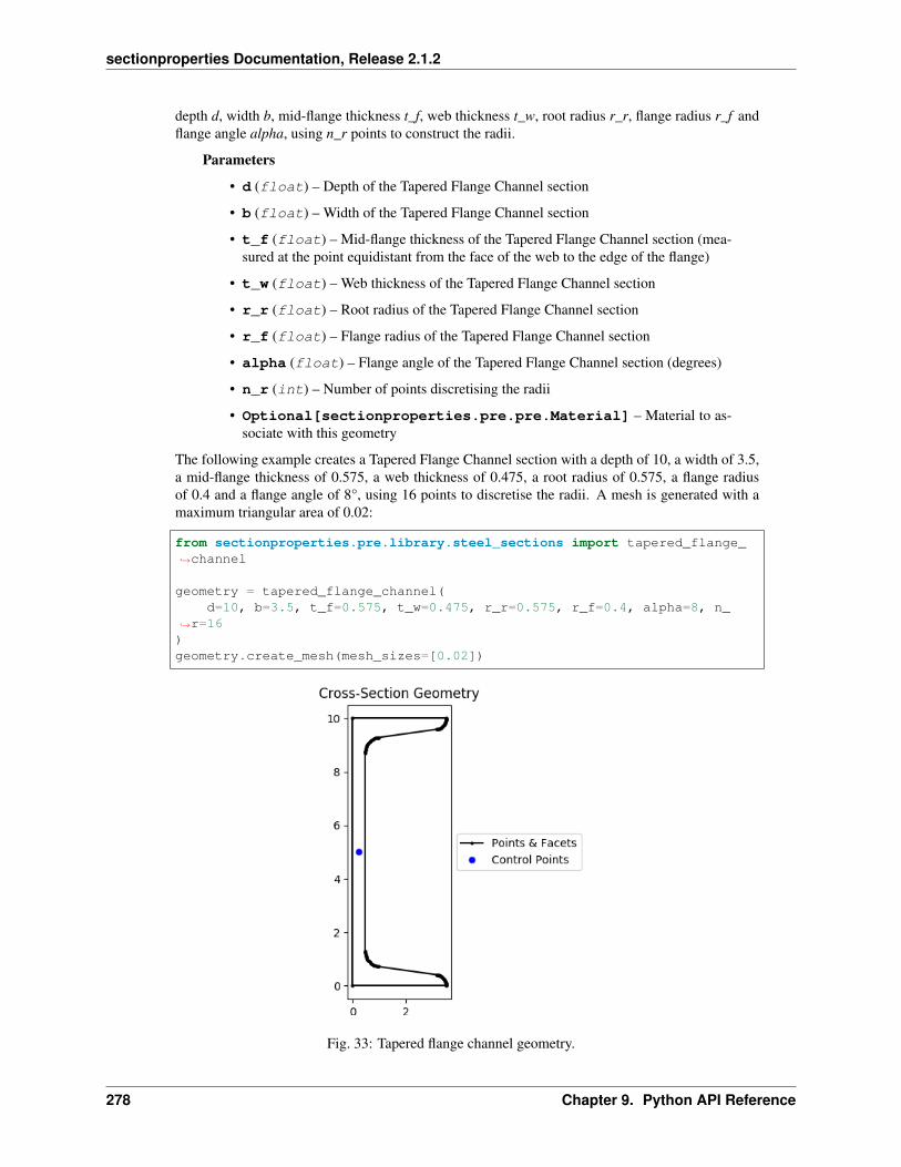
sectionproperties Documentation, Release 2.1.2
depth d, width b, mid-flange thickness t_f, web thickness t_w, root radius r_r, flange radius r_f andflange angle alpha, using n_r points to construct the radii.
Parameters
• d (float) – Depth of the Tapered Flange Channel section
• b (float) – Width of the Tapered Flange Channel section
• t_f (float) – Mid-flange thickness of the Tapered Flange Channel section (mea-sured at the point equidistant from the face of the web to the edge of the flange)
• t_w (float) – Web thickness of the Tapered Flange Channel section
• r_r (float) – Root radius of the Tapered Flange Channel section
• r_f (float) – Flange radius of the Tapered Flange Channel section
• alpha (float) – Flange angle of the Tapered Flange Channel section (degrees)
• n_r (int) – Number of points discretising the radii
• Optional[sectionproperties.pre.pre.Material] – Material to as-sociate with this geometry
The following example creates a Tapered Flange Channel section with a depth of 10, a width of 3.5,a mid-flange thickness of 0.575, a web thickness of 0.475, a root radius of 0.575, a flange radiusof 0.4 and a flange angle of 8°, using 16 points to discretise the radii. A mesh is generated with amaximum triangular area of 0.02:
from sectionproperties.pre.library.steel_sections import tapered_flange_→˓channel
geometry = tapered_flange_channel(d=10, b=3.5, t_f=0.575, t_w=0.475, r_r=0.575, r_f=0.4, alpha=8, n_
→˓r=16)geometry.create_mesh(mesh_sizes=[0.02])
Fig. 33: Tapered flange channel geometry.
278 Chapter 9. Python API Reference
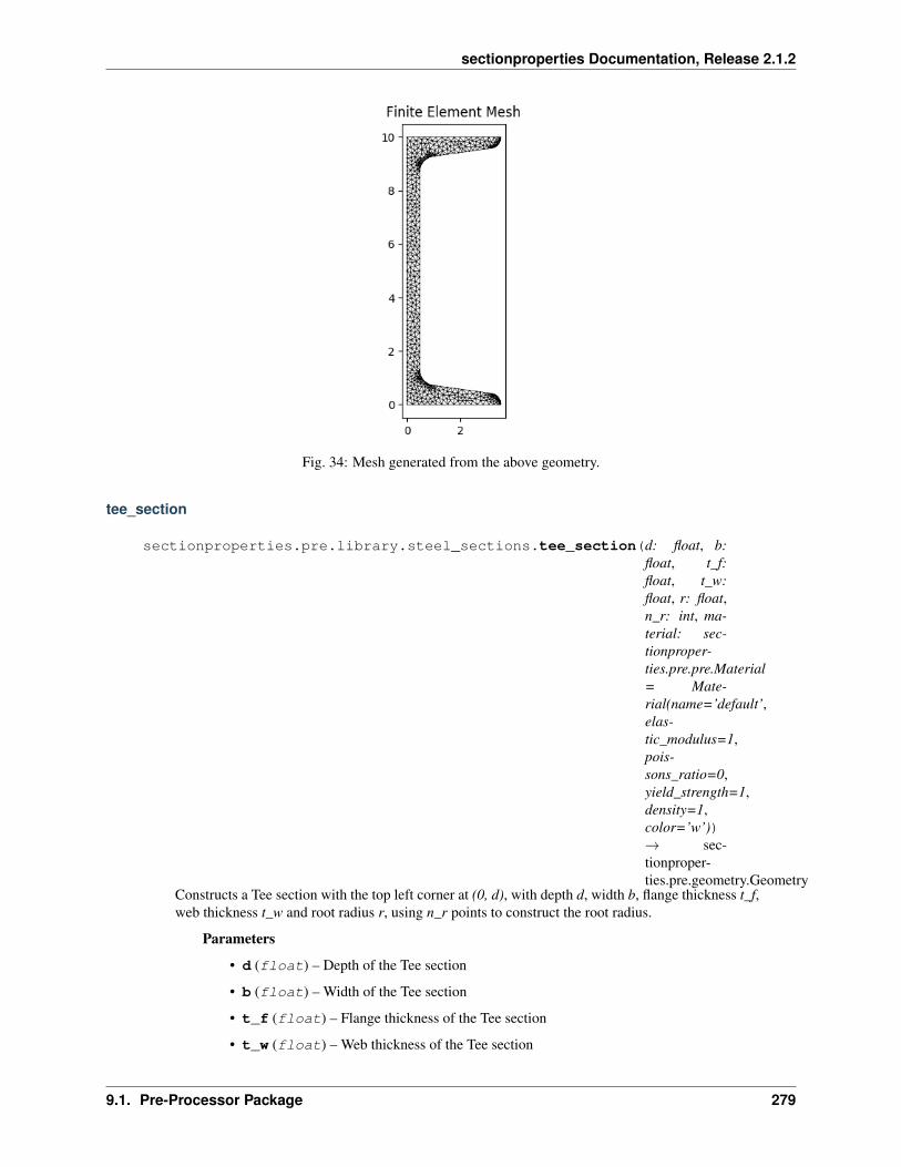
sectionproperties Documentation, Release 2.1.2
Fig. 34: Mesh generated from the above geometry.
tee_section
sectionproperties.pre.library.steel_sections.tee_section(d: float, b:float, t_f:float, t_w:float, r: float,n_r: int, ma-terial: sec-tionproper-ties.pre.pre.Material= Mate-rial(name=’default’,elas-tic_modulus=1,pois-sons_ratio=0,yield_strength=1,density=1,color=’w’))→ sec-tionproper-ties.pre.geometry.Geometry
Constructs a Tee section with the top left corner at (0, d), with depth d, width b, flange thickness t_f,web thickness t_w and root radius r, using n_r points to construct the root radius.
Parameters
• d (float) – Depth of the Tee section
• b (float) – Width of the Tee section
• t_f (float) – Flange thickness of the Tee section
• t_w (float) – Web thickness of the Tee section
9.1. Pre-Processor Package 279
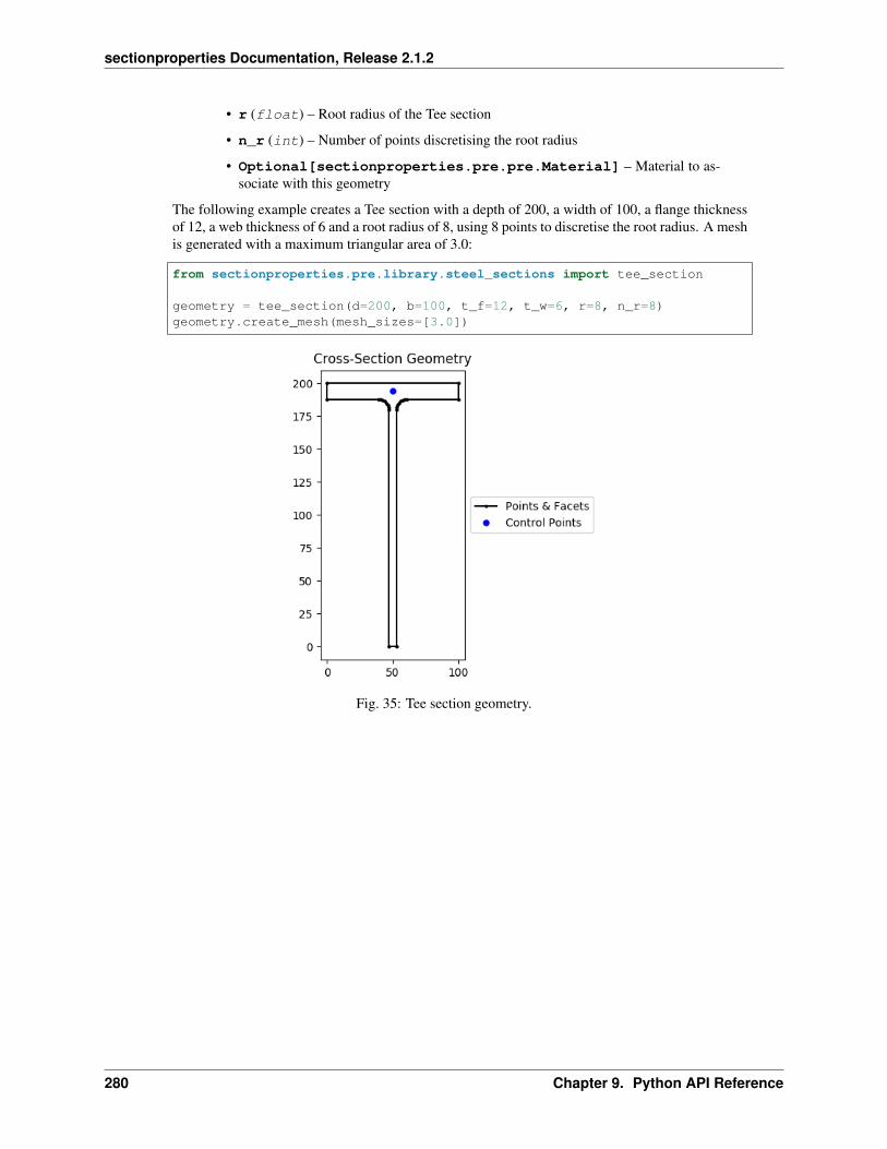
sectionproperties Documentation, Release 2.1.2
• r (float) – Root radius of the Tee section
• n_r (int) – Number of points discretising the root radius
• Optional[sectionproperties.pre.pre.Material] – Material to as-sociate with this geometry
The following example creates a Tee section with a depth of 200, a width of 100, a flange thicknessof 12, a web thickness of 6 and a root radius of 8, using 8 points to discretise the root radius. A meshis generated with a maximum triangular area of 3.0:
from sectionproperties.pre.library.steel_sections import tee_section
geometry = tee_section(d=200, b=100, t_f=12, t_w=6, r=8, n_r=8)geometry.create_mesh(mesh_sizes=[3.0])
Fig. 35: Tee section geometry.
280 Chapter 9. Python API Reference

sectionproperties Documentation, Release 2.1.2
Fig. 36: Mesh generated from the above geometry.
angle_section
sectionproperties.pre.library.steel_sections.angle_section(d: float,b: float,t: float,r_r: float,r_t: float,n_r: int,material:section-proper-ties.pre.pre.Material= Mate-rial(name=’default’,elas-tic_modulus=1,pois-sons_ratio=0,yield_strength=1,density=1,color=’w’))→ section-proper-ties.pre.geometry.Geometry
Constructs an angle section with the bottom left corner at the origin (0, 0), with depth d, width b,thickness t, root radius r_r and toe radius r_t, using n_r points to construct the radii.
Parameters
• d (float) – Depth of the angle section
• b (float) – Width of the angle section
• t (float) – Thickness of the angle section
9.1. Pre-Processor Package 281
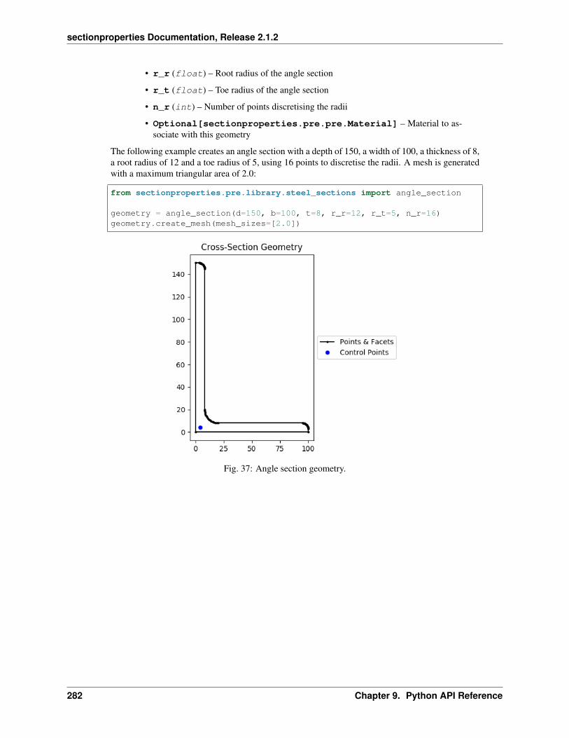
sectionproperties Documentation, Release 2.1.2
• r_r (float) – Root radius of the angle section
• r_t (float) – Toe radius of the angle section
• n_r (int) – Number of points discretising the radii
• Optional[sectionproperties.pre.pre.Material] – Material to as-sociate with this geometry
The following example creates an angle section with a depth of 150, a width of 100, a thickness of 8,a root radius of 12 and a toe radius of 5, using 16 points to discretise the radii. A mesh is generatedwith a maximum triangular area of 2.0:
from sectionproperties.pre.library.steel_sections import angle_section
geometry = angle_section(d=150, b=100, t=8, r_r=12, r_t=5, n_r=16)geometry.create_mesh(mesh_sizes=[2.0])
Fig. 37: Angle section geometry.
282 Chapter 9. Python API Reference

sectionproperties Documentation, Release 2.1.2
cee_section
sectionproperties.pre.library.steel_sections.cee_section(d: float,b: float, l:float, t: float,r_out: float,n_r: int, ma-terial: sec-tionproper-ties.pre.pre.Material= Mate-rial(name=’default’,elas-tic_modulus=1,pois-sons_ratio=0,yield_strength=1,density=1,color=’w’))→ sec-tionproper-ties.pre.geometry.Geometry
Constructs a Cee section (typical of cold-formed steel) with the bottom left corner at the origin (0,0), with depth d, width b, lip l, thickness t and outer radius r_out, using n_r points to construct theradius. If the outer radius is less than the thickness of the Cee Section, the inner radius is set to zero.
Parameters
• d (float) – Depth of the Cee section
• b (float) – Width of the Cee section
• l (float) – Lip of the Cee section
• t (float) – Thickness of the Cee section
• r_out (float) – Outer radius of the Cee section
9.1. Pre-Processor Package 283

sectionproperties Documentation, Release 2.1.2
• n_r (int) – Number of points discretising the outer radius
• Optional[sectionproperties.pre.pre.Material] – Material to as-sociate with this geometry
Raises Exception – Lip length must be greater than the outer radius
The following example creates a Cee section with a depth of 125, a width of 50, a lip of 30, athickness of 1.5 and an outer radius of 6, using 8 points to discretise the radius. A mesh is generatedwith a maximum triangular area of 0.25:
from sectionproperties.pre.library.steel_sections import cee_section
geometry = cee_section(d=125, b=50, l=30, t=1.5, r_out=6, n_r=8)geometry.create_mesh(mesh_sizes=[0.25])
Fig. 38: Cee section geometry.
284 Chapter 9. Python API Reference

sectionproperties Documentation, Release 2.1.2
zed_section
sectionproperties.pre.library.steel_sections.zed_section(d: float,b_l: float,b_r: float, l:float, t: float,r_out: float,n_r: int, ma-terial: sec-tionproper-ties.pre.pre.Material= Mate-rial(name=’default’,elas-tic_modulus=1,pois-sons_ratio=0,yield_strength=1,density=1,color=’w’))→ sec-tionproper-ties.pre.geometry.Geometry
Constructs a zed section with the bottom left corner at the origin (0, 0), with depth d, left flange widthb_l, right flange width b_r, lip l, thickness t and outer radius r_out, using n_r points to construct theradius. If the outer radius is less than the thickness of the Zed Section, the inner radius is set to zero.
Parameters
• d (float) – Depth of the zed section
• b_l (float) – Left flange width of the Zed section
• b_r (float) – Right flange width of the Zed section
• l (float) – Lip of the Zed section
9.1. Pre-Processor Package 285
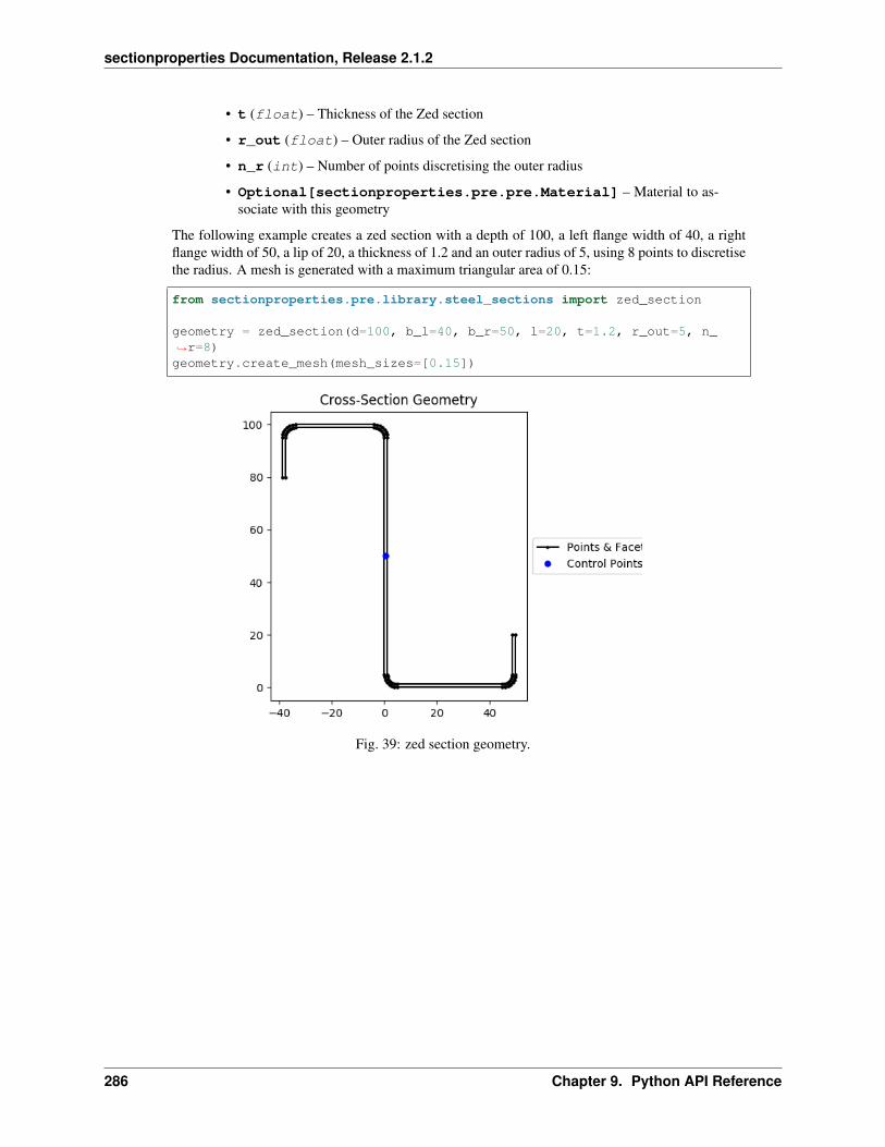
sectionproperties Documentation, Release 2.1.2
• t (float) – Thickness of the Zed section
• r_out (float) – Outer radius of the Zed section
• n_r (int) – Number of points discretising the outer radius
• Optional[sectionproperties.pre.pre.Material] – Material to as-sociate with this geometry
The following example creates a zed section with a depth of 100, a left flange width of 40, a rightflange width of 50, a lip of 20, a thickness of 1.2 and an outer radius of 5, using 8 points to discretisethe radius. A mesh is generated with a maximum triangular area of 0.15:
from sectionproperties.pre.library.steel_sections import zed_section
geometry = zed_section(d=100, b_l=40, b_r=50, l=20, t=1.2, r_out=5, n_→˓r=8)geometry.create_mesh(mesh_sizes=[0.15])
Fig. 39: zed section geometry.
286 Chapter 9. Python API Reference
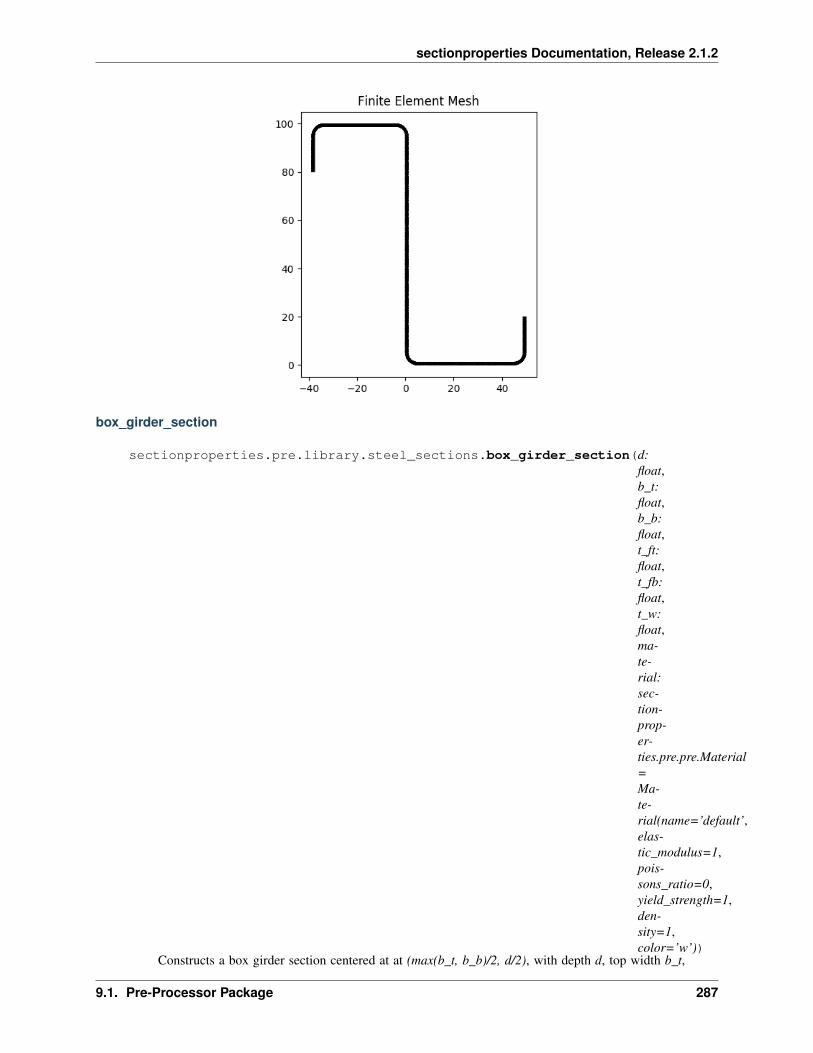
sectionproperties Documentation, Release 2.1.2
box_girder_section
sectionproperties.pre.library.steel_sections.box_girder_section(d:float,b_t:float,b_b:float,t_ft:float,t_fb:float,t_w:float,ma-te-rial:sec-tion-prop-er-ties.pre.pre.Material=Ma-te-rial(name=’default’,elas-tic_modulus=1,pois-sons_ratio=0,yield_strength=1,den-sity=1,color=’w’))
Constructs a box girder section centered at at (max(b_t, b_b)/2, d/2), with depth d, top width b_t,
9.1. Pre-Processor Package 287
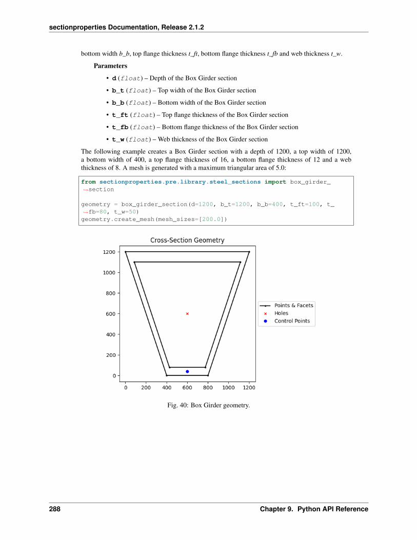
sectionproperties Documentation, Release 2.1.2
bottom width b_b, top flange thickness t_ft, bottom flange thickness t_fb and web thickness t_w.
Parameters
• d (float) – Depth of the Box Girder section
• b_t (float) – Top width of the Box Girder section
• b_b (float) – Bottom width of the Box Girder section
• t_ft (float) – Top flange thickness of the Box Girder section
• t_fb (float) – Bottom flange thickness of the Box Girder section
• t_w (float) – Web thickness of the Box Girder section
The following example creates a Box Girder section with a depth of 1200, a top width of 1200,a bottom width of 400, a top flange thickness of 16, a bottom flange thickness of 12 and a webthickness of 8. A mesh is generated with a maximum triangular area of 5.0:
from sectionproperties.pre.library.steel_sections import box_girder_→˓section
geometry = box_girder_section(d=1200, b_t=1200, b_b=400, t_ft=100, t_→˓fb=80, t_w=50)geometry.create_mesh(mesh_sizes=[200.0])
Fig. 40: Box Girder geometry.
288 Chapter 9. Python API Reference

sectionproperties Documentation, Release 2.1.2
Fig. 41: Mesh generated from the above geometry.
bulb_section
sectionproperties.pre.library.steel_sections.bulb_section(d: float,b: float,t: float,r: float,n_r: int,d_b: float =None, ma-terial: sec-tionproper-ties.pre.pre.Material= Mate-rial(name=’default’,elas-tic_modulus=1,pois-sons_ratio=0,yield_strength=1,density=1,color=’w’))→ sec-tionproper-ties.pre.geometry.Geometry
Constructs a bulb section with the bottom left corner at the point (-t / 2, 0), with depth d, bulb depthd_b, bulb width b, web thickness t and radius r, using n_r points to construct the radius.
Parameters
• d (float) – Depth of the section
• b (float) – Bulb width
9.1. Pre-Processor Package 289

sectionproperties Documentation, Release 2.1.2
• t (float) – Web thickness
• r (float) – Bulb radius
• d_b (float) – Depth of the bulb (automatically calculated for standard sections,if provided the section may have sharp edges)
• n_r (int) – Number of points discretising the radius
• Optional[sectionproperties.pre.pre.Material] – Material to as-sociate with this geometry
The following example creates a bulb section with a depth of 240, a width of 34, a web thicknessof 12 and a bulb radius of 16, using 16 points to discretise the radius. A mesh is generated with amaximum triangular area of 5.0:
from sectionproperties.pre.library.steel_sections import bulb_section
geometry = bulb_section(d=240, b=34, t=12, r=10, n_r=16)geometry.create_mesh(mesh_sizes=[5.0])
Fig. 42: Bulb section geometry.
9.1.7 concrete_sections Module
290 Chapter 9. Python API Reference
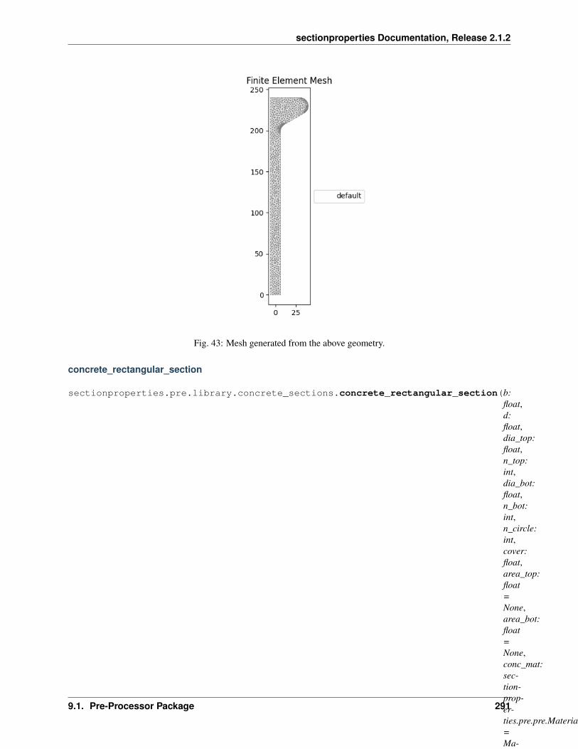
sectionproperties Documentation, Release 2.1.2
Fig. 43: Mesh generated from the above geometry.
concrete_rectangular_section
sectionproperties.pre.library.concrete_sections.concrete_rectangular_section(b:float,d:float,dia_top:float,n_top:int,dia_bot:float,n_bot:int,n_circle:int,cover:float,area_top:float=None,area_bot:float=None,conc_mat:sec-tion-prop-er-ties.pre.pre.Material=Ma-te-rial(name=’default’,elas-tic_modulus=1,pois-sons_ratio=0,yield_strength=1,den-sity=1,color=’w’),steel_mat:sec-tion-prop-er-ties.pre.pre.Material=Ma-te-rial(name=’default’,elas-tic_modulus=1,pois-sons_ratio=0,yield_strength=1,den-sity=1,color=’w’))→sec-tion-prop-er-ties.pre.geometry.CompoundGeometry
Constructs a concrete rectangular section of width b and depth d, with n_top top steel bars of diameter dia_top,
9.1. Pre-Processor Package 291

sectionproperties Documentation, Release 2.1.2
n_bot bottom steel bars of diameter dia_bot, discretised with n_circle points with equal side and top/bottomcover to the steel.
Parameters
• b (float) – Concrete section width
• d (float) – Concrete section depth
• dia_top (float) – Diameter of the top steel reinforcing bars
• n_top (int) – Number of top steel reinforcing bars
• dia_bot (float) – Diameter of the bottom steel reinforcing bars
• n_bot (int) – Number of bottom steel reinforcing bars
• n_circle (int) – Number of points discretising the steel reinforcing bars
• cover (float) – Side and bottom cover to the steel reinforcing bars
• area_top (float) – If provided, constructs top reinforcing bars based on their area ratherthan diameter (prevents the underestimation of steel area due to circle discretisation)
• area_bot (float) – If provided, constructs bottom reinforcing bars based on their arearather than diameter (prevents the underestimation of steel area due to circle discretisation)
• conc_mat (Optional[sectionproperties.pre.pre.Material]) – Materialto associate with the concrete
• steel_mat (Optional[sectionproperties.pre.pre.Material]) – Mate-rial to associate with the steel
Raises ValueErorr – If the number of bars is not greater than or equal to 2 in an active layer
The following example creates a 600D x 300W concrete beam with 3N20 bottom steel reinforcing bars and 30mm cover:
from sectionproperties.pre.library.concrete_sections import concrete_rectangular_→˓sectionfrom sectionproperties.pre.pre import Material
concrete = Material(name='Concrete', elastic_modulus=30.1e3, poissons_ratio=0.2, yield_
→˓strength=32,density=2.4e-6, color='lightgrey'
)steel = Material(
name='Steel', elastic_modulus=200e3, poissons_ratio=0.3, yield_strength=500,density=7.85e-6, color='grey'
)
geometry = concrete_rectangular_section(b=300, d=600, dia_top=20, n_top=0, dia_bot=20, n_bot=3, n_circle=24, cover=30,conc_mat=concrete, steel_mat=steel
)geometry.create_mesh(mesh_sizes=[500])
292 Chapter 9. Python API Reference

sectionproperties Documentation, Release 2.1.2
Fig. 44: Concrete rectangular section geometry.
Fig. 45: Mesh generated from the above geometry.
9.1. Pre-Processor Package 293
sectionproperties Documentation, Release 2.1.2
concrete_tee_section
sectionproperties.pre.library.concrete_sections.concrete_tee_section(b:float,d:float,b_f:float,d_f:float,dia_top:float,n_top:int,dia_bot:float,n_bot:int,n_circle:int,cover:float,area_top:float =None,area_bot:float =None,conc_mat:sec-tion-proper-ties.pre.pre.Material=Mate-rial(name=’default’,elas-tic_modulus=1,pois-sons_ratio=0,yield_strength=1,den-sity=1,color=’w’),steel_mat:sec-tion-proper-ties.pre.pre.Material=Mate-rial(name=’default’,elas-tic_modulus=1,pois-sons_ratio=0,yield_strength=1,den-sity=1,color=’w’))→ sec-tion-proper-ties.pre.geometry.CompoundGeometry
Constructs a concrete tee section of width b, depth d, flange width b_f and flange depth d_f, with n_top top
294 Chapter 9. Python API Reference
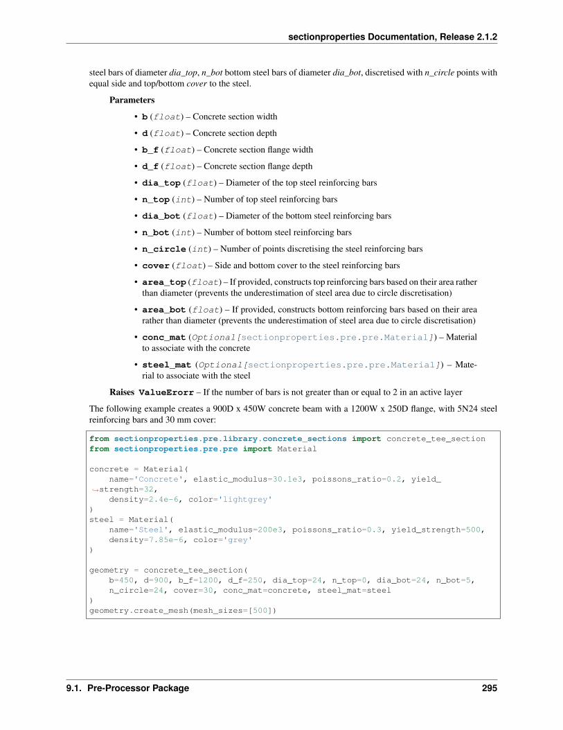
sectionproperties Documentation, Release 2.1.2
steel bars of diameter dia_top, n_bot bottom steel bars of diameter dia_bot, discretised with n_circle points withequal side and top/bottom cover to the steel.
Parameters
• b (float) – Concrete section width
• d (float) – Concrete section depth
• b_f (float) – Concrete section flange width
• d_f (float) – Concrete section flange depth
• dia_top (float) – Diameter of the top steel reinforcing bars
• n_top (int) – Number of top steel reinforcing bars
• dia_bot (float) – Diameter of the bottom steel reinforcing bars
• n_bot (int) – Number of bottom steel reinforcing bars
• n_circle (int) – Number of points discretising the steel reinforcing bars
• cover (float) – Side and bottom cover to the steel reinforcing bars
• area_top (float) – If provided, constructs top reinforcing bars based on their area ratherthan diameter (prevents the underestimation of steel area due to circle discretisation)
• area_bot (float) – If provided, constructs bottom reinforcing bars based on their arearather than diameter (prevents the underestimation of steel area due to circle discretisation)
• conc_mat (Optional[sectionproperties.pre.pre.Material]) – Materialto associate with the concrete
• steel_mat (Optional[sectionproperties.pre.pre.Material]) – Mate-rial to associate with the steel
Raises ValueErorr – If the number of bars is not greater than or equal to 2 in an active layer
The following example creates a 900D x 450W concrete beam with a 1200W x 250D flange, with 5N24 steelreinforcing bars and 30 mm cover:
from sectionproperties.pre.library.concrete_sections import concrete_tee_sectionfrom sectionproperties.pre.pre import Material
concrete = Material(name='Concrete', elastic_modulus=30.1e3, poissons_ratio=0.2, yield_
→˓strength=32,density=2.4e-6, color='lightgrey'
)steel = Material(
name='Steel', elastic_modulus=200e3, poissons_ratio=0.3, yield_strength=500,density=7.85e-6, color='grey'
)
geometry = concrete_tee_section(b=450, d=900, b_f=1200, d_f=250, dia_top=24, n_top=0, dia_bot=24, n_bot=5,n_circle=24, cover=30, conc_mat=concrete, steel_mat=steel
)geometry.create_mesh(mesh_sizes=[500])
9.1. Pre-Processor Package 295
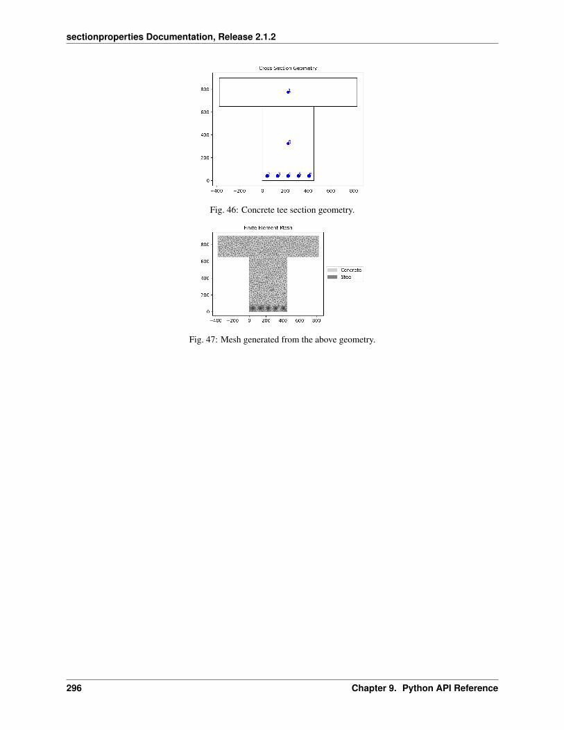
sectionproperties Documentation, Release 2.1.2
Fig. 46: Concrete tee section geometry.
Fig. 47: Mesh generated from the above geometry.
296 Chapter 9. Python API Reference
sectionproperties Documentation, Release 2.1.2
concrete_circular_section
sectionproperties.pre.library.concrete_sections.concrete_circular_section(d:float,n:int,dia:float,n_bar:int,n_circle:int,cover:float,area_conc:float=None,area_bar:float=None,conc_mat:sec-tion-prop-er-ties.pre.pre.Material=Ma-te-rial(name=’default’,elas-tic_modulus=1,pois-sons_ratio=0,yield_strength=1,den-sity=1,color=’w’),steel_mat:sec-tion-prop-er-ties.pre.pre.Material=Ma-te-rial(name=’default’,elas-tic_modulus=1,pois-sons_ratio=0,yield_strength=1,den-sity=1,color=’w’))→sec-tion-prop-er-ties.pre.geometry.CompoundGeometry
Constructs a concrete circular section of diameter d discretised with n points, with n_bar steel bars of diameter
9.1. Pre-Processor Package 297
sectionproperties Documentation, Release 2.1.2
dia, discretised with n_circle points with equal side and bottom cover to the steel.
Parameters
• d (float) – Concrete diameter
• n (float) – Number of points discretising the concrete section
• dia (float) – Diameter of the steel reinforcing bars
• n_bar (int) – Number of steel reinforcing bars
• n_circle (int) – Number of points discretising the steel reinforcing bars
• cover (float) – Side and bottom cover to the steel reinforcing bars
• area_conc (float) – If provided, constructs the concrete based on its area rather thandiameter (prevents the underestimation of concrete area due to circle discretisation)
• area_bar (float) – If provided, constructs reinforcing bars based on their area ratherthan diameter (prevents the underestimation of steel area due to
• conc_mat (Optional[sectionproperties.pre.pre.Material]) – Materialto associate with the concrete
• steel_mat (Optional[sectionproperties.pre.pre.Material]) – Mate-rial to associate with the steel
Raises ValueErorr – If the number of bars is not greater than or equal to 2
The following example creates a 450DIA concrete column with with 6N20 steel reinforcing bars and 45 mmcover:
from sectionproperties.pre.library.concrete_sections import concrete_circular_→˓sectionfrom sectionproperties.pre.pre import Material
concrete = Material(name='Concrete', elastic_modulus=30.1e3, poissons_ratio=0.2, yield_
→˓strength=32,density=2.4e-6, color='lightgrey'
)steel = Material(
name='Steel', elastic_modulus=200e3, poissons_ratio=0.3, yield_strength=500,density=7.85e-6, color='grey'
)
geometry = concrete_circular_section(d=450, n=64, dia=20, n_bar=6, n_circle=24, cover=45, conc_mat=concrete, steel_
→˓mat=steel)geometry.create_mesh(mesh_sizes=[500])
9.1.8 bridge_sections Module
298 Chapter 9. Python API Reference

sectionproperties Documentation, Release 2.1.2
Fig. 48: Concrete circular section geometry.
Fig. 49: Mesh generated from the above geometry.
9.1. Pre-Processor Package 299
sectionproperties Documentation, Release 2.1.2
super_t_girder_section
sectionproperties.pre.library.bridge_sections.super_t_girder_section(girder_type:int,girder_subtype:int =2, w:float =2100,t_w:float =None,t_f:float =75, ma-terial:sec-tion-proper-ties.pre.pre.Material=Mate-rial(name=’default’,elas-tic_modulus=1,pois-sons_ratio=0,yield_strength=1,den-sity=1,color=’w’))→ sec-tion-proper-ties.pre.geometry.Geometry
Constructs a Super T Girder section to AS5100.5.
Parameters
• girder_type (int) – Type of Super T (1 to 5)
• girder_subtype (int) – Era Super T (1: pre-2001, 2:contemporary)
• w (float) – Overall width of top flange
• t_w (float) – Web thickness of the Super-T section (defaults to those of AS5100.5 TbD3(B))
• t_f (float) – Thickness of top flange (VIC (default) = 75 mm; NSW = 90 mm)
• Optional[sectionproperties.pre.pre.Material] – Material to associatewith this geometry
The following example creates a T5 Super-T section with a 180 mm overlay slab and assigns the differentmaterial properties:
import sectionproperties.pre.library.bridge_sections as bridge_sectionsimport sectionproperties.pre.library.primitive_sections as primitive_sections
(continues on next page)
300 Chapter 9. Python API Reference

sectionproperties Documentation, Release 2.1.2
(continued from previous page)
from sectionproperties.pre.pre import Materialfrom sectionproperties.analysis.section import Section
Dslab, w, t_f = 180, 2100, 75
precast = Material(name="65 MPa",elastic_modulus=37.4e3,poissons_ratio=0.2,yield_strength=65,density=2.4e-6,color="grey",
)insitu = Material(
name="40 MPa",elastic_modulus=32.8e3,poissons_ratio=0.2,yield_strength=40,density=2.4e-6,color="lightgrey",
)
super_t = bridge_sections.super_t_girder_section(girder_type=5, w=w,→˓material=precast)slab = primitive_sections.rectangular_section(
d=Dslab, b=w, material=insitu).shift_section(-w / 2, t_f)
geom = super_t + slabgeom.plot_geometry()geom.create_mesh(mesh_sizes=[500])
sec = Section(geom)sec.plot_mesh()
sec.calculate_geometric_properties()sec.calculate_warping_properties()sec.display_results(fmt=".3f")
Note that the properties are reported as modulus weighted properties (e.g. E.A) and can be normalized tothe reference material by dividing by that elastic modulus:
A_65 = section.get_ea() / precast.elastic_modulus
The reported section centroids are already weighted.
9.1. Pre-Processor Package 301

sectionproperties Documentation, Release 2.1.2
Fig. 50: Super Tee Girder.
i_girder_section
sectionproperties.pre.library.bridge_sections.i_girder_section(girder_type:int, material:sectionproper-ties.pre.pre.Material= Mate-rial(name=’default’,elas-tic_modulus=1,pois-sons_ratio=0,yield_strength=1,density=1,color=’w’)) →sectionproper-ties.pre.geometry.Geometry
Constructs a precast I girder section to AS5100.5.
Parameters
• girder_type (int) – Type of I Girder (1 to 4)
• Optional[sectionproperties.pre.pre.Material] – Material to associatewith this geometry
As an example, replicate the table shown in AS5100.5 Fig. D1(A):
import pandas as pdimport sectionproperties.pre.library.bridge_sections as bridge_sectionsfrom sectionproperties.analysis.section import Section
df = pd.DataFrame(columns=["Ag", "Zt", "Zb", "I", "dy", "th"])
for i in range(4):geom = bridge_sections.i_girder_section(girder_type=i + 1)dims = bridge_sections.get_i_girder_dims(girder_type=i + 1)d = sum(dims[-5:])geom.create_mesh(mesh_sizes=[200])geom.plot_geometry()
(continues on next page)
302 Chapter 9. Python API Reference

sectionproperties Documentation, Release 2.1.2
(continued from previous page)
sec = Section(geom)sec.plot_mesh()sec.calculate_geometric_properties()sec.calculate_warping_properties()
A = sec.get_area()th = A / (sec.get_perimeter() / 2)
df.loc[i] = [A,
*(sec.get_z()[:2]),sec.get_ic()[0],d + sec.get_c()[1],th,
]
print(df)
Note that the section depth is obtained by summing the heights from the section dictionary inget_i_girder_dims().
Fig. 51: I Girder.
get_super_t_girder_dims
sectionproperties.pre.library.bridge_sections.get_super_t_girder_dims(girder_type)Returns a dictionary of Super-T dimensions, refer to AS5100.5, Appendix D
Parameters girder_type (int) – Type of Super T (1 to 5)
get_i_girder_dims
sectionproperties.pre.library.bridge_sections.get_i_girder_dims(girder_type)Returns a dictionary of I girder dimensions, refer to AS5100.5, Appendix D
Parameters girder_type (int) – Type of I Girder (1 to 4)
9.1. Pre-Processor Package 303

sectionproperties Documentation, Release 2.1.2
9.1.9 nastran_sections Module
This module contains sections as defined by Nastran and Nastran-based programs, such as MYSTRAN and ASTROS.
nastran_bar
sectionproperties.pre.library.nastran_sections.nastran_bar(DIM1: float, DIM2:float, material:sectionproper-ties.pre.pre.Material= Mate-rial(name=’default’,elastic_modulus=1,poissons_ratio=0,yield_strength=1,density=1,color=’w’)) →sectionproper-ties.pre.geometry.Geometry
Constructs a BAR section with the center at the origin (0, 0), with two parameters defining dimensions. SeeNastran documentation12345 for definition of parameters. Added by JohnDN90.
Parameters
• DIM1 (float) – Width (x) of bar
• DIM2 (float) – Depth (y) of bar
• Optional[sectionproperties.pre.pre.Material] – Material to associatewith this geometry
The following example creates a BAR cross-section with a depth of 1.5 and width of 2.0, and generates a meshwith a maximum triangular area of 0.001:
from sectionproperties.pre.library.nastran_sections import nastran_bar
geom = nastran_bar(DIM1=2.0, DIM2=1.5)mesh = geometry.create_mesh(mesh_sizes=[0.001])
1 MSC Nastran Quick Reference Guide 2012, PBEAML - Simple Beam Cross-Section Property, pp. 2890-2894 https://simcompanion.mscsoftware.com/infocenter/index?page=content&id=DOC10351
2 Siemens NX Nastran 12 Quick Reference Guide, PBEAML, pp. 16-59 - 16-62 https://docs.plm.automation.siemens.com/data_services/resources/nxnastran/12/help/tdoc/en_US/pdf/QRG.pdf
3 AutoDesk Nastran Online Documentation, Nastran Reference Guide, Section 4 - Bulk Data, PBEAML http://help.autodesk.com/view/NSTRN/2018/ENU/?guid=GUID-B7044BA7-3C26-49DA-9EE7-DA7505FD4B2C
4 Users Reference Manual for the MYSTRAN General Purpose Finite Element Structural Analysis Computer Program, Jan. 2019, Section6.4.1.53 - PBARL, pp. 154-156 https://www.mystran.com/Executable/MYSTRAN-Users-Manual.pdf
5 Astros Enhancements - Volume III - Astros Theoretical Manual, Section 5.1.3.2, pp. 56 https://apps.dtic.mil/dtic/tr/fulltext/u2/a308134.pdf
304 Chapter 9. Python API Reference
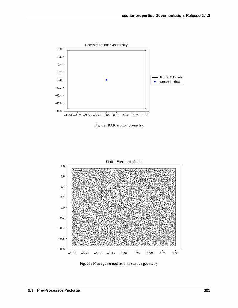
sectionproperties Documentation, Release 2.1.2
Fig. 52: BAR section geometry.
Fig. 53: Mesh generated from the above geometry.
9.1. Pre-Processor Package 305

sectionproperties Documentation, Release 2.1.2
nastran_box
sectionproperties.pre.library.nastran_sections.nastran_box(DIM1: float, DIM2:float, DIM3: float,DIM4: float, mate-rial: sectionproper-ties.pre.pre.Material= Mate-rial(name=’default’,elastic_modulus=1,poissons_ratio=0,yield_strength=1,density=1,color=’w’)) →sectionproper-ties.pre.geometry.Geometry
Constructs a BOX section with the center at the origin (0, 0), with four parameters defining dimensions. SeeNastran documentation12345 for definition of parameters. Added by JohnDN90.
Parameters
• DIM1 (float) – Width (x) of box
• DIM2 (float) – Depth (y) of box
• DIM3 (float) – Thickness of box in y direction
• DIM4 (float) – Thickness of box in x direction
• Optional[sectionproperties.pre.pre.Material] – Material to associatewith this geometry
The following example creates a BOX cross-section with a depth of 3.0 and width of 4.0, and generates a meshwith a maximum triangular area of 0.001:
from sectionproperties.pre.library.nastran_sections import nastran_box
geom = nastran_box(DIM1=4.0, DIM2=3.0, DIM3=0.375, DIM4=0.5)mesh = geometry.create_mesh(mesh_sizes=[0.001])
306 Chapter 9. Python API Reference

sectionproperties Documentation, Release 2.1.2
Fig. 54: BOX section geometry.
Fig. 55: Mesh generated from the above geometry.
9.1. Pre-Processor Package 307
sectionproperties Documentation, Release 2.1.2
nastran_box1
sectionproperties.pre.library.nastran_sections.nastran_box1(DIM1: float, DIM2:float, DIM3: float,DIM4: float, DIM5:float, DIM6:float, material:sectionproper-ties.pre.pre.Material= Mate-rial(name=’default’,elastic_modulus=1,poissons_ratio=0,yield_strength=1,density=1,color=’w’)) →sectionproper-ties.pre.geometry.Geometry
Constructs a BOX1 section with the center at the origin (0, 0), with six parameters defining dimensions. SeeNastran documentation1234 for more details. Added by JohnDN90.
Parameters
• DIM1 (float) – Width (x) of box
• DIM2 (float) – Depth (y) of box
• DIM3 (float) – Thickness of top wall
• DIM4 (float) – Thickness of bottom wall
• DIM5 (float) – Thickness of left wall
• DIM6 (float) – Thickness of right wall
• Optional[sectionproperties.pre.pre.Material] – Material to associatewith this geometry
The following example creates a BOX1 cross-section with a depth of 3.0 and width of 4.0, and generates a meshwith a maximum triangular area of 0.007:
from sectionproperties.pre.library.nastran_sections import nastran_box1
geom = nastran_box1(DIM1=4.0, DIM2=3.0, DIM3=0.375, DIM4=0.5, DIM5=0.25, DIM6=0.75
)mesh = geometry.create_mesh(mesh_sizes=[0.007])
308 Chapter 9. Python API Reference

sectionproperties Documentation, Release 2.1.2
Fig. 56: BOX1 section geometry.
Fig. 57: Mesh generated from the above geometry.
9.1. Pre-Processor Package 309

sectionproperties Documentation, Release 2.1.2
nastran_chan
sectionproperties.pre.library.nastran_sections.nastran_chan(DIM1: float, DIM2:float, DIM3: float,DIM4: float, mate-rial: sectionproper-ties.pre.pre.Material= Mate-rial(name=’default’,elastic_modulus=1,poissons_ratio=0,yield_strength=1,density=1,color=’w’)) →sectionproper-ties.pre.geometry.Geometry
Constructs a CHAN (C-Channel) section with the web’s middle center at the origin (0, 0), with four parametersdefining dimensions. See Nastran documentation1234 for more details. Added by JohnDN90.
Parameters
• DIM1 (float) – Width (x) of the CHAN-section
• DIM2 (float) – Depth (y) of the CHAN-section
• DIM3 (float) – Thickness of web (vertical portion)
• DIM4 (float) – Thickness of flanges (top/bottom portion)
• Optional[sectionproperties.pre.pre.Material] – Material to associatewith this geometry
The following example creates a CHAN cross-section with a depth of 4.0 and width of 2.0, and generates amesh with a maximum triangular area of 0.008:
from sectionproperties.pre.library.nastran_sections import nastran_chan
geom = nastran_chan(DIM1=2.0, DIM2=4.0, DIM3=0.25, DIM4=0.5)mesh = geometry.create_mesh(mesh_sizes=[0.008])
310 Chapter 9. Python API Reference

sectionproperties Documentation, Release 2.1.2
Fig. 58: CHAN section geometry.
Fig. 59: Mesh generated from the above geometry.
9.1. Pre-Processor Package 311

sectionproperties Documentation, Release 2.1.2
nastran_chan1
sectionproperties.pre.library.nastran_sections.nastran_chan1(DIM1: float,DIM2: float,DIM3: float,DIM4: float,material: sec-tionproper-ties.pre.pre.Material= Mate-rial(name=’default’,elas-tic_modulus=1,poissons_ratio=0,yield_strength=1,density=1,color=’w’))→ sectionproper-ties.pre.geometry.Geometry
Constructs a CHAN1 (C-Channel) section with the web’s middle center at the origin (0, 0), with four parametersdefining dimensions. See Nastran documentation1234 for more details. Added by JohnDN90.
Parameters
• DIM1 (float) – Width (x) of channels
• DIM2 (float) – Thickness (x) of web
• DIM3 (float) – Spacing between channels (length of web)
• DIM4 (float) – Depth (y) of CHAN1-section
• Optional[sectionproperties.pre.pre.Material] – Material to associatewith this geometry
The following example creates a CHAN1 cross-section with a depth of 4.0 and width of 1.75, and generates amesh with a maximum triangular area of 0.01:
from sectionproperties.pre.library.nastran_sections import nastran_chan1
geom = nastran_chan1(DIM1=0.75, DIM2=1.0, DIM3=3.5, DIM4=4.0)mesh = geometry.create_mesh(mesh_sizes=[0.01])
312 Chapter 9. Python API Reference

sectionproperties Documentation, Release 2.1.2
Fig. 60: CHAN1 section geometry.
Fig. 61: Mesh generated from the above geometry.
9.1. Pre-Processor Package 313

sectionproperties Documentation, Release 2.1.2
nastran_chan2
sectionproperties.pre.library.nastran_sections.nastran_chan2(DIM1: float,DIM2: float,DIM3: float,DIM4: float,material: sec-tionproper-ties.pre.pre.Material= Mate-rial(name=’default’,elas-tic_modulus=1,poissons_ratio=0,yield_strength=1,density=1,color=’w’))→ sectionproper-ties.pre.geometry.Geometry
Constructs a CHAN2 (C-Channel) section with the bottom web’s middle center at the origin (0, 0), with fourparameters defining dimensions. See Nastran documentation1234 for more details. Added by JohnDN90.
Parameters
• DIM1 (float) – Thickness of channels
• DIM2 (float) – Thickness of web
• DIM3 (float) – Depth (y) of CHAN2-section
• DIM4 (float) – Width (x) of CHAN2-section
• Optional[sectionproperties.pre.pre.Material] – Material to associatewith this geometry
The following example creates a CHAN2 cross-section with a depth of 2.0 and width of 4.0, and generates amesh with a maximum triangular area of 0.01:
from sectionproperties.pre.library.nastran_sections import nastran_chan2
geom = nastran_chan2(DIM1=0.375, DIM2=0.5, DIM3=2.0, DIM4=4.0)mesh = geometry.create_mesh(mesh_sizes=[0.01])
Fig. 62: CHAN2 section geometry.
314 Chapter 9. Python API Reference
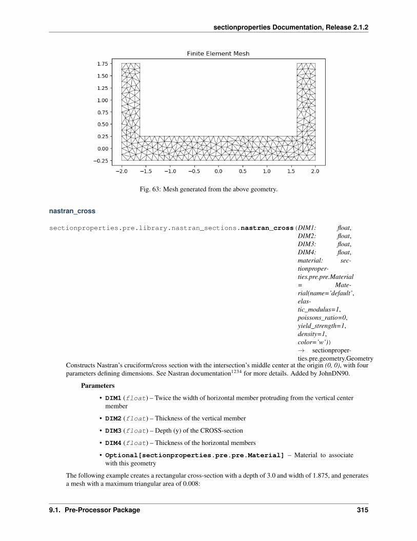
sectionproperties Documentation, Release 2.1.2
Fig. 63: Mesh generated from the above geometry.
nastran_cross
sectionproperties.pre.library.nastran_sections.nastran_cross(DIM1: float,DIM2: float,DIM3: float,DIM4: float,material: sec-tionproper-ties.pre.pre.Material= Mate-rial(name=’default’,elas-tic_modulus=1,poissons_ratio=0,yield_strength=1,density=1,color=’w’))→ sectionproper-ties.pre.geometry.Geometry
Constructs Nastran’s cruciform/cross section with the intersection’s middle center at the origin (0, 0), with fourparameters defining dimensions. See Nastran documentation1234 for more details. Added by JohnDN90.
Parameters
• DIM1 (float) – Twice the width of horizontal member protruding from the vertical centermember
• DIM2 (float) – Thickness of the vertical member
• DIM3 (float) – Depth (y) of the CROSS-section
• DIM4 (float) – Thickness of the horizontal members
• Optional[sectionproperties.pre.pre.Material] – Material to associatewith this geometry
The following example creates a rectangular cross-section with a depth of 3.0 and width of 1.875, and generatesa mesh with a maximum triangular area of 0.008:
9.1. Pre-Processor Package 315

sectionproperties Documentation, Release 2.1.2
from sectionproperties.pre.library.nastran_sections import nastran_cross
geom = nastran_cross(DIM1=1.5, DIM2=0.375, DIM3=3.0, DIM4=0.25)mesh = geometry.create_mesh(mesh_sizes=[0.008])
Fig. 64: Cruciform/cross section geometry.
nastran_dbox
sectionproperties.pre.library.nastran_sections.nastran_dbox(DIM1: float, DIM2:float, DIM3: float,DIM4: float, DIM5:float, DIM6: float,DIM7: float, DIM8:float, DIM9: float,DIM10: float, mate-rial: sectionproper-ties.pre.pre.Material= Mate-rial(name=’default’,elastic_modulus=1,poissons_ratio=0,yield_strength=1,density=1,color=’w’)) →sectionproper-ties.pre.geometry.Geometry
Constructs a DBOX section with the center at the origin (0, 0), with ten parameters defining dimensions. SeeMSC Nastran documentation1 for more details. Added by JohnDN90.
Parameters
316 Chapter 9. Python API Reference

sectionproperties Documentation, Release 2.1.2
Fig. 65: Mesh generated from the above geometry.
• DIM1 (float) – Width (x) of the DBOX-section
• DIM2 (float) – Depth (y) of the DBOX-section
• DIM3 (float) – Width (x) of left-side box
• DIM4 (float) – Thickness of left wall
• DIM5 (float) – Thickness of center wall
• DIM6 (float) – Thickness of right wall
• DIM7 (float) – Thickness of top left wall
• DIM8 (float) – Thickness of bottom left wall
• DIM9 (float) – Thickness of top right wall
• DIM10 (float) – Thickness of bottom right wall
• Optional[sectionproperties.pre.pre.Material] – Material to associatewith this geometry
The following example creates a DBOX cross-section with a depth of 3.0 and width of 8.0, and generates a meshwith a maximum triangular area of 0.01:
from sectionproperties.pre.library.nastran_sections import nastran_dbox
geom = nastran_dbox(DIM1=8.0, DIM2=3.0, DIM3=3.0, DIM4=0.5, DIM5=0.625, DIM6=0.75, DIM7=0.375,
→˓DIM8=0.25,DIM9=0.5, DIM10=0.375
)mesh = geometry.create_mesh(mesh_sizes=[0.01])
9.1. Pre-Processor Package 317

sectionproperties Documentation, Release 2.1.2
Fig. 66: DBOX section geometry.
Fig. 67: Mesh generated from the above geometry.
nastran_fcross
sectionproperties.pre.library.nastran_sections.nastran_fcross(DIM1: float,DIM2: float,DIM3: float,DIM4: float,DIM5: float,DIM6: float,DIM7: float,DIM8: float,material: sec-tionproper-ties.pre.pre.Material= Mate-rial(name=’default’,elas-tic_modulus=1,pois-sons_ratio=0,yield_strength=1,density=1,color=’w’))→ sectionproper-ties.pre.geometry.Geometry
Constructs a flanged cruciform/cross section with the intersection’s middle center at the origin (0, 0), with eight
318 Chapter 9. Python API Reference
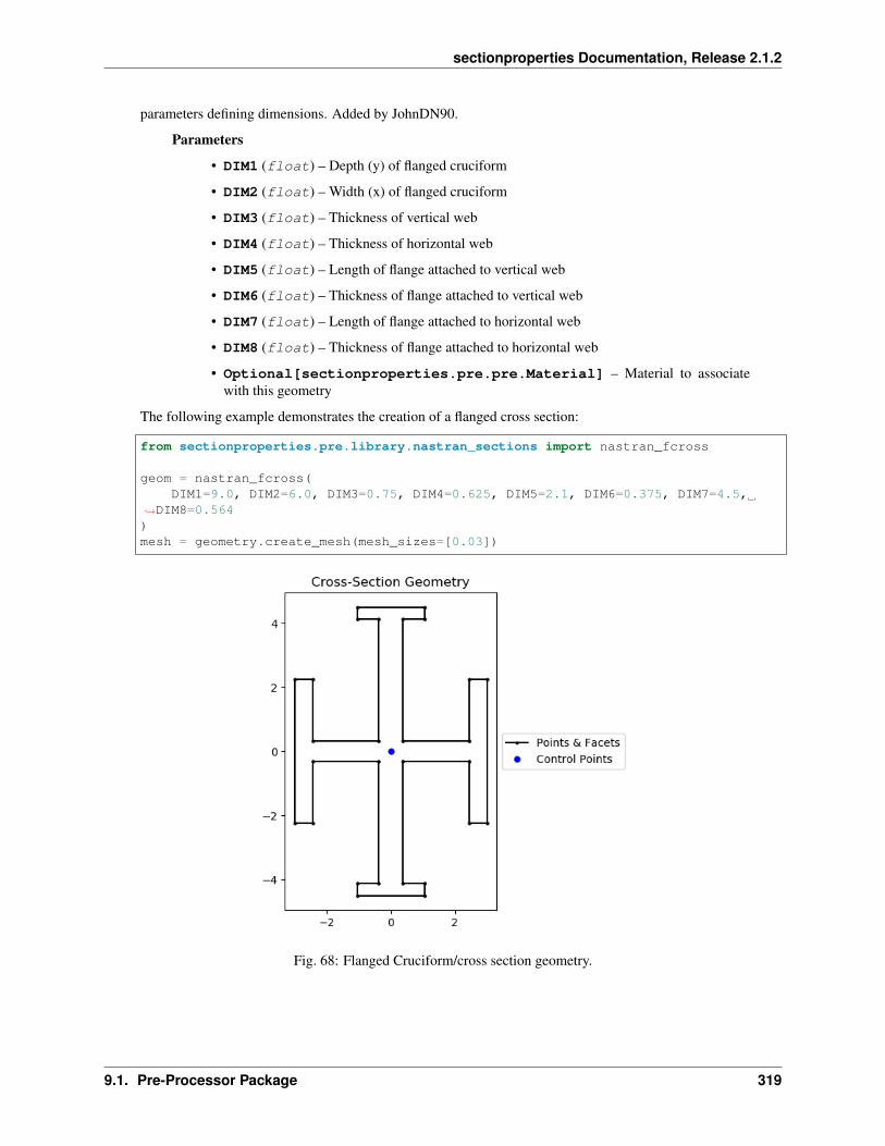
sectionproperties Documentation, Release 2.1.2
parameters defining dimensions. Added by JohnDN90.
Parameters
• DIM1 (float) – Depth (y) of flanged cruciform
• DIM2 (float) – Width (x) of flanged cruciform
• DIM3 (float) – Thickness of vertical web
• DIM4 (float) – Thickness of horizontal web
• DIM5 (float) – Length of flange attached to vertical web
• DIM6 (float) – Thickness of flange attached to vertical web
• DIM7 (float) – Length of flange attached to horizontal web
• DIM8 (float) – Thickness of flange attached to horizontal web
• Optional[sectionproperties.pre.pre.Material] – Material to associatewith this geometry
The following example demonstrates the creation of a flanged cross section:
from sectionproperties.pre.library.nastran_sections import nastran_fcross
geom = nastran_fcross(DIM1=9.0, DIM2=6.0, DIM3=0.75, DIM4=0.625, DIM5=2.1, DIM6=0.375, DIM7=4.5,
→˓DIM8=0.564)mesh = geometry.create_mesh(mesh_sizes=[0.03])
Fig. 68: Flanged Cruciform/cross section geometry.
9.1. Pre-Processor Package 319
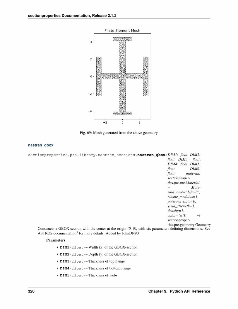
sectionproperties Documentation, Release 2.1.2
Fig. 69: Mesh generated from the above geometry.
nastran_gbox
sectionproperties.pre.library.nastran_sections.nastran_gbox(DIM1: float, DIM2:float, DIM3: float,DIM4: float, DIM5:float, DIM6:float, material:sectionproper-ties.pre.pre.Material= Mate-rial(name=’default’,elastic_modulus=1,poissons_ratio=0,yield_strength=1,density=1,color=’w’)) →sectionproper-ties.pre.geometry.Geometry
Constructs a GBOX section with the center at the origin (0, 0), with six parameters defining dimensions. SeeASTROS documentation5 for more details. Added by JohnDN90.
Parameters
• DIM1 (float) – Width (x) of the GBOX-section
• DIM2 (float) – Depth (y) of the GBOX-section
• DIM3 (float) – Thickness of top flange
• DIM4 (float) – Thickness of bottom flange
• DIM5 (float) – Thickness of webs
320 Chapter 9. Python API Reference
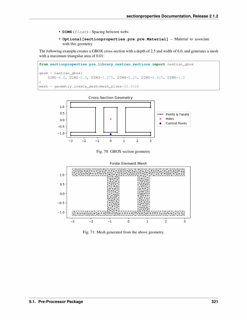
sectionproperties Documentation, Release 2.1.2
• DIM6 (float) – Spacing between webs
• Optional[sectionproperties.pre.pre.Material] – Material to associatewith this geometry
The following example creates a GBOX cross-section with a depth of 2.5 and width of 6.0, and generates a meshwith a maximum triangular area of 0.01:
from sectionproperties.pre.library.nastran_sections import nastran_gbox
geom = nastran_gbox(DIM1=6.0, DIM2=2.5, DIM3=0.375, DIM4=0.25, DIM5=0.625, DIM6=1.0
)mesh = geometry.create_mesh(mesh_sizes=[0.01])
Fig. 70: GBOX section geometry.
Fig. 71: Mesh generated from the above geometry.
9.1. Pre-Processor Package 321

sectionproperties Documentation, Release 2.1.2
nastran_h
sectionproperties.pre.library.nastran_sections.nastran_h(DIM1: float, DIM2: float,DIM3: float, DIM4: float,material: sectionproper-ties.pre.pre.Material= Mate-rial(name=’default’,elastic_modulus=1,poissons_ratio=0,yield_strength=1, den-sity=1, color=’w’))→ sectionproper-ties.pre.geometry.Geometry
Constructs a H section with the middle web’s middle center at the origin (0, 0), with four parameters definingdimensions. See Nastran documentation1234 for more details. Added by JohnDN90.
Parameters
• DIM1 (float) – Spacing between vertical flanges (length of web)
• DIM2 (float) – Twice the thickness of the vertical flanges
• DIM3 (float) – Depth (y) of the H-section
• DIM4 (float) – Thickness of the middle web
• Optional[sectionproperties.pre.pre.Material] – Material to associatewith this geometry
The following example creates a H cross-section with a depth of 3.5 and width of 2.75, and generates a meshwith a maximum triangular area of 0.005:
from sectionproperties.pre.library.nastran_sections import nastran_h
geom = nastran_h(DIM1=2.0, DIM2=0.75, DIM3=3.5, DIM4=0.25)mesh = geometry.create_mesh(mesh_sizes=[0.005])
nastran_hat
sectionproperties.pre.library.nastran_sections.nastran_hat(DIM1: float, DIM2:float, DIM3: float,DIM4: float, mate-rial: sectionproper-ties.pre.pre.Material= Mate-rial(name=’default’,elastic_modulus=1,poissons_ratio=0,yield_strength=1,density=1,color=’w’)) →sectionproper-ties.pre.geometry.Geometry
Constructs a Hat section with the top most section’s middle center at the origin (0, 0), with four parametersdefining dimensions. See Nastran documentation1234 for more details. Note that HAT in ASTROS is actuallyHAT1 in this code. Added by JohnDN90.
322 Chapter 9. Python API Reference

sectionproperties Documentation, Release 2.1.2
Fig. 72: H section geometry.
Fig. 73: Mesh generated from the above geometry.
9.1. Pre-Processor Package 323
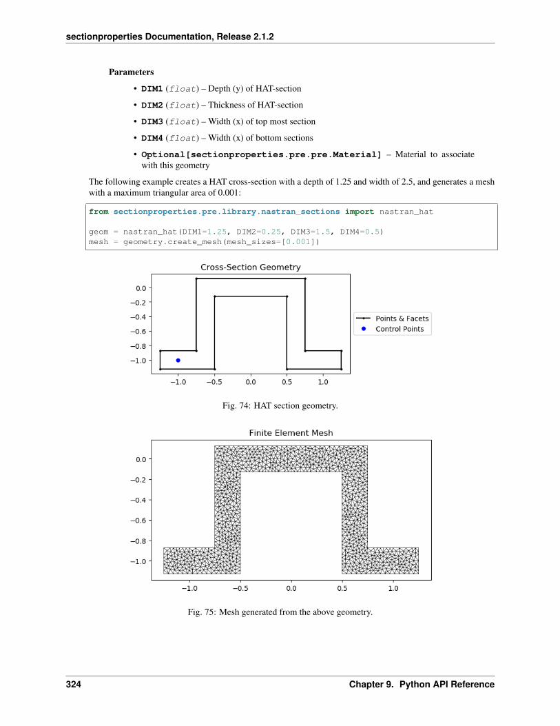
sectionproperties Documentation, Release 2.1.2
Parameters
• DIM1 (float) – Depth (y) of HAT-section
• DIM2 (float) – Thickness of HAT-section
• DIM3 (float) – Width (x) of top most section
• DIM4 (float) – Width (x) of bottom sections
• Optional[sectionproperties.pre.pre.Material] – Material to associatewith this geometry
The following example creates a HAT cross-section with a depth of 1.25 and width of 2.5, and generates a meshwith a maximum triangular area of 0.001:
from sectionproperties.pre.library.nastran_sections import nastran_hat
geom = nastran_hat(DIM1=1.25, DIM2=0.25, DIM3=1.5, DIM4=0.5)mesh = geometry.create_mesh(mesh_sizes=[0.001])
Fig. 74: HAT section geometry.
Fig. 75: Mesh generated from the above geometry.
324 Chapter 9. Python API Reference

sectionproperties Documentation, Release 2.1.2
nastran_hat1
sectionproperties.pre.library.nastran_sections.nastran_hat1(DIM1: float, DIM2:float, DIM3: float,DIM4: float, DIM5:float, material:sectionproper-ties.pre.pre.Material= Mate-rial(name=’default’,elastic_modulus=1,poissons_ratio=0,yield_strength=1,density=1,color=’w’)) →sectionproper-ties.pre.geometry.Geometry
Constructs a HAT1 section with the bottom plate’s bottom center at the origin (0, 0), with five parametersdefining dimensions. See Nastran documentation1235 for definition of parameters. Note that in ASTROS, HAT1is called HAT. Added by JohnDN90.
Parameters
• DIM1 (float) – Width(x) of the HAT1-section
• DIM2 (float) – Depth (y) of the HAT1-section
• DIM3 (float) – Width (x) of hat’s top flange
• DIM4 (float) – Thickness of hat stiffener
• DIM5 (float) – Thicknesss of bottom plate
• Optional[sectionproperties.pre.pre.Material] – Material to associatewith this geometry
The following example creates a HAT1 cross-section with a depth of 2.0 and width of 4.0, and generates a meshwith a maximum triangular area of 0.005:
from sectionproperties.pre.library.nastran_sections import nastran_hat1
geom = nastran_hat1(DIM1=4.0, DIM2=2.0, DIM3=1.5, DIM4=0.1875, DIM5=0.375)mesh = geometry.create_mesh(mesh_sizes=[0.005])
Fig. 76: HAT1 section geometry.
9.1. Pre-Processor Package 325

sectionproperties Documentation, Release 2.1.2
Fig. 77: Mesh generated from the above geometry.
nastran_hexa
sectionproperties.pre.library.nastran_sections.nastran_hexa(DIM1: float, DIM2:float, DIM3:float, material:sectionproper-ties.pre.pre.Material= Mate-rial(name=’default’,elastic_modulus=1,poissons_ratio=0,yield_strength=1,density=1,color=’w’)) →sectionproper-ties.pre.geometry.Geometry
Constructs a HEXA (hexagon) section with the center at the origin (0, 0), with three parameters defining dimen-sions. See Nastran documentation1234 for more details. Added by JohnDN90.
Parameters
• DIM1 (float) – Spacing between bottom right point and right most point
• DIM2 (float) – Width (x) of hexagon
• DIM3 (float) – Depth (y) of hexagon
• Optional[sectionproperties.pre.pre.Material] – Material to associatewith this geometry
The following example creates a rectangular cross-section with a depth of 1.5 and width of 2.0, and generates amesh with a maximum triangular area of 0.005:
from sectionproperties.pre.library.nastran_sections import nastran_hexa
geom = nastran_hexa(DIM1=0.5, DIM2=2.0, DIM3=1.5)mesh = geometry.create_mesh(mesh_sizes=[0.005])
326 Chapter 9. Python API Reference

sectionproperties Documentation, Release 2.1.2
Fig. 78: HEXA section geometry.
Fig. 79: Mesh generated from the above geometry.
9.1. Pre-Processor Package 327

sectionproperties Documentation, Release 2.1.2
nastran_i
sectionproperties.pre.library.nastran_sections.nastran_i(DIM1: float, DIM2:float, DIM3: float,DIM4: float, DIM5:float, DIM6: float,material: sectionproper-ties.pre.pre.Material= Mate-rial(name=’default’,elastic_modulus=1,poissons_ratio=0,yield_strength=1, den-sity=1, color=’w’))→ sectionproper-ties.pre.geometry.Geometry
Constructs Nastran’s I section with the bottom flange’s middle center at the origin (0, 0), with six parametersdefining dimensions. See Nastran documentation1234 for definition of parameters. Added by JohnDN90.
Parameters
• DIM1 (float) – Depth(y) of the I Section
• DIM2 (float) – Width (x) of bottom flange
• DIM3 (float) – Width (x) of top flange
• DIM4 (float) – Thickness of web
• DIM5 (float) – Thickness of bottom web
• DIM6 (float) – Thickness of top web
• Optional[sectionproperties.pre.pre.Material] – Material to associatewith this geometry
The following example creates a Nastran I cross-section with a depth of 5.0, and generates a mesh with amaximum triangular area of 0.008:
from sectionproperties.pre.library.nastran_sections import nastran_i
geom = nastran_i(DIM1=5.0, DIM2=2.0, DIM3=3.0, DIM4=0.25, DIM5=0.375, DIM6=0.5
)mesh = geometry.create_mesh(mesh_sizes=[0.008])
328 Chapter 9. Python API Reference

sectionproperties Documentation, Release 2.1.2
Fig. 80: Nastran’s I section geometry.
Fig. 81: Mesh generated from the above geometry.
9.1. Pre-Processor Package 329

sectionproperties Documentation, Release 2.1.2
nastran_i1
sectionproperties.pre.library.nastran_sections.nastran_i1(DIM1: float, DIM2:float, DIM3: float,DIM4: float, mate-rial: sectionproper-ties.pre.pre.Material= Mate-rial(name=’default’,elastic_modulus=1,poissons_ratio=0,yield_strength=1, den-sity=1, color=’w’))→ sectionproper-ties.pre.geometry.Geometry
Constructs a I1 section with the web’s middle center at the origin (0, 0), with four parameters defining dimen-sions. See Nastran documentation1234 for more details. Added by JohnDN90.
Parameters
• DIM1 (float) – Twice distance from web end to flange end
• DIM2 (float) – Thickness of web
• DIM3 (float) – Length of web (spacing between flanges)
• DIM4 (float) – Depth (y) of the I1-section
• Optional[sectionproperties.pre.pre.Material] – Material to associatewith this geometry
The following example creates a I1 cross-section with a depth of 5.0 and width of 1.75, and generates a meshwith a maximum triangular area of 0.02:
from sectionproperties.pre.library.nastran_sections import nastran_i1
geom = nastran_i1(DIM1=1.0, DIM2=0.75, DIM3=4.0, DIM4=5.0)mesh = geometry.create_mesh(mesh_sizes=[0.02])
nastran_l
sectionproperties.pre.library.nastran_sections.nastran_l(DIM1: float, DIM2: float,DIM3: float, DIM4: float,material: sectionproper-ties.pre.pre.Material= Mate-rial(name=’default’,elastic_modulus=1,poissons_ratio=0,yield_strength=1, den-sity=1, color=’w’))→ sectionproper-ties.pre.geometry.Geometry
Constructs a L section with the intersection’s center at the origin (0, 0), with four parameters defining dimen-sions. See Nastran documentation123 for more details. Added by JohnDN90.
Parameters
330 Chapter 9. Python API Reference

sectionproperties Documentation, Release 2.1.2
Fig. 82: I1 section geometry.
Fig. 83: Mesh generated from the above geometry.
9.1. Pre-Processor Package 331

sectionproperties Documentation, Release 2.1.2
• DIM1 (float) – Width (x) of the L-section
• DIM2 (float) – Depth (y) of the L-section
• DIM3 (float) – Thickness of flange (horizontal portion)
• DIM4 (float) – Thickness of web (vertical portion)
• Optional[sectionproperties.pre.pre.Material] – Material to associatewith this geometry
The following example creates a L cross-section with a depth of 6.0 and width of 3.0, and generates a mesh witha maximum triangular area of 0.01:
from sectionproperties.pre.library.nastran_sections import nastran_l
geom = nastran_l(DIM1=3.0, DIM2=6.0, DIM3=0.375, DIM4=0.625)mesh = geometry.create_mesh(mesh_sizes=[0.01])
Fig. 84: L section geometry.
332 Chapter 9. Python API Reference
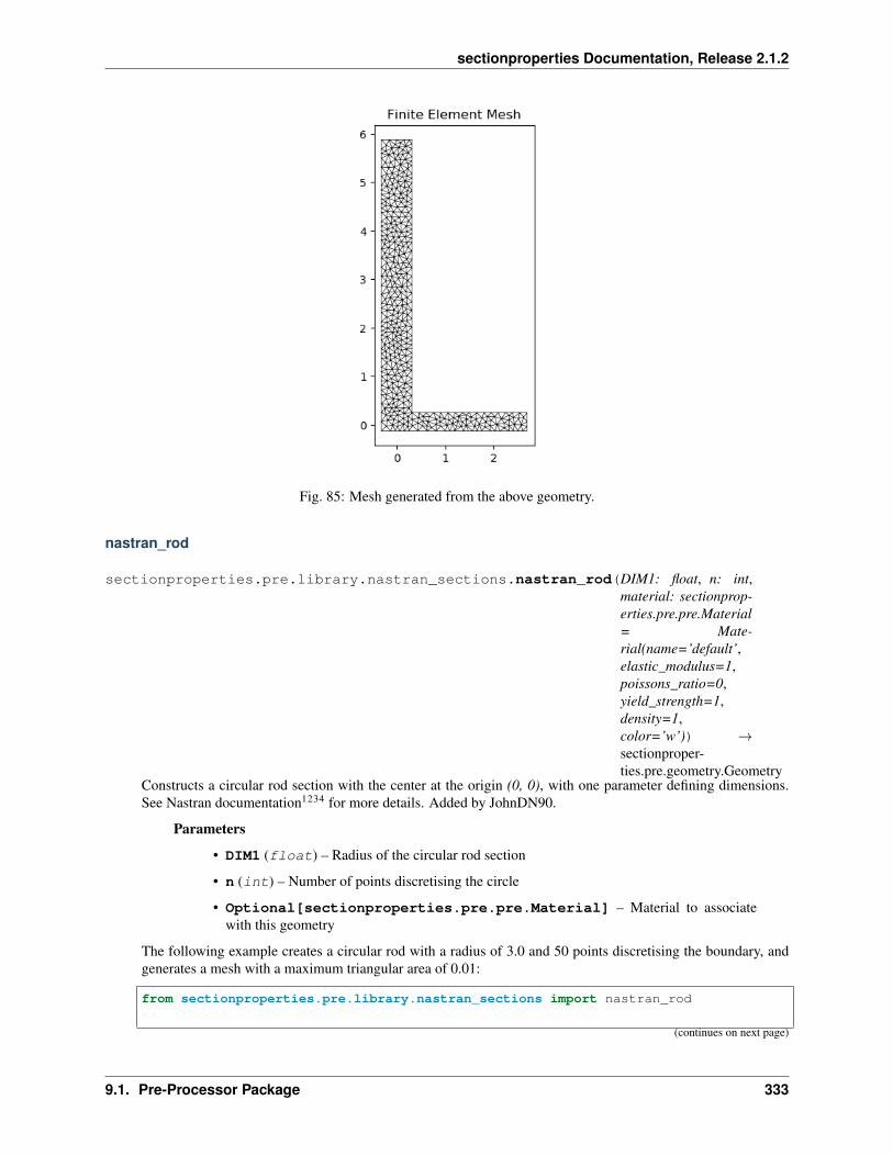
sectionproperties Documentation, Release 2.1.2
Fig. 85: Mesh generated from the above geometry.
nastran_rod
sectionproperties.pre.library.nastran_sections.nastran_rod(DIM1: float, n: int,material: sectionprop-erties.pre.pre.Material= Mate-rial(name=’default’,elastic_modulus=1,poissons_ratio=0,yield_strength=1,density=1,color=’w’)) →sectionproper-ties.pre.geometry.Geometry
Constructs a circular rod section with the center at the origin (0, 0), with one parameter defining dimensions.See Nastran documentation1234 for more details. Added by JohnDN90.
Parameters
• DIM1 (float) – Radius of the circular rod section
• n (int) – Number of points discretising the circle
• Optional[sectionproperties.pre.pre.Material] – Material to associatewith this geometry
The following example creates a circular rod with a radius of 3.0 and 50 points discretising the boundary, andgenerates a mesh with a maximum triangular area of 0.01:
from sectionproperties.pre.library.nastran_sections import nastran_rod
(continues on next page)
9.1. Pre-Processor Package 333

sectionproperties Documentation, Release 2.1.2
(continued from previous page)
geom = nastran_rod(DIM1=3.0, n=50)mesh = geometry.create_mesh(mesh_sizes=[0.01])
Fig. 86: Rod section geometry.
nastran_tee
sectionproperties.pre.library.nastran_sections.nastran_tee(DIM1: float, DIM2:float, DIM3: float,DIM4: float, mate-rial: sectionproper-ties.pre.pre.Material= Mate-rial(name=’default’,elastic_modulus=1,poissons_ratio=0,yield_strength=1,density=1,color=’w’)) →sectionproper-ties.pre.geometry.Geometry
Constructs a T section with the top flange’s middle center at the origin (0, 0), with four parameters definingdimensions. See Nastran documentation12345 for more details. Added by JohnDN90.
Parameters
• DIM1 (float) – Width (x) of top flange
• DIM2 (float) – Depth (y) of the T-section
• DIM3 (float) – Thickness of top flange
334 Chapter 9. Python API Reference
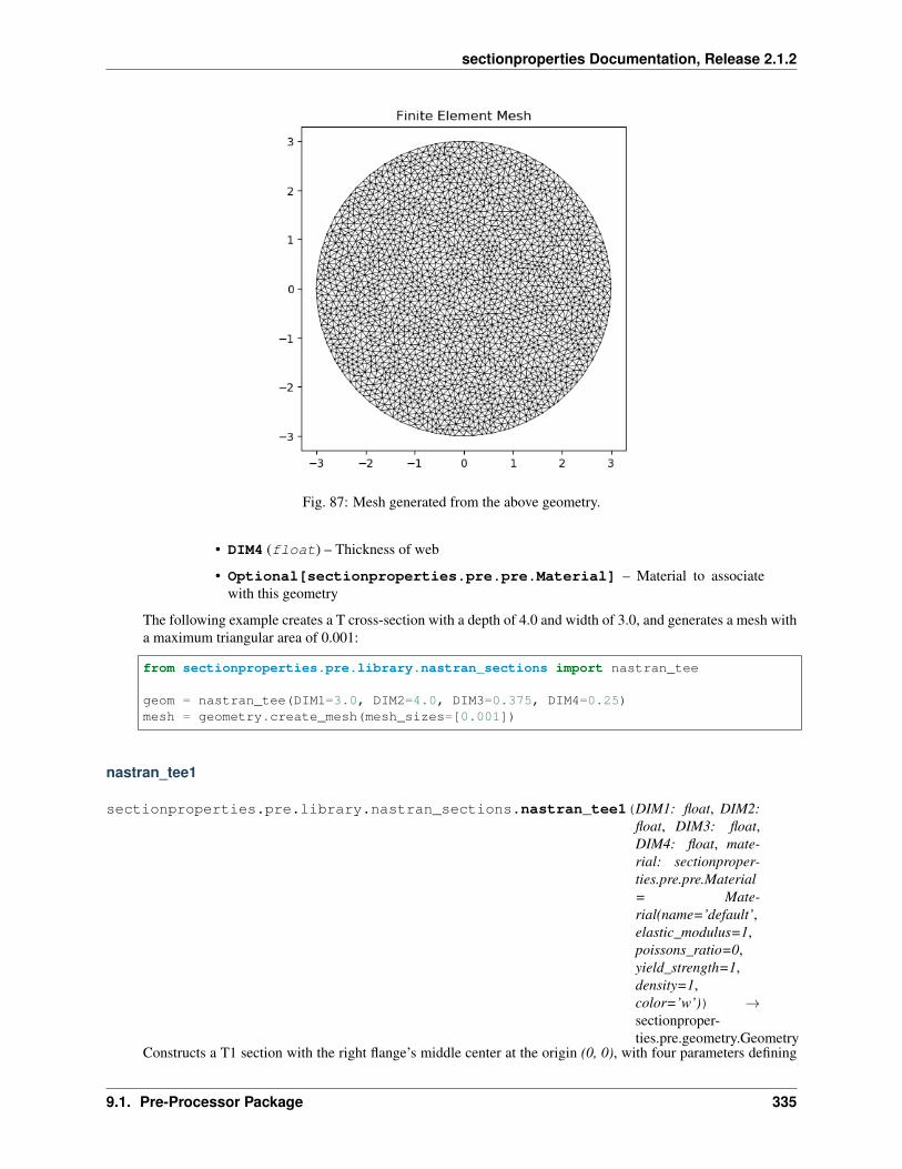
sectionproperties Documentation, Release 2.1.2
Fig. 87: Mesh generated from the above geometry.
• DIM4 (float) – Thickness of web
• Optional[sectionproperties.pre.pre.Material] – Material to associatewith this geometry
The following example creates a T cross-section with a depth of 4.0 and width of 3.0, and generates a mesh witha maximum triangular area of 0.001:
from sectionproperties.pre.library.nastran_sections import nastran_tee
geom = nastran_tee(DIM1=3.0, DIM2=4.0, DIM3=0.375, DIM4=0.25)mesh = geometry.create_mesh(mesh_sizes=[0.001])
nastran_tee1
sectionproperties.pre.library.nastran_sections.nastran_tee1(DIM1: float, DIM2:float, DIM3: float,DIM4: float, mate-rial: sectionproper-ties.pre.pre.Material= Mate-rial(name=’default’,elastic_modulus=1,poissons_ratio=0,yield_strength=1,density=1,color=’w’)) →sectionproper-ties.pre.geometry.Geometry
Constructs a T1 section with the right flange’s middle center at the origin (0, 0), with four parameters defining
9.1. Pre-Processor Package 335

sectionproperties Documentation, Release 2.1.2
Fig. 88: T section geometry.
Fig. 89: Mesh generated from the above geometry.
336 Chapter 9. Python API Reference

sectionproperties Documentation, Release 2.1.2
dimensions. See Nastran documentation1234 for more details. Added by JohnDN90.
Parameters
• DIM1 (float) – Depth (y) of T1-section
• DIM2 (float) – Length (x) of web
• DIM3 (float) – Thickness of right flange
• DIM4 (float) – Thickness of web
• Optional[sectionproperties.pre.pre.Material] – Material to associatewith this geometry
The following example creates a T1 cross-section with a depth of 3.0 and width of 3.875, and generates a meshwith a maximum triangular area of 0.001:
from sectionproperties.pre.library.nastran_sections import nastran_tee1
geom = nastran_tee1(DIM1=3.0, DIM2=3.5, DIM3=0.375, DIM4=0.25)mesh = geometry.create_mesh(mesh_sizes=[0.001])
Fig. 90: T1 section geometry.
9.1. Pre-Processor Package 337
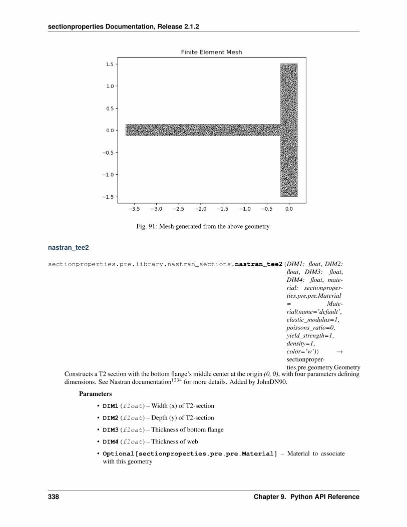
sectionproperties Documentation, Release 2.1.2
Fig. 91: Mesh generated from the above geometry.
nastran_tee2
sectionproperties.pre.library.nastran_sections.nastran_tee2(DIM1: float, DIM2:float, DIM3: float,DIM4: float, mate-rial: sectionproper-ties.pre.pre.Material= Mate-rial(name=’default’,elastic_modulus=1,poissons_ratio=0,yield_strength=1,density=1,color=’w’)) →sectionproper-ties.pre.geometry.Geometry
Constructs a T2 section with the bottom flange’s middle center at the origin (0, 0), with four parameters definingdimensions. See Nastran documentation1234 for more details. Added by JohnDN90.
Parameters
• DIM1 (float) – Width (x) of T2-section
• DIM2 (float) – Depth (y) of T2-section
• DIM3 (float) – Thickness of bottom flange
• DIM4 (float) – Thickness of web
• Optional[sectionproperties.pre.pre.Material] – Material to associatewith this geometry
338 Chapter 9. Python API Reference
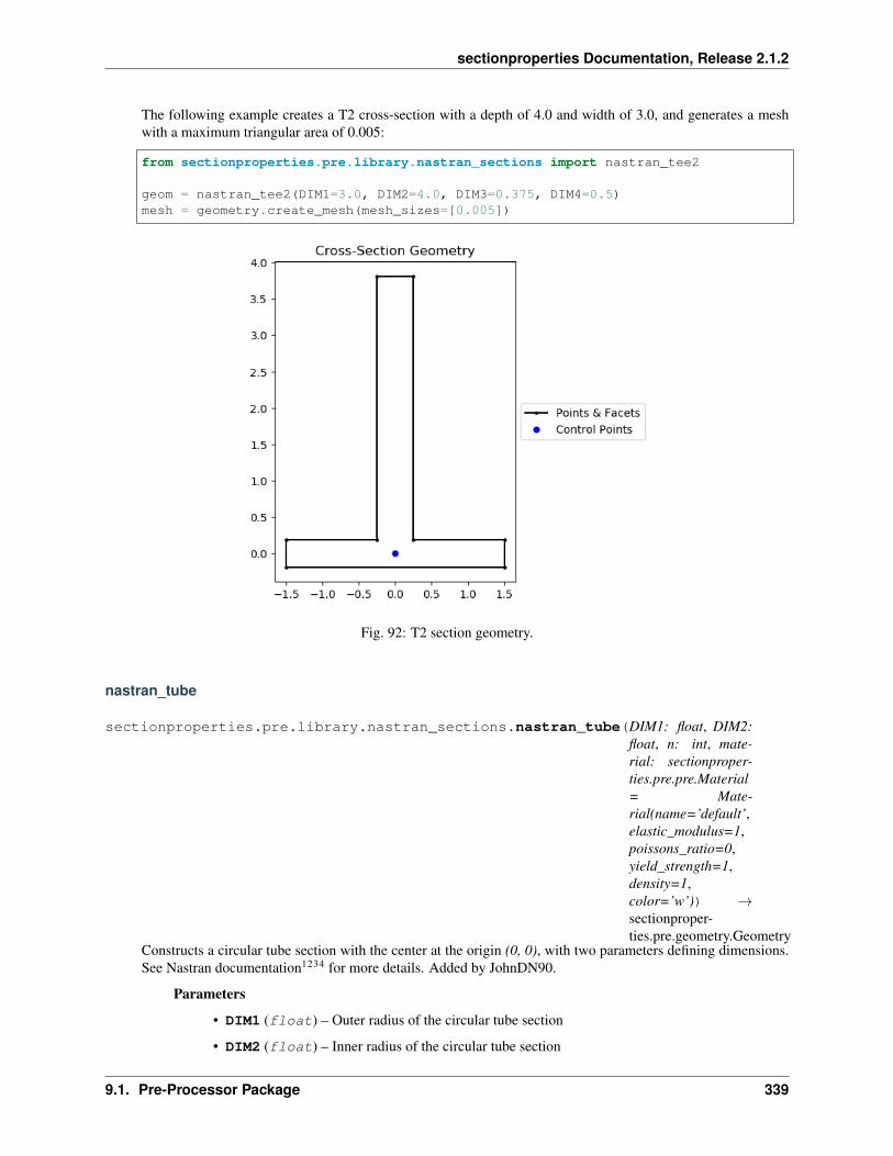
sectionproperties Documentation, Release 2.1.2
The following example creates a T2 cross-section with a depth of 4.0 and width of 3.0, and generates a meshwith a maximum triangular area of 0.005:
from sectionproperties.pre.library.nastran_sections import nastran_tee2
geom = nastran_tee2(DIM1=3.0, DIM2=4.0, DIM3=0.375, DIM4=0.5)mesh = geometry.create_mesh(mesh_sizes=[0.005])
Fig. 92: T2 section geometry.
nastran_tube
sectionproperties.pre.library.nastran_sections.nastran_tube(DIM1: float, DIM2:float, n: int, mate-rial: sectionproper-ties.pre.pre.Material= Mate-rial(name=’default’,elastic_modulus=1,poissons_ratio=0,yield_strength=1,density=1,color=’w’)) →sectionproper-ties.pre.geometry.Geometry
Constructs a circular tube section with the center at the origin (0, 0), with two parameters defining dimensions.See Nastran documentation1234 for more details. Added by JohnDN90.
Parameters
• DIM1 (float) – Outer radius of the circular tube section
• DIM2 (float) – Inner radius of the circular tube section
9.1. Pre-Processor Package 339

sectionproperties Documentation, Release 2.1.2
Fig. 93: Mesh generated from the above geometry.
• n (int) – Number of points discretising the circle
• Optional[sectionproperties.pre.pre.Material] – Material to associatewith this geometry
The following example creates a circular tube cross-section with an outer radius of 3.0 and an inner radius of2.5, and generates a mesh with 37 points discretising the boundaries and a maximum triangular area of 0.01:
from sectionproperties.pre.library.nastran_sections import nastran_tube
geom = nastran_tube(DIM1=3.0, DIM2=2.5, n=37)mesh = geometry.create_mesh(mesh_sizes=[0.01])
340 Chapter 9. Python API Reference

sectionproperties Documentation, Release 2.1.2
Fig. 94: TUBE section geometry.
Fig. 95: Mesh generated from the above geometry.
9.1. Pre-Processor Package 341

sectionproperties Documentation, Release 2.1.2
nastran_tube2
sectionproperties.pre.library.nastran_sections.nastran_tube2(DIM1: float,DIM2: float, n:float, material:sectionproper-ties.pre.pre.Material= Mate-rial(name=’default’,elas-tic_modulus=1,poissons_ratio=0,yield_strength=1,density=1,color=’w’))→ sectionproper-ties.pre.geometry.Geometry
Constructs a circular TUBE2 section with the center at the origin (0, 0), with two parameters defining dimen-sions. See MSC Nastran documentation1 for more details. Added by JohnDN90.
Parameters
• DIM1 (float) – Outer radius of the circular tube section
• DIM2 (float) – Thickness of wall
• n (int) – Number of points discretising the circle
• Optional[sectionproperties.pre.pre.Material] – Material to associatewith this geometry
The following example creates a circular TUBE2 cross-section with an outer radius of 3.0 and a wall thicknessof 0.5, and generates a mesh with 37 point discretising the boundary and a maximum triangular area of 0.01:
from sectionproperties.pre.library.nastran_sections import nastran_tube2
geom = nastran_tube2(DIM1=3.0, DIM2=0.5, n=37)mesh = geometry.create_mesh(mesh_sizes=[0.01])
nastran_zed
sectionproperties.pre.library.nastran_sections.nastran_zed(DIM1: float, DIM2:float, DIM3: float,DIM4: float, mate-rial: sectionproper-ties.pre.pre.Material= Mate-rial(name=’default’,elastic_modulus=1,poissons_ratio=0,yield_strength=1,density=1,color=’w’)) →sectionproper-ties.pre.geometry.Geometry
Constructs a Z section with the web’s middle center at the origin (0, 0), with four parameters defining dimen-sions. See Nastran documentation1234 for more details. Added by JohnDN90.
342 Chapter 9. Python API Reference
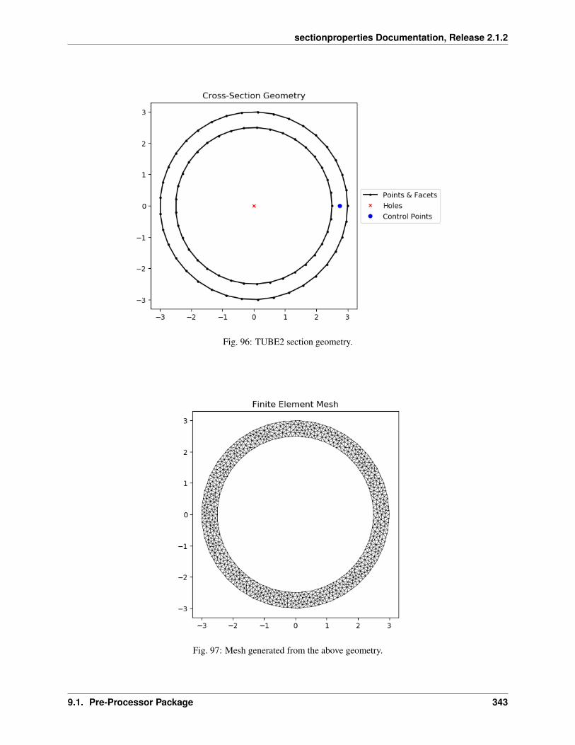
sectionproperties Documentation, Release 2.1.2
Fig. 96: TUBE2 section geometry.
Fig. 97: Mesh generated from the above geometry.
9.1. Pre-Processor Package 343

sectionproperties Documentation, Release 2.1.2
Parameters
• DIM1 (float) – Width (x) of horizontal members
• DIM2 (float) – Thickness of web
• DIM3 (float) – Spacing between horizontal members (length of web)
• DIM4 (float) – Depth (y) of Z-section
• Optional[sectionproperties.pre.pre.Material] – Material to associatewith this geometry
The following example creates a rectangular cross-section with a depth of 4.0 and width of 2.75, and generatesa mesh with a maximum triangular area of 0.005:
from sectionproperties.pre.library.nastran_sections import nastran_zed
geom = nastran_zed(DIM1=1.125, DIM2=0.5, DIM3=3.5, DIM4=4.0)mesh = geometry.create_mesh(mesh_sizes=[0.005])
Fig. 98: Z section geometry.
Nastran References
9.2 Analysis Package
9.2.1 section Module
344 Chapter 9. Python API Reference
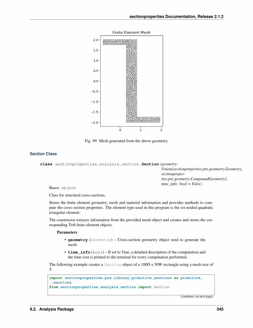
sectionproperties Documentation, Release 2.1.2
Fig. 99: Mesh generated from the above geometry.
Section Class
class sectionproperties.analysis.section.Section(geometry:Union[sectionproperties.pre.geometry.Geometry,sectionproper-ties.pre.geometry.CompoundGeometry],time_info: bool = False)
Bases: object
Class for structural cross-sections.
Stores the finite element geometry, mesh and material information and provides methods to com-pute the cross-section properties. The element type used in this program is the six-noded quadratictriangular element.
The constructor extracts information from the provided mesh object and creates and stores the cor-responding Tri6 finite element objects.
Parameters
• geometry (Geometry) – Cross-section geometry object used to generate themesh
• time_info (bool) – If set to True, a detailed description of the computation andthe time cost is printed to the terminal for every computation performed.
The following example creates a Section object of a 100D x 50W rectangle using a mesh size of5:
import sectionproperties.pre.library.primitive_sections as primitive_→˓sectionsfrom sectionproperties.analysis.section import Section
(continues on next page)
9.2. Analysis Package 345

sectionproperties Documentation, Release 2.1.2
(continued from previous page)
geometry = primitive_sections.rectangular_section(d=100, b=50)geometry.create_mesh(mesh_sizes=[5])section = Section(geometry)
Variables
• elements (list[Tri6]) – List of finite element objects describing the cross-sectionmesh
• num_nodes (int) – Number of nodes in the finite element mesh
• geometry (Geometry) – Cross-section geometry object used to generate themesh
• mesh (dict(mesh)) – Mesh dict returned by triangle
• mesh_nodes (numpy.ndarray) – Array of node coordinates from the mesh
• mesh_elements (numpy.ndarray) – Array of connectivities from the mesh
• mesh_attributes (numpy.ndarray) – Array of attributes from the mesh
• materials – List of materials
• material_groups – List of objects containing the elements in each defined ma-terial
• section_props (SectionProperties) – Class to store calculated sectionproperties
Raises
• AssertionError – If the number of materials does not equal the number ofregions
• ValueError – If geometry does not contain a mesh
assemble_torsion(progress=None, task=None)Assembles stiffness matrices to be used for the computation of warping properties and thetorsion load vector (f_torsion). A Lagrangian multiplier (k_lg) stiffness matrix is returned. Thestiffness matrix are assembled using the sparse COO format and returned in the sparse CSCformat.
Returns Lagrangian multiplier stiffness matrix and torsion load vector (k_lg,f_torsion)
Return type tuple(scipy.sparse.csc_matrix, numpy.ndarray)
calculate_frame_properties(solver_type=’direct’)Calculates and returns the properties required for a frame analysis. The properties are alsostored in the SectionProperties object contained in the section_props class vari-able.
Parameters solver_type (string) – Solver used for solving systems of linearequations, either using the ‘direct’ method or ‘cgs’ iterative method
Returns Cross-section properties to be used for a frame analysis (area, ixx, iyy, ixy, j,phi)
Return type tuple(float, float, float, float, float, float)The following section properties are calculated:
• Cross-sectional area (area)• Second moments of area about the centroidal axis (ixx, iyy, ixy)• Torsion constant (j)
346 Chapter 9. Python API Reference
sectionproperties Documentation, Release 2.1.2
• Principal axis angle (phi)If materials are specified for the cross-section, the area, second moments of area and torsionconstant are elastic modulus weighted.
The following example demonstrates the use of this method:
section = Section(geometry)(area, ixx, iyy, ixy, j, phi) = section.calculate_frame_properties()
calculate_geometric_properties()Calculates the geometric properties of the cross-section and stores them in theSectionProperties object contained in the section_props class variable.
The following geometric section properties are calculated:• Cross-sectional area• Cross-sectional perimeter• Cross-sectional mass• Area weighted material properties, composite only 𝐸𝑒𝑓𝑓 , 𝐺𝑒𝑓𝑓 , 𝑛𝑢𝑒𝑓𝑓
• Modulus weighted area (axial rigidity)• First moments of area• Second moments of area about the global axis• Second moments of area about the centroidal axis• Elastic centroid• Centroidal section moduli• Radii of gyration• Principal axis properties
If materials are specified for the cross-section, the moments of area and section moduli areelastic modulus weighted.
The following example demonstrates the use of this method:
section = Section(geometry)section.calculate_geometric_properties()
calculate_plastic_properties(verbose=False)Calculates the plastic properties of the cross-section and stores them in theSectionProperties object contained in the section_props class variable.
Parameters verbose (bool) – If set to True, the number of iterations required foreach plastic axis is printed to the terminal.
The following warping section properties are calculated:• Plastic centroid for bending about the centroidal and principal axes• Plastic section moduli for bending about the centroidal and principal axes• Shape factors for bending about the centroidal and principal axes
If materials are specified for the cross-section, the plastic section moduli are displayed as plasticmoments (i.e 𝑀𝑝 = 𝑓𝑦𝑆) and the shape factors are not calculated.
Note that the geometric properties must be calculated before the plastic properties are calcu-lated:
section = Section(geometry)section.calculate_geometric_properties()section.calculate_plastic_properties()
Raises RuntimeError – If the geometric properties have not been calculated priorto calling this method
calculate_stress(N=0, Vx=0, Vy=0, Mxx=0, Myy=0, M11=0, M22=0, Mzz=0)Calculates the cross-section stress resulting from design actions and returns a StressPost
9.2. Analysis Package 347

sectionproperties Documentation, Release 2.1.2
object allowing post-processing of the stress results.Parameters
• N (float) – Axial force• Vx (float) – Shear force acting in the x-direction• Vy (float) – Shear force acting in the y-direction• Mxx (float) – Bending moment about the centroidal xx-axis• Myy (float) – Bending moment about the centroidal yy-axis• M11 (float) – Bending moment about the centroidal 11-axis• M22 (float) – Bending moment about the centroidal 22-axis• Mzz (float) – Torsion moment about the centroidal zz-axis
Returns Object for post-processing cross-section stressesReturn type StressPost
Note that a geometric and warping analysis must be performed before a stress analysis is carriedout:
section = Section(geometry)section.calculate_geometric_properties()section.calculate_warping_properties()stress_post = section.calculate_stress(N=1e3, Vy=3e3, Mxx=1e6)
Raises RuntimeError – If a geometric and warping analysis have not been per-formed prior to calling this method
calculate_warping_properties(solver_type=’direct’)Calculates all the warping properties of the cross-section and stores them in theSectionProperties object contained in the section_props class variable.
Parameters solver_type (string) – Solver used for solving systems of linearequations, either using the ‘direct’ method or ‘cgs’ iterative method
The following warping section properties are calculated:• Torsion constant• Shear centre• Shear area• Warping constant• Monosymmetry constant
If materials are specified, the values calculated for the torsion constant, warping constant andshear area are elastic modulus weighted.
Note that the geometric properties must be calculated prior to the calculation of the warpingproperties:
section = Section(geometry)section.calculate_geometric_properties()section.calculate_warping_properties()
Raises RuntimeError – If the geometric properties have not been calculated priorto calling this method
display_mesh_info()Prints mesh statistics (number of nodes, elements and regions) to the command window.
The following example displays the mesh statistics for a Tee section merged from two rectan-gles:
import sectionproperties.pre.library.primitive_sections as primitive_→˓sectionsfrom sectionproperties.analysis.section import Section
(continues on next page)
348 Chapter 9. Python API Reference

sectionproperties Documentation, Release 2.1.2
(continued from previous page)
rec1 = primitive_sections.rectangular_section(d=100, b=25)rec2 = primitive_sections.rectangular_section(d=25, b=100)rec1 = rec1.shift_section(x_offset=-12.5)rec2 = rec2.shift_section(x_offset=-50, y_offset=100)
geometry = rec1 + rec2geometry.create_mesh(mesh_sizes=[5, 2.5])section = Section(geometry)section.display_mesh_info()
>>>Mesh Statistics:>>>--4920 nodes>>>--2365 elements>>>--2 regions
display_results(fmt=’8.6e’)Prints the results that have been calculated to the terminal.
Parameters fmt (string) – Number formatting stringThe following example displays the geometric section properties for a 100D x 50W rectanglewith three digits after the decimal point:
import sectionproperties.pre.library.primitive_sections as primitive_→˓sectionsfrom sectionproperties.analysis.section import Section
geometry = primitive_sections.rectangular_section(d=100, b=50)geometry.create_mesh(mesh_sizes=[5])
section = Section(geometry)section.calculate_geometric_properties()
section.display_results(fmt='.3f')
get_As()Returns Shear area for loading about the centroidal axis (A_sx, A_sy)Return type tuple(float, float)
section = Section(geometry)section.calculate_geometric_properties()section.calculate_warping_properties()(A_sx, A_sy) = section.get_As()
get_As_p()Returns Shear area for loading about the principal bending axis (A_s11, A_s22)Return type tuple(float, float)
section = Section(geometry)section.calculate_geometric_properties()section.calculate_warping_properties()(A_s11, A_s22) = section.get_As_p()
get_area()Returns Cross-section areaReturn type float
9.2. Analysis Package 349

sectionproperties Documentation, Release 2.1.2
section = Section(geometry)section.calculate_geometric_properties()area = section.get_area()
get_beta()Returns Monosymmetry constant for bending about both global axes (beta_x_plus,
beta_x_minus, beta_y_plus, beta_y_minus). The plus value relates to the top flangein compression and the minus value relates to the bottom flange in compression.
Return type tuple(float, float, float, float)
section = Section(geometry)section.calculate_geometric_properties()section.calculate_warping_properties()(beta_x_plus, beta_x_minus, beta_y_plus, beta_y_minus) = section.get_→˓beta()
get_beta_p()Returns Monosymmetry constant for bending about both principal axes
(beta_11_plus, beta_11_minus, beta_22_plus, beta_22_minus). The plus valuerelates to the top flange in compression and the minus value relates to the bottomflange in compression.
Return type tuple(float, float, float, float)
section = Section(geometry)section.calculate_geometric_properties()section.calculate_warping_properties()(beta_11_plus, beta_11_minus, beta_22_plus, beta_22_minus) = section.→˓get_beta_p()
get_c()Returns Elastic centroid (cx, cy)Return type tuple(float, float)
section = Section(geometry)section.calculate_geometric_properties()(cx, cy) = section.get_c()
get_e_eff()Returns Effective elastic modulus based on areaReturn type float
section = Section(geometry)section.calculate_warping_properties()e_eff = section.get_e_eff()
get_ea()Returns Modulus weighted area (axial rigidity)Return type float
section = Section(geometry)section.calculate_geometric_properties()ea = section.get_ea()
get_g_eff()Returns Effective shear modulus based on areaReturn type float
350 Chapter 9. Python API Reference

sectionproperties Documentation, Release 2.1.2
section = Section(geometry)section.calculate_geometric_properties()g_eff = section.get_g_eff()
get_gamma()Returns Warping constantReturn type float
section = Section(geometry)section.calculate_geometric_properties()section.calculate_warping_properties()gamma = section.get_gamma()
get_ic()Returns Second moments of area centroidal axis (ixx_c, iyy_c, ixy_c)Return type tuple(float, float, float)
section = Section(geometry)section.calculate_geometric_properties()(ixx_c, iyy_c, ixy_c) = section.get_ic()
get_ig()Returns Second moments of area about the global axis (ixx_g, iyy_g, ixy_g)Return type tuple(float, float, float)
section = Section(geometry)section.calculate_geometric_properties()(ixx_g, iyy_g, ixy_g) = section.get_ig()
get_ip()Returns Second moments of area about the principal axis (i11_c, i22_c)Return type tuple(float, float)
section = Section(geometry)section.calculate_geometric_properties()(i11_c, i22_c) = section.get_ip()
get_j()Returns St. Venant torsion constantReturn type float
section = Section(geometry)section.calculate_geometric_properties()section.calculate_warping_properties()j = section.get_j()
get_mass()Returns Cross-section massReturn type float
section = Section(geometry)section.calculate_geometric_properties()perimeter = section.get_mass()
get_nu_eff()Returns Effective Poisson’s ratioReturn type float
9.2. Analysis Package 351
sectionproperties Documentation, Release 2.1.2
section = Section(geometry)section.calculate_geometric_properties()nu_eff = section.get_nu_eff()
get_pc()Returns Centroidal axis plastic centroid (x_pc, y_pc)Return type tuple(float, float)
section = Section(geometry)section.calculate_geometric_properties()section.calculate_plastic_properties()(x_pc, y_pc) = section.get_pc()
get_pc_p()Returns Principal bending axis plastic centroid (x11_pc, y22_pc)Return type tuple(float, float)
section = Section(geometry)section.calculate_geometric_properties()section.calculate_plastic_properties()(x11_pc, y22_pc) = section.get_pc_p()
get_perimeter()Returns Cross-section perimeterReturn type float
section = Section(geometry)section.calculate_geometric_properties()perimeter = section.get_perimeter()
get_phi()Returns Principal bending axis angleReturn type float
section = Section(geometry)section.calculate_geometric_properties()phi = section.get_phi()
get_q()Returns First moments of area about the global axis (qx, qy)Return type tuple(float, float)
section = Section(geometry)section.calculate_geometric_properties()(qx, qy) = section.get_q()
get_rc()Returns Radii of gyration about the centroidal axis (rx, ry)Return type tuple(float, float)
section = Section(geometry)section.calculate_geometric_properties()(rx, ry) = section.get_rc()
get_rp()Returns Radii of gyration about the principal axis (r11, r22)Return type tuple(float, float)
352 Chapter 9. Python API Reference
sectionproperties Documentation, Release 2.1.2
section = Section(geometry)section.calculate_geometric_properties()(r11, r22) = section.get_rp()
get_s()Returns Plastic section moduli about the centroidal axis (sxx, syy)Return type tuple(float, float)
If material properties have been specified, returns the plastic moment 𝑀𝑝 = 𝑓𝑦𝑆.
section = Section(geometry)section.calculate_geometric_properties()section.calculate_plastic_properties()(sxx, syy) = section.get_s()
get_sc()Returns Centroidal axis shear centre (elasticity approach) (x_se, y_se)Return type tuple(float, float)
section = Section(geometry)section.calculate_geometric_properties()section.calculate_warping_properties()(x_se, y_se) = section.get_sc()
get_sc_p()Returns Principal axis shear centre (elasticity approach) (x11_se, y22_se)Return type tuple(float, float)
section = Section(geometry)section.calculate_geometric_properties()section.calculate_warping_properties()(x11_se, y22_se) = section.get_sc_p()
get_sc_t()Returns Centroidal axis shear centre (Trefftz’s approach) (x_st, y_st)Return type tuple(float, float)
section = Section(geometry)section.calculate_geometric_properties()section.calculate_warping_properties()(x_st, y_st) = section.get_sc_t()
get_sf()Returns Centroidal axis shape factors with respect to the top and bottom fibres
(sf_xx_plus, sf_xx_minus, sf_yy_plus, sf_yy_minus)Return type tuple(float, float, float, float)
section = Section(geometry)section.calculate_geometric_properties()section.calculate_plastic_properties()(sf_xx_plus, sf_xx_minus, sf_yy_plus, sf_yy_minus) = section.get_sf()
get_sf_p()Returns Principal bending axis shape factors with respect to the top and bottom fibres
(sf_11_plus, sf_11_minus, sf_22_plus, sf_22_minus)Return type tuple(float, float, float, float)
9.2. Analysis Package 353

sectionproperties Documentation, Release 2.1.2
section = Section(geometry)section.calculate_geometric_properties()section.calculate_plastic_properties()(sf_11_plus, sf_11_minus, sf_22_plus, sf_22_minus) = section.get_sf_→˓p()
get_sp()Returns Plastic section moduli about the principal bending axis (s11, s22)Return type tuple(float, float)
If material properties have been specified, returns the plastic moment 𝑀𝑝 = 𝑓𝑦𝑆.
section = Section(geometry)section.calculate_geometric_properties()section.calculate_plastic_properties()(s11, s22) = section.get_sp()
get_z()Returns Elastic section moduli about the centroidal axis with respect to the top and
bottom fibres (zxx_plus, zxx_minus, zyy_plus, zyy_minus)Return type tuple(float, float, float, float)
section = Section(geometry)section.calculate_geometric_properties()(zxx_plus, zxx_minus, zyy_plus, zyy_minus) = section.get_z()
get_zp()Returns Elastic section moduli about the principal axis with respect to the top and
bottom fibres (z11_plus, z11_minus, z22_plus, z22_minus)Return type tuple(float, float, float, float)
section = Section(geometry)section.calculate_geometric_properties()(z11_plus, z11_minus, z22_plus, z22_minus) = section.get_zp()
plot_centroids(title=’Centroids’, **kwargs)Plots the elastic centroid, the shear centre, the plastic centroids and the principal axis, if theyhave been calculated, on top of the finite element mesh.
Parameters• title (string) – Plot title• kwargs – Passed to plotting_context()
Returns Matplotlib axes objectReturn type matplotlib.axes
The following example analyses a 200 PFC section and displays a plot of the centroids:
import sectionproperties.pre.library.steel_sections as steel_sectionsfrom sectionproperties.analysis.section import Section
geometry = steel_sections.channel_section(d=200, b=75, t_f=12, t_w=6,→˓r=12, n_r=8)geometry.create_mesh(mesh_sizes=[20])
section = Section(geometry)section.calculate_geometric_properties()section.calculate_warping_properties()section.calculate_plastic_properties()
(continues on next page)
354 Chapter 9. Python API Reference

sectionproperties Documentation, Release 2.1.2
(continued from previous page)
section.plot_centroids()
Fig. 100: Plot of the centroids generated by the above example.
The following example analyses a 150x90x12 UA section and displays a plot of the centroids:
import sectionproperties.pre.library.steel_sections as steel_sectionsfrom sectionproperties.analysis.section import Section
geometry = steel_sections.angle_section(d=150, b=90, t=12, r_r=10, r_→˓t=5, n_r=8)geometry.create_mesh(mesh_sizes=[20])
section = Section(geometry)section.calculate_geometric_properties()section.calculate_warping_properties()section.calculate_plastic_properties()
section.plot_centroids()
9.2. Analysis Package 355
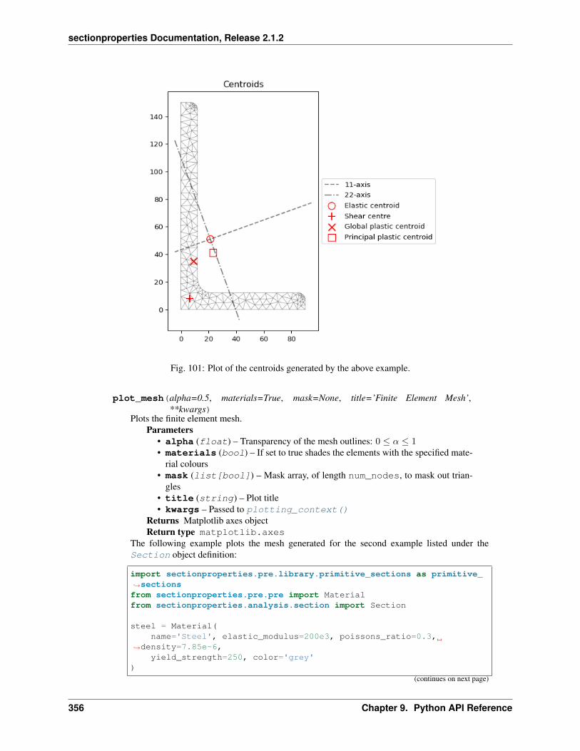
sectionproperties Documentation, Release 2.1.2
Fig. 101: Plot of the centroids generated by the above example.
plot_mesh(alpha=0.5, materials=True, mask=None, title=’Finite Element Mesh’,**kwargs)
Plots the finite element mesh.Parameters
• alpha (float) – Transparency of the mesh outlines: 0 ≤ 𝛼 ≤ 1• materials (bool) – If set to true shades the elements with the specified mate-
rial colours• mask (list[bool]) – Mask array, of length num_nodes, to mask out trian-
gles• title (string) – Plot title• kwargs – Passed to plotting_context()
Returns Matplotlib axes objectReturn type matplotlib.axes
The following example plots the mesh generated for the second example listed under theSection object definition:
import sectionproperties.pre.library.primitive_sections as primitive_→˓sectionsfrom sectionproperties.pre.pre import Materialfrom sectionproperties.analysis.section import Section
steel = Material(name='Steel', elastic_modulus=200e3, poissons_ratio=0.3,
→˓density=7.85e-6,yield_strength=250, color='grey'
)(continues on next page)
356 Chapter 9. Python API Reference

sectionproperties Documentation, Release 2.1.2
(continued from previous page)
timber = Material(name='Timber', elastic_modulus=8e3, poissons_ratio=0.35,
→˓density=6.5e-7,yield_strength=20, color='burlywood'
)
geom_steel = primitive_sections.rectangular_section(d=50, b=50,→˓material=steel)geom_timber = primitive_sections.rectangular_section(d=50, b=50,→˓material=timber)geometry = geom_timber.align_to(geom_steel, on="right") + geom_steel
geometry.create_mesh(mesh_sizes=[10, 5])
section = Section(geometry)section.plot_mesh(materials=True, alpha=0.5)
Fig. 102: Finite element mesh generated by the above example.
PlasticSection Class
class sectionproperties.analysis.section.PlasticSection(geom:Union[sectionproperties.pre.geometry.Geometry,sectionproper-ties.pre.geometry.CompoundGeometry])
Bases: object
Class for the plastic analysis of cross-sections.
Stores the finite element geometry and material information and provides methods to compute theplastic section properties.
Parameters section (Section) – Section object
Variables
9.2. Analysis Package 357
sectionproperties Documentation, Release 2.1.2
• geometry (Geometry) – Deep copy of the Section geometry object provided tothe constructor
• materials (list[Material]) – A list of material properties corresponding tovarious regions in the geometry and mesh.
• mesh (dict(mesh)) – Mesh dict returned by triangle
• mesh_nodes (numpy.ndarray) – Array of node coordinates from the mesh
• mesh_elements (numpy.ndarray) – Array of connectivities from the mesh
• elements (list[Tri6]) – List of finite element objects describing the cross-sectionmesh
• f_top – Current force in the top region
• c_top – Centroid of the force in the top region (c_top_x, c_top_y)
• c_bot – Centroid of the force in the bottom region (c_bot_x, c_bot_y)
calculate_centroid(elements)Calculates the elastic centroid from a list of finite elements.
Parameters elements (list[Tri6]) – A list of Tri6 finite elements.Returns A tuple containing the x and y location of the elastic centroid.Return type tuple(float, float)
calculate_extreme_fibres(angle)Calculates the locations of the extreme fibres along and perpendicular to the axis specified by‘angle’ using the elements stored in self.elements.
Parameters angle (float) – Angle (in degrees) along which to calculate the ex-treme fibre locations
Returns The location of the extreme fibres parallel (u) and perpendicular (v) to theaxis (u_min, u_max, v_min, v_max)
Return type tuple(float, float, float, float)
calculate_plastic_force(u: numpy.ndarray, p: numpy.ndarray) → Tuple[float,float]
Sums the forces above and below the axis defined by unit vector u and point p. Also returns theforce centroid of the forces above and below the axis.
Parameters• elements (list[Tri6]) – A list of Tri6 finite elements.• u (numpy.ndarray) – Unit vector defining the direction of the axis• p (numpy.ndarray) – Point on the axis
Returns Force in the top and bottom areas (f_top, f_bot)Return type tuple(float, float)
calculate_plastic_properties(section, verbose, progress=None)Calculates the location of the plastic centroid with respect to the centroidal and principal bend-ing axes, the plastic section moduli and shape factors and stores the results to the suppliedSection object.
Parameters• section (Section) – Cross section object that uses the same geometry and
materials specified in the class constructor• verbose (bool) – If set to True, the number of iterations required for each
plastic axis is printed to the terminal.
check_convergence(root_result, axis)Checks that the function solver converged and if not, raises a helpful error.
Parameters
358 Chapter 9. Python API Reference

sectionproperties Documentation, Release 2.1.2
• root_result (scipy.optimize.RootResults) – Result object fromthe root finder
• axis (string) – Axis being considered by the function solverRaises RuntimeError – If the function solver did not converge
evaluate_force_eq(d, u, u_p, verbose)Given a distance d from the centroid to an axis (defined by unit vector u), creates a meshincluding the new and axis and calculates the force equilibrium. The resultant force, as a ratioof the total force, is returned.
Parameters• d (float) – Distance from the centroid to current axis• u (numpy.ndarray) – Unit vector defining the direction of the axis• u_p (numpy.ndarray) – Unit vector perpendicular to the direction of the axis• verbose (bool) – If set to True, the number of iterations required for each
plastic axis is printed to the terminal.Returns The force equilibrium normReturn type float
pc_algorithm(u, dlim, axis, verbose)An algorithm used for solving for the location of the plastic centroid. The algorithm searchesfor the location of the axis, defined by unit vector u and within the section depth, that satisfiesforce equilibrium.
Parameters• u (numpy.ndarray) – Unit vector defining the direction of the axis• dlim (list[float, float]) – List [dmax, dmin] containing the distances
from the centroid to the extreme fibres perpendicular to the axis• axis (int) – The current axis direction: 1 (e.g. x or 11) or 2 (e.g. y or 22)• verbose (bool) – If set to True, the number of iterations required for each
plastic axis is printed to the terminal.Returns The distance to the plastic centroid axis d, the result object r, the force in the
top of the section f_top and the location of the centroids of the top and bottom areasc_top and c_bottom
Return type tuple(float, scipy.optimize.RootResults, float, list[float,float], list[float, float])
print_verbose(d, root_result, axis)Prints information related to the function solver convergence to the terminal.
Parameters• d (float) – Location of the plastic centroid axis• root_result (scipy.optimize.RootResults) – Result object from
the root finder• axis (string) – Axis being considered by the function solver
StressPost Class
class sectionproperties.analysis.section.StressPost(section)Bases: object
Class for post-processing finite element stress results.
A StressPost object is created when a stress analysis is carried out and is returned as an object to allow post-processing of the results. The StressPost object creates a deep copy of the MaterialGroups within the cross-section to allow the calculation of stresses for each material. Methods for post-processing the calculated stressesare provided.
Parameters section (Section) – Cross section object for stress calculation
9.2. Analysis Package 359
sectionproperties Documentation, Release 2.1.2
Variables
• section (Section) – Cross section object for stress calculation
• material_groups (list[MaterialGroup]) – A deep copy of the section materialgroups to allow a new stress analysis
get_stress()Returns the stresses within each material belonging to the current StressPost object.
Returns A list of dictionaries containing the cross-section stresses for each material.
Return type list[dict]
A dictionary is returned for each material in the cross-section, containing the following keys and values:
• ‘Material’: Material name
• ‘sig_zz_n’: Normal stress 𝜎𝑧𝑧,𝑁 resulting from the axial load 𝑁
• ‘sig_zz_mxx’: Normal stress 𝜎𝑧𝑧,𝑀𝑥𝑥 resulting from the bending moment 𝑀𝑥𝑥
• ‘sig_zz_myy’: Normal stress 𝜎𝑧𝑧,𝑀𝑦𝑦 resulting from the bending moment 𝑀𝑦𝑦
• ‘sig_zz_m11’: Normal stress 𝜎𝑧𝑧,𝑀11 resulting from the bending moment 𝑀11
• ‘sig_zz_m22’: Normal stress 𝜎𝑧𝑧,𝑀22 resulting from the bending moment 𝑀22
• ‘sig_zz_m’: Normal stress 𝜎𝑧𝑧,Σ𝑀 resulting from all bending moments
• ‘sig_zx_mzz’: x-component of the shear stress 𝜎𝑧𝑥,𝑀𝑧𝑧 resulting from the torsion moment
• ‘sig_zy_mzz’: y-component of the shear stress 𝜎𝑧𝑦,𝑀𝑧𝑧 resulting from the torsion moment
• ‘sig_zxy_mzz’: Resultant shear stress 𝜎𝑧𝑥𝑦,𝑀𝑧𝑧 resulting from the torsion moment
• ‘sig_zx_vx’: x-component of the shear stress 𝜎𝑧𝑥,𝑉 𝑥 resulting from the shear force 𝑉𝑥
• ‘sig_zy_vx’: y-component of the shear stress 𝜎𝑧𝑦,𝑉 𝑥 resulting from the shear force 𝑉𝑥
• ‘sig_zxy_vx’: Resultant shear stress 𝜎𝑧𝑥𝑦,𝑉 𝑥 resulting from the shear force 𝑉𝑥
• ‘sig_zx_vy’: x-component of the shear stress 𝜎𝑧𝑥,𝑉 𝑦 resulting from the shear force 𝑉𝑦
• ‘sig_zy_vy’: y-component of the shear stress 𝜎𝑧𝑦,𝑉 𝑦 resulting from the shear force 𝑉𝑦
• ‘sig_zxy_vy’: Resultant shear stress 𝜎𝑧𝑥𝑦,𝑉 𝑦 resulting from the shear force 𝑉𝑦
• ‘sig_zx_v’: x-component of the shear stress 𝜎𝑧𝑥,Σ𝑉 resulting from all shear forces
• ‘sig_zy_v’: y-component of the shear stress 𝜎𝑧𝑦,Σ𝑉 resulting from all shear forces
• ‘sig_zxy_v’: Resultant shear stress 𝜎𝑧𝑥𝑦,Σ𝑉 resulting from all shear forces
• ‘sig_zz’: Combined normal stress 𝜎𝑧𝑧 resulting from all actions
• ‘sig_zx’: x-component of the shear stress 𝜎𝑧𝑥 resulting from all actions
• ‘sig_zy’: y-component of the shear stress 𝜎𝑧𝑦 resulting from all actions
• ‘sig_zxy’: Resultant shear stress 𝜎𝑧𝑥𝑦 resulting from all actions
• ‘sig_1’: Major principal stress 𝜎1 resulting from all actions
• ‘sig_3’: Minor principal stress 𝜎3 resulting from all actions
• ‘sig_vm’: von Mises stress 𝜎𝑣𝑀 resulting from all actions
360 Chapter 9. Python API Reference

sectionproperties Documentation, Release 2.1.2
The following example returns stresses for each material within a composite section, note that a result isgenerated for each node in the mesh for all materials irrespective of whether the materials exists at thatpoint or not.
import sectionproperties.pre.library.steel_sections as steel_sectionsfrom sectionproperties.analysis.section import Section
geometry = steel_sections.angle_section(d=150, b=90, t=12, r_r=10, r_t=5, n_→˓r=8)geometry.create_mesh(mesh_sizes=[20])section = Section(geometry)
section.calculate_geometric_properties()section.calculate_warping_properties()stress_post = section.calculate_stress(
N=50e3, Mxx=-5e6, M22=2.5e6, Mzz=0.5e6, Vx=10e3, Vy=5e3)stresses = stress_post.get_stress()
print("Number of nodes: 0".format(section.num_nodes))
for stress in stresses:print('Material: 0'.format(stress['Material']))print('List Size: 0'.format(len(stress['sig_zz_n'])))print('Normal Stresses: 0'.format(stress['sig_zz_n']))print('von Mises Stresses: 0'.format(stress['sig_vm']))
$ Number of nodes: 2465
$ Material: Timber$ List Size: 2465$ Normal Stresses: [0.76923077 0.76923077 0.76923077 ... 0.76923077 0.→˓76923077 0.76923077]$ von Mises Stresses: [7.6394625 5.38571866 3.84784964 ... 3.09532948 3.→˓66992556 2.81976647]
$ Material: Steel$ List Size: 2465$ Normal Stresses: [19.23076923 0. 0. ... 0. 0. 0.]$ von Mises Stresses: [134.78886419 0. 0. ... 0. 0. 0.]
plot_mohrs_circles(x, y, title=None, **kwargs)Plots Mohr’s Circles of the 3D stress state at position x, y
Parameters
• x (float) – x-coordinate of the point to draw Mohr’s Circle
• y (float) – y-coordinate of the point to draw Mohr’s Circle
• title (string) – Plot title
• kwargs – Passed to plotting_context()
Returns Matplotlib axes object
Return type matplotlib.axes
The following example plots the Mohr’s Circles for the 3D stress state within a 150x90x12 UA sectionresulting from the following actions:
9.2. Analysis Package 361
sectionproperties Documentation, Release 2.1.2
• 𝑁 = 50 kN
• 𝑀𝑥𝑥 = −5 kN.m
• 𝑀22 = 2.5 kN.m
• 𝑀𝑧𝑧 = 1.5 kN.m
• 𝑉𝑥 = 10 kN
• 𝑉𝑦 = 5 kN
at the point (10, 88.9).
import sectionproperties.pre.library.steel_sections as steel_sectionsfrom sectionproperties.analysis.section import Section
geometry = steel_sections.angle_section(d=150, b=90, t=12, r_r=10, r_t=5, n_→˓r=8)mesh = geometry.create_mesh(mesh_sizes=[2.5])section = Section(geometry, mesh)
section.calculate_geometric_properties()section.calculate_warping_properties()stress_post = section.calculate_stress(
N=50e3, Mxx=-5e6, M22=2.5e6, Mzz=0.5e6, Vx=10e3, Vy=5e3)
stress_post.plot_mohrs_circles(10, 88.9)
plot_stress_1(title=’Stress Contour Plot - $\\sigma_1$’, cmap=’coolwarm’, normalize=True,**kwargs)
Produces a contour plot of the major principal stress 𝜎1 resulting from all actions.
Parameters
• title (string) – Plot title
• cmap (string) – Matplotlib color map.
• normalize (bool) – If set to true, the CenteredNorm is used to scale the colormap. Ifset to false, the default linear scaling is used.
• kwargs – Passed to plotting_context()
Returns Matplotlib axes object
Return type matplotlib.axes
The following example plots a contour of the major principal stress within a 150x90x12 UA section result-ing from the following actions:
• 𝑁 = 50 kN
• 𝑀𝑥𝑥 = −5 kN.m
• 𝑀22 = 2.5 kN.m
• 𝑀𝑧𝑧 = 1.5 kN.m
• 𝑉𝑥 = 10 kN
• 𝑉𝑦 = 5 kN
362 Chapter 9. Python API Reference
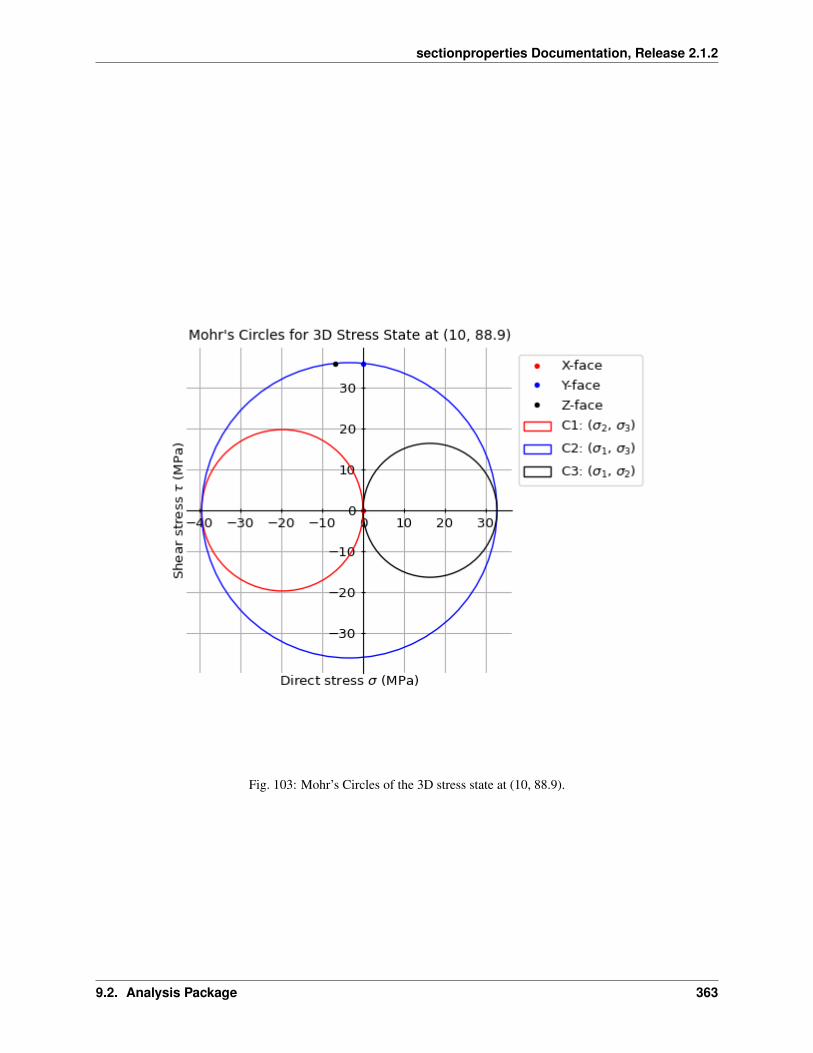
sectionproperties Documentation, Release 2.1.2
Fig. 103: Mohr’s Circles of the 3D stress state at (10, 88.9).
9.2. Analysis Package 363

sectionproperties Documentation, Release 2.1.2
import sectionproperties.pre.library.steel_sections as steel_sectionsfrom sectionproperties.analysis.section import Section
geometry = steel_sections.angle_section(d=150, b=90, t=12, r_r=10, r_t=5, n_→˓r=8)mesh = geometry.create_mesh(mesh_sizes=[2.5])section = CrossSection(geometry, mesh)
section.calculate_geometric_properties()section.calculate_warping_properties()stress_post = section.calculate_stress(
N=50e3, Mxx=-5e6, M22=2.5e6, Mzz=0.5e6, Vx=10e3, Vy=5e3)
stress_post.plot_stress_1()
Fig. 104: Contour plot of the major principal stress.
plot_stress_3(title=’Stress Contour Plot - $\\sigma_3$’, cmap=’coolwarm’, normalize=True,**kwargs)
Produces a contour plot of the Minor principal stress 𝜎3 resulting from all actions.
Parameters
• title (string) – Plot title
• cmap (string) – Matplotlib color map.
• normalize (bool) – If set to true, the CenteredNorm is used to scale the colormap. Ifset to false, the default linear scaling is used.
• kwargs – Passed to plotting_context()
Returns Matplotlib axes object
Return type matplotlib.axes
The following example plots a contour of the Minor principal stress within a 150x90x12 UA sectionresulting from the following actions:
• 𝑁 = 50 kN
• 𝑀𝑥𝑥 = −5 kN.m
364 Chapter 9. Python API Reference
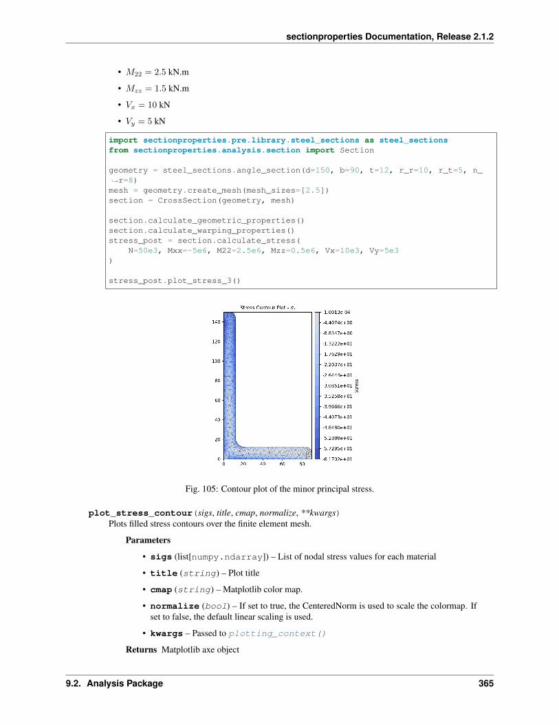
sectionproperties Documentation, Release 2.1.2
• 𝑀22 = 2.5 kN.m
• 𝑀𝑧𝑧 = 1.5 kN.m
• 𝑉𝑥 = 10 kN
• 𝑉𝑦 = 5 kN
import sectionproperties.pre.library.steel_sections as steel_sectionsfrom sectionproperties.analysis.section import Section
geometry = steel_sections.angle_section(d=150, b=90, t=12, r_r=10, r_t=5, n_→˓r=8)mesh = geometry.create_mesh(mesh_sizes=[2.5])section = CrossSection(geometry, mesh)
section.calculate_geometric_properties()section.calculate_warping_properties()stress_post = section.calculate_stress(
N=50e3, Mxx=-5e6, M22=2.5e6, Mzz=0.5e6, Vx=10e3, Vy=5e3)
stress_post.plot_stress_3()
Fig. 105: Contour plot of the minor principal stress.
plot_stress_contour(sigs, title, cmap, normalize, **kwargs)Plots filled stress contours over the finite element mesh.
Parameters
• sigs (list[numpy.ndarray]) – List of nodal stress values for each material
• title (string) – Plot title
• cmap (string) – Matplotlib color map.
• normalize (bool) – If set to true, the CenteredNorm is used to scale the colormap. Ifset to false, the default linear scaling is used.
• kwargs – Passed to plotting_context()
Returns Matplotlib axe object
9.2. Analysis Package 365

sectionproperties Documentation, Release 2.1.2
Return type matplotlib.axes
plot_stress_m11_zz(title=’Stress Contour Plot - $\\sigma_zz, M11$’, cmap=’coolwarm’, nor-malize=True, **kwargs)
Produces a contour plot of the normal stress 𝜎𝑧𝑧,𝑀11 resulting from the bending moment 𝑀11.
Parameters
• title (string) – Plot title
• cmap (string) – Matplotlib color map.
• normalize (bool) – If set to true, the CenteredNorm is used to scale the colormap. Ifset to false, the default linear scaling is used.
• kwargs – Passed to plotting_context()
Returns Matplotlib axes object
Return type matplotlib.axes
The following example plots the normal stress within a 150x90x12 UA section resulting from a bendingmoment about the 11-axis of 5 kN.m:
import sectionproperties.pre.library.steel_sections as steel_sectionsfrom sectionproperties.analysis.section import Section
geometry = steel_sections.angle_section(d=150, b=90, t=12, r_r=10, r_t=5, n_→˓r=8)geometry.create_mesh(mesh_sizes=[20])section = Section(geometry)
section.calculate_geometric_properties()section.calculate_warping_properties()stress_post = section.calculate_stress(M11=5e6)
stress_post.plot_stress_m11_zz()
Fig. 106: Contour plot of the bending stress.
plot_stress_m22_zz(title=’Stress Contour Plot - $\\sigma_zz, M22$’, cmap=’coolwarm’, nor-malize=True, **kwargs)
Produces a contour plot of the normal stress 𝜎𝑧𝑧,𝑀22 resulting from the bending moment 𝑀22.
366 Chapter 9. Python API Reference

sectionproperties Documentation, Release 2.1.2
Parameters
• title (string) – Plot title
• cmap (string) – Matplotlib color map.
• normalize (bool) – If set to true, the CenteredNorm is used to scale the colormap. Ifset to false, the default linear scaling is used.
• kwargs – Passed to plotting_context()
Returns Matplotlib axes object
Return type matplotlib.axes
The following example plots the normal stress within a 150x90x12 UA section resulting from a bendingmoment about the 22-axis of 2 kN.m:
import sectionproperties.pre.library.steel_sections as steel_sectionsfrom sectionproperties.analysis.section import Section
geometry = steel_sections.angle_section(d=150, b=90, t=12, r_r=10, r_t=5, n_→˓r=8)geometry.create_mesh(mesh_sizes=[20])section = Section(geometry)
section.calculate_geometric_properties()section.calculate_warping_properties()stress_post = section.calculate_stress(M22=5e6)
stress_post.plot_stress_m22_zz()
Fig. 107: Contour plot of the bending stress.
plot_stress_m_zz(title=’Stress Contour Plot - $\\sigma_zz, \\Sigma M$’, cmap=’coolwarm’, nor-malize=True, **kwargs)
Produces a contour plot of the normal stress 𝜎𝑧𝑧,Σ𝑀 resulting from all bending moments 𝑀𝑥𝑥 + 𝑀𝑦𝑦 +𝑀11 + 𝑀22.
Parameters
• title (string) – Plot title
• cmap (string) – Matplotlib color map.
9.2. Analysis Package 367

sectionproperties Documentation, Release 2.1.2
• normalize (bool) – If set to true, the CenteredNorm is used to scale the colormap. Ifset to false, the default linear scaling is used.
• kwargs – Passed to plotting_context()
Returns Matplotlib axes object
Return type matplotlib.axes
The following example plots the normal stress within a 150x90x12 UA section resulting from a bendingmoment about the x-axis of 5 kN.m, a bending moment about the y-axis of 2 kN.m and a bending momentof 3 kN.m about the 11-axis:
import sectionproperties.pre.library.steel_sections as steel_sectionsfrom sectionproperties.analysis.section import Section
geometry = steel_sections.angle_section(d=150, b=90, t=12, r_r=10, r_t=5, n_→˓r=8)geometry.create_mesh(mesh_sizes=[20])section = Section(geometry)
section.calculate_geometric_properties()section.calculate_warping_properties()stress_post = section.calculate_stress(Mxx=5e6, Myy=2e6, M11=3e6)
stress_post.plot_stress_m_zz()
Fig. 108: Contour plot of the bending stress.
plot_stress_mxx_zz(title=’Stress Contour Plot - $\\sigma_zz, Mxx$’, cmap=’coolwarm’, nor-malize=True, **kwargs)
Produces a contour plot of the normal stress 𝜎𝑧𝑧,𝑀𝑥𝑥 resulting from the bending moment 𝑀𝑥𝑥.
Parameters
• title (string) – Plot title
• cmap (string) – Matplotlib color map.
• normalize (bool) – If set to true, the CenteredNorm is used to scale the colormap. Ifset to false, the default linear scaling is used.
• kwargs – Passed to plotting_context()
368 Chapter 9. Python API Reference

sectionproperties Documentation, Release 2.1.2
Returns Matplotlib axes object
Return type matplotlib.axes
The following example plots the normal stress within a 150x90x12 UA section resulting from a bendingmoment about the x-axis of 5 kN.m:
import sectionproperties.pre.library.steel_sections as steel_sectionsfrom sectionproperties.analysis.section import Section
geometry = steel_sections.angle_section(d=150, b=90, t=12, r_r=10, r_t=5, n_→˓r=8)geometry.create_mesh(mesh_sizes=[20])section = Section(geometry)
section.calculate_geometric_properties()section.calculate_warping_properties()stress_post = section.calculate_stress(Mxx=5e6)
stress_post.plot_stress_mxx_zz()
Fig. 109: Contour plot of the bending stress.
plot_stress_myy_zz(title=’Stress Contour Plot - $\\sigma_zz, Myy$’, cmap=’coolwarm’, nor-malize=True, **kwargs)
Produces a contour plot of the normal stress 𝜎𝑧𝑧,𝑀𝑦𝑦 resulting from the bending moment 𝑀𝑦𝑦 .
Parameters
• title (string) – Plot title
• cmap (string) – Matplotlib color map.
• normalize (bool) – If set to true, the CenteredNorm is used to scale the colormap. Ifset to false, the default linear scaling is used.
• kwargs – Passed to plotting_context()
Returns Matplotlib axes object
Return type matplotlib.axes
The following example plots the normal stress within a 150x90x12 UA section resulting from a bendingmoment about the y-axis of 2 kN.m:
9.2. Analysis Package 369

sectionproperties Documentation, Release 2.1.2
import sectionproperties.pre.library.steel_sections as steel_sectionsfrom sectionproperties.analysis.section import Section
geometry = steel_sections.angle_section(d=150, b=90, t=12, r_r=10, r_t=5, n_→˓r=8)geometry.create_mesh(mesh_sizes=[20])section = Section(geometry)
section.calculate_geometric_properties()section.calculate_warping_properties()stress_post = section.calculate_stress(Myy=2e6)
stress_post.plot_stress_myy_zz()
Fig. 110: Contour plot of the bending stress.
plot_stress_mzz_zx(title=’Stress Contour Plot - $\\sigma_zx, Mzz$’, cmap=’coolwarm’, nor-malize=True, **kwargs)
Produces a contour plot of the x-component of the shear stress 𝜎𝑧𝑥,𝑀𝑧𝑧 resulting from the torsion moment𝑀𝑧𝑧 .
Parameters
• title (string) – Plot title
• cmap (string) – Matplotlib color map.
• normalize (bool) – If set to true, the CenteredNorm is used to scale the colormap. Ifset to false, the default linear scaling is used.
• kwargs – Passed to plotting_context()
Returns Matplotlib axes object
Return type matplotlib.axes
The following example plots the x-component of the shear stress within a 150x90x12 UA section resultingfrom a torsion moment of 1 kN.m:
import sectionproperties.pre.library.steel_sections as steel_sectionsfrom sectionproperties.analysis.section import Section
(continues on next page)
370 Chapter 9. Python API Reference
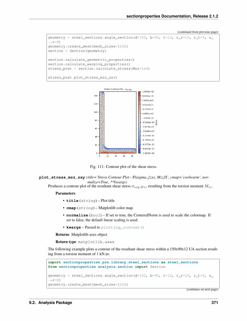
sectionproperties Documentation, Release 2.1.2
(continued from previous page)
geometry = steel_sections.angle_section(d=150, b=90, t=12, r_r=10, r_t=5, n_→˓r=8)geometry.create_mesh(mesh_sizes=[20])section = Section(geometry)
section.calculate_geometric_properties()section.calculate_warping_properties()stress_post = section.calculate_stress(Mzz=1e6)
stress_post.plot_stress_mzz_zx()
Fig. 111: Contour plot of the shear stress.
plot_stress_mzz_zxy(title=’Stress Contour Plot - $\\sigma_zxy, Mzz$’, cmap=’coolwarm’, nor-malize=True, **kwargs)
Produces a contour plot of the resultant shear stress 𝜎𝑧𝑥𝑦,𝑀𝑧𝑧 resulting from the torsion moment 𝑀𝑧𝑧 .
Parameters
• title (string) – Plot title
• cmap (string) – Matplotlib color map.
• normalize (bool) – If set to true, the CenteredNorm is used to scale the colormap. Ifset to false, the default linear scaling is used.
• kwargs – Passed to plotting_context()
Returns Matplotlib axes object
Return type matplotlib.axes
The following example plots a contour of the resultant shear stress within a 150x90x12 UA section result-ing from a torsion moment of 1 kN.m:
import sectionproperties.pre.library.steel_sections as steel_sectionsfrom sectionproperties.analysis.section import Section
geometry = steel_sections.angle_section(d=150, b=90, t=12, r_r=10, r_t=5, n_→˓r=8)geometry.create_mesh(mesh_sizes=[20])
(continues on next page)
9.2. Analysis Package 371

sectionproperties Documentation, Release 2.1.2
(continued from previous page)
section = Section(geometry)
section.calculate_geometric_properties()section.calculate_warping_properties()stress_post = section.calculate_stress(Mzz=1e6)
stress_post.plot_stress_mzz_zxy()
Fig. 112: Contour plot of the shear stress.
plot_stress_mzz_zy(title=’Stress Contour Plot - $\\sigma_zy, Mzz$’, cmap=’coolwarm’, nor-malize=True, **kwargs)
Produces a contour plot of the y-component of the shear stress 𝜎𝑧𝑦,𝑀𝑧𝑧 resulting from the torsion moment𝑀𝑧𝑧 .
Parameters
• title (string) – Plot title
• cmap (string) – Matplotlib color map.
• normalize (bool) – If set to true, the CenteredNorm is used to scale the colormap. Ifset to false, the default linear scaling is used.
• kwargs – Passed to plotting_context()
Returns Matplotlib axes object
Return type matplotlib.axes
The following example plots the y-component of the shear stress within a 150x90x12 UA section resultingfrom a torsion moment of 1 kN.m:
import sectionproperties.pre.library.steel_sections as steel_sectionsfrom sectionproperties.analysis.section import Section
geometry = steel_sections.angle_section(d=150, b=90, t=12, r_r=10, r_t=5, n_→˓r=8)geometry.create_mesh(mesh_sizes=[20])section = Section(geometry)
(continues on next page)
372 Chapter 9. Python API Reference
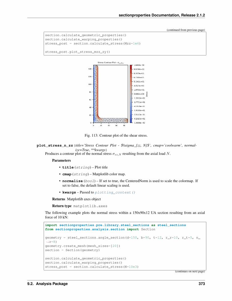
sectionproperties Documentation, Release 2.1.2
(continued from previous page)
section.calculate_geometric_properties()section.calculate_warping_properties()stress_post = section.calculate_stress(Mzz=1e6)
stress_post.plot_stress_mzz_zy()
Fig. 113: Contour plot of the shear stress.
plot_stress_n_zz(title=’Stress Contour Plot - $\\sigma_zz, N$’, cmap=’coolwarm’, normal-ize=True, **kwargs)
Produces a contour plot of the normal stress 𝜎𝑧𝑧,𝑁 resulting from the axial load 𝑁 .
Parameters
• title (string) – Plot title
• cmap (string) – Matplotlib color map.
• normalize (bool) – If set to true, the CenteredNorm is used to scale the colormap. Ifset to false, the default linear scaling is used.
• kwargs – Passed to plotting_context()
Returns Matplotlib axes object
Return type matplotlib.axes
The following example plots the normal stress within a 150x90x12 UA section resulting from an axialforce of 10 kN:
import sectionproperties.pre.library.steel_sections as steel_sectionsfrom sectionproperties.analysis.section import Section
geometry = steel_sections.angle_section(d=150, b=90, t=12, r_r=10, r_t=5, n_→˓r=8)geometry.create_mesh(mesh_sizes=[20])section = Section(geometry)
section.calculate_geometric_properties()section.calculate_warping_properties()stress_post = section.calculate_stress(N=10e3)
(continues on next page)
9.2. Analysis Package 373
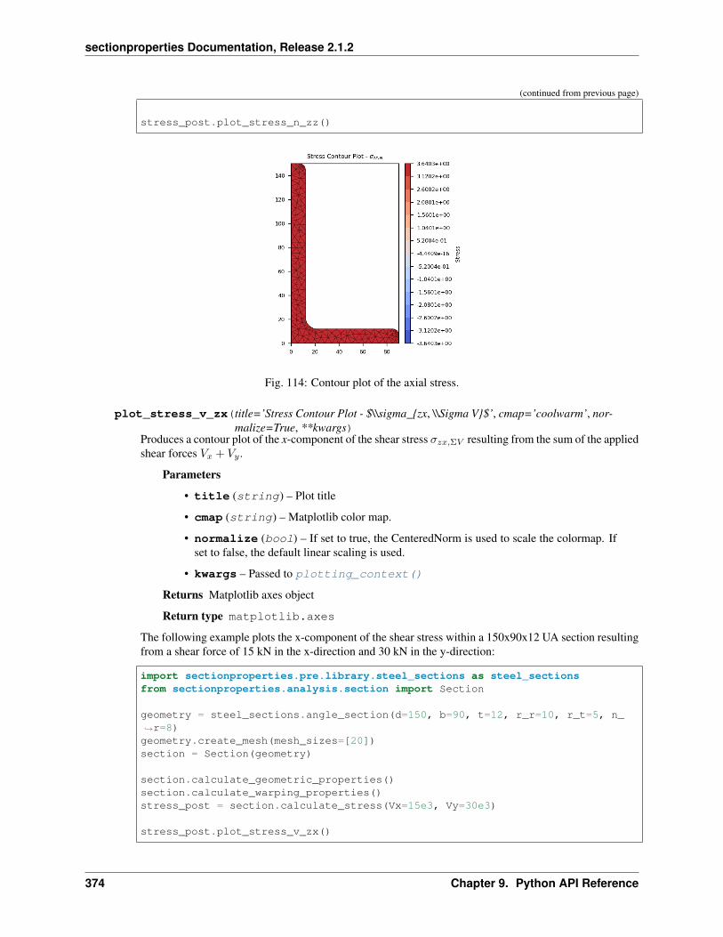
sectionproperties Documentation, Release 2.1.2
(continued from previous page)
stress_post.plot_stress_n_zz()
Fig. 114: Contour plot of the axial stress.
plot_stress_v_zx(title=’Stress Contour Plot - $\\sigma_zx, \\Sigma V$’, cmap=’coolwarm’, nor-malize=True, **kwargs)
Produces a contour plot of the x-component of the shear stress 𝜎𝑧𝑥,Σ𝑉 resulting from the sum of the appliedshear forces 𝑉𝑥 + 𝑉𝑦 .
Parameters
• title (string) – Plot title
• cmap (string) – Matplotlib color map.
• normalize (bool) – If set to true, the CenteredNorm is used to scale the colormap. Ifset to false, the default linear scaling is used.
• kwargs – Passed to plotting_context()
Returns Matplotlib axes object
Return type matplotlib.axes
The following example plots the x-component of the shear stress within a 150x90x12 UA section resultingfrom a shear force of 15 kN in the x-direction and 30 kN in the y-direction:
import sectionproperties.pre.library.steel_sections as steel_sectionsfrom sectionproperties.analysis.section import Section
geometry = steel_sections.angle_section(d=150, b=90, t=12, r_r=10, r_t=5, n_→˓r=8)geometry.create_mesh(mesh_sizes=[20])section = Section(geometry)
section.calculate_geometric_properties()section.calculate_warping_properties()stress_post = section.calculate_stress(Vx=15e3, Vy=30e3)
stress_post.plot_stress_v_zx()
374 Chapter 9. Python API Reference
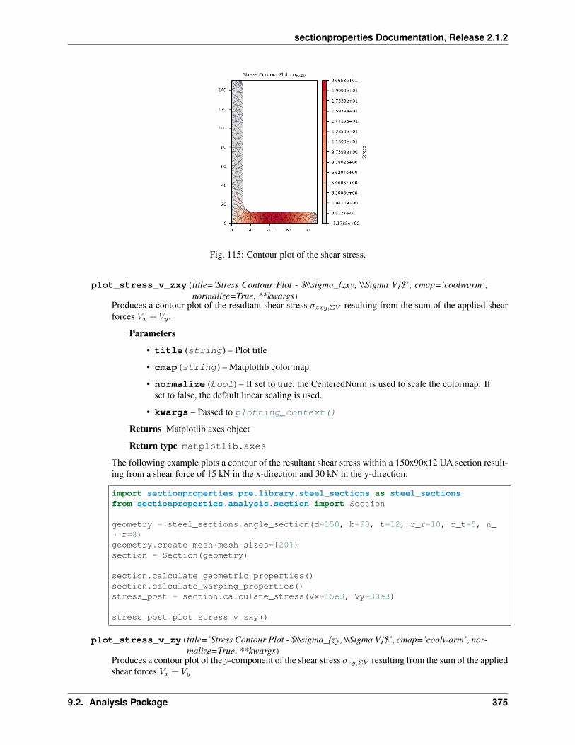
sectionproperties Documentation, Release 2.1.2
Fig. 115: Contour plot of the shear stress.
plot_stress_v_zxy(title=’Stress Contour Plot - $\\sigma_zxy, \\Sigma V$’, cmap=’coolwarm’,normalize=True, **kwargs)
Produces a contour plot of the resultant shear stress 𝜎𝑧𝑥𝑦,Σ𝑉 resulting from the sum of the applied shearforces 𝑉𝑥 + 𝑉𝑦 .
Parameters
• title (string) – Plot title
• cmap (string) – Matplotlib color map.
• normalize (bool) – If set to true, the CenteredNorm is used to scale the colormap. Ifset to false, the default linear scaling is used.
• kwargs – Passed to plotting_context()
Returns Matplotlib axes object
Return type matplotlib.axes
The following example plots a contour of the resultant shear stress within a 150x90x12 UA section result-ing from a shear force of 15 kN in the x-direction and 30 kN in the y-direction:
import sectionproperties.pre.library.steel_sections as steel_sectionsfrom sectionproperties.analysis.section import Section
geometry = steel_sections.angle_section(d=150, b=90, t=12, r_r=10, r_t=5, n_→˓r=8)geometry.create_mesh(mesh_sizes=[20])section = Section(geometry)
section.calculate_geometric_properties()section.calculate_warping_properties()stress_post = section.calculate_stress(Vx=15e3, Vy=30e3)
stress_post.plot_stress_v_zxy()
plot_stress_v_zy(title=’Stress Contour Plot - $\\sigma_zy, \\Sigma V$’, cmap=’coolwarm’, nor-malize=True, **kwargs)
Produces a contour plot of the y-component of the shear stress 𝜎𝑧𝑦,Σ𝑉 resulting from the sum of the appliedshear forces 𝑉𝑥 + 𝑉𝑦 .
9.2. Analysis Package 375
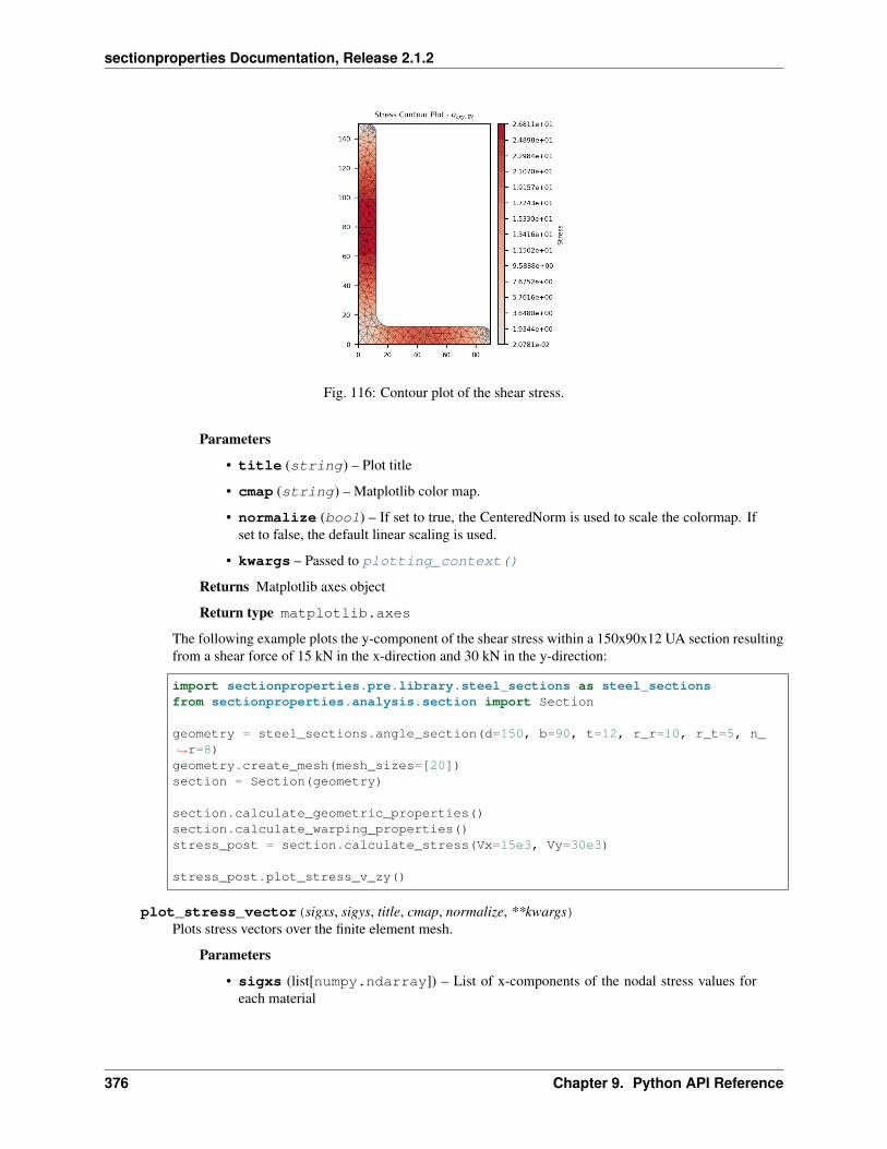
sectionproperties Documentation, Release 2.1.2
Fig. 116: Contour plot of the shear stress.
Parameters
• title (string) – Plot title
• cmap (string) – Matplotlib color map.
• normalize (bool) – If set to true, the CenteredNorm is used to scale the colormap. Ifset to false, the default linear scaling is used.
• kwargs – Passed to plotting_context()
Returns Matplotlib axes object
Return type matplotlib.axes
The following example plots the y-component of the shear stress within a 150x90x12 UA section resultingfrom a shear force of 15 kN in the x-direction and 30 kN in the y-direction:
import sectionproperties.pre.library.steel_sections as steel_sectionsfrom sectionproperties.analysis.section import Section
geometry = steel_sections.angle_section(d=150, b=90, t=12, r_r=10, r_t=5, n_→˓r=8)geometry.create_mesh(mesh_sizes=[20])section = Section(geometry)
section.calculate_geometric_properties()section.calculate_warping_properties()stress_post = section.calculate_stress(Vx=15e3, Vy=30e3)
stress_post.plot_stress_v_zy()
plot_stress_vector(sigxs, sigys, title, cmap, normalize, **kwargs)Plots stress vectors over the finite element mesh.
Parameters
• sigxs (list[numpy.ndarray]) – List of x-components of the nodal stress values foreach material
376 Chapter 9. Python API Reference
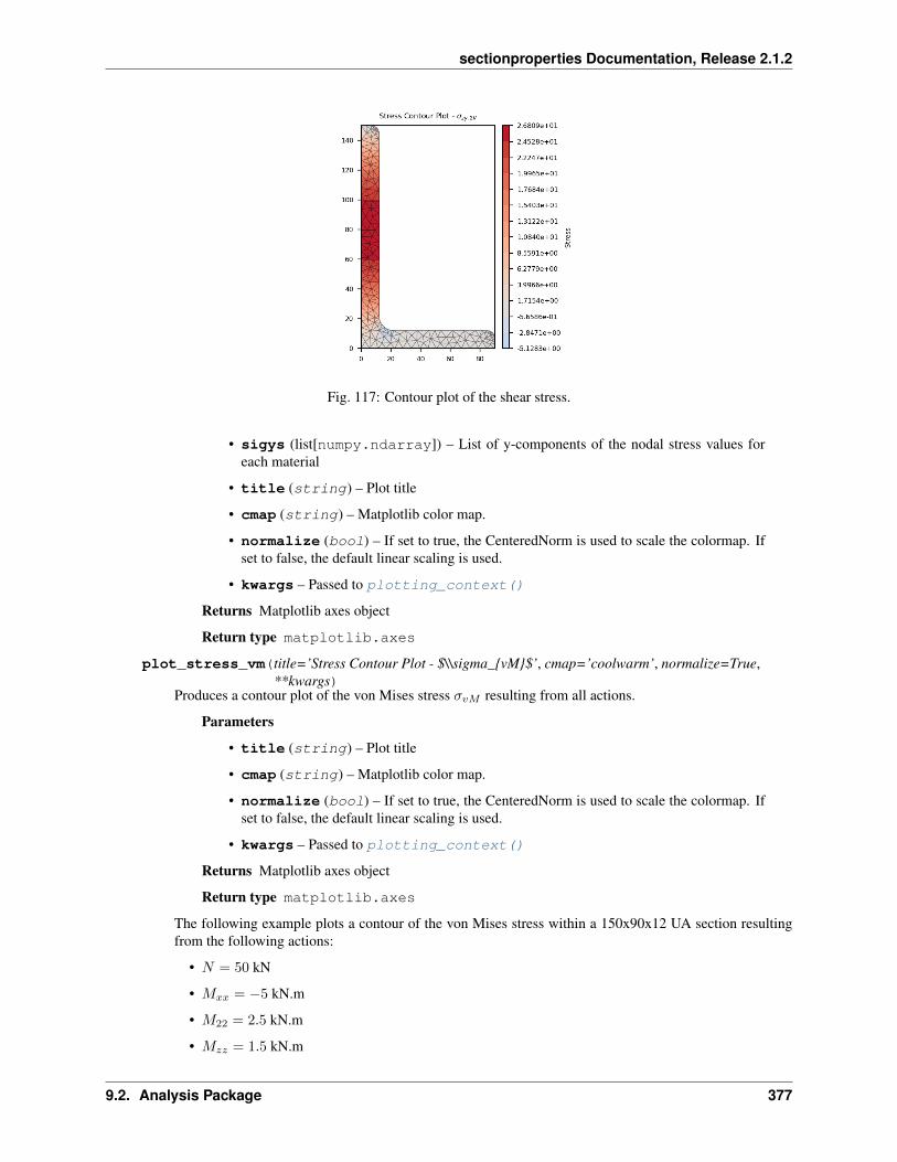
sectionproperties Documentation, Release 2.1.2
Fig. 117: Contour plot of the shear stress.
• sigys (list[numpy.ndarray]) – List of y-components of the nodal stress values foreach material
• title (string) – Plot title
• cmap (string) – Matplotlib color map.
• normalize (bool) – If set to true, the CenteredNorm is used to scale the colormap. Ifset to false, the default linear scaling is used.
• kwargs – Passed to plotting_context()
Returns Matplotlib axes object
Return type matplotlib.axes
plot_stress_vm(title=’Stress Contour Plot - $\\sigma_vM$’, cmap=’coolwarm’, normalize=True,**kwargs)
Produces a contour plot of the von Mises stress 𝜎𝑣𝑀 resulting from all actions.
Parameters
• title (string) – Plot title
• cmap (string) – Matplotlib color map.
• normalize (bool) – If set to true, the CenteredNorm is used to scale the colormap. Ifset to false, the default linear scaling is used.
• kwargs – Passed to plotting_context()
Returns Matplotlib axes object
Return type matplotlib.axes
The following example plots a contour of the von Mises stress within a 150x90x12 UA section resultingfrom the following actions:
• 𝑁 = 50 kN
• 𝑀𝑥𝑥 = −5 kN.m
• 𝑀22 = 2.5 kN.m
• 𝑀𝑧𝑧 = 1.5 kN.m
9.2. Analysis Package 377
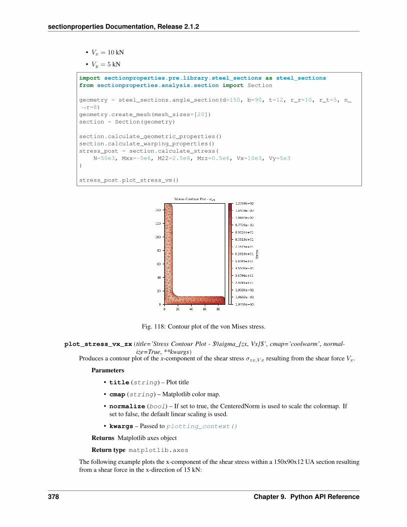
sectionproperties Documentation, Release 2.1.2
• 𝑉𝑥 = 10 kN
• 𝑉𝑦 = 5 kN
import sectionproperties.pre.library.steel_sections as steel_sectionsfrom sectionproperties.analysis.section import Section
geometry = steel_sections.angle_section(d=150, b=90, t=12, r_r=10, r_t=5, n_→˓r=8)geometry.create_mesh(mesh_sizes=[20])section = Section(geometry)
section.calculate_geometric_properties()section.calculate_warping_properties()stress_post = section.calculate_stress(
N=50e3, Mxx=-5e6, M22=2.5e6, Mzz=0.5e6, Vx=10e3, Vy=5e3)
stress_post.plot_stress_vm()
Fig. 118: Contour plot of the von Mises stress.
plot_stress_vx_zx(title=’Stress Contour Plot - $\\sigma_zx, Vx$’, cmap=’coolwarm’, normal-ize=True, **kwargs)
Produces a contour plot of the x-component of the shear stress 𝜎𝑧𝑥,𝑉 𝑥 resulting from the shear force 𝑉𝑥.
Parameters
• title (string) – Plot title
• cmap (string) – Matplotlib color map.
• normalize (bool) – If set to true, the CenteredNorm is used to scale the colormap. Ifset to false, the default linear scaling is used.
• kwargs – Passed to plotting_context()
Returns Matplotlib axes object
Return type matplotlib.axes
The following example plots the x-component of the shear stress within a 150x90x12 UA section resultingfrom a shear force in the x-direction of 15 kN:
378 Chapter 9. Python API Reference

sectionproperties Documentation, Release 2.1.2
import sectionproperties.pre.library.steel_sections as steel_sectionsfrom sectionproperties.analysis.section import Section
geometry = steel_sections.angle_section(d=150, b=90, t=12, r_r=10, r_t=5, n_→˓r=8)geometry.create_mesh(mesh_sizes=[20])section = Section(geometry)
section.calculate_geometric_properties()section.calculate_warping_properties()stress_post = section.calculate_stress(Vx=15e3)
stress_post.plot_stress_vx_zx()
Fig. 119: Contour plot of the shear stress.
plot_stress_vx_zxy(title=’Stress Contour Plot - $\\sigma_zz, Myy$’, cmap=’coolwarm’, nor-malize=True, **kwargs)
Produces a contour plot of the resultant shear stress 𝜎𝑧𝑥𝑦,𝑉 𝑥 resulting from the shear force 𝑉𝑥.
Parameters
• title (string) – Plot title
• cmap (string) – Matplotlib color map.
• normalize (bool) – If set to true, the CenteredNorm is used to scale the colormap. Ifset to false, the default linear scaling is used.
• kwargs – Passed to plotting_context()
Returns Matplotlib axes object
Return type matplotlib.axes
The following example plots a contour of the resultant shear stress within a 150x90x12 UA section result-ing from a shear force in the x-direction of 15 kN:
import sectionproperties.pre.library.steel_sections as steel_sectionsfrom sectionproperties.analysis.section import Section
geometry = steel_sections.angle_section(d=150, b=90, t=12, r_r=10, r_t=5, n_→˓r=8) (continues on next page)
9.2. Analysis Package 379

sectionproperties Documentation, Release 2.1.2
(continued from previous page)
geometry.create_mesh(mesh_sizes=[20])section = Section(geometry)
section.calculate_geometric_properties()section.calculate_warping_properties()stress_post = section.calculate_stress(Vx=15e3)
stress_post.plot_stress_vx_zxy()
Fig. 120: Contour plot of the shear stress.
plot_stress_vx_zy(title=’Stress Contour Plot - $\\sigma_zy, Vx$’, cmap=’coolwarm’, normal-ize=True, **kwargs)
Produces a contour plot of the y-component of the shear stress 𝜎𝑧𝑦,𝑉 𝑥 resulting from the shear force 𝑉𝑥.
Parameters
• title (string) – Plot title
• cmap (string) – Matplotlib color map.
• normalize (bool) – If set to true, the CenteredNorm is used to scale the colormap. Ifset to false, the default linear scaling is used.
• kwargs – Passed to plotting_context()
Returns Matplotlib axes object
Return type matplotlib.axes
The following example plots the y-component of the shear stress within a 150x90x12 UA section resultingfrom a shear force in the x-direction of 15 kN:
import sectionproperties.pre.library.steel_sections as steel_sectionsfrom sectionproperties.analysis.section import Section
geometry = steel_sections.angle_section(d=150, b=90, t=12, r_r=10, r_t=5, n_→˓r=8)geometry.create_mesh(mesh_sizes=[20])section = Section(geometry)
(continues on next page)
380 Chapter 9. Python API Reference

sectionproperties Documentation, Release 2.1.2
(continued from previous page)
section.calculate_geometric_properties()section.calculate_warping_properties()stress_post = section.calculate_stress(Vx=15e3)
stress_post.plot_stress_vx_zy()
Fig. 121: Contour plot of the shear stress.
plot_stress_vy_zx(title=’Stress Contour Plot - $\\sigma_zx, Vy$’, cmap=’coolwarm’, normal-ize=True, **kwargs)
Produces a contour plot of the x-component of the shear stress 𝜎𝑧𝑥,𝑉 𝑦 resulting from the shear force 𝑉𝑦 .
Parameters
• title (string) – Plot title
• cmap (string) – Matplotlib color map.
• normalize (bool) – If set to true, the CenteredNorm is used to scale the colormap. Ifset to false, the default linear scaling is used.
• kwargs – Passed to plotting_context()
Returns Matplotlib axes object
Return type matplotlib.axes
The following example plots the x-component of the shear stress within a 150x90x12 UA section resultingfrom a shear force in the y-direction of 30 kN:
import sectionproperties.pre.library.steel_sections as steel_sectionsfrom sectionproperties.analysis.section import Section
geometry = steel_sections.angle_section(d=150, b=90, t=12, r_r=10, r_t=5, n_→˓r=8)geometry.create_mesh(mesh_sizes=[20])section = Section(geometry)
section.calculate_geometric_properties()section.calculate_warping_properties()stress_post = section.calculate_stress(Vy=30e3)
(continues on next page)
9.2. Analysis Package 381
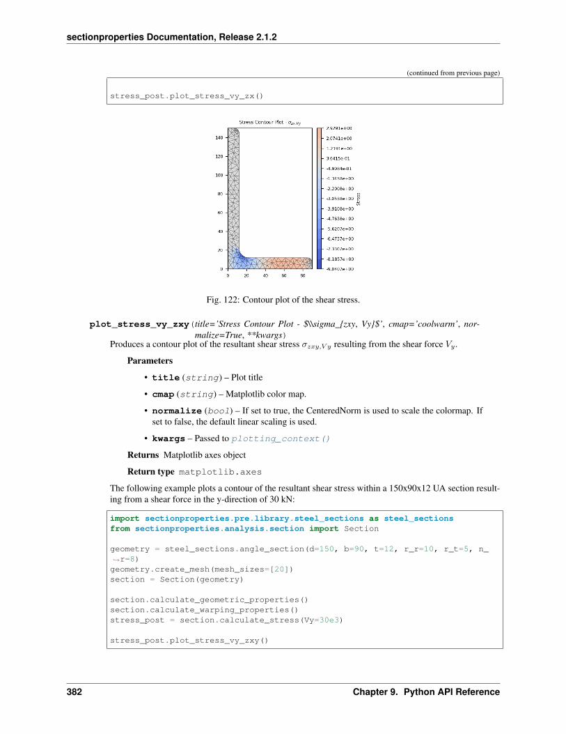
sectionproperties Documentation, Release 2.1.2
(continued from previous page)
stress_post.plot_stress_vy_zx()
Fig. 122: Contour plot of the shear stress.
plot_stress_vy_zxy(title=’Stress Contour Plot - $\\sigma_zxy, Vy$’, cmap=’coolwarm’, nor-malize=True, **kwargs)
Produces a contour plot of the resultant shear stress 𝜎𝑧𝑥𝑦,𝑉 𝑦 resulting from the shear force 𝑉𝑦 .
Parameters
• title (string) – Plot title
• cmap (string) – Matplotlib color map.
• normalize (bool) – If set to true, the CenteredNorm is used to scale the colormap. Ifset to false, the default linear scaling is used.
• kwargs – Passed to plotting_context()
Returns Matplotlib axes object
Return type matplotlib.axes
The following example plots a contour of the resultant shear stress within a 150x90x12 UA section result-ing from a shear force in the y-direction of 30 kN:
import sectionproperties.pre.library.steel_sections as steel_sectionsfrom sectionproperties.analysis.section import Section
geometry = steel_sections.angle_section(d=150, b=90, t=12, r_r=10, r_t=5, n_→˓r=8)geometry.create_mesh(mesh_sizes=[20])section = Section(geometry)
section.calculate_geometric_properties()section.calculate_warping_properties()stress_post = section.calculate_stress(Vy=30e3)
stress_post.plot_stress_vy_zxy()
382 Chapter 9. Python API Reference
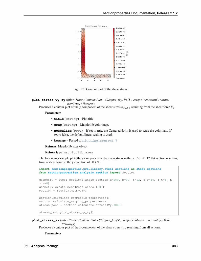
sectionproperties Documentation, Release 2.1.2
Fig. 123: Contour plot of the shear stress.
plot_stress_vy_zy(title=’Stress Contour Plot - $\\sigma_zy, Vy$’, cmap=’coolwarm’, normal-ize=True, **kwargs)
Produces a contour plot of the y-component of the shear stress 𝜎𝑧𝑦,𝑉 𝑦 resulting from the shear force 𝑉𝑦 .
Parameters
• title (string) – Plot title
• cmap (string) – Matplotlib color map.
• normalize (bool) – If set to true, the CenteredNorm is used to scale the colormap. Ifset to false, the default linear scaling is used.
• kwargs – Passed to plotting_context()
Returns Matplotlib axes object
Return type matplotlib.axes
The following example plots the y-component of the shear stress within a 150x90x12 UA section resultingfrom a shear force in the y-direction of 30 kN:
import sectionproperties.pre.library.steel_sections as steel_sectionsfrom sectionproperties.analysis.section import Section
geometry = steel_sections.angle_section(d=150, b=90, t=12, r_r=10, r_t=5, n_→˓r=8)geometry.create_mesh(mesh_sizes=[20])section = Section(geometry)
section.calculate_geometric_properties()section.calculate_warping_properties()stress_post = section.calculate_stress(Vy=30e3)
stress_post.plot_stress_vy_zy()
plot_stress_zx(title=’Stress Contour Plot - $\\sigma_zx$’, cmap=’coolwarm’, normalize=True,**kwargs)
Produces a contour plot of the x-component of the shear stress 𝜎𝑧𝑥 resulting from all actions.
Parameters
9.2. Analysis Package 383

sectionproperties Documentation, Release 2.1.2
Fig. 124: Contour plot of the shear stress.
• title (string) – Plot title
• cmap (string) – Matplotlib color map.
• normalize (bool) – If set to true, the CenteredNorm is used to scale the colormap. Ifset to false, the default linear scaling is used.
• kwargs – Passed to plotting_context()
Returns Matplotlib axes object
Return type matplotlib.axes
The following example plots the x-component of the shear stress within a 150x90x12 UA section resultingfrom a torsion moment of 1 kN.m and a shear force of 30 kN in the y-direction:
import sectionproperties.pre.library.steel_sections as steel_sectionsfrom sectionproperties.analysis.section import Section
geometry = steel_sections.angle_section(d=150, b=90, t=12, r_r=10, r_t=5, n_→˓r=8)geometry.create_mesh(mesh_sizes=[20])section = Section(geometry)
section.calculate_geometric_properties()section.calculate_warping_properties()stress_post = section.calculate_stress(Mzz=1e6, Vy=30e3)
stress_post.plot_stress_zx()
plot_stress_zxy(title=’Stress Contour Plot - $\\sigma_zxy$’, cmap=’coolwarm’, normal-ize=True, **kwargs)
Produces a contour plot of the resultant shear stress 𝜎𝑧𝑥𝑦 resulting from all actions.
Parameters
• title (string) – Plot title
• cmap (string) – Matplotlib color map.
• normalize (bool) – If set to true, the CenteredNorm is used to scale the colormap. Ifset to false, the default linear scaling is used.
384 Chapter 9. Python API Reference
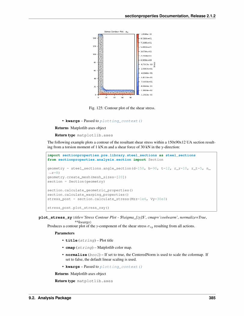
sectionproperties Documentation, Release 2.1.2
Fig. 125: Contour plot of the shear stress.
• kwargs – Passed to plotting_context()
Returns Matplotlib axes object
Return type matplotlib.axes
The following example plots a contour of the resultant shear stress within a 150x90x12 UA section result-ing from a torsion moment of 1 kN.m and a shear force of 30 kN in the y-direction:
import sectionproperties.pre.library.steel_sections as steel_sectionsfrom sectionproperties.analysis.section import Section
geometry = steel_sections.angle_section(d=150, b=90, t=12, r_r=10, r_t=5, n_→˓r=8)geometry.create_mesh(mesh_sizes=[20])section = Section(geometry)
section.calculate_geometric_properties()section.calculate_warping_properties()stress_post = section.calculate_stress(Mzz=1e6, Vy=30e3)
stress_post.plot_stress_zxy()
plot_stress_zy(title=’Stress Contour Plot - $\\sigma_zy$’, cmap=’coolwarm’, normalize=True,**kwargs)
Produces a contour plot of the y-component of the shear stress 𝜎𝑧𝑦 resulting from all actions.
Parameters
• title (string) – Plot title
• cmap (string) – Matplotlib color map.
• normalize (bool) – If set to true, the CenteredNorm is used to scale the colormap. Ifset to false, the default linear scaling is used.
• kwargs – Passed to plotting_context()
Returns Matplotlib axes object
Return type matplotlib.axes
9.2. Analysis Package 385
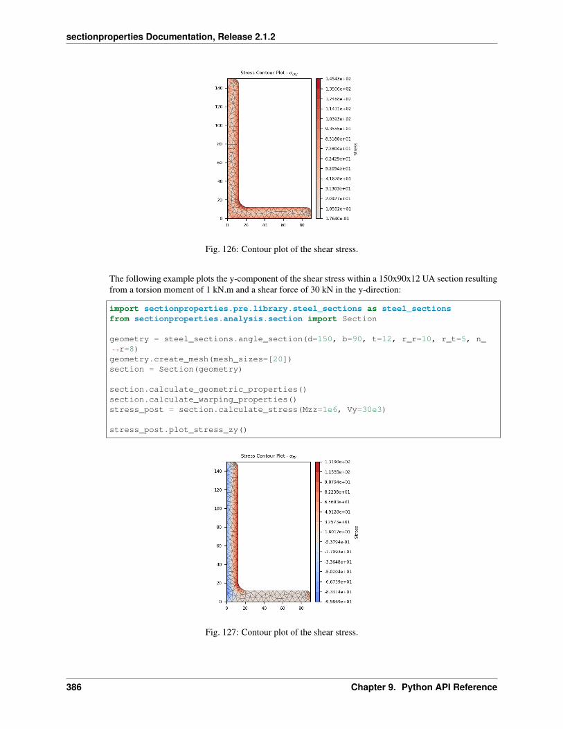
sectionproperties Documentation, Release 2.1.2
Fig. 126: Contour plot of the shear stress.
The following example plots the y-component of the shear stress within a 150x90x12 UA section resultingfrom a torsion moment of 1 kN.m and a shear force of 30 kN in the y-direction:
import sectionproperties.pre.library.steel_sections as steel_sectionsfrom sectionproperties.analysis.section import Section
geometry = steel_sections.angle_section(d=150, b=90, t=12, r_r=10, r_t=5, n_→˓r=8)geometry.create_mesh(mesh_sizes=[20])section = Section(geometry)
section.calculate_geometric_properties()section.calculate_warping_properties()stress_post = section.calculate_stress(Mzz=1e6, Vy=30e3)
stress_post.plot_stress_zy()
Fig. 127: Contour plot of the shear stress.
386 Chapter 9. Python API Reference

sectionproperties Documentation, Release 2.1.2
plot_stress_zz(title=’Stress Contour Plot - $\\sigma_zz$’, cmap=’coolwarm’, normalize=True,**kwargs)
Produces a contour plot of the combined normal stress 𝜎𝑧𝑧 resulting from all actions.
Parameters
• title (string) – Plot title
• cmap (string) – Matplotlib color map.
• normalize (bool) – If set to true, the CenteredNorm is used to scale the colormap. Ifset to false, the default linear scaling is used.
• kwargs – Passed to plotting_context()
Returns Matplotlib axes object
Return type matplotlib.axes
The following example plots the normal stress within a 150x90x12 UA section resulting from an axialforce of 100 kN, a bending moment about the x-axis of 5 kN.m and a bending moment about the y-axis of2 kN.m:
import sectionproperties.pre.library.steel_sections as steel_sectionsfrom sectionproperties.analysis.section import Section
geometry = steel_sections.angle_section(d=150, b=90, t=12, r_r=10, r_t=5, n_→˓r=8)geometry.create_mesh(mesh_sizes=[20])section = Section(geometry)
section.calculate_geometric_properties()section.calculate_warping_properties()stress_post = section.calculate_stress(N=100e3, Mxx=5e6, Myy=2e6)
stress_post.plot_stress_zz()
Fig. 128: Contour plot of the normal stress.
plot_vector_mzz_zxy(title=’Stress Vector Plot - $\\sigma_zxy, Mzz$’, cmap=’YlOrBr’, normal-ize=False, **kwargs)
Produces a vector plot of the resultant shear stress 𝜎𝑧𝑥𝑦,𝑀𝑧𝑧 resulting from the torsion moment 𝑀𝑧𝑧 .
Parameters
9.2. Analysis Package 387

sectionproperties Documentation, Release 2.1.2
• title (string) – Plot title
• cmap (string) – Matplotlib color map.
• normalize (bool) – If set to true, the CenteredNorm is used to scale the colormap. Ifset to false, the default linear scaling is used.
• kwargs – Passed to plotting_context()
Returns Matplotlib axes object
Return type matplotlib.axes
The following example generates a vector plot of the shear stress within a 150x90x12 UA section resultingfrom a torsion moment of 1 kN.m:
import sectionproperties.pre.library.steel_sections as steel_sectionsfrom sectionproperties.analysis.section import Section
geometry = steel_sections.angle_section(d=150, b=90, t=12, r_r=10, r_t=5, n_→˓r=8)geometry.create_mesh(mesh_sizes=[20])section = Section(geometry)
section.calculate_geometric_properties()section.calculate_warping_properties()stress_post = section.calculate_stress(Mzz=1e6)
stress_post.plot_vector_mzz_zxy()
Fig. 129: Vector plot of the shear stress.
plot_vector_v_zxy(title=’Stress Vector Plot - $\\sigma_zxy, \\Sigma V$’, cmap=’YlOrBr’, nor-malize=False, **kwargs)
Produces a vector plot of the resultant shear stress 𝜎𝑧𝑥𝑦,Σ𝑉 resulting from the sum of the applied shearforces 𝑉𝑥 + 𝑉𝑦 .
Parameters
• title (string) – Plot title
• cmap (string) – Matplotlib color map.
388 Chapter 9. Python API Reference

sectionproperties Documentation, Release 2.1.2
• normalize (bool) – If set to true, the CenteredNorm is used to scale the colormap. Ifset to false, the default linear scaling is used.
• kwargs – Passed to plotting_context()
Returns Matplotlib axes object
Return type matplotlib.axes
The following example generates a vector plot of the shear stress within a 150x90x12 UA section resultingfrom a shear force of 15 kN in the x-direction and 30 kN in the y-direction:
import sectionproperties.pre.library.steel_sections as steel_sectionsfrom sectionproperties.analysis.section import Section
geometry = steel_sections.angle_section(d=150, b=90, t=12, r_r=10, r_t=5, n_→˓r=8)geometry.create_mesh(mesh_sizes=[20])section = Section(geometry)
section.calculate_geometric_properties()section.calculate_warping_properties()stress_post = section.calculate_stress(Vx=15e3, Vy=30e3)
stress_post.plot_vector_v_zxy()
Fig. 130: Vector plot of the shear stress.
plot_vector_vx_zxy(title=’Stress Vector Plot - $\\sigma_zxy, Vx$’, cmap=’YlOrBr’, normal-ize=False, **kwargs)
Produces a vector plot of the resultant shear stress 𝜎𝑧𝑥𝑦,𝑉 𝑥 resulting from the shear force 𝑉𝑥.
Parameters
• title (string) – Plot title
• cmap (string) – Matplotlib color map.
• normalize (bool) – If set to true, the CenteredNorm is used to scale the colormap. Ifset to false, the default linear scaling is used.
• kwargs – Passed to plotting_context()
Returns Matplotlib axes object
9.2. Analysis Package 389

sectionproperties Documentation, Release 2.1.2
Return type matplotlib.axes
The following example generates a vector plot of the shear stress within a 150x90x12 UA section resultingfrom a shear force in the x-direction of 15 kN:
import sectionproperties.pre.library.steel_sections as steel_sectionsfrom sectionproperties.analysis.section import Section
geometry = steel_sections.angle_section(d=150, b=90, t=12, r_r=10, r_t=5, n_→˓r=8)geometry.create_mesh(mesh_sizes=[20])section = Section(geometry)
section.calculate_geometric_properties()section.calculate_warping_properties()stress_post = section.calculate_stress(Vx=15e3)
stress_post.plot_vector_vx_zxy()
Fig. 131: Vector plot of the shear stress.
plot_vector_vy_zxy(title=’Stress Vector Plot - $\\sigma_zxy, Vy$’, cmap=’YlOrBr’, normal-ize=False, **kwargs)
Produces a vector plot of the resultant shear stress 𝜎𝑧𝑥𝑦,𝑉 𝑦 resulting from the shear force 𝑉𝑦 .
Parameters
• title (string) – Plot title
• cmap (string) – Matplotlib color map.
• normalize (bool) – If set to true, the CenteredNorm is used to scale the colormap. Ifset to false, the default linear scaling is used.
• kwargs – Passed to plotting_context()
Returns Matplotlib axes object
Return type matplotlib.axes
The following example generates a vector plot of the shear stress within a 150x90x12 UA section resultingfrom a shear force in the y-direction of 30 kN:
390 Chapter 9. Python API Reference

sectionproperties Documentation, Release 2.1.2
import sectionproperties.pre.library.steel_sections as steel_sectionsfrom sectionproperties.analysis.section import Section
geometry = steel_sections.angle_section(d=150, b=90, t=12, r_r=10, r_t=5, n_→˓r=8)geometry.create_mesh(mesh_sizes=[20])section = Section(geometry)
section.calculate_geometric_properties()section.calculate_warping_properties()stress_post = section.calculate_stress(Vy=30e3)
stress_post.plot_vector_vy_zxy()
Fig. 132: Vector plot of the shear stress.
plot_vector_zxy(title=’Stress Vector Plot - $\\sigma_zxy$’, cmap=’YlOrBr’, normalize=False,**kwargs)
Produces a vector plot of the resultant shear stress 𝜎𝑧𝑥𝑦 resulting from all actions.
Parameters
• title (string) – Plot title
• cmap (string) – Matplotlib color map.
• normalize (bool) – If set to true, the CenteredNorm is used to scale the colormap. Ifset to false, the default linear scaling is used.
• kwargs – Passed to plotting_context()
Returns Matplotlib axes object
Return type matplotlib.axes
The following example generates a vector plot of the shear stress within a 150x90x12 UA section resultingfrom a torsion moment of 1 kN.m and a shear force of 30 kN in the y-direction:
import sectionproperties.pre.library.steel_sections as steel_sectionsfrom sectionproperties.analysis.section import Section
geometry = steel_sections.angle_section(d=150, b=90, t=12, r_r=10, r_t=5, n_→˓r=8) (continues on next page)
9.2. Analysis Package 391

sectionproperties Documentation, Release 2.1.2
(continued from previous page)
geometry.create_mesh(mesh_sizes=[20])section = Section(geometry)
section.calculate_geometric_properties()section.calculate_warping_properties()stress_post = section.calculate_stress(Mzz=1e6, Vy=30e3)
stress_post.plot_vector_zxy()
Fig. 133: Vector plot of the shear stress.
MaterialGroup Class
class sectionproperties.analysis.section.MaterialGroup(material,num_nodes)
Bases: object
Class for storing elements of different materials.
A MaterialGroup object contains the finite element objects for a specified material. The stress_resultvariable provides storage for stresses related each material.
Parameters
• material (Material) – Material object for the current MaterialGroup
• num_nods (int) – Number of nodes for the entire cross-section
Variables
• material (Material) – Material object for the current MaterialGroup
• stress_result (StressResult) – A StressResult object for saving thestresses of the current material
• elements (list[Tri6]) – A list of finite element objects that are of the currentmaterial type
• el_ids (list[int]) – A list of the element IDs of the elements that are of thecurrent material type
392 Chapter 9. Python API Reference

sectionproperties Documentation, Release 2.1.2
add_element(element)Adds an element and its element ID to the MaterialGroup.
Parameters element (Tri6) – Element to add to the MaterialGroup
StressResult Class
class sectionproperties.analysis.section.StressResult(num_nodes)Bases: object
Class for storing a stress result.
Provides variables to store the results from a cross-section stress analysis. Also provides a method to calculatecombined stresses.
Parameters num_nodes (int) – Number of nodes in the finite element mesh
Variables
• sig_zz_n (numpy.ndarray) – Normal stress (𝜎𝑧𝑧,𝑁 ) resulting from an axial force
• sig_zz_mxx (numpy.ndarray) – Normal stress (𝜎𝑧𝑧,𝑀𝑥𝑥) resulting from a bendingmoment about the xx-axis
• sig_zz_myy (numpy.ndarray) – Normal stress (𝜎𝑧𝑧,𝑀𝑦𝑦) resulting from a bendingmoment about the yy-axis
• sig_zz_m11 (numpy.ndarray) – Normal stress (𝜎𝑧𝑧,𝑀11) resulting from a bendingmoment about the 11-axis
• sig_zz_m22 (numpy.ndarray) – Normal stress (𝜎𝑧𝑧,𝑀22) resulting from a bendingmoment about the 22-axis
• sig_zx_mzz (numpy.ndarray) – Shear stress (𝜎𝑧𝑥,𝑀𝑧𝑧) resulting from a torsion mo-ment about the zz-axis
• sig_zy_mzz (numpy.ndarray) – Shear stress (𝜎𝑧𝑦,𝑀𝑧𝑧) resulting from a torsion mo-ment about the zz-axis
• sig_zx_vx (numpy.ndarray) – Shear stress (𝜎𝑧𝑥,𝑉 𝑥) resulting from a shear force inthe x-direction
• sig_zy_vx (numpy.ndarray) – Shear stress (𝜎𝑧𝑦,𝑉 𝑥) resulting from a shear force inthe x-direction
• sig_zx_vy (numpy.ndarray) – Shear stress (𝜎𝑧𝑥,𝑉 𝑦) resulting from a shear force inthe y-direction
• sig_zy_vy (numpy.ndarray) – Shear stress (𝜎𝑧𝑦,𝑉 𝑦) resulting from a shear force inthe y-direction
• sig_zz_m (numpy.ndarray) – Normal stress (𝜎𝑧𝑧,Σ𝑀 ) resulting from all bending mo-ments
• sig_zxy_mzz (numpy.ndarray) – Resultant shear stress (𝜎𝑧𝑥𝑦,𝑀𝑧𝑧) resulting from atorsion moment in the zz-direction
• sig_zxy_vx (numpy.ndarray) – Resultant shear stress (𝜎𝑧𝑥𝑦,𝑉 𝑥) resulting from a ashear force in the x-direction
• sig_zxy_vy (numpy.ndarray) – Resultant shear stress (𝜎𝑧𝑥𝑦,𝑉 𝑦) resulting from a ashear force in the y-direction
• sig_zx_v (numpy.ndarray) – Shear stress (𝜎𝑧𝑥,Σ𝑉 ) resulting from all shear forces
9.2. Analysis Package 393

sectionproperties Documentation, Release 2.1.2
• sig_zy_v (numpy.ndarray) – Shear stress (𝜎𝑧𝑦,Σ𝑉 ) resulting from all shear forces
• sig_zxy_v (numpy.ndarray) – Resultant shear stress (𝜎𝑧𝑥𝑦,Σ𝑉 ) resulting from allshear forces
• sig_zz (numpy.ndarray) – Combined normal force (𝜎𝑧𝑧) resulting from all actions
• sig_zx (numpy.ndarray) – Combined shear stress (𝜎𝑧𝑥) resulting from all actions
• sig_zy (numpy.ndarray) – Combined shear stress (𝜎𝑧𝑦) resulting from all actions
• sig_zxy (numpy.ndarray) – Combined resultant shear stress (𝜎𝑧𝑥𝑦) resulting from allactions
• sig_1 (numpy.ndarray) – Major principal stress (𝜎1) resulting from all actions
• sig_3 (numpy.ndarray) – Minor principal stress (𝜎3) resulting from all actions
• sig_vm (numpy.ndarray) – von Mises stress (𝜎𝑉𝑀 ) resulting from all actions
calculate_combined_stresses()Calculates the combined cross-section stresses.
394 Chapter 9. Python API Reference

sectionproperties Documentation, Release 2.1.2
SectionProperties Class
class sectionproperties.analysis.section.SectionProperties(area: Optional[float]= None, perimeter:Optional[float] =None, mass: Op-tional[float] = None,ea: Optional[float]= None, ga: Op-tional[float] =None, nu_eff: Op-tional[float] = None,e_eff: Optional[float]= None, g_eff: Op-tional[float] = None,qx: Optional[float]= None, qy: Op-tional[float] = None,ixx_g: Optional[float]= None, iyy_g:Optional[float] =None, ixy_g: Op-tional[float] = None,cx: Optional[float]= None, cy: Op-tional[float] = None,ixx_c: Optional[float]= None, iyy_c: Op-tional[float] = None,ixy_c: Optional[float]= None, zxx_plus:Optional[float] =None, zxx_minus:Optional[float] =None, zyy_plus:Optional[float] =None, zyy_minus: Op-tional[float] = None,rx_c: Optional[float]= None, ry_c: Op-tional[float] = None,i11_c: Optional[float]= None, i22_c: Op-tional[float] = None,phi: Optional[float]= None, z11_plus:Optional[float] =None, z11_minus:Optional[float] =None, z22_plus:Optional[float] =None, z22_minus: Op-tional[float] = None,r11_c: Optional[float]= None, r22_c: Op-tional[float] = None,j: Optional[float] =None, omega: Op-tional[numpy.ndarray]= None,psi_shear: Op-tional[numpy.ndarray]= None,phi_shear: Op-tional[numpy.ndarray]= None, Delta_s:Optional[float] =None, x_se: Op-tional[float] = None,y_se: Optional[float]= None, x11_se:Optional[float]= None, y22_se:Optional[float] =None, x_st: Op-tional[float] = None,y_st: Optional[float]= None, gamma:Optional[float] =None, A_sx: Op-tional[float] = None,A_sy: Optional[float]= None, A_sxy:Optional[float]= None, A_s11:Optional[float]= None, A_s22:Optional[float] =None, beta_x_plus:Optional[float] =None, beta_x_minus:Optional[float] =None, beta_y_plus:Optional[float] =None, beta_y_minus:Optional[float] =None, beta_11_plus:Optional[float] =None, beta_11_minus:Optional[float] =None, beta_22_plus:Optional[float] =None, beta_22_minus:Optional[float] =None, x_pc: Op-tional[float] = None,y_pc: Optional[float]= None, x11_pc:Optional[float]= None, y22_pc:Optional[float] =None, sxx: Op-tional[float] = None,syy: Optional[float]= None, sf_xx_plus:Optional[float] =None, sf_xx_minus:Optional[float] =None, sf_yy_plus:Optional[float] =None, sf_yy_minus:Optional[float] =None, s11: Op-tional[float] = None,s22: Optional[float]= None, sf_11_plus:Optional[float] =None, sf_11_minus:Optional[float] =None, sf_22_plus:Optional[float] =None, sf_22_minus:Optional[float] =None)
Bases: object
9.2. Analysis Package 395

sectionproperties Documentation, Release 2.1.2
Class for storing section properties.
Stores calculated section properties. Also provides methods to calculate section properties entirely derived fromother section properties.
Variables
• area (float) – Cross-sectional area
• perimeter (float) – Cross-sectional perimeter
• mass (float) – Cross-sectional mass
• ea (float) – Modulus weighted area (axial rigidity)
• ga (float) – Modulus weighted product of shear modulus and area
• nu_eff (float) – Effective Poisson’s ratio
• e_eff (float) – Effective elastic modulus
• g_eff (float) – Effective shear modulus
• qx (float) – First moment of area about the x-axis
• qy (float) – First moment of area about the y-axis
• ixx_g (float) – Second moment of area about the global x-axis
• iyy_g (float) – Second moment of area about the global y-axis
• ixy_g (float) – Second moment of area about the global xy-axis
• cx (float) – X coordinate of the elastic centroid
• cy (float) – Y coordinate of the elastic centroid
• ixx_c (float) – Second moment of area about the centroidal x-axis
• iyy_c (float) – Second moment of area about the centroidal y-axis
• ixy_c (float) – Second moment of area about the centroidal xy-axis
• zxx_plus (float) – Section modulus about the centroidal x-axis for stresses at the pos-itive extreme value of y
• zxx_minus (float) – Section modulus about the centroidal x-axis for stresses at thenegative extreme value of y
• zyy_plus (float) – Section modulus about the centroidal y-axis for stresses at the pos-itive extreme value of x
• zyy_minus (float) – Section modulus about the centroidal y-axis for stresses at thenegative extreme value of x
• rx_c (float) – Radius of gyration about the centroidal x-axis.
• ry_c (float) – Radius of gyration about the centroidal y-axis.
• i11_c (float) – Second moment of area about the centroidal 11-axis
• i22_c (float) – Second moment of area about the centroidal 22-axis
• phi (float) – Principal axis angle
• z11_plus (float) – Section modulus about the principal 11-axis for stresses at the pos-itive extreme value of the 22-axis
396 Chapter 9. Python API Reference
sectionproperties Documentation, Release 2.1.2
• z11_minus (float) – Section modulus about the principal 11-axis for stresses at thenegative extreme value of the 22-axis
• z22_plus (float) – Section modulus about the principal 22-axis for stresses at the pos-itive extreme value of the 11-axis
• z22_minus (float) – Section modulus about the principal 22-axis for stresses at thenegative extreme value of the 11-axis
• r11_c (float) – Radius of gyration about the principal 11-axis.
• r22_c (float) – Radius of gyration about the principal 22-axis.
• j (float) – Torsion constant
• omega (numpy.ndarray) – Warping function
• psi_shear (numpy.ndarray) – Psi shear function
• phi_shear (numpy.ndarray) – Phi shear function
• Delta_s (float) – Shear factor
• x_se (float) – X coordinate of the shear centre (elasticity approach)
• y_se (float) – Y coordinate of the shear centre (elasticity approach)
• x11_se (float) – 11 coordinate of the shear centre (elasticity approach)
• y22_se (float) – 22 coordinate of the shear centre (elasticity approach)
• x_st (float) – X coordinate of the shear centre (Trefftz’s approach)
• y_st (float) – Y coordinate of the shear centre (Trefftz’s approach)
• gamma (float) – Warping constant
• A_sx (float) – Shear area about the x-axis
• A_sy (float) – Shear area about the y-axis
• A_sxy (float) – Shear area about the xy-axis
• A_s11 (float) – Shear area about the 11 bending axis
• A_s22 (float) – Shear area about the 22 bending axis
• beta_x_plus (float) – Monosymmetry constant for bending about the x-axis with thetop flange in compression
• beta_x_minus (float) – Monosymmetry constant for bending about the x-axis withthe bottom flange in compression
• beta_y_plus (float) – Monosymmetry constant for bending about the y-axis with thetop flange in compression
• beta_y_minus (float) – Monosymmetry constant for bending about the y-axis withthe bottom flange in compression
• beta_11_plus (float) – Monosymmetry constant for bending about the 11-axis withthe top flange in compression
• beta_11_minus (float) – Monosymmetry constant for bending about the 11-axis withthe bottom flange in compression
• beta_22_plus (float) – Monosymmetry constant for bending about the 22-axis withthe top flange in compression
9.2. Analysis Package 397

sectionproperties Documentation, Release 2.1.2
• beta_22_minus (float) – Monosymmetry constant for bending about the 22-axis withthe bottom flange in compression
• x_pc (float) – X coordinate of the global plastic centroid
• y_pc (float) – Y coordinate of the global plastic centroid
• x11_pc (float) – 11 coordinate of the principal plastic centroid
• y22_pc (float) – 22 coordinate of the principal plastic centroid
• sxx (float) – Plastic section modulus about the centroidal x-axis
• syy (float) – Plastic section modulus about the centroidal y-axis
• sf_xx_plus (float) – Shape factor for bending about the x-axis with respect to the topfibre
• sf_xx_minus (float) – Shape factor for bending about the x-axis with respect to thebottom fibre
• sf_yy_plus (float) – Shape factor for bending about the y-axis with respect to the topfibre
• sf_yy_minus (float) – Shape factor for bending about the y-axis with respect to thebottom fibre
• s11 (float) – Plastic section modulus about the 11-axis
• s22 (float) – Plastic section modulus about the 22-axis
• sf_11_plus (float) – Shape factor for bending about the 11-axis with respect to thetop fibre
• sf_11_minus (float) – Shape factor for bending about the 11-axis with respect to thebottom fibre
• sf_22_plus (float) – Shape factor for bending about the 22-axis with respect to thetop fibre
• sf_22_minus (float) – Shape factor for bending about the 22-axis with respect to thebottom fibre
asdict()Returns the SectionProperties dataclass object as a dictionary.
calculate_centroidal_properties(mesh)Calculates the geometric section properties about the centroidal and principal axes based on the resultsabout the global axis.
calculate_elastic_centroid()Calculates the elastic centroid based on the cross-section area and first moments of area.
9.2.2 fea Module
Tri6 Class
class sectionproperties.analysis.fea.Tri6(el_id: int, coords: numpy.ndarray,node_ids: List[int], material: sectionprop-erties.pre.pre.Material)
Bases: object
Class for a six noded quadratic triangular element.
398 Chapter 9. Python API Reference
sectionproperties Documentation, Release 2.1.2
Provides methods for the calculation of section properties based on the finite element method.
Parameters
• el_id (int) – Unique element id
• coords (numpy.ndarray) – A 2 x 6 array of the coordinates of the tri-6 nodes. The firstthree columns relate to the vertices of the triangle and the last three columns correspond tothe mid-nodes.
• node_ids (list[int]) – A list of the global node ids for the current element
• material (Material) – Material object for the current finite element.
Variables
• el_id (int) – Unique element id
• coords (numpy.ndarray) – A 2 x 6 array of the coordinates of the tri-6 nodes. The firstthree columns relate to the vertices of the triangle and the last three columns correspond tothe mid-nodes.
• node_ids (list[int]) – A list of the global node ids for the current element
• material (Material) – Material of the current finite element.
element_stress(N, Mxx, Myy, M11, M22, Mzz, Vx, Vy, ea, cx, cy, ixx, iyy, ixy, i11, i22, phi, j, nu,omega, psi_shear, phi_shear, Delta_s)
Calculates the stress within an element resulting from a specified loading. Also returns the shape functionweights.
Parameters
• N (float) – Axial force
• Mxx (float) – Bending moment about the centroidal xx-axis
• Myy (float) – Bending moment about the centroidal yy-axis
• M11 (float) – Bending moment about the centroidal 11-axis
• M22 (float) – Bending moment about the centroidal 22-axis
• Mzz (float) – Torsion moment about the centroidal zz-axis
• Vx (float) – Shear force acting in the x-direction
• Vy (float) – Shear force acting in the y-direction
• ea (float) – Modulus weighted area
• cx (float) – x position of the elastic centroid
• cy (float) – y position of the elastic centroid
• ixx (float) – Second moment of area about the centroidal x-axis
• iyy (float) – Second moment of area about the centroidal y-axis
• ixy (float) – Second moment of area about the centroidal xy-axis
• i11 (float) – Second moment of area about the principal 11-axis
• i22 (float) – Second moment of area about the principal 22-axis
• phi (float) – Principal bending axis angle
• j (float) – St. Venant torsion constant
• nu (float) – Effective Poisson’s ratio for the cross-section
9.2. Analysis Package 399
sectionproperties Documentation, Release 2.1.2
• omega (numpy.ndarray) – Values of the warping function at the element nodes
• psi_shear (numpy.ndarray) – Values of the psi shear function at the element nodes
• phi_shear (numpy.ndarray) – Values of the phi shear function at the element nodes
• Delta_s (float) – Cross-section shear factor
Returns Tuple containing element stresses and integration weights (𝜎𝑧𝑧,𝑛, 𝜎𝑧𝑧,𝑚𝑥𝑥, 𝜎𝑧𝑧,𝑚𝑦𝑦 ,𝜎𝑧𝑧,𝑚11, 𝜎𝑧𝑧,𝑚22, 𝜎𝑧𝑥,𝑚𝑧𝑧 , 𝜎𝑧𝑦,𝑚𝑧𝑧 , 𝜎𝑧𝑥,𝑣𝑥, 𝜎𝑧𝑦,𝑣𝑥, 𝜎𝑧𝑥,𝑣𝑦 , 𝜎𝑧𝑦,𝑣𝑦, 𝑤𝑖)
Return type tuple(numpy.ndarray, numpy.ndarray, . . . )
geometric_properties()Calculates the geometric properties for the current finite element.
Returns Tuple containing the geometric properties and the elastic and shear moduli of the ele-ment: (area, qx, qy, ixx, iyy, ixy, e, g, rho)
Return type tuple(float)
monosymmetry_integrals(phi)Calculates the integrals used to evaluate the monosymmetry constant about both global axes and bothprincipal axes.
Parameters phi (float) – Principal bending axis angle
Returns Integrals used to evaluate the monosymmetry constants (int_x, int_y, int_11, int_22)
Return type tuple(float, float, float, float)
point_within_element(pt)Determines whether a point lies within the current element.
Parameters pt (list[float, float]) – Point to check (x, y)
Returns Whether the point lies within an element
Return type bool
shear_coefficients(ixx, iyy, ixy, psi_shear, phi_shear, nu)Calculates the variables used to determine the shear deformation coefficients.
Parameters
• ixx (float) – Second moment of area about the centroidal x-axis
• iyy (float) – Second moment of area about the centroidal y-axis
• ixy (float) – Second moment of area about the centroidal xy-axis
• psi_shear (numpy.ndarray) – Values of the psi shear function at the element nodes
• phi_shear (numpy.ndarray) – Values of the phi shear function at the element nodes
• nu (float) – Effective Poisson’s ratio for the cross-section
Returns Shear deformation variables (kappa_x, kappa_y, kappa_xy)
Return type tuple(float, float, float)
shear_load_vectors(ixx, iyy, ixy, nu)Calculates the element shear load vectors used to evaluate the shear functions.
Parameters
• ixx (float) – Second moment of area about the centroidal x-axis
• iyy (float) – Second moment of area about the centroidal y-axis
400 Chapter 9. Python API Reference
sectionproperties Documentation, Release 2.1.2
• ixy (float) – Second moment of area about the centroidal xy-axis
• nu (float) – Effective Poisson’s ratio for the cross-section
Returns Element shear load vector psi (f_psi) and phi (f_phi)
Return type tuple(numpy.ndarray, numpy.ndarray)
shear_warping_integrals(ixx, iyy, ixy, omega)Calculates the element shear centre and warping integrals required for shear analysis of the cross-section.
Parameters
• ixx (float) – Second moment of area about the centroidal x-axis
• iyy (float) – Second moment of area about the centroidal y-axis
• ixy (float) – Second moment of area about the centroidal xy-axis
• omega (numpy.ndarray) – Values of the warping function at the element nodes
Returns Shear centre integrals about the x and y-axes (sc_xint, sc_yint), warping integrals(q_omega, i_omega, i_xomega, i_yomega)
Return type tuple(float, float, float, float, float, float)
torsion_properties()Calculates the element stiffness matrix used for warping analysis and the torsion load vector.
Returns Element stiffness matrix (k_el) and element torsion load vector (f_el)
Return type tuple(numpy.ndarray, numpy.ndarray)
gauss_points
sectionproperties.analysis.fea.gauss_points(n)Returns the Gaussian weights and locations for n point Gaussian integration of a quadratic triangular element.
Parameters n (int) – Number of Gauss points (1, 3 or 6)
Returns An n x 4 matrix consisting of the integration weight and the eta, xi and zeta locations for nGauss points
Return type numpy.ndarray
shape_function
sectionproperties.analysis.fea.shape_function(coords, gauss_point)Computes shape functions, shape function derivatives and the determinant of the Jacobian matrix for a tri 6element at a given Gauss point.
Parameters
• coords (numpy.ndarray) – Global coordinates of the quadratic triangle vertices [2 x6]
• gauss_point (numpy.ndarray) – Gaussian weight and isoparametric location of theGauss point
Returns The value of the shape functions N(i) at the given Gauss point [1 x 6], the derivative ofthe shape functions in the j-th global direction B(i,j) [2 x 6] and the determinant of the Jacobianmatrix j
Return type tuple(numpy.ndarray, numpy.ndarray, float)
9.2. Analysis Package 401

sectionproperties Documentation, Release 2.1.2
extrapolate_to_nodes
sectionproperties.analysis.fea.extrapolate_to_nodes(w)Extrapolates results at six Gauss points to the six nodes of a quadratic triangular element.
Parameters w (numpy.ndarray) – Result at the six Gauss points [1 x 6]
Returns Extrapolated nodal values at the six nodes [1 x 6]
Return type numpy.ndarray
principal_coordinate
sectionproperties.analysis.fea.principal_coordinate(phi, x, y)Determines the coordinates of the cartesian point (x, y) in the principal axis system given an axis rotation anglephi.
Parameters
• phi (float) – Principal bending axis angle (degrees)
• x (float) – x coordinate in the global axis
• y (float) – y coordinate in the global axis
Returns Principal axis coordinates (x1, y2)
Return type tuple(float, float)
global_coordinate
sectionproperties.analysis.fea.global_coordinate(phi, x11, y22)Determines the global coordinates of the principal axis point (x1, y2) given principal axis rotation angle phi.
Parameters
• phi (float) – Principal bending axis angle (degrees)
• x11 (float) – 11 coordinate in the principal axis
• y22 (float) – 22 coordinate in the principal axis
Returns Global axis coordinates (x, y)
Return type tuple(float, float)
point_above_line
sectionproperties.analysis.fea.point_above_line(u, px, py, x, y)Determines whether a point (x, y) is a above or below the line defined by the parallel unit vector u and the point(px, py).
Parameters
• u (numpy.ndarray) – Unit vector parallel to the line [1 x 2]
• px (float) – x coordinate of a point on the line
• py (float) – y coordinate of a point on the line
• x (float) – x coordinate of the point to be tested
402 Chapter 9. Python API Reference
sectionproperties Documentation, Release 2.1.2
• y (float) – y coordinate of the point to be tested
Returns This method returns True if the point is above the line or False if the point is below the line
Return type bool
9.2.3 solver Module
solve_cgs
sectionproperties.analysis.solver.solve_cgs(k, f, m=None, tol=1e-05)Solves a linear system of equations (Ku = f) using the CGS iterative method.
Parameters
• k (scipy.sparse.csc_matrix) – N x N matrix of the linear system
• f (numpy.ndarray) – N x 1 right hand side of the linear system
• tol (float) – Tolerance for the solver to achieve. The algorithm terminates when eitherthe relative or the absolute residual is below tol.
• m (scipy.linalg.LinearOperator) – Preconditioner for the linear matrix approxi-mating the inverse of k
Returns The solution vector to the linear system of equations
Return type numpy.ndarray
Raises RuntimeError – If the CGS iterative method does not converge
solve_cgs_lagrange
sectionproperties.analysis.solver.solve_cgs_lagrange(k_lg, f, tol=1e-05, m=None)Solves a linear system of equations (Ku = f) using the CGS iterative method and the Lagrangian multipliermethod.
Parameters
• k (scipy.sparse.csc_matrix) – (N+1) x (N+1) Lagrangian multiplier matrix of thelinear system
• f (numpy.ndarray) – N x 1 right hand side of the linear system
• tol (float) – Tolerance for the solver to achieve. The algorithm terminates when eitherthe relative or the absolute residual is below tol.
• m (scipy.linalg.LinearOperator) – Preconditioner for the linear matrix approxi-mating the inverse of k
Returns The solution vector to the linear system of equations
Return type numpy.ndarray
Raises RuntimeError – If the CGS iterative method does not converge or the error from theLagrangian multiplier method exceeds the tolerance
9.2. Analysis Package 403
sectionproperties Documentation, Release 2.1.2
solve_direct
sectionproperties.analysis.solver.solve_direct(k, f)Solves a linear system of equations (Ku = f) using the direct solver method.
Parameters
• k (scipy.sparse.csc_matrix) – N x N matrix of the linear system
• f (numpy.ndarray) – N x 1 right hand side of the linear system
Returns The solution vector to the linear system of equations
Return type numpy.ndarray
solve_direct_lagrange
sectionproperties.analysis.solver.solve_direct_lagrange(k_lg, f)Solves a linear system of equations (Ku = f) using the direct solver method and the Lagrangian multipliermethod.
Parameters
• k (scipy.sparse.csc_matrix) – (N+1) x (N+1) Lagrangian multiplier matrix of thelinear system
• f (numpy.ndarray) – N x 1 right hand side of the linear system
Returns The solution vector to the linear system of equations
Return type numpy.ndarray
Raises RuntimeError – If the Lagrangian multiplier method exceeds a tolerance of 1e-5
9.3 Post-Processor Package
9.3.1 post Module
plotting_context
sectionproperties.post.post.plotting_context(ax=None, pause=True, title=”, file-name=”, render=True, axis_index=None,**kwargs)
Executes code required to set up a matplotlib figure.
Parameters
• ax (matplotlib.axes.Axes) – Axes object on which to plot
• pause (bool) – If set to true, the figure pauses the script until the window is closed. If setto false, the script continues immediately after the window is rendered.
• title (string) – Plot title
• filename (string) – Pass a non-empty string or path to save the image as. If this optionis used, the figure is closed after the file is saved.
• render (bool) – If set to False, the image is not displayed. This may be useful if thefigure or axes will be embedded or further edited before being displayed.
404 Chapter 9. Python API Reference

sectionproperties Documentation, Release 2.1.2
• axis_index (Union[None, int, Tuple(int)]) – If more than 1 axes is createdby subplot, then this is the axis to plot on. This may be a tuple if a 2D array of plots isreturned. The default value of None will select the top left plot.
• kwargs – Passed to matplotlib.pyplot.subplots()
draw_principal_axis
sectionproperties.post.post.draw_principal_axis(ax, phi, cx, cy)Draws the principal axis on a plot.
Parameters
• ax (matplotlib.axes.Axes) – Axes object on which to plot
• phi (float) – Principal axis angle in radians
• cx (float) – x-location of the centroid
• cy (float) – y-location of the centroid
print_results
sectionproperties.post.post.print_results(cross_section, fmt)Prints the results that have been calculated to the terminal.
Parameters
• cross_section (CrossSection) – structural cross-section object
• fmt (string) – Number format
9.3. Post-Processor Package 405
sectionproperties Documentation, Release 2.1.2
406 Chapter 9. Python API Reference
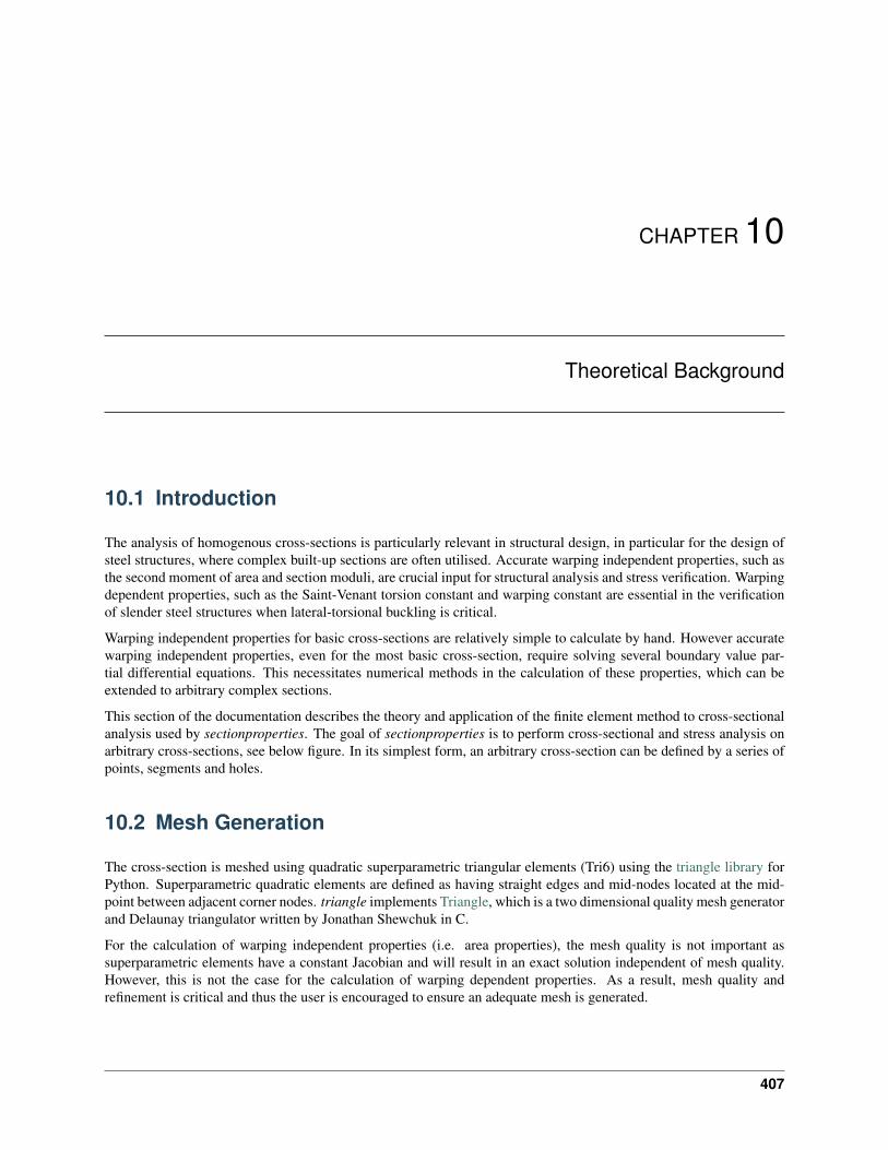
CHAPTER 10
Theoretical Background
10.1 Introduction
The analysis of homogenous cross-sections is particularly relevant in structural design, in particular for the design ofsteel structures, where complex built-up sections are often utilised. Accurate warping independent properties, such asthe second moment of area and section moduli, are crucial input for structural analysis and stress verification. Warpingdependent properties, such as the Saint-Venant torsion constant and warping constant are essential in the verificationof slender steel structures when lateral-torsional buckling is critical.
Warping independent properties for basic cross-sections are relatively simple to calculate by hand. However accuratewarping independent properties, even for the most basic cross-section, require solving several boundary value par-tial differential equations. This necessitates numerical methods in the calculation of these properties, which can beextended to arbitrary complex sections.
This section of the documentation describes the theory and application of the finite element method to cross-sectionalanalysis used by sectionproperties. The goal of sectionproperties is to perform cross-sectional and stress analysis onarbitrary cross-sections, see below figure. In its simplest form, an arbitrary cross-section can be defined by a series ofpoints, segments and holes.
10.2 Mesh Generation
The cross-section is meshed using quadratic superparametric triangular elements (Tri6) using the triangle library forPython. Superparametric quadratic elements are defined as having straight edges and mid-nodes located at the mid-point between adjacent corner nodes. triangle implements Triangle, which is a two dimensional quality mesh generatorand Delaunay triangulator written by Jonathan Shewchuk in C.
For the calculation of warping independent properties (i.e. area properties), the mesh quality is not important assuperparametric elements have a constant Jacobian and will result in an exact solution independent of mesh quality.However, this is not the case for the calculation of warping dependent properties. As a result, mesh quality andrefinement is critical and thus the user is encouraged to ensure an adequate mesh is generated.
407
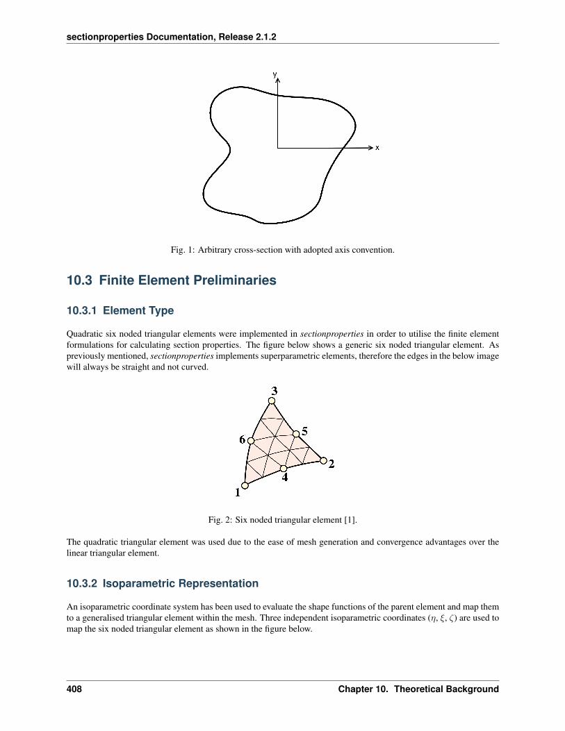
sectionproperties Documentation, Release 2.1.2
Fig. 1: Arbitrary cross-section with adopted axis convention.
10.3 Finite Element Preliminaries
10.3.1 Element Type
Quadratic six noded triangular elements were implemented in sectionproperties in order to utilise the finite elementformulations for calculating section properties. The figure below shows a generic six noded triangular element. Aspreviously mentioned, sectionproperties implements superparametric elements, therefore the edges in the below imagewill always be straight and not curved.
Fig. 2: Six noded triangular element [1].
The quadratic triangular element was used due to the ease of mesh generation and convergence advantages over thelinear triangular element.
10.3.2 Isoparametric Representation
An isoparametric coordinate system has been used to evaluate the shape functions of the parent element and map themto a generalised triangular element within the mesh. Three independent isoparametric coordinates (𝜂, 𝜉, 𝜁) are used tomap the six noded triangular element as shown in the figure below.
408 Chapter 10. Theoretical Background

sectionproperties Documentation, Release 2.1.2
Fig. 3: Isoparametric coordinates for the two dimensional triangular element.
Shape Functions
The shape functions for the six noded triangular element in terms of the isoparametric coordinates are as follows:
𝑁1 = 𝜂(2𝜂 − 1)
𝑁2 = 𝜉(2𝜉 − 1)
𝑁3 = 𝜁(2𝜁 − 1)
𝑁4 = 4𝜂𝜉
𝑁5 = 4𝜉𝜁
𝑁6 = 4𝜂𝜁
The above shape functions can be combined into the shape function row vector:
N = [𝑁1 𝑁2 𝑁3 𝑁4 𝑁5 𝑁6]
Cartesian Partial Derivatives
The partial derivatives of the shape functions with respect to the cartesian coordinates, denoted as the B matrix, arerequired in the finite element formulations of various section properties. Felippa [1] describes the multiplication of theJacobian matrix (J) and the partial derivative matrix (P):
J P =
⎡⎣ 1 1 1∑𝑥𝑖
𝜕𝑁𝑖
𝜕𝜂
∑𝑥𝑖
𝜕𝑁𝑖
𝜕𝜉
∑𝑥𝑖
𝜕𝑁𝑖
𝜕𝜁∑𝑦𝑖
𝜕𝑁𝑖
𝜕𝜂
∑𝑦𝑖
𝜕𝑁𝑖
𝜕𝜉
∑𝑦𝑖
𝜕𝑁𝑖
𝜕𝜁
⎤⎦⎡⎢⎣
𝜕𝜂𝜕𝑥
𝜕𝜂𝜕𝑦
𝜕𝜉𝜕𝑥
𝜕𝜉𝜕𝑦
𝜕𝜁𝜕𝑥
𝜕𝜁𝜕𝑦
⎤⎥⎦ =
⎡⎣0 01 00 1
⎤⎦The determinant of the Jacobian matrix scaled by one half is equal to the Jacobian:
𝐽 =1
2det J
The equation for textbfJ P can be re-arranged to evaluate the partial derivate matrix (P):
P = J−1
⎡⎣0 01 00 1
⎤⎦
10.3. Finite Element Preliminaries 409
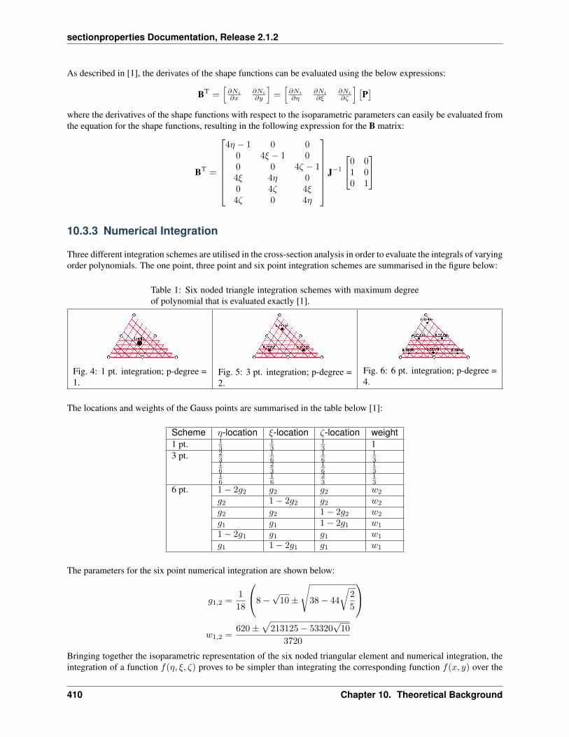
sectionproperties Documentation, Release 2.1.2
As described in [1], the derivates of the shape functions can be evaluated using the below expressions:
BT =[𝜕𝑁𝑖
𝜕𝑥𝜕𝑁𝑖
𝜕𝑦
]=[𝜕𝑁𝑖
𝜕𝜂𝜕𝑁𝑖
𝜕𝜉𝜕𝑁𝑖
𝜕𝜁
] [P]
where the derivatives of the shape functions with respect to the isoparametric parameters can easily be evaluated fromthe equation for the shape functions, resulting in the following expression for the B matrix:
BT =
⎡⎢⎢⎢⎢⎢⎢⎣4𝜂 − 1 0 0
0 4𝜉 − 1 00 0 4𝜁 − 14𝜉 4𝜂 00 4𝜁 4𝜉4𝜁 0 4𝜂
⎤⎥⎥⎥⎥⎥⎥⎦ J−1
⎡⎣0 01 00 1
⎤⎦
10.3.3 Numerical Integration
Three different integration schemes are utilised in the cross-section analysis in order to evaluate the integrals of varyingorder polynomials. The one point, three point and six point integration schemes are summarised in the figure below:
Table 1: Six noded triangle integration schemes with maximum degreeof polynomial that is evaluated exactly [1].
Fig. 4: 1 pt. integration; p-degree =1.
Fig. 5: 3 pt. integration; p-degree =2.
Fig. 6: 6 pt. integration; p-degree =4.
The locations and weights of the Gauss points are summarised in the table below [1]:
Scheme 𝜂-location 𝜉-location 𝜁-location weight1 pt. 1
313
13 1
3 pt. 23
16
16
13
16
23
16
13
16
16
23
13
6 pt. 1 − 2𝑔2 𝑔2 𝑔2 𝑤2
𝑔2 1 − 2𝑔2 𝑔2 𝑤2
𝑔2 𝑔2 1 − 2𝑔2 𝑤2
𝑔1 𝑔1 1 − 2𝑔1 𝑤1
1 − 2𝑔1 𝑔1 𝑔1 𝑤1
𝑔1 1 − 2𝑔1 𝑔1 𝑤1
The parameters for the six point numerical integration are shown below:
𝑔1,2 =1
18
⎛⎝8 −√
10 ±
√38 − 44
√2
5
⎞⎠𝑤1,2 =
620 ±√
213125 − 53320√
10
3720
Bringing together the isoparametric representation of the six noded triangular element and numerical integration, theintegration of a function 𝑓(𝜂, 𝜉, 𝜁) proves to be simpler than integrating the corresponding function 𝑓(𝑥, 𝑦) over the
410 Chapter 10. Theoretical Background
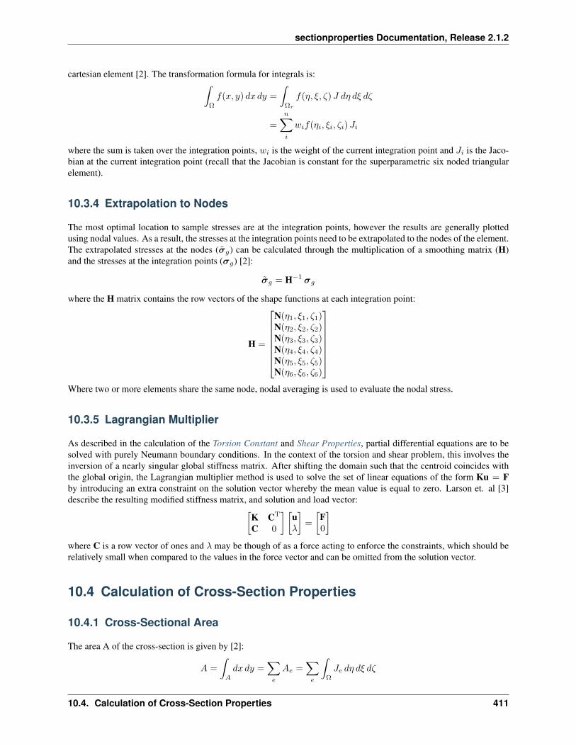
sectionproperties Documentation, Release 2.1.2
cartesian element [2]. The transformation formula for integrals is:∫Ω
𝑓(𝑥, 𝑦) 𝑑𝑥 𝑑𝑦 =
∫Ω𝑟
𝑓(𝜂, 𝜉, 𝜁) 𝐽 𝑑𝜂 𝑑𝜉 𝑑𝜁
=
𝑛∑𝑖
𝑤𝑖𝑓(𝜂𝑖, 𝜉𝑖, 𝜁𝑖) 𝐽𝑖
where the sum is taken over the integration points, 𝑤𝑖 is the weight of the current integration point and 𝐽𝑖 is the Jaco-bian at the current integration point (recall that the Jacobian is constant for the superparametric six noded triangularelement).
10.3.4 Extrapolation to Nodes
The most optimal location to sample stresses are at the integration points, however the results are generally plottedusing nodal values. As a result, the stresses at the integration points need to be extrapolated to the nodes of the element.The extrapolated stresses at the nodes (𝑔) can be calculated through the multiplication of a smoothing matrix (H)and the stresses at the integration points (𝜎𝑔) [2]:
𝑔 = H−1 𝜎𝑔
where the H matrix contains the row vectors of the shape functions at each integration point:
H =
⎡⎢⎢⎢⎢⎢⎢⎣N(𝜂1, 𝜉1, 𝜁1)N(𝜂2, 𝜉2, 𝜁2)N(𝜂3, 𝜉3, 𝜁3)N(𝜂4, 𝜉4, 𝜁4)N(𝜂5, 𝜉5, 𝜁5)N(𝜂6, 𝜉6, 𝜁6)
⎤⎥⎥⎥⎥⎥⎥⎦Where two or more elements share the same node, nodal averaging is used to evaluate the nodal stress.
10.3.5 Lagrangian Multiplier
As described in the calculation of the Torsion Constant and Shear Properties, partial differential equations are to besolved with purely Neumann boundary conditions. In the context of the torsion and shear problem, this involves theinversion of a nearly singular global stiffness matrix. After shifting the domain such that the centroid coincides withthe global origin, the Lagrangian multiplier method is used to solve the set of linear equations of the form Ku = Fby introducing an extra constraint on the solution vector whereby the mean value is equal to zero. Larson et. al [3]describe the resulting modified stiffness matrix, and solution and load vector:[
K CT
C 0
] [u𝜆
]=
[F0
]where C is a row vector of ones and 𝜆 may be though of as a force acting to enforce the constraints, which should berelatively small when compared to the values in the force vector and can be omitted from the solution vector.
10.4 Calculation of Cross-Section Properties
10.4.1 Cross-Sectional Area
The area A of the cross-section is given by [2]:
𝐴 =
∫𝐴
𝑑𝑥 𝑑𝑦 =∑𝑒
𝐴𝑒 =∑𝑒
∫Ω
𝐽𝑒 𝑑𝜂 𝑑𝜉 𝑑𝜁
10.4. Calculation of Cross-Section Properties 411

sectionproperties Documentation, Release 2.1.2
As the Jacobian is constant over the element, the integration over the element domain in the above equation can beperformed using one point integration:
𝐴 =∑𝑒
1∑𝑖=1
𝑤𝑖𝐽𝑖
10.4.2 First Moments of Area
The first moments of area are defined by [2]:
𝑄𝑥 =
∫𝐴
𝑦 𝑑𝐴 =∑𝑒
∫Ω
Ny𝑒𝐽𝑒 𝑑𝜂 𝑑𝜉 𝑑𝜁
𝑄𝑦 =
∫𝐴
𝑥 𝑑𝐴 =∑𝑒
∫Ω
Nx𝑒𝐽𝑒 𝑑𝜂 𝑑𝜉 𝑑𝜁
where x𝑒 and y𝑒 are column vectors containing the cartesian coordinates of the element nodes. The above equationscan be evaluated using three point integration as the shape functions (N) are quadratic:
𝑄𝑥 =∑𝑒
3∑𝑖=1
𝑤𝑖N𝑖y𝑒𝐽𝑒
𝑄𝑦 =∑𝑒
3∑𝑖=1
𝑤𝑖N𝑖x𝑒𝐽𝑒
10.4.3 Centroids
The coordinates of the centroid are found from [2]:
𝑥𝑐 =𝑄𝑦
𝐴
𝑦𝑐 =𝑄𝑥
𝐴
10.4.4 Second Moments of Area
The second moments of area are defined by [2]:
𝐼𝑥𝑥 =
∫𝐴
𝑦2 𝑑𝐴 =∑𝑒
∫Ω
(Ny𝑒)2𝐽𝑒 𝑑𝜂 𝑑𝜉 𝑑𝜁
𝐼𝑦𝑦 =
∫𝐴
𝑥2 𝑑𝐴 =∑𝑒
∫Ω
(Nx𝑒)2𝐽𝑒 𝑑𝜂 𝑑𝜉 𝑑𝜁
𝐼𝑥𝑦 =
∫𝐴
𝑥𝑦 𝑑𝐴 =∑𝑒
∫Ω
Ny𝑒Nx𝑒𝐽𝑒 𝑑𝜂 𝑑𝜉 𝑑𝜁
412 Chapter 10. Theoretical Background

sectionproperties Documentation, Release 2.1.2
The above equations can be evaluated using six point integration as the square of the shape functions are quartic:
𝐼𝑥𝑥 =∑𝑒
6∑𝑖=1
𝑤𝑖(N𝑖y𝑒)2𝐽𝑒
𝐼𝑦𝑦 =∑𝑒
6∑𝑖=1
𝑤𝑖(N𝑖x𝑒)2𝐽𝑒
𝐼𝑥𝑦 =∑𝑒
6∑𝑖=1
𝑤𝑖Ny𝑒Nx𝑒𝐽𝑒
The above equations list the second moments of area about the global coordinate system axis, which is chosen arbi-trarily by the user. These properties can be found about the centroidal axis of the cross-section by using the parallelaxis theorem:
𝐼𝑥𝑥 = 𝐼𝑥𝑥 − 𝑦𝑐2𝐴 = 𝐼𝑥𝑥 − 𝑄𝑥
2
𝐴
𝐼𝑦𝑦 = 𝐼𝑦𝑦 − 𝑥𝑐2𝐴 = 𝐼𝑦𝑦 −
𝑄𝑦2
𝐴
𝐼𝑥𝑦 = 𝐼𝑥𝑦 − 𝑥𝑐𝑦𝑐𝐴 = 𝐼𝑥𝑦 −𝑄𝑥𝑄𝑦
𝐴
10.4.5 Radii of Gyration
The radii of gyration can be calculated from the second moments of area and the cross-sectional area as follows [2]:
𝑟𝑥 =
√𝐼𝑥𝑥𝐴
𝑟𝑦 =
√𝐼𝑦𝑦𝐴
10.4.6 Elastic Section Moduli
The elastic section modulii can be calculated from the second moments of area and the extreme (min. and max.)coordinates of the cross-section in the x and y-directions [2]:
𝑍+𝑥𝑥 =
𝐼𝑥𝑥𝑦𝑚𝑎𝑥 − 𝑦𝑐
𝑍−𝑥𝑥 =
𝐼𝑥𝑥𝑦𝑐 − 𝑦𝑚𝑖𝑛
𝑍+𝑦𝑦 =
𝐼𝑦𝑦𝑥𝑚𝑎𝑥 − 𝑥𝑐
𝑍−𝑦𝑦 =
𝐼𝑦𝑦𝑥𝑐 − 𝑥𝑚𝑖𝑛
10.4.7 Plastic Section Moduli
For a homogenous section, the plastic centroid can be determined by finding the intersection of the two lines that evenlydivide the cross-sectional area in both the 𝑥 and 𝑦 directions. A suitable procedure could not be found in literatureand thus an algorithm involving the iterative incrementation of the plastic centroid was developed. The algorithm usesBrent’s method to efficiently locate the plastic centroidal axes in the global and principal directions.
10.4. Calculation of Cross-Section Properties 413

sectionproperties Documentation, Release 2.1.2
Once the plastic centroid has been located, the plastic section moduli can be readily computed using the followingexpression:
𝑆𝑥𝑥 =𝐴
2|𝑦𝑐,𝑡 − 𝑦𝑐,𝑏|
𝑆𝑦𝑦 =𝐴
2|𝑥𝑐,𝑡 − 𝑥𝑐,𝑏|
where 𝐴 is the cross-sectional area, and 𝑥𝑐,𝑡 and 𝑥𝑐,𝑏 refer to the centroids of the top half section and bottom halfsection respectively.
10.4.8 Principal Axis Properties
The principal bending axes are determined by calculating the principal moments of inertia[2]:
𝐼11 =𝐼𝑥𝑥 + 𝐼𝑦𝑦
2+ ∆
𝐼22 =𝐼𝑥𝑥 + 𝐼𝑦𝑦
2− ∆
where:
∆ =
√(𝐼𝑥𝑥 − 𝐼𝑦𝑦
2
)2
+ 𝐼𝑥𝑦2
The angle between the axis and the axis belonging to the largest principal moment of inertia can be computed asfollows:
𝜑 = tan−1 𝐼𝑥𝑥 − 𝐼11𝐼𝑥𝑦
The prinicpal section moduli require the calculation of the perpendicular distance from the principal axes to the extremefibres. All the nodes in the mesh are considered with vector algebra used to compute the perpendicular distances andthe minimum and maximum distances identified. The perpendicular distance from a point 𝑃 to a line parallel to −→𝑢that passes through 𝑄 is given by:
𝑑 = |−−→𝑃𝑄×−→𝑢 |
The location of the point is checked to see whether it is above or below the principal axis. Again vector algebra is usedto check this condition. The condition in the below equation will result in the point being above the −→𝑢 axis.
−−→𝑄𝑃 ×−→𝑢 < 0
Using the above equations, the principal section moduli can be computed similar to that in the calculation of the ElasticSection Moduli and Plastic Section Moduli.
10.4.9 Torsion Constant
The Saint-Venant torsion constant (𝐽) can be obtained by solving the below partial differential equation for the warpingfunction, 𝜔:
∇2𝜔 = 0
subject to the boundary condition described below:
𝜕𝜔
𝜕𝑥𝑛𝑥 +
𝜕𝜔
𝜕𝑦𝑛𝑦 = 𝑦𝑛𝑥 − 𝑥𝑛𝑦
414 Chapter 10. Theoretical Background

sectionproperties Documentation, Release 2.1.2
Pilkey [2] shows that by using the finite element method, this problem can be reduced to a set of linear equations ofthe form:
K𝜔 = F
where K and F are assembled through summation at element level. The element equations for the 𝑒th element are:
k𝑒𝜔𝑒 = f𝑒
with the stiffness matrix defined as:
k𝑒 =
∫Ω
BTB𝐽𝑒 𝑑𝜂 𝑑𝜉 𝑑𝜁
and the load vector defined as:
f𝑒 =
∫Ω
BT
[Ny−Nx
]𝐽𝑒 𝑑𝜂 𝑑𝜉 𝑑𝜁
Applying numerical integration to the stiffness matrix and load vector results in the following expressions:
k𝑒 =
3∑𝑖=1
𝑤𝑖BT𝑖 B𝑖𝐽𝑒
f𝑒 =
6∑𝑖=1
𝑤𝑖BT𝑖
[N𝑖y𝑒−N𝑖x𝑒
]𝐽𝑒
Once the warping function has been evaluated, the Saint-Venant torsion constant can be calculated as follows:
𝐽 = 𝐼𝑥𝑥 + 𝐼𝑦𝑦 − 𝜔TK𝜔
10.4.10 Shear Properties
The shear behaviour of the cross-section can be described by Saint-Venant’s elasticity solution for a homogenousprismatic beam subjected to transverse shear loads [2]. Through cross-section equilibrium and linear-elasticity, anexpression for the shear stresses resulting from a transverse shear load can be derived. Pilkey [2] explains that this isbest done through the introduction of shear functions, Ψ and Φ, which describe the distribution of shear stress withina cross-section resulting from an applied transverse load in the 𝑥 and 𝑦 directions respectively. These shear functionscan be obtained by solving the following uncoupled partial differential equations:
∇2Ψ = 2(𝐼𝑥𝑦𝑦 − 𝐼𝑥𝑥𝑥)
∇2Φ = 2(𝐼𝑥𝑦𝑥− 𝐼𝑦𝑦𝑦)
subject to the respective boundary conditions:
𝜕Ψ
𝜕𝑛= n · d
𝜕Φ
𝜕𝑛= n · h
where n is the normal unit vector at the boundary and d and h are defined as follows:
d = 𝜈
(𝐼𝑥𝑥
𝑥2 − 𝑦2
2− 𝐼𝑥𝑦𝑥𝑦
)i + 𝜈
(𝐼𝑥𝑥𝑥𝑦 + 𝐼𝑥𝑦
𝑥2 − 𝑦2
2
)j
h = 𝜈
(𝐼𝑦𝑦𝑥𝑦 − 𝐼𝑥𝑦
𝑥2 − 𝑦2
2
)i − 𝜈
(𝐼𝑥𝑦𝑥𝑦 + 𝐼𝑦𝑦
𝑥2 − 𝑦2
2
)j
10.4. Calculation of Cross-Section Properties 415

sectionproperties Documentation, Release 2.1.2
Pilkey [2] shows that the shear equations subject to the boundary conditions can be solved using the finite elementmethod. This results in a set of linear equations at element level of the form:
k𝑒Ψ𝑒 = f𝑒𝑥k𝑒Φ𝑒 = f𝑒𝑦
The local stiffness matrix, k𝑒, is identical to the matrix used to determine the torsion constant:
k𝑒 =
∫Ω
BTB𝐽𝑒 𝑑𝜂 𝑑𝜉 𝑑𝜁
The load vectors are defined as:
f𝑒𝑥 =
∫Ω
[𝜈
2BT
[𝑑1𝑑2
]+ 2(1 + 𝜈)NT(𝐼𝑥𝑥Nx − 𝐼𝑥𝑦Ny)
]𝐽𝑒 𝑑𝜂 𝑑𝜉 𝑑𝜁
f𝑒𝑦 =
∫Ω
[𝜈
2BT
[ℎ1
ℎ2
]+ 2(1 + 𝜈)NT(𝐼𝑦𝑦Ny − 𝐼𝑥𝑦Nx)
]𝐽𝑒 𝑑𝜂 𝑑𝜉 𝑑𝜁
where:
𝑑1 = 𝐼𝑥𝑥𝑟 − 𝐼𝑥𝑦𝑞
𝑑2 = 𝐼𝑥𝑦𝑟 + 𝐼𝑥𝑥𝑞
ℎ1 = −𝐼𝑥𝑦𝑟 + 𝐼𝑦𝑦𝑞
ℎ2 = −𝐼𝑦𝑦𝑟 − 𝐼𝑥𝑦𝑞
𝑟 = (Nx)2 − (Ny)2
𝑞 = 2NxNy
Applying numerical integration to the stiffness matrix and load vector results in the following expressions:
k𝑒 =
3∑𝑖=1
𝑤𝑖BT𝑖 B𝑖𝐽𝑒
f𝑒𝑥 =
6∑𝑖=1
𝑤𝑖
[𝜈
2BT𝑖
[𝑑1,𝑖𝑑2,𝑖
]+ 2(1 + 𝜈)NT
𝑖 (𝐼𝑥𝑥N𝑖x𝑒 − 𝐼𝑥𝑦N𝑖y𝑒)]𝐽𝑒
f𝑒𝑦 =
6∑𝑖=1
𝑤𝑖
[𝜈
2BT𝑖
[ℎ1,𝑖
ℎ2,𝑖
]+ 2(1 + 𝜈)NT
𝑖 (𝐼𝑦𝑦N𝑖y𝑒 − 𝐼𝑥𝑦N𝑖x𝑒)]𝐽𝑒
Shear Centre
The shear centre can be computed consistently based on elasticity, or through Trefftz’s definition, which is based onthin-wall assumptions [2].
Elasticity: Pilkey [2] demonstrates that the coordinates of the shear centre are given by the following expressions:
𝑥𝑠 =1
∆𝑠
[𝜈
2
∫Ω
(𝐼𝑦𝑦𝑥 + 𝐼𝑥𝑦𝑦)(𝑥2 + 𝑦2
)𝑑Ω −
∫Ω
g ·∇Φ 𝑑Ω
]𝑦𝑠 =
1
∆𝑠
[𝜈
2
∫Ω
(𝐼𝑥𝑥𝑦 + 𝐼𝑥𝑦𝑥)(𝑥2 + 𝑦2
)𝑑Ω +
∫Ω
g ·∇Ψ 𝑑Ω
]where:
∆𝑠 = 2(1 + 𝜈)(𝐼𝑥𝑥𝐼𝑦𝑦 − 𝐼𝑥𝑦2)
g = 𝑦i − 𝑥j
416 Chapter 10. Theoretical Background

sectionproperties Documentation, Release 2.1.2
The first integral in shear centre equations can be evaluated using quadrature for each element. The second integralcan be simplified once the shear functions, Ψ and Φ, have been obtained:∫
Ω
g ·∇Φ 𝑑Ω = FTΦ∫Ω
g ·∇Ψ 𝑑Ω = FTΨ
where F is the global load vector determined for the torsion problem in Torsion Constant. The resulting expression forthe shear centre therefore becomes:
𝑥𝑠 =1
∆𝑠
[(𝜈
2
6∑𝑖=1
𝑤𝑖(𝐼𝑦𝑦N𝑖x𝑒 + 𝐼𝑥𝑦N𝑖y𝑒)(
(N𝑖x𝑒)2 + (N𝑖y𝑒)2)𝐽𝑒
)− FTΦ
]
𝑦𝑠 =1
∆𝑠
[(𝜈
2
6∑𝑖=1
𝑤𝑖(𝐼𝑥𝑥N𝑖y𝑒 + 𝐼𝑥𝑦N𝑖x𝑒)(
(N𝑖x𝑒)2 + (N𝑖y𝑒)2)𝐽𝑒
)+ FTΨ
]
Trefftz’s Definition: Using thin walled assumptions, the shear centre coordinates according to Trefftz’s definition aregiven by:
𝑥𝑠 =𝐼𝑥𝑦𝐼𝑥𝜔 − 𝐼𝑦𝑦𝐼𝑦𝜔
𝐼𝑥𝑥𝐼𝑦𝑦 − 𝐼𝑥𝑦2
𝑦𝑠 =𝐼𝑥𝑥𝐼𝑥𝜔 − 𝐼𝑥𝑦𝐼𝑦𝜔
𝐼𝑥𝑥𝐼𝑦𝑦 − 𝐼𝑥𝑦2
where the sectorial products of area are defined as:
𝐼𝑥𝜔 =
∫Ω
𝑥𝜔(𝑥, 𝑦) 𝑑Ω
𝐼𝑦𝜔 =
∫Ω
𝑦𝜔(𝑥, 𝑦) 𝑑Ω
The finite element implementation of the above integrals are shown below:
𝐼𝑥𝜔 =∑𝑒
6∑𝑖=1
𝑤𝑖N𝑖x𝑒N𝑖𝜔𝑒𝐽𝑒
𝐼𝑦𝜔 =∑𝑒
6∑𝑖=1
𝑤𝑖N𝑖y𝑒N𝑖𝜔𝑒𝐽𝑒
Shear Deformation Coefficients
The shear deformation coefficients are used to calculate the shear area of the section as a result of transverse loading.The shear area is defined as 𝐴𝑠 = 𝑘𝑠𝐴. Pilkey [2] describes the finite element formulation used to determine the sheardeformation coefficients:
𝜅𝑥 =∑𝑒
∫Ω
(Ψ𝑒TBT − dT
)(BΨ𝑒 − d) 𝐽𝑒 𝑑Ω
𝜅𝑦 =∑𝑒
∫Ω
(Φ𝑒TBT − hT
)(BΦ𝑒 − h) 𝐽𝑒 𝑑Ω
𝜅𝑥𝑦 =∑𝑒
∫Ω
(Ψ𝑒TBT − dT
)(BΦ𝑒 − h) 𝐽𝑒 𝑑Ω
10.4. Calculation of Cross-Section Properties 417
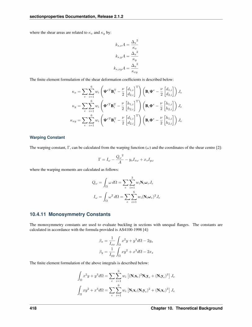
sectionproperties Documentation, Release 2.1.2
where the shear areas are related to 𝜅𝑥 and 𝜅𝑦 by:
𝑘𝑠,𝑥𝐴 =∆𝑠
2
𝜅𝑥
𝑘𝑠,𝑦𝐴 =∆𝑠
2
𝜅𝑦
𝑘𝑠,𝑥𝑦𝐴 =∆𝑠
2
𝜅𝑥𝑦
The finite element formulation of the shear deformation coefficients is described below:
𝜅𝑥 =∑𝑒
6∑𝑖=1
𝑤𝑖
(Ψ𝑒TBT
𝑖 − 𝜈
2
[𝑑1,𝑖𝑑2,𝑖
]T)(B𝑖Ψ
𝑒 − 𝜈
2
[𝑑1,𝑖𝑑2,𝑖
])𝐽𝑒
𝜅𝑦 =∑𝑒
6∑𝑖=1
𝑤𝑖
(Φ𝑒TBT
𝑖 − 𝜈
2
[ℎ1,𝑖
ℎ2,𝑖
]T)(B𝑖Φ
𝑒 − 𝜈
2
[ℎ1,𝑖
ℎ2,𝑖
])𝐽𝑒
𝜅𝑥𝑦 =∑𝑒
6∑𝑖=1
𝑤𝑖
(Ψ𝑒TBT
𝑖 − 𝜈
2
[𝑑1,𝑖𝑑2,𝑖
]T)(B𝑖Φ
𝑒 − 𝜈
2
[ℎ1,𝑖
ℎ2,𝑖
])𝐽𝑒
Warping Constant
The warping constant, Γ, can be calculated from the warping function (𝜔) and the coordinates of the shear centre [2]:
Γ = 𝐼𝜔 − 𝑄𝜔2
𝐴− 𝑦𝑠𝐼𝑥𝜔 + 𝑥𝑠𝐼𝑦𝜔
where the warping moments are calculated as follows:
𝑄𝜔 =
∫Ω
𝜔 𝑑Ω =∑𝑒
3∑𝑖=1
𝑤𝑖N𝑖𝜔𝑒𝐽𝑒
𝐼𝜔 =
∫Ω
𝜔2 𝑑Ω =∑𝑒
6∑𝑖=1
𝑤𝑖(N𝑖𝜔𝑒)2𝐽𝑒
10.4.11 Monosymmetry Constants
The monosymmetry constants are used to evaluate buckling in sections with unequal flanges. The constants arecalculated in accordance with the formula provided is AS4100-1998 [4]:
𝛽𝑥 =1
𝐼𝑥𝑥
∫Ω
𝑥2𝑦 + 𝑦3𝑑Ω − 2𝑦𝑠
𝛽𝑦 =1
𝐼𝑦𝑦
∫Ω
𝑥𝑦2 + 𝑥3𝑑Ω − 2𝑥𝑠
The finite element formulation of the above integrals is described below:∫Ω
𝑥2𝑦 + 𝑦3𝑑Ω =∑𝑒
6∑𝑖=1
𝑤𝑖
[(N𝑖x𝑒)2N𝑖y𝑒 + (N𝑖y𝑒)
3]𝐽𝑒
∫Ω
𝑥𝑦2 + 𝑥3𝑑Ω =∑𝑒
6∑𝑖=1
𝑤𝑖
[N𝑖x𝑒(N𝑖y𝑒)
2 + (N𝑖x𝑒)3]𝐽𝑒
418 Chapter 10. Theoretical Background
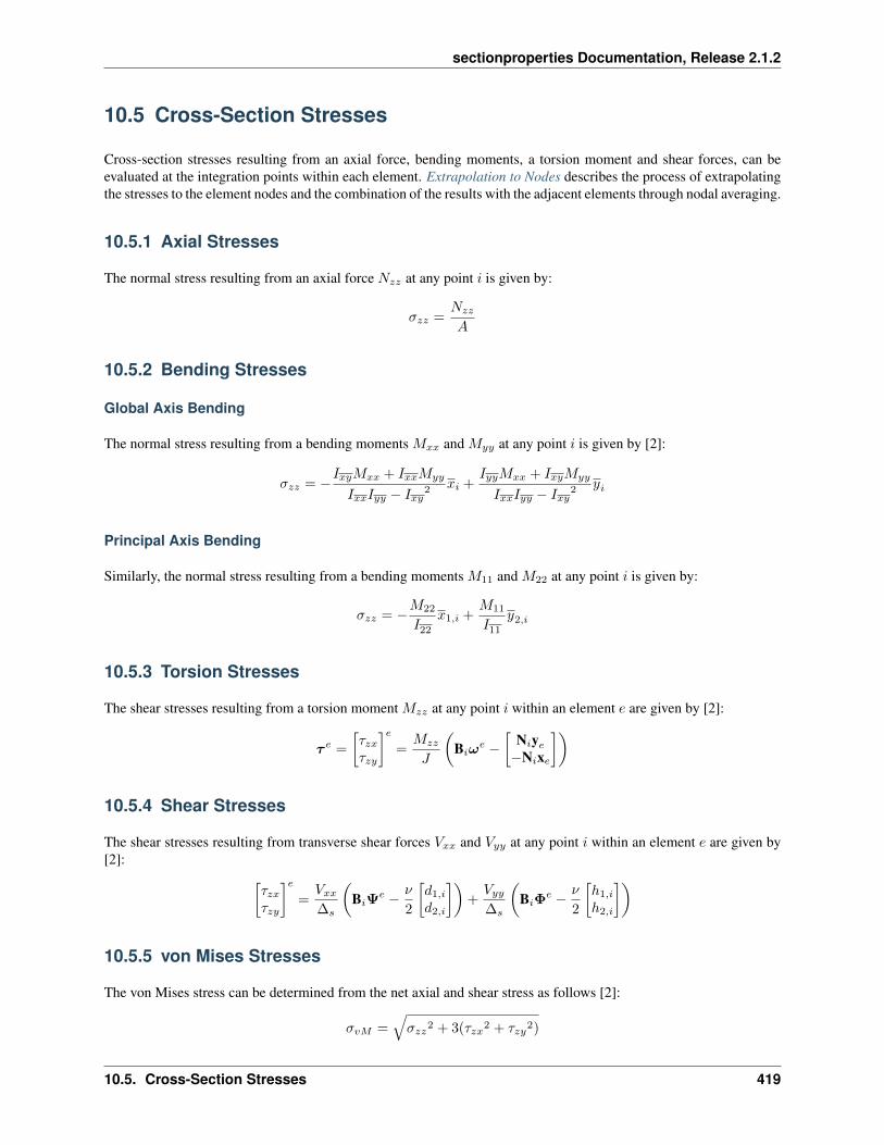
sectionproperties Documentation, Release 2.1.2
10.5 Cross-Section Stresses
Cross-section stresses resulting from an axial force, bending moments, a torsion moment and shear forces, can beevaluated at the integration points within each element. Extrapolation to Nodes describes the process of extrapolatingthe stresses to the element nodes and the combination of the results with the adjacent elements through nodal averaging.
10.5.1 Axial Stresses
The normal stress resulting from an axial force 𝑁𝑧𝑧 at any point 𝑖 is given by:
𝜎𝑧𝑧 =𝑁𝑧𝑧
𝐴
10.5.2 Bending Stresses
Global Axis Bending
The normal stress resulting from a bending moments 𝑀𝑥𝑥 and 𝑀𝑦𝑦 at any point 𝑖 is given by [2]:
𝜎𝑧𝑧 = −𝐼𝑥𝑦𝑀𝑥𝑥 + 𝐼𝑥𝑥𝑀𝑦𝑦
𝐼𝑥𝑥𝐼𝑦𝑦 − 𝐼𝑥𝑦2 𝑥𝑖 +
𝐼𝑦𝑦𝑀𝑥𝑥 + 𝐼𝑥𝑦𝑀𝑦𝑦
𝐼𝑥𝑥𝐼𝑦𝑦 − 𝐼𝑥𝑦2 𝑦𝑖
Principal Axis Bending
Similarly, the normal stress resulting from a bending moments 𝑀11 and 𝑀22 at any point 𝑖 is given by:
𝜎𝑧𝑧 = −𝑀22
𝐼22𝑥1,𝑖 +
𝑀11
𝐼11𝑦2,𝑖
10.5.3 Torsion Stresses
The shear stresses resulting from a torsion moment 𝑀𝑧𝑧 at any point 𝑖 within an element 𝑒 are given by [2]:
𝜏 𝑒 =
[𝜏𝑧𝑥𝜏𝑧𝑦
]𝑒=
𝑀𝑧𝑧
𝐽
(B𝑖𝜔
𝑒 −[
N𝑖y𝑒−N𝑖x𝑒
])
10.5.4 Shear Stresses
The shear stresses resulting from transverse shear forces 𝑉𝑥𝑥 and 𝑉𝑦𝑦 at any point 𝑖 within an element 𝑒 are given by[2]: [
𝜏𝑧𝑥𝜏𝑧𝑦
]𝑒=
𝑉𝑥𝑥
∆𝑠
(B𝑖Ψ
𝑒 − 𝜈
2
[𝑑1,𝑖𝑑2,𝑖
])+
𝑉𝑦𝑦
∆𝑠
(B𝑖Φ
𝑒 − 𝜈
2
[ℎ1,𝑖
ℎ2,𝑖
])
10.5.5 von Mises Stresses
The von Mises stress can be determined from the net axial and shear stress as follows [2]:
𝜎𝑣𝑀 =√𝜎𝑧𝑧
2 + 3(𝜏𝑧𝑥2 + 𝜏𝑧𝑦2)
10.5. Cross-Section Stresses 419
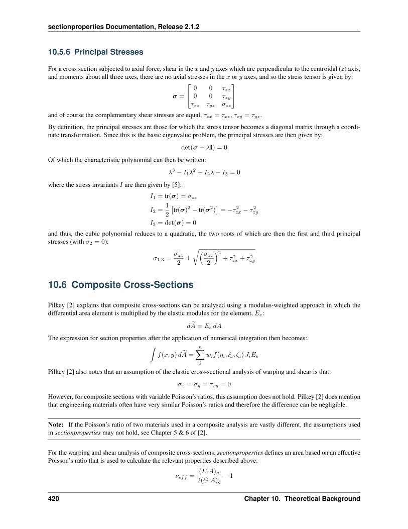
sectionproperties Documentation, Release 2.1.2
10.5.6 Principal Stresses
For a cross section subjected to axial force, shear in the 𝑥 and 𝑦 axes which are perpendicular to the centroidal (𝑧) axis,and moments about all three axes, there are no axial stresses in the 𝑥 or 𝑦 axes, and so the stress tensor is given by:
𝜎 =
⎡⎣ 0 0 𝜏𝑧𝑥0 0 𝜏𝑧𝑦𝜏𝑥𝑧 𝜏𝑦𝑧 𝜎𝑧𝑧
⎤⎦and of course the complementary shear stresses are equal, 𝜏𝑧𝑥 = 𝜏𝑥𝑧 , 𝜏𝑧𝑦 = 𝜏𝑦𝑧 .
By definition, the principal stresses are those for which the stress tensor becomes a diagonal matrix through a coordi-nate transformation. Since this is the basic eigenvalue problem, the principal stresses are then given by:
det(𝜎 − 𝜆I) = 0
Of which the characteristic polynomial can then be written:
𝜆3 − 𝐼1𝜆2 + 𝐼2𝜆− 𝐼3 = 0
where the stress invariants 𝐼 are then given by [5]:
𝐼1 = tr(𝜎) = 𝜎𝑧𝑧
𝐼2 =1
2
[tr(𝜎)2 − tr(𝜎2)
]= −𝜏2𝑧𝑥 − 𝜏2𝑧𝑦
𝐼3 = det(𝜎) = 0
and thus, the cubic polynomial reduces to a quadratic, the two roots of which are then the first and third principalstresses (with 𝜎2 = 0):
𝜎1,3 =𝜎𝑧𝑧
2±√(𝜎𝑧𝑧
2
)2+ 𝜏2𝑧𝑥 + 𝜏2𝑧𝑦
10.6 Composite Cross-Sections
Pilkey [2] explains that composite cross-sections can be analysed using a modulus-weighted approach in which thedifferential area element is multiplied by the elastic modulus for the element, 𝐸𝑒:
𝑑 𝐴 = 𝐸𝑒 𝑑𝐴
The expression for section properties after the application of numerical integration then becomes:∫𝑓(𝑥, 𝑦) 𝑑 𝐴 =
𝑛∑𝑖
𝑤𝑖𝑓(𝜂𝑖, 𝜉𝑖, 𝜁𝑖) 𝐽𝑖𝐸𝑒
Pilkey [2] also notes that an assumption of the elastic cross-sectional analysis of warping and shear is that:
𝜎𝑥 = 𝜎𝑦 = 𝜏𝑥𝑦 = 0
However, for composite sections with variable Poisson’s ratios, this assumption does not hold. Pilkey [2] does mentionthat engineering materials often have very similar Poisson’s ratios and therefore the difference can be negligible.
Note: If the Poisson’s ratio of two materials used in a composite analysis are vastly different, the assumptions usedin sectionproperties may not hold, see Chapter 5 & 6 of [2].
For the warping and shear analysis of composite cross-sections, sectionproperties defines an area based on an effectivePoisson’s ratio that is used to calculate the relevant properties described above:
𝜈𝑒𝑓𝑓 =(𝐸.𝐴)𝑔2(𝐺.𝐴)𝑔
− 1
420 Chapter 10. Theoretical Background

sectionproperties Documentation, Release 2.1.2
10.7 References
1. C. A. Felippa, Introduction to Finite Element Methods, Department of Aerospace Engineering Sciences andCenter for Aerospace Structures University of Colorado, Boulder, Colorado, 2004.
2. W. D. Pilkey, Analysis and Design of Elastic Beams: Computational Methods, John Wiley & Sons, Inc.,New York, 2002.
3. M. G. Larson, F. Bengzon, The Finite Element Method: Theory, Implementation, and Applications, Vol. 10,Springer, Berlin, Heidelberg, 2013. doi:10.1007/978-3-642-33287-6.
4. AS 4100 - 1998: Steel Structures. (1998, June). Standards Australia.
5. Oñate, E. (2009), Structural Analysis with the Finite Element Method. Linear Statics. Volume 1: The Basis andSolids, Springer Netherlands
10.7. References 421

sectionproperties Documentation, Release 2.1.2
422 Chapter 10. Theoretical Background

CHAPTER 11
Testing and Results Validation
sectionproperties has a (slowly) growing suite of tests. The testing suite serves to verify functionality and find ex-ceptions from edge cases, but also validate the results against known cases. Since this library performs engineeringcalculations, it should have some manner of proving its accuracy. Each analyst who uses it is responsible for their ownprojects and calculations, but having a high level of confidence that the software can produce correct results, given thecorrect inputs, is a boon to all users. Some test results and explanations from the latter category will be outlined onthis page, since the former really serves no use to the end user.
11.1 Textbook Examples
An obvious starting location is replicating examples from academic texts. “Aircraft Structures” by David J. Peery is ahighly regarded text in the field of aerospace structures1.
11.1.1 Peery - Symmetric Sections
The simplest example of a realistic section problem is the symmetric I-Beam, with a free-fixed boundary conditionand a transverse tip load. The free-body-diagram and shear and moment diagrams are shown in the problem statement,referenced below. This problem is Example 1 in Section 6.2.
1 D. J. Peery, Aircraft Structures. New York: Dover Publications, 2011. ISBN-10: 0-486-48580-3
423

sectionproperties Documentation, Release 2.1.2
Check #1:
In sectionproperties, there are multiple ways to set this problem up. We could different shapely geometries and mergetogether, or a set of custom points, or a built-in constructor. For the sake of simplicity, this simpler I-section isidentical to the Nastran I-section definition, so it makes sense to utilize the built-in constructor from pre.library.nastran_sections.nastran_i.
Using an arbitrarily coarse mesh, the properties can then be directly calculated from the class method Section.calculate_geomtric_properties().
Peery lists the second moment of area about the primary bending axis as a value of 43.3[𝑖𝑛4]. For the automated testsin this library, we check against this hardcoded value, with a tolerance of ±0.1
Check #2:
As a final check against this example, we can calculate the maximum bending stress on the I-beam. From simplestatics, the maximum moment from the FBD will be 800, 000[𝑖𝑛− 𝑙𝑏𝑠] at the fixed end. Applying this moment to oursection from before will allow computation of stress over the FEM.
Peery quotes the peak value at 55.5[𝑘𝑠𝑖], which is rounded to the nearest decimal place. From the equatio listed in thetext, the theoretical value is actually 55, 427.3[𝑝𝑠𝑖].
𝑓 =𝑀𝑦
𝐼= 55, 427.3 = 55, 400
Again, the automated test against this checks the hardcoded value with a tolerance of ±0.1𝑟𝑜𝑢𝑛𝑑𝑒𝑑𝑣𝑎𝑙𝑢𝑒.
For full details and the most updated code of this exampe, see the examples page in the documentation gallery. For theexact test code execution, check the source.
11.1.2 Peery - Unsymmetric Sections
For a more complex example, we can turn to Example 1 in Section 7.2 of Peery. Here, we have a still-simplifiedZ-section, but bending about two axes. Note axes definitions in the problem statement. Beam axial direction insectionproperties is always referenced as the z-axis, and loads must be applied in this coordinate system.
424 Chapter 11. Testing and Results Validation

sectionproperties Documentation, Release 2.1.2
The construction of this geometry takes a similar approach to Ex 6.2.1, and utilizes a built-in factory: pre.library.nastran_sections.nastran_zed. The only difference you may notice in the test code is usage of a customclass for ease of initialization. This is not necessary.
Using an arbitrarily coarse mesh, the properties can then be directly calculated from the class method Section.calculate_geomtric_properties(). Each property listed directly by Peery is taken as a hardcoded valueand checked against, within the testing suite.
Property Peery ValueI_x 693.3 [in4]I_y 173.3 [in4]I_xy -240 [in4]I_p 787.1 [in4]I_q 79.5 [in4]theta 21.35 [deg]
For stress results, the theoretical values follow the biaxial bending equation. These values are checked against auto-matically in the testing suite. Note that again Peery rounds the values quoted directly, for simplicity. The testing suitealso verifies that the theoretical value as per the equation matches the theoretical value quoted in the text, which alsomatches the computed value from the sectionproperties FEM.
𝑓𝑏 =𝑀𝑥𝐼𝑥𝑦 −𝑀𝑦𝐼𝑥
𝐼𝑥𝐼𝑦 − 𝐼2𝑥𝑦𝑥 +
𝑀𝑦𝐼𝑥𝑦 −𝑀𝑥𝐼𝑦𝐼𝑥𝐼𝑦 − 𝐼2𝑥𝑦
𝑦
Point x y -494x -315y 𝑓𝑏, [psi]A -5 4 2470 -1260 1210.0 = 1210B -5 6 2470 -1890 580.0 = 580C 1 6 -494 -1890 -2384.0 = -2380
11.1. Textbook Examples 425
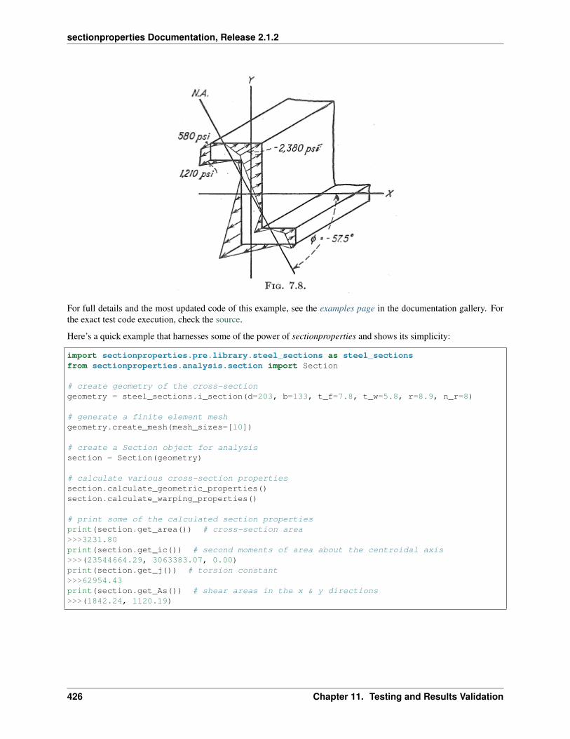
sectionproperties Documentation, Release 2.1.2
For full details and the most updated code of this example, see the examples page in the documentation gallery. Forthe exact test code execution, check the source.
Here’s a quick example that harnesses some of the power of sectionproperties and shows its simplicity:
import sectionproperties.pre.library.steel_sections as steel_sectionsfrom sectionproperties.analysis.section import Section
# create geometry of the cross-sectiongeometry = steel_sections.i_section(d=203, b=133, t_f=7.8, t_w=5.8, r=8.9, n_r=8)
# generate a finite element meshgeometry.create_mesh(mesh_sizes=[10])
# create a Section object for analysissection = Section(geometry)
# calculate various cross-section propertiessection.calculate_geometric_properties()section.calculate_warping_properties()
# print some of the calculated section propertiesprint(section.get_area()) # cross-section area>>>3231.80print(section.get_ic()) # second moments of area about the centroidal axis>>>(23544664.29, 3063383.07, 0.00)print(section.get_j()) # torsion constant>>>62954.43print(section.get_As()) # shear areas in the x & y directions>>>(1842.24, 1120.19)
426 Chapter 11. Testing and Results Validation

CHAPTER 12
Support
Raise an issue on the GitHub issue tracker or contact me at [email protected]. If you have a request fora feature to be added to the sectionproperties package, please don’t hesitate to get in touch
427

sectionproperties Documentation, Release 2.1.2
428 Chapter 12. Support

CHAPTER 13
License
The project is licensed under the MIT license.
429

sectionproperties Documentation, Release 2.1.2
430 Chapter 13. License

Index
Aadd_element() (sectionproper-
ties.analysis.section.MaterialGroup method),392
align_center() (sectionproper-ties.pre.geometry.Geometry method), 233
align_to() (sectionproper-ties.pre.geometry.Geometry method), 234
angle_section() (in module sectionproper-ties.pre.library.steel_sections), 281
asdict() (sectionproper-ties.analysis.section.SectionPropertiesmethod), 398
assemble_torsion() (sectionproper-ties.analysis.section.Section method), 346
assign_control_point() (sectionproper-ties.pre.geometry.Geometry method), 234
Bbox_girder_section() (in module sectionproper-
ties.pre.library.steel_sections), 287bulb_section() (in module sectionproper-
ties.pre.library.steel_sections), 289
Ccalculate_area() (sectionproper-
ties.pre.geometry.Geometry method), 234calculate_centroid() (sectionproper-
ties.analysis.section.PlasticSection method),358
calculate_centroid() (sectionproper-ties.pre.geometry.Geometry method), 234
calculate_centroidal_properties()(sectionproper-ties.analysis.section.SectionPropertiesmethod), 398
calculate_combined_stresses() (sectionprop-erties.analysis.section.StressResult method),394
calculate_elastic_centroid() (section-properties.analysis.section.SectionPropertiesmethod), 398
calculate_extents() (sectionproper-ties.pre.geometry.Geometry method), 235
calculate_extreme_fibres() (sectionproper-ties.analysis.section.PlasticSection method),358
calculate_frame_properties() (sectionprop-erties.analysis.section.Section method), 346
calculate_geometric_properties() (section-properties.analysis.section.Section method),347
calculate_perimeter() (sectionproper-ties.pre.geometry.Geometry method), 235
calculate_plastic_force() (sectionproper-ties.analysis.section.PlasticSection method),358
calculate_plastic_properties() (section-properties.analysis.section.PlasticSectionmethod), 358
calculate_plastic_properties() (section-properties.analysis.section.Section method),347
calculate_stress() (sectionproper-ties.analysis.section.Section method), 347
calculate_warping_properties() (section-properties.analysis.section.Section method),348
cee_section() (in module sectionproper-ties.pre.library.steel_sections), 283
channel_section() (in module sectionproper-ties.pre.library.steel_sections), 275
check_convergence() (sectionproper-ties.analysis.section.PlasticSection method),358
circular_hollow_section() (in module section-properties.pre.library.steel_sections), 260
circular_section() (in module sectionproper-ties.pre.library.primitive_sections), 249
431
sectionproperties Documentation, Release 2.1.2
circular_section_by_area() (in module sec-tionproperties.pre.library.primitive_sections),251
compile_geometry() (sectionproper-ties.pre.geometry.Geometry method), 235
CompoundGeometry (class in sectionproper-ties.pre.geometry), 241
concrete_circular_section() (in module sec-tionproperties.pre.library.concrete_sections),297
concrete_rectangular_section()(in module sectionproper-ties.pre.library.concrete_sections), 291
concrete_tee_section() (in module sectionprop-erties.pre.library.concrete_sections), 294
create_exterior_points() (in module section-properties.pre.geometry), 242
create_facets() (in module sectionproper-ties.pre.geometry), 242
create_interior_points() (in module section-properties.pre.geometry), 242
create_line_segment() (in module sectionprop-erties.pre.bisect_section), 246
create_mesh() (in module sectionproperties.pre.pre),243
create_mesh() (sectionproper-ties.pre.geometry.Geometry method), 235
create_points_and_facets() (in module sec-tionproperties.pre.geometry), 242
cruciform_section() (in module sectionproper-ties.pre.library.primitive_sections), 258
Ddisplay_mesh_info() (sectionproper-
ties.analysis.section.Section method), 348display_results() (sectionproper-
ties.analysis.section.Section method), 349draw_principal_axis() (in module sectionprop-
erties.post.post), 405
Eelement_stress() (sectionproper-
ties.analysis.fea.Tri6 method), 399elliptical_hollow_section() (in module sec-
tionproperties.pre.library.steel_sections), 262elliptical_section() (in module sectionproper-
ties.pre.library.primitive_sections), 253evaluate_force_eq() (sectionproper-
ties.analysis.section.PlasticSection method),359
extrapolate_to_nodes() (in module sectionprop-erties.analysis.fea), 402
Ffrom_3dm() (sectionproper-
ties.pre.geometry.Geometry class method),235
from_dxf() (sectionproper-ties.pre.geometry.Geometry static method),236
from_points() (sectionproper-ties.pre.geometry.Geometry static method),236
from_rhino_encoding() (sectionproper-ties.pre.geometry.Geometry class method),237
Ggauss_points() (in module sectionproper-
ties.analysis.fea), 401geometric_properties() (sectionproper-
ties.analysis.fea.Tri6 method), 400Geometry (class in sectionproperties.pre.geometry),
233get_area() (sectionproper-
ties.analysis.section.Section method), 349get_As() (sectionproperties.analysis.section.Section
method), 349get_As_p() (sectionproper-
ties.analysis.section.Section method), 349get_beta() (sectionproper-
ties.analysis.section.Section method), 350get_beta_p() (sectionproper-
ties.analysis.section.Section method), 350get_c() (sectionproperties.analysis.section.Section
method), 350get_e_eff() (sectionproper-
ties.analysis.section.Section method), 350get_ea() (sectionproperties.analysis.section.Section
method), 350get_g_eff() (sectionproper-
ties.analysis.section.Section method), 350get_gamma() (sectionproper-
ties.analysis.section.Section method), 351get_i_girder_dims() (in module sectionproper-
ties.pre.library.bridge_sections), 303get_ic() (sectionproperties.analysis.section.Section
method), 351get_ig() (sectionproperties.analysis.section.Section
method), 351get_ip() (sectionproperties.analysis.section.Section
method), 351get_j() (sectionproperties.analysis.section.Section
method), 351get_mass() (sectionproper-
ties.analysis.section.Section method), 351
432 Index

sectionproperties Documentation, Release 2.1.2
get_nu_eff() (sectionproper-ties.analysis.section.Section method), 351
get_pc() (sectionproperties.analysis.section.Sectionmethod), 352
get_pc_p() (sectionproper-ties.analysis.section.Section method), 352
get_perimeter() (sectionproper-ties.analysis.section.Section method), 352
get_phi() (sectionproperties.analysis.section.Sectionmethod), 352
get_q() (sectionproperties.analysis.section.Sectionmethod), 352
get_rc() (sectionproperties.analysis.section.Sectionmethod), 352
get_rp() (sectionproperties.analysis.section.Sectionmethod), 352
get_s() (sectionproperties.analysis.section.Sectionmethod), 353
get_sc() (sectionproperties.analysis.section.Sectionmethod), 353
get_sc_p() (sectionproper-ties.analysis.section.Section method), 353
get_sc_t() (sectionproper-ties.analysis.section.Section method), 353
get_sf() (sectionproperties.analysis.section.Sectionmethod), 353
get_sf_p() (sectionproper-ties.analysis.section.Section method), 353
get_sp() (sectionproperties.analysis.section.Sectionmethod), 354
get_stress() (sectionproper-ties.analysis.section.StressPost method),360
get_super_t_girder_dims() (in module section-properties.pre.library.bridge_sections), 303
get_z() (sectionproperties.analysis.section.Sectionmethod), 354
get_zp() (sectionproperties.analysis.section.Sectionmethod), 354
global_coordinate() (in module sectionproper-ties.analysis.fea), 402
group_top_and_bottom_polys() (in modulesectionproperties.pre.bisect_section), 246
Ii_girder_section() (in module sectionproper-
ties.pre.library.bridge_sections), 302i_section() (in module sectionproper-
ties.pre.library.steel_sections), 268
Lline_intersection() (in module sectionproper-
ties.pre.bisect_section), 246
line_mx_plus_b() (in module sectionproper-ties.pre.bisect_section), 246
load_3dm() (in module sectionproperties.pre.rhino),244
load_brep_encoding() (in module sectionproper-ties.pre.rhino), 245
load_dxf() (in module sectionproper-ties.pre.geometry), 242
MMaterial (class in sectionproperties.pre.pre), 242MaterialGroup (class in sectionproper-
ties.analysis.section), 392mirror_section() (sectionproper-
ties.pre.geometry.Geometry method), 238mono_i_section() (in module sectionproper-
ties.pre.library.steel_sections), 270monosymmetry_integrals() (sectionproper-
ties.analysis.fea.Tri6 method), 400
Nnastran_bar() (in module sectionproper-
ties.pre.library.nastran_sections), 304nastran_box() (in module sectionproper-
ties.pre.library.nastran_sections), 306nastran_box1() (in module sectionproper-
ties.pre.library.nastran_sections), 308nastran_chan() (in module sectionproper-
ties.pre.library.nastran_sections), 310nastran_chan1() (in module sectionproper-
ties.pre.library.nastran_sections), 312nastran_chan2() (in module sectionproper-
ties.pre.library.nastran_sections), 314nastran_cross() (in module sectionproper-
ties.pre.library.nastran_sections), 315nastran_dbox() (in module sectionproper-
ties.pre.library.nastran_sections), 316nastran_fcross() (in module sectionproper-
ties.pre.library.nastran_sections), 318nastran_gbox() (in module sectionproper-
ties.pre.library.nastran_sections), 320nastran_h() (in module sectionproper-
ties.pre.library.nastran_sections), 322nastran_hat() (in module sectionproper-
ties.pre.library.nastran_sections), 322nastran_hat1() (in module sectionproper-
ties.pre.library.nastran_sections), 325nastran_hexa() (in module sectionproper-
ties.pre.library.nastran_sections), 326nastran_i() (in module sectionproper-
ties.pre.library.nastran_sections), 328nastran_i1() (in module sectionproper-
ties.pre.library.nastran_sections), 330
Index 433

sectionproperties Documentation, Release 2.1.2
nastran_l() (in module sectionproper-ties.pre.library.nastran_sections), 330
nastran_rod() (in module sectionproper-ties.pre.library.nastran_sections), 333
nastran_tee() (in module sectionproper-ties.pre.library.nastran_sections), 334
nastran_tee1() (in module sectionproper-ties.pre.library.nastran_sections), 335
nastran_tee2() (in module sectionproper-ties.pre.library.nastran_sections), 338
nastran_tube() (in module sectionproper-ties.pre.library.nastran_sections), 339
nastran_tube2() (in module sectionproper-ties.pre.library.nastran_sections), 342
nastran_zed() (in module sectionproper-ties.pre.library.nastran_sections), 342
Ooffset_perimeter() (sectionproper-
ties.pre.geometry.Geometry method), 238
Ppc_algorithm() (sectionproper-
ties.analysis.section.PlasticSection method),359
perp_mx_plus_b() (in module sectionproper-ties.pre.bisect_section), 246
PlasticSection (class in sectionproper-ties.analysis.section), 357
plot_centroids() (sectionproper-ties.analysis.section.Section method), 354
plot_geometry() (sectionproper-ties.pre.geometry.Geometry method), 238
plot_mesh() (sectionproper-ties.analysis.section.Section method), 355
plot_mohrs_circles() (sectionproper-ties.analysis.section.StressPost method),361
plot_stress_1() (sectionproper-ties.analysis.section.StressPost method),362
plot_stress_3() (sectionproper-ties.analysis.section.StressPost method),364
plot_stress_contour() (sectionproper-ties.analysis.section.StressPost method),365
plot_stress_m11_zz() (sectionproper-ties.analysis.section.StressPost method),366
plot_stress_m22_zz() (sectionproper-ties.analysis.section.StressPost method),366
plot_stress_m_zz() (sectionproper-ties.analysis.section.StressPost method),367
plot_stress_mxx_zz() (sectionproper-ties.analysis.section.StressPost method),368
plot_stress_myy_zz() (sectionproper-ties.analysis.section.StressPost method),369
plot_stress_mzz_zx() (sectionproper-ties.analysis.section.StressPost method),370
plot_stress_mzz_zxy() (sectionproper-ties.analysis.section.StressPost method),371
plot_stress_mzz_zy() (sectionproper-ties.analysis.section.StressPost method),372
plot_stress_n_zz() (sectionproper-ties.analysis.section.StressPost method),373
plot_stress_v_zx() (sectionproper-ties.analysis.section.StressPost method),374
plot_stress_v_zxy() (sectionproper-ties.analysis.section.StressPost method),374
plot_stress_v_zy() (sectionproper-ties.analysis.section.StressPost method),375
plot_stress_vector() (sectionproper-ties.analysis.section.StressPost method),376
plot_stress_vm() (sectionproper-ties.analysis.section.StressPost method),377
plot_stress_vx_zx() (sectionproper-ties.analysis.section.StressPost method),378
plot_stress_vx_zxy() (sectionproper-ties.analysis.section.StressPost method),379
plot_stress_vx_zy() (sectionproper-ties.analysis.section.StressPost method),380
plot_stress_vy_zx() (sectionproper-ties.analysis.section.StressPost method),381
plot_stress_vy_zxy() (sectionproper-ties.analysis.section.StressPost method),382
plot_stress_vy_zy() (sectionproper-ties.analysis.section.StressPost method),382
434 Index
sectionproperties Documentation, Release 2.1.2
plot_stress_zx() (sectionproper-ties.analysis.section.StressPost method),383
plot_stress_zxy() (sectionproper-ties.analysis.section.StressPost method),384
plot_stress_zy() (sectionproper-ties.analysis.section.StressPost method),385
plot_stress_zz() (sectionproper-ties.analysis.section.StressPost method),386
plot_vector_mzz_zxy() (sectionproper-ties.analysis.section.StressPost method),387
plot_vector_v_zxy() (sectionproper-ties.analysis.section.StressPost method),388
plot_vector_vx_zxy() (sectionproper-ties.analysis.section.StressPost method),389
plot_vector_vy_zxy() (sectionproper-ties.analysis.section.StressPost method),390
plot_vector_zxy() (sectionproper-ties.analysis.section.StressPost method),391
plotting_context() (in module sectionproper-ties.post.post), 404
point_above_line() (in module sectionproper-ties.analysis.fea), 402
point_within_element() (sectionproper-ties.analysis.fea.Tri6 method), 400
polygon_hollow_section() (in module section-properties.pre.library.steel_sections), 266
principal_coordinate() (in module sectionprop-erties.analysis.fea), 402
print_results() (in module sectionproper-ties.post.post), 405
print_verbose() (sectionproper-ties.analysis.section.PlasticSection method),359
Rrectangular_hollow_section() (in module
sectionproperties.pre.library.steel_sections),264
rectangular_section() (in module sectionprop-erties.pre.library.primitive_sections), 247
rotate_section() (sectionproper-ties.pre.geometry.Geometry method), 239
SSection (class in sectionproperties.analysis.section),
345SectionProperties (class in sectionproper-
ties.analysis.section), 395shape_function() (in module sectionproper-
ties.analysis.fea), 401shear_coefficients() (sectionproper-
ties.analysis.fea.Tri6 method), 400shear_load_vectors() (sectionproper-
ties.analysis.fea.Tri6 method), 400shear_warping_integrals() (sectionproper-
ties.analysis.fea.Tri6 method), 401shift_points() (sectionproper-
ties.pre.geometry.Geometry method), 240shift_section() (sectionproper-
ties.pre.geometry.Geometry method), 240solve_cgs() (in module sectionproper-
ties.analysis.solver), 403solve_cgs_lagrange() (in module sectionproper-
ties.analysis.solver), 403solve_direct() (in module sectionproper-
ties.analysis.solver), 404solve_direct_lagrange() (in module section-
properties.analysis.solver), 404split_section() (sectionproper-
ties.pre.geometry.Geometry method), 241StressPost (class in sectionproper-
ties.analysis.section), 359StressResult (class in sectionproper-
ties.analysis.section), 393sum_poly_areas() (in module sectionproper-
ties.pre.bisect_section), 247super_t_girder_section() (in module section-
properties.pre.library.bridge_sections), 300
Ttapered_flange_channel() (in module section-
properties.pre.library.steel_sections), 277tapered_flange_i_section() (in module sec-
tionproperties.pre.library.steel_sections), 273tee_section() (in module sectionproper-
ties.pre.library.steel_sections), 279torsion_properties() (sectionproper-
ties.analysis.fea.Tri6 method), 401Tri6 (class in sectionproperties.analysis.fea), 398triangular_radius_section() (in module sec-
tionproperties.pre.library.primitive_sections),256
triangular_section() (in module sectionproper-ties.pre.library.primitive_sections), 255
Zzed_section() (in module sectionproper-
ties.pre.library.steel_sections), 285
Index 435