
FOQUS Documentation
198
FOQUS Documentation Release 3.1.0 CCIS team Jun 19, 2019
-
Upload
khangminh22 -
Category
Documents
-
view
1 -
download
0
Transcript of FOQUS Documentation

FOQUS DocumentationRelease 3.1.0
CCIS team
Jun 19, 2019


Contents
1 Installation 1
2 Introduction 5
3 Flowsheets and Settings 9
4 Optimization 35
5 Uncertainty Quantification 47
6 Optimization Under Uncertainty 103
7 Surrogate Modeling 113
8 Sequential Design of Experiments (SDOE) 125
9 Solvent Fit 135
10 Simulation Standard Interface (SimSinter) 139
11 Debugging 187
12 References 189
13 Copyright and License 191
14 FOQUS 193
i

ii
CHAPTER 1
Installation
1.1 Install Python
Python 3.6 or higher is required to run FOQUS. Miniconda (https://docs.conda.io/en/latest/miniconda.html) or Ana-conda (https://www.anaconda.com/download/) are convenient Python distributions, but the choice of interpreter is upto the user. One advantage of using Miniconda or Anaconda is that it is easy to create self-contained environments,which can help managing package version dependencies between different projects. This guide will walk through theinstallation process with a few optional steps for installing Miniconda and setting up an environment.
If you have a working version of Python 3.6 or greater, which you prefer over Anaconda, you can skip steps 1 to 4.
1. Get the correct version of Miniconda (https://docs.conda.io/en/latest/miniconda.html) for your platform, prefer-ably Python >=3.6, but Python 3.x environments can be installed with the Python 2.7 version.
2. Install Miniconda by running the installer, and following a few simple prompts.
3. Set up a foqus environment; this environment will be referred to as “foqus” in the installation documentation,but you can use any name you like. If you would like to install multiple version of FOQUS (for example a stableversion and the latest development version), this can be done with environments. In a terminal or, on Windows,in the Anaconda Prompt type conda create -n foqus python=3 pip
4. Activate the environment on Linux in a terminal type: source activate foqus on Windows in the Ana-conda Prompt type: conda activate foqus
If you create an environment in which to install FOQUS, you will need to ensure that environment is active beforeinstalling FOQUS. On Windows, once FOQUS is installed a batch file is created that will activate the proper environ-ment when running FOQUS. On Linux or Mac, you will need to activate the appropriate environment before runningFOQUS.
1.2 Get FOQUS
There are 2 ways to get FOQUS either download it from the github page (https://github.com/CCSI-Toolset/FOQUS)or if you are a developer and would like to contribute, you can fork the repository and clone your fork.
1

FOQUS Documentation, Release 3.1.0
6. Download FOQUS
• Get a tagged release here https://github.com/CCSI-Toolset/FOQUS/releases,
• Click the clone or download button here https://github.com/CCSI-Toolset/FOQUS to get the latest developmentversion. or
• Use the git client to clone your fork of FOQUS (if you want to contribute).
7. If you downloaded a zip file extract the FOQUS source to a convenient location.
1.3 Install FOQUS
8. Open the Anaconda prompt (or appropriate terminal or shell depending on operating system and choice ofPython), and change to the directory containing the FOQUS files.
9. If you set up a “foqus” conda environment activate it
• On Windows: conda activate foqus
• On Linux and OSX: source activate foqus
10. Install requirements: pip install -r requirements.txt
11. Install FOQUS. The in-place install will allow you to easily edit source code while the regular install will installFOQUS in the central Python library location, and not allow editing of the source code.
• Install in-place: python setup.py develop
• Regular install: python setup.py install
1.4 Run FOQUS Installation
12. Run foqus:
• On Windows a batch file (foqus.bat) is created in the source directory. This can be moved to any convenientlocation, and linked by a Windows shortcut if desired. Start FOQUS by running the batch file. The batchfile should run FOQUS in the appropriate conda environment, if an Anaconda environment was used. If youencounter any trouble with the batch file, an additional batch file (foqus_debug.bat) is provided which will keepthe cmd windows open after FOQUS quits allowing you to see any error messages which may be generated.
• On Linux or OSX launch foqus in a terminal. Activate the appropriate conda environment if necessary. sincethe script is installed you can run if by typing foqus.py in a terminal in any directory.
13. The first time FOQUS is run, it will ask for a working directory location. This is the location FOQUS willput any working files. This setting can be changed later. Files passed as command line arguments to FOQUSwill be relative to where FOQUS is run. Once FOQUS starts, file paths will be relative to the FOQUS workingdirectory.
1.5 Install Optional Software
There are several optional pieces of software which are not written in Python and not easily installed automatically.There are a couple packages which most users would want to install. The first is PSUADE, which provides FOQUSUQ functionality. The second is TurbineLite which requires Windows, and is used to interface with Excel, Aspen, andgPROMS software.
Other software listed below will enable additional features of FOQUS if available.
2 Chapter 1. Installation
FOQUS Documentation, Release 3.1.0
1.5.1 Install PSUADE (current version: 1.7.12)
PSUADE (Problem Solving environment for Uncertainty Analysis and Design Exploration) is a software toolkit con-taining a rich set of tools for performing uncertainty analysis, global sensitivity analysis, design optimization, modelcalibration, and more.
PSUADE install instructions are on the PSUADE github site (https://github.com/LLNL/psuade). For Windows users,there is an installer at https://github.com/LLNL/psuade/releases for your convenience.
1.5.2 Install Turbine and SimSinter (Windows Only)
• Install Microsoft SQL Server Compact 4.0 (https://www.microsoft.com/en-us/download/details.aspx?id=17876).
• Download and install the SimSinter (https://github.com/CCSI-Toolset/SimSinter/releases/) and TurbineLite(https://github.com/CCSI-Toolset/turb_sci_gate/releases/).
• Install SimSinter first, then TurbineLite.
• After the install the Turbine Web API Service Will start automatically when Windows starts, but it will not start directly after the install. Do one of these two things (only after install).
– Restart computer, or
– Start the “Turbine Web API service”: (1) open Task Manager, (2) go to the “Services” tab, (3) clickthe “Services” button (in the lower right corner), (4) right-click “Turbine Web API Service” from thelist, and (5) click “Start”
1.5.3 Install ALAMO
ALAMO (Automated Learning of Algebraic Models for Optimization) is a software toolkit that generates algebraicmodels of simulations, experiments, or other black-box systems. For more information, go to http://archimedes.cheme.cmu.edu/?q=alamo.
Download ALAMO and request a license from the ALAMO download page (https://minlp.com/alamo-downloads).
1.5.4 Install NLopt
NLopt is an optional optimization library, which can be used by FOQUS. Unfortunately, the Python module is notavailable to be installed with pip. For installation instructions, see https://nlopt.readthedocs.io/en/latest/, or NLopt canbe installed with conda as follows: conda install -c conda-forge nlopt
1.5.5 Install R
R is a software toolbox for statistical computing and graphics. R version 3.1+ are required for the ACOSSO andBSS-ANOVA surrogate models and the Basic Data’s SolventFit model.
• Follow instructions from the R website (http://cran.r-project.org/) to download and install R.
• Open R and type the following to install and load the prerequisite packages:
– install.packages('quadprog')
– library(quadprog)
– install.packages('abind')
1.5. Install Optional Software 3
FOQUS Documentation, Release 3.1.0
– library(abind)
– install.packages('MCMCpack')
– library(MCMCpack)
– install.packages('MASS')
– library(MASS)
– q()
• The last command exits R. When asked to save workspace image, type “y”.
• Open FOQUS, go to the “Settings” tab, and set the “RScript Path” to the proper location of the R executable.
1.6 Optional FOQUS Settings
• Go to the FOQUS settings tab. - Set ALAMO and PSUADE locations. - Test TurbineLite config.
1.7 Automated tests
From top level of foqus repo type: python foqus.py -s test/system_test/ui_test_01.py orfoqus.bat -s test/system_test/ui_test_01.py
1.8 Building a Local Copy of Documentation
In the FOQUS source directory go to the docs directory and type make html. This will build the docs which can beopened by opening build\html\index.html in a web browser.
4 Chapter 1. Installation
CHAPTER 2
Introduction
The Framework for Optimization, Quantification of Uncertainty, and Surrogates (FOQUS) software provides a graphi-cal interface and standard platform for several Carbon Capture Simulation Initiative (CCSI) tools. The primary featureof FOQUS is its ability to interact with commonly-used chemical engineering process modeling software. Modelsconstructed using a variety of software can be combined into a larger composite model. CCSI tools SimSinter and theTurbine Science Gateway (TSG) provide connectivity to external process simulation software. SimSinter provides astandard library to enable interfacing with other software; TSG provides a simulation job queuing system that can beused on: (1) a single workstation, (2) networked workstations, (3) cluster, or (4) cloud computing resources.
In FOQUS, simulations can be connected in a meta-flowsheet, which enables parts of a process to be modeled usingthe most appropriate software and combines them into a single large model, possibly including recycle streams. Forexample, in studying a carbon capture system for a coal-fired power plant: a power plant may be modeled in Ther-moflex; a solvent-based carbon capture system may be modeled in Aspen Plus; and a compression system may bemodeled in gPROMS. To optimize the entire system, these models can be combined into a single large model. Theresulting meta-flowsheet can be used for simulation-based optimization, uncertainty quantification (UQ), or generationof surrogate models.
This section provides brief overview and motivating examples, for different uses of FOQUS.
2.1 Simulation Based Optimization
Simulation-based optimization considers a process simulation to be a black box model, which is a model where themathematical details are not known. In this case, models are evaluated using process simulation software; multiplemodels can be combined to form larger models. Due to the long run times and the limitations of the methods used, alimited set of optimization variables (usually less than 30) is considered. Simulation-based optimization has some ad-vantages and disadvantages, compared to equation-based optimization methods. With simulation-based optimization,there is no need to provide simplified algebraic models, problem formulation is relatively simple, and a good solutioncan usually be obtained; however, a provably-global optimum cannot be found and it is impractical to deal with verylarge numbers of variables. Large numbers of variables may be found in superstructure and heat integration problemswhere the structure of a process is being optimized. Both simulation and equation-based optimization methods areused in CCSI.
5
FOQUS Documentation, Release 3.1.0
Capture of CO2 from a pulverized coal-fired power plant involves several very different systems including: a boiler,steam cycle, flue gas desulfurization, carbon capture, and CO2 compression. It is convenient to separate many of theseprocesses into smaller, more reliable simulations. The different processes may also be better simulated in differentsoftware packages. Although some process simulation software contains optimization features, there are several rea-sons these may not be practical for a large composite system. It may be hard to develop a large model of the entiresystem that reliably converges. Many optimization methods have a difficult time dealing with simulation errors, andmany black box derivative free optimization solvers are better able to handle occasional simulation failures. It maynot be practical to simulate the entire process accurately using a single tool. Derivatives are also difficult to estimatefor many systems when models do not provide exact derivatives, making derivative-free methods a good option.
The motivating example used to demonstrate the optimization framework is fairly simple. The system consists of aseries of bubbling fluidized bed (BFB) CO2 adsorbers and regenerators modeled in Aspen Custom Modeler (ACM).The details of the BFB system are described in the CCSI BFB model documentation. A cost analysis for a 650 MWpower plant and capture system is presented in an Excel spreadsheet. The simulation and spreadsheet files are providedin the examples directory in the FOQUS installation directory (see the tutorial in Section ref{tutorial.sim.flowsheet}for more information). The spreadsheet contains capital cost as well as operating and maintenance cost estimates,which are used to estimate the cost of electricity.
In this example, the objective function is the cost of electricity; the decision variables are design and operating variablesin the ACM model. The cost of electricity is minimized while maintaining a 90 CO2 percent capture rate. The BFBsystem model and the cost of electricity are contained in separate models connected in a FOQUS flowsheet, whichenables the cost of electricity to be calculated in Excel, using data acquired from the ACM model. See Sectionsref{tutorial.sim.flowsheet} and ref{sec.opt.tutorial} for more information about the optimization problem.
2.2 Uncertainty Quantification
The Uncertainty Quantification (UQ) module of FOQUS encompasses a rich selection of mathematical, statistical, anddiagnostic tools for application users to perform UQ studies on their simulation models. The PSUADE tool providesmost of the UQ functionality available in FOQUS (Tong 2011). The recommended systematic multi-step approachconsists of the following steps:
1. Define the objectives of the analysis (e.g., identify the most important sources of uncertainties).
2. Specify a simulation model to be studied. Acquire the model input files and the executable that runs the sim-ulation (i.e., an executable that uses the specified inputs and generates model outputs). Identify the outputs ofinterest, identify all relevant sources of uncertainties, and ensure that they can be used as input variables to thesimulation model.
3. Select some or all input parameters that have uncertainty attributed. Characterize the prior probability distri-bution of these selected parameters by specifying the upper/lower bounds. For non-uniform prior distributions(e.g., Gaussian), additional information (e.g., mean and standard deviation) is required to define the shape of theprior distribution. This prior distribution represents the user’s best initial guess about the selected parameters’uncertainties.
4. Identify, if available, relevant data from physical experiments that can be used for model parameter calibration.Model calibration is a process that applies the observational data to update the prior distribution. The modelcalibration correlates the observational data to predict a distribution as a result.
5. Select a sample scheme and sample size. From this information, a set of input values are sampled from the priordistribution. The choice of sampling scheme (which affects how the samples populate the input space) dependson the UQ objective(s) specified in the first step.
6. “Run” the input samples. Running the input samples is the process where each sampled input value is fed to thesimulation executable (specified in Step 2) and the corresponding output value is returned.
7. Analyze the results and make decisions on how to proceed.
6 Chapter 2. Introduction
FOQUS Documentation, Release 3.1.0
Steps 1-4 are often done through expert knowledge elicitation and/or literature search. Steps 5-7 can be achievedthrough software provided in the FOQUS UQ module.
The FOQUS UQ module provides a number of sampling and analysis methods, including:
• Parameter screening methods: computes the importance of input parameters to identify which are important (tobe kept in subsequent analyses) and which to ignore (to be weeded out).
• Response surface (used interchangeably with ‘surrogate’) construction: approximates the relationship betweenthe input samples and their outputs via a smooth mathematical function. This response surface or surrogate canthen be used in place of the actual simulation model to speed up lengthy simulations.
• Response surface validation methods: evaluates how well a given response surface fits the data. This is importantfor choosing different response surfaces.
• Basic uncertainty analysis: propagates input uncertainty to output uncertainty.
• Sensitivity analysis methods: quantifies how much varying an input value can impact the resulting output value.
• Bayesian calibration: applies observational data to refine the estimate of input uncertainties.
• Visualization tools: views computed distributions and response surfaces.
• Diagnostics tools (mainly in the form of scatter plots): checks samples and model behaviors (e.g., outliers).
The adsorber 650.1 subsystem process model is used to demonstrate the UQ framework. The A650.1 process modelwas developed and is continuously refined by our Process Synthesis and Design Team. The model is based on theirdesign and optimization of an initial full-scale design of a solid sorbent capture system for a net 650 MW (beforecapture) supercritical pulverized coal power plant. The A650.1 model describes a solid sorbent-based carbon capturesystem that uses the NETL-32D sorbent. NETL-32D is a mixture of polyethyleneamine (PEI) and aminosilanesimpregnated into the mesoporous structure of a silica substrate. CO2 removal is achieved through chemical reactionsbetween the amine sites within the sorbent. The A650.1 model is implemented in Aspen Custom Modeler (ACM) andcontains many components (e.g., adsorbers, regenerators, compressors, heat exchangers). For the UQ analyses, thismanual focuses is on the adsorber units, which are responsible for the adsorption of CO2 from the input flue gas.
In its original form, the A650.1 model consists of a deterministic simulation model, which means to consider all theparameters (e.g. chemical reaction parameters, heat and mass transfer coefficients) to have a fixed value (most likelyfixed to a mean value, lower or upper bound for robustness). With the FOQUS UQ module, the model uncertaintiescan be addressed. Thus, UQ analysis of the A650.1 model would help to develop a robust design by addressing thefollowing questions: * How accurately does each subsystem model predict actual system performance (under uncertainoperating conditions)? * Which input parameters should be examined to improve prediction accuracy? * What is eachinput parameters’ contribution to prediction uncertainty?
2.3 Optimization Under Uncertainty
The Optimization Under Uncertainty (OUU) module in FOQUS is an extension of simulation-based optimization byincluding the contribution of model parameter uncertainties in the objective function. OUU is useful when inclusionof uncertainties may significantly alter the optimal design configurations. A straightforward approach to include theeffect of uncertainty is to replace the objective function with its statistical mean on an ensemble drawn from the proba-bility distributions of the continuous uncertain parameters (other options are available in FOQUS). Alternatively, userscan provide a set of ‘scenarios’, where each scenario is associated with a probability. The latter case is often called‘scenario optimization.’ The FOQUS OUU accommodates both continuous and scenario-based uncertain parameters.OUU makes use of the flowsheet for evaluations of the objective function. Naturally, OUU requires more computa-tional resources than deterministic optimization. However, the ensemble runs can be launched in parallel so ideally, theturnaround time remains about the same as that of deterministic optimization if high performance computing capability(such as the CCSI Turbine gateway) is used in conjunction with FOQUS.
2.3. Optimization Under Uncertainty 7

FOQUS Documentation, Release 3.1.0
2.4 Surrogate Models
Process simulations are often time consuming and occasionally fail to converge. For mathematical optimization, it issometimes necessary to replace a simulation with a surrogate model, which is a simplified model that executes muchfaster. FOQUS contains tools for creating and quantifying the uncertainty associated with surrogate models.
2.4.1 ALAMO
While simulation based optimization can often do a good job of providing optimal design and operating conditionsfor a predetermined flowsheet, it cannot provide an optimal flowsheet. To obtain a more optimal flowsheet, a mixedinteger nonlinear program must be solved. These types of problems cannot generally be solved using simulation basedoptimization. A solution is to generate relatively simple algebraic models that accurately represent the high fidelitymodels. FOQUS currently provides an interface for ALAMO (Cozad et al. 2014), which builds surrogate model thatare well suited for superstructure optimization.
2.4.2 ACOSSO
The Adaptive Component Selection and Shrinkage Operator (ACOSSO) surface approximation was developed underthe Smoothing Spline Analysis of Variance (SS-ANOVA) modeling framework (Storlie et al. 2011). As it is a smooth-ing type method, ACOSSO works best when the underlying function is somewhat smooth. For functions which areknown to have sharp changes or peaks, etc., other methods may be more appropriate. Since it implicitly performsvariable selection, ACOSSO can also work well when there are a large number of input variables. To facilitate thedescription of ACOSSO, the univariate smoothing spline is reviewed first. The ACOSSO procedure also allows forcategorical inputs (Storlie et al. 2013).
2.4.3 BSS-ANOVA
The Bayesian Smoothing Spline ANOVA (BSS-ANOVA) is essentially a Bayesian version of ACOSSO (Reich 2009).It is Gaussian Process (GP) model with a non-conventional covariance function that borrows its form from SS-ANOVA. It tackles the high dimensionality (of inputs) on two fronts: (1) variable selection to eliminate uninformativevariables from the model and (2) restricting the level of interactions involved among the variables in the model. This isdone through a fully Bayesian approach which can also allow for categorical input variables with relative ease. Sinceit is closely related to ACOSSO, it generally works well in similar settings as ACOSSO. The BSS-ANOVA procedurealso allows for categorical inputs (Storlie et al. 2013).
8 Chapter 2. Introduction
CHAPTER 3
Flowsheets and Settings
This chapter provides general information about using FOQUS and constructing flowsheets. The FOQUS flowsheetprovides the basis for other analysis tools.
3.1 Contents
3.1.1 Reference
Getting Started
Follow the installation instructions provided in the Installation chapter.
The first time FOQUS is started, the user is prompted to specify a working directory. The working directory preferenceis stored in %APPDATA%\.foqus.cfg on Windows (APPDATA is an environment variable). On Linux or OSX,the working directory is specified in $HOME/.foqus.cfg. Additionally the user can override the working directorywhen starting FOQUS by using the --working_dir <working dir> or -w <working dir> commandline option. Log files, user plugins, and files related to other FOQUS tools are stored in the working directory. Theworking directory can be changed at a later time from within FOQUS. A full list of FOQUS command line argumentsis available using the -h or --help arguments.
Home Menu
Session Information Display
FOQUS flowsheet information and settings are stored in a session. The session screen displays information about thecurrent session. A menu is available by clicking the Session drop-down menu. The figure below shows the Homewindow.
Fig. 1: Home Screen
9
FOQUS Documentation, Release 3.1.0
1. The buttons displayed at the top of the Home window, excluding Help, are tab-like buttons that change thewindow when selected. The depressed button indicates the currently displayed window.
A. Session displays the Session window, which contains a description of the session that is currently open. Sessionhas a drop-down menu that displays the Session menu.
B. Flowsheet displays the meta-flowsheet editing window.
C. Uncertainty displays the interface for PSAUDE and UQ visualization.
D. Optimization displays the simulation-based optimization interface.
E. OUU displays the optimization under uncertainty interface.
F. Surrogates displays the surrogate model generation window.
G. DRM-Builder displays the dynamic reduced model builder, which can be used to develop reduced models fordynamic simulations.
H. Settings displays the main FOQUS settings window.
2. Help toggles the Help browser. The Help browser contains HTML help, licensing and copyright information,log messages, and debugging console.
3. The main Session window displays information about the current session and is divided into three tabs:
• Metadata displays information about the current FOQUS session. The Session Name provides a descriptivename for the session. This name is used by the data management framework and when running flowsheetsremotely, so a name is required. Entering a name should be the first step in creating a FOQUS flowsheet.Version number can be used to keep track of changes to a FOQUS session. Confidence describes whether theFOQUS session is expected to produce reliable results or not. ID is a unique identifier to identify a particularsaved version of the session. Creation Time is the date and time that the flowsheet was first saved. ModificationTime is the time and date that the flowsheet was last saved.
• Description displays a detailed explanation of the purpose of the current session file, the problem being solved,and other useful information provided by the creator of the session file.
• Change Log displays a record of changes made to the file. If the Automatically create backup session file,when saving changes checkbox is selected in FOQUS Settings, a backup file should exist for entries in theChange Log. The backup can be matched to the Change Log by the unique identifier appended to the filename.
Session Menu
The figure below illustrates the Session menu.
Fig. 2: Home Window, Session Drop-Down Menu
1. Add Current FOQUS Session to Turbine. . . * upload the current FOQUS session to Turbine. This can be usedrun a flowsheet in parallel with turbine.
2. Add\Update Model to Turbine enables additional models to be uploaded to Turbine. Turbine provides simu-lation job queuing functionality so models cannot be run in FOQUS until they have been added to the Turbineserver.
3. New Session clears all session information so that a new session can be started.
4. Open Recent shows a list of recently open FOQUS sessions that can be quickly reloaded for convenience.
5. Open Session opens a session that was previously saved to a file.
10 Chapter 3. Flowsheets and Settings
FOQUS Documentation, Release 3.1.0
6. Save Session saves the current session with the current session file name. If the session has not been previouslysaved, the user will be prompted to enter a file name. Save Session commands the user to save two session files:(1) a file with the selected name and (2) if backup option is enabled, a backup file with a name constructed fromthe Session Name and ID. The Session ID is shown on the Session, Metadata tab. The backup file is saved tothe working directory. This system prevents accidental saving over an important file. It also enables the user toopen any previously saved session.
7. Save Session As is similar to Save Session; however, the user is prompted for a new file name.
8. Exit FOQUS exits FOQUS. The user is asked whether to save the current session before exiting.
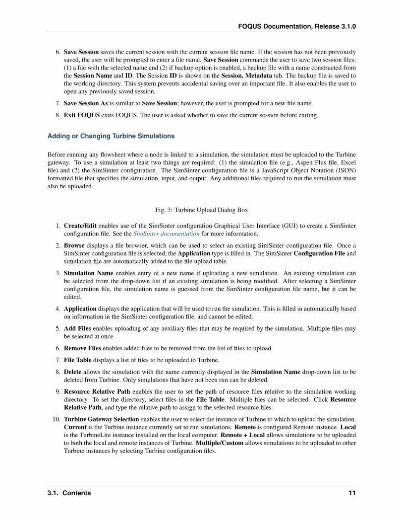
Adding or Changing Turbine Simulations
Before running any flowsheet where a node is linked to a simulation, the simulation must be uploaded to the Turbinegateway. To use a simulation at least two things are required: (1) the simulation file (e.g., Aspen Plus file, Excelfile) and (2) the SimSinter configuration. The SimSinter configuration file is a JavaScript Object Notation (JSON)formatted file that specifies the simulation, input, and output. Any additional files required to run the simulation mustalso be uploaded.
Fig. 3: Turbine Upload Dialog Box
1. Create/Edit enables use of the SimSinter configuration Graphical User Interface (GUI) to create a SimSinterconfiguration file. See the SimSinter documentation for more information.
2. Browse displays a file browser, which can be used to select an existing SimSinter configuration file. Once aSimSinter configuration file is selected, the Application type is filled in. The SimSinter Configuration File andsimulation file are automatically added to the file upload table.
3. Simulation Name enables entry of a new name if uploading a new simulation. An existing simulation canbe selected from the drop-down list if an existing simulation is being modified. After selecting a SimSinterconfiguration file, the simulation name is guessed from the SimSinter configuration file name, but it can beedited.
4. Application displays the application that will be used to run the simulation. This is filled in automatically basedon information in the SimSinter configuration file, and cannot be edited.
5. Add Files enables uploading of any auxiliary files that may be required by the simulation. Multiple files maybe selected at once.
6. Remove Files enables added files to be removed from the list of files to upload.
7. File Table displays a list of files to be uploaded to Turbine.
8. Delete allows the simulation with the name currently displayed in the Simulation Name drop-down list to bedeleted from Turbine. Only simulations that have not been run can be deleted.
9. Resource Relative Path enables the user to set the path of resource files relative to the simulation workingdirectory. To set the directory, select files in the File Table. Multiple files can be selected. Click ResourceRelative Path, and type the relative path to assign to the selected resource files.
10. Turbine Gateway Selection enables the user to select the instance of Turbine to which to upload the simulation.Current is the Turbine instance currently set to run simulations. Remote is configured Remote instance. Localis the TurbineLite instance installed on the local computer. Remote + Local allows simulations to be uploadedto both the local and remote instances of Turbine. Multiple/Custom allows simulations to be uploaded to otherTurbine instances by selecting Turbine configuration files.
3.1. Contents 11
FOQUS Documentation, Release 3.1.0
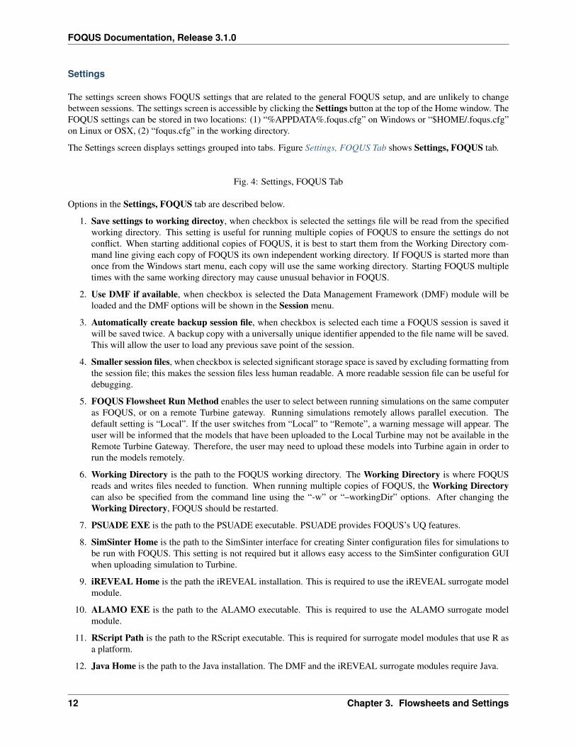
Settings
The settings screen shows FOQUS settings that are related to the general FOQUS setup, and are unlikely to changebetween sessions. The settings screen is accessible by clicking the Settings button at the top of the Home window. TheFOQUS settings can be stored in two locations: (1) “%APPDATA%.foqus.cfg” on Windows or “$HOME/.foqus.cfg”on Linux or OSX, (2) “foqus.cfg” in the working directory.
The Settings screen displays settings grouped into tabs. Figure Settings, FOQUS Tab shows Settings, FOQUS tab.
Fig. 4: Settings, FOQUS Tab
Options in the Settings, FOQUS tab are described below.
1. Save settings to working directoy, when checkbox is selected the settings file will be read from the specifiedworking directory. This setting is useful for running multiple copies of FOQUS to ensure the settings do notconflict. When starting additional copies of FOQUS, it is best to start them from the Working Directory com-mand line giving each copy of FOQUS its own independent working directory. If FOQUS is started more thanonce from the Windows start menu, each copy will use the same working directory. Starting FOQUS multipletimes with the same working directory may cause unusual behavior in FOQUS.
2. Use DMF if available, when checkbox is selected the Data Management Framework (DMF) module will beloaded and the DMF options will be shown in the Session menu.
3. Automatically create backup session file, when checkbox is selected each time a FOQUS session is saved itwill be saved twice. A backup copy with a universally unique identifier appended to the file name will be saved.This will allow the user to load any previous save point of the session.
4. Smaller session files, when checkbox is selected significant storage space is saved by excluding formatting fromthe session file; this makes the session files less human readable. A more readable session file can be useful fordebugging.
5. FOQUS Flowsheet Run Method enables the user to select between running simulations on the same computeras FOQUS, or on a remote Turbine gateway. Running simulations remotely allows parallel execution. Thedefault setting is “Local”. If the user switches from “Local” to “Remote”, a warning message will appear. Theuser will be informed that the models that have been uploaded to the Local Turbine may not be available in theRemote Turbine Gateway. Therefore, the user may need to upload these models into Turbine again in order torun the models remotely.
6. Working Directory is the path to the FOQUS working directory. The Working Directory is where FOQUSreads and writes files needed to function. When running multiple copies of FOQUS, the Working Directorycan also be specified from the command line using the “-w” or “–workingDir” options. After changing theWorking Directory, FOQUS should be restarted.
7. PSUADE EXE is the path to the PSUADE executable. PSUADE provides FOQUS’s UQ features.
8. SimSinter Home is the path to the SimSinter interface for creating Sinter configuration files for simulations tobe run with FOQUS. This setting is not required but it allows easy access to the SimSinter configuration GUIwhen uploading simulation to Turbine.
9. iREVEAL Home is the path the iREVEAL installation. This is required to use the iREVEAL surrogate modelmodule.
10. ALAMO EXE is the path to the ALAMO executable. This is required to use the ALAMO surrogate modelmodule.
11. RScript Path is the path to the RScript executable. This is required for surrogate model modules that use R asa platform.
12. Java Home is the path to the Java installation. The DMF and the iREVEAL surrogate modules require Java.
12 Chapter 3. Flowsheets and Settings
FOQUS Documentation, Release 3.1.0
13. Revert Changes The settings changes are applied when the user navigates away from the settings screen. Toundo changes made to settings the revert button can be clicked before changing to another screen.
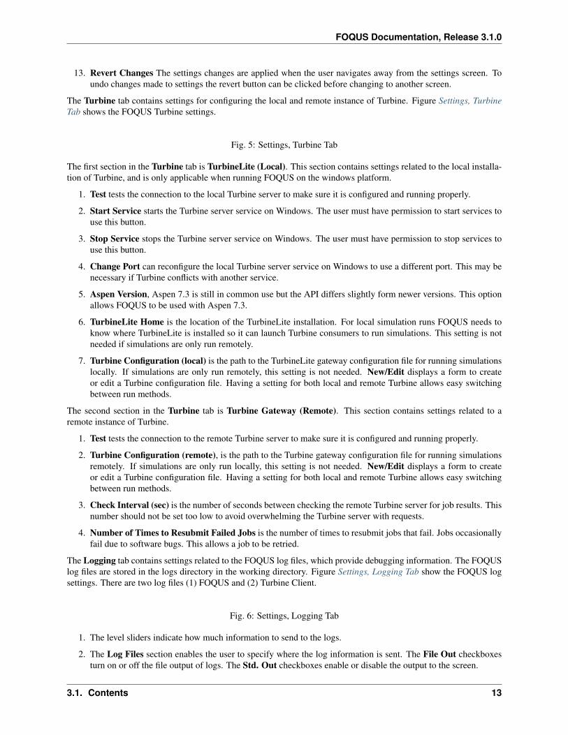
The Turbine tab contains settings for configuring the local and remote instance of Turbine. Figure Settings, TurbineTab shows the FOQUS Turbine settings.
Fig. 5: Settings, Turbine Tab
The first section in the Turbine tab is TurbineLite (Local). This section contains settings related to the local installa-tion of Turbine, and is only applicable when running FOQUS on the windows platform.
1. Test tests the connection to the local Turbine server to make sure it is configured and running properly.
2. Start Service starts the Turbine server service on Windows. The user must have permission to start services touse this button.
3. Stop Service stops the Turbine server service on Windows. The user must have permission to stop services touse this button.
4. Change Port can reconfigure the local Turbine server service on Windows to use a different port. This may benecessary if Turbine conflicts with another service.
5. Aspen Version, Aspen 7.3 is still in common use but the API differs slightly form newer versions. This optionallows FOQUS to be used with Aspen 7.3.
6. TurbineLite Home is the location of the TurbineLite installation. For local simulation runs FOQUS needs toknow where TurbineLite is installed so it can launch Turbine consumers to run simulations. This setting is notneeded if simulations are only run remotely.
7. Turbine Configuration (local) is the path to the TurbineLite gateway configuration file for running simulationslocally. If simulations are only run remotely, this setting is not needed. New/Edit displays a form to createor edit a Turbine configuration file. Having a setting for both local and remote Turbine allows easy switchingbetween run methods.
The second section in the Turbine tab is Turbine Gateway (Remote). This section contains settings related to aremote instance of Turbine.
1. Test tests the connection to the remote Turbine server to make sure it is configured and running properly.
2. Turbine Configuration (remote), is the path to the Turbine gateway configuration file for running simulationsremotely. If simulations are only run locally, this setting is not needed. New/Edit displays a form to createor edit a Turbine configuration file. Having a setting for both local and remote Turbine allows easy switchingbetween run methods.
3. Check Interval (sec) is the number of seconds between checking the remote Turbine server for job results. Thisnumber should not be set too low to avoid overwhelming the Turbine server with requests.
4. Number of Times to Resubmit Failed Jobs is the number of times to resubmit jobs that fail. Jobs occasionallyfail due to software bugs. This allows a job to be retried.
The Logging tab contains settings related to the FOQUS log files, which provide debugging information. The FOQUSlog files are stored in the logs directory in the working directory. Figure Settings, Logging Tab show the FOQUS logsettings. There are two log files (1) FOQUS and (2) Turbine Client.
Fig. 6: Settings, Logging Tab
1. The level sliders indicate how much information to send to the logs.
2. The Log Files section enables the user to specify where the log information is sent. The File Out checkboxesturn on or off the file output of logs. The Std. Out checkboxes enable or disable the output to the screen.
3.1. Contents 13

FOQUS Documentation, Release 3.1.0
3. Format allows the format of the log messages to be changed. See the documentation for the Python 2.7 loggingmodule for more information.
4. Rotate Log Files turns on or off log file rotation. When a log file reaches a certain size, a new log file isstarted and the contents of the old log are moved to a new file. There currently seems to be a bug in the log filerotation which occasionally makes the log file output stop; therefore, the Rotate Log Files option is labeled asan experimental feature.
Flowsheet
The meta-flowsheet defines connections between simulations. The flowsheet defines the order that simulations areperformed and what data is transferred between them. Simulations are represented as nodes in the flowsheet. Thesesimulations may be links to external simulation software through the Turbine gateway, or custom simulations orsimulation wrappers written in Python. Directed edges in the flowsheet connect nodes. The edges also specify whichvariables in the simulations are equivalent.
If the flowsheet contains cycles, they are solved iteratively. Tear streams are selected by FOQUS based on two criteria:(1) minimize the maximum number of times any cycle is torn and (2) minimize the total number of tear edges (whichonly is considered when two tear sets have the same value for the first criteria).
FOQUS currently has two methods available for solving flowsheets with recycle: (1) direct substitution and (2)Wegstien Wegstein 1958. FOQUS will solve strongly connected components in the order they are encountered inthe flowsheet. FOQUS flowsheets are generally not very complicated, so if a strongly connected component containsmore than one tear stream, they are solved simultaneously. More advanced solution options will be added if a needarises. Figure Flowsheet Recycle shows how a simple flowsheet with recycle would be solved.
Fig. 7: Flowsheet Recycle
Flowsheet Editor
Figure Flowsheet Editor illustrates the main Flowsheet Editor screen and a description of the pieces. The toolbar onthe left contains various flowsheet tools.
Fig. 8: Flowsheet Editor
The first three buttons are mouse mode buttons. The current mouse mode is shown by the depressed button. Theremaining buttons on the toolbar perform an action. The flowsheet editing toolbar and flowsheet are described indetail below.
1. Selection mode enables the user to select nodes and edges. Multiple items may be selected by holding down theShift key. To deselect everything, click an empty area of the flowsheet while not holding the Shift key. Selecteditems can be moved by dragging them. To move multiple items, hold down the Shift key while dragging. Thelast item selected becomes the current object to be edited in the Node or Edge Editor.
2. Add node mode enables the user to add a node by clicking anywhere on the flowsheet. Once a location isclicked, a dialog box opens where the new node name can be entered. If Cancel is selected, no node is added.The new node name cannot be “graph” and cannot match any existing node name.
3. Add edge mode enables edges to be added by selecting the node that the edge originates from, followed by thenode the edge terminates at.
4. Center flowsheet in display centers the display on the flowsheet.
14 Chapter 3. Flowsheets and Settings
FOQUS Documentation, Release 3.1.0
5. Delete selected deletes all selected nodes and edges. If a node is deleted, all edges connecting to that node arealso deleted.
6. Run a simulation starts a single simulation run. This is primarily used to test a simulation before runningoptimization or UQ.
7. Stop a simulation is enabled when a simulation is running and stops any running simulation. The simulationmay take several seconds to stop.
8. Set inputs to defaults returns all of the inputs to their default values.
9. Determine tear edges makes it easier to see where initial guesses are needed and makes it possible to edit thetear set before running the flowsheet. If tear streams are needed but not specified before running a flowsheet,they will be automatically specified, however inputs that will be used for the initial guess will not be knownbefore running.
10. Flowsheet solver settings contains options related to tear solvers.
11. Toggle node editor display displays or hides the Node Editor. The user can change the node being edited byselecting from Name in the Node Editor or selecting it on the flowsheet in selection mode.
12. Toggle edge editor display displays or hides the edge editor. The user can change the edge being edited in theEdge Editor, or by selecting it in selection mode.
13. Show results from all flowsheet runs displays the results of all flowsheet runs in a table view. This can beexported to a spreadsheet.
14. Node represents a simulation or calculations.
15. Edge connects simulation data, represents data transfer between two nodes.
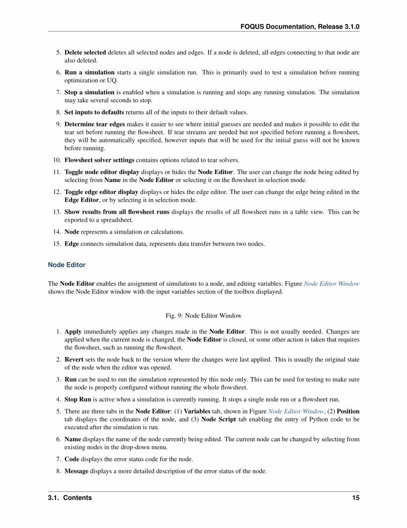
Node Editor
The Node Editor enables the assignment of simulations to a node, and editing variables. Figure Node Editor Windowshows the Node Editor window with the input variables section of the toolbox displayed.
Fig. 9: Node Editor Window
1. Apply immediately applies any changes made in the Node Editor. This is not usually needed. Changes areapplied when the current node is changed, the Node Editor is closed, or some other action is taken that requiresthe flowsheet, such as running the flowsheet.
2. Revert sets the node back to the version where the changes were last applied. This is usually the original stateof the node when the editor was opened.
3. Run can be used to run the simulation represented by this node only. This can be used for testing to make surethe node is properly configured without running the whole flowsheet.
4. Stop Run is active when a simulation is currently running. It stops a single node run or a flowsheet run.
5. There are three tabs in the Node Editor: (1) Variables tab, shown in Figure Node Editor Window, (2) Positiontab displays the coordinates of the node, and (3) Node Script tab enabling the entry of Python code to beexecuted after the simulation is run.
6. Name displays the name of the node currently being edited. The current node can be changed by selecting fromexisting nodes in the drop-down menu.
7. Code displays the error status code for the node.
8. Message displays a more detailed description of the error status of the node.
3.1. Contents 15
FOQUS Documentation, Release 3.1.0
9. Type enables the user to select the type of model to run. The model types are none, Turbine, DMF Lite, DMFServer, or Python Plugin. None allows no model to be assigned to the node; this is useful when the nodeonly executes a script entered directly into FOQUS. Turbine is used to execute Aspen, gPROMS, or Excelsimulations. Python plugins are custom simulations or wrappers written by the user. Surrogate model methodsmay also produce Python plugin models.
10. Model enables selection of the models available on Turbine or loaded Python plugins.
11. Input Variables enables viewing and editing the node’s input variables. Most of these variables are addedautomatically when a simulation is selected.
a. Add variable enables the addition of an input variable. There are two reasons to add an input: (1) to use avariable to pass information to another simulation (even if the variable is not used in any node calculation,it can receive data from the previous simulation and be passed on to the next simulation) and (2) to use ina node script. For example, a variable could be added that provides output in different units of measure.
b. Remove variable removes variables. If an input variable is removed that originally came from a Turbinesimulation, the simulation will run with the default value.
c. Tags displays a tag browser that lists commonly used variable tags.
d. Input Variables table displays information about variables. Most attributes can be edited, except for theName column within the Input Variables table. The rows for input variables are color coded dependingon whether they are set by an edge from results in another node. White rows are not connected. Yellowrows are set by a tear edge. These variables serve as initial guesses but their value may change once thesimulation has run. Red rows are set by an edge that is not a tear edge. The value set for these inputs doesnot matter and it may change once the simulation has run.
12. Output Variables is a variable table similar to the Input Variables table for node output variables. This area isdisplayed by clicking Output Variables.
13. Settings displays simulation settings. A description is provided for each setting. The available settings varydepending on simulation.
Node Variables
Variables in the node editor are grouped into two sections, inputs and outputs. The input and output variable tables areaccessible as described in the previous section. The contents of the variable tables are described here.
The columns in the input variable list are:
• Name is the name of the variable,
• Value is the current value,
• Unit is the unit of measure,
• Type is the data type (float, int, or str),
• Default is the default value,
• Min is the minimum value,
• Max is the maximum value,
• Description is a description string,
• Tag is a list of strings that can be used to attach additional information to a variable
• Distribution is a distribution type,
• Param1 is the first parameter of a parametric distribution the exact meaning depends on the selected distribution,and
16 Chapter 3. Flowsheets and Settings

FOQUS Documentation, Release 3.1.0
• Param2 is the second parameter of a parametric distribution the exact meaning depends on the selected distri-bution.
The minimum and maximum values for are not enforced when running simulations are not enforced. A value can begiven outside the range. Optimization and UQ features make use of these values to set upper and lower bounds ondecision variables or sampling. The distribution information is used when setting up sampling for UQ. In the future,this may also be used for things like optimization under uncertainty. Integer and string type variables cannot currentlybe used as optimization decision variables, or sampled with the UQ tool.
The rows of the input variable table are color coded. Some of the input variables may be set by connections to othernodes. White rows are variables who’s values are not set by a connection. The variables that are red have values setby a connection, and the value given will be overwritten and does not matter. The values that are colored yellow areinputs set by a connection that is a tear stream. The values of these variables serves as an initial guess for solvingrecycles.
The output variable table is similar to the input table, however it only contains the columns: Name, Value, Unit, Type,Description, and Tags. The value of the outputs may not correspond to the inputs until the simulation has been run.
Node Script
There are three type of Node Script that can be used: (1) Pre runs before a node simulation, (2) Post runs after a nodesimulation, and (3) Total scripts how a node runs the simulation.
Figure Node Script Tab illustrates the Node Script tab of the Node Editor with calculations for an optimization testproblem.
Fig. 10: Node Script Tab
Node scripts can be any valid Python code. The input and output variables for node scripts are stored in dictionariesx and f. The dictionary keys are the variable names. The f dictionary is used to update the node variables after thecalculations are executed.
Edge Editor
The Edge Editor is illustrated in Figure Edge Editor. The Edge Editor can be used to set connections between nodevariables.
Fig. 11: Edge Editor
1. Index is the index of the current edge. The current edge can be changed by selecting an index from the drop-down menu, but since the index is not a very meaningful identifier it is usually more convenient to select theedge to edit with the graphical selection tool.
2. Origin Node is the node where an edge starts. This may be edited by selecting a different node from thedrop-down menu.
3. Destination Node is the node to which the edge goes.
4. Curve can be a positive or negative number. The greater the magnitude of number, the more curved an edgewill appear in the flowsheet. This setting is used to keep edges from overlapping in the flowsheet display.
5. Tear marks this edge as a tear. Before a simulation is run, if a valid tear set is not specified, FOQUS locatesone.
6. Active specifies whether the edge is active or not. This allows connections to be temporarily disabled.
3.1. Contents 17
FOQUS Documentation, Release 3.1.0
7. Variable Connections table displays which variables are connected. Inputs or outputs in the origin node can beconnected to inputs in the destination node.
8. Add connection adds a new connection.
9. Remove connection deletes the selected connections.
10. Auto automatically connects variables having the same name. For example, in connecting a simulation to aspreadsheet to calculate costs there are a large number of variables for which it makes sense that the variableshave the same name in the simulation and spreadsheet. Auto should be used with great care. Connectingvariables with the same name is often not what is wanted. For example two simulations may have a variablenamed FlowAIn; however, it is very unlikely that they should be connected. It is more likely FlowAOut shouldbe connected to FlowAIn.
Sample Results
Flowsheet evaluations that have been run in a FOQUS session can be viewed by clicking the table button in theflowsheet toolbar (#13 in Figure Flowsheet Editor. The results are displayed in a table, and the contents can be copiedand pasted into a spreadsheet or exported to a CSV file. Figure Flowsheet Results Table Window show the FlowsheetResults Table window.
Fig. 12: Flowsheet Results Table Window
1. Menu contains a menu with four sub menus.
1. Import data from files or the clipboard.
2. Export data to files or the clipboard.
3. Edit or delete data.
4. View options for the table.
2. The Current Filter drop-down list enables the user to select a data filter, which can be used to filter and sortdata.
3. Edit Filters enables the user to create or edit data filters.
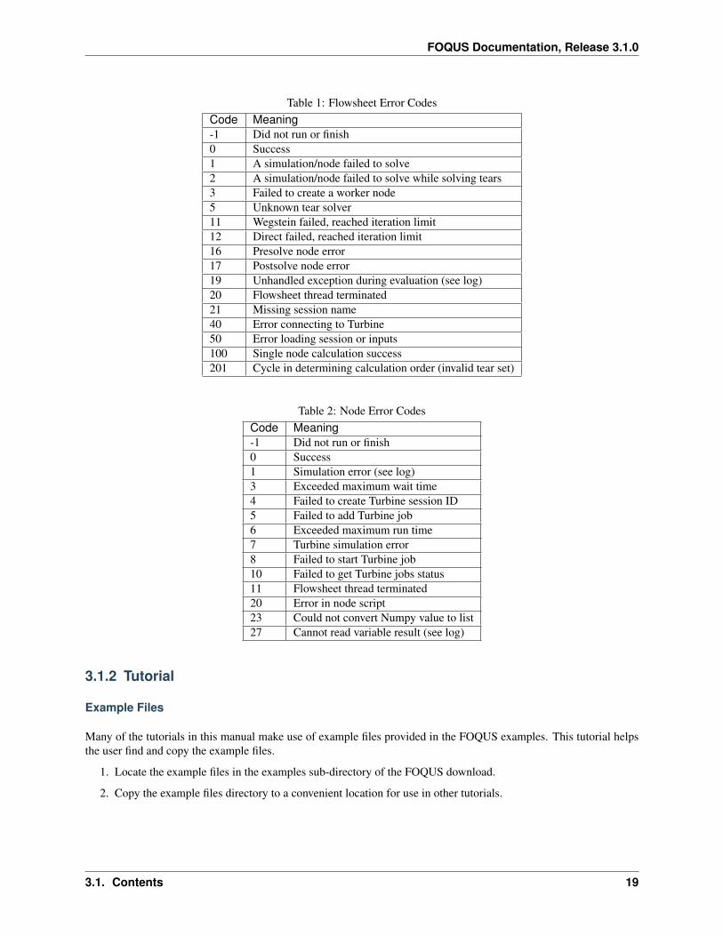
Error Codes
Error codes are listed in the Flowsheet Results table for the whole flowsheet and for individual nodes. Table FlowsheetError Codes shows the flowsheet error codes and Table Node Error Codes shows the node error codes. The mostcommon flowsheet error is 1, a node calculation failed. The most common node error is 7, Turbine simulation error.These errors are typically caused by a simulation that fails to converge or has some other calculation error (e.g., ACMdoes not converge or an Excel spreadsheet simulation with a division by 0 error).
18 Chapter 3. Flowsheets and Settings
FOQUS Documentation, Release 3.1.0
Table 1: Flowsheet Error CodesCode Meaning-1 Did not run or finish0 Success1 A simulation/node failed to solve2 A simulation/node failed to solve while solving tears3 Failed to create a worker node5 Unknown tear solver11 Wegstein failed, reached iteration limit12 Direct failed, reached iteration limit16 Presolve node error17 Postsolve node error19 Unhandled exception during evaluation (see log)20 Flowsheet thread terminated21 Missing session name40 Error connecting to Turbine50 Error loading session or inputs100 Single node calculation success201 Cycle in determining calculation order (invalid tear set)
Table 2: Node Error CodesCode Meaning-1 Did not run or finish0 Success1 Simulation error (see log)3 Exceeded maximum wait time4 Failed to create Turbine session ID5 Failed to add Turbine job6 Exceeded maximum run time7 Turbine simulation error8 Failed to start Turbine job10 Failed to get Turbine jobs status11 Flowsheet thread terminated20 Error in node script23 Could not convert Numpy value to list27 Cannot read variable result (see log)
3.1.2 Tutorial
Example Files
Many of the tutorials in this manual make use of example files provided in the FOQUS examples. This tutorial helpsthe user find and copy the example files.
1. Locate the example files in the examples sub-directory of the FOQUS download.
2. Copy the example files directory to a convenient location for use in other tutorials.
3.1. Contents 19

FOQUS Documentation, Release 3.1.0
Creating a Flowsheet
This tutorial provides information about the basic use of FOQUS and setting up a very simple flowsheet. A singlenode flowsheet will be created that performs a simple calculation using a square root so that simulation errors can beobserved when a negative input value is provided.
1. Start FOQUS (see Section Getting Started).
2. In the session form enter the Session Name as “Simple_Flow” (Figure Setting the Session Name).
Fig. 13: Setting the Session Name
3. Set the session description.
a. Select the Description tab (Figure Setting the Session Description).
b. Type the description shown in Figure Setting the Session Description. The buttons above the Descriptiontab box can be used to format the text.
Fig. 14: Setting the Session Description
4. Click the Flowsheet button at the top of the Home window (Figure Flowsheet, Input Variables).
5. Add a node named “calc.”
a. Click the Add Node button in the toolbar on the left side of the Home window.
b. Click a location on the gridded flowsheet area.
c. Enter the node name “calc” in the dialog box.
6. Click the Select Mode button in the toolbar.
7. Open the Node Editor by clicking the Node Editor button in the toolbar.
8. Add input variables to the node. (When linking a node to an external simulation the input and output variablesare populated automatically, and this step is not necessary.)
a. Click + above the Input Variables table.
b. Enter x1 in the variable Name dialog box.
c. Click + above the Input Variables table.
d. Enter x2 in the variable Name dialog box.
e. Enter -2 and 2 for the Min and Max of x1 in the Input Variables table.
f. Enter -1 and 4 for the Min and Max of x2 in the Input Variables table.
g. Enter 1 for the value of x1.
h. Enter 4 for the value of x2.
Fig. 15: Flowsheet, Input Variables
9. Add an output variable to the node. (When linking a node to an external simulation the input and output variablesare populated automatically.)
a. Click Output Variables to show the Output Variables table (Figure Flowsheet, Output Variables).
b. Click + above the Output Variables table to add a variable.
20 Chapter 3. Flowsheets and Settings

FOQUS Documentation, Release 3.1.0
c. Enter z in the output Name dialog box.
Fig. 16: Flowsheet, Output Variables
In this example, the node is not linked to any external simulation. The FOQUS nodes contain a section called nodescript, which can be used to do calculations before, after or instead of a simulation linked to the node. The node scriptcan be used for things such as unit conversion, simple calculations, or simulation convergence procedures. The nodescripts are written as Python. The Input Variables are contained in a dictionary named x and the Output Variablesare contained in a dictionary named f. The dictionary keys are the variables names shown in the input and outputtables. Only Output Variables can be modified by a node script.
10. Add a calculation to the node.
a. Click the Node Script tab (Figure Node Calculation).
b. Enter the following code into the Python code box:f['z'] = x['x1']*math.sqrt(x['x2'])
11. Click the Variables tab.
12. Click the Run button (Figure Node Calculation).
The flowsheet should run successfully and the output value should be 2. Rerun the flowsheet with a negative value forx2, and observe the result. The simulation should report an error.
Fig. 17: Node Calculation
13. Save the FOQUS session.
a. Click the Session drop-down menu at the top of the Home window (Figure Save Session).
b. Click Save. The exact location of save in the menu depends on whether or not the data managementframework is enabled.
c. The Change Log entry can be left blank.
d. The default file name is the session name. Change the file name and location if desired.
Fig. 18: Save Session
Creating a Flowsheet with Linked Simulations
This tutorial is referenced by other tutorials. Save the flowsheet in a convenient location for future use.
This tutorial demonstrates how to link simulations to nodes, and how to connect nodes in a flowsheet. Two models areused: (1) a bubbling fluidized bed model in ACM and (2) a cost of electricity (COE) model in Excel. The COE modelestimates the cost of electricity for a 650 MW (net before adding capture) supercritical pulverized coal power plantwith solid sorbent post combustion CO2 capture process added.
Before starting the tutorial, see Section Example Files to locate and copy the example files to a convenient location.
1. Start FOQUS. The Session window displays (Figure Session Setup).
2. Enter “BFB_opt” in Session Name (without quotes).
3. Click the Description tab. The problem description box displays and is shown in (Figure Session Description).
3.1. Contents 21
FOQUS Documentation, Release 3.1.0
4. In the problem description box enter information about the problem being solved in the FOQUS session; thisinformation can be more extensive than what is shown in the example.
5. Save the session file. Click Save Session from the Session drop-down menu. Enter change log information anda file name when prompted. The Creation Time in metadata page will be the time the session is first saved. TheModification Time will be the last time the session was saved. The ID is a unique identifier that changes eachtime the user saves the simulation. The Change Log tab provides a record of the changes made each time thesession is saved.
Fig. 19: Session Setup
Fig. 20: Session Description
[subsec.opt.tutorial.flowsheet] There are two models needed for this optimization problem: (1) the ACM model forthe BFB capture system and (2) the Excel cost estimating spreadsheet. These models are provided in the example filesdirectory, under optimization/models (see Section Example Files). There are two SimSinter configuration files: (1)BFB_sinter_config_v6.2.json for the process model and (2) BFB_cost_v6.2.3.json for the cost model. The next stepis to upload the models to Turbine.
6. Open the AddUpdate Model to Turbine dialog box (Figure Open Upload to Turbine Dialog).
7. In this case, the SimSinter configuration files have already been created. If a SimSinter configuration file needsto be created for the simulation, Create/Edit displays the SimSinter configuration GUI (see Figure Upload toTurbine Dialog). See the SimSinter documentation or Chapter Simulation Standard Interface (SimSinter) formore information.
8. Click Browse to select a SimSinter configuration file (Figure Upload to Turbine Dialog). Once the SimSinterconfiguration file is selected, the simulation file and sinterconfig file is automatically added to the files to upload.The application type is entered automatically. If there are additional files required for the simulation, those filescan be added by clicking Add File.
9. Enter the simulation name in Simulation Name. This name is determined by the user, but will default to theSimSinter configuration file name. For this tutorial use BFB_v6_2.
10. Click OK to upload the simulation.
11. Repeat the upload process for the cost model. Name the modelBFB_v6_2_Cost.
Fig. 21: Open Upload to Turbine Dialog
The next step is to create the flowsheet. Figure Flowsheet Editor illustrates the steps to draw the flowsheet.
12. Click Flowsheet at the top of the Home window.
13. Click Add Node mode.
14. Add two nodes to the flowsheet. Name the first node “BFB” and the second node “cost”.
15. Click Add Edge mode.
16. Click the BFB node followed by the cost node.
17. Click Selection mode and select the BFB node.
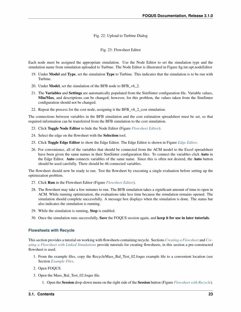
18. Click Toggle Node Editor. The Node Editor displays as illustrated in Figure fig.tut.opt.nodeEditor.
22 Chapter 3. Flowsheets and Settings
FOQUS Documentation, Release 3.1.0
Fig. 22: Upload to Turbine Dialog
Fig. 23: Flowsheet Editor
Each node must be assigned the appropriate simulation. Use the Node Editor to set the simulation type and thesimulation name from simulation uploaded to Turbine. The Node Editor is illustrated in Figure fig.tut.opt.nodeEditor
19. Under Model and Type, set the simulation Type to Turbine. This indicates that the simulation is to be run withTurbine.
20. Under Model, set the simulation of the BFB node to BFB_v6_2.
21. The Variables and Settings are automatically populated from the SimSinter configuration file. Variable values,Min/Max, and descriptions can be changed; however, for this problem, the values taken from the SimSinterconfiguration should not be changed.
22. Repeat the process for the cost node, assigning it the BFB_v6_2_cost simulation.
The connections between variables in the BFB simulation and the cost estimation spreadsheet must be set, so thatrequired information can be transferred from the BFB simulation to the cost simulation.
23. Click Toggle Node Editor to hide the Node Editor (Figure Flowsheet Editor).
24. Select the edge on the flowsheet with the Selection tool.
25. Click Toggle Edge Editor to show the Edge Editor. The Edge Editor is shown in Figure Edge Editor.
26. For convenience, all of the variables that should be connected from the ACM model to the Excel spreadsheethave been given the same names in their SimSinter configuration files. To connect the variables click Auto inthe Edge Editor. Auto connects variables of the same name. Since this is often not desired, the Auto buttonshould be used carefully. There should be 46 connected variables.
The flowsheet should now be ready to run. Test the flowsheet by executing a single evaluation before setting up theoptimization problem.
27. Click Run in the Flowsheet Editor (Figure Flowsheet Editor).
28. The flowsheet may take a few minutes to run. The BFB simulation takes a significant amount of time to open inACM. While running optimization, the evaluations take less time because the simulation remains opened. Thesimulation should complete successfully. A message box displays when the simulation is done. The status baralso indicates the simulation is running.
29. While the simulation is running, Stop is enabled.
30. Once the simulation runs successfully, Save the FOQUS session again, and keep it for use in later tutorials.
Flowsheets with Recycle
This section provides a tutorial on working with flowsheets containing recycle. Sections Creating a Flowsheet and Cre-ating a Flowsheet with Linked Simulations provide tutorials for creating flowsheets, in this section a pre-constructedflowsheet is used.
1. From the example files, copy the RecycleMass_Bal_Test_02.foqus example file to a convenient location (seeSection Example Files.
2. Open FOQUS.
3. Open the Mass_Bal_Test_02.foqus file.
1. Open the Session drop-down menu on the right side of the Session button (Figure Flowsheet with Recycle).
3.1. Contents 23
FOQUS Documentation, Release 3.1.0
Fig. 24: Node Editor
Fig. 25: Edge Editor
24 Chapter 3. Flowsheets and Settings

FOQUS Documentation, Release 3.1.0
2. Select Open Session from the drop-down menu.
3. Locate Mass_Bal_Test_02.foqus in the file browser, and open it.
4. Click Flowsheet button from the toolbar at the top of the Home window.
The flowsheet is shown in Figure Flowsheet with Recycle. The flowsheet consists of two reactors in recycle loops. Theflowsheet contains mixers, reactors, separators, and splitters. Each node uses a set of simple calculations in the nodescript section. The tear edges are shown in light blue.
Fig. 26: Flowsheet with Recycle
5. Inspect a node.
1. Make sure the Selection tool is selected (Figure React_01 Node.
2. Open the Node Editor by clicking the Node Edit button in the left toolbar in the Flowsheet view.
3. Click the “React_01” node.
4. Click Input Variables table. Note: Some input rows are colored red. This denotes that their values are setby output of the previous flowsheet node by the edge connecting “Mix_01” to “React_01.”
5. Click the Node Script tab.
6. Note the equations. Input Variables are stored in the x dictionary and Output Variables are stored in thef dictionary.
6. Click the gear icon in the left toolbar (see Figure React_01 Node. The tear solver settings are shown in FigureTear Solver Settings.
Fig. 27: React_01 Node
Fig. 28: Tear Solver Settings
7. Remove the tear edges.
1. Close the Node Editor.
2. Open the Edge Editor. Click the Edge Editor icon in the left toolbar (see Figure Edge Edit.
3. Click the edge between “React_01” and “Sep_01.”
4. In the Edge Editor, clear the Tear checkbox.
5. Repeat for the other tear edge.
8. Close the Edge Editor.
There should now be no tear edges in the flowsheet. The user can select tear edges or FOQUS can automatically selecta set. If there is not a valid set of tear edges marked when a flowsheet is run, tear edges will automatically be selected.
9. Automatically select a tear edge set by clicking the Tear icon in the left toolbar (see Figure Edge Edit).
10. Open the Node Editor and look at node “Sep_01.” In the Input Variables table, notice that some of the inputlines are colored yellow. The yellow inputs serve as initial guesses for the tear solver. The final value will bedifferent from the initial value.
11. Click the Run button on the left toolbar. The flowsheet should solve quickly.
12. The results of the completed run are in the flowsheet. An entry will also be created in the Flowsheet Resultsdata table (see Section Flowsheet Result Data.
3.1. Contents 25

FOQUS Documentation, Release 3.1.0
Fig. 29: Edge Edit
Flowsheet Result Data
Flowsheet evaluation results are stored in a table in the FOQUS session. This data can be used for many purposes.The flowsheet evaluations may be single runs, part of an optimization problem, or part of a UQ ensemble. This tutorialprovide information about sorting, filtering, and exporting data.
Copy the Data/Simple_flow.foqus file from the example files to a convenient location (see section Example Files).This file is similar to the one created in the tutorial Section Creating a Flowsheet with Linked Simulations, but it hasbeen run an additional 100 times using a UQ ensemble (see Uncertainty Quantification).
1. Open FOQUS.
2. Open the Simple_flow.foqus session from the example files.
3. Click the Flowsheet button from the Home window.
4. Click Flowsheet Data in the toolbar on the left side of the Home window.
Fig. 30: Flowsheet Results Data Table, All Data
A data table should be displayed like the one shown in the figure below. There are 102 flowsheet evaluations. The firsttwo evaluations are single runs, as can be seen in the SetName column, and the remaining 100 evaluation are from aUQ ensemble. The Error column shows several of the evaluations resulted in an error from a negative number beingpassed to the square root function.
This tutorial is broken up into mini-tutorials in the remaining subsections, which can be done independently. Theyeach use the example data file described above.
Sorting Data
1. Open FOQUS.
2. Open the Simple_flow.foqus session from the example files.
3. Click Flowsheet in the main toolbar at the top of the FOQUS Home window.
4. Click Flowsheet Data in the toolbar on the left side of the Home Window.
5. Click Edit Filters.
6. Click New Filter.
7. Enter “Sort1” as the new filter name.
8. Click New Filter.
9. Enter “Sort2” as the new filter name.
10. Select “Sort1” from the Filter drop-down list.
11. Enter ["-result"] as the Sort by Column. Include the square brackets. The square brackets indicate thatthere is a list of sort terms, although in this case there is only one. If multiple search terms are given, theadditional terms will be used to sort results having the same value for the previous terms. The “-” in front ofresult indicates the results should be sorted in reverse. The names of the sort terms come from the columnheadings, and are case sensitive.
12. Click Done to save the filters and return to the results table.
26 Chapter 3. Flowsheets and Settings

FOQUS Documentation, Release 3.1.0
Fig. 31: Sort1 Data Filter
14. Select “Sort1” from the Current Filter drop-down list.
15. The results are shown in below. The data should be sorted in reverse alphabetical order by result. Some of thecolumns are hidden to make the relevant results easier to see.
Fig. 32: Sort1 Data Filter Results
16. Click Edit Filters.
17. Select “Sort2” from Filter drop-down list.
19. Enter ["err", "-result"] in the Sort Term field. This will sort the data first by Error code then byresult in reverse alphabetical order.
20. Click Done.
Fig. 33: Sort2 Data Filter
21. Select “Sort2” in the Current Filter drop-down list.
22. The results are shown in below. The data should be sorted so all Error code zero results are first then sorted inreverse alphabetical order by result.
Filtering Data
1. Open FOQUS.
2. Open the Simple_flow.foqus session from the example files.
3. Click the Flowsheet button in the Home window.
4. Click the Results Data button (Table icon in left toolbar).
5. In the data table dialog, click Edit Filters.
6. Click New Filter and enter “Filter1” in the Filter field as the new filter name.
The filter expression is a Python expression. The c("Comlumn Name") function returns a numpy array containingthe column data. The expression should evaluate to a column of bools where rows containing True will be included inthe filtered results and rows containing False will be excluded. If combining multiple logical expressions the numpylogical functions https://docs.scipy.org/doc/numpy-1.15.1/reference/routines.logic.html should be used. Numpy is im-ported as np
8. In this example, results without errors in the “Single_runs” should be selected. In the filer expression field enternp.logical_and(c("err") == 0, c("set") == "Single_runs")
10. Click Done.
11. In the data table dialog, select “Filter1” from the Current Filter drop-down list.
12. The result is displayed in the Figure below.
3.1. Contents 27
FOQUS Documentation, Release 3.1.0
Fig. 34: Sort2 Data Filter Result
Fig. 35: Filter1 Data Filter
Exporting Data
This tutorial uses a spreadsheet program such as Excel or Open Office. The exported data is subject to the selectedfilter. See the previous tutorials in this section for more information about sorting and filtering data to be exported.
Clipboard
FOQUS can export data directly to the Clipboard. The data can be pasted into a spreadsheet or as text. Copying datato the Clipboard eliminates the need for an intermediate file when creating spreadsheets.
1. Open FOQUS.
2. Open a spreadsheet program.
3. Open the Simple_flow.foqus session from the example files.
4. Click the Flowsheet button in the Home window.
5. Click the Results Data button (Table icon in left toolbar).
6. Click on the Menu drop-down list in the data table dialog.
7. Select “Export” from the Menu drop-down list.
8. Click Copy Data to Clipboard.
9. Select Paste in the spreadsheet program. The data table in FOQUS should paste into the spreadsheet. Filters canbe used to sort or reduce the exported data.
CSV File
CSV (comma separated value) files can be read by almost any spreadsheet program, and are common formats readableby many types of software. FOQUS exports CSV files using the column headings from the data table as a header.
1. Open FOQUS.
2. Open a spreadsheet program.
3. Open the Simple_flow.foqus session from the example files.
4. Click the Flowsheet button in the Home window.
5. Click the Results Data button (Table icon in left toolbar).
6. Click the Menu drop-down list.
7. Select “Export” from the Menu drop-down list.
8. Click Export to CSV File.
Fig. 36: Filter1 Data Filter Result
28 Chapter 3. Flowsheets and Settings
FOQUS Documentation, Release 3.1.0
9. Enter a file name in the file dialog.
10. In the spreadsheet program, open the CSV file exported in the previous step.
Using a Remote Turbine Instance
A remote Turbine instance may be used instead of TurbineLite. TurbineLite, used by default, runs simulations (e.g.,Aspen Plus) on the user’s local machine. The remote Turbine gateway has several potential advantages over Tur-bineLite, while the main disadvantage is the effort required for installation and configuration. Some reasons to run aremote Turbine instance are:
• Simulations can be run in parallel. The Turbine gateway can distribute simulations to multiple machines con-figured to run FOQUS flowsheet consumers. FOQUS consumers are basically additional instances of FOQUSrunning on remote systems which can run a FOQUS flowsheet.
• Simulations can be run on machines other than the user’s, so as not to tie-up the user’s machine running simu-lations.
Running Remote Turbine on Your Own Computer
To run remote turbine on you own computer (e.g., if your computer has multiple processors):
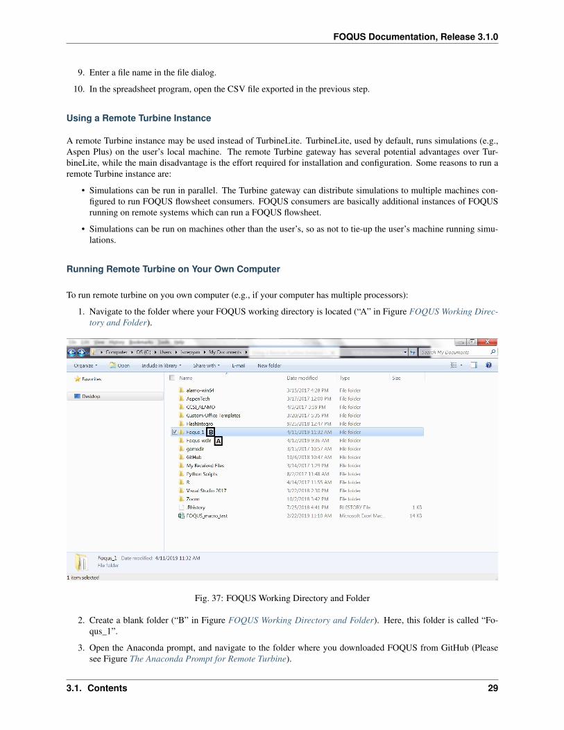
1. Navigate to the folder where your FOQUS working directory is located (“A” in Figure FOQUS Working Direc-tory and Folder).
Fig. 37: FOQUS Working Directory and Folder
2. Create a blank folder (“B” in Figure FOQUS Working Directory and Folder). Here, this folder is called “Fo-qus_1”.
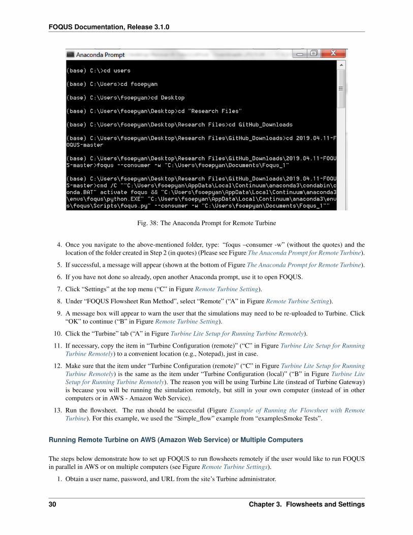
3. Open the Anaconda prompt, and navigate to the folder where you downloaded FOQUS from GitHub (Pleasesee Figure The Anaconda Prompt for Remote Turbine).
3.1. Contents 29
FOQUS Documentation, Release 3.1.0
Fig. 38: The Anaconda Prompt for Remote Turbine
4. Once you navigate to the above-mentioned folder, type: “foqus –consumer -w” (without the quotes) and thelocation of the folder created in Step 2 (in quotes) (Please see Figure The Anaconda Prompt for Remote Turbine).
5. If successful, a message will appear (shown at the bottom of Figure The Anaconda Prompt for Remote Turbine).
6. If you have not done so already, open another Anaconda prompt, use it to open FOQUS.
7. Click “Settings” at the top menu (“C” in Figure Remote Turbine Setting).
8. Under “FOQUS Flowsheet Run Method”, select “Remote” (“A” in Figure Remote Turbine Setting).
9. A message box will appear to warn the user that the simulations may need to be re-uploaded to Turbine. Click“OK” to continue (“B” in Figure Remote Turbine Setting).
10. Click the “Turbine” tab (“A” in Figure Turbine Lite Setup for Running Turbine Remotely).
11. If necessary, copy the item in “Turbine Configuration (remote)” (“C” in Figure Turbine Lite Setup for RunningTurbine Remotely) to a convenient location (e.g., Notepad), just in case.
12. Make sure that the item under “Turbine Configuration (remote)” (“C” in Figure Turbine Lite Setup for RunningTurbine Remotely) is the same as the item under “Turbine Configuration (local)” (“B” in Figure Turbine LiteSetup for Running Turbine Remotely). The reason you will be using Turbine Lite (instead of Turbine Gateway)is because you will be running the simulation remotely, but still in your own computer (instead of in othercomputers or in AWS - Amazon Web Service).
13. Run the flowsheet. The run should be successful (Figure Example of Running the Flowsheet with RemoteTurbine). For this example, we used the “Simple_flow” example from “examplesSmoke Tests”.
Running Remote Turbine on AWS (Amazon Web Service) or Multiple Computers
The steps below demonstrate how to set up FOQUS to run flowsheets remotely if the user would like to run FOQUSin parallel in AWS or on multiple computers (see Figure Remote Turbine Settings).
1. Obtain a user name, password, and URL from the site’s Turbine administrator.
30 Chapter 3. Flowsheets and Settings
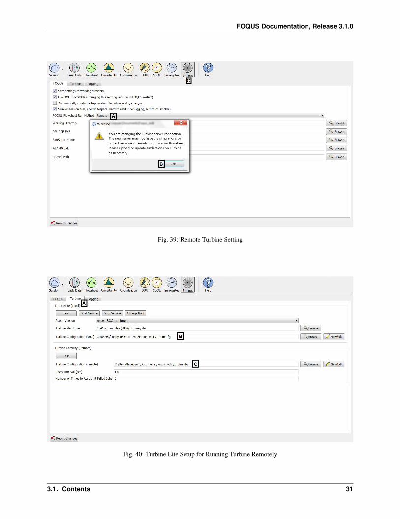
FOQUS Documentation, Release 3.1.0
Fig. 39: Remote Turbine Setting
Fig. 40: Turbine Lite Setup for Running Turbine Remotely
3.1. Contents 31

FOQUS Documentation, Release 3.1.0
Fig. 41: Example of Running the Flowsheet with Remote Turbine
2. Open FOQUS.
3. Click Settings at the top right of the Home window (Figure Run Method Settings).
4. Select “Remote” from the FOQUS Flowsheet Run Method drop-down list. A message box will appear. Theuser will be warned that the models that have been uploaded to Turbine Local may not be available in TurbineRemote Gateway, which means that the user may need to upload the models into Turbine again (please see Step7).
5. Click the Turbine tab; this displays the Turbine settings shown in Figure Remote Turbine Settings.
Fig. 42: Run Method Settings
6. Create a Turbine configuration file; this contains your password in plain text, so it is very important that if youare allowed to choose your own password, you choose one that is not used for any other purpose.
1. Click New/Edit next to the Turbine Configuration (remote) field. The Turbine Configuration windowdisplays (see Figure Remote Turbine Settings).
2. Select “Cluster/Cloud” from the Turbine Gateway Version drop-down list in the Turbine Configurationwindow.
3. Enter the Turbine URL in the Address field.
4. Enter the User name and Password.
5. Click Save as and enter a new file name.
6. Set the remote Turbine configuration file. Click Browse next to the Turbine Configuration (remote)field. Select the file created in Step 6e.
At this point the remote gateway is ready to use. The last step is to ensure that all simulations referenced by flowsheetsto be run are uploaded to the remote Turbine gateway.
32 Chapter 3. Flowsheets and Settings

FOQUS Documentation, Release 3.1.0
Fig. 43: Remote Turbine Settings
7. Upload any necessary simulations to Turbine (see Section Adding or Changing Turbine Simulations and thetutorial in Section Creating a Flowsheet with Linked Simulations)
Once all settings are specified there is no apparent difference between running flowsheets locally or on a remoteTurbine gateway, and FOQUS can readily be switched between the two.
3.1. Contents 33

FOQUS Documentation, Release 3.1.0
34 Chapter 3. Flowsheets and Settings

CHAPTER 4
Optimization
4.1 Contents
4.1.1 Reference
The simulation based optimization tool provides a plug-in system where different derivative free optimization (DFO)solvers can be used with FOQUS. Several solvers are provided with FOQUS. The CMA-ES solver (Hansen 2006) isa good global derivative free optimization (DFO) solver. The NLopt library provides access to several DFO solvers(Johnson 2015). SLSQP and BFGS from the Scipy module are also provided (Jones et al. 2015). Since FOQUSdoes not generally have access to derivative information the Scipy solvers rely on finite difference approximations,and should only be used with well-behaved functions. Due to convergence tolerances in process simulators, finitedifference approximations may not be good for many of FOQUS’s intended applications.
CMA-ES offers a restart feature, which can be used to resume an optimization if it is interrupted for any reason. Othersolvers may use an auto-save feature, which does not provide the ability to restart, but will allow optimization to startfrom the best solution found up to the point the optimization was interrupted. Samples making up the population inCMA-ES can be run in parallel. The NLopt and Scipy plugins do not offer parallel computing for standard optimiza-tion. For any solver, parallel computation can be used for parameter estimation and optimization under uncertainty,where multiple flowsheet evaluations go into an objective function calculation.
Problem Set Up
See Chapter [chpt.flowsheet] for information about setting up a flowsheet in FOQUS. Once the flowsheet has beenset up and tested, an optimization problem can be added. FOQUS allows multiple flowsheet evaluations to be usedto calculate a single objective function value. This allows FOQUS to do parameter estimation and scenario basedoptimization under uncertainty. There are three types of variables used in the optimization problem: (1) fixed variablesdo not change during the optimization, (2) decision variables are modified by the optimization algorithm to find thebest value of the objective function, and (3) sample variables, which are used to construct the multiple flowsheetevaluations that can go into an objective calculation. If no sample variables are defined, each objective functionvalue will be based on a single flowsheet evaluation. Figure Optimization Variable Selection shows the Variables tabselection form.
35
FOQUS Documentation, Release 3.1.0
Fig. 1: Optimization Variable Selection
1. The Variables tab contains the form for variables selection.
2. The Variable column shows the name of input variables in the flowsheet. If a variable is set by a connectionto another variable through an edge, it is not shown in the table. The format for a variable name is {NodeName}.{Variable Name}.
3. The Type column allows the variables to be assigned as one of three types (1) fixed, (2) decision, or (3) sample.
4. The Scale column allows the scaling method to be set for each variable. Decision variables must be scaled.Scaling is ignored for other variables. In the FOQUS example files, there is a scaling spreadsheet that provides ademonstration of the different scaling methods. The upper and lower bound are used in the scaling calculations.Regardless of the scaling method, the optimizer sees the decision variables as running from 0 at their minimumto 10 at their maximum.
5. The Min and Max columns are used to define the upper and lower bounds for the variables. FOQUS requiresthat all optimization problems be bounded.
6. The Value column provides the starting point for the optimization. How the starting point is used depends onthe optimization method. The starting point for sample variables is irrelevant. Fixed variables will remain attheir starting point during the optimization.
The sample variables define a set of samples that will be used to calculate an objective function. For each objectivefunction, the decision variables are fixed at values set by the optimization solver, and the flowsheet is evaluated foreach row on the sample table. The results of the samples can be used to calculate the objective function. Usingthe Samples tab is optional. If no sample variables are set, each objective function value will be based on a singlesimulation. Figure Optimization Sample Table shows the Samples table form.
Fig. 2: Optimization Sample Table
1. The Samples tab contains the table used to define samples for objective function calculations. If there are nosample variables, the table should be empty.
2. Add Sample adds a row to the Samples table.
3. Delete Samples deletes the selected rows from the Samples table.
4. Generate Samples opens a dialog box that provides a selection of methods to generate samples or read samplesfrom a file.
5. Clear Samples clears the Samples table.
Once the variables and (optionally) samples have been selected, the objective function and constraints can be defined.FOQUS is set up to handle multi-objective optimization, but no multi-objective optimization plug-ins are currentlyprovided in the FOQUS installer, so some of the options may seem to be extraneous. There are two methods forentering the objective function and constraints into FOQUS: (1) Simple Python expressions and (2) a more extensivePython function. Python expressions are easier and sufficient for most cases. If the objective function is complicatedit may be necessary to write a Python function, which can be as complex as needed.
The variables used in the Python code for the objective function or constraints are stored in two Python dictio-naries, “f” for outputs and “x” for inputs. There are two ways to index the dictionaries depending on whether ornot sample variables are used. For an input variable with sampling, the indexing is x[Sample Index][’NodeName’][’Variable Name’][Time Step Index]. If no sample variables are defined, the sample index isnot needed, so the indexing would be, x[’Node Name’][’Variable Name’][Time Step]. Node Nameand Variable Name are strings so they should be in quotes. The sample and time step indexes are integers. For steadystate simulations, the time step should be 0.
36 Chapter 4. Optimization

FOQUS Documentation, Release 3.1.0
Figure Optimization Simple Objective Function shows the form for entering the objective function and constraints asPython expressions.
Fig. 3: Optimization Simple Objective Function
1. The Objective/Constraints tab contains the form used to enter the objective function and constraints.
2. The drop-down list enables the selection of either the “Simple Python Expression” or “Custom Python” form ofthe objective function.
3. + adds an objective function to the table. The solvers currently available are single objective and will only usethe first objective function.
4. - removes the selected objective from the table.
5. The Python expression for the objective function can be entered in the Expression column.
6. The Penalty Scale column is intended for use with multi-objective solvers and allows the constraint violationpenalty to be applied differently to objective functions with different magnitudes.
7. The Value for Failure column contains the value to be assigned to the objective function if the objective can-not be evaluated for any reason. The value should be higher than the expected highest value for a successfulobjective.
8. + adds an inequality constraint.
9. - removes selected inequality constraints.
10. The inequality constraints are in the form 𝑔(x) ≤ 0. The Expression column contains the Python expressionfor 𝑔(x).
11. The Penalty Factor contains the coefficient 𝑎 used in calculating the penalty for a constraint violation, seeEquations [eq.linear.constriant] to [eq.step.constriant].
12. The Form column contains a selection of different methods to calculate a constraint penalty.
13. Check Input checks the problem for any mistakes that can be detected before running the optimization.
14. Variable Explorer enables the user to browse the variables in the simulation. They can be copied and pastedinto the Python expression. The variables are provided without the sample index.
The calculations for each type of constraint penalty are given in Equations [eq.linear.constriant] to[eq.step.constriant].
Linear penalty form: 𝑝𝑖 =
{︃0 if 𝑔𝑖(x) ≤ 0
𝑎× 𝑔𝑖(x) if 𝑔𝑖(x) > 0
Quadratic penalty form: 𝑝𝑖 =
{︃0 if 𝑔𝑖(x) ≤ 0
𝑎× 𝑔𝑖(x)2 if 𝑔𝑖(x) > 0
Step penalty form: 𝑝𝑖 =
{︃0 if 𝑔𝑖(x) ≤ 0
𝑎 if 𝑔𝑖(x) > 0
If the Simple Python Expression method of entering the objective function does not offer enough flexibility, the CustomPython method can be used. The Custom Python method enables the user to enter the objective calculation as a Pythonfunction, which also should include any required constraint penalties.
Figure Custom Objective Function shows the Custom Python objective form. The top text box provides instructionsfor writing a custom objective function. The bottom text box provides a place to enter Python code. The numpy andmath modules have been imported and are available as numpy and math. To use the Custom Python objective, the user
4.1. Contents 37
FOQUS Documentation, Release 3.1.0
must define a function called “onjfunc(x, f, fail).”” The three arguments are: (1) “x” is the dictionary of input variables,(2) “f” is the dictionary of output variables, and (3) “fail” is a boolean vector that indicates whether a particular samplecalculation has failed. The “objfunc” function should return three values: (1) a list of objective function values formulti-objective optimization (in most cases with single objective optimization this will be a list with one value), (2) alist of constraint violations, and (3) the total constraint penalty. The constraint violation and penalty information areonly used for debugging, so they are not required. It is safe to return [0] and 0 for the constraint information regardlessof whether a constraint penalty has been added to the objective.
Fig. 4: Custom Objective Function
The code in Figure fig.opt.problem.objective2_code provides an example of a custom objective function for parameterestimation. The objective function minimizes the sum of the differences between simulation and empirical data. Inthis case the decision variables would be model parameters. The first line defines a function with three arguments. The“x” and “f” arguments are the input and output variables. The variable indexing is explained in the simple objectivefunction section. The “fail” argument is a boolean vector where element “i” is true if sample “i” failed. If there are nosample variables, “fail” will only have one element.
The “if” in the function determines if any flowsheet evaluation failed, and assigns a bad objective function value ifso. If all the flowsheet evaluations where successful, the results are used to calculate the objective function. In theobjective function calculation, Python list comprehension is used to calculate the sum of squared errors. In this case,no constraint penalty is needed. The objective function is returned as a list with only one element. The last two returnvalues are debugging information for constraints. In this case, the “zeros” are just place holders and have no realutility.
Solver Options
The Solver tab in the Optimization button tool enables the selection of the DFO method and setting of solver param-eters. Figure Optimization Solver Form illustrates the solver form.
Fig. 5: Optimization Solver Form
Elements of the solver form are:
1. Select Solver drop-down list, which enables the user to select from available DFO solvers.
2. Description text box provides a description of the selected DFO solver.
3. Solver Options table contains the solver settings and a description of each option. The settings depend on theselected plug-in.
Running Optimization
The optimization monitor is displayed under the Run tab in the Optimization button tool. The optimization monitor,illustrated in Figure Optimization Monitor Form, is used to monitor the progress of the optimization as it runs.
Fig. 6: Optimization Monitor Form
Elements of the optimization monitor are:
1. Start starts the optimization.
2. Stop stops the optimization. The best solution found when optimization is stopped is stored in the flowsheet.
38 Chapter 4. Optimization
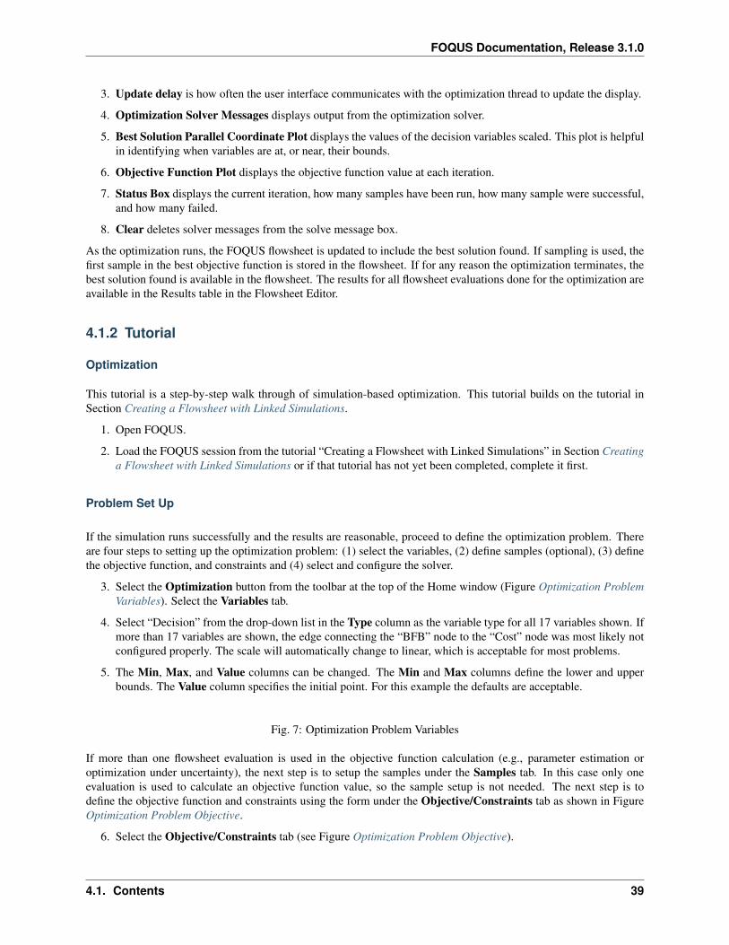
FOQUS Documentation, Release 3.1.0
3. Update delay is how often the user interface communicates with the optimization thread to update the display.
4. Optimization Solver Messages displays output from the optimization solver.
5. Best Solution Parallel Coordinate Plot displays the values of the decision variables scaled. This plot is helpfulin identifying when variables are at, or near, their bounds.
6. Objective Function Plot displays the objective function value at each iteration.
7. Status Box displays the current iteration, how many samples have been run, how many sample were successful,and how many failed.
8. Clear deletes solver messages from the solve message box.
As the optimization runs, the FOQUS flowsheet is updated to include the best solution found. If sampling is used, thefirst sample in the best objective function is stored in the flowsheet. If for any reason the optimization terminates, thebest solution found is available in the flowsheet. The results for all flowsheet evaluations done for the optimization areavailable in the Results table in the Flowsheet Editor.
4.1.2 Tutorial
Optimization
This tutorial is a step-by-step walk through of simulation-based optimization. This tutorial builds on the tutorial inSection Creating a Flowsheet with Linked Simulations.
1. Open FOQUS.
2. Load the FOQUS session from the tutorial “Creating a Flowsheet with Linked Simulations” in Section Creatinga Flowsheet with Linked Simulations or if that tutorial has not yet been completed, complete it first.
Problem Set Up
If the simulation runs successfully and the results are reasonable, proceed to define the optimization problem. Thereare four steps to setting up the optimization problem: (1) select the variables, (2) define samples (optional), (3) definethe objective function, and constraints and (4) select and configure the solver.
3. Select the Optimization button from the toolbar at the top of the Home window (Figure Optimization ProblemVariables). Select the Variables tab.
4. Select “Decision” from the drop-down list in the Type column as the variable type for all 17 variables shown. Ifmore than 17 variables are shown, the edge connecting the “BFB” node to the “Cost” node was most likely notconfigured properly. The scale will automatically change to linear, which is acceptable for most problems.
5. The Min, Max, and Value columns can be changed. The Min and Max columns define the lower and upperbounds. The Value column specifies the initial point. For this example the defaults are acceptable.
Fig. 7: Optimization Problem Variables
If more than one flowsheet evaluation is used in the objective function calculation (e.g., parameter estimation oroptimization under uncertainty), the next step is to setup the samples under the Samples tab. In this case only oneevaluation is used to calculate an objective function value, so the sample setup is not needed. The next step is todefine the objective function and constraints using the form under the Objective/Constraints tab as shown in FigureOptimization Problem Objective.
6. Select the Objective/Constraints tab (see Figure Optimization Problem Objective).
4.1. Contents 39

FOQUS Documentation, Release 3.1.0
Fig. 8: Optimization Problem Objective
7. In the drop-down list, verify “Simple Python Expression” is selected.
8. Add an objective function by clicking + to the right of the Objective Function table.
9. The objective function is the cost of electricity from the cost spreadsheet. Enter:f.Cost.COE
in the Expression column.
10. Enter 1 in the Penalty Scale column. This setting is used mostly for multi-objective optimization to apply theconstraint penalty to different objectives.
11. Enter 500 in the Value for Failure column. This should be worse than the objective for any non-failed simula-tions.
12. Add a constraint by clicking + next to the Inequality Constraints table.
13. The constraint is that the fraction of CO2 captured must be greater than or equal to 0.9. The constraint is in theform 𝑔(x) ≤ 0; therefore, in the Expression column enter:0.9 - f.BFB.removalCO2.
14. Enter 1000 for the Penalty Factor.
15. The constraint penalty Form should be linear.
16. The Variable Explorer button can be used to help select flowsheet variables.
Solver Settings
The last step before running the optimization is to select and configure the solver. The solver configuration form isshown in Figure Optimization Solver Setup.
Fig. 9: Optimization Solver Setup
17. Select the Solver tab (see Figure Optimization Solver Setup).
18. Select “OptCMA” from the Select Solver drop-down list.
19. The default options are acceptable. Solver options are described in the Solver Options table.
Running Optimization
The optimization run form is shown in Figure Optimization Monitor.
Fig. 10: Optimization Monitor
20. Click the Run tab to display the optimization run form (see Figure Optimization Monitor).
21. Click Start.
22. Once the optimization has run for while click Stop.
40 Chapter 4. Optimization
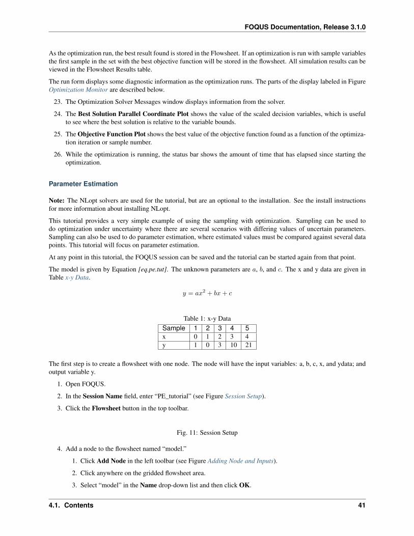
FOQUS Documentation, Release 3.1.0
As the optimization run, the best result found is stored in the Flowsheet. If an optimization is run with sample variablesthe first sample in the set with the best objective function will be stored in the flowsheet. All simulation results can beviewed in the Flowsheet Results table.
The run form displays some diagnostic information as the optimization runs. The parts of the display labeled in FigureOptimization Monitor are described below.
23. The Optimization Solver Messages window displays information from the solver.
24. The Best Solution Parallel Coordinate Plot shows the value of the scaled decision variables, which is usefulto see where the best solution is relative to the variable bounds.
25. The Objective Function Plot shows the best value of the objective function found as a function of the optimiza-tion iteration or sample number.
26. While the optimization is running, the status bar shows the amount of time that has elapsed since starting theoptimization.
Parameter Estimation
Note: The NLopt solvers are used for the tutorial, but are an optional to the installation. See the install instructionsfor more information about installing NLopt.
This tutorial provides a very simple example of using the sampling with optimization. Sampling can be used todo optimization under uncertainty where there are several scenarios with differing values of uncertain parameters.Sampling can also be used to do parameter estimation, where estimated values must be compared against several datapoints. This tutorial will focus on parameter estimation.
At any point in this tutorial, the FOQUS session can be saved and the tutorial can be started again from that point.
The model is given by Equation [eq.pe.tut]. The unknown parameters are 𝑎, 𝑏, and 𝑐. The x and y data are given inTable x-y Data.
𝑦 = 𝑎𝑥2 + 𝑏𝑥 + 𝑐
Table 1: x-y DataSample 1 2 3 4 5x 0 1 2 3 4y 1 0 3 10 21
The first step is to create a flowsheet with one node. The node will have the input variables: a, b, c, x, and ydata; andoutput variable y.
1. Open FOQUS.
2. In the Session Name field, enter “PE_tutorial” (see Figure Session Setup).
3. Click the Flowsheet button in the top toolbar.
Fig. 11: Session Setup
4. Add a node to the flowsheet named “model.”
1. Click Add Node in the left toolbar (see Figure Adding Node and Inputs).
2. Click anywhere on the gridded flowsheet area.
3. Select “model” in the Name drop-down list and then click OK.
4.1. Contents 41
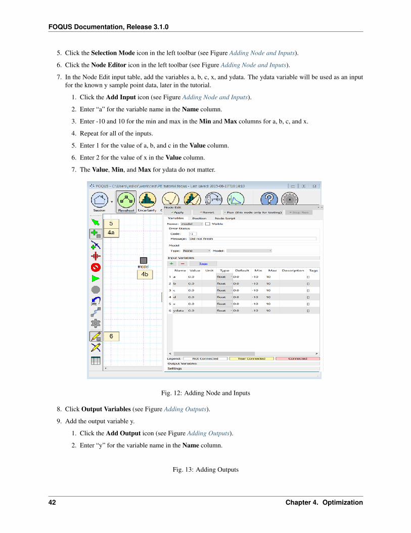
FOQUS Documentation, Release 3.1.0
5. Click the Selection Mode icon in the left toolbar (see Figure Adding Node and Inputs).
6. Click the Node Editor icon in the left toolbar (see Figure Adding Node and Inputs).
7. In the Node Edit input table, add the variables a, b, c, x, and ydata. The ydata variable will be used as an inputfor the known y sample point data, later in the tutorial.
1. Click the Add Input icon (see Figure Adding Node and Inputs).
2. Enter “a” for the variable name in the Name column.
3. Enter -10 and 10 for the min and max in the Min and Max columns for a, b, c, and x.
4. Repeat for all of the inputs.
5. Enter 1 for the value of a, b, and c in the Value column.
6. Enter 2 for the value of x in the Value column.
7. The Value, Min, and Max for ydata do not matter.
Fig. 12: Adding Node and Inputs
8. Click Output Variables (see Figure Adding Outputs).
9. Add the output variable y.
1. Click the Add Output icon (see Figure Adding Outputs).
2. Enter “y” for the variable name in the Name column.
Fig. 13: Adding Outputs
42 Chapter 4. Optimization
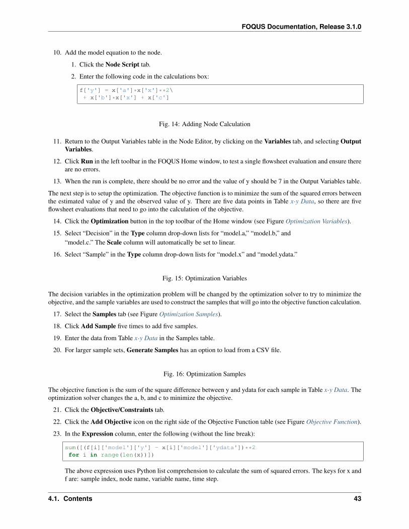
FOQUS Documentation, Release 3.1.0
10. Add the model equation to the node.
1. Click the Node Script tab.
2. Enter the following code in the calculations box:
f['y'] = x['a']*x['x']**2\+ x['b']*x['x'] + x['c']
Fig. 14: Adding Node Calculation
11. Return to the Output Variables table in the Node Editor, by clicking on the Variables tab, and selecting OutputVariables.
12. Click Run in the left toolbar in the FOQUS Home window, to test a single flowsheet evaluation and ensure thereare no errors.
13. When the run is complete, there should be no error and the value of y should be 7 in the Output Variables table.
The next step is to setup the optimization. The objective function is to minimize the sum of the squared errors betweenthe estimated value of y and the observed value of y. There are five data points in Table x-y Data, so there are fiveflowsheet evaluations that need to go into the calculation of the objective.
14. Click the Optimization button in the top toolbar of the Home window (see Figure Optimization Variables).
15. Select “Decision” in the Type column drop-down lists for “model.a,” “model.b,” and“model.c.” The Scale column will automatically be set to linear.
16. Select “Sample” in the Type column drop-down lists for “model.x” and “model.ydata.”
Fig. 15: Optimization Variables
The decision variables in the optimization problem will be changed by the optimization solver to try to minimize theobjective, and the sample variables are used to construct the samples that will go into the objective function calculation.
17. Select the Samples tab (see Figure Optimization Samples).
18. Click Add Sample five times to add five samples.
19. Enter the data from Table x-y Data in the Samples table.
20. For larger sample sets, Generate Samples has an option to load from a CSV file.
Fig. 16: Optimization Samples
The objective function is the sum of the square difference between y and ydata for each sample in Table x-y Data. Theoptimization solver changes the a, b, and c to minimize the objective.
21. Click the Objective/Constraints tab.
22. Click the Add Objective icon on the right side of the Objective Function table (see Figure Objective Function).
23. In the Expression column, enter the following (without the line break):
sum([(f[i]['model']['y'] - x[i]['model']['ydata'])**2for i in range(len(x))])
The above expression uses Python list comprehension to calculate the sum of squared errors. The keys for x andf are: sample index, node name, variable name, time step.
4.1. Contents 43

FOQUS Documentation, Release 3.1.0
24. Enter 1 for the Penalty Scale.
25. Enter 100 for the Value for Failure.
26. No constraints are required.
Fig. 17: Objective Function
Once the objective is set up, a solver needs to be selected and configured. Almost any solver in FOQUS should workwell for this problem with the default values.
27. Click the Solver tab (see Figure Optimization Samples).
28. Select “NLopt” from the Select Solver drop-down list. NLopt is a collection of solvers that share a standardinterface (Johnson 2015).
29. Select “BOBYQA” under the Solver Options table in the Settings column drop-down list.
Fig. 18: Optimization Samples
30. Click the Run tab (see Figure Running Optimization).
31. Click the Start button.
32. The Optimization Solver Messages window displays the solver progress. As the solver runs, the best resultsfound is placed into the flowsheet.
33. The Best Solution Parallel Coordinate Plot shows the scaled decision variable values for the best solutionfound so far.
34. The Objective Function Plot shows the value of the objective function as the optimization progresses.
Fig. 19: Running Optimization
The best result at the end of the optimization is stored in the flowsheet. All flowsheet evaluations run during theoptimization are stored in the flowsheet results table.
35. Once the optimization has completed, click Flowsheet in the top toolbar.
36. Open the Node Editor and look at the Input Variables table. The approximate result should be a = 2, b = -3,and c = 1 (see Figure Flowsheet, Input Variables Results).
44 Chapter 4. Optimization

FOQUS Documentation, Release 3.1.0
Fig. 20: Flowsheet, Input Variables Results
4.1. Contents 45

FOQUS Documentation, Release 3.1.0
46 Chapter 4. Optimization
CHAPTER 5
Uncertainty Quantification
5.1 Contents
[sec:uq_overview]
5.1.1 Reference
The Uncertainty Quantification (UQ) module of FOQUS provides a multitude of analysis and visualization capabilitiesto facilitate the understanding of uncertainty’s impact on a given system. In a generic UQ study, the workflow is usuallycomprised of the following steps:
1. Define the objectives of the analysis.
2. Specify and acquire the simulation model, which implements an input-to-output mapping from inputs to outputs.
3. Select the inputs that have uncertainty and characterize said uncertainty in the form of prior distributions.
4. Identify relevant data from physical experiments that can be used to refine these prior distributions on the inputs.
5. Generate a set of input samples according to the input distribution.
6. Propagate the set of input samples through the simulation model to get the corresponding output values.
7. Analyze the results to make informed decisions about subsequent analyses.
FOQUS UQ provides tools to perform Steps 5-7. With respect to Step 7, a variety of analysis capabilities are available.They include parameter screening methods, response surface construction/validation/prediction, uncertainty analysis,sensitivity analysis, and visualization.
In this chapter, components of the UQ user interface are first explained, then the use of these components for UQanalyses is illustrated.
47
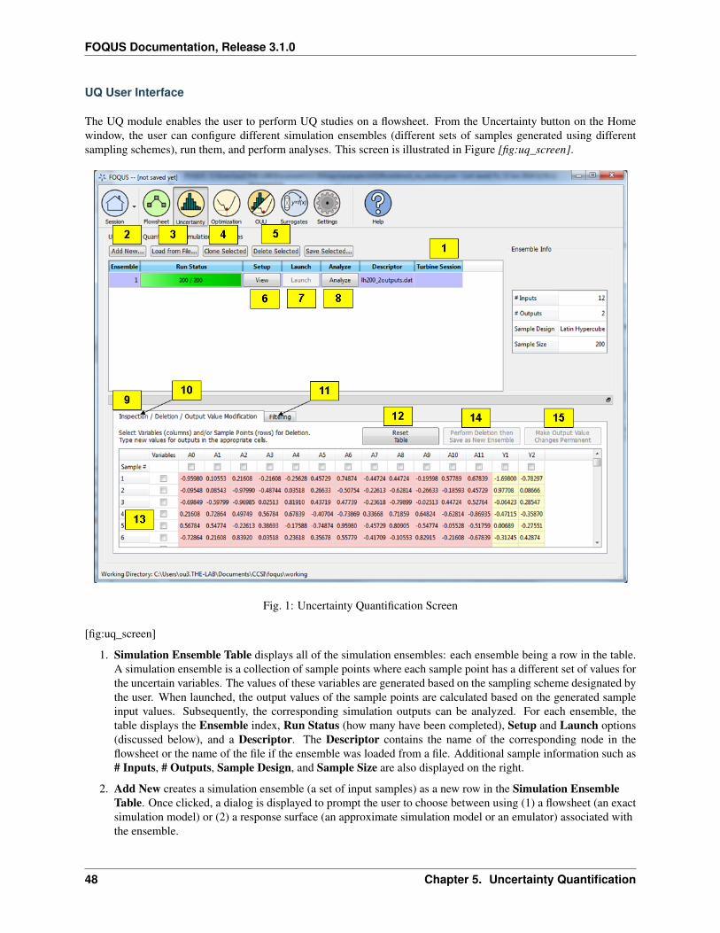
FOQUS Documentation, Release 3.1.0
UQ User Interface
The UQ module enables the user to perform UQ studies on a flowsheet. From the Uncertainty button on the Homewindow, the user can configure different simulation ensembles (different sets of samples generated using differentsampling schemes), run them, and perform analyses. This screen is illustrated in Figure [fig:uq_screen].
Fig. 1: Uncertainty Quantification Screen
[fig:uq_screen]
1. Simulation Ensemble Table displays all of the simulation ensembles: each ensemble being a row in the table.A simulation ensemble is a collection of sample points where each sample point has a different set of values forthe uncertain variables. The values of these variables are generated based on the sampling scheme designated bythe user. When launched, the output values of the sample points are calculated based on the generated sampleinput values. Subsequently, the corresponding simulation outputs can be analyzed. For each ensemble, thetable displays the Ensemble index, Run Status (how many have been completed), Setup and Launch options(discussed below), and a Descriptor. The Descriptor contains the name of the corresponding node in theflowsheet or the name of the file if the ensemble was loaded from a file. Additional sample information such as# Inputs, # Outputs, Sample Design, and Sample Size are also displayed on the right.
2. Add New creates a simulation ensemble (a set of input samples) as a new row in the Simulation EnsembleTable. Once clicked, a dialog is displayed to prompt the user to choose between using (1) a flowsheet (an exactsimulation model) or (2) a response surface (an approximate simulation model or an emulator) associated withthe ensemble.
48 Chapter 5. Uncertainty Quantification

FOQUS Documentation, Release 3.1.0
If using an emulator, the user must browse a PSUADE-formatted file that contains the training data for theemulator (in this version, the response surface type has been designated inside the sample file and can only bechanged by editing the sample file) and select the output(s) to be evaluated by the trained emulator.Subsequently, a simulation setup dialog box is displayed for setting up the distributions of input variables andthe sampling scheme to generate samples of the uncertain input variables. This Simulation Ensemble Setupdialog is explained in further detail in Section 1.1.
3. Load from File loads a simulation ensemble from a sample file that conforms to the PSUADE full file format.(See Section [ap:psuadefiles] for details on the PSUADE full file format.) The user can click Save Selectedto save an existing ensemble as a PSUADE full file, and load it by clicking Load from File to perform furtheranalyses.
4. Clone Selected clones the selected simulation ensemble and adds the copy as a new row at the end of the table.This ensemble can then be edited (e.g., depending on whether the ensemble has been run, the user has differentoptions for modifying the ensemble). This allows the user to create a new ensemble similar to the currentensemble without having to start from scratch (i.e., setting up the input parameters). For example: (1) CloneSelected can be used in conjunction with Load from File to clone an existing ensemble before input/outputmodification to prepare a new but similar ensemble for UQ analysis. (2) Clone Selected can also be used toprepare a fresh ensemble for evaluation via a different simulation model. In this case, the user should save thecloned ensemble, reload it by clicking Add New, associate it with a node, and then click Launch to start theruns.
5. Delete Selected deletes the currently selected simulation ensemble.
6. Revise enables a user to change a simulation ensemble before launching the run. If the ensemble was previouslyrun or it is cloned from an already-generated sample, the corresponding button becomes View so the user canview the input samples in the simulation ensemble.
7. Launch starts the simulation process of the ensemble. (Launch is not enabled until the user has setup everythingneeded for simulations.) A simulation is launched for each sample point to compute the corresponding outputs.
8. Analyze, when enabled (after all simulation results are ready), enables the user to perform various UQ analysisto the ensemble. When clicked, a new dialog box displays, allowing the user to configure and run analysis.
9. Data Manipulation enables (1) the deletion of inputs, outputs, or samples, (2) the modification of output valuesfor specific sample points, and (3) the range-based filtering of samples.
10. Inspection/Deletion/Output Value Modification serves three purposes: it enables the user to (1) view thenumerical values of samples in table form, (2) delete variables and/or samples, and (3) edit the output values ofspecific samples. Deletion creates a new simulation ensemble as a new row in the simulation table that containsonly those inputs/outputs and samples that were not selected for deletion. Output Value Modification changesthe values within the ensemble itself.
11. Filtering enables the user to filter samples based on the values of an input or output. First, select the ensembleto be filtered from the Simulation Ensemble Table. Once filtering is complete, a new simulation ensembleis added as a new row in the simulation table. The new simulation ensemble contains only those samples thatsatisfy the filtering criterion (with input or output samples within the specified range).
12. Reset Table resets the table to default, meaning all variable and sample selections are unselected and outputvalues within the table are reverted back to their original values, thus undoing any edits to the table.
13. The table displays the values of inputs and outputs for each sample. Inputs are highlighted in pink; outputsare highlighted in yellow. The user can select which variables (columns) to delete by selecting the checkboxeson top. Likewise, the user can select which samples (rows) to delete by selecting the checkboxes on the left.Multiple samples can also be selected/deselected by using (1) Shift+Click or Ctrl+Click to select multiple rows,or (2) right-clicking to bring up a menu to check or uncheck the checkboxes corresponding to the rows of theselected samples. In addition, the user can change any output value by editing the appropriate cell. Thesemodified cells are highlighted green until changes are made permanent by clicking the appropriate button.
5.1. Contents 49
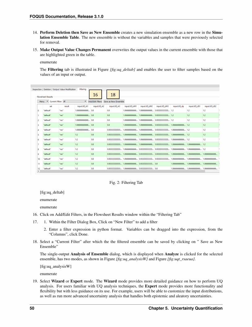
FOQUS Documentation, Release 3.1.0
14. Perform Deletion then Save as New Ensemble creates a new simulation ensemble as a new row in the Simu-lation Ensemble Table. The new ensemble is without the variables and samples that were previously selectedfor removal.
15. Make Output Value Changes Permanent overwrites the output values in the current ensemble with those thatare highlighted green in the table.
enumerate
The Filtering tab is illustrated in Figure [fig:uq_deltab] and enables the user to filter samples based on thevalues of an input or output.
Fig. 2: Filtering Tab
[fig:uq_deltab]
enumerate
enumerate
16. Click on Add/Edit Filters, in the Flowsheet Results window within the “Filtering Tab”
17. 1. Within the Filter Dialog Box, Click on “New Filter” to add a filter
2. Enter a filter expression in python format. Variables can be dragged into the expression, from the“Columns”, click Done.
18. Select a “Current Filter” after which the the filtered ensemble can be saved by clicking on ” Save as NewEnsemble”
The single-output Analysis of Ensemble dialog, which is displayed when Analyze is clicked for the selectedensemble, has two modes, as shown in Figure [fig:uq_analysisW] and Figure [fig:uqt_rsaeua].
[fig:uq_analysisW]
enumerate
19. Select Wizard or Expert mode. The Wizard mode provides more detailed guidance on how to perform UQanalysis. For users familiar with UQ analysis techniques, the Expert mode provides more functionality andflexibility but with less guidance on its use. For example, users will be able to customize the input distributions,as well as run more advanced uncertainty analysis that handles both epistemic and aleatory uncertainties.
50 Chapter 5. Uncertainty Quantification
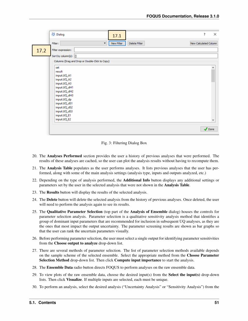
FOQUS Documentation, Release 3.1.0
Fig. 3: Filtering Dialog Box
20. The Analyses Performed section provides the user a history of previous analyses that were performed. Theresults of these analyses are cached, so the user can plot the analysis results without having to recompute them.
21. The Analysis Table populates as the user performs analyses. It lists previous analyses that the user has per-formed, along with some of the main analysis settings (analysis type, inputs and outputs analyzed, etc.)
22. Depending on the type of analysis performed, the Additional Info button displays any additional settings orparameters set by the user in the selected analysis that were not shown in the Analysis Table.
23. The Results button will display the results of the selected analysis.
24. The Delete button will delete the selected analysis from the history of previous analyses. Once deleted, the userwill need to perform the analysis again to see its results.
25. The Qualitative Parameter Selection (top part of the Analysis of Ensemble dialog) houses the controls forparameter selection analysis. Parameter selection is a qualitative sensitivity analysis method that identifies agroup of dominant input parameters that are recommended for inclusion in subsequent UQ analyses, as they arethe ones that most impact the output uncertainty. The parameter screening results are shown as bar graphs sothat the user can rank the uncertain parameters visually.
26. Before performing parameter selection, the user must select a single output for identifying parameter sensitivitiesfrom the Choose output to analyze drop-down list.
27. There are several methods of parameter selection. The list of parameter selection methods available dependson the sample scheme of the selected ensemble. Select the appropriate method from the Choose ParameterSelection Method drop-down list. Then click Compute input importance to start the analysis.
28. The Ensemble Data radio button directs FOQUS to perform analyses on the raw ensemble data.
29. To view plots of the raw ensemble data, choose the desired input(s) from the Select the input(s) drop-downlists. Then click Visualize. If multiple inputs are selected, each must be unique.
30. To perform an analysis, select the desired analysis (“Uncertainty Analysis” or “Sensitivity Analysis”) from the
5.1. Contents 51
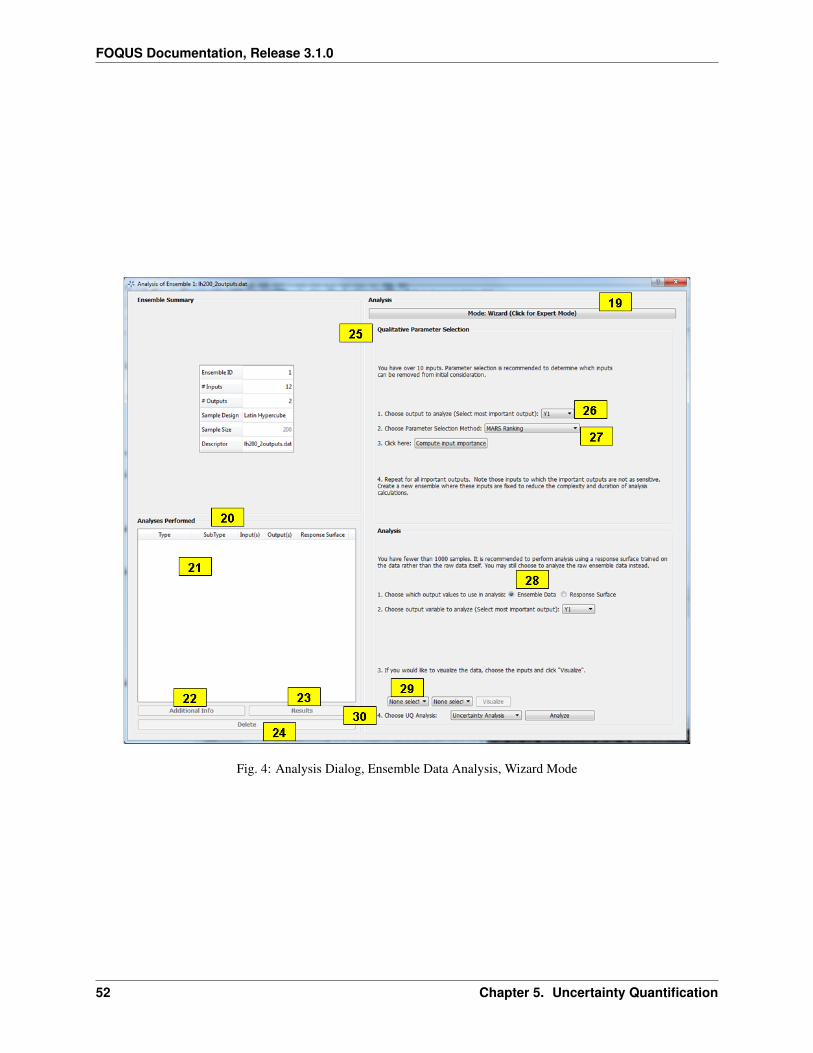
FOQUS Documentation, Release 3.1.0
Fig. 4: Analysis Dialog, Ensemble Data Analysis, Wizard Mode
52 Chapter 5. Uncertainty Quantification

FOQUS Documentation, Release 3.1.0
Choose UQ Analysis drop-down list. Uncertainty Analysis computes and displays the probability distributionof the single selected output parameter and displays its sufficient statistics, such as mean, standard deviation,skewness, and kurtosis. Sensitivity Analysis computes and displays each uncertain input parameter’s contri-bution to the total variance of the output. If Sensitivity Analysis is selected, choose the type of sensitivityanalysis desired in the next drop-down list. There are three options for Sensitivity Analysis: (1) first-order, (2)second-order, and (3) total-order.
• First-order analysis examines the effect of varying an input parameter alone.
• Second-order analysis examines the effect of varying pairs of input parameters.
• Total-order analysis examines all interactions’ effect of varying an input parameter alone and as a combi-nation with any other input parameters.
Click Analyze to run the analysis. (Note: Raw ensemble data analysis may not be suitable if the sample size issmall. It may be useful if the data set has tens of thousands of sample points or if an adequate response surfacecannot be constructed. Otherwise, response surface-based analyses are recommended.)
Fig. 5: Analysis Dialog, Response Surface Analysis, Wizard Mode
[fig:uq_analysisW2]
[itm:uq_analysis]
31. Response Surface enables the user to perform all analyses related to response surfaces. A response surface isan approximation of the input-to-output relationship. This is an inexpensive way to approximate the values ofoutputs given different input values when the actual simulation of output values is computationally intensive.
5.1. Contents 53

FOQUS Documentation, Release 3.1.0
FOQUS uses the data (i.e., input-output samples) to fit a response surface scheme. The first step in this analysisis to select which output to analyze.
32. Select the Response Surface Model to be used to approximate the input-to-output mapping. Selection of“Polynomial” or “MARS” requires one further selection in the second drop-down list. If “Polynomial” is chosenin the first drop-down list and “Legendre” is chosen in the second drop-down list, the user needs to specify anumber for the Legendre polynomial order before analysis can proceed. [itm:uq_rs]
33. The response surface selected must be validated before further analyses can be performed. The user can specifythe error envelope for the validation plot. When Validate is clicked, the resulting plots display the best fitbetween the response surface (based on the model selected) and the actual data.
34. Choose UQ Analysis enables the user to perform response-surface-based UQ analyses. Select the analysis inthe first drop-down list. If the desired analysis is Sensitivity Analysis, select the desired type of sensitivityanalysis in the second drop-down list and then click Analyze. Uncertainty Analysis and Sensitivity Analysiscompute and display the same quantities as in item #[itm:uq_analysis]. However, the results displayed arebased on samples drawn from the trained response surface, not the simulation ensemble itself. Moreover, if theselected response surface has uncertainty, the resulting plots also reflect this uncertainty information.
35. FOQUS also provides visualization capabilities, enabling the user to view the response surface as a functionof one or multiple inputs. Up to three inputs can be visualized at once. Click Visualize to view. A 2-D lineplot displays if only one input parameter is selected. A 3-D surface plot and a 2-D contour plot display if twoinput parameters are selected. A 3-D isosurface plot with a slider bar displays if three input parameters arechosen. For the isosurface plot, the user can use the slider to selectively display the 3-D input parameter spacethat activates a particular range in the output parameter.
Finally, the Bayesian Inference of Ensemble dialog (shown in Figure [fig:uq_inf]) is used to calculate theposterior distributions (prior distributions integrated with data) of the uncertain input parameters. Inferenceutilizes Markov Chain Monte Carlo (MCMC) to compute the posterior distributions, using response surfacesthat serve as fast approximations to the actual simulation model.
[fig:uq_inf]
enumerate
36. Inference uses a response surface to approximate the input-to-output mapping. In Output Settings, selectthe observed outputs and select the response surface type that works best with each observed output. As initem ([itm:uq_rs]), further selections may be required based on the response surface chosen. The simulationensemble is used as the training data for generating the response surfaces.
37. The user can specify which inputs are fixed, design (fixed per experiment, but changes between experiments),or variable using the Input Settings Table. In addition, the user can specify which inputs are displayed in theresulting plots of the posterior distributions. By default, once inference completes, all inputs will be displayedin the plots. To omit specific inputs, clear the checkboxes from the Display column of the table. Finally, inExpert mode, this table can also be used to modify the input prior distributions. The default prior is the inputdistribution specified in the simulation ensemble. To change the prior distribution type, use the drop-down listin the PDF column and enter corresponding values for the PDF parameters. To change the range of a uniformprior, scroll all the way to the right to modify Min/Max.
38. The Observations section enables the user to add experimental data in the form of observations of certainoutput variables. At least one observation is required. Currently, the observation noise model is assumed tobe a normal distribution. Other distributions may be supported in the future. To specify the observation noisemodel, enter the mean (and standard deviation, if standard inference is selected) for each output observation.For convenience, the Mean and Standard Deviation fields have been populated with the statistics from theensemble uncertainty analysis. If any inputs are selected as design inputs, their values will also be required here.
39. Save Posterior Input Samples to File checkbox, when selected, saves the posterior input samples as a PSUADEsample file (format described in Section [ap:psuadefiles]). This file characterizes the input uncertainty as a set of
54 Chapter 5. Uncertainty Quantification
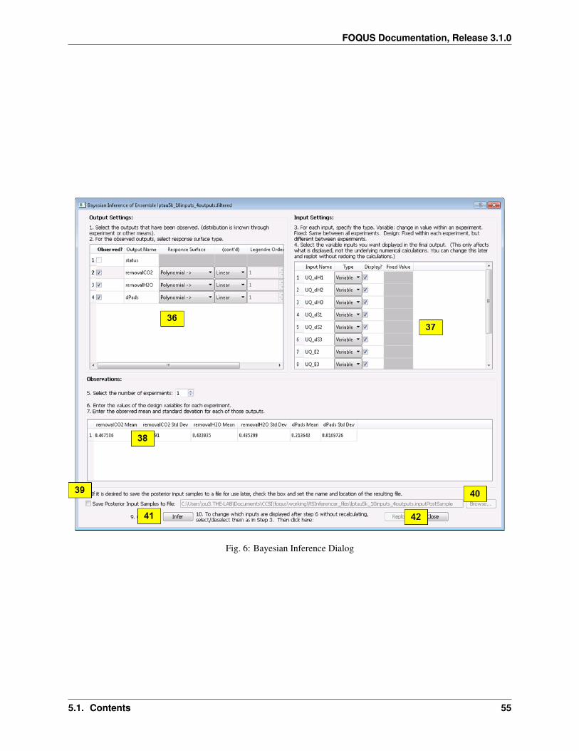
FOQUS Documentation, Release 3.1.0
Fig. 6: Bayesian Inference Dialog
5.1. Contents 55
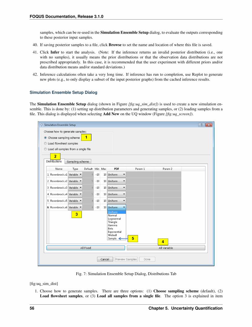
FOQUS Documentation, Release 3.1.0
samples, which can be re-used in the Simulation Ensemble Setup dialog, to evaluate the outputs correspondingto these posterior input samples.
40. If saving posterior samples to a file, click Browse to set the name and location of where this file is saved.
41. Click Infer to start the analysis. (Note: If the inference returns an invalid posterior distribution (i.e., onewith no samples), it usually means the prior distributions or that the observation data distributions are notprescribed appropriately. In this case, it is recommended that the user experiment with different priors and/ordata distribution means and/or standard deviations.)
42. Inference calculations often take a very long time. If inference has run to completion, use Replot to generatenew plots (e.g., to only display a subset of the input posterior graphs) from the cached inference results.
Simulation Ensemble Setup Dialog
The Simulation Ensemble Setup dialog (shown in Figure [fig:uq_sim_dist]) is used to create a new simulation en-semble. This is done by: (1) setting up distribution parameters and generating samples, or (2) loading samples from afile. This dialog is displayed when selecting Add New on the UQ window (Figure [fig:uq_screen]).
Fig. 7: Simulation Ensemble Setup Dialog, Distributions Tab
[fig:uq_sim_dist]
1. Choose how to generate samples. There are three options: (1) Choose sampling scheme (default), (2)Load flowsheet samples, or (3) Load all samples from a single file. The option 3 is explained in item
56 Chapter 5. Uncertainty Quantification
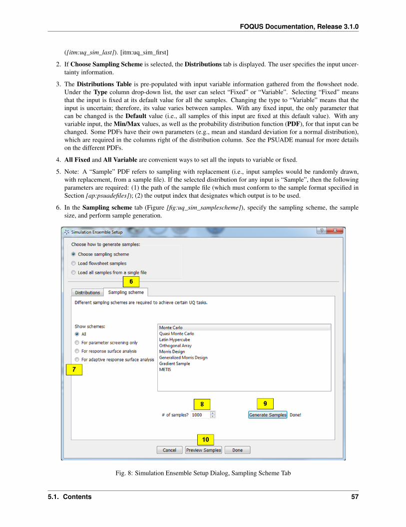
FOQUS Documentation, Release 3.1.0
([itm:uq_sim_last]). [itm:uq_sim_first]
2. If Choose Sampling Scheme is selected, the Distributions tab is displayed. The user specifies the input uncer-tainty information.
3. The Distributions Table is pre-populated with input variable information gathered from the flowsheet node.Under the Type column drop-down list, the user can select “Fixed” or “Variable”. Selecting “Fixed” meansthat the input is fixed at its default value for all the samples. Changing the type to “Variable” means that theinput is uncertain; therefore, its value varies between samples. With any fixed input, the only parameter thatcan be changed is the Default value (i.e., all samples of this input are fixed at this default value). With anyvariable input, the Min/Max values, as well as the probability distribution function (PDF), for that input can bechanged. Some PDFs have their own parameters (e.g., mean and standard deviation for a normal distribution),which are required in the columns right of the distribution column. See the PSUADE manual for more detailson the different PDFs.
4. All Fixed and All Variable are convenient ways to set all the inputs to variable or fixed.
5. Note: A “Sample” PDF refers to sampling with replacement (i.e., input samples would be randomly drawn,with replacement, from a sample file). If the selected distribution for any input is “Sample”, then the followingparameters are required: (1) the path of the sample file (which must conform to the sample format specified inSection [ap:psuadefiles]); (2) the output index that designates which output is to be used.
6. In the Sampling scheme tab (Figure [fig:uq_sim_samplescheme]), specify the sampling scheme, the samplesize, and perform sample generation.
Fig. 8: Simulation Ensemble Setup Dialog, Sampling Scheme Tab
5.1. Contents 57
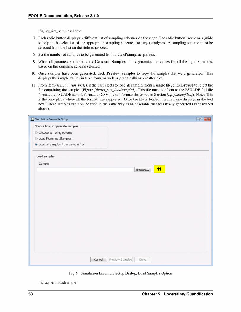
FOQUS Documentation, Release 3.1.0
[fig:uq_sim_samplescheme]
7. Each radio button displays a different list of sampling schemes on the right. The radio buttons serve as a guideto help in the selection of the appropriate sampling schemes for target analyses. A sampling scheme must beselected from the list on the right to proceed.
8. Set the number of samples to be generated from the # of samples spinbox.
9. When all parameters are set, click Generate Samples. This generates the values for all the input variables,based on the sampling scheme selected.
10. Once samples have been generated, click Preview Samples to view the samples that were generated. Thisdisplays the sample values in table form, as well as graphically as a scatter plot.
11. From item ([itm:uq_sim_first]), if the user elects to load all samples from a single file, click Browse to select thefile containing the samples (Figure [fig:uq_sim_loadsample]). This file must conform to the PSUADE full fileformat, the PSUADE sample format, or CSV file (all formats described in Section [ap:psuadefiles]). Note: Thisis the only place where all the formats are supported. Once the file is loaded, the file name displays in the textbox. These samples can now be used in the same way as an ensemble that was newly generated (as describedabove).
Fig. 9: Simulation Ensemble Setup Dialog, Load Samples Option
[fig:uq_sim_loadsample]
58 Chapter 5. Uncertainty Quantification
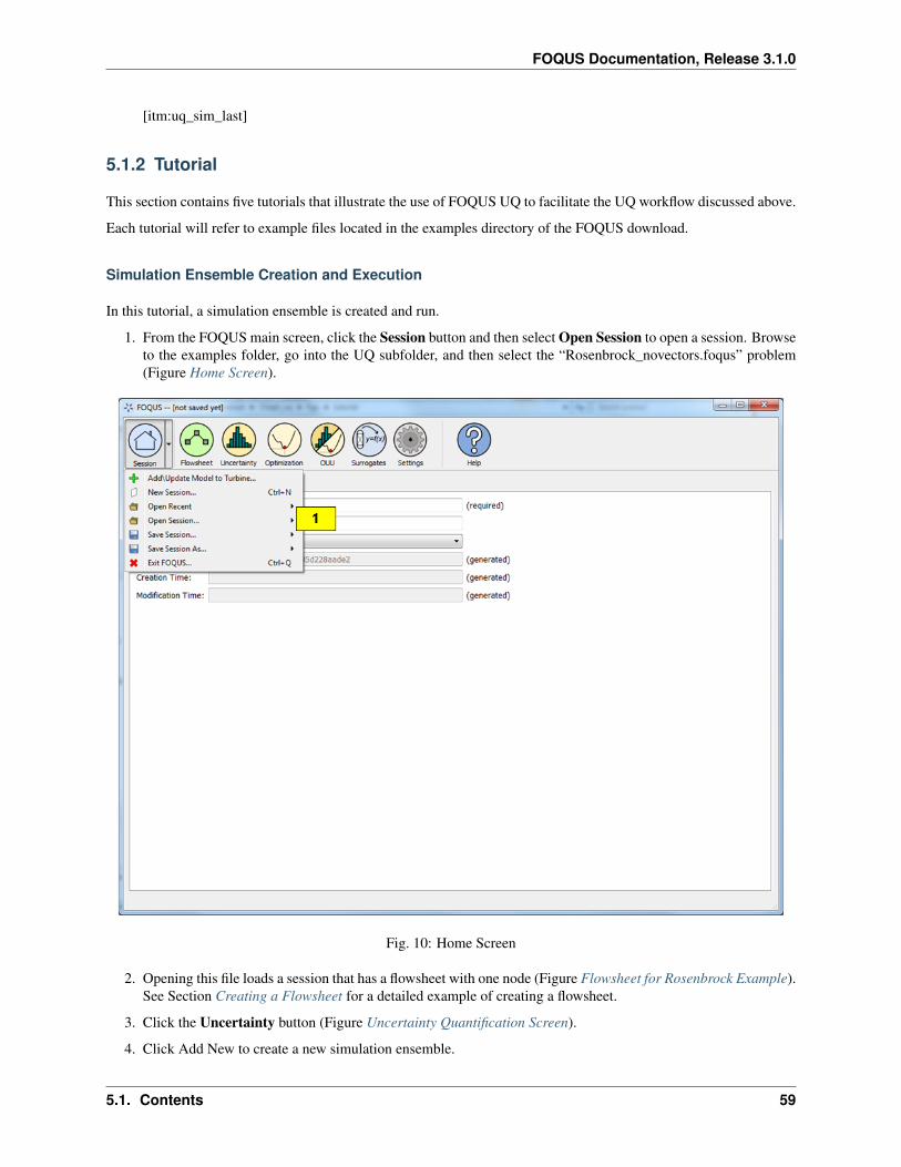
FOQUS Documentation, Release 3.1.0
[itm:uq_sim_last]
5.1.2 Tutorial
This section contains five tutorials that illustrate the use of FOQUS UQ to facilitate the UQ workflow discussed above.
Each tutorial will refer to example files located in the examples directory of the FOQUS download.
Simulation Ensemble Creation and Execution
In this tutorial, a simulation ensemble is created and run.
1. From the FOQUS main screen, click the Session button and then select Open Session to open a session. Browseto the examples folder, go into the UQ subfolder, and then select the “Rosenbrock_novectors.foqus” problem(Figure Home Screen).
Fig. 10: Home Screen
2. Opening this file loads a session that has a flowsheet with one node (Figure Flowsheet for Rosenbrock Example).See Section Creating a Flowsheet for a detailed example of creating a flowsheet.
3. Click the Uncertainty button (Figure Uncertainty Quantification Screen).
4. Click Add New to create a new simulation ensemble.
5.1. Contents 59
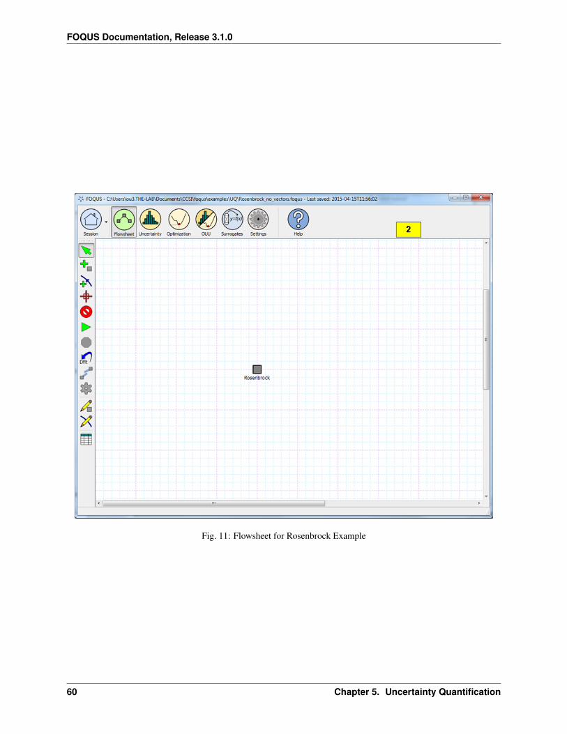
FOQUS Documentation, Release 3.1.0
Fig. 11: Flowsheet for Rosenbrock Example
60 Chapter 5. Uncertainty Quantification
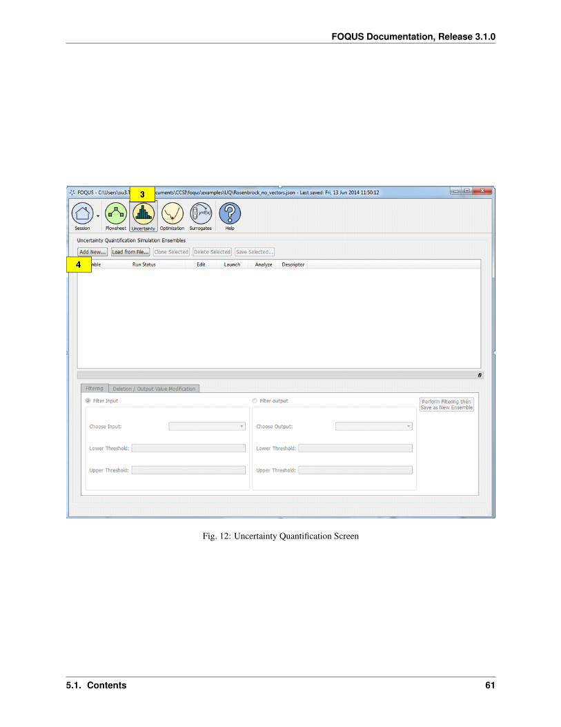
FOQUS Documentation, Release 3.1.0
Fig. 12: Uncertainty Quantification Screen
5.1. Contents 61

FOQUS Documentation, Release 3.1.0
5. The Add New Ensemble dialog displays (Figure Add New Ensemble Dialog, Flowsheet Option). The “Useflowsheet” option should be enabled.
6. This item describes additional features and is provided for information only. It is not intended to be followed aspart of the step-by-step tutorial.An alternative is to use an emulator by selecting “Use emulator.” This alternative is preferred if the actualsimulation model is too computationally expensive to be practical for a large number of samples. This optionenables the user to trade off accuracy for speed by training a response surface to approximate the actualsimulation model. If this option is selected (Figure Add New Ensemble Dialog, Emulator Option), the userneeds to provide a training data file containing a small simulation ensemble generated from the actualsimulation model. This training data file is be in the PSUADE full file format (Section [ap:psuadefiles]).
• Click Browse and select the training data file with which to train the response surface. The inputs, outputsand response surface type is read from the training data and populated accordingly on this dialog box.
• Select Output(s) of Interest. To select multiple outputs, the user can use Shift + Click to select a range, oruse Ctrl + Click to select/deselect individual outputs.
7. Click OK.
Fig. 13: Add New Ensemble Dialog, Flowsheet Option
enumerate
8. This displays the Simulation Ensemble Setup dialog box (Figure Simulation Ensemble Setup Dialog,Distributions Tab ) that prompts the user for options specific to the creation of input samples.
62 Chapter 5. Uncertainty Quantification
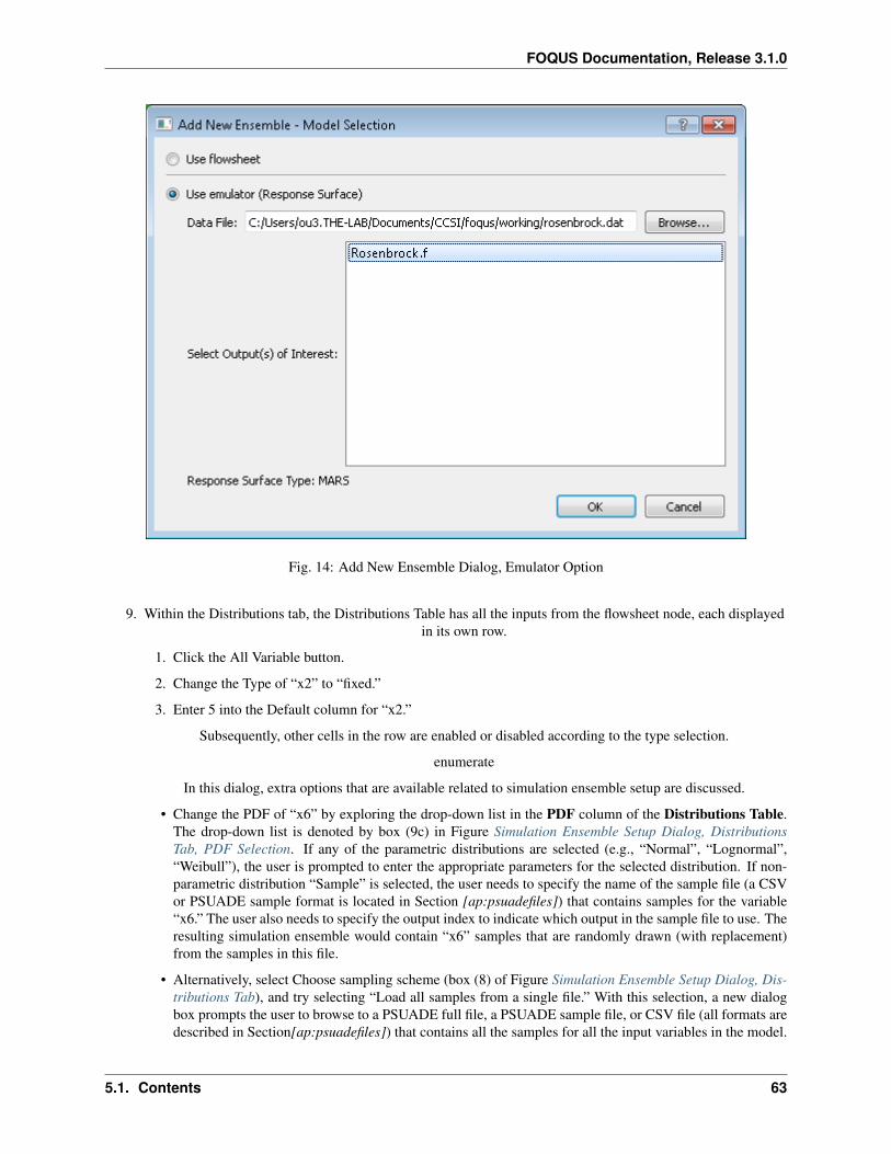
FOQUS Documentation, Release 3.1.0
Fig. 14: Add New Ensemble Dialog, Emulator Option
9. Within the Distributions tab, the Distributions Table has all the inputs from the flowsheet node, each displayedin its own row.
1. Click the All Variable button.
2. Change the Type of “x2” to “fixed.”
3. Enter 5 into the Default column for “x2.”
Subsequently, other cells in the row are enabled or disabled according to the type selection.
enumerate
In this dialog, extra options that are available related to simulation ensemble setup are discussed.
• Change the PDF of “x6” by exploring the drop-down list in the PDF column of the Distributions Table.The drop-down list is denoted by box (9c) in Figure Simulation Ensemble Setup Dialog, DistributionsTab, PDF Selection. If any of the parametric distributions are selected (e.g., “Normal”, “Lognormal”,“Weibull”), the user is prompted to enter the appropriate parameters for the selected distribution. If non-parametric distribution “Sample” is selected, the user needs to specify the name of the sample file (a CSVor PSUADE sample format is located in Section [ap:psuadefiles]) that contains samples for the variable“x6.” The user also needs to specify the output index to indicate which output in the sample file to use. Theresulting simulation ensemble would contain “x6” samples that are randomly drawn (with replacement)from the samples in this file.
• Alternatively, select Choose sampling scheme (box (8) of Figure Simulation Ensemble Setup Dialog, Dis-tributions Tab), and try selecting “Load all samples from a single file.” With this selection, a new dialogbox prompts the user to browse to a PSUADE full file, a PSUADE sample file, or CSV file (all formats aredescribed in Section[ap:psuadefiles]) that contains all the samples for all the input variables in the model.
5.1. Contents 63

FOQUS Documentation, Release 3.1.0
Fig. 15: Simulation Ensemble Setup Dialog, Distributions Tab
64 Chapter 5. Uncertainty Quantification
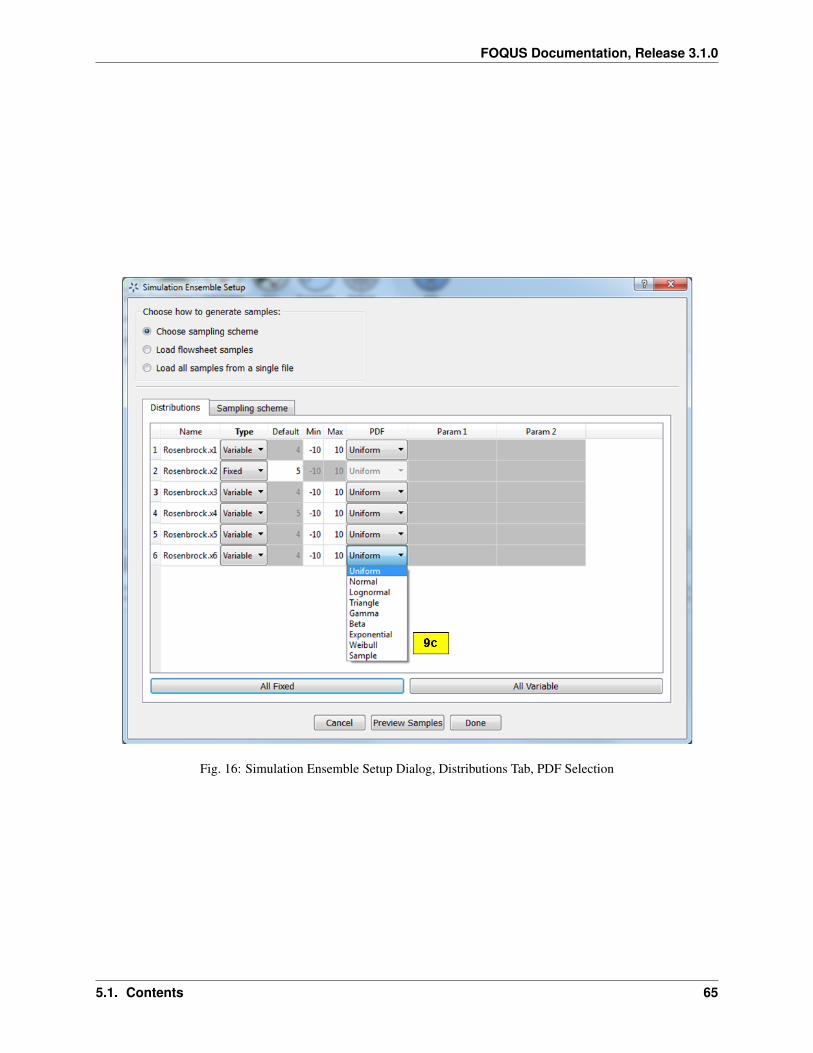
FOQUS Documentation, Release 3.1.0
Fig. 16: Simulation Ensemble Setup Dialog, Distributions Tab, PDF Selection
5.1. Contents 65
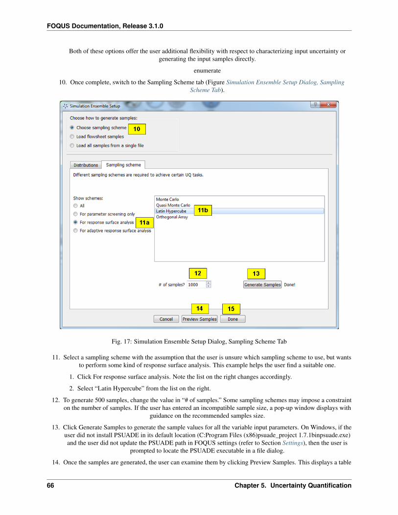
FOQUS Documentation, Release 3.1.0
Both of these options offer the user additional flexibility with respect to characterizing input uncertainty orgenerating the input samples directly.
enumerate
10. Once complete, switch to the Sampling Scheme tab (Figure Simulation Ensemble Setup Dialog, SamplingScheme Tab).
Fig. 17: Simulation Ensemble Setup Dialog, Sampling Scheme Tab
11. Select a sampling scheme with the assumption that the user is unsure which sampling scheme to use, but wantsto perform some kind of response surface analysis. This example helps the user find a suitable one.
1. Click For response surface analysis. Note the list on the right changes accordingly.
2. Select “Latin Hypercube” from the list on the right.
12. To generate 500 samples, change the value in “# of samples.” Some sampling schemes may impose a constrainton the number of samples. If the user has entered an incompatible sample size, a pop-up window displays with
guidance on the recommended samples size.
13. Click Generate Samples to generate the sample values for all the variable input parameters. On Windows, if theuser did not install PSUADE in its default location (C:Program Files (x86)psuade_project 1.7.1binpsuade.exe)and the user did not update the PSUADE path in FOQUS settings (refer to Section Settings), then the user is
prompted to locate the PSUADE executable in a file dialog.
14. Once the samples are generated, the user can examine them by clicking Preview Samples. This displays a table
66 Chapter 5. Uncertainty Quantification
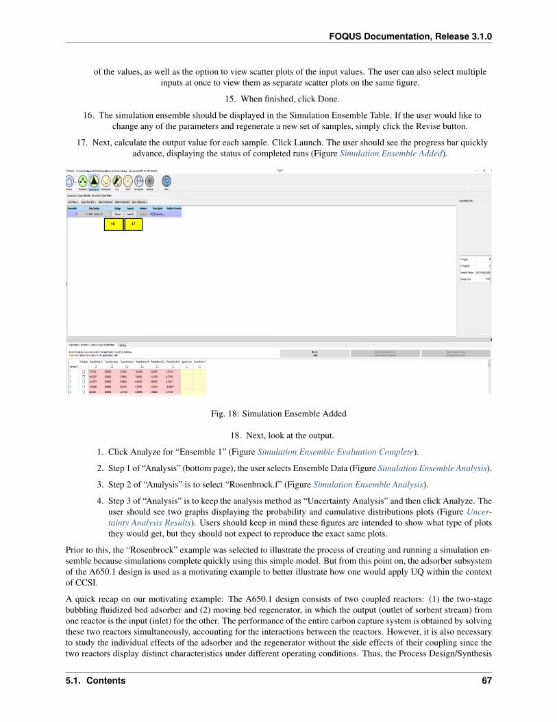
FOQUS Documentation, Release 3.1.0
of the values, as well as the option to view scatter plots of the input values. The user can also select multipleinputs at once to view them as separate scatter plots on the same figure.
15. When finished, click Done.
16. The simulation ensemble should be displayed in the Simulation Ensemble Table. If the user would like tochange any of the parameters and regenerate a new set of samples, simply click the Revise button.
17. Next, calculate the output value for each sample. Click Launch. The user should see the progress bar quicklyadvance, displaying the status of completed runs (Figure Simulation Ensemble Added).
Fig. 18: Simulation Ensemble Added
18. Next, look at the output.
1. Click Analyze for “Ensemble 1” (Figure Simulation Ensemble Evaluation Complete).
2. Step 1 of “Analysis” (bottom page), the user selects Ensemble Data (Figure Simulation Ensemble Analysis).
3. Step 2 of “Analysis” is to select “Rosenbrock.f” (Figure Simulation Ensemble Analysis).
4. Step 3 of “Analysis” is to keep the analysis method as “Uncertainty Analysis” and then click Analyze. Theuser should see two graphs displaying the probability and cumulative distributions plots (Figure Uncer-tainty Analysis Results). Users should keep in mind these figures are intended to show what type of plotsthey would get, but they should not expect to reproduce the exact same plots.
Prior to this, the “Rosenbrock” example was selected to illustrate the process of creating and running a simulation en-semble because simulations complete quickly using this simple model. But from this point on, the adsorber subsystemof the A650.1 design is used as a motivating example to better illustrate how one would apply UQ within the contextof CCSI.
A quick recap on our motivating example: The A650.1 design consists of two coupled reactors: (1) the two-stagebubbling fluidized bed adsorber and (2) moving bed regenerator, in which the output (outlet of sorbent stream) fromone reactor is the input (inlet) for the other. The performance of the entire carbon capture system is obtained by solvingthese two reactors simultaneously, accounting for the interactions between the reactors. However, it is also necessaryto study the individual effects of the adsorber and the regenerator without the side effects of their coupling since thetwo reactors display distinct characteristics under different operating conditions. Thus, the Process Design/Synthesis
5.1. Contents 67
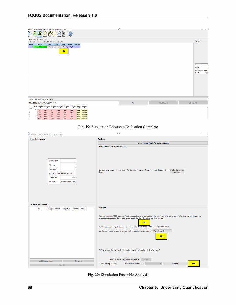
FOQUS Documentation, Release 3.1.0
Fig. 19: Simulation Ensemble Evaluation Complete
Fig. 20: Simulation Ensemble Analysis
68 Chapter 5. Uncertainty Quantification
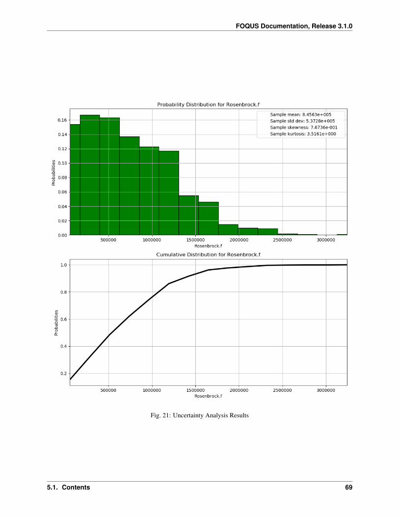
FOQUS Documentation, Release 3.1.0
Fig. 21: Uncertainty Analysis Results
5.1. Contents 69
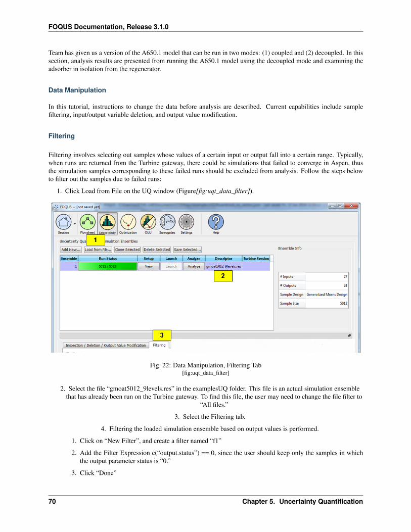
FOQUS Documentation, Release 3.1.0
Team has given us a version of the A650.1 model that can be run in two modes: (1) coupled and (2) decoupled. In thissection, analysis results are presented from running the A650.1 model using the decoupled mode and examining theadsorber in isolation from the regenerator.
Data Manipulation
In this tutorial, instructions to change the data before analysis are described. Current capabilities include samplefiltering, input/output variable deletion, and output value modification.
Filtering
Filtering involves selecting out samples whose values of a certain input or output fall into a certain range. Typically,when runs are returned from the Turbine gateway, there could be simulations that failed to converge in Aspen, thusthe simulation samples corresponding to these failed runs should be excluded from analysis. Follow the steps belowto filter out the samples due to failed runs:
1. Click Load from File on the UQ window (Figure[fig:uqt_data_filter]).
Fig. 22: Data Manipulation, Filtering Tab[fig:uqt_data_filter]
2. Select the file “gmoat5012_9levels.res” in the examplesUQ folder. This file is an actual simulation ensemblethat has already been run on the Turbine gateway. To find this file, the user may need to change the file filter to
“All files.”
3. Select the Filtering tab.
4. Filtering the loaded simulation ensemble based on output values is performed.
1. Click on “New Filter”, and create a filter named “f1”
2. Add the Filter Expression c(“output.status”) == 0, since the user should keep only the samples in whichthe output parameter status is “0.”
3. Click “Done”
70 Chapter 5. Uncertainty Quantification
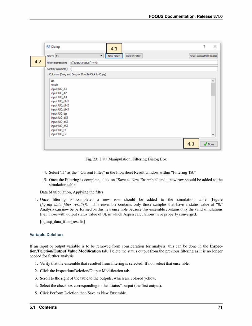
FOQUS Documentation, Release 3.1.0
Fig. 23: Data Manipulation, Filtering Dialog Box
4. Select ‘f1’ as the ” Current Filter” in the Flowsheet Result window within “Filtering Tab”
5. Once the Filtering is complete, click on “Save as New Ensemble” and a new row should be added to thesimulation table
Data Manipulation, Applying the filter
1. Once filtering is complete, a new row should be added to the simulation table (Figure[fig:uqt_data_filter_results]). This ensemble contains only those samples that have a status value of “0.”Analysis can now be performed on this new ensemble because this ensemble contains only the valid simulations(i.e., those with output status value of 0), in which Aspen calculations have properly converged.
[fig:uqt_data_filter_results]
Variable Deletion
If an input or output variable is to be removed from consideration for analysis, this can be done in the Inspec-tion/Deletion/Output Value Modification tab. Delete the status output from the previous filtering as it is no longerneeded for further analysis.
1. Verify that the ensemble that resulted from filtering is selected. If not, select that ensemble.
2. Click the Inspection/Deletion/Output Modification tab.
3. Scroll to the right of the table to the outputs, which are colored yellow.
4. Select the checkbox corresponding to the “status” output (the first output).
5. Click Perform Deletion then Save as New Ensemble.
5.1. Contents 71

FOQUS Documentation, Release 3.1.0
72 Chapter 5. Uncertainty Quantification
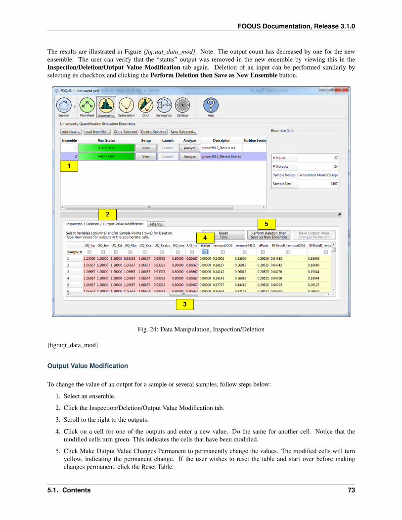
FOQUS Documentation, Release 3.1.0
The results are illustrated in Figure [fig:uqt_data_mod]. Note: The output count has decreased by one for the newensemble. The user can verify that the “status” output was removed in the new ensemble by viewing this in theInspection/Deletion/Output Value Modification tab again. Deletion of an input can be performed similarly byselecting its checkbox and clicking the Perform Deletion then Save as New Ensemble button.
Fig. 24: Data Manipulation, Inspection/Deletion
[fig:uqt_data_mod]
Output Value Modification
To change the value of an output for a sample or several samples, follow steps below:
1. Select an ensemble.
2. Click the Inspection/Deletion/Output Value Modification tab.
3. Scroll to the right to the outputs.
4. Click on a cell for one of the outputs and enter a new value. Do the same for another cell. Notice that themodified cells turn green. This indicates the cells that have been modified.
5. Click Make Output Value Changes Permanent to permanently change the values. The modified cells will turnyellow, indicating the permanent change. If the user wishes to reset the table and start over before makingchanges permanent, click the Reset Table.
5.1. Contents 73
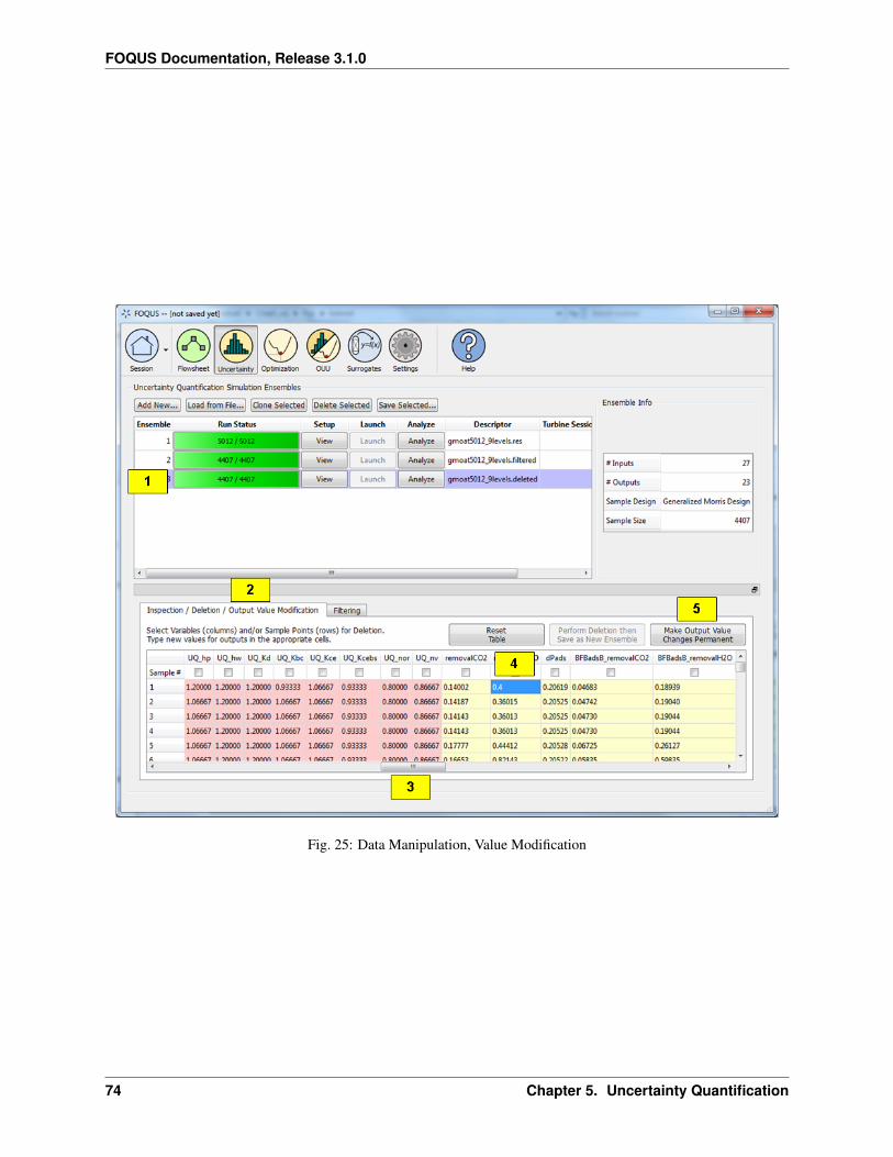
FOQUS Documentation, Release 3.1.0
Fig. 25: Data Manipulation, Value Modification
74 Chapter 5. Uncertainty Quantification

FOQUS Documentation, Release 3.1.0
[fig:uqt_data_mod_output]
5.1. Contents 75
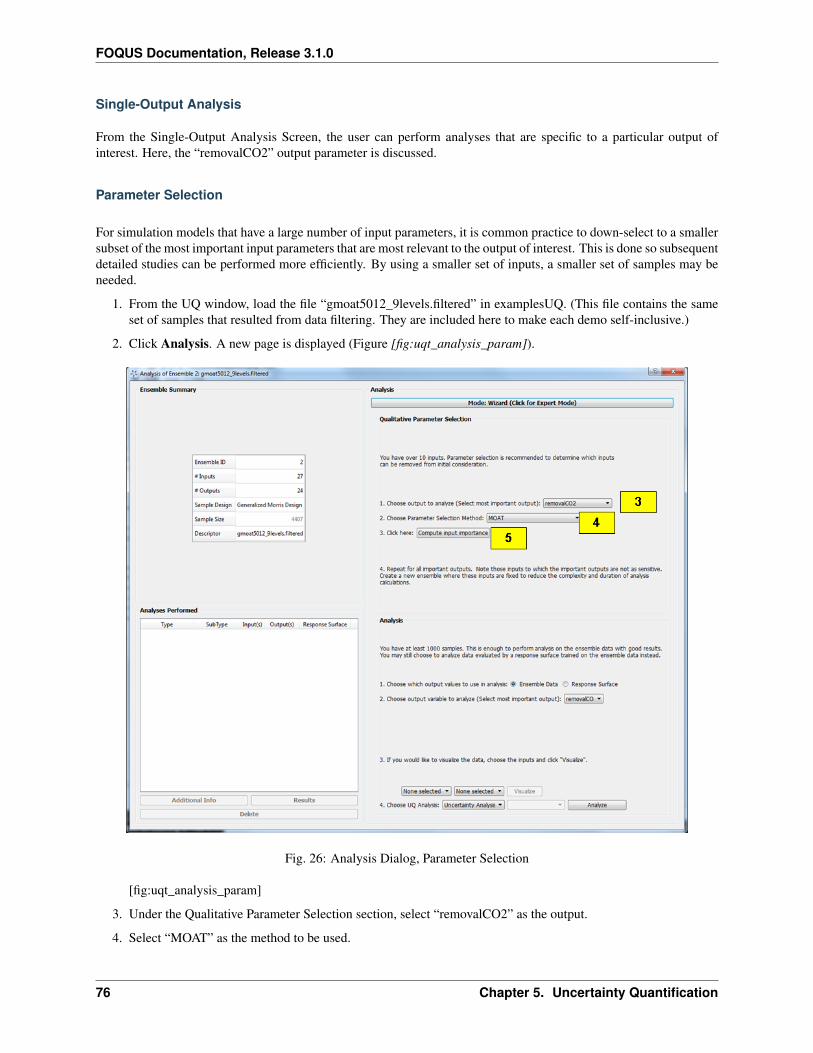
FOQUS Documentation, Release 3.1.0
Single-Output Analysis
From the Single-Output Analysis Screen, the user can perform analyses that are specific to a particular output ofinterest. Here, the “removalCO2” output parameter is discussed.
Parameter Selection
For simulation models that have a large number of input parameters, it is common practice to down-select to a smallersubset of the most important input parameters that are most relevant to the output of interest. This is done so subsequentdetailed studies can be performed more efficiently. By using a smaller set of inputs, a smaller set of samples may beneeded.
1. From the UQ window, load the file “gmoat5012_9levels.filtered” in examplesUQ. (This file contains the sameset of samples that resulted from data filtering. They are included here to make each demo self-inclusive.)
2. Click Analysis. A new page is displayed (Figure [fig:uqt_analysis_param]).
Fig. 26: Analysis Dialog, Parameter Selection
[fig:uqt_analysis_param]
3. Under the Qualitative Parameter Selection section, select “removalCO2” as the output.
4. Select “MOAT” as the method to be used.
76 Chapter 5. Uncertainty Quantification
FOQUS Documentation, Release 3.1.0
5. Click Compute input importance. A graph should appear with the results (Figure [fig:uqt_param_results]).
[fig:uqt_param_results]
The bars in the plot represent the importance of a particular input in determining the value of the output. For example,the values of dH3 and dS3 are very important in determining the value of removalCO2, whereas Hce and hp have noaffect (the y-axis displays the average changes in the model output as a result of changing the inputs in their respectiveranges. For example, from Figure [fig:uqt_param_results], changing dH2 in its range results in an average changein CO2 removal as much as about 57 percent with a margin of +/- 3 percent). Thus, it would be safe to exclude anyinputs that have negligible bar lengths from analysis. Next, down-select the ten most important inputs based on theseresults. See Section [subsubsec:uqt_vardel] for details. Change the number of samples and scheme as desired andthen generate new samples. Click Launch to run these samples to obtain another simulation ensemble that can beanalyzed.
Ensemble Data Analysis
If the user is interested in the output uncertainty of “removalCO2” based on the uncertainties from the ten most im-portant input parameters, perform uncertainty analysis, which would compute the probability distribution and samplestatistics of “removalCO2.”
1. Load “lptau20k_10inputs_4outputs.filtered” from the examples\ UQ folder. Assume this is the file that the userwould receive after running the cloned simulation ensemble in which the user has down-selected the ten mostimportant inputs, set the Sampling Scheme to “Quasi-Monte Carlo (LPTAU)”, set the sample size to 20K, andperformed data filtering to retain only the samples with the status output equal to “0.”
2. Click Analyze. A new page displays (Figure[fig:uqt_analysis_ua]).
3. Select “Ensemble Data” to indicate that analysis is to be directly performed on the raw sample data.
4. Select “removalCO2” as the output variable to analyze.
5. Select “Uncertainty Analysis” and then click Analyze.
[fig:uqt_analysis_ua]
Once uncertainty analysis is complete, results display (Figure [fig:uqt_ua_results]) illustrating the probabilitydistribution function (PDF), cumulative distribution function (CDF), and the sufficient statistics (e.g., mean,standard deviation) of “removalCO2” (top left corner of the PDF plot). This is used to evaluate if the outputuncertainty is acceptable. If the output uncertainty is too great or the user prefers the system to operate withina higher percentage of capture, pursue further analyses to understand the relationships between the inputs andoutputs, and investigate what can be done to reduce the output uncertainties by reducing the input uncertainties.
[fig:uqt_ua_results]
Next, the user may apply variance-based sensitivity analysis to quantify each input’s contribution to the outputvariance:
enumerate
6. From the bottom of the “Analysis” section, select “Sensitivity Analysis.”
7. There are three options for sensitivity analysis: (1) first-order, (2) second-order, and (3) total-order. First-orderanalysis examines the effect of varying an input parameter alone. Second-order analysis examines the effectof varying pairs of input parameters. Total-order analysis examines all interactions’ effect of varying an inputparameter alone and as a combination with any other input parameters. For this demonstration, select “Total-order” and click Analyze. The total sensitivity indices display in a graph. Note: If the simulation ensemble hasmore than ten inputs, “Total-order” is disabled (since any reasonable sample size is not sufficient). Additionally,since quantitative sensitivity analysis in general requires large ensembles with many samples (thousands ormore), ensemble sensitivity analysis (without the use of response surfaces) is often less practical and accuratethan response surface based analyses. The result is illustrated in Figure[fig:uqt_sa_results].
5.1. Contents 77
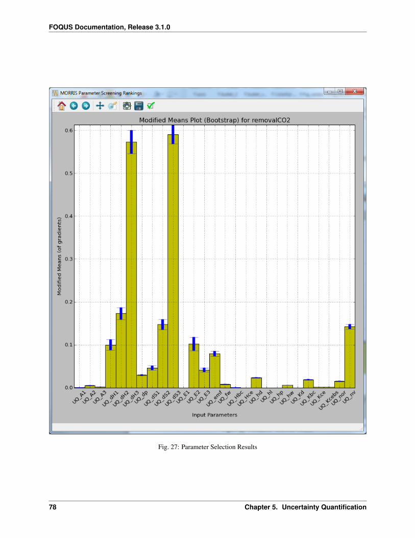
FOQUS Documentation, Release 3.1.0
Fig. 27: Parameter Selection Results
78 Chapter 5. Uncertainty Quantification
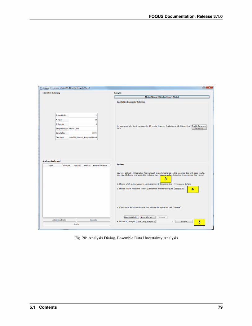
FOQUS Documentation, Release 3.1.0
Fig. 28: Analysis Dialog, Ensemble Data Uncertainty Analysis
5.1. Contents 79
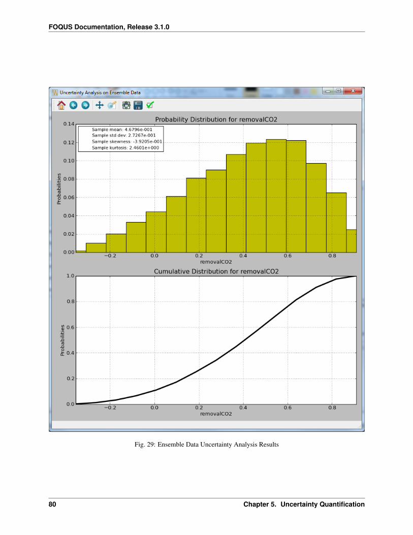
FOQUS Documentation, Release 3.1.0
Fig. 29: Ensemble Data Uncertainty Analysis Results
80 Chapter 5. Uncertainty Quantification
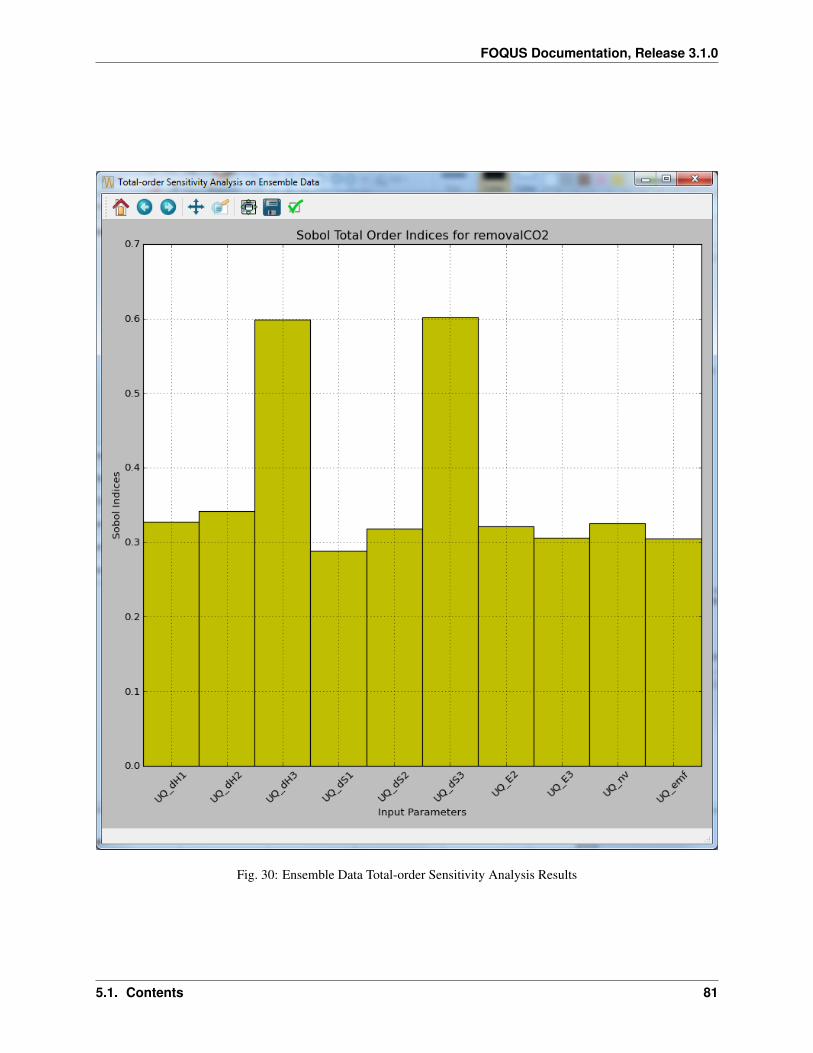
FOQUS Documentation, Release 3.1.0
Fig. 30: Ensemble Data Total-order Sensitivity Analysis Results
5.1. Contents 81
FOQUS Documentation, Release 3.1.0
[fig:uqt_sa_results]
These results confirm that “removalCO2” is more sensitive to “dH3” and “dS3” than other inputs. (The y-axis displaysan approximate percentage of output variance attributed to each individual parameter. Since total sensitivity includeshigher order interaction terms with other parameters, the sum of these total sensitivity indices usually exceeds 1.)
Ensemble Data Visualization
1. In this release, ensemble data visualization is only available in “Expert” mode. At the top of the “Analyze”page, toggle the bar to expert mode and select “removalCO2” as the output. Next, to “Visualize Data,” choosean input (e.g., “UQ_dH1”) and click Visualize for a 2-D scatter plot of “removalCO2” versus that input (Figure[fig:uqt_splot1_results]).
[fig:uqt_splot1_results]
2. Next, select a second input (e.g., “UQ_dH2”) and click Visualize for a 3-D scatter plot of “removalCO2” versusthe two inputs. (Note: The input selections must be unique for the Visualize button to be enabled.) Figure[fig:uqt_splot2_results] shows the results.
[fig:uqt_splot2_results]
The plot in Figure [fig:uqt_splot2_results] can be rotated by clicking and dragging.
Response Surface Based Analysis
For simulation models that are expensive to run, response surface analysis can be a resourceful option. To constructa response surface, a space-filling sampling design is desired. For example, quasi-Monte Carlo (LPTAU) or Latinhypercube sampling schemes are recommended. Additionally, there are several possibilities for curve fitting methods.If the sample size is relatively small, polynomial regression or Gaussian process (if installed as part of PSUADE) ispreferred. Alternatively, if the sample size is large enough (one hundred or more), cubic splines (if installed) may alsobe feasible.
Response Surface Model Validation
To proceed with response surface based analysis, the user needs to find a suitable response surface with which toapproximate the input-to-output mapping. Validation is performed to see how well a particular response surface canpredict a subset of the withheld data.
1. Load “lptau100_10inputs_4outputs.dat” from the examplesUQ folder. Note: This is an extremely small simula-tion ensemble, as this is used to highlight the differences (in validation results) between a good response surfaceand a bad one.
2. Click Analyze for the current ensemble. A new dialog page displays (Figure[fig:uqt_rs_validate]).
3. Under “Analysis” (bottom section), under Step 1, select “Response Surface.”
[fig:uqt_rs_validate]
4. Under Step 2, select “removalCO2” as the output for analysis.
5. Under Step 3, select “Polynomial” for response surface method.
6. There are multiple types of polynomial response surfaces, with increasing complexity as the user navigates downthe list. For now, select “Linear” in the next drop-down list.
7. Insert 5.00 as the error envelope for the validation plot. Click Validate. The result is illustrated in Fig-ure[fig:uqt_rs_validate_results].
82 Chapter 5. Uncertainty Quantification
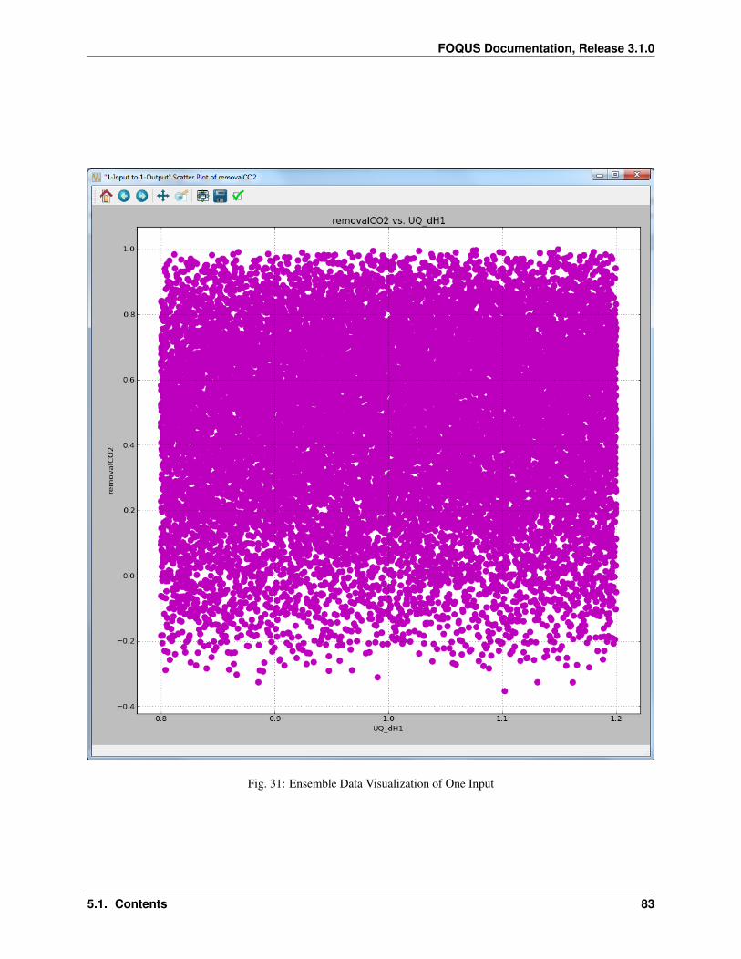
FOQUS Documentation, Release 3.1.0
Fig. 31: Ensemble Data Visualization of One Input
5.1. Contents 83
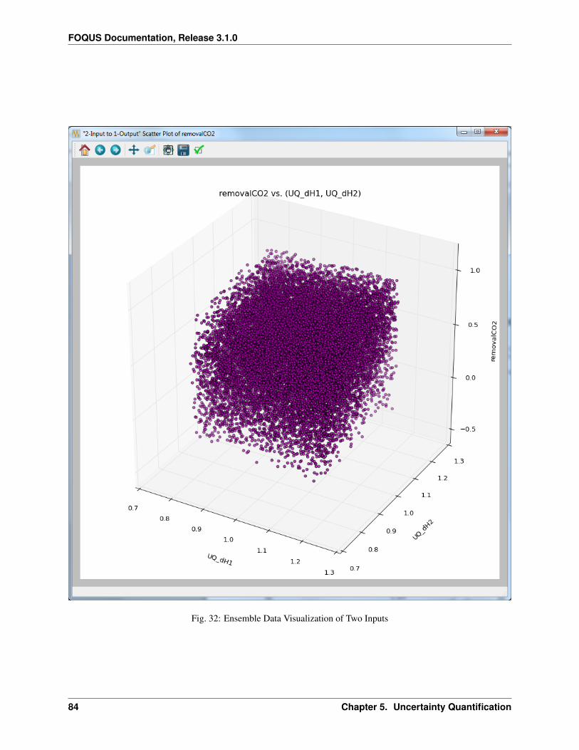
FOQUS Documentation, Release 3.1.0
Fig. 32: Ensemble Data Visualization of Two Inputs
84 Chapter 5. Uncertainty Quantification
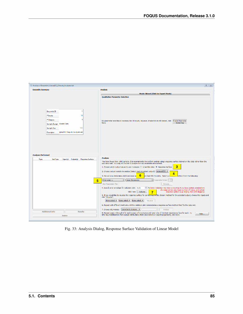
FOQUS Documentation, Release 3.1.0
Fig. 33: Analysis Dialog, Response Surface Validation of Linear Model
5.1. Contents 85
FOQUS Documentation, Release 3.1.0
Fig. 34: Linear Response Validation Results
86 Chapter 5. Uncertainty Quantification
FOQUS Documentation, Release 3.1.0
[fig:uqt_rs_validate_results]
The cross-validation results for the linear regression model are displayed as a histogram of errors to the left and a plotof predicted values versus actual values to the right. The histogram displays the cross validation error distribution,which provides the user information on what the errors are like overall. If this distribution is not centered on zero,there may be a systematic bias in the response surface model. If the distribution is too wide, it is not a good fit. Asfor the plot of predicted values versus actual values, the more closely the points are to the diagonal, the better the fit.Most response surface models, with the exception of MARS, also provide uncertainty information about the responsesurface. The vertical error bars on the left plot reflect the uncertainty in the linear response’s predictions.
In summary, these two figures should provide sufficient information for the user to judge how good the fit is. As isapparent in the figures, the linear model consistently overestimates and thus is an ill-suited response surface to modelour data. In general, the user may use a few response surface methods to see which method gives the best fit.
Response Surface Based Uncertainty Analysis
These capabilities are similar to those for ensemble data analysis. The difference is that the results are now derivedfrom a much larger ensemble that is computed from the response surface. With the 100 samples from the ensembledata, a response surface is trained and is used to generate 100K samples internally to compute the results for uncertaintyand sensitivity analyses. (Note: Validation must be performed before these analyses are available.)
After the response surface validation step, select “Uncertainty Analysis” to be the UQ analysis in Step 7 of “Analysis”(Figure [fig:uqt_rs_validate]). Click Analyze and a distribution representing the output uncertainty will be displayed(Figure [fig:uqt_rsua_results]).
[fig:uqt_rsua_results]
Compare the response surface based uncertainty results (Figure [fig:uqt_rsua_results]) to the results from ensembledata analysis (Figure [fig:uqt_ua_results]). The two main differences are easily seen.
• Two PDFs on top plot: A response surface (in this case, linear regression) is used to predict the output valuescorresponding to the input samples. From the validation step (left plot of Figure[fig:uqt_rs_validate_results]).Note: There is error associated with the response surface’s predictions. This error is propagated in uncertaintyanalysis, in the form of standard deviations around the predicted output values (i.e., the means). Accordingly,two histograms are presented: The “mean PDF” represents the output probability distribution computed fromthe response surface’s predicted output values only, without consideration for the uncertainties surroundingthese predicted values. The “ensemble PDF” represents the output probability distribution that encompasses theuncertainties surrounding these predicted values. In most cases, the ensemble PDF should have a larger spreadbecause it is accounting for more uncertainties (i.e., those that stem from the approximations inherent in theresponse surface).
• Multiple cumulative distribution functions (CDFs) on bottom plot: The “mean CDF” is constructed from acumulative sum on the mean PDF in the top plot. Since each predicted output value (i.e., the mean) has anassociated standard deviation, this information is used to construct other PDFs that correspond to output valuesthat are +/- 1, 2, and 3 standard deviations from the mean. These PDFs are then converted to CDFs and shownas colored lines. These colored lines provide an uncertainty “envelope” around the mean CDF.
Response Surface Based Mixed Epistemic-Aleatory Uncertainty Analysis
In “Expert Mode”, the user can perform more advanced uncertainty analysis that handles both epistemic and aleatoryuncertainties. To do so, the user will need to designate the uncertainty type (epistemic or aleatory) for each uncer-tain input. In general, epistemic uncertainties are reducible uncertainties that arise due to lack of knowledge, suchas simplifying assumptions in a mathematical model. Therefore, epistemic uncertainty is often characterized by up-per and lower bounds. On the other hand, aleatory uncertainties are irreducible uncertainties that represent natural,
5.1. Contents 87
FOQUS Documentation, Release 3.1.0
Fig. 35: Response Surface Based Uncertainty Analysis Results
88 Chapter 5. Uncertainty Quantification
FOQUS Documentation, Release 3.1.0
physical variability in the phenomenon under study. As such, aleatory uncertainties are often characterized by distri-butions. Hence, the user is required to provide a PDF for each aleatory input. (In FOQUS, with the exception of mixedepistemic-aleatory uncertainty analysis, all uncertain inputs are treated as aleatory inputs.)
To perform mixed epistemic-aleatory uncertainty (Figure [fig:uqt_rsaeua]), switch to “Expert Mode” by clickingthe Mode button that toggles between the analysis modes. After response surface validation, select “UncertaintyAnalysis” in the first Choose UQ Analysis drop-down list, then “Epistemic-Aleatory” in the secondary drop-downlist, for the UQ analysis. In the input table, designate the parameter Type (“Epistemic”, “Aleatory” or “Fixed”) andthe corresponding information for each input. Once complete, click Analyze. In this tutorial we consider dH1 & dH2as epistemic uncertain parameters, and rest of them are aleatory.
Fig. 36: Response Surface Based Mixed Epistemic-Aleatory Uncertainty Analysis
[fig:uqt_rsaeua]
The results of mixed epistemic-aleatory uncertainty analysis is a plot (Figure [fig:uqt_rsaeua_results]) containingmultiple CDFs. In the mixed analysis, the epistemic inputs are sampled according to their lower and upper bounds.Each sample point spawns a response surface based uncertainty analysis, in which the epistemic inputs are fixed attheir sampled value and the aleatory input uncertainties are propagated to generate a CDF that represents the output
uncertainty. A slider is provided for the user to extract the probability range corresponding to a particular value of theoutput.
[fig:uqt_rsaeua_results]
5.1. Contents 89
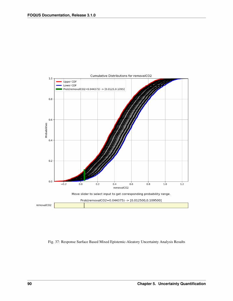
FOQUS Documentation, Release 3.1.0
Fig. 37: Response Surface Based Mixed Epistemic-Aleatory Uncertainty Analysis Results
90 Chapter 5. Uncertainty Quantification
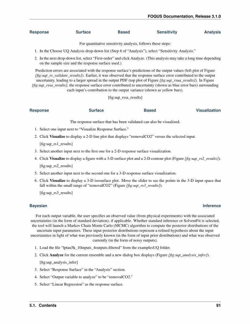
FOQUS Documentation, Release 3.1.0
Response Surface Based Sensitivity Analysis
For quantitative sensitivity analysis, follows these steps:
1. In the Choose UQ Analysis drop-down list (Step 6 of “Analysis”), select “Sensitivity Analysis.”
2. In the next drop-down list, select “First-order” and click Analyze. (This analysis may take a long time dependingon the sample size and the response surface used.)
Prediction errors are associated with the response surface’s predictions of the output values (left plot of Figure[fig:uqt_rs_validate_results]). Earlier, it was observed that the response surface error contributed to the outputuncertainty, leading to a larger spread in the output PDF (top plot of Figure [fig:uqt_rsua_results]). In Figure
[fig:uqt_rssa_results], the response surface error contributed to uncertainty (shown as blue error bars) surroundingeach input’s contribution to the output variance (shown as yellow bars).
[fig:uqt_rssa_results]
Response Surface Based Visualization
The response surface that has been validated can also be visualized.
1. Select one input next to “Visualize Response Surface.”
2. Click Visualize to display a 2-D line plot that displays “removalCO2” versus the selected input.
[fig:uqt_rs1_results]
3. Select another input next to the first one for a 2-D response surface visualization.
4. Click Visualize to display a figure with a 3-D surface plot and a 2-D contour plot (Figure [fig:uqt_rs2_results]).
[fig:uqt_rs2_results]
5. Select another input next to the second one for a 3-D response surface visualization.
6. Click Visualize to display a 3-D isosurface plot. Move the slider to see the points in the 3-D input space thatfall within the small range of “removalCO2” (Figure [fig:uqt_rs3_results]).
[fig:uqt_rs3_results]
Bayesian Inference
For each output variable, the user specifies an observed value (from physical experiments) with the associateduncertainties (in the form of standard deviation), if applicable. Whether standard inference or SolventFit is selected,the tool will launch a Markov Chain Monte Carlo (MCMC) algorithm to compute the posterior distributions of the
uncertain input parameters. These input posterior distributions represent a refined hypothesis about the inputuncertainties in light of what was previously known (in the form of input prior distributions) and what was observed
currently (in the form of noisy outputs).
1. Load the file “lptau5k_10inputs_4outputs.filtered” from the examplesUQ folder.
2. Click Analyze for the current ensemble and a new dialog box displays (Figure [fig:uqt_analysis_infer]).
[fig:uqt_analysis_infer]
3. Select “Response Surface” in the “Analysis” section.
4. Select “Output variable to analyze” to be “removalCO2.”
5. Select “Linear Regression” as the response surface.
5.1. Contents 91
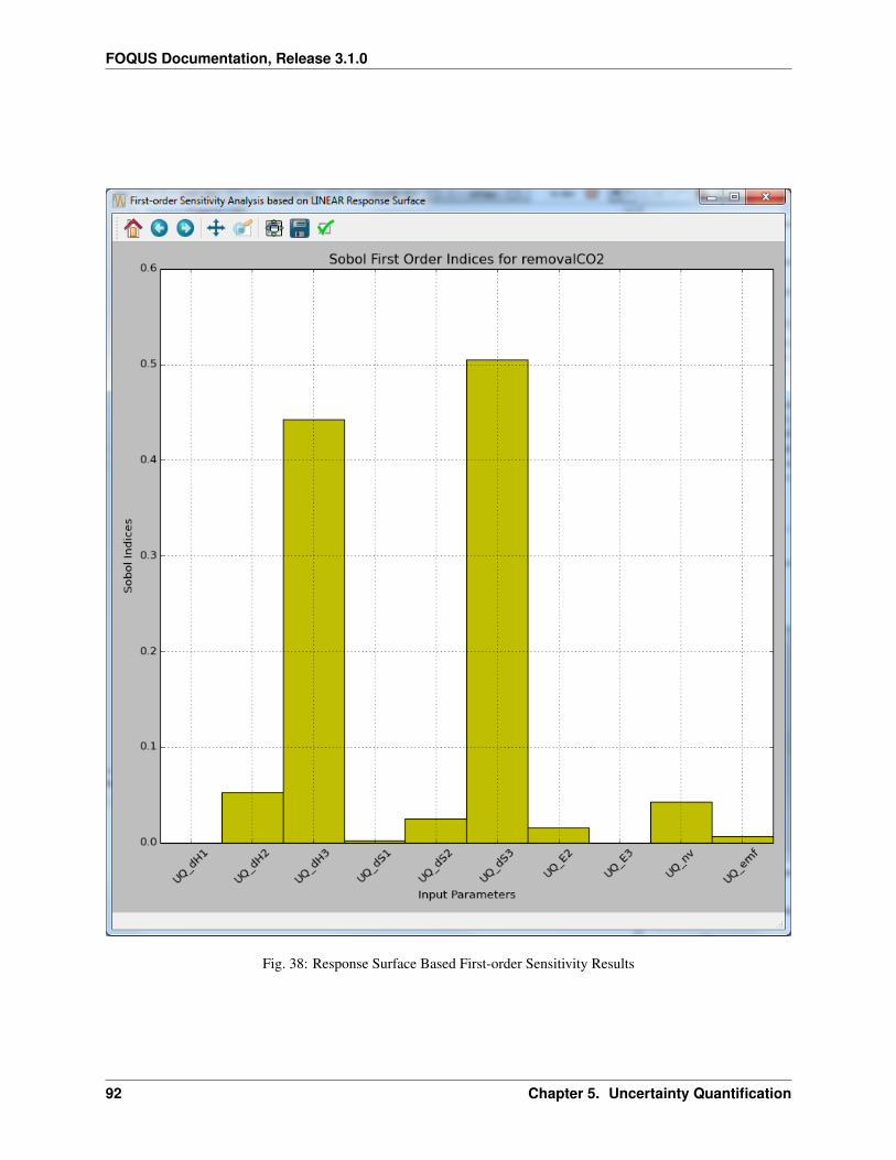
FOQUS Documentation, Release 3.1.0
Fig. 38: Response Surface Based First-order Sensitivity Results
92 Chapter 5. Uncertainty Quantification
FOQUS Documentation, Release 3.1.0
Fig. 39: 1-D Response Surface Visualization
5.1. Contents 93
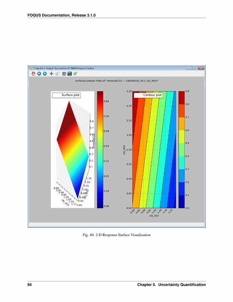
FOQUS Documentation, Release 3.1.0
Fig. 40: 2-D Response Surface Visualization
94 Chapter 5. Uncertainty Quantification
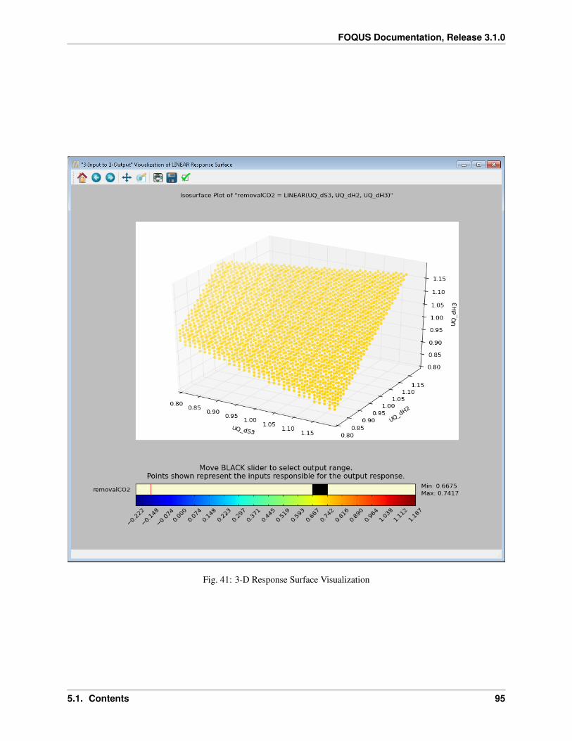
FOQUS Documentation, Release 3.1.0
Fig. 41: 3-D Response Surface Visualization
5.1. Contents 95
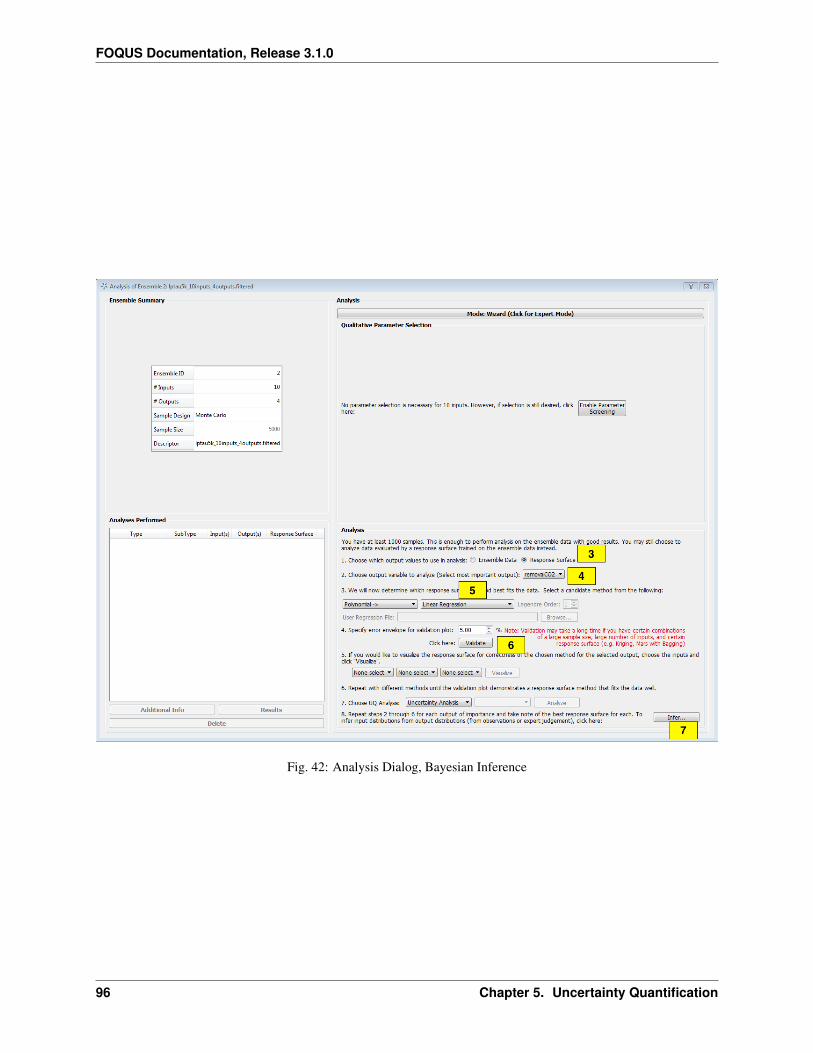
FOQUS Documentation, Release 3.1.0
Fig. 42: Analysis Dialog, Bayesian Inference
96 Chapter 5. Uncertainty Quantification

FOQUS Documentation, Release 3.1.0
6. Insert 5.00 as the error envelope for the validation plot. Click Validate. The GUI allows the user to proceed withBayesian inference after one input has been validated; however, the user may want to validate all outputs sincethey are all used in the inference.
7. Once validation is completed, click Infer at the lower right corner, which displays a new dialog box (Fig-ure[fig:uqt_infer]).
8. In the Output Settings table (on the left), select the second, third, and fourth outputs as the observed outputs.The user can experiment with using different response surface models (for example, linear polynomials) toapproximate the mapping from inputs to each of the outputs.
9. In the Input Settings table (on the right), designate input types (variable, design, or fixed) and if necessary,switch to Expert Mode to revise the prior distribution on the input parameters. The prior distribution representsknowledge that the user possesses about the inputs before observational data (from experiments) has been incor-porated into this knowledge. If the user does not have any updated knowledge about the simulation ensemble, itis OK to leave the table as is.
10. In the Observations table (in the middle), select the number of experiments from which the user can get obser-vational data. In essence, if the user has 𝑁 observations, then 𝑁 should be set as the number of experiments.The table will then populate columns for design inputs (if any) and observed outputs. Currently, only normaldistribution is supported as the noise model for observations. Enter the mean and standard deviation for each ofthese observations. For convenience, the mean and standard deviation values are prepopulated with the resultsfrom uncertainty analysis. These values have been provided as a sanity check for the user, in case the observationfor a particular output is way out of range from these distributions.
[fig:uqt_infer]
11. To save an input sample drawn from the posterior distribution, select the Save Posterior Input Samples to Filecheckbox and select a location and file name to store the sample.
12. Click Infer to start the analysis. Inference can take a long time; thus, a stop feature has been implemented. Onceinference starts, the Infer button changes to Stop. To stop inference calculations, click Stop which changes thebutton back to Infer, allowing the user to restart the calculations from scratch. If inference is allowed to run itscourse, its results are interpolated to produce heat maps (off-diagonal subplots in Figure[fig:uqt_infer_results])for visualization. This interpolation step can take a few minutes and while it is running, Infer is disabled.
5.1. Contents 97
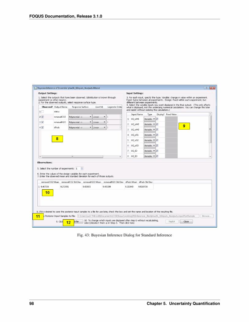
FOQUS Documentation, Release 3.1.0
Fig. 43: Bayesian Inference Dialog for Standard Inference
98 Chapter 5. Uncertainty Quantification
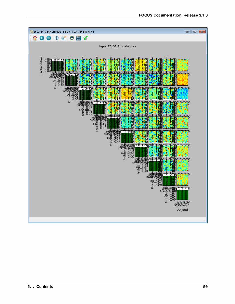
FOQUS Documentation, Release 3.1.0
5.1. Contents 99
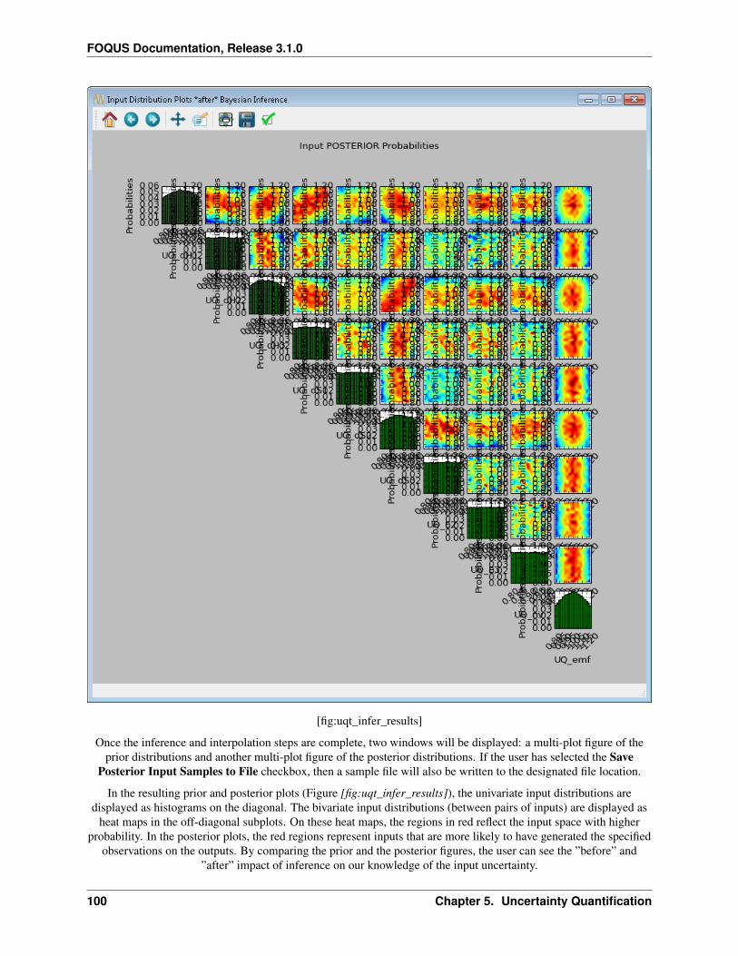
FOQUS Documentation, Release 3.1.0
[fig:uqt_infer_results]
Once the inference and interpolation steps are complete, two windows will be displayed: a multi-plot figure of theprior distributions and another multi-plot figure of the posterior distributions. If the user has selected the Save
Posterior Input Samples to File checkbox, then a sample file will also be written to the designated file location.
In the resulting prior and posterior plots (Figure [fig:uqt_infer_results]), the univariate input distributions aredisplayed as histograms on the diagonal. The bivariate input distributions (between pairs of inputs) are displayed as
heat maps in the off-diagonal subplots. On these heat maps, the regions in red reflect the input space with higherprobability. In the posterior plots, the red regions represent inputs that are more likely to have generated the specified
observations on the outputs. By comparing the prior and the posterior figures, the user can see the ”before” and”after” impact of inference on our knowledge of the input uncertainty.
100 Chapter 5. Uncertainty Quantification
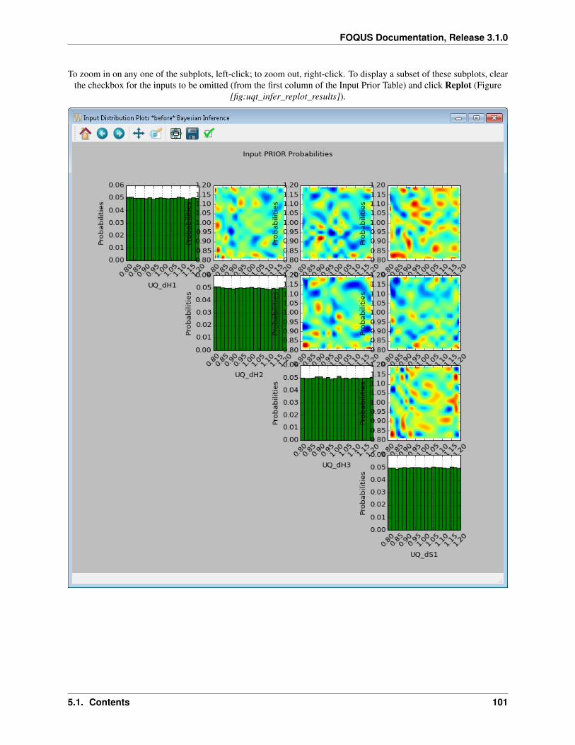
FOQUS Documentation, Release 3.1.0
To zoom in on any one of the subplots, left-click; to zoom out, right-click. To display a subset of these subplots, clearthe checkbox for the inputs to be omitted (from the first column of the Input Prior Table) and click Replot (Figure
[fig:uqt_infer_replot_results]).
5.1. Contents 101
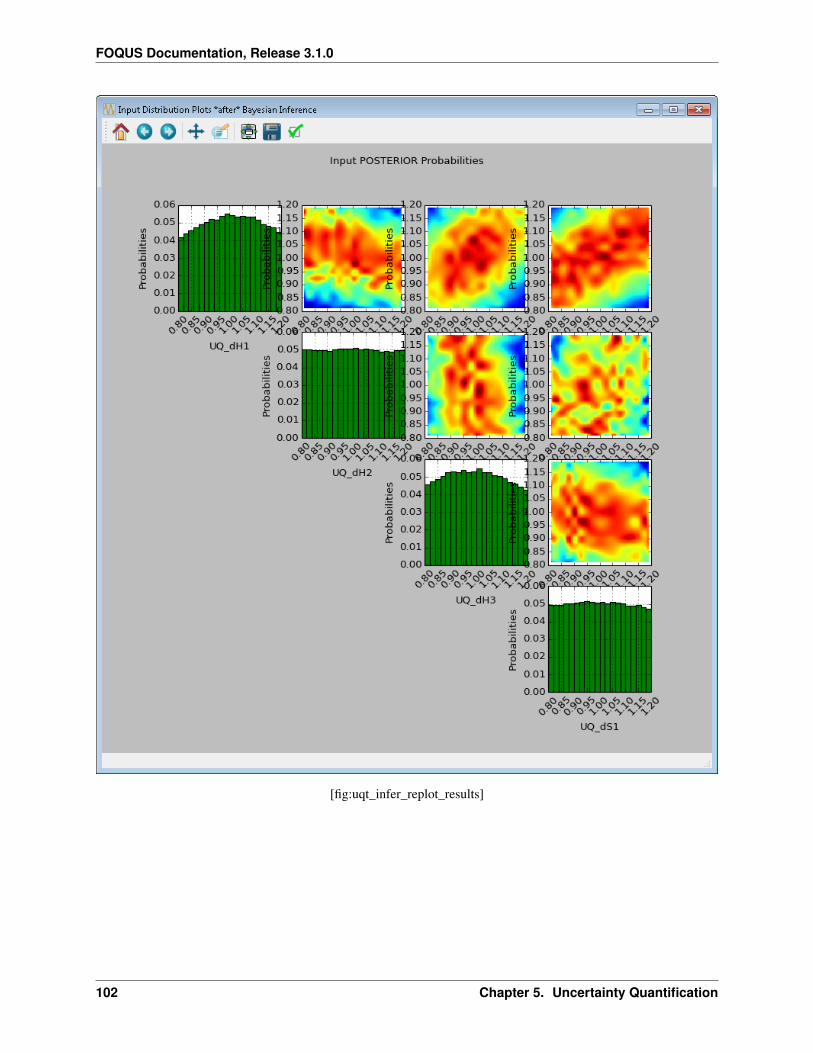
FOQUS Documentation, Release 3.1.0
[fig:uqt_infer_replot_results]
102 Chapter 5. Uncertainty Quantification
CHAPTER 6
Optimization Under Uncertainty
6.1 Contents
[sec:ouu_overview]
6.1.1 Reference
The FOQUS OUU module supports several variants of optimization under uncertainty. This chapter first presents themathematical formulations of these variants. Subsequently, details of the OUU graphical user interface will be
discussed.
OUU Variables
Suppose a simulation model is available for an OUU study. Let this simulation model be represented by the followingfunction:
𝑌 = 𝐹 (𝑍1, 𝑍2, 𝑍3, 𝑍4),
𝑤ℎ𝑖𝑐ℎ𝑖𝑠𝑐ℎ𝑎𝑟𝑎𝑐𝑡𝑒𝑟𝑖𝑧𝑒𝑑𝑏𝑦𝑓𝑜𝑢𝑟𝑡𝑦𝑝𝑒𝑠𝑜𝑓𝑣𝑎𝑟𝑖𝑎𝑏𝑙𝑒𝑠 :
1. Design/Decision/Optimization variables
• Notation: 𝑍1 with dimension 𝑛1
• Definition: Design variables are continuous variables that may be bounded or unbounded. They are gener-ally the set of optimization variables in a single-stage optimization or the set of outer optimization variablesin the two-stage optimization.
2. Recourse/Operating variables
• Notation: 𝑍2 with dimension 𝑛2
• Definition: Operating variables are optimization variables in the inner optimization for a given scenario(or realization) of the uncertain variables in a two-stage optimization.
103
FOQUS Documentation, Release 3.1.0
3. Discrete uncertain variables
• Notation: 𝑍3 with dimension 𝑛3
• Definition: Discrete variables are uncertain variables that have an enumerable set of states (called sce-narios) such that each state is associated with a finite probability and the sum of probabilities for all thescenarios is equal to 1.
4. Continuous uncertain variables
• Notation: 𝑍4 with dimension 𝑛4
• Definition: Continuous uncertain variables are associated with a joint probability distribution functionfrom which a sample can be drawn to compute the basic statistics.
OUU Objective Functions
In the presence of uncertainties, OUU seeks to find the optimal solution in some statistical sense. For example, anoptimization goal may to be find the design settings that minimizes the statistical mean of the system response. Other
popular objective functions are:
1. a linear combination of statistical mean and standard deviation of some selected output,
2. probability of exceeding the best value is smaller than some percentage at any point in the design space (this isanalogous to conditional value at risk).
Note that these metrics are defined in the design variable space - that is, at each iteration of an OUU algorithm, theselected metric will be computed for the decision point under consideration. Since the calculation of these statisticalmetrics requires a sample (possibly large), OUU can benefit from parallel computing capabilities (e.g., the Turbine
gateway).
Mathematical Formulations
FOQUS supports two types of OUU methods: single-stage OUU and two-stage OUU. The main difference betweensingle-stage and two-stage OUU is the presence of the recourse (or operational) variables. Strictly speaking, sincerecourse variables are generally hidden (they are only needed in the inner stage and their values are not used in theouter stage of two-stage OUU), the distinction between single-stage and two-stage OUU is not clear. Nevertheless,for the sake of clarify, we will describe details of each formulation separately. The current OUU does not support
linearly or nonlinearly-constrained optimization.
Single-Stage Formulation
In this formulation, there is no recourse variable:
𝑌 = 𝐹 (𝑍1, 𝑍3, 𝑍4)
𝑎𝑛𝑑𝑡ℎ𝑒𝑜𝑝𝑡𝑖𝑚𝑖𝑧𝑎𝑡𝑖𝑜𝑛𝑝𝑟𝑜𝑏𝑙𝑒𝑚𝑏𝑒𝑐𝑜𝑚𝑒𝑠 :
min𝑍1
Φ𝑍3,𝑍4[𝐹 (𝑍1, 𝑍3, 𝑍4)]
where Φ𝑍3,𝑍4 [𝐹 (𝑍1, 𝑍3, 𝑍4)] is the statistical metric (one of the three options given above).
For example, if the objective function is the statistical mean, then the formulation becomes:
min𝑍1
E𝑍3,𝑍4[𝐹 (𝑍1, 𝑍3, 𝑍4)] ≈ min
𝑍1
𝑛3∑︁𝑗=1
𝜋𝑗
(︂∫︁𝐹 (𝑍1, 𝑍3, 𝑍4)𝑃 (𝑍4)𝑑𝑍4
)︂where, again, 𝑛3 is the number of scenarios for the discrete uncertain variables, 𝜋𝑗 is the probability of the 𝑗-th
scenario, and 𝑃 (𝑍4) is the joint probability of the continuous uncertain variables.
104 Chapter 6. Optimization Under Uncertainty
FOQUS Documentation, Release 3.1.0
Two-Stage Formulation
In this formulation all four types of variables are present. The objective function is given by:
min𝑍3,𝑍4
Φ𝑍3,𝑍4
[︂min𝑍2
𝐹 (𝑍1, 𝑍2, 𝑍3, 𝑍4)
]︂.
If the objective function is the statistical mean, the formulation becomes:
min𝑍1
E𝑍3,𝑍4
[︂min𝑍2
𝐹 (𝑍1, 𝑍2, 𝑍3, 𝑍4)
]︂≈ min
𝑍1
𝑛3∑︁𝑗=1
𝜋𝑗
(︂∫︁ [︂min𝑍2
𝐹 (𝑍1, 𝑍2, 𝑍3, 𝑍4)
]︂𝑃 (𝑍4)𝑑𝑍4
)︂𝐿𝑒𝑡
𝐺(Z1,Z3,Z4) = min𝑍2
𝐹 (𝑍1, 𝑍2, 𝑍3, 𝑍4).
𝑇ℎ𝑒𝑛𝑡ℎ𝑒𝑡𝑤𝑜− 𝑠𝑡𝑎𝑔𝑒𝑒𝑞𝑢𝑎𝑡𝑖𝑜𝑛𝑐𝑎𝑛𝑏𝑒𝑟𝑒𝑤𝑟𝑖𝑡𝑡𝑒𝑛𝑎𝑠 :
min𝑍1
E𝑍3,𝑍4 [𝐺(𝑍1, 𝑍3, 𝑍4)]
≈ min𝑍1
𝑛3∑︁𝑗=1
𝜋𝑗
(︂∫︁𝐺(𝑍1, 𝑍3, 𝑍4)𝑃 (𝑍4)𝑑𝑍4
)︂𝑤ℎ𝑖𝑐ℎ𝑖𝑠𝑎𝑠𝑖𝑛𝑔𝑙𝑒− 𝑠𝑡𝑎𝑔𝑒𝑂𝑈𝑈𝑤𝑖𝑡ℎ𝑟𝑒𝑠𝑝𝑒𝑐𝑡𝑡𝑜𝑡ℎ𝑒 : 𝑚𝑎𝑡ℎ : ‘𝐺‘𝑓𝑢𝑛𝑐𝑡𝑖𝑜𝑛.
Windows Users
Before using the OUU module, Windows users may need to update the following registry keys:
1. HKEY_CLASSES_ROOT\Applications\python.exe\shell\open\command
2. HKEY_CLASSES_ROOT\py_auto_file\shell\open\command
To update these registry keys:
1. Open the Registry Editor by going to the Windows Start menu, typing “regedit” (without the quotes), andselecting “regedit” (Figure regedit in the Windows Start menu).
2. After the Registry Editor is opened, locate “HKEY_CLASSES_ROOT” (Figure HKEY_CLASSES_ROOT in theRegistry Editor).
3. Under “HKEY_CLASSES_ROOT”, locate “Applications” (Figure Applications underHKEY_CLASSES_ROOT).
4. Under “Applications”, locate “python.exe\shell\open\command” (Figure python under Applications).
5. In the table on the right, double-click “(Default)” under “Name” (Figure python under Applications).
6. In the input box (Figure python under Applications), type (including the quotations): “the location of the Ana-conda 3 version of python.exe” “%1” %*
7. After clicking “OK”, the information you typed in the input box should appear under “Data” in the table on theright (Figure python under Applications).
8. Under “HKEY_CLASSES_ROOT”, locate “py_auto_file\shell\open\command” (Figure py_auto_file underHKEY_CLASSES_ROOT).
6.1. Contents 105
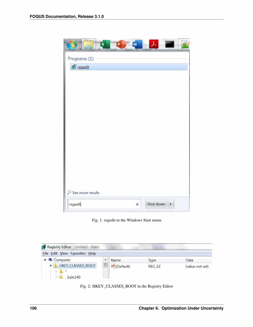
FOQUS Documentation, Release 3.1.0
Fig. 1: regedit in the Windows Start menu
Fig. 2: HKEY_CLASSES_ROOT in the Registry Editor
106 Chapter 6. Optimization Under Uncertainty
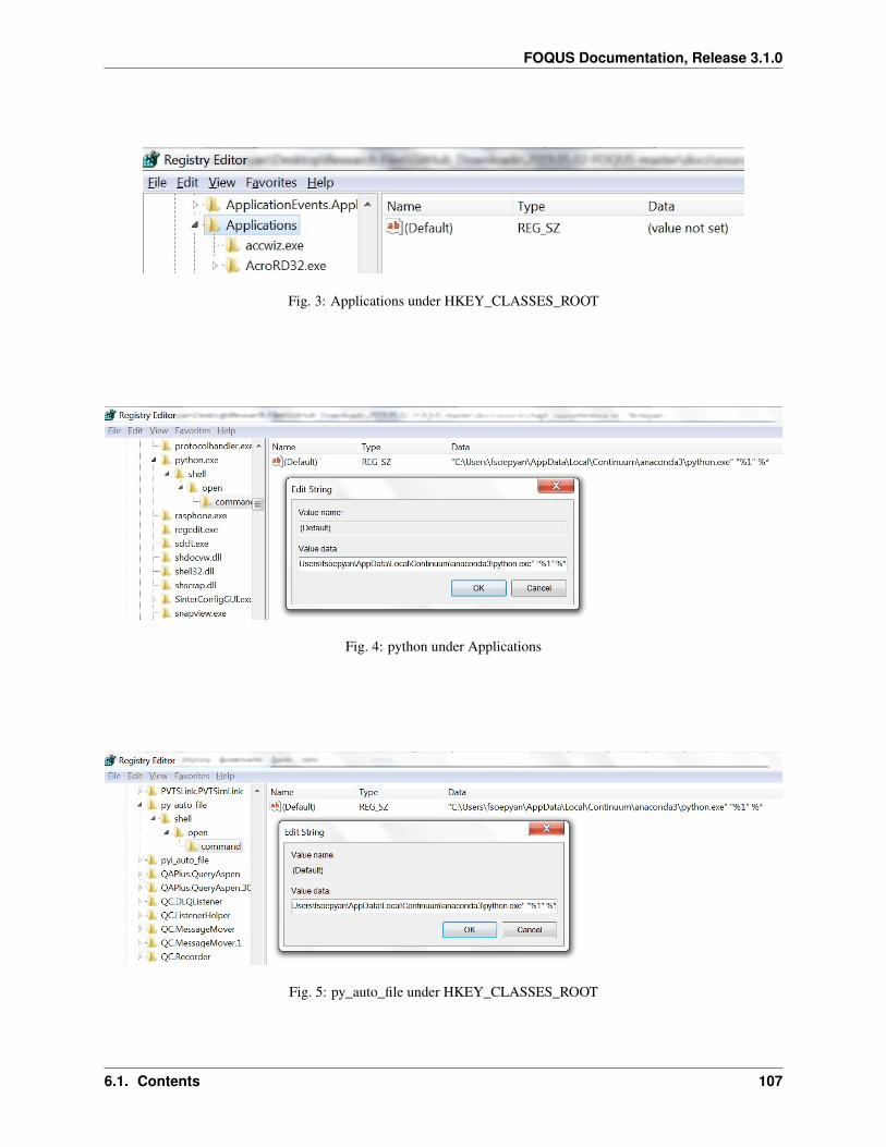
FOQUS Documentation, Release 3.1.0
Fig. 3: Applications under HKEY_CLASSES_ROOT
Fig. 4: python under Applications
Fig. 5: py_auto_file under HKEY_CLASSES_ROOT
6.1. Contents 107
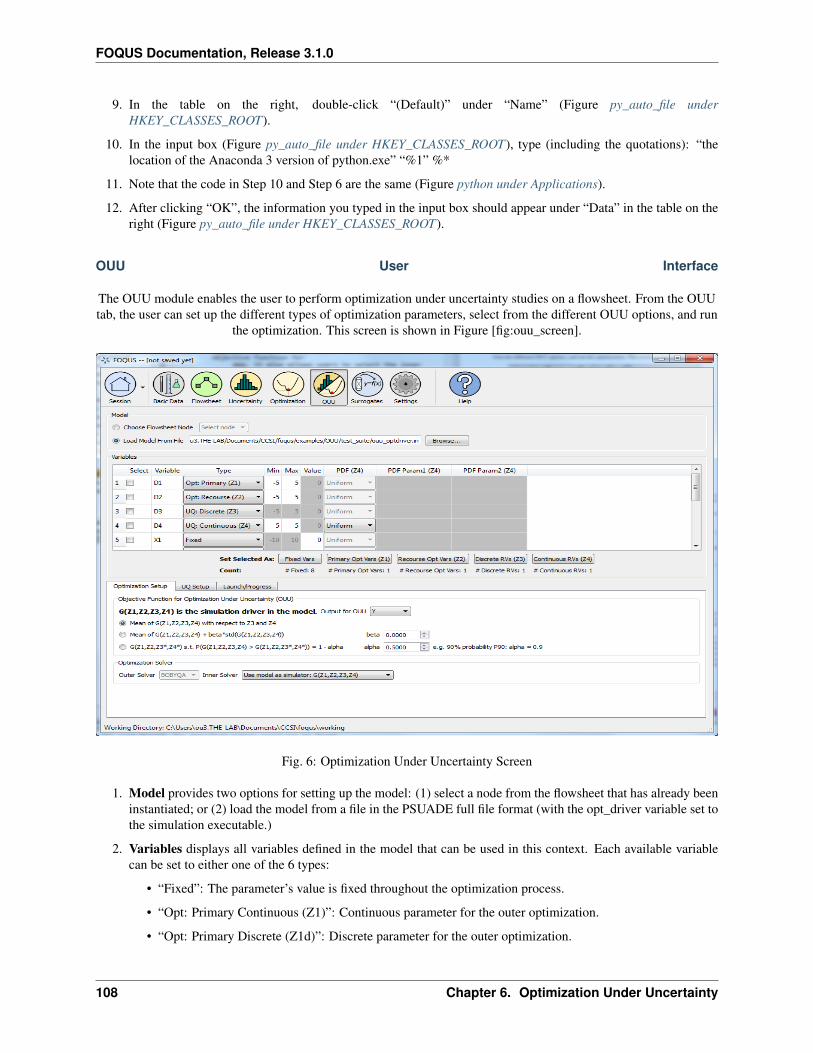
FOQUS Documentation, Release 3.1.0
9. In the table on the right, double-click “(Default)” under “Name” (Figure py_auto_file underHKEY_CLASSES_ROOT).
10. In the input box (Figure py_auto_file under HKEY_CLASSES_ROOT), type (including the quotations): “thelocation of the Anaconda 3 version of python.exe” “%1” %*
11. Note that the code in Step 10 and Step 6 are the same (Figure python under Applications).
12. After clicking “OK”, the information you typed in the input box should appear under “Data” in the table on theright (Figure py_auto_file under HKEY_CLASSES_ROOT).
OUU User Interface
The OUU module enables the user to perform optimization under uncertainty studies on a flowsheet. From the OUUtab, the user can set up the different types of optimization parameters, select from the different OUU options, and run
the optimization. This screen is shown in Figure [fig:ouu_screen].
Fig. 6: Optimization Under Uncertainty Screen
1. Model provides two options for setting up the model: (1) select a node from the flowsheet that has already beeninstantiated; or (2) load the model from a file in the PSUADE full file format (with the opt_driver variable set tothe simulation executable.)
2. Variables displays all variables defined in the model that can be used in this context. Each available variablecan be set to either one of the 6 types:
• “Fixed”: The parameter’s value is fixed throughout the optimization process.
• “Opt: Primary Continuous (Z1)”: Continuous parameter for the outer optimization.
• “Opt: Primary Discrete (Z1d)”: Discrete parameter for the outer optimization.
108 Chapter 6. Optimization Under Uncertainty
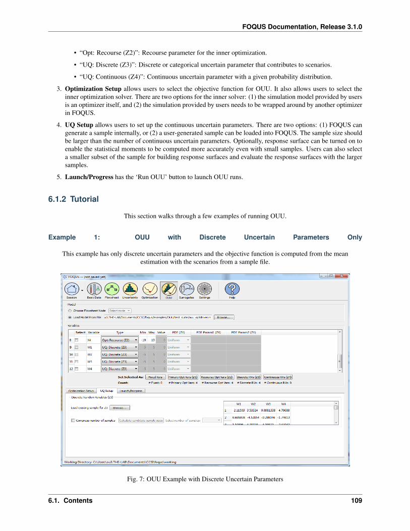
FOQUS Documentation, Release 3.1.0
• “Opt: Recourse (Z2)”: Recourse parameter for the inner optimization.
• “UQ: Discrete (Z3)”: Discrete or categorical uncertain parameter that contributes to scenarios.
• “UQ: Continuous (Z4)”: Continuous uncertain parameter with a given probability distribution.
3. Optimization Setup allows users to select the objective function for OUU. It also allows users to select theinner optimization solver. There are two options for the inner solver: (1) the simulation model provided by usersis an optimizer itself, and (2) the simulation provided by users needs to be wrapped around by another optimizerin FOQUS.
4. UQ Setup allows users to set up the continuous uncertain parameters. There are two options: (1) FOQUS cangenerate a sample internally, or (2) a user-generated sample can be loaded into FOQUS. The sample size shouldbe larger than the number of continuous uncertain parameters. Optionally, response surface can be turned on toenable the statistical moments to be computed more accurately even with small samples. Users can also selecta smaller subset of the sample for building response surfaces and evaluate the response surfaces with the largersamples.
5. Launch/Progress has the ‘Run OUU’ button to launch OUU runs.
6.1.2 Tutorial
This section walks through a few examples of running OUU.
Example 1: OUU with Discrete Uncertain Parameters Only
This example has only discrete uncertain parameters and the objective function is computed from the meanestimation with the scenarios from a sample file.
Fig. 7: OUU Example with Discrete Uncertain Parameters
6.1. Contents 109
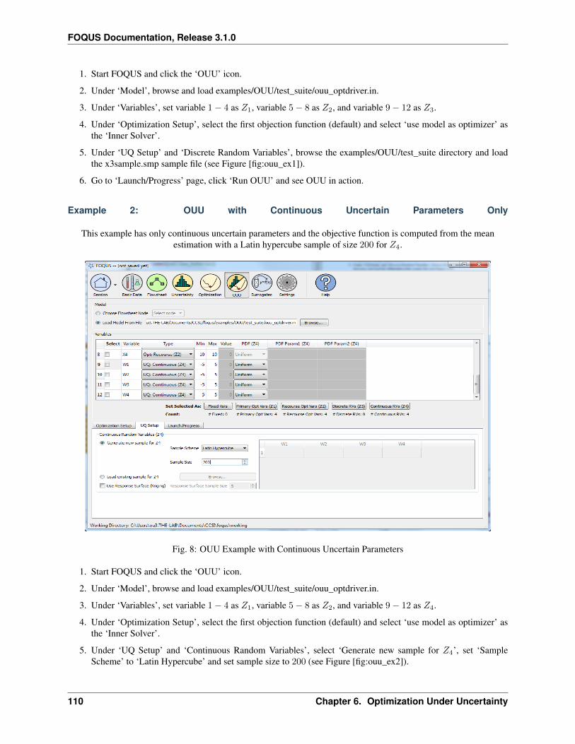
FOQUS Documentation, Release 3.1.0
1. Start FOQUS and click the ‘OUU’ icon.
2. Under ‘Model’, browse and load examples/OUU/test_suite/ouu_optdriver.in.
3. Under ‘Variables’, set variable 1 − 4 as 𝑍1, variable 5 − 8 as 𝑍2, and variable 9 − 12 as 𝑍3.
4. Under ‘Optimization Setup’, select the first objection function (default) and select ‘use model as optimizer’ asthe ‘Inner Solver’.
5. Under ‘UQ Setup’ and ‘Discrete Random Variables’, browse the examples/OUU/test_suite directory and loadthe x3sample.smp sample file (see Figure [fig:ouu_ex1]).
6. Go to ‘Launch/Progress’ page, click ‘Run OUU’ and see OUU in action.
Example 2: OUU with Continuous Uncertain Parameters Only
This example has only continuous uncertain parameters and the objective function is computed from the meanestimation with a Latin hypercube sample of size 200 for 𝑍4.
Fig. 8: OUU Example with Continuous Uncertain Parameters
1. Start FOQUS and click the ‘OUU’ icon.
2. Under ‘Model’, browse and load examples/OUU/test_suite/ouu_optdriver.in.
3. Under ‘Variables’, set variable 1 − 4 as 𝑍1, variable 5 − 8 as 𝑍2, and variable 9 − 12 as 𝑍4.
4. Under ‘Optimization Setup’, select the first objection function (default) and select ‘use model as optimizer’ asthe ‘Inner Solver’.
5. Under ‘UQ Setup’ and ‘Continuous Random Variables’, select ‘Generate new sample for 𝑍4’, set ‘SampleScheme’ to ‘Latin Hypercube’ and set sample size to 200 (see Figure [fig:ouu_ex2]).
110 Chapter 6. Optimization Under Uncertainty
FOQUS Documentation, Release 3.1.0
6. Go to ‘Launch/Progress’ page, click ‘Run OUU’ and see OUU in action.
Example 3: OUU with Continuous Uncertain Parameters and Response Surface
This example is similar to Example 2 except that response surfaces will be used on the 𝑍4 sample (that is, the 𝑍4
sample will be used to construct response surfaces and the means will be estimated from a large sample evaluated onthe response surfaces).
1. Start FOQUS and click the ‘OUU’ icon.
2. Under ‘Model’, browse and load examples/OUU/test_suite/ouu_optdriver.in.
3. Under ‘Variables’, set variable 1 − 4 as 𝑍1, variable 5 − 8 as 𝑍2, and variable 9 − 12 as 𝑍4.
4. Under ‘Optimization Setup’, select the first objection function (default) and select ‘use model as optimizer’ asthe ‘Inner Solver’.
5. Under ‘UQ Setup’ and ‘Continuous Random Variables’, select ‘Generate new sample for 𝑍4’, set ‘SampleScheme’ to ‘Latin Hypercube’ and set sample size to 200.
6. Under ‘UQ Setup’ and ‘Continuous Random Variables’, check the ‘Use Response Surface’ box (see Figure[fig:ouu_ex2]).
7. Go to ‘Launch/Progress’ page, click ‘Run OUU’ and see OUU in action.
Example 4: OUU with Discrete and Continuous Uncertain Parameters
This example has both discrete and continuous parameters. The discrete scenarios will be loaded from a sample file.A Latin hypercube sample will be generated for the continuous variables.
1. Start FOQUS and click the ‘OUU’ icon.
2. Under ‘Model’, browse and load examples/OUU/test_suite/ouu_optdriver.in.
3. Under ‘Variables’, set variable 1 − 4 as 𝑍1, variable 5 − 8 as 𝑍2, variable 9 as 𝑍3, and variable 10 − 12 as 𝑍4.
4. Under ‘Optimization Setup’, select the first objection function (default) and select ‘use model as optimizer’ asthe ‘Inner Solver’.
5. Under ‘UQ Setup’ and ‘Discrete Random Variables’, browse the examples/OUU/test_suite directory and loadthe x3sample4.smp sample file.
6. Under ‘UQ Setup’ and ‘Continuous Random Variables’, select ‘Generate new sample for 𝑍4’, set ‘SampleScheme’ to Latin hypercube and set ‘Sample Size’ to 100.
7. Go to ‘Launch/Progress’ page, click ‘Run OUU’ and see OUU in action.
Example 5: OUU with Mixed Uncertain Parameters and Response Surface
This example is similar to Example 4 except that response surfaces will be used to estimate the means for thecontinuous uncertain variables.
1. Start FOQUS and click the ‘OUU’ icon.
2. Under ‘Model’, browse and load examples/OUU/test_suite/ouu_optdriver.in.
3. Under ‘Variables’, set variable 1 − 4 as 𝑍1, variable 5 − 8 as 𝑍2, variable 9 as 𝑍3, and variable 10 − 12 as 𝑍4.
4. Under ‘Optimization Setup’, select the first objection function (default) and select ‘use model as optimizer’ asthe ‘Inner Solver’.
6.1. Contents 111
FOQUS Documentation, Release 3.1.0
5. Under ‘UQ Setup’ and ‘Discrete Random Variables’, browse the examples/OUU/test_suite directory and loadthe x3sample4.smp sample file.
6. Under ‘UQ Setup’ and ‘Continuous Random Variables’, select ‘Generate new sample for 𝑍4’, set ‘SampleScheme’ to Latin hypercube and set ‘Sample Size’ to 100.
7. Under ‘UQ Setup’ and ‘Continuous Random Variables’, check the ‘Use Response Surface’ box.
8. Go to ‘Launch/Progress’ page, click ‘Run OUU’ and see OUU in action.
Example 6: OUU with User-provided Samples and Response Surface
This example is similar to Example 4 except that a sample for 𝑍4 will be used (instead of the Latin hypercube samplegenerated internally).
1. Start FOQUS and click the ‘OUU’ icon.
2. Under ‘Model’, browse and load examples/OUU/test_suite/ouu_optdriver.in.
3. Under ‘Variables’, set variable 1 − 4 as 𝑍1, variable 5 − 8 as 𝑍2, variable 9 as 𝑍3, and variable 10 − 12 as 𝑍4.
4. Under ‘Optimization Setup’, select the first objection function (default) and select ‘use model as optimizer’ asthe ‘Inner Solver’.
5. Under ‘UQ Setup’ and ‘Discrete Random Variables’, browse the examples/OUU/test_suite directory and loadthe x3sample4.smp sample file.
6. Under ‘UQ Setup’ and ‘Continuous Random Variables’, check ‘Load existing sample for 𝑍4’ and load the 𝑍4
sample examples/OUU/test_suite/x4sample4.smp.
7. Go to ‘Launch/Progress’ page, click ‘Run OUU’ and see OUU in action.
Example 7: OUU with Large User-provided Samples and Response Surface
This example is similar to Example 5 except that a sample for 𝑍4 is provided (instead of generated internally).
1. Start FOQUS and click the ‘OUU’ icon.
2. Under ‘Model’, browse and load examples/OUU/test_suite/ouu_optdriver.in.
3. Under ‘Variables’, set variable 1 − 4 as 𝑍1, variable 5 − 8 as 𝑍2, and variable 9 − 12 as 𝑍4.
4. Under ‘Optimization Setup’, select the first objection function (default) and select ‘use model as optimizer’ asthe ‘Inner Solver’.
5. Under ‘UQ Setup’ and ‘Continuous Random Variables’, check ‘Load existing sample for 𝑍4’ and load the 𝑍4
sample examples/OUU/test_suite/x4sampleLarge.smp (10000 sample points).
6. Under ‘UQ Setup’ and ‘Continuous Random Variables’, check ‘Use Response Surface’ and set ‘Sample Size’to 100.
7. Go to ‘Launch/Progress’ page, click ‘Run OUU’ and see OUU in action.
112 Chapter 6. Optimization Under Uncertainty
CHAPTER 7
Surrogate Modeling
7.1 Contents
7.1.1 Surrogate Models Overview
Large-scale computational models are crucial tools to analyze complex systems. When coupled with uncertaintyquantification and optimization methods, the resulting computational expense becomes intractable. In order to facethe computational burden, surface approximation methods, black box models, or surrogate models are commonly
used. FOQUS provides a selection of surrogate modeling tools all using a similar work-flow. This section provides anoverview of the surrogate modeling features and capabilities. The details of each tool are provided in the tutorial
sections.
The following surrogate modeling tools are currently available:
• ACOSSO – Adaptive COmponent Selection and Shrinkage Operator is a regularization method for simultaneousmodel fitting and variable selection based in nonparametric regression methods. ACCOSSO is suitable forapproximating models with many inputs and no sharp changes.
• ALAMO – Automated Learning of Algebraic Models for Optimization generates algebraic models from datasets. These surrogate models are ideal for equation oriented optimization problems (which are easily differen-tiable), such as super structure optimization.
• BSS-ANOVA – Bayesian Smoothing Spline Analysis of Variance is a method similar to ACOSSO.
• iREVEAL – Surrogate models for CFD simulations using Kriging or Neural Networks. It contains specialfeatures specifically designed for working with CFDs.
Data Selection
The Data tab allows the selection of training data to be used to generate a surrogate model (Surrogate Data Form). Ifthe session is associated with a flowsheet data (results from a single flowsheet run, optimization runs, or UQ
samples), then the flowsheet data is available to be the training data and the table will be populated accordingly.
1. Run the surrogate modeling method.
113
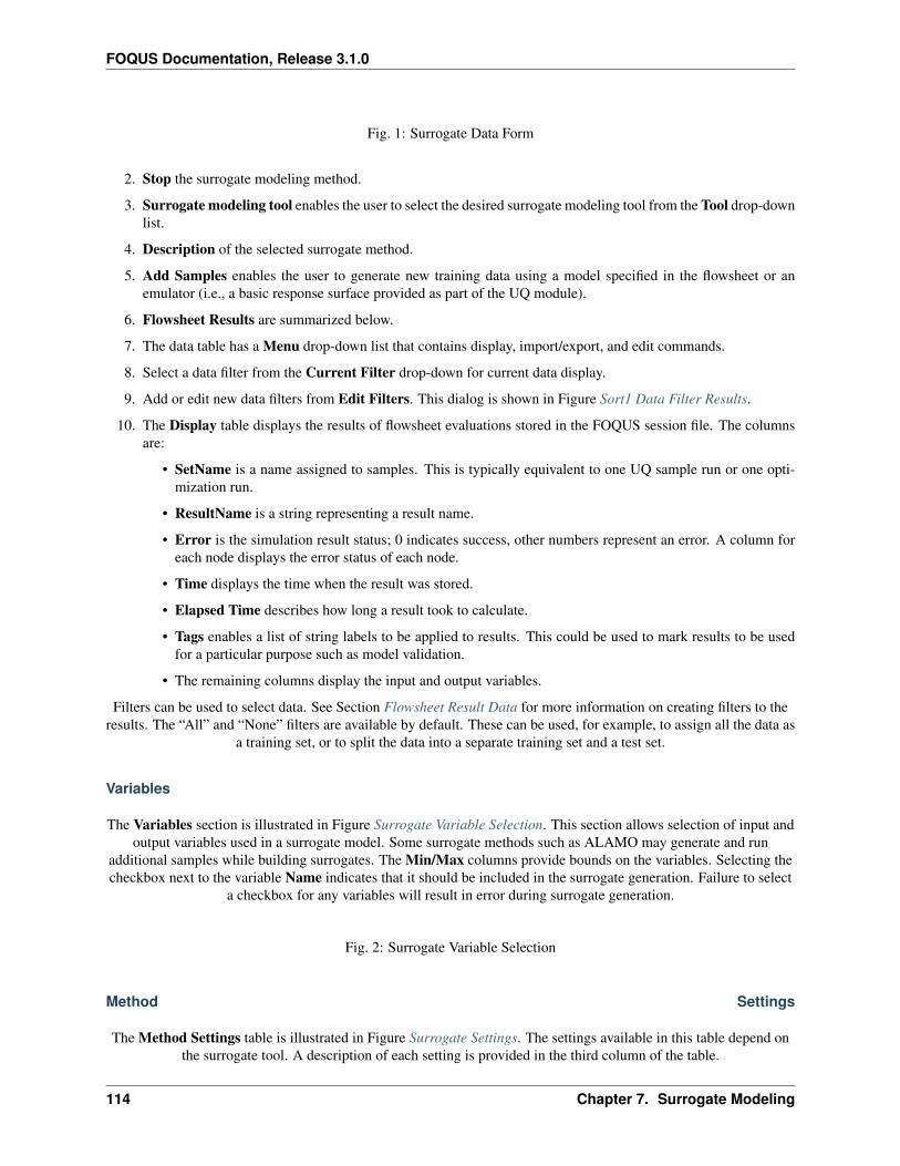
FOQUS Documentation, Release 3.1.0
Fig. 1: Surrogate Data Form
2. Stop the surrogate modeling method.
3. Surrogate modeling tool enables the user to select the desired surrogate modeling tool from the Tool drop-downlist.
4. Description of the selected surrogate method.
5. Add Samples enables the user to generate new training data using a model specified in the flowsheet or anemulator (i.e., a basic response surface provided as part of the UQ module).
6. Flowsheet Results are summarized below.
7. The data table has a Menu drop-down list that contains display, import/export, and edit commands.
8. Select a data filter from the Current Filter drop-down for current data display.
9. Add or edit new data filters from Edit Filters. This dialog is shown in Figure Sort1 Data Filter Results.
10. The Display table displays the results of flowsheet evaluations stored in the FOQUS session file. The columnsare:
• SetName is a name assigned to samples. This is typically equivalent to one UQ sample run or one opti-mization run.
• ResultName is a string representing a result name.
• Error is the simulation result status; 0 indicates success, other numbers represent an error. A column foreach node displays the error status of each node.
• Time displays the time when the result was stored.
• Elapsed Time describes how long a result took to calculate.
• Tags enables a list of string labels to be applied to results. This could be used to mark results to be usedfor a particular purpose such as model validation.
• The remaining columns display the input and output variables.
Filters can be used to select data. See Section Flowsheet Result Data for more information on creating filters to theresults. The “All” and “None” filters are available by default. These can be used, for example, to assign all the data as
a training set, or to split the data into a separate training set and a test set.
Variables
The Variables section is illustrated in Figure Surrogate Variable Selection. This section allows selection of input andoutput variables used in a surrogate model. Some surrogate methods such as ALAMO may generate and run
additional samples while building surrogates. The Min/Max columns provide bounds on the variables. Selecting thecheckbox next to the variable Name indicates that it should be included in the surrogate generation. Failure to select
a checkbox for any variables will result in error during surrogate generation.
Fig. 2: Surrogate Variable Selection
Method Settings
The Method Settings table is illustrated in Figure Surrogate Settings. The settings available in this table depend onthe surrogate tool. A description of each setting is provided in the third column of the table.
114 Chapter 7. Surrogate Modeling

FOQUS Documentation, Release 3.1.0
Fig. 3: Surrogate Settings
Execution
Clicking Run starts the surrogate model building process. The execution monitor displays after Run is clicked (seeFigure Surrogate Status Monitor). The execution monitor displays the status of the surrogate build. The messages
displayed depends on the surrogate tool.
Fig. 4: Surrogate Status Monitor
After a successful execution and model building, the results are displayed. Note that in this case, the surrogatemodeling tool ends with an error, the errors are displayed in this window. After surrogate generation completes, one
or two Python files will be generated depending on the tool. Each tool generates a file that encodes the surrogatemodel as a general Python script that can be used to evaluate output values for UQ analyses within the UQ module.
The other file, if available, is a FOQUS flowsheet plugin model that allows the surrogate to be run in a FOQUSflowsheet. The next version of FOQUS will generate a FOQUS flowsheet plugin model (i.e., the second file) for all
surrogate tools.
7.1.2 Tutorial
ALAMO
This tutorial focuses on the use of the ALAMO tool for building algebraic surrogate models. ALAMO buildssimplified algebraic models, which are particularly well suited for rigorous equation oriented optimization. To keep
the execution of this tutorial fast, a toy problem is used. In this case study the flowsheet calculations and samplegeneration are done within FOQUS, alternatively, the user can provide a simulation model such as: Excel, Aspen
plus, Aspen custom modeler, etc.
Note: Before starting this tutorial the ALAMO product must be downloaded from the products page on the CCSIwebsite. The path for the ALAMO executable file must be set in FOQUS settings (see Section Settings).
Flowsheet Setup
1. Open FOQUS.
2. Name the session “Surrogate_Tutorial_1” (Figure Session Set Up).
Fig. 5: Session Set Up
3. Navigate to the Flowsheet Editor (Figure Flowsheet Setup).
4. Add a Flowsheet Node named “eq.”
5. Display the Node Editor by clicking the Node Editor toggle button.
The Node Editor displays (Figure Node Variables). Thefirst step to setting up the node for this problem is to addinput and output variables to the node.
6. If the input variables table is not displayed as shown in Figure Node Variables, click the Variables tab and thenclick the Input Variables toolbox section.
7. Add the variables “x1” and “x2” by clicking the Add icon (+) above the input table.
7.1. Contents 115
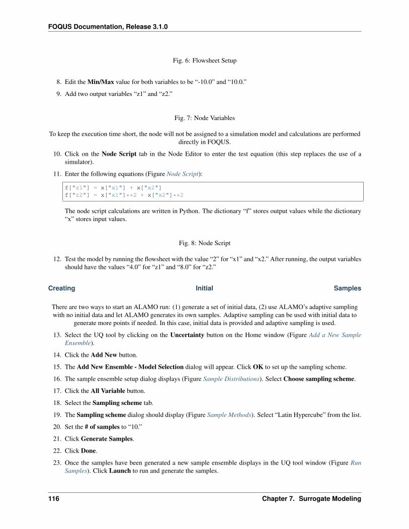
FOQUS Documentation, Release 3.1.0
Fig. 6: Flowsheet Setup
8. Edit the Min/Max value for both variables to be “-10.0” and “10.0.”
9. Add two output variables “z1” and “z2.”
Fig. 7: Node Variables
To keep the execution time short, the node will not be assigned to a simulation model and calculations are performeddirectly in FOQUS.
10. Click on the Node Script tab in the Node Editor to enter the test equation (this step replaces the use of asimulator).
11. Enter the following equations (Figure Node Script):
f["z1"] = x["x1"] + x["x2"]f["z2"] = x["x1"]**2 + x["x2"]**2
The node script calculations are written in Python. The dictionary “f” stores output values while the dictionary“x” stores input values.
Fig. 8: Node Script
12. Test the model by running the flowsheet with the value “2” for “x1” and “x2.” After running, the output variablesshould have the values “4.0” for “z1” and “8.0” for “z2.”
Creating Initial Samples
There are two ways to start an ALAMO run: (1) generate a set of initial data, (2) use ALAMO’s adaptive samplingwith no initial data and let ALAMO generates its own samples. Adaptive sampling can be used with initial data to
generate more points if needed. In this case, initial data is provided and adaptive sampling is used.
13. Select the UQ tool by clicking on the Uncertainty button on the Home window (Figure Add a New SampleEnsemble).
14. Click the Add New button.
15. The Add New Ensemble - Model Selection dialog will appear. Click OK to set up the sampling scheme.
16. The sample ensemble setup dialog displays (Figure Sample Distributions). Select Choose sampling scheme.
17. Click the All Variable button.
18. Select the Sampling scheme tab.
19. The Sampling scheme dialog should display (Figure Sample Methods). Select “Latin Hypercube” from the list.
20. Set the # of samples to “10.”
21. Click Generate Samples.
22. Click Done.
23. Once the samples have been generated a new sample ensemble displays in the UQ tool window (Figure RunSamples). Click Launch to run and generate the samples.
116 Chapter 7. Surrogate Modeling
FOQUS Documentation, Release 3.1.0
Fig. 9: Add a New Sample Ensemble
Fig. 10: Sample Distributions
Data Selection
Initial and validation data can be specified by creating filters that specify subsets of flowsheet data. In this tutorialonly initial data will be used. A filter must be created to separate the results of the single test run from the UQ
samples.
24. Click on the Surrogates button from the Home window. The surrogate tool displays Surrogate Data.
25. Select “ALAMO” from the Tool drop-down list.
26. Click Edit Filters in the Flowsheet Results section to create a filter.
27. Figure fig.tut.sur.dataFilter displays the Data Filter Editor.
28. Add the filter for initial data.
1. Click New Filter, and enter “f1” as the filter name.
2. Type the Filter expression: c(“set”) = = “UQ_Ensemble”.
29. Click Done.
Variable Selection
In this section, input and output variables need to be selected. Generally, any input variables that vary in the data setshould be selected. However, in some cases, variables may be found to have no, or very little, effect on the outputs.Only the output variables of interest need to be selected. Note: Each output is independent from each other and for
the model building, selecting one output is the same as selecting more.
30. Select the Variables tab (Figure Variable Selection).
31. Select the checkbox for both input variables.
32. Select the checkbox for both output variables.
Method Settings
The most important feature to generate “good” algebraic models is to configure the settings accordingly to theproblem to be solved. Each setting has a good description in FOQUS. The JSON parser is used to read methodsettings values. Strings must be contained in quotes. Lists have the following format: [element 1, element 2].
33. Click on the Method Settings tab (see Figure ALAMO Method Settings).
34. Set the FOQUS Model (for UQ) to “ALAMO_tutorial_UQ.py.”
35. Set the FOQUS Model (for Flowsheet) to “ALAMO_tutorial_FS.py”
36. Set Initial Data Filter to “Initial.”
Fig. 11: Sample Methods
7.1. Contents 117

FOQUS Documentation, Release 3.1.0
Fig. 12: Run Samples
Fig. 13: Surrogate Data
Fig. 14: Data Filter Dialog
Fig. 15: Variable Selection
118 Chapter 7. Surrogate Modeling
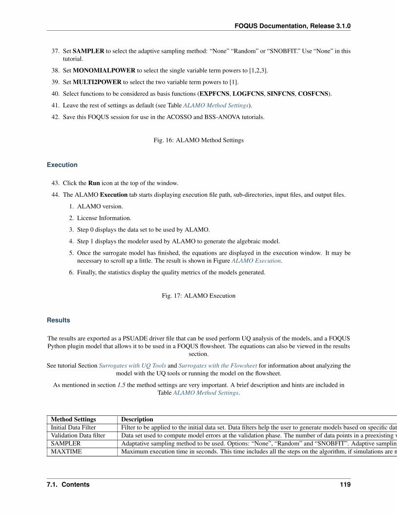
FOQUS Documentation, Release 3.1.0
37. Set SAMPLER to select the adaptive sampling method: “None” “Random” or “SNOBFIT.” Use “None” in thistutorial.
38. Set MONOMIALPOWER to select the single variable term powers to [1,2,3].
39. Set MULTI2POWER to select the two variable term powers to [1].
40. Select functions to be considered as basis functions (EXPFCNS, LOGFCNS, SINFCNS, COSFCNS).
41. Leave the rest of settings as default (see Table ALAMO Method Settings).
42. Save this FOQUS session for use in the ACOSSO and BSS-ANOVA tutorials.
Fig. 16: ALAMO Method Settings
Execution
43. Click the Run icon at the top of the window.
44. The ALAMO Execution tab starts displaying execution file path, sub-directories, input files, and output files.
1. ALAMO version.
2. License Information.
3. Step 0 displays the data set to be used by ALAMO.
4. Step 1 displays the modeler used by ALAMO to generate the algebraic model.
5. Once the surrogate model has finished, the equations are displayed in the execution window. It may benecessary to scroll up a little. The result is shown in Figure ALAMO Execution.
6. Finally, the statistics display the quality metrics of the models generated.
Fig. 17: ALAMO Execution
Results
The results are exported as a PSUADE driver file that can be used perform UQ analysis of the models, and a FOQUSPython plugin model that allows it to be used in a FOQUS flowsheet. The equations can also be viewed in the results
section.
See tutorial Section Surrogates with UQ Tools and Surrogates with the Flowsheet for information about analyzing themodel with the UQ tools or running the model on the flowsheet.
As mentioned in section 1.5 the method settings are very important. A brief description and hints are included inTable ALAMO Method Settings.
Table 1: ALAMO Method SettingsMethod Settings DescriptionInitial Data Filter Filter to be applied to the initial data set. Data filters help the user to generate models based on specific data for each variable.Validation Data filter Data set used to compute model errors at the validation phase. The number of data points in a preexisting validation data set can be specified by the user.SAMPLER Adaptative sampling method to be used. Options: “None”, “Random” and “SNOBFIT”. Adaptive sampling method to be used by ALAMO when more sampling points are needed by the model. If Random is used a simulator must be provided by the user. If SNOBFIT is used a simulator must be provided by the user and MATLAB must be installed.MAXTIME Maximum execution time in seconds. This time includes all the steps on the algorithm, if simulations are needed they run in this time.
Continued on next page
7.1. Contents 119
FOQUS Documentation, Release 3.1.0
Table 1 – continued from previous pageMINPOINTS Convergence is assessed only if the simulator is able to compute the output variables for at least MINPOINTS of the data set. A reduced number of MINPOINTS may reduce the computational time to get a model, but also reduces the accuracy of the model. MINPOINTS must be a positive integer.PRESET Value to be used if the simulator fails. This value must be carefully chosen to be an otherwise not realizable value for the output variables.MONOMIALPOWERS Vector of monomial powers to be considered as basis functions, use empty vector for none []. Exponential terms allowed in the algebraic model. i.e., if selecting [1,2] the model considers x1 and x1**2 as basis functions.MULTI2POWER Vector of pairwise combination of powers to be considered as basis functions. Pairwise combination of powers allowed in the algebraic model. i.e., [1,2] allows terms like x1*x2 in the algebraic model.MULTI3POWER Vector of three variables combinations of powers to be considered as basis functions.
Use or not of exp, log, sin, and cos functions as basis functions in the model.RATIOPOWER Vector of ratio combinations of powers to be considered in the basis functions. Ratio combinations of powers are [empty as default].Radial Basis Functions Radial basis functions centered around the data set provided by the user. These functions are Gaussian and are deactivated if their textual representation requires more than 128 characters (in the case of too many input variables and/or datapoints).RBF parameter Constant penalty used in the Gaussian radial basis functions.Modeler Fitness metric to be used for model building. Options: BIC (Bayesian Information Criterion), Mallow’s Cp, AICc (Corrected Akaike’s Information Criterio), HQC (Hannan-Quinn Information Criterion), MSE (Mean Square Error), and Convex Penalty.ConvPen Convex penalty term. Used if Convex Penalty is selected.Regularizer Regularization method is used to reduce the number of potential basis functions before the optimization.Tolrelmetric Convergence tolerance for the chosen fitness metric is needed to terminate the algorithm.ScaleZ If used, the variables are scaled prior to the optimization problem is solved. The problem is solved using a mathematical programming solver. Usually, scaling the variables may help the optimization procedure.GAMS GAMS is the software used to solve the optimization problems. The executable path is expected or the user must declare GAMS.exe in the environment path.GAMS Solver Solver to be used by GAMS to solve the optimization problems. Mixed integer quadratic programming solver is expected like BARON (other solvers can be used).MIPOPTCR Relative convergence tolerance for the optimization problems solved in GAMS. The optimization problem is solved when the optcr is reached. 5 to 1 % is expected (0.005 to 0.001).MIPOPTCA Absolute convergence tolerance for mixed-integer optimization problems. This must be a nonnegative scalar.Linear error If true, a linear objective function is used when solving the mixed integer optimization problems; otherwise, a quadratic objective function is used.
Specify whether constraint regression is used or not, if true bounds on output variables are enforced.CRNCUSTOM If true, Custom constraints are entered in the Variable tab.CRNINITIAL Number of random bounding points at which constraints are sampled initially (must be a nonnegative integer).CRNMAXITER Maximum allowed constrained regressions iterations. Constraints are enforced on additional points during each iteration (must be positive integer).CRNVIOL Number of bounding points added per round per bound in each iteration (must be positive integer).CRNTRIALS Number of random trial bounding points per round of constrained regression (must be a positive integer).CUSTOMBAS A list of user-supplied custom basis functions can be provided by the user. The parser is not case sensitive and allows for any Fortran functional expression in terms of the XLABELS (symbol ^ may be used to denote power).
ACOSSO
This tutorial covers the ACOSSO surrogate modeling method. The Adaptive COmponent Selection and ShrinkageOperator (ACOSSO) surface approximation was developed under the Smoothing Spline Analysis of Variance
(SS-ANOVA) modeling framework (Storlie et al. 2011). As it is a smoothing type method, ACOSSO works bestwhen the underlying function is somewhat smooth. For functions which are known to have sharp changes or peaks,
etc., other methods may be more appropriate. Since it implicitly performs variable selection, ACOSSO can also workwell when there are a large number of input variables. The ACOSSO procedure also allows for categorical inputs
(Storlie et al. 2013).
This tutorial uses the same flowsheet and sample setup as the ALAMO tutorial in Section ALAMO. The statisticssoftware “R” is also required to use ACOSSO and BSS-ANOVA. Before starting this tutorial, you will need to install
R version 3.1 or later (see https://cran.r-project.org/).
Once R is installed, you will need to install the “quadprog” package. ACOSSO requires this package for solvingquadratic programming problems. You will only need to perform this step once.
1. Start R. In Windows, this must be done with administrative privileges. Either run this from an administratoraccount, or right-click “R x64 3.1.2” and click “Run with administrator” and type in administrator credentials.
2. Inside the R console, type:
• install.packages(’quadprog’)
• library(quadprog)
• q()
120 Chapter 7. Surrogate Modeling

FOQUS Documentation, Release 3.1.0
The first line installs the package. If prompted for a CRAN mirror, select the one closest to you geographically.The second line loads the package. The last line quits R. If prompted to save workspace image, choose ‘y’.
Once you have done these steps, ACOSSO is ready to be invoked inside FOQUS.
1. Set the path to the RScript executable.
1. Click the Settings button in the Home window.
2. Change the RScript path if necessary. The Browse button opens a file browser that can be used to set thepath.
2. Complete the ALAMO tutorial in Section ALAMO through Step 32, or load the FOQUS session saved aftercompleting the ALAMO tutorial.
3. Click the Surrogates button in the Home window (Figure ACOSSO Session Set Up).
4. Select “ACOSSO” in the Tool drop-down list.
5. Select the Method Settings tab.
6. Set “Data Filter” to “Initial.”
7. Set “Use Flowsheet Data” to “Yes.”
8. Set “FOQUS Model (for UQ)” to “ACOSSO_Tutorial_UQ.py.”
9. Set “FOQUS Model (for Flowsheet)” to “ACOSSO_Tutorial_FS.py.”
10. Click the Run icon (Figure ACOSSO Session Set Up).
Fig. 18: ACOSSO Session Set Up
11. The execution window will automatically display. While ACOSSO is running, the execution window may showwarnings, but this is normal.
12. When the run completes, a UQ driver file is created, allowing the ACOSSO surrogate to be used as a user-definedresponse surface in UQ analyses. (See Section Surrogates with UQ Tools.)
13. ACOSSO also produces a flowsheet plugin; however.
BSS-ANOVA
This tutorial covers the BSS-ANOVA surrogate modeling method. The Bayesian Smoothing Spline ANOVA(BSS-ANOVA) is essentially a Bayesian version of ACOSSO (Reich et al. 2009). It is Gaussian Process (GP) model
with a non-conventional covariance function that borrows its form from SS-ANOVA. It tackles the highdimensionality (of inputs) on two fronts: (1) variable selection to eliminate uninformative variables from the modeland (2) restricting the level of interactions involved among the variables in the model. This is done through a fully
Bayesian approach which can also allow for categorical input variables with relative ease. Since it is closely relatedto ACOSSO, it generally works well in similar settings as ACOSSO. The BSS-ANOVA procedure also allows for
categorical inputs (Storlie et al. 2013). In this current implementation, BSS-ANOVA is more computationallyintensive than ACOSSO, so ACOSSO is preferred for faster surrogate generation.
This tutorial uses the same flowsheet and sample setup as the ALAMO tutorial in Section ALAMO. The statisticssoftware “R” is also required to use ACOSSO and BSS-ANOVA. Before starting this tutorial, you will need to install
R version 3.1 or later (see http://cran.r-project.org/).
1. Set the path to the RScript executable.
1. Click the Settings button from the Home window.
7.1. Contents 121

FOQUS Documentation, Release 3.1.0
2. Change the RScript path if necessary. The Browse button opens a file browser that can be used to set thepath.
2. Complete the ALAMO tutorial in Section ALAMO through Step 32, or load the FOQUS session saved aftercompleting the ALAMO tutorial.
3. Click the Surrogates button from the Home window (Figure BSS-ANOVA Session Set Up).
4. Select “BSS-ANOVA” in the Tool drop-down list.
5. Select the Method Settings tab.
6. Set “Data Filter” to “Initial.”
7. Set “Use Flowsheet Data” to “Yes.”
8. Set “FOQUS Model (for UQ)” to “bssanova_tutorial_uq.py.”
9. Set “FOQUS Model (for Flowsheet)” to “bssanova_tutorial_fs.py.”
10. Click the Run icon (Figure BSS-ANOVA Session Set Up).
Fig. 19: BSS-ANOVA Session Set Up
11. The execution window will automatically display. While BSS-ANOVA is running, the execution window mayshow warnings, but this is normal.
12. When the run completes, a UQ driver file is created, allowing the BSS-ANOVA surrogate to be used as a user-defined response surface in UQ analyses. (See Section Surrogates with UQ Tools.)
13. BSS-ANOVA also produces a flowsheet plugin.
Surrogates with UQ Tools
For the purpose of this tutorial, we will use ACOSSO to demonstrate the use of a surrogate within the UQ module.The steps are the same regardless of the surrogate tool chosen.
To perform the UQ analysis, Python is required for use the “User Regression” response surface that will be used.Before starting this tutorial, you will need to install Python 2.7.x (not Python 3). (See
https://www.python.org/downloads/). In addition, if *.py files have been re-associated with other executables (e.g.editors), please change the association back to python.exe.
1. Load a fresh session by clicking the Session button from the Home window. Select Open Session and thennavigate to the “examples/UQ” directory. Select “Rosenbrock_no_vectors.foqus.” This will load a session witha simple flowsheet containing a single node.
2. Click Settings and ensure that (1) FOQUS Flowsheet Run Method is set to “Local”, and that (2) proper pathsare set for PSUADE and RScript.
3. Train an ACOSSO surrogate of this node by clicking the Surrogates button from the Home window.
1. Click Add Samples and select “Use Flowsheet”. This will display the Simulation Ensemble Setup dialog.
2. Within this dialog, ensure all variables are set to “Variable” type in the Distributions tab. In the Samplingscheme tab, select “Monte Carlo” as your sampling scheme, set the number of samples to 100, and thenclick Generate Samples to generate the set of input values. Click Done to return to the Surrogates screen.
3. Once sample generation completes, click the Uncertainty button from the Home window.
4. Click the Launch button to generate the samples.
122 Chapter 7. Surrogate Modeling
FOQUS Documentation, Release 3.1.0
5. Click the Surrogates button from the Home window. The Data tab of the Surrogates screen should nowdisplays a Flowsheet Results table that is populated with the values of the new input samples.
6. From the Variables tab, select all of the checkboxes. (There should be six checkboxes for input variablesand one checkbox for output variable.) Here, you are defining the inputs and outputs for your surrogatefunction.
7. From the Method Settings tab, note the name of the file next to “FOQUS Model (for UQ)”. This will bethe name of the UQ driver file that contains the Python code that implements the surrogate function.
8. On top of this screen, select “ACOSSO” as your surrogate tool from the Tool drop-down list and then clickon the green arrow to start training the surrogate.
9. Once complete, a popup window will display, reminding you of the location of the drive file. Note thelocation as you will need this information later inside the UQ module.
4. Perform a response-surface-based uncertainty analysis by clicking the Uncertainty button from the Home win-dow.
1. In the Uncertainty Quantification Simulation Ensembles table. A row corresponding to the ensemble thatwas just generated for surrogate training should be displayed. This same ensemble can be used or a newone can be created to be used as the test data set for analysis. In the row corresponding to the ensemble tobe analyzed, click the Analyze button to proceed. This action will bring up an analysis dialog.
2. Within this analysis dialog, navigate to “Analysis” section. For Step 1, select “Response Surface”. ForStep 3, select “User Regression” in the first drop-down list. Lastly, for “User Regression File”, browse tothe same location as the UQ driver file that was generated within the Surrogates module. (This is the samelocation that was previously noted from the popup message.) At this point, your surrogate function is nowset up as a user-defined response surface and all response-surface-based UQ analyses are accessible.
3. Click Validate (Step 4) to perform response surface validation. Once complete, a figure with cross-validation results will be displayed: a histogram of errors to the left and a plot of predicted values versusactual values to the right. For more information, refer to the UQ Tutorial in Section[tutorial.uq.rs].
4. Once a “Response Surface” has been validated, other UQ analysis options are available. Choose “Un-certainty Analysis” in Step 5 and click Analyze to perform uncertainty analysis using your ACOSSOsurrogate.
During validation, if the error, “RSAnalyzer: RSTest_hs.m does not exist.” displays, this is likely caused byincompatibility with the surrogate and the test data. An example scenario might be your test data has six inputs, but
your surrogate assumes five inputs. This is easily fixed by returning to the Surrogates screen, clicking on theVariables tab, and making sure the appropriate selections are made (i.e., check off six inputs instead of just five).
Surrogates with the Flowsheet
This section provides a brief tutorial for using the flowsheet plugin models generated by surrogate modeling methods.In the next FOQUS release all surrogate modeling methods will produce a model that can be run in a FOQUS
flowsheet. Currently iREVEAL does not produce a flowsheet model.
Before doing this tutorial complete the ALAMO tutorial in Section :ref:‘sec.surrogate.alamo‘.
1. Open FOQUS. If FOQUS has not been closed since completing the ALAMO tutorial, close it and reopen it.There is a known issue where existing flowsheet model plugins may not update until FOQUS is restarted.
2. Enter “FS_Plugin_Tutorial” as the Session Name.
3. Click the Flowsheet button from the Home window.
4. Click the Add Node icon in the left toolbar (see Figure Plugin Flowsheet).
5. Click a location for the node in the Flowsheet area.
7.1. Contents 123

FOQUS Documentation, Release 3.1.0
6. Enter “model” for the node name (without quotes).
7. Click the Node Editor icon in the left toolbar (see Figure Plugin Flowsheet).
8. In the Node Editor, select “Plugin” from the Model Type drop-down list.
9. Select “ALAMO_Tutorial_FS” from the Model drop-down list.
10. Set the Value of the Input Variables “eq.x1” to 2.
11. Set the Value of the Input Variables “eq.x2” to 3.
12. Click the Run icon in the left toolbar (see Figure Plugin Flowsheet).
13. Wait for the Flowsheet evaluation to complete. It should finish successfully.
14. Check the value of the Output Variables; the approximate values should be z1 = 5 and z2 = 13.
Fig. 20: Plugin Flowsheet
124 Chapter 7. Surrogate Modeling
CHAPTER 8
Sequential Design of Experiments (SDOE)
A sequential design of experiments strategy allows for adaptive learning based on incoming results as the experimentis being run. The SDoE module in FOQUS allows the experimenter to flexibly incorporate this strategy into theirdesigned experimental planning to allow for maximal relevant information to be collected. Statistical design ofexperiments is an important strategy to improve the amount of information that can be gleaned from the overall
experiment. It leverages principles of putting experimental runs where they are of maximum value, theinterdependence of the runs to estimate model parameters, and robustness to the variability of results that can be
obtained when the same experimental conditions are repeated. There are two major categories of designedexperiments: those for which a physical experiment is being run, and designs for a computer experiment where theoutput from a theoretical model is explored. While the methods available were initially focused on experiments forphysical experiments, opportunities also exist for accelerated learning through strategic selection and updating of
experimental runs for computer experiments.
The overall process for Sequential Design of Experiments (SDoE) is detailed below:
1. Identify one or more criteria over which to optimize. Common choices are (a) refining the region of interest, (b)improving the precision (or reducing the uncertainty) in the estimation of model parameters, (c) improving theprecision of prediction for new observations in the design region, (d) quantifying the discrepancy between themodel and data, or (e) optimizing the value of responses of interest. If more than one criterion is going to beused, then identify how they will be combined into a utility function.
2. Develop a working model of the process that can be used to calculate the criteria values based on currentlyavailable knowledge and data.
3. Define the inputs that will be manipulated during the experiment, and the ranges of interest for these factors.
4. Identify candidate input factor locations that are being considered for new experiments. This can be a gridof input combinations or continuous regions in the design space. If there are combinations of the factors thatwill not yield results or that are not of interest, these regions of the design space should be excluded fromconsideration.
5. Develop a working model of the process that is able to receive new data and incorporate them to update thecalculated criteria values.
6. Develop a plan for the size of the sequential design batches, based on the time required to set-up and run theexperiments as well as the computational time required to process new data and update the working model.
125
FOQUS Documentation, Release 3.1.0
7. Identify the initial batch of experiments to be run at the beginning of the experiments based on the modeldeveloped in step 2 and conditional on any already available data. This involves examining the utility of newdata at each candidate location, and comparing which locations have the highest anticipated utility.
8. Run the first batch of experimental runs, update the model developed in step 5 with the new results. Based onthe updated model, generate the next batch of experimental runs.
9. For the duration of the experiment, repeat steps 7 and 8 for subsequent batches based on the updated model afterincorporating the newly obtained data.
The first version of the SDoE module has functionality that can produce flexible space-filling designs to be created.Later versions will allow for additional design criteria to be utilized, but the first version already had considerable
flexibility to construct helpful design based on several different strategies. Key features of the approach that we use inthis module are: a) designs will be constructed by selecting from a user-provided candidate set of input combinations,and b) historical data, which has already been collected can be integrated into the design construction to ensure that
new data are collected with a view to disperse from where data are already available.
We begin with some basic terminology that will help provide structure to the process and instructions below.
• Input factors – these are the controllable experimental settings that are manipulated during the experiment. Itis important to carefully define the ranges of interest for the inputs (eg. Temperature in [200°C,400°C]) aswell as any logistical or operational constraints on these input factors (eg. Flue Gas Rate < 1000 kg/hr whenTemperature > 350°C)
• Input combinations (or design runs) – these are the choices of settings for each of the input factors for a particularrun of the experiment. It is assumed that the implementers of the experiment are able to set the input factors tothe desired operating conditions to match the prescribed choice of settings.
• Input space (or design space) – the region of interest for the input factors in which the experiment will be run.This is typically constructed by combining the individual input factor ranges, and then adapting the region totake into account any constraints. Any suggested runs of the experiment will be located in this region.
• Responses (or outputs) – these are the measured results obtained from each experimental run. These are mostdesirably quantitative summaries of a characteristic of interest from running the process at the prescribed set ofoperating conditions (eg. CO2 capture efficiency is a typical response of interest for CCSI).
• Design criterion / Utility function – this is a mathematical expression of the goal (or goals) of the experimentthat is used to guide the selection of new input combinations, based on the prior information before the start ofthe experiment and during the running of the experiment. The design criterion can be based on a single goalor multiple competing goals, and can be either static throughout the experiment or evolve as goals change inimportance over the course of the experiment. Common choices of goals for the experiment are:
1. exploring the region of interest,
2. improving the precision (or reducing the uncertainty) in the estimation of model parameters,
3. improving the precision of prediction for new observations in the design region,
4. quantifying the discrepancy between the model and data, or
5. optimizing the value of responses of interest.
An optimal design of experiment strategy uses the design criterion to evaluate potential choices of input combinationsto maximize the improvement in the criterion over the available candidates. If the optimal design strategy is
sequential, then the goal is to use early results from the beginning of the experiment to guide the choice of new inputcombinations based on what has been learned about the responses.
126 Chapter 8. Sequential Design of Experiments (SDOE)
FOQUS Documentation, Release 3.1.0
8.1 Why Space-Filling Designs?
Space-filling designs are a design of experiments strategy that is well suited to both physical experiments with anaccompanying model to describe the process and to computer experiments. The idea behind a space-filling design isthat the design points are spread throughout the input space of interest. If the goal is to predict values of the response
for a new set of input combinations within the ranges of the inputs, then having data spread throughout the spacemeans that there should be an observed data point relatively close to where the new prediction is sought.
In addition, if there is a model for the process, then having data spread throughout the input space means that theconsistency of the model to the observed data can be evaluated at multiple locations to look for possible discrepancies
and to quantify the magnitude of those differences throughout the input space.
Hence, for a variety of criteria, a space-filling design can serve as good choice for exploration and for understandingthe relationship between the inputs and the response without making a large number of assumptions about the nature
of that relationship. As we will see in subsequent examples, the sequential approach allows for great flexibility toleverage what has been learned in early stages to influence the later choices of designs. In addition, the
candidate-based approach that is supported in this module has the advantage that it can make the space-fillingapproach easier to adapt to design space constraints and specialized design objectives that may evolve through the
stages of the sequential design.
8.2 Using the SDoE Module - The Basics
In this section, we descibe the basic steps in for creating a design with this module. When you first click on theSDOE button from the main FOQUS homepage, a first window appears. To create a design, the progression of steps
takes you through the Ensemble Selection box (top left), then a transition triggered by the Confirm button to theEnsemble Aggregation box, and finally there are optional changes that can be made in the box at the bottom of the
window. The final step in this window is to click on Analyze.
We now consider some details for each of these steps:
1. In the Ensemble Selection box, click on the Load from File.. button to select the file(s) for the construction ofthe design. Several files can be selected and added to the box listing the chosen files.
2. For each of the files selected using the pull-down menu, identify them as either a Candidate file or a History file.Candidate .csv files are comprised of possible input combinations from which the design can be constructed. The
columns of the file should contain the different input factors that define the dimensions of the input space. The rowsof the file each identify one combination of input values that could be selected as a run in the final design. Typically,a good candidate file will have many different candidate runs listed, and they should fill the available ranges of theinputs to be considered. Leaving gaps or holes in the input space is possible, but generally should correspond to a
region where it is not possible (or desirable) to collect data. History .csv files should have the same number ofcolumns for the input space as the candidate file, and represent data that have already been collected. The algorithmfor creating the design aims to place points in different locations from where data have already been obtained, while
filling the input space around those locations.
3. Click on the View button to open the Preview Inputs pop-up widow, to see the list of columns contained ineach file. The left hand side displays the first few rows of input combinations from the file. Select the columnsthat you wish to see graphically in the right hand box , and then click on Plot SDOE to see a scatterplot matrixof the data.
The plot shows histograms of each of the inputs on the diagonals to provide a view of the distribution of values aswell as the range of each input. The off-diagonals show pairwise scatterplots of each pair of inputs. This should
provide the experimenter with the ability to assess if the ranges specified and any constraints for the inputs have beenappropriately captured for the specified candidate set. In addition, repeating this process for any historical data will
provide verification that the already observed data have been suitably characterized.
8.1. Why Space-Filling Designs? 127
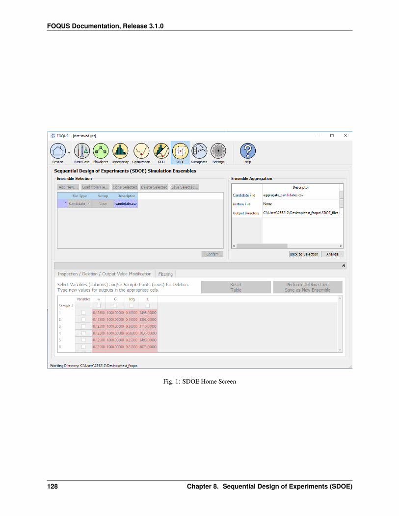
FOQUS Documentation, Release 3.1.0
Fig. 1: SDOE Home Screen
128 Chapter 8. Sequential Design of Experiments (SDOE)
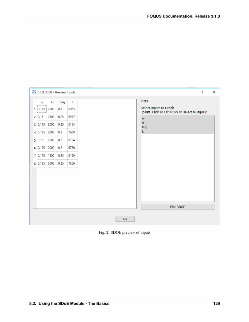
FOQUS Documentation, Release 3.1.0
Fig. 2: SDOE preview of inputs
8.2. Using the SDoE Module - The Basics 129
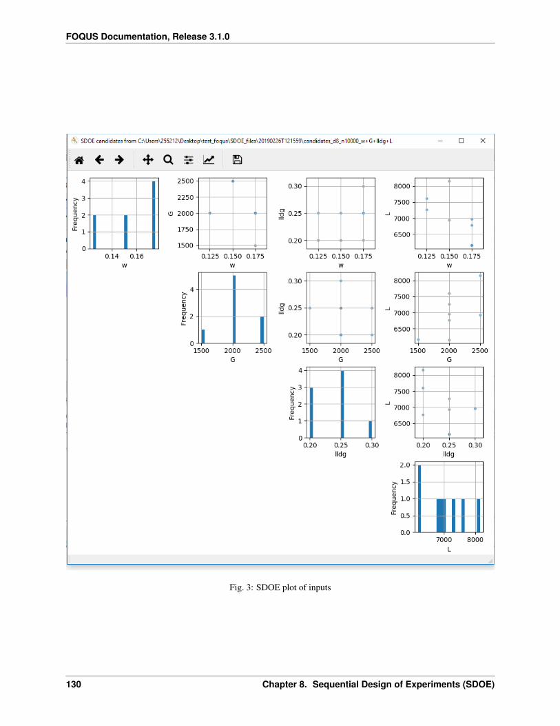
FOQUS Documentation, Release 3.1.0
Fig. 3: SDOE plot of inputs
130 Chapter 8. Sequential Design of Experiments (SDOE)

FOQUS Documentation, Release 3.1.0
4. Once the data have been verified for both the Candidate and History files, click on the Confirm button to makethe Ensemble Aggregation window active.
5. If more than one Candidate file was specified, then the aggregate_candidates.csv file that was created willhave combined these files into a single file. Similarly if more than one Histoy file was specified, then theaggregate_history.csv file has been created with all runs from these files. If only a single file was selected foreither the Candidate and History files, then their aggregated matching files will be the same as the original.
6. Once the data have been verified as the desired set to be used for the design construction, then click on theAnalyze button at the bottom right corner of the Ensemble Aggregation window. This opens the second SDOEwindow, which allows for specific design choices to be made.
Fig. 4: SDOE second window
7. The first choice to be made for the design is whether to optimize using minimax or maximin. The first choice,minimax, looks to choose design points that minimize the maximum distance that any point in the input space(as characterized by the candidate set and historical data, if it is available) is away from a design point. Hence,the idea here is that if we want to use data to help predict new outcomes throughout the input space, then wenever want to be too far away from an observed location. The second choice, maximin looks to choose a designwhere the design points are as far away from each other as possible. In this case, the design criterion is lookingto maximize how close any two points are away from their nearest neighbor. In practice the two design criterionoften give similar designs, with the maximin criterion tending to push the chosen design points closer to theedges of the specified regions.
Hint: If there is uncertainty about some of the edge points in the candidate set being viable options, then minimaxwould be preferred. If the goal is to place points throughout the input space with them going right to the edges, than
maximin would be preferred. Note, that creating the designs is relatively easy, so it may be helpful to try bothapproaches to examine them and then choose which is preferred.
8. The next choice to be made falls under Design Specification, when the experimenter can select the sizes ofdesigns to be created. The Min Design Size specifies the smallest design size to be created. Not that the default valueis set at 2, which would lead to choosing the best two design runs from the candidate set to fill the space (after taking
8.2. Using the SDoE Module - The Basics 131
FOQUS Documentation, Release 3.1.0
into account any historical data that have already been gathered). The Max Design Size specifies the largest designsize to be created. The default value is set at 8, which means that if this combination were used, designs would be
created of size 2, 3, 4, 5, 6, 7 and 8. Hence, it may be prudent to select a relatively small range of values to expeditethe creation of the designs, as each of these choices triggers a separate optimization search.
9. Next, there are options for the columns of the candidate set to be used for the construction of the design. UnderInclude? in the box on the right hand side, the experimenter has the option of whether particular columns shouldbe included in the space-filling design search. Unclick a box, if a particular column should not be included inthe search.
Next select the Type for each column. Typically most of the columns will be designated as Inputs, which means thatthey will be used to find the best design. In addition, we recommend including one Index column which contains aunique identifier for each run of the candidate set. This makes tracking which runs are included in the constructed
designs easier. If no Index column is specified, a warning appears later in the process, but this column is not strictlyrequired.
Finally, the Min and Max columns in the box allow the range of values for each input column to be specified. Thedefault is to extract the smallest and largest values from the candidate and history data files, and use these. This
approach generally works well, as it scales the inputs to be in a uniform hypercube for comparing distances betweenthe design points.
Hint: the default values for Min and Max can generally be left at their defaults unless: (1) the range of some inputsrepresent very different amounts of change in the process. For example, if temperature is held nearly constant, whilea flow rate changes substantially, then it may be desirable to extend the range of the temperature beyond its nominalvalues to make the amount of change in temperature more commensurate with the amount of change in the flow rate.(2) if changes are made in the candidate or history data files. For example, if one set of designs are created from one
candidate set, and then another set of designs are created from a different candidate set. These designs and theachieved criterion value will not be comparable unless the range of each input has been fixed at matching values.
10. Once the design choices have been made, click on the TestSDOE button. This generates a small number ofiterations of the search algorithm to calibrate the timing for constructing and evaluating the designs. The timetaken to generate a design is a function of the size of the candidate set, the size of the design, as well as thedimension of the input space. The slider below TestSDOE now indicates an estimate of the time to constructthe designs across the range of the Min Design Size and Max Design Size specified. The smallest Number ofRandom Starts is 10^3 = 1000 is generally too small to produce a good design, but this will run very quickly.Powers of 10 can be chosen with an Estimated Runtime provided below the slider.
Hint: The choice of Number of Random Starts involves a trade-off between the quality of the design generated andthe time to generate the design. The larger the chosen number of random starts, the better the design is likely to be.
However, there are diminishing gains for increasingly large numbers of random starts. If running the actualexperiment is expensive, it is generally recommended to choose as large a number of random starts as possible for the
available time frame, to maximize the chance of an ideal design being found.
11. Once the slider has been set to the desired Number of Random Starts, click on the Run SDOE button, andinitate the construction of the designs. The progress bar indicates how design construction is progressing throughthe chosen range of designs between the Min Design Size and Max Design Size specified.
8.3 Example 1: 8-run 2-D design
For this first example, the goal is to construct a simple space-filling design with 8 runs in a 2-dimensional space usingthe example files provided with FOQUS.
1. From the FOQUS main screen, click the SDOE button. On the top left side, select Load from File, and selectthe candidate.csv file from examples folder. This identifies the possible input combinations from which thedesign will be constructed. The more possible candidates that can be provided to the search algorithm used toconstruct the design, the better the design might be for the specified criterion. Home Screen.
132 Chapter 8. Sequential Design of Experiments (SDOE)
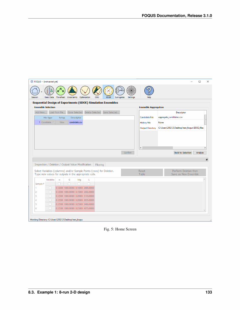
FOQUS Documentation, Release 3.1.0
Fig. 5: Home Screen
8.3. Example 1: 8-run 2-D design 133

FOQUS Documentation, Release 3.1.0
134 Chapter 8. Sequential Design of Experiments (SDOE)

CHAPTER 9
Solvent Fit
9.1 Contents
[sec:solvent_fit]
The SolventFit module is an uncertainty quantification tool for full Bayesian calibration of an Aspen Plus solventprocess model to experimental data. SolventFit may provide improved predictions with uncertainty bounds byaccounting for uncertainty in model parameters and deficiencies in the model form. The result is a posterior
distribution of parameters allowing for predictions with uncertainty. uses a custom BSS-ANOVA-based responsesurface for the outputs. Like the Bayesian inference module, the *SolventFit* algorithm (Bhat et al. 2015) utilizes
Markov Chain Monte Carlo (MCMC) to compute the posterior distributions, and uses a custom BSS-ANOVA-basedresponse surface (emulators) that serves as a fast approximations to the actual simulation model.
9.1.1 SolventFit Instructions
To use *SolventFit*, the user will need to install R, as well as the R packages “MCMCpack”, “abind” and “MASS”.Please refer to the installation instructions in Section [(sec.surrogate.acosso)]. Once R is installed, the user will also
need to set the path to the RScript executable within FOQUS.
1. Basic Data. From the FOQUS main screen, click the Basic Data button and select SolventFit to enter aSolventFit session.
2. Load Training Data loads the file of design and variable inputs and their relevant simulation outputs (fromAspen or other computer simulation code). This file usually has extension .txt, .dat, or .csv.
3. Output Settings lists the available outputs for analysis. The Output Name column lists the name of each output.The user can select/deselect outputs for analysis using the checkboxes in the Observed column. The responsesurface in SolventFit will be prepopulated with “SolventFit Emulator” because SolventFit uses its own customBSS-ANOVA response surface model. The simulation ensemble is used as the training data for generating theresponse surfaces.
4. Input Settings is populated with input variable information from the training data. Under the column, Type,the user can specify which inputs are fixed, design, or variable using the from the drop-down menu in theInput Settings Table. Selecting “Fixed” means that the input is fixed at its default value for all design points.
135
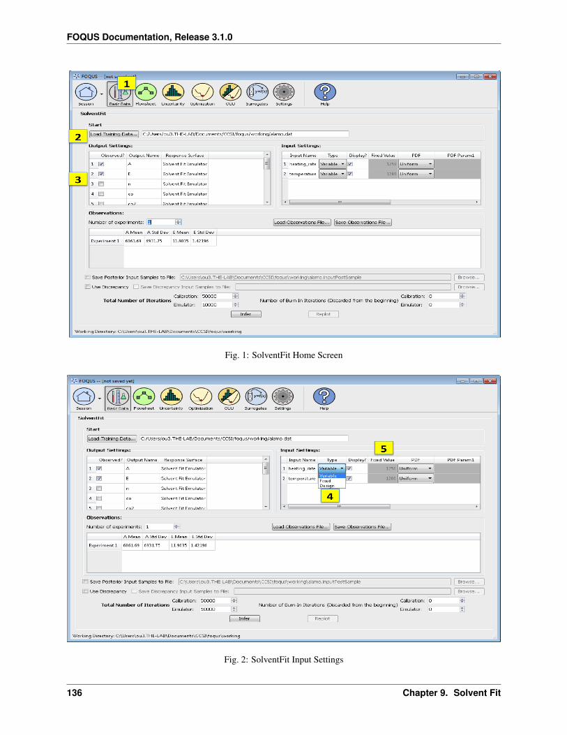
FOQUS Documentation, Release 3.1.0
Fig. 1: SolventFit Home Screen
Fig. 2: SolventFit Input Settings
136 Chapter 9. Solvent Fit
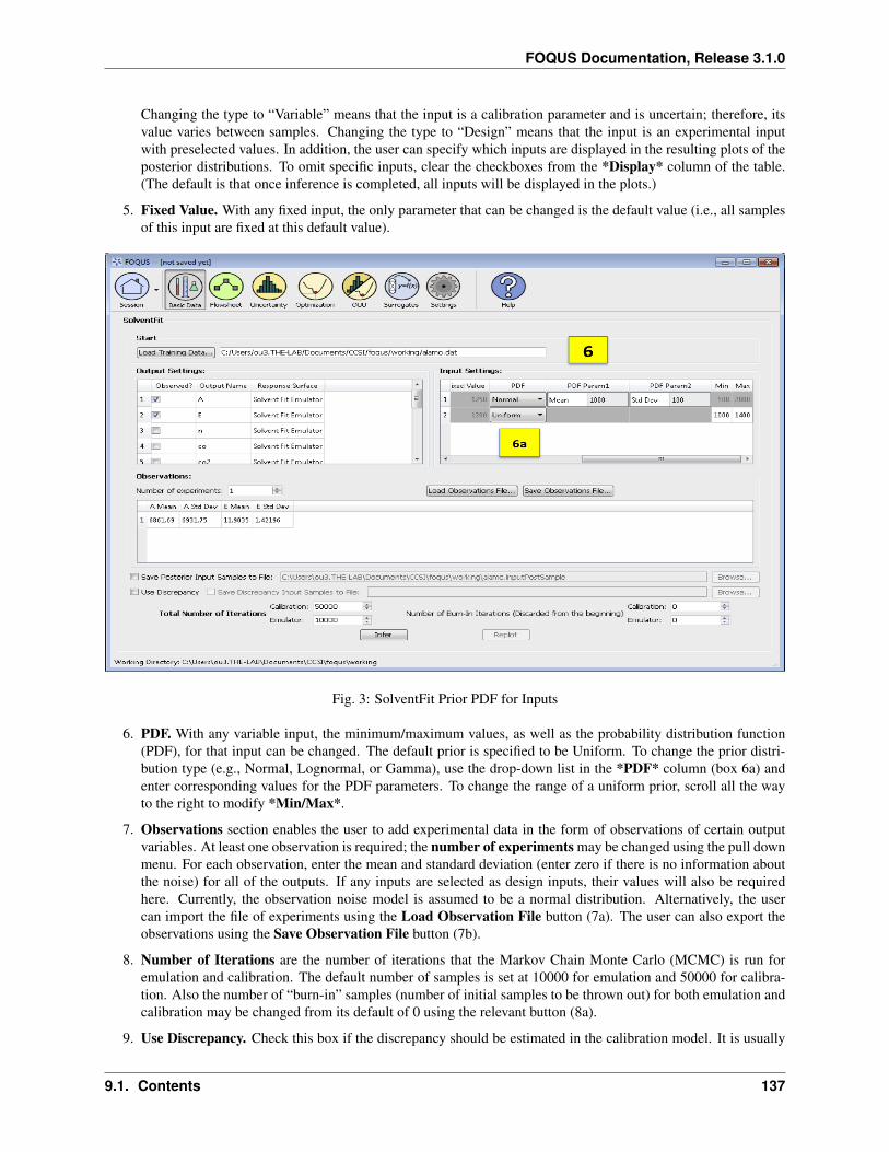
FOQUS Documentation, Release 3.1.0
Changing the type to “Variable” means that the input is a calibration parameter and is uncertain; therefore, itsvalue varies between samples. Changing the type to “Design” means that the input is an experimental inputwith preselected values. In addition, the user can specify which inputs are displayed in the resulting plots of theposterior distributions. To omit specific inputs, clear the checkboxes from the *Display* column of the table.(The default is that once inference is completed, all inputs will be displayed in the plots.)
5. Fixed Value. With any fixed input, the only parameter that can be changed is the default value (i.e., all samplesof this input are fixed at this default value).
Fig. 3: SolventFit Prior PDF for Inputs
6. PDF. With any variable input, the minimum/maximum values, as well as the probability distribution function(PDF), for that input can be changed. The default prior is specified to be Uniform. To change the prior distri-bution type (e.g., Normal, Lognormal, or Gamma), use the drop-down list in the *PDF* column (box 6a) andenter corresponding values for the PDF parameters. To change the range of a uniform prior, scroll all the wayto the right to modify *Min/Max*.
7. Observations section enables the user to add experimental data in the form of observations of certain outputvariables. At least one observation is required; the number of experiments may be changed using the pull downmenu. For each observation, enter the mean and standard deviation (enter zero if there is no information aboutthe noise) for all of the outputs. If any inputs are selected as design inputs, their values will also be requiredhere. Currently, the observation noise model is assumed to be a normal distribution. Alternatively, the usercan import the file of experiments using the Load Observation File button (7a). The user can also export theobservations using the Save Observation File button (7b).
8. Number of Iterations are the number of iterations that the Markov Chain Monte Carlo (MCMC) is run foremulation and calibration. The default number of samples is set at 10000 for emulation and 50000 for calibra-tion. Also the number of “burn-in” samples (number of initial samples to be thrown out) for both emulation andcalibration may be changed from its default of 0 using the relevant button (8a).
9. Use Discrepancy. Check this box if the discrepancy should be estimated in the calibration model. It is usually
9.1. Contents 137
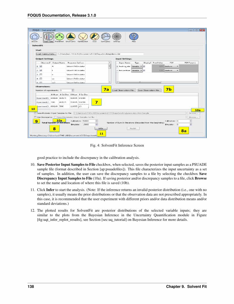
FOQUS Documentation, Release 3.1.0
Fig. 4: SolventFit Inference Screen
good practice to include the discrepancy in the calibration analysis.
10. Save Posterior Input Samples to File checkbox, when selected, saves the posterior input samples as a PSUADEsample file (format described in Section [ap:psuadefiles]). This file characterizes the input uncertainty as a setof samples. In addition, the user can save the discrepancy samples to a file by selecting the checkbox SaveDiscrepancy Input Samples to File (10a). If saving posterior and/or discrepancy samples to a file, click Browseto set the name and location of where this file is saved (10b).
11. Click Infer to start the analysis. (Note: If the inference returns an invalid posterior distribution (i.e., one with nosamples), it usually means the prior distributions or that the observation data are not prescribed appropriately. Inthis case, it is recommended that the user experiment with different priors and/or data distribution means and/orstandard deviations.)
12. The plotted results for SolventFit are posterior distributions of the selected variable inputs; they aresimilar to the plots from the Bayesian Inference in the Uncertainty Quantification module in Figure[fig:uqt_infer_replot_results], see Section [sec:uq_tutorial] on Bayesian Inference for more details.
138 Chapter 9. Solvent Fit
CHAPTER 10
Simulation Standard Interface (SimSinter)
10.1 Contents
10.1.1 SimSinter Configuration
SimSinter is the standard interface library that FOQUS and Turbine use to drive the target simulation software.SimSinter currently supports AspenPlus, Aspen Custom Modeler (ACM), gPROMS, and Microsoft Excel. SimSinter
is used to: (1) open the simulator, (2) initialize the simulation, (3) set variables in the simulation, (4) run thesimulation, and (5) get resulting output variables from the simulation.
To drive a particular simulation, SimSinter must be told which input variables to set and which output variables toread when the simulation is finished (there are generally far too many variables in a simulation to set and read themall). Each simulation must have a “Sinter Config File” which records this information. FOQUS keeps the simulationfile and the “Sinter Config File” together and sends them to the Turbine gateway when a simulation run is requested.
The configuration is simplified by a GUI included with the SimSinter distribution called, “SinterConfigGUI.”FOQUS can launch the SinterConfigGUI on simulations that have not been configured. To run the
“SinterConfigGUI” the user must have:
1. SimSinter distribution installed. SimSinter is installed by the FOQUS bundle installer.
2. The simulation file the user wants to configure. For example, if the user has an Aspen Custom Modeler simula-tion called BFB.acmf, that file must be on the user’s computer, and the user should know its location.
3. The application used to execute the simulation file. For example, if the user wants to configure an Aspen CustomModeler simulation called BFB.acmf, Aspen Custom Modeler must be installed on the user’s machine.
The rest of this section details two step-by-step tutorials on configuring a simulation with “SinterConfigGUI.” Thefirst simulation is an Aspen Custom Modeler simulation and the second, Aspen Plus. Please also see the D-RMBuilder tutorials for configuring dynamic ACM models. For more details on SimSinter or a tutorial on how to
configure a Microsoft Excel file, please see the “SimSinter Technical Manual,” which is included in the FOQUSdistribution. The default location is at C:Program Files (x86)foqusfoqusdoc. It is also available on the CCSI website.
139
FOQUS Documentation, Release 3.1.0
10.1.2 Tutorial
Aspen Plus Configuration
1. The initial steps for opening a simulation and entering metadata for an Aspen Plus simulation are similar toACM. Refer to the SimSinter ACM tutorial Aspen Custom Modeler Configuration. In this tutorial, a flash model“Flash_Example.bkp” installed in the “C:SimSinterFilesAspen_Plus_Install_Test” is used as an example. Openthe Aspen Plus file and enter the metadata as shown in Figure SinterConfigGUI Simulation Meta-Data with DataCompleted.
Fig. 1: SinterConfigGUI Simulation Meta-Data with Data Completed
2. The SinterConfigGUI Variable Configuration Page displays as illustrated in Figure SinterConfigGUI VariableConfiguration Page Empty Variables. Aspen Plus has no settings, so there are no setting variables in the inputsection. Unlike ACM, AspenPlus displays the Variable Tree on the left side, so the user can explore the tree asis done in Aspen Plus Tools → Variable Explorer. Unfortunately, searching is not possible.
3. Variable Tree nodes can be expanded for searching (Figure SinterConfigGUI Variable Configuration PageExpanded Aspen Plus Variable Tree).
4. The user can type the node address directly into the Selected Path field (this is useful for copy/paste from AspenPlus’ Variable Explorer) (Figure SinterConfigGUI Variable Configuration Page Aspen Plus Variable Selected).Click Lookup or Preview (which automatically causes the tree to expand and selects selected variables in theVariable Tree).
5. To make the temperature of the Flash chamber an Input Variable, click Make Input. Additionally, the usercan Name the variable, fix the Description, and enter the Min/Max fields by clicking on the appropriate textand entering it.
140 Chapter 10. Simulation Standard Interface (SimSinter)

FOQUS Documentation, Release 3.1.0
Fig. 2: SinterConfigGUI Variable Configuration Page Empty Variables
10.1. Contents 141
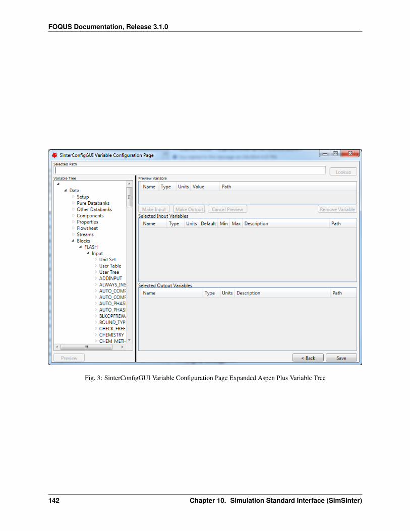
FOQUS Documentation, Release 3.1.0
Fig. 3: SinterConfigGUI Variable Configuration Page Expanded Aspen Plus Variable Tree
142 Chapter 10. Simulation Standard Interface (SimSinter)
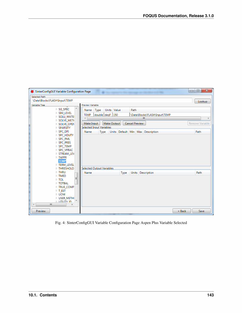
FOQUS Documentation, Release 3.1.0
Fig. 4: SinterConfigGUI Variable Configuration Page Aspen Plus Variable Selected
10.1. Contents 143
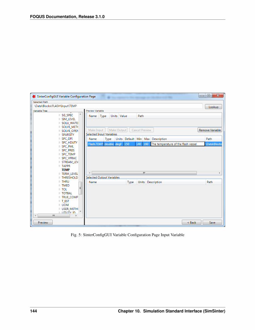
FOQUS Documentation, Release 3.1.0
Fig. 5: SinterConfigGUI Variable Configuration Page Input Variable
144 Chapter 10. Simulation Standard Interface (SimSinter)
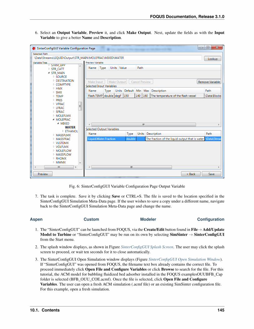
FOQUS Documentation, Release 3.1.0
6. Select an Output Variable, Preview it, and click Make Output. Next, update the fields as with the InputVariable to give a better Name and Description.
Fig. 6: SinterConfigGUI Variable Configuration Page Output Variable
7. The task is complete. Save it by clicking Save or CTRL+S. The file is saved to the location specified in theSinterConfigGUI Simulation Meta-Data page. If the user wishes to save a copy under a different name, navigateback to the SinterConfigGUI Simulation Meta-Data page and change the name.
Aspen Custom Modeler Configuration
1. The “SinterConfigGUI” can be launched from FOQUS, via the Create/Edit button found in File→ Add/UpdateModel to Turbine or “SinterConfigGUI” may be run on its own by selecting SimSinter → SinterConfigGUIfrom the Start menu.
2. The splash window displays, as shown in Figure SinterConfigGUI Splash Screen. The user may click the splashscreen to proceed, or wait ten seconds for it to close automatically.
3. The SinterConfigGUI Open Simulation window displays (Figure SinterConfigGUI Open Simulation Window).If “SinterConfigGUI” was opened from FOQUS, the filename text box already contains the correct file. Toproceed immediately click Open File and Configure Variables or click Browse to search for the file. For thistutorial, the ACM model for bubbling fluidized bed adsorber installed in the FOQUS examplesOUUBFB_Capfolder is selected (BFB_OUU_COE.acmf). Once the file is selected, click Open File and ConfigureVariables. The user can open a fresh ACM simulation (.acmf file) or an existing SimSinter configuration file.For this example, open a fresh simulation.
10.1. Contents 145

FOQUS Documentation, Release 3.1.0
Fig. 7: SinterConfigGUI Splash Screen
146 Chapter 10. Simulation Standard Interface (SimSinter)
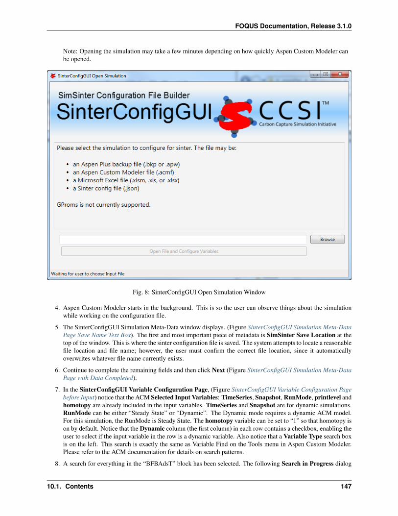
FOQUS Documentation, Release 3.1.0
Note: Opening the simulation may take a few minutes depending on how quickly Aspen Custom Modeler canbe opened.
Fig. 8: SinterConfigGUI Open Simulation Window
4. Aspen Custom Modeler starts in the background. This is so the user can observe things about the simulationwhile working on the configuration file.
5. The SinterConfigGUI Simulation Meta-Data window displays. (Figure SinterConfigGUI Simulation Meta-DataPage Save Name Text Box). The first and most important piece of metadata is SimSinter Save Location at thetop of the window. This is where the sinter configuration file is saved. The system attempts to locate a reasonablefile location and file name; however, the user must confirm the correct file location, since it automaticallyoverwrites whatever file name currently exists.
6. Continue to complete the remaining fields and then click Next (Figure SinterConfigGUI Simulation Meta-DataPage with Data Completed).
7. In the SinterConfigGUI Variable Configuration Page, (Figure SinterConfigGUI Variable Configuration Pagebefore Input) notice that the ACM Selected Input Variables: TimeSeries, Snapshot, RunMode, printlevel andhomotopy are already included in the input variables. TimeSeries and Snapshot are for dynamic simulations.RunMode can be either “Steady State” or “Dynamic”. The Dynamic mode requires a dynamic ACM model.For this simulation, the RunMode is Steady State. The homotopy variable can be set to “1” so that homotopy ison by default. Notice that the Dynamic column (the first column) in each row contains a checkbox, enabling theuser to select if the input variable in the row is a dynamic variable. Also notice that a Variable Type search boxis on the left. This search is exactly the same as Variable Find on the Tools menu in Aspen Custom Modeler.Please refer to the ACM documentation for details on search patterns.
8. A search for everything in the “BFBAdsT” block has been selected. The following Search in Progress dialog
10.1. Contents 147
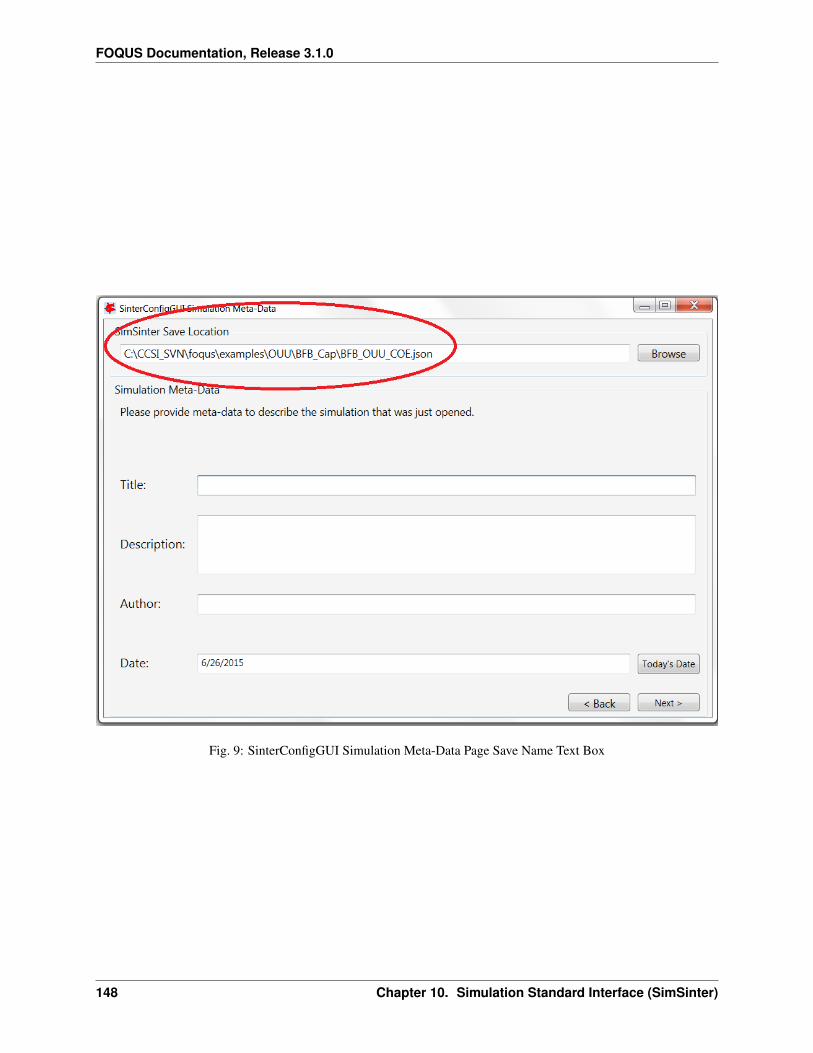
FOQUS Documentation, Release 3.1.0
Fig. 9: SinterConfigGUI Simulation Meta-Data Page Save Name Text Box
148 Chapter 10. Simulation Standard Interface (SimSinter)

FOQUS Documentation, Release 3.1.0
Fig. 10: SinterConfigGUI Simulation Meta-Data Page with Data Completed
10.1. Contents 149
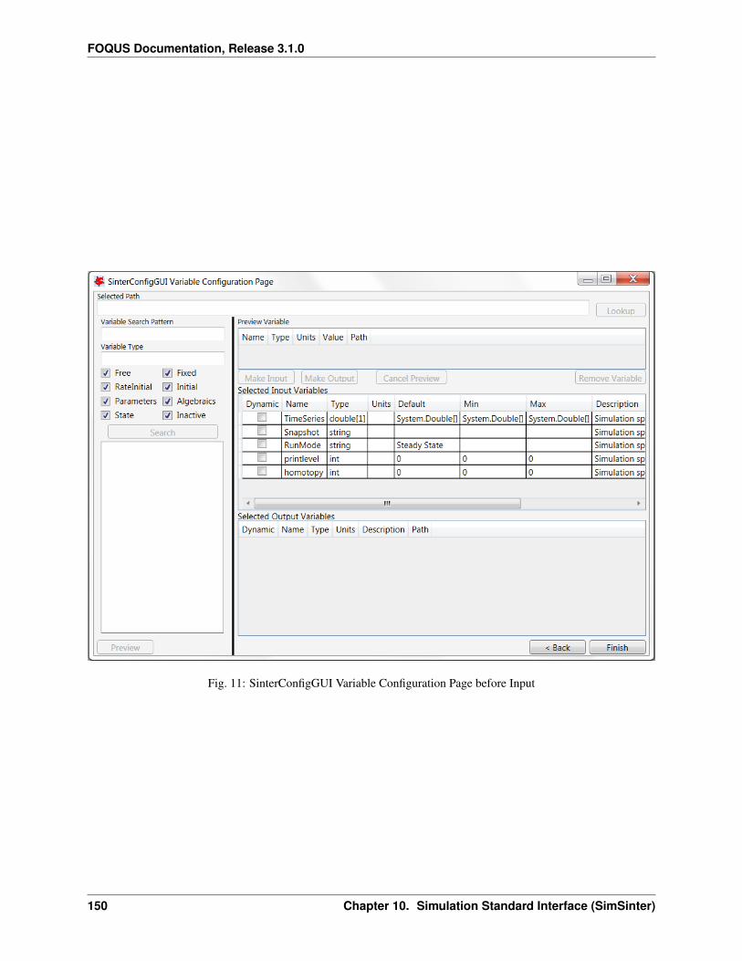
FOQUS Documentation, Release 3.1.0
Fig. 11: SinterConfigGUI Variable Configuration Page before Input
150 Chapter 10. Simulation Standard Interface (SimSinter)
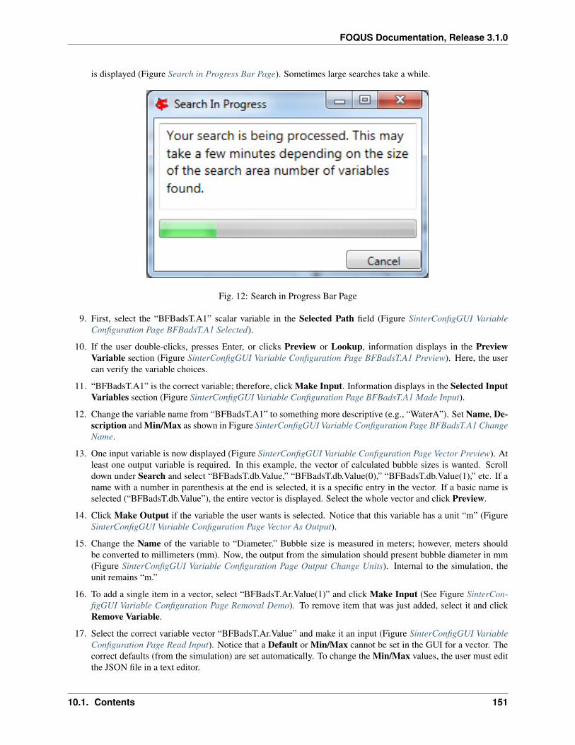
FOQUS Documentation, Release 3.1.0
is displayed (Figure Search in Progress Bar Page). Sometimes large searches take a while.
Fig. 12: Search in Progress Bar Page
9. First, select the “BFBadsT.A1” scalar variable in the Selected Path field (Figure SinterConfigGUI VariableConfiguration Page BFBadsT.A1 Selected).
10. If the user double-clicks, presses Enter, or clicks Preview or Lookup, information displays in the PreviewVariable section (Figure SinterConfigGUI Variable Configuration Page BFBadsT.A1 Preview). Here, the usercan verify the variable choices.
11. “BFBadsT.A1” is the correct variable; therefore, click Make Input. Information displays in the Selected InputVariables section (Figure SinterConfigGUI Variable Configuration Page BFBadsT.A1 Made Input).
12. Change the variable name from “BFBadsT.A1” to something more descriptive (e.g., “WaterA”). Set Name, De-scription and Min/Max as shown in Figure SinterConfigGUI Variable Configuration Page BFBadsT.A1 ChangeName.
13. One input variable is now displayed (Figure SinterConfigGUI Variable Configuration Page Vector Preview). Atleast one output variable is required. In this example, the vector of calculated bubble sizes is wanted. Scrolldown under Search and select “BFBadsT.db.Value,” “BFBadsT.db.Value(0),” “BFBadsT.db.Value(1),” etc. If aname with a number in parenthesis at the end is selected, it is a specific entry in the vector. If a basic name isselected (“BFBadsT.db.Value”), the entire vector is displayed. Select the whole vector and click Preview.
14. Click Make Output if the variable the user wants is selected. Notice that this variable has a unit “m” (FigureSinterConfigGUI Variable Configuration Page Vector As Output).
15. Change the Name of the variable to “Diameter.” Bubble size is measured in meters; however, meters shouldbe converted to millimeters (mm). Now, the output from the simulation should present bubble diameter in mm(Figure SinterConfigGUI Variable Configuration Page Output Change Units). Internal to the simulation, theunit remains “m.”
16. To add a single item in a vector, select “BFBadsT.Ar.Value(1)” and click Make Input (See Figure SinterCon-figGUI Variable Configuration Page Removal Demo). To remove item that was just added, select it and clickRemove Variable.
17. Select the correct variable vector “BFBadsT.Ar.Value” and make it an input (Figure SinterConfigGUI VariableConfiguration Page Read Input). Notice that a Default or Min/Max cannot be set in the GUI for a vector. Thecorrect defaults (from the simulation) are set automatically. To change the Min/Max values, the user must editthe JSON file in a text editor.
10.1. Contents 151
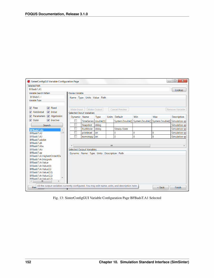
FOQUS Documentation, Release 3.1.0
Fig. 13: SinterConfigGUI Variable Configuration Page BFBadsT.A1 Selected
152 Chapter 10. Simulation Standard Interface (SimSinter)

FOQUS Documentation, Release 3.1.0
Fig. 14: SinterConfigGUI Variable Configuration Page BFBadsT.A1 Preview
10.1. Contents 153
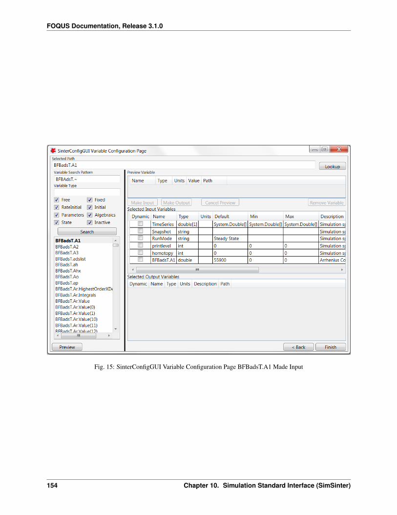
FOQUS Documentation, Release 3.1.0
Fig. 15: SinterConfigGUI Variable Configuration Page BFBadsT.A1 Made Input
154 Chapter 10. Simulation Standard Interface (SimSinter)
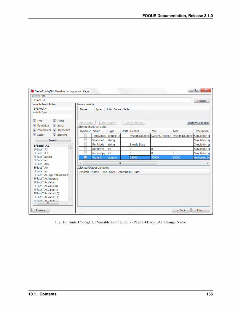
FOQUS Documentation, Release 3.1.0
Fig. 16: SinterConfigGUI Variable Configuration Page BFBadsT.A1 Change Name
10.1. Contents 155
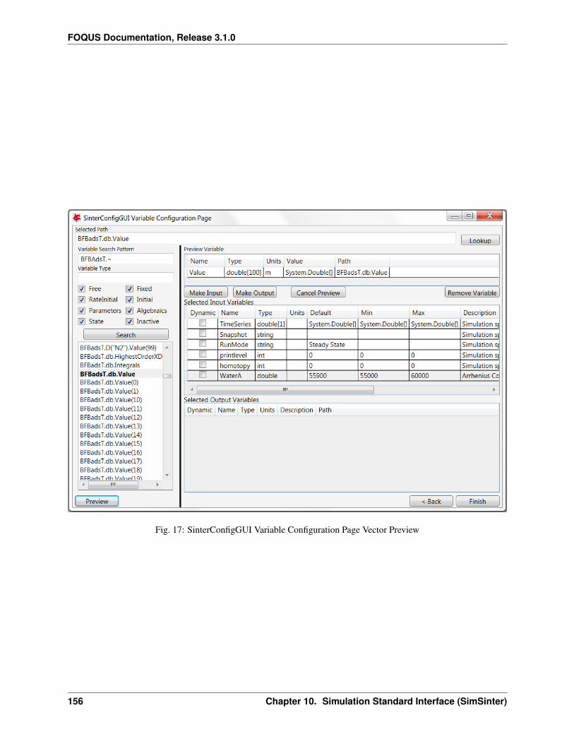
FOQUS Documentation, Release 3.1.0
Fig. 17: SinterConfigGUI Variable Configuration Page Vector Preview
156 Chapter 10. Simulation Standard Interface (SimSinter)
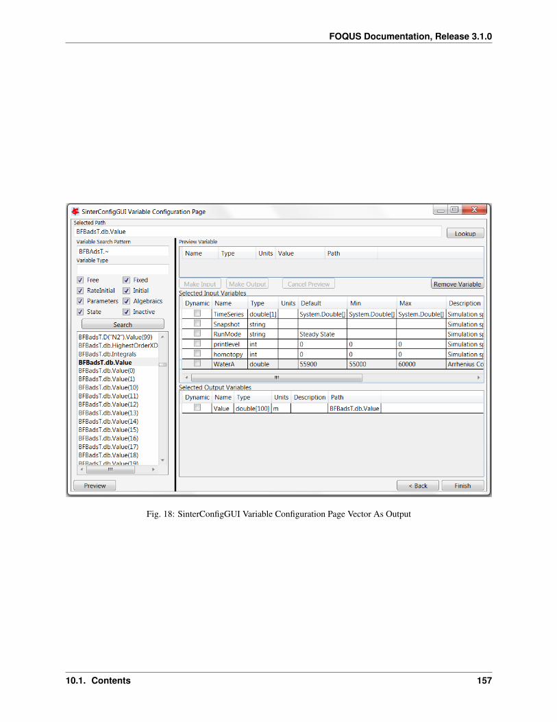
FOQUS Documentation, Release 3.1.0
Fig. 18: SinterConfigGUI Variable Configuration Page Vector As Output
10.1. Contents 157
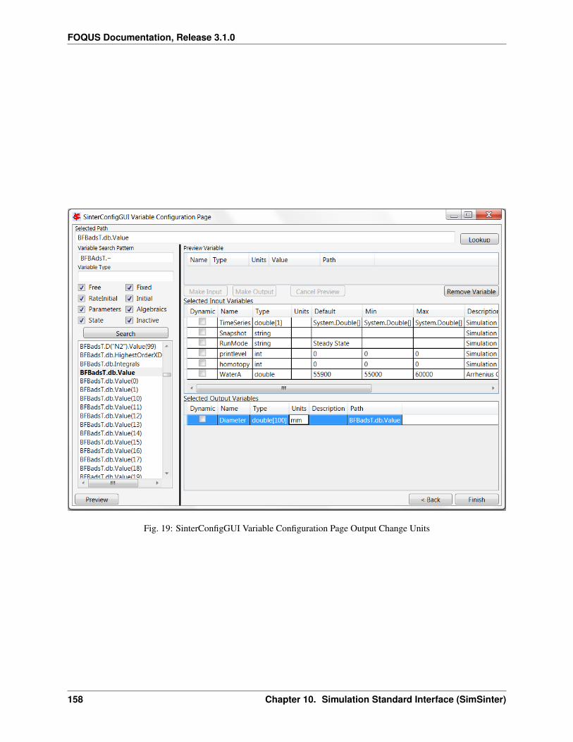
FOQUS Documentation, Release 3.1.0
Fig. 19: SinterConfigGUI Variable Configuration Page Output Change Units
158 Chapter 10. Simulation Standard Interface (SimSinter)
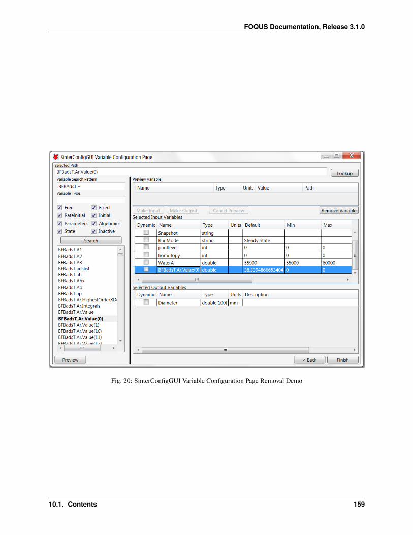
FOQUS Documentation, Release 3.1.0
Fig. 20: SinterConfigGUI Variable Configuration Page Removal Demo
10.1. Contents 159
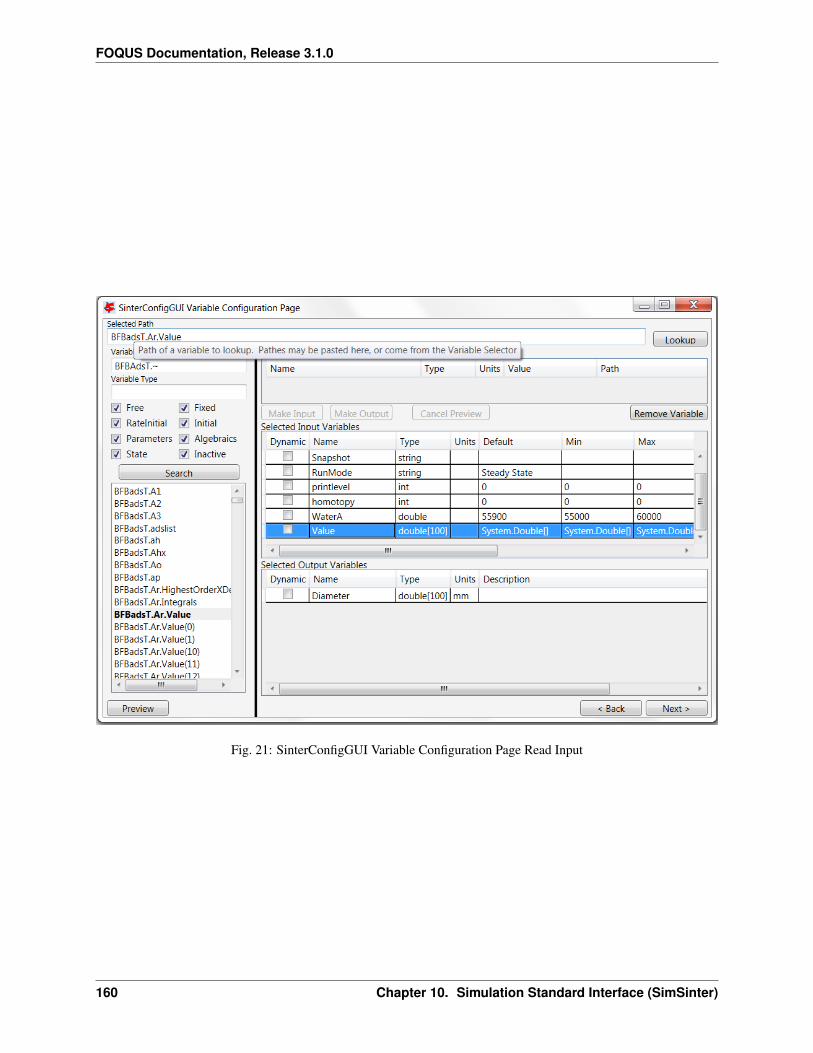
FOQUS Documentation, Release 3.1.0
Fig. 21: SinterConfigGUI Variable Configuration Page Read Input
160 Chapter 10. Simulation Standard Interface (SimSinter)

FOQUS Documentation, Release 3.1.0
18. Click Next to display the SinterConfigGUI Vector Default Initialization window as shown in Figure SinterCon-figGUI Vector Default Initialization Input Page. Since the input variable “Value” is a vector, its default valuescan be modified in the window. In this case there is no need to change the values.
Fig. 22: SinterConfigGUI Vector Default Initialization Input Page
19. The simulation is now setup. Save the configuration file by clicking Finish. The file is saved to the locationspecified on the SinterConfigGUI Simulation Meta-Data page. Clicking Finish will close the SinterConfigGUI,but NOT Aspen Custom Modeler. The user must close ACM manually.
20. If “SinterConfigGUI” was launched from FOQUS, the path to the configuration file is automatically passed toFOQUS. The next step in FOQUS is to click OK in the Add/Update Turbine Model window. FOQUS may thenbe used to upload it to the Turbine gateway. If “SinterConfigGUI” was not launched from FOQUS (e.g., it waslaunched from the Start menu), the configuration file name must be entered in FOQUS manually.
Microsoft Excel Configuration
1. The “SinterConfigGUI” can be launched from FOQUS, via the Create/Edit button found in File→ Add/UpdateModel to Turbine or “SinterConfigGUI” may be run on its own by selecting CCSI Tools → FOQUS →SinterConfigGUI from the Start menu.
2. The splash window displays, as shown in Figure SinterConfigGUI Splash Screen. The user may click the splashscreen to proceed, or wait 10 seconds for it to close automatically.
3. The SinterConfigGUI Open Simulation window displays (Figure SinterConfigGUI Open Simulation Window).If “SinterConfigGUI” was opened from FOQUS, the filename text box already contains the correct file. Toproceed immediately click Open File and Configure Variables or click Browse to search for the file. For thistutorial, a fresh copy of the BMI test is opened. It can be found at:
10.1. Contents 161

FOQUS Documentation, Release 3.1.0
Fig. 23: SinterConfigGUI Splash Screen
162 Chapter 10. Simulation Standard Interface (SimSinter)
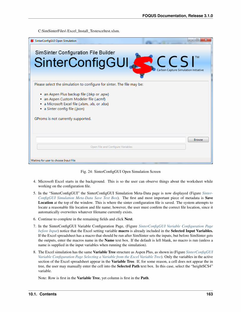
FOQUS Documentation, Release 3.1.0
C:SimSinterFiles\ Excel_Install_Testexceltest.xlsm.
Fig. 24: SinterConfigGUI Open Simulation Screen
4. Microsoft Excel starts in the background. This is so the user can observe things about the worksheet whileworking on the configuration file.
5. In the “SinterConfigGUI” the SinterConfigGUI Simulation Meta-Data page is now displayed (Figure Sinter-ConfigGUI Simulation Meta-Data Save Text Box). The first and most important piece of metadata is SaveLocation at the top of the window. This is where the sinter configuration file is saved. The system attempts tolocate a reasonable file location and file name; however, the user must confirm the correct file location, since itautomatically overwrites whatever filename currently exists.
6. Continue to complete in the remaining fields and click Next.
7. In the SinterConfigGUI Variable Configuration Page, (Figure SinterConfigGUI Variable Configuration Pagebefore Input) notice that the Excel setting variable macro is already included in the Selected Input Variables.If the Excel spreadsheet has a macro that should be run after SimSinter sets the inputs, but before SimSinter getsthe outputs, enter the macros name in the Name text box. If the default is left blank, no macro is run (unless aname is supplied in the input variables when running the simulation).
8. The Excel simulation has the same Variable Tree structure as Aspen Plus, as shown in (Figure SinterConfigGUIVariable Configuration Page Selecting a Variable from the Excel Variable Tree). Only the variables in the activesection of the Excel spreadsheet appear in the Variable Tree. If, for some reason, a cell does not appear the intree, the user may manually enter the cell into the Selected Path text box. In this case, select the “height$C$4”variable.
Note: Row is first in the Variable Tree, yet column is first in the Path.
10.1. Contents 163
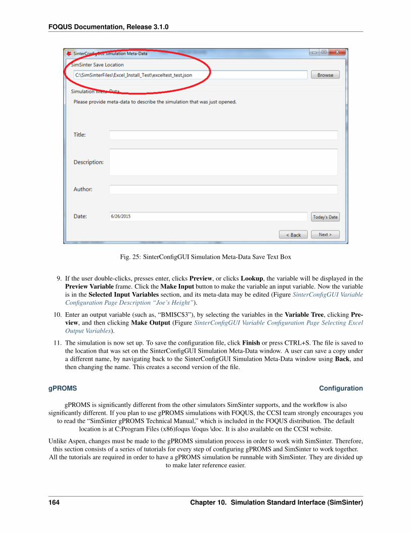
FOQUS Documentation, Release 3.1.0
Fig. 25: SinterConfigGUI Simulation Meta-Data Save Text Box
9. If the user double-clicks, presses enter, clicks Preview, or clicks Lookup, the variable will be displayed in thePreview Variable frame. Click the Make Input button to make the variable an input variable. Now the variableis in the Selected Input Variables section, and its meta-data may be edited (Figure SinterConfigGUI VariableConfiguration Page Description “Joe’s Height”).
10. Enter an output variable (such as, “BMI$C$3”), by selecting the variables in the Variable Tree, clicking Pre-view, and then clicking Make Output (Figure SinterConfigGUI Variable Configuration Page Selecting ExcelOutput Variables).
11. The simulation is now set up. To save the configuration file, click Finish or press CTRL+S. The file is saved tothe location that was set on the SinterConfigGUI Simulation Meta-Data window. A user can save a copy undera different name, by navigating back to the SinterConfigGUI Simulation Meta-Data window using Back, andthen changing the name. This creates a second version of the file.
gPROMS Configuration
gPROMS is significantly different from the other simulators SimSinter supports, and the workflow is alsosignificantly different. If you plan to use gPROMS simulations with FOQUS, the CCSI team strongly encourages you
to read the “SimSinter gPROMS Technical Manual,” which is included in the FOQUS distribution. The defaultlocation is at C:Program Files (x86)foqus \foqus \doc. It is also available on the CCSI website.
Unlike Aspen, changes must be made to the gPROMS simulation process in order to work with SimSinter. Therefore,this section consists of a series of tutorials for every step of configuring gPROMS and SimSinter to work together.
All the tutorials are required in order to have a gPROMS simulation be runnable with SimSinter. They are divided upto make later reference easier.
164 Chapter 10. Simulation Standard Interface (SimSinter)
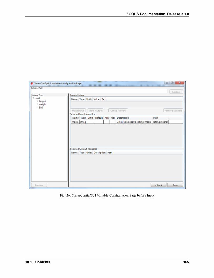
FOQUS Documentation, Release 3.1.0
Fig. 26: SinterConfigGUI Variable Configuration Page before Input
10.1. Contents 165
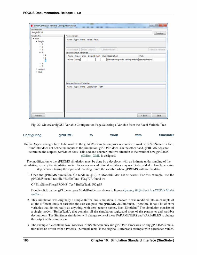
FOQUS Documentation, Release 3.1.0
Fig. 27: SinterConfigGUI Variable Configuration Page Selecting a Variable from the Excel Variable Tree
Configuring gPROMS to Work with SimSinter
Unlike Aspen, changes have to be made to the gPROMS simulation process in order to work with SimSinter. In fact,SimSinter does not define the inputs to the simulation, gPROMS does. On the other hand, gPROMS does notdetermine the outputs, SimSinter does. This odd and counter-intuitive situation is the result of how gPROMS
gO:Run_XML is designed.
The modification to the gPROMS simulation must be done by a developer with an intimate understanding of thesimulation, usually the simulation writer. In some cases additional variables may need to be added to handle an extra
step between taking the input and inserting it into the variable where gPROMS will use the data.
1. Open the gPROMS simulation file (ends in .gPJ) in ModelBuilder 4.0 or newer. For this example, use thegPROMS install test file “BufferTank_FO.gPJ”, found in:
C:\ SimSinterFilesgPROMS_Test\ BufferTank_FO.gPJ
Double-click on the .gPJ file to open ModelBuilder, as shown in Figure Opening BufferTank in gPROMS ModelBuilder.
2. This simulation was originally a simple BufferTank simulation. However, it was modified into an example ofall the different kinds of variables the user can pass into gPROMS via SimSinter. Therefore, it has a lot of extravariables that do not really do anything, with very generic names, like “SingleInt.” The simulation consists ofa single model, “BufferTank”, that contains all the simulation logic, and most of the parameter and variabledeclarations. The SimSinter simulation will change some of these PARAMETERS and VARIABLES to changethe output of the simulation.
3. The example file contains two Processes. SimSinter can only run gPROMS Processes, so any gPROMS simula-tion must be driven from a Process. “SimulateTank” is the original BufferTank example with hardcoded values,
166 Chapter 10. Simulation Standard Interface (SimSinter)
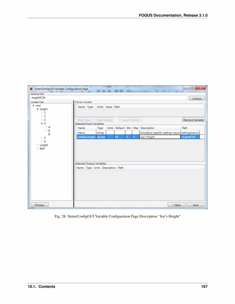
FOQUS Documentation, Release 3.1.0
Fig. 28: SinterConfigGUI Variable Configuration Page Description “Joe’s Height”
10.1. Contents 167
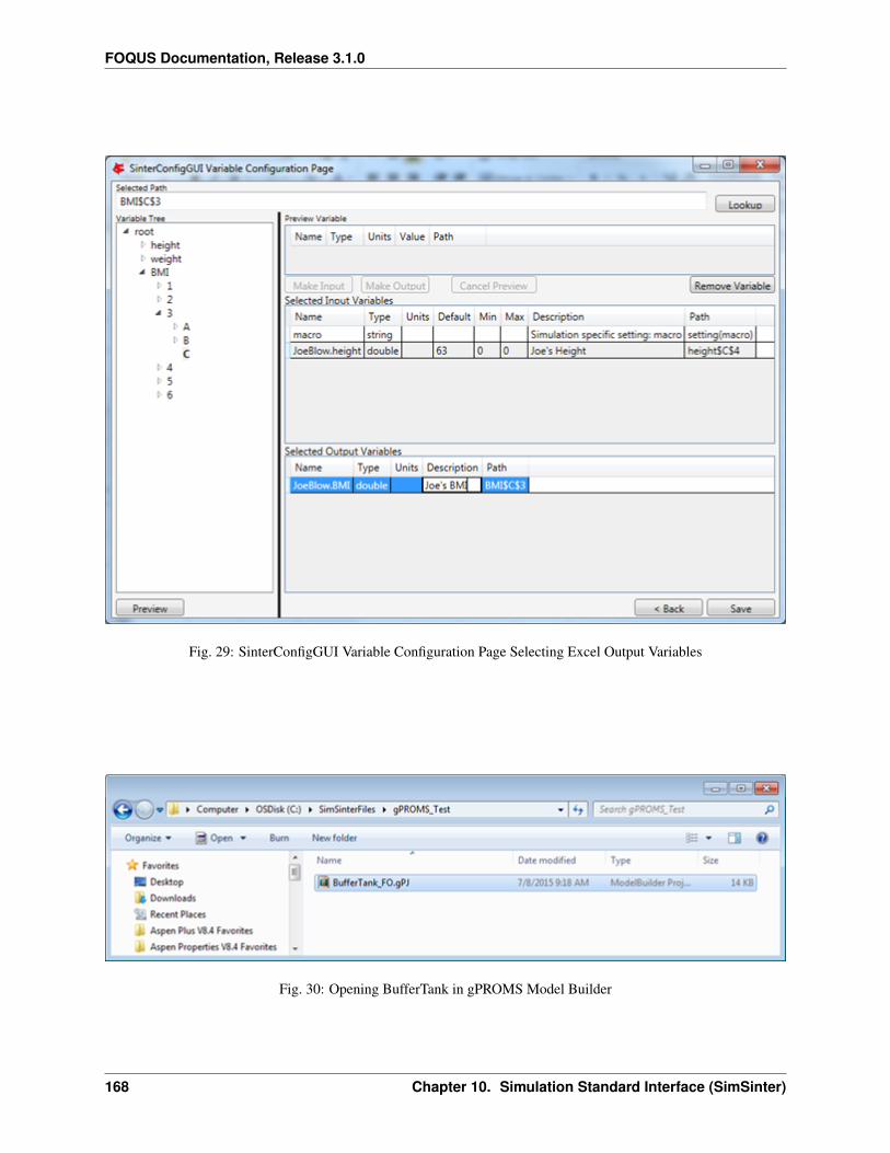
FOQUS Documentation, Release 3.1.0
Fig. 29: SinterConfigGUI Variable Configuration Page Selecting Excel Output Variables
Fig. 30: Opening BufferTank in gPROMS Model Builder
168 Chapter 10. Simulation Standard Interface (SimSinter)
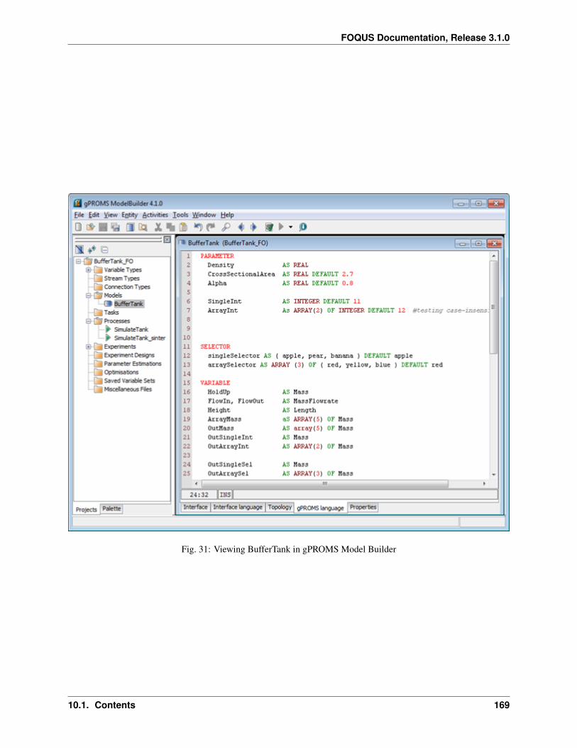
FOQUS Documentation, Release 3.1.0
Fig. 31: Viewing BufferTank in gPROMS Model Builder
10.1. Contents 169
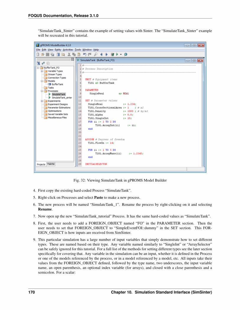
FOQUS Documentation, Release 3.1.0
“SimulateTank_Sinter” contains the example of setting values with Sinter. The “SimulateTank_Sinter” examplewill be recreated in this tutorial.
Fig. 32: Viewing SimulateTank in gPROMS Model Builder
4. First copy the existing hard-coded Process “SimulateTank”.
5. Right-click on Processes and select Paste to make a new process.
6. The new process will be named “SimulateTank_1”. Rename the process by right-clicking on it and selectingRename.
7. Now open up the new “SimulateTank_tutorial” Process. It has the same hard-coded values as “SimulateTank”.
8. First, the user needs to add a FOREIGN_OBJECT named “FO” in the PARAMETER section. Then theuser needs to set that FOREIGN_OBJECT to “SimpleEventFOI::dummy” in the SET section. This FOR-EIGN_OBJECT is how inputs are received from SimSinter.
9. This particular simulation has a large number of input variables that simply demonstrate how to set differenttypes. These are named based on their type. Any variable named similarly to “SingleInt” or “ArraySelector”can be safely ignored for this tutorial. For a full list of the methods for setting different types see the later sectionspecifically for covering that. Any variable in the simulation can be an input, whether it is defined in the Processor one of the models referenced by the process, or in a model referenced by a model, etc. All inputs take theirvalues from the FOREIGN_OBJECT defined, followed by the type name, two underscores, the input variablename, an open parenthesis, an optional index variable (for arrays), and closed with a close parenthesis and asemicolon. For a scalar:
170 Chapter 10. Simulation Standard Interface (SimSinter)
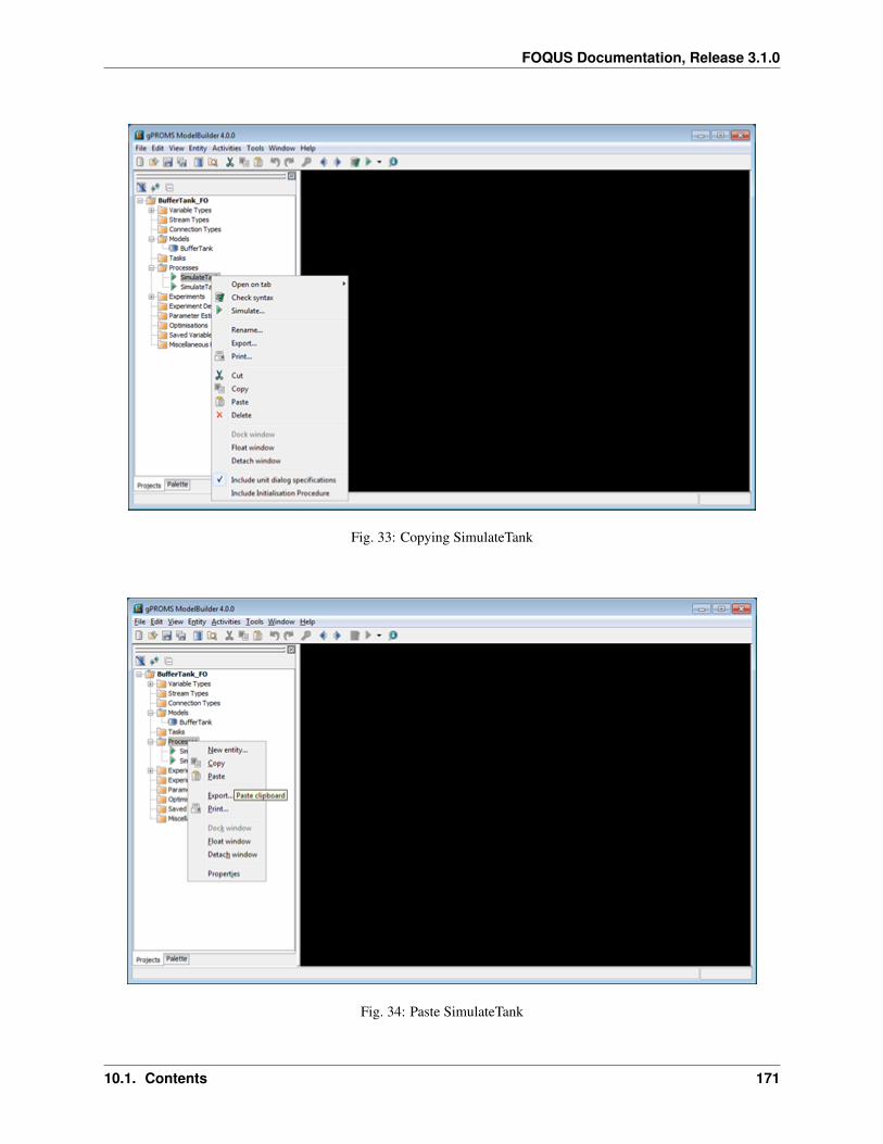
FOQUS Documentation, Release 3.1.0
Fig. 33: Copying SimulateTank
Fig. 34: Paste SimulateTank
10.1. Contents 171
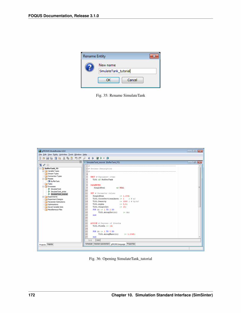
FOQUS Documentation, Release 3.1.0
Fig. 35: Rename SimulateTank
Fig. 36: Opening SimulateTank_tutorial
172 Chapter 10. Simulation Standard Interface (SimSinter)
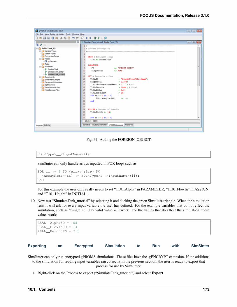
FOQUS Documentation, Release 3.1.0
Fig. 37: Adding the FOREIGN_OBJECT
FO.<Type>__<InputName>();
SimSinter can only handle arrays inputted in FOR loops such as:
FOR ii := 1 TO <array size> DO<ArrayName>(ii) := FO.<Type>1__<InputName>(ii);
END
For this example the user only really needs to set “T101.Alpha” in PARAMETER, “T101.FlowIn” in ASSIGN,and “T101.Height” in INITIAL.
10. Now test “SimulateTank_tutorial” by selecting it and clicking the green Simulate triangle. When the simulationruns it will ask for every input variable the user has defined. For the example variables that do not effect thesimulation, such as “SingleInt”, any valid value will work. For the values that do effect the simulation, thesevalues work:
REAL__AlphaFO = .08REAL__FlowInFO = 14REAL__HeightFO = 7.5
Exporting an Encrypted Simulation to Run with SimSinter
SimSinter can only run encrypted gPROMS simulations. These files have the .gENCRYPT extension. If the additionsto the simulation for reading input variables ran correctly in the previous section, the user is ready to export that
process for use by SimSinter.
1. Right-click on the Process to export (“SimulateTank_tutorial”) and select Export.
10.1. Contents 173
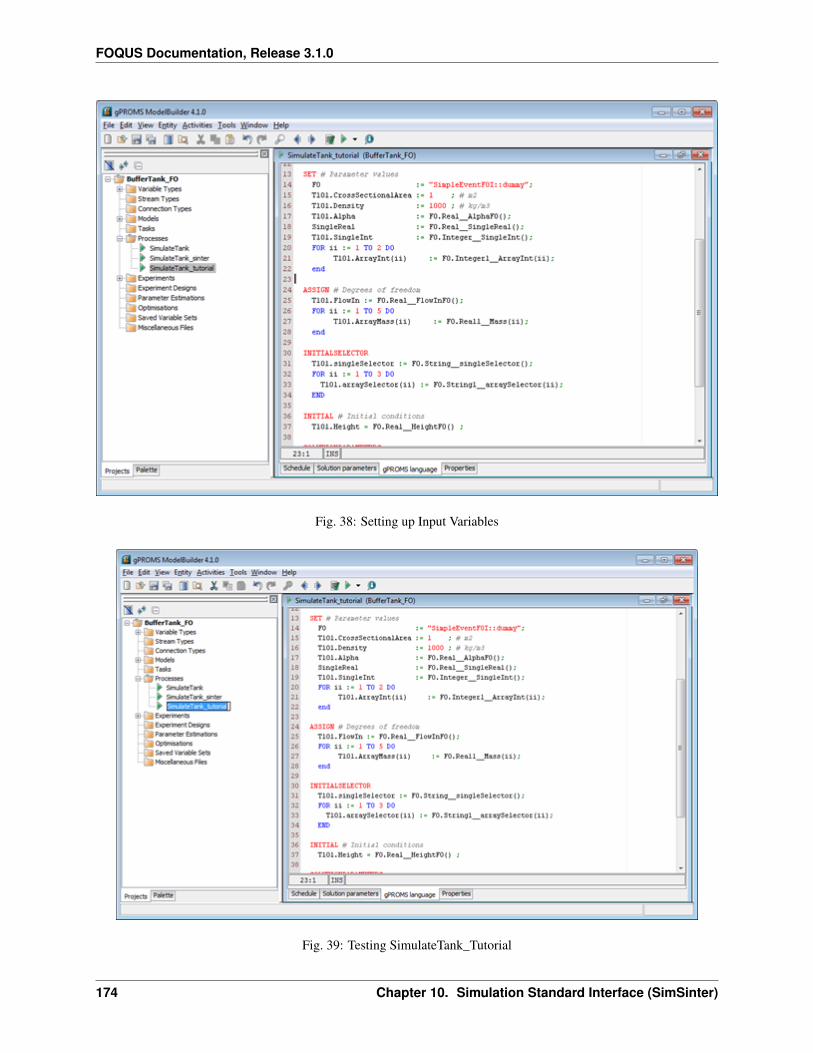
FOQUS Documentation, Release 3.1.0
Fig. 38: Setting up Input Variables
Fig. 39: Testing SimulateTank_Tutorial
174 Chapter 10. Simulation Standard Interface (SimSinter)
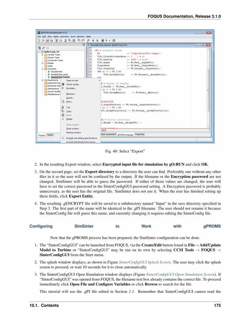
FOQUS Documentation, Release 3.1.0
Fig. 40: Select “Export”
2. In the resulting Export window, select Encrypted input file for simulation by gO:RUN and click OK.
3. On the second page, set the Export directory to a directory the user can find. Preferably one without any otherfiles in it so the user will not be confused by the output. If the filename or the Encryption password are notchanged, SimSinter will be able to guess the password. If either of those values are changed, the user willhave to set the correct password in the SinterConfigGUI password setting. A Decryption password is probablyunnecessary, as the user has the original file. SimSinter does not use it. When the user has finished setting upthese fields, click Export Entity.
4. The resulting .gENCRYPT file will be saved to a subdirectory named “Input” in the save directory specified inStep 3. The first part of the name will be identical to the .gPJ filename. The user should not rename it becausethe SinterConfig file will guess this name, and currently changing it requires editing the SinterConfig file.
Configuring SimSinter to Work with gPROMS
Now that the gPROMS process has been prepared, the SimSinter configuration can be done.
1. The “SinterConfigGUI” can be launched from FOQUS, via the Create/Edit button found in File→ Add/UpdateModel to Turbine or “SinterConfigGUI” may be run on its own by selecting CCSI Tools → FOQUS →SinterConfigGUI from the Start menu.
2. The splash window displays, as shown in Figure SinterConfigGUI Splash Screen. The user may click the splashscreen to proceed, or wait 10 seconds for it to close automatically.
3. The SinterConfigGUI Open Simulation window displays (Figure SinterConfigGUI Open Simulation Screen). If“SinterConfigGUI” was opened from FOQUS, the filename text box already contains the correct file. To proceedimmediately click Open File and Configure Variables or click Browse to search for the file.
This tutorial will use the .gPJ file edited in Section 1.1. Remember that SinterConfigGUI cannot read the
10.1. Contents 175
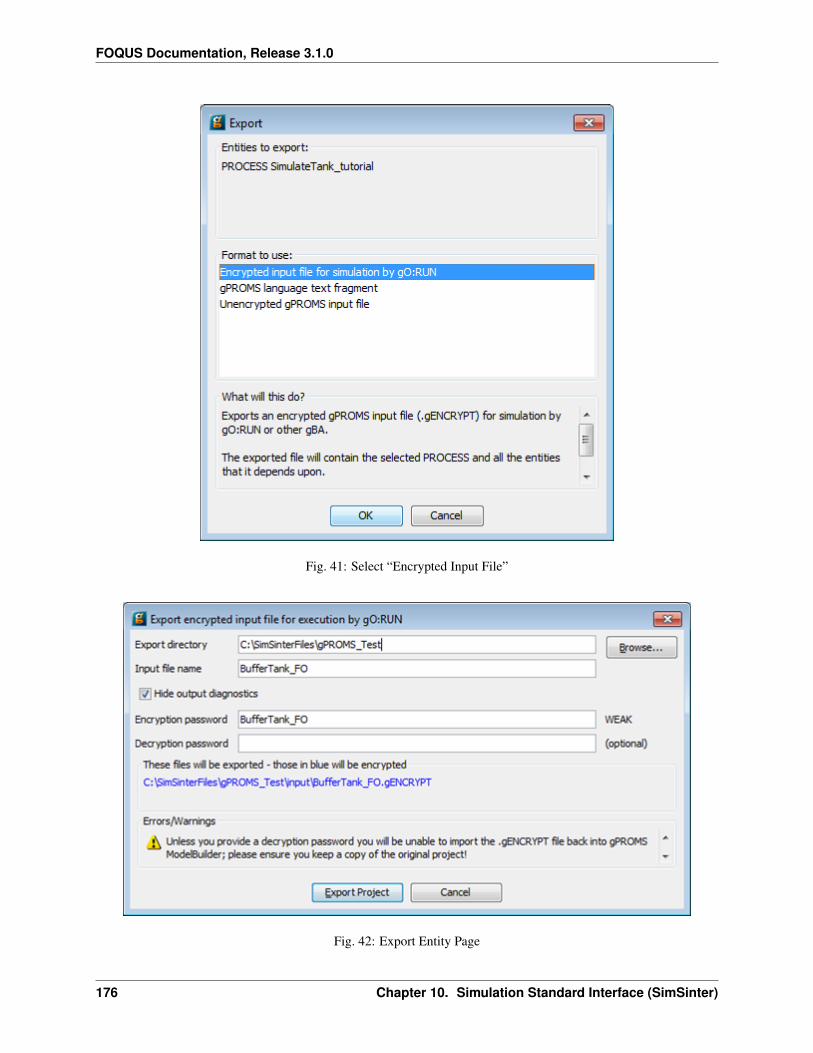
FOQUS Documentation, Release 3.1.0
Fig. 41: Select “Encrypted Input File”
Fig. 42: Export Entity Page
176 Chapter 10. Simulation Standard Interface (SimSinter)

FOQUS Documentation, Release 3.1.0
Fig. 43: SinterConfigGUI Splash Screen
10.1. Contents 177
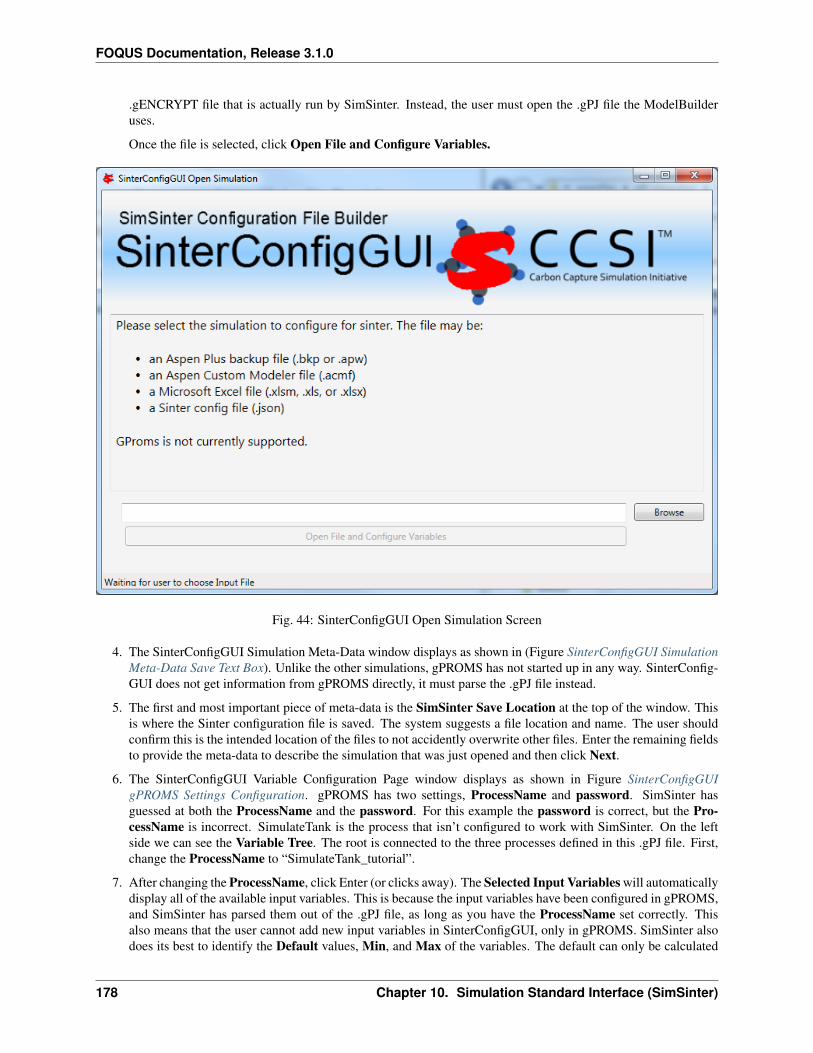
FOQUS Documentation, Release 3.1.0
.gENCRYPT file that is actually run by SimSinter. Instead, the user must open the .gPJ file the ModelBuilderuses.
Once the file is selected, click Open File and Configure Variables.
Fig. 44: SinterConfigGUI Open Simulation Screen
4. The SinterConfigGUI Simulation Meta-Data window displays as shown in (Figure SinterConfigGUI SimulationMeta-Data Save Text Box). Unlike the other simulations, gPROMS has not started up in any way. SinterConfig-GUI does not get information from gPROMS directly, it must parse the .gPJ file instead.
5. The first and most important piece of meta-data is the SimSinter Save Location at the top of the window. Thisis where the Sinter configuration file is saved. The system suggests a file location and name. The user shouldconfirm this is the intended location of the files to not accidently overwrite other files. Enter the remaining fieldsto provide the meta-data to describe the simulation that was just opened and then click Next.
6. The SinterConfigGUI Variable Configuration Page window displays as shown in Figure SinterConfigGUIgPROMS Settings Configuration. gPROMS has two settings, ProcessName and password. SimSinter hasguessed at both the ProcessName and the password. For this example the password is correct, but the Pro-cessName is incorrect. SimulateTank is the process that isn’t configured to work with SimSinter. On the leftside we can see the Variable Tree. The root is connected to the three processes defined in this .gPJ file. First,change the ProcessName to “SimulateTank_tutorial”.
7. After changing the ProcessName, click Enter (or clicks away). The Selected Input Variables will automaticallydisplay all of the available input variables. This is because the input variables have been configured in gPROMS,and SimSinter has parsed them out of the .gPJ file, as long as you have the ProcessName set correctly. Thisalso means that the user cannot add new input variables in SinterConfigGUI, only in gPROMS. SimSinter alsodoes its best to identify the Default values, Min, and Max of the variables. The default can only be calculated
178 Chapter 10. Simulation Standard Interface (SimSinter)
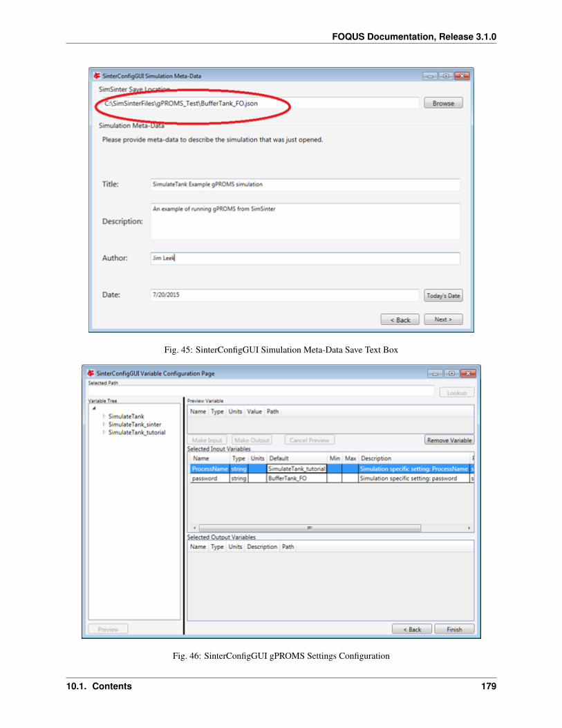
FOQUS Documentation, Release 3.1.0
Fig. 45: SinterConfigGUI Simulation Meta-Data Save Text Box
Fig. 46: SinterConfigGUI gPROMS Settings Configuration
10.1. Contents 179

FOQUS Documentation, Release 3.1.0
from the file if it was defined purely in terms of actual numbers. SimSinter cannot evaluate other variables orfunctions. Therefore,
DEFAULT 2 * 3.1415 * 12
will work. However,
DEFAULT 2 * PI * radius
will not work, because SimSinter does not know the value of either PI or radius, and SimSinter will just set thedefault to 0.
Min and Max values are taken from the variable type, if there is one.
Fig. 47: SinterConfigGUI Automatically Displays Input Variables
8. Now the output values can be entered. Expand the “SimulateTank_tutorial” Process on the Variable Tree, expandthe “T101” model, and then double-click on “FlowOut” to make it the Preview Variable. Notice that the MakeInput button is disabled. As stated above, the user cannot make new Input Variables in SinterConfigGUI. OnlyMake Output is allowed.
9. If Make Output is clicked, “FlowOut” will be made an Output Variable as shown in Figure FlowOut as anInput Variable. The Description can be updated, but SimSinter made a good guess in this example; therefore,there is no need to change the description.
10. By the same method, make Output Variables “HoldUp” and “Height.”
11. The variables names should be made shorter. Simply click on the Name column and change the name to yourpreferred name.
12. For future testing, make sure the defaults are good values. The only three input variables that matter have thefollowing defaults:
180 Chapter 10. Simulation Standard Interface (SimSinter)
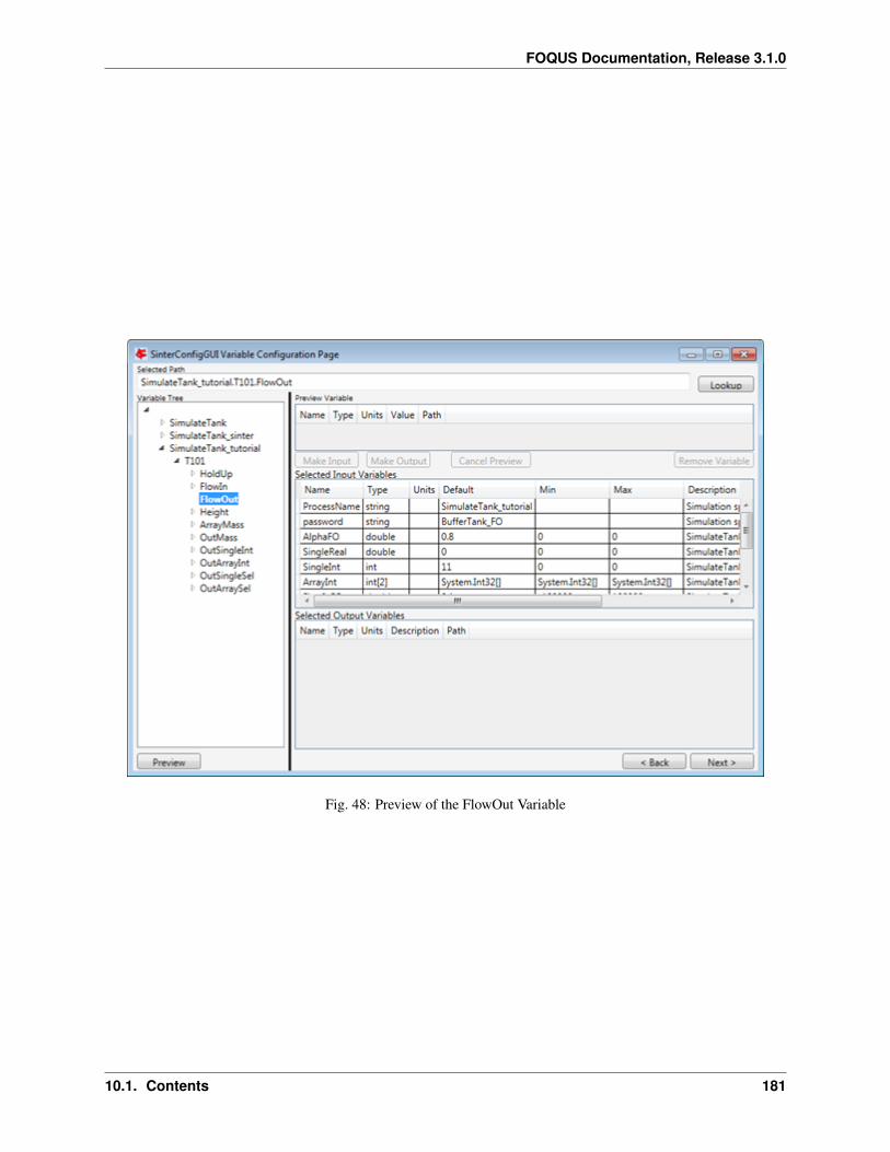
FOQUS Documentation, Release 3.1.0
Fig. 48: Preview of the FlowOut Variable
10.1. Contents 181
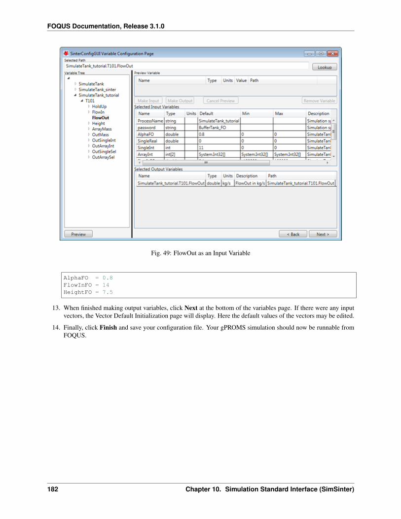
FOQUS Documentation, Release 3.1.0
Fig. 49: FlowOut as an Input Variable
AlphaFO = 0.8FlowInFO = 14HeightFO = 7.5
13. When finished making output variables, click Next at the bottom of the variables page. If there were any inputvectors, the Vector Default Initialization page will display. Here the default values of the vectors may be edited.
14. Finally, click Finish and save your configuration file. Your gPROMS simulation should now be runnable fromFOQUS.
182 Chapter 10. Simulation Standard Interface (SimSinter)
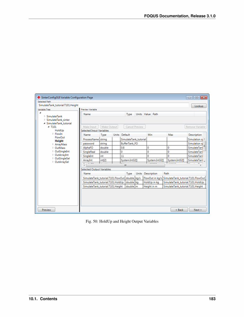
FOQUS Documentation, Release 3.1.0
Fig. 50: HoldUp and Height Output Variables
10.1. Contents 183

FOQUS Documentation, Release 3.1.0
Fig. 51: Editing Variable Names
184 Chapter 10. Simulation Standard Interface (SimSinter)
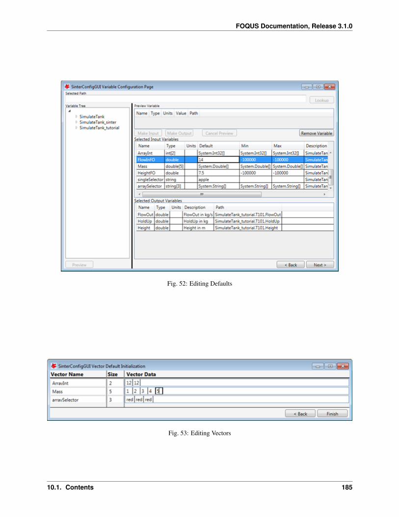
FOQUS Documentation, Release 3.1.0
Fig. 52: Editing Defaults
Fig. 53: Editing Vectors
10.1. Contents 185

FOQUS Documentation, Release 3.1.0
186 Chapter 10. Simulation Standard Interface (SimSinter)
CHAPTER 11
Debugging
This chapter contains information that may be helpful in resolving a problem or filing a bug report.
11.1 How to Debug
Log files may contain very useful information when reporting problems. The log files are contained in the logssub-directory of the FOQUS working directory. To change the log message levels in FOQUS go to the FOQUS
Settings button from the Home window. From there various log settings can be changed. The debugging log levelprovides the highest level of information.
Almost any error that occurs in FOQUS should be logged. Occasionally, an error may occur that is difficult to find, orcauses FOQUS to crash before logging it. In that case the “FOQUS Console” application can be used. All output
from FOQUS, including messages that cannot be seen otherwise will be shown in a “cmd” window which willremain open even after FOQUS closes.
When running heat integration, the debugging information can be found in\gamsHeatIntegration.lst. This file includes detailed results and errors returned by GAMS.
Most UQ routines interact with PSUADE via Python wrappers. When PSUADE is running, the stdout is written topsuadelog in the working directory. (At present, only some PSUADE commands write to this log; however, this willbe standardized in the near future so that all PSUADE commands write to this log.) Other errors that are due to the
Python wrappers or PySide GUI components are written to the logs subdirectory in the working directory.
11.2 Known Issues
The following are known unresolved issues:
• The FOQUS flowsheet can be edited while a flowsheet evaluation, optimization, or UQ is running. This shouldnot be allowed, and may cause problems.
187

FOQUS Documentation, Release 3.1.0
• With the windows installer, FOQUS may produce output to standard error, especially if it immediately failsto launch. Output is usually caught and redirected to the FOQUS log and displayed in dialog boxes withinFOQUS, but rare instances may occur where error messages are not caught. Output to standard error is loggedin the directory with foqus.exe in the file foqus.exe.log. The user does not typically have permission to writeto the FOQUS install location, so an error message such as “Cannot write to foqus.exe.log” will be displayed.If this occurs there are two solutions (1) change the permissions for the FOQUS install directory or (2) run“FOQUS Console” application, which will direct FOQUS output to the “cmd” window.
• The win32com module generates Python code, which it needs to run. This code is generated in the FOQUSinstall location “\distwin32comgen_py.” In some cases there may be a problem writing to that directory due topermission settings. This will prevent FOQUS from running simulations locally. If this error is encountered thesolution is to make the “gen_py” directory user writable. So far, in testing, this error seems to occur in Windows8 and 10, but not 7.
• The user regression analysis features, iREVEAL and ALAMO, of the UQ tool requires a separate Python 2.7installation. Furthermore, Python must be both in PATH variable and associated with .py files. Details oninstalling Python and fixing any issues encountered may be found in the iREVEAL Installation Guide and theiREVEAL User Manual, Known Issues section.
• FOQUS has trouble getting files from Turbine and saving them to the DMF when dealing with files in Turbineinvolving directories.
• The default port for TurbineLite is 8080. If another program is already using port 8000, there will be an error inFOQUS when connecting to TurbineLite. In the Turbine Tab of the Settings window, there is a tool to changethe TurbineLite port. If the TurbineLite port is changed the configuration file that FOQUS uses to connect toTurbineLite, must also be changed.
11.3 Reporting Issues
To report an issue, please send an email to:
Please include detailed steps on how to reproduce the error, including screenshots and log files.
188 Chapter 11. Debugging

CHAPTER 12
References
C. Tong, “PSUADE User’s Manual, Version 1.2.0,” Tech. Rep. LLNL-SM-407882, Lawrence Livermore NationalLaboratory, Livermore, CA 94551-0808, May 2011.
A. Cozad, N. V. Sahinidis, and D. C. Miller, “Automatic Learning of Algebraic Models for Optimization,” AIChEJournal, vol. 60, pp. 2211–2227, 2014.
C. B. Storlie, H. D. Bondell, B. J. Reich, and H. H. Zhang, “Surface estimation, variable selection, and thenonparametric oracle property,” Statistica Sinica, vol. 21, no. 2, pp. 679–705, 2011.
C. B. Storlie, B. J. Reich, J. C. Helton, L. P. Swiler, and C. J. Sallaberry, “Analysis of computationally demandingmodels with continuous and categorical inputs,” Reliability Engineering & System Safety, vol. 113, pp.30–41, 2013.
B. J. Reich, C. B. Storlie, and H. D. Bondell, “Variable selection in bayesian smoothing spline anova models:Application to deterministic computer codes,” Technometrics, vol. 51, no. 2, pp. 110–120, 2009.
J. H. Wegstein, “Accelerating Convergence of Iterative Processes,” j-CACM, vol. 1, no. 6, pp. 9–13, 1958.
N. Hansen, Towards a New Evolutionary Computation. Advances in Estimation of Distribution Algorithms, ch.The CMA Evolution Strategy: A Comparing Review, pp. 75–102. Springer, 2006.
S. G. Johnson, “The nlopt nonlinear-optimization package.” http://ab-initio.mit.edu/nlopt, May 2015.
E. Jones, T. Oliphant, P. Peterson, et al., “Scipy: Open source scientic tools for python.” http://www.scipy.org/,May 2015.
K. Bhat, B. Sherman, K. Ajayi, B. Ng, J. Eslick, J. Ou, and J.Kress, “Solventt: A calibration tool for solvent-basedCO2 capture models,” in 2015 CCSI Industry Advisory Board (IAB) Program Review Meeting, (Reston, VA),September 2015.
189

FOQUS Documentation, Release 3.1.0
190 Chapter 12. References

CHAPTER 13
Copyright and License
Copyright (c) 2012 - 2019
13.1 Copyright Notice
Foqus was produced under the DOE Carbon Capture Simulation Initiative (CCSI), and is copyright (c) 2012 - 2019by the software owners: Oak Ridge Institute for Science and Education (ORISE), TRIAD National Security, LLC.,
Lawrence Livermore National Security, LLC., The Regents of the University of California, through LawrenceBerkeley National Laboratory, Battelle Memorial Institute, Pacific Northwest Division through Pacific Northwest
National Laboratory, Carnegie Mellon University, West Virginia University, Boston University, the Trustees ofPrinceton University, The University of Texas at Austin, URS Energy & Construction, Inc., et al.. All rights reserved.
NOTICE. This Software was developed under funding from the U.S. Department of Energy and the U.S. Governmentconsequently retains certain rights. As such, the U.S. Government has been granted for itself and others acting on itsbehalf a paid-up, nonexclusive, irrevocable, worldwide license in the Software to reproduce, distribute copies to the
public, prepare derivative works, and perform publicly and display publicly, and to permit other to do so.
13.2 License Agreement
Foqus Copyright (c) 2012 - 2019, by the software owners: Oak Ridge Institute for Science and Education (ORISE),TRIAD National Security, LLC., Lawrence Livermore National Security, LLC., The Regents of the University of
California, through Lawrence Berkeley National Laboratory, Battelle Memorial Institute, Pacific Northwest Divisionthrough Pacific Northwest National Laboratory, Carnegie Mellon University, West Virginia University, Boston
University, the Trustees of Princeton University, The University of Texas at Austin, URS Energy & Construction,Inc., et al. All rights reserved.
Redistribution and use in source and binary forms, with or without modification, are permitted provided that thefollowing conditions are met:
1. Redistributions of source code must retain the above copyright notice, this list of conditions and the followingdisclaimer.
191

FOQUS Documentation, Release 3.1.0
2. Redistributions in binary form must reproduce the above copyright notice, this list of conditions and the follow-ing disclaimer in the documentation and/or other materials provided with the distribution.
3. Neither the name of the Carbon Capture Simulation Initiative, U.S. Dept. of Energy, the National EnergyTechnology Laboratory, Oak Ridge Institute for Science and Education (ORISE), TRIAD National Security,LLC., Lawrence Livermore National Security, LLC., the University of California, Lawrence Berkeley NationalLaboratory, Battelle Memorial Institute, Pacific Northwest National Laboratory, Carnegie Mellon University,West Virginia University, Boston University, the Trustees of Princeton University, the University of Texas atAustin, URS Energy & Construction, Inc., nor the names of its contributors may be used to endorse or promoteproducts derived from this software without specific prior written permission.
THIS SOFTWARE IS PROVIDED BY THE COPYRIGHT HOLDERS AND CONTRIBUTORS “AS IS” ANDANY EXPRESS OR IMPLIED WARRANTIES, INCLUDING, BUT NOT LIMITED TO, THE IMPLIED
WARRANTIES OF MERCHANTABILITY AND FITNESS FOR A PARTICULAR PURPOSE AREDISCLAIMED. IN NO EVENT SHALL THE COPYRIGHT OWNER OR CONTRIBUTORS BE LIABLE FOR
ANY DIRECT, INDIRECT, INCIDENTAL, SPECIAL, EXEMPLARY, OR CONSEQUENTIAL DAMAGES(INCLUDING, BUT NOT LIMITED TO, PROCUREMENT OF SUBSTITUTE GOODS OR SERVICES; LOSS OF
USE, DATA, OR PROFITS; OR BUSINESS INTERRUPTION) HOWEVER CAUSED AND ON ANY THEORYOF LIABILITY, WHETHER IN CONTRACT, STRICT LIABILITY, OR TORT (INCLUDING NEGLIGENCE OROTHERWISE) ARISING IN ANY WAY OUT OF THE USE OF THIS SOFTWARE, EVEN IF ADVISED OF THE
POSSIBILITY OF SUCH DAMAGE.
You are under no obligation whatsoever to provide any bug fixes, patches, or upgrades to the features, functionality orperformance of the source code (“Enhancements”) to anyone; however, if you choose to make your Enhancements
available either publicly, or directly to Lawrence Berkeley National Laboratory, without imposing a separate writtenlicense agreement for such Enhancements, then you hereby grant the following license: a non-exclusive, royalty-free
perpetual license to install, use, modify, prepare derivative works, incorporate into other computer software,distribute, and sublicense such enhancements or derivative works thereof, in binary and source code form.
192 Chapter 13. Copyright and License
CHAPTER 14
FOQUS
14.1 Overview
The Framework for Optimization, Quantification of Uncertainty, and Surrogates (FOQUS) serves as the primarycomputational platform enabling advanced Process Systems Engineering (PSE) capabilities to be integrated with
commercial process simulation software. It can be used to synthesize, design, and optimize a complete carboncapture system while considering uncertainty. FOQUS enables users to effectively screen potential capture conceptsin the context of a complete industrial process so that trade-offs can be appropriately evaluated. The technical and
economic performance characteristics of the capture process are highly dependent on employing an effectiveapproach for process synthesis. Since large-scale carbon capture processes are outside of current experience,
heuristic and evolutionary approaches are likely to be inadequate. Thus, a key aspect of FOQUS is that it bridges thisgap by supporting a superstructure-based approach to determine the optimal process configuration and equipment
interconnections.
14.2 Modules
1. SimSinter provides a wrapper to enable models created in process simulators to be linked into a FOQUS Flow-sheet.
2. The FOQUS Flowsheet is used to link simulations together and connect model variables between simulationson the flowsheet. FOQUS enables linking models from different simulation packages.
3. Simulations are run through Turbine, which manages the multiple runs needed to build surrogate models, per-form derivative-free optimization or conduct an Uncertainty Quantification (UQ) analysis. Turbine provides thecapability for job queuing and enables these jobs to be run in parallel using cloud- or cluster-based computingplatforms or a single workstation.
4. The Surrogates module can create algebraic surrogate models to support large-scale deterministic optimization,including superstructure optimization to determine process configurations. One of the available surrogate mod-els is the Automated Learning of Algebraic Models for Optimization (ALAMO). ALAMO is an external productdue to background Intellectual Property (IP) issues.
193

FOQUS Documentation, Release 3.1.0
5. The Derivative-Free Optimization (DFO) module enables derivative-free (or simulation-based) optimizationdirectly on the process models linked together on a FOQUS Flowsheet. It utilizes Excel to calculate complexobjective functions, such as the cost of electricity.
6. The UQ module enables the effects of uncertainty to be propagated through the complete system model, sensi-tivity of the model to be assessed, and the most significant sources of uncertainty identified to enable prioritizingof experimental resources to obtain additional data.
7. The Optimization Under Uncertainty (OUU) module combines the capabilities of the DFO and the UQ modulesto enable scenario-based optimization, such as optimization over a range of operating scenarios.
8. The SolventFit module is an uncertainty quantification tool for the calibration of an Aspen Plus® solvent processmodel. The current state of the art is a regression that yields single best fit point estimates of some parameters.This shows neither the level of uncertainty in each parameter, nor the level of uncertainty in model output, suchas equivalent work. SolventFit allows for predictions with uncertainty bounds by accounting for uncertaintyin model parameters and deficiencies in the model form. This yields an improved understanding of the modelparameters and results in more complete predictions with uncertainty bounds. This distribution of parametersallows for predictions with uncertainty.
9. The Sequential Design of Experiments (SDOE) module currently provides a way to construct flexible space-filling designs based on a user-provided candidate set of input points. The method allows for new designs tobe constructed as well as augmenting existing data to strategically select input combintions that minimizes thedistance between points. Development of this module is continuing and will soon include other options fordesign construction.
194 Chapter 14. FOQUS